MARCH 2014

Young Professionals Journal

VOLUME I, 2014

Contents1. Model Risk: A Promising Place to Start... - pg 1

2. Fed’s QE Not Working... - pg 13

3. Systemic Risk Redux... - pg 16

4. Basel III & Liquidity Risk Management... - pg 24

5. Loan Sale Operations: cleaver to scalpel... - pg 32

6. Bubble VaR - A Countercyclical Approach... - pg 35

7. A Career in Risk.... - pg 47

8. IFRS 9: New Modeling Risk Challenges... - pg 53

Chairman’s Message

lvi

The Future of Risk Management

Since the initial conception of The Financial Risk Institute (FinRisk) in April 2013, several volunteers have been working hard to organize exciting events and make available resources for participants in the FinRisk community. At FinRisk, we focus on shaping the “Future of Risk Management”. To us, that means focusing on “hot topics” and “building the next generation”.

Above are some pictures with click-through links to give you more information about recent and past FinRisk events outlining our efforts towards these goals. This inaugural Young Professionals Journal is another key initiative to help us advance these goals. We have compiled several interesting writings to that end in this inaugural issue. We hope you will find this publication helpful. Please do give us your com-ments and suggestions via email to info@finrisk.org.

We are planning much more this coming year. We encourage all readers to learn more about this and other FinRisk initiatives at our website: www.finrisk.org.

Steven P. Lee

Chair, FinRisk Founding Committee

Founding Committee

lvii

Chairman: Steven P. Lee, Managing Director, Governance, Risk & Compliance, Global Client Consulting LLC

Secretary: Daniel Danello, Attorney at Law Venable LLP

Programs: Ralph Giraud, Director, Financial Markets Lab, Rutgers School of Business, Camden

Finance: Nick Kiritz, Managing Director/ Principal Equitem Capital LLC

Information & Technology: Jefferson Braswell, Founding Partner & CEO Tahoe Blue Ltd

Young Professionals: Werner Hahn, Senior Analyst Corporate Executive Board

Members: Jason Ackerman, Associate Vice President & Chief Audit Executive Georgetown University

Jeff Curry, Director, AERS/ Financial Services, Governance, Regulatory & Risk Strategies, Deloitte & Touche LLP

Thomas Day, Managing Director, Risk & Policy Moodys Analytics

Pam Gogol, Principal Examination Specialist, Office of Market Risk Federal Housing Finance Agency

Zlatica Kraljevic, Ph.D., President The Anders Frontier Group

Roberto Setola, Director, Operational Risk, Office of Risk FINRA

Graham Strong, Faculty Advisor, Systems Analytics, Carnegie Mellon University, H. John Heinz College, School of Public Policy & Management

Mikael Sundberg, Head, Risk Analytics MIGA, The World Bank Group

Marti Tirinnanzi, CEO Financial Standards, Inc.

FinRisk Regional Centers:

Chair, FinRisk DC Steven P. Lee, Managing Director, Global Client Consulting

Chair, FinRisk Singapore Lawrence W. Ho, Founder, KEE+

Chair, FinRisk London Moorad Choudhry, IPO Treasurer, Group Treasury, Royal Bank of Scotand

lviii

Editor-in-charge: Steven P. Lee

Members: Jason Ackerman Jefferson Braswell Jeff Curry Ralph Giraud Werner Hahn Nick Kiritz Zlatica Kraljevic Candy Liu Mandy Liu Weihua Ni Wang Panjun Graham Strong Mikael Sundberg Marti Tirinnanzi

Editorial Board

This FinRisk Young Professionals Journal’s primary goal is to create a Young Professionals friendly environment, to encour-age participation by seasoned and Young Professionals alike, to share and create a credible source of up-to-date risk manage-ment information and thought-provoking discussion. We welcome written contributions on FinRisk hot topics, including regula-tory issues and risk management, especially those would be particularly helpful for Young Professionals.

We endeavor to bring an interesting collection of articles for our FinRisk participants and Young Professionals readers; one that will hopefully interest you to engage and participate actively in our FinRisk and Young Professionals events and activities. It is our belief that through active participation, we can all benefit from our collective sharing.

We welcome diverse topics, discussions and points of view. Publication is merit based, and submission does not guarantee publication. As a policy, we do not accept compensation of any kind, including money, gifts or other favors, in exchange for edi-torial publication. The FinRisk Young Professionals Journal Editorial Board makes all editorial decisions, and decisions are final. The Board reserves the right to edit all content for clarity, accuracy, length and/or other factors. Authors are responsible for the content and accuracy of reported data and statistics. The individual viewpoints represented in this Journal express the view-points of the author, and do not necessarily reflect the views of the Financial Risk Institute (FinRisk) or our sponsors and support-ers.

FinRiskYoung Professionals Journal accepts paid or sponsored advertising, separate from editorial content. Please contact us at Info@FinRisk.org for more information on sponsorship and ad rate structure.

Editorial Policy

Model Risk Management: A Promising Start to A Quant Career

1

Introduction

If you have looking through the risk job postings across the United States over you are likely to have seen many opportuni-ties in the area of model risk management (MRM). For those who haven’t worked in the risk area, and even for many that have, the roles, responsibilities – and signifi-cance – of MRM within organizations may be opaque.

In fact, model risk management has stead-ily increased in significance over the last 15 years and it can be a fascinating and re-warding function in which to work. MRM

can also provide an entrée into other excit-ing areas. Whether for its own sake, or as a stepping-stone, MRM is a function that anyone interested in quantitative analytics or risk management should seriously con-sider.

The recent “London Whale” case at JPMor-gan Chase’s London trading desk provided a rare public reference to the MRM func-tion. Press reports suggest that the losses suffered in the case may have been due to a failure of MRM controls around changes to the Value-at-Risk model used to meas-ure the riskiness of the London CIO desk’s

1

QUOTE: “All models are wrong, some are useful.” - George E.P. Box in Empirical Model-Building and Response Surfaces (1987)

Nick Kiritz, Member & CFO, FinRisk Founding CommitteeManaging Director, Equitem Capital

positions. This is probably an unfair charac-terization of the causal chain, however.  Public reports suggest that the trader, Bruno Iksil, placed huge bets in relatively (to the size of his positions) illiquid CDS markets.  The bulk of the MRM failures ap-pear to have occurred afterwards, as at-tempts were made to change models to re-duce reported VaR and Risk Weighted As-sets (to reduce capital charges). Still, the failure of MRM to block the changes may point to a failure of the function to ade-quately perform its duties, even though this may not have caused the loss itself.

Figure 1, below, illustrates why this change has occurred: the foundational nature of modeling and analytics and the data on which it is based for all risk management functions. As shown by the brackets to the left, Model and Data Validation may be seen as providing assurance that these foundations are robust, while the complete Model Risk Management function helps to more broadly assure the appropriateness of model usage throughout the risk organi-zation. Of course many functions besides risk, including accounting, financial plan-ning and analysis and the business lines themselves, may also rely on models, and thus the MRM function.

Figure 1

What is Model Risk Management?

Regulators define model risk as, “. . . possi-ble adverse consequences (including finan-cial loss) of decisions based on models that are incorrect or misused.”2 Initially, model risk management, whether by inter-nal risk managers or regulators, focused on the model validation activity, as de-scribed in OCC 2000-16, the Office of the Comptroller of the Currency’s guidance on Model Validation issued in May, 2000.

While 2000-16 may be viewed as a driving force for the increase in resources (both managerial and financial) devoted to model validation in subsequent years, the OCC’s guidance did not arise from thin air. Like most regulatory risk mandates, 2000-16 was based on best, or at least good, practices already undertaken by leading in-stitutions. 2000-16 may thus be seen largely as an attempt to collect and distrib-

2

ute good practices in order to bring other institutions closer to the levels of risk man-agement observed in better-managed com-panies.

As a function, MRM is usually, but not al-ways, located in the Risk area. Organiza-tions may also place MRM within Audit. This is usually justifiable where Risk is re-sponsible for significant model develop-ment activities. For instance, for many years Bank of America located their MRM function in Audit, while Fannie Mae’s re-ported up through the Chief Risk Officer.

Model Validation

Model validation focuses on the appropri-ateness and accuracy of models for their intended use. The three elements of model validation listed in OCC 2000-16 are still valid today:

• Independent review of logical and con-ceptual soundness

• Comparison against other models

• Comparison of model predictions against historical and subsequent real-world events (in-sample and out-of-sample)

Two additional, usually mutually exclusive, activities that may be undertaken in some circumstances are line-by-line code-checking and building a parallel model. The parallel model construction approach is one that is generally used for simple, but critical models.

Each of these categories of activity can re-quire an enormous amount of challenging work.   For instance, review of logical and conceptual soundness, should include:

1. Review of relevant literature

2. Evaluation of the underlying theoreti-cal soundness of the approach for its in-tended use(s)

3. Review of approaches used by others to address similar issues, whether in other financial institutions, academic papers or regulatory documents

4. Review of underlying quantitative ana-lytics including testing of model structure and parameters

5. Review of data used as input for ana-lytics construction (such as that used for econometric analysis to set model parame-ters or functional forms)

3

6. Examination of accuracy and appropri-ateness of data used to feed the model once in place

7. Evaluation of the appropriateness of the uses of model output in downstream models or reports

8. Evaluation of the adequacy of model documentation including limitations of the model.

Model validation can be seen primarily as a check on the model development and im-plementation process, with smaller compo-nents checking on production data quality and appropriateness and uses of model outputs. It thus requires an ability to dig quickly and deeply into the relevant litera-ture, discover standard industry ap-proaches to the problem at hand, and then review the modelers approach in that light.3

Subsequently, the underlying quantitative analytics must be reviewed and checked. In some cases this may mean conducting a series of tests on the model, reviewing all or part of the code or even building a paral-lel model. Model results should always be compared to market prices and the output of other models, where available. Models under validation need not produce results identical to either, but explanations for de-

viations should be reasonable and rein-force the case for the appropriateness of the model for its intended use.

Model risk management in the first half of the 2000’s focused for the most part on validating the development process, while somewhat neglecting many aspects of im-plementation.

Model Risk Management

In 2011, the Federal Reserve Board,pub-lished the SR11-07 Guidance on Model Risk Management , and the Office of the Comptroller of the Currency (OCC) pub-lished OCC 2011-12a Supervisory Guid-ance on Model Risk Management. These publications promoted a broader concept of model risk management and also raised the level of awareness and expectations re-garding MRM functions.

Largely codifying procedures already in place in the best shops, the OCC docu-ment adds “robust model development, im-plementation and use” and “governance” to the model validation elements empha-sized in previous guidance.4

4

This first area, model development, imple-mentation and use, has been covered by activities, old and new, including:

1. Robust model development should be covered by traditional model validation re-quirements and would include such things as thorough literature reviews, review of the appropriateness of input data and other items.

2. Model implementation checks – this process is particularly critical in environ-ments where researchers initially design and develop a model using one platform (e.g., SAS or MatLab), after which the model is recoded and implemented using a different and more robust production plat-form and codebase, such as the C lan-guage.

3. Model use controls could be seen as covered by model governance and are de-signed to provide assurance that models are only used as intended, and that new models are in compliance with model risk management guidelines prior to implemen-tation

4. Model use controls should also ad-dress production data quality assurance.

Model governance can be seen as cover-ing the whole model risk management process, but items not already covered in-clude such activities as:

• Model risk management policy devel-opment

• Model definition and application

• Model inventory development and maintenance

• Model risk rating

• Model implementation controls

Another critical contribution of this pair of regulatory documents is the addition of ’ef-fective challenge’ as a

“guiding principle for managing model risk . . . that is, critical analysis by ob-jective, informed parties who can iden-tify model limitations and assumptions and produce appropriate changes.”

This ability “depends on a combination of incentives, competence, and influence.”5 Sustaining this “effective challenge” is the role of those in Model Risk Management.

This important concept addresses weak-nesses evidenced by model risk manage-

5

ment groups, which in many cases lacked the training, experience or power within the organization to challenge model devel-opers.  In a number of organizations model risk management had become a rubber stamp, either performing perfunctory re-views with inadequately trained or complet-ing effective, critical evaluations, the con-clusions of which were never enforced due to poor incentives or corporate politics. To the list of requirements for effective chal-lenge we would add the need for courage - which, while it may be hidden in incen-tives and influence, has been seen wanting in enough cases that it should be called out as it’s own item.  Without a strong risk ethic, including the courage to engage in spirited debate with modelers, traders and others who wield significant organizational power, model risk management can easily become a show, without real effectiveness as a risk control function.

Why does MRM matter?

Model Risk Management matters for two main reasons. First and foremost, it is a critical risk management function. Risk management, accounting, senior manage-ment, investors and regulators all rely on the calculations of models. While sophisti-

cated users may understand modeling’s limitations, most will still assume that the outputs are unbiased and more-or-less cor-rect. Modeling is increasingly the founda-tion for much of planning, financial report-ing and controls, strategy development and accounting, not to mention risk man-agement.

Second, model risk management is re-quired by financial regulators, who have recognized the enormous vulnerability of organizations to model failure through is-sues both well known and quietly ob-served.

Famous MRM Failures

A few famous MRM failures stand out in the history of model risk, should be well un-derstood by anyone going into the area. Probably the two most famous ones are the model failures that led to Long-Term Capital Management’s and AIG’s insolven-cies.

Long Term Capital Management

The failure of Long-Term Capital Manage-ment (LTCM) in 1998, a major crisis before it was dwarfed by the 2008 disaster, is one

6

of the most famous cases of model risk causing havoc. Indeed Philippe Jorion (author of a large and popular book on value-at-risk), concludes his article on Long-Term Capital by saying, “LTCM failed because it mismanaged its risk modeling”6 He points out several ways in which this was done, including using VaR as both a risk metric and portfolio optimization met-ric (leading modelers to exploit model weaknesses). Other likely errors pointed out by Jorion include using too short a his-tory for model calibration (which over-stated correlation stability among assets) and using too short a holding period (which understated potential losses by overestimating the speed with which as-sets could be sold or funds raised).

These two critiques are standard issues we see in VaR models. MRM personnel regularly engage in conversations with trad-ers, modelers and other risk areas regard-ing the appropriate historical calibration pe-riod and holding period, as well as the ap-propriate distributional assumptions (an is-sue also addressed by Jorion’s paper).

The first and most interesting point, though, regarding the hazard of utilizing the risk model to gauge portfolio efficiency is one less commonly heard, but worth pay-ing attention to. If all models are wrong, it

stands to reason that exposing traders to any set of models long enough, with the wrong incentive structure will likely cause them to arbitrage the system meant to con-trol them.

The failure of Long-Term Capital Manage-ment shows the dangers of relying on sim-ple VaR models to capture the risk of highly leveraged and illiquid portfolios.

AIG Credit Default Swaps

One of the better-known more recent ex-amples of catastrophic model failure is the under-pricing of sub-prime mortgage pool Credit Default Swaps (CDS) by AIG. As Roddy Boyd recounts in his book, Fatal Risk, part of AIG’s willingness to get into the business of writing CDS on subprime CDOs– and even more so it’s unwilling-ness to recognize trouble as it began -- was due to the values produced by its models. A model developed by an exter-nal consultant, (Yale professor) Gary Gor-ton, was used to price the CDS. While the low prices were consistent with market pricing at the time the model was devel-oped, there seems to have been a number of breakdowns in the model governance process. In particular, the following appear to have been model governance issues:

7

1. Model losses were driven only by de-fault and ignored the mark-to-market collat-eral postings required by the contracts. The model thus ignored market price risk entirely.

2. Assumptions about the credit quality of the underlying CDOs at origination ap-pears to have failed to keep pace with real-ity, creating a garbage-in-garbage-out (GIGO) problem

3. Modeled CDS values were taken as superior to market prices, where available. This is generally considered problematic and requires increased scrutiny, although not necessarily incorrect, since strong-form market efficiency cannot be as-sumed.

Of course the biggest problem was Gor-ton’s assumption that the US would not ex-perience a national drop in home prices with declines of over 30% in many regions; a possibility, which, although obvious in hindsight, was missed by most market players.

More broadly, much of the blame for the 2008 financial crisis overall has been laid at the feet of the now-infamous Gaussian copula, which was incorporated into struc-tured credit rating models by Moody’s and then Standard and Poor’s in 2004. The

Gaussian copula has been criticized for building in assumptions of a low, non-varying correlation structure and very low probability tail events, leading market par-ticipants to discard old rules of thumb about diversification of asset pools and buy into synthetic deals made up largely of subprime mortgages until the credit col-lapse at the end of the decade palpably disproved its stationary assumptions.7

MRM Failure: Case Study Summaries.

In my 15 years in risk, I have seen numer-ous examples of severe failure in model risk management, some of which have re-sulted in significant financial loss.  For in-stance, one firm was taking speculative (they called it arbitrage) positions in Bermu-dan swaptions using a standard Black-Scholes model coded in Excel that an ana-lyst had learned at a weekend seminar.  We called out the poor fit of this model for the application.  The bank ended up losing several million dollars on their adventure.   

In another case, a simplistic historical VaR model using 4 sigma tail cuts suffered two exceedances in two weeks, leading to sig-nificant losses because historical calibra-tion data had marked certain assets at a constant spread due to lack of data, rather

8

than a lock-step correlation history.   When trades started occurring, true correlation turned out to be far less than 1.

Another important set of examples of model failure is the phenom-ena of classifying simple al-gorithms as outside the scope of model risk manage-ment because of their sim-plicity.  This can be a mis-take for two reasons:  first, some simplistic models are inappropriately simple for the problem at hand.  For in-stance one bank substituted a made-up number for one that had been derived from a robust technical analysis (a model) for a variable that measures checking deposit “stickiness”, simply because a survey suggested the bank was now viewed as a “leader” in customer service.

Yet another issue that some-times arises involves theoreti-cally simple algorithms that may have a large impact on risk assessments or valua-tions, are of a reasonable level of mechani-cal complexity and are thus subject to sub-stantial implementation risk.  One signifi-

cant example of this is an Allowance for Loan and Lease Losses model, which I once encountered. The model owner ar-gued that it was not a model but merely an implementation of accounting guidelines.

However, the guide-lines were not so pre-cise as to dictate every as-pect of the model and, fur-thermore, it was a large a complex algorithm imple-mented in Microsoft Excel over many years. The validation

team ended up replicating the model in SAS and uncovered numerous coding er-rors – a major issue for a critical input to the financial statements.

9

Increasing Regulatory Scrutiny

As model issues like those above have con-tinued to be uncovered, both publicly and in bank examinations, the recognition of the importance of model risk among regula-tors has continued to grow. Beginning with the issuance of OCC 2000-16, model review requirements were then enhanced with the inclusion in Basel II of a validation requirement for everything from internal credit ratings models to calculation of capi-tal charges for equity exposures and “vali-dation of any significant change in the risk measurement process.”8 Then, 2011 saw the release of the twin OCC and Fed docu-ments referred to earlier.

Yet, despite this increase in regulatory fo-cus, banks themselves seem to have quite disparate levels of appreciation for the sig-nificance of model risk. Some, particularly non-US based institutions, still seem to treat model risk management as merely a regulatory requirement, content to trust to the “black box” made by internal quants or purchased from external ones. However, as discussed above, history shows that this mental laziness of senior management can have catastrophic results.

Why work in Model Risk Management?

Model Risk Management has several ad-vantages as an area for quants to begin their career.  These include increasingly ro-bust job market demand due to increasing regulatory requirements, the opportunity to learn important risk principles and the po-tential for exposure to a broad array of models and modeling principles across the enterprise.

As mentioned earlier, the standards for Model Risk Management applied by regula-tors are reported to be constantly on the rise with regulatory guidance for model risk management increasingly robust and logical.  The introduction of OCC 2011-12/SR 7-1 gave bank model risk management units a stronger mandate to do the right thing regarding model risk management and validation.  Experienced risk managers know that regulatory mandates are a double-edged sword, sometimes arbitrarily forcing seemingly unnecessary work, but also giving the risk manager needed authority to do the right thing in the face of budget and business-line opposition.

In addition to mandates such as the 2011 joint Model Risk Management guidance, there is a growing category of regulatory models that banks are mandated to both

10

build and control. For instance, just as the Basel capital guidance includes explicit model validation guidelines, so does the Federal Reserve’s new Comprehensive Capital Analysis and Review (CCAR) proc-ess (a stress-testing exercise) which is be-ing required of an increasing number of large bank holding companies (BHCs). Regulators have come to understand that any process that relies on a financial institu-tion’s own calculations must include re-quirements for comprehensive model risk management if the results are to be relied upon. This evolving regulatory environ-ment has not only increased employment opportunities in MRM, but, by supporting “effective challenge”, made that work po-tentially more rewarding and effective.

As regulatory requirements have evolved, internal frameworks for model risk manage-ment have also changed and now incorpo-rate many of the ideas that are critical to an understanding of risk principles.  These include a skeptical view of all models and modeling results, emphasis on the impor-tance and unpredictability of tail risk in all its facets including behavioral, valuation and correlation aspects.  MRM also teaches the importance of record keeping, documentation and our profound inability to predict the future.  Finally, model risk management in general, and model valida-

tion, the core function of MRM, in particu-lar, gives the risk-aware quant a great op-portunity to learn about broad swaths of the modeling world in his or her target in-dustry.  Because the model risk quant is validating, rather than developing and maintaining models, she will touch many more models than the developers them-selves.  This will give her a relatively deep understanding of a broad swath of models and many quants who begin in model vali-dation go on to become model developers in their favorite area - or to work in other areas of risk management.  Understanding a company’s model infrastructure first, in-cluding its strengths, weaknesses and de-velopment agenda, can serve as a great en-tree into a variety of exciting risk and non-risk roles.

Conclusion

As a novice in the financial risk manage-ment field, model risk management can seem like a sideshow - a strange distrac-tion from the more “sexy” core areas of market, credit and operational risk that form the primary three legs of any risk man-agement platform.  The truth, however, is that model risk management is a founda-tional activity without which all the other fi-

11

nancial risk areas, not to mention much of modern accounting in financial firms, risk catastrophic failure. Whether a short pe-riod or an extended tenor in a model valida-tion unit can be rewarding on a number of levels and is something that every finance quant should consider.

NOTES & REFERENCES

1. Wood, Duncan. JP Morgan manipulated VaR and CRM models at London whale unit – Senate report, in Risk Magazine, March 15, 2013

2. SR 11-7, Board of Governors of the Federal Reserve System, April 4, 2011, p. 1.

3. Just because a model is the industry standard does not make it correct since we have recently seen indus-try standard approaches fail in spectacular fashion. It does mean that whether the approach is typical or not, should be noted and the position justified.

4. OCC 2011-12a Supervisory Guidance on Model Risk Management, p. 5.

5. Ibid., p. 4.

6. Jorion, Phillippe, Risk Management Lessons from Long-Term Capital Management, Draft: June 1999 found on SSRN, pg. 24.

7. Madigan, Peter. Quant Congress: Gaussian Copula “failing dramatically in Pricing CDOs in Risk Maga-zine, July 8, 2008. For an interesting investigation into the sociology of model error, See, Mackenzie, Donald and Spears, Taylor, ‘The Formula That Killed Wall Street’: The Gaussian Copula and Modelling Prac-tices in Investment Banking, University of Edinburgh, working papers, October, 2013.

8. See International Convergence of Capital Measure-ment and Capital Standards: A Revised Framework, Basel Committee on Banking Supervision, Basel, Swit-zerland, June 2004.

12

Fed’s QE Not Working, Causing More Confusion

2

The Federal Reserve's quantitative easing program is not working and causes confu-sion, according to William Isaac, former head of the FDIC and senior managing di-rector of FTI Consulting.

The decision announced by the Fed not to taper the program was "quite surprising, almost stunning," Isaac told Newsmax TV in an exclusive interview.

"[QE is] taking money away that would be going to retirees or people close to retire-ment, making it very difficult for them to make spending decisions. It's creating great uncertainty in the business commu-

nity. Loan demand has flattened at all of the major banks in the past month or two. We don't know what the future is."

The Federal Open Market Committee said it wants more evidence of an economic re-covery before paring its $85 billion-a-month bond-buying program, surprising economists who predicted a reduction in the plan, according to Bloomberg News.

The Fed has held the main interest rate near zero since December 2008 and pushed its balance sheet to a record $3.66 trillion through three rounds of stimulus,

13

ABSTRACT: The Federal Reserve’s quantitative easing program is not working and causes confusion, accord-ing to William Isaac, former head of the FDIC and senior managing director of FTI Consulting. The decision an-nounced by the Fed not to taper the program was “quite surprising, almost stunning,” Isaac told Newsmax TV in an exclusive interview.

“[QE is] taking money away that would be going to retirees or people close to retirement, making it very difficult for them to make spending decisions. It’s creating great uncertainty in the business community. Loan demand has flattened at all of the major banks in the past month or two. We don’t know what the future is.”

William IsaacSenior Managing Director &Global Head, Financial Institutions Practice, FTI Consulting

helping send the S&P 500 155 percent higher since March 2009.

"We don't know when they're going to ... start to taper ... whether they will, how much," he said.

"There was a clear path to beginning to wind down the quantitative easing and to try to normalize interest rates and let peo-ple have confidence that they can predict the future, and now it's all up in the air again on top of all of the other confusion that's created by budget crises and the like," he said.

"We know it's got to end. We know it's artificial. It's propping up markets that shouldn't be propped up and causing distortions in markets that we shouldn't be causing. They are hurt-ing this economic recov-ery."

Isaac also discussed companies tending to hire temporary workers, not permanent employees.

"Part of that may be because of Oba-macare," he said. "Part of it because they

have no clue where the U.S. is going in terms of fiscal, monetary and regulatory policy. The system's broken and it's time we all get involved and try to change these policies."

Fed actions were also discussed in the context of a great wealth drain in American society.

"[We] are taking money away from the older people ... and they can't earn any-thing on it," he said.

"The fiscal poli-cies are taking money away from the next gen-erations because these bills have got to be paid someday, and it's apparently not go-ing to be by us. It really is an intoler-

able situation and we've got things wrong on the regulatory policies, monetary poli-cies, and fiscal policies, and if we don't fix them, we're headed into another crisis.

"We are still propping up this economy in unhealthy ways and we're causing things

14

to be distorted. Is the stock market real or is it because there's no other place to put the money? Is what's happening in real es-tate or the commodities market ... real or is that because there's no other place to put the money? Is the escalation, the specula-tion, in farmland, is that real? Is that natu-ral because there's a lot of demand and so forth, or is that because of what the Fed is doing with monetary policy? We don't really know where to put our money be-cause we know the markets aren't real right now."

Isaac also said the Fed's policies are help-ing the rich get richer.

"There's no doubt that the people who are in the stock market tend to be people who are the fortunate people in our society," he said.

"The lower third's not much worried about what the stock market's doing. The bond market is a play for large institutions and people who have lots of money. I don't think the Fed can create a single job."

The above interview originally reported in Money-news, September 19, 2013 by Glenn J. Kalinoski and David Nelson. Interview reprinted here with permission from William Isaac, former FDIC Chief.

15

Systemic Risk Redux1

3

BACKGROUND

Since 1971, polices of financial deregula-tion and liberalization reinforced a trend to institutionalize liquidity as a category and instrument of the market and it pricing mechanism. This has meant that liquidity is no longer primarily a property of assets, but rather an indicator of general condi-tions and strength of a financial market. This development produced securitization, the ability to transform illiquid assets into tradable securities. This “innovation”, rather than creating market completion and risk optimization, actually produced

systemic risk, an externality arising from these securities, and an opaque financial system where the value or price of the un-derlying asset became obscured.

Leverage: debt-driven strategies are de-signed to maintain profits, which decline as a market matures. Leverage is em-ployed when returns decline as demand for an asset increases its price. Essen-tially, leverage lengthens the debt chain (re-packages debt), where the weakest link (e.g. money market mutual funds) in-creases illiquidity funding risk in the finan-cial system as a whole. The fallacy of effi-

16

Innovation in finance has always been driven by the search for greater liquidity. Critics of financial innovation, such as Hyman Minsky, have argued that new credit instruments only add to the “sense” of greater liquidity but which in reality rely on the liquidity of the underlying assets.

Once the value of these underlying assets decline, such as in the MBS market in 2007, “market” liquidity evaporates.”

Graham Strong Member, FinRisk Founding CommitteeFaculty Advisor of System Analytics at Carnegie-Mellon University

cient market hypothesis is to assume that a well-functioning market is always liquid, where liquidity can be permanently sus-tained. The reality is that risk becomes con-centrated in pooled financial markets, which abstract information from the asset to an aggregate. This in turn, actually pro-duces an opaque financial system. Con-centration is an erosion of diversity. Diver-sity in financial markets is a necessary con-dition for liquidity where heterogeneity is the crucial component.

Securitization: any asset type can be “liq-uefied” such that the notion of liquidity is removed from the asset and attached to market liquidity instead. Liquidity is most

commonly associated with “willingness to trade” at a given price level. However, the securitization underpinning the 2007-2008 credit crunch, rather than creating plentiful liquidity, drove the financial system into a structurally illiquid and crisis-prone state.

In consequence, the evaporation of liquid-ity is mostly seen as a market failure rather than as a systemic tendency in which the excess of private financial innovation pro-duces liquidity-risk funding affects, in par-ticular, shadow credit intermediation, a process highly dependent on liquidity wholesale funding.

Systemic risk: in the aftermath of the global financial crisis that began in 2007, the systemic risk debate has shifted to dis-cuss whether interconnectedness or conta-gion theory is the more accurate explana-tion for systemic risk. Systemic risk has emerged as the most important and chal-lenging aspect of financial regulation and

policy and is defined as the “risk of disrup-tion to financial services that is caused by an impairment of all or parts of the finan-cial system and has the potential to have serious negative consequences for the real economy.”1

17

Young Professionals Forum Washington DC November 7th 2013 Graham Strong!Systemic Risk1 Redux

Background Since 1971, polices of financial deregulation and liberalization reinforced a trend to institutionalize liquidity as a category and instrument of the market and it pricing mechanism. This has meant that liquidity is no longer primarily a property of assets, but rather an indicator of general conditions and strength of a financial market. This development produced securitization, the ability to transform illiquid assets into tradable securities. This “innovation”, rather than creating market completion and risk optimization, actually produced an opaque financial system that almost nobody understood, that resulted in market contagion.

Securitization: at the level of financial institutions, any asset type can be “liquefied” such that the notion of liquidity is removed from the asset to focus on market liquidity instead. Liquidity is most commonly associated with “willingness to trade” at a given price level. However, the securitization underpinning the 2007-2008 credit crunch, rather than creating plentiful liquidity, drove the financial system into a structurally illiquid and crisis-prone state. In consequence, the evaporation of liquidity is mostly seen as a market failure rather than as a systemic tendency in which the excess of private financial innovation produces liquidity-decreasing affects. Unpacking the root cause of the credit crunch requires delving into the assumptions being made concerning systemic risk.

Systemic risk: in the aftermath of the global financial crisis that began in 2007, the systemic risk debate has shifted to discuss whether interconnectedness or contagion theory is the more accurate explanation for creating systemic risk. Systemic risk has emerged as the most important and challenging aspect of financial regulation and policy and is defined as the “risk of disruption to financial services that is caused by an impairment of all or parts of the financial system and has the potential to have serious negative consequences for the real economy.”1

A recent paper by Hal Scott2 contrasts the systemic risk debate in terms of asset-liability interconnectedness versus contagion, and suggests that contagion rather than connectedness was at the root of the crisis, and that the Dodd Frank legislation has weakened safeguards to contain contagion.

Contagion: the financial system is uniquely vulnerable to contagion because it depends on short-term borrowing to fund long-term investment. A funding curtailment, can lead to classic “bank runs”, where contagion is the result of an extension of structural dependency on short-term finance throughout segments of the non-depository financial system, such as the asset backed commercial paper market (ABCP). The failure of an important bank can also intensify contagion and thereby, shrink liquidity. In the context of the financial crisis, liquidity played a crucial, and ultimately destructive, role, chiefly through the process of securitization.

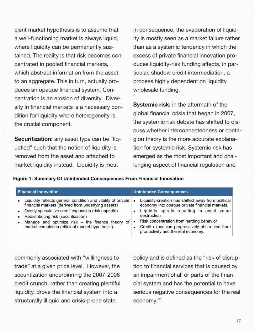
Figure 1: Summary Of Unintended Consequences From Financial Innovation

!!

Financial Innovation Unintended Consequences

▪ Liquidity reflects general condition and vitality of private financial markets (derived from underlying assets)

▪ Overly speculative credit expansion (risk appetite) ▪ Redistributing risk (securitization) ▪ Manage and optimize risk – the finance theory of

market completion (efficient market hypothesis).

▪ Liquidity-creation has shifted away from political economy into opaque private financial markets.

▪ Liquidity spirals resulting in asset value destruction

▪ Risk concentration from herding behavior ▪ Credit expansion progressively abstracted from

productivity and the real economy.

Page !1

A recent paper by Hal Scott2 contrasts the systemic risk debate in terms of asset-liability interconnectedness versus conta-gion, and suggests that contagion rather than connectedness was at the root of the crisis, and that the Dodd Frank legislation has weakened safeguards to contain conta-gion.

Contagion: the financial system is uniquely vulnerable to contagion because it depends on short-term borrowing to fund long-term investment. A funding cur-tailment, arising from maturity and liquidity mismatch can lead to shadow “bank runs”, where contagion is the result, em-bedded rollover risks inherent in funding long-term assets through short-term securi-tization sold into money markets that trig-gered the run on the shadow banking sys-tem.

When entities leverage their balance sheets to the hilt, an asset price drop has a disproportionate adverse impact that is widespread. Asset price declines become synchronized. In the context of the finan-cial crisis, synchronized asset declines played a crucial, and ultimately destruc-tive, role. Once the spreading illiquidity of formerly highly liquid instruments called into question the value of the underlying collateral, as well as the strength of many

counterparties, the shadow banking sys-tem proved extremely fragile.

DOWNWARD LIQUIDITY SPIRAL

Innovation in finance has always been driven by the search for greater liquidity. Critics of financial innovation, such as Hy-man Minsky, have argued that new credit instruments only add to the “sense” of greater liquidity but which in reality rely on the liquidity of the underlying assets. Once the value of these underlying assets decline, such as in the MBS market in 2007, “market” liquidity evaporates.

Systemic liquidity crises coincide with the worst cases (wrong-way risk) of market dis-tress, as in the crash of 1987, the 1998 Russia/LTCM crisis, the Asian Crisis, and 2007-08 credit (and liquidity) crunch. Forced selling, a hallmark of financial cri-sis, becomes prevalent. The feedback loop in figure 2 shows an exogenous shock leads to position liquidations (1 and 2). Such (pro-cyclical) dynamics can be overlaid on the performance of any asset type. Feedbacks effects from pro-cyclicality make asset returns and risks en-dogenous, resulting in herd behavior and reflexivity between liquidity distress and credit quality (3 and 4). Feedback loops

18

amplify market movements and assets price declines contribute to rising asset market volatility (5) Quantitative easing (6) is the policy response de jour where global policy makers’ aggressive stimulus and li-quidity support programs have boosted “toxic” asset valuations and sharply nar-rowed various yield spreads.

Vicious cycles: the evaporation of liquidity in many markets in 2007-08 has justifiably attracted much attention. The vicious cy-cles involving the simultaneous falling of market liquidity and funding liquidity, lower

market prices, de-leveraging and higher volatility all contributing to increased mar-ket illiquidity. Such dynamics make liquid-ity inherently pro-cyclical and raise the risk that liquidations from overcrowded levered positions take place at fire sale prices. The systemic aspect of liquidity arises when there is a shift to aggregate liquidity and li-quidity shock commonality across asset classes.

INFORMATION ASYMMETRY

The increasingly complex external forces arising from market illiquidity create a com-pelling need to look beyond internal/

Young Professionals Forum Washington DC November 7th 2013 Graham Strong!Liquidity Spirals Innovation in finance has always been driven by the search for greater liquidity. Critics of financial innovation, such as Hyman Minsky, have argued that new credit instruments only add to the “sense” of greater liquidity but which in reality, rely on the liquidity of the underlying assets. Once the value of these underlying assets decline, such as in the MBS market in 2007, “market” liquidity evaporates.

Efficient market hypothesis: the securitization of asset classes in tradable securities, only create a market if liquidity can be permanently sustained. Since the search for liquidity almost always involves the lengthening of the debt chain, the result is invariably less, not more liquidity in the financial system as a whole. The fallacy of efficient market hypothesis is to assume that a well-functioning market is always liquid. This is an unfounded conceptual assumption and it is unwise to build a whole system of finance theories and regulatory rules based on it.

Systemic liquidity crisis coincide with the worst cases of market distress, as in the crash of 1987, the 1998 Russia/LTCM crisis, the Asian Crisis, and 2007-2008 credit (and liquidity) crunch. Forced selling, a hallmark of financial crisis, becomes prevalent. The feedback loop in figure 2, shows how position liquidations (assets price declines) contribute to rising asset (stock market) volatility. Quantitative easing (QE) is the policy response de jour where global policy makers’ aggressive stimulus and liquidity support programs have boosted “toxic” asset valuations and sharply narrowed various yield spreads.

Figure 2: The dynamics of liquidity spirals has been amplified because access to liquidity has become more dependent on market conditions

!

Vicious cycles: the evaporation of liquidity in many markets in 2007-2008 has justifiably attracted much attention. The vicious cycles involving the simultaneous falling of market liquidity and funding liquidity, lower market prices, de-leveraging and higher volatility all contributing to increased market illiquidity. Such dynamics make liquidity inherently procyclical and raise the risk that liquidations from overcrowded levered positions take place at fire sale prices. The systemic aspect of liquidity arises when there is a shift to aggregate liquidity and liquidity shock commonality across asset classes.

!Information Asymmetry

2. Asset Price

Declines

4. Credit Deterioration

6. Policy Response

1. Exogenous Shock

Liquidity Spiral

3. Bank

Funding Liquidity Distress

5. Stock Market

Volatility

Page !2

19

organizational performance metrics and industry-specific benchmarks. In addition, the more global you become the more you need to integrate with your external envi-ronment. In particular, the credibility of in-formation about market prices can influ-ence asset valuations as much as informa-tion about economic fundamentals. Infor-mation asymmetry in asset values can ef-fectively cause more fragile markets, such as shadow banking, to close down.

Risk appetite: when information is insuffi-cient for decision-making (as depicted in Figure 3), efficient markets can no longer be counted on (always liquid assumption). Securitized products were assumed to con-tain accurate information about their value and risk. An entity must therefore under-stand how systemic risk influences the ex-ternal environment and how business cy-cle expansion or contraction influences the prevailing risk appetite.

At the top of the business cycle, greater risk appetite leads to greater liquidity. It is the reverse at the bottom of the cycle, where illiquidity predominates. All asset types suffer when market illiquidity or vola-tility escalates. Risk factors differ in their market price of risk, reflecting their covari-ance with the business cycle. Wrong way risk occurs exposures are correlated with a

downturn, where an entity maintains risk homeostasis, despite changes in external environmental conditions3.  Consequently tail risk insurance for both credit and liquid-ity risk will generally be underpriced.

Threat analysis: to maintain the appropri-ate risk appetite, an entity must do two things in tandem. First, it needs to ac-count for and obtain all the available data that is meaningful to its business, including the data from its entire value network. Emerging threats must be taken into ac-count and vulnerabilities made explicit. Second, the entity must adjust its risk ap-petite to reflect the external environment and threat landscape it faces.

20

Figure 3: Data Used in Decision-Making

Note: Red arrows show directions of Information FlowsPink arrows show maturity of use

Data Used in Decision Making

External Environment

Customer/SuppliersCustomer/Suppliers

Uses information from reliable external operating

environment

Internal Organization

Existing Enterprise

Architecture

Uses internal organizational information

Uses publicly available information (e.g. Census)

Maturity of Use(Low)

Maturity of Use(Medium)

Maturity of Use (High)

Internal Organization

ExistingEnterprise

Architecture

Uses internal organizational information

Note: Red arrows show directions of Information FlowsPink arrows show maturity of use

Data Used in Decision Making

External Environment

Customer/SuppliersCustomer/Suppliers

Uses information from reliable external operating

environment

Internal Organization

Existing Enterprise

Architecture

Uses internal organizational information

Uses publicly available information (e.g. Census)

Maturity of Use(Low)

Maturity of Use(Medium)

Maturity of Use (High)

Internal Organization

ExistingEnterprise

Architecture

Uses internal organizational information

External EnvironmentExternal Environment

Customer/SuppliersCustomer/Suppliers

Uses information from reliable external operating

environment

Internal Organization

Existing Enterprise

Architecture

Uses internal organizational information

Uses publicly available information (e.g. Census)

Maturity of Use(Low)

Maturity of Use(Medium)

Maturity of Use (High)

Internal Organization

ExistingEnterprise

Architecture

Uses internal organizational information

INFORMATION MANAGEMENT SYS-TEMS FOR FINANCIAL INSTITUTIONS

Information management systems consist of publicly available data from such organi-zations as the Census Bureau, the Depart-ments of Labor, Treasury, and Health, OECD databases, BIS, IMF, IFC, MSCI, World Financial institution, regulatory and commercial databases. It also includes fi-nancial institution data and data generated from a financial institution’s constituency, extended communities in the financial in-dustry, and other players in the global economy. Information management sys-tems can help a financial institution normal-ize all relevant data so that it can be tracked, correlated, and viewed through useful lenses to enable better decision-making concerning its threats and opportu-nities (e.g. growth strategy). Risk manag-ers can only make the best decisions when considering the strength of causal re-lationships among macro variables in their ecosystems. Essentially there are three scenarios:

1. Known causal relationships or root cause where causal mapping of the inter-connected relationships, and quantifying the cause–effect relationships, is possible, or

2. Limited data (weak signal/loud noise) where the data needed for macro- model-ing exposures is generally sparse, or

3. Unknown, rarely occurring or complex systems where correlations are not recog-nized while in the making, such as growing homogeneity of market behavior in the fi-nancial crisis.

The major risk posed by the growing homo-geneity of market behavior is that when dis-tress hits the market, similar investor posi-tions are unable to diffuse the shock. Dur-ing the later years of the credit boom, warn-ings were made about the herding in the derivatives market. One of the most telling (generally unrecognized) signs was the un-interrupted narrowing of credit spreads be-tween 2003 and early 20073.

The problem for many financial institutions is that they do not have enough external data to be able to formulate any conclu-sions about potential threats. The first step is to identify vulnerabilities by assess-ing abnormalities in environmental factors. Macro financial indicators need to be tracked to help isolate potential threats. These indicators should include credit spreads, interest rates, exchange rates, yield spreads, asset prices, credit expo-sures for the following purposes:

21

1. Macro surveillance of financial mar-kets to provide a forward-looking assess-ment of the likelihood of extreme shocks that could hit the financial system. An indi-cator, such as credit spreads, provides a single measure of risk and can focus on vulnerabilities using macro economic or other selected indicators as key explana-tory variables.

2. Macro prudential indicators of finan-cial soundness (FSIs) show financial sector vulnerabilities and cover asset quality, man-agement soundness, earnings and profit-ability, liquidity and sensitivity to market risk. Mapping causal relationships, and inter-linkages among FSIs and their mac-roeconomic determinants, together with an assessment of their sensitivity to various

shocks, provide the basic building blocks of financial stability analysis.

CONCLUSION

A macro view of exposure is necessary to provide systemic risk management if ex-treme events are to be avoided. Extreme event risk is perhaps the dimension of risk most often misunderstood, and therefore also overlooked by financial institution management. Simply stated, it is the moni-toring of credit creation and using indica-tors to visualize less probable outcomes and their causal relationships. Information management capabilities enable financial institution to better focus on what truly con-stitutes unexpected risk events and to take pre-emptive action when encountered. Monitoring indicators will help assess finan-cial market risk and describe the pattern of asset returns under the influence of erratic self-reinforcing systems (feedback loops). In particular, it is important to anticipate and recognize the threat to price stability when it comes about through the accumu-lation of debt to a point where its subse-quent monetization becomes inevitable. That is to say, before a given bubble reaches a point at which it’s bursting be-comes a systemic risk to the economy.

Young Professionals Forum Washington DC November 7th 2013 Graham Strong!

The major risk posed by the growing homogeneity of market behavior is that when distress hits the market, similar investor positions are unable to diffuse the shock. During the later years of the credit boom, warnings were made about the herding in the derivatives market. One of the most telling signs was the uninterrupted narrowing of credit spreads between 2003 and early 20073.

The problem for many financial institutions is that they do not have enough external data to be able to formulate any conclusions about potential threats. The first step is to identify vulnerabilities by assessing abnormalities in environmental factors. Macro financial indicators need to be tracked to help isolate potential threats. These indicators will show potential sources of shock and should include credit spreads, interest rates, exchange rates, yield spreads, asset prices, credit exposures for the following purposes:

1. Macro surveillance of financial markets to provide a forward-looking assessment of the likelihood of extreme shocks that could hit the financial system. Indicators such as credit spreads, provide a single measure of risk and can focus on vulnerabilities using macro economic or other selected indicators as key explanatory variables.

2. Macro prudential indicators of financial soundness (FSIs) show financial sector vulnerabilities and cover asset quality management soundness, earnings and profitability, liquidity and sensitivity to market risk. Mapping causal relationships, an analysis of inter-linkages among FSIs and their macroeconomic determinants, together with an assessment of their sensitivity to various shocks, provide the basic building blocks of financial stability analysis.

Conclusion

A macro view of exposure is instrumental in providing systemic risk management if extreme events are to be avoided. Extreme event risk is perhaps the dimension of risk most often misunderstood, and therefore also overlooked by financial institution management. Simply stated, it is the monitoring of credit creation and using indicators to visualize less probable outcomes and their causal relationships. Information management capabilities enable financial institution to better focus on what truly constitutes unexpected risk events and to take pre-emptive action when encountered. Monitoring indicators will help assess financial market risk and describe the pattern of asset returns under the influence of erratic self-reinforcing systems (feedback loops). In particular, it is important to anticipate and recognize the threat to price stability when it comes about through the accumulation of debt to a point where its subsequent monetization becomes inevitable. That is to say, before a given bubble reaches a point at which it’s bursting becomes a systemic risk to the economy.

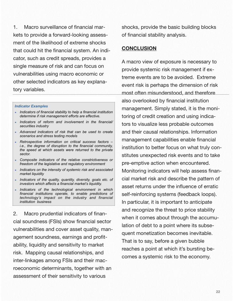
Indicator Examples

▪ Indicators of financial stability to help a financial institution determine if risk management efforts are effective.

▪ Indicators of reform and involvement in the financial/securities industry

▪ Advanced indicators of risk that can be used to create scenarios and stress testing models

▪ Retrospective information on critical success factors – i.e., the degree of disruption to the financial community, the speed at which assets were returned to the private sector.

▪ Composite indicators of the relative constrictiveness or freedom of the legislative and regulatory environment

▪ Indicators on the intensity of systemic risk and associated market liquidity

▪ Indicators of the quality, quantity, diversity, goals etc. of investors which affects a financial market’s liquidity.

▪ Indicators of the technological environment in which financial institutions operate, to enable predictions of technology’s impact on the industry and financial institution business

Page !4

22

FOOTNOTES & REFERENCES

1. See, e.g., Jaime Caruana, Systemic Risk: How to Deal with It?, BANK FOR INT’L SETTLEMENTS, Feb. 12, 2010, http://www.bis.org/publ/othp08.htm#P01

2. Hal S. Scott, The Reduction of Sys-temic Risk in the United States Finan-cial System, 33 HARV. J.L. & PUB. POL’Y 671, 672-79 (2010)

3. Graham Strong, FDIC Strategic Impera-tives White Paper. (Sept. 2006)

23

Basel III and the critical challenge for bank liquidity risk

4

Art of liquidity risk management

The Wikipedia definition of liquidity states,“In banking, liquidity is the ability to meet obligations when they become due.”

The important part is understanding ex-actly what is meant by “when they become due”. From the risk management perspec-tive this means in perpetuity, or at least as long as we wish the bank to remain a go-ing concern. In other words, maintenance

of liquidity at all times is the paramount or-der of banking.

Bank risk management is the practice of balance sheet management. The risks in question are those affecting the balance sheet, which are capital, liquidity and fund-ing (generally grouped together under “asset-liability management” or ALM). We categorize balance sheet risk as the proc-ess of:

• managing the bank’s capital;

24

ABSTRACT: The art of banking is that of managing liquidity. While capital is correctly viewed as being of utmost importance to a bank’s viability and public perception, the practitioners’ common saying that “capital kills you slowly, while liquidity kills you quickly” is an accurate one. Genuine pure liquidity-scarcity events are rare events, however the experience of the UK bank Northern Rock in 2007 illustrates perfectly the key risk for banks and regulators, that of the risk of complacency.This article suggests that, although it is the technical requirements of Basel III and the need to maintain ade-quate liquidity buffers that is exercising practitioners’ and academics’ attention, the critical challenge concerns that of banks’ culture, and ensuring that control and governance infrastructure put in place today is maintained over the long term. A change in the Treasury and risk management operating model is a necessary step towards ensuring this longevity in liquidity risk management principles

Professor Moorad ChoudhryChair, FinRisk London CouncilIPO Treasurer, RBS Group Treasury

• managing the liquidity mismatch, arising from the fundamental ingredient of bank-ing termed “maturity transformation”; the recognition that loans (assets) generally have a longer tenor than deposits (liabili-ties);

This is also the paradox of banking. Bank-ing creates maturity mismatches between assets and liabilities, because assets are invariably long-dated and liabilities are short-dated, and this creates liquidity risk. To undertake banking is to assume a con-tinuous ability to roll over funding, other-wise banks would never originate long-dated illiquid assets such as residential mortgages or project finance loans. As it is not good business practice to rely on as-sumptions, prudent liquidity risk manage-ment dictates that all leveraged financial institutions need to set in place an infra-structure and governance ability to ensure that liquidity is always available, to cover for when market conditions deteriorate. The fundamental challenge for all banks is to maintain this robust control infrastruc-ture and governance over the long term.

The scope of liquidity risk

Basel I and Basel II did not concern them-selves with liquidity, only capital. The Basel III regime, which is expected to be

fully implemented by 2019, makes material demands on banks with respect to the way they manage liquidity.

However liquidity risk management is not simply a matter of liquidity metrics and ra-tios. There are important governance and policy issues that also need to be built into the infrastructure and workings of a bank’s Treasury and Risk departments. Liquidity risk management needs to be addressed at the highest level of a bank’s manage-ment, the Board of Directors. The Board typically delegates this responsibility to a management operating committee such as ALCO, but it is the Board that owns liquid-ity policy. If it does not own it, then it is not following business best-practice. Given this, it is important that the Board also understands every aspect of liquidity risk management.

We classify liquidity risk management as encompassing the following specific areas:

• Liquidity strategy, policy and processes;

• Regulatory requirements and reporting obligations;

• Bank funding strategy and policies;

• Liquidity risk appetite;

25

• Institution-specific and market-wide stress scenarios, and stress testing;

• The liquid asset buffer;

• Liquidity contingency funding plan.

Given its importance, it is best that liquid-ity management is devised and dictated from the highest level, as it will influence every aspect of the bank’s business strat-egy and operating processes.

Basel III enshrines the new risk approach in formal regulatory law with two new struc-tural risk metrics, one for short-term and one for long-term funding. On the surface, this seems like just a step-change in liquid-ity management culture, but that is only be-cause principles accepted as common-place in the 1860s or 1960s had been dis-carded by 2008. Nonetheless, in sub-stance, they will prove to be a challenge to work towards for many banks.

The stated objective of the Basel III liquid-ity coverage ratio (LCR) is to promote short-term resilience of banks to liquidity shocks. Setting a limit for it, and requiring banks to hold a stock of sufficient high quality genuinely liquid assets, is designed to ensure a more stable funding regime that will be less susceptible to a freeze in

interbank markets, of the kind observed in October 2008.

The LCR requirement results in banks hav-ing to maintain a liquidity buffer that matches expected cash outflows in a stressed environment. The amount of funds that might be observed in a market stress situation is given by the stress tests that banks run every month, under speci-fied assumptions. The time period cov-ered in the stress test is 30 days, which im-plies that a stressed environment lasting for only a month, which may be unrealisti-cally short. For this reason, some regula-tors, including the UK PRA, uses a longer 90-day time stress period for its test re-quirements.

The relevance of each bank’s stress tests are themselves only as great as the as-sumptions behind them. Any analysis un-dertaken under assumed conditions is al-ways at risk of inaccuracy, which is why continuous review and back-testing is also part of a bank’s risk management regime. Suggestions have also been made that the size of the liquidity buffer should be a func-tion of other metrics, including the follow-ing:

26

• Set at 2.0 or 2.5 times the size of the ag-gregate of a bank’s liabilities that are of less than 1-year maturity;

• Set at 110% of the stressed outflow num-ber.

The implication of the LCR for the world’s banks is that, in theory they will be hold-ing, in differing amounts, a stock of theo-retically genuinely liquid assets. The chal-lenge comes from the impact this will have on the bottom line, as a risk-free portfolio generates less income (if it is run at a profit at all), and so all else being equal, a bank’s profit can be expected to be reduced un-der such a regime.

The foundation LCR calculation relates to the short-term (30-day) stressed outflow amount of a bank’s liabilities. The critical long-term metric is the net stable funding ratio (NSFR). The NSFR is designed to pro-mote resilience over the longer-term. Set-ting a limit for it in theory ensures that suffi-cient long-term funding is in place to sup-port a bank’s balance sheet. In other words, maintaining an adequate NSFR should help considerably in ensuring a sta-ble funding structure because more of a bank’s liabilities will be comprised of longer-dated funding. (In Treasury terms,

we might define “long-dated” as being over 12- or 24-months in tenor).

Setting a minimum level for term funding would reduce dependency on short-term funding, while increasing cost of business as more liabilities are moved into longer term funding. Again, the issue for banks is one of cost, and impact on profit. Longer-dated liabilities cost more than short-dated liabilities, and in a stressed environment are difficult to raise. The challenge for risk managers and regulators is ensuring that the spirit of NSFR, which has not yet been enshrined in formal legislation, is main-tained throughout the business cycle.

Establishing a genuine risk governance culture

This article’s premise is that the cultural challenge, and its wider impact on stake-holders, especially shareholders, is a more difficult one to address than the regulation-related requirements banks have faced up to now. Nevertheless it is imperative that this challenge be met at all levels, to en-sure a greater ability to mitigate the impact of the next crash. What the current debate in banks needs to focus on is the need for a genuine, firm-wide approach to balance sheet risk. To effect this, it becomes neces-sary to establish the ALM committee or

27

ALCO as the premier risk management fo-rum in the bank, with Board-delegated authority.

As we all recognize, culture needs to be set from the top down. To remove its de-pendence on individuals, banks need to consider their operating model and risk in-frastructure, and how exactly capital, bal-ance sheet and liquidity are to be man-aged. Some issues to consider are:

• Operating model and internal organiza-tion;

• Risk governance infrastructure, and the risk management “triumvirate” of the CRO, CFO and Treasury. This should be organized so that the three constituents

of the triumvirate are able to work to-gether effectively.

The challenge is for banks to establish a cultural mindset and operating framework, that embeds balance sheet risk in every-one’s thinking. In other words, something beyond the regulatory requirements set out under Basel III.

Exhibit 1 appears to state the obvious, but in fact is making a much more subtle, and potentially controversial, point. The three departments are peers, therefore the re-porting line could not logically be subordi-nated one to the other. Crucially, the ALCO would have the oversight for all of balance sheet risk, including credit risk pol-icy at the highest level. It would then seem logical that any credit risk committee

28

Exhibit 1

Chief Risk Officer ! Treasury! Chief Financial Officer!

Finance Accounting Budget setting, forecasting Strategy and planning Product control Valuation and MtM Financial reporting !

Risk Management Market risk Credit risk Operational risk Monitoring and control Management information reporting Compliance monitoring Stress testing policy ERM

ALCO

!

Asset-Liability Management Strategy and planning Liquidity risk management Interest rate risk management Hedging policy Balance sheet management Internal funds pricing policy Liquidity stress testing Capital management ALCO reporting

Bank Balance Sheet Management Triumvirate

or CRO forum should be subordinated to it.

The logic for this is irresistible. As the membership of ALCO covers both front-office business line heads with P&L respon-sibilities as well as risk management per-sonnel, it has the overarching balance sheet view that an “Enterprise Risk Man-agement” (ERM) forum perhaps may not. It makes sense to make ALCO the premier risk management body.

For Treasury, the reporting line is a key in-fluencer of the extent of the risk culture. From its position in the triumvirate, Treas-ury will need to report to the same level as the CFO and CRO. This would logically be the CEO, and such an arrangement is com-mon.

In some cases, the reporting line is higher. One large Western Euro-pean bank organizes the Treasury function as a direct report of the Board, with the Group Treasurer re-porting in to a named non-executive director. This removes any conflict of interest issues, while ensuring that balance sheet risk management is undertaken at the appropriate level of seniority. It

also clears the way for the Treasurer to chair the ALCO, something that is usually undertaken by the CEO or the CFO. When one remembers that Treasury is the only department in a bank that looks at the en-tire balance sheet, assets and liabilities, and is both inward and outward looking, this arrangement carries logic.

Ensuring effective teamwork

Changes in culture and operating method are perhaps the hardest to make in any firm, including a bank. The larger the bank, the more bureaucratic the process of risk management is. In large firms there is a danger that “risk management” be-comes more of a forms-based box-ticking process than a genuine exercise in manag-ing risk exposure. However, effective team-

29

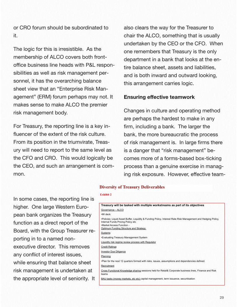
Exhibit 2

Treasury will be tasked with multiple workstreams as part of its objectives Governance – ALCO

• MI deck

• Policies: Liquid Asset Buffer, Liquidity & Funding Policy, Interest Rate Risk Management and Hedging Policy, Internal Funds Pricing Policy etc • Market Access Function - Optimum Funding Structure and Strategy

Systems

• Evaluating Treasury Management System

Liquidity risk regime review process with Regulator

Credit Ratings

Investor Due Diligence

Planning

• Plan for the next 12 quarters formed with risks, issues, assumptions and dependencies defined.

Recruitment

Cross Functional Knowledge sharing sessions held for Retail& Corporate business lines, Finance and Risk teams

BAU tasks (money markets, etc etc) capital management, term issuance, securitisation

Diversity of Treasury Deliverables

work is essential if the “triumvirate” is to work together efficiently.

One way to try to address the issues raised by a growing bureaucracy and proc-ess is to drive a culture of genuine team-work. In a Treasury team, this calls for what one might term “Total Treasury”. This is modeled loosely on the team-building concept first espoused by Rinus Michels, the coach of the Holland team during the 1974 football World Cup.

Exhibit 2 shows that the Treasury function is a multi-disciplinary one, with a diverse set of objectives and deliverables. These are better served if members of the team are able to support each other. In the Dutch national side, “Total Football” re-ferred to the concept whereby each out-field player was able to play in any posi-tion, and so could cover for any other team member. This concept is replicated in “Total Treasury”.

This is not something that can be imple-mented overnight. It requires mindset shift, experience, and learned judgement, together with a genuinely open and trans-parent culture, to work properly. But if it can be operated successfully, it makes bal-ance sheet risk management much easier to be implemented firm-wide, because the

triumvirate of CRO, CFO and Treasurer, and their teams, will be able to work much more effectively.

Exhibit 3 illustrates the recommended team building doctrine. Six years after the first signs of the crash the discipline of risk management, the need to have a rigorous risk framework in place at all banks with re-spect to capital, liquidity and funding, is ac-cepted universally. There is no disagree-ment with what Basel III, and national regu-lators, wish to implement with respect to levels of capital and liquidity

The real challenge comes with the need to embed a genuine risk management culture in the bank. If this is successful, it will en-sure that principles of balance sheet risk are adhered to throughout the cycle, par-

30

Exhibit 3

Teambuilding Doctrine Everyone is involved in all tasks

Each person is able to cover for at least 2 other persons across differenrt teams

No single-person dependencies

Genuinely open, collaborative and challenging environment

Effective upward and downward delegation

“Total Treasury” Team Building Doctrine

ticularly when bull market condi-tions return. A change in operat-ing model style and firm culture, to one of genuine openness and understanding, will help to ensure that this becomes the case.

Conclusions

Liquidity management is a disci-pline that is as old as banking, but from historical observation we conclude that its principles need to be refreshed and main-tained throughout the business cycle. For the new regime being implemented under Basel III, the need to adhere to old- fashioned beliefs on sound liquidity practice is something that will be enshrined in law. However the two new funding metrics reflect banking logic, and the principles behind them should be fol-lowed regardless, simply because bank management should be aware of their im-portance.

31

“Reference Information box” Liquidity Coverage Ratio The LCR for a bank is given by: Stock of high quality liquid assets >100%!Stressed net cash outflows over a 30-day time period! High quality assets are specified by the Basel Committee, and include sovereign bonds and multilateral agency bonds. The LCR identifies the amount of unencumbered, high quality liquid assets required to offset the net cash outflows arising in a short-term liquidity stress scenario. A regulatory limit for the LCR ensures that banks meet this requirement continuously. Net Stable Funding Ratio The NSFR is given by:

Funding Stable RequiredFunding Stable Available >c.100%

The metric measures the amount of stable funding as a proportion of the total requirement for such stable funding. Definitions on what constitutes “stable” are given by the Basel Committee. The NSFR is typically used to monitor and control the level of dependency on volatile, short term wholesale markets, as a key structural balance sheet ratio. A low ratio indicates a concentration of funding in shorter maturities (under 1-year tenor) which can give rise to funding roll-over and mismatch risks. End of Box

Loan sale operations go from cleaver to scalpel

5

Big non-performing loan portfolio sales, typically valued at over €500m, are moti-vated by the need to demon- strate a stra-tegic refocusing and a reduction in balance sheet exposure. Lloyds Bank’s success-ful string of Euro-pean NPL sales are a clear exam-ple of this type of deal; the bank proved to the market and regulators that it was exiting non-core markets and shrinking its bal-ance sheet.

Smaller NPL portfolio sales are equally im-portant but achieve an entirely different goal: to reduce operational costs and com-plexities in the work-out and legal depart-ments. Smaller, more targeted sales allow

banks to execute very specific strategies: for example, to dispose of the 5% of loans by balance that generate 20% of work-out

related costs; or to eliminate all loans with exposure to a high-risk segment, such as Spanish resort develop-ment.

For institutions experienc-ing steady growth of work-outs and associated ex-penses, more targeted loans may be the only way

to manage staff capacity constraints and caps on legal counsel costs.

In 2012, there were a number of big, suc-cessful deals. Most major European banks had created big non-core groups, some holding over €100bn of assets. European banks’ balance sheets held more than €1trn of non-core and non-performing

Gifford WestManaging Director & Head of International OperationsDebtX

32

loans. Buy-side firms of all sizes had flocked to Europe.

This year opened with the hope of a steady flow of very large portfolio sales from banks and government agencies in the UK, Spain, Germany and Ireland. But at the start of the second half of the year, a different picture is emerging. While a num-ber of big portfolio deals have been exe-cuted in Ireland, Germany and the UK, many of the big deals (notably in Spain) seem to be stuck. The rumour mill is oddly quiet on further mega-deals.

On the other hand, DebtX forecasts an in-creasing flow of deals with unpaid bal-ances from €10m to €150m and has re-cently been engaged to sell portfolios of this size in Germany, the UK, Ireland, Scan-dinavia and the Netherlands. In all these

cases, the bank’s management had bal-anced the upside of the asset versus the nuisance of retaining the debt and decided a tactical sale was best.

Interest in smaller loan sales is accelerat-ing and we are reviewing portfolios of this nature in seven European countries. While

there is no shortage of big buyers with very big chequebooks, banks do not seem to be as active in exploring very large sales. The trend is being driven by a short-age of bank capital, fatigue with very large deals and an urgency to manage rising op-erational costs.

Banks cannot afford the capital losses as-sociated with big sales campaigns; capital is too precious. Regulators are pressing banks to raise capital, but most banks are not reserved at levels that will allow sales in today’s market. How likely are they to take an additional capital hit through a large NPL sale?

Big, strategic deals tend to take on the seri-ousness of heart surgery for banks. Staff with full-time responsibili- ties are pulled into ‘temporary’ second roles that expand

to full-time requirements. The deals are ex-hilarating when successful, less so when they fail. The internal pressure is immense and often forces sellers to take prices they did not imagine acceptable when they be-gan the process.

33

A typical smaller loan sale is about dispos-ing of a headache; the process itself is not a headache

The transaction team watches the deal dy-namics shift from seller to buyer as internal awareness of deal costs percolate up the organisation. The bank’s board and the fi-nancial press add pressure to close a deal at any cost.

In contrast, smaller sales do not involve the complexity of selling hundreds (or thou-sands) of loans. If large sales are like merg-ers and acquisitions deals in their complex-ity, small loan sales are like a simple club deal. Managing the sale is a part- time job and the professional risk more manageable. A typical smaller loan sale is about disposing of a headache; the proc-ess itself is not a headache.

Very large European NPL deals are by no means dead, but a more active, smaller sales market is emerging. This is an excel-lent outcome for banks in terms of liquidity and good news for the smaller distressed debt funds eagerly waiting to snap up dis-tressed bank loans.

34

Bubble VaR, a countercyclical value-at-risk approach

6

VaR and financial crisesIt is a great irony that our advancement in risk management has created a new kind of risk—the risk of risk measurement—the misuse of (frequentist) statistics. The credit crisis has debunked some well-established risk models used by banks, in particular Value- at-risk (VaR), an essential tool used for the purpose of regulatory capital and banks’ own eco-nomic capital. In fact, the risk of using VaR models has been forewarned by Danielsson et al. as early as 2001 in a response paper to the Basel authority. Nonetheless, VaR has become the industry standard because of its practical simplicity and a lack of agreeable alternatives.

VaR is the loss quantile of the P&L distribution of a portfolio,

statistically determined using data over a sample period (of multiple years) and esti-mated over a specified time horizon (10 days for market risk) at a certain confi-dence level (for example at 97.5% confi-dence level i.e. a 2.5% quantile is used). The crisis has shown that, as a risk metric intended to measure extreme losses or tail

Max Wong Member, FinRisk Singapore CouncilHead of Risk Model TestingRoyal Bank of Scotland, Singapore.

35

Figure 1: 97.5% VaR of Dow Jones index calculated using Riskmetrics method, and VaR exceedences for long/ short sides. The same stylized facts also hold for other VaR

methods. Figure 2: The leverage effect, or inverse relationship between price and volatility

risk, VaR is just “too little, too late”. How far off are we?

Figure 1 shows the 97.5% VaR for the Dow Jones index; the P&L’s which exceeded the VaRs for longs and shorts are shown as vertical bars. During the credit crisis in 2007, the exceedences are a lot larger than VaR, in fact, very much larger than that expected by the commonly assumed normal distribution. To get an idea if the exceedences are realistic, consider Table 1 which shows the top-10 largest daily losses in history. Certainly crises have oc-curred more often than suggested by VaR models. These led to the popular idea of Black Swans (see Taleb (2007)), events of low probability and high devastation lo-cated at the extreme tail of the distribution.

Taleb found that such events in financial markets are not statistically reproducible (atypical), a phenomenon he termed ex-tremistan. Without the element of repro-ducibility, Black Swans are not amenable to statistical quantification; the usage of fre-quentist statistics as applied in VaR will lead to precise but misleading (inaccurate) numbers. Because of finite sampling, a mathematical quantile can always be deter-mined, but the expected loss beyond this quantile is an elusive number which may never converge under extremistan. This illu-

sion of precision could undermine risk man-agement preparedness by putting risk con-trollers in a comfort zone.

Table 1: Top-10 daily losses in the history of Dow Jones index

Secondly, VaR is always late in crisis detec-tion—it increases sharply only after the ini-tial sharp selloff of a crisis. The cause, the use of a recent rolling-window in such mod-els means that this metric will always re-spond late to large market movements that mark the onset of a regime shift. Thus, VaR is an effective analytics during “peace time” when changes are gradual, but is useless for crisis warning. As VaR is used to determine regulatory capital, the burden on banks will rise sharply in a crisis situa-tion after the fact, forcing banks to reduce positions in a falling market. Conversely, VaR is muted in a bullish market and the benign capital requirement encourages bal-ance sheet expansion and the use of lever-age. This phenomenon of low volatility dur-

36

!!!

Event Date Daily log return

Mean number of years between occurrences (if normally distributed,

assuming volatility of 25% p.a.)

19-Oct-87 -25.6% 1.86E+56

26-Oct-87 -8.4% 69,074

15-Oct-08 -8.2% 37,326

1-Dec-08 -8.0% 19,952

9-Oct-08 -7.6% 5,482

27-Oct-97 -7.5% 3,258

17-Sep-01 -7.4% 2,791

29-Sep-08 -7.23% 1,684

13-Oct-89 -7.16% 1,346

8-Jan-88 -7.10% 1,120

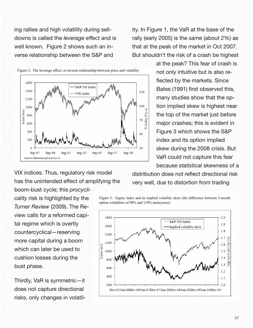
ing rallies and high volatility during sell-downs is called the leverage effect and is well known. Figure 2 shows such an in-verse relationship between the S&P and

VIX indices. Thus, regulatory risk model has the unintended effect of amplifying the boom-bust cycle; this procycli-cality risk is highlighted by the Turner Review (2009). The Re-view calls for a reformed capi-tal regime which is overtly countercyclical—reserving more capital during a boom which can later be used to cushion losses during the bust phase.

Thirdly, VaR is symmetric—it does not capture directional risks, only changes in volatil-

ity. In Figure 1, the VaR at the base of the rally (early 2005) is the same (about 2%) as that at the peak of the market in Oct 2007. But shouldn’t the risk of a crash be highest

at the peak? This fear of crash is not only intuitive but is also re-flected by the markets. Since Bates (1991) first observed this, many studies show that the op-tion implied skew is highest near the top of the market just before major crashes; this is evident in Figure 3 which shows the S&P index and its option implied skew during the 2008 crisis. But VaR could not capture this fear because statistical skewness of a

distribution does not reflect directional risk very well, due to distortion from trading

37

Figure 1: 97.5% VaR of Dow Jones index calculated using Riskmetrics method, and VaR exceedences for long/ short sides. The same stylized facts also hold for other VaR

methods. Figure 2: The leverage effect, or inverse relationship between price and volatility

Figure 3: Equity index and its implied volatility skew (the difference between 3-month option volatilities of 90% and 110% moneyness)

!!

around support/ resistance levels. To un-derstand this microstructure, consider a pegged currency attack. Speculators who sell against the peg will bring prices down to test the peg gradually because the cur-rency is supported by opposing traders (and the central bank) who bet that the peg will hold. Conversely, each time the peg holds, short covering will likely see quick upward spikes. This causes occa-sional positive skewness in the distribution even though the real directional risk is downwards. Since trading can be seen as a battle between bulls and bears for resis-tances and supports, statistical skewness is highly dependent on price levels. Figure 4 illustrates the statistical skew for the S&P index—there is no obvious pattern

near the market peak, the realized distribu-tion is virtually symmetric.

This leads to the fourth weakness, VaR does not distinguish between long and short positions. In Figure 1, the VaR just be-fore the crisis (Oct 2007) has effectively the same values for longs and shorts. But a crash can only happen downwards! (never up). So shouldn’t the risk be higher for longs? Likewise, at the trough of the mar-ket, shorts should be more at risk to a (rapid) bounce, which can only happen up-wards. Thus, the present day capital re-gime does not penalize longs for chasing an asset bubble nor recognize that the crash risks of opposing positions are une-qual. Since the banking system is profit

maximizing and capital effi-cient, the rules incentivize banks to chase the latest hot assets collectively; it is not macro-prudential.

Misuse of statisticsVaR models are appealing be-cause they are mathematically tractable, meaning a risk con-troller can test his results and state with precision that his VaR is “true” within certain con-fidence. (Thinking in terms of an existence of a “true” value

38

Figure 4: Equity index and its statistical skewness (calculated using 1 year rolling prices)

Figure 3: Equity index and its implied volatility skew (the difference between 3-month option volatilities of 90% and 110% moneyness)

!!

waiting to be uncovered is a hallmark of the frequentist school of thought.) Tractabil-ity comes with a high price— you have to assume returns are independent and identi-cally distributed (i.i.d). The abstraction of i.i.d. is just a sleight of hand of modelers to forecast VaR over the next time horizon—if i.i.d. is true, then it seems acceptable to in-fer that tomorrow’s quantile is identical to the quantile calculated from the most re-cent past data sample.

I.i.d. also allows a risk controller to perform back testing to “prove” that a VaR of say 99% confidence level does indeed contain on average one exceedence per 100 days of observations. In fact, back testing is nothing more than a test of the various nu-ances of i.i.d. In addition, when residuals are i.i.d., standard statistical estimation methods (such as regression) can produce consistent and unbiased estimates.

Ironically, the same i.i.d. assumption is the root-cause of the failures of VaR. The prac-tice of statistics and the notion of precision (as opposed to accuracy) hinges on repro-ducibility of observations, which is ques-tionable when financial markets are in cri-sis mode. In a crisis, contagion and posi-tive feedback among market participants (panic selling) cause price to spiral in a self-reinforcing way. The return series be-

come serially correlated, which leads to a breakdown of the i.i.d. assumption. This ex-plains why high volatilites and back testing breaks are clustered together during cri-ses, which makes back testing a tricky task—back testing is meant to validate in-dependence of tail losses, but it is exactly at stressful periods of interest to VaR that i.i.d. is violated.

When i.i.d. is violated, the aggregate distri-bution becomes fat-tailed (leptokurtic) be-cause the central limit theorem (CLT) no longer holds. The CLT states that even if variables are non-normally distributed indi-vidually, as long as they are i.i.d., their joint distribution becomes normally distributed when many variables are aggregated. Even models based on extreme value theory (EVT), which attempts to model extreme tails, rest on the i.i.d. requirement. This could explain why VaR models are so often surprised by the actual loss magnitudes witnessed during crises (as seen in Table 1)—the distributional models do not work when i.i.d. is broken.

The ideal of i.i.d. is the reason risk models are based on returns as opposed to raw prices. Empirical research provides the comfort that returns exhibit this ideal char-acteristic during regular most-of-the-time periods (even though VaR is more con-

39

cerned with irregular crisis periods). The process of differencing to arrive at returns means that useful information on cycles and trends are lost from the VaR input1. Fig-ure 5 shows the classical decomposition of a price series into three major compo-nents—trend, cycle and residual. The resid-ual (returns) is the input for VaR. It is not surprising why VaR cannot distinguish be-tween peaks and troughs, longs and shorts—it is missing cyclical information in its input. VaR is unable to reflect the obvi-ous asymmetry of a crash. Without this di-rectional element, VaR necessarily underes-timates fat-tail losses.

If we ask a retail investor who has never heard of Markowitz port-folio theory, what is his risk after buying a stock, his answer will naively (and quite cor-rectly) be downside (di-rectional) risk, not vola-tility. Arguably, volatility is only a risk for an op-tion, and only in the spe-cial case of a delta-hedged option. The per-vasiveness of thinking in terms of volatility in risk management is a legacy of Markowitz

(1952). If directional risk is truly potent, it seemed odd that we are leaving out trends from risk models.

By working exclusively with the i.i.d. re-turns, VaR models have gained the ele-gance of tractability and precision, unfortu-nately, at the expense of accuracy during times of crises. Keynes dictum is apt in risk management, “it is better to be roughly accurate than to be precisely wrong”.

It’s in the CycleIn Figure 5, the clustering and fat-tailness of residuals are evident during crises. Aca-demic research has attempted to explain

40

Figure 4: Equity index and its statistical skewness (calculated using 1 year rolling prices) !Figure 5: Classical decomposition of a price series

!Figure 6: Illustrates how cycle breaks and compression can cause fat-tails and serial correlation in returns

these phenomena by modeling the proc-ess or the distribution of returns (residual), as in the GARCH and the EVT literature. Unfortunately, practical application is marred with difficulties and these methods are not widely adopted by the banking in-dustry.

We posit that these phenomena are caused by the cycle component instead. Crashes are just breaks in the cycle —asymmetric and often sharp — which give rise to fat- tailed returns. The trend is driven by real economic growth and the i.i.d. residual is due to trading under effi-cient market condi-tions. The leverage effect is explained by observing that a cycle break is more common downward than upward. Furthermore, cycle compres-sion during a crisis—i.e. shortening of pe-riodicity and widening of amplitude— in-creases serial correlation and leads to vola-tility clustering. Figure 6 illustrates this; we simulate a stylized trend, cycle and i.i.d.

noise. A cycle break is introduced as a ver-tical drop, and cycle compression is intro-duced in the shaded zone. We combine all three elements into a price series and take its returns. The returns in the lower panel shows manifested fat-tail events, cluster-ing and serial correlation—similar to what is often observed in financial time series.

If crashes indeed originate from the cycle, we can design a forward looking risk met-ric by studying the cycle. Under this new paradigm, the larger a bubble forms on the upside (downside), the larger the risk of a crash (bounce), the long (short) positions are more risky to a crash (bounce). It fol-lows that at the peak of a bubble, longs

41

Figure 4: Equity index and its statistical skewness (calculated using 1 year rolling prices) !Figure 5: Classical decomposition of a price series

!Figure 6: Illustrates how cycle breaks and compression can cause fat-tails and serial correlation in returns

should be penalized most (in terms of risk capital), and at the trough, shorts should be penalized most. We propose a new met-ric called bubble value-at-risk (buVaR) which recognizes that “crashes” can only happen in the countertrend direction and the risks of longs and shorts are unequal.

VaR robustifiedBuVaR starts with the premise that crashes are extremistan, thus, can never be meas-ured precisely. The goal is to robustify VaR against the four weaknesses men-tioned earlier for the purpose of risk capi-tal. In other words, buVaR should provide a larger buffer to cover tail losses one step ahead of a potential crisis such that banks can build up a countercyclical safety buffer.

We first need to design a measure of the cyclical euphoria which we shall call the bubble (B). If the bubble is on the upside (B>0) then we inflate the return distribution on the negative side, which would penalize longs. If the bubble is on the downside (B<0), we inflate the positive returns which would penalize shorts. At time t, for risk factor Xn, its daily return variable Rn = ln(Xn/ Xn-1) undergoes a transformation:

times of crises. Keynes dictum is apt in risk management, “it is better to be roughly accurate than to be precisely wrong”. It’s in the Cycle In Figure 5, the clustering and fat-tailness of residuals are evident during crises. Academic research has attempted to explain these phenomena by modeling the process or the distribution of returns (residual), as in the GARCH and the EVT literature. Unfortunately, practical application is marred with difficulties and these methods are not widely adopted by the banking industry.

We posit that these phenomena are caused by the cycle component instead. Crashes are just breaks in the cycle—asymmetric and often sharp—which give rise to fat-tailed returns. The trend is driven by real economic growth and the i.i.d. residual is due to trading under efficient market conditions. The leverage effect is explained by observing that a cycle break is more common downward than upward. Furthermore, cycle compression during a crisis—i.e. shortening of periodicity and widening of amplitude—increases serial correlation and leads to volatility clustering. Figure 6 illustrates this; we simulate a stylized trend, cycle and i.i.d. noise. A cycle break is introduced as a vertical drop, and cycle compression is introduced in the shaded zone. We combine all three elements into a price series and take its returns. The returns in the lower panel shows manifested fat-tail events, clustering and serial correlation—similar to what is often observed in financial time series.

If crashes indeed originate from the cycle, we can design a forward looking risk metric by studying the cycle. Under this new paradigm, the larger a bubble forms on the upside (downside), the larger the risk of a crash (bounce), the long (short) positions are more risky to a crash (bounce). It follows that at the peak of a bubble, longs should be penalized most (in terms of risk capital), and at the trough, shorts should be penalized most. We propose a new metric called bubble value-at-risk (buVaR) which recognizes that “crashes” can only happen in the countertrend direction and the risks of longs and shorts are unequal. VaR robustified BuVaR starts with the premise that crashes are extremistan, thus, can never be measured precisely. The goal is to robustify VaR against the four weaknesses mentioned earlier for the purpose of risk capital. In other words, buVaR should provide a larger buffer to cover tail losses one step ahead of a potential crisis such that banks can build up a countercyclical safety buffer. We first need to design a measure of the cyclical euphoria which we shall call the bubble (B). If the bubble is on the upside (B>0) then we inflate the return distribution on the negative side, which would penalize longs. If the bubble is on the downside (B<0), we inflate the positive returns which would penalize shorts. At time t, for risk factor Xn, its daily return variable Rn = ln(Xn/ Xn-1) undergoes a transformation: !

! (1) !"#

=

≠Δ→

)()()()(

tnn

tnntn BsignRsignifR

BsignRsignifRR

where Δt (≥1) the inflator is a function of Bt

and n is the scenario number in the histori-cal simulation VaR approach. We shall use a 1-year sample window, so n=1,..,250.

BuVaR is not statistically estimated but is derived using heuristic boundary argu-ments. It is reasonable to expect the tail loss to be above VaR (a known underesti-mate) and below some structural upper limit. This upper limit exists because of the imposition of circuit breakers by ex-changes which restrain daily loss (to say below 10%). By arbitrage argument, re-lated derivatives in the OTC markets will also be restrained. In between the bounds, it is reasonable that the expected loss rises monotonically with the bubble.

The bubble is computed using a method called rank filtering using a rolling- window of four years of daily prices (not returns). This process creates a cycle measure which has many desirable characteristics, such as being in synch with (or even lead-ing) the market cycle, and reducing false positives where a bubble evolves into a long-term trend, etc. The inflator is then given by:

42

!where Δt (≥1) the inflator is a function of Bt and n is the scenario number in the historical simulation VaR approach. We shall use a 1-year sample window, so n=1,..,250. BuVaR is not statistically estimated but is derived using heuristic boundary arguments. It is reasonable to expect the tail loss to be above VaR (a known underestimate) and below some structural upper limit. This upper limit exists because of the imposition of circuit breakers by exchanges which restrain daily loss (to say below 10%). By arbitrage argument, related derivatives in the OTC markets will also be restrained. In between the bounds, it is reasonable that the expected loss rises monotonically with the bubble.

The bubble is computed using a method called rank filtering using a rolling-window of four years of daily prices (not returns). This process creates a cycle measure which has many desirable characteristics, such as being in synch with (or even leading) the market cycle, and reducing false positives where a bubble evolves into a long-term trend, etc. The inflator is then given by: !

! (2) !where:

Ψ : average of 5 most extreme (absolute) returns in all available history of that asset, capped by a circuit-breaker if applicable.

Bmax : largest absolute Bn observed in all history of that asset σt : standard deviation of returns of the last 250 days ω2 = 0.5 The form of (2) ensures that buVaR ranges between VaR and the upper limit, and grows with the bubble. For technical details please see Wong (2011a). The inflated distribution(s) of the risk factor(s), Rn is then used to reprice a portfolio at scenario n, giving the P&L at scenario n. For n=1,2..,250, a distribution of P&L, y, can be sampled. The buVaR at confidence level q% is the expected shortfall of the distribution y estimated over a 1-day horizon at (1-q) coverage: ! ! where ! (3) !Figure 7 compares the buVaR and conventional expected shortfall for the Nasdaq index; a few stylized facts are noteworthy. First, buVaR inflates in the direction of the bubble formation to discourage speculators—it peaks and troughs in synch with the market, and often months ahead of major reversals and crashes. Second, consider the period 1995-96, when the rally proves to be sustainable (and not a real bubble), buVaR has an in-built mechanism to deflate in order not to penalize a long-term trend. This ensures that banks

!!

"

#

$$

%

&

'(

')*

'+

',-

!!"

#$$%

&!!"

#$$%

&=Δ

t

t

tt B

BAbsMinσψ

σψ

ω

2ln

)(exp,

2

2

max

( )µ<Ε= yyBuVaRq | ( ) qy −=< 1Pr µ

The form of (2) above ensures that buVaR ranges between VaR and the upper limit, and grows with the bub-ble. For technical de-tails, please see Wong (2011a).

The inflated distribu-tion(s) of the risk fac-tor(s), Rn is then used to reprice a portfolio at scenario n, giving the P&L at scenario n. For n=1,2..,250, a distri-bution of P&L, y, can be sampled. The bu-VaR at confidence level q% is the ex-pected shortfall of t!he distribution y esti-mated over a 1-day horizon at (1-q) cover-age:

!where Δt (≥1) the inflator is a function of Bt and n is the scenario number in the historical simulation VaR approach. We shall use a 1-year sample window, so n=1,..,250. BuVaR is not statistically estimated but is derived using heuristic boundary arguments. It is reasonable to expect the tail loss to be above VaR (a known underestimate) and below some structural upper limit. This upper limit exists because of the imposition of circuit breakers by exchanges which restrain daily loss (to say below 10%). By arbitrage argument, related derivatives in the OTC markets will also be restrained. In between the bounds, it is reasonable that the expected loss rises monotonically with the bubble.

The bubble is computed using a method called rank filtering using a rolling-window of four years of daily prices (not returns). This process creates a cycle measure which has many desirable characteristics, such as being in synch with (or even leading) the market cycle, and reducing false positives where a bubble evolves into a long-term trend, etc. The inflator is then given by: !

! (2) !where:

Ψ : average of 5 most extreme (absolute) returns in all available history of that asset, capped by a circuit-breaker if applicable.

Bmax : largest absolute Bn observed in all history of that asset σt : standard deviation of returns of the last 250 days ω2 = 0.5 The form of (2) ensures that buVaR ranges between VaR and the upper limit, and grows with the bubble. For technical details please see Wong (2011a). The inflated distribution(s) of the risk factor(s), Rn is then used to reprice a portfolio at scenario n, giving the P&L at scenario n. For n=1,2..,250, a distribution of P&L, y, can be sampled. The buVaR at confidence level q% is the expected shortfall of the distribution y estimated over a 1-day horizon at (1-q) coverage: ! ! where ! (3) !Figure 7 compares the buVaR and conventional expected shortfall for the Nasdaq index; a few stylized facts are noteworthy. First, buVaR inflates in the direction of the bubble formation to discourage speculators—it peaks and troughs in synch with the market, and often months ahead of major reversals and crashes. Second, consider the period 1995-96, when the rally proves to be sustainable (and not a real bubble), buVaR has an in-built mechanism to deflate in order not to penalize a long-term trend. This ensures that banks

!!

"

#

$$

%

&

'(

')*

'+

',-

!!"

#$$%

&!!"

#$$%

&=Δ

t

t

tt B

BAbsMinσψ

σψ

ω

2ln

)(exp,

2

2

max

( )µ<Ε= yyBuVaRq | ( ) qy −=< 1Pr µ

Figure 7 compares the buVaR and conven-tional expected shortfall for the Nasdaq in-dex; a few stylized facts are noteworthy. First, buVaR inflates in the direction of the

bubble formation to discourage specula-tors—it peaks and troughs in synch with the market, and often months ahead of ma-jor reversals and crashes. Second, con-sider the period 1995-96, when the rally proves to be sustainable (and not a real

bubble), buVaR has an in-built mechanism to deflate in order not to penalize a long-term trend. This ensures that banks are not discouraged from sustainable investments, only frothy ones. Third, during the sharp falls at the onset of crises, buVaR is de-signed not to deflate so that the penalty on longs is sustained. This discourages banks from averaging down during a crash and is prudential. Similar behavior is seen in Fig-ure 8, the buVaR for crude oil futures. Com-prehensive tests of buVaR are done in

43

Figure 7: BuVaR vs. expected shortfall for Nasdaq index

!Figure 8: BuVaR vs. expected shortfall for crude oil futures (near contract)

Wong (2013) cover-ing various asset classes, and per-formed on specific extreme events in financial history. The results are char-acteristically similar.

BuVaR is reliable for risk factors that are quoted in price and yield terms, where trends and cycles are clearly defined. But for variables that are fairly stationary such as option volatility and spreads, buVaR is unneces-sary. Without a cycle element, the rank fil-tering process will measure a false posi-tive. In addition, credit spread has a unique asymmetric (upward) mean-fleeing behavior when credit deterioration occurs. This risk is specific to an issuer and not di-rectly related to the overall market cycle. Credit spreads are thus modeled using a different approach called Credit buVaR; see Wong (2011b).

A countercyclical risk metricWe summarize the design advantages of buVaR:

a. It is overtly countercyclical: it is preemp-tive of a crisis or crash, and often peaks months in advance. Risk capital is built up ahead of a crisis.b. It reflects risk asymmetry, that the risks of longs and shorts are unequal. It penal-izes positions that are chasing the bubble.c. It gives a thicker capital buffer against fat-tail events: when an asset bubble is forming, buVaR becomes a multiple of VaR and provides better protection against the risk of a crash in the countertrend direc-tion.

In effect, buVaR weighs one side of today’s distribution with a parameter which is re-calibrated daily using cyclical information. Since the cyclical parameter is modeled us-

44

Figure 7: BuVaR vs. expected shortfall for Nasdaq index

!Figure 8: BuVaR vs. expected shortfall for crude oil futures (near contract)

ing a non-i.i.d. method, tractability is com-promised and there is no unique “true” so-lution2. It also means back testing cannot be used to give comfort that the model is precise and unbiased. We argue that i.i.d. is violated anyway under stressful market conditions, during which precision is mis-leading.

BuVaR is a more accurate (as distinct from precise) risk metric than VaR because it gives a best guess of the estimated loss between VaR (which is known to under-state risks) and a credible upper bound. We stressed that buVaR does not produce a mathematically “true” estimate, but in-stead, provides a more robust (thicker and more timely) number for the purpose of risk capital. The higher capital buffer can be seen as a model reserve against our lack of knowledge of fat-tail phenomena.

Since buVaR requires the use of daily prices, its application is primarily for the trading book or for market risk, where data is abundant. It acts as a cycle dampener and is macro-prudential because positions that are “chasing the bubble” become in-creasingly costly in regulatory capital com-pared to contrarian positions. Used collec-tively, it can have an effect of reducing pro-cyclical risk and systemic contagion.

BuVaR is also a deviation from conven-tional frequentist thinking. It adopts a phi-losophy that extreme tails are inherently im-measurable. Questions of “true risk” are empty, and a risk metric’s value lies in its usefulness. The important question to ask is: used in a given application, will buVaR promote prudence and desirable behavior at financial institutions?

Notes

1 You can illustrate this by computing the Shannon entropy for the time series before and after differencing.

2 For sure, equation (2) is a simple but not the only way to implement buVaR. One can design more rigorous formulations within the buVaR framework.

References

Danielsson, J., Embrechts, P., Goodhart, C., Keating, C., Muennich, F., Renault, O., Shin, H.S. (2001) ‘An Academic Response to Basel II’, Special Paper 130, ESRC Re-search Centre.

Financial Service Authority (2009) ‘The Turner Review: A regulatory response to the global banking crisis’, Financial Service Authority.

45

Taleb, N. N. (2007) ‘The Black Swan: The Impact of the Highly Improbable’, Random House (US) and Penguin (UK).

Bates, D. (1991) ‘The Crash of '87: Was it Expected? The Evidence from Options Markets’, Journal of Finance, Vol. 46 (3), 1009-1044.

Wong, M. (2011a) ‘Market BuVaR: A coun-tercyclical risk metric’, Journal of Risk Man-agement in Financial Institutions, Vol 4(4), 1-14.

Wong, M. (2013) ‘Bubble Value at Risk: A countercyclical risk management ap-proach’, Wiley Finance, Singapore Wong, M. (2011b) ‘Credit BuVaR: Asymmet-ric spread VaR with default’, Journal of Risk Management in Financial Institutions, Vol 5(1), 86-95.

About the author

Max Wong is a quantitative risk manager at a UK bank, a risk professional with 17 years of experience in financial services, and book-author of “Bubble value at risk: A countercyclical risk management approach”. Max’s current research is in the area of financial regulatory reform and innovative risk manage-ment. The views expressed in this article are his own and do not represent the views of any organizations that he is affili-ated to. The source code for the computations is available at: www.bubble-value-at-risk.com Email: max.wong@bubble-value-at-risk.com

46

Careers in Financial RiskA quick survey of the current landscape

7

Five years after the financial collapse of 2008, six after many of the more astute be-gan to realize the perils of a systemically interconnected network of financial transactions, understanding the na-ture of risk remains one of the most highly prized an elusive goals in the modern economy.

With greater understanding of the nature of risk, the financial community hopes to pre-vent future collapses. Institutions and gov-ernments have invested, will invest in curb-ing volatility in the markets. Those enter-ing careers in financial risk analysis can look forward to playing a role in, not simply identifying opportunities for financial re-wards, but preventing another economic disaster. The opportunities available to young professionals entering the economy are numerous. The career paths they

choose will dramatically alter how they manage and measure financial risks and in what form the fruits of their labor will take.

This article lays out the possibilities available to those entering the work-force. It will high-light the benefits and requirements of

choosing different career paths. The indus-try is quickly evolving, take note of the pro-fessional organizations discussed below and make sure to keep up to date with new programs, and new positions in the in-dustry.

A Ridiculously Brief History of Financial Risk

Werner Andrew Kraljevic HahnChair, FinRisk Young Professionals CommitteeSenior Analyst, Legal, Risk and Compliance PracticeCorporate Executive Board (CEB)

47

Financial risk is a very broad term. The his-tory of professional financial risk analysis often dates back to the first limited liability corporations like the Dutch East India Com-pany and large insurance houses like Lloyd’s of London. In truth, financial risk analysis is as old as the barter system. Any time someone considers the risks of handing out a loan, insuring a project or en-deavor, or embarks on an entrepreneurial venture themselves they are inherently ana-lyzing the financial risks of their actions.

Modern financial risk analysis more accu-rately can be seen as rising alongside the modern economy. As the global economy became more complex, so too did risk analysis. The profession arose as speciali-zation in analysis that drove out other re-sponsibilities. Banking institutions quickly created positions dedicated to the credit risk of their clientele. Corporate strategists began outsourcing the analysis of new and emerging markets to individuals tasked with little more. In academics, the study of financial risk became a subset of the loosely defined economics field.

As laws began to develop to try and coun-teract financial scandals, government regu-lators began to take an active interest on the financial risk of entire economies. First with the Federal Reserve, but more re-

cently in the newly created Financial Stabil-ity Oversight Council (FSOC) and the Of-fice of Financial Research (OFR) under Dodd-Frank.

Today, financial risk plays an important role in all sectors of professional life; the pri-vate sector, the public sector, and acade-mia. The number of titles associated with the field can number in the hundreds. For the purposes of this article we will narrow the discussions to the most common in the public and private sector.

Financial Institutions

The most fertile and traditional ground for financial risk analysts remains the financial sector. Banks, brokerage firms, insurers, exchanges, traders, and any other institu-

tion that deals heavily in financial instru-ments bring in top dollar for risk analysts coming out of their graduate programs.

48

Most young professionals in these roles will have ample opportunity to apply the quantitative modeling they’ve learned in school into immediate practice. They will be responsible for the discovery of new economic opportunities for their clientele

and profiling the overall risk of their em-ployer’s investment strategies. Depending on the corporation and division in which they work, young risk analysts may have the opportunity to quickly engage with indi-vidual clients or manage pools of money to identify the best strategies for safeguard-ing assets or maximizing their use. The fi-nancial industry tends to employ a levels system to label its financial analysts. Ana-lysts begin at level I and move up to ladder depending on performance and experi-ence in the field. Those coming out of a graduate program may be able to move up the ladder much more quickly. Depending on the institution and education level of the young professional, salaries can begin as low as $40,000 and go as high as $100,000.

The growth potential is unbounded for these salaries depending on performance, but be warned, competition is cutthroat in these institutions. Companies expect much of young analysts and 60 or 80 hour work weeks are not uncommon. Expect to

a hard time fighting for promotions and a numbers only assess-ment of your worth to the company. The culture at these insti-tutions also tend to be highly stressful.

In risk terms, these professions tend to be the epitome of high risk, high reward.

Non-Financial Institutions

Non-financial corporations tend to value risk analysis in more broad terms than fi-nancial institutions. While many positions still provide young professionals the oppor-tunity to apply their modeling and quantita-tive skills, many other positions are avail-able under more general assurance depart-ments. A young professional could spend time analyzing fraud risk, compliance risks, corruption risks, and general business risks for the company. Not all of these are covered in a general masters program for financial risk.

49

Not all of these, in fact, look similar to the traditional model for financial risk analysis. Yet as globalization and regulations con-tinue to take on more importance, corpora-tions have begun to develop specializa-tions in analyzing risks from a bevy of sources; all of which have a direct, though often difficult to define, effect on the busi-ness’s bottom line. Identifying opportuni-ties in these corporations, often creating positions in smaller corporations, can pro-vide young professionals to branch out be-yond their immediate course work and take on new challenges in increasingly im-portant professions. A financial risk ana-lyze education can bring instrumental value to corporations in many assurance functions that traditionally, have not bene-fited from the stricter disciplines.

Still, corporations house numerous more traditional risk management positions. Strategic planning, economic forecasting, target setting, budget analysis, investor re-lations, marketing analysis, sales analysis, and operational analysis just to name a few. While not as lucrative as the “hard sci-ences” found in financial institutions, many of these positions can lead to lucrative po-sitions culminating in CFO or the increas-ingly popular Chief Risk Officer.

Starting salaries fluctuate wildly with higher starting salaries for the positions that traditionally benefit from postgraduate work. Expect salaries to hover between $40,000 and $75,000 out of school. Find-ing management positions within your cho-sen field in the company allows for those base salaries to increase dramatically and quickly. Corporate life generally tends to-ward the model of developing employees for long-term growth and are willing to train employees in new skills, broadening an already broad set of possibilities for ca-reer advancement.

It should be noted that after setting aside the Glass-Steagall Act, many hybrid (finan-cial and non-financial) corporations were formed. Do not be surprised if an other-wise non-financial institution houses de-partments that behave similarly to the fi-nancial institutions discussed above; in-cluding long work hours and high levels of competition.

Regulatory Agencies

Government work, is well government work. Great work-life balance. Serving the public interest. Lower paying jobs. Well … that last one may surprise you. The Office of the Treasury, which houses a number of financial regulatory agencies, of-

50

fers lucrative positions for employees with certain experiences. For instance, at the Office of Financial Research could be look-ing for a Senior Standards Specialist with one year experience with broad knowledge of financial market operations could gain a salary between $115,000 to $185,000. Al-ternatively, a financial analyst can seek a starting salary of $75,000-$140,000. It is worth looking for government positions for all young professionals in financial risk.

The best, and often only, way to identify po-sitions for regulatory agencies is through USAJobs.com. Spend a few hours on the site and it will amaze you at the need for professionals with financial risk experience and knowledge. But be forewarned, the qualifications for each agency vary dramati-cally as does its connection with financial risk analysis. For instance, economists at the Federal Reserve must possess a PhD; though, if you have not yet entered gradu-ate school, it is worth looking to become a

research assistant with the Federal Re-serve for two years through one of many programs available to students.

The Office of the Comptroller of the Cur-rency (OCC) offers financial risk analysts with the possibility of hands on policy crea-tion in international working groups or eco-nomic impact analysis. Any agency deal-ing with market regulations can be a great place to work: FINRA, the SEC, the OTC to name a few. For those looking for a posi-tion off the beaten path, the Library of Con-gress generates reports for Congress on a wide-array of topics through its Congres-sional Research Services division. Finan-cial policy, research, and analysis can have a direct influence on how Congress deals with emerging financial risk issues.

Professional Certification and Non-Profit Organizations

Over the years, a number of certifications programs began to develop to assist young professionals in proving their com-petency in specific areas of financial risk analysis. Some, though by no means all financial risk positions require certification. Be aware of those positions that do require certification and prepare for them early in your career. Regulatory requirements on certification abound in financial institu-

51

tions. If you’d like to work for a brokerage firm, receiving accreditation is a must. Sell-ing securities can lead to a litany of exams through FINRA or the North American Se-curities Administrators Association (NA-SAA).

Beyond required licenses to practice your profession, you may want to look into op-tional certification programs through a number of nonprofits industry organiza-tions that will help you gain employment in the industry. The Chartered Financial Ana-lyst (CFA) certification can be applied for after four years of work experience of quali-fied investment work. The Global Associa-tion of Risk Professionals (GARP) offers an FRM certification recognized globally. It re-quires only two years of professional expe-rience and a passing grade on a multi-part examination. A similar organization, the Professional Risk Managers’ International Association (PRIMIA) offers certification without work experience. In fact, students enrolled in a graduate program at an ac-credited university can become a member of PRIMIA and sit for the examination.

Each of these organizations offer not just certification programs that will help young professionals demonstrate their expertise, but also valuable resources and network-

ing opportunities that can be invaluable in the evolving world of financial risk analysis.

Last Word

The financial risk field holds many advan-tages to young professionals. It also re-mains highly fluid. Choosing one career path does not necessarily prevent one from choosing an alternate course mid-stream. Both the private and the public sectors feed into themselves with amazing regularity. While the first decision, as with all professions, tends to be seen with great significance, young professionals should take comfort in knowing that what they choose for tomorrow does not lock them into a certain lifestyle or career path. The analytical and statistical training required for the financial risk field can be applied well to a very wide array of professions. The hardest part is in finding the path that best suits your particular skills and inter-ests. We live in interesting times. Take ad-vantage of all your opportunities.

52

IFRS 9: New modeling challenges for risk professionals

8

The International Accounting Standards Board (IASB) released on 7 March 2013 a new exposure draft (referred to as ED) enti-tled “Financial Instruments: Expected Credit Losses”. It proposes the recognition and measurement of a credit loss impair-ment based on an (forward-looking) ex-pected credit losses approach rather than the current (backward-looking) incurred loss accounting approach under which loan losses are recognized only when they occur. This model is commonly referred to as the “three-bucket” expected credit loss model (although the ED does not use this term). One of the main purposes is that banks build up sufficient provisions to cope with future potential problems, i.e. a lot earlier than during the run-up to the 2007-2009 global financial crisis. The com-ment period on this proposal ended on 5 July 2013. However, the final rule is un-

likely to be effective before 2015 as the ISAB is looking for harmonization with its US corresponding authority, the US Finan-cial Accounting Standards Board (FSAB).

This article focuses on some of the main modeling challenges this new proposal will pose for the recognition and measurement of expected credit losses.The proposal is structured around the prin-ciples illustrated in the figure below. The challenges here are twofold: (a) how to measure credit risk and (b) how to define “significant increase in credit risk”.The proposal implies that institutions should develop various approaches to track and measure credit risk, but does not explicitly define the concept of default. For example, measurement of credit risk could be based on an individual (account) or col-

Oliver Salome ManagerRisk Dynamics

53

lective (pool) approach. The latter requires shared risk characteristics to be identified (e.g. instrument type, date of origination, remaining term to maturity, correlation with the unemployment rate, etc.).

Identifying significant deterioration in credit risk requires that specific criteria and thresholds are developed. These could be different depending on the underlying finan-cial assets, for e.g. consumer and corpo-rate loans or debt securities. Whilst the pro-posal allows for significant flexibility, it im-poses the “lifetime criterion” when contrac-tual payments are more than 30 days past-due.

The lifetime expected credit losses would be estimated based on the present value of all cash shortfalls over the remaining life of the financial instrument. The 12 month

expected credit losses would be a portion of the lifetime expected credit losses that are associ-ated with the probabil-ity of default

occurring over the 12 months period follow-ing the reporting date. However, those fi-nancial institutions that already apply a 12-month expected loss concept for (Basel II) regulatory purposes would have to identify and quantify the effect of any differences in definition between the regulatory require-ments and the ED.

As mentioned above, the concept of de-fault is not defined in the proposal and the approaches to estimate expected credit losses are not prescribed. Instead they should incorporate the following attributes.

First, the expected credit losses should re-flect a probability-weighted outcome. It

54

IFRS 9: New modelling challenges for risk professionals by Olivier Salomé !The International Accounting Standards Board (IASB) released on 7 March 2013 a new exposure draft (referred to as ED) entitled “Financial Instruments: Expected Credit Losses”. It proposes the recognition and measurement of a credit loss impairment based on an (forward-looking) expected credit losses approach rather than the current (backward-looking) incurred loss accounting approach under which loan losses are recognized only when they occur. This model is commonly referred to as the “three-bucket” expected credit loss model (although the ED does not use this term). One of the main purposes is that banks build up sufficient provisions to cope with future potential problems, i.e. a lot earlier than during the run-up to the 2007-2009 global financial crisis. The comment period on this proposal ended on 5 July 2013. However, the final rule is unlikely to be effective before 2015 as the ISAB is looking for harmonization with its US corresponding authority, the US Financial Accounting Standards Board (FSAB). This blog focuses on some of the main modelling challenges this new proposal will pose for the recognition and measurement of expected credit losses. The proposal is structured around the principles illustrated in the figure below:

! The challenges here are twofold: (a) how to measure credit risk and (b) how to define “significant increase in credit risk”.The proposal implies that institutions should develop various approaches to track and measure credit risk, but does not explicitly define the concept of default. For example, measurement of credit risk could be based on an individual (account) or collective (pool) approach. The latter requires shared risk characteristics to be identified (e.g. instrument type, date of origination, remaining term to maturity, correlation with the

means an unbiased and probability-weighted amount in a range of possible outcomes with at least two scenarios con-sidered: the probability that a credit loss results and the probability that no credit loss results.

Second, the expected losses must be dis-counted back to the reporting date.

Lastly, the best possible available informa-tion should be embedded in the estimate, including expert judgement for the future, internal historical credit loss experience, internal and external ratings, credit loss ex-perience of other entities, external reports, etc.

New methodologies or adjustments to ex-isting internal models would therefore need to be re-evaluated so that the losses they estimate comply with the require-ments laid out in the proposal. For exam-ple, the downturn LGD required for Basel 2 would need to be adjusted to comply with an estimate based on the actual expecta-tions at the end of the reporting period. Similarly, banks would likely need to iden-tify the “optimal” default definition in light of their own risk profile, portfolio composi-tion, and the extent to which the level and volatility of the provisions will increase. The probability-weighted approach would

also require the incorporation of scenarios and expert judgements on how the future may unfold and data may have to be ad-justed to reflect forecast conditions. Most importantly, the impacts of this new ex-pected credit losses calculation on capital, liquidity, and profitability measures would have to be carefully evaluated. It is to be expected that banks will arbitrage their portfolios, with potentially unintended con-sequences (*). Last but not least, the new proposal is likely to generate extra (maybe undue) cost or effort for determining the credit risk losses, whilst at the same time requiring extensive disclosure regarding in-puts, assumptions, estimation techniques, changes in estimates, the causes of these changes, the discount rates, collaterals, etc. All these elements will undoubtedly pose significant challenges to risk profes-sionals.

55