Feeding, Reading out, and Digitizing one Channel Electronic ...

Feeding, Reading out, and Digitizing one Channel Electronic Board for theS12572-100P Hamamatsu Photodiode

L.J. Arceo∗, J. Felix

Laboratorio de Partıculas Elementales, Division de Ciencias e Ingenierıas campus Leon, Universidad de Guanajuato,Loma del Bosque, 103, Col. Lomas del Campestre, C.P. 37150, Leon, Guanajuato, Mexico.

Abstract

The advantages of the solid state photodiodes, Hamamatsu S12572-100P type, are the reduced occupiedvolume, the small operation voltage, the high amplification factor, the magnetic field effects insensibleness,and other desirable physical characteristics against the conventional big vacuum-phototubes technical fea-tures. Here are the studies on a feeding, reading out, and digitizing one channel electronic board for theS12572-100P Hamamatsu photodiode. The applications are very general in cosmic ray detectors, high en-ergy particle detectors, and radiation detection in general. The results are based on a study of 15 electronicboards (ten feeding and reading out boards and five digitizing boards) planned, designed, constructed, andtested for these purposes. The waveband of operation varies within a range from 100 Hz to 1 MHz; theratio of outgoing signal to incoming signal (attenuation factor) is about 82% between 100 Hz-10 kHz, is72% between 10 kHz-1 MHz, and is 78% between 100 Hz-1 MHz; phase shifts between the incoming andoutgoing signals are close to zero degrees for all frequencies, and occasionally have values different from zerodegrees; digitizing efficiency is 99.99%; signal transit time is about 738.08±62.38 ps; and digitizing time isabout 2.88±0.15 ns. The electronic board one channel ensemble works as it was planned. More technicaldetails and physical characteristics are described in this paper.

Keywords: Photodiodes, high vacuum-phototubes, cosmic ray detectors, waveband, cosmic radiation,electronic boards, attenuation factor, phase shift, digitizing efficiency, transit time, digitizing time.2000 MSC: xx-xx, xx-xx

1. Introduction

Solid state photodiodes have many applications, with many advantages against the big high-vacuum-photomultipliers, in many fields of physics, like data communications, aerospace, laser range finders, radi-ation detection in high energy physics and cosmic ray physics, medicine, and other areas of science, dueto their physical qualities like high speed, high sensitivity, big quantum efficiency, small rising time, broadwave-length range of detection, unaffected by external magnetic fields, good operation at moderate ambiencetemperature, small volume, small operation voltage, big amplification factor, and low cost.

Between the photodiodes based on Silicon, the S12572-100P Hamamatsu photodiode is an excellentoption, due to its good physical properties and good price, on many applications including radiation detectionfor high energy physics and cosmic ray studies, for both research and teaching [1].

Normally, Hamamatsu company only supplies a circuit hint on how to connect and feed this device,leaving to the user many possibilities on how to use the photodiode. Elsewhere we have presented someapplications of this photodiode [2, 3, 4]. Here we present ample technical details on how to electrically feed

∗Corresponding authorEmail address: [email protected],+52(477)7885100e8444 (L.J. Arceo)URL: http://laboratoriodeparticulaselementales.blogspot.mx/ (J. Felix)

Preprint submitted to Nuclear Instruments and Methods in Physics Research Section A June 14, 2022

arX

iv:2

206.

0555

7v1

[ph

ysic

s.in

s-de

t] 1

1 Ju

n 20

22

this photodiode, on how to read out its signal, on how to digitize its signal, on the proposed electronicboards and on the experimental setup to characterize the S12572-100P Hamamatsu photodiode.

2. Front-end electronic boards

Basically, in this proposed experimental system, there are three separate electronic boards, planned,designed, constructed and tested to run the S12572-100P Hamamatsu photodiode: 1). Connection board,where this photodiode is placed to attach it mechanically to the detector material; 2). Feeding and readingout electronic board, to apply the feeding voltage, to create the analogical signal and to read it out; and3). Digitizing electronic board, where the analogical signal is digitized and sent out to the data acquisitionsystem (DAQ). All of them were separately planned, designed, and constructed to evaluate them on eachstage. In future designs they will be in just one electronic board, specially, the last two boards, the feedingand reading out board and the digitizing board. Ten feeding and reading out boards and five digitizingboards were manufactured and tested. The present results are based on these electronic boards. The resultswere satisfactory and we operated S12572-100P Hamamatsu photodiode under good and safe conditions.

2.1. Connection electronic board

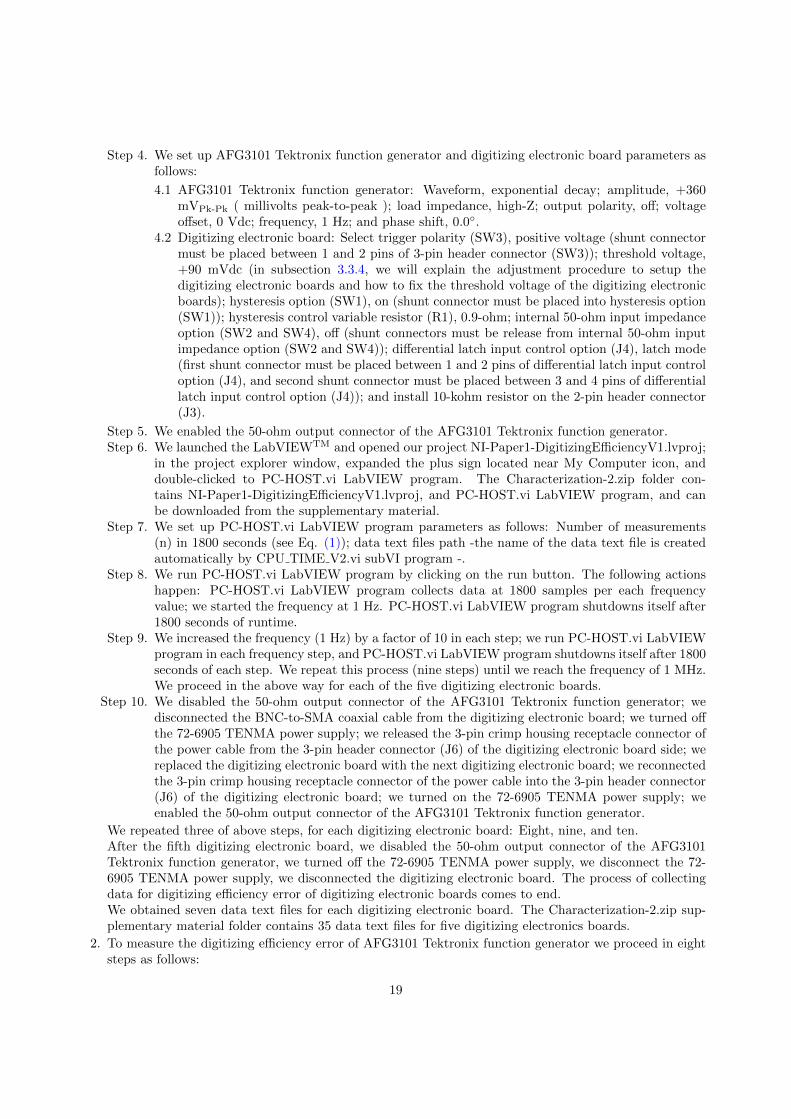
In Fig. 1 and Fig. 2, there are two different views of the connection electronic board. It is very simpleone. It is where the S12572-100P Hamamatsu photodiode surface mount type is soldered on the top layer;the anode and cathode terminals go to 2-pin header connector [5]; the Fig. 2 displays this 2-pin headerconnector installed from the bottom layer and soldered on the top layer; and then it goes to 2-pin receptacleconnector of the feeding and reading out electronic board, see Fig. 20. The connection electronic board isused to provide mechanical rigidity to the photodiode connection and to attach it to the detection material,in this case an 1 in × 2 in × 8 in Aluminum bar.

Figure 1: Connection electronic board top layer.

We proposed in our design a 90-degree relative position between connection electronic board, attachedand assembled to an Aluminum bar which functions as a detector, and the feeding and reading out electronicboard.

2

Figure 2: Connection electronic board bottom layer.

2.2. Feeding and reading out electronic board

In this subsection we report on a detailed technical description of the electronic boards designed, con-structed, and operated to feed the S12572-100P Hamamatsu photodiode, to generate and read out itsanalogue signal. See Fig. 3.

In Fig. 3 there is the schematic diagram design of the feeding and reading out electronic board for theS12572-100P Hamamatsu photodiode.

We divided this electronic board into five stages as follows:

1. Feeding and reading out electronic circuit (STAGE 1).

2. Operational amplifier electronic circuit (STAGE 2).

3. Feeding and reading out operation LED signal (STAGE 3).

4. Operational amplifier operation LED signal (STAGE 4).

5. External circuit for tuning voltage (STAGE 5).

This electronic board has two connectors to get electrical feeding. First, the 2-pin header connector(BT1) [6] is used to apply voltages between +1 Vdc and +100 Vdc; it provides electrical power to STAGE1 and STAGE 3, voltages between 1Vdc-100Vdc, with XLN10014 model, by BK Precision, power supply[7]. Second, the 3-pin header connector [8] (J2) is used to apply two fixed voltages: +5 Vdc, (VCC) powersupply input, and -5 Vdc, (VEE) power supply input; it provides power to STAGE 2 and STAGE 4, with72-6905 [9] model, by TENMA, power supply.

The STAGE 1 is composed of three voltage nodes and one power supply: The +HV(1Vdc-100Vdc) powersupply input contains one 2.2-Mohm resistor (R3), directly connected to 1-NODE; the R3 resistor limitselectrical current from power supply avoiding photodiode damage.

The 1-NODE consists of three passive components: First, avalanche photodiode (D2) (connected witha 2-pin receptacle bond [10]) with reverse polarity and connected to 2-NODE; second, the 1-NODE hasone 100-pF capacitor (C1) connected to ground, its function is to reduce power supply noise; third, the R3resistor is bonded to +HV(1Vdc-100Vdc) power supply input.

The 2-NODE voltage node is formed by the following components: Avalanche photodiode (D2) bondedto 1-NODE; 1.2-kohm resistor (R7) connected to ground; and 100-pF capacitor (C3) bonded to 3-NODE.

3

VCC

VEE

VCC

VEE

VCC VEE

VEE VCC

VCC

VEE

+HV(1V-100V)+HV(1V-100V) +100V Power Supply

+HV(1V-100V)

+HV(1V-100V)

STAGE 1STAGE 3

STAGE 2

STAGE 43-NODE

1-NODE

2-NODE

STAGE 5

4-NODE

5-NODE

TP3

Mounting Hole

TP3

Mounting Hole

1

R13 1kR13 1k1 2U2

AD8000_SOIC_N_EP

U2

AD8000_SOIC_N_EP

FB1

IN2

IN3

VEE4 NC 5

OUT 6

VCC 7

PD 8

R12 432R12 4321 2

TP4

Mounting Hole

TP4

Mounting Hole

1

BT1BT1

12

+C4

0.33uF

+C4

0.33uF

12

R9330R9330

12

C9 0.1uFC9 0.1uF

1 2

TP5

Mounting Hole

TP5

Mounting Hole

1

C70.1uFC70.1uF1

2

+ C810uF

+ C810uF

12

D3LEDD3LED

12

C2

0.1uF

C2

0.1uF

12

R1

100 k

R1

100 k

13

2

J2 CON3J2 CON3

1 2 3

R5330R5330

12

R810kR810k

12

R1939 kR1939 k

12

R10 1kR10 1k1 2

R1850R1850

12

D4LEDD4LED

12

TP1TEST POINT

TP1TEST POINT

1

R15 50R15 501 2

C1

100pF

C1

100pF

1 2

SW1SW SPDT

SW1SW SPDT

21

3R11 0R11 01 2

+ C610uF

+ C610uF

12

R14 1kR14 1k

1 2

C50.1uFC50.1uF

12

C3 100pFC3 100pF

1 2

J1

OUT

J1

OUT'1

'2

'3

'4

'5

U1

MC78L05A

U1

MC78L05A

Vout1GND2GND3NC4 NC 5GND 6GND 7Vin 8

R17330R17330

12

R32.2MR32.2M

12

TP2

Mounting Hole

TP2

Mounting Hole

1

R210kR210k

12

R410kR410k

12

R610kR610k

12

D1LED_OND1LED_ON

12

D2S12572-100PD2S12572-100P

12

R71.2kR71.2k

12

R16 50R16 50

1 2

Figure 3: Schematic diagram of the feeding and reading out electronic board for the S12572-100P Hamamatsu photodiode.

When the particle deposits its energy in the detection material and photons are created, the D2 photodiodegathers them and creates a multiplied electrical signal, collected with C3 capacitor in the order of millivolts.

The 3-NODE consists of a C3 capacitor bonded to 2-NODE, a test point connector (TP1), and a 50-ohmresistor (R15) connected to IN pin (amplifier IC pin number three) of STAGE 2, (U2) circuit. The C3capacitor1 decouples analogue signal from D2 photodiode, from feeding voltage; the test point connector(TP1) is for oscilloscope testing; the R15 resistor or RS is for configuring the operational amplifier asnon-inverting one and unitary amplifier (U2).

The STAGE 2 works as a noninverting unity-gain amplifier; its actual configuration is called a voltagefollower or unity-gain buffer, circuit (U2). It is used when impedance matching and circuit isolation are veryimportant and analogical signal amplification is not important. The electronic circuit used was the AD8000model, from Analog Devices, Inc. [11]. The main features are as follows: 1.5 GHz with -3 dB bandwidth(G = +1), slew rate of 4100 V/µs, 100 mA of load current with minimal distortion, and 2 to 3.6 Mohm/pFnoninverting input impedance. This STAGE was not really useful for operation but for electrical protection.

The 4-NODE is formed by R11 resistor, or RG, bonded to ground; R12 resistor, or RF, connected to pinnumber 1 (FB) of AD8000 circuit (U2); and the 4-NODE bonded to (IN) pin number 2 of AD8000 circuit

1Coupling capacitor confines dc voltages to 3-NODE.

4

(U2). The value of R112, R123, and R154 resistors are manufacturer’s recommendation.From the STAGE 2 electronic design, the unity-gain (G = +1) configuration was considered the main

configuration; the gain of 2 (G = +2) configuration was considered for testing the amplifier, or to amplify theanalogue signal amplitude from the S12572-100P Hamamatsu photodiode, if necessary. In order to complywith the PCB design software rules, the resistor R11 value was assigned to 0-ohm by default. See Fig. 3.To configure the noninverting amplifier to unity-gain (G = +1), the resistor R12 is fixed to 432-ohm andresistor R11 is eliminated, its footprint is left open. To configure the noninverting amplifier to gain to 2 (G= +2), the resistor R12 is fixed to 432-ohm and R11 resistor is fixed to 432-ohm.

The output analogue signal comes from pin number 6 of AD8000 (U2), which is bonded to a 50-ohmresistor (R16); the other end of the R16 resistor is connected to 5-NODE; this voltage node contains a50-ohm resistor (R18) bonded to ground, a SMA connector (J1) [12], and R16 resistor bonded back to thecircuit (U2). The role of this node is to adjust output impedance. The final configuration was R16 resistorequals 0-ohm and R18 resistor was removed. The switch (SW1) [13] is used to turn on and turn off theAD8000 circuit (U2) (instead, the end user needs to install the shunt connector [14] between pin 1 and 2 atSW1 to turn on AD8000 (U2), or between pin 2 and 3 to turn off).

The STAGE 3, operation LED signal, is for monitoring the correct applied voltage on STAGE 1; ifthe LED is on (bright red), the D2 photodiode is enabled; otherwise, disabled. The +HV(1Vdc-100Vdc)power supply input from 2-pin header connector (BT1) is connected to a voltage divider circuit formed byfour 10-kohm resistors (R2, R4, R6, and R8), where R8 resistor is bonded to ground, having a quarter of+HV(1Vdc-100Vdc) power supply input, which is applied to MC78L05A circuit (U1) [15]; the circuit (U1)output voltage is fixed at +5 Vdc, and this is bonded to 330-ohm resistor (R5) in series with LED (D1) andthen to ground; the voltage divider circuit and voltage regulator circuit (U1) allow enabling the LED (D1)signal and avoid its damage.

The STAGE 4, operation LED signal, D3 and D4, is for monitoring the proper function of STAGE 2.The STAGE 4 is formed by VCC power supply input and VEE power supply input. VCC power supplyinput is connected to 330-ohm resistor (R9), the other end of the R9 resistor is bonded to the anode of theLED 3 (D3), the cathode is connected to ground. VEE power supply input is connected to 330-ohm resistor(R17), the other end of the R17 resistor is bonded to the cathode of the LED 4 (D4), the anode is connectedto ground.

The STAGE 5 is an external circuit for tuning voltage; it consists of 100-kohm variable resistor (R1)and 39-kohm resistor (R19) in series, the other end of the R19 resistor is bonded to ground; the end usercan adjust the +HV(dc) power supply between +1 Vdc to +100 Vdc, obtaining the output voltage at pinnumber 2; it must be connected to 2-pin header connector (BT1) by wire. The +100 Vdc was appliedusing XLN10014 model BK Precision power supply. If we need to enable and feed voltage for two or moreexperimental setups using a single XLN10014 model BK Precision power supply, the STAGE 5 electroniccircuit allows us to electric feed each experimental setup with a different feed voltage; each D2 photodiodein the experimental setup may require a different feed voltage.

In the final operation, STAGE 2 was partially disconnected removing R15, R16, and R18 resistors.3-NODE from STAGE 1 was bonded to SMA connector (J1), pin 1, by wire.

In Fig. 4 it is shown an example of manufactured electronic board and its external circuit for tuningvoltage (STAGE 5).

For future designs, we recommend two updates of feeding and reading out electronic board: First,replace AD8000 Analog Device, Inc. amplifier circuit (U2) of STAGE 2 by LMH6559 Texas Instrumentshigh-speed, closed-loop buffer [16]; it is a good option for impedance matching and electrical isolation.Second, incorporate TL783C Texas Instruments high-voltage adjustable regulator circuit [17] at STAGE 5;output range has +1.25 Vdc to +125 Vdc, and 700 mA output current; the output voltage adjustment willbe more precise.

2RG resistor is absent in the Analog Devices, Inc. circuit.3RF resistor is 432-ohm in the Analog Devices, Inc. circuit.4RS resistor is 50-ohm in the Analog Devices, Inc. circuit.

5

Figure 4: Manufactured feeding and reading out electronic board and its external circuit for tuning voltage (STAGE 5).

2.3. Digitizing electronic board

In this subsection we report on a detailed technical description of electronic boards designed to digitizethe S12572-100P Hamamatsu photodiode analogue signal.

With this electronic board, the photodiode analogue signal is compared with threshold voltage signaldefined by the end user (three times bigger above noise signal was the selected criterion); if the photodiodeanalogical signal is bigger than the threshold voltage signal, the comparator digital output is turned on,otherwise it remains turned off. In Fig. 5 is shown the schematic diagram design of the digitizing electronicboard. The electronic design was based on ADCMP582 chip (U1) [18] fabricated by Analog Devices, Inc.with the following features: One-channel, ultrafast voltage comparators5, on-chip termination at both inputpins, PECL (positive emitter-coupled logic) logic family output drivers, resistor-programmable hysteresis,and differential latch control option.

The electronic board design is divided into five stages as follows:

1. Comparator electronic circuit (STAGE 1).

2. Threshold electronic circuit (STAGE 2).

3. VCC 3.3 voltage and VTT VCCO-2V voltage electronic circuit (STAGE 3).

4. -2V voltage electronic circuit (STAGE 4).

5180 ps propagation delay, and 100 ps minimum pulse width.

6

Threshold(mV)

Threshold(mV)

VCC VEE

VCC

VCC

VEE

VCC_3.3

VCC_3.3

VCC_3.3VCC

VEE

VCC VTT_VCCO-2V

VTT_VCCO-2VVCC_3.3VEE

VCC_3.3

-2V

VCC VEE

VCC

VCC_3.3VEE

VTT_VCCO-2V

-2VVEE

STAGE 1

STAGE 2 STAGE 3

STAGE 5

STAGE 4

2-NODE

1-NODE

3-NODE

Monitor

ThresholdVoltage

TriggerPolaritySelection

Adjustand FixThresholdVoltage

VoltageDivider

4-NODE

D2

-5V

D2

-5V

1 2

J11

OUT

J11

OUT_1

_2

_3

R11 2kR11 2k1 2

D1

+5V

D1

+5V

1 2

J5J512

R8 330R8 3301 2

R7

619

R7

619

1 2

C6 0.1uFC6 0.1uF12

J6J6

1 2 3

R450R450

12

R9

61.9

R9

61.9

12

J3J3

12

C2

0.1uF

C2

0.1uF12

SW2

50

SW2

501 2

TP4

Mounting Hole

TP4

Mounting Hole

1

SW4 50SW4 501 2

R10 1.5kR10 1.5k

1 2

J12J12

12345

C7

100pF

C7

100pF

12

C1

0.1uF

C1

0.1uF

12

R13

1k

R13

1k

12

U1

ADCMP582

U1

ADCMP582

V_TP1Vp2Vn3V_TN4

VC

CI

5LE

6LE

7V

_TT

8

VCCO 9Q 10Q 11VCCO 12

VE

E13

HY

S14

GN

D15

VC

CI

16

C8

100pF

C8

100pF

12

TP3

Mounting Hole

TP3

Mounting Hole

1

C3 0.1uFC3 0.1uF1 2

U2

MC10ELT21DG

U2

MC10ELT21DG

NC1DO2DO3VBB4 GND 5NC 6Q0 7VCC 8

SW1

HYS

SW1

HYS

1 2

R6

5k

R6

5k

13

2

C10

1uF

C10

1uF

12

R141kR141k

12

C9

1uF

C9

1uF

12

J1

IN

J1

IN' 1

'2

'3

'4

'5

TP1

Mounting Hole

TP1

Mounting Hole

1

R350R350

12

U3

ADP3339AKC-3.3

U3

ADP3339AKC-3.3

GN

D1

VIN3 VOUT 4

VOUT 2

J4J413

24

R250R250

12

SW3

SW SPDT

SW3

SW SPDT

21

3

C4 0.01uFC4 0.01uF1 2

C50.1uFC50.1uF

12

TP2

Mounting Hole

TP2

Mounting Hole

1

R5 750R5 7501 2

R1 5kR1 5k1 3

2R12 330R12 330

12

R15 750R15 750

1 2

Figure 5: Schematic diagram of the digitizing electronic board.

5. Digitizing electronic board LED signal (STAGE 5).

STAGE 1 was based on ADCMP582 (U1) and MC10ELT21DG (U2) [19] chips, the last one fabricatedby ON Semiconductor6. STAGE 1 is composed of two voltage nodes: 1-NODE and 2-NODE.

1-NODE consists of a SMA connector (J1) [12], and 2-pin header connector7 (J3) [5] connected to VP

pin (non-inverting analogue input pin or pin number 2) of ADCMP582 (U1) chip. The function of theSMA connector (J1) is to connect electrically the feeding and reading out electronic board by SMA-to-SMAadapter [20], getting the analogue signal and sending it to VP pin of ADCMP582 (U1) chip. The 2-pinheader connector (J3) was installed for testing (it purpose is to change the VP input impedance with anexternal resistor attached by end user).

2-NODE is formed by single-ended TTL digital output MC10ELT21DG (U2) chip (pin number 7), BNCconnector (J11) [21], and the 50-ohm resistor (R4) bonded to ground. 2-NODE receives the final informationof the analogue signal, and converts it into its digital version. R4 resistor was not used. VN pin (pin number3) of ADCMP582 (U1) chip, inverting analogue input, is used for threshold signal input.

The comparator chip (U1) provides internal 50-ohm termination resistors for both VP and VN inputs.The VTP input pin (pin number 1), or termination resistor return pin, enables the 50-ohm terminationresistor option inserting shunt connector on 2-pin header connector (SW2) [5], otherwise, disables the 50-ohm termination resistor option; similarly, VTN input pin (pin number 4), or termination resistor return

6https://www.onsemi.com/7pin number 1 bonded to 1-NODE voltage and pin number 2 bonded to ground.

7

pin, enables the 50-ohm termination resistor option inserting shunt connector on 2-pin header connector(SW4) [5], otherwise, disables the 50-ohm termination resistor option.

Differential latch input control option comes from pin number 7, or non-inverting side (LE), and frompin number 6, or inverting side (LE), of ADCMP582 chip (U1). Differential latch input control optionhas two configurations: First, latch mode (LE = low and LE = high), the output remains as in the inputstate; second, compare mode (LE = high and LE = low), the output follows changes at the input state;compare mode was the selected option. The high level is VCC 3.3 voltage with +3.3 Vdc from STAGE 3,and low level is VEE power supply input with -5 Vdc. Differential latch input control is formed by 2-pindual header connector (J4) [22], LE and LE pins are bonded to 1 and 3 pins of 2-pin dual header connector(J4) respectively; 2 and 4 pins (the opposite side 2-pin dual header connector (J4) are bonded to pull-up750-ohm resistor (R5) in series with +3.3 Vdc voltage from STAGE 3, and bonded to pull-down 750-ohmresistor (R15) in series with VEE power supply input from 3-pin header connector (J6) [23], respectively.To enable compare mode, then it is necessary to insert two shunt connector [14]: First, between 1 and 2pins; Second, between 3 and 4 pins of 2-pin dual header connector (J4).

The VTT pin, termination return or pin number 8 of ADCMP582 chip (U1), has two goals: First,activate differential latch input control option. Second, activate PECL logic output. Analog Device Inc.recommends connect this pin to VCCO8 pin (pin number 9 and 12 of U1 circuit) minus +2 Vdc; in ourdesign, we connected VTT pin to VTT VCCO-2V voltage from STAGE 3.

The Hysteresis control, pin number 13 of ADCMP582 chip (U1), consists of 2-pin header connector (SW1)[5] in series with 5-kohm variable resistor (R1) bonded to VEE (-5 Vdc) power supply input. To enablehysteresis control is necessary to insert a shunt connector on 2-pin header connector (SW1), and adjustthe desired amount of hysteresis; the maximum range of hysteresis that can be applied is approximately±70 mVdc. The advantage of applying hysteresis is to improve accuracy, stability, and reduction of doubleor multiple counting of digital signal. To obtain the advantages mentioned above, we set up the 5-kohmvariable resistor (R1) at 0.9-ohm.

The two output characteristics of ADCMP582 chip (U1) are as follows: First, Q (non-inverting, pinnumber 11) and Q (inverting, pin number 10) pins are differential output; second, Q and Q pins are PECLlogic family (positive ECL). Analog Device Inc. recommends connect Q and Q pins with a pull up 50-ohm resistor (R2 and R3, respectively) to VTT

9 pin of ADCMP582 chip (U1). R2 resistor, R3 resistor,and VTT VCCO-2V voltage from STAGE 3 allow to get +400 mVdc digital output at high frequencies.PECL logic family is incompatible with our module C NI-9402 CompactRIO (cRIO) of National Instruments(NI) [24]. To make it compatible, this digitizing electronic board requires to use single-ended output andLVTTL logic family characteristic devices, like MC10ELT21DG chip (U2). MC10ELT21DG chip (U2) isconfigured, by On Semiconductor, for a differential to single-ended conversion and PECL to TTL translator;for these two characteristics, MC10ELT21DG chip (U2) is a good option for this electronic design. Q andQ pins differential output from ADCMP582 chip (U1) are bonded to D0 and D0 differential input pins ofMC10ELT21DG chip (U2) respectively; VCC (+5 Vdc) power supply input and ground are required; andthe single-ended TTL digital output is read out using a BNC connector (J11). See 2-NODE of Fig. 3.

STAGE 2 comprehends of two voltage nodes and two power supplies. 3-pin header connector (SW3) [25]works to select trigger polarity; pin number 1 is bonded to VCC 3.3 voltage of STAGE 3; and pin number 3is bonded to -2V voltage of STAGE 4; for positive voltage selection, shunt connector must be placed between1 and 2 pins of 3-pin header connector (SW3); for negative voltage selection, shunt connector must be placedbetween 2 and 3 pins of 3-pin header connector (SW3). 5-kohm variable resistor (R6) works to adjust andfix threshold voltage, in this way: Pin number 2 of 3-pin header connector (SW3) is bonded to pin number1 of R6 variable resistor, pin number 2 of 5-kohm variable resistor (R6) is bonded to 3-NODE (the outputvoltage of this pin is -2 Vdc to +3.3 Vdc), and pin number 3 of R6 variable resistor is bonded to ground.

3-NODE and 4-NODE correspond to the input signal and the output signal of the voltage divider circuitformed by 619-ohm (R7) and 61.9-ohm (R9) resistors; 100-pF (C7) and 100-pF (C8) capacitors help eliminatenoise from the power supply.

8VCCO = +3.3 Vdc, recommended voltage by Analog Device Inc.9VTT pin (pin number 8) must be bonded to VTT VCCO-2V voltage from STAGE 3.

8

3-NODE is formed by R7 resistor bonded to 4-NODE, C7 capacitor connected to ground, and pin number2 of R6 variable resistor.

4-NODE is formed by R7 resistor bonded back to 3-NODE, C8 capacitor connected to ground, R9resistor bonded to ground, 2-pin header connector (J5)10 [5] works to threshold voltage monitor, and VIN

pin (pin number 3) of ADCMP582 chip (U1) from STAGE 1 (hierarchical port Threshold (mV) of STAGE2 is connected to hierarchical port Threshold (mV) of STAGE 1, see Fig. 5). Output voltage obtained on2-pin header connector (J5), or threshold voltage monitor, was between -134 mVdc and +298 mVdc.

STAGE 3 was designed to generate two output voltages: VCC 3.3 and VTT VCCO-2V.To generate VCC 3.3 voltage a ADP3339AKC-3.3-RL chip (U3), of Analog Devices, Inc. [26], was used;

this chip is a positive linear regulator with Low Dropout Output (LDO), with input voltage range from +2.8Vdc to +6 Vdc, and a fix +3.3 Vdc output; the capacitors11 C9 and C10 were fixed at 1 µF; pin number3 of U3 chip is bonded to VCC power supply input; pin number 1 of U3 chip is bonded to ground; andVCC 3.3 voltage was obtained from output pins number 2 and 4.

To generate VTT VCCO-2V voltage, we used a voltage divider circuit. This circuit is formed by thefollowing components: 1-kohm resistor (R14) connected to ground and 2-kohm resistor (R11) bonded backto VCC 3.3 voltage. Output voltage obtained on R14 resistor was +1.1 Vdc.

STAGE 4 generates -2V voltage (-2 Vdc) using a voltage divider circuit, see Fig. 5. VEE power supplyinput provides the input voltage (-5 Vdc), and the -2V voltage is the output voltage. The -2V voltage isthe drop voltage on the bonded to VEE power supply input 1.5-kohm resistor (R10) and on the bonded toground 1-kohm resistor (R13). The output voltage obtained on R13 resistor was -2 Vdc.

STAGE 5, operation LED signal, D1 and D2 is for monitoring the proper function of STAGE 1. TheSTAGE 5 is formed by VCC power supply input and VEE power supply input. VCC power supply input isconnected to 330-ohm resistor (R8), the other end of the R8 resistor is bonded to the anode of the LED (D1),and the cathode is connected to ground. VEE power supply input is connected to 330-ohms resistor (R12),the other end of the R12 resistor is bonded to the cathode of the LED (D2), and the anode is connectedto ground. If the LED (D1) and LED (D2) are on (bright red), the digitizing electronic board is enable;otherwise, unable.

The digitizing electronic board has one connector to get voltage feeding. The 3-pin header connector(J6) is used to apply two fixed voltages: +5 Vdc or VCC power supply input, and -5 Vdc or VEE powersupply input; it provides power to STAGE 1, 3, 4, and 5 with 72-6905 TENMA power supply.

The 5-pin header connector (J12) [27] was incorporated for test; ground is bonded to pin number 1,VCC power supply input is bonded to pin number 2, VEE power supply input is bonded to pin number 3,VCC 3.3 voltage is applied to pin number 4, and VTT VCCO-2V voltage is applied to pin number 5.

The manufactured electronic board is illustrated in Fig. 6.

10Pin number 1 is bonded to 4-NODE, and pin number 2 is bonded to ground.11manufacturer recommended value.

9

Figure 6: Manufactured digitizing electronic board.

3. Front-end electronic boards’ characterization

In this section we report on the procedures of evaluating the physical characteristics of the connectionelectronic board, feeding and reading out electronic board, and digitizing electronic board for the S12572-100P Hamamatsu photodiode [1].

We divided this evaluation procedure into five subsections as follows:

1. S12572-100P Hamamatsu photodiode connection electronic board.

2. Feeding and reading out electronic board attenuation factor and phase shift.

3. Digitizing-electronic-board digitizing efficiency error and digitizing efficiency.

4. Feeding and reading out electronic board transit time.

5. Digitizing electronic board digitizing time.

3.1. S12572-100P Hamamatsu photodiode connection electronic board

There is no electronic evaluation of this board. See Fig. 1 and Fig. 2. Mechanically it is fine and fits allrequired characteristics.

3.2. Feeding and reading out electronic board attenuation factor and phase shift

We describe the attenuation factor (output signal amplitude divided by input signal amplitude) of theanalogical signal as function of frequency, and the phase shift (the relative phase shift of the output signalwith respect to the input signal) also as a function of frequency. The attenuation factor is very importantfor the S12572-100P Hamamatsu photodiode calibration.

10

3.2.1. Connections

In Fig. 7 is illustrated the block diagram of attenuation factor and phase shift measurement experimentalsetup.

Figure 7: Block diagram of the experimental setup to measure attenuation factor and phase shift as function of frequency.

Fig. 7 contains four blocks as follows:

1. BLOCK 1. AFG3101 Tektronix function generator [28].

2. BLOCK 2. Feeding and reading out electronic board.

3. BLOCK 3. TDS2022C-EDU Tektronix Oscilloscope [29].

4. BLOCK 4. PC-host (1525 Dell Inspiron) with LabVIEWTM.

BLOCK 1: It represents an AFG3101 Tektronix function generator we used to simulate an input analoguesignal, with similar characteristics of an analogue signal from the S12572-100P Hamamatsu photodiode, withthe advantage of controlling the analogue signal frequency for evaluation purposes.

BLOCK 2: It represents the feeding and reading out electronic board under characterization. It hasthree connectors: Input 2-pin receptacle connector (D2); output SMA connector (J1); and output test point(TP1). See Fig. 3.

BLOCK 3: It represents the TDS2022C-EDU Tektronix oscilloscope. We used it to measure the analogueinput signal (a VPk-Pk of CH1), the analogue output signal (a VPk-Pk of CH2) of the feeding and readingout electronic board, and the phase shift of CH2 with respect to CH1.

BLOCK 4: It represents the PC-host with LabVIEWTM12 [30] [31] installed. We used this PC-hostto configure and to control the AFG3101 Tektronix function generator and the TDS2022C-EDU Tektronixoscilloscope, to read out the oscilloscope measurement, and to save data text file measurements.

The connection between AFG3101 Tektronix function generator and feeding and reading out electronicboard was done using a BNC-to-alligator clip cable [32]. The BNC is used to connect AFG3101 Tektronixfunction generator; the alligator clip, to connect feeding and reading out electronic board via 2-pin recepta-cle13 connector and a board-to-board adapter connector [33].

12Virtual Instrument Engineering Workbench is a system-design platform and development environment for a visual pro-gramming language.

13Red color alligator clip is connected to pin number 1 (anode) and black color alligator clip to pin number 2 (cathode).

11

The connection between feeding and reading out electronic board and TDS2022-EDU Tektronix oscillo-scope was done using two TPP0101 Tektronix voltage probes [34], as follows:

First probe connection is between 2-pin receptacle connector (D2) of the feeding and reading out elec-tronic board and oscilloscope CH1. Probe hook-tip is connected to pin number 1 (anode) and alligator clipis connected to pin number 2 (cathode) via a board-to-board adapter.

Second probe connection is between test point (TP1) of feeding and reading out electronic board andoscilloscope CH2. Probe hook-tip is connected to TP1 and alligator clip is connected to SMA ground (J1).

The connection between AFG3101 Tektronix function generator and PC-host was done using an USB2.0 A-to-B cable (printer cable).

The Connection between TDS2022-EDU Tektronix oscilloscope and PC-host was done using an USB 2.0A-to-B cable (printer cable).

3.2.2. Measurement processes

The measurement processes consisted on seven steps - to configure, to control, to read out AFG3101Tektronix function generator and TDS2022-EDU Tektronix oscilloscope, and to save measurements-, asfollows:

Step 1. We turn on measurement equipment (AFG3101 Tektronix function generator, TDS2022-EDU Tek-tronix oscilloscope, and PC-host). 50-ohm output connector of the AFG3101 Tektronix functiongenerator was disabled by default.

Step 2. We open LabVIEWTM; the getting started window appears. We use this window to select and openthe AttenuationF PhaseS.vi file14, and run it by clicking on the run button. It is a home madeprogram; we based it on the programming manual of the function generator and of the oscilloscope[35, 36].

Step 3. We set up AttenuationF PhaseS.vi parameters as follows:

3.1 Function generator tap control. We chose and fixed positive exponential decay waveform and0 Vdc offset. Amplitude: +2000 mVpp ( voltage peak-to-peak ); load impedance: High-Z15;output polarity: Off.

3.2 Oscilloscope tap control. CH1 Coupling: DC; CH1 bandwidth limit: Off; CH1 invert inputsignal: Off; CH1 attenuation: 10X; CH1 vertical scale: 500 mV/DIV; CH2 coupling: DC; CH2bandwidth limit: Off; CH2 invert input signal: Off; CH2 attenuation: 10X; CH2 vertical scale:500 mV/DIV; trigger source: CH1; trigger slope: Rise; trigger mode: Auto; trigger type: Edge;measure 1 menu source and type: CH1, VPk-Pk; measure 2 menu source and type: CH2, VPk-Pk;measure 3 menu source and type: CH2, phase; measure 4 menu source and type: CH1, none;measure 5 menu source and type: CH1, none.

3.3 AttenuationF PhaseS.vi recording setting LabVIEW program tap control. Start frequency: 100Hz; end frequency: 1 MHz; first increase frequency: 100 Hz; change frequency: 10 kHz; secondincrease frequency: 10 kHz; name and path: Name and path of output data text file.

Step 4. We run AttenuationF PhaseS.vi LabVIEW program. The following actions happen:

4.1 Starts sending all setup instructions to AFG3101 Tektronix function generator (step 3.1) andto TDS2022-EDU Tektronix oscilloscope (step 3.2), except recording setting (step 3.3).

4.2 Enables 50-ohm output connector of the AFG3101 Tektronix function generator.4.3 Awaits eight seconds, for the stability of the output analogue signal.4.4 Extracts the TDS2022-EDU Tektronix oscilloscope measurements: Measurement 1 (input ana-

logue signal of the feeding and reading out electronic board), measurement 2 (output analoguesignal of the feeding and reading out electronic board), and measurement 3 (CH2 phase shiftwith respect CH1).

14The Characterization-1.zip folder contains AttenuationF PhaseS.vi LabVIEW program, and can be downloaded from thesupplementary material.

15The High-Z, load impedance, is infinity, and its value is 9.9×10+37ohm [35].

12

4.5 Saves TDS2022-EDU Tektronix oscilloscope measurements 1, 2, and 3, and AFG3101 Tektronixfunction generator frequency value in a text file as follows: Frequency, a VPk-Pk of CH1, aVPk-Pk of CH2, and the phase shift of CH2 with respect to CH1.

4.6 Compares the actual frequency of the AFG3101 Tektronix function generator with the endfrequency of recording setting LabVIEW program tap control; if the actual frequency of theAFG3101 Tektronix function generator is greater or equal than the end frequency of the record-ing setting LabVIEW program tap control, the program runs the following processes: Closesthe text file, disables the output connector of the AFG3101 Tektronix function generator, andstops; on the contrary, it increases the frequency by 100 Hz or 10 kHz and continues to step 4.3.

Step 5. We closed AttenuationF PhaseS.vi and switched off all measurement equipment. We obtained a datatext file for every feeding and reading out electronic board, a total of ten data text files, the tendata text files can be found in Characterization-1.zip supplementary material folder; each obtaineddata text file contains a total of 199 measurements, according to the configuration parameters ofstep 3.3; we created the first 100 measurements in steps of 100 Hz, starting at 100 Hz and endingat 10 kHz, to closely examine the region of frequencies between 100 Hz and 10 kHz; the remainingmeasurements, in steps of 10 kHz, starting at 10 kHz and ending at 1 MHz.

Step 6. We run an attenuation factor vs frequency scripts to plot data for every feeding and reading outelectronic board. From the TDS2022-EDU Tektronics oscilloscope, we consider a systematic errorof 10%; this systematic error was included in the least square technique to measure the attenuationfactor as a function of the frequency. According to the TDS2022-EDU Tektronix oscilloscope usermanual, the reading error is 6%; the calibration error, 5% (taken from the report of D. Mowbray,from the University of Sheffield [37]).

6.1 AT100Fs FITv3.c script to plot the first 100 measurements of every feeding and reading outelectronic board. We obtained ten graphs, a graph for each feeding and reading out electronicboard. The AT100Fs FITv3.c script and the ten graphs can be found in Characterization-1.zipsupplementary material folder.

6.2 AT100Ss FITv3.c script to plot the remaining measurements of every feeding and reading outelectronic board. We obtained ten graphics, a graph for each feeding and reading out electronicboard. The AT100Ss FITv3.c script and the ten graphs can be found in Characterization-1.zipsupplementary material folder.

6.3 AT199s FITv3.c script to plot all 199 measurements of every feeding and reading out electronicboard. We obtained ten graphics, a graph for each feeding and reading out electronic board. TheAT199s FITv3.c script and the ten graphs can be found in Characterization-1.zip supplementarymaterial folder.

Step 7. We run two phase shift vs frequency scripts to plot data for every feeding and reading out electronicboard.

7.1 PhaseShift199sLV3.c script to plot all 199 measurements of every feeding and reading out elec-tronic board; the plot scale is linear in both axes. We obtained ten graphics, one graph for eachfeeding and reading out electronic board. The PhaseShift199sLV3.c script and the ten graphscan be found in Characterization-1.zip supplementary material folder.

7.2 PhaseShift199sLog.c script to plot all 199 measurements of every feeding and reading out elec-tronic board; the plot scale is logarithmic, in the horizontal axis and linear in the vertical axis.We obtained ten graphics, one graph for each feeding and reading out electronic board. ThePhaseShift199sLog.c script and the ten graphs can be found in Characterization-1.zip supple-mentary material folder.

The attenuation factor measurement experimental setup performs a very similar and elementary mea-surement akin to the measurement that the professional equipment called vector network analyzer does[38].

In Fig. 8, we show the attenuation factor and phase shift vs frequency measurement setup; at the top leftside is displayed a figure close up that shows function generator BNC-to-alligator clip cable and oscilloscopevoltage probe CH1 and CH2.

13

Figure 8: Experimental setup to measure attenuation factor and phase shift as function of frequency.

For a video of this experimental setup, of attenuation factor and phase shift measurements, click here orvisit https://youtu.be/zcXlBgUngn4

3.3. Digitizing-electronic-board digitizing efficiency error and digitizing efficiency

We describe the digitizing efficiency error, the digitizing efficiency, and the DAQ system used for thischaracterization.

The technique of digitizing efficiency error is to supply ω pulses per second (test analogue signal) at theinput of the digitizing electronic board and get ωj pulses per second (digital signal of test) at the output;where j is an iteration number; the digitizing efficiency error (eff) is defined as follows:

eff =1

n

n∑j=1

ωj − ω

ω× 100. (1)

Here eff is given in %; n is the number of measurements; ω is the frequency; ωj is the measuredfrequency.

The digitizing efficiency (%) is obtained by subtracting the digitizing efficiency error (%) from 100percent; and it depends on the frequency.

3.3.1. The data acquisition system

The used DAQ system was the CompactRIO (cRIO) from National Instruments, and this system consistsof three electronics components as follows: First, the cRIO-9025 controller [39]; it is an embedded real-timecontroller based on core 800 MHz CPU, 512 MB DRAM, 4 GB storage; it controls and monitors the Cmodules across a chassis. Second, cRIO-9118 chassis [40]; it is based on Virtex-5 LX110 FPGA technology,time-base at 40 MHz by default (80, 120, 160, or 200 MHz can be selected by software), and 8-slot to add Cseries modules. Third, the NI-9402 [24]; it is a bidirectional four channel C series, 55 ns update rate, digitalmodule; each channel is configurable digital I/O of the LVTTL family.

14

https://laboratoriointernacionaldeparticulaselementales.net/detecci%C3%B3n-de-radiaci%C3%B3n

https://youtu.be/zcXlBgUngn4

The cRIO-9025 controller and the eight NI-9402 C modules were installed inside the cRIO-9118 chassisobtaining 32-channel I/O DAQ system.

We used only one channel of one NI-9402 C module, to sense digital pulses of digitizing electronic boardoutput (J11); the measurements (counts) were sent to the PC-host by an Ethernet cable and saved them ina data text file.

To run cRIO, we create a project16 on the LabVIEWTM, and within the project, we created two programsas follows: LabVIEW-FPGA program17 (FPGA LabVIEW programming) to run in cRIO (to read out thedigitizing electronic board measurements and transfer them into a cRIO FIFO memory) and LabVIEW VIprogram18 to run in the PC-host (to read out PC-host FIFO memory data and saved it into a data textfile).

The function of these two programs are the following:

1. LabVIEW-FPGA program.The LabVIEW-FPGA program is to activate and configure the channel number 1 (CH1 or Slot1/DIO0),and to read out the digitizing electronic board digital signal (ωj).The LabVIEW-FPGA program contains the following four sequential circuits and one FIFO memoryelement [41]:1. One initialized rising-edge detector circuit to generate one pulse (first tick only) when the digitizing

electronic board signal output changes from 0 logical to 1 logical, and to discriminate the digitalsignal complement of second tick go-ahead from digitizing electronic board.

2. One initialized up-counter unsigned 32-bit (U32) circuit to count one pulse (first tick only) fromrising-edge detector circuit.

3. One initialized master up-counter U32 circuit to determine one-second lapse based on 40 MHzfrequency clock.

4. One initialized without reset slave up-counter U32 circuit to count time, each second (the j counterfrom Eq. (1)), from the master up-counter U32 circuit.

5. One Direct Memory Access First Input First Output (DMA FIFO) memory, with these characteris-tics: U32 data type, target-to-host DMA type, and the number of memory elements equals 15; andwith these functions: Receive data from without-reset-slave-up-counter U32 circuit (the j iterationnumber from Eq. (1)), and from up-counter U32 circuit (CH1 count or ωj from digitizing electronicboard, see Eq. (1)), and send these data to PC-host.

The digital signal from digitizing electronic board is monitored by the rising-edge detector circuit, ifone signal is detected (1 logical signal), the content of the up-counter U32 circuit increases by one(only the first tick of digital signal); if the digital signal was not detected (0 logical) or the digitalsignal is the complement of the first tick (1 logical in the second tick), the content of the up-counterU32 is not increased by one, and the monitoring process repeats itself indefinitely.When the content of the master up-counter U32 circuit reaches one-second lapse (40 × 106 ticks), thecontent of without reset slave up-counter U32 increases by one, it is copied to DMA FIFO (counttime in seconds or j iteration number from Eq. (1)); next, the last result of up-counter U32 is copiedto DMA FIFO (count of CH1 or ωj pulses per second, see from Eq. (1)) the copy process is calledinterleaving-1D; next, content of up-counter U32 circuit, and content of master up-counter U32 areinitialized (only one tick); the process repeats itself indefinitely.

2. LabVIEW VI program.The LabVIEW VI program works to collect data from cRIO. We configures LabVIEW VI programparameter as follows: Number of measurements (N) Eq. (1): 1800 seconds; and data file path: Setthe path of output data text file.When we run this program, the following action happens: Actual and requested depth of DMA FIFOconfigure function is setup with the following two parameters: U32 data type, and number of memoryelements equals 15.

16NI-Paper1-DigitizingEfficiencyV1.lvproj can be found inside Characterization-2.zip supplementary material folder.17DigitizingEfficiencyMeasurement-1CH.vi can be found inside Characterization-2.zip supplementary material folder.18PC-HOST.vi LabVIEW program can be found inside Characterization-2.zip supplementary material folder.

15

The operation of the LabVIEW VI program is as follows:LabVIEW VI program creates and opens one data text file (set data text file name at date and timefrom PC-host by CPU TIME V2.vi19 LabVIEW SubVI program); when DMA FIFO memory of PC-host gets two U32 data from cRIO, then decimate 1D array function will be applied to separate dataat current time in seconds (j iteration number, see Eq. (1)) and count of CH1 or ωj of Eq. (1) pulsesper second, and it is written to data text file; at once, the current time in seconds (j iteration number,see Eq. (1)) from cRIO is compared to number of measurements (N) (see Eq. (1)) from PC-host bya LabVIEW VI program, if its comparison is greater or equal, the LabVIEW VI program closes thedata text file, and then, LabVIEW VI program shutdowns itself; otherwise, LabVIEW VI programcontinues.

3.3.2. Connections

To perform the digitizing efficiency error characterization, we divided the experimental setup into twoparticular experimental setups, for comparison purposes, as follows: The first one is to measure the digitizingefficiency error of digitizing electronic boards; the second one, to measure the digitizing efficiency error ofthe AFG3101 Tektronix function generator. We define the cRIO system as the reference to measure thedigitizing efficiency error of digitizing electronic boards and to measure the digitizing efficiency error of theAFG3101 Tektronix function generator.

1. Experimental setup to measure the digitizing efficiency error of digitizing electronic boards. We carriedout this measurement process for each digitizing electronic board, with a total of five.In Fig. 9, we show the block diagram of the experimental setup to measure the digitizing efficiency errorof digitizing electronic boards.

Figure 9: Block diagram of the experimental setup to measure digitizing efficiency error of digitizing electronic boards.

Fig. 9 contains five blocks as follows:

19CPU TIME V2.vi subVI program can be found inside Characterization-2.zip supplementary material folder.

16

1. BLOCK 1. AFG3101 Tektronix function generator.2. BLOCK 2. Digitizing electronic board.3. BLOCK 3. DAQ system with National Instruments cRIO.4. BLOCK 4. 72-6905 TENMA power supply.5. BLOCK 5. PC-host (1525 Dell Inspiron) with LabVIEWTM.

BLOCK 1: It represents an AFG3101 Tektronix function generator. We used it to supply ω pulses persecond (test analogue signal) at the input of the digitizing electronic board.BLOCK 2: It represents the digitizing electronic board under characterization. It has one input, theSMA connector (J1), and one output, the BNC connector (J11). See Fig. 5, for schematic diagram ofdigitizing electronic board; and see Fig. 6, for manufactured of digitizing electronic board.BLOCK 3: It represents the cRIO. We used it to count the number of pulses from digitizing electronicboard per second (ωj). See Eq. (1).BLOCK 4: It represents the 72-6905 TENMA power supply. We used it to generate two output voltageswith respect to ground: +5 Vdc (VCC) power supply input and -5 Vdc (VEE) power supply input, tofeed the digitizing electronic board. See the schematic diagram of digitizing electronic board, Fig. 5.BLOCK 5: It represents the PC-host with installed LabVIEWTM [31]. We used this PC-host to configure,to read out the Mod1/DIO0 channel of cRIO, and to save data text file measurements.We used a BNC-to-SMA coaxial cable [42] to connect the AFG3101 Tektronix function generator withthe digitizing electronic board. The BNC goes to the AFG3101 Tektronix function; and the SMA goesto the digitizing electronic board.We used a BNC-to-BNC coaxial cable [43] to connect the digitizing electronic board with the cRIO.The BNC goes to BNC (J11) of digitizing electronic board; and the BNC goes to number 0 of slot 1(Slot1/DIO0) BNC connector of cRIO.We used a power cable to connect the digitizing electronic board with the 72-6905 TENMA powersupply, with the following characteristic: Multiconductor unshielded cable, 26 AWG, three conductors,black jacket (ground), red jacket (VCC power supply input), and white jacket (VEE power supply input),300 Vdc voltage rating; the ended stripped wires were connected to the 72-6905 TENMA power supplyside; and 3-pin crimp housing receptacle connector [44], to 3-pin header connector (J6) of the digitizingelectronic board side.We used an Ethernet standard Category 5 (CAT-5) cable to connect the cRIO with PC-host; the RJ-45Ethernet port number 1 was used to configure, program, and run the cRIO.

2. Experimental setup to measure the digitizing efficiency error of AFG3101 Tektronix function generator.We compared this measurement with the digitizing efficiency error of the five digitizing electronic boards;we carried out this measurement just one time. In Fig. 10, we show the block diagram of the experimentalsetup to measure the digitizing efficiency error of the AFG3101 Tektronix function generator.From Fig. 9 block diagram of the experimental setup to measure digitizing efficiency error of the digitizingelectronic board, we removed the BLOCK 2 and BLOCK 4 and obtained the block diagram of theexperimental setup to measure digitizing efficiency error of the AFG3101 Tektronix function generator.See Fig. 10.Fig. 10 contains three blocks as follows:

1. BLOCK 1. AFG3101 Tektronix function generator.2. BLOCK 2. DAQ system with National Instruments cRIO.3. BLOCK 3. PC-host (1525 Dell Inspiron) with LabVIEWTM.

We used a BNC-to-BNC coaxial cable to connect the AFG3101 Tektronix function generator with cRIO;the 50-ohm output of AFG3101 Tektronix function generator to input BNC connector number 0 of slot1 (Slot1/DIO0) of cRIO.The connection between cRIO and PC-host is unchanged from digitizing efficiency error measurementexperimental setup.

17

Figure 10: Block diagram of the experimental setup to measure digitizing efficiency error of the AFG3101 Tektronix functiongenerator.


There are two types of measurements, on which we are interested, as follows: The first one is the measure-ment of the digitizing efficiency error of the digitizing electronic boards; the second one, the measurementof the digitizing efficiency error of AFG3101 Tektronix function generator.

1. To measure the digitizing efficiency error of the digitizing electronic boards we proceed in ten steps:

Step 1. We assembled the experimental setup represented in Fig. 9 as a block diagram.Step 2. We turned on 72-6905 TENMA power supply; adjust the VCC power supply input at +5 Vdc,

and VEE at -5 Vdc.Step 3. We turned on the measurement equipment (AFG3101 Tektronix function generator, cRIO, and

PC-host). 50-ohm output connector of the AFG3101 Tektronix function generator was disabledby default.

18

Step 4. We set up AFG3101 Tektronix function generator and digitizing electronic board parameters asfollows:

4.1 AFG3101 Tektronix function generator: Waveform, exponential decay; amplitude, +360mVPk-Pk ( millivolts peak-to-peak ); load impedance, high-Z; output polarity, off; voltageoffset, 0 Vdc; frequency, 1 Hz; and phase shift, 0.0◦.

4.2 Digitizing electronic board: Select trigger polarity (SW3), positive voltage (shunt connectormust be placed between 1 and 2 pins of 3-pin header connector (SW3)); threshold voltage,+90 mVdc (in subsection 3.3.4, we will explain the adjustment procedure to setup thedigitizing electronic boards and how to fix the threshold voltage of the digitizing electronicboards); hysteresis option (SW1), on (shunt connector must be placed into hysteresis option(SW1)); hysteresis control variable resistor (R1), 0.9-ohm; internal 50-ohm input impedanceoption (SW2 and SW4), off (shunt connectors must be release from internal 50-ohm inputimpedance option (SW2 and SW4)); differential latch input control option (J4), latch mode(first shunt connector must be placed between 1 and 2 pins of differential latch input controloption (J4), and second shunt connector must be placed between 3 and 4 pins of differentiallatch input control option (J4)); and install 10-kohm resistor on the 2-pin header connector(J3).

Step 5. We enabled the 50-ohm output connector of the AFG3101 Tektronix function generator.Step 6. We launched the LabVIEWTM and opened our project NI-Paper1-DigitizingEfficiencyV1.lvproj;

in the project explorer window, expanded the plus sign located near My Computer icon, anddouble-clicked to PC-HOST.vi LabVIEW program. The Characterization-2.zip folder con-tains NI-Paper1-DigitizingEfficiencyV1.lvproj, and PC-HOST.vi LabVIEW program, and canbe downloaded from the supplementary material.

Step 7. We set up PC-HOST.vi LabVIEW program parameters as follows: Number of measurements(n) in 1800 seconds (see Eq. (1)); data text files path -the name of the data text file is createdautomatically by CPU TIME V2.vi subVI program -.

Step 8. We run PC-HOST.vi LabVIEW program by clicking on the run button. The following actionshappen: PC-HOST.vi LabVIEW program collects data at 1800 samples per each frequencyvalue; we started the frequency at 1 Hz. PC-HOST.vi LabVIEW program shutdowns itself after1800 seconds of runtime.

Step 9. We increased the frequency (1 Hz) by a factor of 10 in each step; we run PC-HOST.vi LabVIEWprogram in each frequency step, and PC-HOST.vi LabVIEW program shutdowns itself after 1800seconds of each step. We repeat this process (nine steps) until we reach the frequency of 1 MHz.We proceed in the above way for each of the five digitizing electronic boards.

Step 10. We disabled the 50-ohm output connector of the AFG3101 Tektronix function generator; wedisconnected the BNC-to-SMA coaxial cable from the digitizing electronic board; we turned offthe 72-6905 TENMA power supply; we released the 3-pin crimp housing receptacle connector ofthe power cable from the 3-pin header connector (J6) of the digitizing electronic board side; wereplaced the digitizing electronic board with the next digitizing electronic board; we reconnectedthe 3-pin crimp housing receptacle connector of the power cable into the 3-pin header connector(J6) of the digitizing electronic board; we turned on the 72-6905 TENMA power supply; weenabled the 50-ohm output connector of the AFG3101 Tektronix function generator.

We repeated three of above steps, for each digitizing electronic board: Eight, nine, and ten.After the fifth digitizing electronic board, we disabled the 50-ohm output connector of the AFG3101Tektronix function generator, we turned off the 72-6905 TENMA power supply, we disconnect the 72-6905 TENMA power supply, we disconnected the digitizing electronic board. The process of collectingdata for digitizing efficiency error of digitizing electronic boards comes to end.We obtained seven data text files for each digitizing electronic board. The Characterization-2.zip sup-plementary material folder contains 35 data text files for five digitizing electronics boards.

2. To measure the digitizing efficiency error of AFG3101 Tektronix function generator we proceed in eightsteps as follows:

19

Step 1. We assembled the experimental setup represented in Fig. 10 as a block diagram.Step 2. We turned on the measurement equipment (AFG3101 Tektronix function generator, cRIO, and

PC-host). 50-ohm output connector of the AFG3101 Tektronix function generator was disabledby default.

Step 3. We set up AFG3101 Tektronix function generator parameters as follows: Set waveform, pulse;set amplitude, +3 VPk-Pk ( voltage peak-to-peak ); set load impedance, high-Z; set duty cycle,5%; set the voltage offset, +1.5 Vdc; set initial frequency, 1 Hz; and set phase shift, 0.0◦.

Step 4. We enabled the 50-ohm output connector of the AFG3101 Tektronix function generator.Step 5. We launched the LabVIEWTM and opened our project NI-Paper1-DigitizingEfficiencyV1.lvproj,

and double-clicked to PC-HOST.vi LabVIEW program.Step 6. We set up PC-HOST.vi LabVIEW program parameters as follows: Set number of measurements

(n) at 1800 seconds of runtime (see Eq. (1)), and set the data text files path.Step 7. We run PC-HOST.vi LabVIEW program by clicking on the run button. The following actions

happen: PC-HOST.vi LabVIEW program collects data at 1800 samples per each frequencyvalue; we started the frequency at 1 Hz. PC-HOST.vi LabVIEW program shutdowns itself after1800 seconds of runtime.

Step 8. We increased the frequency (1 Hz) by a factor of 10 Hz in each step; we run PC-HOST.viLabVIEW program in each frequency step, and PC-HOST.vi LabVIEW program shutdownsitself after 1800 seconds of runtime on each step. We repeat this process (eight steps) until wereach the frequency of 1 MHz.

After PC-HOST.vi LabVIEW program shutdowns itself, we performed the following steps: We disabledthe 50-ohm output connector of the AFG3101 Tektronix function generator; we turned off AFG3101Tektronix function generator, cRIO, and PC-host; and we disconnected all the measuring equipment.The process of collecting data for digitizing efficiency error of AFG3101 Tektronix function generatorcame to end.We obtained only seven data text files for AFG3101 Tektronix function generator. The Characteriza-tion2.zip supplementary material folder contains seven data text files for digitizing efficiency error ofAFG3101 Tektronix function generator.

3. We declared 42 data text file (of digitizing efficiency error, 35 data text files of five digitizing electronicsboards; and digitizing efficiency error, seven data text files of AFG3101 Tektronix function generator);and we run a script, eff.c, to plot digitizing efficiency error and digitizing efficiency of five electronicboards and one AFG3101 Tektronix function generator. We obtained two graphs, a graph for digitizingefficiency error, and a graph for digitizing efficiency. The Characterization-2.zip folder contains eff.cscript, two graphs, and can be downloaded from the supplementary material for close inspection.

In Fig. 11, we show the experimental setup to measure the digitizing efficiency error of digitizingelectronic boards assembled; at the top left side is displayed a figure close up which shows power supply,power cable, AFG3101 Tektronix function generator BNC-to-SMA coaxial cable, and cRIO BNC-to-BNCcoaxial cable.

In Fig. 12, we show the experimental setup to measure the digitizing efficiency error of AFG3101Tektronix function generator.

For a video of this experimental setup, of digitizing-electronic-board digitizing efficiency error and digi-tizing efficiency, please click here or visit https://youtu.be/eYnpFRaQVbs

3.3.4. Adjust and fix threshold voltage procedure of digitizing electronic board

The digitizing electronic board has one connector to read out threshold voltage, 2-pin header connector(J5) [5], or threshold voltage monitor. PIN 1 is to read out threshold voltage; PIN 2, is the ground orreference. See Fig. 5 STAGE-2. The connection between the multimeter and the threshold voltage monitor(J5) was done using two-alligator clips to 2-pin receptacle crimp housing [45] cable 20; the red color alligatorclip is bonded to PIN 1; the black one, to PIN 2.

20The cable is homemade.

20


https://youtu.be/eYnpFRaQVbs

Figure 11: Experimental setup to measure digitizing efficiency error of the digitizing electronic boards.

Figure 12: Experimental setup to measure digitizing efficiency error of the AFG3101 Tektronix function generator.

The red multimeter probe is connected to the red color alligator clip; the black one, to the black coloralligator clip; The PIN 1 and PIN 2 of the homemade cable must be plugged into PIN 1 and PIN 2 ofthreshold voltage monitor (J5), respectively.

We configured the multimeter in millivolts (mV). To adjust the threshold voltage, we used a smallscrewdriver on R6 variable resistor to modify the potential difference on (R6), and saw the display of themultimeter at the same time.

Fig. 13 shows the threshold voltage adjustment connection.After fixing the threshold voltage of the digitizing electronic board, we disconnected the two-alligator

clips to 2-pin receptacle crimp housing cable and the multimeter.

21

Figure 13: Threshold voltage adjustment connection.

3.4. Feeding and reading out electronic board transit time

We analyzed and measured the time an electrical signal takes to travel through the feeding and reading outelectronic boards. This time interval is known as propagation delay and response time [46]. We adumbratedthis process as follows: 1) connections, we enumerate and sketch all the used equipment; 2) measurementprocesses, we explain the sequence in which we ran the experimental setup.

3.4.1. Connections

In Fig. 14, we show the block diagram of the feeding and reading out electronic board transit timeexperimental setup.

It contains three blocks as follows:

1. BLOCK 1. AFG3101 Tektronix function generator.


3. BLOCK 3. TDS5104B Tektronix oscilloscope [47].

BLOCK 1: It represents an AFG3101 Tektronix function generator. We used it to supply test analoguesignal at the input of the feeding and reading out electronic board.

BLOCK 2: It represents the feeding and reading out electronic board under characterization. It hasone input, the 2-pin receptacle connector (D2); and two outputs, the test point (TP1), and SMA connector(J11). See Fig. 3, for schematic diagram of feeding and reading out electronic board; and see Fig. 4, formanufactured feeding and reading out electronic board.

22

Figure 14: Block diagram of the experimental setup to measure transit time of the feeding and reading out electronic board.

BLOCK 3: It represents the TDS5104B Tektronix oscilloscope. We used it to measure the delay of theanalogue output signal (CH2) with respect to the analogue input signal (CH1) of the feeding and readingout electronic board.

We used a BNC-to-alligator clip cable to connect the AFG3101 Tektronix function generator with thefeeding and reading out electronic board. The BNC goes to the AFG3101 Tektronix functions generator;the alligator clip end21, to 2-pin receptacle connector (D2) [10] using a board-to-board adapter connector[33].

We used two TEKP5050 Tektronix voltage probes [48] to connect the feeding and reading out electronicboard with the TDS5104B Tektronix oscilloscope, as follows:

Connection 1, between 2-pin receptacle connector (D2) of feeding and reading out electronic board andCH1 of the TDS5104B Tektronix oscilloscope. Probe hook-tip goes to pin number 1 (anode); and alligatorclip, to pin number 2 (cathode) via a board-to-board adapter connector. The CH1 of the TDS5104BTektronix oscilloscope is to measure the input analogue signal in the feeding and reading out electronicboard.

Connection 2, between test point (TP1) of the feeding and reading out electronic board and CH2 ofTDS5104B Tektronix oscilloscope. Probe hook-tip goes to TP1 connector; and alligator clip, to SMA metal(J1). This CH2 of the TDS5104B Tektronix oscilloscope is to measure the output analogue signal in thefeeding and reading out electronic board.


The measurement processes consisted on ten steps as follows:

Step 1. We assembled the experimental setup represented in Fig. 14 as a block diagram.

Step 2. We turned on the measurement equipment (AFG3101 Tektronix function generator, and TDS5104BTektronix oscilloscope). 50-ohm output connector of the AFG3101 Tektronix function generatorwas disabled by default.

Step 3. We set up AFG3101 Tektronix function generator and TDS5104B Tektronix oscilloscope parametersas follows:

3.1 We set up AFG3101 Tektronix function generator parameters as follows: Waveform: Exponen-tial decay; amplitude: +2 VPk-Pk ( voltage peak-to-peak ); load impedance: High-Z; outputpolarity: Off; voltage offset: 0 Vdc; frequency: 1 MHz; and phase shift: 0.0◦.

3.2 We enabled the 50-ohm output connector of the AFG3101 Tektronix function generator.3.3 We set up TDS5104B Tektronix oscilloscope parameters as follows: CH1 termination: 1-Mohm;

CH1 coupling: DC; CH1 invert input signal: Off; CH1 bandwidth: Full; CH1 attenuation: 10X;

21Red alligator clip connected to pin number 1 (anode) and black alligator clip connected to pin number 2 (cathode).

23

CH1 vertical scale: 200 mV/DIV; CH1 deskew time: 0.0 s; CH2 termination: 1-Mohm; CH2coupling: DC; CH2 invert input signal: Off; CH2 bandwidth: Full; CH2 attenuation: 10X; CH2vertical scale: 200 mV/DIV; CH2 deskew time: 0.0 s; horizontal scale: 2 ns/DIV; trigger source:CH1; trigger slope: Rise; trigger mode: Auto; trigger type: Edge; measure 1 menu source andtype: CH1, Delay (C1, C2). The Delay (C1, C2) measurement procedure is from C1 to C2 (intime units).

3.4 We set up the TDS5104B Tektronix oscilloscope front-panel print button as a save button quickstorage of screenshots as follows: From the menu bar of the TDS5104B Tektronix oscilloscope,we selected the Save As..., dialog boxes will be displayed, and we fill the next parameters asfollows: Base file name: Defined by us; count: 000; save as type: JPEG; auto-increment filename check box: On. Click the Save button.

Step 4. We saved at least 30 screenshots of a waveform by clicking 30 times on the front-panel print button.

Step 5. We disabled the 50-ohm output connector of the AFG3101 Tektronix function generator; we dis-connected the BNC-to-alligator clip cable and two TEKP5050 Tektronix voltage probes from theboard-to-board adapter connector; we disconnected the board-to-board adapter connector from thefeeding and reading out electronic board; we replaced the feeding and reading out electronic boardwith the next feeding and reading out electronic board; we connected again the board-to-boardadapter connector into the 2-pin receptacle connector (D2) of the feeding and reading out electronicboard; we connected the BNC-to-alligator clip cable and two TEKP5050 Tektronix voltage probeson the board-to-board adapter connector; we enabled the 50-ohm output connector of the AFG3101Tektronix function generator.

Step 6. We repeated the step four, and the step five for each feeding and reading out electronic board. Afterthe tenth feeding and reading out electronic board, we disabled the 50-ohm output connector of theAFG3101 Tektronix function generator, we turned off the AFG3101 Tektronix function generator,and TDS5104B Tektronix oscilloscope, we disconnected the tenth feeding and reading out electronicboard, AFG3101 Tektronix function generator, and TDS5104B Tektronix oscilloscope. The processof collecting data for transit time of feeding and reading out electronic boards comes to end. TheCharacterization-3.zip supplementary material folder contains at least 30 screenshots of a waveformof each feeding and reading out electronic board; the delay measurement or Delay (C1, C2) isdisplayed.

Step 7. We read the Delay (C1, C2) measurement from each screenshot of a waveform, and we wrote intoa data text file. This process was not automatic.

Step 8. We repeated the above step seven for each feeding and reading out electronic board screenshot of awaveform. We obtained one data text file for each feeding and reading out electronic board. TheCharacterization-3.zip supplementary material folder contains ten data text files for ten feeding andreading out electronics boards.

Step 9. We read ten feeding and reading out electronic board data text files and compute the average valuesand standard deviations of these ten data text files, using Statistics02 TTime.vi LabVIEW program,contained in the Characterization-3.zip supplementary material folder.

Step 10. We wrote ten statistical error results from Statistics02 TTime.vi LabVIEW program into the scriptPlotErrorsTTimeNI-4.c; we run a script, PlotErrorsTTimeNI-4.c, we obtained one plot of the tenfeeding and reading out electronic boards transit time statistical error. The Characterization-3.zipsupplementary material folder contains the PlotErrorsTTimeNI-4.c script, and one plot.

In Fig. 15, we show the experimental setup to measure the transit time of feeding and reading outelectronic assembled board; at the top left side is displayed a figure close up that shows function generatorBNC-to-alligator clip cable, and oscilloscope voltage probe CH1 and CH2.

24

Figure 15: Experimental setup to measure transit time of the feeding and reading out electronic board.

3.5. Digitizing electronic board digitizing time

Digitizing electronic board is a basic analogue-to-digital converter (ADC) with the following parameters:1-bit resolution, high-speed, single analogue input, single analogue output, and basic control signal formicroprocessor connection such as: Differential latch control option (LE, LE) [18]. The digitizing electronic,which satisfies LVTTL family logic interface and high speed requirements, is an excellent option to beconnected to the National Instruments cRIO.

We want to know and measure the time that the digitizing electronic board spends to convert theanalogue signal into the digital one; this time interval is known as conversion time [46, 49] or digitizing time.The digitizing time of the digitizing electronic board is limited by the transit time of comparator circuit,ADCMP582 chip (U1), and logic gate circuit, MC10ELT21DG (U2) [19]. In Fig. 5 we have shown theschematic diagram design of the digitizing electronic board.

We adumbrated this process as follows: 1) connections, we enumerate and sketch all the used equipment;2) measurement processes, we explain the sequence in which we ran the experimental setup.

3.5.1. Connections

In Fig. 16, we show the block diagram of the digitizing electronic board digitizing time experimentalsetup.

It contains four blocks as follows:

25

Figure 16: Block diagram of the experimental setup to measure digitizing time of the digitizing electronic board.

1. BLOCK 1. 72-6905 TENMA power supply.

2. BLOCK 2. AFG3101 Tektronix function generator.

3. BLOCK 3. Digitizing electronic board.

4. BLOCK 4. TDS5104B Tektronix oscilloscope.

BLOCK 1: It represents a 72-6905 TENMA power supply. We used it to generate two output voltageswith respect to ground: +5 Vdc (VCC) power supply input and -5 Vdc (VEE) power supply input, to feedthe digitizing electronic board.

BLOCK 2: It represents an AFG3101 Tektronix function generator. We used it to supply test analoguesignal at the input of the digitizing electronic board.

BLOCK 3: It represents the digitizing electronic board under characterization. It has one analogueinput, the SMA connector (J1); and one digital output, BNC connector (J11). See Fig. 5, for schematicdiagram of digitizing electronic board; and see Fig. 6, for manufactured digitizing electronic board.

BLOCK 4: It represents a TDS5104B Tektronix oscilloscope. We used it to measure the delay of thedigital output signal (CH2) with respect to the analogue input signal (CH1) of the digitizing electronicboard.

We used a power cable to connect the digitizing electronic board with the 72-6905 TENMA powersupply; power cable features were mentioned in the connection subsection 3.3.2; the ended stripped wireswere connected at the 72-6905 TENMA power supply side; and 3-pin crimp housing receptacle connector,at 3-pin header connector (J6) of the digitizing electronic board side.

We used a BNC-to-SMA coaxial cable to connect the AFG3101 Tektronix function generator with thedigitizing electronic board. The BNC goes to the AFG3101 Tektronix functions generator; the SMA, to theSMA connector (J1) of digitizing electronic board.

We used two TEKP5050 Tektronix voltage probes to connect the digitizing electronic board with theTDS5104B Tektronix oscilloscope, as follows:

26

Connection 1, between 2-pin header connector (J3) [5] of digitizing electronic board and CH1 of oscil-loscope. Probe hook-tip goes to pin number 1; and alligator clip, to SMA metal (J1). The CH1 of theoscilloscope is used to measure the input analogue signal in the digitizing electronic board.

Connection 2, between BNC connector (J11) of the digitizing electronic board and CH2 of oscilloscope.Probe hook-tip goes to contact pin of BNC connector (J11); and alligator clip, to BNC metal (J11). ThisCH2 of the oscilloscope is used to measure the output digital signal in the digitizing electronic board.


The measurement processes consisted on twelve steps as follows:

Step 1. We assembled the experimental setup represented in Fig. 16 as a block diagram.

Step 2. We turned on 72-6905 TENMA power supply; adjusted the VCC power supply input at +5 Vdc,and VEE at -5 Vdc.

Step 3. We turned on the measurement equipment (AFG3101 Tektronix function generator, and TDS5104BTektronix oscilloscope). 50-ohm output connector of the AFG3101 Tektronix function generatorwas disabled by default.

Step 4. We set up AFG3101 Tektronix function generator, digitizing electronic board, and TDS5104B Tek-tronix oscilloscope parameters as follows:

4.1 AFG3101 Tektronix function generator. Waveform: Exponential decay; amplitude: +400mVPk-Pk ( millivolts peak-to-peak ); load impedance: High-Z; output polarity: Off; voltageoffset: 0 Vdc; frequency: 1 MHz; and phase shift: 0.0◦.

4.2 Digitizing electronic board. Select trigger polarity (SW3): Positive voltage (shunt connectormust be placed between 1 and 2 pins of 3-pin header connector (SW3)); threshold voltage,+100 mVdc; hysteresis option (SW1), on (shunt connector must be placed into hysteresis option(SW1)); hysteresis control variable resistor (R1), 0.9-ohm; internal 50-ohm input impedanceoption (SW2 and SW4), off (shunt connectors must be released from internal 50-ohm inputimpedance option (SW2 and SW4)); differential latch input control option (J4), latch mode(first shunt connector must be placed between 1 and 2 pins of differential latch input controloption (J4), second shunt connector must be placed between 3 and 4 pins of differential latchinput control option (J4)); and install 10-kohm resistor on the 2-pin header connector (J3).

4.3 TDS5104B Tektronix oscilloscope parameters. CH1 termination: 1-Mohm; CH1 coupling: DC;CH1 invert input signal: Off; CH1 bandwidth: Full; CH1 attenuation: 10X; CH1 vertical scale:100 mV/DIV; CH1 deskew time: 0.0 s; CH2 termination: 1-Mohm; CH2 coupling: DC; CH2invert input signal: Off; CH2 bandwidth: Full; CH2 attenuation: 10X; CH2 vertical scale: 1V/DIV; CH2 deskew time: 0.0 s; horizontal scale: 2 ns/DIV; trigger source: CH1; trigger slope:Rise; trigger mode: Auto; trigger type: Edge; measure 1 menu source and type: CH1, Delay(C1, C2). The Delay (C1, C2) measurement procedure is from C1 to C2 (in time units).

4.4 The TDS5104B Tektronix oscilloscope front-panel print button was configured as a save but-ton quick storage of screenshots waveform parameters as follows: From the menu bar of theTDS5104B Tektronix oscilloscope, we selected the Save As..., dialog boxes are displayed, wefilled the next parameters as follows: Base file name: Defined by us; count: 000; save as type:JPEG; auto-increment file name check box: On. We clicked the Save Button.

Step 5. We enabled the 50-ohm output connector of the AFG3101 Tektronix function generator.

Step 6. We saved at least 20 screenshots of a waveform.

Step 7. We disabled the 50-ohm output connector of the AFG3101 Tektronix function generator; we dis-connected the BNC-to-SMA coaxial cable, and two TEKP5050 Tektronix voltage probes from thedigitizing electronic board; we turned off 72-6905 TENMA power supply; we released the 3-pin crimphousing receptacle connector of the power supply from 3-pin header connector (J6) of digitizing elec-tronic board; we replaced the digitizing electronic board with the next digitizing electronic board;we connected again the 3-pin crimp housing receptacle connector into the 3-pin header connector(J6) of digitizing electronic board; we turned on 72-6905 TENMA power supply; we connected

27

the BNC-to-SMA coaxial cable into SMA coaxial connector (J1) of digitizing electronic board; weconnected two TEKP5050 Tektronix voltage probes: The first connection between 2-pin header con-nector (J3) of digitizing electronic board and CH1 of oscilloscope, and second connection betweenBNC connector (J11) of the digitizing electronic board and CH2 of oscilloscope.

Step 8. We repeated the above steps five, six, and seven for each digitizing electronic board. After the fifthdigitizing electronic board, we disabled the 50-ohm output connector of the AFG3101 Tektronixfunction generator; we turned off the AFG3101 Tektronix function generator, TDS5104B Tektronixoscilloscope, 72-6905 TENMA power supply; we disconnected the fifth digitizing electronic board,AFG3101 Tektronix function generator, TDS5104B Tektronix oscilloscope, and 72-6905 TENMApower supply. The process of collecting data for digitizing time of digitizing electronic boards comesto end. The Characterization-4.zip supplementary material folder contains at least 30 screenshotsof a waveform of each digitizing electronic board; the delay measurement or Delay (C1, C2) isdisplayed.

Step 9. We read the Delay (C1, C2) measurement from each screenshot of a waveform, and we wrote intoa data text file. This process was not automatic.

Step 10. We repeated the above step nine for each digitizing electronic board screenshot of a waveform.We obtained one data text file for each digitizing electronic board. The Characterization-4.zipsupplementary material folder contains five data text files for five digitizing electronics boards.

Step 11. We read five digitizing electronic board data text files and compute the average values and standarddeviations of these five data text files, using Statistics02 DTime.vi LabVIEW program, containedin the Characterization-4.zip supplementary material folder.

Step 12. We wrote five statistical error results from Statistics02 DTime.vi LabVIEW program into the script,PlotErrorsDTimeNI-4.c; we run a script, PlotErrorsDTimeNI-4.c, we obtained one plot of the fivedigitizing electronic boards digitizing time statistical error. The Characterization-4.zip supplemen-tary material folder contains the PlotErrorsDTimeNI-4.c script, and one plot.

In Fig. 17, we show the experimental setup to measure the digitizing time of the digitizing electronicboard; at the top left side is displayed a figure close up that shows power supply power cable, functiongenerator BNC-to-SMA coaxial cable, and oscilloscope voltage probe CH1 and CH2.

28

Figure 17: Experimental setup to measure the digitizing time of digitizing electronic board.

4. Experimental setup

In this section we report on two cases running the experimental setup: First, exposing the experimentalsetup to cosmic rays. Second, exposing the experimental setup to a controlled LED light source.

4.1. Exposing the experimental setup to cosmic rays

In this subsection we report on the connections between the detection material, the connection electronicboard, the feeding and reading out electronic board, the digitizing electronic board, the power supplies, andthe TDS2022C-EDU Tektronix oscilloscope; these equipment elements conform the experimental setup. Weexplain the procedure to turn it on. We describe how to configure the digitizing electronic board, theoscilloscope, and the power supplies. We detail the way to run the experimental setup and take data. Weinform how to turn off the experimental setup. And we present some results obtained from exposing thedetector to cosmic rays.

With this experimental setup we observe photon-like signals produced in the S12572-100P Hamamatsuphotodiode when the detection material is exposed to cosmic rays. We investigated the origin and propertiesof these signals. Here we use them to test this experimental setup.

4.1.1. Connections

In Fig. 18, we show the block diagram of the complete experimental setup.Fig. 18 contains six blocks as follows:

29

Figure 18: Block diagram of the complete experimental setup.

1. BLOCK 1. XLN10014 BK Precision power supply [7].

2. BLOCK 2. 72-6905 TENMA power supply [9].

3. BLOCK 3. Connection electronic board with detection material.


5. BLOCK 5. Digitizing electronic board.

6. BLOCK 6. TDS2022C-EDU Tektronix oscilloscope [29].

BLOCK 1: It represents an XLN10014 BK Precision power supply. We used it to feed voltage on thefeeding and reading out electronic board, on the 2-pin header connector (BT1) [6], from 0 Vdc to +100 Vdc.

BLOCK 2: It represents a 72-6905 TENMA power supply, which we used to feed the digitizing electronicboard with two output voltages: +5 Vdc (VCC) and -5 Vdc (VEE). The prefixes VCC and VEE are definedas power supply inputs in section 2.3.

BLOCK 3: It represents the connection electronic board. It supports mechanically and electrically theS12572-100P Hamamatsu photodiode, which is attached to the detection material, an 1 in × 2 in × 8 inAluminum bar, see section 2.1.

BLOCK 4: It represents the feeding and reading out electronic board. It has two purposes: First, to feedthe S12572-100P Hamamatsu photodiode voltage supply using the connection electronic board. Second, toread out the analogue signal from the S12572-100P Hamamatsu photodiode.

BLOCK 5: It represents the digitizing electronic board. It is used to select and fix triggering voltage,and to convert analogue-to-digital signal from feeding and reading out electronic board; the threshold, ortriggering, voltage is three times above noise signal.

30

BLOCK 6: It represents the TDS2022C-EDU Tektronix oscilloscope. We use it to inspect the ana-logue and digital signals from the feeding and reading out electronic board and digitizing electronic board,respectively.

We used a power cable to connect the XLN10014 BK Precision power supply with the feeding and readingout electronic board. The characteristics of the cable are as follows: Multiconductor not shielded cable, 24AWG, two conductors, black jacket (ground or PIN 2 of BT1) and red jacket (+HV(1V-100V) power supplyinput or PIN 1 of BT1), 300 Vdc voltage rating. The 2-pin crimp housing receptacle connector [50] goes tothe feeding and reading out electronic board; and the solderless type terminal block with screw connector[51] goes to the XLN10014 BK Precision power supply.

We used a power cable to connect the 72-6905 TENMA power supply with the digitizing electronic board.The characteristics of the power cable are the same as those described in subsections 3.3.2 and 3.5.1. Theend stripped wires goes to the 72-6905 TENMA power supply side; and the 3-pin crimp housing receptacleconnector [44], to the digitizing electronic board.

We assembled the Aluminum bar to the connection electronic board as follows: We polished a 1 in ×2 in end of an 8 in long rectangular Aluminum bar up to a mirror like finishing; we insulated with blackelectrical tape the soldered anode and cathode pins of the connection electronic board (by the top layer); weapplied an additional black electrical tape layer on the top layer of connection electronic board, excluding theoptical aperture of the S12572-100P Hamamatsu photodiode; we isolated optically the connection electronicboard with one layer of Aluminum tape 3311, except the optical aperture of the S12572-100P Hamamatsuphotodiode; we installed the connection electronic board on the above mentioned Aluminum bar 1 in × 2in end as follows: The optical aperture of the photodiode touches the polished area of the Aluminum bar,then we fixed the connection electronic board to the Aluminum bar with Aluminum tape 3311, except the2-pin header connector (anode pin and cathode pin) of the bottom layer. In Fig. 19, we show the connectionelectronic board attached, assembled, and optically isolated with the Aluminum bar.

We used only, without additional board-to-board adapters [33], a 2-pin header connector of the connectionelectronic board to connect it to 2-pin receptacle connector (D2) [10] of the feeding and reading out electronicboard.

In Fig. 20, we show the connection electronic board attached and assembled to the Aluminum bar andconnected to the feeding and reading out electronic board. We used a SMA-to-SMA adapter [20] to connectthe feeding and reading out electronic board to the digitizing electronic board, from the SMA connector (J1)of the feeding and reading out electronic board to SMA connector (J1) of the digitizing electronic board.

We used TPP0101 Tektronix voltage probes [34] to connect the feeding and reading out electronic boardto the TDS2022C-EDU Tektronix oscilloscope. The probe hook-tip goes to the test point (TP1); andalligator clip, to SMA metal (J1). The BNC goes to channel 1 (CH1) of oscilloscope.

We used a BNC-to-BNC coaxial cable to connect the digitizing electronic board to the TDS2022C-EDUTektronix oscilloscope.

4.1.2. Operations

The operations to run the experimental setup consist of the following 16 steps:

Step 1. We assembled the experimental setup represented in Fig. 18 as a block diagram.Step 2. We turned on 72-6905 TENMA power supply; adjusted the VCC power supply input to +5 Vdc,

and VEE power supply input to -5 Vdc; the output of the 72-6905 TENMA power supply is disabledby default.

Step 3. We set up the digitizing electronic board as follows: Select trigger polarity (SW3), positive voltage(shunt connector must be placed between 1 and 2 pins of 3-pin header connector (SW3)); hysteresisoption (SW1), on (shunt connector must be placed into hysteresis option (SW1)); hysteresis controlvariable resistor (R1), 0.9-ohm; internal 50-ohm input impedance option (SW2 and SW4), off (shuntconnectors must be release from internal 50-ohm input impedance option (SW2 and SW4)); differ-ential latch input control option (J4), latch mode (first shunt connector must be placed between 1and 2 pins of differential latch input control option (J4), second shunt connector must be placedbetween 3 and 4 pins of differential latch input control option (J4)); and install 10-kohm resistor onthe 2-pin header connector (J3).

31

Figure 19: Connection electronic board attached, assembled, and optically isolated with an Aluminum bar.

Step 4. We enable the output of the 72-6905 TENMA power supply by clicking on the ON/OFF outputbutton.

Step 5. We turn on XLN10014 BK Precision power supply; we set up the output at +75 Vdc, and 50 mA;we enable output button. The experimental setup is working.

Step 6. We turn on the TDS2022C-EDU Tektronix oscilloscope; we set up oscilloscope parameters as follows:CH1 coupling, DC; CH1 invert input signal, off; CH1 bandwidth, full; CH1 attenuation, 10X; CH1vertical scale, 100 mV/DIV; CH2 coupling, DC; CH2 invert input signal, off; CH2 bandwidth, full;CH2 attenuation, 10X; CH2 vertical scale, 2 V/DIV; horizontal scale, 50 ns/DIV; trigger source,CH1; trigger slope, rise; trigger mode, auto; trigger type, edge; measure 1 menu source and type,CH1 -VPk-Pk ( voltage peak-to-peak )-; measure 2 menu source and type, CH1 -rise time-; measure3 menu source and type, CH1 -fall time-; measure 4 menu source and type, CH2 -VPk-Pk ( voltagepeak-to-peak )-; measure 5 menu source and type, CH2 -positive width-.

Step 7. We set up the TDS2022C-EDU Tektronix oscilloscope to save triggers -waveform screenshots- asfollows: We insert a USB flash drive into the USB flash drive port for data storage; we push theSave/Recall button to save the oscilloscope screen images, the format selected is JPEG of the saveimage sub-menu; automatically the file name is generated.

Step 8. We measured noise signal on CH1; the vertical scale of the oscilloscope needed to be adjusted at+2 mV/DIV (only for this step); measurement is not affected if the rising pulse analogue signalgoes out of the oscilloscope screen vertical scale; peak-to-peak voltage must be measured before the

32

Figure 20: Connection electronic board attached and assembled to the Aluminum bar and connected to the feeding and readingout electronic board.

analogue rising signal appears; after measuring the noise signal on CH1, we set up again the CH1vertical scale at 100 mV/DIV of TDS2022C-EDU Tektronix oscilloscope (with the same parameterdescribed above in step 6, subsection 4.1.2).

Step 9. We adjusted and fixed the threshold voltage at +60 mVdc (three times bigger above the noise signal,as it was the selection criterion to fix threshold voltage). In subsection 3.3.4, we describe in detailthe procedure to adjust and fix the threshold voltage.

Step 10. We saved at least 29 screenshots of a waveform by clicking, one time for each screenshot, on thefront-panel print button of the oscilloscope; the information was stored in ExperimentalSetup.zipfolder, see supplementary material, ExpSet-onHYS-Threshold60mV-PS75Vdc folder.

Step 11. We changed the threshold voltage to +110 mVdc in the digitizing electronic board. We saved atleast 26 screenshots of a waveform by clicking one time for each screenshots, on the front-panelprint button of the oscilloscope; the information was stored in ExperimentalSetup.zip folder, seesupplementary material, ExpSet-onHYS-Threshold110mV-PS75Vdc folder.

Step 12. We changed the threshold voltage to +200 mVdc in the digitizing electronic board. We saved atleast 32 screenshots of a waveform by clicking one time for each screenshots, on the front-panelprint button of the oscilloscope; the information was stored in ExperimentalSetup.zip folder, see

33

supplementary material, ExpSet-onHYS-Threshold200mV-PS75Vdc folder.

Step 13. We turned off all equipment as follows: First, XLN10014 BK Precision power supply. Second,TDS2022C-EDU Tektronix oscilloscope. Third, 72-6905 TENMA power supply; we disconnectedall cables, equipment, and electronic boards.

Step 14. We read, from each screenshot of +60 mVdc threshold voltage, the VPk-Pk of CH1, the rise time ofCH1, the fall time of CH1, the VPk-Pk of CH2, the positive width of CH2. We wrote them into aExpSet-onHYS-Threshold60mV-PS75Vdc.txt data text file. This process was not automatic.

Step 15. We repeated the step fourteen for +110 mVdc threshold voltage, and for +200 mVdc thresholdvoltage. We obtained one data text file for each threshold voltage; ExpSet-onHYS-Threshold110mV-PS75Vdc.txt for +110 mVdc, and ExpSet-onHYS-Threshold200mV-PS75Vdc.txt for +200 mVdc,respectively. The ExperimentalSetup.zip supplementary material folder contains these three datatext files.

Step 16. We read each of the three data text file of threshold voltage -the VPk-Pk of CH1, the rise time ofCH1, the fall time of CH1, the VPk-Pk of CH2, the positive width of CH2- and compute their averagewith ExpSet.c script, contained in ExperimentalSetup.zip folder.

The experimental setup is finished. For collecting data the TDS2022C-EDU Tektronix oscilloscope canbe replaced with a data acquisition system.

In Fig. 21 we show the experimental setup finally assembled; at the top left side corner is displayed afigure close up that shows the power supply’s power cables, and oscilloscope voltage probe CH1 and CH2.

Figure 21: Experimental setup final assembly.

For a video of this experimental setup, please click here or visit https://youtu.be/YcJFaUSOd1U

34


https://youtu.be/YcJFaUSOd1U

4.2. Exposing the experimental setup to a controlled LED light source

In this subsection we report on the experimental setup tests, it consists on exposing the S12572-100PHamamatsu photodiode to a pulse sequence from a light source (green LED controlled by an AFG3101Tektronix function generator) in two different experimental setups: Complete experimental setup (which isformed by connection electronic board, feeding and reading out electronic board, and digitizing electronicboard); partial experimental setup (which is formed by connection electronic board, and feeding and readingout electronic board). The pulse sequence is produced by the pulsating light source from the experimentalsetup tests, a digital output was measured in an environment isolated from electromagnetic waves (woodenbox painted black inside, coated with Aluminum tape outside, and hermetically sealed from electromagneticradiation). The LED light source was excited with pulse waveform (amplitude: 4 Vpp ( voltage peak-to-peak ); offset: 0 Vdc) and exponential decay waveform (amplitude: 4 Vpp ( voltage peak-to-peak ); offset: 0Vdc; duty cycle: 1.5%). The feeding voltage of +80 Vdc was used on the feeding and reading out electronicboard. The feeding voltage of +5 Vdc (VCC) power supply input, -5 Vdc (VEE) power supply input, andthreshold voltage of +20 mVdc was using on the digitizing electronic board. The same parameters wereused in all the experimental setup tests.

The experimental setup tests were evaluated for two different waveform responses as follows:

1. Exponential decay waveform response to the LED light source.Two preliminary results were obtained as follows:

(a) Partial experimental setup.The S12572-100P Hamamatsu photodiode in the connection electronic board and feeding and readingout electronic board worked very well for frequencies between 1 Hz up to 1 MHz.

(b) Complete experimental setup.The S12572-100P Hamamatsu photodiode in the connection electronic board, feeding and readingout electronic board, and digitizing electronic board worked for frequencies between 1 Hz up to 10kHz.

2. Pulse waveform response to the LED light source.Two preliminary results were obtained as follows:

(a) Partial experimental setup.The S12572-100P Hamamatsu photodiode in the connection electronic board and feeding and readingout electronic board worked very well for frequencies between 1 Hz up to 2 MHz.

(b) Complete experimental setup.The S12572-100P Hamamatsu photodiode in the connection electronic board, feeding and readingout electronic board, and digitizing electronic board worked for frequencies between 1 Hz up to 100kHz.

The offset voltage of -1 Vdc at frequencies close to 100 kHz (pulse waveform) and 10 kHz (exponentialdecay waveform) between the connection of feeding and reading out electronic board and digitizing electronicboard were measured; by increasing the LED light source frequency, an offset voltage different from 0 Vdcwas observed. The 10-kohm resistor (J3) in conjunction with the comparator circuit (U1) in the digitizingelectronic board has a limit of operation when connected to STAGE 1 circuit of the feeding and readingout electronic board; an improvement in the electronic coupling between the two electronic boards will berequired.

5. Results

In this section, we present the results of the front-end electronic boards characterization -attenuationfactor, phase shift, transit time of the feeding and reading out electronic board, digitizing efficiency error,digitizing efficiency, digitizing time of digitizing electronic board - and experimental setup -three screenshotsamples corresponding to +60 mVdc, +110 mVdc, and +200 mVdc of threshold voltage, using a feedingvoltage of +75 Vdc; and the average values from all the screenshots of VPk-Pk of CH1, rise time of CH1, falltime of CH1, VPk-Pk of CH2, positive width of CH2-.

35

5.1. Results from front-end electronic boards’ characterization

We show six characterization results as follows:

1. Feeding and reading out electronic board attenuation factor.

2. Feeding and reading out electronic board phase shift.

3. Feeding and reading out electronic board transit time.

4. Digitizing-electronic-board digitizing efficiency error.

5. Digitizing-electronic-board digitizing efficiency.

6. Digitizing-electronic board digitizing time.

5.1.1. Results from feeding and reading out electronic board attenuation factor

In this subsection, we show the results of the attenuation factor from feeding and reading out electronicboard number 1, as a function of the injected signal frequency.

We displayed the data from the data text file -2018-04-20 1CH T1.txt, from Characterization-1.zip folder-in three graphs: Attenuation factor as function of the frequency between 100 Hz to 10 kHz, attenuationfactor as function of the frequency between 10 kHz to 1 MHz, and attenuation factor as function of thefrequency between 100 Hz to 1 MHz; all of them include the linear fit parameters and the χ2 per dof (thenumber of degrees of freedom), p0 (the Y intercept of the first order polynomial fit and, physically, theaverage attenuation factor of the feeding and reading out electronic board number 1), and p1 (the slope).The p0’s are very similar, in the average it is 0.78; the p1’s are near to zero; the best fit is linear in the threecases.

In Fig. 22, Fig. 23, and Fig. 24, we show the results of the attenuation factor as a function of frequency;from 100 Hz to 10 kHz (the first 100 measurements), 10 kHz to 1 MHz (the remaining measurements), and100 Hz to 1 MHz frequencies (199 measurements), respectively.

The fit parameters are as follows:

Frequency (Hz)0 2000 4000 6000 8000 10000

Atte

nuat

ion

fact

or (

Vou

t/Vin

)

0

0.1

0.2

0.3

0.4

0.5

0.6

0.7

0.8

0.9

1

/ dof 44.20 / 982χ 0.01±p0 0.82

2.13e-006±p1 -3.06e-006

Figure 22: Attenuation factor as a function of the frequency between 100 Hz to 10 kHz from feeding and reading out electronicboard number 1; superimposed linear fit.

In the range of frequencies from 100 Hz to 10 kHz: χ2 is 44.20, dof is 98, p0 is 0.82±0.01, and p1 is(-3.06±2.13) ×10−6.

In the range of frequencies from 10 kHz to 1 MHz: χ2 is 36.57, dof is 98, p0 is 0.72 ±0.01, and p1 is(-11.30±1.80) ×10−8.

36

Frequency (Hz)0 200 400 600 800 1000

310×

Atte

nuat

ion

fact

or (

Vou

t/Vin

)

0

0.1

0.2

0.3

0.4

0.5

0.6

0.7

0.8

0.9

1

/ dof 36.57 / 982χ 0.01±p0 0.72

1.80e-008±p1 -1.13e-007

Figure 23: Attenuation factor as a function of the frequency between 10 kHz to 1 MHz from feeding and reading out electronicboard number 1; superimposed linear fit.

Frequency (Hz)0 200 400 600 800 1000

310×

Atte

nuat

ion

fact

or (

Vou

t/Vin

)

0

0.1

0.2

0.3

0.4

0.5

0.6

0.7

0.8

0.9

1

/ dof 125.91 / 1972χ 0.01±p0 0.78

1.18e-008±p1 -2.03e-007

Figure 24: Attenuation factor as a function of the frequency between 100 Hz to 1 MHz from feeding and reading out electronicboard number 1; superimposed linear fit.

In the range of frequencies from 100 Hz to 1 MHz, are as follows: χ2 is 125.91, dof is 197, p0 is 0.78±0.01, and p1 is (-20.30±1.18) ×10−8.

We repeated the characterization procedure for the attenuation factor as a function of frequency forfeeding and reading out electronic boards number 2 to 10; we plot in 27 graphs the results; nine graphsfrom 100 Hz to 10 kHz (the first 100 measurements), nine graphs from 10 kHz to 1 MHz (the remainingmeasurements), and nine graphs from 100 Hz to 1 MHz (199 measurements).

In Table 1, Table 2 and Table 3, we show the results of the first-order polynomial fit, of the attenuationfactor from ten feeding and reading out electronic boards, in frequencies from 100 Hz to 10kHz (the first100 measurements), in frequencies from 10 kHz to 1 MHz (the remaining measurements), and frequencies

37

from 100 Hz to 1 MHz (199 measurements), respectively.

Table 1: Attenuation factor as a function of frequencies from 100 Hz to 10 kHz (the first 100 measurements) for ten feedingand reading out electronic boards.

Boardnumber

χ2 dof p0p1

(×10−9)1 44.20 98 0.82±0.01 -3060.00±2130.002 59.11 98 0.80±0.01 -2320.00±2100.003 65.57 98 0.81±0.01 -2650.00±2120.004 59.75 98 0.82±0.01 +1930.00±2180.005 115.99 98 0.79±0.01 -2640.00±2060.006 59.74 98 0.78±0.01 -8.15±2100.007 75.98 98 0.78±0.01 -870.00±2060.008 66.61 98 0.78±0.01 +509.00±2110.009 88.25 98 0.78±0.01 -1180.00±2040.00

10 55.54 98 0.80±0.01 -1830.00±2070.00

Table 2: Attenuation factor as a function of frequencies from 10 kHz to 1 MHz (the remaining measurements) for ten feedingand reading out electronic boards.

Boardnumber

χ2 dof p0p1

(×10−8)1 36.57 98 0.72±0.01 -11.30±1.802 37.83 98 0.73±0.01 -12.50±1.793 46.56 98 0.72±0.01 -11.20±1.794 27.52 98 0.75±0.01 -8.59±1.825 41.09 98 0.73±0.01 -11.90±1.806 43.67 98 0.73±0.01 -11.40±1.827 41.42 98 0.73±0.01 -12.80±1.818 58.04 98 0.72±0.01 -10.00±1.819 37.14 98 0.72±0.01 -11.30±1.79

10 37.33 98 0.73±0.01 -11.50±1.80

Table 3: Attenuation factor as a function of frequencies from 100 Hz to 1 MHz (199 measurements) for ten feeding and readingout electronic boards.

Boardnumber

χ2 dof p0p1

(×10−8)1 125.91 197 0.78±0.01 -20.30±1.182 127.99 197 0.78±0.01 -19.90±1.173 152.20 197 0.77±0.01 -19.60±1.174 138.30 197 0.81±0.01 -18.60±1.205 170.26 197 0.76±0.01 -17.80±1.176 126.96 197 0.77±0.01 -18.20±1.187 130.71 197 0.76±0.01 -17.80±1.178 149.85 197 0.77±0.01 -17.00±1.189 147.19 197 0.76±0.01 -17.70±1.16

10 120.13 197 0.78±0.01 -18.60±1.17

The complete information, ten data text files, three scripts, and 30 graphics with the first-order polyno-

38

mial of the attenuation factor included, from ten feedings and reading out electronic boards can be foundinside the Characterization-1.zip supplementary material folder.

5.1.2. Results from feeding and reading out electronic board phase shift

In this subsection, we show the results of the phase shift from feeding and reading out electronic boardnumber 1, as a function of the injected signal frequency; we showed a graph of the data text file -2018-04-201CH T01.txt- phase shift in the range of 100 Hz to 1 MHz (199 measurements).

In Fig. 25, we show the results of the phase shift as a function of frequency for 100 Hz to 1 MHz(199 measurements) from feeding and reading out electronic board number 1; the scale is linear; at lowfrequencies, 100 Hz to 10 kHz, there are two values for the phase shift less than two degrees, not clearlydistinguished; at higher frequencies, 10 kHz to 1 MHz, there are four values for the phase shift higher thantwo degrees and less than six degrees, clearly distinguished. In Fig. 26, we show the results in logarithmicscale, the phase shifts at low frequencies are clearly distinguished.

Frequency (Hz)0 200 400 600 800 1000

310×

Pha

se s

hift

(deg

rees

)

6−

4−

2−

0

2

4

6

Figure 25: Phase shift measurements vs frequency for 100 Hz to 1 MHz from feeding and reading out electronic board number1; linear scale.

We repeated the characterization procedure of the phase shift as a function frequency for the feedingand reading out electronic boards number 2 to 10; we got the results of the attenuation factor as a functionof frequency from 100 Hz to 1 MHz (199 measurements, for each electronic board); we display the resultsin 18 graphs, two for each feeding and reading out electronic board; the 20 graphs (ten linear scale, andten logarithmic scale for each of the ten feeding and reading out electronic boards) can be found inside theCharacterization-1.zip supplementary material folder.

In Table 4, we show the phase shift results for ten feeding and reading out electronic boards; phase shiftreported measurements are equal or greater than 2 degrees.

From the results of Table 4, we observe that the phase shift is not generated at all frequencies, butwere randomly produced at some frequencies, with very small values, occasionally with high values. Theseare some observed values: A phase shift between -3.91◦ and +6.13◦ at the input analogue signal frequencybetween 4 Hz to 8.1 Hz, from the feeding and reading out electronic boards numbers 2 to 10. A phase shiftbetween -7.59◦ and +4.65◦ at the injected analogue signal frequency near 400 kHz, from the feeding andreading out electronic boards numbers 5, 6, 8, and 9. A phase shift of -36.22◦ at the injected analogue signal

39

Table 4: Phase shift for ten feeding and reading out electronic boards; phase shift measurements reported are equal or greaterthan 2 degrees.

Boardnumber

Frequency(kHz)

Phaseshift

(Deg.)

Boardnumber

Frequency(kHz)

Phaseshift

(Deg.)

Boardnumber

Frequency(kHz)

Phaseshift

(Deg.)

780.0 -5.17 4.0 -3.91 7.9 +5.06790.0 -5.17 4.1 -3.91 8.0 +5.06

1 800.0 -5.11 2 790.0 -5.33 3 390.0 -36.22810.0 -5.11 800.0 -5.33 400.0 -36.22

800.0 -5.99810.0 -5.99

4.0 +6.13 7.9 +3.94 6.0 +3.394.1 +6.13 8.0 +3.94 8.0 +3.688.0 +3.42 400.0 -7.59 8.1 +3.68

4 8.1 +3.42 5 410.0 -7.59 6 400.0 +4.04660.0 +2.11 790.0 -4.49 410.0 +4.04670.0 +2.11 800.0 -4.49 790.0 -4.49800.0 -4.55 800.0 -4.49810.0 -4.55

4.0 +3.92 6.0 -2.55 4.0 +3.904.1 +3.92 6.1 -2.55 4.1 +3.90

790.0 -3.93 400.0 -7.31 8.0 +5.397 800.0 -3.93 8 410.0 -7.31 9 8.1 +5.39

790.0 -5.99 400.0 +4.65800.0 -5.99 410.0 +4.65

790.0 -4.03800.0 -4.03

8.0 +2.84780.0 -5.26

10 790.0 -5.26800.0 -3.78810.0 -3.78

40

Frequency (Hz)210 310 410 510 610

Pha

se s

hift

(deg

rees

)

6−

4−

2−

0

2

4

6

Figure 26: Phase shift measurements vs frequency for 100 Hz to 1 MHz from feeding and reading out electronic board number1; logarithmic scale.

frequency 390 kHz and 400 kHz, from the feeding and reading out electronic board number 3. A phase shiftbetween -5.99◦ and -3.78◦ at the injected analogue signal frequency near 800 kHz, from feeding and readingout electronic boards numbers 1 to 10.

5.1.3. Results from feeding and reading out electronic board transit time

We show the results from the subsection 3.4 of the time an electrical signal takes to travel through theelectronic channel of each feeding and reading out electronic board.

In Table 5 and Fig. 27, we show the transit time and its error for ten feeding and reading out electronicboards. The overall transit time is approximately 738.08±62.38 ps; it is an average of 10 feeding and readingout electronic boards transit time from Table 5.

Table 5: Transit time for ten feeding and reading out electronic boards.

Boardnumber

Transit time(ps)

1 +741.72± 82.802 +741.27± 29.073 +731.52±121.874 +704.07± 86.755 +769.46± 39.806 +819.75± 33.067 +748.60± 49.218 +676.65± 42.799 +710.68± 68.59

10 +737.05± 69.82

41

Electronic board number2 4 6 8 10

Tra

nsit

Tim

e (p

s)

0

100

200

300

400

500

600

700

800

900

1000

Figure 27: Transit time vs electronic board number, from Table 5, statistical errors only.

5.1.4. Results from digitizing-electronic-board digitizing efficiency error

In this subsection, we show the results of digitizing efficiency error (eff) Eq. (1) from five digitizingelectronic boards and AFG3101 Tektronix function generator. When the pulses per second measured atthe output of the digitizing electronic board are equal to the input pulses per second, the eff is zero. Weobserve that the eff is a function of input frequency and the digitizing electronic boards. These are someobserved results: At frequencies between 1 Hz to 10 Hz, the eff is zero; at frequencies between 100 Hz to 1MHz, the eff is increased; the digitizing electronic board number 2 showed the lowest eff and very closeto AFG3101 Tektronix function generator eff ; the digitizing electronic board number 1 has greater eff .

In Table 6 and Fig. 28, we show the eff for five digitizing electronic boards and AFG3101 Tektronixfunction generator, as function of frequency.

Table 6: Digitizing efficiency error (%) for five digitizing electronic boards and AFG3101 Tektronix function generator, asfunction of frequency.

Boardnumber

1 Hz 10 Hz100 Hz

(×10−3)1 kHz

(×10−3)10 kHz

(×10−3)100 kHz(×10−3)

1 MHz(×10−3)

1 0.00 0.00 1.11 1.28 1.27 1.26 1.242 0.00 0.00 1.11 1.11 1.13 1.14 1.143 0.00 0.00 1.11 1.11 1.16 1.17 1.174 0.00 0.00 1.11 1.22 1.21 1.21 1.195 0.00 0.00 1.11 1.17 1.17 1.16 1.14

Functiongenerator

0.00 0.00 1.11 1.11 1.12 1.14 1.12

42

Frequency (Hz)1 10 210 310 410 510 610

Dig

itizi

ng e

ffici

ency

err

or (

%)

0

0.2

0.4

0.6

0.8

1

1.2

1.43−10×

Function generator

Digitizing electronic board 1





Figure 28: Digitizing efficiency error (%) vs frequency of five digitizing electronic boards and the AFG3101 Tektronix functiongenerator, empty circle.

5.1.5. Results from digitizing-electronic-board digitizing efficiency

In this subsection, we show the results of digitizing efficiency (%) from five digitizing electronic boardsand the AFG3101 Tektronix function generator as function of the input frequency. These are some observedresults: At frequencies between 1 Hz to 10 Hz, the digitizing efficiency is 100%; at frequencies between100 Hz to 1 MHz, the digitizing efficiency decreases; the digitizing electronic board number 2 showed thehighest digitizing efficiency and very close to AFG3101 Tektronix function generator digitizing efficiency;the digitizing electronic board number 1 has lowest digitizing efficiency.

In Table 7 and Fig. 29, we show the digitizing efficiency for five digitizing electronic boards and AFG3101Tektronix function generator, as function of frequency.

Table 7: Digitizing efficiency (%) for five digitizing electronic boards and the AFG3101 Tektronix function generator, as functionof frequency.

Boardnumber

1 Hz 10 Hz 100 Hz 1 kHz 10 kHz 100 kHz 1 MHz

1 100.00 100.00 99.99889 99.99873 99.99873 99.99874 99.998762 100.00 100.00 99.99889 99.99889 99.99887 99.99886 99.998863 100.00 100.00 99.99889 99.99889 99.99884 99.99883 99.998834 100.00 100.00 99.99889 99.99878 99.99879 99.99879 99.998815 100.00 100.00 99.99889 99.99883 99.99883 99.99884 99.99886

FunctionGenerator

100.00 100.00 99.99889 99.99889 99.99888 99.99886 99.99888

From Table 7, practically, the digitizing efficiency is 100%; there are some small fluctuations.The digitizing efficiency error and digitizing efficiency depend on the hysteresis control variable resis-

tor (R1) of each digitizing electronic boards. We have two possible explanations why digitizing efficiencydecreases to frequencies greater than 10 Hz in five electronic boards and AFG3101 Tektronix function gen-

43

Frequency (Hz)1 10 210 310 410 510 610

Dig

itizi

ng e

ffici

ency

(%

)

99.9988

99.999

99.9992

99.9994

99.9996

99.9998

100Function generator






Figure 29: Digitizing efficiency of five digitizing electronic boards and AFG3101 Tektronix function generator, empty circle.

erator. First, the AFG3101 Tektronix function generator and the cRIO system have a time-base of 10 MHzand 40 MHz, respectively; if we use the same frequency in their internal time-base of each instrument, thefluctuations could vanish. Second, as the phase shift of time-base of both instruments are different, if weuse the external time-bases of the AFG3101 Tektronix function generator and the cRIO system and applya Rubidium or Cesium clock as external frequency references, the fluctuations could vanish; however thecRIO system may not function properly, as 40 MHz was defined as internal time-base minimum frequencyby National Instruments.

5.1.6. Results from digitizing electronic board digitizing time

We show subsection 3.5 results of the time the digitizing electronic boards take to convert analoguesignal to digital signal. In Table 8 and Fig. 30, we show the digitizing time and its error for five digitizingelectronic boards. The overall digitizing time is approximately 2.88±0.15 ns; it is an average of five digitizingelectronic boards digitizing time from Table 8.

Table 8: Digitizing time for five digitizing electronic boards.

Boardnumber

Digitizing time(ns)

1 2.96 ±0.132 3.34 ±0.193 2.67 ±0.104 2.67 ±0.135 2.76 ±0.19

Our result is too close to the value reported by the manufacturers; the electronic channel of the digitizingelectronic board consists of the ADCMP582 comparator chip (U1) [18] and MC10ELT21DG chip (U2) [19],see STAGE 1 of Fig. 5; the digitizing time is achieved by the sum of time of 180 ps -ADCMP582 comparatorchip (U1)- and 3.5 ns -MC10ELT21DG chip (U2)-.

44

Electronic board number1 1.5 2 2.5 3 3.5 4 4.5 5

Dig

itizi

ng ti

me

(ns)

0

0.5

1

1.5

2

2.5

3

3.5

4

Figure 30: Digitizing time vs electronic board number, from Table 8; statistical errors only.

5.2. Results from experimental setup

In this subsection we present the average basic characteristics results of the analogue signal from S12572-100P Hamamatsu photodiode and of the respective digital signal from digitizing electronic board, obtainedusing at least 20 waveform screenshots for each measurement, see section 4. In Table 9 we show an exampleof three average waveform screenshot samples. They correspond to +60 mVdc, +110 mVdc, and +200mVdc of digitizing electronic board threshold voltage, and feeding voltage of +75 Vdc, see Fig. 31, Fig. 32,and Fig. 33, respectively; we show signal amplitude (VPk-Pk), rise time (ns), and fall time (ns) of analoguesignal; and we show signal amplitude (VPk-Pk), and positive width (ns) of digital signal.

Table 9: Analogue signal and digital signal measurements detected by the S12572-100P Hamamatsu photodiode and convertedby the digitizing electronic board, respectively; threshold voltage is applied to the digitizing electronic board.

Analogue signal Digital signalThreshold

voltage(mVdc)

Amplitude(mVPk-Pk)

Risetime(ns)

Falltime(ns)

Amplitude(VPk-Pk)

Positivewidth(ns)

+60 277 15.43 259.40 6.72 344.10+110 258 15.79 250.00 6.71 181.90+200 267 15.55 242.40 6.68 70.90

The experimental setup output is an analogue signal, positive exponential decay, with amplitude of267.33 mVPk-Pk, rise time of 15.59 ns, and a fall time of 250.60 ns; corresponding digital signal has a 6.70VPk-Pk of amplitude (we detected positive overshoot and negative overshoot, by discriminating the over-shooting in the digital signal, the amplitude is very close to +5 Vdc or TTL logic family), a positive width

45

Figure 31: Waveform screenshot from experimental setup using threshold voltage at +60 mVdc and feeding voltage at +75Vdc; analogue signal is represented by channel 1 (CH1), and digital signal is represented by channel 2 (CH2).

depends of the selected threshold voltage; if the threshold voltage is near 0 Vdc, then the positive width ofthe digital pulse increases in time, otherwise, it decreases. The reported analogue signal and digital signalmeasurements are the results of the average in Table 9.

The experimental setup noise signal result was ∼20 mVPk-Pk (see step eight from subsection 4.1.2 oper-ations).

From the analogue signal, we observed an offset of -8 mVdc approximately; this offset is due to theconnection between the feeding and reading out electronic board and digitizing electronic board; particularly,due to the installation of the 10-kohm resistor (J3) on the digitizing electronic board; the 10-kohm resistor(J3) directly affects the electronic circuit STAGE 1 from the feeding and reading out electronic board; ifwe remove the 10-kohm resistor (J3) of the digitizing electronic board, the offset in the analogue signal isdecremented to -1 Vdc; if we decrease the 10-kohm (J3) resistor value from the digitizing electronic board, theanalogue signal will present the highest attenuation; in the digital signal, an offset voltage was not observed.From the digitizing electronic board, we observed a maximum overshoot of +2 Vdc and minimal overshootof -3 Vdc; this overshoot doesn’t affect the cRIO system measurements, because, the positive overshoot issmaller than +5 Vdc (TTL logic family), see digital signal of Fig. 31, Fig. 32, and Fig. 33, the negativeovershoot is discriminated by the NI-9402 [24] C module from cRIO system; the digitizing-electronic-boarddigitizing efficiency error is not affected by overshooting.

46

Figure 32: Waveform screenshot from experimental setup using threshold voltage at +110 mVdc and feeding voltage at +75Vdc; analogue signal is represented by channel 1 (CH1), and digital signal is represented by channel 2 (CH2).

Figure 33: Waveform screenshot from experimental setup using threshold voltage at +200 mVdc and feeding voltage at +75mVdc; analogue signal is represented by channel 1 (CH1), and digital signal is represented by channel 2 (CH2).

47

6. Conclusions

We have planned, designed, manufactured, tested and run a set of 15 electronic boards (ten feedingand reading out electronic boards and five digitizing electronic boards) to connect, to electrically feed theS12572-100P Hamamatsu photodiode, to read out its signals, and to digitize them. All electronic boards,four front-end electronic boards’ characterization, one experimental setup, and cRIO DAQ system workedproperly.

From the experimental setup used to evaluate the S12572-100P Hamamatsu photodiode, the digitalsignal corresponds perfectly to the analogue signal reported by S12572-100P Hamamatsu photodiode.

We have evaluated attenuation factor, phase shift, and transit time of ten feeding and reading outelectronic boards; the results were similar between them. Attenuation factor was measured to be ∼0.80;phase shift, at average very low, but at 400 kHz and 800 kHz, the phase shift was big; transit time,∼738.08±62.38 ps.

We have evaluated digitizing efficiency error, digitizing efficiency, and digitizing time of five digitizingelectronic boards; the results are similar between them for both digitizing efficiency error and digitizingefficiency. Digitizing efficiency error was measured to be ∼1.11×10−3%; digitizing efficiency, ∼99.99% valuetypically; digitizing time, 2.88±0.15 ns.

From the above measurements, the proposed electronic circuit in electronic boards is very convenient toelectrically feed the S12572-100P Hamamatsu photodiode, to read out its analogue signals and to digitizethem. The applications of this photodiode are very far-reaching. The costs of operations, compared withphotomultiplier, are substantially reduced.

Supplementary material

The supplementary material is divided into five compressed folders, as follows:

1. The Characterization-1.zip folder contains attenuation factor and phase shift material. This supplemen-tary material includes a LabVIEW program (VI program developed by us), ten data text file supplementalresults, ten attenuation factor plots (the first 100 measurements), ten attenuation factor plots (the re-maining measurements), ten attenuation factor plots (199 measurements), ten linear scale phase shiftplots (199 measurements), ten logarithmic scale phase shift plots (199 measurements), and five scripts inC code.

2. The Characterization-2.zip folder contains digitizing efficiency error material and digitizing efficiencymaterial. This supplementary material includes a cRIO-9025 LabVIEW project22 (project and VI’sdeveloped by us), 42 data text files supplemental results, two plots, and one script in C code.

3. The Characterization-3.zip folder contains transit time material. This supplementary material includesat least 30 screenshots of a waveform for each feeding and reading out electronic boards, ten data textfile supplemental results, one plot, one LabVIEW program, and one script in C code.

4. The Characterization-4.zip folder contains digitizing time material. This supplementary material includesat least 20 screenshots of a waveform for each digitizing electronic boards, five data text file supplementalresults, one plot, one LabVIEW program, and one script in C code.

5. The ExperimentalSetup.zip folder includes at least 29 screenshots of a waveform corresponding to +60mVdc of threshold voltage, at least 26 screenshots of a waveform corresponding to +110 mVdc of thresholdvoltage, at least 32 screenshots of a waveform corresponding to +200 mVdc of threshold voltage, threedata text file supplemental results, and one script in C code.

6. The References.zip folder includes datasheets, user manuals, and programmer manuals of the electroniccircuits, connectors, cables, power supplies, Tektronix oscilloscopes, and Tektronix function generatorused on this reseach.

Click here for all the supplementary material.

22This project can be compiled on any National Instruments cRIO controller.

48

https://drive.google.com/drive/folders/1JV1KHiFaHEMyfcZ1JRZ0864kKgq07PoG?usp=sharing

Acknowledgements

The authors gratefully acknowledge the support of Universidad de Guanajuato, Guanajuato, Mexico.The corresponding author wishes to thank Roberto Valdivia (student of Departamento de Fısica de

la Division de Ciencias e Ingenierıas campus Leon – Universidad de Guanajuato) for his collaborationin obtaining the photographic and video material, and for co-producing the first version of three videopresentation.

The corresponding author wishes to thank Juan Arceo for producing and narrating the three videopresentations for this publication.

References

[1] Mppc (multi-pixel photon counter), s12572-025, -050, -100c/p, kAPD1043E03 (2013).URL http://www.hamamatsu.com.cn/UserFiles/DownFile/Product/s12572-025_etc_kapd1043e03.pdf

[2] L. Arceo, J. Felix, On a three-channel cosmic ray detector based on aluminum blocks, in: Proc. 31st Annual Meeting ofthe Division of Particles and Fields of the Mexican Physical Society (AMDPF 2017), Vol. 912 of Journal of Physics:Conference Series, Institute of Physics Publishing ( IOP ), Mexico City, Mexico, 2017, pp. 337–341.doi:10.1088/1742-6596/912/1/012045.

[3] L. Arceo, J. Felix, Basic readout electronic board for three channel cosmic ray detector, in: Proc. 38th InternationalConference on High Energy Physics (ICHEP 2016), Vol. 282, Proceedings of science ( PoS ), Chicago, IL, USA, 2016, pp.1–3. doi:10.22323/1.282.0769.

[4] L. Arceo, J. Felix, Design, construction and characterization of a three-channel cosmic ray detector based on aluminumblocks electronics, in: Proc. XIII Semana nacional de ingenierıa electronica (SENIE2017), Vol. 39, Pistas Educativas,Leon, GTO, MEXICO, 2017, pp. 154–168.

[5] 2.54 mm pitch, square post terminal strips, standard board-to-board connector, two contacts, single row, through-hole(tht) style, vertical orientation, tSW-102-07-S-S.URL https://www.samtec.com/products/tsw-102-07-s-s

[6] 2.54 mm pitch, connector partially shrouded, wire-to-board connector, two contacts, single row, tht style, right angleorientation, mC34641.URL https://www.farnell.com/datasheets/2977292.pdf

[7] Model: Xln3640, xln6024, xln8018, xln10014, xln15010, xln30052, xln60026, high power programmable dc power supply,080618 (2018).URL https://bkpmedia.s3.amazonaws.com/downloads/manuals/en-us/XLN_manual.pdf

[8] 2.54 mm pitch, connector partially shrouded, wire-to-board connector, three contacts, single row, through-hole (tht)style, right angle orientation, mC34643.URL https://www.farnell.com/datasheets/2977292.pdf

[9] 200w multiple output linear d.c. power supply, v1.0, 72-6905 part number (12/06/15).URL www.farnell.com/datasheets/1955359.pdf?_ga=2.128576908.162186527.1538505000-67685546.1538505000

[10] 2.54 mm pitch, square post socket strips, standard board-to-board connector, two contacts, single row, through-hole(tht) style, right angle orientation, sSW-102-02-G-S-RA.URL https://www.samtec.com/products/ssw-102-02-g-s-ra

[11] Ad8000: 1.5 ghz, ultrahigh speed op amp, rev. C. D05321-0-5/16(C) (2005-2016).URL https://www.analog.com/media/en/technical-documentation/data-sheets/AD8000.pdf

[12] 50 ohms, sma jack receptacle to pcb, edge mount, 0732511150.URL https://www.molex.com/webdocs/datasheets/pdf/en-us/0732514432_RF_COAX_CONNECTORS.pdf

[13] 2.54 mm pitch, square post terminal strips, standard board-to-board connector, three contacts, single row, through-hole(tht) style, right angle orientation, tSW-103-08-G-S-RA.URL https://www.samtec.com/products/tsw-103-08-g-s-ra

[14] 2.54 mm pitch, shunt connector, two positions, sNT-100-BK-T.URL https://www.samtec.com/products/snt-100-bk-t

[15] Mc78l05a: Linear voltage regulator positive 5.0 v, 100 ma, rev. 18. Publication order number: MC78L00A/D (October,2016).URL http://www.onsemi.com/pub/Collateral/MC78L00A-D.PDF

[16] Lmh6559, high-speed, closed-loop buffer, sNOSA57C (2013).URL http://www.ti.com/lit/ds/symlink/lmh6559.pdf

[17] Tl783 high-voltage adjustable regulator, sLVS036N (2015).URL http://www.ti.com/lit/ds/symlink/tl783.pdf

[18] Ultrafast sige voltage comparators adcmp580/adcmp581/adcmp582, rev. B. D04672-0-4/16(B) (2005–2016).URL http://www.analog.com/media/en/technical-documentation/data-sheets/ADCMP580_581_582.pdf

[19] Mc10elt21, mc100elt21: 5 v differential pecl to ttl translator, rev. 13. Publication order number: MC10ELT21/D(August, 2015).URL https://www.mouser.com/ProductDetail/onsemi/MC10ELT21DR2G?qs=OSf9jACorvYT8JAT6umESg%3D%3D

49

http://www.hamamatsu.com.cn/UserFiles/DownFile/Product/s12572-025_etc_kapd1043e03.pdf

http://www.hamamatsu.com.cn/UserFiles/DownFile/Product/s12572-025_etc_kapd1043e03.pdf

http://dx.doi.org/10.1088/1742-6596/912/1/012045

http://dx.doi.org/10.22323/1.282.0769

https://www.samtec.com/products/tsw-102-07-s-s



https://www.farnell.com/datasheets/2977292.pdf



https://bkpmedia.s3.amazonaws.com/downloads/manuals/en-us/XLN_manual.pdf

https://bkpmedia.s3.amazonaws.com/downloads/manuals/en-us/XLN_manual.pdf




www.farnell.com/datasheets/1955359.pdf?_ga=2.128576908.162186527.1538505000-67685546.1538505000

www.farnell.com/datasheets/1955359.pdf?_ga=2.128576908.162186527.1538505000-67685546.1538505000

https://www.samtec.com/products/ssw-102-02-g-s-ra



https://www.analog.com/media/en/technical-documentation/data-sheets/AD8000.pdf

https://www.analog.com/media/en/technical-documentation/data-sheets/AD8000.pdf

https://www.molex.com/webdocs/datasheets/pdf/en-us/0732514432_RF_COAX_CONNECTORS.pdf

https://www.molex.com/webdocs/datasheets/pdf/en-us/0732514432_RF_COAX_CONNECTORS.pdf

https://www.samtec.com/products/tsw-103-08-g-s-ra



https://www.samtec.com/products/snt-100-bk-t

https://www.samtec.com/products/snt-100-bk-t

http://www.onsemi.com/pub/Collateral/MC78L00A-D.PDF

http://www.onsemi.com/pub/Collateral/MC78L00A-D.PDF

http://www.ti.com/lit/ds/symlink/lmh6559.pdf

http://www.ti.com/lit/ds/symlink/lmh6559.pdf

http://www.ti.com/lit/ds/symlink/tl783.pdf

http://www.ti.com/lit/ds/symlink/tl783.pdf

http://www.analog.com/media/en/technical-documentation/data-sheets/ADCMP580_581_582.pdf

http://www.analog.com/media/en/technical-documentation/data-sheets/ADCMP580_581_582.pdf

https://www.mouser.com/ProductDetail/onsemi/MC10ELT21DR2G?qs=OSf9jACorvYT8JAT6umESg%3D%3D

https://www.mouser.com/ProductDetail/onsemi/MC10ELT21DR2G?qs=OSf9jACorvYT8JAT6umESg%3D%3D

[20] Adapter, sma plug to sma plug, straight, 50-ohm, 132168.URL https://www.rfsolutions.co.uk/downloads/1625055197ADP-SMAM-SMAM.pdf

[21] 50 ohms, bnc right-angle pcb jack receptacle, 0731000105.URL http://www.farnell.com/datasheets/2698407.pdf

[22] 2.54 mm pitch, square post terminal strips, standard board-to-board connector, two contact, double row, through-hole(tht) style, vertical orientation, tSW-102-05-G-D.URL https://www.samtec.com/products/tsw-102-05-g-d

[23] 2.54 mm pitch, connector partially shrouded, wire-to-board connector, three contacts, single row, through-hole (tht)style, vertical orientation, mC34631.URL http://www.farnell.com/datasheets/1751313.pdf

[24] Ni 9402, 4 dio, lvttl, bidirectional, 55 ns, 374614A-02 (January, 2016).URL http://www.ni.com/pdf/manuals/374614a_02.pdf

[25] 2.54 mm pitch, square post terminal strips, standard board-to-board connector, three contacts, single row, through-hole(tht) style, vertical orientation, tSW-103-05-G-S.URL https://www.samtec.com/products/tsw-103-05-g-s

[26] Adp3339: High accuracy, ultralow iq, 1.5 a, anycap low dropout regulator, rev. C. D02191-0-8/11(C) (2001-2011).URL http://www.analog.com/media/en/technical-documentation/data-sheets/ADP3339.pdf

[27] 2.54 mm pitch, square post terminal strips, standard board-to-board connector, five contacts, single row, through-hole(tht) style, vertical orientation, tSW-105-05-G-S.URL https://www.samtec.com/products/tsw-105-05-g-s

[28] Afg3000 and afg3000c series arbitrary function generators user manual, part Number: 077095701 (Aug 04, 2015).URL https://download.tek.com/manual/077095702_July_2019.pdf

[29] Tds2000c and tds1000c-edu series digital storage oscilloscopes user manual, part number 077082600 (April 11, 2013).URL https://download.tek.com/manual/TDS2000C-and-TDS1000C-EDU-Oscilloscope-User-Manual-EN.pdf

[30] J. K. J. Travis, LabVIEW for everyone: graphical programming made easy and fun, 3rd Edition, Prentice Hall, 2006.[31] What is labview?

URL https://www.ni.com/en-us/shop/labview.html

[32] Model 4531 bnc (m) with strain relief to alligator clips, d1094182 Rev. 10 (2011).URL https://www.pomonaelectronics.com/sites/default/files/d4531_101.pdf

[33] 2.54 mm pitch, square post terminal strips, standard board-to-board connector, two contacts, single row, through-hold(tht) style, rigth angle orientation, tSW-102-09-T-S-RE.URL https://www.samtec.com/products/tsw-102-09-t-s-re

[34] Passive 10x voltage probe, tpp0100, tpp0101 datasheet, 51W-25690-2 (October 02, 2018).URL https://www.tek.com/datasheet/passive-10x-voltage-probe-0

[35] Afg3000 series arbitrary function generators programmer manual, part number 077074302 (August 11, 2015).URL https://www.tek.com/function-generator/afg3000-function-generator-manual/afg3000-series

[36] Tds200, tds1000/tds2000, tds1000b/tds2000b, tds1000c-edu/tds2000c, and tps2000/tps2000b series digital oscilloscopesprogrammer, part number 077044401 (April 14, 2011).URL https://www.tek.com/oscilloscope/tds210-manual/

tds200-tds1000-2000-tds1000b-2000b-tds1000c-edu-tds2000c-tps2000-tps2000b

[37] Use of an oscilloscope (2003).URL https://www.sheffield.ac.uk/polopoly_fs/1.14413!/file/use_of_an_oscilloscope.pdf

[38] R&s®znb vector network analyzers (2019).URL https://www.rohde-schwarz.com/us/products/test-and-measurement/network-analyzers/

rs-znb-vector-network-analyzer_63493-11648.html?change_c=true

[39] Ni crio-9025 intelligent real-time embedded controller for compactrio, 375490D-01 (October, 2015).URL http://www.ni.com/pdf/manuals/375490d.pdf

[40] Ni crio-9111/9112/9113/9114/9116/9118 compactrio reconfigurable embedded chassis, 375079E-01 (April, 2016).URL http://www.ni.com/pdf/manuals/375079e.pdf

[41] P. Pong, FPGA prototyping by VHDL examples: Xilinx Spartan-3 Version, 1st Edition, Wiley-Interscience, 2007.[42] Bnc straight plug to sma straight plug on rg-58 cable, 0.25 meters, 245101-04-M0.50 (2019).

URL https://www.amphenolrf.com/library/download/link/link_id/592927/parent/245101-04-M0.50/

[43] Bnc straight plug to bnc straight plug on rg-58 cable, 0.50 meters, 115101-19-M0.50 (2018).URL https://www.amphenolrf.com/library/download/link/link_id/593026/parent/115101-19-M0.50//

[44] 2.54 mm pitch, crimp housing receptacle with friction lock, standard wire-to-board connector, three contacts, single row,mC34483.URL http://www.farnell.com/datasheets/1758068.pdf

[45] 2.54 mm pitch, crimp housing receptacle, standard wire-to-board connector, two contacts, single row, iSSM-02.URL https://www.samtec.com/products/issm

[46] F. D. R. Coughlin, Operational Amplifiers and Linear Integrated Circuits, 6th Edition, Prentice-Hall, Inc., Upper SaddleRiver, New Jersey, USA, 2001.

[47] Tds5000 series digital phosphor oscilloscopes, part number 071087602 (Agost 04, 2011).URL https://www.tek.com/oscilloscope/tds5052-manual/tds5000-series-digital-phosphor-oscilloscopes

[48] P5050 10x passive probe manual, part number 071101801 (October 18, 2001).URL https://www.tek.com/manual/p5050-10x-passive-probe

50

https://www.rfsolutions.co.uk/downloads/1625055197ADP-SMAM-SMAM.pdf

https://www.rfsolutions.co.uk/downloads/1625055197ADP-SMAM-SMAM.pdf

http://www.farnell.com/datasheets/2698407.pdf


https://www.samtec.com/products/tsw-102-05-g-d






http://www.ni.com/pdf/manuals/374614a_02.pdf

http://www.ni.com/pdf/manuals/374614a_02.pdf

https://www.samtec.com/products/tsw-103-05-g-s



http://www.analog.com/media/en/technical-documentation/data-sheets/ADP3339.pdf

http://www.analog.com/media/en/technical-documentation/data-sheets/ADP3339.pdf




https://download.tek.com/manual/077095702_July_2019.pdf

https://download.tek.com/manual/077095702_July_2019.pdf

https://download.tek.com/manual/TDS2000C-and-TDS1000C-EDU-Oscilloscope-User-Manual-EN.pdf

https://download.tek.com/manual/TDS2000C-and-TDS1000C-EDU-Oscilloscope-User-Manual-EN.pdf

https://www.ni.com/en-us/shop/labview.html

https://www.ni.com/en-us/shop/labview.html

https://www.pomonaelectronics.com/sites/default/files/d4531_101.pdf

https://www.pomonaelectronics.com/sites/default/files/d4531_101.pdf

https://www.samtec.com/products/tsw-102-09-t-s-re



https://www.tek.com/datasheet/passive-10x-voltage-probe-0

https://www.tek.com/datasheet/passive-10x-voltage-probe-0

https://www.tek.com/function-generator/afg3000-function-generator-manual/afg3000-series

https://www.tek.com/function-generator/afg3000-function-generator-manual/afg3000-series

https://www.tek.com/oscilloscope/tds210-manual/tds200-tds1000-2000-tds1000b-2000b-tds1000c-edu-tds2000c-tps2000-tps2000b




https://www.sheffield.ac.uk/polopoly_fs/1.14413!/file/use_of_an_oscilloscope.pdf

https://www.sheffield.ac.uk/polopoly_fs/1.14413!/file/use_of_an_oscilloscope.pdf

https://www.rohde-schwarz.com/us/products/test-and-measurement/network-analyzers/rs-znb-vector-network-analyzer_63493-11648.html?change_c=true



http://www.ni.com/pdf/manuals/375490d.pdf

http://www.ni.com/pdf/manuals/375490d.pdf

http://www.ni.com/pdf/manuals/375079e.pdf

http://www.ni.com/pdf/manuals/375079e.pdf

https://www.amphenolrf.com/library/download/link/link_id/592927/parent/245101-04-M0.50/

https://www.amphenolrf.com/library/download/link/link_id/592927/parent/245101-04-M0.50/

https://www.amphenolrf.com/library/download/link/link_id/593026/parent/115101-19-M0.50//

https://www.amphenolrf.com/library/download/link/link_id/593026/parent/115101-19-M0.50//



https://www.samtec.com/products/issm

https://www.samtec.com/products/issm

https://www.tek.com/oscilloscope/tds5052-manual/tds5000-series-digital-phosphor-oscilloscopes

https://www.tek.com/oscilloscope/tds5052-manual/tds5000-series-digital-phosphor-oscilloscopes

https://www.tek.com/manual/p5050-10x-passive-probe

https://www.tek.com/manual/p5050-10x-passive-probe

[49] N. Storey, Electrical and electronic system, 1st Edition, Pearson Prentice-Hall, Edinburgh Gate, Harlow, Essex CM202JE, England, 2004.

[50] 2.54 mm pitch, crimp housing receptacle with friction lock, standard wire-to-board connector, two contacts, single row,mC34481.URL http://www.farnell.com/datasheets/1758068.pdf

[51] Solderless type terminal block with screw connector for high current xln series power supplies, xLNTB.URL http:

//www.bkprecision.com/products/power-supplies/XLN10014-100v-144a-144kw-programmable-dc-power-supply.html

51



http://www.bkprecision.com/products/power-supplies/XLN10014-100v-144a-144kw-programmable-dc-power-supply.html



Feeding, Reading out, and Digitizing one Channel Electronic ...

Documents

Transcript of Feeding, Reading out, and Digitizing one Channel Electronic ...