
Fascicle III.1 - CCITT (Málaga-Torremolinos, 1984) - ITU
352
This electronic version (PDF) was scanned by the International Telecommunication Union (ITU) Library & Archives Service from an original paper document in the ITU Library & Archives collections. La présente version électronique (PDF) a été numérisée par le Service de la bibliothèque et des archives de l'Union internationale des télécommunications (UIT) à partir d'un document papier original des collections de ce service. Esta versión electrónica (PDF) ha sido escaneada por el Servicio de Biblioteca y Archivos de la Unión Internacional de Telecomunicaciones (UIT) a partir de un documento impreso original de las colecciones del Servicio de Biblioteca y Archivos de la UIT. ﻫﺬﻩ ﺍﻹﻟﻜﺘﺮﻭﻧﻴﺔ ﺍﻟﻨﺴﺨﺔ(PDF) ﻧﺘﺎﺝ ﺗﺼﻮﻳﺮ ﺑﺎﻟﻤﺴﺢ ﻗﺴﻢ ﺃﺟﺮﺍﻩ ﺍﻟﻀﻮﺋﻲ ﻭﺍﻟﻤﺤﻔﻮﻇﺎﺕ ﺍﻟﻤﻜﺘﺒﺔ ﻓﻲ ﺍﻟﺪﻭﻟﻲ ﺍﻻﺗﺤﺎﺩ ﻟﻼﺗﺼﺎﻻﺕ(ITU) ً ﻧﻘﻼ◌ ﻭﺛﻴﻘﺔ ﻣﻦ ﻭﺭﻗﻴﺔ ﺿﻤﻦ ﺃﺻﻠﻴﺔ ﻓﻲ ﺍﻟﻤﺘﻮﻓﺮﺓ ﺍﻟﻮﺛﺎﺋﻖ ﻗﺴﻢﻭﺍﻟﻤﺤﻔﻮﻇﺎﺕ ﺍﻟﻤﻜﺘﺒﺔ. 此电子版(PDF版本)由国际电信联盟(ITU)图书馆和档案室利用存于该处的纸质文件扫描提供。 Настоящий электронный вариант (PDF) был подготовлен в библиотечно-архивной службе Международного союза электросвязи путем сканирования исходного документа в бумажной форме из библиотечно-архивной службы МСЭ. © International Telecommunication Union
-
Upload
khangminh22 -
Category
Documents
-
view
1 -
download
0
Transcript of Fascicle III.1 - CCITT (Málaga-Torremolinos, 1984) - ITU

This electronic version (PDF) was scanned by the International Telecommunication Union (ITU) Library & Archives Service from an original paper document in the ITU Library & Archives collections.
La présente version électronique (PDF) a été numérisée par le Service de la bibliothèque et des archives de l'Union internationale des télécommunications (UIT) à partir d'un document papier original des collections de ce service.
Esta versión electrónica (PDF) ha sido escaneada por el Servicio de Biblioteca y Archivos de la Unión Internacional de Telecomunicaciones (UIT) a partir de un documento impreso original de las colecciones del Servicio de Biblioteca y Archivos de la UIT.
(ITU) لالتصاالت الدولي االتحاد في والمحفوظات المكتبة قسم أجراه الضوئي بالمسح تصوير نتاج (PDF) اإللكترونية النسخة هذه .والمحفوظات المكتبة قسم في المتوفرة الوثائق ضمن أصلية ورقية وثيقة من نقال◌
此电子版(PDF版本)由国际电信联盟(ITU)图书馆和档案室利用存于该处的纸质文件扫描提供。
Настоящий электронный вариант (PDF) был подготовлен в библиотечно-архивной службе Международного союза электросвязи путем сканирования исходного документа в бумажной форме из библиотечно-архивной службы МСЭ.
© International Telecommunication Union
INTERNATIONAL TELECOMMUNICATION UNION
CCITTTHE INTERNATIONAL TELEGRAPH AN D TELEPHONE CONSULTATIVE COMMITTEE
RED BOOK
VOLUME III - FASCICLE 111.1
GENERAL CHARACTERISTICS OF INTERNATIONAL TELEPHONE CONNECTIONS AND CIRCUITS
RECOM M ENDAT IO NS G.101-G.181
V I I I ™ PLENARY ASSEM BLYMALAGA-TORREMOLINOS, 8 -19 OCTOBER 1 98 4
Geneva 1985
ISBN 92 -61 -02041 -0

m i ©
Volume I
Volume II
FASCICLE II. 1
FASCICLE II.2
FASCICLE II.3
FASCICLE II.4
FASCICLE II.5
Volume III
FASCICLE III.l
FASCICLE III.2
FASCICLE III.3
FASCICLE III.4
FASCICLE III.5
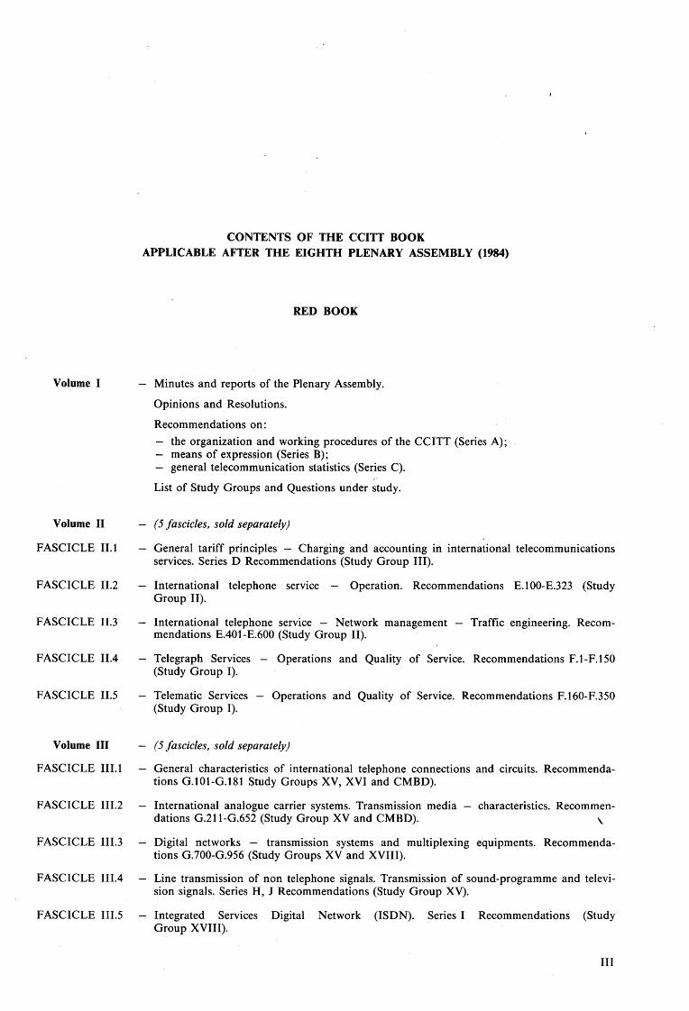
CONTENTS OF THE CCITT BOOKAPPLICABLE AFTER THE EIGHTH PLENARY ASSEMBLY (1984)
RED BOOK
— Minutes and reports of the Plenary Assembly.
Opinions and Resolutions.
Recommendations on:— the organization and working procedures of the CCITT (Series A);— means of expression (Series B);— general telecommunication statistics (Series C).
List of Study Groups and Questions under study.
— (5 fascicles, sold separately)
— General tariff principles — Charging and accounting in international telecommunications services. Series D Recommendations (Study Group III).
— International telephone service — Operation. Recommendations E.100-E.323 (Study Group II).
— International telephone service — Network management — Traffic engineering. Recommendations E.401-E.600 (Study Group II).
— Telegraph Services — Operations and Quality of Service. Recommendations F.1-F.150 (Study Group I).
— Telematic Services — Operations and Quality of Service. Recommendations F.160-F.350 (Study Group I).
— (5 fascicles, sold separately)
— General characteristics of international telephone connections and circuits. Recommendations G.101-G.181 Study Groups XV, XVI and CMBD).
— International analogue carrier systems. Transmission media — characteristics. Recommendations G.211-G.652 (Study Group XV and CMBD). V
— Digital networks — transmission systems and multiplexing equipments. Recommendations G.700-G.956 (Study Groups XV and XVIII).
— Line transmission of non telephone signals. Transmission of sound-programme and television signals. Series H, J Recommendations (Study Group XV).
— Integrated Services Digital Network (ISDN). Series I Recommendations (Study Group XVIII).
I l l
Volume IV
FASCICLE IV. 1
FASCICLE IV.2
FASCICLE IV.3
FASCICLE IV.4
Volume V
Volume VI
FASCICLE VI. 1
FASCICLE VI.2
FASCICLE VI.3
FASCICLE VI.4
FASCICLE VI.5
FASCICLE VI.6
FASCICLE VI.7
FASCICLE VI.8
FASCICLE VI.9
FASCICLE VI. 10
/
FASCICLE VI. 11
FASCICLE VI. 12
FASCICLE VI. 13
IV
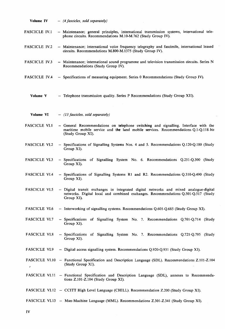
(4 fascicles, sold separately)
M aintenance; general principles, international transmission systems, international telephone circuits. Recommendations M.10-M.762 (Study Group IV).
M aintenance; international voice frequency telegraphy and fascimile, international leased circuits. Recommendations M.800-M.1375 (Study Group IV).
M aintenance; international sound programme and television transmission circuits. Series N Recommendations (Study Group IV).
Specifications of measuring equipment. Series 0 Recommendations (Study G roup IV).
Telephone transmission quality. Series P Recommendations (Study Group XII).
(13 fascicles, sold separately)
General Recommendations on telephone switching and signalling. Interface with the maritime mobile service and the land mobile services. Recommendations Q .l-Q .l 18 bis (Study G roup XI).
Specifications of Signalling Systems Nos. 4 and 5. Recommendations Q.120-Q.180 (Study Group XI).
Specifications of Signalling System No. 6. Recommendations Q.251-Q.300 (StudyG roup XI).
Specifications of Signalling Systems R1 and R2. Recommendations Q.310-Q.490 (Study Group XI).
Digital transit exchanges in integrated digital networks and mixed analogue-digital networks. Digital local and combined exchanges. Recommendations Q.501-Q.517 (Study G roup XI).
Interworking of signalling systems. Recommendations Q.601-Q.685 (Study Group XI).
— Specifications of Signalling System No. 7. Recommendations Q.701-Q.714 (StudyGroup XI).
— Specifications of Signalling System No. 7. Recommendations Q.721-Q.795 (StudyGroup XI).
— Digital access signalling system. Recommendations Q.920-Q.931 (Study Group XI).
— Functional Specification and Description Language (SDL). Recommendations Z.101-Z.104 (Study Group XI).
— Functional Specification and Description Language (SDL), annexes to Recommendations Z.101-Z.104 (Study Group XI).
— CCITT High Level Language (CHILL). Recommendation Z.200 (Study Group XI).
— M an-M achine Language (MML). Recommendations Z.301-Z.341 (Study Group XI).
Volume VII
FASCICLE VII. 1
FASCICLE VII.2
FASCICLE VII.3
Volume VIII
FASCICLE VIII. 1
FASCICLE VIII.2
FASCICLE VIII.3
FASCICLE VIII.4
FASCICLE VIII.5
FASCICLE VIII.6
FASCICLE VIII.7
Volume IX
Volume X
FASCICLE X.l
FASCICLE X.2
(3 fascicles, sold separately)
Telegraph transmission. Series R Recommendations (Study Group IX). Telegraph services terminal equipment. Series S Recommendations (Study Group IX).
Telegraph switching. Series U Recommendations (Study Group IX).
Terminal equipment and protocols for telematic services. Series T Recommendations (Study Group VIII).
(7 fascicles, sold separately)
Data communication over the telephone network. Series V Recommendations (Study Group XVII).
Data communication networks: services and facilities. Recommendations X .l-X .l5 (Study Group VII).
Data communication networks: interfaces. Recommendations X.20-X.32 (StudyGroup VII).
Data communication networks: transmission, signalling and switching, network aspects, maintenance and administrative arrangements. Recommendations X.40-X.181 (Study Group VII).
Data communication networks: Open Systems Interconnection (OSI), system description techniques. Recommendations X.200-X.250 (Study Group VII).
Data communication networks: interworking between networks, mobile data transmission systems. Recommendations X.300-X.353 (Study Group VII).
Data communication networks: message handling systems. Recommendations X.400-X.430 (Study Group VII).
Protection against interference. Series K Recommendations (Study Group V). Construction, installation and protection of cable, and other elements of outside plant. Series L Recommendations (Study Group VI).
(2 fascicles, sold separately)
Terms and definitions.
Index of the Red Book.
V

PAGE INTENTIONALLY LEFT BLANK
PAGE LAISSEE EN BLANC INTENTIONNELLEMENT

CONTENTS OF FASCICLE III.l OF THE RED BOOK
Part I — Recommendations G.101 to G.181
General characteristics of international telephone connections and circuits
Rec. No. Page
SECTION 1 — General characteristics fo r international telephone connections and international telephone circuits
1.0 General
G.101 The transmission p l a n ........................................................................................................................ 3
G.102 Transmission performance objectives and recommendations ................................................. 19
G.103 Hypothetical reference c o n n e c tio n s ............................................................................................... 22
G.104 Hypothetical reference connections (digital n e tw o rk )................................................................ 31
G.105 Hypothetical reference connection for crosstalk studies ......................................................... 33
G.106 Terms and definitions related to quality of service, availability and re lia b ili ty ................. 37
G.107 General considerations and model of a basic telephone c a l l ................................................... 94
G.108 Models for the allocation of international telephone connection retainability .................... 96
1.1 General recommendations on the transmission quality for an entire international telephone connection
G. I l l Corrected reference equivalents (CREs) and loudness ratings (LRs) in an internationalconnection .................................................................. 98
G.113 Transmission im p a irm e n ts ............................................................................................................... 123
G.114 Mean one-way propagation tim e ...................................................................................................... 130
G.117 Transmission aspects of unbalance about earth (definitions and methods) ....................... 135
Fascicle III.l — Table of Contents VII
Rec. No.
1.2 General characteristics of national systems forming part of international connections
G.120 Transmission characteristics of national ne tw orks......................................................................
G.121 Corrected reference equivalents (CREs) and loudness ratings (LRs) of national systems
G.122 Influence of national systems on stability, talker echo, and listener echo in international connections . . ...........................................................
G.123 Circuit noise in national ne tw orks..................................................................................................
G.125 Characteristics of national circuits on carrier systems ............................................................
1.3 General characteristics of the 4-wire chain formed by the international circuits andnational extension circuits
G.131 Stability and e c h o ...............................................................................................................................
G.132 Attenuation d is to r tio n ............................................................................................ •..........................
G.133 Group-delay d i s to r t io n .....................................................................................................................
G.134 Linear crosstalk ................ ; . . . . . ............................................................ • ..............
G.135 Error on the reconstituted f re q u e n c y ...........................................................................................
1.4 General characteristics of the 4-wire chain of international circuits; international transit
G.141 Transmission losses, relative levels and attenuation d isto rtio n ...............................................
G.142 Transmission characteristics of e x c h a n g e s ..................................................................................
G.143 Circuit noise and the use of co m p an d o rs .....................................................................................
1.5 General characteristics of international telephone circuits and national extension circuits
G.151 General performance objectives applicable to all modern international circuits andnational extension circuits ..............................................................................................................
G.152 Characteristics appropriate to long-distance circuits of a length not exceeding 2500 km
G.153 Characteristics appropriate to international circuits more than 2500 km in length . . . .
1.6 Apparatus associated with long-distance telephone circuits
G.161 Echo-suppressors suitable for circuits having either short or long propagation times
G.162 Characteristics of compandors for telephony .................................................................. . . .
G.163 Call concentrating systems ............................... ..............................................................
G.164 , Echo suppressors.................................................................................................................................
G.165 Echo cancellers............................................................................................................ .........................
Page
149
150
166
178
183
183
195
196
197
198
199
200
204
208
213
214
216
217
223
225
258
VIII Fascicle III.l — Table of Contents
Rec. No. Page
G.166 Characteristics of syllabic compandors for telephony on high capacity long distancesystems .......................................................................................................... 280
1.7 Transmission plan aspects of special circuits and connections using the international telephone connection network
G.171 Transmission plan aspects of privately operated n e tw o rk s ...................................................... 286
G.172 Transmission plan aspects of international conference c a l l s . . 295
1.8 General Recommendations on availability and reliability of entire international telephoneconnections
G.180 Connection accessibility objective for the international telephone s e rv ic e ........................... 298
G.181 Connection retainability objective for the international telephone se rv ic e ........................... 302
Part II — Supplements to Section 1 of the series G Recommendations
Supplement No. 2 Talker echo on international connections.............................................................. 313
Supplement No. 20 Possible combinations of basic transmission impairments in hypothetical referencec o n n e c tio n s .................................................................................................................................... 319
Supplement No. 21 The use of quantizing distortion units in the planning of international connections(contribution of Bell-Northern R esearch )............................................................................... 326
Supplement No. 24 Considerations concerning quantizing distortion units o f some digital devices thatprocess encoded s ig n a ls .............................................................................................................. 333
Supplement No. 25 Guidelines for placement of microphones and loudspeakers in telephone conferencerooms .............................................................................................................................................. 335
— Supplements Nos. 1, 3, 4, 6 to 10 and 13 to 15 have not been reproduced in the Red Book. They can
PRELIM INARY NOTES
1 Supplements to the Series G Recommendations not published in this fascicle can be found as follows:
— Supplements Nos. 1, 3, 4, 6 to 10 and 13 to 15 have not been reproduced in the Red Book. The}be found in Fascicle III.3 of the Orange Book, ITU, Geneva, 1977.
— Supplements Nos. 5, 11, 17 to 19, 22, 23, 26 and 27 are printed in Fascicle III.2 of the Red Book
— Supplements Nos. 27 and 28 are to be found in Fascicle III.3 of the Red Book
— Supplements Nos. 12 and 16 are to be found in Fascicle III.4 of the Red Book
Fascicle III.l — Table of Contents IX

2 The Questions entrusted to each Study G roup for the Study Period 1985-1988 can be found in Contribution No. 1 to that Study Group.
3 Units
The following abbreviations are used, particularly in diagrams and tables, and always have the following clearly defined meanings:
dBm the absolute (power) level in decibels;
dBmO the absolute (power) level in decibels referred to a point of zero relative level;
dBr the relative (power) level in decibels;
dBmOp the absolute psophometric power level in decibels referred to a point of zero relative level.
4 In this fascicle, the expression “Adm inistration” is used for shortness to indicate both a telecommunication Administration and a recognized private operating agency.
X Fascicle III.l — Table of Contents

PART I
Recommendations G.101 to G.181
GENERAL CHARACTERISTICS OF INTERNATIONAL TELEPHONE CONNECTIONS AND CIRCUITS

PAGE INTENTIONALLY LEFT BLANK
PAGE LAISSEE EN BLANC INTENTIONNELLEMENT
SECTION 1
GENERAL CHARACTERISTICS FOR INTERNATIONAL TELEPHONE CONNECTIONS AND INTERNATIONAL TELEPHONE CIRCUITS
1.0 General
Recommendation G.101
THE TRANSM ISSION PLAN»
(Geneva, 1964; amended at Mar del Plata, 1968, Geneva, 1972, 1976 and 1980; Malaga-Torremolinos, 1984)
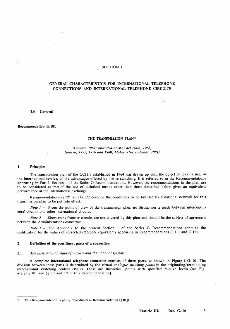
1 Principles
The transmission plan of the CCITT established in 1964 was drawn up with the object of making use, in the international service, of the advantages offered by 4-wire switching. It is referred to in the Recommendations appearing in Part I, Section 1 of the Series G Recommendations. However, the recommendations in the plan are to be considered as met if the use of technical means other than those described below gives an equivalent performance at the international exchange.
Recommendations G.121 and G.122 describe the conditions to be fulfilled by a national network for this transmission plan to be put into effect.
Note 1 — From the point o f view of the transmission plan, no distinction is made between intercontinental circuits and other international circuits.
Note 2 — Short trans-frontier circuits are not covered by this plan and should be the subject o f agreement between the Administrations concerned. ,
Note 3 — The Appendix to the present Section 1 of the Series G Recommendations contains the justification for the values of corrected reference equivalents appearing in Recommendations G . l l l and G.121.
2 Definition of the constituent parts of a connection
2.1 The international chain o f circuits and the national systems
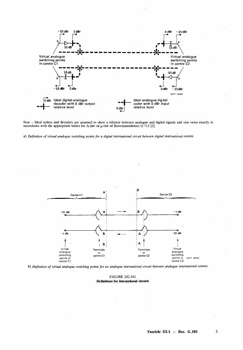
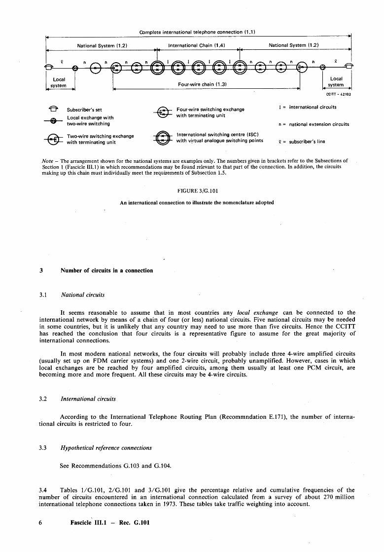
A complete international telephone connection consists o f three parts, as shown in Figure 1/G.101. The division between these parts is determined by the virtual analogue switching points in the originating/term inating international switching centres (ISCs). These are theoretical points with specified relative levels (see Figure 2/G.101 and §§ 5.1 and 5.2 of this Recommendation).
This Recommendation is partly reproduced in Recommendation Q.40 [1].
Fascicle III.l — Rec. G.101 3

The three parts of the connection are: '
— Two national systems, one at each end. These may comprise one or more 4-wire national trunk circuits with 4-wire interconnection, as well as circuits with 2-wire connection up to the local exchanges and the subscriber sets with their subscriber lines.
— An international chain made up of one or more 4-wire international circuits. These are interconnectedon a 4-wire basis in the international centres which provide for transit traffic and are also connectedon a 4-wire basis to national systems in the international centres.
An international 4-wire circuit is delimited by its virtual analogue switching points in an internationalswitching centre.
Note 1 — In principle the choice of values of the relative levels at the virtual analogue switching pointson the side of a national system is a national matter. In practice, several countries have chosen —3.5 dBr forreceiving as well as for sending. These are theoretical values; they need not actually occur as any special equipment item; however, they serve to determine the relative levels at other points in the national network. If, for instance, the loss “ t—b ” or “a — t ” is 3.5 dB (as is the case in several countries, cf. Table A-1/G.121), then in follows that the relative levels at point t are 0 dBr (input) and — 7 dBr (output).
Note 2 — The virtual analogue switching points may not be the same as the points at which the circuitterminates physically in the switching equipment. These latter points are known as the circuit terminals; the exact position of these terminals is decided in each case by the Administration concerned.
International switching centres (ISCs)
*
National system
X Exchange
L - * - — ;!* ------
-x— O
International chain National system
CCITT- 4 2 0 9 2
($) ISC that carries international transit traffic
FIGURE 1/G.101
Definition of the constituent parts of an international connection
2.2 National extension circuits: 4-wire chain
When the maximum distance between an international exchange and a subscriber who can be reached from it does not exceed about 1000 km or, exceptionally, 1500 km, the country concerned is considered as of average size. In such countries, in most cases, not more than three national circuits are interconnected on a 4-wire basis between each other and to international circuits. These circuits should comply with the recommendations of Subsection 1.2.
In a large country, a fourth and possibly a fifth national circuit may be included in the 4-wire chain, provided it has the nominal transmission loss and the characteristics recommended for international circuits used in a 4-wire chain (see Recommendation G.141, § 1, § 4 of this Recommendation and the Recommendations in Subsection 1.5).
Note — The abbreviation “a 4-wire chain” (see Figure 3/G.101) signifies the chain composed of the international chain and the national extension circuits connected to it, either by 4-wire switching or by some equivalent procedure (as understood in § 1 above).
4 Fascicle III.l — Rec. G.101
r r/ M H - - ,
” 3.5 dB 1
-3.5 dBr 0 dBr
Virtual analogue switching points in centre C1
♦ ♦
3.5 dB\ J UD a
J j-3,5 dBr OdBr
[cTdBr Ideal digital-analogue ■ decoder with 0 dBr output
‘“ I relative level
OdBr -3.5 dBrr rT °
Virtual analogue switching points in centre C2
J JOdBr -3,5 dBr
CCITT - 3 3 831
t Ideal analogue-digital"I coder with 0 dBr input
OdBr I relative leveldBr)
Note - Ideal coders and decoders are assumed to show a relation between analogue and digital signals and vice versa exactly accordance with the appropriate tables for A-law or p-law of Recommendation G.711 [2].
a) Definition o f virtual analogue switching points for a digital international circuit between digital international centres
a n a lo g u e sw itc h in g p o in ts in
c e n tr e C1
c e n tre C1
I
A
T erm in a lsin
c e n tre C2
C e n tre C2
- 4 dBr
-3.5 dBr
V irtuala n a lo g u esw itc h in gp o in ts in CCITT- 3 6 8 6 1
c e n tr e C2
b) Definition o f virtual analogue switching points for an analogue international circuit between analogue international centres
FIGURE 2/G.101 Definitions for international circuits
Fascicle III.l - Rec. G.101
National System (1.2) International Chain (1.4) National System (1.2)
£^ n ( 7 \ n (
^ n / - v n ^ ^ I I 1 1 n /•—\ n n /—\ n £^ /7XT_F---------- £
Localsystem
* \ ? 7 i ^ W ^ W
Four-wire chain (1.3)
' j wLocal
system
-0=
Subscriber's setLocal exchange with two-wire switching
Two-wire switching exchange with terminating unit
Four-wire switching exchange with terminating unit
International switching centre (ISC) with virtual analogue switching points
CCITT - 4 2 1 0 2
I = international circuits
n = national extension circuits
£ = subscriber's line
Note - The arrangement shown for the national systems are examples only. The numbers given in brackets refer to the Subsections of Section 1 (Fascicle III. 1) in which recommendations may be found relevant to that part of the connection. In addition, the circuits making up this chain must individually meet the requirements of Subsection 1.5.
FIGURE 3/G.101
An international connection to illustrate the nomenclature adopted
Number of circuits in a connection
3.1 National circuits
It seems reasonable to assume that in most countries any local exchange can be connected to the international network by means of a chain of four (or less) national circuits. Five national circuits may be needed in some countries, but it is unlikely that any country may need to use more than five circuits. Hence the CCITT has reached the conclusion that four circuits is a representative figure to assume for the great majority of international connections.
In most modern national networks, the four circuits will probably include three 4-wire amplified circuits (usually set up on FDM carrier systems) and one 2-wire circuit, probably unamplified. However, cases in which local exchanges are be reached by four amplified circuits, among them usually at least one PCM circuit, are becoming more and more frequent. All these circuits may be 4-wire circuits.
3.2 International circuits
According to the International Telephone Routing Plan (Recommndation E.171), the number of international circuits is restricted to four.
3.3 Hypothetical reference connections
See Recommendations G.103 and G.104.
3.4 Tables 1/G.101, 2/G.101 and 3/G.101 give the percentage relative and cumulative frequencies of the number of circuits encountered in an international connection calculated from a survey of about 270 million international telephone connections taken in 1973. These tables take traffic weighting into account.
6 Fascicle III.1 - Rec. G.101
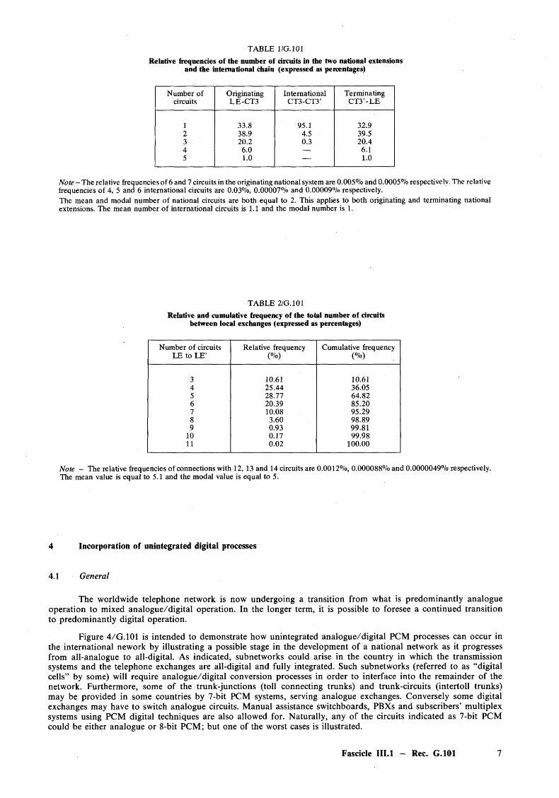
TABLE 1/G.101Relative frequencies of the number of circuits in the two national extensions
and the international chain (expressed as percentages)
Number of circuits
OriginatingLE-CT3
InternationalCT3-CT3'
TerminatingCT3'-LE
1 33.8 95.1 32.92 38.9 4.5 39.53 20.2 0.3 20.44 6.0 — 6.15 1.0 — 1.0
Note - The relative frequencies of 6 and 7 circuits in the originating national system are 0.005°/o and 0.0005°/o respectively. The relative frequencies of 4, 5 and 6 international circuits are 0.03%, 0.00007% and 0.00009% respectively.The mean and modal number of national circuits are both equal to 2. This applies to both originating and terminating national extensions. The mean number of international circuits is 1.1 and the modal number is 1.
TABLE 2/G.101Relative and cumulative frequency of the total number of circuits
between local exchanges (expressed as percentages)
Number of circuits LE to LE'
Relative frequency (%)
Cumulative frequency (%)
3 10.61 10.614 25.44 36.055 28.77 64.826 20.39 85.207 10.08 95.298 3.60 98.899 0.93 99.81
10 0.17 99.9811 0.02 100.00
Note — The relative frequencies of connections with 12, 13 and 14 circuits are 0.0012%, 0.000088% and 0.0000049% respectively. The mean value is equal to 5.1 and the modal value is equal to 5.
4 Incorporation of unintegrated digital processes
4.1 General
The worldwide telephone network is now undergoing a transition from what is predominantly analogue operation to mixed analogue/digital operation. In the longer term, it is possible to foresee a continued transition to predominantly digital operation.
Figure 4/G.101 is intended to demonstrate how unintegrated analogue/digital PCM processes can occur in the international nework by illustrating a possible stage in the development of a national network as it progresses from all-analogue to all-digital. As indicated, subnetworks could arise in the country in which the transmission systems and the telephone exchanges are all-digital and fully integrated. Such subnetworks (referred to as “digital cells” by some) will require analogue/digital conversion processes in order to interface into the remainder of the network. Furthermore, some of the trunk-junctions (toll connecting trunks) and trunk-circuits (intertoll trunks) may be provided in some countries by 7-bit PCM systems, serving analogue exchanges. Conversely some digital exchanges may have to switch analogue circuits. M anual assistance switchboards, PBXs and subscribers’ multiplex systems using PCM digital techniques are also allowed for. Naturally, any of the circuits indicated as 7-bit PCM could be either analogue or 8-bit PCM; but one of the worst cases is illustrated.
Fascicle III.l - Rec. G.101 7
\
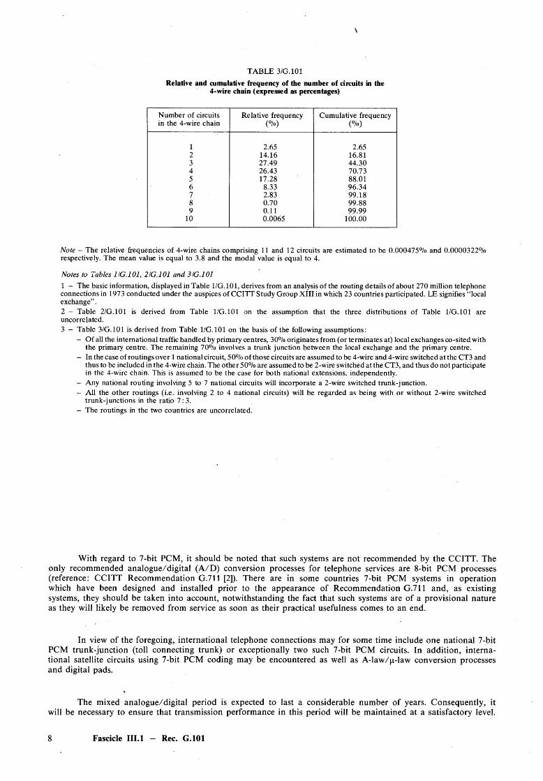
TABLE 3/G.101Relative and cumulative frequency of the number of circuits in the
4-wire chain (expressed as percentages)
Number of circuits in the 4-wire chain
Relative frequency (%)
Cumulative frequency (%)
1 2.65 2.652 14.16 16.813 27.49 44.304 26.43 70.735 17.28 88.016 8.33 96.347 2.83 99.188 0.70 99.889 0.11 99.99
10 0.0065 100.00
Note - The relative frequencies of 4-wire chains comprising 11 and 12 circuits are estimated to be 0.000475% and 0.0000322% respectively. The mean value is equal to 3.8 and the modal value is equal to 4.
Notes to Tables IIG .101,2 IG. 101 and 3 IG. 1011 - The basic information, displayed in Table 1/G. 101, derives from an analysis of the routing details of about 270 million telephone connections in 1973 conducted under the auspices of CCITT Study Group XIII in which 23 countries participated. LE signifies “local exchange” .2 - Table 2/G.101 is derived from Table 1/G.101 on the assumption that the three distributions of Table 1/G.101 are uncorrelated.3 - Table 3/G.101 is derived from Table 1/G. 101 on the basis of the following assumptions:
- Of all the international traffic handled by primary centres, 30% originates from (or terminates at) local exchanges co-sited with the primary centre. The remaining 70% involves a trunk junction between the local exchange and the primary centre.
- In the case of routings over 1 national circuit, 5 0% of those circuits are assumed to be 4-wire and 4-wire switched at the CT3 and thus to be included in the 4-wire chain. The other 50% are assumed to be 2-wire switched at the CT3, and thus do not participate in the 4-wire chain. This is assumed to be the case for both national extensions, independently.
- Any national routing involving 5 to 7 national circuits will incorporate a 2-wire switched trunk-j unction.- All the other routings (i.e. involving 2 to 4 national circuits) will be regarded as being with or without 2-wire switched
trunk-j unctions in the ratio 7:3.- The routings in the two countries are uncorrelated.
With regard to 7-bit PCM, it should be noted that such systems are not recommended by the CCITT. The only recommended analogue/digital (A /D ) conversion processes for telephone services are 8-bit PCM processes (reference: CCITT Recommendation G.711 [2]). There are in some countries 7-bit PCM systems in operation which have been designed and installed prior to the appearance of Recommendation G.711 and, as existing systems, they should be taken into account, notwithstanding the fact that such systems are of a provisional nature as they will likely be removed from service as soon as their practical usefulness comes to an end.
In view of the foregoing, international telephone connections may for some time include one national 7-bit PCM trunk-junction (toll connecting trunk) or exceptionally two such 7-bit PCM circuits. In addition, international satellite circuits using 7-bit PCM coding may be encountered as well as A-law/p-law conversion processes and digital pads.
The mixed analogue/digital period is expected to last a considerable number of years. Consequently, it will be necessary to ensure that transmission performance in this period will be maintained at a satisfactory level.
8 Fascicle III.l - Rec. G.101
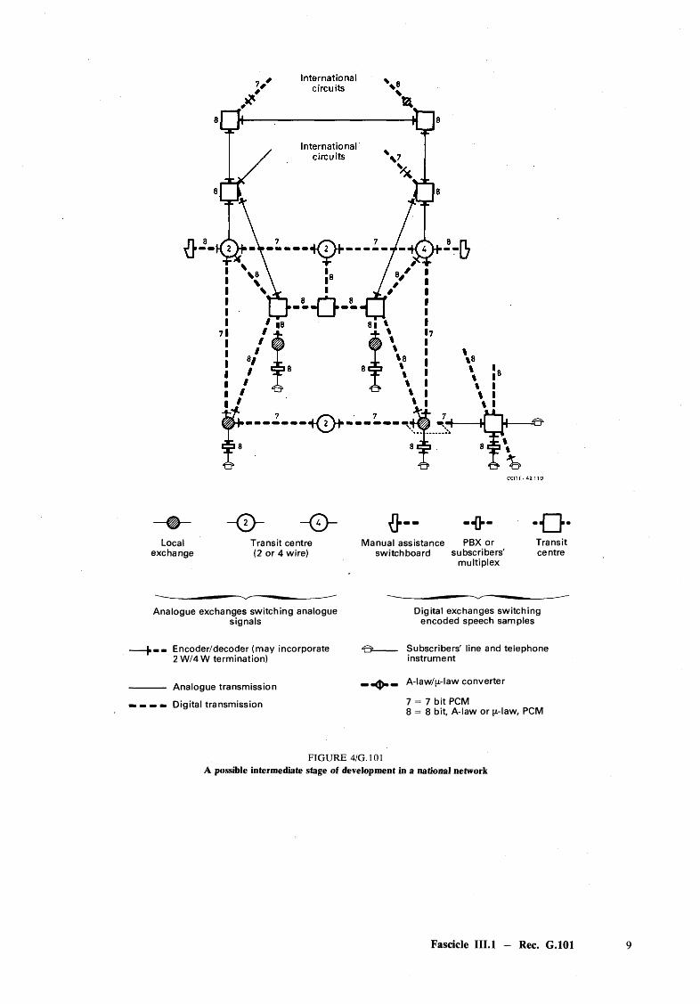
Localexchange
- © - - 0 -Transit centre (2 or 4 wire)
- 0 »Manual assistance PBX or
switchboard subscribers' multiplex
- o -Transitcentre
Analogue exchanges switching analogue signals
Digital exchanges switching encoded speech samples
mm Encoder/decoder (may incorporate 2 W/4 W termination)
O - Subscribers' line and telephone instrument
Analogue transmission
Digital transmission
— J>«— A-law/p-law converter
7 = 7 bit PCM8 = 8 bit, A-law or p-law, PCM
FIGURE 4/G.101 A possible intermediate stage of development in a national network
Fascicle III.l - Rec. G.101
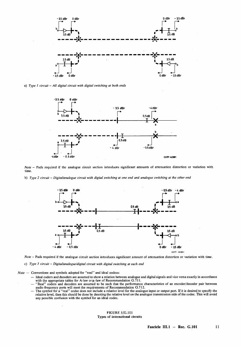
4.2 Types o f telephone circuits
In the mixed analogue/digital period, international circuits could, in particular, consist of the types indicated in Figure 5/G.101. In all cases, the virtual analogue switching points are identified (conceptually) and the relative levels at these points, specified.
Although the circuit types shown in Figure 5/G.101 are classed as international circuits, the configurations involved could also occur in national telephone networks. However, in national networks the relative levels at the virtual analogue switching points of the circuits could be different from those indicated for international circuits.
The Type 1 circuit in Figure 5a)/G.101 represents the case where digital transmission is used for the entire length o f the circuit and digital switching is used at both ends. Such a circuit can generally be operated at a nominal transmission loss of 0 dB as shown because of the transmission properties exhibited by such circuits (e.g., relatively small loss variations with time).
The Type 2 circuit in Figure 5b)/G.101 represents the case where the transmission path is established on a digital transmission channel in tandem with an analogue transmission channel. Digital switching is used at the digital end and analogue switching at the analogue end.
It might be possible, in some cases, to operate Type 2 circuits with a nominal loss of 0 dB in each direction of transmission. For example, where the analogue portion could be provided with the necessary gain stability and where the attenuation distortion would permit such operation.
The Type 3 circuit in Figure 5c)/G.101 represents the case where the transmission path is established over a tandem arrangement consisting of digital/analogue/digital channels as shown. Digital switching is assumed at both ends.
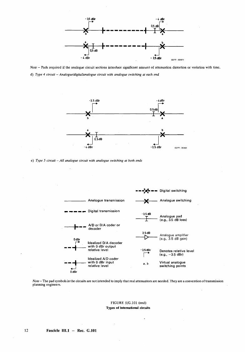
The Type 4 circuit in Figure 5d)/G.101 represents the case where the transmission path is established over a tandem arrangement consisting of analogue/digital/analogue channels as shown. Analogue switching is assumed at both ends.
The Type 5 circuit in Figure 5e)/G.101 represents the case where analogue transmission is used for the entire length of the circuit and analogue switching is used at both ends.
International circuits o f this type are usually operated at a loss L, where L is nominally = 0.5 dB betweenvirtual analogue switching points.
Note — General remarks concerning the allocation o f losses in the mixed analogue/digital circuits
In circuit types 2, 3 and 4, the pads needed to control any variability in the analogue circuit sections(arising from loss variations with time or attenuation distortion) are shown in a symmetrical fashion in bothdirections of transmission. However, in practice, such arrangements may require nonstandard levels at the boundaries between circuit sections. Administrations are advised that should they prefer to adopt an asymmetric arrangement, e.g., by putting all the loss into the receive direction at only one end of a circuit (or circuit section); then, provided that the loss is small, e.g., a total of not more than 1 dB, there is no objection on transmission plan grounds.
The small amount of asymmetry that results in the international portion of the connection will be acceptable, bearing in mind the small number of international circuits encountered in most actual connections.
As far as national circuits are concerned, Administrations may adopt any arrangements they wish provided that the requirements o f Recommendation G.121, § 2.2, are complied with.
In some cases transmultiplexers may be used, in which case the circuits may not be available at audio-frequency at the point at which a pad symbol is used in the diagrams of Figure 5/G.101. Should the variability of the analogue portions merit additional loss, the precise way in which this loss can be inserted into the circuits is a matter for Administrations to decide bilaterally.
4.3 Number o f unintegrated PCM digital processes
Restrictions due to transmission impairments
In the mixed analogue/digital period, it may be necessary to include a substantial number of unintegrated digital processes in international telephone connections. To ensure that the resulting transmission impairments (quantizing, attenuation and group-delay distortion) introduced by such processes do not accumulate to the point where overall transmission quality can be appreciably impaired, it is recommended that the planning rule given in Recommendation G.113 § 3 be complied with. The effect of this rule is to limit the number of unintegrated digital processes in both the national and international parts of telephone connections.
10 Fascicle III.l - Rec. G.101
r r r rt> —| - ,«■ H I °3.5 dB J J 3.5 dB
-3.5 dBr OdBr OdBr -3 .5 dBr
♦ ♦V"3,5 dB I , 3,5 dB
J J J J-3.5 dBr OdBr OdBr -3 .5dBr
a) Type 1 circuit - All digital circuit with digital switching at both ends
-3.5 dBr OdBrri i - 3.5 dBr -AdBr
r „,dBr 4,--------------------- 1--------------- ^ j_ x _
" i “ M xJ °'5d0 J
I - L rIDr -1 5HR|- i, dBr -3,5dBr
A ^-AdBr -0 ,5 dBr CCITT-42J01
Note - Pads required if the analogue circuit section introduces significant amounts of attenuation distortion or variation with time.
b) Type 2 circuit - Digital/analogue circuit with digital switching at one end and analogue switching at the other end
- 3.5 dBr OdBr -0.5 dBr -U dBrr r r r. . . . H - E L
o a
15 dB ■ 0.5 dB \ 3,5 dB______ I
♦
y j t I t I_______ oV3.5 dB , 0.5 dB Z 3,5 dB
— H ^ T bJ J J J- U dBr - 0.5 dBr 0 dBr - 3.5 dBr
CCITT - 3 3 8S1
Note - Pads required if the analogue circuit section introduces significant amount of attenuation distortion or variation with time,
c) Type 3 circuit - Digitallanalogueldigital circuit with digital switching at each end
Note — Conventions and symbols adopted for “real” and ideal codecs:— Ideal coders and decoders are assumed to show a relation between analogue and digital signals and vice versa exactly in accordance
with the appropriate tables for A-law or p.-law of Recommendation G .711.— “ Real” coders and decoders are assumed to be such that the performance characteristics of an encoder/decoder pair between
audio frequency ports will meet the requirements of Recommendation G .712.— The symbol for a “ real” codec does not include a relative level for the analogue input or output port. If it is desired to specify the
relative level, then this should be done by denoting the relative level on the analogue transmission side of the codec. This will avoid any possible confusion with the symbol for an ideal codec.
FIGURE 5/G.101 Types of international circuits
Fascicle III.l - Rec. G.101 11
r o.5aBr— i — h - -------------------- f - t % —
Xi-E—h---------------- 1------X-------> dB J- 1* dBr - 3.5 dBr
' CCITT- 3 3 871
Note — Pads required if the analogue circuit sections introduce significant amount of attenuation distortion or variation with time,
d) Type 4 circuit - AnalogueIdigitallanalogue circuit with analogue switching at each end
- 3,5 dBr - L, dBr
-3.5 dBr -4 dBr
f a s « r- x - ------------------------------------ ^ x -
-X-ri ---------------- rX-J°5dB J-U dBr -3.5 dBr CCITT - 33 861
e) Type 5 circuit - A ll analogue circuit with analogue switching at both ends
- — — — Digital switching
Analogue transmission
Digital transmission
A/D or D/A coder or decoder
OdBrr *
— i -
-3.5 dB
3.5 dB
Idealized D/A decoderwith 0 dBr outputrelative level -3.5 dBrrIdealized A/D coderwith 0 dBr input a , brelative level
Analogue switching
Analogue pad (e.g., 3.5 dB loss)
A nalog ue a m p lifie r (e .g ., 3 .5 dB gain)
Denotes relative level (e.g., -3 .5 dBr)
Virtual analogue switching points
OdBr
Note — The pad symbols in the circuits are not intended to imply that real attenuators are needed. They are a convention of transmission planning engineers.
FIGURE 5/G.101 (end) Types of international circuits
12 Fascicle III.l - Rec. G.101
In the case of all-digital connections, transmission impairments can also accumulate due to the incorporation of digital processes (e.g., digital pads). The matter of accumulating such impairments under all-digital conditions is also dealt with in Recommendation G.113 § 3.
4.4 Transmission o f analogue and digital data
In the mixed analogue/digital period, the presence in telephone connections of analogue/digital converters, encoding law converters, digital pads, or other types of digital processes, would not preclude the transmission of analogue data. However, on overall digital connections, digital type data could be adversely affected by devices such as encoding law converters and digital pads, since they involve signal recoding processes. Consequently, for the transmission of digital data, arrangements should be made to switch-out or bypass any device whose operation entails the recoding of digital data signals.
4.5 General principle
It is recognized that in the mixed analogue/digital period, there could be a considerable presence of unintegrated digital processes in the worldwide telephone network. Consequently, it is im portant that the incorporation of these processes should take place in such a way that when integration of functions can occur, unnecessary items of equipment would not remain in the all-digital network.
5 Conventions and definitions
5.1 Virtual analogue switching points
The concept “virtual switching points” has been useful in making transmission studies with regard to all-analogue connections. For example, these points have been used to define the boundary between international circuits as well as between international circuits and national extensions. The “virtual switching points” also provided convenient locations to which transmission quantities could be referred.
The incorporation of digital encoding processes into the worldwide telephone network no longer makes it possible, in all cases, to determine theoretical points which correspond to the “virtual switching points” of all-analogue connections. Since it would be desirable, in mixed analogue/digital connections to have analogous points, the concept of “virtual analogue switching points” has been adopted. This concept postulates the existence of ideal codecs through which the desired analogue points could be derived.
The term “virtual analogue switching points” is also used for all-analogue situations and replaces the older term “virtual switching points”.
5.2 Relative level specified in the virtual analogue switching points o f international circuits
The virtual analogue switching points of an international 4-wire telephone circuit are fixed by convention at points o f the circuit where the nominal relative levels at the reference frequency are:
— sending: —3.5 dBr;
— receiving: —4.0 dBr, for analogue;— 3.5 dBr for digital circuits.
The nominal transmission loss of this circuit at the reference frequency between virtual analogue switching points is therefore 0.5 dB for analogue and 0 dB for digital circuits.
Note 1 — See the definition in § 5.3 below. The position of the virtual analogue switching points is shown in Figure 2/G.101, and in Figure 1/G. 122.
Note 2 — Since the 4-wire terminating set forms part of national systems and since its actual attenuation may depend on the national transmission plan adopted by each Administration, it is no longer possible to define the relative levels on international 4-wire circuits by reference to the 2-wire terminals of a terminating set. In particular, the transmission loss in terminal service of the chain created by connecting a pair of terminating sets to a 4-wire international circuit cannot be fixed at a single value by Recommendations. The virtual analogue switching points of circuits might therefore have been chosen at points of arbitrary relative level. However, the values adopted above are such that in general they permit the passage from the old plan to the new to be made with the minimum amount of difficulty.
Fascicle HI-1 — Rec. G.101 13
Note 3 — If a 4-wire analogue circuit forming part of the 4-wire chain contributes negligible delay and variation of transmission loss with time, it may be operated at zero nominal transmission loss between virtual analogue switching points. This relaxation refers particularly to short 4-wire tie-circuits between switching centres — e.g., circuits between two international switching centres in the same city:
5.3 Definitions
5.3.1 transmission reference point
F: point de reference pour la transmission
S: punto de referenda para la transmisidn
A hypothetical point used as the zero relative level point in the computation of nominal relative levels. At those points in a telephone circuit the nominal mean power level ( —15 dBm) defined in Recommendation G.223 [3] shall be applied when checking whether the transmission system conforms to the noise objectives defined in Recommendation G.222 [4].
Note — For certain systems, e.g. submarine cable systems (Recommendation G.371 [5]), other valuesapply.
Such a point exists at the sending end of each channel of a 4-wire switched circuit preceding the virtual switching point; on an international circuit it is defined as having a signal level of +3.5 dB above that of the virtual switching point.
In frequency division multiplex equipment, a hypothetical point o f flat zero relative level (i.e. where all channels have the same relative level) is defined as a point where the multiplex signal, as far as the effect of intermodulation is concerned, can be represented by a uniform spectrum random noise signal with a mean power level as defined in Recommendation G.223 [6]. The nominal mean power level in each telephone channel is — 15 dBm as defined in Recommendation G.223 [3].
5.3.2 relative (power) level
F: niveau relatif de puissance
S: nivel relativo (de potencia)
5.3.2.1 Basic significance o f relative level in FDM systems
The relative level at a point in a transmission system characterizes the signal power handling capacity at this point with respect to the conventional power level at a zero relative level point 2\
If, for example, at a particular point an FDM system designed for a large number of channels the mean power handling capacity per telephone channel corresponds to an absolute power level of S dBm, the relative level associated with this point is (S + 15) dBr. In particular, at 0 dBr point, the conventional mean power level referred to one telephone channel is —15 dBm.
5.3.2.2 Definition o f relative level, generally applicable to all systems
The relative level at a point on a circuit is given by the expression 10 log10 (P /P q) dBr, where P represents the power of a sinusoidal test signal at the point concerned and \P0 the power of that signal at the transmission reference point. This is numerically equal to the composite gain (definition in Yellow Book, Fascicle X .l) between the transmission reference point and the point concerned, for a nominal frequency of 1000 Hz. For example, if a reference signal of 0 dBm at 1000 Hz is injected at the transmission reference point, the level at a point of x dBr will be x dBm (apparent power Px = 10*/10mW). In addition, application of a digital reference sequence (DRS, § 5.3.3) will give a level of x dBm at a point o f x dBr. The voltage of a 0 dBmO tone at any voiceband frequency at a point o f x dBr is given by the expression:
V = j/10*/10 x 1 W x 10~3 | Z R Ijooo volts
where | Z^jiooo is the modulus of the nominal impedance of the point at a nominal frequency of 1000 Hz.
Taking into account such aspects as (basic) noise, intermodulation noise, peak power, etc. (see Recommendation G.223).
14 Fascicle III.1 - Rec. G.101
Note 1 — The nominal reference frequency of 1000 Hz is in accordance with Recommendation G .712, § 16. For existing (analogue) transmission systems, one may continue to use a reference frequency of 800 Hz.
Note 2 — The relative levels at particular points in a transmission system (e.g. input and output of distribution frames or of equipment like channel translators) are fixed by convention, usually by agreement between manufacturers and users.
The recommendations of the CCITT are elaborated in such a way that the absolute power level of any testing signal to be applied at the input of a particular transmission system, to check whether it conforms to these recommendations, is clearly defined as soon as the relative level at this point is fixed.
Note 3 — The impedance Z R may be resistive or complex; in the latter case the power Px is an apparentpower.
Note 4 — It is assumed that between the virtual analogue switching points of a circuit, established over international transmission systems, only points of equal relative level are interconnected in those systems, so that the transmission loss of the circuit will be equal to the difference in relative levels at the virtual analogue switching points (see § 5.2 of this Recommendation).
5.3.2.3 Relation between corrected send reference equivalents, loudness ratings and relative levels
The relationship between the 0 dBr point and the level of Tmax in PCM encoding/decoding processes standardized by the CCITT is set forth in Recommendation G.711 [2]. In particular, if the minimum nominal corrected send reference equivalent (CSRE) of local systems referred to a point o f 0 dBr of a PCM encoder is not less than 3.5 dB, or the minimum nominal send loudness rating (SLR) under the same conditions is not less than — 1.5 dB, and the value of Tmax of the process is set at + 3 dBmO (more accurately 3.14 dBmO for A-law and 3.17 for p-law), then in accordance with § 3 of Recommendation G.121, the peak power of the speech will be suitably controlled.
5.3.2.4 Compatibility o f relative levels o f analogue and digital systems
When the signal load is controlled as outlined in § 5.3.2.3, points of equal relative levels of FDM and PCM circuits may be directly connected together and each will respect the other’s design criteria. This is of particular importance when points in the two multiplex hierarchies are connected together by means of transmultiplexers, codecs or modems.
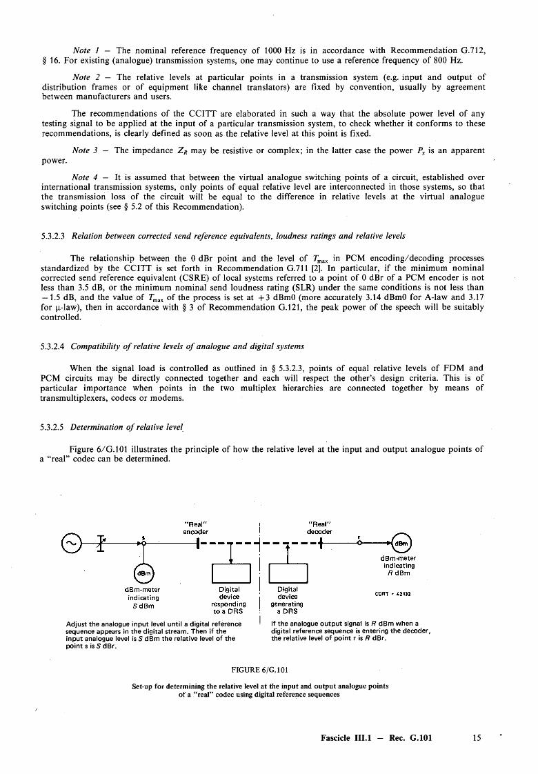
5.3.2.5 Determination o f relative level
Figure 6/G.101 illustrates the principle of how the relative level at the input and output analogue points of a “real” codec can be determined.
Adjust the analogue input level until a digital reference sequence appears in the digital stream. Then if the input analogue level is 5 dBm the relative level of the point s is 5 dBr.
If the analogue output signal is R dBm when a digital reference sequence is entering the decoder, the relative level of point r is R dBr.
FIGURE 6/G. 101
Set-up for determining the relative level at the input and output analogue points of a “ real” codec using digital reference sequences
Fascicle III.l — Rec. G.101 15
When using Figure 6/G.101 to determine the relative levels of a “real” codec with non-resistive impedances at the analogue input and output ports, the following precautions must be observed:
i) the test frequency should be 1000 Hz with a suitable offset;ii) the power at points s and r is expressed as apparent power, i.e.
f (Voltage at point)2 x 10³ 1Apparent power level = 10 logio I ------------------------------------------------------------------------ I dBm
L (Modulus of nominal impedance at 1000 Hz) (1 W) J
iii) point r is terminated with the nominal design impedance of the decoder to avoid significant impedance mismatch errors.
Note — Precautions ii), iii) above are, of course equally applicable to the case of resistive input and output impedances and would generally be observed by conventional test procedures. Standardizing the reference frequency as in i) above is, however, essential for complex impedances because of the variation of nominal impedance with the test frequency.
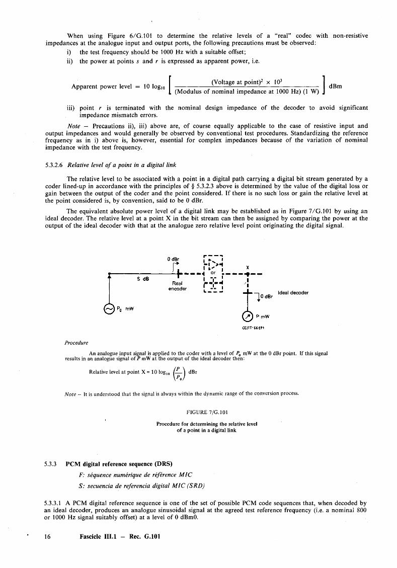
5.3.2.6 Relative level o f a point in a digital link
The relative level to be associated with a point in a digital path carrying a digital bit stream generated by a coder lined-up in accordance with the principles of § 5.3.2.3 above is determined by the value of the digital loss or gain between the output of the coder and the point considered. If there is no such loss or gain the relative level at the point considered is, by convention, said to be 0 dBr.
The equivalent absolute power level of a digital link may be established as in Figure 7/G.101 by using an ideal decoder. The relative level at a point X in the bit stream can then be assigned by comparing the power at the output o f the ideal decoder with that at the analogue zero relative level point originating the digital signal.
0 dBrIdeal decoder
Procedure
An analogue input signal is applied to the coder with a level of P0 mW at the 0 dBr point. If this signal results in an analogue signal of P mW at the output of the ideal decoder then:
Relative level at point X = 10 log10 (— \ dBrw
Note - It is understood that the signal is always within the dynamic range of the conversion process.
FIGURE 7/G.101
Procedure for determining the relative level of a point in a digital link
5.3.3 PCM digital reference sequence (DRS)
F: sequence numerique de reference M IC
S: secuencia de referenda digital M IC (SRD)
5.3.3.1 A PCM digital reference sequence is one of the set of possible PCM code sequences that, when decoded by an ideal decoder, produces an analogue sinusoidal signal at the agreed test reference frequency (i.e. a nominal 800 or 1000 Hz signal suitably offset) at a level of 0 dBmO.
16 Fascicle III.l - Rec. G.101
Conversely an analogue sinusoidal signal at 0 dBmO at the test reference frequency applied to the input of an ideal coder will generate a PCM digital reference sequence.
Some particular PCM digital reference sequences are defined in Recommendation G.711 [2] in respect to A-law and (i-law codecs.
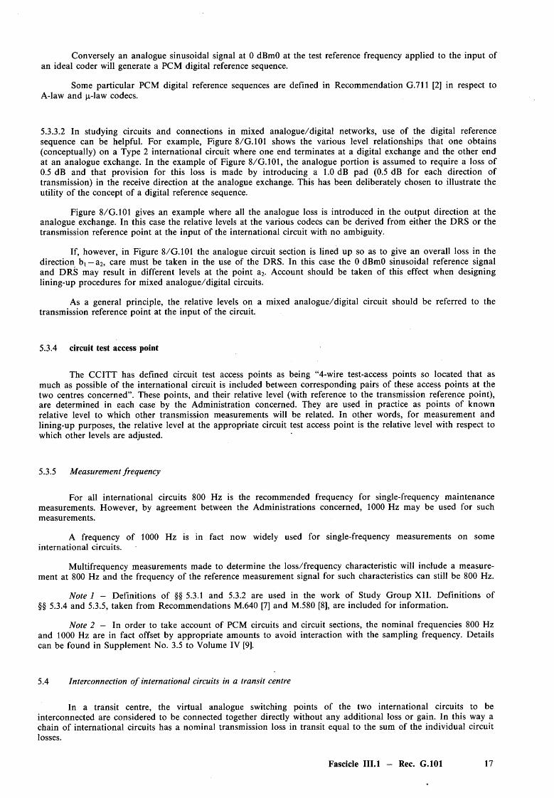
5.3.3.2 In studying circuits and connections in mixed analogue/digital networks, use of the digital reference sequence can be helpful. For example, Figure 8/G.101 shows the various level relationships that one obtains (conceptually) on a Type 2 international circuit where one end terminates at a digital exchange and the other end at an analogue exchange. In the example of Figure 8/G.101, the analogue portion is assumed to require a loss of0.5 dB and that provision for this loss is made by introducing a 1.0 dB pad (0.5 dB for each direction of transmission) in the receive direction at the analogue exchange. This has been deliberately chosen to illustrate the utility o f the concept of a digital reference sequence.
Figure 8/G.101 gives an example where all the analogue loss is introduced in the output direction at the analogue exchange. In this case the relative levels at the various codecs can be derived from either the DRS or the transmission reference point at the input of the international circuit with no ambiguity.
If, however, in Figure 8/G.101 the analogue circuit section is lined up so as to give an overall loss in the direction bi — a2, care must be taken in the use of the DRS. In this case the 0 dBmO sinusoidal reference signal and DRS may result in different levels at the point a2. Account should be taken of this effect when designing lining-up procedures for mixed analogue/digital circuits.
As a general principle, the relative levels on a mixed analogue/digital circuit should be referred to the transmission reference point at the input of the circuit.
5.3.4 circuit test access point
The CCITT has defined circuit test access points as being “4-wire test-access points so located that as much as possible of the international circuit is included between corresponding pairs of these access points at the two centres concerned”. These points, and their relative level (with reference to the transmission reference point), are determined in each case by the Administration concerned. They are used in practice as points of known relative level to which other transmission measurements will be related. In other words, for measurement and lining-up purposes, the relative level at the appropriate circuit test access point is the relative level with respect to which other levels are adjusted.
5.3.5 Measurement frequency
For all international circuits 800 Hz is the recommended frequency for single-frequency maintenance measurements. However, by agreement between the Administrations concerned, 1000 Hz may be used for such measurements.
A frequency of 1000 Hz is in fact now widely used for single-frequency measurements on some international circuits.
Multifrequency measurements made to determine the loss/frequency characteristic will include a measurement at 800 Hz and the frequency of the reference measurement signal for such characteristics can still be 800 Hz.
Note 1 - Definitions of §§ 5.3.1 and 5.3.2 are used in the work of Study Group XII. Definitions of §§ 5.3.4 and 5.3.5, taken from Recommendations M.640 [7] and M.580 [8], are included for information.
Note 2 - In order to take account of PCM circuits and circuit sections, the nominal frequencies 800 Hz and 1000 Hz are in fact offset by appropriate amounts to avoid interaction with the sampling frequency. Details can be found in Supplement No. 3.5 to Volume IV [9].
5.4 Interconnection o f international circuits in a transit centre
In a transit centre, the virtual analogue switching points of the two international circuits to be interconnected are considered to be connected together directly without any additional loss or gain. In this way a chain of international circuits has a nominal transmission loss in transit equal to the sum of the individual circuit losses.
Fascicle III.l — Rec. G.101 17

International digital exchange (send relative
level = —3.5 dBr)
3.5 dBr OdBr
* r
2 I___________j» r♦_
h
3.SdB
♦ ♦
I.L
J J
PCM
DRS
DRS
PCM
-3.5 dBr OdBr
DRS Digital reference sequencePCM PCM channelFDM FDM channel* one of the set of VF relative
levels cited in [1 0 ] for the purpose of illustration
—• — Multiplex VF input/output point
■4
Intermediate repeater station
OdBr *7*d8r -16*dBr
7dB 23 dB
16dB 23 dB
OdBr -16*dBr *7*dBr
FDM0 dBmO sinusoidal
test signal
0 dBmO sinusoidal test signal
23 dB
>
123* dB FDM j
I ^
International analogue exchange (send relative
level = —3.5 dBr)
♦7*dBr -4.5 dBr
11.5 dB
- I -
12,5 dB b.
-16* dBr -3.5dBr
Transmission loss: b2 — a1 = 1.0dBbj — a2 = 0 dB
Note - For meaning of other symbols, see legend for Figure 5/G.101.
FIGURE 8/G.101
Use of a digital reference sequence in the design and line-up of a Type-2 international circuit
References
[1] CCITT Recommendation Transmission Plan, Vol. VI, Rec. Q.40.
[2] CCITT Recommendation Pulse Code Modulation (PCM) o f Voice Frequencies, Vol. I l l , Rec. G.711.
[3] CCITT Recommendation Assumption fo r the Calculation o f Noise on Hypothetical Reference Circuits fo rTelephony, Vol. I l l , Rec. G.223, § 1.
[4] CCITT Recommendation Noise Objectives fo r Design o f Carrier-Transmission Systems, Vol. I l l , Rec. G.222.
[5] CCITT Recommendation Carrier Systems fo r Submarine Cable, Vol. I l l , Rec. G.371.
[6] CCITT Recommendation Assumption fo r the Calculation o f Noise on Hypothetical Reference Circuits fo rTelephony, Vol. I l l , Rec. G.223, § 2.
[7] CCITT Recommendation Four-Wire Switched Connections and Four-Wire Measurements on circuits,Vol. IV, Rec. M.640.
[8] CCITT Recommendation Setting-Up and Lining-Up an International Circuit fo r Public Telephony, Vol. IV,Rec. M.580. '
[9] Test frequencies on circuits routed over PCM systems, Vol. IV, Supplement No. 3.5.
[10] CCITT Recommendation 12-Channel Terminal Equipments, Vol. I ll , Rec. G.232, § 11.
18 Fascicle III.l - Rec. G.101
Recommendation G.102
TRANSM ISSION PERFORMANCE OBJECTIVES AND RECOMMENDATIONS
(Geneva, 1980)
1 General
The CCITT has drawn up (or is in the process of studying) Recommendations concerning transmission impairments and their permissible magnitude with the object of achieving satisfactory performance of the network. Such impairments include for example:
a) corrected reference equivalent (CRE) and loss,
b) noise,
c) attenuation distortion,
d) crosstalk,
e) single tone interference,
f) spurious modulation,
g) effects of errors in digital systems.
Some Recommendations state objectives for an impairment with the implicit assumption that other impairments are at their maximum value (e.g. noise and loss).
In many instances the objectives are based primarily on telephony; this however may require special measures to be applied when other, more demanding services (e.g. sound-programme transmission) are to be incorporated within the network or constituent parts thereof.
The following distinctions may be made between different types of objectives:1) performance objectives for networks,2) performance objectives for circuits, transmission and switching equipment,3) design objectives for transmission and switching equipment,4) commissioning objectives for circuits, transmission and switching equipment,5) maintenance/service limits for circuits, transmission and switching equipment.
2 Explanation of a performance objective
The performance objective for a measurable transmission impairment for networks, entire connections, national systems forming part of international connections, international chains of circuits, individual circuits etc. often describes in statistical terms (mean value, standard deviation, or probability of exceeding stated value, etc.) the value to be aimed at in transmission network and systems planning. It describes the performance which, based for example on subjective or other performance assessment tests, it is desirable to aim at in order to offer the user a satisfactory service.
The items (circuits, systems, equipments) making up the network are normally assumed to have a performance related to that recommended by the performance objectives. Traffic weighting will, in some cases, be applied to calculations.
A powerful set of tools which may be used in analyses concerning network objectives and compliance therewith are the hypothetical reference connections described in Recommendation G.103.
3 Explanation of a design objective
The “design objective” for a measurable transmission impairment (e.g. noise, error-rate, attenuation-distor- tion) for an item of equipment (e.g. a line system, a telephone exchange) is its value when the item is operating in certain electrical/physical environments which might be defined by such parameters as power supply voltage, signal load, temperature, humidity, etc. Some of these parameters may be the subject of CCITT Recommendations and some may not, and it is for the Administrations to assign values to them when they prepare specifications. A suitable allowance may also be made for aging. The most adverse combination of the specified parameters is often assumed.
Fascicle III.l - Rec. G.102 19
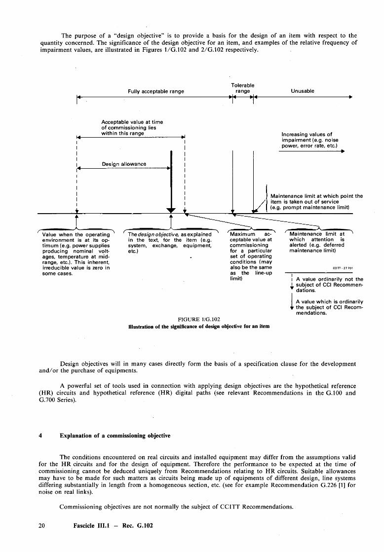
The purpose of a “design objective” is to provide a basis for the design of an item with respect to the quantity concerned. The significance of the design objective for an item, and examples of the relative frequency of impairment values, are illustrated in Figures 1/G. 102 and 2/G.102 respectively.
r -
TolerableFully acceptable range range Unusable
------------------------------------------- ►U---------------------------
Acceptable value at time of commissioning lies within this range Increasing values of
impairment (e.g. noise power, error rate, etc.)
Maintenance limit at which point the item is taken out of service (e.g. prompt maintenance limit)
Value when the operating environment is at its optimum (e.g. power supplies producing nominal voltages, temperature at midrange, etc.). This inherent, irreducible value is zero in som e cases.
The design objective, as explained in the text, for the item (e.g. system, exchange, equipment, etc.)
Maximum acceptable value at commissioning for a particular set of operating conditions (may also be the same as the line-up limit)
Maintenance limit at which attention is alerted (e.g. deferred maintenance limit)
CCITT - 27 701
A value ordinarily not the subject of CCI Recommendations.
FIGURE 1/G. 102 Illustration of the significance of design objective for an item
A value which is ordinarily the subject of CCI Recommendations.
Design objectives will in many cases directly form the basis of a specification clause for the development a n d /o r the purchase of equipments.
A powerful set of tools used in connection with applying design objectives are the hypothetical reference (HR) circuits and hypothetical reference (HR) digital paths (see relevant Recommendations in the G.100 and G.700 Series).
4 Explanation of a commissioning objective
The conditions encountered on real circuits and installed equipment may differ from the assumptions valid for the HR circuits and for the design of equipment. Therefore the performance to be expected at the time of commissioning cannot be deduced uniquely from Recommendations relating to HR circuits. Suitable allowances may have to be made for such matters as circuits being made up of equipments of different design, line systems differing substantially in length from a homogeneous section, etc. (see for example Recommendation G.226 [1] for noise on real links).
Commissioning objectives are not normally the subject of CCITT Recommendations.
20 Fascicle III.l — Rec. G.102
objective
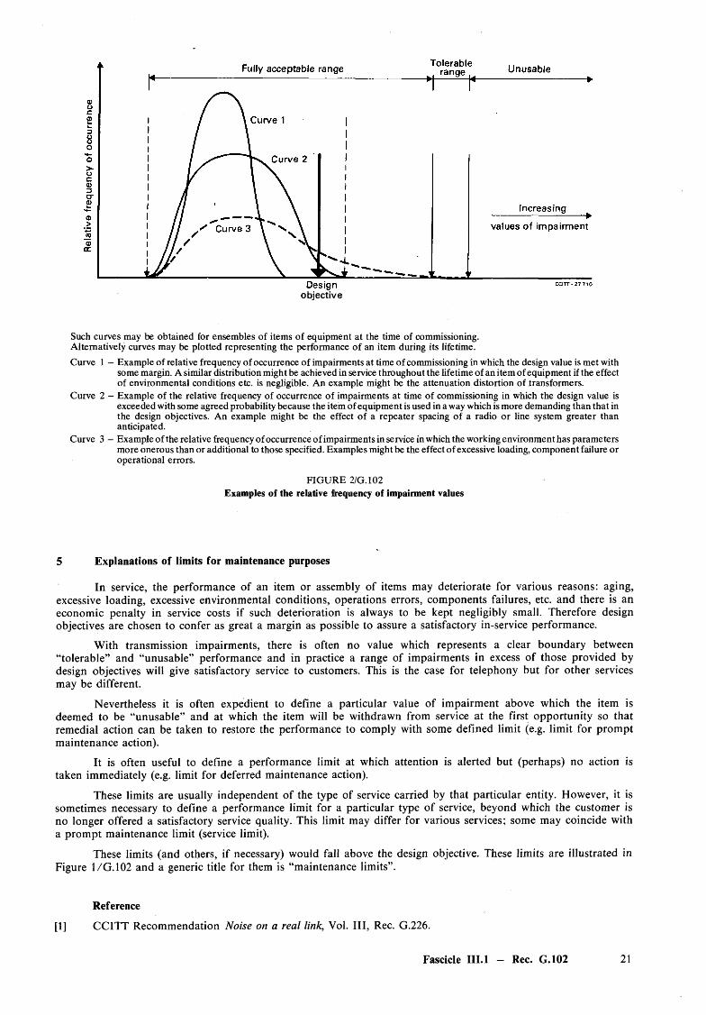
Such curves may be obtained for ensembles of items of equipment at the time of commissioning.Alternatively curves may be plotted representing the performance of an item during its lifetime.Curve 1 - Example of relative frequency of occurrence of impairments at time of commissioning in which the design value is met with
some margin. A similar distribution might be achieved in service throughout the lifetime of an item of equipment if the effect of environmental conditions etc. is negligible. An example might be the attenuation distortion of transformers.
Curve 2 - Example of the relative frequency of occurrence of impairments at time of commissioning in which the design value is exceeded with some agreed probability because the item of equipment is used in a way which is more demanding than that in the design objectives. An example might be the effect of a repeater spacing of a radio or line system greater than anticipated.
Curve 3 - Example of the relative frequency of occurrence of impairments in service in which the working environment has parameters more onerous than or additional to those specified. Examples might be the effect of excessive loading, component failure or operational errors.
FIGURE 2/G.102 Examples of the relative frequency of impairment values
§ Explanations of limits for maintenance purposes
In service, the performance of an item or assembly of items may deteriorate for various reasons: aging,excessive loading, excessive environmental conditions, operations errors, components failures, etc. and there is aneconomic penalty in service costs if such deterioration is always to be kept negligibly small. Therefore design objectives are chosen to confer as great a margin as possible to assure a satisfactory in-service performance.
With transmission impairments, there is often no value which represents a clear boundary between “tolerable” and “unusable” performance and in practice a range of impairments in excess of those provided by design objectives will give satisfactory service to customers. This is the case for telephony but for other services may be different.
Nevertheless it is often expedient to define a particular value of impairment above which the item is deemed to be “unusable” and at which the item will be withdrawn from service at the first opportunity so that remedial action can be taken to restore the performance to comply with some defined limit (e.g. limit for prom pt maintenance action).
It is often useful to define a performance limit at which attention is alerted but (perhaps) no action istaken immediately (e.g. limit for deferred maintenance action).
These limits are usually independent o f the type of service carried by that particular entity. However, it is sometimes necessary to define a performance limit for a particular type of service, beyond which the customer is no longer offered a satisfactory service quality. This limit may differ for various services; some may coincide with a prom pt maintenance limit (service limit).
These limits (and others, if necessary) would fall above the design objective. These limits are illustrated in Figure 1/G . 102 and a generic title for them is “maintenance limits”.
Reference
[1] CCITT Recommendation Noise on a real link, Vol. I ll , Rec. G.226.
Fascicle III.I - Rec. G.102 21
Recommendation G.103
HYPOTHETICAL REFERENCE CONNECTIONS
(Mar del Plata, 1968; amended at Geneva, 1972, 1976 and 1980; at Malaga-Torremolinos, 1984)
This Recommendation mainly deals with the analogue network, Recommendation G.104 deals with the wholly digital network and § 4 of this Recommendation deals with the transitional problems when some digital circuits are introduced into the analogue network. Ultimately, it is envisaged that all reference connections, whether they refer to analogue or digital systems, will be combined within one Recommendation.
1 Purpose
A hypothetical reference connection for transmission impairment studies is a model in which theimpairments contributed by circuits and exchanges are described.
Such a model may be used by an Administration:
— to examine the effect on transmission quality of possible changes of routing structure, noiseallocations and transmission losses in national networks, and
— to test national planning rules for prima facie compliance with any statistical impairment criteria which may be recommended by the CCITT for national systems.
For these purposes, several models are desirable. The three hypothetical reference connections described below should encompass most o f the studies required to be undertaken.
Hypothetical reference connections are not to be regarded as recommending particular values of loss or noise or other impairments, although the various values quoted are in many cases recommended values.Hypothetical reference connections are not intended to be used for the design of transmission systems.
2 Composition of hypothetical reference connections
2.1 The composition of the various connections is defined in Figures 1/G.103, 2/G.103 and 3/G.103.
Figure 1/G .103 — The longest international connection with the maximum number of international and national circuits expected to occur in practice. Such a connection would typically have high corrected reference equivalents and high noise contributions, and the noise contribution from international circuits may be significant. The attenuation distortion, group delay, and group-delay distortion would also all be extremely high. Such connections are rare.Figure 2/G.103 — An international connection of moderate length (say, not longer than 2000 km) comprising the most frequent number of international and national circuits. In such a connection, the noise contribution of the national systems would be expected to predominate. Such a connection is used in a large proportion of international calls.
Figure 3/G.103 — An international connection comprising the practically maximum number of international circuits and the least number of national circuits. Such connections are numerous.
2.2 The following General Remarks apply to Figures 1 /G .103, 2/G.103 and 3/G.103
2.2.1 The hypothetical reference connections show the international circuits connected together at 0 dBr and — 0.5 dBr virtual switching points instead of —3.5 dBr and —4 dBr points. This was felt to be more directly useful to those who might have to use the reference connections in their studies.
It might be felt that it is somewhat inconsistent that the hypothetical reference connections do not use “conventional” —3.5/ —4 dBr virtual switching points. However, if the reference connections are drawn using that convention, the noise power figures appearing on the diagram can no longer be the familiar ones that appear elsewhere in other Recommendations. Annex A gives further explanations.
22 Fascicle III. 1 — Rec. G.103
2.2.2 The nomenclature is based on the international routing plan recommended in Recommendation E.171,i.e. ISC = International Switching Centre (formerly referred to as CT3), ITC = International Transit Centre.
2.2.3 In each case only one direction of transmission is shown.
2.2.4 The design objectives for the mean noise powers are indicated according to current recommendations. For long-distance carrier circuits they are proportional to length, the appropriate noise power rate, 4 pW /km or 1 pW /km , being used according to whether the basic hypothetical reference circuit is one 2500 km long or 7500 km long.
2.2.5 The abbreviation pWOp stands for picowatts psophometric referred to a point of zero relative level. In the case of exchange noise, the point referred to is considered to be in the circuit immediately downstream, of the exchange. The noise powers for circuits are referred to points of zero relative level in the circuits themselves and not to some point on the connection.
2.2.6 The pad symbols represent the nominal loss of the particular channel or circuit, and the relative position of the noise generator, and the pad indicates that if the noise is to be referred to the receiving end of a circuit it must be modified by the power ratio corresponding to the loss of the pad.
If it is required to refer the noise powers to some particular point on the connection (for example, the receiving local exchange or the point of zero relative level on the first international circuit) then the rule to be applied is as follows:
If a noise power level at a point A is to be referred to a point B downstream of its position, it is obtained by augmenting the level at point B by the sum of the losses that is imagined to be traversed from A to B. If it is to be referred to a point C upstream of its position, it is obtained by diminishing the level at point C by the sum of all the losses that is imagined to be traversed from A to C.
2.2.7 The nominal terminal loss of the connection [i.e. the normal overall loss less the sum of the transit losses (via net losses) o f the individual circuits] is shown as one pad associated with the extreme right-hand circuit in the 4-wire chain. This artifice enables the noise powers to be indicated as if they were injected at zero relative level points on the individual circuits as explained in Annex A.
2.2.8 Inform ation concerning the distributions of attenuation distortion and group-delay distortion is to befound in Annex A of Recommendation G. 113. Calculated values of some possible combinations of basic transmission impairments are given in Supplement No. 20.
Recommendation G.114 gives information concerning group delay.
2.2.9 The standard deviation of transmission loss of circuits is in accord with the objectives of Recommendation G.151 § 3 and also with the results obtained in practice and specified in [1].
2.2.10 “Circuit” in these reference connections is defined in the sense of Recommendation M.700 [2] as the whole of the line and the equipment proper to the line; it extends from the switches of one exchange to the switches of the next. In this way switching and exchange cabling losses are included in the values of transmission loss assigned to the circuits, together with the loss (or gain) introduced by the transmission system. If it is required to separately distinguish exchange losses, an additional pad symbol of appropriate value may be used.
It should also be noted that, according to this convention, the 3.5-dB loss ordinarily assigned to a terminating set does not figure explicitly in 2-wire/4-wire circuits; its value is also included in the loss assigned to the circuit.
3 Number of modulation and demodulation equipments
For the study of transmission performance, the longest international connection expected to occur (see Figure 1/G . 103) may be considered to have the following arrangement of m odulator/dem odulator pairs in the 4-wire chain.
Fascicle III.l - Rec. G.103 23
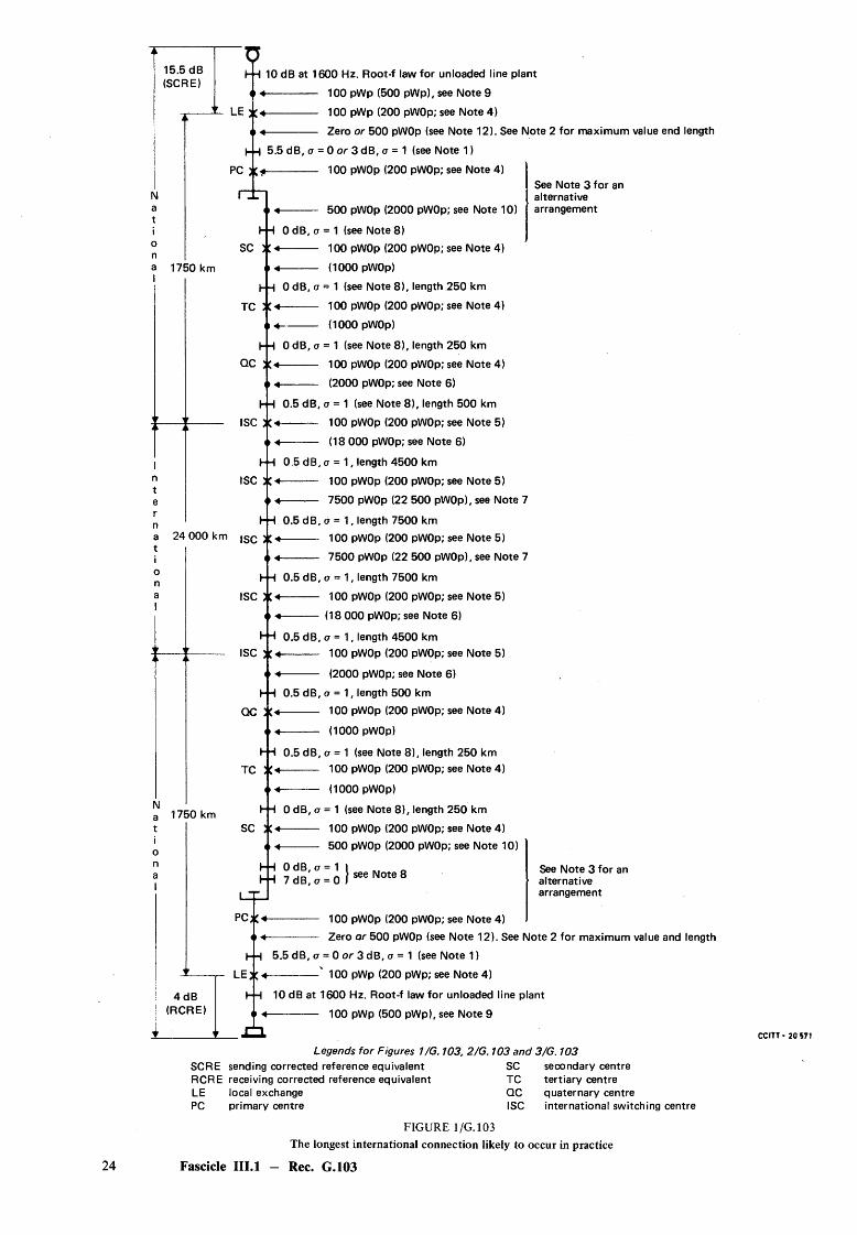
15.5 dB(SCRE)
hH 10 dB at 1600 Hz. Root-f law for unloaded line plant< > 4------------- 100 pWp (500 pWp), see Note 9
LE ) 100 pWp (200 pWOp; see Note 4)i \ 4------------- Zero or 500 pWOp (see Note 12). See Note 2 for maximum value end length
h q 5.5 dB, o = 0 or 3 dB, o = 1 (see Note 1)PC )(■*»------------- 100 pWOp (200 pWOp; see Note 4)
1750 km
H4 OdB, ct = 1 (see Note 8 )SC # 4---------- 100 pWOp (200 pWOp; see Note 4)
4---------- (1000 pWOp)h|h 0 dB, (7 = 1 (see Note 8 ), length 250 km
TC /£•«---------- 100 pWOp (200 pWOp; see Note 4)4----------(1000 pWOp)
l-H 0 dB, a = 1 (see Note 8 ), length 250 kmQC ---------- 100 pWOp (200 pWOp; see Note 4)
4---------- (2000 pWOp; see Note 6 )
|-|h 0.5 dB, o = 1 (see Note 8 ), length 500 kmISC ---------- 100 pWOp (200 pWOp; see Note 5)
4---------- (18 000 pWOp; see Note 6 )
FH 0.5 dB, o = 1, length 4500 kmISC 3 C 4--------- 100 pWOp (200 pWOp; see Note 5)
4--------- 7500 pWOp (22 500 pWOp), see Note 7
h H 0.5 dB, a = 1, length 7500 km24 000 km jgQ j j
1750 km
PCX*
4 dB (RCRE)
500 pWOp (2000 pWOp; see Note 10)
See Note 3 for analternativearrangement
100 pWOp (200 pWOp; see Note 5) 7500 pWOp (22 500 pWOp), see Note 7
l-|H 0.5 dB, <7 = 1, length 7500 kmISC % 4------- 100 pWOp (200 pWOp; see Note 5)
4--------- (18 000 pWOp; see Note 6 )
H H 0.5 dB, a = 1, length 4500 km ISC -------- 100 pWOp (200 pWOp; see Note 5)
(2000 pWOp; see Note 6 )h|H 0.5 dB, a = 1, length 500 km
QC -------- 100 pWOp (200 pWOp; see Note 4)
•«---------- (1000 pWOp)
F H 0.5 dB, a = 1 (see Note 8 ), length 250 kmTC ) C*-------- 100 pWOp (200 pWOp; see Note 4)
4---------------- (1000 pWOp)
H 0 dB, a = 1 (see Note 8 ), length 250 kmSC -------- 100 pWOp (200 pWOp; see Note 4)
4 4-------- 500 pWOp (2000 pWOp; see Note 10)
FH OdB, ct = 1 FH 7 dB, (7 = 0 see Note 8 See Note 3 for an
alternativearrangement
100 pWOp (200 pWOp; see Note 4)Zero or 500 pWOp (see Note 12). See Note 2 for maximum value and length
FH 5.5 dB, o = 0 or 3 dB, o = 1 (see Note 1)LE) j 4------------- 100 pWp (200 pWp; see Note 4)
10 dB at 1600 Hz. Root-f law for unloaded line plant ------------ 100 pWp (500 pWp), see Note 9
CCITT-
24
Legends for Figures 1/G. 103, 2/G. 103 and 3/G.103 SCRE sending corrected reference equivalent SC secondary centreRCRE receiving corrected reference equivalent TC tertiary centreLE local exchange QC quaternary centrePC primary centre ISC international switching centre
FIGURE 1/G. 103 The longest international connection likely to occur in practice
Fascicle III.l — Rec. G.103
20 S71
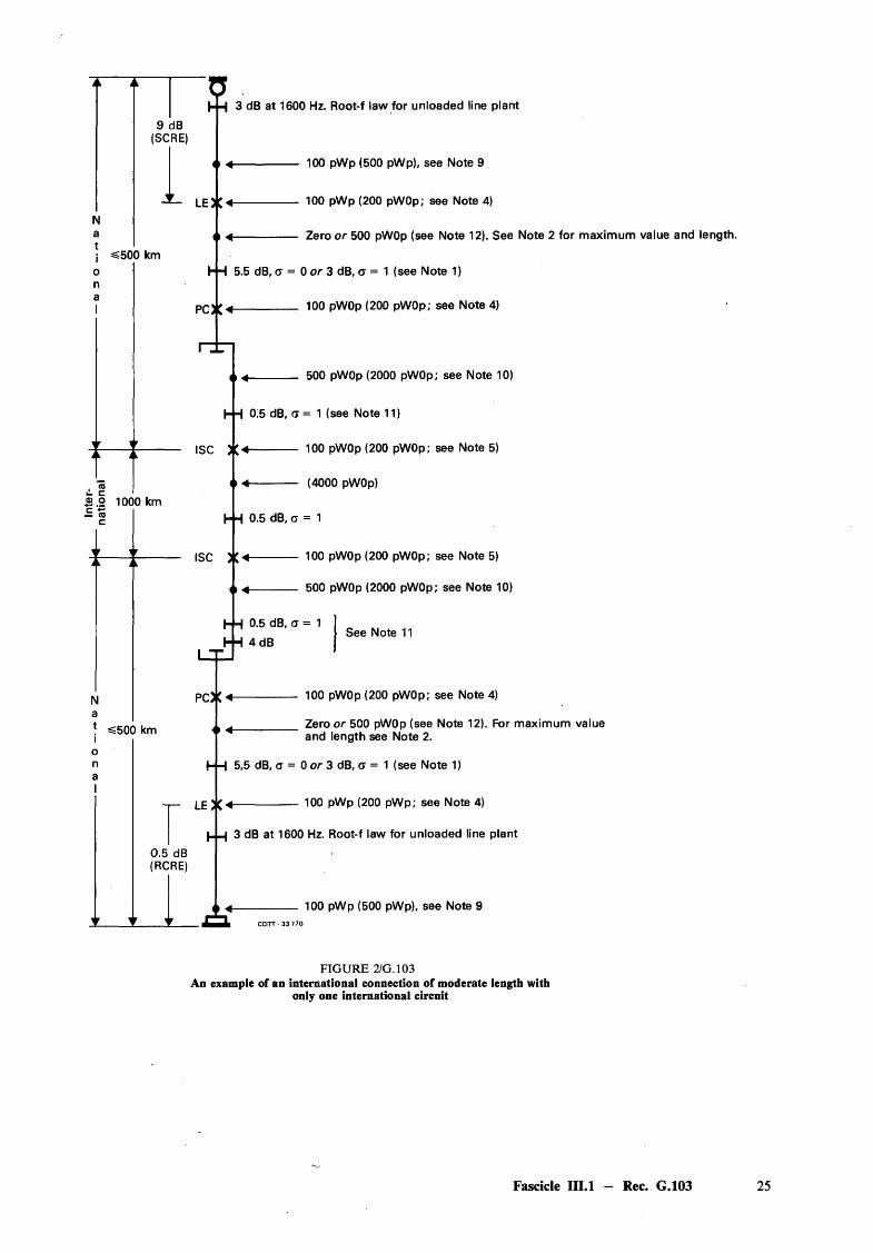
j =5500 km
. *°5 . 1 1 0 0 0 kmC +-
=500 km
H 3 dB at 1600 Hz. Root-f law for unloaded line plant
9 dB(SCRE)
<> 4 -
LEX*
n 4 -
100 pWp (500 pWp), see Note 9
100 pWp (200 pWOp; see Note 4)
Zero or 500 pWOp (see Note 12). See Note 2 for maximum value and length.
h|H 5.5 dB, cr = 0 or 3 dB, a = 1 (see Note 1)
P C * ^__________ 100 pWOp (200 pWOp; see Note 4)
0 4 -
hH 0.5 dB, a = 1 (see Note 11)
ISC ------------ 100 pWOp (200 pWOp; see Note 5)
4 4------------ (4000 pWOp)
ISC X *
PCX *
O 4 -
h H 5,5 dB, a = 0 or 3 dB, a = 1 (see Note 1)
t - l e x *
0.5 dB (RCRE)
500 pWOp (2000 pWOp; see Note 10)
h H 0.5 dB, a = 1
0 4 -
100 pWOp (200 pWOp; see Note 5)
500 pWOp (2000 pWOp; see Note 10)
0.5 dB, a = 1 4 dB
See Note 11
100 pWOp (200 pWOp; see Note 4)
Zero or 500 pWOp (see Note 12). For maximum value and length see Note 2.
100 pWp (200 pWp; see Note 4)
3 dB at 1600 Hz. Root-f law for unloaded line plant
< > 4 ---------------- 100 pWp (500 pWp), see Note 9CCITT - 3 3 7 70
FIGURE 2/G.103 An example of an international connection of moderate length with
only one international circuit
Fascicle I1I.1 — Rec. G.103
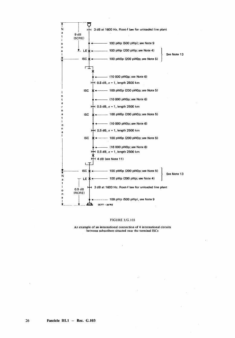
9 dB(SCRE)
LE)C
ISC ;c
r x
3 dB at 1600 Hz. Root-f law for unloaded line plant
100 pWp (500 pWp); see Note 9
100 pWp (200 pWp; see Note 4)
100 pWOp (200 pWOp; see Note 5)
ISC :c
ISC 3C
LE X
0.5 dB (RCRE)
(10 000 pWOp; see Note 6)
Fp 0.5 dB, a = 1, length 2500 km
ISC 4----------- 100 pWOp (200 pWOp; see Note 5)
(10 000 pWOp; see Note 6)
F}H 0.5 dB, o = 1, length 2500 km
ISC ------------- 100 pWOp (200 pWOp; see Note 5)
(10 000 pWOp; see Note 6)
FfH 0.5 dB, o = 1, length 2500 km
100 pWOp (200 pWOp; see Note 5)
(10 000 pWOp; see Note 6)FfH 0.5 dB, a = 1, length 2500 km
4dB (see Note 11)
100 pWOp (200 pWOp; see Note 5)
100 pWp (200 pWp; see Note 4)
See Note 13
See Note 13
FH 3 dB at 1600 Hz. Root-f law for unloaded line plant
100 pWp (500 pWp), see Note 9c c i t t - t » m
FIGURE 3/G.103
An example of an international connection of 4 international circuits between subscribers situated near the terminal ISCs
Fascicle III.l — Rec. G.103
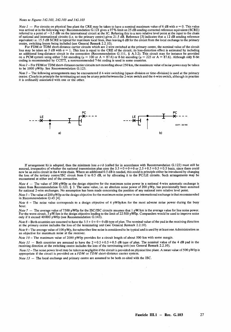
Notes to Figures 1IG.103, 2IG.103 and 3IG.103
Note 1 — For circuits on physical line plant the CRE may be taken to have a nominal maximum value of 6 dB with a = 0. This value was arrived at in the following way: Recommendation G.121 gives a 97% limit on 25 dB sending corrected reference equivalent (SCRE) referred to a point of —3.5 dBr on the international circuit at the IC. Referring this to a zero relative level point at the input to the chain of national and international circuits (i.e. to the primary centre) gives 21.5 dB. Reference [3] indicates that a 12 dB sending reference equivalent i.e. 15.5 dB SCRE is typical for maximum local lines, thus leaving 6 dB for the circuit from the local exchange to the primary centre, switching losses being included (see General Remark 2.2.10).
For FDM or TDM short-distance carrier circuits which are 2-wire switched at the primary centre, the nominal value of the circuit loss may be taken as 3 dB with a = 1. This loss is equal to the CRE of the circuit; its loss-distortion effect is estimated by including an additional long-distance circuit in the connection (Recommendation G . l l l , § A.3.2). This circuit may for instance be provided on a PCM system using either 7-bit encoding (p = 100 or A = 87.6) or 8-bit encoding (p = 225 or A = 87.6). Although only 8-bit coding is recommended by CCITT, a nonrecommended 7-bit coding is used in some countries.Note 2 - For FDM or TDM short-distance carrier circuits not exceeding about 250 km, the maximum value of noise power may be taken to be 1000 pWOp. See Recommendation G.123.Note 3 - The following arrangements may be encountered if 4-wire switching (space-division or time-division) is used at the primary centre. Clearly in principle the terminating set may be at any point between the 2-wire switch and the 4-wire switch, although in practice it is ordinarily associated with one or the other.
LE-X — •-
PCr LE— - X - H
PC- X - - - - - - -
CCITT - 3 3 7 9 0
b)
If arrangement b) is adopted, then the minimum loss a-t-b (called for in accordance with Recommendation G. 122) must still be assured, irrespective of whether the national transmission plan uses the 3.5 + 0 + 0 + 0 or 2.5 +0.5 +0.5 + 0 .5 basis, since there could now be an extra circuit in the 4-wire chain. Where an additional 0.5 dB is needed, this could in principle either be introduced by changing the loss of the tertiary centre/ISC circuit from 0 to 0.5 dB, or by allocating it to the PC/LE circuits. Such arrangements may be encountered at either end of the connection.Note 4 — The value of 200 pWOp as the design objective for the maximum noise power in a national 4-wire automatic exchange is taken from Recommendation G.123, § 3. The same value, i.e. an absolute noise power of 200 pWp, has provisionally been assumed for national 2-wire exchanges. No assumption has been made concerning the position of any national zero relative level point.Note 5 — The value of 200 pWOp as the design objective for the maximum noise power in an international exchange is that recommended in Recommendation Q.45 [4].Note 6 - The noise value corresponds to a design objective of 4 pWOp/km for the most adverse noise power during the busy hour.Note 7 — The average value of 7500 pWOp for the ISC/ISC circuits assumes that 1 pW/km is the average value for line noise power. For the worst circuit, 3 pW/km is the design objective leading to the limit of 22 500 pWOp. Companders would be used to improve noise only if it exceed 40000 pWOp (see Recommendation G.143).Note 8 — Both countries are assumed to have the 3 .5+ 0+ 0+ 0 dB type of plan. The nominal value of the pad in the receiving direction at the primary centre includes the loss of the terminating unit (see General Remark 2.2.10).Note 9 - The average value of 100 pWp, for subscriber line noise is considered to be typical and is used by at least one Administration as an objective for maximum noise at the receiver.Note 10 - The maximum value of 2000 pWOp provides for a circuit length of about 500 km with some margin.Note 11 — Both countries are assumed to have the 2 + 0.5 +0.5 +0.5 dB type of plan. The nominal value of the 4 dB pad in thereceiving direction at the switching centre includes the loss of the terminating unit (see General Remark 2.2.10).Note 1 2 - The noise power level may be taken as negligible if the circuit is provided on physical line plant. A mean value of 500 pWOp is appropriate if the circuit is provided on a FDM or TDM short-distance carrier system.Note 13 — The local exchange and primary centre are assumed to be both co-sited with the ISC.
Fascicle III.l — Rec. G.103 27
TABLE 1/G. 103
Number of m odulator/dem odulator pairs in a wholly analogue 4-wire chain
Eight national circuits
Circuits between ISCs Total
Channel 8 4 12
Group 12 10 22
Supergroup 16 20 36
O f the 12 channel m odulator/dem odulator pairs a maximum of three may be of the special type which provide more than 12 telephone circuits per group.
4 Developments arising from the introduction of PCM digital processes
The worldwide telephone network is undergoing a transition from what is largely an analogue network to a mixed analogue/digital network. Looking farther into the future, this transition is expected to continue and result in a network that would be predominantly digital. Background on this transitional process is given in Recommendations G.101, § 4.1 and G.104.
With reference to the hypothetical reference connections of Figures 1/G.103, 2/G.103 and 3/G.103, the configurations used concerning numbers of circuits and numbers of exchanges should also be appropriate for network conditions in the mixed analogue/digital period. However, for transmission studies pertaining to mixed analogue/digital connections, account must also be taken of all unintegrated digital processes that might be present. Such unintegrated digital processes could have an important effect on overall transmission performance particularly with regard to such parameters as quantizing distortion (Recommendation G.113), and transmission delay. Guidance is provided on the use of appropriate hypothetical reference connections for a mixed analogue/ digital network in Annex B.
Where the worldwide network becomes all-digital, many of the transmission impairments that were present in the mixed analogue/digital period, due to the incorporation of unintegrated digital processes, would be eliminated. However, certain processes might remain which could introduce transmission penalties. These are the processes which operate on the basis of recoding the bit stream as is done, for example, in the case of digital pads. Although the accumulated transmission impairments introduced by such processes may be well within recommended limits, the resulting loss of bit integrity could be an important disadvantage. This is particularly true in the case of services requiring the preservation of bit integrity on an end-to-end basis. Consequently, processes of this type should be avoided where possible, or appropriate arrangements made to circumvent them, where services requiring bit integrity are to be carried over the affected connections.
ANNEX A
(to Recommendation G.103)
An explanation of how hypothetical reference connections can be drawn assuming all send switching levels are 0 dBr
A.l Consider the connection shown in Figure A-1/G. 103 in which 3 circuits with losses of 1 dB, 6 dB and 2 dB are connected together by exchanges with actual send switching levels of — 2, +1 and — 3 dBr.
28 Fascicle III.l — Rec. G.103
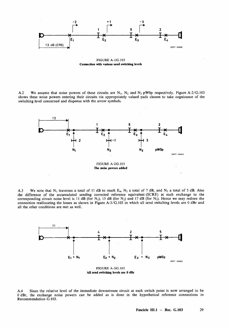
I >
- 2
r-3r i r
13 dB (CRE)CCITT - 3 3 8 0 0
FIGURE A-1/G. 103 Connection with various send switching levels
A.2 We assume that noise powers of these circuits are N j, N2 and N 3 pWOp respectively. Figure A-2/G.103 shows these noise powers entering their circuits via appropriately valued pads chosen to take cognizance of the switching level concerned and dispense with the arrow symbols.
13
f-H 2
3 r *h H- 1
N3 pWOpCCITT* 3 3 8 1 0
FIGURE A-2/G.103 The noise powers added
A.3 We note that N t traverses a total of 11 dB to reach E4, N2 a total of 7 dB, and N 3 a total o f 5 dB. Also the difference of the accumulated sending corrected reference equivalent (SCRE) at each exchange to the corresponding circuit noise level is 11 dB (for Nj), 15 dB (for N 2) and 17 dB (for N 3). Hence we may redraw the connection reallocating the losses as shown in Figure A-3/G.103 in which all send switching levels are 0 dBr and all the other conditions are met as well.
11
- x - » -
i 2
-F -*— d
E i ♦ N, E2 ♦ n 2 E 3 ♦ N 3 pWOpCCITT - 3 3 8 2 0
FIGURE A-3/G.103 Ail send switching levels are 0 dBr
A.4 Since the relative level of the immediate downstream circuit at each switch point is now arranged to be0 dBr, the exchange noise powers can be added as is done in the hypothetical reference connections in Recommendation G.103.
Fascicle III.l — Rec. G.103 29

ANNEX B
(to Recommendation G.103)
Guidance on hypothetical reference connections for a mixed analogue/digital connection
This annex provides guidance on a method to model a mixed analogue/digital network. For simplicity and for ease of comparison with an all-analogue network, retention of the network configurations now given in Figures 1/G.103 to 3/G.103 is appropriate. Figures 1/G.103 and 2/G.103, in particular, represent respectively, examples of the longest, though infrequent, type of connection and a connection of moderate length which occurs most frequently. The three connections provide an adequate range of connection types for most purposes but some guidance is desirable with respect to the selection of the circuits and exchanges which should be analogue and those which should be digital. This choice may depend on the matter under study. Two examples are designated for each of the connections: one which maximizes the number of digital processes and one which would be more representative of an evolving network. The worst case situation can be represented by making all of the exchanges digital and leaving all of the circuits analogue. A set of more representative connections is obtained by defining islands of digital connectivity such that the number of independent digital processes in each connection is approximately one-half of the maximum. For the representative connections all exchanges are assumed to be digital. In addition, the specific circuits designated in Table B-1/G.103 are also assumed to be digital with digital connection to the digital switches at each end of the circuit. This has the effect of creating “digital islands” with integrated digital processes, such that each island may be regarded as a single digital process.
TABLE B-1/G. 103
Assumed digital circuits (listed from top to bottom)
Figure 1/G . 103 Figure 2/G.103 Figure 3/G.103
PC to SC PC to ISC LE to ISC
TC to QC ISC to PC
1st ISC to 2nd ISC 2nd ISC to 4th ISC a)
4th ISC to 5th ISC
QC to TC
SC to PC
ISC to LE
a) Single digital island.
Note — For an explanation of abbreviations, see Figure 1/G. 103.
References
[1] CCITT Green Book, Vol. IV.2, Section 4, Supplements, ITU, Geneva, 1973.
[2] CCITT Recommendation Definitions fo r the maintenance organization, Vol. IV, Rec. M.700.
[3] CCITT manual Transmission planning o f switched telephone networks, ITU, Geneva, 1976.
[4] CCITT Recommendation Transmission characteristics o f an international exchange, Vol. VI, Rec. Q.45.
30 Fascicle III.l — Rec. G.103
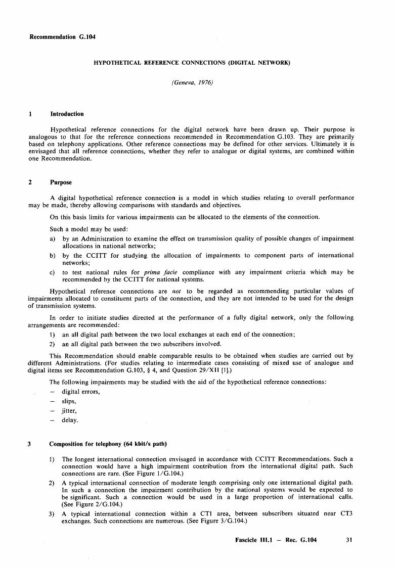
Recommendation G.104
HYPOTHETICAL REFERENCE CONNECTIONS (DIGITAL NETWORK)
(Geneva, 1976)
1 Introduction
Hypothetical reference connections for the digital network have been drawn up. Their purpose is analogous to that for the reference connections recommended in Recommendation G.103. They are primarily based on telephony applications. Other reference connections may be defined for other services. Ultimately it is envisaged that all reference connections, whether they refer to analogue or digital systems, are combined within one Recommendation.
2 Purpose
A digital hypothetical reference connection is a model in which studies relating to overall performance may be made, thereby allowing comparisons with standards and objectives.
On this basis limits for various impairments can be allocated to the elements of the connection.
Such a model may be used:a) by an Administration to examine the effect on transmission quality of possible changes of impairment
allocations in national networks;b) by the CCITT for studying the allocation of impairments to component parts o f international
networks;c) to test national rules for prima facie compliance with any impairment criteria which may be
recommended by the CCITT for national systems.
Hypothetical reference connections are not to be regarded as recommending particular values of impairments allocated to constituent parts of the connection, and they are not intended to be used for the design of transmission systems.
In order to initiate studies directed at the performance of a fully digital network, only the following arrangements are recommended:
1) an all digital path between the two local exchanges at each end of the connection;2) an all digital path between the two subscribers involved.
This Recommendation should enable comparable results to be obtained when studies are carried out by different Administrations. (For studies relating to intermediate cases consisting of mixed use of analogue and digital items see Recommendation G.103, § 4, and Question 29/X II [1].)
The following impairments may be studied with the aid of the hypothetical reference connections:— digital errors,— slips,— jitter,— delay.
3 Composition for telephony (64 kbit/s path)
1) The longest international connection envisaged in accordance with CCITT Recommendations. Such aconnection would have a high impairment contribution from the international digital path. Such connections are rare. (See Figure 1/G . 104.)
2) A typical international connection of moderate length comprising only one international digital path. In such a connection the impairment contribution by the national systems would be expected to be significant. Such a connection would be used in a large proportion of international calls.(See Figure 2/G.104.)
3) A typical international connection within a CT1 area, between subscribers situated near CT3exchanges. Such connections are numerous. (See Figure 3/G.104.)
Fascicle III.l — Rec. G.104 31
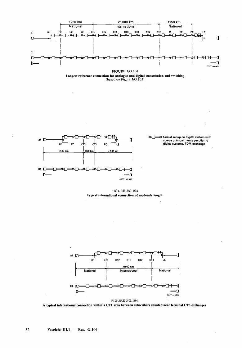
1250 kmTCT3
25 000 km International
CT1 CTX CT1
1250 km
CT2 CT3
FIGURE 1/G. 104Longest reference connection for analogue and digital transmission and switching
(based on Figure 1/G. 103)
LE PC CT3 CT3 PC LE
< 500 km ! 1000 km < 500 km
I
CCITT - 4 0 4 4 0
B)=0 B Circuit set up on digital system with source of impairments peculiar to digital systems. TDM-exchange.
FIGURE 2/G.104 Typical international connection of moderate length
a) DCT3 CT2 CT1 CT2 CT3
1 10000 km J .
National | International | National
CCITT- 4 3 8 6 0
FIGURE 3/G.104A typical international connection within a CT1 area between subscribers situated near terminal CT3 exchanges
Fascicle III.l — Rec. G.104
Note 1 — The reference connections defined apply to telephony only. The necessity for defining similar reference connections for other services such as data, sound- and television-programme transmission, etc., will have to be studied.
Note 2 — The effect o f digital concentrators, digital echo suppressors, satellite paths in the national network, etc. and the possible necessity of including these items in the reference connections is under study.
4 Remarks
It is common practice to estimate the performance of a reference connection from the knowledge of the individual design objectives of the component parts. It is recognized however that it is unlikely that every item is experiencing the most adverse combination of specified conditions, and also the working conditions of some items may be worse than those specified. Therefore the actual performance of a connection will only rarely be identical with the performance estimated by the calculations.
Reference
[1] CCITT Question 29/X II, Contribution COM XII-No. 1, Study Period 1985-1988, Geneva, 1985.
Recommendation G.10S
HYPOTHETICAL REFERENCE CONNECTION FOR CROSSTALK STUDIES
(Geneva, 1980)
1 Purpose
This Recommendation gives guidance concerning the application of Recommendation P. 16 [1] in the general switched telephone network and recommends the structure and parameters of a hypothetical reference connection specifically designed for crosstalk studies.
2 General remarks
2.1 Accuracy o f fundam ental data
2.1.1 There is always some degree of uncertainty in applying to real telephone conversation the results o f tests in which subjects were asked to listen attentively to see if they were able to detect the presence of intelligible crosstalk. Furthermore, this type of test cannot be expected to indicate reliably the extent to which a subscriber’s confidence in the privacy of his own conversation is undermined by overhearing another conversation. Hence in general the aim should be to reduce the risk of potentially intelligible crosstalk as much as possible.
2.1.2 In applying the calculation method given in Recommendation P. 16 [1], errors can occur if the distributions of crosstalk attenuations and corrected reference equivalents are skew, rather than normal, or are truncated by test acceptance procedures. This arises because we are generally seeking low probabilities of encountering intelligible crosstalk which are highly dependent on the tails of distributions being accurately defined. One way of avoiding this difficulty is to apply M onte-Carlo methods as described, for example, in the CCITT manual cited in [2], taking care to make enough iterations to secure the necessary accuracy.
Fascicle III.l - Rec. G.105 33
2.1.3 Considerable care must be taken to obtain representative values of the loss and noise in crosstalk paths being studied. In particular, errors arising from small changes in mean values can easily result in the calculated probability of overhearing being in error by a factor of 10 or more (see, for example, [3]).
2.2 Effect o f line and room noise
2.2.1 The masking effect of line noise is another aspect which is im portant and raises some difficulties. On the one hand if, for the purpose of establishing crosstalk limits, the level of line noise is assumed to be negligible, unrealistic demands may be placed on the crosstalk attenuation required to be introduced by items of plant. On the other hand, if it is assumed that circuits and exchanges in service introduce noise power levels comparable with their design objectives, e.g. the well known 4 pWOp/km, the incidence of overhearing may be unacceptably high, particularly when the network is lightly loaded so that noise power levels can be expected to be at their lowest.
As in many transmission studies, a compromise has to be made somewhere between these extremes. In some cases, it may be necessary to rely on measurements of noise power levels on established plant during light and busy traffic periods. However, it must not be overlooked that limits devised now must, if possible, take the future into account. It is a wise principle that the successful performance of equipment in one part o f the network should not be dependent upon adventitious imperfections of other parts of the network, particularly if such imperfections are likely to be eliminated or reduced in the future, e.g. by new designs of local exchange or by the extensive use of digital long-distance transmission systems.
2.2.2 Unlike line noise the effect o f room noise can be reduced by a determined listener. Hence Recommendation P. 16 [1] recommends that negligible room noise be assumed when deriving a design objective for equipment.
2.3 Probabilities and distributions involved
2.3.1 When constructing the distribution of crosstalk attenuation introduced by equipment and cables, it is appropriate to consider only the worst (acceptable) values. For example, in a 10-pair cable only the worst disturber for each pair should be taken into account, i.e. 10 values. This distribution should not be diluted by the other 80 better values. In the busy period the worst potential disturber of a particular pair can be relied upon to be activated.
2.3.2 In respect of intelligible crosstalk between local calls established in the same local exchange network, the probability of a potentially disturbing subscriber making a call at the same time as the disturbed subscriber can be significantly low certainly in the case of residential subscribers, although this is probably not the case for business subscribers and PBXs. Information concerning this topic and showing how to calculate the probabilities concerned will be found in [4].
2.3.3 Multiple entries into a telephone connection of intelligible crosstalk signals all at significant levels and all derived from one source is so unlikely an event that it may be ignored for the purposes of deriving design limits. Hence the crosstalk mechanism of interest is assumed to be the dominant one when deriving limits, and all other sources are deemed to be negligible, and may thus attract the whole of the allowance.
However, when a network performance objective for crosstalk has to be divided among the exchanges and circuits making up the connection, it may be necessary to give some consideration to the number of potential crosstalk paths from different sources. For example, crosstalk limits may be assigned to complete paths through an exchange and to complete junction or trunk circuits. Thus, on simple other-exchange connections (ignoring, for the moment, crosstalk arising within local cables) there are three dominant sources of crosstalk, and if, for example, the aim were to be not greater than 1 in 100 for such connections, the probability of overhearing from each source should be reduced to 1 in 300 (assuming equal probabilities and no correlation between the sources).
Figures 1/G. 105 and 2/G.105 illustrate some crosstalk paths of significance.
34 Fascicle III.l — Rec. G.105
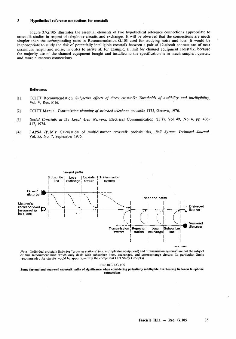
3 Hypothetical reference connections for crosstalk
Figure 3/G.105 illustrates the essential elements of two hypothetical reference connections appropriate to crosstalk studies in respect of telephone circuits and exchanges. It will be observed that the connections are much simpler than the corresponding ones in Recommendation G.103 used for studying noise and loss. It would be inappropriate to study the risk of potentially intelligible crosstalk between a pair of 12-circuit connections of near maximum length and noise, in order to arrive at, for example, a limit for channel equipment crosstalk, because the majority use of the channel equipment bought and installed to the specification is in much simpler, quieter, and more numerous connections.
References
[1] CCITT Recommendation Subjective effects o f direct crosstalk; Thresholds o f audibility and intelligibility,Vol. V, Rec. P. 16.
[2] CCITT M anual Transmission planning o f switched telephone networks, ITU, Geneva, 1976.
[3] Social Crosstalk in the Local Area Network, Electrical Communication (ITT), Vol. 49, No. 4, pp. 406-417, 1974.
[4] LAPS A (P. M.): Calculation of multidisturber crosstalk probabilities, Bell System Technical Journal,Vol. 55, No. 7, September 1976.
Far-end paths
Note - Individual crosstalk limits for “repeater stations” (e.g. multiplexing equipment) and “transmission systems” are not the subject of this Recommendation which only deals with subscriber lines, exchanges, and interexchange circuits. In particular, limits recommended for circuits would be apportioned by the competent CCI Study Group(s).
FIGURE 1/G. 105Some far-end and near-end crosstalk paths of significance when considering potentially intelligible overhearing between telephone
connections
Fascicle III.l - Rec. G.105 35
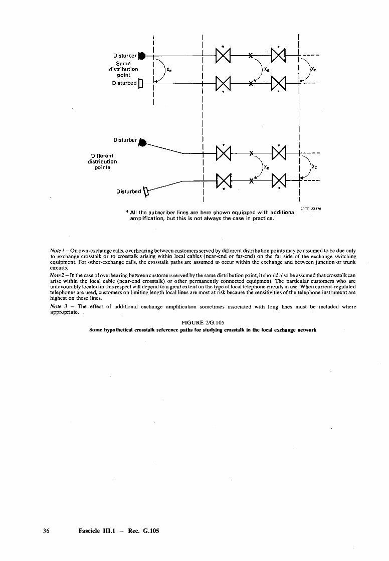
amplification, but this is not always the case in practice.
Note 1 - On own-exchange calls, overhearing between customers served by different distribution points may be assumed to be due only to exchange crosstalk or to crosstalk arising within local cables (near-end or far-end) on the far side of the exchange switching equipment. For other-exchange calls, the crosstalk paths are assumed to occur within the exchange and between junction or trunk circuits.Note 2 - In the case of overhearing between customers served by the same distribution point, it should also be assumed that crosstalk can arise within the local cable (near-end crosstalk) or other permanently connected equipment. The particular customers who are unfavourably located in this respect will depend to a great extent on the type of local telephone circuits in use. When current-regulated telephones are used, customers on limiting length local lines are most at risk because the sensitivities of the telephone instrument are highest on these lines.Note 3 - The effect of additional exchange amplification sometimes associated with long lines must be included where appropriate.
FIGURE 2/G.105Some hypothetical crosstalk reference paths for studying crosstalk in the local exchange network
36 Fascicle III.l - Rec. G.105

a) Far-end crosstalk paths
Note 1 — The disturbing connection should be assumed to have a somewhat high overall reference equivalent so that the correction factor C to take account of real talker volume becomes 4 dB, as explained in Recommendation P. 16 [1].Note 2 — The disturbed connection is taken to be a very simple one, the disturbed listener being connected to a local exchange co-sited with the trunk exchange (e.g. the first ISC or the national primary centre).Note 3 - Suitable values for the various circuit and exchange noise powers are Circuit noise (Nc) : subscribers local line: 100 pWp
4-wire circuit: 500 pWOp(Satellite circuit: 10 000 pWOp)
Exchange noise (Ne) : local exchange: 50 pWp or pWOp (as appropriate)4-wire exchange: 100 pWOp
Note 4 - In accordance with the convention adopted in Recommendation G.103, the send switching level at all exchanges is shown as 0 dBr. In practice, other values of relative level are encountered and must be taken into account in the study.Note 5 - Only one crosstalk mechanism is assumed to be dominant at any one time.
FIGURE 3/G.105 Hypothetical reference connections for crosstalk
between switched telephone connections
Fascicle III.l - Rec. G.105 37
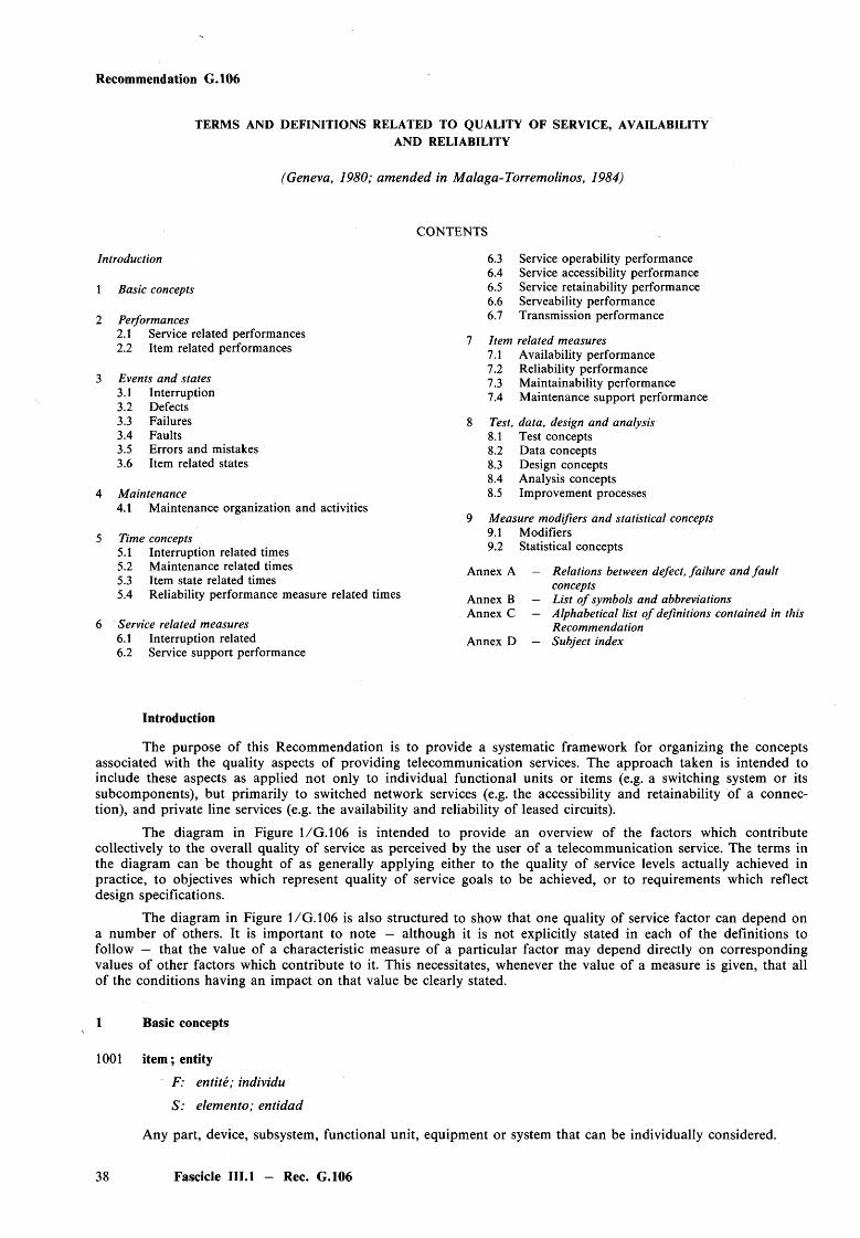
Recommendation G.106
TERMS AND DEFINITIONS RELATED TO QUALITY OF SERVICE, AVAILABILITYAND RELIABILITY
(Geneva, 1980; amended in Malaga-Torremolinos, 1984)
CONTENTS
Introduction
1 Basic concepts
2 Performances2.1 Service related performances2.2 Item related performances
3 Events and states3.1 Interruption3.2 Defects3.3 Failures3.4 Faults3.5 Errors and mistakes3.6 Item related states
4 Maintenance4.1 M aintenance organization and activities
5 Time concepts5.1 Interruption related times5.2 M aintenance related times5.3 Item state related times5.4 Reliability performance measure related times
6 Service related measures6.1 Interruption related6.2 Service support performance
6.3 Service operability performance6.4 Service accessibility performance6.5 Service retainability performance6.6 Serveability performance6.7 Transmission performance
7 Item related measures7.1 Availability performance7.2 Reliability performance7.3 Maintainability performance7.4 Maintenance support performance
8 Test, data, design and analysis8.1 Test concepts8.2 Data concepts8.3 Design concepts8.4 Analysis concepts8.5 Improvement processes
9 Measure modifiers and statistical concepts9.1 Modifiers9.2 Statistical concepts
Annex A — Relations between defect, failure and fau ltconcepts
Annex B — List o f symbols and abbreviationsAnnex C — Alphabetical list o f definitions contained in this
Recommendation Annex D — Subject index
Introduction
The purpose of this Recommendation is to provide a systematic framework for organizing the concepts associated with the quality aspects of providing telecommunication services. The approach taken is intended to include these aspects as applied not only to individual functional units or items (e.g. a switching system or its subcomponents), but primarily to switched network services (e.g. the accessibility and retainability of a connection), and private line services (e.g. the availability and reliability of leased circuits).
The diagram in Figure 1/G . 106 is intended to provide an overview of the factors which contribute collectively to the overall quality of service as perceived by the user of a telecommunication service. The terms in the diagram can be thought of as generally applying either to the quality of service levels actually achieved in practice, to objectives which represent quality of service goals to be achieved, or to requirements which reflect design specifications.
The diagram in Figure 1/G . 106 is also structured to show that one quality of service factor can depend on a number of others. It is im portant to note — although it is not explicitly stated in each of the definitions to follow — that the value of a characteristic measure of a particular factor may depend directly on corresponding values of other factors which contribute to it. This necessitates, whenever the value of a measure is given, that all of the conditions having an impact on that value be clearly stated.
1 Basic concepts
1001 item; entity
F: entite; individu
S: elemento; entidad
Any part, device, subsystem, functional unit, equipment or system that can be individually considered.
38 Fascicle III.l - Rec. G.106

Note 1 — An item may consist of hardware, software or both, and may also include people, e.g. operators in a telephone operator system.
Note 2 — In French, the term entite replaces the term dispositif previously used in this meaning, because the term dispositif is also the common equivalent for the English term “device”.
Note 3 — In French, the term individu is used mainly in statistics.
FIGURE 1/G. 106
Performance concepts
1002 repaired itemF: entite reparee S: elemento reparado
A repairable item which is in fact repaired after a failure.
1003 non-repaired itemF: entite non reparee
S: elemento no reparado
An item which is not repaired after a failure.Note — A non-repaired item may be repairable or not.
1004 serviceF: service
S: servicio
A set o f functions offered to a user by an organization.
1005 required functionF: fonction requise
S: funcion requerida
A function or a combination of functions of an item which is considered necessary for the provisioning of a given service.
Fascicle III.l - Rec. G.106 39
1006 functional mode
F: mode de fonctionnement
S: modo de funcionamiento
A subset of the whole set of possible functions of an item.
1007 instant of time
F: instant
S: instante de tiempo
A single point on a time scale.
Note — The time scale may be continuous as calendar time, or discrete, e.g. number of use cycles.
1008 time interval
F: intervalle de temps
S: intervalo de tiempo
All instants o f time between two given instants o f time.
1009 (time) duration
F: duree
S: duracion
The difference between the end points o f a time interval.
1010 accumulated time
F: duree cumulee
S: tiempo acumulado
The sum of time durations characterized by given conditions over a given time interval.
1011 measure (as applied in the field of reliability and related areas)
F: caracteristique (probability); mesure (en fiabilite et domaines connexes)
S: medida (aplicada en relacion con la fiabilidad y aspectos conexos)
A function or quantity used to describe a random variable or a random process.
Note - For a random variable, examples of measures are the distribution function and the mean.
1012 operation
F: exploitation
S: explotacion
Combination of all technical and corresponding administrative actions intended so that an item can perform a required function, recognizing necessary adaptation to changes in external conditions.
Note — By external conditions are understood, for example, service demand and environmental conditions.
1013 modification (of an item)
F: modification (d’une entite)
S: modificacion (de un elemento)
The combination of all technical and corresponding administrative actions intended to alter the capability of an item by changing, adding or deleting one or more required functions.
40 Fascicle III.l - Rec. G.106

2 Performances
2.1 Service related performances
2101 quality of service
F: qualite de service
S: calidad de servicio
The collective effect of service performances which determine the degree of satisfaction of a user o f theservice.
Note — The quality o f service is characterized by the combined aspects of service support performance,service operability performance, serveability performance, service integrity and other factors specific to each service.
2102 serveability performance
F: servibilite (d’un service)
S: servibilidad (de un servicio)
The ability of a service to be obtained - within specified tolerances and other given conditions — when requested by the user and continue to be provided for a requested duration.
Note — Serveability performance may be subdivided into the service accessibility performance and the service retainability performance.
2103 service accessibility performance
F: accessibility (d’un service)
S: accesibilidad (de un servicio)
The ability of a service to be obtained, within specified tolerances and other given conditions, when requested by the user.
Note - This takes into account the transmission tolerance and the combined aspects o f propagation performance, trafficability performance and availability performance o f the related systems.
2104 service retainability performance
F: continuabilite (d’un service)
S: retenibilidad (de un servicio)
The ability of a service, once obtained, to continue to be provided under given conditions for a requested duration.
Note — Generally this depends on the transmission tolerances, the propagation performance and reliability performance of the related systems. For some services, for example packet switching, this also depends on the trafficability performance and the availability performance of the related systems.
2105 service support performance
F: logistique de service
S: logistica del servicio
The ability of an organization to provide a service and assist in its utilization.
Note — An example of service support performance is the ability to provide assistance in commissioning a basic service, or a supplementary service such as the call waiting service or directory enquiries service.
Fascicle III.l — Rec. G.106 41
2106 service operability performance
F: facilite d ’utilisation (d’un service)
S: facilidad de utilizacidn (de un servicio)
The ability of a service to be successfully and easily operated by a user.
2107 service integrity
F: integrite de service
S: integridad del servicio
The degree to which a service is provided without excessive impairments, once obtained.
Note — This service is characterized by the transmission performance of the system.
2108 transmission performance
F: qualite de transmission
S: calidad de transmision
The level o f reproduction of a signal offered to a telecommunications system, under given conditions, when this system is in an up state.
2.2 Item related performances
2201 effectiveness (performance)
F: efficacite
S: efectividad
The ability of an item to meet a service demand of a given size.
Note — This ability depends on the combined aspects of the capability and the availability performance of the item.
2202 durability
F: durabilite
S: durabilidad
The ability of an item to remain in a condition where it can perform a required function under stated conditions of use and maintenance until a limiting state is reached.
Note — A limiting state of an item may be characterized by the end of the useful life, unsuitability for any economic or technological reasons, etc.
2203 dependability
F: surete de fonctionnement
S: seguridad de funcionamiento
The collective term used to describe the availability performance and its influencing factors: reliability performance, maintainability performance and maintenance support performance.
Note — Dependability is used only for general descriptions in non-quantitative terms.
2204 capability
F: capacite; capabilite (d’une entite)
S: capacidad
The ability of an item to meet a demand of a given size under given internal conditions.
Note 1 — Internal conditions refer, for example, to any given combination of faulty and not faulty sub-items.
Note 2 — This is also called trafficability performance.
42 Fascicle III.l — Rec. G.106
2205 trafficability performance
F: traficabilite; capacite d ’ecoulement du trafic
S: aptitud para cursor trajico
The ability of an item to meet a traffic demand of a given size and other characteristics, under given internal conditions.
Note — Given internal conditions refer, for example, to any combination of faulty and not faulty sub-items.
2206 availability (performance)
F: disponibilite
S: disponibilidad
The ability of an item to be in a state to perform a required function at a given instant o f time or at any instant o f time within a given time interval, assuming that the external resources, if required, are provided.
Note 1 — This ability depends on the combined aspects of the reliability performance, the maintainabilityperformance and the maintenance support performance of an item.
Note 2 — In the definition of the item the external resources required must be delineated.
Note 3 — The term availability is used as an availability performance measure.
2207 reliability (performance)
F: fiabilite
S: fiabilidad
The ability of an item to perform a required function under given conditions for a given time interval.
Note 1 — It is generally assumed that the item is in a state to perform this required function at thebeginning of the time interval.
Note 2 — The term reliability is used as a measure of reliability performance.
2208 maintainability (performance)
F: maintenabilite
S: mantenibilidad
The ability of an item under stated conditions of use, to be retained in, or restored to, a state in which it can perform a required function, when maintenance is performed under given conditions and using stated procedures and resources.
Note — The term maintainability is used as a measure of maintainability performance.
2209 maintenance support (performance)
F: logistique de maintenance
S: logistica de mantenimiento
The ability of a maintenance organization, under given conditions, to provide upon demand the resources required to maintain an item, under a given maintenance policy.
Note — The given conditions are related to the item itself and to the conditions under which the item is used and maintained.
2210 propagation performance
F: caracteristiques de propagation
S: caracteristicas de propagacion
The ability of a propagation medium, in which a wave propagates without artificial guide, to transmit a signal within the given tolerances.
Note — The given tolerances may apply to variations in signal level, noise, interference levels, etc.
Fascicle III.l — Rec. G.106 43
3 Events and states
3.1 Interruption
3101 interruption; break (of service)
F: interruption; coupure (d’un service)
S: interrupcion (de un servicio); corte (de un servicio)
Temporary inability of a service to be provided persisting for more than a given time duration, characterized by a change beyond given limits in at least one parameter essential for the service.
Note 1 — An interruption of a service may be caused by disabled states of the items used for the service or by external reasons such as high service demand.
Note 2 — An interruption of a service is generally an interruption of the transmission, which may be characterized by an abnormal value of power level, noise level, signal distortion, error rate, etc.
3.2 Defects
3201 defect
F: defaut
S: defecto
Any departure o f a characteristic o f an item from requirements.
Note 1 — The requirements may or may not be expressed in the form of a specification.
Note 2 — A defect may or may not affect the ability of an item to perform a required function.
3202 bug
F: erreur de programmation; bogue
S: error de programacion
A software defect caused by a mistake.
3203 critical defect
F: defaut critique
S: defecto critico
A defect that is assessed likely to result in injury to persons or significant material damage.
3204 non-critical defect
F: defaut non critique
S: defecto no critico
A defect other than a critical defect.
3205 major defect
F: defaut majeur
S: defecto mayor
A defect that is likely to result in a failure or to reduce materially the usability of the item for its intended purpose.
44 Fascicle III.l — Rec. G.106
3206 minor defect; imperfection
F: defaut mineur; imperfection
S: defecto menor; imperfeccion
A defect other than a major defect.
3207 defective; defective item
F: defectueux; entite defectueuse
S: defectuoso; elemento defectuoso
An item which contains one or more defects.
3208 critical defective
F: defectueux critique
S: defectuoso critico
An item which contains one or more critical defects.
3209 major defective
F: defectueux majeur
S: defectuoso mayor
An item which contains one or more major defects.
3210 minor defective
F: defectueux mineur
S: defectuoso menor
An item which contains one or more minor defects but no major defects.
3211 design defect
F: defaut de conception *
S: defecto de diseito
A defect due to an inadequate design o f an item.
3212 manufacturing defect
F: defaut de fabrication
S: defecto de fabricacion
A defect due to nonconformance in manufacture to the design of an item or to specified manufacturing processes.
3.3 Failures
3301 failure
F: defaillance
S: fallo
The termination of the ability of an item to perform a required function.
Note — After failure the item has a fault.
Fascicle III.l — Rec. G.106 45
3302 critical failure
F: defaillance critique
S: fallo critico
A failure which is assessed likely to result in injury to persons or significant material damage.
3303 non-critical failure
F: defaillance non critique
S: fallo no critico
A failure other than a critical failure.
3304 misuse failure
F: defaillance par mauvaise utilisation
S: fallo por uso incorrecto
A failure due to induced stresses during use which are beyond the stated capabilities of the item.
3305 mishandling failure
F: defaillance par fausse manoeuvre
S: fallo por manejo incorrecto
A failure caused by incorrect handling or lack of care of the item.
3306 (inherent) weakness failure
F: defaillance par fragilite (inherente)
S: fallo por fragilidad (inherente)
A failure due to a weakness inherent in the item itself when subjected to stresses within the stated capabilities of the item.
3307 design failure
F: defaillance de conception
S: fallo de diseho
A failure due to a design defect.
3308 manufacturing failure
F: defaillance de fabrication
S: fallo de fabricacion
A failure due to a manufacturing defect.
3309 ageing failure; wearout failure
F: defaillance par vieillissement; defaillance par usure
S: fallo por envejecimiento; fallo por desgaste
A failure whose probability of occurrence increases with the passage of time, as a result of processes inherent in the item.
3310 sudden failure
F: defaillance soudaine
S: fallo repentino
A failure that could not be anticipated by prior examination or monitoring.
46 Fascicle III.l — Rec. G.106
3311 gradual failure; degradation failure; drift failure
F: defaillance progressive; degradation; defaillance par derive
S: fallo gradual; fallo por degradacion; fallo por deriva
A failure due to a gradual change in time of given characteristics of an item and that could be anticipated by prior examination or monitoring.
Note — A gradual failure can sometimes be avoided by preventive maintenance.
3312 cataleptic failure; catastrophic failure (deprecated)
F: defaillance cataleptique
S: fallo cataleptico; fallo catastrdfico (desaconsejado)
A sudden failure which results in a complete fault.
3313 relevant failure
F: defaillance pertinente; defaillance a prendre en compte
S: fallo pertinente; fallo a considerar
A failure to be included in interpreting test or operational results or in calculating the value of a reliability performance measure.
Note — The criteria for the inclusion should be stated.
3314 non-relevant failure
F: defaillance non pertinente; defaillance a ne pas prendre en compte
S: fallo no pertinente; fallo a no considerar
A failure to be excluded in interpreting test or operational results or in calculating the value of a reliability performance measure.
Note — The criteria for the exclusion should be stated.
3315 primary failure
F: defaillance primaire
S: fallo primario
A failure of an item, not caused either directly or indirectly by the failure or the fau lt of another item.
3316 secondary failure
F: defaillance secondaire
S: fallo secundario
A failure of an item, caused either directly or indirectly by the failure or the fau lt of another item.
3317 failure cause
F: cause de defaillance
S: causa de fallo
The circumstances during design, manufacture or use which have led to a failure.
3318 failure mechanism
F: mecanisme de defaillance
S: mecanismo de fallo
The physical, chemical or other process which has led to a failure.
Fascicle III.l — Rec. G.106 47
3319 systematic failure; reproducible failure; deterministic failure
F: defaillance systematique; defaillance reproductible
S: fallo sistematico; fallo reproducible; fallo determini'stico
A failure related in a deterministic way to a certain cause, which can only be eliminated by a modification of the design or manufacturing process, operational procedures, documentation or other relevant factors.
Note 1 — Corrective maintenance without modification will usually not eliminate the failure cause.
Note 2 — A systematic failure can be induced at will by simulating the failure cause.
3.4 Faults
3401 fault
F: panne; derangement
S: averia
The inability of an item to perform a required function, excluding that inability due to preventive maintenance, lack of external resources or planned actions.
Note 1 — A fau lt is often the result of a failure of the item itself, but may exist without prior failure.
3402 critical fault
F: panne critique
S: averia critica
A fa u lt which is assessed likely to result in injury to persons or significant damage to material.
3403 non-critical fault
F: panne non critique
S: averia no critica
A fault, other than a critical fault.
3404 major fault
F: panne majeure
S: averia mayor
A fau lt which affects a function considered to be of major importance.
3405 minor fault
F: panne mineure
S: averia menor
A fau lt other than a major fault.
3406 misuse fault
F: panne par mauvaise utilisation
S: averia por uso incorrecto
A fau lt due to induced stresses during use which are beyond the stated capabilities of the item.
48 Fascicle III.l — Rec. G.106
3407 mishandling fault
F: panne par fausse manoeuvre
S: averia por manejo incorrecto
A fa u lt caused by incorrect handling or lack of care of the item.
3408 (inherent) weakness fault
F: panne par fragilite (inherente)
S: averia por fragilidad (inherente)
A fau lt due to a weakness inherent in the item itself when subjected to stresses within the stated capabilities of the item.
3409 design fault
F: panne de conception
S: averia de diseho
A fa u lt due to a design defect.
3410 manufacturing fault
F: panne de fabrication
S: averia de fabricacion
A fa u lt due to a manufacturing defect.
3411 ageing fault; wearout fault
F: panne par vieillissement; panne par usure
S: averia por envejecimiento; averia por desgaste
A fa u lt resulting from an ageing failure.
3412 programme-sensitive fault
F: panne mise en evidence par le programme
S: averia dependiente del programa
A fau lt that is revealed as a result of the execution of some particular sequence of instructions.
3413 data-sensitive fault
F: panne mise en evidence par les donnees
S: averia dependiente de los datos
A fa u lt that is revealed as a result of the processing of a particular pattern of data.
3414 complete fault; function preventing fault
F: panne complete
S: averia completa
A fau lt characterized by complete inability to perform all required functions o f an item.
Note — The criteria for a complete fau lt have to be stated.
3415 partial fault
F: panne partielle
S: averia parcial
A fau lt of an item other than a complete fault.
Fascicle III.l — Rec. G.106 49
3416 persistent fault; permanent fault; solid fault
F: panne permanente
S: averia permanente
A fau lt of an item that persists until an action of corrective maintenance is performed.
3417 intermittent fault; volatile fault; transient fault
F: panne intermittente; panne temporaire
S : averia intermitente; averia transitoria
A fault of an item which persists for a limited time duration following which the item recovers the ability to perform a required function without being subjected to any action of corrective maintenance.
Note — Such a fau lt is often recurrent.
3418 determinate fault
F: panne franche
S: averia clara
For an item, which produces a response as a result of an action, a fau lt for which the response is the same for all actions.
3419 indeterminate fault
F: panne indeterminee
S: averia indeterminada
For an item, which produces a response as a result of an action, a fau lt such that the error affecting the response depends on the action applied.
Note — An example would be a data-sensitive fault.
3420 latent fault
F: panne latente
S: averia latente
An existing fau lt that has not yet been recognized.
3421 systematic fault
F: panne systematique
S: averia sistematica
A fa u lt resulting from a systematic failure.
3422 fault mode; failure mode (deprecated)
F: mode de panne; mode de defaillance (terme deconseille)
■S: modo de averia; modo de fallo (desaconsejado)
One of the possible states of a faulty item, for a given required function.
3423 faulty
F: en panne
S: averiado; en averia
Property of having a fault.
50 Fascicle III.l — Rec. G.106

3.5 Errors and mistakes
3501 error
F: erreur
S: error
A discrepancy between a computed, observed or measured value or condition and the true, specified or theoretically correct value or condition.
Note — An error can be caused by a faulty item, e.g. a computing error made by a fau lty computer equipment.
3502 execution error; generated error
F: erreur d ’execution
S: error de ejecucidn
Error produced during the operation of a fau lty item.
3503 interaction error (man-machine)
F: erreur d ’interaction (homme-machine)
S: error de interaccion (hombre-maquina)
An error in the response of an item caused by a mistake during its use.
3504 propagated error
F: erreur propagee
S: error propagado
An error in the response to erroneous data input to a non-faulty item.
3505 mistake; error (deprecated in this sense)
F: erreur (humaine); fau te
S: equivocacion; error (desaconsejado en este sentido)
A human action that produces an unintended result.
3.6 Item related states (see also Figure 2/G.106)
Up Down* *+• ►
i Disabled
(Lack of (Subject toIdle Busy external preventive Faulty
resources) maintenance)
CCITT-85 770
FIGURE 2/G.106
Classification of item states
Fascicle III.l — Rec. G.106 51
3601 operating state
F: (etat de) fonctionnement
S: estado de funcionamiento
The state when an item is performing a required function.
3602 non-operating state
F: (etat de) non-fonctionnement
S: estado de no funcionamiento
The state when an item is not performing a required function.
3603 standby state
F: (etat d ’) attente
S: estado de espera
A non-operating up state during the required time.
3604 idle state; free state
F: etat vacant; etat libre
S: estado de reposo; estado libre
A non-operating up state during non-required time.
3605 disabled state; outage
F: etat d ’incapicite
S: estado de incapacidad
A state of an item characterized by its inability to perform a required function, for any reason.
3606 external disabled state
F: etat d ’incapacite externe
S: estado de incapacidad externa
That subset o f the disabled state when the item is in an up state, but lacks required external resources.
3607 down state, internal disabled state
F: etat d ’indisponibilite; etat d ’incapacite interne
S: estado de indisponibilidad; estado de incapacidad interna
A state of an item characterized by a fau lt or by a possible inability to perform a required function during preventive maintenance.
Note — This state relates to availability performance.
3608 up state
F: etat de disponibilite
S: estado de disponibilidad
A state of an item characterized by the fact that it can perform a required function, assuming that the external resources, if required, are provided.
Note — This state relates to availability performance.
3609 busy state
F: etat occupe; occupation
S: estado de ocupacion; estado de ocupado
The state of an item in which it performs a required function for a user arid for that reason is not accessible by other users.
52 Fascicle I1I.1 - Rec. G.106
3610 critical state
F: etat critique
S: estado critico
A state of an item assessed likely to result in injury to persons or significant material damage.
Note — A critical state may be the result o f a critical fault, but not necessarily.
4 Maintenance
4.1 Maintenance organization and activities
4101 maintenance philosophy
F: philosophic de maintenance
S: filosofia de mantenimiento
A system o f underlying principles for the organization and execution of the maintenance.
4102 maintenance policy
F: politique de maintenance
S: politico de mantenimiento
A description of the interrelationship between the maintenance echelons, the indenture levels and the levels o f maintenance to be applied for the maintenance o f an item.
4103 maintenance
F: maintenance
S: mantenimiento
The combination of all technical and corresponding administrative actions, including supervision actions, intended to retain an item in, or restore it to, a state in which it can perform a required function.
4104 preventive maintenance
F: maintenance preventive; entretien
S: mantenimiento preventivo
The maintenance carried out at predetermined intervals or according to prescribed criteria and intended to reduce the probability of failure or the degradation of the functioning of an item.
4105 corrective maintenance; repair
F: maintenance corrective; reparation; depannage
S: mantenimiento correctivo; reparacion
The maintenance carried out after fau lt recognition and intended to restore an item to a state in which it can perform a required function.
4106 deferred maintenance
F: maintenance differee
S: mantenimiento diferido
Such corrective maintenance which is not immediately initiated after a fa u lt recognition but is delayed in accordance with given maintenance rules.
Fascicle III.l — Rec. G.106 53
4107 scheduled maintenance
F: maintenance programmee; entretien systematique
S: mantenimiento programado
The preventive maintenance carried out in accordance with an established time schedule.
4108 unscheduled maintenance
F: maintenance non programmee
S: mantenimiento no programado
The maintenance carried out, not in accordance with an established time schedule, but e.g. after reception of an indication regarding the state of an item.
4109 on-site maintenance; in situ maintenance; field maintenance
F: maintenance in situ
S: mantenimiento local; mantenimiento sobre el terreno
Maintenance performed at the premises where the item is used.
4110 off-site maintenance
F: maintenance deportee
S: mantenimiento no local
Maintenance performed at a place different from where th e .item is used.
Note — An example is the repair of a sub-item at a maintenance centre.
4111 remote maintenance
F: telemaintenance
S: mantenimiento remoto; telemantenimiento
Maintenance of an item performed without physical access of the personnel to the item.
4112 automatic maintenance
F: maintenance automatique
S: mantenimiento automatico
Maintenance accomplished without human intervention.
4113 function-affecting maintenance
F: maintenance affectant les fonctions
S: mantenimiento que afecta a la funcion
Such a maintenance action that affects one or more of the required functions o f a maintained item.
Note — Function-affecting maintenance is divided into function-preventing maintenance and function- degrading maintenance.
4114 function-preventing maintenance
F: maintenance-arret; maintenance empechant I’accomplissement des fonctions
S: mantenimiento con discontinuidad de funciones
Such a maintenance action that prevents a maintained item from performing a required function by causing complete loss of all the functions.
54 Fascicle III.l — Rec. G.106
4115 function-degrading maintenance
F: maintenance avec degradation; maintenance degradant les fonctions
S: mantenimiento con degradacidn de funciones
Such a maintenance action that affects one or more of the required functions of a maintained item, but not to such extent as to cause complete loss of all the functions.
4116 function-permitting maintenance
F: maintenance en fonctionnement; maintenance en exploitation
S: mantenimiento sin discontinuidad de funciones
Such a maintenance action that does not affect any of the required functions of a maintained item.
4117 level of maintenance
F: niveau de maintenance
S: nivel de mantenimiento/
The maintenance action to be carried out at a specified indenture level.
Note — Examples of a maintenance action are replacing a component, a printed circuit board, a subsystem, etc.
4118 maintenance echelon; line of maintenance
F: echelon de maintenance
S: escalon de mantenimiento; linea de mantenimiento
The position in an organization where specified levels o f maintenance are to be carried out on an item.
Note 1 — Examples of maintenance echelons are: field, repair shop, manufacturer.
Note 2 — The maintenance echelon is characterized by the skill of the personnel, the facilities available,the location, etc.
4119 indenture level (for maintenance)
F: niveau d ’intervention (pour la maintenance)
S; nivel de intervencion (para el mantenimiento)
A level of subdivision of an item from the point of view of a maintenance action.
Note 1 — Examples of indenture levels could be a subsystem, a circuit board, a component.
Note 2 — The indenture level depends on the complexity of the item’s construction, the accessibility tosub-items, skill level o f maintenance personnel, test equipment facilities, safety considerations, etc.
4120 elementary maintenance activity
F: operation elementaire de maintenance
S: accion elemental de mantenimiento
The unit of work into which a maintenance activity may be broken down at a given indenture level.
4121 maintenance action; maintenance task
F: operation de maintenance; tache de maintenance
S; accion de mantenimiento; tarea de mantenimiento
A sequence of elementary maintenance activities carried out for a given purpose.
Note — Examples are fau lt diagnosis, fau lt localization and function check-out or combinations thereof.
Fascicle III.1 - Rec. G.106 55
4122 supervision
F: surveillance; supervision
S: supervision
Activity, performed either manually or automatically, intended to observe the state of an item.
Note — Automatic supervision may be performed internally or externally to the item.
4123 controlled maintenance
F: maintenance dirigee
S: mantenimiento dirigido
A method to sustain a desired quality o f service by the systematic application of analysis techniques using centralized supervisory facilities a n d /o r sampling to minimize preventive maintenance and to reduce corrective maintenance.
4124 fault recognition
F: detection (de panne)
S: deteccion (de una averia)
The event when a fau lt is recognized.
4125 fault diagnosis
F: diagnostic (de panne)
S: diagnostico (de una averia)
Actions taken for fau lt recognition, fau lt localization and cause identification.
4126 fault localization; fault location (deprecated in this sense)
F: localisation de panne
S: localizacion (de una averia)
Actions taken to identify the faulty sub-item or sub-items at the appropriate indenture level.
4127 fault correction
F: correction (de panne)
S: correccion (de una averia)
Actions taken after fau lt localization intended to restore the ability of the faulty item to perform a required function.
4128 function check-out
F: verification (de fonctionnement)
S: verificacion de funcionamiento
Actions taken after fau lt correction to verify that the item has recovered its ability to perform the required function.
4129 restoration; recovery
F: retablissement
S: restablecimiento
That event when the item regains the ability to perform a required function after a fault.
56 Fascicle III.l — Rec. G.106
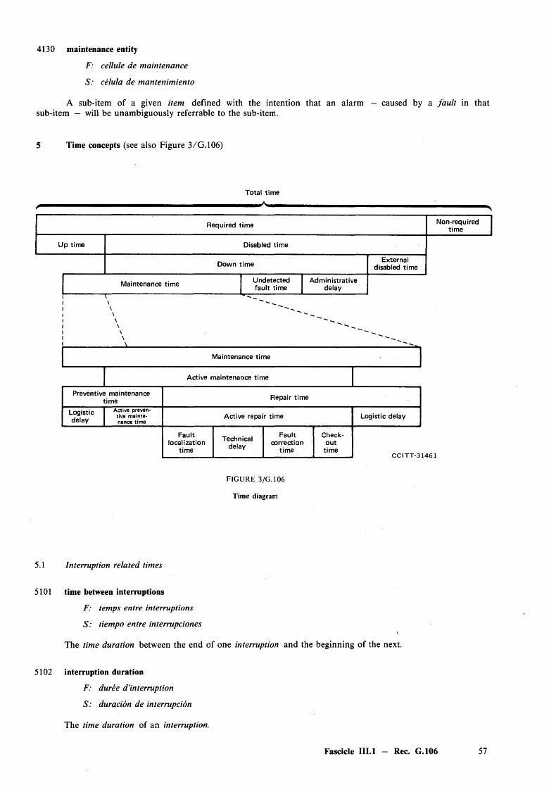
4130 maintenance entity
F: cellule de maintenance
S: celula de mantenimiento
A sub-item of a given item defined with the intention that an alarm — caused by a fau lt in that sub-item — will be unambiguously referrable to the sub-item.
5 Time concepts (see also Figure 3/G.106)
Total time
Required time Non-requiredtime
Up time Disabled time
Down time External disabled time
Maintenance time Undetected fault time
Administrativedelay
Maintenance time
Active maintenance time
Preventive maintenance time Repair time
Logisticdelay
A c t iv e p r e v e n t i v e m a i n t e n a n c e t i m e
Active repair time Logistic delay
Faultlocalization
timeTechnical
delayFault
correctiontime
Checkout
time CCITT-31461
FIGURE 3/G.106
Time diagram
5.1 Interruption related times
5101 time between interruptions
F: temps entre interruptions
S: tiempo entre interrupciones\
The time duration between the end of one interruption and the beginning of the next.
5102 interruption duration
F: duree d ’interruption
S: duracion de interrupcion
The time duration of an interruption.
Fascicle III.l — Rec. G.106 57

5.2 Maintenance related times
5201 maintenance time
F: temps de maintenance
S: tiempo de mantenimiento
The time interval during which a maintenance action is performed on an item either manually or automatically, including technical delays and logistic delays.
Note — Maintenance may be carried out while the item is performing a required function.
5202 maintenance man-hours (MMH)
F: duree equivalente de maintenance
S: duracion equivalente de mantenimiento; horas-hombre de mantenimiento
The accumulated durations of the maintenance times, expressed in hours, used by all maintenance personnel for a given type of maintenance action or over a given time interval.
5203 active maintenance time
F: temps de maintenance active
S: tiempo de mantenimiento activo
That part of the maintenance time during which a maintenance action is performed on an item, either automatically or manually, excluding logistic delays.
Note — Active maintenance may be carried out while the item is performing a required function.
5204 preventive maintenance time
F: temps de maintenance preventive
S: tiempo de mantenimiento preventivo
That part o f the maintenance time during which preventive maintenance is performed on an item, including technical delays and logistic delays inherent in preventive maintenance.
5205 repair time; corrective maintenance time
F: temps de reparation; temps de maintenance corrective
S: tiempo de reparacion; tiempo de mantenimiento correctivo
That part o f the maintenance time during which corrective maintenance is performed on an item, including technical delays and logistic delays inherent in corrective maintenance.
5206 active preventive maintenance time
F: temps de maintenance preventive active
S: tiempo de mantenimiento preventivo activo
That part of the active maintenance time during which actions of preventive maintenance are performed on an item. >
5207 active repair time; active corrective maintenance time
F: temps de reparation active; temps de maintenance corrective active ,
S: tiempo de reparacion activo; tiempo de mantenimiento correctivo activo
That part o f the active maintenance time during which actions of corrective maintenance are performed on an item.
58 Fascicle III.l — Rec. G.106
5208 undetected fault time
F: temps de non-detection de panne
S: tiempo de no deteccion de la averia
The time interval between a failure and recognition o f the resulting fault.
5209 administrative delay (for corrective maintenance)
F: delai administratif (pour la maintenance correctivej
S: retardo administrativo (para el mantenimiento correctivo)
The accumulated time during which an action of corrective maintenance on a faulty item is not performed due to administrative reasons.
5210 logistic delay
F: delai logistique
S: retardo logistico
That accumulated time during which a maintenance action cannot be performed due to the necessity to acquire maintenance resources, excluding any administrative delay.
Note — Logistic delays can be due to, e.g. travelling to unattended installations, to awaiting the arrival of spare parts, specialists or test equipment.
5211 fault correction time
F: temps de correction de panne
S: tiempo de correccion de una averia
That part o f active repair time during which fau lt correction is performed.
5212 technical delay
F: delai technique
S: retardo tecnico
The accumulated time necessary to perform auxiliary technical actions associated with the maintenance action itself.
5213 check-out time
F: temps de verification (du fonctionnement)
S: tiempo de verificacidn (de funcionamiento)
That part of active repair time during which function check-out is performed.
5214 fault localization time; fault location time (deprecated)
F: temps de localisation (de panne)
S: tiempo de localizacion de averia
That part of active repair time during which fau lt localization is performed.
5.3 Item state related times
5301 operating time
F: temps de fonctionnement
S: tiempo de funcionamiento
The time interval during which an item is an operating state.
Fascicle III.l — Rec. G.106 59
5302 non-operating time
F: temps de non-fonctionnement
S: tiempo de no funcionamiento
The time interval during which an item is in a non-operating state.
5303 required time
F: periode requise
S: periodo requerido
The time interval during which the user requires the item to be in a condition to perform a required function.
5304 non-required time
F: periode non requise
S: periodo no requerido
The time interval during which the user, does not require the item to be in a condition to perform a required function.
5305 stand-by time
F: periode d ’attentc
S: tiempo de espera (de reserva)
The time interval during which an item is in a stand-by state.
5306 idle time; free time
F: periode vacante; temps mort; temps libre
S: tiempo de reposo; tiempo muerto; tiempo libre
The time interval during which an item is in a free state.
5307 disabled time
F: temps d ’incapacite
S: tiempo de incapacidad
The time interval during which an item is in a disabled state.
5308 down time
F: temps d ’indisponibilite
S: tiempo de indisponibilidad
The time interval during which an item is in a down state.
5309 accumulated down time
F: duree cumulee d ’indisponibilite
S: tiempo de indisponibilidad acumulado
The sum o f the duration o f down times over a given time interval.
5310 external disabled time; external loss time
F: temps d ’incapacite externe
S: tiempo de incapacidad externa
The time interval during which an item is in an external disabled state.
60 Fascicle III.l - Rec. G.106
5311 uptime
F: temps de disponibilite; temps de bon fonctionnement
S: tiempo de disponibilidad
The time interval during which an item is in an up state.
5.4 Time concepts related to reliability performance
5401 time to first failure
F: duree de fonctionnement avant la premiere defaillance
S: tiempo hasta el primer fallo
Total time duration o f the operating time o f an item from the instant it is first put in an up-state untilfailure.
5402 time to failure
F: duree de fonctionnement avant defaillance
S: tiempo hasta el fallo
Total time duration of the operating time of an item, from the instant it goes from a down state to an up state, after a corrective maintenance action, until next failure.
5403 time between failures
F: temps entre defaillances
S: tiempo entre fallos
The time duration between two successive failures of a repaired item.
Note 1 — Those parts o f non-operating time which are included must be identified.
Note 2 — In some applications only the up time is considered.
5404 time to restoration; time to recovery
F: temps de panne
S: tiempo de averia
The time interval during which an item is in a down state due to a failure.
5405 useful life
F: (duree de) vie utile
S: vida util
Under given conditions, the time interval beginning at a given instant of time, and ending when the failure intensity becomes unacceptable or when the item is considered unrepairable as a result o f a fault.
5406 early failure period
F: periode initiate de defaillance
S: periodo de fallos inicial
That possible early period in the life of an item, beginning at a given instant o f time and during which the instantaneous failure intensity for a repaired item or the instantaneous failure rate for a non-repaired item decreases rapidly.
Note — In any particular case, it is necessary to explain what is meant by “decreases rapidly”.
Fascicle III.l - Rec. G.106 61
5407 constant failure intensity period
F: periode d ’intensite constante de defaillance
S: periodo de intensidad de fallos constante
That possible period in the life of a repaired item during which the failure intensity is approximately constant.
Note — In any particular case it is necessary to explain what is meant by “approximately constant”.
5408 constant failure rate period
F: periode de densite constante de defaillance; periode de taux constante de defaillance
S: periodo de tasa de fallos constante
That possible period in the life of a non-repaired item during which the failure rate is approximately constant.
Note — In any particular case it is necessary to explain what is meant by “approximately constant”.
5409 wear-out failure period
F: periode de defaillance par vieillissement; periode de defaillance par usure
S: periodo de fallos por envejecimiento
That possible later period in the life of a repaired item during which the instantaneous failure intensity for a repaired item or the instantaneous failure rate for a non-repaired item increases rapidly.
Note — In any particular case it is necessary to explain what is meant by “increases rapidly”.
6 Service related measures
6.1 Interruption related
6101 mean time between interruptions
F: duree moyenne entre interruptions
S: tiempo medio entre interrupciones
The expectation of the time between interruptions.
6102 mean interruption duration
F: duree moyenne d ’une interruption
S: duracion media de una interrupcion
The expectation of the interruption duration.
6.2 Service support performance
6201 mean service provisioning time
F: delai moyen pour la fourniture d ’un service
S: tiempo medio de espera para la prestacion de un servicio
The expectation of the duration between the instant o f time a potential user requests that an organization provides the necessary means for a service, and the instant o f time when these means are furnished.
62 Fascicle III.l — Rec. G.106
6202 billing error probability
F: probabilite d ’erreur de facturation
S: probabilidad de error de subtarificacion
The probability of an error when billing a user of a service.
6203 incorrect charging or accounting probability
F: probabilite de taxation erronee
S: probabilidad de tarificacion o de contabilizacion incorrectas
The probability of a call attempt receiving incorrect charging or accounting treatment.
6204 undercharging probability
F: probabilite de sous-taxation
S: probabilidad de subtarificacion
The probability that an effective call will be undercharged for any reason.
6205 overcharging probability
F: probabilite de surtaxation
S: probabilidad de sobretarijicacion
The probability that an effective call will be overcharged for any reason.
6206 billing integrity (probability)
F: (probabilite de) justesse de facturation
S: integridad de la facturacion (probabilidad de)
The probability that the billing information presented to a user correctly reflects the type, destination and duration of the call.
6.3 Service operability performance
6301 service user mistake probability
F: probabilite d ’erreur d ’un usager
S: probabilidad de error de un usuario
Probability of a mistake made by a user in his attempt to utilize a service.
6302 dialling mistake probability
F: probabilite d ’erreur de numerotation
S: probabilidad de error de marcacion
The probability that the user of a telecommunication network makes dialling mistakes during his call attempts.
6303 service user abandonment probability
F: probabilite d ’abandon (d’acces a un service par un usager)
S: probabilidad de abandono de un servicio por un usuario
The probability that a user abandons the attempt to use a service.
Note — Abandonments may be caused by excessive user mistake rates, by excessive service access delays, etc.
6304 call abandonment probability
F: probabilite d ’abandon (d’une tentative d ’appel)
S: probabilidad de abandono de una tentativa de llamada
The probability that a user abandons the call attempt to a telecommunication network.
Fascicle III.l — Rec. G.106 63
6.4 Service accessibility performance
6401 service accessibility; service access probability
F: accessibility (d ’un service)
S: accesibilidad de un servicio; probabilidad de acceso a un servicio
The probability that a service can be obtained within specified tolerances and other given operating conditions when requested by the user.
6402 mean service access delay
F: duree moyenne d ’acces
S: retardo medio de acceso a un servicio
The expectation of the time duration between an initial bid by the user for the acquisition of a service and the instant o f time the user has access to the service, the service being obtained within specified tolerances and other given operating conditions.
6403 connection accessibility
F: accessibility
S: accesibilidad de una conexidn
The probability that a connection can be established within specified tolerances and other given conditions following receipt by the exchange of a valid code.
6404 mean access delay
F: duree moyenne d ’acces
S: retardo medio de acceso
The expectation o f the time duration between the first call attempt made by a user of a telecommunication network to reach another user or a service and the instant o f time the user reaches the wanted other user or service, within specified tolerances and under given operational conditions.
6405 p-fractile access delay
F: quantile-p de la duree d ’acces
S: cuantil-p del retardo de acceso
The p-fractile value of the duration between the first call attempt made by a user of a telecommunication network to reach another user or a service and the instant o f time the user reaches the wanted other user or service, within specified tolerances and under given operational conditions.
6406 accessibility of a connection to be established
F: accessibility d ’une communication a etablir
S: accesibilidad de una conexidn por establecer
The probability that a switched connection can be established, within specified transmission tolerances, to the correct destination, within a given time interval, when requested by the user.
Note 1 — For user-originated calls, it could express the probability o f a successful call establishment on the first attempt. For operator-handled calls, it could represent the probability of having a satisfactory connection established within a given time duration.
Note 2 — In general, the tolerances should correspond to a level o f transmission performance which makes the connection unsatisfactory for service such that, for example, a substantial percentage of users would abandon the connection.
64 Fascicle III.l — Rec. G.106
6407 answer seizure ratio (ASR)
F: taux de prises avec reponse (TPR)
S: tasa de tomas con respuesta (TTR)
Either on a route or a destination code basis, and during a specified time interval, the ratio of the number of seizures that result in an answer signal to the total number of seizures.
Note — It is usually expressed as a percentage.
6408 unacceptable transmission probability
F: probabilite d ’une transmission inacceptable
S: probabilidad de transmision inaceptable
The probability of a connection being established with an unacceptable speech path transmission quality.
6409 no tone probability
F: probabilite de non tonalite
S: probabilidad de ausencia de tono
The probability o f a call attempt encountering no tone following receipt of a valid code by the exchange.
6410 misrouting probability
F: probabilite d ’acheminement errone
S: probabilidad de encaminamiento errbneo
The probability o f a call attempt being misrouted following receipt by the exchange of a valid code.
6.5 Service retainability performance
6501 service retainability
F: continuabilite (d’un service)
S: retenebilidad (de un servicio)
The probability that a service, once obtained, will continue to be provided under given conditions for a given time duration.
6502 connection retainability
F: continuabilite (d ’une chaine de connexion)
S: retenebilidad (de una conexion)
The probability that a connection, once obtained, will continue to be provided for a communication under given conditions for a given time duration.
6503 retainability of an established connection
F: continuabilite d ’une communication etablie
S: retenebilidad de una conexion establecida
The probability that a switched connection, once established, will operate within specified transmission tolerances without interruption for a given time interval.
6504 premature release probability; cut-off call probability
F: probabilite de liberation prematuree
S: probabilidad de liberacion prematura; probabilidad de corte de una llamada
The probability that an established connection will be released for a reason other than intentionally by any of the parties involved in the call.
Fascicle III.l - Rec. G.106 65
6505 release failure probability
F: probabilite de non-liberation
S: probabilidad de fallo de liberacion
The probability that the required release of a connection will not take place.
6.6 Serveability performance
6601 probability of successful service completion
F: probabilite d ’execution correcte du service
S: probabilidad de prestacion satisfactoria de un servicio
The probability that a connection can be established, under satisfactory operating conditions, and retained for a given time interval
6602 completion ratio
F: taux d ’efficacite
S: tasa de eficacia
The ratio of completed call attempts to the total number of call attempts, as measured at a given point o f a network.
6.7 Transmission performance
6701 bit error ratio (BER)
F: taux d ’erreur sur les bits (TEB)
S: tasa de errores en los bits; tasa de error en los bits (TEB)
The ratio of the number of bit errors to the total number of bits transmitted in a given time interval.
6702 error free seconds (EFS)
F: secondes sans erreur (SSE)
S: segundos sin error (SSE)
The ratio o f the number of one-second intervals during which no bits are received in error to the total number of one-second intervals in the time interval
Note 1 — The length of the time interval needs to be specified.
Note 2 — This ratio is usually expressed as a percentage.
7 Item related measures
7.1 Availability performance
7101 instantaneous availability; pointwise availability, A(t) (symbol)
F: disponibilite (instantanee), A(t) (symbole)
S: disponibilidad instantanea, A(t) (simbolo)
The probability that an item is in an up-state at a given instant o f time, t.
Note — In French the term disponibilite is also used to denote the performance quantified by this probability.
7102 instantaneous unavailability; pointwise unavailability, U(t) (symbol)
F: indisponibilite (instantanee), U(t) (symbole)
S: indisponibilidad instantanea, U(t) (simbolo)
The probability that an item is in a down-state at a given instant o f time, t.
66 Fascicle III.l — Rec. G.106

7103 mean availability, A(ti, t2) (symbol)
F: disponibilite moyenne, A (t\, t2) (symbole)
S: disponibilidad media, A (tu t2) (simbolo)
The normalized integral of the instantaneous availability in a given time interval (tu t2).
Note — The mean availability is related to the instantaneous availability as
h~ A {tx ,h )= --------- f A (t)dt.
h ~ h Jh
7104 mean unavailability, U(tj, t2) (symbol)
F: indisponibilite moyenne, U(t\, t2) (symbole)
S: indisponibilidad media, U (tu t2) (simbolo)
The normalized integral of the instantaneous unavailability in a stated time interval (t\, t2).
Note — The mean unavailability is related to the instantaneous unavailability as
h
m,h ) — — f v(t)dth ~ h J
7105 (asymptotic) availability; (steady-state) availability, A (symbol)
F: disponibilite asymptotique; disponibilite, A (symbole)
S: disponibilidad (asintotica); disponibilidad en (regimen permanente), A (simbolo)
The limit, if this exists, of the instantaneous availability when the time tends to infinity.
Note — Under certain conditions, for instance constant failure rate and constant repair rate, the asymptotic availability may be expressed as:
M U TA =
M U T + M D T
where
M D T is the mean down time
M U T is the mean up time.
7106 asymptotic unavailability, U (symbol)
F: indisponibilite asymptotique; indisponibilite, U (symbole)
S: indisponibilidad asintdtica, U (simbolo)
The limit, if this exists, o f the instantaneous unavailability when the time tends to infinity.
Note — Under certain conditions, for instance constant failure rate and constant repair rate, the asymptotic unavailability may be expressed as:
V . M D TM D T + M U T
where
M D T is the mean down time
M U T is the mean up time.
Fascicle III.l — Rec. G.106 67
7107 asymptotic mean availability, A (symbol)
F: disponibilite moyenne asymptotique, A (symbole)
S: disponibilidad media asintdtica, A (simbolo)
The limit, if this exists, o f the mean availability over a time interval (t1? t2) when t2 tends to infinity.
Note 1 — The asymptotic mean availability is related to the mean availability as
A = lim A {t\, t2)t2-*-oo
Note 2 — When such a limit exists it is not dependent on t\.
7108 asymptotic mean unavailability, U (symbol)
F: indisponibilite moyenne asymptotique, U (symbole)
S: indisponibilidad asintotica, U (simbolo)
The limit, if this exists, o f the mean unavailability over a time interval (ft, t2) when t2 tends to infinity.
Note 1 — The asymptotic mean unavailability is related to the mean unavailability as
U = lim U (tu t2)t2 —► o o
Note 2 — When such a limit exists it is not dependent on tx.
7109 mean up time (MUT)
F: temps moyen de disponibilite; duree moyenne de disponibilite (TMD)
S: tiempo medio de disponibilidad (TMD)
The expectation of the up time.
7110 mean accumulated down time (MADT)
F: duree cumulee moyenne d ’indisponibilite
S: tiempo medio acumulado de indisponibilidad (TM AI)
The expectation of the accumulated down time.
7111 instantaneous availability of a leased circuit
F: disponibilite instantanee d ’un circuit loue
S: disponibilidad instantanea de un circuito arrendado
The probability that, under stated operating conditions, a leased circuit can perform a required function when requested by the subscriber.
7.2 Reliability performance
7201 reliability, R (symbol)
F: fiabilite, R (symbole)
S: fiabilidad, R (simbolo)
The probability that an item can perform a required function under stated conditions for a given timeinterval.
Note 1 — It is generally assumed that the item is in a state to perform this required function at the beginning of the time interval.
Note 2 — In French, the term fiabilite is also used to denote the performance quantified by this probability.
68 Fascicle III.l — Rec. G.106
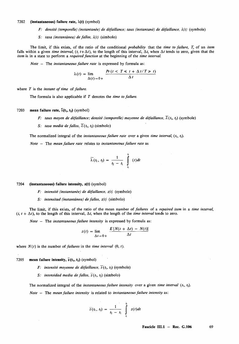
7202 (instantaneous) failure rate, Xft) (symbol)
F: densite (temporelle) (instantanee) de defaillance; taux (instantane) de defaillance, X(t) (symbole)
S: tasa (instantanea) de fallos, X(t) (simbolo)
The limit, if this exists, o f the ratio of the conditional probability that the time to failure, T, of an item falls within a given time interval, ( t, t+ A t), to the length of this interval, At, when A t tends to zero, given that the item is in a state to perform a required function at the beginning of the time interval.
Note — The instantaneous failure rate is expressed by formula as:
X (t) = limA(r)^0+ A t
where T is the instant o f time o f failure.
The formula is also applicable if T denotes the time to failure.
7203 mean failure rate, X(tj, t2) (symbol)
F: taux moyen de defaillance; densite (temporelle) moyenne de defaillance, X((tx, t2) (symbole)
S: tasa medid de fallos, X(/], t2) (simbolo)
The normalized integral o f the instantaneous failure rate over a given time interval, {t\, t2).
Note — The mean failure rate relates to instantaneous failure rate as
hX (t\, t2) = --------- f (t)d t
h — t\ J
7204 (instantaneous) failure intensity, z(t) (symbol)
F: intensite (instantanee) de defaillance, z(t) (symbole)
S: intensitad (instantanea) de fallos, z(t) (simbolo)
The limit, if this exists, o f the ratio of the mean number of failures o f a repaired item in a time interval, ( t, t + A t), to the length of this interval, At, when the length of the time interval tends to zero.
Note — The instantaneous failure intensity is expressed by formula as:
z(() _ „ m £ [ * ( < + A ,) - * ( £ ) ]
A / - 0 + A t
where N ( t ) is the number of failures in the time interval (0, t).
7205 mean failure intensity, z(tj, t2) (symbol)
F: intensite moyenne de defaillance, z ( tu t2) (symbole)
S: intensidad media de fallos, z ( tu t2) (simbolo)
The normalized integral of the instantaneous failure intensity over a given time interval (t\, t2).
Note — The mean failure intensity is related to instantaneous failure intensity as:
h7 (tx, t2) = --------- f z (t)d t
h ~ h J
Fascicle III.l — Rec. G.106 69
7206 mean time to first failure (MTTFF)
F: duree moyenne de fonctionnement avant la premiere defaillance
S: tiempo medio hasta el primer fallo
The expectation of the time to first failure.
7207 mean time to failure (MTTF)
F: duree moyenne de fonctionnement avant defaillance (MTTF)
S: tiempo medio hasta el fallo (MTTF)
The expectation of the time to failure.
7208 mean time between failures (MTBF)
F: moyenne des temps entre defaillances (MTBF)
S: tiempo medio entre fallos (MTBF)
The expectation o f the time between failures.
7209 failure rate acceleration factor
F: facteur decelera tion de la densite de defaillance; facteur decelera tion du taux de defaillance
S: factor de aceleracion de la tasa de fallos
The ratio of the accelerated testing failure rate to the failure rate under stated reference test conditions.
Note — Both failure rates refer to the same time period in the life of the tested items.
7210 failure intensity acceleration factor
F: facteur d ’acceleration de Vintensite de defaillance
S: factor de aceleracion de la intensidad de fallos
In a time interval of given duration, whose beginning is specified by a fixed age of a repaired item, the ratio of the number of failures obtained under two different sets of stress conditions.
7.3 Maintainability performance
7301 maintainability
F: maintenabilite
S: mantenibilidad
The probability that a given active maintenance action, for an item under given conditions of use can be carried out within a stated time interval, when the maintenance is performed under stated conditions and using stated procedures and resources.
Note — In French the term maintenabilite is also to denote the performance quantified by this probability.
7302 (instantaneous) repair rate, |i(t) (symbol)
F: densite (temporelle) (instantanee), de reparation, ji (t) (symbole)
S: tasa (instantanea) de reparaciones, fi(t) (simbolo)
The limit if this exists, of the ratio, of the conditional probability that the corrective maintenance action terminates in a time interval, ( t, t+ A t) and the length of this time interval, when A t tends to zero, given that the action had not terminated at the beginning of the time interval.
70 Fascicle III.l - Rec. G.106
where
7303
7304
7305
7306
7307
7308
7309
Note — The instantaneous repair rate is expressed by formula as:
Pr(t < T < t + A t / T > t )A t
p(r) == limA t-* 0
T is the instant o f time o f restoration.
T may also represent the time to restoration.
mean repair rate, p(tj, t2) (symbol)
F: densite (temporelle) moyenne de reparation, p ( t\ , t2) (symbole)
S: tasa media de reparaciones, p ( t\ , t2) (simbolo)
The normalized integral of the instantaneous repair rate over a given time interval (tu t2).
Note — The mean repair rate is related to instantaneous repair rate as:
h
V ( h , h ) = --------- I \i( t)d th — h J
mean maintenance man-hours
F: duree moyenne equivalente de maintenance
S: duracion media equivalente de mantenimiento
The expectation of the maintenance man-hours.
mean down time (MDT)
F: temps moyen d ’indisponibilite; duree moyenne d ’indisponibilite (TM I)
S: tiempo medio de indisponibilidad (TMI)
The expectation of the down time.
mean repair time (MRT)
F: duree moyenne de reparation
S: tiempo medio de reparacidn
The expectation of the repair time.
p-fractile repair time
F: quantile-p de la duree de reparation
S: cuantil-p del tiempo de reparacidn
The p-fractile value of the repair time.
mean active repair time (MART)
F: duree moyenne de reparation active
S: tiempo medio de reparacidn activa
The expectation of the active repair time.
p-fractile active repair time
F: quantile-p de la duree de reparation active
S: cuantil-p del tiempo de reparacidn activa
The p-fractile value of the active repair time.
Fascicle III.l — Rec. G.106 71

7310
7311
7312
7.4
7401
7402
7403
7404
8
8.1
8101
8102
mean time to restoration; mean time to recovery (MTTR); mean time to repair (deprecated)
F: duree moyenne de panne; moyenne des temps pour la tache de reparation (MTTR)
S: tiempo medio hasta el restablecimiento (M TTR)
The expectation o f the time to restoration.
fault coverage
F: couverture de pannes
S: cobertura de averias
The proportion of faults o f an item that can be recognized under given conditions.
repair coverage
F: couverture des reparations
S: cobertura de reparaciones
The proportion of faults of an item that can be successfully removed.
Maintenance support performance
mean administrative delay (MAD)
F: duree moyenne du delai administratif
S: retardo medio administrativo
The expectation of the administrative delay.
p-fractile administrative delay
F: quantile-p du delai administratif S: cuantil-p del retardo administrativo
The p-fractile value of the administrative delay.
mean logistic delay (MLD)
F: duree moyenne du delai logistique
S: retardo medio logistico
The expectation of the logistic delay.
p-fractile logistic delay
F: quantile-p du delai logistique
S: cuantil-p del retardo logistico
The p-fractile value o f the logistic delay.
Test, data, design and analysis
Test concepts
test
F: essai
S: prueba
An experiment made in order to measure or classify a characteristic.
compliance test
F: essai de conformite
S: prueba de conformidad
A test used to show whether or not a characteristic of an item complies with the stated requirements.
72 Fascicle III.l - Rec. G.106
8103 determination test
F: essai de determination
S: prueba de determination
A test used to establish the value of a characteristic.
8104 laboratory test
F: essai en laboratoire
S: prueba de labor at orio
A compliance test or a determination test made under prescribed and controlled conditions which may or may not simulate field conditions.
8105 field test
F: essai dans des conditions d ’exploitation
S: prueba en condiciones de explotacion; prueba en condiciones reales
A compliance test or determination test made in the field where operating, environmental, maintenance and measurement conditions are recorded.
8106 endurance test
F: essai d ’endurance
S: prueba de resistencia
A test carried out over a time interval to investigate how the properties of an item are affected by the application of stated stresses and by their time duration.
8107 accelerated test
F: essai accelere
S: prueba acelerada
A test in which the applied stress level is chosen to exceed that stated in the reference conditions in order to shorten the time duration required to observe the stress response of the item, or to magnify the responses in a given time duration.
Note — To be valid, an accelerated test shall not alter the basic fau lt modes and failure mechanisms, or their relative prevalence.
8108 step stress test
F: essai sous contrainte echelonnee
S: prueba de esfuerzo escalonado
A test consisting of several stress levels applied sequentially for periods of equal time duration to an item, in such a way that during each time interval a stated stress level is applied and the stress level is increased from one time interval to the next.
8109 screening testF: essai de selection
S: prueba de selection
A test, or combination of tests, intended to remove or detect unsatisfactory items or those likely to exhibit early failures.
8110 time acceleration factor
F: facteur d ’acceleration temporelle
S: factor de aceleracion temporal
The ratio between the time durations necessary to obtain the same stated number o f failures or degradations in two equal size samples under two different sets of stress conditions involving the same failure mechanisms and fau lt modes and their relative prevalence.
Note — One of the two sets of stress conditions should be a reference set.
Fascicle III.1 - Rec. G.106 73
8111 maintainability verification
F: verification de la maintenabilite
S: verificacion de la mantenibilidad
A procedure applied for the purpose of determining whether the requirements for maintainability performance measures for an item has been achieved or not.
Note — The procedures may range from analysis of appropriate data to a maintainability demonstration.
8112 maintainability demonstration
F: verification experim ental de maintenabilite
S: demostracion de la mantenibilidad
A maintainability verification performed as a compliance test.
8.2 Data concepts
8201 observed data
F: valeur observee; donnee observee
S: datos observados; valores observados
Values related to an item or a process obtained by direct observation.
Note — Values referred to could be events, time instants, time intervals, etc.
8202 test data
F: donnees d ’essai
S: datos de prueba
Observed data obtained during tests.
8203 field data
F: donnee d ’exploitation
S: datos de explotacion
Observed data obtained during field operation.
8204 reference data
F: valeur de reference; donnees de reference
S: datos de referenda; valores de referenda
Data, which by general agreement may be used for prediction an d /o r comparison with observed data.
8.3 Design concepts
8301 redundancy
F: redondance
S: redundancia
In an item, the existence of more than one means for performing a *required function.
8302 active redundancy
F: redondance active
S: redundancia activa
That redundancy wherein all means for performing a required function are intended to operate simultaneously.
74 Fascicle III.l — Rec. G.106
8303 standby redundancy
F: redondance en attente; redondance passive; redondance en secours
S: redundancia pasiva; redundancia de reserva
That redundancy wherein one means for performing a required function is intended to operate, while the alternative means are inoperative until needed.
8304 fail safe
F: protege contre defaillances (critique); a surete integree
S: prevencion de fallos
A designed property of an item which prevents its failures from resulting in critical faults.
8305 fault tolerance
F: tolerance aux pannes
S: tolerancia a las averias
The attribute of an item that makes it able to perform a required function in the presence of certain given sub-item faults.
8306 fault masking
F: masquage de panne
S: enmascaramiento de averia
The condition in which a fa u lt exists in a sub-item of an item but cannot be recognized because of afeature of the item or because of another fau lt of the sub-item or of another sub-item.
8.4 Analysis concepts
8401 prediction
F: prevision; prediction
S: prevision; prediccion
1) The process of computation used to obtain (a) predicted value(s) of a quantity.
2) The predicted value(s) o f a quantity.
8402 reliability model
F: modele de fiabilite
S: modelo de fiabilidad
A mathematical model used for prediction or estimation of reliability measures of an item or for similar purposes.
8403 fault modes and effects analysis (FMEA)
F: analyse des modes de panne et de leurs effets (AMDE)
S: analisis de modo de averia y de sus efectos
A qualitative method of reliability analysis which involves the study of the fau lt modes which can exist in every sub-item of the item and the determination of the effects of each fau lt mode on other sub-items of the item and on the required functions of the item.
8404 fault modes, effects and criticality analysis (FMECA)
F: analyse des modes de panne, de leurs effets et de leur criticite (AMDEC)
S: analisis de los modos de averia; sus efectos y su criticidad
Fault modes and effect analysis together with a consideration of the probability o f occurrence and a ranking of the seriousness of the fault.
Fascicle III.l — Rec. G.106 75
8405 fault tree analysis (FTA)
F: analyse par arbre de panne
S: analisis en arbol de averias
An analysis to determine which fau lt modes of the sub-items or external events, or combinations thereof,may result in a stated fau lt mode of the item, resulting in a fau lt tree.
8406 stress analysis
F: analyse de contraintes
S: analisis de esfuerzos
A quantitative or qualitative determination of the physical, chemical or other stresses an item is subjected to under given use conditions.
8407 reliability block diagram
F: diagramme de fiabilite
S: diagrama de fiabilidad
Block diagram showing, for one or more functional modes of a complex item, how faults of the sub-itemsrepresented by the blocks, or combinations thereof, result in a fau lt of the item.
8408 fault tree
F: arbre de panne
S: arbol de averias
A logic diagram showing which fau lt modes of sub-items or external events, or combinations thereof, result in a given fau lt mode of the item.
8409 state-transition diagram
F: diagramme de transition
S: diagrama de transicion de estados
A diagram showing the set of possible states of an item and the possible one step transitions between these states.
8410 stress model
F: modele de contraintes
S: modelo de esfuerzos
A mathematical model which describes how a reliability performance measure of an item varies as a function o f the applied stresses.
8411 fault analysis
F: analyse des pannes
S: analisis de averiasi
The logical, systematic examination of an item or its diagram(s) to identify and analyse the probability, causes and consequences of potential and real faults.
76 Fascicle III.l — Rec. G.106

8412 maintainability model
F: modele de maintenabilite
S: modelo de mantenibilidad
A mathematical model used for prediction or estimation o f maintainability performance measures of an item or for similar purposes.
Note — An example is the maintenance tree.
8413 maintainability prediction
F: prevision de maintenabilite; prediction de maintenabilite
S: prevision de mantenibilidad; prediccion de mantenibilidad
An activity performed with the intention to forecast the numerical values of a maintainability performance measure o f an item, taking into account the maintainability performance and reliability performance measures of its sub-items, under given operational and maintenance conditions.
8414 maintenance tree
F: arbre de maintenance
S: arbol de mantenimiento
A logic diagram showing the pertinent alternative sequences of elementary maintenance activities to be performed on an item and the conditions for their choice.
8415 maintainability allocation; maintainability apportionment
F: repartition de la maintenabilite
S: disiribucion de la mantenibilidad; asignacion de la mantenibilidad
A procedure applied during the design of an item intended to apportion the requirements for maintainability performance measures for an item to its sub-items according to given criteria.
8.5 Improvement processes
8501 learning process
F: apprentissage
S: aprendizaje
Growth in experience and familiarity by personnel with design or constructional techniques, which reduces the risk of future mistakes.
8502 burn-in
F: rodage
S: rodaje
A process of reliability improvement of hardware, employing operation of every item in a prescribed environment, with successive fa u lt correction, replacement or removal at every failure, during the steeply falling failure intensity period within the early failure period.
8503 reliability growth
F: croissance de la fiabilite
S: crecimiento de la fiabilidad
A condition characterized by a progressive improvement of a reliability performance measure o f an item, or population of similar items, with time.
Note — A growth can result either from active improvement or from burn-in.
Fascicle III.l — Rec. G.106 77
8504 reliability improvement
F: amelioration de fiabilite
S: mejora de la fiabilidad
A process undertaken with the deliberate intention of promoting reliability growth by the elimination of systematic faults.
8505 maintainability programme
F: programme de maintenabilite
S: programa de mantenibilidad
A detailed plan, including the human and material resources, procedures, tasks and responsibilities during the life of an item, intended to ascertain the fulfilment of the requirements for maintainability performance measures for an item and facilitate the planning of the maintenance.
9 Measure modifiers and statistical concepts
9.1 Modifiers
9101 true...
F: ... vrai
S: ... verdadero
The ideal value which characterizes a quantity perfectly defined under the conditions which exist at the moment when that quantity is observed, or the subject of a determination.
Note — This value could be arrived at only if all causes of measurement error were eliminated.
9102 predicted...
F: ...predit; ...prevu
S: ... previsto; ... predicho
The numerical value assigned to a quantity, before the quantity is actually observable, computed on the basis of earlier observed or estimated values of the same quantity or of other quantities using a mathematical model.
9103 extrapolated...
F: ... extrapole
S: ... extrapolado
The predicted value based on estimated values for one or a set of conditions, intended to apply to other conditions such as time, maintenance and environmental conditions.
9104 estimated...
F: ... estime
S: ... estimado
The value obtained as the result of an estimation.
Note — The result may be expressed either as a single numerical value, a point estimate, or as a confidence interval.
9105 intrinsic ...; inherent...
F: ... intrinseque; ... inherent
S: ... intrinseco; ... inherente
Value of a measure determined when maintenance and operational conditions are assumed to be ideal.
78 Fascicle III.l — Rec. G.106
9106 operational...
F: ... operationnel
S: ... operacional
Value determined under given operational conditions.
9107 mean . . . ; average ... (deprecated)
F: ... moyen (adjectif)
S: ... medio (adjetivo); promedio (desaconsejado)
1) The value obtained as the expectation o f a random variable.
2) The normalized integral o f a time dependant quantity.
9108 p-fractile...
F: ... quantile-p
S: cuantil-p d e ...
The value obtained as the p-fractile of the distribution of a random variable.
9109 instantaneous...
F: ... instantane
S: ... instantaneo
The value of a measure determined for a given instant o f time.
9.2 Statistical concepts
9201 characteristic
F: caractere (statistique)
S: caracteristica
A property which helps to differentiate between the individuals of a given population.
Note — The differentiation may be either quantitative (by variables) or qualitative (by attributes).
9202 probability
F: probabilite
S: probabilidad
Note — The concept of probability may be introduced in either of two forms, depending on whether it is intended to designate a degree of belief or whether it is considered as the limit value of a frequency. In both cases, its introduction requires that some precautions be taken which cannot be developed within the context of an International Standard and for which users should refer to specialized literature.
For practical reasons, however, it may be considered that, whenever the conditions of a test can be reproduced, the probability Pr(E) of an event E occurring is the value around which the occurrence frequency of the latter oscillates and towards which it tends when the number of tests is indefinitely increased.
9203 random variable; variate
F: variable aleatoire
S: variable aleatoria
A variable which may take any of the values of a specified set of values and with which is associated a probability distribution.
Note — A random variable which may take only isolated values is said to be “discrete”. A random variable which may take all the values of a finite or infinite interval is said to be “continuous”.
Fascicle III.l - Rec. G.106 79
9204 random process
F: processus aleatoire; processus stochastique
S: proceso aleatorio; proceso estocastico
A collection of time-dependent random variables where the values are governed by a given set of multivariate distributions for all combinations of the random variables.
9205 distribution function
F: fonction de repartition
S: funcion de distribucion
A function giving, for every value x, the probability that the random variable X is less than or equal to x:
F(x) = Pr(X < x).
9206 probability density function
F: densite de probabilite
S: funcion densidad de probabilidad
The derivative, if this exists, of the distribution function :
dF(x)f i x ) =
dX
9207 p-fractile; p-quantile (of a probability distribution)
F: quantile d ’ordre p; quantile-p (d’une loi de probabilite)
S: cuantil-p; cuantil de orden p (de una ley de distribucion de probabilidad)
If p is a number between 0 and 1, the p-fractile is the value of the random variable for which the distribution function equals p or “jum ps” from a value less than or equal to p to a value greater than p.
Note — It is possible that the distribution function equals p throughout the interval between consecutivepossible values of the 'variate. In this case, any value in this interval may be considered as the p-fractile.
9208 expectation (of a random variable); mean (of a random variable)
F: esperance mathematique (d’une variable aleatoire); moyenne (d’une variable aleatoire)
S: esperanza matematica (de una variable aleatoria); media (de una variable aleatoria)
a) For a discrete random variable X taking the values x, with the probabilites /?, ,
E( X) = I piX(
the sum being extended over all the values x, which can be taken by X.
b) For a continuous random variable X having the probability density function /(x ) ,
E( X) = | x f ( x ) dx
the integral being extended over all values of the interval of variation of X.
Note 1 — No distinction is made between the expectation of a random variable and that of a probability distribution.
Note 2 — The term mean is also used with other meanings, for example as the normalized integral over a time interval.
80 Fascicle III.l — Rec. G.106
9209 variance (of a random variable)
F: variance (d’une variable aleatoire)
S: varianza (de una variable aleatoria)
' The expectation o f the square of the difference between a random variable and the expectation o f this variable.
9210 standard deviation, 5 (symbol)
F: ecart-type, 8 (symbole)
S: desviacion tipica, 8 (simbolo)
The positive square root o f the variance.
9211 observed value (in statistics)
F: valeur observee (en statistique)
S: valor observado (en estadistica)
The value of a characteristic determined as the result o f an observation or test.
9212 relative frequency
F: frequence (statistique)
S: frecuencia relativa
The ratio of the number of times a particular value, or a value falling within a given class, is observed to the total number of observations.
9213 statistical test
F: test (statistique)
S: prueba estadistica
A procedure that is intended to decide whether a hypothesis about the distribution of one or more populations should be rejected or not rejected (accepted).
Note 1 — The decision taken is a result of the value of an appropriate statistic or statistics, calculated from values observed in samples taken from the populations under consideration. As the value of the statistic is subject to random variations, there is some risk of error when the decision is taken.
Note 2 — It is im portant to note that, generally speaking, a test assumes a priori that certain assumptions are fulfilled (for example, assumption of independence of the observations, assumption of normality, etc.). These assumptions serve as a basis o f the test.
9214 one-sided test
F: test unilateral
S: prueba unilateral
A statistical test in which the statistic used is one-dimensional and the critical region is the set of valueslower than, or the set o f values greater than, a given number.
9215 two-sided test
F: test bilateral
S: prueba bilateral
A statistical test in which the statistic used is one-dimensional and in which the critical region is the set ofvalues lower than a first given number and the set of values greater than a second given number.
Fascicle III.l — Rec. G.106 81

9216 null hypothesis, H0 (symbol)
F: hypothese nulle, H0 (symbole)
S: hipdtesis nula, H0 (simbolo)
The hypothesis to be rejected or not rejected (accepted) at the outcome of the statistical test.
9217 alternative hypothesis, Hi (symbol)
F: hypothese alternative, Hx (symbole)
S: hipdtesis alternativa, Hx (simbolo)
The hypothesis, usually composite, which is opposed to the null hypothesis.
9218 critical region
F: region critique
S: region critica
The set of possible values of the statistic used such that, if the value of the statistic which results from the observed values belongs to the set, the null hypothesis will be rejected, whereas it will not be rejected (accepted) if the opposite is the case.
9219 critical values
F: valeurs critiques
S: valores criticos
The given value(s) which limit the critical region.
9220 error of the first kind
F: erreur de premiere espece
S: error de primer a clase
The error committed in rejecting the null hypothesis, because the statistic takes a value which belongs to the critical region, when the null hypothesis is true.
9221 type I risk
F: risque de premiere espece
S: riesgo de tipo I
The probability of committing the error o f the first kind, which varies according to the real situation (within the framework of the null hypothesis). Its maximum value is the significance level of the statistical test.
9222 error of the second kind
F: erreur de seconde espece
S: error de segunda clase
The error committed in failing to reject (accept) the null hypothesis (because the value of the statistic does not belong to the critical region), when the null hypothesis is not true (the alternative hypothesis therefore being true).
9223 type II risk
F: risque de seconde espece
S: riesgo de tipo I I
The probability, designated P, of committing the error o f the second kind. Its value depends on the real situation and can only be calculated if the alternative hypothesis is adequately specified.
82 Fascicle III.l — Rec. G.106
9224 operating characteristic curve; OC curve (for a statistical test plan)
F: courbe d ’efficacite (d’un plan de test)
S: curva caracteristica de funcionamiento (para un plan de prueba estadistica
A curve showing, for a given statistical test plan, the probability o f acceptance as a function of the actual value of a given measure.
9225 producer’s risk (point)
F: (point du) risque du fournisseur
S: (punto de) riesgo del proveedor
A point on the operating characteristic curve corresponding to some predetermined and usually low probability o f rejection.
9226 consumer’s risk (point)
F: (point du) risque du client
S: (punto de) riesgo del consumidor
A point on the operating characteristic curve corresponding to a predetermined and usually low probability o f acceptance.
9227 power of the test
F: puissance du test
S: potencia de la prueba
The probability of not committing the error o f the second kind, equal to 1 — a , and thus the probability of rejecting the null hypothesis when this hypothesis is false.
9228 significance level (of a statistical test), a (symbol)
F: niveau de signification (d’un test); seuil de signification, a (symbole)
S: nivel de signification (de una prueba estadistica); umbral de signification, a (simbolo)
The given value which limits the probability of the null hypothesis being rejected, if the null hypothesis istrue.
Note — The critical region is determined in such a way that if the null hypothesis is true, the probability of this null hypothesis being rejected should be not more than this given value.
9229 probability of acceptance
F: probabilite d ’acceptation
S: probabilidad de aceptacion
The probability that an item will be accepted by a given statistical test plan.
9230 probability of rejection
F: probabilite de rejet
S: probabilidad de rechazo
The probability that an item will not be accepted by a given statistical test plan.
9231 confidence interval
F: intervalle de confiance
S: intervalo de conjianza
The random interval limited by two statistics or by a single statistic, such that the probability that a parameter to be estimated is covered by this interval is equal to a given value 1 — a.
Fascicle III.l — Rec. G.106 83

9232 statistical tolerance interval
F: intervalle statistique de dispersion
S: intervalo estadistico de tolerancia
A random interval limited by two statistics or by a single statistic, such that the probability that a fraction of the population, equal to or greater than a given value between 0 and 1, is covered by this interval is equal to a given value 1 — a.
9233 confidence limit
F: limite de conjiance
S: limite de confianza
Each of the limits of a two-sided confidence interval, or the single limit of a one-sided confidence interval.
9234 estimation
F: estimation (de parametres)
S: estimacidn (de parametros)
The operation made for the purpose of assigning, from the observed values in a sample, numerical values to the parameters of the distribution chosen as the statistical model of the population from which this sample is taken.
9235 estimate
F: estimation
S: estimacidn
The result of an estimation.
Note — This result may be expressed either as a single numerical value (point estimation) or as a confidence interval.
9236 estimator
F: estimateur
S: estimador
A statistic intended to estimate a population parameter.
9237 confidence coefficient; confidence level
F: niveau de confiance
S: coeficiente de confianza; nivel de confianza
The value 1 — a of the probability associated with a confidence interval or a statistical tolerance interval.
9238 statistic
F: statistique
S: estadistico
A function of the observed values derived from a sample.
9239 acceptable level (of a measure)
F: niveau acceptable (d’une caracteristique)
S: nivel aceptable (de una medida)
A level for a measure o f a given performance which in a test plan corresponds to a specified but relatively high probability o f acceptance.
84 Fascicle III.l — Rec. G.106
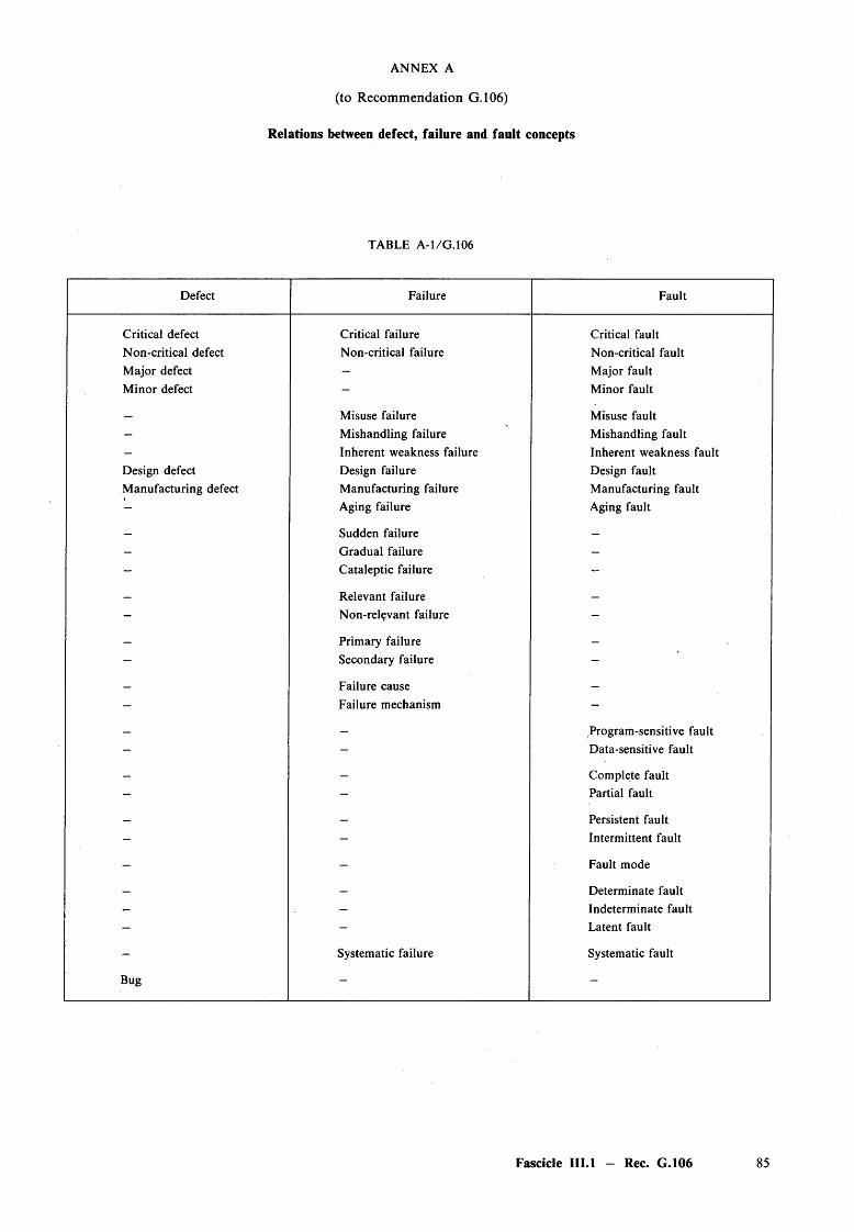
Relations between defect, failure and fault concepts
ANNEX A
(to Recommendation G.106)
TABLE A -1/G . 106
Defect Failure Fault
Critical defect Critical failure Critical faultNon-critical defect Non-critical failure Non-critical faultM ajor defect - Major faultM inor defect - M inor fault
— Misuse failure Misuse fault- Mishandling failure M ishandling fault- Inherent weakness failure Inherent weakness faultDesign defect Design failure Design faultM anufacturing defect M anufacturing failure Manufacturing fault- Aging failure Aging fault
— Sudden failure -
- Gradual failure -
- Cataleptic failure -
— Relevant failure —
- Non-relevant failure -
- Primary failure -
- Secondary failure -
- Failure cause -
- Failure mechanism -
- - Program-sensitive fault- - Data-sensitive fault
- - Complete fault- - Partial fault
— — Persistent fault
- - Intermittent fault
- - Fault mode
— — Determinate fault- - Indeterminate fault- - Latent fault
- Systematic failure Systematic fault
Bug - -
Fascicle III.l - Rec. G.106 85
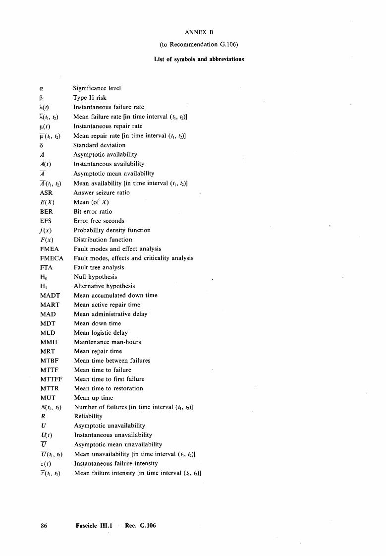
List of symbols and abbreviations
ANNEX B
(to Recommendation G.106)
a Significance levelp Type II risk7(f) Instantaneous failure rateX(rl9 t2) Mean failure rate [in time interval (t\, t2)\|i(r) Instantaneous repair rate
t2) Mean repair rate [in time interval (fl5 t2)]8 Standard deviationA Asymptotic availabilityA(t) Instantaneous availability~A Asymptotic mean availability~A(t\, t2) Mean availability [in time interval (tu t2)]ASR Answer seizure ratioE{X) Mean (of X)BER Bit error ratioEFS Error free secondsf ( x ) Probability density functionF ( x ) Distribution functionFMEA Fault modes and effect analysisFMECA Fault modes, effects and criticality analysisFTA Fault tree analysisH0 Null hypothesisHi Alternative hypothesisMADT Mean accumulated down timeMART Mean active repair timeMAD Mean administrative delayMDT Mean down timeMLD Mean logistic delayMMH M aintenance man-hoursMRT Mean repair timeMTBF Mean time between failuresMTTF Mean time to failureM TTFF Mean time to first failureMTTR Mean time to restorationMUT Mean up timeN(t\, t2) Number of failures [in time interval (tu t2)]R ReliabilityU Asymptotic unavailabilityU(t) Instantaneous unavailability77 Asymptotic mean unavailabilityU(t\, t2) Mean unavailability [in time interval (ft, /2)1z(t) Instantaneous failure intensityJ ( t x, t2) Mean failure intensity [in time interval (tu t2)]
86 Fascicle III.l — Rec. G.106
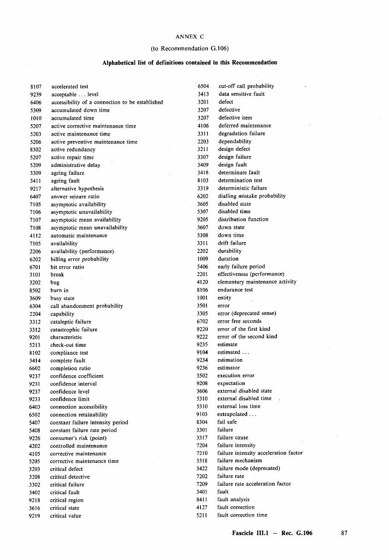
Alphabetical list of definitions contained in this Recommendation
ANNEX C
(to Recommendation G.106)
8107 accelerated test 6504 cut-off call probability9239 acceptable . . . level 3413 data sensitive fault6406 accessibility of a connection to be established 3201 defect5309 accumulated down time 3207 defective1010 accumulated time 3207 defective item5207 active corrective maintenance time 4106 deferred maintenance5203 active maintenance time 3311 degradation failure5206 active preventive maintenance time 2203 dependability8302 active redundancy 3211 design defect5207 active repair time 3307 design failure5209 administrative delay 3409 design fault3309 ageing failure 3418 determinate fault3411 ageing fault 8103 determination test9217 alternative hypothesis 3319 deterministic failure6407 answer seizure ratio 6202 dialling mistake probability7105 asymptotic availability 3605 disabled state7106 asymptotic unavailability 5307 disabled time7107 asymptotic mean availability 9205 distribution function7108 asymptotic mean unavailability 3607 down state4112 automatic maintenance 5308 down time7105 availability 3311 drift failure2206 availability (performance) 2202 durability6202 billing error probability 1009 duration6701 bit error ratio 5406 early failure period3101 break 2201 effectiveness (performance)3202 bug 4120 elementary maintenance activity8502 burn in 8106 endurance test3609 busy state 1001 entity6304 call abandonment probability 3501 error2204 capability 3305 error (deprecated sense)3312 cataleptic failure 6702 error free seconds3312 catastrophic failure 9220 error of the first kind9201 characteristic 9222 error of the second kind5213 check-out time 9235 estimate8102 compliance test 9104 estimated . . .3414 complete fault 9234 estimation6602 completion ratio 9236 estimator9237 confidence coefficient 3502 execution error9231 confidence interval 9208 expectation9237 confidence level 3606 external disabled state9233 confidence limit 5310 external disabled time
6403 connection accessibility 5310 external loss time6502 connection retainability 9103 extrapolated . . .5407 constant failure intensity period 8304 fail safe5408 constant failure rate period 3301 failure9226 consumer’s risk (point) 3317 failure cause4202 controlled maintenance 7204 failure intensity4105 corrective maintenance 7210 failure intensity acceleration factor5205 corrective maintenance time 3318 failure mechanism
3203 critical defect 3422 failure mode (deprecated)3208 critical detective 7202 failure rate3302 critical failure 7209 failure rate acceleration factor3402 critical fault 3401 fault9218 critical region 8411 fault analysis3616 critical state 4127 fault correction
9219 critical value 5211 fault correction time
Fascicle III.l - Rec. G.106 87
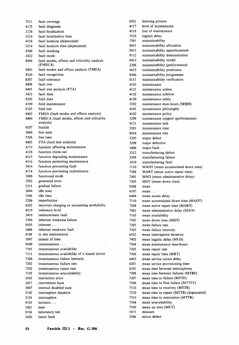
731141252126521441245214830634228404
84034124830784088405342382034109810584038404
9207360453068405411341284115411634144114100635023311360453063206620341193419330691053408410910079109710171117204720273027102350334173607510231019105100181043420
88
fault coverage fault diagnosis fault localization fault localization time fault location (deprecated) fault location time (deprecated) fault masking fault modefault modes, effects and criticality analysis (FMECA)fault modes and effects analysis (FMEA) fault recognition fault tolerance fault treefault tree analysis (FTA) fault item Field data field maintenance field testFMEA (fault modes and effects analysis)FMECA (fault modes, effects and criticalityanalysis)fractilefree statefree timeFTA (fault tree analysis)function affecting maintenancefunction check-outfunction degrading maintenancefunction permitting maintenancefunction preventing faultfunction preventing maintenancefunctional modegenerated errorgradual failureidle stateidle timeimperfectionincorrect charging or accounting probabilityindenture levelindeterminate faultinherent weakness failureinherent . . .inherent weakness faultin situ maintenanceinstant of timeinstantaneous . . .instantaneous availabilityinstantaneous availability of a leased circuitinstantaneous failure intensityinstantaneous failure rateinstantaneous repair rateinstantaneous unavailabilityinteraction errorintermittent faultinternal disabled stateinterruption durationinterruptionintrinsic . . .itemlaboratory test latent fault
8501 learning process4117 level of maintenance4118 line of maintenance5210 logistic delay7301 maintainability8415 maintainability allocation8415 maintainability apportionment8112 maintainability demonstration8412 maintainability model2208 maintainability (performance)8413 maintainability prediction8506 maintainability programme8111 maintainability verification4103 maintenance4121 maintenance action4118 maintenance echelon4130 maintenance entity5202 maintenance man-hours (MMH)4101 . maintenance philosophy4102 maintenance policy2209 maintenance support (performance)4121 maintenance task5201 maintenance time8414 maintenance tree3205 major defect3209 major defective3404 major fault ,3212 manufacturing defect3308 manufacturing failure3410 manufacturing fault7110 MADT (mean accumulated down time)7308 MART (mean active repair time)7401 MAD (mean administrative delay)7305 MDT (mean down time)9208 mean9107 mean . . .6404 mean access delay7110 mean accumulated down time (MADT)7308 mean active repair time (MART)7401 mean administrative delay (MAD)7103 mean availability7305 mean down time (MDT)7203 mean failure rate7205 mean failure intensity6102 mean interruption duration7403 mean logistic delay (MLD)7304 mean maintenance man-hours7303 mean repair rate7306 mean repair time (MRT)6402 mean service access delay6201 mean service provisioning time6101 mean time between interruptions7208 mean time between failures (MTBF)7207 mean time to failure (MTTF)7206 mean time to first failure (MTTFF)7310 mean time to recovery (MTTR)7310 mean time to repair (MTTR) (deprecated)7310 mean time to restoration (MTTR)7104 mean unavailability7109 mean up time (MUT)1011 measure3206 minor defect
Fascicle III.l - Rec. G.106
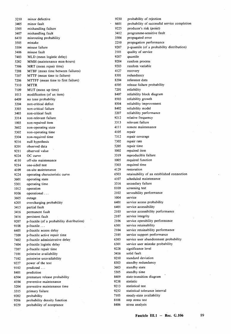
3210 minor defective 9230 probability of rejection
3405 minor fault • 6601 probability of successful service completion
3305 mishandling failure 9225 producer’s risk (point)3407 mishandling fault 3412 programme-sensitive fault6410 misrouting probability 3504 propagated error3505 mistake 2210 propagation performance3304 misuse failure 9207 p-quantile (of a probability distribution)3406 misuse fault 2101 quality of service7403 MLD (mean logistic delay) 9207 quantile5202 MMH (maintenance man-hours) 9204 random process7306 MRT (mean repair time) 9203 random variable7208 MTBF (mean time between failures) 4127 recovery7207 MTTF (mean time to failure) 8301 redundancy7206 M TTFF (mean time to First failure) 8204 reference data7310 MTTR 6505 release failure probability
7109 MUT (mean up time) 7201 reliability1013 modification (of an item) 8407 reliability block diagram
6409 no tone probability 8503 reliability growth3204 non-critical defect 8504 reliability improvement3303 non-critical failure 8402 reliability model3403 non-critical fault 2207 reliability performance3314 non-relevant failure 9212 relative frequency1003 non-repaired item 3313 relevant failure3602 non-operating state 4111 remote maintenance
5302 non-operating time 4105 repair5304 non-required time 7312 repair coverage
9216 null hypothesis 7302 repair rate
8201 observed data 5205 repair time9211 observed value 1002 repaired item
9224 OC curve 3319 reproducible failure4110 off-site maintenance 1005 required function9214 one-sided test 5303 required time
4109 on-site maintenance 4129 restoration
9224 operating characteristic curve 6503 retainability of an established connection
3601 operating state 4107 scheduled maintenance
5301 operating time 3316 secondary failure1012 operation 8109 screening test
9106 operational . . . 2102 serveability performance
3605 outage 1004 service
6205 overcharging probability 6401 service access probability
3415 partial fault 6401 service accessibility
3416 permanent fault 2103 service accessibility performance
3416 persistent fault 2107 service integrity
9207 p-fractile (of a probability distribution) 2106 service operability performance9108 p-fractile . . . 6501 service retainability
6405 p-fractile access delay 2104 service retainability performance
7309 p-fractile active repair time 2105 service support performance
7402 p-fractile administrative delay 6303 service user abandonment probability
7404 p-fractile logistic delay 6301 service user mistake probability
7307 p-fractile repair time 9228 significance level
7101 pointwise availability 3416 solid fault
7102 pointwise unavailability 9210 standard deviation9227 power of the text 8303 standby redundancy
9102 predicted . . . 3603 standby state
8401 prediction 5305 standby time6504 premature release probability 8409 state-transition diagram4104 preventive maintenance 9238 statistic5204 preventive maintenance time 9213 statistical test3315 primary failure 9232 statistical tolerance interval9202 probability 7105 steady-state availability9206 probability density function 8108 step stress test9229 probability of acceptance 8406 stress analysis
Fascicle III.l - Rec. G.106 89
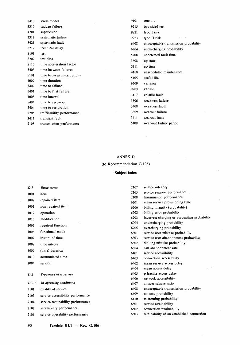
8410
3310
4201
33193421
5212
8101
8202
8110
5403
5101
10095402
5401
1008
5404
5404
220534172108
D .l
1001
1002
1003
1012
1013
1005
1006
1007
1008
1009
1010
1004
D.2
D.2.1
2101
2103
2104
2102
2106
90
stress model 9101 true . . .
sudden failure 9215 two-sided test
supervision 9221 type I risksystematic failure 9223 type II risksystematic fault 6408 unacceptable transmission probabilitytechnical delay 6204 undercharging probabilitytest 5208 undetected fault timetest data 3608 up-statetime acceleration factor
5311time between failures
up time
4108 unscheduled maintenancetime between interruptions
time duration5405 useful life
time to failure9209 variance
time to first failure 9203 variate
time interval 3417 volatile fault
time to recovery 3306 weakness failure
time to restoration 3408 weakness fault
trafficability performance 3309 wearout failure
transient fault 3411 wearout fault
transmission performance 5409
ANNEX D
wear-out failure period
(to Recommendation G .106)
Subject index
Basic terms 2107 service integrity
item 2105 service support performance2108 transmission performance
repaired item6201 mean service provisioning time
non repaired item 6206 billing integrity (probability)
operation 6202 billing error probability
modification 6203 incorrect charging or accounting probability
required function6204 undercharging probability6205 overcharging probability
functional mode 6301 service user mistake probabilityinstant of time 6303 service user abandonment probability
time interval 6302 dialling mistake probability
(time) duration6304 call abandonment rate
service accessibility6401accumulated time 6403 connection accessibilityservice 6402 mean service access delay
6404 mean access delay
Properties o f a service 6405 p-fractile access delay6406 network accessibility
In operating conditions 6407 answer seizure ratio
quality of service 6408 unacceptable transmission probability
service accessibility performance 6409 no tone probability
service retainability performance6410 misrouting probability6501 service retainability
serveability performance 6502 connection retainability
service operability performance 6503 retainability of an established connection
Fascicle III.l — Rec. G.106
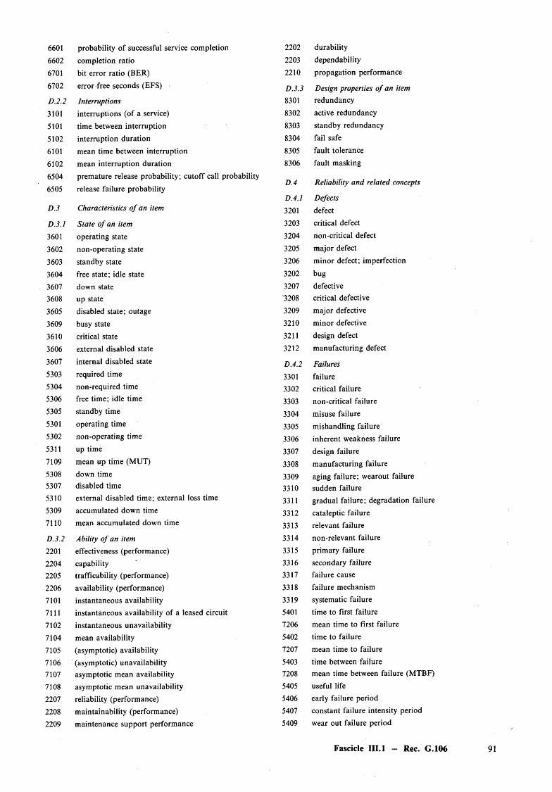
6601 probability of successful service completion 2202 durability
6602 completion ratio 2203 dependability
6701 bit error ratio (BER) 2210 propagation performance
6702 error free seconds (EFS) D.3.3 Design properties o f an item
D.2.2 Interruptions 8301 redundancy
3101 interruptions (of a service) 8302 active redundancy
5101 time between interruption 8303 standby redundancy
5102 interruption duration 8304 fail safe
6101 mean time between interruption 8305 fault tolerance
6102 mean interruption duration 8306 fault masking
6504 premature release probability; cutoff call probabilityD.4 Reliability and related concepts
Defects6505 release failure probability
D.4.1D.3 Characteristics o f an item 3201 defect
D.3.1 State o f an item 3203 critical defect
3601 operating state 3204 non-critical defect
3602 non-operating state 3205 major defect
3603 standby state 3206 minor defect; imperfection
3604 free state; idle state 3202 bug
3607 down state 3207 defective
3608 up state 3208 critical defective
3605 disabled state; outage 3209 major defective
3609 busy state 3210 minor defective
3610 critical state 3211 design defect
3606 external disabled state 3212 manufacturing defect
3607 internal disabled state D.4.2 Failures5303 required time 3301 failure5304 non-required time 3302 critical failure5306 free time; idle time 3303 non-critical failure5305 standby time 3304 misuse failure5301 operating time 3305 mishandling failure5302 non-operating time 3306 inherent weakness failure5311 up time 3307 design failure7109 mean up time (MUT) 3308 manufacturing failure5308 down time 3309 aging failure; wearout failure5307 disabled time 3310 sudden failure5310 external disabled time; external loss time 3311 gradual failure; degradation failure5309 accumulated down time 3312 cataleptic failure7110 mean accumulated down time 3313 relevant failure
D.3.2 Ability o f an item 3314 non-relevant failure
2201 effectiveness (performance) 3315 primary failure
2204 capability 3316 secondary failure
2205 trafficability (performance) 3317 failure cause
2206 availability (performance) 3318 failure mechanism
7101 instantaneous availability 3319 systematic failure
7111 instantaneous availability of a leased circuit 5401 time to first failure
7102 instantaneous unavailability 7206 mean time to first failure
7104 mean availability 5402 time to failure
7105 (asymptotic) availability 7207 mean time to failure
7106 (asymptotic) unavailability 5403 time between failure
7107 asymptotic mean availability 7208 mean time between failure (MTBF)
7108 asymptotic mean unavailability 5405 useful life
2207 reliability (performance) 5406 early failure period
2208 maintainability (performance) 5407 constant failure intensity period
2209 maintenance support performance 5409 wear out failure period
Fascicle III.l — Rec. G.106 91
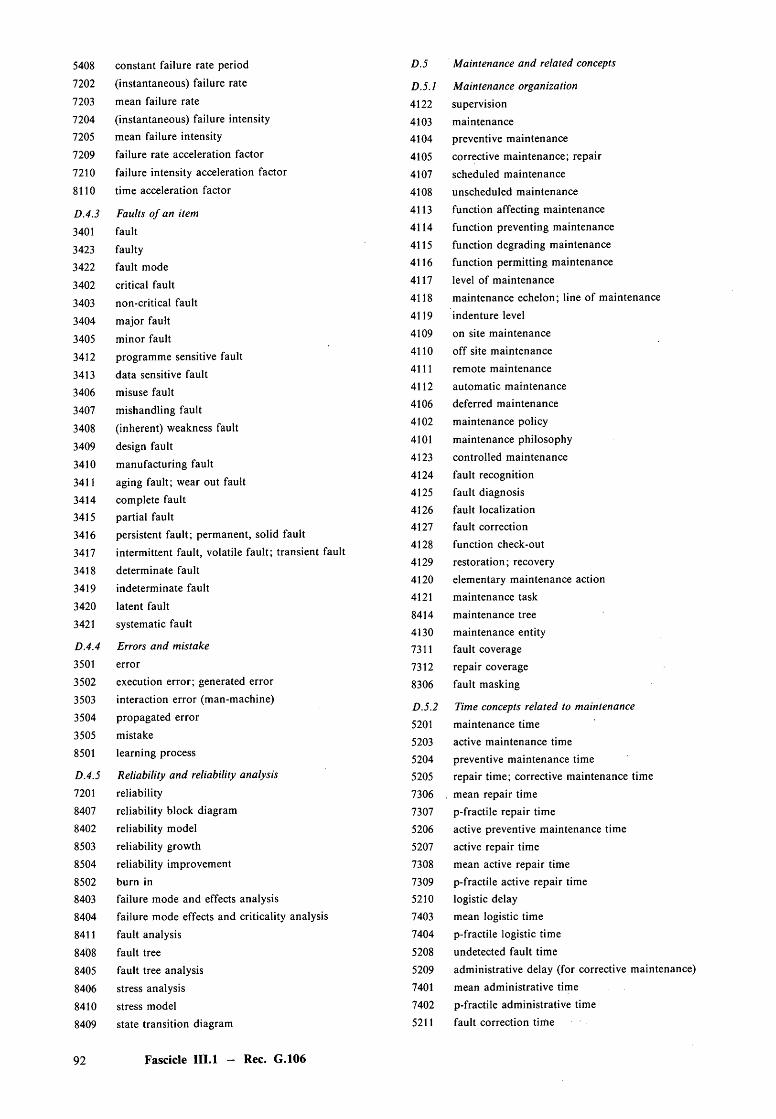
5408
7202
7203
72047205
7209
7210
8110
D.4.3
3401
34233422
3402
3403
3404
3405
3412
34133406
3407
3408
3409
3410
341134143415
3416
3417
3418
3419
3420
3421
D.4.4
3501
3502
3503
3504
3505
8501
D.4.57201
8407
8402
8503
8504
850284038404
8411
84088405
8406
8410
8409
92
constant failure rate period
(instantaneous) failure rate
mean failure rate
(instantaneous) failure intensity mean failure intensity
failure rate acceleration factor
failure intensity acceleration factor
time acceleration factor
Faults o f an item
fault
faulty fault mode
critical fault
non-critical fault
major fault
minor fault
programme sensitive fault
data sensitive fault
misuse fault
mishandling fault
(inherent) weakness fault
design fault
manufacturing fault
aging fault; wear out fault
complete fault partial faultpersistent fault; permanent, solid fault
intermittent fault, volatile fault; transient fault
determinate fault
indeterminate fault
latent fault
systematic fault
Errors and mistake
errorexecution error; generated error
interaction error (man-machine)
propagated error
mistake
learning process
Reliability and reliability analysis
reliabilityreliability block diagram
reliability model
reliability growth
reliability improvement
burn infailure mode and effects analysisfailure mode effects and criticality analysis
fault analysis
fault tree
fault tree analysis
stress analysis
stress modelstate transition diagram
Maintenance and related concepts
Maintenance organization
supervision
maintenance preventive maintenance
corrective maintenance; repair
scheduled maintenance
unscheduled maintenance
function affecting maintenance
function preventing maintenance
function degrading maintenance function permitting maintenance
level of maintenancemaintenance echelon; line of maintenance
indenture level
on site maintenance
off site maintenance
remote maintenanceautomatic maintenancedeferred maintenance
maintenance policy
maintenance philosophy
controlled maintenancefault recognition
fault diagnosisfault localizationfault correctionfunction check-out
restoration; recoveryelementary maintenance action
maintenance task
maintenance treemaintenance entityfault coverage
repair coveragefault masking
Time concepts related to maintenance
maintenance timeactive maintenance timepreventive maintenance timerepair time; corrective maintenance time
mean repair timep-fractile repair timeactive preventive maintenance time
active repair timemean active repair time
p-fractile active repair timelogistic delay
mean logistic timep-fractile logistic time
undetected fault timeadministrative delay (for corrective maintenance)
mean administrative time
p-fractile administrative time fault correction time
D.5
D.5.14122
41034104
41054107
4108
41134114
411541164117
4118
4119
41094110
4111
4112
41064102
4101
412341244125
41264127
4128412941204121
8414
413073117312
8306
D.5.2
5201520352045205
73067307
520652077308
73095210
74037404
5208
520974017402
5211
Fascicle III.l — Rec. G.106
5212 technical delay D.6.2 Statistics
5213 check out time 9238 statistic
5214 fault localization time 9201 characteristic
5202 maintenance man-hours 9212 relative frequency7302 instantaneous repair rate 9213 statistical test
7303 mean repair rate 9216 null hypothesis5404 time to restoration; time to recovery 9217 alternative hypothesis
7310 mean time to recovery; mean time to restoration 9214 one sided test
7305 mean down time 9215 two sided test
7304 mean maintenance man-hours 9228 significance level
D.5.3 Maintainability concepts 9218 critical region
7301 maintainability 9219 critical values
8505 maintainability program 9220 error of the first kind
8412 maintainability model 9221 type I risk
8111 maintainability verification 9222 error of the second kind
8112 maintainability demonstration 9223 type II risk
8415 maintainability allocation; maintainability 9227 power of the test
apportionm ent '8201 observed data; observed value
8413 maintainability prediction 8202 test data
D.5.4 Test concepts 8203 field data
8101 test 8204 reference data
8102 compliance test 9101 true
8103 determination test 9102 predicted
8104 laboratory test 8401 prediction
8105 field test 9104 estimated . . .
8106 endurance test 9103 extrapolated . . .
8107 accelerated test 9105 intrinsic . . . ; inherent . . .
8108 step stress test 9106 operational . . .
8109 screening test 9234 estimation
9235 estimateD.6 Probability, statistics and related concepts 9236 estimator
D.6.1 Probability 9237 confidence coefficient
9202 probability 9233 confidence limit
9203 random variable; variate 9231 confidence interval9204 random process; stochastic process 9232 statistical tolerance interval
9205 distribution function 9229 probability of acceptance
9206 probability density function 9230 probability of rejection
9208 mean; expectation 9239 acceptable level
9209 variance 9224 operating characteristic curve
9210 standard deviation 9225 producer risk
9207 p-fractile; p-quantile (of a probability distribution) 9226 consumer’s risk
Fascicle III.l — Rec. G.106 93
Recommendation G.107
GENERAL CONSIDERATIONS AND MODEL OF A BASIC TELEPHONE CALL')
(Malaga-Torremolinos, 1984)
Introduction\
This Recommendation is one of a set of closely related Recommendations concerned with the accessibility and retainability of telephone services, as listed below.
The CCITT,
considering
(a) that there is a desire to establish overall objectives for the quality of service as perceived by the users;
(b) that such objectives can then be used as a basis for the design, planning, operation and maintenanceof telecommunication networks and their component parts;
(c) that Recommendation G.106 contains terms and definitions for the quality of service, the reliabilityand availability performances and related characteristics of services and networks,
recommends
that the telephone call model given in this Recommendation shall be used by Administrations to design, plan, operate and m aintain their networks taking into account the objectives given in Recommendations:
G.180 Connection accessibility objective for the international telephone service;G.181 Connection retainability objective for the international telephone service;G.108 Models for the allocation of international telephone connection retainability objectives.
Note — Refer also to draft Recommendation G.ABC on interruption objectives which is being studied under Question 39/11 (Annex 1).
1 Model of a basic telephone call
The following simplified model illustrates the principal phases of a basic telephone call. It also interrelates these phases to the service-related performance concepts and their principal measures as well as to the main causes of failure in the establishment and retention of such a call and its subsequent billing.
The model also indicates where, in this series of phases, user actions or mistakes may influence the call.
2 Comments to the model and its applications
2.1 Mathematical modelling
In a simple case of statistical independence, the probabilities may be combined into the following mathematical models:
P = ( i ’ll • Pm) • Pi • (A i • P32) • P4
to express the probability of a correctly billed revenue-making call and,
P - ( i ’ll • Pm) • Pi ■ (i>3i • Pn)
to express the probability of a successfully completed call.
^ Some of the terms in this Recommendation, for example the noun “measure”, are used in the sense of their definition given in Recommendation G.106.
94 Fascicle III.l — Rec. G.107
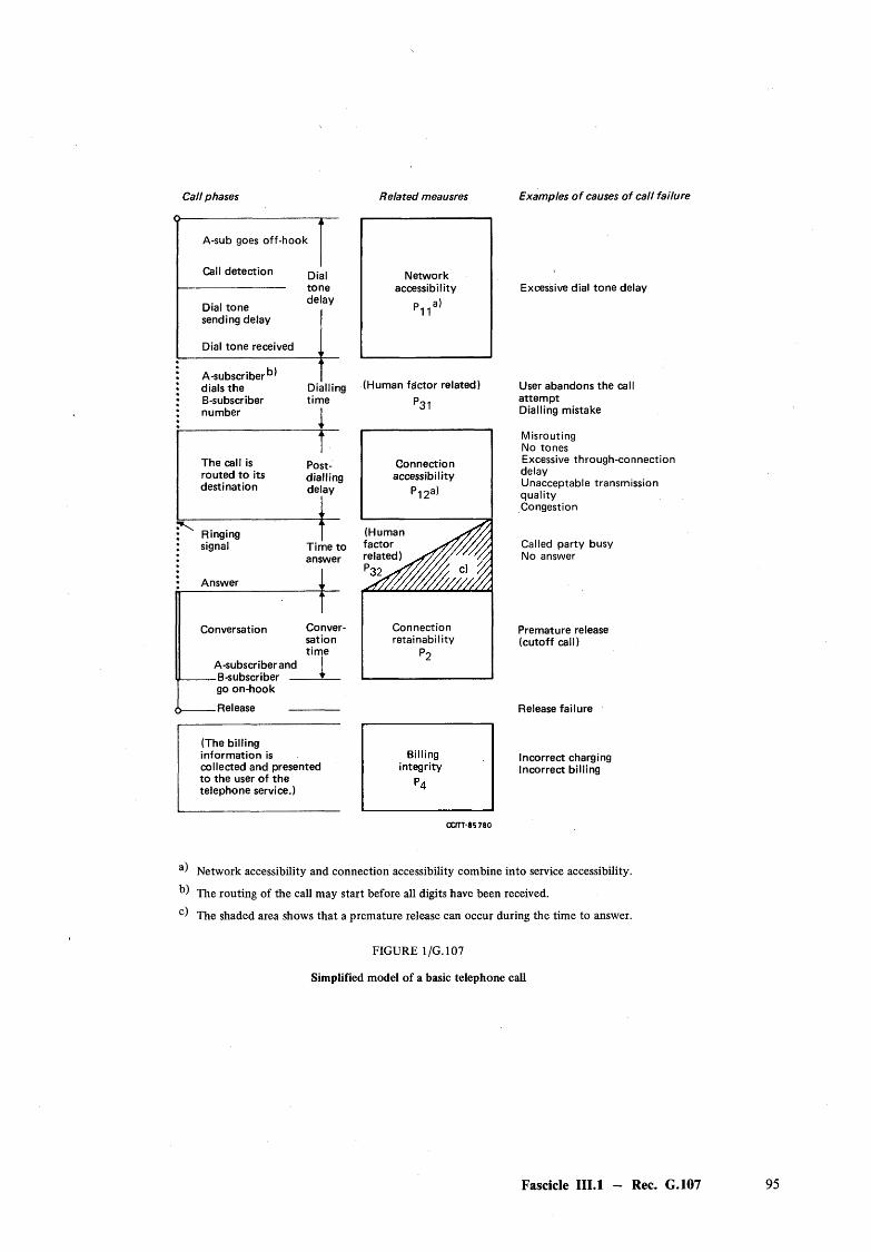
C all p h a se s R e la te d m e a u sres E x a m p le s o f c a u ses o f ca ll fa ilu re
A-sub goes off-hook
Call detection
Dial tone sending delay
Dial tone received
Dialtonedelay
A-subscriber*- dials the DiallingB-subscriber timenumber
The call is routed to its destination
Post-diallingdelay
Ringingsignal
Answer
Time to answer
Conversation
A-subscriberand _ B-subscriber
go on-hook
Conversationtime
.Release
(The billing information is collected and presented to the user of the telephone service.)
Networkaccessibility
p a) P11
(Human factor related)
P31
Connection accessibility
P12a)
(Human factor related) P
Connectionretainability
Excessive dial tone delay
User abandons the call attemptDialling mistake
Misrouting No tonesExcessive through-connection delayUnacceptable transmissionqualityCongestion
Called party busy No answer
Premature release (cutoff call)
Release failure
Incorrect charging Incorrect billing
a-* Network accessibility and connection accessibility combine into service accessibility,
k) The routing of the call may start before all digits have been received.
The shaded area shows that a premature release can occur during the time to answer.
FIGURE 1/G. 107
Simplified model of a basic telephone call
Fascicle III.l — Rec. G.107
2.2 Contributions to causes o f call failure
It is generally recognized that the various parts of a national or international network may be of different importance to the successful completion of the various phases of a call. For example, the network accessibility is mainly determined by the telephone set, the subscriber line and the local exchange; the connection accessibility by the exchanges, transmission network and signalling network used; the billing integrity is dependent on the charging facilities used by the network parts that constitute the connection and the equipment for processing the billing information, etc.
2.3 Time aspects o f measures
Depending on the intended application of the measures indicated in Figure 1 /G.107, it may be appropriateto express these measures as instantaneous values related to a given instant o f time or as a mean over a given timeinterval.
Advice on which variant to use should be given in each specific relevant Recommendation.
2.4 Space aspects o f averages
The measures as indicated in Figure 1/G . 107 could be applied to calls between particular destinations astraffic weighted averages over a num ber of destinations, etc.
Each relevant Recommendation should clearly specify which alternative(s) to use.
Recommendation G.108
MODELS FOR THE ALLOCATION OF INTERNATIONAL TELEPHONE CONNECTION RETAINABILITY
(Malaga-Torremolinos, 1984)
Introduction
This Recommendation is one of a set o f closely related Recommendations, comprising Recommendations G.107, G.108, G.180 and G.181 concerned with the accessibility and retainability of telephone services.
The CCITT,
considering
that there is a need to establish hypothetical reference connection models to allocate overall connection retainability objectives to the com ponent parts o f international connections,
recommends
three models, one for a typical, or average, international connection.
1 Model types
The models are shown respectively, in Figures 1/G . 108, 2/G.108 and 3/G.108. As indicated by Figure 1/G . 108, the typical connection has two circuits in each of the national systems, and one in the international chain. In the 90th percentile case, there would be three in the national systems and one in the international chain.
96 Fascicle III.l — Rec. G.108
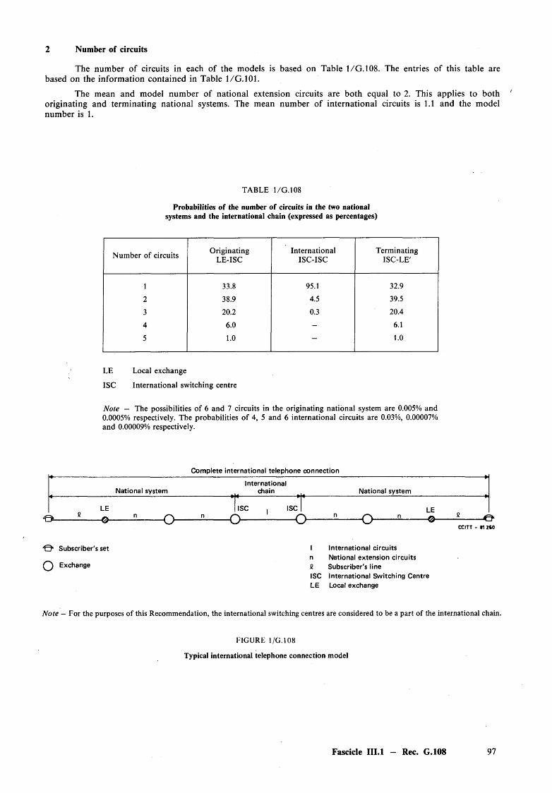
2 Number of circuits
The number of circuits in each of the models is based on Table 1/G . 108. The entries of this table are based on the information contained in Table 1/G . 101.
The mean and model number of national extension circuits are both equal to 2. This applies to both originating and terminating national systems. The mean number of international circuits is 1.1 and the model number is 1.
TABLE 1/G . 108
Probabilities of the number of circuits in the two national systems and the international chain (expressed as percentages)
Number of circuits OriginatingLE-ISC
InternationalISC-ISC
TerminatingISC-LE'
1 33.8 95.1 32.9
2 38.9 4.5 39.5
3 20.2 0.3 20.4
4 6.0 - 6.1
5 1.0 - 1.0
LE Local exchange
ISC International switching centre
Note — The possibilities of 6 and 7 circuits in the originating national system are 0.005% and0.0005% respectively. The probabilities of 4, 5 and 6 international circuits are 0.03%, 0.00007%and 0.00009% respectively.
Complete international telephone connection
InternationalNational system chain National system
LE ISC , ISC LEl_C IOO 1 IOG
© ------- e-— 0 ------- =-------- o -------- 2--------O ----------------- O -------- 2--------O --------2-------- 0 — --------&CCITT - r 2 (0
Subscriber's set I International circuitsn National extension circuits
O Exchange q Subscriber's lineISC International Switching Centre LE Local exchange
Note - For the purposes of this Recommendation, the international switching centres are considered to be a part of the international chain.
FIGURE 1/G.108
Typical international telephone connection model
Fascicle III.l — Rec. G.108 97
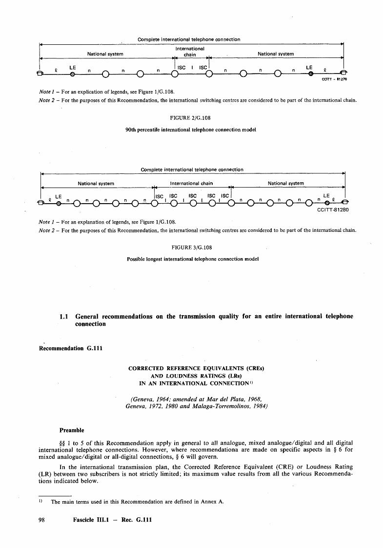
Complete international telephone connection
National systemInternational
chain National system
O -LE ISC I ISC LE!L_o—=—o— o------o ——o—-— — • - O
CCITT - s i 270
Note 1 - For an explication of legends, see Figure 1/G. 108.Note 2 - For the purposes of this Recommendation, the international switching centres are considered to be part of the international chain.
FIGURE 2/G.108
90th percentile international telephone connection model
Complete international telephone connection
National system International chain National system
n LE ISC ISC ISC ISC ISC LE
CCITT-81280
Note 1 - For an explanation of legends, see Figure 1/G.108.Note 2 - For the purposes of this Recommendation, the international switching centres are considered to be part of the international chain.
FIGURE 3/G. 108
Possible longest international telephone connection model
1.1 General recommendations on the transmission quality for an entire international telephone connection
Recommendation G .l l l
CORRECTED REFERENCE EQUIVALENTS (CREs) AND LOUDNESS RATINGS (LRs)
IN AN INTERNATIONAL CONNECTION1)
(Geneva, 1964; amended at M ar del Plata, 1968, Geneva, 1972, 1980 and Malaga-Torremolinos, 1984)
Preamble
§§ 1 to 5 of this Recommendation apply in general to all analogue, mixed analogue/digital and all digital international telephone connections. However, where recommendationa are made on specific aspects in § 6 for mixed analogue/digital or all-digital connections, § 6 will govern.
In the international transmission plan, the Corrected Reference Equivalent (CRE) or Loudness Rating (LR) between two subscribers is not strictly limited; its maximum value results from all the various Recommendations indicated below.
0 The main terms used in this Recommendation are defined in Annex A.
98 Fascicle III.l - Rec. G .l l l

The CCITT,
considering
(a) that the studies of the CCITT during the Study Period 1977-1980 have enabled values of sending, receiving and overall reference equivalents to be converted to corrected reference equivalents (CREs), the properties of which are described in Annex A;
(b) that loudness ratings (LRs) have been defined in Recommendation P.76;
(c) that there now exists a complete set of Recommendations based on CRE in this Volume III, thus eliminating most of the uncertainties concerning the use of reference equivalents for planning purposes and at the same time keeping continuity with past practice;
(d) that the conversion from reference equivalent and CRE to loudness rating is sufficiently accurate for general comparison purposes and it is therefore possible to recommend limits and mean values in terms of LR in Recommendations G . l l l and G.121;
(e) that for the reasons given in Recommendation G.121 it is necessary to have the limits and mean values for national systems expressed both in terms of CRE and LR,
that the values given below, either in terms of CRE or LR, should be used to verify that international telephone connections provide an adequate loudness of received speech.
Note — The conversion formulas mentioned in (d) above should not be used to translate CREs for a specific telephone set to LRs, but, rather, the LRs should be determined by direct measurements on this telephone set.
1 Nominal CREs and LRs of the national systems
1.1 Definition o f nominal CREs or LRs of the national systems
The sending and receiving CRE or LR of the national systems are calculated to, and from, the virtual analogue switching points of the international system; that is to say, points a and b of Figure 1 /G .l l l .
recommends
I ►-3,5 dBr
O —x—x—x—"t* * *
For the relative levels of digital circuits, see a) of Figure 2/G.101
National system International circuit
CCITT - 4 1 9 8 2
Virtual analogue switching points of the international circuit
Note - The values of relative level shown are those of the international circuit. The values of the relative levels of the national circuit are not shown, since they depend on the national transmission plan. The virtual analogue switching points will generally have no physical existence, but are a necessary concept in the planning of national systems.
FIGURE 1 /G .ll l
Definition of the virtual analogue switching points
Fascicle III.I — Rec. G . l l l 99
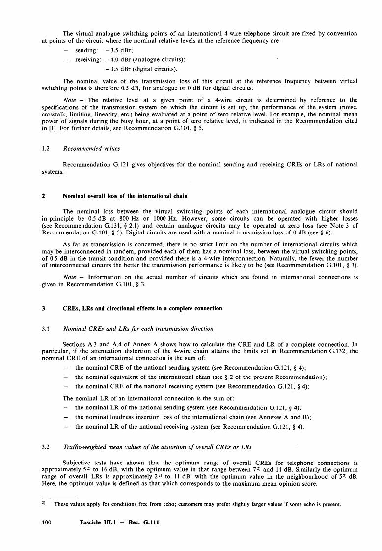
The virtual analogue switching points of an international 4-wire telephone circuit are fixed by convention at points of the circuit where the nominal relative levels at the reference frequency are:
— sending: —3.5 dBr;— receiving: —4.0 dBr (analogue circuits);
— 3.5 dBr (digital circuits).
The nominal value of the transmission loss of this circuit at the reference frequency between virtual switching points is therefore 0.5 dB, for analogue or 0 dB for digital circuits.
Note — The relative level at a given point of a 4-wire circuit is determined by reference to the specifications of the transmission system on which the circuit is set up, the performance of the system (noise, crosstalk, limiting, linearity, etc.) being evaluated at a point of zero relative level. For example, the nominal meanpower of signals during the busy hour, at a point of zero relative level, is indicated in the Recommendation citedin [1]. For further details, see Recommendation G.101, § 5.
1.2 Recommended values
Recommendation G.121 gives objectives for the nominal sending and receiving CREs or LRs of national systems.
2 Nominal overall loss of the international chain
The nominal loss between the virtual switching points of each international analogue circuit should in principle be 0.5 dB at 800 Hz or 1000 Hz. However, some circuits can be operated with higher losses (see Recommendation G.131, § 2.1) and certain analogue circuits may be operated at zero loss (see Note 3 of Recommendation G.101, § 5). Digital circuits are used with a nominal transmission loss of 0 dB (see § 6).
As far as transmission is concerned, there is no strict limit on the number of international circuits which may be interconnected in tandem, provided each of them has a nominal loss, between the virtual switching points, of 0.5 dB in the transit condition and provided there is a 4-wire interconnection. Naturally, the fewer the number o f interconnected circuits the better the transmission performance is likely to be (see Recommendation G.101, § 3).
Note — Inform ation on the actual number of circuits which are found in international connections is given in Recommendation G.101, § 3.
3 CREs, LRs and directional effects in a complete connection
3.1 Nominal CREs and LRs fo r each transmission direction
Sections A.3 and A.4 of Annex A shows how to calculate the CRE and LR of a complete connection. In particular, if the attenuation distortion of the 4-wire chain attains the limits set in Recommendation G.132, the nominal CRE of an international connection is the sum of:
— the nominal CRE of the national sending system (see Recommendation G.121, § 4);— the nominal equivalent o f the international chain (see § 2 of the present Recommendation);— the nominal CRE of the national receiving system (see Recommendation G.121, § 4);
The nominal LR of an international connection is the sum of:— the nominal LR of the national sending system (see Recommendation G.121, § 4);— the nominal loudness insertion loss of the international chain (see Annexes A and B);— the nominal LR of the national receiving system (see Recommendation G.121, § 4).
3.2 Traffic-weighted mean values o f the distortion o f overall CREs or LRs
Subjective tests have shown that the optimum range of overall CREs for telephone connections isapproximately 52> to 16 dB, with the optimum value in that range between 7 2> and 11 dB. Similarly the optimumrange of overall LRs is approximately 2 2> to 11 dB, with the optimum value in the neighbourhood of 5 2> dB. Here, the optimum value is defined as that which corresponds to the maximum mean opinion score.
These values apply for conditions free from echo; customers may prefer slightly larger values if some echo is present.
100 Fascicle III.l - Rec. G .l l l
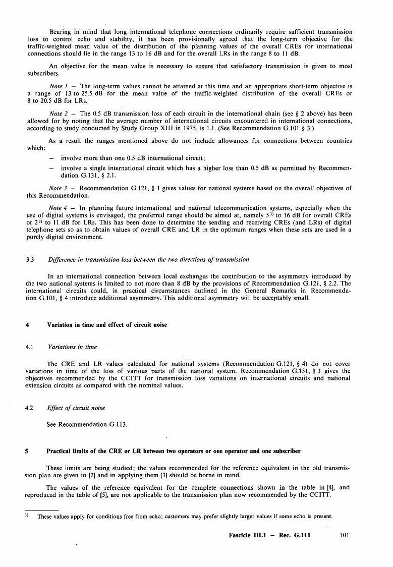
Bearing in mind that long international telephone connections ordinarily require sufficient transmission loss to control echo and stability, it has been provisionally agreed that the long-term objective for the traffic-weighted mean value of the distribution o f the planning values o f the overall CREs for international connections should lie in the range 13 to 16 dB and for the overall LRs in the range 8 to 11 dB.
An objective for the mean value is necessary to ensure that satisfactory transmission is given to most subscribers.
Note 1 — The long-term values cannot be attained at this time and an appropriate short-term objective is a range of 13 to 25.5 dB for the mean value of the traffic-weighted distribution of the overall CREs or 8 to 20.5 dB for LRs.
Note 2 — The 0.5 dB transmission loss of each circuit in the international chain (see § 2 above) has been allowed for by noting that the average number of international circuits encountered in international connections, according to study conducted by Study Group X III in 1975, is 1.1. (See Recommendation G.101 § 3.)
As a result the ranges mentioned above do not include allowances for connections between countrieswhich:
— involve more than one 0.5 dB international circuit;
— involve a single international circuit which has a higher loss than 0.5 dB as permitted by Recommendation G.131, § 2.1.
Note 3 — Recommendation G.121, § 1 gives values for national systems based on the overall objectives of this Recommendation.
Note 4 — In planning future international and national telecommunication systems, especially when the use of digital systems is envisaged, the preferred range should be aimed at, namely 53> to 16 dB for overall CREs or 2 3> to 11 dB for LRs. This has been done to determine the sending and receiving CREs (and LRs) of digital telephone sets so as to obtain values of overall CRE and LR in the optimum ranges when these sets are used in a purely digital environment.
3.3 Difference in transmission loss between the two directions o f transmission
In an international connection between local exchanges the contribution to the asymmetry introduced by the two national systems is limited to not more than 8 dB by the provisions of Recommendation G.121, § 2.2. The international circuits could, in practical circumstances outlined in the General Remarks in Recommendation G.101, § 4 introduce additional asymmetry. This additional asymmetry will be acceptably small.
4 Variation in time and effect of circuit noise
4.1 Variations in time
The CRE and LR values calculated for national systems (Recommendation G.121, § 4) do not cover variations in time of the loss of various parts of the national system. Recommendation G.151, § 3 gives the objectives recommended by the CCITT for transmission loss variations on international circuits and national extension circuits as compared with the nominal values.
4.2 Effect o f circuit noise
See Recommendation G.113.
5 Practical limits of the CRE or LR between two operators or one operator and one subscriber
These limits are being studied; the values recommended for the reference equivalent in the old transmission plan are given in [2] and in applying them [3] should be borne in mind.
The values of the reference equivalent for the complete connections shown in the table in [4], and reproduced in the table of [5], are not applicable to the transmission plan now recommended by the CCITT.
These values apply for conditions free from echo; customers may prefer slightly larger values if some echo is present.
Fascicle III.l — Rec. G .l l l 101
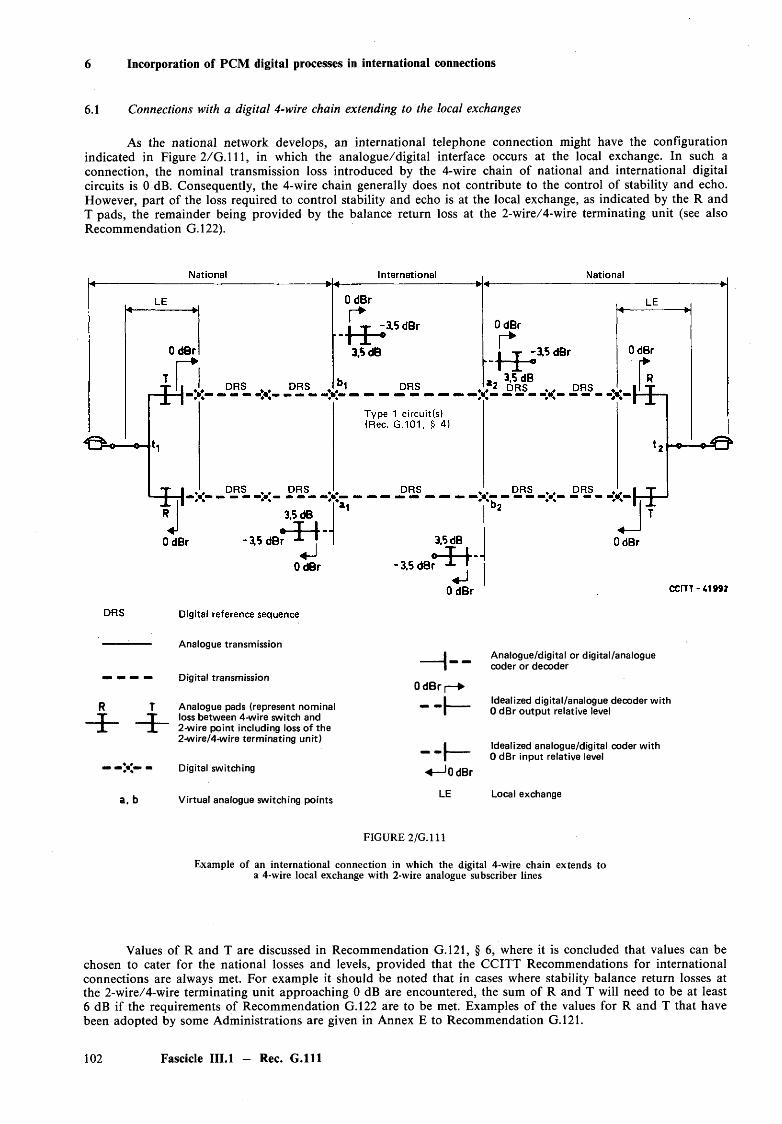
6 Incorporation of PCM digital processes in international connections
6.1 Connections with a digital 4-wire chain extending to the local exchanges
As the national network develops, an international telephone connection might have the configuration indicated in Figure 2 /G .l 11, in which the analogue/digital interface occurs at the local exchange. In such a connection, the nominal transmission loss introduced by the 4-wire chain of national and international digital circuits is 0 dB. Consequently, the 4-wire chain generally does not contribute to the control of stability and echo. However, part of the loss required to control stability and echo is at the local exchange, as indicated by the R and T pads, the remainder being provided by the balance return loss at the 2-wire/4-wire terminating unit (see also Recommendation G.122).
Analogue transmission
Digital transmission
R T Analogue pads (represent nominalT T loss between 4-wire switch and1 I 2-wire point including loss of the
2-wire/4-wire terminating unit)
a. b
Digital switching
Virtual analogue switching points
O d B r
- I —<«— •OdBr
LE
Analogue/digital or digital/analogue coder or decoder
Idealized digital/analogue decoder with 0 dBr output relative level
Idealized analogue/digital coder with 0 dBr input relative level
Local exchange
FIGURE 2/G .l 11
Example of an international connection in which the digital 4-wire chain extends to a 4-wire local exchange with 2-wire analogue subscriber lines
Values of R and T are discussed in Recommendation G.121, § 6, where it is concluded that values can be chosen to cater for the national losses and levels, provided that the CCITT Recommendations for international connections are always met. For example it should be noted that in cases where stability balance return losses at the 2-wire/4-wire terminating unit approaching 0 dB are encountered, the sum of R and T will need to be at least 6 dB if the requirements of Recommendation G.122 are to be met. Examples of the values for R and T that have been adopted by some Administrations are given in Annex E to Recommendation G.121.
102 Fascicle III.l — Rec. G .l l l
Other transmission considerations to be taken into account in the planning of connections involving 4-wire local exchanges in a mixed analogue/digital network include system loading and crosstalk.
tThe amount of loss to be introduced individually by the R and T pads of Figure 2 /G .l 11, can be regarded
as a national matter within the constraints referred to above. Within these constraints, individual national transmission plans should govern the values to be assigned to the R and T pads. This aspect is dealt with in some detail in Recommendation G.121, § 6.
Figure 2 /G .l 11 also shows R and T as analogue pads. This need not always be the case since under some conditions it might be more practical or necessary to introduce the required loss by means of digital pads. However, if digital pads are used, their detrimental effect on digital data or other services requiring end-to-end bit integrity must be taken into account as indicated in Recommndations G.101, § 4.4 and G.103, § 4.
6.2 M ixed analogue/digital connections
To provide satisfactory transmission on international connections in the mixed analogue/digital period, it is likely that existing national transmission plans will have to be amended or new ones developed to provide for appropriate national extensions. All the relevant CCITT Recommendations should be complied with. The Recommendations concerning national extensions with 4-wire chains extending 4-wire local exchanges are given in Recommendation G.121, § 6.
ANNEX A
(to Recommendation G .l l l )
Definitions related to Recommendations G .l l l and G.121: properties of the CREs
A.l Terminology to be used in relation with Recommendations G. l l l , G.120 and G.121
A. 1.1 B rief definitions
A. 1.1.1 Loudness loss (F: affaiblissement en sonie ; S: perdida de sonoridad): the most general term.
A. 1.1.2 Loudness insertion loss (F: affaiblissement d ’insertion en sonie; S: perdida de sonoridad por insercion): defined in Annex B.
A. 1.1.3 Loudness rating (F: equivalent pour la sonie, E S ; S : indice de sonoridad, IS): is very general and might well apply to loudness loss. In CCITT usage, it should be restricted to a measure conforming to Recommendation P.76 and may be abbreviated to LR.
722.43.25 4>
A. 1.1.4 Reference equivalent, R E (F: equivalent de reference, E R ; S: equivalente de referenda, ER): see § A. 1.2.1.
722.43.14
A. 1.1.5 Relative equivalent (F: equivalent relatif; S: equivalente relativo): defined in Recommendation P.72 with reference to a working standard (systeme etalon de travail).
722.43.22
A. 1.1.6 R25 equivalent (F: equivalent R25; S: equivalente R 25 ): determined as a reference equivalent, except that the listening level is constant, corresponding to 25 dB in NOSFER (see § A. 1.3).
4) These numbers refer to Chapter 722 of the IEV (1984 edition), published by IEC; the definitions are reproduced in Recommendation P. 10.
Fascicle III.l — Rec. G .l l l 103

A. 1.1.7 Corrected reference equivalent (F: equivalent de reference corrige, ERC; S: equivalente de referenda corregido, ERC): defined in § A. 1.3 below, may be abbreviated to CRE.
722.43.17
A .I.1.8 Planning equivalent (F: equivalent de planification; S: equivalente de planificacion): result of a measurement with an objective meter which may be considered equal to an R25 equivalent or to a CRE, with an accuracy which is sufficient for planning purposes.
A .I.1.9 Attenuation distortion equivalent (ADE) (F: equivalent de distortion d ’affaiblissement, EDA S: equivalente de distorsion de atenuacion, E D A ): see §§ A.3.3, Note 2 and for more details Annex B.
A. 1.2 Reasons fo r introducing CRE
A. 1.2.1 In older draftings of Recommendation G .l l l [6] it was assumed that the “planning value of the overall reference equivalent of a complete connection” is the sum of the following nominal values:
— the reference equivalents, q, of the local sending and receiving systems which are involved,
— the transmission losses, x, (at 800 or 1000 Hz) of the chain of lines and exchanges interconnecting the two local systems.
In practice, the reference equivalents of the local systems are determined by subjective tests, in accordance with Recommendation P.72, by comparing paths 3 or 4 of Figure A - l /G . l l l (where x3 and x4 have been fixed at values taken at random between 24 and 34 dB) with the NOSFER reference system (path 2), x2 being adjusted so as to obtain the same impression of loudness.
A. 1.2.2 If a local system were to be associated with a circuit having a loss x and without distortion, it would be found that the reference equivalent of the system increases by a value smaller than x. Consequently, the “planning values” obtained by addition do not correspond to any physically well-defined quantity which can be determined directly by subjective tests or by calculation from objective measurements.
A. 1.2.3 This situation has caused many difficulties in the past. Tests made in the CCITT Laboratory have shown that most of these difficulties are connected with the method of determining reference equivalents, where the level of the sounds received varies with the reference equivalent to be determined.
A.l.2.4 As a first stage in the study of Question 19/X II, the V llth Plenary Assembly of the CCITT (Geneva, 1980) approved the revision of Recommendations G .l l l and G.121 on the basis o f the “corrected reference equivalents” defined in § A. 1.3 below. The sections or paragraphs of the Recommendations to which the paragraphs of this Annex apply are shown in brackets.
A. 1.3 Definition o f R25 quivalent and corrected reference equivalent (CRE) ( G .l l l , § 1.1)
If x2 is fixed at 25 dB in the NOSFER (path 2 of Figure A - l /G .l l l ) , the relevant provisions of Recommendation P.72 being applied, then “R25 equivalents” of a sending system (path 3), a receiving system (path 4) or a complete system (path 6) can be determined. In this case, the rating of a distortionless circuit is by definition equal to its loss x, which greatly simplifies planning. The introduction of a new subjective test method does not, however, seem to be justified, since reference equivalent values, q, are available for many local systems and the corresponding R25 equivalents may be calculated as described below.
The “corrected reference equivalent” (CRE) of a local system or a complete system is termed y.
y = 0.0082 q2 + 1.148 q + 0.48 dB (A-l)
which can also be written:
y = 0.0082 (q + 70)2 -3 9 .7 dB.
This formula has been deduced from tests in which IRS-2, which transmits a frequency band comparable to that o f a commercial system, has been compared to NOSFER with a very wide range of variation of q. It has been found that R25 equivalent is obtained with a good approximation for various types of local systems (subscriber sets with their line) comprising, as for IRS-2, a linear microphone.
Table A - l /G . l l l gives the values y o f CRE for the integral values of q within the range useful for network planning.
104 Fascicle III.l - Rec. G .l l l

JS NS IS IR NR JR
Path 1 — Complete connection
JS ' X'Path 2 — Reference system (NOSFER) *
LTSl«---------------------- ►
JR
Ee
Equivalent measured (see note)
IReferencereception
- a Sending equivalent
JS
Path 3 — For the determination of a sending equivalent
JR
LTS
Circuitstudied
JS *5Path 5 — For the determination of overall equivalent
LTSh -Et
JS
Path 6 — Overall system, send and receive
JR
JR
LTS
Overall equivalent
OVE = x2 ~ x 5
LTS -►I Equivalent for send and receive
] OSR =. 2 — 6
dCCITT - 42001
JS Junction sending side JR Junction receiving side NS National sending side IS International sending side IR International receiving side NR National receiving sideLTS Local telephone system studied (telephone set + line + feeding bridge).
Note - x is obtained in each case by balancing the path in question with NOSFER. The equivalents measured are:
a) reference equivalents if x 2 is varied so as to obtain the balance;b) R25 equivalents if x 2 is set at 25 dB.
FIGURE A -l/G .lll
Connections and systems considered for the definition of reference equivalents and R25 equivalents
Fascicle III.1 - Rec. G .l l l
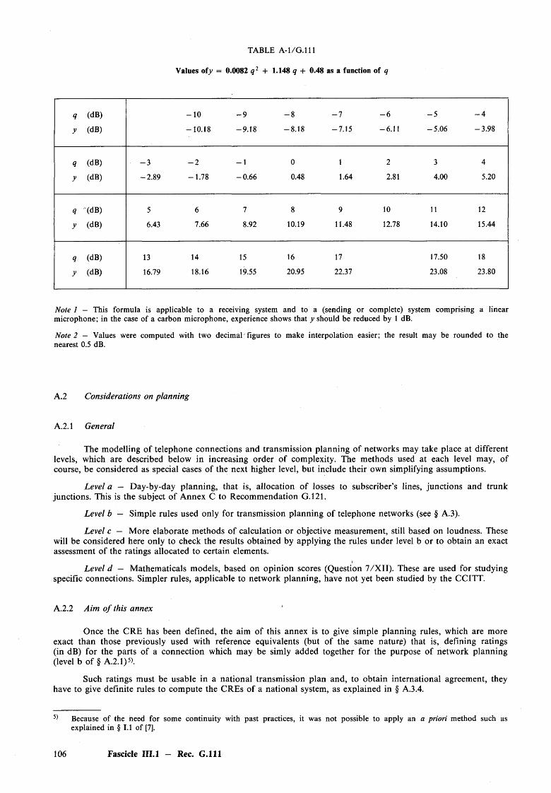
TABLE A - l /G . l l l
Values ofy = 0.0082 q 2 + 1.148 q -I- 0.48 as a function of q
q (dB) - 1 0 - 9 - 8 - 7 - 6 - 5 - 4
y (dB) -10 .18 -9 .1 8 -8 .1 8 -7 .1 5 -6 .11 -5 .0 6 -3 .9 8
q (dB) - 3 - 2 - 1 0 1 2 3 4
y (dB) -2 .8 9 -1 .7 8 -0 .6 6 0.48 1.64 2.81 4.00 5.20
q "(dB) 5 6 7 8 9 10 11 12
y (dB) 6.43 7.66 8.92 10.19 11.48 12.78 14.10 15.44
q (dB) 13 14 15 16 17 17.50 18
y (dB) 16.79 18.16 19.55 20.95 22.37 23.08 23.80
Note 1 — This formula is applicable to a receiving system and to a (sending or complete) system comprising a linear microphone; in the case of a carbon microphone, experience shows that y should be reduced by 1 dB.
Note 2 — Values were computed with two decimal figures to make interpolation easier; the result may be rounded to the nearest 0.5 dB.
A.2 Considerations on planning
A.2.1 General
The modelling of telephone connections and transmission planning of networks may take place at different levels, which are described below in increasing order of complexity. The methods used at each level may, of course, be considered as special cases of the next higher level, but include their own simplifying assumptions.
Level a — Day-by-day planning, that is, allocation o f losses to subscriber’s lines, junctions and trunk junctions. This is the subject of Annex C to Recommendation G.121.
Level b — Simple rules used only for transmission planning of telephone networks (see § A.3).
Level c — More elaborate methods of calculation or objective measurement, still based on loudness. These will be considered here only to check the results obtained by applying the rules under level b or to obtain an exact assessment of the ratings allocated to certain elements.
Level d — Mathematicals models, based on opinion scores (Question 7 /X II). These are used for studying specific connections. Simpler rules, applicable to network planning, have not yet been studied by the CCITT.
A.2.2 Aim o f this annex
Once the CRE has been defined, the aim of this annex is to give simple planning rules, which are more exact than those previously used with reference equivalents (but of the same nature) that is, defining ratings (in dB) for the parts of a connection which may be simly added together for the purpose of network planning (level b of § A.2.1)5>.
Such ratings must be usable in a national transmission plan and, to obtain international agreement, they have to give definite rules to compute the CREs of a national system, as explained in § A.3.4.
Because of the heed for some continuity with past practices, it was not possible to apply an a priori method such as explained in § 1.1 of [7].
106 Fascicle III.l - Rec. G .l l l
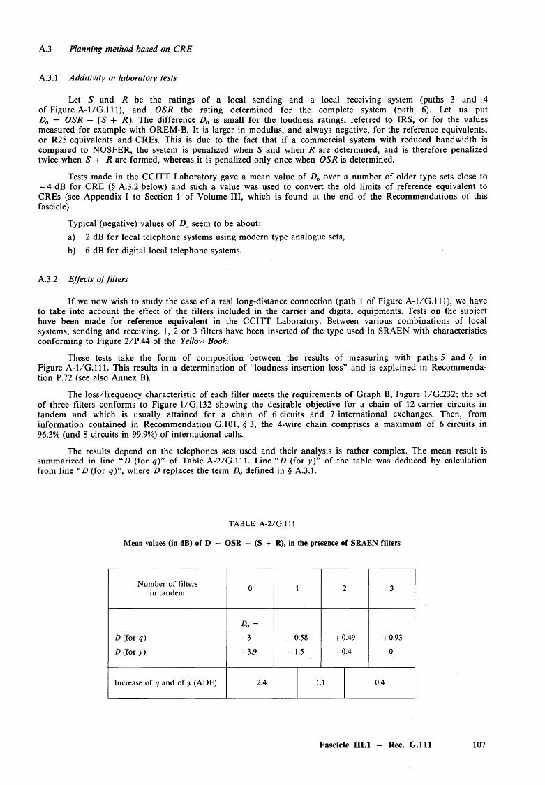
A.3 Planning method based on CRE
A.3.1 Additivity in laboratory tests
Let S and R be the ratings of a local sending and a local receiving system (paths 3 and 4 of Figure A - l /G .l l l ) , and OSR the rating determined for the complete system (path 6). Let us put D0 = OSR — (S + R). The difference D0 is small for the loudness ratings, referred to IRS, or for the values measured for example with OREM-B. It is larger in modulus, and always negative, for the reference equivalents, or R25 equivalents and CREs. This is due to the fact that if a commercial system with reduced bandwidth is compared to NOSFER, the system is penalized when S and when R are determined, and is therefore penalized twice when S + R are formed, whereas it is penalized only once when OSR is determined.
Tests made in the CCITT Laboratory gave a mean value of D0 over a number of older type sets close to — 4 dB for CRE (§ A.3.2 below) and such a value was used to convert the old limits of reference equivalent to CREs (see Appendix I to Section 1 of Volume III, which is found at the end of the Recommendations of this fascicle).
Typical (negative) values of D0 seem to be about:a) 2 dB for local telephone systems using modern type analogue sets,b) 6 dB for digital local telephone systems.
A.3.2 Effects offilters
If we now wish to study the case of a real long-distance connection (path 1 of Figure A - l /G .l l l ) , we have to take into account the effect of the Filters included in the carrier and digital equipments. Tests on the subject have been made for reference equivalent in the CCITT Laboratory. Between various combinations of local systems, sending and receiving. 1, 2 or 3 filters have been inserted of the type used in SRAEN with characteristicsconforming to Figure 2 /R 44 of the Yellow Book.
These tests take the form of composition between the results o f measuring with paths 5 and 6 in Figure A - l /G . l l l . This results in a determination of “loudness insertion loss” and is explained in Recommendation P.72 (see also Annex B).
The loss/frequency characteristic of each Filter meets the requirements o f Graph B, Figure 1/G.232; the set of three filters conforms to Figure 1/G . 132 showing the desirable objective for a chain of 12 carrier circuits in tandem and which is usually attained for a chain of 6 cicuits and 7 international exchanges. Then, from information contained in Recommendation G.101, § 3, the 4-wire chain comprises a maximum of 6 circuits in 96.3% (and 8 circuits in 99.9%) of international calls.
The results depend on the telephones sets used and their analysis is rather complex. The mean result is summarized in line “D (for q)” of Table A-2/G.111. Line “ Z> (for y )” of the table was deduced by calculation from line “D (for q )”, where D replaces the term D0 defined in § A.3.1.
TABLE A-2/G.111
Mean values (in dB) of D = OSR — (S + R), in the presence of SRAEN filters
Number o f filters in tandem 0 1 2 3
D0 =
D (for q) - 3 -0 .5 8 + 0.49 + 0.93
D (for y) -3 .9 -1 .5 - 0 .4 0
Increase of q and of y (ADE) 2.4 1.1 0.4
Fascicle III.l — Rec. G .l l l 107
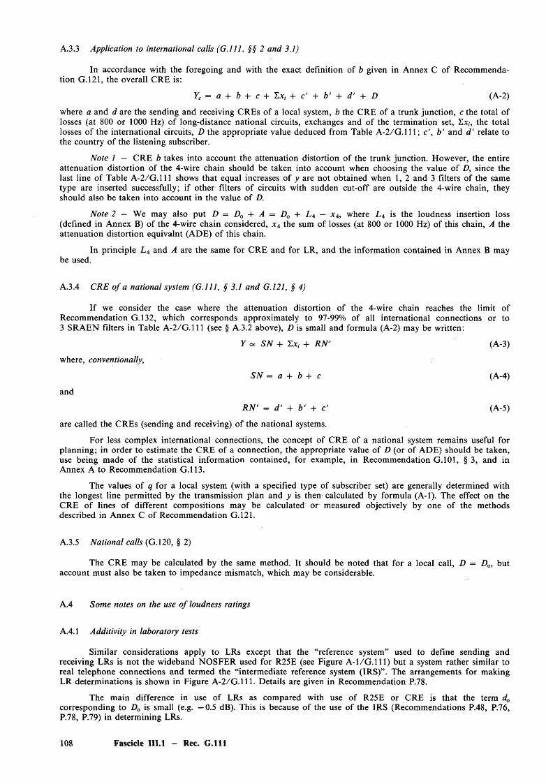
A.3.3 Application to international calls (G .l l l , §§ 2 and 3.1)
In accordance with the foregoing and with the exact definition of b given in Annex C of Recommendation G.121, the overall CRE is:
Yc = a + b -t- c + Ex,- c' b ' d ' D (A-2)
where a and d are the sending and receiving CREs of a local system, b the CRE of a trunk junction, c the total of losses (at 800 or 1000 Hz) of long-distance national circuits, exchanges and of the termination set, Ex,, the total losses of the international circuits, D the appropriate value deduced from Table A-2/G.111; c', b ' and d ' relate to the country of the listening subscriber.
Note 1 — CRE b takes into account the attenuation distortion of the trunk junction. However, the entire attenuation distortion of the 4-wire chain should be taken into account when choosing the value of D, since the last line of Table A-2/G.111 shows that equal increases of y are not obtained when 1, 2 and 3 filters of the same type are inserted successfully; if other filters o f circuits with sudden cut-off are outside the 4-wire chain, theyshould also be taken into account in the value of D.
Note 2 — We may also put D = D0 + A = D0 + L 4 — x 4, where L 4 is the loudness insertion loss (defined in Annex B) of the 4-wire chain considered, x 4 the sum of losses (at 800 or 1000 Hz) of this chain, A the attenuation distortion equivalnt (ADE) of this chain.
In principle L 4 and A are the same for CRE and for LR, and the inform ation contained in Annex B may be used.
A.3.4 CRE o f a national system (G .l l l , § 3.1 and G.121, § 4)
If we consider the case where the attenuation distortion of the 4-wire chain reaches the limit ofRecommendation G.132, which corresponds approximately to 97-99% of all international connections or to3 SRAEN filters in Table A-2/G.111 (see § A.3.2 above), D is small and formula (A-2) may be written:
Y ~ S N + Ex,- + R N ' (A-3)
where, conventionally,
S N = a + b + c (A-4)
and
R N ' = d ' + b ' + c' (A-5)
are called the CREs (sending and receiving) of the national systems.
For less complex international connections, the concept of CRE of a national system remains useful for planning; in order to estimate the CRE of a connection, the appropriate value of D (or of ADE) should be taken, use being made of the statistical inform ation contained, for example, in Recommendation G.101, § 3, and in Annex A to Recommendation G.113.
The values of q for a local system (with a specified type of subscriber set) are generally determined with the longest line permitted by the transmission plan and y is then calculated by formula (A-l). The effect on the CRE of lines of different compositions may be calculated or measured objectively by one of the methods described in Annex C of Recommendation G.121.
A.3.5 National calls (G.120, § 2)
The CRE may be calculated by the same method. It should be noted that for a local call, D = D0, but account must also be taken to impedance mismatch, which may be considerable.
A.4 Some notes on the use o f loudness ratings
A.4.1 Additivity in laboratory tests
Similar considerations apply to LRs except that the “reference system” used to define sending and receiving LRs is not the wideband NOSFER used for R25E (see Figure A - l /G . l l l ) but a system rather similar to real telephone connections and termed the “intermediate reference system (IRS)”. The arrangements for making LR determinations is shown in Figure A-2/G.111. Details are given in Recommendation R78.
The main difference in use of LRs as compared with use of R25E or CRE is that the term dQ corresponding to D0 is small (e.g. —0.5 dB). This is because of the use of the IRS (Recommendations R48, R76, R78, P.79) in determining LRs.
108 Fascicle III.l - Rec. G . l l l
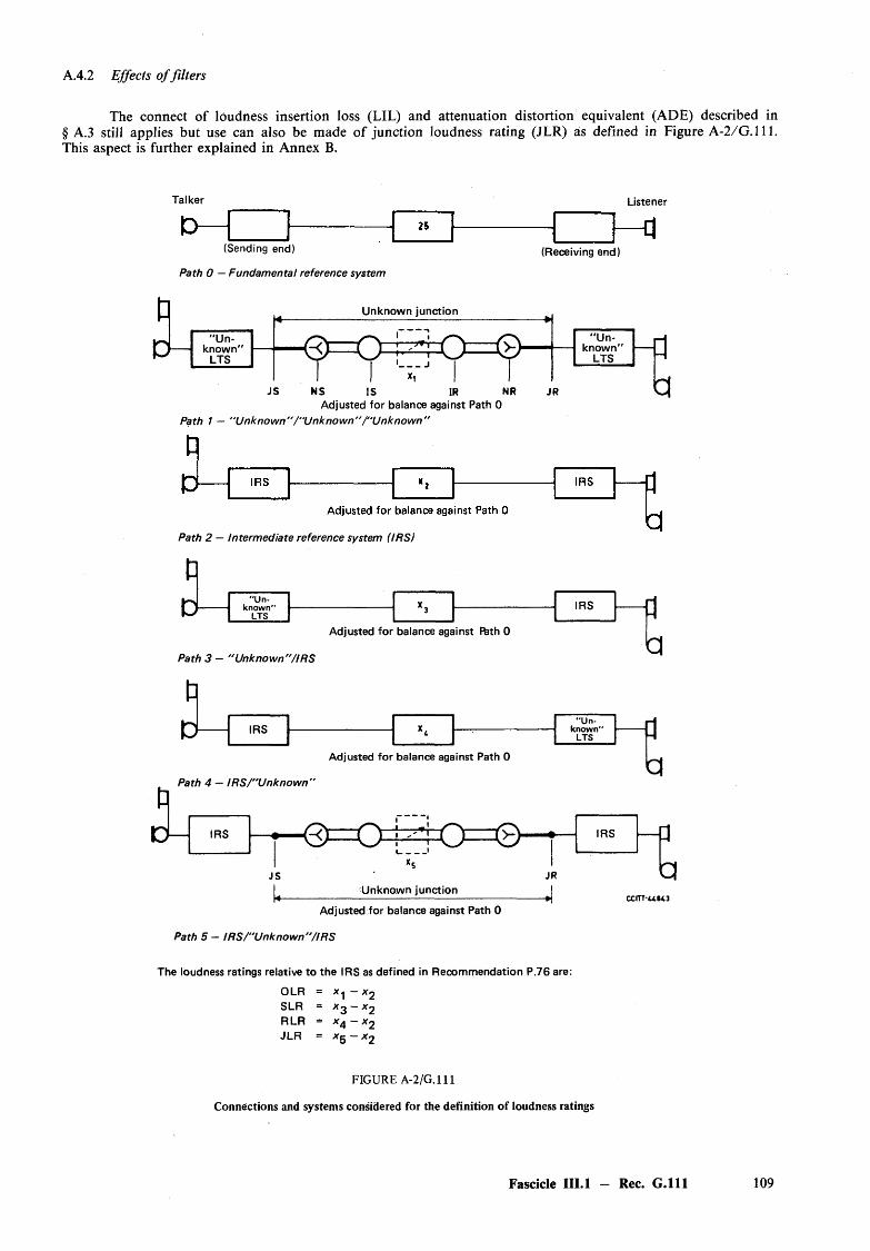
A.4.2 Effects o f filters
The connect of loudness insertion loss (LIL) and attenuation distortion equivalent (ADE) described in § A.3 still applies but use can also be made o f junction loudness rating (JLR) as defined in Figure A-2/G . 111. This aspect is further explained in Annex B.
Talker Listener
(Sending end)
Path 0 — Fundamental reference system
(Receiving end)
P"Un
known"LTS
Unknown junction
< ? = 9 + ? o = * ? > 'I I "x,‘ I I
"Unknown"
LTS
JS NS IS IR NR JRAdjusted for balance against Path 0
Path 1 — "Unknown”/"Unknown” /"Unknown"
Path 2 — Intermediate reference system (IRS)
P"U n
known"LTS
IRS
Adjusted for balance against fcith 0
Path 3 — "Unknown”/IRS
PIRS
"U nknown"
LTS
Adjusted for balance against Path 0
PPath 4 — IRS/"Unknown"
IRS <2)=O=H=rO==0i _ _____
X
IRS
JS JRUnknown junction
- a
[!
b
b
Adjusted for balance against Path 0
Path 5 — IRS /"Unknown”/IRS
The loudness ratings relative to the IRS as defined in Recommendation P.76 are:OLR = * 1 - x2
SLR ~ Xj — x 2
R LR = X4 - * 2
JLR = * 5 — * 2
F IG U R E A -2 /G . I l l
Connections and systems considered for the definition of loudness ratings
Fascicle III.l — Rec. G . l l l 109
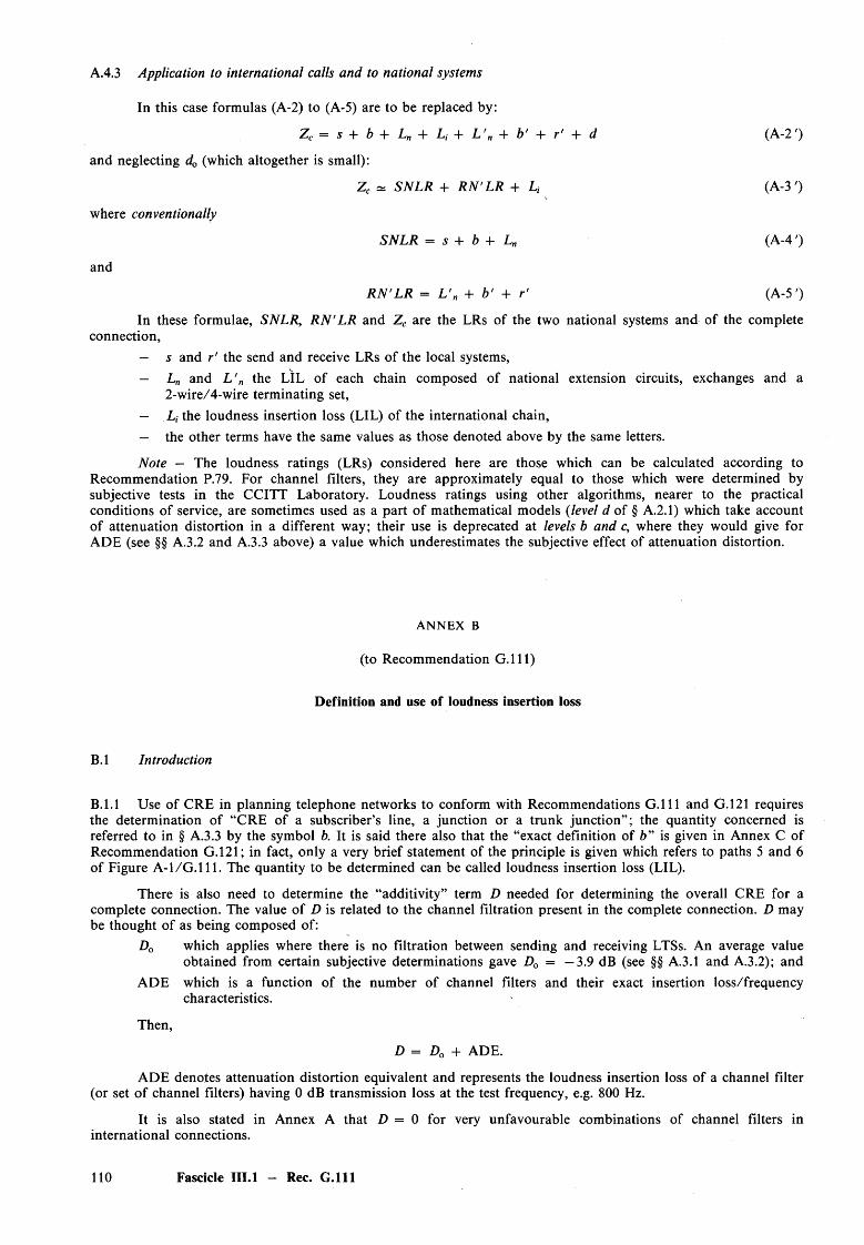
A.4.3 Application to international calls and to national systems
In this case formulas (A-2) to (A-5) are to be replaced by:
Z c = s + b + L„ + Lj + L 'n + b' + r ' + d (A -2')
and neglecting d0 (which altogether is small):
Z c » SiVLR + R N 'L R + U (A -3')
where conventionally
SN L R = s + b + Ln (A -4')
and
R N 'L R = L'„ + b ' + r ’ (A-5')
In these formulae, SN LR, R N 'L R and Z c are the LRs of the two national systems and of the completeconnection,
— s and r ' the send and receive LRs of the local systems,— Ln and L 'n the LIL of each chain composed of national extension circuits, exchanges and a
2-wire/4-wire terminating set,— L, the loudness insertion loss (LIL) of the international chain,— the other terms have the same values as those denoted above by the same letters.
Note — The loudness ratings (LRs) considered here are those which can be calculated according toRecommendation P.79. For channel filters, they are approximately equal to those which were determined by subjective tests in the CCITT Laboratory. Loudness ratings using other algorithms, nearer to the practical conditions of service, are sometimes used as a part o f mathematical models (level d of § A.2.1) which take accountof attenuation distortion in a different way; their use is deprecated at levels b and c, where they would give forADE (see §§ A.3.2 and A.3.3 above) a value which underestimates the subjective effect of attenuation distortion.
ANNEX B
(to Recommendation G .l l l )
Definition and use of loudness insertion loss
B.l Introduction
B.1.1 Use of CRE in planning telephone networks to conform with Recommendations G .l l l and G.121 requires the determination of “CRE of a subscriber’s line, a junction or a trunk junction” ; the quantity concerned is referred to in § A.3.3 by the symbol b. It is said there also that the “exact definition of h ” is given in Annex C of Recommendation G.121; in fact, only a very brief statement of the principle is given which refers to paths 5 and 6 of Figure A - l /G . l l l . The quantity to be determined can be called loudness insertion loss (LIL).
There is also need to determine the “additivity” term D needed for determining the overall CRE for a complete connection. The value of D is related to the channel Filtration present in the complete connection. D may be thought of as being composed of:
D0 which applies where there is no filtration between sending and receiving LTSs. An average value obtained from certain subjective determinations gave D0 = —3.9 dB (see §§ A.3.1 and A.3.2); and
ADE which is a function of the number of channel filters and their exact insertion loss/frequency characteristics.
Then,
D = D0 + ADE.
A DE denotes attenuation distortion equivalent and represents the loudness insertion loss of a channel filter (or set o f channel filters) having 0 dB transmission loss at the test frequency, e.g. 800 Hz.
It is also stated in Annex A that D = 0 for very unfavourable combinations of channel filters in international connections.
1 1 0 Fascicle III.l - Rec. G .l l l
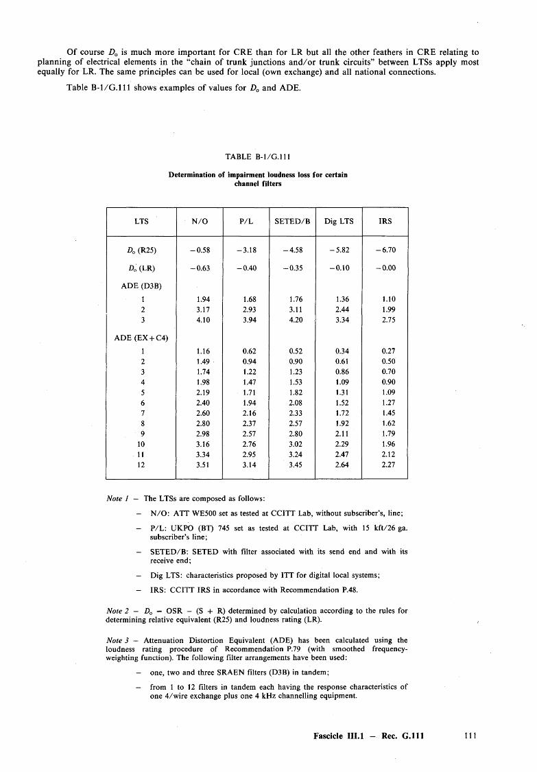
O f course D0 is much more im portant for CRE than for LR but all the other feathers in CRE relating to planning of electrical elements in the “chain of trunk junctions an d /o r trunk circuits” between LTSs apply most equally for LR. The same principles can be used for local (own exchange) and all national connections.
Table B - l /G . l l l shows examples of values for D0 and ADE.
TABLE B - l /G .l l l
Determination of impairment loudness loss for certain channel filters
LTS N /O P/L SETED/B Dig LTS IRS
D0 (R25) -0 .5 8 -3 .1 8 -4 .5 8 -5 .8 2 -6 .7 0
D0 (LR) -0 .6 3 -0 .4 0 -0 .35 -0 .1 0 -0 .0 0
ADE (D3B)
1 1.94 1.68 1.76 1.36 1.102 3.17 2.93 3.11 2.44 1.993 4.10 3.94 4.20 3.34 2.75
ADE (EX + C4)
1 1.16 0.62 0.52 0.34 0.272 1.49 0.94 0.90 0.61 0.503 1.74 1.22 1.23 0.86 0.704 1.98 1.47 1.53 1.09 0.905 2.19 1.71 1.82 1.31 1.096 2.40 1.94 2.08 1.52 1.277 2.60 2.16 2.33 1.72 1.458 2.80 2.37 2.57 1.92 1.629 2.98 2.57 2.80 2.11 1.79
10 3.16 2.76 3.02 2.29 1.9611 3.34 2.95 3.24 2.47 2.1212 3.51 3.14 3.45 2.64 2.27
Note 1 — The LTSs are composed as follows:
— N /O : ATT WE500 set as tested at CCITT Lab, without subscriber’s, line;
— P /L : UKPO (BT) 745 set as tested at CCITT Lab, with 15 kft/26 ga. subscriber’s line;
— SETED /B : SETED with filter associated with its send end and with its receive end;
— Dig LTS: characteristics proposed by ITT for digital local systems;
— IRS: CCITT IRS in accordance with Recommendation P.48.
Note 2 — D0 = OSR — (S + R) determined by calculation according to the rules for determining relative equivalent (R25) and loudness rating (LR).
Note 3 — Attenuation Distortion Equivalent (ADE) has been calculated using the loudness rating procedure of Recommendation P.79 (with smoothed frequency- weighting function). The following filter arrangements have been used:
— one, two and three SRAEN filters (D3B) in tandem ;
— from 1 to 12 filters in tandem each having the response characteristics of one 4/w ire exchange plus one 4 kHz channelling equipment.
Fascicle III.l — Rec. G .l l l 111
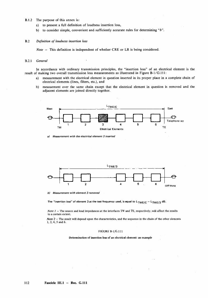
B.1.2 The purpose of this annex is:a) to present a full definition of loudness insertion loss,b) to consider simple, convenient and sufficiently accurate rules for determining “6 ”.
B.2 Definition o f loudness insertion loss
Note — This definition is independent of whether CRE or LR is being considered.
B.2.1 General '
In accordance with ordinary transmission principles, the “insertion loss” of an electrical element is the result of making two overall transmission loss measurements as illustrated in Figure B - l /G . l l l :
a) measurement with the electrical element in question inserted in its proper place in a complete chain of electrical elements (lines, filters, etc.), and
b) measuement over the same chain except that the electrical element in question is removed and the adjacent elements are joined directly together.
a) Measurement with the electrical element 3 inserted
b) Measurement with element 3 removed
The "insertion loss" of element 3 at the test frequency used, is equal to Ljw e /C — *"TWE/3
Note 1 - The source and load impedances at the interfaces TW and TE, respectively; will affect the results to a certain extent.
Note 2 — The result will depend upon the characteristics, and the sequence in the chain of the other elements 1, 2, 4, 5 and 6.
FIGURE B -l/G .lll
Determination of insertion loss of an electrical element: an example
112 Fascicle III.l — Rec. G . l l l
B.2.2 Application to CRE and LR
B.2.2.1 Principles
Paths 5 and 6 in Figure A - l /G . l l l can be regarded as represented in more complete form by a and b, respectively, in Figure B - l /G .l l l . We can then imagine a subjective comparison by loudness of paths a and b. So long as this is performd by the “margin method”, i.e. at constant listening level, it does not matter whether it is done via NOSFER (as shown in Figure A - l /G . l l l ) or in accordance with the rules for determining loudness rating (Recommendation P.76). Path 1 in Figure 2/P.76 would be the equivalent of path 5 in Figure A - l /G .l l l and therefore represented by path a) in Figure B - l /G . l l l ; path 1 in Figure 2/P.76 with the electrical element in question removed would be the equivalent of path 6 in Figure A - l /G . l l l and therefore represented by path b) in Figure B - l /G .l l l .
Loudness insertion loss is defined in a m anner analogous to ordinary “insertion loss”. Therefore, loudness insertion loss (LIL) of element 3 is given by:
LIL = O R E R25/path a) - O R E R25 /path b)
or, what is exactly the same in numerical value,
LIL = OVELR/path a) — OVELR/path bj
ORER25/Path a) means subjective determination of the relative equivalent of the complete path a) at the listening level defined by 25 dB setting of NOSFER.
O V E L R / Path a) means subjective determination of the overall loudness rating (OLR) of the complete path a) in accordance with Recommendation P.78.
Corresponding definitions apply for path b).
B.2.2.2 Calculation
Although loudness loss is defined in principle in terms of subjective tests, it can be calculated with sufficient accuracy. The problem must be solved in two stages. First, to establish the objective quantities that are to be operated upon and secondly to choose a suitable calculation algorithm.
To calculate OLR, we need to know LUME for the two paths a) and b) in Figure B - l /G .l l l . This should be available, in principle, for the 20 ISO bands having mid-frequencies from 100-8000 Hz but, as will be shown later, less than the full number will suffice in many cases. Methods have been proposed for calculating O RER25 and some are suitable for certain applicaions but none has yet been shown to be suitable for the present purpose.
But we do have Recommendation P.79 which is suitable for calculating OVELR and, therefore, LIL can be determined by using it. (In fact the decision to use the algorithm given in Recommendation R79 was made largely because it allows to predict the loudness insertion losses of examples of channel filters.)
An example of the use of the calculation procedure of Recommendation R79 for determining LIL is given in Appendix I to this annex.
B.3 Use o f loudness insertion loss fo r determining planning values o f CRE or LR fo r electrical elements
B.3.1 General
The various aspects of the matter are classified here and solutions of the associated problems indicated.
Firstly, it is very desirable, if not essential, to be able to add together the planning values for differentelements in tandem in a telephone connection and obtain the correct “overall” value for the complete tandem,i.e. connected set of elements. For example in Figure B - l /G . l l l , it is to be hoped that LIL( 1 + 2 + 3 + 4 + 5 + 6) will be about the same as LIL (1) + LIL + (2) . . . + LIL (6), where LIL (X) is theloudness insertion loss of X, which may be a single element or a set of tandem connected elements.
Secondly, the calculation procedure must be as simple as possible. For example, the calculation procedure indicated above requires much inform ation in addition to the ordinary insertion loss/frequency characteristic of the element in question. It would be convenient to be able to apply a very simple calculation procedure directly to the insertion loss values at the smallest number of frequency points possible.
Fascicle III.l — Rec. G .l l l 113
These problems cannot be solved in a completely general manner but they can be treated rigorously and the most suitable practical compromise solutions sought.
B.3.2 Additivity
We must be clear about our aim. In essence, we want to assign numbers to the various parts of a connection, to add them together and to obtain a value close to the true “overall” value obtained for the complete connection. This aim is usually attained in two stages: the two local telephone systems (LTSs) independently and then the chain of trunk junctions, junctions an d /o r trunk circuits which are used to connect the LSTs together.
B.3.2.1 Local systems
We may subdivide a complete connection into the three parts of § 3.2 in any desired way. For example, in Figure B - l /G . l l l we may wish to put the LTS/junction interfaces at the west (JW) and east (JE) ends respectively, at the junctions of elements 2 and 3 and of elements 4 and 5; if elements 1 and 6 are subscribers’ lines and elements 2 and 5 are feeding bridges, this might correspond to interfaces used in planning.
But, the interfaces JW and JE may be put at the terminals of the telephone sets, i.e. coincident with TW and TE, if planning is done in terms of the complete chain of electrical elements lying between the two telephone sets.
Another arrangement might correspond to a sub-division into two national systems and a chain of international circuits.
For any of these cases we start by determining a SCRE (or SLR) for one LTS and a RCRE (or RLR) for the other. We then determine the “overall loudness loss” for the direct connection, via a 600 ohms impedance buffer, of the two LTSs; this is denoted by ORSR25. For CRE this amounts to a subjective determination of ORSR25 or the assumption that D0 = —3.9. For loudness rating we can obtain OSRLr by subjective determination or by calculation, whichever has been used to determine SLR and RLR. Then D0 = OSRlr — (SL R + R LR ).
Some examples are shown in Table B-2/G.111.
Clearly, local telephone systems that are very similar to the IRS will attract small values of D0 for loudness rating: if the LTSs are much broader or much narrower in frequency response than the IRS, D0 is likely to be negative; if they differ appreciably within the same frequency range, D0 may become positive.
B.3.2.2 The chain o f electrical elements
The (overall) CRE or LR for the combination only of two LTSs, termed OSRR25 or OSRLr, has to be augmented by the loudness insertion loss (LIL) of the chain of electrical elements, which cannect them together, to give the overall CRE or overall loudness rating (CORE or OVELR) for the complete connection.
The fundamental principles for determining LIL have already been explained and it now remains to show some examples and to see what degree of additivity is achieved for various combinations of elements. When a large number of channel filters are included, the additivity for individual elements, o f whatever kind, will usually be improved, but care must be taken to check whether the same values can also be used in simpler local connections.
Table B-3/G.111 shows the loudness insertion loss (LIL) and four other estimates of the loudness losses of the combinations of trunk junctions and trunk circuits.
Clearly, when a lot of channel filters are present, the entire frequency band need not be used and some (possibly severe) restriction in frequency range may be possible over when calculations are made.
Finally, if a single complete hypothetical system is used and a single location of interface is chosen at which to insert the “unknow n” electrical element, very considerable simplification of calculation procedure will be possible.
114 Fascicle III.l - Rec. G . l l l
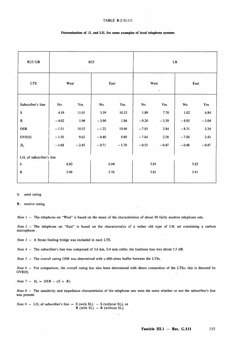
TABLE B-2/G.111
Determination of D0 and LIL for some examples of local telephone systems
R 25/LR R25 LR
LTS West East West East
Subscriber’s line No Yes No Yes No Yes No Yes
S 4.19 11.01 3.39 10.33 1.89 7.70 1.02 6.84
R -4 .0 2 1.96 -3 .9 0 1.86 -9 .2 0 -3 .3 9 -8 .8 5 -3 .0 4
OSR -1 .51 10.52 -1 .2 2 10.49 -7 .8 5 3.84 -8 .31 3.34
OVE(O) -1 .5 0 9.62 -0 .4 0 9.89 -7 .8 4 2.58 -7 .8 8 2.43
D0 -1 .6 8 -2 .4 5 -0 .71 -1 .7 0 -0 .5 3 -0 .4 7 -0 .4 8 -0 .4 7
LIL o f subscriber’s line
S 6.82 6.94 5.81 5.82
R 5.98 5.76 5.81 5.81
S: send rating
R: receive rating
Note 1 — The telephone set “West” is based on the mean of the characteristics of about 90 fairly modern telephone sets.
Note 2 — The telephone set “East” is based on the characteristics of a rather old type of UK set containing a carbonmicrophone .
Note 3 — A Stone feeding bridge was included in each LTS.
Note 4 — The subscriber’s line was composed of 3.6 km, 0.4 mm cable; the loudness loss was about 5.5 dB.
Note 5 — The overall rating OSR was determined with a 600-ohms buffer between the LTSs.
Note 6 — For comparison, the overall rating has also been determined with direct connection of the LTSs; this is denoted byOVE(O).
Note 7 — D0 = OSR - (S + R).
Note 8 — The sensitivity and impedance characteristics of the telephone sets were the same whether or not the subscriber’s linewas present.
Note 9 — LIL of subscriber’s line = S (with SL) — S (without SL), orR (with SL) - R (without SL).
Fascicle III.l - Rec. G .l l l 115

TABLE B-3/G.111
Additivity overall of LRs of LTSs and LIL of “Junction”
Example : l(W-E) l(E-W) 2(W-E) 2(E-W)
S 7.70 6.83 4.81 3.34
R -3 .0 4 -3 .3 9 -7 .6 8 -5 .7 9
OSR 4.22 3.25 -3 .4 2 -2 .7 9
D0 -0 .4 4 -0 .1 9 -0 .55 -0 .3 5
OVE(O) 3.11 2.32
OVE 31.52 30.61 7.38 7.85
LIL 27.30 27.36 10.80 10.64
OVE - (S + R) 26.86 27.17 10.25 10.30
JUN 25.68 25.68 10.09 10.09
L IL /IR S 26.36 26.36 10.06 10.06
LIL/RS1A 27.31 27.31 10.78 10.78
Note 1 — Examples l(W -E) and l(E-W) are for the two directions of transmission of a hypothetical connection representative of a maximum- loss international connection.
Note 2 — Examples 2(W-E) and 2(E-W) are for the two directions of transmission of a hypothetical connection representative of an international connection complying with the recommendations for the long-term objective.
Note 3 — Examples 1 include telephone sets of the types described in Notes 1 and 2 to Table B-2/G.111.
Note 4 — Examples 2 include the same type of telephone set at West as in Examples 1, but the telephone set at East is representative o f a fairly modern type of carbon-microphone set (NTT 600).
Note 5 — The subscribers’ lines in Examples 1 were as described in Note 4 to Table B -2/G .111 for Examples 2, the subscribers’ lines are “average”.
Note 6 — In Examples 1, the electrical elements connecting the two LTSs comprised two unloaded cable junctions (3.7 dB image attenuation at 800 Hz) and the equivalent of twelve FDM or PCM systems. The total nominal loss of this combination was 24 dB.
Note 7 — In Examples 2, the electrical elements connecting the two LTSs comprised three PCM or FDM systems. The total nominal loss was9.5 dB.
116 Fascicle III.l - Rec. G .l l l
APPENDIX I
(to Annex B to Recommendation G .lll)
Effects on loudness insertion loss of the characteristics of the terminating telephone systems
LI Introduction
The objective values of insertion loss for a given electrical transmission element depend, o f course, upon the values of modulus and argument of the source and load impedances. Naturally, changes in such quantities also cause changes in the values of LIL calculated therefrom. However, even when a single set of objective values of insertion loss is used, the values of LIL will be affected by the frequency response characteristics of the terminating electro-acoustical systems.
Another feature must be contended with; namely, the rather complicated manner in which the LIL grows as we introduce more electrical elements between the terminating systems. If the image impedances of the electrical elements in question are all the same and are matched to the source and load impedances, we can simply add the insertion losses without any difficulty. But, even then, any uniform increase in objective values of insertion loss may not result in exactly corresponding uniform increases in LIL, because of the frequency response effect mentioned above.
When impedance mismatches are present and differences in frequency response are encountered both in the electrical elements and in the terminating systems, it is very difficult to predict the result without making a specific and rigorous examination. W ithout any attempt to be exhaustive, the material gathered here attempts to display the effects o f some of the more im portant combinations of circumstances.
1.2 Some examples
First, it should be noted that the sensitivity/frequency responses of the terminating systems, which may have source and load impedances that depart from 600 ohms N R (non-reactive), are defined (in accordance with Recommendation P.64) in terms of measurements using a 600 ohms NR load for sending, and a 600 ohms NR source for receiving.
In the following examples, three different electrical elements will be considered. The values of nominal loss are taken as the image attenuation at 800 Hz.
a) An unloaded cable junction of 0.9 mm cable, 5.6 km long; nominal loss 3.66 dB; image impedance at 800 Hz 365-y365 ohms.
b) A loaded cable juntion of 0.6 mm cable loaded at 1.84 km intervals with 88 mH coils; there are fourfull loading sections and two (end) half-cable sections; nominal loss 3.94 dB; image impedance at800 Hz 1132-y244 ohms.
c) A trunk junction of which the loss/frequency characteristics were taken from Table 4 of Reference [2];it is assumed to represent a nominally 3 dB PCM junction having 600 ohms N R image impedances.The 2-w/4-w terminating units are included.
The following are approximately in order to increasing complexity.
1.2.1 Example 1 (see a) of Figure I - l /G .l 11)
The first example uses the IRS send and receive parts as terminating systems. The impedances of theterminating systems are therefore 600 ohms NR. For the special purposes of this example, the electricalelements a) and b) of Table I - l /G .l 11 will be replaced by hypothetical electrical elements having the same imageattenuations but having 600 ohms N R image impedances. There are therefore no impedance mismatches. Theresults for one, two and three identical elements in tandem using the IRS as terminating systems are given in Table I - l /G .l 11.
Fascicle III.1 - Rec. G .l l l 117
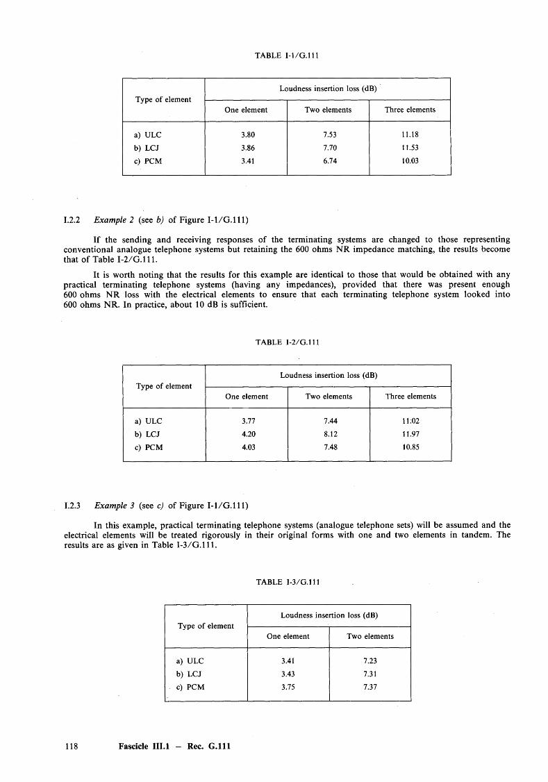
TABLE I-l/G .l 11
Type of elementLoudness insertion loss (dB)
One element Two elements Three elements
a) ULC 3.80 7.53 11.18
b) LCJ 3.86 7.70 11.53
c) PCM 3.41 6.74 10.03
1.2.2 Example 2 (see b) of Figure I - l /G .l 11)
If the sending and receiving responses of the terminating systems are changed to those representing conventional analogue telephone systems but retaining the 600 ohms N R impedance matching, the results become that o f Table I-2 /G .111.
It is worth noting that the results for this example are identical to those that would be obtained with any practical terminating telephone systems (having any impedances), provided that there was present enough 600 ohms N R loss with the electrical elements to ensure that each terminating telephone system looked into 600 ohms NR. In practice, about 10 dB is sufficient.
TABLE I-2/G.111
Type of elementLoudness insertion loss (dB)
One element Two elements Three elements
a) ULC 3.77 7.44 11:02
b) LCJ 4.20 8.12 11.97
c) PCM 4.03 7.48 10.85
1.2.3 Example 3 (see c) of Figure I - l /G .l 11)
In this example, practical terminating telephone systems (analogue telephone sets) will be assumed and the electrical elements will be treated rigorously in their original forms with one and two elements in tandem. The results are as given in Table I-3/G.111.
TABLE I-3/G.111
Type o f elementLoudness insertion loss (dB)
One element Two elements
a) ULC 3.41 7.23
b) LCJ 3.43 7.31
c) PCM 3.75 7.37
118 Fascicle III.l — Rec. G .l l l
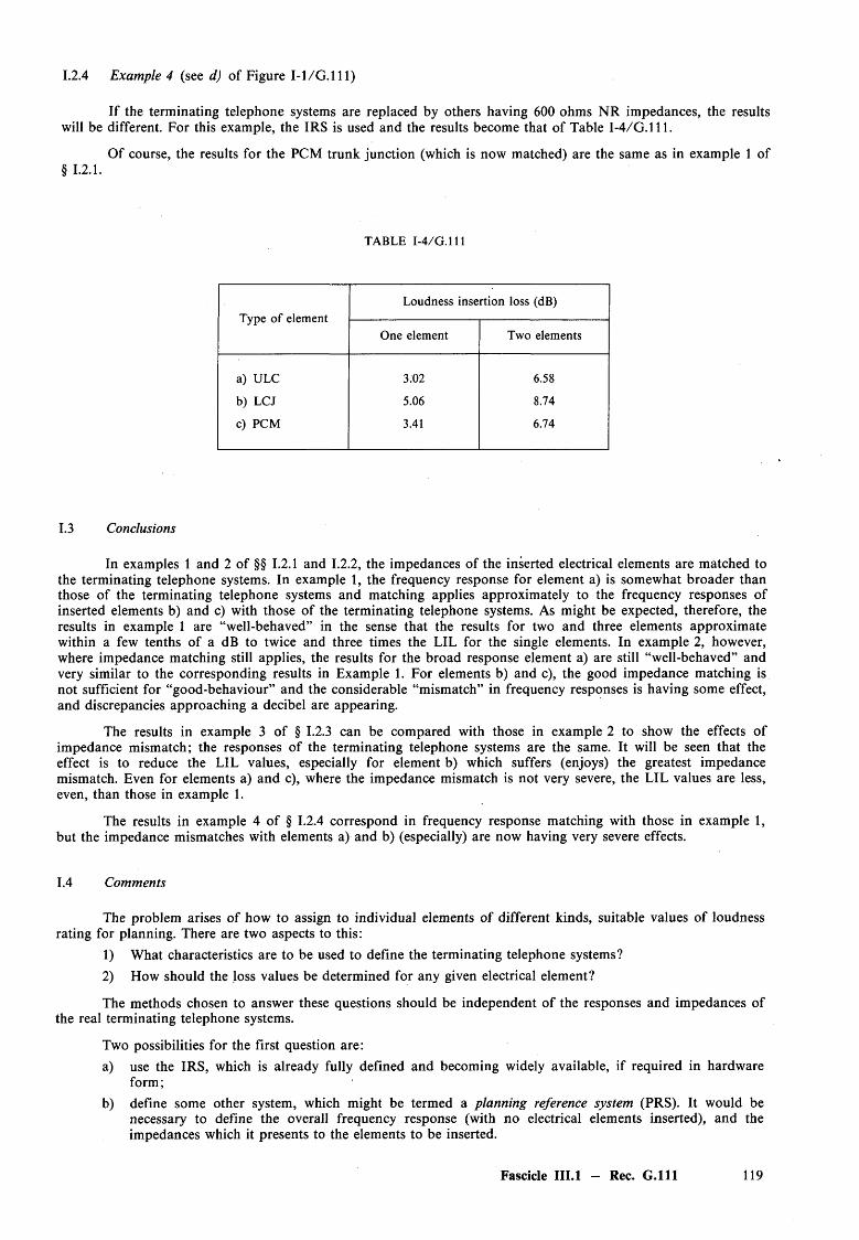
1.2.4 Example 4 (see d) of Figure I- l/G .l 11)
If the terminating telephone systems are replaced by others having 600 ohms NR impedances, the results will be different. For this example, the IRS is used and the results become that of Table I-4/G.111.
O f course, the results for the PCM trunk junction (which is now matched) are the same as in example 1 of§ 1.2 . 1.
TABLE I-4/G.111
Type o f elementLoudness insertion loss (dB)
One element Two elements
a) ULC 3.02 6.58
b) LCJ 5.06 8.74
c) PCM 3.41 6.74
1.3 Conclusions
In examples 1 and 2 of §§ 1.2.1 and 1.2.2, the impedances of the inserted electrical elements are matched to the terminating telephone systems. In example 1, the frequency response for element a) is somewhat broader than those of the terminating telephone systems and matching applies approximately to the frequency responses of inserted elements b) and c) with those of the terminating telephone systems. As might be expected, therefore, the results in example 1 are “well-behaved” in the sense that the results for two and three elements approximate within a few tenths of a dB to twice and three times the LIL for the single elements. In example 2, however, where impedance matching still applies, the results for the broad response element a) are still “well-behaved” and very similar to the corresponding results in Example 1. For elements b) and c), the good impedance matching is not sufficient for “good-behaviour” and the considerable “mismatch” in frequency responses is having some effect, and discrepancies approaching a decibel are appearing.
The results in example 3 of § 1.2.3 can be compared with those in example 2 to show the effects o f impedance mismatch; the responses of the terminating telephone systems are the same. It will be seen that the effect is to reduce the LIL values, especially for element b) which suffers (enjoys) the greatest impedance mismatch. Even for elements a) and c), where the impedance mismatch is not very severe, the LIL values are less, even, than those in example 1.
The results in example 4 of § 1.2.4 correspond in frequency response matching with those in example 1, but the impedance mismatches with elements a) and b) (especially) are now having very severe effects.
1.4 Comments
The problem arises of how to assign to individual elements of different kinds, suitable values of loudness rating for planning. There are two aspects to this:
1) What characteristics are to be used to define the terminating telephone systems?2) How should the loss values be determined for any given electrical element?
The methods chosen to answer these questions should be independent of the responses and impedances ofthe real terminating telephone systems.
Two possibilities for the first question are:a) use the IRS, which is already fully defined and becoming widely available, if required in hardware
form;b) define some other system, which might be termed a planning reference system (PRS). It would be
necessary to define the overall frequency response (with no electrical elements inserted), and theimpedances which it presents to the elements to be inserted.
Fascicle III.l — Rec. G . l l l 119
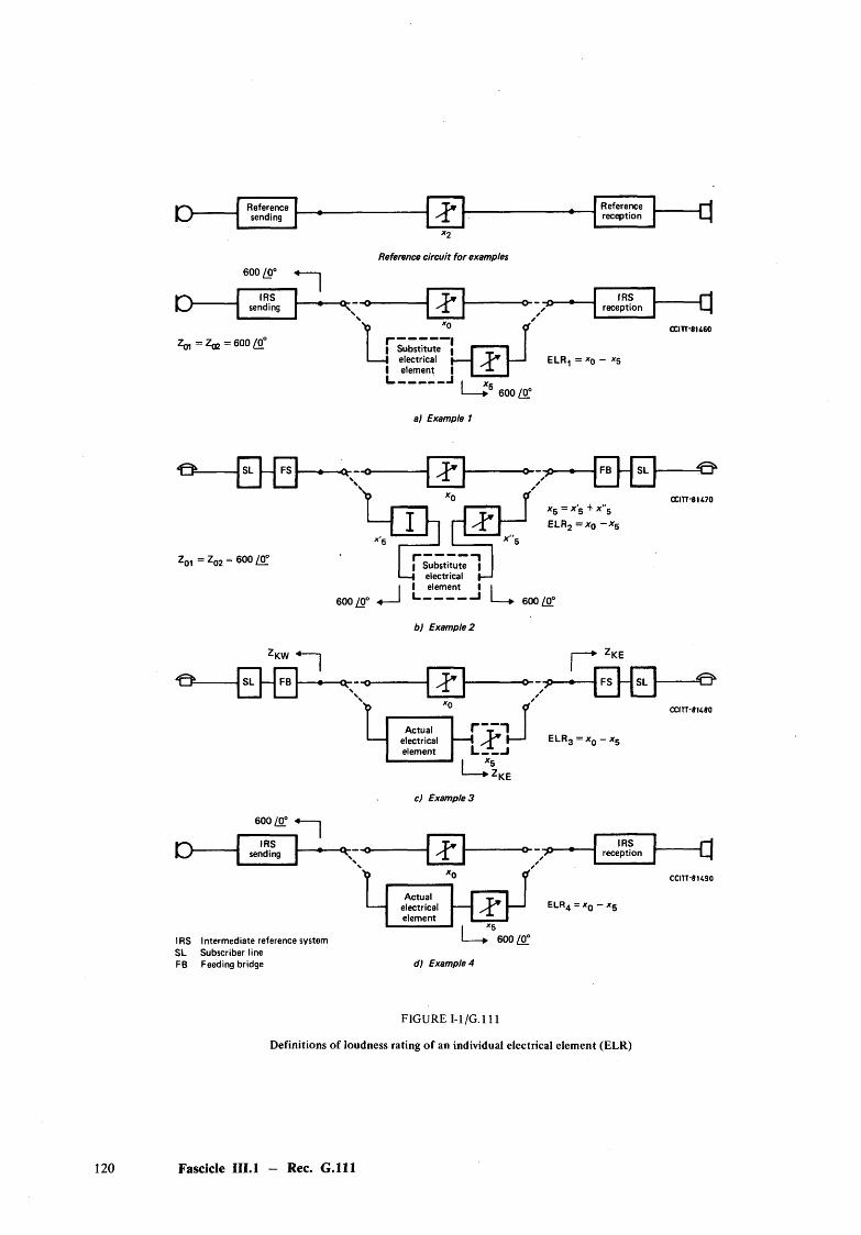
D - R e fe r e n c e z R e fe r e n c esen d in g r e c e p t io n
*2
Reference circuit for examples600 /Q°
On
z o i = z a 2 = 6 0 ° Z 0 o
*0
^ S u b s t i tu te { e le c tr ic a l f -
I e le m e n t |I_______ _ J
Z ~ * ELR < = * o ~ * 5
600/0°
IR S z IR Ss en d in g • V 0s
\s
/r e c e p t io n
C C in -8 U 6 0
a) Example 1
O - SL F S
Z 0 1 = Z Q2 = 600/0?
-Qr~0- Z F B — S L - O
I b D ' ?
x 5 = X S + * " 5
E L R 2 = x0 ~ x5x"K
600/0°
I S u b s t i tu te |-I e le c tr ic a l | -
I I e le m e n t I 1
«— I 1------------ 1 L_> 600/0°
o
b) Example 2
: K W
S L H3n
600/0°
-Q;— o-r -K E
- 0 — -p-
x0
A c tu a le le c tr ic a le le m e n t
F S S L - O
E L R 3 = x 0 - x 5
L_2•KE
Example 3
IR S z IR Ssen d in g • V 0NN
o p •✓/
r e c e p t io n
L x0
A c tu a l T I
e le c tr ic a l ------- * ------e le m e n t
Z E L R 4 - X q — X g
IR S I n te r m e d ia te r e fe r e n c e s y s te m S L S u b sc r ib e r lin eF B F e e d in g b r id g e
* 5
600/0?
d) Example 4
FIGURE I-l/G .l 11
Definitions of loudness rating of an individual electrical element (ELR)
120 Fascicle III.l - Rec. G . l l l
From the conclusions drawn from the examples given above, it seems quite clear that there is no perfect choice of PRS and therefore it appears wise first to explore more fully the use of the IRS.
The second question is o f a rather practical nature, and is concerned with how to obtain the loss/ frequency responses of the electrical elements. These values are then to be entered into the LR calculation algorithm (i.e. Recommendation P.79). There seems to be no problem when the elements are all matched to (say) 600 ohms NR; examples are multiplex transmission systems. But, when they are not matched in impedance to each other and to that of the PRS (or IRS) (e.g. unamplified lines and exchanges), it is clear from the above that the decision may make a lof of difference. The possibilities seem to be:
i) to use the image attenuation but notionally assume the element to have 600 ohms N R image impedances (this was done in examples 1 and 2);
ii) to use the insertion loss frequency characteristic between (say) 600 ohms NR source and load (this corresponds to what was done in example 4);
iii) to use the insertion loss frequency characteristic between defined impedances chosen to represent some practical terminating telehone systems (an example of his method is given in example 3).
It is believed that possibilities a) and i) above for both questions ought to be recommended on the grounds that they are simple to implement and (as has been shown in recent studies) they seem to work well provided certain simple precautions are taken when dealing with one or more band-pass-filtered elements connected in tandem.
It is very im portant to note that the methods suggested do not correspond exactly to using JLR unless the element in question has 600 ohms N R image impedances.
Fascicle III.l - Rec. G . l l l 121
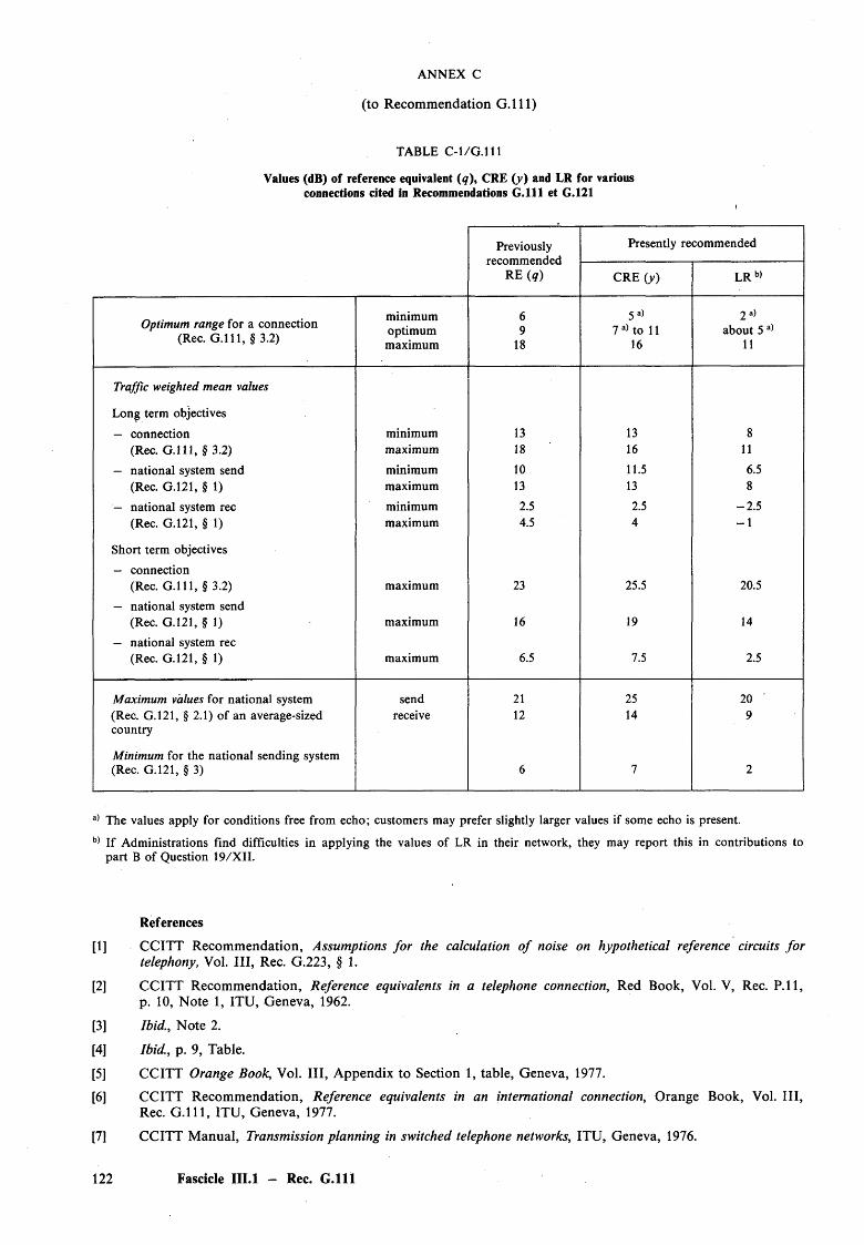
ANNEX C
(to Recommendation G .lll)
TABLE C - l /G .l l l
Values (dB) of reference equivalent (q), CRE (y) and LR for various connections cited in Recommendations G .lll et G.121
Previously recommended
RE (q )
Presently recommended
CRE 0 0 LR b)
Optimum range for a connection (Rec. G . l l l , § 3.2)
minimumoptimummaximum
69
18
5 a>7 a) to 11
16
2 a> about 5 a)
11
Traffic weighted mean values
Long term objectives
- connection minimum 13 13 8(Rec. G . l l l , § 3.2) maximum 18 16 11
- national system send minimum 10 11.5 6.5(Rec. G.121, § 1) maximum 13 13 8
- national system rec minimum 2.5 2.5 -2 .5(Rec. G.121, § 1)
Short term objectives
— connection
maximum 4.5 4 - 1
(Rec. G . l l l , § 3.2)
— national system send
maximum 23 25.5 20.5
(Rec. G.121, § 1)
— national system rec
maximum 16 19 14
(Rec. G.121, § 1) maximum 6.5 7.5 2.5
Maximum values for national system send 21 25 20(Rec. G.121, § 2.1) o f an average-sized country
receive 12 14 9
Minimum for the national sending system(Rec. G.121, § 3) 6 7 2
a) The values apply for conditions free from echo; customers may prefer slightly larger values if some echo is present.
b) If Administrations find difficulties in applying the values of LR in their network, they may report this in contributions to part B of Question 19/X II.
References
[1] CCITT Recommendation, Assumptions fo r the calculation o f noise on hypothetical reference circuits fo r telephony, Vol. I l l , Rec. G.223, § 1.
[2] CCITT Recommendation, Reference equivalents in a telephone connection, Red Book, Vol. V, Rec. P. 11, p. 10, Note 1, ITU, Geneva, 1962.
[3] Ibid., Note 2.
[4] Ibid., p. 9, Table.
[5] CCITT Orange Book, Vol. I l l , Appendix to Section 1, table, Geneva, 1977.
[6] CCITT Recommendation, Reference equivalents in an international connection, Orange Book, Vol. I ll ,Rec. G . l l l , ITU, Geneva, 1977.
[7] CCITT M anual, Transmission planning in switched telephone networks, ITU, Geneva, 1976.
122 Fascicle III.l - Rec. G .l l l

Recommendation G.113
TRANSMISSION IMPAIRMENTS
(Geneva, 1980; amended at Malaga-Torremolinos, 1984)
1 Transmission impairment
1.1 The objectives for the attenuation distortion of a maximum-length 4-wire chain are given in Recommendation G.132 and those of the signal-independent noise performance of such maximum-length connections are given in § 2 of this Recommendation. Bearing in mind that less complicated connections (which are more numerous) will have less attenuation distortion and less noise, then the maximum, average and minimum values of corrected reference equivalent or loudness rating recommended in Recommendation G.121 will ensure an adequate transmission performance on international connections.
1.2 Should values of attenuation distortion or noise greatly different from those recommended by the CCITT for systems and equipments be contemplated, then guidance concerning possible changes in transmission performance can be found in Recommendation P. 11 and Annexes [1], with some indication of possible trade-offs between them.
2 Network performance objective for circuit noise on complete telephone connections
The CCITT recommends that the network performance objective for the mean value, expressed in decibels and taken over a large number of worldwide connections (each including four international circuits), of the distribution of one-minute mean values of signal-independent noise power of the connections, should not exceed — 43 dBmOp referred to the input o f the first circuit in the chain of international circuits.
3 Transmission impairments due to digital processes
The incorporation of unintegrated digital processes in international telephone connections, particularly during the mixed analogue/digital period, can result in an appreciable accumulation of transmission impairments. It is, therefore, necessary to ensure that this accumulation does not reach a point where it can seriously degrade overall transmission quality.
3.1 Quantizing distortion
From the point of view of quantizing distortion, it is provisionally recommended that no more than 14 units o f quantizing distortion should be introduced in an international telephone connection.
For telephone connections which incorporate unintegrated digital processes, it is permissible to simply add the units of quantizing distortion that have been assigned to the individual digital processes to determine the total or overall quantizing distortion. Some sources of quantizing distortion and the units tentatively assigned to them are given in § 3.2.
By definition, an average 8-bit codec pair (A /D and D /A conversions, A-law or p-law) which complies with Recommendation G.711 introduces 1 quantizing distortion units (1 qd unit). An average codec pair produces about 2 dB less quantizing distortion than the limits indicated in Recommendation G .712. This would correspond to a single-to-distortion ratio of 35 dB for the sine-wave test method and approximately 36 dB for the noise test method. (A total of fourteen 8-bit PCM processes each of which just comply with the limits for signal-to-distortion ratio in Recommendation G.712 would be unacceptable). The same principle should be applied when proposing planning valves of quantizing distortion units for other digital processes.
In principle, the number o f units for other digital processes are determined by comparison with an 8-bit PCM codec pair such that the distortion of the digital process being evaluated is assigned n quantizing distortion units if it is equivalent to n unintegrated 8-bit PCM process in tandem. Several methods of comparison are possible; these include objective measurements (or equivalent analysis), subjective tests, and data tests in which the effect on the bit error ratio at the output of a voice-band data modern receiver is used as a criterion. The results are not necessarily the same.
Fascicle III.l - Rec. G.113 123
Since planning rules should be aplicable to all signals transmitted in the voice-frequency band, both speech quality and data performance must be considered. In general, speech quality should be evaluated by subjective tests and data performance sould be evaluated by objective measurements which provide estimates of the expected bit error ratio and signalling performance. Therefore, some of the values given in this Recommendation are based on subjective tests and other values are based on objective measurements.
Note — The effect o f quantizing distortion on speech transmission is under study in Question 18/X II and the effect of quantizing distortion on data transmission is under study in Question 25/X II.
3.2 Sources o f quantizing distortion
The units o f quantizing distortion tentatively assigned to a number of digital processes are given in Table 1/G . 113. Background inform ation on these assignments is given in Supplement Nos. 21 and 22 at the end of this fascicle and in the notes associated with the table.
3.3 Effect o f random bit errors
The effect o f random bit errors is under study in Question 25/X II.
3.4 Attenuation distortion and group-delay distortion
The provisional recommendation made in § 3.1 specifies that the total quantizing distortion introduced by unintegrated digital processes in international telephone connections should be limited to a maximum of 14 units. It is expected that if this provisional recommendation is complied with, the accumulated attenuation distortion and the accumulated group-delay distortion introduced by unintegrated digital processes in such connections would also be kept within acceptable limits.
Note — The relationships among limitations imposed by quantizing distortion, attenuation distortion and group-delay distortion are under study in Study G roup XII.
3.5 Provisional planning rule
As a consequence of the relationship indicated in § 3.4 above concerning quantizing distortion, attenuation distortion and group-delay distortion, it is possible to recommend a provisional planning rule governing the incorporation of unintegrated digital processes in international telephone connections. This provisional planning rule is in terms of units of transmission impairment which numerically are the same as the units o f quantizing distortion allocated to specific digital processes as indicated in Table 1/G. 113. The provisional planning rule is as follows:
The number o f units o f transmission impairment in an international telephone connection should not exceed:5 4- 4 + 5 = 14 units.
Under the above rule, each of the two national portions of an international telephone connection are permitted to introduce up to a maximum of 5 units o f transmission impairment and the international portion up to a maximum of 4 units.
Note — It is recognized that in the mixed analogue/digital period, it might for a time not be practical for some countries to limit their national contributions to a maximum of 5 units of transmission impairment. To accommodate such countries, a temporary relaxation of the provisional planning rule is being permitted. Through this relaxation, the national portion of an international telephone connection would be permitted to introduce up to 7 units of transmission impairment. Theoretically, this could result in international telephone connections with a total o f 18 units of transmission impairment. Such connections would not only introduce an additional transmission penalty insofar as telephone service is concerned, but they could also have an adverse effect on high speed analogue data (e.g., above 4800 bit/s). Administrations which find it necessary to have a national allowance of more than 5 units (but no more than 7 units) should make every effort to meet the 5 units limit at the earliest possible date.
124 Fascicle III.l - Rec. G.113
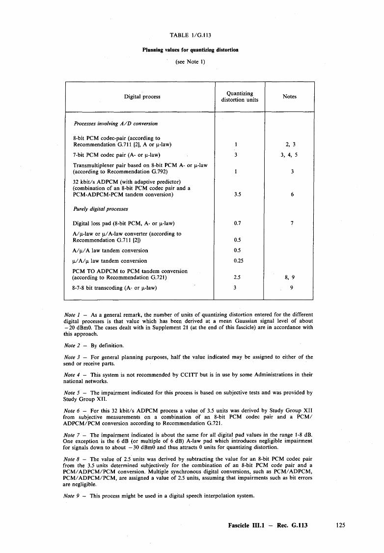
Planning values for quantizing distortion
(see Note 1)
TABLE 1/G. 113
Digital process Quantizing distortion units Notes
Processes involving A /D conversion
8-bit PCM codec-pair (according toRecommendation G .711 [2], A or p-law) 1 2, 3
7-bit PCM codec pair (A- or p-law) 3 3, 4, 5
Transmultiplexer pair based on 8-bit PCM A- or p-law (according to Recommendation G.792) 1 3
32 kb it/s ADPCM (with adaptive predictor) (combination of an 8-bit PCM codec pair and a PCM-ADPCM-PCM tandem conversion) 3.5 6
Purely digital processes
Digital loss pad (8-bit PCM, A- or p-law) 0.7 7
A /p-law or p/A -law converter (according to Recommendation G .711 [2]) 0.5
A /p /A law tandem conversion 0.5
p /A /p law tandem conversion 0.25
PCM TO ADPCM to PCM tandem conversion (according to Recommendation G.721) 2.5 8, 9
8-7-8 bit transcoding (A- or p-law) 3 9
Note 1 — As a general remark, the number of units of quantizing distortion entered for the different digital processes is that value which has been derived at a mean Gaussian signal level of about — 20 dBmO. The cases dealt with in Supplement 21 (at the end of this fascicle) are in accordance with this approach.
Note 2 — By definition.
Note 3 — For general planning purposes, half the value indicated may be assigned to either of thesend or receive parts.
Note 4 — This system is not recommended by CCITT but is in use by some Administrations in their national networks.
Note 5 — The impairment indicated for this process is based on subjective tests and was provided by Study Group XII.
Note 6 — For this 32 kb it/s ADPCM process a value of 3.5 units was derived by Study Group XII from subjective measurements on a combination of an 8-bit PCM codec pair and a P C M / A D PCM /PCM conversion according to Recommendation G.721.
Note 7 — The im pairment indicated is about the same for all digital pad values in the range 1-8 dB. One exception is the 6 dB (or multiple of 6 dB) A-law pad which introduces negligible impairment for signals down to about — 30 dBmO and thus attracts 0 units for quantizing distortion.
Note 8 — The value of 2.5 units was derived by subtracting the value for an 8-bit PCM codec pairfrom the 3.5 units determined subjectively for the combination of an 8-bit PCM code pair and aPC M /A D PC M /PC M conversion. Multiple synchronous digital conversions, such as PCM /A D PCM , PC M /A D PC M /PC M , are assigned a value of 2.5 units, assuming that impairments such as bit errors are negligible.
Note 9 — This process might be used in a digital speech interpolation system.
Fascicle III.l - Rec. G.113
3.6 Limitations o f the provisional planning rule
In § 3.5, it is assumed that for estimating the transmission impairment due to the presence of unintegrated digital processes in international telephone connections, the units of transmission impairment correspond to the units o f quantizing distortion and that the simple addition of such units would apply.
For international telephone circuits that include tandem digital processes in an all-digital environment, adding the individual units of quantizing distortion might not accurately reflect the accumulated quantizing distortion (and, consequently, the accumulated units of transmission impairment). This could be the case since the individual amounts of quantizing distortion power produced by the individual digital processes might not be uncorrelated and, therefore, the addition of individual units of quantizing distortion might, under some circumstances, indicate totals that could be different from those actually in effect. This is explained in some detail in Suplement No. 21 at the end of this fascicle.
Although the 5 + 4 + 5 = 14 rule given in § 3.5 might under some conditions provide only approximate results, the rule, nevertheless, is considered to be suitable for most planning purposes particularly in cases involving unintegrated digital processes. Examples of tandem digital processes which are explicitly taken into account in Table 1/G.113 are A-p-A code conversion, p-A-p code conversion, and PCM-ADPCM-PCM conversion.
4 Effect of transmission impairments on voiceband data performance
The effect o f transmission impairments on voiceband data performance is under study in Question 25/X II. Some information provided by one Administration is available in Annex 4 to the Question.
ANNEX A
(to Recommendation G.113)
Information for planning purposes concerning attenuation distortion and group-delay distortion introduced by circuits and exchanges in
the switched telephone network
A.l The information given in Tables A-1/G.113 to A-6/G.113 is derived from measurements1) on modern equipment. The performance of actual connections in the switched telephone network can be expected to be worse than would be calculated from the tabulated data because o f:
— mismatch and reflexion;
— unloaded subscribers’ lines;
— loaded trunk-junctions with a low cutoff frequency;
— older equipment.
A.2 The reference frequency for attenuation distortion is 800 Hz. The reference frequency for group-delay distortion (i.e. the frequency at which the group delay is a minimum) has been estimated in each case.
A.3 In the results for circuits no allowance has been made for line signalling terminations although in some cases these distortions are included in the data for exchanges.
0 Supplied by AT&T, Telecom Australia, Italy, British Telecom, NTT and Switzerland.
126 Fascicle III.l - Rec. G.113
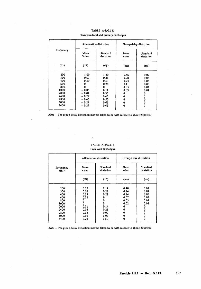
TABLE A-1/G.113 Two-wire local and primary exchanges
Attenuation distortion Group-delay distortion
FrequencyMean Standard Mean StandardValue deviation value deviation
(Hz) (dB) (dB) (ms) (ms)
200 1.69 1.20 0.56 0.07300 0.63 0.81 0.28 0.05400 0.30 0.43 0.23 0.05600 0 0.28 0.11 0.03800 0 0 0.05 0.02
1000 - 0.05 0.11 0.03 0.012000 - 0.04 0.35 0 02400 - 0 .2 9 0.45 0 02800 - 0.45 0.50 0 03000 -0 .2 4 0.65 0 03400 - 0.29 0.63 0 0
Note - The group-delay distortion may be taken to be with respect to about 2000 Hz.
TABLE A-2/G.113 Four-wire exchanges
Attenuation distortion Group-delay distortion
Frequency. Mean Standard Mean Standard(Hz) value deviation value deviation
(dB) (dB) (ms) (ms)
200 0.32 0.14 0.40 0.02300 0.16 0.28 0.14 0.02400 0.13 0.21 0.14 0.03600 0.02 0 0.07 0.02800 0 0 0.03 0.01
1000 0 0 0.02 0.012000 0.01 0.14 0 02400 0.06 0.21 0 02800 0.02 0.02 0 03000 0.10 0.07 0 03400 0.20 0.50 0 0
Note - The group-delay distortion may be taken to be with respect to about 2000 Hz.
Fascicle III.l — Rec. G.113
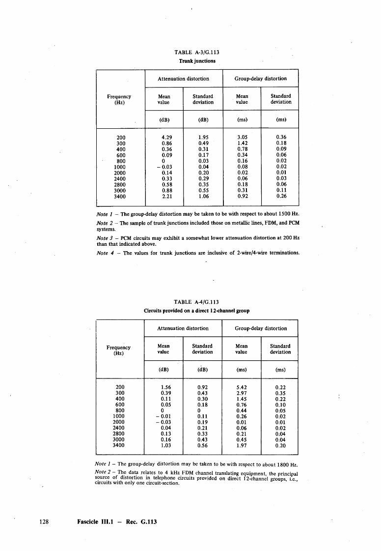
TABLE A-3/G.113 Trunk junctions
Attenuation distortion Group-delay distortion
Frequency Mean Standard Mean Standard(Hz) value deviation value deviation
(dB) (dB) (ms) (ms)
200 4.29 1.95 3.05 0.36300 0.86 0.49 1.42 0.18400 0.36 0.31 0.78 0.09600 0.09 0.17 0.34 0.06800 0 0.03 0.16 0.02
1000 -0 .0 3 0.04 0.08 0.022000 0.14 0.20 0.02 0.012400 0.33 0.29 0.06 0.032800 0.58 0.35 0.18 0.063000 0.88 0.55 0.31 0.113400 2.21 1.06 0.92 0.26
Note 1 - The group-delay distortion may be taken to be with respect to about 1500 Hz.
Note 2 - The sample of trunk junctions included those on metallic lines, FDM, and PCM systems.
Note 3 - PCM circuits may exhibit a somewhat lower attenuation distortion at 200 Hz than that indicated above.
Note 4 - The values for trunk junctions are inclusive of 2-wire/4-wire terminations.
TABLE A-4/G.113 Grcuits provided on a direct 12-channel group
Attenuation distortion Group-delay distortion
Frequency Mean Standard Mean Standard(Hz) value deviation value deviation
(dB) (dB) (ms) (ms)
200 1.56 0.92 5.42 0.22300 0.39 0.43 2.97 0.35400 0.11 0.30 1.45 0.22600 0.05 0.18 0.76 0.10800 0 0 0.44 0.05
1000 -0 .0 1 0.11 0.26 0.022000 -0 .0 3 0.19 0.01 0.012400 0.04 0.21 0.06 0.022800 0.13 0.33 0.21 0.043000 0.16 0.43 0.45 0.043400 1.03 0.56 1.97 0.20
Note 1 - The group-delay distortion may be taken to be with respect to about 1800 Hz.
Note 2 - The data relates to 4 kHz FDM channel translating equipment, the principal source of distortion in telephone circuits provided on direct 12-channel groups, i.e. circuits with only one circuit-section.
Fascicle III.l - Rec. G.113
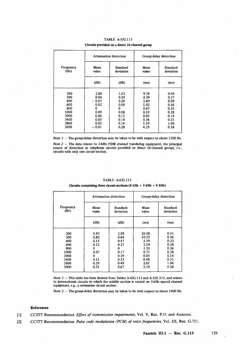
TABLE A-5/G.113 Circuits provided on a direct 16-channel group
Attenuation distortion Group-delay distortion
Frequency Mean Standard Mean Standard(Hz) value deviation value deviation
(dB) (dB) (ms) (ms)
200 2.80 1.63 9.74 0.40300 0.04 0.19 4.39 0.27400 - 0.07 0.20 2.49 0.09600 0.02 0.09 1.02 0.56 -800 0 0 0.47 0.35
1000 0.09 0.08 0.19 0.282000 0.06 0.12 0.03 0.142400 0.03 0.14 0.36 0.312800 0.03 0.16 1.59 1.063000 -0 .0 1 0.28 4.29 0.38
Note 1 - The group-delay distortion may be taken to be with respect to about 1200 Hz.
Note 2 - The data relates:to 3-kHz FDM channel translating equipment, the principal source of distortion in telephone circuits provided on direct 16-channel groups, i.e., circuits with only one circuit-section.
TABLE A-6/G.U3 Circuits comprising three circuit-sections (4 kHz + 3 kHz + 4 kHz)
Attenuation distortion Group-delay distortion
Frequency Mean Standard Mean Standard(Hz) value deviation value deviation
(dB) (dB) (ms) (ms)
200 5.92 2.09 20.58 0.51300 0.82 0.64 10.33 0.56400 0.15 0.47 5.39 0.32600 0.12 0.27 2.54 0.58800 0 0 1.35 0.36
1000 0.07 0.17 0.71 0.282000 0 0.29 0.05 0.142400 0.11 0.33 0.48 0.312800 0.29 0.49 2.01 1.063000 0.31 0.67 5.19 0.38
Note 1 - This table has been derived from Tables A-4/G.113 and A-5/G.113, and relates to international circuits in which the middle section is routed on 3-kHz spaced channel equipment, e.g., a submarine circuit section.
N ote 2 — The group-delay distortion may be taken to be with respect to about 1400 Hz.
References
CCITT Recommendation Effect o f transmission impairments, Vol. V, Rec. P. 11 and Annexes.
CCITT Recommendation Pulse code modulation (PCM) o f voice frequencies, Vol. I l l , Rec. G.711.
Fascicle III.l — Rec. G.113
Recommendation G.114
MEAN ONE-WAY PROPAGATION TIME
(Geneva, 1964; amended Mar del Plata, 1968, Geneva, 1980 and Malaga-Torremolinos, 1984)
The times in this Recommendation are the means of the propagation times in the two directions of transmission in a connection. When opposite directions of transmission are provided by different media (e.g. a satellite channel in one direction and a terrestrial channel in the other) the two times contributing to the mean may differ considerably.
1 Limits for a connection
It is necessary in an international telephone connection to limit the propagation time between two subscribers. As the propagation time is increased, subscriber difficulties increase, and the rate of increase of difficulty rises. Relevant evidence is given in references [1]-[10J, particularly with regard to b) below.
As a network performance objective, the CCITT therefore recommends the following limitations on mean one-way propagation times when echo sources exist and appropriate echo control devices, such as echo suppressors and echo cancellers, are used:
a) 0 to 150 ms, acceptable.Note — Echo suppressors specified in Recommendation G.161 of the Blue Book [111 may be used for delays not exceeding 50 ms (see Recommendation G.131, § 2.2).
b) 150 to 400 ms, acceptable, provided that increasing care is exercised on connections when the mean one-way propagation time exceeds about 300 ms, and provided that echo control devices, such as echosuppressors and echo cancellers, designed for long-delay circuits are used;
c) above 400 ms, unacceptable. Connections with these delays should not be used except under the most exceptional circumstances.
Until such time as additional, significant information permits Administrations to make a firmer determination o f acceptable delay limits, they should take full account of the documents referred to under References in selecting, from alternatives, plans involving delays in range b) above.
Note 1 — The above values refer only to the propagation time between two subscribers. However, for other purposes (e.g. in Recommendation G.131) the mean one-way propagation time of an echo path is to be estimated. The values in § 2 may be used in such estimations.
Note 2 — There is good evidence that echo cancellers fitted at both ends of a long-delay connectiongenerally yield superior performance over current types of echo suppressors. (For further details, see § 2.2 ofRecommendation G.131.)
Note 3 — It should be noted that although an echo suppressor and an echo canceller on the same connection are compatible (they can satisfactorily interwork), the full benefits of echo cancellers are only experienced when both ends are so equipped. In particular, an Administration unilaterally replacing its echo suppressors with echo cancellers will cause little benefit to its own subscriber on international connections if the echo suppressor still remains at the other end.
2 Values for circuits
In the establishment of the general interconnection plan within the limits in § 1 the one-way propagation time of both the national extension circuits and the international circuits must be taken into account. The propagation time of circuits and connections is the aggregate of several components; e.g. group delay in cables and in filters encountered in FDM modems of different types. Digital transmission and switching also contribute delays. The conventional planning values given in § 2.1 may be used to estimate the total propagation time of specified assemblies which may form circuits or connections.
130 Fascicle III.l - Rec. G.1I4
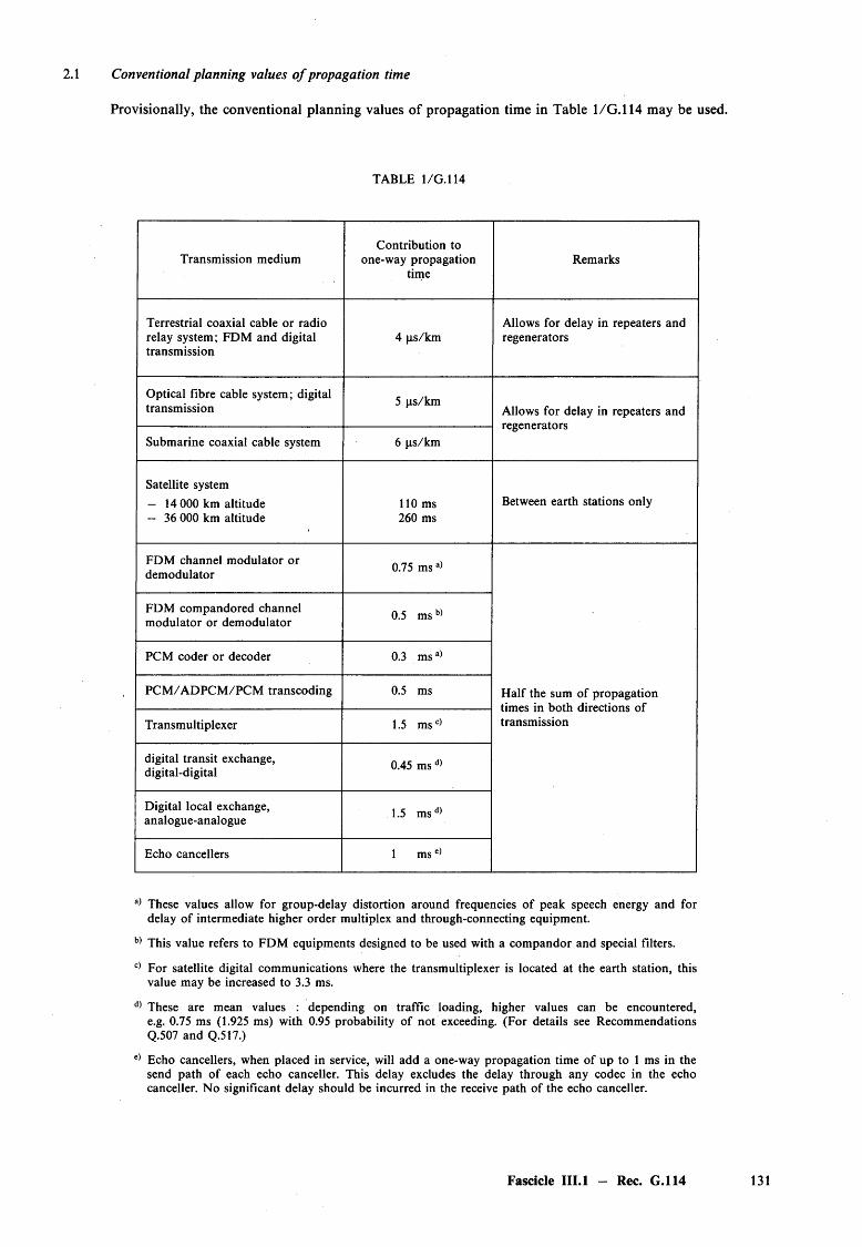
Conventional planning values o f propagation time
Provisionally, the conventional planning values of propagation time in Table 1/G. 114 may be used.
TABLE 1/G. 114
Transmission mediumContribution to
one-way propagation time
Remarks
Terrestrial coaxial cable or radio relay system; FDM and digital transmission
4 ps/kmAllows for delay in repeaters and regenerators
Optical fibre cable system; digital transmission 5 ps/km
Allows for delay in repeaters and regenerators
Submarine coaxial cable system 6 ps/km
Satellite system— 14 000 km altitude— 36 000 km altitude
110 ms 260 ms
Between earth stations only
FDM channel m odulator or demodulator 0.75 ms a)
FDM compandored channel modulator or demodulator 0.5 m sb)
PCM coder or decoder 0.3 m sa)
PC M /A D PC M /PC M transcoding 0.5 ms H alf the sum of propagation times in both directions of transmissionT ransmultiplexer 1.5 m sc)
digital transit exchange, digital-digital 0.45 m sd)
Digital local exchange, analogue-analogue 1.5 m sd)
Echo cancellers 1 m se)
a) These values allow for group-delay distortion around frequencies of peak speech energy and for delay o f intermediate higher order multiplex and through-connecting equipment.
b) This value refers to FDM equipments designed to be used with a com pandor and special filters.
c) For satellite digital communications where the transmultiplexer is located at the earth station, this value may be increased to 3.3 ms.
d) These are mean values : depending on traffic loading, higher values can be encountered, e.g. 0.75 ms (1.925 ms) with 0.95 probability of not exceeding. (For details see Recommendations Q.507 and Q.517.)
e) Echo cancellers, when placed in service, will add a one-way propagation time of up to 1 ms in the send path of each echo canceller. This delay excludes the delay through any codec in the echo canceller. No significant delay should be incurred in the receive path of the echo canceller.
Fascicle III.l — Rec. G.114
2.2 National extension circuits
The main arteries of the national network should consist of high-velocity propagation lines. In these conditions, the propagation time between the international centre and the subscriber farthest away from it in the national network will be as follows:
a) in purely analogue networks, the propagation time will probably not exceed:12 + (0.004 x distance in kilometres) ms.
Here the factor 0.004 is based on the assumption that national trunk circuits will be routed over high-velocity plant (250 km /m s). The 12 ms constant term makes allowance for terminal equipment and for the probable presence in the national network of a certain quantity of loaded cables (e.g. three pairs o f channel translating equipments plus about 160 km of H 88/36 loaded cables). For an average size country (see Figure 2 /G .l03) the one-way propagation time will be less than 18 ms;
b) in mixed analogue/digital networks, the propagation time can generally be estimated by the equation given for purely analogue networks. However under certain unfavourable conditions increased delay may occur compared with the purely analogue case. This occurs in particular when digital exchanges are connected with analogue transmission systems through PC M /FD M equipments in tandem, or transmultiplexers. With the growing degree of digitization the propagation time will gradually approach the condition of purely digital networks;
c) in purely digital networks between exchanges (e.g. an IDN), the propagation time as defined above will probably not exceed:
3 + (0.004 x distance in kilometers) ms.The 3 ms constant term makes allowance for one PCM coder or decoder and five digitally switched exchanges, (see Figure 1/G . 104).Note — The value 0.004 is a mean value for coaxial cable systems and radio-relay systems; for optical fibre systems 0.005 is to be used;
d) in purely digital networks between susbscribers (e.g. an ISDN), the delay of c) above has to be increased by up to 3.6 ms if burst-mode (time compression multiplexing) transmission is used on 2-W local subscriber lines.
2.3 International circuits
International circuits 0 will use high-velocity transmission systems, e.g. terrestrial cable or radio-relay systems, submarine systems or satellite systems. The planning values of § 2.1 may be used.
The magnitude of the mean one-way propagation time for circuits on high altitude communication satellite systems makes it desirable to impose some routing restrictions on their use. Details of these restrictions are given in Recommendation Q.13 [12]. (See also Annex A below.)
ANN EX A
(to Recommendation G.114)
Transmission delay and echo problems caused by multiple satellite hops
A.l Introduction
According to Recommendation G.114 mean one-way propagation times above 400 ms are unacceptable. The transmission delays to be expected in the case of modern terrestrial transmission systems are by no means as long; delays of up to 100 ms only occurred with loaded VF cables such as were also used in the past of relatively long international circuits. Even the longest international connections (see Figure 1/G. 103 or Figure 1/G. 104) will not exceed a delay time of about 170 ms, taking submarine cables into account. When satellite circuits were introduced about fifteen years ago, transmission delays of several 100 ms had to be taken into account again — for a single satellite hop.
For short nearby links, telecommunications cables operated at voice frequencies may also be used in the conditions set out in the introduction to Sub-section 5.4 o f Fascicle III.2.
132 Fascicle III.l — Rec. G.114

The installation of national satellites means that transmission delays above 400 ms could occur on international connections as a result of tandem connection of several satellite hops. These problems are discussed below.
A.2 Transmission delay on satellite hops
C C IR Report 383-4 [13] specifies a transmission delay of approximately 260 ms for one satellite hop and approximately 290 ms including the terrestrial links. For two satellite hops a total transmission delay of approximately 550 ms is to be expected. Supposing that there were a national satellite hop at each end of an international satellite hop, the overall one way propagation time between the subscribers would be approximately 810 ms, almost one second.
A.3 Effect o f long transmision delays on the subscriber
Early investigations using a 4-wire test arrangement were carried out aroud 1931 as a “difficulty” test, undertaken by H.Decker in the laboratory. The transmission delay was reduced from an initial one-way delay of 1370 ms to a value at which the test person indicated that there was no difficulty in the conversation (transmitted bandwidth 300-2400 Hz). No echo problems were found in this test; noise conditions are unknown. The result of this test is shown in Figure A-1/G .114 as curve 1.
Mean one-way propagation time ccm-moo
FIGURE A-l/G. 114
Effect of long transmission delay on the difficulty of conversation.
Later investigations undertaken in 1964 and 1965 with a view to the installation of the first telecommunication satellite Early Bird on real circuits between France, the United Kingdom, the United States and the Federal Republic of Germany show principally the same result as arrived at by H. Decker. The main difference in the test conditions is that the circuits were now equipped with different types of echo suppressors, had a certain amount of noise power (about 20000 pWOp) and had different bandwidths on the TAT-3 cable route (230 — 3200 Hz) and on the satellite (170 — 3400 Hz). The result is shown in Figure A-1/G.114 as curve 2.
Both tests show that, at about 400 ms, 50% of the subscribers have difficulties with the conversation. The lower degree of difficulties found on real circuits above 400 ms may be due to echo, noise, etc.
Fascicle III.l — Rec. G.114 133
Curve 3 in Figure A -l/G .114 shows the interview results on the fair-or-poor opinion of the subscribers. They differ at higher delay remarkably from curve 1. This may result from the fact that some of the inquired customers, in spite of the difficulties they had due to the long delay, found the received speech quality good or excellent. It seems, therefore, that for assessing the obtained results, only the difficulties experienced should be considered.
Connections with more than 300 ms can only be used by very disciplined subscribers who are aware of the problems involved in such a connection.
A.4 Conclusions
If a 40% value of difficulty is taken from curve 1 as a limit - this is indeed a very high limit — a delay of 300 ms should never be exceeded.
In public telephone networks, only connections which do not contain more than one satellite hop should be permitted. Two hops can only be tolerated in special cases. Connections with more than two hops are totally unsuitable for telephony. (Study Group GAS 3 was aware of this fact when preparing the CCITT manual Rural Telecommunication, Appendix I following; [14].)
APPENDIX I
(to Annex A to Recommendation G.114)
(Extract from CCITT manual Rural Telecommunications Geneva, 1979, page 113)
It is to be mentioned that with geostationary satellites at a n 2) altitude of 36 000 km, the standard altitude used nowadays [55],a mean single-path propagation time of 260 ms can normally be expected for a satellite link between earth stations. Twice this value can be expected for two satellite links, three times the value for three sections, i.e. 520 or 780 ms respectively.
The CCITT Recommendation cited in [56] 3> states that links with single-path propagation times of more than 400 ms are not acceptable for the international long-distance network.
It is questionable whether multiple links will be accepted by all customers even if the necessary speech discipline is maintained, since the pauses in conversation and increased number of questions would cause added disturbance.
What is really required is to minimize the probability of having several satellite sections. This would mean, for example, that by appropriate routing of traffic at the switching centres subscribers connected over national satellites only have access to terrestrial lines or to the worldwide marine cable network. Even then, it is feasible that in rare cases two satellite sections could occur in a link if two countries both had national satellites.
References
[1] CCITT Red Book, Volume V bis, Annex E (United States), ITU, Geneva, 1965.
[2] Ibid:, Annex F (United Kingdom).
[3] Ibid:, Annex 4 to Question 6 /X II (Italy).
[4] CCITT Red Book, Volume V, Supplements 1-6, ITU, Geneva, 1985.
[5] BARSTOW (J. M.): Results o f user reaction tests on communication via Early Bird satellite, Progress inAstronautic Aeronautics, 19, 1966, Academic Press, New York and London.
[6] HELDER (G. K.): Customer evaluation of telephone circuits with delay, Bell System Technical Journal, 45,September 1966, pp. 1157-1191.
2) The reference was to CCIR Report 383-3.3) The reference was to Recommendation G.114
134 Fascicle III.l - Rec. G.114
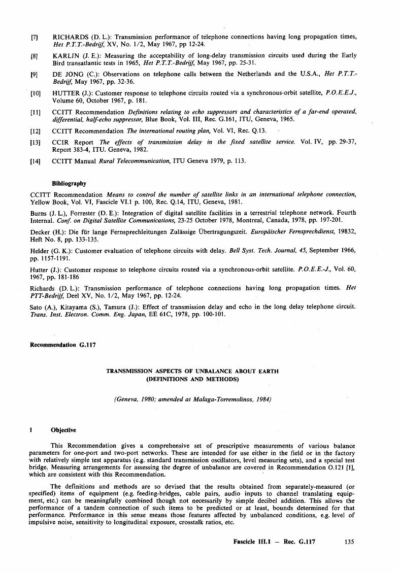
[7] RICHARDS (D. L.): Transmission performance of telephone connections having long propagation times, Het P. T. T.-Bedrijf XV, No. 1/2, May 1967, pp 12-24.
[8] KARLIN (J. E.): Measuring the acceptability o f long-delay transmission circuits used during the Early Bird transatlantic tests in 1965, Het P. T. T.-Bedrijf May 1967, pp. 25-31.
[9] DE JONG (C.): Observations on telephone calls between the Netherlands and the U.S.A., Het P. T. T.- Bedrijf May 1967, pp. 32-36.
[10] HUTTER (J.): Customer response to telephone circuits routed via a synchronous-orbit satellite, P.O.E.E.J., Volume 60, October 1967, p. 181.
[11] CCITT Recommendation Definitions relating to echo suppressors and characteristics o f a far-end operated,differential, half-echo suppressor, Blue Book, Vol. I ll, Rec. G.161, ITU, Geneva, 1965.
[12] CCITT Recommendation The international routing plan, Vol. VI, Rec. Q.13.
[13] CCIR Report The effects o f transmission delay in the fixed satellite service. Vol. IV, pp. 29-37,Report 383-4, ITU. Geneva, 1982.
[14] CCITT Manual Rural Telecommunication, ITU Geneva 1979, p. 113.
Bibliography
CCITT Recommendation Means to control the number o f satellite links in an international telephone connection, Yellow Book, Vol. VI, Fascicle VI. 1 p. 100, Rec. Q.14, ITU, Geneva, 1981.
Burns (J. L.), Forrester (D. E.): Integration of digital satellite facilities in a terrestrial telephone network. FourthInternal. C onf on Digital Satellite Communications, 23-25 October 1978, Montreal, Canada, 1978, pp. 197-201.
Decker (H.): Die fur lange Fernsprechleitungen Zulassige Ubertragungszeit. Europaischer Fernsprechdienst, 19832, Heft No. 8, pp. 133-135.
Helder (G. K.): Customer evaluation of telephone circuits with delay. Bell Syst. Tech. Journal, 45, September 1966, pp. 1157-1191.
Hutter (J.): Customer response to telephone circuits routed via a synchronous-orbit satellite. P.O.E.E.-J., Vol. 60, 1967, pp. 181-186
Richards (D. L.): Transmission performance of telephone connections having long propagation times. Het PTT-Bedrijf Deel XV, No. 1/2, May 1967, pp. 12-24.
Sato (A.), Kitayama (S.), Tamura (J.): Effect of transmission delay and echo in the long delay telephone circuit.Trans. Inst. Electron. Comm. Eng. Japan, EE 61C, 1978, pp. 100-101.
Recommendation G.117
TRANSMISSION ASPECTS OF UNBALANCE ABOUT EARTH (DEFINITIONS AND METHODS)
(Geneva, 1980; amended at Malaga-Torremolinos, 1984)
1 Objective
This Recommendation gives a comprehensive set of prescriptive measurements o f various balance parameters for one-port and two-port networks. These are intended for use either in the field or in the factory with relatively simple test apparatus (e.g. standard transmission oscillators, level measuring sets), and a special test bridge. Measuring arrangements for assessing the degree of unbalance are covered in Recommendation 0.121 [1], which are consistent with this Recommendation.
The definitions and methods are so devised that the results obtained from separately-measured (or specified) items of equipment (e.g. feeding-bridges, cable pairs, audio inputs to channel translating equipment, etc.) can be meaningfully combined though not necessarily by simple decibel addition. This allows the performance of a tandem connection of such items to be predicted or at least, bounds determined for that performance. Performance in this sense means those features affected by unbalanced conditions, e.g. level of impulsive noise, sensitivity to longitudinal exposure, crosstalk ratios, etc.
Fascicle III.l — Rec. G.117 135

2 Principles of the scheme of nomenclature
Many different terms have been used throughout the literature concerning unbalance about earth, some conflicting, or in other respects inadequate. The descriptive titles of the quantities given in this Recommendation are based on the following principles which have been adopted:
Mode conversion, e.g. a poor (unbalanced) termination will develop an unwanted transverse signal when excited by a longitudinal signal. The measure of this effect is here termed longitudinal conversion ratio, and when expressed in transmission units longitudinal conversion loss, or LCL.
When a two-port is involved where for example an excitation at one port produces a signal at the other port, then the designation will include the word transfer, for example longitudinal conversion transfer ratio and the corresponding loss, LCTL.
The impedance of the longitudinal path presented by a test object is a key parameter. The term longitudinal impedance ratio and the corresponding decibel expression, longitudinal impedance loss, are used to characterize the particular measurement defined.
Active devices which are sources of signals (e.g. an oscillator, the output port of an amplifier) are additionally characterized by the amount of unwanted longitudinal signal that is present in the output. The key word output is now included, to give longitudinal output voltage, and the corresponding longitudinal output level. When such unwanted signals are expressed as a proportion of the wanted (transverse) signal the key phrase is output signal balance ratio, the decibel expression of which is output signal balance.
Devices which continuously respond to signals (e.g. level-measuring sets, the input port of an amplifier) and which can in principle respond to unwanted longitudinal signals by reason of internal mechanisms (i.e. even if their input impedances were perfectly balanced) are characterized by measures containing the words input interference. These measures are input longitudinal interference ratio and the corresponding decibel expression input longitudinal interference loss. The long-established and well- defined common-mode rejection ratio is maintained. The term sensitivity coefficient is avoided, since this is widely used in the Directives [2] and the work of Study G roup V with a rather specialized meaning.
When a two-port network is involved, the input and output signals may not be the same, for example, they may have different levels, frequencies (FDM modems) or structure (PCM multiplex equipments). These aspects should be taken into account when formulating proposals for the item under test.
In the case of receiving devices in which the operation is not a linear continuous function of the level of the input signal (e.g. a group-delay measuring set or a data modem) the key principle is the threshold level of the interference; this is the level at or above which an unacceptable amount of degradation of performance or misoperation occurs. Thus we obtain longitudinal interference threshold voltage and the corresponding level.
3 Summary of the descriptive terms used
3.1 One-port networks
a) transverse reflexion factor (transverse return loss: TRL),
b) transverse conversion ratio (loss: TCL),
c) longitudinal conversion ratio (loss: LCL),
d) longitudinal impedance ratio (loss: LIL),
e) transverse output voltage (level: TOL),
f) longitudinal output voltage (level: LOL).
(Voltages e) and f) are unwanted signals uncorrelated to the wanted signals.)
136 Fascicle HI.1 - Rec. G.117
a)
b)
c)
d)
e)
f)
g)
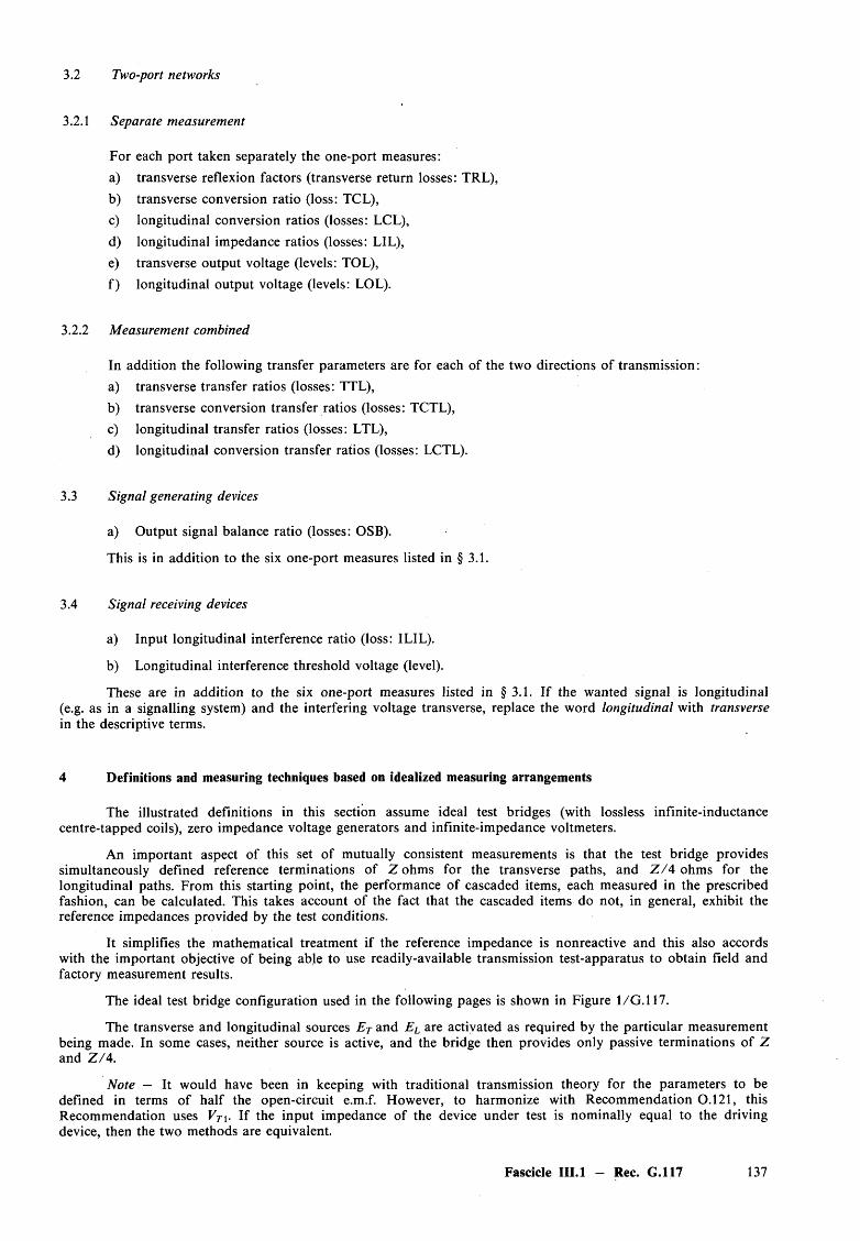
3.2 Two-port networks
3.2.1 Separate measurement
For each port taken separately the one-port measures:a) transverse reflexion factors (transverse return losses: TRL),
b) transverse conversion ratio (loss: TCL),c) longitudinal conversion ratios (losses: LCL),d) longitudinal impedance ratios (losses: LIL),e) transverse output voltage (levels: TOL),f) longitudinal output voltage (levels: LOL).
3.2.2 Measurement combined
In addition the following transfer parameters are for each of the two directions of transmission:a) transverse transfer ratios (losses: TTL),b) transverse conversion transfer ratios (losses: TCTL),c) longitudinal transfer ratios (losses: LTL),d) longitudinal conversion transfer ratios (losses: LCTL).
3.3 Signal generating devices
a) Output signal balance ratio (losses: OSB).
This is in addition to the six one-port measures listed in § 3.1.
3.4 Signal receiving devices
a) Input longitudinal interference ratio (loss: ILIL).
b) Longitudinal interference threshold voltage (level).
These are in addition to the six one-port measures listed in § 3.1. If the wanted signal is longitudinal(e.g. as in a signalling system) and the interfering voltage transverse, replace the word longitudinal with transversein the descriptive terms.
4 Definitions and measuring techniques based on idealized measuring arrangements
The illustrated definitions in this section assume ideal test bridges (with lossless infinite-inductance centre-tapped coils), zero impedance voltage generators and infinite-impedance voltmeters.
An im portant aspect of this set of mutually consistent measurements is that the test bridge provides simultaneously defined reference terminations of Z ohms for the transverse paths, and Z /4 ohms for the longitudinal paths. From this starting point, the performance of cascaded items, each measured in the prescribed fashion, can be calculated. This takes account of the fact that the cascaded items do not, in general, exhibit the reference impedances provided by the test conditions.
It simplifies the mathematical treatment if the reference impedance is nonreactive and this also accords with the im portant objective of being able to use readily-available transmission test-apparatus to obtain field and factory measurement results.
The ideal test bridge configuration used in the following pages is shown in Figure 1/G . 117.
The transverse and longitudinal sources E T and EL are activated as required by the particular measurement being made. In some cases, neither source is active, and the bridge then provides only passive terminations of Z and Z /4 .
Note — It would have been in keeping with traditional transmission theory for the parameters to be defined in terms of half the open-circuit e.m.f. However, to harmonize with Recommendation 0.121, this Recommendation uses VT\. If the input impedance of the device under test is nominally equal to the driving device, then the two methods are equivalent.
Fascicle III.l — Rec. G.117 137
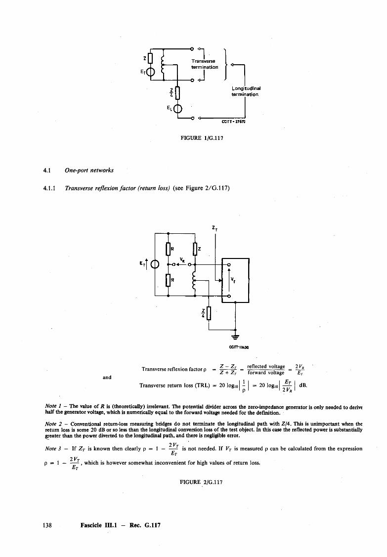
FIGURE 1/G.117
4.1 One-port networks
4.1.1 Transverse reflexion factor (return loss) (see Figure 2 /G .l 17)
T n r . Z — Z T reflected voltage 2 VRTransverse reflexion factor p = —— = -= j ;Z + Z T forward voltage Erand
111 I Et I .Transverse return loss (TRL) = 20 logio - = 2 0 logio dB.1 p I \ 2 V r I
Note 1 — The value of R is (theoretically) irrelevant. The potential divider across the zero-impedance generator is only needed to derive half the generator voltage, which is numerically equal to the forward voltage needed for the definition.
Note 2 - Conventional retum-loss measuring bridges do not terminate the longitudinal path with Z/4. This is unimportant when the return loss is some 20 dB or so less than the longitudinal conversion loss of the test object. In this case the reflected power is substantially greater than the power diverted to the longitudinal path, and there is negligible error.
2 VTNote 3 — If Z T is known then clearly p = 1 — ----- is not needed. If VT is measured p can be calculated from the expressionEt
2 Ftp = 1 — ------, which is however somewhat inconvenient for high values of return loss.Et
FIGURE 2/G.l 17
138 Fascicle III.l - Rec. G.117
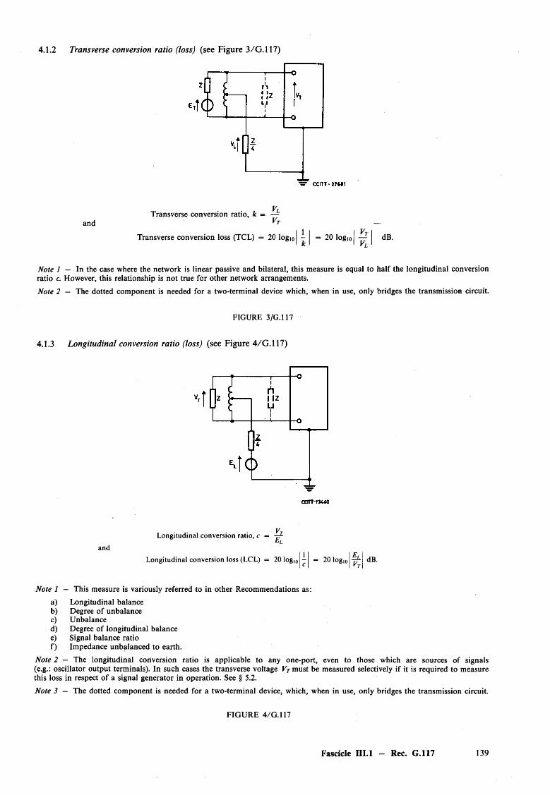
4.1.2 Transverse conversion ratio (loss) (see Figure 3/G.117)
Transverse conversion ratio, k — —and —
111 I Vt ITransverse conversion loss (TCL) = 20 logio - = 2 0 logio — dB.
1 k i ' VL i
Note 1 — In the case where the network is linear passive and bilateral, this measure is equal to half the longitudinal conversion ratio a However, this relationship is not true for other network arrangements.Note 2 — The dotted component is needed for a two-terminal device which, when in use, only bridges the transmission circuit.
FIGURE 3/G.117
4.1.3 Longitudinal conversion ratio (loss) (see Figure 4/G.117)
VTLongitudinal conversion ratio, c = -=r-and
111 I E ILongitudinal conversion loss (LCL) = 20 log,0 - = 20 logl0 r r r dB.I C I I * T I
Note 1 — This measure is variously referred to in other Recommendations as:a) Longitudinal balanceb) Degree of unbalancec) Unbalanced) Degree of longitudinal balancee) Signal balance ratiof) Impedance unbalanced to earth.
Note 2 — The longitudinal conversion ratio is applicable to any one-port, even to those which are sources of signals (e.g.: oscillator output terminals). In such cases the transverse voltage VT must be measured selectively if it is required to measure this loss in respect of a signal generator in operation. See § 5.2.Note 3 — The dotted component is needed for a two-terminal device, which, when in use, only bridges the transmission circuit.
FIGURE 4/G.117
Fascicle III.l — Rec. G.117 139
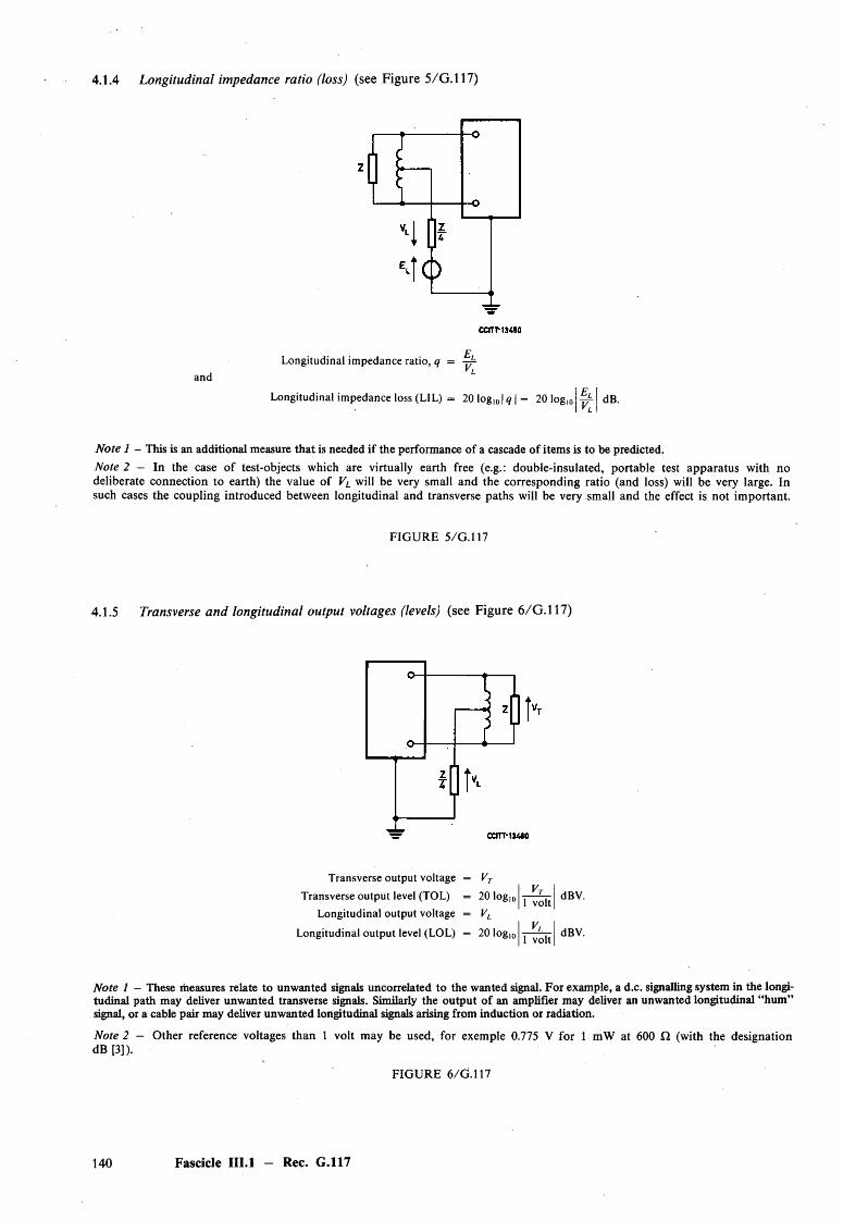
4.1.4 Longitudinal impedance ratio (loss) (see Figure 5/G.117)
£Longitudinal impedance ratio, q = -y=-
and LI F ILongitudinal impedance loss (LIL) = 201og:0| ^ |= 20 log,0 -rf dB.I *L I
Note 1 - This is an additional measure that is needed if the performance of a cascade of items is to be predicted.Note 2 — In the case of test-objects which are virtually earth free (e.g.: double-insulated, portable test apparatus with no deliberate connection to earth) the value of VL will be very small and the corresponding ratio (and loss) will be very large. In such cases the coupling introduced between longitudinal and transverse paths will be very small and the effect is not important.
FIGURE 5/G.117
4.1.5 Transverse and longitudinal output voltages (levels) (see Figure 6/G.117)
Transverse output voltage = VT Transverse output level (TOL) = 20 log.
Longitudinal output voltage = VL
Longitudinal output level (LOL) = 20 log.
Vt1 volt
Vl 1 volt
dBV.
dBV.
Note 1 - These measures relate to unwanted signals uncorrelated to the wanted signal. For example, a d.c. signalling system in the longitudinal path may deliver unwanted transverse signals. Similarly the output of an amplifier may deliver an unwanted longitudinal “hum” signal, or a cable pair may deliver unwanted longitudinal signals arising from induction or radiation.
Note 2 — Other reference voltages than 1 volt may be used, for exemple 0.775 V for 1 mW at 600 Q (with the designation dB [3]).
FIGURE 6/G.l 17
140 Fascicle III.l — Rec. G.117
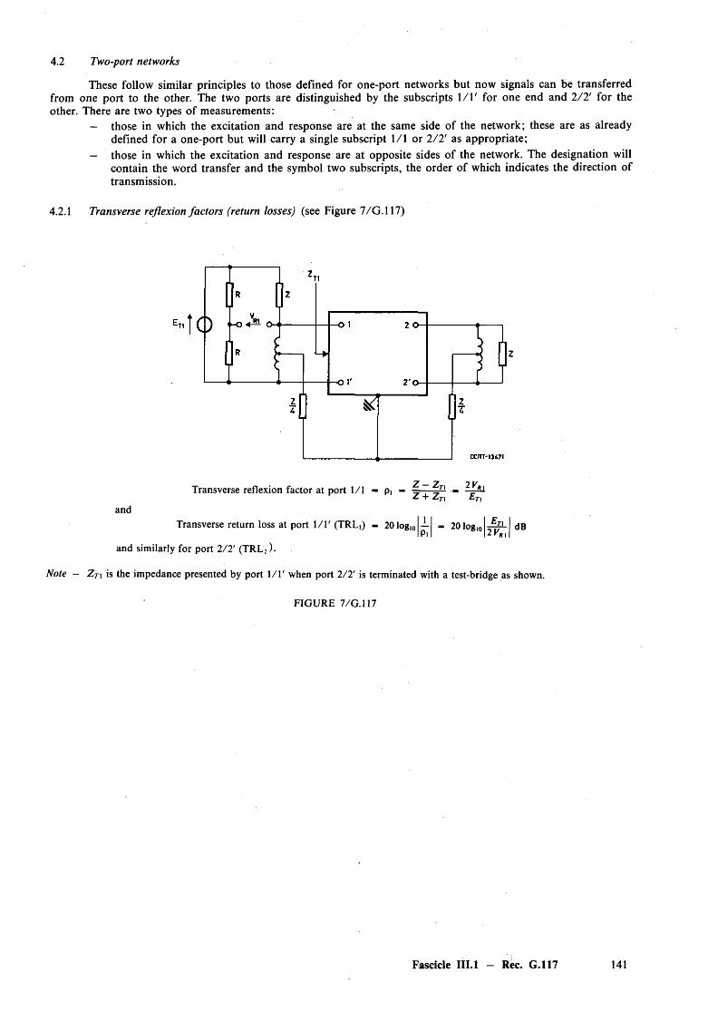
4.2 Two-port networks
These follow similar principles to those defined for one-port networks but now signals can be transferred from one port to the other. The two ports are distinguished by the subscripts 1/1 ' for one end and 2 /2 ' for the other. There are two types of measurements:
— those in which the excitation and response are at the same side of the network; these are as already defined for a one-port but will carry a single subscript 1/1 or 2 /2 ' as appropriate;
— those in which the excitation and response are at opposite sides of the network. The designation will contain the word transfer and the symbol two subscripts, the order of which indicates the direction of transmission.
4.2.1 Transverse reflexion factors (return losses) (see Figure 1/G . 117)
2 „ 7 2 VTransverse reflexion factor at port 1/1 — Pi - -=■•■ n ■«
z + £ tx e Txand
111 I I— * 20 log,o dBPi I 12 l/u 11
and similarly for port 2 / 2 ' (TR L; ).
Note — Z TX is the impedance presented by port 1/1 ' when port 2 /2 ' is terminated with a test-bridge as shown.
FIG URE 7 /G .l 17
Fascicle III.l - Rec. G.117 141
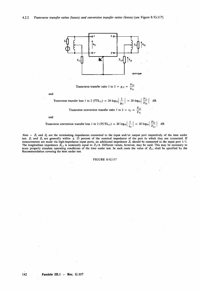
4.2.2 Transverse transfer ratios (losses) and conversion transfer ratios (losses) (see Figure 8/G.117)
Transverse transfer ratio 1 to 2 = g n = —VT\
and
1 1 1 | Vt\ ITransverse transfer loss 1 to 2 (TTL)2) = 20 logio — = 2 0 logio dB.
1 g\2 1 1 Vt2 1
Transverse conversion transfer ratio 1 to 2 = tn = —^Vt\
and
Transverse conversion transfer loss 1 to 2 (TCTL]2) = 20 logio I — I = 20 logio I — I dB.1 *12 I I VL2 1
Note — Z\ and Zi are the terminating impedances connected to the input an d /o r output port respectively of the item undertest. Zi and Zi are generally within ± 25 percent of the nominal impedance of the port to which they are connected. Ifmeasurements are made via high-impedance input ports, an additional impedance Z, should be connected to the input port 1/1. The longitudinal impedance Z L2 is nominally equal to Z 2/4 . Different values, however, may be used. This may be necessary to more properly simulate operating conditions of the time under test. In such , cases the value of Z L2 shall be specified by the Recommendation covering the item under test.
FIG URE 8 /G .l 17
142 Fascicle III.l — Rec. G.117
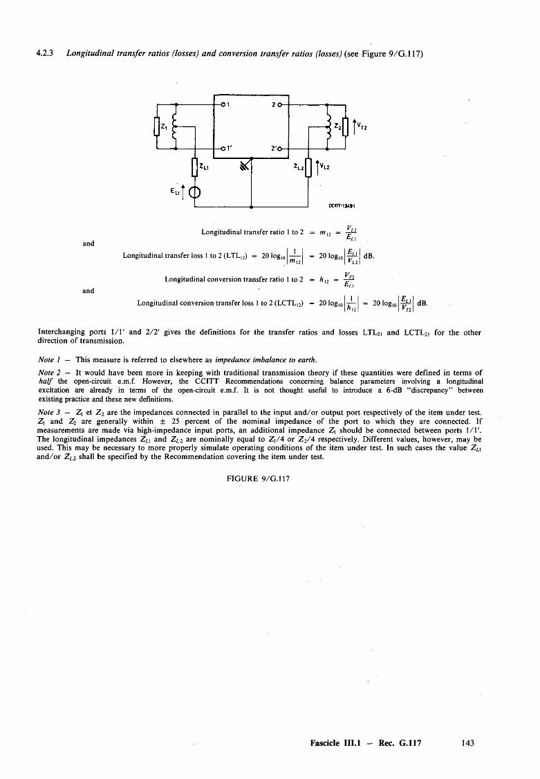
4.2.3 Longitudinal transfer ratios (losses) and conversion transfer ratios (losses) (see Figure 9/G.117)
Longitudinal transfer ratio 1 to 2 = m l2 =and
Longitudinal transfer loss 1 to 2 (LTL,2) = 20 log,0 ---- = 201og,0|*** \ ViI W|2l
Eu
ELl dB.
Longitudinal conversion transfer ratio 1 to 2 = h ,2 =and
Eu
Longitudinal conversion transfer loss 1 to 2 (LCTL,2) = 201og|0U— = 20 log,H I ?
dB.
Interchanging ports 1/1 ' and 2 /2 ' gives the definitions for the transfer ratios and losses LTL2i and LCTL2i for the other direction of transmission.
Note 1 — This measure is referred to elsewhere as impedance imbalance to earth.
Note 2 — It would have been more in keeping with traditional transmission theory if these quantities were defined in terms of ha lf the open-circuit e.m.f. However, the CCITT Recommendations concerning balance parameters involving a longitudinal excitation are already in terms of the open-circuit e.m.f. It is not thought useful to introduce a 6-dB “discrepancy” between existing practice and these new definitions.
Note 3 — Zi et Z 2 are the impedances connected in parallel to the input an d /o r output port respectively of the item under test. Z\ and Zi are generally within ± 25 percent of the nominal impedance of the port to which they are connected. If measurements are made via high-impedance input ports, an additional impedance Z\ should be connected between ports 1/1'. The longitudinal impedances Z L\ and Z L1 are nominally equal to Z ]/4 or Z 2/4 respectively. Different values, however, may be used. This may be necessary to more properly simulate operating conditions of the item under test. In such cases the value Z u an d /o r Zi2 shall be specified by the Recommendation covering the item under test.
FIG URE 9/G.117
Fascicle III.l — Rec. G.117 143

4.3 Signal generating devices
In addition to the six one-port measures already defined, an additional measure is required to control the amount of unwanted signal correlated with the wanted signal delivered by the device to the circuit it is connected to. This special measure is the output signal balance ratio (loss).
4.3.1 Output signal balance ratio (loss) (see Figure 10/G. 117)
Output signal balance ratio, b = —Vt
and
111 | VT IOutput signal balance loss (OSB) = 20 logio - = 20 logio — dB.
I b l
Note 1 — This measure is a generalized version of the quantities referred to as the unbalance of ouput e.m.f.Note 2 — This measure is also related in a somewhat indirect and complicated fashion to the sensitivity coefficients for electromagnetic and electrostatic induction defined in [2], if the cable pair is considered as a simultaneous source of a transverse signal correlated with the induced longitudinal voltages.
Note 3 - The test object itself provides the source of signal. Hence a separate generator is not required.
Note 4 - The definition relates particularly to generators of transverse signals (e.g.: transmission oscillators) but can be readily extended to cover the case of a longitudinal signal generator (e.g.: a low-frequency signalling system using the earthed-phantom). In this case the ratio could be inverted so that the decibel expression remains positive.Note 5 — The other quantities (return loss, longitudinal conversion loss, longitudinal impedance loss and the uncorrelated transverse and longitudinal output voltages) must be measured selectively in order that their values in working conditions be obtained.
FIG URE 10/G.117
144 Fascicle III.l - Rec. G.117
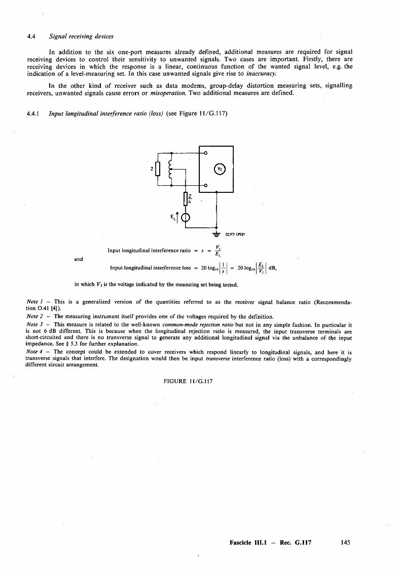
In addition to the six one-port measures already defined, additional measures are required for signal receiving devices to control their sensitivity to unwanted signals. Two cases are important. Firstly, there are receiving devices in which the response is a linear, continuous function of the wanted signal level, e.g. the indication of a level-measuring set. In this case unwanted signals give rise to inaccuracy.
In the other kind of receiver such as data modems, group-delay distortion measuring sets, signalling receivers, unwanted signals cause errors or misoperation. Two additional measures are defined.
4.4.1 Input longitudinal interference ratio (loss) (see Figure 11/G.117)
4.4 Signal receiving devices
yInput longitudinal interference ratio = 5 = -=r
t - 'L
and111 \ E \Input longitudinal interference loss = 201og|0 — = 20 log,0 -rf dB,I s I I * / I
in which V/ is the voltage indicated by the measuring set being tested.
Note I — This is a generalized version o f the quantities referred to as the receiver signal balance ratio (Recommendation 0.41 [4]).Note 2 — The measuring instrument itself provides one of the voltages required by the definition.Note 3 — This measure is related to the well-known common-mode rejection ratio but not in any simple fashion. In particular itis not 6 dB different. This is because when the longitudinal rejection ratio is measured, the input transverse terminals are short-circuited and there is no transverse signal to generate any additional longitudinal signal via the unbalance of the input impedance. See § 5.3 for further explanation.Note 4 — The concept could be extended to cover receivers which respond linearly to longitudinal signals, and here it istransverse signals that interfere. The designation would then be input transverse interference ratio (loss) with a correspondinglydifferent circuit arrangement.
FIG URE 11/G .l 17
Fascicle III.l — Rec. G.117 145
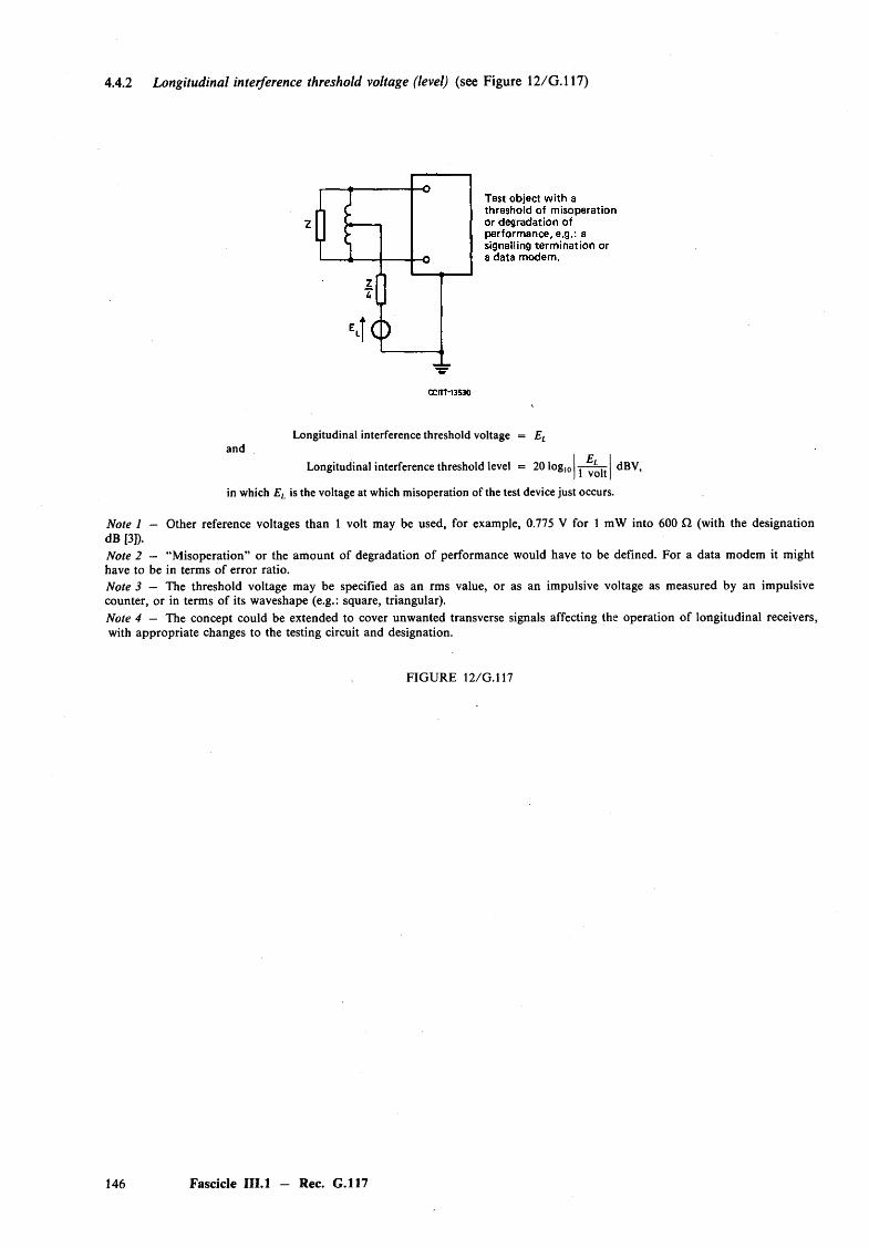
4.4.2 Longitudinal interference threshold voltage (level) (see Figure 12 /G .l 17)
Longitudinal interference threshold voltage = ELand
I E ILongitudinal interference threshold level = 20 log,0 j~ ^ [ t dBV,
in which EL is the voltage at which misoperation of the test device just occurs.
Note 1 — Other reference voltages than 1 volt may be used, for example, 0.775 V for 1 mW into 600 Cl (with the designationdB [3]).Note 2 — “Misoperation” or the amount of degradation of performance would have to be defined. For a data modem it might have to be in terms of error ratio.Note 3 — The threshold voltage may be specified as an rms value, or as an impulsive voltage as measured by an impulsive counter, or in terms of its waveshape (e.g.: square, triangular).Note 4 — The concept could be extended to cover unwanted transverse signals affecting the operation of longitudinal receivers,with appropriate changes to the testing circuit and designation.
FIG URE 12/G.117
146 Fascicle III.l - Rec. G.117
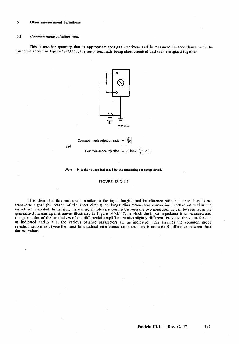
5 Other measurement definitions
5.1 Common-mode rejection ratio
This is another quantity that is appropriate to signal receivers and is measured in accordance with the principle shown in Figure 13/G.117, the input terminals being short-circuited and then energized together.
CCITT-13S61
and
Common-mode rejection ratio = | -pf
Common-mode rejection = 20 log,, dB.
Note - V, is the voltage indicated by the measuring set being tested.
FIG URE 13/G.117
It is clear that this measure is similar to the input longitudinal interference ratio but since there is no transverse signal (by reason of the short circuit) no longitudinal/transverse conversion mechanism within the test-object is excited. In general, there is no simple relationship between the two measures, as can be seen from the generalized measuring instrument illustrated in Figure 14/G.117, in which the input impedance is unbalanced and the gain ratios of the two halves of the differential amplifier are also slightly different. Provided the value for e is as indicated and A < 1, the various balance parameters are as indicated. This assumes the common mode rejection ratio is not twice the input longitudinal interference ratio, i.e. there is not a 6-dB difference between their decibel values.
Fascicle III.l - Rec. G.117 147
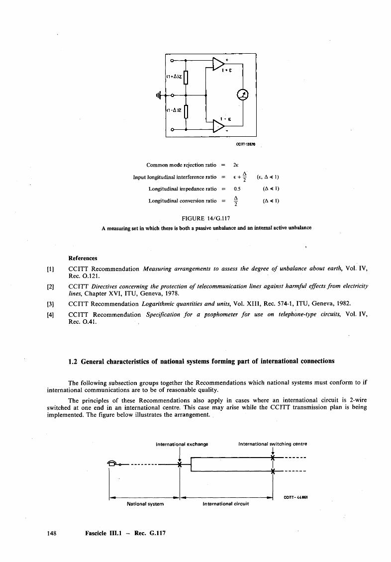
Common mode rejection ratio = 2e
Input longitudinal interference ratio = e + y (e, A < 1)
Longitudinal impedance ratio = 0.5 (A < 1)
Longitudinal conversion ratio = ^ (A< 1)
FIGURE 14/G.117A measuring set in which there is both a passive unbalance and an internal active imbalance
References
[1] CCITT Recommendation Measuring arrangements to assess the degree o f unbalance about earth, Vol. IV,Rec. 0.121.
[2] CCITT Directives concerning the protection o f telecommunication lines against harmful effects from electricitylines, Chapter XVI, ITU, Geneva, 1978.
[3] CCITT Recommendation Logarithmic quantities and units, Vol. X III, Rec. 574-1, ITU, Geneva, 1982.
[4] CCITT Recommendation Specification fo r a psophometer fo r use on telephone-type circuits, Vol. IV,Rec. 0.41.
1.2 General characteristics of national systems forming part of international connections
The following subsection groups together the Recommendations which national systems must conform to if international communications are to be of reasonable quality.
The principles of these Recommendations also apply in cases where an international circuit is 2-wire switched at one end in an international centre. This case may arise while the CCITT transmission plan is being implemented. The figure below illustrates the arrangement.
International exchange International switching centre
a V
------------------------------------------- - . . . j
jII ^
CCITT-44861
National system International circuit
148 Fascicle III.l — Rec. G.117
Recommendation G.120
TRANSMISSION CHARACTERISTICS OF NATIONAL NETWORKS1)
1 Application of CCITT Recommendations on telephone performance to national networks
The different parts of a national network likely to be used for an international connection should meet the following general recommendations:
1.1 The national sending and receiving systems should satisfy the limits recommended in:
— Recommendation G.121 as regards corrected reference equivalent (CRE) or loudness rating (LR);— Recommendation G.133 as regards group-delay distortion;— Recommendation G.122 as regards balance return loss and transmission loss;
— Recommendation G.123 for circuit noise.
Note — Reference should also be made to Recommendations P.12 [2] and G.113.
1.2 Long-distance trunk circuits forming part of the main arteries of the national network should be high-velocity propagation circuits which enable the limits fixed in Recommendation G.114 to be respected. They should conform to Recommendations G.151 and G.152.
Loaded-cable circuits should conform to Recommendation G.124 [3] and carrier circuits to Recommendation G.123.
1.3 National trunk circuits should have characteristics enabling them to conform to Recommendations G.131, G.132 and G.134 as regards the other characteristics of the 4-wire chain constituted by the international telephone circuits and the national trunk extension circuits.
1.4 International centres should satisfy Recommendation Q.45 [4].
N ational automatic 4-wire centres should observe the noise limits specified in Recommendation G.123, § 3.
M anual telephone trunk exchanges should satisfy Recommendation P.22 [5].
Information on the transmission performance of automatic local exchanges is given in the CCITT manual cited in [6].
2 National transmission plan
Every Administration is free to choose whatever method it considers appropriate for specifying transmission performance and to adopt the appropriate limits to ensure satisfactory quality for national calls, it being understood that in addition the Recommendation relating to corrected reference equivalents (CREs or LRs) (Recommendation G.121) should be satisfied for international calls.
Note — To meet this twofold condition with respect to national and international calls, each Administration has to draw up a national transmission plan, i.e. it must specify limits for each part o f the national network.
The manual cited in [6] contains descriptions of the transmission plans adopted by various countries and also some indications concerning the methods that can be used to establish such a plan.
In particular, Annexes A and B to Recommendation G .l l l contain useful information for Administrations who wish to apply the CRE or LE method to their national connections.
9 Former Recommendation P.21 [1].
Fascicle III.l - Rec. G.120 149
References
[1] CCITT Recommendation Application o f C C ITT Recommendations on telephone performance to national networks, Red Book, Vols. V and V bis, Rec. P.21, ITU, Geneva, 1962 and 1965; amended at Mar del Plata, 1968, to become Rec. P.20 (G.120) Transmission characteristics o f national networks, White Book, Vol. V (Vol. I ll) , ITU, Geneva, 1969.
[2] CCITT Recommendation Articulation reference equivalent (AEN), Yellow Book, Vol. V, Rec. P. 12, ITU, Geneva, 1981.
[3] CCITT Recommendation Characteristics o f long-distance loaded-cable circuits liable to carry international calls, Orange Book, Vol. I l l , Rec. G.124, ITU, Geneva, 1977.
[4] CCITT Recommendation Transmission characteristics o f an international exchange, Vol. VI, Rec. Q.45.
[5] CCITT Recommendation Manual trunk exchanges, Orange Book, Vol. V, Rec. P.22, ITU, Geneva, 1977.
[6] CCITT manual Transmission planning o f switched telephone networks, ITU, Geneva, 1976.
Recommendation G.121
CORRECTED REFERENCE EQUIVALENTS (CREs) AND LOUDNESS RATINGS (LRs)O F NATIONAL SYSTEM S')
(Geneva, 1964; amended at M ar del Plata, 1968; Geneva, 1972, 1976 and 1980 and Malaga-Torremolinos, 1984)
Preamble
Parts 1 to 5 of this Recommendation apply in general to all analogue, mixed analogue/digital and all digital international telephone connections. However, where recommendations are made on specific aspects in § 6 for mixed analogue/digital or all-digital connections, § 6 will govern.
All sending and receiving CREs and LRs in this Recommendation are “nominal values” as explained in § 4 of this Recommendation and are referred to the corresponding virtual analogue switching points of an international circuit at the international switching centre.
The definition of the virtual analogue switching points o f international circuits can be found in Figure 1 /G .l l l .
The CCITT,
considering
(a) that values of corrected reference equivalent (CRE) for sending and receiving local systems are obtained by simple conversions if their reference equivalents are known, as explained in Annex A to Recommendation G .l l l and planning equivalents may be measured objectively, as explained in Recommendation P.62;
(b) that loudness ratings (LRs), as defined in Recommendation P.76, may be determined directly by subjective tests described in Recommendation P.78 or computed as indicated in Recommendation P.79, from objective measurements described in Recommendation P.64;
(c) that the differences between values determined by subjective tests in various laboratories (including the CCITT Laboratory) are smaller for loudness ratings than for reference equivalents;
') The main terms used in this Recommendation are defined in Annex A to Recommendation G .l l l .
150 Fascicle III. I - Rec. G.121
(d) that several Administrations have expressed the view that the speaking position used in the determination of loudness ratings (Recommendation P.76, Annex A) is more realistic than that used for reference equivalents and therefore values of LR at their disposal for the types of telephone sets they use (from subjective tests, or from an objective measurement method which gives reliable results for those sets), they may well use such values to check if their national systems meet the limits and mean values recommended below;
(e) that, however, neither the conversion from reference equivalent and CRE to LR nor objective measurements according to Recommendation R64 are accurate enough in the case of certain sets with carbon microphones; that therefore, the numerous Administrations who still rely on values of reference equivalent for the types of telephone sets they use need to find recommended values of CRE in CCITT documentation until a reliable objective method of measuring loudness ratings, especially for all types of sets containing carbon microphones, can be agreed and recommended by the CCITT,
recommends
that Administrations should use either the values of CRE or the values of LR given below, to check that their natural systems meet the general objectives resulting from Recommendation G .l l l .
1 Traffic-weighted mean values of the distributions of sending and receiving CREs and LRs
An objective for the mean value is necessary to ensure that satisfactory transmission is given to most subscribers. Transmission would not be satisfactory if the maximum values permitted in § 2 were consistently used for every connection.
It has been provisionally agreed, taking into account the long-term objectives for the overall CREs or LRs given in Recommendation G . l l l , § 3.2 and the need to control the mean power applied to long-distance FDM transmission systems, that an appropriate subdivision of the overall objective should place the long-term objectives for the sending and receiving national systems in the ranges:
sending CRE: 11.5-13 dB or sending LR: 6.5 to 8 dB
receiving CRE: 2.5-4 dB or receiving LR: —2.5 to —1 dB.
(These are the mean values of the traffic-weighted distributions. If the traffic distribution cannot be foreseen with sufficient accuracy, it can be assumed that all subscribers generate the same am ount of traffic.)
Note — In some networks the long-term values cannot be attained at this time and it has beenprovisionally agreed that appropriate short-term objectives for these ranges are:
sending CRE: 11.5 to 19 dB or sending LR: 6.5 to 14 dB
receiving CRE: 2.5 to 7.5 dB or receiving LR: —2.5 to 2.5 dB
corresponding to the short-term objective given in Recommendation G . l l l , § 3.2 of a range of 13-25.5 dB for themean value of the traffic-weighted distribution of the overall CRE or 8 to 20.5 dB for the overall LR.
The short-term mean values have been determined under the assumption that the statistic distribution isnormal (Gaussian). It might occur that a real distribution is not normal but asymmetric. In such cases it isacceptable that the mean values fall somewhat outside the stated limits, provided that the distribution as a wholeleads to transmission conditions equal to those of a normal distribution having its mean value inside the statedrange.
2 Maximum sending and receiving CREs and LRs
2.1 Values fo r each direction o f transmission
It has been agreed that the national sending and receiving systems used to set up all actual outgoing or incoming calls in an average-sized country (see Recommendation G.101, § 2.2) should individually meet both the following objectives:
— for the sending system between a subscriber and the first international circuit, the CRE should notexceed 25 dB or the LR should not exceed 20 dB (nominal maximum values);
— for the receiving system between the same two points, the CRE should not exceed 14 dB or the LRshould not exceed 9 dB (nominal maximum values).
In a large country, these limits are somewhat widened (see Table 1/G. 121).
Fascicle III.l — Rec. G.121 151

Nominal maximum CREs or LRs (in dB) recommended for national systems
TABLE 1/G.121
CRE LR
For an average-sized country (see Figure 1/G . 121)
SendingReceiving
2514
209
For large countries:
— if a fourth national circuit is part of the 4-wire chain (see Figure 2 /G .l21)
SendingReceiving
25.514.5
20.59.5
— if five national circuits form part of the 4-wire chain
SendingReceiving
2615
2110
In Figures 1/G.121 and 2/G .121, the numbers in rectangles are values recommended by the CCITT. The others are given only as examples of possible arrangements, subject to Recommendation G.122.
2.2 Difference in transmission loss between the two directions o f transmission in national systems
It is recommended that the absolute value of the difference between loss t-b and loss a-t (see Recommendation G.122) should not exceed 4 dB, so that in theory a difference no greater than 8 dB could be introduced in international connections.
The following points should be noted:
1) Bearing in mind that most Administrations allocate the losses of their national extension circuits in much the same sort o f way (see Annex A), connections set up in practice should not exhibit differences much in excess of 3 dB.
2) As far as speech transmission is concerned, from the studies carried out by several Administrations in 1968-1972, it is clear that for connections with overall CREs or LRs falling within the range found in practice, no great disadvantage attaches to any reasonable difference in overall CRE or LR between the two directions of transmission.
Reference [1] is a resume of the test results from various Administrations concerning the subjective effects of such asymmetry.
3) When devising national transmission plans, Administrations should take into account the needs of data transmission between modems complying with the pertinent Recommendations (e.g., V.2 [2], V.21 [3], V.23 [4]). Annex B gives some information on this point.
3 Minimum CREs and LRs
Administrations must take care not to overload the international transmission systems if they reduce the attenuation in their national trunk network.
Provisionally, a nominal minimum value of 7 dB sending CRE or 2 dB sending LR, referred to the send virtual analogue switching point o f the international circuit is recommended in order to control the peak value of the speech power applied to international transmission systems. It should be noted that the imposition of such a limit does not serve to control the long-term mean power offered to the system.
In some countries a very low sending reference equivalent may occur if unregulated telephone sets are used. Furthermore, the speech power applied to the international circuits by operators’ sets must be controlled so that it does not become excessive.
152 Fascicle III.1 - Rec. G.121
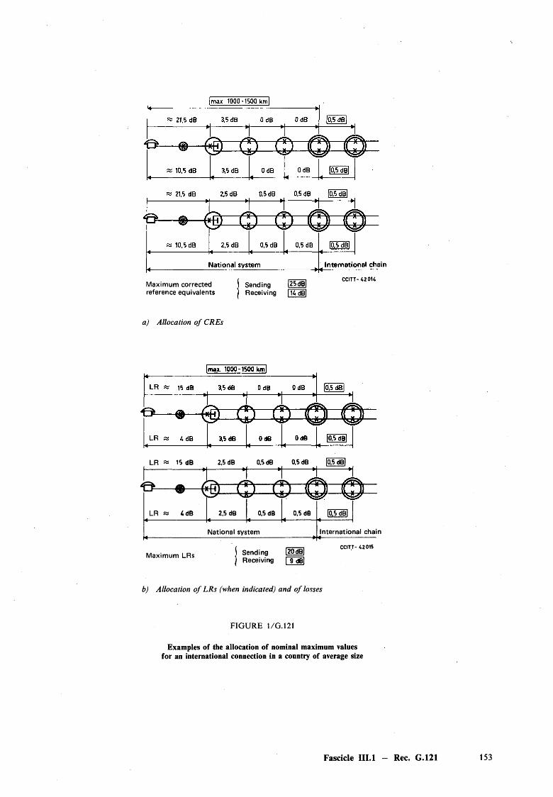
Maximum corrected reference equivalents
Sending |25 dB[Receiving 114 dB|
C C IT T -4 2 o u
a) Allocation o f CREs
LR « 15 dB 2.5 dB 0.5 dB 0.5 dB [0.5 dB
1 " H-------
LR » 4dB 2.5 dB 0.5 dB 0.5 dB
National system
[QTdBl
International chain
Maximum LRs Sending |20 dB[Receiving [ 9 dB|
C C IT T - 4 2 0 1 5
b) Allocation o f LRs (when indicated) and o f losses
FIGURE 1/G.121
Examples of the allocation of nominal maximum values for an international connection in a country of average size
Fascicle III.l — Rec. G.121 153
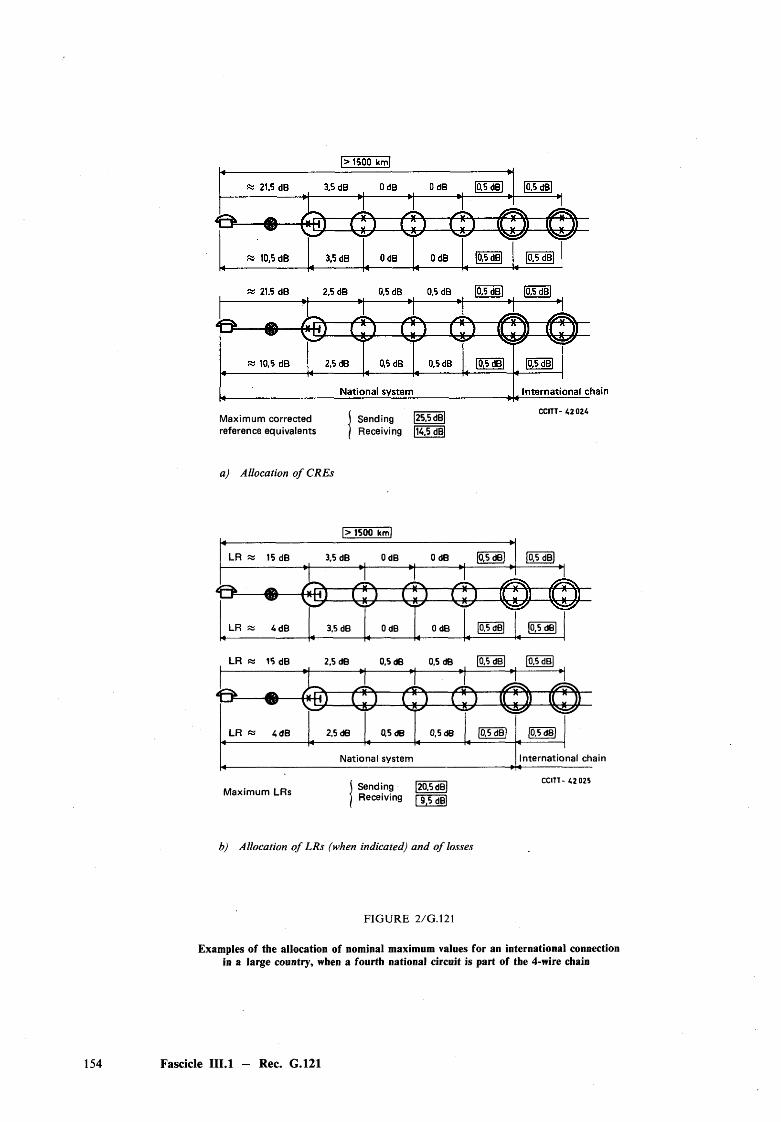
Maximum corrected reference equivalents
Sending 125.5 dB|Receiving |14,5 dB|
C C IT T - 4 2 0 2 4
a) Allocation o f CREs
|> 1500 km|
LR « 15 dB 3.5 dB OdB OdB |0,5 dBj----------------- M H --------- H--------- H--------- MM
LR a 4 dB 3.5 dB OdB OdB fo5d§l 10,5 dB |
LR « 15 dB 2.5 dB 0,5 dB 0.5 dB [OSdBl lQ.5 dB
* ^ ftbk /, p y ------------- 1------------1
---- l f ^ \
LR « 4dB
^ ^
2.5 dB^ 1
0,5 dB
J ------ V-J
0,5 dB
b*------^
10.5 dB) |0.5d8|
nal chainNational system Internatio
Maximum LRs Sending |20.5dB| Receiving | g S dB|
CCITT - 4 2 0 2 5
b) Allocation o f LR s (when indicated) and o f losses
FIGURE 2/G.121
Examples of the allocation of nominal maximum values for an international connection in a large country, when a fourth national circuit is part of the 4-wire chain
154 Fascicle III.l - Rec. G.121
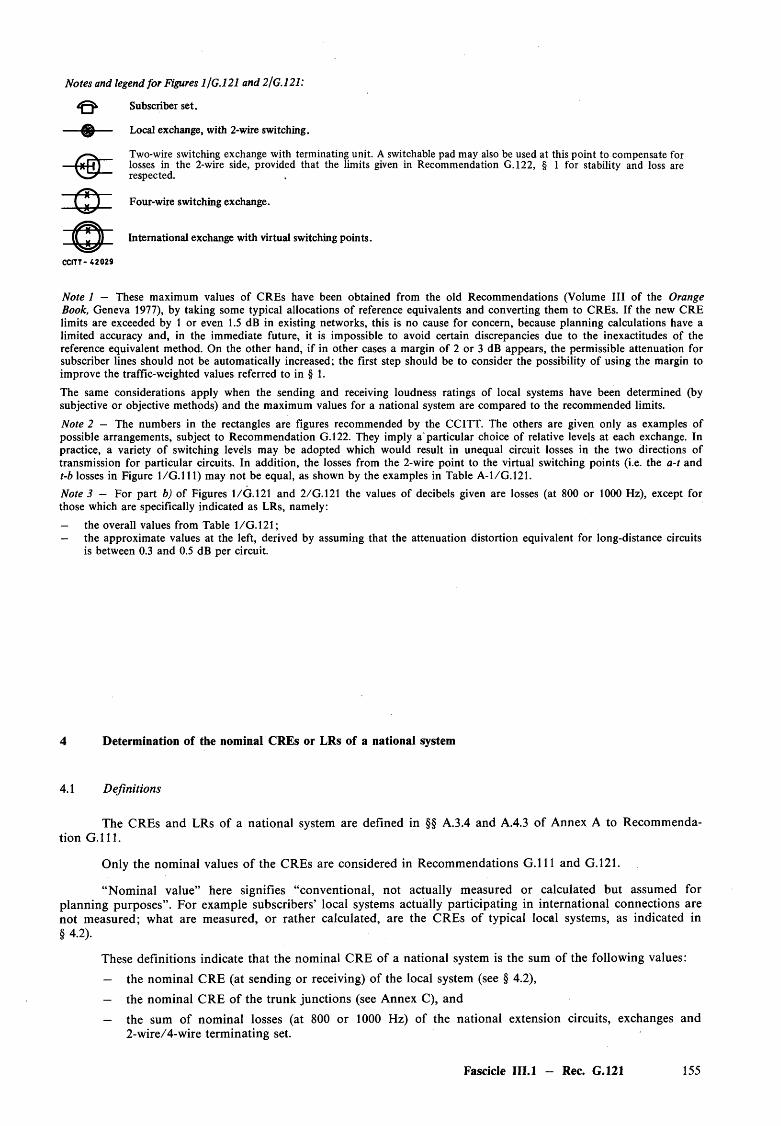
Notes and legend for Figures l/G.121 and 2/G.121:
Subscriber set.
Local exchange, with 2-wire switching.
Two-wire switching exchange with terminating unit. A switchable pad may also be used at this point to compensate for losses in the 2-wire side, provided that the limits given in Recommendation G.122, § 1 for stability and loss are respected.
Four-wire switching exchange.
International exchange with virtual switching points.
CCITT- 4 2 0 2 9
Note 1 — These maximum values o f CREs have been obtained from the old Recommendations (Volume III of the Orange Book, Geneva 1977), by taking some typical allocations o f reference equivalents and converting them to CREs. If the new CRE limits are exceeded by 1 or even 1.5 dB in existing networks, this is no cause for concern, because planning calculations have a limited accuracy and, in the immediate future, it is impossible to avoid certain discrepancies due to the inexactitudes of the reference equivalent method. On the other hand, if in other cases a margin of 2 or 3 dB appears, the permissible attenuation for subscriber lines should not be automatically increased; the first step should be to consider the possibility of using the margin to improve the traffic-weighted values referred to in § 1.
The same considerations apply when the sending and receiving loudness ratings of local systems have been determined (by subjective or objective methods) and the maximum values for a national system are compared to the recommended limits.
Note 2 — The numbers in the rectangles are figures recommended by the CCITT. The others are given only as examples of possible arrangements, subject to Recommendation G.122. They imply a particular choice of relative levels at each exchange. In practice, a variety o f switching levels may be adopted which would result in unequal circuit losses in the two directions of transmission for particular circuits. In addition, the losses from the 2-wire point to the virtual switching points (i.e. the a-t and t-b losses in Figure 1 /G .l l l ) may not be equal, as shown by the examples in Table A-l/G .121.
Note 3 — For part b) o f Figures l/G .121 and 2/G.121 the values of decibels given are losses (at 800 or 1000 Hz), except for those which are specifically indicated as LRs, namely:
— the overall values from Table l/G .121;— the approximate values at the left, derived by assuming that the attenuation distortion equivalent for long-distance circuits
is between 0.3 and 0.5 dB per circuit.
4 Determination of the nominal CREs or LRs of a national system
4.1 Definitions
The CREs and LRs of a national system are defined in §§ A.3.4 and A.4.3 of Annex A to Recommendation G .l l l .
Only the nominal values o f the CREs are considered in Recommendations G .l l l and G.121.
“Nominal value” here signifies “conventional, not actually measured or calculated but assumed for planning purposes”. For example subscribers’ local systems actually participating in international connections are not measured; what are measured, or rather calculated, are the CREs of typical local systems, as indicated in §4.2).
These definitions indicate that the nominal CRE of a national system is the sum of the following values:
— the nominal CRE (at sending or receiving) of the local system (see § 4.2),
— the nominal CRE o f the trunk junctions (see Annex C), and
— the sum of nominal losses (at 800 or 1000 Hz) of the national extension circuits, exchanges and 2-wire/4-wire terminating set.
Fascicle III.l — Rec. G.121 155

The nominal LR of a national system is the sum of the following values:— the nominal LR (at sending or receiving) of the local system (see § 4.2);
— the loudness insertion loss of the trunk junctions (see Annex B to Recommendation G .l l l and Annex C to this Recommendation G.121), and
— the total loudness insertion loss of the national extension circuits, exchanges and 2-wire/4-wire terminating set2).
4.2 Nominal CREs and LRs o f a local system
The CREs are usually calculated by the formula giving y (q ) in § A. 1.3 of Annex A to Recommendation G . l l l from the reference equivalents q determined on local systems (consisting of a telephone set of the relevant type, an artificial line with a model feeding bridge) by subjective tests in accordance with Recommendation P.72 [5]. Planning equivalents may also be used, if available; by definition, they are measured objectively and should be equal to the R25 equivalent or to the CRE, with an accuracy which is sufficient for planning purposes (see Recommendation P.62).
The LRs given of a local system may be determined by subjective tests (Recommendation P.78); they may also be calculated according to Recommendation P.79, if a method of objective measurement is available, which is known to given reliable results for the type of telephone set used.
Note 1 — The CREs or LRs given for local systems are to be based upon the average values of the sensitivities of the transducers o f a large number of working telephone sets. As far as carbon microphones are concerned, the average value of the sensitivity of the carbon microphones in the national network is effectively represented by the value of sensitivity corresponding to the long, stable period of their lifetime.
As regards systematic differences between actual and average sensitivities, if the average sensitivity is obtained by measuring a sample of working sets, any systematic differences will automatically be taken into account. However, if this average value is calculated, then the systematic difference must be part of the calculation.
The average values of sensitivity do not include fortuitous variations introduced by subjective methods used when reference equivalents or LRs are assessed.
Note 2 — The variations with time of circuits and other items of equipment connecting the local exchange with the international centre are not included in the values of nominal CREs or LRs. Recommendation G.151, § 3 sets forth the objectives concerning variations with time of transmission losses of national extension circuits relative to the nominal values.
Note 3 — Reference equivalents or LRs are often determined with only one type of telephone set and only one length of line. To take account of the effect o f other lines, one of the methods described in Annex C may be used.
5 Sidetone reference equivalent3)
Every precaution must be taken to avoid further transmission impairment in communications which reach the CRE or LR and noise limits. Tests have shown that in these unfavourable conditions the sidetone reference equivalent (for speech) should be at least 17 dB. In fact, this value cannot be achieved without additional networks, which increase line costs and are only justified when the subscriber has to exchange calls frequently in very bad conditions. In most cases, values between 7 and 10.5 dB are to be expected.
Note 1 — Strong sidetone (corresponding to a low value for sidetone reference equivalent) impairs transmission in two ways. At the sending end a subscriber who hears himself clearly is tempted to lower his voice; at the receiving end the room noise is transmitted as sidetone to the ear o f the listener thus increasing the total noise received.
Note 2 — The influence of sidetone and room noise on transmission performance is discussed in Recommendation P .l l , §§ 2.4 and 2.5.
Note 3 — Suitable .values for sidetone ratings in accordance with Recommendation P.76 (STMR) are under study in Question 9 /X II. Until a complete reply to Question 9 /X II is available, the value expressed here as a reference equivalent and the method of Recommendation R73 is retained. Further information on the effects of sidetone on the subscriber when talking, is given in Supplement No. 11, Volume V.
2) This definition is consistent with Annex A, § A.2 to Recommendation G . l l l with Figures 16/G.121 and 26/G.121 and with the values recommended above.
3) Refer to § 1.6 of the Appendix I to Section 1, at the end o f this fascicle.
156 Fascicle III.l - Rec. G.121

6 Incorporation of PCM digital processes in national extensions
6.1 Effect on national transmission plans
The incorporation of PCM digital processes into national extensions might require that existing national transmission plans be amended or replaced with new ones.
The national transmission plans to be adopted should be compatible with existing national analogue transmission plans and also capable of providing for mixed analogue/digital operation. In addition, the plans should be capable of providing for a smooth transition to all-digital operation.
6.2 Transmission loss considerations
Where the national portion of the 4-wire chain is wholly digital between the local exchange and the international exchange, the transmission loss which the extension must contribute to the maintenance of stability and the control of echo on an international connection can be introduced at the local exchange. The m anner in which the required loss should be introduced is to be governed by the national transmission plan adopted. Three of possibly many different configurations of such national extensions are shown in Figure 3/G.121.
In case 1 and 2 of Figure 3/G.121, the R pad represents the transmission loss between the 0 dBr point at the digital/analogue decoder and the 2-wire side of the 2W /4W terminating unit. Similarly, the T pad represents the transmission loss between the 2-wire side of the 2W /4W terminating unit and the 0 dBr point at the analogue/digital coder. In practice there can be levels other than 0 dBr and hence consequential changes in the R and T pad-values.
The individual values of R and T can be chosen to cater for the national losses and levels, provided that the CCITT Recommendations for international connections are always met. It is recognized that for evolving networks, the values of R and T may not be the same as the values appropriate to the all digital 4-wire national chain. However, for the case of an all-digital national chain, the choice of values of R and T is particularly im portant in determining the performance in respect o f echo and stability. For example, if the balance return loss at the 2W /4W terminating unit can approach 0 dB under worst case terminating conditions, then the sum of R and T needs to be at least 6 dB if the requirements of Recommendation G.122 are to be met. Examples of the values for R and T that have been adopted by some Administrations are given in Annex E to Recommendation G.121.
In case 2 of Figure 3/G.121, it is possible with a sufficiently high balance return loss to comply with the Recommendations concerning corrected reference equivalents or loudness ratings, stability, and echo without requiring a particular value for the sum of the R and T pad values. However it will still be necessary to comply with the provisions concerning differential loss (§ 6.3 of this Recommendation) which in turn implies that
R - T = 3 to 11 dB.
However, a local exchange designed on these principles and which is at the end of a national extension containing asymmetric analogue portions cannot take the whole of the asymmetry allowance.
It may be desirable to reduce the range of 3 to 11 dB and this is under study (Question 29 /X II [6]).
The R and T pads shown in Figure 3/G.121 are also shown as analogue pads. This type of pad might not necessarily be introduced under all conditions. In some situations it might be more practical to introduce the required loss at the local exchange, or at some other point o f the national extension, by means of digital pads. However, if digital pads are used, their detrimental effect on digital data or other services requiring end-to-end bit integrity must be taken into account as indicated in Recommendation G.101, § 4.4 and G.103, § 4.
The arrangement in case 3 of Figure 3/G.121 assumes 4-wire digital switching at the local exchange in combination with a 4-wire digital local line and a 4-wire “digital telephone set”.
Fascicle III.l - Rec. G.121 157
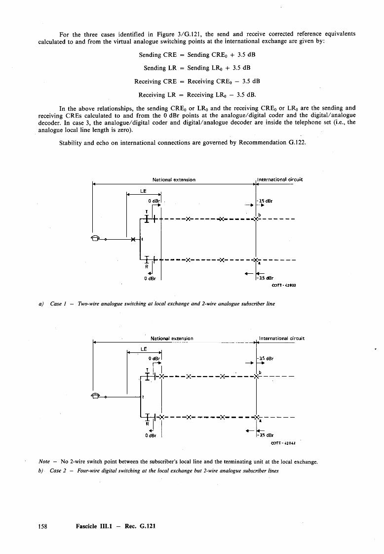
For the three cases identified in Figure 3/G.121, the send and receive corrected reference equivalents calculated to and from the virtual analogue switching points at the international exchange are given by:
Sending CRE = Sending CRE0 + 3.5 dB
Sending LR = Sending LR0 + 3.5 dB
Receiving CRE = Receiving CRE0 — 3.5 dB
Receiving LR = Receiving LR0 — 3.5 dB.
In the above relationships, the sending CRE0 or LRo and the receiving CREo or LRo are the sending and receiving CREs calculated to and from the 0 dBr points at the analogue/digital coder and the digital/analogue decoder. In case 3, the analogue/digital coder and digital/analogue decoder are inside the telephone set (i.e., the analogue local line length is zero).
Stability and echo on international connections are governed by Recommendation G.122.
a) Case 1 — Two-wire analogue switching at local exchange and 2-wire analogue subscriber line
Note — No 2-wire switch point between the subscriber’s local line and the terminating unit at the local exchange. b) Case 2 — Four-wire digital switching at the local exchange but 2-wire analogue subscriber lines
158 Fascicle III.l — Rec. G.121
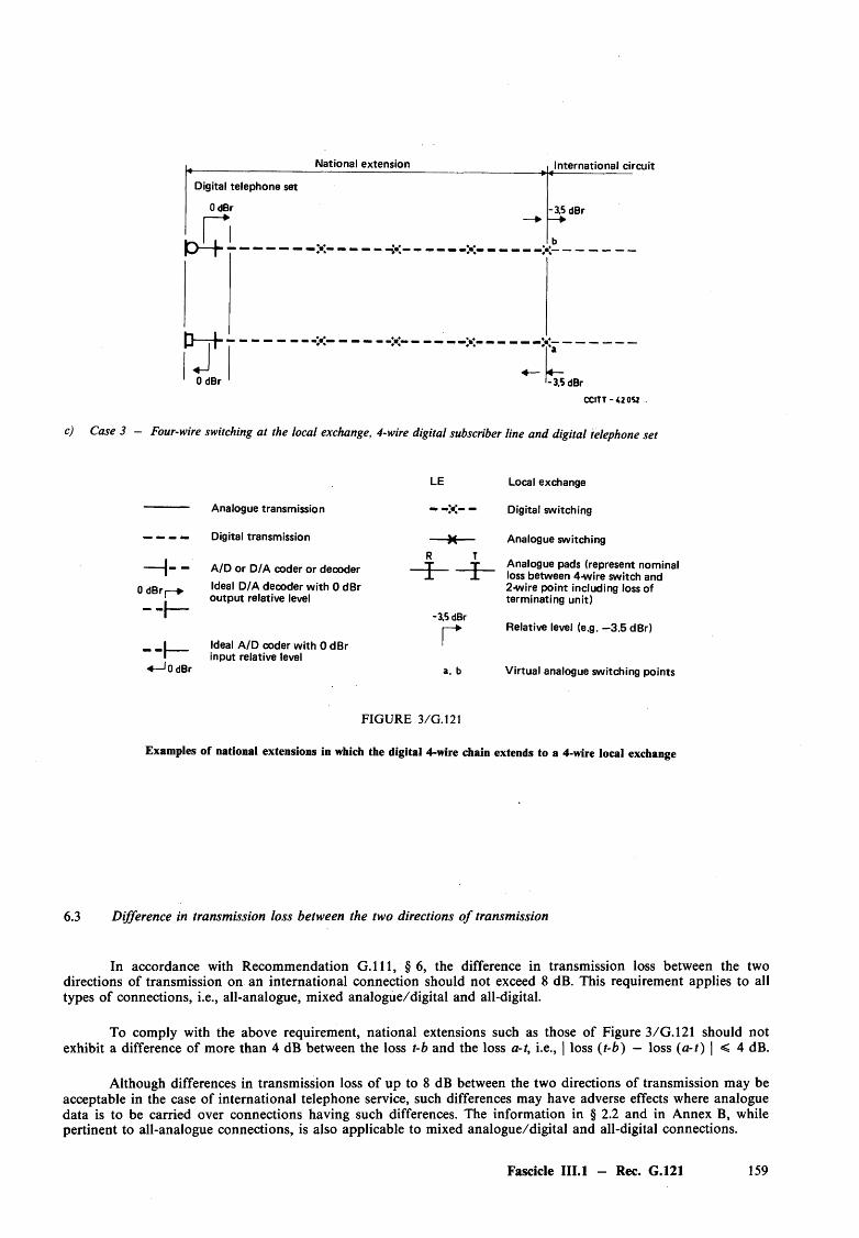
National extension International circuit
Digital telephone set
0 dBr
o + -A-
OdBr
- 3.5 dBr
-3.5 dBrCCITT -4 2 0 5 1
c) Case 3 - Four-wire switching at the local exchange, 4-wire digital subscriber line and digital telephone set
LE
Analogue transmission
— — — — Digital transmission
- — A/D or D/A coder or decoder
0 dBr|—►
J0dBr
Ideal D/A decoder with 0 dBr output relative level
Ideal A/D coder with 0 dBr input relative level
R■ *
-3.5 dBr
ra, b
Local exchange
Digital switching
Analogue switching
Analogue pads (represent nominal loss between 4-wire switch and 2-wire point including loss of terminating unit)
Relative level (e.g. —3.5 dBr)
Virtual analogue switching points
FIGURE 3/G.121
Examples of national extensions in which the digital 4-wire chain extends to a 4-wire local exchange
6.3 Difference in transmission loss between the two directions o f transmission
In accordance with Recommendation G . l l l , § 6, the difference in transmission loss between the two directions of transmission on an international connection should not exceed 8 dB. This requirement applies to all types of connections, i.e., all-analogue, mixed analogue/digital and all-digital.
To comply with the above requirement, national extensions such as those of Figure 3/G.121 should not exhibit a difference of more than 4 dB between the loss t-b and the loss a-t, i.e., | loss ( t-b) — loss (a-t) | < 4 dB.
Although differences in transmission loss of up to 8 dB between the two directions of transmission may be acceptable in the case of international telephone service, such differences may have adverse effects where analogue data is to be carried over connections having such differences. The information in § 2.2 and in Annex B, while pertinent to all-analogue connections, is also applicable to mixed analogue/digital and all-digital connections.
Fascicle III.l - Rec. G.121 159
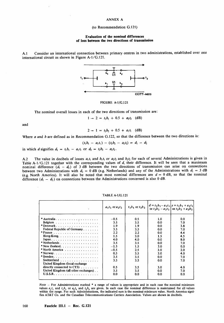
ANNEX A
Evaluation of the nominal differences of loss between the two directions of transmission
A.l Consider an international connection between primary centres in two administrations, established over one international circuit as shown in Figure A-1/G . 121.
(to Recommendation G.121)
0»2
--------------------------------------------CCITT-44870
FIGURE A-1/G.121
The nominal overall losses in each of the two directions of transmission are:
1 - 2 = txbx + 0.5 + a2t2 (dB)
and
2 —► 1 = t2b2 + 0.5 + ci\t\ (dB)
Where a and b are defined as in Recommendation G.122, so that the difference between the two directions is:
(txbx — axtx) — ( ^ — ^2*2) = d\ — d2
in which d signifies dx = txbx — axtx or d2 = t2b2 — a2t2.
A.2 The value in decibels of losses axtx and bxtx or a2t2 and for each of several Administrations is given inTable A-1/G . 121 together with the corresponding values of d, their difference. It will be seen that a maximumnominal difference (dx - d2) o f 3 dB between the two directions of transmission can arise on connectionsbetween two Administrations with d2 = 0 dB (e.g. Netherlands) and any of the Administrations with dx = 3 dB (e.g. N orth America). It will also be noted that most nominal differences are d = 0 dB, so that the nominal difference (dx — d2) on connections between the Administrations concerned is also 0 dB.
TABLE A-1/G.121
a xt \ o ta 2t 2 t xb x or t2b2 d = t 1b l - or t 2b2 -
« if ia2t 2
s — t xb x + fiifj or t 2b2 + a2b2
* Australia...................................................... -0 .5 0.5 1.0 0.0B elg ium ........................... ' . ....................... 3.5 3.5 0.0 7.0
* Denmark...................................................... 1.9 1.9 0.0 3.8Federal Republic of Germany.................. 3.5 3.5 0.0 7.0
* F ran ce ......................................................... 2.2 2.2 0.0 4.4Hong-Kong................................................... 1.5 3.0 1.5 4.5Japan ............................................................ 4.0 4.0 0.0 8.0
* N etherlands................................................ 3.5 3.5 0.0 7.0* New Zealand................................................ -1 .5 1.5 3.0 0.0* North A m erica .......................................... -0 .5 2.5 3.0 2.0* Norway......................................................... 0.5 3.5 3.0 4.0* Sweden......................................................... 3.5 3.5 0.0 7.0
Sw itzerland................................................ 3.5 3.5 0.0 7.0United Kingdom (local exchange directly connected to C T 3 ) ..................... 0.5 3.5 3.0 4.0United Kingdom (all other exchanges). . 3.5 3.5 0.0 7.0U.S.S.R......................................................... 0.0 0.0 0.0 0.0
Note — For Administrations marked * a range of values is appropriate and in each case the nominal minimum values alt i and t lb1 or a2t2 and t2b2 are given. In each case the nominal difference is maintained for all values within the range. For such Administrations, the indicated sum is the nominal minimum value. North America signifies AT&T Co. and the Canadian Telecommunications Carriers Association. Values are shown in decibels.
160 Fascicle III.l — Rec. G.121
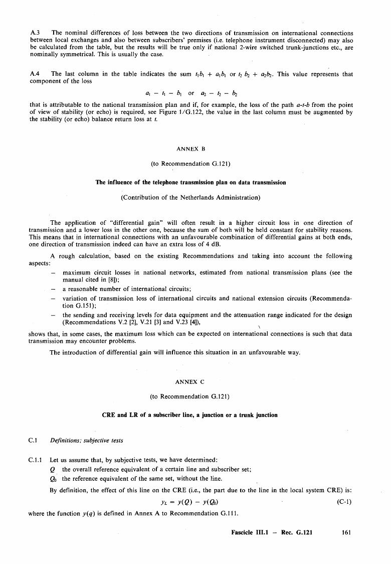
A.3 The nominal differences of loss between the two directions of transmission on international connections between local exchanges and also between subscribers’ premises (i.e. telephone instrument disconnected) may also be calculated from the table, but the results will be true only if national 2-wire switched trunk-junctions etc., are nominally symmetrical. This is usually the case.
A.4 The last column in the table indicates the sum txb\ + afi\ or t2 bj + a2b2. This value represents that component of the loss
a\ — t\ — b\ or a2 — t2 —
that is attributable to the national transmission plan and if, for example, the loss of the path a-t-b from the point of view of stability (or echo) is required, see Figure 1/G. 122, the value in the last column must be augmented by the stability (or echo) balance return loss at t.
ANNEX B
(to Recommendation G.121)
The influence of the telephone transmission plan on data transmission
(Contribution of the Netherlands Administration)
The application of “differential gain” will often result in a higher circuit loss in one direction of transmission and a lower loss in the other one, because the sum of both will be held constant for stability reasons. This means that in international connections with an unfavourable combination of differential gains at both ends, one direction of transmission indeed can have an extra loss of 4 dB.
A rough calculation, based on the existing Recommendations and taking into account the followingaspects:
— maximum circuit losses in national networks, estimated from national transmission plans (see the manual cited in [8]);
— a reasonable number of international circuits;— variation of transmission loss of international circuits and national extension circuits (Recommenda
tion G.151);— the sending and receiving levels for data equipment and the attenuation range indicated for the design
(Recommendations V.2 [2], V.21 [3] and V.23 [4]),
shows that, in some cases, the maximum loss which can be expected on international connections is such that data transmission may encounter problems.
The introduction of differential gain will influence this situation in an unfavourable way.
A NN EX C
(to Recommendation G.121)
CRE and LR of a subscriber line, a junction or a trunk junction
C.l Definitions; subjective tests
C.1.1 Let us assume that, by subjective tests, we have determined:Q the overall reference equivalent of a certain line and subscriber set;Qn the reference equivalent of the same set, without the line.
By definition, the effect o f this line on the CRE (i.e., the part due to the line in the local system CRE) is:
yL - y ( Q ) - y(Qo) (C -i)
where the function y(q) is defined in Annex A to Recommendation G .l l l .
Fascicle III.l - Rec. G.121 161
C.1.2 If by subjective tests conforming to Recommendation R78, we have determined:2 the overall loudness rating (LR) of a certain line and subscriber set,2o the LR of the same set, without the line, by definition, the effect of this line on the LR (i.e. the part
due to the line in the local system LR) is:
zL = z - Zo (C-2)
(See also § B.2.2.1 of Annex B to Recommendation G .l l l .)
Note - (Applying to §§ C. 1.1 and C.1.2) - The effect of the line may be different for sending and receiving, if only because the effect of feed current on sensitivity is different. If desired, this effect of feed current may be assessed separately.
C.1.3 The CRE of a junction or of a trunk junction can be determined directly by subjective tests by comparing path 5 in Figure A - l /G . l l l with path 6 via path 2 where x2 — 25 dB.
Similarly, junction loudness rating is defined in Recommendation P.76 in Figure 2 /R 76 and § 2.2.4 andmay be determined subjectively as indicated in Recommendation R78, in particular, Figure 2h)/R 78.
C.1.4 Administrations may need to calculate the CREs of various subscriber lines for local network transmission planning. The CCITT advises Administrations which do not possess many results of subjective tests to apply the objective measurements or calculation methods described below. It is understood that Administrations which have the necessary means to assess the CREs of the various types of lines used by them, with the telephone sets of the types used in their networks, may in all cases continue to apply any simple calculation methods which they may have aleady developed.
C.2 General principles fo r calculation
The LR of a subscriber line, a junction or a trunk junction is its loudness insertion loss (LIL) under the conditions where it is used. Annex B to Recommendation G . l l l gives the definition of LIL and indicates how to calculate it from objectively measured frequency characteristics.
Since the CRE of such a line or junction is always determined (objectively or subjectively) in association with a commercial telephone set having a restricted bandwidth, this CRE is equal to the LR with an accuracy which is sufficient for planning purposes.
C.3 Objective measurement
C.3.1 I f we call:
I the indication of an apparatus for the objective measurement of planning equivalent or LR when measuring a subscriber set with a line, and
70 the corresponding value without a line, we obtain:
zL = Yl = I — Iq (C-3)
The same apparatus may be used to measure the LIL (CRE or LR) of a junction or trunk junction.
C.4 Other methods
C.4.1 Objective measurement with OBDM or OREM -B
This apparatus introduces a systematic error on the CRE (or LR) of a local telephone system, which is cancelled out by substraction when applying equation (C-3), so that this equation is still satisfied in practice with sufficient accuracy for planning purposes [8].
Note — This procedure should be applied with caution to telephone sets having carbon microphones because the effect of feed current may be wrongly measured using this type of objective information. In this case, the effect of feed current should be measured separately using real speech.
The CREs and LRs of junctions or trunk junctions can also be measured with the OBDM or the OREM-B; the results agree well with those of the subjective tests [9].
C.4.2 Calculations based on insertion loss
These are a simplified form of the method mentioned in § C.2 above. They are described in § C.3 of [10].
162 Fascicle III.l - Rec. G.121
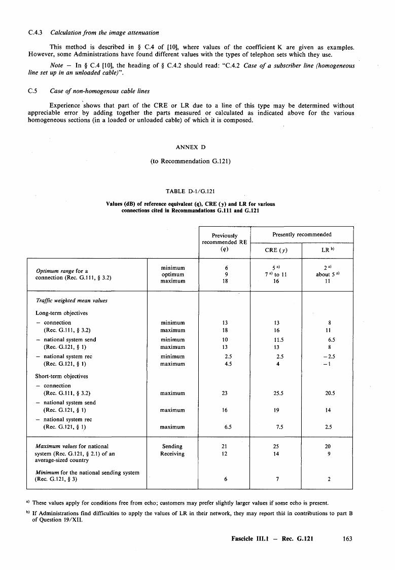
C.4.3 Calculation from the image attenuation
This method is described in § C.4 of [10], where values of the coefficient K are given as examples. However, some Administrations have found different values with the types of telephon sets which they use.
Note — In § C.4 [10], the heading of § C.4.2 should read: “C.4.2 Case o f a subscriber line (homogeneous line set up in an unloaded cable)".
C.5 Case o f non-homogenous cable lines
Experience shows that part of the CRE or LR due to a line of this type may be determined without appreciable error by adding together the parts measured or calculated as indicated above for the various homogeneous sections (in a loaded or unloaded cable) of which it is composed.
ANNEX D
(to Recommendation G.121)
TABLE D-1/G.121
Values (dB) of reference equivalent (q), CRE (y) and LR for various connections cited in Recommandations G . l l l and G.121
Previously recommended RE
(q)
Presently recommended
CRE (y ) LR b)
Optimum range for a connection (Rec. G . l l l , § 3.2)
minimumoptimummaximum
69
18
5 a)7 a) to 11
16
2 a)about 5 a)
11
Traffic weighted mean values
Long-term objectives
— connection minimum 13 13 8(Rec. G . l l l , § 3.2) maximum 18 16 11
— national system send minimum 10 11.5 6.5(Rec. G.121, § 1) maximum 13 13 8
— national system rec minimum 2.5 2.5 -2 .5(Rec. G.121, § 1)
Short-term objectives
— connection
maximum 4.5 4 - 1
(Rec. G . l l l , § 3.2)
— national system send
maximum 23 25.5 20.5
(Rec. G.121, § 1)
— national system rec
maximum 16 19 14
(Rec. G.121, § 1) maximum 6.5 7.5 2.5
Maximum values for national Sending 21 25 20system (Rec. G.121, § 2.1) of an average-sized country
Receiving 12 14 9
Minimum for the national sending system(Rec. G.121, § 3) 6 7 2
a) These values apply for conditions free from echo; customers may prefer slightly larger values if some echo is present.
b) If Administrations find difficulties to apply the values of LR in their network, they may report this in contributions to part B o f Question 19 /X II.
Fascicle III.l - Rec. G.121 163
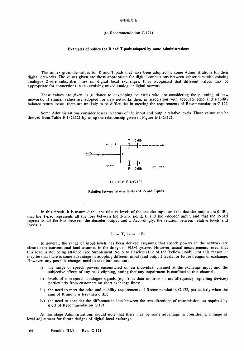
ANNEX E
(to Recommendation G.121)
Examples of values for R and T pads adopted by some Administrations
This annex gives the values for R and T pads that have been adopted by some Administrations for their digital networks. The values given are those appropriate for digital connections between subscribers with existing analogue 2-wire subscriber lines on digital local exchanges. It is recognized that different values may be appropriate for connections in the evolving mixed analogue/digital network.
These values are given as guidance to developing countries who are considering the planning of new networks. If similar values are adopted for new networks then, in association with adequate echo and stability balance return losses, there are unlikely to be difficulties in meeting the requirements of Recommendation G.122.
Some Administrations consider losses in terms of the input and output relative levels. These values can be derived from Table E-1/G.121 by using the relationship given in Figure E-1/G.121.
L:
O - —►-
T OdBr
- i — I —
T H -R OdBr
FIG URE E-l/G.121
Relation between relative levels and R- and T-pads
In this circuit, it is assumed that the relative levels of the encoder input and the decoder output are 0 dBr, that the T-pad represents all the loss between the 2-wire point, t, and the encoder input, and that the R-pad represents all the loss between the decoder output and t. Accordingly, the relation between relative levels and losses is:
L; = T, L0 = - R .
In general, the range of input levels has been derived assuming that speech powers in the network are close to the conventional load assumed in the design of FDM systems. However, actual measurements reveal that this load is not being attained (see Supplement No. 5 to Fascicle III.2 of the Yellow Book). For this reason, it may be that there is some advantage in adopting different input (and output) levels for future designs of exchange. However, any possible changes need to take into account:
i) the range of speech powers encountered on an individual channel at the exchange input and the subjective effects of any peak clipping, noting that any impairment is confined to that channel;
ii) levels o f non-speech analogue signals (e.g. from data modems or multifrequency signalling devices) particularly from customers on short exchange lines;
iii) the need to meet the echo and stability requirements of Recommendation G.122, particularly when the sum of R and T is less than 6 dB;
iv) the need to consider the difference in loss between the two directions of transmission, as required by § 6.3 of Recommendation G.121.
At this stage Administrations should note that there may be some advantage in considering a range of level adjustment for future designs of digital local exchange.
164 Fascicle III.l — Rec. G.121
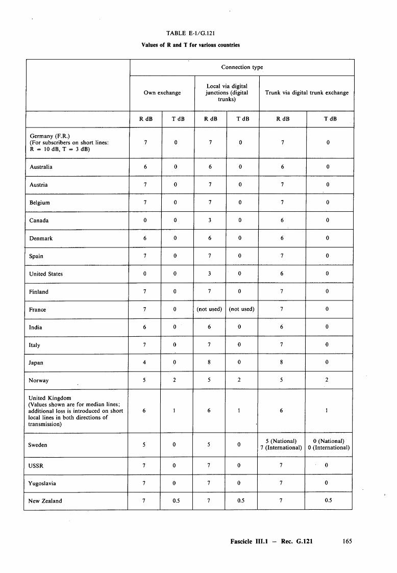
TABLE E-l/G .121
Values of R and T for various countries
Connection type
Own exchangeLocal via digital
junctions (digital trunks)
Trunk via digital trunk exchange
R dB T dB R dB T dB R dB T dB
Germany (F.R.)(For subscribers on short lines: R = 10 dB, T = 3 dB)
7 0 7 0 7 0
Australia 6 0 6 0 6 0
Austria 7 0 7 0 7 0
Belgium 7 0 7 0 7 0
Canada 0 0 3 0 6 0
Denmark 6 0 6 0 6 0
Spain 7 0 7 0 7 0
United States 0 0 3 0 6 0
Finland 7 0 7 0 7 0
France 7 0 (not used) (not used) 7 0
India 6 0 6 0 6 0
Italy 7 0 7 0 7 0
Japan 4 0 8 0 8 0
Norway 5 2 5 2 5 2
United Kingdom(Values shown are for median lines; additional loss is introduced on short local lines in both directions of transmission)
6 1 6 1 6 1
Sweden 5 0 5 0 5 (National)7 (International)
0 (National)0 (International)
USSR 7 0 7 0 7 0
Yugoslavia 7 0 7 0 7 0
New Zealand 7 0.5 7 0.5 7 0.5
Fascicle III.l — Rec. G.121 165
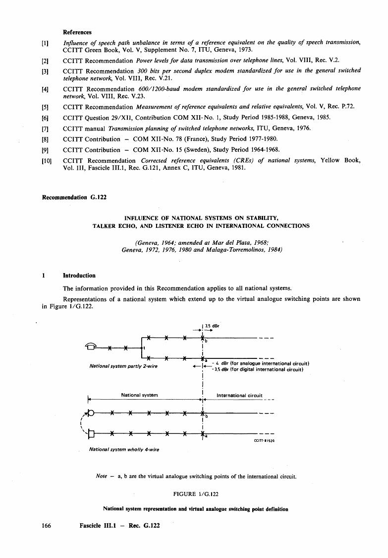
[1] Influence o f speech path unbalance in terms o f a reference equivalent on the quality o f speech transmission,CCITT Green Book, Vol. V, Supplement No. 7, ITU, Geneva, 1973.
[2] CCITT Recommendation Power levels fo r data transmission over telephone lines, Vol. VIII, Rec. V.2.
[3] CCITT Recommendation 300 bits per second duplex modem standardized fo r use in the general switchedtelephone network, Vol. V III, Rec. V.21.
[4] CCITT Recommendation 600/1200-baud modem standardized fo r use in the general switched telephonenetwork, Vol. VIII, Rec. V.23.
[5] CCITT Recommendation Measurement o f reference equivalents and relative equivalents, Vol. V, Rec. P.72.
[6] CCITT Question 29/X II, Contribution COM X II-N o. 1, Study Period 1985-1988, Geneva, 1985.
[7] CCITT manual Transmission planning o f switched telephone networks, ITU, Geneva, 1976.
[8] CCITT Contribution - COM X II-No. 78 (France), Study Period 1977-1980.
[9] CCITT Contribution - COM XII-N o. 15 (Sweden), Study Period 1964-1968.
[10] CCITT Recommendation Corrected reference equivalents (CREs) o f national systems, Yellow Book,Vol. I l l , Fascicle II I .l , Rec. G.121, Annex C, ITU, Geneva, 1981.
References
Recommendation G.122
INFLUENCE OF NATIONAL SYSTEMS ON STABILITY,TALKER ECHO, AND LISTENER ECHO IN INTERNATIONAL CONNECTIONS
(Geneva, 1964; amended at Mar del Plata, 1968;Geneva, 1972, 1976, 1980 and Malaga-Torremolinos, 1984)
Introduction
The information provided in this Recommendation applies to all national systems.
Representations of a national system which extend up to the virtual analogue switching points are shownin Figure 1/G . 122.
3.5 dBr
O -
National system partly 2-wire
, b
------------------------------_i - 4 dBr (for analogue international circuit)
, -3.5 dBr (for digital international circuit)
National system International circuit
A >
National system wholly 4-wire
Note — a, b are the virtual analogue switching points of the international circuit.
FIGURE 1/G. 122
National system representation and virtual analogue switching point definition
166 Fascicle I I I .l — Rec. G.122
The transmission loss introduced between a and b by thenational system, referred to as the loss (a-b), is important from three points of view:
a) it contributes to the margin that the international connection has against oscillation during thesetting-up and clearing-down of the connection. A minimum loss over the band 0-4 kHz is thecharacteristic value;
b) it contributes to the margin of stability during a communication. Again, a minimum loss in theband 0-4 kHz is the characteristic value, but in this case the subscribers’ apparatuses (telephone,modem, etc.) are assumed to be connected and in the operating condition;
c) it contributes to the control o f echoes and, in respect o f the subjective effect of talker echo, a weighted sum of the loss (a-b) over the band 300-3400 Hz is the characteristic value.
In addition, echoes circulating in any of the 4-wire loops in the national system or in the international 4-wire chain, give rise to listener echo, which can affect voice-band analogue data transmission.
The requirements stated in this Recommendation represent network performance objectives.
2 Loss (a-b) to avoid instability during set-up, clear-down and changes in a connection
2.1 Instability should be avoided during all normal conditions of set-up, clear-down and other changes in the composition (e.g. call-transfer) of a complete connection. To ensure adequate stability of international connections the distribution (taken over many actual calls) o f the loss (a-b) during the worst situation should be such that the risk of a loss (a-b) o f 0 dB or less does not exceed 6 in 100 calls when using the calculation method applied in § 2.2. This requirement should be observed at any frequency in the band 0 to 4 kHz.
Note 1 — The signalling and switching systems have an influence on the loss (a-b) under set-up and clear-down conditions. For example, in some systems 4-wire registers control the set-up and do not establish the 4-wire path until the answer signal is successfully received. In others, circuits are released immediately if busy conditions are encountered. In these circumstances the risk of oscillation does not arise.
Note 2 — Recommendation Q.32 gives information on methods of securing an adequate loss (a-b) o f an incoming national system before the called-subscriber answers (i.e. while ringing tone is transmitted) or if busy or number unobtainable conditions are encountered.
Note 3 — If there are no such arrangements as described in Notes 1 or 2 above then in general it would be safe to assume that there is no balance return loss provided by the called local telephone circuit (if 2-wire). In this case the necessary loss (a-b) must be provided by the transmission losses in the national system.
Note 4 — The stability o f international telephone connections at frequencies outside the band of effectively transmitted frequencies (i.e. below 300 Hz and above 3400 Hz) is governed by the following transmission losses at the frequencies of interest:
— the balance return loss at the terminating units;
— the transmission losses of the terminating units;
— the transmission losses o f the 4-wire circuits.
Note 5 — Conditions which only last for a few tens of milliseconds can be left out o f considerationbecause in such a short time oscillations cannot built up to a significant level.
2.2 The limit recommended in § 2.1 may be met, for instance, by imposing the following simultaneous conditions on the national network:
1) The sum of the nom inal transmission losses in both directions of transmission a-b and t-b measured between the 2-wire input o f the terminating set /, and one or other of the virtual switching points on the international circuit, a or b should not be less than (4 + rt) dB, where n is the number of 4-wire circuits in the national chain.
2) The stability balance return loss at the terminating set t, should have a value not less than 2 dB for the terminal conditions encountered during normal operation.
3) The standard deviation o f variations o f transmission loss of a circuit should not exceed 1 dB (see Recommendation G.151, § 3).
Fascicle III.l — Rec. G.122 167
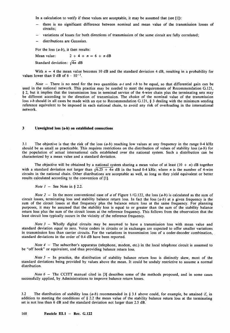
In a calculation to verify if these values are acceptable, it may be assumed that (see [1]):
— there is no significant difference between nominal and mean value of the transmission losses ofcircuits;
— variations of losses for both directions of transmission of the same circuit are fully correlated;
— distributions are Gaussian.
For the loss (a-b), it then results:
Mean value: 2 + 4 + n = 6 + « d B
Standard deviation: ]/4n dB
With n = 4 the mean value becomes 10 dB and the standard deviation 4 dB, resulting in a probability forvalues lower than 0 dB of 6 • 10~3.
Note — There is no need for the two quantities a-t and t-b to be equal, so that differential gain can be used in the national network. This practice may be needed to meet the requirements of Recommendation G.121, § 2, but it implies that the transmission loss in terminal service of the 4-wire chain plus the terminating sets may be different according to the direction of transmission. The choice of the nominal value of the transmission loss t-b should in all cases be made with an eye to Recommendation G.121, § 3 dealing with the minimum sending reference equivalent to be imposed in each national chain, to avoid any risk of overloading in the international network.
3 Unweighted loss (a-b) on established connections
3.1 The objective is that the risk of the loss (a-b) reaching low values at any frequency in the range 0-4 kHz should be as small as practicable. This requires restrictions on the distribution of values of stability loss (a-b) for the population of actual international calls established over the national system. Such a distribution can be characterized by a mean value and a standard deviation.
The objective will be obtained by a national system sharing a mean value of at least (10 + n) dB together with a standard deviation not larger than |/6.25 + 4n dB in the band 0-4 kHz; where n is the number of 4-wire circuits in the national chain. Other distributions are acceptable as well, as long as they yield equivalent or better results calculated according to the convention of [1].
Note 1 — See Note in § 2.2.
Note 2 — In the more conventional case of a o f Figure 1/G. 122, the loss (a-b) is calculated as the sum of circuit losses, terminating loss and stability balance return loss. In fact the loss (a-b) at a given frequency is the sum of the circuit losses at that frequency plus the balance return loss at the same frequency. For planning purposes, it may be assumed that the stability loss is equal to or greater than the sum of the stability balance return loss plus the sum of the circuit losses at the reference frequency. This follows from the observation that the least circuit loss typically occurs in the vicinity of the reference frequency.
Note 3 — Wholly digital circuits may be assumed to have a transmission loss with mean value and standard deviation equal to zero. Voice coders in circuits or in exchanges are expected to offer smaller variations in transmission loss than carrier circuits. For the variations in transmission loss o f a coder-decoder combination, standard deviations in the order of 0.4 dB have been reported.
Note 4 — The subscriber’s apparatus (telephone, modem, etc.) in the local telephone circuit is assumed to be “off hook” or equivalent, and thus providing balance return loss.
Note 5 — In practice, the distribution of stability balance return loss is distinctly skew, most o f the standard deviations being provided by values above the mean. It could be unduly restrictive to assume a normal distribution.
Note 6 — The CCITT manual cited in [3] describes some of the methods proposed, and in some cases successfully applied, by Administrations to improve balance return losses.
3.2 The distribution of stability loss (a-b) recommended in § 3.1 above could, for example, be attained if, in addition to meeting the conditions of § 2.2 the mean value of the stability balance return loss at the terminating set is not less than 6 dB and the standard deviation not larger than 2.5 dB.
168 Fascicle III.l - Rec. G.122
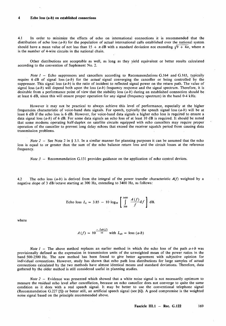
4 Echo loss (a-b) on established connections
4.1 In order to minimize the effects of echo on international connections it is recommended that the distribution of echo loss (a-b) for the population of actual international calls established over the national system should have a mean value of not less than 15 + n dB with a standard deviation not exceeding |/9 + 4n, where n is the num ber of 4-wire circuits in the national chain.
Other distributions are acceptable as well, as long as they yield equivalent or better results calculated according to the convention of Suplement No. 2.
Note 1 — Echo suppressors and cancellers according to Recommendations G. 164 and G. 165, typically require 6 dB of signal loss (a-b) for the actual signal converging the canceller or being controlled by the suppressor. This signal loss (a-b) is the ratio of incident to reflected signal power on the return path. The value of signal loss (a-b) will depend both upon the loss (a-b) frequency response and the signal spectrum. Therefore, it is desirable from a performance point o f view that the stability loss (a-b) during an established connection should be at least 6 dB, since this will ensure proper operation for any signal (frequency spectrum) in the band 0-4 kHz.
However it may not be practical to always achieve this level of performance, especially at the higher frequencies characteristic of voice-band data signals. For speech, typically the speech signal loss (a-b) will be at least 6 dB if the echo loss is 6 dB. However, for voice-band data signals a higher echo loss is required to ensure a data signal loss (a-b) of 6 dB. For some data signals an echo loss of at least 10 dB is required. It should be noted that some modems operating half-duplex on satellite circuits equipped with echo cancellers may require proper operation of the canceller to prevent long delay echoes that exceed the receiver squelch period from causing data transmission problems.
Note 2 — See Note 2 in § 3.1. In a similar manner for planning purposes it can be assumed that the echo loss is equal to or greater than the sum of the echo balance return loss and the circuit losses at the reference frequency.
Note 3 - Recommendation G.131 provides guidance on the application of echo control devices.
4.2 The echo loss (a-b) is derived from the integral of the power transfer characteristic A (f) weighted by a negative slope of 3 dB/octave starting at 300 Hz, extending to 3400 Hz, as follows:
3400 A ( f )Echo loss Le = 3.85 - 10 logI0 | J —~ d / | dB.
300 /
where
- L a b ( f )A ( f ) = 10 io with Lab = loss (a-b)
Note 1 - The above method replaces an earlier method in which the echo loss of the path a-t-b was provisionally defined as the expression in transmission units of the unweighted mean of the power ratios in the band 500-2500 Hz. The new method has been found to give better agreement with subjective opinion for individual connections. However, study has shown that echo path loss distributions for large samples of actual connections calculated by the two methods have almost identical means and standard deviations. Therefore, data gathered by the older method is still considered useful in planning studies.
Note 2 — Evidence was presented which showed that a white noise signal is not necessarily optimum to measure the residual echo level after cancellation, because an echo cancellor does not converge to quite the same condition as it does with a real speech signal. It may be better to use the conventional telephone signal (Recommendation G . l l l [5]) or better still, an artificial speech signal (see [6]). A good compromise is the weighted noise signal based on the principle recommended above.
Fascicle III.l - Rec. G.122 169

Note 3 — Improved balance return losses at t can be obtained when the local exchange uses 4-wire switching and the local line is permanently associated with the 2-wire/4-wire conversion unit and its balance network (see Recommendation Q.517 for examples). When there is 2-wire switching a compromise balance network must be used.
Note 4 — There is evidence that a 4-wire handset telephone in normal use can contribute significant acoustic echo to the communication. Hence in some circumstances (low transmission loss, long delay times) echo control devices may be needed.
4.3 An example of how the recommendation quoted in § 4.1 above can be achieved would be for the mean value o f the sum of the transmission losses a-t and t-b not to be less than (4 + n) dB with a standard deviation from the mean not exceeding 2 |/n dB, accompanied by an echo balance return loss at the terminating set /, of not less than 11 dB with a standard deviation not exceeding 3 dB.
5 Effects of listener echo (double-reflected signals) 0
5.1 General
It has been assumed in §§ 1 to 4 that only one 2-wire-4-wire-2-wire loop (further referred to as loop) occurs in a connection. Consequently, the requirements in §§ 1 to 4 are valid for that case, i.e. they refer to the “semi-loop” seen directly from the VASPs (virtual analogue switching points). However, in mixed analogue/digital connections several loops may occur when 4-wire digital exchanges (including PABXs) are connected 2-wire to other exchanges. Such loops have typically low loss and short delay times (at most a few milliseconds). Signals reflected twice, i.e. at both hybrids that terminate a loop, would therefore contribute to listener echo. These listener echo signals:
— can lead to objectionable “hollowness” in voice communications, and
— can impair the bit error ratio of received voice-band data signals.
In general it has been found that for satisfactory transmission, data modem receivers require higher values o f listener echo loss (in the band 500-2500 Hz) than speech (in the band 300-3400 Hz).
The effect o f listener echo is characterized by the difference in level between the direct signal and the multiple reflected signal. In Figure 2 /G .l22 the loss of the direct path is assumed to be S dB, whereas the loss along the path of the reflected signal is L dB. The listener echo loss (LE) then is L — S dB. It can be seen from Figure 2 /G .l22 that if only two reflections occur (only double-reflected signals), the listener echo loss LE equals the loss around the loop (open-loop loss, OLL), as all other losses are incurred equally by the direct and the reflected signals.
s
*4-------------------------- CCITT-M U 0
FIG URE 2 /G .l22
Listener echo
It should be noted that usually the listener echo will consists of a series of signals being reflected two times, four times, etc. and hence LE and OLL are in principle not equal. In practice however LE and OLL may be taken as equal when OLL exceeds about 8 dB.
The use of “listener echo” in this context might be misleading. It could be substituted by a more appropriate term. This matter is under further study.
170 Fascicle III.l - Rec. G.122
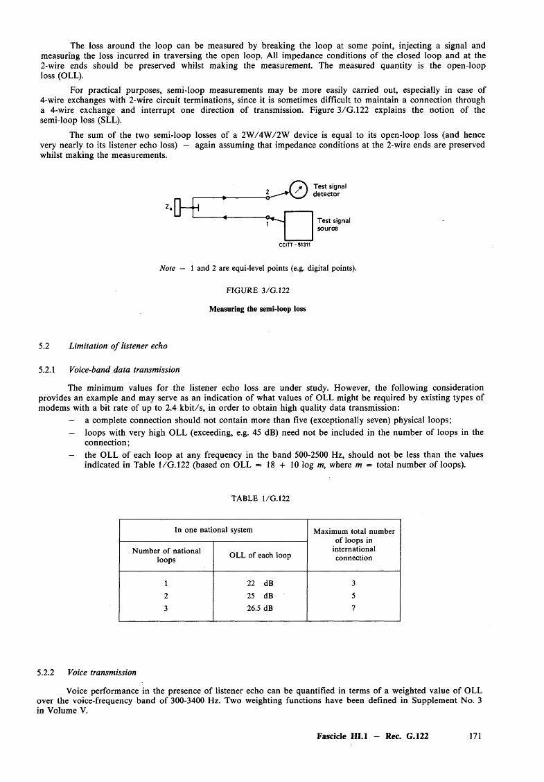
The loss around the loop can be measured by breaking the loop at some point, injecting a signal and measuring the loss incurred in traversing the open loop. All impedance conditions of the closed loop and at the 2-wire ends should be preserved whilst making the measurement. The measured quantity is the open-loop loss (OLL).
For practical purposes, semi-loop measurements may be more easily carried out, especially in case of 4-wire exchanges with 2-wire circuit terminations, since it is sometimes difficult to maintain a connection through a 4-wire exchange and interrupt one direction of transmission. Figure 3/G.122 explains the notion of the semi-loop loss (SLL).
The sum of the two semi-loop losses of a 2W /4W /2W device is equal to its open-loop loss (and hence very nearly to its listener echo loss) — again assuming that impedance conditions at the 2-wire ends are preserved whilst making the measurements.
[}
Test signal detector
Test signal source
C C IT T -8 1 3 1 1
Note — 1 and 2 are equi-level points (e.g. digital points).
FIG URE 3/G.122
Measuring the semi-loop loss
5.2 Limitation o f listener echo
5.2.1 Voice-band data transmission
The minimum values for the listener echo loss are under study. However, the following consideration provides an example and may serve as an indication of what values of OLL might be required by existing types of modems with a bit rate of up to 2.4 kb it/s, in order to obtain high quality data transmission:
— a complete connection should not contain more than five (exceptionally seven) physical loops;— loops with very high OLL (exceeding, e.g. 45 dB) need not be included in the number of loops in the
connection;— the OLL of each loop at any frequency in the band 500-2500 Hz, should not be less than the values
indicated in Table 1/G . 122 (based on OLL = 1 8 + 1 0 log m, where m = total number of loops).
TABLE 1/G . 122
In one national system Maximum total number of loops in
international connection
Number o f national loops OLL of each loop
1 22 dB 3
2 25 dB 5
3 26.5 dB 7
5.2.2 Voice transmission
Voice performance in the presence of listener echo can be quantified in terms of a weighted value of OLL over the voice-frequency band of 300-3400 Hz. Two weighting functions have been defined in Supplement No. 3 in Volume V.
Fascicle H I.l — Rec. G.122 171
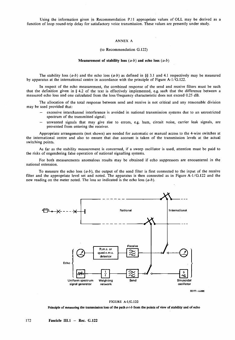
Using the information given in Recommendation P. 11 appropriate values of OLL may be derived as a function of loop round-trip delay for satisfactory voice transmission. These values are presently under study.
ANNEX A
(to Recommendation G.122)
Measurement of stability loss (a-b) and echo loss (a-b)
The stability loss (a-b) and the echo loss (a-b) as defined in §§ 3.1 and 4.1 respectively may be measured by apparatus at the international centre in accordance with the principle of Figure A-1/G. 122.
In respect o f the echo measurement, the combined response of the send and receive filters must be such that the definition given in § 4.2 of the text is effectively implemented, e.g. such that the difference between a measured echo loss and one calculated from the loss/frequency characteristic does not exceed 0.25 dB.
The allocation of the total response between send and receive is not critical and any reasonable division may be used provided that:
— excessive interchannel interference is avoided in national transmission systems due to an unrestricted spectrum of the transmitted signal;
— unwanted signals that may give rise to errors, e.g. hum, circuit noise, carrier leak signals, are prevented from entering the receiver.
Appropriate arrangements (not shown) are needed for automatic or manual access to the 4-wire switches at the international centre and also to ensure that due account is taken of the transmission levels at the actual switching points.
As far as the stability measurement is concerned, if a sweep oscillator is used, attention must be paid to the risks of engendering false operation of national signalling systems.
For both measurements anomalous results may be obtained if echo suppressors are encountered in the national extension.
To measure the echo loss (a-b), the output of the send filter is first connected to the input of the receive filter and the appropriate level set and noted. The apparatus is then connected as in Figure A- 1/G . 122 and the new reading on the meter noted. The loss so indicated is the echo loss (a-b).
Uniform spectrum Weighting Send Sinusoidalsignal generator network oscillator
CCITT- U 881
FIGURE A-1/G.122
Principle of measuring the transmission loss of the path a-t-b from the points of view of stability and of echo
172 Fascicle III.l — Rec. G.122
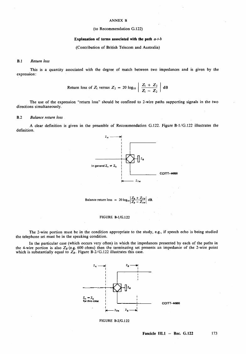
ANNEX B
(to Recommendation G.122)
Explanation of terms associated with the path a-t-b
(Contribution of British Telecom and Australia)
B. 1 Return loss
This is a quantity associated with the degree of match between two impedances and is given by the expression:
Return loss o f Z\ versus Z 2 = 20 log 10
Z, + Z 2z , - z 2
dB
The use of the expression “return loss” should be confined to 2-wire paths supporting signals in the two directions simultaneously.
B.2 Balance return loss
A clear definition is given in the preamble of Recommendation G.122. Figure B-1/G. 122 illustrates the definition.
In general ZH ZBm
N Zi
CCITT-44890
Balance return loss = 20 log Z b _ + _ Z jw I 10 2 d — Z t w \
dB.
FIGURE B-1/G.122
The 2-wire portion must be in the condition appropriate to the study, e.g., if speech echo is being studied the telephone set must be in the speaking condition.
In the particular case (which occurs very often) in which the impedances presented by each of the paths in the 4-wire portion is also Z B (e.g. 600 ohms) then the terminating set presents an impedance of the 2-wire point which is substantially equal to Z B• Figure B-2/G.122 illustrates this case.
CCITT- 44900
FIGURE B-2/G.122
Fascicle III.l - Rec. G.122 173
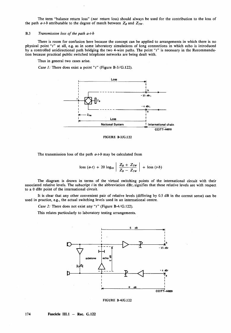
The term “balance return loss” (not return loss) should always be used for the contribution to the loss of the path a-t-b attributable to the degree of match between Z B and Z TW.
B.3 Transmission loss o f the path a-t-b
There is room for confusion here because the concept can be applied to arrangements in which there is no physical point “ f” at all, e.g. as in some laboratory simulations of long connections in which echo is introduced by a controlled unidirectional path bridging the two 4-wire paths. The point is necessary in the Recommendation because practical public switched telephone networks are being dealt with.
Thus in general two cases arise.
Case 1: There does exist a point “ f” (Figure B-3/G.122).
Loss
m
Loss
National System
FIGURE B-3/G.122
IIl b—X---
3,5 dBrj
- 4 dBrj X—
International chainCCITT-44910
The transmission loss o f the path a-t-b may be calculated from
Z B + Z jwloss (a-t) + 20 logioZ B - Z T W
+ loss (t-b)
The diagram is drawn in terms of the virtual switching points o f the international circuit with their associated relative levels. The subscript i in the abbreviation dBr, signifies that these relative levels are with respect to a 0 dBr point o f the international circuit.
It is clear that any other convenient pair o f relative levels (differing by 0.5 dB in the correct sense) can be used in practice, e.g., the actual switching levels used in an international centre.
Case 2: There does not exist any “ f” (Figure B-4/G.122).
This relates particularly to laboratory testing arrangements.
dB
D - o — t -
sidetone e c h o '
3.5 dBr
- 4 dBr— X
R dBCCITT-44920
FIGURE B-4/G.122
174 Fascicle III.l - Rec. G.122
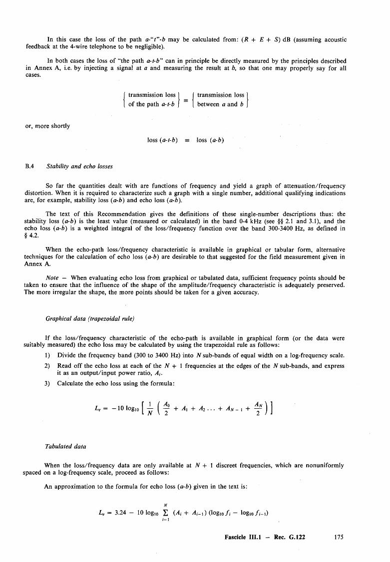
In this case the loss o f the path a-“t ”-b may be calculated from: (R + E + S) dB (assuming acoustic feedback at the 4-wire telephone to be negligible).
In both cases the loss of “the path a-t-b” can in principle be directly measured by the principles described in Annex A, i.e. by injecting a signal at a and measuring the result at b, so that one may properly say for all cases.
transmission loss of the path a-t-b ~~
or, more shortly
loss {a-t-b) =
B.4 Stability and echo losses
So far the quantities dealt with are functions of frequency and yield a graph of attenuation/frequency distortion. When it is required to characterize such a graph with a single number, additional qualifying indicationsare, for example, stability loss {a-b) and echo loss {a-b).
The text o f this Recommendation gives the definitions of these single-number descriptions thus: the stability loss {a-b) is the least value (measured or calculated) in the band 0-4 kHz (see §§ 2.1 and 3.1), and theecho loss {a-b) is a weighted integral of the loss/frequency function over the band 300-3400 Hz, as defined in§ 4.2.
When the echo-path loss/frequency characteristic is available in graphical or tabular form, alternative techniques for the calculation of echo loss {a-b) are desirable to that suggested for the field measurement given in Annex A.
Note — When evaluating echo loss from graphical or tabulated data, sufficient frequency points should be taken to ensure that the influence of the shape of the amplitude/frequency characteristic is adequately preserved. The more irregular the shape, the more points should be taken for a given accuracy.
Graphical data (trapezoidal rule)
If the loss/frequency characteristic o f the echo-path is available in graphical form (or the data were suitably measured) the echo loss may be calculated by using the trapezoidal rule as follows:
1) Divide the frequency band (300 to 3400 Hz) into TV sub-bands of equal width on a log-frequency scale.
2) Read off the echo loss at each of the N + 1 frequencies at the edges of the N sub-bands, and express it as an ou tput/input power ratio, A (.
3) Calculate the echo loss using the formula:
Le = —10 logio + At + A2 . . . + A n - 1 + j j
Tabulated data
When the loss/frequency data are only available at N + 1 discreet frequencies, which are nonuniformly spaced on a log-frequency scale, proceed as follows:
An approximation to the formula for echo loss {a-b) given in the text is:
NLe = 3.24 — 10 logio 2 (^ i + -di— 1) (logio/ / — logio / / - 1)
1=1
transmission loss between a and b
loss {a-b)
Fascicle III.l - Rec. G.122 175
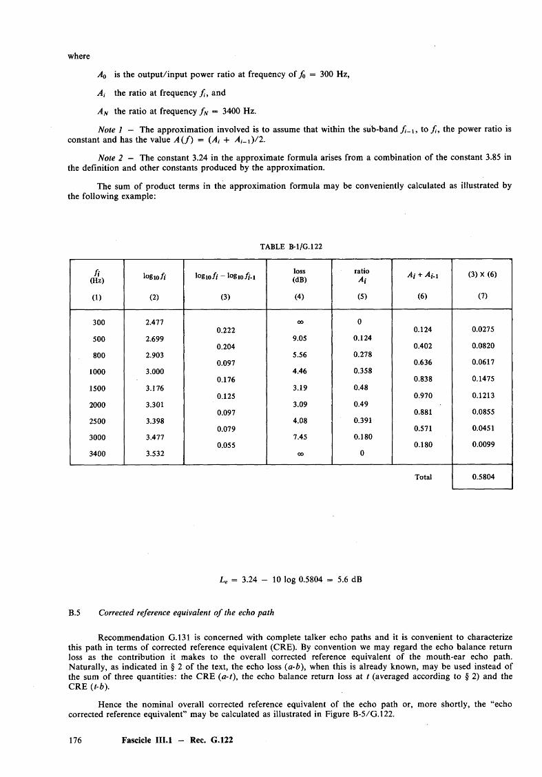
where
Aq is the ou tput/input power ratio at frequency of f 0 = 300 Hz,
Ai the ratio at frequency f , and
A n the ratio at frequency f N = 3400 Hz.
Note 1 — The approxim ation involved is to assume that within the sub-band f _ \ , to f , the power ratio is constant and has the value A ( / ) = (A t + A,_ j )/2 .
Note 2 — The constant 3.24 in the approximate formula arises from a combination of the constant 3.85 in the definition and other constants produced by the approximation.
The sum of product terms in the approxim ation formula may be conveniently calculated as illustrated by the following example:
TABLE B-1/G.122
f i(Hz) log io f i logio f i ~ log 10//-I
loss(dB)
ratioA i
A i + A j.i (3) X (6)
(1) (2) (3) (4) (5) (6) (7)
300 2.4770.222
00 00.124 0.0275
500 2.6990.204
9.05 0.1240.402 0.0820
800 2.9030.097
5.56 0.2780.636 0.0617
1000 3.0000.176
4.46 0.3580.838 0.1475
1500 3.1760.125
3.19 0.480.970 0.1213
2000 3.3010.097
3.09 0.490.881 0.0855
2500 3.3980.079
4.08 0.3910.571 0.0451
3000 3.4770.055
7.45 0.1800.180 0.0099
3400 3.532 00 0
Total 0.5804
Le = 3.24 - 10 log 0.5804 = 5.6 dB
B.5 Corrected reference equivalent o f the echo path
Recommendation G.131 is concerned with complete talker echo paths and it is convenient to characterize this path in terms of corrected reference equivalent (CRE). By convention we may regard the echo balance return loss as the contribution it makes to the overall corrected reference equivalent of the mouth-ear echo path. Naturally, as indicated in § 2 of the text, the echo loss (a-b), when this is already known, may be used instead of the sum of three quantities: the CRE (a-t), the echo balance return loss at t (averaged according to § 2) and the CRE (t-b).
Hence the nominal overall corrected reference equivalent of the echo path or, more shortly, the “echo corrected reference equivalent” may be calculated as illustrated in Figure B-5/G.122.
176 Fascicle III.l — Rec. G.122
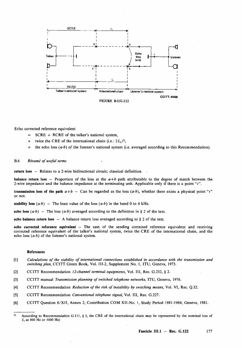
CCITT-44930FIGURE B-5/G.122
Echo corrected reference equivalent
= SCRE + RCRE of the talker’s national system,
+ twice the CRE of the international chain (i.e.: 2L J 2),
4- the echo loss (a-b) o f the listener’s national system (i.e. averaged according to this Recommendation).
B.6 Resume o f useful terms
return loss — Relates to a 2-wire bidirectional circuit; classical definition.
balance return loss — Proportion of the loss at the a-t-b path attributable to the degree of match between the 2-wire impedance and the balance impedance at the terminating unit. Applicable only if there is a point “ t ”.
transmission loss of the path a-t-b — Can be regarded as the loss (a-b), whether there exists a physical point “ t ” or not.
stability loss (a-b) — The least value of the loss (a-b) in the band 0 to 4 kHz.
echo loss (a-b) — The loss (a-b) averaged according to the definition in § 2 of the text.
echo balance return loss — A balance return loss averaged according to § 2 of the text.
echo corrected reference equivalent — The sum of the sending corrected reference equivalent and receivingcorrected reference equivalent o f the talker’s national system, twice the CRE of the international chain, and the echo loss (a-b) of the listener’s national system.
References
[1] Calculations o f the stability o f international connections established in accordance with the transmission and switching plan, CCITT Green Book, Vol. III-2, Supplement No. 1, ITU, Geneva, 1973.
[2] CCITT Recommendation 12-channel terminal equipments, Vol. I l l , Rec. G.232, § 2.
[3] CCITT manual Transmission planning o f switched telephone networks, ITU, Geneva, 1976.
[4] CCITT Recommendation Reduction o f the risk o f instability by switching means, Vol. VI, Rec. Q.32.
[5] CCITT Recommendation Conventional telephone signal, Vol. I l l , Rec. G.227.
[6] CCITT Question 8 /X II, Annex 2, Contribution COM XII-No. 1, Study Period 1981-1984, Geneva, 1981.
2) According to Recommendation G . l l l , § 3 , the CRE of the international chain may be represented by the nominal loss of Li at 800 Hz or 1000 Hz)
Fascicle III.l — Rec. G.122 177
Recommendation G.123
CIRCUIT NOISE IN NATIONAL NETWORKS
(Geneva, 1964, amended at M ar del Plata, 1968 and at Geneva, 1972, 1976 and 1980)
1 Noise induced by power lines
The network performance objective for the psophometric e.m.f. o f the noise produced by magnetic an d /o r electrostatic induction from all the power lines affecting one or more parts of a chain of telephone lines'? joining a subscriber’s set to its international centre should not exceed 1 millivolt, this being the value at the line') terminals of the subscriber’s set (when receiving), it being assumed that the telecommunication installations inserted in that chain are balanced to earth as perfectly as possible, in conformity with the most modern equipment construction.
It should be noted that, even in the case of perfectly balanced lines1?, the insertion of equipment having too great a degree of unbalance to earth may cause unacceptable noise at the terminals of a subscriber’s receiver.
In every national network, it is usually possible, in practice, to find switching centres such that some of the lines') that terminate at those centres (lines') in cable, conforming to CCITT specifications) are free from noise arising from neighbouring power lines. It is then sufficient to determine the psophometric e.m.f.s arising from all the power lines') affecting one or more parts of the chain of lines') joining such a centre to the subscriber’s set.
2 Noise contributed by transmission systems
2.1 Analogue systems
2.1.1 Very-long-distance circuits (about 2500-25 000 km)
If an extension circuit more than 2500 km long is used in a large country, it will have to meet all the recommendations applicable to an international circuit of the same length (Recommendation G.153). This implies that the equipment design objective for the line noise in channels used to provide these circuits should not exceed 2 pWOp/km.
2.1.2 Circuit ranging in length from very short distances up to 2500 km
These circuits should meet the requirements of Recommendation G.152. This implies that according to the noise objectives of Recommendation G.222 [1] the accumulated line noise should correspond to an average of not more than 3 pWOp/km and the noise power produced by the various modulating equipments should meet the provisions of the Recommendation cited in [2].
Taking account of the particular structure of a real circuit the pertinent Recommendations CCITT/G.226 [3] (for cable systems) or CCIR/395-2 [4] (for radio-relay systems) must be applied when assessing its noise performance.
Note 1 — The permissible noise contributions from equipment do not depend on whether the circuits form part of the international 4-wire chain or are connected to it by 2-wire switching. However, the circuit noise powers assume that the hypothetical reference connections of Recommendation G.103 are, or will be in future, reasonably typical of connections. They also assume that the total length of circuits connecting the local exchange to the primary centre is not excessive. The attention of Administrations is drawn to a conclusion of studies carried out by the CCITT during the 1964-1968 Study Period, that if the additional percentage of “poor or bad” opinions on the quality of connections due to noise introduced by the circuits connecting the local exchange to the primary centre is not to exceed one half o f that caused by the presence in the connection of all other sources of circuit noise, then the noise contributed by each one of these circuits should be limited to about 500 pWOp (mean for all the channels of the system during any hour).
“Line” as used in this § 1 should be understood as meaning subscriber’s line, trunk junction or trunk circuit.
178 Fascicle III.1 - Rec. G.123
Note 2 — Under the above conditions and assuming the maximum noise values permitted for pairs of channel modulators (200 pWOp), group modulators (80 pWOp) and supergroup modulators (60 pWOp), a total noise power of 500 pWOp will not be exceeded by a circuit connecting the local exchange to the primary centre (Figure 1/G . 103) when its length is less than about 50 to 100 km.
Note 3 — In the case that those circuits are operated with compandors conforming to Recommendation G.162, the permitted noise powers are to be understood inclusive of the effect of the com pandor gain.
2.2 Digital system
Circuits provided by PCM systems which accord with the G.700 Series of Recommendations, in particular Recommendation G .712 [5], will have an acceptable noise performance which is substantially independent of their length.
3 Noise in a national 4-wire automatic exchange2)
3.1 Definition o f a connection through an exchange
Noise conditions in a national 4-wire automatic exchange are defined by reference to a “connection” through this exchange. By “connection through an exchange” is to be understood the pair of wires corresponding to a direction of transmission and connecting the input point of a circuit incoming in the exchange to the output point o f a different circuit outgoing from the exchange. These input or output points are those defined in Recommendation Q.45 (points A and D of Figure 1/Q.45 [8]) and are not necessarily the same as the text access points defined in Recommendation M.640 [9].
3.2 Equipment design objective fo r the mean noise power during the busy-hour
The mean of the noise over a long period during the busy-hour should not exceed the following values:
1) Psophometrically weighted noise: —67 dBmOp (200 pWOp),2) Unweighted noise: —40 dBmO (100 000 pWO) measured with a device with a uniform response curve
throughout the band 30-20 000 Hz.
Note — A sufficient variety of connections should be chosen to ensure that the measurements arerepresentative of the various possible routes through the exchange.
3.3 Equipment design objective fo r the impulsive noise during the busy-hour
Noise counts should not exceed 5 counts in 5 minutes at the threshold level of —35 dBmO (see the Recommendation cited in [10] for measurement procedure).
Note — Figure 3/Q.45 [11] shows the maximum number of impulsive noise counts acceptable in a5-minute period.
4 Noise allocation for a national system (guide for planning purposes)
The noise powers indicated in the following text are nominal values.
Network planning should be such that the noise power entering the international network and attributableto national sending systems meets the limits of the following rule:
The psophometric noise power introduced by the national sending system at a point of zero relative level on the first international circuit must not exceed either (4000 + 4L) or (7000 + 2L) pWp, whichever is less, and where L is the total length in kilometres of the long-distance FDM carrier systems in the national chain. The corresponding quantities referred to the send virtual switching point are (1800 + 1.8L) and (3100 + 0.9L) pWp.
The derivation of this rule is explained in the Annex A.
In accordance with Recommendation Q.31 [6], the limits are the same as in Recommendation Q.45 [7].
Fascicle III.l - Rec. G.123 179
Note - A problem, which has already arisen in some national networks, as regards the receiving direction, is that when losses are reduced the circuit noise becomes more noticeable, particularly during periods of no conversation. This is particularly relevant in the case of large countries in which the noise contribution from line systems is high. Hence if an Administration complies with a recommendation concerning national noise power levels and then subsequently improves transmission, perhaps by introducing 4-wire switching in lower-order exchanges, it may find itself in a worse situation as regards noise. It follows that it is im portant to preserve a proper balance between noise and loss.
ANNEX A
(to Recommendation G.123)
Noise allocation for a national system
A.l It is desirable that the noise power arising in national networks be limited in terms of the level appearing at the virtual switching points — the agreed interface between the national and the international network. In order to do this, some particular distribution of losses within the national network must be assumed. The solution is to adopt an agreed reference connection in order to specify maximum noise power levels from national sources referred to the virtual switching point o f the international circuit.
A.2 Having regard to the way in which national networks are constructed, it is appropriate to express the noise allowance in the form A + BL where A is a fixed allowance resulting from noise in exchanges and from short-haul multiplex systems, B is an allowance for a noise rate per unit length from long-haul multiplex systems and L is the total length of these latter systems in the national portion of the international connection. Two such expressions are necessary, one for countries o f average size and another for large countries (in the sense of Recommendation G.121).
A.3 This approach is comparatively straightforward in the national sending system and serves to limit the am ount of noise injected into the international connection.
A.4 Average-sized countries (i.e. not greater than 1500 km from the CT3 to the most remote local exchange).
The relevant hypothetical reference chain for the national sending system is given in Figure A -l/G .1233). The circuit between the local exchange and the primary centre is assumed to be routed on an FDM carrier system of length not exceeding 250 km and operated at a nominal loss of 3 dB. The noise power on this circuit is taken to be the maximum value of 2000 pWO. The circuit between the primary centre and the secondary centre is also assumed to be routed on an FDM carrier system of the same type.
The line noise power rate of the two long-distance trunk circuits is assumed to be 4 pW /km and the total line length of these two circuits (L \ + L2 in Figure A-1/G.123) approaches the limit of 1500 km arbitrarily defining“a country of average size” in Recommendation G.121. It is thus assumed that the distance covered by the two short-haul systems is a very small proportion of the total length of the complete national sending system.
Each exchange is assumed to contribute 200 pWp in accordance with § 3 of the text, or Q.31 [6].
Note by the C C ITT Secretariat. — The noise values shown in this figure are maximum values; see also the corresponding element of Figure 1/G . 103.
180 Fascicle III.l - Rec. G.123
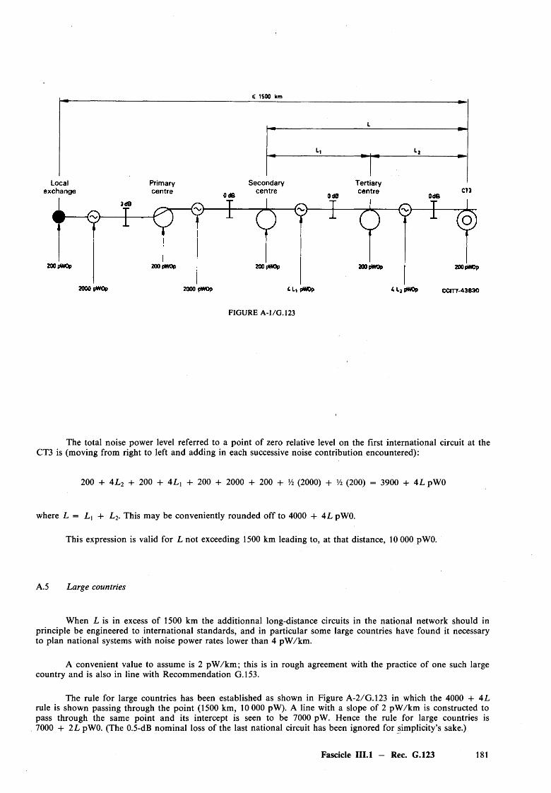
£ 1SOO km
I
Li L2
Local Primary Secondary Tertiary
FIGURE A-1/G.123
The total noise power level referred to a point of zero relative level on the first international circuit at the CT3 is (moving from right to left and adding in each successive noise contribution encountered):
200 + 4L 2 + 200 + 4 L x + 200 + 2000 + 200 + Vi (2000) + (200) = 3900 + 4L pWO
where L = L\ + L 2. This may be conveniently rounded off to 4000 + 4L pWO.
This expression is valid for L not exceeding 1500 km leading to, at that distance, 10 000 pWO.
A.5 Large countries
When L is in excess of 1500 km the additionnal long-distance circuits in the national network should in principle be engineered to international standards, and in particular some large countries have found it necessary to plan national systems with noise power rates lower than 4 pW /km .
A convenient value to assume is 2 pW /km ; this is in rough agreement with the practice of one such large country and is also in line with Recommendation G.153.
The rule for large countries has been established as shown in Figure A-2/G.123 in which the 4000 + 4L rule is shown passing through the point (1500 km, 10 000 pW). A line with a slope of 2 pW /km is constructed to pass through the same point and its intercept is seen to be 7000 pW. Hence the rule for large countries is 7000 + 2L pWO. (The 0.5-dB nominal loss of the last national circuit has been ignored for simplicity’s sake.)
Fascicle III.1 - Rec. G.123 181
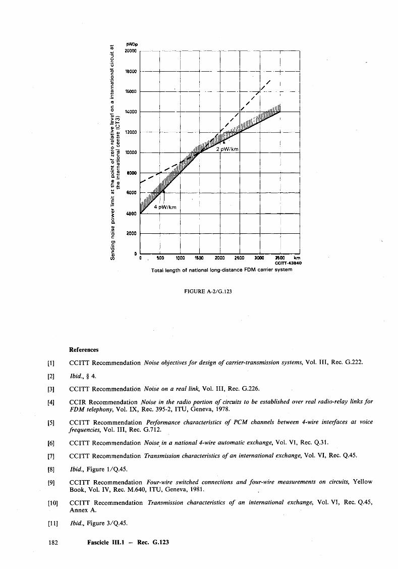
CCITT-43840
Total length of national long-distance FDM carrier system
FIGURE A-2/G.123
References
CCITT Recommendation Noise objectives fo r design o f carrier-transmission systems, Vol. I l l , Rec. G.222.
Ibid., § 4.
CCITT Recommendation Noise on a real link, Vol. I l l , Rec. G.226.
CCIR Recommendation Noise in the radio portion o f circuits to be established over real radio-relay links fo r FDM telephony, Vol. IX, Rec. 395-2, ITU, Geneva, 1978.
CCITT Recommendation Performance characteristics o f PCM channels between 4-wire interfaces at voice frequencies, Vol. I l l , Rec. G .712.
CCITT Recommendation Noise in a national 4-wire automatic exchange, Vol. VI, Rec. Q.31.
CCITT Recommendation Transmission characteristics o f an international exchange, Vol. VI, Rec. Q.45.
Ibid., Figure 1/Q.45.
CCITT Recommendation Four-wire switched connections and four-wire measurements on circuits, Yellow Book, Vol. IV, Rec. M.640, ITU, Geneva, 1981.
CCITT Recommendation Transmission characteristics o f an international exchange, Vol. VI, Rec. Q.45, Annex A.
Ibid., Figure 3/Q.45.
Fascicle III.l — Rec. G.123
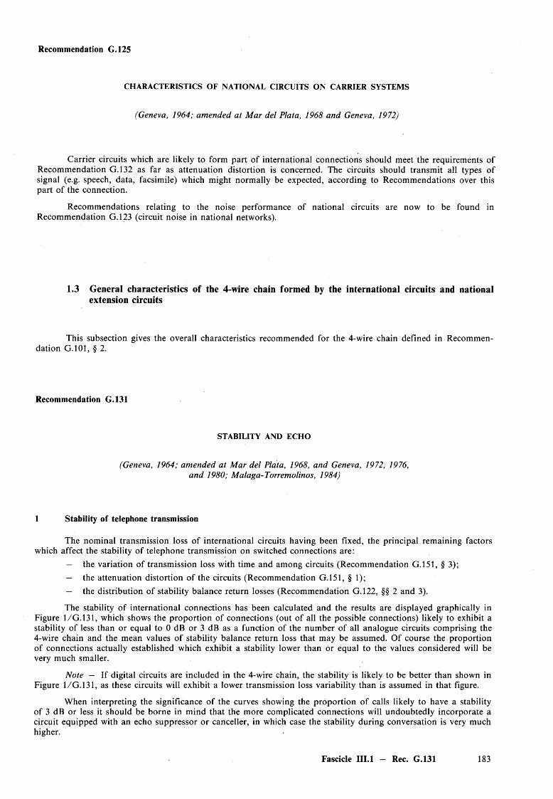
Recommendation G.125
CHARACTERISTICS OF NATIONAL CIRCUITS ON CARRIER SYSTEMS
(Geneva, 1964; amended at Mar del Plata, 1968 and Geneva, 1972)
Carrier circuits which are likely to form part of international connections should meet the requirements of Recommendation G.132 as far as attenuation distortion is concerned. The circuits should transmit all types of signal (e.g. speech, data, facsimile) which might normally be expected, according to Recommendations over this part of the connection.
Recommendations relating to the noise performance of national circuits are now to be found in Recommendation G.123 (circuit noise in national networks).
1.3 General characteristics o f the 4-wire chain formed by the international circuits and national extension circuits
This subsection gives the overall characteristics recommended for the 4-wire chain defined in Recommendation G.101, § 2.
Recommendation G.131
STABILITY AND ECHO
(Geneva, 1964; amended at Mar del Plata, 1968, and Geneva, 1972, 1976, and 1980; Malaga-Torremolinos, 1984)
1 Stability of telephone transmission
The nominal transmission loss of international circuits having been fixed, the principal remaining factors which affect the stability of telephone transmission on switched connections are:
— the variation of transmission loss with time and among circuits (Recommendation G.151, § 3);— the attenuation distortion of the circuits (Recommendation G.151, § 1);— the distribution of stability balance return losses (Recommendation G.122, §§ 2 and 3).
The stability of international connections has been calculated and the results are displayed graphically inFigure 1/G.131, which shows the proportion of connections (out o f all the possible connections) likely to exhibit a stability of less than or equal to 0 dB or 3 dB as a function of the number of all analogue circuits comprising the 4-wire chain and the mean values of stability balance return loss that may be assumed. Of course the proportion of connections actually established which exhibit a stability lower than or equal to the values considered will be very much smaller.
Note — If digital circuits are included in the 4-wire chain, the stability is likely to be better than shown in Figure 1/G.131, as these circuits will exhibit a lower transmission loss variability than is assumed in that figure.
When interpreting the significance of the curves showing the proportion of calls likely to have a stability of 3 dB or less it should be borne in mind that the more complicated connections will undoubtedly incorporate a circuit equipped with an echo suppressor or canceller, in which case the stability during conversation is very much higher.
Fascicle III.l — Rec. G.131 183
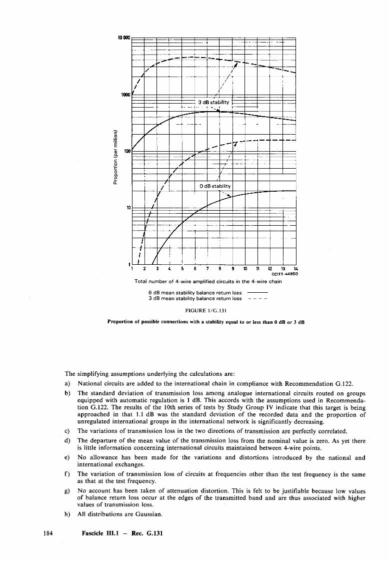
Total number of 4-wire amplified circuits in the 4-wire chain
6 dB mean stability balance return loss -----------3 dB mean stability balance return l o s s ----------
FIGURE 1/G. 131
Proportion of possible connections with a stability equal to or less than 0 dB or 3 dB
The simplifying assumptions underlying the calculations are:a) N ational circuits are added to the international chain in compliance with Recommendation G.122.b) The standard deviation of transmission loss among analogue international circuits routed on groups
equipped with automatic regulation is 1 dB. This accords with the assumptions used in Recommendation G.122. The results of the 10th series of tests by Study Group IV indicate that this target is being approached in that 1.1 dB was the standard deviation of the recorded data and the proportion of unregulated international groups in the international network is significantly decreasing.
c) The variations of transmission loss in the two directions of transmission are perfectly correlated.d) The departure of the mean value of the transmission loss from the nominal value is zero. As yet there
is little information concerning international circuits maintained between 4-wire points.e) No allowance has been made for the variations and distortions introduced by the national and
international exchanges.f) The variation of transmission loss of circuits at frequencies other than the test frequency is the same
as that at the test frequency.g) No account has been taken of attenuation distortion. This is felt to be justifiable because low values
of balance return loss occur at the edges of the transmitted band and are thus associated with higher values of transmission loss.
h) All distributions are Gaussian.
184 Fascicle III.l — Rec. G.131
Bearing in mind these assumptions, the conclusion is that the Recommendations made by the CCITT are self-consistent and that if these Recommendations are observed and the maintenance standard set for variation of loss among circuits is achieved, there should be no instability problems in the transmission plan. It is also evident that those national networks which can exhibit no better stability balance return loss than 3 dB mean, 1.5 dB standard deviation are unlikely to seriously jeopardize the stability of international connections as far as oscillation is concerned. However, the near-singing distortion and echo effects that may result give no grounds for complacency in this matter.
Details o f the calculations are set out in [1].
2 Limitation of echoes
The main circuits of a modern telephone network providing international communications are high- velocity carrier circuits on symmetric, coaxial or optical fibre pairs or radio-relay systems. Echo control devices such as echo suppressors and echo cancellers are not normally used except on connections involving very long international circuits. There is often no general need for echo control devices in national networks but they may be required for the inland service in large countries. Echo control devices may also be needed on loaded-cable circuits (low-velocity circuits) used for international calls.
Echoes may be controlled in one of two ways: either the overall loss of the 4-wire chain of circuits may be adjusted so that echo currents are sufficiently attenuated (which tacitly assumes a particular value for the echo return loss) or an echo control device can be fitted.
2.1 Transmission loss adjustment
The curves of Figure 2/G.131 indicate the minimum value of the nominal corrected reference equivalent (C R E )1) in the echo path that must be introduced if no echo suppressor is to be fitted. The CRE is shown as a function of the mean one-way propagation time. Supplement No. 2, at the end of this fascicle, explains how these curves have been derived and Annex A to this Recommendation gives an example of their application.
The solid curves are applicable to a chain of analogue circuits which are connected together 4-wire. However, they may also be used for circuits connected together 2-wire if precautions have been taken to ensure good echo return losses at these points (i.e. averaged in accordance with Recommendation G.122) for example, a mean value of 27 dB with a standard deviation of 3 dB.
The dashed curve is applicable to fully digital connections with analogue subscriber lines (such as shown in Figure 2 /G .l 11), and, under certain assumptions (see Supplement No. 2), to fully digital connections with digital subscriber lines (such as shown in b) of Figure 1/G. 104. In the latter case the echo path includes the acoustical path between earpiece and mouthpiece of the handset.
When an international circuit is used only for comparatively short and straightforward international connections the nominal transmission loss between virtual analogue switching points may be increased in proportion to the length of the circuit according to the following rule, if the use of echo control devices can thereby be avoided:
— up to 500 km route distance: 0.5 dB;
— between 500 km and 1000 km route distance: 1.0 dB;
— for every additional 500 km or part thereof: 0.5 dB.
However, such a circuit may not form part of multicircuit connections unless the nominal transmission loss is restored to 0.5 dB.
While Figure 2/G.131 is based on nominal values of CRE of trunk junction and trunk circuits, it refers to minimum send C RE and receive CRE values o f subscriber systems. Refer also to § 1.7 of the Appendix to Section 1 o f the Series G Recommendations at the end o f this fascicle.
Fascicle III.l — Rec. G.131 185

Mean one-way propagation time
Analogue circuits, with indication of number
Fully digital connections
10 50 100 150 200 25 0 300 m sCCITT - 4 4 9 6 3
4-wire circuits
Note 1 — The percentages refer to the probability of encountering objectionable echo.
Note 2 — The corrected reference equivalent of the echo path is here defined as the sum o f:
— the corrected reference equivalents in the two directions of transmission of the local telephone system of the talking subscriber (assumed to have minimum values of CRE);
— the corrected reference equivalents in the two directions of transmission of the chain of circuits between the 2-wire end of the local telephone system of the talking subscriber and the 2-wire terminals of the 4W /2W terminating set at the listener’s end;
— the mean value of the echo balance return loss at the listener’s end.
Note 3 — The ordinate values are 4 dB higher than those in the pervious version of this Recommendation ( Yellow Book, Geneva 1980) which arose in converting the reference equivalents of particular local telephone system used in the original test, to corrected reference equivalents. Different values may apply to other types of local systems, in particular lower than 4 dB. However it should be noted that this should be offset (partially or wholly) by taking the CRE values of the other circuits in the echo path. The CRE-values can be expected to be somewhat greater than the normal transmission losses used in the earlier versions of the Recommendation.
FIG URE 2/G.131
Echo tolerance curves
186 Fascicle III.l - Rec. G.131

2.2 Echo control devices
The preferred type of echo suppressor is a terminal, differential, half-echo suppressor operated from the far end. There are several types of half-echo suppressor in use in the international network, one suitable only for use in connections with mean one-way propagation times not exceeding 50 ms, referred to as a short-delay echo suppressor, and the others suitable for use in connections with any mean one-way propagation time, especially times well over 50 ms, referred to as a long-delay echo suppressor like those used on circuits routed on communication-satellite systems. The characteristics of the short-delay echo suppressors are given in [2]. The characteristics-of echo suppressors which can be used on connections with either short or long propagation times are given in [3] and in Recommendation G.164 (echo suppressors with new functions). Another type of echocontrol can be obtained by echo cancellers. The characteristics are given in Recommendation G.165.
From subjective test inform ation received, it is concluded that:
1) Echo cancellers in accordance with Recommendation G.165 provide superior speech transmission performance (at the 0.05 confidence level) to that provided by:
a) echo suppressors according to Recommendation G.161 (Orange Book);
b) echo suppressors according to Recommendation G.164 without adaptive break-in control function ABCF.
Note — Two Administrations have the view that echo cancellers according to Recommendation G.165 and echo suppressors according to Recommendation G.164 with ABCF provide about the same performance when the echo path loss is considerably above the lower end of its range; calculations based on Recommendation G.122, § 2 and assuming a minimum echo loss of 6 dB, indicate that the majority of echo path losses will be greater than the minimum value.
2) echo suppressors in accordance with Recommendation G.164 with ABCF provide superior speech transmission performance to that provided by echo suppressors without ABCF.
3) echo control devices of different types (i.e. echo suppressors or cancellers in accordance with the series G Recommendations) placed at opposite ends of a connection will operate compatibly. In this case the subjective quality perceived at one end is almost uniquely dependent on the performance of the echo control device installed at the opposite end.
Note 1 — Regional satellite circuits routed in parallel with terrestrial circuits, without perceivable echo,will benefit from the use of echo control devices of the best quality. Otherwise any degradation of the normalquality by routing over the satellite circuit may be found objectionable by the subscriber.
Note 2 — Bilateral agreement between Administrations may facilitate the introduction in the network ofecho control devices of better quality.
2.3 Rules governing the limitation o f echoes
The rules given below are subdivided into ideal rules and practical rules. It is recognized that no practical solution to the problem could comply with rules so exclusive and inflexible as the ideal rules. Practical rules are suggested in the hope that they will ease the switching and economic problems. They should not be invoked unless the ideal rules cannot reasonably be complied with.
2.3.1 Rules fo r connections without echo control devices2~>
2.3.1.1 Ideal rule — Rule A
For a connection between any pair of local exchanges in different countries, the probability of incurring the opinion “unsatisfactory” due to talker echo shall be less than 1%, when minimum practical nominal sending and receiving corrected reference equivalents are assumed for the talker’s telephone and line.
The rules in this Recommendation have been updated (to include echo cancellers) and regrouped, compared with previous versions of Recommendation G.131. The letters indicating the rules are the same as in previous versions of Recommendation G.131 in order to provide a degree of continuity.
Fascicle III.l — Rec. G.131 187
Note — Calls between a given pair of local exchanges may encounter different numbers of 4-wire circuits, according to the routing discipline and time of day. Figure 2 /G .l31 permits compliance with this rule to be assessed for the separate parts o f the total traffic which encounter 1, 2, 3 . . . 9 4-wire circuits, under certain conventional assumptions. (See Supplement No. 2 at the end of this fascicle.)
2.3.1.2 Practical rule — Rule E
For connections involving the longest national 4-wire extensions of the two countries, a probability of incurring an “unsatisfactory” opinion due to echo not of 1% (Rule A) but of 10% can, by agreement between the Administrations concerned, be tolerated. This Rule E 3> is valid only in those cases where it would otherwise be necessary, according to Rule A 3), to use an echo control device solely for these connections, and where there is no need for echo control devices on connections between the regions in the immediate neighbourhood of the two international centres concerned.
2.3.2 Rules fo r connections with echo control devices
2.3.2.1 Ideal rules
2.3.2.1.1 Rule B
1) Not more than the equivalent of one full echo suppressor (i.e. two half-echo suppressors) should be included in any connection needing an echo suppressor. When there is more than one full echo suppressor the conversation is liable to be clipped; lockout can also occur.
2) Circuits equipped with echo cancellers (Recommendation G.165) can be connected together in tandem without echo performance degradation.
3) A circuit equipped with echo suppressors (Recommendation G.164) can be connected with another circuit equipped with echo cancellers (Recommendation G.165) without additional performance degradation.
Note — The overall performance will not be better than that provided by the poorer performing device.
2.3.2.1.2 Rule D
The half-echo suppressors should be associated with the terminating sets of the 4-wire chain of the complete connection. This:
— reduces the chance of speech being multilated by the echo suppressors because the hangover times can be very short;
— reduces the change of ineffective echo canceller operation as end delays are short and minimum required echo losses can be assured.
2.3.2.2 Practical rules
2.3.2.2.1 Rule F
If, as is appreciated, Rule D above cannot be complied with, the echo control device may be fitted at the international exchange or at an appropriate national transit centre. However, each echo control device should be located sufficiently near to the respective subscribers for the end delays not to exceed the maximum value recommended in Recommendation G.161, (Orange Book) and Recommendations G.164 and G.165 of this fascicle. For countries of average size, this will normally mean that the originating and terminating control devices will be in the countries of origin and destination of the call.
2.3.2.2.2 Rule G
In isolated cases a full short-delay echo suppressor may be fitted at the outgoing end of a transit circuit (instead of two half-echo suppressors at the terminal centres) provided that neither of the two hangover times exceeds 70 ms. This relaxation may reduce the number of echo suppressors required and may also simplify the signalling and switching arrangements. It is emphasized that full echo suppressors must not be used indiscrimi
Recommendation Q.115 [41 is a study o f the application of Rules A and E to the United Kingdom-European network relations.
188 Fascicle III.l — Rec. G.131

nately; the preferred arrangement is two half-echo suppressors as near the terminating sets as possible. A full echo suppressor should be as near to the “time-centre” of the connection as possible, because this will require lower hangover times.
Whether a full long-delay echo suppressor or canceller can be used in this circumstance is under study.
23.2.2.3 Rule K
On a connection that requires an echo suppressor, up to the equivalent of two full echo suppressors (e.g. three half-echo suppressors or two half-echo suppressors and a full one) may be permitted. Every effort should be made to avoid appealing to this relaxation because the equivalent of two or more full echo suppressors, with long hangover times, on a connection can cause severe clipping of the conversation and considerably increases the risk of lockout. This rule does not apply to echo cancellers (see Rule B).
2.3.2.2A Rule L
In general it will not be desirable to switch out (or disable) the intermediate echo suppressors when a circuit equipped with long-delay echo control devices is connected to one with short-delay echo suppressors. However, it would be desirable to switch out (or disable) the intermediate echo suppressors if the mean one-way propagation time of that portion of the connection which would now fall between the terminal half-echo suppressors is not greater than 50 ms, since the different types are likely to be compatible. An intermediate echo canceller need not be switched out.
2.3.3 General rules
2.3.3.1 Ideal rule — Rule C
Connections that do not require echo control devices should not be fitted with them, because they increase the fault rate and are an additional maintenance burden.
2.3.3.2 Practical rules
2.3.3.2.1 Rule H
In exceptional circumstances, such as breakdown, an emergency route may be provided. The circuits of this route need not be fitted with echo control devices if they are usable without them for a short period. However, if the emergency routing is to last more than a few hours, echo control devices must be fitted according to Rules A to E above.
2.3.3.2.2 Rule J
It is accepted that a connection that does not require an echo control devices may in fact be unnecessarily equipped with one or two half-echo suppressors, or a full echo suppressor or echo cancellers. (The presence of an echo suppressor in good adjustment on a circuit with modest delay times can hardly be detected and in the case of echo cancellers it may improve the overall performance of the connection.)
Where a terminating international exchange is accessible from an originating international exchange by more than one route, and
1) at least one route requires echo suppressors, and at least one route does not; and
2) the originating exchange is unable to determine which route is to be used;
echo control devices should be connected in all cases.
2.3.3.2.3 Rule M
It has been found in actual practice that echo can be made tolerable by providing loss in the circuit if the one-way propagation time (delay) of the echo is less than about 25 ms. For delays longer than this, too much circuit loss is needed to attenuate echo, and echo control devices are required.
Note — The equivalent of this rule is stated in Recommendation G.161, § B.b. (Orange Book). This rule has not been expressed in earlier versions of Recommendation G.131.
Fascicle III.l- — Rec. G.131 189
2.4 Insertion o f echo control devices in a connection
Ways of inserting echo control devices in a connection which have been considered are the following:
1) provide a pool of echo control devices common to several groups of circuits, and arrange for an echo control device to be associated with any circuit that requires one (see Recommendation Q. 115 [4]);
2) arrange for the circuits to be permanently equipped with echo control devices but switch them out (or disable them) when they are not required (see [5]);
3) divide the circuits of an international route into two groups, one with and one without echo control devices and route the connection over a circuit selected from the appropriate group according to whether the connection merits an echo control device. However, it is recognized that circuits may not be used efficiently when they are divided into separate groups. This must be borne in mind;
4) conceive schemes in which the originating country and the terminal country are divided into zones at increasing mean radial distances from the international centre and determine the nominal lengths of the national extensions by examining routing digits and circuits-of-origin.
Whichever method is used, due regard must be paid to the last sentence of § 2.1 above. Methods of achieving the required reduction of circuit losses are under study by the CCITT. The nature and volume of the traffic carried by a particular connection will also influence the economics of the methods and hence the choice among them.
The CCITT is currently studying what recommendations are necessary to ensure that the insertion of echo control devices in international connections complies, overall, with the practical rules given above.
It should be appreciated that different continents need not use the same method although the methods must be compatible to permit intercontinental connections. There appears to be no great difficulty in arranging this.
2.5 Speech processing devices
Some speech processing devices, such as speech interpolation devices, have an inherent echo-suppressor function. However, such devices may only suppress echo during the single talk mode and not during double talking conditions (see Recommendation G.164, § 1.7) unless they are equipped to perform full echo-suppressor functions. When devices without full echo control are connected in tandem with echo cancellers, performance degradation due to echo may occur during double talking conditions as the intermediate echo canceller will not be effective during double talk.
ANNEX A
(to Recommendation G.131)
Application of Recommendation G.131, § 2
Recommendation G.131, § 2.3.1.1, Rule A, requires, for each pair of countries, an assessment of echo conditions for each possible pair of local exchanges to ascertain whether the plot of corrected reference equivalent of echo path against mean one-way propagation time for that pair of exchanges, lies above or below the appropriate 1% line in Figure 2/G.131.
The variables in the problem are indicated in Table A-1/G.131 and illustrated for all analogue connections in Figure A-1/G.131 and for all digital connections in Figure A-2/G.131.
For a given pair of exchanges, all eight items are known or can be estimated. A plot of corrected reference equivalent [1) + 2) + 3) + 4) o f Table A-1/G.131] as a function of mean one-way propagation time[5) + 6) + 7) of Table A-l/G .131] on Figure 2 /G .l31 may be assessed in relation to the 1% curve, for a given number of analogue circuits in the 4-wire chain for fully analogue connections and mixed analogue/digital connections or, for fully digital connections using the appropriate curve.
190 Fascicle III.l — Rec. G.131
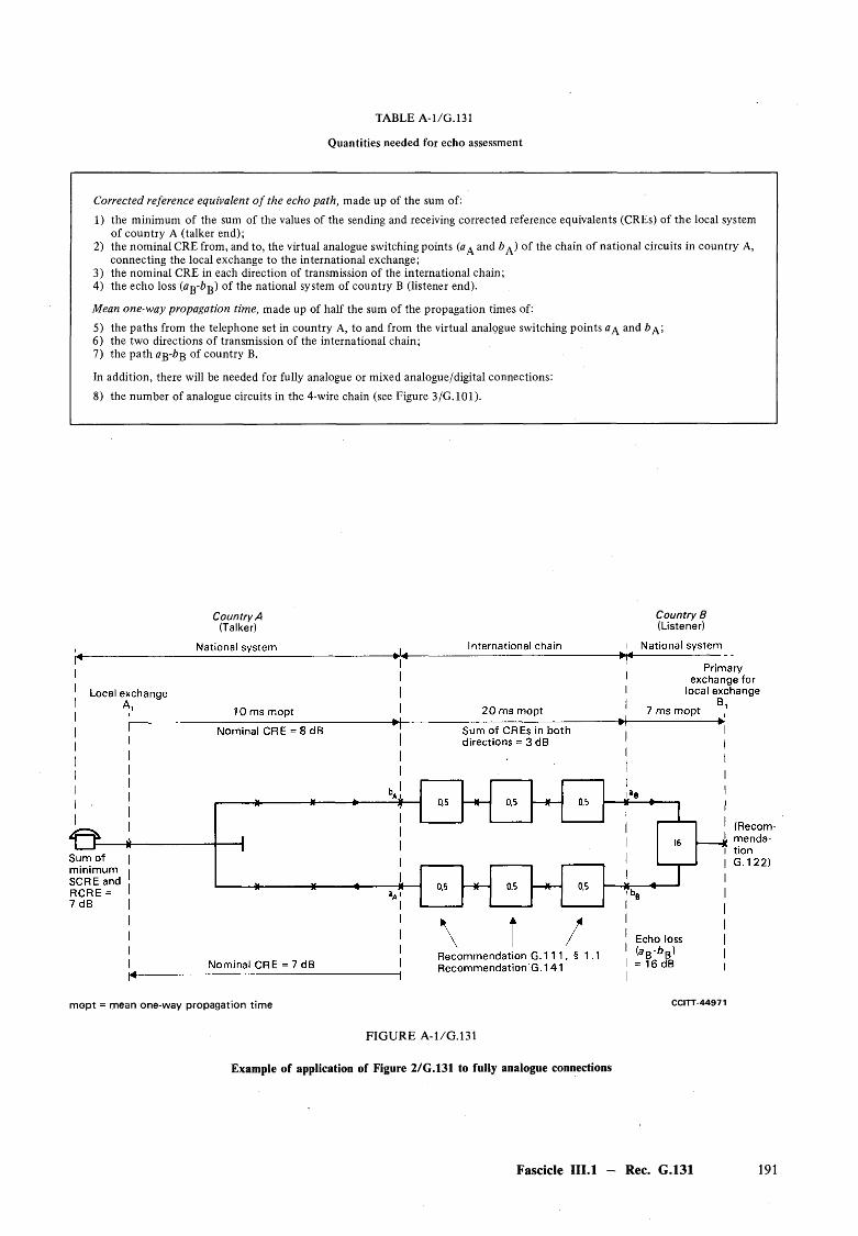
TABLE A-1/G.131
Quantities needed for echo assessment
Corrected reference equivalent o f the echo path, made up of the sum of:1) the minimum of the sum of the values of the sending and receiving corrected reference equivalents (CREs) of the local system
of country A (talker end);2) the nominal CRE from, and to, the virtual analogue switching points (a^ and b^ ) of the chain of national circuits in country A,
connecting the local exchange to the international exchange;3) the nominal CRE in each direction of transmission of the international chain;4) the echo loss (tfg-Z?g) of the national system of country B (listener end).
Mean one-way propagation time, made up of half the sum of the propagation times of:5) the paths from the telephone set in country A, to and from the virtual analogue switching points a ^ and b6) the two directions of transmission of the international chain;7) the path a^-b-Q of country B.
In addition, there will be needed for fully analogue or mixed analogue/digital connections:8) the number of analogue circuits in the 4-wire chain (see Figure 3/G.101).
Country A (Talker)
Country B (Listener)
m opt = mean one-w ay propagation tim e
F I G U R E A -1 /G .1 3 1
Example of application of Figure 2/G.131 to fully analogue connections
CCITT-44971
Fascicle III.l - Rec. G.131 191
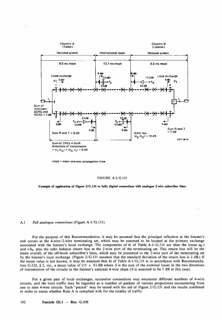
Country A (Talker)
Country B (Listener)
directions of transmission = (f -b + (3^-f.j) = 6 dB
mopt = mean one-way propagation time
FIG URE A-2/G.131
Example of application of Figure 2/G.131 to fully digital connections with analogue 2-wire subscriber lines
A.l Full analogue connections (Figure A-1/G . 131)
For the purpose of this Recommendation, it may be assumed that the principal reflection at the listener’s end occurs at the 4-wire/2-wire terminating set, which may be assumed to be located at the primary exchange associated with the listener’s local exchange. The components of 4) of Table A-l /G.131 are then the losses aB-t and t-bn, plus the echo balance return loss at the 2-wire port of the terminating set. This return loss will be the mean overall, of the off-hook subscriber’s lines, which may be presented to the 2-wire port of the terminating set by the listener’s local exchange. (Figure 2/G.131 assumes that the standard deviation of the return loss is 3 dB.) If the mean value is not known, it may be assumed that 4) of Table A-l/G .131 is in accordance with Recommendation G.122, § 2, viz., a mean value of (15 + S ) dB where S is the sum of the nominal losses in the two directions of transmission of the circuits in the listener’s national 4-wire chain (S is assumed to be 1 dB in this case).
For a given pair of local exchanges, successive connections may encounter different numbers of 4-wire circuits, and the total traffic may be regarded as a number of packets of various proportions encountering from one to nine 4-wire circuits. Each “packet” may be tested with the aid of Figure 2/G.131 and the results combined in order to assess whether Rule A is complied with for the totality of traffic.
192 Fascicle III.l - Rec. G.131

Figure A-l/G .131 shows, as an example, an application of Recommendation G.131, § 2, where a listener’s a-t-b path is assumed to be in accordance with Recommendation G.122. For simplicity, it is assumed that 100% ofthe traffic encounters the given conditions. Values for the example are as follows:
Talker’s country A
Distance from local exchange At to international exchange 1600 km
Mean one-way propagation time from local exchange Aj to international e x c h a n g e 11 m s4)
Simultaneous-minimum sending and receiving CRE (sum) of the local s y s te m 7 dB
CRE from local exchange to international exchange (bA) 8 dB 5)
CRE from international exchange to local exchange (aA) 7 dB 5)
Number of 4-wire c i r c u i ts .................................................................................................................................... 2
International chain A to B
Number of c i r c u i t s ................................................................................................................................................. 3 6)
D is ta n c e 3200 km
Mean one-way propagation t i m e 17 m s4)
Sum of CREs in both directions 2 x 3 x 0.5 d B 3 dB
Listener’s country B
Mean echo loss (aB — b^) = (15 + 1) d B 16 dB(Rec. G.122)
Distance from international exchange to primary exchange associated with local exchange Bt(i.e. point of principal re flec tio n ) 1120 km
Mean one-way propagation time corresponding to above d i s t a n c e 16 m s4)
Number of 4-wire circuits ........................................................................................................................... 1
Total number of 4-wire circuits = 2 + 3 + l = 6
Total mean one-way propagation time = 1 1 + 1 7 + 1 6 = 44 m s ......................................................... (A-l)
Total CRE of the echo path = 7 + 8 + 7 + 3 + 16 = 41 dB ..................... (A-2)7)
If (A-l) and (A-2) are plotted on Figure 2/G.131, the point lies below the 1% line for six 4-wire circuits, indicating a probability of more than 1% of incurring an “unsatisfactory” opinion. The conclusion also applies to other possible numbers of 4-wire circuits.
Conclusion
a) An echo-control device should be used on the connection,
orb) the loss in the echo path should be increased (but the limitations of Recommendation G.121 must be
observed).
4) Assuming a velocity of propagation for the transmission systems of 250 km /m s, 3 FDM channel modulators anddemodulators of 1.5 ms each for talker’s country A and the international chain of circuits A to B, and a 12 ms constant forlistener’s country B (see Recommendation G.114).
5) It is assumed that the loaded trunk-junction introduces an additional 1 dB (in each direction) when changing from nominal transmission loss to CRE.
6) An unusually large number, chosen only to illustrate the principle o f addition o f loss.
7) The D-factor for the remaining 4-wire circuits (i.e. “ 10 filters” in the echo path) is 0 dB.
Fascicle III.l — Rec. G.131 193
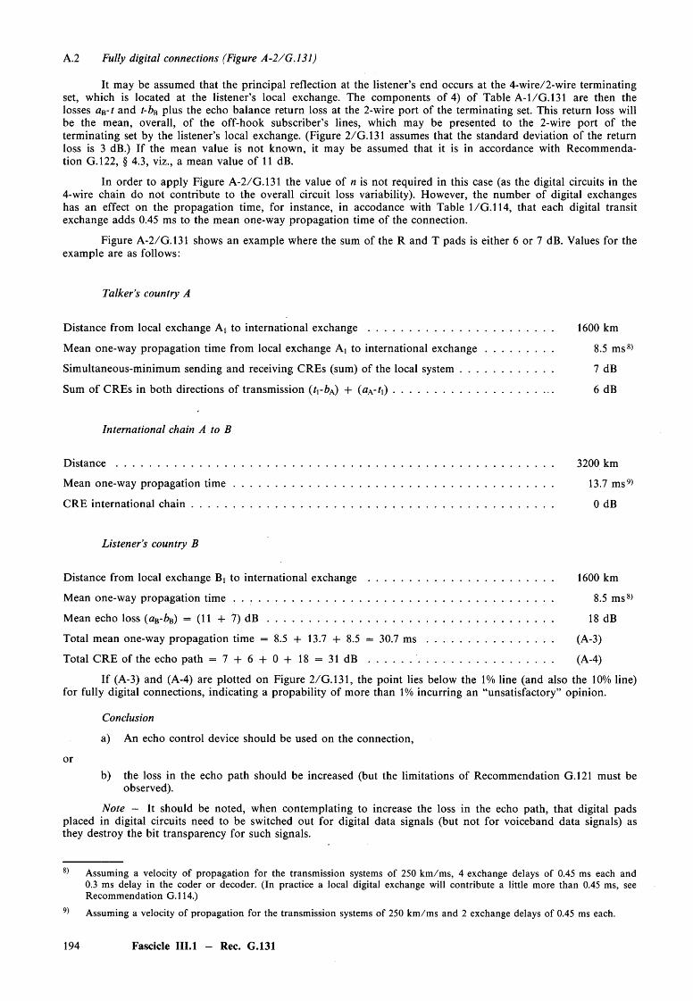
It may be assumed that the principal reflection at the listener’s end occurs at the 4-wire/2-wire terminating set, which is located at the listener’s local exchange. The components of 4) of Table A-1/G.131 are then the losses aB-t and t-bs plus the echo balance return loss at the 2-wire port of the terminating set. This return loss willbe the mean, overall, of the off-hook subscriber’s lines, which may be presented to the 2-wire port of theterminating set by the listener’s local exchange. (Figure 2/G.131 assumes that the standard deviation of the return loss is 3 dB.) If the mean value is not known, it may be assumed that it is in accordance with Recommendation G.122, § 4.3, viz., a mean value of 11 dB.
In order to apply Figure A-2/G.131 the value of n is not required in this case (as the digital circuits in the 4-wire chain do not contribute to the overall circuit loss variability). However, the number of digital exchanges has an effect on the propagation time, for instance, in accodance with Table 1/G.114, that each digital transit exchange adds 0.45 ms to the mean one-way propagation time of the connection.
Figure A-2/G.131 shows an example where the sum of the R and T pads is either 6 or 7 dB. Values for the example are as follows:
A.2 Fully digital connections (Figure A-2/G.131)
Talker’s country A
Distance from local exchange A\. to international e x c h a n g e 1600 km
Mean one-way propagation time from local exchange Ai to international e x c h a n g e ......................... 8.5 m s8)
Simultaneous-minimum sending and receiving CREs (sum) of the local sy s tem 7 dB
Sum of CREs in both directions of transmission ( tr bA) + (aA- t{ ) 6 dB
International chain A to B
D is ta n c e 3200 km
Mean one-way propagation t i m e ....................................................................................................................... 13.7 m s9)
CRE international c h a in 0 dB
Listener’s country B
Distance from local exchange Bt to international exchange 1600 km
Mean one-way propagation t i m e ....................................................................................................................... 8.5 m s8>
Mean echo loss (a^-bs) = (11 + 7) d B ........................................................................................................... 18 dB
Total mean one-way propagation time = 8.5 + 13.7 + 8.5 = 30.7 m s ............................................... (A-3)
Total CRE of the echo path = 7 + 6 + 0 + 18 = 31 dB .................. (A-4)
If (A-3) and (A-4) are plotted on Figure 2/G.131, the point lies below the 1% line (and also the 10% line) for fully digital connections, indicating a propability of more than 1% incurring an “unsatisfactory” opinion.
Conclusion
a) An echo control device should be used on the connection,
orb) the loss in the echo path should be increased (but the limitations of Recommendation G.121 must be
observed).
Note — It should be noted, when contemplating to increase the loss in the echo path, that digital pads placed in digital circuits need to be switched out for digital data signals (but not for voiceband data signals) as they destroy the bit transparency for such signals.
8) Assuming a velocity of propagation for the transmission systems of 250 km /m s, 4 exchange delays of 0.45 ms each and 0.3 ms delay in the coder or decoder. (In practice a local digital exchange will contribute a little more than 0.45 ms, see Recommendation G.114.)
9) Assuming a velocity of propagation for the transmission systems of 250 km /m s and 2 exchange delays of 0.45 ms each.
194 Fascicle III.l - Rec. G.131
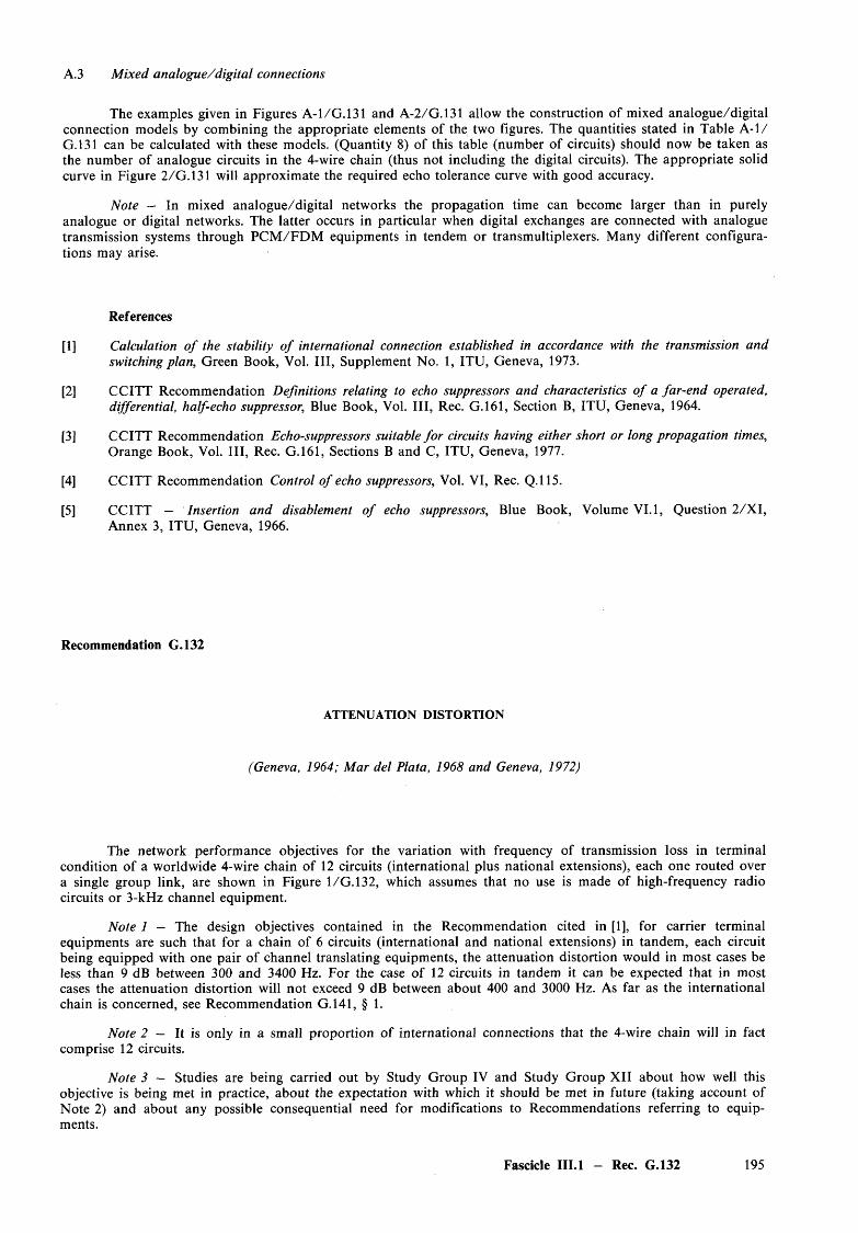
A.3 M ixed analogue/digital connections
The examples given in Figures A-l/G .131 and A-2/G.131 allow the construction of mixed analogue/digital connection models by combining the appropriate elements of the two figures. The quantities stated in Table A - l/ G.131 can be calculated with these models. (Quantity 8) of this table (number of circuits) should now be taken as the number of analogue circuits in the 4-wire chain (thus not including the digital circuits). The appropriate solid curve in Figure 2/G.131 will approximate the required echo tolerance curve with good accuracy.
Note — In mixed analogue/digital networks the propagation time can become larger than in purely analogue or digital networks. The latter occurs in particular when digital exchanges are connected with analogue transmission systems through PC M /FD M equipments in tendem or transmultiplexers. Many different configurations may arise.
References
[1] Calculation o f the stability o f international connection established in accordance with the transmission and switching plan, Green Book, Vol. I ll , Supplement No. 1, ITU, Geneva, 1973.
[2] CCITT Recommendation Definitions relating to echo suppressors and characteristics o f a far-end operated,differential, half-echo suppressor, Blue Book, Vol. I ll , Rec. G.161, Section B, ITU, Geneva, 1964.
[3] CCITT Recommendation Echo-suppressors suitable fo r circuits having either short or long propagation times,Orange Book, Vol. I l l , Rec. G.161, Sections B and C, ITU, Geneva, 1977.
[4] CCITT Recommendation Control o f echo suppressors, Vol. VI, Rec. Q.115.
[5] CCITT — Insertion and disablement o f echo suppressors, Blue Book, Volume VI. 1, Question 2 /X I,Annex 3, ITU, Geneva, 1966.
Recommendation G.132
ATTENUATION DISTORTION
(Geneva, 1964; Mar del Plata, 1968 and Geneva, 1972)
The network performance objectives for the variation with frequency of transmission loss in terminal condition of a worldwide 4-wire chain of 12 circuits (international plus national extensions), each one routed over a single group link, are shown in Figure 1/G. 132, which assumes that no use is made of high-frequency radio circuits or 3-kHz channel equipment.
Note 1 — The design objectives contained in the Recommendation cited in [1], for carrier terminal equipments are such that for a chain of 6 circuits (international and national extensions) in tandem, each circuit being equipped with one pair of channel translating equipments, the attenuation distortion would in most cases be less than 9 dB between 300 and 3400 Hz. For the case of 12 circuits in tandem it can be expected that in most cases the attenuation distortion will not exceed 9 dB between about 400 and 3000 Hz. As far as the international chain is concerned, see Recommendation G. 141, § 1.
Note 2 — It is only in a small proportion of international connections that the 4-wire chain will in fact comprise 12 circuits.
Note 3 — Studies are being carried out by Study Group IV and Study Group XII about how well this objective is being met in practice, about the expectation with which it should be met in future (taking account of Note 2) and about any possible consequential need for modifications to Recommendations referring to equipments.
Fascicle III.l - Rec. G.132 195
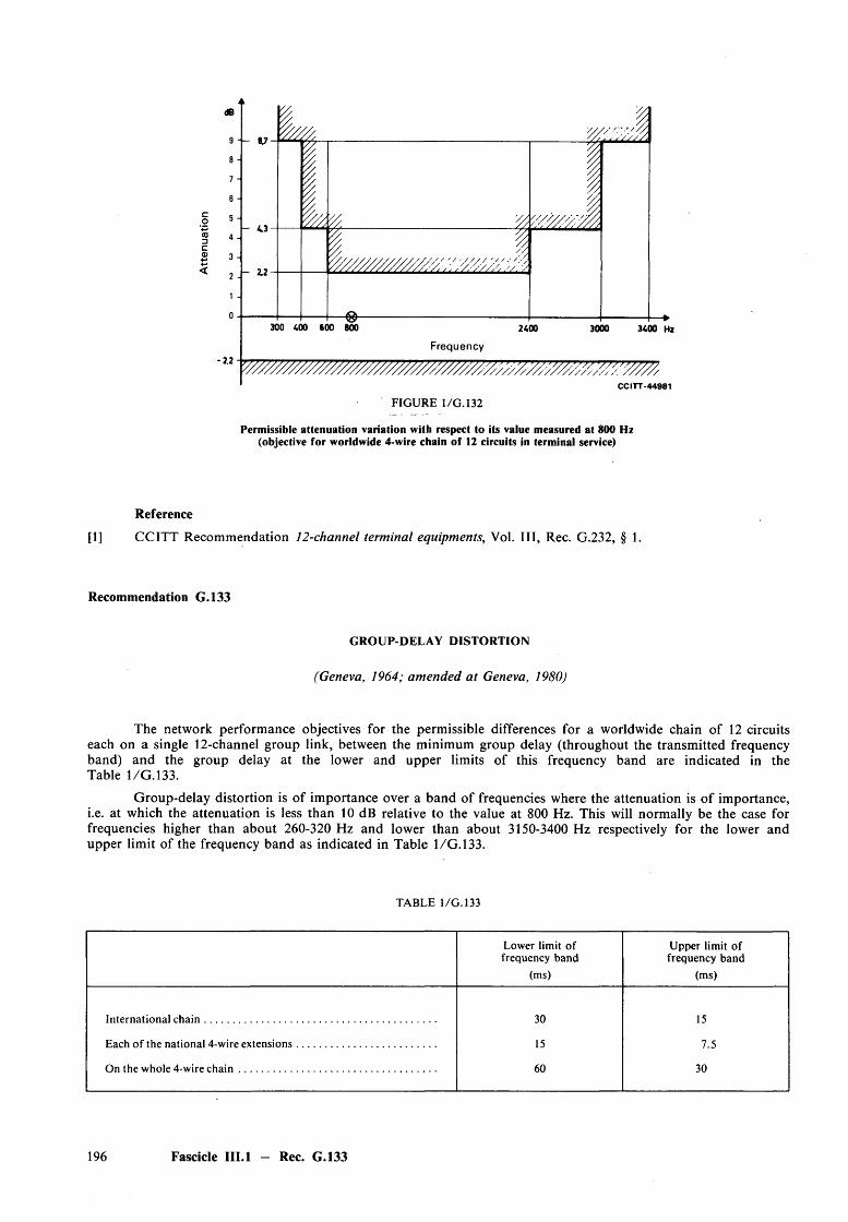
-icB 3 -|
< Mi -
- 2.2
1- 2.2
300 400 600 800 2400 3000 3400 Hz
Frequency
CCITT-44981
FIGURE 1/G. 132
Permissible attenuation variation with respect to its value measured at 800 Hz (objective for worldwide 4-wire chain of 12 circuits in terminal service)
Reference
[1] CCITT Recommendation 12-channel terminal equipments, Vol. I l l , Rec. G.232, § 1.
Recommendation G.133
GROUP-DELAY DISTORTION
(Geneva, 1964; amended at Geneva, 1980)
The network performance objectives for the permissible differences for a worldwide chain of 12 circuits each on a single 12-channel group link, between the minimum group delay (throughout the transmitted frequency band) and the group delay at the lower and upper limits of this frequency band are indicated in the Table 1/G . 133.
Group-delay distortion is o f importance over a band of frequencies where the attenuation is o f importance, i.e. at which the attenuation is less than 10 dB relative to the value at 800 Hz. This will normally be the case for frequencies higher than about 260-320 Hz and lower than about 3150-3400 Hz respectively for the lower and upper limit o f the frequency band as indicated in Table 1/G. 133.
TABLE 1/G. 133
Lower limit of frequency band
(ms)
Upper limit of frequency band
(ms)
International chain ............................................................................... 30 15
Each of the national 4-wire extensions................................................ 15 7.5
On the whole 4-wire ch a in ................................................................... 60 30
196 Fascicle III.l - Rec. G.133
Recommendation G.134
LINEAR CROSSTALK')
(Geneva, 1964; amended at Mar del Plata, 1968)
1 Linear crosstalk between different 4-wire chains of circuits (formerly Part A)
As a network performance objective, the signal-to-crosstalk ratio which may exist between two 4-wire chains of circuits comprising international and national circuits is restricted by Recommendation G.151, § 4.1, as regards circuits, and by Recommendation Q.45 [1], as regards international centres.
2 Linear crosstalk between go and return channels of the 4-wire chain of circuits (formerly Part B)
As a network performance objective, the signal-to-crosstalk ratio between the two directions of transm ission of a 4-wire chain of circuits is restricted by Recommendation G.151, § 4.2, as regards circuits and by Recommendation Q.45 [1] as regards international centres.
ANNEX A
(to Recommendation G.134)
Methods for measuring crosstalk in exchanges, on international telephone circuits
and on a chain of international telephone circuits
A.l The method used for measuring crosstalk will depend on the type of crosstalk. In general one or the otherof the following two situations will be encountered:
a) crosstalk in an exchange arising mainly from a single source or from several nearby sources;b) crosstalk measured at the end of a circuit or chain of circuits and which is the result o f multiple
sources of crosstalk occurring at points along the circuit or chain of circuits. The total crosstalk willdepend on the relative phases of the individual contributions and may accordingly vary greatly withfrequency. On long circuits or chains of circuits, difficulties may arise when making crosstalk measurements at a single frequency owing to small variations in the frequency of the master oscillators supplying translating equipment at various points along the circuit or chain of circuits.
A.2 Available methods for measuring crosstalk are as follows2):a) single-frequency measurements (e.g. at 800 Hz or 1000 Hz);b) measurements made at several frequencies (e.g. at 500, 1000 and 2000 Hz), the results being averaged
on a current or voltage basis;c) measurements made using a uniform spectrum random noise or closely spaced harmonic series signal
shaped in accordance with a speech power density curve. Such measurements should be made in accordance with the Recommendation cited in [3];
d) voice/ear tests, in which speech is used as the disturbing source and the crosstalk is measured by listening and comparing its level with a reference source whose level can be adjusted by some form of calibrated attenuating network.
A.3 Pending further study, the following methods are provisionally recommended for “type tests” and“acceptance tests” involving crosstalk measurement.
A.3.1 Crosstalk in exchanges
Crosstalk should be measured at 1100 Hz which, in the experience of some Administrations, is equivalent to a measurement made with a conventional telephone signal generator (Recommendation G.227 [4]) and a psophometer.
0 Recommended methods for the measurement of crosstalk are described in Annex A.
It is a question here of the measurement of the frequency (or frequencies) to be used; the measure of the crosstalk for a given frequency is described in [2]
Fascicle III.l — Rec. G.134 197
A.3.2 Crosstalk on an international telephone circuit or chain o f international telephone circuits
Crosstalk should be measured using a uniform spectrum random noise or closely spaced harmonic series signal shaped in accordance with the speech power density curve of Recommendation G.227 [4]. The measurements should be made in accordance with the Recommendation cited in [3].
Note 1 — In cases of difficulty with A.2.a) and A.2.b), voice/ear tests are recommended.
Note 2 — In the case of telephone circuits used for voice-frequency telegraphy the near-end signal-to- crosstalk ratio between the two directions of transmission should be measured at each of the telegraph channel carrier frequencies, i.e. at each odd multiple of 60 Hz from 420 Hz to 3180 Hz inclusive. However, difficulty can arise in practice because of the effect mentioned in A .l.b) above.
References
[1] CCITT Recommendation Transmission characteristics o f an international exchange, Vol. VI, Rec. Q.45.
[2] Measurement o f crosstalk, Green Book, Vol. VI.2, Supplement No. 2.4, ITU, Geneva, 1973.
[3] CCITT Recommendation 12-channel terminal equipments, Vol. I l l , Rec. G.232, § 9.2.
[4] CCITT Recommendation Conventional telephone signal, Vol. I ll , Rec. G .l l l .
Recommendation G.13S
ERROR ON THE RECONSTITUTED FREQUENCY
(Mar del Plata, 1968)
As the channels of any international telephone circuit should be suitable for voice-frequency telegraphy, the network performance objective for the accuracy of the virtual carrier frequencies should be such that the difference between an audiofrequency applied to one end of the circuit and the frequency received at the other end should not exceed 2 Hz, even when there are intermediate modulating and demodulating processes.
To attain this objective, the CCITT recommends that the channel and group carrier frequencies of the various stages should have the accuracies specified in the corresponding clauses of Recommendation G.225 [1].
Experience shows that, if a proper check is kept on the operation of oscillators designed to these specifications, the difference between the frequency applied at the origin of a telephone channel and the reconstituted frequency at the other end hardly ever exceeds 2 Hz if the channel has the same composition as the 2500-km hypothetical reference circuit for the system concerned.
Calculations indicate that, if these recommendations are followed, in the 4-wire chain forming part of the hypothetical reference connection defined in Figure 1/G .1 0 3 1) there is about 1% probability that the frequency difference between the beginning and the end of the connection will exceed 3 Hz and less than 0.1% probability that it will exceed 4 Hz.
References
[1] CCITT Recommendation Recommendations relating to the accuracy o f carrier frequencies, Vol. I l l , Rec. G.225.
[2] CCITT Recommendation 16-channel terminal equipments, Vol. I ll , Rec. G.235.
[31 C C IR Report The effects o f doppler frequency-shifts and switching discontinuities in the fixed satellite service,Vol. IV, Report 214-3, ITU, Geneva, 1978.
In fact, the chain considered for these calculations comprised 16 (instead of 12) modulator-demodulator pairs to allow for the possibility that submarine cables with equipments in conformity with Recommendation G.235 [2] might form part of the chain. No allowance was made, however, for the effects of Doppler frequency-shift due to inclusion of a non-stationary satellite; values for this shift are given in CCIR Report 214-3 [3].
198 Fascicle III.l - Rec. G.135
1.4 General characteristics o f the 4-wire chain o f international circu its; international transit
Recommendation G.141
TRANSM ISSION LOSSES, RELATIVE LEVELS AND ATTENUATION DISTORTION
(Geneva, 1964; amended at Mar del Plata, 1968 and Geneva, 1972 and 1980
Parts A and B in previous issues of this Recommendation dealt with “Conventions and definitions” and the “Interconnection of international circuits in a transit centre” respectively. The latter information has been amended and now forms part of Recommendation G.101, § 5.
1 Attenuation distortion
1.1 All-analogue conditions
The design objectives recommended for carrier terminal equipment by the Recommendation cited in [1] are such that for a chain of six circuits, each equipped with a single pair of channel translating equipments in accordance with that Recommendation, the network performance objective for the attenuation distortion given by Figure 1/G . 132 will in most cases be met. The distortion contributed by the seven international centres is thereby included.
Note — To assess the attenuation distortion of the international chain, the limits indicated for international circuits in Recommendation G.151, § 1 must not be added to the limits for international centres mentioned in Recommendation Q.45 [2]. In fact, on the one hand, some exchange equipment would be counted twice if this addition were made; on the other, the specification limits of Recommendation Q.45 [2] apply to the worst possible connection through an international exchange, while the maintenance limits of Recommendation G.151, § 1 apply to the poorest international circuit. The specifications of the various equipments are such that the mean performance will be appreciably better than could be estimated by the above-mentioned addition.
1.2 M ixed analogue/digital conditions
In the mixed analogue/digital period, it is expected that the attenuation/frequency characteristics of the analogue carrier terminal equipment that is to be used in international telephone connections will continue to be governed by existing Recommendations that are relevant to this type of circuit.
Where unintegrated PCM digital processes are to be included in international telephone connections, it is recommended that the attenuation/frequency characteristic of the bandpass filters associated with such processes should comply with the more stringent version of Figure 1 /G .7 12 [3]. The latter Recommendation applies specifically to cases where integrated PCM digital processes are associated with trunk junctions (toll connecting trunks), trunk circuits (intertoll trunks), and international circuits.
With regard to the incorporation of unintegrated PCM digital processes in local telephone networks, the required attenuation/frequency characteristics of the bandpass filters involved are still under study.
References
[1] CCITT Recommendation 12-channel terminal equipments, Vol. I l l , Rec. G.232, § 1.
[2] CCITT Recommendation Transmission characteristics o f an international exchange, Vol. VI, Rec. Q.45.
[3] CCITT Recommendation Performance characteristics o f PCM channels between 4-wire interfaces at voicefrequencies, Vol. I ll , Rec. G .712, Figure 1 /G .7 12.
Fascicle III.l — Rec. G.141 199

Recommendation G.142
TRANSM ISSION CHARACTERISTICS OF EXCHANGES
(Geneva, 1980)
This Recommendation consists of two parts. The first part, § 1, is concerned with the voice-frequency transmission characteristics of international analogue exchanges. The information involved is encompassed within Recommendation Q.45 [1], the text of which is reproduced below. The second part, § 2, is concerned with the voice-frequency transmission considerations that should be taken into account in the design of digital exchanges and their incorporation into the network. The digital exchanges referred to include local exchanges and transit exchanges (national and international). The transmission considerations relate primarily to the properties which digital exchanges should possess to enable them to operate under different and changing network conditions with respect to the content of analogue, mixed analogue/digital and all-digital plant.
1 International analogue exchange
The commissioning objectives for the transmission requirements to be respected by an international analogue exchange are included in Recommendation Q.45 [1].
2 Digital exchanges
2.1 Digital processes — effect on transmission
Digital (TDM) exchanges, to varying degrees, are required to include such digital processes as analogue-to- digital coders, digital-to-analogue decoders and digital recoding processes, examples of which are companding law converters and digital pads. The extent to which such digital processes might be included in a digital exchange is determined by the network environment in which the exchange is to operate (i.e., all-analogue, mixed analogue/ digital or all-digital).
Digital processes such as those referred to above, attract transmission penalties. These penalties can be expressed in terms of “units of transmission impairment”.
A limit is placed on the permissible accumulation of units of transmission impairment in an international telephone connection. Details o f the planning rule resulting from this limit and the penalties introduced by individual digital processes are given in Recommendations G.101, § 4 and G.113, § 3.
In accordance with Recommendation G.113, § 3 it is provisionally recommended that no more than 14 units of transmission impairment be permitted to accumulate in an international connection. O f these 14 units, a maximum of 5 units could be introduced by each national extension and a maximum of 4 units by the international portion. Since one 8-bit PCM codec pair (coder and decoder) introduces 1 unit of transmission impairment, it is clear that unintegrated PCM digital processes involving analogue/digital conversions, (e.g. codecs) or digital processes involving the recoding of information (e.g. digital pads) should not be allowed to proliferate in an uncontrolled fashion. Figure 1/G . 142 shows some of the transmission paths that might be established through a digital exchange and the “units of transmission im pairm ent” attributable to the digital processes in these paths.
2.2 Transmission loss through a digital exchange
The 4-wire digital switching function at a digital exchange should introduce a nominal transmission loss of 0 dB. Thus, in Figure 1/G. 142 (Case 1) if a 0 dBmO sinusoidal test signal is introduced at the analogue terminals of an ideal coder connected to the input of a digital switch, a Digital Reference Sequence (DRS) should be transmitted unaltered through the switch and produce a 0 dBmO sinusoidal signal at the analogue terminals o f a decoder connected to the output o f the digital switch.
Except for the transmission loss considered above (and perhaps the possible loss due to exchange wiring) all transmission losses which are to be introduced by a digital exchange, either in a digital or analogue form, are to be governed by the applicable transmission plan (see § 2.4 below).
200 Fascicle III.l — Rec. G.142
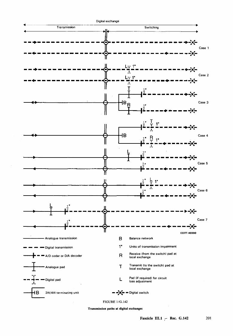
i
■ Analogue transmission
1 Digital transmission
' A/D coder or D/A decoder
' Analogue pad
•4 ■■ ™ Digital pad
H B 2W/4W terminating unit
Case 1
Case 2
Case 3
Case 4
Case 5
Case 6
" t
4
► -V - ^ ♦ ♦
Case 7
V -*%CCITT-40390
0 Balance network
r
R
T
L
Units of transmission impairment
Receive (from the switch) pad at local exchange
Transmit (to the switch) pad at local exchange
Pad (if required) for circuit loss adjustment
— "" Digital switch
F IG U R E 1 /G . 142
Transmission paths at digital exchanges
Fascicle III.l — Rec. G.142 201
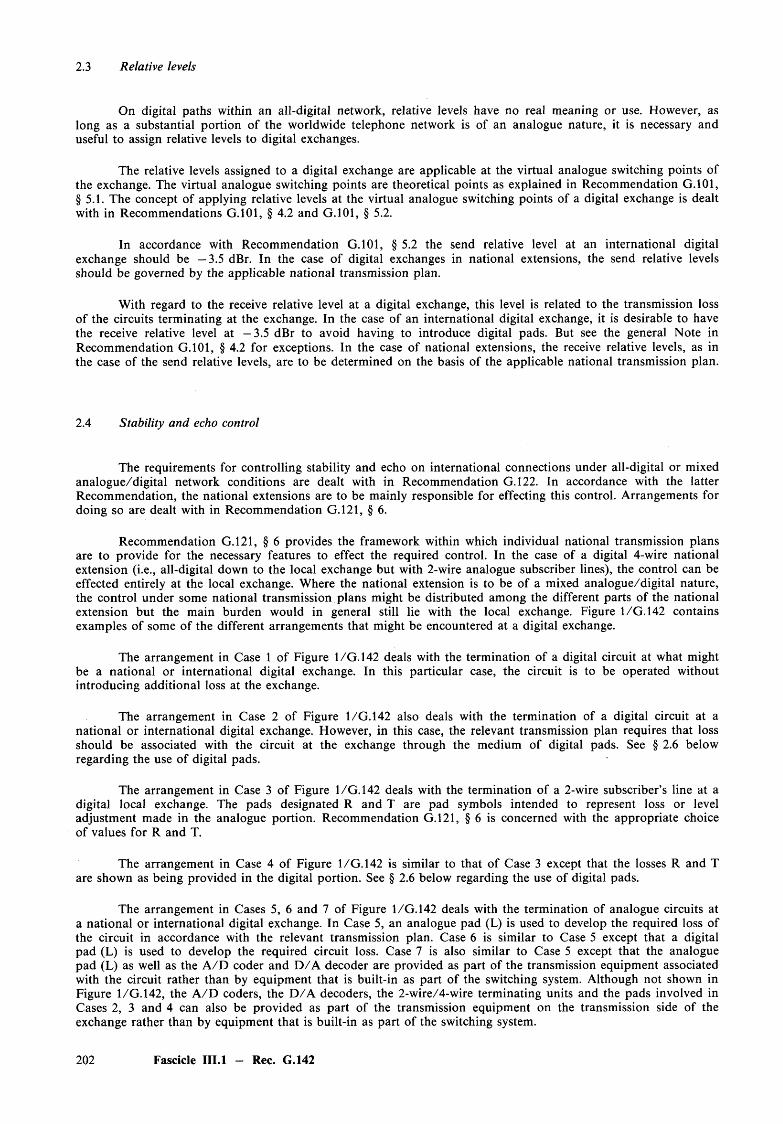
2.3 Relative levels
On digital paths within an all-digital network, relative levels have no real meaning or use. However, as long as a substantial portion of the worldwide telephone network is of an analogue nature, it is necessary and useful to assign relative levels to digital exchanges.
The relative levels assigned to a digital exchange are applicable at the virtual analogue switching points of the exchange. The virtual analogue switching points are theoretical points as explained in Recommendation G.101, §5.1. The concept of applying relative levels at the virtual analogue switching points of a digital exchange is dealt with in Recommendations G.101, § 4.2 and G.101, § 5.2.
In accordance with Recommendation G.101, § 5.2 the send relative level at an international digital exchange should be —3.5 dBr. In the case of digital exchanges in national extensions, the send relative levels should be governed by the applicable national transmission plan.
With regard to the receive relative level at a digital exchange, this level is related to the transmission loss of the circuits terminating at the exchange. In the case of an international digital exchange, it is desirable to have the receive relative level at -3 .5 dBr to avoid having to introduce digital pads. But see the general Note in Recommendation G.101, § 4.2 for exceptions. In the case of national extensions, the receive relative levels, as in the case of the send relative levels, are to be determined on the basis of the applicable national transmission plan.
2.4 Stability and echo control
The requirements for controlling stability and echo on international connections under all-digital or mixed analogue/digital network conditions are dealt with in Recommendation G.122. In accordance with the latter Recommendation, the national extensions are to be mainly responsible for effecting this control. Arrangements for doing so are dealt with in Recommendation G.121, § 6.
Recommendation G.121, § 6 provides the framework within which individual national transmission plans are to provide for the necessary features to effect the required control. In the case of a digital 4-wire national extension (i.e., all-digital down to the local exchange but with 2-wire analogue subscriber lines), the control can be effected entirely at the local exchange. Where the national extension is to be of a mixed analogue/digital nature, the control under some national transmission plans might be distributed among the different parts of the national extension but the main burden would in general still lie with the local exchange. Figure 1/G . 142 contains examples of some of the different arrangements that might be encountered at a digital exchange.
The arrangement in Case 1 of Figure 1/G. 142 deals with the termination of a digital circuit at what might be a national or international digital exchange. In this particular case, the circuit is to be operated without introducing additional loss at the exchange.
The arrangement in Case 2 of Figure 1/G. 142 also deals with the termination of a digital circuit at a national or international digital exchange. However, in this case, the relevant transmission plan requires that loss should be associated with the circuit at the exchange through the medium of digital pads. See § 2.6 below regarding the use of digital pads.
The arrangement in Case 3 of Figure 1/G. 142 deals with the termination of a 2-wire subscriber’s line at a digital local exchange. The pads designated R and T are pad symbols intended to represent loss or level adjustment made in the analogue portion. Recommendation G.121, § 6 is concerned with the appropriate choice of values for R and T.
The arrangement in Case 4 of Figure 1/G . 142 is similar to that of Case 3 except that the losses R and T are shown as being provided in the digital portion. See § 2.6 below regarding the use of digital pads.
The arrangement in Cases 5, 6 and 7 of Figure 1/G . 142 deals with the termination of analogue circuits at a national or international digital exchange. In Case 5, an analogue pad (L) is used to develop the required loss of the circuit in accordance with the relevant transmission plan. Case 6 is similar to Case 5 except that a digital pad (L) is used to develop the required circuit loss. Case 7 is also similar to Case 5 except that the analogue pad (L) as well as the A /D coder and D /A decoder are provided as part of the transmission equipment associated with the circuit rather than by equipment that is built-in as part of the switching system. Although not shown in Figure 1/G . 142, the A /D coders, the D /A decoders, the 2-wire/4-wire terminating units and the pads involved in Cases 2, 3 and 4 can also be provided as part of the transmission equipment on the transmission side of the exchange rather than by equipment that is built-in as part of the switching system.
202 Fascicle III.l - Rec. G.142
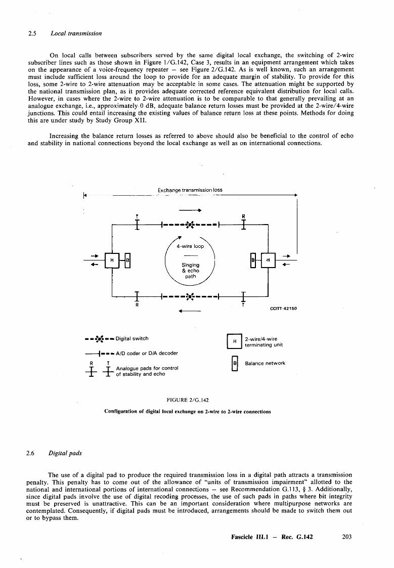
2.5 Local transmission
On local calls between subscribers served by the same digital local exchange, the switching of 2-wire subscriber lines such as those shown in Figure 1/G. 142, Case 3, results in an equipment arrangement which takes on the appearance of a voice-frequency repeater — see Figure 2 /G .l42. As is well known, such an arrangement must include sufficient loss around the loop to provide for an adequate margin of stability. To provide for this loss, some 2-wire to 2-wire attenuation may be acceptable in some cases. The attenuation might be supported by the national transmission plan, as it provides adequate corrected reference equivalent distribution for local calls. However, in cases where the 2-wire to 2-wire attenuation is to be comparable to that generally prevailing at an analogue exchange, i.e., approximately 0 dB, adequate balance return losses must be provided at the 2-wire/4-wire junctions. This could entail increasing the existing values of balance return loss at these points. Methods for doing this are under study by Study G roup XII.
Increasing the balance return losses as referred to above should also be beneficial to the control of echo and stability in national connections beyond the local exchange as well as on international connections.
CCITT-42150
— — <£•£ — — Digital switch
!■ ■ ■ A/D coder or D/A decoder
H I 2-wire/4-wire terminating unit
R T4 - - f - Analogue pads for control
of stability and echo
□aB Balance network
FIGURE 2/G.142
Configuration of digital local exchange on 2-wire to 2-wire connections
2.6 Digital pads
The use of a digital pad to produce the required transmission loss in a digital path attracts a transmission penalty. This penalty has to come out of the allowance of “units of transmission impairment” allotted to the national and international portions of international connections — see Recommendation G.113, § 3. Additionally, since digital pads involve the use of digital recoding processes, the use of such pads in paths where bit integrity must be preserved is unattractive. This can be an im portant consideration where multipurpose networks are contemplated. Consequently, if digital pads must be introduced, arrangements should be made to switch them out or to bypass them.
Fascicle III.l - Rec. G.142 203
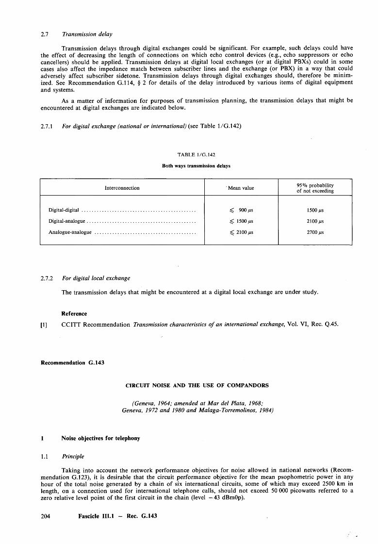
2.7 Transmission delay
Transmission delays through digital exchanges could be significant. For example, such delays could have the effect of decreasing the length of connections on which echo control devices (e.g., echo suppressors or echo cancellers) should be applied. Transmission delays at digital local exchanges (or at digital PBXs) could in some cases also affect the impedance match between subscriber lines and the exchange (or PBX) in a way that could adversely affect subscriber sidetone. Transmission delays through digital exchanges should, therefore be minimized. See Recommendation G.114, § 2 for details of the delay introduced by various items of digital equipment and systems.
As a matter of information for purposes of transmission planning, the transmission delays that might be encountered at digital exchanges are indicated below.
2.7.1 For digital exchange (national or international) (see Table 1/G. 142)
TABLE 1/G. 142
Both ways transmission delays
Interconnection ' Mean value 95% probability of not exceeding
Digital-digital....................................................................................... ^ 900 /is 1500 /us
Digital-analogue................................................................................... .<C 1500 fi s 2100 /us
Analogue-analogue ............................................................................. ^ 2100 fis 2700 fis
2.7.2 For digital local exchange
The transmission delays that might be encountered at a digital local exchange are under study.
Reference
[1] CCITT Recommendation Transmission characteristics o f an international exchange, Vol. VI, Rec. Q.45.
Recommendation G.143
CIRCUIT NOISE AND THE USE OF COMPANDORS
(Geneva, 1964; amended at Mar del Plata, 1968; Geneva, 1972 and 1980 and Malaga-Torremolinos, 1984)
1 Noise objectives for telephony
1.1 Principle
Taking into account the network performance objectives for noise allowed in national networks (Recomm endation G.123), it is desirable that the circuit performance objective for the mean psophometric power in any hour of the total noise generated by a chain of six international circuits, some of which may exceed 2500 km in length, on a connection used for international telephone calls, should not exceed 50 000 picowatts referred to a zero relative level point of the first circuit in the chain (level —43 dBmOp).
204 Fascicle III.l — Rec. G.143
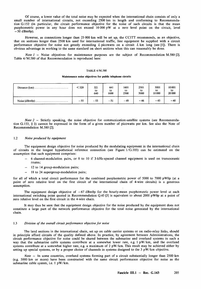
O f course, a lower value of the total noise may be expected when the international chain consists o f only a small num ber of international circuits, not exceeding 2500 km in length and conforming to Recommendation G.152 (in particular, the circuit performance objective for the noise of such circuits is that the mean psophometric power in any hour does not exceed 10 000 pW at a zero level point on the circuit, level - 50 dBmOp).
However, as connections longer than 25 000 km will be set up, the CCITT recommends, as an objective, that on sections longer than 2500 km used for international traffic, line equipment be supplied with a circuit performance objective for noise not greatly exceeding L picowatts on a circuit L km long (see [1]). There is obvious advantage in working to the same standard on short sections when this can reasonably be done.
Note 1 - Noise objectives for maintenance purposes are the subject of Recommendation M.580 [2]. Table 4/M .580 of that Recommendation is reproduced here:
TABLE 4/M .580
Maintenance noise objectives for public telephone circuits
Distance (km )................................................ <320 321 641 1601 2501 5001 10001to to to to to to
640 1600 2500 5000 10000 20000
Noise (dBmOp).............................................. -5 5 -5 3 -51 -4 9 -4 6 -4 3 -4 0
Note 2 — Strictly speaking, the noise objective for communication-satellite systems (see Recommendation G.153, § 3) cannot be expressed in the form of a given number of picowatts per km. See also the Note of Recommendation M.580 [2].
1.2 Noise produced by equipment
The equipment design objective for noise produced by the modulating equipment in the international chainof circuits in the longest hypothetical reference connection (see Figure 1/G . 103) can be estimated on theassumption that such equipment comprises:
— 6 channel-modulation pairs, or 8 to 10 if 3-kHz-spaced channel equipment is used on transoceanic routes;
— 12 to 14 group-modulation pairs;— 18 to 24 supergroup-modulation pairs;
for all of which a total circuit performance for the combined psophometric power of 5000 to 7000 pWOp (at a point o f zero relative level on the first circuit of the international chain of 4-wire circuits) is a generous assumption.
The equipment design objective of —67 dBmOp for the hourly-mean psophometric power level at each international switching point quoted in Recommendation Q.45 [3] is equivalent to about 2000 pWOp at a point of zero relative level on the first circuit in the 4-wire chain.
It may thus be seen that the equipment design objective for the noise produced by the equipment does not constitute a large part of the network performance objective for the total noise generated by the international chain.
1.3 Division o f the overall circuit performance objective fo r noise
The land sections in the international chain, set up on cable carrier systems or on radio-relay links, should in principle afford circuits of the quality defined above. In practice, by agreement between Administrations, the circuit performance objective for noise could be shared between the submarine and overland systems in such a way that the submarine cable systems contribute at a somewhat lower rate, e.g. 1 pW /km , and the overland systems contribute at a somewhat higher rate, e.g. a maximum of 2 pW /km . This result may be achieved either by setting up special systems, or by a proper choice of channels in systems designed to the 3 pW /km objective.
Note — In some countries, overland systems forming part of a circuit substantially longer than 2500 km (e.g. 5000 km or more) have been constructed with the same circuit performance objective for noise as the submarine cable system, i.e. 1 pW /km .
Fascicle III.l - Rec. G.143 205
1.4 Circuits operated with speech concentrators0
It would be desirable for all the circuits making up a group for use with a concentrator system to have approximately the same noise power level under operating conditions.
2 Use of syllabic compandors2)’ 3>’ 4)
For many years, international (and national) circuits will continue to be provided on existing transmission systems which have been designed to other standards, e.g. 4 pW /km , as given in Recommendation G. 152. Furthermore, the circuit noise produced by transmission systems can increase above the values originally achieved because of ageing effects, and changes of system loading. There is therefore a need for a simple practical criterion that can be applied for planning purposes to an international circuit to determine if, as far as noise power is concerned, it is suitable for establishing multicircuit worldwide telephone connections or whether it can be made suitable by fitting com pandors2).
It is recommended that, for the present, the systematic use of compandors conforming to Recommendation G.162 in the long-distance national and international network be restricted.
It must be pointed out that the action of a compandor doubles the effect of any variations in the transmission loss occurring in that part of the circuit which lies between the compressor and the expander and for this reason compandors, if needed, should be fitted at the ends of circuit sections provided by inherently stable line transmission systems such as submarine cable systems.
The following planning rule is recommended by the CCITT as a guide for deciding whether an international circuit requires a compandor:
If the hourly-mean psophometric circuit noise power level of an international circuit substantially longer than 2500 km (e.g. 5000 km or more) is less than —44 dBmOp (at a point of zero relative level on the circuit) no com pandor is necessary.
If the circuit noise power level is — 44 dBmOp (40 000 pWOp) or greater, a compandor should be fitted.
It is, of course, to be understood that circuits of length 2500 km or less will always meet the appropriate general noise objectives (Recommendation G.222 [4]) without the need for compandors.
Note 1 — This rule has been devised to make possible the planning of the international telephone network, using presently available circuits. It should in no way be interpreted as relaxation of the design objectives recommended in § 1 of this Recommendation, nor should it be applied for maintenance purposes (see Note 1 of § 1.1 above).
Note 2 — The compandors used should conform to the limits proposed in Recommendation G.162.
Note 3 - In accordance with the Recommendation cited in [5], circuits with a noise power level of — 37 dBmOp or worse are removed from service.
3 Noise limits for telegraphy
Noise limits for telegraphy are given in Recommendation H.22 [6].
4 Noise limits for data transmission
The following objectives are acceptable for data transmission at data signalling rates not exceeding 1200 b it/s . It is expected that the values actually experienced on many circuits and connections will be better than the following limits.
For example, TASI (Time Assignment Speech Interpolation) of CELTIC (Concentrateur exploitant les temps d’inoccupa- tion des circuits); see Recommendation G.163.
The instantaneous compandors that are associated with certain transmission systems are considered to be an integral part of these systems.
For characteristics of syllabic com pandors for telephony on high capacity long distance systems, see Recommendation G.166.
See Annex A for further considerations relating to the use of syllabic compandors.
206 Fascicle III.l — Rec. G.143
4.1 Leased circuits fo r data transmission
A reasonable limit for uniform spectrum random noise for a data transmission leased circuit, assuming that plant liable to impulsive noise interference is avoided, and as high a modulation rate as possible is to be used without significant error rate, would appear to be — 40 dBmOp.
4.2 Switched connections
For switched connections a limit of, say, —36 dBmOp without compandors may be taken for intercontinental circuits on which compandors may be used.
ANNEX A
(to Recommendation G.143)
Additional considerations relating to the use of syllabic compandors(The following information was available from Study Group XII)
This annex addresses com pandor advantage in § A .l, followed by a recommendation of the permissible advantage limits for planning purposes (§ A.2). A requirement of circuit stability between compressor and expander is given in § A.3, and §§ A.4 and A.5 deals with aspects of system loading and companded circuits in tandem.
A.l Compandor advantage
To define compandor advantage, assume:
a) an international circuit not equipped with compandors and contributing N dBmO of noise to the overall end-to-end connection (including typical national extensions) and meeting the noise objectives of Recommendation G.152 or Recommendation G.153, and
b) the same international circuit equipped with compandors and connected to typical national extensions, yielding the noise performance subjectively equivalent to or better than that of the circuit described in a), while contributing N' dBmO of noise in between compressor and expander.
Then the com pandor advantage for the international circuit of b) is defined as (IV' — N ) dB.
A.2 Compandor advantage limit
For planning purposes, the com pandor advantage defined in § A.l should not exceed 10 dB.
Note — It should be emphasized that this value applies to the international portion of the connection only. Other portions of the connection could permit a higher value when selected with due regard to the effect it has on the total noise of the end-to-end connection during the presence of the signal.
A.3 Circuit stability
The international circuit between compressor and expander should have an insertion loss which, when considered over a long period of time, has a standard deviation not exceeding 0.75 dB.
A.4 Circuit loading
It is generally advisable to select the unaffected level of the com pandor equal to —10 dBmO. However, if Administrations mutually desire to operate at a different value of unaffected level, it should be selected such that it results in a system loading which minimizes total distortion due to noise, intermodulation, or other load- dependent characterisics and should always be dictated by the allowable com pandor advantage limit.
Fascicle III.l — Rec. G.143 207

A. 5 Compandored circuits in tandem
Results of experiments with compandored circuit links in tandem show that two compandored links in tandem can produce a noticeable degradation only if the second link exceeds, by a considerable margin, the recommended com pandor advantage limit of 10 dB. The experiment was admittedly designed to uncover gross effects by limiting the subjective judgement to only seven persons per test condition.
The conclusion drawn was that two links in tandem, each of which is limited to 10 dB compandoradvantage, will not pose a restriction to users. This however, does not constitute sufficient guidance forapplication for the number of com pandored links permissible in an end-to-end international connection. Thistopic is under study in Question 11/X .II.
References
[1] CCITT Red Book, Vol. V bis, Annexes B and C, ITU, Geneva, 1965.
[2] CCITT Recommendation Setting-up and lining-up an international circuit fo r public telephony, Vol. IV,Rec. M.580.
[3] CCITT Recommendation Transmission characteristics o f an international exchange, Vol. VI, Rec. Q.45.
[4] CCITT Recommendation Noise objectives fo r design o f carrier-transmission systems o f 2500 km, Vol. I l l ,Rec. G.222.
[5] CCITT Recommendation Setting-up and lining-up an international circuit fo r public telephony, Vol. IV, Rec. M.580, § 6.
[6] CCITT Recommendation Transmission requirements o f international voice-frequency telegraph links (at 50, 100 and 200 bauds), Vol. I l l , Rec. H.22.
1.5 General characteristics of international telephone circuits and national extension circuits
Recommendation G.151
GENERAL PERFORM ANCE OBJECTIVES APPLICABLE TO ALL MODERN INTERNATIONAL CIRCUITS AND NATIONAL EXTENSION CIRCUITS
(Geneva, 1964; amended at Mar del Plata, 1968 and Geneva, 1972 and 1980)
1 Attenuation distortion
The circuit performance objectives for attenuation distortion of international circuits and national extension circuits should individually be such that the network performance objectives of Recommendation G.132 are complied with. Recommendation G.232 [1] gives equipment design objectives.
It follows from the Recommendations mentioned above that, as a rule, the frequency band effectively transmitted by a telephone circuit, according to the definition adopted by the CCITT (i.e. the band in which the attenuation distortion does not exceed 9 dB compared with the value for 800 Hz), will be a little wider than the 300-3400 Hz band, and for a single pair of channel terminal equipments of this type, the attenuation distortion at 300 Hz and 3400 Hz should never exceed 3 dB and in a large number of equipments should not average more than 1.7 dB (see Graphs A and B in Figure 1/G .232 [2]). Even more complex circuits, and circuits using terminal equipments with 3-kHz-channel spacing in accordance with Recommendation G.235 [3], should satisfy the limits in Figure 1/G.151; to ensure that these limits are respected, equalizers are inserted, if necessary, when the circuits are set up (Recommendation M.580 [4]).
208 Fascicle III.l — Rec. G.151
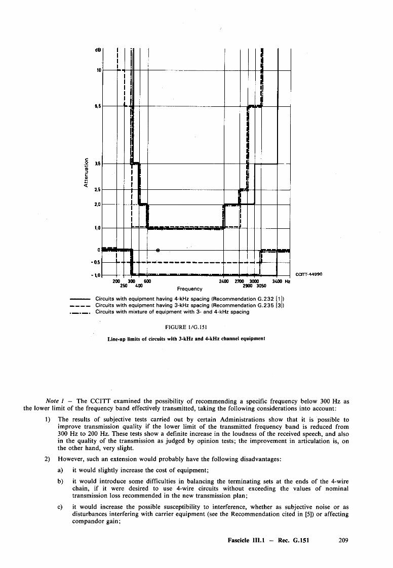
200 300 600250 400 Frequency
2400 2700 3000 3400 Hz2900 3050
— - Circuits with equipment having 4-kHz spacing (Recommendation G.232 [ l ]> Circuits with equipment having 3-kHz spacing (Recommendation G .235 [3]) Circuits with mixture of equipment with 3- and 4-kHz spacing
F IG U R E 1 /G . 151
Line-up limits o f circuits with 3-kH z and 4-kHz channel equipment
Note 1 — The CCITT examined the possibility of recommending a specific frequency below 300 Hz as the lower limit of the frequency band effectively transmitted, taking the following considerations into account:
1) The results of subjective tests carried out by certain Administrations show that it is possible toimprove transmission quality if the lower limit of the transmitted frequency band is reduced from300 Hz to 200 Hz. These tests show a definite increase in the loudness of the received speech, and also in the quality of the transmission as judged by opinion tests; the improvement in articulation is, on the other hand, very slight.
2) However, such an extension would probably have the following disadvantages:
a) it would slightly increase the cost o f equipment;
b) it would introduce some difficulties in balancing the terminating sets at the ends of the 4-wirechain, if it were desired to use 4-wire circuits without exceeding the values of nominal transmission loss recommended in the new transmission plan;
c) it would increase the possible susceptibility to interference, whether as subjective noise or as disturbances interfering with carrier equipment (see the Recommendation cited in [5]) or affecting com pandor gain;
Fascicle III.l - Rec. G.151 209
d) the additional energy transmitted in consequence of extending the band could increase the loading of carrier systems;
e) the out-of-band signalling systems recognized by the CCITT could not be used.
In view of the above, the CCITT has issued the aforementioned Recommendations concerning signals transmitted at frequencies between 300 and 3400 Hz.
Note 2 — In applying the Recommendations, Administrations may mutually agree to transmit signals at frequencies below 300 Hz over international circuits. Every Administration may, of course, decide to transmit signals at frequencies below 300 Hz over its national extension circuits, provided it is still able to apply the CCITT transmission plan to international communications.
2 Group delay
The group-delay performance objectives of international circuits and national extension circuits should be such that the network performance objectives of Recommendations G.114 and G.133 are met.
3 Variations of transmission loss with time
The CCITT recommends the following circuit performance objectives [objective a) has been used to assess the stability of international connections — see Recommendation G.131, § 1]:
a) The standard deviation of the variation in transmission loss of a circuit should not exceed 1 dB. This objective can be obtained already for circuits on a single group link equipped with automatic regulation and should be obtained for each national circuit, whether regulated or not. The standard deviation should not exceed 1.5 dB for other international circuits.
b) The difference between the mean value and the nominal value of the transmission loss for each circuit should not exceed 0.5 dB.
4 Linear crosstalk1 >
4.1 Between circuits
The circuit performance objective for the near-end or far-end crosstalk ratio (intelligible crosstalk only) measured at audio-frequency at trunk exchanges between two complete circuits in terminal service position should not be less than 65 dB.
Note 1 — When a minimum noise level of at least 4000 pWOp is always present in a system (e.g. this may be the case in satellite systems, for example) a reduced crosstalk ratio of 58 dB between circuits is acceptable.
Note 2 — Coaxial pair cables complying with Recommendations G.622 [6] and G.623 [7] already allow this condition to be fulfilled if it is assumed that the frequency bands for which crosstalk is caused by the cable and those for which crosstalk is due to the equipments are not the same. On the other hand FDM systems on symmetric pair cables do not always allow a limit more stringent than 58 dB to be met.
Note 3 — In cases where the length of a homogeneous section of a real transmission system substantially exceeds the length of a homogeneous section of the HRC, the 65 dB limit may not be met in all cases for all the channels in the system.
4.2 Between the go and return channels o f a 4-wire circuit
4.2.1 Ordinary telephone circuit (see Note 1 below)
Since all ordinary telephone circuits may also be used as VF telegraph bearers, the circuit performance objective for the near-end crosstalk ratio between the two directions of transmission should be at least 43 dB.
0 The methods recommended for measuring crosstalk are described in Annex A to Recommendation G.134.
210 Fascicle III.l - Rec. G.151
4.2.2 Circuits used with a speech concentrator
For circuits and circuit sections used to interconnect terminal speech concentrator equipments, near-end crosstalk between any two channels will appear in the form of crosstalk between circuits and hence the circuit performance objective for the total near-end crosstalk ratio introduced between speech concentrators should not be less than 58 dB. (See Notes 2 and 4 below.)
4.2.3 Circuits used with modern echo suppressors, fo r example high-altitude satellite circuits
The circuit performance objective for the near-end crosstalk ratio of any circuit equipped with terminal far-end operated, half-echo suppressors of modern design should not be less than 55 dB. This is to avoid nullifying the effect of the suppression loss introduced by modern echo suppressors. (See Notes 2, 3 and 4 below.)
Note 1 — Telephone circuits which are not equipped with (or used in conjunction with) modern echo suppressors designed for long propagation times are referred to in § 4.2.1 above. Circuits which can form part of switched connections with a long propagation time and which then lie between terminal half-echo suppressors o f modern design should, wherever possible, conform to the higher standards given in this § 4.2.3.
Note 2 — The channel-translating equipment provides the principal go-to-return crosstalk path on circuits or circuit-sections routed on carrier systems with modern translating and line transmission equipment (but see Note 4 below). It should be noted that crosstalk paths between the high-frequency input and the high-frequency output and also between the voice-frequency input and the voice-frequency output on channel-translating equipments contribute to the go-to-return crosstalk ratios of circuits and circuit sections. Both these paths must be taken into account when considering circuits or circuit sections used between terminal speech concentrator equipments or modern echo suppressors. The following cases arise:
Speech concentrators
Both the high-frequency path and the voice-frequency path contribute to the crosstalk ratio.
Echo suppressors
1) A circuit comprising one circuit section between far-end operated, half-echo suppressors: the high- frequency path is dominant.
2) A circuit comprising more than one circuit section between the suppressors: at points where channel-translating equipments are connected together at voice-frequency. The voice frequency crosstalk path of one equipment is effectively in parallel with the high-frequency crosstalk path of the other, so that both must be taken into account.
3) More than one circuit between the suppressors: this occurs when intermediate adjacent half-echo suppressors are switched out (or disabled) and the go-to-return crosstalk arises in a fashion analogous to that described in 2) above, circuits replacing circuit sections.
Note 3 — If channel equipments just conforming to the Recommendation cited in [8] are used on a circuit comprising three circuit sections, then assuming r.m.s. addition of crosstalk paths the crosstalk ratio would be approximately 60 dB.
Note 4 — If channel equipments used on a circuit comprising three circuit sections just comply with the Recommendation cited in [9], then the least go-to-return crosstalk ratio, assuming r.m.s. addition of the various paths, would be approximately 56 dB which is 2 dB less than is required for speech concentrators in § 4.2.2 above. However, the assumptions are most pessimistic and there is not likely to be any difficulty in practice. The limit for echo suppressor in § 4.2.3 above is complied with.
Note 5 — Some types of symmetrical-pair line transmission systems introduce significantly low go-to- return crosstalk ratios on the derived circuits and wherever possible such systems should not be used to provide circuits or circuit sections for use with speech concentrators or modern echo suppressors.
Note 6 — Some attention must be given to the unbalance of the audio parts of FDM channel equipments if the crosstalk of 65 dB is not to be diminished by crosstalk in station cabling due to unbalanced cable terminating equipment.
Fascicle III. 1 — Rec. G.151 211
5 Nonlinear distortion
Experience has shown that telephone circuits set up on systems for which the CCITT has issued recommendations (the elements of which systems, taken separately, meet the relevant nonlinearity requirements) are equally suitable, as far as nonlinearity is concerned, for telephone and voice-frequency telegraph transmission.
Note — In carrier telephone circuits, the nonlinear distortion produced by the line amplifiers and by modulation stages other than the channel-translating equipment can be ignored. Hence the above remarks are applicable to circuits of any length.
6 Error on the reconstituted frequency
See Recommendation G.135.
7 Interference at harmonics from the mains and other low frequencies
Signals carried by transmission systems are sometimes modulated by interfering signals from mains frequency power supplies, induced voltages caused by railway traction currents and from other sources. This unwanted modulation can take the form of amplitude or phase modulation or a combination of both. This interference may be characterized by the level of the strongest unwanted side component when a sine wave signal is applied with a power of 1 mW at the point of zero relative level (0 dBmO) on a telephone circuit. The circuit performance objective for the maximum admissible level of the unwanted side components on a complete telephone circuit should then not exceed - 4 5 dBmO (i.e. the minimum side component attenuation should be 45 dB). This circuit performance objective should apply to all low frequency interfering signals up to about 400 Hz.
Note 1 — This level was found to be acceptable for circuits for FM and AM VF-telegraphy, facsimile transmission, speech, telephone signalling and data transmission.
Note 2 — For limits applicable to sound-programme circuits, see the Recommendation cited in [10].
Note 3 — The main causes of interference due to power sources are:
a) residual ripples at the terminals of d.c. supply which are directly transmitted to equipments through the power-fed circuits;
b) the a.c. to the dependent power-fed stations in some systems, which interferes through the power-separating filter or through the iron tapes of coaxial pairs;
c) the induction voltages in the d.c. supply line to power-fed dependent stations in some systems;
d) the amplitude and phase unwanted modulations of the various carriers due to cause a) which are increased in the frequency-multiplying equipments.
Note 4 - The effect of the modulation process is that an input signal of frequency / H z will produce, for example, corresponding output signals at frequencies f , f ± 50, / ± 100, / ± 150 Hz, etc.
8 Single tone interference in telephone circuits
The single tone interference level in a telephone circuit should not be higher than —73 dBmOp (provisional value, pending the conclusion of studies by Study G roup XII). Psophometric weighting should only be accounted for when the frequency of the interference is well defined.
References
[1] CCITT Recommendation 12-channel terminal equipments, Vol. I l l , Rec. G.232.
[2] Ibid., Figure 1/G.232, Graphs A and B.
[3] CCITT Recommendation 16-channel terminal equipments, Vol. I l l , Rec. G.235.
[4] CCITT Recommendation Setting-up and lining-up an international circuit fo r public telephony, Vol. IV,Rec. M.580.
212 Fascicle III.1 - Rec. G.151
[5] CCITT Recommendation 12-channel terminal equipments, Vol. I l l , Rec. G.232, § 6.
[6] CCITT Recommendation Characteristics o f 1.2/4.4-mm coaxial cable pairs, Vol. I ll , Rec. G.622.
[7] CCITT Recommendation Characteristics o f 2 .6 /9 .5-mm coaxial cable pairs, Vol. I ll , Rec. G.623.
[8] CCITT Recommendation 12-channel terminal equipments, Vol. I l l , Rec. G.232, § 9.1.
[9] Ibid., § 9.3.
[10] CCITT Recommendation Performance characteristics o f 15-kHz type sound-programme circuits, Vol. I ll , Rec. J.21, § 3.1.7.
Recommendation G.152
CHARACTERISTICS APPROPRIATE TO LONG-DISTANCE CIRCUITS O F A LENGTH NOT EXCEEDING 2500 km
(Geneva, 1964; amended at M ar del Plata, 1968 and Geneva, 1972 and 1980)
This Recommendation applies to all modern international circuits not more than 2500 km in length. It also applies to national trunk circuits in an average-size country, and which may be used in the 4-wire chain of an international connection.
It is understood that, should an extension circuit more than 2500-km long be used in a large country, it will have to meet all the recommendations applicable to an international circuit of the same length.
1 Circuits on land or submarine cable systems or on line-of-sight radio-relay systems
The circuits in question are mostly set up in cable or radio-relay link carrier systems, such that the noise objectives of Recommendation G.222 [1] are applicable to a circuit with the same make-up as the hypothetical reference circuit 2500-km long.
A consequence of Recommendation G.222 [1] is that, for a circuit Z^km long (L < 2500 km), the circuit performance objective for the mean psophometric noise power during any hour should be of the order of 4 L picowatts, excluding very short circuits and those with a very complicated composition, this latter case being dealt with in Recommendation G.226 [2].
2 Circuits on tropospheric-scatter radio-relay systems
The CCIR has defined a hypothetical reference circuit and fixed circuit performance objectives in its Recommendations 396-1 [3] and 397-3 [4] respectively.
3 Circuits on open-wire carrier systems
The Recommendation cited in [5] contains relevant noise objectives.
Note — Recommendation M.580 [6] deals with noise objectives for maintenance purposes. See Note 1 of Recommendation G.143, § 1.1.
References
[1] CCITT Recommendation Noise objectives fo r design o f carrier-transmission systems o f 2500 km, Vol. I l l , Rec. G.222.
[2] CCITT Recommendation Noise on a real link, Vol. I ll , Rec. G.226.
[3] CCIR Recommendation Hypothetical reference circuit fo r trans-horizon radio-relay systems fo r telephony using frequency-division multiplex, Vol. IX, Rec. 396-1, ITU, Geneva, 1978.
[4] CCIR Recommendation Allowable noise power in the hypothetical reference circuit o f trans-horizon radiorelay systems fo r telephony using frequency-division multiplex, Vol. IX, Rec. 397-3, ITU, Geneva, 1978.
[5] CCITT Recommendation General characteristics o f systems providing 12 carrier telephone circuits on an open-wire pair, Vol. I ll , Rec. G.311, § 8.
[6] CCITT Recommendation Setting-up and lining-up an international circuit fo r public telephony, Vol. IV, Rec. M.580.
Fascicle III. 1 — Rec. G.152 213
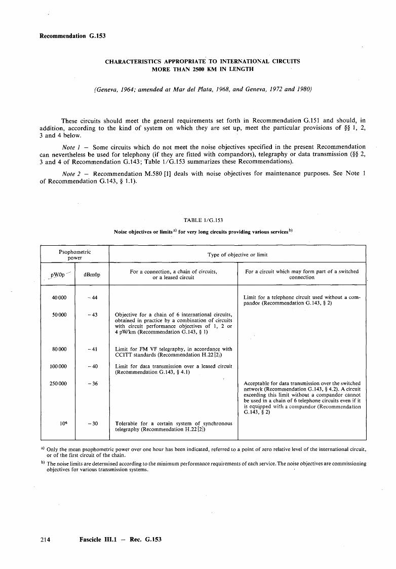
Recommendation G.153
CHARACTERISTICS APPROPRIATE TO INTERNATIONAL CIRCUITS M ORE THAN 2500 KM IN LENGTH
(Geneva, 1964; amended at Mar del Plata, 1968, and Geneva, 1972 and 1980)
These circuits should meet the general requirements set forth in Recommendation G.151 and should, in addition, according to the kind o f system on which they are set up, meet the particular provisions of §§ 1, 2, 3 and 4 below.
Note 1 — Some circuits which do not meet the noise objectives specified in the present Recommendation can nevertheless be used for telephony (if they are fitted with compandors), telegraphy or data transmission (§§ 2, 3 and 4 of Recommendation G.143; Table 1/G . 153 summarizes these Recommendations).
Note 2 — Recommendation M.580 [1] deals with noise objectives for maintenance purposes. See Note 1 of Recommendation G.143, § 1.1).
TABLE 1/G. 153
Noise objectives or limits for very long circuits providing various services
Psophometricpower Type of objective or limit
p WOp dBmOp For a connection, a chain of circuits, or a leased circuit
For a circuit which may form part of a switched connection
40000 -4 4 Limit for a telephone circuit used without a compandor (Recommendation G.143, § 2)
50000 -4 3 Objective for a chain of 6 international circuits, obtained in practice by a combination of circuits with circuit performance objectives of 1, 2 or 4 pWkm (Recommendation G.143, § 1)
80000 -41 Limit for FM VF telegraphy, in accordance with CCITT standards (Recommendation H.22 [2])
100000 -4 0 Limit for data transmission over a leased circuit (Recommendation G.143, § 4.1)
250000 -3 6 Acceptable for data transmission over the switched network (Recommendation G.143, § 4.2). A circuit exceeding this limit without a compandor cannot be used in a chain of 6 telephone circuits even if it is equipped with a compandor (Recommendation G.143, § 2)
106 -3 0 Tolerable for a certain system of synchronous telegraphy (Recommendation H.22 [2])
Only the mean psophometric power over one hour has been indicated, referred to a point of zero relative level of the international circuit, or of the first circuit of the chain.
b) The noise limits are determined according to the minimum performance requirements of each service. The noise objectives are commissioning objectives for various transmission systems.
214 Fascicle III.l — Rec. G.153
1 Circuits more than 2500 km in length on cable or radio-relay systems, with no long submarine cable section
In many cases circuits o f this kind, between 2500 km and about 25 000 km long will, throughout most of their length, be carried in land-cable systems or radio-relay systems already used to give international circuits not more than 2500 km long, and designed on the basis of the objectives already recommended for such systems in Recommendation G.222 [3].
Moreover, it is unlikely that the number of channel demodulations will exceed that envisaged in the corresponding part of the longest international connection referred to in Recommendation G.103. There will also be cases where it will be possible to establish such circuits on systems designed on the basis of national hypothetical reference circuits of the type referred to in the Recommendation cited in [4]. This being so, the CCITT issues the following recommendations:
1.1 Variations in transmission loss with time
Automatic level adjustment should be used on each group link on which the circuit is routed. In addition, all possible steps should be taken to reduce changes of transmission loss with time.
1.2 Performance objectives fo r circuit noise
It is provisionally recommended that systems to provide such international circuits not more than 25 000 km long should be designed on the basis of the noise objectives at present recommended for 2500-km hypothetical reference circuits.
Whenever possible lower noise objectives should be sought and it is recognized that in some large countries systems forming part of a circuit substantially longer than 2500 km (e.g. 5000 km) are constructed according to the principles referred to in the Recommendation cited in [4]. Alternatively lower noise figures can be obtained by a suitable choice of telephone channels making up the circuits. Provisionally the short-term noise performance objectives for circuits o f this kind of length up to about 7500 km are as follows:
The one-minute mean noise power shall not exceed 50 000 pW ( — 43 dBmOp) for more than 0.3% of any month and the unweighted noise power, measured or calculated with an integrating time of 5 ms, shall not exceed 106 pW ( — 30 dBmO) for more than 0.03% of any month. It is to be understood that these objectives are derived pro rata from the objectives for circuits of 2500 km length (Recommendation G.222 [3]); for lengths between 2500 and 7500 km proportionate intermediate values should apply.
The CCITT is not yet able to recommend objectives for short-term noise performance on circuits of the above type which exceed 7500 km in length.
2 Circuits more than 2500 km with a long submarine cable section
2.1 Attenuation distortion
A circuit o f this kind may, for reasons o f economy, comprise terminal equipments with carriers spaced 3 kHz apart, in accordance with Recommendation G.235 [5].
If terminal equipment be used with carrier spacing of 4 kHz, it must at least meet the requirements of Recommendation G.232 [6]. Some countries use improved terminal equipment in circuits permanently used for intercontinental operation.
2.2 Performance objectives fo r circuit noise attributable to the submarine cable section
2.2.1 Without compandor
The circuit performance objective for the mean noise per hour of a very long submarine-cable system designed for use without compandors and with no restrictions for telephony, voice-frequency telegraphy and data transmission should not exceed 3 pW /km on the worst channel. The circuit performance objective for the mean noise power for each direction of transmission, extended over all the channels used for the longest circuits, should not exceed 1 pW /km .
Fascicle III.l — Rec. G.153 215
Note — However, it would be desirable that the circuits in a group to be operated with a speechconcentrator system 1) should all have more or less the same noise level.
2.2.2 With compandor
At present, the CCITT does not propose to study systems which, by relying on the systematic use ofcompandors, have noise objectives which are greatly different from those of § 2.2.1 above.
2.3 Performance objectives fo r circuit noise attributable to other sections
The other sections of the circuit should comply with the recommendations given in § 1 of this Recommendation.
3 Circuits on communication-satellite systems
The CCIR and the CCITT are considering the extent to which circuits set up on communication-satellite systems may be integrated into the worldwide network; some of the limitations on the use of such circuits are outlined in Recommendation Q.13 [7].
The CCIR has made recommendations as far as circuit noise is concerned and has defined a hypothetical reference circuit (CCIR Recommendation 352-3 [8]) and the allowable noise power in this reference circuit (CCIR Recommendation 353-3 [9]).
4 Circuits more than 2500 km in length set up on open-wire lines
Paragraph 4 is not published in this Book, but can be found under Part D of Recommendation G.153, Orange Book, ITU, Geneva, 1977.
References
[1] CCITT Recommendation Setting-up and lining-up an international circuit fo r public telephony, Vol. IV,Rec. M.580.
[2] CCITT Recommendation Transmission requirements o f international voice-frequency telegraph links (at 50,100 and 200 bauds), Vol. I l l , Rec. H.22.
[3] CCITT Recommendation Noise objectives fo r design o f carrier-transmission systems o f 2500 km, Vol. I ll ,Rec. G.222.
[4] Ibid., § 3.
[5] CCITT Recommendation 16-channel terminal equipments, Vol. I l l , Rec. G.235.
[6] CCITT Recommendation 12-channel terminal equipments, Vol. I l l , Rec. G.232.
[7] CCITT Recommendation The international routing plan, Vol. VI, Rec. Q.13.
[8] CCIR Recommendation Hypothetical reference circuits fo r telephony and television in the fixed satelliteservice, Vol. IV, Rec. 352-3, ITU, Geneva, 1978.
[9] C C IR Recommendation Allowable noise power in the hypothetical reference circuit fo r frequency-division multiplex telephony in the fixed satellite service, Vol. IV, Rec. 353-3, ITU, Geneva, 1978.
1.6 Apparatus associated with long-distance telephone circuits
Recommendation G.161
ECHO-SUPPRESSORS SUITABLE FOR CIRCUITS HAVING EITHER SHORT OR LONG PROPAGATION TIM ES
(See Vol. I l l of the Orange Book, ITU, Geneva, 1977).
See footnote 2) in Recommendation G.143, § 2.
216 Fascicle III.l — Rec. G.161
Recommendation G.162
CHARACTERISTICS OF COM PANDORS FOR TELEPHONY
(Geneva, 1964; amended at Mar del Plata, 1968)
These characterisics are applicable to compandors of modern design for use either on very long international circuits or on national and international circuits o f moderate length.
Some of the clauses given below specify the joint characteristics of a compressor and an expander in the same direction of transmission of a 4-wire circuit. The characteristics specified in this way can be obtained more easily if the compressors and expanders are of similar design; in certain cases close cooperation between Administrations may be necessary.
It should also be noted that the equipement produced so far for circuits o f moderate length may be completely satisfactory for those circuits and yet not quite meet the clauses of this Recommendation.
1 Definition and value of the unaffected level
The unaffected level is the absolute level, at a point of zero relative level on the line between the compressor and the expander of a signal at 800 Hz, which remains unchanged whether the circuit is operated with the compressor or not. The unaffected level is defined in this way in order not to impose any particular values ofrelative level at the input to the compressor or the output of the expander.
The unaffected level should be, in principle, 0 dBmO. Nevertheless, to make allowances for the increase in mean power introduced by the compressor, and to avoid the risk of increasing the intermodulation noise and the overload which might result, the unaffected level may, in some cases, be reduced by perhaps as much as 5 dB. However, this reduction of unaffected level entails a diminution of the improvement in signal-to-noise ratio provided by the compandor. This possible reduction should be made by direct agreement between the Administrations concerned. No reduction is necessary, in general, for systems with less than 60 channels.
Note — The increase in the mean power in the transmitted band determined by the compressor in thetelephone channel depends on the value of the unaffected level, the attack and recovery times, the distribution of the speech volumes and the mean power level of transmitted speech. When 0 dBmO is adopted for the unaffected level, it appears that the effective increase in the mean power level is of the order of 2 or 3 dB.
2 Ratio of compression and expansion
2.1 Definition and preferred value o f the ratio of compression
The ratio compression of a compressor is defined by the formula:
ne - «e o a = -----------fts ftsO
where:ne is the input level;ne0 is the input level corresponding to 0 dBmO;ns is the output level;ns0 is the output level corresponding to an input level of neo-
The preferred value of a is 2, though lower values are permissible, provided sufficient noise improvement is obtained. The value shall not exceed 2.5 for any level o f input signal and at any temperature between + 10 °C and + 40 °C.
2.2 Definition and preferred value o f the ratio of expansion
The ratio of expansion of an expander is defined by the formula:
= ft's - n 'so
f t ' e ~ f t 'e O
Fascicle III. 1 — Rec. G.162 217
where:/i'e is the input level;/j'eo is the input level corresponding to 0 dBmO;« 's is the output level;n 'so is the output level corresponding to an input level of n 't0.
The preferred value of P is 2, though lower values are permissible, provided sufficient noise improvement is obtained. The value shall not exceed 2.5 for any level of input signal and at any temperature between + 1 0 °C and + 40 °C.
2.3 Range o f level
The range of level over which the recommended value of a and P should apply should extend at least: from + 5 to — 45 dBmO at the input o f the compressor, andfrom + 5 to — 50 dBmO at the nominal output of the expander.
2.4 Variation o f compressor gain
The level at the output o f the compressor, measured at 800 Hz, for an input level of 0 dBmO, should not vary from its nominal value by more than ± 0.5 dB for a temperature range of + 1 0 °C to + 4 0 °C and a deviation of the supply voltage of ± 5% from its nominal value.
2.5 Variation o f expander gain
The level at the output o f the expander, measured at 800 Hz for an input level of 0 dBmO, should not varyfrom its nominal value by more than ± 1 dB for a temperature range of + 10 °C and +40 °C and a deviation ofthe supply voltage of ± 5% from its nominal value.
Note — It is desirable, especially for compandors intended for very long circuits, to set stricter limits than the values of +0.5 dB and ± 1 dB given under § 2.4 and § 2.5; +0.25 dB and +0.5 dB respectively are preferable.
2.6 Conditions fo r stability
The insertion of a com pandor shall not appreciably reduce the margin of stability. To ensure this, for the combination of an expander and a compressor on the same 4-wire circuit and at a given station, the error of the output level o f the compressor with respect to any value of expander input level shall not exceed + 0.5 dB. This error is referred to the level obtained at the compressor output when the input level is 0 dBmO. This limit shall beobserved at all frequencies between 200 and 4000 Hz within the temperature range + 1 0 °C to + 40 °C. Nonegative limit is specified for the error. In this test an attenuator shall be inserted between the expander and the compressor, the value of which is to be set in accordance with the following Note 1.
Note 1 — This Note concerns the influence of a compandor on the loop gain of a 4-wire circuit and on the margin of stability.
In examining this problem, a connection was considered made up of three 4-wire circuits, AB, BC and CD, which link the terminal stations A and D (at which the terminating sets are located) through the intermediate stations B and C. It is assumed that the circuit BC is equipped with compandors. It is desired to determine the tolerances for the gain of the combination of expander and compressor at C in order to limit the reduction in the margin of stability caused by their insertion. To facilitate study of this question it is assumed that, in normal use, theexpander output and compressor input are points o f the same relative level.
The following expression then gives the loss between the output of the expander at C and the input o f the compressor at C:
as = Oq + ar + ax + ay
whereao is the nominal transmission loss of the chain of circuits between the 2-wire terminals at A and D ; ar is the balance return loss at the terminating set at D; ax is the departure of transmission loss of channel CD from its nominal value; ay is the departure of transmission loss of channel DC from its nominal value.
The two latter values may be positive or negative.
218 Fascicle III.l — Rec. G.162
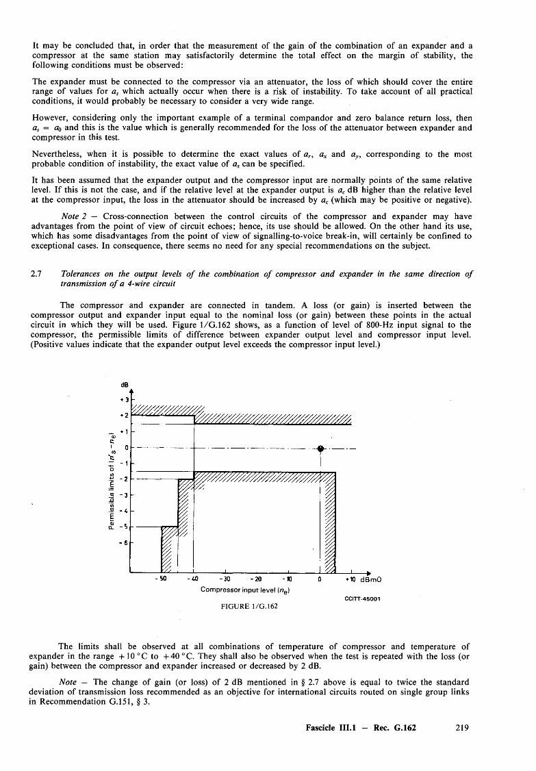
It may be concluded that, in order that the measurement of the gain of the combination of an expander and a compressor at the same station may satisfactorily determine the total effect on the margin of stability, the following conditions must be observed:
The expander must be connected to the compressor via an attenuator, the loss of which should cover the entire range of values for as which actually occur when there is a risk of instability. To take account of all practical conditions, it would probably be necessary to consider a very wide range.
However, considering only the im portant example of a terminal compandor and zero balance return loss, then as = oq and this is the value which is generally recommended for the loss of the attenuator between expander and compressor in this test.
Nevertheless, when it is possible to determine the exact values of ar, ax and ay, corresponding to the most probable condition of instability, the exact value of as can be specified.
It has been assumed that the expander output and the compressor input are normally points of the same relative level. If this is not the case, and if the relative level at the expander output is ac dB higher than the relative level at the compressor input, the loss in the attenuator should be increased by ac (which may be positive or negative).
Note 2 — Cross-connection between the control circuits o f the compressor and expander may have advantages from the point of view of circuit echoes; hence, its use should be allowed. On the other hand its use, which has some disadvantages from the point of view of signalling-to-voice break-in, will certainly be confined to exceptional cases. In consequence, there seems no need for any special recommendations on the subject.
2.7 Tolerances on the output levels o f the combination o f compressor and expander in the same direction o f transmission o f a 4-wire circuit
The compressor and expander are connected in tandem. A loss (or gain) is inserted between the compressor output and expander input equal to the nominal loss (or gain) between these points in the actual circuit in which they will be used. Figure 1/G. 162 shows, as a function of level o f 800-Hz input signal to the compressor, the permissible limits o f difference between expander output level and compressor input level. (Positive values indicate that the expander output level exceeds the compressor input level.)
dB
Compressor input level (ne )CCITT-45001
F IG U R E 1 /G .162
The limits shall be observed at all combinations of temperature of compressor and temperature of expander in the range +10 °C to + 40 °C. They shall also be observed when the test is repeated with the loss (or gain) between the compressor and expander increased or decreased by 2 dB.
Note — The change of gain (or loss) of 2 dB mentioned in § 2.7 above is equal to twice the standard deviation of transmission loss recommended as an objective for international circuits routed on single group links in Recommendation G.151, § 3.
Fascicle III.l — Rec. G.162 219
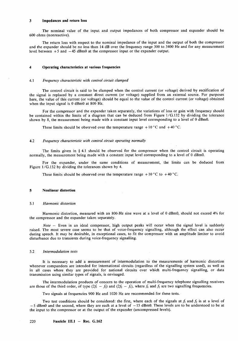
3 Impedances and return loss
The nominal value of the input and output impedances of both compressor and expander should be 600 ohms (nonreactive).
The return loss with respect to the nominal impedance of the input and the output of both the compressor and the expander should be no less than 14 dB over the frequency range 300 to 3400 Hz and for any measurement level between + 5 and - 45 dBmO at the compressor input or the expander output.
4 Operating characteristics at various frequencies
4.1 Frequency characteristic with control circuit clamped
The control circuit is said to be clamped when the control current (or voltage) derived by rectification of the signal is replaced by a constant direct current (or voltage) supplied from an external source. For purposes here, the value of this current (or voltage) should be equal to the value of the control current (or voltage) obtained when the input signal is 0 dBmO at 800 Hz.
For the compressor and the expander taken separately, the variations of loss or gain with frequency should be contained within the limits of a diagram that can be deduced from Figure 1/G. 132 by dividing the tolerance shown by 8, the measurement being made with a constant input level corresponding to a level of 0 dBmO.
These limits should be observed over the temperature range + 10 °C and + 40 °C.
4.2 Frequency characteristic with control circuit operating normally
The limits given in § 4.1 should be observed for the compressor when the control circuit is operating normally, the measurement being made with a constant input level corresponding to a level of 0 dBmO.
For the expander, under the same conditions of measurement, the limits can be deduced from Figure 1/G . 132 by dividing the tolerances shown by 4.
These limits should be observed over the temperature range + 10 °C to + 40 °C.
5 Nonlinear distortion
5.1 Harmonic distortion
Harmonic distortion, measured with an 800-Hz sine wave at a level of 0 dBmO, should not exceed 4% for the compressor and the expander taken separately.
Note — Even in an ideal compressor, high output peaks will occur when the signal level is suddenly raised. The most severe case seems to be that of voice-frequency signalling, although the effect can also occur during speech. It may be desirable, in exceptional cases, to fit the compressor with an amplitude limiter to avoid disturbance due to transients during voice-frequency signalling.
5.2 Intermodulation tests
It is necessary to add a measurement of intermodulation to the measurements of harmonic distortion whenever compandors are intended for international circuits (regardless of the signalling system used), as well as in all cases where they are provided for national circuits over which multi-frequency signalling, or data transmission using similar types of signals, is envisaged.
The intermodulation products of concern to the operation of multi-frequency telephone signalling receivers are those of the third order, of type (2f - f 2) and (2 /2 - f ), where f\ and f 2 are two signalling frequencies.
Two signals at frequencies 900 Hz and 1020 Hz are recommended for these tests.
Two test conditions should be considered: the first, where each of the signals at f and f 2 is at a level of — 5 dBmO and the second, where they are each at a level of — 15 dBmO. These levels are to be understood to be at the input to the compressor or at the output o f the expander (uncompressed levels).
220 Fascicle III.l — Rec. G.162
The limits for the intermodulation products are defined as the difference between the level of either of the signals at frequencies / or f 2 and the level of either o f the intermodulation products at frequencies (2f — f 2) or (2 /2 - / ) •
A value for this difference which seems adequate for the requirements of multi-frequency telephone signalling (including end-to-end signalling over three circuits in tandem, each equipped with a compandor) is 26 dB for the compressor and the expander separately.
Note 1 — These values seem suitable for Signalling System No. 5, which will be used on some long international circuits.
Note 2 — It is inadvisable to make measurements on a compressor plus expander in tandem, because the individual intermodulation levels o f the compressor and of the expander might be quite high, although much less intermodulation is given in tandem measurements since the characteristics of compressor and expander may be closely complementary. The compensation encountered in tandem measurements on compressor and expander may not be encountered in practice, either because there may be phase distortion in the line or because the compressor and expander at the two ends of the line may be less closely complementary than the compressor and expander measured in tandem.
Hence the measurements have to be performed separately for the compressor and the expander. The two signals at frequencies / and f 2 must be applied simultaneously, and the levels at the output of the compressor or expander measured selectively.
6 Noise voltages
The effective value of the sum of all noise voltages referred to a zero relative level point, the input and the output being terminated with resistances of 600 ohms, shall be less than or equal to the following values:
— at the output of the compressor: (10 mV unweighted —38 dBmO)( 7 mV weighted —41 dBmOp)
— at the output of the expander: (0.5 mV weighted —84 dBmOp)
It is not considered useful to specify a value of unweighted noise voltage for the expander.
7 Transient response
The overall transient response of the combination of a compressor and expander which are to be used in the same direction of transmission of a 4-wire circuit fitted with compandors shall be checked as follows:
The compressor and expander are connected in tandem, the appropriate loss (or gain) being inserted between them as in § 2.7.
A 12-dB step signal at a frequency of 2000 Hz is applied to the input o f the compressor, the actual values being a change from —16 to —4 dBmO for attack, and from —4 to —16 dBmO for recovery. The envelope of the expander output is observed. The overshoot (positive or negative), after an upward 12-dB step expressed as a percentage of the final steady-state voltage, is a measure of the overall transient distortion of the compressor- expander combination for attack. The overshoot (positive or negative) after a downward 12 dB step, expressed as a percentage of the final steady-state voltage is a measure of the overall transient distortion of the compressor- expander combination for recovery. For both these quantities the permissible limits shall be ± 20%. These limits shall be observed for the same conditions of temperature and of variation of loss (or gain) between compressor and expander as for the test in § 2.7.
In addition, the attack and recovery times of the compressor alone shall be measured as follows:
Using the same 12-dB steps as above for attack and recovery respectively, the attack time is defined as the time between the instant when the sudden change is applied and the instant when the output voltage envelope reaches a value equal to 1.5 times its steady-state value. The recovery time is defined as the time between the instant when the sudden change is applied and the instant when the output voltage envelope reaches a value equal to 0.75 times its steady-state value.
The permissible limits shall be not greater than:
— 5 ms for attack,
— 22.5 ms for recovery.
Fascicle III.l - Rec. G.162 221
The following additional test shall be used to check the effect of the compandor on certain signalling systems which may be sensitive to envelope distortion immediately following the sudden application of a sinusoidal signal.
The overall transient response of the combination of a compressor and expander which are to be used in the same direction of transmission on a 4-wire circuit is measured with an “infinite” upward input step, i.e. with a signal applied after a period with no input.
The level of the signal to be applied is — 5 dBmO.
Provided the measurement is effected with an interval of at least 50 ms between the pulses, the limits shown by an unbroken line in Figure 2 /G .l62 should be observed for the overshoot of the final voltage V\; in most cases an attempt should be made if possible to observe the narrower limits, indicated in the figure by a broken line.
TimeCCITT-45010
FIGURE 2/G.162
These limits shall be observed for the same conditions of temperature loss (or gain) between compressorand expander as for the tests with 12-dB steps.
Note 1 — The tests of transient distortion described involve the measurement of the overshoot orundershoot of the envelope of the applied sinusoidal signal. It may happen that, due to small unbalances in thevariable loss device, very-low-frequency components of the control current appear at the output. These are not a m odulation of the signal frequency, but they produce an unsymmetrical waveform and render it difficult todetermine the overshoot or undershoot of the envelope. While it is undesirable that these low-frequencycomponents should be so large as to increase significantly the risk of overload of the line equipment, they are of no importance for speech transmission and will not affect tuned signalling receivers. However, it is desirable to consider whether these components may affect the guard circuits of some signalling receivers. If so, it may be necessary to specify a maximum value for these components and to include an appropriate test in this Recommendation.
To simplify the measurement of the true envelope amplitude in the presence of these unbalance components, it is admissible and convenient to insert at the input to the measuring oscillograph a high-pass filter having a cut-off frequency of about 300 Hz. However, a filter which is effective in removing unbalance components may itself introduce additional transient distortion in the signal envelope. To avoid this difficulty, the following method of calculation may be adopted which does not require a filter.
If at any instant the amplitude of the envelope in a positive direction is + Eu and in the negative direction is — Ejthen the two-envelope amplitude is given by
i [ (+£i ) - ( - £ , ) ] « i [ |E, | + | £ 2| ]
222 Fascicle III.l — Rec. G.162
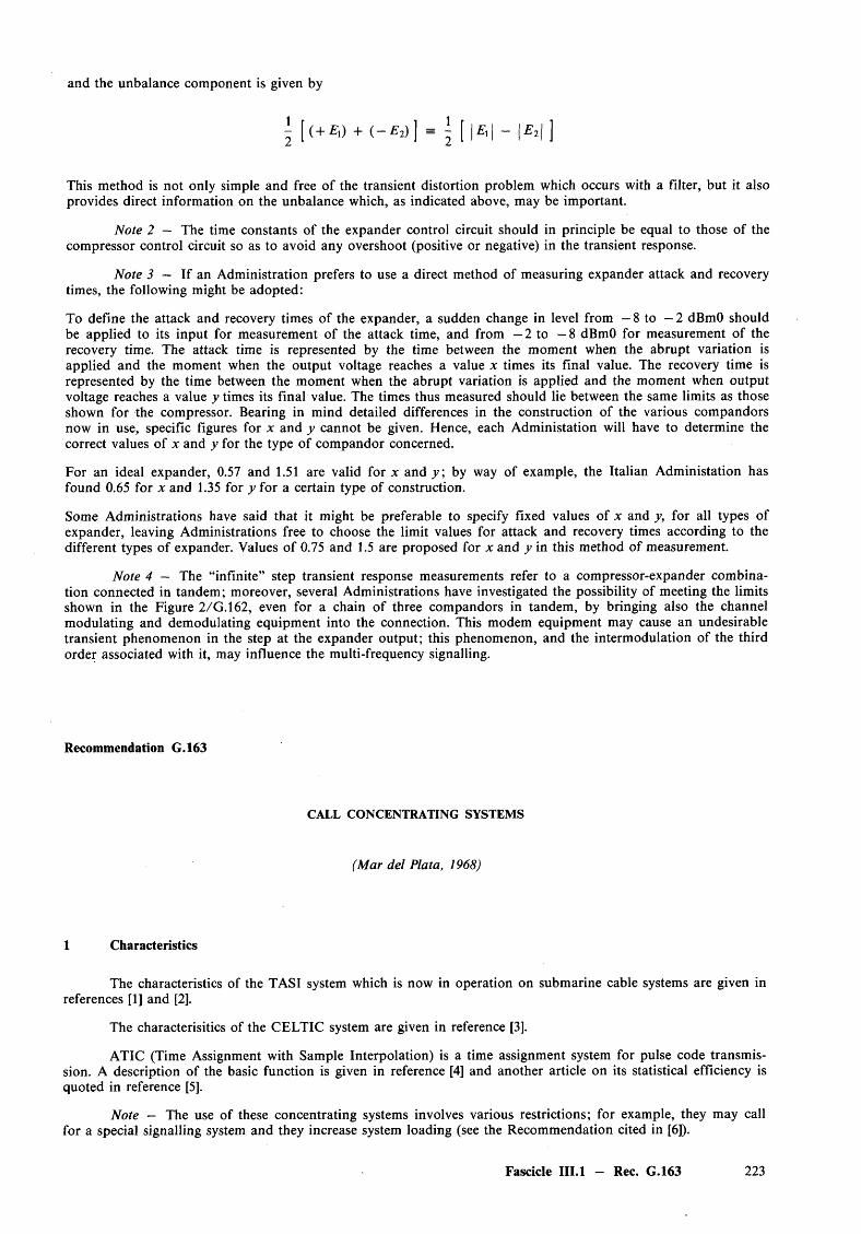
and the unbalance component is given by
i [( + £,) + ( - £ 2)] = i [ |£,| - |£2| ]
This method is not only simple and free of the transient distortion problem which occurs with a filter, but it also provides direct information on the unbalance which, as indicated above, may be important.
Note 2 — The time constants of the expander control circuit should in principle be equal to those of the compressor control circuit so as to avoid any overshoot (positive or negative) in the transient response.
Note 3 — If an Administration prefers to use a direct method of measuring expander attack and recovery times, the following might be adopted:
To define the attack and recovery times of the expander, a sudden change in level from —8 to — 2 dBmO should be applied to its input for measurement of the attack time, and from —2 to —8 dBmO for measurement of the recovery time. The attack time is represented by the time between the moment when the abrupt variation is applied and the moment when the output voltage reaches a value x times its final value. The recovery time is represented by the time between the moment when the abrupt variation is applied and the moment when output voltage reaches a value y times its final value. The times thus measured should lie between the same limits as those shown for the compressor. Bearing in mind detailed differences in the construction of the various compandors now in use, specific figures for x and y cannot be given. Hence, each Administation will have to determine the correct values of x and y for the type of com pandor concerned.
For an ideal expander, 0.57 and 1.51 are valid for x and y ; by way of example, the Italian Administation has found 0.65 for x and 1.35 for y for a certain type of construction.
Some Administrations have said that it might be preferable to specify fixed values of x and y, for all types of expander, leaving Administrations free to choose the limit values for attack and recovery times according to the different types of expander. Values of 0.75 and 1.5 are proposed for x and y in this method of measurement.
Note 4 — The “infinite” step transient response measurements refer to a compressor-expander com bination connected in tandem ; moreover, several Administrations have investigated the possibility of meeting the limits shown in the Figure 2 /G .l62, even for a chain o f three compandors in tandem, by bringing also the channel modulating and demodulating equipment into the connection. This modem equipment may cause an undesirable transient phenomenon in the step at the expander output; this phenomenon, and the intermodulation of the third order associated with it, may influence the multi-frequency signalling.
Recommendation G.163
CALL CONCENTRATING SYSTEMS
(Mar del Plata, 1968)
1 Characteristics
The characteristics of the TASI system which is now in operation on submarine cable systems are given in references [1] and [2].
The characterisitics of the CELTIC system are given in reference [3].
ATIC (Time Assignment with Sample Interpolation) is a time assignment system for pulse code transm ission. A description of the basic function is given in reference [4] and another article on its statistical efficiency is quoted in reference [5].
Note — The use of these concentrating systems involves various restrictions; for example, they may call for a special signalling system and they increase system loading (see the Recommendation cited in [6]).
Fascicle III.l — Rec. G.163 223
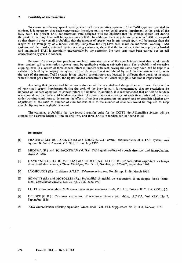
2 Possibility of interconnection
To ensure satisfactory speech quality when call concentrating systems of the TASI type are operated in tandem, it is necessary that each concentrator introduce only a very small speech impairment at the peak of the busy hour. The present TASI concentrators were designed with the objective that the average speech lost during the peak of the busy hour will be approximately 0.5%. In addition, the interpolation process in TASI is designed so that there is a very small probability that the am ount of speech lost in any speech spurt will be greater than the length of an average syllable (about 250 ms). Subjective tests [7] have been made on individual working TASI systems and the results, obtained by interviewing customers, show that the impairment due to a properly loaded and maintained TASI is essentially undetectable by the customer. No such tests have been carried out on call concentration systems in tandem.
Because of the subjective problems involved, estimates made of the speech impairment that would result from tandem call concentration systems must be qualitative without subjective tests. The probability of excessive clipping, even in a system of three concentrators in tandem with each having the same busy hour, can be kept to a satisfactory level by arranging the system so that the impairment introduced by each concentrator is small, as in the case of the present TASI system. If the tandem concentrators are located in different time zones or in areas with different peak traffic hours, the lighter loaded concentrators will cause negligible additional impairment.
Assuming that present and future concentrators will be operated and designed so as to meet the criterion of very small speech impairment during the peak of the busy hour, it is recommended that no restrictions be imposed on tandem operation of concentrators at this time. In addition, it is recommended that no test on tandem operation should be made until tandem operation of concentrators is a reality. At such time, tests could be made under working conditions to determine the effects o f tandem concentrators on speech and to establish whether any adjustment of the ratio of number of simultaneous calls to the number of channels would be required to keep speech clipping to a negligible amount.
The estimated probability that the forward-transfer pulse for the CCITT No. 5 Signalling System will be clipped for a certain length of time in one, two, and three TASIs in tandem can be found in [8].
References
[1] FRASER (J. M.), BULLOCK (D. B.) and LONG (N. G.).: Overall characteristics of a TASI system, Bell System Technical Journal, Vol. XLI, No. 4, July 1962.
[2] M IDEM A (H.) and SCHACHTM AN (M. G.).: TASI quality-effect of speech detectors and interpolation,B.S.T.J., ibid.
[3] DAYONNET (F. D.), JOUSSET (A.) and PROFIT (A.).: Le CELTIC: Concentrateur exploitant les temps d ’inactivite des circuits, L ’Onde Electrique, Vol. XLII, No. 426, pp. 675-687, September 1962.
[4] LYGHOUNIS (E.).: II sistema A.T.I.C., Telecommunicazioni, No. 26, pp. 21-29, March 1968.
[5] BONATTI (M.) and MOTOLESE (F.).: Probability di attivita delle giunzioni di un doppio fascio telefo- nico, Telecommunicazioni, No. 23, pp. 24-28, June 1967.
[6] CCITT Recommendation FDM carrier systems fo r submarine cable, Vol. I l l , Fascicle III.2, Rec. G.371, § 3.
[7] HELDER (G. K.).: Customer evaluation of telephone circuits with delay, B.S.T.J., Vol. XLV, No. 7, September 1966.
[8] TA SI characteristics affecting signalling, Green Book, Vol. VI.4, Supplement No. 2, ITU, Geneva, 1973.
224 Fascicle III.l — Rec. G.163
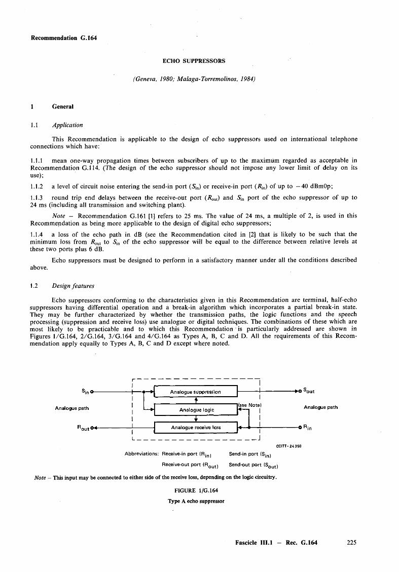
Recommendation G.164
ECHO SUPPRESSORS
(Geneva, 1980; Malaga-Torremolinos, 1984)
1 General
1.1 Application
This Recommendation is applicable to the design of echo suppressors used on international telephone connections which have:
1.1.1 mean one-way propagation times between subscribers of up to the maximum regarded as acceptable inRecommendation G.114. (The design of the echo suppressor should not impose any lower limit of delay on itsuse);
1.1.2 a level of circuit noise entering the send-in port (S jn) or receive-in port (R j„ ) of up to —40 dBmOp;
1.1.3 round trip end delays between the receive-out port (.Rout) an^ *Sin port o f the echo suppressor of up to24 ms (including all transmission and switching plant).
Note — Recommendation G.161 [1] refers to 25 ms. The value of 24 ms, a multiple of 2, is used in thisRecommendation as being more applicable to the design of digital echo suppressors;
1.1.4 a loss of the echo path in dB (see the Recommendation cited in [2] that is likely to be such that theminimum loss from Rout to ^in of the echo suppressor will be equal to the difference between relative levels atthese two ports plus 6 dB.
Echo suppressors must be designed to perform in a satisfactory m anner under all the conditions describedabove.
1.2 Design features
Echo suppressors conforming to the characteristics given in this Recommendation are terminal, half-echo suppressors having differential operation and a break-in algorithm which incorporates a partial break-in state. They may be further characterized by whether the transmission paths, the logic functions and the speech processing (suppression and receive loss) use analogue or digital techniques. The combinations of these which are most likely to be practicable and to which this Recommendation is particularly addressed are shown in Figures 1/G. 164, 2 /G .l64, 3/G.164 and 4/G.164 as Types A, B, C and D. All the requirements of this Recommendation apply equally to Types A, B, C and D except where noted.
CCITT-2< 350
Abbreviations: Receive-in port ( R j n j Send-in port (Sjn)
Receive-out port (Rout) Send-out port (SQut)
Note - This input may be connected to either side of the receive loss, depending on the logic circuitry.
FIGURE 1/G.164
Type A echo suppressor
Fascicle III.l — Rec. G.164 225
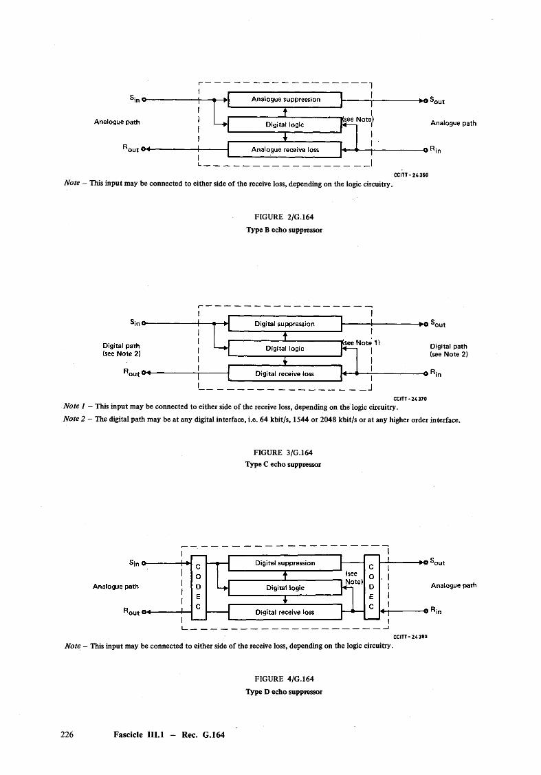
C C IT T - 2 4 3 6 0
Note - This input may be connected to either side of the receive loss, depending on the logic circuitry.
FIGURE 2/G.164
Type B echo suppressor
-►O °out
Digital path (see Note 2)
Rir-O n in
C C IT T - 2 4 3 7 0
Note 1 — This input may be connected to either side of the receive loss, depending on the logic circuitry.
Note 2 - The digital path may be at any digital interface, i.e. 64 kbit/s, 1544 or 2048 kbit/s or at any higher order interface.
FIGURE 3/G.164 Type C echo suppressor
C C IT T -2 4 3 8 0
Note - This input may be connected to either side of the receive loss, depending on the logic circuitry.
FIGURE 4/G.164
Type D echo suppressor
226 Fascicle III.l - Rec. G.164

1.3 Variants
1.3.1 Recommendation G.161 [1] is still applicable for the design of analogue echo suppressors. Analogue echo suppressors must conform to either Recommendation G.164 in its entirety or Recommendation G.161 [1] in its entirety.
1.3.2 This Recommendation is applicable to echo suppressors that employ fixed differential sensitivity, see § 3, and those that employ adaptive differential sensitivity, see § 4.
1.4 Compatibility
It is necessary for all echo control devices used on international connections to be compatible with each other. Echo suppressors designed according to this Recommendation will be compatible with each other, with echo suppressors conforming to Recommendation G.161 [1] and with echo cancellers designed to Recommendation G.165. Compatibility is defined as follows:
Given:
1) that a particular type of echo control device (say Type I) has been designed so that satisfactoryperformance is achieved when any practical connection is equipped with a pair of such devices, and
2) that another particular type of echo control device (say Type II) has been likewise designed;
then Type II is said to be compatible with Type I if it is possible to replace an echo control device of one type with one of the other type, without degrading the performance of the connection to an unsatisfactory level.
In this sense compatibility does not imply that the same test apparatus or methods can necessarily be used to test both Type I and Type II echo control devices.
1.5 Need fo r test methods
Objective test methods are very important to permit measurement of essential operating characteristics of echo suppressors. Suitable test methods are therefore given in § 6 of this Recommendation. Echo suppressors must operate properly in response to speech signals. Because of the difficulty of defining a speech test signal, the following tests are type tests and rely on the use of sine wave signals for convenience and repeatability. These tests should be performed on echo suppressors only after the design has been shown to properly operate on speech input signals.
1.6 Enabling/disabling
Each echo suppressor should be equipped with:
a) a facility which provides for enabling or disabling by an externally derived ground (earth) from the trunk circuit. The enabler should function to permit or prevent normal echo suppressor operation. Certain Type C echo suppressors may be disabled directly by a digital signal.
Some digital data signals may require type C echo suppressors to provide 64 kbit/s bit sequence integrity in the externally disabled state.
b) a tone disabler which functions to prevent the introduction of the suppression and receive loss when specified disabling tone signals are transmitted through the suppressors. Thus it should disable for specified tones but should not disable on speech. (See § 5.)
1.7 Explanatory notes
1.7.1 When an echo suppressor is in its suppression mode, it places a large loss in the return path which, besides suppressing echo, prevents the speech of the second party of the conversation from reaching the first party when both parties are talking simultaneously (termed “double-talking”). To reduce this effect (called “chopping”) during double-talking, the echo suppressor must be able to operate in a second mode when both parties are talking simultaneously. The terminology usually used is that the second party must be able to “break-in” or remove suppression when the second party interrupts during an utterance by the first party.
Fascicle III.l — Rec. G.164 227
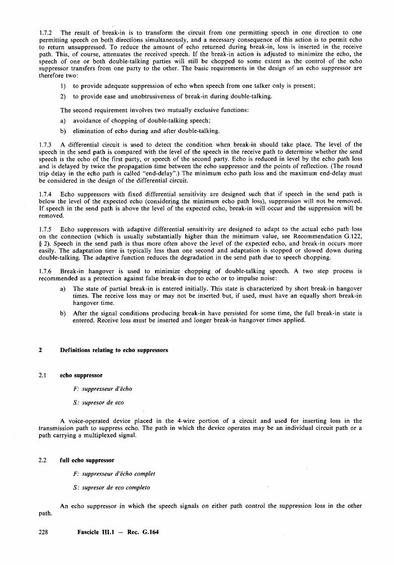
1.7.2 The result of break-in is to transform the circuit from one permitting speech in one direction to one permitting speech on both directions simultaneously, and a necessary consequence of this action is to permit echo to return unsuppressed. To reduce the amount of echo returned during break-in, loss is inserted in the receive path. This, o f course, attenuates the received speech. If the break-in action is adjusted to minimize the echo, the speech of one or both double-talking parties will still be chopped to some extent as the control of the echo suppressor transfers from one party to the other. The basic requirements in the design of an echo suppressor are therefore two:
1) to provide adequate suppression of echo when speech from one talker only is present;
2) to provide ease and unobtrusiveness of break-in during double-talking.
The second requirement involves two mutually exclusive functions:
a) avoidance of chopping o f double-talking speech;
b) elimination of echo during and after double-talking.
1.7.3 A differential circuit is used to detect the condition when break-in should take place. The level of the speech in the send path is compared with the level o f the speech in the receive path to determine whether the send speech is the echo of the first party, or speech of the second party. Echo is reduced in level by the echo path loss and is delayed by twice the propagation time between the echo suppressor and the points of reflection. (The round trip delay in the echo path is called “end-delay”.) The minimum echo path loss and the maximum end-delay must be considered in the design of the differential circuit.
1.7.4 Echo suppressors with fixed differential sensitivity are designed such that if speech in the send path is below the level of the expected echo (considering the minimum echo path loss), suppression will not be removed. If speech in the send path is above the level of the expected echo, break-in will occur and the suppression will be removed.
1.7.5 Echo suppressors with adaptive differential sensitivity are designed to adapt to the actual echo path loss on the connection (which is usually substantially higher than the minimum value, see Recommendation G.122, § 2). Speech in the send path is thus more often above the level of the expected echo, and break-in occurs more easily. The adaptation time is typically less than one second and adaptation is stopped or slowed down during double-talking. The adaptive function reduces the degradation in the send path due to speech chopping.
1.7.6 Break-in hangover is used to minimize chopping of double-talking speech. A two step process is recommended as a protection against false break-in due to echo or to impulse noise:
a) The state of partial break-in is entered initially. This state is characterized by short break-in hangover times. The receive loss may or may not be inserted but, if used, must have an equally short break-in hangover time.
b) After the signal conditions producing break-in have persisted for some time, the full break-in state is entered. Receive loss must be inserted and longer break-in hangover times applied.
2 Definitions relating to echo suppressors
2.1 echo suppressor
F: suppresseur d ’echo
S : supresor de eco
A voice-operated device placed in the 4-wire portion of a circuit and used for inserting loss in the transmission path to suppress echo. The path in which the device operates may be an individual circuit path or a path carrying a multiplexed signal.
2.2 full echo suppressor
F: suppresseur d ’echo com plet
S : supresor de eco com pleto
An echo suppressor in which the speech signals on either path control the suppression loss in the otherpath.
228 Fascicle III.l — Rec. G.164
2.3 half-echo suppressor
F: demi-suppresseur d ’echo
S: semisupresor de eco
An echo suppressor in which the speech signals of one path control the suppression loss in the other path but in which this action is not reciprocal.
2.4 differential echo suppressor
F: suppresseur d ’echo differentiel
S: supresor de eco diferencial
An echo suppressor whose operation is controlled by the difference in level between the signals on the two speech paths.
2.5 partial break-in echo suppressor
F: suppresseur d ’echo a intervention partielle
S: supresor de eco con intervencidn parcial
An echo suppressor which includes partial and full break-in functions.
2.6 adaptive break-in echo suppressor
F: suppresseur d ’echo a intervention adaptable
S: supresor de eco con intervencidn adaptativa
An echo suppressor in which the break-in differential sensitivity is automatically adjusted according to the attenuation of the echo path.
2.7 suppression loss
F: affaiblissement de blocage
S: atenuacion para la supresion
The specified minimum loss which an echo suppressor introduces into the send path (of the echo suppressor) to reduce the effect o f echo currents.
2.8 receive loss
F: affaiblissement a la reception
S: atenuacion en la recepcion
The specified loss which an echo suppressor introduces into the receive path (of the echo suppressor) to reduce the effect o f echo currents during break-in.
2.9 terminal echo suppressor (see Figure 5/G.164)
F: suppresseur d ’echo terminal
S: supresor de eco terminal
An echo suppressor designed for operation at one or both terminals o f a circuit.
2.10 suppression operate time
F: temps de fonctionnement pour le blocage
S: tiempo de funcionamiento para la supresidn
The time interval between the instant when defined test signals, applied to the send- an d /o r receive-in ports, are altered in a defined m anner and the instant when the suppression loss is introduced into the send path of the echo suppressor.
Fascicle III.l — Rec. G.164 229
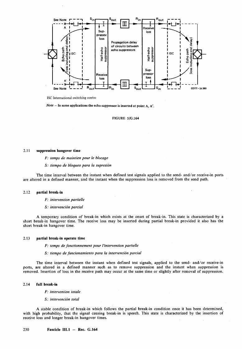
See Note r~ T * - H _ b
See N o t e ----------- 'out
Suppressor
loss
-C M0<p 0)*2 a (0 Q.1 2
Receiveloss
'outIE
Propagation delay of circuits between echo suppressors
Ri, m'out
Receiveloss
O <s><p 0)a re Q.
X 2
Suppressor
loss
’out
ISC S SI 7 \ 1 _Q. cn r > ---o E V Vc. "o V
C C IT T - 2 4 3 9 0
ISC International switching centre
Note — In some applications the echo suppressor is inserted at point A, A'.
FIGURE 5/G.164
2.11 suppression hangover time
F: temps de maintien pour le blocage
S: tiempo de bloqueo para la supresion
The time interval between the instant when defined test signals applied to the send- an d /o r receive-in ports are altered in a defined manner, and the instant when the suppression loss is removed from the send path.
2.12 partial break-in
F: intervention partielle
S: intervencidn parcial
A temporary condition of break-in which exists at the onset of break-in. This state is characterized by a short break-in hangover time. The receive loss may be inserted during partial break-in provided it also has the short break-in hangover time.
2.13 partial break-in operate time
F: temps de fonctionnement pour Vintervention partielle
S: tiempo de funcionamiento para la intervencidn parcial
The time interval between the instant when defined test signals, applied to the send- an d /o r receive-in ports, are altered in a defined m anner such as to remove suppression and the instant when suppression isremoved. Insertion of loss in the receive path may occur at the same time or slightly after removal of suppression.
2.14 full break-in
F: intervention totale
S: intervencidn total
A stable condition of break-in which follows the partial break-in condition once it has been determined, with high probability, that the signal causing break-in is speech. This state is characterized by the insertion of receive loss and longer break-in hangover times.
230 Fascicle III.l — Rec. G.164
2.15 full break-in operate time
F: temps de fonctionnement pour I’intervention totale
S: tiempo de funcionamiento para la intervencidn total
The time interval between the instant when defined test signals, applied to the send- an d /o r receive-inports, are altered in a defined m anner such as to remove suppression and extend the hangover time and theinstant when the extended hangover time is applied. Removal of suppression occurs at the same time as for partial break-in. Insertion of loss in the receive path may occur at the same time or slightly after removal of suppression.
2.16 break-in hangover time
F: temps de maintien pour I’intervention
S: tiempo de bloqueo para la intervencidn
The time interval between the instant when defined test signals, applied to the send- a n d /o r receive-inports, are altered in a defined m anner such as to restore suppression and the instant when suppression is restored.The hangover time for removal of loss in the receive path may be longer than that for restoration of suppression.
2.17 differential sensitivity
F: sensibilite differentielle
S: sensibilidad diferencial
The difference, in dB, between the relative level of the test signals applied to the send path and receive path when break-in occurs.
3 Characteristics of echo suppressors with fixed break-in differential sensitivity
3.1 Transmission performance
The performance characteristics apply, unless otherwise noted, when steady state signals are separately applied to the send and receive paths.
The limits on transmission characteristics specified below shall be observed over the temperature range + 10°C to 40 °C and over the power supply variations permitted by individual Administrations.
Echo suppressors of Types A, B and D are placed in the voice-frequency portion of a 4-wire circuit which is nominally of 600-ohms impedance. The send (transmit or office-to-line) and the receive (line-to-office) paths are at different relative levels in different national networks; two such sets of levels are:
1) send, —16 dBr; receive, + 7 dBr;2) send, —4 dBr; receive, + 4 dBr.
Test tone frequencies are 800 Hz or 1000 Hz, nominal. To avoid submultiples of the 8000-Hz sampling frequency, test tone frequencies should fall within the ranges 804 to 860 Hz and 1004 to 1020 Hz respectively.
3.1.1 Type A and B echo suppressors
3.1.1.1 Insertion loss
The insertion loss at 800 Hz (or 1000 Hz) of an echo suppressor in an unoperated condition shall be0 ± 0.3 dB, for test tone levels < 0 dBmO.
3.1.1.2 Attenuation distortion
The attenuation distortion shall be such that if Q dB is the loss at 800 Hz (or 1000 Hz), the loss shall bewithin the range (Q + 0.3) dB to (Q — 0.2) dB at any frequency in the band 300-3400 Hz, and at 200 Hz withinthe range of (Q + 1.0) dB to (Q — 0.2) dB.
3.1.1.3 Delay distortion
The delay distortion shall not exceed 30 ps measured between any two frequencies in the band 1000-2400 Hz and 60 ps in the band 500-3000 Hz.
Fascicle III.l — Rec. G.164 231
3.1.1.4 Impedance
The values of impedance and return loss shall apply to all states of operation of the echo suppressors.1) The nominal value of the inputs and outputs shall be 600 ohms (nonreactive).2) The return loss with respect to the nominal impedance shall not be less than 20 dB from 300-600 Hz
nor less than 25 dB from 600-3400 Hz.3) The impedance unbalance to earth of each port shall not be less than 50 dB over the frequency range
300 to 3400 Hz.
3.1.1.5 Overload
The insertion loss at 800 Hz (or 1000 Hz) shall not increase by more than 0.2 dB for test tone levels from 0 to + 5.0 dBmO.
3.1.1.6 Harmonic distortion
The total harmonic distortion power, for a pure 800 Hz (or 1000 Hz) sine wave at a level of 0 dBmO, shall not exceed — 34 dBmO.
3.1.1.7 Intermodulation
For frequencies f = 900 Hz and f 2 .= 1020 Hz applied simultaneously each at a level o f —5 dBmO, the difference between the output levels o f either frequency f x or f 2 and the level of either of the intermodulation products at (2 fx — f 2) or (2f 2 — f ) should be at least 45 dB. When speech compressors are used to provide loss during break-in, this requirement is reduced during the break-in mode to 26 dB for the receive path (W-state receive path).
3.1.1.8 Transient response
I f loss devices which are inserted in the receive path operate at a syllabic rate, the transient performance of such devices should conform to Recommendation G.162 which deals with the overall transient response of compandors.
3.1.1.9 Noise
The mean weighted psophometric power introduced by an echo suppressor shall not exceed —70 dBmOp. The mean unweighted noise power in a band of 300-3400 Hz introduced by an echo suppressor shall not exceed — 50 dBmO.
3.1.1.10 Crosstalk
When an echo suppressor is installed in a working circuit, the crosstalk attenuation between the send path and the receive path (and conversely) shall be such that the signal power in the disturbed path due to crosstalk from the disturbing path shall not exceed —65 dBmO for any sinusoidal signal in the disturbing path having a power of + 5 dBmO or less and within the band 300-3400 Hz.
3.1.1.11 Spurious outputs produced by the echo suppressor
The various operations of the echo suppressor must not result in any appreciable spurious outputs such as internally generated impulses due to transient conditions. In particular these must not be of such magnitude as would be likely to falsely operate the suppression or break-in feature of any other echo suppressor that might be in the connection. Consideration must include that of multilink connections having several pairs of echo suppressors in tandem.
To prevent false operation of other echo suppressors in a built-up connection, the zero-to-peak voltage o f ’ any transient output produced in the receive or transmit paths (terminated in 600 ohms) due to echo suppressor operation caused by signals in the opposite path should not exceed 20 mV at a point of zero relative level ( — 34 dBVO) after first filtering the transient to a 500 to 3000 Hz bandwidth. Additionally, the duration of any such transient should be such that it is not audible in the presence of normal levels of noise (e.g. —50 dBmOp).
232 Fascicle III.l - Rec. G.164
3.1.2 Type C echo suppressor
3.1.2.1 General
An echo suppressor of Type C inserted into a digital transmission path between codecs meeting the performance characteristics of Recommendation G .712 [3] should not alter such performance.
3.1.2.2 Group delay
The group delay through the echo suppressor shall not exceed 0.25 ms.
3.1.2.3 Effect o f digital loss pads
Digital loss pads inserted into the receive path during the break-in mode may increase the quantizing distortion. Type C echo suppressors, which maintain signalling bit integrity for channel associated signalling for systems in accordance with Recommendation G.733 [4] by bypassing the least significant bit, are likely to exhibit a greater increase in quantizing distortion during the break-in mode than Type C echo suppressors used in systems with common channel signalling. See Footnote c) to Table 1/G. 164.
3.1.2.4 Effect o f instantaneous digital compressors
When an instantaneous compressor is employed in the receive path of the suppressor during break-in, it shall not produce distortion exceeding the following limits:
a) Harmonic distortionWith a sinusoidal input signal of 0 dBmO at any frequency between 300 Hz and 1 KHz, the third harmonic distortion produced should not exceed —30 dBmO.
b) Intermodulation distortionWith an input signal of two equal amplitude sinusoids at f = 900 and f 2 = 1020 Hz at levels of —3 to —35 dBmO, the distortion products at (2f — f 2) and (2f2 — f ) should not exceed a level of —16 dB relative to the output level of each tone. For input levels below —35 dBmO this ratio should be at least — 20 dB.
3.1.3 Type D echo suppressors
3.1.3.1 General
The performance characteristics of Recommendation G .712 [3] apply for the codecs.
3.1.3.2 Group delay
The group delay shall not exceed that of the codecs alone by more than 0.25 ms.
3.1.3.3 Effect o f digital loss pads
Digital loss pads inserted into the receive path during the break-in mode may increase the quantization distortion over the limits specified in Recommendation G.712 [3]. See Footnote c) to Table 1/G.164.
3.1.3.4 Effect o f instantaneous digital compressors
See § 3.1.2.4.
3.2 Characteristics with steady-state input signals applied independently to the send and receive paths
3.2.1 The action of an echo suppressor with fixed differential sensitivity which incorporates the general features described in § 1 is explained below with the aid of the idealized operational diagram shown in Figure 6/G.164. The significant combinations of input signals are represented by the areas X, Y, Z, W and V.
Fascicle III.l - Rec. G.164 233
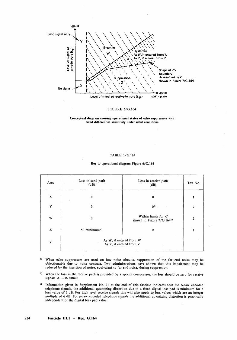
dBmO
FIG URE 6/G.164
Conceptual diagram showing operational states of echo suppressors with fixed differential sensitivity under ideal conditions
TABLE 1/G . 164
Key to operational diagram Figure 6/G.164
Area Loss in send path (dB)
Loss in receive path (dB) Test No.
X 0 0 1
Y 0 0 b> 2
W 0 Within limits for C shown in Figure 7 /G .164c) 2
Z 50 m inim um a) 0 1
V As W, if entered from W As Z, if entered from Z
a) When echo suppressors are used on low noise circuits, suppression of the far end noise may be objectionable due to noise contrast. Two administrations have shown that this impairment may be reduced by the insertion of noise, equivalent to far end noise, during suppression.
b) When the loss in the receive path is provided by a speech compressor, the loss should be zero for receive signals < — 36 dBmO.
c) Information given in Supplement No. 21 at the end of this fascicle indicates that for A-law encoded telephone signals, the additional quantizing distortion due to a fixed digital loss pad is minimum for a loss value of 6 dB. For high level receive signals this will also apply to loss values which are an integer multiple of 6 dB. For p-law encoded telephone signals the additional quantizing distortion is practically independent of the digital loss pad value.
Fascicle III.l - Rec. G.164
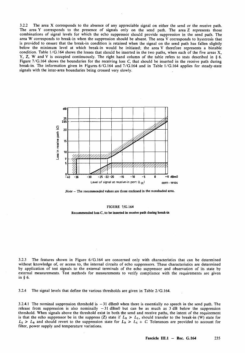
3.2.2 The area X corresponds to the absence of any appreciable signal on either the send or the receive path. The area Y corresponds to the presence of signals only on the send path. The area Z represents those combinations of signal levels for which the echo suppressor should provide suppression in the send path. The area W corresponds to break-in when the suppression should be absent. The area V corresponds to hysteresis that is provided to ensure that the break-in condition is retained when the signal on the send path has fallen slightly below the minimum level at which break-in would be initiated; the area V therefore represents a bistable condition. Table 1/G . 164 shows the losses that should be inserted in the two paths, when each of the five areas X, Y, Z, W and V is occupied continuously. The right hand column of the table refers to tests described in § 6. Figure 7/G.164 shows the boundaries for the receiving loss C, that should be inserted in the receive path during break-in. The information given in Figures 6/G .164 and 7/G.164 and in Table 1/G . 164 applies for steady-state signals with the inter-area boundaries being crossed very slowly.
dB
2523.5
~ 20 £(0a .0)> 158O)£ 103o-J 7
----- ^\\Y\ J
M S
1
nW
-40 -36 - 30 - 25 -22 -20 -15 -10 - 5 0 + 6 dBmO
Level o f signal a t receive-in p o rt (L p ) ccitt- 18524
Note - The recommended values are those enclosed in the nonshaded area.
FIGURE 7/G.164
Recommended loss C, to be inserted in receive path during break-in
3.2.3 The features shown in Figure 6/G.164 are concerned only with characteristics that can be determined without knowledge of, or access to, the internal circuits of echo suppressors. These characteristics are determined by application of test signals to the external terminals of the echo suppressor and observation of its state by external measurements. Test methods for measurements to verify compliance with the requirements are given in § 6.
3.2.4 The signal levels that define the various thresholds are given in Table 2 /G .l64.
3.2.4.1 The nominal suppression threshold is —31 dBmO when there is essentially no speech in the send path. The release from suppression is also nominally —31 dBmO but can be as much as 3 dB below the suppression threshold. When signals above the threshold exist in both the send and receive paths, the intent of the requirement is that the echo suppressor be in the suppress (Z) state if L R > L s , should transfer to the break-in (W) state for L s > L R and should revert to the suppression state for L R > L s + C. Tolerances are provided to account for filter, power supply and temperature variations.
Fascicle III.l - Rec. G.164 235
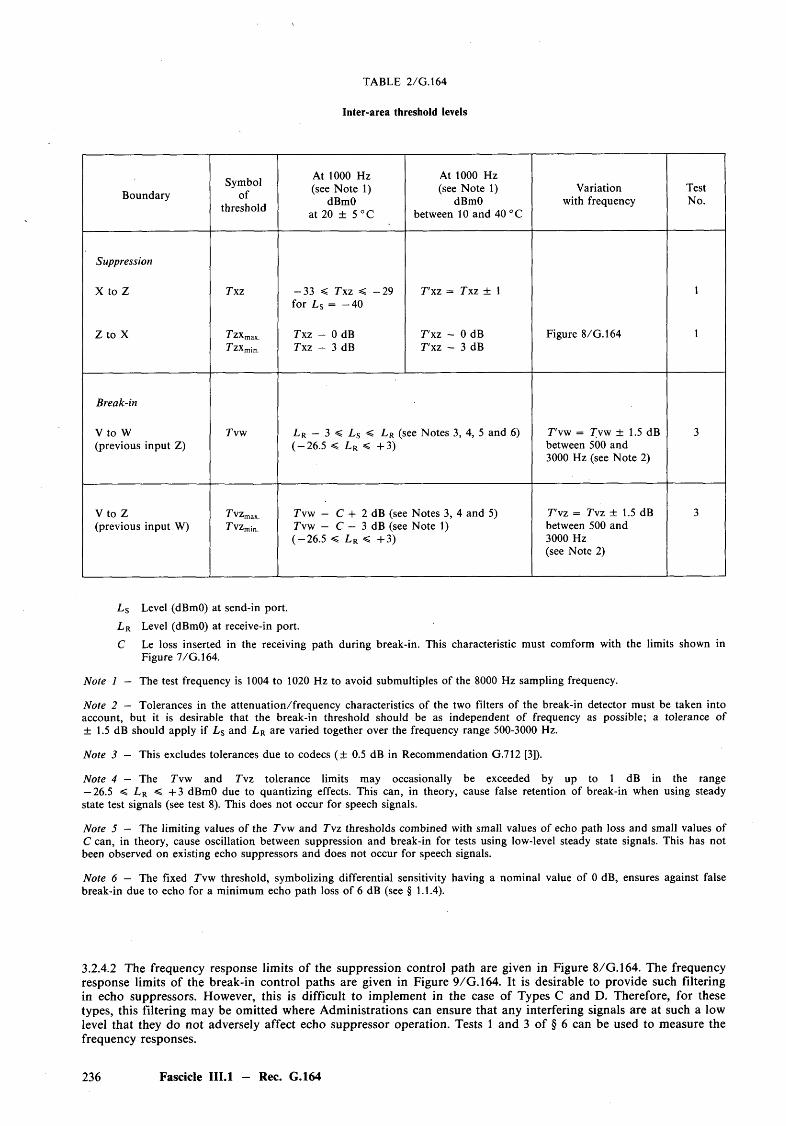
TABLE 2/G.164
Inter-area threshold levels
BoundarySymbol
ofthreshold
At 1000 Hz (see Note 1)
dBmO at 20 ± 5 °C
At 1000 Hz (see Note 1)
dBmO between 10 and 40 °C
Variation with frequency
TestNo.
Suppression
X to Z Tx z - 3 3 < Txz < - 2 9 for L s = - 4 0
T'xz = Txz ± 1 1
Z to X TzxmaxT ZXmin.
Txz — 0 dB Txz — 3 dB
T'xz — 0 dB T'xz — 3 dB
Figure 8/G.164 1
Break-in
V to W(previous input Z)
Tv W L r — 3 < L s < L r (see Notes 3, 4, 5 and 6) (-2 6 .5 < L r < + 3)
T'vw = Tvw ± 1.5 dB between 500 and 3000 Hz (see Note 2)
3
V to Z(previous input W)
T vzmax Tvzmjn
Tvw — C -1- 2 dB (see Notes 3, 4 and 5) Tvw — C — 3 dB (see Note 1)( — 26.5 ^ L r ^ + 3)
T'vz = Tvz ± 1.5 dB between 500 and 3000 Hz (see Note 2)
3
Ls Level (dBmO) at send-in port.
L r Level (dBmO) at receive-in port.
C Le loss inserted in the receiving path during break-in. This characteristic must comform with the limits shown in Figure 7/G.164.
Note 1 — The test frequency is 1004 to 1020 Hz to avoid submultiples of the 8000 Hz sampling frequency.
Note 2 — Tolerances in the attenuation/frequency characteristics of the two filters of the break-in detector must be taken into account, but it is desirable that the break-in threshold should be as independent of frequency as possible; a tolerance of± 1.5 dB should apply if L s and L R are varied together over the frequency range 500-3000 Hz.
Note 3 — This excludes tolerances due to codecs (± 0.5 dB in Recommendation G .712 [3]).
Note 4 — The Tvw and Tvz tolerance limits may occasionally be exceeded by up to 1 dB in the range— 26.5 < L r < + 3 dBmO due to quantizing effects. This can, in theory, cause false retention of break-in when using steadystate test signals (see test 8). This does not occur for speech signals.
Note 5 — The limiting values of the Tvw and T vz thresholds combined with small values of echo path loss and small values of C can, in theory, cause oscillation between suppression and break-in for tests using low-level steady state signals. This has not been observed on existing echo suppressors and does not occur for speech signals.
Note 6 — The fixed T vw threshold, symbolizing differential sensitivity having a nominal value of 0 dB, ensures against false break-in due to echo for a minimum echo path loss of 6 dB (see § 1.1.4).
3.2.4.2 The frequency response limits o f the suppression control path are given in Figure 8/G.164. The frequency response limits o f the break-in control paths are given in Figure 9/G.164. It is desirable to provide such filtering in echo suppressors. However, this is difficult to implement in the case of Types C and D. Therefore, for these types, this filtering may be omitted where Administrations can ensure that any interfering signals are at such a low level that they do not adversely affect echo suppressor operation. Tests 1 and 3 of § 6 can be used to measure the frequency responses.
236 Fascicle III.l - Rec. G.164
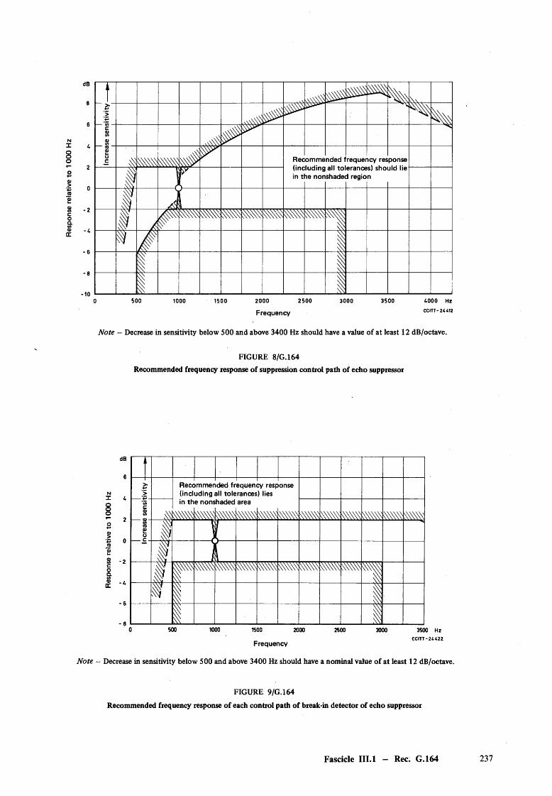
Resp
onse
re
lative
to
1000
H
z
dB
8
- 2
t s \ \ M. naV sX
%£>
c0)(A0)
\ #CO0)oc Rec
(inc in t
omme luding le non
nded f all to shadei
requer erance 1 regio
icy res s) sho n
ponse Li Id lie
1r
1V-
Aj
i
1 V
m s S M M S
1
1 11 1-10
500 1000 1500 2000 2500
Frequency3000 3500 4000 Hz
CCITT-24412
Note - Decrease in sensitivity below 500 and above 3400 Hz should have a value of at least 12 dB/octave.
FIGURE 8/G.164
Recommended frequency response of suppression control path of echo suppressor
-2
- 4
>4-»>
Recc (incl in th
immer uding e nons
ded fr all tole haded
km
equenraneesarea
k\\\\\cy resp ) lies
1*
onse
km*35c0)</> m m\N m$£o 1 J
11 r m WM* m m m m I
1 !i I
500 1000 1500 2000
Frequency
2500 3000 3500 Hz CCITT-2 4 422
Note - Decrease in sensitivity below 500 and above 3400 Hz should have a nominal value of at least 12 dB/octave.
FIGURE 9/G.164
Recommended frequency response of each control path of break-in detector of echo suppressor
Fascicle 1II.1 — Rec. G.164 237
3.3 Dynamic characteristics when signals are applied, removed or changed in the send and receive paths independently
3.3.1 The dynamic characteristics can be specified by stating the time that elapses when the conditions of the signals pass from a point in one area to one in another before the state appropriate to the second area is established (Figure 12 /G .l64 and Figure 11/G.164). When passing from X to Z, this is termed the suppression operate time and when passing in the opposite direction it is termed suppression hangover time. When passing from the Z area through V to W (or Y) it is termed the break-in operate time and when passing from W through V to Z it is termed the break-in hangover time. The V /W and V /Z boundaries may, in practice, be crossed at any angle; the requirements in Table 3/G.164 deal with vertical and horizontal directions.
3.3.2 The suppression (X /Z ) operate time should be nearly constant for the sudden application of any signal in the receive path greater than the threshold ( — 31 dBmO) in the absence of any appreciable signal in the send path. Similarly, for transitions from suppression to break-in for L R constant (Z /V /W ), the operate times shown in Table 3/G.164 should in general apply to the complete range of possible signal pairs (L R and L s ) and not just to the two pairs shown in Table 3/G.164.
3.3.3 The hangover times shown in Table 4/G .164 should in general apply whenever suppression or break-in has occurred irrespective of the levels of the causative signals.
3.3.4 When sudden changes are made in the levels of sinusoidal test signals at a frequency of 1000 Hz, the times of operation given in Table 3/G .164 apply and the recommended values of hangover given in Table 4/G.164 apply. The right-hand part o f each table refers to tests described in § 6.
3.3.5 The operate times of the receive pad in the Y /W transition is not separately stated or tested, but should be ' within the limits allowed for the suppression operate time.
3.4 Performance under conditions o f small echo-path loss and when end-delay may be present
The foregoing requirements apply when the echo suppressor is tested under conditions such that the signals in the send and receive paths are independent. In practice, satisfactory performance must also be maintained when the send path is connected to the receive path through an echo path that may have end-delay and low loss. Three features of the dynamic performance must be checked under these conditions. § 6 describes test arrangements suitable for measuring these conditions. The three conditions are described as follows:
3.4.1 An echo (leakage through the echo path) must not cause false operation of the break-in condition when the echo-path loss is low and the end-delay is zero. The trouble could be caused by inappropriate design of the control path time constants. When a signal is suddenly applied to R m, this trouble would show itself as a tem porary false operation of the break-in condition, persisting for the duration of the break-in hangover time (see Test No. 7).
3.4.2 If insufficient protection against end-delay is incorporated in the echo suppressor, the break-in circuit may operate on the trailing edge of the echo. This can occur with the sudden removal of a signal at R\n when the echo-path loss is low and the end-delay is large (see Test No. 7).
3.4.3 In certain designs it can happen that the hysteresis represented by the bistable area V (see Figure 6/G.164) is excessive in relation to the am ount of loss inserted in the receive path. This can result in the false retention of break-in by echo occurring under the following conditions: A steady-state signal is present at Rj„ port and is coupled to Si„ port via the echo path. A signal o f sufficient amplitude and duration to cause break-in is then applied to Sin port. Upon cessation of this signal, the echo of the receive signal falsely maintains the break-in condition (see Test No. 8).
238 Fascicle III.l - Rec. G.164
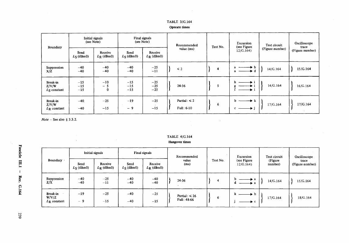
Fascicle III.l
— Rec.
G.164 239
TABLE 3/G.164 Operate times
Boundary
Initial signals (see Note)
Final signals (see Note)
Recommended value (ms) Test No.
Excursion (see Figure 12/G.164)
Test circuit (Figure number)
Oscilloscope trace
(Figure number)Send Lg (dBmO)
Receive Lr (dBmO)
Send L s (dBmO)
Receive Lr (dBmO)
SuppressionX/Z
-4 0-4 0
-4 0-4 0
-4 0-4 0
-2 5-1 1 } <2 > 4
a ---------- ► ba ---------- ► d | 14/G.164 | 15/G.164
Break-inz/v/wL$ constant
-1 5-1 5-1 5
-1 0- 5
0
-1 5-1 5-1 5
-2 5-2 5-2 5
J 24-36 1 5
h -— ---- ► ig ---------- ► if ---------- ► i
J 14/G.164 J 16/G.164
Break-in Z/V/W Lr constant
-4 0
-4 0
-2 5
-1 5
-1 9
- 9
-2 5
-1 5
| Partial: < 2
/ Full: 6-10 1 6
b ---------- ► k
c ---------- ► jJ 17/G.164 | 17/G.164
Note - See also § 3.3.2.
TABLE 4/G.164 Hangover times
Boundary •
Initial signals Final signalsRecommended
value(ms)
Test No.Excursion (see Figure 12/G.l 64)
Test circuit (Figure
number)
Oscilloscope trace
(Figure number)Send L s (dBmO)
Receive L r (dBmO)
Send L s (dBmO)
Receive L r (dBmO)
SuppressionZ/X
-4 0-4 0
-2 5-11
-4 0-4 0
-4 0-4 0 } 24-36 > 4
b ---------- ^ ad ----------^ a J 14/G.164 J 15/G.164
Break-inw/v/zL r constant
-1 9
- 9
-2 5
-1 5
-4 0
-4 0
-2 5
-1 51 Partial: < 26 | Full: 48-66 1 6
k ---------- b
j ----------► cJ 17/G.164 | 18/G.164
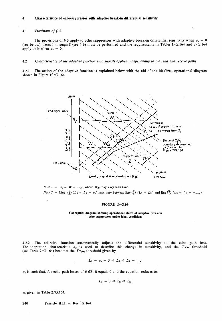
4 Characteristics of echo-suppressor with adaptive break-in differential sensitivity
4.1 Provisions o f § 3
The provisions of § 3 apply to echo suppressors with adaptive break-in differential sensitivity when ax — 0 (see below). Tests 1 through 8 (see § 6) must be performed and the requirements in Tables 1/G . 164 and 2 /G .l64 apply only when ax = 0.
4.2 Characteristics o f the adaptive function with signals applied independently to the send and receive paths
4.2.1 The action of the adaptive function is explained below with the aid of the idealized operational diagramshown in Figure 10/G.164.
dBmO
Note 1 — Wj = W + WAi, where WAi may vary with time
Note 2 — Line (7) (L s = L R — ax) may vary between line ( I ) (L s = L R) and line (2) (L s = L R — axmax)-
FIG URE 10/G.164
Conceptual diagram showing operational states of adaptive break-in echo suppressors under ideal conditions
4.2.2 The adaptive function automatically adjusts the differential sensitivity to the echo path loss. The adaptation characteristic ax is used to describe this change in sensitivity, and the T v w threshold (see Table 2 /G .l64) becomes the T v jWj threshold given by
LR — ax — 3 < Ls < Lr — ax,
ax is such that, for echo path losses of 6 dB, it equals 0 and the equation reduces to:
L r — 3 ^ L s < L r
as given in Table 2 /G .l64.
240 Fascicle III.l — Rec. G.164
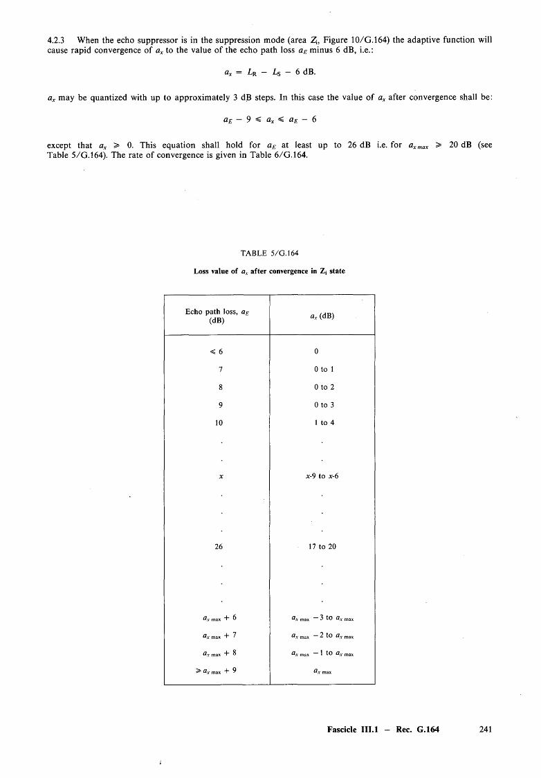
4.2.3 When the echo suppressor is in the suppression mode (area Zi, Figure 10/G.164) the adaptive function willcause rapid convergence of ax to the value of the echo path loss aE minus 6 dB, i.e.:
clx = .Lr — Ls — 6 dB.
ax may be quantized with up to approximately 3 dB steps. In this case the value of ax after convergence shall be:
aE - 9 < ax < aE - 6
except that ax > 0. This equation shall hold for aE at least up to 26 dB i.e. for axmax > 20 dB (seeTable 5/G.164). The rate of convergence is given in Table 6/G.164.
TABLE 5/G.164
Loss value of ax after convergence in Zj state
Echo path loss, aE (dB) a , (dB)
< 6 0
7 0 to 1
8 0 to 2
9 0 to 3
10 1 to 4
X x-9 to x-6
26 17 to 20
dx m ax + 6 dx m ax 3 tO Qx m ax
&x m ax + 7 dx m ax — 2 tO dx max
dx m ax + 8 dx max 1 tO Clx max
> dx m ax + 9 dx max
Fascicle II1.1 - Rec. G.164 241
i
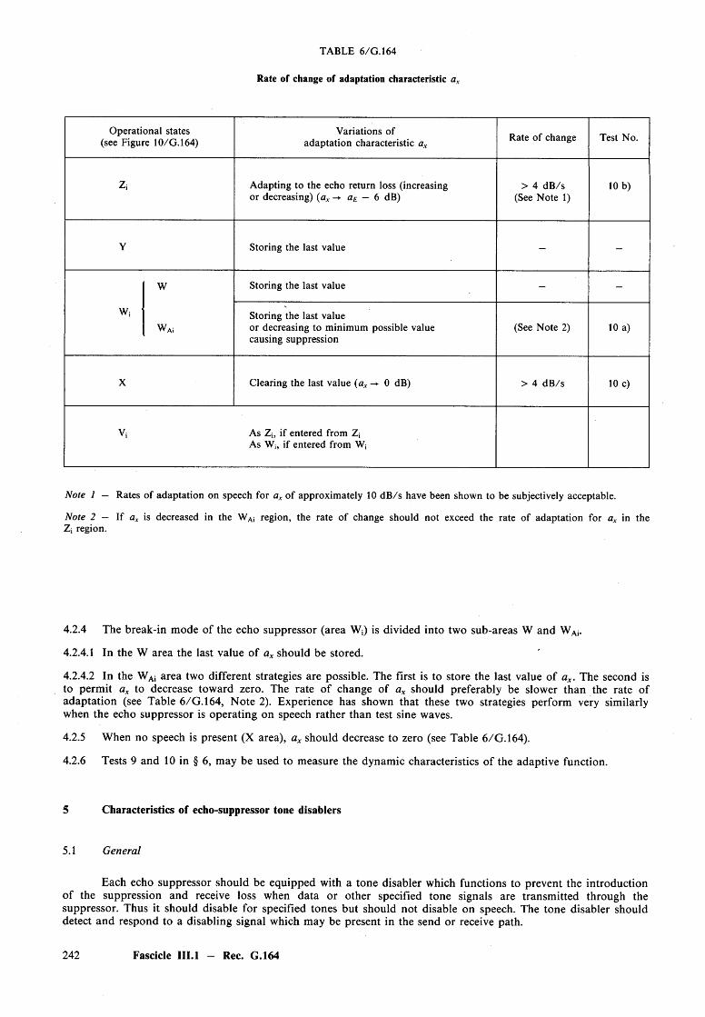
TABLE 6/G.164
Rate of change of adaptation characteristic ax
Operational states (see Figure 10/G.164)
Variations of adaptation characteristic ax Rate of change Test No.
Zi Adapting to the echo return loss (increasing or decreasing) (ax -► aE — 6 dB)
> 4 dB /s (See Note 1)
10 b)
Y Storing the last value - -
W Storing the last value - -
WiwAi
Storing the last valueor decreasing to minimum possible valuecausing suppression
(See Note 2) 10 a)
X Clearing the last value (ax -► 0 dB) > 4 dB /s 10 c)
V; As Zi, if entered from ZjAs Wi, if entered from W;
Note 1 — Rates of adaptation on speech for ax of approximately 10 dB /s have been shown to be subjectively acceptable.
Note 2 — If ax is decreased in the WAi region, the rate of change should not exceed the rate of adaptation for ax in the Z, region.
4.2.4 The break-in mode of the echo suppressor (area Wj) is divided into two sub-areas W and WAj.
4.2.4.1 In the W area the last value of ax should be stored.
4.2.4.2 In the WAi area two different strategies are possible. The first is to store the last value of ax. The second isto permit ax to decrease toward zero. The rate of change of ax should preferably be slower than the rate ofadaptation (see Table 6/G.164, Note 2). Experience has shown that these two strategies perform very similarlywhen the echo suppressor is operating on speech rather than test sine waves.
4.2.5 When no speech is present (X area), ax should decrease to zero (see Table 6/G.164).
4.2.6 Tests 9 and 10 in § 6, may be used to measure the dynamic characteristics of the adaptive function.
5 Characteristics of echo-suppressor tone disablers
5.1 General
Each echo suppressor should be equipped with a tone disabler which functions to prevent the introduction of the suppression and receive loss when data or other specified tone signals are transmitted through the suppressor. Thus it should disable for specified tones but should not disable on speech. The tone disabler should detect and respond to a disabling signal which may be present in the send or receive path.
242 Fascicle III.l — Rec. G.164
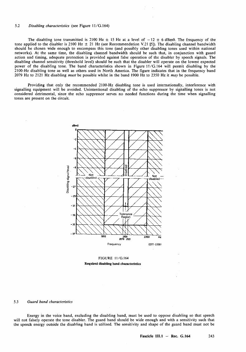
5.2 Disabling characteristics (see Figure 11/G.164)
The disabling tone transmitted is 2100 Hz ± 15 Hz at a level of —12 ± 6 dBmO. The frequency of the tone applied to the disabler is 2100 Hz ± 21 Hz (see Recommendation V.21 [5]). The disabling channel bandwidth should be chosen wide enough to encompass this tone (and possibly other disabling tones used within national networks). At the same time, the disabling channel bandwidth should be such that, in conjunction with guard action and timing, adequate protection is provided against false operation of the disabler by speech signals. The disabling channel sensitivity (threshold level) should be such that the disabler will operate on the lowest expected power of the disabling tone. The band characteristics shown in Figure 11/G .164 will permit disabling by the 2100-Hz disabling tone as well as others used in North America. The figure indicates that in the frequency band 2079 Hz to 2121 Hz disabling must be possible whilst in the band 1900 Hz to 2350 Hz it may be possible.
Providing that only the recommended 2100-Hz disabling tone is used internationally, interference with signalling equipment will be avoided. Unintentional disabling of the echo suppressor by signalling tones is not considered detrimental, since the echo suppressor serves no needed functions during the time when signalling tones are present on the circuit.
dBmO
2079 2121
F r e q u e n c y CCITT-33081
FIG URE 11/G.164
Required disabling band characteristics
5.3 Guard band characteristics
Energy in the voice band, excluding the disabling band, must be used to oppose disabling so that speech will not falsely operate the tone disabler. The guard band should be wide enough and with a sensitivity such that the speech energy outside the disabling band is utilized. The sensitivity and shape of the guard band must not be
Fascicle III.l - Rec. G.164 243
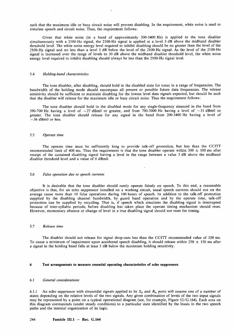
such that the maximum idle or busy circuit noise will prevent disabling. In the requirement, white noise is used to simulate speech and circuit noise. Thus, the requirement follows:
Given that white noise (in a band of approximately 300-3400 Hz) is applied to the tone disabler simultaneously with a 2100-Hz signal, the 2100-Hz signal is applied at a level 3 dB above the midband disabler threshold level. The white noise energy level required to inhibit disabling should be no greater than the level of the 2100-Hz signal and no less than a level 5 dB below the level of the 2100-Hz signal. As the level o f the 2100-Hz signal is increased over the range of levels to 30 dB above the midband disabler threshold level, the white noise energy level required to inhibit disabling should always be less than the 2100-Hz signal level.
5.4 Holding-band characteristics
The tone disabler, after disabling, should hold in the disabled state for tones in a range of frequencies. The bandwidth of the holding mode should encompass all present or possible future data frequencies. The release sensitivity should be sufficient to m aintain disabling for the lowest level data signals expected, but should be such that the disabler will release for the maximum idle or busy circuit noise. Thus the requirement follows:
The tone disabler should hold in the disabled mode for any single-frequency sinusoid in the band from 390-700 Hz having a level of —27 dBmO or greater, and from 700-3000 Hz having a level o f —31 dBmO or greater. The tone disabler should release for any signal in the band from 200-3400 Hz having a level of — 36 dBmO or less.
5.5 Operate time
The operate time must be sufficiently long to provide talk-off protection, but less than the CCITT recommended limit of 400 ms. Thus the requirement is that the tone disabler operate within 300 ± 100 ms after receipt of the sustained disabling signal having a level in the range between a value 3 dB above the midband disabler threshold level and a value of 0 dBmO.
5.6 False operation due to speech currents
It is desirable that the tone disabler should rarely operate falsely on speech. To this end, a reasonable objective is that, for an echo suppressor installed on a working circuit, usual speech currents should not on the average cause more than 10 false operations during 100 hours of speech. In addition to the talk-off protection supplied by the disabling channel bandwidth, by guard band operation and by the operate time, talk-off protection can be supplied by recycling. That is, if speech which simulates the disabling signal is interrupted because of inter-syllabic periods, before disabling has taken place the operate timing mechanism should reset. However, momentary absence or change of level in a true disabling signal should not reset the timing.
5.7 Release time
The disabler should not release for signal drop-outs less than the CCITT recommended value of 100 ms. To cause a minimum of impairment upon accidental speech disabling, it should release within 250 ± 150 ms after a signal in the holding band falls at least 3 dB below the maximum holding sensitivity.
6 Test arrangements to measure essential operating characteristics of echo suppressors
6.1 General considerations
6.1.1 An echo suppressor with sinusoidal signals applied to its S-m and Rin ports will assume one of a number of states depending on the relative levels of the two signals. Any given combination of levels of the two input signals may be represented by a point on a typical operational diagram (see, for example, Figure 12 /G .l64). Each area on this diagram corresponds (under steady conditions) to a particular state identified by the losses in the two speech paths and the internal organization of its logic.
244 Fascicle III.l — Rec. G.164
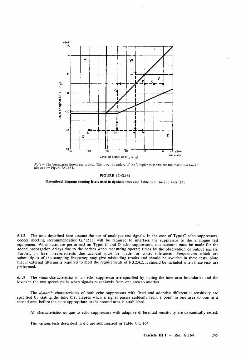
dBmO
Level o f signal a t R jn (LR ) c c t t - asozo
Note - The boundaries shown are typical. The lower boundary of the V region is shown for the maximum loss C allowed by Figure 7/G.164.
FIG URE 12 /G .l 64
Operational diagram showing levels used in dynamic tests (see Table 3/G .164 and 4/G.164)
6.1.2 The tests described here assume the use of analogue test signals. In the case of Type C echo suppressors, codecs meeting Recommendation G .712 [3] will be required to interface the suppressor to the analogue test equipment. When tests are performed on Types C and D echo suppressors, due account must be made for the added propagation delays due to the codecs when measuring operate times by the observation of output signals. Further, in level measurements due account must be made for codec tolerances. Frequencies which are submultiples of the sampling frequency may give misleading results and should be avoided in these tests. Note that if external filtering is required to meet the requirements of § 3.2.4.2, it should be included when these tests are performed.
6.1.3 The static characteristics of an echo suppressor are specified by stating the inter-area boundaries and the losses in the two speech paths when signals pass slowly from one area to another.
The dynamic characteristics of both echo suppressors with fixed and adaptive differential sensitivity are specified by stating the time that elapses when a signal passes suddenly from a point in one area to one in a second area before the state appropriate to the second area is established.
All characteristics unique to echo suppressors with adaptive differential sensitivity are dynamically tested.
The various tests described in § 6 are summarized in Table 7/G.164.
Fascicle III.1 - Rec. G.164 245
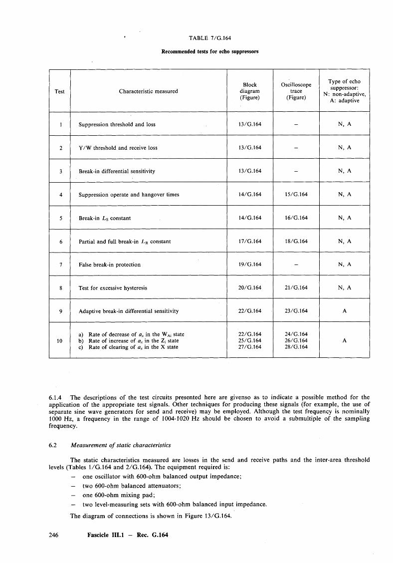
TABLE 7/G.164
Recommended tests for echo suppressors
Test Characteristic measuredBlock
diagram(Figure)
Oscilloscopetrace
(Figure)
Type of echo suppressor:
N: non-adaptive, A: adaptive
1 Suppression threshold and loss 13/G.164 - N, A
2 Y /W threshold and receive loss 13/G.164 - N, A
3 Break-in differential sensitivity 13/G.164 - N, A
4 Suppression operate and hangover times 14/G.164 15/G.164 N, A
5 Break-in L s constant 14/G.164 16/G.164 N, A
6 Partial and full break-in L R constant 17/G.164 18/G.164 N, A
7 False break-in protection 19/G.164 - N, A
8 Test for excessive hysteresis 20/G.164 21/G.164 N, A
9 Adaptive break-in differential sensitivity 22/G.164 23/G.164 A
10a) Rate of decrease of ax in the WAi stateb) Rate of increase of ax in the Zj statec) Rate of clearing of ax in the X state
22/G.16425/G.16427/G.164
24/G.16426/G.16428/G.164
A
6.1.4 The descriptions of the test circuits presented here are givenso as to indicate a possible method for theapplication of the appropriate test signals. Other techniques for producing these signals (for example, the use ofseparate sine wave generators for send and receive) may be employed. Although the test frequency is nominally 1000 Hz, a frequency in the range of 1004-1020 Hz should be chosen to avoid a submultiple of the sampling frequency.
6.2 Measurement o f static characteristics
The static characteristics measured are losses in the send and receive paths and the inter-area threshold levels (Tables 1/G . 164 and 2 /G .l64). The equipment required is:
— one oscillator with 600-ohm balanced output impedance;— two 600-ohm balanced attenuators;— one 600-ohm mixing pad;— two level-measuring sets with 600-ohm balanced input impedance.
The diagram of connections is shown in Figure 13/G.164.
246 Fascicle III.l — Rec. G.164
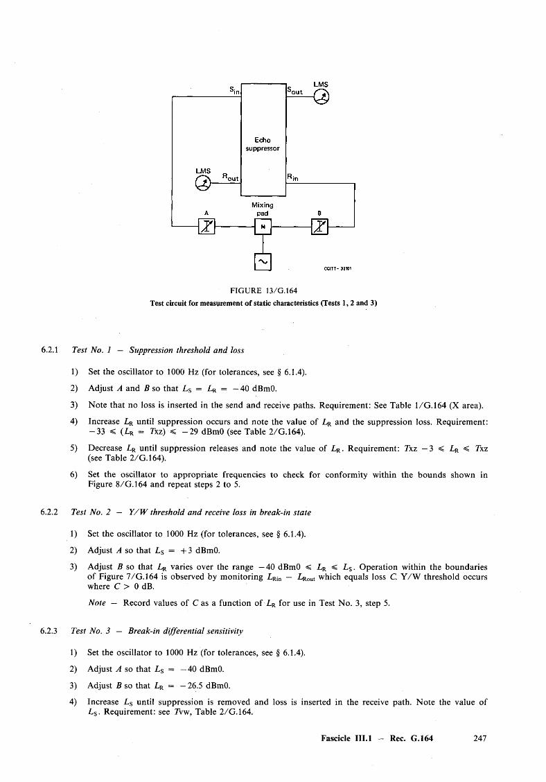
FIGURE 13/G.164
Test circuit for measurement of static characteristics (Tests 1 ,2 and 3)
6.2.1 Test No. 1 — Suppression threshold and loss
1) Set the oscillator to 1000 Hz (for tolerances, see § 6.1.4).
2) Adjust A and B so that Ls = LR = — 40 dBmO.
3) Note that no loss is inserted in the send and receive paths. Requirement: See Table 1/G . 164 (X area).
4) Increase LR until suppression occurs and note the value of LR and the suppression loss. Requirement: - 3 3 < (Lr = Txz) < - 2 9 dBmO (see Table 2/G.164).
5) Decrease LR until suppression releases and note the value of LR. Requirement: Txz —3 < LR < 7xz (see Table 2 /G .l64).
6) Set the oscillator to appropriate frequencies to check for conformity within the bounds shown in Figure 8/G.164 and repeat steps 2 to 5.
6.2.2 Test No. 2 — Y /W threshold and receive loss in break-in state
1) Set the oscillator to 1000 Hz (for tolerances, see § 6.1.4).
2) Adjust A so that L s = + 3 dBmO.
3) Adjust B so that LR varies over the range —40 dBmO < LR < L s . Operation within the boundariesof Figure 7/G.164 is observed by monitoring LRin — LRout which equals loss C. Y /W threshold occurswhere C > 0 dB.
Note — Record values of C as a function of LR for use in Test No. 3, step 5.
6.2.3 Test No. 3 — Break-in differential sensitivity
1) Set the oscillator to 1000 Hz (for tolerances, see § 6.1.4).
2) Adjust A so that L s = —40 dBmO.
3) Adjust B so that LR = — 26.5 dBmO.
4) Increase L s until suppression is removed and loss is inserted in the receive path. Note the value of L s . Requirement: see 7vw, Table 2/G.164.
Fascicle III.l - Rec. G.164 247
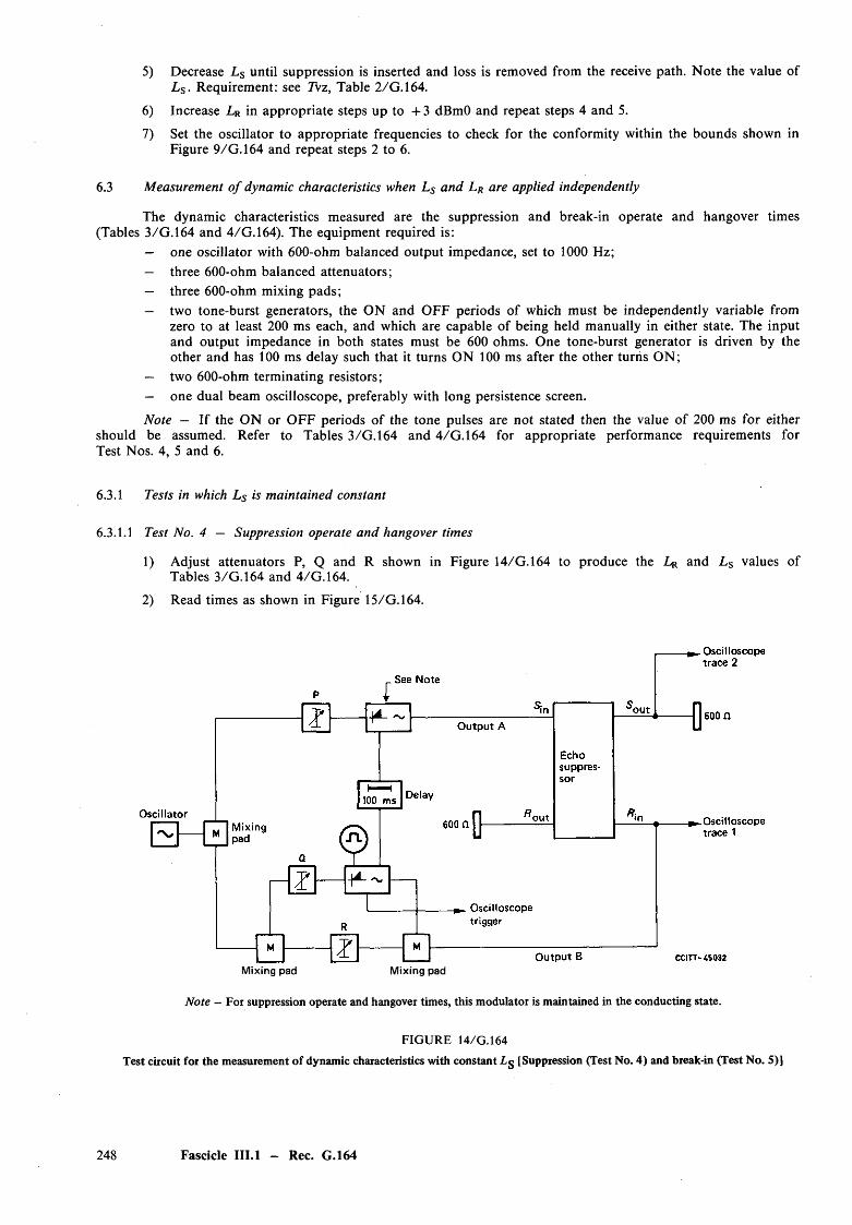
5) Decrease L s until suppression is inserted and loss is removed from the receive path. Note the value of L s . Requirement: see 7Vz, Table 2/G.164.
6) Increase LR in appropriate steps up to + 3 dBmO and repeat steps 4 and 5.
7) Set the oscillator to appropriate frequencies to check for the conformity within the bounds shown inFigure 9/G .164 and repeat steps 2 to 6.
6.3 Measurement o f dynamic characteristics when Ls and L R are applied independently
The dynamic characteristics measured are the suppression and break-in operate and hangover times(Tables 3/G.164 and 4/G.164). The equipment required is:
— one oscillator with 600-ohm balanced output impedance, set to 1000 Hz;— three 600-ohm balanced attenuators;— three 600-ohm mixing pads;— two tone-burst generators, the ON and O FF periods of which must be independently variable from
zero to at least 200 ms each, and which are capable of being held manually in either state. The inputand output impedance in both states must be 600 ohms. One tone-burst generator is driven by the other and has 100 ms delay such that it turns ON 100 ms after the other turns ON;
— two 600-ohm terminating resistors;— one dual beam oscilloscope, preferably with long persistence screen.
Note — If the ON or O FF periods of the tone pulses are not stated then the value of 200 ms for eithershould be assumed. Refer to Tables 3/G.164 and 4/G .164 for appropriate performance requirements for Test Nos. 4, 5 and 6.
6.3.1 Tests in which Ls is maintained constant
6.3.1.1 Test No. 4 — Suppression operate and hangover times
1) Adjust attenuators P, Q and R shown in Figure 14/G.164 to produce the LR and L s values ofTables 3/G.164 and 4/G.164.
2) Read times as shown in Figure 15/G.164.
Mixing pad Mixing pad
Note - For suppression operate and hangover times, this modulator is maintained in the conducting state.
FIG URE 14/G.164
Test circuit for the measurement of dynamic characteristics with constant Z-g [Suppression (Test No. 4) and break-in (Test No. 5)]
248 Fascicle III.l - Rec. G.164

Trace 1
Trace 2
p . CCITT 33120a S u p p ress io n o p e ra te tim eP S u p p ress io n han g o v er tim e
FIG URE 15/G.164 Trace for suppression operate and hangover times
6.3.1.2 Test No. 5 — Break-in operate time, Ls constant
In this test, LR is decreased while a constant L s is maintained, and a break-in operate time is measured. Since break-in hangover with L s constant is difficult to measure (due to the difficulty of ensuring a return to the Z state), it is not possible to distinguish between partial and full break-in. This is not considered to be im portant for break-in with L s constant.
1) Adjust attenuators P, Q and R shown in Figure 14/G.164 to produce the LR and the L s values of Table 16/G.164.
2) Read times as shown in Figure 16/G.164.
FIG URE 16/G.164
Trace for break-in operate time, L§ constant
6.3.2 Test in which LR is maintained constant
6.3.2.1 Test No. 6 — Partial and fu ll break-in operate and hangover times, L r constant
The equipment required is the same as for Test Nos. 4 and 5, set up according to Figure 17/G.164. In this test Lr is kept constant, Ls is increased, and the partial and full break-in operate and hangover times are measured. To test for partial and full break-in, the duration of time L s is in the ON state must be varied.
1) Set oscillator to 1000 Hz (for tolerances, see § 6.1.4).2) Adjust attenuator P of Figure 17/G.164 to produce LR = —25 dBmO.3) Adjust attenuators Q and R of Figure 17/G.164 to produce L s = —40 dBmO in the OFF state and
L s — —19 dBmO in the ON state.4) Starting with a 0 ms duration ON state for L s , increase the duration of the ON state until partial
break-in occurs. Partial break-in is characterized by the short operate and hangover times given in Tables 3 and 4/G.164. Note the oscilloscope traces in a) of Figure 18/G.164 for the definitions of the times.
Fascicle III.l — Rec. G.164 249
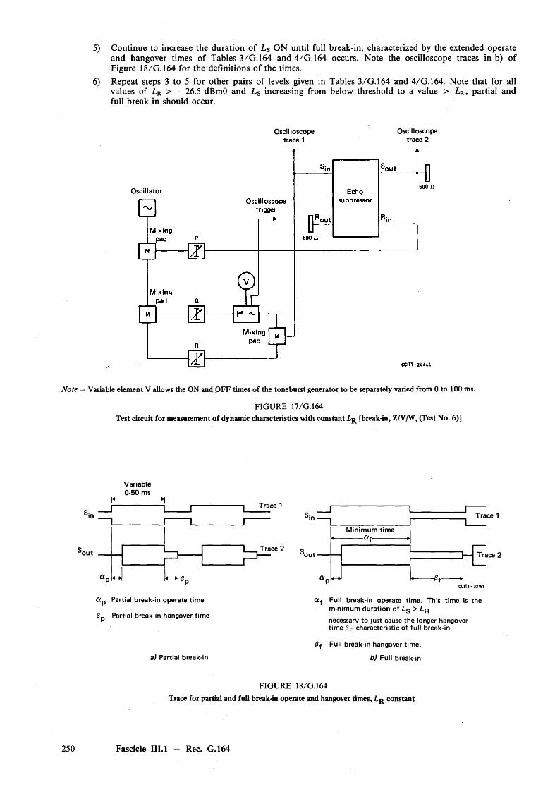
5) Continue to increase the duration of L s ON until full break-in, characterized by the extended operateand hangover times of Tables 3/G .164 and 4/G.164 occurs. Note the oscilloscope traces in b) ofFigure 18/G.164 for the definitions of the times.
6) Repeat steps 3 to 5 for other pairs of levels given in Tables 3/G.164 and 4/G.164. Note that for allvalues of LR > —26.5 dBmO and L s increasing from below threshold to a value > LR, partial andfull break-in should occur.
Oscilloscope Oscilloscopetrace 1 trace 2
Oscillator 600 a
Note - Variable element V allows the ON and OFF times of the toneburst generator to be separately varied from 0 to 100 ms.
FIGURE 17/G.164Test circuit for measurement of dynamic characteristics with constant Zr [break-in, Z/V/W, (Test No. 6)]
Variable 0-50 ms
Sir
’out
L
Q!p Partial break-in operate time
0p Partial break-in hangover time
a) Partial break-in
Trace 1
1 ^TraTrace 2’out •
Minimum time------ Of--------
- f ir
Trace 1
T race 2
CCITT-33161
G£f Full break-in operate time. This time is the minimum duration of Lg > Lpnecessary to just cause the longer hangover time characteristic of full break-in.
Full break-in hangover time.
b) Full break-in
FIGURE 18/G.164
Trace for partial and full break-in operate and hangover times, constant
250 Fascicle III.l — Rec. G.164
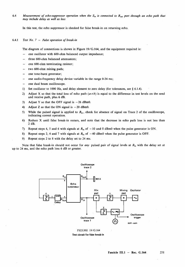
6.4 Measurement o f echo-suppressor operation when the S in is connected to R out port through an echo path that may include delay as well as loss
In this test, the echo suppressor is checked for false break-in on returning echo.
6.4.1 Test No. 7 — False operation o f break-in
The diagram of connections is shown in Figure 19/G.164, and the equipment required is:
— one oscillator with 600-ohm balanced output impedance;
— three 600-ohm balanced attenuators;
— one 600-ohm terminating resistor;
— two 600-ohm mixing pads;
— one tone-burst generator;
— one audio-frequency delay device variable in the range 0-24 ms;
— one dual beam oscilloscope.
1) Set oscillator to 1000 Hz, and delay element to zero delay (for tolerances, see § 6.1.4).
2) Adjust X so that the total loss of echo path {a-t-b) is equal to the difference in test levels on the sendand receive path, plus 6 dB.
3) Adjust Y so that the OFF signal is — 26 dBmO.
4) Adjust Z so that the ON signal is - 20 dBmO.
5) While the pulsed signal is applied to Rin, check for absence of signal on Trace 2 of the oscilloscope, indicating correct operation.
6) Reduce X until false break-in occurs, and note that the decrease in echo path loss is not less than 2 dB.
7) Repeat steps 4, 5 and 6 with signals at Rin o f —10 and 0 dBmO when the pulse generator is ON.
8) Repeat steps 2, 4 and 7 with signals at Rin of —40 dBmO when the pulse generator is OFF.
9) Repeat steps 2 to 8 with the delay set to 24 ms.
Note that false break-in should not occur for any pulsed pair of signal levels at R,n with the delay set at up to 24 ms, and the echo path loss 6 dB or greater.
Oscilloscope trace 2
600 n
Mixing Oscillator pad
I yM M
4 2 HOscilloscope
trace 1 £Oscilloscope
trigger
F I G U R E 1 9 /G .1 6 4
Test circuit for false break-in
Fascicle III.I — Rec. G.164 251
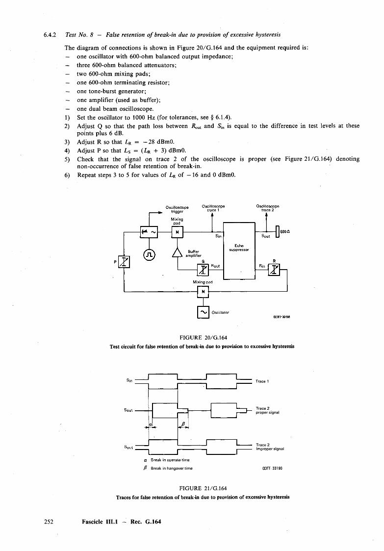
The diagram of connections is shown in Figure 20/G.164 and the equipment required is:— one oscillator with 600-ohm balanced output impedance;— three 600-ohm balanced attenuators;— two 600-ohm mixing pads;— one 600-ohm terminating resistor;— one tone-burst generator;— one amplifier (used as buffer);— one dual beam oscilloscope.1) Set the oscillator to 1000 Hz (for tolerances, see § 6.1.4).2) Adjust Q so that the path loss between Rout and Sin is equal to the difference in test levels at these
points plus 6 dB.3) Adjust R so that LR = —28 dBmO.4) Adjust P so that Ls = (L r 4- 3) dBmO.5) Check that the signal on trace 2 of the oscilloscope is proper (see Figure 2 1/G. 164) denoting
non-occurrence of false retention of break-in.6) Repeat steps 3 to 5 for values of LR of —16 and 0 dBmO.
6.4.2 Test No. 8 — False retention o f break-in due to provision o f excessive hysteresis
FIGURE 20/G.164
Test circuit for false retention of break-in due to provision to excessive hysteresis
Sjn
P Break-in h angover tim e
Trace 1
Trace 2 p roper signal
T race 2im proper signal
CCITT-33190
FIG URE 21/G. 164
Traces for false retention of break-in due to provision of excessive hysteresis
252 Fascicle III.l — Rec. G.164
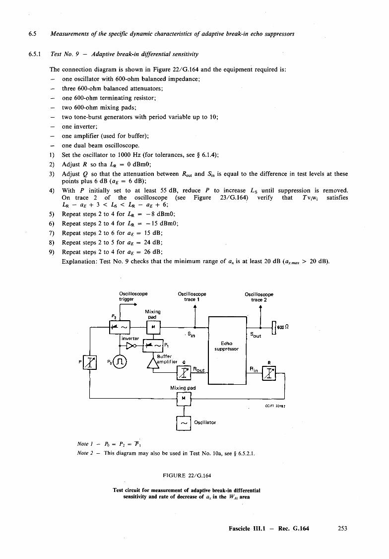
6.5.1 Test No. 9 — Adaptive break-in differential sensitivity
The connection diagram is shown in Figure 22/G.164 and the equipment required is:— one oscillator with 600-ohm balanced impedance;— three 600-ohm balanced attenuators;— one 600-ohm terminating resistor;— two 600-ohm mixing pads;— two tone-burst generators with period variable up to 10;— one inverter;— one amplifier (used for buffer);— one dual beam oscilloscope.1) Set the oscillator to 1000 Hz (for tolerances, see § 6.1.4);2) Adjust R so tha LR = 0 dBmO;3) Adjust Q so that the attenuation between RoUt and Sin is equal to the difference in test levels at these
points plus 6 dB (aE = 6 dB);4) With P initially set to at least 55 dB, reduce P to increase L s until suppression is removed.
On trace 2 of the oscilloscope (see Figure 23/G.164) verify that TviWj satisfiesLr — aE + 3 < Ls < Tr — o.e + 6;
5) Repeat steps 2 to 4 for LR = — 8 dBmO;6) Repeat steps 2 to 4 for LR = —15 dBmO;7) Repeat steps 2 to 6 for aE = 15 dB;8) Repeat steps 2 to 5 for aE — 24 dB;9) Repeat steps 2 to 4 for aE = 26 dB;
Explanation: Test No. 9 checks that the minimum range of ax is at least 20 dB (axmax > 20 dB).
6.5 Measurements o f the specific dynamic characteristics o f adaptive break-in echo suppressors
Oscilloscope Oscilloscope Oscilloscopetrigger trace 1 trace 2
Note 1 — Po = P2 = P\Note 2 — This diagram may also be used in Test No. 10a, see § 6.5.2.1.
FIGURE 22/G.164
Test circuit for measurement of adaptive break-in differential sensitivity and rate of decrease of ax in the WAi area
Fascicle III. 1 — Rec. G.164 253
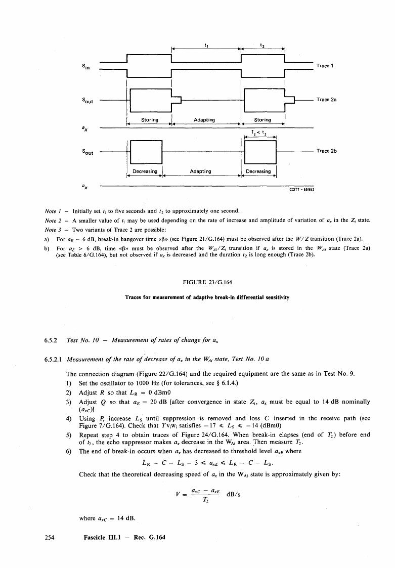
Ai
s :. Trace 1
out
out
I
Storing Adapting Storing
T,< t.h— 1-----1— H
AdaptingDecreasing Decreasing
Trace 2a
Trace 2b
CCITT - 69862
Note 1 - Initially set t\ to five seconds and t2 to approximately one second.
Note 2 - A smaller value of t\ may be used depending on the rate of increase and amplitude of variation of ax in the Z, state.
Note 3 — Two variants of Trace 2 are possible:
a) For aE = 6 dB, break-in hangover time «P» (see Figure 21/G.164) must be observed after the W / Z transition (Trace 2a).
b) For aE > 6 dB, time «P» must be observed after the WM/Z i transition if ax is stored in the WAi state (Trace 2a) (see Table 6/G.164), but not observed if ax is decreased and the duration t2 is long enough (Trace 2b).
FIG U R E 23/G.164
Traces for measurem ent o f adaptive break-in d ifferential sensitivity
6.5.2 Test No. 10 — Measurement o f rates o f change fo r ax
6.5.2.1 Measurement o f the rate o f decrease o f ax in the WAi state, Test No. 10 a
The connection diagram (Figure 22/G.164) and the required equipment are the same as in Test No. 9.1) Set the oscillator to 1000 Hz (for tolerances, see § 6.1.4.)2) Adjust R so that L R = 0 dBmO3) Adjust Q so that aE = 20 dB [after convergence in state Z,, ax must be equal to 14 dB nominally
(axC)\4) Using P, increase L s until suppression is removed and loss C inserted in the receive path (see
Figure 7/G.164). Check that LvjWj satisfies - 1 7 < L s < - 1 4 (dBmO)5) Repeat step 4 to obtain traces of Figure 24/G.164. When break-in elapses (end of T2) before end
of t2, the echo suppressor makes ax decrease in the WAi area. Then measure T2.6) The end of break-in occurs when ax has decreased to threshold level axE where
L r — C — L$ — 3 < axE < L r — C — L s .
Check that the theoretical decreasing speed of ax in the WAi state is approximately given by:
V - dB /sTi
where axC = 1 4 dB.
254 Fascicle III.l — Rec. G.164
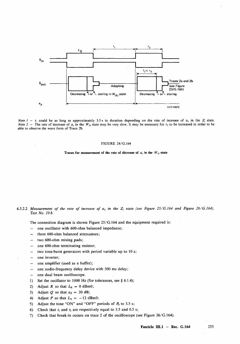
S,out AdaptingTraces 2a and 2b(see Figure 23/G.164)
Decreasing ^ o r V storing in W^j state Decreasing x o n - storing
a,CCITT-69872
Note 1 — t\ could be as long as approximately 3.5 s in duration depending on the rate of increase of ax in the Z, state. Note 2 — The rate of decrease of ax in the WAi state may be very slow. It may be necessary for t 2 to be increased in order to be able to observe the wave form of Trace 2b.
6.5.2.2 Measurement o f the rate o f increase o f ax in the Z, state (see Figure 25/G.164 and Figure 26/G.164), Test No. 10 b
The connection diagram is shown Figure 25/G.164 and the equipment required is:— one oscillator with 600-ohm balanced impedance;— three 600-ohm balanced attenuators;— two 600-ohm mixing pads;— one 600-ohm terminating resistor;— two tone-burst generators with period variable up to 10 s;— one inverter;— one amplifier (used as a buffer);— one audio-frequency delay device with 500 ms delay;— one dual beam oscilloscope.1) Set the oscillator to 1000 Hz (for tolerances, see § 6.1.4);2) Adjust R so that LR = 0 dBmO;3) Adjust Q so that aE = 20 dB;4) Adjust P so that L s = —12 dBmO;5) Adjust the tone “O N ” and “O FF” periods of P0 to 3.5 s;6) Check that t\ and t2 are respectively equal to 3.5 and 0.5 s;7) Check that break-in occurs on trace 2 of the oscilloscope (see Figure 26/G.164).
FIG URE 24/G.164
Traces for measurement of the rate of decrease of ax in the WAi state
Fascicle III.l — Rec. G.164 255
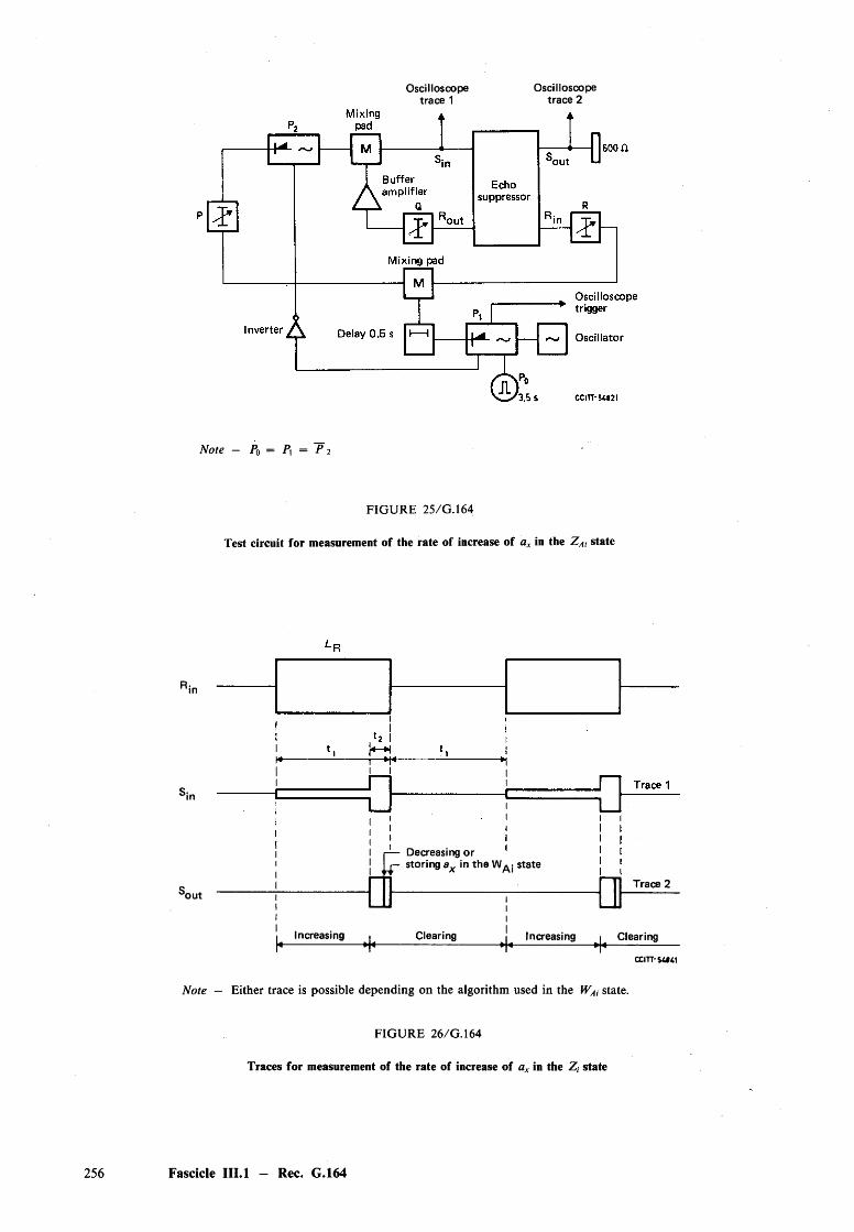
Oscilloscope Oscilloscopetrace 1 trace 2
Note — P0 — P\ = P 2
FIG U R E 25/G.164
Test circuit for measurement of the rate of increase of ax in the Z Ai state
Rir
Sir
— Decreasing or r- storing ax in the W^j state
Trace 2out
Increasing Clearing Increasing i Clearing
CCITT-S « 4 1
Note — Either trace is possible depending on the algorithm used in the WAi state.
FIG URE 26/G.164
Traces for measurement of the rate of increase of ax in the Z, state
256 Fascicle III.l — Rec. G.164
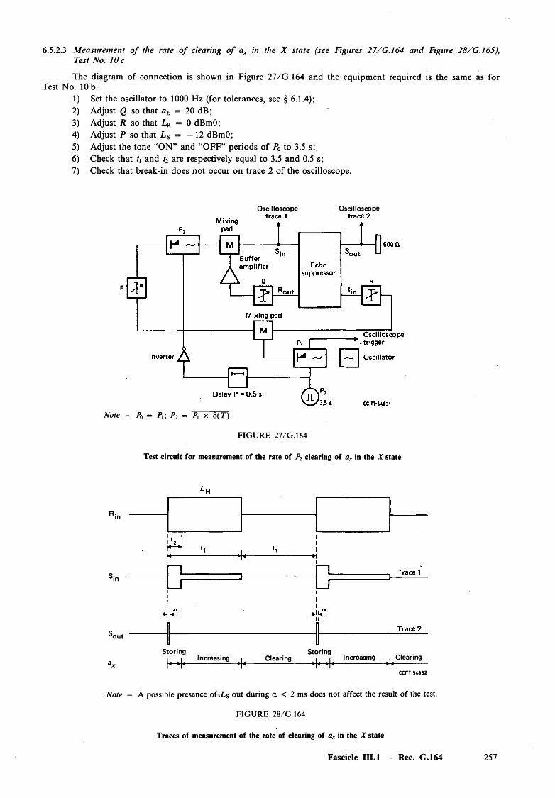
6.5.2.3 Measurement o f the rate o f clearing o f ax in the X state (see Figures 27/G.164 and Figure 28/G.165), Test No. 10 c
The diagram of connection is shown in Figure 27/G.164 and the equipment required is the same as for Test No. 10 b.
1) Set the oscillator to 1000 Hz (for tolerances, see § 6.1.4);2) Adjust Q so that aE = 20 dB;3) Adjust R so that Lr = 0 dBmO;4) Adjust P so that L s = —12 dBmO;5) Adjust the tone “O N ” and “OFF” periods of P0 to 3.5 s;6) Check that t\ and t2 are respectively equal to 3.5 and 0.5 s;7) Check that break-in does not occur on trace 2 of the oscilloscope.
Oscilloscope Oscilloscope
Note - P0 = Px\ Pi = P\ x 5(T )
FIG URE 27/G.164
Test circuit for measurement of the rate of P2 clearing of ax in the X state
R;r
Sir
out
Storing
H - IncreasingStoring
Clearing . . Increasing . Clearing
Note — A possible presence o f >L$ out during a < 2 ms does not affect the result o f the test.
FIG URE 28/G.164
Traces of measurement of the rate of clearing of ax in the X state
Fascicle III.l — Rec. G.164 257

[1] CCITT Recommendation Echo suppressors suitable fo r circuits having either short or long propagation times,Orange Book, Vol. I l l , Rec. G.161, ITU, Geneva, 1977.
[2] CCITT Recommendation Influence o f national networks on stability and echo in international connections,Orange Book, Vol. I l l , Rec. G.122, Part B, b), ITU, Geneva, 1977.
[3] CCITT Recommendation Performance characteristics o f PCM channels between 4-wire interfaces at voicefrequencies, Vol. I l l , Rec. G.712.
[4] CCITT Recommendation Characteristics o f primary PCM multiplex equipment operating at 1544 kbit/s,Vol. I ll , Rec. G.733.
[5] CCITT Recommendation 300-baud modem standardized fo r use in the general switched telephone network,Vol. VIII, Rec. V.21.
References
Recommendation G.165
ECH O CANCELLERS
(Geneva, 1980; amended at Malaga-Torremolinos, 1984)
1 General
1.1 Echo cancellers are voice operated devices placed in the 4-wire portion of a circuit (which may be an individual circuit path or a path carrying a multiplexed signal) and are used for reducing the echo by subtracting an estimated echo from the circuit echo. They may be characterized by whether the transmission path or the subtraction of the echo is by analogue or digital means (see Figures 1/G . 165, 2 /G .l65 and 3/G.165).
1.2 This Recommendation is applicable to the design of echo cancellers using digital or analogue techniques, and intended for use in an international circuit. Echo cancellers designed to this Recommendation will be compatible with each other and with echo suppressors designed in accordance with Recommendations G.161 [1] and G.164. Compatibility is defined in Recommendation G.164, § 1.4. Freedom is permitted in design details not covered by the requirements.
Echo cancellers may be used for purposes other than network echo control on international circuits, e.g. in active 2-wire/4-wire hybrids or 2-wire repeaters, but this Recommendation does not apply to such echo cancellors.
CCtTT-22041
Abbreviations: Receive-in port (Rin) Send-in port (Sin)Receive-out port (Rout) Send-out port (Sout)
FIGURE 1/G.165
Type A echo canceller
258 Fascicle III.l — Rec. G.165

CCITT-33 260
Note — Functionally, a type C digital echo canceller (DEC) interfaces at 64 kbit/s. However, 24 or 30 digital echo cancellers for example may be combined corresponding to the primary digital hierarchy levels of 1544 kbit/s or 2048 kb it/s respectively.
FIG URE 2 /G .l65
Type C echo canceller
CCITT-33270
FIG URE 3/G.165
Type D echo canceller
2 Definitions relating to echo cancellers1)
In the definition and text, L will refer to the relative power level of a signal, expressed in dBmO and A will refer to the attenuation or loss of a signal path expressed in dB.
2.1 echo canceller (see Figure 4/G.165)
F: annuleur d ’echo
S: compensador de eco; cancelador de eco
A voice operated device placed in the 4-wire portion of a circuit and used for reducing near-end echo present on the send path by subtracting an estimation of that echo from the near-end echo.
9 These definitions assume that nonlinear processing, e.g. centre clipping, is not present in the send or receive paths unless otherwise specified and that the signal at Sm is purely echo.
Fascicle 1II.1 - Rec. G.165 259
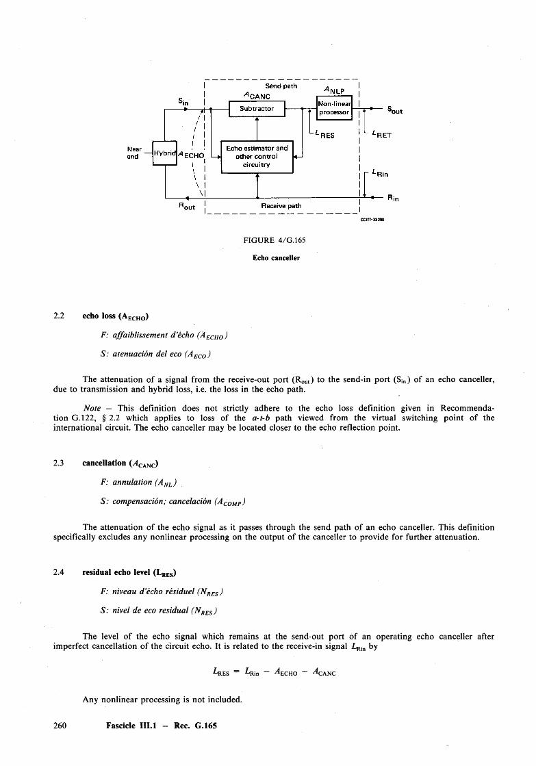
CCITT-33 2M
FIG URE 4/G.165
Echo canceller
2.2 echo loss (AECHO)
F: affaiblissement d ’echo (AECHO)
S: atenuacion del eco (AECO)
The attenuation of a signal from the receive-out port (Rout) to the send-in port (S j„ ) of an echo canceller, due to transmission and hybrid loss, i.e. the loss in the echo path.
Note — This definition does not strictly adhere to the echo loss definition given in Recommendation G.122, § 2.2 which applies to loss of the a-t-b path viewed from the virtual switching point o f the international circuit. The echo canceller may be located closer to the echo reflection point.
2.3 cancellation ( ^ C a n c )
F: annulation (ANL)
S: compensacion; cancelacion (ACOMP)
The attenuation of the echo signal as it passes through the send path of an echo canceller. This definition specifically excludes any nonlinear processing on the output of the canceller to provide for further attenuation.
2.4 residual echo level (LRES)
F: niveau d ’echo residuel (NRES)
S: nivel de eco residual (NRES)
The level o f the echo signal which remains at the send-out port of an operating echo canceller after imperfect cancellation of the circuit echo. It is related to the receive-in signal by
AlES = ^Rin — ^ECHO — ^CANC
Any nonlinear processing is not included.
260 Fascicle I1I.1 - Rec. G.165
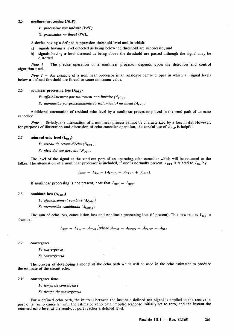
2.5 nonlinear processing (NLP)
F: processeur non lineaire (PNL)
S: procesador no lineal (PNL)
A device having a defined suppression threshold level and in which:a) signals having a level detected as being below the threshold are suppressed, andb) signals having a level detected as being above the threshold are passed although the signal may be
distorted.
Note 1 — The precise operation of a nonlinear processor depends upon the detection and control algorithm used.
Note 2 — An example of a nonlinear processor is an analogue centre clipper in which all signal levels below a defined threshold are forced to some minimum value.
2.6 nonlinear processing loss (ANLP)
F: affaiblissement par traitement non lineaire (Am h )
S: atenuacion por procesamiento (o tratamiento) no lineal (Am L )
Additional attenuation of residual echo level by a nonlinear processor placed in the send path of an echocanceller.
Note — Strictly, the attenuation of a nonlinear process cannot be characterized by a loss in dB. However,for purposes of illustration and discussion of echo canceller operation, the careful use of ^ NLP is helpful.
2.7 returned echo level (LRET)
F: niveau de retour d ’echo (NRET )
S: nivel del eco devuelto (NDEW )
The level o f the signal at the send-out port of an operating echo canceller which will be returned to the talker. The attenuation of a nonlinear processor is included, if one is normally present. L rEX is related to L^ in by
AlET = Alin — (^ECHO + ^CANC + ^NLP )■
If nonlinear processing is not present, note that LrES = LrET .
2.8 combined loss (ACOIV|)
F: affaiblissement combine (ACOM )
S: atenuacion combinada (ACOMB )
The sum of echo loss, cancellation loss and nonlinear processing loss (if present). This loss relates 1 ^^ to L re t b y :
£ ret = Aiin — ^ com > where ^ com = 'A cho + ^ canc + ^ nlp •
2.9 convergence
F: convergence
S: convergencia
The process of developing a model of the echo path which will be used in the echo estimator to produce the estimate of the circuit echo.
2.10 convergence time
F: temps de convergence
S: tiempo de convergencia
For a defined echo path, the interval between the instant a defined test signal is applied to the receive-in port o f an echo canceller with the estimated echo path impulse response initially set to zero, and the instant the returned echo level at the send-out port reaches a defined level.
Fascicle IIL1 - Rec. G.165 261
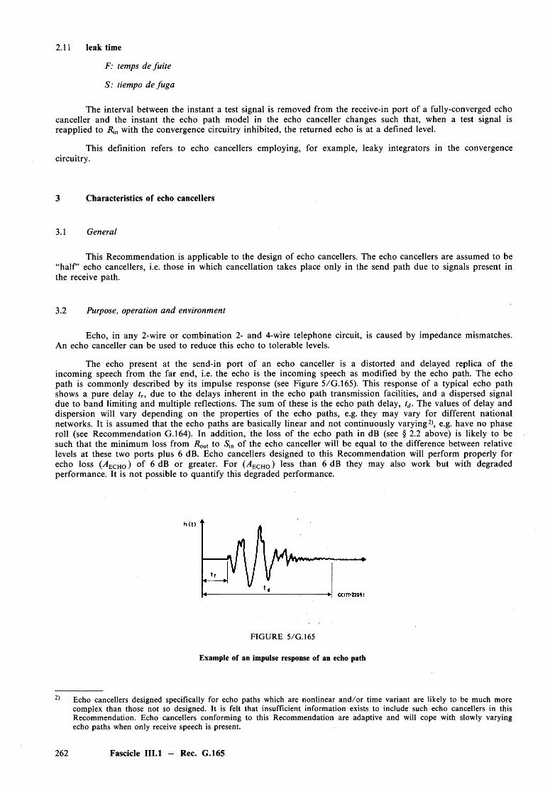
2.11 leak time
F: temps de fu ite
S: tiempo de fuga
The interval between the instant a test signal is removed from the receive-in port of a fully-converged echo canceller and the instant the echo path model in the echo canceller changes such that, when a test signal is reapplied to R\n with the convergence circuitry inhibited, the returned echo is at a defined level.
This definition refers to echo cancellers employing, for example, leaky integrators in the convergence circuitry.
3 Characteristics of echo cancellers
3.1 General
This Recommendation is applicable to the design of echo cancellers. The echo cancellers are assumed to be “h a lf ’ echo cancellers, i.e. those in which cancellation takes place only in the send path due to signals present in the receive path.
3.2 Purpose, operation and environment
Echo, in any 2-wire or combination 2- and 4-wire telephone circuit, is caused by impedance mismatches. An echo canceller can be used to reduce this echo to tolerable levels.
The echo present at the send-in port of an echo canceller is a distorted and delayed replica of the incoming speech from the far end, i.e. the echo is the incoming speech as modified by the echo path. The echo path is commonly described by its impulse response (see Figure 5/G.165). This response of a typical echo path shows a pure delay tr, due to the delays inherent in the echo path transmission facilities, and a dispersed signal due to band limiting and multiple reflections. The sum of these is the echo path delay, td. The values of delay and dispersion will vary depending on the properties of the echo paths, e.g. they may vary for different national networks. It is assumed that the echo paths are basically linear and not continuously varying2), e.g. have no phase roll (see Recommendation G.164). In addition, the loss of the echo path in dB (see § 2.2 above) is likely to be such that the minimum loss from RoUt to Sjn of the echo canceller will be equal to the difference between relative levels at these two ports plus 6 dB. Echo cancellers designed to this Recommendation will perform properly for echo loss (v4echo) of 6 dB or greater. For 04ECho) ess than 6 dB they may also work but with degraded performance. It is not possible to quantify this degraded performance.
FIG U R E 5/G.165
Example of an impulse response of an echo path
Echo cancellers designed specifically for echo paths which are nonlinear an d /o r time variant are likely to be much more complex than those not so designed. It is felt that insufficient information exists to include such echo cancellers in this Recommendation. Echo cancellers conforming to this Recommendation are adaptive and will cope with slowly varying echo paths when only receive speech is present.
262 Fascicle III.l — Rec. G.165
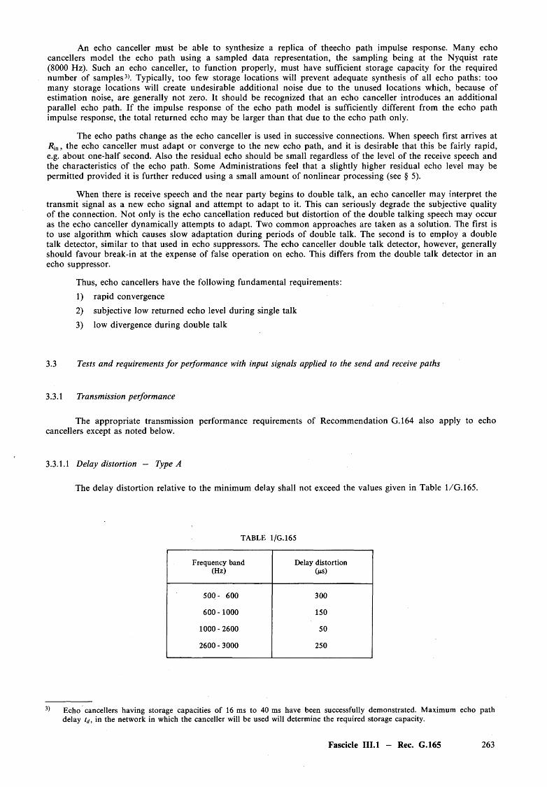
An echo canceller must be able to synthesize a replica of theecho path impulse response. Many echo cancellers model the echo path using a sampled data representation, the sampling being at the Nyquist rate (8000 Hz). Such an echo canceller, to function properly, must have sufficient storage capacity for the required number of samples3). Typically, too few storage locations will prevent adequate synthesis of all echo paths: too many storage locations will create undesirable additional noise due to the unused locations which, because of estimation noise, are generally not zero. It should be recognized that an echo canceller introduces an additional parallel echo path. If the impulse response of the echo path model is sufficiently different from the echo path impulse response, the total returned echo may be larger than that due to the echo path only.
The echo paths change as the echo canceller is used in successive connections. When speech first arrives at R \n, the echo canceller must adapt or converge to the new echo path, and it is desirable that this be fairly rapid, e.g. about one-half second. Also the residual echo should be small regardless of the level of the receive speech and the characteristics of the echo path. Some Administrations feel that a slightly higher residual echo level may be permitted provided it is further reduced using a small amount of nonlinear processing (see § 5).
When there is receive speech and the near party begins to double talk, an echo canceller may interpret the transmit signal as a new echo signal and attempt to adapt to it. This can seriously degrade the subjective quality of the connection. Not only is the echo cancellation reduced but distortion of the double talking speech may occur as the echo canceller dynamically attempts to adapt. Two common approaches are taken as a solution. The first is to use algorithm which causes slow adaptation during periods of double talk. The second is to employ a double talk detector, similar to that used in echo suppressors. The echo canceller double talk detector, however, generally should favour break-in at the expense of false operation on echo. This differs from the double talk detector in an echo suppressor.
Thus, echo cancellers have the following fundamental requirements:
1) rapid convergence
2) subjective low returned echo level during single talk
3) low divergence during double talk
3.3 Tests and requirements fo r performance with input signals applied to the send and receive paths
3.3.1 Transmission performance
The appropriate transmission performance requirements of Recommendation G.164 also apply to echo cancellers except as noted below.
3.3.1.1 Delay distortion — Type A
The delay distortion relative to the minimum delay shall not exceed the values given in Table 1/G. 165.
TABLE 1/G. 165
Frequency band (Hz)
Delay distortion (ms)
500 - 600 300
600 -1000 150
1000-2600 50
2600 - 3000 250
Echo cancellers having storage capacities of 16 ms to 40 ms have been successfully demonstrated. Maximum echo path delay td, in the network in which the canceller will be used will determine the required storage capacity.
Fascicle III.l — Rec. G.165 263

3.3.1.2 Attenuation distortion — Type A
The attenuation distortion shall be such that if Q dB is the attenuation at 800 Hz (or 1000 Hz) the attenuation shall be within the range (Q + 0.5) dB to (Q — 0.2) dB at any frequency in the band 300-3400 Hz and at 200 Hz, within the range of (Q + 1.0) dB to (Q — 0.2) dB.
3.3.1.3 Group delay — Type C
The group delay in the send path should be kept to a minimum and should not exceed 1 ms. No significant delay should occur in the receive path. Any delay necessary for synchronization of independent bit streams in the send and receive paths should be placed in the echo estimator.
3.3.1.4 Group delay — Type D
The group delay in the send and receive paths shall meet the requirements of § 3.3.1.3 for Type C echo cancellers with the addition of the delay allowed for codecs as given in Recommendation G .712.
3.3.2 Echo canceller performance
The performance requirements which follow are for echo cancellers which include nonlinear processors (see Annex A for echo cancellers which do not include a nonlinear processor).
In the tests, it is assumed that the nonlinear processor can be disabled, that the echo path impulse response store (H register) can be cleared (set to zero) and that adaptation can be inhibited.
The requirements are described in terms of tests made by applying signals to Rin and Sin of an echo canceller, and measuring the Sout signals. The test set-up is as shown in Figure 6/G.165. The ports are assumed to be at equal relative level points. Band-limited noise is used as the receive input test signal. The echo loss is independent of frequency.
convergence
Note — The requirements in § 3.3.2 are based on the use of band-limited white noise (300 — 3400 Hz) as the test signal. Noise shaped in accordance with Recommendation G.227 may also be used. However, the applicability of the requirements in § 3.3.2 requires confirmation and is under study.The use o f alternative test signals more representative of real speech and possible changes in test procedures and requirements are also under study.
FIG URE 6/G.165
Test for echo canceller performance
264 Fascicle IIL1 — Rec. G.165
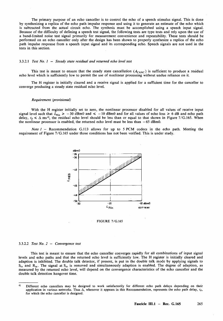
The primary purpose of an echo canceller is to control the echo of a speech stimulus signal. This is done by synthesizing a replica of the echo path impulse response and using it to generate an estimate of the echo which is subtracted from the actual circuit echo. The synthesis must be accomplished using a speech input signal. Because of the difficulty of defining a speech test signal, the following tests are type tests and rely upon the use of a band-limited noise test signal primarily for measurement convenience and repeatability. These tests should be performed on an echo canceller only after the design has been shown to properly synthesize a replica of the echo path impulse response from a speech input signal and its corresponding echo. Speech signals are not used in the tests in this section.
3.3.2.1 Test No. 1 — Steady state residual and returned echo level test
This test is meant to ensure that the steady state cancellation (^ CANC) is sufficient to produce a residual echo level which is sufficiently low to permit the use of nonlinear processing without undue reliance on it.
The H register is initially cleared and a receive signal is applied for a sufficient time for the canceller to converge producing a steady state residual echo level.
Requirement (provisional)
With the H register initially set to zero, the nonlinear processor disabled for all values o f receive input signal level such that > — 30 dBmO and < —10 dBmO and for all values of echo loss > 6 dB and echo path delay, tj < A m s4), the residual echo level should be less than or equal to that shown in Figure 7/G.165. When the nonlinear processor is enabled, the returned echo level must be less than — 65 dBmO.
Note 1 — Recommendation G.113 allows for up to 5 PCM codecs in the echo path. Meeting the requirement of Figure 7/G.165 under those conditions has not been verified. This is under study.
dBmO
* - R i n CCITT-59JS1
FIG URE 7/G.165
3.3.2.2 Test No. 2 — Convergence test
This test is meant to ensure that the echo canceller converges rapidly for all combinations o f input signal levels and echo paths and that the returned echo level is sufficiently low. The H register is initially cleared and adaption is inhibited. The double talk detector, if present, is put in the double talk mode by applying signals to Sin and Rin. The signal at Sin is removed and simultaneously adaption is enabled. The degree of adaption, as measured by the returned echo level, will depend on the convergence characteristics of the echo canceller and the double talk detection hangover time.
Different echo cancellers may be designed to work satisfactorily for different echo path delays depending on their application in various networks. Thus A, whenever it appears in this Recommendation, represents the echo path delay, tj, for which the echo canceller is designed.
Fascicle III.l - Rec. G.165 265
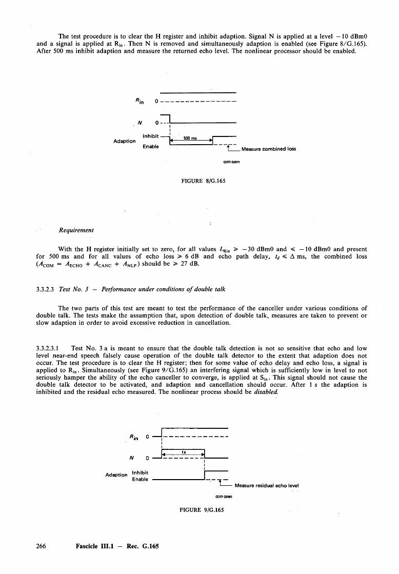
The test procedure is to clear the H register and inhibit adaption. Signal N is applied at a level —10 dBmO and a signal is applied at Rin. Then N is removed and simultaneously adaption is enabled (see Figure 8/G.165). After 500 ms inhibit adaption and measure the returned echo level. The nonlinear processor should be enabled.
N 0 ---I
Inhibit 500 msAdaptionEnable Measure combined loss
CCITT-22071
FIGURE 8/G.165
Requirement
With the H register initially set to zero, for all values > —30 dBmO and < —10 dBmO and present for 500 ms and for all values of echo loss > 6 dB and echo path delay, td < A ms, the combined loss ( - ^ c o m ~ - ^ e c h o + ^ c a n c + ^ n l p ) should be > 27 dB.
3.3.2.3 Test No. 3 — Performance under conditions o f double talk
The two parts of this test are meant to test the performance of the canceller under various conditions ofdouble talk. The tests make the assumption that, upon detection of double talk, measures are taken to prevent orslow adaption in order to avoid excessive reduction in cancellation.
3.3.2.3.1 Test No. 3 a is meant to ensure that the double talk detection is not so sensitive that echo and low level near-end speech falsely cause operation of the double talk detector to the extent that adaption does not occur. The test procedure is to clear the H register; then for some value of echo delay and echo loss, a signal is applied to Rin. Simultaneously (see Figure 9/G.165) an interfering signal which is sufficiently low in level to not seriously hamper the ability o f the echo canceller to converge, is applied at Sin. This signal should not cause the double talk detector to be activated, and adaption and cancellation should occur. After 1 s the adaption is inhibited and the residual echo measured. The nonlinear process should be disabled.
N
Adaption InhibitEnable
Measure residual echo level
GCITT-220S1
FIGURE 9/G.165
266 Fascicle III.l - Rec. G.165
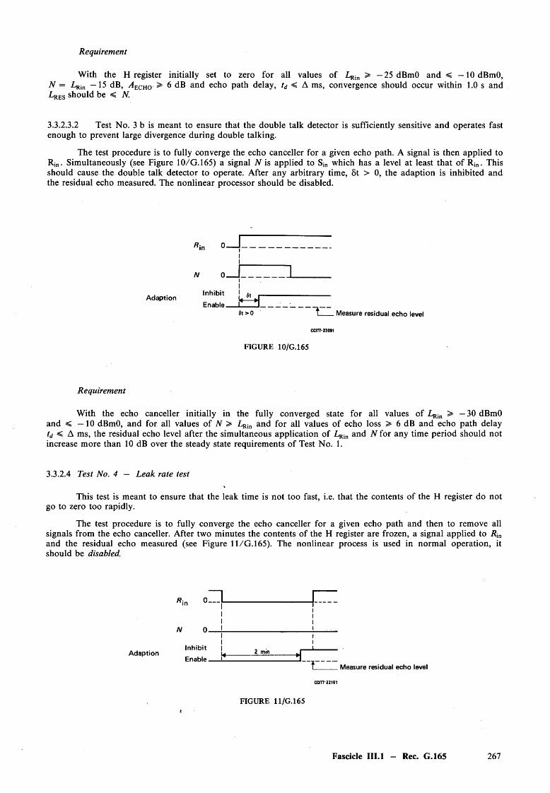
Requirement
With the H register initially set to zero for all values of LRin > - 2 5 dBmO and < -lO dB m O , N = Atin dB, A echo > 6 dB and echo path delay, td < A ms, convergence should occur within 1.0 s and L rES should be < N.
3.3.2.3.2 Test No. 3 b is meant to ensure that the double talk detector is sufficiently sensitive and operates fast enough to prevent large divergence during double talking.
The test procedure is to fully converge the echo canceller for a given echo path. A signal is then applied to R in . Simultaneously (see Figure 10/G.165) a signal N is applied to Sjn which has a level at least that o f R j n . This should cause the double talk detector to operate. After any arbitrary time, 8t > 0, the adaption is inhibited and the residual echo measured. The nonlinear processor should be disabled.
Adaption
N
I
Inhibit ; 6t Enable C
St >0 Measure residual echo level
FIGURE 10/G.165
Requirement
With the echo canceller initially in the fully converged state for all values of > —30 dBmO and < —10 dBmO, and for all values of N > L r^ and for all values of echo loss > 6 dB and echo path delay td < A ms, the residual echo level after the simultaneous application of LRin and N for any time period should not increase more than 10 dB over the steady state requirements of Test No. 1.
3.3.2.4 Test No. 4 — Leak rate test
This test is meant to ensure that the leak time is not too fast, i.e. that the contents of the H register do notgo to zero too rapidly.
The test procedure is to fully converge the echo canceller for a given echo path and then to remove allsignals from the echo canceller. After two minutes the contents of the H register are frozen, a signal applied to Rinand the residual echo measured (see Figure 11/G.165). The nonlinear process is used in norm al operation, it should be disabled.
, Z L
Adaption
N 0.
Inhibit Enable.
2 min
Measure residual echo level
FIGURE 11/G.165
Fascicle III.l - Rec. G.165 267
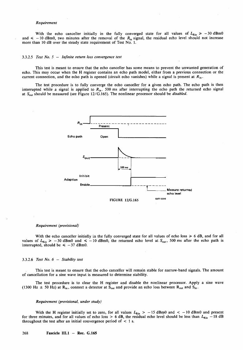
Requirement
With the echo canceller initially in the fully converged state for all values of > — 30 dBmO and < —10 dBmO, two minutes after the removal of the Rjn signal, the residual echo level should not increase more than 10 dB over the steady state requirement of Test No. 1.
3.3.2.5 Test No. 5 — Infinite return loss convergence test
This test is meant to ensure that the echo canceller has some means to prevent the unwanted generation of echo. This may occur when the H register contains an echo path model, either from a previous connection or the current connection, and the echo path is opened (circuit echo vanishes) while a signal is present at R m.
The test procedure is to fully converge the echo canceller for a given echo path. The echo path is then interrupted while a signal is applied to . 500 ms after interrupting the echo path the returned echo signal at Sout should be measured (see Figure 12 /G .l65). The nonlinear processor should be disabled.
Ri. J .Present
Echo path Open
Adaption
FIGURE 12/G.165
Requirement (provisional)
With the echo canceller initially in the fully converged state for all values of echo loss > 6 dB, and for all values of L ^ n > — 30 dBmO and < —10 dBmO, the returned echo level at Sout, 500 ms after the echo path is interrupted, should be < — 37 dBmO.
3.3.2.6 Test No. 6 — Stability test
This test is meant to ensure that the echo canceller will remain stable for narrow-band signals. The amountof cancellation for a sine wave input is measured to determine stability.
The test procedure is to clear the H register and disable the nonlinear processor. Apply a sine wave(1300 Hz ± 50 Hz) at Rin, connect a detector at Sout and provide an echo loss between Rout and Sin.
Requirement (provisional, under study)
With the H register initially set to zero, for all values > —15 dBipO and < —10 dBmO and present for three minutes, and for all values of echo loss > 6 dB, the residual echo level should be less than Z^,, —18 dB throughout the test after an initial convergence period of < 1 s.
268 Fascicle III.l - Rec. G.165
3.4 External enabling/disabling
An option should be included in the echo canceller to provide for enabling or disabling by an externally derived ground (earth) from the trunk circuit. The enabler should function to permit or prevent normal echo canceller operation. Certain type C echo cancellers may be disabled directly by a digital signal. Some digital data signals may require Type C echo cancellers to provide 64 kbit/s bit sequence integrity in the externally disabled state.
4 Characteristics of an echo canceller tone disabler
4.1 General
To ensure proper operation of all currently specified V-series modems, the echo cancellers covered by this Recommendation should be equipped with a tone detector that conforms to this section. This tone detector responds to a disabling signal which is different from that used to disable the echo suppressor as described in Recommendation G.164, § 5 and consists of a 2100 Hz tone with periodic phase reversals inserted in that tone.The tone disabler should respond only to the specified in-band signal. It should not respond to other in-bandsignals, e.g. speech, or a 2100 Hz tone without a phase reversal. The tone disabler should detect and respond to adisabling signal which may be present in either the send or the receive path.
The requirements for echo canceller disabling to ensure proper operation with ATME No. 2 equipment that transmits the 2100 Hz tone with phase reversals could be met by using either the tone disabler specified in this section, or the echo suppressor tone disabler specified in Recommendation G.164, § 5. However, use of the Recommendation G.164, § 5 disabler does not assure proper operation with all currently specified V-series modems.
The term disabled in this section refers to a condition in which the echo canceller is configured in such a way as to no longer modify the signals which pass through it in either direction. Under this condition the nonlinear processor is made transparent, no echo estimate is subtracted from the send path and the delay though the echo canceller remains unchanged from that in the enabled state.
It should be noted that this condition does not necessarily fulfil the requirements for 64 kb it/s bit sequence integrity, for which case other means of disabling in line with Recommendation G.165, § 3.4 will apply.
A reference tone disabler is described in Annex B.
4.2 Disabler characteristics
The echo canceller tone disabler requires the detection of a 2100 Hz tone with phase reversals o f that tone. The characteristics of the transmitted signal are defined in Recommendation V.25.
The frequency characteristics of the tone detector are the same as the characteristics of the echo suppressor tone detector given in Recommendation G.164, § 5.2.
The dynamic range of this detector should be consistent with the input levels as specified in Recommendation V.2 and H.51 with allowances for variation introduced by the public switched telephone network.
4.3 Guardband characteristics
Same as defined in Recommendation G.164, § 5.3, consistent with the dynamic range given in § 4.2 above.
4.4 Holding-band characteristics
Same as defined in Recommendation G.164, § 5.4.
4.5 Operate time
The operate time must be sufficiently long to provide immunity from false operation due to voice signals, but not so long as to needlessly extend the time to disable. The tone disabler is required to operate within one second of the receipt o f the disabling signal.
Fascicle III.l — Rec. G.165 269
4.6 False operation due to speech currents
Same as in Recommendation G.164, § 5.6.
4.7 False operation due to data signals
It is desirable that the tone disabler should rarely operate falsely on data signals from data sets that would be adversely affected by disabling of the echo canceller. To this end, a reasonable objective is that, for an echo canceller installed on a working circuit, usual data signals from such data sets should not, on the average, cause more than 10 false operations during 100 hours of data transmissions.
4.8 Release time
Same as in Recommendation G.164, § 5.7.
5 Nonlinear processors for use in echo cancellers
5.1 Scope
For the purpose of this Recommendation the term “nonlinear processor” is intended to mean only those devices which fall within the definition given in § 2.5 and which have been proven to be effective in echo cancellers. It is possible to implement such nonlinear processors in a number of ways (centre clippers being just one example), with fixed or adaptive operating features, but no recommendation is made for any particular implementation. General principles and guidelines are given in § 5.2. More detailed and concrete information requires reference to specific implementations. This is done in Annex C for the particular case of a “reference nonlinear processor”. The use of this term denotes an implementation given for guidance and illustration only. It does not exclude other implementations nor does it imply that the reference nonlinear processor is necessarily the most appropriate realization on any technical, operational or economic grounds.
5.2 General principles and guidelines
5.2.1 Function
5.2.1.1 General
The nonlinear processor is located in the send path between the output of the subtractor and the send-out port o f the echo canceller. Conceptually, it is a device which blocks low level signals and passes high level signals. Its function is to further reduce the residual echo level (LrES as defined in § 2.4) which remains after imperfect cancellation of the circuit echo so that the necessary low returned echo level (LrET as defined in § 2.7) can be achieved.
5.2.1.2 Network performance
Imperfect cancellation can occur because echo cancellers which conform to this Recommendation may not be capable of adequately modelling echo paths which generate significant levels o f nonlinear distortion (see § 3.2). Such distortion can occur, for example, in networks conforming to Recommendation G.113 in which up to five pairs o f PCM codecs (conforming to Recommendation G.712) are permitted in an echo path. The accumulated quantization distortion from these codecs may prevent an echo canceller from achieving the necessary by using linear cancellation techniques alone. It is therefore recommended that all echo cancellers capable only of modelling the linear components of echo paths but intended for general network use should incorporate suitable nonlinear processors.
5.2.1.3 Limitations
This use of nonlinear processors represents a compromise in the circuit transparency which would be possible by an echo canceller which could achieve the necessary Lrej by using only modelling and cancellation techniques. Ideally, the non-linear processor should not cause distortion of near-end speech. In practical devices it may not be possible to sufficiently approach this ideal in this case it is recommended that nonlinear processors should not be active under double talk or near-end single-talk conditions. From this it follows that excessive dependence must not be placed on the nonlinear processor and that LrES must be low enough to prevent objectionable echo under double-talk conditions.
270 Fascicle III.1 - Rec. G.165

5.2.1.4 Data transmission
N onlinear processors may affect the transmission of data through an enabled echo canceller. This is understudy.
5.2.2 Suppression threshold
5.2.2.1 General
The suppression threshold level (TSUP) of a nonlinear processor is expressed in dBmO and is equal to the highest level o f a sine-wave signal at a given moment that is just suppressed. Either fixed or adaptive suppression threshold levels may be used.
5.2.2.2 Fixed suppression threshold
With a fixed suppression threshold level the appropriate level to use will depend upon the cancellation achieved and the statistics of speech levels and line conditions found in the particular network in which the echo canceller is to be used. It is therefore recommended that the actual level should be field selectable to permit the user to adjust it for the actual network environment. Values of fixed suppression threshold levels to be used are under study — see Notes 1 and 2.
Note 1 — As an interim guide, it is suggested that the suppression threshold level should be set a few decibels above the level that would result in the peaks of L rES for a “20-talker” and a “20-echo return loss” being suppressed.
Note 2 — Results of a field trial reported by one Administration indicated that a fixed suppression threshold level of —36 dBmO gave a satisfactory performance. A theoretical study, by another Administration, of an echo path contianing five pairs of PCM codecs showed that for an L r of —10 dBmO, the quantization noise could result in an L rES of - 3 8 dBmO.
5.2.2.3 Adaptive suppression threshold
A good compromise can be made between using a high SUP to prevent it being exceeded by loud talker residual echo and using a low SUP to reduce speech distortion on break-in by making SUP adaptive to the actual circuit conditions and speech levels. This may be achieved in a number of ways and no recommendation is made for any particular implementation. General guidelines applicable to the control algorithm and suppression threshold levels are under study.
5.2.3 Control o f nonlinear processor activation
5.2.3.1 General
To conform to the recommendation made in § 5.2.1.3, it is necessary to control the activation of the nonlinear processor so that it is not active when near-end speech is likely to be present. When “active”, the nonlinear processor should function as intended to reduce LrES. When “inactive”, it should not perform any nonlinear processing on any signal passing through the echo canceller.
5.2.3.2 Control guidelines
It is recommended that the following two guidelines should govern control of the activation of a nonlinear processor. First, because they are intended to further reduce LrES, they should be active when LrES is at a significant level. Second, because they should not distort near-end speech, they should be inactive when near-end speech is present. Where these two guidelines conflict the control function should favour the second.
Fascicle III.l - Rec. G.165 271
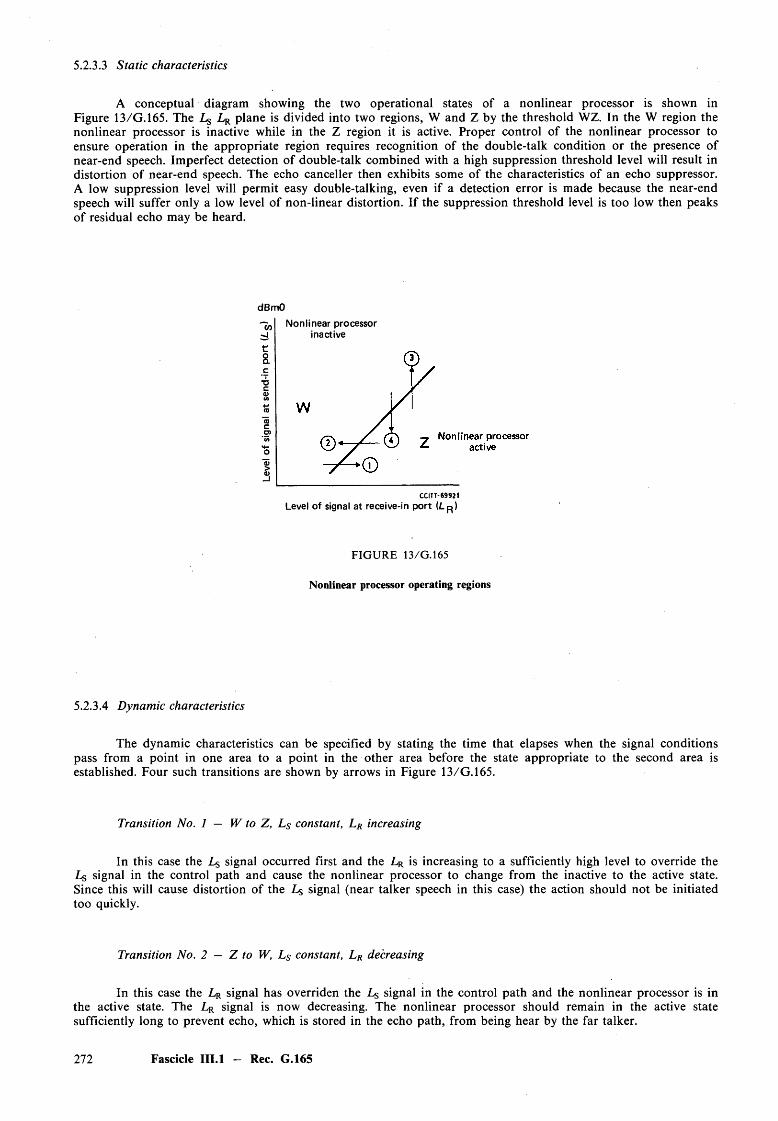
5.2.3.3 Static characteristics
A conceptual diagram showing the two operational states of a nonlinear processor is shown in Figure 13/G.165. The L$ L r plane is divided into two regions, W and Z by the threshold WZ. In the W region the nonlinear processor is inactive while in the Z region it is active. Proper control of the nonlinear processor to ensure operation in the appropriate region requires recognition of the double-talk condition or the presence of near-end speech. Imperfect detection of double-talk combined with a high suppression threshold level will result in distortion of near-end speech. The echo canceller then exhibits some of the characteristics of an echo suppressor. A low suppression level will permit easy double-talking, even if a detection error is made because the near-end speech will suffer only a low level o f non-linear distortion. If the suppression threshold level is too low then peaks of residual echo may be heard.
dBmO
(/)~JNonlinear processor
inactive
CCITT-69921
Level of signal at receive-in port (Lp)
FIG URE 13/G.165
Nonlinear processor operating regions
5.2.3.4 Dynamic characteristics
The dynamic characteristics can be specified by stating the time that elapses when the signal conditions pass from a point in one area to a point in the other area before the state appropriate to the second area is established. Four such transitions are shown by arrows in Figure 13/G.165.
Transition No. 1 — W to Z, Ls constant, L r increasing
In this case the Ls signal occurred first and the LR is increasing to a sufficiently high level to override the Ls signal in the control path and cause the nonlinear processor to change from the inactive to the active state. Since this will cause distortion of the Ls signal (near talker speech in this case) the action should not be initiated too quickly.
Transition No. 2 — Z to W, Ls constant, LR decreasing
In this case the LR signal has overriden the Ls signal in the control path and the nonlinear processor is in the active state. The LR signal is now decreasing. The nonlinear processor should remain in the active state sufficiently long to prevent echo, which is stored in the echo path, from being hear by the far talker.
272 Fascicle III.l — Rec. G.165
Transition No. 3 — Z to W, LR constant, Ls increasing
This transition is replicating the onset of double talk. As soon as possible after the Ls signal is detected the nonlinear processor should be switched to the inactive state in order to minimise any distortion of the near talker speech.
Transition No. 4 — W to Z, LR constant, Ls decreasing
In this case L$ has been recognised but is decreasing. Any action which is taken should favour continuing to permit the Ls signal to pass. This implies there should be some delay in switching the nonlinear processor back to the active state.
5.2.4 Frequency limits o f control paths (under study)
Note — Depending on the particular implementation of the nonlinear processor, the considerations and frequency response limits given in Recommendation G.164, § 3.2.4.2 for the suppression and break-in control paths of echo suppressors may also be applicable to similar control paths used in nonlinear processors. These control paths may include the activation control and adaptive suppression threshold level control.
5.2.5 Signal attenuation below threshold level
The attenuation of signals having a level below that of the suppression threshold level of a nonlinear processor in the active state must be such that the requirements of § 3.3.2.1 are met.
5.2.6 Testing o f nonlinear processors
The nonlinear processor may be considered as a special case of an echo suppressor which is limited to suppressing only low level signals. The types of test required to determine the nonlinear processor performance characteristics are very similar to the echo suppressor tests given in Recommendation G.164. However, depending on the specific implementation of a nonlinear processor, the transitions between areas W and Z of Figure 13/G.165 may not be as sharply defined as is the case for echo suppressors. Signals observed at the send-out port of the echo canceller may be distorted for short periods when transitions between the W and Z operating regions occur. Although Recommendation G.164 may be used as a guide to the testing of nonlinear processors it may be necessary to introduce unique test circuit modifications in order to make measurements on some specific nonlinear processor implementations. No recommendation can be given for a universal test circuit appropriate for all nonlinear processor implementations.
ANNEX A
(to Recommendation G.165)
Echo cancellers without nonlinear processing
It may be possible to implement echo cancellers without the inclusion of nonlinear processing. For these echo cancellers the total echo loss is provided by echo cancellation. The achievable echo cancellation is limited by the characteristics of the echo path and by the method of implementing the echo canceller. In particular, if one pair o f codecs conforming to Recommendation G .712 is used in the echo path or in the echo canceller, the maximum echo cancellation (considering quantizing errors in the echo canceller and other impairments) is that shown by the solid line in Figure A-1/G . 165.
Echo cancellers conforming to the solid line in Figure A- 1/G. 165 have been tested and found to provide acceptable performance in Japan. Other tests; however, suggest that the echo cancellation required in echo cancellers for general application is at least that shown by the broken line in Figure A-1/G . 165. Further study is needed. Pending the results of that study, echo cancellers which do not include nonlinear processors are not yet recommended for general application.
All the provisions and tests in the body of Recommendation G.165 apply to these echo cancellers except as follows:
a) § 3.3.2.1: the residual echo level requirement is that shown by the solid line of Figure A-1/G.165.b) For all other tests, any reference to non-linear processing should be ignored.
Fascicle III.l — Rec. G.165 273
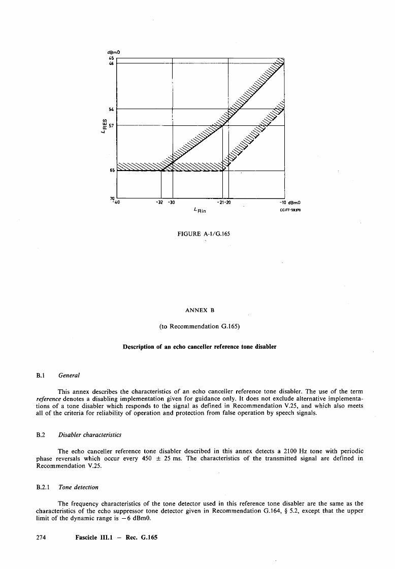
-AO -32 -30 -21-20 -10 dBmO* - R j n CCITT-59370
FIGURE A- 1/G. 165
ANNEX B
(to Recommendation G.165)
Description of an echo canceller reference tone disabler
B. 1 General
This annex describes the characteristics of an echo canceller reference tone disabler. The use of the term reference denotes a disabling implementation given for guidance only. It does not exclude alternative implementations o f a tone disabler which responds to the signal as defined in Recommendation V.25, and which also meets all of the criteria for reliability of operation and protection from false operation by speech signals.
B.2 Disabler characteristics
The echo canceller reference tone disabler described in this annex detects a 2100 Hz tone with periodic phase reversals which occur every 450 ± 25 ms. The characteristics of the transmitted signal are defined in Recommendation V.25.
B.2.1 Tone detection
The frequency characteristics of the tone detector used in this reference tone disabler are the same as the characteristics of the echo suppressor tone detector given in Recommendation G.164, § 5.2, except that the upper limit o f the dynamic range is —6 dBmO.
274 Fascicle III.l - Rec. G.165
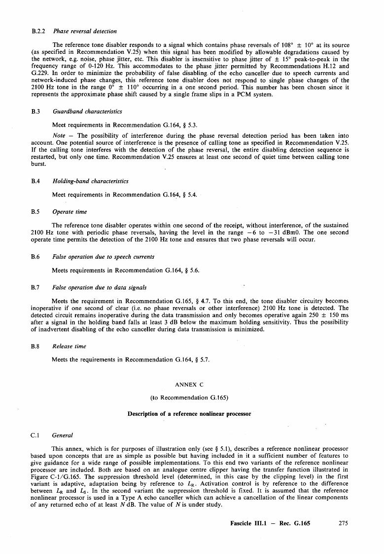
B.2.2 Phase reversal detection
The reference tone disabler responds to a signal which contains phase reversals of 108° ± 10° at its source (as specified in Recommendation V.25) when this signal has been modified by allowable degradations caused by the network, e.g. noise, phase jitter, etc. This disabler is insensitive to phase jitter of ± 15° peak-to-peak in the frequency range of 0-120 Hz. This accommodates to the phase jitter permitted by Recommendations H.12 and G.229. In order to minimize the probability of false disabling of the echo canceller due to speech currents and network-induced phase changes, this reference tone disabler does not respond to single phase changes of the 2100 Hz tone in the range 0° ± 110° occurring in a one second period. This number has been chosen since it represents the approximate phase shift caused by a single frame slips in a PCM system.
B.3 Guardband characteristics
Meet requirements in Recommendation G.164, § 5.3.
Note — The possibility of interference during the phase reversal detection period has been taken into account. One potential source of interference is the presence of calling tone as specified in Recommendation V.25. If the calling tone interferes with the detection of the phase reversal, the entire disabling detection sequence is restarted, but only one time. Recommendation V.25 ensures at least one second of quiet time between calling tone burst.
B.4 Holding-band characteristics
Meet requirements in Recommendation G.164, § 5.4.
B.5 Operate time
The reference tone disabler operates within one second of the receipt, without interference, of the sustained 2100 Hz tone with periodic phase reversals, having the level in the range —6 to —31 dBmO. The one second operate time permits the detection of the 2100 Hz tone and ensures that two phase reversals will occur.
B.6 False operation due to speech currents
Meets requirements in Recommendation G.164, § 5.6.
B.7 False operation due to data signals
Meets the requirement in Recommendation G.165, § 4.7. To this end, the tone disabler circuitry becomes inoperative if one second of clear (i.e. no phase reversals or other interference) 2100 Hz tone is detected. The detected circuit remains inoperative during the data transmission and only becomes operative again 250 ± 150 ms after a signal in the holding band falls at least 3 dB below the maximum holding sensitivity. Thus the possibility of inadvertent disabling of the echo canceller during data transmission is minimized.
B.8 Release time
Meets the requirements in Recommendation G.164, § 5.7.
ANNEX C
(to Recommendation G.165)
Description of a reference nonlinear processor
C.l General
This annex, which is for purposes of illustration only (see § 5.1), describes a reference nonlinear processor based upon concepts that are as simple as possible but having included in it a sufficient number of features to give guidance for a wide range of possible implementations. To this end two variants of the reference nonlinear processor are included. Both are based on an analogue centre clipper having the transfer function illustrated in Figure C- 1/G. 165. The suppression threshold level (determined, in this case by the clipping level) in the first variant is adaptive, adaptation being by reference to LR. Activation control is by reference to the difference between LR and L§. In the second variant the suppression threshold is fixed. It is assumed that the reference nonlinear processor is used in a Type A echo canceller which can achieve a cancellation of the linear components of any returned echo of at least N dB. The value of N is under study.
Fascicle III.l — Rec. G.165 275
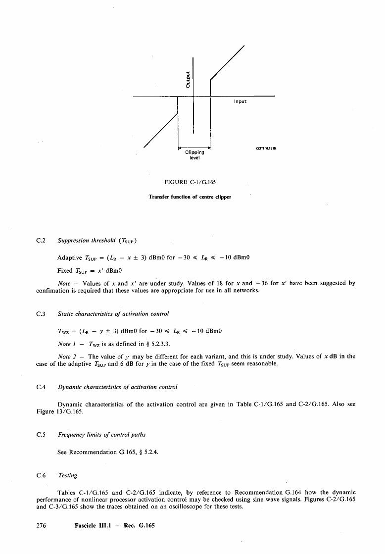
level
FIG U R E C -1/G . 165
Transfer function of centre clipper
C.2 Suppression threshold (Tsu p )
Adaptive r SUP = (LR — x ± 3) dBmO for — 30 < LR < —10 dBmO
Fixed r SUP = x ' dBmO
Note — Values of x and x ' are under study. Values of 18 for x and —36 for x ' have been suggested by confimation is required that these values are appropriate for use in all networks.
C.3 Static characteristics o f activation control
FWz = (L r - y ± 3) dBmO for - 3 0 < LR < - 1 0 dBmO
Note 1 — Twz is as defined in § 5.2.3.3.
Note 2 — The value of y may be different for each variant, and this is under study. Values of x dB in thecase of the adaptive 7sup and 6 dB for y in the case of the fixed r SUP seem reasonable.
C.4 Dynamic characteristics o f activation control
Dynamic characteristics of the activation control are given in Table C-1/G.165 and C-2/G.165. Also see Figure 13/G.165.
C.5 Frequency limits o f control paths
See Recommendation G.165, § 5.2.4.
C.6 Testing
Tables C -1/G . 165 and C-2/G.165 indicate, by reference to Recommendation G.164 how the dynamic performance of nonlinear processor activation control may be checked using sine wave signals. Figures C-2/G.165 and C-3/G.165 show the traces obtained on an oscilloscope for these tests.
276 Fascicle III.l - Rec. G.165
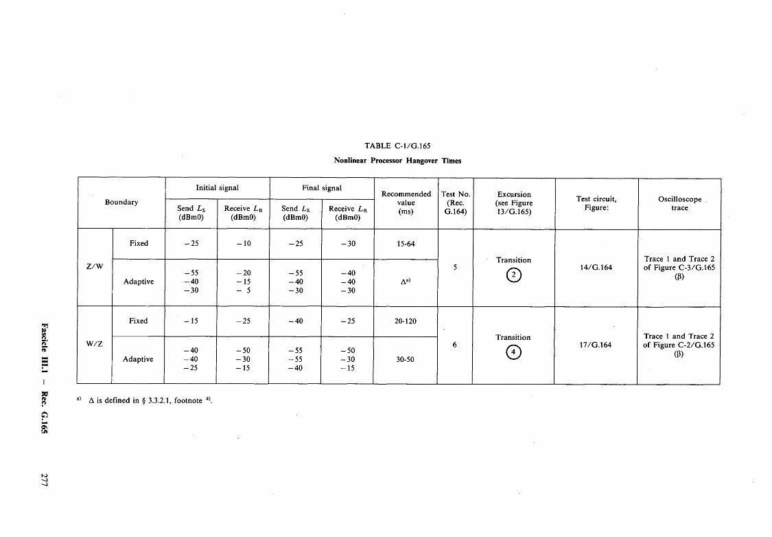
Fascicle III.l
- Rec.
G.165 277
TABLE C- 1/G . 165
Nonlinear Processor Hangover Times
Boundary
Initial signal Final signalRecommended
value(ms)
Test No. (Rec.
G.164)
Excursion (see Figure 13/G.165)
Test circuit, Figure:
OscilloscopetraceSend L s
(dBmO)Receive L R
(dBmO)Send Ls (dBmO)
Receive L R (dBmO)
Z /W
Fixed - 2 5 - 1 0 - 2 5 - 3 0 15-64
5Transition
014/G.164
Trace 1 and Trace 2 of Figure C-3/G .165
(3)Adaptive- 5 5- 4 0- 3 0
- 2 0 -1 5 - 5
-5 5- 4 0- 3 0
- 4 0- 4 0- 3 0
Aa)
w /z
Fixed -1 5 - 2 5 - 4 0 - 2 5 20-120
6Transition
o17/G.164
Trace 1 and Trace 2 of Figure C-2/G.165
(3)Adaptive- 4 0- 4 0- 2 5
- 5 0- 3 0- 1 5
- 5 5-5 5- 4 0
- 5 0- 3 0- 1 5
30-50
a) A is defined in § 3.3.2.1, footnote 4).
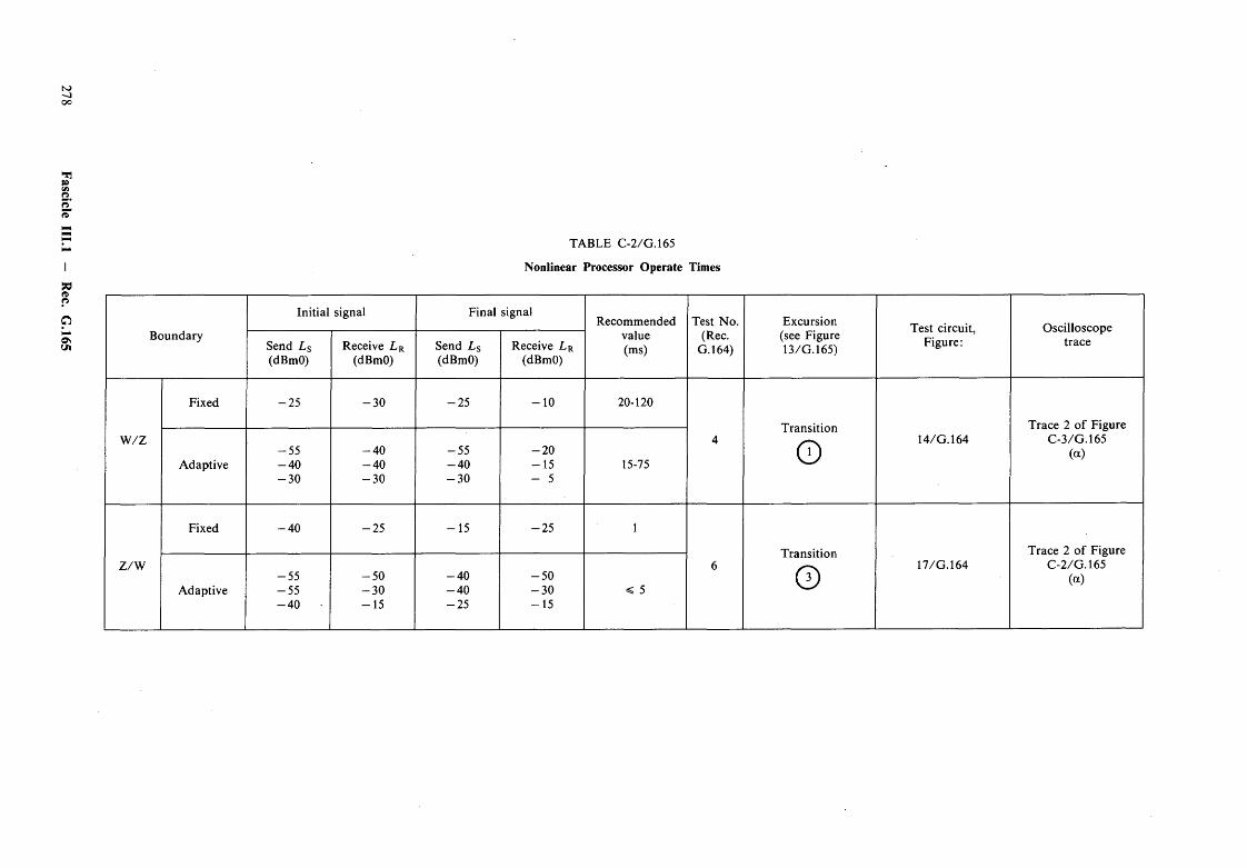
Fascicle III.l
— Rec.
G.165
to-ooo
TABLE C-2/G.165
Nonlinear Processor Operate Times
Boundary
Initial signal Final signalRecommended
value(ms)
Test No. (Rec.
G.164)
Excursion (see Figure 13/G.165)
Test circuit, Figure:
OscilloscopetraceSend L s
(dBmO)Receive L R
(dBmO)Send L s (dBmO)
Receive L R (dBmO)
W /Z
Fixed -2 5 - 3 0 -2 5 - 1 0 20-120
4Transition
o 14/G.164Trace 2 of Figure
C-3/G.165 (a)
Adaptive-5 5- 4 0- 3 0
- 4 0- 4 0- 3 0
-5 5- 4 0- 3 0
- 2 0 - 1 5 - 5
15-75
z/w
Fixed - 4 0 - 2 5 - 1 5 - 2 5 1
6Transition
© 17/G.164Trace 2 o f Figure
C-2/G.165 (a)
Adaptive-5 5-5 5- 4 0
- 5 0- 3 0- 1 5
- 4 0- 4 0- 2 5
- 5 0- 3 0-1 5
< 5
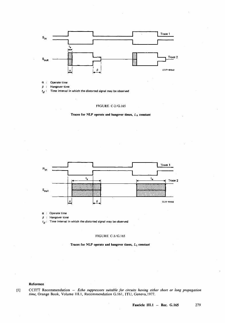
J I_ _ _ _ _ _ _ _ _ _ I ' 1 Trace 1
a : Operate time fi : Hangover timettf : Time interval in which the distorted signal may be observed
FIG U R E C-2/G.165
Traces for NLP operate and hangover times, LR constant
a : Operate time fi : Hangover timettf : Time interval in which the distorted signal may be observed
FIG U R E C-3/G.165
Traces for NLP operate and hangover times, Ls constant
Reference
[1] CCITT Recommendation — Echo suppressors suitable fo r circuits having either short or long propagation time, Orange Book, Volume III .l , Recommendation G.161, ITU, Geneva, 1977.
Fascicle III.1 - Rec. G.165 279
Recommendation G.166
CHARACTERISTICS OF SYLLABIC COM PANDORS FOR TELEPHONY ON H IGH CAPACITY LONG DISTANCE SYSTEMS
(Malaga- Torremolinos, 1984)
Compandors adhering to Recommendation G.162, Yellow Book, were intended for use in small capacity systems and their use in large capacity long-distance systems is not recommended. Compandors adhering to this Recommendation are intended for use in large capacity long-distance systems. Their use on small capacity systems is optional.
1 General
1.1 Syllabic compandors are devices in which gain variations occur at a rate comparable to the syllabic rate ofspeech. A com pandor consists of a combination of a compressor at one point in a communication path, for reducing the amplitude range of signals followed by an expander at another point for a complementary increase in the amplitude range. The com pandor enhances the subjective speech performance primarily due to two actions. The compressor increases the average speech level of weaker signals prior to entering a communication path where increased noise is expected to be encountered. The expander, in returning the speech signal to its original dynamic range provides a subjective enhancement to the communication path by attenuating the noise perceived by the listening party during silences. For a further description of compandor operation see Annex A.
1.2 This Recommendation does not specify the detector characteristics, e.g., peak, r.m.s. or average, and alsopermits a recovery time range from 0 to 17 ms.
The peformance recommended may not be sufficient to ensure compatibility between compandors conforming to this Recommendation but which are of different design. Before using compressors and expanders of different design origins at opposite ends of the same circuit, Administrations should test them for compatibility. The tests should take account of the sensitivity of com pandor performance to the characteristics of the test signal.
1.3 The use of a number of syllabic compandors on circuits carried on the same FDM carrier may result in achanged load being presented to the FDM system. The FDM system operating parameters could, therefore, require appropriate adjustment as a function of the load.
1.4 It should be noted that the subjective enhancement which occurs on speech, when syllabic compandors are used, does not apply to transmission of non-speech signals which may experience a signal-to-noise degradation on syllabic compandored circuits.
1.5 Some of the clauses given below specify the joint characteristics of a compressor and an expander in thesame direction of transmission of a 4-wire circuit. The characteristics specified in this way can be obtained more easily if the compressors and expanders are o f similar design; in certain cases close cooperation between Administrations may be necessary. Application rules for syllabic compandors address this issue.
2 Definitions
2.1 unaffected level
The unaffected level is the absolute level, at a point of zero relative level on the line between the compressor and the expander of a signal at 800 Hz, which remains unchanged whether the circuit is operated with the compressor or not. The unaffected level is defined in this way in order not to impose any particular values of relative level at the input to the compressor or the output of the expander.
To make allowances for the increase in mean power introduced by the compressor, and to avoid the risk of increasing the intermodulation noise and the overload which might result, the unaffected level must be adjusted taking into account the capacity of the system. (See Reference [1], Chapter II, Annex 4, for detailed discussion of this adjustment.)
280 Fascicle III.l - Rec. G.166
2.2 ratio of compression
The ratio of compression of a compressor is defined by the formula:
L\ cin — L 2 cin a = --------------------------L 1 COUT — L 2 cout
whereL\ cin and L 2 Cin are any two different compressor input levels within the compressor operating range.L\ cout and L 2 Cout are the compressor output levels corresponding to input levels L x Cin and L 2 Cmrespectively.
2.3 ratio of expansion
The ratio of expansion of an expander is defined by the formula:
p _ L\ EqUT — L 2 eout L 1 E I N — L 2 e i n
whereL] EIN and L 2 E!N are any two different expander input levels within the expander operating range.L i eout and L 2 EOut are the expander output levels corresponding to input levels L x Ein and L 2 ErNrespectively.
3 Characteristics of syllabic compandors
3.1 Unaffected level
A nominal value of —10 dBmO for the unaffected level is recommended for high capacity systems. However, Administrations are free to mutually negotiate a different unaffected level to allow optimal loading of their transmission systems. Such variation is expected to be in the range —10 to —24 dBmO. The loading effects of pilot tones should be considered.
3.2 Ratio o f compression, a
The value of a is 2 ± 0.02 over the temperature range + 10 °C to +40 °C.
3.3 Ratio o f expansion, p
The value of P is 2 ± 0.02 over the temperature range + 10 °C to + 40 °C.
3.4 Range o f level (under study)
The range of level over which the recommended value of a and p should apply, should extend at least:from + 5 to —60 dBmO at the input of the compressor, andfrom + 5 to — 65 dBmO at the nominal output of the expander.
3.5 Variation o f compressor gain
The level at the output of the compressor, measured at 800 Hz, for an input level equal to the unaffected level, should not vary from its nominal value by more than ± 0.25 dB for a temperature range of + 1 0 ° C to + 40 ° C and a deviation of the supply voltage of ± 5% from its nominal value.
3.6 Variation o f expander gain
The level at the output of the expander, measured at 800 Hz for an input level equal to the unaffected level, should not vary from its nominal value by more than ± 0.5 dB for a temperature range of + 1 0 ° C to + 40 ° C and a deviation of the supply voltage of ± 5% from its nominal value.
Fascicle III.l — Rec. G.166 281
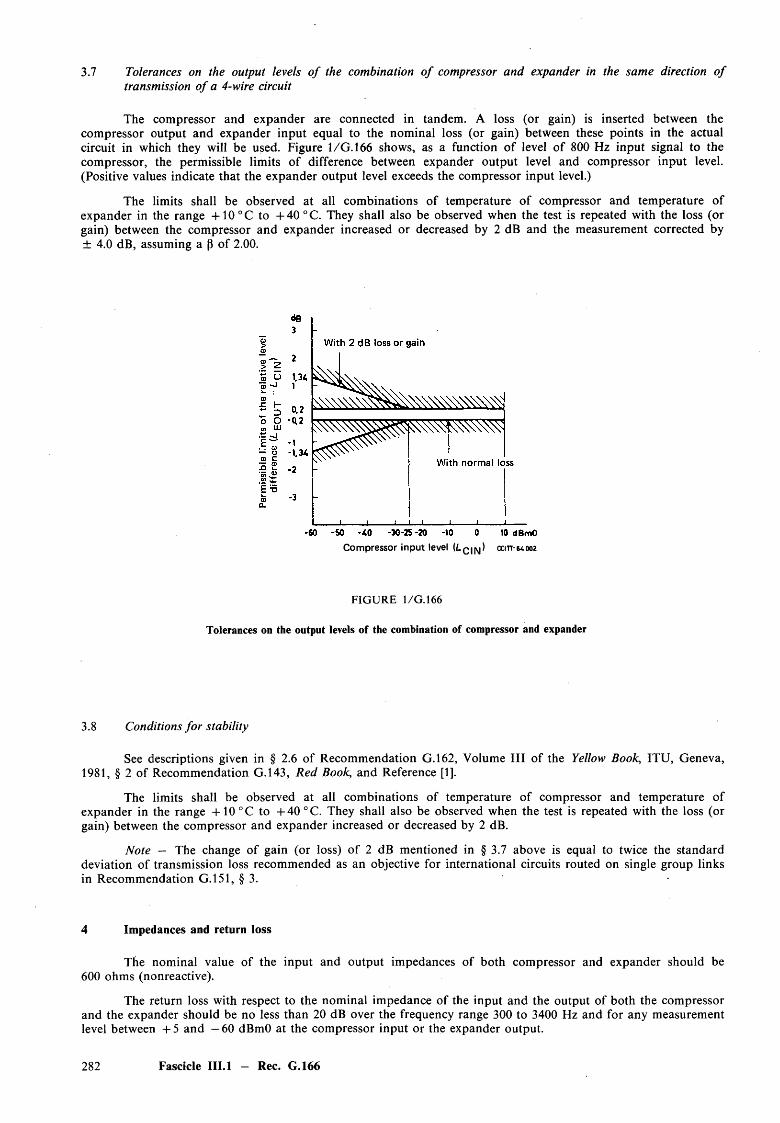
3.7 Tolerances on the output levels o f the combination o f compressor and expander in the same direction o f transmission o f a 4-wire circuit
The compressor and expander are connected in tandem. A loss (or gain) is inserted between the compressor output and expander input equal to the nominal loss (or gain) between these points in the actual circuit in which they will be used. Figure 1/G. 166 shows, as a function of level of 800 Hz input signal to the compressor, the permissible limits o f difference between expander output level and compressor input level. (Positive values indicate that the expander output level exceeds the compressor input level.)
The limits shall be observed at all combinations of temperature of compressor and temperature of expander in the range + 1 0 °C to + 40 °C. They shall also be observed when the test is repeated with the loss (or gain) between the compressor and expander increased or decreased by 2 dB and the measurement corrected by ± 4.0 dB, assuming a (3 of 2.00.
C om pressor inp u t level U - q i n ) c c i t t - m o o 2
FIG URE 1/G. 166
Tolerances on the output levels of the combination of compressor and expander
3.8 Conditions fo r stability
See descriptions given in § 2.6 of Recommendation G.162, Volume III of the Yellow Book, ITU, Geneva,1981, § 2 of Recommendation G.143, Red Book, and Reference [1].
The limits shall be observed at all combinations of temperature of compressor and temperature of expander in the range + 1 0 °C to + 40 °C. They shall also be observed when the test is repeated with the loss (or gain) between the compressor and expander increased or decreased by 2 dB.
Note — The change of gain (or loss) o f 2 dB mentioned in § 3.7 above is equal to twice the standarddeviation of transmission loss recommended as an objective for international circuits routed on single group links in Recommendation G.151, § 3.
4 Impedances and return loss
The nominal value of the input and output impedances of both compressor and expander should be 600 ohms (nonreactive).
The return loss with respect to the nominal impedance of the input and the output of both the compressor and the expander should be no less than 20 dB over the frequency range 300 to 3400 Hz and for any measurement level between + 5 and —60 dBmO at the compressor input or the expander output.
282 Fascicle III.l - Rec. G.166
5 Operating characteristics at various frequencies
5.1 Frequency characteristic with control circuit clamped
The control circuit is said to be clamped when the control current (or voltage) derived by rectification of the signal is replaced by a constant direct current (or voltage) supplied from an external source. For purposes here, the value of this current (or voltage) should be equal to the value of the control current (or voltage) obtained when the input signal is set to the unaffected level.
For the compressor and the expander taken separately, the variations of loss or gain with frequency should be contained within the limits o f a diagram that can be deduced from Figure 1/G . 132 by dividing the tolerance shown by 8, the measurement being made with a constant input level corresponding to the unaffected level.
5.2 Frequency characteristic with control circuit operating normally
The limits given in § 5.1 should be observed for the compressor when the control circuit is operating normally, the measurement being made with a constant input level corresponding to the unaffected level.
For the expander, under the same conditions of measurement, the limits can be deduced from Figure 1/G . 132 by dividing the tolerances shown by 4.
These limits should be observed over the temperature range + 10 °C to + 40 °C.
6 Nonlinear distortion
6.1 Harmonic distortion
The total harmonic distortion, measured with an 800 Hz sine wave at the unaffected level, should not exceed 0.5% for the compressor and the expander taken separately.
Note — Even in an ideal compressor, high output peaks will occur when the signal level is suddenly raised. The most severe case seems to be that of voice-frequency signalling, although the effect can also occur during speech. It may be desirable, in exceptional cases, to Fit the compressor with an amplitude limiter to avoid disturbance due to transients during voice-frequency signalling.
6.2 Intermodulation tests
It is necessary to add a measurement of intermodulation to the measurements of harmonic distortion whenever compandors are intended for international circuits (regardless of the signalling system used), as well as in all cases where they are provided for national circuits over which multi-frequency signalling, or data transmission using similar types of signals, is envisaged.
The intermodulation products of concern to the operation of multi-frequency telephone signalling receivers are those of the third order, of type (2/i — />) and (2 / — /i), where f and f 2 are two signalling frequencies.
Two signals at frequencies 900 Hz and 1020 Hz are recommended for these tests.
Two test conditions should be considered: the first, where each of the signals at / and f 2 is at a level of — 5 dBmO and the second, where they are each at a level of —15 dBmO. These levels are to be understood to be at the input to the compressor or at the output of the expander (uncompressed levels).
The limits for the intermodulation products are defined as the difference between the level of either of the signals at frequencies f or f 2 and the level of either of the intermodulation products at frequencies (2/i — f 2) or (2 /2 - / ) •
A value for this difference which seems adequate for the requirements of multi-frequency telephone signalling (including end-to-end signalling over three circuits in tandem, each equipped with a compandor) is 32 dB for the compressor and the expander separately.
Note 1 — These values seem suitable for Signalling System No. 5, which will be used on some long international circuits.
Fascicle III.l — Rec. G.166 283
Note 2 — It is inadvisable to make measurements on a compressor plus expander in tandem, because the individual intermodulation levels o f the compressor and of the expander might be quite high, although much less intermodulation is given in tandem measurements since the characteristics of compressor and expander may be closely complementary. The compensation encountered in tandem measurements on compressor and expander may not be encountered in practice, either because there may be phase distortion in the line or because the compressor and expander at the two ends of the line may be less closely complementary than the compressor and expander measured in tandem.
Hence the measurements have to be performed separately for the compressor and the expander. The two signals at frequencies f and f 2 must be applied simultaneously, and the levels at the output of the compressor or expander measured selectively.
7 Noise
The effective value of the sum of all noise referred to a zero relative level point, the input and the output being terminated with resistances of 600 ohms, shall be less than or equal to the following values:
— at the output of the compressor: —45 dBmOp— at the output o f the expander: - 80 dBmOp.
8 Transient response
The overall transient response of the combination of a compressor and expander which are to be used in the same direction of transmission of a 4-wire circuit fitted with compandors shall be checked as follows:
The compressor and expander are connected in tandem, the appropriate loss (or gain) being inserted between them as in § 3.7.
A 12-dB step signal at a frequency of 2000 Hz is applied to the input of the compressor, the actual values being a change from —16 to —4 dBmO for attack, and from —4 to - 1 6 dBmO for recovery. The envelope of the expander output is observed. The overshoot (positive or negative), after an upward 12-dB step expressed as a percentage of the final steady-state voltage, is a measure of the overall transient distortion of the compressor- expander combination for attack. The overshoot (positive or negative) after a downward 12-dB step, expressed as a percentage of the final steady-state voltage is a measure of the overall transient distortion of the compressor- expander combination for recovery. For both these quantities the permissible limits shall be ± 20%. These limits shall be observed for the same conditions of temperature and of variation of loss (or gain) between compressor and expander as for the test in § 3.7.
In addition, the attack and recovery times of the compressor alone shall be measured as follows:
Using the same 12-dB steps as above for attack and recovery respectively, the attack time is defined as the time between the instant when the sudden change is applied and the instant when the output voltage envelope reaches a value equal to 1.5 times its steady-state value. The recovery time is defined as the time between the instant when the sudden change is applied and the instant when the output voltage envelope reaches a value equal to 0.75 times its steady-state value.
The permissible limits shall be not greater than:— 3 ms for attack,— 17 ms for recovery.
ANNEX A
(to Recommendation G.166)
Compandor enhancement characteristics
The improvement which the compandor makes available is based on the fact that interference is most objectionable during quiet speech or pauses, but is masked by relatively loud speech. While it will not be necessary, therefore, to alter the performance of the system for speech signals at a high level, an improvement has to be provided when the signal level is low. This noise reduction can be arranged by introducing loss at the receiving end of the circuit during periods when the signal is faint or absent. The loss so introduced will affect the noise or crosstalk which has crept in along the route, so that the interference is reduced by the amount of this loss. However, the desired signals are also affected, and in order that the speech level finally received shall be
284 Fascicle III.1 - Rec. G.166
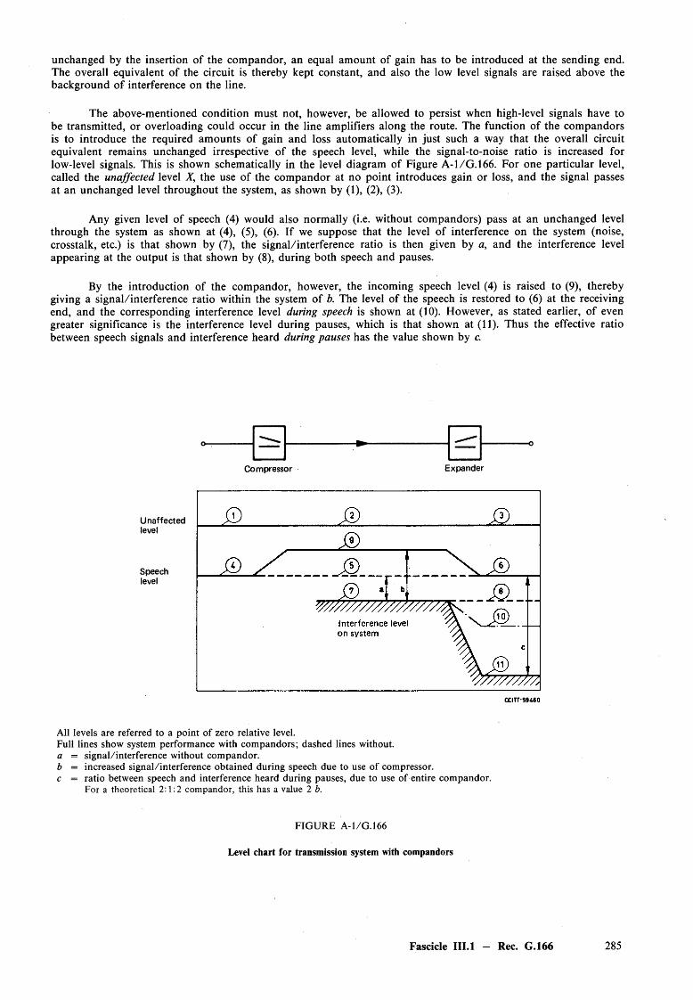
unchanged by the insertion of the compandor, an equal amount of gain has to be introduced at the sending end. The overall equivalent of the circuit is thereby kept constant, and also the low level signals are raised above the background of interference on the line.
The above-mentioned condition must not, however, be allowed to persist when high-level signals have to be transmitted, or overloading could occur in the line amplifiers along the route. The function of the compandors is to introduce the required amounts of gain and loss automatically in just such a way that the overall circuit equivalent remains unchanged irrespective of the speech level, while the signal-to-noise ratio is increased for low-level signals. This is shown schematically in the level diagram of Figure A-1/G . 166. For one particular level, called the unaffected level X , the use of the com pandor at no point introduces gain or loss, and the signal passes at an unchanged level throughout the system, as shown by (1), (2), (3).
Any given level of speech (4) would also normally (i.e. without compandors) pass at an unchanged level through the system as shown at (4), (5), (6). If we suppose that the level of interference on the system (noise, crosstalk, etc.) is that shown by (7), the signal/interference ratio is then given by a, and the interference level appearing at the output is that shown by (8), during both speech and pauses.
By the introduction of the compandor, however, the incoming speech level (4) is raised to (9), thereby giving a signal/interference ratio within the system of b. The level of the speech is restored to (6) at the receiving end, and the corresponding interference level during speech is shown at (10). However, as stated earlier, of even greater significance is the interference level during pauses, which is that shown at (11). Thus the effective ratio between speech signals and interference heard during pauses has the value shown by c.
Compressor Expander
Unaffectedlevel
Speechlevel
C CITT-S9M 0
All levels are referred to a point of zero relative level.Full lines show system performance with compandors; dashed lines without. a = signal/interference without compandor.b = increased signal/interference obtained during speech due to use of compressor. c = ratio between speech and interference heard during pauses, due to use of entire compandor.
For a theoretical 2:1:2 compandor, this has a value 2 b.
FIG URE A-1/G. 166
Level chart for transmission system with compandors
Fascicle III.l — Rec. G.166 285
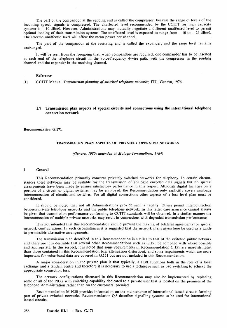
The part of the compandor at the sending end is called the compressor, because the range of levels o f the incoming speech signals is compressed. The unaffected level recommended by the CCITT for high capacity systems is —10 dBmO. However, Administrations may mutually negotiate a different unaffected level to permit optimal loading of their transmission systems. The unaffected level is expected to range from - 1 0 to - 2 4 dBmO. The selected unaffected level will affect the mean power per channel.
The part of the com pandor at the receiving end is called the expander, and the same level remains unchanged.
It will be seen from the foregoing that, when compandors are required, one compandor has to be inserted at each end of the telephone circuit in the voice-frequency 4-wire path, with the compressor in the sending channel and the expander in the receiving channel.
Reference
[1] CCITT M anual Transmission planning o f switched telephone networks, ITU, Geneva, 1976.
1.7 Transmission plan aspects of special circuits and connections using the international telephone connection network
Recommendation G.171
TRANSM ISSION PLAN ASPECTS OF PRIVATELY OPERATED NETWORKS
(Geneva, 1980; amended at Malaga-Torremolinos, 1984)
1 General
This Recommendation primarily concerns privately switched networks for telephony. In certain circumstances these networks may be suitable for the transmission of analogue encoded data signals but no special arrangements have been made to ensure satisfactory performance in this respect. Although digital facilities on a portion of a circuit or digital switches may be employed, the Recommendation only explicitly covers analogue interconnection of circuits and switches. For all digital connections other aspects of a loss level plan must be considered.
It should be noted that not all Administrations provide such a facility. Others permit interconnection between private telephone networks and the public telephone network. In this latter case assurance cannot always be given that transmission performance conforming to CCITT standards will be obtained. In a similar manner the interconnection of multiple private networks may result in connections with degraded transmission performance.
It is not intended that this Recommendation should prevent the making of bilateral agreements for special network configurations. In such circumstances it is suggested that the network plans given here be used as a guide to permissible alternative arrangements.
The transmission plan described in this Recommendation is similar to that of the switched public network and therefore it is desirable that several other Recommendations such as G.151 be complied with where possible and appropriate. In this respect, it is noted that some requirements in Recommendation G.151 are more stringent than those contained in this Recommendation (e.g. attenuation distortion), and some impairments which are more im portant for voice-band data are covered in G.151 but are not included in this Recommendation.
A major consideration in the private plan is that typically, a PBX functions both in the role of a local exchange and a tandem centre and therefore it is necessary to use a technique such as pad switching to achieve the appropriate connection loss.
The network configurations discussed in this Recommendation may also be implemented by replacing some or all of the PBXs with switching capability dedicated to a private user that is located on the premises of the telephone Administration rather than on the customers’ premises.
Recommendation M.1030 provides information on the maintenance of international leased circuits forming part o f private switched networks. Recommendation Q.8 describes signalling systems to be used for international leased circuits.
286 Fascicle III.1 - Rec. G.171
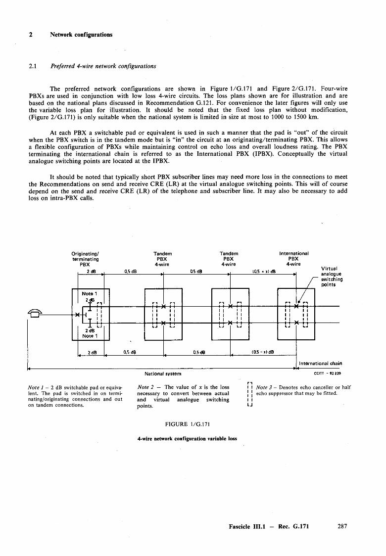
2 Network configurations
2.1 Preferred 4-wire network configurations
The preferred network configurations are shown in Figure 1/G. 171 and Figure 2/G.171. Four-wire PBXs are used in conjunction with low loss 4-wire circuits. The loss plans shown are for illustration and are based on the national plans discussed in Recommendation G.121. For convenience the later figures will only use the variable loss plan for illustration. It should be noted that the fixed loss plan without modification, (Figure 2/G.171) is only suitable when the national system is limited in size at most to 1000 to 1500 km.
At each PBX a switchable pad or equivalent is used in such a m anner that the pad is “out” of the circuit when the PBX switch is in the tandem mode but is “in” the circuit at an originating/term inating PBX. This allows a flexible configuration of PBXs while maintaining control on echo loss and overall loudness rating. The PBX terminating the international chain is referred to as the International PBX (IPBX). Conceptually the virtual analogue switching points are located at the IPBX.
It should be noted that typically short PBX subscriber lines may need more loss in the connections to meet the Recommendations on send and receive CRE (LR) at the virtual analogue switching points. This will of course depend on the send and receive CRE (LR) of the telephone and subscriber line. It may also be necessary to add loss on intra-PBX calls.
Originating/ terminating
PBX
TandemPBX
4-wire
TandemPBX
4-wire
InternationalPBX
4-wire
Note 1 - 2 dB switchable pad or equivalent. The pad is switched in on terminating/originating connections and out on tandem connections.
Note 2 — The value of x is the loss necessary to convert between actual and virtual analogue switching points.
n I I I I i I l I U
Note 3 - Denotes echo canceller or half echo suppressor that may be fitted.
FIG URE 1/G.171
4-wire network configuration variable loss
Fascicle III.l - Rec. G.171 287
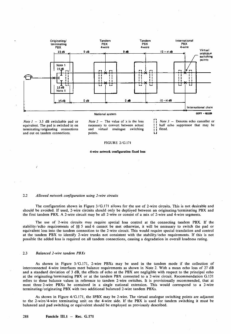
Originating/terminating
PBX
TandemPBX
4-wire
TandemPBX
4wire
InternationalPBX
4wire
Note 1 — 3.5 dB switchable pad or equivalent. The pad is switched in on term inating/originating connections and out on tandem connections.
National system
Note 2 — The value of x is the loss necessary to convert between actual and virtual analogue switching points.
n I I I I I I I I LJ
CCITT - u r n
Note 3 — Denotes echo canceller or half echo suppressor that may be fitted.
FIG URE 2/G.171
4-wire network configuration fixed loss
/
2.2 Allowed network configuration using 2-wire circuits
The configuration shown in Figure 3/G.171 allows for the use of 2-wire circuits. This is not desirable and should be avoided. If used, 2-wire circuits should only be deployed between an originating/term inating PBX and the first tandem PBX. A 2-wire circuit may be all 2-wire or consist of a mix of 2-wire and 4-wire segments.
The use of 2-wire circuits may require special loss control at the connecting tandem PBX. If the stability/echo requirements of §§ 5 and 6 cannot be met otherwise, it will be necessary to switch the pad or equivalent loss into the tandem connection to the 2-wire circuit. This would require special translation and control at the tandem PBX to identify 2-wire trunks not consistent with the stability/echo requirements. If this is not possible the added loss is required on all tandem connections, causing a degradation in overall loudness rating.
2.3 Balanced 2-wire tandem PBXs
As shown in Figure 3/G.171, 2-wire PBXs may be used in the tandem mode if the collection of interconnected 4-wire interfaces meet balance requirements as shown in Note 2. With a mean echo loss of 27 dB and a standard deviation of 3 dB, the effects of echo at the PBX are negligible with respect to the principal echo at the originating/term inating PBX or at the tandem PBX connected to a 2-wire circuit. Recommendation G.131 refers to these balance values in reference to tandem 2-wire switches. It is provisionally recommended, that at most three 2-wire PBXs be contained in a single national extension. This would correspond to a 2-wire term inating/originating PBX with two additional balanced 2-wire tandem PBXs.
As shown in Figure 4/G.171, the IPBX may be 2-wire. The virtual analogue switching points are adjacent to the 2-wire/4-wire terminating unit on the 4-wire side. If the PBX is used for tandem switching it must be balanced and pad switching or equivalent should be employed as previously described.
288 Fascicle III.l — Rec. G.171
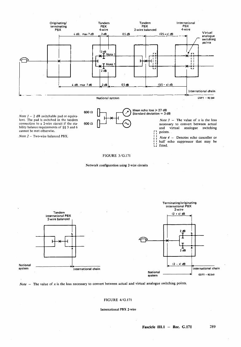
Originating/terminating
PBX
TandemPBX
4-wire
Tandem PBX
2-wire balanced
InternationalPBX
4-wire
Note 1 - 2 dB switchable pad or equivalent. The pad is switched in the tandem connection to a 2-wire circuit if the stability balance requirements of §§ 5 and 6 cannot be met otherwise.Note 2 - Two-wire balanced PBX.
600 ft
600 ft L - ©
Mean echo loss > 27 dB Standard deviation = 3 dB
Note 3 — The value of x is the loss necessary to convert between actual and virtual analogue switching points. .
Note 4 — Denotes echo canceller or half echo suppressor that may be fitted.
FIG URE 3/G.171
Network configuration using 2-wire circuits
Nationalsystem
Tandem international PBX
2-wire balanced
International chain
Terminating/originating international PBX
2-wire (2 ♦ x) dB
O -
2 dB
i s2 dB
(2 - x) dB
Nationalsystem
International chain
CCITT - 8 2 2 4 0
Note — The value of x is the loss necessary to convert between actual and virtual analogue switching points.
FIG URE 4/G.171
International PBX 2-wire
Fascicle III.l - Rec. G.171 289
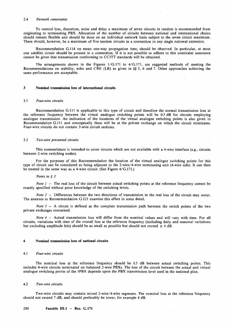
2.4 Network constraints
To control loss, distortion, noise and delay a maximum of seven circuits in tandem is recommended from originating to terminating PBX. Allocation of the number of circuits between national and international chains should remain flexible and should be done on an individual network basis subject to the seven circuit maximum. There should, however, be a maximum of five tandem circuits in a connection in any single national extension.
Recommendation G.114 on mean one-way propagation time, should be observed. In particular, at most one satellite circuit should be present in a connection. If it is not possible to adhere to this constraint assurance cannot be given that transmission conforming to CCITT standards will be obtained.
The arrangements shown in the Figures 1/G . 171 to 4/G.171, are suggested methods of meeting the Recommendations on stability, echo and CRE (LR) as given in §§ 5, 6 and 7. Other approaches achieving the same performance are acceptable.
3 Nominal transmission loss of international circuits
3.1 Four-wire circuits
Recommendation G . l l l is applicable to this type of circuit and therefore the normal transmission loss at the reference frequency between the virtual analogue switching points will be 0.5 dB for circuits employing analogue transmission. An indication of the locations of the virtual analogue switching points is also given in Recommendation G . l l l and conceptually these will be at the private exchange on which the circuit terminates. Four-wire circuits do not contain 2-wire circuit sections.
3.2 Two-wire presented circuits
This nomenclature is intended to cover circuits which are not available with a 4-wire interface (e.g., circuits between 2-wire switching nodes).
For the purposes of this Recommendation the location of the virtual analogue switching points for this type of circuit can be considered as being adjacent to the 2-wire/4-wire terminating unit (4-wire side). It can then be treated in the same way as a 4-wire circuit. (See Figure 4/G.171.)
Notes to § 3
Note 1 — The real loss of the circuit between actual switching points at the reference frequency cannot be exactly specified without prior knowledge of the switching levels.
Note 2 — Differences between the two directions of transmission in the real loss of the circuit may occur. The annexes to Recommendation G.121 examine this effect in some detail.
Note 3 — A circuit is defined as the complete transmission path between the switch points of the two private exchanges concerned.
Note 4 — Actual transmission loss will differ from the nominal values and will vary with time. For all circuits, variations with time of the overall loss at the reference frequency (including daily and seasonal variations but excluding amplitude hits) should be as small as possible but should not exceed ± 4 dB.
4 Nominal transmission loss of national circuits
4.1 Four-wire circuits
The nominal loss at the reference frequency should be 0.5 dB between actual switching points. This includes 4-wire circuits terminated on balanced 2-wire PBXs. The loss of the circuit between the actual and virtual analogue switching points of the IPBX depends upon the PBX transmission level used in the national plan.
4.2 Two-wire circuits
Two-wire circuits may contain mixed 2-wire/4-wire segments. The nominal loss at the reference frequency should not exceed 7 dB, and should preferably be lower, for example 4 dB.
290 Fascicle III.1 - Rec. G.171
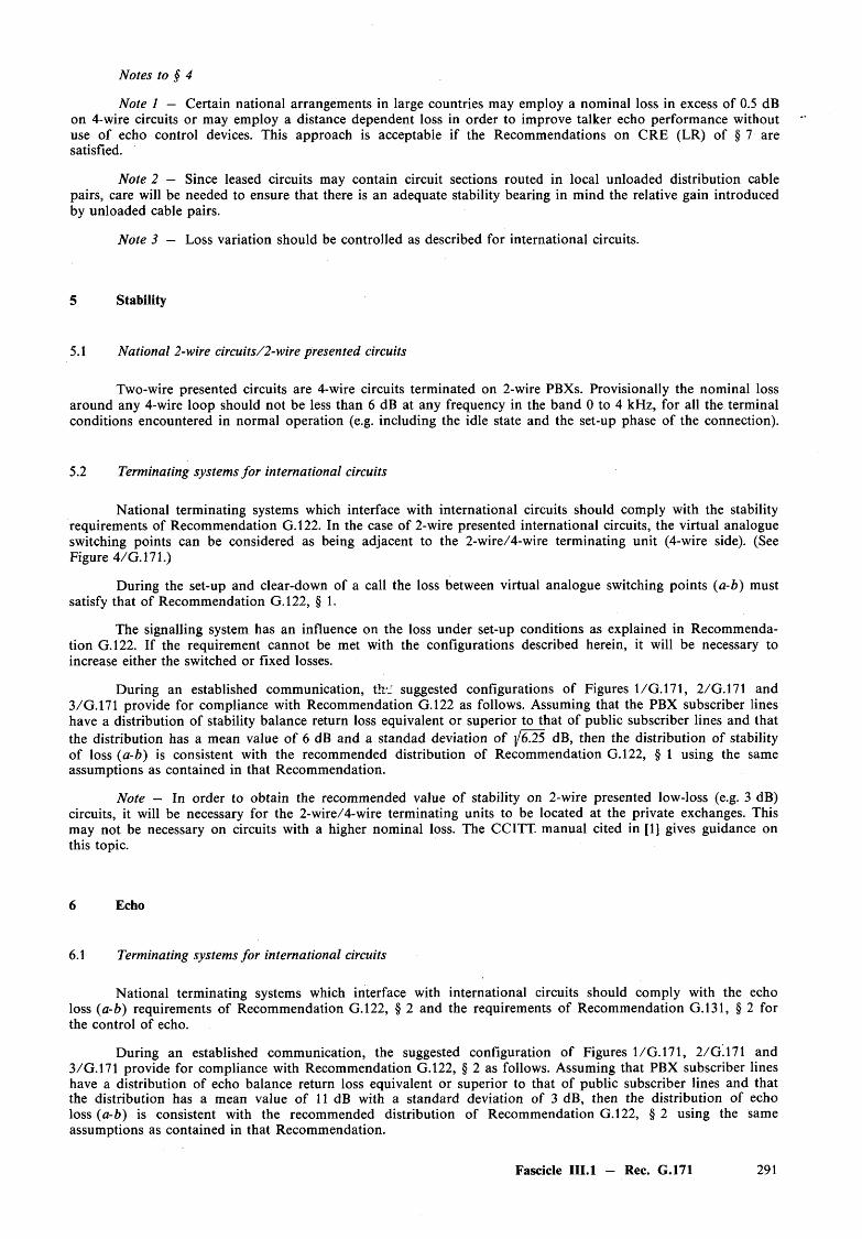
Notes to § 4
Note 1 — Certain national arrangements in large countries may employ a nominal loss in excess of 0.5 dB on 4-wire circuits or may employ a distance dependent loss in order to improve talker echo performance without use of echo control devices. This approach is acceptable if the Recommendations on CRE (LR) of § 7 are satisfied.
Note 2 — Since leased circuits may contain circuit sections routed in local unloaded distribution cable pairs, care will be needed to ensure that there is an adequate stability bearing in mind the relative gain introduced by unloaded cable pairs.
Note 3 — Loss variation should be controlled as described for international circuits.
5 Stability
5.1 National 2-wire circuits/2-wire presented circuits
Two-wire presented circuits are 4-wire circuits terminated on 2-wire PBXs. Provisionally the nominal loss around any 4-wire loop should not be less than 6 dB at any frequency in the band 0 to 4 kHz, for all the terminal conditions encountered in normal operation (e.g. including the idle state and the set-up phase of the connection).
5.2 Terminating systems fo r international circuits
National terminating systems which interface with international circuits should comply with the stability requirements of Recommendation G.122. In the case of 2-wire presented international circuits, the virtual analogue switching points can be considered as being adjacent to the 2-wire/4-wire terminating unit (4-wire side). (See Figure 4/G.171.)
During the set-up and clear-down of a call the loss between virtual analogue switching points (a-b) must satisfy that o f Recommendation G.122, § 1.
The signalling system has an influence on the loss under set-up conditions as explained in Recommendation G.122. If the requirement cannot be met with the configurations described herein, it will be necessary to increase either the switched or fixed losses.
During an established communication, th i suggested configurations of Figures 1/G . 171, 2/G.171 and 3/G.171 provide for compliance with Recommendation G.122 as follows. Assuming that the PBX subscriber lines have a distribution of stability balance return loss equivalent or superior to that o f public subscriber lines and that the distribution has a mean value o f 6 dB and a standad deviation of j/6.25 dB, then the distribution of stability of loss (a-b) is consistent with the recommended distribution of Recommendation G.122, § 1 using the same assumptions as contained in that Recommendation.
Note — In order to obtain the recommended value of stability on 2-wire presented low-loss (e.g. 3 dB) circuits, it will be necessary for the 2-wire/4-wire terminating units to be located at the private exchanges. This may not be necessary on circuits with a higher nominal loss. The CCITT manual cited in [1] gives guidance on this topic.
6 Echo
6.1 Terminating systems fo r international circuits
National terminating systems which interface with international circuits should comply with the echo loss (a-b) requirements of Recommendation G.122, § 2 and the requirements of Recommendation G.131, § 2 for the control of echo.
During an established communication, the suggested configuration of Figures 1/G . 171, 2/G.171 and 3/G.171 provide for compliance with Recommendation G.122, § 2 as follows. Assuming that PBX subscriber lines have a distribution of echo balance return loss equivalent or superior to that of public subscriber lines and that the distribution has a mean value o f 11 dB with a standard deviation of 3 dB, then the distribution of echo loss (a-b) is consistent with the recommended distribution of Recommendation G.122, § 2 using the same assumptions as contained in that Recommendation.
Fascicle III.l - Rec. G.171 291

6.2 Echo control devices
When echo control devices (e.g., echo suppressors or echo cancellers) are necessary it is preferable that they be located at the private exchange. This minimizes end delay and also allows disabling of the device during tandem operation, if necessary. In addition, some signalling systems require local disabling of echo control devices during certain signalling phases. The echo control device (echo canceller or far-end operated half-echo suppressor) for the international circuit would be located at the PBX terminating the international chain, since this same PBX typically could originate/term inate traffic or tandem switch to many trunks without echo control. However, if connecting national circuits introduce enough delay to w arrant echo control, then echo control devices would also be provided on these circuits.
If far-end operated half-echo suppressors are used, intermediate suppressors should be disabled. This is not necessary for echo cancellers since tandem operation does not cause degraded performance. In either case the functioning echo control device on the connection is effectively moved closer to the PBX subscriber line, further reducing end delay. The echo control devices are located in the 4-wire portion of the network and between the first hybrid and the international chain. However, the devices may be located at the international centre when the previously described performance factors can still be satisfactorily controlled and there is a maintenance a n d /o r cost advantage for such location.
The loss of circuits fitted with echo control devices should be 0 dB.
Echo suppressors and cancellers according to Recommendation G.164 and Recommendation G.165, typically require 6 dB of signal loss (a-b) for the actual signal converging the canceller or being controlled by the suppressor. Therefore it is desirable from a performance point of view that the stability loss (a-b) during an established connection should be at least 6 dB, since this will ensure proper operation for any signal (frequency spectrum) in the band 0-4 kHz. However this may not be economically achievable. The spectrum of a typical speech signal and return path is such that if the echo loss (a-b) is at least 6 dB, then the signal loss (a-b) for the speech signal is expected to be at least 6 dB and the echo control devices should operate properly. However, the spectrum of some voice-band data signals and of the return path is such that an echo loss (a-b) of at least 10 dB is required to ensure that the signal loss (a-b) for the actual data signal is 6 dB. (Modems operating half-duplex on satellite circuits may require echo protection for proper operation.) Therefore, when an echo control device is located at a PBX, the echo loss at the 4-wire terminals o f the device looking towards the subscriber line should be at least 6 dB for 99.5% of the connections and 10 dB for 95% of the connections for all network configurations during an established communication. This is not a new requirement in that the values are consistent with the recommended distribution for echo loss independent of the number of circuits between the echo control device and the subscriber line, assuming the distribution is Gaussian, which is a conservative assumption.
The suggested configuration of Figures 1/G.171, 2/G.171 and 3/G.171 provided for compliance with the minimum echo loss Recommendations. Using these configurations there is always a loss pad or equivalent between the echo control device and the 2-wire termination. Then, under the conditions described in § 6.1, the distribution of echo loss at the terminals of the echo control device is consistent with the recommended distribution.
If the private network uses echo suppressors and connects to a public network using echo cancellers, then difficulty in canceller convergence may be experienced when the suppressor is in the tail path of the canceller. However, performance will then be determined by the echo control devices at each end of the connection.
7 Corrected reference equivalents (CREs) and loudness ratings (LRs) of extension circuits
7.1 Loading
Administrations must ensure that the technical arrangements that they authorize in respect of operating levels, sensitivities, etc. for private networks are not in conflict with the design criteria of the international transmission system. Attention is drawn to Recommendation G.121, § 3, which specifies a nominal minimum value of 7 dB sending CRE (2 dB sending LR) referred to the virtual analogue switching point.
292 Fascicle III.l - Rec. G.171
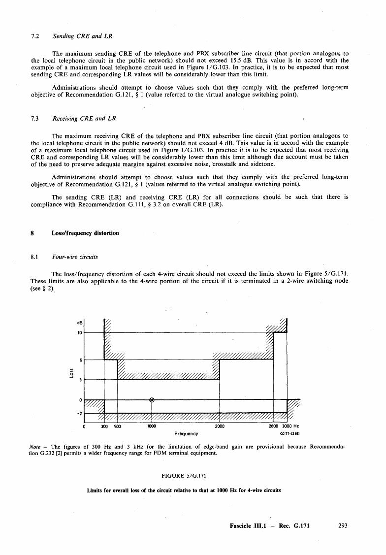
7.2 Sending CRE and LR
The maximum sending CRE of the telephone and PBX subscriber line circuit (that portion analogous to the local telephone circuit in the public network) should not exceed 15.5 dB. This value is in accord with the example of a maximum local telephone circuit used in Figure 1/G . 103. In practice, it is to be expected that most sending CRE and corresponding LR values will be considerably lower than this limit.
Administrations should attempt to choose values such that they comply with the preferred long-term objective of Recommendation G.121, § 1 (value referred to the virtual analogue switching point).
7.3 Receiving CRE and LR
The maximum receiving CRE of the telephone and PBX subscriber line circuit (that portion analogous to the local telephone circuit in the public network) should not exceed 4 dB. This value is in accord with the example of a maximum local telephone circuit used in Figure 1/G.103. In practice it is to be expected that most receiving CRE and corresponding LR values will be considerably lower than this limit although due account must be taken of the need to preserve adequate margins against excessive noise, crosstalk and sidetone.
Administrations should attem pt to choose values such that they comply with the preferred long-term objective of Recommendation G.121, § 1 (values referred to the virtual analogue switching point).
The sending CRE (LR) and receiving CRE (LR) for all connections should be such that there is compliance with Recommendation G . l l l , § 3.2 on overall CRE (LR).
8 Loss/frequency distortion
8.1 Four-wire circuits
The loss/frequency distortion of each 4-wire circuit should not exceed the limits shown in Figure 5/G.171. These limits are also applicable to the 4-wire portion of the circuit if it is terminated in a 2-wire switching node (see § 2).
SI y //A
V ///A V ////////////A
- vVW
y/A.’'////////A V //////////////Z y.0 300 500 1000 2000 2800 3000 Hz
Frequency ccitt-*2 i«i
Note — The figures of 300 Hz and 3 kHz for the limitation of edge-band gain are provisional because Recommendation G.232 [2] permits a wider frequency range for FDM terminal equipment.
FIG URE 5/G.171
Limits for overall loss of the circuit relative to that at 1000 Hz for 4-wire circuits
Fascicle III.l — Rec. G.171 293

The loss/frequency distortion of each 2-wire circuit should not exceed the limits shown in Figure 6/G.171.
8.2 Two-wire presented circuits
Frequency ccitt-»032
Note — The figures of 300 Hz and 3 kHz for the limitation of edge-band gain are provisional because Recommendation G.232 [2] permits a wider frequency range for FDM terminal equipment.
FIG URE 6/G.171 •
Lim its for overall loss o f the circuit relative to that at 1000 H z for 2-wire presented circuits
9 Noise
The requirements of the relevant Recommendations should be met in respect of noise by each of the circuit sections and Recommendations G.123 and G.143, § 1 gives some general guidance on system noise characteristics. The nominal level o f random noise power at the private exchange will depend upon the actual constitution of the circuit but should not exceed —38 dBmOp (provisional maintenance limit for circuits longer than 10 000 kilometres). In practice circuits of shorter length will exhibit substantially less random noise. Figure 7/G.171 serves as a guide to the expected performance.
Circuits having sections routed via communication satellites, designed according to Recommendation G.153, may be assessed in respect o f noise performance by ascribing a nominal 1000 km of circuit length for the satellite path. It should be noted, however, that although such an allowance is appropriate for most satellites carrying international traffic, there may be certain locations where noise levels in excess o f this value may be found.
294 Fascicle III.l - Rec. G.171
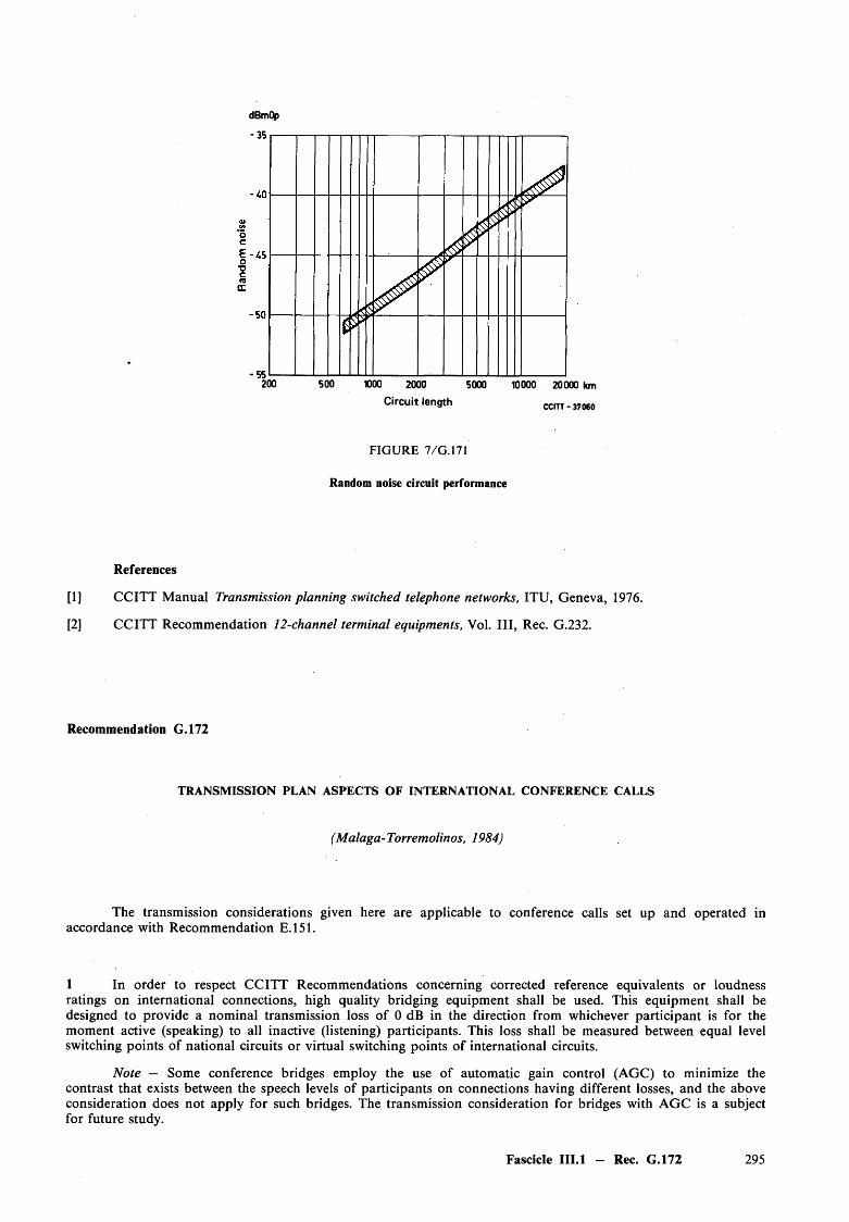
dBmOp
- 351—
551----- I II II I-----------1— I--- I I I I I I---------200 500 1000 2000 5000 10000 20000 km
Circuit length c c it t-37060
F IG U R E 7 /G .171
Random noise circuit performance
References
[1] CCITT M anual Transmission planning switched telephone networks, ITU, Geneva, 1976.
[2] CCITT Recommendation 12-channel terminal equipments, Vol. I l l , Rec. G.232.
Recommendation G.172
T R A N S M IS S IO N P L A N A S P E C T S O F IN T E R N A T IO N A L C O N F E R E N C E CA L LS
(Malaga-Torremolinos, 1984)
The transmission considerations given here are applicable to conference calls set up and operated in accordance with Recommendation E.151.
1 In order to respect CCITT Recommendations concerning corrected reference equivalents or loudness ratings on international connections, high quality bridging equipment shall be used. This equipment shall be designed to provide a nominal transmission loss of 0 dB in the direction from whichever participant is for the moment active (speaking) to all inactive (listening) participants. This loss shall be measured between equal level switching points of national circuits or virtual switching points of international circuits.
Note — Some conference bridges employ the use of automatic gain control (AGC) to minimize the contrast that exists between the speech levels of participants on connections having different losses, and the above consideration does not apply for such bridges. The transmission consideration for bridges with AGC is a subject for future study.
Fascicle III.l - Rec. G.172 295
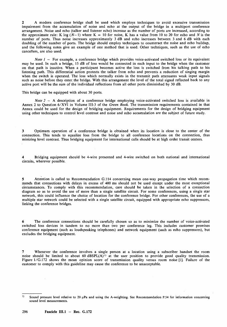
2 A modern conference bridge shall be used which employs techniques to avoid excessive transmission impairment from the accumulation of noise and echo at the output of the bridge in a multiport conference arrangement. Noise and echo (talker and listener echo) increase as the number of ports are increased, according to the approximate rule: K log (N — 1) where K = 10 for noise, K has a value from 10 to 20 for echo and AT is the number of ports. Thus noise increases approximately 3 dB and echo increases between 3 and 6 dB with each doubling of the number of ports. The bridge should employ techniques to counteract the noise and echo buildup, and the following notes give an example of one method that is used. Other techniques, such as the use of echo cancellers, are also used.
Note 1 — For example, a conference bridge which provides voice-activated switched loss or its equivalent may be used. In such a bridge, 15 dB of loss would be connected in each input to the bridge when the customer on that path is inactive. When a participant becomes active the loss is switched from his talking path to his listening path. This differential action protects the talker from echo and prevents a reduction of singing margin when the switch is operated. The loss which normally exists in the transm it path attenuates weak input signals such as noise before they enter, the bridge. With this arrangement the level o f the total signal reflected back to any active port will be the sum of the individual reflections from all other ports diminished by 30 dB.
This bridge can be equipped with about 30 ports.
Note 2 — A description of a conference bridge employing voice-activated switched loss is available in Annex 2 to Question 6/X V I in Volume III-3 of the Green Book The transmission requirements contained in that Annex could be used for the design of bridging equipment. Requirements for the design of bridging equipment using other techniques to control level contrast and noise and echo accumulation are the subject of future study.
3 Optimum operation of a conference bridge is obtained when its location is close to the center of the connection. This tends to equalize loss from the bridge to all conference locations on the connection, thus minizing level contrast. Thus bridging equipment for international calls should be at high order transit centers.
4 Bridging equipment should be 4-wire presented and 4-wire switched on both national and international circuits, wherever possible.
5 Attention is called to Recommendation G.114 concerning mean one-way propagation time which recommends that connections with delays in excess of 400 ms should not be used except under the most exceptional circumstances. To comply with this recommendation, care should be taken in the selection of a connection diagram so as to avoid the use of more than a single satellite circuit. For some conferences, using a single star network, this could influence the choice of location for the conference bridge. For other conferences, the use of a multiple star network could be selected with a single satellite circuit, equipped with appropriate echo suppressors, linking the conference bridges.
6 The conference connections should be carefully chosen so as to minimize the number of voice-activated switched loss devices in tandem to no more than two per conference leg. This includes customer premises conference equipment (such as loudspeaking telephones) and network equipment (such as echo suppressors), but excludes the bridging equipment.
7 Whenever the conference involves a single person at a location using a subscriber handset the room noise should be limited to about 60 dBSPL(A)1* at the user position to provide good quality transmission. Figure 1/G . 172 shows the mean opinion score of transmission quality versus room noise [1]. Failure of the customer to comply with this guideline may cause the conference to be unacceptable.
Sound pressure level relative to 20 pPa and using the A-weighting. See Recommendation P.54 for information concerning sound level measurements.
296 Fascicle III.l — Rec. G.172
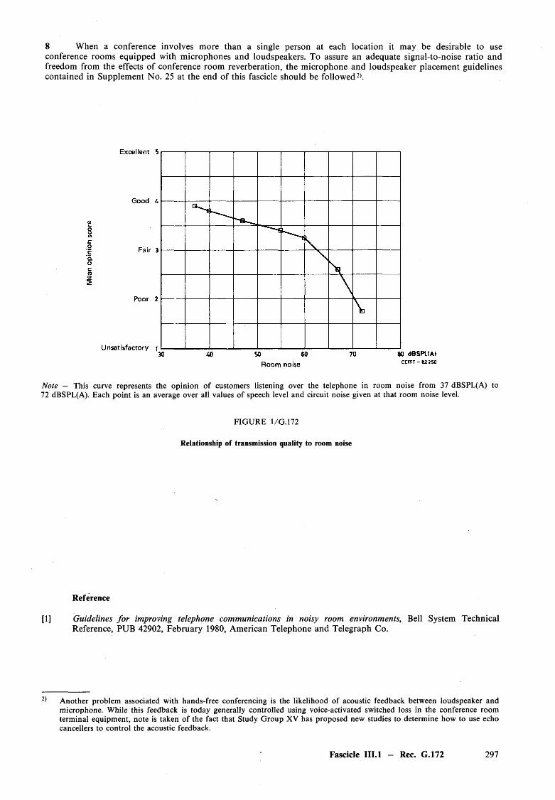
8 When a conference involves more than a single person at each location it may be desirable to use conference rooms equipped with microphones and loudspeakers. To assure an adequate signal-to-noise ratio and freedom from the effects of conference room reverberation, the microphone and loudspeaker placement guidelines contained in Supplement No. 25 at the end of this fascicle should be followed2).
Note — This curve represents the opinion of customers listening over the telephone in room noise from 37 dBSPL(A) to 72 dBSPL(A). Each point is an average over all values of speech level and circuit noise given at that room noise level.
FIG URE 1/G . 172
Relationship of transmission quality to room noise
Reference
[1] Guidelines fo r improving telephone communications in noisy room environments, Bell System Technical Reference, PUB 42902, February 1980, American Telephone and Telegraph Co.
A nother problem associated with hands-free conferencing is the likelihood of acoustic feedback between loudspeaker and microphone. While this feedback is today generally controlled using voice-activated switched loss in the conference room terminal equipment, note is taken of the fact that Study Group XV has proposed new studies to determine how to use echo cancellers to control the acoustic feedback.
Fascicle III.l — Rec. G.172 297
1.8 General Recommendations on availability and reliability of entire international telephone connections
Recommendation G.180
CONNECTION ACCESSIBILITY OBJECTIVE FOR THE INTERNATIONAL TELEPHONE SERVICE’)
(Malaga-Torremolinos, 1984)
Introduction
This Recommendation is one of a set of closely related Recommendations, comprising Recommendations G.107, G.108, G.180 and G.181 concerned with the accessibility and retainability of telephone services.
Preamble
This Recommendation provides an overall end-to-end connection accessibility (availability) objective for international switched telephone service.
Connection accessibility is a component of service accessibility as defined in Recommendation G.106.
This Recommendation contains a measure of connection accessibility, an objective, and an allocation of the objective to the national systems and international chain of international connections. The Recommendation also relates the overall end-to-end performance to the reliability and availability of circuits and exchanges in a way useful for network design purposes.
The objective includes the effects of equipment faults and traffic congestion.
The CCITT,
considering
(a) that connection accessibility is defined in Recommendation G.106;
(b) that customers rank connection inaccessibility as one of the most annoying of call set-up impairments;
(c) that an objective for connection accessibility which takes into account customer opinion about the call set-up phase is consistent with other Recommendations which have recommended an objective for service retainability based, in part, on customer opinion;
(d) that connection accessibility will not be constant over time, even for a particular calling and called line pair. One suitable measure is a long-term average network connection failure probability. (Other suitable measures may also be required.);
(e) that the overall objective for connection accessibility should be allocable to the national systems and the international chain of the international connection;
(f) that the objective should take into account the concerns of network planners and system designers, provide useful guidance to both and may be used by Administrations in providing a method for verifying whether or not network performance is acceptable;
(g) that the overall connection accessibility should be controlled by the accessibility performances of individual exchanges and circuits, and that to obtain this control, the overall connection accessibility must be mathematically linked to the equipment availability and reliability,
’) Some of the terms in this Recommendation, for example, the noun “measure”, are used in the sense of their definition given in Recommendation G.106.
298 Fascicle III.l — Rec. G.180
recommends
1 Measure of connection accessibility
Connection accessibility shall be measured using the long-term average network connection failure probability, which is the complement of the connection access probability as defined in Recommendation G.106.
The network connection failure probability PNCf can be estimated by using the following formula:
p _ QnPncf ~ n
where QN is the number of unsuccessful connection access attempts and JVis the total number of connection access attempts in some time period (to be determined).
A method for estimating the required call sample size is contained in Annex A.
For purposes of network design, the network connection failure probability, Pncf, can also be calculated using the method outlined in Annex B.
Note 1 — Those unsuccessful connection access attempts reflecting failure of the network to work properly, from the user’s perspective, are called network connection failure. They are call failures an astute caller can determine and are caused by network faults and congestion. A network connection failure is any valid bid for service which receives one of the following network responses:
1) dial tone returned after dialling is completed;2) no ring and no answer;
3) all circuits busy signal or announcement;4) connection to the wrong number (misrouting);5) double connection.
This list may not be exhaustive.
Note 2 — This definition of network connection failure is based on the response the caller can hear.
Note 3 — There are two generic causes of network connection failures: equipment faults and traffic congestion.
Note 4 — The averaging interval (to be determined) used for estimating the connection failure probability shall include normal and peak hour traffic periods. In the event of exceptionally high traffic demand (public holiday, natural disaster, etc.) failure rates higher than the objective may be tolerated.
Note 5 — The network connection failure probability should be estimated by Administrations in a mannerconsistent with obtaining, from the Administration’s point o f view, reasonably accurate estimates.
2 Objective for connection accessibility
Connection accessibility is acceptable if the long-term average connection failure probability, expressed asa percentage, does not exceed a value (overall average for all international calls) of A% to B% (values to bedetermined). Additionally, the long-term average failure probability at any single international homing exchange should never exceed C% (value to be determined).
Note — Possible values for A, B and C are in the range of 10% to 20%.
3 Allocation of the overall objective to the national systems and international chain
The network connection failure probability objective shall be apportioned as follows:X% to the originating national system,Y% to the international chain,Z% to the terminating national system,
where X + Y + Z = P, and P is the overall objective stated in § 2. (The values of X, Y and Z are to be determined.)
Fascicle III.1 - Rec. G.180 299
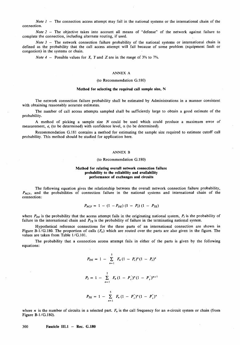
Note 1 — The connection access attempt may fail in the national systems or the international chain of the connection.
Note 2 — The objective takes into account all means of “defense” of the network against failure to complete the connection, including alternate routing, if used.
Note 3 - The network connection failure probability of the national systems or international chain is defined as the probability that the call access attempt will fail because of some problem (equipm ent fault or congestion) in the systems or chain.
Note 4 - Possible values for X, Y and Z are in the range of 3% to 7%.
A NNEX A
(to Recommendation G.180)
Method for selecting the required call sample size, N
The network connection failure probability shall be estimated by Administrations in a manner consistent with obtaining reasonably accurate estimates.
The number of call access attempts sampled shall be sufficiently large to obtain a good estimate of the probability.
A method of picking a sample size N could be used which could produce a maximum error ofmeasurement, e, (to be determined) with confidence level, a (to be determined).
Recommendation G.181 contains a method for estimating the sample size required to estimate cutoff callprobability. This method should be studied for application here.
A NNEX B
(to Recommendation G.180)
Method for relating overall network connection failure probability to the reliability and availability
performance of exchanges and circuits
The following equation gives the relationship between the overall network connection failure probability, Pncf, and the probabilities of connection failure in the national systems and international chain of the connection:
Pncf - 1 - ( 1 -Poe) ( 1 - Pi) ( 1 - Pte)where P0e is the probability that the access attempt fails in the originating national system, Pj is the probability of failure in the international chain and P Te is the probability of failure in the terminating national system.
Hypothetical reference connections for the three parts of an international connection are shown in Figure B-1/G. 180. The proportion o f calls (Fn) which are routed over the parts are also given in the figure. The values are taken from Table 1/G . 101.
The probability that a connection access attempt fails in either of the parts is given by the following equations:
5
POE= 1 - £ F , ( 1 - pcy ( l - psy 1
2
Pj - l - I F „ ( 1 - P'CY(. 1 - P’SY"«= 1
Pte - 1 - Z f » ( l - P'c)"( 1 - Pi)"«= 1
where n is the number of circuits in a selected part. F„ is the call frequency for an ^-circuit system or chain (from Figure B- 1/G . 180).
300 Fascicle III.l - Rec. G.180
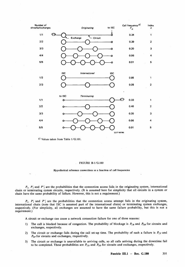
Number of Call frequency3 Indexcircuits/exchanges Originating to ISC Fn n
1/1 O --------------------------p-------------------------O 0.34 1Exchange Circuit
2/2 o — -— o — ---------O 0.39 2
3/3 o — o — o — 0 0.20 3
4/4 O — O — Q — O — ° 006 4o—o—o—o—o5/5 r 1----- C 1----- C 1----- ( V — C 1 O 0.01 5
ISC International ISC
1/2--------------------- Q ----------------------------------------------------Q 0.95 1
2/3 Q ---------------------- Q -----------------------Q 0.05 2
to ISC Terminating1/1 O------ -o—° 0.33 1
2/2 O------— o-------------------o 0.40 2
3/3 o ------—o— o——o 0.20 3
4/4 o -----
669 -o 0.06 4
5/5 o ----- O- O” O' O” oCCITT-S5790
0.01 5
a) Values taken from Table 1/G .1 0 1 .
FIG URE B-1/G. 180
Hypothetical reference connections as a function of call frequencies
Pc, P'c and P"c are the probabilities that the connection access fails in the originating system, international chain or terminating system circuits, respectively. (It is assumed here for simplicity that all circuits in a system orchain have the same probability of failure. However, this is not a requirement.)
Ps, P's and P's are the probabilities that the connection access attem pt fails in the originating system, international chain (note that ISC is assumed part of the international chain) or terminating system exchanges, respectively. (For simplicity, all exchanges are assumed to have the same failure probability, but this is not a requirement.)
A circuit or exchange can cause a network connection failure for one of three reasons:
1) The call is blocked because of congestion. The probability of blockage is PCb and PSb for circuits andexchanges, respectively.
2) The circuit or exchange fails during the call set-up time. The probability of such a failure is P Cf and Psf for circuits and exchanges, respectively.
3) The circuit or exchange is unavailable to arriving calls, so all calls arriving during the downtime fail to be completed. These probabilities are Pcd and PSd for circuits and exchanges, respectively.
Fascicle III.I - Rec. G.180 301
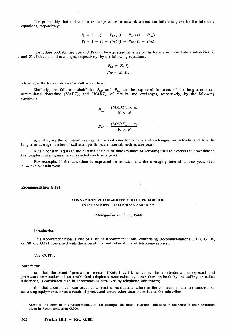
The probability that a circuit or exchange causes a network connection failure is given by the following equations, respectively:
Pc = 1 - (1 - PCB) (1 - PCF) (1 - P c d )
Ps = 1 - ( 1 - PSB) ( 1 - P s f ) ( 1 - P s d )
The failure probabilities P Cf and P Sf can be expressed in terms of the long-term mean failure intensities Z cand Zs of circuits and exchanges, respectively, by the following equations:
P cf = Z c Ts
P s f = Z s Ts ,
where Ts is the long-term average call set-up time.
Similarly, the failure probabilities P Cd and P SD can be expressed in terms of the long-term mean accumulated downtime (M A D T)C and (M A D T)S o f circuits and exchanges, respectively, by the following equations:
CD
P sd —
(M A D T )C x a c K x N
(M A D T )S x a s K x N
a c and a* are the long-term average call arrival rates for circuits and exchanges, respectively, and N is the long-term average number of call attempts (in some interval, such as one year).
K is a constant equal to the number of units o f time (minutes or seconds) used to express the downtime in the long-term averaging interval selected (such as a year).
For example, if the downtime is expressed in minutes and the averaging interval is one year, then K = 525 600 m in/year.
Recommendation G.181
CONNECTION RETAINABILITY OBJECTIVE FOR THE INTERNATIONAL TELEPHONE SERVICE1)
(Malaga-Torremolinos, 1984)
Introduction
This Recommendation is one of a set of Recommendations, comprising Recommendations G.107, G.108, G.180 and G.181 concerned with the accessibility and retainability of telephone services.
The CCITT,
considering
(a) that the event “premature release” (“cutoff call”), which is the unintentional, unexpected and premature termination of an established telephone connection by other than on-hook by the calling or called subscriber, is considered high in annoyance as perceived by telephone subscribers;
(b) that a cutoff call can occur as a result o f equipment failure in the connection path (transmission or switching equipment), or as a result of procedural errors other than those due to the subscriber;
') Some of the terms in this Recommendation, for example, the noun “measure”, are used in the sense of their definition given in Recommendation G.106.
302 Fascicle III.l — Rec. G.181
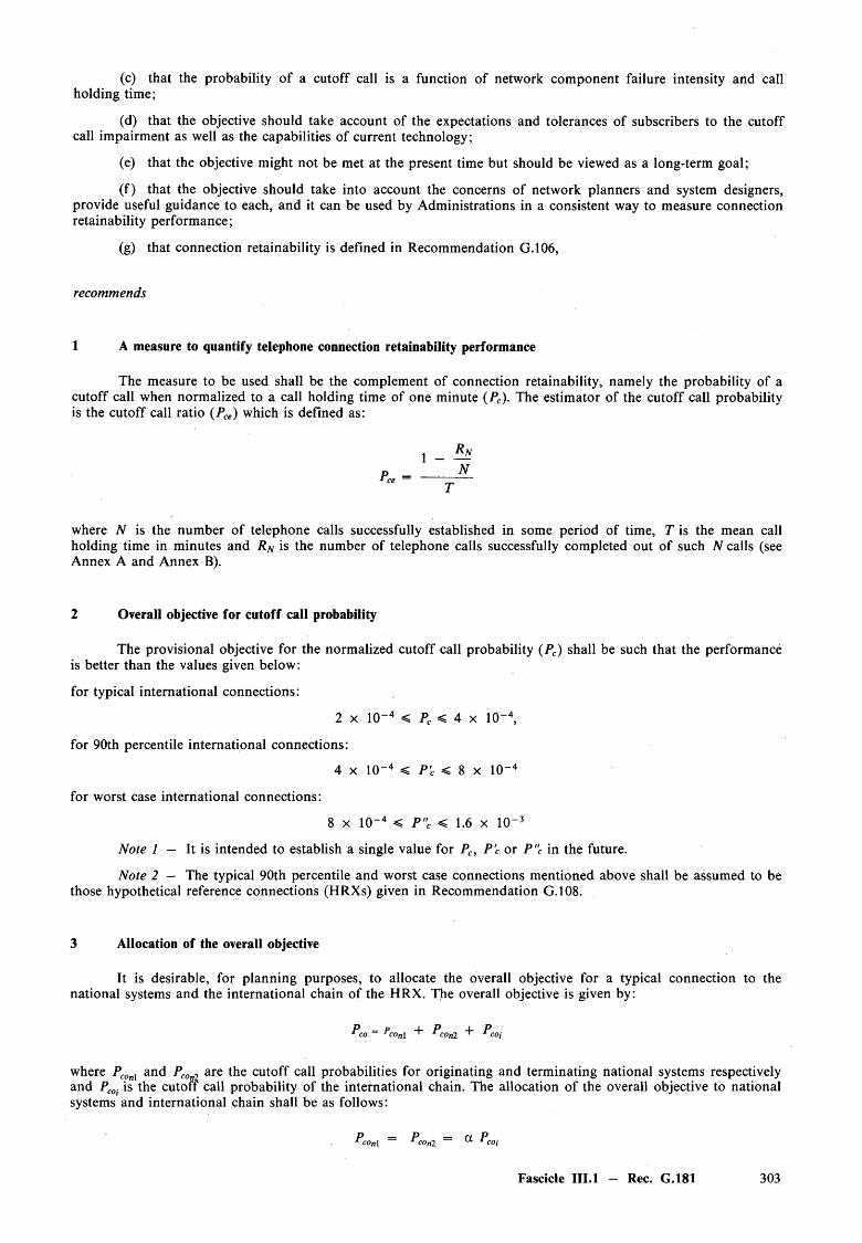
(c) that the probability of a cutoff call is a function of network component failure intensity and call holding time;
(d) that the objective should take account of the expectations and tolerances of subscribers to the cutoff call impairment as well as the capabilities of current technology;
(e) that the objective might not be met at the present time but should be viewed as a long-term goal;
(f) that the objective should take into account the concerns of network planners and system designers, provide useful guidance to each, and it can be used by Administrations in a consistent way to measure connection retainability performance;
(g) that connection retainability is defined in Recommendation G.106,
recommends
1 A measure to quantify telephone connection retainability performance
The measure to be used shall be the complement of connection retainability, namely the probability of a cutoff call when normalized to a call holding time of one minute (Pc). The estimator of the cutoff call probability is the cutoff call ratio (Pce) which is defined as:
, Rn
where N is the number of telephone calls successfully established in some period of time, T is the mean call holding time in minutes and R N is the number of telephone calls successfully completed out of such N calls (see Annex A and Annex B).
2 Overall objective for cutoff call probability
The provisional objective for the normalized cutoff call probability (Pc) shall be such that the performance is better than the values given below:
for typical international connections:
2 x 10~4 < Pc < 4 x 10 -4,
for 90th percentile international connections:
4 x 10 -4 < P'c < 8 x 10"4
for worst case international connections:
8 x 10~4 < P"c < 1.6 x 1 0 -3
Note 1 — It is intended to establish a single value for Pc, P'c or P"c in the future.
Note 2 — The typical 90th percentile and worst case connections mentioned above shall be assumed to be those hypothetical reference connections (HRXs) given in Recommendation G.108.
3 Allocation of the overall objective
It is desirable, for planning purposes, to allocate the overall objective for a typical connection to the national systems and the international chain of the HRX. The overall objective is given by:
P — P ^~ P Px co C0 n\ ' con2 coi
where PCOnX and PCOn2 are the cutoff call probabilities for originating and terminating national systems respectively and Pcoj is the cutoff call probability of the international chain. The allocation of the overall objective to national systems and international chain shall be as follows:
P = P — a P1 con\ con 2 coi
Fascicle III.l — Rec. G.181 303
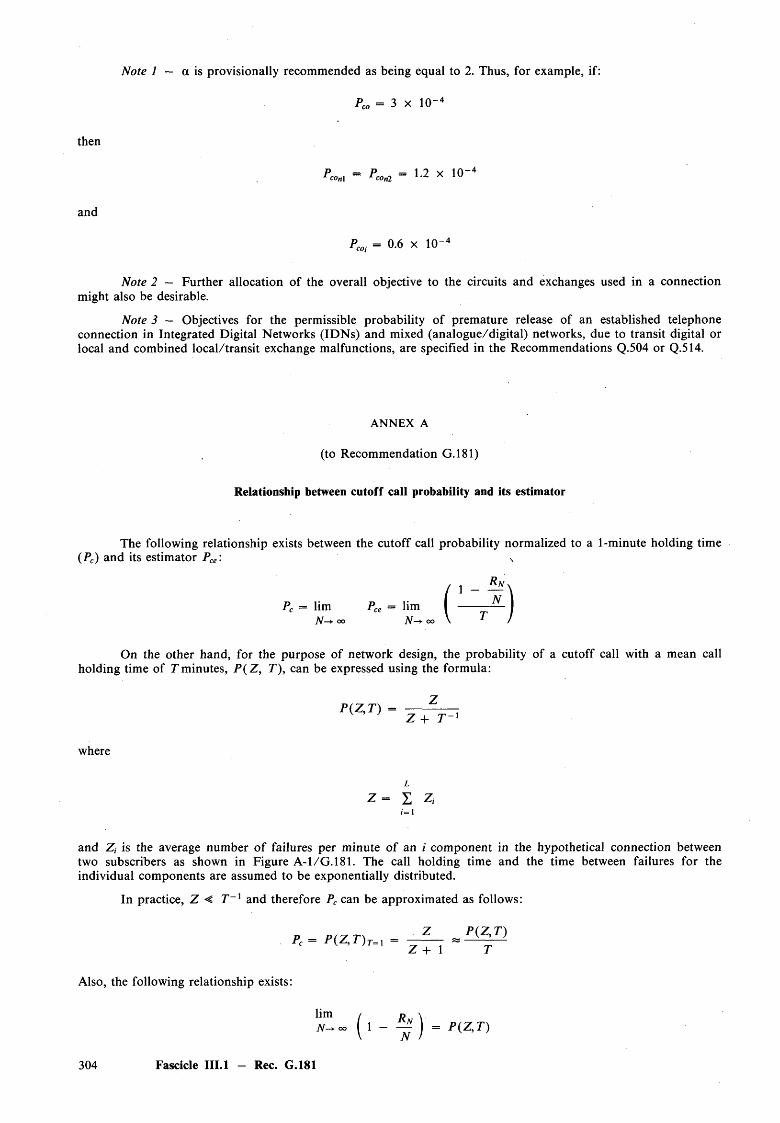
Note 1 — a is provisionally recommended as being equal to 2. Thus, for example, if:
Pco = 3 x 10'
then
n.„, - = i-z x io-4and
Pco. = 0.6 x 10-
Note 2 — Further allocation of the overall objective to the circuits and exchanges used in a connection might also be desirable.
Note 3 — Objectives for the permissible probability of premature release of an established telephone connection in Integrated Digital Networks (IDNs) and mixed (analogue/digital) networks, due to transit digital or local and combined local/transit exchange malfunctions, are specified in the Recommendations Q.504 or Q.514.
ANNEX A
(to Recommendation G.181)
Relationship between cutoff call probability and its estimator
The following relationship exists between the cutoff call probability normalized to a 1-minute holding time (Pc) and its estimator Pce : v
Pc = lim Pce = limff-> oo ( ^ )
On the other hand, for the purpose of network design, the probability of a cutoff call with a mean call holding time of T minutes, P (Z , T), can be expressed using the formula:
P (Z ,T ) - ZZ + T
where
L
z - S z,i=i
and Zi is the average number o f failures per minute of an i component in the hypothetical connection between two subscribers as shown in Figure A-1/G.181. The call holding time and the time between failures for the individual components are assumed to be exponentially distributed.
In practice, Z < T ~ x and therefore Pc can be approximated as follows:
Z P (Z ,T )Pc = P (Z , T ) t=x = --------- « }
Z + 1 T
Also, the following relationship exists:
limAT- oo ( l - - P (Z ,T )
304 Fascicle III.l — Rec. G.181
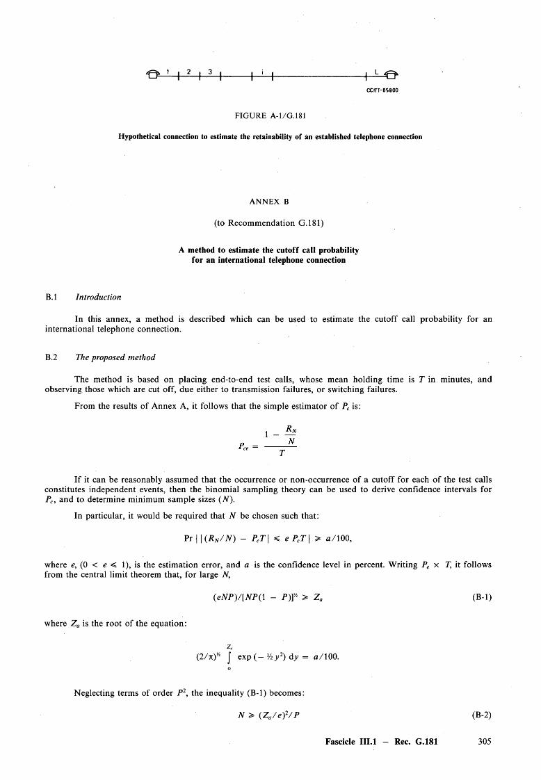
O 1 I 2 I 3 1----------- 1—■—|--------------------------------CCITT-85800
F I G U R E A -1 /G .1 8 1
Hypothetical connection to estimate the retainability of an established telephone connection
A N N E X B
(to Recommendation G.181)
A method to estimate the cutoff call probability for an international telephone connection
B.l Introduction
In this annex, a method is described which can be used to estimate the cutoff call probability for an international telephone connection.
B.2 The proposed method
The method is based on placing end-to-end test calls, whose mean holding time is T in minutes, and observing those which are cut off, due either to transmission failures, or switching failures.
From the results of Annex A, it follows that the simple estimator of Pc is:
. Rn
If it can be reasonably assumed that the occurrence or non-occurrence of a cutoff for each of the test calls constitutes independent events, then the binomial sampling theory can be used to derive confidence intervals for Pc, and to determine minimum sample sizes (N ).
In particular, it would be required that N be chosen such that:
Pr ] | (R n / N ) - PCT \ < e PCT \ > a / 100,
where e, (0 < e < 1), is the estimation error, and a is the confidence level in percent. Writing Pe X T, it follows from the central limit theorem that, for large N,
(eN P )/[N P ( 1 - P ) f > Z a (B-l)
where Z a is the root of the equation:
Z a
(2/tt)Vl J exp ( — Viy2) dy = a / 100.
Neglecting terms of order P2, the inequality (B-l) becomes:
N > (Z a/ e f / P (B-2)
Fascicle III.1 - Rec. G.181 305
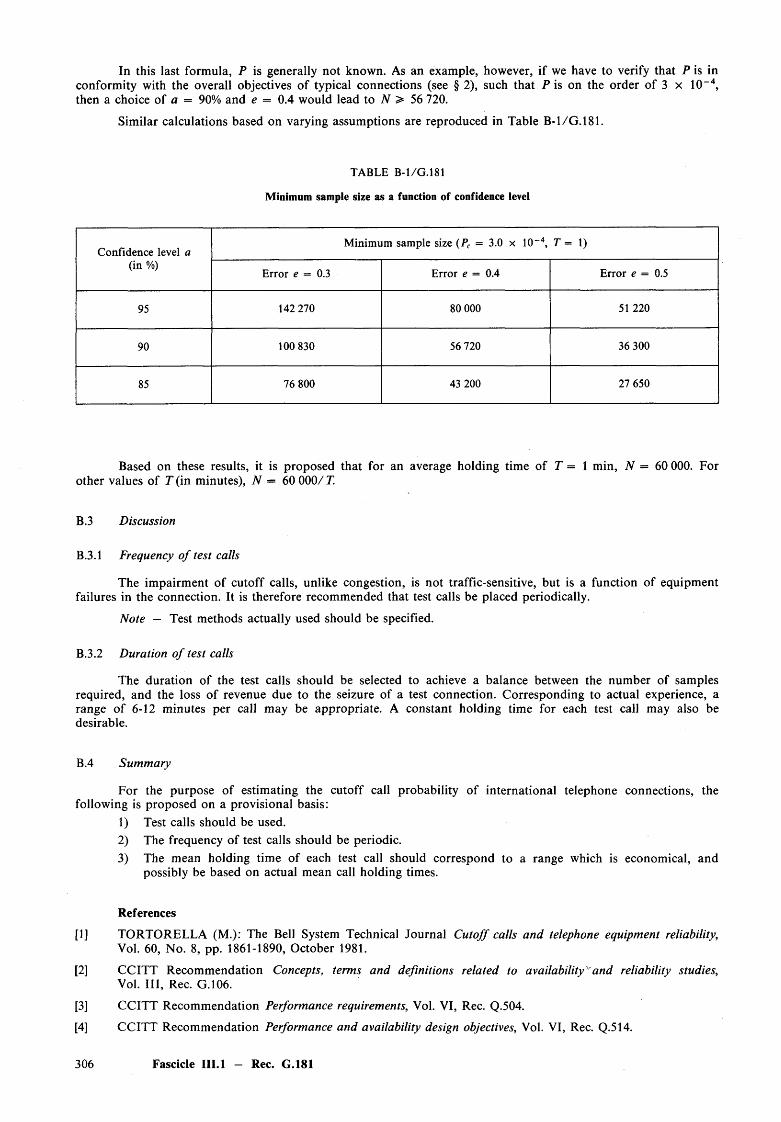
In this last formula, P is generally not known. As an example, however, if we have to verify that P is in conformity with the overall objectives of typical connections (see § 2), such that P is on the order of 3 x 10⁻⁴, then a choice of a = 90% and e = 0.4 would lead to N > 56 720.
Similar calculations based on varying assumptions are reproduced in Table B-l/G.181.
TABLE B-1/G.181
Minimum sample size as a function of confidence level
Confidence level a (in %)
Minimum sample size (Pc = 3.0 x 10 4, T = 1)
Error e = 0.3 Error e = 0.4 Error e = 0.5
95 142 270 80 000 51 220
90 100 830 56 720 36 300
85 76 800 43 200 27 650
Based on these results, it is proposed that for an average holding time of T = 1 min, N = 60 000. For other values of T (in minutes), N — 60 000/ T.
B.3 Discussion
B.3.1 Frequency o f test calls
The impairment of cutoff calls, unlike congestion, is not traffic-sensitive, but is a function of equipment failures in the connection. It is therefore recommended that test calls be placed periodically.
Note — Test methods actually used should be specified.
B.3.2 Duration o f test calls
The duration of the test calls should be selected to achieve a balance between the number of samples required, and the loss of revenue due to the seizure of a test connection. Corresponding to actual experience, a range of 6-12 minutes per call may be appropriate. A constant holding time for each test call may also be desirable.
B.4 Summary
For the purpose of estimating the cutoff call probability of international telephone connections, the following is proposed on a provisional basis:
1) Test calls should be used.2) The frequency of test calls should be periodic.3) The mean holding time of each test call should correspond to a range which is economical, and
possibly be based on actual mean call holding times.
References
[1] TORTORELLA (M.): The Bell System Technical Journal Cutoff calls and telephone equipment reliability,Vol. 60, No. 8, pp. 1861-1890, October 1981.
[2] CCITT Recommendation Concepts, terms and definitions related to availability^ and reliability studies,Vol. I l l , Rec. G.106.
[3] CCITT Recommendation Performance requirements, Vol. VI, Rec. Q.504.
[4] CCITT Recommendation Performance and availability design objectives, Vol. VI, Rec. Q.514.
306 Fascicle III.l — Rec. G.181
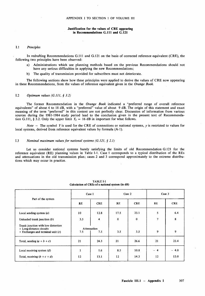
APPENDIX I TO SECTION 1 OF VOLUME III
Justification for the values of CRE appearing in Recommendations G .l l l and G.121
In redrafting Recommendations G .l l l and G.121 on the basis of corrected reference equivalent (CRE), the following two principles have been observed:
a) Administrations which use planning methods based on the previous Recommendations should not have any serious difficulties in applying the new Recommendations;
b) The quality of transmission provided for subscribers must not deteriorate.
The following sections show how these principles were applied to derive the values of CRE now appearing in these Recommendations, from the values of reference equivalent given in the Orange Book.
1.1 Principles
1.2 Optimum values (G .l l l , § 3.2)
The former Recommendation in the Orange Book indicated a “preferred range of overall reference equivalents” of about 6 to 18 dB, with a “preferred” value of about 9 dB. The origin of this statement and exact meaning of the term “preferred” in this context are not perfectly clear. Discussion of information from various sources during the 1981-1984 study period lead to the conclusion given in the present text of Recommendation G . l l l , § 3.2. Only the upper limit Y2 = 16 dB in im portant for what follows.
Note — The symbol Y is used for the CRE of connections or national systems, y is restricted to values for local systems, derived from reference equivalent values by formula (A-l).
1.3 Nominal maximum values fo r national systems (G.121, § 2.1)
Let us consider national systems barely satisfying the limits of old Recommendation G.121 for the reference equivalent (RE) planning values in Table 1-1. Case 1 corresponds to a typical distribution of the REs and attenuations in the old transmission plan; cases 2 and 3 correspond approximately to the extreme distributions which may occur in practice.
TABLE 1-1Calculation of CREs o f a national system (in dB)
Part of the system
Case 1 Case 2 Case 3
RE CRE RE CRE RE CRE
Local sending system (a) 10 12.8 17.5 23.1 5 6.4
Unloaded trunk junction (b) 3.5 4 0 0 7 8
Trunk junction with low distortion+ Long-distance circuits Attenuation+ Exchanges and terminal unit (c) 7.5 7.5 3.5 3.5 9 9
Total, sending (a + b + c) 21 24.3 21 26.6 21 23.4
Local receiving system (d) 1 1.6 8.5 10.8 - 4 - 4.0
Total, receiving (b + c + d) 12 13.1 12 14.3 12 13.0
Fascicle III.l — Appendix I 307
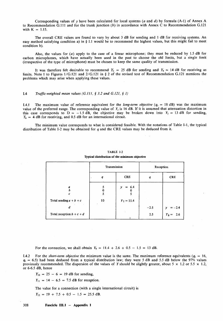
Corresponding values of y have been calculated for local systems (a and d ) by formula (A-l) of Annex A to Recommendation G .l l l and for the trunk junction (b ) in accordance with Annex C to Recommendation G.121 with K = 1.15.
The overall CRE values are found to vary by about 3 dB for sending and 1 dB for receiving systems. An easy method satisfying condition a) in § 1.1 would be to recommend the highest values, but this might fail to meet condition b).
Also, the values for (a) apply to the case of a linear microphone; they must be reduced by 1.5 dB for carbon microphones, which have actually been used in the past to choose the old limits, but a single limit (irrespective of the type of microphone) must be chosen to keep the same quality of transmission.
It was therefore felt desirable to recommend Y3 = 25 dB for sending and Y4 = 14 dB for receiving as limits. Note 1 to Figures l/G .121 and 2/G.121 in § 2 of the revised text o f Recommendation G.121 mentions the problems which may arise when applying these values.
1.4 Traffic-weighted mean values (G .l l l , § 3.2 and G.121, § 1)
1.4.1 The maximum value of reference equivalent for the long-term objective (qc = 18 dB) was the maximum value of the preferred range. The corresponding value of Yc is 16 dB. If it is assumed that attenuation distortion in this case corresponds to D = —1.5 dB, the objective may be broken down into Y5 = 13 dB for sending, T6 = 4 dB for receiving, and 0.5 dB for an international circuit.
The minimum value corresponds to what is considered feasible. With the notations of Table 1-1, the typical distribution of Table 1-2 may be obtained for q and the CRE values may be deduced from it.
TABLE 1-2 Typical distribution of the minimum objective
Transmission Reception
q CRE <7 CRE
a 5 y = 6.4b 0 0c 5 5
Total sending a + b + c 10 r 7 = 11.4
d -2 .5
Tf1II
Total reception b + c + d!
2.5 Y s = 2.6
For the connection, we shall obtain Y9 = 11.4 + 2.6 + 0.5 - 1.5 = 13 dB.
1.4.2 For the short-term objective the minimum value is the same. The maximum reference equivalents (qs = 16, qr = 6.5) had been deduced from a typical distribution law; they were 5 dB and 5.5 dB below the 97% values previously recommended. The dispersion of the values of Y should be slightly greater, about 5 x 1.2 or 5.5 x 1.2, or 6-6.5 dB, hence
Yio = 25 — 6 = 19 dB for sending,
yn = 14 — 6.5 = 7.5 dB for reception.
The value for a connection (with a single international circuit) is
Yn = 19 + 7.5 + 0.5 - 1.5 = 25.5 dB.
308 Fascicle III.l - Appendix I
1.5 Minimum CREs fo r the national sending system (G.121, § 3)
q = 6 dB, with the notations of Table 1-1 might correspond, for example,to a = 2.5 b — 0 c = 3.5, hence Y = 3.4 + 3.5 = 6.9 or a = 4 b = 0 c = 2, hence 7 = 5.2 + 2 = 7.2
713 = 7 dB may be taken as a minimum.
1.6 Sidetone reference equivalent (G.121, § 5) .
Until a complete reply to Question 9 /X II [2] is available, the method of Recommendation P.73 [3] and the present value expressed as a reference equivalent should be retained.
1.7 Other values
Several Recommendations contain “echo path reference equivalents” (G.131), “cross-talk reference equivalents” (P. 16), which were certainly calculated by inexact addition: A note should be inserted to that effect, without changing the present terms and these texts should be revised during the coming study period.
References
[1] RICHARDS (D. L.): Telecommunication by Speech, Butterworths, pp. 279-281, 1973.
[2] CCITT Question 9 /X II, Contribution COM XII-No. 1, Study Period 1981-1984, Geneva, 1981.
[3] CCITT Recommendation Measurement o f the sidetone reference equivalent, Vol. V, Rec. P.73.
Fascicle III.l — Appendix I 309

PAGE INTENTIONALLY LEFT BLANK
PAGE LAISSEE EN BLANC INTENTIONNELLEMENT
PART II
SUPPLEMENTS TO SECTION 1 OF THE SERIES G RECOMMENDATIONS

PAGE INTENTIONALLY LEFT BLANK
PAGE LAISSEE EN BLANC INTENTIONNELLEMENT
Supplement No. 2
TALKER ECHO ON INTERNATIONAL CONNECTIONS
(Geneva, 1964; amended at M ar del Plata, 1968 and Geneva, 1976 and 1980 and Malaga-Torremolinos, 1984;referred to in Recommendation G.131, § 2)
1 The curves of Figure 2 /G .l31 may be used to determine whether a given international connection requires an echo control device (echo suppressor or echo canceller). Alternatively they may be used to find what value of nominal overall loss shall be adopted for the 4-wire chain of a complete connection so that an echo control device is not needed. Before the curves can be used it must be decided what proportion of calls are to be allowed to exhibit an objectionable echo and Recommendation G.131 gives guidance on this matter.
The coordinates of the graph represent two of the parameters of a telephone connection that govern echo, i.e. the CRE (corrected reference equivalent) of the echo path and the mean one-way propagation time. By making certain assumptions (discussed below) these two parameters become the principal ones.
Each curve divides the coordinate plane into two portions and the position, relative to the curve, of the point describing the connection indicates whether an echo control device is needed, bearing in mind the percentage of calls permitted to exhibit an objectionable echo.
2 Factors governing echo
The principal factors which must be considered in order to describe whether an echo control device is needed on a particular connection are:
a) the number of echo paths;
b) the time taken by the echo currents to traverse these paths;c) the CREs of the echo path including the subscriber lines;
d) the tolerance to echo exhibited by subscribers.
These factors are discussed in turn in the following.
When circuits are switched together 4-wire there is only one echo path, assuming negligible go-to-return crosstalk. This is also substantially true if the circuits are switched together 2-wire and good echo return losses are achieved at these connection points (e.g. a mean value of 27 dB and a standard deviation of 3 dB). The principal echo currents are those due to the relatively poor echo balance return losses at the ends of the two extreme 4-wire circuits, where the connection is reduced to 2-wire.
The time taken to traverse the echo path is virtually dependent solely on the length of the 4-wire connection, because the main circuits of modern national and international networks are high-velocity circuits.
The CRE of the talker echo path for a symmetrical connection for planning purposes is approximately given by the sum o f:
— twice the CRE of the connection between the 2-wire point in the talker’s local terminal exchange and the 2-wire side of the 4-wire/2-wire terminating set at the listener’s e n d 1);
— the echo balance return loss at the listener’s end;— the sum of the sending CRE and receiving CRE of the talker’s telephone and subscriber line2)
In general, values of sending CRE and receiving CRE corresponding to low-loss subscriber lines should beused.
The echo experienced by subscribers on lines with more loss will be further attenuated. This is, therefore, a conservative assumption.
J) According to Recommendation G . l l l , § A.3.3 the CRE of 4-wire circuits should be taken as the 800 or 1000 Hz loss.
2) When summing these values to obtain the talker echo path CRE, in principle a correction factor D needs to be included inthe sum to account for filters in the connection. (See Table A-2/G.111.) For purposes of this supplement, the term D is assumed to be 0 dB, corresponding to 2 or more SRAEN filters in the echo path. This approach is consistent with the approach in Appendix I to Section 1 of Volume III.
Fascicle III.l — Suppl. No. 2 313
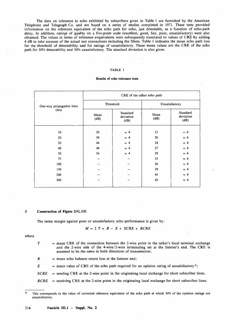
The data on tolerance to echo exhibited by subscribers given in Table 1 are furnished by the American Telephone and Telegraph Co. and are based on a series of studies completed in 1971. These tests provided information on the reference equivalent of the echo path for echo, just detectable, as a function of echo-path delay. In addition, ratings of quality on a five-point scale (excellent, good, fair, poor, unsatisfactory) were also obtained. The values in terms of reference evquivalents were subsequently translated to values of CRE by adding 4 dB to take account of the actual test connections including the filters. Table 1 indicates the mean echo path loss for the threshold of detectability and for ratings of unsatisfactory. These mean values are the CRE of the echo path for 50% detectability and 50% unsatisfactory. The standard deviation is also given.
TABLE 1
Results of echo tolerance tests
One-way propagation time (ms)
CRE of the talker echo path
Threshold Unsatisfactory
Mean(dB)
Standarddeviation
(dB)
Mean(dB)
Standarddeviation
(dB)
10 30 * 4 13 * 6
20 39 ^ 4 20 ~ 6
30 44 « 4 24 ~ 6
40 49 ~ 4 27 ~ 6
50 54 » 4 29 ~ 6
75 - - 33 « 6
100 - - 36 =* 6
150 - - 39 = 6
200 - - 41 ~ 6
300 — — 43 ~ 6
3 Construction of Figure 2/G.131
The mean margin against poor or unsatisfactory echo performance is given by:
M = 2 T + B - E + SC R E + RC RE
where
T = mean CRE of the connection between the 2-wire point in the talker’s local terminal exchangeand the 2-wire side of the 4-wire/2-wire terminating set at the listener’s end. The CRE isassumed to be the same in both directions of transmission;
B = mean echo balance return loss at the listener end;
E = mean value of CRE of the echo path required for an opinion rating of unsatisfactory3);
SC R E = sending CRE at the 2-wire point in the originating local exchange for short subscriber lines;
RC R E = receiving CRE at the 2-wire point in the originating local exchange for short subscriber lines.
3) This corresponds to the value of corrected reference equivalent of the echo path at which 50% of the opinion ratings are unsatisfactory.
314 Fascicle III.l — Suppl. No. 2

4 Fully analogue connections
The echo balance return loss is assumed to have a mean value of not less than 11 dB, with a standard deviation of 3 dB expressed as a weighted mean-power ratio (see Recommendation G.122). The mean value of the transmission loss is assumed to be uniform over this band and the standard deviation of transmission loss for each 4-wire circuit is assumed to be 1 dB for each direction of transmission. The correlation between the variations of loss of the two directions of transmission is assumed to be unity.
The standard deviation of the margin is given by:
m 2 = n { t2x + 2 rtx t2 + t22) + b 2 + e2
where
m = standard deviation of the margin;
tx, t2 = standard deviation of the transmission loss in the two directions of transmission of one 4-wirecircuit, national or international;
b = standard deviation of echo balance return loss;
e = standard deviation of the distribution of talker echo path CREs required for opinion ratings ofunsatisfactory;
r = correlation factor between tx and t2\
n — the number of 4-wire circuits in the 4-wire chain.
Inserting tx = t2 = 1 dB; r = 1; b = 3 dB; e = 6 dB gives m 2 = {An + 45).
In Recommendation G.131, § 2.3, Rules A and E refer to 1% and 10% probabilities o f encountering unsatisfactory echo and for these cases nine 4-wire circuits are assumed (3 national and 3 international + 3 national). For both the 1% and 10% curves therefore m = 9.0 dB.
For 10% probability, the margin may fall to 1.28 times the standard deviation. The corresponding factor for the 1% curve is 2.33. Hence the corresponding values of M are:
M = 1.28 x 9.0 dB = 11.5 dB for 10% probabilityM = 2.33 x 9.0 dB = 21 dB for 1% probability.
Putting these values into M = 2 T + B — E + SC R E + R C RE gives the following values for the mean talker echo attenuation, 2 T + B + SC R E + RCRE.
2 T + B + SC R E + R C R E = 11.5 dB + E fo r 10% probability2 T + B + SC R E + R C R E = 2 1 dB + E fo r 1% probability.
The values in Table 2 have been calculated (to the nearest whole decibel) using these equations. Thefigures in the length of connection column have been calculated assuming a velocity of propagation of160 km /m s.
TABLE 2
Mean one-way propagation time
(ms)
Length of connection (km)
Mean CRE of the talker echo path 2 T + B + SC R E + R C R E
(dB)
10%unsatisfactory
1%unsatisfactory
10 1600 25 3420 3 200 32 4130 4 800 36 4540 6 400 39 4850 8 000 41 5075 12 000 45 54
100 16 000 48 57150 24 000 51 60200 32 000 53 62300 48 000 55 64
Fascicle III.l — Suppl. No. 2 315
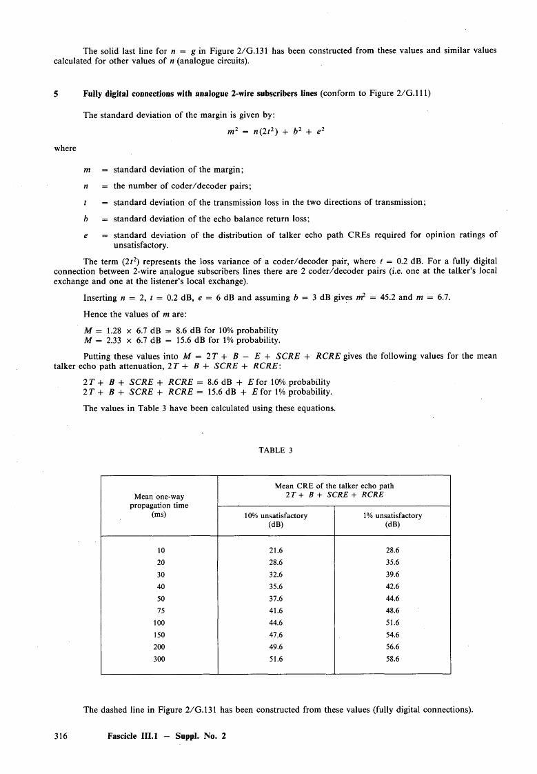
The solid last line for n = g in Figure 2/G.131 has been constructed from these values and similar values calculated for other values of n (analogue circuits).
5 Fully digital connections with analogue 2-wire subscribers lines (conform to Figure 2 /G .l 11)
The standard deviation of the margin is given by:
m 2 = n (2 t2) + b 2 + e2
where
m = standard deviation of the margin;
n = the number of coder/decoder pairs;
t = standard deviation of the transmission loss in the two directions of transmission;
b = standard deviation of the echo balance return loss;
e = standard deviation of the distribution o f talker echo path CREs required for opinion ratings ofunsatisfactory.
The term (212) represents the loss variance of a coder/decoder pair, where t = 0.2 dB. For a fully digital connection between 2-wire analogue subscribers lines there are 2 coder/decoder pairs (i.e. one at the talker’s local exchange and one at the listener’s local exchange).
Inserting n = 2, t = 0.2 dB, e = 6 dB and assuming b = 3 dB gives m2 = 45.2 and m = 6.7.
Hence the values of m are:
M — 1.28 x 6.7 dB = 8.6 dB for 10% probability M = 2.33 x 6.7 dB = 15.6 dB for 1% probability.
Putting these values into M = 2 T + B - E + SC R E + RC R E gives the following values for the mean talker echo path attenuation, 2 T + B + SC R E + RC RE:
2 T + B + SC R E + R C R E = 8.6 dB + E fo r 10% probability 2 T + B + SC R E + R C R E = 15.6 dB + E fo r 1% probability.
The values in Table 3 have been calculated using these equations.
TABLE 3
Mean one-way propagation time
(ms)
Mean CRE of the talker echo path 2 T + B + SC RE + R C R E
10% unsatisfactory (dB)
1% unsatisfactory (dB)
10 21.6 28.6
20 28.6 35.6
30 32.6 39.6
40 35.6 42.6
50 37.6 44.6
75 41.6 48.6
100 44.6 51.6
150 47.6 54.6
200 49.6 56.6
300 51.6 58.6
The dashed line in Figure 2/G.131 has been constructed from these values (fully digital connections).
316 Fascicle III.l — Suppl. No. 2
In this case there are no 2-wire points in the connection. However, there is an acoustical feed-back path between the earpiece and mouthpiece of the telephone set. Therefore the echo balance return loss used above is now represented by the loss of this acoustical path. Representative values of this acoustical loss are under wider study. The appendix to this supplement gives some information on this question.
It may be assumed that the standard deviation of the transmission loss of the coder/decoder pair equals the value given above for digital connections with 2-wire subscriber lines. The value of the equivalent of T should be taken as zero. The quantities SC R E and R C R E now refer to virtual analogue 4-wire points of 0 dBr level.
If it can be assumed that the standard deviation of the acoustical echo path loss equals 3 dB and a normal distribution applies, then the values of Table 3 also apply to the digital subscriber line case and the dashed curve of Figure 2 /G .l31 may be used.
6 Fully digital connections with digital subscribers lines [conform to Figure 1/G. 104 b)]
7 Mixed analogue/digital connections
This case is a combination of the cases given above and the appropriate variables and their values should be taken from the above information and an appropriate table can be constructed.
In general, if there are only two coder/decoder pairs in the connection, the variability of the transmission loss of the codecs may be ignored compared with the variability of the analogue circuits and the other variabilities. For such connections the solid curve given in Figure 2/G.131 for the number of analogue circuits in the connection may be used with good accuracy.
APPENDIX I
(to Supplement No. 2)
Echo loss in 4-wire telephone sets
(Contribution by Norway)
Abstract
In a 4-wire telephone set, echo may arise both by electrical crosstalk in the cord and by acoustical coupling between earpiece and mouthpiece in the handset. The echo loss for these paths has been determined for two analogue 2-wire telephone sets. This data is used to derive the echo loss of a hypothetical 4-wire set having SC R E + RC RE = 7 dB, and acoustical and electrical properties the same as the 2-wire telephone sets.
1.1 Introduction
It has been pointed out in several contributions that the choice of CREs for digital telephone sets has to be made considering aspects of loudness and echo in a complete 4-wire connection. To enable a study of the risk of objectionable echo, Study Group XVI has asked Study Group XII to present information on the subjective effect of talker echo as a function of delay, overall CRE and echo path loss.
In a digital 4-wire connection, including 4-wire subscriber lines and digital telephone sets, the main echo paths are found in the telephone set itself:
— the acoustical coupling between earpiece and mouthpiece of the handset, and— the electrical coupling in the flexible cord to the handset.
In order to assess the echo performance of a 4-wire connection, the echo loss of the digital telephone set must be estimated.
As an example of what can be expected, measurements of these echo paths have been made on two different analogue telephone sets. These results have been used to derive the echo loss between the receive and send terminals of a hypothetical 4-wire telephone set having SC R E = 5 dB and RC R E = 2 dB, and having the same electrical and acoustical properties as the measured sets.
Fascicle III.l — Suppl. No. 2 317
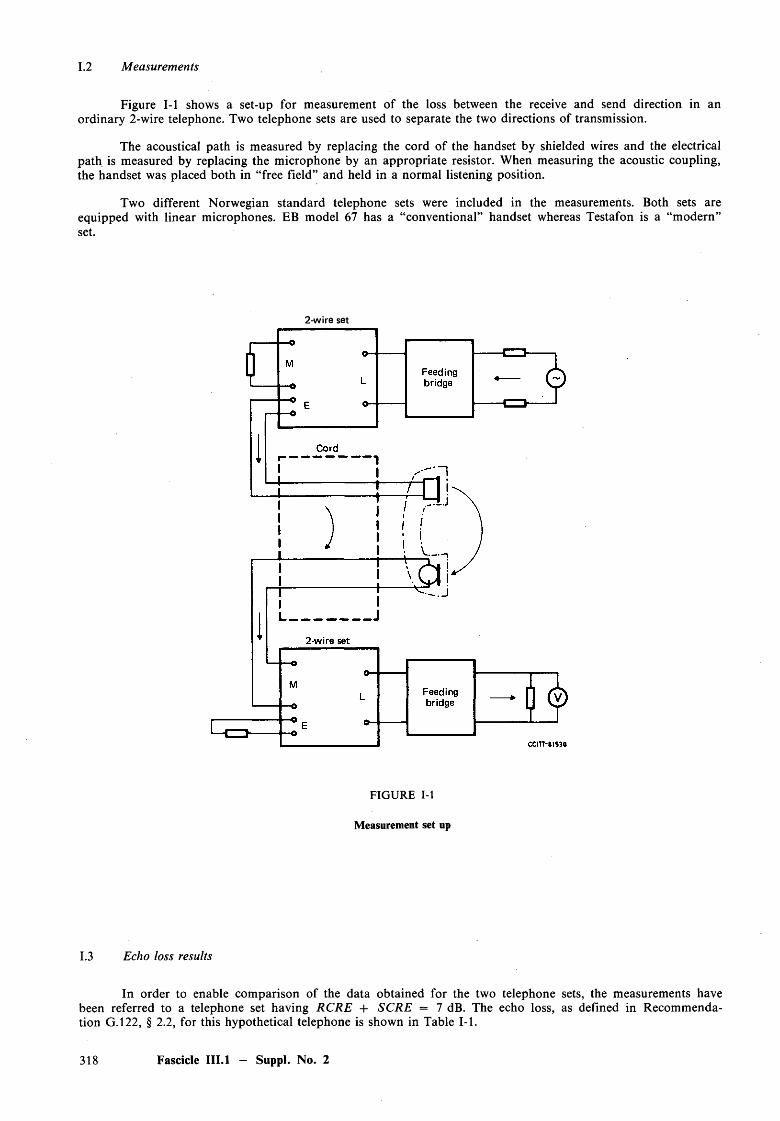
1.2 Measurements
Figure 1-1 shows a set-up for measurement of the loss between the receive and send direction in an ordinary 2-wire telephone. Two telephone sets are used to separate the two directions of transmission.
The acoustical path is measured by replacing the cord of the handset by shielded wires and the electrical path is measured by replacing the microphone by an appropriate resistor. When measuring the acoustic coupling, the handset was placed both in “free field” and held in a normal listening position.
Two different Norwegian standard telephone sets were included in the measurements. Both sets are equipped with linear microphones. EB model 67 has a “conventional” handset whereas Testafon is a “m odern” set.
2-wire set
FIGURE 1-1
Measurement set up
1.3 Echo loss results
In order to enable comparison of the data obtained for the two telephone sets, the measurements have been referred to a telephone set having RC R E + SC R E = 7 dB. The echo loss, as defined in Recommendation G.122, § 2.2, for this hypothetical telephone is shown in Table 1-1.
318 Fascicle III.l — Suppl. No. 2
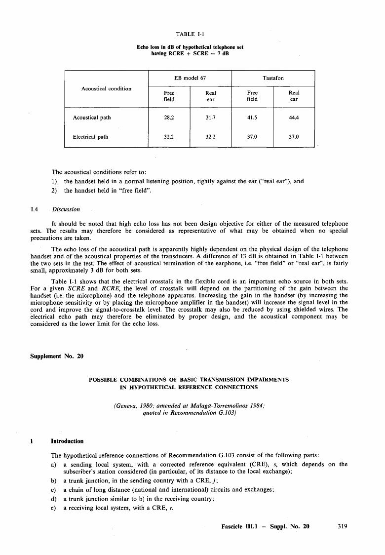
TABLE 1-1
Echo loss in dB of hypothetical telephone set having RCRE + SCRE = 7 dB
EB model 67 Tastafon
Acoustical conditionFree Real Free Realfield ear field ear
Acoustical path 28.2 31.7 41.5 44.4
Electrical path 32.2 32.2 37.0 37.0
The acoustical conditions refer to:1) the handset held in a normal listening position, tightly against the ear (“real ear”), and2) the handset held in “free field”.
1.4 Discussion
It should be noted that high echo loss has not been design objective for either of the measured telephonesets. The results may therefore be considered as representative of what may be obtained when no specialprecautions are taken.
The echo loss of the acoustical path is apparently highly dependent on the physical design of the telephone handset and of the acoustical properties of the transducers. A difference of 13 dB is obtained in Table 1-1 between the two sets in the test. The effect of acoustical termination of the earphone, i.e. “free field” or “real ear”, is fairly small, approximately 3 dB for both sets.
Table 1-1 shows that the electrical crosstalk in the flexible cord is an im portant echo source in both sets. For a given SC R E and RCRE, the level o f crosstalk will depend on the partitioning of the gain between the handset (i.e. the microphone) and the telephone apparatus. Increasing the gain in the handset (by increasing the microphone sensitivity or by placing the microphone amplifier in the handset) will increase the signal level in the cord and improve the signal-to-crosstalk level. The crosstalk may also be reduced by using shielded wires. The electrical echo path may therefore be eliminated by proper design, and the acoustical component may be considered as the lower limit for the echo loss.
Supplement No. 20
POSSIBLE COMBINATIONS OF BASIC TRANSMISSION IMPAIRMENTS IN HYPOTHETICAL REFERENCE CONNECTIONS
(Geneva, 1980; amended at Malaga-Torremolinos 1984; quoted in Recommendation G.103)
1 Introduction
The hypothetical reference connections of Recommendation G.103 consist of the following parts:a) a sending local system, with a corrected reference equivalent (CRE), 5, which depends on the
subscriber’s station considered (in particular, of its distance to the local exchange);b) a trunk junction, in the sending country with a CRE, j ;c) a chain of long distance (national and international) circuits and exchanges;d) a trunk junction similar to b) in the receiving country;e) a receiving local system, with a CRE, r.
Fascicle III.l — Suppl. No. 20 319
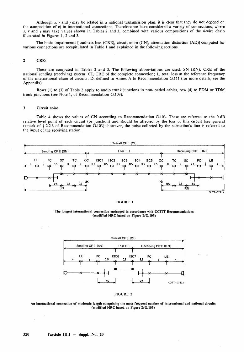
Although 5, r and j may be related in a national transmission plan, it is clear that they do not depend on the composition of c) in international connections. Therefore we have considered a variety of connections, where s, r and j may take values shown in Tables 2 and 3, combined with various compositions of the 4-wire chain illustrated in Figures 1, 2 and 3.
The basic impairments [loudness loss (CRE), circuit noise (CN), attenuation distortion (AD)] computed for various connections are recapitulated in Table 1 and explained in the following sections.
2 CREs
These are computed in Tables 2 and 3. The following abbreviations are used: SN (RN), CRE of the national sending (receiving) system; C l, CRE of the complete connection; L, total loss at the reference frequency of the international chain of circuits; D, defined in Annex A to Recommendation G .l l l (for more details, see the Appendix).
Rows (1) to (3) of Table 2 apply to audio trunk junctions in non-loaded cables, row (4) to FDM or TDM trunk junctions (see Note 1, of Recommendation G.103).
3 Circuit noise
Table 4 shows the values of CN according to Recommendation G.103. These are referred to the 0 dB relative level point of each circuit (or junction) and should be affected by the loss of this circuit (see general remark of § 2.2.6 of Recommendation G.103); however, the noise collected by the subscriber’s line is referred to the input of the receiving station.
Overall CRE (Cl)
Sending CRE (SN) Loss (L) Receiving CRE (RN)
LE PC SC TC QC ISC1 ISC2 ISC3 ISC4 ISC5 QC TC SC PC LE * 1 35 0 0 °-5 °-s °<s °-5 °-s os 0 0 3,5 1 r
D *--------* - H->K- -X X- -X HK-
>K0.5 . a s .I . 2.5
RN
FIGURE 1
The longest international connection envisaged in accordance with CCITT Recommendations (modified HRC based on Figure 1/G. 103)
C C I T T - 37 S 23
Overall CRE (Cl)
Sending CRE (SN) Loss (L) Receiving CRE (RN)
LE PC ISC6 ISC7 PC LEs . . . j , 3.5 0.5 3.5 ^ j ^ r
D - - x -
2.5
-HK-
2.5
-X-
C C IT T - 3 7 5 3 2
FIG URE 2
An international connection of moderate length comprising the most frequent number of international and national circuits(modified HRC based on Figure 2/G.103)
320 Fascicle III.l — Suppl. No. 20
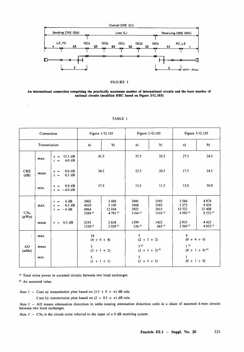
Overall CRE (Cl)
Sending CRE (SN) ___________________ Loss (L) Receiving CRE (RN)
LE, PC ISCa ISCb ISCc ISCd ISCe PC, LEs . . . 3.5 . . . 0,5 015 05 . . . 0.S 3.5 . . . r
CCITT -37544
FIG URE 3
An international connection comprising the practically maximum number of international circuits and the least number ofnational circuits (modified HRC based on Figure 3/G.103)
TABLE 1
Connection Figure 1/G. 103 Figure 2 /G .l03 Figure 3/G.103
Transmission a) b) a) b) a) b)
s = 15.5 dB 41.5 37.5 35.5 27.5 24.5max. r = 4.0 dB
CRE s = 9.0 dB 26.5 22.5 20.5 17.5 14.5(dB) mean r = 0.5 dB
s = 9.0 dB 17.5 13.5 11.5 13.0 10.0min. r = -4 .0 dB
r = 4 dB 3002 3 488 2045 2185 3 566 4 974max. r = 0.5 dB 4010 5 100 1868 2183 5 273 8 426
r = — 4 dB 8964 12 034 2925 3813 12 522 21 408CN 0 3569 a) 4 791 a) 1164a) 1518 a) 4 985 a) 8 523 a)
(pWp)
mean r = 0.5 dB 2193 2 638 1299 1422 2 933 4 4231530 a) 2 029 a) 526 a) 665 a) 2 360 a) 4 032 a)
max. 14 5 4(4 + 6 + 4) (2 + 1 + 2) (0 + 4 + 0)
AD mean 5 5 b) 1 b)(addu) (2 + 1 + 2) (2 + 1 + 2) b) (0 + 1 + 0 )b>
min. 3 3 1(1 + 1 + 1) (1 + 1 + 1) (0 + 1 + 0)
a) Total noise power in assumed circuits between two local exchanges.
b) An assumed value.
Note 1 — Case a): transmission plan based on (3.5 + 0 x n) dB rule.
Case b): transmission plan based on (2 + 0.5 x n) dB rule.
Note 2 — AD means attenuation distortion in addu (analog attenuation distortion unit) in a chain of assumed 4-wire circuits between two local exchanges.
Note 3 - C N 0 is the circuit noise referred to the input of a 0 dB receiving system.
Fascicle III.l — Suppl. No. 20 321

322 Fascicle
III.l —
Suppl. N
o. 20
TABLE 2
CREs for Figures 1 and 2
Local system Trunk junction
L =
Figure 1 a) and b)
= 3 n = 12 L =
Figure 2 a)
0.5 n == 3 L =
Figure 2 b)
0.5 n == 3RE CRE loss CRE
s' r' s r j SN RN D C l SN RN D C l SN RN D C l
(1) max. 12 3 15.5 4.0 — 6.0 25 13.5 0 41.5 25 13.5 -1 .5 37.5 ' 24 12.5 -1 .5 35.5
(2) mean 7 0 9.0 0.5 - 3.5 16 7.5 0 26.5 16 7.5 -1 .5 22.5 15 6.5 -1 .5 20.5
(3) min. 7 - 4 9.0 -4 .0 - 1.0 13.5 0.5 0 17.5 13.5 0.5 -1 .5 13.5 12.5 -0 .5 -1 .5 11.5
(4) mean 7 0 9.0 0.5 3.0 - 15.5 7 0 25.5 15.5 7 - 1 .0 22.0 14.5 6 -1 .0 20.0
Note — The numbers are rounded to the nearest 0.5 dB.
TABLE 3
CREs for Figure 3 ( j = 0, L = 2, n = 4)
Local system Figure 3 a)
Figure 3 b)
s r SN RN D C l SN RN D C l
max. 15.5 4.0 19 7.5 -1 .0 27.5 17.5 6 - 1 .0 24.5
mean 9.0 0.5 12.5 4 -1 .0 17.5 11 2.5 - 1 .0 14.5
min. 9.0 - 4 .0 12.5 -0 .5 -1 .0 13.0 11 - 2 - 1 .0 10.0
Note — The numbers are rounded to the nearest 0.5 dB.
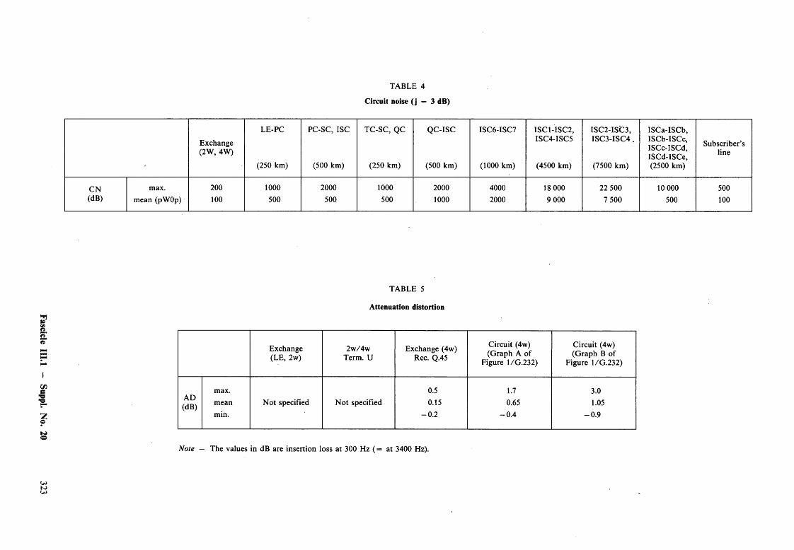
Fascicle III.l
- Suppl.
No.
20
TABLE 4
Circuit noise (j = 3 dB)
Exchange (2W, 4W)
LE-PC
(250 km)
PC-SC, ISC
(500 km)
TC-SC, QC
(250 km)
QC-ISC
(500 km)
ISC6-ISC7
(1000 km)
ISC1-ISC2,ISC4-ISC5
(4500 km)
ISC2-ISC3, ISC 3-ISC 4.
(7500 km)
ISCa-ISCb, ISCb-ISCc, ISCc-ISCd, ISCd-ISCe, (2500 km)
Subscriber’sline
CN max. 200 1000 2000 1000 2000 4000 18 000 22 500 10 000 500(dB) mean (pWOp) 100 500 500 500 1000 2000 9 000 7 500 500 100
TABLE 5
Attenuation distortion
Exchange (LE, 2w)
2w/4w Term. U
Exchange (4w) Rec. Q.45
Circuit (4w) (G raph A of
Figure 1/G .232)
Circuit (4w) (G raph B of
Figure 1/G .232)
max. 0.5 1.7 3.0AD(dB) mean N ot specified N ot specified 0.15 0.65 1.05\ /
min. -0 .2 -0 .4 -0 .9
Note — The values in dB are insertion loss at 300 Hz (= at 3400 Hz).
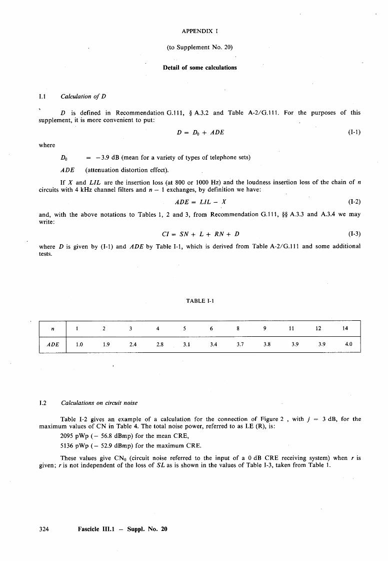
A PPENDIX I
(to Supplement No. 20)
Detail of some calculations
1.1 Calculation o f D
D is defined in Recommendation G . l l l , § A.3.2 and Table A-2/G.111. For the purposes of this supplement, it is more convenient to put:
D = D0 + A D E (1-1)
where
D0 = — 3.9 dB (mean for a variety of types of telephone sets)
A D E (attenuation distortion effect).
If X and L IL are the insertion loss (at 800 or 1000 Hz) and the loudness insertion loss of the chain of ncircuits with 4 kHz channel filters and n — 1 exchanges, by definition we have:
A D E = L IL - X (1-2)
and, with the above notations to Tables 1, 2 and 3, from Recommendation G . l l l , §§ A.3.3 and A.3.4 we may write:
C l = S N + L + R N + D (1-3)
where D is given by (1-1) and A D E by Table 1-1, which is derived from Table A-2/G.111 and some additionaltests.
TABLE 1-1
n 1 2 3 4 5 6 8 9 11 12 14
A D E 1.0 1.9 2.4 2.8 3.1 3.4 3.7 3.8 3.9 3.9 4.0
1.2 Calculations on circuit noise
Table 1-2 gives an example of a calculation for the connection of Figure 2 , with j — 3 dB, for themaximum values of CN in Table 4. The total noise power, referred to as LE (R), is:
2095 pWp ( — 56.8 dBmp) for the mean CRE,
5136 pWp ( — 52.9 dBmp) for the maximum CRE.
These values give CN 0 (circuit noise referred to the input of a 0 dB CRE receiving system) when r isgiven; r is not independent of the loss of S L as is shown in the values of Table 1-3, taken from Table 1.
324 Fascicle III.l — Suppl. No. 20
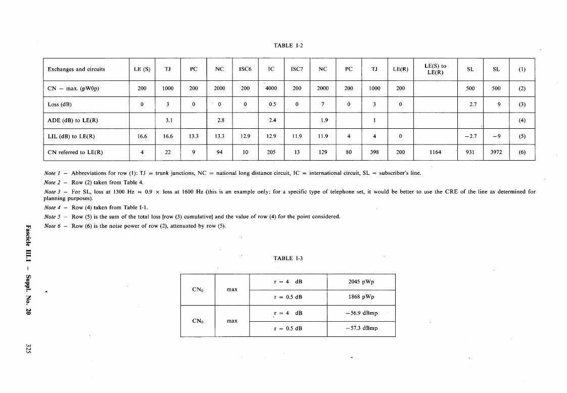
Fascicle III.l
— Suppl.
No.
20
TABLE 1-2
Exchanges and circuits LE (S) TJ PC NC ISC6 IC ISC7 NC PC TJ LE(R) LE(S) to LE(R) SL SL (1)
CN - max. (pWOp) 200 1000 200 2000 200 4000 200 2000 200 1000 200 500 500 (2)
Loss (dB) 0 3 0 0 0 0.5 0 7 0 3 0 2.7 9 (3)
ADE (dB) to LE(R) 3.1 2.8 2.4 1.9 1 (4)
LIL (dB) to LE(R) 16.6 16.6 13.3 13.3 12.9 12.9 - 11.9 11.9 4 4 0 -2 .7 - 9 (5)
CN referred to LE(R) 4 22 9 94 10 205 13 129 80 398 200 1164 931 3972 (6)
Note 1 — Abbreviations for row (1): TJ = trunk junctions, NC = national long distance circuit, IC = international circuit, SL = subscriber’s line.
Note 2 — Row (2) taken from Table 4.
Note 3 — For SL, loss at 1300 Hz « 0.9 x loss at 1600 Hz (this is an example only; for a specific type o f telephone set, it would be better to use the CRE of the line as determined forplanning purposes).
Row (4) taken from Table 1-1.
Row (5) is the sum of the total loss [row (3) cumulative] and the value of row (4) for the point considered.
Row (6) is the noise power of row (2), attenuated by row (5).
TABLE 1-3
C N 0 maxr = 4 dB 2045 pWp
r = 0.5 dB 1868 pWp
CN 0 maxr = 4 dB -5 6 .9 dBmp
r = 0.5 dB -5 7 .3 dBmp
Note 4 —
Note 5 —
Note 6 —
OJK>cn
Supplement No. 21
THE USE OF QUANTIZING DISTORTION UNITS IN THE PLANNING OF INTERNATIONAL CONNECTIONS
(CONTRIBUTION OF BELL-NORTHERN RESEARCH)
(Geneva, 1980; amended at Malaga-Torremolinos, 1984; quoted in Recommendation G.113)
Introduction
This supplement provides background information on the use of the concept of associating objectively derived quantizing distortion units (qd units) with PCM processing devices. This concept may be used in the planning of international connections involving several unintegrated PCM processes, to ensure that the overall quantizing distortion is within limits. The supplement discusses the basis for the use of qd units, provides values for several commonly occurring PCM processes, and shows how the concept may be used in a mixed
, analogue/digital and an all-digital network. Exact calculations for the all-digital network are also included. The method as given in this supplement is not applicable for non-PCM processes such as 32 kbit/s ADPCM (according to Recommendation G.721). For these processes, subjective tests are required to determine the units of quantizing distortion, and this is presently under study in Question 18/XII.
1 Basic principles of quantizing distortion units
The basic principle for assigning qd units to a digital process is that the associated quantizing distortion power is uncorrelated with the distortion produced by other processes, and individual qd units can therefore be added algebraically to give the overall distortion for a complete connection.
It is convenient to use the quantizing distortion produced by a single 8-bit PCM process (i.e., one encoder and decoder, A-law or p-law) as the basic reference and to assign it a value of 1 unit. With this reference a single7-bit PCM process, which is known to produce 6 dB more quantizing distortion (i.e., 4 times more power), would be assigned 4 qd units. A further subdivision can be made, so that an individual 8-bit encoder or decoder is assigned 0.5 units and similarly an individual 7-bit encoder or decoder is assigned 2 units. Other processes can also be converted into equivalent qd units.
An overall limit of 14 qd units has been assigned for an international connection, to be divided into 5 units for each national extension and 4 units for the international portion. This corresponds to 14 times more distortion than a single 8-bit PCM process, or an 11.5 dB (i.e., 10 1og1014) reduction in signal-to-distortion ratio (SDR). Since a practical 8-bit codec might have an SDR of about 36 dB (for a Gaussian input signal, and distortion flat-weighted in the band 300 to 3400 Hz), 14 qd units therefore represents an overall SDR of about24.5 dB. This is consistent with previously published estimates (about 24 db) [1] of the subjective limit for overall signal to distortion ratio.
2 Values of quantizing distortion units for other PCM processing devices
To calculate a qd unit value for other digital processing devices it is necessary first of all to estimate the increase in quantizing distortion for that process relative to a single 8-bit PCM process. This can be conveniently derived from calculations of SDR for the particular process, compared to the SDR for 8-bit PCM alone. Examples of such calculations of SDR (for a Gaussian input signal, and distortion flat-weighted in the band 300 to 3400 Hz) for various processes are given in Figures 1, 2 and 3. For each process the reduction in SDR compared to 8-bit coding alone can be converted into the equivalent qd unit. For example, if the reduction in SDR = x dB then the qd value = 10*/10.
Some PCM processes, however, give a reduction in SDR which is not constant with input signal level. In these cases the reduction in SDR at a mean input signal level of — 20 dBmO has been used.
326 Fascicle III.l — Suppl. No. 21
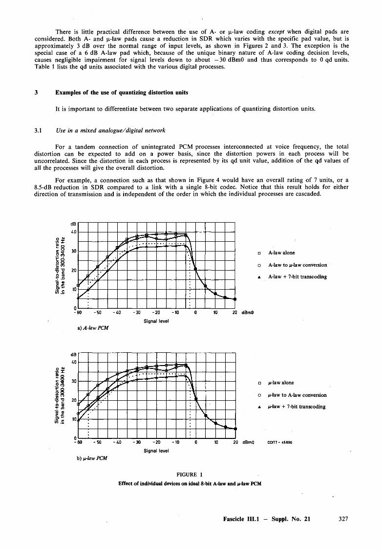
There is little practical difference between the use of A- or p-law coding except when digital pads are considered. Both A- and p-law pads cause a reduction in SDR which varies with the specific pad value, but is approximately 3 dB over the normal range of input levels, as shown in Figures 2 and 3. The exception is the special case of a 6 dB A-law pad which, because of the unique binary nature of A-law coding decision levels, causes negligible impairment for signal levels down to about —30 dBmO and thus corresponds to 0 qd units. Table 1 lists the qd units associated with the various digital processes.
3 Examples of the use of quantizing distortion units
It is im portant to differentiate between two separate applications of quantizing distortion units.
3.1 Use in a mixed analogue/digital network
For a tandem connection of unintegrated PCM processes interconnected at voice frequency, the total distortion can be expected to add on a power basis, since the distortion powers in each process will be uncorrelated. Since the distortion in each process is represented by its qd unit value, addition of the qd values of all the processes will give the overall distortion.
For example, a connection such as that shown in Figure 4 would have an overall rating of 7 units, or a 8.5-dB reduction in SDR compared to a link with a single 8-bit codec. Notice that this result holds for either direction of transmission and is independent of the order in which the individual processes are cascaded.
□ A-law alone
o A-law to /u-law conversion
▲ A-law + 7-bit transcoding
Signal levela) A-law PCM
□ ju-law alone
o /Li-law to A-law conversion
a /u-law + 7-bit transcoding
20 dBmO CCITT - 45890
Signal levelb) n-law PCM
FIGURE 1
Effect of individual devices on ideal 8-bit A-law and M-law PCM
Fascicle III.l — Suppl. No. 21 327

Sign
al-to
-dist
ortio
n ra
tio
Sign
al-to
-dist
ortio
n ra
tioin
the
band
30
0-34
00
Hz
in the
ba
nd
300-
3400
H
z □ A-law alone
o A-law + 1 dB pad
a A-law + 2 dB pad
O A-law + 3 dB pad
a A-law + 4 dB pad
-60 -50 -AO -30 -20 -10 0 10 20 dBmOSignal level
a) A-law PCM
Signal level
□ ju-law alone
o /u-law + 1 dB pad
▲ /u-law + 2 dB pad
O /u-law + 3 dB pad
a ju-law + 4 dB pad
CCITT - 46900
b) ii-law PCM
FIGURE 2
Effect of digital pads on ideal 8-bit A-law and ju-law PCM
328 Fascicle III.l — Suppl. No. 21

Sign
al-to
-dist
ortio
n Si
gnal
-to-
dist
ortio
n rat
io in
the
band
30
0-34
00
Hz
ratio
in the
ba
nd
300-
3400
H
z
□ A-law alone
O A-law + 5 dB pad
▲ A-law + 6 dB pad
O A-law + 7 dB pad
a A-law + 8 dB pad
a) A-law PCM
□ /i-law alone
o M-law + 5 dB pad
▲ M-law + 6 dB pad
O M-law + 7 dB pad
a M-law + 8 dB pad
CCITT - i S 910
b) n-law PCMFIGURE 3
Effect o f digital pads on ideal 8-bit A-law and M-law PCM
Fascicle III.l — Suppl. No. 21 329
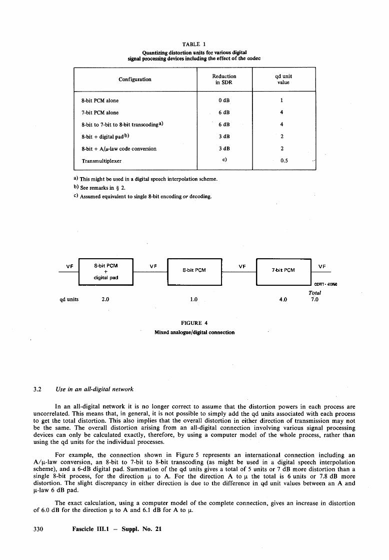
TABLE 1Quantizing distortion units for various digital
signal processing devices including the effect of the codec
Configuration Reduction in SDR
qd unit value
8-bit PCM alone OdB 1
7-bit PCM alone 6dB 4
8-bit to 7-bit to 8-bit transcoding4) 6 dB 4
8-bit + digital pad 6) 3 dB 2
8-bit + A//i-law code conversion 3 dB 2
Transmultiplexer c) 0.5
a) This might be used in a digital speech interpolation scheme.b) See remarks in § 2.c) Assumed equivalent to single 8-bit encoding or decoding.
Totalqd units 2.0 1.0 4.0 7.0
FIGURE 4
Mixed analogue/digital connection
3.2 Use in an all-digital network
In an all-digital network it is no longer correct to assume that the distortion powers in each process are uncorrelated. This means that, in general, it is not possible to simply add the qd units associated with each process to get the total distortion. This also implies that the overall distortion in either direction of transmission may not be the same. The overall distortion arising from an all-digital connection involving various signal processing devices can only be calculated exactly, therefore, by using a computer model o f the whole process, rather than using the qd units for the individual processes.
For example, the connection shown in Figure 5 represents an international connection including an A /p-law conversion, an 8-bit to 7-bit to 8-bit transcoding (as might be used in a digital speech interpolation scheme), and a 6-dB digital pad. Summation of the qd units gives a total of 5 units or 7 dB more distortion than a single 8-bit process, for the direction p to A. For the direction A to p the total is 6 units or 7.8 dB more distortion. The slight discrepancy in either direction is due to the difference in qd unit values between an A and p-law 6 dB pad.
The exact calculation, using a computer model of the complete connection, gives an increase in distortion of 6.0 dB for the direction p to A and 6.1 dB for A to p.
330 Fascicle III.l — Suppl. No. 21
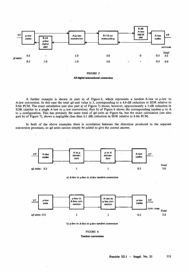
Total0.5 - 1.0 3.0 0 0.5 5.0
id units0.5 1.0 1.0 3.0 - 0.5 6.0
FIGURE 5
All-digital international connection
A further example is shown in part a) of Figure 6, which represents a tandem A-law to p-law to A-law conversion. In this case the total qd unit value is 3, corresponding to a 4.8-dB reduction in SDR relative to8-bit PCM. The exact calculation (see also part a) o f Figure 7) shows, however, approximately a 3-dB reduction in SDR (similar to a single A-law to p-law conversion). Part b) of Figure 6 shows the corresponding tandem p to A to p configuration. This has precisely the same total of qd units as Figure 6a, but the exact calculation (see also part b) o f Figure 7), shows a negligible (less than 0.1 dB) reduction in SDR relative to 8-bit PCM.
In both of the above examples there is correlation between the distortion produced in the separate conversion processes, so qd units cannot simply be added to give the correct answer.
Totalqd units: 0.5 1 1 0.5 3.0
a) A-law to n-law to A-law tandem conversion
Totalqd units: 0.5 1 1 0.5 3.0
b) n-law to A-law to n-law tandem conversion
FIGURE 6
Tandem conversions
Fascicle IIL1 — Suppl. No. 21 331
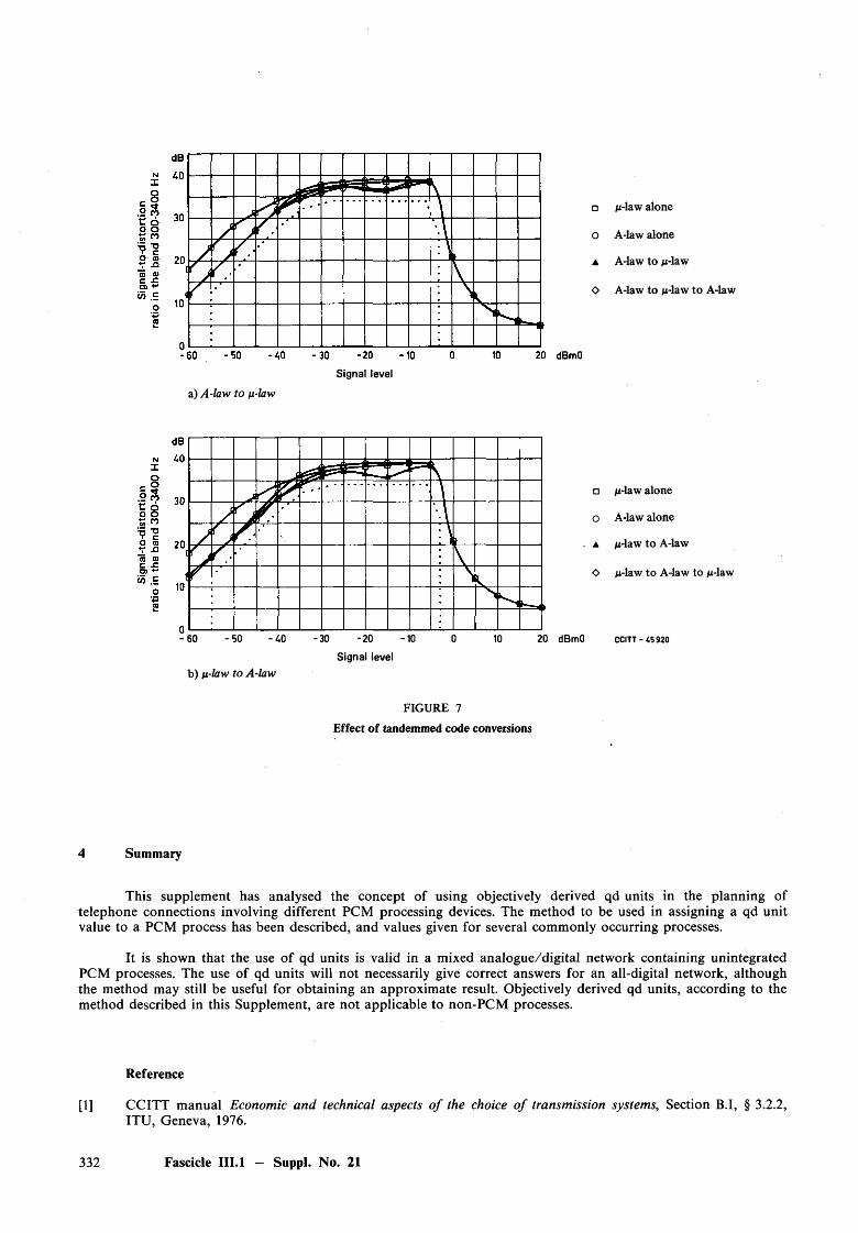
o A-law alone
▲ A-law to M-law
O A-law to /Lt-law to A-law
□ M-law alone
20 dBmO
Signal level
a) A-law to n-law
□ M-law alone
O A-law alone
▲ M-law to A-law
O M-law to A-law to M-law
- 6 0 -5 0 -AO -30 -20 -10 0 10 20 dBmO ccitt-45920Signal level
b) n-law to A-law
FIGURE 7
Effect of tandemmed code conversions
4 Summary
This supplement has analysed the concept of using objectively derived qd units in the planning of telephone connections involving different PCM processing devices. The method to be used in assigning a qd unit value to a PCM process has been described, and values given for several commonly occurring processes.
It is shown that the use of qd units is valid in a mixed analogue/digital network containing unintegrated PCM processes. The use of qd units will not necessarily give correct answers for an all-digital network, although the method may still be useful for obtaining an approximate result. Objectively derived qd units, according to the method described in this Supplement, are not applicable to non-PCM processes.
Reference
[1] CCITT manual Economic and technical aspects o f the choice o f transmission systems, Section B.I, § 3.2.2, ITU, Geneva, 1976.
332 Fascicle III.l - Suppl. No. 21
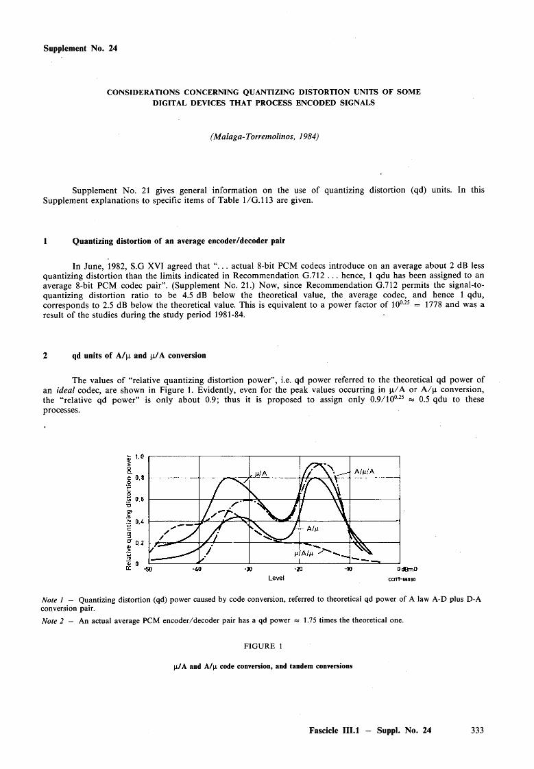
Supplement No. 24
CONSIDERATIONS CONCERNING QUANTIZING DISTORTION UNITS OF SOM E DIGITAL DEVICES THAT PROCESS ENCODED SIGNALS
(Malaga-Torremolinos, 1984)
Supplement No. 21 gives general information on the use of quantizing distortion (qd) units. In this Supplement explanations to specific items of Table 1/G. 113 are given.
1 Quantizing distortion of an average encoder/decoder pair
In June, 1982, S.G XVI agreed that “. . . actual 8-bit PCM codecs introduce on an average about 2 dB less quantizing distortion than the limits indicated in Recommendation G .712 . . . hence, 1 qdu has been assigned to an average 8-bit PCM codec pair”. (Supplement No. 21.) Now, since Recommendation G.712 permits the signal-to- quantizing distortion ratio to be 4.5 dB below the theoretical value, the average codec, and hence 1 qdu, corresponds to 2.5 dB below the theoretical value. This is equivalent to a power factor of 10025 = 1778 and was a result of the studies during the study period 1981-84.
2 qd units of A/p and u/A conversion
The values of “relative quantizing distortion power”, i.e. qd power referred to the theoretical qd power of an ideal codec, are shown in Figure 1. Evidently, even for the peak values occurring in p /A or A /p conversion, the “relative qd power” is only about 0.9; thus it is proposed to assign only 0.9/10°25 « 0.5 qdu to these processes.
Level c c iT T -M O jo
Note 1 — Quantizing distortion (qd) power caused by code conversion, referred to theoretical qd power of A law A-D plus D-A conversion pair.
Note 2 — An actual average PCM encoder/decoder pair has a qd power « 1.75 times the theoretical one.
FIG URE 1
p/A and A /p code conversion, and tandem conversions
Fascicle III.l — Suppl. No. 24 333
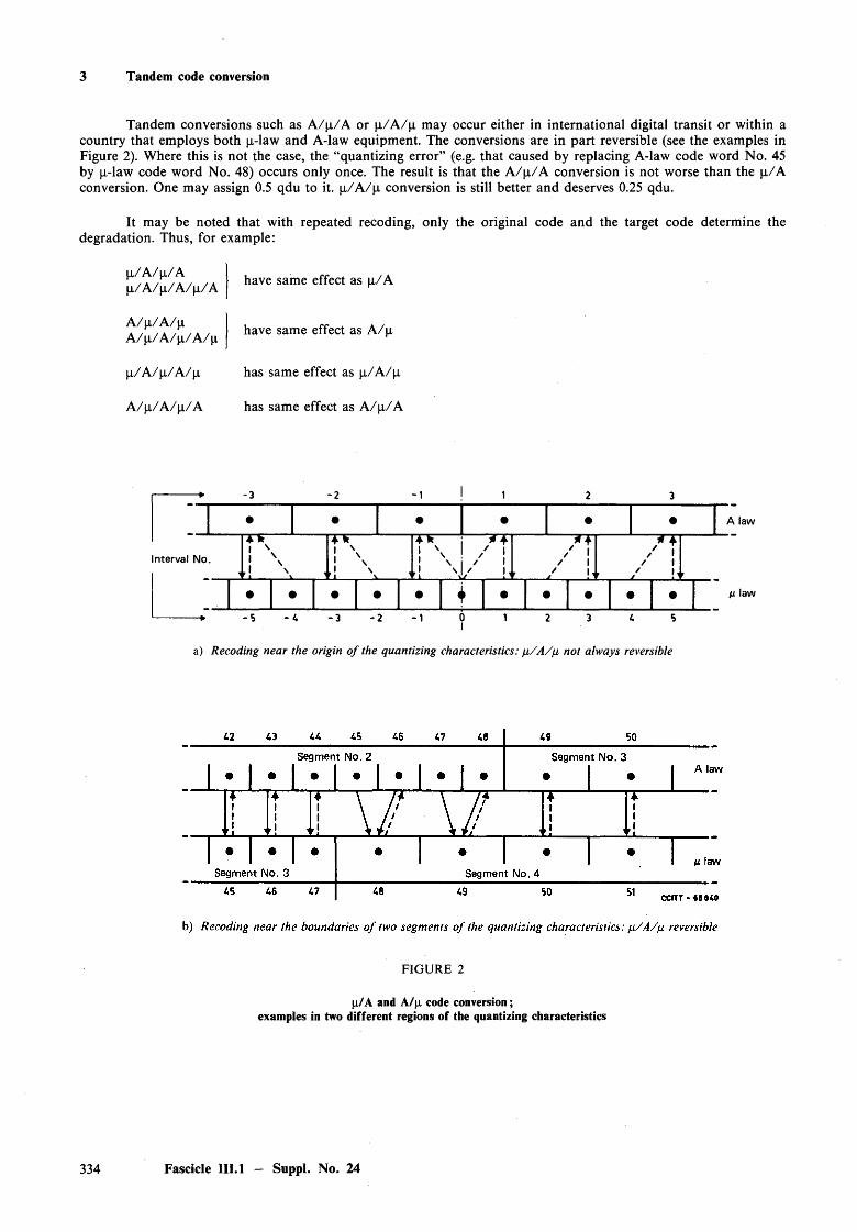
3 Tandem code conversion
Tandem conversions such as A / |i /A or p /A /p may occur either in international digital transit or within a country that employs both p-law and A-law equipment. The conversions are in part reversible (see the examples in Figure 2). Where this is not the case, the “quantizing error” (e.g. that caused by replacing A-law code word No. 45 by p-law code word No. 48) occurs only once. The result is that the A /p /A conversion is not worse than the p /A conversion. One may assign 0.5 qdu to it. p /A /p conversion is still better and deserves 0.25 qdu.
It may be noted that with repeated recoding, only the original code and the target code determine the degradation. Thus, for example:
p /A /p /A p /A /p /A /p /A have same effect as p /A
A /p /A /p A /p /A /p /A /p have same effect as A /p
p /A /p /A /p
A /p /A /p /A
has same effect as p /A /p
has same effect as A /p /A
Interval No.
- 2 -1
• • • • • i • • • • • u law
- ► - 5 - 4 - 3 - 2 - 1 0 1 2 3 4 5
A *
J \ ,- j - - - - - - *—
A W
■i \ .
A W j# Ai \ 1 / l! N i ' 1
r 1 ' \ ' 1 i
/ t/ 1r / ! ’
/ t/ 1r / !'
A l aw
a) Recoding near the origin o f the quantizing characteristics: fx /A /fi not always reversible
FIGURE 2
p/A and A /p code conversion; examples in two different regions of the quantizing characteristics
334 Fascicle III.l — Suppl. No. 24
4 Digital loss pads
In the essential range of signal levels (down to — 30 dBmO) these pads contribute at most a “relative quantizing distortion power” of « 1.25, which corresponds to 0.7 qdu.
Supplement No. 25
GUIDELINES FOR PLACEMENT OF MICROPHONES AND LOUDSPEAKERS IN TELEPHONE CONFERENCE ROOMS [1]
(Malaga-Torremolinos, 1984; quoted in Recommendation G.172)
1 General
The following guidelines provide basic rules for assessing the acoustics of telephone conference rooms and for installing audio equipment consistent with excellent speech intelligibility and easy talker recognition.
2 Conference room acoustics — General requirements
The design and installation of a telephone conferencing system which meets reasonable cost and performance specifications involves numerous judgements and trade-offs. These guidelines will enable the planner and installation engineer to assess the acoustics of a room, to make the necessary choices and decisions, to installthe appropriate equipment properly and thereby provide satisfactory service.
The audio portion of a telephone conference system consists o f terminal equipment with microphones and loudspeakers installed in conference rooms and interconnected by an audio transmission facility. This transmissionfacility may be either public switched telephone connections or private line facilities.
•In both public and private systems, transmission is frequently interconnected via a multipoint conference
bridge so that each room can communicate simultaneously with any of the other locations. When this is done, it is most im portant that the bridge be located at the electrical loss center of the network in order to minimize level contrast between the speech originating in the different rooms.
Unlike telephony between handsets, the acoustic properties of the conference room and the placement of microphones in the room critically determine the level, the speech signal-to-ambient-noise ratio and the reverberant quality (rain-barrel effect) o f the transmitted speech. Particularly in multipoint conferences, these three factors are easily judged and critically commented upon by users.
In general, the larger, noisier and more reverberant a room is, the less suitable it will be for telephone conferencing. The presence of noise a n d /o r reverberation in the transmitted speech results in a system whose performance is unsatisfactory. In extreme cases, experience has demonstrated that excess noise in one room, e.g. from overflying aircraft, can temporarily block transmission between all rooms of a multipoint system. Excess reverberation results in such hollowness to the received speech that talkers become difficult to recognize and understand, causing users to fatigue easily and refuse to use the system.
Fascicle III.l — Suppl. No. 25 335
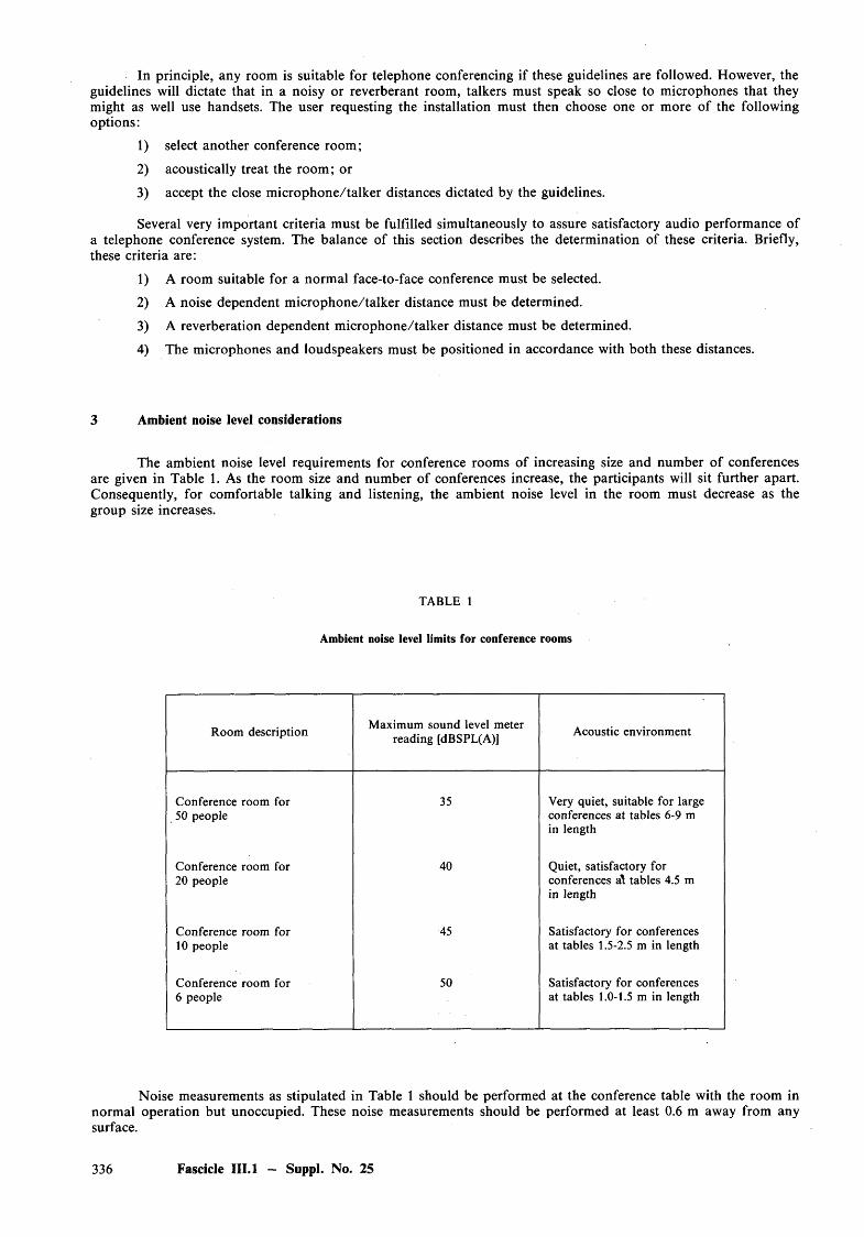
In principle, any room is suitable for telephone conferencing if these guidelines are followed. However, the guidelines will dictate that in a noisy or reverberant room, talkers must speak so close to microphones that theymight as well use handsets. The user requesting the installation must then choose one or more of the followingoptions:
1) select another conference room;
2) acoustically treat the room ; or
3) accept the close m icrophone/talker distances dictated by the guidelines.
Several very im portant criteria must be fulfilled simultaneously to assure satisfactory audio performance of a telephone conference system. The balance of this section describes the determination of these criteria. Briefly, these criteria are:
1) A room suitable for a normal face-to-face conference must be selected.
2) A noise dependent m icrophone/talker distance must be determined.
3) A reverberation dependent m icrophone/talker distance must be determined.
4) The microphones and loudspeakers must be positioned in accordance with both these distances.
3 Ambient noise level considerations
The ambient noise level requirements for conference rooms of increasing size and number o f conferences are given in Table 1. As the room size and number of conferences increase, the participants will sit further apart. Consequently, for comfortable talking and listening, the ambient noise level in the room must decrease as the group size increases.
TABLE 1
Ambient noise level limits for conference rooms
Room description Maximum sound level meter reading [dBSPL(A)] Acoustic environment
Conference room for 50 people
35 Very quiet, suitable for large conferences at tables 6-9 m in length
Conference room for 20 people
40 Quiet, satisfactory for conferences at tables 4.5 m in length
Conference room for 10 people
45 Satisfactory for conferences at tables 1.5-2.5 m in length
Conference room for 6 people
50 Satisfactory for conferences at tables 1.0-1.5 m in length
Noise measurements as stipulated in Table 1 should be performed at the conference table with the room in normal operation but unoccupied. These noise measurements should be performed at least 0.6 m away from any surface.
336 Fascicle III.l — Suppl. No. 25
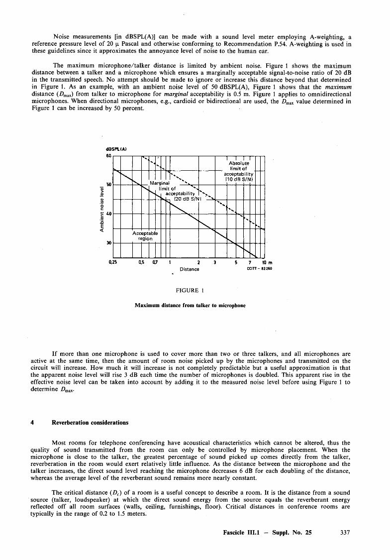
Noise measurements [in dBSPL(A)] can be made with a sound level meter employing A-weighting, a reference pressure level o f 20 p Pascal and otherwise conforming to Recommendation P.54. A-weighting is used in these guidelines since it approximates the annoyance level of noise to the human ear.
The maximum m icrophone/talker distance is limited by ambient noise. Figure 1 shows the maximum distance between a talker and a microphone which ensures a marginally acceptable signal-to-noise ratio of 20 dB in the transmitted speech. No attempt should be made to ignore or increase this distance beyond that determined in Figure 1. As an example, with an ambient noise level of 50 dBSPL(A), Figure 1 shows that the maximum distance (Anax) from talker to microphone for marginal acceptability is 0.5 m. Figure 1 applies to omnidirectional microphones. When directional microphones, e.g., cardioid or bidirectional are used, the Dmax value determined in Figure 1 can be increased by 50 percent.
0125 0.5 07 1 2 3 5 7 10 mDistance c a n - $2260
FIG URE 1
Maximum distance from talker to microphone
I f more than one microphone is used to cover more than two or three talkers, and all microphones are active at the same time, then the amount of room noise picked up by the microphones and transmitted on the circuit will increase. How much it will increase is not completely predictable but a useful approximation is that the apparent noise level will rise 3 dB each time the number of microphones is doubled. This apparent rise in the effective noise level can be taken into account by adding it to the measured noise level before using Figure 1 to determine Z)max.
4 Reverberation considerations
Most rooms for telephone conferencing have acoustical characteristics which cannot be altered, thus the quality o f sound transmitted from the room can only be controlled by microphone placement. When the microphone is close to the talker, the greatest percentage of sound picked up comes directly from the talker, reverberation in the room would exert relatively little influence. As the distance between the microphone and the talker increases, the direct sound level reaching the microphone decreases 6 dB for each doubling of the distance, whereas the average level o f the reverberant sound remains more nearly constant.
The critical distance (Dc) of a room is a useful concept to describe a room. It is the distance from a sound source (talker, loudspeaker) at which the direct sound energy from the source equals the reverberant energy reflected off all room surfaces (walls, ceiling, furnishings, floor). Critical distances in conference rooms are typically in the range of 0.2 to 1.5 meters.
Fascicle III.l — Suppl. No. 25 337
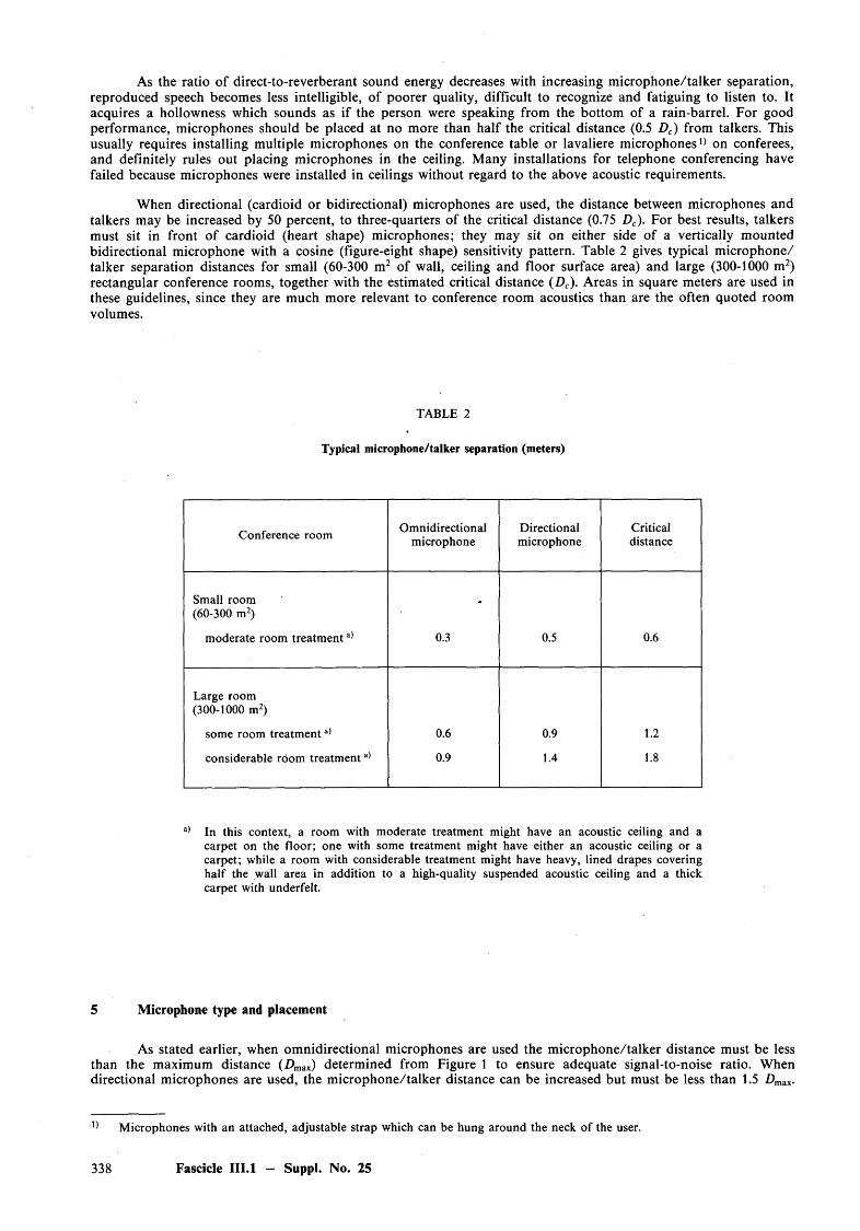
As the ratio of direct-to-reverberant sound energy decreases with increasing m icrophone/talker separation, reproduced speech becomes less intelligible, of poorer quality, difficult to recognize and fatiguing to listen to. It acquires a hollowness which sounds as if the person were speaking from the bottom of a rain-barrel. For good performance, microphones should be placed at no more than half the critical distance (0.5 Dc) from talkers. This usually requires installing multiple microphones on the conference table or lavaliere m icrophones1) on conferees, and definitely rules out placing microphones in the ceiling. Many installations for telephone conferencing have failed because microphones were installed in ceilings without regard to the above acoustic requirements.
When directional (cardioid or bidirectional) microphones are used, the distance between microphones and talkers may be increased by 50 percent, to three-quarters of the critical distance (0.75 Dc). For best results, talkers must sit in front o f cardioid (heart shape) microphones; they may sit on either side of a vertically mounted bidirectional microphone with a cosine (figure-eight shape) sensitivity pattern. Table 2 gives typical m icrophone/ talker separation distances for small (60-300 m2 of wall, ceiling and floor surface area) and large (300-1000 m2) rectangular conference rooms, together with the estimated critical distance (Dc). Areas in square meters are used in these guidelines, since they are much more relevant to conference room acoustics than are the often quoted room volumes.
TABLE 2
Typical microphone/talker separation (meters)
Conference room Omnidirectionalmicrophone
Directionalmicrophone
Criticaldistance
Small room (60-300 m2)
moderate room trea tm en ta) 0.3 0.5 0.6
Large room (300-1000 m2)
some room trea tm en ta) 0.6 0.9 1.2
considerable room treatm enta) 0.9 1.4 1.8
a) In this context, a room with moderate treatment might have an acoustic ceiling and a carpet on the floor; one with some treatment might have either an acoustic ceiling or a carpet; while a room with considerable treatment might have heavy, lined drapes covering half the wall area in addition to a high-quality suspended acoustic ceiling and a thick carpet with underfelt.
5 Microphone type and placement
As stated earlier, when omnidirectional microphones are used the m icrophone/talker distance must be less than the maximum distance (Dmax) determined from Figure 1 to ensure adequate signal-to-noise ratio. When directional microphones are used, the m icrophone/talker distance can be increased but must be less than 1.5 DmaK.
M icrophones with an attached, adjustable strap which can be hung around the neck of the user.
338 Fascicle III.l — Suppl. No. 25
Also stated earlier, when using omnidirectional microphones, the m icrophone/talker separation must be less than half the critical distance to ensure highly-intelligible, easily-recognizable, nonreverberant speech. When directional microphones are used, the m icrophone/talker distance can be increased but must be less than 0.75 Dc.
Microphones must be placed to satisfy both the above rules; in other words the m icrophone/talker distance must not exceed the smaller distance.
So that all talkers can satisfy the above m icrophone/talker criteria, more than one microphone is usually required. Typically one microphone for every 3 talkers is necessary. For each doubling of the number of microphones, the effective noise level in the room will increase by 3 dB. Thus, in the example of § 3 if four microphones were used, the reading of 50 dBSPL(A) would be raised to an effective value of 56 dBSPL(A). The noise determined, Dmax from Figure 1 would thus be reduced to 25 cm. Clearly, lavaliere microphones would provide a practical solution to keeping talkers within 25 centimeters of a microphone.
6 Loudspeaker placement
The requirements for placing loudspeakers in a conference room are much less critical than those for microphones. It is generally considered good practice to limit the distance from any listener in the room to the nearest loudspeaker to not more than twice the critical distance.
Loudspeakers should be distributed in the ceiling, on the walls, or on the conference table to ensure a minimum sound pressure level of 60 dBSPL(A) at listener positions. If there is significant noise, the sound pressure level should be at least 10 dB above the ambient noise level. More “presence” and less “voice-on-high” effect is achieved when the loudspeakers are placed on or in the edge of the conference table.
Ceiling mounted loudspeakers are usually simpler to install and less conspicuous. Generally, loudspeakers installed in a visible grid, suspended, acoustic panel ceiling should be placed approximately 0.6 meters outside the edge of the conference table. Best results are obtained when the loudspeakers are not installed symetrically but somewhat randomly. This prevents exciting pronounced room modes of vibration.
Reference
[1] Teleconference center construction guidelines, Bell System Technical Reference, PUB 42903, May 1980, American Telephone and Telegraph Co.
Fascicle III.l — Suppl. No. 25 339

Printed in Switzerland — ISBN 92 -61 -02041 -0