Failure of Rubber Components under Fatigue - Queen Mary ...

1

Failure of Rubber Components under Fatigue

Samuel Asare

School of Engineering and Materials Science

Queen Mary University of London

A thesis submitted in partial fulfilment of the requirements of the Degree

of Doctor of Philosophy

July 2013

2

Abstract

Rubber components under cyclic loading conditions often are considered to

have failed as a result of the stiffness changing to an amount that makes the part no

longer useful. This thesis considers three distinctive but related aspect of the fatigue

failure exhibited by rubber components. The first considers the reduction in stiffness

that can result from a phenomenon known as cyclic stress relaxation. The second

considers fatigue crack growth encountered resulting in potentially catastrophic failure.

The final issue relates to the complex topography of the resulting fatigue fracture

surfaces.

Previous work has shown that the amount of relaxation observed from cycle to

cycle is significantly greater than that expected from static relaxation tests alone. In this

thesis the reduction in the stress attained on the second and successive loading cycles as

compared with the stress attained on the first cycle in a stress strain cyclic test of fixed

strain amplitude has been measured for elastomer test pieces and engineering

components. Adopting the approach of Davies et al. (1996) the peak force, under cyclic

testing to a specific maximum displacement, plotted against the number of cycles on

logarithmic scales produces a straight line graph, whose slope correlates to the rate of

cyclic stress relaxation per decade. Plotting the rate of stress relaxation per decade

against the maximum average strain energy density attained in the cycle reduces the

data measured in different deformation modes for both simple test pieces and

components to a single curve. This approach allows the cyclic stress relaxation in a real

component under any deformation to be predicted from simple laboratory tests (Asare

et al., 2009).

Earlier work (Busfield et al., 2005) has shown that a fracture mechanics

approach can predict fatigue failure in rubber or elastomer components using a finite

element analysis technique that calculates the strain energy release rate for cracks

introduced into bonded rubber components. This thesis extends this previous work to

examine real fatigue measurements made at both room temperature and 70±1ºC in both

tension and shear using cylindrical rubber to metal bonded components. Dynamic

testing of these components generated fatigue failures not only in the bulk of the

component but also at the rubber to metal bond interface. The fatigue crack growth

characteristics were measured independently using a pure shear test piece. Using this

independent crack growth data and an accurate estimate for the initial flaw size allowed

3

the fatigue life to be calculated. The fracture mechanics approach predicted the crack

growth rates accurately at both room temperature and 70±1ºC (Asare et al., 2011).

Fatigue crack growth often results in rough fatigue crack surfaces. The rough

fatigue crack surface is, in part, thought to result from anisotropy being developed at

the front of a crack tip. This anisotropy in strength whereby the material is less strong

in the direction that the material is stretched might allow the fatigue crack to grow in an

unanticipated direction. It might also allow the crack front to split. Therefore the final

part of this thesis examines how, once split, the strain energy release rate associated

with growth of each split fatigue crack develops as the cracks extend in a pure shear

crack growth test specimen. The aim being to understand how the extent of out of plane

crack growth that results might allow a better understanding of the generation of

particular crack tip roughness profiles. Using a method of extending one split crack at a

time, whilst keeping a second split crack at a constant length, it has been possible to

evaluate the initial strain energy release rates of split cracks of different configurations

in a pure shear specimen. It was observed that, for a split crack in a pure shear

specimen, the initial strain energy release rate available for crack growth depends on

the precise location of the split crack. It is also clear that the tearing energy is shared

evenly when the crack tip is split into two paths of equal length, but as one crack

accelerates ahead it quickly increases in tearing energy and leaves the slower crack

behind. It is thought that this phenomenon is responsible for a lot of the roughness

observed on the resulting fracture surfaces.

4

Contents

ABSTRACT ..................................................................................................................... 2

CONTENTS ..................................................................................................................... 4

FIGURES ......................................................................................................................... 8

TABLES ........................................................................................................................ 16

ACKNOWLEDGEMENT ............................................................................................. 17

ABBREVIATIONS ....................................................................................................... 18

SYMBOLS ..................................................................................................................... 19

1.0 GENERAL INTRODUCTION ........................................................................... 21

2.0 LITERATURE REVIEW ................................................................................... 25

2.1 DEFINITION OF A RUBBER AND AN ELASTOMER ................................................ 25

2.2 PROPERTIES AND USES OF ELASTOMERS ........................................................... 25

2.3 TYPES OF ELASTOMERS .................................................................................... 26

2.3.1 Natural rubber (NR) ..................................................................................... 26

2.3.2 Polyisoprene (synthetic) rubber (IR) ........................................................... 27

2.3.3 Styrene-butadiene rubber (SBR) ................................................................. 27

2.3.4 Polybutadiene rubber (BR) .......................................................................... 28

2.4 COMPOUNDING OF A RUBBER COMPOUND ........................................................ 29

2.5 VULCANISATION .............................................................................................. 30

2.5.1 The vulcanising systems .............................................................................. 33

2.5.2 Accelerated sulphur vulcanisation ............................................................... 33

2.5.3 Conventional sulphur systems ..................................................................... 34

2.5.4 Efficient sulphur systems............................................................................. 34

2.5.5 Semi-efficient sulphur systems .................................................................... 35

2.5.6 Peroxide vulcanisation ................................................................................. 35

2.6 RUBBER-LIKE ELASTICITY ................................................................................ 36

2.6.1 Rubber-like elasticity (at small strains) ....................................................... 36

2.6.2 Rubber-like elasticity (at large strains) ........................................................ 37

2.6.3 Thermodynamics of elastomer deformation ................................................ 37

2.6.4 The statistical theory of elasticity ................................................................ 40

5

2.6.5 Phenomenological theories .......................................................................... 43

2.6.6 The theory of Mooney ................................................................................. 44

2.6.7 Imperfect elasticity ...................................................................................... 46

2.6.8 Stress relaxation, creep, set recovery and hysteresis ................................... 46

2.6.9 Cyclic stress relaxation ................................................................................ 49

2.7 FRACTURE MECHANICS .................................................................................... 49

2.7.1 Fracture mechanics of rubber ...................................................................... 50

2.7.2 Analytical expressions for the strain energy release rate, T, for some test

piece geometries ..................................................................................................... 53

2.7.3 Microscopic flaws........................................................................................ 55

2.7.4 The cyclic fatigue crack growth phenomenon ............................................. 56

2.7.5 The characteristics of steady state cyclic crack growth ............................... 58

2.7.6 Effect of test variables on fatigue crack growth .......................................... 65

2.7.7 Fatigue life prediction .................................................................................. 69

2.7.8 Fatigue crack surfaces ................................................................................. 70

2.8 FINITE ELEMENT ANALYSIS (FEA) ................................................................... 72

2.8.1 The FEA concept ......................................................................................... 72

2.8.2 Typical procedures for developing a finite element model using an FEA

programme .............................................................................................................. 76

2.8.3 Types of FEA models .................................................................................. 77

2.8.4 Axial symmetry ........................................................................................... 77

2.8.5 Planar symmetry .......................................................................................... 78

2.8.6 Finite element analysis of elastomers .......................................................... 78

2.8.7 Modelling cyclic fatigue crack growth ........................................................ 79

2.9 MOTIVATION FOR THIS STUDY .......................................................................... 80

3.0 MATERIALS, EXPERIMENTAL AND FEA METHODS .............................. 82

3.1 INTRODUCTION ................................................................................................. 82

3.2 MATERIALS ...................................................................................................... 82

3.3 MATERIAL CHARACTERISATION ....................................................................... 85

3.3.1 Material stress strain characterisation .......................................................... 85

3.3.2 Bonded cylindrical component force deflection measurement ................... 87

3.3.3 Equilibrium swelling tests ........................................................................... 87

3.4 MEASUREMENT OF CYCLIC STRESS RELAXATION.............................................. 87

3.4.1 Average strain energy density determination .............................................. 90

6

3.5 EXPERIMENTAL FATIGUE CRACK GROWTH MEASUREMENTS ............................. 91

3.5.1 Pure shear crack growth characterisation .................................................... 91

3.5.2 Bonded cylindrical component fatigue crack growth measurement ........... 93

3.6 FINITE ELEMENT ANALYSIS .............................................................................. 93

3.6.1 Introduction ................................................................................................. 93

3.6.2 FEA model of the bonded cylindrical component to predict stiffness ........ 94

3.6.3 Modelling crack growth in a tensile deformation mode .............................. 98

3.6.4 Modelling crack growth in shear deformation mode................................. 101

3.6.5 Modelling crack bifurcation in a pure shear test piece .............................. 101

4.0 CYCLIC STRESS RELAXATION .................................................................. 104

4.1 INTRODUCTION ............................................................................................... 104

4.2 RESULTS AND DISCUSSION ............................................................................. 105

4.3 CONCLUSION .................................................................................................. 115

5.0 FATIGUE LIFE PREDICTION ....................................................................... 116

5.1 INTRODUCTION ............................................................................................... 116

5.2 RESULTS AND DISCUSSIONS ............................................................................ 118

5.2.1 Material stress strain behaviour ................................................................. 118

5.2.2 Equilibrium swelling test results ............................................................... 122

5.2.3 Material pure shear crack growth characterisation .................................... 123

5.2.4 Experimental and predicted component force deflection behaviour in

tension at room temperature and 70±1ºC ............................................................. 134

5.2.5 Fatigue life prediction and experimental validation .................................. 136

5.2.6 Predicted and measured component fatigue life in tension and shear at room

temperature and 70 degrees Celsius ..................................................................... 138

5.3 CONCLUSION .................................................................................................. 160

6.0 CRACK BIFURCATION IN A PURE SHEAR TEST PIECE ........................ 161

6.1 INTRODUCTION ............................................................................................... 161

6.2 RESULTS AND DISCUSSION ............................................................................. 163

6.3 CONCLUSION .................................................................................................. 173

7.0 SUMMARY, CONCLUSIONS AND FUTURE WORK ................................ 174

7.1 CYCLIC STRESS RELAXATION ......................................................................... 174

7.2 FATIGUE LIFE PREDICTION OF BONDED RUBBER COMPONENTS ....................... 175

7

7.3 FINITE ELEMENT ANALYSIS OF CRACK BIFURCATION IN A PURE SHEAR SPECIMEN

176

REFERENCES ............................................................................................................ 178

APPENDIX – REFEREED JOURNAL PAPERS PUBLISHED BY THE AUTHOR

AS PART OF THIS RESEARCH ............................................................................... 185

8

Figures

Figure 2.1 (a) cis-polyisoprene (NR) (b) trans-polyisoprene (gutta percha) ..... 27

Figure 2.2 Chemical structure of styrene-butadiene rubber (SBR) ............................... 28

Figure 2.3 Chemical structure of polybutadiene rubber (BR) ....................................... 28

Figure 2.4 Rubber structure: (a) before vulcanisation and (b) after vulcanisation. ....... 31

Figure 2.5 Illustration of the three different curemeter responses (Hamed, 1992). ....... 32

Figure 2.6 A diagrammatic representation of the network structure of a sulphur

vulcanisate (Chapman and Porter, 1988). ...................................................................... 34

Figure 2.7 Chemical structure of carbon to carbon cross-link in a peroxide cured

network. ......................................................................................................................... 35

Figure 2.8 Stress at constant extension as a function of absolute temperature, at an

extension of 350% (Meyer and Ferri, 1935) .................................................................. 39

Figure 2.9 Comparison of statistical theory with experimental data for unfilled

elastomers by Treloar (1975). ........................................................................................ 43

Figure 2.10 Mooney plot for data of simple extension and uniaxial compression

(Treloar, 1975). .............................................................................................................. 45

Figure 2.11 Hysteresis loops for natural rubber taken from Lindley (1974b). (a) The

first cycle loops for unfilled natural rubber extended to various strains and (b) first,

second and tenth cycle loops for a natural rubber that contains 50 phr of carbon black.

........................................................................................................................................ 48

Figure 2.12 Schematic diagram for the shape of a crack tip used in equation Eq.2-30

(Thomas, 1955). ............................................................................................................. 52

Figure 2.13 Types of tear test-pieces (a) trouser (b) pure shear (c) angled (d) split and

(e) edge crack (Busfield, 2000). ..................................................................................... 53

Figure 2.14 Crack growth per cycle, dc/dn, as a function of strain energy release rate,

T, for unfilled NR (●) and SBR (o). The inset shows the region near the threshold strain

9

energy release rate for mechanical fatigue, T0, plotted on a linear scale (Lake (1983)).

........................................................................................................................................ 57

Figure 2.15 The strain energy release rate, T versus crack growth rate (r) for an unfilled

SBR using the various test piece geometries shown in Figure 2.13. - trousers; - pure

shear; - angled and - split (Greensmith et al., 1960). ............................................ 59

Figure 2.16 The effect of crack growth rate and temperature on strain energy release

rate, T for (a) unfilled SBR, (b) unfilled NR and (c) FT black filled SBR. (Greensmith

and Thomas, 1955)......................................................................................................... 60

Figure 2.17 Schematic diagrams illustrating force–time relationships and crack paths

for different types of crack growth (Papadopoulos, 2006). ........................................... 63

Figure 2.18 The effect of temperature on the T/r relationship for unfilled SBR

(Tsunoda, 2001). ............................................................................................................ 64

Figure 2.19 Superposition of the data given in Figure 2.18 using the WLF shift factor aT

(Tsunoda, 2001). ............................................................................................................ 64

Figure 2.20 Effect of the vulcanising system and cross-link density on the crack growth

behaviour for unfilled NR at a crack growth rate of 10µms-1 (Brown, Porter and

Thomas, 1987). .............................................................................................................. 65

Figure 2.21 The crack growth per cycle, dc/dn, as a function of maximum strain energy

release rate, T, for different minimum tearing energies, Tmin. Tmin = 0% and Tmin = 6%

of the maximum (Lake and Lindley, 1964). .................................................................. 67

Figure 2.22 Cyclic life, N as a function of temperature for unfilled NR and SBR

determined using tensile test specimens (Lake and Lindley, 1964). ............................. 68

Figure 2.23 Different types of element shapes (Abaqus Manual, 1998). ...................... 75

Figure 2.24 A schematic to demonstrate axial symmetry and planar symmetry

commonly adopted to simplify the finite element modelling of a component (Busfield,

2000) .............................................................................................................................. 80

Figure 3.1 Picture and a schematic of a typical bonded cylindrical suspension

component ...................................................................................................................... 83

10

Figure 3.2 A schematic of a pure shear specimen ......................................................... 84

Figure 3.3 Set up for pure shear cyclic stress relaxation measurement ......................... 88

Figure 3.4 Set up for bonded cylindrical component cyclic stress relaxation

measurement in tension and compression modes of deformation ................................. 89


measurement in simple shear mode of deformation ...................................................... 89

Figure 3.6 Typical force deflection behaviour of an engineering component; the area

under the curve is the stored elastic energy in the component at that specific

displacement .................................................................................................................. 91

Figure 3.7 A schematic of various regions according to the state of deformation in a

pure shear sample. All the dimensions are referred to the undeformed state. The entire

shaded area is region B. ................................................................................................. 93

Figure 3.8 A meshed undeformed cylindrical component (a) and a meshed cylindrical

component deformed in tension (b) ............................................................................... 96

Figure 3.9 A meshed undeformed cylindrical component (a) and a meshed cylindrical

component deformed in simple shear (b) ....................................................................... 97

Figure 3.10 An undeformed axisymmetric mesh (a), a tension deformed axisymmetric

mesh (b) and a tension deformed axisymmetric mesh with a crack (c) ......................... 99

Figure 3.11 An undeformed half symmetry mesh (a), a simple shear deformed half

symmetry mesh (b) and a simple shear deformed half symmetry mesh containing two

large cracks (c) ............................................................................................................. 100

Figure 3.12 A schematic of a pure shear specimen with a crack (c) splitting into two

cracks c1 and c2: Both c1 and c2 are parallel to the horizontal centre-line of the specimen

...................................................................................................................................... 103

Figure 4.1 The maximum force versus number of cycles data for two bonded

suspension mounts deformed in cyclic simple shear from 0mm to +60mm

displacements. .............................................................................................................. 105

11

Figure 4.2 Plot of log (maximum force) against log (number of cycles) for pure shear

samples tested at 20%, 40%, 60%, 80%, 100%, 120%, 140% and 150% maximum

engineering strain. ........................................................................................................ 107

Figure 4.3 Cyclic stress relaxation rate against extension ratio for the pure shear test

pieces............................................................................................................................ 108

Figure 4.4 Plot of log peak force (maximum force) against log (number of cycles) for

the bonded suspension mount at 26%, 40%, 53%, 79% and 92% maximum

displacement expressed as a percentage of the rubber cylinder height in tension. ...... 110


the bonded suspension mount at 26%, 53%, 79%, 105%, 132% and 158% maximum

shear displacement expressed as a percentage of the rubber cylinder height. ............. 111


the bonded suspension mount at 16%, 26%, 42%, 53% and 63% maximum

compression, expressed as a percentage of the cylinder rubber section height. .......... 112

Figure 4.7 Cyclic stress relaxation rate plotted against the maximum engineering strain

for the pure shear test pieces and maximum displacement divided by the rubber

cylinder height for the suspension mount under different deformations ..................... 113

Figure 4.8 Cyclic stress relaxation rate plotted against the maximum average strain

energy density for the pure shear test pieces and the suspension mount under different

deformations ................................................................................................................ 114

Figure 5.1 Virgin stress strain behaviour of the elastomer material (NR, 65 phr) at room

temperature obtained from a dumbbell test piece ........................................................ 118

Figure 5.2 1000th cycle stress strain behaviour of the elastomer material (NR, 65 phr)

measured at room temperature from a dumbbell test piece after softening at 90% strain

for 999 cycles ............................................................................................................... 119

Figure 5.3 Virgin stress strain behaviour of the elastomer material (NR, 65 phr) at 70

ºC obtained from a dumbbell test piece ....................................................................... 120

12

Figure 5.4 1000th cycle stress strain behaviour of the elastomer material (NR, 65 phr)

measured at 70 ºC from a dumbbell test piece after softening at 90% strain for 999

cycles............................................................................................................................ 121

Figure 5.5 Plot of absorbed n-decane per unit volume of sample for bonded cylindrical

component sample, sheet samples S1, S6 and S7 ........................................................ 123

Figure 5.6(a) A plot of Crack length against No. of cycles for 5mm sinusoidal

displacement amplitude at room temperature .............................................................. 125

Figure 5.6(b) A plot of Crack length against No. of cycles for 6mm sinusoidal


Figure 5.6(c) A plot of Crack length against No. of cycles for 7mm sinusoidal


Figure 5.6(d) A plot of Crack length against No. of cycles for 8mm sinusoidal


Figure 5.6(e) A plot of Crack length against No. of cycles for 9mm sinusoidal


Figure 5.6(f) A plot of Crack length against No. of cycles for 10mm sinusoidal


Figure 5.6(g) A plot of Crack length against No. of cycles for 11mm sinusoidal


Figure 5.6(h) A plot of Crack length against No. of cycles for 12mm sinusoidal



displacement amplitude at 70 ºC .................................................................................. 129





13









Figure 5.8 log dc/dn against log T for pure shear characterisation of NR 65 material at

room temperature and 70 degrees Celsius. .................................................................. 133

Figure 5.9 Experimental and predicted 1000th cycle force deflection behaviour of NR

65 phr elastomer material at room temperature ........................................................... 135

Figure 5.10 Experimental and predicted 1000th cycle force deflection behaviour of NR

65 phr elastomer material at 70 ºC ............................................................................... 136

Figure 5.11 Stored energy against crack length for crack growth in tension at 5mm,

10mm and 15mm amplitudes respectively at room temperature ................................. 138

Figure 5.12 Tearing energy crack length relationship for crack growth in tension at

5mm, 10mm and 15mm amplitudes respectively at room temperature ....................... 139

Figure 5.13 1/dc/dn versus crack length for crack growth in tension at 5mm amplitude

at room temperature ..................................................................................................... 140

Figure 5.14 1/dc/dn vrs crack length for crack growth in tension at 10mm amplitude at

room temperature ......................................................................................................... 141



Figure 5.16 Stored energy against crack length for component crack growth in tension

at 70 degrees Celsius .................................................................................................... 143

Figure 5.17 Tearing energy against crack length for component crack growth in tension

and at 70 degrees Celsius ............................................................................................. 144

14


70ºC .............................................................................................................................. 145


70ºC .............................................................................................................................. 146

Figure 5.20 1/dc/dn vrs crack length for crack growth in tension at 12.5mm amplitude

at 70ºC .......................................................................................................................... 147


70ºC .............................................................................................................................. 148

Figure 5.22 Stored energy crack length relationship for shear crack growth at 5mm,

9mm and 13mm amplitudes respectively at room temperature ................................... 149

Figure 5.23 Tearing energy crack length relationship for shear crack growth at 5mm,

9mm and 13mm amplitudes respectively at room temperature ................................... 150

Figure 5.24 1/dc/dn against crack length for shear crack growth at 5mm amplitude at






Figure 5.27 Stored energy crack length relationship for shear crack growth at 5mm,

9mm and 13mm amplitudes respectively at 70ºC ........................................................ 154

Figure 5.28 Tearing energy crack length relationship for shear crack growth at 5mm,

9mm and 13mm amplitudes respectively at 70ºC ........................................................ 155


70ºC .............................................................................................................................. 156


70ºC .............................................................................................................................. 157


70ºC .............................................................................................................................. 158

15


cracks c1 and c2: Both c1 and c2 are parallel to the horizontal centre-line of the specimen

...................................................................................................................................... 163

Figure 6.2 Deformed finite element meshes of a pure shear specimen showing split

parallel cracks c1 and c2 with equal lengths (a) and, split crack c2 extended keeping the

initial length of split crack c1 constant (b) ................................................................... 164

Figure 6.3 Stored energy crack length relationship for a split crack (c2) growing in a

pure shear specimen at 20% strain and, 0.5 mm measured vertical distance (y mm)

from the horizontal centre-line of the specimen .......................................................... 165

Figure 6.4 Tearing energy crack length relationships for a single and a split parallel

crack (c2) growing in a pure shear specimen at 20% strain ......................................... 166

Figure 6.5 Tearing energy crack length relationships for split crack c1 (where x =

constant = 4 mm in all models) for the respective models .......................................... 168

Figure 6.6 Tearing energy crack length relationships for split crack c2 (where y varied

and had values of 0.5 mm, 1 mm, 2 mm, 3 mm and 4 mm) for the respective models 169

Figure 6.7 Initial tearing energies of split crack c2, versus measured vertical distance (y

mm) of the split crack from the pure shear specimen horizontal centre-line in the

respective models at 20% strain ................................................................................... 170

Figure 6.8 Dependence of the initial tearing energy of split cracks on strain ............. 172

16

Tables

Table 3.1 Formulation for the materials used in this study 85

Table 5.1 Predicted and measured numbers of fatigue cycles required

to grow cracks from estimated rubber–metal bond edge flaw size until

specified crack size just before failure

159

17

Acknowledgement

I would like to express my sincere gratitude to my supervisors, Dr. James Busfield and

Professor Alan Thomas, for their guidance, tremendous help, and encouragement

throughout the course of this research work.

I would like to express my gratitude to the Department of Materials, Queen Mary,

University of London, for my fees scholarship which enabled me to pursue my research

studies. I am also grateful to Trelleborg AVS for the supply of materials for this

research work. I am thankful to my colleagues in the rubber group and all others who

contributed in one way or another to make my research studies a success.

Finally, I am deeply thankful to my family and friends for their continuous support and

encouragement throughout my studies.

18

Abbreviations

ACM Polyacrylate rubber

AEM Ethylene-acrylic rubber

ASTM American society for testing and materials

BR Butadiene rubber

CM Chlorinated polyethylene

CR Polychloroprene

CSM Chorosulfonated polyethylene

CV Conventional systems

ECO Epichlorohydrin rubber

EPR, EPDM Ethylene-propylene rubber

EV Efficient systems

FEA Finite element analysis

FKM Fluorocarbon rubbers

HAF High abrasion furnace

HNBR Hydrogenated nitrile rubber

IIR Butyl rubber

IR Synthetic rubber

MBTS Benzothiazyl Disulfide

MQ Silicone rubber

NBR Acrylonitrile-butadiene rubber

NR Natural rubber

phr Parts by mass per hundred elastomer

SBR Styrene-butadiene rubber

SE Surface free energy per unit area

SEF Strain energy function

SMR Standard Malaysian Rubber

S-N Stress versus fatigue life relation

T Polysulfide rubber

TMTM Tetramethylthiuram Monosulfide

WLF Williams, Landel and Ferry (1955)

19

Symbols

1, 2, 3 = Principal extension ratios

A = Area of a single fracture surface

At = Crack growth constant

B = Bulk modulus

C = Arbitrary constant

c = Crack length

C1 and C2 = Mooney constants

'1C and '

2C = WLF constants

C0 = Edge crack length at T0

d = Diameter of the modelled crack tip

d = Effective tip diameter

db = Diameter of the strained crack tip

dc/dn = Crack growth per cycle

e = Engineering strain

E = Young’s modulus

F = Force

G = Shear Modulus

h = Thickness of the specimen

k = Boltzmann constant

kz = Rate constant due to Ozone

l = Length

l0 = Un-gripped height of a pure shear specimen

mc = Number average molecular weight of segments of molecules between successive

cross-links

N = Count of chains per unit volume

N = Moles of cross-links per unit volume

n = Number of moles of chains per unit volume

Nf = Number of cycles to failure

Nm = Measured number of cycles

Np = Predicted number of cycles

P(r) = Probability density function

20

Q = Heat

r = End-to-end distance

R = Gas constant

rt = Radius of the semi circle

S = Entropy

t = Sheet thickness

T = Tearing energy

ϑ = Temperature

t = time

Tc = Critical strain energy release rate

Tg = Glass transition temperature

TM = Temperature at which the test is conducted

T0 = Threshold strain energy release rate

U = Internal energy

V = Volume of rubber

VS = Molar volume of the swelling solvent

W = Elastic stored energy per unit volume

w = Pure shear specimen width

W = Elastic stored energy per unit volume of the rubber at the crack tip

w0 = Total width of the test piece

Wb = Work to break per unit volume of rubber

Wt = A suitable average of W

x = A strip of material at the cracked part of the test piece that is not energy free

α = Angular distance

γ = Shear strain

θ = Angle

λ = Extension ratio

ρ = Density

σ = Engineering stress

σ1, σ2, σ3 = Principal stresses

υ = Poison ratio

Φ = Volume fraction of polymer in the swollen gel

χ = Polymer-solvent interaction parameter

Ψ, χ = Steady state crack growth constants

21

CHAPTER ONE

1.0 General Introduction

In recent years, industrial competition has led elastomer component

manufacturers to validate their products analytically prior to manufacture to ensure

more robust design and to try to reduce product lead times. The prediction of the

fatigue life of elastomer components, such as tyres, suspension components and engine

and gearbox mounts, has become a necessary research subject (Busfield et al., 2005).

An essential prerequisite, therefore, for the finite element simulation of mechanical

fatigue is an accurate knowledge of the material behaviour.

Elastomers exhibit a highly non-linear material behaviour characterised by three

main phenomena: a non-linear elastic behaviour under static load; a rate dependent or

viscoelastic behaviour with hysteresis under cyclic loading and the Payne effect

(Payne, 1962), which involves a substantial decrease in the storage modulus of a

particle reinforced elastomer with an increase in the amplitude of mechanical

oscillations. Another important phenomenon is cyclic stress relaxation which is

observed in elastomer materials. The cyclic stress relaxation involves a reduction in the

stress attained on the second and successive loading cycles as compared with the stress

attained on the first cycle in a stress strain cyclic test of fixed strain amplitude. Cyclic

stress relaxation itself is a manifestation of one specific type of fatigue behaviour of

elastomeric materials used in engineering applications. A detailed qualitative and

quantitative understanding of cyclic stress relaxation, therefore, is a necessary step

towards a scientific evaluation of the fatigue life of a rubber product.

In this work, the cyclic stress relaxation behaviour of a cylindrical rubber to

metal bonded component and test pieces made from carbon black filled natural rubber

material were measured experimentally. The cylindrical rubber to metal bonded

component was displaced to different fixed maximum displacements in tension and

shear deformation modes whilst, the test pieces were deformed to different fixed

maximum displacements in pure shear deformation mode. The objectives of these tests

were first to confirm the linear logarithmic dependence of the force at maximum

displacement on the logarithm of the number of cycles for successive cycles observed

by Davies et al. for a wide range of filled elastomer compound test pieces deformed in

tension (Davies, De, and Thomas, 1996). Secondly, and more importantly, to develop

22

an approach to correlate the rate of cyclic stress relaxation measured in elastomer

components to that measured in test pieces using an appropriate physical quantity –

found to be the maximum average strain energy density in this work. This aspect of the

work has been published in Asare et al., (2009). The method developed in the cyclic

stress relaxation work was subsequently incorporated into the finite element analysis

based approach to fatigue life prediction – to account for cyclic stress relaxation

quantitatively (Asare et al., 2011).

Extensive work has been done in the past on the prediction of fatigue life of

elastomer components. Busfield et al. (2005) presented a fracture mechanics approach,

which uses finite element analysis techniques, to calculate strain energy release rates

for cracks located in three-dimensional components, in combination with experimental

measurements of cyclic crack growth rates of specific strain energy release rates, to

predict the cyclic crack growth rate and the eventual fatigue failure of an elastomeric

engineering component in three modes of deformation, namely: tension, simple shear

and combined shear and tensile (45º angle) deformations. They used a gearbox mount

with a narrowly shaped middle section which raises the strain energy density in this

section under deformation and therefore failure initiation in the middle section of the

elastomer component. Their work was limited to room temperature conditions and also

prediction of the crack growth in the component after inserting an initial razor cut into

the middle section of the elastomer component. The cyclic stress relaxation associated

with fatigue crack growth was also poorly accounted for by pre-stressing the test piece

for stress strain characterisation to an arbitrary strain for 1000 cycles.

The research described here extends this previous work to examine real fatigue

measurements made at both room temperature and 70±1ºC in both tension and shear

using the cylindrical rubber to metal bonded component used in the cyclic stress

relaxation studies. The objective being to validate the fracture mechanics approach to

fatigue life prediction at above room temperature conditions. The cylindrical rubber to

metal bonded component generated fatigue failures not only in the bulk of the

component but also at the rubber to metal bond interface. In calculating the strain

energy release rates necessary for fatigue life prediction using the finite element

analysis (FEA) based fracture mechanics approach, the cyclic stress relaxation

associated with fatigue crack growth in the elastomer component is often poorly

accounted for by pre-stressing the test piece for stress strain characterisation to an

arbitrary strain for 1000 cycles. An original method is proposed in this work to

23

quantitatively account for the component cyclic stress relaxation, associated with the

fatigue crack growth, in the FEA strain energy release rate calculations, by

characterising the stress strain behaviour of the component material test piece after

repeated stressing for 1000 cycles, at a maximum average strain energy density

comparable to that obtained in the component when loaded. The material fatigue crack

growth characteristics were measured independently using a pure shear crack growth

test specimen. This independent crack growth data and an accurate estimate for the

initial flaw size, around the rubber-metal bond edge of the cylindrical component,

allowed the fatigue life to be calculated. The fracture mechanics approach predicted the

crack growth rates well at both room temperature and 70±1ºC. This aspect of adopting

fracture mechanics at elevated environmental service temperatures being entirely novel.


fatigue crack surface is, in part, thought to result from strain induced strength

anisotropy in front of the advancing fatigue crack which can then cause the crack to

split during crack growth. Part of this thesis examines strain energy release rates

associated with growth of split fatigue cracks, in a pure shear specimen, in an attempt

to investigate how fatigue crack bifurcation alters fatigue crack surface roughness.

Using a method of extending one split crack at a time, whilst keeping a second split

crack at a constant length, it has been possible to evaluate the initial strain energy

release rate for a split crack at different locations in a pure shear specimen. It was

observed that, for a split crack in a pure shear specimen, the initial strain energy release

rates available for crack growth depend on the location of the split crack in relation to

the central horizontal plane of the specimen. This work also shows that, split cracks

closer to the central plane of the pure shear specimen possess higher strain energy

release rates for growth than split cracks displaced further from the central plane. This

trend becomes more pronounced at higher global strains. It is concluded in this work

that the observed roughness of fatigue crack surfaces, to a large extent, may be the

result of a cyclic process involving a fatigue crack tip splitting, the twin growth of both

split cracks with the one that has a higher energy release rate eventually accelerating

and leaving behind the lower energy release rate component.

In Chapter two a literature review of elastomer materials including their uses

and properties is presented. The stress-strain behaviour of elastomer materials, cyclic

stress relaxation and the concept of elastomer fracture mechanics are discussed. This

24

review examines both the experiments done by earlier workers and the theories that

have been developed to explain the behaviour.

In Chapter three the material and experimental methods used to test the

cylindrical rubber to metal bonded component and test pieces in this work are presented

in detail. The finite element analysis technique for strain energy release rate

calculations is also explained.

Chapter four presents the results and discussion of the cyclic stress relaxation

behaviour of the cylindrical rubber to metal bonded component and test pieces. The

effects of maximum loading displacement and mode of deformation of the component

on the cyclic stress relaxation rate are discussed. Finally an original approach based

upon the average strain energy density in the component is proposed to correlate the

cyclic stress relaxation rate found in the test pieces with the rate measured in the

engineering components.

In chapter five, the results and discussion of fatigue life prediction of the

cylindrical rubber to metal bonded component are presented. It is demonstrated that a

fracture mechanics based approach can predict the fatigue life of elastomer engineering

components both at room temperature and for the first time at 70±1ºC.

Chapter six presents the results and discussion of FEA calculated strain energy

release rates of growing split cracks in a pure shear specimen. Chapter seven

summarises the conclusions and future work for the entire thesis.

25

CHAPTER TWO

2.0 Literature Review

2.1 Definition of a rubber and an elastomer

An elastomer is a macromolecular material which returns rapidly approximately

to its initial dimensions and shape after substantial deformation by a weak stress and

the release of the stress. A rubber is an elastomer which can be, or already is, modified

to a state in which it is essentially insoluble (but can swell) in a solvent and which in its

modified state cannot be easily remoulded to a permanent shape by the application of

heat and moderate pressure (BS3558-1).

2.2 Properties and uses of elastomers

In general elastomers exhibit the following combination of physical properties;

a low tensile modulus (0.5 – 10 MPa), high extensibility, good strength, low

permeability and good electrical insulation properties (Morton, 1987). Elastomers are

used in tyres, in sealing applications, as protection against abrasion and vibration, as

electrical insulation, in corrosion protection, in conveyor belting applications, and in

hoses and tubes. Three physical requirements are needed to be fulfilled for a material to

exhibit rubber-like behaviour:

1) The molecular chains have to be flexible and the molecular weight has to be

large with, for the most part, very weak interactions between the molecular

chains.

2) The chains should be fairly regular on a molecular level. These chains need to

be connected to each other in a loose network by chemical bonds, usually via a

short segment called a cross-link. A molecular weight of about 10 000 between

junction points is a typical value for vulcanised natural rubber (Brydson, 1988;

Sperling, 1986).

3) The glass transition temperature of the material must be below the temperature

of application of the material (Sperling, 2001).

26

2.3 Types of elastomers

Elastomers can be classified into general-purpose elastomers and specialty

elastomers. This classification is mainly based on suitability of the elastomer for a

given application. Though general purpose elastomers are widely used, in some

applications they can become unsuitable. This may be due to insufficient properties

such as solvent resistance, aging resistance, and/or temperature resistance. As an

alternative, several special purpose elastomers (specialty elastomers) have been

developed to meet these needs. General-purpose elastomers include styrene-butadiene

rubber (SBR), butadiene rubber (BR), and polyisoprene – both natural rubber (NR) and

synthetic rubber (IR). Specialty elastomers include polychloroprene (CR), acrylonitrile-

butadiene rubber (NBR), hydrogenated nitrile rubber (HNBR), Butyl rubber (IIR),

ethylene-propylene rubber (EPR, EPDM), silicone rubber (MQ), polysulfide rubber

(T), chlorosulfonated polyethylene (CSM), polyacrylate rubber (ACM), fluorocarbon

rubbers (FKM), chlorinated polyethylene (CM), epichlorohydrin rubber (ECO) and

ethylene-acrylic rubber (AEM) (Gent, 1992).

2.3.1 Natural rubber (NR)

Natural rubber (NR) is a polymer prepared either by the smoked sheet or the

hevea crumb process from field latex (Allen and Bloomfield, 1963). The rubber

consists mainly of linear cis-1,4-polyisoprene with a number average molar mass of

about 105 –106 and has a glass transition temperature Tg, of approximately –70°C. It has

the same empirical formula as trans-1,4-polyisoprene called Gutta-percha, (C5H8)n

having one carbon-carbon double bond for each C5H8 unit, the difference being solely

in the spatial arrangement of the carbon-carbon bond adjacent to the double bond

(Treloar, 1975). A diagram illustrating the structure of the repeat units for NR and

Gutta-percha is given in figure 2.1. These differences give markedly different physical

properties for the two materials, with NR being rubbery at room temperature while

Gutta-percha being a crystalline solid. NR crystallises at low temperature (maximum

rate at – 26°C) and upon straining. This is a consequence of a high degree of stereo

regularity, permitting a regular molecular alignment upon stretching. The ability to

strain crystallise imparts outstanding strength and gives vulcanisates with high crack

growth resistance at very large gross deformations. Unfortunately, NR also has a high

27

Figure 2.1 (a) cis-polyisoprene (NR) (b) trans-polyisoprene (gutta percha)

chemical reactivity with the ambient environment, in particular with oxygen and even

higher reactivity with ozone (Morton, 1987; Cunneen and Higgins, 1963; Treloar,

1975).

2.3.2 Polyisoprene (synthetic) rubber (IR)

Isoprene rubber (IR) is a synthetic rubber equivalent to NR with almost the

same chemical structure, 94-98% of cis-1,4-polyisoprene and 6-2% of trans-3,4-

polyisoprene (Blow, 1971). IR is produced both anionically and by Ziegler-Natta

polymerisation. NR and IR are both recognised as exhibiting strain induced

crystallisation. Under large strains these rubbers have extremely high strengths and

fatigue resistance with IR compounds having a lower modulus than similarly

formulated NR compositions due to a reduction in the strain-induced crystallisation

especially at the highest rates of deformation.

2.3.3 Styrene-butadiene rubber (SBR)

Styrene-butadiene rubber (SBR) is the most widely used synthetic rubber with

the largest global production volume. SBR is a random copolymer of styrene and

butadiene made by free radical emulsion polymerisation or anionically in solution. The

most commonly used SBR consists of 23.5% styrene and 76.5% butadiene, with a glass

transition temperature, Tg, of approximately –53°C (Barlow, 1988). A diagram

illustrating the structure of the repeat units of SBR is given in figure 2.2.

28

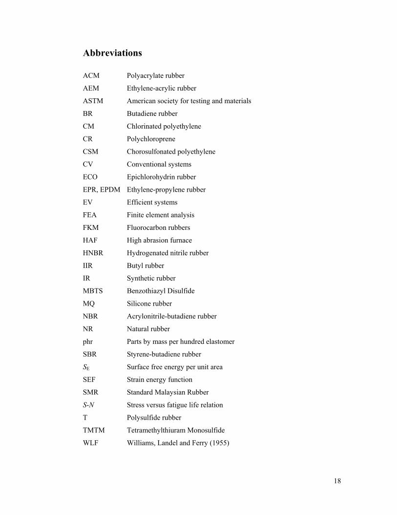
Figure 2.2 Chemical structure of styrene-butadiene rubber (SBR)

SBR is known as an essentially non strain-crystallising rubber, as under a large strain,

only limited if any crystallisation can take place. This feature results in significant

differences between the mechanical properties of NR (a strain crystallising rubber) and

SBR. SBR has lower tensile strength and tear resistance and it is necessary to reinforce

all SBR compounds for use in engineering applications with fillers such as carbon

black to impart more useful properties. It is also quite a common practice to blend SBR

with other rubbers to improve some of its basic properties.

2.3.4 Polybutadiene rubber (BR)

BR is a homopolymer of butadiene (C4H6) and can be made either by solution

or emulsion polymerisation. It is a non-polar rubber like NR and SBR, with a very low

Tg approximately –100°C. The 1,4-polybutadiene is an approximately equal mix of cis

and trans. Because of the regularity of its structure BR has a tendency to crystallise that

depends on the amount of cis and trans present (Blow, 1971). A diagram illustrating the

structure of repeat units is given in figure 2.3. BR is a resilient rubber which is

commonly used in combination with NR and SBR in long life rubber tyre treads.

Figure 2.3 Chemical structure of polybutadiene rubber (BR)

29

2.4 Compounding of a rubber compound

None of the elastomers mentioned in section 2.3 have useful properties until

they have been properly formulated. Rubber compounding is a process of blending the

rubber with vulcanising agents and other substances to produce a homogeneous mix.

Ingredients used in a rubber compound may be classified in the approximate order of

importance as follows (Blow, 1971; Morton, 1987):

1. Vulcanising agents; these are chemicals which can initiate the chemical cross-

linking of the rubber molecules leading to the formation of a three-dimensional

macromolecular network. The most common cross linking agents are based

around a sulphur curing system.

2. Accelerators; these are substances which can increase the rate of sulphur

combination with rubber. They are capable of promoting more efficient use of

sulphur; that is more cross-links, for a given amount of sulphur. They are also

used to reduce the vulcanisation time.

3. Activators; these are also used to increase the vulcanisation rate. They activate the

accelerators, which become more efficient. The most common system being zinc

oxide and stearic acid in combination to create soluble zinc ions that activate the

intermediate reactions involved in cross-link formation.

4. Fillers; these are added to reinforce or modify physical properties, impart certain

processing properties, or potentially in lower specification products to reduce

cost. Carbon black and silica are popular types of fillers which are used to

increase the stiffness and strength of the elastomers.

5. Processing aids; these are materials used to modify rubber during mixing or

processing steps. Processing oils are often used when fillers are mixed with

rubber. These are hydrocarbon oils and their presence reduces the frictional

energy during mixing.

6. Protective agents; these are added to protect the rubber from degradation. The

types of protective agent used depend on the use of the finished product. Waxes

are incorporated to protect the rubber against ozone attack while chemicals such

as 1,2-dihydro-2,2,4-trimethyl-6-phenyl quinoline are used to protect against

other forms of oxidative degradation.

7. Additional ingredients can be used for specific purposes but are not normally

required in the majority of rubber compounds. Examples are retarders (the

30

opposite of accelerators), colouring pigments, blowing aids, deodorants and fire

retardants.

Mixing of the compounding ingredients with rubber is usually carried out on a two-roll

mill or in an internal mixer (Morton, 1987).

2.5 Vulcanisation

A raw rubber often known as an elastomer or occasionally as a gum rubber is a

soft-flexible material. It shows viscoelastic properties since the molecules interact with

their neighbours due to forces of attraction and physical entanglements. Without cross-

links, the elastomer only exhibits limited elastic properties. Rubber is tacky when hot

and slowly crystallises to a rather hard and tough material when stored at low

temperature (for NR this is below 15°C) (Wood and Bekkedahl, 1946). In the

unvulcanised state, raw rubber only has rather limited uses but it can be transformed

into a more useful highly elastic state through a process called vulcanisation.

Vulcanisation is the chemical treatment of a natural or synthetic rubber by the addition

of a vulcanising agent such as sulphur, peroxides (or metal oxides) followed by curing

at elevated temperature and/or pressure into a stable, elastic and resilient material.

Vulcanisation of rubber creates cross-links, which form chemical bonds between the

long network chains of the rubber matrix. A diagram illustrating the structure of gum

rubber before and after vulcanisation is given in figure 2.4 (Barlow, 1988; Chapman

and Porter, 1988). Measurements of vulcanisation characteristics using an oscillating

disc rheometer (ODR) or moving-die rheometer (MDR) is common practice in the

rubber industry to help determine the kinetics of the cross-linking process. An

oscillating rotor is surrounded by a test compound, which is enclosed in a heated

chamber. The torque required to oscillate the rotor is monitored as a function of time at

the temperature chosen for vulcanisation. Figure 2.5 shows a typical torque-time curve

along with characteristic terms to describe the different behaviours. The scorch time, ts1

is the time at which the torque is 0.1 Nm above minimum torque. It gives an indication

of the safe period before the mix becomes impossible to process further due to the

formation of cross-links (Morrell, 1987).

31

Figure 2.4 Rubber structure: (a) before vulcanisation and (b) after vulcanisation.

32

Figure 2.5 Illustration of the three different curemeter responses (Hamed, 1992).

At the start of the test, there is a sudden increase in torque. Then, as the elastomer is

heated, its viscosity decreases, resulting in a net decrease in torque. Eventually, the

compound begins to vulcanise and transform into an elastic solid (known as an

elastomer), and the torque rises. Molecular chain scission may also occur; however, an

increasing torque indicates that an increase in cross-links is dominant. If the torque

reaches a plateau (curve b), this indicates a completion of curing and the formation of a

stable network. If chain scission and/or cross-link breakage become dominant during

prolonged heating, the torque passes through a maximum and then decreases (curve a),

a phenomenon termed reversion. Some NR compounds, particularly at high curing

temperatures, exhibit reversion. On the other hand, some compounds show a slowly

increasing torque at long cure times often called creeping cure (curve c). This

behaviour often occurs in compounds that initially form many polysulphidic linkages.

With extended cure times, these linkages may break down and re-form into linkages of

lower sulphur rank, thereby increasing the total number of cross-links (Hamed, 1992).

33

2.5.1 The vulcanising systems

In general, the type and number of cross-links formed between the network

chains affect both the physical and chemical properties of the material. The number of

cross-links depends on the amount and the type of vulcanising agent added. The time

allowed for curing/vulcanisation also produces different types of cross-links and

imparts different properties to the rubber vulcanisates. However, only the three kinds of

cross-link systems that are of commercial importance are discussed in the following

sections.

2.5.2 Accelerated sulphur vulcanisation

Accelerated sulphur vulcanisation was discovered in the 19th Century in

separate works carried out by Goodyear and Hancock and is still the most widely used

cross-linking method. A vulcanising system comprises a mixture of additives required

to vulcanise or “cure” a rubber. The three main classes of chemicals used for curing in

this vulcanising system are vulcanising agents, accelerators and activators. Accelerated

sulphur vulcanisation systems may give mono-, di-, tri- or higher polysulphidic cross-

links and the types of cross-links obtained are determined by the amount and type of

vulcanisation systems used (the ratio of mass of sulphur to accelerator) (Porter, 1969).

They also contain main chain modifications such as cyclic sulphides, pendent

accelerator group, and extra network materials which are primarily vulcanisation

residues. A diagrammatic representation of the network structure of a sulphur

vulcanisate is shown in figure 2.6. The accelerated sulphur vulcanisation systems can

be classified into three types:

1. Conventional systems (CV); containing high sulphur to accelerator ratios.

2. Efficient systems (EV); containing high accelerator to sulphur ratios.

3. Semi efficient systems (Semi-EV); that is, intermediate between 1 and 2.

34

Figure 2.6 A diagrammatic representation of the network structure of a sulphur

vulcanisate (Chapman and Porter, 1988).

2.5.3 Conventional sulphur systems

Conventional vulcanising systems (CV systems) have a high ratio of sulphur

(2–3.5 phr by mass) to accelerator (0.5–1.0 phr by mass). These systems contain more

polysulphidic cross-links (70–80%) than the disulphidic cross-links (20–30%) with a

relatively high degree of polymer chain modification. These systems give vulcanisates

which have excellent initial properties like strength, resilience and resistance to fatigue

and abrasion and are satisfactory for many applications. However, they show poor heat

and oxidation resistance because the polysulphidic cross-links are thermally unstable

and can be readily oxidised (Porter, 1968).

2.5.4 Efficient sulphur systems

Efficient vulcanising systems (EV systems) have a low ratio of sulphur (0.3–1.0

phr by mass) to accelerator (2.0–6.0 phr by mass). They give mainly monosulphidic

cross-links and less polymer chain modification. EV systems show good heat stability

and oxidation resistance, but have a poorer resistance to fatigue because of the presence

of the monosulphidic cross-links (Chapman and Porter, 1988; Skinner and Watson,

1967).

35

2.5.5 Semi-efficient sulphur systems

Semi efficient vulcanising systems are intermediate between CV systems and

EV systems, with similar levels of accelerator (1.0–2.5 phr by mass) and sulphur (1.0–

2.0 phr by mass) (Porter, 1973). This results in approximately equal amounts of

monosulphidic and polysulphidic chains to be present in the rubber network. They offer

a compromise between a good resistance to thermal ageing and a good fatigue life

performance.

2.5.6 Peroxide vulcanisation

Peroxides are another curing system for rubbers. Unlike sulphur curing, double

bonds are not required along the polymer chain for peroxide vulcanisation. Saturated

rubbers like ethylene propylene rubber and silicone rubber cannot be cross-linked by

sulphur and accelerators, and organic peroxides are often used for their vulcanisation.

When peroxides decompose, free radicals are formed on the polymer chains, and these

chains then combine to form carbon-to-carbon bonds (C-C) which serve as cross-links.

A diagram illustrating the cross-link system in peroxide vulcanisation is given in figure

2.7.

Figure 2.7 Chemical structure of carbon to carbon cross-link in a peroxide cured

network.

Peroxide vulcanisates have the best heat resistance when suitable antioxidants are also

included due to the good stability of C-C cross-links (Bristow, 1970). However, cure

rates are slow and their formation can require higher temperatures. Long cure times are

needed to ensure the complete decomposition of the peroxide so that resistance to

36

oxidative ageing is retained. Peroxide vulcanisates have a worse resistance to low

temperature crystallisation and inferior strength properties compared with sulphur

vulcanised rubber (Barlow, 1988; Baker, 1988).

2.6 Rubber-like elasticity

Elastomers exhibit a unique property of being capable of being stretched to

several hundred percents of their original length when loaded and recovering upon

removal of the load. For most engineering elastomers, extension within the range of

200% to 1000% is typical. The engineering stress-strain relationship becomes non-

linear at deformations that are this large and much lower. As a result a single parameter

(Young’s modulus) to describe the modulus of the elastomer is inappropriate. However,

as is the case with most solids at small strains, the force extension relationship is

considered to be approximately linear and a small strain elastic modulus is often used

in engineering practice.

2.6.1 Rubber-like elasticity (at small strains)

Elastomers can be considered to be elastic and isotropic in their undeformed

state and can, therefore, be characterised by only two fundamental elastic constants.

The first deals with the materials resistance to compression under a hydrostatic

pressure. It is termed the bulk modulus B and defined as the ratio of the applied

pressure to the volumetric strain. The second term is the shear modulus G, which is

defined as the ratio of the applied shear stress required to produce a shear strain .

The other frequently used small strain elastic constants, the tensile modulus E and

Poisson’s ratio , are related to the bulk modulus and the shear modulus as shown

below,

+

EG =

12 (Eq.2-1)

213 E

B = (Eq.2-2)

Elastomers being a unique class of engineering materials have very low shear and

tensile moduli (in the region of 0.5–10 MPa) while the bulk modulus is typically very

large (at about 1.5–2.0 GPa). As a result the value of Poisson’s ratio is close to 0.5

(typically, 0.4995) (Sperling, 2001) and the tensile modulus E is almost exactly equal

to 3G. For many engineering applications elastomers can be considered as being

37

incompressible and the elastic behaviour at small strains (<10% strain) can be defined

by just a single elastic constant G (Gent, 1992).

2.6.2 Rubber-like elasticity (at large strains)

There are two main approaches that attempt to describe the large strain

behaviour of elastomers. These are either molecular models based around the

configuration entropy of the rubber network (the simplest of which is known as the

simple statistical theory) and various other phenomenological approaches (Sperling,

2001).

1) Molecular approach

The molecular approach is based on the random morphology of the rubber

chain molecular network in three-dimensions and the response of this

network to the application or removal of a force.

2) Phenomenological approach

The phenomenological approach can be based on classical mechanics, and

just attempts to model the behaviour in a suitable mathematical way without

assuming any specific arrangement of the polymer molecules.

Both approaches can result in the derivation of a stored or strain energy function (SEF).

This is a measure of the amount of recoverable elastic energy W, stored in a unit

volume of the material having been subjected to a specific state of strain.

2.6.3 Thermodynamics of elastomer deformation

Two phenomena are observed in elastomers, which indicate that elastic

behaviour and the thermodynamic behaviour are related.

1. When an elastomer is stretched rapidly, it warms up. Conversely, when a

stretched specimen is allowed to contract, it cools down.

2. Under conditions of constant load, the stretched length decreases on heating

and increases on cooling.

The two effects are known as the thermo-elastic properties or Gough-Joule effects

(Treloar, 1975). It is possible to explain these two phenomena by considering the

deformation of the rubber in thermodynamic terms. The first law of thermodynamics

gives the definition for a change in the internal energy, dU:

WQU ddd (Eq.2-3)

38

where dQ is the heat absorbed by the system and dW is the work done by external

force. This equation states that the increase in dU in any change taking place in a

system equals the sum of the energy added to the system by the heat process, dQ, and

the work performed on it dW.

The second law of thermodynamics defines the entropy change dS in any reversible

process as:

Q

Sd

d (Eq.2-4)

where ϑ is the temperature and dS is the change in the entropy of the system.

For a reversible process, combining both laws of thermodynamics gives;

WSU ddd (Eq.2-5)

For elastic solids, the work done by the applied stress is important. If tensile force is F

and l is the initial length of the elastic specimen in the direction of the force, the work

done in creating an elongation dl is:

lFW dd (Eq.2-6)

The force, F in the tension mode can be expressed from equation 2-6 in the form of

l

S

l

UF (Eq.2-7)

The first term refers to the change in internal energy with extension and the second

term to the change in entropy with extension. From thermodynamic considerations it

can be shown that:

l

SF

l

(Eq.2-8)

This gives the entropy change per unit extension,

l

S, in terms of the temperature

coefficient of tension at constant length l

F

, which can be measured. When an

elastomer is stretched the randomly coiled molecules are straightened and this

decreases the disorder and hence also decreases the entropy of the network. Therefore,

the entropy of elongation at constant temperature must be negative. Therefore,

l

F

l

UF (Eq.2-9)

39

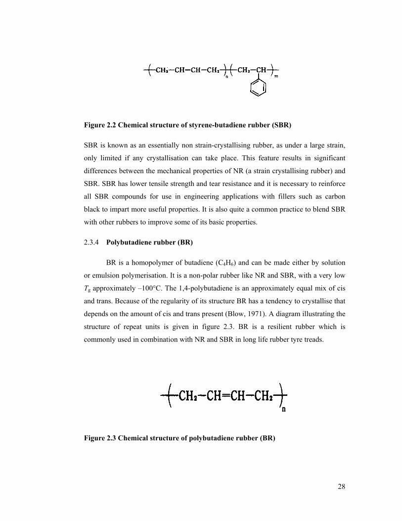
Figure 2.8 Stress at constant extension as a function of absolute temperature, at an

extension of 350% (Meyer and Ferri, 1935)

This equation allows the internal energy term and entropy term to be evaluated. Meyer

and Ferri (1935) investigated the relation between the force, at an applied strain of

350%, against the temperature. Their results are shown in figure 2.8 and indicate that

the relationship between stress and temperature in the rubbery region, when the

temperature is higher than the glass transition temperature, is linear and can be

extrapolated to approximately zero tension at absolute zero temperature. This

relationship implies that the change in the entropy with an extension is temperature

independent. The approximately zero intercept indicates that there is virtually no

change in the internal energy associated with the extension. The small discrepancy

might be explained by complications caused by the effects of thermal expansion. From

the thermodynamic theory, it is seen that the deformation of the rubber network

involves a reversible transformation of work into heat. This thermodynamic concept is

a basic foundation for the statistical development of the kinetic theory of rubber

elasticity.

40

2.6.4 The statistical theory of elasticity

The statistical treatment requires the calculation of the entropy of the whole

assembly of chains as a function of the macroscopic state of strain in the sample and

the derivation of the free energy or work of deformation. The work done in deforming

the rubber elastically is considered to arise from the decrease in entropy when the

molecules are forced by deformation to take up a less probable configuration. The

development of the theory for a cross-linked rubber has been carried out by a number

of workers; Kuhn (1936), Wall (1942), James and Guth (1943) and Treloar (1943).

The assumptions of the theory are:

1. The network contains N chains per unit volume each containing q identical, freely

jointed links of length l. A chain is defined as a segment of molecules between

successive cross-links.

2. The rubber deforms in a manner which causes the configurational entropy of the

chains to alter, but which results in no change in internal energy.

3. The distribution of possible end to end distance, r, follows a Gaussian distribution

in the unstrained state described by a probability density function:

rrbrb

r=r )dexp(4)dP( 2223/2

3

(Eq.2-10)

where 2

2

2

3

lqb . It follows that the root-mean-square distance is given by

2r = ql and it is implicit in assuming a Gaussian distribution that r << ql; in

other words the end to end distance of the chains is much less than their fully

extended length.

4. The volume remains unchanged on deformation. (That is the material is

incompressible).

5. The cross-links move in deformation as if embedded in an elastic continuum so

that the components of length in each chain change in the same ratio as in the

bulk rubber. This is known as the assumption of affine deformation.

6. The entropy of the individual chains is given by:

2

2

2

3

lq

rCS

k (Eq.2-11)

41

where C is arbitrary constant and k is the Boltzmann constant. The entropy of the

network is the sum of the entropies of the individual chains.

Using equation 2-11 to calculate the entropy change associated with deforming

a chain and summed over the assembly of N chains yields:

)3(2

1 23

22

21 kNS (Eq.2-12)

where S is the change in entropy of the network per unit volume under a deformation

in which 1 , 2 and 3 are the three principal extension ratios (the ratios of the

stretched to unstretched length) along three mutually perpendicular axes. Thus a unit

cube would be deformed into a cuboid of edge lengths 1 , 2 and 3 . The basic

assumption of the kinetic theory is that all states of deformation have the same internal

energy )0( U and the same non-configurational entropy. Hence, for an isothermal

reversible process the work W done by the applied forces becomes:

SSUW (Eq.2-13)

The work of deformation per unit volume is then:

)3(2

1 23

22

21 kNW (Eq.2-14)

W represents the work of deformation or elastically stored energy per unit volume and

is also called the strain energy function. It is convenient to write:

cmnRNG

Rk (Eq.2-15)

where n is the number of moles of chains per unit volume, is the density of rubber, R

is the gas constant, ϑ is the temperature and mc is the number average molecular weight

of segments of molecules between successive cross-links. Equation 2-14 becomes:

)3(2

1 23

22

21 GW (Eq.2-16)

Thus, the strain energy function represented by equation 2-16 involves only one

physical constant, G, which may be determined from the degree of cross-linking in the

rubber. If the assumption of constant volume is applied then;

1321 (Eq.2-17)

in simple tensile extension which can be defined in terms of a single extension ratio .

The two equal contractions in the transverse directions can be derived from the

incompressibility condition as:

42

1

, 321 (Eq.2-18)

and equation 2-16 becomes:

)32

(2

1 2

GW (Eq.2-19)

The force per unit undeformed cross sectional area or engineering stress σ required to

deform the network is given by (Treloar, 1975):

)1

(d

d2

GW

(Eq.2-20)

For an incompressible material the state of deformation is unaffected by the imposition

of the hydrostatic stress. The differences between any two principal stresses in any

homogeneous deformation may be determined absolutely. These are given by:

22

2121 G

22

2232 G

21

2313 G (Eq.2-21)

The stress-strain behaviour for particular modes of deformation may be determined

from equation 2-21 by the substitution of the appropriate relationships for the stresses

and the extension ratios. Experimental examination of the stress-strain relationships in

figure 2.9 (tensile stress versus strain plotted with the relation predicted in tension

using equation 2-20) however, reveals significant deviations between the theoretical

and experimental results. In simple extension there are two distinct deviations (Treloar,

1944). This theory is subject to all the limitations imposed by the assumption of the

Gaussian chain behaviour and in addition to the assumption of affine deformation. The

theory worked quite well over a limited range of extension ratios ranging from about

1.0 to 1.3. Above this range, deviations from the theory were apparent, especially in

uniaxial extensions where, at extension ratios between 1.3 and 5.5, the theory predicted

a modulus that was higher. At extensions greater than 5.5, the measured stress-strain

behaviour for an actual elastomer showed a marked upturn which this simple statistical

theory failed to predict. The deviation at higher strains (>400%) is caused by the effects

of a finite chain extensibility which is not considered (Wall, 1942; James and Guth,

1943). In strain crystallising elastomers, strain-induced crystallisation effects, which

also increase the materials stiffness, dominate at high strains.

43

Figure 2.9 Comparison of statistical theory with experimental data for unfilled

elastomers by Treloar (1975).

2.6.5 Phenomenological theories

Phenomenological approaches are based upon a mathematical description of the

stress-strain behaviour and not on molecular or structural concepts of the material,

assuming an isotropic material in the unstrained state. These theories represent the large

strain behaviour of both unfilled elastomers and filled elastomers. This, rather general,

treatment of the stress-strain relations of rubber-like solids started with Mooney (1940)

before the derivation of the statistical theory, and was further developed by Rivlin

(1956). Other forms of the stored energy function have been developed by many

workers since then, a detailed review of Rivlin’s theory and the work of others,

including the Yeoh stored energy function which was used in all the finite element

analysis work in this thesis, can be found in Busfield (2000). The Yeoh stored energy

function was chosen to model the material behaviour in this work because of its

accuracy in modelling the stiffness behaviour of filled elastomers at large strains. The

Yeoh stored energy function is also able to accurately predict the stress strain behaviour

of filled elastomers in different deformation modes using experimental data measured

in one simple deformation mode such as uni-axial extension. The Yeoh model differs

44

from other higher order models in that it depends on the first strain invariant only. Its

accuracy at fitting stress strain data at low strains is limited and therefore caution needs

to be excercised when applying this model at low strains (Gent, 1992). In the following

section, the theory of Mooney is reviewed.

2.6.6 The theory of Mooney

One of the earliest and most widely applied of the phenomenological theories is

that due to Mooney (1940). Mooney was concerned with the problem of developing a

general theory for large elastic deformations. Making use of the assumptions that a

rubber is incompressible and isotropic in the unstrained state, and that Hooke’s Law is

obeyed in simple shear, Mooney derived by purely mathematical arguments based on

the considerations of symmetry, the following stored energy function,

3

1113

23

22

21

223

22

211

CCW (Eq.2-22)

which contains two elastic constants, C1 and C2. The first term in equation 2-22

corresponds to the form derived from the statistical theory with 2C1=Nkϑ. The

statistical theory is therefore a particular case of the Mooney function corresponding to

C2 = 0.

For a simple extension or uniaxial compression, where 2 = 3 =1

equation 2-22

becomes,

32

13

212

12

1

211

CCW (Eq.2-23)

and the nominal stress is given by

1

212

11

12

d

d

C

CW

(Eq.2-24)

The term C1 was found to be dependent on the cross-link density and was consequently

related to the elastic constant of the statistical theory (Gumbrell et al, 1953). The origin

of the C2 term is still not clear, but it can be regarded as a measure of the departure of

the observed stress-strain relationship from the form suggested by the statistical theory.

Numerous experiments have been carried out which give support to the applicability of

the Mooney equation in simple extension for natural rubber and other polymers

(Grumbell et al., 1953; Mooney, 1940). However, the data of Rivlin and Saunders

45

(1951) for equibiaxial extension (which is kinematically equivalent to uniaxial

compression) showed a marked deviation from the Mooney relationship. Figure 2.10

shows the relationship between the extension and compression. In the extension region

(1/λ<1) the Mooney line corresponds to a value of C2/C10.8, but in compression (1/λ

>1), C2 was found to be about zero. Thus, when considering the extension and

compression data together, it is clear that the Mooney equation is no improvement over

the statistical theory. Taken as a whole, the Mooney equation does not seem to give a

closer fit to the experimental data than the statistical theory. The interpretation of

experimental data using the Mooney equation must be treated with caution since the

Mooney form of the stored energy function cannot be adequately used to describe the

mechanical properties of rubber for all possible types of strain, particularly those in

compression predicted using properties measured in tension.

Figure 2.10 Mooney plot for data of simple extension and uniaxial compression

(Treloar, 1975).

46

2.6.7 Imperfect elasticity

The preceding section of rubber-like elasticity was concerned mainly with the

ideal behaviour of elastomers, which were assumed to follow reversible relations

between load and displacement. In practice, deviations from such ideal behaviour are to

be expected. An ideal elastic solid obeys Hooke’s law: stress is proportional to strain.

An ideal viscous liquid obeys Newton’s law: stress is proportional to rate of change of

strain with time. Many materials and elastomers in particular, have properties that are

intermediate between these two cases. The response of these materials, which act

neither as ideal elastic solids nor as ideal liquids, is known as viscoelastic behaviour.

While viscous properties might be desired in elastomers for shock damping

applications, many industrial problems arise as a consequence of excessive viscous

response. Such common phenomena as stress relaxation, creep, compression set (and

unrecovered deformations, in general), energy losses during a deformation cycle

(“hysteresis”), limited rebound, heat generation, temperature rise during flexing and

cyclic stress relaxation are all manifestations of the inelastic properties of elastomers.

2.6.8 Stress relaxation, creep, set recovery and hysteresis

Stress relaxation is a time-dependent reduction in stress under constant

deformation. It is usually defined as the loss in stress expressed as a percentage of the

initial stress. Thus,

Stress loss (t) %100o

to

(Eq.2-25)

where 0 is the initial stress and t is the stress at time t. The rate of stress relaxation

is then the stress relaxation divided by some function of time.

Creep is the increase in strain with time at a specified load and is usually expressed as a

percentage of the initial deflection. Thus,

Creep (t) %100i

it

l

ll (Eq.2-26)

where lt is the length of rubber specimen at time t and li is the initial extended length of

the specimens. The initial deflection must be measured at a defined initial time to,

which should be about 10 times longer than the time taken to apply the deformation.

Set is a specific deformation, which remains when a material is released from the force

imposed on it. Thus, set measures the ability of the elastomer to recover its original

47

dimensions. When the deformation is tensile, it is referred to as tension set. Hence,

tension set is defined as:

Set (t) %100oi

ox

ll

ll (Eq.2-27)

where lx is the recovered length, lo is the initial length and li is the extended length

(Gent, 1992). Energy lost during loading and unloading cycles in a cyclic test is termed

hysteresis. Here the energy dissipated during a loading cycle is considered as the area

between the loading and the unloading cycle. Examples are shown in Figure 2.11 taken

from Lindley (1974b). For an unfilled elastomer, the magnitude of the energy loss at

extension ratios below 3 is quite small. Payne and Whittaker (1972) showed that at

higher extension ratios in excess of 4 with strain crystallising elastomers, such as

natural rubber, the amount of hysteresis was dramatically increased due to the

formation and the dissolution of strain induced crystals during the loading cycle. This

hysteresis, expressed as the fraction of the energy input lost, increases as the fraction of

particulate filler is increased. Payne (1962) and Deeprasertkul (2000) attributed this to

the breakdown and reformations of the agglomerates of the carbon black particles that

can themselves dissipate energy.

48

Figure 2.11 Hysteresis loops for natural rubber taken from Lindley (1974b). (a)

The first cycle loops for unfilled natural rubber extended to various strains and

(b) first, second and tenth cycle loops for a natural rubber that contains 50 phr of

carbon black.

(a)

(b)

49

2.6.9 Cyclic stress relaxation

Many engineering components undergo repeated stressing. Under repeated

stressing it is well known that rubber materials exhibit cyclic stress relaxation. Under

specific conditions for many components, this results in fatigue failure such as that

described by Busfield et al. (2005), Papadopoulos et al. (2008) and Busfield et al.

(2002). Cyclic stress relaxation involves a reduction in the stress attained on the second

and successive loading cycles as compared with the stress attained on the first cycle in

a stress strain cyclic test of fixed strain amplitude. This cyclic stress relaxation

behaviour is sometimes mistakenly referred to as the Mullins (1948) effect. This is

inappropriate, as the classical Mullins effect describes behaviour where if the maximum

strain experienced previously by the rubber is exceeded, the stress strain curve returns

to the value measured in the virgin cycle. The relaxation phenomenon has been studied

for simple extension by Derham and Thomas (1977), McKenna and Zappas (1981),

Davies et al. (1996) and Pond and Thomas (1979), but not for other deformation

modes. It was found that the fractional relaxation or creep rate was strongly dependent

on the maximum stress as well as the composition of the compound. In particular the

filler content and the ability to strain crystallise appears to be important in enhancing

the relaxation rate. Rubber in engineering applications experiences many modes of

deformation. One of the key aims of this thesis is therefore to examine how cyclic

stress relaxation might be predicted in more than one mode of deformation. In chapter

4, results of cyclic stress relaxation measurements on test pieces and cylindrical bonded

elastomer components will be presented and discussed.

2.7 Fracture mechanics

A fracture mechanics approach that was based upon an energy balance approach

was originally developed by Griffith in 1920 for brittle materials. Griffith observed that

the stress needed to fracture bulk glass was much less compared with the theoretical

stress needed for breaking atomic bonds in the glass. Griffith conducted experiments on

glass fibres which showed an increase in the fracture stress of the glass fibre samples as

the diameter decreased. Griffith attributed the observed reduction in strength of the

bulk glass compared with its theoretical strength and the increase in the fracture stress

of the glass fibre with a decrease in its diameter to the presence of microscopic flaws

(cracks) in the bulk of the glass material. In an effort to quantitatively assess the

50

influence of these flaws on the strength of the material Griffith assumed that, a crack in

a strained sheet of glass will grow if the elastic stored energy released due to the crack

growth was greater than the free energy required to create a new surface. He thus

established a fracture criterion expressed in differential form as shown in equation 2-

28.

lc

U

tS

1

2 (Eq.2-28)

where SE is the surface free energy per unit area, U is the total elastic energy stored in

the sheet, c is the crack length, t is the sheet thickness and the subscript l indicates that

the differentiation is carried out at constant overall extension so that the externally

applied forces do no work. The adoption of the elasticity solution for the stress

distribution in a loaded sheet containing an elliptical hole, made it possible for Griffith

to calculate the differential for a crack in an infinite sheet. The results generated in his

experiments containing flaws of a given size were in agreement with measurements of

the surface energy of molten glass using the expression in Equation 2-28 above.

2.7.1 Fracture mechanics of rubber

The problem of crack growth in elastomers was originally studied by Rivlin and

Thomas (1953). They extended the Griffith criterion for the growth of a crack in a

brittle material to the case of vulcanised rubber. Griffith’s approach can be applied to

elastomers since it is not limited to small strains and linear elastic responses. However,

the decrease in elastic strain energy in elastomers is not used only to increase surface

free energy of the cracked body, but it is also partly transformed to other forms of

energy, like irreversible deformations of the bulk of the material and dissipative

processes at the crack tip. These dissipative processes at the crack tip occur in a

relatively small volume of the material compared with the overall dimensions of the

body. The three factors that determine the magnitude of the dissipation are: the

viscoelastic properties of the elastomer, the strain in the crack tip region and the rate at

which the crack is growing. Therefore, the energy required to drive a crack at a

particular rate is a material characteristic and is defined as strain energy release rate

which is also sometimes known as the tearing energy, T (Rivlin and Thomas, 1953).

dA

dUT (Eq.2-29)

where A is the area of a single fracture surface.

51

The detail of the crack tip is a very important aspect of the fracture process as stated

earlier. In the work of Thomas (1955) he showed that a relationship exists between the

strain energy release rate and the strain distribution around the tip of a crack of a

defined radius in a test piece. Considering an incision of the form of two parallel sided

slits terminated by a semicircle in a test piece, he proposed:

dcosΔΔ t2

2

α hrcWU

(Eq.2-30)

where W is the elastic stored energy per unit volume of the rubber at the crack tip at an

angular distance α from the pole, h is the thickness of the specimen and rt is the radius

of the semi-circle (figure 2.12).

Using equation 2-30 he showed that:

dWrWααWrc

U

hT

lttt

2

2

αt 2dcosd

d1

(Eq.2-31)

where Wt is a suitable average of W and d is the diameter of the model crack tip.

Calculations of the strain energy release rate using the relation proposed, considering

the over-all forces or strains applied to the test piece (Rivlin and Thomas, 1953), and

that determined considering the strain distribution around the crack tip (Thomas, 1955)

compared excellently. Thomas (1955) further showed that when test pieces were

extended to tensile rupture, Wt in Equation 2-31 becomes the work to break per unit

volume of rubber, Wb, and Equation 2-31 takes the form,

bbdWT or b

b d

TW (Eq.2-32)

where db is the diameter of the strained crack tip that results in a tensile rupture.

He verified this relationship experimentally by measuring the strain energy release rate

of test pieces having modelled tip diameters in the range of 1mm to 3mm and found

T/db to be fairly constant and approximately equal to the work to break (Wb) in tensile

tests.

52

Figure 2.12 Schematic diagram for the shape of a crack tip used in equation Eq.2-

30 (Thomas, 1955).

Following the work of Thomas (1955), extensive research has been carried out by other

workers on the crack tip such as the work of Gent and Henry (1967). Andrews (1961,

1963) showed by applying a microscopic technique that, a combination of hysteresis

and large displacements results in blunting of the crack tip in highly deformable

materials. Andrews provided better understanding of the crack tip strain distribution

and thus confirmed Thomas’ (1955) conclusions. Rice (1968) developed a

mathematical method which related the local crack tip conditions to the strain energy

release rate known as the J-integral. The integral expresses an energy balance in a

volume of material surrounding a crack tip. Rice showed that the value of the integral is

independent of the choice of integration path. Hence, the path can be chosen close to

the crack tip to give a measure of local crack tip conditions. The integration path may

also be chosen to follow the boundaries of the specimen. Mars and Fatemi (2002)

reported that under this condition the integral turns out to be equivalent to the strain

energy release rate. It can be inferred, therefore, that the strain energy release rate is a

measure of the intensity of local crack tip fields for a given material and crack tip

geometry.

α

2rt

53

2.7.2 Analytical expressions for the strain energy release rate, T, for some test

piece geometries

For rubber, we cannot assume that strains, and therefore stresses, are

infinitesimal hence analytical calculation of T for a particular case may be very

difficult. Rivlin and Thomas (1953), however, presented several different test pieces for

which analytical expressions for T may be derived.

Figure 2.13 Types of tear test-pieces (a) trouser (b) pure shear (c) angled (d) split

and (e) edge crack (Busfield, 2000).

(a) (b)

(c) (d)

(e)

54

Rivlin and Thomas (1953), Greensmith and Thomas (1955), Thomas (1960) and Lake

et al. (1969) used differently shaped test pieces of the same material to test the

hypothesis that the energy required to grow a crack at a given rate is geometrically

independent and hence a material characteristic alone. Diagrams of the test piece

geometries they used are shown in figure 2.13. The resulting relationships for

calculating T for the different geometries are given below:

1. The trouser test crack growth measurement:

Wwh

FT 0

2

(Eq.2-33)

where F is the applied tearing force, λ is the extension ratio in the legs, h is the

specimen thickness in the unstrained state, w0 is the total width of the test piece and W

is the elastic stored energy density in the legs of the test piece that are in simple

extension.

2. The pure shear crack growth test:

This is preferred for crack growth studies because the crack grows at a constant rate for

a specified applied strain. This enables the strain energy release rate to be determined

as the complications caused by the stress concentration effects at the crack tip are

eliminated. The strain energy release rate is given by,

0WlT (Eq.2-34)

where W is the elastic stored energy density in the region of the test piece which is

subjected to the pure shear state and l0 is the unstrained distance between the two

parallel clamps.

3. The angle crack growth test:

2sin

2 t

FT (Eq.2-35)

where F and t are again the applied force and the test piece thickness and θ is the angle

between the separating legs.

4. The split crack growth test:

{[T FA λAsin θ + FB (λA cos θ - λB)]/t} - w0 (WA – WB) (Eq.2-36)

where FA and FB are the forces applied to the respective pairs of legs, λA, λB and WA,

WB the corresponding extension ratios and stored energy densities respectively in the

legs. 2θ corresponds to the angle of the opening (tan θ = FA / FB) and w0 and t are the

width and thickness of the test piece.

55

5. The edge crack in a tensile crack growth test piece:

In this case the strain energy release rate is given by

kWcT 2 (Eq.2-37)

where W is the elastic stored energy density in the bulk of the material at large

strains, c is the crack length, and k is a changing strain dependent term, given as,

λk

π (Eq.2-38)

where λ is the extension ratio (Lake, 1970).

2.7.3 Microscopic flaws

The work of Griffith in 1920 indicated the existence of intrinsic flaws in

materials. Work by Mars and Fatami (2003) suggested that the fatigue phenomenon in

elastomers consists of two stages: the crack nucleation stage and subsequently the crack

growth stage. This view of the fatigue phenomenon assumes that no inherent flaws pre-

exist in the elastomer material contrary to the observations made by Griffith in his

work. Tsunoda (2001) in his work noted that fatigue crack initiation may arise from

accidental scratches and nicks on the moulded or cut surface of the elastomer material.

Further to that, Gent and Tompkins (1969) suggested that even if such scratches and

nicks are carefully avoided by moulding the rubber material against polished glass

surface, the breaking strength of the rubber is not increased dramatically. This implies

that other sources of flaws such as dirt, dust particles, local inhomogeneities in cross-

link density and filler particle distributions may be present in the material. An approach

for estimating the size of intrinsic flaws in a material is by using equation 2-37 and

taking T to be T0 and c to be c0. Here, T0 is the threshold strain energy release rate and

c0, the edge crack length at T0, the intrinsic flaw size. The threshold strain energy

release rate may be described as the special energy release rate when the crack tip

energy losses are minimised. Lake and Thomas (1967) carried out cyclic crack growth

tests where they defined the minimum tearing limit at which cyclic crack growth will

occur. They suggested that below T0 crack growth was solely attributed to chemical

attack by ozone. It is interesting to note that, the average size of intrinsic flaws has been

found by this approach to be independent of the material compound formulation and of

the order of 25 to 50μm. The work of Abraham (2002) and Kingston and Muhr (2012)

suggest that there are flaws in commercial rubber components that have lengths in

excess of 200µm. Abraham (2002) showed that the large scatter normally occurring in

56

a set of fatigue tests on rubber compounds could be eliminated by introducing regular

flaws of 200µm throughout the test samples. It is useful to recall, however, that the

rubber material type and formulation has effect on the strength of the elastomer. It

appears that, there is no clear distinction between the crack nucleation and subsequent

growth states as suggested by Fatami (2003). What then appears to be important is the

rate at which an existing flaw of a given size grows for a specific set of loading

conditions.

2.7.4 The cyclic fatigue crack growth phenomenon

In the work of Rivlin and Thomas (1953) they established that the energy

required to grow a crack in a material at a given rate is a material characteristic. It is

also generally observed that the extent of crack growth during a loading cycle is

determined by the maximum strain energy release rate achieved in the loading cycle

and that, the extent of crack growth is not affected very much by the manner in which

the maximum strain energy release rate was achieved even for relatively viscous

materials (Gent et al., 1964). The relationship between crack growth rate per cycle and

the strain energy release rate may be represented mathematically in the form:

)(d

dTf

n

c (Eq.2-39)

The crack growth rate per cycle and the strain energy release rate relationship is known

as the crack growth characteristic of the material because it is independent of the test

piece geometry. Lake (1983) presented typical curves of the crack growth characteristic

for NR and SBR materials measured under relaxing conditions. Figure 2.14 (Lake,

1983) shows three distinct regions of crack growth characteristics. In region I the strain

energy release rate, T, is less than the threshold strain energy release rate T0 and hence

no mechanical crack growth occurs (Tsunoda, 2001). Below T0, crack growth is caused

by ozone degradation and the crack growth characteristic may be expressed as:

z3zd

dROk

n

c (Eq.2-40)

where kz is the rate constant due to ozone, [O3] is the ozone concentration and Rz is the

crack growth rate. The chemical reaction between ozone and carbon-carbon double

bonds, which are present in the backbone of natural and various olefin rubbers, is very

rapid, resulting in molecular scission. Ozone attacks rubbers above a critical tensile

57

stress equivalent to a strain energy release rate of about 0.1 J/m2 for unprotected NR

and SBR compounds.

Figure 2.14 Crack growth per cycle, dc/dn, as a function of strain energy release

rate, T, for unfilled NR (●) and SBR (o). The inset shows the region near the

threshold strain energy release rate for mechanical fatigue, T0, plotted on a linear

scale (Lake (1983)).

Above this critical energy level, the rate of crack growth is proportional to ozone

concentration (O3) and independent of the strain energy release rate as expressed by

equation 2-40. In region II, the crack growth is dependent on both ozone attack and

mechanical factors in a somewhat linear and additive fashion. This may be expressed

mathematically as:

Log (T / Jm-2)

Log

(dc

/dN

/ m

)

58

0tzd

dTTAR

n

c (Eq.2-41)

where At is a crack growth constant for region II. In region III, the power law

dependency between crack growth rate and T has been found for many rubbers as well

as for non-rubbery materials. Thus;

Tdn

dc (Eq.2-42)

where χ and ψ are constants, characteristic of region III. For natural rubber ψ is about 2,

and for SBR, ψ is about 4. In general, ψ lies between 2 and 6 for most elastomers,

depending mainly on the rubber and to a lesser extent on secondary factors such as

compounding ingredients. At the highest values of strain energy release rate, dc/dn

approaches the velocity of the elastic waves in rubber, about 50ms-1. Thus;

cTT (Eq.2-43)

where Tc is the critical strain energy release rate, where catastrophic tearing takes place.

2.7.5 The characteristics of steady state cyclic crack growth

Lake and Thomas (1967) showed that the surface energy for elastomers amount

to about 2 Jm-2. The work of Greensmith et al. (1960), shown in figure 2.15, confirmed

that unfilled SBR which does not undergo strain crystallisation at large strains, that a

specific value of T is required to propagate a crack at a specific rate. Typical values of

T for crack growth have been shown to lie in the region of 0.5 – 10 kJm-2 which is

considerably greater than the surface energy of elastomers. This confirms that other

irreversible changes occur as the crack is extended. The magnitude of the strain energy

release rate depends significantly on the irreversible energy losses that take place as the

crack is extended. These energy loss processes are dependent on temperature and so is

the crack growth versus strain energy release rate relationship. The relationship

between crack growth rate, temperature, and strain energy release rate is presented in

figure 2.16 for unfilled SBR, NR and FT black filled SBR. Figure 2.16(a) which

represents a plot for an unfilled SBR shows that strain energy release rate increases

with increasing crack growth rate and decreasing temperature. Mullins (1959) pointed

out that this dependence highlights the influence of visco-elastic energy dissipation

processes. However, for the strain crystallising rubber NR, Figure 2.16(b), the effect of

temperature on the rate of tear is much lower.

59

Figure 2.15 The strain energy release rate, T versus crack growth rate (r) for an

unfilled SBR using the various test piece geometries shown in Figure 2.13. -

trousers; - pure shear; - angled and - split (Greensmith et al., 1960).

T /

kJ.m

-2

r / cm.s-1

60

Figure 2.16 The effect of crack growth rate and temperature on strain energy

release rate, T for (a) unfilled SBR, (b) unfilled NR and (c) FT black filled SBR.

(Greensmith and Thomas, 1955).

T / J.m-2

T / J.m-2

T / J.m-2

61

In this case, strain crystallisation has the dominant influence on the crack growth

behaviour and, according to Tsunoda (2001), the high strain energy release rate

observed in NR, over a wide range of crack growth rates and temperatures, could be

attributed to the high energy losses associated with the heat of strain crystallisation.

The plot for carbon black filled SBR represented in Figure 2.16(c) demonstrates a

plateau at low crack growth rates and at low temperatures. This plateau shows that a

wide range of tear rates can exist for a specific strain energy release rate which results

in the formation of knotty crack growth. Beyond this region, knotty crack growth does

not occur and as a result the carbon black loading is responsible for a minimal increase

in strain energy release rate compared with that of unfilled SBR. This leads to the

conclusion that initiation of knotty crack growth depends on both crack growth rate and

temperature. Tsunoda (2001) observed that even in the presence of carbon black, the

crack growth behaviour is governed mainly by visco-elastic effects. In the presence of

carbon black the strain energy release rate can, over certain ranges, decrease with

increasing crack growth rate due to the onset of some degree of strength anisotropy.

This phenomenon is also called crack tip blunting or knotty-tearing and is thought to be

caused by strain-induced crystallisation or the presence of carbon black. “Knotty”

tearing consists of a discontinuous stick-slip process, in which the tear develops

laterally or even circularly under increasing force until a new tear breaks ahead and the

tear force drops sharply. The tear pattern then repeats itself. Figure 2.17 (c) presents an

example together with three other types of tear with their respective force and tear

patterns. Steady tearing results in macroscopic surface roughness: small deviations

from the tear path produce stick-slip tear and longer deviations give knotty-tearing.

Apart from crystallisation mechanical energy loss due to hysteresis is also related to the

visco-elastic properties of the material. The degree of dissipation is determined by the

internal viscosity of the material which is a function of temperature. Williams et al.

(1955) developed an equation which rationalises the temperature dependence of

viscosity for glass-forming liquids. The equation is known as the WLF equation and is

given as,

SM'2

SM'1

t

)()log(

TTC

TTCa

(Eq.2-44)

where TS = Tg +50oC, and TM is the temperature at which the test is conducted. '1C and

'2C are the WLF constants which have been found to vary from polymer to polymer

(Sperling, 2001). Andrews (1964) used a WLF type relation to correlate rupture data at

62

various temperatures for non-crystallising elastomers. He observed that there is a close

correlation between the strain energy release rate and the internal viscosity. Tsunoda

(2001) carried out work on an unfilled SBR. In Figure 2.18 (Tsunoda, 2001) as

expected the strain energy release rate, T available to drive a crack at a given rate

decreased with increasing temperature as the visco-elastic losses decreased. The data

were then shifted using Equation 2-44, taking '1C = 8.86 and '

2C = 101.6 for unfilled

SBR, to form the WLF relationship (Figure 2.19) (Tsunoda, 2001). The fact that the

results from different temperatures superimposed in the fast crack growth rate range is

also expected since the large visco-elastic losses at these rates were likely to dominate

the crack growth process. The data in the slow crack growth range does not

superimpose as well. This is where rough fracture surfaces developed suggesting that

here the effective tip diameter, d also varied with temperature. Tsunoda (2001)

remarked that fracture surfaces at a given rate become rougher with increasing

temperature. This could be attributed to cavitation occurring more readily due to

increased temperature. With increasing temperature the extent of cavitation increased

as the elastic modulus decreased and hence d increased, resulting in rougher fracture

surfaces. The strain energy release rate and hence the crack growth behaviour of an

unfilled rubber depends on the nature of the backbone of the polymer molecule, the

molar mass and the concentration and nature of cross-links. Depending on the

vulcanisation process employed (Tsunoda, 2001), widely different strengths for the

same polymer backbone can be produced, even when compared at similar degrees of

cross-linking. Brown et al. (1987) investigated the effect of vulcanising systems on the

strain energy release rate for mono-sulphide, poly-sulphide and peroxide cross-linked

systems. The results are presented in Figure 2.20. From the plot, where the shear

modulus is indicative of the cross-link density, the strain energy release rate required

for a crack to grow at 10ms-1 decreases with increasing shear modulus in all three

vulcanising systems. The observed ranking of the strength was poly-sulphide cross-

links had the greatest strength followed by mono-sulphide cross-links with the peroxide

system producing the weakest cross-linked network. The decreasing order of strength

follows an increase in the bond strength of the cross-link. Mullins (1959) concluded in

his work that mechanically weak cross-links presumably re-distributed local stresses in

the network by breaking and reforming during deformation. It is assumed that the poly-

sulphidic cross-links break before the main polymer backbone chain under the high

63

stresses around the crack tip resulting in higher strength for the poly-sulphidic cross-

links than for C-C cross-links.

Figure 2.17 Schematic diagrams illustrating force–time relationships and crack

paths for different types of crack growth (Papadopoulos, 2006).

Crack growth Graph

Direction of crack Direction of

(a) smooth crack

(b) steady crack growth

(c) stick-slip crack

(d) knotty crack growth

64

Figure 2.18 The effect of temperature on the T/r relationship for unfilled SBR

(Tsunoda, 2001).

Figure 2.19 Superposition of the data given in Figure 2.18 using the WLF shift

factor aT (Tsunoda, 2001).

2.0

2.5

3.0

3.5

4.0

4.5

-6 -4 -2 0 2 4 6Log (r / mm.s

-1)

Log

(T /

J.m

-2)

20°C

60°C

100°C

Region-A Region-B Region-C

2.0

2.5

3.0

3.5

4.0

4.5

-8 -6 -4 -2 0 2 4

Log (a Tr / mm.s-1

)

Log

(T

/ J

.m-2

)

20°C

60°C

100°C

65

Figure 2.20 Effect of the vulcanising system and cross-link density on the crack

growth behaviour for unfilled NR at a crack growth rate of 10µms-1 (Brown,

Porter and Thomas, 1987).

2.7.6 Effect of test variables on fatigue crack growth

A number of factors are known to affect cyclic fatigue crack growth tests: the

maximum and minimum loading limits (also expressed as the R-ratio), the test

frequency and the test temperature. The R-ratio is defined as the ratio of the minimum

test displacement to the maximum test displacement in a displacement controlled cyclic

test or the ratio of the minimum load to the maximum load in a load controlled cyclic

test. When the R-ratio is equal to zero, the loading condition is said to be fully relaxing

whereas when the R-ratio is not equal to zero the loading condition is said to be non-

fully relaxing. Lake and Lindley (1964) observed in the case of NR materials a

decrease in the crack growth per cycle under non-fully relaxing loading conditions.

GS / MPa

T /

J.m

-2

Poly-Sulphide

Mono-Sulphide

P.O.

66

Figure 2.21 shows the difference in crack growth rate per cycle when the minimum

strain energy release rate in a loading cycle is about 6% of the maximum, the threshold

strain energy release rate is effectively increased and the crack growth per cycle at

higher strain energy release rates is reduced by a factor of 10. Strain crystallisation in

the highly strained region around the crack tip is thought to be responsible for this

behaviour. According to Thomas (1974) the crystals melt as the strain decreases to

zero. As a result increments of crack growth occur on subsequent extension before

strain crystallisation takes place. SBR materials are non-crystallising and the

phenomenon is not present. In the experimental work of this thesis only NR materials

were examined. In order to avoid the complications arising from non-fully relaxing

loading conditions, all crack growth experiments were carried out under fully relaxing

conditions for both test pieces and elastomer components. Another difference between

non-crystallising and strain crystallising elastomers is their response to the frequency of

cyclic testing.

In the case of non-crystallising materials such as SBR, the total crack growth is

a result of two components; the time dependent and a dynamic crack growth

component. Ellul (1992) reported on the significant effect of frequency on non-

crystallising rubbers which reflects the time dependent component of the cyclic crack

growth, which is superimposed onto the dynamic crack growth component. This time

dependent component dominates the behaviour at low frequencies and reflects the

steady tearing that can arise in these non-crystallising rubbers. For strain crystallising

elastomers the crack growth does not occur in a time dependent manner and cracks can

only propagate above a given critical applied strain energy release rate. Consequently,

the time dependent component is much less important and the cyclic frequency has

only a very small effect on the crack growth per cycle. However, if the frequency is

high, especially for bulky components, excessive heat can be generated and the

predominant cause of failure is now no longer mechanical cyclic crack growth but

rather as a result of elevated temperature degradation. The effects of temperature are

significant on non-crystallising elastomers.

67

Figure 2.21 The crack growth per cycle, dc/dn, as a function of maximum strain

energy release rate, T, for different minimum tearing energies, Tmin. Tmin = 0%

and Tmin = 6% of the maximum (Lake and Lindley, 1964).

T / Jm-2

dc/d

n / n

m

Tmin=0% strain

Tmin=6% strain

68

Figure 2.22 Cyclic life, N as a function of temperature for unfilled NR and SBR

determined using tensile test specimens (Lake and Lindley, 1964).

Temperature / ºC

Log

N

69

Figure 2.22 shows the difference in the fatigue life with increase in temperature

between NR and SBR unfilled materials. The decrease in the fatigue life of SBR is 104-

fold compared with a 4-fold decrease for the unfilled NR when the temperature is

raised from 0°C to 100°C. In the case of carbon black filled materials, a general

increase in the crack growth rate with increasing temperature is observed in both NR

and synthetic rubbers.

2.7.7 Fatigue life prediction

Traditionally, the fatigue characteristics of materials, including rubbers, were

determined by a “Wöhler” curve, also known as S-N curve (S denotes the applied

dynamic stress σ for a stress controlled test or, alternatively, strain ε for a strain

controlled test, and N is the number of cycles to failure). Normally, the dynamic stress

range (or strain range) is plotted against the number of cycles to failure on a

logarithmic scale (Gent, 1992). With elastomer materials, the results obtained from this

approach would be specific to the particular specimen geometry and loading conditions

which may not be representative of the typical service conditions for a given

engineering component. Therefore, it is not possible to derive specific materials data in

order to calculate the failure of any component geometry. In addition, long testing

times would be required to obtain the S-N data for a wide range of geometries and the

scatter in the measured results can be large. Jerrams et al. (2012) have shown that the

scatter in fatigue life predicted by the S-N (Wöhler) curve approach can be greatly

reduced by using the equi-biaxial bubble inflation test method. On real design and

development projects, it is frequently observed that the S-N prediction and measured

fatigue lives can be out by factors in excess of three orders of magnitude. The inability

of the S-N method to reliably predict the fatigue life of rubber engineering components

has led to development of an alternative approach.

Busfield et al. (2005) presented a fracture mechanics approach, which uses

finite element analysis techniques to calculate strain energy release rates for cracks

located in three-dimensional components, in combination with experimental

measurements of cyclic crack growth rates of specific strain energy release rate, to

predict the cyclic crack growth propagation rate and the eventual fatigue failure of an

elastomeric engineering component. Lake (G. J. Lake, 1995) reviewed the fracture

mechanics approach adopted in the work of Busfield et al. (2005). According to

Busfield (2000) it is likely that as a crack increases in size, geometric effects in the

70

region of the crack will alter the magnitude of the strain energy release rate, T.

Therefore, an analytical or finite element based technique could be employed to

establish a relationship between the changes in strain energy release rate T with the

change in crack size c in the form shown in equation 2-45 below:

T = F(c) (Eq.2-45)

By combining Equations 2-42 and 2-45 it is possible to derive a single functional

relationship between the cyclic crack growth rate and the size of a crack,

)(d

dc

n

c (Eq.2-46)

Rearranging the above equation and integrating allows a prediction of the number of

cycles to failure, Nf to be established thus:

c

c

Nnc

c

0

fd)(

d

(Eq.2-47)

Employing a fracture mechanics based approach, Busfield et al (2005) successfully

predicted the number of cycles to grow a crack, located in a bonded gearbox mount, to

within a factor of 2 accuracy in three modes of deformation namely: tension, simple

shear and combined shear and tensile (45º angle) deformations. Their work was limited

to room temperature conditions and also a prediction of the crack growth in the

component after inserting an initial razor cut into the middle section of the elastomer

component. This thesis discusses an extension of their work by using the fracture

mechanics approach to predict the fatigue life of a bonded cylindrical elastomer

component at room temperature and for the first time at 70±1ºC in tension and shear

deformation modes. The cylindrical geometry of the components studied in this work

resulted in fatigue failure not only in the bulk but also at the rubber to metal bond

interface. In chapter five, fatigue life prediction results for the bonded cylindrical

elastomer components studied are presented and discussed.

2.7.8 Fatigue crack surfaces

The study of fatigue crack surfaces has been the subject of scientific research

for many decades. In many cases fatigue crack surfaces are observed to be rough. The

roughness associated with fatigue crack surfaces is prominent when one compares the

surface morphology of a sharp razor cut to that obtained after the crack has grown to

steady state rate in an elastomer material. Papadopoulos (2008) reviews this

phenomenon in a work which investigates rate transitions in fatigue crack growth in

71

elastomers. The rough fatigue crack surface is, in part, thought to be the result of the

fatigue crack splitting during fatigue crack growth. Thomas (1958) in an explanation of

the transition from sharp razor cut crack tip to a rough steady state crack tip suggested

the rough crack tip to consist of multiple sharp crack tips. The study of fracture

surfaces in elastomer materials is usually qualitative because no single technique can

readily describe all the features present or can accurately describe the fracture surface

structure. Fukahori and Andrews (1978) studied 2D fracture surface microscopic

images by counting the number of steps crossing a reference line and weighted these

according to their apparent depth. They differentiated the degrees of roughness by

assuming that the broader the step lines, the deeper the steps, with the deeper steps

casting a greater shadow. The technique gives an indication of the roughness at various

parts of the fracture surfaces but; it would be challenging to differentiate small

variations in depth. They observed fracture surface roughness in rubber at various

values of strain energy release rate (tearing energy) under steady tearing and noted that

there is a direct relation between the rate of propagation and the nature of the crack tip.

They reported a general observation that increased crack growth rate due to an increase

in the strain energy release rate results in smoother elastomer fracture surfaces. Gent

and Pulford (1984) used a similar method to measure the distance between steps of the

surface texture of 2D images. They attributed the variation in roughness to the joining

of secondary cracks originating from flaws and filler particles. Furthermore, they

observed that for the more tear resistant materials, the height of the steps was greater.

Quantitative analysis of fracture surface roughness is not a simple task since there is no

widely accepted parameter. Although there is general agreement that fatigue crack

surfaces become rough with crack growth and that the extent of roughness is linked to

the strain energy release rate associated with the crack growth, there is no general

agreement as yet on the mechanisms responsible for the creation of the rough fracture

surfaces. Gent et al. (2003) investigated why cracks turn sideways by considering a

rubber sheet with a small edge crack subjected to a far-field simple extension. They

calculated the strain energy release rate for crack growth in both the forwards and the

sideways directions. They observed that when the imposed extension is large, the strain

energy release rate at which a small sideways crack will initiate is found to be about

60% of that for forwards crack growth for their specific material. In this thesis, finite

element analysis results of strain energy release rate associated with growth of split

fatigue cracks compared with, the strain energy release rate of a single straight crack

72

through the horizontal centre-line of a filled Natural Rubber pure shear specimen is

presented. The objective of this study being to investigate the effect of fatigue crack

bifurcation on the generation of fatigue crack surface roughness by examining the

behaviour of the characteristic strain energy release rates associated with growth of

split fatigue cracks. Chapter six of this thesis discusses the results of the crack

bifurcation studies.

2.8 Finite element analysis (FEA)

The finite element method is a numerical analysis technique for obtaining

approximate solutions to a wide variety of engineering problems. Although originally

developed to study stresses in complex engineering structures, it has since been

extended and applied to a broad field of engineering disciplines. Because of its

diversity and flexibility as an analysis tool, it is has received much attention in industry

and academia.

2.8.1 The FEA concept

Engineers are often called upon to solve problems in which either the geometry

or some other feature is irregular or “arbitrary”. Without much effort, the necessary

governing equations and boundary conditions for these problems are established but

one sees immediately that no simple analytical solution to the equations of state can be

established. Analytical solutions to problems of this type seldom exist. One possibility

is to make simplifying assumptions – to ignore the difficulties and reduce the problem

to one that can be handled. Sometimes this procedure works; but, more often than not,

it leads to serious inaccuracies or wrong answers. With the increased computer power

available today it has become possible to retain the complexities of the problem and to

still find an approximate numerical solution. In a continuum problem of any dimension,

the field variable (whether it is pressure, temperature, displacement, stress, or some

other quantity) possesses infinite values because it is a function of each generic point in

the body or solution region. As a result, the problem is one with an infinite number of

unknowns. The finite element method regards the solution region as built up of many

small, interconnected sub-regions or elements. Since these elements can be put together

in a variety of ways, they can be used to represent exceedingly complex shapes. The

finite element discretisation procedures reduce the problem to one of a finite number of

unknowns by dividing the solution region into elements and by expressing the

73

unknown field variables in terms of assumed approximating functions within each

element. The approximating functions (sometimes called interpolation functions) are

defined in terms of the values of the field variables at specific points called nodes or

nodal points. Nodes usually sit on the element boundaries where typically neighbouring

elements are connected. The nodal values of the field variable and the interpolation

functions for the elements completely define the behaviour of the field variable within

the elements. For the finite element representation of a problem the nodal values of the

field variable become the unknowns. Once the unknowns are found, the interpolation

functions define the field variable throughout the assembly of the elements. A feature

of the finite element method is its ability to formulate solutions for individual elements

before putting them together to represent the entire problem. For example if one is

treating a problem in stress analysis, the force-displacement or stiffness characteristics

of each individual element can be found and the characteristics of the individual

elements are assembled to find the stiffness of the whole structure. In essence, a

complex problem is reduced to a series of greatly simplified problems (Huebner et al.,

2001).

Another advantage of the finite element method is the variety of ways in which

one can formulate the properties of individual elements. There are basically three

different ways. The first approach to obtaining element properties is called the direct

approach because its origin is traceable to the direct stiffness method of structural

analysis. The direct approach can be used for relatively simple problems. Element

properties obtained by the direct approach can also be determined by the variational

approach. Whereas the direct approach can be used to formulate element properties for

only the simplest element shapes, the variational approach can be employed for both

simple and sophisticated element shapes. A third and even more versatile approach to

deriving element properties has its basis in mathematics and is known as the weighted

residuals approach. The weighted residuals approach begins with the governing

equations of the problem and proceeds without relying on a variational statement. This

approach is advantageous because it affords a means to extend the finite element

method to problems where no functional is available. The method of weighted residuals

is widely used to derive element properties for nonstructural applications such as heat

transfer and fluid mechanics (Huebner et al., 2001).

Regardless of the approach used to find the element properties, the solution of a

continuum problem by the finite element method always follows an orderly step-by-

74

step process. A general summary of how the finite element method works is listed

below (Huebner et al., 2001):

1. Discretise the Continuum – The first step is to divide the continuum or solution

region into elements. A variety of element shapes (Figure 2.23) may be used, and

different element shapes may be employed in the same solution region. For instance,

when analysing an elastic structure that has different types of components such as

plates and beams, it is not only desirable but also necessary to use different elements in

the same solution.

2. Select interpolation functions – The next step is to assign nodes to each element

and then choose the interpolation function to represent the variation of the field variable

over the element. The field variable may be a scalar, a vector, or a higher-order tensor.

Often, polynomials are selected as interpolation functions for the field variable because

they are easy to integrate and differentiate. The degree of the polynomial chosen

depends on the number of nodes assigned to the element, the nature and number of

unknowns at each node, and certain continuity requirements imposed at the nodes and

along the element boundaries. The magnitude of the field variable as well as the

magnitude of its derivative may be the unknowns at the nodes.

3. Find the element properties – Once the finite element model has been

established (that is, once the element and their interpolation functions have been

selected), we are ready to determine the matrix equations expressing the properties of

the individual elements. For this task, one of the three approaches mentioned earlier:

the direct approach, the variational approach, or the weighted residuals approach may

be used.

4. Assemble the element properties to obtain the system equations – To find the

properties of the overall system modelled by the network of elements all the element

properties must be “assembled”. In other words, we combine the matrix equations

expressing the behaviour of the elements and form the matrix equations expressing the

behaviour of the entire system. The matrix equations for the system have the same form

as the equations for an individual element except that they contain many more terms

because they include all nodes. The basis for the assembly procedure stems from the

fact that at a node, where elements are interconnected, the value of the field variable is

the same for each element sharing that node.

75

5. Impose the boundary conditions – Before the system equations are ready for

solution they must be modified to account for the boundary conditions of the problem.

At this stage we impose known nodal values of the dependent variables or nodal loads.

6. Solve the system equations – The assembly process gives a set of simultaneous

equations that must be solved to obtain the unknown nodal values of the problem. If the

problem describes steady or equilibrium behaviour, then a set of linear or nonlinear

algebraic equations are solved. If the problem is unsteady the nodal unknowns are a

function of time, and a set of linear or nonlinear ordinary differential equations are

solved.

7. Make additional computations if desired – Many times the solution of the

system equations can be used to calculate other important parameters. For instance, in a

structural problem the nodal unknowns are displacement components from which

element strains and stresses may be calculated. Similarly, in a heat-conduction problem

the nodal unknowns are temperatures, and from these heat fluxes may be calculated.

Figure 2.23 Different types of element shapes (Abaqus Manual, 1998).

76

2.8.2 Typical procedures for developing a finite element model using an FEA

programme

Busfield (2000) detailed five separate stages involved in developing a typical

finite element model as given below:

1. Determination of the most suitable type of analytical model to accurately

represent the component behaviour. Factors that require consideration are: sources of

the geometrical shape of a design, its expected structural behaviour when subjected to

loads, typical applied loads and material properties.

2. Mesh generation. The model is broken up into finite elements to form a mesh of

elements and nodes. In some cases, in rubber FEA, the mesh deforms at large strains to

an extent whereby certain elements assume unacceptable shapes, and aspect ratios.

When this occurs, ‘rezoning’ is required. This process takes the stress state from the

deformed mesh and maps the solution onto a new mesh created by the user that has the

same overall geometric shape with smaller element distortions. In this way, the analysis

can be resumed.

3. Definition of the boundary conditions and the material properties of all the

elements. An input deck is then assembled, which describes the geometric problem in a

tabulated form.

4. This input deck can then be submitted to a dedicated equation solver working

on a powerful computer. This will calculate a numerical solution for the mesh being

considered with the appropriate boundary conditions and material properties.

5. Analysis of the results to determine whether the numerical solution is

satisfactory. The analysis is followed by the post-processing phase, where an

examination is done on such quantities as nodal displacements, stress contours, failure

criteria, distribution of contact forces, strain energy contours and so on. A successful

rubber analysis requires: a non-linear FEA code preferably with the necessary materials

test data input and good pre- and post-processing software which is closely coupled to

the solver to generate the model and allow a careful interrogation of the analysis

results.

As stated in stage 3 above, an input deck is required to describe the problem under

consideration. The data required is given below:

Header - Statement to define the problem, the title section, and the format of the output

files.

77

Geometry - Define the positions, in co-ordinate space of the nodes and the spatial

arrangement of the material about the nodes using elements.

Material Definition - Ascribe the type of model as 1D-2D-3D and the type of material.

For elastomers this is most usually achieved by using a Hyperelastic material

definition, which describes the mechanical behaviour of an elastomer using a strain

energy function.

Boundary Conditions - Define the global displacements, symmetry constraints and the

relationships prescribed by Multi-Point Constraints (MPCs) where nodes can be tied

together.

Step Definition - Define the type of analysis and the actual loading conditions.

2.8.3 Types of FEA models

Engineering structures can be complex in their shape and state of loading hence

creating a full 3D finite element analysis model can be both time consuming and

difficult to solve. A 3D solid with insignificant dimension in one direction which is

loaded in the plane of the body may be modelled as a plane stress finite element model

(2D) to simplify the problem. Similarly a 3D solid which is infinitely long with a

geometry and loading conditions that do not vary in its longitudinal direction may be

modelled as a plane strain finite element model (2D) to simplify the problem. When

faced with a problem which cannot be reduced to a 2D model to enable ease of

analysis, recourse is often made to various symmetry approximations to simplify the

model geometry namely: Axial symmetry, planar symmetry, cyclic symmetry and

repetitive symmetry. It is important however, that the loading and constraints

conditions are applied to the model in such a way that they truly reflect the symmetry

of the problem (Fagan, 1992).

2.8.4 Axial symmetry

This type of symmetry takes into account a constant variable distribution in the

circumferential direction. This type of a problem is similar to those of plane strain,

since the distributions and loading experienced in axial symmetry problems are limited

to two directions which are the radial and axial directions (Figure 2.24(a)).

78

2.8.5 Planar symmetry

An appropriate example of this is a flat plate with a hole loaded uniformly.

Modelling a quarter of the flat plate is adequate. It is critical to apply the correct

constraint conditions throughout the model; that is the horizontal displacements must

equal zero along the vertical line of symmetry and the vertical displacements must

equal zero along the horizontal line of symmetry (Figure 2.24(b)).

2.8.6 Finite element analysis of elastomers

FEA of elastomers became a reality for the elastomer component design

engineer in the early 1980s with commercial finite element programmes such as

MARC®. Since that time, additional FEA programs such as ANSYS® and ABAQUS®

have incorporated analysing elastomer-like materials (Gent, 1992). In this work, the

commercial software Abaqus CAE (version 6.6-1) was used to create all the FEA

models and the analysis and results output were made by Abaqus solver and Abaqus

viewer (version 6.6-1) respectively. The filled natural rubber material was modelled as

hyperelastic using the Yeoh stored energy function (SEF) (Busfield, 2000) for all the

FEA modelling and analysis done in this work.

Busfield (2000) discusses several constitutive theories for modelling large

elastic deformations of rubber based on the strain energy density function. Examples of

such theories include: the Neo-Hookean SEF, the Mooney SEF, the Rivlin SEF, the

Ogden SEF and the Yeoh SEF. The Yeoh SEF was chosen to model the material

behaviour in this work because of its accuracy in modelling the stiffness behaviour of

filled elastomers at large strains. The Yeoh SEF is also able to accurately predict the

stress strain behaviour of filled elastomers in different deformation modes using

experimental data measured in one simple deformation mode such as uni-axial

extension. In a finite element analysis it is possible to employ a range of different types

of elements to describe the component geometry. The basic shapes available in the

finite element method vary from a single point of no dimensions to a full volume or

three-dimensional shape. Rectangular two-dimensional and brick three-dimensional

elements were used throughout this work. Since elastomer materials are incompressible

(Poisson’s ratio ≈ 0.5) it becomes necessary with Abaqus to use reformulated (hybrid)

elements. These elements interpolate the hydrostatic pressure (or the volume change)

separately. Without this the analysis becomes over constrained and the model would

79

again be locked into its original shape irrespective of the applied forces. Two of the

most common element formulations applicable to continuum problems are the normal

and reduced integration elements. A fewer number of integration points are required

with the reduced integration elements affording less computing time. On the other

hand, the normal integration element involves calculations at several locations

distributed in each element which leads to longer computing time. The choice between

the two, in a typical elastomer component finite element analysis problem, may depend

on factors such as the strain level expected in the elastomer component being modelled

and the degree of accuracy to which the relevant field variable is to be calculated.

2.8.7 Modelling cyclic fatigue crack growth

The fracture mechanics approach to fatigue life prediction involves the

calculation of the strain energy release rate associated with the growth of a crack (this

could be a pre-existing flaw in an elastomer component). What makes the strain energy

release rate a suitable parameter for modelling crack growth is the relationship between

the strain energy release rate and dissipative processes that occur at the crack tip.

Busfield et al. (1999) evaluated three different methods for calculating the strain energy

release rate namely: the energy balance, the J-integral and the crack tip closure

approaches:

The J-Integral: This is based on the work of Rice (1968) and it has been

implemented in the Abaqus FEA software. The advantage of this approach is that it

requires only a single analysis model to calculate the strain energy release rate.

The crack tip closure: This technique measures the forces required to close up

the nodes on a crack tip and integrates the force by the distance the nodes move when

unstrained. The work done is evaluated by the integral .F de, where e is the distance

to close up the nodes and F is a measure of the nodal force.

The energy balance approach: With this approach the difference in the

magnitude of the internal stored energy (dU) is calculated between two models held at

a fixed displacement when the crack tip area A is extended by a small area (dA). The

strain energy release rate is equal to dU/dA. This technique is also known as the node

release or the virtual crack extension technique. The change in total energy calculated

when a small crack is extended a small amount is little, therefore it is essential that the

models are identical remote from the crack otherwise the errors inherent in the finite

80

element technique will mask the changes to the model as the crack is extended

(Busfield, 2000).

Figure 2.24 A schematic to demonstrate axial symmetry and planar symmetry

commonly adopted to simplify the finite element modelling of a component

(Busfield, 2000)

2.9 Motivation for this study

As can be seen in earlier discussions, cyclic stress relaxation, a manifestation of

fatigue which is often mistakenly referred to as Mullins effect and neglected in fatigue

life predictions, has been studied for simple extension but not for other deformation

modes. The cyclic stress relaxation rate is found to be different in different modes of

deformation, yet there is no single parameter which explains the observed difference in

relaxation rates in the different modes of deformation. Therefore, in this work, cyclic

stress relaxation will be measure in test pieces and components and for different

deformation modes. An attempt will be made to correlate the observed amounts of

cyclic stress relaxation in different modes of deformation using a single parameter. The

understanding gained from this approach will be used to quantitatively account for the

cyclic stress relaxation phenomenon in the fracture mechanics approach to fatigue life

prediction of elastomer components.

As can be seen in the work of Busfield et al., (2005) described earlier, the

fracture mechanics approach to fatigue life prediction of elastomer components gives

good results at room temperature conditions after inserting an initial cut into the

elastomer component. The applicability of the fracture mechanics approach to fatigue

life prediction at elevated temperatures, however, is not known. As a result a

programme of studies will be carried out to validate the fracture mechanics approach to

81

fatigue life prediction at elevated temperatures and without an initial razor cut in the

elastomer component.


fatigue crack surface is, in part, thought to result from a strain induced strength

anisotropy in front of the advancing fatigue crack which can cause the crack to split

during crack growth. The characteristics of the strain energy release rates associated

with the growth of split fatigue cracks is not well studied. Part of this thesis will

examine strain energy release rates associated with growth of split fatigue cracks, in a

pure shear specimen, in an attempt to understand the effect of fatigue crack bifurcation

and its relation to fatigue crack surface roughness.

82

CHAPTER THREE

3.0 Materials, Experimental and FEA Methods

3.1 Introduction

In this chapter the elastomer material, experimental and finite element methods

used in the study of cyclic stress relaxation, fatigue life prediction using the fracture

mechanics approach and fatigue crack surface roughness are described in detail. The

equipment and the test procedures, as well as the conditions that are used to obtain the

scientific data that are discussed in chapters 4, 5 and 6 are also explained.

In the first part of this research, the cyclic stress relaxation of the filled NR

material and the bonded cylindrical components used in this work was measured. This

was achieved by loading test pieces of the material and components supplied by

Trelleborg AVS cyclically to a fixed displacement whilst measuring the force at the

maximum displacement for each cycle. A detailed description of the experimental

procedure used is presented in section 3.4. In the second part of this work, fatigue crack

growth in elastomer test pieces and components were measured experimentally. The

finite element method was employed to calculate the strain energy release rates

associated with crack growth in elastomer components. The methods used to

characterise the elastomer material together with the finite element procedures, and

crack growth measurements, are also presented in this chapter. The third aspect of this

work examines the effect of fatigue crack bifurcation (crack tip splitting) on the

observed roughness of the fatigue crack surfaces. This was achieved by using FEA to

calculate the strain energy release rates associated with growth of split fatigue cracks in

a pure shear test piece. In this chapter, the method used to calculate the strain energy

release rates of split fatigue cracks is also explained.

3.2 Materials

The material used in this work were commercially formulated 65 phr HAF 330

carbon black filled natural rubber (NR) compound supplied by Trelleborg AVS. The

hardness of the material, determined using ASTM D2240 test method was 62 IRHD.

The formulation of the compound is presented in Table 3.1.

83

Figure 3.1 Picture and a schematic of a typical bonded cylindrical suspension

component

Height 42mm (With metal plates)

Two metal plates (each 2mm thick)

Rubber part (47.5mm diameter)

84

The rubber materials were supplied as rubber sheets of approximately 2mm thickness,

from which pure shear samples of 175mm width (w), 25mm height (l0 ≈ 14mm) and

approximately 2mm thickness (t), were prepared as well as dumbbell test pieces using

an ASTM D412 type C dumbbell die. In addition, simple bonded cylindrical

suspension mounts were injection moulded using the same compound. Figure 3.1

shows a picture and a schematic of a typical bonded cylindrical suspension component

used in this study. It has dimensions of 42mm in height (including bonded metal plates)

and a diameter of approximately 47.5mm. The two metal end-plates were each 2mm in

thickness. Figure 3.2 shows a schematic of a pure shear specimen.

Figure 3.2 A schematic of a pure shear specimen

85

Table 3.1 Formulation for the materials used in this study

Ingredients Type phr

Rubber SMR10CV 100

Carbon Black N330(HAF) 65

Stearic Acid 2

Zinc Oxide 5

Accelerator TMTM-75 0.7

Accelerator MBTS-80 1.5

Sulphur 1.5

3.3 Material characterisation

3.3.1 Material stress strain characterisation

The mechanical stress strain behaviour of the filled NR material used in this

research was characterised experimentally at both room temperature (23±2°C) and

70±1°C. In order to do this, dumbbell specimens were prepared from the rubber sheets

supplied by Trelleborg AVS using an ASTM D412 type C dumbbell die. The

equipment used to carry out the measurements at room temperature (23±2°C) was an

Instron 5567 universal test machine equipped with 1 kN load cell, to measure the force,

and an optical extensometer to measure the displacement (strain) of the two white

marks inserted on the front face of the test pieces. The following procedure was

followed to measure the stress strain behaviour of the test pieces:

1. Calibrate the load cell and the optical extensometer fitted to the Instron 5567

universal test machine.

2. With the dumbbell specimen un-gripped, insert two white marks on the reduced

width section of the specimen equidistant from the centre and perpendicular to the

longitudinal axis using a marker pen.

3. Measure the distance between the two white marks inserted on the dumbbell

specimen using a Vernier calliper and recorded the distance. Measure the width of the

86

dumbbell specimen at three different points along the reduced width section using a

Vernier calliper and recorded the values.

4. Both ends of the dumbbell specimen were gripped and mounted into the

assembly on the Instron 5567 test machine.

5. Carefully set up the sample in position and use the optical extensometer to

measure again the distance between the two white marks to confirm the initial distance

before testing.

6. Reset the load cell on the Instron 5567 test machine to zero.

7. Run the tensile test using a test speed of 50mm/min.

8. Record the tensile force data from the load cell and the distance between the

two white marks measured using the optical extensometer to determine the room

temperature stress strain behaviour of the material.

To determine the stress strain behaviour at 70±1°C the experiment was repeated

using an Instron 8801 servo-hydraulic test machine and an environment chamber to

provide the required temperature equipped with a 1 kN load cell, to measure the force,

and thermocouples to measure the temperature of the air in the oven. With the sample

in the environment chamber it was not possible to measure the strain using the optical

follower, so the strain was recorded manually for the elevated temperature testing at

70±1°C. The test piece was stretched incrementally by uniform small displacements.

After allowing the load to equilibrate the load cell output (force) was recorded. The

displacement between the two white marks on the surface of the test piece was

manually measured using a travelling microscope. In all stress strain measurements at

70±1°C the dumbbell sample was carefully mounted into the oven which was already

heated to 70±1°C and allowed approximately an hour for the sample to thermally

equilibrate with the surrounding air temperature. For all the stress strain

characterisation work (both room temperature and at 70±1°C), measurements were

made on virgin dumbbell samples as well as dumbbell samples softened by cyclic

loading by 999 pre-cycles. The softening of the dumbbell specimens was done using

the Instron 8801 servo-hydraulic test machine operated at a frequency of 1 Hz to an

approximate maximum pre-strain of 90%. The virgin stress strain behaviour was used

for stiffness and crack initiation region studies whereas the 1000th cycle stress strain

behaviour was used to calculate strain energy release rates associated with crack growth

in the elastomer materials and components.

87

3.3.2 Bonded cylindrical component force deflection measurement

The force deflection behaviour of the bonded cylindrical component was

measured at room temperature (23±2°C) and at 70±1ºC (in an oven) using Instron 8801

servo-hydraulic test machine operating under a static load condition and at a strain rate

of 50mm/min. The virgin force deflection behaviour and the 1000th cycle force

deflection behaviour (after softening the component for 999 cycles at a strain energy

density or displacement equivalent to that found when a dumbbell specimen is

stretched at 90% strain in tension) were both measured at room temperature and

70±1ºC for the bonded cylindrical component.

3.3.3 Equilibrium swelling tests

Equilibrium swelling tests were carried out using n-decane as the swelling agent

to determine the cross-link density of the elastomer sheet materials and that of the

bonded cylindrical component material. Samples were cut from both the elastomer

sheet material and the bonded cylindrical component material and weighed using a

mass balance. The test samples were placed in bottles and n-decane was added to the

samples in the bottles, until all the samples were fully immersed in n-decane, and the

bottles were covered. The test samples were carefully removed from the n-decane and

weighed from time to time to observe the changes in mass. The tests were stopped

when no further change in mass was observed between subsequent readings of the mass

of the samples. The cross link density of the elastomer materials was determined using

the Flory Rehner equation given below:

2

)1(

2

131

2

In

VN

S

(Eq.3-1)

Where:

N = moles of cross links per unit volume

VS = molar volume of the swelling solvent

Φ = volume fraction of polymer in the swollen gel

χ = polymer-solvent interaction parameter

3.4 Measurement of cyclic stress relaxation

An Instron 8872 Servo-hydraulic test machine was used to measure the cyclic

stress relaxation behaviour of both the pure shear test pieces and the bonded cylindrical

88

components. Cyclic constant maximum displacement tests with sinusoidal wave form

at 1 Hz frequency under fully relaxing conditions were carried out on all samples up to

3000 cycles. The pure shear samples were deformed over a range of maximum strains

from 20% - 150%. The bonded cylindrical components were deformed in tension, shear

and compression by the following amounts, expressed as a percentage of the original

rubber section height, 26% - 92%, 26% - 158% and 16% - 63% respectively. All

measurements were carried out at 23±2°C. The maximum (peak) force attained at

maximum displacement was monitored and recorded throughout each test with 1kN

and 25kN load cells for test pieces and bonded cylindrical components respectively.

Figures 3.3, 3.4 and 3.5 below show the set up used to measure the cyclic stress

relaxation of the pure shear test pieces and the bonded cylindrical components.

Figure 3.3 Set up for pure shear cyclic stress relaxation measurement

89


measurement in tension and compression modes of deformation


measurement in simple shear mode of deformation

90

The objective of the cyclic stress relaxation tests was to measure the cyclic

stress relaxation rates of material test pieces and engineering components in different

modes of deformation and to establish a correlation between them. Using the maximum

force versus number of cycles data, a log-log plot was made for both the pure shear

cyclic stress relaxation and the bonded cylindrical component’s cyclic stress relaxation

data. The slopes of the straight lines obtained from the log-log plots are a measure of

the cyclic stress relaxation rate per decade for the respective pure shear samples and the

bonded cylindrical components at defined test amplitudes. Chapter four presents the

results and discusses the cyclic stress relaxation measurements.

3.4.1 Average strain energy density determination

Figure 3.6 shows typical force deflection behaviour of an engineering

component. The area under the force deflection curve gives the stored elastic energy

(U) in the component. In this work, the stored elastic energy was calculated for the

different maximum (constant) test amplitudes at which cyclic stress relaxation

measurements were made. The second cycle force deflection curve for each constant

amplitude cyclic stress relaxation test was used for the stored elastic energy

calculations. The second cycle curve was used due to the difficulty of capturing

completely using the servo-hydraulic test machine the entirety of the first loading cycle.

This results in a loss of the first ¼ of the first cycle force deflection behaviour leaving

only ¾ of the first cycle force deflection curve measured. To determine the volume of

the rubber part of the cylindrical engineering component, the cross sectional area was

calculated (knowing the component diameter) and multiplied by the height of the

rubber part of the component. The volume of the pure shear samples was calculated by

multiplying the dimensions (height, width and thickness) of the test piece. Dividing the

stored elastic energy by the volume of the rubber part, equation 3-2, gives the average

strain energy density (J/m3).

V

UW (Eq.3-2)

where

U is the stored energy in J

V is volume of rubber in m3

W is the average strain energy density in J/m3

In chapter four a correlation of the cyclic stress relaxation rates of pure shear test

91

pieces and the bonded cylindrical engineering component, measured in different modes

of deformation, in terms of average strain energy density is presented and discussed.

Figure 3.6 Typical force deflection behaviour of an engineering component; the

area under the curve is the stored elastic energy in the component at that specific

displacement

3.5 Experimental fatigue crack growth measurements

3.5.1 Pure shear crack growth characterisation

To characterise the elastomer material’s pure shear crack growth behaviour,

pure shear crack growth samples were prepared from the sheets of elastomer materials

supplied by Trelleborg AVS (figure 3.2). An initial razor cut of 30mm length was

inserted at one side of the specimens approximately equidistant between the grips. The

remaining sections of the pure shear test pieces along which the crack would grow were

identified by inserting vertical marks using a white marker pen at intervals of

approximately 4mm. As can be seen in figure 3.7, a pure shear specimen under load has

four main regions of deformation state thus, region “A”, region “B”, region “C” and

region “D”. Region “A” is undeformed. Region “B” around the crack tip has a complex

stress field. Region “C” is in pure shear mode of deformation. Region “D” is close to

the free edge so its behaviour is complex (Rivlin and Thomas, 1953). Inserting an

initial razor cut of 30mm ensures that edge effects are avoided in the crack growth

measurement and that the crack grows effectively reducing the region of the test piece

in pure shear. The pure shear test pieces were gripped and tested using an Instron 8872

U/J

92

servo-hydraulic test machine equipped with a 25kN load cell. The wave form of the test

was sinusoidal with a frequency of 1Hz. For all the crack growth measurements, care

was taken to ensure that the initial relative high crack growth rate due to the sharp razor

crack tip (Thomas, 1958) was eliminated from the measurement by allowing the initial

razor crack to grow approximately 10mm before starting to record the crack growth

versus number of cycles data. Allowing the crack to grow about 10mm before

beginning the crack growth data measurement ensures that the crack tip transforms

from the initial sharp and smooth razor cut tip to a more typical steady state crack

growth tip. All the crack growth measurements were carried out under fully relaxing

conditions. Crack lengths were measured at corresponding number of cycles for tests at

different amplitudes by visually counting the number of graduation marks crossed by

the growing crack along the pure shear specimen. Plots of crack length against number

of cycles were then made to calculate the crack growth rate (dc/dn) for specific

amplitudes. The 65 phr filled NR material was characterised at both room temperature

(23±2°C) and at 70±1ºC in an oven.

It has been shown (Busfield et al., 1997) that for a pure shear test piece

(figure 3.2) with unstrained height (l0), thickness (t), width (w), and a crack of size (c)

the strain energy release rate (T) can be calculated from equation 3-2 below:

)( xcwt

UT

(Eq.3-3)

where x is a strip of material in the cracked part of the test piece that is not energy free.

x has been experimentally found to be about 28% of l0 (De, 1994). U is the stored

energy for a given test amplitude. Using equation 3-3, the strain energy release rates for

the different pure shear test amplitudes were calculated for both the room temperature

pure shear crack growth test amplitudes and that measured at 70±1ºC. A plot of log

dc/dn against log T was made to determine the pure shear line of the material at both

room temperature and 70±1ºC. The results of the crack growth behaviour

measurements are presented in chapter five of this thesis.

93

Figure 3.7 A schematic of various regions according to the state of deformation in

a pure shear sample. All the dimensions are referred to the undeformed state. The

entire shaded area is region B.

3.5.2 Bonded cylindrical component fatigue crack growth measurement

The bonded cylindrical component was tested at different amplitudes and at a

frequency of 1Hz at room temperature and 70±1ºC to determine the experimental

number of cycles required to grow cracks to a measurable size. Sinusoidal wave form

was used in all the tests. No initial razor cuts were inserted into the component and the

experiment was conducted under fully relaxing conditions. It was observed in the

experiment that cracks initiated at the rubber-metal bond edge of the bonded cylindrical

component. The size of the crack was measured by stopping the test and using a depth

probe (the protruding metallic rod from the end of a Vernier calliper) into the crack.

Fatigue tests were conducted in tension and in shear modes of deformation.

Experimental results of number of cycles and corresponding crack length for the

bonded cylindrical elastomer components are presented and discussed in chapter five.

3.6 Finite element analysis

3.6.1 Introduction

The finite element analysis technique was used to predict the stiffness of the

bonded cylindrical component, predict failure initiation sites on the bonded cylindrical

component and to calculate the strain energy release rate associated with cracks located

in the bonded cylindrical component and pure shear test pieces. The energy balance

B C A D

w

l0

λ1

c

x

94

technique was used to calculate the strain energy release rate associated with crack

growth in the elastomer test pieces and components. With this approach, the difference

in the magnitude of the total internal strain energy dU is calculated between two

models held at a fixed displacement where the crack tip area A is extended by a small

area dA. The strain energy release rate is given by equation 3-4. This technique is also

known as the node release or the virtual crack extension technique. Developing a finite

element model generally involves the definition of the necessary component or test

piece geometry, the definition of an appropriate material model, the application of

boundary conditions and loading, the meshing of the model and then compiling the

information so that it can be submitted to calculate the solution. In this research work,

the commercial software Abaqus CAE (version 6.6-1) was used to create all the FEA

models and the analysis and results output were carried out using Abaqus solver

(version 6.6-1) and Abaqus viewer (version 6.6-1). A number of models were created

to predict the component’s stiffness and to model the fatigue crack growth phenomenon

in the bonded cylindrical component under different modes of fatigue loading. Models

were also created to calculate the strain energy release rates associated with the growth

of split fatigue cracks. The following sections describe in detail the FEA models

created in this work.

dA

dUT (Eq.3-4)

where

T is the strain energy release rate (commonly called tearing energy in the rubber

literature),

A is the area of a single fracture surface, and

U is a measure of the internal stored energy.

3.6.2 FEA model of the bonded cylindrical component to predict stiffness

The bonded cylindrical component was first modelled to evaluate its stiffness.

The component geometry was modelled in 3D using Abaqus CAE with the rubber part

having a diameter of 47.5 mm and a height of 38 mm. The elastomer material of the

component was modelled as hyperelastic material using the Yeoh stored energy

function. Experimental stress strain behaviour determined using a dumbbell test piece

was used to derive the three coefficients required for the Yeoh stored energy function

in Abaqus in order to calculate the deformation state and the reaction forces. The model

95

was meshed with an 8-node linear brick, hybrid, constant pressure elements C3D8H.

The top surface nodes of the component were constrained in the x and y-translational

directions and allowed to translate in the z-direction. All the top surface rotational

degrees of freedom were constrained. All translational and rotational degrees of

freedom of the bottom surface were constrained. An output request of a summation of

all the reaction forces of the top surface nodes was made and used together with the top

surface translation in the z-direction to predict the force displacement behaviour of the

component. Figure 3.8 below shows the undeformed and deformed FEA models of the

bonded cylindrical elastomer component in tension. Figure 3.9 shows the undeformed

and deformed models of the bonded cylindrical component in shear.

96

(a) (b)

Figure 3.8 A meshed undeformed cylindrical component (a) and a meshed cylindrical component deformed in tension (b)

97

(a) (b)

Figure 3.9 A meshed undeformed cylindrical component (a) and a meshed cylindrical component deformed in simple shear (b)

98

3.6.3 Modelling crack growth in a tensile deformation mode

Considering the cylindrical geometry of the bonded elastomer component and

the nature of the distribution of strain energy in tension, crack initiation and growth was

predicted to start at the rubber-metal bond edge as this is the region of highest strain

energy density. The initial assumption was for the crack to grow from the edge along

the rubber-metal bond interface into the component at both bonded ends. In an effort to

model this, an axisymmetric model was created using Abaqus CAE and meshed with a

4-node bilinear axisymmetric quadrilateral, hybrid, constant pressure elements

(CAX4H). This model describes a crack growth profile where the crack grows

circumferentially, starting from the rubber metal-bond edge, into the rubber-metal bond

interface at both bonded ends of the component. In figure 3.10 an undeformed

axisymmetric model, a deformed axisymmetric model without a crack and a deformed

axisymmetric model with a crack are shown. The axisymmetric model exploits the

symmetric nature of the geometry of the bonded component and the loading. It reduces

a complex three dimensional problem to a much simpler two dimensional problem. In

figure 3.10 nodes along the central y-axis have their x and z-translational as well as

their rotational degrees of freedom constrained. Similarly nodes along the symmetry

imposed x-axis have their y and z-translational and rotational degrees of freedom

constrained. The crack growth along the rubber-metal bond interface was modelled by

deforming the model to the displacement of interest and then releasing the nodes along

the edge of the model. For simplicity, the metal plates at the ends of the bonded

component were not modelled. In order to determine strain energy release rates for

cracks of the size of initial flaws around the rubber-metal bond edge, the model was

meshed with size 0.2 mm for the first 1 mm of crack growth. Results of the stored

energy versus crack length as well as strain energy release rate and crack length for this

model are presented and discussed in chapter five.

99

(a) (b) (c)

Figure 3.10 An undeformed axisymmetric mesh (a), a tension deformed axisymmetric mesh (b) and a tension deformed

axisymmetric mesh with a crack (c)

100

(a) (b) (c)

Figure 3.11 An undeformed half symmetry mesh (a), a simple shear deformed half symmetry mesh (b) and a simple shear

deformed half symmetry mesh containing two large cracks (c)

101

3.6.4 Modelling crack growth in shear deformation mode

Crack growth in a simple shear deformation mode was predicted to initiate at

the rubber-metal bond edge and propagate along the rubber-metal bond interface due to

the nature of the strain energy density distribution in the component under deformation.

To model the component’s fatigue crack growth in shear a half symmetry three-

dimensional model was used exploiting the symmetry found in the cylindrical

component and the crack growth profile. Figure 3.11 shows an undeformed half

symmetry model, a simple shear deformed half symmetry model without a crack and a

simple shear deformed half symmetry model with cracks. The half symmetry model

was developed in 3D with Abaqus CAE and meshed with an 8-node linear brick,

hybrid, constant pressure elements C3D8H. The elastomer material was again modelled

using the Yeoh stored energy function using coefficients derived from the experimental

stress strain data measured on the dumbbell test pieces. This again allowed the

calculation of the total stored energy variation associated with the crack growth and

hence allowed the derivation of the strain energy release rate. To account for small

changes in the strain energy due to growth of defects (flaws) at the rubber–metal bond

edge, the model was meshed with a mesh size of 0.2 mm for the first 1 mm of crack

growth. The virtual crack extension technique was used to calculate the strain energy

release rate associated with crack growth along the rubber-metal bond interface.

3.6.5 Modelling crack bifurcation in a pure shear test piece

In figure 3.12, a schematic of the finite element analysis models developed for

the crack bifurcation studies is shown. All the crack bifurcation models were developed

as 2D plane stress models and meshed with a 4-node bilinear plane stress quadrilateral,

reduced integration, hour-glass control elements (CPS4R). All the models were seeded

with a global element seed size of 0.5 mm. The filled natural rubber material was

modelled as an incompressible hyperelastic material using the Yeoh material model in

Abaqus CAE (version 6.6-1) using the experimental 1000th cycle stress strain data. In

all the finite element analysis a full pure shear test piece was modelled. The models

developed follow the schematic of figure 3.12, where a single crack (c) splits into two

cracks c1 and c2 with both cracks parallel to the horizontal centre-line of the pure shear

test piece and at a vertical distance of x and y, for c1 and c2 respectively, from it.

Several different instances of the schematic in figure 3.12 were analysed in this work.

102

In each, the vertical distance of split crack c1 above the horizontal plane (x mm) was

kept constant at 4 mm. The vertical distance of split crack c2 (y mm), however, was

varied in each case and had values of 0.5 mm, 1 mm, 2 mm, 3 mm and 4 mm

respectively. For each model instance of the schematic in figure 3.12, with the model at

a fixed displacement, the length of one crack (say the length of c2) was held constant

whilst the other crack (c1) was incrementally extended and the overall stored energy of

the model as well as the crack surface area calculated at each incremental extension.

This process was repeated for both split cracks (thus c1 and c2) in each of the different

models. In all the models, split cracks c1 and c2 had initial lengths of 1 mm prior to

extending one split crack whilst keeping the other constant. For each specified

displacement, a plot of stored energy in the model against one of the corresponding

crack surface areas at each incremental crack extension was then made. Following the

virtual crack extension technique, for a fixed displacement of the model, the strain

energy release rate of the advancing crack at a given crack length can be determined as

the negative of the gradient of the total stored energy in the model against the crack

surface area curve around the crack length of interest. Gradients at specific crack

lengths along the stored energy against crack surface area curves, therefore, give the

strain energy release rate crack length relationships for all the different split crack

profiles. To distinguish between the strain energy release rate data of split cracks c1 and

c2 in their respective model instances, the following labelling convention was adopted;

thus, in a model instance where the initial length of split crack c1 was kept constant and

the crack had at a vertical distance x = 4 mm from the horizontal centre-line of the pure

shear specimen and, the length of split crack c2 was incrementally extended and the

crack had a vertical distance y = 0.5 mm, the label for the strain energy release rate data

is presented as “c1=4mm c2=0.5mm c2 extended”. In the results and discussion section

in chapter six, graphs of strain energy release rate data for the split cracks are presented

and labelled following this convention. The strain energy release rate data for a single

crack in a pure shear specimen is simply labelled as “single crack tearing energy” in

this work. It is important to mention that, the strain energy release rate of a single crack

through the horizontal centre-line of a pure shear specimen is a constant.

103

Figure 3.12 A schematic of a pure shear specimen with a crack (c) splitting into

two cracks c1 and c2: Both c1 and c2 are parallel to the horizontal centre-line of the

specimen

104

CHAPTER FOUR

4.0 Cyclic Stress Relaxation

4.1 Introduction

Dynamically loaded engineering components undergo repeated stressing. Under

specific conditions for many rubber components this results in fatigue failure (Busfield

et al, 2005). Laboratory tests of vulcanised rubber also suggest that they may

experience stress relaxation or creep which is substantially greater than might have

been expected from static measurements (Davies et al., 1996; Pond and Thomas, 1979).

This cyclic stress relaxation behaviour is sometimes mistakenly referred to as the

Mullins (1948) effect. This is inappropriate, as the classical Mullins effect describes

behaviour where if the maximum strain experienced previously by the rubber is

exceeded, the stress strain curve returns to the value measured in the virgin cycle. The

relaxation phenomenon has been studied for simple extension by Derham and Thomas

(1977), McKenna and Zappas (1981), Davies et al (1996) and Pond and Thomas (1979)

but not for other deformation modes. It was found that the fractional relaxation or creep

rate was strongly dependent on the maximum stress as well as the composition of the

compound. In particular the filler content and the ability to strain crystallise appear to

be important in enhancing the relaxation rate. A possible reason for this is that under

large stresses the chemical bonds, particularly in the cross-links, can fracture with the

crystallites acting as stress raisers. A close correlation was found between the amount

of creep and the molecular scission estimated from the measurements of set and

changes in the equilibrium swelling by Pond and Thomas (1979).

In engineering applications, the rubber experiences many modes of deformation

and this chapter presents experimental results of cyclic stress relaxation measured in

other modes of deformation. The chapter also discusses how the various relaxation

rates from different deformation modes can be inter-related and how relaxation rates

may be estimated for components of complex shape using data measured from test

pieces.

105

4.2 Results and Discussion

In chapter three, the material and methods used to measure the cyclic stress

relaxation results presented here were discussed in detail. Stress relaxation

measurements were made using 65 phr carbon black filled natural rubber material

prepared as both a flat sheet cut into pure shear test pieces and bonded cylindrical

engineering components. In figure 4.1 below, typical cyclic stress relaxation behaviour

of bonded cylindrical engineering components deformed in simple shear to positive

60mm maximum displacement from zero displacement level is shown.

3.5

4.0

4.5

5.0

5.5

6.0

6.5

0 500 1000 1500 2000 2500 3000

No. of cycles

Pe

ak

forc

e/k

N

Figure 4.1 The maximum force versus number of cycles data for two bonded

suspension mounts deformed in cyclic simple shear from 0mm to +60mm

displacements.

The relaxation behaviour is typically non-linear as has been observed by earlier

workers (Davies et al., 1996). The decrease in stress from cycle to cycle is rapid during

the initial stages of the relaxation with subsequent stress decreases becoming relatively

less. Clearly the relaxation continues over the entire range of the data and this is

0mm to +60mm

i di l t

106

contrary to earlier remarks in the general literature that cyclic stress relaxation occurs

over about 10 cycles or so. The relaxation behaviour in figure 4.1 was also observed for

the rubber test pieces and also when the components were tested in other modes of

deformation including simple tension and compression.

The mechanism of relaxation has been discussed in earlier papers by Pond and

Thomas (1979), Derham and Thomas (1977) and Davies et al (1996). It appears to

involve strain induced crystallisation and the rupture of chemical bonds, especially

those in the sulphur-sulphur cross-links. These sulphur-sulphur cross-links are

mechanically weaker than primary carbon-carbon bonds or even carbon cross-links.

This weakness is believed to promote greater strength as they effectively introduce a

yielding mechanism (Thomas, 1974). Thus rubber compounds that are designed for

maximum strength often show greater cyclic stress relaxation. This picture is

complicated by the presence of filler, which appears to increase the stress relaxation

rate, making a contribution even in a non-crystallising rubber such as styrene butadiene

rubber (Pond and Thomas, 1979). The presence of the filler causes strain amplification

(Mullins and Tobin, 1965) which will both stiffen the materials and will also most

likely make these effects of cyclic stress relaxation more significant even at relatively

modest strains.

Davies et al. (1996) showed that the cyclic stress relaxation behaviour observed

in figure 4.1 may be plotted using logarithmic axes. The slope of the resulting plot is a

measure of the rate of cyclic stress relaxation per decade. Figure 4.2 presents results of

cyclic stress relaxation measurements made on the pure shear samples for a range of

different maximum strains. Apart from the initial points taken from the first few cycles,

the data reduces to simple straight lines. The causes of the less than perfect fit for the

first point results from the first maximum displacement being attained before a whole

loading and unloading cycle has been completed as discussed by Davies et al (1996).

Figure 4.3 shows how the slopes of the lines fitted to data in figure 4.2 change with the

maximum strain in the test cycle. The cyclic stress relaxation rate shows an

approximately five fold increase as the deformation is increased from 20% to 150% of

the original test piece height.

107

2.2

2.4

2.6

2.8

3.0

3.2

3.4

0 1 2 3 4

log (No. of cycles)

log

(m

axi

mu

m fo

rce

/N)

Figure 4.2 Plot of log (maximum force) against log (number of cycles) for pure

shear samples tested at 20%, 40%, 60%, 80%, 100%, 120%, 140% and 150%

maximum engineering strain.

20%

150%

l0 λ

108

0

1

2

3

4

5

6

7

1 1.5 2 2.5 3

Maximum extension ratio,λ

Cyc

lic s

tres

s re

laxa

tion

rate

/ % p

er

deca

de

Figure 4.3 Cyclic stress relaxation rate against extension ratio for the pure shear

test pieces

The cyclic stress relaxation measurements made on the bonded cylindrical engineering

components in tensile, shear and compressive deformation directions are presented in

figures 4.4, 4.5 and 4.6 respectively. In figure 4.7 a plot of the slopes of the lines fitted

to data in figures 4.2, 4.4, 4.5 and 4.6 are plotted together in terms of maximum

extension ratio (deformation). For the bonded component, the maximum deformation

was expressed as a percentage of the component’s original rubber section height. In

each respective deformation mode it is apparent that the rate of cyclic stress relaxation

increases with the extent of the deformation in figure 4.7. It is immediately obvious in

figure 4.7 that the rate of cyclic stress relaxation is very different when compared in

terms of the respective maximum cyclic deformation for the different deformation

modes. One approach to the unification of these results is as follows. When a filled

rubber is deformed, the elastic energy will be stressed in the rubber phase only and will

thus reflect the deformation of the rubber chains between the cross links. It is thought

l0 λ

109

that the stress in a chain will be the factor which induces fracture in the chemical bonds

(in either the main chain or the cross-link) or possibly slippage of the rubber molecules

over the surface of the filler. These being the two factors most commonly proposed to

explain cyclic stress relaxation. If so then the maximum average energy density

proposed by Muhr et al (1988) and adopted by Busfield and Thomas (1999) to model

indentation hardness may be an appropriate parameter with which to attempt

correlation between the various different deformation modes. The deformations applied

to the bonded suspension mount are not perfectly homogeneous, the extension and

compression modes in particular having non uniform strains. Thus the maximum

average strain energy density, simply derived by dividing the work done on the sample

up to working strain by the volume of rubber, was adopted as the parameter to describe

the cyclic stress relaxation rate. The outcome of presenting the results in this way is

shown in figure 4.8. This shows that this approach works well and that even for an

inhomogeneous strain state found in the component the average strain energy density is

a useful measure.

This approach gives promise that it may be applied to more complex

geometries and loading regimes encountered in engineering applications, so that the

cyclic stress relaxation for a component may be estimated from laboratory

measurements to determine the behaviour of the material itself.

110

3.0

3.1

3.2

3.3

3.4

3.5

3.6

3.7

0 1 2 3 4

log (No. of cycles)

log

(m

axi

mu

m fo

rce

/N)

Figure 4.4 Plot of log peak force (maximum force) against log (number of cycles)

for the bonded suspension mount at 26%, 40%, 53%, 79% and 92% maximum

displacement expressed as a percentage of the rubber cylinder height in tension.

26%

92%

Tension

111

2.4

2.6

2.8

3.0

3.2

3.4

3.6

3.8

0 1 2 3 4

log (No. of cycles)

log

(m

axi

mu

m fo

rce

/N)


for the bonded suspension mount at 26%, 53%, 79%, 105%, 132% and 158%

maximum shear displacement expressed as a percentage of the rubber cylinder

height.

26%

158%

Simple shear

112

2.9

3.1

3.3

3.5

3.7

3.9

4.1

4.3

4.5

0 1 2 3 4log (No. of cycles)

log

(m

axi

mu

m fo

rce

/N)


for the bonded suspension mount at 16%, 26%, 42%, 53% and 63% maximum

compression, expressed as a percentage of the cylinder rubber section height.

63%

16%

Compression

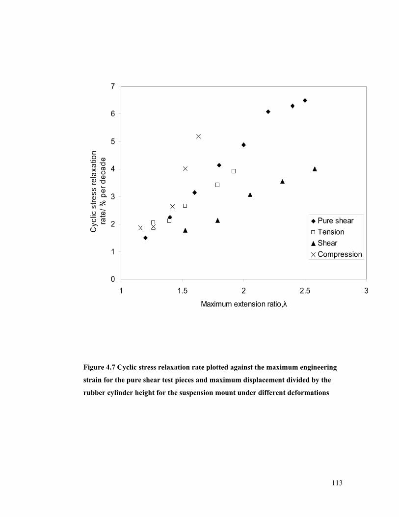
113

0

1

2

3

4

5

6

7

1 1.5 2 2.5 3

Maximum extension ratio,λ

Cyc

lic s

tre

ss r

ela

xatio

n r

ate

/ % p

er

de

cad

e

Pure shear

Tension

Shear

Compression

Figure 4.7 Cyclic stress relaxation rate plotted against the maximum engineering

strain for the pure shear test pieces and maximum displacement divided by the

rubber cylinder height for the suspension mount under different deformations

114

0

1

2

3

4

5

6

7

8

0 500 1000 1500 2000 2500 3000

Maximum strain energy density/kJ/m3

Cyc

lic s

tre

ss r

ela

xatio

n r

ate

/ % p

er

de

cad

e

Pure shear

Tension

Shear

Compression

Figure 4.8 Cyclic stress relaxation rate plotted against the maximum average

strain energy density for the pure shear test pieces and the suspension mount

under different deformations

115

4.3 Conclusion

Cyclic stress relaxation has been studied for bonded cylindrical engineering

components and test pieces. The results of the studies confirm that the cyclic stress

relaxation rate increases with displacement amplitude (strain) for all directions of

deformation in test pieces and components. Plotting the cyclic stress relaxation rate in

terms of average strain energy density, reduces both test piece and component data to a

single straight line. This suggests a general dependence of the cyclic stress relaxation

rate only relies on the average maximum strain energy density experienced in a loading

cycle. The average strain energy density concept presents an approach for determining

the amount of cyclic stress relaxation of an elastomer component from a measure of the

material’s cyclic stress relaxation behaviour.

116

CHAPTER FIVE

5.0 Fatigue Life Prediction

5.1 Introduction

Elastomer components fail at cyclic strain amplitudes much lower than their

catastrophic tear strength due to cumulative cyclic fatigue crack growth. Fatigue cracks

usually initiate in regions of high strain energy density in components. In general, the

rate of crack growth is determined by the geometry of the component and the nature

and magnitude of the deformation imposed. The empirical approach of stress versus the

number of cycles to failure (S–N) (W. D. Callister, 1994), which is traditionally used to

determine the fatigue life of components, has also been adopted by the elastomer

component industry. An alternative approach to predicting the fatigue life of carbon

black filled elastomer test pieces makes use of fracture mechanics. Lake (1995)

reviewed the fracture mechanics approach adopted in the present study. Here, the

energy required to drive the crack at a given rate is defined as the strain energy release

rate which is also referred to as the tearing energy T.

dA

dUT (Eq.5-1)

where A is the area of a single fracture surface of the crack and U is a measure of the

internal energy stored in the component. The magnitude of T is mostly determined by

the viscous work that has to be done in the crack tip region. Rivlin and Thomas (1953)

showed that the relationship between crack growth rate and the strain energy release

rate is a material property, which is independent of the mode of loading and specimen

geometry. Similarly, it has been shown by Lindley and Thomas (1962) that a

characteristic crack growth rate per cycle relationship exists for an elastomer that is

dependent only on the maximum strain energy release rate attained during the loading

cycle. Busfield and Ng (2005) reported that the actual strain energy release rate against

applied loading relationships has been difficult to calculate accurately for anything

other than the simplest components, hence for more complex component types,

researchers have resorted to approximate relationships for the strain energy release rate.

For instance, Lindley and Stevenson (1982) used an approximate fracture mechanics

approach to predict the fatigue behaviour of engineering mounts loaded in compression

117

where, estimates of fatigue lives were made that were of the correct order of magnitude.

This technique for predicting fatigue failure has been dramatically extended by the

arrival of large deformation finite element analysis. It is now possible to calculate the

strain energy release rate for specific loading configurations for cracks in components

of any geometry. Gent and Wang (1993) adopted this type of FEA approach to study

the crack growth behaviour of bonded elastomer suspension components subjected to

large shear. This technique was successfully used to predict the strain energy release

rate and hence the mode of failure for these types of components. Busfield et al. (2005)

extended the FEA based fracture mechanics approach by calculating the relationships

between strain energy release rate and crack size for a gearbox mount at different

amplitudes of cyclic fatigue loading and combined with material crack growth rate

versus strain energy release rate relationships to predict crack growth rate in the

gearbox mount under different modes of loading. In their work, Busfield et al. (2005)

made predictions of crack growth rate and therefore fatigue life for room temperature

conditions. In practice elastomer engineering components usually operate above the

ambient temperature as a result of hysteresis. This thesis extends the work of Busfield

et al. (2005) to examine real fatigue measurements made at both room temperature and

for the first time 70±1ºC. Effort was made in this work to calculate the strain energy

release rate of small cracks of the order of the size of existing defects (flaws) observed,

after careful visual inspection, at the rubber-metal bond edge of the cylindrical

component.

In chapter three of this thesis, the material, experimental and FEA methods used

to collect data for the fatigue life prediction of the bonded cylindrical elastomer

component is explained. Dumbbell specimens, pure shear specimens and bonded

cylindrical elastomer components were prepared from a 65 phr carbon black filled NR

material. The dumbbell specimens were used for uni-axial stress strain characterisation

whereas the pure shear specimens were used for fatigue crack growth characterisation.

The bonded cylindrical components were used in experiments to validate the predicted

number of fatigue cycles required to grow a crack in the component to a measurable

size.

118

5.2 Results and discussions

In this chapter, material characterisation results, results of FEA calculations of

strain energy release rate versus crack length relationships, fatigue life prediction and

experimentally measured number of fatigue cycles to grow a crack in the bonded

cylindrical component are presented and discussed.

5.2.1 Material stress strain behaviour

0.0

0.5

1.0

1.5

2.0

2.5

3.0

3.5

4.0

4.5

5.0

0.0 0.2 0.4 0.6 0.8 1.0 1.2 1.4 1.6 1.8 2.0

Strain

Str

ess

/MP

a

Figure 5.1 Virgin stress strain behaviour of the elastomer material (NR, 65 phr) at

room temperature obtained from a dumbbell test piece

119

0.0

0.5

1.0

1.5

2.0

2.5

0 0.1 0.2 0.3 0.4 0.5 0.6 0.7 0.8 0.9 1 1.1

Strain

Str

ess

/MP

a

Figure 5.2 1000th cycle stress strain behaviour of the elastomer material (NR, 65

phr) measured at room temperature from a dumbbell test piece after softening at

90% strain for 999 cycles

120

0.0

0.5

1.0

1.5

2.0

2.5

3.0

3.5

4.0

0.0 0.2 0.4 0.6 0.8 1.0 1.2 1.4 1.6 1.8 2.0

Strain

Str

ess

/MP

a

Figure 5.3 Virgin stress strain behaviour of the elastomer material (NR, 65 phr) at

70 ºC obtained from a dumbbell test piece

121

y = 2.7509x3 - 3.4865x2 + 2.6347x

0.0

0.2

0.4

0.6

0.8

1.0

1.2

1.4

1.6

1.8

2.0

0 0.1 0.2 0.3 0.4 0.5 0.6 0.7 0.8 0.9 1 1.1

Strain

Str

ess

/MP

a

Figure 5.4 1000th cycle stress strain behaviour of the elastomer material (NR, 65

phr) measured at 70 ºC from a dumbbell test piece after softening at 90% strain

for 999 cycles

All the stress strain curves presented above are typical of a filled elastomer

material and were required in order to use a finite element approach to determine the

strain energy distribution in the bonded cylindrical component under load. The carbon

black filled natural rubber material’s mechanical behaviour was initially modelled

using the virgin stress strain curves of figures 5.1 and 5.3 to observe the regions of high

strain energy density. Figures 3.8 and 3.9 in chapter three show typical meshed finite

element analysis models of the bonded cylindrical component. Under both tensile and

shear deformation directions, the regions of highest strain energy density were

observed to be around the rubber-metal bond edge of the bonded cylindrical

component. In general fatigue crack growth initiates in components where the strain

energy density or stress concentration is the greatest (Busfield et al., 2005). The models

122

of the bonded component under strain allow the strain energy distribution in tension

and shear deformation modes to be determined and so, it was possible to predict the

regions where fatigue crack growth and subsequent failure may initiate at both room

temperature and 70±1ºC.

In order to calculate the relationship between strain energy release rate and

crack length in the cylindrical component, both 2D and 3D models (Chapter 3, figures

3.10 and 3.11) of crack growth at the rubber-metal bond interface were made. To

calculate the fracture behaviour, the material stress strain behaviour from the 1000th

cycle stress strain curves shown in figures 5.2 and 5.4 was used. In figure 5.4, the

experimentally measured 1000th cycle stress strain curve was fitted using a polynomial

to characterise the experimental data using a Yeoh type stored energy function. This

provided the necessary number of stress strain points at 70±1ºC needed in the Abaqus

FEA software to ensure accurate stress strain interpolation by the FEA software. Using

the 1000th cycle stress strain curves ensured that the initial cyclic stress relaxation,

described in Chapter 4 (Asare et al., 2010) and which is associated with fatigue crack

growth was in part accounted for and that the stored energies were not significantly

over estimated by the FEA models. The results of the stored energy crack length

relationships at both room temperature and 70±1ºC for different modes of deformation

are presented and discussed in section 5.5 below.

5.2.2 Equilibrium swelling test results

Figure 5.5 shows the equilibrium swelling in n-decane of a sample taken from a

component (Component) compared with samples cut from three different rubber sheets

(S1, S6 and S7). The sheet materials cured from nominally identical materials swell to

a greater extent in n-decane than materials taken from the component. This indicates

that the degree of cross linking in the component material was slightly greater than that

in the sheet material. Using the Flory-Rehner equation (Eq.3-1), a cross link density of

1.452 x 10-4 mol/cm3 was calculated, from the average absorbed decane measured on

three different sheets, for the sheet material and 1.609 x 10-4 mol/cm3 for the bonded

cylindrical component material. The average cross link density of the bonded

cylindrical component material was found to be about 10% higher than that of the sheet

material, possibly arising as the sheets were compression moulded whereas the

components were injection moulded.

123

0.0

0.2

0.4

0.6

0.8

1.0

1.2

1.4

0 5 10 15 20

√(time)/h1/2

Ab

sorb

ed

de

can

e(c

m3)/

un

it vo

lum

e o

f sa

mp

le(c

m3)

Component

S1

S7

S6

Figure 5.5 Plot of absorbed n-decane per unit volume of sample for bonded

cylindrical component sample, sheet samples S1, S6 and S7

5.2.3 Material pure shear crack growth characterisation

Figures 5.6 (a to h) and 5.7 (a to g) present the results of many different pure

shear crack growth characterisations done at both room temperature and at 70±1ºC. The

plot of crack length against number of cycles for each test amplitude produces quite

reliable linear plots with limited scatter, where the slope equals the rate of cyclic crack

growth at that amplitude. The room temperature pure shear characterisation was carried

out at strain energy release rates of 10 kJ/m2, 13 kJ/m2, 17 kJ/m2, 20 kJ/m2, 24 kJ/m2,

26 kJ/m2, 29 kJ/m2 and 35 kJ/m2. The 70±1ºC pure shear characterisation was carried

out at strain energy release rates of 4 kJ/m2, 7 kJ/m2, 10 kJ/m2, 13 kJ/m2, 15 kJ/m2, 18

kJ/m2 and 21 kJ/m2. It has been shown that for a pure shear crack growth test piece

(Chapter 3, figure 3.2) with an unstrained height of l0, thickness t, width w, and a crack

of size c the strain energy release rate, T is given as Eq.3-3. The strain energy release

rate for the different pure shear crack growth test amplitudes was thus calculated for

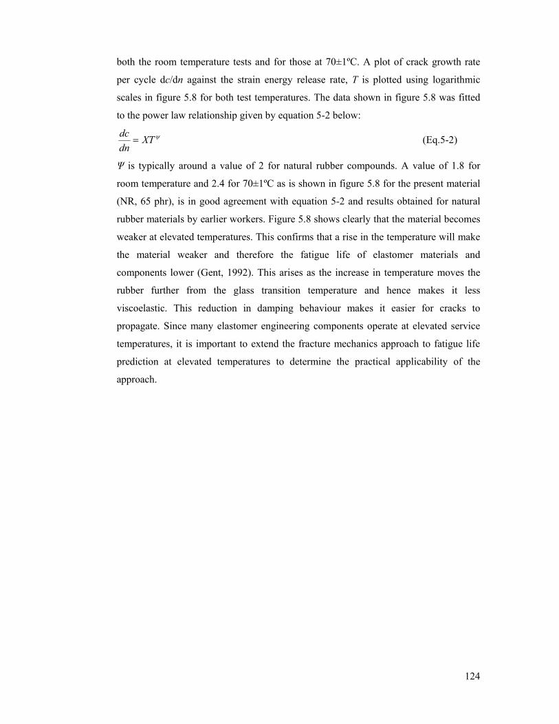
124

both the room temperature tests and for those at 70±1ºC. A plot of crack growth rate

per cycle dc/dn against the strain energy release rate, T is plotted using logarithmic

scales in figure 5.8 for both test temperatures. The data shown in figure 5.8 was fitted

to the power law relationship given by equation 5-2 below:

XTdn

dc (Eq.5-2)

Ψ is typically around a value of 2 for natural rubber compounds. A value of 1.8 for

room temperature and 2.4 for 70±1ºC as is shown in figure 5.8 for the present material

(NR, 65 phr), is in good agreement with equation 5-2 and results obtained for natural

rubber materials by earlier workers. Figure 5.8 shows clearly that the material becomes

weaker at elevated temperatures. This confirms that a rise in the temperature will make

the material weaker and therefore the fatigue life of elastomer materials and

components lower (Gent, 1992). This arises as the increase in temperature moves the

rubber further from the glass transition temperature and hence makes it less

viscoelastic. This reduction in damping behaviour makes it easier for cracks to

propagate. Since many elastomer engineering components operate at elevated service

temperatures, it is important to extend the fracture mechanics approach to fatigue life

prediction at elevated temperatures to determine the practical applicability of the

approach.

125

y = 0.0007x + 29.789

28

33

38

43

48

53

0 5000 10000 15000 20000 25000 30000

No. of cycles

Cra

ck le

ng

th/m

m


displacement amplitude at room temperature

y = 0.0009x + 31.921

30

35

40

45

50

55

60

3000 8000 13000 18000 23000 28000

No. of cycles

Cra

ck le

ng

th/m

m



126

y = 0.0012x + 49.963

50

55

60

65

70

75

3500 8500 13500 18500

No. of cycles

Cra

ck le

ng

th/m

m



y = 0.0013x + 55.424

50

55

60

65

70

75

80

85

90

2000 7000 12000 17000 22000 27000

No. of cycles

Cra

ck le

ng

th/m

m



127

y = 0.0025x + 72.5

80

85

90

95

100

105

110

0 5000 10000 15000

No. of cycles

Cra

ck le

ng

th/m

m



y = 0.0037x + 36.122

30

35

40

45

50

55

60

65

1000 2000 3000 4000 5000 6000 7000

No. of Cycles

Cra

ck le

ngth

/mm



128

y = 0.006x + 58.399

60

65

70

75

80

85

90

0 1000 2000 3000 4000 5000

No. of cycles

Cra

ck le

ngth

/mm



y = 0.0048x + 34.185

30

35

40

45

50

55

60

65

1000 2000 3000 4000 5000 6000

No. of cycles

Cra

ck le

ngth

/mm

Figure 5.6(h) A plot of Crack length against No. of cycles for 12mm sinusoidal


129

y = 0.0001x + 18.018

20

22

24

26

28

30

32

34

36

38

40

40000 60000 80000 100000 120000 140000

No. of cycles

Cra

ck le

ngth

/mm


displacement amplitude at 70 ºC

y = 0.0009x - 0.4482

0

5

10

15

20

5000 10000 15000 20000

No. of cycles

Cra

ck le

ngth

/mm



130

y = 0.0012x + 0.1102

0

5

10

15

20

25

30

0 5000 10000 15000 20000 25000

No. of cycles

Cra

ck le

ngth

/mm



y = 0.0021x - 0.7019

0

5

10

15

20

25

0 2000 4000 6000 8000 10000 12000

No. of cycles

Cra

ck le

ngth

/mm



131

y = 0.0032x - 2.6717

0

5

10

15

20

25

30

35

40

0 2000 4000 6000 8000 10000

No. of cycles

Cra

ck le

ng

th/m

m



y = 0.0051x - 0.2647

0

5

10

15

20

25

0 500 1000 1500 2000 2500 3000 3500 4000

No. of cycles

Cra

ck le

ngth

/mm



132

y = 0.0052x + 1.85

0

5

10

15

20

0 500 1000 1500 2000 2500 3000 3500

No. of cycles

Cra

ck le

ng

th/m

m



133

y = 2.366x - 15.398

y = 1.8012x - 13.451

-7.5

-7.0

-6.5

-6.0

-5.5

-5.0

-4.5

3.2 3.4 3.6 3.8 4 4.2 4.4 4.6 4.8

log T / Jm-2

log

dc/

dn

/m

70 degreesRoom tempLi ( 0 d )

Figure 5.8 log dc/dn against log T for pure shear characterisation of NR 65

material at room temperature and 70 degrees Celsius.

134

5.2.4 Experimental and predicted component force deflection behaviour in

tension at room temperature and 70±1ºC

Figures 5.9 and 5.10 show the results of experimental force deflection

behaviour and FEA prediction of force deflection behaviour of the cylindrical

component at room temperature and 70±1ºC respectively. The FEA prediction was

determined using the Yeoh stored energy function characterised using the 1000th cycle

test piece stress versus strain data obtained at room temperature (figure 5.2) and that at

70±1ºC (figure 5.4). In figure 5.9 there is good agreement between the experimental

and predicted component force deflection behaviour until 25mm displacement above

which the FEA prediction is somewhat greater than the experimentally measured force

deflection curve. In figure 5.10, the agreement between the measured force deflection

behaviour and the predicted force deflection behaviour is good until 20mm

displacement, above which the predicted force deflection behaviour is again greater

than the experimentally measured behaviour.

The observed discrepancies between the measured and FEA predicted

component force deflection behaviour may be attributed, in part, to the slight difference

in cross link density between the sheet material, from which the test piece stress strain

curves were measured, and the bonded component material. In general, it is inherently

difficult to achieve exactly the same amount of cross link density from batch to batch

for cured elastomer materials. This picture is complicated by the fact that the

experimental component force deflection response was determined after cyclically

loading the component for 999 cycles at a maximum displacement at which the average

strain energy density, in the component, was calculated to equal that obtained in the

sheet test piece material stretched to 90% strain. The determination of maximum

displacements, necessary in experiments, for softening of components and test pieces

are at best estimates and not the exact required displacements, due to the use of average

strain energy densities. The maximum average strain energy densities at which the

bonded component and the sheet material stress strain test piece were softened are only

of a similar order of magnitude. This difference in the maximum strain energy

encountered in the component will also introduce a discrepancy between the measured

and predicted component force deflection behaviour. The situation is further

complicated at elevated temperatures; because the surrounding experimental

temperature can be controlled reasonably well but the additional heat generated in the

135

bulk of the sample by the component during a test depends upon factors such as the

rubber hysteresis and also the rate of heat lost during the test. Clearly this is going to be

different between the bulky component and the much thinner test sheets. Considering

these practical difficulties, it is evident from figures 5.9 and 5.10 that Yeoh stored

energy function measured using the 1000th cycle at both temperatures give

approximately the correct displacement and that it allows a sufficiently accurate

measurement of the tearing energy to be made for this work.

0

500

1000

1500

2000

2500

3000

3500

4000

0 5 10 15 20 25 30 35

Displacement/mm

Fo

rce

/N

Exp_1000 Cyc

FEA_prediction

Figure 5.9 Experimental and predicted 1000th cycle force deflection behaviour of

NR 65 phr elastomer material at room temperature

136

0

500

1000

1500

2000

2500

3000

3500

0 5 10 15 20 25 30 35

Deflection/mm

Fo

rce

/N

FEA-1000@70

Exp_1000cycle@70

Figure 5.10 Experimental and predicted 1000th cycle force deflection behaviour of

NR 65 phr elastomer material at 70 ºC

5.2.5 Fatigue life prediction and experimental validation

To predict the fatigue life of the bonded cylindrical component for a particular

mode of loading and displacement amplitude, stored energy crack length relationship

for that amplitude and mode of loading must first be determined using FEA techniques.

To do this a series of models were made with a wide range of different crack lengths.

The total stored energy in each model at a specific displacement was calculated using

the finite element analysis techniques. A graph of the total energy in the model versus

the crack length was created and the slope of the stored energy crack length curve at

specific crack lengths determines the strain energy release rate crack length relationship

for that displacement amplitude (Chapter 2, Eq.2-45). By combining the strain energy

release rate crack length relationship with the respective power law relationship of

figure 5.8 (Chapter 2, Eq.2-42), it is possible to derive a single functional relationship

between the cyclic crack growth rate and the size of a crack in a component (Chapter 2,

137

Eq.2-46). This relationship can be inverted to form 1/(dc/dn) versus crack length.

Integrating under 1/(dc/dn) versus crack length curve from an initial crack size c0 to a

final crack size c gives the number of cycles required to grow a crack between those

limits and hence to predict the fatigue life if c is sufficiently large to cause a

catastrophic failure.

In figures 5.11, 5.16, 5.22 and 5.27, stored energy crack length relationships for

the bonded cylindrical component deformed in tension and shear at room temperature

and 70±1ºC respectively are shown. FEA calculated strain energy release rate crack

length relationship for tensile crack growth (figures 5.12 and 5.17) along the rubber-

metal bond interface of the component show a general trend of increasing strain energy

release rate with crack length for both room temperature crack growth and at 70±1ºC.

This trend was also observed in the work of Busfield et al. (2005). Since an increasing

strain energy release rate implies an increasing crack growth rate, the observed trend in

tension suggests that the rate of crack growth at the rubber-metal bond interface

increases with crack length in tension. On the contrary, the FEA calculated strain

energy release rate crack length relationship for crack growth at the rubber-metal bond

interface of the bonded component in shear (figures 5.23 and 5.28) initially increased

through a maximum and then decreased. This suggests an initial increase in crack

growth rate in shear to a peak value and a subsequent decrease in crack growth rate.

This trend is observed for both room temperature and at 70±1ºC in shear. This

phenomenon can be attributed to the cylindrical geometry of the bonded component

studied in this work. In figures 5.13, 5.14, 5.15, 5.18, 5.19, 5.20, 5.21, 5.24, 5.25, 5.26,

5.29, 5.30 and 5.31 below plots of 1/(dc/dn) versus crack length for the respective test

amplitudes and temperature conditions are presented.

Using the method discussed earlier, the number of cycles required to grow

cracks at the rubber-metal bond edge of the elastomer component in tension and shear

at both room temperature and 70±1ºC were calculated as Np and compared with the

experimentally measured number of fatigue cycles Nm in Table 5.1. It must be noted in

table 5.1 that the value of c0 in each calculation of Np is an estimate of the initial

average flaw size observed at the rubber-metal bond edge of the bonded component

made as accurately as is practical using a careful visual inspection of the rubber-metal

bond edge. The approach used here of estimating an initial average flaw size at the

rubber-metal bond edge clearly does not take into consideration any local variations in

the flaw size. The fatigue life predicted with the fracture mechanics approach generally

138

results in a fatigue life within a factor of 2 of the experimentally measured fatigue life

cycles which is excellent especially when considering the extent that the predicted

fatigue life depends on the initial size estimate of the flaw at the rubber-metal bond

edge of the component. It is apparent in Table 5.1 that the method works well for the

fatigue life predictions made at both room temperatures and 70ºC irrespective of the

deformation mode.

5.2.6 Predicted and measured component fatigue life in tension and shear at

room temperature and 70 degrees Celsius

0

5000

10000

15000

20000

25000

0 3 6 9 12 15 18

Crack length/mm

Sto

red

en

erg

y/m

J

5mm Amplitude 10mm Amplitude 15mm Amplitude

Figure 5.11 Stored energy against crack length for crack growth in tension at

5mm, 10mm and 15mm amplitudes respectively at room temperature

139

0

5

10

15

20

25

0 3 6 9 12 15 18

Crack length/mm

Te

ari

ng

en

erg

y/ k

J/m

2


Figure 5.12 Tearing energy crack length relationship for crack growth in tension

at 5mm, 10mm and 15mm amplitudes respectively at room temperature

140

0.0E+00

5.0E+08

1.0E+09

1.5E+09

2.0E+09

2.5E+09

0 0.005 0.01 0.015

Crack length/m

1/d

c/d

n/(

m-1

)

5mm Amplitude

Figure 5.13 1/dc/dn versus crack length for crack growth in tension at 5mm

amplitude at room temperature

141

0.0E+00

1.0E+08

2.0E+08

3.0E+08

4.0E+08

5.0E+08

6.0E+08

7.0E+08

0 0.005 0.01 0.015

Crack length/m

1/d

c/d

n/(

m-1

)

10mm Amplitude

Figure 5.14 1/dc/dn vrs crack length for crack growth in tension at 10mm


142

0.0E+00

2.0E+07

4.0E+07

6.0E+07

8.0E+07

1.0E+08

1.2E+08

1.4E+08

0 0.005 0.01 0.015

Crack length/m

1/d

c/d

n/(m

-1)

15mm Amplitude



143

0

5000

10000

15000

20000

25000

0 2 4 6 8 10 12 14 16 18

Crack length/mm

Sto

red

en

erg

y/m

J

5mm Amplitude 10mm Amplitude 12.5mm Amplitude 15mm Amplitude

Figure 5.16 Stored energy against crack length for component crack growth in

tension at 70 degrees Celsius

144

0

5

10

15

20

25

0 2 4 6 8 10 12 14 16 18

Crack length/mm

Te

ari

ng

en

erg

y/kJ

/m2

5mm Amplitude 10mm Amplitude 12.5mm Amplitude 15mm Amplitude

Figure 5.17 Tearing energy against crack length for component crack growth in

tension and at 70 degrees Celsius

145

0.0E+00

2.0E+09

4.0E+09

6.0E+09

8.0E+09

1.0E+10

1.2E+10

0 0.005 0.01 0.015 0.02

Crack length/m

Te

ari

ng

en

erg

y/kJ

/m2

5mm Amplitude


amplitude at 70ºC

146

0.0E+00

2.0E+08

4.0E+08

6.0E+08

8.0E+08

1.0E+09

1.2E+09

1.4E+09

1.6E+09

1.8E+09

2.0E+09

0 0.005 0.01 0.015 0.02

Crack length/m

Te

ari

ng

en

erg

y/kJ

/m2

10mm Amplitude


amplitude at 70ºC

147

0.0E+00

1.0E+08

2.0E+08

3.0E+08

4.0E+08

5.0E+08

6.0E+08

7.0E+08

8.0E+08

9.0E+08

0 0.005 0.01 0.015 0.02

Crack length/m

Te

ari

ng

en

erg

y/kJ

/m2

12.5mm Amplitude

Figure 5.20 1/dc/dn vrs crack length for crack growth in tension at 12.5mm

amplitude at 70ºC

148

0.0E+00

5.0E+07

1.0E+08

1.5E+08

2.0E+08

2.5E+08

3.0E+08

3.5E+08

4.0E+08

0 0.005 0.01 0.015 0.02

Crack length/m

Te

arin

g e

ner

gy/k

J/m

2

15mm Amplitude


amplitude at 70ºC

149

0

1000

2000

3000

4000

5000

6000

0 3 6 9 12 15 18

Crack length/mm

Sto

red

en

erg

y/m

J


Figure 5.22 Stored energy crack length relationship for shear crack growth at


150

0.0

0.5

1.0

1.5

2.0

2.5

3.0

3.5

4.0

4.5

5.0

0 3 6 9 12 15 18

Crack length/mm

Te

ari

ng

en

erg

y/kJ

/m2


Figure 5.23 Tearing energy crack length relationship for shear crack growth at


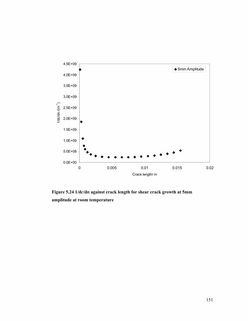
151

0.0E+00

5.0E+08

1.0E+09

1.5E+09

2.0E+09

2.5E+09

3.0E+09

3.5E+09

4.0E+09

4.5E+09

0 0.005 0.01 0.015 0.02

Crack length/ m

1/dc

/dn

/(m

-1)

5mm Amplitude

Figure 5.24 1/dc/dn against crack length for shear crack growth at 5mm


152

0.0E+00

2.0E+08

4.0E+08

6.0E+08

8.0E+08

1.0E+09

1.2E+09

0 0.005 0.01 0.015 0.02

Crack length/ m

1/d

c/d

n /(

m-1

)

9mm Amplitude



153

0.0E+00

5.0E+07

1.0E+08

1.5E+08

2.0E+08

2.5E+08

3.0E+08

3.5E+08

4.0E+08

4.5E+08

0 0.002 0.004 0.006 0.008 0.01 0.012 0.014 0.016 0.018

Crack length/ m

1/dc

/dn

/(m

-1)

13mm Amplitude



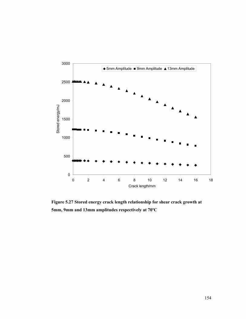
154

0

500

1000

1500

2000

2500

3000

0 2 4 6 8 10 12 14 16 18

Crack length/mm

Sto

red

en

erg

y/m

J


Figure 5.27 Stored energy crack length relationship for shear crack growth at

5mm, 9mm and 13mm amplitudes respectively at 70ºC

155

0.0

0.5

1.0

1.5

2.0

2.5

3.0

3.5

4.0

4.5

0 5 10 15 20

Crack length/mm

Te

ari

ng

en

erg

y/kJ

/m2


Figure 5.28 Tearing energy crack length relationship for shear crack growth at

5mm, 9mm and 13mm amplitudes respectively at 70ºC

156

0.0E+00

5.0E+09

1.0E+10

1.5E+10

2.0E+10

2.5E+10

3.0E+10

3.5E+10

0 0.005 0.01 0.015 0.02

Crack length/m

1/d

c/d

n /(

m-1

)

5mm Amplitude


amplitude at 70ºC

157

0.0E+00

1.0E+09

2.0E+09

3.0E+09

4.0E+09

5.0E+09

6.0E+09

0 0.005 0.01 0.015 0.02

Crack length/m

1/d

c/d

n /(

m-1

)

9mm Amplitude


amplitude at 70ºC

158

0.0E+00

2.0E+08

4.0E+08

6.0E+08

8.0E+08

1.0E+09

1.2E+09

1.4E+09

1.6E+09

0 0.005 0.01 0.015 0.02

Crack length/m

1/d

c/d

n /(

m-1

)

13mm Amplitude


amplitude at 70ºC

159

Table 5.1 Predicted and measured numbers of fatigue cycles required to grow cracks from estimated rubber–metal bond

edge flaw size until specified crack size just before failure

Maximum

Displacement/mm Temperature/ºC

Tension

Or Shear

Range of crack

Lengths/mm

Measured No.

of cycles Nm

Predicted No.

of cycles Np Np/ Nm

5.0 23 Tension 0.5-4 723 937 441 145 0.61

10.0 23 Tension 0.9-10 64 524 116 912 1.81

15.0 23 Tension 0.5-8 63 494 36 366 0.57

10.0 70 Tension 0.5-15 163 988 155 454 0.95

15.0 70 Tension 0.9-11 24 047 22 131 0.92

9.0 23 Shear 0.5-9 357 009 406 145 1.14

13.0 23 Shear 0.5-10 168 093 160 189 0.95

13.0 70 Shear 0.5-7 418 130 182 320 0.44

160

5.3 Conclusion

The fracture mechanics approach to fatigue life prediction of engineering

components has been validated using a bonded cylindrical engineering elastomer

component for fatigue crack growth within the ‘power law’ region of crack growth

behaviour. The cylindrical geometry of the engineering elastomer component induced

rubber-metal bond interface crack growth for both tensile and shear fatigue loading.

The fatigue crack growth behaviour was successfully predicted for crack growth at both

room temperature and 70±1ºC to within a factor of 2 for the bonded cylindrical

component. For the first time, the cyclic stress softening associated with fatigue of

filled elastomer materials was quantitatively accounted for by softening the dumbbell

specimens for the stress strain characterisation and subsequent FEA strain energy

calculations at a strain level deduced following the average strain energy density

approach. The effect of temperature on the fatigue life of the cylindrical component

was also well accounted for by the approach of characterising the material stress versus

strain and the fatigue crack growth behaviour at the elevated test temperature.

Considering the poor reproducibility of fatigue life predictions in previous work, the

accuracy of the fracture mechanics approach method to predict the fatigue crack growth

rate with an accuracy of 2 for the fatigue life at both room temperature and 70±1ºC is

excellent.

161

CHAPTER SIX

6.0 Crack Bifurcation in a Pure Shear Test Piece

6.1 Introduction

The study of fatigue crack surfaces has been the subject of scientific research

for many decades. In many cases fatigue crack surfaces have been observed to be

rough. The roughness associated with fatigue crack surfaces is prominent when one

considers the surface morphology of a sharp razor cut to that obtained after the crack

has grown to steady state rate in an elastomer material. Papadopoulos (2008) reviews

this phenomenon in a work which investigates rate transitions in fatigue crack growth

in elastomers. The rough fatigue crack surface is, in part, thought to be the result of

fatigue crack splitting during fatigue crack growth. Thomas (1958) in an explanation of

the transition from sharp razor cut crack tip to a rough steady state crack tip suggested

the rough crack tip to consist of multiple sharp crack tips. The study of fracture

surfaces in elastomer materials is usually qualitative because no single technique can

readily describe all the features present or can accurately describe the fracture surface

structure. Fukahori and Andrews (1978) studied 2D fracture surface microscopic

images by counting the number of steps crossing a reference line and weighted these

according to their apparent depth. They differentiated the degrees of roughness by

assuming that the broader the step lines, the deeper the steps, with the deeper steps

casting a greater shadow. The technique gives an indication of the roughness at various

parts of the fracture surfaces but; it would be challenging to differentiate small

variations in depth. They observed fracture surface roughness in rubber at various

values of strain energy release rate (tearing energy) under steady tearing and noted that

there is a direct relation between the rate of propagation and the nature of the crack tip.

They reported a general observation that increased crack growth rate due to an increase

in the strain energy release rate results in smoother elastomer fracture surfaces. Gent

and Pulford (1984) used a similar method to measure the distance between steps of the

surface texture of 2D images. They attributed the variation in roughness to the joining

of secondary cracks originating from flaws and filler particles. Furthermore, they

observed that for the more tear resistant materials the height of the steps was greater.

Quantitative analysis of fracture surface roughness is not a simple task since there is no

162

widely accepted parameter. Although there is general agreement that fatigue crack

surfaces become rough with crack growth and that the extent of roughness is linked to

the strain energy release rate associated with the crack growth, there is no agreement as

yet on the mechanisms responsible for the creation of the rough fracture surfaces.

Gent et al. (2003), in a work to investigate why cracks turn sideways considered

a rubber sheet with a small edge crack subjected to a far-field simple extension. They

calculated the strain energy release rate for crack growth in both forwards and sideways

directions. They observed that when the imposed extension is large, the strain energy

release rate at which a small sideways crack will initiate is found to be about 60% of

that for forwards crack growth for their specific material. It is clear therefore that for a

crack to follow what appears at first sight to be a less energetically favourable pathway

something else must be taking place. Cracks split or bifurcate due to extensive strain

induced anisotropy particularly at the tip of the crack (Busfield et. al, 1997). This

anisotropy results from the extensive local strain in the crack tip region and the

potential for some materials such as NR to experience the onset of strain induced

crystallisation. In effect it becomes easier for the crack to grow at right angles to the

applied strain field as this still releases energy, albeit of a lesser amount than in the

straight forward direction, because the material is much weaker in that direction.

Cracks that form like this can now follow multiple pathways. Each individually shares

some of the strain energy release rate from the initial single crack and so the crack

growth rate slows down. The key concern now becomes which pathway is followed

and how far apart do the two cracks have to grow apart for one to accelerate and

become a dominant single crack tip.

It is beyond the scope of this thesis to consider the complications associated

with modelling strain induced anisotropy. So the task of understanding why cracks

deviate is not considered in detail. The somewhat simpler initial task is tackled which

considers how far an already bifurcated crack has to grow, as clearly, understanding

something about this distance helps understand the extent of the surface roughness of a

fatigue fractured component. To do this, simple finite element analysis models that

ignore any significant anisotropy in the strength at the crack tip were made. These

models were used to model how the strain energy release rate associated with growth of

split fatigue cracks compare, with the strain energy release rate of a single straight

crack propagating along the central horizontal plane, in a typical filled Natural Rubber

pure shear crack growth specimen, at the same strain. The objective of this study being

163

to investigate the effect of fatigue crack bifurcation on the generation of fatigue crack

surface roughness by examining the behaviour of the characteristic strain energy

release rates as cracks extend from an already split fatigue crack profile.

6.2 Results and discussion

In figure 6.1, a schematic of a pure shear specimen with a crack c splitting into

two cracks c1 and c2 is shown. To model a crack into a finite element mesh, nodes

along the direction of crack growth are released. Figure 6.2 shows typical finite element

mesh for a pure shear crack growth specimen model with split cracks. The crack is

modeled over a wide range of lengths by releasing the connection between nodes along

a predetermined crack growth pathway. With each node release, provided the external

boundaries do not move, the total stored energy in the model decreases.


cracks c1 and c2: Both c1 and c2 are parallel to the horizontal centre-line of the

specimen

164

(a)

(b)

Figure 6.2 Deformed finite element meshes of a pure shear specimen showing split parallel cracks c1 and c2 with equal lengths (a)

and, split crack c2 extended keeping the initial length of split crack c1 constant (b)

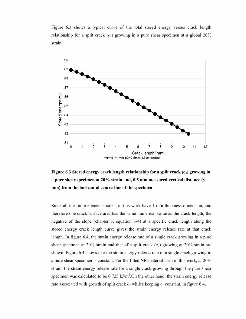
Figure 6.3 shows a typical curve of the total stored energy versus crack length

relationship for a split crack (c2) growing in a pure shear specimen at a global 20%

strain.

Figure 6.3 Stored energy crack length relationship for a split crack (c2) growing in

a pure shear specimen at 20% strain and, 0.5 mm measured vertical distance (y

mm) from the horizontal centre-line of the specimen

Since all the finite element models in this work have 1 mm thickness dimension, and

therefore one crack surface area has the same numerical value as the crack length, the

negative of the slope (chapter 3, equation 3-4) at a specific crack length along the

stored energy crack length curve gives the strain energy release rate at that crack

length. In figure 6.4, the strain energy release rate of a single crack growing in a pure

shear specimen at 20% strain and that of a split crack (c2) growing at 20% strain are

shown. Figure 6.4 shows that the strain energy release rate of a single crack growing in

a pure shear specimen is constant. For the filled NR material used in this work, at 20%

strain, the strain energy release rate for a single crack growing through the pure shear

specimen was calculated to be 0.725 kJ/m2.On the other hand, the strain energy release

rate associated with growth of split crack c2 whiles keeping c1 constant, in figure 6.4,

166

varies. Initially the energy is uniformly distributed over the two cracks, as one of the

cracks, c2, is extended the strain energy release rate of 0.413 kJ/m2 was calculated at a

crack length of 0.25 mm.

Figure 6.4 Tearing energy crack length relationships for a single and a split

parallel crack (c2) growing in a pure shear specimen at 20% strain

The strain energy release rate subsequently increases with extension through to a

maximum of 0.723 kJ/m2 at the final crack length of 10.25 mm by which point the

initial split in the crack tip is no longer felt. The increase in strain energy release rate

for a split crack c2, upon extension of c2 whilst keeping c1 constant in figure 6.4, is due

to simultaneous creation of new fracture surface as a result of split crack c2 extending

and transfer of energy from the split crack c1 to c2. At the limit of extension of split

crack c2, where the area around split crack c1 is almost energy free, the strain energy

release rate of split crack c2 approaches that of a single crack c in a pure shear specimen

167

at 20% strain which is a constant. It is interesting to note that the strain energy release

rate crack length curve of split crack c2 in figure 6.4, does not extrapolate back to the

origin of the graph but to an intercept strain energy release rate of approximately 0.374

kJ/m2. This is a manifestation of the node release technique for measuring strain energy

release rates, as the method requires the differences between two different models to be

compared. Therefore the energy release rate is for a crack length somewhat between the

two points where the total energy is being calculated. Since any point on the tearing

energy axis in figure 6.4 corresponds to zero crack length extension, extrapolating the

split crack c2 curve to the vertical axis determines the strain energy release rate of split

crack c2 at zero extension. As a result of this slight inaccuracy the strain energy release

rates calculated at an increase in 0.25 mm of a crack length is considered approximately

the same as the initial strain energy release rates for a split crack.

In figure 6.5, the strain energy release rates for split crack c1 in the five model

instances described in chapter three are presented. It is important to note that in all of

the model instances, split crack c1 had a constant vertical distance of 4 mm from the

horizontal centre-line plane of the pure shear specimen. The trend in the strain energy

release rate versus crack length relationship is similar in all cases to that observed for

the split crack in figure 6.4. In all the instances, the strain energy release rate increases

with crack extension due to the combined processes of new fracture surface creation

and transfer of energy from split crack c2, which is kept at a constant length, to split

crack c1. It is interesting to note, however, that when extrapolation of the lines of fit

through the strain energy release rate data set was made, all the lines converged

approximately to a point on the tearing energy axis in figure 6.5, showing that at the

outset all the models converge on a solution whereby the strain energy release rate is

split evenly between both cracks. Strain energy release rates calculated for split crack c1

for the different model instances at 0.25 mm crack extension had a mean of 0.356 kJ/m2

and a standard deviation of 0.006 kJ/m2. It can be inferred from figure 6.5 that at a

constant vertical distance of 4 mm from the horizontal centre-line of the pure shear

specimen, the initial energy of split crack c1 in all the model instances is approximately

constant. In figure 6.5, starting from the tearing energy axis, where split crack c1 has

zero extension, the strain energy release rate curves of the different model instances of

split crack c1 follow slightly different paths.

168

Figure 6.5 Tearing energy crack length relationships for split crack c1 (where x =

constant = 4 mm in all models) for the respective models

This trend can be attributed to a faster rate of energy transfer from split crack c2, which

is kept at a constant length when the cracks are closer together at the outset.

In figure 6.6, the strain energy release rate results for the different model

instances of split crack c2 are presented. The trends in the transfer of the strain energy

release rate from being shared by both cracks to being dominated by a single crack are

similar to that which has been observed and discussed in figures 6.4 and 6.5 but, unlike

figure 6.5, strain energy release rate curves for split crack c2 when extrapolated to the

tearing energy axis does not converge to a single point. In this graph the vertical

position of the extending split crack, c2, was varied from the horizontal centre-line

plane of the pure shear specimen. Figure 6.6 suggests that the initial strain energy

release rates of split crack c2 depend on its vertical distance from the horizontal centre-

line plane of the pure shear specimen, or at least perhaps the proximity of the crack to

the clamped boundary.

169

Figure 6.6 Tearing energy crack length relationships for split crack c2 (where y

varied and had values of 0.5 mm, 1 mm, 2 mm, 3 mm and 4 mm) for the respective

models

A plot of the initial strain energy release rates for the split crack c2 observed in figure

6.6 against the respective vertical distances from the central horizontal plane is shown

in figure 6.7. The initial strain energy release rate of split crack c2 is inversely

proportional to the vertical distance of the split crack from the horizontal centre-line

plane of the pure shear specimen. It is important to mention that in a separate analysis a

single crack modeled in a pure shear specimen, and located 4 mm from the central

horizontal plane of the specimen, there was no difference between the calculated values

for the strain energy release rate and that derived for a single crack located in the

middle of the specimen at the same strain.

170

Figure 6.7 Initial tearing energies of split crack c2, versus measured vertical

distance (y mm) of the split crack from the pure shear specimen horizontal centre-

line in the respective models at 20% strain

The trend in figure 6.7, therefore, is not caused by edge effects alone. The 16%

difference in strain energy release rate observed for split crack c2 located at 0.5 mm and

4 mm vertical distances respectively from the horizontal centre-line plane of the pure

shear specimen was determined at 20% global strain to the specimen. It was of research

interest to examine this difference in energy at higher strains. Therefore, split crack c2

models where “c1=4mm c2=4mm c2 extended” and “c1=4mm c2=0.5mm c2 extended”

were analyzed further at 40%, 60%, 80% and 100% strains. The difference in initial

strain energy release rates for split crack c2 at the different strains was calculated and

has been presented in figure 6.8. The trend in figure 6.8 suggests that, the difference in

initial strain energy release rate between split cracks with shorter vertical distance

(y=0.5 mm in this work) from the horizontal centre-line and split cracks with longer

vertical distance (y=4 mm in this work) from the horizontal centre-line of the pure

shear specimen increases with strain.

171

As stated previously several physical processes are thought to be the causes of

crack tip splitting; prominent among them being the interaction of advancing cracks

with strain induced crystals or oriented aggregate filler particles in filled elastomers,

which make the material around the crack tip region anisotropic. Strength anisotropy

ahead of an advancing fatigue crack implies existence of weak local regions in the

material around the crack tip. In figure 6.7, depending on the location of split crack c2

in the pure shear specimen, it had initial strain energy release rates ranging from

approximately 48 % to 57 % of the energy of a single crack growing through the

horizontal centre-line of a pure shear specimen at 20 % strain. Figure 6.8 suggests that

at higher strains split cracks located near the horizontal centre-line in a pure shear

specimen have higher initial energy than that calculated for low strains. It can be

inferred, therefore, that the existence of material anisotropy combined with the

significant initial strain energy release rate available to split cracks, depending on their

location and the global strain of the material, will cause split cracks to propagate under

fatigue loading. In figure 6.6, apart from the initial strain energy release rates of split

crack c2 being a function of the location of the split crack from the horizontal centre-

line plane of the pure shear specimen, at equivalent crack extensions split crack c2

located nearer the horizontal centre-line released more energy than when farther from

the horizontal centre-line. This trend suggests that the rate of propagation of split

cracks at different locations from the horizontal centre-line of a pure shear specimen

will not be uniform, rather split cracks with higher strain energy release rates will

propagate faster. This phenomenon will induce energy transfer from split cracks with

lower strain energy release rates to those with higher strain energy release rates

subsequently resulting in “arrest” of low energy split cracks. It appears that advancing

fatigue cracks, in an effort to overcome resistance caused by strain induced crystals and

oriented aggregate filler particles, split at the tip. The split cracks, depending on their

location and orientation, exploit the weak regions around the strain induced crystals and

oriented aggregate filler particles and propagate. The most “energetic” and fast growing

split crack subsequently gains the energy of the “weak” split cracks which eventually

results in the “arrest” of the crack. The most energetic and fastest growing split cracks

extend in length until conditions ahead of it (formation of strain induced crystals and

presence of oriented aggregate particles) causes it to split and repeat the entire process.

This cyclic process involving crack tip splitting, the growth of the most energetic split

crack and the eventual “arrest” of lower energy split cracks, must in some part explain

172

the rough nature of fatigue crack surfaces compared with the smooth surfaces obtained

from rapid catastrophic torn surfaces.

Figure 6.8 Dependence of the initial tearing energy of split cracks on strain

173

6.3 Conclusion

Following the suggestion of Thomas (1958), strain energy release rates due to

growth of split fatigue cracks in a pure shear specimen have been calculated using

finite element analysis. Upon extension of one split crack while keeping the second

split crack at a constant length, all the split cracks studied in this work showed a

general increase in strain energy release rate with extension; the strain energy release

rate of the extending split crack approached that of a single crack through the

horizontal centre-line of a pure shear specimen as the stain energy at the second split

crack tip region approached zero. Using the method of extending one split crack whilst

keeping the second split crack at a constant length, the initial strain energy release rate

available to a split crack was successfully calculated. For a pure shear specimen fitted

to the behaviour of a filled NR material used in this work, strain energy release rates of

approximately 48% to 57% were calculated for split cracks at different vertical

distances measured from the horizontal centre-line plane of the specimen. It was

observed that the initial strain energy release rate of a split crack is a function of its

location from the central horizontal plane of the pure shear specimen. Split cracks with

shorter vertical distance measured from the horizontal centre-line plane had larger

initial strain energy release rates and this trend is pronounced at higher strains.

Considering the magnitude of the initial strain energy release rate available to split

cracks and the general trend of increasing energy release rate with split crack extension,

it can be concluded that, a cyclic process involving crack tip splits, growth of the most

energetic split crack, and “arrest” of low energy split cracks may be the mechanism for

crack advance in the presence of fatigue crack growth inhibitors such as strain induced

crystals and aggregate filler particles. In conclusion, the observed and well reported

rough nature of fatigue crack surfaces compared with the smooth surfaces obtained

from rapid catastrophic torn surfaces in elastomer materials is, to a large extent, a

byproduct of the cyclic crack split process studied in this work.

The next stage in this work would be to examine in much more detail exactly

how the scale of the initial bifurcation of the crack tip plays an important role in the

rate of crack growth of the advancing crack tip and again to investigate if it is possible

to calculate for different sizes of splitting how far cracks have to advance from each

other before the shortest crack is no longer felt. This can then be used to derive

empirical measures of how crack surface roughness might develop.

174

CHAPTER SEVEN

7.0 Summary, conclusions and future work

7.1 Cyclic stress relaxation

This research has analysed fatigue in filled elastomer test pieces and bonded

cylindrical engineering components. The research work was carried out in three stages.

Firstly, cyclic stress relaxation was experimentally measured for carbon black filled

natural rubber test pieces and bonded cylindrical elastomer engineering components.

Cyclic stress relaxation is a manifestation of fatigue in filled elastomer materials. The

result of cyclic stress relaxation of filled elastomer materials is significant reduction in

stiffness of the material, over the first thousand fatigue cycles. This stiffness reduction

which presents as a “downward” shift of the non-linear stress strain curve of filled

elastomer materials, possess a design challenge. Neglecting cyclic stress relaxation in

the design of elastomer components introduces inaccuracies in predicted component

fatigue life.

Quantifying cyclic stress relaxation rate in percent per decade, it was observed

that the relaxation rate is different for different modes of mechanical loading at the

same extension ratio. Plotting the cyclic stress relaxation rate in terms of the maximum

average strain energy density, however, correlates the results of both test piece and

engineering components tested under different modes of loading into a single curve.

This suggests a general dependence of the cyclic stress relaxation rate on only the

maximum average strain energy density experienced in a loading cycle. In conclusion,

the maximum average strain energy density approach allows the cyclic stress relaxation

in a real component to be predicted from simple test piece results.

This research work was limited to carbon black filled natural rubber as the

material of study. In order to validate the maximum average strain energy density

approach for a wide range of elastomer material types, test temperatures, formulation

and component geometries, future work is required. Cyclic stress relaxation

measurements must be made using elastomer components made from different rubber

types, other than carbon black filled natural rubber and of complex geometries other

than a simple bonded cylinder. Cyclic stress relaxation measurements must also be

made using test pieces made from the same compounds as those of the complexly

175

shaped elastomer components. The test piece and complex geometry component

results, must then be correlated in terms of maximum average strain energy density, as

has been done for carbon black filled natural rubber test pieces and bonded cylindrical

elastomer component in this research, to establish the validity of the approach or

otherwise to all elastomer materials and geometries.

7.2 Fatigue Life prediction of bonded rubber components

The fracture mechanics approach to fatigue life prediction of engineering

components, was validated using a bonded cylindrical elastomer component for fatigue

crack growth within the “power law” region of crack growth behaviour, in the second

stage of this research work. The bonded cylindrical geometry of the elastomer

component induced rubber-metal bond interface crack growth for both tensile and shear

fatigue loadings. The fatigue crack growth behaviour was successfully predicted for

crack growth at both room temperature and 70±1ºC to within a factor of 2 for the

bonded cylindrical component. For the first time, the cyclic stress softening associated

with fatigue of filled elastomer materials was quantitatively accounted for in the

prediction by softening the dumbbell specimens for the stress strain characterisation

and subsequent FEA strain energy calculations at a strain level deduced following the

average strain energy density approach. The effect of temperature on the fatigue life of

the bonded cylindrical component was also well accounted for by the approach of

characterising the material stress strain and fatigue crack growth behaviour at the test

temperature. Considering the irreproducibility of fatigue life predictions in previous

work, the accuracy of the fracture mechanics approach to predict fatigue crack growth

rate within a factor of 2 for the fatigue life at both room temperature and 70±1ºC is

reasonable.

It is worth mentioning that, due to limited supply of bonded cylindrical

engineering components in this research work, statistical validation of the accuracy of

the fatigue life prediction could not be made. Future work is required in which larger

numbers of engineering components, made from different rubber materials and

compounds, are tested for fatigue crack growth, and subsequent fatigue failure, as well

as a prediction of the fatigue life using fracture mechanics over a range of temperatures.

The experimentally determined fatigue life, from large component samples, and the

fracture mechanics predicted fatigue life can then be evaluated statistically, to establish

the statistical significance of the factor of two accuracy observed in experiments in this

176

work which involved a relatively small number of components – a total of 65

components were altogether tested in this research work.

7.3 Finite element analysis of crack bifurcation in a pure shear specimen

The final part of this research work investigated the effect of fatigue crack tip

splits on the evolution of fatigue crack surface roughness. The approach adopted for the

investigation involved using finite element analysis to calculate the characteristic strain

energy release rates associated with growth of bifurcated fatigue cracks in a pure shear

specimen. As part of this approach, the trends in strain energy release rate versus crack

extension obtained from growth of bifurcated cracks were examined in an effort to

identify the mechanisms underlying fatigue crack surface roughness generation.

Finite element models were made of single fatigue cracks growing through the

horizontal centre-line plane of a pure shear specimen. Models were also made of single

fatigue cracks that initially grow along the horizontal centre-line of a pure shear

specimen but subsequently split into two crack tips, with both split cracks having

parallel orientation to the horizontal centre-line plane of the pure shear specimen and at

known vertical distances from it. Strain energy release rates were then calculated for

growth of the split fatigue cracks by extending one split crack tip whilst keeping the

second split crack tip constant. Depending on the vertical distance of the split fatigue

crack tip from the horizontal centre-line plane of the pure shear specimen, different

strain energy release rate curves were obtained for the growth of the split crack. It was

generally observed that, whilst keeping one split crack constant and extending a second

split crack, strain energy release rate increased with extension. However, comparing the

strain energy release rate curves at equivalent crack extension, split fatigue crack tips

that had a shorter vertical separation from the central horizontal plane of the pure shear

specimen released more energy, upon extension, than those with longer vertical

distances from the horizontal centre-line plane. Physical phenomena such as strain

induced crystalisation and crack tip filler particle interaction cause anisotropy and this

is the source of the fatigue crack tip splitting. Observing the trends in strain energy

release rates for growing split fatigue crack tips in this work, split crack tips with

vertical distances nearest to the horizontal centre-line plane in a pure shear specimen

will preferentially grow since they are the most energetic. This will lead to crack

“arrest” of the tips with longer vertical distances from the horizontal centre-line plane

in the pure shear specimen since they possess less energy. The rapid increase in the

177

strain energy release rate, of the split crack tip with shorter vertical distance from the

central horizontal plane in the pure shear specimen, implies intensification of

phenomenon such as strain induced crystalisation ahead of the growing tip. When the

less energetic split crack tip becomes “arrested” the larger stress field developed around

the advancing crack tip will produce more anisotropy which can repeat the whole cycle

again. It appears, therefore, that advancing fatigue cracks, in an effort to overcome

resistance caused by strain induced crystals and oriented aggregate filler particles, split

at the tip. Examining the order of magnitude and trends in strain energy release rate

versus crack extension for split fatigue cracks in a pure shear specimen; it appears that

a cyclic process involving crack tip splits, growth of the most energetic split cracks,

and “arrest” of low energy split cracks may be the mechanism for crack advance in the

presence of fatigue crack growth inhibitors such as strain induced crystals and

aggregate filler particles in elastomers.

In conclusion, the observed and well reported rough nature of fatigue crack

surfaces compared with the smooth surfaces obtained from rapid catastrophic torn

surfaces in elastomer materials is, to a large extent, a byproduct of the cyclic crack split

process studied in this work.

Investigations into the characteristic strain energy release rate associated with

growth of split fatigue cracks, in this work, was limited to two dimension plane stress

models of a pure shear specimen and a single material type. Future work should be

carried out to investigate the effect of material type on the trends in the characteristic

strain energy release rate. The analysis may also be extended to complex three

dimensional models of split fatigue cracks in elastomer components. It should also be

extended to attempt to model the amount of anisotropy that is produced under different

conditions to examine exactly which conditions create the split in the crack in the first

place.

178

References

Abaqus, (1998). Abaqus/ Standard User’s Manual, Version 5.8., Hibbit, Karlsson &

Sorensen, Inc, Pawtucket, USA.

Abraham, F., (2002). “The Influence of Minimum Stress on the Fatigue Properties of

Non Strain-Crystallising Elastomers”, PhD thesis, Coventry University, Coventry, UK.

Allen, P.W. and Bloomfield, G.W., (1963), “Natural rubber hydrocarbon”, in Bateman,

L., (ed.), The Chemistry and Physics of Rubber-like Substances, Mclaren and Sons

Ltd., Chapter 1, 3.

Andrews, E.H., (1961). “Stresses at a crack in an elastomer”, Proceedings of the

Physical Society, Vol. 77, p. 483.

Andrews, E.H., (1963). “Rupture propagation in hysteresial materials: stress at a

notch”, Journal of Mechanics and Physics of Solids, Vol. 11, p.231.

Andrews, E.H., (1964). “Crystalline morphology in thin films of natural rubber II.

Crystallisation under strain”, Proceedings of the Royal Society A, Vol. 277, p. 562.

Baker, C.S.L., (1988), “Non-sulphur vulcanisation”, in Roberts, A.D., (ed.), Natural

Rubber and Technology, Oxford University Press, Chapter 11, 457.

Barlow, F.W., (1988), Rubber Compounding: Principles, Materials and Techniques,

Marcell Dekker Inc, 97.

Blow, C.M., (1971), Rubber Technology and Manufacture, Butterworths.

Bristow, G.M., (1970), “Improved compression set with peroxide-cured vulcanizates”,

NR Technology, I, 1.

British Standards: BS3558-1:1997

Brown, P.S, Porter, M. and Thomas, A.G. (1987). “The dependence of strength

properties on crosslink structure in vulcanised polyisoprene”, Kautschuk Gummi

Kunst, Vol. 40, p. 17.

Brydson J.A. (1988), Rubbery Materials and their Compounds, Elsevier Applied

Science.

Busfield J.J.C., Papadopoulos, I.C., Jha V., Liang H. and Thomas A.G. (2005).

“Prediction of fatigue crack growth using finite element analysis techniques to three-

dimensional elastomeric components”, Plastics Rubber Composites, Vol.34, No. 8,

p.349.

Busfield, J. J. C and Thomas A. G. (1999). “Indentation tests on elastomer blocks”,

Rubber Chemistry and Technology, Vol. 72, p. 876.

179

Busfield, J. J. C., Thomas, A. G. and Ngah, M. F., (1999)”,Application of fracture

mechanics for the fatigue life prediction of carbon black filled elastomers”,

Constitutive Models for Rubber. Edited by A. Dorfmann and A. Muhr. pp. 249-256.

Busfield, J. J. C., Tsunoda K., Davies, C. K. L., and Thomas A. G. (2002),

"Contributions of time dependent and cyclic crack growth to the crack growth

behaviour of non strain-crystallising elastomers",Rubber Chemistry and Technology,

Vol. 75, p. 643.

Busfield, J.J.C. (2000). “The prediction of the mechanical performance of elastomeric

components using finite element analysis”, Ph.D. Thesis, Queen Mary, University of

London.

Busfield, J.J.C., Ratsimba, C.H.H. and Thomas, A.G. (1997). “Crack growth and strain

induced anisotropy in carbon black filled natural rubber”, Journal of Natural Rubber

Research, Vol. 12 p. 131.

Busfield, J.J.C., Ratsimba, C.H.H. and Thomas, A.G. (1999). “Crack growth and

complex loading in filled elastomers”, Finite Element Analysis of Elastomers,

Professional Engineering Publishing Ltd., Bury St. Edmunds, p. 235.

Callister, W.D. (1994). An Introduction to Materials Science and Engineering - 3rd

Edition. John Wiley and Sons, New York.

Chapman, A.V. and Porter, M., (1988), “Sulphur vulcanisation chemistry”, in Roberts,

A.D., (ed.), Natural Rubber and Technology, Oxford University Press, Chapter 12, 513.

Cunneen, J.I. and Higgins, G.M.C., (1963), “Cis-trans isomerism in natural

polyisoprenes”, in Bateman, L., (ed.), The Chemistry and Physics of Rubber-like

Substances, Mclaren and Sons Ltd., Chapter 2, 19.

Davies, C.K.L., De, D.K. and Thomas, A.G. (1996). “Characterisation of the behaviour

of rubber for engineering design purposes: (II) Stress relaxation under repeated

stressing”, Progress in Rubber and Plastics Technology, Vol.12, p. 208.

De, D.K. (1994). “The effect of particulate fillers on the strain energy function and the

crack growth in rubbers”, PhD Thesis: Queen Mary and Westfield College, London

University.

Deeprasertkul, C. (2000). “Dynamic properties of carbon black filled elastomers

containing liquids”, PhD Thesis: Queen Mary and Westfield College, London

University.

Derham, C. J., and Thomas, A. G. (1977), Rubber Chemistry and Technology, Vol. 50,

p. 397.

180

Ellul, M.D. (1992). “Engineering with Rubber, how to design rubber components”, 2nd

edition. Ed. by Gent A.N. Hanser, Munich.

Fagan, M.J. (1992). Finite Element Analysis - Theory and Practice, Longman Group,

Harlow.

Fukahori, Y. and Andrews, E.H. (1978). “Fracture surface roughness in highly

deformable polymers”, Journal of Materials Science Vol. 13, p.777.

Gent A.N. and Pulford C.T.R. (1984). “Mechanisms of rubber abrasion”, Journal of

Polymer Science, Vol. 28, p. 943.

Gent, A. N. and Wang, C. (1993),Rubber Chemistry and Technology, Vol. 66, p. 712.

Gent, A.N. (1992). “Engineering with Rubber, how to design rubber components”, –

2nd edition. Hanser, Munich.

Gent, A.N. and Henry, A.W. (1967). “On the tear strength of rubbers”, Proceedings of

the International Rubber Conference (Brighton), p.193.

Gent, A.N. and Tompkins, D.A. (1969). “Nucleation and growth of gas bubbles in

elastomers”, Journal of Applied Physics, Vol. 40, p. 2520.

Gent, A.N., Lindley, P.B. and Thomas, A.G. (1964). “Cut growth and fatigue of

rubbers. I. The relationship between cut growth and fatigue”, Journal of Applied

Polymer Science Vol. 8, p. 455.

Gent, A.N., Razzaghi-Kashani, M. and Hamed, G.R. (2003). “Why do cracks turn

sideways”, Rubber Chemistry and Technology, Vol. 76, p. 122.

Greensmith, H.W. and Thomas, A.G. (1955). “Rupture of rubber. Part III.

Determination of tear properties”, Journal of Polymer Science, Vol. 18, p. 189.

Greensmith, H.W., Mullins, L. and Thomas, A.G. (1960). “Rupture of rubber”,

Transactions of the Society of Rheology, Vol. 4, p. 179.

Griffith, A.A. (1920). “The phenomena of rupture and flow in solids”, Philosophical

Transactions of the Royal Society A, Vol. 221, p. 163.

Gumbrell, S. M., Mullins, L. and Rivlin, R. S. (1953) Trans. Faraday Soc.,49,1495.

Hamed, G.R., (1992), “Materials and compounds”, in Gent, A.N., (ed.), Engineering

Design with Elastomers, Hanser Verlag, Munich, Chapter 2, 33.

Huebner, K. H., Dewhirst, D. L., Smith, D. E., and Byrom T. G. (2001),”The Finite

Element Method for Engineers”, John Wiley & Sons, Inc., 4th Edition.

James, A.G. and Guth, E. (1943). “Theory of elastic properties of rubber”, Journal of

Chemical Physics, Vol. 11, p. 455.

181

Jerrams, S., Murphy, N., Hanley, J (2012).: “The Significance of Equi-biaxial Bubble

Inflation in Determining Elastomeric Fatigue Properties”. Published in the book

'Elastomers' edited by Anna Boczkowska (ISBN 979-953-307-1019-5), InTech.

Kuhn, W., (1936), “Beziehungen zwischen molekülgröße, statischer molekülgestalt und

elastichen eigenschaften hochpolymere stoffe”, Kolloid-Zeitschrift, 76, 258.

Kingston, J. Muhr, A. (2012), “Determination of effective flaw size for fatigue life

prediction”, Constitutive models for Rubber VII, Editors Jerrams S and Murphy N,

ISBN 978-0-415-68389-0, 337-342.

Lake G.J and Lindley P.B., Rubber J. (1964). “Ozone cracking, flex cracking and

fatigue of rubber”, Vol.146, No.10, p.24.

Lake, G.J. (1970). “Application of fracture mechanics to rubber articles, with particular

reference to tyres”, Proc. Int. Conference of Yield, Deformation and Fracture of

Polymers, Cambridge UK.

Lake, G.J. (1983). “Aspects of fatigue and fracture of rubber”, Progress of Rubber

Technology, Vol. 45, p. 89.

Lake, G.J. (1995). “Fatigue and fracture of elastomers”, Rubber Chemistry and

Technology, Vol. 68, p. 435.

Lake, G.J. and Thomas, A.G. (1967). “The strength of highly elastic materials”,

Proceedings of the Royal Society A, Vol. 300, p. 108.

Lake, G.J., Lindley, P.B. and Thomas, A.G. (1969). “Fracture mechanics of rubber”,

Proceedings 2nd International Conference on Fracture (Brighton).

Lindley, P.B. (1974b) Engineering Design with Natural Rubber, 4th ed. The Malaysian

Rubber Producers' Research Association, Hertford.

Lindley, P.B. and Thomas, A.G. (1962) “Fundamental study of the fatigue of rubbers”,

The Fourth Rubber Technology Conference. ,London, UK, May 1962, Institute of

Rubber Industries, p. 1-14.

Mars, W.V. and Fatemi, A. (2002). “A literature survey on fatigue analysis approaches

for rubber”, International Journal of Fatigue, Vol. 24, p. 949.

Mars, W.V. and Fatemi, A. (2003). “Fatigue crack nucleation and growth in filled

natural rubber”, Fatigue & Fracture of Engineering Materials & Structures, Vol. 26, p.

779.

McKenna, G. B., and Zapas, L. J. (1981), Rubber Chemistry and Technology, Vol. 54,

718 (1981).

Meyer, K.H. and Ferri, C., (1935), Helv. Chim. Acta., 18, 570.

182

Mooney, M. (1940). “A theory of large elastic deformation”, Journal of Applied

Physics, Vol. 11, p. 582.

Morrell, S.H., (1987), “The chemistry and technology of vulcanisation”, in Blow, C.M.

and Hepburn, C., (ed), Rubber Technology and Manufacture Plastic and Rubber

Institute, Butterworths, 171.

Morton, M., (1987), Rubber Technology, Van Nonstrand Reinhold Co. New York.

Muhr, A.H., Tan, G.H. and Thomas, A.G., (1988) “A method of allowing for non-

linearity of filled rubber in force-deflection calculations”, Journal of Natural Rubber

Research, Vol. 3, p. 261-276.

Mullins, L. (1948) “Effect of stretching on the properties of rubber”, Rubber Chem.

Technol., Vol. 21, p. 281-300.

Mullins, L. (1959). “Rupture of rubber. Part IX. Role of hysteresis in the tearing of

rubbers”, Transactions of the Institute of Rubber Industries, Vol. 35, p. 213.

Mullins, L. and Tobin, N. R., (1965), Journal of Applied Polymer Science, Vol. 9 p.

2995.

Papadopoulos, I. C. (2006). “Predicting the fatigue life of elastomer components”, PhD

Thesis: Queen Mary and Westfield College, University of London.

Papadopoulos, I. C., Thomas, A. G., and Busfield, J.J.C. (2008), ”Rate Transitions in

Fatigue Crack Growth of Elastomers”, Journal of Applied Polymer Science, Vol. 109,

pp. 1900-1910.

Payne, A.R. (1962) “The dynamic properties of carbon black loaded natural rubber

vulcanisates”, Journal of Applied Polymer Science, Vol. 6, p. 57-63.

Payne, A.R. and Whittaker, R.E. (1972) “Influence of hysteresis on tensile and fatigue

failure in rubbers”, Rubber Chemistry and Technology, Vol. 45, p. 1043-1050.

Pond, T. J., and Thomas, A. G. (1979),”Creep under repeated stressing”, Presented at

AIRIEL International Rubber Conference, Venice, Italy, Oct 3-6, 1979, p. 810-817.

Porter, M., (1968), “The chemistry of the sulfur vulcanisation of natural rubber”, In

Tobolsky, A.V., (ed), Chemistry of Sulphides, Interscience Publishers, New York, 165.

Porter, M., (1969), “Effect of reinforcing fillers on the chemical structure of sulfur

vulcanizates of natural rubber”, Kautschuk Gummi Kunststoffe, 22, 80, 419.

Porter, M., (1973), “A new crosslinking system for natural rubber”, Kautschuk Gummi

Kunststoffe, 26, 540.

183

Rice, J.R. (1968). “A path-independent integral and the approximate analysisof strain

concentration by notches and cracks”, Journal ofApplied Mechanics, Trans ASME.

Vol. 35. p.379.

Rivlin, R.S. (1956). “Large elastic deformations”, in Eirich, F.R. (ed.) Rheology Vol. 1,

Academic Press, New York, p. 351.

Rivlin, R.S. and Saunders, D.W. (1951). “Large elastic deformations of isotropic

materials VII. Experiments on the deformation of rubber”, Philosophical Transactions

of the Royal Society A, Vol. 243, p. 251.

Rivlin, R.S. and Thomas, A.G. (1953). “Rupture of rubber. Part 1. Characteristic

energy for tearing”, Journal of Polymer Science, Vol. 10, p. 291.

Skinner, T.D., and Watson, A.A., (1967), “EV systems for NR Part 1 and 2”, Rubber

Age, 99, No 11&12, 76 & 69.

Sperling, L.H., (1986), Introduction to Physical Polymer Science, John Wiley & Sons,

New York.

Sperling, L.H., (2001), Introduction to Physical Polymer Science, John Wiley & Sons,

New York.

Thomas, A.G. (1955). “Rupture of rubber. Part II. The strain concentration at an

incision”, Journal of Polymer Science, Vol. 18, p. 177.

Thomas, A.G. (1958). “Rupture of rubber. Part V. Cut growth in natural rubber

vulcanizates”, Journal of Polymer Science, Vol. 31, p. 467.

Thomas, A.G. (1960). “Rupture of Rubber. Part VI. Further experiments on the tear

criterion”, Journal of Applied Polymer Science, Vol. 3, p. 168.

Thomas, A.G. (1974). “Deformation and fracture of high polymers”, Ed. by H. Kausch,

J.A. Hassel and R. Jaffe, Plenum Press, 1974.

Treloar, L.R.G. (1944) “Stress strain data for vulcanised rubber under various types of

deformation”, Transactions of the Faraday Society, Vol. 40, p. 59-70.

Treloar, L.R.G. (1975). “The Physics of Rubber Elasticity”, 3rd Edition, Clarendon

Press, Oxford.

Treloar, L.R.G., (1943), “The elasticity of a network of long chain molecules Part II”,

Transactions Faraday Society, 39, 36, 241.

Tsunoda, K. (2001). “The role of visco-elasticity on the crack growth behaviour of

rubber”, PhD Thesis: Queen Mary, University of London.

Wall, F.T., (1942), “Statistical thermodynamics of rubber: Part II”, Journal Chemical

Physics, 10, 485.

184

Williams, M.L., Landel, R.F. and Ferry, J.D. (1955). “The temperature dependence of

relaxation mechanisms in amorphous polymers and other glass forming liquids”,

Journal of the American Chemical Society, Vol. 77, p 3701.

Wood, L.A. and Bekkedahl, N., (1946), “Crystallization of unvulcanized rubber at

different temperatures”, Journal Applied Physics, 17, 362.

Yeoh, O.H. (1990). “Characterisation of elastic properties of carbon black filled rubber

vulcanizates”, Rubber Chemistry and Technology, Vol. 63, p. 792.

185

Appendix – Refereed Journal papers published by the author

as part of this research

Failure of Rubber Components under Fatigue - Queen Mary ...

Documents

Transcript of Failure of Rubber Components under Fatigue - Queen Mary ...