Extreme Environmental Loading of Fixed Offshore Structures

Extreme Environmental Loading of FixedOffshore Structures:

Evaluation of Extreme Loading

24 November 2020

OCG-50-04-22C

Rev Author Reviewer DateC R Gibson M Christou 24 November 2020B R Gibson M Christou 6 April 2020A R Gibson M Christou 18 August 2019

Revision History

Revision DescriptionC New title.B Platforms anonymised.

Results updated.A Original report.

Evaluating Extreme Loading OCG-50-04-22C

Contents

1 Summary 2

2 Introduction 4

3 Platforms 6

4 Metocean 74.1 Data . . . . . . . . . . . . . . . . . . . . . . . . . . . . . . . . . . . . . . . . . . . . . 74.2 Analysis . . . . . . . . . . . . . . . . . . . . . . . . . . . . . . . . . . . . . . . . . . . 10

5 Loading 19

6 Deterministic Wave Events 236.1 Regular Waves . . . . . . . . . . . . . . . . . . . . . . . . . . . . . . . . . . . . . . . . 236.2 Irregular Waves . . . . . . . . . . . . . . . . . . . . . . . . . . . . . . . . . . . . . . . . 31

References 37

1 of 37


1 Summary

This report forms part of the research study into 10,000 year return period extreme environmental loading.

The overall aim of the study is to develop guidance on the management of the risks to the structuralintegrity of fixed offshore structures exposed to extreme environmental loading. This comprises twocomplementary objectives:

O1: Review of current prediction methods for, and the provision of recommendations on, the effect ofextreme environmental loads on the structural integrity of fixed offshore installations.

O2: Development of a risk-based framework for assessing the structural integrity of fixed offshore instal-lations.

The report concerns objective O2/D3:

Production of a report demonstrating the effect that methods used to evaluate extreme loads may haveon the three highest risk-ranked structures highlighted in O2.D2.

In this study extreme wave loads have been calculated for a range of return periods using a number ofdifferent deterministic wave events and load models. These have been compared to the true long-termdistribution of wave loading. The comparisons have been completed at five locations across the NorthSea that cover a range of water depths. The platforms that have been considered have varying degreesof inundation of the deck at a ten thousand year return period. Hence, the analysis has included bothwave-in-jacket and, where relevant, wave-in-deck loading. The deterministic wave events have been de-fined using both regular and irregular wave models. The true long-term distribution of loading has beenderived using the LOADS methodology, which represents the present state-of-the-art, and includes allof the essential physics: the irregularity of wave events, nonlinearities beyond second-order, and wavebreaking.

The principal conclusions from the study are as follows:

1. Traditional methods for calculating loading, such as defining regular wave events using Forristall(1978) heights and/or second-order Forristall (2000) crests, are usually non-conservative in deepwater, but can be conservative in shallow water. This is particularly true if there is wave-in-deckloading and is most significant in instances where the wave-in-deck loads arise due to the area effect.The explanation for this is three-fold:

(a) The wave events under-predict the crest elevation.

(b) The wave events under-predict the velocities in the crest of a wave.

(c) The wave events are defined using point statistics, and hence, they cannot predict inundationdue to the area effect.

2. The application of regular waves that are matched to a crest elevation that includes non-linearitiesbeyond second-order and wave breaking results in predictions that are usually conservative if a wavekinematics factor Φ = 1.00 is used and it is applied with a well-calibrated wave-in-deck model.

2 of 37


3. The application of the silhouette method for calculating wave-in-deck loads is usually non-conservative.If the regular waves are defined so that they match the crest elevation that includes non-linearitiesbeyond second-order and wave breaking then the agreement can be reasonable, but there are in-stances where the loads are under-predicted.

4. The application of irregular wave models provides a consistent estimate of the loading across thereturn periods, water depths and platforms that have been considered.

5. If the deterministic irregular wave events are matched to a second-order crest elevation then thereis a consistent under-prediction of the loading in deep-water. However, even if they are matched toa higher order estimate the loads are still slightly under-predicted if wave breaking is neglected.

6. The application of a deterministic irregular wave event that is a plunging breaker leads to a consistentand slightly conservative estimate of wave loads. The only exceptions are cases where the wave-in-deck loading is due to the ‘area’ effect.

3 of 37


2 Introduction

This report forms part of the research study into 10,000 year return period extreme environmental loading.

The overall aim of the study is to develop guidance on the management of the risks to the structuralintegrity of fixed offshore structures exposed to extreme environmental loading. This comprises twocomplementary objectives:

O1: Review of current prediction methods for, and the provision of recommendations on, the effect ofextreme environmental loads on the structural integrity of fixed offshore installations.

O2: Development of a risk-based framework for assessing the structural integrity of fixed offshore instal-lations.

The report concerns objective O2/D3:

Production of a report demonstrating the effect that methods used to evaluate extreme loads may haveon the three highest risk-ranked structures highlighted in O2.D2.

In this study extreme wave loads have been calculated for a range of return periods using a number ofdifferent deterministic wave events and load models. These have been compared to the true long-termdistribution of wave loading. The comparisons have been completed at five locations across the NorthSea that cover a range of water depths. The platforms that have been considered have varying degreesof inundation of the deck at a ten thousand year return period. Hence, the analysis has included bothwave-in-jacket and, where relevant, wave-in-deck loading. The deterministic wave events have been de-fined using both regular and irregular wave models. The true long-term distribution of loading has beenderived using the LOADS methodology, which represents the present state-of-the-art, and includes allof the essential physics: the irregularity of wave events, nonlinearities beyond second-order, and wavebreaking.

The study has proceeded in the following manner:

1. A long-term model of the metocean environment has been derived using NEXTRA hindcast datafollowing an approach that is similar to Jonathan et al. (2013) and Ross et al. (2017).

2. Metocean criteria, such as extreme significant wave heights, maximum wave heights, maximum crestelevations, and maximum total water elevations, have been estimated from the metocean model.

3. The long-term model has been applied in conjunction with the short-term distribution of loadingin order to derive the long-term distribution of loading. This has been achieved using the LOADSmethodology.

4. The loading from deterministic wave events, defined using a range of regular and irregular wavemodels, has been compared to the true long-term loading. The wave events have been specifiedusing the metocean criteria, and the loading has been assessed by applying a range of load models.

4 of 37


The report is organised into the following sections

• Section 3 describes the locations and platforms that have been considered.

• Section 4 describes the derivation of the long-term metocean model and the estimation of metoceancriteria.

• Section 5 considers the calculation of the long-term distribution of wave-in-jacket and wave-in-deckload.

• Section 6 compares the true long-term distribution of loading with that calculated using regular andirregular deterministic wave events.

The report can be navigated using the bookmarks listed in the left hand panel of the pdf, or using theembedded hyperlinks, which include all section, figure and table numbers.

Figure 1: Map showing the North Sea.

5 of 37


3 Platforms

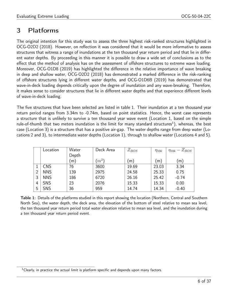
The original intention for this study was to assess the three highest risk-ranked structures highlighted inOCG-O2D2 (2018). However, on reflection it was considered that it would be more informative to assessstructures that witness a range of inundations at the ten thousand year return period and that lie in differ-ent water depths. By proceeding in this manner it is possible to draw a wide set of conclusions as to theeffect that the method of analysis has on the assessment of offshore structures to extreme wave loading.Moreover, OCG-O1D8 (2019) has highlighted the difference in the relative importance of wave breakingin deep and shallow water, OCG-O2D2 (2018) has demonstrated a marked difference in the risk-rankingof offshore structures lying in different water depths, and OCG-O1D6B (2019) has demonstrated thatwave-in-deck loading depends critically upon the degree of inundation and any wave-breaking. Therefore,it makes sense to consider structures that lie in different water depths and that experience different levelsof wave-in-deck loading.

The five structures that have been selected are listed in table 1. Their inundation at a ten thousand yearreturn period ranges from 3.34m to -0.74m, based on point statistics. Hence, the worst case representsa structure that is unlikely to survive a ten thousand year wave event (Location 1, based on the simplerule-of-thumb that two meters inundation is the limit for many standard structures1), whereas, the bestcase (Location 3) is a structure that has a positive air-gap. The water depths range from deep water (Lo-cations 2 and 3), to intermediate water depths (Location 1), through to shallow water (Locations 4 and 5).

Location WaterDepth

Deck Area ZBOS η10k η10k − ZBOS

(m) (m2) (m) (m) (m)1 CNS 76 3600 19.69 23.03 3.342 NNS 139 2975 24.58 25.33 0.753 NNS 186 6720 26.16 25.42 -0.744 SNS 23 2076 15.33 15.33 0.005 SNS 36 959 14.74 14.34 -0.40

Table 1: Details of the platforms studied in this report showing the location (Northern, Central and SouthernNorth Sea), the water depth, the deck area, the elevation of the bottom of steel relative to mean sea level,the ten thousand year return period total water elevation relative to mean sea level, and the inundation duringa ten thousand year return period event.

1Clearly, in practice the actual limit is platform specific and depends upon many factors.

6 of 37


4 Metocean

The first step in the analysis is the derivation of the model for the long-term metocean environment.This has been completed by using the LOADS methodology with NEXTRA hindcast data. The resultis the long-term distributions of significant wave height, maximum crest elevation, maximum total waterelevation, and maximum wave height. This has been used as input into the LOADS methodology for waveloading and also in order to derive metocean criteria; for example, the ten thousand year return periodextremes.

4.1 Data

The data set that has been used is the NEXTRA hindcast. It was carried out by Oceanweather, and hasthree-hourly output from 1964 to 2014. The hindcast applied NCEP/NCAR reanalysis winds (after kine-matic analysis) and OceanWeather’s UNIWAVE wave model. Severe summer storms and winter months(October to March) are represented in all years and the hindcast is continuous from 1987. The domainspans 45.4◦N − 72.4◦N, 21.2◦W − 36.6◦E at a resolution of 30km. A map showing the grid points atwhich results are available is shown in figure 2. The hindcast was updated in the Southern North Sea(SNEXT) by simulating waves on both a 3km and a 1km grid. This was in order to be able to resolve thecomplex shallow water bathymetry that can be found in this region; in particular, the sandbanks that canbe found off the Norfolk coast.

The DHI hydrodynamic model was run as part of the NEXTRA JIP and hourly output of depth averagedcurrents and water levels have been provided at a number of grid points across the North Sea region. Ithas been validated by PhysE (2011) and shown to be in good agreement with measurements in locationswhere tidal effects dominate.

The HSE has access to this data set as it is a member of the NEXTRA JIP.

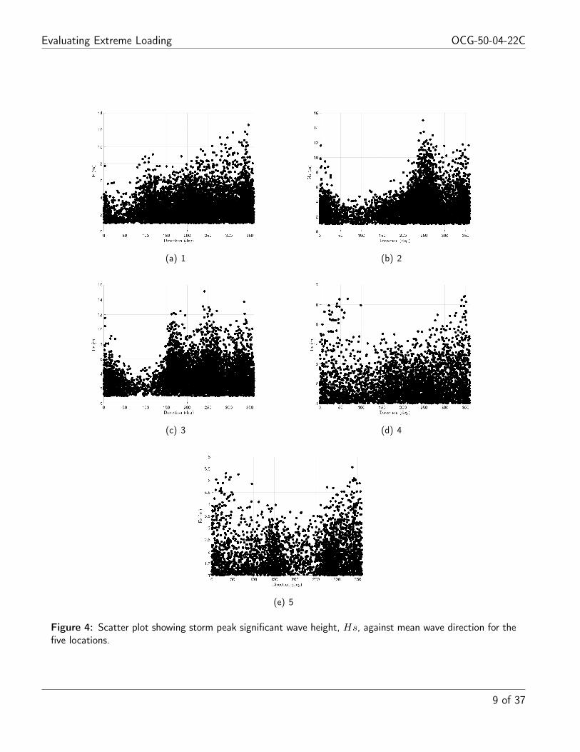
A comparison between the long-term distribution of significant wave height at the five locations of interestis provided in figure 3. It shows that Locations 2 and 3 observe much more severe metocean conditionsthan the other sites. Figure 4 shows scatter plots of mean wave direction against storm peak significantwave height. It indicates that at locations that lie within the central or southern North Sea (Locations 1,4 and 5) the largest sea-states arise from the North, whereas, at the two locations that are exposed tothe North Atlantic (Locations 2 and 3) the largest waves arise from the West.

7 of 37


Figure 2: Map showing the NEXTRA 30km grid.

Figure 3: The long-term distribution of significant wave height at the five locations.

8 of 37


(a) 1 (b) 2

(c) 3 (d) 4

(e) 5

Figure 4: Scatter plot showing storm peak significant wave height, Hs, against mean wave direction for thefive locations.

9 of 37


4.2 Analysis

The analysis of the long-term metocean environment has proceeded using a methodology that is largelybased upon Jonathan et al. (2013) and Ross et al. (2017). This represents the state-of-the-art in metoceanextremes.

1. The storm peak significant wave height has been identified for each independent storm event andthe associated values of the following have been recorded: mean wave direction θpeak, spectral peakperiod Tppeak, bandwidth γpeak, spreading at the spectral peak σpeak, and storm surge ηres,peak.

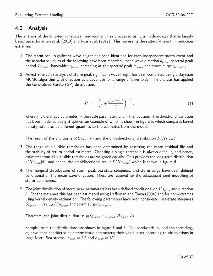
2. An extreme value analysis of storm peak significant wave height has been completed using a BayesianMCMC algorithm with direction as a covariate for a range of thresholds. The analysis has appliedthe Generalised Pareto (GP) distribution:

P =

(1 +

ξ(x− γ)

σ

)− 1ξ

, (1)

where ξ is the shape parameter, σ the scale parameter, and γ the location. The directional variationhas been modelled using B-splines; an example of which is shown in figure 5, which compares kerneldensity estimates at different quantiles to the estimates from the model.

The result of the analysis is p(Hspeak|θ) and the omnidirectional distribution P (Hspeak).

3. The range of plausible thresholds has been determined by assessing the mean residual life andthe stability of return period estimates. Choosing a single threshold is always difficult, and hence,estimates from all plausible thresholds are weighted equally. This provides the long-term distributionp(Hspeak|θ), and hence, the omnidirectional result P (Hspeak) which is shown in figure 6.

4. The marginal distributions of storm peak sea-state steepness, and storm surge have been definedconditional on the mean wave direction. These are required for the subsequent joint modelling ofstorm parameters.

5. The joint distribution of storm peak parameters has been defined conditional onHspeak and directionθ. For the extremes this has been estimated using Heffernan and Tawn (2004) and for non-extremesusing kernel density estimation. The following parameters have been considered: sea-state steepnessSppeak = Hspeak/Tp

2peak, and storm surge ηres,peak.

Therefore, the joint distribution is: p(Sppeak, ηres,peak|Hspeak, θ).

Samples from the distributions are shown in figure 7 and 8. The bandwidth, γ, and the spreading,σ, have been considered as deterministic parameters; their value is set according to observations inlarge North Sea storms: γpeak = 2.5 and σpeak = 15◦.

10 of 37


The metocean model describes the long-term distribution of stationary metocean conditions associatedwith storm events. This can be used in conjunction with the relevant short-term distributions of crestelevation and wave height in order to derive the long-term distribution of these parameters. The resultsfor crest elevation, C, are shown in figure 9, for total still water elevation, ηtot = C + ηres + ηtide, areshown in figure 10, and for wave height, H, are shown in figure 11.

The calculations have been completed using the following short-term distributions:

• Crest elevation: at Locations 1, 2 and 3 the LOADS distribution; at Locations 4 and 5 the LOWISHdistribution. These incorporate nonlinearities beyond second-order and wave breaking.

• Wave height: at Locations 1, 2 and 3 the Boccotti (1983) distribution; at Locations 4 and 5the LOWISH distribution. These incorporate bandwidth effects, and the LOWISH distributionincorporates wave breaking.

This approach follows best practice as defined in OCG-O1D3 (2018) and OCG-O1D8 (2019).

Inevitably, the estimates of ten thousand year return period total water elevation are slightly different tothe consensus estimates derived in OCG-O2D2 (2018) upon which the inundations in table 1 are based2.Therefore, in order to maintain consistency between the various analyses the bottom of steel of the variousplatforms has been shifted by a small amount in order that the values in table 1 are matched.

2This is because the consensus estimates have been derived using an average of the values from different consultantsand operators over a region close to the platforms of interest.

11 of 37


(a) 1 (b) 2

(c) 3 (d) 4

(e) 5

Figure 5: Example of the directional variation in storm peak significant wave height, Hs, and the spline fitfor Locations 1-5. The black lines represent the results from a kernel density estimate and the coloured linesthe estimates from the metocean model: P50, P75, P90 and P95 (from bottom to top).

12 of 37


(a) 1 (b) 2

(c) 3 (d) 4

(e) 5

Figure 6: The long-term distribution of storm peak significant wave height, Hs, for Locations 1-5. The blackcircles represent the underlying data, dark blue line shows the median, the red shows the posterior predictivevalue and the fan shows the uncertainty (P5-P95 and P25-P75).

13 of 37


(a) 1 (b) 2

(c) 3 (d) 4

(e) 5

Figure 7: Scatter plot of significant wave height, Hs, against spectral peak period, Tp, for Locations 1-5.The grey circles represent the underlying data, the red crosses are a fair sample from the metocean model,whereas the blue dots are a stratified sample from the metocean model.

14 of 37


(a) 1 (b) 2

(c) 3 (d) 4

(e) 5

Figure 8: Scatter plot of significant wave height, Hs, against residual still water elevation, ηres. The greycircles represent the underlying data, the red crosses are a fair sample from the metocean model, whereas theblue dots are a stratified sample from the metocean model.

15 of 37


(a) 1 (b) 2

(c) 3 (d) 4

(e) 5

Figure 9: The long-term distribution of maximum crest elevation at Locations 1-5: linear (black); second-order (blue); LOADS (green); LOWISH (red); LOADS with uncertainty (solid grey); and LOWISH withuncertainty (dashed grey).

16 of 37


(a) 1 (b) 2

(c) 3 (d) 4

(e) 5

Figure 10: The long-term distribution of crest (light) and maximum total water elevation (dark) at Locations1-5.

17 of 37


(a) 1 (b) 2

(c) 3 (d) 4

(e) 5

Figure 11: The long-term distribution of maximum wave height at Locations 1-5: Forristall (black); Boccotti(blue); and LOWISH (red); Boccotti with uncertainty (solid grey); and LOWISH with uncertainty (dashedgrey).

18 of 37


5 Loading

The second step in the analysis is the derivation of the long-term distribution of wave-in-jacket (WIJ) andwave-in-deck (WID) loading. This has been completed by using the LOADS methodology. The resultis the best estimate of the actual long-term distribution of loading against which different deterministicmethods of analysis can be compared.

Discrete extreme wave events have been defined using the approach developed in the LOADS JIP. This isan efficient application of the Monte Carlo method based upon independent storm events and individualirregular nonlinear wave events; it is described below. The fundamental equation that the approach isinterested in solving is

P (Xmax) =

∫P (Xmax|Hs, Tp, σθ...) p(Hs, Tp, σθ...) dHs dTp dσθ... . (2)

If the long-term distribution p(Hs, Tp, σθ...) corresponds to independent storm events then the left-handside is P (Xmax)RandomStorm which can be converted to the annual probability of non-exceedance

P (Xmax)Annual =

∫P (Xmax)nRandomStorm p(n|ν)dn , (3)

where n is the number of storms in a year and ν is the mean storm arrival rate. These equations aresolved as follows:

1. The long-term distribution of sea-states associated with storm events is defined using methodsdescribed in OCG-50-01-04 (2017): p(Hs, Tp, ...).

2. A set of storms events are sampled from the long-term distribution. This is provided in terms of a setof sea-states that define the time history of wave, wind and current conditions through each storm.The storm sampling scheme that is employed is efficient rather than a straightforward applicationof naive or crude Monte Carlo.

3. Within each sea-state in each storm a number of linear wave events are sampled using efficientMonte Carlo methods.

4. The wave events are transformed in order to include nonlinearity beyond second-order and the effectsof wave breaking using the methods described in LOADS Task B Report (2018). This defines thenonlinear surface profile, η(x, y, t), the velocities u(x, y, z, t) and accelerations u̇(x, y, z, t).

5. The profile and kinematics are input into the wave-in-jacket and wave-in-deck load models describedin LOADS Task B Report (2018); in particular, the latter is the momentum flux method of Ma andSwan (2019). This results in a time history of the static loading on each element of the structure.The size of the jacket and of the deck has been defined based upon the input data from the pro-forma(task O2D1). It has been assumed that all of the wave energy that enters the deck is destroyedimmediately, this would be consistent with platforms which have: numerous deep under-deck girdersand are plated; or are grated, but densely packed with process equipment.

19 of 37


6. The wave events are used in order to define the short-term distribution P (X|Hs, Tp...) of responseand maximum response P (Xmax|Hs, Tp...), in each sea-state in every storm. This can be used todefine the distribution of maximum response over each storm P (Xmax)Storm =

∏i P (Xmax|Hsi, Tpi).

7. Integrating over the set of storms provides the long-term distribution P (Xmax)RandomStorm, andhence, equation 3 can be used in order to define the annual probability of exceedance of a responseP (Xmax)Annual.

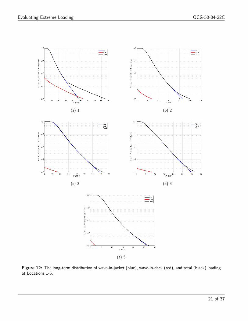
The long-term distributions of WIJ, and total WIJ and WID, loading are shown in figure 12. In the nextsection these will be compared to the estimates from several deterministic wave events and design recipes.The most obvious thing of note is the rapid increase in load once waves begin to inundate the deck.However, there are other details that are also of interest. For example, Locations 1 and 2 are inundatedat the ten thousand year return period according to point statistics, whereas, the other platforms are not.Therefore, the wave-in-deck loading at the ten thousand year level at Locations 3 to 5, is entirely dueto the area effect. Furthermore, another thing of note is that pure wave-in-jacket loading can increasequite slowly at very high return periods when there are large inundations - this is simply because the crestof the waves are now above the top of the jacket, and hence, the largest velocities have effectively beenremoved from the load calculation.

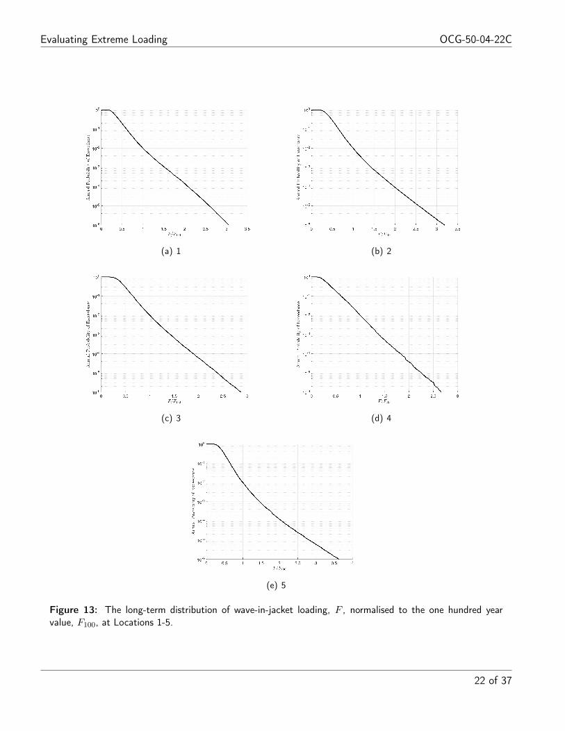
The hazard curves for purely wave-in-jacket loading are shown in figure 13. They indicate that the ratioof the one hundred to ten thousand year return period loading is typically around 2 – without includingepistemic uncertainties, which will increase the ratio further. This is contrast to the assumption withinthe ISO code calibration that the ratio is around 1.65.

It should be noted that LOADS Phase One was concerned with intermediate to deep water, and didnot consider shallow water. This is being addressed in LOADS Phase Two which is presently underway.Therefore, all of the results in shallow water have been developed using the following explicit assumption:the empirical wave model developed for intermediate and deep water is valid except that the short-termdistribution of crest elevation can be described using the LOWISH distribution. This entails a numberof implicit assumptions: that large wave events can be described using the linear dispersion relationship;that the kinematics associated with breaking waves is governed by wave steepness; and that the effectof nonlinearity on the shape of large wave events is a function of the wave steepness. Clearly, all ofthese assumptions are questionable, but until LOADS Phase Two is complete their importance cannot beassessed. Therefore, the load distribution at Locations 4 and 5 is uncertain and should be regarded withsome caution.

20 of 37


(a) 1 (b) 2

(c) 3 (d) 4

(e) 5

Figure 12: The long-term distribution of wave-in-jacket (blue), wave-in-deck (red), and total (black) loadingat Locations 1-5.

21 of 37


(a) 1 (b) 2

(c) 3 (d) 4

(e) 5

Figure 13: The long-term distribution of wave-in-jacket loading, F , normalised to the one hundred yearvalue, F100, at Locations 1-5.

22 of 37


6 Deterministic Wave Events

A number of different methods for assessing offshore structures have been considered using deterministicregular and irregular wave events. These include different methods for characterising the events and dif-ferent methods for calculating the wave-in-deck loading – it is assumed that wave-in-jacket loading canbe derived using the Morison equation.

The waves have been defined using standard metocean return period criteria values taken from the long-term metocean model described in section 4: wave height H; crest elevation C; total water elevation, η,and spectral peak period Tp. The values are dependent upon the short-term distribution that is used (forexample, Forristall (1978) or Boccotti (1983)) and so wave events can be defined in a number of differentways.

6.1 Regular Waves

Five different regular wave events have been considered. They are described in table 2. The waves havebeen defined by either specifying the target wave height or the crest elevation. In each case the heightor the crest has been assigned based on return period criteria values using the distribution noted in thetable. For each wave, three associated wave periods have been used (low, medium and high) based onpercentiles of the distribution of spectral peak period conditional on significant wave height. In all casesthe still water elevation was shifted so that the total water elevation matched the return period valuecalculated using either second-order, LOADS or LOWISH distributions. Effectively, the five waves coverthe spread of approaches that might be considered in typical practice:

• A and B follow historical practice by defining the wave using criteria values of the height: Buses Forristall (1978) which is the distribution that has traditionally been applied in the North Sea;whereas A improves upon this by incorporating recent knowledge through the application of Boccotti(1983) in deep water and LOWISH in shallow water. The total water elevation has been matchedto second-order criteria for B and to either LOADS or LOWISH criteria for A.

• C and D define the wave using the crest elevation: D follows the traditional practice of usingsecond-order crests (Forristall, 2000), whereas, C improves upon this by considering higher ordernonlinearities and wave breaking (LOADS or LOWISH). The total water elevation has been matchedto second-order criteria for D and to either LOADS or LOWISH criteria for C.

• E defines the wave using the solution to the ‘crest-conundrum’ detailed in Santala (2017) whichinvolves a change in the wave period. The wave height has been defined using Forristall (1978) andthe total water elevation has been matched to second-order criteria.

The profiles associated with ten thousand year return period regular wave events at Location 1 are shownin figure 14 for A-E relative to still water elevation – as noted above, in each case the still water level isshifted such that the desired extreme total water surface elevation is matched.

Return period values of WIJ loading are shown in figures 15 and 16 using a wave kinematics factor, Φ, of0.90 and 1.00, respectively. The former is consistent with the recommendations in ISO19901-1.

23 of 37


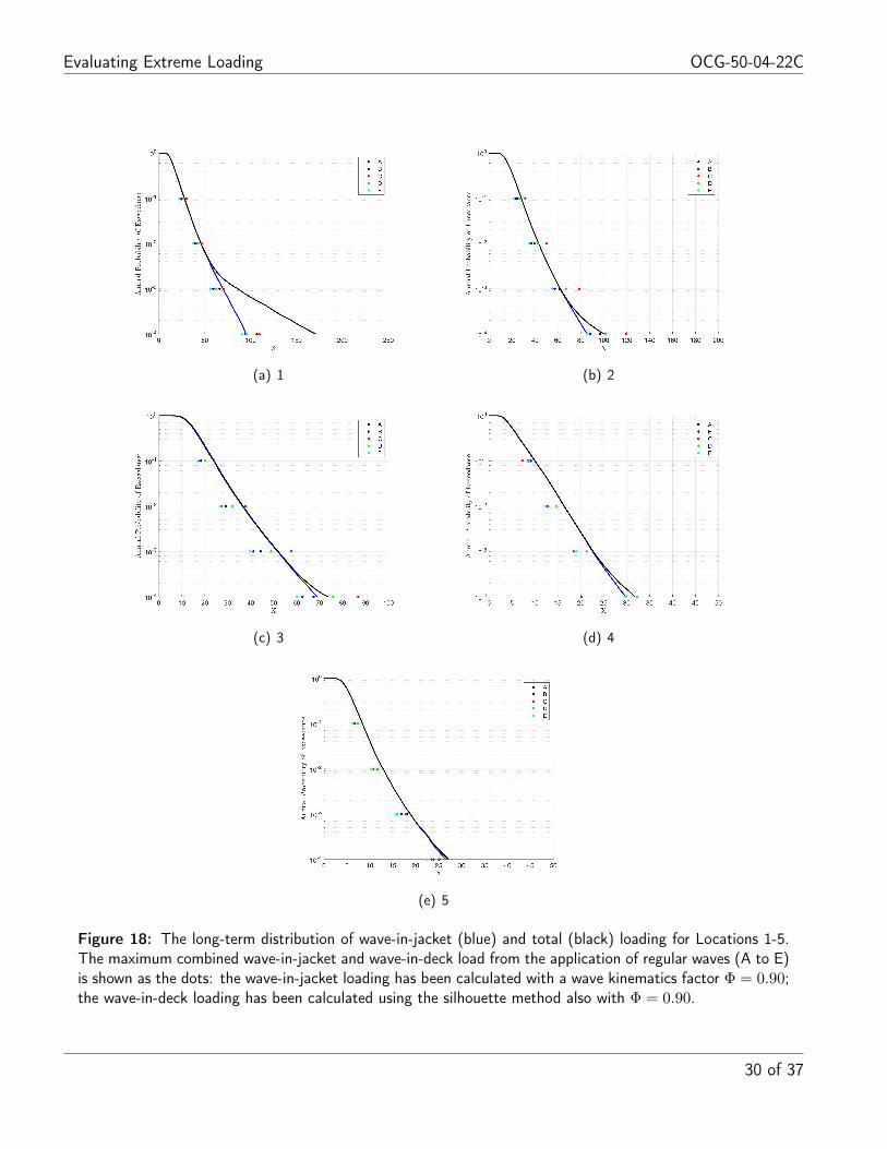
Return period values of combined WIJ and WID loading are shown in figures 17 to 18. These haveused a wave kinematics factor of Φ = 0.90, and two different methods for calculating the wave-in deckloading: the momentum flux method of Ma and Swan (2019); and the silhouette method recommendedin API2SIM (2014) and ISO19902. The results show the following:

1. Wave-in-Jacket Loading

(a) The application of the typical design recipe with a wave height defined using Forristall (1978)and a set of associated periods (B) is non-conservative across the range of return periods andlocations considered when Φ = 0.90; the estimates improve and have little to no bias when Φis increased to 1.00.

(b) Increasing the wave height so that it is defined using the return period values calculatedusing Boccotti (1983) (A) improves the match between the predictions and the actual long-term distribution, but the approach is often still non-conservative with Φ = 0.90, but oftenconservative when Φ is increased to 1.00.

(c) Matching regular waves to the return period crest elevation (including nonlinearities beyondsecond-order and wave breaking, (C) improves the agreement in both deep and shallow water;using a wave kinematics factor Φ = 0.90 it can be conservative or non-conservative, but usingΦ = 1.00 it is almost always conservative.

2. Wave-in-Deck Loading

(a) There is a large spread in the results for combined wave-in-jacket and wave-in-deck loadingdepending on the methods used to define the wave events (A-E) and calculate the loads.

(b) At locations where the inundation at a ten thousand year return period is due to the areaeffect, none of the methods predict wave-in-deck loading as none of the waves reach the deck.This is because although the still water level has been shifted in order to match the total waterelevation, this has been defined based on point statistics.

(c) Matching regular waves to the return period crest elevation (including nonlinearities beyondsecond-order and wave breaking (C) with a wave kinematics factor Φ = 0.90 and using themomentum flux method in order to calculate the wave-in-deck loads provides the best match,but can still be non-conservative in cases with large inundation (for example Location 1).Increasing the wave kinematics factor (results not shown here), obviously, reduces the non-conservatism in this case.

(d) Calculating wave-in-deck loads using the silhouette method provides an underestimate of theloading as it does not include the momentum that enters the underside of the deck. This issometimes compensated by an over-prediction of jacket loads, but overall this is not a rationalsolution.

24 of 37


Wave Height Wave Period Crest Elevation Total Water ElevationA Hboc,LOWISH Tmax = 0.85TpP10,P50,P90 NA ηLOADS,LOWISH

B Hfor Tmax = 0.85TpP10,P50,P90 NA ηo2C NA Tmax = 0.85TpP10,P50,P90 CLOADS,LOWISH ηLOADS,LOWISH

D NA Tmax = 0.85TpP10,P50,P90 Co2 ηo2E Hfor Tmax = 0.85 (TpP10,P50,P90 −∆TAPI) NA ηo2

Table 2: The five regular wave cases considered - each of which has three associated wave periods. Thewaves have been defined in terms of either their height, H, or their crest elevation, C. The still water elevationhas been shifted so that they match a total water elevation, η.

25 of 37


(a)

(b)

Figure 14: Example showing the surface profiles of the 10,000 year return period regular waves (A to E) atLocation 1. Panels (a) and (b) show the same data on different axes. The dashed grey line is the second-ordercrest elevation whereas the solid grey line is the LOADS crest elevation.

26 of 37


(a) 1 (b) 2

(c) 3 (d) 4

(e) 5

Figure 15: The long-term distribution of wave-in-jacket (blue) and total (black) loading for Locations 1-5.The maximum wave-in-jacket load from the application of regular waves (A to E) with a wave kinematicsfactor Φ = 0.90 is shown as the dots.

27 of 37


(a) 1 (b) 2

(c) 3 (d) 4

(e) 5

Figure 16: The long-term distribution of wave-in-jacket (blue) and total (black) loading for Locations 1-5.The maximum wave-in-jacket load from the application of regular waves (A to E) with a wave kinematicsfactor Φ = 1.00 is shown as the dots.

28 of 37


(a) 1 (b) 2

(c) 3 (d) 4

(e) 5

Figure 17: The long-term distribution of wave-in-jacket (blue) and total (black) loading for Locations 1-5.The maximum combined wave-in-jacket and wave-in-deck load from the application of regular waves (A to E)is shown as the dots: the wave-in-jacket loading has been calculated with a wave kinematics factor Φ = 0.90;the wave-in-deck loading has been calculated using a momentum flux method with Φ = 0.90.

29 of 37


(a) 1 (b) 2

(c) 3 (d) 4

(e) 5

Figure 18: The long-term distribution of wave-in-jacket (blue) and total (black) loading for Locations 1-5.The maximum combined wave-in-jacket and wave-in-deck load from the application of regular waves (A to E)is shown as the dots: the wave-in-jacket loading has been calculated with a wave kinematics factor Φ = 0.90;the wave-in-deck loading has been calculated using the silhouette method also with Φ = 0.90.

30 of 37


6.2 Irregular Waves

Four different irregular wave events have been considered. They are described in table 3 and representfocussed NewWave events. The waves have been defined in terms of their nonlinear crest elevation asfollows:

• F: the second-order point estimate, Co2, with the median TpP50.

• G: the high-order point estimate, CLOADS,LOWISH , which is defined using LOADS in deep waterand LOWISH in shallow water, with the median TpP50.

• H: the high-order estimate over the platform area Carea, with the associated median TpP50.

• I: the high-order point estimate, CLOADS,LOWISH , with a wave period defined such that Ckp = 0.40where kp is the spectral peak wave-number. Therefore, this wave represents a steep breaking event.

The profiles associated with waves F to H are shown in figure 19 where they are compares to two of theregular wave solutions. The vertical profile of the horizontal water particle kinematics beneath a wavecrest are shown in figure 20.

Return period values of WIJ loading and combined WIJ and WID loading are shown in figures 21 and 22,respectively. The results show the following:

1. Wave-in-Jacket Loading

(a) The application of second-order wave theory (F) is usually non-conservative. The exception isin shallow water (Location 4) where it can be conservative.

(b) The application of non-breaking high-order wave events (G) leads to a fairly consistent set ofloads across the locations and water depths that are larger than second-order theory. However,it can be slightly non-conservative as it does not consider the possibility that the waves maybe breaking.

(c) The application of a plunging breaker (H) results in reasonable agreement between the predictedloading and the true long-term distribution across all water depths and return periods. It istypically slightly conservative – presumably because at most locations the design events fortotal base shear are spilling breakers.

(d) The application of an irregular wave defined using the median period, but with the crestmatched to the area statistic (I) is conservative. This must be considered to be a somewhatnon-physical wave-event for purely wave-in-jacket loading.

2. Wave-in-Deck Loading

(a) The application of second-order wave theory (F) is usually very non-conservative. The exceptionis shallow water (Location 4) where it is conservative.

(b) The non-breaking high-order wave events (G) provide a consistent set of loads that are typicallyslightly non-conservative. They cannot identify cases where wave-in-deck loading is due to the‘area’ effect (Locations 3 to 5).

31 of 37


(c) The application of a plunging breaker (H) results in a consistent slightly conservative set ofloads. It cannot identify cases where wave-in-deck loading is due to the ‘area’ effect (Location3 to 5).

(d) The application of the median period with a crest matched to the area statistic (I) is conserva-tive across all water depths and return periods. It is always conservative and is the only eventthat can capture inundation at return periods where the ‘area’ effect is important (the onlyexception is second-order theory in shallow water).

Crest Elevation Wave PeriodF Co2 TpP50

G CLOADS,LOWISH TpP50

H Carea TpP50

I CLOADS,LOWISH Tpbreak

Table 3: The four irregular wave cases considered: F and G have three associated wave periods; H and Ihave one associated wave period.

32 of 37


(a)

(b)

Figure 19: Example showing the surface profiles of 10,000 year return period waves at Location 1: A and Care regular waves; F to H are irregular waves. Panels (a) and (b) show the same data on different axes. Thedashed grey line is the second-order crest elevation whereas the solid grey line is the LOADS crest elevation.

33 of 37


Figure 20: Example showing the horizontal velocity profile beneath a 10,000 year wave event at Location 1:A and B are regular waves, whereas, F to I are irregular waves.

34 of 37


(a) 1 (b) 2

(c) 3 (d) 4

(e) 5

Figure 21: The long-term distribution of wave-in-jacket (blue) and total (black) loading for Locations 1-5.The maximum wave-in-jacket load from the application of irregular waves (F to I) is shown as the dots.

35 of 37


(a) 1 (b) 2

(c) 3 (d) 4

(e) 5

Figure 22: The long-term distribution of wave-in-jacket (blue) and total (black) loading for Locations 1-5.The maximum combined wave-in-jacket and wave-in-deck load from the application of irregular waves (F toI) is shown as the dots. The wave-in-deck load has been calculated using the momentum flux method.

36 of 37


References

API2SIM. Recommended practice for the structural integrity management of fixed offshore structures.2014.

P. Boccotti. Some new results on statistical properties of wind waves. Applied Ocean Research, 1983.

G. Z. Forristall. Wave crest distributions: observations and second-order theory. Journal of PhysicalOceanography, 30:1931–1943, 2000.

G.Z. Forristall. On the statistical distribution of wave heights in a storm. Journal of Geophysical Research,83:2353–2358, 1978.

J.E. Heffernan and J.A. Tawn. A conditional approach for multivariate extreme values. Journal of theRoyal Statistical Society B, 2004.

ISO19901-1. Metocean design and operating considerations. Technical report, ISO.

ISO19902. Fixed steel offshore structures. Technical report, ISO.

P Jonathan, K C Ewans, and D Randell. Multidimensional covariate effects in spatial and joint extremes.Waves workshop, pages 1–13, 2013.

LOADS Task B Report. LOADS short term models. Swan C., and Ma, Li., and Zve, E., 2018.

L. Ma and C. Swan. The effective prediction of wave-in-deck loads. Journal of Fluids and Structures,2019.

OCG-50-01-04. LOADS JIP Task A. Technical report, OCG, 2017.

OCG-O1D3. Metocean research relevant to fixed offshore platforms. Technical report, OCG, 2018.

OCG-O1D6B. Extreme loading events and target reliability levels part B: wave-in-deck loading. Technicalreport, OCG, 2019.

OCG-O1D8. Review of current methods for predicting the extreme environmental loads acting on offshoreinstallations. Technical report, OCG, 2019.

OCG-O2D2. Risk Ranking of Fixed Installations on the UKCS. Technical report, OCG, 2018.

PhysE. DHI Current Model Validation, C413-R482-11. Technical report, 2011.

E. Ross, D. Randell, K. Ewans, G. Feld, and P. Jonathan. Efficient estimation of return value distributionsfrom non-stationary marginal extreme value models using bayesian inference. Ocean Engineering, 2017.

M. Santala. Resolving the API RP 2MET crest conundrum for wave-in-deck loading. Offshore TechnologyConference, 2017.

37 of 37

Extreme Environmental Loading of Fixed Offshore Structures

Documents

Transcript of Extreme Environmental Loading of Fixed Offshore Structures