EVALUATING SADT BY ADVANCED KINETICS-BASED ...
13
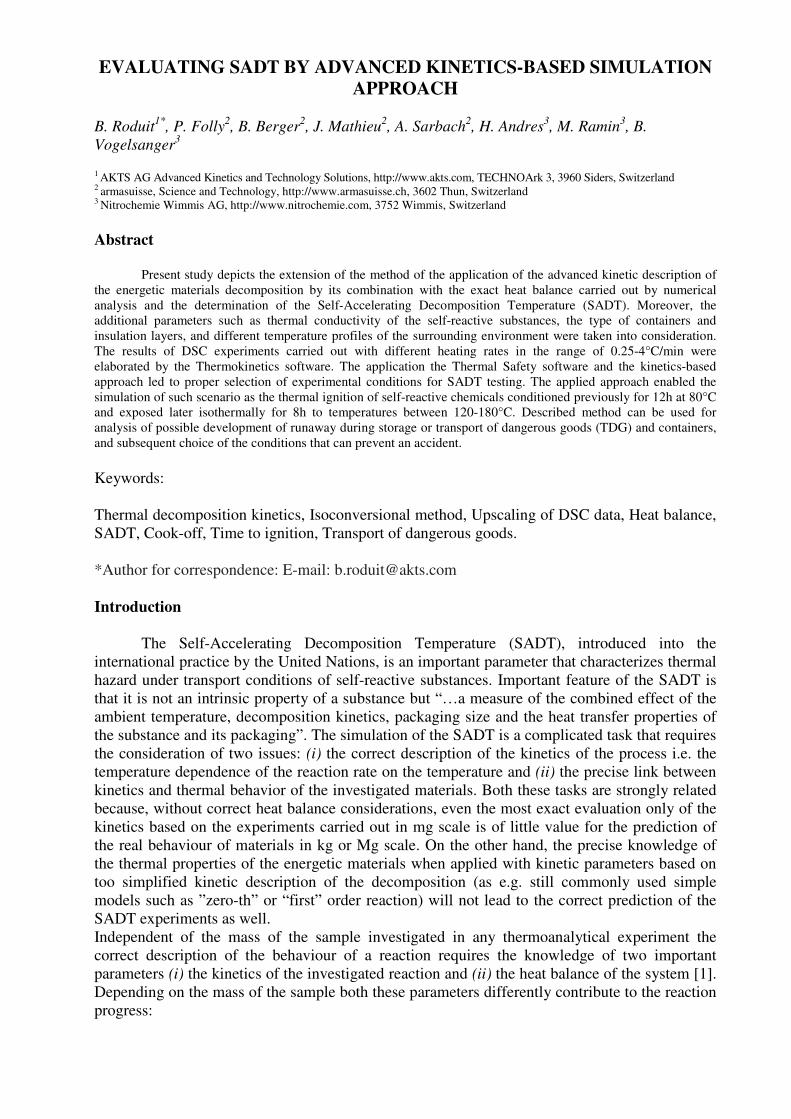
EVALUATING SADT BY ADVANCED KINETICS-BASED SIMULATION APPROACH B. Roduit 1* , P. Folly 2 , B. Berger 2 , J. Mathieu 2 , A. Sarbach 2 , H. Andres 3 , M. Ramin 3 , B. Vogelsanger 3 1 AKTS AG Advanced Kinetics and Technology Solutions, http://www.akts.com, TECHNOArk 3, 3960 Siders, Switzerland 2 armasuisse, Science and Technology, http://www.armasuisse.ch, 3602 Thun, Switzerland 3 Nitrochemie Wimmis AG, http://www.nitrochemie.com, 3752 Wimmis, Switzerland Abstract Present study depicts the extension of the method of the application of the advanced kinetic description of the energetic materials decomposition by its combination with the exact heat balance carried out by numerical analysis and the determination of the Self-Accelerating Decomposition Temperature (SADT). Moreover, the additional parameters such as thermal conductivity of the self-reactive substances, the type of containers and insulation layers, and different temperature profiles of the surrounding environment were taken into consideration. The results of DSC experiments carried out with different heating rates in the range of 0.25-4°C/min were elaborated by the Thermokinetics software. The application the Thermal Safety software and the kinetics-based approach led to proper selection of experimental conditions for SADT testing. The applied approach enabled the simulation of such scenario as the thermal ignition of self-reactive chemicals conditioned previously for 12h at 80°C and exposed later isothermally for 8h to temperatures between 120-180°C. Described method can be used for analysis of possible development of runaway during storage or transport of dangerous goods (TDG) and containers, and subsequent choice of the conditions that can prevent an accident. Keywords: Thermal decomposition kinetics, Isoconversional method, Upscaling of DSC data, Heat balance, SADT, Cook-off, Time to ignition, Transport of dangerous goods. *Author for correspondence: E-mail: [email protected] Introduction The Self-Accelerating Decomposition Temperature (SADT), introduced into the international practice by the United Nations, is an important parameter that characterizes thermal hazard under transport conditions of self-reactive substances. Important feature of the SADT is that it is not an intrinsic property of a substance but “…a measure of the combined effect of the ambient temperature, decomposition kinetics, packaging size and the heat transfer properties of the substance and its packaging”. The simulation of the SADT is a complicated task that requires the consideration of two issues: (i) the correct description of the kinetics of the process i.e. the temperature dependence of the reaction rate on the temperature and (ii) the precise link between kinetics and thermal behavior of the investigated materials. Both these tasks are strongly related because, without correct heat balance considerations, even the most exact evaluation only of the kinetics based on the experiments carried out in mg scale is of little value for the prediction of the real behaviour of materials in kg or Mg scale. On the other hand, the precise knowledge of the thermal properties of the energetic materials when applied with kinetic parameters based on too simplified kinetic description of the decomposition (as e.g. still commonly used simple models such as ”zero-th” or “first” order reaction) will not lead to the correct prediction of the SADT experiments as well. Independent of the mass of the sample investigated in any thermoanalytical experiment the correct description of the behaviour of a reaction requires the knowledge of two important parameters (i) the kinetics of the investigated reaction and (ii) the heat balance of the system [1]. Depending on the mass of the sample both these parameters differently contribute to the reaction progress:
-
Upload
khangminh22 -
Category
Documents
-
view
1 -
download
0
Transcript of EVALUATING SADT BY ADVANCED KINETICS-BASED ...
EVALUATING SADT BY ADVANCED KINETICS-BASED SIMULATION
APPROACH
B. Roduit1*
, P. Folly2, B. Berger
2, J. Mathieu
2, A. Sarbach
2, H. Andres
3, M. Ramin
3, B.
Vogelsanger3
1 AKTS AG Advanced Kinetics and Technology Solutions, http://www.akts.com, TECHNOArk 3, 3960 Siders, Switzerland 2 armasuisse, Science and Technology, http://www.armasuisse.ch, 3602 Thun, Switzerland 3 Nitrochemie Wimmis AG, http://www.nitrochemie.com, 3752 Wimmis, Switzerland
Abstract
Present study depicts the extension of the method of the application of the advanced kinetic description of
the energetic materials decomposition by its combination with the exact heat balance carried out by numerical
analysis and the determination of the Self-Accelerating Decomposition Temperature (SADT). Moreover, the
additional parameters such as thermal conductivity of the self-reactive substances, the type of containers and
insulation layers, and different temperature profiles of the surrounding environment were taken into consideration.
The results of DSC experiments carried out with different heating rates in the range of 0.25-4°C/min were
elaborated by the Thermokinetics software. The application the Thermal Safety software and the kinetics-based
approach led to proper selection of experimental conditions for SADT testing. The applied approach enabled the
simulation of such scenario as the thermal ignition of self-reactive chemicals conditioned previously for 12h at 80°C
and exposed later isothermally for 8h to temperatures between 120-180°C. Described method can be used for
analysis of possible development of runaway during storage or transport of dangerous goods (TDG) and containers,
and subsequent choice of the conditions that can prevent an accident.
Keywords:
Thermal decomposition kinetics, Isoconversional method, Upscaling of DSC data, Heat balance,
SADT, Cook-off, Time to ignition, Transport of dangerous goods.
*Author for correspondence: E-mail: [email protected]
Introduction
The Self-Accelerating Decomposition Temperature (SADT), introduced into the
international practice by the United Nations, is an important parameter that characterizes thermal
hazard under transport conditions of self-reactive substances. Important feature of the SADT is
that it is not an intrinsic property of a substance but “…a measure of the combined effect of the
ambient temperature, decomposition kinetics, packaging size and the heat transfer properties of
the substance and its packaging”. The simulation of the SADT is a complicated task that requires
the consideration of two issues: (i) the correct description of the kinetics of the process i.e. the
temperature dependence of the reaction rate on the temperature and (ii) the precise link between
kinetics and thermal behavior of the investigated materials. Both these tasks are strongly related
because, without correct heat balance considerations, even the most exact evaluation only of the
kinetics based on the experiments carried out in mg scale is of little value for the prediction of
the real behaviour of materials in kg or Mg scale. On the other hand, the precise knowledge of
the thermal properties of the energetic materials when applied with kinetic parameters based on
too simplified kinetic description of the decomposition (as e.g. still commonly used simple
models such as ”zero-th” or “first” order reaction) will not lead to the correct prediction of the
SADT experiments as well.
Independent of the mass of the sample investigated in any thermoanalytical experiment the
correct description of the behaviour of a reaction requires the knowledge of two important
parameters (i) the kinetics of the investigated reaction and (ii) the heat balance of the system [1].
Depending on the mass of the sample both these parameters differently contribute to the reaction
progress:

(i) The kinetics of the process is always the same, because it is not depending on the mass of the
substance, therefore the correct determination of the kinetic parameters allows simulation of the
reaction progress under any temperature mode independent on the mass of investigated sample.
(ii) On the other hand, the heat balance in the system strongly depends on the sample mass and
therefore has to be considered in adiabatic and semi-adiabatic conditions. One can distinguish
following boundary cases:
- in mg scale, i.e. under typical thermoanalytical experiments (DSC, HFC) one assumes the
ideal exchange of the reaction heat with the environment, what, in turn, allows to carry
on the experiments under isothermal conditions or with constant heating rates. The
reaction heat does not influence the course of the reaction.
- in ton scale one assumes that the reactions proceeds in adiabatic conditions, without any
heat exchange with surroundings, therefore all heat evolved during exothermic reactions
remains in the sample increasing its temperature. Therefore the prediction of the reaction
course has to take into account not only the kinetics of the reaction but also the
temperature increase resulting from the self-heating.
- in kg scale the problem of the heat accumulation is more complicated because, depending
on the thermal properties of the sample, its mass and type of the reactor (or container) a
different amount of heat will be exchanged with the surroundings and some part of it will
accumulate in the system. The heat balance in this situation is more complicated and
generally can be correctly done only using numerical techniques such as finite element
analysis, finite differences or finite volumes.
Evaluation of the decomposition kinetics
The evaluation of the kinetics of the decomposition of energetic materials is one of the main
prerequisite necessary for the correct modelling of their properties. Generally, the kinetic
parameters are calculated from the experimental data obtained by means of thermoanalyzers or
calorimeters such as e.g. TG, DTA or DSC signals. For safety issues, the experiments should be
run in ‘closed high pressure sealed crucibles’ (isochoric conditions) in order to consider the
influence of the pressure on strongly pressure dependent reactions [2]. Independent of the
experimental technique applied, the kinetic calculations require the dependence of the reaction
extent α on the time or temperature.
In DSC, the most commonly applied thermal analysis technique for examining energetic
materials, the determination of the kinetic parameters from the recorded signal requires its
integration in order to obtain the α-time and temperature relationship necessary for kinetic
calculations. Therefore the DSC runs should be carried out till the end of the reaction and
stopped slightly after this point, because the thermokinetic approach requires a baseline after the
final peak for the determination of the heat of the reaction. The integration of DSC signal is
influenced by the method chosen for the determination of the baseline.
Often applied the straight-line form of the baseline is incorrect [3]. The recorded signal depends
not only on the heat of the reaction but is additionally affected by the change of the specific heat
of the mixture reactant-products during the progress of the reaction.
With:
B(t) - the baseline,
S(t) - the differential signal (DSC)
the reaction rate dt
dαand progress α(t) can be expressed as:

∫ −
−=
tend
to
B(t))dt(S(t)
B(t))(S(t)
dt
dα (1)
∫
∫
−
−
=tend
to
t
to
B(t))dt(S(t)
B(t))dt(S(t)
(t)α (0 < α < 1) (2)
with B(t) = (1-α (t))*(a1+b1*t) + α(t)*(a2+b2*t) (3)
where (a1+b1*t) is a tangent at the beginning and (a2+b2*t) a tangent at the end of the DSC
signal S(t).
Fig. 1: DSC traces of the single base propellant: the construction of the baseline for DSC heat flow signal recorded with the
heating rate of 1 K/min. The construction of the baseline can significantly influence the determination of the heat of the reaction
and the estimation of the α -T dependence.
The construction of the baseline for the DSC signal obtained during decomposition of the single
base propellant with a heating rate of 1 K/min is depicted in the Fig.1. It can be seen that the
course of the baseline can significantly influence the determination of the heat of the reaction
and the estimation of the α-T dependence what, in turn, will significantly influence the
determination of the kinetic parameters.
The very important feature of the AKTS-Thermokinetics Software [4] is the possibility of the
optimization of the baseline for all experiments collected by different heating rates (or
temperatures) so that the random errors in the various baseline constructions for all heating rates
will “average themselves out”. This is because different baseline construction are just as likely to
give a value of heat of reaction that is slightly too high as one that is too low.
When the decomposition follows a single kinetic model then the reaction can be described in
terms of a single pair of Arrhenius parameters and the commonly used set of functions f(α)
reflecting the mechanism of the process. In such a case the dependence of the logarithm of the
reaction rate over 1/T is linear with the constant slope m = E/R in full range of conversion degree
α. The reaction rate can be described by only one value of the activation energy E and one value
of the pre-exponential factor A by the following expression:
)f(RT(t)
Eexp A
dt
dα
α
−= (4)

where t is time, T - temperature, R- the gas constant, E - the activation energy, A- the pre-
exponential factor, α is the fraction converted and f(α) is a differential form of the conversion
function depending on the reaction model.
However, the decomposition reactions are generally too complex to be described in terms of a
single pair of Arrhenius parameters (A and E) and the commonly applied set of reaction models
f(α). In general, decomposition reactions demonstrate profound multi-step characteristics. The
assumption that the decomposition of an energetic material will obey a simple rate law is very
rarely true. Moreover, the determination of the kinetic parameters from the single run recorded
with one heating rate only (so called ‘single curve’ method) leads to erroneous results and
according to the recent recommendations should not be applied anymore [5,6].
As concluded in the International ICTAC Kinetics project [6-9], the proper calculation of the
kinetics requires the series of non-isothermal measurements carried out at different heating rates.
This procedure allows supplying the data set that generally contains the necessary amount of
information required for full identification of the complexity of a process.
In the present paper the kinetic parameters have been calculated by the isoconversional method
of Friedman [10] based on the calculation of E and A values at different degrees of conversion α
without assuming the form of f(α) function, i.e. applying logarithmic form of the following
reaction rate expression :
{ }
−=
)RT(t
Eexp)f( A
dt
d
α
αα
α
αα
(5)
according to Friedman we obtain
( ){ }α
αα
α
αα
TR
EfA
dt
d 1lnln −=
(6)
where tα, Tα, Eα and Aα are the time, temperature, apparent activation energy and preexponential
factor, at conversion α, respectively, and –Eα/R and ln{Aαf(α)} are the slope and the intercept
with the vertical axis of the plot of ln(dα/dtα ) vs. 1/Tα.
It is then possible to make kinetic predictions at any temperature profile T(t), from the values of
Eα and ( ){ }αα fA extracted directly from the Friedman method by the separation of the terms
followed by an integration:
( ){ }∫ ∫
−
==α
α
α
α
α
α
α
αt
RT
E
efA
ddtt
0 0
(7)
No specification of the reaction model term, f(α), is necessary for the kinetic prediction since it
requires (Eq. 7), along with Eα, only the product term, {Aα f(α)}, which is experimentally
extracted from the kinetic experiment according to Eq. (6). However, nothing can be inferred
about the pre-exponential factor, Aα, unless f(α) is assumed to have some particular form (first-
order reaction, nucleation-growth, etc.). And when f(α) is associated with a specific reaction
model, still the experimentally extracted product term {Aα f(α)} remains unchanged. The AKTS-
Thermokinetics Software and AKTS-Thermal Safety Software [4] take advantage of this unique
property of the Friedman method of the isoconversional kinetics evaluation and enable

determination and displaying, in arbitrarily chosen form, the apparent “first-order pre-
exponential factor”, Aα (see Fig.2).
Fig. 2: Kinetic analysis of 155 mm artillery charge of Swiss army: (A, B): combustible cartridge, (C, D): single-base
propellant. (A, C): Activation energy E and pre-exponential factor A as a function of the reaction progress. (B, D):
Normalized DSC-signals as a function of the temperature and heating rate (marked in °C/min on the curves).
Experimental data are depicted as symbols, solid lines represent the signals calculated on the basis of kinetic
parameters determined by the Friedman method.
The results of the determination of the kinetic parameters for a 155 mm artillery charge of Swiss
army are depicted in Figs.2. The Figs.2A-C present the dependence of E and A on the reaction
progress. Figs.2B-D show the comparison of the experimental (dots) and calculated courses of
the reactions for different heating rates (lines) by applying the determined E and A values. Note
the very good fit of calculated and experimental relationships.
The application of the advanced kinetics for the investigation of the properties of energetic
materials was also recently presented by A.K. Burnham and L.N. Dinh [11].
Heat balance
To perform the exact heat balance the numerical techniques like finite element analysis or finite
differences or volumes can be applied. The sample is virtually divided into the set of adjoining
elements (see Fig.3). These elements are organized in a virtual mesh and described by the
advanced thermokinetics based on the Friedman analysis in each node of the time and space.

Fig. 3: Generalized heat balance over a container and a volume element.
(A) Kinetic parameters calculated from the DSC measurements, independent of the sample mass, enable the determination
of the reaction rate required for the heat balance.
(B) Heat balance depends on the sample mass and has to be calculated by the numerical techniques.
When the heat is transferred to the surrounding environment the temperature profile within a
body depends upon the rate of heat generation, its capacity to store the part of this heat, and the
rate of heat conduction to its boundaries. Mathematically, using Fourier’s law of heat
conduction, we can derive from the heat equation:
r
PP
qC
TC ρρ
λ 1
t
T 2 +∇=∂
∂ (8)
where λ, ρ, CP, T, qr mean: thermal conductivity, density, specific heat, temperature and the
power generated per unit volume by the decomposition reaction, respectively. With
dt
dHq rr
αρ ∆= (9)
after considering cylindrical coordinates and some simplifications,
2
2
2
2
z
T
r
T
z
T
r
T
∂
∂
∂
∂
∂
∂
∂
∂>>⇒>> (10)
one can write
dt
dT
Cad
P
α
∂
∂
∂
∂
ρ
λ∆+
+=
∂
∂
r
T
r
J
r
T
t
T2
2
(11)
where:
J is a geometry factor dependent on the type of the container: J=0 for the infinite plate, J=1 for
the infinite cylinder and J=2 for the sphere, dα/dt is the rate of the decomposition reaction
expressed by the Arrhenius type equation as those applied in Friedman analysis (eq.5) and ∆Tad
is the adiabatic temperature rise expressed by the heat of reaction ∆Hr and the specific heat CP :
∆Tad = -∆Hr/CP.

Simulation of properties of 155 mm artillery charge of Swiss army
The extension of the simulations under isothermal conditions on the prediction of the time to
self-ignition is illustrated by the results depicting the investigation of a 155mm artillery charge
used in Swiss army. During modeling the geometry, dimension of the container and,
additionally, the amount, properties and thickness of the layers of different materials used for the
construction of the ammunition container have been taken into account. Application of the
appropriate decomposition kinetics (results presented in Fig.2) and proper heat balance
calculated by finite element analysis enabled the determination of the effect of scale and
geometry of the container as well as the heat transfer, thermal conductivity and surrounding
temperature on the heat accumulation in the sample. The simulation results together with the
experimental data are depicted in Fig. 4. The simulation has been done for the sample in the form
of cylinder containing four layers of the following materials possessing significantly different
thermal properties: single-base propellant, combustible cartridge case, protection material and
steel container. The properties of these materials, required for the modeling, are summarized in
Tab. 1.
Fig. 4: Single-base propellant for a 155 mm artillery charge applied in Swiss army: the dependence of the calculated
time to ignition on the temperature under non-adiabatic conditions.
Table 1. The properties of the components of 155 mm artillery charge.
container
wall
protection
material
combustible
cartridge case
single-base
propellant
Layer thickness [mm] 0.7 9 3 64.5
Thermal
conductivity λ [W/cm/K]
0.163 0.0023 0.002 0.001
density ρ [g/cm3] 8 0.4 1.38 1.38
Specific heat CP [J/g/K] 0.5 2.3 1.5 1.5
Heat of reaction ∆Hr [J/g] - - -2768±256 -3579±350.6

Fig. 5: Slow cook-off of the 155 mm artillery charge (A) experiment and (B) simulation. The predicted temperature
of explosion 137°C was in good agreement with the slow cook-off experimental value of 138°C.
Additionally to the isothermal simulations and investigations of the properties of the energetic
materials also the commonly applied ‘slow cook-off’ experiment (heating rate 3.3 °C/h, initial
temperature of the charge 40°C, 6h) has been carried out with the 4.5 kg artillery charge. The
experimental data and results of the simulation of the slow cook-off investigation are presented
in the Fig. 5. As for the isothermal simulation, the heat balance calculated by finite element
analysis was applied together with the advanced kinetic description of the reaction. The
experimentally determined ignition temperature of artillery charge amounted to 137°C (Fig. 5-
A). The predicted ignition temperature of 138°C (Fig. 5-B) was in a very good agreement with
the experimental value.

Self- accelerating decomposition temperature (SADT)
The Self-Accelerating Decomposition Temperature (SADT) is an important parameter that
characterizes thermal hazard under transport conditions of self-reactive substances. The SADT
has been introduced into the international practice by the regulations of the United Nations
presented in “Recommendations on the Transport of Dangerous Goods, Manual of Tests and
Criteria” (TDG) [12]. The Globally Harmonized System (GHS) [13] has inherited the SADT as
a classification criterion for self-reactive substances. According to the Recommendations on
TDG the SADT is defined as “the lowest temperature at which self-accelerating decomposition
may occur with a substance in the packaging as used in transport”. Important feature of the
SADT is that it is not an intrinsic property of a substance but “…a measure of the combined
effect of the ambient temperature, decomposition kinetics, packaging size and the heat transfer
properties of the substance and its packaging” [12].
The Manual of Tests and Criteria of the United Nations on the transport of dangerous goods and
on the globally harmonized system of classification and labelling of chemicals indicates that the
characterization of the materials is based on the heat accumulation storage tests. One can find the
following definitions:
(i) SADT is the lowest environment temperature at which overheat in the middle of the specific
commercial packaging exceeds 6 °C (∆T6) after a lapse of the period of seven days (168 hours)
or less. This period is measured from the time when the packaging center temperature reaches
2°C below the surrounding temperature.
(ii) SADT is the critical ambient temperature rounded to the next higher multiple of 5 °C.
The first definition is based on two essential parameters – maximal permissible overheating
temperature and minimal acceptable induction period. The second definition considers only one
parameter: the critical ambient temperature of thermal runaway rounded to the next higher
multiple of 5 °C without any fixed transportation time in the definition.
Up-scaling of DSC data for the determination of the SADT
Having the advanced kinetic description performed by AKTS-Thermokinetics Software, the
numerical techniques implemented in AKTS-Thermal Safety Software enable to simulate the
heat conduction properties of the energetic material stored in a specific container. Thus, applying
previously determined kinetic parameters and heat balance, it was possible to determine
precisely the SADT for the 155 mm artillery charge as illustrated in figure 6. For the
determination of the SADT we had to specify the properties of the containers. The simulations
have been done for a container containing four layers of the materials possessing significantly
different thermal properties: single-base propellant, combustible cartridge case, protection
material and steel container. The properties of these materials, required for the modelling, are
summarized in Tab. 1. For the determination of the SADT in the current study a heat transfer
coefficient U = 30 W/m2/K has been chosen according to the EU norm recommendations
EN1991-1-2 (2002). For each simulation, the initial temperature in each layer is 20°C. The
SADT based on the first definition (i) amounts to 100oC (Fig. 6A). The temperature course of the
reaction reveals that it will probably proceed in a thermal runaway scenario soon after 8 days.
Anyhow, based on the definition, ∆T6 is reached after a lapse of about 6.7 days. This period is
measured from the time when the packaging centre temperature reaches 2 °C below the surrounding
temperature.

Bearing in mind the abovementioned SADT definitions, it is important to understand in more
details how the ‘SADT’ correlates with the ‘critical temperature of thermal runaway’ (TCR). For a
packaging of given size, the TCR delimits the runaway and non-runaway domains of reaction
proceeding and represents fundamental attribute of a thermal runaway. Due to the fact that
simulation enables calculation of a possible thermal runaway as a function of any surrounding
temperature one can deliberately avoid considering any fixed transportation time in the
definition. It may be or 7 days as in the TDG definition (i) or any undefined time if the second
definition (ii) is considered. Thus, Fig. 6B presents the dependence of the thermal runaway time
as a function of the ambient temperature calculated according to this second definition of the
SADT. The critical ambient temperature TCR for the examined cylinder (Fig. 6B) is 65oC, what,
according to the second SADT definition (ii), results in the SADT temperature of 70°C.
However, under these conditions the induction period is about 78 years! Particularly, if a self-
accelerating reaction proceeds in a substance, the critical temperature based on definition (ii) is
reached after a period longer than 7 days and it is lower than the SADT based on definition (i).
This is very often the case with autocatalytic reactions, for such self-accelerating reactions, the
SADT is always higher than the critical temperature and this difference may reach even 35°C as
illustrated in the present study.
Note the similarity of Fig.6B and Fig.4 presenting the dependence of the time to ignition on the
temperature under non-adiabatic conditions. The Fig. 6C presents the change of the temperature
in the container at the SADT (ii) temperature of 70°C, the runaway process occurs after ca 33
years. The evidence of the strong autocatalytic behaviour of the investigated energetic materials
can be easily illustrated by displaying the reaction rate under isothermal conditions (Fig.7). The
decomposition reaction is strongly autocatalytic because the initial rate of the reaction is low
with a long induction time under isothermal conditions. This observation is in accordance with
other studies of isothermal experiments at 100°C and 110°C [14] showing experimentally that
propellants do tend to have a rapid decomposition after a long induction time at modest
temperatures during isothermal heating. Note that if we would be facing a non-self accelerating
reaction (such as ‘nth-order’ decomposition reaction types), the SADT would be equal or slightly
lower than critical temperature and it would be reached after the period shorter than 7 days.
Thus the kinetic based method can be used for analysis of possible development of runaway
during storage or transport of dangerous goods (TDG) and containers as specified in the first
definition (i) of the SADT considering a period of transport of seven days or less. However, the
method can also be applied for finding out the exact critical ambient temperature leading to a
thermal runaway as specified in the second definition (ii) without specifying any fixed
transportation time. Therefore, by examining the type of the decomposition kinetics, the kinetic
based approach enables to give always the most critical value for the SADT. In addition to the
experiments, it can be therefore considered as a reliable and quick method to increase safety
during transport and storage of dangerous chemicals.

Fig. 6: Determination of SADT and critical temperature of thermal runaway (TCR).
(A) – Based on the first definition (i) we obtain a SADT of 100°C. This temperature is the lowest environment
temperature at which the overheat in the middle of the specific packaging exceeds 6 °C (∆T6) after a lapse of the period of
seven days (168 hours) or less. This period is measured from the time when the packaging centre temperature reaches 2°C
below the surrounding temperature. This overheat of 6°C occurs after about 6.7 days.
(B) –For the TCR of 65°C the time to thermal runaway amounts to ca. 80 years. Since the SADT according to the
second definition (ii) is expressed as the critical ambient temperature rounded to the next higher multiple of 5 °C we
obtain for the definition (ii) a SADT of 70°C.
(C) Development of the temperatures of the container (bottom curve- the temperature of the wall, top curve- the
temperature in the center) at the SADT temperature (ii) of 70°C.

Fig. 7: Simulated reaction rates of the single-base propellant under isothermal conditions (100, 110 and 120°C). The
reaction is strongly autocatalytic because the initiation rate of the reaction is low leading to a long induction time
under isothermal conditions.
Note that the presented approach can be easily extended to the simulation of the impact of the
fire. In the current study a heat transfer coefficient U = 30 W/m2/K has been chosen according to
the EU norm recommendations EN1991-1-2 (2002). In case of fire, this heat transfer coefficient
can be adjusted correspondingly according to same EU norm. During fire, the heat transfer
occurs by both convection and radiation. Generally, the radiation is more dominant than the
convection after the very early stages of the fire. The thermal actions can be represented by the
net heat flux to the surface of the container. On the fire exposed surfaces, the net heat flux netQ
considering heat transfer by convection and radiation can be determined by:
rnetcnetnet QQQ ,, += (12)
where
cnetQ , is the net convective heat flux component as given in Eq. 13:
)(, sgccnet TTUQ −= (W/m2) (13)
with
Tg - the surrounding gas temperature around the container (°C)
Ts - the surface temperature of the container (°C)
rnetQ , is the net radiative heat flux component that can be calculated using the Stefan-Boltzmann
law:
))15.273()15.273(( 44
, +−+Φ= srrsrnet TTQ σεε (14)
where
εr - the emissivity of the fire (=1.0)
εs - the surface emissivity of the container
Φ - the configuration factor (≤ 1.0)
Tr - the effective radiation temperature of the fire environment (°C)
Ts - the surface temperature of the container (°C)
σ - the Stephan Boltzmann constant (= 5.67 × 10⁻⁸
W/m2K
4)

Using rnetcnetnet QQQ ,, += one can now generalized the kinetic based approach by estimating an
equivalent heat transfer coefficient (convection and radiation) for any given surrounding
temperature with
)(
,
sg
netr
crcequivalentTT
QUUUU
−+=+= (15)
Conclusions
Independent of the mass of the sample investigated in any thermoanalytical experiment, the
correct description of the time to thermal runaway of a decomposition reaction requires the
knowledge of two important parameters (i) the kinetics of the investigated reaction and (ii) the
heat balance of the system. Depending on the mass of the sample both these parameters
differently contribute to the reaction progress. Therefore, the advanced method of the simulation
of the thermal properties of the energetic materials consists in the determination of the kinetic
parameters of the decomposition process which are applied later, together with the exact heat
balance calculated by finite element analysis method, for the prediction of the thermal behaviour
of the investigated material under any temperature mode. The results of the simulation of the
time-to-ignition under non-adiabatic conditions and ‘slow cook-off’ experiment for a 155 mm
artillery charge of Swiss army indicated the very good fit of the simulated and the experimental
data. For the slow-cook-off experiment the predicted temperature of the explosion was 137°C
whereas the experimentally found temperature amounted to 138°C. During the simulation, many
parameters influencing the heat transport such as dimensions and shape of the container, amount
and thickness of the layers of the materials used for the construction of the ammunition, their
specific heat and thermal conductivity have been taken into account. The possibility of
considering all these factors enabled the determination of the Self-Accelerating Decomposition
Temperature (SADT) or, according to its both, recommended definitions or, under specific,
arbitrarily chosen scenario. Additionally, the application of the AKTS Thermal Safety Software
can be extended for the prediction of the time to thermal runaway in the thermal environment
created by the fire at conditions included in EN Standard concerning fire resistance.
References 1 B. Roduit, C. Borgeat, B. Berger, P. Folly, H. Andres, U. Schädeli and B. Vogelsanger, J. Therm. Anal. Cal.,
85 (2006) 195.
2 Swiss Institute of Safety and Security: http://www.swissi.ch/index.cfm?rub=1010.
3 W.F. Hemminger and S.M. Sarge, J. Thermal. Anal., 37 (1991), 1455.
4 Advanced Kinetics and Technology Solutions: http://www.akts.com (AKTS-Thermokinetics software and
AKTS-Thermal Safety software).
5 M.E. Brown, J. Therm. Anal. Cal. 82 (2005) 665.
6 M. Maciejewski, Thermochim. Acta, 355 (2000) 145.
7 M.E. Brown, M. Maciejewski, S. Vyazovkin, R. Nomen, J. Sempere, A. Burnham,
J. Opfermann, R. Strey, H.L. Anderson, A. Kemmler, R. Keuleers, J. Janssens, H.O. Desseyn, C.R. Li, T.B.
Tang, B. Roduit, J. Malek, and T. Mitsuhashi, Thermochim. Acta, 355 (2000) 125.
8 A. Burnham, Thermochim. Acta, 355 (2000) 165.
9 B. Roduit, Thermochim. Acta, 355 (2000) 171.
10 H.L. Friedman, J. Polym. Sci, Part C, Polymer Symposium (6PC), 183 (1964).
11 A. K. Burnham, L.N. Dinh, J. Therm. Anal. Cal. 89 (2007) 2, 479.
12 2003, Recommendations on the Transport of Dangerous Goods, Manual of Tests and Criteria, 4 revised
edition, United Nations, ST/SG/AC.10/11/Rev.4 (United Nations, New York and Geneva).
13 2003, Globally Harmonized System of Classification and Labelling of Chemicals (GHS), Uvnited Nations,
New York and Geneva.
14 B. Roduit, C. Borgeat, B. Berger, P. Folly, B. Alonso and J. N. Aebischer, J. Therm. Anal. Cal. 80 (2005) 91.