Eureka Math™ - Algebra II Module 1 Teacher Edition
511
Published by the non-profit GREAT MINDS ® . Copyright © 2015 Great Minds. No part of this work may be reproduced, sold, or commercialized, in whole or in part, without written permission from Great Minds. Non-commercial use is licensed pursuant to a Creative Commons Attribution-NonCommercial-ShareAlike 4.0 license; for more information, go to http://greatminds.net/maps/math/copyright. “Great Minds” and “Eureka Math” are registered trademarks of Great Minds. Printed in the U.S.A. This book may be purchased from the publisher at eureka-math.org 10 9 8 7 6 5 4 3 2 Alg II-M1-TE-1.3.1-06.2016 Eureka Math ™ Algebra II Module 1 Teacher Edition
-
Upload
khangminh22 -
Category
Documents
-
view
1 -
download
0
Transcript of Eureka Math™ - Algebra II Module 1 Teacher Edition

Published by the non-profit GREAT MINDS®.
Copyright © 2015 Great Minds. No part of this work may be reproduced, sold, or commercialized, in whole or in part, without written permission from Great Minds. Non-commercial use is licensed pursuant to a Creative Commons Attribution-NonCommercial-ShareAlike 4.0 license; for more information, go to http://greatminds.net/maps/math/copyright. “Great Minds” and “Eureka Math” are registered trademarks of Great Minds.
Printed in the U.S.A. This book may be purchased from the publisher at eureka-math.org 10 9 8 7 6 5 4 3 2
Alg II-M1-TE-1.3.1-06.2016
Eureka Math™
Algebra II Module 1
Teacher Edition

Eureka Math: A Story of Functions Contributors
Mimi Alkire, Lead Writer / Editor, Algebra I Michael Allwood, Curriculum Writer Tiah Alphonso, Program Manager—Curriculum Production Catriona Anderson, Program Manager—Implementation Support Beau Bailey, Curriculum Writer Scott Baldridge, Lead Mathematician and Lead Curriculum Writer Christopher Bejar, Curriculum Writer Andrew Bender, Curriculum Writer Bonnie Bergstresser, Math Auditor Chris Black, Mathematician and Lead Writer, Algebra II Gail Burrill, Curriculum Writer Carlos Carrera, Curriculum Writer Beth Chance, Statistician, Assessment Advisor, Statistics Andrew Chen, Advising Mathematician Melvin Damaolao, Curriculum Writer Wendy DenBesten, Curriculum Writer Jill Diniz, Program Director Lori Fanning, Math Auditor Joe Ferrantelli, Curriculum Writer Ellen Fort, Curriculum Writer Kathy Fritz, Curriculum Writer Thomas Gaffey, Curriculum Writer Sheri Goings, Curriculum Writer Pam Goodner, Lead Writer / Editor, Geometry and Precalculus Stefanie Hassan, Curriculum Writer Sherri Hernandez, Math Auditor Bob Hollister, Math Auditor Patrick Hopfensperger, Curriculum Writer James Key, Curriculum Writer Jeremy Kilpatrick, Mathematics Educator, Algebra II Jenny Kim, Curriculum Writer Brian Kotz, Curriculum Writer Henry Kranendonk, Lead Writer / Editor, Statistics Yvonne Lai, Mathematician, Geometry Connie Laughlin, Math Auditor Athena Leonardo, Curriculum Writer Jennifer Loftin, Program Manager—Professional Development James Madden, Mathematician, Lead Writer, Geometry Nell McAnelly, Project Director Ben McCarty, Mathematician, Lead Writer, Geometry Stacie McClintock, Document Production Manager Robert Michelin, Curriculum Writer Chih Ming Huang, Curriculum Writer Pia Mohsen, Lead Writer / Editor, Geometry Jerry Moreno, Statistician Chris Murcko, Curriculum Writer Selena Oswalt, Lead Writer / Editor, Algebra I, Algebra II, and Precalculus

Roxy Peck, Mathematician, Lead Writer, Statistics Noam Pillischer, Curriculum Writer Terrie Poehl, Math Auditor Rob Richardson, Curriculum Writer Kristen Riedel, Math Audit Team Lead Spencer Roby, Math Auditor William Rorison, Curriculum Writer Alex Sczesnak, Curriculum Writer Michel Smith, Mathematician, Algebra II Hester Sutton, Curriculum Writer James Tanton, Advising Mathematician Shannon Vinson, Lead Writer / Editor, Statistics Eric Weber, Mathematics Educator, Algebra II Allison Witcraft, Math Auditor David Wright, Mathematician, Geometry

Board of Trustees
Lynne Munson, President and Executive Director of Great Minds Nell McAnelly, Chairman, Co-Director Emeritus of the Gordon A. Cain Center for STEM Literacy at Louisiana State University William Kelly, Treasurer, Co-Founder and CEO at ReelDx Jason Griffiths, Secretary, Director of Programs at the National Academy of Advanced Teacher Education Pascal Forgione, Former Executive Director of the Center on K-12 Assessment and Performance Management at ETS Lorraine Griffith, Title I Reading Specialist at West Buncombe Elementary School in Asheville, North Carolina Bill Honig, President of the Consortium on Reading Excellence (CORE) Richard Kessler, Executive Dean of Mannes College the New School for Music Chi Kim, Former Superintendent, Ross School District Karen LeFever, Executive Vice President and Chief Development Officer at ChanceLight Behavioral Health and Education Maria Neira, Former Vice President, New York State United Teachers

ALGEBRA II • MODULE 1
Mathematics Curriculum
Module 1: Polynomial, Rational, and Radical Relationships
Table of Contents1
Polynomial, Rational, and Radical Relationships Module Overview............................................................................................................................... 3
Topic A: Polynomials—From Base Ten to Base X (A-SSE.A.2, A-APR.C.4) .................................................. 15
Lesson 1: Successive Differences in Polynomials ........................................................................ 17
Lesson 2: The Multiplication of Polynomials.............................................................................. 28
Lesson 3: The Division of Polynomials ...................................................................................... 40
Lesson 4: Comparing Methods—Long Division, Again? ............................................................... 51
Lesson 5: Putting It All Together.............................................................................................. 59
Lesson 6: Dividing by 𝑥𝑥− 𝑎𝑎 and by 𝑥𝑥 + 𝑎𝑎 ................................................................................. 68
Lesson 7: Mental Math .......................................................................................................... 78
Lesson 8: The Power of Algebra—Finding Primes....................................................................... 89
Lesson 9: Radicals and Conjugates..........................................................................................101
Lesson 10: The Power of Algebra—Finding Pythagorean Triples..................................................111
Lesson 11: The Special Role of Zero in Factoring .......................................................................120
Topic B: Factoring—Its Use and Its Obstacles (N-Q.A.2, A-SSE.A.2, A-APR.B.2, A-APR.B.3, A-APR.D.6, F-IF.C.7c)............................................................................................................................131
Lesson 12: Overcoming Obstacles in Factoring .........................................................................133
Lesson 13: Mastering Factoring..............................................................................................144
Lesson 14: Graphing Factored Polynomials ..............................................................................152
Lesson 15: Structure in Graphs of Polynomial Functions ............................................................169
Lessons 16–17: Modeling with Polynomials—An Introduction ....................................................183
Lesson 18: Overcoming a Second Obstacle in Factoring—What If There Is a Remainder? ................197
Lesson 19: The Remainder Theorem .......................................................................................206
1Each lesson is ONE day, and ONE day is considered a 45-minute period.
A STORY OF FUNCTIONS
1
©2015 Great Minds. eureka-math.org

M1 Module Overview ALGEBRA II
Module 1: Polynomial, Rational, and Radical Relationships
Lessons 20–21: Modeling Riverbeds with Polynomials...............................................................217
Mid-Module Assessment and Rubric..................................................................................................233 Topics A through B (assessment 1 day, return, remediation, or further applications 1 day)
Topic C: Solving and Applying Equations—Polynomial, Rational, and Radical (A-APR.D.6, A-REI.A.1, A-REI.A.2, A-REI.B.4b, A-REI.C.6, A-REI.C.7, G-GPE.A.2)............................................................243
Lesson 22: Equivalent Rational Expressions..............................................................................245
Lesson 23: Comparing Rational Expressions .............................................................................256
Lesson 24: Multiplying and Dividing Rational Expressions ..........................................................268
Lesson 25: Adding and Subtracting Rational Expressions............................................................280
Lesson 26: Solving Rational Equations .....................................................................................291
Lesson 27: Word Problems Leading to Rational Equations..........................................................301
Lesson 28: A Focus on Square Roots .......................................................................................313
Lesson 29: Solving Radical Equations ......................................................................................323
Lesson 30: Linear Systems in Three Variables ...........................................................................330
Lesson 31: Systems of Equations ............................................................................................339
Lesson 32: Graphing Systems of Equations ..............................................................................353
Lesson 33: The Definition of a Parabola...................................................................................365
Lesson 34: Are All Parabolas Congruent? .................................................................................382
Lesson 35: Are All Parabolas Similar? ......................................................................................402
Topic D: A Surprise from Geometry—Complex Numbers Overcome All Obstacles (N-CN.A.1, N-CN.A.2, N-CN.C.7, A-REI.A.2, A-REI.B.4b, A-REI.C.7) ............................................................................418
Lesson 36: Overcoming a Third Obstacle to Factoring—What If There Are No Real Number Solutions? ...........................................................................................................420
Lesson 37: A Surprising Boost from Geometry ..........................................................................433
Lesson 38: Complex Numbers as Solutions to Equations ............................................................446
Lesson 39: Factoring Extended to the Complex Realm ...............................................................460
Lesson 40: Obstacles Resolved—A Surprising Result..................................................................470
End-of-Module Assessment and Rubric ..............................................................................................481 Topics A through D (assessment 1 day, return 1 day, remediation or further applications 1 day)
A STORY OF FUNCTIONS
2
©2015 Great Minds. eureka-math.org

M1 Module Overview ALGEBRA II
Module 1: Polynomial, Rational, and Radical Relationships
Algebra II • Module 1
Polynomial, Rational, and Radical Relationships OVERVIEW In this module, students draw on their foundation of the analogies between polynomial arithmetic and base-ten computation, focusing on properties of operations, particularly the distributive property (A-SSE.B.2, A-APR.A.1). Students connect multiplication of polynomials with multiplication of multi-digit integers and division of polynomials with long division of integers (A-APR.A.1, A-APR.D.6). Students identify zeros of polynomials, including complex zeros of quadratic polynomials, and make connections between zeros of polynomials and solutions of polynomial equations (A-APR.B.3). Students explore the role of factoring, as both an aid to the algebra and to the graphing of polynomials (A-SSE.2, A-APR.B.2, A-APR.B.3, F-IF.C.7c). Students continue to build upon the reasoning process of solving equations as they solve polynomial, rational, and radical equations, as well as linear and non-linear systems of equations (A-REI.A.1, A-REI.A.2, A-REI.C.6, A-REI.C.7). The module culminates with the fundamental theorem of algebra as the ultimate result in factoring. Students pursue connections to applications in prime numbers in encryption theory, Pythagorean triples, and modeling problems.
An additional theme of this module is that the arithmetic of rational expressions is governed by the same rules as the arithmetic of rational numbers. Students use appropriate tools to analyze the key features of a graph or table of a polynomial function and relate those features back to the two quantities that the function is modeling in the problem (F-IF.C.7c).
Focus Standards Reason quantitatively and use units to solve problems.
N-Q.A.22 Define appropriate quantities for the purpose of descriptive modeling.★
Perform arithmetic operations with complex numbers.
N-CN.A.1 Know there is a complex number 𝑖𝑖 such that 𝑖𝑖2 = – 1, and every complex number has the form 𝑎𝑎 + 𝑏𝑏𝑖𝑖 with a and b real.
2This standard is assessed in Algebra II by ensuring that some modeling tasks (involving Algebra II content or securely held content from previous grades and courses) require the student to create a quantity of interest in the situation being described (i.e., this is not provided in the task). For example, in a situation involving periodic phenomena, the student might autonomously decide that amplitude is a key variable in a situation and then choose to work with peak amplitude.
A STORY OF FUNCTIONS
3
©2015 Great Minds. eureka-math.org

M1 Module Overview ALGEBRA II
Module 1: Polynomial, Rational, and Radical Relationships
N-CN.A.2 Use the relation 𝑖𝑖2 = – 1 and the commutative, associative, and distributive properties to add, subtract, and multiply complex numbers.
Use complex numbers in polynomial identities and equations.
N-CN.C.7 Solve quadratic equations with real coefficients that have complex solutions.
Interpret the structure of expressions.
A-SSE.A.23 Use the structure of an expression to identify ways to rewrite it. For example, see 𝑥𝑥4 − 𝑦𝑦4 as (𝑥𝑥2)2− (𝑦𝑦2)2, thus recognizing it as a difference of squares that can be factored as (𝑥𝑥2 − 𝑦𝑦2)(𝑥𝑥2+ 𝑦𝑦2).
Understand the relationship between zeros and factors of polynomials.
A-APR.B.24 Know and apply the Remainder Theorem: For a polynomial 𝑝𝑝(𝑥𝑥) and a number a, the remainder on division by 𝑥𝑥 − 𝑎𝑎 is 𝑝𝑝(𝑎𝑎), so 𝑝𝑝(𝑎𝑎) = 0 if and only if (𝑥𝑥 − 𝑎𝑎) is a factor of 𝑝𝑝(𝑥𝑥).
A-APR.B.35 Identify zeros of polynomials when suitable factorizations are available, and use the zeros to construct a rough graph of the function defined by the polynomial.
Use polynomial identities to solve problems.
A-APR.C.4 Prove polynomial identities and use them to describe numerical relationships. For example, the polynomial identity (𝑥𝑥2 + 𝑦𝑦2)2 = (𝑥𝑥2 − 𝑦𝑦2)2 + (2𝑥𝑥𝑦𝑦)2 can be used to generate Pythagorean triples.
Rewrite rational expressions.
A-APR.D.66 Rewrite simple rational expressions in different forms; write 𝑎𝑎(𝑥𝑥)/𝑏𝑏(𝑥𝑥) in the form 𝑞𝑞(𝑥𝑥) + 𝑟𝑟(𝑥𝑥)/𝑏𝑏(𝑥𝑥), where 𝑎𝑎(𝑥𝑥), 𝑏𝑏(𝑥𝑥), 𝑞𝑞(𝑥𝑥), and 𝑟𝑟(𝑥𝑥) are polynomials with the degree of 𝑟𝑟(𝑥𝑥) less than the degree of 𝑏𝑏(𝑥𝑥), using inspection, long division, or, for the more complicated examples, a computer algebra system.
Understand solving equations as a process of reasoning and explain the reasoning.
A-REI.A.17 Explain each step in solving a simple equation as following from the equality of numbers asserted at the previous step, starting from the assumption that the original equation has a solution. Construct a viable argument to justify a solution method.
3In Algebra II, tasks are limited to polynomial, rational, or exponential expressions. Examples: see 𝑥𝑥4 − 𝑦𝑦4 as (𝑥𝑥2)2 − (𝑦𝑦2)2, thus recognizing it as a difference of squares that can be factored as (𝑥𝑥2 − 𝑦𝑦2)(𝑥𝑥2+ 𝑦𝑦2). In the equation 𝑥𝑥2 + 2𝑥𝑥 + 1 + 𝑦𝑦2 = 9, see an opportunity to rewrite the first three terms as (𝑥𝑥+ 1)2, thus recognizing the equation of a circle with radius 3 and center (−1, 0). See (𝑥𝑥2 + 4)/(𝑥𝑥2 + 3) as ((𝑥𝑥2+ 3) + 1)/(𝑥𝑥2 + 3), thus recognizing an opportunity to write it as 1 + 1/(𝑥𝑥2 + 3). 4Include problems that involve interpreting the remainder theorem from graphs and in problems that require long division. 5 In Algebra II, tasks include quadratic, cubic, and quadratic polynomials and polynomials for which factors are not provided. For example, find the zeros of (𝑥𝑥2 − 1)(𝑥𝑥2 + 1). 6Include rewriting rational expressions that are in the form of a complex fraction. 7In Algebra II, tasks are limited to simple rational or radical equations.
A STORY OF FUNCTIONS
4
©2015 Great Minds. eureka-math.org

M1 Module Overview ALGEBRA II
Module 1: Polynomial, Rational, and Radical Relationships
A-REI.A.2 Solve simple rational and radical equations in one variable, and give examples showing how extraneous solutions may arise.
Solve equations and inequalities in one variable.
A-REI.B.48 Solve quadratic equations in one variable.
b. Solve quadratic equations by inspection (e.g., for 𝑥𝑥2 = 49), taking square roots, completing the square, the quadratic formula and factoring, as appropriate to the initial form of the equation. Recognize when the quadratic formula gives complex solutions and write them as 𝑎𝑎 ± 𝑏𝑏𝑖𝑖 for real numbers a and b.
Solve systems of equations.
A-REI.C.69 Solve systems of linear equations exactly and approximately (e.g., with graphs), focusing on pairs of linear equations in two variables.
A-REI.C.7 Solve a simple system consisting of a linear equation and a quadratic equation in two variables algebraically and graphically. For example, find the points of intersection between the line 𝑦𝑦 = −3𝑥𝑥 and the circle 𝑥𝑥2 + 𝑦𝑦2 = 3.
Analyze functions using different representations.
F-IF.C.7 Graph functions expressed symbolically and show key features of the graph (by hand in simple cases and using technology for more complicated cases).★
c. Graph polynomial functions, identifying zeros when suitable factorizations are available and showing end behavior.
Translate between the geometric description and the equation for a conic section.
G-GPE.A.2 Derive the equation of a parabola given a focus and directrix.
Extension Standards The (+) standards below are provided as an extension to Module 1 of the Algebra II course to provide coherence to the curriculum. They are used to introduce themes and concepts that are fully covered in the Precalculus course.
Use complex numbers in polynomial identities and equations.
N-CN.C.8 (+) Extend polynomial identities to the complex numbers. For example, rewrite 𝑥𝑥2 + 4 as (𝑥𝑥 + 2𝑖𝑖)(𝑥𝑥 − 2𝑖𝑖).
8In Algebra II, in the case of equations having roots with nonzero imaginary parts, students write the solutions as 𝑎𝑎 ± 𝑏𝑏𝑖𝑖, where 𝑎𝑎 and 𝑏𝑏 are real numbers. 9In Algebra II, tasks are limited to 3 × 3 systems.
A STORY OF FUNCTIONS
5
©2015 Great Minds. eureka-math.org

M1 Module Overview ALGEBRA II
Module 1: Polynomial, Rational, and Radical Relationships
N-CN.C.9 (+) Know the Fundamental Theorem of Algebra; show that it is true for quadratic polynomials.
Rewrite rational expressions.
A-APR.C.7 (+) Understand that rational expressions form a system analogous to the rational numbers, closed under addition, subtraction, multiplication, and division by a nonzero rational expression; add, subtract, multiply, and divide rational expressions.
Foundational Standards Use properties of rational and irrational numbers.
N-RN.B.3 Explain why the sum or product of two rational numbers is rational; that the sum of a rational number and an irrational number is irrational; and that the product of a nonzero rational number and an irrational number is irrational.
Reason quantitatively and use units to solve problems.
N-Q.A.1 Use units as a way to understand problems and to guide the solution of multi-step problems; choose and interpret units consistently in formulas; choose and interpret the scale and the origin in graphs and data displays.★
Interpret the structure of expressions.
A-SSE.A.1 Interpret expressions that represent a quantity in terms of its context.★
a. Interpret parts of an expression, such as terms, factors, and coefficients. b. Interpret complicated expressions by viewing one or more of their parts as a single
entity. For example, interpret 𝑃𝑃(1 + 𝑟𝑟)𝑛𝑛 as the product of 𝑃𝑃 and a factor not depending on 𝑃𝑃.
Write expressions in equivalent forms to solve problems.
A-SSE.B.3 Choose and produce an equivalent form of an expression to reveal and explain properties of the quantity represented by the expression.★
a. Factor a quadratic expression to reveal the zeros of the function it defines.
Perform arithmetic operations on polynomials.
A-APR.A.1 Understand that polynomials form a system analogous to the integers, namely, they are closed under the operations of addition, subtraction, and multiplication; add, subtract, and multiply polynomials.
A STORY OF FUNCTIONS
6
©2015 Great Minds. eureka-math.org
M1 Module Overview ALGEBRA II
Module 1: Polynomial, Rational, and Radical Relationships
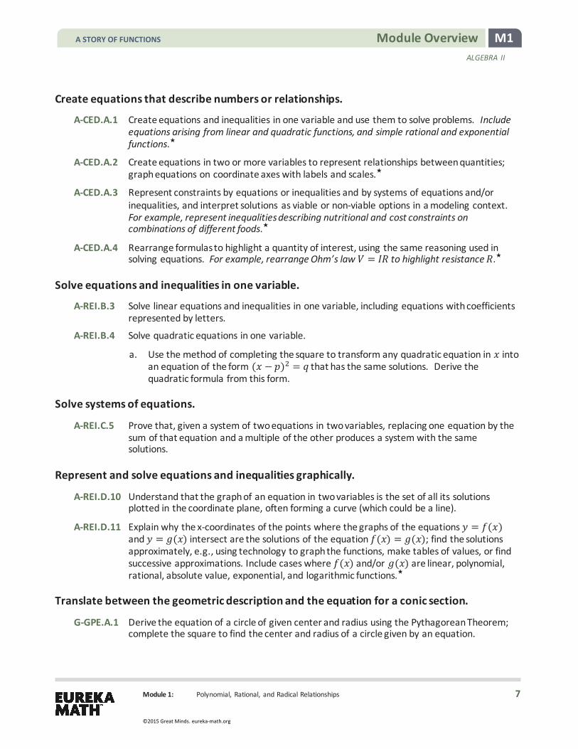
Create equations that describe numbers or relationships.
A-CED.A.1 Create equations and inequalities in one variable and use them to solve problems. Include equations arising from linear and quadratic functions, and simple rational and exponential functions.★
A-CED.A.2 Create equations in two or more variables to represent relationships between quantities; graph equations on coordinate axes with labels and scales.★
A-CED.A.3 Represent constraints by equations or inequalities and by systems of equations and/or inequalities, and interpret solutions as viable or non-viable options in a modeling context. For example, represent inequalities describing nutritional and cost constraints on combinations of different foods.★
A-CED.A.4 Rearrange formulas to highlight a quantity of interest, using the same reasoning used in solving equations. For example, rearrange Ohm’s law 𝑉𝑉 = 𝐼𝐼𝐼𝐼 to highlight resistance 𝐼𝐼.★
Solve equations and inequalities in one variable.
A-REI.B.3 Solve linear equations and inequalities in one variable, including equations with coefficients represented by letters.
A-REI.B.4 Solve quadratic equations in one variable.
a. Use the method of completing the square to transform any quadratic equation in 𝑥𝑥 into an equation of the form (𝑥𝑥 − 𝑝𝑝)2 = 𝑞𝑞 that has the same solutions. Derive the quadratic formula from this form.
Solve systems of equations.
A-REI.C.5 Prove that, given a system of two equations in two variables, replacing one equation by the sum of that equation and a multiple of the other produces a system with the same solutions.
Represent and solve equations and inequalities graphically.
A-REI.D.10 Understand that the graph of an equation in two variables is the set of all its solutions plotted in the coordinate plane, often forming a curve (which could be a line).
A-REI.D.11 Explain why the x-coordinates of the points where the graphs of the equations 𝑦𝑦 = 𝑓𝑓(𝑥𝑥) and 𝑦𝑦 = 𝑔𝑔(𝑥𝑥) intersect are the solutions of the equation 𝑓𝑓(𝑥𝑥) = 𝑔𝑔(𝑥𝑥); find the solutions approximately, e.g., using technology to graph the functions, make tables of values, or find successive approximations. Include cases where 𝑓𝑓(𝑥𝑥) and/or 𝑔𝑔(𝑥𝑥) are linear, polynomial, rational, absolute value, exponential, and logarithmic functions.★
Translate between the geometric description and the equation for a conic section.
G-GPE.A.1 Derive the equation of a circle of given center and radius using the Pythagorean Theorem; complete the square to find the center and radius of a circle given by an equation.
A STORY OF FUNCTIONS
7
©2015 Great Minds. eureka-math.org

M1 Module Overview ALGEBRA II
Module 1: Polynomial, Rational, and Radical Relationships
Focus Standards for Mathematical Practice MP.1 Make sense of problems and persevere in solving them. Students discover the value of
equating factored terms of a polynomial to zero as a means of solving equations involving polynomials. Students solve rational equations and simple radical equations, while considering the possibility of extraneous solutions and verifying each solution before drawing conclusions about the problem. Students solve systems of linear equations and linear and quadratic pairs in two variables. Further, students come to understand that the complex number system provides solutions to the equation 𝑥𝑥2 + 1 = 0 and higher-degree equations.
MP.2 Reason abstractly and quantitatively. Students apply polynomial identities to detect prime numbers and discover Pythagorean triples. Students also learn to make sense of remainders in polynomial long division problems.
MP.4 Model with mathematics. Students use primes to model encryption. Students transition between verbal, numerical, algebraic, and graphical thinking in analyzing applied polynomial problems. Students model a cross-section of a riverbed with a polynomial, estimate fluid flow with their algebraic model, and fit polynomials to data. Students model the locus of points at equal distance between a point (focus) and a line (directrix) discovering the parabola.
MP.7 Look for and make use of structure. Students connect long division of polynomials with the long-division algorithm of arithmetic and perform polynomial division in an abstract setting to derive the standard polynomial identities. Students recognize structure in the graphs of polynomials in factored form and develop refined techniques for graphing. Students discern the structure of rational expressions by comparing to analogous arithmetic problems. Students perform geometric operations on parabolas to discover congruence and similarity.
MP.8 Look for and express regularity in repeated reasoning. Students understand that polynomials form a system analogous to the integers. Students apply polynomial identities to detect prime numbers and discover Pythagorean triples. Students recognize factors of expressions and develop factoring techniques. Further, students understand that all quadratics can be written as a product of linear factors in the complex realm.
Terminology New or Recently Introduced Terms
� Axis of Symmetry (The axis of symmetry of a parabola given by a focus point and a directrix is the perpendicular line to the directrix that passes through the focus.)
� Dilation at the Origin (A dilation at the origin 𝐷𝐷𝑘𝑘 is a horizontal scaling by 𝑘𝑘 > 0 followed by a vertical scaling by the same factor 𝑘𝑘. In other words, this dilation of the graph of 𝑦𝑦 = 𝑓𝑓(𝑥𝑥) is the graph of the equation 𝑦𝑦 = 𝑘𝑘𝑓𝑓 �1
𝑘𝑘𝑥𝑥� . A dilation at the origin is a special type of a dilation.)
A STORY OF FUNCTIONS
8
©2015 Great Minds. eureka-math.org
M1 Module Overview ALGEBRA II
Module 1: Polynomial, Rational, and Radical Relationships
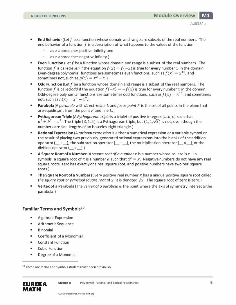
� End Behavior (Let 𝑓𝑓 be a function whose domain and range are subsets of the real numbers. The end behavior of a function 𝑓𝑓 is a description of what happens to the values of the function à as 𝑥𝑥 approaches positive infinity and à as 𝑥𝑥 approaches negative infinity.)
� Even Function (Let 𝑓𝑓 be a function whose domain and range is a subset of the real numbers. The function 𝑓𝑓 is called even if the equation 𝑓𝑓(𝑥𝑥) = 𝑓𝑓(−𝑥𝑥) is true for every number 𝑥𝑥 in the domain. Even-degree polynomial functions are sometimes even functions, such as 𝑓𝑓(𝑥𝑥) = 𝑥𝑥10, and sometimes not, such as 𝑔𝑔(𝑥𝑥) = 𝑥𝑥2 − 𝑥𝑥.)
� Odd Function (Let 𝑓𝑓 be a function whose domain and range is a subset of the real numbers. The function 𝑓𝑓 is called odd if the equation 𝑓𝑓(−𝑥𝑥) = −𝑓𝑓(𝑥𝑥) is true for every number 𝑥𝑥 in the domain. Odd-degree polynomial functions are sometimes odd functions, such as 𝑓𝑓(𝑥𝑥) = 𝑥𝑥11, and sometimes not, such as ℎ(𝑥𝑥) = 𝑥𝑥3 − 𝑥𝑥2.)
� Parabola (A parabola with directrix line 𝐿𝐿 and focus point 𝐹𝐹 is the set of all points in the plane that are equidistant from the point 𝐹𝐹 and line 𝐿𝐿.)
� Pythagorean Triple (A Pythagorean triple is a triplet of positive integers (𝑎𝑎,𝑏𝑏, 𝑐𝑐) such that 𝑎𝑎2 + 𝑏𝑏2 = 𝑐𝑐2. The triple (3,4, 5) is a Pythagorean triple, but (1, 1,√2) is not, even though the numbers are side lengths of an isosceles right triangle.)
� Rational Expression (A rational expression is either a numerical expression or a variable symbol or the result of placing two previously generated rational expressions into the blanks of the addition operator (__+__), the subtraction operator (__−__), the multiplication operator (__×__), or the division operator (__÷__).)
� A Square Root of a Number (A square root of a number 𝑥𝑥 is a number whose square is 𝑥𝑥. In symbols, a square root of 𝑥𝑥 is a number 𝑎𝑎 such that 𝑎𝑎2 = 𝑥𝑥. Negative numbers do not have any real square roots, zero has exactly one real square root, and positive numbers have two real square roots.)
� The Square Root of a Number (Every positive real number 𝑥𝑥 has a unique positive square root called the square root or principal square root of 𝑥𝑥; it is denoted √𝑥𝑥. The square root of zero is zero.)
� Vertex of a Parabola (The vertex of a parabola is the point where the axis of symmetry intersects the parabola.)
Familiar Terms and Symbols10
� Algebraic Expression � Arithmetic Sequence � Binomial � Coefficient of a Monomial � Constant Function � Cubic Function � Degree of a Monomial
10 These are terms and symbols students have seen previously.
A STORY OF FUNCTIONS
9
©2015 Great Minds. eureka-math.org

M1 Module Overview ALGEBRA II
Module 1: Polynomial, Rational, and Radical Relationships
� Degree of a Polynomial Function � Degree of a Polynomial in One Variable � Discriminant of a Quadratic Function � Equivalent Polynomial Expressions � Function � Graph of 𝑓𝑓 � Graph of 𝑦𝑦 = 𝑓𝑓(𝑥𝑥) � Increasing/Decreasing � Like Terms of a Polynomial � Linear Function � Monomial � Numerical Expression � Numerical Symbol � Polynomial Expression � Polynomial Function � Polynomial Identity � Quadratic Function � Relative Maximum � Relative Minimum � Sequence � Standard Form of a Polynomial in One Variable � Terms of a Polynomial � Trinomial � Variable Symbol � Zeros or Roots of a Function
Suggested Tools and Representations � Graphing Calculator � Wolfram Alpha Software � GeoGebra Software
A STORY OF FUNCTIONS
10
©2015 Great Minds. eureka-math.org

M1 Module Overview ALGEBRA II
Module 1: Polynomial, Rational, and Radical Relationships
Preparing to Teach a Module Preparation of lessons will be more effective and efficient if there has been an adequate analysis of the module first. Each module in A Story of Functions can be compared to a chapter in a book. How is the module moving the plot, the mathematics, forward? What new learning is taking place? How are the topics and objectives building on one another? The following is a suggested process for preparing to teach a module. Step 1: Get a preview of the plot.
A: Read the Table of Contents. At a high level, what is the plot of the module? How does the story develop across the topics?
B: Preview the module’s Exit Tickets to see the trajectory of the module’s mathematics and the nature of the work students are expected to be able to do.
Note: When studying a PDF file, enter “Exit Ticket” into the search feature to navigate from one Exit Ticket to the next.
Step 2: Dig into the details.
A: Dig into a careful reading of the Module Overview. While reading the narrative, liberally reference the lessons and Topic Overviews to clarify the meaning of the text—the lessons demonstrate the strategies, show how to use the models, clarify vocabulary, and build understanding of concepts.
B: Having thoroughly investigated the Module Overview, read through the Student Outcomes of each lesson (in order) to further discern the plot of the module. How do the topics flow and tell a coherent story? How do the outcomes move students to new understandings?
Step 3: Summarize the story.
Complete the Mid- and End-of-Module Assessments. Use the strategies and models presented in the module to explain the thinking involved. Again, liberally reference the lessons to anticipate how students who are learning with the curriculum might respond.
A STORY OF FUNCTIONS
11
©2015 Great Minds. eureka-math.org

M1 Module Overview ALGEBRA II
Module 1: Polynomial, Rational, and Radical Relationships
Preparing to Teach a Lesson A three-step process is suggested to prepare a lesson. It is understood that at times teachers may need to make adjustments (customizations) to lessons to fit the time constraints and unique needs of their students. The recommended planning process is outlined below. Note: The ladder of Step 2 is a metaphor for the teaching sequence. The sequence can be seen not only at the macro level in the role that this lesson plays in the overall story, but also at the lesson level, where each rung in the ladder represents the next step in understanding or the next skill needed to reach the objective. To reach the objective, or the top of the ladder, all students must be able to access the first rung and each successive rung. Step 1: Discern the plot.
A: Briefly review the module’s Table of Contents, recalling the overall story of the module and analyzing the role of this lesson in the module.
B: Read the Topic Overview related to the lesson, and then review the Student Outcome(s) and Exit Ticket of each lesson in the topic.
C: Review the assessment following the topic, keeping in mind that assessments can be found midway through the module and at the end of the module.
Step 2: Find the ladder.
A: Work through the lesson, answering and completing each question, example, exercise, and challenge.
B: Analyze and write notes on the new complexities or new concepts introduced with each question or problem posed; these notes on the sequence of new complexities and concepts are the rungs of the ladder.
C: Anticipate where students might struggle, and write a note about the potential cause of the struggle.
D: Answer the Closing questions, always anticipating how students will respond.
Step 3: Hone the lesson.
Lessons may need to be customized if the class period is not long enough to do all of what is presented and/or if students lack prerequisite skills and understanding to move through the entire lesson in the time allotted. A suggestion for customizing the lesson is to first decide upon and designate each question, example, exercise, or challenge as either “Must Do” or “Could Do.”
A: Select “Must Do” dialogue, questions, and problems that meet the Student Outcome(s) while still providing a coherent experience for students; reference the ladder. The expectation should be that the majority of the class will be able to complete the “Must Do” portions of the lesson within the allocated time. While choosing the “Must Do” portions of the lesson, keep in mind the need for a balance of dialogue and conceptual questioning, application problems, and abstract problems, and a balance between students using pictorial/graphical representations and abstract representations. Highlight dialogue to be included in the delivery of instruction so that students have a chance to articulate and consolidate understanding as they move through the lesson.
A STORY OF FUNCTIONS
12
©2015 Great Minds. eureka-math.org
M1 Module Overview ALGEBRA II
Module 1: Polynomial, Rational, and Radical Relationships
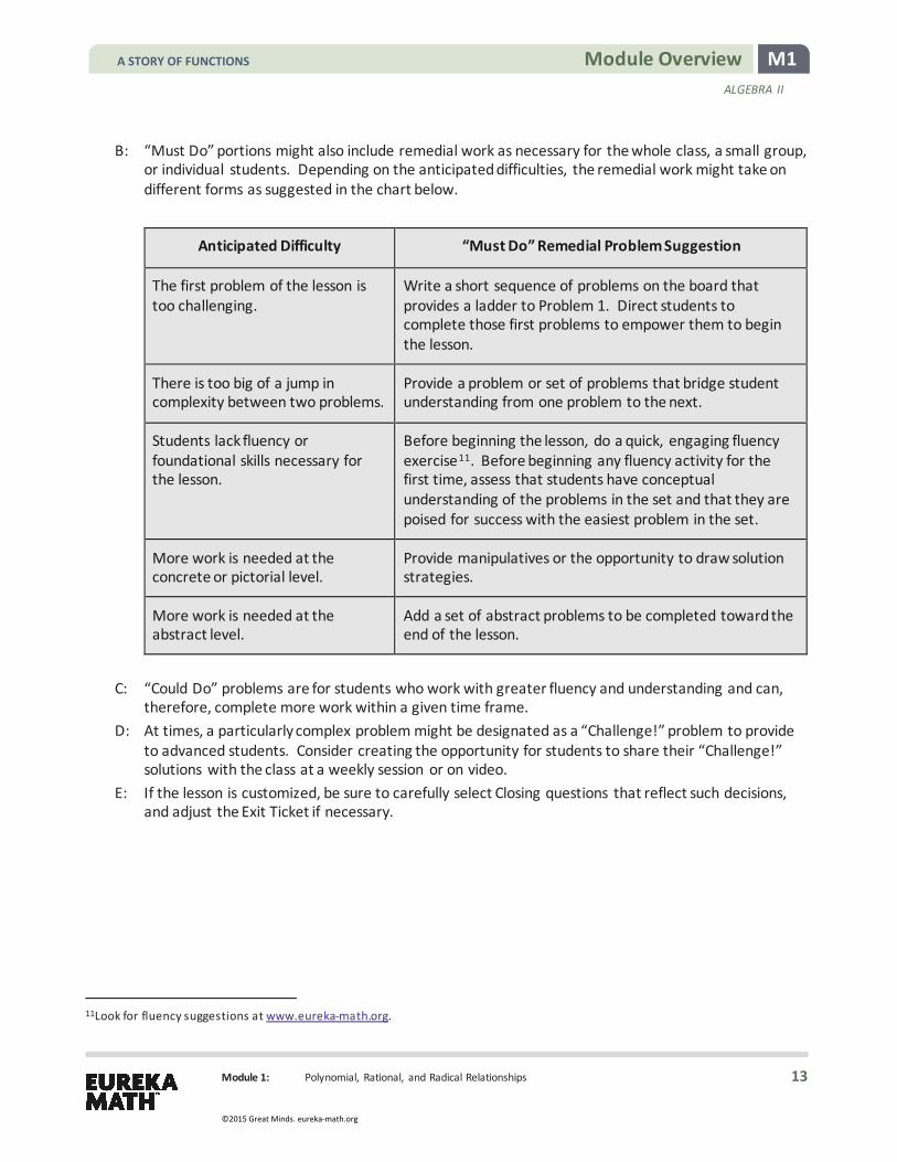
B: “Must Do” portions might also include remedial work as necessary for the whole class, a small group, or individual students. Depending on the anticipated difficulties, the remedial work might take on different forms as suggested in the chart below.
Anticipated Difficulty “Must Do” Remedial Problem Suggestion
The first problem of the lesson is too challenging.
Write a short sequence of problems on the board that provides a ladder to Problem 1. Direct students to complete those first problems to empower them to begin the lesson.
There is too big of a jump in complexity between two problems.
Provide a problem or set of problems that bridge student understanding from one problem to the next.
Students lack fluency or foundational skills necessary for the lesson.
Before beginning the lesson, do a quick, engaging fluency exercise11. Before beginning any fluency activity for the first time, assess that students have conceptual understanding of the problems in the set and that they are poised for success with the easiest problem in the set.
More work is needed at the concrete or pictorial level.
Provide manipulatives or the opportunity to draw solution strategies.
More work is needed at the abstract level.
Add a set of abstract problems to be completed toward the end of the lesson.
C: “Could Do” problems are for students who work with greater fluency and understanding and can,
therefore, complete more work within a given time frame. D: At times, a particularly complex problem might be designated as a “Challenge!” problem to provide
to advanced students. Consider creating the opportunity for students to share their “Challenge!” solutions with the class at a weekly session or on video.
E: If the lesson is customized, be sure to carefully select Closing questions that reflect such decisions, and adjust the Exit Ticket if necessary.
11Look for fluency suggestions at www.eureka-math.org.
A STORY OF FUNCTIONS
13
©2015 Great Minds. eureka-math.org

M1 Module Overview ALGEBRA II
Module 1: Polynomial, Rational, and Radical Relationships
Assessment Summary Assessment Type Administered Format Standards Addressed
Mid-Module Assessment Task After Topic B Constructed response with rubric
N-Q.A.2, A-SSE.A.2, A-APR.B.2, A-APR.B.3, A-APR.C.4, A-REI.A.1, A-REI.B.4b, F-IF.C.7c
End-of-Module Assessment Task After Topic D Constructed response with rubric
N-Q.A.2, A.SSE.A.2, A.APR.B.2, A-APR.B.3, A-APR.C.4, A-APR.D.6, A-REI.A.1, A-REI.A.2, A-REI.B.4b, A-REI.C.6, A-REI.C.7, F-IF.C.7c, G-GPE.A.2
A STORY OF FUNCTIONS
14
©2015 Great Minds. eureka-math.org

Mathematics Curriculum ALGEBRA II • MODULE 1
Topic A: Polynomials—From Base Ten to Base X
Topic A
Polynomials—From Base Ten to Base X
A-SSE.A.2, A-APR.C.4
Focus Standards: A-SSE.A.2 Use the structure of an expression to identify ways to rewrite it. For example, see 𝑥𝑥4 − 𝑦𝑦4 as (𝑥𝑥2)2− (𝑦𝑦2)2, thus recognizing it as a difference of squares that can be factored as (𝑥𝑥2 − 𝑦𝑦2)(𝑥𝑥2 + 𝑦𝑦2).
A-APR.C.4 Prove polynomial identities and use them to describe numerical relationships. For example, the polynomial identity (𝑥𝑥2 + 𝑦𝑦2)2 = (𝑥𝑥2 − 𝑦𝑦2)2 + (2𝑥𝑥𝑦𝑦)2 can be used to generate Pythagorean triples.
Instructional Days: 11
Lesson 1: Successive Differences in Polynomials (P)1
Lesson 2: The Multiplication of Polynomials (P)
Lesson 3: The Division of Polynomials (E)
Lesson 4: Comparing Methods—Long Division, Again? (P)
Lesson 5: Putting It All Together (P)
Lesson 6: Dividing by 𝑥𝑥 −𝑎𝑎 and by 𝑥𝑥 + 𝑎𝑎 (P)
Lesson 7: Mental Math (P)
Lesson 8: The Power of Algebra—Finding Primes (P)
Lesson 9: Radicals and Conjugates (P)
Lesson 10: The Power of Algebra—Finding Pythagorean Triples (P)
Lesson 11: The Special Role of Zero in Factoring (S)
In Topic A, students draw on their foundation of the analogies between polynomial arithmetic and base-ten computation, focusing on properties of operations, particularly the distributive property. In Lesson 1, students write polynomial expressions for sequences by examining successive differences. They are engaged in a lively lesson that emphasizes thinking and reasoning about numbers and patterns and equations. In Lesson 2, they use a variation of the area model referred to as the tabular method to represent polynomial multiplication and connect that method back to application of the distributive property.
1Lesson Structure Key: P-Problem Set Lesson, M-Modeling Cycle Lesson, E-Exploration Lesson, S-Socratic Lesson
A STORY OF FUNCTIONS
15
©2015 Great Minds. eureka-math.org

M1 Topic A ALGEBRA II
Topic A: Polynomials—From Base Ten to Base X
In Lesson 3, students continue using the tabular method and analogies to the system of integers to explore division of polynomials as a missing factor problem. In this lesson, students also take time to reflect on and arrive at generalizations for questions such as how to predict the degree of the resulting sum when adding two polynomials. In Lesson 4, students are ready to ask and answer whether long division can work with polynomials too and how it compares with the tabular method of finding the missing factor. Lesson 5 gives students additional practice on all operations with polynomials and offers an opportunity to examine the
structure of expressions such as recognizing that 𝑛𝑛(𝑛𝑛 1)(2𝑛𝑛 1)
is a 3rd degree polynomial expression with
leading coefficient 13 without having to expand it out.
In Lesson 6, students extend their facility with dividing polynomials by exploring a more generic case; rather than dividing by a factor such as (𝑥𝑥 + 3), they divide by the factor (𝑥𝑥 + 𝑎𝑎) or (𝑥𝑥 − 𝑎𝑎). This gives them the opportunity to discover the structure of special products such as (𝑥𝑥 − 𝑎𝑎)(𝑥𝑥2 + 𝑎𝑎𝑥𝑥 + 𝑎𝑎2) in Lesson 7 and go on to use those products in Lessons 8–10 to employ the power of algebra over the calculator. In Lesson 8, they find they can use special products to uncover mental math strategies and answer questions such as whether or not 2100− 1 is prime. In Lesson 9, they consider how these properties apply to expressions that contain square roots. Then, in Lesson 10, they use special products to find Pythagorean triples.
The topic culminates with Lesson 11 and the recognition of the benefits of factoring and the special role of zero as a means for solving polynomial equations.
A STORY OF FUNCTIONS
16
©2015 Great Minds. eureka-math.org

M1 Lesson 1 ALGEBRA II
Lesson 1: Successive Differences in Polynomials
Lesson 1: Successive Differences in Polynomials
Student Outcomes
� Students write explicit polynomial expressions for sequences by investigating successive differences of those sequences.
Lesson Notes This first lesson of the year tells students that this course is about thinking and reasoning with mathematics. It reintroduces the study of polynomials in a surprising new way involving sequences. This offers a chance to evaluate how much students recall from Algebra I. The lesson starts with discussions of expressions, polynomials, sequences, and equations. In this lesson, students continue the theme that began in Grade 6 of evaluating and building expressions. Explore ways to test students’ recall of the vocabulary terms listed at the end of this lesson.
Throughout this lesson, l isten carefully to students’ discussions. Their reactions will indicate how to best approach the rest of the module. The homework set to this lesson should also offer insight into how much they remember from previous grades and how well they can read instructions. In particular, if they have trouble with evaluating or simplifying expressions or solving equations, then consider revisiting Lessons 6–9 in Algebra I, Module 1, and Lesson 2 in Algebra I, Module 4. If they are having trouble solving equations, use Lessons 10–12, 15–16, and 19 in Algebra I, Module 1 to give them extra practice.
Finally, the use of the term constant may need a bit of extra discussion. It is used throughout this PK–12 curriculum in two ways: either as a constant number (e.g., the 𝑎𝑎 in 𝑎𝑎𝑥𝑥2+ 𝑏𝑏𝑥𝑥 + 𝑐𝑐 is a number chosen once-and-for-all at the beginning of a problem) or as a constant rate (e.g., a copier that reproduces at a constant rate of 40 copies/minute). Both uses are offered in this lesson.
Classwork Opening Exercise (7 minutes)
This exercise provides an opportunity to think about and generalize the main concept of today’s lesson: that the second differences of a quadratic polynomial are constant. This generalizes to the th differences of a degree polynomial. The goal is to help students investigate, discuss, and generalize the second and higher differences in this exercise.
Present the exercise to students and ask them (in groups of two) to study the table and explain to their partner how to calculate each line in the table. If they get stuck, help them find entry points into this question, possibly by drawing segments connecting the successive differences on their papers (e.g., connect 5.76 and 11.56 to 5.8 and ask, “How are these three numbers related?”). This initial problem of the school year is designed to encourage students to persevere and look for and express regularity in repeated reasoning.
Teachers may also use the Opening Exercise to informally assess students’ pattern-finding abilities and fluency with rational numbers.
MP.1 &
MP.8
Scaffolding: Before presenting the problem below, consider starting by displaying the first two rows of the table on the board and asking students to investigate the relationship between them, including making a conjecture about the nature of the relationship.
A STORY OF FUNCTIONS
17
©2015 Great Minds. eureka-math.org

M1 Lesson 1 ALGEBRA II
Lesson 1: Successive Differences in Polynomials
Opening Exercise
John noticed patterns in the arrangement of numbers in the table below.
Number . . . . .
Square . . . . .
First Differences . . . .
Second Differences
Assuming that the pattern would continue, he used it to find the value of . . Explain how he used the pattern to find
. , and then use the pattern to find . .
To find . , John assumed the next term in the first differences would have to be . since . is more than . . Therefore, the next term in the square numbers would have to be . + . , which is . . Checking with a calculator, we also find . = . .
To find . , we follow the same process: The next term in the first differences would have to be . , so the next term in the square numbers would be . + . , which is . .
Check: . = . .
How would you label each row of numbers in the table?
Number, Square, First Differences, Second Differences
Discuss with students the relationship between each row and the row above it and how to label the rows based upon that relationship. Feel free to have this discussion before or after they find 7.42 and 8.42. They are l ikely to come up with labels such as subtract or difference for the third and fourth row. However, guide them to call the third and fourth rows First Differences and Second Differences, respectively.
Discussion (3 minutes)
The pattern i llustrated in the Opening Exercise is a particular case of a general phenomenon about polynomials. In Algebra I, Module 3, students saw how to recognize l inear functions and exponential functions by recognizing similar growth patterns; that is, l inear functions grow by a constant difference over successive intervals of equal length, and exponential functions grow by a constant factor over successive intervals of equal length. This lesson sees the generalization of the l inear growth pattern to polynomials of second degree (quadratic expressions) and third degree (cubic expressions).
Discussion
Let the sequence { , , , ,… } be generated by evaluating a polynomial expression at the values , , , , … The numbers found by evaluating − , − , − , … form a new sequence, which we will call the first differences of the polynomial. The differences between successive terms of the first differences sequence are called the second differences and so on.
It is a good idea to use an actual sequence of numbers such as the square numbers {1, 4,9, 16,… } to help explain the meaning of the terms first differences and second differences.
MP.8
Scaffolding: For students working below grade level, consider using positive integers {1,2, 3,… } and corresponding squares {1,4, 9, … } instead of using {2.4,3.4,4.4,… }.
A STORY OF FUNCTIONS
18
©2015 Great Minds. eureka-math.org

M1 Lesson 1 ALGEBRA II
Lesson 1: Successive Differences in Polynomials
Example 1 (4 minutes)
Although it may be tempting to work through Example 1 using numbers instead of 𝑎𝑎 and 𝑏𝑏, using symbols 𝑎𝑎 and 𝑏𝑏 actually makes the structure of the first differences sequence obvious, whereas numbers could hide that structure. Also, working with constant coefficients gives the generalization all at once.
Note: Consider using Example 1 to informally assess students’ fluency with algebraic manipulations. Example 1
What is the sequence of first differences for the linear polynomial given by + , where and are constant coefficients?
The terms of the first differences sequence are found by subtracting consecutive terms in the sequence generated by the polynomial expression + , namely, { , + , + , + , + ,… }.
1st term: ( + ) − = ,
2nd term: ( + ) − ( + ) = ,
3rd term: ( + ) − ( + ) = ,
4th term: ( + ) − ( + ) = .
The first differences sequence is { , , , ,… } . For first-degree polynomial expressions, the first differences are constant and equal to .
What is the sequence of second differences for + ?
Since − = , the second differences are all . Thus, the sequence of second differences is { , , , , … }.
� How is this calculation similar to the arithmetic sequences you studied in Algebra I, Module 3?
à The constant derived from the first differences of a linear polynomial is the same constant addend used to define the arithmetic sequence generated by the polynomial. That is, the 𝑎𝑎 in ( ) = 𝑎𝑎 + 𝑏𝑏 for
0. Written recursively this is (0) = 𝑏𝑏 and ( + 1) = ( ) + 𝑎𝑎 for 0.
For Examples 2 and 3, let students work in groups of two to fi l l in the blanks of the tables (3 minute maximum for each table). Walk around the room, checking student work for understanding. Afterward, discuss the paragraphs below each table as a whole class.
Scaffolding:
Try starting the example by first asking students to generate sequences of first differences for 2𝑥𝑥 + 3, 3𝑥𝑥 − 1, and 4𝑥𝑥 + 2. For example, the sequence generated by 2𝑥𝑥 + 3 is {3,5, 7,9, …}, and its sequence of first differences is {2,2, 2, 2 … }.
These three sequences can then be used as a source of examples from which to make and verify conjectures.
A STORY OF FUNCTIONS
19
©2015 Great Minds. eureka-math.org

M1 Lesson 1 ALGEBRA II
Lesson 1: Successive Differences in Polynomials
Example 2 (5 minutes)
Example 2
Find the first, second, and third differences of the polynomial + + by filling in the blanks in the following table.
+ + First Differences Second Differences Third Differences
+ + +
+ + +
+ + +
+ + +
+ + +
The table shows that the second differences of the polynomial 𝑎𝑎𝑥𝑥2 + 𝑏𝑏𝑥𝑥+ 𝑐𝑐 all have the constant value 2𝑎𝑎. The second differences hold for any sequence of values of 𝑥𝑥 where the values in the sequence differ by 1, as the Opening Exercise shows. For example, if we studied the second differences for 𝑥𝑥-values , + 1, + 2, + 3, …, we would find that the second differences would also be 2𝑎𝑎. In your homework, you will show that this fact is indeed true by finding the second differences for the values + 0, + 1, + 2, + 3, + 4.
Ask students to describe what they notice in the sequences of first, second, and third differences. Have them make a conjecture about the third and fourth differences of a sequence generated by a third degree polynomial.
Students are l ikely to say that the third differences have the constant value 3𝑎𝑎 (which is incorrect). Have them work through the next example to help them discover what the third differences really are. This is a good example of why it is necessary to follow up conjecture based on observation with proof.
Example 3 (7 minutes)
Example 3
Find the second, third, and fourth differences of the polynomial + + + by filling in the blanks in the following table.
+ + + First Differences Second Differences Third Differences Fourth Differences
+ + + + + +
+ + + + + +
+ + + + + +
+ + + + + +
+ + + + +
MP.7 &
MP.8
A STORY OF FUNCTIONS
20
©2015 Great Minds. eureka-math.org

M1 Lesson 1 ALGEBRA II
Lesson 1: Successive Differences in Polynomials
The third differences of 𝑎𝑎𝑥𝑥3 + 𝑏𝑏𝑥𝑥2 + 𝑐𝑐𝑥𝑥+ all have the constant value 6𝑎𝑎. Also, if a different sequence of values for 𝑥𝑥 that differed by 1 was used instead, the third differences would still have the value 6𝑎𝑎.
� Ask students to make a conjecture about the fourth differences of a sequence generated by a degree 4 polynomial. Students who were paying attention to their (likely wrong) conjecture of the third differences before doing this example may guess that the fourth differences are constant and equal to (1 2 3 4)𝑎𝑎, which is 24𝑎𝑎. This pattern continues: the th differences of any sequence generated by an th degree polynomial with leading coefficient 𝑎𝑎 will be constant and have the value 𝑎𝑎 ( !).
� Ask students to make a conjecture about the ( + 1)st differences of a degree polynomial, for example, the 5th differences of a fourth-degree polynomial.
Students are now ready to tackle the main goal of this lesson—using differences to recognize polynomial relationships and build polynomial expressions.
Example 4 (7 minutes)
When collecting bivariate data on an event or experiment, the data does not announce, “I satisfy a quadratic relationship,” or “I satisfy an exponential relationship.” There need to be ways to recognize these relationships in order to model them with functions. In Algebra I, Module 3, students studied the conditions upon which they could conclude that the data satisfied a l inear or exponential relationship. Either the first differences were constant, or first factors were constant. By checking that the second or third differences of the data are constant, students now have a way to recognize a quadratic or cubic relationship and can write an equation to describe that relationship (A-CED.A.3, F-BF.A.1a).
Give students an opportunity to attempt this problem in groups of two. Walk around the room helping them find the leading coefficient.
Example 4
What type of relationship does the set of ordered pairs ( , ) satisfy? How do you know? Fill in the blanks in the table below to help you decide. (The first differences have already been computed for you.)
First Differences Second Differences Third Differences
−
Since the third differences are constant, the pairs could represent a cubic relationship between and .
A STORY OF FUNCTIONS
21
©2015 Great Minds. eureka-math.org

M1 Lesson 1 ALGEBRA II
Lesson 1: Successive Differences in Polynomials
Find the equation of the form = + + + that all ordered pairs ( , ) above satisfy. Give evidence that your equation is correct.
Since third differences of a cubic polynomial are equal to , using the table above, we get = , so that = . Also, since ( , ) satisfies the equation, we see that = . Thus, we need only find and . Substituting ( , ) and ( , ) into the equation, we get
= + + + = + + + .
Subtracting two times the first equation from the second, we get = + − , so that = . Substituting in for in the first equation gives = − . Thus, the equation is = − + .
� After finding the equation, have students check that the pairs (3,23) and (4, 58) satisfy the equation.
Help students to persevere in finding the coefficients. They will most l ikely try to plug three ordered pairs into the equation, which gives a 3 × 3 system of l inear equations in 𝑎𝑎, 𝑏𝑏, and 𝑐𝑐 after they find that = 2. Using the fact that the third differences of a cubic polynomial are 6𝑎𝑎 will greatly simplify the problem. (It implies 𝑎𝑎 = 1 immediately, which reduces the system to the easy 2 × 2 system above.) Walk around the room as they work, and ask questions that lead them to realize that they can use the third differences fact if they get too stuck. Alternatively, find a student who used the fact, and then have the class discuss and understand his or her approach.
Closing (7 minutes)
� What are some of the key ideas that we learned today? à Sequences whose second differences are constant satisfy a quadratic relationship. à Sequences whose third differences are constant satisfy a cubic relationship.
The following terms were introduced and taught in Module 1 of Algebra I. The terms are listed here for completeness and reference.
Relevant Vocabulary
NUMERICAL SYMBOL: A numerical symbol is a symbol that represents a specific number. Examples: , , , , ,− . .
VARIABLE SYMBOL: A variable symbol is a symbol that is a placeholder for a number from a specified set of numbers. The set of numbers is called the domain of the variable. Examples: , , .
ALGEBRAIC EXPRESSION: An algebraic expression is either
1. a numerical symbol or a variable symbol or
2. the result of placing previously generated algebraic expressions into the two blanks of one of the four operators ((__) + (__), (__)− (__), (__)× (__), (__) ÷ (__)) or into the base blank of an exponentiation with an exponent that is a rational number.
Following the definition above, � ( )× ( ) × ( )�+ ( ) × ( ) is an algebraic expression, but it is generally written more simply as + .
NUMERICAL EXPRESSION: A numerical expression is an algebraic expression that contains only numerical symbols (no variable
symbols) that evaluates to a single number. Example: The numerical expression ( )
evaluates to .
MONOMIAL: A monomial is an algebraic expression generated using only the multiplication operator (__ × __). The expressions and are both monomials.
BINOMIAL: A binomial is the sum of two monomials. The expression + is a binomial.
MP.1
A STORY OF FUNCTIONS
22
©2015 Great Minds. eureka-math.org

M1 Lesson 1 ALGEBRA II
Lesson 1: Successive Differences in Polynomials
POLYNOMIAL EXPRESSION: A polynomial expression is a monomial or sum of two or more monomials.
SEQUENCE: A sequence can be thought of as an ordered list of elements. The elements of the list are called the terms of the sequence.
ARITHMETIC SEQUENCE: A sequence is called arithmetic if there is a real number such that each term in the sequence is the sum of the previous term and .
Exit Ticket (5 minutes)
A STORY OF FUNCTIONS
23
©2015 Great Minds. eureka-math.org

M1 Lesson 1 ALGEBRA II
Lesson 1: Successive Differences in Polynomials
Name Date
Lesson 1: Successive Differences in Polynomials
Exit Ticket 1. What type of relationship is indicated by the following set of ordered pairs? Explain how you know.
0 0
1 2
2 10
3 24
4 44
2. Find an equation that all ordered pairs above satisfy.
A STORY OF FUNCTIONS
24
©2015 Great Minds. eureka-math.org

M1 Lesson 1 ALGEBRA II
Lesson 1: Successive Differences in Polynomials
Exit Ticket Sample Solutions
1. What type of relationship is indicated by the following set of ordered pairs? Explain how you know.
First Differences Second Differences
Since the second differences are constant, there is a quadratic relationship between and .
2. Find an equation that all ordered pairs above satisfy.
Since ( , ) satisfies an equation of the form = + + , we have that = . Using the points ( , ) and ( , ), we have
= + = +
Subtracting twice the first equation from the second gives = , which means = . Substituting into the first equation gives = − . Thus, = − is the equation.
OR
Since the pairs satisfy a quadratic relationship, the second differences must be equal to . Therefore, = , so = . Since ( , ) satisfies the equation, = . Using the point ( , ), we have that = + + , so = − . Thus, = − is the equation that is satisfied by these points.
Problem Set Sample Solutions
1. Create a table to find the second differences for the polynomial − for integer values of from to .
− First Differences Second Differences
− −
− − −
− − −
− − −
− −
A STORY OF FUNCTIONS
25
©2015 Great Minds. eureka-math.org

M1 Lesson 1 ALGEBRA II
Lesson 1: Successive Differences in Polynomials
2. Create a table to find the third differences for the polynomial − + for integer values of from − to .
− + First Differences Second Differences Third Differences − −
− − −
− − −
−
3. Create a table of values for the polynomial , using , + , + , + , + as values of . Show that the second differences are all equal to .
First Differences Second Differences
+ + + +
+ + + +
+ + + +
+ + + +
4. Show that the set of ordered pairs ( , ) in the table below satisfies a quadratic relationship. (Hint: Find second
differences.) Find the equation of the form = + + that all of the ordered pairs satisfy.
− − − −
Students show that second differences are constant and equal to − . The equation is = − + + .
5. Show that the set of ordered pairs ( , ) in the table below satisfies a cubic relationship. (Hint: Find third differences.) Find the equation of the form = + + + that all of the ordered pairs satisfy.
Students show that third differences are constant and equal to . The equation is = − + .
A STORY OF FUNCTIONS
26
©2015 Great Minds. eureka-math.org

M1 Lesson 1 ALGEBRA II
Lesson 1: Successive Differences in Polynomials
6. The distance . required to stop a car traveling at under dry asphalt conditions is given by the following table.
. .
a. What type of relationship is indicated by the set of ordered pairs?
Students show that second differences are constant and equal to . . Therefore, the relationship is quadratic.
b. Assuming that the relationship continues to hold, find the distance required to stop the car when the speed reaches , when = .
.
c. Extension: Find an equation that describes the relationship between the speed of the car and its stopping distance .
= . + . (Note: Students do not need to find the equation to answer part (b).)
7. Use the polynomial expressions + + and + to answer the questions below.
a. Create a table of second differences for the polynomial + + for the integer values of from to .
+ + First Differences Second Differences
b. Justin claims that for , the th differences of the sum of a degree polynomial and a linear polynomial
are the same as the th differences of just the degree polynomial. Find the second differences for the sum ( + + ) + ( + ) of a degree and a degree polynomial, and use the calculation to explain why Justin might be correct in general. Students compute that the second differences are constant and equal to , just as in part (a). Justin is correct because the differences of the sum are the sum of the differences. Since the second (and all other higher) differences of the degree polynomial are constant and equal to zero, only the th differences of the degree polynomial contribute to the th difference of the sum.
c. Jason thinks he can generalize Justin’s claim to the product of two polynomials. He claims that for , the ( + )st differences of the product of a degree polynomial and a linear polynomial are the same as the th differences of the degree polynomial. Use what you know about second and third differences (from Examples 2 and 3) and the polynomial ( + + )( + ) to show that Jason’s generalization is incorrect.
The second differences of a quadratic polynomial are , so the second differences of + + are always . Since ( + + )( + ) = + + + , and third differences are equal to , we have
that the third differences of ( + + )( + ) are always , which is not .
A STORY OF FUNCTIONS
27
©2015 Great Minds. eureka-math.org

Lesson 2: The Multiplication of Polynomials
M1 Lesson 2 ALGEBRA II
Lesson 2: The Multiplication of Polynomials
Student Outcomes � Students develop the distributive property for application to polynomial multiplication. Students connect
multiplication of polynomials with multiplication of multi-digit integers.
Lesson Notes This lesson begins to address standards A-SSE.A.2 and A-APR.C.4 directly and provides opportunities for students to practice MP.7 and MP.8. The work is scaffolded to allow students to discern patterns in repeated calculations, leading to some general polynomial identities that are explored further in the remaining lessons of this module.
As in the last lesson, if students struggle with this lesson, they may need to review concepts covered in previous grades, such as:
• The connection between area properties and the distributive property: Grade 7, Module 6, Lesson 21. • Introduction to the table method of multiplying polynomials: Algebra I, Module 1, Lesson 9. • Multiplying polynomials (in the context of quadratics): Algebra I, Module 4, Lessons 1 and 2.
Since division is the inverse operation of multiplication, it is important to make sure that your students understand how to multiply polynomials before moving on to division of polynomials in Lesson 3 of this module. In Lesson 3, division is explored using the reverse tabular method, so it is important for students to work through the table diagrams in this lesson to prepare them for the upcoming work.
There continues to be a sharp distinction in this curriculum between justification and proof, such as justifying the identity (𝑎𝑎 + 𝑏𝑏)2 = 𝑎𝑎2 + 2𝑎𝑎𝑏𝑏 + 𝑏𝑏 using area properties and proving the identity using the distributive property. The key point is that the area of a figure is always a nonnegative quantity and so cannot be used to prove an algebraic identity where the letters can stand for negative numbers (there is no such thing as a geometric figure with negative area). This is one of many reasons that manipulatives such as Algebra Tiles need to be handled with extreme care: depictions of negative area actually teach incorrect mathematics. (A correct way to model expressions involving the subtraction of two positive quantities using an area model is depicted in the last problem of the Problem Set.)
The tabular diagram described in this lesson is purposely designed to look l ike an area model without actually being an area model. It is a convenient way to keep track of the use of the distributive property, which is a basic property of the number system and is assumed to be true for all real numbers—regardless of whether they are positive or negative, fractional or irrational.
Classwork Opening Exercise (5 minutes)
The Opening Exercise is a simple use of an area model to justify why the distributive property works when multiplying 28 × 27. When drawing the area model, remember that it really matters that the length of the side of the big square is about 2 1
2 times the length of the top side of the upper right rectangle (20 units versus 8 units) in the picture below and
similarly for the lengths going down the side of the large rectangle. It should be an accurate representation of the area of a rectangular region that measures 28 units by 27 units.
A STORY OF FUNCTIONS
28
©2015 Great Minds. eureka-math.org

Lesson 2: The Multiplication of Polynomials
M1 Lesson 2 ALGEBRA II
( + )( + ) = + +
+
+
Scaffolding: For students working above grade level, consider asking them to prove that (𝑎𝑎 + 𝑏𝑏)(𝑐𝑐 + ) = 𝑎𝑎𝑐𝑐 + 𝑏𝑏𝑐𝑐 +𝑎𝑎 + 𝑏𝑏 , where 𝑎𝑎, 𝑏𝑏, 𝑐𝑐, and are all positive real numbers.
Opening Exercise
Show that × = ( + )( + ) using an area model. What do the numbers you placed inside the four rectangular regions you drew represent?
The numbers placed into the blanks represent the number of unit squares (or square units) in each sub-rectangle.
Example 1 (9 minutes)
Explain that the goal today is to generalize the Opening Exercise to multiplying polynomials. Start by asking students how the expression (𝑥𝑥 + 8)(𝑥𝑥+ 7) is similar to the expression 28 × 27. Then suggest that students replace 20 with 𝑥𝑥 in the area model. Since 𝑥𝑥 in (𝑥𝑥 + 8)(𝑥𝑥 + 7) can stand for a negative number, but lengths and areas are always positive, an area model cannot be used to represent the polynomial expression (𝑥𝑥 + 8)(𝑥𝑥+ 7) without also saying that 𝑥𝑥 > 0. So it is not correct to say that the area model above (with 20 replaced by 𝑥𝑥) represents the polynomial expression (𝑥𝑥 + 8)(𝑥𝑥 + 7) for all values of 𝑥𝑥. The tabular method below is meant to remind students of the area model as a visual representation, but it is not an area model.
Example 1
Use the tabular method to multiply ( + )( + ) and combine like terms.
� Explain how the result 𝑥𝑥2 + 15𝑥𝑥 + 56 is related to 756 determined in the Opening Exercise.
à If 𝑥𝑥 is replaced with 20 in 𝑥𝑥2+ 15𝑥𝑥 + 56, then the calculation becomes the same as the one shown in the Opening Exercise: (20)2+ 15(20) + 56 = 400 + 300 + 56 = 756.
× = ( + )( + )
= + + + =
MP.7
A STORY OF FUNCTIONS
29
©2015 Great Minds. eureka-math.org

Lesson 2: The Multiplication of Polynomials
M1 Lesson 2 ALGEBRA II
Scaffolding: If students need to work another problem, ask students to use an area model to find 16 × 19 and then use the tabular method to find (𝑥𝑥 + 6)(𝑥𝑥 + 9).
� How can we multiply these binomials without using a table? à Think of 𝑥𝑥 + 8 as a single number and distribute over 𝑥𝑥 + 7:
Next, distribute the 𝑥𝑥 over 𝑥𝑥 + 8 and the 7 over 𝑥𝑥 + 8. Combining like terms shows that (𝑥𝑥 + 8)(𝑥𝑥 + 7) = 𝑥𝑥2+ 15𝑥𝑥+ 56.
� What property did we repeatedly use to multiply the binomials? à The distributive property
� The table in the calculation above looks like the area model in the Opening Exercise. What are the similarities? What are the differences?
à The expressions placed in each table entry correspond to the expressions placed in each rectangle of the area model. The sum of the table entries represents the product, just as the sum of the areas of the sub-rectangles is the total area of the large rectangle.
à One difference is that we might have 𝑥𝑥 < 0 so that 7𝑥𝑥 and 8𝑥𝑥 are negative, which does not make sense in an area model.
� How would you have to change the table so that it represents an area model?
à First, all numbers and variables would have to represent positive lengths. So, in the example above, we would have to assume that 𝑥𝑥 > 0. Second, the lengths should be commensurate with each other; that is, the side length for the rectangle represented by 7 should be slightly shorter than the side length represented by 8.
� How is the tabular method similar to the distributive property?
à The sum of the table entries is equal to the result of repeatedly applying the distributive property to (𝑥𝑥 + 8)(𝑥𝑥 + 7). The tabular method graphically organizes the results of using the distributive property.
� Does the table work even when the binomials do not represent lengths? Why?
à Yes it does because the table is an easy way to summarize calculations done with the distributive property—a property that works for all polynomial expressions.
Exercises 1–2 (6 minutes)
Allow students to work in groups or pairs on these exercises. While Exercise 1 is analogous to the previous example, in Exercise 2, students may need time to think about how to handle the zero coefficient of 𝑥𝑥 in 𝑥𝑥2 − 2. Allow them to struggle and discuss possible solutions.
𝑥𝑥 + 8 (𝑥𝑥 + 7) = 𝑥𝑥+ 8 𝑥𝑥+ 𝑥𝑥 + 8 7
(𝑥𝑥 + 8)(𝑥𝑥+ 7) = (𝑥𝑥 + 8) 𝑥𝑥 + (𝑥𝑥 + 8) 7 = 𝑥𝑥2 + 8𝑥𝑥+ 7𝑥𝑥 + 56
MP.7
A STORY OF FUNCTIONS
30
©2015 Great Minds. eureka-math.org

Lesson 2: The Multiplication of Polynomials
M1 Lesson 2 ALGEBRA II
Exercises 1–2
1. Use the tabular method to multiply ( + + )( − + ) and combine like terms.
Sample student work:
2. Use the tabular method to multiply ( + + )( − ) and combine like terms.
Sample student work:
Example 2 (6 minutes)
Prior to Example 2, consider asking students to find the products of each of these expressions.
(𝑥𝑥 − 1)(𝑥𝑥+ 1) (𝑥𝑥− 1)(𝑥𝑥2+ 𝑥𝑥 + 1)
(𝑥𝑥 − 1)(𝑥𝑥3 + 𝑥𝑥2 + 𝑥𝑥 + 1) Students may work on this in mixed-ability groups and come to generalize the pattern.
( + + )( − + ) = − − + +
( + + )( − ) = + − − −
Another solution method would be to omit the row for in the table and to manually add all table entries instead of adding along the diagonals:
( + + )( − ) = + + − − − = + − − −
Scaffolding: For further scaffolding, consider asking students to see the pattern using numerical expressions, such as:
(2 − 1)(21 + 1) (2 − 1)(22 + 2 + 1)
(2 − 1)(23 + 22 + 2 + 1). Can they describe in words or symbols the meaning of these quantities?
A STORY OF FUNCTIONS
31
©2015 Great Minds. eureka-math.org

Lesson 2: The Multiplication of Polynomials
M1 Lesson 2 ALGEBRA II
Example 2
Multiply the polynomials ( − )( + + + + ) using a table. Generalize the pattern that emerges by writing down an identity for ( − )( + + + + + ) for a positive integer.
The pattern suggests ( − )( + + + + + ) = − .
� What quadratic identity from Algebra I does the identity above generalize?
à This generalizes (𝑥𝑥 − 1)(𝑥𝑥 + 1) = 𝑥𝑥2− 1, or more generally, the difference of squares formula (𝑥𝑥 −𝑦𝑦)(𝑥𝑥 + 𝑦𝑦) = 𝑥𝑥2 − 𝑦𝑦2 with 𝑦𝑦 = 1. We will explore this last identity in more detail in Exercises 4 and 5.
Exercises 3–4 (10 minutes)
Before moving on to Exercise 3, it may be helpful to scaffold the problem by asking students to multiply (𝑥𝑥 −𝑦𝑦)(𝑥𝑥 + 𝑦𝑦) and (𝑥𝑥 −𝑦𝑦)(𝑥𝑥2+ 𝑥𝑥𝑦𝑦+ 𝑦𝑦2). Ask students to make conjectures about the form of the answer to Exercise 3.
Exercises 3–4
3. Multiply ( − )( + + + ) using the distributive property and combine like terms. How is this calculation similar to Example 2?
Distribute the expression + + + through − to get
( − )( + + + ) = + + + − − − − = −
Substitute in for to get the identity for = in Example 2.
This calculation is similar to Example 2 because it has the same structure. Substituting for results in the same expression as Example 2.
Exercise 3 shows why the mnemonic FOIL is not very helpful—and in this case does not make sense. By now, students should have had enough practice multiplying to no longer require such mnemonics to help them. They understand that the multiplications they are doing are really repeated use of the distributive property, an idea that started when they learned the multiplication algorithm in Grade 4. However, it may still be necessary to summarize the process with a mnemonic. If this is the case, try Each-With-Each, or EWE, which is short for the process of multiplying each term of one polynomial with each term of a second polynomial and combining like terms.
MP.8 ( − )( + + + + ) = −
−
−
−
−
−
−
−
MP.1
A STORY OF FUNCTIONS
32
©2015 Great Minds. eureka-math.org

Lesson 2: The Multiplication of Polynomials
M1 Lesson 2 ALGEBRA II
To introduce Exercise 4, consider starting with a group activity to help i lluminate the generalization. For example, students could work in groups again to investigate the pattern found in expanding these expressions.
(𝑥𝑥2 + 𝑦𝑦2)(𝑥𝑥2− 𝑦𝑦2)
(𝑥𝑥3 + 𝑦𝑦3)(𝑥𝑥3− 𝑦𝑦3)
(𝑥𝑥4 + 𝑦𝑦4)(𝑥𝑥4− 𝑦𝑦4)
(𝑥𝑥 + 𝑦𝑦 )(𝑥𝑥 −𝑦𝑦 )
4. Multiply ( − )( + ) using the distributive property and combine like terms. Generalize the pattern that emerges to write down an identity for ( − )( + ) for positive integers .
( − )( + ) = ( − ) + ( − ) = − + − = − .
Generalization: ( − )( + ) = − .
Sample student work:
� The generalized identity 𝑥𝑥2𝑛𝑛− 𝑦𝑦2𝑛𝑛 = (𝑥𝑥𝑛𝑛−𝑦𝑦𝑛𝑛)(𝑥𝑥𝑛𝑛 + 𝑦𝑦𝑛𝑛) is used several times in this module. For example, it helps to recognize that 2130 − 1 is not a prime number because it can be written as (2 − 1)(2 + 1). Some of the problems in the Problem Set rely on this type of thinking.
Closing (4 minutes)
Ask students to share two important ideas from the day’s lesson with their neighbor. You can also use this opportunity to informally assess their understanding.
� Multiplication of two polynomials is performed by repeatedly applying the distributive property and combining l ike terms.
� There are several useful identities:
- (𝑎𝑎 + 𝑏𝑏)(𝑐𝑐 + ) = 𝑎𝑎𝑐𝑐 + 𝑎𝑎 + 𝑏𝑏𝑐𝑐 + 𝑏𝑏 (an example of each-with-each)
- (𝑎𝑎 + 𝑏𝑏) 2 = 𝑎𝑎2 + 2𝑎𝑎𝑏𝑏 + 𝑏𝑏2
- (𝑥𝑥𝑛𝑛 −𝑦𝑦𝑛𝑛)(𝑥𝑥𝑛𝑛 + 𝑦𝑦𝑛𝑛) = 𝑥𝑥2𝑛𝑛 − 𝑦𝑦2𝑛𝑛, including (𝑥𝑥 −𝑦𝑦)(𝑥𝑥 + 𝑦𝑦) = 𝑥𝑥2 − 𝑦𝑦2 and (𝑥𝑥2 − 𝑦𝑦2)(𝑥𝑥2+ 𝑦𝑦2) = 𝑥𝑥4 − 𝑦𝑦4
- (𝑥𝑥 − 1)(𝑥𝑥𝑛𝑛 + 𝑥𝑥𝑛𝑛 1+ 𝑥𝑥2+ 𝑥𝑥+ 1) = 𝑥𝑥𝑛𝑛 1 − 1
( − )( + ) = −
Scaffolding: For further scaffolding, consider asking students to see the pattern using numerical expressions, such as:
(32 + 22)(32 − 22) (33 + 23)(33 − 23) (34 + 24)(34 − 24).
How do 13 5 and 34 − 24 relate to the first l ine? How do 35 19 and 3 − 2 relate to the second line? Etc.
A STORY OF FUNCTIONS
33
©2015 Great Minds. eureka-math.org

Lesson 2: The Multiplication of Polynomials
M1 Lesson 2 ALGEBRA II
� (Optional) Consider a quick white board activity in which students build fluency with applying these identities.
The vocabulary used in this lesson was introduced and taught in Algebra I. The definitions included in this lesson are for reference. To support students, consider creating a poster with these vocabulary words for the classroom wall.
Relevant Vocabulary
EQUIVALENT POLYNOMIAL EXPRESSIONS: Two polynomial expressions in one variable are equivalent if, whenever a number is substituted into all instances of the variable symbol in both expressions, the numerical expressions created are equal.
POLYNOMIAL IDENTITY: A polynomial identity is a statement that two polynomial expressions are equivalent. For example, ( + ) = + + for any real number is a polynomial identity.
COEFFICIENT OF A MONOMIAL: The coefficient of a monomial is the value of the numerical expression found by substituting the number into all the variable symbols in the monomial. The coefficient of is , and the coefficient of the monomial ( ) is .
TERMS OF A POLYNOMIAL: When a polynomial is expressed as a monomial or a sum of monomials, each monomial in the sum is called a term of the polynomial.
LIKE TERMS OF A POLYNOMIAL: Two terms of a polynomial that have the same variable symbols each raised to the same power are called like terms.
STANDARD FORM OF A POLYNOMIAL IN ONE VARIABLE: A polynomial expression with one variable symbol, , is in standard form if it is expressed as
+ + + + ,
where is a non-negative integer, and , , ,… , are constant coefficients with .
A polynomial expression in that is in standard form is often just called a polynomial in or a polynomial.
The degree of the polynomial in standard form is the highest degree of the terms in the polynomial, namely . The term is called the leading term and (thought of as a specific number) is called the leading coefficient. The constant
term is the value of the numerical expression found by substituting into all the variable symbols of the polynomial, namely .
Exit Ticket (5 minutes)
A STORY OF FUNCTIONS
34
©2015 Great Minds. eureka-math.org

Lesson 2: The Multiplication of Polynomials
M1 Lesson 2 ALGEBRA II
Name Date
Lesson 2: The Multiplication of Polynomials
Exit Ticket Multiply (𝑥𝑥 − 1)(𝑥𝑥3+ 4𝑥𝑥2 + 4𝑥𝑥 − 1) and combine l ike terms. Explain how you reached your answer.
A STORY OF FUNCTIONS
35
©2015 Great Minds. eureka-math.org
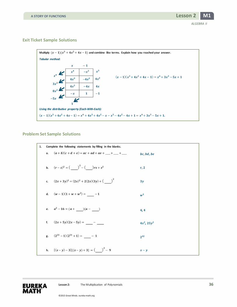
Lesson 2: The Multiplication of Polynomials
M1 Lesson 2 ALGEBRA II
Exit Ticket Sample Solutions
Multiply ( − )( + + − ) and combine like terms. Explain how you reached your answer.
Tabular method:
Using the distributive property (Each-With-Each):
( − )( + + − ) = + + − − − − + = + − + .
Problem Set Sample Solutions
1. Complete the following statements by filling in the blanks.
a. ( + )( + + ) = + + + ____ + ____ + ____
, ,
b. ( − ) = − +
,
c. ( + ) = ( ) + ( )( ) +
d. ( − )( + + ) = −
e. − = ( + )( − )
,
f. ( + )( − ) = −
,
g. ( − )( + ) = −
h. [( − )− ][( − ) + ] = − −
−
−
−
−
−
−
−
( − )( + + − ) = + − +
A STORY OF FUNCTIONS
36
©2015 Great Minds. eureka-math.org
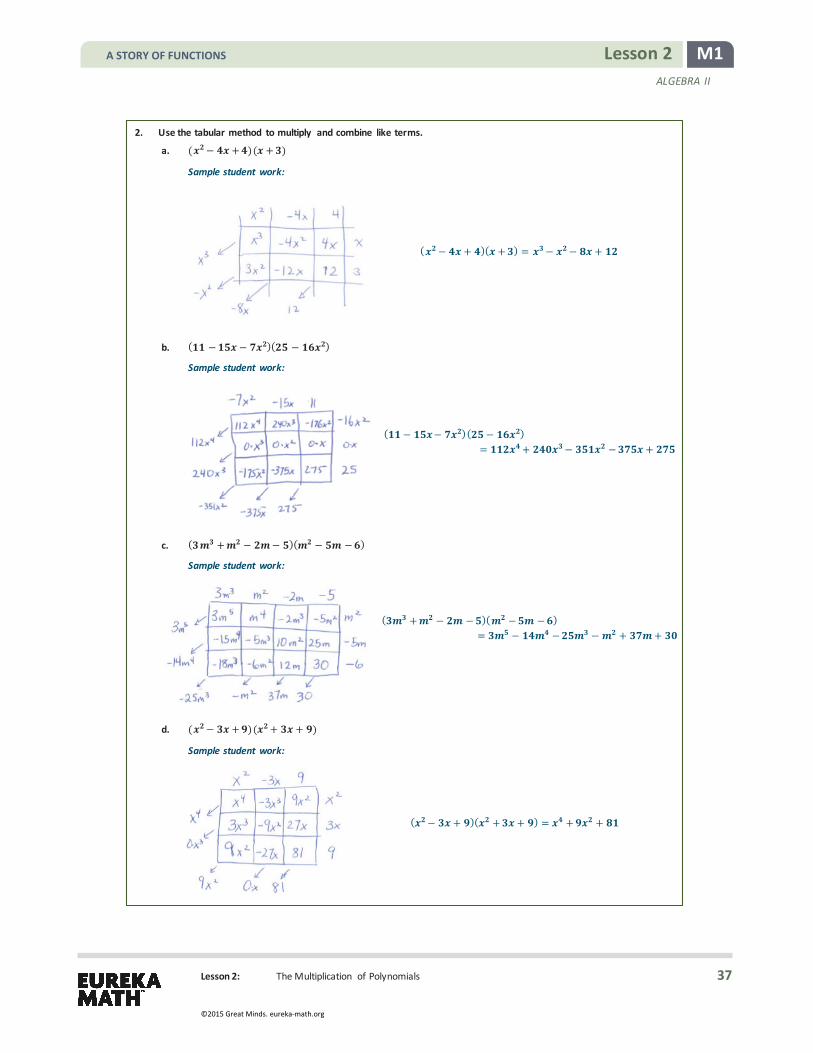
Lesson 2: The Multiplication of Polynomials
M1 Lesson 2 ALGEBRA II
2. Use the tabular method to multiply and combine like terms.
a. ( − + )( + )
Sample student work:
b. ( − − )( − )
Sample student work:
c. ( + − − )( − − )
Sample student work:
d. ( − + )( + + )
Sample student work:
( − + )( + ) = − − +
( − − )( − )= + − − +
( + − − )( − − )= − − − + +
( − + )( + + ) = + +
A STORY OF FUNCTIONS
37
©2015 Great Minds. eureka-math.org

Lesson 2: The Multiplication of Polynomials
M1 Lesson 2 ALGEBRA II
3. Multiply and combine like terms to write as the sum or difference of monomials.
a. ( + ) +
b. ( + ) +
+ +
c. ( + )
+
d. ( − )
−
e. ( − )( + )
+ −
f. ( − )( + )
−
g. ( − )( + )
−
h. (− − )
− −
i. ( + . )
+
j. ( + )( + )
+ + +
k. ( − )( + )( + )
−
l. ( − )( + + + + + )
−
m. ( + )( + )( + )
+ + +
n. ( + )( + )
+ +
o. ( + )( + )( + )
+ + +
p. ( + )( + )( + )( + )
+ + + +
q. ( + )( − + − )
−
r. ( + )( − + − + − )
−
s. ( + )( − + − + − + − )
−
t. ( − + )( − + )
− + − +
4. Polynomial expressions can be thought of as a generalization of place value.
a. Multiply × using the standard paper-and-pencil algorithm.
b. Multiply ( + + )( + + ) using the tabular method and combine like terms.
( + + )( + + ) = + + + +
A STORY OF FUNCTIONS
38
©2015 Great Minds. eureka-math.org

Lesson 2: The Multiplication of Polynomials
M1 Lesson 2 ALGEBRA II
c. Substitute = into your answer from part (b).
,
d. Is the answer to part (c) equal to the answer from part (a)? Compare the digits you computed in the algorithm to the coefficients of the entries you computed in the table. How do the place-value units of the digits compare to the powers of the variables in the entries?
Yes. The digits computed in the algorithm are the same as the coefficients computed in the table entries. The zero-degree term in the table corresponds to the ones unit, the first-degree terms in the table correspond to the tens unit, the second-degree terms in the table correspond to the hundreds unit, and so on.
5. Jeremy says ( − )( + + + + + + + ) must equal + + + + + + + because when = , multiplying by − is the same as multiplying by .
a. Multiply ( − )( + + + + + + + ).
− − − − − − − −
b. Substitute = into your answer.
− − − − − − − −
− =
c. Is the answer to part (b) the same as the value of + + + + + + + when = ?
Yes
d. Was Jeremy right?
No, just because it is true when is does not make it true for all real . The two expressions are not algebraically equivalent.
6. In the diagram, the side of the larger square is units, and the side of the smaller square is units. The area of the shaded region is ( − ) square units. Show how the shaded area might be cut and rearranged to illustrate that the area is ( − )( + ) square units.
Solution:
+
− −
A STORY OF FUNCTIONS
39
©2015 Great Minds. eureka-math.org

M1 Lesson 3 ALGEBRA II
Lesson 3: The Division of Polynomials
Lesson 3: The Division of Polynomials
Student Outcomes
� Students develop a division algorithm for polynomials by recognizing that division is the inverse operation of multiplication.
Lesson Notes This lesson begins to address standards A-SSE.A.2 and A-APR.C.4 and provides many opportunities for students to practice MP.7 and 8. Students explore reversing the tabular method they learned in Lesson 2 as a means to divide two polynomials. They develop a procedure for polynomial division using a table. The problems are scaffolded to lead students to discover this method in small groups, allowing them to discern patterns in repeated calculations, reinforcing the work from Lessons 1 and 2. Discussion questions and the lesson closure are key to guiding struggling students. In this lesson it is critical to emphasize the relationships between the table entries and the position of the dividend and divisor and how the diagonals in the table sum to the terms of the dividend. In the next lesson, students will connect this method to the traditional long division algorithm of polynomial division while reinforcing the relationship between polynomial division and integer arithmetic. All of the problems in this lesson divide without a remainder; division with remainders is addressed in later lessons in this module. General polynomial identities that are used heavily and explored further in the remaining lessons of this module are also touched on in this lesson.
Since division is the inverse operation of multiplication, it is important to make sure that students understand how to multiply polynomials before moving on to division of polynomials found in this lesson. If students are struggling with the content of this lesson, they may need to review problems from Lesson 2 in this module and the following lessons from previous grades:
� Studying the connection between area properties and the distributive property: Grade 7, Module 6, Lesson 21.
� Introduction to the tabular method of multiplying polynomials: Algebra I, Module 1, Lesson 9.
In the early lessons on division (Lessons 3–7), the issue of potential zeros in the denominator is not emphasized but becomes prominent in Lesson 21 when rational expressions are introduced. When introducing polynomial division in this lesson, choose whether or not to emphasize that it is necessary to exclude certain values of 𝑥𝑥 that cause division by zero.
Classwork Opening Exercise (3 minutes)
This exercise provides students with an opportunity to practice the tabular method of multiplication of polynomials. This problem is continued in the Discussion and Exploratory Challenge that follow.
Scaffolding: For students who are unfamiliar with the vocabulary in this lesson (divisor, quotient, dividend, factor, product), take time to pre-teach these terms. Use a vocabulary journal or notebook to help them learn and use proper terminology throughout the lesson.
A visual representation l ike the one below may be of assistance.
(Factor)(Factor) = Product Dividend
Divisor= Quotient
A STORY OF FUNCTIONS
40
©2015 Great Minds. eureka-math.org

M1 Lesson 3 ALGEBRA II
Lesson 3: The Division of Polynomials
Opening Exercise
a. Multiply these polynomials using the tabular method.
( + )( + + )
The product is + + + .
b. How can you use the expression in part (a) to quickly multiply ?
If you let = , then the product is
( ) + ( ) + ( ) + = + + + = .
Discussion (5 minutes)
Lead a discussion that connects multiplication and division. Display the following problem on the board, and ask how it could be transformed into a division problem.
25 151 = 3,775
� How can a multiplication problem be rewritten as a division problem? à One of the factors is the divisor and the other is the quotient. The product is the dividend.
377525
= 151 OR 3775151
= 25
� How can we rewrite the Opening Exercise as a division problem?
(2𝑥𝑥 + 5)(𝑥𝑥2 + 5𝑥𝑥 + 1) = 2𝑥𝑥3 + 15𝑥𝑥2+ 27𝑥𝑥+ 5
à It would be rewritten the same way. One of the factors is the divisor and the other is the quotient. The product is the dividend.
2𝑥𝑥3 + 15𝑥𝑥2+ 27𝑥𝑥 + 52𝑥𝑥 + 5
= 𝑥𝑥2 + 5𝑥𝑥 + 1 OR 2𝑥𝑥3 + 15𝑥𝑥2+ 27𝑥𝑥 + 5
𝑥𝑥2+ 5𝑥𝑥 + 1= 2𝑥𝑥 + 5
� Let 𝑥𝑥 = 10. Substitute that value into each polynomial, and compare the results of multiplying and dividing the polynomials with the arithmetic problem. How do polynomial multiplication and division compare to multiplication and division of integers?
à When 𝑥𝑥 = 10, the polynomial problems result in the same values as the number problems. This reinforces the fact that arithmetic operations with polynomials are similar to arithmetic operations with integers.
Exploratory Challenge (27 minutes): Reverse the Tabular Method to Divide Polynomials
Give students time to discuss how they would fill in the rows and columns in the table below. Let them struggle to make sense of the problem and look for patterns. If they are proficient with the tabular method of multiplication, they should quickly discover a method for populating the table and then verifying that the quotient is in the top row. Read through this entire section before attempting this with students in order to clearly understand how the process works. Start this challenge by asking students to consider how they might reverse the tabular method for multiplying to solve a polynomial division problem.
A STORY OF FUNCTIONS
41
©2015 Great Minds. eureka-math.org

M1 Lesson 3 ALGEBRA II
Lesson 3: The Division of Polynomials
Encourage them to discuss where to position the polynomials now that they have the “answer” (the product) and one of the factors. In the last lessons on multiplication, the factors positioned along the top and right side of the table and the product positioned along the left and bottom came from summing the l ike terms in each diagonal. The student pages pose the problem and provide an empty two-row by three-column table. If needed, use the scaffolded tables provided in the teacher notes that follow to provide more support for students.
Exploratory Challenge
1. Does = ( + + )? Justify your answer.
The partially completed tables shown below provide some suggestions for scaffolding this lesson exploration (if needed). Encourage students to place the dividend where the product would result from multiplying and the quotient where one of the factors would be located. Then, have them work backward to show that the top row of this table is the quotient, 𝑥𝑥2 + 5𝑥𝑥 + 1. Since the table is two by three, it would make sense that 2𝑥𝑥 + 5 is positioned along the vertical side on the right. Notice that the terms of the quotient are located around the left and bottom side of the table. This is where they would appear if these terms represented the result of multiplying two polynomials whose product was 2𝑥𝑥3 + 15𝑥𝑥2+ 27𝑥𝑥 + 5. Notice also that the divisor is positioned along the right side of the table (as was found with one of the factors in the earlier tabular method multiplication problems). The arrows in the diagram indicate that the diagonal entries must sum to the term outside the table (e.g., 15𝑥𝑥2 = 5𝑥𝑥2 + 10𝑥𝑥2).
+
+ +
+
A STORY OF FUNCTIONS
42
©2015 Great Minds. eureka-math.org

M1 Lesson 3 ALGEBRA II
Lesson 3: The Division of Polynomials
After students have had a few minutes to discuss their ideas in groups, lead a short discussion (as needed) if they appear to be stuck. Use these questions to prompt groups while also circulating around the room.
� The quotient will be the polynomial that would go along the top of the table. Remember we know it should be 𝑥𝑥2 + 5𝑥𝑥 + 1. How can you get started to confirm this using the dividend and the divisor? à We need to think about how the divisor terms fill back into the table, and then we need to use the
2𝑥𝑥 and the 5 terms to determine the other factor for each column at the top of the table.
� Are there any cells in the table that we can fi ll in based on the information we have? What must be in the top left cell? Why?
à The 2𝑥𝑥3 term will be the top left entry, and the 5 will be the bottom right entry. Because the diagonals add to produce the terms of the product, we know that the top left and bottom right entries must be the first and last terms of the dividend since those terms do not involve combining any like terms when we compute the product.
� What must the first term of the missing polynomial in the top row be? à It would have to be 𝑥𝑥2 since that term and 2𝑥𝑥 must multiply to be 2𝑥𝑥3.
� What goes in the rest of the cells in the first column? How can you continue this pattern?
à Multiply 𝑥𝑥2 and 5 to get 5𝑥𝑥2. Then the 2nd column in the first row would need to be 10𝑥𝑥2 because 15𝑥𝑥2 = 10𝑥𝑥2 + 5𝑥𝑥2. Since the 2nd column of the first row is now known, we can figure out the remaining term of the quotient since that term times 2𝑥𝑥 would have to equal 10𝑥𝑥2.
� Compare your work on this problem with the Opening Exercise. How could you verify that 𝑥𝑥2 + 5𝑥𝑥 + 1 really is the quotient? Explain?
à In the Opening Exercise, we multiplied the quotient and divisor and got the dividend. So (2𝑥𝑥 + 5)(𝑥𝑥2 + 5𝑥𝑥 + 1) must equal 2𝑥𝑥3 + 15𝑥𝑥2+ 27𝑥𝑥 + 5.
2. Describe the process you used to determine your answer to Exercise 1. Student descriptions will vary but should be similar to the detailed directions provided on the following page.
Check each group’s work before moving on to the next exercise. Have a couple of groups present their solution methods to the Exercises 1 and 2 on the board, especially if other groups seem to be struggling. Then, if needed, go over the steps outlined below in detail to clarify this process for all students. Provide additional scaffolding if needed.
Step 1—Draw a table with factors along the right sides and bottom corner, and fill in known entries along the top left and bottom right.
A STORY OF FUNCTIONS
43
©2015 Great Minds. eureka-math.org

M1 Lesson 3 ALGEBRA II
Lesson 3: The Division of Polynomials
Step 2—Use the top left entry to find the second-degree term along the top. It has to be 𝑥𝑥2 because 2𝑥𝑥 𝑥𝑥2 = 2𝑥𝑥3.
Step 3—Use 𝑥𝑥2 and 5 to find the bottom left entry, 5𝑥𝑥2, and then use that entry to find the top middle term. It has to be 10𝑥𝑥2 because 5𝑥𝑥2+ 10𝑥𝑥2 = 15𝑥𝑥2.
nd
A STORY OF FUNCTIONS
44
©2015 Great Minds. eureka-math.org
Step 4—Repeat these steps to fi ll in the bottom entry in the 2 and last columns.

M1 Lesson 3 ALGEBRA II
Lesson 3: The Division of Polynomials
Students do not already know the quotient in Exercise 3, making this more challenging than the previous exercises.
3. Reverse the tabular method of multiplication to find the quotient:
After these two exercises, lead a short discussion to help students learn how to reverse their thinking about the tabular method of multiplication to divide polynomials.
� We will call this approach to dividing polynomials the reverse tabular method. Let’s make a conjecture about the number of rows and columns you will need to perform the division. How can you predict how many rows you will need in your table? How can you predict how many columns you will need in your table?
à The number of rows will be one more than the degree of the divisor. The number of columns will be one more than the difference between the degree of the dividend and the degree of the divisor.
4. Test your conjectures. Create your own table, and use the reverse tabular method to find the quotient.
+ + + ++
+ +
+
The quotient is + + .
+
− − −
−
−
−
MP.3
A STORY OF FUNCTIONS
45
©2015 Great Minds. eureka-math.org

M1 Lesson 3 ALGEBRA II
Lesson 3: The Division of Polynomials
If necessary, remind groups to include a 0 coefficient term place holder when missing a needed term.
5. Test your conjectures. Use the reverse tabular method to find the quotient.
− + − − ++
The quotient is − − + .
6. What is the quotient of ? What is the quotient of ?
The quotients are + + + + and + + + + + , respectively.
After students complete Exercise 6, see if they can extend the patterns to make predictions about similar problems.
� What is the result of dividing 11
?
à 𝑥𝑥 + 𝑥𝑥 + 𝑥𝑥 + 𝑥𝑥4 + 𝑥𝑥3 + 𝑥𝑥2 + 𝑥𝑥 + 1
� What is the result of dividing 11
?
à 𝑥𝑥𝑛𝑛 1+ 𝑥𝑥𝑛𝑛 2+ + 𝑥𝑥 + 1
� What is the result of dividing 1
1?
à 𝑥𝑥4 − 𝑥𝑥3 + 𝑥𝑥2− 𝑥𝑥 + 1
Wrap up this lesson by having groups present their solutions to Exercises 3–5 and discuss the strategies they used to solve the problems. It is fine if two groups present the same problem since they may have had slightly different approaches to completing the table. Students may notice that it is easier to fi ll in the table by columns. Some may have started working from the lower right corner where the constant is located. Students may realize that they do not need to fi l l in every cell to finish the problem but may wish to do so to check their work. If time permits, have them verify their conjectures to the follow-up questions for Exercise 6.
Closing (5 minutes)
These questions help to reinforce the relationship between multiplication and division and some of the patterns that emerge in using the reverse tabular method to divide polynomials with no remainder. Have students respond to the questions below (either in writing or with a partner) to provide a summary and formative assessment information. The questions that ask about the degree and leading coefficient help to reinforce the A.APR standards addressed in this lesson.
MP.7 &
MP.8
Scaffolding: If students are struggling to extend this pattern in Exercise 6, begin with simpler problems such as:
(𝑥𝑥2− 1)(𝑥𝑥− 1)
= 𝑥𝑥 + 1
𝑥𝑥3− 1𝑥𝑥− 1
= 𝑥𝑥2+ 𝑥𝑥+ 1
𝑥𝑥4− 1𝑥𝑥− 1
= 𝑥𝑥3+ 𝑥𝑥2 + 𝑥𝑥 + 1.
They should solve these simpler problems using the reverse tabular method. Perhaps have different groups each work a different problem, and then record the results on the board. Conduct a class discussion so they can generalize the pattern.
A STORY OF FUNCTIONS
46
©2015 Great Minds. eureka-math.org

M1 Lesson 3 ALGEBRA II
Lesson 3: The Division of Polynomials
� What strategies were helpful when you set up and solved these problems? What patterns did you notice as you solved these problems?
à The number of rows will be one more than the degree of the divisor. The number of columns will be one more than the difference between the degree of the dividend and the degree of the divisor. For example, when dividing 2𝑥𝑥4 − 𝑥𝑥3 + 4𝑥𝑥2− 1 by 𝑥𝑥3 + 2𝑥𝑥 + 1, we will have four rows since the divisor has degree 3. Then we will need 4− 3 + 1 = 2 columns for the quotient.
à You need to use a place holder for missing terms. For example, 𝑥𝑥2+ 1 = 𝑥𝑥2+ 0𝑥𝑥 + 1. à The diagonals must add to the correct terms, and the cells in the table must be the product of the
factors along the sides of the table. � What happens to the degree of the product when you multiply two polynomials?
à When you multiply polynomials, the degree of the product will be the sum of the degrees of each factor. � What happens to the degree of the quotient when you divide two polynomials?
à When you divide polynomials, the degree of the quotient will be the difference of the degrees of the dividend and divisor.
� What happens to leading coefficients when you multiply or divide polynomials?
à The leading coefficient of the result is the product or quotient of the leading coefficients of the original polynomials.
Exit Ticket (5 minutes)
A STORY OF FUNCTIONS
47
©2015 Great Minds. eureka-math.org

M1 Lesson 3 ALGEBRA II
Lesson 3: The Division of Polynomials
Name Date
Lesson 3: The Division of Polynomials
Exit Ticket Find the quotient. Justify your answer.
𝑥𝑥 + 2𝑥𝑥4 − 7𝑥𝑥2− 19𝑥𝑥+ 15
𝑥𝑥2 + 2𝑥𝑥 + 5
A STORY OF FUNCTIONS
48
©2015 Great Minds. eureka-math.org

M1 Lesson 3 ALGEBRA II
Lesson 3: The Division of Polynomials
Exit Ticket Sample Solutions
Find the quotient. Justify your answer.
+ − − +
+ +
The quotient is − + .
Problem Set Sample Solutions
Use the reverse tabular method to solve these division problems.
1. + −
2. ( ) + + +
3. −
4. −
5. − + −
6. ( ) + +
7. + +
8. + + +
A STORY OF FUNCTIONS
49
©2015 Great Minds. eureka-math.org

M1 Lesson 3 ALGEBRA II
Lesson 3: The Division of Polynomials
9. Use the results of Problems 7 and 8 to predict the quotient of .
Explain your prediction. Then check your prediction using the reverse tabular method.
The quotient is + + + + . In Problems 7 and 8, the result is a polynomial of degree one less than the dividend where all the coefficients were . The dividend in this problem has the same structure except it was degree , and it is also divided by + .
10. Use the results of Problems 7–9 above to predict the quotient of . Explain your prediction. Then check your prediction using the reverse tabular method.
The quotient is − + − .
11. Make and test a conjecture about the quotient of . Explain your reasoning.
The quotient is + + + + . Since we are missing the term, there will not be two or two terms. Otherwise it will follow the same pattern as Problems 7–9.
12. Consider the following quotients:
+ ++
and
a. How are these expressions related?
If we let = , then + + = ( ) + ( ) + = and + = ( ) + = , so
= .
b. Find each quotient.
= + and =
c. Explain the connection between the quotients.
If we let = , then. + = ( ) + = .
A STORY OF FUNCTIONS
50
©2015 Great Minds. eureka-math.org

Lesson 4: Comparing Methods—Long Division, Again?
M1 Lesson 4 ALGEBRA II
Lesson 4: Comparing Methods—Long Division, Again?
Student Outcomes
� Students connect long division of polynomials with the long division algorithm of arithmetic and use this algorithm to rewrite rational expressions that divide without a remainder.
Lesson Notes This lesson reinforces the analogous relationship between arithmetic of numbers and the arithmetic of polynomials (A-APR.6, A-APR.7). These standards address working with rational expressions and focus on using a long division algorithm to rewrite simple rational expressions. In addition, it provides another method for students to fluently calculate the quotient of two polynomials after the Opening Exercises.
Classwork Opening
Have students work individually on the Opening Exercises to confirm their understanding of the previous lesson’s outcomes. Circulate around the room to observe their progress, or have students check their work with a partner after a few minutes. Today’s lesson will transition to another method for dividing polynomials.
Opening Exercises (5 minutes) Opening Exercises
1. Use the reverse tabular method to determine the quotient .
+ +
+
+ + +
A STORY OF FUNCTIONS
51
©2015 Great Minds. eureka-math.org

Lesson 4: Comparing Methods—Long Division, Again?
M1 Lesson 4 ALGEBRA II
2. Use your work from Exercise 1 to write the polynomial + + + in factored form, and then multiply the factors to check your work above.
( + )( + + )
+ +
+
The product is + + + .
Division and multiplication of polynomials are very similar to those operations with real numbers. In these problems, if 𝑥𝑥 = 10, the result would match an arithmetic problem. Yesterday, students divided two polynomials using the reverse tabular method. Today, the goal is to see how polynomial division is related to the long division algorithm learned in elementary school.
Discussion (5 minutes)
We have seen how division of polynomials relates to multiplication and that both of these operations are similar to the arithmetic operations you learned in elementary school.
� Can we relate division of polynomials to the long division algorithm?
à We would need to use the fact that the terms of a polynomial expression represent place value when 𝑥𝑥 = 10.
Prompt students to consider the long division algorithm they learned in elementary school, and ask them to apply it to evaluate 1573 ÷ 13. Have a student model the algorithm on the board as well. The solution to this problem is included in the example below.
Example 1 (5 minutes): The Long Division Algorithm for Polynomial Division
When solving the problem in Example 1, be sure to record the polynomial division problem next to the arithmetic problem already on the board. Guide students through this example to demonstrate the parallels between the long division algorithm for numbers and this method. Emphasize that the long division algorithm they learned in elementary school is a special case of polynomial long division. They should record the steps on their handouts or in their notebooks. Have students check their work by solving this problem using the reverse tabular method. Use the questions below while working the example.
See the sample problem written out after Example 1, and use the questions that follow as discussion points while modeling this algorithm.
MP.7
A STORY OF FUNCTIONS
52
©2015 Great Minds. eureka-math.org

Lesson 4: Comparing Methods—Long Division, Again?
M1 Lesson 4 ALGEBRA II
� What expression multiplied by 𝑥𝑥 will result in 𝑥𝑥3? à 𝑥𝑥2
� When you do long division, you multiply the first digit of the quotient by the divisor and then subtract the result. It works the same with polynomial division. How do we represent multiplication and subtraction of polynomials?
à You apply the distributive property to multiply, and to subtract you add the opposite.
� Then, we repeat the process to determine the next term in the quotient. What do we need to bring down to complete the process? à You should bring down the next term.
Example 1
If = , then the division ÷ can be represented using polynomial division.
3753 23 xxxx
The quotient is + + .
The completed board work for this example should look something like this:
Example 2 (5 minutes): The Long Division Algorithm for Polynomial Division
Any two numbers can be divided as long as the divisor is not equal to 0. Similarly, any two polynomials can be divided as long as the divisor is not equal to 0. Note: The number 0 is also a polynomial. Because the class is now dealing with a general case of polynomials and not simply numbers, it is possible to solve problems where the coefficients of the terms are any real numbers. It would be difficult, but not impossible, if the coefficients of the terms of the polynomials were irrational. In the next example, model again how this process works. Be sure to point out that students must use a 0 coefficient place holder for the missing 𝑥𝑥 term.
Example 2
Use the long division algorithm for polynomials to evaluate
− +−
The quotient is − − .
Scaffolding: � For further scaffolding,
consider starting with a simpler problem, such as 126 ÷ 18. Have students compare this problem to the polynomial division problem (𝑥𝑥2+ 2𝑥𝑥 + 6) ÷(𝑥𝑥 + 8) by explaining the structural similarities. Have students consider this as the teacher places them side by side on the board. This shows students that if 𝑥𝑥 = 10, the polynomial division problem is analogous to the integer division problem.
� For advanced learners, challenge them to create two examples, a numerical one and a polynomial one, that i l lustrate the structural similarities. Note, however, that not every problem will work nicely. For example, 800 ÷ 32 = 25, but 8𝑥𝑥2 ÷ (3𝑥𝑥 + 2) 2𝑥𝑥+ 5 because there are many polynomials in 𝑥𝑥 that evaluate to 25 when 𝑥𝑥 = 10.
A STORY OF FUNCTIONS
53
©2015 Great Minds. eureka-math.org

Lesson 4: Comparing Methods—Long Division, Again?
M1 Lesson 4 ALGEBRA II
Before beginning the next exercises, take the time to reinforce the idea that polynomial division is analogous to whole number division by posing a reflection question. Students can discuss this with a partner or respond in writing.
� Why are we able to do long division with polynomials? à Polynomials form a system analogous to the integers. The same operations that hold for integers hold
for polynomials.
Exercises 1–8 (15 minutes)
These problems start simple and become more complicated. Monitor student progress as they work. Have students work these problems independently or in pairs, and use this as an opportunity to informally assess their understanding. After students have completed the exercises, post the solutions on the board but not the work. Have students with errors team up with a partner and trade papers. Ask students to find the mistakes in their partner’s work. Choose an incorrect solution to display on the board, and then lead a class discussion to point out where students are l ikely to make errors and how to prevent them. Students typically make careless errors in multiplying or subtracting terms. Other errors can occur if they forget to include the zero coefficient place holder terms when needed. If students appear to be running short on time, have them check every other result using the reverse tabular method. Alternately, students could check their work using multiplication.
Exercises 1–8
Use the long division algorithm to determine the quotient. For each problem, check your work by using the reverse tabular method.
1.
+
2.
− −
3.
+ +
4.
+ +
5.
−
A STORY OF FUNCTIONS
54
©2015 Great Minds. eureka-math.org

Lesson 4: Comparing Methods—Long Division, Again?
M1 Lesson 4 ALGEBRA II
6.
+ +
7.
− +
8.
− + − + −
Closing (5 minutes)
Ask students to summarize the important parts of this lesson either in writing, to a partner, or as a class. Use this opportunity to informally assess their understanding prior to starting the Exit Ticket. Important elements are included in the Lesson Summary box below. The questions that follow are recommended to guide the discussions with sample student responses included in italics. Depending on the structure of the closure activity, the sample responses would be similar to student-written, partner, or whole-class summaries.
� Which method do you prefer, long division or the reverse tabular method?
à Student responses will vary. The reverse tabular method may appeal to visual learners. The long division algorithm works well as long as you avoid careless mistakes.
� Is one method easier than another? à This will depend on student preferences, but some will like the connection to prior methods for dividing
and multiplying. Perhaps when many terms are missing (as in Exercise 8), the reverse tabular method can go more quickly than long division.
� What advice would you give to a friend that is just learning how to do these problems quickly and accurately? à Be careful when multiplying terms and working with negative terms.
Exit Ticket (5 minutes)
Lesson Summary
The long division algorithm to divide polynomials is analogous to the long division algorithm for integers. The long division algorithm to divide polynomials produces the same results as the reverse tabular method.
A STORY OF FUNCTIONS
55
©2015 Great Minds. eureka-math.org
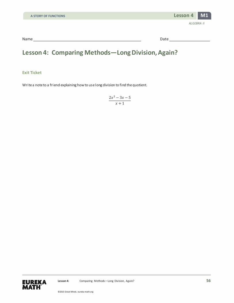
Lesson 4: Comparing Methods—Long Division, Again?
M1 Lesson 4 ALGEBRA II
Name Date
Lesson 4: Comparing Methods—Long Division, Again?
Exit Ticket Write a note to a friend explaining how to use long division to find the quotient.
2𝑥𝑥2 − 3𝑥𝑥 − 5
𝑥𝑥 + 1
A STORY OF FUNCTIONS
56
©2015 Great Minds. eureka-math.org

Lesson 4: Comparing Methods—Long Division, Again?
M1 Lesson 4 ALGEBRA II
Exit Ticket Sample Solutions
Write a note to a friend explaining how to use long division to find the quotient.
− −+
Set up the divisor outside the division symbol and the dividend underneath it. Then ask yourself what number multiplied by is . Then multiply that number by + , and record the results underneath − . Subtract these terms and bring down the − . Then repeat the process.
Problem Set Sample Solutions
Use the long division algorithm to determine the quotient in problems 1–5.
1.
− +
2.
− +
3.
+ −
4. ( + + − ) ÷ ( + )
+ −
5. ( + + ) ÷ ( + + )
6. Use long division to find the polynomial, , that satisfies the equation below.
− − = ( + )( ( ))
( ) = −
7. Given ( ) = − + + .
a. Determine the value of so that − is a factor of the polynomial .
= −
b. What is the quotient when you divide the polynomial by − ?
+ +
A STORY OF FUNCTIONS
57
©2015 Great Minds. eureka-math.org

Lesson 4: Comparing Methods—Long Division, Again?
M1 Lesson 4 ALGEBRA II
8. In parts (a)–(b) and (d)–(e), use long division to evaluate each quotient. Then, answer the remaining questions.
a.
−
b.
− + −
c. Is + a factor of − ? Explain your answer using the long division algorithm.
No. The remainder is not when you perform long division.
d.
− +
e.
− + − +
f. Is + a factor of + ? Explain your answer using the long division algorithm.
No. The remainder is not when you perform long division.
g. For which positive integers is + a factor of + ? Explain your reasoning.
Only if is an odd number. By extending the patterns in parts (a)–(c) and (e), we can generalize that + divides evenly into + for odd powers of only.
h. If is a positive integer, is + a factor of − ? Explain your reasoning.
Only for even numbers . By extending the patterns in parts (a)–(c), we can generalize that + will always divide evenly into the dividend.
MP.2 &
MP.8
A STORY OF FUNCTIONS
58
©2015 Great Minds. eureka-math.org

Lesson 5: Putting It All Together
M1 Lesson 5 ALGEBRA II
Lesson 5: Putting It All Together
Student Outcomes
� Students perform arithmetic operations on polynomials and write them in standard form. � Students understand the structure of polynomial expressions by quickly determining the first and last terms if
the polynomial were to be written in standard form.
Lesson Notes In this lesson, students work with all four polynomial operations. The first part of the lesson is a relay exercise designed to build fluency, and the second part of the lesson includes combining two or more operations to write a polynomial in standard form. Prepare a set of notecards as described below for Exercises 1–15.
The Algebra Progressions name three different forms for a quadratic expression: standard, factored, and vertex. Examples of these forms are shown below.
� Standard Form: 𝑥𝑥2 + 4𝑥𝑥− 5 � Factored Form: (𝑥𝑥 + 5)(𝑥𝑥 − 1) � Vertex Form: (𝑥𝑥 + 2) 2− 9
It is possible to define a standard and factored form of a degree polynomial expression as well. The final lessons in this module introduce the fundamental theorem of algebra, which states that a degree polynomial with real coefficients can be written as the product of l inear factors. Precise definitions of the following terms are provided for teacher reference at the end of this lesson: monomial, polynomial expression, coefficient of a monomial, degree of a monomial, terms of a polynomial, standard form of a polynomial in one variable, and degree of a polynomial in one variable. This lesson concludes by challenging students to quickly determine the first and last term of a polynomial expression if it were to be written in standard form. Students who have this capacity can quickly analyze the end behavior of the graph of a polynomial function or compute key features such as a 𝑦𝑦-intercept without having to fully rewrite the expression in standard form. This allows for quick analysis when applying properties of polynomials in future mathematics courses such as Precalculus and Advanced Topics or Calculus.
Classwork Exercises 1–15 (20 minutes): Polynomial Pass
Prior to the lesson, write Exercises 1–15 on index cards, one exercise per card. On the back of each card, write the solution to the previous exercise. For example, on the back of the card for Exercise 2, write the answer to Exercise 1. On the back of the index card for Exercise 1, write the answer to Exercise 15. Students should be seated in a circle if possible. If more than 15 different cards are needed, create additional exercises that require addition, subtraction, multiplication, or division without remainder of linear, quadratic, or cubic polynomial expressions.
Scaffolding: Before beginning these exercises, it may be necessary to review the definition and/or post an example of a polynomial in standard form. Also consider reminding students of the vertex and factored forms of quadratic expressions using the examples in the Lesson Notes if needed. For example,
� Standard Form: 𝑥𝑥2 + 4𝑥𝑥 − 5
� Factored Form: (𝑥𝑥 + 5)(𝑥𝑥 − 1)
� Vertex Form: (𝑥𝑥 + 2)2− 9
A STORY OF FUNCTIONS
59
©2015 Great Minds. eureka-math.org

Lesson 5: Putting It All Together
M1 Lesson 5 ALGEBRA II
To complete the exercise, have students work in pairs. Pass out cards to pairs in numerical order so that when the cards are passed, each pair gets a new exercise that contains the answer to the one they just worked on the back of the card. (Alternatively, have students work individually and make two sets of cards so that cards 16–30 are duplicates of 1–15.) Allow one minute for students to work each calculation on a separate sheet of paper, and then have them pass the card to the next pair and receive a card from the previous pair. They should check their answers and begin the next exercise. After all the rounds are completed, have students complete the graphic organizer on their student handouts to model each operation.
Exercises 1–15: Polynomial Pass
Perform the indicated operation to write each polynomial in standard form.
1. ( − )( + − ) + − − +
2. ( − − )− ( + − ) − −
3. + +
4. ( + )( − )( + ) + − −
5. ( + ) − ( − ) − ( + ) −
6. ( + )( − + ) − − +
7. + −
8. ( − + )− ( − + ) − −
9. ( − + )( − + ) − + − +
10. + +
11. ( + − )( − + ) − − + −
12. ( − − − ) + ( + + − ) − − −
13. ( − )( − + ) − + − + −
14. − +
15. ( + − − ) + ( − − ) − +
A STORY OF FUNCTIONS
60
©2015 Great Minds. eureka-math.org

Lesson 5: Putting It All Together
M1 Lesson 5 ALGEBRA II
Exercise 16 (5 minutes)
Use this exercise to help students see the structure of polynomial expressions and to create a graphic organizer of how to perform the four polynomial operations for future reference. They should complete this exercise either with a partner or in groups of four.
Exercises 16
16. Review Exercises 1–15 and then select one exercise for each category and record the steps in the operation below as an example. Be sure to show all your work.
Addition Exercise
Multiplication Exercise
Subtraction Exercise
Division Exercise
Exercises 17–20 (5 minutes)
Before starting the next exercises, lead a short discussion transitioning into the problems below that combine polynomial operations. Say (or paraphrase) the following:
� In the previous exercises, you applied one operation to two or three polynomials, but many times we work with expressions that contain more than one operation. In the next exercises, more than one operation is indicated. How do you determine which operation to perform first?
à The parentheses and the use of the fraction bar for division tell us which operations to perform first. The order of operations also can be applied to polynomials. For example, you have to multiply before you can add or subtract.
After this discussion, have students work with the same partner (or group) that they worked with on Exercise 16. Have different groups present their work to the class. Students could use white boards or chart paper to present their solutions to the class.
Exercises 17–20
For Exercises 17–20, rewrite each polynomial in standard form by applying the operations in the appropriate order.
17.
+
18. ( − )( + )− ( + − )
+ − −
A STORY OF FUNCTIONS
61
©2015 Great Minds. eureka-math.org

Lesson 5: Putting It All Together
M1 Lesson 5 ALGEBRA II
19. ( )
−
20. ( + )( − ) − ( − + − ) ÷ ( − )
+ −
Exercise 21 (4 minutes)
This exercise, along with Exercise 22, helps students understand that they can learn quite a bit about the nature of a polynomial expression without performing all the operations required to write it in standard form.
� Sometimes we do not need to perform the entire operation to understand the structure of an expression. Can you think of a situation where we might only need to know the first term or the last term of a polynomial expression?
à If we wanted to understand the shape of the graph of a polynomial, like 𝑝𝑝(𝑥𝑥) = 𝑥𝑥2 + 2𝑥𝑥+ 3, we would only need to know the coefficient and degree of the first term to get a general idea of its behavior.
à The constant term of a polynomial expression indicates the 𝑦𝑦-intercept of the corresponding graph. Exercise 21
21. What would be the first and last terms of the polynomial if it was rewritten in standard form? Answer these quickly without performing all of the indicated operations.
a. ( − − + ) + ( − + − )
First term: − , Last term: −
b. ( − )( + )( − )
First term: , Last term:
c. ( − )( + )− ( + )( − + )
First term: − , Last term: −
d. ( + )( − ) − ( − )
First term: , Last term: −
After students complete this exercise, lead a short discussion.
� How did you determine your answer quickly?
à I knew that the first term would be the one with the highest degree, so I focused on that operation. I knew that the last term would be the constant term unless it turned out to equal 0.
� Did any of the solutions surprise you?
à In parts (a) and (c), I had to pay attention to the order of the terms and which operation would produce the largest degree term.
MP.7
A STORY OF FUNCTIONS
62
©2015 Great Minds. eureka-math.org

Lesson 5: Putting It All Together
M1 Lesson 5 ALGEBRA II
Exercise 22 (4 minutes) Exercise 22
22. What would the first and last terms of the polynomial be if it was rewritten in standard form?
a. ( + )( + )( + ) ( + )( + )
First term: , Last term: !
b. ( − )
First term: , Last term: (− )
c. ( )
( )
First term: , Last term: (− )
d. ( )( ) First term: ,
Last term:
Closing (2 minutes)
Consider having students record their answers to these questions in writing or by sharing their thoughts with a partner.
� How is polynomial arithmetic similar to integer arithmetic?
à The four operations produce a new polynomial. The four operations can be combined by following the order of operations conventions.
� How can you quickly determine the first and last terms of a polynomial without performing all of the operations needed to rewrite it in standard form? à Analyze the problem to identify the highest degree terms and perform the
indicated operation on only those terms. Do the same with the lowest degree terms to determine the last term.
Precise definitions of terms related to polynomials are presented here. These definitions were first introduced in Algebra I, Modules 1 and 4. These definitions are for teacher reference and can be shared with students at the teacher’s discretion. Following these definitions are discussion questions for closing this lesson.
Relevant Vocabulary
POLYNOMIAL EXPRESSION: A polynomial expression is either a numerical expression or a variable symbol or the result of placing two previously generated polynomial expressions into the blanks of the addition operator (__ + __) or the multiplication operator (__ × __).
The definition of polynomial expression includes subtraction (𝑎𝑎 − 𝑏𝑏 = 𝑎𝑎+ (−1 𝑏𝑏)), exponentiation by a nonnegative integer (𝑥𝑥3 = (𝑥𝑥 𝑥𝑥) 𝑥𝑥), and dividing by a nonzero number (multiplying by the multiplicative inverse). Because subtraction, exponentiation, and division still apply, the regular notation for these operations is still used. In other
words, polynomials are still written simply as ( 3 )
2 instead of
12� (𝑥𝑥 𝑥𝑥) 𝑥𝑥 + −1 (3 𝑥𝑥) �
Scaffolding: For advanced learners or early finishers, increase the complexity of these exercises by posing the following problem (or one similar to it): � Generate three different
polynomial expressions NOT already expressed in standard form that would have a first term of −3𝑥𝑥3 and a last term of
12
if the
polynomial expression was written in standard form.
A STORY OF FUNCTIONS
63
©2015 Great Minds. eureka-math.org

Lesson 5: Putting It All Together
M1 Lesson 5 ALGEBRA II
Note, however, that the definition excludes dividing by 𝑥𝑥 or dividing by any polynomial in 𝑥𝑥.
All polynomial expressions are algebraic expressions.
MONOMIAL: A monomial is a polynomial expression generated using only the multiplication operator (__ × __).
Monomials are products whose factors are numerical expressions or variable symbols.
COEFFICIENT OF A MONOMIAL: The coefficient of a monomial is the value of the numerical expression found by substituting the number 1 into all the variable symbols in the monomial.
Sometimes the coefficient is considered as a constant (l ike the constant 𝑎𝑎 in 𝑎𝑎𝑥𝑥2) instead of an actual number. In those cases, when a monomial is expressed as a product of a constant and variables, then the constant is called a constant coefficient.
DEGREE OF A MONOMIAL: The degree of a nonzero monomial is the sum of the exponents of the variable symbols that appear in the monomial.
For example, the degree of 7𝑥𝑥2𝑦𝑦4 is 6, the degree of 8𝑥𝑥 is 1, the degree of 8 is 0, and the degree of 9𝑥𝑥2𝑦𝑦3𝑥𝑥10 is 15.
TERMS OF A POLYNOMIAL: When a polynomial is expressed as a monomial or a sum of monomials, each monomial in the sum is called a term of the polynomial.
A monomial can now be described as a polynomial with only one term. But please realize that the word term means many, seemingly disparate things in mathematics (e.g., sin(𝑥𝑥) is often called a term of the expression sin(𝑥𝑥) + cos(𝑥𝑥)), whereas monomial is a specific object. This is why monomial is defined first, and then used to define a term of a polynomial.
STANDARD FORM OF A POLYNOMIAL IN ONE VARIABLE: A polynomial expression with one variable symbol 𝑥𝑥 is in standard form if it is expressed as,
𝑎𝑎𝑛𝑛𝑥𝑥𝑛𝑛 + 𝑎𝑎𝑛𝑛 1𝑥𝑥𝑛𝑛 1+ + 𝑎𝑎1𝑥𝑥+ 𝑎𝑎0,
where is a nonnegative integer, and 𝑎𝑎0, 𝑎𝑎1, 𝑎𝑎2,…, 𝑎𝑎𝑛𝑛 are constant coefficients with 𝑎𝑎𝑛𝑛 0.
A polynomial expression in 𝑥𝑥 that is in standard form is often called a polynomial in 𝑥𝑥.
The degree of the polynomial in standard form is the highest degree of the terms in the polynomial, namely . The term 𝑎𝑎𝑛𝑛𝑥𝑥𝑛𝑛 is called the leading term and 𝑎𝑎𝑛𝑛 is called the leading coefficient. The constant term is the value of the numerical expression found by substituting 0 into all the variable symbols of the polynomial, namely 𝑎𝑎0.
In general, one has to be careful about determining the degree of polynomials that are not in standard form: For example, the degree of the polynomial,
(𝑥𝑥 + 1)2 − (𝑥𝑥 − 1)2,
is not 2 since its standard form is 4𝑥𝑥.
DEGREE OF A POLYNOMIAL IN ONE VARIABLE: The degree of a polynomial expression in one variable is the degree of the polynomial in standard form that is equivalent to it.
Exit Ticket (5 minutes)
A STORY OF FUNCTIONS
64
©2015 Great Minds. eureka-math.org

Lesson 5: Putting It All Together
M1 Lesson 5 ALGEBRA II
Name Date
Lesson 5: Putting It All Together
Exit Ticket Jenny thinks that the expression below is equal to 𝑥𝑥2− 4. If you agree, show that she is correct. If you disagree, show that she is wrong by rewriting this expression as a polynomial in standard form.
(𝑥𝑥 − 2)3
𝑥𝑥 − 2
A STORY OF FUNCTIONS
65
©2015 Great Minds. eureka-math.org

Lesson 5: Putting It All Together
M1 Lesson 5 ALGEBRA II
Exit Ticket Sample Solutions
Jenny thinks that the expression below is equal to − . If you agree, show that she is correct. If you disagree, show that she is wrong by rewriting this expression as a polynomial in standard form.
( − )−
Multiple approaches are possible to justify why Jenny is incorrect. One possible solution is shown below.
Jenny is incorrect. To perform this operation, you can first divide by − and then expand the quotient.
( − )−
= ( − )
= − +
Problem Set Sample Solutions
For Problems 1–7, rewrite each expression as a polynomial in standard form.
1. ( − )
− + −
2. ( − − + )− ( + − + )
− + −
3. ( − + )( − )
− + −
4.
+ −
5. ( + )( − ) − ( + )( − )
6. ( + ) − ( + )
− −
7. +
+ −
MP.3
A STORY OF FUNCTIONS
66
©2015 Great Minds. eureka-math.org
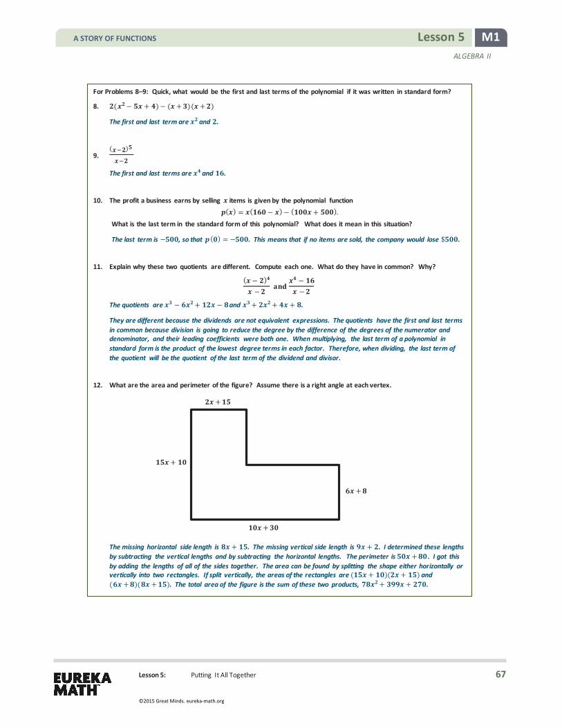
Lesson 5: Putting It All Together
M1 Lesson 5 ALGEBRA II
For Problems 8–9: Quick, what would be the first and last terms of the polynomial if it was written in standard form?
8. ( − + )− ( + )( + )
The first and last term are and .
9. ( )
The first and last terms are and .
10. The profit a business earns by selling items is given by the polynomial function ( ) = ( − )− ( + ).
What is the last term in the standard form of this polynomial? What does it mean in this situation?
The last term is − , so that ( ) = − . This means that if no items are sold, the company would lose $ .
11. Explain why these two quotients are different. Compute each one. What do they have in common? Why?
( − )−
−−
The quotients are − + − and + + + .
They are different because the dividends are not equivalent expressions. The quotients have the first and last terms in common because division is going to reduce the degree by the difference of the degrees of the numerator and denominator, and their leading coefficients were both one. When multiplying, the last term of a polynomial in standard form is the product of the lowest degree terms in each factor. Therefore, when dividing, the last term of the quotient will be the quotient of the last term of the dividend and divisor.
12. What are the area and perimeter of the figure? Assume there is a right angle at each vertex.
The missing horizontal side length is + . The missing vertical side length is + . I determined these lengths by subtracting the vertical lengths and by subtracting the horizontal lengths. The perimeter is + . I got this by adding the lengths of all of the sides together. The area can be found by splitting the shape either horizontally or vertically into two rectangles. If split vertically, the areas of the rectangles are ( + )( + ) and ( + )( + ). The total area of the figure is the sum of these two products, + + .
+
+
+
+
A STORY OF FUNCTIONS
67
©2015 Great Minds. eureka-math.org

Lesson 6: Dividing by 𝑥𝑥 − 𝑎𝑎 and by 𝑥𝑥 + 𝑎𝑎
M1 Lesson 6 ALGEBRA II
Scaffolding: Provide support for struggling learners by asking them to recall the two methods for dividing polynomials: the reverse tabular method and the long division algorithm. Provide a table with the dividend and divisor in the proper location or a long division problem with the missing zero coefficient terms already in place.
903 2 xxx
27003 23 xxxx
Or using the tabular method as shown.
Ask advanced learners to generate a similar sequence of problems that have a quotient equal to 𝑥𝑥 − 4 and to then explain how they determined their expressions.
Lesson 6: Dividing by − and by +
Student Outcomes
� Students work with polynomials with constant coefficients to derive and use polynomial identities.
Lesson Notes Students extend their understanding of polynomial division to abstract situations that involve division by 𝑥𝑥 −𝑎𝑎 and by 𝑥𝑥 + 𝑎𝑎. Through this work they derive the fundamental identities for the difference of two squares and the sum and difference of two cubes. Further, they connect this work back to divisibility of integers. This lesson bridges the first five lessons of Topic A of this module with the upcoming lessons in Topic B in which students extend work with division and polynomial identities to factoring. In those lessons, they learn the usefulness of the factored form of a polynomial expression to solve polynomial equations and analyze the zeros of the graph of a polynomial function. This lesson addresses aspects of several standards (most notably A.SSE.A.2 and A.APR.C.4) in a way that also emphasizes MP.7 and MP.8. Students recognize and then generalize patterns and use them to fluently rewrite polynomial expressions and perform polynomial operations.
Classwork Opening (1 minute)
Students may choose to solve the problems using either the reverse tabular method or long division. Encourage and model both approaches throughout this lesson. Have students work with a partner on these problems and then randomly select pairs to present each of the problems on the board. Begin by paraphrasing the following statement as students start the Opening Exercise:
� Today we want to observe patterns when we divide certain types of polynomials and make some generalizations to help us quickly compute quotients without having to do the work involved with the reverse tabular method or the long division algorithm.
Opening Exercise (4 minutes) Opening Exercise
Find the following quotients, and write the quotient in standard form.
a.
+
𝑥𝑥 +3 𝑥𝑥2 3𝑥𝑥 𝑥𝑥 𝑥𝑥2 −3𝑥𝑥 −9 −3
0𝑥𝑥 −9
A STORY OF FUNCTIONS
68
©2015 Great Minds. eureka-math.org

Lesson 6: Dividing by 𝑥𝑥 − 𝑎𝑎 and by 𝑥𝑥 + 𝑎𝑎
M1 Lesson 6 ALGEBRA II
b.
+ +
c.
+ + +
Discussion (5 minutes)
Have students come to the board to present their solutions. After students check and correct their work, discuss the patterns that they notice in these problems.
� What patterns do you notice in the Opening Exercise? à The expression 𝑥𝑥 − 3 divides without a remainder into all three dividends, which means it is a factor of
each dividend. à The dividends are differences of powers of 𝑥𝑥 and powers of 3. For example, 𝑥𝑥3 − 27 = 𝑥𝑥3 − 33. à The degree of the quotient is 1 less than the degree of the dividend. The terms of the quotient are
products of powers of 𝑥𝑥 and powers of 3. The exponents on 𝑥𝑥 decrease by one, and the exponents on 3 increase by one. Each term is positive.
� Use the patterns you observed in the Opening Exercise to determine the quotient of 2433
. Explain your
reasoning.
à Since 243 = 3 , we should be able to apply the same pattern, and the quotient should be 𝑥𝑥4 + 3𝑥𝑥3+ 9𝑥𝑥2+ 27𝑥𝑥 + 81.
� Test your conjecture by using long division or the reverse tabular method to compute the quotient. à The result is the same.
Exercise 1 (5 minutes)
Have students work in groups of two or three to complete these problems. Have them make and test conjectures about the quotient that results in each problem. Have the groups divide up the work so at least two students are working on each problem. Then have them share their results in their small groups.
Exercise 1
1. Use patterns to predict each quotient. Explain how you arrived at your prediction, and then test it by applying the reverse tabular method or long division.
a.
The quotient is + . I arrived at this conclusion by noting that = , so I could apply the patterns in the previous problems to obtain the result.
A STORY OF FUNCTIONS
69
©2015 Great Minds. eureka-math.org
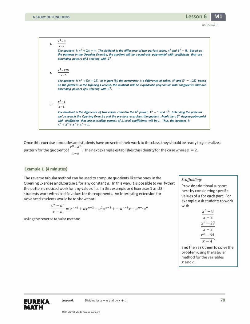
Lesson 6: Dividing by 𝑥𝑥 − 𝑎𝑎 and by 𝑥𝑥 + 𝑎𝑎
M1 Lesson 6 ALGEBRA II
b.
The quotient is + + . The dividend is the difference of two perfect cubes, and = . Based on the patterns in the Opening Exercise, the quotient will be a quadratic polynomial with coefficients that are ascending powers of starting with .
c.
The quotient is + + . As in part (b), the numerator is a difference of cubes, and = . Based on the patterns in the Opening Exercise, the quotient will be a quadratic polynomial with coefficients that are ascending powers of starting with .
d.
The dividend is the difference of two values raised to the 6th power, = and . Extending the patterns we’ve seen in the Opening Exercise and the previous exercises, the quotient should be a 5th degree polynomial with coefficients that are ascending powers of 1, so all coefficients will be 1. Thus, the quotient is
+ + + + .
Once this exercise concludes and students have presented their work to the class, they should be ready to generalize a
pattern for the quotient of . The next example establishes this identity for the case where = 2.
Example 1 (4 minutes)
The reverse tabular method can be used to compute quotients like the ones in the Opening Exercise and Exercise 1 for any constant 𝑎𝑎. In this way, it is possible to verify that the patterns noticed work for any value of 𝑎𝑎. In this example and Exercises 1 and 2, students work with specific values for the exponents. An interesting extension for advanced students would be to show that
𝑥𝑥𝑛𝑛 −𝑎𝑎𝑛𝑛
𝑥𝑥 −𝑎𝑎= 𝑥𝑥𝑛𝑛 1 + 𝑎𝑎𝑥𝑥𝑛𝑛 2+ 𝑎𝑎2𝑥𝑥𝑛𝑛 3+ 𝑎𝑎𝑛𝑛 2𝑥𝑥+ 𝑎𝑎𝑛𝑛 1𝑥𝑥0
using the reverse tabular method.
Scaffolding: Provide additional support here by considering specific values of 𝑎𝑎 for each part. For example, ask students to work with
𝑥𝑥3 − 8𝑥𝑥 − 2
𝑥𝑥3− 27𝑥𝑥 − 3
𝑥𝑥3 − 64𝑥𝑥 − 4
,
and then ask them to solve the problem using the tabular method for the variables 𝑥𝑥 and 𝑎𝑎.
A STORY OF FUNCTIONS
70
©2015 Great Minds. eureka-math.org

Lesson 6: Dividing by 𝑥𝑥 − 𝑎𝑎 and by 𝑥𝑥 + 𝑎𝑎
M1 Lesson 6 ALGEBRA II
Example 1
What is the quotient of ? Use the reverse tabular method or long division.
+
− − −
−
Exercise 2 (7 minutes) Exercise 2
2. Work with your group to find the following quotients.
a.
+ +
b.
+ + +
Before moving on, discuss these results as a whole class. It may be necessary to model a solution to the third question below if students are still struggling with connecting division back to multiplication.
� What patterns do you notice in the quotient?
à The terms are always added, and each term is a product of a power of 𝑥𝑥 and a power of 𝑎𝑎. As the powers of 𝑥𝑥 decrease by 1 for each consecutive term, the powers of 𝑎𝑎 increase by 1.
� How do these patterns compare to the ones you observed in the opening exercises?
à They support the patterns we discovered earlier. This work shows that we can quickly compute the quotient for any problem that fits the pattern.
� How can you rewrite these division problems as multiplication problems?
à The dividend is equal to the product of the quotient and the divisor. For example, 𝑥𝑥3 − 𝑎𝑎3 = (𝑥𝑥 −𝑎𝑎)(𝑥𝑥2+ 𝑎𝑎𝑥𝑥+ 𝑎𝑎2). The other problems would be 𝑥𝑥2− 𝑎𝑎2 = (𝑥𝑥 −𝑎𝑎)(𝑥𝑥 + 𝑎𝑎) and 𝑥𝑥4 − 𝑎𝑎4 = (𝑥𝑥 −𝑎𝑎)(𝑥𝑥3+ 𝑎𝑎𝑥𝑥2+ 𝑎𝑎2𝑥𝑥+ 𝑎𝑎3).
The result of dividing − by − is + .
MP.7
A STORY OF FUNCTIONS
71
©2015 Great Minds. eureka-math.org
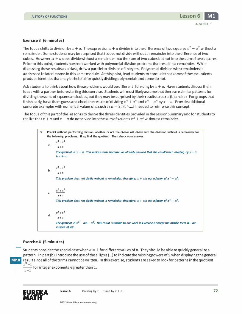
Lesson 6: Dividing by 𝑥𝑥 − 𝑎𝑎 and by 𝑥𝑥 + 𝑎𝑎
M1 Lesson 6 ALGEBRA II
Exercise 3 (6 minutes)
The focus shifts to division by 𝑥𝑥 + 𝑎𝑎. The expression 𝑥𝑥 + 𝑎𝑎 divides into the difference of two squares 𝑥𝑥2 − 𝑎𝑎2 without a remainder. Some students may be surprised that it does not divide without a remainder into the difference of two cubes. However, 𝑥𝑥 + 𝑎𝑎 does divide without a remainder into the sum of two cubes but not into the sum of two squares. Prior to this point, students have not worked with polynomial division problems that result in a remainder. While discussing these results as a class, draw a parallel to division of integers. Polynomial division with remainders is addressed in later lessons in this same module. At this point, lead students to conclude that some of these quotients produce identities that may be helpful for quickly dividing polynomials and some do not.
Ask students to think about how these problems would be different if dividing by 𝑥𝑥 + 𝑎𝑎. Have students discuss their ideas with a partner before starting this exercise. Students will most l ikely assume that there are similar patterns for dividing the sums of squares and cubes, but they may be surprised by their results to parts (b) and (c). For groups that finish early, have them guess and check the results of dividing 𝑥𝑥4 + 𝑎𝑎4 and 𝑥𝑥4 − 𝑎𝑎4 by 𝑥𝑥 + 𝑎𝑎. Provide additional concrete examples with numerical values of 𝑎𝑎 such as 𝑎𝑎 = 2, 3, 4,… if needed to reinforce this concept.
The focus of this part of the lesson is to derive the three identities provided in the Lesson Summary and for students to realize that 𝑥𝑥 + 𝑎𝑎 and 𝑥𝑥 −𝑎𝑎 do not divide into the sum of squares 𝑥𝑥2 + 𝑎𝑎2 without a remainder.
3. Predict without performing division whether or not the divisor will divide into the dividend without a remainder for the following problems. If so, find the quotient. Then check your answer.
a.
The quotient is − . This makes sense because we already showed that the result when dividing by − is + .
b.
This problem does not divide without a remainder; therefore, + is not a factor of − .
c.
This problem does not divide without a remainder; therefore, + is not a factor of + .
d.
The quotient is − + . This result is similar to our work in Exercise 2 except the middle term is − instead of .
Exercise 4 (5 minutes)
Students consider the special case when 𝑎𝑎 = 1 for different values of . They should be able to quickly generalize a pattern. In part (b), introduce the use of the ell ipsis (…) to indicate the missing powers of 𝑥𝑥 when displaying the general result since all of the terms cannot be written. In this exercise, students are asked to look for patterns in the quotient
11
for integer exponents greater than 1.
MP.8
A STORY OF FUNCTIONS
72
©2015 Great Minds. eureka-math.org

Lesson 6: Dividing by 𝑥𝑥 − 𝑎𝑎 and by 𝑥𝑥 + 𝑎𝑎
M1 Lesson 6 ALGEBRA II
4.
a. Find the quotient for = , , , and .
For = , the quotient is + .
For = , the quotient is + + .
For = , the quotient is + + + .
For = , the quotient is + + + + + .
b. What patterns do you notice?
The degree of the quotient is less than the degree of the dividend. The degree of each term is less than the degree of the previous term. The last term is . The number of terms will be equal to the degree of the dividend.
c. Use your work in part (a) to write an expression equivalent to for any integer > .
+ + + + +
Closing (5 minutes)
The summary details the identities derived in this lesson. Ask students to summarize the important results of this lesson either in writing, to a partner, or as a class. Take the opportunity to informally assess their understanding of this lesson before moving on to the Exit Ticket. Note that the last identity has not been formally derived; inductive reasoning was used to generalize the pattern based on the work done in Exercise 4.
Exit Ticket (3 minutes)
In this Exit Ticket, students actually apply the identities they worked with to determine quotients. This Exit Ticket allows the teacher to test their fluency in working with these new relationships. The Lesson Summary is reinforced by having them rewrite each quotient as a product.
Lesson Summary
Based on the work in this lesson, it can be concluded that the following statements are true for all real values of and :
− = ( − )( + ) − = ( − )( + + ) + = ( + )( − + ),
and it seems that the following statement is also an identity for all real values of and :
− = ( − )( + + + + + ), for integers > .
MP.8
A STORY OF FUNCTIONS
73
©2015 Great Minds. eureka-math.org

Lesson 6: Dividing by 𝑥𝑥 − 𝑎𝑎 and by 𝑥𝑥 + 𝑎𝑎
M1 Lesson 6 ALGEBRA II
Name Date
Lesson 6: Dividing by − and by +
Exit Ticket Compute each quotient using the identities you discovered in this lesson.
1. 12
2. 100010
3. 11
A STORY OF FUNCTIONS
74
©2015 Great Minds. eureka-math.org

Lesson 6: Dividing by 𝑥𝑥 − 𝑎𝑎 and by 𝑥𝑥 + 𝑎𝑎
M1 Lesson 6 ALGEBRA II
Exit Ticket Sample Solutions
Compute each quotient using the identities you discovered in this lesson.
1.
= + + +
2.
= − +
3.
= + + + +
Problem Set Sample Solutions
1. Compute each quotient.
a.
+
b.
− +
c.
+ +
d. ..
+ .
A STORY OF FUNCTIONS
75
©2015 Great Minds. eureka-math.org
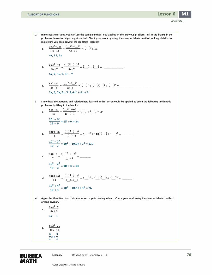
Lesson 6: Dividing by 𝑥𝑥 − 𝑎𝑎 and by 𝑥𝑥 + 𝑎𝑎
M1 Lesson 6 ALGEBRA II
2. In the next exercises, you can use the same identities you applied in the previous problem. Fill in the blanks in the problems below to help you get started. Check your work by using the reverse tabular method or long division to make sure you are applying the identities correctly.
a. =(___) (___)
= (___) +
, ,
b. =(___) (___)
= (___)− (___) = ___________________
, , , , −
c. =(___) (___)
= (___) + (___)(___) + (___) = _______________________________
, , , , , , + +
3. Show how the patterns and relationships learned in this lesson could be applied to solve the following arithmetic
problems by filling in the blanks.
a. =(___) ( )
(___) = (___) + (___) =
−−
= + =
b. =(___) (___)
(___) = (___) + ( )(___) + (___) = __________
−−
= + ( ) + =
c. =(___) (___)
(___) = __________
−−
= + =
d. =(___) (___)
(___) (___) = (___) − (___)(___) + (___) = __________
++
= − ( ) + =
4. Apply the identities from this lesson to compute each quotient. Check your work using the reverse tabular method
or long division.
a.
−
b.
+
A STORY OF FUNCTIONS
76
©2015 Great Minds. eureka-math.org

Lesson 6: Dividing by 𝑥𝑥 − 𝑎𝑎 and by 𝑥𝑥 + 𝑎𝑎
M1 Lesson 6 ALGEBRA II
c.
+ +
5. Extend the patterns and relationships you learned in this lesson to compute the following quotients. Explain your reasoning, and then check your answer by using long division or the tabular method.
a.
The quotient is − + . This problem has the variable and constant terms reversed using the commutative property, so it is the same as computing ( + ) ÷ ( + ).
b.
The quotient is + + + . This problem is similar to Opening Exercise part (c), except that instead of and in the dividend and quotient, we have a power of . You can also extend the patterns for
= + + using the variable instead of the variable .
c.
The quotient is − + . In this example, is in the position, and is in the position. Then, the divisor fits the pattern of + .
d.
The quotient is + + + + + + . In this problem, replace with and extend the powers of pattern using the identities in the Lesson Summary.
A STORY OF FUNCTIONS
77
©2015 Great Minds. eureka-math.org

Lesson 7: Mental Math
M1 Lesson 7 ALGEBRA II
Lesson 7: Mental Math
Student Outcomes
� Students perform arithmetic by using polynomial identities to describe numerical relationships.
Lesson Notes Students continue exploring the usefulness of polynomial identities to perform arithmetic calculations. This work reinforces the essential understanding of standards A-APR and A-SEE. The lesson concludes by discussing prime and composite numbers and using polynomial identities to check whether a number is prime or composite. This lesson ties into the work in the next lesson, which further investigates prime numbers.
The tree diagram analysis, touched upon later in the lesson, offers a connection to some of the probability work from later in this course.
Classwork Opening (1 minute)
Students perform arithmetic that they might not have thought possible without the assistance of a calculator or computer. To motivate this lesson, mention a multiplication problem of the form (𝑎𝑎 − 𝑏𝑏)(𝑎𝑎 + 𝑏𝑏) that is difficult to calculate without pencil and paper, such as 87 93. Perhaps even time students to see how long it takes them to do this calculation without a calculator.
� Today we use the polynomial identities derived in Lesson 6 to perform a variety of calculations quickly using mental arithmetic.
Opening Exercise (3 minutes)
Have students complete the following exercises. Ask students to discuss their ideas with a partner, and then have them summarize their thoughts on the lesson handout. These two exercises build upon the concept of division of polynomials developed in previous lessons by addressing both multiplication and division.
Opening Exercise
a. How are these two equations related? −
+ = − and − = ( + )( − )
They represent the same relationship between the expressions − , − , and + as long as − . One shows the relationship as division and the other as multiplication.
b. Explain the relationship between the polynomial identities − = ( + )( − ) and − = ( − )( + ).
The expression − is of the form − , with = . Note that this works with = − as well.
A STORY OF FUNCTIONS
78
©2015 Great Minds. eureka-math.org

Lesson 7: Mental Math
M1 Lesson 7 ALGEBRA II
Discussion (8 minutes)
Call on a student to share his or her solutions to the Opening Exercise. Then invite other students to add their thoughts to the discussion. This discussion should show students how to apply the difference of two squares identity to quickly find the product of two numbers. Use the questions below to prompt a discussion.
� Consider (𝑥𝑥 − 1)(𝑥𝑥 + 1) = 𝑥𝑥2− 1. If 𝑥𝑥 = 100, what number sentence is represented by this identity? Which side of the equation is easier to compute? à This is 99 101 = 1002 − 1. à Computing 1002 − 1 is far easier than the original multiplication.
� Now let’s consider the more general 𝑥𝑥2− 𝑎𝑎2 = (𝑥𝑥 −𝑎𝑎)(𝑥𝑥 + 𝑎𝑎). Keep 𝑥𝑥 = 100, and test some small positive integer values for 𝑎𝑎. What multiplication problem does each one represent?
� How does the identity (𝑥𝑥 −𝑎𝑎)(𝑥𝑥 + 𝑎𝑎) = 𝑥𝑥2− 𝑎𝑎2 make these multiplication problems easier? à Let 𝑥𝑥 = 100 and 𝑎𝑎 = 5.
(𝑥𝑥 −𝑎𝑎)(𝑥𝑥 + 𝑎𝑎) = 𝑥𝑥2 − 𝑎𝑎2 95 105 = (100 − 5)(100 + 5) = 1002 − 52
Therefore, 95 105 = 1002 − 52 = 10000 − 25 = 9975.
Let 𝑥𝑥 = 100 and 𝑎𝑎 = 7.
(𝑥𝑥 −𝑎𝑎)(𝑥𝑥 + 𝑎𝑎) = 𝑥𝑥2 − 𝑎𝑎2 93 107 = (100 − 7)(100 + 7) = 1002 − 72
Therefore, 93 107 = 1002 − 72 = 10000 − 49 = 9951.
� Do you notice any patterns? à The products in these examples are differences of squares. à The factors in the product are exactly ‘𝑎𝑎’ above and ‘𝑎𝑎’ below 100.
� How could you use the difference of two squares identity to multiply 92 108? How did you determine the values of 𝑥𝑥 and 𝑎𝑎? à You could let 𝑥𝑥 = 100 and 𝑎𝑎 = 8. We must figure out each number’s distance from 100 on the number
line. � How would you use the difference of two squares identity to multiply 87 93? What values should you select
for 𝑥𝑥 and 𝑎𝑎? How did you determine them? à We cannot use 100, but these two numbers are 3 above and 3 below 90. So we can use
(90 − 3)(90 + 3) = 902 − 32 = 8100 − 9 = 8091.
à In general, 𝑥𝑥 is the mean of the factors, and 𝑎𝑎 is half of the absolute value of the difference between the factors.
Depending on the level of students, it may be appropriate to wait until after Exercise 1 to make a generalized statement about how to determine the 𝑥𝑥 and 𝑎𝑎 values used to solve these problems. They may need to experiment with some additional problems before they are ready to generalize a pattern.
A STORY OF FUNCTIONS
79
©2015 Great Minds. eureka-math.org
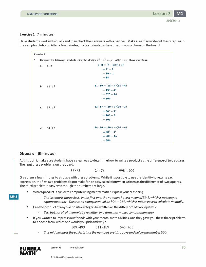
Lesson 7: Mental Math
M1 Lesson 7 ALGEBRA II
Exercise 1 (4 minutes)
Have students work individually and then check their answers with a partner. Make sure they write out their steps as in the sample solutions. After a few minutes, invite students to share one or two solutions on the board.
Exercise 1
1. Compute the following products using the identity − = ( − )( + ). Show your steps.
a.
= ( − )( + ) = − = − =
b.
= ( − )( + ) = − = − =
c.
= ( + )( − ) = − = − =
d.
= ( + )( − ) = − = − =
Discussion (5 minutes)
At this point, make sure students have a clear way to determine how to write a product as the difference of two squares. Then put these problems on the board.
56 63 24 76 998 1002
Give them a few minutes to struggle with these problems. While it is possible to use the identity to rewrite each expression, the first two problems do not make for an easy calculation when written as the difference of two squares. The third problem is easy even though the numbers are large.
� Which product is easier to compute using mental math? Explain your reasoning.
à The last one is the easiest. In the first one, the numbers have a mean of 59.5, which is not easy to square mentally. The second example would be 502 − 262, which is not so easy to calculate mentally.
� Can the product of any two positive integers be written as the difference of two squares? à Yes, but not all of them will be rewritten in a form that makes computation easy.
� If you wanted to impress your friends with your mental math abilities, and they gave you these three problems to choose from, which one would you pick and why?
509 493 511 489 545 455 à This middle one is the easiest since the numbers are 11 above and below the number 500.
MP.3
A STORY OF FUNCTIONS
80
©2015 Great Minds. eureka-math.org

Lesson 7: Mental Math
M1 Lesson 7 ALGEBRA II
Discussion (10 minutes)
At this point, it is possible to introduce the power of algebra over the calculator.
� The identity 𝑥𝑥2 − 𝑎𝑎2 is just the = 2 case of the identity 𝑥𝑥𝑛𝑛− 𝑎𝑎𝑛𝑛 = (𝑥𝑥− 𝑎𝑎)(𝑥𝑥𝑛𝑛 1+ 𝑎𝑎𝑥𝑥𝑛𝑛 2+ 𝑎𝑎2𝑥𝑥𝑛𝑛 2+ 𝑎𝑎𝑛𝑛 1).
� How might we use this general identity to quickly count mentally?
To see how, let’s doodle. A tree is a figure made of points called vertices and segments called branches. My tree splits into two branches at each vertex.
� How many vertices does my tree have?
Allow students to count the vertices for a short while, but don’t dwell on the answer.
� It is difficult to count the vertices of this tree, so let’s draw it in a more organized way.
Present the following drawing of the tree, with vertices aligned in rows corresponding to their levels.
A STORY OF FUNCTIONS
81
©2015 Great Minds. eureka-math.org

Lesson 7: Mental Math
M1 Lesson 7 ALGEBRA II
For the following question, give students time to write or share their thinking with a neighbor.
� How many vertices are in each level? Find a formula to describe the number of vertices in level . à The number of vertices in each level follows this sequence: {1,2, 4,8, 16,… }, so in level there are
2𝑛𝑛 1 vertices. � How many vertices are there in all 5 levels? Explain how you know.
à The number of vertices in our tree, which has five levels, is 24 + 23 + 22 + 2 + 1. First, we recognize that 2− 1 = 1, so we can rewrite our expression as (2 − 1)(24 + 23 + 22 + 2 + 1). If we let 𝑥𝑥 = 2, this numerical expression becomes a polynomial expression.
24 + 23 + 22 + 2 + 1 = (2 − 1)(24 + 23 + 22 + 2 + 1) = (𝑥𝑥 − 1)(𝑥𝑥4 + 𝑥𝑥3+ 𝑥𝑥2 + 𝑥𝑥 + 1) = 𝑥𝑥 − 1 = 2 − 1 = 31
� How could you find the total number of vertices in a tree l ike this one with levels? Explain. à Repeating what we did with = 5 in the previous step, we have
2𝑛𝑛 1+ 2𝑛𝑛 2 + + 2 + 1 = (2 − 1)(2𝑛𝑛 1 + 2𝑛𝑛 2+ + 2 + 1) = (𝑥𝑥 − 1)(𝑥𝑥𝑛𝑛 1 + 𝑥𝑥𝑛𝑛 2 + + 𝑥𝑥 + 1) = 𝑥𝑥𝑛𝑛 − 1 = 2𝑛𝑛 − 1.
Thus, a tree l ike this one with levels has 2𝑛𝑛 − 1 vertices.
� Now, suppose I drew a tree with 30 levels:
� How many vertices would a tree with 30 levels have? à According to the formula we developed in the last step, the number of vertices is à 2𝑛𝑛 − 1 = 230 − 1.
MP.3
A STORY OF FUNCTIONS
82
©2015 Great Minds. eureka-math.org

Lesson 7: Mental Math
M1 Lesson 7 ALGEBRA II
� Would you prefer to count all 1,073,741,823 vertices? à No
Discussion (5 minutes)
This discussion is designed to setup the general identity for 𝑥𝑥𝑛𝑛 −𝑎𝑎𝑛𝑛 to identify some composite numbers in the next lesson.
� Recall that a prime number is a positive integer greater than 1 whose only positive integer factors are 1 and itself. A composite number can be written as the product of positive integers with at least one factor that is not 1 or itself.
� Suppose that 𝑎𝑎, 𝑏𝑏, and are positive integers with 𝑏𝑏 > 𝑎𝑎. What does the identity 𝑥𝑥𝑛𝑛 −𝑎𝑎𝑛𝑛 = (𝑥𝑥 −𝑎𝑎)(𝑥𝑥𝑛𝑛 1+ 𝑎𝑎𝑥𝑥𝑛𝑛 2 + 𝑎𝑎2𝑥𝑥𝑛𝑛 3 + + 𝑎𝑎𝑛𝑛 1) suggest about whether or not the number 𝑏𝑏𝑛𝑛−𝑎𝑎𝑛𝑛 is prime? à We see that 𝑏𝑏𝑛𝑛−𝑎𝑎𝑛𝑛 is divisible by 𝑏𝑏 −𝑎𝑎 and that
𝑏𝑏𝑛𝑛−𝑎𝑎𝑛𝑛 = (𝑏𝑏 −𝑎𝑎)(𝑏𝑏𝑛𝑛 1+ 𝑎𝑎𝑏𝑏𝑛𝑛 2+ + 𝑎𝑎𝑛𝑛 1). à If 𝑏𝑏 −𝑎𝑎 = 1, then we do not know if 𝑏𝑏𝑛𝑛−𝑎𝑎𝑛𝑛 is prime because we do not know
if 𝑏𝑏𝑛𝑛 1+ 𝑎𝑎𝑏𝑏𝑛𝑛 2+ + 𝑎𝑎𝑛𝑛 1is prime. For example, 152 − 142 = 225 − 196 = 29 is prime, but 172 − 162 = 289− 256 = 33 is composite.
à But, if 𝑏𝑏 −𝑎𝑎 > 1, then we know that that 𝑏𝑏𝑛𝑛− 𝑎𝑎𝑛𝑛 is not prime.
� Use the identity 𝑏𝑏𝑛𝑛−𝑎𝑎𝑛𝑛 = (𝑏𝑏−𝑎𝑎)(𝑏𝑏𝑛𝑛 1 + 𝑎𝑎𝑏𝑏𝑛𝑛 2+ 𝑎𝑎2𝑏𝑏𝑛𝑛 3 + + 𝑎𝑎𝑛𝑛 1) to determine whether or not 143 is prime. Check your work using a calculator.
à Let 𝑏𝑏 = 12, 𝑎𝑎 = 1, and = 2. Since 𝑏𝑏 −𝑎𝑎 is a factor of 𝑏𝑏𝑛𝑛− 𝑎𝑎𝑛𝑛, and 𝑏𝑏 −𝑎𝑎 = 12− 1 = 11, we know that 11 is a factor of 143, which means that 143 is not prime. The calculator shows 143 = 11 13.
� We could have used a calculator to determine that 11 13 = 143, so that 143 is not prime. Will a calculator help us determine whether 2100 − 1 is prime? Try it. à The calculator will have difficulty calculating a number this large.
� Can we determine whether or not 2100 − 1 is prime using identities from this lesson?
à We can try to apply the following identity. 𝑥𝑥𝑛𝑛− 1 = (𝑥𝑥 − 1)(𝑥𝑥𝑛𝑛 1+ 𝑥𝑥𝑛𝑛 2+ + 1)
à If we let = 100, then this identity does not help us because 1 divides both composites and primes. 2100 − 1 = (2 − 1)(2 + 2 + 2 + 1)
� But, what if we look at this problem a bit differently? 2100 − 1 = (24)2 − 1 = 162 − 1 = (16 − 1)(1624 + 1623 + + 16 + 1)
à We can see now that 2100 − 1 is divisible by 15, so 2100 − 1 is not prime. � What can we conclude from this discussion?
à If we can write a positive integer as the difference of squares of nonconsecutive integers, then that integer is composite.
Scaffolding: If students are struggling with the words prime and composite, try doing a quick T-chart activity in which students classify numbers as prime or composite on either side of the T.
A STORY OF FUNCTIONS
83
©2015 Great Minds. eureka-math.org

Lesson 7: Mental Math
M1 Lesson 7 ALGEBRA II
Exercises 2–3 (4 minutes) Exercises 2–3
2. Find two additional factors of − .
− = ( ) − = − = ( − )( + + + + )
− = ( ) − = − = ( − )( + + + + )
Thus is a factor and so is .
3. Show that − is divisible by .
− = ( − )( + + ) =
Closing (2 minutes)
Ask students to write a mental math problem that they can now do easily and to explain why the calculation can be done simply.
Ask students to summarize the important parts of the lesson, either in writing, to a partner, or as a class. Use this opportunity to informally assess their understanding of the lesson. The following are some important summary elements:
Exit Ticket (3 minutes)
Lesson Summary
Based on the work in this lesson, students can convert differences of squares into products (and vice versa) using
− = ( − )( + ).
If , , and are integers with ( − ) ± and > , then numbers of the form − are not prime because
− = ( − )( + + + + + ).
A STORY OF FUNCTIONS
84
©2015 Great Minds. eureka-math.org

Lesson 7: Mental Math
M1 Lesson 7 ALGEBRA II
Name Date
Lesson 7: Mental Math
Exit Ticket 1. Explain how you could use the patterns in this lesson to quickly compute (57)(43). 2. Jessica believes that 103 − 1 is divisible by 9. Support or refute her claim using your work in this lesson.
A STORY OF FUNCTIONS
85
©2015 Great Minds. eureka-math.org

Lesson 7: Mental Math
M1 Lesson 7 ALGEBRA II
Exit Ticket Sample Solutions
1. Explain how you could use the patterns in this lesson to quickly compute ( )( ).
Subtract from , . That would be , . You can use the identity − = ( + )( − ). In this case, = and = .
2. Jessica believes that − is divisible by . Support or refute her claim using your work in this lesson.
Since we recognize that = − , then fits the pattern of where = and = . Therefore,
− = −− = + + = ,
and Jessica is correct.
Problem Set Sample Solutions
1. Using an appropriate polynomial identity, quickly compute the following products. Show each step. Be sure to state your values for and .
a.
= , = ( + )( − ) = −
( + )( − ) = − = − =
b. ,
= , = ( − )( + ) = −
( − )( + ) = − = − =
c. = , = ( − )( + ) = −
( − )( + ) = − = − =
d.
= , = ( − )( + ) = −
( − )( + ) = − = − =
e. = , = ( − )( + ) = −
( − )( + ) = − = − =
MP.3
A STORY OF FUNCTIONS
86
©2015 Great Minds. eureka-math.org

Lesson 7: Mental Math
M1 Lesson 7 ALGEBRA II
2. Give the general steps you take to determine and when asked to compute a product such as those in Problem 1.
The number is the mean (average is also acceptable) of the two factors, and is the positive difference between and either factor.
3. Why is easier to compute than ?
The mean of and is . , whereas the mean of and is the integer . I know that the square of is and the square of is . However, I cannot quickly compute the squares of . and . .
4. Rewrite the following differences of squares as a product of two integers.
a. −
− = − = ( − )( + ) =
b. −
− = − = ( − )( + ) =
5. Quickly compute the following differences of squares.
a. −
− = ( − )( + ) = =
b. − − = ( − )( + ) = =
c. − − = ( − )( + ) = =
6. Is prime? Use the fact that = and an identity to support your answer.
No, is not prime because it is equal to − . Therefore, = ( − )( + ).
Note: This problem can also be solved through factoring.
7. The number − is prime and so are − and − . Does that mean − is prime? Explain why or why not.
− = ( ) − = ( − )(( ) + ( ) + )
The factors are and . As such, − is not prime.
8. Show that , , , is not prime without using a calculator or computer.
Note that = − . Since is the square of , , , , is the square of . Since is the square of , = − , which is divisible by − and by + .
A STORY OF FUNCTIONS
87
©2015 Great Minds. eureka-math.org

Lesson 7: Mental Math
M1 Lesson 7 ALGEBRA II
9. Show that , is not prime without using a calculator or computer.
Note that = − . Since = and = are both perfect cubes, we have = − . Therefore, we know that , is divisible by − = .
10. Find a value of so that the expression − is always divisible by for any positive integer . Explain why your value of works for any positive integer .
There are many correct answers. If = , then the expression − will always be divisible by because = − . This will work for any value of that is one more than a multiple of , such as = or = .
11. Find a value of so that the expression − is always divisible by for any positive integer . Explain why your
value of works for any positive integer .
There are many correct answers. If = , then the expression − will always be divisible by because = − . This will work for any value of that is one more than a multiple of , such as = or = .
12. Find a value of so that the expression − is divisible by both and 9 for any positive integer . Explain why
your value of works for any positive integer .
There are multiple correct answers, but one simple answer is = . Since = , − = ( ) − has a factor of − , which factors into ( − )( + ) = .
A STORY OF FUNCTIONS
88
©2015 Great Minds. eureka-math.org

M1 Lesson 8 ALGEBRA II
Lesson 8: The Power of Algebra—Finding Primes
Lesson 8: The Power of Algebra—Finding Primes
Student Outcomes
� Students apply polynomial identities to the detection of prime numbers.
Lesson Notes This lesson applies the identities students have been working with in previous lessons to finding prime numbers, a rich topic with a strong historical background. Many famous mathematicians have puzzled over prime numbers, and their work is the foundation for mathematics used today in the RSA encryption algorithm that provides for secure Internet transmissions. This is an engaging topic for students and is readily accessible to them because of its current use in providing safe and secure electronic communications and transactions. Students will be actively engaging several mathematical practice standards during this lesson, including making sense of problems (MP.1), looking for patterns, and seeing the structure in expressions (MP.7 and MP.8), as they investigate patterns with prime numbers. The lesson includes many opportunities to prove conjectures (MP.3) as students gain experience using algebraic properties to prove statements about integers. Several excellent resources are available for students wishing to learn more about prime numbers, their history, and their application to encryption and decryption. A good starting place for additional exploration about prime numbers is the website The Prime Pages, http://primes.utm.edu/.
Classwork Opening (10 minutes)
To motivate students, show the YouTube video on RSA encryption (http://www.youtube.com/watch?v=M7kEpw1tn50) to the class. This video introduces students to encryption and huge numbers. Encryption algorithms are the basis of all secure Internet transactions. Today, many encryption algorithms rely on very large prime numbers or very large composite numbers that are the product of two primes to create an encryption key. Often these numbers are Mersenne Primes—primes of the form 2 − 1, where 𝑝𝑝 is itself prime. Interestingly, not all numbers in this form are prime. As of December 2013, only 43 Mersenne Primes have been discovered. Encourage students to research the following terms: Mersenne Primes, Data Encryption, and RSA. The Opening Exercise along with the first examples engage students in the exploration of large primes.
Mathematicians have tried for centuries to find a formula that always yields a prime number but have been unsuccessful in their quest. The search for large prime numbers and a formula that will generate all the prime numbers has provided ferti le ground for work in number theory. The mathematician Pierre de Fermat (1601–1665, France) applied the difference of two squares identity to factor very large integers as the product of two prime numbers. Up to this point, students have worked with numbers that can be expressed as the difference of two perfect squares. If a prime number could be written as a difference of perfect squares 𝑎𝑎2− 𝑏𝑏2, then it would have to be of the form (𝑎𝑎 + 𝑏𝑏)(𝑎𝑎 −𝑏𝑏), where 𝑎𝑎 and 𝑏𝑏 are consecutive whole numbers and 𝑎𝑎 + 𝑏𝑏 is prime. The challenge is that not every pair of consecutive whole numbers yields a prime number when added. For example, 3 + 4 = 7 is prime, but 4 + 5 = 9 is not. This idea is further addressed in the last exercise and in the Problem Set.
A STORY OF FUNCTIONS
89
©2015 Great Minds. eureka-math.org

M1 Lesson 8 ALGEBRA II
Lesson 8: The Power of Algebra—Finding Primes
Opening Exercise (10 minutes): When is − prime and when is it composite?
Before beginning this exercise, have students predict when an expression in this form will be prime and when it will be composite. Questions l ike this are ideal places to engage students in constructing viable arguments.
� When will this expression be prime and when will it be composite?
à Student responses will vary. Some may say always prime or always composite. A response that goes back to the identity 𝑥𝑥𝑛𝑛− 1 = (𝑥𝑥 − 1)(𝑥𝑥𝑛𝑛 1+ 𝑥𝑥𝑛𝑛 2+ + 1) from the previous lesson is showing some good initial thinking.
Students should work the Opening Exercise in small groups. After about seven minutes of group work, have one student from each group come up and fi ll in the table values and the supporting work. Then, lead a whole group discussion to debrief this problem.
Opening Exercise: When is − prime and when is it composite?
Complete the table to investigate which numbers of the form − are prime and which are composite.
Exponent
Expression −
Value Prime or Composite? Justify your answer if composite.
− Prime
− Prime
− Prime
− Composite ( )
− Prime
− Composite ( )
− Prime
− Composite ( )
− Composite ( )
− Composite ( − )( + )
− Composite ( )
What patterns do you notice in this table about which expressions are prime and which are composite?
Answers will vary. Suggested responses are in the discussion questions.
Encourage students to use tools strategically as they work with these problems. They should have a calculator available to determine if the larger numbers are composite. When debriefing, point out the fact that students can use the difference of two squares identity to factor these expressions when the exponent is an even number.
Use these questions to lead a short discussion on the results of this Opening Exercise.
MP.2 MP.7
& MP.8
Scaffolding: For more advanced students, consider posing the question: Can you construct an expression that always yields a prime number? Do this before starting the Opening Exercise, and then ask them to test their expressions.
If students are having a hard time constructing an expression, consider asking the following questions: Can you construct an expression that will always yield an even number? Can you construct an expression that will always yield an odd number?
If is an integer, then 2 is always an even number, and 2 + 1 is always an odd number.
MP.3
A STORY OF FUNCTIONS
90
©2015 Great Minds. eureka-math.org

M1 Lesson 8 ALGEBRA II
Lesson 8: The Power of Algebra—Finding Primes
� What patterns do you notice about which expressions are composite and which are prime?
à When the exponent is an even number greater than 2, the result is composite and can be factored using this identity: 22𝑛𝑛 − 1 = (2𝑛𝑛 + 1)(2𝑛𝑛 − 1).
à When the exponent is a prime number, the result is sometimes prime and sometimes not prime. 211 − 1 was the first number with a prime exponent that was composite.
à When the exponent is a composite odd number, the expression appears to be composite, but we have yet to prove that.
The statements above are examples of the types of patterns students should notice as they complete the Opening Exercise. If the class was not able to prove that the case for even exponents resulted in a composite number, encourage them to consider the identities learned in the last lesson involving the difference of two squares. See if they can solve the problem with that hint. Of course, that technique does not work when the exponent is odd. Make sure students have articulated the answer to the last problem. To transition to the next section, ask students how they might prove that 2 − 1 is composite when the exponent 𝑎𝑎𝑏𝑏 is an odd composite number.
Example 1 (5 minutes): Proving a Conjecture
This example and the next exercise prove patterns students noticed in the table in the Opening Exercise. Some scaffolding is provided, but feel free to adjust as needed for students. Give students who need less support the conjecture on the board for Example 1 (without the additional scaffolding on the student pages); others may need more assistance to get started.
Example 1: Proving a Conjecture
Conjecture: If is a positive odd composite number, then − is a composite number.
Start with an identity: − = ( − )( + + + )
In this case, = , so the identity above becomes:
− = ( − )( + + + + ) = ( + + + + ),
and it is not clear whether or not − is composite.
Rewrite the expression: Let = be a positive odd composite number. Then and must also be odd, or else the product would be even. The smallest such number is , so we have and
.
Then we have
− = ( ) − = ( − ) (( ) + ( ) + + ( ) + )
Some number larger than
.
Since , we have ; thus, − . Since the other factor is also larger than , − is composite, and we have proven our conjecture.
MP.2 MP.7
& MP.8
A STORY OF FUNCTIONS
91
©2015 Great Minds. eureka-math.org

M1 Lesson 8 ALGEBRA II
Lesson 8: The Power of Algebra—Finding Primes
Exercises 1–3 (4 minutes)
In these exercises, students confirm the conjecture proven in Example 1. Emphasize that it does not really matter what the 2nd factor is once the first one is known. There is more than one way to solve each of these problems depending on how students decide to factor the exponent on the 2. Students should work in small groups on these exercises. Encourage them to use a calculator to determine the prime factors of 537 in Exercise 3. Have different groups present their results.
Exercises 1–3
For Exercises 1–3, find a factor of each expression using the method discussed in Example 1.
1. −
( ) − = ( − )(( ) + + ) = ( ) + + Some number larger than
Thus, is a factor of − .
2. −
( ) = ( − ) + + + +Some number larger than
Thus, is a factor of − .
3. − (Hint: is the product of two prime numbers that are both less than .)
Using a calculator we see that = , so
( ) − = ( − ) ( ) + + +Some number larger than
.
Thus, − is a factor of − .
Discussion (4 minutes)
Cryptography is the science of making codes, and cryptanalysis is the science of breaking codes. The rise of Internet commerce has created a demand for encoding methods that are hard for unintended observers to decipher. One encryption method, known as RSA encryption, uses very large numbers with hundreds of digits that are the product of two primes; the product of the prime factors is called the key. The key itself is made public so anyone can encode using this system, but in order to break the code, you would have to know how to factor the key, and that is what is so difficult.
� You had a hint in Exercise 3 that made it easier for you to factor a very large number, but what if you do not have any hints? à It would be almost impossible to factor the number because you would have to check all the prime
numbers up to the square root of the exponent to find the factors.
If you know the key, then decoding is not particularly difficult. Programmers select a number that is almost impossible to factor without significant time and computing power and use this as the key to encode data and communications. The last exercise illuminates the logic behind modern encryption algorithms.
A STORY OF FUNCTIONS
92
©2015 Great Minds. eureka-math.org

M1 Lesson 8 ALGEBRA II
Lesson 8: The Power of Algebra—Finding Primes
Exercise 4 (6 minutes): How quickly can a computer factor a very large number?
To determine if a number is prime, it is possible to just try dividing by every prime number 𝑝𝑝 that is less than √ . This takes the longest time if happens to be a perfect square. In this exercise, students consider the speed it takes a certain computer algorithm to factor a square of a large prime number; this is the case where it should take the algorithm the longest to find the factorization. Actual algorithms used to factor large numbers are quicker than this, but it sti l l takes a really long time and works to the advantage of people who want to encrypt information electronically using these large numbers. Introduce the problem and review the table as a whole class; then, have students answer the question in small groups. Have students working in groups apply the given function to estimate the time it would take to factor a 32-digit number. Make sure they convert their answer to years. Because we are using an exponential function, the factorization time grows very rapidly. Take the time after Exercise 4 to remind students that exponential functions increase very rapidly over intervals of equal length, ideas that were introduced in Algebra I and will be revisited in Module 3 of Algebra II.
Exercise 4: How quickly can a computer factor a very large number?
4. How long would it take a computer to factor some squares of very large prime numbers?
The time in seconds required to factor an -digit number of the form , where is a large prime, can roughly be approximated by ( ) = . × ( )/ . Some values of this function are listed in the table below.
Number of Digits Time needed to
factor the number (sec)
, , , . , , , , .
, , , , , , . , , , , , , , , , , , , , , , , , , , , , ,
Use the function given above to determine how long it would take this computer to factor a number that contains digits.
Using the given function, ( ) = . × seconds = . × minutes = × hours = , days, which is about . years.
After allowing groups to take a few minutes to evaluate the function and convert their answer to years, connect this exercise to the context of this situation by summarizing the following points.
� Using a very fast personal computer with a straightforward algorithm, it would take about 342 years to factor a 32-digit number, making any secret message encoded with that number obsolete before it could be cracked with that computer.
� However, we have extremely fast computers (much faster than one personal computer) and very efficient algorithms designed for those computers for factoring numbers. These computers can factor a number thousands of times faster than the computer used above, but they are still not fast enough to factor huge composite numbers in a reasonable amount of time.
A STORY OF FUNCTIONS
93
©2015 Great Minds. eureka-math.org

M1 Lesson 8 ALGEBRA II
Lesson 8: The Power of Algebra—Finding Primes
� In 2009, computer scientists were able to factor a 232-digit number in two years by distributing the work over hundreds of fast computers running at the same time. That means any message encoded using that 232-digit number would take two years to decipher, by which time the message would no longer be relevant. Numbers used to encode secret messages typically contain over 300 digits, and extremely important secret messages use numbers that have over 600 digits—a far bigger number than any bank of computers can currently factor in a reasonable amount of time.
Closing (2 minutes)
There are better ways of factoring numbers than just checking all of the factors, but even advanced methods take a long time to execute. Products of primes of the magnitude of 2204 are almost impossible to factor in a reasonable amount of time, which is how mathematics is used to guarantee the security of electronic transactions. Give students a few minutes to summarize what they have learned in writing or by discussing it with a partner before starting the Exit Ticket.
� Polynomial identities can help us prove conjectures about numbers and make calculations easier.
� The field of number theory has contributed greatly to the fields of cryptography and cryptanalysis (code-making and code-breaking).
Exit Ticket (4 minutes)
A STORY OF FUNCTIONS
94
©2015 Great Minds. eureka-math.org

M1 Lesson 8 ALGEBRA II
Lesson 8: The Power of Algebra—Finding Primes
Name Date
Lesson 8: The Power of Algebra—Finding Primes
Exit Ticket Express the prime number 31 in the form 2 − 1 where 𝑝𝑝 is a prime number and as a difference of two perfect squares using the identity (𝑎𝑎 + 𝑏𝑏)(𝑎𝑎 −𝑏𝑏) = 𝑎𝑎2− 𝑏𝑏2.
A STORY OF FUNCTIONS
95
©2015 Great Minds. eureka-math.org

M1 Lesson 8 ALGEBRA II
Lesson 8: The Power of Algebra—Finding Primes
Exit Ticket Sample Solutions
Express the prime number in the form − where is a prime number and as a difference of two perfect squares using the identity ( + )( − ) = − .
= ( − )( + )
= −
= −
Problem Set Sample Solutions
1. Factor − in two different ways using the identity − = ( − )( + + + + ) and the difference of squares identity.
( − )( + )
( − )( + +. . . + + )
2. Factor + using the identity + = ( + )( − + − + ) for odd numbers .
( ) + = ( + )(( ) − + )
3. Is , , , prime? Explain your reasoning.
No, because it is of the form + , which could be written as ( ) + = ( + )(( ) − + ).
4. Explain why − is never prime if is a composite number.
If is composite, then it can be written in the form = , where and are integers larger than . Then − = − = ( ) − = ( − )(( ) + + + ). For > , this number will be composite because − will be larger than .
5. Fermat numbers are of the form + where is a positive integer.
a. Create a table of Fermat numbers for odd values of up to .
+ + = + = + = + = + =
b. Explain why if is odd, the Fermat number + will always be divisible by .
The Fermat number + will factor as ( + )( − + + ) using the identity in Exercise 2.
A STORY OF FUNCTIONS
96
©2015 Great Minds. eureka-math.org

M1 Lesson 8 ALGEBRA II
Lesson 8: The Power of Algebra—Finding Primes
c. Complete the table of values for even values of up to .
+ + = + = + = + = + = , + = ,
d. Show that if can be written in the form where is odd, then + is divisible by .
Let = , where is odd. Then + = + = ( ) + = ( + ) (( ) + + + )number larger than
.
Since + = , we know that is a factor of + . This only holds when is an odd number because that is the only case when we can factor expressions of the form + .
e. Which even numbers are not divisible by an odd number? Make a conjecture about the only Fermat numbers that might be prime.
The powers of are the only positive integers that are not divisible by any odd numbers. This implies that when the exponent in + is a power of , the Fermat number + might be prime.
6. Complete this table to explore which numbers can be expressed as the difference of two perfect squares.
Number Difference of Two Squares Number Difference of Two Squares − = − = − = − = Not possible − = − = − = − = − = − = − = − = Not possible − = − = − = − = Not possible − = − = − = − = − = − = − = − = Not possible − = − = − = − = Not possible − = − =
a. For which odd numbers does it appear to be possible to write the number as the difference of two squares?
It appears that we can write any positive odd number as the difference of two squares.
b. For which even numbers does it appear to be possible to write the number as the difference of two squares?
It appears that we can write any multiple of as the difference of two squares.
c. Suppose that is an odd number that can be expressed as = − for positive integers and . What do you notice about and ?
When is odd, and are consecutive whole numbers and + = .
d. Suppose that is an even number that can be expressed as = − for positive integers and . What do you notice about and ?
When is an even number that can be written as a difference of squares, then is a multiple of , and and are either consecutive even integers or consecutive odd integers. We also have + = .
A STORY OF FUNCTIONS
97
©2015 Great Minds. eureka-math.org

M1 Lesson 8 ALGEBRA II
Lesson 8: The Power of Algebra—Finding Primes
7. Express the numbers from to as the difference of two squares, if possible.
This is not possible for , , and . Otherwise we have the following.
= − = − = − = − = − = − = −
8. Prove this conjecture: Every positive odd number can be expressed as the difference of the squares of two consecutive numbers that sum to the original number . a. Let be a positive odd number. Then for some integer , = + . We will look at the consecutive
integers and + . Show that + ( + ) = .
+ ( + ) = + + = + =
b. What is the difference of squares of + and ?
( + ) − = + + − = + =
c. What can you conclude from parts (a) and (b)?
We can write any positive odd number as the difference of squares of two consecutive numbers that sum to .
9. Prove this conjecture: Every positive multiple of can be expressed as the difference of squares of two numbers
that differ by . Use the table below to organize your work for parts (a)–(c).
a. Write each multiple of in the table as a difference of squares.
Difference of squares −
− 0 − − − − ( ) − ( ) + −
b. What do you notice about the numbers and that are squared? How do they relate to the number ?
The values of and in the differences of two squares differ by every time. They are one larger and one smaller than ; that is, = + and = − .
A STORY OF FUNCTIONS
98
©2015 Great Minds. eureka-math.org

M1 Lesson 8 ALGEBRA II
Lesson 8: The Power of Algebra—Finding Primes
c. Given a positive integer of the form , prove that there are integers and so that = − and that − = . (Hint: Refer to parts (a) and (b) for the relationship between and and .)
Define = + and = − . Then we can calculate − as follows.
− = ( + ) − ( − ) = ( + ) + ( − ) ( + ) − ( − ) = ( )( ) =
We can also see that
− = ( + ) − ( − ) = + − + = .
Thus every positive multiple of can be written as a difference of squares of two integers that differ by .
10. The steps below prove that the only positive even numbers that can be written as a difference of square integers are the multiples of . That is, completing this exercise will prove that it is impossible to write a number of the form
− as a difference of square integers.
a. Let be a positive even integer that we can write as the difference of square integers = − . Then = ( + )( − ) for integers and . How do we know that either and are both even or and are
both odd?
If one of and is even and the other one is odd, then one of and is even and the other one is odd. Since the difference of an odd and an even number is odd, this means that = − would be odd. Since we know that is even, it must be that either and are both even or and are both odd.
b. Is + even or odd? What about − ? How do you know?
Since and are either both odd or both even, we know that both + and − are even.
c. Is a factor of + ? Is a factor of − ? Is a factor of ( + )( − )? Explain how you know.
Because + and − are both even, 2 is a factor of both + and − . Thus, = is a factor of ( + )( − ).
d. Is a factor of any integer of the form − ?
No. If were a factor of − , we could factor it out: − = � − �. But this means that − is an integer, which it clearly is not. This means that is not a factor of any number of the form − .
e. What can you conclude from your work in parts (a)–(d)?
If is a positive even integer and can be written as the difference of two square integers, then cannot be of the form − for any integer . Another way to say this is that the positive integers of the form
− for some integer cannot be written as the difference of two square integers.
A STORY OF FUNCTIONS
99
©2015 Great Minds. eureka-math.org

M1 Lesson 8 ALGEBRA II
Lesson 8: The Power of Algebra—Finding Primes
11. Explain why the prime number can only be expressed as the difference of two squares in only one way, but the composite number can be expressed as the difference of two squares in more than one way.
Since every odd number can be expressed as the difference of two squares, − = ( + )( − ), the number must fit this pattern. Because is prime, there is only one way to factor , which is = .
Let + = and − = . The two numbers that satisfy this system of equations are and . Thus,
= = ( − )( + ) = − .
A composite number has more than one factorization, not all of which will lead to writing the number as the difference of squares of two integers. For the number , you could use
= = ( − )( + ) = − .
Or, you could use
= = ( − )( + ) = − .
12. Explain why you cannot use the factors of and to rewrite as the difference of two square integers.
If = , then − = and + = . The solution to this system of equations is ( . , . ). If we are restricting this problem to the set of whole numbers, then you cannot apply the identity to rewrite as the difference of two perfect squares where and are whole numbers. It certainly is true that
= ( . − . )( . + . ) = . − . , but this is not necessarily an easy way to calculate .
MP.3
A STORY OF FUNCTIONS
100
©2015 Great Minds. eureka-math.org

Lesson 9: Radicals and Conjugates
M1 Lesson 9 ALGEBRA II
Lesson 9: Radicals and Conjugates
Student Outcomes � Students understand that the sum of two square roots (or two cube roots) is not equal to the square root (or
cube root) of their sum. � Students convert expressions to simplest radical form. � Students understand that the product of conjugate radicals can be viewed as the difference of two squares.
Lesson Notes Because this lesson deals with radicals, it might seem out of place amid other lessons on polynomials. A major theme, however, is the parallelism between the product of conjugate radicals and the difference of two squares. There is also parallelism between taking the square root or cube root of a sum and taking the square of a sum; both give rise to an error sometimes called the freshman’s dream or the illusion of linearity. If students are not careful, they may easily conclude that (𝑥𝑥 + 𝑦𝑦)𝑛𝑛 and 𝑥𝑥𝑛𝑛 + 𝑦𝑦𝑛𝑛 are equivalent expressions for all 0, when this is only true for = 1. Additionally, this work with radicals prepares students for later work with radical expressions in Module 3. Throughout this lesson, students employ MP.7, as they see complicated expressions as being composed of simpler ones. Additionally, the Opening Exercise offers further practice in making a conjecture (MP.3).
Classwork Opening Exercise (3 minutes)
The Opening Exercise is designed to show students that they need to be cautious when working with radicals. The multiplication and division operations combine with radicals in a predictable way, but the addition and subtraction operations do not.
The square root of a product is the product of the two square roots. For example,
√4 9 = √2 2 3 3 =√6 6 = 6 = 2 3 =√4 √9.
Similarly, the square root of a quotient is the quotient of the two square roots: 21
=4
= √2
√1. And the same holds
true for multiplication and division with cube roots, but not for addition or subtraction with square or cube roots.
Scaffolding: If necessary, remind students that √2 and −√4 are irrational numbers. They cannot be written in the form for integers 𝑝𝑝 and 𝑞𝑞. They are numbers, however, and, just l ike √4 and −√64, can be found on a number l ine. On the number l ine, √2 = 1.414… is just to the right of 1.4, and −√4 = −1.5874… is just to the left of −1.587.
A STORY OF FUNCTIONS
101
©2015 Great Minds. eureka-math.org
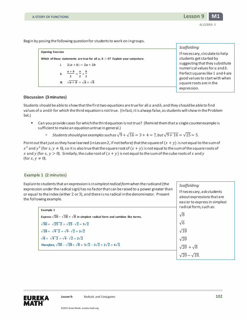
Lesson 9: Radicals and Conjugates
M1 Lesson 9 ALGEBRA II
Begin by posing the following question for students to work on in groups.
Opening Exercise
Which of these statements are true for all , > ? Explain your conjecture.
i. ( + ) = +
ii.
= +
iii. √ + = √ + √
Discussion (3 minutes)
Students should be able to show that the first two equations are true for all 𝑎𝑎 and 𝑏𝑏, and they should be able to find values of 𝑎𝑎 and 𝑏𝑏 for which the third equation is not true. (In fact, it is always false, as students will show in the Problem Set.)
� Can you provide cases for which the third equation is not true? (Remind them that a single counterexample is sufficient to make an equation untrue in general.)
à Students should give examples such as √9 +√16 = 3 + 4 = 7, but √9+ 16 = √25 = 5.
Point out that just as they have learned (in Lesson 2, if not before) that the square of (𝑥𝑥 + 𝑦𝑦) is not equal to the sum of 𝑥𝑥2 and 𝑦𝑦2 (for 𝑥𝑥, 𝑦𝑦 0), so it is also true that the square root of (𝑥𝑥 + 𝑦𝑦) is not equal to the sum of the square roots of 𝑥𝑥 and 𝑦𝑦 (for 𝑥𝑥, 𝑦𝑦 > 0). Similarly, the cube root of (𝑥𝑥+ 𝑦𝑦) is not equal to the sum of the cube roots of 𝑥𝑥 and 𝑦𝑦 (for 𝑥𝑥, 𝑦𝑦 0).
Example 1 (2 minutes)
Explain to students that an expression is in simplest radical form when the radicand (the expression under the radical sign) has no factor that can be raised to a power greater than or equal to the index (either 2 or 3), and there is no radical in the denominator. Present the following example.
Example 1
Express √ − √ + √ in simplest radical form and combine like terms.
√ = √ = √ √ = √
√ = √ = √ √ = √
√ = √ = √ √ = √
Therefore, √ − √ + √ = √ − √ + √ = √ .
Scaffolding: If necessary, circulate to help students get started by suggesting that they substitute numerical values for 𝑎𝑎 and 𝑏𝑏. Perfect squares like 1 and 4 are good values to start with when square roots are in the expression.
Scaffolding: If necessary, ask students about expressions that are easier to express in simplest radical form, such as:
√8
√6
√18
√20
√20 +√8
√20−√18.
A STORY OF FUNCTIONS
102
©2015 Great Minds. eureka-math.org

Lesson 9: Radicals and Conjugates
M1 Lesson 9 ALGEBRA II
Exercises 1–5 (8 minutes)
The following exercises make use of the rules for multiplying and dividing radicals. Express each expression in simplest radical form and combine l ike terms.
Exercises 1–5
1. + − √
− √
2. √ √ −√
√ −
3.
√√
=√√
=√
4.
√√
=√√
=√
5. √
=
In the example and exercises above, we repeatedly used the following properties of radicals (write the following statements on the board).
√𝑎𝑎 √𝑏𝑏 = √𝑎𝑎𝑏𝑏 √𝑎𝑎 √𝑏𝑏 = √𝑎𝑎𝑏𝑏
√√
= √√
=
� When do these identities make sense?
à Students should answer that the identities make sense for the square roots whenever 𝑎𝑎 0 and 𝑏𝑏 0, with 𝑏𝑏 0 when 𝑏𝑏 is a denominator. They make sense for the cube roots for all 𝑎𝑎 and 𝑏𝑏, with 𝑏𝑏 0 when 𝑏𝑏 is a denominator.
Example 2 (8 minutes)
This example is designed to introduce conjugates and their properties.
Example 2
Multiply and combine like terms. Then explain what you notice about the two different results.
√ + √ √ + √
√ + √ √ − √
Scaffolding: Circulate to make sure that students understand that they are looking for perfect square factors when the index is 2 and perfect cube factors when the index is 3. Remind students that the cubes of the first counting numbers are 1, 8, 27, 64, and 125.
A STORY OF FUNCTIONS
103
©2015 Great Minds. eureka-math.org

Lesson 9: Radicals and Conjugates
M1 Lesson 9 ALGEBRA II
Solution (with teacher comments and a question):
The first product is √3 √3 + 2 √3 √2 +√2 √2 = 5 + 2√6.
The second product is √3 √3− √3 √2 + √3 √2 −√2 √2 = 3 − 2 = 1.
The first product is an irrational number; the second is an integer.
The second product has the nice feature that the radicals have been eliminated. In that case, the two factors are given a special name: two binomials of the form √𝑎𝑎 +√𝑏𝑏 and √𝑎𝑎−√𝑏𝑏 are called conjugate radicals:
√𝑎𝑎+√𝑏𝑏 is the conjugate of √𝑎𝑎− √𝑏𝑏, and
√𝑎𝑎−√𝑏𝑏 is the conjugate of √𝑎𝑎+ √𝑏𝑏.
More generally, for any expression in two terms, at least one of which contains a radical, its conjugate is an expression consisting of the same two terms but with the opposite sign separating the terms. For example, the conjugate of 2 −√3 is 2 +√3, and the conjugate of √5 +√3 is √5− √3.
� What polynomial identity is suggested by the product of two conjugates?
à Students should answer that it looks like the difference of two squares. The product of two conjugates has the form of the difference of squares: (𝑥𝑥 + 𝑦𝑦)(𝑥𝑥 −𝑦𝑦) = 𝑥𝑥2 − 𝑦𝑦2.
The following exercise focuses on the use of conjugates.
Exercise 6 (5 minutes) Exercise 6
6. Find the product of the conjugate radicals.
√ +√ √ −√ − =
+ √ −√ − =
√ + √ − − =
� In each case in Exercise 6, is the result the difference of two squares?
à Yes. For example, if we think of 5 as √52 and 3 as √3
2, then 5 − 3 = √5
2− √3
2.
Scaffolding: Students may have trouble with the word conjugate. If so, have them fil l out the following diagram.
A STORY OF FUNCTIONS
104
©2015 Great Minds. eureka-math.org

Lesson 9: Radicals and Conjugates
M1 Lesson 9 ALGEBRA II
Example 3 (6 minutes)
This example is designed to show how division by a radical can be reduced to division by an integer by multiplication by the conjugate radical in the numerator and denominator.
Example 3
Write √√
in simplest radical form.
√− √
=√− √
+ √+ √
=√ + √
−=
√ +
The process for simplifying an expression with a radical in the denominator has two steps:
1. Multiply the numerator and denominator of the fraction by the conjugate of the denominator.
2. Simplify the resulting expression.
Closing (5 minutes)
� Radical expressions with the same index and same radicand combine in the same way as l ike terms in a polynomial when performing addition and subtraction.
For example, √3 + √2 + 5√3−√7 +√3 +√7 + 3√2 = 6√3 + 4√2 +√3. � Simplifying an expression with a radical in the denominator relies on an application of the difference of squares
formula.
à For example, to simplify 3
√2 √3, we treat the denominator like a binomial.
Substitute √2 = 𝑥𝑥 and √3 = 𝑦𝑦, and then 3
√2 +√3=
3𝑥𝑥 + 𝑦𝑦
=3
𝑥𝑥 + 𝑦𝑦𝑥𝑥 −𝑦𝑦𝑥𝑥 −𝑦𝑦
= 3(𝑥𝑥 −𝑦𝑦)𝑥𝑥2 − 𝑦𝑦2
.
Since 𝑥𝑥 = √2 and 𝑦𝑦 = √3, 𝑥𝑥2 − 𝑦𝑦2 is an integer. In this case, 𝑥𝑥2 − 𝑦𝑦2 = −1.
3√2 +√3
√2− √3√2− √3
=3 √2− √3
2 − 3= −3 √2−√3
A STORY OF FUNCTIONS
105
©2015 Great Minds. eureka-math.org

Lesson 9: Radicals and Conjugates
M1 Lesson 9 ALGEBRA II
Ask students to summarize the important parts of the lesson, either in writing, to a partner, or as a class. Use this as an opportunity to informally assess understanding of the lesson. The following are some important summary elements.
Exit Ticket (5 minutes)
Lesson Summary
� For real numbers and , where when is a denominator,
√ = √ √ and = √ .
� For real numbers and , where when is a denominator,
√ = √ √ and = √ .
� Two binomials of the form √ + √ and √ − √ are called conjugate radicals:
√ + √ is the conjugate of √ − √ , and
√ − √ is the conjugate of √ + √ .
For example, the conjugate of −√ is + √ .
� To rewrite an expression with a denominator of the form √ + √ in simplest radical form, multiply the numerator and denominator by the conjugate √ −√ and combine like terms.
A STORY OF FUNCTIONS
106
©2015 Great Minds. eureka-math.org

Lesson 9: Radicals and Conjugates
M1 Lesson 9 ALGEBRA II
Name Date
Lesson 9: Radicals and Conjugates
Exit Ticket 1. Rewrite each of the following radicals as a rational number or in simplest radical form.
a. √49
b. √40
c. √242
2. Find the conjugate of each of the following radical expressions.
a. √5 +√11
b. 9 −√11
c. √3 + 1.5
3. Rewrite each of the following expressions as a rational number or in simplest radical form.
a. √3 √3− 1
b. 5 +√32
c. (10 +√11)(10−√11)
A STORY OF FUNCTIONS
107
©2015 Great Minds. eureka-math.org

Lesson 9: Radicals and Conjugates
M1 Lesson 9 ALGEBRA II
Exit Ticket Sample Solution
1. Rewrite each of the following radicals as a rational number or in simplest radical form.
a. √
b. √ √
c. √ √
2. Find the conjugate of each of the following radical expressions.
a. √ +√ √ −√
b. − √ + √
c. √ + . √ − .
3. Rewrite each of the following expressions as a rational number or in simplest radical form.
a. √ (√ − ) − √
b. + √ + √
c. ( + √ )( −√ )
Problem Set Sample Solutions Problem 10 is different from the others and may require some discussion and explanation before students work on it. Consider explaining that the converse of an if–then theorem is obtained by interchanging the clauses introduced by if and then, and that the converse of such a theorem is not necessarily a valid theorem. The converse of the Pythagorean theorem will be important for the development of a formula leading to Pythagorean triples in Lesson 10.
1. Express each of the following as a rational number or in simplest radical form. Assume that the symbols , , and represent positive numbers.
a. √
b. √ √
c. √ √
d. √ √
A STORY OF FUNCTIONS
108
©2015 Great Minds. eureka-math.org

Lesson 9: Radicals and Conjugates
M1 Lesson 9 ALGEBRA II
e. √ √
f. √ √
g. √ √
h. √ + √ +
2. Express each of the following in simplest radical form, combining terms where possible.
a. √ + √ − √ + √
b. √ − + √
c. √ − √ + √
−
d. + √ − √
−√
3. Evaluate − when = and = . √
4. Evaluate + when = and = . √
5. Express each of the following as a rational expression or in simplest radical form. Assume that the symbols and represent positive numbers.
a. √ √ − √ √ −
b. + √ + √
c. ( +√ )( − √ )
d. ( + √ )( − √ ) −
e. √ − √ + −
f. √ +√ √ −√
g. − √ + √ −
h. √ + √ − −
A STORY OF FUNCTIONS
109
©2015 Great Minds. eureka-math.org
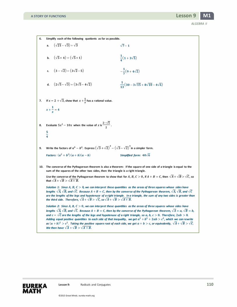
Lesson 9: Radicals and Conjugates
M1 Lesson 9 ALGEBRA II
6. Simplify each of the following quotients as far as possible.
a. √ − √ ÷ √ √ −
b. √ + ÷ √ + + √
c. − √ ÷ √ − − + √
d. √ − √ ÷ √ − √ − √ + √ − √
7. If = +√ , show that + has a rational value.
+ =
8. Evaluate − when the value of is √ .
9. Write the factors of − . Express √ +√ − √ − √ in a simpler form.
Factors: ( + )( + )( − ) Simplified form: √
10. The converse of the Pythagorean theorem is also a theorem: If the square of one side of a triangle is equal to the
sum of the squares of the other two sides, then the triangle is a right triangle.
Use the converse of the Pythagorean theorem to show that for , , > , if + = , then √ + √ > √ , so that √ + √ > √ + .
Solution 1: Since , , > , we can interpret these quantities as the areas of three squares whose sides have lengths √ , √ , and √ . Because + = , then by the converse of the Pythagorean theorem, √ , √ , and √ are the lengths of the legs and hypotenuse of a right triangle. In a triangle, the sum of any two sides is greater than the third side. Therefore, √ + √ > √ , so √ + √ > √ + .
Solution 2: Since , B, > , we can interpret these quantities as the areas of three squares whose sides have lengths √ , √ , and √ . Because + = , then by the converse of the Pythagorean theorem, √ = , √ = , and = √ are the lengths of the legs and hypotenuse of a right triangle, so , , > . Therefore, > . Adding equal positive quantities to each side of that inequality, we get + + > , which we can rewrite as ( + ) > . Taking the positive square root of each side, we get + > , or equivalently, √ + √ > √ . We then have √ +√ > √ + .
A STORY OF FUNCTIONS
110
©2015 Great Minds. eureka-math.org

Lesson 10: The Power of Algebra—Finding Pythagorean Triples
M1 Lesson 10 ALGEBRA II
Lesson 10: The Power of Algebra—Finding Pythagorean
Triples
Student Outcomes
� Students explore the difference of two squares identity 𝑥𝑥2− 𝑦𝑦2 = (𝑥𝑥 −𝑦𝑦)(𝑥𝑥 + 𝑦𝑦) in the context of finding Pythagorean triples.
Lesson Notes This lesson addresses standards A-SSE.A.2 and A-APR.C.4, and MP.7 directly. In particular, this lesson investigates the example suggested by A-APR.C.4: Show how “the polynomial identity (𝑥𝑥2+ 𝑦𝑦2)2 = (𝑥𝑥2 − 𝑦𝑦2)2+ (2𝑥𝑥𝑦𝑦)2 can be used to generate Pythagorean triples.” This polynomial identity is proven in this lesson using the difference of two squares identity by
(𝑥𝑥2 + 𝑦𝑦2)2 − (𝑥𝑥2 − 𝑦𝑦2)2 = (𝑥𝑥2+ 𝑦𝑦2)− (𝑥𝑥2 − 𝑦𝑦2) (𝑥𝑥2+ 𝑦𝑦2) + (𝑥𝑥2 − 𝑦𝑦2) = (2𝑦𝑦2)(2𝑥𝑥2) = (2𝑥𝑥𝑦𝑦)2.
However, students are first asked to prove the identity on their own in the case when 𝑦𝑦 = 1. Very few (or l ikely none) of the students will use the difference of two squares identity, offering an opportunity to surprise them with the quick solution presented here.
The lesson starts with a quick review of the most important theorem in all of geometry and arguably in all of mathematics: the Pythagorean theorem. Students have already studied the Pythagorean theorem in Grade 8 and high school Geometry, have proven the theorem in numerous ways, and have used it in a wide variety of situations. Students are asked to prove it in yet a different way in the Problem Set to this lesson. The Pythagorean theorem plays an important role in both this module and the next.
Classwork Opening Exercise (10 minutes)
This exercise is meant to help students recall facts about the Pythagorean theorem. Because it is not the main point of this lesson, feel free to move through this exercise quickly. After they have worked the problem, summarize with a statement of the Pythagorean theorem and its converse, and then move on.
Have students work in groups of two on this problem. Suggest immediately that they draw a diagram to represent the problem.
Scaffolding: Consider starting by showing a simple example of the Pythagorean theorem.
52 + 122 = 𝑥𝑥2 𝑥𝑥 = 13
12 cm
5 cm 𝑥𝑥 cm
A STORY OF FUNCTIONS
111
©2015 Great Minds. eureka-math.org

Lesson 10: The Power of Algebra—Finding Pythagorean Triples
M1 Lesson 10 ALGEBRA II
Opening Exercise
Sam and Jill decide to explore a city. Both begin their walk from the same starting point.
� Sam walks block north, block east, blocks north, and blocks west. � Jill walks blocks south, block west, block north, and blocks east.
If all city blocks are the same length, who is the farthest distance from the starting point?
Students may have a question about what the problem is asking: Does distance mean, “Who walked the farthest?”, or “Who is the farthest (as the crow fl ies) from the starting point?” This question boils down to the difference between the definitions of path length versus distance. While Sam’s path length is 8 city blocks and Ji ll’s is 10 city blocks, the question asks for the distance between the starting point and their final destinations. To calculate distance, students need to use the Pythagorean theorem.
The problem is designed so that answers cannot be guessed easily from precisely drawn pictures.
Another (valid) issue that a student may bring up is whether the streets are considered to have width or not. Discuss this possibility with the class (again, it is a valid point). Suggest that for the purposes of this problem, the assumption is that the streets have no width (or, as some may point out, Sam and Jill could walk down the center of the streets—but this is not advisable).
Try to get students to conclude that √18 < √20 simply because 18 < 20 and the square root function increases.
� Why must the side length of a square with area 18 square units be smaller than the side length of a square with area 20 square units?
� Can you state the Pythagorean theorem?
à If a right triangle has legs of length 𝑎𝑎 and 𝑏𝑏 units and a hypotenuse of length 𝑐𝑐 units, then 𝑎𝑎2+ 𝑏𝑏2 = 𝑐𝑐2.
� What is the converse of the Pythagorean theorem? Can you state it as an if–then statement?
à If the lengths 𝑎𝑎, 𝑏𝑏, 𝑐𝑐 of the sides of a triangle are related by 𝑎𝑎2 + 𝑏𝑏2 = 𝑐𝑐2, then the angle opposite the side of length 𝑐𝑐 is a right angle.
� We will need the converse of the Pythagorean theorem for this lesson.
Sam’s distance: √ city block lengths
Jill’s distance: √ city block lengths
Sam was farthest away from the starting point.
MP.6
A STORY OF FUNCTIONS
112
©2015 Great Minds. eureka-math.org

Lesson 10: The Power of Algebra—Finding Pythagorean Triples
M1 Lesson 10 ALGEBRA II
Example 1 (15 minutes)
In this example, students explore a specific case of the general method of generating Pythagorean triples, that is triples of positive integers (𝑎𝑎,𝑏𝑏, 𝑐𝑐) that satisfy 𝑎𝑎2 + 𝑏𝑏2 = 𝑐𝑐2. The general form that students explore in the Problem Set is (𝑥𝑥2− 𝑦𝑦2,2𝑥𝑥𝑦𝑦, 𝑥𝑥2− 𝑦𝑦2) for 𝑥𝑥 > 𝑦𝑦.
Example 1
Prove that if > , then a triangle with side lengths − , , and + is a right triangle.
Note: By the converse to the Pythagorean theorem, if + = , then a triangle with side lengths , , is a right triangle with a right angle opposite the side of length . We are given that the triangle exists with these side lengths, so we do not need to explicitly verify that the lengths are positive. Therefore, we need only check that for any > , we have ( − ) + ( ) = ( + ) .
PROOF: We are given a triangle with side lengths , − , and + for some real number > . We need to show that the three lengths , − , and + form a Pythagorean triple. We will first show that ( ) is equivalent to ( + ) − ( − ) .
( + ) − ( − ) = ( + ) + ( − ) ( + )− ( − ) = ( )( ) = = ( )
Since ( ) = ( + ) − ( − ) , we have shown that ( − ) + ( ) = ( + ) , and thus the numbers −, , and + form a Pythagorean triple. Then by the converse of the Pythagorean theorem, a triangle with sides of
length , − , and + for some > is a right triangle.
Proving that (𝑥𝑥2 − 1)2+ (2𝑥𝑥)2 = (𝑥𝑥2 + 1)2 can be done in different ways. Consider asking students to try their own method first, and then show the method above. Very few students will use the identity 𝑎𝑎2 − 𝑏𝑏2 = (𝑎𝑎 −𝑏𝑏)(𝑎𝑎 + 𝑏𝑏). Most will use (𝑥𝑥2 − 1)2 + 4𝑥𝑥2 = 𝑥𝑥4− 2𝑥𝑥2+ 1 + 4𝑥𝑥2 = 𝑥𝑥4 + 2𝑥𝑥2 + 1 = (𝑥𝑥2 + 1)2. This is an excellent exercise as well, since it gets students to wrestle with squares of quadratic polynomials and requires factoring. After they have tried it on their own, they will be surprised by the use of the difference of squares identity.
� A Pythagorean triple is a triple of positive integers (𝑎𝑎, 𝑏𝑏,𝑐𝑐) such that 𝑎𝑎2 + 𝑏𝑏2 = 𝑐𝑐2. So, while (3,4, 5) is a Pythagorean triple, the triple (1, 1,√2) is not, even though 1, 1, and √2 are side lengths of a 45°-45°-90°
triangle and 12 + 12 = √22. While the triangle from Example 1 can have non-integer side lengths, notice that
a Pythagorean triple must comprise positive integers by definition.
� Note that any multiple of a Pythagorean triple is also a Pythagorean triple: if (𝑎𝑎,𝑏𝑏, 𝑐𝑐) is a Pythagorean triple, then so is ( 𝑎𝑎, 𝑏𝑏, 𝑐𝑐) for any positive integer (discuss why). Thus, (6,8, 10), (9, 12,15), (12, 16,20), (15, 20,25) are all Pythagorean triples because they are multiples of (3,4, 5).
Scaffolding: To make this example more concrete and accessible, generate (or ask students to generate) a set of triples of the form (𝑥𝑥2− 𝑦𝑦2,2𝑥𝑥𝑦𝑦, 𝑥𝑥2 + 𝑦𝑦2) and verify that they are Pythagorean triples. For example, (3,4,5) arises when 𝑥𝑥 = 2 and 𝑦𝑦 = 1. Furthermore, consider challenging them to find a triple of this form that is not a Pythagorean triple.
If > , is this triangle right?
MP.3
MP.7
A STORY OF FUNCTIONS
113
©2015 Great Minds. eureka-math.org
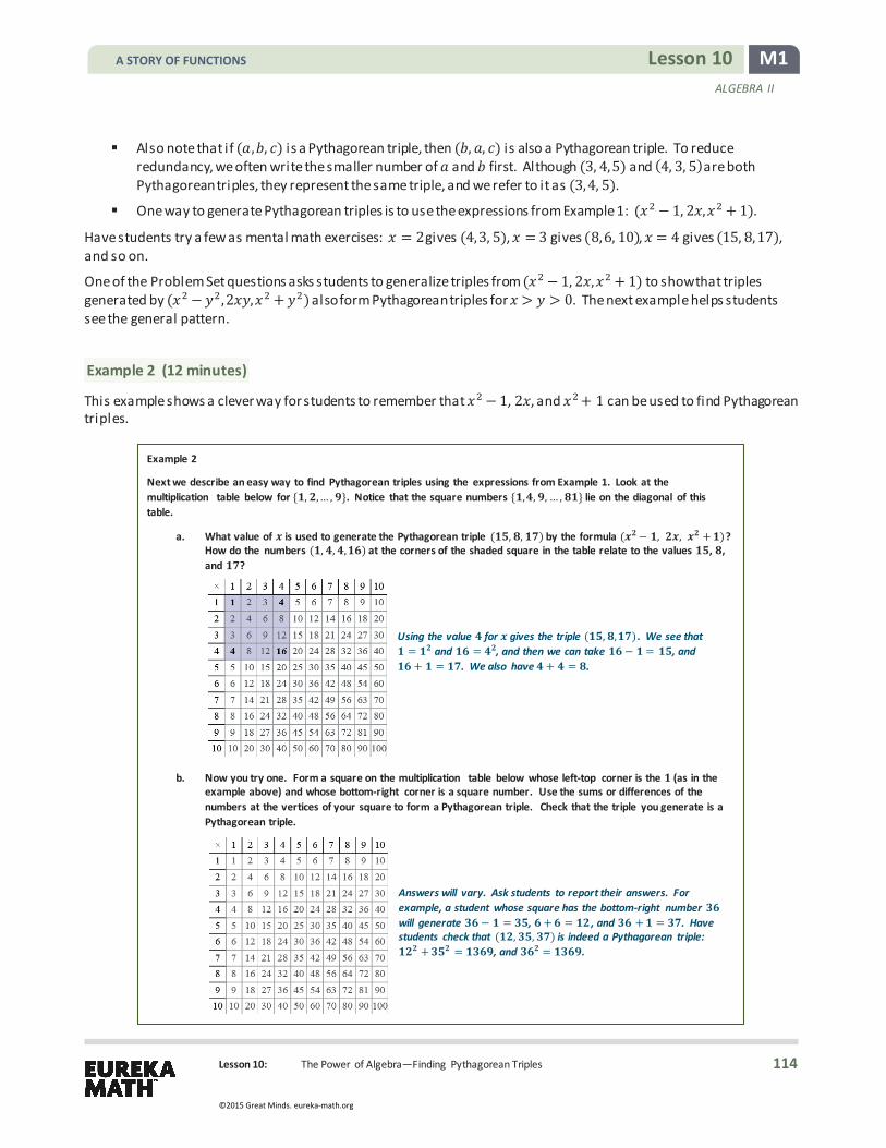
Lesson 10: The Power of Algebra—Finding Pythagorean Triples
M1 Lesson 10 ALGEBRA II
� Also note that if (𝑎𝑎,𝑏𝑏, 𝑐𝑐) is a Pythagorean triple, then (𝑏𝑏, 𝑎𝑎, 𝑐𝑐) is also a Pythagorean triple. To reduce redundancy, we often write the smaller number of 𝑎𝑎 and 𝑏𝑏 first. Although (3, 4,5) and (4, 3, 5) are both Pythagorean triples, they represent the same triple, and we refer to it as (3,4, 5).
� One way to generate Pythagorean triples is to use the expressions from Example 1: (𝑥𝑥2 − 1, 2𝑥𝑥,𝑥𝑥2 + 1).
Have students try a few as mental math exercises: 𝑥𝑥 = 2 gives (4,3, 5), 𝑥𝑥 = 3 gives (8,6, 10), 𝑥𝑥 = 4 gives (15, 8,17), and so on.
One of the Problem Set questions asks students to generalize triples from (𝑥𝑥2 − 1, 2𝑥𝑥,𝑥𝑥2 + 1) to show that triples generated by (𝑥𝑥2 − 𝑦𝑦2,2𝑥𝑥𝑦𝑦,𝑥𝑥2 + 𝑦𝑦2) also form Pythagorean triples for 𝑥𝑥 > 𝑦𝑦 > 0. The next example helps students see the general pattern.
Example 2 (12 minutes)
This example shows a clever way for students to remember that 𝑥𝑥2 − 1, 2𝑥𝑥, and 𝑥𝑥2+ 1 can be used to find Pythagorean triples.
Example 2
Next we describe an easy way to find Pythagorean triples using the expressions from Example 1. Look at the multiplication table below for { , ,… , }. Notice that the square numbers { , , , … , } lie on the diagonal of this table.
a. What value of is used to generate the Pythagorean triple ( , , ) by the formula ( − , , + )? How do the numbers ( , , , ) at the corners of the shaded square in the table relate to the values , , and ?
Using the value for gives the triple ( , , ) . We see that = and = , and then we can take − = , and
+ = . We also have + = .
b. Now you try one. Form a square on the multiplication table below whose left-top corner is the (as in the example above) and whose bottom-right corner is a square number. Use the sums or differences of the numbers at the vertices of your square to form a Pythagorean triple. Check that the triple you generate is a Pythagorean triple.
Answers will vary. Ask students to report their answers. For example, a student whose square has the bottom-right number will generate − = , + = , and + = . Have students check that ( , , ) is indeed a Pythagorean triple:
+ = , and = .
A STORY OF FUNCTIONS
114
©2015 Great Minds. eureka-math.org

Lesson 10: The Power of Algebra—Finding Pythagorean Triples
M1 Lesson 10 ALGEBRA II
Let’s generalize this square to any square in the multiplication table where two opposite vertices of the square are square numbers.
c. How can you use the sums or differences of the numbers at the vertices of the shaded square to get a triple ( , , )? Is it a Pythagorean triple?
Following what we did above, take − = , + = , and + = to get the triple ( , , ). Yes, it is a Pythagorean triple: + = + = = .
d. Using instead of and instead of in your calculations in part (c), write down a formula for generating Pythagorean triples in terms of and .
The calculation − generalizes to − as the length of one leg. The length of the other leg can be found by + = ( ), which generalizes to . The length of the hypotenuse, + , generalizes to
+ . It seems that Pythagorean triples can be generated by triples ( − , , + ) where > > .
In the Problem Set, students prove that if 𝑥𝑥 and 𝑦𝑦 are positive integers with 𝑥𝑥 > 𝑦𝑦, then (𝑥𝑥2 − 𝑦𝑦2, 2𝑥𝑥𝑦𝑦,𝑥𝑥2 + 𝑦𝑦2) is a Pythagorean triple, mimicking the proof of Example 1.
Closing (3 minutes)
� Pythagorean triples are triples of positive integers (𝑎𝑎, 𝑏𝑏,𝑐𝑐) that satisfy the relationship 𝑎𝑎2+ 𝑏𝑏2 = 𝑐𝑐2. Such a triple is called a Pythagorean triple because a right triangle with legs of length 𝑎𝑎 and 𝑏𝑏 will have a hypotenuse of length 𝑐𝑐 by the Pythagorean theorem.
� To generate a Pythagorean triple, take any two positive integers 𝑥𝑥 and 𝑦𝑦 with 𝑥𝑥 > 𝑦𝑦, and compute (𝑥𝑥2− 𝑦𝑦2,2𝑥𝑥𝑦𝑦, 𝑥𝑥2+ 𝑦𝑦2). Relevant Facts and Vocabulary
PYTHAGOREAN THEOREM: If a right triangle has legs of length and units and hypotenuse of length units, then + = .
CONVERSE TO THE PYTHAGOREAN THEOREM: If the lengths , , of the sides of a triangle are related by + = , then the angle opposite the side of length is a right angle.
PYTHAGOREAN TRIPLE: A Pythagorean triple is a triple of positive integers ( , , ) such that + = . The triple ( , , ) is a Pythagorean triple but ( , ,√ ) is not, even though the numbers are side lengths of an isosceles right triangle.
Exit Ticket (5 minutes)
A STORY OF FUNCTIONS
115
©2015 Great Minds. eureka-math.org

Lesson 10: The Power of Algebra—Finding Pythagorean Triples
M1 Lesson 10 ALGEBRA II
Name Date
Lesson 10: The Power of Algebra—Finding Pythagorean Triples
Exit Ticket Generate six Pythagorean triples using any method discussed during class. Explain each method you use.
A STORY OF FUNCTIONS
116
©2015 Great Minds. eureka-math.org

Lesson 10: The Power of Algebra—Finding Pythagorean Triples
M1 Lesson 10 ALGEBRA II
Exit Ticket Sample Solutions
Generate six Pythagorean triples using any method discussed during class. Explain each method you use.
Answers will vary. One example should use either ( − , , + ) or ( − , , + ), but after that students can use the fact that a multiple of a Pythagorean triple is again a Pythagorean triple.
Problem Set Sample Solutions
1. Rewrite each expression as a sum or difference of terms.
a. ( − )( + )
−
b. ( − )( + )
−
c. ( + )( − )
−
d. ( − )( + )( + )
−
e. ( + )( − )
−
f. ( + )
+ +
g. ( − ) ( + )
− +
h. ( − ) ( + ) ( + )
− +
2. Tasha used a clever method to expand ( + + )( + − ). She grouped the addends together like this
[( + ) + ][( + )− ] and then expanded them to get the difference of two squares:
( + + )( + − ) = [( + ) + ][( + )− ] = ( + ) − = + + − .
a. Is Tasha's method correct? Explain why or why not.
Yes, Tasha is correct. Expanding in the traditional way gives the same result.
( + + )( + − ) = ( + + ) + ( + + ) − ( + + ) = + + + + + − − − = + + −
b. Use a version of her method to find ( + + )( − − ).
+ ( + ) − ( + ) = − ( + ) = − − −
c. Use a version of her method to find ( + − )( − + ).
+ ( − ) − ( − ) = − ( − ) = − + −
3. Use the difference of two squares identity to factor each of the following expressions.
a. −
( − )( + )
b. ( + ) − ( )
( − )( + ) = ( − )( + )
c. − ( − )
( − )( + )
d. ( + ) − ( + )
( − )( + + )
A STORY OF FUNCTIONS
117
©2015 Great Minds. eureka-math.org

Lesson 10: The Power of Algebra—Finding Pythagorean Triples
M1 Lesson 10 ALGEBRA II
4. Show that the expression ( + )( − )− + may be written as the difference of two squares, and then factor the expression.
( + )( − )− + = − − + = ( − + )− = ( − ) − = ( − − )( − + )
5. Show that ( + ) − ( − ) = for all real numbers and .
( + ) − ( − ) = [( + ) − ( − )][( + ) + ( − )] = ( )( ) =
6. Prove that a triangle with side lengths − , , and + with > > is a right triangle.
The proof should look like the proof in Example 1 but with instead of .
7. Complete the table below to find Pythagorean triples (the first row is done for you).
− + Check: Is it a Pythagorean Triple?
Yes: + = =
Yes: + = =
Yes: + = =
Yes: + = = Yes: + = = Yes: + = =
Yes: + = =
8. Answer the following parts about the triple ( , , ) . a. Show that ( , , ) is a Pythagorean triple.
We see that + = + = , and = so + = .
b. Prove that neither ( , , ) nor ( , , ) can be found by choosing a pair of integers and with >
and computing ( − , , + ). (Hint: What are the possible values of and if = ? What about if = ?)
PROOF: Since is odd and is even, there are no integer values of and that satisfy = . Thus, our formula cannot generate the triple ( , , ) . Now suppose and are integers such that = . Thus
= and > . There are only two possibilities: either = and = , or = and = . In the first case, our formula generates the triple ( − , , + ) = ( , , ). In the second case, our formula generates the triple ( − , , + ) = ( , , ). Thus, there is no way to generate the triple ( , , ) using this method, even though it is a Pythagorean triple.
c. Wouldn’t it be nice if all Pythagorean triples were generated by ( − , , + )? Research Pythagorean triples on the Internet to discover what is known to be true about generating all Pythagorean triples using this formula.
All Pythagorean triples are some multiple of a Pythagorean triple generated using this formula. For example, while ( , , ) is not generated by the formula, it is a multiple of a Pythagorean triple ( , , ) , which is generated by the formula.
9. Follow the steps below to prove the identity ( + )( + ) = ( − ) + ( + ) . a. Multiply ( + )( + ) .
( + )( + ) = + + +
A STORY OF FUNCTIONS
118
©2015 Great Minds. eureka-math.org

Lesson 10: The Power of Algebra—Finding Pythagorean Triples
M1 Lesson 10 ALGEBRA II
b. Square both binomials in ( − ) + ( + ) and collect like terms.
( − ) + ( + ) = − + + + + = + + +
c. Use your answers from part (a) and part (b) to prove the identity.
( + )( + ) = + + + = ( − ) + ( + )
10. Many U.S. presidents took great delight in studying mathematics. For example, President James Garfield, while still a congressman, came up with a proof of the Pythagorean theorem based upon the ideas presented below.
In the diagram, two congruent right triangles with side lengths , , and hypotenuse , are used to form a trapezoid composed of three triangles.
a. Explain why is a right angle.
Since is a right angle, the measures of and sum to °, so and are complementary angles. Since by SSS
triangle congruence, we have . Thus, and must also be complementary. By the angle sum properties,
+ +°
= °
so that
+ ° = °
and we have shown that = °. Thus, is a right angle.
b. What are the areas of , , and in terms of , , and ?
We see that ( ) = , ( ) = , and because is a right angle, ( ) = .
c. Using the formula for the area of a trapezoid, what is the total area of trapezoid in terms of and ?
( ) = ( + )( + )
d. Set the sum of the areas of the three triangles from part (b) equal to the area of the trapezoid you found in part (c), and simplify the equation to derive a relationship between , , and . Conclude that a right triangle with legs of length and and hypotenuse of length must satisfy the relationship + = .
Equate areas:
+ + = ( + )( + ) ,
+ = ( + + ). Multiply both sides by ,
+ = + + ,
and subtract from both sides,
= + .
A STORY OF FUNCTIONS
119
©2015 Great Minds. eureka-math.org

Lesson 11: The Special Role of Zero in Factoring
M1 Lesson 11 ALGEBRA II
Lesson 11: The Special Role of Zero in Factoring
Student Outcomes � Students find solutions to polynomial equations where the polynomial expression is not factored into l inear
factors. � Students construct a polynomial function that has a specified set of zeros with stated multiplicity.
Lesson Notes This lesson focuses on the first part of standard A-APR.B.3, identifying zeros of polynomials presented in factored form. Although the terms root and zero are interchangeable, for consistency only the term zero is used throughout this lesson and in later lessons. The second part of the standard, using the zeros to construct a rough graph of a polynomial function, is delayed until Lesson 14. The ideas that begin in this lesson continue in Lesson 19, in which students will be able to associate a zero of a polynomial function to a factor in the factored form of the associated polynomial as a consequence of the remainder theorem, and culminate in Lesson 39, in which students apply the fundamental theorem of algebra to factor polynomial expressions completely over the complex numbers.
Classwork Opening Exercise (12 minutes)
Opening Exercise
Find all solutions to the equation ( + + )( − − ) = .
The main point of this opening exercise is for students to recognize and then formalize that the statement “If 𝑎𝑎𝑏𝑏 = 0, then 𝑎𝑎 = 0 or 𝑏𝑏 = 0” applies not only when 𝑎𝑎 and 𝑏𝑏 are numbers or linear functions (which we used when solving a quadratic equation), but also applies to cases where 𝑎𝑎 and 𝑏𝑏 are polynomial functions of any degree.
In small groups, let students discuss ways to solve this equation. Walk around the room and offer advice such as, “Have you considered factoring each quadratic expression? What do you get?” As soon as one group factors both quadratic expressions, or when three minutes have passed, show, or let that group show, the factorization on the board.
(𝑥𝑥 + 2)(𝑥𝑥 + 3) (𝑥𝑥 − 4)(𝑥𝑥 + 1)3 4
= 0
� What are the solutions to this equation?
à −2,−3,4,−1
Scaffolding: Here is an alternative opening activity that may better i l luminate the special role of zero.
� For each equation, l ist some possible values for 𝑥𝑥 and 𝑦𝑦.
𝑥𝑥𝑦𝑦 = 10, 𝑥𝑥𝑦𝑦 = 1, 𝑥𝑥𝑦𝑦 = −1, 𝑥𝑥𝑦𝑦 = 0
� What do you notice? Does one equation tell you more information than others?
A STORY OF FUNCTIONS
120
©2015 Great Minds. eureka-math.org

Lesson 11: The Special Role of Zero in Factoring
M1 Lesson 11 ALGEBRA II
� Why?
à If 𝑥𝑥 is any number other than −2, −3, 4, or −1, then each factor is a nonzero number that is 𝑥𝑥 + 2 0, 𝑥𝑥 + 3 0, etc. However, the multiplication of four nonzero numbers is nonzero, so that value of 𝑥𝑥 cannot be a solution. Therefore, the only possible solutions are −2, −3, 4, and −1. It is easy to confirm that these are indeed solutions by substituting them each into the equation individually.
� Why are these numbers also solutions to the original equation? à Because the expression (𝑥𝑥 + 2)(𝑥𝑥+ 3)(𝑥𝑥 − 4)(𝑥𝑥 + 1) is equivalent to (𝑥𝑥2 + 5𝑥𝑥 + 6)(𝑥𝑥2 − 3𝑥𝑥 − 4).
Now let’s study the solutions to 𝑥𝑥2 + 5𝑥𝑥 + 6 = 0 and 𝑥𝑥2 − 3𝑥𝑥 − 4 = 0 separately.
� What are the solutions to 𝑥𝑥2+ 5𝑥𝑥+ 6 = 0? à −2, −3
� What are the solutions to 𝑥𝑥2− 3𝑥𝑥− 4 = 0? à 4, −1
� Relate the solutions of the equation (𝑥𝑥2 + 5𝑥𝑥 + 6)(𝑥𝑥2 − 3𝑥𝑥 − 4) = 0 to the solutions of the compound statement, “𝑥𝑥2 + 5𝑥𝑥 + 6 = 0 or 𝑥𝑥2 − 3𝑥𝑥 − 4 = 0.” à They are the same.
� Given two polynomial functions 𝑝𝑝 and 𝑞𝑞 of any degree, the solution set of the equation 𝑝𝑝(𝑥𝑥)𝑞𝑞(𝑥𝑥) = 0 is the union of the solution set of 𝑝𝑝(𝑥𝑥) = 0 and the solution set of 𝑞𝑞(𝑥𝑥) = 0. Let’s think about why.
Lead students in a discussion of the following proof:
� Suppose 𝑎𝑎 is a solution to the equation 𝑝𝑝(𝑥𝑥)𝑞𝑞(𝑥𝑥) = 0; that is, it is a number that satisfies 𝑝𝑝(𝑎𝑎)𝑞𝑞(𝑎𝑎) = 0. Since 𝑝𝑝(𝑎𝑎) is a number and 𝑞𝑞(𝑎𝑎) is a number, one or both of them must be zero, by the zero product property that states, “If the product of two numbers is zero, then at least one of the numbers is zero.” Therefore, 𝑝𝑝(𝑎𝑎) = 0 or 𝑞𝑞(𝑎𝑎) = 0, which means 𝑎𝑎 is a solution to the compound statement, “𝑝𝑝(𝑥𝑥) = 0 or 𝑞𝑞(𝑥𝑥) = 0.”
� Now let’s prove the other direction and show that if 𝑎𝑎 is a solution to the compound statement, then it is a solution to the equation 𝑝𝑝(𝑥𝑥)𝑞𝑞(𝑥𝑥) = 0. This direction is also easy: Suppose 𝑎𝑎 is a number such that either 𝑝𝑝(𝑎𝑎) = 0 or 𝑞𝑞(𝑎𝑎) = 0. In the first case, 𝑝𝑝(𝑎𝑎)𝑞𝑞(𝑎𝑎) = 0 𝑞𝑞(𝑎𝑎) = 0. In the second case, 𝑝𝑝(𝑎𝑎)𝑞𝑞(𝑎𝑎) = 𝑝𝑝(𝑎𝑎) 0 = 0. Hence, in either case, 𝑎𝑎 is a solution to the equation 𝑝𝑝(𝑥𝑥)𝑞𝑞(𝑥𝑥) = 0.
Students may have difficulty understanding the distinction between the equations 𝑝𝑝(𝑥𝑥)𝑞𝑞(𝑥𝑥) = 0 and 𝑝𝑝(𝑎𝑎)𝑞𝑞(𝑎𝑎) = 0. Help students understand that 𝑝𝑝(𝑥𝑥)𝑞𝑞(𝑥𝑥) = 0 is an equation in a variable 𝑥𝑥, while 𝑝𝑝(𝑎𝑎) is the value of the function 𝑝𝑝 when it is evaluated at the number 𝑎𝑎. Thus, 𝑝𝑝(𝑎𝑎)𝑞𝑞(𝑎𝑎) is a number. For example, if 𝑝𝑝 and 𝑞𝑞 are the quadratic polynomials 𝑝𝑝(𝑥𝑥) = 𝑥𝑥2 + 5𝑥𝑥 + 6 and 𝑞𝑞(𝑥𝑥) = 𝑥𝑥2 − 3𝑥𝑥 − 4 from the Opening Exercise, and students are considering the case when 𝑎𝑎 is 5, then 𝑝𝑝(5) = 56 and 𝑞𝑞(5) = 6. Therefore, 5 cannot be a solution to the equation 𝑝𝑝(𝑥𝑥)𝑞𝑞(𝑥𝑥) = 0.
� Communicate to students that they can use the statement below to break problems into simpler parts:
Given any two polynomial functions 𝑝𝑝 and 𝑞𝑞, the set of solutions to the equation 𝑝𝑝(𝑥𝑥)𝑞𝑞(𝑥𝑥) = 0 can be found by solving 𝑝𝑝(𝑥𝑥) = 0, solving 𝑞𝑞(𝑥𝑥) = 0, and combining the solutions into one set.
Ask students to try the following exercise on their own.
MP.1
A STORY OF FUNCTIONS
121
©2015 Great Minds. eureka-math.org

Lesson 11: The Special Role of Zero in Factoring
M1 Lesson 11 ALGEBRA II
Exercise 1 (2 minutes) Exercise 1
1. Find the solutions of ( − )( − ) = .
The solutions to ( − )( − ) are the solutions of − = combined with the solutions of − = . These solutions are − , , − , and .
The next example looks at a polynomial equation for which the solution is already known. The goal of this example and the discussion that follows is to use a solution to the equation 𝑓𝑓(𝑥𝑥) = 0 to further factor the polynomial 𝑓𝑓. In doing so, the class ends with a description of the zeros of a function, a concept first introduced in Algebra I, Module 4.
Example 1 (8 minutes)
Example 1
Suppose we know that the polynomial equation − + + = has three real solutions and that one of the factors of − + + is ( − ). How can we find all three solutions to the given equation?
Steer the discussion to help students conjecture that the polynomial 4𝑥𝑥3− 12𝑥𝑥2 + 3𝑥𝑥 + 5 must be the product of (𝑥𝑥 − 1) and some quadratic polynomial. Since (𝑥𝑥 − 1) is a factor, and we know how to divide polynomials, we can find the quadratic polynomial by dividing:
4𝑥𝑥3 − 12𝑥𝑥2 + 3𝑥𝑥 + 5 𝑥𝑥 − 1 = 4𝑥𝑥2 − 8𝑥𝑥 − 5.
Now we know that 4𝑥𝑥3− 12𝑥𝑥2 + 3𝑥𝑥 + 5 = (𝑥𝑥 − 1)(4𝑥𝑥2− 8𝑥𝑥 − 5), and we also know that 4𝑥𝑥2− 8𝑥𝑥 − 5 is a quadratic polynomial that has linear factors (2𝑥𝑥+ 1) and (2𝑥𝑥 − 5).
Therefore, 4𝑥𝑥3 − 12𝑥𝑥2 + 3𝑥𝑥 + 5 = 0 has the same solutions as (𝑥𝑥 − 1)(4𝑥𝑥2 − 8𝑥𝑥 − 5) = 0, which has the same solutions as
(𝑥𝑥 − 1)(2𝑥𝑥 + 1)(2𝑥𝑥 − 5) = 0.
In this factored form, the solutions of 𝑓𝑓(𝑥𝑥) = 0 are readily apparent: −12, 1, and
2.
Scaffolding: Allow students to generate ideas about how the l inear factors affect the behavior of the graph so that they can use the graph of a function to identify zeros.
A STORY OF FUNCTIONS
122
©2015 Great Minds. eureka-math.org

Lesson 11: The Special Role of Zero in Factoring
M1 Lesson 11 ALGEBRA II
Zeros of 𝑓𝑓 are
−12, 1, and 5
2.
𝑦𝑦 = 𝑓𝑓(𝑥𝑥)
Discussion (8 minutes)
� In Example 1 above, we saw that factoring the polynomial into linear factors helped us to find solutions to the original polynomial equation 4𝑥𝑥3 − 12𝑥𝑥2+ 3𝑥𝑥 + 5 = 0.
� There is a corresponding notion for the zeros of a function. Let 𝑓𝑓 be a function whose domain is a subset of the real numbers and whose range is a subset of the real numbers. A zero (or root) of the function 𝑓𝑓 is a number 𝑐𝑐 such that 𝑓𝑓(𝑐𝑐) = 0.
� The zeros of the function 𝑓𝑓(𝑥𝑥) = 4𝑥𝑥3− 12𝑥𝑥2 + 3𝑥𝑥 + 5 are the 𝑥𝑥-intercepts of the graph of 𝑓𝑓: these are − 1
2, 1,
and 2
.
� By definition, a zero of a polynomial function 𝑓𝑓 is a solution to the equation 𝑓𝑓(𝑥𝑥) = 0. If (𝑥𝑥 −𝑎𝑎) is a factor of a polynomial function 𝑓𝑓, then 𝑓𝑓(𝑎𝑎) = 0 and 𝑎𝑎 is a zero of 𝑓𝑓.
However, consider the polynomial functions 𝑝𝑝(𝑥𝑥) = (𝑥𝑥 − 2)(𝑥𝑥 + 3)2, 𝑞𝑞(𝑥𝑥) = (𝑥𝑥 − 2)2(𝑥𝑥+ 3)4, and 𝑟𝑟(𝑥𝑥) = (𝑥𝑥 − 2)4(𝑥𝑥− 3) . Because 𝑝𝑝(2) = 0, 𝑞𝑞(2) = 0, and 𝑟𝑟(2) = 0, the number 2 is a zero of 𝑝𝑝, 𝑞𝑞, and 𝑟𝑟. Likewise, −3 is also a zero of 𝑝𝑝, 𝑞𝑞, and 𝑟𝑟. Even though these polynomial functions have the same zeros, they are not the same function; they do not even have the same degree!
We would l ike to be able to distinguish between the zeros of these two polynomial functions. If we write out all of the factors for 𝑝𝑝, 𝑞𝑞, and 𝑟𝑟, we see that
𝑝𝑝(𝑥𝑥) = (𝑥𝑥 − 2)(𝑥𝑥 + 3)(𝑥𝑥 + 3) 𝑞𝑞(𝑥𝑥) = (𝑥𝑥 − 2)(𝑥𝑥 − 2)(𝑥𝑥 + 3)(𝑥𝑥 + 3)(𝑥𝑥+ 3)(𝑥𝑥 + 3) 𝑟𝑟(𝑥𝑥) = (𝑥𝑥 − 2)(𝑥𝑥 − 2)(𝑥𝑥 − 2)(𝑥𝑥− 2)(𝑥𝑥 + 3)(𝑥𝑥 + 3)(𝑥𝑥 + 3)(𝑥𝑥 + 3)(𝑥𝑥+ 3).
𝑦𝑦 = 𝑝𝑝(𝑥𝑥) 𝑦𝑦 = 𝑞𝑞(𝑥𝑥) 𝑦𝑦 = 𝑟𝑟(𝑥𝑥)
A STORY OF FUNCTIONS
123
©2015 Great Minds. eureka-math.org

Lesson 11: The Special Role of Zero in Factoring
M1 Lesson 11 ALGEBRA II
� We notice that (𝑥𝑥 − 2) is a factor of 𝑝𝑝 once, and (𝑥𝑥 + 3) is a factor of 𝑝𝑝 twice. Thus, we say that 2 is a zero of 𝑝𝑝 of multiplicity 1, and −3 is a zero of 𝑝𝑝 of multiplicity 2. Zeros of multiplicity 1 are usually just referred to as zeros, without mentioning the multiplicity.
� What are the zeros of 𝑞𝑞, with their multiplicities? à For 𝑞𝑞, 2 is a zero of multiplicity 2, and −3 is a zero of multiplicity 4.
� What are the zeros of 𝑟𝑟, with their multiplicities? à For 𝑟𝑟, 2 is a zero of multiplicity 4, and −3 is a zero of multiplicity 5.
� Can you look at the factored form of a polynomial equation and identify the zeros with their multiplicities? Explain how you know.
à Yes. Each linear factor (𝑎𝑎𝑥𝑥 −𝑏𝑏) of the polynomial will produce a zero with multiplicity .
� Can multiplicity be negative? Can it be zero? Can it be a fraction?
à No. Multiplicity is the count of the number of times a factor appears in a factored polynomial expression. Polynomials can only have positive integer exponents, so a factor must have positive integer exponents. Thus, the multiplicity of a zero must be a positive integer.
Note: In Lesson 14, students use the zeros of a polynomial function together with their multiplicities to create a graph of the function, and in Lesson 19, students use the zeros of a polynomial function with their multiplicities to construct the equation of the function.
Exercises 2–5 (8 minutes) Exercises 2–5
2. Find the zeros of the following polynomial functions, with their multiplicities. a. ( ) = ( + )( − )( + )
− with multiplicity
with multiplicity
b. ( ) = ( − ) ( − )
with multiplicity
with multiplicity
c. ( ) = ( − )
with multiplicity
d. ( ) = ( + ) ( − )
− with multiplicity
with multiplicity
A STORY OF FUNCTIONS
124
©2015 Great Minds. eureka-math.org

Lesson 11: The Special Role of Zero in Factoring
M1 Lesson 11 ALGEBRA II
3. Find a polynomial function that has the following zeros and multiplicities. What is the degree of your polynomial?
Zero Multiplicity
−
−
( ) = ( − ) ( + )( − ) ( + )
The degree of is .
4. Is there more than one polynomial function that has the same zeros and multiplicities as the one you found in Exercise 3?
Yes. Consider ( ) = ( + )( − ) ( + )( − ) ( + ) . Since there are no real solutions to + = , adding this factor does not produce a new zero. Thus and have the same zeros and multiplicities but are different functions.
5. Can you find a rule that relates the multiplicities of the zeros to the degree of the polynomial function?
Yes. If is a polynomial function of degree , then the sum of the multiplicities of all of the zeros is less than or equal to . If can be factored into linear terms, then the sum of the multiplicities of all of the zeros is exactly equal to .
Closing (2 minutes)
Ask students to summarize the key ideas of the lesson, either in writing or with a neighbor. Consider posing the questions below.
� Part of the lesson today has been that given two polynomials, 𝑝𝑝 and 𝑞𝑞, we can determine solutions to 𝑝𝑝(𝑥𝑥)𝑞𝑞(𝑥𝑥) = 0 by solving both 𝑝𝑝(𝑥𝑥) = 0 and 𝑞𝑞(𝑥𝑥) = 0, even if they are high-degree polynomials. If 𝑝𝑝 and 𝑞𝑞 are polynomial functions that do not have any real number zeros, do you think the equation 𝑝𝑝(𝑥𝑥)𝑞𝑞(𝑥𝑥) = 0 still has real number solutions? Can you give an example of two such functions?
à If 𝑝𝑝(𝑥𝑥) 0 for all real numbers 𝑥𝑥 and 𝑞𝑞(𝑥𝑥) 0 for all real numbers 𝑥𝑥, then there is no possible way to have 𝑝𝑝(𝑥𝑥)𝑞𝑞(𝑥𝑥) = 0.
à For example: If 𝑝𝑝(𝑥𝑥) = 𝑥𝑥2 + 1 and 𝑞𝑞(𝑥𝑥) = 𝑥𝑥4 + 1, then the equation (𝑥𝑥2 + 1)(𝑥𝑥4 + 1) = 0 has no real solutions.
The following vocabulary was introduced in Algebra I (please see Module 3 and Module 4 in Algebra I). While the teacher should not have to teach these terms explicitly, it may still be a good idea to go through them with the class.
Relevant Vocabulary Terms
In the definitions below, the symbol stands for the set of real numbers.
FUNCTION: A function is a correspondence between two sets, and , in which each element of is assigned to one and only one element of .
The set in the definition above is called the domain of the function. The range (or image) of the function is the subset of , denoted ( ), that is defined by the following property: is an element of ( ) if and only if there is an in such that ( ) = .
If ( ) = where can be any real number, then the domain is all real numbers (denoted ), and the range is the set of nonnegative real numbers.
A STORY OF FUNCTIONS
125
©2015 Great Minds. eureka-math.org

Lesson 11: The Special Role of Zero in Factoring
M1 Lesson 11 ALGEBRA II
POLYNOMIAL FUNCTION: Given a polynomial expression in one variable, a polynomial function in one variable is a function : such that for each real number in the domain, ( ) is the value found by substituting the number into all
instances of the variable symbol in the polynomial expression and evaluating.
It can be shown that if a function : is a polynomial function, then there is some nonnegative integer and collection of real numbers , , ,… , with such that the function satisfies the equation
( ) = + + + + ,
for every real number in the domain, which is called the standard form of the polynomial function. The function ( ) = + + + , where can be any real number, is an example of a function written in standard form.
DEGREE OF A POLYNOMIAL FUNCTION: The degree of a polynomial function is the degree of the polynomial expression used to define the polynomial function.
The degree of ( ) = + + + is 3, but the degree of ( ) = ( + ) − ( − ) is because when is put into standard form, it is ( ) = .
CONSTANT FUNCTION: A constant function is a polynomial function of degree 0. A constant function is of the form ( ) = , for a constant .
LINEAR FUNCTION: A linear function is a polynomial function of degree . A linear function is of the form ( ) = + , for constants and with .
QUADRATIC FUNCTION: A quadratic function is a polynomial function of degree . A quadratic function is in standard form if it is written in the form ( ) = + + , for constants , , with and any real number .
CUBIC FUNCTION: A cubic function is a polynomial function of degree . A cubic function is of the form ( ) = + ++ , for constants , , , with .
ZEROS OR ROOTS OF A FUNCTION: A zero (or root) of a function : is a number of the domain such that ( ) = . A zero of a function is an element in the solution set of the equation ( ) = .
Exit Ticket (5 minutes)
Lesson Summary
Given any two polynomial functions and , the solution set of the equation ( ) ( ) = can be quickly found by solving the two equations ( ) = and ( ) = and combining the solutions into one set.
The number is a zero of a polynomial function with multiplicity if the factored form of contains ( − ) .
A STORY OF FUNCTIONS
126
©2015 Great Minds. eureka-math.org

Lesson 11: The Special Role of Zero in Factoring
M1 Lesson 11 ALGEBRA II
Name Date
Lesson 11: The Special Role of Zero in Factoring
Exit Ticket Suppose that a polynomial function 𝑝𝑝 can be factored into seven factors: (𝑥𝑥 − 3), (𝑥𝑥 + 1), and 5 factors of (𝑥𝑥 − 2). What are its zeros with multiplicity, and what is the degree of the polynomial? Explain how you know.
A STORY OF FUNCTIONS
127
©2015 Great Minds. eureka-math.org

Lesson 11: The Special Role of Zero in Factoring
M1 Lesson 11 ALGEBRA II
Exit Ticket Sample Solutions Suppose that a polynomial function can be factored into seven factors: ( − ) , ( + ), and factors of ( − ). What are its zeros with multiplicity, and what is the degree of the polynomial? Explain how you know.
Zeros: with multiplicity ; − with multiplicity ; with multiplicity
The polynomial has degree seven. There are seven linear factors as given above, so ( ) = ( − )( + )( − ) .
If the factors were multiplied out, the leading term would be , so the degree of is .
Problem Set Sample Solutions
For Problems 1–4, find all solutions to the given equations.
1. ( − )( + ) =
, −
2. ( − )( + )( + ) =
, − , −
3. ( − )( + ) =
, −
4. ( − )( + )( − ) =
, − ,
5. Find four solutions to the equation ( − )( − ) = .
, − , , −
6. Find the zeros with multiplicity for the function ( ) = ( − )( − ) .
We can factor to give ( ) = ( − )( + + )( − )( + ) = ( − ) ( + )( + + ) . Then, is a zero of multiplicity , − is a zero of multiplicity , and is a zero of multiplicity .
7. Find two different polynomial functions that have zeros at , , and of multiplicity .
( ) = ( − )( − )( − ) and ( ) = ( + )( − )( − )( − )
8. Find two different polynomial functions that have a zero at of multiplicity and a zero at − of multiplicity .
( ) = ( − ) ( + ) and ( ) = ( + )( − ) ( + )
9. Find three solutions to the equation ( − )( − ) = .
From Lesson 6, we know that ( − ) is a factor of ( − ), so three solutions are ,− , and .
A STORY OF FUNCTIONS
128
©2015 Great Minds. eureka-math.org
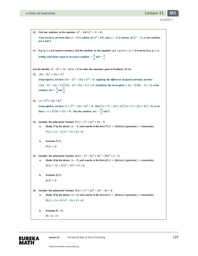
Lesson 11: The Special Role of Zero in Factoring
M1 Lesson 11 ALGEBRA II
10. Find two solutions to the equation ( − )( − ) = .
From Lesson 6, we know that ( − ) is a factor of ( − ), and ( − ) is a factor of ( − ), so two solutions are and .
11. If , , , are nonzero numbers, find the solutions to the equation ( + )( + ) = in terms of , , , .
Setting each factor equal to zero gives solutions − and − .
Use the identity − = ( − )( + ) to solve the equations given in Problems 12–13.
12. ( − ) = ( + )
Using algebra, we have ( − ) − ( + ) = . Applying the difference of squares formula, we have
( − )− ( + ) ( − ) + ( + ) = . Combining like terms gives (− − )( − ) = , so the
solutions are − and .
13. ( + ) = ( + )
Using algebra, we have ( + ) − ( + ) = . Then ( + ) − ( + ) ( + ) + ( + ) = , so we
have (− + )( + ) = . Thus the solutions are − and .
14. Consider the polynomial function ( ) = + + − .
a. Divide by the divisor ( − ) and rewrite in the form ( ) = ( )( ) + .
( ) = ( − )( + + ) +
b. Evaluate ( ).
( ) =
15. Consider the polynomial function ( ) = − + − + − .
a. Divide by the divisor ( − ) and rewrite in the form ( ) = ( )( ) + .
( ) = ( − )( + + ) +
b. Evaluate ( ).
( ) =
16. Consider the polynomial function ( ) = + − − + .
a. Divide by the divisor ( + ) and rewrite in the form ( ) = ( )( ) + .
( ) = ( + )( − + ) +
b. Evaluate (− ).
(− ) =
A STORY OF FUNCTIONS
129
©2015 Great Minds. eureka-math.org

Lesson 11: The Special Role of Zero in Factoring
M1 Lesson 11 ALGEBRA II
17. Consider the polynomial function ( ) = + − − + + − − .
a. Divide by the divisor ( + ) and rewrite in the form ( ) = ( )( ) + .
( ) = ( + )( − + − ) +
b. Evaluate (− ).
(− ) =
18. Make a conjecture based on the results of Problems 14–17.
It seems that the zeros of a polynomial function correspond to factors ( − ) in the equation of the polynomial.
A STORY OF FUNCTIONS
130
©2015 Great Minds. eureka-math.org

ALGEBRA II • MODULE 1
Topic B: Factoring—Its Use and Its Obstacles
Mathematics Curriculum
Topic B
Factoring—Its Use and Its Obstacles
N-Q.A.2, A-SSE.A.2, A-APR.B.2, A-APR.B.3, A-APR.D.6, F-IF.C.7c
Focus Standards: N-Q.A.2 Define appropriate quantities for the purpose of descriptive modeling.★
A-SSE.A.2 Use the structure of an expression to identify ways to rewrite it. For example, see 𝑥𝑥4 − 𝑦𝑦4 as (𝑥𝑥2)2 − (𝑦𝑦2)2, thus recognizing it as a difference of squares that can be factored as (𝑥𝑥2 − 𝑦𝑦2)(𝑥𝑥2 + 𝑦𝑦2).
A-APR.B.2 Know and apply the Remainder Theorem: For a polynomial 𝑝𝑝(𝑥𝑥) and a number a, the remainder on division by 𝑥𝑥 − 𝑎𝑎 is 𝑝𝑝(𝑎𝑎), so 𝑝𝑝(𝑎𝑎) = 0 if and only if (𝑥𝑥 − 𝑎𝑎) is a factor of 𝑝𝑝(𝑥𝑥).
A-APR.B.3 Identify zeros of polynomials when suitable factorizations are available, and use the zeros to construct a rough graph of the function defined by the polynomial.
A-APR.D.6 Rewrite simple rational expressions in different forms; write 𝑎𝑎(𝑥𝑥)/𝑏𝑏(𝑥𝑥) in the form 𝑞𝑞(𝑥𝑥) + 𝑟𝑟(𝑥𝑥)/𝑏𝑏(𝑥𝑥), where 𝑎𝑎(𝑥𝑥), 𝑏𝑏(𝑥𝑥), 𝑞𝑞(𝑥𝑥), and 𝑟𝑟(𝑥𝑥) are polynomials with the degree of 𝑟𝑟(𝑥𝑥) less than the degree of 𝑏𝑏(𝑥𝑥), using inspection, long division, or, for the more complicated examples, a computer algebra system.
F-IF.C.7 Graph functions expressed symbolically and show key features of the graph, by hand in simple cases and using technology for more complicated cases.★
c. Graph polynomial functions, identifying zeros when suitable factorizations are available, and showing end behavior.
Instructional Days: 10
Lesson 12: Overcoming Obstacles in Factoring (S)1
Lesson 13: Mastering Factoring (P)
Lesson 14: Graphing Factored Polynomials (S)
Lesson 15: Structure in Graphs of Polynomial Functions (P)
Lessons 16–17: Modeling with Polynomials—An Introduction (M, M)
Lesson 18: Overcoming a Second Obstacle in Factoring—What If There Is a Remainder? (P)
Lesson 19: The Remainder Theorem (S)
Lessons 20–21: Modeling Riverbeds with Polynomials (M, M)
1Lesson Structure Key: P-Problem Set Lesson, M-Modeling Cycle Lesson, E-Exploration Lesson, S-Socratic Lesson
A STORY OF FUNCTIONS
131
©2015 Great Minds. eureka-math.org

Topic B: Factoring—Its Use and Its Obstacles
M1 Topic B ALGEBRA II
Armed with a newfound knowledge of the value of factoring, students develop their facility with factoring and then apply the benefits to graphing polynomial equations in Topic B. In Lessons 12–13, students are presented with the first obstacle to solving equations successfully. While dividing a polynomial by a given factor to find a missing factor is easily accessible, factoring without knowing one of the factors is challenging. Students recall the work with factoring done in Algebra I and expand on it to master factoring polynomials with degree greater than two, emphasizing the technique of factoring by grouping.
In Lessons 14–15, students find that another advantage to rewriting polynomial expressions in factored form is how easily a polynomial function written in this form can be graphed. Students read word problems to answer polynomial questions by examining key features of their graphs. They notice the relationship between the number of times a factor is repeated and the behavior of the graph at that zero (i.e., when a factor is repeated an even number of times, the graph of the polynomial touches the 𝑥𝑥-axis and “bounces” back off, whereas when a factor occurs only once or an odd number of times, the graph of the polynomial at that zero “cuts through” the 𝑥𝑥-axis). In these lessons, students compare hand plots to graphing-calculator plots and zoom in on the graph to examine its features more closely.
In Lessons 16–17, students encounter a series of more serious modeling questions associated with polynomials, developing their fluency in translating between verbal, numeric, algebraic, and graphical thinking. One example of the modeling questions posed in this lesson is how to find the maximum possible volume of a box created from a flat piece of cardboard with fixed dimensions.
In Lessons 18–19, students are presented with their second obstacle: “What if there is a remainder?” They learn the remainder theorem and apply it to further understand the connection between the factors and zeros of a polynomial and how this relates to the graph of a polynomial function. Students explore how to determine the smallest possible degree for a depicted polynomial and how information such as the value of the 𝑦𝑦-intercept is reflected in the equation of the polynomial.
The topic culminates with two modeling lessons (Lessons 20–21) involving approximating the area of the cross-section of a riverbed to model the volume of flow. The problem description includes a graph of a polynomial equation that could be used to model the situation, and students are challenged to find the polynomial equation itself.
A STORY OF FUNCTIONS
132
©2015 Great Minds. eureka-math.org

M1 Lesson 12 ALGEBRA II
Lesson 12: Overcoming Obstacles in Factoring
Lesson 12: Overcoming Obstacles in Factoring
Student Outcomes
� Students factor certain forms of polynomial expressions by using the structure of the polynomials.
Lesson Notes Students have factored polynomial expressions in earlier lessons and in earlier courses. In this lesson, students explore further techniques for factoring polynomial expressions, including factoring by completing the square, by applying the quadratic formula, and by grouping. They apply these techniques to solve polynomial equations.
The idea of the greatest common factor (GCF) is important to this lesson. The teacher may want to consider displaying a GCF poster on the classroom wall for reference. Consider using some of the problem set exercises during the lesson to supplement the examples included here.
Classwork Opening (4 minutes)
Consider the following polynomial equation.
(𝑥𝑥2 − 4𝑥𝑥 + 3)(𝑥𝑥2 + 4𝑥𝑥 − 5) = 0
Discuss the following questions in pairs or small groups:
1. What is the degree of this polynomial? How do you know? 2. How many solutions to this equation should there be? How do you know? 3. How might you begin to solve this equation?
We can solve this equation by factoring because we can solve each of the equations
𝑥𝑥2 − 4𝑥𝑥 + 3 = 0
𝑥𝑥2 + 4𝑥𝑥− 5 = 0.
There is no need to solve the whole way through; students completed a problem like this in Lesson 11. The idea is that students see that this can be done relatively quickly. The factored form of the original equation is
(𝑥𝑥2 − 4𝑥𝑥 + 3)(𝑥𝑥2 + 4𝑥𝑥 − 5) = (𝑥𝑥− 1)(𝑥𝑥 − 3)(𝑥𝑥 − 1)(𝑥𝑥 + 5) = (𝑥𝑥 − 1)2(𝑥𝑥− 3)(𝑥𝑥 + 5) = 0,
and the three solutions are 1, 3, and −5.
However, consider the next example.
Example 1 (8 minutes)
Example 1
Find all real solutions to the equation ( − + )( − − ) = .
Scaffolding: Ask struggling students to first solve the equation (𝑥𝑥 − 3)(𝑥𝑥 − 1) = 0. Point out that they have used the zero product property, and ask how that property applies to the given problem.
A STORY OF FUNCTIONS
133
©2015 Great Minds. eureka-math.org

M1 Lesson 12 ALGEBRA II
Lesson 12: Overcoming Obstacles in Factoring
Allow students the opportunity to struggle with factoring these expressions, discuss with their neighbors, and reach the conclusion that neither expression can be factored with integer coefficients.
� We have discovered an obstacle to factoring. The expressions 𝑥𝑥2− 6𝑥𝑥 + 3 and 2𝑥𝑥2 − 4𝑥𝑥− 7 do not factor as readily as the examples from the previous lesson. Does anybody recall how we might factor them?
Students have completed the square in both Geometry and Algebra I, so give them an opportunity to recall the process.
� When a quadratic expression is not easily factorable, we can either apply a technique called completing the square, or we can use the quadratic formula. Let’s factor the first expression by completing the square.
� We first create some space between the 𝑥𝑥 term and the constant term:
𝑥𝑥2 − 6𝑥𝑥 + ______− ______+ 3 = 0.
� The next step is the key step. Take half of the coefficient of the 𝑥𝑥 term, square that number, and add and subtract it in the space we created:
𝑥𝑥2− 6𝑥𝑥+ (−3)2− (−3)2+ 3 = 0 𝑥𝑥2 − 6𝑥𝑥 + 9 − 9 + 3 = 0.
Discuss the following questions with the class, and give them the opportunity to justify this step.
� Why did we choose 9? Why did we both add and subtract 9? How does this help us solve the equation? à Adding 9 creates a perfect square trinomial in the first three terms.
à Adding and subtracting 9 means that we have not changed the value of the expression on the left side of the equation.
à Adding and subtracting 9 creates a perfect square trinomial 𝑥𝑥2 − 6𝑥𝑥 + 9 = (𝑥𝑥 − 3)2. � We cannot just add a number to an expression without changing its value. By adding 9 and subtracting 9, we
have essentially added 0 using the additive identity property, which leads to an equivalent expression on the left-hand side of the equation and thus preserves solutions of the equation.
� This process creates a structure that allows us to factor the first three terms of the expression on the left side of the equation and then solve for the variable.
𝑥𝑥2 − 6𝑥𝑥 + 9− 9 + 3 = 0
(𝑥𝑥 − 3)2− 6 = 0
� Solving for 𝑥𝑥:
(𝑥𝑥 − 3)2 = 6
𝑥𝑥 − 3 = √6 or 𝑥𝑥− 3 = −√6
𝑥𝑥 = 3 +√6 or 𝑥𝑥 = 3− √6 .
� Thus, we have found two solutions by setting the first quadratic expression equal to zero, completing the square, and solving the factored equation. Since the leading coefficient of 𝑥𝑥2 − 6𝑥𝑥 + 3 is 1, we know from our work in Algebra I that the factored form is
𝑥𝑥2 − 6𝑥𝑥 + 3 = �𝑥𝑥 − 3 +√6 ��𝑥𝑥 − 3 −√6 �.
Scaffolding: We can use the tabular method to give a visual representation of the process of completing the square. For example, the polynomial 𝑥𝑥2 − 6𝑥𝑥 can be represented as follows to i llustrate the “missing” term.
𝑥𝑥 − 3 𝑥𝑥2
−3𝑥𝑥
𝑥𝑥 −
3
−3𝑥𝑥
?
Perfect square trinomial
A STORY OF FUNCTIONS
134
©2015 Great Minds. eureka-math.org

M1 Lesson 12 ALGEBRA II
Lesson 12: Overcoming Obstacles in Factoring
� Let’s repeat the process with the second equation. What is the first step to completing the square?
2𝑥𝑥2− 4𝑥𝑥 − 7 = 0
Allow students an opportunity to suggest the first step to completing the square.
� We can only complete the square when the leading coefficient is 1, so our first step is to factor out the 2.
2 𝑥𝑥2− 2𝑥𝑥 −72
= 0
� Now we can complete the square with the expression inside the parentheses.
2 𝑥𝑥2 − 2𝑥𝑥 + ______− ______+72
= 0
2 𝑥𝑥2 − 2𝑥𝑥 + (−1)2− (−1)2−72
= 0
2 𝑥𝑥2 − 2𝑥𝑥+ 1−92
= 0
2 (𝑥𝑥 − 1)2−92
= 0
� Next, we divide both sides by 2.
(𝑥𝑥 − 1)2−92
= 0
� Finally, we solve for 𝑥𝑥.
(𝑥𝑥− 1)2 =92
𝑥𝑥 = 1 +92
or 𝑥𝑥 = 1−92
𝑥𝑥 = 1 +3√2
2 or 𝑥𝑥 = 1−
3√22
� Thus, we have found two more solutions to our original fourth-degree equation. We then have
2𝑥𝑥2 − 4𝑥𝑥 − 7 = 2 𝑥𝑥2 − 2𝑥𝑥 −72
= 2 𝑥𝑥 − 1 +3√2
2𝑥𝑥 − 1 −
3√22
.
� Notice that we needed to multiply the factors by 2 to make the leading coefficients match. � Finally, we have the factored form of our original polynomial equation:
(𝑥𝑥2 − 6𝑥𝑥 + 3)(2𝑥𝑥2 − 4𝑥𝑥 − 7) = 0 in factored form
2 𝑥𝑥− (3 + √6) 𝑥𝑥− (3 −√6) 𝑥𝑥− 1 +3√2
2𝑥𝑥 − 1 −
3√22
= 0.
A STORY OF FUNCTIONS
135
©2015 Great Minds. eureka-math.org

M1 Lesson 12 ALGEBRA II
Lesson 12: Overcoming Obstacles in Factoring
� Thus, the solutions to the equation (𝑥𝑥2 − 6𝑥𝑥 + 3)(2𝑥𝑥2 − 4𝑥𝑥− 7) = 0 are the four values 3 +√6, 3−√6,
1 + 3 22 , and 1− 3 2
2 .
� Similarly, we could have applied the quadratic formula to find the solutions to each quadratic equation in the previous example. Recall the quadratic formula.
à The two solutions to the quadratic equation 𝑎𝑎𝑥𝑥2 + 𝑏𝑏𝑥𝑥 + 𝑐𝑐 = 0 are √ 42
and √ 42
.
Exercise 1 (6 minutes) Exercise 1
Factor and find all real solutions to the equation ( − − )( + − ) = .
Ask half of the students to apply the quadratic formula to solve 𝑥𝑥2 − 2𝑥𝑥 − 4 = 0 and the other half to apply the quadratic formula to solve 3𝑥𝑥2+ 8𝑥𝑥− 3 = 0.
The quadratic formula gives solutions 1 +√5 and 1− √5 for the first equation and −3 and 13 for the second equation.
Since 1 +√5 and 1 −√5 are the two solutions to 𝑥𝑥2 − 2𝑥𝑥 − 4 = 0 found by the quadratic formula, we know from work in Algebra I that �𝑥𝑥 − 1 +√5 ��𝑥𝑥 − 1 −√5 �= 𝑥𝑥2 − 2𝑥𝑥 − 4. However, we need to be more careful when using the
solutions to factor the second quadratic expression. The leading coefficient of (𝑥𝑥 + 3)�𝑥𝑥 − 13�= 𝑥𝑥2 + 8
3𝑥𝑥 − 1 is 1, and the leading coefficient of 3𝑥𝑥2 + 8𝑥𝑥 − 3 is 3, so we need to multiply our factors by 3:
3𝑥𝑥2 + 8𝑥𝑥 − 3 = 3(𝑥𝑥 + 3) 𝑥𝑥 −13
.
Thus, the factored form of the original equation is
(𝑥𝑥2− 2𝑥𝑥 − 4)(3𝑥𝑥2+ 8𝑥𝑥 − 3) = 3�𝑥𝑥 − 1 +√5 ��𝑥𝑥 − 1− √5 �(𝑥𝑥 + 3) 𝑥𝑥 −13
= 0,
and the four solutions to (𝑥𝑥2− 2𝑥𝑥 − 4)(3𝑥𝑥2+ 8𝑥𝑥 − 3) = 0 are 1 +√5, 1−√5, −3, and 13 .
To summarize, if we have a fourth-degree polynomial already factored into two quadratic expressions, we can try to factor the entire polynomial by completing the square on one or both quadratic expressions, or by using the quadratic formula to find the roots of the quadratic polynomials and then constructing the factored form of each quadratic polynomial.
Discussion (6 minutes)
� We have overcome the obstacle of difficult-to-factor quadratic expressions. Let’s look next at the obstacles encountered when attempting to solve a third-degree polynomial equation such as the following:
𝑥𝑥3 + 3𝑥𝑥2− 9𝑥𝑥− 27 = 0.
Scaffolding: Allow students to generate ideas. Advanced students may benefit from significant independent time to attempt to solve the equation (MP.1).
A STORY OF FUNCTIONS
136
©2015 Great Minds. eureka-math.org

M1 Lesson 12 ALGEBRA II
Lesson 12: Overcoming Obstacles in Factoring
� How might we begin to solve this equation?
Allow students an opportunity to brainstorm as a class, in pairs, or in table groups. Students may note that coefficients are powers of 3 but may not be sure how that helps. Let them know they are seeing something important that they may be able to use. Stronger students might even try to group the components.
� While we have made some interesting observations, we have not quite found a way to factor this expression. What if we know that 𝑥𝑥 + 3 is one factor?
If students do not come up with polynomial division, point them in that direction through a numerical example: Suppose we want the factors of 210, and we know that one factor is 3. How do we find the other factors?
Have students perform the polynomial division
to find additional factors. Students may also use the tabular method discussed in earlier lessons in this module.
� Since 𝑥𝑥3 + 3𝑥𝑥3− 9𝑥𝑥 − 27 = (𝑥𝑥+ 3)(𝑥𝑥2− 9), we know that
𝑥𝑥3 + 3𝑥𝑥2 − 9𝑥𝑥− 27 = (𝑥𝑥 + 3)(𝑥𝑥 − 3)(𝑥𝑥 + 3) = (𝑥𝑥 + 3)2(𝑥𝑥− 3).
� By the zero product property, the solutions to 𝑥𝑥3 + 3𝑥𝑥2− 9𝑥𝑥− 27 = 0 are −3 and 3. � But, how do we start if we don’t know any of the factors in advance?
Example 2 (6 minutes)
Example 2
Find all solutions to + − − = by factoring the equation.
� Let’s start with our original equation 𝑥𝑥3 + 3𝑥𝑥2 − 9𝑥𝑥 − 27 = 0. Is there a greatest common factor (GCF) for all four terms on the left-hand side we can factor out? à No, the GCF is 1.
Scaffolding: If needed, have students compute the GCF for some numerical examples such as GCF 75,100 is 25 GCF 72,16,24 is 8 GCF 10,35,63 is 1.
A STORY OF FUNCTIONS
137
©2015 Great Minds. eureka-math.org

M1 Lesson 12 ALGEBRA II
Lesson 12: Overcoming Obstacles in Factoring
� Let’s group the terms of the left-hand side as follows: 𝑥𝑥3 + 3𝑥𝑥2 − 9𝑥𝑥 − 27 = (𝑥𝑥3 + 3𝑥𝑥2)− (9𝑥𝑥 + 27).
� Can we factor out a GCF from each set of parentheses independently? à Yes, 𝑥𝑥2 can be factored out of the first piece and 9 out of the second.
Factor the GCF out of each part. Have students do as much of this work as possible.
𝑥𝑥3 + 3𝑥𝑥2− 9𝑥𝑥− 27 = 𝑥𝑥2(𝑥𝑥+ 3)− 9(𝑥𝑥+ 3)
� Do you notice anything interesting about the right side of the above equation? à I noticed that 𝑥𝑥 + 3 is a common factor.
� Since both terms have a factor of (𝑥𝑥+ 3), we have found a quantity that can be factored out.
𝑥𝑥3+ 3𝑥𝑥2 − 9𝑥𝑥 − 27 = (𝑥𝑥 + 3)(𝑥𝑥2− 9)
� And as we saw above, we can take this one step further.
𝑥𝑥3 + 3𝑥𝑥2− 9𝑥𝑥 − 27 = (𝑥𝑥 + 3)(𝑥𝑥 + 3)(𝑥𝑥 − 3)
� Because of the zero property, the original problem is now easy to solve because 𝑥𝑥3 + 3𝑥𝑥2 − 9𝑥𝑥 − 27 = 0 exactly when (𝑥𝑥 + 3)2(𝑥𝑥− 3) = 0. What are the solutions to the original equation? à The solutions to 𝑥𝑥3 + 3𝑥𝑥2− 9𝑥𝑥 − 27 = 0 are 𝑥𝑥 = −3 and 𝑥𝑥 = 3.
� The process you just completed is often called factoring by grouping, and it works only on certain 3rd degree polynomial expressions, such as 𝑥𝑥3 + 3𝑥𝑥2− 9𝑥𝑥− 27.
Exercise 2 (4 minutes)
Allow students to work in pairs or small groups on these exercises. Realize that there are two ways to group the terms that result in the same factored expression. Circulate around the room while students are working, and take note of any groups that are using a different approach. At the end of these exercises, ask students who grouped differently to share their method, and discuss as a class.
Exercise 2
Find all real solutions to − − + = .
− − + = ( − )− ( − ) =
( − )( − ) = ( − )( − )( + ) = Thus, the solutions are , , and − .
Alternate approach: − − + =
( − )− ( − ) = ( − )( − ) =
( − )( − )( + ) =
MP.7
A STORY OF FUNCTIONS
138
©2015 Great Minds. eureka-math.org

M1 Lesson 12 ALGEBRA II
Lesson 12: Overcoming Obstacles in Factoring
Exercise 3 (4 minutes) Exercise 3
Find all real solutions to − − + = .
− − + = ( − )− ( − ) =
( − )( − ) = Thus, the solutions are , √ , and −√ .
− − + = ( − )− ( − ) =
( − )( − ) =
Closing (2 minutes)
Ask students to summarize the important parts of the lesson in writing, to a partner, or as a class. Use this as an opportunity to informally assess understanding of the lesson. The following are some important summary elements.
Exit Ticket (5 minutes)
Lesson Summary
In this lesson, we learned some techniques to use when faced with factoring polynomials and solving polynomial equations.
� If a fourth-degree polynomial can be factored into two quadratic expressions, then each quadratic expression might be factorable either using the quadratic formula or by completing the square.
� Some third-degree polynomials can be factored using the technique of factoring by grouping.
A STORY OF FUNCTIONS
139
©2015 Great Minds. eureka-math.org
M1 Lesson 12 ALGEBRA II
Lesson 12: Overcoming Obstacles in Factoring
Name Date
Lesson 12: Overcoming Obstacles in Factoring
Exit Ticket Solve the following equation, and explain your solution method.
𝑥𝑥3 + 7𝑥𝑥2 − 𝑥𝑥 − 7 = 0
A STORY OF FUNCTIONS
140
©2015 Great Minds. eureka-math.org

M1 Lesson 12 ALGEBRA II
Lesson 12: Overcoming Obstacles in Factoring
Exit Ticket Sample Solutions
Solve the following equation, and explain your solution method.
+ − − =
( + )− ( + ) = ( + )( − ) =
( + )( − )( + ) =
The solutions are − , , and − . The equation was solved by factoring and by grouping. I grouped the four terms into two groups, and then factored the GCF from each group. I then factored out the common term ( + ) from each group to find the factored form of the equation. I then applied the zero product property to find the solutions to the equation.
Problem Set Sample Solutions
1. Solve each of the following equations by completing the square.
a. − + =
+ √ , −√
b. − = −
+ √ , −√
c. + − =
, −
d. − = −
,
e. ( − + )( − + ) =
, , ,
f. − + = +√ , − + √ , −√ , − −√
2. Solve each of the following equations using the quadratic formula.
a. − − =
+√
, −√
b. ( − + )( − + ) =
, , +√ , − √
c. ( − + )( − + ) = , , + √ , − √
A STORY OF FUNCTIONS
141
©2015 Great Minds. eureka-math.org

M1 Lesson 12 ALGEBRA II
Lesson 12: Overcoming Obstacles in Factoring
3. Not all of the expressions in the equations below can be factored using the techniques discussed so far in this course. First, determine if the expression can be factored with real coefficients. If so, factor the expression, and find all real solutions to the equation.
a. − − =
Can be factored: ( − )( + ) = .
Solutions: , −
b. + − =
Can be factored: ( − )( + ) = .
Solutions: , −
c. + + =
Cannot be factored with real number coefficients.
d. + − + =
Cannot be factored with real number coefficients.
e. + + + =
Can be factored: ( + )( + ) = .
Solution: −
f. + − − =
Can be factored: ( + )( − √ )( +√ ) =.
Solutions: − , √ , −√
g. − + − =
Can be factored: ( − )( + ) = .
Solution:
h. + + + =
Can be factored: ( + )( + ) = .
Solution: −
i. + − − =
Can be factored: ( + )( − )( + ) = .
Solutions: − , , −
j. − − =
Can be factored: � + �( − ) = .
Solutions: − ,
4. Solve the following equations by bringing all terms to one side of the equation and factoring out the greatest
common factor.
a. ( − )( − ) = ( − )( + )
( − )( + ) − ( − )( − ) = ( − ) + − ( − ) =
( − )( ) = =
So, the only solution to ( − )( − ) = ( − )( + ) is .
b. ( + )( − ) = ( + )( + )
( + )( − ) − ( + )( + ) = ( + ) − − ( + ) =
( + )(− ) =
= −
So, the only solution to ( + )( − ) = ( + )( + ) is − .
A STORY OF FUNCTIONS
142
©2015 Great Minds. eureka-math.org
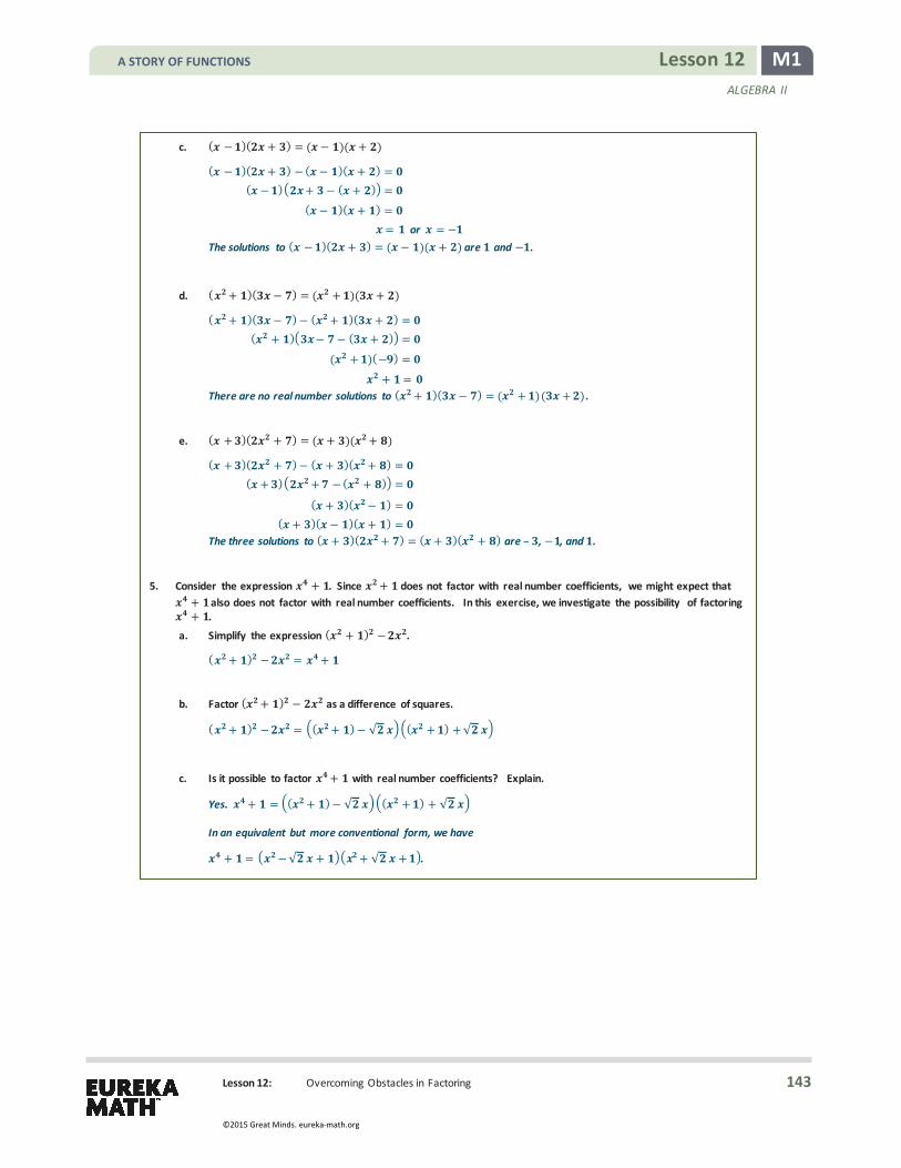
M1 Lesson 12 ALGEBRA II
Lesson 12: Overcoming Obstacles in Factoring
c. ( − )( + ) = ( − )( + )
( − )( + ) − ( − )( + ) = ( − ) + − ( + ) =
( − )( + ) = = or = −
The solutions to ( − )( + ) = ( − )( + ) are and − .
d. ( + )( − ) = ( + )( + )
( + )( − )− ( + )( + ) = ( + ) − − ( + ) =
( + )(− ) = + =
There are no real number solutions to ( + )( − ) = ( + )( + ) .
e. ( + )( + ) = ( + )( + )
( + )( + )− ( + )( + ) = ( + ) + − ( + ) =
( + )( − ) = ( + )( − )( + ) =
The three solutions to ( + )( + ) = ( + )( + ) are – , − , and .
5. Consider the expression + . Since + does not factor with real number coefficients, we might expect that + also does not factor with real number coefficients. In this exercise, we investigate the possibility of factoring + .
a. Simplify the expression ( + ) − .
( + ) − = +
b. Factor ( + ) − as a difference of squares.
( + ) − = �( + )− √ ��( + ) +√ �
c. Is it possible to factor + with real number coefficients? Explain.
Yes. + = �( + )− √ ��( + ) + √ �
In an equivalent but more conventional form, we have
+ = −√ + + √ + .
A STORY OF FUNCTIONS
143
©2015 Great Minds. eureka-math.org

Lesson 13: Mastering Factoring
M1 Lesson 13 ALGEBRA II
Lesson 13: Mastering Factoring
Student Outcomes
� Students use the structure of polynomials to identify factors.
Lesson Notes In previous lessons in this module, students practiced the techniques of factoring by completing the square, by applying the quadratic formula, and by grouping. In this lesson, students look for structure in more complicated polynomial expressions that allow factorization. But first, students review several factoring techniques; some they learned about in the last lesson, and others they learned about in previous classes.
Opening Exercise (8 minutes)
In this exercise, students should begin to factor polynomial expressions by first analyzing their structure, a skill that is developed throughout the lesson. Suggest that students work on their own for five minutes and then compare answers with a neighbor; allow students to help each other out for an additional three minutes, if needed.
Opening Exercise
Factor each of the following expressions. What similarities do you notice between the examples in the left column and those on the right?
a. − b. −
( − )( + ) ( − )( + )
c. + + d. + +
( + )( + ) ( + )( + )
e. − f. −
( − )( + ) ( − )( + )
Students should notice that the structure of each of the factored polynomials is the same; for example, the factored forms of part (a) and part (b) are nearly the same, except that part (b) contains 3𝑥𝑥 in place of the 𝑥𝑥 in part (a). In parts (c) and (d), the factored form of part (d) contains 2𝑥𝑥, where there is only an 𝑥𝑥 in part (c). The factored form of part (f) is nearly the same as the factored form of part (e), with 𝑥𝑥2 replacing 𝑥𝑥 and 𝑦𝑦2 replacing 𝑦𝑦.
MP.7
A STORY OF FUNCTIONS
144
©2015 Great Minds. eureka-math.org

Lesson 13: Mastering Factoring
M1 Lesson 13 ALGEBRA II
Discussion (2 minutes)
The difference of two squares formula,
𝑎𝑎2 − 𝑏𝑏2 = (𝑎𝑎 + 𝑏𝑏)(𝑎𝑎 −𝑏𝑏),
can be used to factor an expression even when the two squares are not obvious.
Consider the following examples.
Example 1 (3 minutes)
Example 1
Write − as the product of two factors.
− = ( ) − ( ) = ( − )( + )
Example 2 (3 minutes)
Example 2
Factor − .
− = ( ) − ( ) = ( + )( − ) = [ ( + )][ ( − )] = ( + )( − )
Have students discuss with each other the structure of each polynomial expression in the previous two examples and how it helps to factor the expressions.
There are two terms that are subtracted, and each term can be written as the square of an expression.
Example 3 (3 minutes)
Consider the quadratic polynomial expression 9𝑥𝑥2 + 12𝑥𝑥 − 5. We can factor this expression by considering 3𝑥𝑥 as a single quantity as follows:
9𝑥𝑥2 + 12𝑥𝑥− 5 = (3𝑥𝑥)2+ 4(3𝑥𝑥)− 5.
Ask students to suggest the next step in factoring this expression.
Now, if we rename = 3𝑥𝑥, we have a quadratic expression of the form 2 + 4 − 5, which we can factor 2 + 4 − 5 = ( − 1)( + 5).
Replacing by 3𝑥𝑥, we have the following form of our original expression:
9𝑥𝑥2 + 12𝑥𝑥 − 5 = (3𝑥𝑥 − 1)(3𝑥𝑥 − 5).
Scaffolding: If students are unfamiliar with the difference of squares formula, work through a table of numeric examples, and ask them to look for patterns.
𝑎𝑎 𝑏𝑏 𝑎𝑎 + 𝑏𝑏 𝑎𝑎 −𝑏𝑏 𝑎𝑎2 − 𝑏𝑏2 3 1 4 2 8 4 1 5 3 15 5 2 7 3 21 6 4 10 2 20
Students may benefit from teacher modeling.
A STORY OF FUNCTIONS
145
©2015 Great Minds. eureka-math.org

Lesson 13: Mastering Factoring
M1 Lesson 13 ALGEBRA II
Exercise 1 (4 minutes)
Allow students to work in pairs or small groups on the following exercises.
Exercise 1
1. Factor the following expressions:
a. + −
+ − = ( ) + ( )− = ( + )( − )
b. − −
− − = ( − − )
= (( ) − ( )− ) = ( + )( − )
Example 4 (10 minutes)
Use the example of factoring 𝑥𝑥3 − 8 to scaffold the discussion of factoring 𝑥𝑥3 + 8. Students should be pretty familiar by now with factors of 𝑥𝑥3 − 8. Let them try the problem on their own to check their understanding.
� Suppose we want to factor 𝑥𝑥3 − 8. � Do you see anything interesting about this expression?
If they do not notice it, guide them toward both terms being perfect cubes.
� We can rewrite 𝑥𝑥3 − 8 as 𝑥𝑥3 − 23. � Guess a factor.
à Anticipate that they will suggest 𝑥𝑥 − 2 and 𝑥𝑥 + 2 as possible factors, or guide them to these suggestions.
Ask half of the students to divide 2
and the other half to divide 2
. They should discover that 𝑥𝑥 − 2 is a factor of
𝑥𝑥3 − 8, but 𝑥𝑥 + 2 is not.
A STORY OF FUNCTIONS
146
©2015 Great Minds. eureka-math.org

Lesson 13: Mastering Factoring
M1 Lesson 13 ALGEBRA II
� Use the results of the previous step to factor 𝑥𝑥3 − 8. à 𝑥𝑥3 − 8 = (𝑥𝑥 − 2)(𝑥𝑥2 + 2𝑥𝑥 + 4)
� Repeat the above process for 𝑥𝑥3 − 27. à 𝑥𝑥3 − 27 = (𝑥𝑥 − 3)(𝑥𝑥2 + 3𝑥𝑥 + 9)
� Make a conjecture about a rule for factoring 𝑥𝑥3 − 𝑎𝑎3. à 𝑥𝑥3 − 𝑎𝑎3 = (𝑥𝑥 −𝑎𝑎)(𝑥𝑥2+ 𝑎𝑎𝑥𝑥+ 𝑎𝑎2)
� Verify the conjecture: Multiply out (𝑥𝑥 −𝑎𝑎)(𝑥𝑥2+ 𝑎𝑎𝑥𝑥+ 𝑎𝑎2) to establish the identity for factoring a difference of cubes.
� While we can factor a difference of squares such as the expression 𝑥𝑥2− 9, we cannot similarly factor a sum of squares such as 𝑥𝑥2+ 9. Do we run into a similar problem when trying to factor a sum of cubes such as 𝑥𝑥3 + 8?
Again, ask students to propose potential factors of 𝑥𝑥3 + 8. Lead students to 𝑥𝑥 + 2 if they do not guess it automatically.
Work through the polynomial long division for 2
as shown.
Conclude that 𝑥𝑥3 + 8 = (𝑥𝑥 + 2)(𝑥𝑥2 − 2𝑥𝑥 + 4).
� Make a conjecture about a rule for factoring 𝑥𝑥3 + 𝑎𝑎3. à 𝑥𝑥3 + 𝑎𝑎3 = (𝑥𝑥 + 𝑎𝑎)(𝑥𝑥2− 𝑎𝑎𝑥𝑥+ 𝑎𝑎2)
� Verify the conjecture: Multiply out the expression (𝑥𝑥 + 𝑎𝑎)(𝑥𝑥2 − 𝑎𝑎𝑥𝑥 + 𝑎𝑎2) to establish the identity for factoring a sum of cubes.
Exercises 2–4 (5 minutes) Exercises 2–4
Factor each of the following, and show that the factored form is equivalent to the original expression.
2. +
( + )( − + )
3. −
( − )( + + )
4. +
( + ) = ( + )( − + )
Closing (2 minutes)
Ask students to summarize the important parts of the lesson in writing, to a partner, or as a class. Use this as an opportunity to informally assess understanding of the lesson. The following are some important summary elements.
Scaffolding: Ask advanced students to generate their own factoring problems using the structure of 𝑎𝑎3 + 𝑏𝑏3 or 𝑎𝑎3 − 𝑏𝑏3.
A STORY OF FUNCTIONS
147
©2015 Great Minds. eureka-math.org

Lesson 13: Mastering Factoring
M1 Lesson 13 ALGEBRA II
Exit Ticket (5 minutes)
Lesson Summary
In this lesson we learned additional strategies for factoring polynomials.
� The difference of squares identity − = ( − )( + ) can be used to factor more advanced binomials.
� Trinomials can often be factored by looking for structure and then applying our previous factoring methods.
� Sums and differences of cubes can be factored by the formulas
+ = ( + )( − + ) − = ( − )( + + ).
A STORY OF FUNCTIONS
148
©2015 Great Minds. eureka-math.org

Lesson 13: Mastering Factoring
M1 Lesson 13 ALGEBRA II
Name Date
Lesson 13: Mastering Factoring
Exit Ticket 1. Factor the following expression, and verify that the factored expression is equivalent to the original: 4𝑥𝑥2 − 9𝑎𝑎
2. Factor the following expression, and verify that the factored expression is equivalent to the original: 16𝑥𝑥2 − 8𝑥𝑥 − 3
A STORY OF FUNCTIONS
149
©2015 Great Minds. eureka-math.org

Lesson 13: Mastering Factoring
M1 Lesson 13 ALGEBRA II
Exit Ticket Sample Solutions
1. Factor the following expression, and verify that the factored expression is equivalent to the original: −
( − )( + ) = + − − = −
2. Factor the following expression, and verify that the factored expression is equivalent to the original: − −
( − )( + ) = + − − = − −
Problem Set Sample Solutions
1. If possible, factor the following expressions using the techniques discussed in this lesson.
a. − − ( − )( + )
g. − ( − )( + )
b. − + ( − )( − )
h. − ( − )( + )
c. + − ( + )( − )
i. + Cannot be factored.
d. − − ( − )( + )
j. − − √ +√ ( + )
e. − ( − )( + + )
k. + ( + )( − + )
f. − ( − )( + + )
l. + ( + )( − + )
A STORY OF FUNCTIONS
150
©2015 Great Minds. eureka-math.org

Lesson 13: Mastering Factoring
M1 Lesson 13 ALGEBRA II
2. Consider the polynomial expression + + .
a. Is + + factorable using the methods we have seen so far?
No. This will not factor into the form ( + )( + ) using any of our previous methods.
b. Factor − first as a difference of cubes, and then factor completely: ( ) − .
− = ( − )( + + ) = ( − )( + )( + + )
c. Factor − first as a difference of squares, and then factor completely: ( ) − .
− = ( − )( + ) = ( − )( + + )( + )( − + ) = ( − )( + )( − + )( + + )
d. Explain how your answers to parts (b) and (c) provide a factorization of + + .
Since − can be factored two different ways, those factorizations are equal. Thus we have
( − )( + )( + + ) = ( − )( + )( − + )( + + ) .
If we specify that and − , we can cancel the common terms from both sides:
( + + ) = ( − + )( + + ).
Multiplying this out, we see that
( − + )( + + ) = + + − − − + + + = + +
for every value of .
e. If a polynomial can be factored as either a difference of squares or a difference of cubes, which formula
should you apply first, and why?
Based on this example, a polynomial should first be factored as a difference of squares and then as a difference of cubes. This will produce factors of lower degree.
3. Create expressions that have a structure that allows them to be factored using the specified identity. Be creative, and produce challenging problems! a. Difference of squares
−
b. Difference of cubes
−
c. Sum of cubes
+
A STORY OF FUNCTIONS
151
©2015 Great Minds. eureka-math.org

M1 Lesson 14 ALGEBRA II
Lesson 14: Graphing Factored Polynomials
Lesson 14: Graphing Factored Polynomials
Student Outcomes
� Students use the factored forms of polynomials to find zeros of a function. � Students use the factored forms of polynomials to sketch the components of graphs between zeros.
Lesson Notes In this lesson, students use the factored form of polynomials to identify important aspects of the graphs of polynomial functions and, therefore, important aspects of the situations they model. Using the factored form, students identify zeros of the polynomial (and thus 𝑥𝑥-intercepts of the graph of the polynomial function) and see how to sketch a graph of the polynomial functions by examining what happens between the 𝑥𝑥-intercepts. They are also introduced to the concepts of relative minima and maxima and determining the possible degree of the polynomial by noting the number of relative extrema by looking at the graph of a function. A relative maximum (or minimum) is a property of a function that is visible in its graph. A relative maximum occurs at an 𝑥𝑥-value, 𝑐𝑐, in the domain of the function, and the relative maximum value is the corresponding function value at 𝑐𝑐. If a relative maximum of a function 𝑓𝑓 occurs at 𝑐𝑐, then 𝑐𝑐,𝑓𝑓(𝑐𝑐) is a relative maximum point. As an example, if (10,300) is a relative maximum point of a function 𝑓𝑓, then the
relative maximum value of 𝑓𝑓 is 300 and occurs at 10. When speaking about relative extrema, however, relative maximum is often used informally to refer to either a relative maximum at 𝑐𝑐, a relative maximum value, or a relative maximum point when the context is clear. Definitions of relevant vocabulary are included at the end of the lesson
The use of a graphing utility is recommended for some examples in this lesson to encourage students to focus on understanding the structure of the polynomials without the tedium of repeated graphing by hand.
Opening Exercise (10 minutes)
Prompt students to answer part (a) of the Opening Exercise independently or in pairs before continuing with the scaffolded questions.
Opening Exercise
An engineer is designing a roller coaster for younger children and has tried some functions to model the height of the roller coaster during the first yards. She came up with the following function to describe what she believes would make a fun start to the ride:
( ) = − + − + ,
where ( ) is the height of the roller coaster (in yards) when the roller coaster is yards from the beginning of the ride. Answer the following questions to help determine at which distances from the beginning of the ride the roller coaster is at its lowest height.
a. Does this function describe a roller coaster that would be fun to ride? Explain.
Yes, the roller coaster quickly goes to the top and then drops you down. This looks like a fun ride.
No, I don’t like roller coasters that climb steeply, and this one goes nearly straight up.
MP.3
Scaffolding:
� Consider beginning the class by reviewing graphs of simpler functions modeling simple roller coasters, such as
(𝑥𝑥) = −𝑥𝑥2 + 4𝑥𝑥.
� A more visual approach may be taken by first describing and analyzing the graph of before connecting each concept to the algebra associated with the function. Pose questions such as When is the roller coaster going up? Going down? How many times does the roller coaster touch the bottom?
MP.5 &
MP.7
A STORY OF FUNCTIONS
152
©2015 Great Minds. eureka-math.org
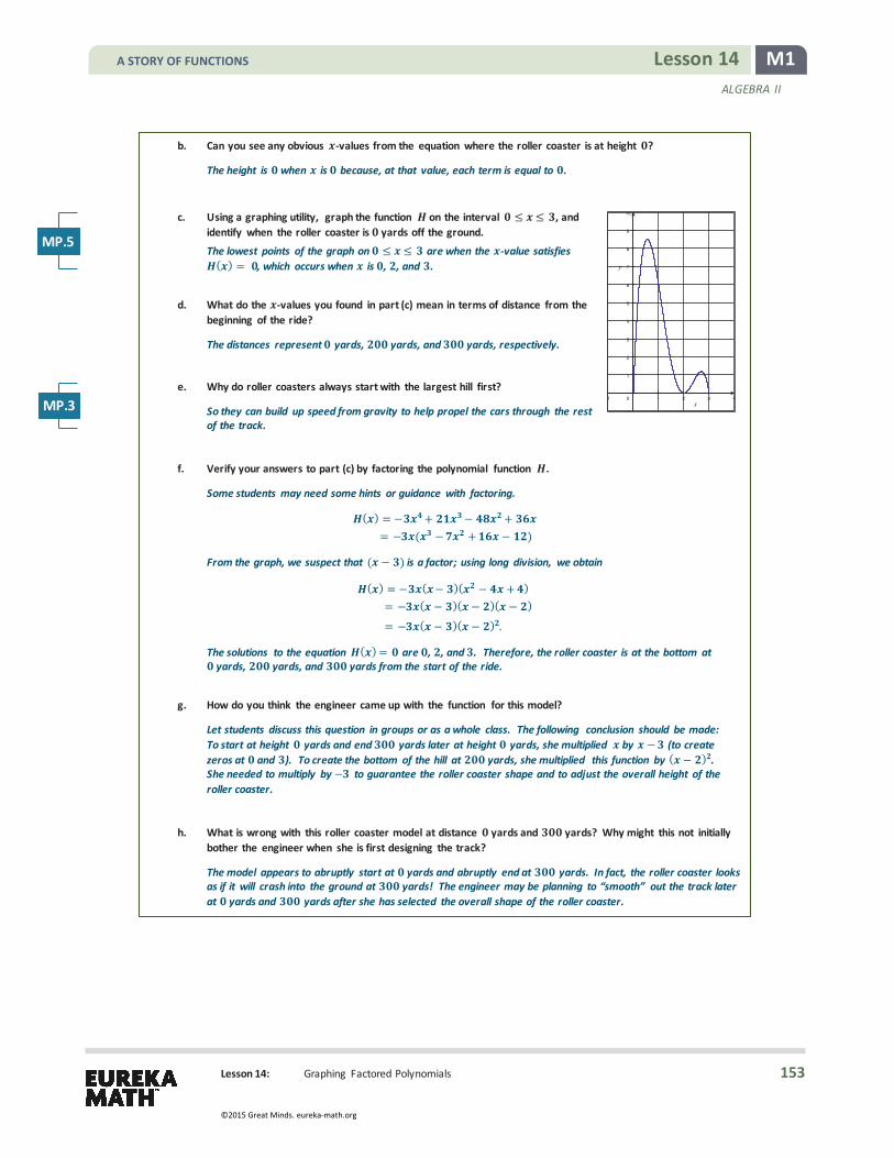
M1 Lesson 14 ALGEBRA II
Lesson 14: Graphing Factored Polynomials
b. Can you see any obvious -values from the equation where the roller coaster is at height ?
The height is when is because, at that value, each term is equal to .
c. Using a graphing utility, graph the function on the interval , and identify when the roller coaster is yards off the ground. The lowest points of the graph on are when the -value satisfies
( ) = , which occurs when is , , and .
d. What do the -values you found in part (c) mean in terms of distance from the
beginning of the ride?
The distances represent yards, yards, and yards, respectively.
e. Why do roller coasters always start with the largest hill first?
So they can build up speed from gravity to help propel the cars through the rest of the track.
f. Verify your answers to part (c) by factoring the polynomial function .
Some students may need some hints or guidance with factoring.
( ) = − + − + = − ( − + − )
From the graph, we suspect that ( − ) is a factor; using long division, we obtain
( ) = − ( − )( − + ) = − ( − )( − )( − ) = − ( − )( − ) .
The solutions to the equation ( ) = are , , and . Therefore, the roller coaster is at the bottom at yards, yards, and yards from the start of the ride.
g. How do you think the engineer came up with the function for this model?
Let students discuss this question in groups or as a whole class. The following conclusion should be made: To start at height yards and end yards later at height yards, she multiplied by − (to create zeros at and ). To create the bottom of the hill at yards, she multiplied this function by ( − ) . She needed to multiply by − to guarantee the roller coaster shape and to adjust the overall height of the roller coaster.
h. What is wrong with this roller coaster model at distance yards and yards? Why might this not initially
bother the engineer when she is first designing the track?
The model appears to abruptly start at yards and abruptly end at yards. In fact, the roller coaster looks as if it will crash into the ground at yards! The engineer may be planning to “smooth” out the track later at yards and yards after she has selected the overall shape of the roller coaster.
MP.5
MP.3
A STORY OF FUNCTIONS
153
©2015 Great Minds. eureka-math.org

M1 Lesson 14 ALGEBRA II
Lesson 14: Graphing Factored Polynomials
Discussion (4 minutes)
By manipulating a polynomial function into its factored form, we can identify the zeros of the function as well as identify the general shape of the graph. Thinking about the Opening Exercise, what else can we say about the polynomial function and its graph?
� The degree of the polynomial function is 4. How can you find the degree of the function from its factored form? à Add the highest degree term from each factor:
� −3 is a degree 0 factor � 𝑥𝑥 is degree 1 factor � 𝑥𝑥 − 3 is degree 1 factor � (𝑥𝑥 − 2)2 is a degree 2 factor, since (𝑥𝑥 − 2)2 = (𝑥𝑥 − 2)(𝑥𝑥 − 2).
à Thus, 0 + 1 + 1 + 2 = 4. � How many 𝑥𝑥-intercepts does the graph of the polynomial function have?
à For this graph, there are three: 0, 2 and 3.
You may want to include a discussion that the zeros of a function correspond to the 𝑥𝑥-intercepts of the graph of the function.
� Note that there are four factors, but only three 𝑥𝑥-intercepts. Why is that? à Two of the factors are the same.
Remind students that the 𝑥𝑥-intercepts of the graph of 𝑦𝑦= 𝑓𝑓(𝑥𝑥) are solutions to the equation 𝑓𝑓(𝑥𝑥) = 0. Values of 𝑟𝑟 that satisfy 𝑓𝑓(𝑟𝑟) = 0 are called zeros (or roots) of the function. Some of these zeros may be repeated.
� Can you make one change to the polynomial function such that the new graph would have four 𝑥𝑥-intercepts? à Change one of the (𝑥𝑥 − 2) factors to (𝑥𝑥 − 1), for example.
Example 1 (10 minutes)
Students are now going to examine a few polynomial functions in factored form and compare the zeros of the function to the graph of the function on the calculator. Help students with part (a), and ask them to do part (b) on their own.
Scaffolding:
Encourage struggling learners to graph the original and the factored forms using a graphing utility to confirm that they are the same.
Scaffolding: � For advanced learners,
consider challenging students to construct a variety of functions to meet different criteria such as three factors and no 𝑥𝑥-intercepts or four factors with two 𝑥𝑥-intercepts.
� Students may enjoy challenging each other by trying to guess the equation that goes with the graph of their classmates.
A STORY OF FUNCTIONS
154
©2015 Great Minds. eureka-math.org

M1 Lesson 14 ALGEBRA II
Lesson 14: Graphing Factored Polynomials
Example 1
Graph each of the following polynomial functions. What are the function’s zeros (counting multiplicities)? What are the solutions to ( ) = ? What are the -intercepts to the graph of the function? How does the degree of the polynomial function compare to the -intercepts of the graph of the function?
a. ( ) = ( − )( + )
Zeros: − , ,
Solutions to ( ) = : − , ,
-intercepts: − , ,
The degree is , which is the same as the number of -intercepts.
Before graphing the next equation, ask students where they think the graph of 𝑓𝑓 will cross the 𝑥𝑥-axis and how the repeated factor will affect the graph. After graphing, students may need to trace near 𝑥𝑥 =−3 depending on the graphing window to obtain a clear picture of the 𝑥𝑥-intercept.
b. ( ) = ( + )( + )( + )( + )
Zeros: − ,− ,− ,− (repeated zero)
Solutions to ( ) = : −
-intercept: −
The degree is , which is greater than the number of -intercepts.
By now, students should have an idea of what to expect in part (c). It may be worth noting the differences in the end behavior of the graphs, which will be explored further in Lesson 15. Discuss the degree of each polynomial.
A STORY OF FUNCTIONS
155
©2015 Great Minds. eureka-math.org

M1 Lesson 14 ALGEBRA II
Lesson 14: Graphing Factored Polynomials
c. ( ) = ( − )( − )( + )( + )( + )
Zeros: − ,− ,− , ,
Solutions to ( ) = : − ,− , ,
-intercepts: − ,− , ,
The degree is , which is greater than the number of -intercepts.
d. ( ) = ( + )( − )( − )
Zeros: ,
Solutions to ( ) = : ,
-intercepts: ,
The degree is , which is greater than the number of -intercepts.
� Why is the factor 𝑥𝑥2 + 1 never zero and how does this affect the graph of 𝑓𝑓?
(At this point in the module, all polynomial functions are defined from the real numbers to the real numbers; hence, the functions can have only real number zeros. We will extend polynomial functions to the domain of complex numbers later, and then it will be possible to consider complex solutions to a polynomial equation.)
à For real numbers 𝑥𝑥, the value of 𝑥𝑥2 is always greater than or equal to zero, so 𝑥𝑥2+ 1 will always be strictly greater than zero. Thus, 𝑥𝑥2+ 1 0 for all real numbers 𝑥𝑥. Since there can be no 𝑥𝑥-intercept from this factor, the graph of 𝑓𝑓 can have at most two 𝑥𝑥-intercepts.
If there is time, consider graphing the functions for parts (e)–(h) on the board and asking students to match the functions to the graphs. Encourage students to use a graphing utility to graph their guesses, talk about the differences between guesses and the actual graph, and what may cause them in each case.
A STORY OF FUNCTIONS
156
©2015 Great Minds. eureka-math.org

M1 Lesson 14 ALGEBRA II
Lesson 14: Graphing Factored Polynomials
e. ( ) = ( − )
Zeros: ,
Solutions to ( ) = :
-intercepts:
The degree is , which is greater than the number of -intercepts.
f. ( ) = ( − )( + )( − )( + )( − )( + )( − )
Zeros: ,− , ,− , ,− ,
Solutions to ( ) = : ,− , ,− , ,− ,
-intercepts: ,− , ,− , ,− ,
The degree is , which is equal to the number of -intercepts.
g. ( ) = ( + )
Zeros: None
Solutions to ( ) = : No solutions
-intercepts: No -intercepts
The degree is , which is greater than the number of -intercepts.
A STORY OF FUNCTIONS
157
©2015 Great Minds. eureka-math.org

M1 Lesson 14 ALGEBRA II
Lesson 14: Graphing Factored Polynomials
h. ( ) = ( + ) ( − )
Zeros: − ,− , , ,
Solutions to ( ) = : − , ,
-intercepts: − , ,
The degree is , which is greater than the number of -intercepts.
Discussion (1 minutes)
Ask students to summarize what they have learned so far, either in writing or with a partner. Check for understanding of the concepts, and help students reach the following conclusions if they do not do so on their own.
� The 𝑥𝑥-intercepts in the graph of a function correspond to the solutions to the equation 𝑓𝑓(𝑥𝑥) = 0 and correspond to the number of distinct zeros of the function (but the 𝑥𝑥-intercepts do not help us to determine the multiplicity of a given zero).
� The graph of a polynomial function of degree has at most 𝑥𝑥-intercepts but may have fewer. � A polynomial function whose graph has 𝑥𝑥-intercepts is at least a degree polynomial.
Example 2 (8 minutes)
Lead students through the questions in order to arrive at a sketch of the final graph. The main point of this exercise is that if students know the 𝑥𝑥-intercepts of a polynomial function, then they can sketch a fairly accurate graph of the function by just checking to see if the function is positive or negative at a few points. They are not graphing by plotting points and connecting the dots but by applying properties of polynomial functions.
Give time for students to work through parts (a) and (b) in pairs or small groups before continuing with the discussion in parts (c)-(i). When sketching the graph in part (j), it is important to let students know that we cannot pinpoint exactly the high and low points on the graph—the relative maximum and relative minimum points. For this reason, omit a scale on the 𝑦𝑦-axis in the sketch.
Example 2
Consider the function ( ) = − + − .
a. Use the fact that − is a factor of to factor this polynomial.
Using polynomial division and then factoring, ( ) = ( − )( − + ) = ( − )( − )( − ).
b. Find the -intercepts for the graph of .
The -intercepts are , , and .
A STORY OF FUNCTIONS
158
©2015 Great Minds. eureka-math.org

M1 Lesson 14 ALGEBRA II
Lesson 14: Graphing Factored Polynomials
c. At which -values can the function change from being positive to negative or from negative to positive?
Only at the -intercepts , , and .
d. To sketch a graph of , we need to consider whether the function is positive or negative on the four intervals < , < < , < < , and > . Why is that?
The function can only change sign at the -intercepts; therefore, on each of those intervals, the graph will always be above or always be below the axis.
e. How can we tell if the function is positive or negative on an interval between -intercepts?
Evaluate the function at a single point in that interval. Since the function is either always positive or always negative between -intercepts, checking a single point will indicate behavior on the entire interval.
f. For < , is the graph above or below the -axis? How can you tell?
Since ( ) = − is negative, the graph is below the -axis for < .
g. For < < , is the graph above or below the -axis? How can you tell?
Since ( ) = is positive, the graph is above the -axis for < < .
h. For < < , is the graph above or below the -axis? How can you tell?
Since ( ) = − is negative, the graph is below the -axis for < < .
i. For > , is the graph above or below the -axis? How can you tell?
Since ( ) = is positive, the graph is above the -axis for > .
j. Use the information generated in parts (f)–(i) to sketch a graph of .
k. Graph = ( ) on the interval from [ , ] using a graphing utility, and compare your sketch with the graph generated by the graphing utility.
A STORY OF FUNCTIONS
159
©2015 Great Minds. eureka-math.org

M1 Lesson 14 ALGEBRA II
Lesson 14: Graphing Factored Polynomials
Scaffolding: For English language learners, the term relative may need some additional instruction and practice to help differentiate it from other uses of this word.
It may help to think of the other points in the interval containing the relative maximum as all being related, and of all the relatives present, 𝑐𝑐 is the value that gives the highest function value.
Discussion (6 minutes)
� Let’s examine the graph of 𝑓𝑓(𝑥𝑥) = 𝑥𝑥3 − 13𝑥𝑥2+ 44𝑥𝑥− 32 for 1 𝑥𝑥 4. Is there a number 𝑐𝑐 in that interval where the value 𝑓𝑓(𝑐𝑐) is greater than or equal to any other value of the function on that interval? Do we know exactly where that is?
à There is a value of 𝑐𝑐 such that 𝑓𝑓(𝑐𝑐) that is greater than or equal to the other values. It seems that 2 < 𝑐𝑐 < 2.5, but we do not know its exact value.
It could be mentioned that the exact value of 𝑐𝑐 can be found exactly using calculus, but this is a topic for another class. For now, point out that the relative maximum or relative minimum point of a quadratic function can always be found— the only one is the vertex of the parabola.
� If such a number 𝑐𝑐 exists, then the function has a relative maximum at 𝑐𝑐. The relative maximum value, 𝑓𝑓(𝑐𝑐), may not be the greatest overall value of the function, but there is an open interval around 𝑐𝑐 so that for every 𝑥𝑥 in that interval, 𝑓𝑓(𝑥𝑥) 𝑓𝑓(𝑐𝑐). That is, for values of 𝑥𝑥 near 𝑐𝑐 (where “near” is a relative term), the point 𝑥𝑥,𝑓𝑓(𝑥𝑥) on the graph of 𝑓𝑓 is not higher than 𝑐𝑐,𝑓𝑓(𝑐𝑐) .
� Similarly, a function 𝑓𝑓 has a relative minimum at if there is an open interval around so that for every 𝑥𝑥 in that interval, 𝑓𝑓(𝑥𝑥) 𝑓𝑓( ). That is, for values of 𝑥𝑥 near , the point 𝑥𝑥,𝑓𝑓(𝑥𝑥) on the graph of 𝑓𝑓 is not lower than the point ,𝑓𝑓( ) . In this case, the relative minimum value is 𝑓𝑓( ).
� Show the relative maxima and relative minima on the graph. The image below clarifies the distinction between the relative maximum point and the relative minimum value. Point out that there are values of the function that are larger than 𝑓𝑓(𝑐𝑐), such as 𝑓𝑓(9), but that 𝑓𝑓(𝑐𝑐) is the highest value among the “neighbors” of 𝑐𝑐.
A STORY OF FUNCTIONS
160
©2015 Great Minds. eureka-math.org

M1 Lesson 14 ALGEBRA II
Lesson 14: Graphing Factored Polynomials
The precise definitions of relative maxima and relative minima are l isted in the glossary of terms for this lesson. These definitions are new to students, so it is worth going over them at the end of the lesson. Reiterate to students that if a relative maximum occurs at a value 𝑐𝑐, then that the relative maximum point is the point 𝑐𝑐,𝑓𝑓(𝑐𝑐) on the graph, and the relative maximum value is the 𝑦𝑦-value of the function at that point, 𝑓𝑓(𝑐𝑐). Analogous definitions hold for relative minimum, relative minimum value, and relative minimum point.
Discussion
For any particular polynomial, can we determine how many relative maxima or minima there are? Consider the following polynomial functions in factored form and their graphs.
( ) = ( + )( − )
( ) = ( + )( − )( − )
( ) = ( )( + )( − )( − )
Degree of each polynomial:
Number of -intercepts in each graph:
Number of relative maximum and minimum points shown in each graph:
What observations can we make from this information? The number of relative maximum and minimum points is one less than the degree and one less than the number of -intercepts. Is this true for every polynomial? Consider the examples below.
( ) = +
( ) = ( + )( − )
( ) = ( + )( − )( − )( − )
Degree of each polynomial:
Number of -intercepts in each graph:
Number of relative maximum and minimum points shown in each graph:
A STORY OF FUNCTIONS
161
©2015 Great Minds. eureka-math.org

M1 Lesson 14 ALGEBRA II
Lesson 14: Graphing Factored Polynomials
What observations can we make from this information?
The observations made in the previous examples do not hold for these examples, so it is difficult to determine from the degree of the polynomial function the number of relative maximum and minimum points in the graph of the function. What we can say is that for a degree polynomial function, there are at most − relative maxima and minima. You can also think about the information you can get from a graph. If a graph of a polynomial function has relative maximum and minimum points, you can say that the degree of the polynomial is at least + .
Closing (1 minute)
� By looking at the factored form of a polynomial, we can identify important characteristics of the graph such as 𝑥𝑥-intercepts and degree of the function, which in turn allow us to develop a sketch of the graph.
� A polynomial function of degree may have up to 𝑥𝑥-intercepts. � A polynomial function of degree may have up to − 1 relative maxima and minima.
Relevant Vocabulary
INCREASING/DECREASING: Given a function whose domain and range are subsets of the real numbers and is an interval contained within the domain, the function is called increasing on the interval if
( ) < ( ) whenever < in .
It is called decreasing on the interval if
( ) > ( ) whenever < in .
RELATIVE MAXIMUM: Let be a function whose domain and range are subsets of the real numbers. The function has a relative maximum at if there exists an open interval of the domain that contains such that
( ) ( ) for all in the interval .
If has a relative maximum at , then the value ( ) is called the relative maximum value.
RELATIVE MINIMUM: Let be a function whose domain and range are subsets of the real numbers. The function has a relative minimum at if there exists an open interval of the domain that contains such that
( ) ( ) for all in the interval .
If has a relative minimum at , then the value ( ) is called the relative minimum value.
GRAPH OF : Given a function whose domain and the range are subsets of the real numbers, the graph of is the set of ordered pairs in the Cartesian plane given by
, ( ) }.
GRAPH OF = ( ): Given a function whose domain and the range are subsets of the real numbers, the graph of = ( ) is the set of ordered pairs ( , ) in the Cartesian plane given by
{( , ) | and = ( )}.
A STORY OF FUNCTIONS
162
©2015 Great Minds. eureka-math.org

M1 Lesson 14 ALGEBRA II
Lesson 14: Graphing Factored Polynomials
Lesson Summary
A polynomial of degree may have up to -intercepts and up to − relative maximum/minimum points.
The function has a relative maximum at if there is an open interval around so that for all in that interval, ( ) ( ). That is, looking near the point , ( ) on the graph of , there is no point higher than , ( ) in
that region. The value ( ) is a relative maximum value.
The function has a relative minimum at if there is an open interval around so that for all in that interval, ( ) ( ). That is, looking near the point , ( ) on the graph of , there is no point lower than , ( ) in
that region. The value ( ) is a relative minimum value.
The plural of maximum is maxima, and the plural of minimum is minima.
Exit Ticket (5 minutes)
A STORY OF FUNCTIONS
163
©2015 Great Minds. eureka-math.org

M1 Lesson 14 ALGEBRA II
Lesson 14: Graphing Factored Polynomials
Name Date
Lesson 14: Graphing Factored Polynomials
Exit Ticket Sketch a graph of the function 𝑓𝑓(𝑥𝑥) = 𝑥𝑥3+ 𝑥𝑥2− 4𝑥𝑥 − 4 by finding the zeros and determining the sign of the function between zeros. Explain how the structure of the equation helps guide your sketch.
A STORY OF FUNCTIONS
164
©2015 Great Minds. eureka-math.org

M1 Lesson 14 ALGEBRA II
Lesson 14: Graphing Factored Polynomials
Exit Ticket Sample Solutions
Sketch a graph of the function ( ) = + − − by finding the zeros and determining the sign of the function between zeros. Explain how the structure of the equation helps guide your sketch.
( ) = ( + )( + )( − )
Zeros: − , − ,
For < − : (− ) = − , so the graph is below the -axis on this interval.
For − < < − : (− . ) = . , so the graph is above the -axis on this interval.
For – < < : ( ) = − , so the graph is below the -axis on this interval.
For > : ( ) = , so the graph is above the -axis on this interval.
Problem Set Sample Solutions
1. For each function below, identify the largest possible number of -intercepts and the largest possible number of relative maxima and minima based on the degree of the polynomial. Then use a calculator or graphing utility to graph the function and find the actual number of -intercepts and relative maxima and minima.
a. ( ) = − + b. ( ) = − − +
c. ( ) = + + − +
Function Largest number of -intercepts
Largest number of relative max/min
Actual number of -intercepts
Actual number of relative max/min
a. b. c.
A STORY OF FUNCTIONS
165
©2015 Great Minds. eureka-math.org

M1 Lesson 14 ALGEBRA II
Lesson 14: Graphing Factored Polynomials
2. Sketch a graph of the function ( ) = ( + )( + )( − ) by finding the zeros and determining the sign of the values of the function between zeros.
The zeros are − , − , and .
For < − : (− ) = − , so the graph is below the -axis for < − .
For – < < − : (− ) = , so the graph is above the -axis for − < < − .
For – < < : ( ) = − , so the graph is below the -axis for − < < .
For > : ( ) = , so the graph is above the -axis for > .
a. ( ) = − + b. ( ) = − − +
c. ( ) = + + − +
A STORY OF FUNCTIONS
166
©2015 Great Minds. eureka-math.org

M1 Lesson 14 ALGEBRA II
Lesson 14: Graphing Factored Polynomials
3. Sketch a graph of the function ( ) = −( + )( − )( − ) by finding the zeros and determining the sign of the values of the function between zeros.
The zeros are − , , and .
For < − : (− ) = , so the graph is above the -axis for < − .
For – < < : ( ) = − , so the graph is below the -axis for − < < .
For < < : ( ) = , so the graph is above the -axis for < < .
For > : ( ) = − , so the graph is below the -axis for > .
4. Sketch a graph of the function ( ) = − − + by finding the zeros and determining the sign of the values of the function between zeros.
We can factor by grouping to find ( ) = ( − )( − ). The zeros are – , , and .
For < − : (− ) = − , so the graph is below the -axis for < − .
For – < < : ( ) = , so the graph is above the -axis for − < < .
For < < : � �= − , so the graph is below the -axis for < < .
For > : ( ) = , so the graph is above the -axis for > .
5. Sketch a graph of the function ( ) = − + + − by determining the sign of the values of the function between the zeros − , , and .
We are told that the zeros are − , , and .
For < − : (− ) = , so the graph is above the -axis for < − .
For − < < : ( ) = − , so the graph is below the -axis for − < < .
For < < : ( ) = − , so the graph is below the -axis for < < .
For > : ( ) = , so the graph is above the -axis for > .
A STORY OF FUNCTIONS
167
©2015 Great Minds. eureka-math.org

M1 Lesson 14 ALGEBRA II
Lesson 14: Graphing Factored Polynomials
6. A function has zeros at − , , and . We know that (− ) and ( ) are negative, while ( ) and ( ) are positive. Sketch a graph of .
From the information given, the graph of lies below the -axis for < − and − < < and that it touches the -axis at − . Similarly, we know that the graph of lies above the -axis for < < and < and that it
touches the -axis at . We also know that the graph crosses the -axis at .
7. The function ( ) = − + + represents the height of a ball tossed upward from the roof of a building feet in the air after seconds. Without graphing, determine when the ball will hit the ground.
Factor: ( ) = ( − )(− − )
Solve ( ) = : ( − )(− − ) =
= seconds or = − seconds.
The ball hits the ground at time seconds; the solution – does not make sense in the context of the problem.
A STORY OF FUNCTIONS
168
©2015 Great Minds. eureka-math.org

Lesson 15: Structure in Graphs of Polynomial Functions
M1 Lesson 15 ALGEBRA II
Lesson 15: Structure in Graphs of Polynomial Functions
Student Outcomes
� Students graph polynomial functions and describe end behavior based upon the degree of the polynomial.
Lesson Notes So far in this module, students have practiced factoring polynomials using several techniques and examined how they can use the factored form of the polynomial to identify interesting characteristics of the graphs of these functions. In this lesson, students continue exploring graphs of polynomial functions in order to identify how the degree of the polynomial influences the end behavior of these graphs. They also discuss how to identify 𝑦𝑦-intercepts of the graphs of polynomial functions and are given an opportunity to construct viable arguments and critique the reasoning of others in the Opening Exercise (MP.3).
Opening Exercise (8 minutes) Opening Exercise
Sketch the graph of ( ) = . What will the graph of ( ) = look like? Sketch it on the same coordinate plane. What will the graph of ( ) = look like?
Have students recall and sketch the graph of 𝑓𝑓(𝑥𝑥) = 𝑥𝑥2. Discuss the characteristics of the graph, where the 𝑥𝑥-intercept is, and why the graph stays above the 𝑥𝑥-axis on either side of the 𝑥𝑥-intercept.
In pairs or in groups, have them discuss or write what they think the graph of 𝑔𝑔(𝑥𝑥) = 𝑥𝑥4 will look like and how they think it compares to the graph of 𝑓𝑓(𝑥𝑥) = 𝑥𝑥2. Once they do so, they should sketch their idea of the graph of 𝑔𝑔 on top of the graph of 𝑓𝑓. Discuss with students what they have sketched, and emphasize the similarities between the two graphs.
Since ( ) = ( ) , ( ) will increase faster as increases than ( ) does. Both graphs pass through ( , ). The basic shapes are the same, but near the origin the graph of is flatter than the graph of .
Finally, in pairs or in groups, have students discuss or write what they think the graph of ℎ(𝑥𝑥) = 𝑥𝑥 will look l ike and how they think it will compare to graphs of 𝑓𝑓 and 𝑔𝑔. Once they do so, students should sketch on the same graph the previous two graphs. Again, discuss graphs with students, and emphasize the similarities between graphs.
Since ( ) = , the graph of again passes through the origin. Since we are squaring and multiplying by squares, the graph of should look about the same as the graphs of and but increase even faster and be even flatter near the origin.
MP.3
A STORY OF FUNCTIONS
169
©2015 Great Minds. eureka-math.org

Lesson 15: Structure in Graphs of Polynomial Functions
M1 Lesson 15 ALGEBRA II
� Using a graphing utility, have students graph all three functions simultaneously to confirm their sketches.
Discussion (5 minutes)
Use the graphs from the Opening Exercise to frame the following discussion about end behavior.
Ask students to compare and describe the behavior of the value 𝑓𝑓(𝑥𝑥) as the absolute value of 𝑥𝑥 increases without bound. Introduce the term end behavior as a way to talk about the function and what happens to its graph beyond the bounded region of the coordinate plane that is drawn on paper. That is, the end behavior is a way to describe what happens to the function as 𝑥𝑥 approaches positive and negative infinity without having to draw the graph.
Note to teacher: It is important to note that end behavior cannot be given a precise mathematical definition until the concept of a l imit is introduced in calculus. To get around this difficulty, most high school textbooks draw pictures and state things l ike, “As 𝑥𝑥 , 𝑓𝑓(𝑥𝑥) .” We do this also, but it is important to carefully describe to students the meaning of the phrase, “As 𝑥𝑥 approaches positive infinity,” before using the phrase (or its symbol version) to describe end behavior. That is because the phrase appears to mean that the symbol 𝑥𝑥 is l iterally “moving along the number l ine to the right.” Not true! Recall that a variable is just a placeholder for which a number can be substituted (think of a blank or box used in Grade 2 equations) and, therefore, does not actually move or vary.
The phrase, “As 𝑥𝑥 ,” can be profitably described as a process by which the user of the phrase thinks of repeatedly substituting larger and larger positive numbers in for 𝑥𝑥, each time performing whatever calculation is required by the problem for that number (which in this lesson is finding the value of the function).
This is how mathematicians often use the phrase even though the precise definition of l imit removes any need to think of a l imit as a process.
� END BEHAVIOR (description): Let 𝑓𝑓 be a function whose domain and range are subsets of the real numbers. The end behavior of a function 𝑓𝑓 is a description of what happens to the values of the function
• as 𝑥𝑥 approaches positive infinity, and • as 𝑥𝑥 approaches negative infinity.
A STORY OF FUNCTIONS
170
©2015 Great Minds. eureka-math.org

Lesson 15: Structure in Graphs of Polynomial Functions
M1 Lesson 15 ALGEBRA II
Help students understand the description of end behavior using the following picture.
As 𝑥𝑥 − , As 𝑥𝑥 , 𝑓𝑓(𝑥𝑥) − 𝑓𝑓(𝑥𝑥)
Ask students to make a generalization about the end behavior of polynomials of even degree in writing individually or with a partner. They should conclude that an even degree polynomial function has the same end behavior as 𝑥𝑥 and as 𝑥𝑥 − . After students have generalized the end behavior, have them create their own graphic organizer like the following.
𝑥𝑥
𝑥𝑥 −
𝑓𝑓(𝑥𝑥) −
𝑓𝑓(𝑥𝑥)
Graph of 𝑦𝑦 = 𝑓𝑓(𝑥𝑥)
A STORY OF FUNCTIONS
171
©2015 Great Minds. eureka-math.org

Lesson 15: Structure in Graphs of Polynomial Functions
M1 Lesson 15 ALGEBRA II
If students suspect that end behavior of a polynomial function with even degree will always increase, then suggest examining the graphs of 𝑓𝑓(𝑥𝑥) = 1 −𝑥𝑥2 and 𝑔𝑔(𝑥𝑥) = −𝑥𝑥4.
Example 1 (8 minutes)
Students are now going to look at a new set of functions but ask similar questions to those asked in the Opening Exercise.
Example 1
Sketch the graph of ( ) = . What will the graph of ( ) = look like? Sketch this on the same coordinate plane. What will the graph of ( ) = look like? Sketch this on the same coordinate plane.
Have students recall and sketch the graph of 𝑓𝑓(𝑥𝑥) = 𝑥𝑥3. Discuss the characteristics of the graph, where the 𝑥𝑥-intercept is, and why the graph is above the 𝑥𝑥-axis for 𝑥𝑥 > 0 and below the 𝑥𝑥-axis for 𝑥𝑥 < 0.
In pairs or in groups, have students discuss or write what they think the graph of 𝑔𝑔(𝑥𝑥) = 𝑥𝑥 will look like and how it will relate to the graph of 𝑓𝑓(𝑥𝑥) = 𝑥𝑥3. They should sketch their results on top of the original graph of 𝑓𝑓. Discuss with students what they have sketched, and emphasize the similarities to the graph of 𝑓𝑓(𝑥𝑥) = 𝑥𝑥3.
Finally, in pairs or in groups, have students discuss or write what they think the graph of ℎ(𝑥𝑥) = 𝑥𝑥 will look l ike and how it will relate to the graphs of 𝑓𝑓 and 𝑔𝑔. They should sketch on the same graph they used with the previous two graphs. Again, discuss the graphs with students, and emphasize the similarities between graphs.
Even-Degree
Posit
ive L
eadi
ng Co
effic
ient
Ne
gativ
e Lea
ding
Coef
ficie
nt
𝑓𝑓(𝑥𝑥) = 𝑥𝑥2
𝑓𝑓(𝑥𝑥) = −𝑥𝑥2
As 𝑥𝑥 , 𝑓𝑓(𝑥𝑥)
As 𝑥𝑥 − , 𝑓𝑓(𝑥𝑥)
As 𝑥𝑥 , 𝑓𝑓(𝑥𝑥) −
As 𝑥𝑥 − , 𝑓𝑓(𝑥𝑥) −
MP.3
A STORY OF FUNCTIONS
172
©2015 Great Minds. eureka-math.org

Lesson 15: Structure in Graphs of Polynomial Functions
M1 Lesson 15 ALGEBRA II
Using a graphing utility, have students graph all three functions simultaneously to confirm their sketches.
Ask students to compare and describe the behavior of the value of 𝑓𝑓(𝑥𝑥) as the absolute value of 𝑥𝑥 increases without bound. Guide them to use the terminology of the end behavior of the function.
Ask students to make a generalization about the end behavior of polynomials of odd degree individually or with a partner. After students have generalized the end behavior, have them create their own graphic organizer l ike the following.
𝑓𝑓(𝑥𝑥) = 𝑥𝑥3
𝑓𝑓(𝑥𝑥) = −𝑥𝑥3
Odd-Degree
Posit
ive L
eadi
ng Co
effic
ient
Ne
gativ
e Lea
ding
Coef
ficie
nt
As 𝑥𝑥 , 𝑓𝑓(𝑥𝑥)
As 𝑥𝑥 − , 𝑓𝑓(𝑥𝑥) −
As 𝑥𝑥 , 𝑓𝑓(𝑥𝑥) −
As 𝑥𝑥 − , 𝑓𝑓(𝑥𝑥)
A STORY OF FUNCTIONS
173
©2015 Great Minds. eureka-math.org

Lesson 15: Structure in Graphs of Polynomial Functions
M1 Lesson 15 ALGEBRA II
If students suspect that polynomial functions with odd degree always have the value of the function increase as 𝑥𝑥 increases, then suggest examining a function with a negative leading coefficient, such as 𝑓𝑓(𝑥𝑥) = 4 −𝑥𝑥 or 𝑔𝑔(𝑥𝑥) = −𝑥𝑥3.
� How do these graphs differ from those in the Opening Exercise? Why are they different? à Students may talk about how the Opening Exercise graphs stay above the 𝑥𝑥-axis while in this example
the graphs cut through the 𝑥𝑥-axis. Guide students as necessary to concluding that the end behavior of even-degree polynomial functions is that both ends both approach positive infinity or both approach negative infinity while the end behavior of odd-degree polynomial functions is that the behavior as 𝑥𝑥 is opposite of the behavior as 𝑥𝑥 − .
Exercise 1 (8 minutes)
Keeping the results of the examples above in mind, have students work with partners or in groups to answer the following questions.
Exercise 1
a. Consider the following function, ( ) = + − + + , with a mixture of odd and even degree terms. Predict whether its end behavior will be like the functions in the Opening Exercise or more like the functions from Example 1. Graph the function using a graphing utility to check your prediction.
Students see that this function acts more like the even-degree monomial functions from the Opening Exercise.
b. Consider the following function, ( ) = − − + + + , with a mixture of odd and even degree terms. Predict whether its end behavior will be like the functions in the Opening Exercise or more like the functions from Example 1. Graph the function using a graphing utility to check your prediction.
Students see that this function acts more like odd-degree monomial functions from Example 1. They can draw a conclusion such as that the function behaves like the highest degree term.
c. Thinking back to our discussion of -intercepts of graphs of polynomial functions from the previous lesson,
sketch a graph of an even-degree polynomial function that has no -intercepts.
Students may draw the graph of a quadratic function that stays above the -axis such as the graph of ( ) = + .
d. Similarly, can you sketch a graph of an odd-degree polynomial function with no -intercepts?
Have students work in pairs or groups and discover that because of the “cut through” nature of graphs of odd-degree polynomial function there is always an -intercept.
Conclusion: Graphs of odd-powered polynomial functions always have an -intercept, which means that odd-degree polynomial functions always have at least one zero (or root) and that polynomial functions of odd-degree always have opposite end behaviors as and − .
Have students conclude that the graphs of odd-degree polynomial functions always have at least one 𝑥𝑥-intercept and so the functions always have at least one zero. The graphs of even-degree polynomial functions may or may not have 𝑥𝑥-intercepts.
MP.8
A STORY OF FUNCTIONS
174
©2015 Great Minds. eureka-math.org

Lesson 15: Structure in Graphs of Polynomial Functions
M1 Lesson 15 ALGEBRA II
Exercise 2 (8 minutes)
In this exercise, students use what they learned today about end behavior to determine whether or not the polynomial function used to model the data has an even or odd degree.
Exercise 2
The Center for Transportation Analysis (CTA) studies all aspects of transportation in the United States, from energy and environmental concerns to safety and security challenges. A 1997 study compiled the following data of the fuel economy in miles per gallon (mpg) of a car or light truck at various speeds measured in miles per hour (mph). The data are compiled in the table below.
Fuel Economy by Speed
Speed (mph) Fuel Economy (mpg) . . . . . . . . . . . . .
Source: Transportation Energy Data Book, Table 4.28. http://cta.ornl.gov/data/chapter4.shtml
a. Plot the data using a graphing utility. Which variable is the independent variable?
Speed is the independent variable.
b. This data can be modeled by a polynomial function. Determine if the function that models the data would
have an even or odd degree.
It seems we could model this data by an even-degree polynomial function.
c. Is the leading coefficient of the polynomial that can be used to model this data positive or negative?
The leading coefficient would be negative since the end behavior of this function is to approach negative infinity on both sides.
d. List two possible reasons the data might have the shape that it does.
Possible responses: Fuel economy improves up to a certain speed, but then wind resistance at higher speeds reduces fuel economy; the increased gas needed to go higher speeds reduces fuel economy.
A STORY OF FUNCTIONS
175
©2015 Great Minds. eureka-math.org

Lesson 15: Structure in Graphs of Polynomial Functions
M1 Lesson 15 ALGEBRA II
As 𝑥𝑥 , 𝑓𝑓(𝑥𝑥) As 𝑥𝑥 − , 𝑓𝑓(𝑥𝑥) −
As 𝑥𝑥 , 𝑓𝑓(𝑥𝑥) − As 𝑥𝑥 − , 𝑓𝑓(𝑥𝑥)
As 𝑥𝑥 , 𝑓𝑓(𝑥𝑥) As 𝑥𝑥 − , 𝑓𝑓(𝑥𝑥)
As 𝑥𝑥 , 𝑓𝑓(𝑥𝑥) − As 𝑥𝑥 − , 𝑓𝑓(𝑥𝑥) −
Odd-Degree Even-Degree
Posit
ive L
eadi
ng C
oeffi
cien
t Ne
gativ
e Le
adin
g Coe
ffici
ent
Closing (3 minutes)
� In this lesson, students explored the characteristics of the graphs of polynomial functions of even and odd-degree. Graphs of even-degree polynomials demonstrate the same end behavior as 𝑥𝑥 as it does as 𝑥𝑥 − , while graphs of odd-degree polynomials demonstrate opposite end behavior as 𝑥𝑥 as it does as 𝑥𝑥 − . Because of this fact, graphs of odd-degree polynomial functions always intersect the 𝑥𝑥-axis; therefore, odd-degree polynomial functions have at least one zero or root.
� Students also learned that it is the highest degree term of the polynomial that determines if the graph exhibits odd-degree end behavior or even-degree end behavior. This makes sense because the highest degree term of a polynomial determines the degree of the polynomial.
Have students summarize the lesson either with a graphic organizer or a written summary. A graphic organizer is included below.
Relevant Vocabulary
EVEN FUNCTION: Let be a function whose domain and range is a subset of the real numbers. The function is called even if the equation ( ) = (− ) is true for every number in the domain.
Even-degree polynomial functions are sometimes even functions, like ( ) = , and sometimes not, like ( ) = − .
ODD FUNCTION: Let be a function whose domain and range is a subset of the real numbers. The function is called odd if the equation (− ) = − ( ) is true for every number in the domain.
Odd-degree polynomial functions are sometimes odd functions, like ( ) = , and sometimes not, like ( ) = − .
Exit Ticket (5 minutes)
A STORY OF FUNCTIONS
176
©2015 Great Minds. eureka-math.org

Lesson 15: Structure in Graphs of Polynomial Functions
M1 Lesson 15 ALGEBRA II
Name Date
Lesson 15: Structure in Graphs of Polynomial Functions
Exit Ticket Without using a graphing utility, match each graph below in column 1 with the function in column 2 that it represents.
a.
1. 𝑦𝑦= 3𝑥𝑥3
b.
2. 𝑦𝑦= 12𝑥𝑥
2
c.
3. 𝑦𝑦= 𝑥𝑥3 − 8
d.
4. 𝑦𝑦= 𝑥𝑥4 − 𝑥𝑥3+ 4𝑥𝑥+ 2
e.
5. 𝑦𝑦= 3𝑥𝑥 − 𝑥𝑥3+ 4𝑥𝑥+ 2
A STORY OF FUNCTIONS
177
©2015 Great Minds. eureka-math.org

Lesson 15: Structure in Graphs of Polynomial Functions
M1 Lesson 15 ALGEBRA II
Exit Ticket Sample Solutions
Without using a graphing utility, match each graph below in column 1 with the function in column 2 that it represents.
a.
1. =
b.
2. =
c.
3. = −
d.
4. = − + +
e.
5. = − + +
A STORY OF FUNCTIONS
178
©2015 Great Minds. eureka-math.org

Lesson 15: Structure in Graphs of Polynomial Functions
M1 Lesson 15 ALGEBRA II
Problem Set Sample Solutions
1. Graph the functions from the Opening Exercise simultaneously using a graphing utility and zoom in at the origin.
a. At = . , order the values of the functions from least to greatest.
At = . , < < .
b. At = . , order the values of the functions from least to greatest.
At = . , < < .
c. Identify the -value(s) where the order reverses. Write a brief sentence on why you think this switch occurs.
At = and = − , the values of the functions are equal. Students may write that when a number between and is taken to higher even powers, it gets smaller, and when a number greater than is taken to higher even powers, it gets larger, and when a negative number is raised to an even power it becomes positive. So for − < < the behavior is the same as for < < .
2. The National Agricultural Statistics Service (NASS) is an agency within the USDA that collects and analyzes data
covering virtually every aspect of agriculture in the United States. The following table contains information on the amount (in tons) of the following vegetables produced in the U.S. from 1988–1994 for processing into canned, frozen, and packaged foods: lima beans, snap beans, beets, cabbage, sweet corn, cucumbers, green peas, spinach, and tomatoes.
Vegetable Production by Year
Year Vegetable Production (tons) 1988 , , 1989 , , 1990 , , 1991 , , 1992 , , 1993 , , 1994 , ,
Source: NASS Statistics of Vegetables and Melons, 1995, Table 191. http://www.nass.usda.gov/Publications/Ag Statistics/1995-1996/agr95 4.pdf
a. Plot the data using a graphing utility.
b. Determine if the data display the characteristics of an odd- or even-degree polynomial function.
Looking at the end behavior, the data show the characteristics of an odd-degree polynomial function.
A STORY OF FUNCTIONS
179
©2015 Great Minds. eureka-math.org

Lesson 15: Structure in Graphs of Polynomial Functions
M1 Lesson 15 ALGEBRA II
c. List two possible reasons the data might have such a shape.
Possible responses: Bad weather in 1992 and 1993; shifts in demand for fresh foods vs. processed.
3. The U.S. Energy Information Administration (EIA) is responsible for collecting and analyzing information about energy production and use in the United States and for informing policy makers and the public about issues of energy, the economy, and the environment. The following table contains data from the EIA about natural gas consumption from 1950–2010, measured in millions of cubic feet.
U.S. Natural Gas Consumption by Year
Year U.S. natural gas total consumption (millions of cubic feet)
1950 . 1955 . 1960 . 1965 . 1970 . 1975 . 1980 . 1985 . 1990 . 1995 . 2000 . 2005 . 2010 .
Source: U.S. Energy Information Administration. http://www.eia.gov/dnav/ng/hist/n9140us2a.htm
a. Plot the data using a graphing utility.
b. Determine if the data display the characteristics of an odd- or even-degree polynomial function.
Looking at the end behavior, the data show the characteristics of an odd-degree polynomial function.
c. List two possible reasons the data might have such a shape.
Possible responses: changes in supply, new sources and technology created new supplies, weather may impact usage.
A STORY OF FUNCTIONS
180
©2015 Great Minds. eureka-math.org

Lesson 15: Structure in Graphs of Polynomial Functions
M1 Lesson 15 ALGEBRA II
4. We use the term even function when a function satisfies the equation (− ) = ( ) for every number in its domain. Consider the function ( ) = − + . Note that the degree of the function is even, and each term is of an even degree (the constant term is degree ). a. Graph the function using a graphing utility.
b. Does this graph display any symmetry?
Yes, it is symmetric about the -axis.
c. Evaluate (− ).
(− ) = − (− ) + = − +
d. Is an even function? Explain how you know.
Yes, because (− ) = − + = ( ) for all real values of .
5. We use the term odd function when a function satisfies the equation (− ) = − ( ) for every number in its
domain. Consider the function ( ) = − . The degree of the function is odd, and each term is of an odd degree.
a. Graph the function using a graphing utility.
b. Does this graph display any symmetry?
Yes, but not the same as in part (a). This graph is symmetric about the origin. We can see this because if the graph is rotated ° about the origin, it appears to be unchanged.
c. Evaluate (− ).
(− ) = (− ) − (− ) = − +
d. Is an odd function? Explain how you know.
Yes, we know because (− ) = − + = −( − ) = − ( ) for all real values of .
A STORY OF FUNCTIONS
181
©2015 Great Minds. eureka-math.org

Lesson 15: Structure in Graphs of Polynomial Functions
M1 Lesson 15 ALGEBRA II
6. We have talked about -intercepts of the graph of a function in both this lesson and the previous one. The -intercepts correspond to the zeros of the function. Consider the following examples of polynomial functions and their graphs to determine an easy way to find the -intercept of the graph of a polynomial function.
𝑓𝑓(𝑥𝑥) = 2𝑥𝑥2 − 4𝑥𝑥 − 3 𝑓𝑓(𝑥𝑥) = 𝑥𝑥3 + 3𝑥𝑥2 −𝑥𝑥 + 5 𝑓𝑓(𝑥𝑥) = 𝑥𝑥4 − 2𝑥𝑥3 −𝑥𝑥2 + 3𝑥𝑥 − 6
The -intercept is the value where the graph of a function intersects the -axis, if is in the domain of . Therefore, for a function whose domain and range are a subset of the real numbers, the -intercept is ( ). For polynomial functions, ( ) is easy to determine—it is just the constant term when the polynomial function is written in standard form.
A STORY OF FUNCTIONS
182
©2015 Great Minds. eureka-math.org

M1 Lesson 16 ALGEBRA II
Lesson 16: Modeling with Polynomials—An Introduction
Lesson 16: Modeling with Polynomials—An Introduction
Student Outcomes
� Students transition between verbal, numerical, algebraic, and graphical thinking in analyzing applied polynomial problems.
Lesson Notes Creating an open-topped box of maximum volume is a very common problem seen in calculus. The goal is to optimize resources by enclosing the most volume possible given the constraint of the size of the construction material; here, students use paper. The dimensions given can be adjusted depending on the size of the paper chosen; hence, the dimensions are omitted from the figure on the student pages. This is the first part of a two-day lesson on modeling. Lesson 16 focuses more on students writing equations to model a situation.
Classwork Opening (5 minutes)
Each group has a piece of construction paper that measures 45.7 cm × 30.5 cm. Other sizes of paper may be used if necessary, but ensure that each group is using the same-sized paper. Cut out congruent squares from each corner, and fold the sides in order to create an open-topped box. The goal is to create a box with the maximum possible volume.
Ask students to make conjectures about what size cut will create the box with the largest volume. Demonstrate if desired using the applet http://mste.illinois.edu/carvell/3dbox/.
Mathematical Modeling Exercise (30 minutes)
While students work on their boxes, put the following table on the board. As students measure their boxes and calculate the volume, they should be recording the values in the table. Stop students once each group has recorded its values, and have the discussion below before allowing them to continue working.
Mathematical Modeling Exercise
You will be assigned to a group, which will create a box from a piece of construction paper. Each group will record its box’s measurements and use said measurement values to calculate and record the volume of its box. Each group will contribute to the following class table on the board.
Group Length Width Height Volume
MP.3
A STORY OF FUNCTIONS
183
©2015 Great Minds. eureka-math.org

M1 Lesson 16 ALGEBRA II
Lesson 16: Modeling with Polynomials—An Introduction
Using the given construction paper, cut out congruent squares from each corner, and fold the sides in order to create an open-topped box as shown on the figure below.
1. Measure the length, width, and height of the box to the nearest tenth of a centimeter.
Answers will vary. Sample answer:
Length: = .
Width: = .
Height: = .
2. Calculate the volume.
Answers will vary. Sample answer:
Volume: = = , . 3
3. Have a group member record the values on the table on the board.
Discuss the results, and compare them with the conjectures made before cutting the paper.
� Who was able to enclose the most volume? � Why would our goal be to enclose the most volume?
à We are optimizing our resources by enclosing more volume than the other groups using the same-size paper.
Have students continue with the exercise.
4. Create a scatterplot of volume versus height using technology.
Scaffolding: Some students may have difficulty working with technology. Place them in a group with a student who can assist them through the steps.
A STORY OF FUNCTIONS
184
©2015 Great Minds. eureka-math.org

M1 Lesson 16 ALGEBRA II
Lesson 16: Modeling with Polynomials—An Introduction
5. What type of polynomial function could we use to model the data?
A cubic or quadratic polynomial; we cannot tell from just this portion of the graph.
6. Use the regression feature to find a function to model the data. Does a quadratic or a cubic regression provide a better fit to the data?
Answers will vary based on the accuracy of the measurements, but the cubic regression should be a better fit.
Sample answer: ( ) = − . + , .
7. Find the maximum volume of the box.
The maximum volume is , . 3.
8. What size square should be cut from each corner in order to maximize the volume?
A × square should be cut from each corner.
9. What are the dimensions of the box of maximum volume?
The dimension are . × . ×
� What are the possible values for the height of the box? à From 0 to 15.25 cm
� What is the domain of the volume function? à The domain is the interval 0 < 𝑥𝑥 < 15.25.
Closing (5 minutes)
Use the applet http://www.mathopenref.com/calcboxproblem.html to summarize what the students discovered.
� Revisit your original conjecture either in writing or with a neighbor. Was it accurate? How would you change it now?
Have students share responses.
� Why would our goal be to maximize the volume? à Maximizing resources, enclosing as much volume as possible using the least amount of material
� Is constructing a box in such a way that its volume is maximized always the best option? à No, a box may need to have particular dimensions (such as a shoe box). In some cases, the base of the
box may need to be stronger, so the material is more expensive. Minimizing cost may be different than maximizing the volume.
Exit Ticket (5 minutes)
A STORY OF FUNCTIONS
185
©2015 Great Minds. eureka-math.org
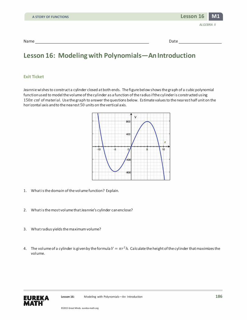
M1 Lesson 16 ALGEBRA II
Lesson 16: Modeling with Polynomials—An Introduction
Name Date
Lesson 16: Modeling with Polynomials—An Introduction
Exit Ticket Jeannie wishes to construct a cylinder closed at both ends. The figure below shows the graph of a cubic polynomial function used to model the volume of the cylinder as a function of the radius if the cylinder is constructed using 150 cm2 of material. Use the graph to answer the questions below. Estimate values to the nearest half unit on the horizontal axis and to the nearest 50 units on the vertical axis.
1. What is the domain of the volume function? Explain.
2. What is the most volume that Jeannie’s cylinder can enclose?
3. What radius yields the maximum volume?
4. The volume of a cylinder is given by the formula 𝑉𝑉 = 𝑟𝑟2ℎ. Calculate the height of the cylinder that maximizes the volume.
A STORY OF FUNCTIONS
186
©2015 Great Minds. eureka-math.org

M1 Lesson 16 ALGEBRA II
Lesson 16: Modeling with Polynomials—An Introduction
Exit Ticket Sample Solutions
Jeannie wishes to construct a cylinder closed at both ends. The figure below shows the graph of a cubic polynomial function used to model the volume of the cylinder as a function of the radius if the cylinder is constructed using
2 of material. Use the graph to answer the questions below. Estimate values to the nearest half unit on the horizontal axis and the nearest units on the vertical axis.
1. What is the domain of the volume function? Explain.
The domain is approximately . because a negative radius does not make sense, and a radius larger than . gives a negative volume, which also does not make sense.
2. What is the most volume that Jeannie’s cylinder can enclose?
Approximately 3
3. What radius yields the maximum volume?
Approximately
4. The volume of a cylinder is given by the formula = . Calculate the height of the cylinder that maximizes the volume.
Approximately .
A STORY OF FUNCTIONS
187
©2015 Great Minds. eureka-math.org

M1 Lesson 16 ALGEBRA II
Lesson 16: Modeling with Polynomials—An Introduction
Problem Set Sample Solutions For a bonus, ask students what is meant by the caption on the t-shirt. (Hint that they can do a web search to find out.)
1. For a fundraiser, members of the math club decide to make and sell “Pythagoras may have been Fermat’s first problem but not his last!” t-shirts. They are trying to decide how many t-shirts to make and sell at a fixed price. They surveyed the level of interest of students around school and made a scatterplot of the number of t-shirts sold ( ) versus profit shown below.
a. Identify the -intercept. Interpret its meaning within the context of this problem.
The -intercept is approximately − . The − represents the money that they must spend on supplies in order to start making t-shirts. That is, they will lose $ if they sell t-shirts.
b. If we model this data with a function, what point on the graph of that function represents the number of
t-shirts they need to sell in order to break even? Why?
The break-even point is the first -intercept of the graph of the function because at this point profit changes from negative to positive. When profit is , the club is breaking even.
c. What is the smallest number of t-shirts they can sell and still make a profit?
Approximately or t-shirts
d. How many t-shirts should they sell in order to maximize the profit?
Approximately t-shirts
e. What is the maximum profit?
Approximately $
f. What factors would affect the profit?
The price of the t-shirts, the cost of supplies, the number of people who are willing to purchase a t-shirt
A STORY OF FUNCTIONS
188
©2015 Great Minds. eureka-math.org

M1 Lesson 16 ALGEBRA II
Lesson 16: Modeling with Polynomials—An Introduction
g. What would cause the profit to start decreasing?
Making more t-shirts than can be sold
2. The following graph shows the temperature in Aspen, Colorado during a 48-hour period beginning at midnight on
Thursday, January 21, 2014. (Source: National Weather Service)
a. We can model the data shown with a polynomial function. What degree polynomial would be a reasonable choice?
Since the graph has turning points ( relative minima, relative maxima), a degree polynomial could be used. Students could also argue that the final point is another minimum point and that a degree polynomial could be used.
b. Let be the function that represents the temperature, in degrees Fahrenheit, as a function of time , in hours.
If we let = correspond to midnight on Thursday, interpret the meaning of ( ) . What is ( )?
The value ( ) represents the temperature at a.m. on Thursday. From the graph, ( ) = .
c. What are the relative maximum values? Interpret their meanings.
The relative maximum values are approximately ( ) = and ( ) = . These points represent the high temperature on Thursday and Friday and the times at which they occurred. The high on Thursday occurred at : (when = ) and was ° . The high on Friday occurred at : (when = ) and was
° .
A STORY OF FUNCTIONS
189
©2015 Great Minds. eureka-math.org

Lesson 17: Modeling with Polynomials—An Introduction
M1 Lesson 17 ALGEBRA II
Lesson 17: Modeling with Polynomials—An Introduction
Student Outcomes
� Students interpret and represent relationships between two types of quantities with polynomial functions.
Lesson Notes In this lesson, students delve more deeply into modeling by writing polynomial equations that can be used to model a particular situation. Students are asked to interpret key features from a graph or table within a contextual situation (F-IF.B.4) and select the domain that corresponds to the appropriate graph or table (F-IF.B.5).
Classwork Opening Exercise (8 minutes)
Give students time to work independently on the Opening Exercise before discussing as a class. Opening Exercise
In Lesson 16, we created an open-topped box by cutting congruent squares from each corner of a piece of construction paper.
a. Express the dimensions of the box in terms of .
Length: = . −
Width: = . −
Height: =
b. Write a formula for the volume of the box as a function of . Give the answer in standard form.
( ) = ( . − )( . − )
( ) = − . + .
� How does this compare with the regression function found yesterday? à Answers will vary. Compare each parameter in the function.
� Which function is more accurate? Why?
à The one found today is more accurate. The one found yesterday depended on measurements that may not have been exact.
A STORY OF FUNCTIONS
190
©2015 Great Minds. eureka-math.org

Lesson 17: Modeling with Polynomials—An Introduction
M1 Lesson 17 ALGEBRA II
Mathematical Modeling Exercises 1–13 (30 minutes)
Allow students to work through the exercises in groups. Circulate the room to monitor students’ progress. Then, discuss results.
Mathematical Modeling Exercises 1–13
The owners of Dizzy Lizzy’s, an amusement park, are studying the wait time at their most popular roller coaster. The table below shows the number of people standing in line for the roller coaster hours after Dizzy Lizzy’s opens.
(hours) (people in line)
Jaylon made a scatterplot and decided that a cubic function should be used to model the data. His scatterplot and curve are shown below.
1. Do you agree that a cubic polynomial function is a good model for this data? Explain.
Yes, the curve passes through most of the points and seems to fit the data.
2. What information would Dizzy Lizzy's be interested in learning about from this graph? How could they determine the answer?
The company should be interested in the time when the line is the longest and how many people are in line at that time. To find this out, they can find a model that could be used to predict the number of people in line at any time during the day. They could then estimate the maximum point from the graph.
3. Estimate the time at which the line is the longest. Explain how you know.
From the graph, the line is longest at . hours because the relative maximum of the function occurs at . hours.
4. Estimate the number of people in line at that time. Explain how you know.
From the graph, there are roughly people in line when = . ; that is the approximate relative maximum value of .
5. Estimate the -intercepts of the function used to model this data.
The -intercepts are roughly , . , and .
6. Use the -intercepts to write a formula for the function of the number of people in line, , after hours.
( ) = ( − . )( − ), where is a constant that has not yet been determined.
Scaffolding: Have early finishers find a quadratic model for comparison. Which model seems to be a better fit? Why? Answers will vary, but one model would be 𝑃𝑃( ) = −10.134 ( − 12). Students should see that the quadratic model does not seem to fit the data as well as the cubic model. They could confirm this using the regression feature of a graphing calculator.
A STORY OF FUNCTIONS
191
©2015 Great Minds. eureka-math.org

Lesson 17: Modeling with Polynomials—An Introduction
M1 Lesson 17 ALGEBRA II
7. Use the relative maximum to find the leading coefficient of . Explain your reasoning.
Since we have estimated ( . ) = , we can plug . into the function above, and we find that ( . ) = . = . Solving for , we find that . . The function that could model the data is then
given by ( ) = . ( − . )( − ).
8. What would be a reasonable domain for your function ? Why?
A reasonable domain for would be . because the opening of the park corresponds to = , and after . hours the park closes, so there are no people waiting in line.
9. Use your function to calculate the number of people in line hours after the park opens.
The formula developed in Exercise 7 gives ( ) = . After the park has been open for hours, there will be people in line.
10. Comparing the value calculated above to the actual value in the table, is your function an accurate model for the data? Explain.
The value of the function differs from the value from the table by about people, so it is not a perfect fit for the data, but it is otherwise very close. It appears to overestimate the number of people in line.
11. Use the regression feature of a graphing calculator to find a cubic function to model the data.
The calculator gives ( ) = . − . + . − . .
12. Graph the function you found and the function produced by the graphing calculator. Use the graphing calculator
to complete the table. Round your answers to the nearest integer.
(hours) (people in line) ( ) (your equation) ( ) (regression eqn.) −
13. Based on the results from the table, which model was more accurate at = hours? = hours?
At = hours, the function found by hand was more accurate. It was off by people whereas the calculator function was off by people. At = hours, the graphing calculator function was more accurate. It was off by
people whereas the function found by hand was off by people.
Closing (2 minutes)
� What type of functions were used to model the data? Were they good models? à Cubic polynomial functions; yes, both functions were reasonably accurate.
� What information did we use to find the function by hand? à We used the 𝑥𝑥-intercepts and the relative maximum.
� Did we have to use the relative maximum specifically to find the leading coefficient? à No, we could have chosen a different point on the curve.
MP.2
MP.3
A STORY OF FUNCTIONS
192
©2015 Great Minds. eureka-math.org

Lesson 17: Modeling with Polynomials—An Introduction
M1 Lesson 17 ALGEBRA II
� How did polynomials help us solve a real-world problem?
à We were able to model the data using a polynomial function. The function allows us to estimate the number of people in line at any time and also to estimate the time when the line is the longest and the maximum number of people are in line.
Exit Ticket (5 minutes)
A STORY OF FUNCTIONS
193
©2015 Great Minds. eureka-math.org

Lesson 17: Modeling with Polynomials—An Introduction
M1 Lesson 17 ALGEBRA II
Name Date
Lesson 17: Modeling with Polynomials—An Introduction
Exit Ticket Jeannie wishes to construct a cylinder closed at both ends. The figure at right shows the graph of a cubic polynomial function, 𝑉𝑉, used to model the volume of the cylinder as a function of the radius if the cylinder is constructed using 150 cm3 of material. Use the graph to answer the questions below. Estimate values to the nearest half unit on the horizontal axis and to the nearest 50 units on the vertical axis.
1. What are the zeros of the function 𝑉𝑉?
2. What is the relative maximum value of 𝑉𝑉, and where does it occur?
3. The equation of this function is 𝑉𝑉(𝑟𝑟) = 𝑐𝑐(𝑟𝑟3 − 72.25𝑟𝑟) for some real number 𝑐𝑐. Find the value of 𝑐𝑐 so that this formula fits the graph.
4. Use the graph to estimate the volume of the cylinder with 𝑟𝑟 = 2 cm.
5. Use your formula for 𝑉𝑉 to find the volume of the cylinder when 𝑟𝑟 = 2 cm. How close is the value from the formula to the value on the graph?
A STORY OF FUNCTIONS
194
©2015 Great Minds. eureka-math.org

Lesson 17: Modeling with Polynomials—An Introduction
M1 Lesson 17 ALGEBRA II
Exit Ticket Sample Solutions
Jeannie wishes to construct a cylinder closed at both ends. The figure at right shows the graph of a cubic polynomial function, , used to model the volume of the cylinder as a function of the radius if the cylinder is constructed using
of material. Use the graph to answer the questions below. Estimate values to the nearest half unit on the horizontal axis and to the nearest units on the vertical axis.
1. What are the zeros of the function ?
Approximately , − . , and . (Students might round up to − and .)
2. What is the relative maximum value of and where does it occur?
The relative maximum value is at = .
3. The equation of this function is ( ) = ( − . ) for some real number . Find the value of so that this formula fits the graph.
Substituting = and ( ) = and solving for gives − . .
4. Use the graph to estimate the volume of the cylinder with = .
Estimating from the graph, the volume of a cylinder of radius is .
5. Use your formula for to find the volume of the cylinder when = . How close is the value from the formula to the value on the graph?
Using the formula: ( ) = − . − . ( ) = . . Therefore, the volume of the cylinder when = is . . This value is close to the value of found using the graph but not exact, particularly because we cannot read much detail from the graph.
Problem Set Sample Solutions Problem 2 requires the use of a graphing calculator. If students do not have the means to complete this, the last two parts could be done in class.
1. Recall the math club fundraiser from the Problem Set of the previous lesson. The club members would like to find a function to model their data, so Kylie draws a curve through the data points as shown.
a. What type of function does it appear that she has drawn?
Degree polynomial (or cubic polynomial)
A STORY OF FUNCTIONS
195
©2015 Great Minds. eureka-math.org
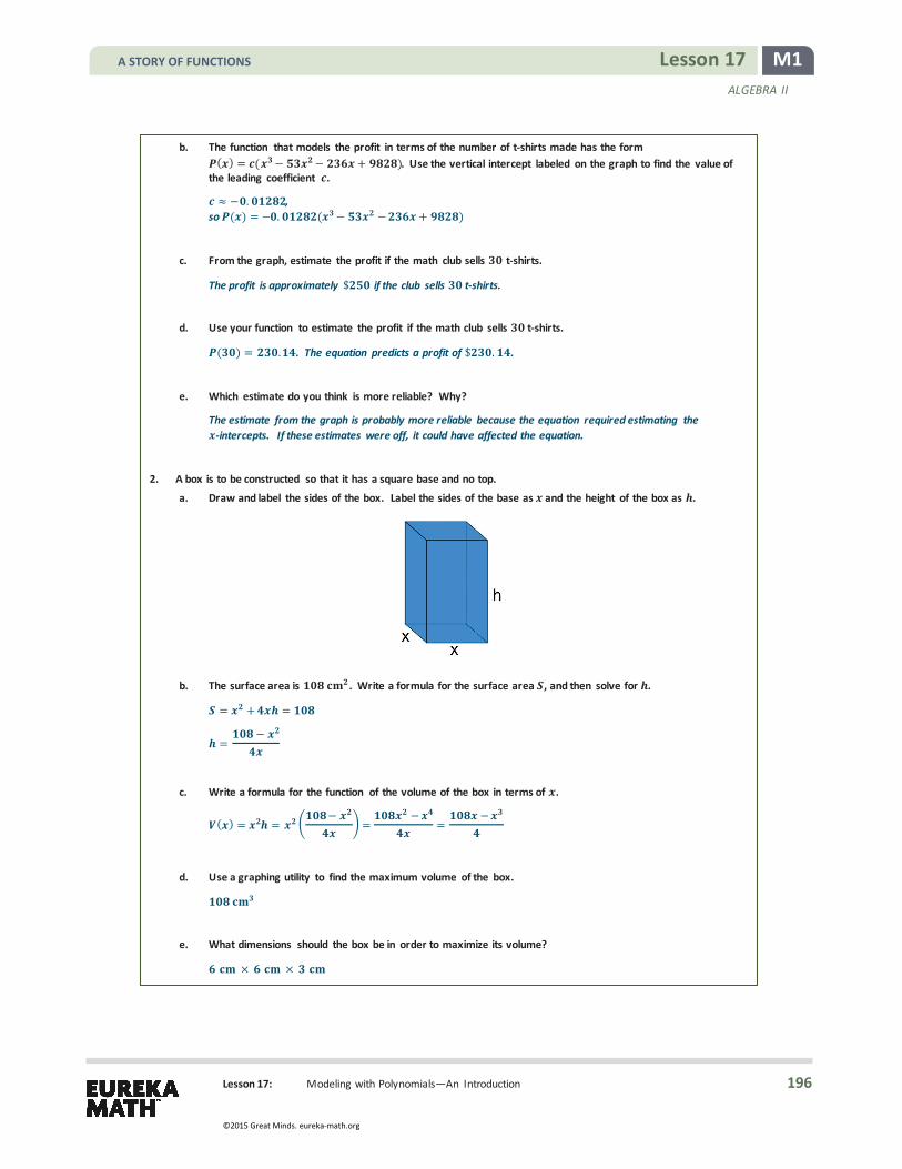
Lesson 17: Modeling with Polynomials—An Introduction
M1 Lesson 17 ALGEBRA II
b. The function that models the profit in terms of the number of t-shirts made has the form ( ) = ( − − + ). Use the vertical intercept labeled on the graph to find the value of
the leading coefficient .
− . , so ( ) = − . ( − − + )
c. From the graph, estimate the profit if the math club sells t-shirts.
The profit is approximately $ if the club sells t-shirts.
d. Use your function to estimate the profit if the math club sells t-shirts.
( ) = . . The equation predicts a profit of $ . .
e. Which estimate do you think is more reliable? Why?
The estimate from the graph is probably more reliable because the equation required estimating the -intercepts. If these estimates were off, it could have affected the equation.
2. A box is to be constructed so that it has a square base and no top. a. Draw and label the sides of the box. Label the sides of the base as and the height of the box as .
b. The surface area is . Write a formula for the surface area , and then solve for .
= + =
=−
c. Write a formula for the function of the volume of the box in terms of .
( ) = =−
=−
=−
d. Use a graphing utility to find the maximum volume of the box.
e. What dimensions should the box be in order to maximize its volume?
× ×
A STORY OF FUNCTIONS
196
©2015 Great Minds. eureka-math.org

Lesson 18: Overcoming a Second Obstacle in Factoring—What If There Is a Remainder?
M1 Lesson 18 ALGEBRA II
Lesson 18: Overcoming a Second Obstacle in Factoring—
What If There Is a Remainder?
Student Outcomes
� Students rewrite simple rational expressions in different forms, including representing remainders when dividing.
Lesson Notes Students have worked on dividing two polynomials using both the reverse tabular method and long division. In this lesson, they continue that work but with quotients that have a remainder. In addition to the two methods of division already presented in this module, students also use the method of inspection as stated in standard A-APR.D.6. The method of inspection is an opportunity to emphasize the mathematical practice of making use of structure (MP.7). The purpose of the Opening Exercise is to get students thinking about this idea of structure by leading them from writing rational numbers as mixed numbers to writing rational expressions as “mixed expressions.”
Classwork Opening Exercise (3 minutes)
Have students work through the Opening Exercise briefly by themselves, and then summarize the exercise as a whole class by displaying all three methods. This starts students thinking about the different ways of rewriting an improper fraction as a mixed number. Students use methods 2 and 3 later today to write rational expressions as “mixed expressions.”
Opening Exercise
Write the rational number as a mixed number.
Method 1:
Method 2: Method 3:
Scaffolding: If students are struggling with the different methods of rewriting a rational number as a mixed number, provide them with extra examples such as the following.
107
= 137
263
= 823
A STORY OF FUNCTIONS
197
©2015 Great Minds. eureka-math.org

Lesson 18: Overcoming a Second Obstacle in Factoring—What If There Is a Remainder?
M1 Lesson 18 ALGEBRA II
Example 1 (8 minutes)
Work through the example as a class. Relate the process of inspection used in part (b) below to method 2 used in the Opening Exercise. Then, demonstrate how the quotient could have been found using the reverse tabular method or long division.
Example 1
a. Find the quotient by factoring the numerator. + +
+
b. Find the quotient. + +
+
+ ++
=( + )( + )
+
= +
See below.
Solutions for part (b):
Method 1: Inspection
� We already know that 3 22
= 𝑥𝑥 + 1, as long as 𝑥𝑥 −2. How could we use this fact to find 32
?
à Since 3 + 2 = 5, there must be 3 left over after performing division. � How could we rewrite the problem in a way that is more convenient?
à 32
=( 3 2) 3
2=
3 22
+32
� So, what are the quotient and remainder? à The quotient is 𝑥𝑥+ 1 with a remainder of 3.
� Since the 3 is left over and has not been divided by the 𝑥𝑥 + 2, it is still written as a quotient.
à 32
=3 2 3
2=
3 22
+32
= (𝑥𝑥 + 1) +32
Method 2: Reverse Tabular Method
= +
𝑥𝑥2 + 3𝑥𝑥 + 5𝑥𝑥 + 2
= (𝑥𝑥 + 1) +3
𝑥𝑥 + 2
MP.7
3 remains and is yet to be divided. So the remainder is 3.
A STORY OF FUNCTIONS
198
©2015 Great Minds. eureka-math.org

Lesson 18: Overcoming a Second Obstacle in Factoring—What If There Is a Remainder?
M1 Lesson 18 ALGEBRA II
Method 3: Long division
Work the problem as a class using long division. Remind the students that we used the same process in method 3 of the Opening Exercise.
Example 2 (7 minutes)
Repeat the process for this example. Work through the process of inspection as a pair/share exercise. Then, ask the students to repeat the process using either the reverse tabular method or long division. Share the work from both methods.
Example 2
a. Find the quotient by factoring the numerator.
−−
b. Find the quotient. −−
= ( − )( + + )
−
= + +
= − +−
=−−
+−
= + + +−
� In pairs, see if you can determine how to use the quotient from (a) to find the quotient of 42
.
Give students a couple of minutes to discuss, and then elicit responses.
� How did you rewrite the numerator?
à 42
=4
2=
2+
42
� Why is this a useful way to rewrite the problem?
à We know that 2
= 𝑥𝑥2 + 2𝑥𝑥 + 4.
� So what are the quotient and remainder of 42
?
à The quotient is 𝑥𝑥2+ 2𝑥𝑥 + 4 with a remainder of 4.
Therefore, 42
= (𝑥𝑥2 + 2𝑥𝑥 + 4) +42
.
MP.7
A STORY OF FUNCTIONS
199
©2015 Great Minds. eureka-math.org

Lesson 18: Overcoming a Second Obstacle in Factoring—What If There Is a Remainder?
M1 Lesson 18 ALGEBRA II
Give students a couple of minutes to rework the problem using either the reverse tabular method or long division and then share student work.
− − − −
− = − +
� Which method is easier? Allow students to discuss advantages and disadvantages of the three methods.
Exercise (5 minutes)
Have students practice finding quotients by factoring the numerator using the cards on the page after next. Cut out the cards and hand each student a card. The students must move around the room and match their card with the same quotient. Then have students stay in these pairs to work on the exercises.
Exercises 1–10 (15 minutes)
Allow students to work through the exercises either independently or in pairs. Some students may need to be reminded how to complete the square.
Exercises 1–10
Find each quotient by inspection.
1. 2. 3.
++
−−
( − ) −+
Find each quotient by using the reverse tabular method.
4. 5. 6.
( + ) +−
− + −+
( − ) −−
The remainder is 4.
Scaffolding: � Some students may have difficulty
with inspection. Encourage them to use the reverse tabular method first, and then see if they can use that to rewrite the numerator.
� Early finishers can be given more challenging inspection problems such as the following. 𝑥𝑥2 − 5𝑥𝑥 + 9
𝑥𝑥 − 1= (𝑥𝑥 − 4) +
5𝑥𝑥 − 1
2𝑥𝑥2− 5𝑥𝑥 − 3
= 2(𝑥𝑥 + 3) +13𝑥𝑥 − 3
A STORY OF FUNCTIONS
200
©2015 Great Minds. eureka-math.org

Lesson 18: Overcoming a Second Obstacle in Factoring—What If There Is a Remainder?
M1 Lesson 18 ALGEBRA II
Find each quotient by using long division.
7. 8. 9.
( − ) ++
( − − + )−+
( + + ) +−
Rewrite the numerator in the form ( − ) + by completing the square. Then find the quotient.
10.
( + ) −+
The mental math exercises on the next page can be used for building fluency. All numerators factor nicely so that there are no remainders. The exercise can be timed and restrictions can be imposed (such as, “Only write your answer in the box next to the expression.”).
It is always a good idea to keep fluency exercises quick and stress-free for students. Here is one way to do that: Tell them that the activity will not be turned in for a grade, but they will be timed. Give them 2 minutes to write down as many answers as possible (using a stopwatch or a cell phone stopwatch feature.). Afterward, go through the solutions with them quickly; allow them only to mark the ones they did correctly/incorrectly—do not let them copy the correct answers down. Celebrate the student who got the greatest number correct, and then provide another 2–4 minutes for students to work on the remaining problems that they did not get right.
Mental Math Exercises
−+
−
− +−
−
−+
−
− −+
−
−−
−−
+ −+
−
−+
−
− +−
−
−+
−
+ ++
+
−−
+
− −+
−
−+
−
− +−
−
− +−
−
+ −−
+
−−
+
−
−
− +−
−
+ ++
+
−−
+
+ ++
+
+ ++
+
A STORY OF FUNCTIONS
201
©2015 Great Minds. eureka-math.org

Lesson 18: Overcoming a Second Obstacle in Factoring—What If There Is a Remainder?
M1 Lesson 18 ALGEBRA II
Closing (2 minutes)
Consider asking students to respond in pairs or in writing.
� In the pair/share exercise, how did we use the structure of the expressions to help us to simplify them? à We were able to factor the numerator. Since the numerator and denominator contained a common
factor, we were able to simplify the expression. � How did we use structure in Exercise 10?
à We rewrote the expression by completing the square and then used inspection. � How does this use of structure help us when working with algebraic expressions?
à We can rewrite expressions into equivalent forms that may be more convenient. � What methods were used to find the quotients?
à Inspection, reverse tabular method, long division � What are some pros and cons of the methods?
à You may not see the answer when trying to divide by inspection, but if you do see the structure of the expression, the quotient can often be quickly found. Using the long division or tabular method can be time consuming, but both rely on a known process instead of insight.
Exit Ticket (5 minutes)
A STORY OF FUNCTIONS
202
©2015 Great Minds. eureka-math.org

Lesson 18: Overcoming a Second Obstacle in Factoring—What If There Is a Remainder?
M1 Lesson 18 ALGEBRA II
Name Date
Lesson 18: Overcoming a Second Obstacle in Factoring—What If
There Is a Remainder?
Exit Ticket
1. Find the quotient of by inspection.
2. Find the quotient of 12 42
by using either long division or the reverse tabular method.
A STORY OF FUNCTIONS
203
©2015 Great Minds. eureka-math.org

Lesson 18: Overcoming a Second Obstacle in Factoring—What If There Is a Remainder?
M1 Lesson 18 ALGEBRA II
Exit Ticket Sample Solutions
1. Find the quotient of by inspection.
+−
2. Find the quotient of by using either long division or the reverse tabular method.
( + + ) +−
Problem Set Sample Solutions
1. For each pair of problems, find the first quotient by factoring the numerator. Then, find the second quotient by using the first quotient.
a. −−
−−
−−
b. − −−
− +−
+ ( + ) +−
c. ++
+
− + ( − + ) −+
d. − +−
− +
−
− ( − )−−
Find each quotient by using the reverse tabular method.
2. 3.
( − − ) −−
( − ) ++
A STORY OF FUNCTIONS
204
©2015 Great Minds. eureka-math.org

Lesson 18: Overcoming a Second Obstacle in Factoring—What If There Is a Remainder?
M1 Lesson 18 ALGEBRA II
4. 5.
+−
( − ) ++
Find each quotient by using long division.
6. 7.
( − − + )−+
( + + + + ) −−
8. 9.
( + ) +−
( − + )−+
10. 11.
( + + ) +−
( + − + ) −
12. Rewrite the numerator in the form ( − ) + by completing the square. Then, find the quotient.
− − −
A STORY OF FUNCTIONS
205
©2015 Great Minds. eureka-math.org

Lesson 19: The Remainder Theorem
M1 Lesson 19 ALGEBRA II
Lesson 19: The Remainder Theorem
Student Outcomes
� Students know and apply the remainder theorem and understand the role zeros play in the theorem.
Lesson Notes In this lesson, students are primarily working on exercises that lead them to the concept of the remainder theorem, the connection between factors and zeros of a polynomial, and how this relates to the graph of a polynomial function. Students should understand that for a polynomial function 𝑃𝑃 and a number 𝑎𝑎, the remainder on division by 𝑥𝑥 −𝑎𝑎 is the value 𝑃𝑃(𝑎𝑎) and extend this to the idea that 𝑃𝑃(𝑎𝑎) = 0 if and only if (𝑥𝑥 −𝑎𝑎) is a factor of the polynomial (A-APR.B.2). There should be plenty of discussion after each exercise.
Classwork Exercises 1–3 (5 minutes)
Assign different groups of students one of the three problems from this exercise. Have them complete their assigned problem, and then have a student from each group put their solution on the board. Having the solutions readily available allows students to start looking for a pattern without making the lesson too tedious.
Exercises 1–3
1. Consider the polynomial function ( ) = + − .
a. Divide by − . b. Find ( ).
( )−
= + −−
= ( + ) +−
( ) =
2. Consider the polynomial function ( ) = − + + .
a. Divide by + . b. Find (− ).
( )+
=− + +
+
= ( − + )−+
(− ) = −
Scaffolding: If students are struggling, replace the polynomials in Exercises 2 and 3 with easier polynomial functions. Examples:
𝑔𝑔(𝑥𝑥) = 𝑥𝑥2− 7𝑥𝑥 − 11 a. Divide by 𝑥𝑥+ 1. b. Find 𝑔𝑔(−1). (𝑥𝑥− 8)−
3𝑥𝑥 + 1
𝑔𝑔(−1) =−3
ℎ(𝑥𝑥) = 2𝑥𝑥2+ 9
a. Divide by 𝑥𝑥− 3. b. Find ℎ(3).
(2𝑥𝑥 + 6) +27
2𝑥𝑥2 + 9 ℎ(3) = 27
A STORY OF FUNCTIONS
206
©2015 Great Minds. eureka-math.org

Lesson 19: The Remainder Theorem
M1 Lesson 19 ALGEBRA II
3. Consider the polynomial function ( ) = + − .
a. Divide by − . b. Find ( ).
( )−
=+ −−
= ( + + ) +−
( ) =
Discussion (7 minutes) � What is 𝑓𝑓(2)? What is 𝑔𝑔(−1)? What is ℎ(3)?
à 𝑓𝑓(2) = 24; 𝑔𝑔(−1) = −2; ℎ(3) = 30 � Looking at the results of the quotient, what pattern do we see?
à The remainder is the value of the function.
� Stating this in more general terms, what do we suspect about the connection between the remainder from dividing a polynomial 𝑃𝑃 by 𝑥𝑥 −𝑎𝑎 and the value of 𝑃𝑃(𝑎𝑎)? à The remainder found after dividing 𝑃𝑃 by 𝑥𝑥 −𝑎𝑎 will be the same value as 𝑃𝑃(𝑎𝑎).
� Why would this be? Think about the quotient 133
. We could write this as 13 = 4 3 + 1, where 4 is the
quotient and 1 is the remainder. � Apply this same principle to Exercise 1. Write the following on the board, and talk through it:
𝑓𝑓(𝑥𝑥)𝑥𝑥 − 2 =
3𝑥𝑥2 + 8𝑥𝑥 − 4𝑥𝑥 − 2
= (3𝑥𝑥 + 14) +24𝑥𝑥 − 2
� How can we rewrite 𝑓𝑓 using the equation above? à Multiply both sides of the equation by 𝑥𝑥 − 2 to get 𝑓𝑓(𝑥𝑥) = (3𝑥𝑥+ 14)(𝑥𝑥 − 2) + 24.
� In general we can say that if you divide polynomial 𝑃𝑃 by 𝑥𝑥− 𝑎𝑎, then the remainder must be a number; in fact, there is a (possibly non-zero degree) polynomial function 𝑞𝑞 such that the equation,
𝑃𝑃(𝑥𝑥) = ( ) (𝑥𝑥 −𝑎𝑎) +
quotient remainder
is true for all 𝑥𝑥. � What is 𝑃𝑃(𝑎𝑎)?
à 𝑃𝑃(𝑎𝑎) = 𝑞𝑞(𝑎𝑎)(𝑎𝑎 −𝑎𝑎) + 𝑟𝑟 = 𝑞𝑞(𝑎𝑎) 0 + 𝑟𝑟 = 0 + 𝑟𝑟 = 𝑟𝑟 We have just proven the remainder theorem, which is formally stated in the box below.
� Restate the remainder theorem in your own words to your partner.
REMAINDER THEOREM: Let 𝑃𝑃 be a polynomial function in 𝑥𝑥, and let 𝑎𝑎 be any real number. Then there exists a unique polynomial function 𝑞𝑞 such that the equation
𝑃𝑃(𝑥𝑥) = 𝑞𝑞(𝑥𝑥)(𝑥𝑥 −𝑎𝑎) +𝑃𝑃(𝑎𝑎) is true for all 𝑥𝑥. That is, when a polynomial is divided by (𝑥𝑥 −𝑎𝑎), the remainder is the value of the polynomial evaluated at 𝑎𝑎.
MP.8
A STORY OF FUNCTIONS
207
©2015 Great Minds. eureka-math.org

Lesson 19: The Remainder Theorem
M1 Lesson 19 ALGEBRA II
Scaffolding: Challenge early finishers with this problem:
Given that 𝑥𝑥 + 1 and 𝑥𝑥 − 1 are factors of 𝑃𝑃(𝑥𝑥) = 𝑥𝑥4 + 2𝑥𝑥3−49𝑥𝑥2 − 2𝑥𝑥+ 48, write 𝑃𝑃 in factored form.
Answer: (𝑥𝑥 + 1)(𝑥𝑥 − 1)(𝑥𝑥 + 8)(𝑥𝑥 − 6)
While students are doing this, circulate and informally assess student understanding before asking students to share their responses as a class.
Exercise 4 (5 minutes)
Students may need more guidance through this exercise, but allow them to struggle with it first. After a few students have found 𝑘𝑘, share various methods used.
Exercise 4–6
4. Consider the polynomial ( ) = + + + .
a. Find the value of so that + is a factor of .
In order for + to be a factor of , the remainder must be zero. Hence, since + = − (− ), we must have (− ) = so that = − + − + .
Then = − .
b. Find the other two factors of for the value of found in part (a).
( ) = ( + )( − + ) = ( + )( − )( − )
Discussion (7 minutes)
� Remember that for any polynomial function 𝑃𝑃 and real number 𝑎𝑎, the remainder theorem says that there exists a polynomial 𝑞𝑞 so that 𝑃𝑃(𝑥𝑥) = 𝑞𝑞(𝑥𝑥)(𝑥𝑥 −𝑎𝑎) + 𝑃𝑃(𝑎𝑎).
� What does it mean if 𝑎𝑎 is a zero of a polynomial 𝑃𝑃? à 𝑃𝑃(𝑎𝑎) = 0
� So what does the remainder theorem say if 𝑎𝑎 is a zero of 𝑃𝑃? à There is a polynomial 𝑞𝑞 so that 𝑃𝑃(𝑥𝑥) = 𝑞𝑞(𝑥𝑥)(𝑥𝑥 −𝑎𝑎) + 0.
� How does (𝑥𝑥 −𝑎𝑎) relate to 𝑃𝑃 if 𝑎𝑎 is a zero of 𝑃𝑃? à If 𝑎𝑎 is a zero of 𝑃𝑃, then (𝑥𝑥 −𝑎𝑎) is a factor of 𝑃𝑃.
� How does the graph of a polynomial function 𝑦𝑦 = 𝑃𝑃(𝑥𝑥) correspond to the equation of the polynomial 𝑃𝑃? à The zeros are the 𝑥𝑥-intercepts of the graph of 𝑃𝑃. If we know a zero of 𝑃𝑃, then we know a factor of 𝑃𝑃.
� If we know all of the zeros of a polynomial function, and their multiplicities, do we know the equation of the function?
à Not necessarily. It is possible that the equation of the function contains some factors that cannot factor into linear terms.
We have just proven the factor theorem, which is a direct consequence of the remainder theorem.
� Give an example of a polynomial function with zeros of multiplicity 2 at 1 and 3.
à 𝑃𝑃(𝑥𝑥) = (𝑥𝑥 − 1)2(𝑥𝑥− 3)2
FACTOR THEOREM: Let 𝑃𝑃 be a polynomial function in 𝑥𝑥, and let 𝑎𝑎 be any real number. If 𝑎𝑎 is a zero of 𝑃𝑃 then (𝑥𝑥 −𝑎𝑎) is a factor of 𝑃𝑃.
A STORY OF FUNCTIONS
208
©2015 Great Minds. eureka-math.org

Lesson 19: The Remainder Theorem
M1 Lesson 19 ALGEBRA II
� Give another example of a polynomial function with zeros of multiplicity 2 at 1 and 3. à (𝑥𝑥) = (𝑥𝑥 − 1)2(𝑥𝑥− 3) 2(𝑥𝑥2+ 1) or 𝐼𝐼(𝑥𝑥) = 4(𝑥𝑥 − 1)2(𝑥𝑥− 3) 2
� If we know the zeros of a polynomial, does the factor theorem tell us the exact formula for the polynomial? à No. But, if we know the degree of the polynomial and the leading coefficient, we can often deduce the
equation of the polynomial.
Exercise 5 (8 minutes)
As students work through this exercise, circulate the room to make sure students have made the connection between zeros, factors, and 𝑥𝑥-intercepts. Question students to see if they can verbalize the ideas discussed in the prior exercise.
5. Consider the polynomial ( ) = + − − + . a. Is a zero of the polynomial ?
No
b. Is + one of the factors of ?
Yes; (− ) = − − + + = .
c. The graph of is shown to the right. What are the zeros of ?
Approximately − , − , , and .
d. Write the equation of in factored form.
( ) = ( + )( + )( − )( − )
� Is 1 a zero of the polynomial 𝑃𝑃? How do you know?
à No. 𝑃𝑃(1) 0. � What are two ways to determine the value of 𝑃𝑃(1)?
à Substitute 1 for 𝑥𝑥 into the function or divide 𝑃𝑃 by 𝑥𝑥 − 1. The remainder will be 𝑃𝑃(1). � Is 𝑥𝑥 + 3 a factor of 𝑃𝑃? How do you know?
à Yes. Because 𝑃𝑃(−3) = 0, then when 𝑃𝑃 is divided by 𝑥𝑥 + 3, the remainder is 0, which means that 𝑥𝑥 + 3 is a factor of the polynomial 𝑃𝑃.
� How do you find the zeros of 𝑃𝑃 from the graph? à The zeros are the 𝑥𝑥-intercepts of the graph.
� How do you find the factors? à By using the zeros: if 𝑥𝑥 = 𝑎𝑎 is a zero, then 𝑥𝑥 −𝑎𝑎 is a factor of 𝑃𝑃.
� Expand the expression in part (d) to see that it is indeed the original polynomial function.
Scaffolding: Encourage students who are struggling to work on part (a) using two methods: � by finding 𝑃𝑃(1), and � by dividing 𝑃𝑃 by 𝑥𝑥 − 1. This helps to reinforce the ideas discussed in Exercises 1 and 2.
A STORY OF FUNCTIONS
209
©2015 Great Minds. eureka-math.org

Lesson 19: The Remainder Theorem
M1 Lesson 19 ALGEBRA II
Exercise 6 (6 minutes)
Allow students a few minutes to work on the problem and then share results.
6. Consider the graph of a degree polynomial shown to the right, with -intercepts − , − , , , and .
a. Write a formula for a possible polynomial function that the graph represents using as the constant factor.
( ) = ( + )( + )( − )( − )( − )
b. Suppose the -intercept is − . Find the value of so that the graph
of has -intercept − .
( ) = ( + )( + )( − )( − )( − )
� What information from the graph was needed to write the equation? à The 𝑥𝑥-intercepts were needed to write the factors.
� Why would there be more than one polynomial function possible?
à Because the factors could be multiplied by any constant and still produce a graph with the same 𝑥𝑥-intercepts.
� Why can’t we find the constant factor 𝑐𝑐 by just knowing the zeros of the polynomial?
à The zeros only determine where the graph crosses the 𝑥𝑥-axis, not how the graph is stretched vertically. The constant factor can be used to vertically scale the graph of the polynomial function that we found to fit the depicted graph.
Closing (2 minutes)
Have students summarize the results of the remainder theorem and the factor theorem.
� What is the connection between the remainder when a polynomial 𝑃𝑃 is divided by 𝑥𝑥 −𝑎𝑎 and the value of 𝑃𝑃(𝑎𝑎)? à They are the same.
� If 𝑥𝑥 −𝑎𝑎 is factor, then _________. à The number 𝑎𝑎 is a zero of 𝑃𝑃.
� If 𝑃𝑃(𝑎𝑎) = 0, then ____________. à (𝑥𝑥 −𝑎𝑎) is a factor of 𝑃𝑃.
A STORY OF FUNCTIONS
210
©2015 Great Minds. eureka-math.org

Lesson 19: The Remainder Theorem
M1 Lesson 19 ALGEBRA II
Exit Ticket (5 minutes)
Lesson Summary
REMAINDER THEOREM: Let be a polynomial function in , and let be any real number. Then there exists a unique polynomial function such that the equation
( ) = ( )( − ) + ( )
is true for all . That is, when a polynomial is divided by ( − ), the remainder is the value of the polynomial evaluated at .
FACTOR THEOREM: Let be a polynomial function in , and let be any real number. If is a zero of , then ( − ) is a factor of .
Example: If ( ) = − and = , then ( ) = ( + )( − ) + where ( ) = + and ( ) = .
Example: If ( ) = − + + , then ( ) = − + + = , so ( − ) is a factor of .
A STORY OF FUNCTIONS
211
©2015 Great Minds. eureka-math.org

Lesson 19: The Remainder Theorem
M1 Lesson 19 ALGEBRA II
Name Date
Lesson 19: The Remainder Theorem
Exit Ticket Consider the polynomial 𝑃𝑃(𝑥𝑥) = 𝑥𝑥3 + 𝑥𝑥2 − 10𝑥𝑥 − 10.
1. Is 𝑥𝑥 + 1 one of the factors of 𝑃𝑃? Explain.
2. The graph shown has 𝑥𝑥-intercepts at √10, −1, and −√10. Could this be the graph of 𝑃𝑃(𝑥𝑥) = 𝑥𝑥3 + 𝑥𝑥2 − 10𝑥𝑥 − 10? Explain how you know.
A STORY OF FUNCTIONS
212
©2015 Great Minds. eureka-math.org
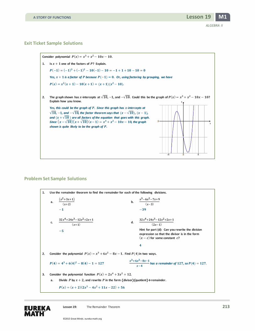
Lesson 19: The Remainder Theorem
M1 Lesson 19 ALGEBRA II
Exit Ticket Sample Solutions
Consider polynomial ( ) = + − − .
1. Is + one of the factors of ? Explain.
(− ) = (− ) + (− ) − (− )− = − + + − =
Yes, + is a factor of because (− ) = . Or, using factoring by grouping, we have
( ) = ( + )− ( + ) = ( + )( − ).
2. The graph shown has -intercepts at √ , − , and −√ . Could this be the graph of ( ) = + − − ? Explain how you know.
Yes, this could be the graph of . Since this graph has -intercepts at √ , − , and −√ , the factor theorem says that ( −√ ) , ( − ), and ( +√ ) are all factors of the equation that goes with this graph. Since −√ + √ ( − ) = + − − , the graph shown is quite likely to be the graph of .
Problem Set Sample Solutions
1. Use the remainder theorem to find the remainder for each of the following divisions.
a. ( ) b. ( )
− −
c. ( )
−
d. ( )
Hint for part (d): Can you rewrite the division expression so that the divisor is in the form ( − ) for some constant ?
2. Consider the polynomial ( ) = + − − . Find ( ) in two ways.
( ) = + ( ) − ( )− = has a remainder of , so ( ) = .
3. Consider the polynomial function ( ) = + + .
a. Divide by + , and rewrite in the form (divisor)(quotient)+remainder.
( ) = ( + )( − + − ) +
A STORY OF FUNCTIONS
213
©2015 Great Minds. eureka-math.org

Lesson 19: The Remainder Theorem
M1 Lesson 19 ALGEBRA II
b. Find (− ).
(− ) = (− + ) (− ) + =
4. Consider the polynomial function ( ) = + . a. Divide by − , and rewrite in the form (divisor )(quotient ) + remainder .
( ) = ( − )( + + ) +
b. Find ( ).
( ) = ( − ) ( ) + =
5. Explain why for a polynomial function , ( ) is equal to the remainder of the quotient of and − .
The polynomial can be rewritten in the form ( ) = ( − )( ( )) + , where ( ) is the quotient function and is the remainder. Then ( ) = ( − ) ( ) + . Therefore, ( ) = .
6. Is − a factor of the function ( ) = + − − ? Show work supporting your answer.
Yes, because ( ) = means that dividing by − leaves a remainder of .
7. Is + a factor of the function ( ) = − + − + ? Show work supporting your answer.
No, because (− ) = − means that dividing by + has a remainder of − .
8. A polynomial function has zeros of , , − , − , − , and . Find a possible formula for , and state its degree. Why is the degree of the polynomial not ?
One solution is ( ) = ( − ) ( + ) ( − ). The degree of is . This is not a degree polynomial function because the factor ( − ) appears twice, and the factor ( + ) appears times, while the factor ( − ) appears once.
9. Consider the polynomial function ( ) = − − + . a. Verify that ( ) = . Since ( ) = , what must one of the factors of be?
( ) = − ( )− ( ) + = ; −
b. Find the remaining two factors of .
( ) = ( − )( − )( + )
c. State the zeros of .
= , , −
d. Sketch the graph of .
A STORY OF FUNCTIONS
214
©2015 Great Minds. eureka-math.org

Lesson 19: The Remainder Theorem
M1 Lesson 19 ALGEBRA II
10. Consider the polynomial function ( ) = + − − .
a. Verify that (− ) = . Since (− ) = , what must one of the factors of be?
(− ) = (− ) + (− ) − (− )− = ; +
b. Find the remaining two factors of .
( ) = ( + )( − )( + )
c. State the zeros of .
= − , , −
d. Sketch the graph of .
11. The graph to the right is of a third-degree polynomial function .
a. State the zeros of .
= − , − ,
b. Write a formula for in factored form using for the constant
factor.
( ) = ( + )( + )( − )
c. Use the fact that (− ) = − to find the constant factor .
− = (− + )(− + )(− − ) = −
( ) = − ( + )( + )( − )
d. Verify your equation by using the fact that ( ) = .
( ) = − ( + )( + )( − ) = − ( )( )(− ) =
A STORY OF FUNCTIONS
215
©2015 Great Minds. eureka-math.org

Lesson 19: The Remainder Theorem
M1 Lesson 19 ALGEBRA II
12. Find the value of so that has remainder .
= −
13. Find the value so that has remainder .
= −
14. Show that − + is divisible by − .
Let ( ) = − + .
Then ( ) = − ( ) + = − + = .
Since ( ) = , the remainder of the quotient ( − + ) ÷ ( − ) is .
Therefore, − + is divisible by − .
15. Show that + is a factor of + − .
Let ( ) = + − .
Then (− ) = (− ) + (− )− = − − = .
Since (− ) = , + must be a factor of .
Note to Teacher: The following problems have multiple correct solutions. The answers provided here are polynomials with leading coefficient 1 and the lowest degree that meet the specified criteria. As an example, the answer to Exercise 16 is given as 𝑝𝑝(𝑥𝑥) = (𝑥𝑥 + 2)(𝑥𝑥 − 1), but the following are also correct responses: 𝑞𝑞(𝑥𝑥) = 14(𝑥𝑥 + 2)(𝑥𝑥− 1), 𝑟𝑟(𝑥𝑥) = (𝑥𝑥 + 2)4(𝑥𝑥− 1) , and (𝑥𝑥) = (𝑥𝑥2 + 1)(𝑥𝑥 + 2)(𝑥𝑥 − 1).
Write a polynomial function that meets the stated conditions.
16. The zeros are − and .
( ) = ( + )( − ) or, equivalently, ( ) = + −
17. The zeros are − , , and .
( ) = ( + )( − )( − ) or, equivalently, ( ) = − + +
18. The zeros are – and .
( ) = � + � � − � or, equivalently, ( ) = − −
19. The zeros are − and , and the constant term of the polynomial is − .
( ) = ( − )( + ) or, equivalently, ( ) = − −
20. The zeros are and – , the polynomial has degree , and there are no other zeros.
( ) = ( − ) ( + ) or, equivalently, ( ) = ( − )( + )
A STORY OF FUNCTIONS
216
©2015 Great Minds. eureka-math.org

Lesson 20: Modeling Riverbeds with Polynomials
M1 Lesson 20 ALGEBRA II
Lesson 20: Modeling Riverbeds with Polynomials
Student Outcomes
� Students learn to fit polynomial functions to data values.
Lesson Notes In previous modeling lessons, students relied on the graphing calculator to find polynomial functions that fit a set of data. Lessons 20 and 21 comprise a two-lesson modeling exercise in which students model the shape of a riverbed in order to calculate flow rate of the river; this can be used to determine if the river is vulnerable to flooding. In this first lesson, students use the remainder theorem as a way to fit a polynomial function to data points without relying on technology. In the second lesson, students use technology, particularly Wolfram Alpha, to find the equation of the interpolating polynomial that best fits the data. The online calculations through Wolfram Alpha can be done as a demonstration for the class or individually if students have access to computers. They can also be replaced by polynomial regression on a graphing calculator.
Students have some experience with modeling with polynomials from previous lessons in this module, but this is the first lesson sequence that takes them through the full modeling cycle as outlined in the modeling standard and as shown in the figure below. Students must first formulate a plan and develop a method for using the remainder theorem to fit a polynomial function to data. They must then use the model to compute the cross-sectional area of the riverbed and then volumetric flow of the water in the river. Students interpret their results and discuss how the results would be useful to the EPA.
Classwork Mathematical Modeling Exercise (7 minutes): Discussion
Have students read through the Mathematical Modeling Exercise. Have them discuss with a partner what questions need to be answered and brainstorm some ideas of how to answer them before having the discussion below. Tell the students that at the end of the next lesson, they will be expected to write a short report about the volumetric flow of the river. They will need to include their data and calculations in their report and should be preparing the report throughout the modeling exercise. Some pertinent vocabulary for this lesson includes the following:
Flow Rate (or volumetric flow rate): The volume of fluid that passes through a given surface per unit time.
Riverbed: The channel in which a river flows.
Cross-Section: A two-dimensional view of a slice through an object.
A STORY OF FUNCTIONS
217
©2015 Great Minds. eureka-math.org

Lesson 20: Modeling Riverbeds with Polynomials
M1 Lesson 20 ALGEBRA II
In order for students to formulate a plan for modeling the shape of the riverbed, they must change their perspective from working with a three-dimensional idea of a river to the idea of working solely with a two-dimensional cross section. A figure such as the one to the right helps students see how the cross-sectional slice of the river relates to the river as a whole. The lower edge of the cross-section (shown in darker blue) is the curve that we need to find that goes through the given data points.
� Read through the statement of the Mathematical Modeling Exercise. What is our goal? à We need to find the flow rate of water through the riverbed.
� How can we estimate the flow rate of water?
à We need the area of the cross-section and the current speed of the water. Then the flow rate is the product of the cross-sectional area (in square feet) and the speed of the water (in feet per second).
� To estimate the area of the cross-section, what information do we need? à We need enough data points to make a good estimate.
� To gather enough data points, we will need to make an assumption that the riverbed changes smoothly between the data points we have. With that assumption, we could estimate other data points by approximating the curve of the cross-section using a polynomial function.
� What is our first task? à We need to find a polynomial function to fit the data.
� Draw the graph of a polynomial function that passes through the 5 given data points. Mathematical Modeling Exercise
The Environmental Protection Agency (EPA) is studying the flow of a river in order to establish flood zones. The EPA hired a surveying company to determine the flow rate of the river, measured as volume of water per minute. The firm set up a coordinate system and found the depths of the river at five locations as shown on the graph below. After studying the data, the firm decided to model the riverbed with a polynomial function and divide the cross-sectional area into six regions that are either trapezoidal or triangular so that the overall area can be easily estimated. The firm needs to approximate the depth of the river at two more data points in order to do this.
A STORY OF FUNCTIONS
218
©2015 Great Minds. eureka-math.org

Lesson 20: Modeling Riverbeds with Polynomials
M1 Lesson 20 ALGEBRA II
Draw the four trapezoids and two triangles that will be used to estimate the cross-sectional area of the riverbed.
� We have five data points. What information are we missing?
à The depths at 𝑥𝑥 = 40 and 𝑥𝑥 = 80 � How can we find the missing values?
à Find a polynomial function 𝑃𝑃 that fits the given data and then use its equation to find 𝑃𝑃(40) and 𝑃𝑃(80), which should approximate the depths at 𝑥𝑥 = 40 and 𝑥𝑥 = 80.
� What is the lowest-degree polynomial that could be used to model this data? à Degree four, because we have three relative maximum and minimum points.
� What constraints must our polynomial meet? à 𝑃𝑃(0) = 0, 𝑃𝑃(20) = −20, 𝑃𝑃(60) =−15, 𝑃𝑃(100) = −25, and 𝑃𝑃(120) = 0
Example 1 (12 minutes)
Work this example out two ways. First, let students find the equation by setting up a system of equations (as in Lesson 1). Then, demonstrate how the remainder theorem can be used to find the polynomial.
� Before trying to find a polynomial function whose graph goes through all five points, let’s try a simpler problem and find a polynomial whose graph goes through just three of the points: (0,28), (2,0), and (8, 12).
Display these three points on a coordinate grid to use as reference through this discussion.
� Will the polynomial function that we find through these points be l inear? à No, looking at the graph, we see that the points do not lie on a line.
� What do you think is the lowest-degree polynomial we can find that passes through the three points (0,28), (2,0), and (8, 12)? (Remind students to look at the locations of these points in the plane as they decide on the lowest possible degree.) à It appears that we could fit a quadratic polynomial to these points; that is, they seem to lie on a
parabola.
� Try to find a quadratic polynomial whose graph passes through these points. (Give students a hint to find a system of equations by plugging in 𝑥𝑥 and 𝑃𝑃(𝑥𝑥) values into the equation 𝑃𝑃(𝑥𝑥) = 𝑎𝑎𝑥𝑥2 + 𝑏𝑏𝑥𝑥+ 𝑐𝑐 as they did in Lesson 1.)
MP.1
A STORY OF FUNCTIONS
219
©2015 Great Minds. eureka-math.org
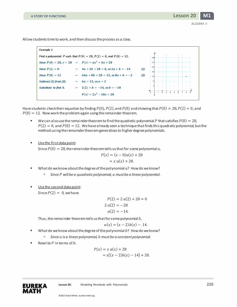
Lesson 20: Modeling Riverbeds with Polynomials
M1 Lesson 20 ALGEBRA II
Allow students time to work, and then discuss the process as a class.
Example 1
Find a polynomial such that ( ) = , ( ) = , and ( ) = .
Since ( ) = , = ( ) = + +
Since ( ) = + + = , so + = − (1)
Since ( ) = + + = , so + = − (2)
Subtract (1) from (2). = , so =
Substitute to find . ( ) + = − , so = −
( ) = − +
Have students check their equation by finding 𝑃𝑃(0), 𝑃𝑃(2), and 𝑃𝑃(8) and showing that 𝑃𝑃(0) = 28, 𝑃𝑃(2) = 0, and 𝑃𝑃(8) = 12. Now work the problem again using the remainder theorem.
� We can also use the remainder theorem to find the quadratic polynomial 𝑃𝑃 that satisfies 𝑃𝑃(0) = 28, 𝑃𝑃(2) = 0, and 𝑃𝑃(8) = 12. We have already seen a technique that finds this quadratic polynomial, but the method using the remainder theorem generalizes to higher degree polynomials.
� Use the first data point: Since 𝑃𝑃(0) = 28, the remainder theorem tells us that for some polynomial 𝑎𝑎,
𝑃𝑃(𝑥𝑥) = (𝑥𝑥 − 0)𝑎𝑎(𝑥𝑥) + 28 = 𝑥𝑥 𝑎𝑎(𝑥𝑥) + 28.
� What do we know about the degree of the polynomial 𝑎𝑎? How do we know? à Since 𝑃𝑃 will be a quadratic polynomial, 𝑎𝑎 must be a linear polynomial.
� Use the second data point:
Since 𝑃𝑃(2) = 0, we have 𝑃𝑃(2) = 2 𝑎𝑎(2) + 28 = 0
2 𝑎𝑎(2) = −28 𝑎𝑎(2) = −14.
Thus, the remainder theorem tells us that for some polynomial 𝑏𝑏, 𝑎𝑎(𝑥𝑥) = (𝑥𝑥 − 2)𝑏𝑏(𝑥𝑥)− 14.
� What do we know about the degree of the polynomial 𝑏𝑏? How do we know? à Since 𝑎𝑎 is a linear polynomial, 𝑏𝑏 must be a constant polynomial.
� Rewrite 𝑃𝑃 in terms of 𝑏𝑏: 𝑃𝑃(𝑥𝑥) = 𝑥𝑥 𝑎𝑎(𝑥𝑥) + 28
= 𝑥𝑥[(𝑥𝑥 − 2)𝑏𝑏(𝑥𝑥)− 14] + 28.
A STORY OF FUNCTIONS
220
©2015 Great Minds. eureka-math.org

Lesson 20: Modeling Riverbeds with Polynomials
M1 Lesson 20 ALGEBRA II
� Use the third data point: Since 𝑃𝑃(8) = 12, we have
𝑃𝑃(8) = 8[(8− 2)𝑏𝑏(𝑥𝑥)− 14] + 28 = 12 48𝑏𝑏(𝑥𝑥)− 104 + 28 = 12
48𝑏𝑏(𝑥𝑥) = 96 𝑏𝑏(𝑥𝑥) = 2.
� Remember that we said the function 𝑏𝑏(𝑥𝑥) would be constant, and we found that 𝑏𝑏(𝑥𝑥) = 2 for all values of 𝑥𝑥. � Now we can rewrite the function 𝑃𝑃:
𝑃𝑃(𝑥𝑥) = 𝑥𝑥[(𝑥𝑥− 2)𝑏𝑏(𝑥𝑥)− 14] + 28 = 𝑥𝑥[(𝑥𝑥− 2)2 − 14] + 28.
� Do the three points satisfy this equation? à 𝑃𝑃(0) = 0[(0− 2) 2− 14] + 28 = 28 9 à 𝑃𝑃(2) = 2[(2− 2) 2− 14] + 28 = 0 9 à 𝑃𝑃(8) = 8[(8− 2) 2− 14] + 28 = 12 9
� For a final check, write the polynomial we just found in standard form. 𝑃𝑃(𝑥𝑥) = 𝑥𝑥[(𝑥𝑥− 2)2 − 14] + 28
= 2𝑥𝑥2 − 18𝑥𝑥 − 28.
� What if we wanted to fit a polynomial function to two data points? What is the lowest degree of a polynomial that fits two data points? à We know from geometry that two points determine a unique line, so a polynomial of degree one fits
two data points.
� In the next example, we fit a polynomial to four data points. What is the lowest degree of a polynomial that fits four data points?
à Since two data points can be fit by a degree 1 polynomial, and three data points can be fit by a degree 2 polynomial, it makes sense that four data points can be fit by a degree 3 polynomial.
Example 2 (15 minutes)
The table below helps students organize their work as they proceed to find the cubic polynomial that fits four data points. Work through the first l ine of the table with students, and then have students work in groups to complete the table to determine the equation of the polynomial 𝑃𝑃. Point out to students that this would be a difficult task if we used systems of equations as we did first in Example 1. Have students present their work on the board.
A STORY OF FUNCTIONS
221
©2015 Great Minds. eureka-math.org

Lesson 20: Modeling Riverbeds with Polynomials
M1 Lesson 20 ALGEBRA II
Example 2
Find a degree polynomial such that (− ) = − , ( ) = − , ( ) = − , and ( ) = .
Function Value
Substitute the data point into the current form of the equation for .
Apply the remainder theorem to , , or .
Rewrite the equation for in terms of , , or .
(− ) = − ( ) = ( + ) ( )−
( ) = − ( + ) ( )− = − ( ) = ( ) + ( ) = ( + )( ( ) + )−
( ) = − ( + )( ( ) + )− = − ( ) = ( − ) ( ) ( ) = ( + )( ( − ) ( ) + )−
( ) = ( + )( ( − ) ( ) + )− = ( ) = ( ) = ( + )( ( − ) + )−
� Write the polynomial 𝑃𝑃 in standard form. à 𝑃𝑃(𝑥𝑥) = (𝑥𝑥 + 1)(𝑥𝑥2 − 𝑥𝑥 + 1)− 3 à 𝑃𝑃(𝑥𝑥) = 𝑥𝑥3− 𝑥𝑥2+ 𝑥𝑥 + 𝑥𝑥2 − 𝑥𝑥 + 1 − 3 à 𝑃𝑃(𝑥𝑥) = 𝑥𝑥3− 2
� Verify that 𝑃𝑃 satisfies the four given constraints. à 𝑃𝑃(−1) = (−1)3− 2 = −3 à 𝑃𝑃(0) = 03 − 2 = −2 à 𝑃𝑃(1) = 13 − 2 = −1 à 𝑃𝑃(2) = 23 − 2 = 6
Closing (5 minutes)
� What methods have we used to find polynomial functions that fit given data?
à We plugged in data values to obtain a system of equations and used the remainder theorem. In previous lessons, we used the graphing calculator.
� If we want a polynomial to perfectly fit data points, how does the degree of the polynomial relate to the number of data points?
à The degree of the polynomial whose graph passes through a set of data points is one less than the number of data points.
Ask students to summarize the important parts of the lesson in writing, to a partner, or as a class. Use this as an opportunity to informally assess understanding of the lesson. The following are some important summary elements.
Exit Ticket (6 minutes)
MP.7
Lesson Summary
A linear polynomial is determined by points on its graph. A degree polynomial is determined by points on its graph. A degree polynomial is determined by points on its graph. A degree polynomial is determined by points on its graph. The remainder theorem can be used to find a polynomial whose graph will pass through a given set of points.
A STORY OF FUNCTIONS
222
©2015 Great Minds. eureka-math.org

Lesson 20: Modeling Riverbeds with Polynomials
M1 Lesson 20 ALGEBRA II
Name Date
Lesson 20: Modeling Riverbeds with Polynomials
Exit Ticket Use the remainder theorem to find a quadratic polynomial 𝑃𝑃 so that 𝑃𝑃(1) = 5, 𝑃𝑃(2) = 12, and 𝑃𝑃(3) = 25. Give your answer in standard form.
A STORY OF FUNCTIONS
223
©2015 Great Minds. eureka-math.org

Lesson 20: Modeling Riverbeds with Polynomials
M1 Lesson 20 ALGEBRA II
Exit Ticket Sample Solutions
Use the remainder theorem to find a quadratic polynomial so that ( ) = , ( ) = , and ( ) = . GIve your answer in standard form.
Since ( ) = , there is a linear polynomial so that ( ) = ( − ) ( ) + .
Since ( ) = , we have ( ) = ( − ) ( ) + = , so ( ) = .
Because ( ) = , there exists a constant so that ( ) = ( − ) + .
Substituting into ( ) gives ( ) = ( − )[( − ) + ].
Since ( ) = , we have ( ) = ( − )[( − ) + ] = . Solving for gives = .
It follows that ( ) = ( − )[( − ) + ], and in standard form we have ( ) = − + .
Problem Set Sample Solutions
1. Suppose a polynomial function is such that ( ) = and ( ) = . a. What is the largest-degree polynomial that can be uniquely determined given the information?
Degree one
b. Is this the only polynomial that satisfies ( ) = and ( ) = ?
No, there are an infinite number of polynomials that pass through those two points. However, two points will determine a unique equation for a linear function.
c. Use the remainder theorem to find the polynomial of least degree that satisfies the two points given.
( ) = −
d. Verify that your equation is correct by demonstrating that it satisfies the given points.
( ) = ( )− =
( ) = ( )− =
2. Write a quadratic function such that ( ) = − , ( ) = , and ( ) = using the specified method.
a. Setting up a system of equations
( ) = − −
b. Using the remainder theorem
( ) = − −
A STORY OF FUNCTIONS
224
©2015 Great Minds. eureka-math.org

Lesson 20: Modeling Riverbeds with Polynomials
M1 Lesson 20 ALGEBRA II
3. Find a degree-three polynomial function such that (− ) = , ( ) = , ( ) = , and ( ) = . Use the table below to organize your work. Write your answer in standard form, and verify by showing that each point satisfies the equation.
Function Value
Substitute the data point into the current form of
the equation for .
Apply the remainder theorem to , , or .
Rewrite the equation for in terms of , , or .
(− ) =
( ) = ( + ) ( )
( ) = ( ) = ( ) = ( ) + ( ) = ( + )( ( ) + )
( ) = ( ( )) + ) =
( ) = ( ) = ( − ) ( ) + ( ) = ( + )[ [( − ) ( ) + ] + ]
( ) =
[ ( ( ) + )] + = ( ) =
( ) = ( ) = ( + )[ [( − ) + ] + ]
( ) = + +
(− ) = − − + = 9 ( ) = + + = 9 ( ) = + + = 9 ( ) = + + = 9
4. The method used in Problem is based on the Lagrange interpolation method. Research Joseph-Louis Lagrange,
and write a paragraph about his mathematical work.
Answers will vary.
A STORY OF FUNCTIONS
225
©2015 Great Minds. eureka-math.org

Lesson 21: Modeling Riverbeds with Polynomials
M1 Lesson 21 ALGEBRA II
Lesson 21: Modeling Riverbeds with Polynomials
Student Outcomes
� Students model a cross-section of a riverbed with a polynomial function and estimate fluid flow with their algebraic model.
Lesson Notes This is the second half of a two-day modeling lesson. In previous modeling lessons, students relied on the graphing calculator to find polynomial functions that fit a set of data, and in the previous lesson the polynomial was found algebraically. In this lesson, we use the website Wolfram Alpha (www.wolframalpha.com) to find the polynomial to fit the data. If students do not have access to computers or the Internet during class, the polynomial can be found using quartic regression on a graphing calculator.
The previous lesson introduced the problem of modeling the shape of a riverbed and computing the volumetric flow. In this lesson, students can actually do the modeling, with the help of technology, and then interpret the results and create a report detailing their findings, thus completing the modeling cycle.
Classwork Opening (3 minutes)
Review the Mathematical Modeling Exercise with students. In this lesson, students:
1. Find a function that models the shape of the riverbed based on the five data points given in the graph below. 2. Approximate the area of the cross-sectional region using triangles and trapezoids. 3. Calculate the volumetric flow rate of the water in gallons per minute. 4. Create a report of the findings.
A STORY OF FUNCTIONS
226
©2015 Great Minds. eureka-math.org

Lesson 21: Modeling Riverbeds with Polynomials
M1 Lesson 21 ALGEBRA II
Mathematical Modeling Exercise
The Environmental Protection Agency (EPA) is studying the flow of a river in order to establish flood zones. The EPA hired a surveying company to determine the flow rate of the river, measured as volume of water per minute. The firm set up a coordinate system and found the depths of the river at five locations as shown on the graph below. After studying the data, the firm decided to model the riverbed with a polynomial function and divide the area into six regions that are either trapezoidal or triangular so that the overall area can be easily estimated. The firm needs to approximate the depth of the river at two more data points in order to do this.
Mathematical Modeling Exercises 1–5 (32 minutes)
Now return to the Mathematical Modeling Exercise.
� How many data points are we given? What is the lowest degree of a polynomial that passes through these points?
à We were given five data points, so we can model the data using a fourth-degree polynomial function.
� We are going to use Wolfram Alpha to find the fourth-degree polynomial that fits the data. It follows a procedure based on the remainder theorem that we used in the previous two examples to find the equation.
Go to www.wolframalpha.com. Type in the following command:
Interpolating polynomial [{(0,0),(20,−20),(60,−15),(100,−25),(120,0)},𝑥𝑥].
Students can find 𝑃𝑃(40) and 𝑃𝑃(80) either by substituting into the function displayed or by editing the command on Wolfram Alpha as follows:
Interpolating polynomial [{(0,0),(20,−20),(60,−15),(100,−25),(120,0)},40] Interpolating polynomial [{(0,0),(20,−20),(60,−15),(100,−25),(120,0)},80].
Allow students time to work through the remainder of the exercise either individually or in groups. The conversion from cubic feet per minute to gallons per minute can also be done using Wolfram Alpha.
Scaffolding:
If students are overwhelmed with the new technology along with new content, most graphing calculators perform polynomial regression up to degree 4, so consider having students use that more familiar technological tool.
MP.5
A STORY OF FUNCTIONS
227
©2015 Great Minds. eureka-math.org

Lesson 21: Modeling Riverbeds with Polynomials
M1 Lesson 21 ALGEBRA II
1. Find a polynomial that fits the five given data points.
( ) = − + −
2. Use the polynomial to estimate the depth of the river at = and = .
( ) = − and ( ) = −
3. Estimate the area of the cross section.
= + + + + +
= + + + + + = ,
Suppose that the river flow speed was measured to be an average speed of . at the cross section.
4. What is the volumetric flow of the water (the volume of water per minute)?
( , ).
= ,
5. Convert the flow to gallons per minute. [Note: cubic foot . gallons.]
, ,
� How could the surveyors measure the speed of the water? à They could time an object (like a ball) floating over a set distance.
� What factors would need to be considered when measuring the flow?
à Water may flow faster below the surface. The flow rate may vary from the edge of the river to the middle of the river and around obstacles such as rocks.
� Remember that the EPA is interested in identifying flood-prone areas. How might the information you have gathered help the EPA?
à If the normal volumetric flow of the river has been recorded by the EPA, then they can record the normal water levels in the river and use that knowledge to predict what level of volumetric flow would result in flooding. In cases of heavy rain, the EPA could identify if an area is likely to flood due to the increased volumetric flow.
A STORY OF FUNCTIONS
228
©2015 Great Minds. eureka-math.org

Lesson 21: Modeling Riverbeds with Polynomials
M1 Lesson 21 ALGEBRA II
Closing (5 minutes)
Ask students to summarize the important parts of the lesson in writing, to a partner, or as a class. Use this as an opportunity to informally assess understanding of the lesson.
Exit Ticket (5 minutes)
A STORY OF FUNCTIONS
229
©2015 Great Minds. eureka-math.org

Lesson 21: Modeling Riverbeds with Polynomials
M1 Lesson 21 ALGEBRA II
Name Date
Lesson 21: Modeling Riverbeds with Polynomials
Exit Ticket Explain the process you used to estimate the volumetric flow of the river, from accumulating the data to calculating the flow of water.
A STORY OF FUNCTIONS
230
©2015 Great Minds. eureka-math.org

Lesson 21: Modeling Riverbeds with Polynomials
M1 Lesson 21 ALGEBRA II
Exit Ticket Sample Solutions
Explain the process you used to estimate the volumetric flow of the river, from accumulating the data to calculating the flow of water.
We were given data points that represented the depth of the river at various points in the cross-section. We used Wolfram Alpha to find a polynomial that passed through those given points. We used the polynomial to find more data points. Then we approximated the area of the cross-section using triangles and trapezoids; figures whose area we know how to calculate. Once we had an approximate area of the cross-section, we multiplied that area by the speed of the water across the cross-section to find the amount of volumetric flow in units of cubic feet per minute. The last step was to convert cubic feet to gallons to get the amount of volumetric flow in units of gallons per minute.
Problem Set Sample Solutions Problem 2 requires the use of a computer. This could be completed in class if students do not have access to computers.
1. As the leader of the surveying team, write a short report to the EPA on your findings from the in-class exercises. Be sure to include data and calculations.
After collecting data at the site, we decided that the cross-sectional area could be approximated using trapezoids. In order to increase the accuracy of our area approximation, more data points were needed. We chose to use the data collected to model the riverbed using a degree polynomial function. We used the computational knowledge engine Wolfram Alpha to find the polynomial that fit the data, which is ( ) = − +
− . Using the polynomial , we were able to estimate enough data points to calculate the cross-sectional area and determined that it was , . Using this information and the average speed of the water at
the cross-section, which was .
, we were able to compute the volumetric flow of the river at that cross-section.
We determined that the volumetric flow is approximately , , which is , , .
2. Suppose that depths of the riverbed were measured for a different cross-section of the river.
a. Use Wolfram Alpha to find the interpolating polynomial with values: ( ) = , ( . ) = − . , ( . ) = − . , ( . ) = − . ,
( . ) = − . , ( . ) = − . , ( ) = .
( ) = − + − + −
A STORY OF FUNCTIONS
231
©2015 Great Minds. eureka-math.org

Lesson 21: Modeling Riverbeds with Polynomials
M1 Lesson 21 ALGEBRA II
b. Sketch the cross-section of the river, and estimate its area.
Area estimates:
= ( . )( . ) = .
= ( . + . )( . − . ) = .
= ( . + . )( . − . ) = .
= ( . + . )( . − . ) = .
= ( . + . )( . − . ) = .
= ( . )( . − . ) = .
So, the total area can be estimated by
= + + + + + = . .
c. Suppose that the speed of the water was measured at . . What is the approximate volumetric flow in this section of the river, measured in gallons per minute?
The volumetric flow is approximately . � . � , . Converting to gallons per minute, this is
. / .
A STORY OF FUNCTIONS
232
©2015 Great Minds. eureka-math.org
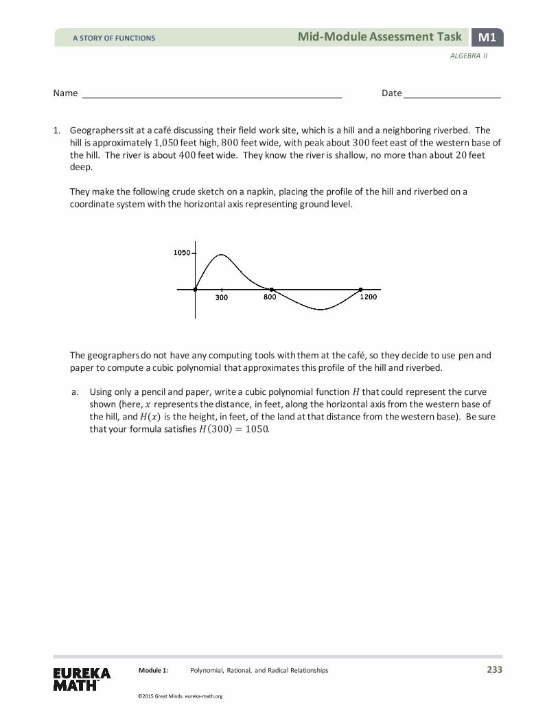
M1 Mid-Module Assessment Task ALGEBRA II
Module 1: Polynomial, Rational, and Radical Relationships
Name Date
1. Geographers sit at a café discussing their field work site, which is a hill and a neighboring riverbed. The hill is approximately 1,050 feet high, 800 feet wide, with peak about 300 feet east of the western base of the hill. The river is about 400 feet wide. They know the river is shallow, no more than about 20 feet deep. They make the following crude sketch on a napkin, placing the profile of the hill and riverbed on a coordinate system with the horizontal axis representing ground level.
The geographers do not have any computing tools with them at the café, so they decide to use pen and paper to compute a cubic polynomial that approximates this profile of the hill and riverbed. a. Using only a pencil and paper, write a cubic polynomial function that could represent the curve
shown (here, 𝑥𝑥 represents the distance, in feet, along the horizontal axis from the western base of the hill, and (𝑥𝑥) is the height, in feet, of the land at that distance from the western base). Be sure that your formula satisfies (300) = 1050.
A STORY OF FUNCTIONS
233
©2015 Great Minds. eureka-math.org

M1 Mid-Module Assessment Task ALGEBRA II
Module 1: Polynomial, Rational, and Radical Relationships
b. For the sake of convenience, the geographers make the assumption that the deepest point of the river is halfway across the river (recall that the river is no more than 20 feet deep). Under this assumption, would a cubic polynomial provide a suitable model for this hill and riverbed? Explain.
2. Luke notices that by taking any three consecutive integers, multiplying them together, and adding the middle number to the result, the answer always seems to be the middle number cubed. For example: 3 4 5 + 4 = 64 = 43 4 5 6 + 5 = 125 = 53 9 10 11 + 10 = 1000 = 103 a. To prove his observation, Luke writes ( + 1)( + 2)( + 3) + ( + 2). What answer is he hoping
to show this expression equals? b. Lulu, upon hearing of Luke’s observation, writes her own version with as the middle number.
What does her formula look like?
A STORY OF FUNCTIONS
234
©2015 Great Minds. eureka-math.org

M1 Mid-Module Assessment Task ALGEBRA II
Module 1: Polynomial, Rational, and Radical Relationships
c. Use Lulu’s expression to prove that adding the middle number to the product of any three consecutive numbers is sure to equal that middle number cubed.
3. A cookie company packages its cookies in rectangular prism boxes designed with square bases that have both a length and width of 4 inches less than the height of the box.
a. Write a polynomial that represents the volume of a box with height 𝑥𝑥 inches. b. Find the dimensions of the box if its volume is 128 cubic inches.
A STORY OF FUNCTIONS
235
©2015 Great Minds. eureka-math.org

M1 Mid-Module Assessment Task ALGEBRA II
Module 1: Polynomial, Rational, and Radical Relationships
c. After solving this problem, Juan was very clever and invented the following strange question: A building, in the shape of a rectangular prism with a square base, has on its top a radio tower. The building is 25 times as tall as the tower, and the side-length of the base of the building is 100 feet less than the height of the building. If the building has a volume of 2 million cubic feet, how tall is the tower?
Solve Juan’s problem.
A STORY OF FUNCTIONS
236
©2015 Great Minds. eureka-math.org

M1 Mid-Module Assessment Task ALGEBRA II
Module 1: Polynomial, Rational, and Radical Relationships
A Progression Toward Mastery
Assessment Task Item
STEP 1 Missing or incorrect answer and little evidence of reasoning or application of mathematics to solve the problem.
STEP 2 Missing or incorrect answer but evidence of some reasoning or application of mathematics to solve the problem.
STEP 3 A correct answer with some evidence of reasoning or application of mathematics to solve the problem OR an incorrect answer with substantial evidence of solid reasoning or application of mathematics to solve the problem.
STEP 4 A correct answer supported by substantial evidence of solid reasoning or application of mathematics to solve the problem.
1
a
N-Q.A.2 A-APR.B.2 A-APR.B.3 F-IF.C.7c
Student identifies zeros on the graph.
Student uses zeros to write a factored cubic polynomial for (𝑥𝑥) without a leading coefficient.
Student uses given condition (300) =1050 to find 𝑎𝑎-value (leading coefficient).
Student writes a complete cubic model for (𝑥𝑥) in factored form with correct 𝑎𝑎-value (leading coefficient).
b
N-Q.A.2 A-APR.B.2 A-APR.B.3 F-IF.C.7c
Student finds the mid-point of the river.
Student evaluates (𝑥𝑥) using the midpoint. The exact answer is not needed, only an approximation.
Student determines if a cubic model is suitable for this hill and riverbed.
Student justifies the answer using
(midpoint) in the explanation.
2 a
A-SSE.A.2 A-APR.C.4
Student does not indicate any expression involving raised to an exponent of 3.
Student uses a base involving being raised to an exponent of 3 in the answer but does not choose a base of ( + 2).
Student writes ( + 2)3 without including parentheses to indicate all of ( + 2) is being cubed (i.e., + 23). OR Student makes another error that shows general understanding but is technically incorrect.
Student writes the correct answer, ( + 2)3.
A STORY OF FUNCTIONS
237
©2015 Great Minds. eureka-math.org

M1 Mid-Module Assessment Task ALGEBRA II
Module 1: Polynomial, Rational, and Radical Relationships
b–c
A-SSE.A.2 A-APR.C.4
Student does not answer parts (b)–(c). OR Student provides incorrect or incomplete answers.
Student answers part (b) incorrectly but uses correct algebra in showing equivalence to 3.
OR Student answers part (b) correctly but makes major errors or is unable to show its equivalence to 3.
Student answers part (b) correctly as ( − 1)( )( + 1) +
= 3 but makes minor errors in showing equivalence to 3.
Student answers correctly as ( − 1)( )( + 1) +
= 3 and correctly multiplies the left side and then combines like terms to show equivalence to 3.
3
a–d
N-Q.A.2 A-SSE.A.2 A-APR.B.2 A-APR.B.3 A-REI.A.1
A-REI.B.4b
Student determines an expression for 𝑉𝑉(𝑥𝑥).
Student sets 𝑉𝑉(𝑥𝑥) equal to the given volume.
Student solves the equation understanding that only real values are possible solutions for the dimensions of a box.
Student states the three dimensions of the box with proper units.
c
N-Q.A.2 A-SSE.A.2 A-APR.B.2 A-APR.B.3 A-REI.A.1
A-REI.B.4b
Student determines an expression for 𝑉𝑉(ℎ) and sets it equal to the given volume but does not solve the equation.
Student writes the equation as a polynomial equation but is unable to find any solutions to the equation.
Student finds one solution to the equation but is unable to use it to factor the polynomial expression to find the other potential solutions. OR Student recognizes the simplified equation as the same as the equation in the previous part and states the solution from the previous part immediately (but as the real number 8, not as a height measurement 8 feet).
Student finds the solutions to the equation, determines which solution is valid, and states the correct answer as the height measurement 8 feet. OR Student recognizes the simplified equation as the same as the equation in the previous part and states the solution from the previous part immediately using the correct units (i.e., 8 feet).
A STORY OF FUNCTIONS
238
©2015 Great Minds. eureka-math.org

M1 Mid-Module Assessment Task ALGEBRA II
Module 1: Polynomial, Rational, and Radical Relationships
Name Date
1. Geographers sit at a café discussing their field work site, which is a hill and a neighboring riverbed. The hill is approximately 1,050 feet high, 800 feet wide, with peak about 300 feet east of the western base of the hill. The river is about 400 feet wide. They know the river is shallow, no more than about 20 feet deep. They make the following crude sketch on a napkin, placing the profile of the hill and riverbed on a coordinate system with the horizontal axis representing ground level.
The geographers do not have any computing tools with them at the café, so they decide to use pen and paper to compute a cubic polynomial that approximates this profile of the hill and riverbed. a. Using only a pencil and paper, write a cubic polynomial function that could represent the curve
shown (here, 𝑥𝑥 represents the distance, in feet, along the horizontal axis from the western base of the hill, and (𝑥𝑥) is the height, in feet, of the land at that distance from the western base). Be sure that your formula satisfies (300) = 1050.
A STORY OF FUNCTIONS
239
©2015 Great Minds. eureka-math.org

M1 Mid-Module Assessment Task ALGEBRA II
Module 1: Polynomial, Rational, and Radical Relationships
b. For the sake of convenience, the geographers make the assumption that the deepest point of the river is halfway across the river (recall that the river is no more than 20 feet deep). Under this assumption, would a cubic polynomial provide a suitable model for this hill and riverbed? Explain.
2. Luke notices that by taking any three consecutive integers, multiplying them together, and adding the
middle number to the result, the answer always seems to be the middle number cubed. For example: 3 4 5 + 4 = 64 = 43 4 5 6 + 5 = 125 = 53
9 10 11 + 10 = 1000 = 103 a. To prove his observation, Luke writes ( + 1)( + 2)( + 3) + ( + 2). What answer is he hoping
to show this expression equals?
b. Lulu, upon hearing of Luke’s observation, writes her own version with as the middle number.
What does her formula look like?
A STORY OF FUNCTIONS
240
©2015 Great Minds. eureka-math.org

M1 Mid-Module Assessment Task ALGEBRA II
Module 1: Polynomial, Rational, and Radical Relationships
c. Use Lulu’s expression to prove that adding the middle number to the product of any three consecutive numbers is sure to equal that middle number cubed.
3. A cookie company packages its cookies in rectangular prism boxes designed with square bases that have
both a length and width of 4 inches less than the height of the box. a. Write a polynomial that represents the volume of a box with height 𝑥𝑥 inches.
b. Find the dimensions of the box if its volume is 128 cubic inches.
A STORY OF FUNCTIONS
241
©2015 Great Minds. eureka-math.org

M1 Mid-Module Assessment Task ALGEBRA II
Module 1: Polynomial, Rational, and Radical Relationships
c. After solving this problem, Juan was very clever and invented the following strange question: A building, in the shape of a rectangular prism with a square base, has on its top a radio tower. The building is 25 times as tall as the tower, and the side-length of the base of the building is 100 feet less than the height of the building. If the building has a volume of 2 million cubic feet, how tall is the tower?
Solve Juan’s problem.
A STORY OF FUNCTIONS
242
©2015 Great Minds. eureka-math.org
Mathematics Curriculum ALGEBRA II • MODULE 1
Topic C: Solving and Applying Equations—Polynomial, Rational, and Radical
Topic C
Solving and Applying Equations—Polynomial, Rational, and Radical
A-APR.D.6, A-REI.A.1, A-REI.A.2, A-REI.B.4b, A-REI.C.6, A-REI.C.7, G-GPE.A.2
Focus Standards: A-APR.D.6 Rewrite simple rational expressions in different forms; write 𝑎𝑎(𝑥𝑥)/𝑏𝑏(𝑥𝑥) in the form 𝑞𝑞(𝑥𝑥) + 𝑟𝑟(𝑥𝑥)/𝑏𝑏(𝑥𝑥), where 𝑎𝑎(𝑥𝑥), 𝑏𝑏(𝑥𝑥), 𝑞𝑞(𝑥𝑥), and 𝑟𝑟(𝑥𝑥) are polynomials with the degree of 𝑟𝑟(𝑥𝑥) less than the degree of 𝑏𝑏(𝑥𝑥), using inspection, long division, or, for the more complicated examples, a computer algebra system.
A-REI.A.1 Explain each step in solving a simple equation as following from the equality of numbers asserted at the previous step, starting from the assumption that the original equation has a solution. Construct a viable argument to justify a solution method.
A-REI.A.2 Solve simple rational and radical equations in one variable, and give examples showing how extraneous solutions may arise.
A-REI.B.4 Solve quadratic equations in one variable. b. Solve quadratic equations by inspection (e.g., for 𝑥𝑥2 = 49), taking square roots,
completing the square, the quadratic formula and factoring, as appropriate to the initial form of the equation. Recognize when the quadratic formula gives complex solutions and write them as 𝑎𝑎 ± 𝑏𝑏𝑖𝑖 for real numbers 𝑎𝑎 and 𝑏𝑏.
A-REI.C.6 Solve systems of linear equations exactly and approximately (e.g., with graphs), focusing on pairs of linear equations in two variables.
A-REI.C.7 Solve a simple system consisting of a linear equation and a quadratic equation in two variables algebraically and graphically. For example, find the points of intersection between the line 𝑦𝑦 = −3𝑥𝑥 and the circle 𝑥𝑥2+ 𝑦𝑦2 = 3.
G-GPE.A.2 Derive the equation of a parabola given a focus and directrix.
Instructional Days: 14
Lesson 22: Equivalent Rational Expressions (S)1
Lesson 23: Comparing Rational Expressions (S)
Lesson 24: Multiplying and Dividing Rational Expressions (P)
Lesson 25: Adding and Subtracting Rational Expressions (P)
1Lesson Structure Key: P-Problem Set Lesson, M-Modeling Cycle Lesson, E-Exploration Lesson, S-Socratic Lesson
A STORY OF FUNCTIONS
243
©2015 Great Minds. eureka-math.org

M1 Topic C ALGEBRA II
Topic C: Solving and Applying Equations—Polynomial, Rational, and Radical
Lesson 26: Solving Rational Equations (P)
Lesson 27: Word Problems Leading to Rational Equations (P)
Lesson 28: A Focus on Square Roots (P)
Lesson 29: Solving Radical Equations (P)
Lesson 30: Linear Systems in Three Variables (P)
Lesson 31: Systems of Equations (E)
Lesson 32: Graphing Systems of Equations (S)
Lesson 33: The Definition of a Parabola (S)
Lesson 34: Are All Parabolas Congruent? (P)
Lesson 35: Are All Parabolas Similar? (S)
In Topic C, students continue to build upon the reasoning used to solve equations and their fluency in factoring polynomial expressions. In Lesson 22, students expand their understanding of the division of polynomial expressions to rewriting simple rational expressions (A-APR.D.6) in equivalent forms. In Lesson 23, students learn techniques for comparing rational expressions numerically, graphically, and algebraically. In Lessons 24–25, students learn to rewrite simple rational expressions by multiplying, dividing, adding, or subtracting two or more expressions. They begin to connect operations with rational numbers to operations on rational expressions. The practice of rewriting rational expressions in equivalent forms in Lessons 22–25 is carried over to solving rational equations in Lessons 26 and 27. Lesson 27 also includes working with word problems that require the use of rational equations. Lessons 28–29 turn to radical equations. Students learn to look for extraneous solutions to these equations as they did for rational equations.
In Lessons 30–32, students solve and graph systems of equations including systems of one linear equation and one quadratic equation and systems of two quadratic equations. Next, in Lessons 33–35, students study the definition of a parabola as they first learn to derive the equation of a parabola given a focus and a directrix and later to create the equation of the parabola in vertex form from the coordinates of the vertex and the location of either the focus or directrix. Students build upon their understanding of rotations and translations from Geometry as they learn that any given parabola is congruent to the one given by the equation 𝑦𝑦 = 𝑎𝑎𝑥𝑥2 for some value of 𝑎𝑎, and that all parabolas are similar.
A STORY OF FUNCTIONS
244
©2015 Great Minds. eureka-math.org
M1 Lesson 22 ALGEBRA II
Lesson 22: Equivalent Rational Expressions
Lesson 22: Equivalent Rational Expressions
Student Outcomes
� Students define rational expressions and write them in equivalent forms.
Lesson Notes In this module, students have been working with polynomial expressions and polynomial functions. In elementary school, students mastered arithmetic operations with integers before advancing to performing arithmetic operations with rational numbers. Just as a rational number is built from integers, a rational expression is built from polynomial expressions. A precise definition of a rational expression is included at the end of the lesson.
Informally, a rational expression is any expression that is made by a finite sequence of addition, subtraction, multiplication, and division operations on polynomials. After algebraic manipulation, a rational expression can always be
written as , where 𝑃𝑃 is any polynomial, and is any polynomial except the zero polynomial. Remember that constants,
such as 2, and variables, such as 𝑥𝑥, count as polynomials, so the rational numbers are also considered to be rational expressions. Standard A-APR.C.6 focuses on rewriting rational expressions in equivalent forms, and the next three
lessons apply that standard to write complicated rational expressions in the simplified form . However, the prompt
simplify the rational expression does not only mean putting expressions in the form but also any form that is conducive
to solving the problem at hand. The skills developed in Lessons 22–25 are necessary prerequisites for addressing standard A-REI.A.2, solving rational equations, which is the focus of Lessons 26 and 27.
Classwork Opening Exercise (8 minutes)
The Opening Exercise serves two purposes: (1) to reactivate prior knowledge of equivalent fractions, and (2) as a review for students who struggle with fractions. The goal is for students to see that the process they use to reduce a fraction to lowest terms is the same process they will use to reduce a rational expression to lowest terms. To begin, pass out 2–3 notecard-sized slips of paper to each student or pair of students.
� We are going to start with a review of how to visualize equivalent fractions. Opening Exercise
On your own or with a partner, write two fractions that are equivalent to , and use the slips of paper to create visual
models to justify your response.
A STORY OF FUNCTIONS
245
©2015 Great Minds. eureka-math.org

M1 Lesson 22 ALGEBRA II
Lesson 22: Equivalent Rational Expressions
Use the following to either walk through the exercise for scaffolding or as an example of l ikely student responses.
� We can use the following area model to represent the fraction 13
. Because the three boxes have the same
area, shading one of the three boxes shows that 13
of the area in the figure is shaded.
� Now, if we draw a horizontal l ine dividing the columns in half, we have six
congruent rectangles, two of which are shaded so that 2
of the area in the figure
is shaded.
� In the figure below, we have now divided the original rectangle into nine
congruent sub-rectangles, three of which are shaded so that 3
of the area in the
figure is shaded.
� Let’s suppose that the area of the original rectangle is 1. In walking the class through the example, point out
that the shaded area in the first figure is 13
, the shaded area in the second figure is 2
, and the shaded area in
the third figure is 3
. Since the area of the shaded regions are the same in all three figures, we see that 13
=2
=3
. Thus, 13
, 2
, and 3
are equivalent fractions.
If students come up with different equivalent fractions, then incorporate those into the discussion of equivalent areas, noting that the shaded regions are the same for every student.
� Now, what if we were to choose any positive integer and draw lines across our figure so that the columns are divided into pieces of the same size? What is the area of the shaded region?
Scaffolding: Students who are already comfortable with fractions can instead reduce the following rational expressions to lowest terms.
1, 23
, √
,
In any case, do not spend too much time on these exercises; instead, use them as a bridge to reducing rational expressions that contain variables.
MP.8
A STORY OF FUNCTIONS
246
©2015 Great Minds. eureka-math.org

M1 Lesson 22 ALGEBRA II
Lesson 22: Equivalent Rational Expressions
If 𝑎𝑎, 𝑏𝑏, and are integers with 0 and 𝑏𝑏 0, then 𝑎𝑎𝑏𝑏
=𝑎𝑎𝑏𝑏
.
Give students time to think and write, and ask them to share their answers with a partner. Anticipate that students will
express the generalization in words or suggest either 13
or 𝑛𝑛3𝑛𝑛
. Both are correct and, ideally, both will be suggested.
� Thus, we have the rule:
The result summarized in the box above is also true for real numbers 𝑎𝑎, 𝑏𝑏, and , as well as for polynomial and rational expressions.
� Then 2
=2(1)2(3)
=13
and 3
=3(1)3(3)
=13
.
� We say that a rational number is simplified, or reduced to lowest terms, when the numerator and denominator
do not have a factor in common. Thus, while 13
, 2
, and 3
are equivalent, only 13
is in lowest terms.
Discussion (10 minutes)
� Which of the following are rational numbers, and which are not?
34
, 3.14, ,50
,−√17,23,1 +√5
2,−1,6.022 × 1023, 0
� Rational: 34
, 3.14, 23,−1, 6.022 × 10²³, 0
� Not rational: , 50 ,−√17, 1+ 5
2
� Of the numbers that were not rational, were they all irrational numbers?
à No. Since division by zero is undefined, 0
is neither rational nor
irrational.
� Today we learn about rational expressions, which are related to the polynomials we've been studying. Just as the integers are the foundational building blocks of rational numbers, polynomial expressions are the foundational building blocks for rational expressions. Based on what we know about rational numbers, give an example of what you think a rational expression is.
Ask students to write down an example and share it with their partner or small group. Allow groups to debate and present one of the group’s examples to the class.
Scaffolding: Students may also express the generalization in words.
Scaffolding: Relate the new ideas of rational expressions back to the more familiar ideas of rational numbers throughout this lesson.
A STORY OF FUNCTIONS
247
©2015 Great Minds. eureka-math.org

M1 Lesson 22 ALGEBRA II
Lesson 22: Equivalent Rational Expressions
� Recall that a rational number is a number that we can write as , where 𝑝𝑝 and 𝑞𝑞 are integers, and 𝑞𝑞 is nonzero.
We can consider a new type of expression, called a rational expression, which is made from polynomials by
adding, subtracting, multiplying, and dividing them. Any rational expression can be expressed as , where 𝑃𝑃
and are polynomial expressions, and is not zero, even though it may not be presented in this form originally.
Remind students that numbers are also polynomial expressions, which means that rational numbers are included in the set of rational expressions.
� The following are examples of rational expressions. Notice that we need to exclude values of the variables that make the denominators zero so that we do not divide by zero.
� 314
à The denominator is never zero, so we do not need to exclude any values.
� 3 2
à We need 3𝑎𝑎 2𝑏𝑏.
� 1
3 4
à The denominator is never zero, so we do not need to exclude any values.
� 3
à We need 𝑏𝑏 √7 and 𝑏𝑏 −√7.
Have students create a Frayer model in their notebooks, such as the one provided. Circulate around the classroom to informally assess student understanding. Since a formal definition of rational expressions has not yet been given, there is some leeway on the description and characteristics sections, but make sure that nothing they have written is incorrect. Ask students to share their characteristics, examples, and non-examples to populate a class model on the board.
Description
An expression that can be written
as , where 𝑃𝑃 and are
polynomials, and is not zero.
Characteristics
Follows similar rules as rational numbers do.
1
0 (cannot divide by 0)
23
(2 is not a polynomial)
Non-examples
3,
41
with 𝑥𝑥 −1
2,
( 2)( 1), with 𝑎𝑎 −2, 1
Examples
Rational Expression
A STORY OF FUNCTIONS
248
©2015 Great Minds. eureka-math.org

M1 Lesson 22 ALGEBRA II
Lesson 22: Equivalent Rational Expressions
It is important to note that the excluded values of the variables remain even after simplification. This is because the two expressions would not be equal if the variables were allowed to take on these values. Discuss with a partner when the following are not equivalent and why:
� 23
and 23
à These are equivalent everywhere except at 𝑥𝑥 = 0. At 𝑥𝑥 = 0, 23
is
undefined, whereas 23
is equal to 23
.
� 3 ( )
4( ) and
34
à At 𝑥𝑥 = 5, 3 ( )
4( ) is undefined, whereas
34
=3( )
4=
14
.
� 3
and 12
à At 𝑥𝑥 = 3, 3
is undefined, whereas 12
=1
3 2=
1.
� Summarize with your partner or in writing any conclusions you can draw about equivalent rational expressions. Circulate around the classroom to assess understanding.
Example (6 minutes)
Example
Consider the following rational expression: ( )
( ) . Turn to your neighbor, and discuss the following: For what
values of is the expression undefined?
Sample students’ answers. When they suggest that the denominator cannot be zero, give the class a minute to work out that the denominator is zero when 𝑎𝑎 = 2.
( − )−( − )−
( − )− = − − =
− = =
Scaffolding: Encourage struggling students to plug in various values of the variables to see that the expressions are equivalent for almost all values of the variables. But for values in which the denominator of one expression is equal to zero, they are not equivalent.
A STORY OF FUNCTIONS
249
©2015 Great Minds. eureka-math.org

M1 Lesson 22 ALGEBRA II
Lesson 22: Equivalent Rational Expressions
� Let’s reduce the rational expression 2 ( 1) 2( 1) 3
with 𝑎𝑎 2 to lowest terms.
Since no common factor is visible in the given form of the expression, we first simplify the numerator and denominator by distributing and combining l ike terms.
2(𝑎𝑎 − 1)− 26(𝑎𝑎 − 1)− 3𝑎𝑎
=2𝑎𝑎 − 2− 2
6𝑎𝑎 − 6 − 3𝑎𝑎
=2𝑎𝑎 − 43𝑎𝑎 − 6
� Next, we factor the numerator and denominator, and divide both by any common factors. This step shows clearly why we had to specify that 𝑎𝑎 2.
2(𝑎𝑎 − 1)− 26(𝑎𝑎 − 1)− 3𝑎𝑎
=2𝑎𝑎 − 43𝑎𝑎 − 6
=2(𝑎𝑎 − 2)3(𝑎𝑎 − 2)
=23
� As long as 𝑎𝑎 2, we see that 2( 1) 2( 1) 3
and 23
are equivalent rational expressions.
If we allow 𝑎𝑎 to take on the value of 2, then 2( 1) 2( 1) 3
is undefined. However, the expression 23
is always defined, so
these expressions are not equivalent.
Exercise (10 minutes)
Allow students to work on the following exercises in pairs.
Exercise
Reduce the following rational expressions to lowest terms, and identify the values of the variable(s) that must be excluded to prevent division by zero.
a. ( )
( ) ( )
( )( ) ( ) = =
( )( )( )
= , for − and − .
b.
=( )( )
( )= , for and − .
Scaffolding: Students may need to be reminded that although (𝑎𝑎 − 1) appears in the numerator and denominator, it is not a common factor to the numerator and denominator, and thus, we cannot simplify the expression by dividing by (𝑎𝑎 − 1).
A STORY OF FUNCTIONS
250
©2015 Great Minds. eureka-math.org

M1 Lesson 22 ALGEBRA II
Lesson 22: Equivalent Rational Expressions
c.
=( )
( )( )= − , for and − .
d.
=( )
( )( ) = − � �, for .
Closing (5 minutes)
The precise definition of a rational expression is presented here for teacher reference and may be shared with students. Discussion questions for closing this lesson follow the definition. Notice the similarity between the definition of a rational expression given here and the definition of a polynomial expression given in the closing of Lesson 5 earlier in this module.
RATIONAL EXPRESSION: A rational expression is either a numerical expression or a variable symbol or the result of placing two previously generated rational expressions into the blanks of the addition operator (__+__), the subtraction operator (__−__), the multiplication operator (__×__), or the division operator (__÷__).
Have students discuss the following questions with a partner and write down their conclusions. Circulate around the room to assess their understanding.
� How do you reduce a rational expression of the form to lowest terms?
à Factor the polynomial expressions in the numerator and denominator, and divide any common factors from both the numerator and denominator.
� How do you know which values of the variable(s) to exclude for a rational expression?
à Any value of the variable(s) that makes the denominator zero at any point of the process must be excluded.
Exit Ticket (6 minutes)
Lesson Summary
� If , , and are integers with and , then
= .
� The rule for rational expressions is the same as the rule for integers but requires the domain of the rational expression to be restricted (i.e., no value of the variable that can make the denominator of the original rational expression zero is allowed).
A STORY OF FUNCTIONS
251
©2015 Great Minds. eureka-math.org

M1 Lesson 22 ALGEBRA II
Lesson 22: Equivalent Rational Expressions
Name Date
Lesson 22: Equivalent Rational Expressions
Exit Ticket 1. Find an equivalent rational expression in lowest terms, and identify the value(s) of the variables that must be
excluded to prevent division by zero. 𝑥𝑥2 − 7𝑥𝑥 + 126 − 5𝑥𝑥+ 𝑥𝑥2
2. Determine whether or not the rational expressions 4
( 2)( 3) and
4( 1)( 2)( 3)
are equivalent for 𝑥𝑥 −1,
𝑥𝑥 −2, and 𝑥𝑥 3. Explain how you know.
A STORY OF FUNCTIONS
252
©2015 Great Minds. eureka-math.org

M1 Lesson 22 ALGEBRA II
Lesson 22: Equivalent Rational Expressions
Exit Ticket Sample Solutions
1. Find an equivalent rational expression in lowest terms, and identify the value(s) of the variables that must be excluded to prevent division by zero.
If and , then we have
− +− +
=( − )( − )( − )( − )
=−−
.
2. Determine whether or not the rational expressions ( )( )
and ( )( )( )
are equivalent for − ,
− , and . Explain how you know.
Since ( ) ( )( ) =( )( )
( )( )( ) = ( )( ) as long as − , − , and , the rational
expressions ( )( )
and ( )( )( )
are equivalent.
Problem Set Sample Solutions
1. Find an equivalent rational expression in lowest terms, and identify the value(s) of the variable that must be excluded to prevent division by zero.
a. ;
b. ; and
c. ;
d. ; and .
e. ; and −
f. ;
g. ; and −
A STORY OF FUNCTIONS
253
©2015 Great Minds. eureka-math.org

M1 Lesson 22 ALGEBRA II
Lesson 22: Equivalent Rational Expressions
h. ;
i. − ;
j. − ; −
k. − ;
l. ( )
− +−
;
m. − −+ ; and −
n. ; and
o. ( )
; +
p. ; and −
2. Write a rational expression with denominator that is equivalent to
a. .
b. one-half of .
c. .
A STORY OF FUNCTIONS
254
©2015 Great Minds. eureka-math.org

M1 Lesson 22 ALGEBRA II
Lesson 22: Equivalent Rational Expressions
3. Remember that algebra is just a symbolic method for performing arithmetic.
a. Simplify the following rational expression: ( )
( ) .
( ) ( )( ) = = =
b. Simplify the following rational expression without using a calculator: .
= = = = = =
c. How are the calculations in parts (a) and (b) similar? How are they different? Which expression was easier to simplify?
Both simplifications relied on using the rules of exponents. It was easier to simplify the algebraic expression in part (a) because we did not have to factor any numbers, such as , , and . However, if we substitute
= , = , and = , these two expressions have the exact same structure. Algebra allows us to do this calculation more quickly.
MP.7
A STORY OF FUNCTIONS
255
©2015 Great Minds. eureka-math.org

M1 Lesson 23 ALGEBRA II
Lesson 23: Comparing Rational Expressions
Lesson 23: Comparing Rational Expressions
Student Outcomes
� Students compare rational expressions by writing them in different but equivalent forms.
Lesson Notes The skills developed in Lessons 22–25 are prerequisites for addressing standard A-REI.A.2, solving rational equations, which is the focus of Lessons 26 and 27. In this lesson, students extend comparisons of rational numbers to comparing rational expressions and using numerical, graphical, and algebraic analysis. Although students use graphing calculators to compare certain rational expressions, learning to graph rational functions is not the focus of this lesson.
Classwork Opening Exercise (10 minutes)
The Opening Exercise serves two purposes: (1) to reactivate prior knowledge of comparing fractions and (2) as a review for students who struggle with fractions. The goal is for students to see that the same process is used to compare fractions and to compare rational expressions.
As done in the previous lesson, give students slips of notecard-sized paper on which to make visual arguments for which fraction is larger. Each student (or pair of students) should get at least two slips of paper. This exercise leads to the graphical analysis employed in the last example of the lesson.
Opening Exercise
Use the slips of paper you have been given to create visual arguments for whether or is larger.
Ask students to make visual arguments as to whether 13
or 3
is larger. Use the following as
either scaffolding for struggling students or as an example of student work.
� We can use the following area models to represent the fraction 13
and 3
as we
did in Lesson 22.
Scaffolding: Students already comfortable with fractions may wish to only briefly review the visual representations. However, it is important for each student to be aware of the three methods of comparison: graphical (or visual), numerical, and algebraic (by finding a common denominator).
In any case, do not spend too much time on these exercises, but instead use them as a bridge to comparing rational expressions that contain variables.
A STORY OF FUNCTIONS
256
©2015 Great Minds. eureka-math.org

M1 Lesson 23 ALGEBRA II
Lesson 23: Comparing Rational Expressions
� We see that these visual representations of the fractions give us strong evidence that 13
<3
.
� Discuss with your neighbor another way to make a comparison between the two fractions and why we might not want to always rely on visual representations.
à Students should suggest finding decimal approximations of fractions and converting the fractions to equivalent fractions with common denominators. Reasons for not using visual representations may include the difficulty with fractions with large denominators.
Once students have had a chance to discuss alternative methods, ask them to choose one of the two methods to verify that the visual representations above are accurate.
à Decimal approximations: We have 13
0.333 and 3
= 0.375; thus, 13
<3
.
à Common denominators: We have 13
=24
and 3
=24
. Since 24
<24
, we know that 13
<3
.
� Discuss with your partner the pros and cons of both methods before discussing as a class.
à Decimal approximations are quick with a calculator but may take a while if long division is needed. Many students prefer decimals to fractions, but they use approximations of the numbers instead of the exact values of the numbers. Common denominators use the actual numbers but require working with fractions.
� Just as we can determine whether two rational expressions are equivalent in a similar way as we can with rational numbers, we can extend our ideas of comparing rational numbers to comparing rational expressions.
Exercises (11 minutes)
As students work on Exercises 1–5, circulate through the class to assess their understanding. Exercises
We will start by working with positive integers. Let and be positive integers. Work through the following exercises with a partner.
1. Fill out the following table.
A STORY OF FUNCTIONS
257
©2015 Great Minds. eureka-math.org

M1 Lesson 23 ALGEBRA II
Lesson 23: Comparing Rational Expressions
2. Do you expect to be larger or smaller than ? Do you expect to be larger or smaller than ? Explain why.
From the table, as increases, decreases. This means that since + > , we will have < . That is,
> > .
3. Compare the rational expressions , , and for = , , and . Do your results support your conjecture from Exercise 2? Revise your conjecture if necessary.
For = , = , = , and = , and we know > > .
For = , we have , , and , and we know > > .
For = , we have , , and , and we know > > .
This supports the conjecture that > > .
4. From your work in Exercises 1 and 2, generalize how compares to , where and are positive integers.
Since is a positive integer being added to , the denominator will increase, which will decrease the value of the
rational expression overall. That is, > for positive integers and .
5. Will your conjecture change or stay the same if the numerator is instead of ? Make a conjecture about what happens when the numerator is held constant, but the denominator increases for positive numbers.
It will stay the same because this would be the same as multiplying the inequality by , and multiplication by a positive number does not change the direction of the inequality. If the numerator is held constant and the denominator increases, you are dividing by a larger number, so you get a smaller number overall.
Example (11 minutes)
� Suppose we want to compare the values of the rational expressions 1
and 21
for positive values of 𝑥𝑥.
What are some ways to do this?
Ask students to suggest some methods of comparison. If needed, guide them to the ideas of using a numerical
comparison through a table of values and a graphical comparison of the related rational functions 𝑦𝑦 = 𝑥𝑥+1𝑥𝑥 and 𝑦𝑦= 𝑥𝑥+2
𝑥𝑥+1 for 𝑥𝑥 > 0.
� Let’s start our comparison of 1
and 21
by looking at a table of values.
A STORY OF FUNCTIONS
258
©2015 Great Minds. eureka-math.org

M1 Lesson 23 ALGEBRA II
Lesson 23: Comparing Rational Expressions
Have students complete the table below using their calculators and rounding to four decimal places.
Example
+
++
. .
.
. . .
. .
. .
. .
. .
Discussion
� From the table of values, it appears that 1
>21
for positive values of 𝑥𝑥. However, we have only checked
7 values of 𝑥𝑥, so we cannot yet say that this is the case for every positive value of 𝑥𝑥. How else can we compare the values of these two expressions?
à Students should suggest graphing the functions 𝑦𝑦 = 𝑥𝑥+1𝑥𝑥 and 𝑦𝑦= 𝑥𝑥+2
𝑥𝑥+1.
Have students graph the two functions 𝑦𝑦 = 𝑥𝑥+1𝑥𝑥 and 𝑦𝑦 = 𝑥𝑥+2
𝑥𝑥+1 on their
calculators, and ask them to share their observations. Does the graph verify the conclusions we drew from the table above?
� It seems from both the table of data and from the graph that 1
>21
for positive values of 𝑥𝑥, but we have not shown it
conclusively. How can we use algebra to determine if this inequality is always true?
à We want to compare 1
and 21
.
Ask students what they need to do before comparing fractions such as 3
and 2
. Wait for someone to suggest that they need to find a common
denominator.
� Let’s take a step back and see how we would compare the two fractions 3
and 2
. First, we find the common
denominator.
𝑦𝑦 = 1
𝑦𝑦 = 2
1
A STORY OF FUNCTIONS
259
©2015 Great Minds. eureka-math.org

M1 Lesson 23 ALGEBRA II
Lesson 23: Comparing Rational Expressions
Wait for a student to volunteer that the common denominator is 56.
� Next, we rewrite each fraction as an equivalent fraction with denominator 56: 38
=2156
and 27
=1656
.
� Since 21 > 16, and 56 is a positive number, we know that 21
>1
; thus, we know that 3
>2
.
� The process for comparing rational expressions is the same as the process for comparing fractions. As is always the case with inequalities, we need to be careful about changing the inequality if we multiply or divide by a negative number.
� What is the common denominator of the two expressions 1
and 21
?
à 𝑥𝑥(𝑥𝑥 + 1) � First, multiply the numerator and denominator of the first expression by (𝑥𝑥 + 1):
𝑥𝑥 + 1𝑥𝑥
=(𝑥𝑥 + 1)(𝑥𝑥 + 1)𝑥𝑥(𝑥𝑥 + 1)
𝑥𝑥 + 1𝑥𝑥
=𝑥𝑥2 + 2𝑥𝑥+ 1𝑥𝑥(𝑥𝑥 + 1)
.
� Next, multiply the numerator and denominator of the second expression by 𝑥𝑥:
𝑥𝑥 + 2𝑥𝑥 + 1
=𝑥𝑥(𝑥𝑥 + 2)𝑥𝑥(𝑥𝑥 + 1)
𝑥𝑥 + 2𝑥𝑥 + 1
=𝑥𝑥2+ 2𝑥𝑥𝑥𝑥(𝑥𝑥 + 1) .
� Clearly, we have
𝑥𝑥2 + 2𝑥𝑥 + 1 > 𝑥𝑥2 + 2𝑥𝑥,
and since 𝑥𝑥 is always positive, we know that the denominator 𝑥𝑥(𝑥𝑥 + 1) is always positive. Thus, we see that
𝑥𝑥2 + 2𝑥𝑥+ 1𝑥𝑥(𝑥𝑥 + 1) >
𝑥𝑥2 + 2𝑥𝑥𝑥𝑥(𝑥𝑥 + 1) ,
so we have established that 1
>21
for all positive values of 𝑥𝑥.
� For rational expressions, numerical and visual comparisons can provide evidence that one expression is larger than another for specified values of the variable. However, finding common denominators and doing the algebra to show that one is larger than the other is the conclusive way to show that the values of one rational expression are consistently larger than the values of another.
A STORY OF FUNCTIONS
260
©2015 Great Minds. eureka-math.org

M1 Lesson 23 ALGEBRA II
Lesson 23: Comparing Rational Expressions
Closing (6 minutes)
Ask students to do a side-by-side comparison of the different methods for comparing rational numbers to the extended method used for comparing rational expressions.
Rational Numbers � Visually: Use area models or number l ines to
represent fractions and compare their relative sizes. Difficult with large numbers
� Numerically: Perform the division to find a decimal approximation to compare the sizes.
� Algebraically: Find equivalent fractions with common denominators and compare their numerators.
Rational Expressions � Visually: Use a graphing utility to graph
functions representing each expression and compare their relative heights. Easy with technology but inconclusive
� Numerically: Compare several values of the functions to see their relative sizes. Straightforward but tells us even less than graphing
� Algebraically: Find equivalent fractions with common denominators and compare their numerators. Best way, but special care needs to be taken with values that may be negative.
� How do you compare two rational expressions of the form ?
à Before comparing the expressions, find equivalent rational expressions with the same denominator. Then we can compare the numerators for values of the variable that do not cause the positive/negative signs to switch. Numerical and graphical analysis may be used to help understand the relative sizes of the expressions.
Exit Ticket (7 minutes)
Lesson Summary
To compare two rational expressions, find equivalent rational expression with the same denominator. Then we can compare the numerators for values of the variable that do not cause the rational expression to change from positive to negative or vice versa.
We may also use numerical and graphical analysis to help understand the relative sizes of expressions.
A STORY OF FUNCTIONS
261
©2015 Great Minds. eureka-math.org

M1 Lesson 23 ALGEBRA II
Lesson 23: Comparing Rational Expressions
Name Date
Lesson 23: Comparing Rational Expressions
Exit Ticket
Use the specified methods to compare the following rational expressions: 1
and 1
.
1. Fil l out the table of values.
+
1
10
25
50
100
500
2. Graph 𝑦𝑦= 𝑥𝑥+1𝑥𝑥2 and 𝑦𝑦= 1
𝑥𝑥 for positive values of 𝑥𝑥.
3. Find the common denominator, and compare numerators for positive values of 𝑥𝑥.
A STORY OF FUNCTIONS
262
©2015 Great Minds. eureka-math.org

M1 Lesson 23 ALGEBRA II
Lesson 23: Comparing Rational Expressions
Exit Ticket Sample Solutions
Use the specified methods to compare the following rational expressions: and .
1. Fill out the table of values.
+
= =
= . = .
= . = .
= . = .
= . = .
= . = .
2. Graph = + and = for positive values of .
=
=+
A STORY OF FUNCTIONS
263
©2015 Great Minds. eureka-math.org

M1 Lesson 23 ALGEBRA II
Lesson 23: Comparing Rational Expressions
3. Find the common denominator, and compare numerators for positive values of .
The common denominator of and is .
= =
+=
+
For any value of , is positive. Since
+ > ,
we then have,
+>
+> .
Problem Set Sample Solutions
1. For parts (a)–(d), rewrite each rational expression as an equivalent rational expression so that all expressions have a common denominator.
a. , , ,
, , ,
b. , ,
, ,
c. ( )
, ( )( )
( )( ) ( )
, ( )
( )( )
d. , ,
( )( )( ) ,
( )( )( )( ) ,
( )( )( )
2. If is a positive number, for which values of is < ?
Before we can compare two rational expressions, we need to express them as equivalent expressions with a
common denominator. Since , we have = . Then < exactly when < , which happens when < . The only positive real number values of that satisfy < are < < .
A STORY OF FUNCTIONS
264
©2015 Great Minds. eureka-math.org
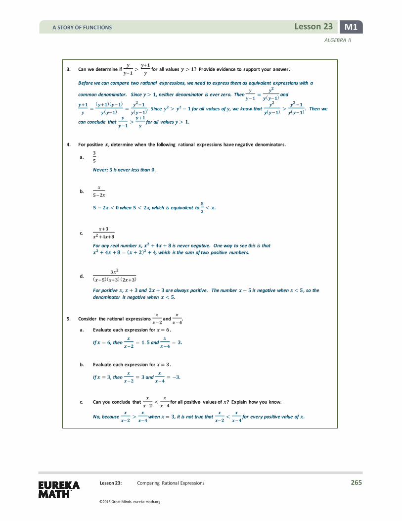
M1 Lesson 23 ALGEBRA II
Lesson 23: Comparing Rational Expressions
3. Can we determine if > for all values > ? Provide evidence to support your answer.
Before we can compare two rational expressions, we need to express them as equivalent expressions with a
common denominator. Since > , neither denominator is ever zero. Then = ( ) and
=( )( )
( ) = ( ). Since > − for all values of , we know that ( ) > ( ) . Then we
can conclude that > for all values > .
4. For positive , determine when the following rational expressions have negative denominators.
a.
Never; is never less than .
b.
− < when < , which is equivalent to < .
c.
For any real number , + + is never negative. One way to see this is that + + = ( + ) + , which is the sum of two positive numbers.
d. ( )( ) ( )
For positive , + and + are always positive. The number − is negative when < , so the denominator is negative when < .
5. Consider the rational expressions and .
a. Evaluate each expression for = .
If = , then = . and = .
b. Evaluate each expression for = .
If = , then = and = − .
c. Can you conclude that < for all positive values of ? Explain how you know.
No, because > when = , it is not true that < for every positive value of .
A STORY OF FUNCTIONS
265
©2015 Great Minds. eureka-math.org

M1 Lesson 23 ALGEBRA II
Lesson 23: Comparing Rational Expressions
d. Extension: Raphael claims that the calculation below shows that < for all values of , where
and . Where is the error in the calculation?
Starting with the rational expressions and , we need to first find equivalent rational expressions with
a common denominator. The common denominator we will use is ( − )( − ). We then have
−=
( − )( − )( − )
−=
( − )( − )( − )
.
Since − < − for > , we can divide each expression by ( − )( − ). We then have ( )
( )( )<
( )( )( )
, and we can conclude that < for all positive values of .
The error in logic in this calculation is that the denominator ( − )( − ) is not always a positive number for all positive values of . In fact, if < < , then ( − )( − ) < . Thus, even though
− < − when > , the inequality ( )( )
<( )( )
is not valid for every positive
value of .
6. Consider the populations of two cities within the same state where the large city’s population is , and the small
city’s population is . For each of the following pairs, state which of the expressions has a larger value. Explain your reasoning in the context of the populations.
a. + and
The value of + is larger than . The expression + represents the total population of the two cities, and represents the population of the larger city. Since these quantities are populations of cities, we can assume they are greater than zero.
b. and
The value of is larger. As stated in part (a), + represents the total population of the two cities.
Hence, and represent each city’s respective fraction of the total population. Since > ,
> .
c. and +
The value of + is larger than the value of . The population of the smaller of the two cities is represented by , so represents a population twice the size of the smaller city, but
> so + > + and thus + > .
d. and
The value of is larger. These expressions represent the ratio between the populations of the cities. For
instance, the larger city is times larger than the smaller city. Since > , > > , we can say that
there are people in the larger city for every one person in the smaller city.
MP.3
MP.2
A STORY OF FUNCTIONS
266
©2015 Great Minds. eureka-math.org
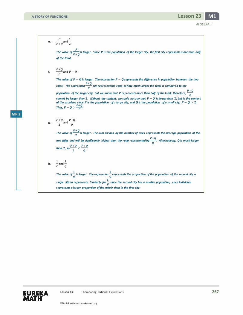
M1 Lesson 23 ALGEBRA II
Lesson 23: Comparing Rational Expressions
e. and
The value of is larger. Since is the population of the larger city, the first city represents more than half
of the total.
f. and −
The value of − is larger. The expression − represents the difference in population between the two
cities. The expression can represent the ratio of how much larger the total is compared to the
population of the larger city, but we know that represents more than half of the total; therefore,
cannot be larger than . Without the context, we could not say that − is larger than , but in the context of the problem, since is the population of a large city, and is the population of a small city, − > . Thus, − >
+.
g. and
The value of is larger. The sum divided by the number of cities represents the average population of the
two cities and will be significantly higher than the ratio represented by . Alternatively, is much larger
than , so < .
h. and
The value of is larger. The expression represents the proportion of the population of the second city a
single citizen represents. Similarly for , since the second city has a smaller population, each individual
represents a larger proportion of the whole than in the first city.
MP.2
A STORY OF FUNCTIONS
267
©2015 Great Minds. eureka-math.org

M1 Lesson 24 ALGEBRA II
Lesson 24: Multiplying and Dividing Rational Expressions
Lesson 24: Multiplying and Dividing Rational Expressions
Student Outcomes
� Students multiply and divide rational expressions and simplify using equivalent expressions.
Lesson Notes This lesson quickly reviews the process of multiplying and dividing rational numbers using techniques students already know and translates that process to multiplying and dividing rational expressions (MP.7). This enables students to develop techniques to solve rational equations in Lesson 26 (A-APR.D.6). This lesson also begins developing facility with simplifying complex rational expressions, which is important for later work in trigonometry. Teachers may consider treating the multiplication and division portions of this lesson as two separate lessons.
Classwork Opening Exercise (5 minutes)
Distribute notecard-sized slips of paper to students, and ask them to shade the paper to
represent the result of 23
4. Circulate around the classroom to assess student proficiency.
If many students are still struggling to remember the area model after the scaffolding, present the problem to them as shown. Otherwise, allow them time to do the multiplication on their own or with their neighbor and then progress to the question of the general rule.
� First, we represent 4
by dividing our region into five vertical strips of equal area
and shading 4 of the 5 parts.
� Now we need to find 23
of the shaded area. So we divide the area horizontally
into three parts of equal area and then shade two of those parts.
Scaffolding: If students do not remember the area model for multiplication of fractions, have them discuss it with their neighbor. If necessary, use an
example l ike 12
12
to see if they
can scale this to the problem presented.
If students are comfortable with multiplying rational numbers, omit the area model, and ask them to determine the following products.
� 23
3=
14
� 14
=24
� 4
=323
A STORY OF FUNCTIONS
268
©2015 Great Minds. eureka-math.org

M1 Lesson 24 ALGEBRA II
Lesson 24: Multiplying and Dividing Rational Expressions
If , , , and are rational expressions with , , then
= .
� Thus, 23
4 is represented by the region that is shaded twice. Since 8 out of 15 subrectangles are shaded
twice, we have 23
4=
1. With this in mind, can we create a general rule about multiplying rational
numbers?
Allow students to come up with this rule based on the example and prior experience. Have them discuss their thoughts with their neighbor and write the rule.
The rule summarized above is also valid for real numbers.
Discussion (2 minutes)
� To multiply rational expressions, we follow the same procedure we use when multiplying rational numbers: we multiply together the numerators and multiply together the denominators. We finish by reducing the product to lowest terms.
Lead students through Examples 1 and 2, and ask for their input at each step.
Example 1 (4 minutes)
Give students time to work on this problem and discuss their answers with a neighbor before proceeding to class discussion.
Example 1
Make a conjecture about the product . What will it be? Explain your
conjecture, and give evidence that it is correct.
� We begin by multiplying the numerators and denominators.
𝑥𝑥3
4𝑦𝑦𝑦𝑦2
𝑥𝑥=𝑥𝑥3𝑦𝑦2
4𝑦𝑦𝑥𝑥
Scaffolding: � To assist students in making the
connection between rational numbers and rational expressions, show a side-by-side comparison of a numerical example from a previous lesson l ike the one shown.
23
45
=8
15
4= ?
� If students are struggling with this example, include some others, such as
3 OR .
If 𝑎𝑎, 𝑏𝑏, 𝑐𝑐, and are integers with 𝑐𝑐 0 and 0, then
𝑎𝑎𝑐𝑐𝑏𝑏
=𝑎𝑎𝑏𝑏𝑐𝑐
.
A STORY OF FUNCTIONS
269
©2015 Great Minds. eureka-math.org

M1 Lesson 24 ALGEBRA II
Lesson 24: Multiplying and Dividing Rational Expressions
� Identify the greatest common factor (GCF) of the numerator and denominator. The GCF of 𝑥𝑥3𝑦𝑦2 and 4𝑥𝑥𝑦𝑦 is 𝑥𝑥𝑦𝑦.
𝑥𝑥3
4𝑦𝑦𝑦𝑦2
𝑥𝑥=
(𝑥𝑥𝑦𝑦)𝑥𝑥2𝑦𝑦4(𝑥𝑥𝑦𝑦)
� Finally, we divide the common factor 𝑥𝑥𝑦𝑦 from the numerator and denominator to find the reduced form of the product:
𝑥𝑥3
4𝑦𝑦𝑦𝑦2
𝑥𝑥=𝑥𝑥2𝑦𝑦
4.
Note that the phrases “cancel 𝑥𝑥𝑦𝑦” or “cancel the common factor” are intentionally avoided in this lesson. The goal is to highlight that it is division that allows these expressions to be simplified. Ambiguous words like “cancel” can lead
students to simplify ( )
to sin—they “canceled” the 𝑥𝑥!
It is important to understand why the numerator and denominator may be divided by 𝑥𝑥. The rule 𝑛𝑛𝑛𝑛
= works for
rational expressions as well. Performing a simplification such as =1
requires doing the following steps:
=1
=1
= 11
=1
.
Example 2 (3 minutes)
Before walking students through the steps of this example, ask them to try to find the product using the ideas of the previous example.
Example 2
Find the following product: � −+ � � +
+ �.
First, factor the numerator and denominator of each rational expression. � Identify any common factors in the numerator and denominator.
3𝑥𝑥 − 62𝑥𝑥 + 6
5𝑥𝑥+ 154𝑥𝑥 + 8
=3(𝑥𝑥 − 2)2(𝑥𝑥 + 3)
5(𝑥𝑥 + 3)4(𝑥𝑥 + 2)
=15(𝑥𝑥 − 2)(𝑥𝑥 + 3)8(𝑥𝑥 + 3)(𝑥𝑥 + 2)
The GCF of the numerator and denominator is 𝑥𝑥 + 3.
Then, divide the common factor (𝑥𝑥 + 3) from the numerator and denominator, and obtain the reduced form of the product.
3𝑥𝑥 − 62𝑥𝑥 + 6
5𝑥𝑥 + 154𝑥𝑥 + 8
=15(𝑥𝑥 − 2)8(𝑥𝑥 + 2)
MP.7
A STORY OF FUNCTIONS
270
©2015 Great Minds. eureka-math.org

M1 Lesson 24 ALGEBRA II
Lesson 24: Multiplying and Dividing Rational Expressions
Exercises 1–3 (5 minutes)
Students can work in pairs on the following three exercises. Circulate around the class to informally assess their understanding. For Exercise 1, l isten for key points such as “factoring the numerator and denominator can help” and “multiplying rational expressions is similar to multiplying rational numbers.”
Exercises 1–3
1. Summarize what you have learned so far with your neighbor.
Answers will vary.
2. Find the following product and reduce to lowest terms: � ++ −
� − .
++ −
−=
( + )( + )( − )
( − )( + )
=( + )( − )( + )
( + )( − )
The factors , + , and − can be divided from the numerator and the denominator in order to reduce the rational expression to lowest terms.
++ −
−=
+
3. Find the following product and reduce to lowest terms: � −+ � − −
+ + .
−+
− −+ +
=+−
− −+ +
=( + ) ( − )( + )
( − ) ( + )
=( + )( − )
Discussion (5 minutes)
Recall that division of numbers is equivalent to multiplication of the numerator by the reciprocal of the denominator. That is, for any two numbers 𝑎𝑎 and 𝑏𝑏, where 𝑏𝑏 0, we have
𝑎𝑎𝑏𝑏
= 𝑎𝑎1𝑏𝑏
,
where the number 1
is the multiplicative inverse of 𝑏𝑏. But, what if 𝑏𝑏 is itself a fraction?
How do we evaluate a quotient such as 3
÷4
?
� How do we evaluate 3
÷4
?
Have students work in pairs to answer this and then discuss.
Scaffolding: Students may need to be reminded how to interpret a negative exponent. If so, ask them to calculate these values.
� 3 2 = 132 = 1
9
� �25�
3= �5
2�3
= 53
23 = 1258
� 𝑥𝑥𝑦𝑦2 = 𝑦𝑦2
𝑥𝑥 =�𝑦𝑦2�
5
𝑥𝑥5 = 𝑦𝑦10
𝑥𝑥5
Scaffolding: Students may be better able to generalize the procedure for dividing rational numbers by repeatedly dividing several
examples, such as 12
÷34
, 23
÷10
, and 1
÷2
. After
dividing several of these examples, ask students to generalize the process (MP.8).
A STORY OF FUNCTIONS
271
©2015 Great Minds. eureka-math.org

M1 Lesson 24 ALGEBRA II
Lesson 24: Multiplying and Dividing Rational Expressions
If , , , and are rational expressions with , , and , then
÷ = = .
By our rule above, 3
÷4
=3 1
4 . But, what is the value of 14 ? Let 𝑥𝑥 represent
14 , which is the multiplicative
inverse of 4
. Then we have
𝑥𝑥47
= 1
4𝑥𝑥 = 7
𝑥𝑥 =74
.
Since we have shown that 14 =
4, we can continue our calculation of
3÷4
as follows:
35
÷47
=35
14 7
=35
74
=2120
.
This same process applies to dividing rational expressions, although we might need to perform the additional step of reducing the resulting rational expression to lowest terms. Ask students to generate the rule for division of rational numbers.
The result summarized in the box above is also valid for real numbers.
Now that we know how to divide rational numbers, how do we extend this to divide rational expressions?
� Dividing rational expressions follows the same procedure as dividing rational numbers: we multiply the first term by the reciprocal of the second. We finish by reducing the product to lowest terms.
If 𝑎𝑎, 𝑏𝑏, 𝑐𝑐, and are integers with 𝑏𝑏 0, 𝑐𝑐 0, and 0, then 𝑎𝑎𝑐𝑐
÷𝑏𝑏
=𝑎𝑎𝑐𝑐 𝑏𝑏
.
Scaffolding: A side-by-side comparison may help as before.
35
÷47
=2120
4
÷ = ?
For struggling students, give
� 4
÷ =2
� 3
1÷
12( 1)
=( 1)4
.
For advanced students, give
� 32
÷1
=1
( 2)
� 2 24
4÷
3 42
=2
.
A STORY OF FUNCTIONS
272
©2015 Great Minds. eureka-math.org

M1 Lesson 24 ALGEBRA II
Lesson 24: Multiplying and Dividing Rational Expressions
Example 3 (3 minutes)
As in Example 2, ask students to apply their knowledge of rational-number division to rational expressions by working on their own or with a partner. Circulate to assist and assess understanding. Once students have made attempts to divide, use the scaffolded questions to develop the concept as necessary.
Example 3
Find the quotient and reduce to lowest terms: ÷ .
� First, we change the division of 4
3 by
22
into multiplication of 4
3 by the multiplicative inverse of
22
.
𝑥𝑥2 − 43𝑥𝑥
÷𝑥𝑥− 2
2𝑥𝑥=𝑥𝑥2− 4
3𝑥𝑥2𝑥𝑥𝑥𝑥 − 2
� Then, we perform multiplication as in the previous examples and exercises. That is, we factor the numerator and denominator and divide any common factors present in both the numerator and denominator.
𝑥𝑥2 − 43𝑥𝑥
÷𝑥𝑥 − 2
2𝑥𝑥=
(𝑥𝑥 − 2)(𝑥𝑥 + 2)3𝑥𝑥
2𝑥𝑥𝑥𝑥 − 2
=2(𝑥𝑥 + 2)
3
Exercise 4 (3 minutes)
Allow students to work in pairs or small groups to evaluate the following quotient.
Exercises 4–5
4. Find the quotient and reduce to lowest terms: ÷ .
− ++
÷−
+ +=
− ++
+ +−
=( − )( − )
+( + )( + )( − )( + )
=( − )( + )
( + )
Discussion (4 minutes)
What do we do when the numerator and denominator of a fraction are themselves fractions? We call a fraction that contains fractions a complex fraction. Remind students that the fraction bar represents division, so a complex fraction represents division between rational expressions.
A STORY OF FUNCTIONS
273
©2015 Great Minds. eureka-math.org

M1 Lesson 24 ALGEBRA II
Lesson 24: Multiplying and Dividing Rational Expressions
Allow students the opportunity to simplify the following complex fraction.
12 4927 28
Allow students to struggle with the problem before discussing solution methods.
12 4927 28
=1249
÷2728
=1249
2827
=3 47 7
4 733
=42
7 32
=1663
Notice that in simplifying the complex fraction above, we are merely performing division of rational numbers, and we already know how to do that. Since we already know how to divide rational expressions, we can also simplify rational expressions whose numerators and denominators are rational expressions.
Exercise 5 (4 minutes)
Allow students to work in pairs or small groups to simplify the following rational expression.
5. Simplify the rational expression.
� +− −
�− −
+ +
+− −− −
+ +=
+− −
÷− −
+ +
=+
− −+ +− −
=+
( − )( + )( + )( + )( − )( + )
=+
( − )
Scaffolding: For struggling students, give a simpler example, such as
�2𝑥𝑥3𝑦𝑦�6𝑥𝑥
4𝑦𝑦2=
2𝑥𝑥3𝑦𝑦
÷6𝑥𝑥
4𝑦𝑦2
=2𝑥𝑥3𝑦𝑦
4𝑦𝑦2
6𝑥𝑥
=49𝑦𝑦
A STORY OF FUNCTIONS
274
©2015 Great Minds. eureka-math.org

M1 Lesson 24 ALGEBRA II
Lesson 24: Multiplying and Dividing Rational Expressions
Closing (3 minutes)
Ask students to summarize the important parts of the lesson in writing, to a partner, or as a class. Use this as an opportunity to informally assess understanding of the lesson. In particular, ask students to articulate the processes for multiplying and dividing rational expressions and simplifying complex rational expressions either verbally or symbolically.
Exit Ticket (4 minutes)
Lesson Summary
In this lesson, we extended multiplication and division of rational numbers to multiplication and division of rational expressions.
� To multiply two rational expressions, multiply the numerators together and multiply the denominators together, and then reduce to lowest terms.
� To divide one rational expression by another, multiply the first by the multiplicative inverse of the second, and reduce to lowest terms.
� To simplify a complex fraction, apply the process for dividing one rational expression by another.
A STORY OF FUNCTIONS
275
©2015 Great Minds. eureka-math.org

M1 Lesson 24 ALGEBRA II
Lesson 24: Multiplying and Dividing Rational Expressions
Name Date
Lesson 24: Multiplying and Dividing Rational Expressions
Exit Ticket Perform the indicated operations, and reduce to lowest terms.
1. 2
2 3 2
2
2. �
�
A STORY OF FUNCTIONS
276
©2015 Great Minds. eureka-math.org

M1 Lesson 24 ALGEBRA II
Lesson 24: Multiplying and Dividing Rational Expressions
Exit Ticket Sample Solutions
Perform the indicated operations, and reduce to lowest terms.
1.
−+ −
− ++
=−
( − )( + )( − )( − )
+
=( − )( + )
2. � �
� −
+ −�
− ++
=−
+ −÷
− ++
=−
+ −+
− +
=−
( − )( + )+
( − )( − )
= ( − )
Problem Set Sample Solutions
1. Perform the following operations:
a. Multiply ( − ) by . b. Divide ( − ) by . c. Multiply � + � by .
− − +
d. Divide � − � by . e. Multiply � + � by . f. Multiply . ( − ) by .
− + −
2. Write each rational expression as an equivalent rational expression in lowest terms.
a. � � ÷ b. c. ÷
( + )
d. e. f. ÷ ( − )
−
− − ( + )
A STORY OF FUNCTIONS
277
©2015 Great Minds. eureka-math.org
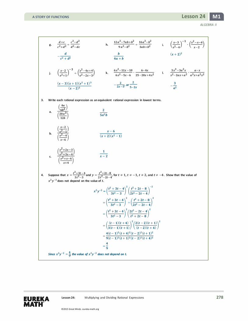
M1 Lesson 24 ALGEBRA II
Lesson 24: Multiplying and Dividing Rational Expressions
g. ÷ h. ÷ i. � � � �
−+
+
( + )
j. � � ÷ � � k. l.
( − )( + )( + )( − ) − − , or −
3. Write each rational expression as an equivalent rational expression in lowest terms.
a. � �
b. � �
−( + )( − )
c. −
4. Suppose that = + −−
and = + −− −
, for , − , , and − . Show that the value of
does not depend on the value of .
=+ −
−+ −− −
=+ −
−÷
+ −− −
=+ −
−− −
+ −
=( − )( + )( − )( + )
( − )( + )( − )( + )
=( − ) ( + ) ( − ) ( + )( − ) ( + ) ( − ) ( + )
=
Since = , the value of does not depend on .
A STORY OF FUNCTIONS
278
©2015 Great Minds. eureka-math.org

M1 Lesson 24 ALGEBRA II
Lesson 24: Multiplying and Dividing Rational Expressions
5. Determine which of the following numbers is larger without using a calculator, or . (Hint: We can
compare two positive quantities and by computing the quotient . If > , then > . Likewise, if
< < , then < .)
÷ =
= ( )( )( )
=
=
=
=
=
Since < , and < , we know that � � � � < . Thus, ÷ < , and we know that
< .
Extension:
6. One of two numbers can be represented by the rational expression , where and .
a. Find a representation of the second number if the product of the two numbers is .
Let the second number be . Then � − � = , so we have
= ÷−
= �−
�
=−
.
b. Find a representation of the second number if the product of the two numbers is .
Let the second number be . Then � − � = , so we have
= ÷−
= �−
�
= .
A STORY OF FUNCTIONS
279
©2015 Great Minds. eureka-math.org

M1 Lesson 25 ALGEBRA II
Lesson 25: Adding and Subtracting Rational Expressions
Lesson 25: Adding and Subtracting Rational Expressions
Student Outcomes
� Students perform addition and subtraction of rational expressions.
Lesson Notes This lesson reviews addition and subtraction of fractions using the familiar number line technique that students have seen in earlier grades. This leads to an algebraic explanation of how to add and subtract fractions and an opportunity to practice MP.7. The lesson then moves to the process for adding and subtracting rational expressions by converting to equivalent rational expressions with a common denominator. As in the past three lessons, parallels are drawn between arithmetic of rational numbers and arithmetic of rational expressions.
Classwork The four basic arithmetic operations are addition, subtraction, multiplication, and division. The previous lesson showed how to multiply and divide rational expressions. This lesson tackles the remaining operations of addition and subtraction of rational expressions, which are skills needed to address A-APR.C.6. As discussed in the previous lesson, rational expressions are worked with in the same way as rational numbers expressed as fractions. First, the lesson reviews the theory behind addition and subtraction of rational numbers.
Exercise 1 (8 minutes)
First, remind students how to add fractions with the same denominator. Allow them to work through the following sum individually. The solution should be presented to the class either by the teacher or by a student because the process of adding fractions will be extended to the new process of adding rational expressions.
Exercises 1–4
1. Calculate the following sum: + .
One approach to this calculation is to factor out from each term.
+ = +
= ( + )
=
Scaffolding: If students need practice adding and subtracting fractions with a common denominator, have them compute the following.
� 2
+1
� −3
� 124
−1224
A STORY OF FUNCTIONS
280
©2015 Great Minds. eureka-math.org

M1 Lesson 25 ALGEBRA II
Lesson 25: Adding and Subtracting Rational Expressions
Ask students for help in stating the rule for adding and subtracting rational numbers with the same denominator.
The result in the box above is also valid for real numbers 𝑎𝑎, 𝑏𝑏, and 𝑐𝑐.
� But what if the fractions have different denominators? Let’s examine a technique to add the fractions 2
and 13
.
� Recall that when we first learned to add fractions, we represented them on a number l ine. Let’s first look at 2
.
� And we want to add to this the fraction 13
.
� If we try placing these two segments next to each other, the exact location of the endpoint is difficult to identify.
� The units on the two original graphs do not match. We need to identify a common unit in order to identify the endpoint of the combined segments. We need to identify a number into which both denominators divide without a remainder and write each fraction as an equivalent fraction with that number as the denominator; such a number is known as a common denominator.
� Since 15 is a common denominator of 2
and 13
, we divide the interval [0,1] into 15 parts of equal length. Now
when we look at the segments of length 2
and 13
placed next to each other on the number line, we can see that
the combined segment has length 111
.
� How can we do this without using the number line every time? The fraction 2
is equivalent to 1
, and the
fraction 13
is equivalent to 1
. We then have
25
+13
=6
15+
515
=1115
.
If 𝑎𝑎, 𝑏𝑏, and 𝑐𝑐 are integers with 𝑏𝑏 0, then 𝑎𝑎𝑏𝑏
+𝑐𝑐𝑏𝑏
=𝑎𝑎 + 𝑐𝑐𝑏𝑏
and 𝑎𝑎𝑏𝑏−𝑐𝑐𝑏𝑏
=𝑎𝑎 − 𝑐𝑐𝑏𝑏
.
A STORY OF FUNCTIONS
281
©2015 Great Minds. eureka-math.org

M1 Lesson 25 ALGEBRA II
Lesson 25: Adding and Subtracting Rational Expressions
� Thus, when adding rational numbers, we have to find a common multiple for the two denominators and write each rational number as an equivalent rational number with the new common denominator. Then we can add the numerators together.
Have students discuss how to rewrite the original fraction as an equivalent fraction with the chosen common denominator. Discuss how the identity property of multiplication allows one to multiply the top and the bottom by the same number so that the product of the original denominator and the number gives the chosen common denominator.
� Generalizing, let’s add together two rational numbers, and . The first step is to rewrite both fractions as
equivalent fractions with the same denominator. A simple common denominator that could be used is the product of the original two denominators:
𝑎𝑎𝑏𝑏
+𝑐𝑐
=𝑎𝑎𝑏𝑏
+𝑏𝑏𝑐𝑐𝑏𝑏
.
� Once we have a common denominator, we can add the two expressions together, using our previous rule for adding two expressions with the same denominator:
𝑎𝑎𝑏𝑏
+𝑐𝑐
=𝑎𝑎 + 𝑏𝑏𝑐𝑐𝑏𝑏
.
� We could use the same approach to develop a process for subtracting rational numbers: 𝑎𝑎𝑏𝑏−𝑐𝑐
=𝑎𝑎 −𝑏𝑏𝑐𝑐𝑏𝑏
.
� Now that we know to find a common denominator before adding or subtracting, we can state the general rule for adding and subtracting rational numbers. Notice that one common denominator that always works is the product of the two original denominators.
As with the other rules developed in this and the previous lesson, the rule summarized in the box above is also valid for real numbers.
Exercises 2–4 (5 minutes)
Ask students to work in groups to write what they have learned in their notebooks or journals. Check in to assess their understanding. Then, have students work in pairs to quickly work through the following review exercises. Allow them to think about how to approach Exercise 4, which involves adding three rational expressions. There are multiple ways to approach this problem. They could generalize the process for two rational expressions, rearrange terms using the commutative property to combine the terms with the same denominator, and then add using the above process, or they could group the addends using the associative property and perform addition twice.
2. −
− = − = −
If 𝑎𝑎, 𝑏𝑏, 𝑐𝑐, and are integers with 𝑏𝑏 0 and 0, then 𝑎𝑎𝑏𝑏
+𝑐𝑐
=𝑎𝑎 + 𝑏𝑏𝑐𝑐𝑏𝑏
and 𝑎𝑎𝑏𝑏−𝑐𝑐
=𝑎𝑎 − 𝑏𝑏𝑐𝑐𝑏𝑏
.
A STORY OF FUNCTIONS
282
©2015 Great Minds. eureka-math.org

M1 Lesson 25 ALGEBRA II
Lesson 25: Adding and Subtracting Rational Expressions
3. +√
+√
= +√
=+ √
4. + −
+ − = + − =+ −
Discussion (2 minutes)
� Before we can add rational numbers or rational expressions, we need to convert to equivalent rational expressions with the same denominators. Finding such a denominator involves finding a common multiple of the original denominators. For example, 60 is a common multiple of 20 and 15. There are other common multiples, such as 120, 180, and 300, but smaller numbers are easier to work with.
� To add and subtract rational expressions, we follow the same procedure as when adding and subtracting rational numbers. First, we find a denominator that is a common multiple of the other denominators, and then we rewrite each expression as an equivalent rational expression with this new common denominator. We then apply the rule for adding or subtracting with the same denominator.
Example 1 (10 minutes)
Work through these examples as a class, getting input from students at each step. Example 1
Perform the indicated operations below and simplify.
a. +
A common multiple of and is , so we can write each expression as an equivalent rational expression
with denominator . We have = and = , so that
+ = + = .
b. −
A common multiple of and is , so we can write each expression as an equivalent rational
expression with denominator . We have − = − = .
If 𝑎𝑎, 𝑏𝑏, and 𝑐𝑐 are rational expressions with 𝑏𝑏 0, then 𝑎𝑎𝑏𝑏
+𝑐𝑐𝑏𝑏
=𝑎𝑎 + 𝑐𝑐𝑏𝑏
and 𝑎𝑎𝑏𝑏−𝑐𝑐𝑏𝑏
=𝑎𝑎 − 𝑐𝑐𝑏𝑏
.
A STORY OF FUNCTIONS
283
©2015 Great Minds. eureka-math.org

M1 Lesson 25 ALGEBRA II
Lesson 25: Adding and Subtracting Rational Expressions
c. +
Since + = ( + ) and − − = ( − )( + ), a common multiple of + and
− − is ( + )( − ). Then we have + =( )
( )( )+
( )( )=
( )( ).
Exercises 5–8 (8 minutes)
Have students work on these exercises in pairs or small groups.
Exercises 5–8
Perform the indicated operations for each problem below.
5. +
A common multiple is ( − ).
−+
−=
( − )+
( − )=
+( − )
6. +
Notice that ( − ) = −( − ).
A common multiple is ( − ).
−+
−=
−+−−
=−
−−
=−
7. −
A common multiple is ( − )( − ).
− +−
−= ( − )( − )−
−( − )( − ) =
( − )
8. −
A common multiple is ( − )( + )( + ).
−−
+ −= ( − )( + ) − ( − )( + ) =
( + )( − )( + )( + )
−( + )
( − )( + )( + )
=−
( − )( + )( + )
A STORY OF FUNCTIONS
284
©2015 Great Minds. eureka-math.org

M1 Lesson 25 ALGEBRA II
Lesson 25: Adding and Subtracting Rational Expressions
Example 2 (5 minutes)
Complex fractions were introduced in the previous lesson with multiplication and division of rational expressions, but these examples require performing addition and subtraction operations prior to doing the division. Remind students that when rewriting a complex fraction as division of rational expressions, they should add parentheses to the expressions both in the numerator and denominator. Then they should work inside the parentheses first following the standard order of operations.
Example 2
Simplify the following expression.
+ −− −
− ( + )
First, we can rewrite the complex fraction as a division problem, remembering to add parentheses.
+ −− −
− ( + )=
+ −−
− ÷ −( + )
Remember that to divide rational expressions, we multiply by the reciprocal of the quotient. However, we first need to write each expression as a rational expression in lowest terms. For this, we need to find common denominators.
+ −−
− =+ −−
−−−
=−−
− ( + ) =( + )
+− ( + )
=−
( + )
=( − )
+
Now, we can substitute these equivalent expressions into our calculation above and continue to perform the division as we did in Lesson 24.
+ −− −
− ( + )=
+ −−
− ÷ −( + )
=−−
÷( − )
+
=( − )−
( + )( − )
=( + )
( − )
MP.7
A STORY OF FUNCTIONS
285
©2015 Great Minds. eureka-math.org

M1 Lesson 25 ALGEBRA II
Lesson 25: Adding and Subtracting Rational Expressions
Closing (2 minutes)
Ask students to summarize the important parts of the lesson in writing, to a partner, or as a class. Use this opportunity to informally assess their understanding of the lesson. In particular, ask students to verbally or symbolically articulate the processes for adding and subtracting rational expressions.
Exit Ticket (5 minutes)
Lesson Summary
In this lesson, we extended addition and subtraction of rational numbers to addition and subtraction of rational expressions. The process for adding or subtracting rational expressions can be summarized as follows:
� Find a common multiple of the denominators to use as a common denominator. � Find equivalent rational expressions for each expression using the common denominator.
� Add or subtract the numerators as indicated and simplify if needed.
A STORY OF FUNCTIONS
286
©2015 Great Minds. eureka-math.org
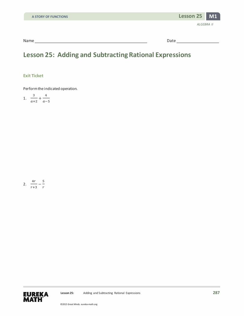
M1 Lesson 25 ALGEBRA II
Lesson 25: Adding and Subtracting Rational Expressions
Name Date
Lesson 25: Adding and Subtracting Rational Expressions
Exit Ticket Perform the indicated operation.
1. 32
+4
2. 43−
A STORY OF FUNCTIONS
287
©2015 Great Minds. eureka-math.org

M1 Lesson 25 ALGEBRA II
Lesson 25: Adding and Subtracting Rational Expressions
Exit Ticket Sample Solutions
Perform the indicated operation.
1. +
++
−=
−( + )( − ) +
+( + )( − )
=−
( + )( − )
2. −
+− = ( + )−
+( + )
=− −( + )
Problem Set Sample Solutions
1. Write each sum or difference as a single rational expression.
a. −√
− √
b. √
+√
+
√ + √ +
c. +
A STORY OF FUNCTIONS
288
©2015 Great Minds. eureka-math.org

M1 Lesson 25 ALGEBRA II
Lesson 25: Adding and Subtracting Rational Expressions
2. Write as a single rational expression.
a. − b. − + c. +
−( − )
−
d. − e. + f. −
( − )( + )
−+
g. − + h. − i. +
+ −
− +
( − )( + )
j. + k. + l. +
−
−−
−
m. − −
n. ( )( )
+
( )( )
o. + +
−+
−( − )( − )( − )
+ +( − )( + )
3. Write each rational expression as an equivalent rational expression in lowest terms.
a.
b.
c.
−
+−
Extension:
4. Suppose that and . We know from our work in this section that is equivalent to . Is it also true
that + is equivalent to ? Provide evidence to support your answer.
No, the rational expressions + and are not equivalent. Consider = and = . Then = = ,
but + = + = . Since , the expressions + and are not equivalent.
A STORY OF FUNCTIONS
289
©2015 Great Minds. eureka-math.org

M1 Lesson 25 ALGEBRA II
Lesson 25: Adding and Subtracting Rational Expressions
5. Suppose that =+
and = −+
. Show that the value of + does not depend on the value of .
+ =+
+−+
= ( + ) +( − )( + )
=+ ( − + )
( + )
=+ ++ +
=
Since + = , the value of + does not depend on the value of .
6. Show that for any real numbers and , and any integers and so that , , , and − ,
� − �� ++ −
−− � = ( − ).
−++
−−−
= −( + )( − )
( + )( − ) −( − )( + )
( − )( + )
=− − + −
−−
( + − −−
= −− − +
−
= −− ( − )
= ( − )
7. Suppose that is a positive integer.
a. Rewrite the product in the form for polynomials and : � + � � + + �.
+ ++
=+ +
+=
+
b. Rewrite the product in the form for polynomials and : � + � � + + � � + + �.
+ ++
++
=+ +
+++
=+
c. Rewrite the product in the form for polynomials and : � + � � + + � � + + � � + + �.
+ ++
++
++
=+ +
+++
++
=+
d. If this pattern continues, what is the product of of these factors?
If we have of these factors, then the product will be
+ ++
++ ( − ) =
+= .
MP.7
A STORY OF FUNCTIONS
290
©2015 Great Minds. eureka-math.org

M1 Lesson 26 ALGEBRA II
Lesson 26: Solving Rational Equations
Lesson 26: Solving Rational Equations
Student Outcomes
� Students solve rational equations, monitoring for the creation of extraneous solutions.
Lesson Notes In the preceding lessons, students learned to add, subtract, multiply, and divide rational expressions so that in this lesson they can solve equations involving rational expressions (A-REI.A.2). The skills developed in this lesson are required to solve equations of the form 𝑓𝑓(𝑥𝑥) = 𝑐𝑐 for a rational function 𝑓𝑓 and constant 𝑐𝑐 in Lesson 27 and later in Module 3 (F-BF.B.4a).
There is more than one approach to solving a rational equation, and this section explores two such methods. The first method is to multiply both sides by the common denominator to clear fractions. The second method is to find equivalent forms of all expressions with a common denominator, set the numerators equal to each other, and solve the resulting equation. Either approach requires keeping an eye out for extraneous solutions; in other words, values that appear to be a solution to the equation but cause division by zero and are, thus, not valid. Throughout the work with rational expressions, students analyze the structure of the expressions in order to decide on their next algebraic steps (MP.7). Encourage students to check their answers by substituting their solutions back into each side of the equation separately.
Classwork Exercises 1–2 (8 minutes)
Let students solve this any way they can, and then discuss their answers. Focus on adding the fractions on the left and equating numerators or multiplying both sides by a common multiple. Indicate a practical technique of finding a common denominator. These first two exercises highlight MP.7, as students must recognize the given expressions to be of
the form + or + ; by expressing the equations in the simplified form = , they
realize that we must have = .
Exercises 1–2
Solve the following equations for , and give evidence that your solutions are correct.
1. + =
Combining the expressions on the left, we have + = , so = ; therefore, + = . Then, = .
Or, using another approach: � + �= � �, so + = ; then, = .
The solution to this equation is . To verify, we see that when = , we have + = + = + = , so is
a valid solution.
Scaffolding: Struggling students may benefit from first solving the
equation −2
=1
.
More advanced students may try to solve
𝑥𝑥 − 1𝑥𝑥 + 2
=34
.
A STORY OF FUNCTIONS
291
©2015 Great Minds. eureka-math.org

M1 Lesson 26 ALGEBRA II
Lesson 26: Solving Rational Equations
2. + =
Since the expressions already have a common denominator, we see that + = , so we need to solve
= . It then follows that the numerators are equal, so + = . Solving for gives = . To verify, we
see that when = , we have + =� �
+ = + = ; thus, is a valid solution.
Remind students that two rational expressions with the same denominator are equal if the numerators are equal.
Discussion (2 minutes)
Now that students know how to add, subtract, multiply, and divide rational expressions, it is time to use some of those basic operations to solve equations involving rational expressions. An equation involving rational expressions is called a rational equation. Keeping the previous exercise in mind, this section looks at two different approaches to solving rational equations.
Example (6 minutes)
Ask students to try to solve this problem on their own. Have them discuss and explain their methods in groups or with neighbors. The teacher should circulate and lead a discussion of both methods once students have had a chance to try solving on their own.
Example
Solve the following equation: = .
Equating Numerators Method: Obtain expressions on both sides with the same denominator and equate numerators.
+=
+=
Thus, + = , and = ; therefore, is the solution to our original equation.
Clearing Fractions Method: Multiply both sides by a common multiple of the denominators to clear the fractions, and then solve the resulting equation.
+=
+ =
We can see, once again, that the solution is .
MP.1
A STORY OF FUNCTIONS
292
©2015 Great Minds. eureka-math.org
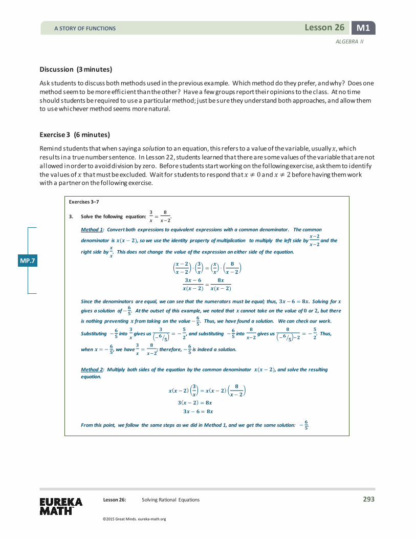
M1 Lesson 26 ALGEBRA II
Lesson 26: Solving Rational Equations
Discussion (3 minutes)
Ask students to discuss both methods used in the previous example. Which method do they prefer, and why? Does one method seem to be more efficient than the other? Have a few groups report their opinions to the class. At no time should students be required to use a particular method; just be sure they understand both approaches, and allow them to use whichever method seems more natural.
Exercise 3 (6 minutes)
Remind students that when saying a solution to an equation, this refers to a value of the variable, usually 𝑥𝑥, which results in a true number sentence. In Lesson 22, students learned that there are some values of the variable that are not allowed in order to avoid division by zero. Before students start working on the following exercise, ask them to identify the values of 𝑥𝑥 that must be excluded. Wait for students to respond that 𝑥𝑥 0 and 𝑥𝑥 2 before having them work with a partner on the following exercise.
Exercises 3–7
3. Solve the following equation: = .
Method 1: Convert both expressions to equivalent expressions with a common denominator. The common
denominator is ( − ), so we use the identity property of multiplication to multiply the left side by and the
right side by . This does not change the value of the expression on either side of the equation.
−−
= � �−
−( − )
=( − )
Since the denominators are equal, we can see that the numerators must be equal; thus, − = . Solving for
gives a solution of − . At the outset of this example, we noted that cannot take on the value of or , but there
is nothing preventing from taking on the value − . Thus, we have found a solution. We can check our work.
Substituting − into gives us � � = − , and substituting − into gives us � � = − . Thus,
when = − , we have = ; therefore, − is indeed a solution.
Method 2: Multiply both sides of the equation by the common denominator ( − ), and solve the resulting equation.
( − ) = ( − )−
( − ) = − =
From this point, we follow the same steps as we did in Method 1, and we get the same solution: − .
MP.7
A STORY OF FUNCTIONS
293
©2015 Great Minds. eureka-math.org

M1 Lesson 26 ALGEBRA II
Lesson 26: Solving Rational Equations
Exercise 4 (6 minutes)
Have students continue to work with partners to solve the following equation. Walk around the room and observe student progress; if necessary, offer the following hints and reminders:
� Reminder: Ask students to identify excluded values of 𝑎𝑎. Suggest that they factor the denominator 𝑎𝑎2 − 4. They should discover that 𝑎𝑎 2 and 𝑎𝑎 −2 must be specified.
� Hint 1: Ask students to identify a common denominator of the three expressions in the equation. They should respond with (𝑎𝑎 − 2)(𝑎𝑎 + 2), or equivalently, 𝑎𝑎2 − 4.
� Hint 2: What do we need to do with this common denominator? They should determine that they need to find equivalent rational expressions for each of the terms with denominator (𝑎𝑎 − 2)(𝑎𝑎 + 2).
4. Solve the following equation for : + = .
First, we notice that we must have and − . Then, we apply Method 1:
−− +
+++ −
= ( − )( + )
−( − )( + ) +
+( − )( + ) = ( − )( + )
( − )( + )=
( − )( + ).
Since the denominators are equal, we know that the numerators are equal; thus, we have = , which means that = . Thus, the only solution to this equation is . However,
is not allowed to be because if = , then is not defined. This means that the
original equation, + = , has no solution.
Introduce the term extraneous solution. An invalid solution that may arise when we manipulate a rational expression is called an extraneous solution. An extraneous solution is a value that satisfies a transformed equation but does not satisfy the original equation.
Exercises 5–7 (8 minutes)
Give students a few minutes to discuss extraneous solutions with a partner. When do they occur, and how do you know when you have one? Extraneous solutions occur when one of the solutions found does not make a true number sentence when substituted into the original equation. The only way to know there is one is to note the values of the variable that will cause a part of the equation to be undefined. This lesson is concerned with division by zero; later lessons exclude values of the variable that would cause the square root of a negative number. Make sure that all students have an understanding of extraneous solutions before proceeding. Then, have them work in pairs on the following exercises.
Scaffolding: Let students know that the word extraneous has meaning outside of the mathematics classroom; ask them to guess its definition, and then provide the actual definition.
EXTRANEOUS: Irrelevant or unrelated to the subject being dealt with.
Students may benefit from choral repetition, as well as a visual representation of this word.
A STORY OF FUNCTIONS
294
©2015 Great Minds. eureka-math.org

M1 Lesson 26 ALGEBRA II
Lesson 26: Solving Rational Equations
5. Solve the following equation. Remember to check for extraneous solutions.
+ =
First, note that we must have .
Equating numerators: + = Then, we have + = , and the solution is = .
Clearing fractions: � + �= � � Then, we have + = , and the solution is = .
The solution is valid since the only excluded value is .
6. Solve the following equation. Remember to check for extraneous solutions.
++
−=
−−
First, note that we must have and − .
Equating numerators: ( )
( )( )+ ( )
( )( )=
( )( )
Matching numerators, we have − + + = − , which leads to = ; therefore, = .
Clearing fractions: ( − )( + ) � + + − � = ( − )( + ) −−
We have ( − ) + ( + ) = − , which leads to = ; therefore, = .
The solution is valid since the only excluded values are and − .
7. Solve the following equation. Remember to check for extraneous solutions.
−+
−=
− +
First, note that we must have and .
Equating numerators:
−( − )( − )
+−
( − )( − )=
( − )( − )
− − = − − =
( − )( + ) =
The solutions are and − .
Clearing fractions:
−+
−( − )( − ) = ( − )( − )
( − )( − )
( − ) + ( − ) = − + − =
− − = ( − )( + ) =
The solutions are and − .
Because is not allowed to be in order to avoid division by zero, the solution is extraneous; thus, − is the only solution to the given rational equation.
A STORY OF FUNCTIONS
295
©2015 Great Minds. eureka-math.org

M1 Lesson 26 ALGEBRA II
Lesson 26: Solving Rational Equations
Closing (2 minutes)
Ask students to summarize the important parts of the lesson in writing, to a partner, or as a class. Use this as an opportunity to informally assess understanding of the lesson. In particular, ask students to explain how to identify extraneous solutions and why they arise when solving rational equations.
Exit Ticket (4 minutes)
Lesson Summary
In this lesson, we applied what we have learned in the past two lessons about addition, subtraction, multiplication, and division of rational expressions to solve rational equations. An extraneous solution is a solution to a transformed equation that is not a solution to the original equation. For rational functions, extraneous solutions come from the excluded values of the variable.
Rational equations can be solved one of two ways:
1. Write each side of the equation as an equivalent rational expression with the same denominator and equate the numerators. Solve the resulting polynomial equation, and check for extraneous solutions.
2. Multiply both sides of the equation by an expression that is the common denominator of all terms in the equation. Solve the resulting polynomial equation, and check for extraneous solutions.
A STORY OF FUNCTIONS
296
©2015 Great Minds. eureka-math.org

M1 Lesson 26 ALGEBRA II
Lesson 26: Solving Rational Equations
Name Date
Lesson 26: Solving Rational Equations
Exit Ticket Find all solutions to the following equation. If there are any extraneous solutions, identify them and explain why they are extraneous.
7𝑏𝑏 + 3
+5
𝑏𝑏− 3=
10𝑏𝑏𝑏𝑏2− 9
A STORY OF FUNCTIONS
297
©2015 Great Minds. eureka-math.org

M1 Lesson 26 ALGEBRA II
Lesson 26: Solving Rational Equations
Exit Ticket Sample Solutions Find all solutions to the following equation. If there are any extraneous solutions, identify them and explain why they are extraneous.
++
−=
−
First, note that we must have and − .
Using the equating numerators method: ( )
( )( )+
( )( )( )
=( )( )
Matching numerators, we have − + + = , which leads to − = ; therefore, = .
However, since the excluded values are and − , the solution is an extraneous solution, and there is no solution to
+ = .
Problem Set Sample Solutions
1. Solve the following equations, and check for extraneous solutions.
a. = b. = c. =
All real numbers except No solution
d. = e. − = f. =
No solution −
−
g. − = h. + = i. − =
−
,− ,
j. + − = k. − = l. − =
,
,− ,
m. − = n. ( )
+ = o. = +
,
− ,−
p. = −
,
A STORY OF FUNCTIONS
298
©2015 Great Minds. eureka-math.org

M1 Lesson 26 ALGEBRA II
Lesson 26: Solving Rational Equations
2. Create and solve a rational equation that has as an extraneous solution.
One such equation is + = .
3. Create and solve a rational equation that has as an extraneous solution.
One such equation is + = .
Extension:
4. Two lengths and , where > , are in golden ratio if the ratio of + is to is the
same as is to . Symbolically, this is expressed as = . We denote this common
ratio by the Greek letter phi (pronounced “fee”) with symbol , so that if and are in
common ratio, then = = + . By setting = , we find that = and is the
positive number that satisfies the equation =+
. Solve this equation to find the
numerical value for .
We can apply either method from the previous lesson to solve this equation.
=+
= + − − =
Applying the quadratic formula, we have two solutions:
=+√
or =− √
.
Since is a positive number, and √
< , we have = + .
5. Remember that if we use to represent an integer, then the next integer can be represented by + .
a. Does there exist a pair of consecutive integers whose reciprocals sum to ? Explain how you know.
Yes, and because + = + = .
A STORY OF FUNCTIONS
299
©2015 Great Minds. eureka-math.org

M1 Lesson 26 ALGEBRA II
Lesson 26: Solving Rational Equations
b. Does there exist a pair of consecutive integers whose reciprocals sum to ? Explain how you know.
If represents the first integer, then + represents the next integer. Suppose + = . Then,
++
=
( + ) +( + )
=( + )( + )
+ = +
− − = .
The solutions to this quadratic equation are √
and √
, so there are no integers that solve this
equation. Thus, there are no pairs of consecutive integers whose reciprocals sum to .
c. Does there exist a pair of consecutive even integers whose reciprocals sum to ? Explain how you know.
If represents the first integer, then + represents the next even integer. Suppose + = . Then,
++
=
( + ) +( + ) =
( + )( + )
+ = + − − = .
The solutions to this quadratic equation are − and ; therefore, the only even integer that solves the
equation is . Then, and are consecutive even integers whose reciprocals sum to .
d. Does there exist a pair of consecutive even integers whose reciprocals sum to ? Explain how you know.
If represents the first integer, then + represents the next even integer. Suppose + = . Then,
++
=
( + ) +( + ) =
( + )( + )
+ = + − − = .
The solutions to this quadratic equation are √
and √
, so there are no integers that solve this
equation. Thus, there are no pairs of consecutive even integers whose reciprocals sum to .
A STORY OF FUNCTIONS
300
©2015 Great Minds. eureka-math.org

Lesson 27: Word Problems Leading to Rational Equations
M1 Lesson 27 ALGEBRA II
Lesson 27: Word Problems Leading to Rational Equations
Student Outcomes
� Students solve word problems using models that involve rational expressions.
Lesson Notes In the preceding lessons, students learned to add, subtract, multiply, and divide rational expressions and solve rational equations in order to develop the tools needed for solving application problems involving rational equations in this lesson (A-REI.A.2). Students develop their problem-solving and modeling abilities by carefully reading the problem description and converting information into equations (MP.1), thus creating a mathematical model of the problem (MP.4).
Classwork Exercise 1 (13 minutes)
This lesson turns to some applied problems that can be modeled with rational equations, strengthening students’ problem-solving and modeling experience in alignment with standards MP.1 and MP.4. These equations can be solved using the skills developed in previous lessons. Have students work in small groups to answer this set of four questions. At the end of the work time, ask different groups to present their solutions to the class. Suggest to students that they: (a) read the problem aloud, (b) paraphrase and summarize the problem in their own words, (c) find an equation that models the situation, and (d) say how it represents the quantities involved. Check to make sure that students understand the problem before they begin trying to solve it.
In Exercise 1, consider encouraging students to assign the variable to the unknown quantity, and ask if they can arrive at an equation that relates to the known quantities.
A STORY OF FUNCTIONS
301
©2015 Great Minds. eureka-math.org

Lesson 27: Word Problems Leading to Rational Equations
M1 Lesson 27 ALGEBRA II
Exercise 1
1. Anne and Maria play tennis almost every weekend. So far, Anne has won out of matches.
a. How many matches will Anne have to win in a row to improve her winning percentage to %?
Suppose that Anne has already won of matches, and let represent the number of additional matches she must win to raise her winning percentage to %. After playing and winning all of those additional matches, she has won + matches out of a total of + matches played. Her winning percentage is then
, and we want to find the value of that solves the equation
++
= . .
Multiply both sides by + .
+ = . ( + ) + = + .
Solve for :
. = =
So, Anne would need to win matches in a row in order to improve her winning percentage to %.
b. How many matches will Anne have to win in a row to improve her winning percentage to %?
This situation is similar to that for part (a), except that we want a winning percentage of . , instead of . . Again, we let represent the number of matches Anne must win consecutively to bring her winning
percentage up to %.
++
= .
Solve for :
+ = . ( + ) + = + .
. = =
In order for Anne to bring her winning percentage up to %, she would need to win the next consecutive matches.
c. Can Anne reach a winning percentage of %?
Allow students to come to the conclusion that Anne will never reach a winning percentage of % because she has already lost matches.
MP.2
Scaffolding: Students may benefit from having the problem read aloud and summarized. They should be encouraged to restate the problem in their own words to a partner.
If students are struggling, present the equation 1220
= 0.75, and ask
students how this models the situation. Students who may be working above grade level could be challenged to write their own word problems that result in rational equations.
MP.1 &
MP.4
A STORY OF FUNCTIONS
302
©2015 Great Minds. eureka-math.org

Lesson 27: Word Problems Leading to Rational Equations
M1 Lesson 27 ALGEBRA II
d. After Anne has reached a winning percentage of % by winning consecutive matches as in part (b), how many matches can she now lose in a row to have a winning percentage of %?
Recall from part (b) that she had won matches out of to reach a winning percentage of %. We will now assume that she loses the next matches in a row. Then, she will have won matches out of + matches, and we want to know the value of that makes this a % win rate.
+= .
Solving the equation:
= . ( + ) = + . = . =
Thus, after reaching a % winning percentage in matches, Anne can lose matches in a row to drop to a % winning percentage.
Example (5 minutes)
Work this problem at the front of the room, but allow the class to provide input and steer the discussion. Depending on how students did with the first exercise, the teacher may lead a discussion of this problem as a class, ask students to work in groups, or ask students to work independently while targeting instruction with a small group that struggled on the first exercise.
Example
Working together, it takes Sam, Jenna, and Francisco two hours to paint one room. When Sam works alone, he can paint one room in hours. When Jenna works alone, she can paint one room in hours. Determine how long it would take Francisco to paint one room on his own.
Consider how much can be accomplished in one hour. Sam, Jenna, and Francisco together can paint half a room in one
hour. If Sam can paint one room in hours on his own, then in one hour he can paint of the room. Similarly, Jenna can
paint of the room in one hour. We do not yet know how much Francisco can paint in one hour, so we will say he can
paint of the room. So, in one hour, Sam has painted of the room, Jenna has painted of the room, and all three
together can paint the room, leading to the following equation for how much can be painted in one hour:
+ + = .
A common multiple of the denominators is . Multiplying both sides by gives us:
+ + =
+ + = ,
which leads us to the value of :
= .
So, Francisco can paint the room in hours on his own.
MP.4
A STORY OF FUNCTIONS
303
©2015 Great Minds. eureka-math.org

Lesson 27: Word Problems Leading to Rational Equations
M1 Lesson 27 ALGEBRA II
Exercise 2 (5 minutes)
Remind students that distance equals rate times time ( = 𝑟𝑟 ) before having them work on this exercise in pairs or small groups. Be sure to have groups share their results before continuing to the next exercise.
Exercises 2–4
2. Melissa walks miles to the house of a friend and returns home on a bike. She averages miles per hour faster when cycling than when walking, and the total time for both trips is two hours. Find her walking speed.
Using the relationship = , we have = . The time it takes for Melissa to walk to her friend’s house is , and
the time to cycle back is . Thus, we can write an equation that describes the combined time for both trips:
++
= .
A common multiple of the denominators is ( + ), so we multiply both sides of the equation by ( + ).
( + ) + = ( + ) + + = + + − =
( − )( + ) =
Thus, = − or = . Since represents Melissa’s speed, it does not make sense for to be negative. So, the only solution is , which means that Melissa’s walking speed is miles per hour.
Exercise 3 (10 minutes)
3. You have liters of a juice blend that is % juice.
a. How many liters of pure juice need to be added in order to make a blend that is % juice?
We start off with liters of a blend containing % juice. Then, this blend contains . ( ) = liters of juice in the liters of mixture. If we add liters of pure juice, then the concentration of juice in the blend is
. We want to know which value of makes this blend % juice.
++
= .
+ = . ( + ) + = . + .
. = . =
Thus, if we add liters of pure juice, we have liters of a blend that contains liters of juice, meaning that the concentration of juice in this blend is %.
MP.1 &
MP.4
A STORY OF FUNCTIONS
304
©2015 Great Minds. eureka-math.org

Lesson 27: Word Problems Leading to Rational Equations
M1 Lesson 27 ALGEBRA II
b. How many liters of pure juice need to be added in order to make a blend that is % juice?
++
= .
+ = . ( + ) + = + .
= . =
Thus, if we add liters of pure juice, we will have liters of a blend that contains liters of pure juice, meaning that the concentration of juice in this blend is %.
c. Write a rational equation that relates the desired percentage to the amount of pure juice that needs to be added to make a blend that is % juice, where < < . What is a reasonable restriction on the set of possible values of ? Explain your answer.
++
=
We need to have < < for the problem to make sense. We already have % juice; the percentage cannot decrease by adding more juice, and we can never have a mixture that is more than % juice.
d. Suppose that you have added liters of juice to the original liters. What is the percentage of juice in this
blend?
=++
= .
So, the new blend contains % pure juice.
e. Solve your equation in part (c) for the amount . Are there any excluded values of the variable ? Does this
make sense in the context of the problem?
++
= ( + ) = ( + ) + = + − = −
( − ) = −
=−−
We see from the equation for that . This makes sense because we can never make a % juice solution since we started with a diluted amount of juice.
Exercise 4 (5 minutes)
Allow students to work together in pairs or small groups for this exercise. This exercise is a bit different from the previous example in that the amount of acid comes from a diluted solution and not a pure solution. Be sure that students set up the numerator correctly. (If there is not enough time to do the entire problem, have students set up the equations in class and finish solving them for homework.)
MP.4
MP.2
A STORY OF FUNCTIONS
305
©2015 Great Minds. eureka-math.org
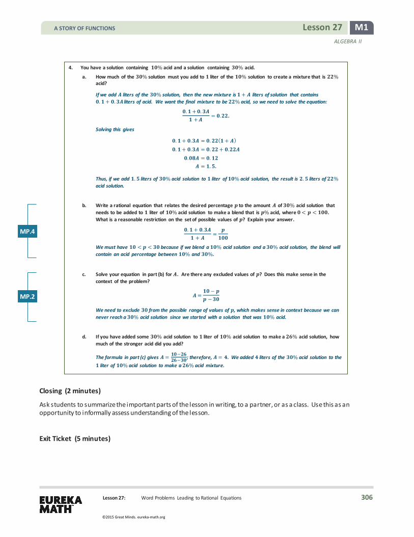
Lesson 27: Word Problems Leading to Rational Equations
M1 Lesson 27 ALGEBRA II
4. You have a solution containing % acid and a solution containing % acid.
a. How much of the % solution must you add to liter of the % solution to create a mixture that is % acid?
If we add liters of the % solution, then the new mixture is + liters of solution that contains . + . liters of acid. We want the final mixture to be % acid, so we need to solve the equation:
. + .+
= . .
Solving this gives
. + . = . ( + )
. + . = . + . . = .
= . .
Thus, if we add . liters of % acid solution to liter of % acid solution, the result is . liters of % acid solution.
b. Write a rational equation that relates the desired percentage to the amount of % acid solution that
needs to be added to liter of % acid solution to make a blend that is % acid, where < < . What is a reasonable restriction on the set of possible values of ? Explain your answer.
. + .+
=
We must have < < because if we blend a % acid solution and a % acid solution, the blend will contain an acid percentage between % and %.
c. Solve your equation in part (b) for . Are there any excluded values of ? Does this make sense in the context of the problem?
=−−
We need to exclude from the possible range of values of , which makes sense in context because we can never reach a % acid solution since we started with a solution that was % acid.
d. If you have added some % acid solution to liter of % acid solution to make a % acid solution, how
much of the stronger acid did you add?
The formula in part (c) gives = −− ; therefore, = . We added liters of the % acid solution to the
liter of % acid solution to make a % acid mixture.
Closing (2 minutes)
Ask students to summarize the important parts of the lesson in writing, to a partner, or as a class. Use this as an opportunity to informally assess understanding of the lesson.
Exit Ticket (5 minutes)
MP.4
MP.2
A STORY OF FUNCTIONS
306
©2015 Great Minds. eureka-math.org

Lesson 27: Word Problems Leading to Rational Equations
M1 Lesson 27 ALGEBRA II
Name Date
Lesson 27: Word Problems Leading to Rational Equations
Exit Ticket Bob can paint a fence in 5 hours, and working with Jen, the two of them painted a fence in 2 hours. How long would it have taken Jen to paint the fence alone?
A STORY OF FUNCTIONS
307
©2015 Great Minds. eureka-math.org

Lesson 27: Word Problems Leading to Rational Equations
M1 Lesson 27 ALGEBRA II
Exit Ticket Sample Solutions
Bob can paint a fence in hours, and working with Jen, the two of them painted a fence in hours. How long would it have taken Jen to paint the fence alone?
Let represent the time it would take Jen to paint the fence alone. Then, Bob can paint the entire fence in hours;
therefore, in one hour he can paint of the fence. Similarly, Jen can paint of the fence in one hour. We know that it
took them two hours to complete the job, and together they can paint of the fence in one hour. We then have to solve the equation:
+ =
+ =
+ =
= .
Thus, it would have taken Jen hours and minutes to paint the fence alone.
Problem Set Sample Solutions
1. If two inlet pipes can fill a pool in one hour and minutes, and one pipe can fill the pool in two hours and minutes on its own, how long would the other pipe take to fill the pool on its own?
.+ =
.
We find that = . ; therefore, it takes hours and minutes for the second pipe to fill the pool by itself.
2. If one inlet pipe can fill the pool in hours with the outlet drain closed, and the same inlet pipe can fill the pool in
. hours with the drain open, how long does it take the drain to empty the pool if there is no water entering the pool?
− =.
We find that = ; therefore, it takes hours for the drain to empty the pool by itself.
3. It takes minutes less time to travel miles by car at night than by day because the lack of traffic allows the average speed at night to be miles per hour faster than in the daytime. Find the average speed in the daytime.
−= +
We find that = . The time it takes to travel miles by car at night is minutes, which is hours. Since
= , the average speed in the daytime is miles per hour.
A STORY OF FUNCTIONS
308
©2015 Great Minds. eureka-math.org

Lesson 27: Word Problems Leading to Rational Equations
M1 Lesson 27 ALGEBRA II
4. The difference in the average speed of two trains is miles per hour. The slower train takes hours longer to travel miles than the faster train takes to travel miles. Find the speed of the slower train.
−+
=
We find that = , so it takes hours for the faster train to travel miles, and it takes hours for the slower train to travel miles. The average speed of the slower train is miles per hour.
5. A school library spends $ a month on magazines. The average price for magazines bought in January was cents more than the average price in December. Because of the price increase, the school library was forced to subscribe to fewer magazines. How many magazines did the school library subscribe to in December?
+ .= −
The solution to this equation is . , so the average price in December is $ . . Thus the school subscribed to magazines in December.
6. An investor bought a number of shares of stock for $ , . After the price dropped by $ per share, the investor
sold all but of her shares for $ , . How many shares did she originally buy?
=−
+
This equation has two solutions: and . Thus, the investor bought either or shares of stock.
7. Newton’s law of universal gravitation, = , measures the force of gravity between two masses and ,
where is the distance between the centers of the masses, and is the universal gravitational constant. Solve this equation for .
=
8. Suppose that =+− .
a. Show that when = and = −+ , the value of does not depend on the value of .
When simplified, we find that = ; therefore, the value of does not depend on the value of .
b. For which values of do these relationships have no meaning?
If is , then has no meaning. If = − , then has no meaning.
9. Consider the rational equation = + .
a. Find the value of when = and = .
= +
So = .
A STORY OF FUNCTIONS
309
©2015 Great Minds. eureka-math.org

Lesson 27: Word Problems Leading to Rational Equations
M1 Lesson 27 ALGEBRA II
b. Solve this equation for , and write as a single rational expression in lowest terms.
There are two approaches to solve this equation for .
The first way is to perform the addition on the right:
The second way is to take reciprocals of both sides and then simplify:
= +
= +
=+
.
=
+
=+
= ( + ) .
In either case, we find that = + .
10. Consider an ecosystem of rabbits in a park that starts with rabbits and can sustain up to rabbits. An equation that roughly models this scenario is
=+ +
,
where represents the rabbit population in year of the study. a. What is the rabbit population in year ? Round your answer to the nearest whole rabbit.
If = , then = . ; therefore, there are rabbits in the park.
b. Solve this equation for . Describe what this equation represents in the context of this problem.
=−−
This equation represents the relationship between the number of rabbits, , and the year, . If we know how many rabbits we have, < < , we will know how long it took for the rabbit population to grow that much. If the population is , then this equation says we are in year of the study, which fits with the given scenario.
c. At what time does the population reach rabbits?
If = , then = −− = −
− = ; therefore, the rabbit population is in year of the study.
A STORY OF FUNCTIONS
310
©2015 Great Minds. eureka-math.org

Lesson 27: Word Problems Leading to Rational Equations
M1 Lesson 27 ALGEBRA II
Extension:
11. Suppose that Huck Finn can paint a fence in hours. If Tom Sawyer helps him paint the fence, they can do it in hours. How long would it take for Tom to paint the fence by himself?
Huck paints the fence in hours, so his rate of fence painting is fence per hour. Let denote the percentage of the fence Tom can paint in an hour. Then
fence = + fence per hour ( hours).
=+
=+
=+
( + ) = =
=
So, Tom can paint of the fence in an hour. Thus, Tom would take = . hours to paint the fence by himself.
12. Huck Finn can paint a fence in hours. After some practice, Tom Sawyer can now paint the fence in hours.
a. How long would it take Huck and Tom to paint the fence together?
The amount of fence that Huck can paint per hour is , and the amount that Tom can paint per hour is . So,
together they can paint + of the fence per hour. Suppose the entire job of painting the fence takes
hours. Then, the amount of the fence that is painted is � + �. Since the entire fence is painted, we need
to solve the equation � + �= .
+ =
=+
=+
=
So, together they can paint the fence in hours, which is hours and minutes.
A STORY OF FUNCTIONS
311
©2015 Great Minds. eureka-math.org

Lesson 27: Word Problems Leading to Rational Equations
M1 Lesson 27 ALGEBRA II
b. Tom demands a half-hour break while Huck continues to paint, and they finish the job together. How long does it take them to paint the fence?
Suppose the entire job of painting the fence takes hours. Then, Huck paints at a rate of of the fence per
hour for hours, so he paints of the fence. Tom paints at a rate of of the fence per hour for − hour, so
he paints � − � of the fence. Together, they paint the whole fence; so, we need to solve the following
equation for :
+ − =
+ − =
+ =
+ =
+ =
= .
Thus, it takes hours, which is hours minutes, to paint the fence with Tom taking a hour break.
c. Suppose that they have to finish the fence in hours. What’s the longest break that Tom can take?
Suppose the entire job of painting the fence takes hours, and Tom stops painting for hours for his break.
Then, Huck paints at a rate of of the fence per hour for hours, so he paints of the fence. Tom paints at
a rate of of the fence per hour for � − � hours, so he paints � − � of the fence. Together, they paint
the whole fence; so, we need to solve the following equation for :
+ − =
+ − =
+ − =
+ − = + − =
= .
Thus, if Tom takes a break for hours, which is hour and minutes, the fence will be painted in hours.
A STORY OF FUNCTIONS
312
©2015 Great Minds. eureka-math.org

M1 Lesson 28 ALGEBRA II
Lesson 28: A Focus on Square Roots
Lesson 28: A Focus on Square Roots
Student Outcomes
� Students solve simple radical equations and understand the possibility of extraneous solutions. They understand that care must be taken with the role of square roots so as to avoid apparent paradoxes.
� Students explain and justify the steps taken in solving simple radical equations.
Lesson Notes In the next two lessons, students work with radical expressions and equations. They extend their understanding of the idea that not all operations are invertible, which was explored in Algebra I and continued in the previous lessons on solving rational equations. Squaring both sides of an equation in some cases produces an extraneous solution. They also continue to work with rational expressions and equations as seen in the previous lessons, but those expressions now contain radicals. This lesson highlights standards A-REI.A.1, which calls for students to be able to explain each step required to solve an equation, and A-REI.A.2, which calls for students to solve a radical equation and show how extraneous solutions might arise. It also addresses the standard MP.3 by building and analyzing arguments used in solving radical equations. In Example 2, students consider the difference between working with an expression, whose value must be preserved, and working with an equation, whose sides can be changed in value as long as equality is preserved. This difference addresses the standard MP.7 because students are stepping back to get an overview of expressions and equations as objects subject to different rules.
Classwork Opening (1 minute)
Recall that working with radical expressions can be tricky, especially when negative numbers are involved. When solving a radical equation, one must always check the answers found to verify that they are indeed valid solutions to the equation. In some cases, extraneous solutions appear and must be eliminated. Recall that an extraneous solution is one that satisfies a transformed equation but not the original one.
Exercises 1–4 (7 minutes)
Give students a few minutes to work through the first four exercises, and then discuss the results as a whole class. Circulate the room to assess students’ understanding.
Scaffolding: � If students are struggling, show a few simpler
examples such as solving √𝑥𝑥 = 5 or √𝑥𝑥 = −5.
� Another option would be to provide the following alternative model for students to complete.
Fill in the blanks to fully show and explain the solution process. √ − = √ =
√ = =
Added to both sides to isolate the radical.
Square both sides.
A STORY OF FUNCTIONS
313
©2015 Great Minds. eureka-math.org
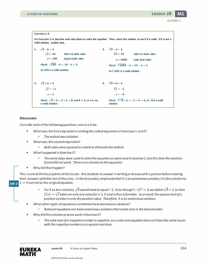
M1 Lesson 28 ALGEBRA II
Lesson 28: A Focus on Square Roots
Exercises 1–4
For Exercises 1–4, describe each step taken to solve the equation. Then, check the solution to see if it is valid. If it is not a valid solution, explain why.
1. √ − =
√ = Add to both sides.
= Square both sides.
Check: √ − = − =
So is a valid solution.
2. √ − =
√ = Add to both sides.
= Cube both sides.
Check: √ − = − =
So , is a valid solution.
3. √ + =
√ = −
=
Check: √ + = + = , and , so is not a valid solution.
4. √ + =
√ = −
= −
Check: √− + = − + = , so − is a valid solution.
Discussion
Consider each of the following questions, one at a time.
� What was the first step taken in solving the radical equations in Exercises 1 and 2? à The radical was isolated.
� What was the second step taken? à Both sides were squared or cubed to eliminate the radical.
� What happened in Exercise 3?
à The same steps were used to solve the equation as were used in Exercise 1, but this time the solution found did not work. There is no solution to the equation.
� Why did that happen?
This is one of the focal points of the lesson. Ask students to answer in writing or discuss with a partner before sharing their answers with the rest of the class. In the discussion, emphasize that 4 is an extraneous solution; it is the solution to 𝑥𝑥 = 4 but not to the original equation.
à For 4 to be a solution, √4 would need to equal −2. Even though (−2)2 = 4, we define √4 = 2 so that 𝑓𝑓(𝑥𝑥) = √𝑥𝑥 takes on only one value for 𝑥𝑥 0 and is thus a function. As a result, the square root of a positive number is only the positive value. Therefore, 4 is an extraneous solution.
� What other types of equations sometimes have extraneous solutions? à Rational equations can have extraneous solutions that create zero in the denominator.
� Why did the solution process work in Exercise 4?
à The cube root of a negative number is negative, so a cube root equation does not have the same issues with the negative numbers as a square root does.
MP.3
A STORY OF FUNCTIONS
314
©2015 Great Minds. eureka-math.org

M1 Lesson 28 ALGEBRA II
Lesson 28: A Focus on Square Roots
Example 1 (5 minutes)
Work through the example to solidify the steps in solving a radical equation. Depending on how students did with the first four exercises, consider having them continue working with a partner. Or, work through this example with the whole class at once. Be sure students can explain and justify the steps they are taking.
Example 1
Solve the following radical equation. Be sure to check your solutions.
√ + − = −
Solution: √ + =
+ =
= −
= −
Check: �− �+ − = √− + − = √ − = − , so − is a valid solution.
Discussion
� What was the first step you took? à I isolated the radical.
� Why did you do that first? à Isolating the radical allows it to be eliminated by squaring or cubing both sides of the equation.
� What was the next step? à I squared both sides.
� Why did you do that? à The purpose was to eliminate the radical from the equation.
� Even though we are solving a new type of equation, does this feel l ike a familiar process?
à Yes. When solving an equation, we work on undoing any operation by doing the inverse. To undo a square root, we use the inverse, so we square the expression.
� How do the steps we are following relate to your previous experiences with solving other types of equations?
à We are still following the basic process to solve an equation, which is to undo any operation on the same side as the variable by using the inverse operation.
� Why is it important to check the solution?
à Sometimes extraneous solutions appear because the square root of a positive number or zero is never negative.
Summarize (in writing or with a partner) what you have learned about solving radical equations. Be sure that you explain what to do when you get an extraneous solution.
A STORY OF FUNCTIONS
315
©2015 Great Minds. eureka-math.org
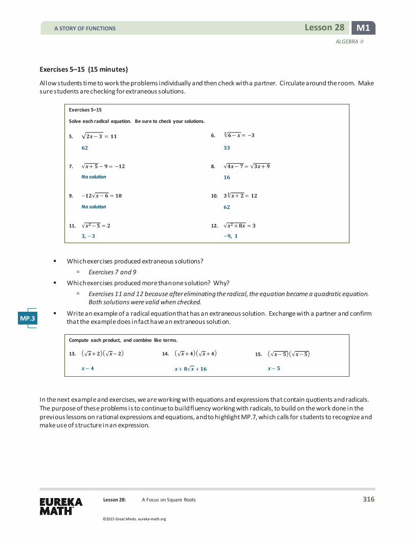
M1 Lesson 28 ALGEBRA II
Lesson 28: A Focus on Square Roots
Exercises 5–15 (15 minutes)
Allow students time to work the problems individually and then check with a partner. Circulate around the room. Make sure students are checking for extraneous solutions.
Exercises 5–15
Solve each radical equation. Be sure to check your solutions.
5. √ − = 6. √ − = −
7. √ + − = − 8. √ − = √ +
No solution
9. − √ − = 10. √ + =
No solution
11. √ − = 12. √ + =
, − − ,
� Which exercises produced extraneous solutions? à Exercises 7 and 9
� Which exercises produced more than one solution? Why? à Exercises 11 and 12 because after eliminating the radical, the equation became a quadratic equation.
Both solutions were valid when checked.
� Write an example of a radical equation that has an extraneous solution. Exchange with a partner and confirm that the example does in fact have an extraneous solution.
Compute each product, and combine like terms.
13. √ + √ − 14. √ + √ + 15. √ − √ −
− + √ + −
In the next example and exercises, we are working with equations and expressions that contain quotients and radicals. The purpose of these problems is to continue to build fluency working with radicals, to build on the work done in the previous lessons on rational expressions and equations, and to highlight MP.7, which calls for students to recognize and make use of structure in an expression.
MP.3
A STORY OF FUNCTIONS
316
©2015 Great Minds. eureka-math.org

M1 Lesson 28 ALGEBRA II
Lesson 28: A Focus on Square Roots
Example 2 (5 minutes)
Work through the two examples as a class, making sure students understand the differences between working with an expression and working with an equation.
Example 2
Rationalize the denominator in each expression. That is, rewrite the expression so that there is a rational expression in the denominator.
a. √
b. √
−√ −
√ −√ −
( − )√ −−
√ −
−√ +
√ −√ −
( − )(√ − )−
√ −
� What do the directions mean by “rationalize the denominator?”
à Remove the radical from the denominator so that the denominator is a rational expression. � How can we accomplish this goal in part (a)?
à Multiply the numerator and denominator by √𝑥𝑥− 9. � Why not just square the expression?
à We are working with an expression, not an equation. You cannot square the expression because you would be changing its value. You can multiply the numerator and denominator by √𝑥𝑥− 9 because that is equivalent to multiplying by 1. It does not change the value of the expression.
� Can we take the same approach in part (b)?
à No, multiplying by √𝑥𝑥+ 3 would not remove the radical from the denominator. � Based on Exercise 13, what number should we multiply the numerator and the denominator by in part (b) in
order to make the denominator rational?
à √𝑥𝑥− 3 � In these examples, what was accomplished by rationalizing the denominator?
à It allowed us to create an equivalent expression that is simpler. � Why would that be advantageous?
à It would be easier to work with if we were evaluating it for a particular value of 𝑥𝑥.
Exercises 16–18 (5 minutes)
Allow students time to work on the three problems and then debrief. Students may have taken different approaches on Exercise 17, such as squaring both sides first or rationalizing the denominator. Share a few different approaches and compare.
MP.7
A STORY OF FUNCTIONS
317
©2015 Great Minds. eureka-math.org

M1 Lesson 28 ALGEBRA II
Lesson 28: A Focus on Square Roots
Exercises 16–18
16. Rewrite √
in an equivalent form with a rational expression in the denominator.
√ +−
17. Solve the radical equation √
= . Be sure to check for extraneous solutions.
=
18. Without solving the radical equation √ + + = , how could you tell that it has no real solution?
The value of the radical expression √ + must be positive or zero. In either case, adding to it cannot give zero.
Closing (2 minutes)
Ask students to respond to these questions in writing or with a partner. Use this as an opportunity to informally assess students’ understanding.
� Explain to your neighbor how to solve a radical equation. What steps do you take and why?
à Isolate the radical, and then eliminate it by raising both sides to an exponent. The radical is isolated so that both sides can be squared or cubed as a means of eliminating the radical.
� How is solving a radical equation similar to solving other types of equations we have solved? à We are isolating the variable by undoing any operation on the same side.
� Why is it important to check the solutions?
à Remember that the square root of a number takes on only the positive value. When solving a radical equation involving a square root, squaring both sides of the equation in the process of solving may make the negative “disappear” and may create an extraneous solution.
Exit Ticket (5 minutes)
Scaffolding: If students are struggling with Exercise 17, have them approach the equation logically first rather than algebraically. If the output must equal 1, and the numerator is 3, what must the denominator equal?
A STORY OF FUNCTIONS
318
©2015 Great Minds. eureka-math.org

M1 Lesson 28 ALGEBRA II
Lesson 28: A Focus on Square Roots
Name Date
Lesson 28: A Focus on Square Roots
Exit Ticket Consider the radical equation 3√6−𝑥𝑥 + 4 = −8.
1. Solve the equation. Next to each step, write a description of what is being done.
2. Check the solution. 3. Explain why the calculation in Problem 1 does not produce a solution to the equation.
A STORY OF FUNCTIONS
319
©2015 Great Minds. eureka-math.org

M1 Lesson 28 ALGEBRA II
Lesson 28: A Focus on Square Roots
Exit Ticket Sample Solutions
Consider the radical equation √ − + = − .
1. Solve the equation. Next to each step, write a description of what is being done.
√ − = − √ − = −
− = = −
Subtract from both sides.
Divide both sides by in order to isolate the radical. Square both sides to eliminate the radical.
Subtract from both sides and divide by − .
2. Check the solution.
− (− ) + = √ + = ( ) + = , and − , so – is not a valid solution.
3. Explain why the calculation in Problem 1 does not produce a solution to the equation.
Because the square root of a positive number is positive, √ − will be positive. A positive number added to cannot be − .
Problem Set Sample Solutions
1.
a. If √ = , then what is the value of ?
=
b. If = , then what is the value of ?
= or = −
c. Is there a value of such that √ + = ? If yes, what is the value? If no, explain why not.
Yes, = −
d. Is there a value of such that √ + = ? If yes, what is the value? If no, explain why not.
No, √ will be a positive value or zero for any value of , so the sum cannot equal . If = , then √ + = .
2.
a. Is the statement √ = true for all -values? Explain.
No, this statement is only true for . If < , it is not true. For example, if = − , (− ) = √ = , then (− ) − .
A STORY OF FUNCTIONS
320
©2015 Great Minds. eureka-math.org

M1 Lesson 28 ALGEBRA II
Lesson 28: A Focus on Square Roots
b. Is the statement √ = true for all -values? Explain.
Yes, this statement is true for all -values. For example, if = , then √ = . If = − , then (− ) = − . Since the cube root of a positive number is positive, and the cube root of a negative number is
negative, this statement is true for any value of .
Rationalize the denominator in each expression.
3. −+√
4. √
5. √ √
−√ √ −−
√ + + √
Solve each equation, and check the solutions.
6. √ + = 7. √ + =
=
=
8. √ + + = 9. √ + − =
No solution
=
10. = +√ 11. √ − =
=
=
12. √ − = √ − 13. √ + + √ − =
=
No solution
14. √
= 15. √
=
=
=
16. √ + = 17. √ − =
= or = −
= or = −
18. √
= 19. √
=
=
=
20. √ − + = 21. √ − =
= − = −
A STORY OF FUNCTIONS
321
©2015 Great Minds. eureka-math.org

M1 Lesson 28 ALGEBRA II
Lesson 28: A Focus on Square Roots
22. Consider the inequality √ + > . Determine whether each -value is a solution to the inequality.
a. = − b. = − c. = d. =
Yes No Yes Yes
23. Show that √ √
= √ + √ for all values of and such that > and > and .
If we multiply the numerator and denominator of √ √
by √ + √ to rationalize the denominator, then we have
√ √=√ √
√ √√ √
=( ) √ √
= √ +√ .
24. Without actually solving the equation, explain why the equation √ + + = has no solution.
The value of √ + must be positive, which is then added to . The sum of two positive numbers is positive; therefore, the sum cannot equal .
A STORY OF FUNCTIONS
322
©2015 Great Minds. eureka-math.org
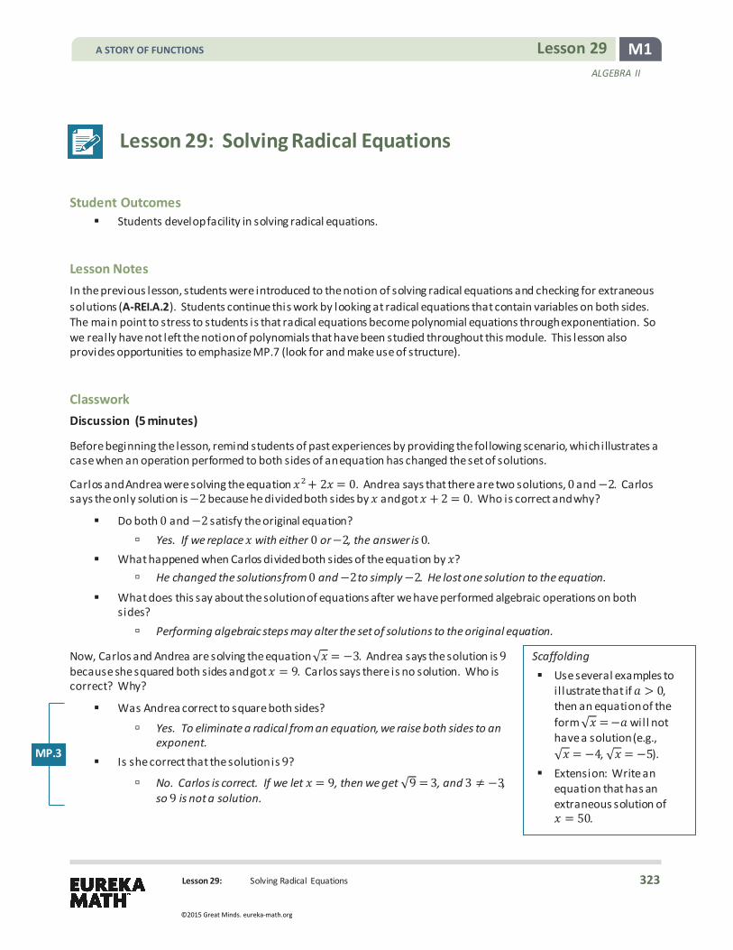
M1 Lesson 29 ALGEBRA II
Lesson 29: Solving Radical Equations
Lesson 29: Solving Radical Equations
Student Outcomes
� Students develop facility in solving radical equations.
Lesson Notes In the previous lesson, students were introduced to the notion of solving radical equations and checking for extraneous solutions (A-REI.A.2). Students continue this work by looking at radical equations that contain variables on both sides. The main point to stress to students is that radical equations become polynomial equations through exponentiation. So we really have not left the notion of polynomials that have been studied throughout this module. This lesson also provides opportunities to emphasize MP.7 (look for and make use of structure).
Classwork Discussion (5 minutes)
Before beginning the lesson, remind students of past experiences by providing the following scenario, which i llustrates a case when an operation performed to both sides of an equation has changed the set of solutions.
Carlos and Andrea were solving the equation 𝑥𝑥2+ 2𝑥𝑥 = 0. Andrea says that there are two solutions, 0 and −2. Carlos says the only solution is −2 because he divided both sides by 𝑥𝑥 and got 𝑥𝑥 + 2 = 0. Who is correct and why?
� Do both 0 and −2 satisfy the original equation? à Yes. If we replace 𝑥𝑥 with either 0 or −2, the answer is 0.
� What happened when Carlos divided both sides of the equation by 𝑥𝑥? à He changed the solutions from 0 and −2 to simply −2. He lost one solution to the equation.
� What does this say about the solution of equations after we have performed algebraic operations on both sides? à Performing algebraic steps may alter the set of solutions to the original equation.
Now, Carlos and Andrea are solving the equation √𝑥𝑥 = −3. Andrea says the solution is 9 because she squared both sides and got 𝑥𝑥 = 9. Carlos says there is no solution. Who is correct? Why?
� Was Andrea correct to square both sides?
à Yes. To eliminate a radical from an equation, we raise both sides to an exponent.
� Is she correct that the solution is 9?
à No. Carlos is correct. If we let 𝑥𝑥 = 9, then we get √9 = 3, and 3 −3, so 9 is not a solution.
Scaffolding � Use several examples to
i l lustrate that if 𝑎𝑎 > 0, then an equation of the form √𝑥𝑥 =−𝑎𝑎 wil l not have a solution (e.g., √𝑥𝑥 = −4, √𝑥𝑥 = −5).
� Extension: Write an equation that has an extraneous solution of 𝑥𝑥 = 50.
MP.3
A STORY OF FUNCTIONS
323
©2015 Great Minds. eureka-math.org

M1 Lesson 29 ALGEBRA II
Lesson 29: Solving Radical Equations
� What is the danger in squaring both sides of an equation?
à It sometimes produces an equation whose solution set is not equivalent to that of the original equation. If both sides of √𝑥𝑥 =−3 are squared, the equation 𝑥𝑥 = 9 is produced, but 9 is not a solution to the original equation. The original equation has no solution.
� Because of this danger, what is the final essential step of solving a radical equation?
à Checking the solution or solutions to ensure that an extraneous solution was not produced by the step of squaring both sides.
� How could we have predicted that the equation would have no solution?
à The square root of a number is never equal to a negative value, so there is no 𝑥𝑥-value so that √𝑥𝑥 = −3.
Example 1 (5 minutes)
While this problem is difficult, students should attempt to solve it on their own first, by applying their understandings of radicals. Students should be asked to verify the solution they come up with and describe their solution method. Discuss Example 1 as a class once they have worked on it individually.
Example 1
Solve the equation = + √ .
− = √
( − ) = √ − + = − + =
( − )( − ) =
The solutions are and .
Check = : + √ = + =
So, is an extraneous solution.
Check = : + √ = + =
The only valid solution is .
� How does this equation differ from the ones from yesterday’s lesson? à There are two 𝑥𝑥’s; one inside and one outside of the radical.
� Explain how you were able to determine the solution to the equation above. à Isolate the radical and square both sides. Solve the resulting equation.
� Did that change the way in which the equation was solved? à Not really; we still eliminated the radical by squaring both sides.
� What type of equation were we left with after squaring both sides? à A quadratic polynomial equation
� Why did 9 fail to work as a solution? à The square root of 9 takes only the positive value of 3.
MP.1
A STORY OF FUNCTIONS
324
©2015 Great Minds. eureka-math.org

M1 Lesson 29 ALGEBRA II
Lesson 29: Solving Radical Equations
Exercises 1–4 (13 minutes)
Allow students time to work the problems independently and then pair up to compare solutions. Use this time to informally assess student understanding by examining their work. Display student responses, making sure that students checked for extraneous solutions.
Exercises 1–4
Solve.
1. = + √ The only solution is .
Note that is an extraneous solution.
2. = √ − The two solutions are and .
3. √ + = − The only solution is . Note that − is an extraneous solution.
4. √ + + √ − = There are no solutions.
� When solving Exercise 1, what solutions did you find? What happened when you checked these solutions?
à The solutions found were 1
and 1. Only 1 satisfies the original equation, so 1
is an extraneous solution.
� Did Exercise 2 have any extraneous solutions? à No. Both solutions satisfied the original equation.
� Looking at Exercise 4, could we have predicted that there would be no solution? à Yes. The only way the two square roots could add to zero would be if both of them produced a zero,
meaning that 3𝑥𝑥 + 7 = 0 and 𝑥𝑥 − 8 = 0. Since 𝑥𝑥 cannot be both − 73 and 8, both radicals cannot be
simultaneously zero. Thus, at least one of the square roots will be positive, and they cannot sum to zero.
Example 2 (5 minutes)
What do we do when there is no way to isolate the radical? What is going to be the easiest way to square both sides? Give students time to work on Example 2 independently. Point out that even though we had to square both sides twice, we were sti l l able to rewrite the equation as a polynomial.
Example 2
Solve the equation √ + √ + = .
√ + = −√ √ + = ( − √ )
+ = − √ + = √ =
Check:
√ +√ + = + =
So the solution is .
Scaffolding: What if we had squared both sides of the equation as it was presented? Have early finishers work out the solution this way and share with the class.
MP.7
MP.7
A STORY OF FUNCTIONS
325
©2015 Great Minds. eureka-math.org

M1 Lesson 29 ALGEBRA II
Lesson 29: Solving Radical Equations
Exercises 5–6 (7 minutes)
Allow students time to work the problems independently and then pair up to compare solutions. Circulate to assess understanding. Consider targeted instruction with a small group of students while others work independently. Display student responses, making sure that students check for extraneous solutions.
Exercises 5–6
Solve the following equations.
5. √ − + √ + =
6. + √ = √ +
Closing (5 minutes)
Ask students to respond to these prompts in writing or with a partner. Use these responses to informally assess their understanding of the lesson.
� How did these equations differ from the equations seen in the previous lesson? à Most of them contained variables on both sides of the equation or a variable outside of the radical.
� How were they similar to the equations from the previous lesson?
à They were solved using the same process of squaring both sides. Even though they were more complicated, the equations could still be rewritten as a polynomial equation and solved using the same process seen throughout this module.
� Give an example where 𝑎𝑎𝑛𝑛 = 𝑏𝑏𝑛𝑛 but 𝑎𝑎 𝑏𝑏 . à We know that (−3)2 = 32 but −3 3.
Exit Ticket (5 minutes)
Lesson Summary
If = and is an integer, then = . However, the converse is not necessarily true. The statement = does not imply that = . Therefore, it is necessary to check for extraneous solutions when both sides of an equation are raised to an exponent.
A STORY OF FUNCTIONS
326
©2015 Great Minds. eureka-math.org

M1 Lesson 29 ALGEBRA II
Lesson 29: Solving Radical Equations
Name Date
Lesson 29: Solving Radical Equations
Exit Ticket 1. Solve √2𝑥𝑥+ 15 = 𝑥𝑥+ 6. Verify the solution(s).
2. Explain why it is necessary to check the solutions to a radical equation.
A STORY OF FUNCTIONS
327
©2015 Great Minds. eureka-math.org

M1 Lesson 29 ALGEBRA II
Lesson 29: Solving Radical Equations
Exit Ticket Sample Solutions
1. Solve √ + = + . Verify the solution(s).
+ = + + = + + = ( + )( + )
The solutions are − and − .
Check = − :
(− ) + = √ = − + =
So, − is a valid solution.
Check = − :
(− ) + = √ =
− + = −
Since − , we see that − is an extraneous solution.
Therefore, the only solution to the original equation is − .
2. Explain why it is necessary to check the solutions to a radical equation.
Raising both sides of an equation to a power can produce an equation whose solution set is not equivalent to that of the original equation. In the problem above, = − does not satisfy the equation.
Problem Set Sample Solutions
Solve.
1. √ − − √ + =
2. √ − + √ + =
No solution
3. √ − − √ + =
No solution
4. √ − − √ + =
5. √ + = − √
6. √ + = + √
No solution
7. √ + = √ + −
8. √ + = −
9. √ + + √ =
10. √ = − √ −
A STORY OF FUNCTIONS
328
©2015 Great Minds. eureka-math.org

M1 Lesson 29 ALGEBRA II
Lesson 29: Solving Radical Equations
11. = √ −
12. √ − = −
13. + = √ −
14. √ − + √ − =
15. = √ − +
,
16. − = √ −
,
17. Consider the right triangle shown to the right, with = and = . a. Write an expression for the length of the hypotenuse in terms of .
= +
b. Find the value of for which − = .
The solutions to the mathematical equation √ + − = are − and . Since lengths must be positive, − is an extraneous solution, and = .
18. Consider the triangle shown to the right where = , and is the altitude of the triangle.
a. If the length of is , and the length of is , write an expression for the lengths of and in terms of .
= = +
b. Write an expression for the perimeter of in terms of .
� + + �
c. Find the value of for which the perimeter of is equal to .
√
A STORY OF FUNCTIONS
329
©2015 Great Minds. eureka-math.org
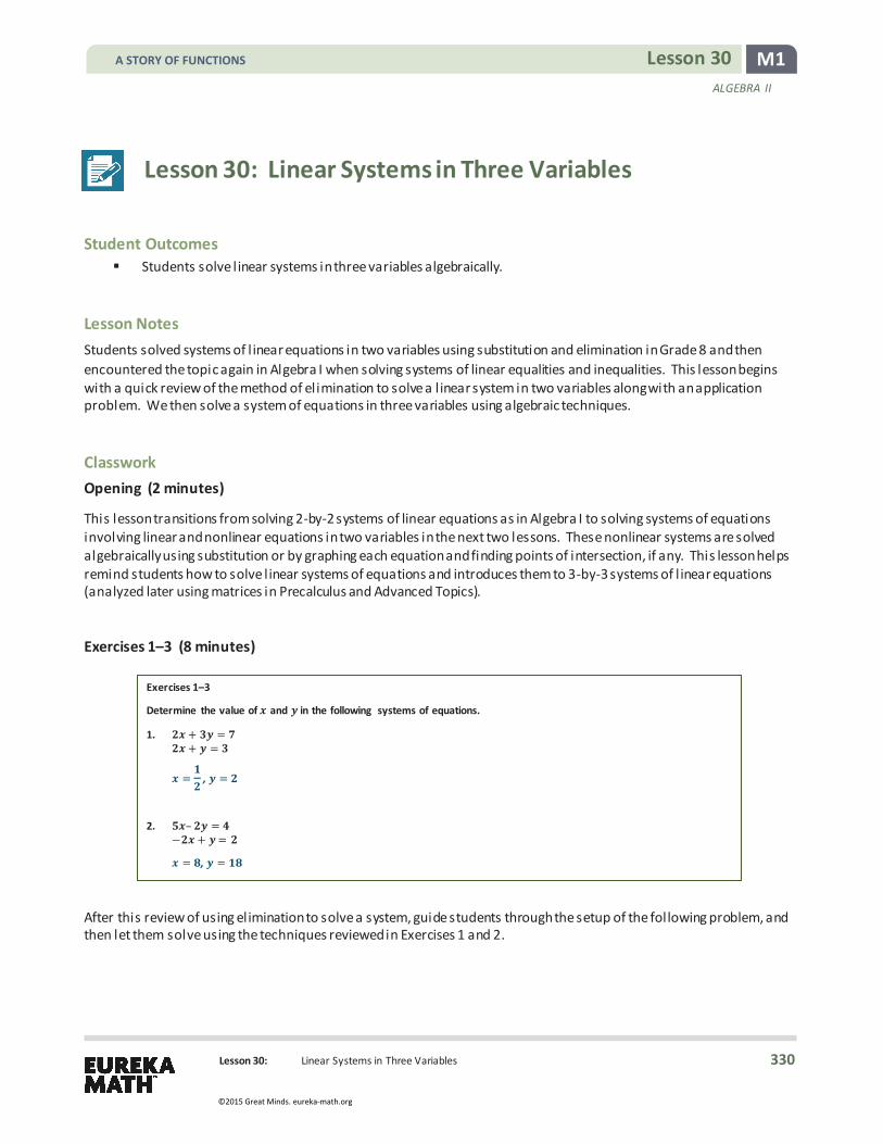
M1 Lesson 30 ALGEBRA II
Lesson 30: Linear Systems in Three Variables
Lesson 30: Linear Systems in Three Variables
Student Outcomes
� Students solve l inear systems in three variables algebraically.
Lesson Notes Students solved systems of l inear equations in two variables using substitution and elimination in Grade 8 and then encountered the topic again in Algebra I when solving systems of linear equalities and inequalities. This lesson begins with a quick review of the method of elimination to solve a l inear system in two variables along with an application problem. We then solve a system of equations in three variables using algebraic techniques.
Classwork Opening (2 minutes)
This lesson transitions from solving 2-by-2 systems of linear equations as in Algebra I to solving systems of equations involving linear and nonlinear equations in two variables in the next two lessons. These nonlinear systems are solved algebraically using substitution or by graphing each equation and finding points of intersection, if any. This lesson helps remind students how to solve l inear systems of equations and introduces them to 3-by-3 systems of l inear equations (analyzed later using matrices in Precalculus and Advanced Topics).
Exercises 1–3 (8 minutes) Exercises 1–3
Determine the value of and in the following systems of equations.
1. + = + =
= , =
2. – = − + =
= , =
After this review of using elimination to solve a system, guide students through the setup of the following problem, and then let them solve using the techniques reviewed in Exercises 1 and 2.
A STORY OF FUNCTIONS
330
©2015 Great Minds. eureka-math.org

M1 Lesson 30 ALGEBRA II
Lesson 30: Linear Systems in Three Variables
3. A scientist wants to create of a solution that is % acidic. To create this solution, she has access to a % solution and a % solution. How many milliliters of each solution should she combine to create the % solution?
Solve this problem using a system of two equations in two variables. Solution:
Milliliters of % solution: Milliliters of % solution:
Write one equation to represent the total amounts of each solution needed:
+ = .
Since % of is , we can write one equation to model the acidic portion:
. + . = .
Writing these two equations as a system:
+ =
. + . =
To solve, multiply both sides of the top equation by either . to eliminate or . to eliminate . The following steps will eliminate :
. ( + ) = . ( ) . + . =
which gives
. + . =
. + . = .
Replacing the top equation with the difference between the bottom equation and top equation results in a new system with the same solutions:
. = . + . = .
The top equation can quickly be solved for ,
= ,
and substituting = back into the original first equation allows us to find :
+ = = .
Thus, we need of the % solution and of the % solution.
A STORY OF FUNCTIONS
331
©2015 Great Minds. eureka-math.org

M1 Lesson 30 ALGEBRA II
Lesson 30: Linear Systems in Three Variables
Scaffolding: Ask students if they can eliminate two of the variables from either equation. (They cannot.) Have a discussion around what that means graphically. (The graph of the solution set is a line, not a point, so there is no single solution to the system.)
Discussion (5 minutes)
� In the previous exercises we solved systems of two linear equations in two variables using the method of elimination. However, what if we have three variables? For example, what are the solutions to the following system of equations?
2𝑥𝑥 + 3𝑦𝑦 − = 5 4𝑥𝑥 −𝑦𝑦 − = −1
Allow students time to work together and struggle with this system and realize that they cannot find a unique solution. Include the following third equation, and ask students if they can solve it now.
𝑥𝑥+ 4𝑦𝑦+ = 12
Give students an opportunity to consider solutions or other ideas on how to begin the process of solving this system. After considering their suggestions and providing feedback, guide them through the process in the example below.
Example (9 minutes)
Example
Determine the values for , , and in the following system:
+ − = (1) − − = − (2)
+ + = (3)
Suggest numbering the equations as shown above to help organize the process.
� Eliminate from equations (1) and (2) by subtraction. Replace equation (1) with the result.
2𝑥𝑥+ 3𝑦𝑦− = 5 −(4𝑥𝑥−𝑦𝑦 − ) = −(−1)
−2𝑥𝑥 + 4𝑦𝑦= 6
� Our goal is to find two equations in two unknowns. Thus, we will also eliminate from equations (2) and (3) by adding as follows. Replace equation (3) with the result.
4𝑥𝑥−𝑦𝑦 − = −1 𝑥𝑥+ 4𝑦𝑦+ = 12
5𝑥𝑥 + 3𝑦𝑦= 11
� Our new system of three equations in three variables has two equations with only two variables in them:
−2𝑥𝑥+ 4𝑦𝑦 = 6
4𝑥𝑥−𝑦𝑦 − = −1
5𝑥𝑥 + 3𝑦𝑦= 11.
MP.1
A STORY OF FUNCTIONS
332
©2015 Great Minds. eureka-math.org

M1 Lesson 30 ALGEBRA II
Lesson 30: Linear Systems in Three Variables
� These two equations now give us a system of two equations in two variables, which we reviewed how to solve in Exercises 1–2.
−2𝑥𝑥+ 4𝑦𝑦 = 6 5𝑥𝑥+ 3𝑦𝑦 = 11
At this point, let students solve this individually or with partners, or guide them through the process if necessary.
� To get matching coefficients, we need to multiply both equations by a constant:
5(−2𝑥𝑥+ 4𝑦𝑦) = 5(6) 2(5𝑥𝑥 + 3𝑦𝑦) = 2(11)
−10𝑥𝑥+ 20𝑦𝑦= 30 10𝑥𝑥 + 6𝑦𝑦= 22.
� Replacing the top equation with the sum of the top and bottom equations together gives the following:
26𝑦𝑦= 52 10𝑥𝑥 + 6𝑦𝑦= 22.
� The new top equation can be solved for 𝑦𝑦:
𝑦𝑦= 2.
� Replace 𝑦𝑦 = 2 in one of the equations to find 𝑥𝑥:
5𝑥𝑥 + 3(2) = 11 5𝑥𝑥 + 6 = 11
5𝑥𝑥 = 5 𝑥𝑥 = 1.
� Replace 𝑥𝑥 = 1 and 𝑦𝑦 = 2 in any of the original equations to find :
2(1) + 3(2)− = 5 2 + 6 − = 5
8 − = 5 = 3.
� The solution, 𝑥𝑥 = 1, 𝑦𝑦 = 2, and = 3, can be written compactly as an ordered triple of numbers (1,2, 3).
Consider pointing out to students that the point (1,2, 3) can be thought of as a point in a three-dimensional coordinate plane, and that it is, l ike a two-by-two system of equations, the intersection point in three-space of the three planes given by the graphs of each equation. These concepts are not the point of this lesson, so addressing them is optional.
Point out that a l inear system involving three variables requires three equations in order for the solution to possibly be a single point.
The following problems provide examples of situations that require solving systems of equations in three variables.
A STORY OF FUNCTIONS
333
©2015 Great Minds. eureka-math.org
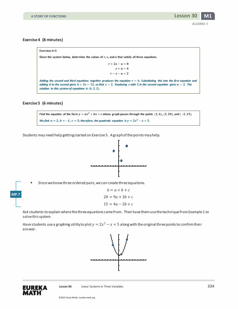
M1 Lesson 30 ALGEBRA II
Lesson 30: Linear Systems in Three Variables
Exercise 4 (8 minutes) Exercises 4–5
Given the system below, determine the values of , s, and that satisfy all three equations.
+ − = + =
− − =
Adding the second and third equations together produces the equation = . Substituting this into the first equation and adding it to the second gives + = , so that = . Replacing with in the second equation gives = . The solution to this system of equations is ( , , ).
Exercise 5 (6 minutes) Find the equation of the form = + + whose graph passes through the points ( , ), ( , ), and (− , ).
We find = , = − , = ; therefore, the quadratic equation is = − + .
Students may need help getting started on Exercise 5. A graph of the points may help.
� Since we know three ordered pairs, we can create three equations.
6 = 𝑎𝑎 + 𝑏𝑏 + 𝑐𝑐
20 = 9𝑎𝑎 + 3𝑏𝑏+ 𝑐𝑐
15 = 4𝑎𝑎 − 2𝑏𝑏+ 𝑐𝑐
Ask students to explain where the three equations came from. Then have them use the technique from Example 1 to solve this system.
Have students use a graphing utility to plot 𝑦𝑦 = 2𝑥𝑥2 − 𝑥𝑥 + 5 along with the original three points to confirm their answer.
MP.7
A STORY OF FUNCTIONS
334
©2015 Great Minds. eureka-math.org

M1 Lesson 30 ALGEBRA II
Lesson 30: Linear Systems in Three Variables
Closing (2 minutes)
� We’ve seen that in order to find a single solution to a system of equations in two variables, we need to have two equations, and in order to find a single solution to a system of equations in three variables, we need to have three equations. How many equations do you expect we will need to find a single solution to a system of equations in four variables? What about five variables?
à It seems that we will need four equations in four variables to find a single solution, and that we will need five equations in five variables to find a single solution.
Exit Ticket (5 minutes)
A STORY OF FUNCTIONS
335
©2015 Great Minds. eureka-math.org

M1 Lesson 30 ALGEBRA II
Lesson 30: Linear Systems in Three Variables
Name Date
Lesson 30: Linear Systems in Three Variables
Exit Ticket For the following system, determine the values of 𝑝𝑝, 𝑞𝑞, and 𝑟𝑟 that satisfy all three equations:
2𝑝𝑝 + 𝑞𝑞 − 𝑟𝑟 = 8 𝑞𝑞 + 𝑟𝑟 = 4 𝑝𝑝 −𝑞𝑞 = 2.
A STORY OF FUNCTIONS
336
©2015 Great Minds. eureka-math.org

M1 Lesson 30 ALGEBRA II
Lesson 30: Linear Systems in Three Variables
Exit Ticket Sample Solutions
For the following system, determine the values of , , and that satisfy all three equations:
+ − = + = − = .
= , = , = , or equivalently ( , , )
Problem Set Sample Solutions
Solve the following systems of equations.
1. + = + = + =
= , = , = or ( , , )
2. = ( − ) = ( − )
+ = −
= , = , = , or ( , , )
3. + + = − = −
+ =
= − , = , = or (− , , )
4. + − = − − + = + + =
= , = − , = or � ,− , �
5. + + = − + =
− + − =
= , = , = − or � , ,− �
6. − =
+ = − − = −
= − , = − , = or (− ,− , )
7. = ( − ) = ( − ) + = +
= , = , = or ( , , )
8. + + = + =
− − = −
= , = , = − or ( , ,− )
9. + + =
+ =
− = −
= , = , = or � , , �
10. + + =
+ =
− = −
= , = , = or � , , �
A STORY OF FUNCTIONS
337
©2015 Great Minds. eureka-math.org

M1 Lesson 30 ALGEBRA II
Lesson 30: Linear Systems in Three Variables
11. Find the equation of the form = + + whose graph passes through the points ( ,− ), ( , ), and (− , ).
= − −
12. Show that for any number , the values = + , = − , and = + are solutions to the system of equations below.
+ = + =
(In this situation, we say that parameterizes the solution set of the system.)
+ = ( + ) + ( − ) = + = ( − ) + ( + ) =
13. Some rational expressions can be written as the sum of two or more rational expressions whose denominators are the factors of its denominator (called a partial fraction decomposition). Find the partial fraction decomposition for
( ) by finding the value of that makes the equation below true for all except and − .
( + )= −
+
Adding to both sides of the equations, we have
= ( + ) + ( + )
= ( + ) + ( + )
=( + )( + )
=
so = and thus ( )
= − .
14. A chemist needs to make of a % acid solution. He has a % acid solution and a % acid solution on hand. If he uses the % and % solutions to create the % solution, how many ml of each does he need?
He needs of the % solution and of the % solution.
15. An airplane makes a -mile trip against a head wind in hours. The return trip takes . hours, the wind now being a tail wind. If the plane maintains a constant speed with respect to still air, and the speed of the wind is also constant and does not vary, find the still-air speed of the plane and the speed of the wind.
The speed of the plane in still wind is , and the speed of the wind is .
16. A restaurant owner estimates that she needs the same number of pennies as nickels and the same number of dimes as pennies and nickels together. How should she divide $ between pennies, nickels, and dimes?
She will need dimes ($ worth), nickels ($ worth), and pennies ($ worth) for a total of $ .
A STORY OF FUNCTIONS
338
©2015 Great Minds. eureka-math.org

M1 Lesson 31 ALGEBRA II
Lesson 31: Systems of Equations
Lesson 31: Systems of Equations
Student Outcomes
� Students solve systems of linear equations in two variables and systems of a l inear and a quadratic equation in two variables.
� Students understand that the points at which the two graphs of the equations intersect correspond to the solutions of the system.
Lesson Notes Students review the solution of systems of linear equations, move on to systems of equations that represent a line and a circle and systems that represent a l ine and a parabola, and make conjectures as to how many points of intersection there can be in a given system of equations. They sketch graphs of a circle and a line to visualize the solution to a system of equations, solve the system algebraically, and note the correspondence between the solution and the intersection. Then they do the same for graphs of a parabola and a line.
The principal standards addressed in this lesson are A-REI.C.6 (solve systems of l inear equations exactly and approximately, e.g., with graphs, focusing on pairs of l inear equations in two variables) and A-REI.C.7 (solve a simple system consisting of a l inear equation and a quadratic equation in two variables algebraically and graphically). The standards MP.5 (use appropriate tools strategically) and MP.8 (look for and express regularity in repeated reasoning) are also addressed.
Materials Graph paper, straightedge, compass, and a tool for displaying graphs (e.g., projector, interactive white board, white board, chalk board, or squared poster paper)
Classwork Exploratory Challenge 1 (8 minutes)
In this exercise, students review ideas about systems of l inear equations from Module 4 in Grade 8 (A-REI.C.6). Consider distributing graph paper for students to use throughout this lesson. Begin by posing the following problem for students to work on individually:
Exploratory Challenge 1
a. Sketch the lines given by + = and − + = on the same set of axes to solve the system graphically. Then solve the system of equations algebraically to verify your graphical solution.
Scaffolding: Circulate to identify students who might be asked to display their sketches and solutions.
A STORY OF FUNCTIONS
339
©2015 Great Minds. eureka-math.org

M1 Lesson 31 ALGEBRA II
Lesson 31: Systems of Equations
Once students have made a sketch, ask one of them to use the display tool and draw the two graphs for the rest of the class to see. While the student is doing that, ask the other students how many points are shared (one) and what the coordinates of that point are.
The point ( , ) should be easily identifiable from the sketch. See the graph to the right.
Solving each equation for gives the system
= − + = + .
This leads to the single-variable equation
− + = + = = = − + = .
Thus, the solution is the point ( , ).
Point out that in this case, there is one solution. Now change the problem as follows. Then discuss the question as a class, and ask one or two students to show their sketches using the display tool.
b. Suppose the second line is replaced by the line with equation + = . Plot the two lines on the same set of axes, and solve the
pair of equations algebraically to verify your graphical solution.
The lines are parallel, and there is no point in common. See the graph to the right.
If we try to solve the system algebraically, we have
= − + = − + ,
which leads to the single-variable equation
− + = − + = .
Since = is not a true number sentence, the system has no solution.
Point out that in this case, there is no solution. Now change the problem again as follows, and again discuss the question as a class. Then ask one or two students to show their sketches using the display tool.
A STORY OF FUNCTIONS
340
©2015 Great Minds. eureka-math.org

M1 Lesson 31 ALGEBRA II
Lesson 31: Systems of Equations
c. Suppose the second line is replaced by the line with equation = − . Plot the lines on the same set of axes, and solve the pair of equations algebraically to verify your graphical solution.
The lines coincide, and they have all points in common. See the graph to the right.
Algebraically, we have the system
= − + = − + ,
which leads to the equation
− + = − + = .
Thus all points ( ,− + ) are solutions to the system.
Point out that in this third case, there are infinitely many solutions. Discuss the following problem as a class.
d. We have seen that a pair of lines can intersect in , , or an infinite number of points. Are there any other possibilities?
No. Students should convince themselves and each other that these three options exhaust the possibilities for the intersection of two lines.
Exploratory Challenge 2 (12 minutes)
In this exercise, students move on to a system of a l inear and a quadratic equation (A-REI.C.6). Begin by asking students to work in pairs to sketch graphs and develop conjectures about the following item:
Exploratory Challenge 2
a. Suppose that instead of equations for a pair of lines, you were given an equation for a circle and an equation for a line. What possibilities are there for the two figures to intersect? Sketch a graph for each possibility.
Once students have made their sketches, ask one pair to use the display tool and draw the graphs for the rest of the class to see.
They can intersect in , , or points as shown below.
Scaffolding: � Circulate to assist pairs of
students who might be having trouble coming up with all three possibilities.
� For students who are ready, ask them to write equations for the graphs they have sketched.
A STORY OF FUNCTIONS
341
©2015 Great Minds. eureka-math.org

M1 Lesson 31 ALGEBRA II
Lesson 31: Systems of Equations
Next, students should continue to work in pairs to sketch graphs and develop conjectures about the following item (A-REI.C.6):
b. Graph the parabola with equation = . What possibilities are there for a line to intersect the parabola? Sketch each possibility.
Once students have made their sketches, ask one pair to use the display tool and draw the graphs for the rest of the class to see.
The parabola and line can intersect in , , or points as shown below. Note that, in contrast to the circle, where all the lines intersecting the circle in one point are tangent to it, lines intersecting the parabola in one point are either tangent to it or are parallel to the parabola’s axis of symmetry—in this case, the -axis.
Next, ask students to work on the following problem individually (A-REI.C.7):
c. Sketch the circle given by + = and the line given by = + on the same set of axes. One solution to the pair of equations is easily identifiable from the sketch. What is it?
The point (− , ) should be easily identifiable from the sketch, but the other point is not.
Scaffolding: Circulate again to assist pairs of students who might be having trouble coming up with all three possibilities.
A STORY OF FUNCTIONS
342
©2015 Great Minds. eureka-math.org

M1 Lesson 31 ALGEBRA II
Lesson 31: Systems of Equations
Once students have made a sketch, ask one of them to use the display tool to draw the two graphs for the rest of the class to see. While the student is doing that, ask the other students how many points are shared (two) and what the coordinates of those points are.
Students should see that they can substitute the value for 𝑦𝑦 in the second equation into the first equation. In other words, they need to solve the following quadratic equation (A-REI.B.4).
d. Substitute = + into the equation + = , and solve the resulting equation for .
Factoring or using the quadratic formula, students should find that the solutions to + ( + ) = are − and − .
e. What does your answer to part (d) tell you about the intersections of the circle and the line from part (c)?
There are two intersections of the line and the circle. When = − , then = , as the sketch shows, so (− , ) is a solution. When = − , then = �− �+ = , so �− , � is another solution.
Note that the problem above does not explicitly tell students to look for intersection points. Thus, the exercise assesses not only whether they can solve the system but also whether they understand that the intersection points of the graphs correspond to solutions of the system.
Students should understand that to solve the system of equations, they look for points that l ie on the l ine and the circle. The points that l ie on the circle are precisely those that satisfy 𝑥𝑥2+ 𝑦𝑦2 = 1, and the points that l ie on the l ine are those that satisfy 𝑦𝑦 = 2𝑥𝑥 + 2. So points on both are in the intersection.
Exercise 1 (8 minutes)
Pose the following three-part problem for students to work on individually, and then discuss as a class.
Exercises
1. Draw a graph of the circle with equation + = .
a. What are the solutions to the system of circle and line when the circle is given by + = , and the line is given by = ?
Substituting = in the equation of the circle yields + = , so = , and = √ or = −√ . The solutions are (−√ , ) and (√ , ).
A STORY OF FUNCTIONS
343
©2015 Great Minds. eureka-math.org
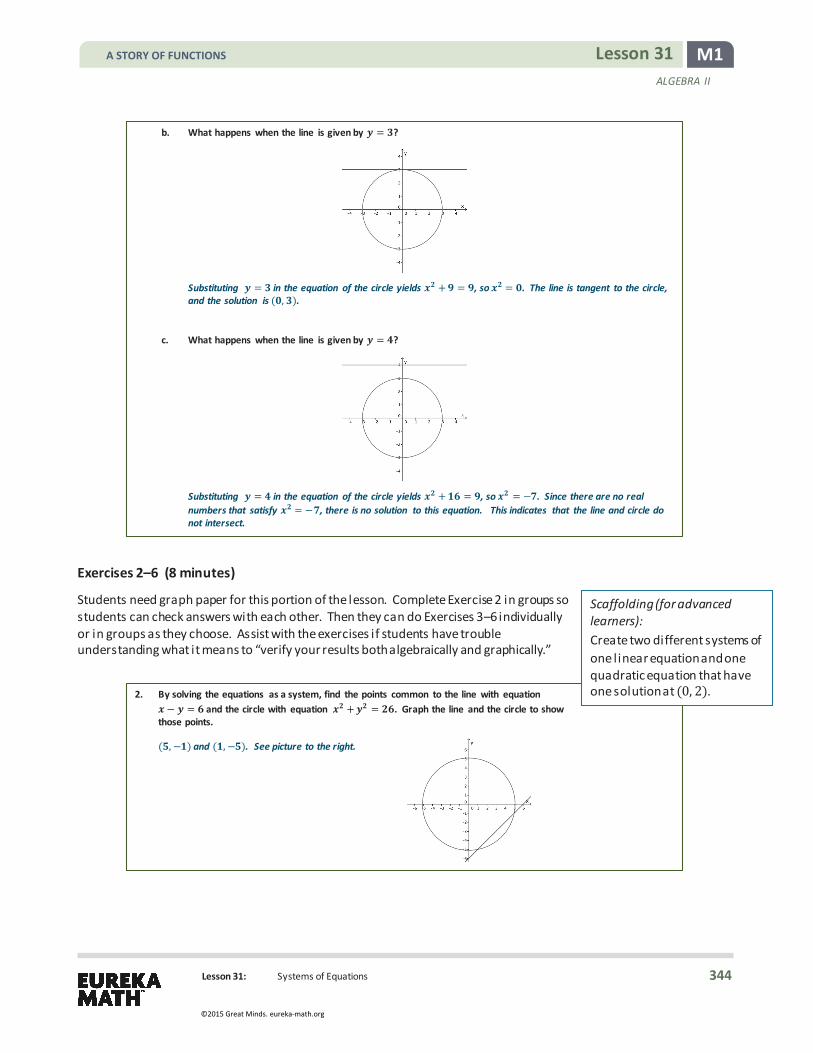
M1 Lesson 31 ALGEBRA II
Lesson 31: Systems of Equations
b. What happens when the line is given by = ?
Substituting = in the equation of the circle yields + = , so = . The line is tangent to the circle, and the solution is ( , ).
c. What happens when the line is given by = ?
Substituting = in the equation of the circle yields + = , so = − . Since there are no real numbers that satisfy = − , there is no solution to this equation. This indicates that the line and circle do not intersect.
Exercises 2–6 (8 minutes)
Students need graph paper for this portion of the lesson. Complete Exercise 2 in groups so students can check answers with each other. Then they can do Exercises 3–6 individually or in groups as they choose. Assist with the exercises if students have trouble understanding what it means to “verify your results both algebraically and graphically.”
2. By solving the equations as a system, find the points common to the line with equation − = and the circle with equation + = . Graph the line and the circle to show
those points.
( ,− ) and ( ,− ). See picture to the right.
Scaffolding (for advanced learners): Create two different systems of one l inear equation and one quadratic equation that have one solution at (0, 2).
A STORY OF FUNCTIONS
344
©2015 Great Minds. eureka-math.org

M1 Lesson 31 ALGEBRA II
Lesson 31: Systems of Equations
3. Graph the line given by + = and the circle given by + = . Find all solutions to the system of equations.
There is no real solution; the line and circle do not intersect. See picture to the right.
4. Graph the line given by + = and the circle given by + = . Find all solutions to the system of equations. Verify your result both algebraically and graphically.
The line is tangent to the circle at ( , ), which is the only solution. See picture to the right.
5. Graph the line given by + = and the circle given by + = . Find all solutions to the system of equations. Verify your result both algebraically and graphically.
The line and circle intersect at (− , ) and � ,− �, which are the two solutions. See picture to the right.
6. Graph the line given by + = − and the quadratic curve given by = − . Find all solutions to the system of equations. Verify your result both algebraically and graphically.
The line and the parabola intersect at ( ,− ) and (− , ), which are the two solutions. See picture to the right.
A STORY OF FUNCTIONS
345
©2015 Great Minds. eureka-math.org

M1 Lesson 31 ALGEBRA II
Lesson 31: Systems of Equations
Closing (4 minutes)
Ask students to respond to these questions with a partner or in writing. Share their responses as a class.
� How does graphing a line and a quadratic curve help you solve a system consisting of a linear and a quadratic equation?
� What are the possibilities for the intersection of a l ine and a quadratic curve, and how are they related to the number of solutions of a system of l inear and quadratic equations?
Present and discuss the Lesson Summary.
Be sure to note that in the case of the circle, the reverse process of solving the equation for the circle first—for either 𝑥𝑥 or 𝑦𝑦—and then substituting in the l inear equation would have yielded an equation with a complicated radical expression and might have led students to miss part of the solution by considering only the positive square root.
Exit Ticket (5 minutes)
MP.1
Scaffolding: Perhaps create a chart with the summary that can serve as a reminder to students.
Lesson Summary
Here are some steps to consider when solving systems of equations that represent a line and a quadratic curve.
1. Solve the linear equation for in terms of . This is equivalent to rewriting the equation in slope-intercept form. Note that working with the quadratic equation first would likely be more difficult and might cause the loss of a solution.
2. Replace in the quadratic equation with the expression involving from the slope-intercept form of the linear equation. That will yield an equation in one variable.
3. Solve the quadratic equation for .
4. Substitute into the linear equation to find the corresponding value of . 5. Sketch a graph of the system to check your solution.
A STORY OF FUNCTIONS
346
©2015 Great Minds. eureka-math.org

M1 Lesson 31 ALGEBRA II
Lesson 31: Systems of Equations
Name Date
Lesson 31: Systems of Equations
Exit Ticket Make and explain a prediction about the nature of the solution to the following system of equations, and then solve the system.
𝑥𝑥2 + 𝑦𝑦2 = 25 4𝑥𝑥 + 3𝑦𝑦= 0
Il lustrate with a graph. Verify your solution, and compare it with your initial prediction.
A STORY OF FUNCTIONS
347
©2015 Great Minds. eureka-math.org

M1 Lesson 31 ALGEBRA II
Lesson 31: Systems of Equations
Exit Ticket Sample Solutions
Make and explain a prediction about the nature of the solution to the following system of equations, and then solve the system.
+ = + =
Illustrate with a graph. Verify your solution, and compare it with your initial prediction.
Prediction: By inspecting the equations, students should conclude that the circle is centered at the origin, and that the line goes through the origin. So, the solution should consist of two points.
Solution: Solve the linear equation for one of the variables: = − .
Substitute that variable in the quadratic equation: + �− � = .
Remove parentheses and combine like terms: − = , so − = .
Solve the quadratic equation in : ( + )( − ) = , which gives the roots and − .
Substitute into the linear equation: If = , then = − ; if = − , then = .
As the graph shows, the solution is the two points of intersection of the circle and the line: ( ,− ) and (− , ).
An alternative solution would be to solve the linear equation for instead of , getting the quadratic equation ( + )( − ) = , which gives the roots and − and the same points of intersection.
As noted before, solving the quadratic equation for or first is not a good procedure. It can lead to a complicated radical expression and loss of part of the solution.
Problem Set Sample Solutions Problem 4 yields a system with no real solution, and the graph shows that the circle and l ine have no point of intersection in the coordinate plane. In Problems 5 and 6, the curve is a parabola. In Problem 5, the l ine intersects the parabola in two points, whereas in Problem 6, the l ine is tangent to the parabola, and there is only one point of intersection. Note that there would also have been only one point of intersection if the l ine had been the l ine of symmetry of the parabola.
1. Where do the lines given by = + and = + intersect?
Since we do not know the value of , we cannot solve this problem by graphing, and we will have to approach it algebraically. Eliminating gives the equation
+ = + = − .
Since = − , we have = + = ( − ) + = − . Thus, the lines intersect at the point ( − , − ).
A STORY OF FUNCTIONS
348
©2015 Great Minds. eureka-math.org

M1 Lesson 31 ALGEBRA II
Lesson 31: Systems of Equations
2. Find all solutions to the following system of equations.
( − ) + ( + ) = − =
Illustrate with a graph. Solve the linear equation for one of the variables: = + . Substitute that variable in the quadratic equation: ( + − ) + ( + ) = . Rewrite the equation in standard form: + + = . Solve the quadratic equation: ( + )( + ) = , so
= − or = − . If = − , then = . If = − , then = . As the graph shows, the solution is the two points ( ,− ) and ( ,− ).
3. Find all solutions to the following system of equations.
+ = − + − − =
Illustrate with a graph. Solve the linear equation for one of the variables: = − . Substitute that variable in the quadratic equation: (− ) − (− ) + − − = . Rewrite the equation in standard form: + − = . Solve the quadratic equation: ( − )( + ) = , so = or
= − .
If = , then = − . If = − , then = .
As the graph shows, the solutions are the two points: �− , � and ( ,− ).
4. Find all solutions to the following system of equations.
+ = ( + ) + ( − ) =
Illustrate with a graph.
Solve the linear equation for one of the variables: = − . Substitute that variable in the quadratic equation: ( − + ) + ( − ) = . Rewrite the equation in standard form: − + = . Solve the equation using the quadratic formula:
=+ √ −
or =−√ −
.
So we have = + √− or = −√− . Therefore, there is no real solution to the system. As the graph shows, the line and circle do not intersect.
A STORY OF FUNCTIONS
349
©2015 Great Minds. eureka-math.org

M1 Lesson 31 ALGEBRA II
Lesson 31: Systems of Equations
5. Find all solutions to the following system of equations.
= − + = − +
Illustrate with a graph.
The linear equation is already solved for one of the variables: = − + .
Substitute that variable in the quadratic equation: − + = − + .
Rewrite the equation in standard form: − = .
Solve the quadratic equation: ( − ) = .
So, = or = .
If = , then = . If = , then = − .
As the graph shows, the solutions are the two points ( , ) and ( ,− ).
6. Find all solutions to the following system of equations.
− + + − = = +
Illustrate with a graph.
Solve the second equation for : = − .
Substitute in the first equation: − + + − − = .
Combine like terms: − + − = .
Rewrite the equation in standard form and factor: −( − ) = .
Therefore, = . Then = − , so = .
There is only one solution ( , ), and as the graph shows, the line is tangent to the parabola.
An alternative solution would be to solve the linear equation for instead of , getting the quadratic equation ( − )( − ) = , which gives the repeated root = and the same point of tangency ( , ).
Another alternative solution would be to solve the quadratic equation for , so that = − + . Substituting in the linear equation would yield = − + + . Converting that to standard form would give
− + = , which gives the repeated root = , as in the first solution. Note that in this case, unlike when the graph of the quadratic equation is a circle, the quadratic equation can be solved for in terms of without getting a radical expression.
A STORY OF FUNCTIONS
350
©2015 Great Minds. eureka-math.org

M1 Lesson 31 ALGEBRA II
Lesson 31: Systems of Equations
7. Find all values of so that the following system has two solutions.
+ = =
Illustrate with a graph.
The center of the circle is the origin, and the line is parallel to the -axis. Therefore, as the graph shows, there are two solutions only when − < < .
8. Find all values of so that the following system has exactly one solution.
= − ( − ) =
Illustrate with a graph.
The parabola opens down, and its axis of symmetry is the vertical line = . The line = is a horizontal line and will intersect the parabola in either two, one, or no points. It intersects the parabola in one point only if it passes through the vertex of the parabola, which is = .
A STORY OF FUNCTIONS
351
©2015 Great Minds. eureka-math.org
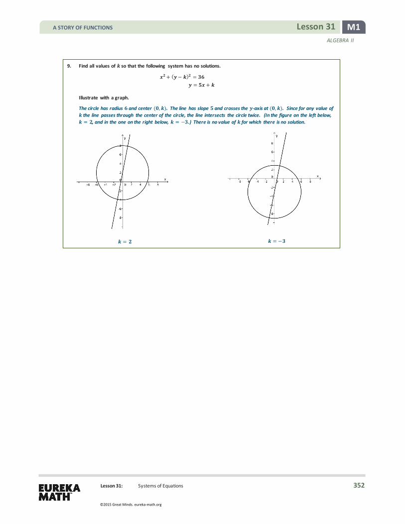
M1 Lesson 31 ALGEBRA II
Lesson 31: Systems of Equations
9. Find all values of so that the following system has no solutions.
+ ( − ) = = +
Illustrate with a graph.
The circle has radius and center ( , ). The line has slope and crosses the -axis at ( , ). Since for any value of the line passes through the center of the circle, the line intersects the circle twice. (In the figure on the left below, = , and in the one on the right below, = − .) There is no value of for which there is no solution.
=
= −
A STORY OF FUNCTIONS
352
©2015 Great Minds. eureka-math.org

M1 Lesson 32 ALGEBRA II
Lesson 32: Graphing Systems of Equations
Lesson 32: Graphing Systems of Equations
Student Outcomes
� Students develop facility with graphical interpretations of systems of equations and the meaning of their solutions on those graphs. For example, they can use the distance formula to find the distance between the centers of two circles and thereby determine whether the circles intersect in 0, 1, or 2 points.
� By completing the squares, students can convert the equation of a circle in general form to the center-radius form and, thus, find the radius and center. They can also convert the center-radius form to the general form by removing parentheses and combining like terms.
� Students understand how to solve and graph a system consisting of two quadratic equations in two variables.
Lesson Notes This lesson is an extension that goes beyond what is required in the standards. In particular, the standard A-REI.C.7 (solve a simple system consisting of a l inear equation and a quadratic equation in two variables algebraically and graphically) does not extend to a system of two quadratic equations, which is a natural culmination of the types of systems formed by l inear and quadratic equations. The lesson also addresses standard MP.8 (look for and express regularity in repeated reasoning).
The lesson begins with a brief review of the distance formula, and its connection both to the Pythagorean theorem and to the center-radius equation of a circle. The distance formula is used extensively in the next few lessons, so be sure to review it with students. Students also briefly review how to solve and graph a system of a l inear equation and an equation of a circle. They then move to the main focus of the lesson, which is graphing and solving systems of pairs of quadratic equations whose graphs include parabolas as well as circles
Materials This lesson requires use of graphing calculators or computer software, such as the Wolfram Alpha engine, the GeoGebra package, or the Geometer’s Sketchpad software for graphing geometric figures, plus a tool for displaying graphs, such as a projector, smart board, white board, chalk board, or squared poster paper.
Classwork Opening (1 minute)
Begin with questions that should remind students of the distance formula and how it is connected to the Pythagorean theorem.
� Suppose you have a point with coordinates (1, 3). Find the distance if has coordinates:
1. (4,2)
Answer: = √10
2. (−3,1)
Answer: = 2√5
3. (𝑥𝑥,𝑦𝑦)
Answer: = (𝑥𝑥− 1)2 + (𝑦𝑦 − 3)2
A STORY OF FUNCTIONS
353
©2015 Great Minds. eureka-math.org

M1 Lesson 32 ALGEBRA II
Lesson 32: Graphing Systems of Equations
If students cannot recall the distance formula (in the coordinate plane), they may need to be reminded of it.
If and are points with coordinates (𝑥𝑥1,𝑦𝑦1) and (𝑥𝑥2,𝑦𝑦2), then the distance between them is the length . Draw horizontal and vertical l ines through and to intersect in point and form right triangle . The length of the horizontal side is the difference in the 𝑥𝑥-coordinates |𝑥𝑥2 − 𝑥𝑥1|, and the length of the vertical side is the difference in the 𝑦𝑦-coordinates |𝑦𝑦2 −𝑦𝑦1|. The Pythagorean theorem gives the length of the hypotenuse as ( )2 = (𝑥𝑥2 − 𝑥𝑥1)2+ (𝑦𝑦2 −𝑦𝑦1)2. Taking the square root gives the distance formula.
Opening Exercise (3 minutes)
Make sure the students all have access to, and familiarity with, some technology (calculator or computer software) for graphing lines and circles in the coordinate plane. Have them work individually on the following exercise.
Opening Exercise
Given the line = , is there a point on the line at a distance from ( , )? Explain how you know.
Yes, there are two such points. They are the intersection of the line = and the circle ( − ) + ( − ) = . (The intersection points are roughly ( . , . ) and ( . , . ).)
Draw a graph showing where the point is.
There are actually two such points. See the graph below.
Students should compare the graph they have drawn with that of a neighbor.
Scaffolding: Circulate to identify and help students who might have trouble managing the graphing tool.
THE DISTANCE FORMULA: Given two points (𝑥𝑥1,𝑦𝑦1) and (𝑥𝑥2,𝑦𝑦2), the distance between these points is given by the formula
= ( − ) + ( − ) .
A STORY OF FUNCTIONS
354
©2015 Great Minds. eureka-math.org

M1 Lesson 32 ALGEBRA II
Lesson 32: Graphing Systems of Equations
Exercise 1 (5 minutes)
This exercise reviews the solution of a simple system consisting of a linear equation and the equation of a circle from the perspective of the defining property of a circle (A-REI.C.7).
Exercise 1
Solve the system ( − ) + ( − ) = and = + .
Substituting + for in the quadratic equation allows us to find the -coordinates.
( − ) + ( + )− = ( − + ) + =
− − = ( − )( + ) =
So, = or = − , and the intersection points are �− , � and ( , ).
What are the coordinates of the center of the circle?
( , )
What can you say about the distance from the intersection points to the center of the circle?
Because they are points on the circle and the radius of the circle is , the intersection points are units away from the center. This can be verified by the distance formula.
Using your graphing tool, graph the line and the circle.
See the graph below.
Example 1 (5 minutes)
It is important to keep in mind that not all quadratic equations in two variables represent circles.
A STORY OF FUNCTIONS
355
©2015 Great Minds. eureka-math.org

M1 Lesson 32 ALGEBRA II
Lesson 32: Graphing Systems of Equations
Example 1
Rewrite + − + = − by completing the square in both and . Describe the circle represented by this equation.
Rearranging terms gives − + + = − .
Then, completing the square in both and , we have
( − + ) + ( + + ) = − + + ( − ) + ( + ) = .
This is the equation of a circle with center ( ,− ) and radius .
Using your graphing tool, graph the circle.
See the graph to the right.
In contrast, consider the following equation: + − − = − .
Rearranging terms gives − + − = − .
Then, completing the square in both and , we have
( − + ) + ( − + ) = − + + ( − ) + ( − ) = − ,
which is not a circle because then the radius would be √− .
What happens when you use your graphing tool with this equation?
The tool cannot draw the graph. There are no points in the plane that satisfy this equation, so the graph is empty.
Exercise 2 (5 minutes)
Allow students time to think these questions over, draw some pictures, and discuss with a partner before discussing as a class.
Exercise 2
Consider a circle with radius and another circle with radius . Let represent the distance between the two centers. We want to know how many intersections there are of these two circles for different values of . Draw figures for each case.
a. What happens if = ?
If the distance is , then the circles touch at only one point. We say that the circles are externally tangent.
b. What happens if = ?
If the distance is , the circles do not intersect, and neither circle is inside the other.
c. What happens if = ?
If the distance is , the circles do not intersect, but one circle lies inside the other.
A STORY OF FUNCTIONS
356
©2015 Great Minds. eureka-math.org

M1 Lesson 32 ALGEBRA II
Lesson 32: Graphing Systems of Equations
d. What happens if = ?
If the distance is , the circles touch at only one point, with one circle inside the other. We say that the circles are internally tangent.
e. For which values of do the circles intersect in exactly one point? Generalize this result to circles of any radius.
If = or = , the circles are tangent. In general, if is either the sum or the difference of the radii, then the circles are tangent.
f. For which values of do the circles intersect in two points? Generalize this result to circles of any radius.
If < < , the circles intersect in two points. In general, if is between the sum and the difference of the radii, then the circles intersect in two points.
g. For which values of do the circles not intersect? Generalize this result to circles of any radius.
The circles do not intersect if < or > . In general, if is smaller than the difference of the radii or larger than the sum of the radii, then the circles do not intersect.
Example 2 (5 minutes)
Example 2
Find the distance between the centers of the two circles with equations below, and use that distance to determine in how many points these circles intersect.
+ = ( − ) + ( − ) =
The first circle has center ( , ), and the second circle has center ( , ). Using the distance formula, the distance between the centers of these circles is
= ( − ) + ( − ) = √ .
Since the distance between the centers is between the sum and the difference of the two radii, that is, √ −√ < √ < √ + √ , we know that the circles must intersect in two distinct points.
� Find the coordinates of the intersection points of the circles. à Multiplying out the terms in the second equation gives
𝑥𝑥2 − 4𝑥𝑥+ 4 + 𝑦𝑦2 − 2𝑦𝑦+ 1 = 3. à We subtract the first equation: 𝑥𝑥2 + 𝑦𝑦2 = 5.
� The reason for subtracting is that we are removing repeated information in the two equations. à We get −4𝑥𝑥− 2𝑦𝑦= −7, which is the equation of the line through the two intersection points of the
circles.
A STORY OF FUNCTIONS
357
©2015 Great Minds. eureka-math.org

M1 Lesson 32 ALGEBRA II
Lesson 32: Graphing Systems of Equations
� To find the intersection points, we find the intersection of the l ine −4𝑥𝑥− 2𝑦𝑦= −7 and the circle 𝑥𝑥2+ 𝑦𝑦2 = 5.
� As with the other systems of quadratic curves and lines, we solve the l inear equation for 𝑦𝑦 and substitute it into the quadratic equation to find two
solutions for 𝑥𝑥: 𝑥𝑥 = 75 −
5110 , and 𝑥𝑥 = 7
5 + 5110 .
� The corresponding 𝑦𝑦-values are
𝑦𝑦 = 710 + 51
5 , and 𝑦𝑦 = 710 −
515 .
� The graph of the circles and the l ine through the intersection points is shown to the right.
Exercise 3 (4 minutes)
This exercise concerns a system of equations that represents circles that do not intersect. Exercise 3
Use the distance formula to show algebraically and graphically that the following two circles do not intersect.
( − ) + ( + ) = ( + ) + ( − ) =
The centers of the two circles are ( ,− ) and (− , ), and the radii are and . The distance between the two centers is √ + = √ , which is greater than + = . The graph below also shows that the circles do not intersect.
Example 3 (10 minutes)
Work through this example with the whole class, showing students how to find the tangent to a circle at a point and one way to determine how many points of intersection there are for a line and a circle.
A STORY OF FUNCTIONS
358
©2015 Great Minds. eureka-math.org

M1 Lesson 32 ALGEBRA II
Lesson 32: Graphing Systems of Equations
Example 3
Point ( , ) is on a circle whose center is (− , ). What is the radius of the circle?
The distance from to is given by ( + ) + ( − ) = √ , which is the length of the radius.
What is the equation of the circle? Graph it.
Given the center and the radius, we can write the equation of the circle as ( + ) + ( − ) = .
The graph is shown at the right.
Use the fact that the tangent at ( , ) is perpendicular to the radius at that point to find the equation of the tangent line. Then graph it.
The slope of the tangent line is the opposite reciprocal of the slope of . The slope of is = − , so the slope of
the tangent line is . Using the point-slope form of the equation of a line with slope and passing through point ( , ) gives
− = ( − ) = − .
The equation of the tangent line is, therefore, = − .
Find the coordinates of point , the second intersection of the and the circle.
The system ( + ) + ( − ) = and = − + can be solved by substituting = − into the equation of the circle, which yields ( − + ) + ( − ) = . This gives ( − )( − ) = . Thus, the -coordinate is either or . If = , then = − = , and if = , then = − = − . Since has coordinates ( , ), it follows that has coordinates (− , ).
What is the equation of the tangent to the circle at (− , )? Graph it as a check.
Using the point-slope form of a line with slope and point (− , ):
− = ( + ) = + .
The equation of the tangent line is, therefore, = + .
The graph is shown to the right.
The lines = + are parallel to the tangent lines to the circle at points and . How is the -intercept for these lines related to the number of times each line intersects the circle?
When = − or = , the line is tangent to the circle, intersecting in one point.
When − < < , the line intersects the circle in two points.
When < − or > , the line and circle do not intersect.
A STORY OF FUNCTIONS
359
©2015 Great Minds. eureka-math.org

M1 Lesson 32 ALGEBRA II
Lesson 32: Graphing Systems of Equations
Closing (2 minutes)
Ask students to summarize how to convert back and forth between the center-radius equation of a circle and the general quadratic equation of a circle.
Ask students to speculate about what might occur with respect to intersections if one or two of the quadratic equations in the system are not circles.
Exit Ticket (5 minutes)
A STORY OF FUNCTIONS
360
©2015 Great Minds. eureka-math.org

M1 Lesson 32 ALGEBRA II
Lesson 32: Graphing Systems of Equations
Name Date
Lesson 32: Graphing Systems of Equations
Exit Ticket 1. Find the intersection of the two circles
𝑥𝑥2 + 𝑦𝑦2 − 2𝑥𝑥 + 4𝑦𝑦 − 11 = 0
and
𝑥𝑥2 + 𝑦𝑦2 + 4𝑥𝑥 + 2𝑦𝑦 − 9 = 0.
2. The equations of the two circles in Question 1 can also be written as follows:
(𝑥𝑥 − 1)2 + (𝑦𝑦+ 2)2 = 16
and
(𝑥𝑥 + 2)2 + (𝑦𝑦+ 1)2 = 14.
Graph the circles and the l ine joining their points of intersection.
3. Find the distance between the centers of the circles in Questions 1 and 2.
A STORY OF FUNCTIONS
361
©2015 Great Minds. eureka-math.org

M1 Lesson 32 ALGEBRA II
Lesson 32: Graphing Systems of Equations
Exit Ticket Sample Solutions
1. Find the intersection of the two circles
+ − + − = and
+ + + − = .
Subtract the second equation from the first: − + − = .
Solve the equation for : = + .
Substitute in the first equation: + ( + ) − + ( + ) − = .
Remove parentheses, and combine like terms: + − = .
Substitute in the quadratic equation to find two values: = − − , and = − + .
The corresponding -values are the following: = − − , and = − + .
2. The equations of the two circles in Question 1 can also be written as follows:
( − ) + ( + ) = and
( + ) + ( + ) = .
Graph the circles and the line joining their points of intersection.
See the graph to the right.
3. Find the distance between the centers of the circles in Questions 1 and 2.
The center of the first circle is ( ,− ), and the center of the second circle is (− ,− ). We then have
= (− − ) + (− + ) = √ + = √ .
Problem Set Sample Solutions In this Problem Set, after solving some problems dealing with the distance formula, students continue converting between forms of the equation of a circle and then move on to solving and graphing systems of quadratic equations, some of which represent circles and some of which do not.
1. Use the distance formula to find the distance between the points (− ,− ) and ( ,− ).
Using the formula with (− ,− ) and ( ,− ),
= − (− ) + (− )− (− )
= + = √ + = √ √ = √ .
Therefore, the distance is √ .
A STORY OF FUNCTIONS
362
©2015 Great Minds. eureka-math.org

M1 Lesson 32 ALGEBRA II
Lesson 32: Graphing Systems of Equations
2. Use the distance formula to find the length of the longer side of the rectangle whose vertices are ( , ), ( , ), ( , ), and ( , ).
Using the formula with ( , ) and ( , ),
= ( − ) + ( − )
= ( ) + ( ) = √ = .
Therefore, the length of the longer side is .
3. Use the distance formula to find the length of the diagonal of the square whose vertices are ( , ) , ( , ), ( , ),
and ( , ).
Using the formula with ( , ) and ( , ),
= ( − ) + ( − )
= ( − ) + ( − ) = √ + = √ .
Therefore, the length of the diagonal is √ .
Write an equation for the circles in Exercises 4–6 in the form ( − ) + ( − ) = , where the center is ( , ) and the radius is units. Then write the equation in the standard form + + + + = , and construct the graph of the equation.
4. A circle with center ( ,− ) and radius units.
( − ) + ( + ) = ; standard form: − + + − =
The graph is shown to the right.
5. A circle with center (− , ) tangent to the -axis.
( + ) + ( − ) = ; standard form: + + − + =
The graph is shown to the right.
6. A circle in the third quadrant, radius unit, tangent to both axes.
( + ) + ( + ) = ; standard form: + + + + =
The graph is shown to the right.
A STORY OF FUNCTIONS
363
©2015 Great Minds. eureka-math.org

M1 Lesson 32 ALGEBRA II
Lesson 32: Graphing Systems of Equations
7. By finding the radius of each circle and the distance between their centers, show that the circles + = and − + − + = intersect. Illustrate graphically.
The second circle is ( − ) + ( − ) = . Each radius is , and the centers are at ( , ) and ( , ). The distance between the centers is √ , which is less than , the sum of the radii.
The graph of the two circles is to the right.
8. Find the points of intersection of the circles + − = and −+ + − = . Check by graphing the equations.
Write the equations as
+ = + − + = .
Subtracting the second equation from the first
− = ,
which is equivalent to
− = .
Solving the system + = and = − yields
+ √ ,− + √ and −√ ,− − √ . The graph is to the right.
9. Solve the system = − and + = . Illustrate graphically.
Substitute = + into the second equation:
+ + = + − =
( − )( + ) =
so = − or = .
If = − , then = + = , and thus = .
If = , then = + = , so = √ or = −√ .
Thus, there are three solutions ( ,− ), √ , , and (−√ , ) . The graph is to the right.
10. Solve the system = − and = − + . Illustrate graphically.
Substitute − for in the second equation: − = − + .
Rewrite the equation in standard form: − + = .
Solve for : ( − )( − ) = .
The root is repeated, so there is only one solution = .
The corresponding -value is = − , and there is only one solution, ( ,− ).
As shown to the right, the line is tangent to the parabola.
A STORY OF FUNCTIONS
364
©2015 Great Minds. eureka-math.org

M1 Lesson 33 ALGEBRA II
Lesson 33: The Definition of a Parabola
Lesson 33: The Definition of a Parabola
Student Outcomes
� Students model the locus of points at equal distance between a point (focus) and a l ine (directrix). They construct a parabola and understand this geometric definition of the curve. They use algebraic techniques to derive the analytic equation of the parabola.
Lesson Notes A Newtonian reflector telescope uses a parabolic mirror to reflect l ight to the focus of the parabola, bringing the image of a distant object closer to the eye. This lesson uses the Newtonian telescope to motivate the discussion of parabolas. The precise definitions of a parabola and the axis of symmetry of a parabola are given here. Figure 1 to the right depicts this definition of a parabola. In this diagram, 𝐹𝐹𝑃𝑃1 = 𝑃𝑃1 1, 𝐹𝐹𝑃𝑃2 = 𝑃𝑃2 2, 𝐹𝐹𝑃𝑃3 = 𝑃𝑃3 3 i l lustrate that for any point 𝑃𝑃 on the parabola, the distance between 𝑃𝑃 and 𝐹𝐹 is equal to the distance between 𝑃𝑃 and the l ine 𝐿𝐿 along a segment perpendicular to 𝐿𝐿.
PARABOLA: (G-GPE.A.2) A parabola with directrix 𝐿𝐿 and focus 𝐹𝐹 is the set of all points in the plane that are equidistant from the point 𝐹𝐹 and l ine 𝐿𝐿.
AXIS OF SYMMETRY OF A PARABOLA: (G-GPE.A.2) The axis of symmetry of a parabola given by a focus point and a directrix is the perpendicular line to the directrix that passes through the focus.
VERTEX OF A PARABOLA: (G-GPE.A.2) The vertex of a parabola is the point where the axis of symmetry intersects the parabola.
This lesson focuses on deriving the analytic equation for a parabola given the focus and directrix (G.GPE.A.2) and showing that it is a quadratic equation. In doing so, students are able to tie together many powerful ideas from geometry and algebra, including transformations, coordinate geometry, polynomial equations, functions, and the Pythagorean theorem.
Parabolas all have the reflective property i llustrated in Figure 2. Rays entering the parabola parallel to the axis of symmetry will reflect off the parabola and pass through the focus point 𝐹𝐹. A Newtonian telescope uses this property of parabolas.
Parabolas have been studied by mathematicians since at least the 4th century B.C. James Gregory's Optical Promata, printed in 1663, contains the first known plans for a reflecting telescope using parabolic mirrors, though the idea itself was discussed earlier by many astronomers and mathematicians, including Galileo Galilei, as early as 1616. Isaac Newton, for whom the telescope is now named, needed such a telescope to prove his theory that white light is made up of a spectrum of colors. This theory explained why earlier telescopes that worked by refraction distorted the colors of objects in the sky. However, the technology did not exist at the time to accurately construct a parabolic mirror because of
Figure 1
Figure 2
A STORY OF FUNCTIONS
365
©2015 Great Minds. eureka-math.org

M1 Lesson 33 ALGEBRA II
Lesson 33: The Definition of a Parabola
difficulties accurately engineering the curve of the parabola. In 1668, he built a reflecting telescope using a spherical mirror instead of a parabolic mirror, which distorted images but made the construction of the telescope possible. Even with the image distortion caused by the spherical mirror, Newton was able to see the moons of Jupiter without color distortion. Around 1721, John Hadley constructed the first reflecting telescope that used a parabolic mirror.
A Newtonian telescope reflects light back into the tube and requires a second mirror to direct the reflected image to the eyepiece. In a modern Newtonian telescope, the primary mirror is a paraboloid—the surface obtained by rotating a parabola around its axis of symmetry—and a second flat mirror positioned near the focus reflects the image directly to the eyepiece mounted along the side of the tube. A quick image search of the Internet will show simple diagrams of these types of telescopes. This type of telescope remains a popular design today, and many amateur astronomers build their own Newtonian telescopes. The diagram shown in the student pages is adapted from this image, which can be accessed at http://en.wikipedia.org/wiki/File:Newton01.png#filelinks.
Classwork Opening (3 minutes)
The Opening Exercise below gets students thinking about reflections on different-shaped lines and curves. According to physics, the measure of the angle of reflection of a ray of l ight is equal to the measure of the angle of incidence when it is bounced off a flat surface. For l ight reflecting on a curved surface, angles can be measured using the ray of l ight and the l ine tangent to the curve where the l ight ray touches the curve. As described below in the scaffolding box, it is important for students to understand that the shape of the mirror will result in different reflected images. After giving students a few minutes to work on this, ask for their ideas.
� How does each mirror reflect the l ight? à Mirror 1 bounces light straight back at you.
à Mirror 2 bounces light at a 90° angle across to the other side of the mirror, then it bounces at another 90° angle away from the mirror.
à Mirror 3 would bounce the light at different angles at different points because the surface is curved.
A STORY OF FUNCTIONS
366
©2015 Great Minds. eureka-math.org

M1 Lesson 33 ALGEBRA II
Lesson 33: The Definition of a Parabola
Some background information that can help the teacher process the Opening Exercise with students is summarized below.
� Semicircular mirrors do not send all rays of l ight to a single focus point; this fact can be seen by carefully drawing the path of three rays of l ight and noticing that they each intersect the other rays in different points after they reflect.
� From physics, the angle of reflection is congruent to the angle of incidence with a line tangent to the curve. On a curved mirror, the slope of the tangent l ine changes, so the rays of light reflect at different angles.
� Remember when working with students to focus on the big ideas: These mirrors will not reflect light back to a single point. Simple student diagrams are acceptable.
After debriefing the opening with the class, introduce the idea of a telescope that uses mirrors to reflect light. We want a curved surface that focuses the incoming l ight to a single point in order to see reflected images from outer space. The question below sets the stage for this lesson. The rest of the lesson defines a parabola as a curve that meets the requirements of the telescope design.
� Is there a curved shape that accomplishes this goal?
Opening Exercise (2 minutes) Opening Exercise
Suppose you are viewing the cross-section of a mirror. Where would the incoming light be reflected in each type of design? Sketch your ideas below.
In Mirror 1, the light would reflect back onto the light rays. In Mirror 2, the light would reflect from one side of the mirror horizontally to the other side, and then reflect back upwards vertically. Incoming and outgoing rays would be parallel. In Mirror 3, the light would reflect back at different angles because the mirror is curved.
Scaffolding: Do not get sidetracked if students struggle to accurately draw the reflected l ight. Work through these as a class if necessary. Emphasize that the l ight is reflected differently as the mirror’s curvature changes.
Mirror 1
Incoming Light
Mirror 3
Incoming Light
Mirror 2
Incoming Light
MP.1 &
MP.4
A STORY OF FUNCTIONS
367
©2015 Great Minds. eureka-math.org
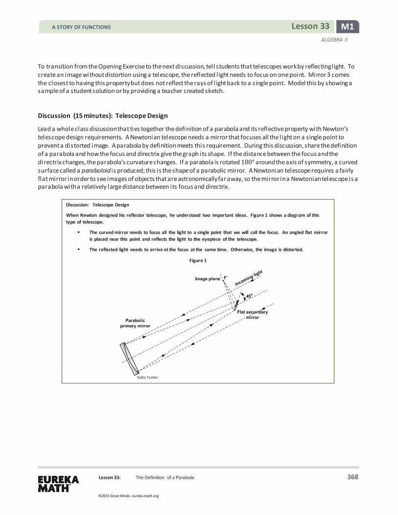
M1 Lesson 33 ALGEBRA II
Lesson 33: The Definition of a Parabola
To transition from the Opening Exercise to the next discussion, tell students that telescopes work by reflecting l ight. To create an image without distortion using a telescope, the reflected l ight needs to focus on one point. Mirror 3 comes the closest to having this property but does not reflect the rays of l ight back to a single point. Model this by showing a sample of a student solution or by providing a teacher created sketch.
Discussion (15 minutes): Telescope Design
Lead a whole class discussion that ties together the definition of a parabola and its reflective property with Newton’s telescope design requirements. A Newtonian telescope needs a mirror that focuses all the l ight on a single point to prevent a distorted image. A parabola by definition meets this requirement. During this discussion, share the definition of a parabola and how the focus and directrix give the graph its shape. If the distance between the focus and the directrix changes, the parabola’s curvature changes. If a parabola is rotated 180° around the axis of symmetry, a curved surface called a paraboloid is produced; this is the shape of a parabolic mirror. A Newtonian telescope requires a fairly flat mirror in order to see images of objects that are astronomically far away, so the mirror in a Newtonian telescope is a parabola with a relatively large distance between its focus and directrix.
Discussion: Telescope Design
When Newton designed his reflector telescope, he understood two important ideas. Figure 1 shows a diagram of this type of telescope.
� The curved mirror needs to focus all the light to a single point that we will call the focus. An angled flat mirror is placed near this point and reflects the light to the eyepiece of the telescope.
� The reflected light needs to arrive at the focus at the same time. Otherwise, the image is distorted.
Figure 1
Tamás
A STORY OF FUNCTIONS
368
©2015 Great Minds. eureka-math.org

M1 Lesson 33 ALGEBRA II
Lesson 33: The Definition of a Parabola
In the diagram below, the dotted and solid lines show the incoming light. Model how to add these additional l ines to the diagram. Make sure students annotate this on their student pages.
Next, discuss the definition of parabola that appears in the student pages and the reflective property of parabolic curves. Take time to explain what the term equidistant means and how distance is defined between a given point and a given l ine as the shortest distance, which is always the length of the segment that l ies on a l ine perpendicular to the given l ine whose endpoints are the given point and the intersection point of the given line and the perpendicular line. Ask students to recall the definition of a circle from Lessons 30–31 and use this to explore the definition of a parabola. Before reading through the definition, give students a ruler and ask them to measure the segments 𝐹𝐹𝑃𝑃1 , 1𝑃𝑃1,𝐹𝐹𝑃𝑃2, 2𝑃𝑃2 , etc., in Figure 2. Then have them locate a few more points on the curve and measure the distance from the curve to point 𝐹𝐹 and from the curve to the horizontal line 𝐿𝐿.
Definition: A parabola with directrix and focus point is the set of all points in the plane that are equidistant from the point and line .
Figure 2 to the right illustrates this definition of a parabola. In this diagram, = , = , = showing that for any point on the parabola, the distance between and is equal to the distance between and the line .
All parabolas have the reflective property illustrated in Figure 3. Rays parallel to the axis reflect off the parabola and through the focus point, .
Thus, a mirror shaped like a rotated parabola would satisfy Newton’s requirements for his telescope design.
Figure 3
Figure 2
A STORY OF FUNCTIONS
369
©2015 Great Minds. eureka-math.org

M1 Lesson 33 ALGEBRA II
Lesson 33: The Definition of a Parabola
Figure 4
Figure 5
Then, move on to Figures 4 and 5. Here we transition back to thinking about the telescope and show how a mirror in the shape of a parabola (as opposed to say a semi-circle or other curve) reflects light to the focus point. Talk about fun house mirrors (modeled by some smartphone apps) that distort images as an example of how other curved surfaces reflect l ight differently.
� If we want the l ight to be reflected to the focus at exactly the same time, then what must be true about the distances between the focus and any point on the mirror and the distances between the directrix and any point on the mirror? à Those distances must be equal.
Figure 4 below shows several different line segments representing the reflected light with one endpoint on the curved mirror that is a parabola and the other endpoint at the focus. Anywhere the light hits this type of parabolic surface, it always reflects to the focus, , at exactly the same time.
Figure 5 shows the same image with a directrix. Imagine for a minute that the mirror was not there. Then, the light would arrive at the directrix all at the same time. Since the distance from each point on the parabolic mirror to the directrix is the same as the distance from the point on the mirror to the focus, and the speed of light is constant, it takes the light the same amount of time to travel to the focus as it would have taken it to travel to the directrix. In the diagram, this means that = , = , and so on. Thus, the light rays arrive at the focus at the same time, and the image is not distorted.
Scaffolding: To help students master the new vocabulary associated with parabolas, make a poster using the diagram shown below and label the parts. Adjust as needed for students, but make sure to include the focus point and directrix in the poster along with marked congruent segments illustrating the definition.
(𝑥𝑥 ,𝑦𝑦)
A STORY OF FUNCTIONS
370
©2015 Great Minds. eureka-math.org

M1 Lesson 33 ALGEBRA II
Lesson 33: The Definition of a Parabola
x
y
( , )
( , )
( , )
To further i llustrate the definition of a parabola, ask students to mark on Figure 5 how the lengths 𝐹𝐹, 𝐹𝐹, 𝐹𝐹, 𝐷𝐷𝐹𝐹, and 𝐹𝐹 are equal to the lengths 𝐹𝐹 , 𝐹𝐹 , 𝐹𝐹 , 𝐷𝐷𝐹𝐹 , and 𝐹𝐹 , respectively.
� How does this definition fit the requirements for a Newtonian telescope? à The definition states exactly what we need to make the incoming light hit the focus at the exact same
time since the distance between any point on the curve to the directrix is equal to the distance between any point on the curve and the focus.
� A parabola looks l ike the graph of what type of function? à It looks like the graph of a quadratic function.
Transition to Example 1 by announcing that the prediction that an equation for a parabola would be a quadratic equation will be confirmed using a specific example.
Example (13 minutes): Finding an Analytic Equation for a Parabola
This example derives an equation for a parabola given the focus and directrix. Work through this example, and give students time to record the steps.. Refer students back to the way the distance formula was used in the definition of a circle, and explain that it can be used here as well to find an analytic equation for this type of curve.
Example: Finding an Analytic Equation for a Parabola
Given a focus and a directrix, create an equation for a parabola.
Focus: ( , )
Directrix: -axis
Parabola: = {( , )| ( , ) is equidistant from F and the -axis.}
Let be any point ( , ) on the parabola . Let be a point on the directrix with the same -coordinate as point .
What is the length ?
=
Use the distance formula to create an expression that represents the length .
= ( − ) + ( − )
Scaffolding: � Provide some additional practice
with using distance formula to find the length of a l ine segment for struggling learners.
� Post the distance formula on the classroom wall.
� Draw a diagram with the points 𝐹𝐹(0,2), 𝐹𝐹 (4,0), and (4,5) labeled. Have them find the lengths 𝐹𝐹 and 𝐹𝐹 .
A STORY OF FUNCTIONS
371
©2015 Great Minds. eureka-math.org

M1 Lesson 33 ALGEBRA II
Lesson 33: The Definition of a Parabola
Create an equation that relates the two lengths, and solve it for .
Therefore, = ( , )| ( − ) + ( − ) = .
The two segments have equal lengths. =
The length of each segment = ( − ) + ( − )
Square both sides of the equation. = + ( − )
Expand the binomial. = + − +
Solve for . = +
= +
Replacing this equation in the definition of = {( , )| ( , ) is equidistant from F and the -axis} gives the statement = ( , )| = + .
Thus, the parabola is the graph of the equation = + .
Verify that this equation appears to match the graph shown.
Consider the point where the -axis intersects the parabola; let this point have coordinates ( , ). From the graph, we see that < < . The distance from the focus ( , ) to ( , ) is − units, and the distance from the directrix to ( , ) is units. Since ( , ) is on the parabola, we have − = , so that = . From this perspective, we see that the point ( , ) must be on the parabola. Does this point satisfy the equation we found? Let = . Then our equation gives
= + = ( ) + , so ( , ) satisfies the equation. This is the only point that we have determined to be on the parabola at this point, but it provides evidence that the equation matches the graph.
Use the questions below to work through Example 1. Have students mark the congruent segments on their diagram and record the derivation of the equation as it is worked out in front of the class. Remind students that when the distance formula is worked with, the Pythagorean theorem is being applied in the coordinate plane. This refers back to their work in both Grade 8 and high school Geometry.
� According to the definition of a parabola, which two line segments in the diagram must have equal measure? Mark them congruent on your diagram. à The length 𝐹𝐹 must be equal to 𝐹𝐹 .
� How long is 𝐹𝐹 ? How do you know? à It is 𝑦𝑦 units long. The 𝑦𝑦-coordinate of point is 𝑦𝑦.
� Recall the distance formula, and use it to create an expression equal to the length of 𝐹𝐹. à The distance formula is
= (𝑥𝑥1− 𝑥𝑥2)2 + (𝑦𝑦1 −𝑦𝑦2)2, where (𝑥𝑥1,𝑦𝑦1) and (𝑥𝑥2,𝑦𝑦2) are two points in the Cartesian plane.
� How can you tell if this equation represents a quadratic function?
à The degree of 𝑥𝑥 will be 2, and the degree of 𝑦𝑦 will be 1, and each 𝑥𝑥 will correspond to exactly one 𝑦𝑦.
A marked up diagram is shown to the right.
A STORY OF FUNCTIONS
372
©2015 Great Minds. eureka-math.org

M1 Lesson 33 ALGEBRA II
Lesson 33: The Definition of a Parabola
-2 2
2
4
x
y
Exercises (4 minutes) Exercises
1. Demonstrate your understanding of the definition of a parabola by drawing several pairs of congruent segments given the parabola, its focus, and directrix. Measure the segments that you drew to confirm the accuracy of your sketches in either centimeters or inches.
2. Derive the analytic equation of a parabola given the focus of ( , ) and the directrix = . Use the diagram to help
you work this problem.
a. Label a point ( , ) anywhere on the parabola.
b. Write an expression for the distance from the point ( , ) to the directrix.
−
c. Write an expression for the distance from the point ( , ) to
the focus.
( − ) + ( − )
d. Apply the definition of a parabola to create an equation in terms of and . Solve this equation for .
− = ( − ) + ( − )
Solved for , we find an equivalent equation is = + .
e. What is the translation that takes the graph of this parabola to the graph of the equation derived in Example 1?
A translation down two units will take this graph of this parabola to the one derived in Example 1.
Closing (3 minutes)
In this lesson, limit the discussion to parabolas with a horizontal directrix. Later lessons show that all parabolas are similar and that the equations are quadratic regardless of the orientation of the parabola in the plane. Have students answer these questions individually in writing. Then discuss their responses as a whole class.
� What is a parabola? à A parabola is a geometric figure that represents the set of all points equidistant from a point called the
focus and a line called the directrix. � Why are parabolic mirrors used in telescope designs?
à Parabolic mirrors are used in telescope designs because they focus reflected light to a single point. � What type of analytic equation can be used to model parabolas?
à A parabola whose directrix is a horizontal line can be represented by a quadratic equation in 𝑥𝑥, given by 𝑦𝑦 = 𝑎𝑎𝑥𝑥2+ 𝑏𝑏𝑥𝑥+ 𝑐𝑐.
A STORY OF FUNCTIONS
373
©2015 Great Minds. eureka-math.org
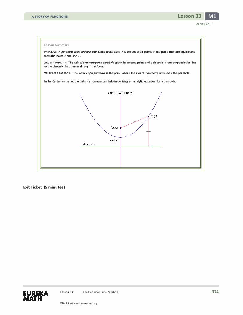
M1 Lesson 33 ALGEBRA II
Lesson 33: The Definition of a Parabola
Exit Ticket (5 minutes)
Lesson Summary
PARABOLA: A parabola with directrix line and focus point is the set of all points in the plane that are equidistant from the point and line .
AXIS OF SYMMETRY: The axis of symmetry of a parabola given by a focus point and a directrix is the perpendicular line to the directrix that passes through the focus.
VERTEX OF A PARABOLA: The vertex of a parabola is the point where the axis of symmetry intersects the parabola.
In the Cartesian plane, the distance formula can help in deriving an analytic equation for a parabola.
A STORY OF FUNCTIONS
374
©2015 Great Minds. eureka-math.org

M1 Lesson 33 ALGEBRA II
Lesson 33: The Definition of a Parabola
Name Date
Lesson 33: The Definition of a Parabola
Exit Ticket 1. Derive an analytic equation for a parabola whose focus is (0,4) and directrix is the 𝑥𝑥-axis. Explain how you got your
answer.
2. Sketch the parabola from Question 1. Label the focus and directrix.
-4 -2 2 4
-4
-2
2
4
x
y
A STORY OF FUNCTIONS
375
©2015 Great Minds. eureka-math.org

M1 Lesson 33 ALGEBRA II
Lesson 33: The Definition of a Parabola
Exit Ticket Sample Solutions
1. Derive an analytic equation for a parabola whose focus is ( , ) and directrix is the -axis. Explain how you got your answer.
Let ( , ) be a point on the parabola. Then, the distance between this point and the focus is given by ( − ) + ( − ) . The distance between the point ( , ) and the directrix is . Then,
= ( − ) + ( − )
= + − + = +
= +
2. Sketch the parabola from Question 1. Label the focus and directrix.
-4 -2 2 4
-4
-2
2
4
x
y
directrix
focus
A STORY OF FUNCTIONS
376
©2015 Great Minds. eureka-math.org
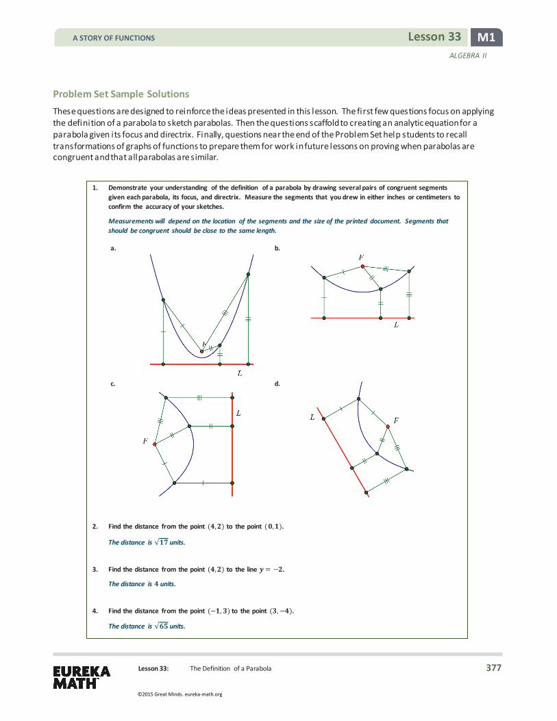
M1 Lesson 33 ALGEBRA II
Lesson 33: The Definition of a Parabola
Problem Set Sample Solutions These questions are designed to reinforce the ideas presented in this lesson. The first few questions focus on applying the definition of a parabola to sketch parabolas. Then the questions scaffold to creating an analytic equation for a parabola given its focus and directrix. Finally, questions near the end of the Problem Set help students to recall transformations of graphs of functions to prepare them for work in future lessons on proving when parabolas are congruent and that all parabolas are similar.
1. Demonstrate your understanding of the definition of a parabola by drawing several pairs of congruent segments given each parabola, its focus, and directrix. Measure the segments that you drew in either inches or centimeters to confirm the accuracy of your sketches.
Measurements will depend on the location of the segments and the size of the printed document. Segments that should be congruent should be close to the same length.
a. b.
c. d.
2. Find the distance from the point ( , ) to the point ( , ).
The distance is √ units.
3. Find the distance from the point ( , ) to the line = − .
The distance is units.
4. Find the distance from the point (− , ) to the point ( ,− ).
The distance is √ units.
A STORY OF FUNCTIONS
377
©2015 Great Minds. eureka-math.org

M1 Lesson 33 ALGEBRA II
Lesson 33: The Definition of a Parabola
5. Find the distance from the point (− , ) to the line = .
The distance is units.
6. Find the distance from the point ( , ) to the line = − .
The distance is units.
7. Find the distance from the point ( ,− ) to the line = .
The distance is units.
8. Find the values of for which the point ( , ) is equidistant from ( , ), and the line = − .
If ( − ) + ( − ) = , then = or = − .
9. Find the values of for which the point ( ,− ) is equidistant from ( ,− ), and the line = .
If ( − ) + − − (− ) = , then = + √ or = − √ .
10. Consider the equation = . a. Find the coordinates of the three points on the graph of = whose -values are , , and .
The coordinates are ( , ), ( , ) , and ( , ) .
b. Show that each of the three points in part (a) is equidistant from the point � , �, and the line = − .
For ( , ) , show that
( − ) + − = + = =
− − = .
( − ) + − = + = =
− − = .
( − ) + − = + = =
− − = .
and
For ( , ) , show that
and
For ( , ) , show that
and
A STORY OF FUNCTIONS
378
©2015 Great Minds. eureka-math.org
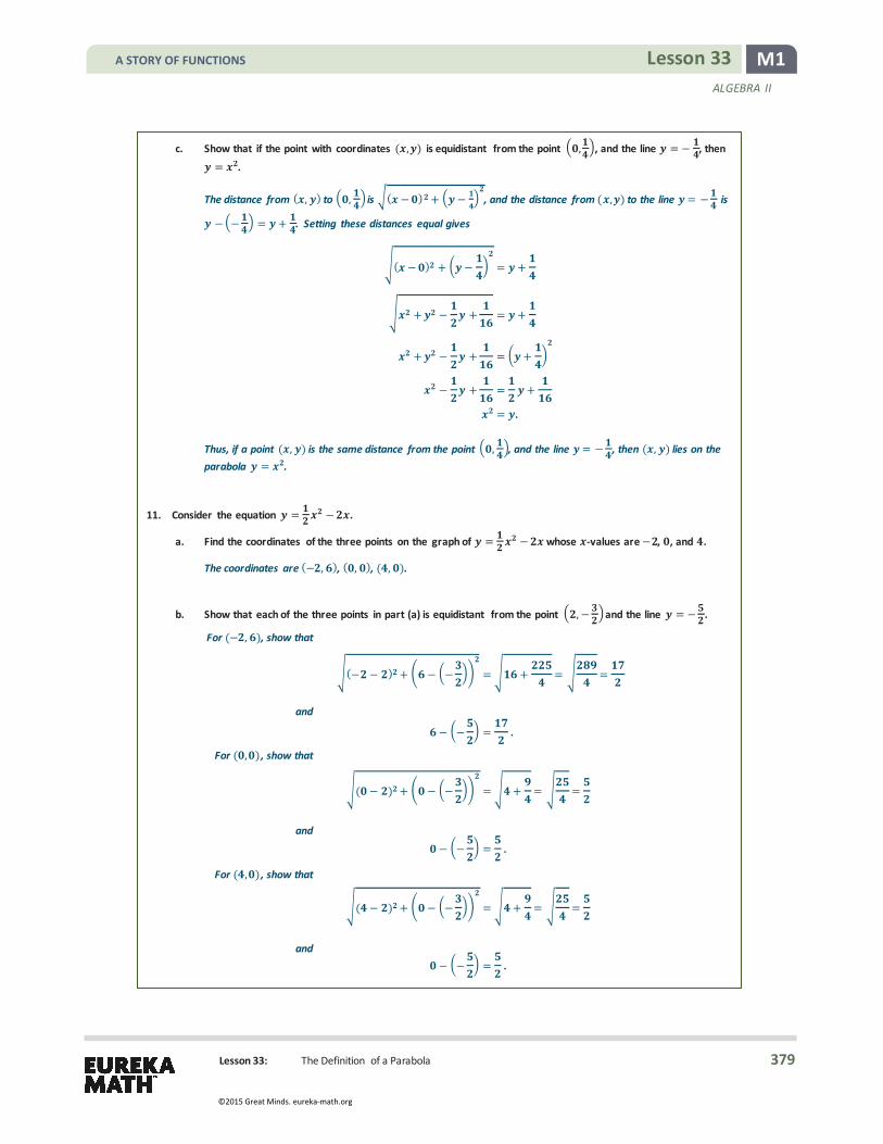
M1 Lesson 33 ALGEBRA II
Lesson 33: The Definition of a Parabola
c. Show that if the point with coordinates ( , ) is equidistant from the point � , �, and the line = − , then = .
The distance from ( , ) to � , � is ( − ) + � − � , and the distance from ( , ) to the line = − is
−�− � = + . Setting these distances equal gives
( − ) + − = +
+ − + = +
+ − + = +
− + = +
= .
Thus, if a point ( , ) is the same distance from the point � , �, and the line = − , then ( , ) lies on the parabola = .
11. Consider the equation = − .
a. Find the coordinates of the three points on the graph of = − whose -values are − , , and .
The coordinates are (− , ), ( , ), ( , ).
b. Show that each of the three points in part (a) is equidistant from the point � ,− � and the line = − .
For (− , ), show that
(− − ) + − − = + = =
− − = .
( − ) + − − = + = =
− − = .
( − ) + − − = + = =
− − = .
and
For ( , ) , show that
and
For ( , ) , show that
and
A STORY OF FUNCTIONS
379
©2015 Great Minds. eureka-math.org

M1 Lesson 33 ALGEBRA II
Lesson 33: The Definition of a Parabola
-2 2 4
2
4
x
y
c. Show that if the point with coordinates ( , ) is equidistant from the point � ,− �, and the line = − , then = − .
The distance from ( , ) to � ,− � is ( − ) + � + � , and the distance from ( , ) to the line
= − is − �− �= + . Setting these distances equal gives
( − ) + + = +
− + + + = +
− + + + = + +
− =
( − ) = .
Thus, if a point ( , ) is the same distance from the point � ,− �, and the line = − , then ( , ) lies on the
parabola = ( − ).
12. Derive the analytic equation of a parabola with focus ( , ) and directrix = . Use the diagram to help you work
this problem.
a. Label a point ( , ) anywhere on the parabola.
b. Write an expression for the distance from the point ( , ) to the directrix.
−
c. Write an expression for the distance from the point ( , ) to the
focus ( , ).
( − ) + ( − )
d. Apply the definition of a parabola to create an equation in terms of and . Solve this equation for .
− = ( − ) + ( − ) ( − ) = ( − ) + ( − ) − + = ( − ) + − +
= ( − ) +
= ( − ) +
= − +
A STORY OF FUNCTIONS
380
©2015 Great Minds. eureka-math.org

M1 Lesson 33 ALGEBRA II
Lesson 33: The Definition of a Parabola
e. Describe a sequence of transformations that would take this parabola to the parabola with equation
= + derived in Example 1.
A translation unit to the left and unit downward will take this parabola to the one derived in Example 1.
13. Consider a parabola with focus ( ,− ) and directrix on the -axis.
a. Derive the analytic equation for this parabola.
= − −
b. Describe a sequence of transformations that would take the parabola with equation = + derived in Example 1 to the graph of the parabola in part (a).
Reflect the graph in Example 1 across the -axis to obtain this parabola.
14. Derive the analytic equation of a parabola with focus ( , ) and directrix on the -axis.
= +
A STORY OF FUNCTIONS
381
©2015 Great Minds. eureka-math.org

M1 Lesson 34 ALGEBRA II
Lesson 34: Are All Parabolas Congruent?
Lesson 34: Are All Parabolas Congruent?
Student Outcomes
� Students learn the vertex form of the equation of a parabola and how it arises from the definition of a parabola.
� Students perform geometric operations, such as rotations, reflections, and translations, on arbitrary parabolas to discover standard representations for their congruence classes. In doing so, they learn that all parabolas with the same distance 𝑝𝑝 between the focus and the directrix are congruent to the graph of 𝑦𝑦 = 1
2𝑝𝑝𝑥𝑥2.
Lesson Notes This lesson builds upon the previous lesson and applies transformations to show that all parabolas with the same distance between their focus and directrix are congruent. Recall that two figures in the plane are congruent if there exists a finite sequence of rigid motions that maps one onto the other, so it makes sense to discuss congruency of parabolas. The lesson closes with a theorem and proof detailing the answer to the question posed in the lesson title. By using transformations in this lesson to determine the conditions under which two parabolas are congruent, this lesson builds coherence with the work students did in Geometry. This lesson specifically asks students to consider how we can use transformations to prove two figures are congruent. Additionally, the lesson reinforces the connections between geometric transformations and transformations of the graphs of functions.
There are many opportunities to provide scaffolding in this lesson for students who are not ready to move quickly to abstract representation. Use technology, patty paper or transparencies, and simple hand-drawn graphs as appropriate to support student learning throughout this lesson. Use the anchor poster created in Lesson 33, and keep key vocabulary words and formulas (e.g., the distance formula) displayed for student reference. Consider breaking this lesson up into two days; on the first day, explore the definition of congruent parabolas, sketch parabolas given their focus and directrix, and explore the consequences of changing the distance between the focus and directrix, 𝑝𝑝. On the second day, derive the analytic equation for a parabola with a given focus and directrix and vertex at the origin, and prove the theorem on parabola congruence.
Classwork Opening Exercise (7 minutes)
Allow students to discuss their approaches to this exercise with a partner or in small groups. Keep encouraging students to consider the definition of a parabola as they try to sketch the parabolas. Encourage students who draw a haphazard curve to consider how they could make sure their graph is the set of points equidistant from the focus and directrix. Throughout this lesson, provide students with access to graphing calculators or other computer graphing software that they can use to test and confirm conjectures. Model this further, and provide additional scaffolding by using an online applet located at the website http://www.intmath.com/plane-analytic-geometry/parabola-interactive.php. Within the applet, students can move either the focus or the directrix to change the value of 𝑝𝑝. They can also slide a point along the parabola noting the equal distances between that point and the focus and that point and the directrix. Depending on the level of students, the teacher can begin these exercises by moving directly to the applet or by having them start the exercises and use the applet later in this section.
A STORY OF FUNCTIONS
382
©2015 Great Minds. eureka-math.org

M1 Lesson 34 ALGEBRA II
Lesson 34: Are All Parabolas Congruent?
Opening Exercise
Are all parabolas congruent? Use the following questions to support your answer.
a. Draw the parabola for each focus and directrix given below.
The solution is shown below.
b. What do we mean by congruent parabolas?
Two parabolas would be congruent if we could find a sequence of rigid motions that takes one parabola onto the other. We could translate the vertex of the first one onto the vertex of the second one, then rotate the image of the first one so that the directrices are parallel and both parabolas open in the same direction. If the transformed first parabola coincides with the original second parabola, then the two original parabolas are congruent.
c. Are the two parabolas from part (a) congruent? Explain how you know.
These two parabolas are not congruent. They have the same vertex but different -values for each in the domain, except for the point ( , ). If we translate the first one somewhere else, then the vertices will not align. If we reflect or rotate, then both parabolas will not open upward. There is no rigid transformation or set of transformations that takes the graph of one parabola onto the other.
d. Are all parabolas congruent?
No, we just found two that are not congruent.
e. Under what conditions might two parabolas be congruent? Explain your reasoning.
Once we align the vertices and get the directrices parallel and parabolas opening in the same direction through rotation or reflection, the parabolas will have the same shape if the focus and directrix are aligned. Thus, two parabolas will be congruent if they have the same distance between the focus and directrix.
Debrief this exercise using the following questions, which can also be used as scaffolds if students are struggling to begin this problem. During the debrief, record student thinking on chart paper to be used for reference at the end of this lesson as a means to confirm or refute their conjectures.
At some point in this discussion, students should recognize that it would be nice if there was a name for the distance between the focus and directrix of the parabola. When appropriate, let them know that this distance is denoted by 𝑝𝑝 in this lesson and lessons that follow. If they do not mention it here, it is brought into the discussion in Exercise 5.
Scaffolding:
� If students struggle with vocabulary, refer them back to the anchor poster.
� As an extension, ask students to derive the equation for the parabola as was shown in Example 1 of the previous lesson.
MP.3
-4 -2 2 4
-4
-2
2
4
x
y
-4 -2 2 4
-4
-2
2
4
x
y
A STORY OF FUNCTIONS
383
©2015 Great Minds. eureka-math.org

M1 Lesson 34 ALGEBRA II
Lesson 34: Are All Parabolas Congruent?
� How can you use the definition of a parabola to quickly locate at least three points on the graph of the parabola with a focus (0,1) and directrix 𝑦𝑦= −1?
à Along the 𝑦𝑦-axis, the distance between the focus and the directrix is 2, so one point, the vertex, will be halfway between them at (0,0). Since the distance between the focus and the directrix is 𝑝𝑝 = 2 units, if we go 2 units to the left and right of the focus, we will be able to locate two more points on the parabola at (2,1) and (−2,1).
� How can you use the definition of a parabola to quickly locate at least three points on the graph of the parabola with a focus (0,2) and directrix 𝑦𝑦= −2? à The distance between the focus and the directrix is 𝑝𝑝 = 4 units, so the vertex is halfway between the
focus and directrix at (0,0). Moving right and left 4 units from the focus gives points (4,2) and (−4,2). � Generalize this process of finding three points on a parabola with a given focus and directrix.
à Find the vertex halfway between the focus and directrix, and let 𝑝𝑝 be the distance between the focus and directrix. Then, sketch a line through the focus parallel to the directrix. Locate the two points 𝑝𝑝 units along that line in either direction from the focus. The vertex and these two points are all on the parabola.
� How does this process help us determine if two parabolas are congruent?
à Two parabolas will be congruent if the two points found through this process are the same distance away from the focus. That is, two parabolas will be congruent if they have the same value of 𝑝𝑝 or the same distance between the focus and directrix.
Exercises 1–5 (5 minutes)
Students practice drawing parabolas given a focus and a directrix. These parabolas are NOT all oriented with a horizontal directrix. Let students struggle with how to construct a sketch of the parabola. Remind them of their work in the Opening Exercise. The teacher may choose to do one problem together to model the process. Draw a l ine perpendicular to the directrix through the focus. Locate the midpoint of the segment connecting the focus and directrix. Then, create a square on either side of this l ine with a side length equal to the distance between the focus and the directrix. One vertex of each square that is not on the directrix or axis of symmetry is another point on the parabola. If dynamic geometry software is available, students could also model this construction using technology.
Exercises 1–5
1. Draw the parabola with the given focus and directrix.
A STORY OF FUNCTIONS
384
©2015 Great Minds. eureka-math.org

M1 Lesson 34 ALGEBRA II
Lesson 34: Are All Parabolas Congruent?
2. Draw the parabola with the given focus and directrix.
3. Draw the parabola with the given focus and directrix.
Give students time to work through these exercises alone or in small groups. Then, have a few students present their approaches on the board. Be sure to emphasize that by applying the definition, a fairly accurate sketch of a parabola can be produced.
� What two geometric objects determine the set of points that forms a parabola? à A point called the focus and a line called the directrix
Direct students to compare and contrast Exercises 1–3 and discuss the implications within their small groups.
4. What can you conclude about the relationship between the parabolas in Exercises 1–3?
The parabolas are all the same size and shape because the distance between the focus and the directrix stayed the same. These parabolas should be congruent.
Direct students’ attention to the diagram in Exercise 5. Have students respond individually and then discuss in small groups.
Scaffolding:
Use sentence frames for this exercise to support English language learners. For example, in Exercise 5, use “As the value of 𝑝𝑝 grows, the parabola ______________.” Later in the lesson, use
“All parabolas with the same distance between the ____ and ____ of the parabola are congruent.”
A STORY OF FUNCTIONS
385
©2015 Great Minds. eureka-math.org

M1 Lesson 34 ALGEBRA II
Lesson 34: Are All Parabolas Congruent?
5. Let be the number of units between the focus and the directrix, as shown. As the value of increases, what happens to the shape of the resulting parabola?
As the value of increases, the graph is dilated and shrinks vertically compared to graphs with a smaller value of . It appears to get flatter.
Example 1 (12 minutes): Derive an Equation for a Parabola
In this example, lead students through the process of creating an equation that represents a parabola with a horizontal directrix, a vertex at the origin, and the distance between the focus and directrix 𝑝𝑝 > 0. This process is similar to the work done in yesterday’s lesson, except students are working with a general case instead of a specified value for 𝑝𝑝. Scaffolding may be necessary for students who are not ready to move to the abstract level. For those students, continued modeling with selected 𝑝𝑝 values and use of the applet mentioned earlier will help bridge the gap between concrete and abstract. Also, recall that several of the exercises in the previous lesson worked through this process with specifc points. Remind students for whom this work is tedious that by deriving a general formula, the work going forward can be simplified, which is the heart of MP.7 and MP.8.
Example 1: Derive an Equation for a Parabola
Consider a parabola with distance >
between the focus with coordinates � , �, and
directrix = − . What is the equation that represents this parabola?
Scaffolding:
For more advanced students, derive the general vertex form of a parabola with the vertex at (ℎ, 𝑘𝑘) and the horizontal directrix and distance 𝑝𝑝 between the focus and directrix: 𝑦𝑦 = ± 1
2𝑝𝑝(𝑥𝑥 − ℎ)2+ 𝑘𝑘.
A STORY OF FUNCTIONS
386
©2015 Great Minds. eureka-math.org

M1 Lesson 34 ALGEBRA II
Lesson 34: Are All Parabolas Congruent?
� What are the coordinates of the vertex? à The coordinates of the vertex are (0,0).
� Find a formula for the distance between the focus and the point (𝑥𝑥,𝑦𝑦).
à (𝑥𝑥− 0) 2+ �𝑦𝑦 − 12 𝑝𝑝�
2
� Find a formula for the distance between (𝑥𝑥 ,𝑦𝑦) and the directrix.
à 𝑦𝑦+ 12𝑝𝑝
� By the definition of a parabola, these distances are equal. Create an equation.
à 𝑦𝑦+ 12𝑝𝑝 = (𝑥𝑥− 0)2 + �𝑦𝑦 − 1
2𝑝𝑝�2
� Solve the equation for 𝑦𝑦.
à Start by squaring both sides. When you expand the
squared binomials, the 𝑦𝑦2 and 14𝑝𝑝2 terms drop out of
the equation. You may need to provide some additional scaffolding for students who are still not fluent with expanding binomial expressions.
𝑦𝑦+12𝑝𝑝
2
= 𝑥𝑥2 + 𝑦𝑦 −12𝑝𝑝
2
𝑦𝑦+12𝑝𝑝
2
− 𝑦𝑦 −12𝑝𝑝
2
= 𝑥𝑥2
𝑦𝑦2+ 𝑝𝑝𝑦𝑦+14𝑝𝑝2− 𝑦𝑦2 + 𝑝𝑝𝑦𝑦 −
14𝑝𝑝 = 𝑥𝑥2
2𝑝𝑝𝑦𝑦= 𝑥𝑥2
𝑦𝑦=1
2𝑝𝑝𝑥𝑥2
à Therefore, 𝑃𝑃 = (𝑥𝑥,𝑦𝑦)| 𝑦𝑦= 12𝑝𝑝 𝑥𝑥
2 .
� How does this result verify the conjecture that as 𝑝𝑝 increases, the parabola gets flatter? (Note to teacher: Now is a good time to demonstrate with the applet http://www.intmath.com/plane-analytic-geometry/parabola-interactive.php.)
à We can confirm the conjecture that the graph of a parabola vertically shrinks as 𝑝𝑝 increases because
the expression 12
will get smaller as 𝑝𝑝 gets larger; thus, the parabola appears flatter.
Discussion (3 minutes)
The goal of this brief discussion is to introduce the vertex form of the equation of a parabola without going through the entire derivation of the formula and to make the connection between what we are doing now with parabolas and what was done in Algebra I, Module 2, Topic B with quadratic functions. Completing the square on any quadratic function 𝑦𝑦 = 𝑓𝑓(𝑥𝑥) produces the equation of a parabola in vertex form, which could then be quickly graphed since the coordinates of the vertex and distance 𝑝𝑝 from focus to directrix are known.
Scaffolding:
As an alternative to Example 1, use graphing software to explore the relationship between the distance between the focus and directrix, and the coefficient of 𝑥𝑥2. Organize the results in a table l ike the one shown below, and ask students to generalize the patterns they are seeing.
Equation Focus Directrix Distance
from focus to directrix
𝑦𝑦 =12𝑥𝑥2 0,
12
𝑦𝑦 =−12
1
𝑦𝑦 =14𝑥𝑥2 (0,1) 𝑦𝑦 = −1 2
𝑦𝑦 =16𝑥𝑥2 0,
32
𝑦𝑦 =−32
3
𝑦𝑦 =18𝑥𝑥2 (0, 2) 𝑦𝑦 = −2 4
𝑦𝑦=1
2𝑝𝑝𝑥𝑥2 0,
12𝑝𝑝 𝑦𝑦 = −
12𝑝𝑝 𝑝𝑝
MP.7
A STORY OF FUNCTIONS
387
©2015 Great Minds. eureka-math.org

M1 Lesson 34 ALGEBRA II
Lesson 34: Are All Parabolas Congruent?
Discussion
We have shown that any parabola with a distance > between the focus � , � and directrix = − has a vertex
at the origin and is represented by a quadratic equation of the form = .
Suppose that the vertex of a parabola with a horizontal directrix that opens upward is ( , ), and the distance from the
focus to directrix is > . Then, the focus has coordinates � , + �, and the directrix has equation = − . If
we go through the above derivation with focus � , + � and directrix = − , we should not be surprised to get a quadratic equation. In fact, if we complete the square on that equation, we can write it in the form
= ( − ) + .
In Algebra I, Module 4, Topic B, we saw that any quadratic function can be put into vertex form: ( ) = ( − ) + . Now we see that any parabola that opens upward can be described by a quadratic function in vertex form, where = .
If the parabola opens downward, then the equation is = − ( − ) + , and the graph of any quadratic equation of this form is a parabola with vertex at ( , ), distance between focus and directrix, and opening downward. Likewise, we can derive analogous equations for parabolas that open to the left and right. This discussion is summarized in the box below.
Vertex Form of a Parabola
Given a parabola with vertex ( , ), horizontal directrix, and distance > between focus and directrix, the analytic equation that describes the parabola is
• = ( − ) + if the parabola opens upward, and
• = − ( − ) + if the parabola opens downward.
Conversely, if > , then
• The graph of the quadratic equation = ( − ) + is a parabola that opens upward with vertex at
( , ) and distance from focus to directrix, and
• The graph of the quadratic equation = − ( − ) + is a parabola that opens downward with vertex at ( , ) and distance from focus to directrix.
Given a parabola with vertex ( , ), vertical directrix, and distance > between focus and directrix, the analytic equation that describes the parabola is
• = ( − ) + if the parabola opens to the right, and
• = − ( − ) + if the parabola opens to the left.
Conversely, if > , then
• The graph of the quadratic equation = ( − ) + is a parabola that opens to the right with vertex at ( , ) and distance from focus to directrix, and
• The graph of the quadratic equation = − ( − ) + is a parabola that opens to the left with
vertex at ( , ) and distance from focus to directrix.
A STORY OF FUNCTIONS
388
©2015 Great Minds. eureka-math.org

M1 Lesson 34 ALGEBRA II
Lesson 34: Are All Parabolas Congruent?
Example 2 (8 minutes)
The goal of this section is to present and prove the theorem that all parabolas that have the same distance from the focus to the directrix (that is, the same value of 𝑝𝑝) are congruent. Start by having students sketch the parabola defined by the focus and directrix on the diagram shown on the student pages.
Example 2
THEOREM: Given a parabola given by a directrix and a focus in
the Cartesian plane, then is congruent to the graph of = , where is the distance from to .
A more concrete approach also appears below and could be used as an alternative approach to the formal proof or as a precursor to the formal proof. If this additional scaffolding is provided, this lesson may need to extend to an additional day to provide time to prove the theorem below rather than just demonstrate it by the examples provided in the scaffolds.
The following examples provide concrete evidence to support the proof provided on the next pages. Use this before or after the proof based on the needs of students. Print graphs of these parabolas on paper. Then, print the graph of 𝑦𝑦=12𝑥𝑥
2 on a transparency. Use this to help students understand the rigid transformations that map the given parabola onto
𝑦𝑦 = 12 𝑥𝑥
2.
� The graphs of 𝑦𝑦 = 12𝑥𝑥
2 (in blue) and another parabola (in red) are shown in each coordinate plane. Describe a
series of rigid transformations that map the red parabola onto the graph of 𝑦𝑦= 12𝑥𝑥
2.
à There are many sequences of transformations that can take the red parabola to the blue one. For the
graphs on the left, translate the red graph one unit vertically up and one unit to the left, then reflect the resulting graph about the 𝑥𝑥-axis. For the graphs on the right, rotate the graph 90° counter-clockwise about the point (−3,0), then translate the graph 3 units to the right.
-5 5
5
5
x
y
-5 5
-5
5
x
y
A STORY OF FUNCTIONS
389
©2015 Great Minds. eureka-math.org

M1 Lesson 34 ALGEBRA II
Lesson 34: Are All Parabolas Congruent?
� Suppose we changed the distance between the focus and the directrix to 2 units instead of 1, and then mapped the given parabolas onto the graph of 𝑦𝑦 = 1
4𝑥𝑥2. Would the resulting graphs be the same? Why?
à The resulting graphs would be the same since the distance between the focus and the directrix for the parabola 𝑦𝑦= 1
4𝑥𝑥2 is 2 units. The parabolas would map exactly onto the parabola whose vertex is
(0,0).
� Under what conditions would two parabolas be congruent? How could you verify this using transformations that map one parabola onto the other?
à If the distance between the focus and the directrix is the same, then the two parabolas will be congruent. You could describe a series of rotations, reflections, and/or translations that will map one parabola onto the other. These rigid transformations preserve the size and shape of the graph and show that the two figures are congruent.
PROOF
Let be the point on the perpendicular line to that passes through , which is the midpoint of the line segment between
and . Translate to the origin = ( , ) using a translation. Then, translates to and translates to .
Next, rotate and about ( , ) until = � , � and
= ( , )| = − . We are guaranteed we can do this because is on the line perpendicular to that passes through . The translations described above are shown below.
Since is determined by and , the first translation takes to a parabola such that . The rotation takes to a parabola such that . Therefore, by transitivity.
Now, by Example 1 above,
= ( , )| = ;
that is, is the graph of the equation = , which is what we wanted to prove.
A STORY OF FUNCTIONS
390
©2015 Great Minds. eureka-math.org

M1 Lesson 34 ALGEBRA II
Lesson 34: Are All Parabolas Congruent?
Depending on the level of students, begin with the scaffold examples using 𝑦𝑦 = 12 𝑥𝑥
2; the proof of this theorem can be presented directly, or students can try to work through the proof with some scaffolding and support.
Consider these discussion questions to help students get started with thinking about a proof if they work collaboratively in small groups to create a proof.
� How can we apply transformations to show that every parabola is congruent to 𝑦𝑦 = 12𝑝𝑝𝑥𝑥
2, where 𝑝𝑝 is the
distance between the focus and the directrix? à The parabola’s vertex is (0,0). We could translate any parabola so that its vertex is also (0,0).
à Then we would need to rotate the parabolas so that the directrix is a horizontal line and the focus is a point along the 𝑦𝑦-axis.
The teacher may need to remind students that translations and rotations are rigid transformations and, therefore, guarantee that the parabolas determined by the focus and directrix as they are translated and rotated remain the same shape and size. For more information, see Module 1 from high school Geometry.
Exercises 6–9 (4 minutes): Reflecting on the Theorem
Have students respond individually and then share within their groups. Post a few responses on the board for a whole class debrief, and correct any misconceptions at that point.
Exercises 6–9: Reflecting on the Theorem
6. Restate the results of the theorem from Example 2 in your own words.
All parabolas that have the same distance between the focus point and the directrix are congruent.
7. Create the equation for a parabola that is congruent to = . Explain how you determined your answer.
= + . As long as the coefficient of the term is the same, the parabolas will be congruent.
8. Create an equation for a parabola that IS NOT congruent to = . Explain how you determined your answer.
= . As long as the coefficient of the term is different, the parabolas will not be congruent.
9. Write the equation for two different parabolas that are congruent to the parabola with focus point ( , ) and directrix line = − .
The distance between the focus and the directrix is units. Therefore, any parabola with a coefficient of
= ( ) = will be congruent to this parabola. Here are two options: = + and = .
A STORY OF FUNCTIONS
391
©2015 Great Minds. eureka-math.org

M1 Lesson 34 ALGEBRA II
Lesson 34: Are All Parabolas Congruent?
Closing (2 minutes)
Revisit the conjecture from the beginning of this lesson: Under what conditions are two parabolas congruent? Give students time to reflect on this question in writing before reviewing the points l isted below. Summarize the following key points as this lesson is wrapped up. In the next lesson, students consider whether or not all parabolas are similar. This lesson has established that given a distance 𝑝𝑝 between the directrix and focus, all parabolas with equal values of 𝑝𝑝 are congruent to the parabola that is the graph of the equation 𝑦𝑦 = 1
2𝑝𝑝𝑥𝑥2.
� The points of a parabola are determined by the directrix and a focus.
� Every parabola is congruent to a parabola defined by a focus on the 𝑦𝑦-axis and a directrix that is parallel to the 𝑥𝑥-axis.
� All parabolas that have the same distance between the focus and the directrix are congruent.
� When the focus is at �0, 12𝑝𝑝� and the directrix is given by the equation 𝑦𝑦 = − 1
2𝑝𝑝, then the parabola is the
graph of the equation 𝑦𝑦 = 12𝑝𝑝 𝑥𝑥
2.
� When the vertex is at (ℎ, 𝑘𝑘), and the distance from the focus to directrix is 𝑝𝑝 > 0, then:
– If it opens upward, the parabola is the graph of the equation 𝑦𝑦 = 12𝑝𝑝
(𝑥𝑥 −ℎ)2 + 𝑘𝑘;
– If it opens downward, the parabola is the graph of the equation 𝑦𝑦 = − 12𝑝𝑝
(𝑥𝑥 −ℎ)2 + 𝑘𝑘;
– If it opens to the right, the parabola is the graph of the equation 𝑥𝑥 = 12𝑝𝑝
(𝑦𝑦 −𝑘𝑘) 2+ ℎ;
– If it opens to the left, the parabola is the graph of the equation 𝑥𝑥 = − 12𝑝𝑝
(𝑦𝑦 −𝑘𝑘)2 + ℎ.
Exit Ticket (4 minutes)
A STORY OF FUNCTIONS
392
©2015 Great Minds. eureka-math.org

M1 Lesson 34 ALGEBRA II
Lesson 34: Are All Parabolas Congruent?
50
5
10
x
y
50
5
10
x
y
5
-5
5
x
y
Name Date
Lesson 34: Are All Parabolas Congruent?
Exit Ticket
Which parabolas shown below are congruent to the parabola that is the graph of the equation 𝑦𝑦 = 112 𝑥𝑥
2? Explain how you know.
a. b. c.
A STORY OF FUNCTIONS
393
©2015 Great Minds. eureka-math.org

M1 Lesson 34 ALGEBRA II
Lesson 34: Are All Parabolas Congruent?
50
5
10
x
y
50
5
10
x
y
5
-5
5
x
y
Exit Ticket Sample Solutions
Which parabolas shown below are congruent to the parabola that is the graph of the equation = ? Explain how you know.
The -value is . So, any parabola where the distance between the focus and the directrix is equal to units will be
congruent to the parabola that is the graph of the equation = . Of the parabolas shown below, (a) and (c) meet this condition, but (b) does not.
a. b. c.
Problem Set Sample Solutions Problems 1–9 in this Problem Set review how to create the analytic equation of a parabola. Students may use the process from the previous lesson or use the vertex form of the equation of a parabola included in this lesson. Starting with Problem 10, the focus of the Problem Set shifts to recognizing when parabolas are congruent.
1. Show that if the point with coordinates ( , ) is equidistant from ( , ) , and the line = , then = − + .
Students might start with the equation ( − ) + ( − ) = − and solve for as follows:
( − ) + − + = − ( − ) + − + = − +
( − ) = − + = −( − ) +
= − ( − + ) +
= − + .
Or, they might apply what we have learned about the vertex form of the equation of a parabola. Since the directrix is above the focus, we know the parabola opens downward, so will be negative. Since the distance from the point ( , ) to the line = is units, we know that = − . The vertex is halfway between the focus and directrix, so the coordinates of the vertex are ( , ). Then, the vertex form of the equation that represents the parabola is
= − ( − ) +
= − + .
A STORY OF FUNCTIONS
394
©2015 Great Minds. eureka-math.org

M1 Lesson 34 ALGEBRA II
Lesson 34: Are All Parabolas Congruent?
2. Show that if the point with coordinates ( , ) is equidistant from the point ( , ) and the line = − , then
= ( − ) − .
Students might start with the equation ( − ) + ( − ) = + , and then solve it for , or they might apply the vertex form of the equation of a parabola. Since the vertex is above the directrix, we know that the parabola opens upward, and > . Since the distance from the point ( , ) to the line = − is units, we know that
= . The vertex is halfway between the focus and directrix, so the vertex is ( ,− ). Thus, the equation that represents the parabola is = ( − ) − .
3. Find the equation of the set of points which are equidistant from ( , ) and the -axis. Sketch this set of points.
The focus is ( , ) , and the directrix is the -axis. Thus, the vertex is the point ( , ) , which is halfway between the vertex and directrix. Since the parabola opens upward, > , so = . Then, the vertex form of the equation of the parabola is
= + .
4. Find the equation of the set of points which are equidistant from the origin and the line = . Sketch this set of
points.
= − +
5. Find the equation of the set of points which are equidistant from ( ,− ) and the line = . Sketch this set of
points.
= − ( − ) +
-6 -4 -2 2 4 6
-6
-4
-2
2
4
6
x
y
-2 2 4 6 8 10
-6
-4
-2
2
4
6
x
y
-6 -4 -2 2 4 6
-6
-4
-2
2
4
6
x
y
A STORY OF FUNCTIONS
395
©2015 Great Minds. eureka-math.org

M1 Lesson 34 ALGEBRA II
Lesson 34: Are All Parabolas Congruent?
6. Find the equation of the set of points which are equidistant from ( , ) and the -axis. Sketch this set of points.
= +
7. Find the equation of the set of points which are equidistant from the origin and the line = − . Sketch this set of
points.
= −
8. Use the definition of a parabola to sketch the parabola defined by the given focus and directrix. a. Focus: ( , ) Directrix: = −
b. Focus: (− , ) Directrix: -axis
-2 2 4 6 8 10
-6
-4
-2
2
4
6
x
y
-6 -4 -2 2 4 6
-6
-4
-2
2
4
6
x
y
A STORY OF FUNCTIONS
396
©2015 Great Minds. eureka-math.org

M1 Lesson 34 ALGEBRA II
Lesson 34: Are All Parabolas Congruent?
c. Focus: ( ,− ) Directrix: -axis
d. Focus: ( , ) Directrix: = −
9. Find an analytic equation for each parabola described in Problem 8.
a. = ( , ) | = + ; thus, is the graph of the equation = + .
b. = ( , ) | = − − ; thus, is the graph of the equation = − − .
c. = ( , ) | = − ( − ) − ; thus, is the graph of the equation = − ( − ) − .
d. = ( , ) | = ( − ) + ; thus, is the graph of the equation = ( − ) + .
10. Are any of the parabolas described in Problem 9 congruent? Explain your reasoning.
(a) = , (b) = , (c) = , and (d) = ; therefore, the parabolas in parts (a) and (d) are congruent because they have the same distance between the focus and directrix.
11. Sketch each parabola, labeling its focus and directrix.
Each sketch should have the appropriate vertex, focus, and directrix and be fairly accurate. Sketches for parts (a) and (c) are shown.
a. = +
Distance between focus and directrix is unit, vertex ( , ), focus ( , . ), directrix = .
A STORY OF FUNCTIONS
397
©2015 Great Minds. eureka-math.org

M1 Lesson 34 ALGEBRA II
Lesson 34: Are All Parabolas Congruent?
b. = − +
Distance between focus and directrix is units, vertex ( , ), focus ( , ), directrix =
c. =
Distance between focus and directrix is units, vertex ( , ), focus ( , ), directrix = −
d. = +
Distance between focus and directrix is unit, vertex ( , ), focus ( . , ), directrix = .
e. = ( − ) −
Distance between focus and directrix is units, vertex ( ,− ), focus ( , . ), directrix = − .
A STORY OF FUNCTIONS
398
©2015 Great Minds. eureka-math.org

M1 Lesson 34 ALGEBRA II
Lesson 34: Are All Parabolas Congruent?
-4 -2 2 4
-4
-2
2
4
x
y
-4 -2 2 4
-4
-2
2
4
x
y
-4 -2 2 4
-4
-2
2
4
x
y
-8 -4 4 8
-8
-4
4
8
x
y
-10 -5 5 10
-10
-5
5
10
x
y
12. Determine which parabolas are congruent to the parabola with equation = − .
a. c.
b. d.
Parabolas (a), (b), and (c) are congruent because all have = . Parabola (d) has = , so it is not congruent to the others.
13. Determine which equations represent the graph of a parabola
that is congruent to the parabola shown to the right.
a. =
b. = +
c. = − +
d. = +
e. =
f. = ( − )
g. = +
The parabolas in parts (a), (c), and (g) are congruent and are congruent to the parabola shown. They all have the same distance of units between the focus and the directrix like the parabola shown.
A STORY OF FUNCTIONS
399
©2015 Great Minds. eureka-math.org
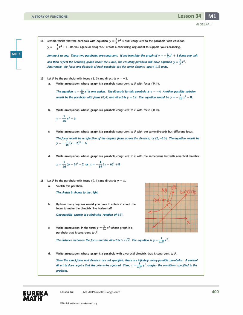
M1 Lesson 34 ALGEBRA II
Lesson 34: Are All Parabolas Congruent?
14. Jemma thinks that the parabola with equation = is NOT congruent to the parabola with equation
= − + . Do you agree or disagree? Create a convincing argument to support your reasoning.
Jemma is wrong. These two parabolas are congruent. If you translate the graph of = − + down one unit
and then reflect the resulting graph about the -axis, the resulting parabola will have equation = . Alternately, the focus and directrix of each parabola are the same distance apart, . units.
15. Let be the parabola with focus ( , ) and directrix = − . a. Write an equation whose graph is a parabola congruent to with focus ( , ).
The equation = is one option. The directrix for this parabola is = − . Another possible solution
would be the parabola with focus ( , ) and directrix = . The equation would be = − + .
b. Write an equation whose graph is a parabola congruent to with focus ( , ).
= −
c. Write an equation whose graph is a parabola congruent to with the same directrix but different focus.
The focus would be a reflection of the original focus across the directrix, or ( ,− ). The equation would be = − ( − ) − .
d. Write an equation whose graph is a parabola congruent to with the same focus but with a vertical directrix.
= ( − ) − or = − ( − ) +
16. Let be the parabola with focus ( , ) and directrix = .
a. Sketch this parabola.
The sketch is shown to the right.
b. By how many degrees would you have to rotate about the focus to make the directrix line horizontal?
One possible answer is a clockwise rotation of °.
c. Write an equation in the form = whose graph is a parabola that is congruent to .
The distance between the focus and the directrix is √ . The equation is = .
d. Write an equation whose graph is a parabola with a vertical directrix that is congruent to .
Since the exact focus and directrix are not specified, there are infinitely many possible parabolas. A vertical directrix does require that the -term be squared. Thus, = satisfies the conditions specified in the
problem.
MP.3
A STORY OF FUNCTIONS
400
©2015 Great Minds. eureka-math.org

M1 Lesson 34 ALGEBRA II
Lesson 34: Are All Parabolas Congruent?
e. Write an equation whose graph is , the parabola congruent to that results after is rotated clockwise ° about the focus.
The directrix will be = − √ . The equation is = + − √ .
f. Write an equation whose graph is , the parabola congruent to that results after the directrix of is rotated ° about the origin.
The focus will be √ , √ , and the directrix will be the -axis. The equation is = − √ +√ .
Extension:
17. Consider the function ( ) = − +− + − , where is a real number.
a. Use polynomial division to rewrite in the form ( ) = + − + − for some real numbers and .
Using polynomial division, ( ) = − + −− + − .
b. Find the -value where the maximum occurs for the function without using graphing technology. Explain how you know.
We can rewrite as ( ) = − + − + . Since − + = ( − ) + , the graph of
= − + is a parabola with vertex ( , ) that opens upward. Thus, the lowest point on the graph is
( , ). The function will take on its maximum value when is maximized; this happens when the
value of − + is minimized. Since we have already seen that − + is minimized at = , the
expression takes on its maximum value when = , and, thus, the original function takes on its
maximum value when = .
MP.2
A STORY OF FUNCTIONS
401
©2015 Great Minds. eureka-math.org

M1 Lesson 35 ALGEBRA II
Lesson 35: Are All Parabolas Similar?
Lesson 35: Are All Parabolas Similar?
Student Outcomes
� Students apply the geometric transformation of dilation to show that all parabolas are similar.
Lesson Notes In the previous lesson, students used transformations to prove that all parabolas with the same distance between the focus and directrix are congruent. In the process, they made a connection between geometry, coordinate geometry, transformations, equations, and functions. In this lesson, students explore how dilation can be applied to prove that all parabolas are similar.
Students may express disagreement with or confusion about the claim that all parabolas are similar because the various graphical representations of parabolas they have seen do not appear to have the “same shape.” Because a parabola is an open figure as opposed to a closed figure, l ike a triangle or quadrilateral, it is not easy to see similarity among parabolas. Students must understand that similar is strictly defined via similarity transformations; in other words, two parabolas are similar if there is a sequence of translations, rotations, reflections, and dilations that takes one parabola to the other. In the last lesson, students saw that every parabola is congruent to the graph of the equation 𝑦𝑦 = 1
2𝑝𝑝 𝑥𝑥2 for some 𝑝𝑝 > 0; in this lesson, students need only consider dilations of parabolas in this form.
When students claim that two parabolas are not similar, they should be reminded that the parts of the parabolas they are looking at may well appear to be different in size or magnification, but the parabolas themselves are not different in shape. Remind students that similarity is established by dilation; in other words, by magnifying a figure in both the horizontal and vertical directions. By analogy, although circles with different radii have different curvature, every student should agree that any circle can be dilated to be the same size and shape as any other circle; thus, all circles are similar.
Quadratic curves such as parabolas belong to a family of curves known as conic sections. The technical term in mathematics for how much a conic section deviates from being circular is eccentricity, and two conic sections with the same eccentricity are similar. Circles have eccentricity 0, and parabolas have eccentricity 1. After this lesson, consider asking students to research and write a report on eccentricity.
Classwork Provide graph paper for students as they work the first seven exercises. They first examine three congruent parabolas and then make a conjecture about whether or not all parabolas are similar. Finally, they explore this conjecture by graphing parabolas of the form 𝑦𝑦 = 𝑎𝑎𝑥𝑥2 that have different 𝑎𝑎-values.
Scaffolding: � Allow students access to graphing
calculators or software to focus on conceptual understanding if they are having difficulty sketching the graphs.
� Consider providing students with transparencies with a variety of parabolas drawn on them (as in prior lesson), such as 𝑦𝑦= 𝑥𝑥2, 𝑦𝑦 = 1
2𝑥𝑥2, and 𝑦𝑦 = 1
4 𝑥𝑥2 to help
them il lustrate these principles.
A STORY OF FUNCTIONS
402
©2015 Great Minds. eureka-math.org

M1 Lesson 35 ALGEBRA II
Lesson 35: Are All Parabolas Similar?
Exercises 1–7 (4 minutes) Exercises 1–8
1. Write equations for two parabolas that are congruent to the parabola given by = , and explain how you determined your equations.
(Student answers will vary.) The parabolas given by = ( − ) and = − are congruent to the parabola given by = . The first parabola is translated horizontally to the right by two units and the second parabola is translated down by 3 units, so they each are congruent to the original parabola.
2. Sketch the graph of = and the two parabolas you created on the same coordinate axes.
3. Write the equation of two parabolas that are NOT congruent to = . Explain how you determined your equations.
(Student answers will vary.) By our work in the previous lesson, we know that the equation any parabola can be written in the form = ( − ) + , and that two parabolas are congruent if and only if their equations have
the same value of | |. Then the parabolas = and = are both not congruent to the parabola given by = .
4. Sketch the graph of = and the two non-congruent parabolas you created on the same coordinate axes.
A STORY OF FUNCTIONS
403
©2015 Great Minds. eureka-math.org

M1 Lesson 35 ALGEBRA II
Lesson 35: Are All Parabolas Similar?
5. What does it mean for two triangles to be similar? How do we use geometric transformation to determine if two triangles are similar?
Two triangles are similar if we can transform one onto the other by a sequence of rotations, reflections, translations and dilations.
6. What would it mean for two parabolas to be similar? How could we use geometric transformation to determine if two parabolas are similar?
Two parabolas should be similar if we can transform one onto the other by a sequence of rotations, reflections, translations and dilations.
7. Use your work in Exercises 1–6 to make a conjecture: Are all parabolas similar? Explain your reasoning.
(Student answers will vary.) It seems that any pair of parabolas should be similar because we can line up the vertices through a sequence of rotations, reflections and translations, then we should be able to dilate the width of one parabola to match the other.
Discussion
After students have examined the fact that when the 𝑎𝑎-value in the equation of the parabola is changed, the resulting graph is basically the same shape, this point can be further emphasized by exploring the graph of 𝑦𝑦 = 𝑥𝑥2 on a graphing calculator or graphing program on the computer. Use the same equation but different viewing windows so students can see that an image can be created of what appears to be a different parabola by transforming the dimensions of the viewing window. However, the images are just a dilation of the original that is created when the scale is changed. See the images to the right. Each figure is a graph of the equation 𝑦𝑦 = 𝑥𝑥2 with different scales on the horizontal and vertical axes.
-5 5
-10
10
x
y
-10 10
-10
10
x
y
-10 10
-5
5
x
y
-10 10
-100
100
x
y
MP.3
A STORY OF FUNCTIONS
404
©2015 Great Minds. eureka-math.org

M1 Lesson 35 ALGEBRA II
Lesson 35: Are All Parabolas Similar?
Exercise 8 (5 minutes)
In this exercise, students derive the analytic equation for a parabola given its graph, focus, and directrix. Students have worked briefly with parabolas with a vertical directrix in previous lessons, so this exercise is an opportunity for the teacher to assess whether or not students are able to transfer and extend their thinking to a slightly different situation.
8. The parabola at right is the graph of which equation?
a. Label a point ( , ) on the graph of .
b. What does the definition of a parabola tell us about the distance between the point ( , ) and the directrix , and the distance between the point ( , ) and the focus ?
Let ( , ) be any point on the graph of . Then, these distances are equal because = {( , )|( , ) is equidistant from and }.
c. Create an equation that relates these two distances.
Distance from ( , ) to : ( − ) + ( − )
Distance from ( , ) to : +
Therefore, any point on the parabola has coordinates ( , ) that satisfy ( − ) + ( − ) = + .
d. Solve this equation for .
The equation can be solved as follows.
( − ) + ( − ) = + ( − ) + = ( + ) − + + = + +
=
=
Thus,
= ( , ) | = .
e. Find two points on the parabola , and show that they satisfy the equation found in part (d).
By observation, ( , ) and ( ,− ) are points on the graph of . Both points satisfy the equation that defines .
( , ): ( ) = =
( ,− ): (− ) = =
A STORY OF FUNCTIONS
405
©2015 Great Minds. eureka-math.org

M1 Lesson 35 ALGEBRA II
Lesson 35: Are All Parabolas Similar?
Discussion (8 minutes)
After giving students time to work through Exercises 1–8, ask the following questions to revisit concepts from Algebra I, Module 3.
� In the previous exercise, is 𝑃𝑃 a function of 𝑥𝑥? à No, because the 𝑥𝑥-value 2 corresponds to two 𝑦𝑦-values.
� Is 𝑃𝑃 a function of 𝑦𝑦?
à Yes, if we take 𝑦𝑦 to be in the domain and 𝑥𝑥 to be in the range, then each 𝑦𝑦-value on 𝑃𝑃 corresponds to exactly one 𝑥𝑥-value, which is the definition of a function.
These two questions remind students that just because we typically use the variable 𝑥𝑥 to represent the domain element of an algebraic function, this does not mean that it must always represent the domain element.
Next, transition to summarizing what was learned in the last two lessons. We have defined a parabola and determined the conditions required for two parabolas to be congruent. Use the following questions to summarize these ideas.
� What have we learned about the definition of a parabola? à The points on a parabola are equidistant from the directrix and the focus.
� What transformations can be applied to a parabola to create a parabola congruent to the original one?
à If the directrix and the focus are transformed by a rigid motion (e.g., translation, rotation, or reflection), then the new parabola defined by the transformed directrix and focus will be congruent to the original.
Essentially, every parabola that has a distance of 𝑝𝑝 units between its focus and directrix is congruent to a parabola with focus �0, 1
2𝑝𝑝� and directrix 𝑦𝑦 =− 12𝑝𝑝. What is the equation of this parabola?
𝑃𝑃 = (𝑥𝑥,𝑦𝑦)| 𝑦𝑦=1
2𝑝𝑝𝑥𝑥2
Thus, all parabolas that have the same distance between the focus and the directrix are congruent.
The family of graphs given by the equation 𝑦𝑦 = 12𝑝𝑝𝑥𝑥
2 for 𝑝𝑝 > 0 describes the set of non-congruent parabolas, one for
each value of 𝑝𝑝.
Ask students to consider the question from the lesson title. Chart responses to revisit at the end of this lesson to confirm or refute their claims.
Discussion
Do you think that all parabolas are similar? Explain why you think so.
Yes, they all have the same basic shape.
What could we do to show that two parabolas are similar? How might you show this?
Since every parabola can be transformed into a congruent parabola by applying one or more rigid transformations, perhaps similar parabolas can be created by applying a dilation which is a non-rigid transformation.
To check to see if all parabolas are similar, it only needs to be shown that any parabola that is the graph of 𝑦𝑦 = 12𝑝𝑝𝑥𝑥
2 for
𝑝𝑝 > 0 is similar to the graph of 𝑦𝑦 = 𝑥𝑥2. This is done through a dilation by some scale factor 𝑘𝑘 > 0 at the origin (0,0).
MP.3
A STORY OF FUNCTIONS
406
©2015 Great Minds. eureka-math.org

M1 Lesson 35 ALGEBRA II
Lesson 35: Are All Parabolas Similar?
Note that a dilation of the graph of a function is the same as performing a horizontal scaling followed by a vertical scaling that students studied in Algebra I, Module 3.
Exercises 9–12 (8 minutes)
The following exercises review the function transformations studied in Algebra I that are required to define dilation at the origin. These exercises provide students with an opportunity to recall what they learned in a previous course so that they can apply it here. Students must read points on the graphs to determine that the vertical scaling is by a
factor of 2 for the graphs on the left and by a factor of 12
for the graphs on the right. In
Algebra I, Module 3, students saw that the graph of a function can be transformed with a non-rigid transformation in two ways: vertical scaling and horizontal scaling.
A vertical scaling of a graph by a scale factor 𝑘𝑘 > 0 takes every point (𝑥𝑥, 𝑦𝑦) on the graph of 𝑦𝑦 = 𝑓𝑓(𝑥𝑥) to (𝑥𝑥, 𝑘𝑘𝑦𝑦). The result of the transformation is given by the graph of 𝑦𝑦 = 𝑘𝑘𝑓𝑓(𝑥𝑥).
A horizontal scaling of a graph by a scale factor 𝑘𝑘 > 0 takes every point (𝑥𝑥, 𝑦𝑦) on the graph of 𝑦𝑦 = 𝑓𝑓(𝑥𝑥) to (𝑘𝑘𝑥𝑥, 𝑦𝑦). The result of the transformation is given by the graph of 𝑦𝑦 = 𝑓𝑓�1
𝑘𝑘𝑥𝑥�.
Exercises 9–12
Use the graphs below to answer Exercises 9 and 10.
9. Suppose the unnamed red graph on the left coordinate plane is the graph of a function . Describe as a vertical scaling of the graph of = ( ); that is, find a value of so that ( ) = ( ). What is the value of ? Explain how you determined your answer.
The graph of is a vertical scaling of the graph of by a factor of . Thus, ( ) = ( ). By comparing points on the graph of to points on the graph of , you can see that the -values on are all twice the -values on .
10. Suppose the unnamed red graph on the right coordinate plane is the graph of a function . Describe as a vertical scaling of the graph of = ( ); that is, find a value of so that ( ) = ( ). Explain how you determined your answer.
The graph of is a vertical scaling of the graph of by a factor of . Thus, ( ) = ( ). By comparing points on the graph of to points on the graph of , you can see that the -values on are all half of the -values on .
Scaffolding: � Allow students access to
graphing calculators or software to focus on conceptual understanding if they are having difficulty sketching the graphs.
� The graphs shown in Exercises 9 and 10 are 𝑓𝑓(𝑥𝑥) = 𝑥𝑥2, 𝑔𝑔(𝑥𝑥) = 2𝑥𝑥2, and ℎ(𝑥𝑥) = 1
2𝑥𝑥2. The
graphs shown in Exercises 11 and 12 are 𝑓𝑓(𝑥𝑥) = 𝑥𝑥2, 𝑔𝑔(𝑥𝑥) = �1
2𝑥𝑥�2, and
ℎ(𝑥𝑥) = (2𝑥𝑥) 2.
A STORY OF FUNCTIONS
407
©2015 Great Minds. eureka-math.org

M1 Lesson 35 ALGEBRA II
Lesson 35: Are All Parabolas Similar?
Use the graphs below to answer Exercises 11–12.
11. Suppose the unnamed function graphed in red on the left coordinate plane is . Describe as a horizontal scaling of the graph of = ( ). What is the value of the scale factor ? Explain how you determined your answer.
The graph of is a horizontal scaling of the graph of by a factor of . Thus, ( ) = � �. By comparing points on the graph of to points on the graph of , you can see that for the same -values, the -values on are all twice the -values on .
12. Suppose the unnamed function graphed in red on the right coordinate plane is . Describe as a horizontal scaling of the graph of = ( ). What is the value of the scale factor ? Explain how you determined your answer.
The graph of is a horizontal scaling of the graph of by a factor of . Thus, ( ) = ( ). By comparing points on the graph of to points on the graph of , you can see that for the same -values, the -values on are all half of the -values on .
When these exercises are debriefed, model marking up the diagrams to i llustrate the vertical and horizontal scaling. A sample is provided below.
Marked up diagrams for vertical scaling in Exercises 9 and 10:
A STORY OF FUNCTIONS
408
©2015 Great Minds. eureka-math.org
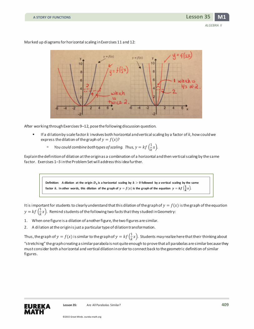
M1 Lesson 35 ALGEBRA II
Lesson 35: Are All Parabolas Similar?
Definition: A dilation at the origin is a horizontal scaling by > followed by a vertical scaling by the same
factor . In other words, this dilation of the graph of = ( ) is the graph of the equation = � �.
Marked up diagrams for horizontal scaling in Exercises 11 and 12:
After working through Exercises 9–12, pose the following discussion question.
� If a dilation by scale factor 𝑘𝑘 involves both horizontal and vertical scaling by a factor of 𝑘𝑘, how could we express the dilation of the graph of 𝑦𝑦 = 𝑓𝑓(𝑥𝑥)?
à You could combine both types of scaling. Thus, 𝑦𝑦 = 𝑘𝑘𝑓𝑓 �1𝑘𝑘𝑥𝑥�.
Explain the definition of dilation at the origin as a combination of a horizontal and then vertical scaling by the same factor. Exercises 1–3 in the Problem Set will address this idea further.
It is important for students to clearly understand that this dilation of the graph of 𝑦𝑦 = 𝑓𝑓(𝑥𝑥) is the graph of the equation 𝑦𝑦 = 𝑘𝑘𝑓𝑓 �1
𝑘𝑘𝑥𝑥�. Remind students of the following two facts that they studied in Geometry:
1. When one figure is a dilation of another figure, the two figures are similar. 2. A dilation at the origin is just a particular type of dilation transformation.
Thus, the graph of 𝑦𝑦 = 𝑓𝑓(𝑥𝑥) is similar to the graph of 𝑦𝑦 = 𝑘𝑘𝑓𝑓�1𝑘𝑘𝑥𝑥�. Students may realize here that their thinking about
“stretching” the graph creating a similar parabola is not quite enough to prove that all parabolas are similar because they must consider both a horizontal and vertical dilation in order to connect back to the geometric definition of similar figures.
A STORY OF FUNCTIONS
409
©2015 Great Minds. eureka-math.org

M1 Lesson 35 ALGEBRA II
Lesson 35: Are All Parabolas Similar?
Example (5 minutes): Dilation at the Origin
This example helps students gain a level of comfort with the notation and mathematics before moving on to proving that all parabolas are similar.
Example: Dilation at the Origin
Let ( ) = and let = . Write a formula for the function that results from dilating at the origin by a factor of .
The new function will have equation ( ) = � �. Since ( ) = , the new function will have equation
( ) = � � . That is, ( ) = .
What would the results be for = , , or ? What about = ?
For = , ( ) = .
For = , ( ) = .
For = , ( ) = .
For = , ( ) = .
After working through this example, the following questions help prepare students for the upcoming proof using a general parabola from the earlier discussion.
� Based on this example, what can you conclude about these parabolas? à They are all similar to one another because they represent
dilations of the graph at the origin of the original function. � Based on this example, what can you conclude about these parabolas? � Is this enough information to prove ALL parabolas are similar?
à No, we have only proven that these specific parabolas are similar.
� How could we prove that all parabolas are similar? à We would have to use the patterns we observed here to make a
generalization and algebraically show that it works in the same way.
Scaffolding:
Some students might find this derivation easier if the parabola 𝑦𝑦 = 𝑎𝑎𝑥𝑥2 is used. Then, the proof would be as follows:
If 𝑓𝑓(𝑥𝑥) = 𝑎𝑎𝑥𝑥2, then the graph of 𝑓𝑓 is similar to the graph of the equation
𝑦𝑦 = 𝑘𝑘 𝑎𝑎�1𝑘𝑘𝑥𝑥�
2.
Simplifying the right side gives
𝑦𝑦 = 𝑎𝑎𝑘𝑘 𝑥𝑥
2.
This new parabola should be similar to
𝑦𝑦 = 𝑥𝑥2, which it will be if 𝑘𝑘
= 1.
Therefore, let 𝑎𝑎 = 𝑘𝑘. Thus, dilating the graph of 𝑦𝑦 = 𝑎𝑎𝑥𝑥2about the origin by a factor of 𝑎𝑎, students see that this parabola is similar to 𝑦𝑦= 𝑥𝑥2.
To further support students, supply written reasons, such as those provided, as these steps are worked through on the board.
A STORY OF FUNCTIONS
410
©2015 Great Minds. eureka-math.org
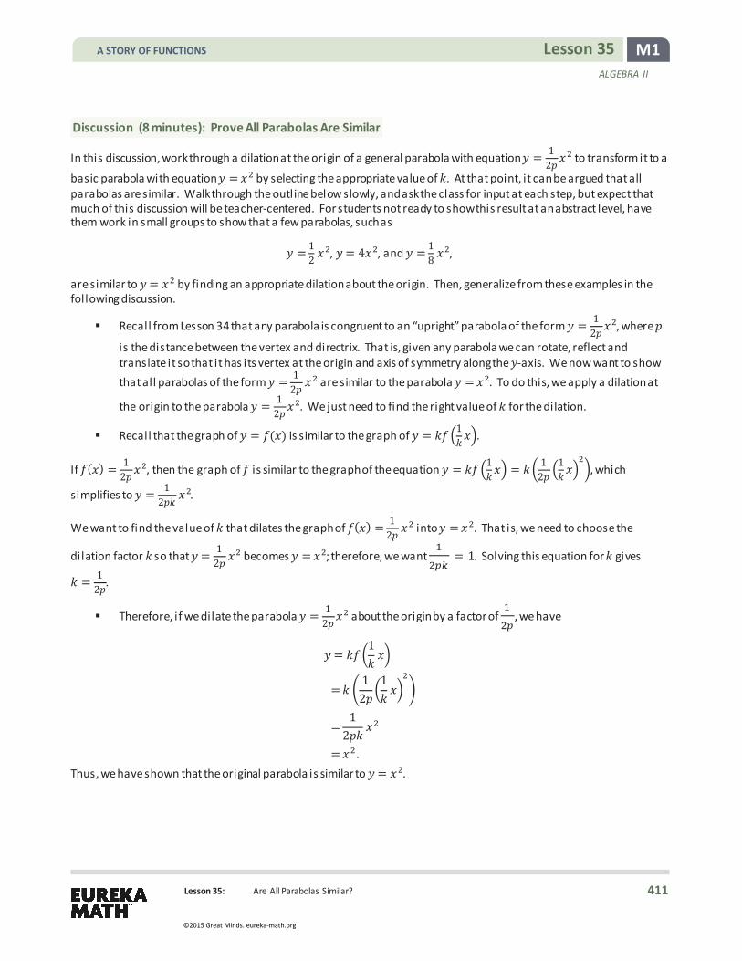
M1 Lesson 35 ALGEBRA II
Lesson 35: Are All Parabolas Similar?
Discussion (8 minutes): Prove All Parabolas Are Similar
In this discussion, work through a dilation at the origin of a general parabola with equation 𝑦𝑦 = 12𝑝𝑝𝑥𝑥
2 to transform it to a
basic parabola with equation 𝑦𝑦 = 𝑥𝑥2 by selecting the appropriate value of 𝑘𝑘. At that point, it can be argued that all parabolas are similar. Walk through the outline below slowly, and ask the class for input at each step, but expect that much of this discussion will be teacher-centered. For students not ready to show this result at an abstract level, have them work in small groups to show that a few parabolas, such as
𝑦𝑦 = 12 𝑥𝑥
2, 𝑦𝑦= 4𝑥𝑥2, and 𝑦𝑦 = 18 𝑥𝑥
2,
are similar to 𝑦𝑦= 𝑥𝑥2 by finding an appropriate dilation about the origin. Then, generalize from these examples in the following discussion.
� Recall from Lesson 34 that any parabola is congruent to an “upright” parabola of the form 𝑦𝑦 = 12𝑝𝑝𝑥𝑥
2, where 𝑝𝑝
is the distance between the vertex and directrix. That is, given any parabola we can rotate, reflect and translate it so that it has its vertex at the origin and axis of symmetry along the 𝑦𝑦-axis. We now want to show that all parabolas of the form 𝑦𝑦 = 1
2𝑝𝑝 𝑥𝑥2 are similar to the parabola 𝑦𝑦 = 𝑥𝑥2. To do this, we apply a dilation at
the origin to the parabola 𝑦𝑦 = 12𝑝𝑝𝑥𝑥
2. We just need to find the right value of 𝑘𝑘 for the dilation.
� Recall that the graph of 𝑦𝑦 = 𝑓𝑓(𝑥𝑥) is similar to the graph of 𝑦𝑦 = 𝑘𝑘𝑓𝑓�1𝑘𝑘𝑥𝑥�.
If 𝑓𝑓(𝑥𝑥) = 12𝑝𝑝𝑥𝑥
2, then the graph of 𝑓𝑓 is similar to the graph of the equation 𝑦𝑦 = 𝑘𝑘𝑓𝑓�1𝑘𝑘𝑥𝑥� = 𝑘𝑘 1
2𝑝𝑝 �1𝑘𝑘𝑥𝑥�
2, which
simplifies to 𝑦𝑦 = 12𝑝𝑝𝑘𝑘 𝑥𝑥
2.
We want to find the value of 𝑘𝑘 that dilates the graph of 𝑓𝑓(𝑥𝑥) = 12𝑝𝑝 𝑥𝑥
2 into 𝑦𝑦 = 𝑥𝑥2. That is, we need to choose the
dilation factor 𝑘𝑘 so that 𝑦𝑦= 12𝑝𝑝 𝑥𝑥
2 becomes 𝑦𝑦 = 𝑥𝑥2; therefore, we want 1
2 𝑘𝑘= 1. Solving this equation for 𝑘𝑘 gives
𝑘𝑘 = 12𝑝𝑝.
� Therefore, if we dilate the parabola 𝑦𝑦 = 12𝑝𝑝𝑥𝑥
2 about the origin by a factor of 12
, we have
𝑦𝑦= 𝑘𝑘𝑓𝑓1𝑘𝑘𝑥𝑥
= 𝑘𝑘1
2𝑝𝑝1𝑘𝑘𝑥𝑥
2
=1
2𝑝𝑝𝑘𝑘𝑥𝑥2
= 𝑥𝑥2. Thus, we have shown that the original parabola is similar to 𝑦𝑦= 𝑥𝑥2.
A STORY OF FUNCTIONS
411
©2015 Great Minds. eureka-math.org

M1 Lesson 35 ALGEBRA II
Lesson 35: Are All Parabolas Similar?
� In the previous lesson, we showed that any parabola is congruent to a parabola given by 𝑦𝑦 = 12𝑝𝑝𝑥𝑥
2 for some
value of 𝑝𝑝. Now, we have shown that every parabola with equation of the form 𝑦𝑦 = 12𝑝𝑝 𝑥𝑥
2 is similar to our
basic parabola given by 𝑦𝑦 = 𝑥𝑥2. Then, any parabola in the plane is similar to the basic parabola given by 𝑦𝑦 = 𝑥𝑥2.
� Further, all parabolas are similar to each other because we have just shown that they are all similar to the same parabola.
Closing (3 minutes)
Revisit the title of this lesson by asking students to summarize what they learned about the reason why all parabolas are similar. Then, take time to bring closure to this cycle of three lessons. The work students have engaged in has drawn together three different domains: geometry, algebra, and functions. In working through these examples and exercises and engaging in the discussions presented here, students can gain an appreciation for how mathematics can model real-world scenarios. The past three lessons show the power of using algebra and functions to solve problems in geometry.
Combining the power of geometry, algebra, and functions is one of the most powerful techniques available to solve science, technology and engineering problems.
Exit Ticket (4 minutes)
Lesson Summary
� We started with a geometric figure of a parabola defined by geometric requirements and recognized that it involved the graph of an equation we studied in algebra.
� We used algebra to prove that all parabolas with the same distance between the focus and directrix are congruent to each other, and in particular, they are congruent to a parabola with vertex at the origin,
axis of symmetry along the -axis, and equation of the form = .
� Noting that the equation for a parabola with axis of symmetry along the -axis is of the form = ( ) for a quadratic function , we proved that all parabolas are similar using transformations of functions.
A STORY OF FUNCTIONS
412
©2015 Great Minds. eureka-math.org
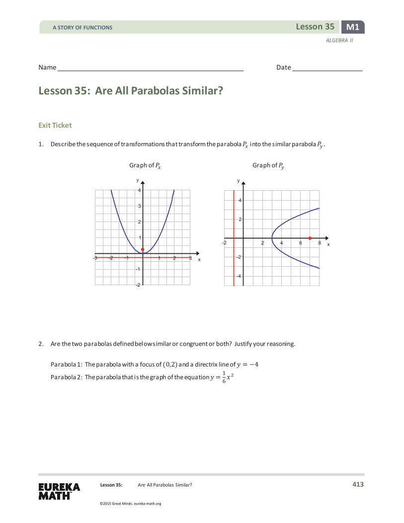
M1 Lesson 35 ALGEBRA II
Lesson 35: Are All Parabolas Similar?
Name Date
Lesson 35: Are All Parabolas Similar?
Exit Ticket 1. Describe the sequence of transformations that transform the parabola 𝑃𝑃 into the similar parabola 𝑃𝑃 .
Graph of 𝑃𝑃 Graph of 𝑃𝑃
2. Are the two parabolas defined below similar or congruent or both? Justify your reasoning. Parabola 1: The parabola with a focus of (0,2) and a directrix line of 𝑦𝑦 = −4
Parabola 2: The parabola that is the graph of the equation 𝑦𝑦 = 16𝑥𝑥
2
-2 2 4 6 8
-4
-2
2
4
x
y
-3 -2 -1 1 2 3
-2
-1
1
2
3
4
x
y
A STORY OF FUNCTIONS
413
©2015 Great Minds. eureka-math.org

M1 Lesson 35 ALGEBRA II
Lesson 35: Are All Parabolas Similar?
Exit Ticket Sample Solutions
1. Describe the sequence of transformations that would transform the parabola into the similar parabola .
Graph of Graph of
Vertical scaling by a factor of , vertical translation up units, and a ° rotation clockwise about the origin
2. Are the two parabolas defined below similar or congruent or both?
Parabola 1: The parabola with a focus of ( , ) and a directrix line of = −
Parabola 2: The parabola that is the graph of the equation =
They are similar but not congruent because the distance between the focus and the directrix on Parabola 1 is units, but on Parabola 2, it is only units. Alternatively, students may describe that you cannot apply a series of rigid transformations that will map Parabola 1 onto Parabola 2. However, by using a dilation and a series of rigid transformations, the two parabolas can be shown to be similar since ALL parabolas are similar.
Problem Set Sample Solutions
1. Let ( ) = √ − . The graph of is shown below. On the same axes, graph the function , where ( ) = � �. Then, graph the function , where ( ) = ( ).
-2 2 4 6 8
-4
-2
2
4
x
y
-3 -2 -1 1 2 3
-2
-1
1
2
3
4
x
y
MP.3
A STORY OF FUNCTIONS
414
©2015 Great Minds. eureka-math.org
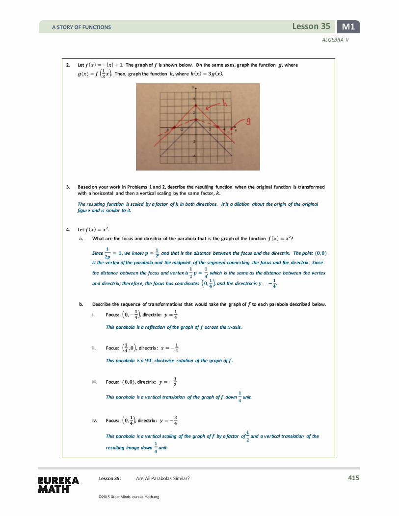
M1 Lesson 35 ALGEBRA II
Lesson 35: Are All Parabolas Similar?
2. Let ( ) = −| | + . The graph of is shown below. On the same axes, graph the function , where
( ) = � �. Then, graph the function , where ( ) = ( ).
3. Based on your work in Problems 1 and 2, describe the resulting function when the original function is transformed with a horizontal and then a vertical scaling by the same factor, .
The resulting function is scaled by a factor of in both directions. It is a dilation about the origin of the original figure and is similar to it.
4. Let ( ) = .
a. What are the focus and directrix of the parabola that is the graph of the function ( ) = ?
Since = , we know = , and that is the distance between the focus and the directrix. The point ( , )
is the vertex of the parabola and the midpoint of the segment connecting the focus and the directrix. Since
the distance between the focus and vertex is = , which is the same as the distance between the vertex
and directrix; therefore, the focus has coordinates � , �, and the directrix is = − .
b. Describe the sequence of transformations that would take the graph of to each parabola described below.
i. Focus: � ,− �, directrix: =
This parabola is a reflection of the graph of across the -axis.
ii. Focus: � , �, directrix: = −
This parabola is a ° clockwise rotation of the graph of .
iii. Focus: ( , ), directrix: = −
This parabola is a vertical translation of the graph of down unit.
iv. Focus: � , �, directrix: = −
This parabola is a vertical scaling of the graph of by a factor of and a vertical translation of the
resulting image down unit.
A STORY OF FUNCTIONS
415
©2015 Great Minds. eureka-math.org

M1 Lesson 35 ALGEBRA II
Lesson 35: Are All Parabolas Similar?
v. Focus: ( , ), directrix: = −
This parabola is a vertical scaling of the graph of by a factor of and a vertical translation of the resulting image up unit.
c. Which parabolas are similar to the parabola that is the graph of ? Which are congruent to the parabola that is the graph of ?
All of the parabolas are similar. We have proven that all parabolas are similar. The congruent parabolas are (i), (ii), and (iii). These parabolas are the result of a rigid transformation of the original parabola that is the graph of . They have the same distance between the focus and directrix line as the original parabola.
5. Derive the analytic equation for each parabola described in Problem 4(b) by applying your knowledge of
transformations.
i. = −
ii. =
iii. = −
iv. = −
v. = +
6. Are all parabolas the graph of a function of in the -plane? If so, explain why, and if not, provide an example (by
giving a directrix and focus) of a parabola that is not.
No, they are not. Examples include the graph of the equation = , or a list stating a directrix and focus. For example, students may give the example of a directrix given by = − and focus ( , ), or an even more interesting example, such as a directrix given by = with focus ( ,− ). Any line and any point not on that line define a parabola.
7. Are the following parabolas congruent? Explain your reasoning.
They are not congruent, but they are similar. I can see that the parabola on the left appears to contain the point ( , ), while the parabola on the right appears to contain the point � , �. This implies that the graph of the parabola on the right is a dilation of the graph of the parabola on the left, so they are not congruent.
-1 1
0.5
0.5
x
y
-1
1
1
x
y
A STORY OF FUNCTIONS
416
©2015 Great Minds. eureka-math.org
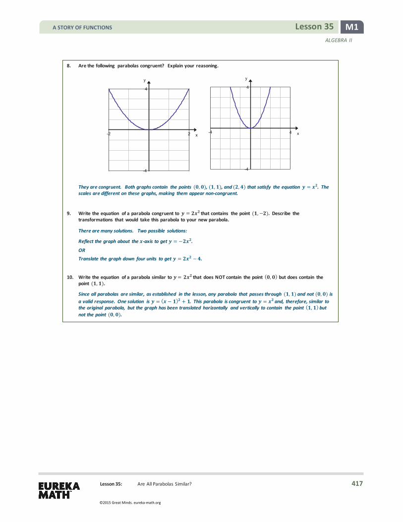
M1 Lesson 35 ALGEBRA II
Lesson 35: Are All Parabolas Similar?
8. Are the following parabolas congruent? Explain your reasoning.
They are congruent. Both graphs contain the points ( , ), ( , ), and ( , ) that satisfy the equation = . The scales are different on these graphs, making them appear non-congruent.
9. Write the equation of a parabola congruent to = that contains the point ( ,− ). Describe the transformations that would take this parabola to your new parabola.
There are many solutions. Two possible solutions:
Reflect the graph about the -axis to get = − .
OR Translate the graph down four units to get = − .
10. Write the equation of a parabola similar to = that does NOT contain the point ( , ) but does contain the point ( , ).
Since all parabolas are similar, as established in the lesson, any parabola that passes through ( , ) and not ( , ) is a valid response. One solution is = ( − ) + . This parabola is congruent to = and, therefore, similar to the original parabola, but the graph has been translated horizontally and vertically to contain the point ( , ) but not the point ( , ).
-4 4
-4
4
x
y
-2 2
-4
4
x
y
A STORY OF FUNCTIONS
417
©2015 Great Minds. eureka-math.org

ALGEBRA II • MODULE 1
Mathematics Curriculum
Topic D: A Surprise from Geometry—Complex Numbers Overcome All Obstacles
Topic D
A Surprise from Geometry—Complex Numbers Overcome All Obstacles N-CN.A.1, N-CN.A.2, N-CN.C.7, A-REI.A.2, A-REI.B.4b, A-REI.C.7
Focus Standards: N-CN.A.1 Know there is a complex number 𝑖𝑖 such that 𝑖𝑖2 = −1 , and every complex number has the form 𝑎𝑎 + 𝑏𝑏𝑖𝑖 with 𝑎𝑎 and 𝑏𝑏 real.
N-CN.A.2 Use the relation 𝑖𝑖2 = −1 and the commutative, associative, and distributive properties to add, subtract, and multiply complex numbers.
N-CN.C.7 Solve quadratic equations with real coefficients that have complex solutions.
A-REI.A.2 Solve simple rational and radical equations in one variable, and give examples showing how extraneous solutions may arise.
A-REI.B.4 Solve quadratic equations in one variable. Solve quadratic equations by inspection (e.g., for 𝑥𝑥2 = 49), taking square roots, completing the square, the quadratic formula and factoring, as appropriate to the initial form of the equation. Recognize when the quadratic formula gives complex solutions and write them as 𝑎𝑎 + 𝑏𝑏𝑖𝑖 for real numbers 𝑎𝑎 and 𝑏𝑏.
A-REI.C.7 Solve a simple system consisting of a linear equation and a quadratic equation in two variables algebraically and graphically. For example, find the points of intersection between the line 𝑦𝑦 = −3𝑥𝑥 and the circle 𝑥𝑥2 + 𝑦𝑦2 = 3.
Instructional Days: 5
Lesson 36: 1
Lesson 37:
Lesson 38:
Lesson 39: Factoring Extended to the Complex
Lesson 40: Obstacles Resolved—A Surprising Result (S)
1Lesson Structure Key: P- M-Modeling Cycle Lesson, E-Exploration Lesson, S-Socratic Lesson
A STORY OF FUNCTIONS
418
©2015 Great Minds. eureka-math.org

M1 Topic C ALGEBRA II
Topic C: Solving and Applying Equations—
In Topic D, students extend their facility with finding zeros of polynomials to include complex zeros. Lesson 36 presents a third obstacle to using factors of polynomials to solve polynomial equations. Students begin by solving systems of linear and nonlinear equations to which no real solutions exist and then relate this to the possibility of quadratic equations with no real solutions. Lesson 37 introduces complex numbers through their relationship to geometric transformations. That is, students observe that scaling all numbers on a number line by a factor of −1 turns the number line out of its one-dimensionality and rotates it 180° through
90° Lesson 38, students discover that complex numbers have real uses; in fact, they can be used in finding real solutions of polynomial equations. In Lesson 39, students develop facility with properties and operations of complex numbers and then apply that facility to factor polynomials with complex zeros. Lesson 40 brings the module to a close with the result that every polynomial can be rewritten as the product of linear factors, which is not possible without complex numbers. Even though standards N-CN.C.8 and N-CN.C.9 are not assessed at the Algebra II level, they are included instructionally to develop further conceptual understanding.
A STORY OF FUNCTIONS
419
©2015 Great Minds. eureka-math.org

Lesson 36: Overcoming a Third Obstacle to Factoring—What If There are No Real Number Solutions?
M1 Lesson 36 ALGEBRA II
Lesson 36: Overcoming a Third Obstacle to Factoring—
What If There Are No Real Number Solutions?
Student Outcomes
� Students understand the possibility that there might be no real number solution to an equation or system of equations. Students identify these situations and make the appropriate geometric connections.
Lesson Notes Lessons 36–40 provide students with the necessary tools to find solutions to polynomial equations outside the realm of the real numbers. This lesson i llustrates how to both analytically and graphically identify a system of equations that has no real number solution. In the next lesson, the imaginary unit 𝑖𝑖 is introduced, and students begin to work with complex numbers through the familiar geometric context of rotation. Students realize that the set of complex numbers inherits the arithmetic and algebraic properties from the real numbers. The work with complex solutions to polynomial equations in these lessons culminates with the fundamental theorem of Algebra in Lesson 40, the final lesson in this module.
Classwork Opening (1 minutes)
This lesson i llustrates how to identify a system of equations that has no real number solution, both graphically and analytically. In this lesson, students explore systems of equations that have no real number solutions.
Opening Exercise 1 (5 minutes)
Instruct students to complete the following exercise individually and then to pair up with a partner after a few minutes to compare their answers. Allow students to search for solutions analytically or graphically as they choose. After a few minutes, ask students to share their answers and solution methods. Both an analytic and a graphical solution should be presented for each system, either by a student or by the teacher if all students used the same approach. Circulate while students are working, and take note of which students are approaching the question analytically and which are approaching the question graphically.
A STORY OF FUNCTIONS
420
©2015 Great Minds. eureka-math.org
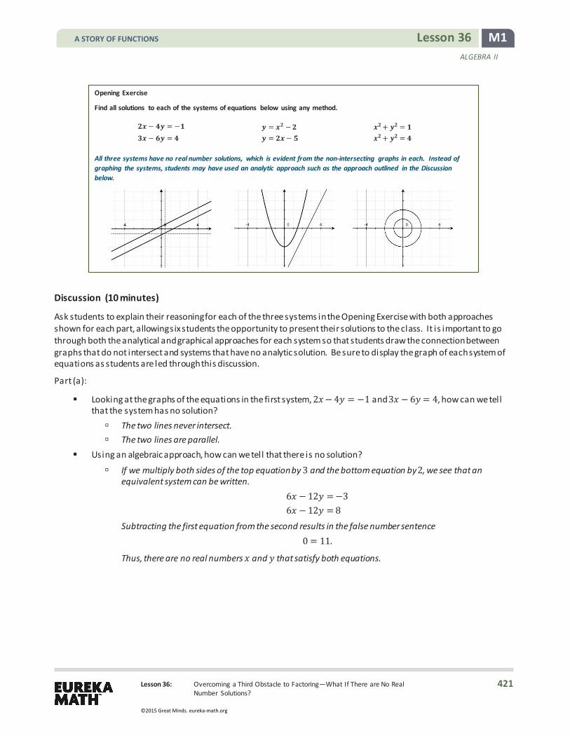
Lesson 36: Overcoming a Third Obstacle to Factoring—What If There are No Real Number Solutions?
M1 Lesson 36 ALGEBRA II
Opening Exercise
Find all solutions to each of the systems of equations below using any method.
All three systems have no real number solutions, which is evident from the non-intersecting graphs in each. Instead of graphing the systems, students may have used an analytic approach such as the approach outlined in the Discussion below.
Discussion (10 minutes)
Ask students to explain their reasoning for each of the three systems in the Opening Exercise with both approaches shown for each part, allowing six students the opportunity to present their solutions to the class. It is important to go through both the analytical and graphical approaches for each system so that students draw the connection between graphs that do not intersect and systems that have no analytic solution. Be sure to display the graph of each system of equations as students are led through this discussion.
Part (a):
� Looking at the graphs of the equations in the first system, 2𝑥𝑥− 4𝑦𝑦 = −1 and 3𝑥𝑥 − 6𝑦𝑦= 4, how can we tell that the system has no solution? à The two lines never intersect. à The two lines are parallel.
� Using an algebraic approach, how can we tell that there is no solution?
à If we multiply both sides of the top equation by 3 and the bottom equation by 2, we see that an equivalent system can be written.
6𝑥𝑥 − 12𝑦𝑦 =−3 6𝑥𝑥 − 12𝑦𝑦 = 8
Subtracting the first equation from the second results in the false number sentence 0 = 11.
Thus, there are no real numbers 𝑥𝑥 and 𝑦𝑦 that satisfy both equations.
− = − − =
= − = −
+ = + =
A STORY OF FUNCTIONS
421
©2015 Great Minds. eureka-math.org

Lesson 36: Overcoming a Third Obstacle to Factoring—What If There are No Real Number Solutions?
M1 Lesson 36 ALGEBRA II
� The graphs of these equations are lines. What happens if we put them in slope-intercept form? à Rewriting both linear equations in slope-intercept form, the system from part (a) can be written as
𝑦𝑦=12𝑥𝑥 +
14
𝑦𝑦=12𝑥𝑥 −
23
.
From what we know about graphing lines, the lines associated to these equations have the same slope and different 𝑦𝑦-intercepts, so they will be parallel. Since parallel lines do not intersect, the lines have no points in common and, therefore, this system has no solution.
Part (b):
� Looking at the graphs of the equations in the second system, 𝑦𝑦 = 𝑥𝑥2 − 2 and = 2𝑥𝑥 − 5 , how can we tell that the system has no solution? à The line and the parabola never intersect.
� Can we confirm, algebraically, that the system in part (b) has no real solution? à Yes. Since 𝑦𝑦= 𝑥𝑥2 − 2 and 𝑦𝑦 = 2𝑥𝑥 − 5, we must have 𝑥𝑥2 − 2 = 2𝑥𝑥 − 5, which is equivalent to the
quadratic equation 𝑥𝑥2 − 2𝑥𝑥 + 3 = 0. Solving for 𝑥𝑥 using the quadratic formula, we get
𝑥𝑥 =−(−2) ± (−2)2− 4(1)(3)
2(1)= 1 ±√−8
2.
Since the square root of a negative real number is not a real number, there is no real number 𝑥𝑥 that satisfies the equation 𝑥𝑥2 − 2𝑥𝑥+ 3 = 0; therefore, there is no point in the plane with coordinates (𝑥𝑥, 𝑦𝑦) that satisfies both equations in the original system.
Part (c):
� Looking at the graphs of the equations in the final system, 𝑥𝑥2+ 𝑦𝑦2 = 1 and 𝑥𝑥2+ 𝑦𝑦2 = 4, how can we tell that there the system has no solution?
à The circles are concentric, meaning that they have the same center and different radii. Thus, they never intersect, and there are no points that lie on both circles.
� Can we algebraically confirm that the system in part (c) has no solution?
à Yes. If we try to solve this system, we could subtract the first equation from the second, giving the false number sentence 0 = 3. Since this statement is false, we know that there are no values of 𝑥𝑥 and 𝑦𝑦 that satisfy both equations simultaneously; thus, the system has no solution.
At this point, ask students to summarize in writing or with a partner what they have learned so far. Use this brief exercise as an opportunity to check for understanding.
Exercise 1 (4 minutes)
Have students work individually and then check their answers with a partner. Make sure they write out their steps as they did in the sample solutions. After a few minutes, invite students to share one or two solutions on the board.
A STORY OF FUNCTIONS
422
©2015 Great Minds. eureka-math.org

Lesson 36: Overcoming a Third Obstacle to Factoring—What If There are No Real Number Solutions?
M1 Lesson 36 ALGEBRA II
Exercises 1–4
1. Are there any real number solutions to the system = and + = ? Support your findings both analytically and graphically.
+ ( ) = + =
= −
Since is non-negative for all real numbers , there are no real numbers so that = − . Then, there is no pair of real numbers ( , ) that solves the system consisting of the line = and the circle + =
. Thus, the line = does not intersect the circle + = in the real plane. This is confirmed
graphically as follows.
Discussion (7 minutes)
This lesson does not mention complex numbers or complex solutions; those are introduced in the next lesson. Make sure students understand that analytical findings can be confirmed graphically and vice-versa. Students turn their focus to quadratic equations in one variable 𝑥𝑥 without real solutions and to how the absence of any real solution 𝑥𝑥 can be confirmed by graphing a system of equations with two variables 𝑥𝑥 and 𝑦𝑦.
Present students with the following graphs of parabolas:
� Remember that a parabola with a vertical axis of symmetry is the graph of an equation of the form 𝑦𝑦 = 𝑎𝑎𝑥𝑥2 + 𝑏𝑏𝑥𝑥+ 𝑐𝑐 for some real number coefficients 𝑎𝑎, 𝑏𝑏, and 𝑐𝑐 with 𝑎𝑎 0. We can consider the solutions of the quadratic equation 𝑎𝑎𝑥𝑥2 + 𝑏𝑏𝑥𝑥+ 𝑐𝑐 = 0 to be the 𝑥𝑥-coordinates of solutions to the system of equations 𝑦𝑦 = 𝑎𝑎𝑥𝑥2 + 𝑏𝑏𝑥𝑥+ 𝑐𝑐 and 𝑦𝑦= 0. Thus, when we are investigating whether a quadratic equation 𝑎𝑎𝑥𝑥2+ 𝑏𝑏𝑥𝑥 + 𝑐𝑐 = 0 has a solution, we can think of this as finding the 𝑥𝑥-intercepts of the graph of 𝑦𝑦 = 𝑎𝑎𝑥𝑥2 + 𝑏𝑏𝑥𝑥+ 𝑐𝑐.
� Which of these three parabolas are represented by a quadratic equation 𝑦𝑦 = 𝑎𝑎𝑥𝑥2+ 𝑏𝑏𝑥𝑥 + 𝑐𝑐 that has no solution to 𝑎𝑎𝑥𝑥2 + 𝑏𝑏𝑥𝑥 + 𝑐𝑐 = 0? Explain how you know.
à Because the parabola has no 𝑥𝑥-intercepts, we know that there are no solutions to the associated equation 𝑎𝑎𝑥𝑥2 + 𝑏𝑏𝑥𝑥 + 𝑐𝑐 = 0.
Parabola 1 Parabola 2 Parabola 3
Scaffolding: Feel free to assign an optional extension exercise, such as: “Which of these equations will have no solution? Explain how you know in terms of a graph.”
𝑥𝑥2 + 5 = 0 𝑥𝑥2 − 4 = 0 𝑥𝑥2 + 1 = 0 𝑥𝑥2 − 10 = 0
Solution: 𝑥𝑥2 + 5 = 0 and 𝑥𝑥2 + 1 = 0 wil l not have real solutions because the graphs of the equations 𝑦𝑦 = 𝑥𝑥2+ 5 and 𝑦𝑦 = 𝑥𝑥2 + 1 do not intersect the 𝑥𝑥-axis, the l ine given by 𝑦𝑦 = 0.
A STORY OF FUNCTIONS
423
©2015 Great Minds. eureka-math.org

Lesson 36: Overcoming a Third Obstacle to Factoring—What If There are No Real Number Solutions?
M1 Lesson 36 ALGEBRA II
� Now, consider Parabola 2, which is the graph of the equation 𝑦𝑦 = 8− (𝑥𝑥 + 1) 2. How many solutions are there to the equation 8 − (𝑥𝑥 + 1)2 = 0? Explain how you know.
à Because Parabola 2 intersects the 𝑥𝑥-axis twice, the system consisting of 𝑦𝑦= 8 − (𝑥𝑥 + 1)2 and 𝑦𝑦= 0 has two real solutions. The graph suggests that the system will have one positive solution and one negative solution.
� Now, consider Parabola 3, which is the graph of the equation 𝑦𝑦 = 𝑥𝑥2. How does the graph tell us how many solutions there are to the equation 𝑥𝑥2 = 0? Explain how you know.
à Parabola 3 touches the 𝑥𝑥-axis only at (0, 0), so the parabola and the line with equation 𝑦𝑦 = 0 intersect at only one point. Accordingly, the system has exactly one solution, and there is exactly one solution to the equation 𝑥𝑥2 = 0.
Pause, and ask students to again summarize what they have learned, either in writing or orally to a neighbor. Students should be making connections between the graph of the quadratic equation 𝑦𝑦 = 𝑎𝑎𝑥𝑥2 + 𝑏𝑏𝑥𝑥+ 𝑐𝑐 (which is a parabola), the number of 𝑥𝑥-intercepts of the graph, and the number of solutions to the system consisting of 𝑦𝑦 = 0 and 𝑦𝑦 = 𝑎𝑎𝑥𝑥2+ 𝑏𝑏𝑥𝑥+ 𝑐𝑐.
Exercises 2–4 (12 minutes)
Students should work individually or in pairs on these exercises. To solve these problems analytically, they need to understand that they can determine the 𝑥𝑥-coordinates of the intersection points of the graphs of these geometric figures by solving an equation. Make sure students are giving their answers to these questions as coordinate pairs. Encourage students to solve the problems analytically and verify the solutions graphically.
2. Does the line = intersect the parabola = − ? If so, how many times and where? Draw graphs on the same set of axes.
= −
+ = ( + ) =
= or = −
If = , then = − = , and if = − , then = − = −(− ) = − .
The line = intersects the parabola = − at two distinct points: ( , ) and (− ,− ).
Scaffolding: � Consider having students
follow along with the instructor using a graphing calculator to show that the graph of 𝑦𝑦= 𝑥𝑥 intersects the graph of 𝑦𝑦= −𝑥𝑥2 twice, at the points indicated.
� Consider tasking advanced students with generating a system that meets certain criteria. For example, ask them to write the equations of a circle and a parabola that intersect once at (0,1). One appropriate answer is 𝑥𝑥2+ 𝑦𝑦2 = 1 and 𝑦𝑦 = 𝑥𝑥2 + 1.
A STORY OF FUNCTIONS
424
©2015 Great Minds. eureka-math.org

Lesson 36: Overcoming a Third Obstacle to Factoring—What If There are No Real Number Solutions?
M1 Lesson 36 ALGEBRA II
3. Does the line = − intersect the circle + = ? If so, how many times and where? Draw graphs on the same set of axes.
+ (− ) = =
=
= −√
or =√
The line = − intersects the circle + = at two distinct points: − , and ,− .
4. Does the line = intersect the parabola = − ? Why or why not? Draw the graphs on the same set of axes.
= − = − = −
A squared real number cannot be negative, so the line = does not intersect the parabola = − .
Before moving on, discuss these results as a whole class. Have students put both graphical and analytical solutions to each exercise on the board. Start to reinforce the connection that when the graphs intersect, the related system of equations has real solutions, and when the graphs do not intersect, there are no real solutions to the related system of equations.
A STORY OF FUNCTIONS
425
©2015 Great Minds. eureka-math.org

Lesson 36: Overcoming a Third Obstacle to Factoring—What If There are No Real Number Solutions?
M1 Lesson 36 ALGEBRA II
Closing (2 minutes)
Have students discuss with their neighbors the key points from today’s lesson. Encourage them to discuss the relationship between the solution(s) to a quadratic equation of the form 𝑎𝑎𝑥𝑥2 + 𝑏𝑏𝑥𝑥 + 𝑐𝑐 = 0 and the system
𝑦𝑦= 𝑎𝑎𝑥𝑥2+ 𝑏𝑏𝑥𝑥 + 𝑐𝑐 𝑦𝑦= 0.
They should discuss an understanding of the relationship between any solution(s) to a system of two equations and the 𝑥𝑥-coordinate of any point(s) of intersection of the graphs of the equations in the system.
The Lesson Summary below contains key findings from today’s lesson.
Exit Ticket (4 minutes)
In this Exit Ticket, students show that a particular system of two equations has no real solutions. They demonstrate this both analytically and graphically.
Lesson Summary An equation or a system of equations may have one or more solutions in the real numbers, or it may have no real number solution.
Two graphs that do not intersect in the coordinate plane correspond to a system of two equations without a real solution. If a system of two equations does not have a real solution, the graphs of the two equations do not intersect in the coordinate plane.
A quadratic equation in the form + + = , where , , and are real numbers and , that has no real solution indicates that the graph of = + + does not intersect the -axis.
A STORY OF FUNCTIONS
426
©2015 Great Minds. eureka-math.org

Lesson 36: Overcoming a Third Obstacle to Factoring—What If There are No Real Number Solutions?
M1 Lesson 36 ALGEBRA II
Name Date
Lesson 36: Overcoming a Third Obstacle—What If There Are No
Real Number Solutions?
Exit Ticket Solve the following system of equations or show that it does not have a real solution. Support your answer analytically and graphically.
𝑦𝑦 = 𝑥𝑥2 − 4 𝑦𝑦 = −(𝑥𝑥+ 5)
A STORY OF FUNCTIONS
427
©2015 Great Minds. eureka-math.org
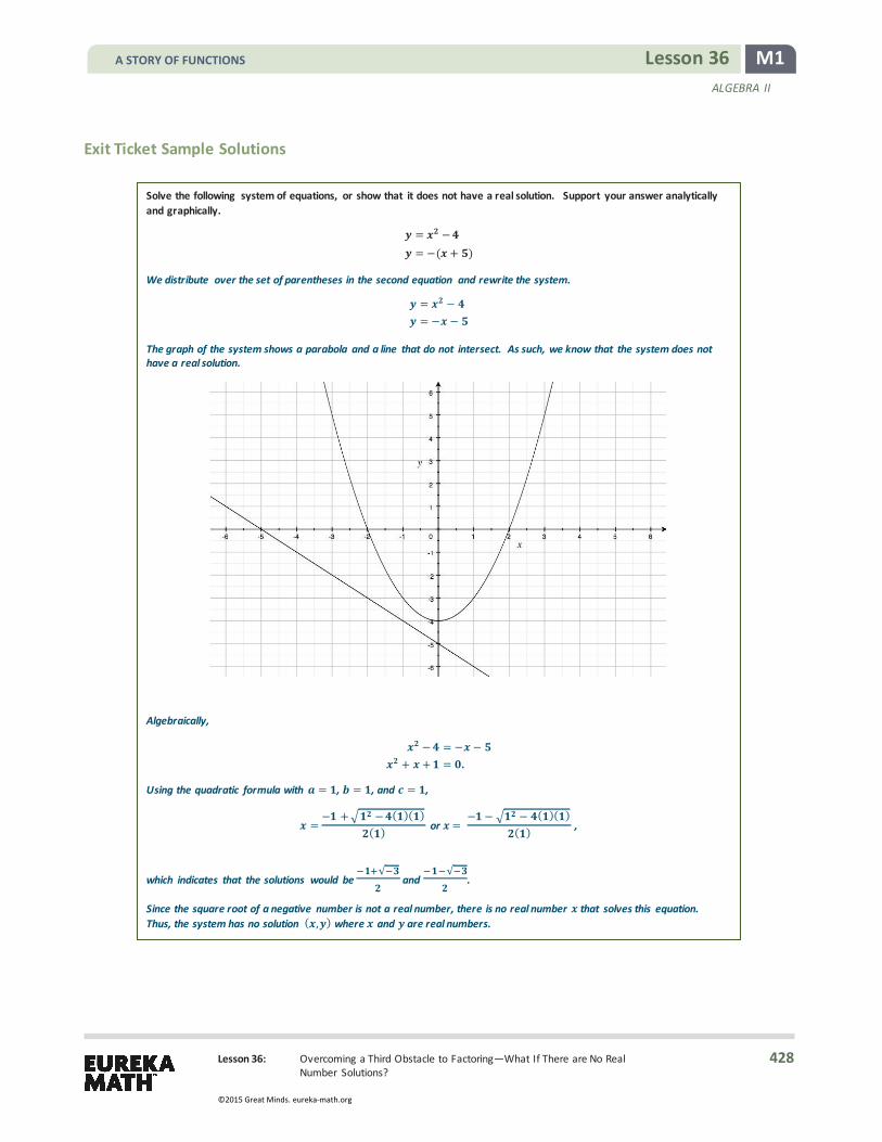
Lesson 36: Overcoming a Third Obstacle to Factoring—What If There are No Real Number Solutions?
M1 Lesson 36 ALGEBRA II
Exit Ticket Sample Solutions
Solve the following system of equations, or show that it does not have a real solution. Support your answer analytically and graphically.
= − = −( + )
We distribute over the set of parentheses in the second equation and rewrite the system.
= − = − −
The graph of the system shows a parabola and a line that do not intersect. As such, we know that the system does not have a real solution.
Algebraically,
− = − − + + = .
Using the quadratic formula with = , = , and = ,
=− + − ( )( )
( ) or = − − − ( )( )
( ) ,
which indicates that the solutions would be √
and √
.
Since the square root of a negative number is not a real number, there is no real number that solves this equation. Thus, the system has no solution ( , ) where and are real numbers.
A STORY OF FUNCTIONS
428
©2015 Great Minds. eureka-math.org

Lesson 36: Overcoming a Third Obstacle to Factoring—What If There are No Real Number Solutions?
M1 Lesson 36 ALGEBRA II
Problem Set Sample Solutions
1. For each part, solve the system of linear equations, or show that no real solution exists. Graphically support your answer.
a. + = + =
Multiply the second equation by .
+ = + =
Subtract the first equation from the second equation.
=
Then = .
Substitute for in the original second equation.
+ =
Then = .
The lines from the system intersect at the point � , �.
A STORY OF FUNCTIONS
429
©2015 Great Minds. eureka-math.org

Lesson 36: Overcoming a Third Obstacle to Factoring—What If There are No Real Number Solutions?
M1 Lesson 36 ALGEBRA II
b. − = − =
Multiply the first equation by and the second equation by on both sides.
− = − =
Subtracting the new second equation from the first equation gives the false number sentences = . Thus, there is no solution to the system. The graph of the system appropriately shows two parallel lines.
2. Solve the following system of equations, or show that no real solution exists. Graphically confirm your answer.
+ = − =
We can factor out from the top equation and isolate in the bottom equation to give us a better idea of what the graphs of the equations in the system look like. The first equation represents a circle centered at the origin with radius √ , and the second equation represents the line = − .
Algebraically,
+ ( − ) = + ( − ) =
+ ( − + ) = − + =
We solve for using the quadratic formula:
= , = − , =
=−(− ) ± (− ) − ( )
=±√ −
.
The solutions would be √ and
√.
Since both solutions for contain a square root of a negative number, no real solution exists; so the system has no solution ( , ) where and are real numbers.
A STORY OF FUNCTIONS
430
©2015 Great Minds. eureka-math.org

Lesson 36: Overcoming a Third Obstacle to Factoring—What If There are No Real Number Solutions?
M1 Lesson 36 ALGEBRA II
3. Find the value of so that the graph of the following system of equations has no solution.
− − = + − =
First, we rewrite the linear equations in the system in slope-intercept form.
= −
= − +
There is no solution to this system when the lines are parallel. Two lines are parallel when they share the same slope
and have different -intercepts. Here, the first line has slope and -intercept − , and the second line has slope
− and -intercept . The lines have different -intercepts and will be parallel when − = .
= −
= − = −
Thus, there is no solution only when = − .
4. Offer a geometric explanation to why the equation − + = has no real solutions.
The graph of = − + opens upward (since the leading coefficient is positive) and takes on its lowest value at the vertex ( , ). Hence, it does not intersect the -axis, and, therefore, the equation has no real solutions.
5. Without his pencil or calculator, Joey knows that + − = has at least one real solution. How does he know?
The graph of every cubic polynomial function intersects the -axis at least once because the end behaviors are opposite: one end goes up and the other goes down. This means that the graph of any cubic equation
= + + + must have at least one -intercept. Thus, every cubic equation must have at least one real solution.
A STORY OF FUNCTIONS
431
©2015 Great Minds. eureka-math.org

Lesson 36: Overcoming a Third Obstacle to Factoring—What If There are No Real Number Solutions?
M1 Lesson 36 ALGEBRA II
6. The graph of the quadratic equation = + has no -intercepts. However, Gia claims that when the graph of = + is translated by a distance of in a certain direction, the new (translated) graph would have exactly one
-intercept. Further, if = + is translated by a distance greater than in the same direction, the new (translated) graph would have exactly two -intercepts. Support or refute Gia’s claim. If you agree with her, in which direction did she translate the original graph? Draw graphs to illustrate.
By translating the graph of = + DOWN by unit, the new graph has equation = , which has one -intercept at = . When translating the original graph DOWN by more than unit, the new graph will cross the -axis exactly twice.
7. In the previous problem, we mentioned that the graph of = + has no -intercepts. Suppose that = + is one of two equations in a system of equations and that the other equation is linear. Give an example of a linear equation such that this system has exactly one solution.
The line with equation = is tangent to = + only at ( , ); so there would be exactly one real solution to the system.
= + =
Another possibility is an equation of any vertical line, such as = − or = , or = for any real number .
8. In prior problems, we mentioned that the graph of = + has no -intercepts. Does the graph of = + intersect the graph of = + ?
Setting these equations together, we can rearrange terms to get − = , which is an equation we can solve by factoring. We have ( − ) = , which has solutions at and . Thus, the graphs of these equations intersect when = and when = . When = , = , and when = , = . Thus, the two graphs intersect at the points ( , ) and ( , ).
The quick answer: The highest term in both equations has degree . The third-degree term does not cancel when setting the two equations (in terms of ) equal to each other. All cubic equations have at least one real solution, so the two graphs intersect at least at one point.
MP.3
A STORY OF FUNCTIONS
432
©2015 Great Minds. eureka-math.org

Lesson 37: A Surprising Boost from Geometry
M1 Lesson 37 ALGEBRA II
Lesson 37: A Surprising Boost from Geometry
Student Outcomes
� Students write a complex number in the form 𝑎𝑎 + 𝑏𝑏𝑖𝑖, where 𝑎𝑎 and 𝑏𝑏 are real numbers and the imaginary unit 𝑖𝑖 satisfies 𝑖𝑖2 = −1. Students geometrically identify 𝑖𝑖 as a multiplicand effecting a 90° counterclockwise rotation of the real number line. Students locate points corresponding to complex numbers in the complex plane.
� Students understand complex numbers as a superset of the real numbers (i .e., a complex number 𝑎𝑎 + 𝑏𝑏𝑖𝑖 is real when 𝑏𝑏 = 0). Students learn that complex numbers share many similar properties of the real numbers: associative, commutative, distributive, addition/subtraction, multiplication, etc.
Lesson Notes Students first receive an introduction to the imaginary unit 𝑖𝑖 and develop an algebraic and geometric understanding of the complex numbers (N-CN.A.1). Notice that at this level, mathematical tools needed to define the complex numbers are unavailable just as they are unavailable for defining the real numbers; however, students can describe them, understand them, and use them. The lesson then underscores that complex numbers satisfy the same properties of operations as real numbers (N-CN.A.2). Finally, students perform exercises to reinforce their understanding of and facility with complex numbers algebraically. This lesson ties into the work in the next lesson, which involves complex solutions to quadratic equations (N-CN.C.7).
Students first encounter complex numbers when they classify equations such as 𝑥𝑥2+ 1 = 0 as having no real number solutions. At that point, the possibility that a solution exists within a superset of the real numbers called the complex numbers is not introduced. At the end of this module, the idea is briefly introduced that every polynomial 𝑃𝑃 of degree has values 𝑟𝑟 for which 𝑃𝑃(𝑟𝑟 ) = 0, where is a whole number and 𝑟𝑟 is a real or complex number. Further, in preparation for students’ work in Precalculus and Advanced Topics, it is stated (but students are not expected to know) that 𝑃𝑃 can be written as the product of l inear factors, a result known as the fundamental theorem of algebra. The usefulness of complex numbers as solutions to polynomial equations comes with a cost: While real numbers can be ordered (put in order from smallest to greatest), complex numbers cannot be compared. For example, the complex
number 12
+ 𝑖𝑖√32
is not larger or smaller than √22
+ 𝑖𝑖√22
. However, this is a small price to pay. Students begin to see just
how important complex numbers are to geometry and computer science in Modules 1 and 2 in Precalculus and Advanced Topics. In college-level science and engineering courses, complex numbers are used in conjunction with differential equations to model circular motion and periodic phenomena in two dimensions.
Classwork Opening (1 minute)
We introduce a geometric context for complex numbers by demonstrating the analogous relationship between rotations in the plane and multiplication. The intention is for students to develop a deep understanding of 𝑖𝑖 through geometry.
� Today, we encounter a new number system that allows us to identify solutions to some equations that have no real number solutions. The complex numbers share many properties with the real numbers with which you are familiar. We take a geometric approach to introducing complex numbers.
A STORY OF FUNCTIONS
433
©2015 Great Minds. eureka-math.org

Lesson 37: A Surprising Boost from Geometry
M1 Lesson 37 ALGEBRA II
Opening Exercise (5 minutes)
Have students work alone on this motivating Opening Exercise. This exercise provides the context and invites the necessity for introducing an alternative number system, namely the complex numbers. Go over parts (a), (b), and (c) with the class; then, suggest that part (d) may be solvable using an alternative number system. Have students table this thought while beginning a geometrically-oriented discussion.
Opening Exercise
Solve each equation for .
a. − =
b. + = −
c. − = ,−
d. + = No real solution
Discussion (20 minutes)
Before beginning, allow students to prepare graph paper for drawing images as the discussion unfolds. At the close of this discussion, have students work with partners to summarize at least one thing they learned; then, provide time for some teacher-guided note-taking to capture the definition of the imaginary unit and its connection to geometric rotation.
Recall that multiplying by −1 rotates the number line in the plane by 180° about the point 0.
Pose this interesting thought question to students: Is there a number we can multiply by that corresponds to a 90° rotation?
Scaffolding: Demonstrate the rotation concept by drawing the number l ine carefully on a piece of white paper, drawing an identical number line on a transparency, putting a pin at zero, and rotating the transparency to show that the number l ine is rotating. For example, rotate from 2 to −2. This, of course, is the same as multiplying by −1.
Scaffolding: There were times in the past when people would have said that an equation such as 𝑥𝑥2 = 2 also had no solution.
A STORY OF FUNCTIONS
434
©2015 Great Minds. eureka-math.org

Lesson 37: A Surprising Boost from Geometry
M1 Lesson 37 ALGEBRA II
Students may find that this is a strange question. First, such a number does not map the number l ine to itself, so we have to imagine another number l ine that is a 90° rotation of the original:
This is l ike the coordinate plane. However, how should we label the points on the vertical axis?
Well, since we imagined such a number existed, let’s call it the imaginary axis and subdivide it into units of something called 𝑖𝑖. Then, the point 1 on the number l ine rotates to 1 𝑖𝑖 on the rotated number line and so on, as follows:
A STORY OF FUNCTIONS
435
©2015 Great Minds. eureka-math.org
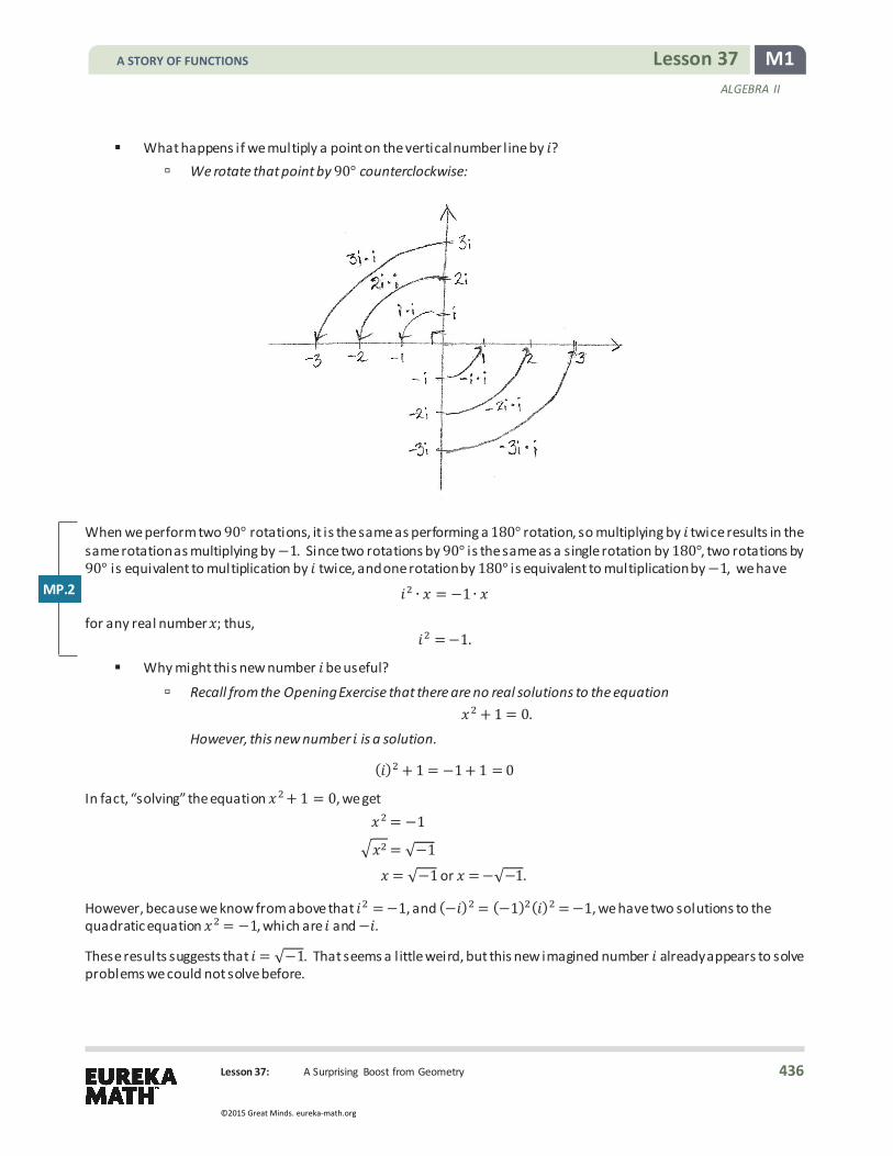
Lesson 37: A Surprising Boost from Geometry
M1 Lesson 37 ALGEBRA II
� What happens if we multiply a point on the vertical number l ine by 𝑖𝑖? à We rotate that point by 90° counterclockwise:
When we perform two 90° rotations, it is the same as performing a 180° rotation, so multiplying by 𝑖𝑖 twice results in the same rotation as multiplying by −1. Since two rotations by 90° is the same as a single rotation by 180°, two rotations by 90° is equivalent to multiplication by 𝑖𝑖 twice, and one rotation by 180° is equivalent to multiplication by −1, we have
𝑖𝑖2 𝑥𝑥 = −1 𝑥𝑥
for any real number 𝑥𝑥; thus, 𝑖𝑖2 =−1.
� Why might this new number 𝑖𝑖 be useful?
à Recall from the Opening Exercise that there are no real solutions to the equation 𝑥𝑥2 + 1 = 0.
However, this new number 𝑖𝑖 is a solution.
(𝑖𝑖)2 + 1 = −1 + 1 = 0
In fact, “solving” the equation 𝑥𝑥2+ 1 = 0, we get 𝑥𝑥2 = −1
𝑥𝑥2 = √−1 𝑥𝑥 = √−1 or 𝑥𝑥 =−√−1.
However, because we know from above that 𝑖𝑖2 =−1, and (−𝑖𝑖)2 = (−1)2(𝑖𝑖)2 =−1, we have two solutions to the quadratic equation 𝑥𝑥2 = −1, which are 𝑖𝑖 and −𝑖𝑖.
These results suggests that 𝑖𝑖 = √−1. That seems a l ittle weird, but this new imagined number 𝑖𝑖 already appears to solve problems we could not solve before.
MP.2
A STORY OF FUNCTIONS
436
©2015 Great Minds. eureka-math.org

Lesson 37: A Surprising Boost from Geometry
M1 Lesson 37 ALGEBRA II
For example, in Algebra I, when we applied the quadratic formula to
𝑥𝑥2 + 2𝑥𝑥+ 5 = 0, we found that
𝑥𝑥 =−2+ 22−4 1 (5)
2(1) or 𝑥𝑥 =2 2 4(1)( )
2(1)
𝑥𝑥 =−2+ −162 or 𝑥𝑥 =
2 √ 12
.
Recognizing the negative number under the square root, we reported that the equation 𝑥𝑥2 + 2𝑥𝑥 + 5 = 0 has no real solutions. Now, however, we can write
√−16 = √16 −1 =√16 √−1 = 4𝑖𝑖.
Therefore, 𝑥𝑥 = −1 + 2𝑖𝑖 or 𝑥𝑥 = −1− 2𝑖𝑖, which means −1 + 2𝑖𝑖 and −1− 2𝑖𝑖 are the solutions to 𝑥𝑥2 + 2𝑥𝑥 + 5 = 0.
The solutions −1 + 2𝑖𝑖 and −1− 2𝑖𝑖 are numbers called complex numbers, which we can locate in the complex plane.
In fact, all complex numbers can be written in the form
𝑎𝑎 + 𝑏𝑏𝑖𝑖 ,
where 𝑎𝑎 and 𝑏𝑏 are real numbers. Just as we can represent real numbers on the number l ine, we can represent complex numbers in the complex plane. Each complex number 𝑎𝑎 + 𝑏𝑏𝑖𝑖 can be located in the complex plane in the same way we locate the point (𝑎𝑎, 𝑏𝑏) in the Cartesian plane. From the origin, translate 𝑎𝑎 units horizontally along the real axis and 𝑏𝑏 units vertically along the imaginary axis.
Since complex numbers are built from real numbers, we should be able to add, subtract, multiply, and divide them. They should also satisfy the commutative, associative, and distributive properties, just as real numbers do.
Let’s check how some of these operations work for complex numbers.
Scaffolding: Name a few complex numbers for students to plot on their graph paper. This builds an understanding of their locations in this coordinate system. For example, consider −2𝑖𝑖− 3, −𝑖𝑖, 𝑖𝑖, 𝑖𝑖 − 1, and 32𝑖𝑖 + 2. Make sure students
are also cognizant of the fact that real numbers are also complex numbers (e.g., −3
2, 0, 1, ).
A STORY OF FUNCTIONS
437
©2015 Great Minds. eureka-math.org

Lesson 37: A Surprising Boost from Geometry
M1 Lesson 37 ALGEBRA II
Examples 1–2 (4 minutes): Addition and Subtraction with Complex Numbers
Addition of variable expressions is a matter of rearranging terms according to the properties of operations. Often, we call this combining like terms. These properties of operations apply to complex numbers.
(𝑎𝑎 + 𝑏𝑏𝑖𝑖) + (𝑐𝑐 + 𝑖𝑖) = (𝑎𝑎 + 𝑐𝑐) + (𝑏𝑏 + )𝑖𝑖 Example 1: Addition with Complex Numbers
Compute ( + ) + ( − ).
( + ) + ( − ) = + + − = ( + ) + ( − ) = −
Example 2: Subtraction with Complex Numbers
Compute ( + )− ( − ).
( + )− ( − ) = + − + = ( − ) + ( + ) = − +
Examples 3-4 (6 minutes): Multiplication with Complex Numbers
Multiplication is analogous to polynomial multiplication, using the addition, subtraction, and multiplication operations and the fact that 𝑖𝑖2 = −1.
(𝑎𝑎 + 𝑏𝑏𝑖𝑖) (𝑐𝑐 + 𝑖𝑖) = 𝑎𝑎𝑐𝑐 + 𝑏𝑏𝑐𝑐𝑖𝑖 + 𝑎𝑎 𝑖𝑖+ 𝑏𝑏 𝑖𝑖2 = (𝑎𝑎𝑐𝑐 − 𝑏𝑏 ) + (𝑏𝑏𝑐𝑐 + 𝑎𝑎 )𝑖𝑖
Example 3: Multiplication with Complex Numbers
Compute ( + )( − ).
( + )( − ) = + − − = + − (− ) = + =
Example 4: Multiplication with Complex Numbers
Verify that − + and − − are solutions to + + = .
− + :
(− + ) + (− + ) + = − + − + + = − + + − + = − + + =
− − :
(− − ) + (− − ) + = + + − − + = + − + − + = − + + =
So, both complex numbers − − and − + are solutions to the quadratic equation + + = .
MP.7
Scaffolding:
As needed, do more exercises with addition and multiplication of complex numbers, such as:
� (6− 𝑖𝑖) + (3 − 2𝑖𝑖) = 9− 3𝑖𝑖 � (3 + 2𝑖𝑖)(−3 + 2𝑖𝑖) = −13 � (5 + 4𝑖𝑖)(2 − 𝑖𝑖) = 14 + 3𝑖𝑖 � 2 +√3 𝑖𝑖 −2+√3 𝑖𝑖 = −7 � (1 − 6𝑖𝑖) 2 = 37− 12𝑖𝑖 � (−3− 𝑖𝑖) (2 − 4𝑖𝑖) + (1 + 3𝑖𝑖) = −10
MP.7
A STORY OF FUNCTIONS
438
©2015 Great Minds. eureka-math.org

Lesson 37: A Surprising Boost from Geometry
M1 Lesson 37 ALGEBRA II
Closing (4 minutes)
Ask students to write or discuss with a neighbor some responses to the following prompts:
� What are the advantages of introducing the complex numbers? � How can we use geometry to explain the imaginary number 𝑖𝑖?
The Lesson Summary box presents key findings from today’s lesson.
Exit Ticket (5 minutes)
In this Exit Ticket, students reduce a complex expression to 𝑎𝑎 + 𝑏𝑏𝑖𝑖 form and then locate the corresponding point on the complex plane.
Lesson Summary Multiplication by rotates every complex number in the complex plane by ° about the origin.
Every complex number is in the form + , where is the real part and is the imaginary part of the number. Real numbers are also complex numbers; the real number can be written as the complex number + . Numbers of the form , for real numbers , are called imaginary numbers.
Adding two complex numbers is analogous to combining like terms in a polynomial expression.
Multiplying two complex numbers is like multiplying two binomials, except one can use = − to further write the expression in simpler form.
Complex numbers satisfy the associative, commutative, and distributive properties.
Complex numbers allow us to find solutions to polynomial equations that have no real number solutions.
A STORY OF FUNCTIONS
439
©2015 Great Minds. eureka-math.org
Lesson 37: A Surprising Boost from Geometry
M1 Lesson 37 ALGEBRA II
Name Date
Lesson 37: A Surprising Boost from Geometry
Exit Ticket Express the quantities below in 𝑎𝑎 + 𝑏𝑏𝑖𝑖 form, and graph the corresponding points on the complex plane. If you use one set of axes, be sure to label each point appropriately.
(1 + 𝑖𝑖)− (1− 𝑖𝑖)
(1 + 𝑖𝑖)(1− 𝑖𝑖)
𝑖𝑖(2 − 𝑖𝑖)(1 + 2𝑖𝑖)
A STORY OF FUNCTIONS
440
©2015 Great Minds. eureka-math.org

Lesson 37: A Surprising Boost from Geometry
M1 Lesson 37 ALGEBRA II
Exit Ticket Sample Solutions
Express the quantities below in + form, and graph the corresponding points on the complex plane. If you use one set of axes, be sure to label each point appropriately.
( + )− ( − ) ( + )( − ) ( − )( + )
( + )− ( − ) = + =
( + )( − ) = + −−
= − = + = +
=
( − )( + ) = ( + − − ) = ( + − (− )) = ( + + ) = ( + ) = + = − +
A STORY OF FUNCTIONS
441
©2015 Great Minds. eureka-math.org
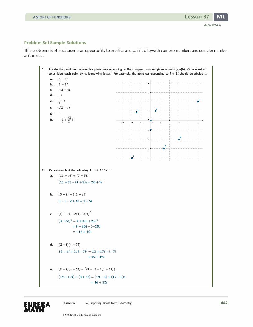
Lesson 37: A Surprising Boost from Geometry
M1 Lesson 37 ALGEBRA II
Problem Set Sample Solutions This problem set offers students an opportunity to practice and gain facility with complex numbers and complex number arithmetic.
1. Locate the point on the complex plane corresponding to the complex number given in parts (a)–(h). On one set of axes, label each point by its identifying letter. For example, the point corresponding to + should be labeled .
a. + b. − c. − − d. −
e. +
f. √ − g.
h. − +
2. Express each of the following in + form. a. ( + ) + ( + )
( + ) + ( + ) = +
b. ( − ) − ( − )
− − + = +
c. ( − )− ( − )
( + ) = + + = + + (− ) = − +
d. ( − )( + )
− + − = + − (− ) = +
e. ( − )( + )− ( − )− ( − )
( + )− ( + ) = ( − ) + ( − ) = +
A STORY OF FUNCTIONS
442
©2015 Great Minds. eureka-math.org

Lesson 37: A Surprising Boost from Geometry
M1 Lesson 37 ALGEBRA II
3. Express each of the following in + form.
a. ( + ) + ( + )
( + ) + ( + ) = ( + ) + ( + ) = +
b. (– + )− ( − )
(− + )− ( − ) = − + − + = − +
c. ( + ) + ( − )− ( − )
( + ) + ( − )− ( − ) = + + − − + = +
d. ( + )( + )
( + )( + ) = + + + = + + + = + − = + =
e. − ( − )( + )
− ( − )( + ) = − ( − + − ) = − ( + + ) = − ( + ) = − − = − + = −
f. ( + )( − ) + ( − )−
( + )( − ) + ( − )− = ( + − − ) + − − = + − + + + − = +
4. Find the real values of and in each of the following equations using the fact that if + = + , then = and = .
a. + = +
= =
= =
MP.7
A STORY OF FUNCTIONS
443
©2015 Great Minds. eureka-math.org

Lesson 37: A Surprising Boost from Geometry
M1 Lesson 37 ALGEBRA II
b. ( + ) = ( − )
( + ) + = + ( − )
( + ) =
= −
= ( − ) − =
=
c. ( − ) − ( − ) = − ( + ) ( − ) =
− = = =
− ( − ) = − ( + ) − ( − ) = − ( + ) − + = − −
=
=
5. Since = − , we see that
= = − = − = = − − = .
Plot , , , and on the complex plane, and describe how multiplication by each rotates points in the complex plane.
Multiplying by rotates points by ° counterclockwise around ( , ). Multiplying by = − rotates points by ° about ( , ) . Multiplying by = − rotates points counterclockwise by ° about the origin, which is equivalent to rotation by ° clockwise about the origin. Multiplying by rotates points counterclockwise by °, which is equivalent to not rotating at all. The points , , , and are plotted below on the complex plane.
6. Express each of the following in + form.
a. +
b. − + c. − d. + e. − +
A simple approach is to notice that every multiplications by result in four ° rotations, which takes back to . Therefore, divide by , which is with remainder . So, ° rotations is equivalent to ° rotations and a ° rotation, and thus = − .
MP.8
MP.7
A STORY OF FUNCTIONS
444
©2015 Great Minds. eureka-math.org

Lesson 37: A Surprising Boost from Geometry
M1 Lesson 37 ALGEBRA II
7. Express each of the following in + form.
a. ( + ) ( + )( + ) = + + + = + − =
b. ( + )
( + ) = (( + ) ) = ( ) = = −
c. ( + )
( + ) = ( + ) ( + ) = ( )(− ) = −
8. Evaluate − when = − .
−
9. Evaluate − when = − .
−
10. Show by substitution that √
is a solution to − + = .
− √−
− √+ = − √ − √ − − √ +
= − √ + − − √ +
= − √ − − − √ +
= − √ − − + √ + =
11.
a. Evaluate the four products below.
Evaluate √ √ . =
Evaluate √ √− . =
Evaluate √− √ . =
Evaluate √− √− . = = −
b. Suppose and are positive real numbers. Determine whether the following quantities are equal or not equal.
√ √ and √− √− not equal
√− √ and √ √− equal
MP.7
A STORY OF FUNCTIONS
445
©2015 Great Minds. eureka-math.org

Lesson 38: Complex Numbers as Solutions to Equations
M1 Lesson 38 ALGEBRA II
Scaffolding: Advanced students may be able to handle a more abstract framing of—in essence—the same exercise. The exercise below offers the advanced student an opportunity to discover the discriminant and its significance on his or her own.
“Recall that a quadratic equation can have exactly two distinct real solutions, exactly one distinct real solution, or exactly two distinct complex solutions. What is the quadratic formula that we can use to solve an equation in the form 𝑎𝑎𝑥𝑥2 + 𝑏𝑏𝑥𝑥 + 𝑥𝑥 = 0, where 𝑎𝑎, 𝑏𝑏, and 𝑐𝑐 are real numbers and 𝑎𝑎 0? Analyze this formula to decide when the equation will have two, one, or no real solutions.”
Solution:
𝑥𝑥 =−𝑏𝑏±√𝑏𝑏2 − 4𝑎𝑎𝑐𝑐
2𝑎𝑎
The type of solutions to a quadratic equation hinges on the expression under the radical in the quadratic formula, namely, 𝑏𝑏2− 4𝑎𝑎𝑐𝑐. When 𝑏𝑏2− 4𝑎𝑎𝑐𝑐 < 0, both solutions will have imaginary parts. When 𝑏𝑏2 − 4𝑎𝑎𝑐𝑐 > 0, the quadratic equation has two distinct real solutions. When 𝑏𝑏2− 4𝑎𝑎𝑐𝑐 = 0, the quadratic formula simplifies to 𝑥𝑥 = − 𝑏𝑏
2𝑎𝑎. In this case, there is only one real solution, which we call a zero of multiplicity two.
Lesson 38: Complex Numbers as Solutions to Equations
Student Outcomes
� Students solve quadratic equations with real coefficients that have complex solutions (N-CN.C.7). They recognize when the quadratic formula gives complex solutions and write them as 𝑎𝑎 + 𝑏𝑏𝑖𝑖 for real numbers 𝑎𝑎 and 𝑏𝑏. (A-REI.B.4b)
Lesson Notes This lesson models how to solve quadratic equations over the set of complex numbers. Students relate the sign of the discriminant to the nature of the solution set for a quadratic equation. Continue to encourage students to make connections between graphs of a quadratic equation, 𝑦𝑦 = 𝑎𝑎𝑥𝑥2+ 𝑏𝑏𝑥𝑥+ 𝑐𝑐, and the number and type of solutions to the equation 𝑎𝑎𝑥𝑥2+ 𝑏𝑏𝑥𝑥 + 𝑐𝑐 = 0.
Classwork Opening (2 minutes)
In Algebra I, students learned that when the quadratic formula resulted in an expression that contained a negative number in the radicand, the equation would have no real solution. Now, students understand the imaginary unit 𝑖𝑖 as a number that satisfies 𝑖𝑖2 = −1, which allows them to solve quadratic equations over the complex numbers. Thus, they can see that every quadratic equation has at least one solution.
Opening Exercises (5 minutes)
Have students work on this opening exercise alone or in pairs. In this exercise, students apply the quadratic formula to three different relatively simple quadratic equations: one with two real roots, one with one real repeated root, and one with two complex roots. Students are then asked to explain the results in terms of the discriminant. Afterward, go over the answers with the class.
A STORY OF FUNCTIONS
446
©2015 Great Minds. eureka-math.org

Lesson 38: Complex Numbers as Solutions to Equations
M1 Lesson 38 ALGEBRA II
Review the quadratic formula 𝑥𝑥 = −𝑏𝑏± 𝑏𝑏2−4𝑎𝑎𝑐𝑐2𝑎𝑎 before beginning this exercise, and define the discriminant as the
number under the radical; that is, the discriminant is the quantity 𝑏𝑏2− 4𝑎𝑎𝑐𝑐. Opening Exercises
1. The expression under the radical in the quadratic formula, − , is called the discriminant. Use the quadratic formula to solve the following quadratic equations. Calculate the discriminant for each equation.
a. − =
The equation − = has two real solutions: = and = − . The discriminant of − = is .
b. − + =
The equation − + = has one real solution: = . The discriminant of − + = is .
c. + =
The equation + = has two complex solutions: = and = − . The discriminant of + = is − .
2. How does the value of the discriminant for each equation relate the number of solutions you found?
If the discriminant is negative, the equation has complex solutions. If the discriminant is zero, the equation has one real solution. If the discriminant is positive, the equation has two real solutions.
Discussion (8 minutes)
� Why do you think we call 𝑏𝑏2− 4𝑎𝑎𝑐𝑐 the discriminant?
à In English, a discriminant is a characteristic that allows something (e.g., an object, a person, a function) among a group of other somethings to be distinguished.
à In this case, the discriminant distinguishes a quadratic equation by its number and type of solutions: one real solution (repeated), two real solutions, or two complex solutions.
� Let’s examine the situation when the discriminant is zero. Why does a quadratic equation with discriminant zero have only one real solution?
à When the discriminant is zero, the quadratic formula gives the single solution − 𝑏𝑏±02𝑎𝑎 = − 𝑏𝑏
2𝑎𝑎.
� Why is the solution when 𝑏𝑏2 − 4𝑎𝑎𝑐𝑐 = 0 a repeated zero?
à If 𝑏𝑏2− 4𝑎𝑎𝑐𝑐 = 0, then 𝑐𝑐 = 𝑏𝑏2
4𝑎𝑎, and we can factor the quadratic expression 𝑎𝑎𝑥𝑥2+ 𝑏𝑏𝑥𝑥 + 𝑐𝑐 as follows:
𝑎𝑎𝑥𝑥2+ 𝑏𝑏𝑥𝑥 + 𝑐𝑐 = 𝑎𝑎𝑥𝑥2+ 𝑏𝑏𝑥𝑥+𝑏𝑏2
4𝑎𝑎= 𝑎𝑎 𝑥𝑥2 +
𝑏𝑏𝑎𝑎𝑥𝑥 +
𝑏𝑏2
4𝑎𝑎2= 𝑎𝑎 𝑥𝑥 +
𝑏𝑏2𝑎𝑎
2
.
From what we know of factoring quadratic expressions from Lesson 11, − 𝑏𝑏2𝑎𝑎 is a repeated zero.
Analytically, the solutions can be thought of as −𝑏𝑏+02𝑎𝑎 and −𝑏𝑏−0
2𝑎𝑎 , which are both − 𝑏𝑏2𝑎𝑎. So, there are
two solutions that are the same number.
Scaffolding: English language learners may benefit from a Frayer diagram or other vocabulary exercise for the word discriminant.
A STORY OF FUNCTIONS
447
©2015 Great Minds. eureka-math.org

Lesson 38: Complex Numbers as Solutions to Equations
M1 Lesson 38 ALGEBRA II
à Geometrically, a quadratic equation represents a parabola. If the discriminant is zero, then the
equation of the parabola is 𝑦𝑦= 𝑎𝑎�𝑥𝑥 + 𝑏𝑏2𝑎𝑎�
2, so the vertex of this parabola is �− 𝑏𝑏
2𝑎𝑎 ,0�, meaning the vertex of the parabola lies on the 𝑥𝑥-axis. Thus, the parabola is tangent to the 𝑥𝑥-axis and intersects the 𝑥𝑥-axis only at the point �− 𝑏𝑏
2𝑎𝑎 ,0�.
� For example, the graph of 𝑦𝑦= 𝑥𝑥2 + 6𝑥𝑥 + 9 intersects the 𝑥𝑥-axis only at (−3,0), as follows.
� Describe the graph of a quadratic equation with positive discriminant. à If the discriminant is positive, then the quadratic formula gives two different real solutions. à Two real solutions mean the graph intersects the 𝑥𝑥-axis at two distinct real points.
� For example, the graph of 𝑦𝑦= 𝑥𝑥2 + 𝑥𝑥 − 6 intersects the 𝑥𝑥-axis at (−3,0) and (2,0), as follows.
A STORY OF FUNCTIONS
448
©2015 Great Minds. eureka-math.org

Lesson 38: Complex Numbers as Solutions to Equations
M1 Lesson 38 ALGEBRA II
� Describe the graph of a quadratic equation with negative discriminant. à Since the discriminant is negative, the quadratic formula will give two different complex solutions. à Since there are no real solutions, the graph does not cross or touch the 𝑥𝑥-axis in the real plane.
� For example, the graph of 𝑦𝑦= 𝑥𝑥2 + 4, shown below, does not intersect the 𝑥𝑥-axis.
Example 1 (5 minutes)
Example 1
Consider the equation + = − .
What does the value of the discriminant tell us about number of solutions to this equation?
Solve the equation. Does the number of solutions match the information provided by the discriminant? Explain.
Consider the equation 3𝑥𝑥+ 𝑥𝑥2 = −7.
� What does the value of the discriminant tell us about number of solutions to this equation? à The equation in standard form is 𝑥𝑥2 + 3𝑥𝑥 + 7 = 0, so we have 𝑎𝑎 = 1, 𝑏𝑏 = 3, 𝑐𝑐 = 7. à The discriminant is 32 − 4(1)(7) = −19. The negative discriminant indicates that no real solutions
exist. There are two complex solutions. � Solve the equation. Does the number of solutions match the information provided by the discriminant?
Explain. à Using the quadratic formula,
𝑥𝑥 =−3+ −192 or 𝑥𝑥 =−3+ −19
2 .
à The solutions, in 𝑎𝑎 + 𝑏𝑏𝑖𝑖 form, are −32 + 19
2 𝑖𝑖 and −32 −
192 𝑖𝑖.
à The two complex solutions are consistent with the rule for a negative discriminant.
A STORY OF FUNCTIONS
449
©2015 Great Minds. eureka-math.org

Lesson 38: Complex Numbers as Solutions to Equations
M1 Lesson 38 ALGEBRA II
Exercise (15 minutes)
Have students work individually on this exercise; then, have them work with a partner or in a small group to check their solutions. This exercise could also be conducted by using personal white boards and having students show their answers to each question after a few minutes. If many students struggle, invite them to exchange papers with a partner to check for errors. Having students identify errors in their work or the work of others will help them to build fluency when working with these complicated expressions. Debrief this exercise by showing the related graph of the equation in the coordinate plane, and verify that the number of solutions corresponds to the number of 𝑥𝑥-intercepts.
Exercise
Compute the value of the discriminant of the quadratic equation in each part. Use the value of the discriminant to predict the number and type of solutions. Find all real and complex solutions.
a. + + =
We have = , = , and = . Then
− = − ( )( ) = .
Note that the discriminant is zero, so this equation has exactly one real solution.
=−( ) ±√
( ) = −
Thus, the only solution is − .
b. + =
We have = , = , and = . Then − = − .
Note that the discriminant is negative, so this equation has two complex solutions.
=− ± √−
( )
Thus, the two complex solutions are and − .
c. − − =
We have = , = − , and = − . Then
− = (− ) − ( )(− ) = + = .
Note that the discriminant is positive, so this equation has two distinct real solutions.
Using the quadratic formula,
=−(− ) ± √
( ) .
So, the two real solutions are √ and √
.
MP.3
A STORY OF FUNCTIONS
450
©2015 Great Minds. eureka-math.org

Lesson 38: Complex Numbers as Solutions to Equations
M1 Lesson 38 ALGEBRA II
d. + + =
We have = , = , and = . Then
− = − ( )( ) = − = − .
The discriminant is negative, so there will be two complex solutions. Using the quadratic formula,
=− ± √−
( ) .
So, the two complex solutions are − + and − − .
e. = +
We can rewrite this equation in standard form with = , = − , and = :
− + = .
Then
− = (− ) − ( )( ) = − = − .
The discriminant is negative, so there will be two complex solutions. Using the quadratic formula,
=−(− ) ± √−
( )
=± √
.
The two solutions are +√
and −√
.
f. + + =
We can factor from the left side of this equation to obtain ( + + ) = , and we know that a product is zero when one of the factors are zero. Since , we must have + + = . This is a quadratic equation with = , = , and
= . Then
− = − ( )( ) = − .
The discriminant is negative, so there will be two complex solutions. Using the quadratic formula,
=− ± √−
( )
=− ± √
.
The complex solutions are − + and − − .
Scaffolding:
Consider assigning advanced students to create quadratic equations that have specific solutions. For example, request a quadratic equation that has only the solution −5.
Answer: One such equation is 𝑥𝑥2 − 10𝑥𝑥+ 25 = 0. This follows from the expansion of the left side of (𝑥𝑥 + 5) 2 = 0. Also consider requesting a quadratic equation with solutions 3 + 𝑖𝑖 and 3− 𝑖𝑖. One answer is 𝑥𝑥2 − 6𝑥𝑥 + 10 = 0.
A STORY OF FUNCTIONS
451
©2015 Great Minds. eureka-math.org

Lesson 38: Complex Numbers as Solutions to Equations
M1 Lesson 38 ALGEBRA II
Closing (5 minutes)
As this lesson is summarized, ask students to create a graphic organizer that allows them to compare and contrast the nature of the discriminant, the number and types of solutions to 𝑎𝑎𝑥𝑥2 + 𝑏𝑏𝑥𝑥+ 𝑐𝑐 = 0, and the graphs of the equation 𝑦𝑦 = 𝑎𝑎𝑥𝑥2+ 𝑏𝑏𝑥𝑥+ 𝑐𝑐. Have them record a problem of each type from the previous exercise as an example in their graphic organizer.
Exit Ticket (5 minutes)
The Exit Ticket gives students the opportunity to demonstrate their mastery of this lesson’s content.
Lesson Summary
� A quadratic equation with real coefficients may have real or complex solutions.
� Given a quadratic equation + + = , the discriminant − indicates whether the equation has two distinct real solutions, one real solution, or two complex solutions. – If − > , there are two real solutions to + + = .
– If − = , there is one real solution to + + = .
– If − < , there are two complex solutions to + + = .
A STORY OF FUNCTIONS
452
©2015 Great Minds. eureka-math.org

Lesson 38: Complex Numbers as Solutions to Equations
M1 Lesson 38 ALGEBRA II
Name Date
Lesson 38: Complex Numbers as Solutions to Equations
Exit Ticket Use the discriminant to predict the nature of the solutions to the equation 4𝑥𝑥 − 3𝑥𝑥2 = 10. Then, solve the equation.
A STORY OF FUNCTIONS
453
©2015 Great Minds. eureka-math.org

Lesson 38: Complex Numbers as Solutions to Equations
M1 Lesson 38 ALGEBRA II
Exit Ticket Sample Solutions
Use the discriminant to predict the nature of the solutions to the equation − = . Then, solve the equation.
− + =
We have = , = − , and = . Then
− = (− ) − ( )( ) = − = − .
The value of the discriminant is negative, indicating that there are two complex solutions.
=−(− ) ±√−
( )
=± √
Thus, the two solutions are +√
and −√
.
Problem Set Sample Solutions The Problem Set offers students more practice solving quadratic equations with complex solutions.
1. Give an example of a quadratic equation in standard form that has …
a. Exactly two distinct real solutions.
Since ( + )( − ) = − , the equation − = has two distinct real solutions, and − .
b. Exactly one distinct real solution.
Since ( + ) = + + , the equation + + = has only one real solution, .
c. Exactly two complex (non-real) solutions.
Since + = has no solutions in the real numbers, this equation must have two complex solutions. They are and − .
2. Suppose we have a quadratic equation + + = so that + = . Does the quadratic equation have one solution or two distinct solutions? Are they real or complex? Explain how you know.
If + = , then either = = , > and < , or < and > .
The definition of a quadratic polynomial requires that , so either > and < or < and > .
In either case, < . Because is positive and is negative, we know − > .
Therefore, a quadratic equation + + = always has two distinct real solutions when + = .
A STORY OF FUNCTIONS
454
©2015 Great Minds. eureka-math.org

Lesson 38: Complex Numbers as Solutions to Equations
M1 Lesson 38 ALGEBRA II
3. Solve the equation − + = .
We have a quadratic equation with = , = − , and = .
=−(− ) ± √−
( )
So, the solutions are +√
and −√
.
4. Solve the equation + = − .
In standard form, this is the quadratic equation + + = with = , = , and = .
=− ± √−
( ) =− ± √
Thus, the solutions are + and − .
5. Solve the equation − = + + .
In standard form, this is the quadratic equation − + = with = , = − , and = .
= −−(− ) ± √−
( ) =± √
Thus, the solutions are +√
and −√
.
6. Solve the equation − + = .
This is a quadratic equation with = , = − , and = .
= −−(− ) ± √−
( ) =± √
Thus, the solutions are +√
and −√
.
7. Solve the equation + − + = ( − ).
When expanded, this is a quadratic equation with = , = − , and = .
+ − + = − − + =
=−(− ) ± {− }
( )
So, the solutions are +√
and − .
A STORY OF FUNCTIONS
455
©2015 Great Minds. eureka-math.org

Lesson 38: Complex Numbers as Solutions to Equations
M1 Lesson 38 ALGEBRA II
8. Solve the equation + + = .
We can factor from the left side of this equation to obtain ( + + ) = , and we know that a product is zero when one of the factors is zero. Since , we must have + + = . This is a quadratic equation with = , = , and = . Then
=− ± √−
,
and the solutions are − + and − − .
9. Write a quadratic equation in standard form such that − is its only solution.
( + ) = + + =
10. Is it possible that the quadratic equation + + = has a positive real solution if , , and are all positive real numbers?
No. The solutions are and . If is positive, the second one of these will be negative.
So, we need to think about whether or not the first one can be positive. If − +√ − > , then √ − > ; so, − > , and − > . This means that either or must be negative. So, if all three coefficients are positive, then there cannot be a positive solution to + + = .
11. Is it possible that the quadratic equation + + = has a positive real solution if , , and are all negative real numbers?
No. If , , and are all negative, then − , − , and − are all positive. The solutions of + + = are the same as the solutions to − − − = , and by Problem 10, this equation has no positive real solution since it has all positive coefficients.
Extension: 12. Show that if > . , the solutions of − + = are not real numbers.
We have = , = − , and = ; then
− = (− ) − = − .
When the discriminant is negative, the solutions of the quadratic function are not real numbers.
− = − < .
− < − ( . ) − <
> .
Thus, if > . , then the discriminant is negative and the solutions of − + = are not real numbers.
MP.2
A STORY OF FUNCTIONS
456
©2015 Great Minds. eureka-math.org

Lesson 38: Complex Numbers as Solutions to Equations
M1 Lesson 38 ALGEBRA II
13. Let be a real number, and consider the quadratic equation ( + ) + + = .
a. Show that the discriminant of ( + ) + + = defines a quadratic function of .
The discriminant of a quadratic equation written in the form + + = is − .
Here, = + , = , and = . We get
− = ( ) − ( + ) = − ( + ) = − − .
With unknown, we can write ( ) = − − , which is a quadratic function of .
b. Find the zeros of the function in part (a), and make a sketch of its graph.
If ( ) = , then we have
= − − = − − = − + − = ( − ) + ( − ) = ( − )( + ).
Then, − = or + = . So, = or = − .
c. For what value of are there two distinct real solutions to the original quadratic equation?
The original quadratic equation has two distinct real solutions when the discriminant given by ( ) is positive. This occurs for all real numbers such that < − or > .
d. For what value of are there two complex solutions to the given quadratic equation?
There are two complex solutions when ( ) < . This occurs for all real numbers such that − < < .
e. For what value of is there one solution to the given quadratic equation?
There is one solution when ( ) = . This occurs at = − and = .
A STORY OF FUNCTIONS
457
©2015 Great Minds. eureka-math.org

Lesson 38: Complex Numbers as Solutions to Equations
M1 Lesson 38 ALGEBRA II
14. We can develop two formulas that can help us find errors in calculated solutions of quadratic equations.
a. Find a formula for the sum of the solutions of the quadratic equation + + = .
The zeros of the quadratic equation are given by =− ± −
. Then
=− + √ −
+− −√ −
=− + √ − + − − √ −
=− + − + √ − − √ −
=−
= − .
Thus, = − .
b. Find a formula for the product of the solutions of the quadratic equation + + = .
=− + √ − − − √ −
Note that the numerators differ only in that one is a sum, and one is a difference. The difference of squares formula applies where = − and = √ − . Then,
=(− ) − √ −
=− +
=
= .
So, the product is = .
c. June calculated the solutions and − to the quadratic equation − + = . Do the formulas from parts (a) and (b) detect an error in her solutions? If not, determine if her solution is correct.
The sum formula agrees with June’s calculations. From June’s zeros,
+ − = , and from the formula,
= = .
However, the product formula does not agree with her calculations. From June’s zeros,
− = − ,
and from the formula,
= = .
June’s solutions are not correct: ( ) − ( ) + = − + = ; so, is not a solution to this quadratic equation. Likewise, − + = , so is also not a solution to this equation. Thus, the formulas caught her error.
A STORY OF FUNCTIONS
458
©2015 Great Minds. eureka-math.org

Lesson 38: Complex Numbers as Solutions to Equations
M1 Lesson 38 ALGEBRA II
d. Paul calculated the solutions − √ and + √ to the quadratic equation − + = . Do the formulas from parts (a) and (b) detect an error in his solutions? If not, determine if his solutions are correct.
In part (c), we calculated that = and = . From Paul’s zeros,
= + √ + − √ = ,
and for the product,
= + √ − √
= − √ = — = .
This disagrees with the calculated version of . So, the formulas do find that he made an error.
e. Joy calculated the solutions − √ and +√ to the quadratic equation − + = . Do the formulas from parts (a) and (b) detect an error in her solutions? If not, determine if her solutions are correct.
Joy’s zeros will have the same sum as Paul’s, so = , which agrees with the sum from the formula. For the product of her zeros we get
= − √ + √ = − = ,
which agrees with the formulas.
Checking her solutions in the original equation, we find
−√ − − √ + = − √ + − + √ + = ,
+√ − + √ + = + √ + − − √ + = .
Thus, Joy has correctly found the solutions of this quadratic equation.
f. If you find solutions to a quadratic equation that match the results from parts (a) and (b), does that mean your solutions are correct?
Not necessarily. We only know that if the sum and product of the solutions do not match and , then we have not found a solution. Evidence suggests that if the sum and product of the solutions do match and , then we have found the correct solutions, but we do not know for sure until we check.
g. Summarize the results of this exercise.
For a quadratic equation of the form + + = , the sum of the solutions is given by = − , and the
product of the solutions is given by = . So, multiplying and adding the calculated solutions will identify if we have made an error. Passing these checks, however, does not guarantee that the numbers we found are the correct solutions.
MP.2
A STORY OF FUNCTIONS
459
©2015 Great Minds. eureka-math.org

Lesson 39: Factoring Extended to the Complex Realm
M1 Lesson 39 ALGEBRA II
Lesson 39: Factoring Extended to the Complex Realm
Student Outcomes � Students solve quadratic equations with real coefficients that have complex solutions. Students extend
polynomial identities to the complex numbers. � Students note the difference between solutions to a polynomial equation and the 𝑥𝑥-intercepts of the graph of
that equation.
Lesson Notes This lesson extends the factoring concepts and techniques covered in Topic B of this module to the complex numbers and specifically addresses N-CN.C.7. Students will learn how to solve and express the solutions to any quadratic equation. Students observe that complex solutions to polynomial equations with real coefficients occur in conjugate pairs and that only real solutions to polynomial equations are also the 𝑥𝑥-intercepts of the graph of the related polynomial function. In essence, this is the transition lesson to the next lesson on factoring all polynomials into linear factors.
Classwork Opening (1 minute)
Since the complex numbers have the same arithmetic properties as the real numbers, we should be able to extend our processes for factoring polynomials and finding solutions to polynomial equations to the complex numbers. Today, we extend factoring polynomial expressions and finding solutions to polynomial equations to the complex numbers.
Opening Exercise (8 minutes)
Have students individually complete this opening exercise. Students will eventually identify the expressions in this exercise as differences of squares, to which they can apply the identity (𝑥𝑥 + 𝑎𝑎𝑖𝑖)(𝑥𝑥 −𝑎𝑎𝑖𝑖) = 𝑥𝑥2 + 𝑎𝑎2. But, for now, allow them to work through the algebra and to confirm for themselves that the imaginary terms combine to 0 in each example, resulting in polynomials in standard form with real coefficients. Invite students to the board to display their solutions, and let the class have the first opportunity to correct any mistakes, should it be necessary.
Opening Exercise
Rewrite each expression as a polynomial in standard form.
a. ( + )( − )
( + )( − ) = + − − = − = − (− ) = +
A STORY OF FUNCTIONS
460
©2015 Great Minds. eureka-math.org

Lesson 39: Factoring Extended to the Complex Realm
M1 Lesson 39 ALGEBRA II
b. ( + )( − )
( + )( − ) = + − − = − = − (− ) = +
c. ( − ( + ))( − ( − ))
− ( + ) − ( − ) = − ( + ) − ( − ) + [( + )( − )]
= − − − + + [ − ] = − + [ − (− )] = − +
Discussion (5 minutes)
Here we begin a dialogue that discusses patterns and regularity observed in the Opening Exercise. As each question is posed, give students time to discuss them with a partner or in their small groups. To encourage students to be accountable for responding to questions during discussion, have them write answers on personal white boards, show a thumbs-up when they have an idea, whisper their idea to a partner before asking for a response from the whole group, or show their agreement or disagreement to a question by showing a thumbs-up/thumbs-down.
� Do you observe any patterns among parts (a)–(c) in the Opening Exercise?
à After each expression is expanded and like terms are collected, we have quadratic polynomials with real coefficients. The imaginary terms were opposites and combined to 0.
� How could you generalize the patterns into a rule (or identity)? à Parts (a) and (b) are instances of the identity
(𝑥𝑥 + 𝑎𝑎𝑖𝑖)(𝑥𝑥 −𝑎𝑎𝑖𝑖) = 𝑥𝑥2+ 𝑎𝑎2. � What about part (c)? Do you notice an instance of the same identity?
à Yes
𝑥𝑥− (2 + 𝑖𝑖) 𝑥𝑥− (2 − 𝑖𝑖) = (𝑥𝑥− 2)− 𝑖𝑖 (𝑥𝑥 − 2) + 𝑖𝑖
� Where have we seen a similar identity to (𝑥𝑥 + 𝑎𝑎𝑖𝑖)(𝑥𝑥 −𝑎𝑎𝑖𝑖) = 𝑥𝑥2 + 𝑎𝑎2? à Recall the polynomial identity (𝑥𝑥 + 𝑎𝑎)(𝑥𝑥 −𝑎𝑎) = 𝑥𝑥2 − 𝑎𝑎2 from Lesson 6.
� Recall the quick mental arithmetic we learned in Lesson 7. Can you compute (3 + 2𝑖𝑖)(3 − 2𝑖𝑖) mentally? à Yes (3 + 2𝑖𝑖)(3 − 2𝑖𝑖) = 32 + 22 = 9 + 4 = 13
� How about (9 + 4𝑖𝑖)(9− 4𝑖𝑖)? à (9 + 4𝑖𝑖)(9 − 4𝑖𝑖) = 92 + 42 = 81 + 16 = 97
Exercises 1–2 (5 minutes)
Students understand that the expansion of (𝑥𝑥+ 𝑎𝑎𝑖𝑖)(𝑥𝑥 −𝑎𝑎𝑖𝑖) is a polynomial with real coefficients; the imaginary terms disappear when working through the algebra. Now, students are expected to understand this process in reverse; in other words, they factor polynomials with real coefficients but complex factors.
MP.7
A STORY OF FUNCTIONS
461
©2015 Great Minds. eureka-math.org

Lesson 39: Factoring Extended to the Complex Realm
M1 Lesson 39 ALGEBRA II
Exercises 1–4
Factor the following polynomial expression into products of linear terms.
1. +
+ = ( + )( − )
2. +
+ = + √ − √
Discussion (6 minutes)
This discussion is the introduction to conjugate pairs in the context of complex numbers. Relate this idea back to the idea of conjugate pairs for radical expressions from Lesson 29.
� In Lesson 29, we saw that the conjugate of a radical expression such as 𝑥𝑥 +√5 is the expression 𝑥𝑥 −√5, and if we multiply a radical expression by its conjugate, the result is a rational expression—the radical part disappears.
𝑥𝑥 +√5 𝑥𝑥−√5 = 𝑥𝑥2 − 𝑥𝑥√5 + 𝑥𝑥√5− 5 = 𝑥𝑥2 − 5
� Analogously, complex numbers 𝑎𝑎 + 𝑏𝑏𝑖𝑖 have conjugates. The conjugate of 𝑎𝑎+ 𝑏𝑏𝑖𝑖 is 𝑎𝑎 −𝑏𝑏𝑖𝑖. Then, we see that
(𝑎𝑎 + 𝑏𝑏𝑖𝑖)(𝑎𝑎 −𝑏𝑏𝑖𝑖) = 𝑎𝑎2 − 𝑎𝑎𝑏𝑏𝑖𝑖 + 𝑎𝑎𝑏𝑏𝑖𝑖 − 𝑏𝑏2𝑖𝑖2 = 𝑎𝑎2 + 𝑏𝑏2. � We have observed, for real values of 𝑥𝑥 and 𝑎𝑎, that the expression
(𝑥𝑥 + 𝑎𝑎𝑖𝑖)(𝑥𝑥 −𝑎𝑎𝑖𝑖) is a real number. The factors (𝑥𝑥+ 𝑎𝑎𝑖𝑖) and (𝑥𝑥 −𝑎𝑎𝑖𝑖) form a conjugate pair.
Quadratic expressions with real coefficients, as we have seen, can be decomposed into real factors or non-real complex factors. However, non-real factors must be members of a conjugate pair; hence, a quadratic expression with real coefficients cannot have exactly one complex factor.
� Similarly, quadratic equations can have real or non-real complex solutions. If there are complex solutions, they will be conjugates of each other.
� Can a polynomial equation with real coefficients have just one complex solution?
à No. If there is a complex solution, then the conjugate is also a solution. Complex solutions come in pairs.
� Now, can a polynomial equation have real and non-real solutions? à Yes, as long as all non-real complex solutions occur in conjugate pairs.
à For example, the polynomial equation (𝑥𝑥2+ 1)(𝑥𝑥2 − 1) = 0 has two real solutions, 1 and −1, and two complex solutions. The complex solutions, 𝑖𝑖 and −𝑖𝑖, form a conjugate pair.
� If you know that 3− 2𝑖𝑖 is a solution to the polynomial equation 𝑃𝑃(𝑥𝑥) = 0, can you tell me another solution?
à Complex solutions come in conjugate pairs, so if 3− 2𝑖𝑖 is a solution to the equation, then its conjugate, 3 + 2𝑖𝑖, is also a solution.
At this point, have students write down or discuss with their neighbors what they have learned so far. The teacher should walk around the room and check for understanding.
Scaffolding:
� Show conjugate pairs graphically by graphing (as in the previous lessons) a parabola with 0, 1, and 2 solutions and cubic curves with a various number of solutions. Let students determine visually what is possible.
� Additionally, consider having students complete a Frayer diagram for the term conjugate.
� As an extension, ask students to generate conjugate pairs.
A STORY OF FUNCTIONS
462
©2015 Great Minds. eureka-math.org

Lesson 39: Factoring Extended to the Complex Realm
M1 Lesson 39 ALGEBRA II
Scaffolding:
Consider having groups work Exercise 3 with different polynomials:
4𝑥𝑥3 − 𝑥𝑥 𝑥𝑥3 − 4𝑥𝑥2 + 29𝑥𝑥 𝑥𝑥3 − 6𝑥𝑥2 + 25𝑥𝑥 𝑥𝑥4 − 1 𝑥𝑥4 + 3𝑥𝑥2 − 4 𝑥𝑥4 − 4𝑥𝑥3 + 5𝑥𝑥2 𝑥𝑥4 − 4𝑥𝑥3 + 13𝑥𝑥2 𝑥𝑥4 − 2𝑥𝑥3 − 10𝑥𝑥2 𝑥𝑥4 + 13𝑥𝑥2 + 36
Exercise 3 (6 minutes)
Students should work in groups of 2–4 on this exercise. Invite students to the board to present their solutions.
3. Consider the polynomial ( ) = − − .
a. What are the solutions to − − = ?
− − = ( ) − − =
( + )( − ) = ( + )( − )( + )( − ) =
The solutions are − , , − , and .
b. How many -intercepts does the graph of the equation = − − have? What are the -intercepts?
The graph of = − − has two -intercepts: − and .
c. Are solutions to the polynomial equation ( ) = the same as the -intercepts of the graph of = ( )?
Justify your reasoning.
No. Only the real solutions to the equation are -intercepts of the graph. By comparing the graph of the polynomial in part (b) to the equation’s solutions from part (c), you can see that only the real number solutions to the equation correspond to the -intercepts in the Cartesian plane.
Exercise 4 (5 minutes)
Transition students to the next exercise by announcing that they now want to reverse their thinking. In the previous problem, they solved an equation to find the solutions. Now, pose the question: Can we construct an equation if we know its solutions? Remind students that when a polynomial equation is written in factored form 𝑎𝑎(𝑥𝑥 − 𝑟𝑟1)(𝑥𝑥 − 𝑟𝑟2) (𝑥𝑥 − 𝑟𝑟𝑛𝑛) = 0, the solutions to the equation are 𝑟𝑟1, 𝑟𝑟2, …, 𝑟𝑟𝑛𝑛. Students will apply what they learned in the previous exercise to create a polynomial equation given its solutions. The problems scaffold from easier to more difficult. Students are encouraged to rewrite the factored form to show the polynomial in standard form for additional practice with complex number arithmetic, but consider having them leave the polynomial in factored form if time is a concern. Have students work with a partner on this exercise.
MP.3
A STORY OF FUNCTIONS
463
©2015 Great Minds. eureka-math.org

Lesson 39: Factoring Extended to the Complex Realm
M1 Lesson 39 ALGEBRA II
4. Write a polynomial with the lowest possible degree that has the given solutions. Explain how you generated each answer. a. − , , − ,
The polynomial has two real zeros and two complex zeros. Since the two complex zeros are members of a conjugate pair, may have as few as four total factors. Therefore, has degree at least .
( ) = ( + )( − )( + )( − ) = ( − − )( − ) = ( − − )( + ) = − − + − − = − + − −
b. − ,
The polynomial has one real zero and two complex zeros because complex zeros come in pairs. Since and − form a conjugate pair, has at least three total factors. Therefore, has degree at least .
( ) = ( + )( − )( + ) = ( + )( − ) = ( + )( + ) = + + +
c. , , + , −
Since + and − are complex conjugates, is at least a 4th degree polynomial.
( ) = ( − ) − ( + ) − ( − ) = ( − )[( − )− ][( − ) + ] = ( − )[( − ) − ] = ( − )[( − + ) + ] = ( − )( − + ) = ( − + − + − ) = ( − + − ) = − + −
d. √ , −√ , , +
Since + is a complex solution to ( ) = , its conjugate, − , must also be a complex solution. Thus, is at least a fifth-degree polynomial.
( ) = − √ + √ ( − ) − ( + ) − ( − )
= ( − )( − )[( − )− ][( − ) + ] = ( − )( − )[( − ) − ] = ( − )( − )[( − + ) + ] = ( − )( − )( − + ) = ( − − + )( − + ) = − + − − +
A STORY OF FUNCTIONS
464
©2015 Great Minds. eureka-math.org

Lesson 39: Factoring Extended to the Complex Realm
M1 Lesson 39 ALGEBRA II
e. , −
The complex conjugates of and − are − and + , respectively. So, is at least a fourth-degree polynomial.
( ) = ( − )( + ) − ( − ) − ( + )
= ( − )[( − ) + ][( − ) − ] = ( + )[( − ) − ] = ( + )[( − + ) + ] = ( + )( − + ) = − + − +
Closing (3 minutes)
Have students break into small groups to discuss what they learned today. Today’s lesson is summarized in the box below.
Exit Ticket (6 minutes)
In this Exit Ticket, students solve quadratic equations with real and complex solutions.
Lesson Summary
� Polynomial equations with real coefficients can have real or complex solutions or they can have both.
� If a complex number is a solution to a polynomial equation, then its conjugate is also a solution. � Real solutions to polynomial equations correspond to the -intercepts of the associated graph, but
complex solutions do not.
A STORY OF FUNCTIONS
465
©2015 Great Minds. eureka-math.org

Lesson 39: Factoring Extended to the Complex Realm
M1 Lesson 39 ALGEBRA II
Name Date
Lesson 39: Factoring Extended to the Complex Realm
Exit Ticket 1. Solve the quadratic equation 𝑥𝑥2+ 9 = 0. What are the 𝑥𝑥-intercepts of the graph of the function 𝑓𝑓(𝑥𝑥) = 𝑥𝑥2 + 9?
2. Find the solutions to 2𝑥𝑥 − 5𝑥𝑥3 − 3𝑥𝑥 = 0. What are the 𝑥𝑥-intercepts of the graph of the function 𝑓𝑓(𝑥𝑥) = 2𝑥𝑥 − 5𝑥𝑥3 − 3𝑥𝑥?
A STORY OF FUNCTIONS
466
©2015 Great Minds. eureka-math.org

Lesson 39: Factoring Extended to the Complex Realm
M1 Lesson 39 ALGEBRA II
Exit Ticket Sample Solutions
1. Solve the quadratic equation + = . What are the -intercepts of the graph of the function ( ) = + ?
+ = = −
= √− or = −√− = √− or = − √−
= or = −
The -intercepts of the graph of the function ( ) = + are the real solutions to the equation + = . However, since both solutions to + = are not real, the function ( ) = + does not have any -intercepts.
2. Find the solutions to − − = . What are the -intercepts of the graph of the function ( ) = − − ?
( − − ) = ( − )( + ) =
+ √ − √ ( + ) =
+ √ −√ +√
−√
=
Thus, = , = −√ , = √ , = − , or = .
The solutions are , √ , −√ , , and− .
The -intercepts of the graph of the function ( ) = − − are the real solutions to the equation − − = , so the -intercepts are , √ , and−√ .
Problem Set Sample Solutions
1. Rewrite each expression in standard form.
a. ( + )( − )
+ = + b. ( − + )( − ( + ))
( − + ) − ( + ) = ( − ) + ( − ) −
= ( − ) + = − + +
c. ( + )( − )( + )( − )
( + )( − )( + )( − ) = ( + )( + ) = ( + )( + ) = + +
A STORY OF FUNCTIONS
467
©2015 Great Minds. eureka-math.org

Lesson 39: Factoring Extended to the Complex Realm
M1 Lesson 39 ALGEBRA II
d. ( + ) ( − )
( + )( − ) ( + )( − ) = ( + )( + ) = + +
2. Suppose in Problem 1 that you had no access to paper, writing utensils, or technology. How do you know that the expressions in parts (a)–(d) are polynomials with real coefficients?
In part (a), the identity ( + )( − ) = + can be applied. Since the number is real, the resulting polynomial will have real coefficients. The remaining three expressions can all be rearranged to take advantage of the conjugate pairs identity. In parts (c) and (d), regrouping terms will produce products of polynomial expressions with real coefficients, which will again have real coefficients.
3. Write a polynomial equation of degree 4 in standard form that has the solutions , − , , − .
The first step is writing the equation in factored form:
( + )( − )( + )( − ) = .
Then, use the commutative property to rearrange terms and apply the difference of squares formula:
( + )( − )( + )( − ) = ( + )( − ) = − .
So, the standard form of the equation is
− = .
4. Explain the difference between -intercepts and solutions to an equation. Give an example of a polynomial with real coefficients that has twice as many solutions as -intercepts. Write it in standard form.
The -intercepts are the real solutions to a polynomial equation with real coefficients. The solutions to an equation can be real or not real. The previous problem is an example of a polynomial with twice as many solutions than -intercepts. Or, we could consider the equation − + − + = , which has zeros of multiplicity at both and .
5. Find the solutions to − − = and the -intercepts of the graph of = − − .
( + )( − ) = ( + )( − )( + )( − ) =
Since the solutions are , − , , and − , and only real solutions to the equation are -intercepts of the graph, the -intercepts are and − .
6. Find the solutions to − + = and the -intercepts of the graph of = − + .
( − + ) = ( − )( − ) =
Since all of the solutions √ , −√ , √ , and −√ are real numbers, the -intercepts of the graph are √ , −√ , √ , and −√ .
A STORY OF FUNCTIONS
468
©2015 Great Minds. eureka-math.org

Lesson 39: Factoring Extended to the Complex Realm
M1 Lesson 39 ALGEBRA II
7. Find the solutions to − = and the -intercepts of the graph of = − .
( + )( − ) = + √ − √ ( +√ )( − √ ) =
The -intercepts are √ and − √ .
8. Use the fact that + = ( − + )( + + ) to explain how you know that the graph of = + has no -intercepts. You need not find the solutions.
The -intercepts of = + are solutions to ( − + )( + + ) = . Both − + = and + + = have negative discriminant values of − , so the equations − + = and + + = have no real solutions. Thus, the equation + = has no real solutions, and the graph of
= + has no -intercepts.
Since + = has no real solutions, the graph of = + has no -intercepts.
A STORY OF FUNCTIONS
469
©2015 Great Minds. eureka-math.org

M1 Lesson 40 ALGEBRA II
Lesson 40: Obstacles Resolved—A Surprising Result
Lesson 40: Obstacles Resolved—A Surprising Result
Student Outcomes
� Students understand the fundamental theorem of algebra and that all polynomial expressions factor into l inear terms in the realm of complex numbers.
Lesson Notes There is no real consensus in the l iterature about what exactly constitutes the fundamental theorem of algebra; it is stated differently in different texts. The two-part theorem stated in this lesson encapsulates the main ideas of the theorem and its corollaries while remaining accessible to students. The first part of what is stated here as the fundamental theorem of algebra is the one that students are not mathematically equipped to prove or justify at this level; this part states that every polynomial equation has at least one solution in the complex numbers and will need to be accepted without proof. The consequence of this first part is what is really interesting—that every polynomial expression factors into the same number of l inear factors as its degree. Justification for this second part of the fundamental theorem of algebra is accessible for students as long as they can accept the first part without needing proof. Since every polynomial of degree 1 will factor into l inear factors, then any polynomial function of degree will have zeros (including repeated zeros).
Classwork Opening Exercise (5 minutes)
At the beginning of the lesson, focus on the most familiar of polynomial expressions, the quadratic equations. Ensure that students understand the l ink provided by the remainder theorem between solutions of polynomial equations and factors of the associated polynomial expression. Allow students time to work on the Opening Exercise, and then debrief.
Opening Exercise
Write each of the following quadratic expressions as a product of linear factors. Verify that the factored form is equivalent.
a. + + ( + )( + )
b. − ( + )( − )
c. + ( + )( − )
d. + + ( + + )( + − )
A STORY OF FUNCTIONS
470
©2015 Great Minds. eureka-math.org

M1 Lesson 40 ALGEBRA II
Lesson 40: Obstacles Resolved—A Surprising Result
Discussion (7 minutes)
Remind students about the remainder theorem studied in Lesson 19 in this module. The remainder theorem states that if 𝑃𝑃 is a polynomial function, and 𝑃𝑃(𝑎𝑎) = 0 for some value of 𝑎𝑎, then 𝑥𝑥 −𝑎𝑎 is a factor of 𝑃𝑃. The remainder theorem plays an important role in the development of this lesson, l inking the solutions of a polynomial equation to the factors of the associated polynomial expression.
� With a partner, describe any patterns you see in the Opening Exercise. � Can every quadratic polynomial be written in terms of l inear factors? If so, how many linear factors?
à Yes; two � How do you know?
à Every quadratic equation has two solutions that can be found using the quadratic formula. These solutions of the equation lead to linear factors of the quadratic polynomial.
� What types of solutions can a quadratic equation have? What does this mean about the graph of the corresponding function? à The equation has either two real solutions, one real solution, or two complex solutions. These
situations correspond to the graph having two 𝑥𝑥-intercepts, one 𝑥𝑥-intercept, or no 𝑥𝑥-intercepts.
Be sure that students realize that real numbers are also complex numbers; a real number 𝑎𝑎 can be written as 𝑎𝑎 + 0𝑖𝑖.
Example 1 (8 minutes)
The purpose of this example is to help students move fluently between the concepts of 𝑥𝑥-intercepts of the graph of a polynomial equation 𝑦𝑦 = 𝑃𝑃(𝑥𝑥), the solutions of the polynomial equation 𝑃𝑃(𝑥𝑥) = 0, and the factors in the factored form of the associated polynomial 𝑃𝑃. Talk students through parts (a)–(e), and then allow them time to work alone or in pairs on part (f) before completing the discussion.
Example 1
Consider the polynomial ( ) = + + – whose graph is shown to the right.
a. Looking at the graph, how do we know that there is only one real solution?
The graph has only one -intercept.
b. Is it possible for a cubic polynomial function to have no zeros?
No. Since the opposite ends of the graph of a cubic function go in opposite directions, the graph must cross the -axis at some point. Since the graph must have an -intercept, the function must have a zero.
c. From the graph, what appears to be one solution to the equation + + – = ?
The only real solution appears to be .
A STORY OF FUNCTIONS
471
©2015 Great Minds. eureka-math.org

M1 Lesson 40 ALGEBRA II
Lesson 40: Obstacles Resolved—A Surprising Result
d. How can we verify that this value is a solution?
Evaluate the function at ; that is, verify that ( ) = .
( ) = ( ) + ( ) + − = + + − =
e. According to the remainder theorem, what is one factor of the cubic expression + + − ?
( − )
f. Factor out the expression you found in part (e) from + + – .
Using polynomial division, we see that + + − = ( − )( + + ).
g. What are all of the solutions to + + − = ?
The quadratic equation + + = has solutions − − and − + by the quadratic formula, so the original equation has solutions , − − , and − + .
h. Write the expression + + − in terms of linear factors.
The factored form of the cubic expression is
+ + − = ( − ) − (− − ) − (− + ) = ( − )( + + )( + − ).
� We established earlier in the lesson that all quadratic expressions can be written in terms of two linear factors. How many factors did our cubic expression have? à Three
� Is it true that every cubic expression can be factored into three l inear factors?
à Yes, because a cubic equation will always have at least one real solution that corresponds to a linear factor of the expression. What is left over will be a quadratic expression, which can be written in terms of two linear factors.
If students don’t seem ready to answer the last question or are unsure of the answer, let them work through Exercise 1 and then readdress it.
Exercises 1–2 (6 minutes)
Give students time to work through the two exercises and then lead the discussion that follows.
Scaffolding: � For students who are
struggling with part (g), point out that the remaining quadratic polynomial is the same as one of the problems from the Opening Exercise.
� As an extension, ask students to create a polynomial equation that has three real and two complex solutions.
A STORY OF FUNCTIONS
472
©2015 Great Minds. eureka-math.org

M1 Lesson 40 ALGEBRA II
Lesson 40: Obstacles Resolved—A Surprising Result
Exercises 1–2
Write each polynomial in terms of linear factors. The graph of = − + − is provided for Exercise 2.
1. ( ) = +
( ) = + √ − √
2. ( ) = – + –
( ) = ( − )( + )( − )
Discussion (3 minutes)
� Do your results from Exercises 1 and 2 agree with our conclusions from Example 1?
à Yes, each cubic function could be written as a product of three linear factors.
� Make a conjecture about what might happen if we factored a degree 4 polynomial. What about a degree 5 polynomial? Explain your reasoning.
à A degree 4 polynomial should have 4 linear factors. Based on the previous examples, it seems that a polynomial has as many linear factors as its degree. Similarly, a degree 5 polynomial should be able to be written as a product of 5 linear factors.
� Our major conclusion in this lesson is a two-part theorem known as the fundamental theorem of algebra (FTA). Part 1 of the fundamental theorem of algebra says that every polynomial equation has at least one solution in the complex numbers. Does that agree with our experience? à Yes
� Think about how we factor a polynomial expression 𝑃𝑃: We find one solution 𝑎𝑎 to 𝑃𝑃(𝑥𝑥) = 0, then we factor out the term (𝑥𝑥 −𝑎𝑎). We are left with a new polynomial expression of one degree lower than 𝑃𝑃, so we look for another solution, and repeat until we have factored everything into linear parts.
� Consider the polynomial 𝑃𝑃(𝑥𝑥) = 𝑥𝑥4 − 3𝑥𝑥3+ 6𝑥𝑥2 − 12𝑥𝑥 + 8 in the next example.
Example 2 (8 minutes)
While we do not have the mathematical tools or experience needed to prove the fundamental theorem of algebra (either part), this example i llustrates how the logic of the second part of the FTA works. Lead students through this example, allowing time for factoring and discussion at each step.
Scaffolding: To meet a variety of student needs, ask students to: � Restate the FTA in their
own words (either in writing or verbally).
� Il lustrate the FTA with an example. For instance, show that the FTA is true for some polynomial function.
� Apply the FTA to some examples. For instance, how many l inear factors would be in the factored form of 𝑥𝑥 − 3𝑥𝑥 + 1?
MP.3
A STORY OF FUNCTIONS
473
©2015 Great Minds. eureka-math.org

M1 Lesson 40 ALGEBRA II
Lesson 40: Obstacles Resolved—A Surprising Result
Example 2
Consider the polynomial function ( ) = − + − + , whose corresponding graph = − + − + is shown to the right. How many zeros does have?
a. Part 1 of the fundamental theorem of algebra says that this equation will have at least one solution in the complex numbers. How does this align with what we can see in the graph to the right?
Since the graph has -intercepts, there appear to be zeros to the function. We were guaranteed one zero, but we know there are at least two.
b. Identify one zero from the graph.
One zero is . (The other is .)
c. Use polynomial division to factor out one linear term from the expression − + − + .
− + − + = ( − )( − + − )
d. Now we have a cubic polynomial to factor. We know by part of the fundamental theorem of algebra that a
polynomial function will have at least one real zero. What is that zero in this case?
The original polynomial function had real zeros at and , so the cubic function ( ) = − + − has a zero at .
e. Use polynomial division to factor out another linear term of − + − + .
− + − + = ( − )( − + − ) = ( − )( − )( + )
f. Are we done? Can we factor this polynomial any further?
At this point, we can see that + = ( + )( − ), so
− + − + = ( − )( − )( + )( − ).
g. Now that the polynomial is in factored form, we can quickly see how many solutions there are to the original
equation – + – + = .
If – + – + = , then ( − )( − )( + )( − ) = , so the solutions are , , and – . So, the polynomial has zeros; are real numbers, and are complex numbers.
h. What if we had started with a polynomial function of degree ?
We would find the first zero and factor out a linear term, leaving a polynomial of degree . We would then find another zero, factor out a linear term, leaving a polynomial of degree . We would repeat this process until we had a quadratic polynomial remaining; then, we would factor that with the help of the quadratic formula. We would have linear factors at the end of the process that correspond to the zeros of the original function.
MP.8
A STORY OF FUNCTIONS
474
©2015 Great Minds. eureka-math.org

M1 Lesson 40 ALGEBRA II
Lesson 40: Obstacles Resolved—A Surprising Result
The logic students just followed leads to part 2 of the fundamental theorem of algebra, which is the result that was already conjectured: A polynomial of degree 1 will factor into l inear factors with complex coefficients. Collectively, these two results are often just referred to as the fundamental theorem of algebra. Although students have only worked with polynomials with real coefficients, the FTA applies to polynomial functions with real coefficients, such as 𝑃𝑃(𝑥𝑥) = 𝑥𝑥3 + 2𝑥𝑥2 − 4 as well as to polynomial functions with non-real coefficients, such as 𝑃𝑃(𝑥𝑥) = 𝑥𝑥3+ 3𝑖𝑖𝑥𝑥2 + 4− 2𝑖𝑖. Students have not attempted to justify the first part, but they should be able to justify the second part of the theorem.
� Why is the fundamental theorem of algebra so “fundamental” to mathematics?
à The fundamental theorem says that the complex number system contains every zero of every polynomial function. We do not need to look anywhere else to find zeros to these types of functions.
� Notice that the fundamental theorem just tells us that the factorization of the polynomial exists; it does not help us actually find it. If we had been given a polynomial function that did not have any real zeros, it would have been very hard to start the factorization process.
Closing (3 minutes)
� With a partner, summarize the key points of this lesson. � What does the fundamental theorem of algebra guarantee?
à A polynomial of degree 1 will factor into linear factors, and the associated function will have zeros, some of which may be repeated.
� Why is this important? à The fundamental theorem of algebra ensures that there are as many zeros as we’d expect for a
polynomial function and that factoring will always (in theory) work to find solutions to polynomial equations.
� Il lustrate the fundamental theorem of algebra with an example.
Fundamental Theorem of Algebra 1. Every polynomial function of degree 1 with real or complex coefficients has at least
one real or complex zero.
2. Every polynomial of degree 1 with real or complex coefficients factors into l inear terms with real or complex coefficients.
A STORY OF FUNCTIONS
475
©2015 Great Minds. eureka-math.org

M1 Lesson 40 ALGEBRA II
Lesson 40: Obstacles Resolved—A Surprising Result
Exit Ticket (5 minutes)
Lesson Summary
Every polynomial function of degree , for , has roots over the complex numbers, counted with multiplicity. Therefore, such polynomials can always be factored into linear factors, and the obstacles to factoring we saw before have all disappeared in the larger context of allowing solutions to be complex numbers.
The Fundamental Theorem of Algebra:
1. If is a polynomial function of degree , with real or complex coefficients, then there exists at least one number (real or complex) such that ( ) = .
2. If is a polynomial function of degree , given by ( ) = + + + + with real or complex coefficients , then has exactly zeros , ,… , (not all necessarily distinct), such that ( ) = ( − )( − ) ( − ).
A STORY OF FUNCTIONS
476
©2015 Great Minds. eureka-math.org

M1 Lesson 40 ALGEBRA II
Lesson 40: Obstacles Resolved—A Surprising Result
Name Date
Lesson 40: Obstacles Resolved—A Surprising Result
Exit Ticket Consider the degree 5 polynomial function 𝑃𝑃(𝑥𝑥) = 𝑥𝑥 − 4𝑥𝑥3+ 2𝑥𝑥2 +3𝑥𝑥 − 5, whose graph is shown below. You do not need to factor this polynomial to answer the questions below.
1. How many linear factors is 𝑃𝑃 guaranteed to have? Explain.
2. How many zeros does 𝑃𝑃 have? Explain.
3. How many real zeros does 𝑃𝑃 have? Explain.
4. How many complex zeros does 𝑃𝑃 have? Explain.
A STORY OF FUNCTIONS
477
©2015 Great Minds. eureka-math.org

M1 Lesson 40 ALGEBRA II
Lesson 40: Obstacles Resolved—A Surprising Result
Exit Ticket Sample Solutions
Consider the degree polynomial function ( ) = − + + − whose graph is shown below. You do not need to factor this polynomial to answer the questions below.
1. How many linear factors is guaranteed to have? Explain.
The polynomial expression must have linear factors. The fundamental theorem of algebra guarantees that a polynomial function can be written in terms of linear factors and must have the same number of linear factors as its degree.
2. How many zeros does have? Explain.
Since can be written in terms of linear factors, the equation must have zeros (counted with multiplicity).
3. How many real zeros does have? Explain.
The graph crosses the -axis times, which means that three of the zeros are real numbers.
4. How many complex zeros does have? Explain.
Since must have total zeros and only of them are real, there must be complex zeros.
Problem Set Sample Solutions
1. Write each quadratic function below in terms of linear factors.
a. ( ) = −
( ) = ( + )( − )
b. ( ) = +
( ) = ( + )( − )
c. ( ) = +
( ) = ( + )( − )
d. ( ) = − +
( ) = ( − )( − )
e. ( ) = − +
( ) = ( − + √ )( − − √ )
2. Consider the polynomial function ( ) = ( + )( + )( + )( − ).
a. Express in terms of linear factors.
( ) = ( + )( − )( + )( − )( + )( − )
b. Fill in the blanks of the following sentence.
The polynomial has degree and can, therefore, be written in terms of linear factors. The function has zeros. There are real zeros and complex zeros. The graph of = ( ) has -intercepts.
A STORY OF FUNCTIONS
478
©2015 Great Minds. eureka-math.org

M1 Lesson 40 ALGEBRA II
Lesson 40: Obstacles Resolved—A Surprising Result
3. Express each cubic function below in terms of linear factors.
a. ( ) = − −
( ) = ( − )( + )
b. ( ) = −
( ) = ( − )
c. ( ) = +
( ) = ( + )( − )
4. For each cubic function below, one of the zeros is given. Express each cubic function in terms of linear factors.
a. ( ) = − − − ; ( ) =
( ) = ( − )( + )( + )
b. ( ) = + + + ; (− ) =
( ) = ( + )( + √ )( − √ )
5. Determine if each statement is always true or sometimes false. If it is sometimes false, explain why it is not always true.
a. A degree polynomial function will have two linear factors.
Always true
b. The graph of a degree polynomial function will have two -intercepts.
False. It is possible for the solutions to a degree polynomial to be complex, in which case the graph would not cross the -axis. It is also possible for the graph to have only one -intercept if the vertex lies on the -axis.
c. The graph of a degree polynomial function might not cross the -axis.
False. A degree polynomial must cross the -axis at least one time.
d. A polynomial function of degree can be written in terms of linear factors.
Always true
6. Consider the polynomial function ( ) = − + .
a. How many linear factors does − + have? Explain.
Since the degree is , t e polynomial must have linear factors.
b. How is this information useful for finding the zeros of ?
We know that the function has zeros since there are linear factors. Each factor corresponds to a zero of the function.
c. Find the zeros of . (Hint: Let = . Rewrite the equation in terms of to factor.)
, , − + √ , − − √ , − + , − −
A STORY OF FUNCTIONS
479
©2015 Great Minds. eureka-math.org

M1 Lesson 40 ALGEBRA II
Lesson 40: Obstacles Resolved—A Surprising Result
7. Consider the polynomial function ( ) = − + − .
a. Use the graph to find the real zeros of .
The real zeros are − and .
b. Confirm that the zeros are correct by evaluating the function at those values.
(− ) = , and ( ) =
c. Express in terms of linear factors.
( ) = ( + )( − ) � − + √ �� − − √ �
d. Find all zeros of .
− , , − √ , + √
8. Penny says that the equation − = has only one solution, = . Use the fundamental theorem of algebra to explain to her why she is incorrect.
Because − is a degree polynomial, the fundamental theorem of algebra guarantees that − can be written as the product of three linear factors; therefore, the corresponding equation has solutions. One of the solutions is . We know that cannot be the only solution because ( − )( − )( − ) − .
9. Roger says that the equation − + = has only one solution, . Regina says Roger is wrong and that the fundamental theorem of algebra guarantees that a quadratic equation must have two solutions. Who is correct and why?
Roger is correct. While the fundamental theorem of algebra guarantees that a quadratic polynomial can be written in terms of two linear factors, the factors are not necessarily distinct. We know that
− + = ( − )( − ), so the equation − + = has only one solution, which is .
MP.3
A STORY OF FUNCTIONS
480
©2015 Great Minds. eureka-math.org

M1 End-of-Module Assessment Task ALGEBRA II
Module 1: Polynomial, Rational, and Radical Relationships
Name Date
1. A parabola is defined as the set of points in the plane that are equidistant from a fixed point (called the focus of the parabola) and a fixed line (called the directrix of the parabola). Consider the parabola with focus point (1,1) and directrix the horizontal line 𝑦𝑦 = −3. a. What are the coordinates of the vertex of the parabola? b. Plot the focus and draw the directrix on the graph below. Then draw a rough sketch of the parabola.
A STORY OF FUNCTIONS
481
©2015 Great Minds. eureka-math.org

M1 End-of-Module Assessment Task ALGEBRA II
Module 1: Polynomial, Rational, and Radical Relationships
c. Find the equation of the parabola with this focus and directrix. d. What is the 𝑦𝑦-intercept of this parabola? e. Demonstrate that your answer from part (d) is correct by showing that the 𝑦𝑦-intercept you identified
is indeed equidistant from the focus and the directrix.
A STORY OF FUNCTIONS
482
©2015 Great Minds. eureka-math.org

M1 End-of-Module Assessment Task ALGEBRA II
Module 1: Polynomial, Rational, and Radical Relationships
f. Is the parabola in this question (with focus point (1, 1) and directrix 𝑦𝑦 = −3) congruent to a parabola with focus (2,3) and directrix 𝑦𝑦 = −1? Explain.
g. Is the parabola in this question (with focus point (1, 1) and directrix 𝑦𝑦 = −3) congruent to the
parabola with equation given by 𝑦𝑦 = 𝑥𝑥2? Explain. h. Are the two parabolas from part (g) similar? Why or why not?
A STORY OF FUNCTIONS
483
©2015 Great Minds. eureka-math.org

M1 End-of-Module Assessment Task ALGEBRA II
Module 1: Polynomial, Rational, and Radical Relationships
2. The graph of the polynomial function 𝑓𝑓(𝑥𝑥) = 𝑥𝑥3 + 4𝑥𝑥2 + 6𝑥𝑥 + 4 is shown below.
a. Based on the appearance of the graph, what does the real solution to the equation 𝑥𝑥3 + 4𝑥𝑥2 + 6𝑥𝑥+ 4 = 0 appear to be? Jiju does not trust the accuracy of the graph. Prove to her algebraically that your answer is in fact a zero of 𝑦𝑦 = 𝑓𝑓(𝑥𝑥).
b. Write 𝑓𝑓 as a product of a linear factor and a quadratic factor, each with real number coefficients.
A STORY OF FUNCTIONS
484
©2015 Great Minds. eureka-math.org
M1 End-of-Module Assessment Task ALGEBRA II
Module 1: Polynomial, Rational, and Radical Relationships
c. What is the value of 𝑓𝑓(10)? Explain how knowing the linear factor of 𝑓𝑓 establishes that 𝑓𝑓(10) is a multiple of 12.
d. Find the two complex zeros of 𝑦𝑦 = 𝑓𝑓(𝑥𝑥). e. Write 𝑓𝑓 as a product of three linear factors.
A STORY OF FUNCTIONS
485
©2015 Great Minds. eureka-math.org

M1 End-of-Module Assessment Task ALGEBRA II
Module 1: Polynomial, Rational, and Radical Relationships
3. A line passes through the points (−1,0) and 𝑃𝑃 = (0, ) for some real number and intersects the circle
𝑥𝑥2 + 𝑦𝑦2 = 1 at a point different from (−1,0).
a. If = 1
2 so that the point 𝑃𝑃 has coordinates �0,12�, find the coordinates of the point .
A STORY OF FUNCTIONS
486
©2015 Great Minds. eureka-math.org

M1 End-of-Module Assessment Task ALGEBRA II
Module 1: Polynomial, Rational, and Radical Relationships
A Pythagorean triple is a set of three positive integers 𝑎𝑎, 𝑏𝑏, and 𝑐𝑐 satisfying 𝑎𝑎2 + 𝑏𝑏2 = 𝑐𝑐2. For example, 3,4, and 5 form a Pythagorean triple.
b. Suppose that �𝑎𝑎𝑐𝑐 , 𝑏𝑏𝑐𝑐 � is a point with rational number coordinates lying on the circle 𝑥𝑥2 + 𝑦𝑦2 = 1.
Explain why then 𝑎𝑎, 𝑏𝑏, and 𝑐𝑐 form a Pythagorean triple. c. Which Pythagorean triple is associated with the point = � 5
13 , 1213� on the circle?
d. If = � 5
13 , 1213�, what is the value of so that the point 𝑃𝑃 has coordinates (0, )?
A STORY OF FUNCTIONS
487
©2015 Great Minds. eureka-math.org

M1 End-of-Module Assessment Task ALGEBRA II
Module 1: Polynomial, Rational, and Radical Relationships
e. Suppose we set 𝑥𝑥 = 1− 2
1+ 2 and 𝑦𝑦 = 21+ 2 for a real number . Show that (𝑥𝑥,𝑦𝑦) is then a point on the
circle 𝑥𝑥2 + 𝑦𝑦2 = 1.
f. Set = 34 in the formulas 𝑥𝑥 = 1− 2
1+ 2 and 𝑦𝑦 = 21+ 2 . Which point on the circle 𝑥𝑥2 + 𝑦𝑦2 = 1 does this
give? What is the associated Pythagorean triple?
A STORY OF FUNCTIONS
488
©2015 Great Minds. eureka-math.org

M1 End-of-Module Assessment Task ALGEBRA II
Module 1: Polynomial, Rational, and Radical Relationships
g. Suppose is a value greater than 1, 𝑃𝑃 = (0, ), and is the point in the second quadrant (different from (−1,0)) at which the line through (−1, 0) and 𝑃𝑃 intersects the circle 𝑥𝑥2 + 𝑦𝑦2 = 1. Find the coordinates of the point in terms of .
A STORY OF FUNCTIONS
489
©2015 Great Minds. eureka-math.org

M1 End-of-Module Assessment Task ALGEBRA II
Module 1: Polynomial, Rational, and Radical Relationships
4.
a. Write a system of two equations in two variables where one equation is quadratic and the other is linear such that the system has no solution. Explain, using graphs, algebra, and/or words, why the system has no solution.
b. Prove that 𝑥𝑥 = √−5𝑥𝑥− 6 has no solution.
A STORY OF FUNCTIONS
490
©2015 Great Minds. eureka-math.org

M1 End-of-Module Assessment Task ALGEBRA II
Module 1: Polynomial, Rational, and Radical Relationships
c. Does the following system of equations have a solution? If so, find one. If not, explain why not.
2𝑥𝑥+ 𝑦𝑦 + = 4 𝑥𝑥 − 𝑦𝑦 + 3 = −2 −𝑥𝑥 + 𝑦𝑦 + = −2
A STORY OF FUNCTIONS
491
©2015 Great Minds. eureka-math.org

M1 End-of-Module Assessment Task ALGEBRA II
Module 1: Polynomial, Rational, and Radical Relationships
A Progression Toward Mastery
Assessment Task Item
STEP 1 Missing or incorrect answer and little evidence of reasoning or application of mathematics to solve the problem.
STEP 2 Missing or incorrect answer but evidence of some reasoning or application of mathematics to solve the problem.
STEP 3 A correct answer with some evidence of reasoning or application of mathematics to solve the problem OR an incorrect answer with substantial evidence of solid reasoning or application of mathematics to solve the problem.
STEP 4 A correct answer supported by substantial evidence of solid reasoning or application of mathematics to solve the problem.
1
a–c
N-Q.A.2 F-IF.C.7c
G-GPE.A.2
(a) Student provides incorrect vertex coordinates. (b) Student sketches a parabola that does not open up or a parabola that is horizontal. (c) Student provides an equation that is not in the form of a vertical parabola.
(a) Student provides either an incorrect 𝑥𝑥- or 𝑦𝑦-coordinate. (b) Student provides a sketch of a parabola that opens up but with little or no scale or labels. (c) Student provides an incorrect equation using the vertex from part (a); the 𝑎𝑎-value is incorrect due to conceptual errors.
(a) Student provides the correct vertex. (b) Student provides a sketch of a parabola that opens up with the correct vertex. The sketch may be incomplete or lack sufficient labels or scale. (c) Student provides a parabola equation with correct vertex. Work showing 𝑎𝑎-value calculation may contain minor errors.
(a) Student provides the correct vertex. (b) Student provides a well-labeled and accurate sketch of a parabola that opens up and includes the focus, directrix, and vertex. (c) Student provides the correct parabola equation in vertex or standard form with or without work
showing how 𝑎𝑎 = 18.
A STORY OF FUNCTIONS
492
©2015 Great Minds. eureka-math.org

M1 End-of-Module Assessment Task ALGEBRA II
Module 1: Polynomial, Rational, and Radical Relationships
d–e
N-Q.A.2 F-IF.C.7c
G-GPE.A.2
(d) Student provides an incorrect 𝑦𝑦-intercept. No work is shown or a conceptual error is made. (e) Student makes no attempt or provides two incorrect distances.
(d) Student provides incorrect 𝑦𝑦-intercept. No work is shown or a conceptual error is made (e.g., 𝑦𝑦 = 0 instead of 𝑥𝑥 = 0). (e) Student provides one correct distance but not both, using student’s incorrect 𝑦𝑦-intercept and the given focus and directrix. OR Student provides the correct 𝑦𝑦-intercept in part (d), but the student is unable to compute one or both distances between the 𝑦𝑦-intercept and the given focus and directrix.
(d) Student substitutes 𝑥𝑥 = 0 to determine the 𝑦𝑦-intercept, but may make a minor calculation error. (e) Student provides the correct distance to the directrix using student’s 𝑦𝑦-intercept. Student provides the correct distance between the focus and 𝑦𝑦-intercept using student’s 𝑦𝑦-intercept. Note that if these are not equal, the student solution should indicate that they should be based on the definition of a parabola.
(d) Student correctly identifies the 𝑦𝑦-intercept. (e) Student correctly identifies the distance to the directrix and applies the distance formula to calculate the distance from focus and 𝑦𝑦-intercept. Both are equal
to 1
.
f–h
N-Q.A.2 F-IF.C.7c
G-GPE.A.2
Student incorrectly answers two or more parts with no justification in all three parts. OR Student incorrectly answers all three parts with faulty or no justification.
Student incorrectly answers two or more parts. Minimal justification is provided that includes a reference to the 𝑎𝑎-value.
Student correctly answers all three parts with no justification. OR Student correctly answers two out of three parts with correct justification.
Student correctly answers all three parts. Justification states that parabolas with equal 𝑎𝑎-values are congruent, but all parabolas are similar.
2 a–b
A-SSE.A.2 A-APR.A.1 A-APR.B.2 A-APR.B.3 A-REI.A.1
A-REI.B.4b F-IF.C.7c
(a) Student concludes that 𝑥𝑥 = −2 is NOT a zero due to conceptual or major calculation errors (e.g., incorrect application of division algorithm). OR Student shows no work at all. (b) Student does not provide factored form, or it is incorrect.
(a) Student concludes that 𝑥𝑥 = −2 is NOT a zero due to minor calculation errors and provides limited justification for the solution. (b) Student does not provide factored form, or it is incorrect.
(a) Student concludes that 𝑥𝑥 = −2 is a zero but may not support this mathematically or verbally. (b) Student correctly identifies both factors, but the polynomial may not be written in factored form
(𝑥𝑥 + 2)(𝑥𝑥2 + 2𝑥𝑥 + 2) .
(a) Student concludes that 𝑥𝑥 = −2 is a zero by showing 𝑓𝑓(−2) = 0 or using division and getting a remainder equal to 0. Work or written explanation supports conclusion. (b) Student writes 𝑓𝑓 in correct factored form and provides work to support the solution. Note that the work may be done in part (a).
A STORY OF FUNCTIONS
493
©2015 Great Minds. eureka-math.org

M1 End-of-Module Assessment Task ALGEBRA II
Module 1: Polynomial, Rational, and Radical Relationships
c
A-SSE.A.2 A-APR.B.2 A-APR.B.3 A-REI.A.1
A-REI.B.4b F-IF.C.7c
Student provides an incorrect value of 𝑓𝑓(10), and a conclusion regarding 12 being a factor is missing or unsupported by any mathematical work or explanation.
Student provides an incorrect value of 𝑓𝑓(10) and an incorrect factored form of 𝑓𝑓 . The student does not attempt to find the numerical factors of 𝑓𝑓(10) or divide 𝑓𝑓(10) by 12 to see if the remainder is 0.
Student provides a complete solution, but the solution may contain minor calculation errors on the value of 𝑓𝑓(10). OR Student concludes that 12 is NOT a factor of 𝑓𝑓(10) because the student used an incorrectly factored form of 𝑓𝑓 in the first place or an incorrect value for 𝑓𝑓(10).
Student correctly identifies the solution as 𝑓𝑓(10) = 1464 . The explanation clearly communicates that 12 is a factor of 𝑓𝑓(10) (i.e., when 𝑥𝑥 = 10, (𝑥𝑥+ 2) is 12.)
d–e
A-SSE.A.2 A-APR.A.1 A-APR.B.2 A-APR.B.3 A-REI.A.1
A-REI.B.4b F-IF.C.7c
(d) Student does not use the quadratic formula or uses the incorrect formula. (e) Student provides incorrect, complex roots, and the solution is not a cubic equivalent to (𝑥𝑥 + 2)(𝑥𝑥− 𝑟𝑟1)(𝑥𝑥 − 𝑟𝑟2), where 𝑟𝑟1 and 𝑟𝑟2 are complex conjugates.
(d) Student makes minor errors in the quadratic formula and provides incorrect roots. (e) Student uses the incorrect roots from (d), but the solution is a cubic equivalent to (𝑥𝑥 + 2)(𝑥𝑥− 𝑟𝑟1)(𝑥𝑥 − 𝑟𝑟2), where 𝑟𝑟1 and 𝑟𝑟2 are the student solutions to (d).
(d) Student provides the correct complex roots using the quadratic formula (does not have to be in simplest form). (e) Student provides a cubic polynomial using −2 and complex roots from (d). May contain minor errors (e.g., leaving out parentheses on 𝑥𝑥 − (1 + 𝑖𝑖) or a multiplication error when writing the polynomial in standard form).
(d) Student provides the correct complex roots expressed as (−1 ± 𝑖𝑖). (e) Student provides a cubic polynomial equivalent to
(𝑥𝑥 + 2) 𝑥𝑥− (1 + 𝑖𝑖) 𝑥𝑥− (1 − 𝑖𝑖) . It is
acceptable to leave it in factored form.
3
a
A-APR.C.4 A-APR.D.6 A-REI.A.2 A-REI.C.6 A-REI.C.7
Student provides an incorrect equation of the line and makes major mathematical errors in attempting to solve a system of a linear and nonlinear equation.
Student provides an incorrect equation of the line, but the solution shows substitution of the student’s linear equation into the circle equation. The solution to the system may also contain minor calculation errors. OR Student provides a correct equation of the line, but the student is unable to solve the system due to major mathematical errors.
Student provides the correct equation of the line. The solution to the system may contain minor calculation errors. The correct solution is not expressed as an ordered pair or the solution only includes a correct 𝑥𝑥- or 𝑦𝑦-value for point .
Student provides the correct equation of the line and the correct solution to the system of equations. The solution is expressed as an ordered pair, 3
5 , 45 .
A STORY OF FUNCTIONS
494
©2015 Great Minds. eureka-math.org
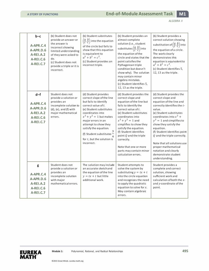
M1 End-of-Module Assessment Task ALGEBRA II
Module 1: Polynomial, Rational, and Radical Relationships
b–c
A-APR.C.4 A-APR.D.6 A-REI.A.2 A-REI.C.6 A-REI.C.7
(b) Student does not provide an answer or the answer is incorrect showing limited understanding of they were asked to do. (c) Student does not provide a triple or it is incorrect.
(b) Student substitutes 𝑎𝑎𝑐𝑐 ,𝑏𝑏𝑐𝑐 into the equation
of the circle but fails to show that this equation is equivalent to 𝑎𝑎2 + 𝑏𝑏2 = 𝑐𝑐2. (c) Student provides an incorrect triple.
(b) Student provides an almost-complete solution (i.e., student
substitutes 𝑎𝑎𝑐𝑐 ,𝑏𝑏𝑐𝑐 into
the equation of the circle and states that the point satisfies the Pythagorean triple condition but doesn’t show why). The solution may contain minor algebra mistakes. (c) Student identifies 5, 12, 13 as the triple.
(b) Student provides a correct solution showing
substitution of 𝑎𝑎𝑐𝑐 ,𝑏𝑏𝑐𝑐 into
the equation of a circle. The work clearly demonstrates this equation is equivalent to 𝑎𝑎2 + 𝑏𝑏2 = 𝑐𝑐2. (c) Student identifies 5, 12, 13 as the triple.
d–f
A-APR.C.4 A-APR.D.6 A-REI.A.2 A-REI.C.6 A-REI.C.7
Student does not provide a solution or provides an incomplete solution to (d), (e), and (f) with major mathematical errors.
(d) Student provides correct slope of the line but fails to identify correct value of t. (e) Student substitutes coordinates into 𝑥𝑥2 + 𝑦𝑦2 = 1 but makes major errors in an attempt to show they satisfy the equation.
(f) Student substitutes 34
for , but the solution is incorrect.
(d) Student provides the correct slope and equation of the line but fails to identify the correct value of . (e) Student substitutes coordinates into 𝑥𝑥2 + 𝑦𝑦2 = 1 and simplifies to show they satisfy the equation. (f) Student identifies point and the triple correctly. Note that one or more parts may contain minor calculation errors.
(d) Student provides the correct slope and equation of the line and correctly identifies the -value. (e) Student substitutes coordinates into 𝑥𝑥2 +𝑦𝑦2 = 1 and simplifies to show they satisfy the equation. (f) Student identifies point
and the triple correctly. Note that all solutions use proper mathematical notation and clearly demonstrate student understanding.
g
A-APR.C.4 A-APR.D.6 A-REI.A.2 A-REI.C.6 A-REI.C.7
Student does not provide a solution or provides an incomplete solution with major mathematical errors.
The solution may include an accurate sketch and the equation of the line 𝑦𝑦 = 𝑥𝑥 + but little additional work.
Student attempts to solve the system by substituting 𝑦𝑦 = 𝑥𝑥 + into the circle equation and recognizes the need to apply the quadratic equation to solve for 𝑥𝑥. May contain algebraic errors.
Student provides a complete and correct solution, showing sufficient work and calculation of both the 𝑥𝑥- and 𝑦𝑦-coordinate of the point.
A STORY OF FUNCTIONS
495
©2015 Great Minds. eureka-math.org

M1 End-of-Module Assessment Task ALGEBRA II
Module 1: Polynomial, Rational, and Radical Relationships
4
a
A-REI.A.2 A-REI.B.4b A-REI.C.6 A-REI.C.7
Student does not provide work or it is incomplete. System does not include a linear and quadratic equation.
Student provides a system that has a solution, but student work indicates understanding that the graphs of the equations should not intersect or that algebraically the system has no real number solutions.
Student provides a system that does not have a solution, but the justification may reveal minor errors in student’s thought process. If a graphical justification is the only one provided the graph must be scaled sufficiently to provide a convincing argument that the two equations do not intersect.
Student provides a system that does not have a solution. Justification includes a graphical, verbal explanation, or algebraic explanation that clearly demonstrates student thinking.
b–c
A-REI.A.2 A-REI.B.4b A-REI.C.6 A-REI.C.7
Student provides incorrect solutions with little or no supporting work shown.
Student provides incorrect solutions to parts (b) and (c). Solutions are limited and reveal major mathematical errors in the solution process.
Student provides incorrect solutions to part (b) or part (c). Solutions show considerable understanding of the processes but may contain minor errors.
Student provides correct solutions with sufficient work shown. AND Mathematical work or verbal explanation show why −2 and −3 are NOT solutions to part (b).
A STORY OF FUNCTIONS
496
©2015 Great Minds. eureka-math.org

M1 End-of-Module Assessment Task ALGEBRA II
Module 1: Polynomial, Rational, and Radical Relationships
Name Date
1. A parabola is defined as the set of points in the plane that are equidistant from a fixed point (called the focus of the parabola) and a fixed line (called the directrix of the parabola). Consider the parabola with focus point (1,1) and directrix the horizontal line 𝑦𝑦 = −3. a. What are the coordinates of the vertex of the parabola?
b. Plot the focus and draw the directrix on the graph below. Then draw a rough sketch of the parabola.
A STORY OF FUNCTIONS
497
©2015 Great Minds. eureka-math.org

M1 End-of-Module Assessment Task ALGEBRA II
Module 1: Polynomial, Rational, and Radical Relationships
c. Find the equation of the parabola with this focus and directrix.
d. What is the 𝑦𝑦-intercept of this parabola?
e. Demonstrate that your answer from part (d) is correct by showing that the 𝑦𝑦-intercept you identified
is indeed equidistant from the focus and the directrix.
A STORY OF FUNCTIONS
498
©2015 Great Minds. eureka-math.org

M1 End-of-Module Assessment Task ALGEBRA II
Module 1: Polynomial, Rational, and Radical Relationships
f. Is the parabola in this question (with focus point (1, 1) and directrix 𝑦𝑦 = −3) congruent to a parabola with focus (2,3) and directrix 𝑦𝑦 = −1? Explain.
g. Is the parabola in this question (with focus point (1, 1) and directrix 𝑦𝑦 = −3) congruent to the
parabola with equation given by 𝑦𝑦 = 𝑥𝑥2? Explain.
h. Are the two parabolas from part (g) similar? Why or why not?
A STORY OF FUNCTIONS
499
©2015 Great Minds. eureka-math.org

M1 End-of-Module Assessment Task ALGEBRA II
Module 1: Polynomial, Rational, and Radical Relationships
2. The graph of the polynomial function 𝑓𝑓(𝑥𝑥) = 𝑥𝑥3 + 4𝑥𝑥2 + 6𝑥𝑥 + 4 is shown below.
a. Based on the appearance of the graph, what does the real solution to the equation 𝑥𝑥3 + 4𝑥𝑥2 + 6𝑥𝑥+ 4 = 0 appear to be? Jiju does not trust the accuracy of the graph. Prove to her algebraically that your answer is in fact a zero of 𝑦𝑦 = 𝑓𝑓(𝑥𝑥).
b. Write 𝑓𝑓 as a product of a linear factor and a quadratic factor, each with real number coefficients.
A STORY OF FUNCTIONS
500
©2015 Great Minds. eureka-math.org

M1 End-of-Module Assessment Task ALGEBRA II
Module 1: Polynomial, Rational, and Radical Relationships
c. What is the value of 𝑓𝑓(10)? Explain how knowing the linear factor of 𝑓𝑓 establishes that 𝑓𝑓(10) is amultiple of 12.
d. Find the two complex zeros of 𝑦𝑦 = 𝑓𝑓(𝑥𝑥).
e. Write 𝑓𝑓 as a product of three linear factors.
A STORY OF FUNCTIONS
501
©2015 Great Minds. eureka-math.org

M1 End-of-Module Assessment Task ALGEBRA II
Module 1: Polynomial, Rational, and Radical Relationships
3. A line passes through the points (−1,0) and 𝑃𝑃 = (0, ) for some real number and intersects the circle
𝑥𝑥2 + 𝑦𝑦2 = 1 at a point different from (−1,0).
a. If = 1
2, so that the point 𝑃𝑃 has coordinates �0, 12�, find the coordinates of the point .
A STORY OF FUNCTIONS
502
©2015 Great Minds. eureka-math.org

M1 End-of-Module Assessment Task ALGEBRA II
Module 1: Polynomial, Rational, and Radical Relationships
A Pythagorean triple is a set of three positive integers 𝑎𝑎, 𝑏𝑏, and 𝑐𝑐 satisfying 𝑎𝑎2 + 𝑏𝑏2 = 𝑐𝑐2. For example, 3,4 and 5 form a Pythagorean triple.
b. Suppose that �𝑎𝑎𝑐𝑐 , 𝑏𝑏𝑐𝑐 � is a point with rational number coordinates lying on the circle 𝑥𝑥2 + 𝑦𝑦2 = 1. Explain why then 𝑎𝑎, 𝑏𝑏, and 𝑐𝑐 form a Pythagorean triple.
c. Which Pythagorean triple is associated with the point = � 513 , 12
13� on the circle?
d. If = � 513 , 12
13�, what is the value of so that the point 𝑃𝑃 has coordinates (0, )?
A STORY OF FUNCTIONS
503
©2015 Great Minds. eureka-math.org
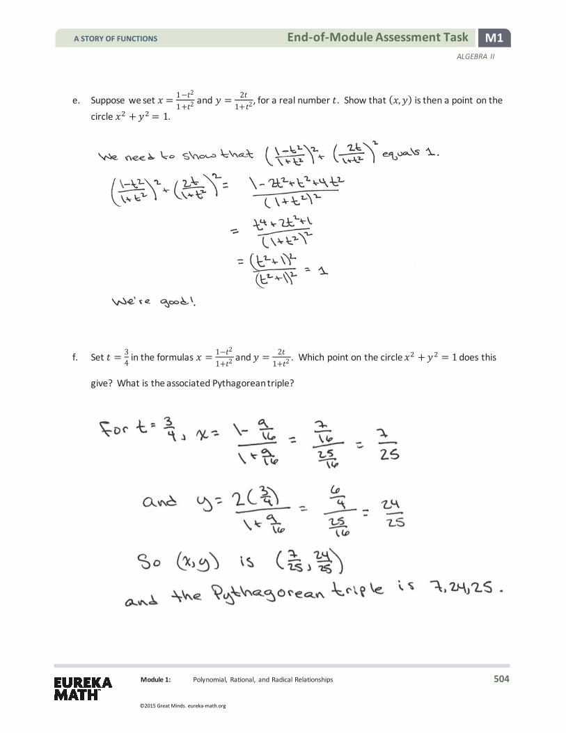
M1 End-of-Module Assessment Task ALGEBRA II
Module 1: Polynomial, Rational, and Radical Relationships
e. Suppose we set 𝑥𝑥 = 1− 2
1+ 2 and 𝑦𝑦 = 21+ 2, for a real number . Show that (𝑥𝑥,𝑦𝑦) is then a point on the
circle 𝑥𝑥2 + 𝑦𝑦2 = 1.
f. Set = 34 in the formulas 𝑥𝑥 = 1− 2
1+ 2 and 𝑦𝑦 = 21+ 2 . Which point on the circle 𝑥𝑥2 + 𝑦𝑦2 = 1 does this
give? What is the associated Pythagorean triple?
A STORY OF FUNCTIONS
504
©2015 Great Minds. eureka-math.org

M1 End-of-Module Assessment Task ALGEBRA II
Module 1: Polynomial, Rational, and Radical Relationships
g. Suppose is a value greater than 1, 𝑃𝑃 = (0, ), and is the point in the second quadrant (different from (−1,0)) at which the line through (−1, 0) and 𝑃𝑃 intersects the circle 𝑥𝑥2 + 𝑦𝑦2 = 1. Find the coordinates of the point in terms of .
A STORY OF FUNCTIONS
505
©2015 Great Minds. eureka-math.org

M1 End-of-Module Assessment Task ALGEBRA II
Module 1: Polynomial, Rational, and Radical Relationships
4.
a. Write a system of two equations in two variables where one equation is quadratic and the other is linear such that the system has no solution. Explain, using graphs, algebra, and/or words, why the system has no solution.
b. Prove that 𝑥𝑥 = √−5𝑥𝑥− 6 has no solution.
A STORY OF FUNCTIONS
506
©2015 Great Minds. eureka-math.org

M1 End-of-Module Assessment Task ALGEBRA II
Module 1: Polynomial, Rational, and Radical Relationships
c. Does the following system of equations have a solution? If so, find one. If not, explain why not.
2𝑥𝑥 + 𝑦𝑦 + = 4 𝑥𝑥 − 𝑦𝑦 + 3 = −2 −𝑥𝑥 + 𝑦𝑦 + = −2
A STORY OF FUNCTIONS
507
©2015 Great Minds. eureka-math.org