Estudio y desarrollo de un sistema de evaluación de la ... - RUC

ii

tesis_main 2019/11/4 19:45 page i #3 ii

ii

ii

Study and development of a

stability assessment system for

shing vessels to prevent capsizing

during navigation

Estudio y desarrollo de un sistema

de evaluación de la estabilidad de

los buques pesqueros para prevenir

la zozobra durante la navegación

Author: Lucía Santiago Caamaño

PhD Thesis / 2019

PhD Supervisors: Vicente Díaz Casás

Marcos Míguez González

PhD program of Naval and Industrial Engineering

ii

tesis_main 2019/11/4 19:45 page ii #4 ii

ii

ii

ii

tesis_main 2019/11/4 19:45 page iii #5 ii

ii

ii

D. Vicente Díaz Casás, Profesor Titular de Universidad del Departamento deIngeniería Naval e Industrial de la Universidade da Coruña,

D. Marcos Míguez González, Profesor Contratado Doctor del Departamento deIngeniería Naval e Industrial de la Universidade da Coruña,

CERTIFICAN:

Que la memoria titulada:

Study and development of a stability assessment system for shing vessels toprevent capsizing during navigation

Estudio y desarrollo de un sistema de evaluación de la estabilidad de los buquespesqueros para prevenir la zozobra durante la navegación

ha sido realizada por Dña. Lucía Santiago Caamaño bajo nuestra direc-ción en el Departamento de Ingeniería Naval e Industrial de la Universidade daCoruña, y constituye la Tesis que presenta para optar al grado de Doctor.

Fdo. Vicente Díaz Casás Fdo. Marcos Míguez González

Codirector de la Tesis Doctoral Codirector de la Tesis Doctoral

ii

tesis_main 2019/11/4 19:45 page iv #6 ii

ii

ii

ii

tesis_main 2019/11/4 19:45 page v #7 ii

ii

ii

To my family

ii

tesis_main 2019/11/4 19:45 page vi #8 ii

ii

ii

ii

tesis_main 2019/11/4 19:45 page vii #9 ii

ii

ii

Abstract

Fishing is well known for being a very hazardous activity. Most of theaccidents, in particular those with the worst consequences, are caused by stabil-ity failures (static or dynamic). Small and medium sized shing vessels, whichrepresent the largest percentage of the eet, are the most aected due to thecrew lack of training in this matter. The use of stability guidance systems hasbeen proposed by several authors, administrations and other stakeholders, asa feasible solution to help the skipper to objectively identify potential risks, tosupport his decision making process and to reduce the probability of accident.

The main objective of this PhD. thesis is to contribute to the developmentof such a stability assessment system, which could estimate in real-time and withminimum need of crew interaction the level of stability of a vessel. Furthermore,it could provide useful information to the skipper and warning messages in caseof potential risk. In order to evaluate the stability level two novel methodologieshave been developed. They automatically compute in real-time the currentmetacentric height from the analysis of roll motion and detect changes on thisparameter. The performance of these proposals has been validated with rollmotion data from dierent vessels, obtained by mathematical model simulations,towing tank tests and sea trials of a real ship.

Such a system could contribute to increase the safety not only of the shingsector, but also of other ship types where crews need simple and easy to under-stand stability information. Although this dissertation represents a large stepin the development of stability guidance systems, further work is still needed tohave a robust operational system. Stability estimation algorithms, informationand guidance interfaces and communication systems should be fully integratedand ready to be installed on board.

ii

tesis_main 2019/11/4 19:45 page viii #10 ii

ii

ii

ii

tesis_main 2019/11/4 19:45 page ix #11 ii

ii

ii

Resumen

La pesca es bien conocida por ser una actividad muy peligrosa. La mayoríade los accidentes, en particular aquellos que entrañan las peores consecuencias,son causados por fallos en la estabilidad (estáticos o dinámicos). Los buquesde pequeño y mediano tamaño, los cuales representan el mayor porcentaje dela ota, son los más afectados debido a la falta de formación de la tripulaciónen esta materia. El uso de sistemas de evaluación de la estabilidad y ayudaal patrón ha sido propuesto por numerosos autores, administraciones y otraspartes interesadas, como una solución viable para ayudar al patrón a identicarobjetivamente los riesgos potenciales, apoyar su proceso de toma de decisionesy reducir la probabilidad de accidente.

El objetivo de esta tesis doctoral es contribuir al desarrollo de tal sistemade evaluación de la estabilidad, el cual podría estimar en tiempo real y con lamínima necesidad de interacción con la tripulación el nivel de estabilidad de unbarco. Además, podría proporcionar información útil al patrón y mensajes deadvertencia en caso de riesgo potencial. Para evaluar el nivel de estabilidad sehan desarrollado dos novedosas metodologías, que automáticamente calculan entiempo real la altura metacéntrica actual a partir del análisis del movimientode balance del barco y detectan cambios en este parámetro. El rendimientode estas propuestas ha sido validado con datos del movimiento de balance dediferentes barcos, obtenidos mediante simulaciones de modelos matemáticos,ensayos en canal y pruebas de mar de un buque real.

Dicho sistema podría contribuir a aumentar la seguridad no sólo del sectorpesquero, sino que también de otros tipos de buques donde las tripulacionesnecesiten información simple y fácil de entender. A pesar de que esta tesisrepresenta un gran paso en el desarrollo de los sistemas de evaluación de laestabilidad y ayuda al patrón, más trabajo es necesario para lograr un sistemaoperativo robusto. Los algoritmos de estimación de la estabilidad, las interfacesde información y guía y los sistemas de comunicación deben estar totalmenteintegrados y listos para ser instalados a bordo.

ii

tesis_main 2019/11/4 19:45 page x #12 ii

ii

ii

ii

tesis_main 2019/11/4 19:45 page xi #13 ii

ii

ii

Resumo

A pesca é ben coñecida por ser unha actividade moi perigosa. A maioríados accidentes, en particular aqueles con peores consecuencias, son causados porfaios na estabilidade (estáticos ou dinámicos). Os buques de pequeno e medianotamaño, os cales representan a maior porcentaxe da ota, son os máis afectadosdebido a falta de formación da tripulación nesta materia. O uso de sistemas deavaliación da estabilidade e axuda ó patrón foi proposto por numerosos autores,administracións e outras partes interesadas, como unha solución viable paraaxudar ó patrón a identicar obxectivamente os riscos potenciais, apoiar o seuproceso de toma de decisións e reducir a probabilidade de accidente.

O obxectivo desta tese doutoral é contribuír o desenvolvemento de tal sis-tema de avaliación da estabilidade, o cal podería estimar en tempo real e coamínima necesidade de interacción coa tripulación o nivel de estabilidade dunbarco. Ademáis, podería proporcionar información útil ó patrón e mensaxes deadvertencia no caso de risco potencial. Para avaliar o nivel de estabilidade de-senvolvéronse dúas novidosas metodoloxías, que automáticamente calculan entempo real a altura metacéntrica actual a partir da análise do movemento debalance do barco e detectan cambios neste parámetro. O rendemento destaspropostas foi validado con datos do movemento de balance de diferentes bar-cos, obtidos mediante simulacións de modelos matemáticos, ensaios en canal eprobas de mar dun buque real.

Dito sistema podería contribuír a aumentar a seguridade non só do sec-tor pesqueiro, senon que tamén doutros tipos de buques onde as tripulaciónsprecisen de información simple e fácil de entender. A pesar de que esta tesisrepresenta un gran paso no desenrolo dos sistemas de avaliación da estabilidadee axuda ó patrón, máis traballo é necesario para lograr un sistema operativorobusto. Os algoritmos de estimación da estabilidade, as interfaces de informa-ción e guía e os sistemas de comunicación deben estar totalmente integrados elistos para ser instalados a bordo.

ii

tesis_main 2019/11/4 19:45 page xii #14 ii

ii

ii

ii

tesis_main 2019/11/4 19:45 page xiii #15 ii

ii

ii

Resumen en español

Cada año numerosos accidentes son registrados alrededor de la pesca. Lasestadísticas la sitúan en una de las profesiones más peligrosas en el mundo.

Las causas de este elevado número de accidentes son muy variadas. Porejemplo, la sobrecarga, fuego o explosión, averías en la maquinaria, inunda-ciones, mal tiempo o fallos en la estabilidad tanto estáticos como dinámicos.Normalmente, los accidentes no son desencadenados por una sola causa, sinoque por la combinación de varias.

De todas ellas la que entraña peores consecuencias son los fallos debidos ala pérdida de estabilidad. El principal motivo es la insuciente formación de latripulación y la falta de información clara y objetiva a bordo. La única guía dela que pueden hacer uso los patrones es el libro de estabilidad, el cual está másorientado al ingeniero naval e implica la realización de cálculos muy tediosospara determinar el nivel de estabilidad. Como consecuencia, en la mayoría delas ocasiones se basan en sus experiencias previas.

Además, la normativa referente a buques de pesca está dirigida a los de másde 24 metros de eslora y algunas de ellas no son de aplicación internacional, sinoque dependen del país. Por otro lado, dicha normativa está centrada en la car-acterización estática de la estabilidad y no contempla fenómenos dinámicos.Actualmente la IMO está trabajando en el desarrollo de los criterios de estabil-idad de segunda generación donde se abordan estos fenómenos dinámicos. Sinembargo, no están pensados para ser de aplicación en buques de pesca.

Debido a esto, los buques más afectados, y que además representan el mayorporcentaje de la ota pesquera operativa, son los de pequeño y mediano tamaño.

En las últimas décadas han surgido los sistemas de evaluación de la estabil-idad y ayuda al patrón como un intento de solucionar esta brecha y reducir elnúmero de accidentes. Básicamente, consisten en un conjunto de procedimien-tos y recomendaciones expresadas de manera clara y sencilla sobre la estabilidaddel barco, incluyendo las condiciones de carga seguras y avisos sobre situacionespotencialmente peligrosas. Estos sistemas deben cumplir tres requisitos: ser de

ii

tesis_main 2019/11/4 19:45 page xiv #16 ii

ii

ii

xiv

fácil uso y entendimiento, no necesitar de interacción con la tripulación parasu correcto funcionamiento y ser de bajo coste de adquisición, instalación ymantenimiento.

Los sistemas más primitivos consistían en un póster donde se representabade manera gráca toda la información necesaria. No ostante, en el caso debuques con un gran número de compartimientos esta representación se compli-caba, por lo que no resultaban demasiado útiles.

La siguiente propuesta está basada en un ordenador que realiza todos loscálculos de estabilidad y emite mensajes de alerta. Algunos de ellos inclusomonitorizan el comportamiento del buque en el mar y cuando se excede el niveloperativo se enciende una alarma y se muestra una serie de recomendaciones. Elpunto débil de estos sistemas es que requieren de la interacción con la tripulaciónpara conocer los datos relativos a la condición de carga y poder evaluar laestabilidad.

Los últimos intentos han estado dirigidos a resolver la interacción con latripulación y se centran en la monitorización en tiempo real y automática de laestabilidad. Concretamente, en la estimación de la altura metacéntrica.

La tesis doctoral se enmarca dentro de este contexto y tiene como objetivoprincipal eliminar la dependencia de datos manuales en estos sistemas. Paraello se han desarrollado dos metodologías que permiten estimar la estabilidadde forma automática y en tiempo real. Ambas están basadas en la asumpciónde que el espectro del movimiento de balance tiene un pico alrededor de sufrecuencia natural, la cual está relacionada a su vez con la altura metacéntrica.Para el cálculo del espectro y la identicación de este pico se han utilizadodiversas herramientas de procesado digital de señales, como son la transformadarápida de Fourier o la transformada de Hilbert-Huang. La diferencia entre estosmétodos es el enfoque empleado para la estimación de la frequencia naturalde balance, uno es en el dominio de la frequencia y otro en el dominio deltiempo. Además de la evaluación de la estabilidad, estas metodologías permitenal patrón conocer el margen de estabilidad, es decir, cuan lejos está de unasituación crítica, emiten alertas en caso de peligro y reconocen los cambios en lacondición de carga. Estas metodologías han sido validadas con series temporalesde balance procedentes de modelos matemáticos, ensayos en canal y pruebas demar.

Aparte del desarrollo de estos métodos, se ha considerado la aplicación delos criterios de estabilidad de segunda generación para identicar la predisposi-ción a sufrir un fallo dinámico.

Por último, se ha integrado la estimación en tiempo real de la estabilidad,así como la evaluación de estos nuevos criterios, en un sistema de evaluación de

ii

tesis_main 2019/11/4 19:45 page xv #17 ii

ii

ii

xv

la estabilidad y ayuda al patrón y se ha rediseñado la interfaz.

Los resultados obtenidos de esta tesis doctoral han demostrado que lasmetodologías propuestas son una alternativa viable para la monitorización ac-tiva de la estabilidad. No obstante, su rendimiento se ve afectado por las condi-ciones de ola, disminuyendo en algunos casos.

La mejora del rendimiento de estas metodologías en estas situaciones abrenuevas vías de investigación. Asimismo, la realización de nuevos experimentospara validarlas en un rango más amplio de escenarios y la ejecución de un testde usabilidad de la interfaz gráca para vericar que se cumple el requisito defacilidad de uso y entendimiento quedan propuestos como trabajo futuro.

ii

tesis_main 2019/11/4 19:45 page xvi #18 ii

ii

ii

ii

tesis_main 2019/11/4 19:45 page xvii #19 ii

ii

ii

Acknowledgements

Despite of being a personal achievement, this PhD thesis could not bepossible without the help and the support of many people.

First of all, I would like to thank to my PhD supervisors, Vicente andMarcos, for all their support and trust put in me since I started this thesis. Alsothanks for all their eort dedicated to search for fundings and new projects inorder that this work could be carried out under the best possible conditions.Without it I would never have had the opportunity to work in the towing tankof the University of A Coruña nor join to the group as research assistant.

One piece of the presented work has been carried out abroad at DTUElectrical Engineering. I am very grateful to Roberto and Ulrik for their contri-butions and the pleasant working environment. What is more, thanks for theirencouragement and ideas during all my research stay and post-collaboration, inparticular in those moments where the results were mostly needed.

Heading back to Ferrol, I would like to thank to all the people from the In-tegrated Group for Engineering Research. It was a pleasure to share laboratorywith them and many lunches and coees. In special, I would like to mentionsome of them for their directly contribution in somehow to this thesis.

Martín and Felix, for introducing me to the hardware world, their guidancealong this thesis and motivate me to do not give up.

Rodrigo and Juan, for teaching me programming in Java and their innitypatience. The part of the software could not be possible without their help.

Juan Carlos, for the great front cover, the icons of the software and hissuggestions and advices about the design.

Moisés, for helping me with the work at the tank when deadlines were closeto have more time to dedicate to this thesis, giving some advice and the coeesafter work to free my mind.

I don't want to miss the opportunity to mention the people from Auto-motation and Control Group for making my external stay more enjoyable and

ii

tesis_main 2019/11/4 19:45 page xviii #20 ii

ii

ii

xviii

all the shared moments, in special at Friday bar. I can not forget to name themates from the Old Guest House, for our long conversations around tea andIranian sweets about our thesis, culture... and for teaching me English andsome words in Persian and Greek.

In addition, I wish to acknowledge to my friends, not enough space tomention them separately but they know who they are. For their support andtrusting more than me in that I could nish this thesis. Also, for understandingmy impossible schedules and always making time in their agenda for catchingup and free my mind after work, listening to my problems and encouraging me.

Finally, I would like to give special thanks to the most important peoplein my life, my family. For their great support and understanding that it is notalways possible being at home and sharing time. They are the ones that sueredthe most this work, bearing my humour changes, my stress and my frustrations.To my parents, Javier and Lui, they give me the room and encourage to followmy own ideas and take care of Nico when I am not at home. To my sister, Sara,she instilled in me the constance and the hard work that make possible thisthesis and she is always there listening to me, including the long phone callswhen I need some advice. To my grandmother, Luisa, she empowered me inthis adventure and I am sure she would be proud of the result of all the eortput in the last 5 years.

This work has been partially funded by an Inditex-UDC predoctoral researchvisit grant from the University of A Coruña and Inditex S. A.

ii

tesis_main 2019/11/4 19:45 page xix #21 ii

ii

ii

Publications

For the development of the present work, the following articles related withthe main topic of this thesis have been published:

Míguez González, M., Díaz Casás, V., Santiago Caamaño, L. (2016). Real-Time Stability Assessment in Mid-Sized Fishing Vessels. Proceedings ofthe 15th International Ship Stability Workshop (ISSW 2016), pages 201-208. Stockholm, Sweden.

Míguez González, M., Bulian, G., Santiago Caamaño, L., Díaz Casás,V. (2017). Towards real-time identication of initial stability from shiproll motion analysis. Proceedings of the 16th International Ship StabilityWorkshop (ISSW 2017), pages 221-229. Belgrade, Serbia.

Santiago Caamaño, L., Míguez González, M., Díaz Casás, V. (2018) Im-proving the safety of shing vessels trough roll motion analysis. Proceed-ings of the ASME 2018 37th International Conference on Ocean, Oshoreand Artic Engineering (OMAE).

Santiago Caamaño, L., Míguez González, M., Díaz Casás, V. (2018). Onthe feasibility of a real time stability assessment for shing vessels. OceanEngineering, 159, 76 - 87.

Míguez González, M., Santiago Caamaño, L., Díaz Casás, V. (2018). Onthe applicability of real time stability monitoring for increasing the safetyof shing vessels. Proceedings of the 13th International Conference on theStability of Ships and Ocean Vehicles.

Santiago Caamaño, L., Galeazzi, R., Nielsen, U. D., Míguez González, M.,Díaz Casás, V. (2019). Real-time detection of transverse stability changesin shing vessels. Ocean Engineering, 189.

Santiago Caamaño, L., Míguez González, M., Galeazzi, R., Nielsen, U. D.,Díaz Casás, V. (2019). On the application of change detection techniques

ii

tesis_main 2019/11/4 19:45 page xx #22 ii

ii

ii

xx

for the stability monitoring of shing vessels. Proceedings of the 17thInternational Ship Stability Workshop (ISSW 2019). Helsinki, Finland.

Santiago Caamaño, L., Galeazzi, R., Nielsen, U. D., Míguez González, M.,Díaz Casás, V. (2019). Experimental Validation of Transverse StabilityMonitoring System for Fishing Vessels. Proceedings of the 12th IFAC Con-ference on Control Applications in Marine Systems, Robotics and Vehicles(CAMS 2019). Daejeon, Korea.

Other publications during this period:

Díaz Casás, V., Santiago Caamaño, L., Míguez González, M., NovásCortés, A., Rubio Planells, J. (2017). Experimental testing of a linearabsorber wave energy converter: Eects of the mooring system, Proceed-ings of the 3rd Marine Energy Week.

Santiago Caamaño, L., Díaz Casás, V. (2019). Estudo comparativo das"blue careers" na Universidade da Coruña: unha perspectiva de xénero.VI Xornada Universitaria Galega en Xénero (XUGeX 2019). A Coruña,Spain.

Santiago Caamaño, L., Aguayo Lorenzo, E. M., Díaz López, A. J., DíazCasás, V. (2019). Brecha de género en las carreras azules: El caso deingeniería naval y oceánica en España. XXXIII Congreso Internacionalde Economía Aplicada (ASEPELT 2019), pages 518 - 526 Vigo, Spain.

ii

tesis_main 2019/11/4 19:45 page xxi #23 ii

ii

ii

Glossary

Greek Symbols

β Quadratic roll damping coecient

∆F Frequency resolution of the FFT

∆ Vessel mass displacement

δ Limit of LPF application

ω0 Roll natural frequency estimate

ω0bh Roll natural frequency estimate when Blackman-Harris window is ap-plied

ω0b Roll natural frequency estimate when Blackman window is applied

ω0h Roll natural frequency estimate when Hanning window is applied

κ Shape parameter of Weibull probability distribution function

λ Scale parameter of Weibull probability distribution function

ν Degrees of freedom in uncertainty estimation

ν Linear roll damping coecient

νL Purely linear roll damping coecient

ω0 Roll natural frequency

ω0c Critical roll natural frequency

ωe Wave encounter frequency

ωw Wave peak frequency

φ(t) Roll motion amplitude

ii

tesis_main 2019/11/4 19:45 page xxii #24 ii

ii

ii

xxii

σ Standard deviation

σω0Standard deviation of the roll natural frequency estimates

θ Heel angle

σ2ω0 Variance of the roll natural frequency estimates

Roman Symbols

H0 Null hypothesis

H1 Alternative hypothesis

GM Metacentric in still water

GZ(φ) Righting lever curve in still water

A44 Roll added mass

b Systematic standard uncertainty

fs Sampling frequency

flim Nyquist frequency

g Acceleration of the gravity

g(ω) Result of applying the FFT

GM Metacentric height

GZ Vessel's righting arm

HScrit Minimum signicant wave height to capsize

HSIMO IMO reference value for the minimum signicant wave height to capsize

Hs Signicant wave height

Ixx Ship transverse mass moment of inertia

kxx Roll gyradius

KG Vertical position of the centre of gravity of the ship

KM Distance from the keel to the metacentre

KN Cross curve of stability

LBP Length between perpendiculars

M Metacenter

ii

tesis_main 2019/11/4 19:45 page xxiii #25 ii

ii

ii

xxiii

mwave(t) Non-dimensional wave excitation in beam seas

mwind(t) Non-dimensional wind moment due to the eect of lateral wind

Medω0 Median of the roll natural frequency estimates

P5ω05th percentile of the roll natural frequency estimates

P95ω095th percentile of the roll natural frequency estimates

PFA Probability of false alarms

R(t) Monotonic function

Range Residual range of positive stability

RMmax Maximum righting moment

S(ω) Signal power spectrum

SX Standard deviation in the uncertainty analysis

Sw Wave steepness

T Draft of the vessel

Ts Sampling period

t95 Student's t for 95

Test Time window for the detection stage of the detector

Test Time window for the estimation stage of the detector

U95 ASME model for computing the uncertainty

U∆ Uncertainty in mass displacement

Uω0Uncertainty in the estimated roll natural frequency

UGM Uncertainty in metacentric height

UI Uncertainty in transverse mass moment of inertia

Ukxx Uncertainty in roll gyradius

wb Blackman window function

wh Hanning window function

wbh Blackman-Harris window function

Abbreviations

ii

tesis_main 2019/11/4 19:45 page xxiv #26 ii

ii

ii

xxiv

2008 IS Code 2008 Intact Stability Code

CENTEC Centre for Marine Technology and Engineering

DAQ Data acquisition

DFT Discrete Fourier Transform

EMD Empirical Mode Decomposition

FAO Food and Agriculture Organization

FD Total number of false detections

FFT Fast Fourier Transform

Fn Froude number

GLRT Generalized Likelihood Ratio Test

GT Gross Tonnage

GUI Graphical User Interface

HHT Hilbert-Huang Transform

i.i.d. Independent identically distributed

ILLC International Convention on Load Lines

ILO International Labour Organization

IMF Intrinsic Mode Function

IMO International Maritime Organization

IMU Inertial measurement unit

ITTC International Towing Tank Conference

MLE Maximum likelihood estimate

pef Peak enhancement factor

RAO Response Amplitude Operator

SGISC Second Generation of Intact Stability Criteria

SI Stability Index

SOLAS International Convention on Safety of Life at Sea

TD Total number of true detections

THREDDS Thematic Realtime Environmental Distributed Data Service

ii

tesis_main 2019/11/4 19:45 page xxv #27 ii

ii

ii

Contents

1 Introduction 1

2 Objectives and methodology 7

2.1 Objectives . . . . . . . . . . . . . . . . . . . . . . . . . . . . . . . 7

2.2 Methodology . . . . . . . . . . . . . . . . . . . . . . . . . . . . . 8

3 Background 9

3.1 State of art of shing sector . . . . . . . . . . . . . . . . . . . . . 9

3.2 Accident rate in shing sector . . . . . . . . . . . . . . . . . . . . 13

3.3 Evolution and current status of regulations . . . . . . . . . . . . 16

3.4 Guidance systems . . . . . . . . . . . . . . . . . . . . . . . . . . . 22

3.5 Roll natural frequency estimation . . . . . . . . . . . . . . . . . . 28

4 Fundamentals of real-time stability assessment 31

4.1 Introduction . . . . . . . . . . . . . . . . . . . . . . . . . . . . . . 31

4.2 Involved parameters in stability evaluation . . . . . . . . . . . . . 31

4.3 Real-time stability estimation . . . . . . . . . . . . . . . . . . . . 33

4.4 Roll motion monitoring . . . . . . . . . . . . . . . . . . . . . . . 33

4.5 Real-time requirements . . . . . . . . . . . . . . . . . . . . . . . . 34

5 Fast Fourier Transform based methodology 37

5.1 Introduction . . . . . . . . . . . . . . . . . . . . . . . . . . . . . . 37

5.2 Fast Fourier Transform based estimation . . . . . . . . . . . . . . 37

5.2.1 Roll natural frequency estimation . . . . . . . . . . . . . . 38

5.2.1.1 Limitations of the Fast Fourier Transform . . . . 40

ii

tesis_main 2019/11/4 19:45 page xxvi #28 ii

ii

ii

xxvi Contents

5.2.1.2 Windowing . . . . . . . . . . . . . . . . . . . . . 41

5.2.1.3 Roll natural frequency uncertainty analysis . . . 43

5.2.2 Transverse mass moment of inertia . . . . . . . . . . . . . 44

5.2.3 Displacement . . . . . . . . . . . . . . . . . . . . . . . . . 45

5.2.4 Metacentric height . . . . . . . . . . . . . . . . . . . . . . 45

5.2.4.1 Metacentric height uncertainty analysis . . . . . 46

5.2.5 Results/Validation . . . . . . . . . . . . . . . . . . . . . . 46

5.2.5.1 Towing tank data (vessel 1) . . . . . . . . . . . . 47

5.2.5.2 Towing tank data (vessel 2) . . . . . . . . . . . . 65

5.3 Recursive Fast Fourier Transform based methodology . . . . . . . 74

5.3.1 Results and validation . . . . . . . . . . . . . . . . . . . . 75

5.3.1.1 Simulated data . . . . . . . . . . . . . . . . . . . 76

5.3.1.2 Sea trials . . . . . . . . . . . . . . . . . . . . . . 81

5.4 Discussion . . . . . . . . . . . . . . . . . . . . . . . . . . . . . . . 86

6 Time domain and change detection methodology 89

6.1 Introduction . . . . . . . . . . . . . . . . . . . . . . . . . . . . . . 89

6.2 Architecture . . . . . . . . . . . . . . . . . . . . . . . . . . . . . . 90

6.2.1 Data acquisition . . . . . . . . . . . . . . . . . . . . . . . 92

6.2.2 Empirical Mode Decomposition . . . . . . . . . . . . . . . 92

6.2.3 Hilbert-Huang Transform . . . . . . . . . . . . . . . . . . 94

6.2.3.1 Constraints on the roll natural frequency . . . . 95

6.2.4 Detector . . . . . . . . . . . . . . . . . . . . . . . . . . . . 96

6.2.5 Filtering . . . . . . . . . . . . . . . . . . . . . . . . . . . . 100

6.3 Results/Validation . . . . . . . . . . . . . . . . . . . . . . . . . . 101

6.3.1 Simulated data . . . . . . . . . . . . . . . . . . . . . . . . 102

6.3.1.1 Test vessel . . . . . . . . . . . . . . . . . . . . . 102

6.3.1.2 Mathematical model . . . . . . . . . . . . . . . . 104

6.3.1.3 Test conditions . . . . . . . . . . . . . . . . . . . 104

6.3.1.4 Tuning of the condition monitoring system . . . 105

6.3.1.5 Evaluation of the monitoring performance . . . . 107

6.3.2 Towing tank data . . . . . . . . . . . . . . . . . . . . . . . 116

ii

tesis_main 2019/11/4 19:45 page xxvii #29 ii

ii

ii

Contents xxvii

6.3.2.1 Vessel model . . . . . . . . . . . . . . . . . . . . 116

6.3.2.2 Towing tank tests . . . . . . . . . . . . . . . . . 117

6.3.2.3 Test conditions . . . . . . . . . . . . . . . . . . . 118

6.3.2.4 Redesigning the lter . . . . . . . . . . . . . . . 119

6.3.2.5 Tuning of the condition monitoring system . . . 120

6.3.2.6 Evaluation of the monitoring performance . . . . 121

6.4 Discussion . . . . . . . . . . . . . . . . . . . . . . . . . . . . . . . 123

7 Comparison of both methodologies 125

7.1 Introduction . . . . . . . . . . . . . . . . . . . . . . . . . . . . . . 125

7.2 Test case . . . . . . . . . . . . . . . . . . . . . . . . . . . . . . . 126

7.2.1 Test vessel . . . . . . . . . . . . . . . . . . . . . . . . . . . 126

7.2.2 Test conditions . . . . . . . . . . . . . . . . . . . . . . . . 127

7.2.3 Results . . . . . . . . . . . . . . . . . . . . . . . . . . . . 127

7.3 Discussion . . . . . . . . . . . . . . . . . . . . . . . . . . . . . . . 129

8 Stability assessment system 131

8.1 Introduction . . . . . . . . . . . . . . . . . . . . . . . . . . . . . . 131

8.2 System description . . . . . . . . . . . . . . . . . . . . . . . . . . 132

8.2.1 Simulation module . . . . . . . . . . . . . . . . . . . . . . 132

8.2.1.1 Stability criteria simulation module . . . . . . . 133

8.2.1.2 Stability Index simulation module . . . . . . . . 134

8.2.2 Real-time module . . . . . . . . . . . . . . . . . . . . . . . 135

8.2.2.1 Stability criteria real-time module . . . . . . . . 137

8.2.2.2 Stability Index real-time module . . . . . . . . . 140

8.2.2.3 Forecast . . . . . . . . . . . . . . . . . . . . . . . 140

8.3 Conclusions . . . . . . . . . . . . . . . . . . . . . . . . . . . . . . 141

9 Conclusions and future work 143

9.1 Conclusions . . . . . . . . . . . . . . . . . . . . . . . . . . . . . . 143

9.2 Future work . . . . . . . . . . . . . . . . . . . . . . . . . . . . . . 146

A Graphical User Interface 149

A.1 Description . . . . . . . . . . . . . . . . . . . . . . . . . . . . . . 149

ii

tesis_main 2019/11/4 19:45 page xxviii #30 ii

ii

ii

xxviii Contents

A.1.1 Simulation panel . . . . . . . . . . . . . . . . . . . . . . . 150

A.1.2 Real-time panel . . . . . . . . . . . . . . . . . . . . . . . . 154

B Application conguration 157

B.1 Introduction . . . . . . . . . . . . . . . . . . . . . . . . . . . . . . 157

B.2 Ship denition . . . . . . . . . . . . . . . . . . . . . . . . . . . . 157

B.2.1 Conguration les characteristics . . . . . . . . . . . . . . 159

B.3 Quick guide for conguration . . . . . . . . . . . . . . . . . . . . 164

Bibliography 167

List of Figures 181

List of Tables 187

ii

tesis_main 2019/11/4 19:45 page 1 #31 ii

ii

ii

Chapter 1

Introduction

Stability is one of the most important concepts surrounding a ship. It isrelated with the statics and dynamics of the vessel and the safety. The rst twoterms refer to the ability of the vessel to keep the upright position under anycircumstance and also the behavior in waves; while the last one encompasses theintegrity of the ship herself, the people on board and the goods (Hanzu-Pazara,Duse, Varsami, Andrei, & Dumitrache, 2016).

Stability calculations focus on centers of gravity, centers of buoyancy, meta-centres and how all of them interact. It is a major design requirement since itdepends on the geometry of the hull and the weight distribution. Even thoughit is also aected by the operational conditions and external hazards such aswaves, wind, currents, collision or grounding (Lewis, 1988).

As a result the owner, operators, shipbuilders and the administration areimplicated. Their matter of concern is to ensure a sucient level of stability toguarantee the safety of the navigation. Otherwise accidents could happen havingserious consequences. For example the damage of the goods, the complete lossof the vessel, injuries to the crew or even losses of lives (Hanzu-Pazara et al.,2016). All of them translate into a lot of money and time without operating.

Despite all the eorts, every year a huge number of accidents due to sta-bility failures are registered around the entire world. They usually happen incombination with other causes such as ooding, overloading, re or explosion,machine failure or very adverse weather conditions. Particularly, small andmedium sized shing vessels are on the top of the list of the most aectedworldwide (Krata, 2008; Petursdottir, Hannibalsson, & Turner, 2001; Roberts,2002; Scarponi, 2017).

These situations are repeated continuously year by year and their cost is

ii


ii

ii

2

very high. It is well known that small vessels are more sensitive to severe windand rough sea than large ships but this is not the origin of the problem (GefaellChamochín, 2005; Krata, 2008).

One of the possible causes may be the low freeboard, that these type ofvessels normally have for shing labors. This characteristic favors deck oodingand water may be trapped on it and come into other spaces if watertight hatchesand doors are not closed (Petursdottir et al., 2001; Royal Institution of NavalArchitects, 2011).

On the other hand, owners try to make their ship adaptable to dierentsheries in order to face the seasonability of certain species and be able to workthe entire year. This implies some modications that in many cases result in areduction in the stability margin (Petursdottir et al., 2001; Royal Institution ofNaval Architects, 2011).

What is more, there is a huge economical pressure over shermen becausetheir salary depends on the amount of sh that they catch. In consequence,they assume that the risk is part of their lives on board and they do not havea proper attitude towards safety. Their focus is shing as much as they canbefore returning to port (Bye & Lamvik, 2007; Lazakis, Kurt, & Turan, 2014;Petursdottir et al., 2001).

Another reason could be that the international regulations related to sta-bility do not cover shing vessels. The major challenge on addressing the regu-lations to this eet is the heterogeneity in size, the nature of shing operationsand the type of voyages. Those characteristics make shing vessels very dier-ent from merchant ships and increase the complexity of the application of thestandard rules (Petursdottir et al., 2001).

There are many IMO, ILO and FAO agreements, protocols and codes butthey are aimed at ships above 24 meters in length. Furthermore, some of themare country dependent and not of international application. A case in pointis the Torremolinos International Convention, the Torremolinos Protocol andthe Cape Town Agreement, three attempts to improve exclusively the safetyof shing vessels that remained in a declaration of intentions as they were notratied by all the countries and they are still aimed at vessels above 24 metersin length (Ba£kalov et al., 2016; International Maritime Organization, 2012;Petursdottir et al., 2001).

The worst part falls on small and medium sized shing vessels consider-ing that there are only safety recommendations and voluntary guidelines. Twoexamples are IMO Guidelines (a and b) (MSC/Circ. 707. 19 October 1995.Guidance to the master for avoiding dangerous situations in following and quar-tering seas and MSC. 1/Circ. 1228. 11 January 2007. Revised guidance to the

ii


ii

ii

Chapter 1. Introduction 3

master for avoiding situations in adverse weather and sea conditions). How-ever, these guidelines are dicult to apply and mainly focused to large merchantvessels (Ba£kalov et al., 2016; International Maritime Organization, 1995, 2007;Petursdottir et al., 2001).

Moreover, stability regulations still rely on the intact criteria derived fromRahola's work in the late 30´s, and they do not consider dynamic instabilitiescaused by ship-wave interaction. In last years, IMO has begun developing theSecond Generation of Intact Stability Criteria to complement the previous cri-teria. These criteria are based on a dierent perspective, including the inuenceof ship dynamics. Their purpose is to determine the failure modes and to estab-lish levels of vulnerability of the vessel to these phenomena. Nonetheless, theyare aimed at ships with 24 meters in length and above and require more than abasic training to be understood and applied (International Maritime Organiza-tion (IMO) Sub-Committee on Ship Design and Construction, 2018; Kobylinski,2012).

Any of these reasons could explain the fatal injury rate of the sector, al-though the main one is the crew lack of training in stability matters. Unlikemerchant seafarers, only few shermen have a deep knowledge about stabilityand can clearly understand what is presented in the stability booklet. Thisbooklet is only mandatory for vessels of 12 meters in length and above andincludes four signicant loading conditions. For intermediate situations it isnecessary to perform manual calculations. On account of that and because ofthe calculations are time consuming, skippers mostly estimate the safety marginconsidering their previous experience which usually lacks any kind of incident(Míguez González et al., 2012; Wolfson Unit, 2004).

As a solution, on board guidance systems have been emerging to help mas-ters to objectively assess the stability level of their vessels. Basically they consiston dierent alternatives where loading conditions are displayed indicating whichare safe situations and which are not. They can be represented as a drawing,a matrix or in any form depending on the system. They only have three mainrequirements: be easy of use and to interact with, low cost of acquisition in-stallation and maintenance and minimum need for crew interaction. Some ofthem include the eect of environmental loads. For example, the maximumwave height to capsize or under which circumstances the ship is prone to para-metric rolling, broaching or any of the failure modes (Deakin, 2005; WolfsonUnit, 2004).

The problem of this systems is that in vessels with a large number ofcompartments the representation becomes too complicated. Moreover, theyonly contain a set of loading conditions that represent the operability of theship. For intermediate or exceptional situations, the skipper should perform

ii


ii

ii

4

the traditional tedious calculations or select the most similar to the current one(Deakin, 2005; Wolfson Unit, 2004).

The most modern assessment systems go an step ahead and perform allof these calculations. They are based on a computer software with a graphicalinterface. The seafarers introduce the details of the loading condition in thecomputer and it provides an estimation of the stability level of the ship (Deakin,2005; Wolfson Unit, 2004).

By a way of example, the Integrated Group for Engineering Research devel-oped its own stability guidance system following the computer-based alternative.It consists of a naval architecture software that performs all necessary calcula-tions regarding to vessel stability from the hull forms and weight distributionand displays in a clear and understandable way the current situation of the shipand its risk level. This software is installed on a PC with a touchable screen toallow the interaction with the crew through a graphical interface, which usabilitylevels have been tested and veried to guarantee the easy of use. Furthermore,the assessment system has an inexpensive cost of acquisition, installation andmaintenance.

However, the weak point of this system, as in most of them, is that itsfull and correct operation relies on the information manually introduced by thecrew. This information comprises the weight items and their positions, the tanklling levels and the sea state (Míguez González et al., 2012).

Most recently, the combination of stability and operational guidance sys-tems arose. Their purpose is carrying out an evaluation of the stability level inreal-time during navigation, reducing the crew interaction and maximizing theease of use. In order to achieve that, the metacentric height (GM), which isa parameter from which the stability level could be characterized, is estimatedfrom the ship motions (Wawrzynski & Krata, 2016).

An example of a system that monitors the metacentric height is the oneproposed by Terada, Tamashima, Nakao, and Matsuda (2016). Their approachis based on an autoregressive and a general state model to estimate the GMand, at the same time, the gyradius of the vessel from roll motion time series.Few years later the methodology was further improved in Terada, Hashimoto,Matsuda, and Umeda (2018) using a Bayesian modelling procedure and theMarkov chain Monte Carlo (MCMC). Nevertheless, authors mention that morevalidation work is still needed.

The work carried out in this PhD thesis follows a similar line to the previoussystem: minimizing the crew interaction for a fully operation in the stabilityguidance systems. The idea is improving the on board guidance system de-veloped by the Integrated Group for Engineering Research in such way that

ii


ii

ii

Chapter 1. Introduction 5

performs all the stability calculations itself and provides information to theskipper about the risk level.

In consequence, the main objective is to evaluate the stability of the vesselin real-time automatically. In order to do that, a similar approach to the wavebuoy analogy has been taken, i.e. the ship is treated as a waverider buoy but,instead of predicting the wave spectrum from her movements, estimating thestability parameters.

It is well known that the spectrum of roll motion has a peak around itsnatural frequency. This feature becomes more noticeable when the resonancephenomenon takes place. Furthermore, the ship's initial stability, also calledmetacentric height, is highly related with oscillations in roll. Then, it can beestimated analysing the ship roll motion.

For this reason, this work poses a new methodology to estimate the meta-centric height during navigation by monitoring roll motion and combining signalprocessing techniques; for instance, the Fast Fourier Transform or the Hilbert-Huang Transform. Its purpose is to aware the master at all time about thestability level of the vessel and how far is from a critical condition.

In order to validate these approaches numerical, experimental and real scaletests have been carried out and the resulting roll motion time series have beenanalysed.

In this work, the Second Generation of Intact Stability criteria are alsocontemplated in spite of the fact that they are not aimed at shing vessels.Their evaluation is included in the functionability of the guidance system.

Summarizing, this PhD thesis addresses the problem of crew interactionwith guidance systems in shing vessels. This work presents a new strategy toimprove the safety in this type of ships through roll motion analysis facilitatingthe evaluation of the risk on board due to stability issues.

The outline of this thesis report could be concluded as follows.

Chapter 2 presents the global objectives of this PhD thesis and the appliedmethodology.

Chapter 3 is dedicated to a literature survey of the most relevant workrelated to the topic of this thesis. The state of art of the shing eet, itsaccident rate and the regulations regarding stability are introduced too.

Chapter 4 establishes the basis of the real-time stability evaluation.

Chapter 5 provides a fully explanation of the rst attempt for estimatingthe stability of the vessel in real-time based on the Fast Fourier Transform

ii


ii

ii

6

and the developed methodology. Validation tests have been performed,including their description and the analysis of the results.

Chapter 6 provides the description of a second methodology for assess-ing the stability level, but based on the Hilbert-Huang Transform. Thismethodology has also been validated, including the description of the testsand the analysis of the results.

Chapter 7 compares both methodologies.

Chapter 8 shows the integration of the proposed methodology into the onboard guidance system. It provides a description of its functionality.

Chapter 9 summarizes the main conclusions of this work and provides aview of possible future research lines derived from it.

Appendix A includes a description of the design of the graphical userinterface.

Appendix B describes the conguration process of the system.

ii


ii

ii

Chapter 2

Objectives and methodology

2.1 Objectives

The research work presented in this dissertation aims to contribute to theeld of the ship stability. In particular, it is addressed to improve the safety ofshing vessels by means of a stability assessment system. As it was mentionedin the previous chapter, these kind of systems have a common drawback: thenecessity of the interaction with the crew to be able to work correctly.

Due to this fact, the main objective of the work carried out in this PhDthesis is minimizing the crew interaction in these systems. However, it has tobe done keeping two well known requirements: ease of use and understandingand low cost of acquisition, installation and maintenance. In order to achievethis, ve sub-objectives can be dened:

1. To develop a methodology to assess the ship's stability in real-time and inan automatic way. The purpose is to estimate the stability level withoutthe intervention of any of the crew members and raise an alarm when thesafety of the vessel could be compromised.

2. To validate the methodology by analysing its performance against datafrom a mathematical model, towing tank tests and full scale trials.

3. To evaluate the stability of the vessel based on the IMO criteria in com-bination with the output of the methodology.

4. To consider the application of the Second Generation of Intact StabilityCriteria that are still under development. The intention is to be able toidentify if the ship is prone to any of the dynamic stability failure modeswhile she is sailing.

ii


ii

ii

8 2.2. Methodology

5. To integrate the methodology into a guidance system. The on board guid-ance system developed by the Integrated Group for Engineering Researchis taken as a basis.

Finally, note that the research work targets towards the collective of shingvessels of 12 meters in length and above. Although they do not represent thelargest number of units within the operational shing eet, they constitute asignicant contribution of GT. In addition, it is the segment where the greatestaccident rate of the sector is concentrated.

Vessels between 0 and 12 meters in length are not considered because theyare mainly undecked, they comprise a variety of gears and they return to porteveryday.

2.2 Methodology

To accomplish with the objectives of the PhD thesis an adequate method-ology is needed. It can be summarized in the following steps:

1. Analysis of the current situation of shing sector in terms of technicalcharacteristics and accident rate.

2. Study the background of the regulations related to stability, in special thecase of shing vessels.

3. Study the background of the actual stability assessment and guidancesystems in order to recognise the weaknesses and to try to avoid or tosolve them in the new proposed design.

4. Study the background and theoretical basis of real-time stability calcula-tion considering the current intact stability criteria and the second gener-ation of them. Likewise, analysis of real-time wind and waves forecasts.

5. Development of a methodology to assess ship's stability in real-time basedon measuring vessel motions and executing digital signal processing tech-niques.

6. To carry out tank test and full scale trials with the purpose of havingdata to verify the functionality of the system. In addition, to executemathematical model simulations to obtain time series of ship motions.

7. Integration of the proposed methodology to an on board system and re-design the graphical interface according to the new requirements.

ii


ii

ii

Chapter 3

Background

3.1 State of art of shing sector

Fishing is one of the main industrial sectors in Spain; the size of the eet(tonnage and power) and the volume of the catches indicate it. At Europeanlevel, the Spanish shing eet represents the largest number of registered tons,reaching 337,812.81 GT and representing 21.18% of the total value according tothe European Vessel Register at 31/12/2017 (Ministerio de Agricultura Pescay Alimentación, 2018). If world data are considered, Europe would be locatedin fth place in the ranking of shery production (3.1%) behind China, In-donesia, India and Vietnam (European Market Observatory for Fisheries andAquaculture Products, 2018).

Fishing sector also highlights in the number of employees, being 34,326 peo-ple in 2017 which represents 0.18% of the total active population of that year(Ministerio de Agricultura Pesca y Alimentación, 2018). In spite of the total na-tional contribution cannot be considered extremely signicant, the distributionof the employment in the sector is not uniform. In some regions this percentagebecomes much greater leading to consider these areas very dependent on shing.

In Spain there are three well dierentiated shing areas: Atlantic-Cantabrian,South-Atlantic and Mediterranean. The eet belonging to the Atlantic-Cantabrianregion is the largest and the most competitive, shing in high seas (deep-seashing). The communities of Galicia, Asturias and Basque Country stand outand the rst one is the most important. The eet corresponding to the South-Atlantic zone is less competitive than the previous one, its size is slightly smallerand they work essentially near to the coast. It encompasses the provinces ofCádiz and Huelva. As for the Mediterranean region, it is an artisanal coastaleet and not very competitive. In Table 3.1 these conclusions can be appreci-

ii


ii

ii

10 3.1. State of art of shing sector

ated.

Table 3.1: Technical characteristics of the Spanish eet by Au-tonomous Community (Ministerio de Agricultura Pesca y Ali-mentación, 2018)

Nº

Vessels

Gross

Tonnage

(GT)

Power

(cv)

Average

Total

Length (m)

GALICIA 4,466 143,155 379,270 8.80

ASTURIAS 264 4,873 21,867 10.76

CANTABRIA 133 7,124 24,679 17.25

BASQUE

COUNTRY201 68,879 157,158 28.06

CATALONIA 727 19,646 115,656 13.94

VALENCIAN C. 577 17,865 87,436 14.74

BALEARIC I. 339 3,250 25,032 9.66

ANDALUSIA 1,472 35,869 154,793 12.03

MURCIA 170 2,547 13,219 10.50

CEUTA 23 7,976 15,197 21.03

MELILLA 0 0 0 0.00

CANARY I. 774 22,628 69,988 9.94

TOTAL 9,146 333,813 1,064,296 10.90

Regarding the technical aspects, the principal characteristic of the Spanisheet is that it is very heterogeneous. There are many dierent typologies ofshing vessels depending on their size, shing distance to the coast, length ofthe shing campaign, type of shing, etc. For this reason there are severalclassications. One of them is according to the distance to the coast, size of thevessel and duration of the voyage and it is divided into (Piniella, Soriguer, &Fernández-Engo, 2007):

Deep water and ocean-going eet: shing is exercised without limitationof seas or distances to the coast. The size of vessels exceeds 100-250 GT.

Coastal or shallow water eet: it is practised in waters under Spanishjurisdiction. The size of the vessels does not exceed 100 GT.

Artisanal or craft shing eet: it is carried out with boats up to 20 GT,in sheltered waters and they return to port every day.

All these categories can be grouped into two: coastal-artisanal eet and in-dustrial eet. The rst group is characterized by vessels with a low degree of

ii


ii

ii

Chapter 3. Background 11

mechanization and specialization among crew members. Productivity dependson human strength and workers' skills. Usually the shipowner is also the captainof the ship and maintains a certain degree of kinship with the crewmen. Thenumber of crew members rarely exceeds 10 people and the vessels sh close totheir base port. The remuneration system is usually proportional to the volumeof catches. The industrial eet consists of deep-sea shing. The vast majority ofvessels exceed 24 meters in length and sh far from their base port. The degreeof mechanization and specialization of the seafarers is high and the number ofpeople on board ranges between 12 and 60. The remuneration system is usuallyxed or at least composed of a xed base and a variable part depending on thevolume of catches (Álvarez-Santullano, 2014).

There is another subdivision of the shing eet relative to the type of shinggear (López Sieiro, n.d.; Ministerio de Agricultura Pesca y Alimentación, 2017):

Trawl

Seine

Longline

Gillnet

Fixed gear

Smaller gear

The total number of shing vessels in the world in 2010 was about 4.36 million;from these, more than the 85% of the engine-powered shing vessels are lessthan 12 meters in length, 13% are between 12 and 24 meters in length and only2% are over 24 meters (Gudmundsson, 2013).

The number of Spanish ships according to their length for each type ofgear are shown below in Table 3.2. As it can be seen, the national trend is thesame as the worldwide: 73% of the boats are less than 12 meters in length andmostly they are dedicated to smaller gear, 19% have a length between 12 and24 meters and 8% are greater than 24 meters.

If the distribution of the number of vessels by length (Table 3.3) at Eu-ropean level is considered, a large number of vessels between 0 and 12 metersstill prevail. Despite of this fact, the largest GT contribution is represented byvessels between 18 and 24 meters (after those of L>75 meters).

ii


ii

ii

12 3.1. State of art of shing sector

Table 3.2: Number of ships according to their length for each typeof gear (Ministerio de Agricultura Pesca y Alimentación, 2018)

Fishing

gear

Length (m)

[0 -

10)

[10 -

12)

[12 -

15)

[15 -

18)

[18 -

24)

[24 -

40)

[>40] Total Vessels

TRAWL

8 9 63 147 377 292 48 944

0.1% 1.4% 9.0% 38.9% 56.9% 48.0% 46.2% 10.3%

0.9% 1.0% 6.7% 15.6% 39.9% 30.9% 5.1% 100.0%

SEINE

12 24 94 116 189 132 28 595

0.2% 3.7% 13.5% 30.7% 28.5% 21.7% 26.9% 6.5%

2.0% 4.0% 15.8% 19.5% 31.8% 22.2% 4.7% 100.0%

LONGLINE

37 27 67 41 59 120 28 379

0.6% 4.2% 9.6% 10.8% 8.9% 19.7% 26.9% 4.1%

9.8% 7.1% 17.7% 10.8% 15.6% 31.7% 7.4% 100.0%

GILLNET

2 5 8 19 27 6 0 67

0.0% 0.8% 1.1% 5.0% 4.1% 1.0% 0.0% 0.7%

3.0% 7.5% 11.9% 28.4% 40.3% 9.0% 0.0% 100.0%

FIXED

GEAR

0 0 0 0 4 51 0 55

0.0% 0.0% 0.0% 0.0% 0.6% 8.4% 0.0% 0.6%

0.0% 0.0% 0.0% 0.0% 7.3% 92.7% 0.0% 100.0%

SMALLER

GEAR

5,987 585 466 55 6 7 0 7,106

99.0% 90.0% 66.8% 14.6% 0.9% 1.2% 0.0% 77.7%

84.3% 8.2% 6.6% 0.8% 0.1% 0.1% 0.0% 100.0%

Total

vessels

6,046 650 698 378 662 608 104 9,146

100.0% 100.0% 100.0% 100.0% 100.0% 100.0% 100.0% 100.0% 100.0%

Percentage of vessels by length interval with respect to type of shing

Percentage of vessels of a given type of shing with respect to the nationaltotal for a length interval

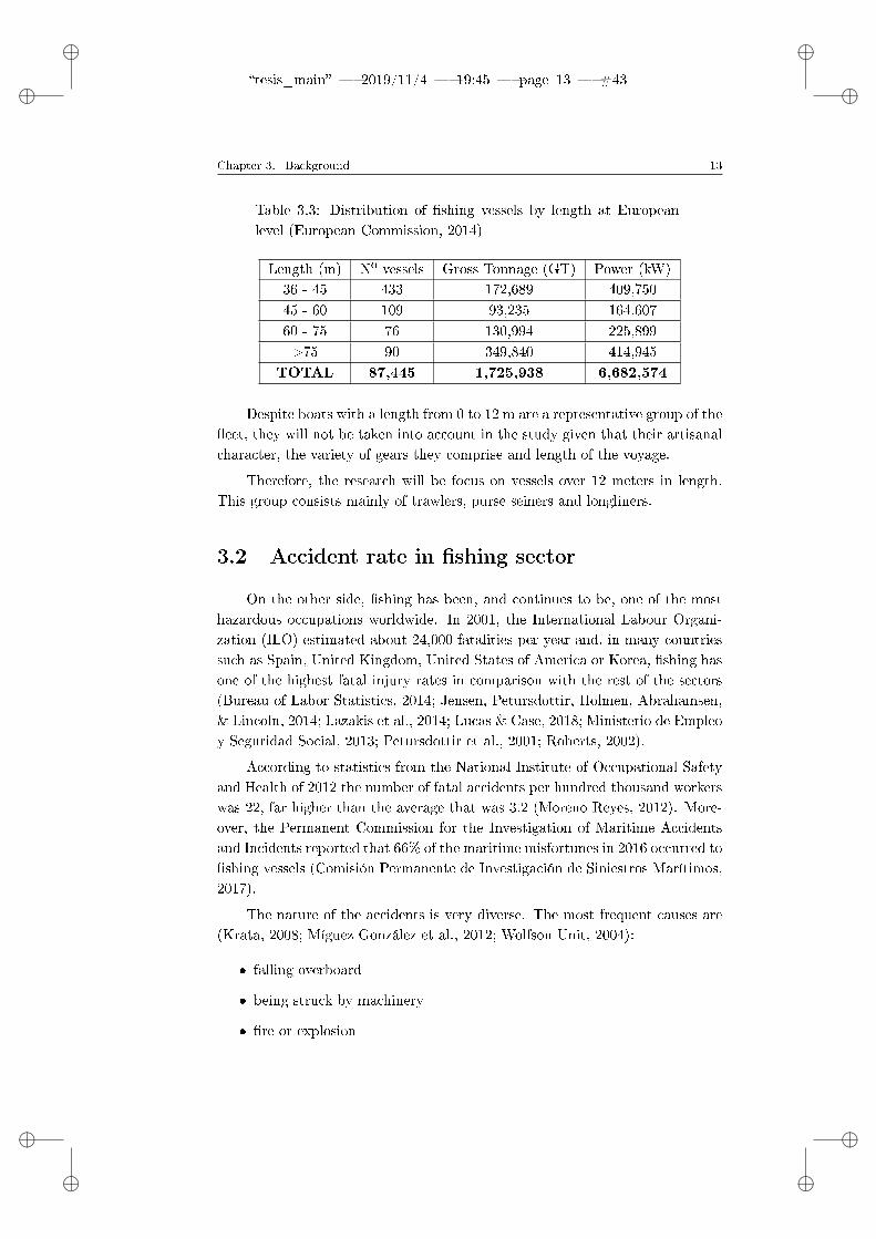
Table 3.3: Distribution of shing vessels by length at Europeanlevel (European Commission, 2014)

Length (m) Nº vessels Gross Tonnage (GT) Power (kW)

0 - 6 28,198 23,385 352,894

6 - 12 45,946 162,730 2,287,848

12 - 18 6,955 159,505 986,749

18 - 24 3,330 249,700 886,491

24 - 30 1,729 243,883 642,124

30 - 36 579 139,979 311,268

ii


ii

ii


Table 3.3: Distribution of shing vessels by length at Europeanlevel (European Commission, 2014)

Length (m) Nº vessels Gross Tonnage (GT) Power (kW)36 - 45 433 172,689 409,750

45 - 60 109 93,235 164,607

60 - 75 76 130,994 225,899

>75 90 349,840 414,945

TOTAL 87,445 1,725,938 6,682,574

Despite boats with a length from 0 to 12 m are a representative group of theeet, they will not be taken into account in the study given that their artisanalcharacter, the variety of gears they comprise and length of the voyage.

Therefore, the research will be focus on vessels over 12 meters in length.This group consists mainly of trawlers, purse seiners and longliners.

3.2 Accident rate in shing sector

On the other side, shing has been, and continues to be, one of the mosthazardous occupations worldwide. In 2001, the International Labour Organi-zation (ILO) estimated about 24,000 fatalities per year and, in many countriessuch as Spain, United Kingdom, United States of America or Korea, shing hasone of the highest fatal injury rates in comparison with the rest of the sectors(Bureau of Labor Statistics, 2014; Jensen, Petursdottir, Holmen, Abrahamsen,& Lincoln, 2014; Lazakis et al., 2014; Lucas & Case, 2018; Ministerio de Empleoy Seguridad Social, 2013; Petursdottir et al., 2001; Roberts, 2002).

According to statistics from the National Institute of Occupational Safetyand Health of 2012 the number of fatal accidents per hundred thousand workerswas 22, far higher than the average that was 3.2 (Moreno Reyes, 2012). More-over, the Permanent Commission for the Investigation of Maritime Accidentsand Incidents reported that 66% of the maritime misfortunes in 2016 occurred toshing vessels (Comisión Permanente de Investigación de Siniestros Marítimos,2017).

The nature of the accidents is very diverse. The most frequent causes are(Krata, 2008; Míguez González et al., 2012; Wolfson Unit, 2004):

falling overboard

being struck by machinery

re or explosion

ii


ii

ii

14 3.2. Accident rate in shing sector

the incorrect operation of the ship

modications of the weight distribution of the vessel

cargo shifting

overloading

ooding

grounding

collision

the entangling of the nets in the case of trawler vessels

static and dynamic instabilities

very adverse weather conditions that can lead to foundering or capsizing

Dierent authors, administrations and associations agree that there is no singlereason for an accident. On the contrary, misfortunes usually occur due to achain of events.

The consequences of these incidents can be very serious, not only injuriesto the crew or the cargo but also the loss of the ship or lives may take place(Hanzu-Pazara et al., 2016).

Figure 3.1: Cumulative percentage of fatalities by accident type, 1999-2010(Transportation Safety Board of Canada, 2012)

ii


ii

ii


Figure 3.1 shows the number of accidents and the percentage of fatalitiesby accidents type. As can be seen, despite stability failures are not the mostcommon they cause the biggest number of deaths. So, they are one of the maincauses of the loss of human life and shing vessels. As a rule, this type ofaccidents involve static and dynamic phenomena such as surf riding, broaching,loss of stability in quartering and stern seas and parametric rolling (Krata, 2008;Míguez González et al., 2012; Roberts, 2002; Transportation Safety Board ofCanada, 2012; Wolfson Unit, 2004).

Another issue that is worth mentioning is how accidents are distributedaccording to the length of the ship. The most aected vessels are those under12 meters in length, followed by those that are between 15 and 24 meters inlength (Marine Accident Investigation Branch (MAIB), 2008).

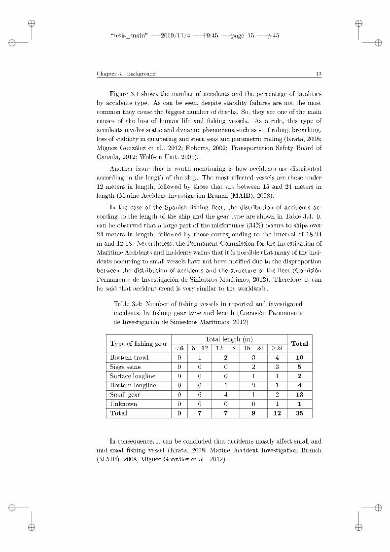
In the case of the Spanish shing eet, the distribution of accidents ac-cording to the length of the ship and the gear type are shown in Table 3.4. Itcan be observed that a large part of the misfortunes (34%) occurs to ships over24 meters in length, followed by those corresponding to the interval of 18-24m and 12-18. Nevertheless, the Permanent Commission for the Investigation ofMaritime Accidents and Incidents warns that it is possible that many of the inci-dents occurring to small vessels have not been notied due to the disproportionbetween the distribution of accidents and the structure of the eet (ComisiónPermanente de Investigación de Siniestros Marítimos, 2012). Therefore, it canbe said that accident trend is very similar to the worldwide.

Table 3.4: Number of shing vessels in reported and investigatedincidents, by shing gear type and length (Comisión Permanentede Investigación de Siniestros Marítimos, 2012)

Type of shing gearTotal length (m)

Total<6 6 - 12 12 - 18 18 - 24 ≥24

Bottom trawl 0 1 2 3 4 10

Siege seine 0 0 0 2 3 5

Surface longline 0 0 0 1 1 2

Bottom longline 0 0 1 2 1 4

Small gear 0 6 4 1 2 13

Unknown 0 0 0 0 1 1

Total 0 7 7 9 12 35

In consequence, it can be concluded that accidents mostly aect small andmid-sized shing vessel (Krata, 2008; Marine Accident Investigation Branch(MAIB), 2008; Míguez González et al., 2012).

ii


ii

ii

16 3.3. Evolution and current status of regulations

One of the reasons could be that large ships have a better ability to sail inheavy weather (Gefaell Chamochín, 2005; Krata, 2008; Scarponi, 2017).

There is another justication related with the safety culture on board his-torically present in this sector. Fishermen are aware that they work in a quiteharsh physical environment and, due to this fact, they assume that the riskis inherit and unavoidable to their activity. Incidents are very often acceptedwith resignation and feeling of bad luck (Bye & Lamvik, 2007; Marine AccidentInvestigation Branch (MAIB), 2008; Oliveira-Goumas & El Houdagui, 2000;Petursdottir et al., 2001).

Furthermore, there is a huge economical pressure over shermen as theirincomes depend on their catches. This situation enforces them to sail and workin unfavourable conditions (Antaõ, Almeida, Jacinto, & Soares, 2008; Lazakiset al., 2014; Marine Accident Investigation Branch (MAIB), 2008; Oliva Remolà& Gudmundsson, 2018).

Nevertheless, the main cause is the human factor. According to the AnnualOverview of Marine Casualties and Incidents 2018 human erroneous actionsaccount for 54.4% of the 338 accidental events analysed in the period 2011-2017 (European Maritime Safety Agency, 2018). In the case of stability-relatedincidents, this issue is related with the crew lack of training in stability matters.Only few shermen have a deep knowledge of stability, in particular this factbecomes more noticeable for the sizes of shing vessels previously mentioned.

In general, skippers carry out a subjective analysis to estimate the stabilitylevel of their ship based on their previous experience, which regularly lacks anykind of incident. This fact is also motivated by the unavailability of useful,practical and objective stability guidance on board, as the only information isthe stability booklet. This booklet is more oriented to a naval architect andmarine engineer than a seafarer and, consequently, it is stored on board andnever consulted. On the one hand, because of their complexity. And on theother, because they are only mandatory on those ships of more than 24 m length.(Deakin, 2005; Lazakis et al., 2014; Míguez González et al., 2012; Petursdottiret al., 2001; Wolfson Unit, 2004).

Another problem could be related to the current stability regulation whichis reviewed in the next section.

3.3 Evolution and current status of regulations

Intact stability of the vessel is an issue that has been researched sinceancient times. It was Archimedes in 300 B.C. who enunciated the rst funda-mental laws of hydrostatics of oating bodies and introduced the concept of

ii


ii

ii


balance of a couple of forces and moments (Francescutto, 2015; Francescutto &Papanikolaou, 2010; Rodríguez Castillo, 2008).

However, the basis of the modern theory of stability was not founded un-til many centuries later with the publication of the books entitled Traité duNaviera, sa Construction and des ses Mouvements by Bouguer in 1746 and Sci-enta Navalis seu Tractatus de Construendis ac Dirigendis Navibus by Euler in1749. Pierre Bouguer established the idea of metacentre (M), that is a prop-erty derived from the form of the vessel, and proposed a method based on thisnotion to measure ship's stability. By contrast at the same time, Leonard Eulerdetermined the concept of righting moment to evaluate the stability. Both au-thors developed their theories with the focus at small heel angles, which meansin the small region around the upright position, and the concept of metacentricheight (GM), which is the vertical distance between centre of gravity of theship and the metacentre, but from a dierent point of view (Francescutto &Papanikolaou, 2010; Rodríguez Castillo, 2008).

The theories of Bouguer and Euler were further developed by George At-wood through two papers presented to the Royal Society of London. The rstof them was published in 1796 and demonstrated the need of evaluating thestability for a nite range of heel angles by the application of the fundamentalprinciples of hydrostatics to simple geometric bodies such as parallelepipeds,cylinders, etc. It was the rst time that a set of inclinations were consideredinstead of only the initial and the nearby region around it for stability evalua-tion. His second work in co-authoring with Vial Du Clairbois was promulgatedin 1798 and it was an extension of the rst one. It consisted of applying theprevious theories to hull forms and a numerical analysis of the vessel's rightingarm (GZ) for a range of heel angles.

The approach of Bouger and Euler together with this new one supposed therst division in the way of assessing the stability of the vessel between small andlarge heel angles and it is still maintained today (Francescutto & Papanikolaou,2010; Rodríguez Castillo, 2008).

For many years, metacentric height was considered as the only measure-ment of ship's stability. After the shipwreck of CAPTAIN in 1868, a war shipfrom British Army, Edgard Reed demonstrated the importance of the freeboardas a reserve of buoyancy at large heel angles and the righting arm curve andso that it was renamed as Reed Curve (Francescutto, 2013; Rodríguez Castillo,2008).

During this period a new concern about the evaluation of stability in wavesarose. Froude suggested to change the classical static approach to a dynamicone. The rst proposal was comparing the heeling energy and the rightingenergy using the area under the righting arm curve (Fernández Polo & Neves,

ii


ii

ii


2012).

Despite all these attempts, the rst criteria of practical application didnot arrive until 1939 with the publication of the doctoral thesis of Rahola Thejudging of stability of ships and the determination of the minimum amount ofstability. His work consisted of carrying out an analysis of the parameters asso-ciated with the initial stability, the characteristics of the righting arm curve andthe curve of areas on a group of boats that suered stability-related accidentsor that did not suer any accident. Based on this study, he developed minimumstandards for all ships in order to avoid capsizing and, consequently, guaranteetheir safety (Fernández Polo & Neves, 2012; Neves, Rodríguez, & Merino, 2009;Rodríguez Castillo, 2008). It must be said that the values required by Raholaare not representative of the entire existing eet, since their study was aimed atships that sailed in Finnish waters and only included a sample of 34 units, fromwhich only one was a shing vessel. Therefore, it can be pointed out that thesecriteria may not be representative of the shing collective (Gefaell Chamochín,2005; Womack, 2003).

Given the simplicity and ease of implementation of these standards, in 1960the International Maritime Organization (IMO) decided to adopt them in theInternational Convention on Safety of Life at Sea (SOLAS) as a requirement.However, shing vessels are excluded from that Convention due to the greatdierences in design and operation in comparison with other ships. They are alsoexcluded from the International Convention on Load Lines (ILLC) that regulatesthe minimum freeboard and hence the reserve of buoyancy (Francescutto, 2013;Francescutto & Papanikolaou, 2010; Molyneux, 2008; Petursdottir et al., 2001).

In order to try to address the safety of shing vessels, in 1977 and againin 1993 the IMO held the Torremolinos Convention. This Convention repre-sented a big step for the shing sector and led to the Torremolinos Protocol,that is a set of rules aimed to improve the safety of shing vessels of 24 me-tres in length and over including the Rahola's criteria with few modications.Unfortunately, it did not enter into force as it was not ratied by the majorpart of the participant countries. For this reason, in 1997 the European Uniondecided to adopt it in all the member countries with the Directive 97/70/EC.This Directive has been replaced by 2002/35/EC in 2002. There was another at-tempt with the Torremolinos Protocol in 2012 with the Cape Town Agreement,but once again it did not enter into force as it has only been ratied by sevencountries (European Union, 2002; Fernández Polo & Neves, 2012; Francescutto,2013; Gefaell Chamochín, 2005; International Maritime Organization, 2012; Ro-dríguez Castillo, 2008).

Due to the fact that Torremolinos Protocol is aimed at shing vessels of 24metres in length and over, the United Nations, the ILO, the IMO and the Food

ii


ii

ii


and Agriculture Organization (FAO) elaborated a set of voluntary guidelinesentitled Code of Safety for Fishermen and Fishing Vessels. It was aimed to coverthe lack of the safety regulation in shing vessels between 12 and 24 meters inlength and it was divided in two parts: Part A, which focuses on safety andhealth issues and it is addressed to skippers and crews, and Part B, related withdesign, construction and equipment of the ship and oriented to shipbuilders andowners. This Code was revised in 2005 and the Safety Recommendations forDecked Fishing Vessels of Less than 12 m in Length and Undecked FishingVessels were included in Part B International Maritime Organization (2005a,2005b).

Another attempt for small shing vessels was the two IMO Guidelines (aand b) (MSC/Circ. 707. 19 October 1995. Guidance to the master for avoidingdangerous situations in following and quartering seas and MSC. 1/Circ. 1228.11 January 2007. Revised guidance to the master for avoiding situations inadverse weather and sea conditions), but as the stability booklet they aredicult to apply and mainly focused to large merchant vessels (InternationalMaritime Organization, 1995, 2007).

Moreover, in 1985 the calculus of severe wind and rolling, known as weathercriterion because it considered the eect of waves and wind, was adopted bythe IMO as Resolution A.562. It was developed by Japan and based on anenergetic method proposed by Pierrotet in 1935. The calculation of the wateron the deck, the passenger to a band and the heeling angle due to a turningmaneuver were incorporated as well (Francescutto, 2013).

Until 1953 ship's stability was considered a static phenomena. This ap-proach changed with the publication of the work of St. Denis and Pierson asthey assumed the vessel as a dynamic system. Likewise, during this period newways to predict capsizing based on probabilistic analysis and theories aboutship behaviour in waves were developed by many authors (Rodríguez Castillo,2008).

All these studies were disseminated through scientic publications and in-ternational conferences and workshops specically created for this purpose andwhich are periodically repeated in dierent countries. The rst of them wasthe International Conference on Stability of Ships and Ocean Vehicles known asSTAB or SHIPSTAB that was born in Glasgow in 1975. Since 1995 Inter-national Ship Stability Workshops (ISSW) are being held to complement STABConferences. Another event that has to be highlighted is the InternationalTowing Tank Conference (ITTC) that was born with the purpose of promotingthe improvement of all aspects of ship model work (in particular ship hydrody-namic performance and safety) and to reach agreement on basic procedures andmethods of presentation of results for publication. From the ITTC, General

ii


ii

ii


and Specialist committees were created in order to review the state of art andcarry out studies in each area. Stability Committee is one of them (Murdey,2014; Rodríguez Castillo, 2008; Ship Stability Dynamics and Safety (ShipStab),2019).

Within this framework and driven by the change in focus in the evaluationof stability, a revision process of the standard stability regulations started in2001 with the idea of developing safety and operational criteria for all type ofvessels. Working Groups (WGIS) were established in order to carry out theanalysis and further studies about the criteria. All this work culminated withthe publication of the International Code on Intact Stability that entry intoforce in 2008 (2008 IS Code). Notwithstanding it represented a good improve-ment in the establishment of a methodology for assessing ship's stability, itmore remained in a revision than in the development of new standards thatcontemplated the dynamic behaviour of the vessel. The 2008 IS Code preservedthe original stability criteria, the probabilistic ones and the weather criteriontogether with some modied criteria for certain kind of ships such as passen-ger vessels, high speed craft, shing vessels (Francescutto, 2015; InternationalMaritime Organization, 2008; Kobylinski, 2012).

As the work was not completely nished in the rst 2008 IS Code, theIMO has proposed to continue with the development of the Second Genera-tion of Intact Stability Criteria (SGISC) to complement or replace the previousones, but with a dierent perspective oriented to the dynamics of the ship.The purpose of this work is to determine the modes of failure and to estab-lish a series of levels of vulnerability to assess the stability (Álvarez-Santullano,2014; Fernández Polo & Neves, 2012; Francescutto, 2015; International Mar-itime Organization (IMO) Sub-Committee on Ship Design and Construction,2018; Kobylinski, 2012; Neves, Rodríguez, & Merino, 2009)

The modes of failure contemplated until now are:

Pure loss of stability: it happens when the ship is located on the crestof a wave for a suciently long period of time. It usually occurs in sternseas when the speed of the ship is close to the celerity of the wave andfor a given wave length and slope. Those vessels, whose their value of therighting arm in the sine of the wave is greater than in still waters andin the crest of the wave it is smaller, are more susceptible to suer thisphenomenon and it can lead to capsize (Umeda & Francescutto, 2016).

Surf-riding/broaching: surf-riding occurs when the ship is caught by awave and is accelerated to the speed of the wave, that is, the ship goes tosurf on the wave reaching a higher speed than in calm waters. If, in addi-tion, directional instability happens with a great and sudden change of the

ii


ii

ii


course due to the ineciency of the rudder, then it can be called broach-ing. The angular velocity associated with this phenomenon introduces adynamic heel that, if combined with other forces, could give rise to thecapsizing of the ship. Broaching is dened therefore as an event in whichthe ship is not able to maintain the course despite the application of itsmaximum government capacity. These two dynamic instabilities normallyoccur in stern seas at high speeds when the encounter frequency tends tozero (Fernández Polo & Neves, 2012; Neves, Rodríguez, & Merino, 2009;Umeda & Francescutto, 2016; Wandji, Veritas, & Corrignan, 2012).

Parametric rolling: it is an oscillating movement in rolling (the x-axis)that develops quickly, reaches great amplitudes and may end in the ship'scapsizing. The cause of this event is the parametric excitation of the wavesacting on the boat at a given speed, at a certain frequency and with anangle of incidence that determines an encounter frequency close to twicethe natural roll frequency, exciting this motion and culminating in reso-nance. It usually happens in head or beam seas (Umeda & Francescutto,2016).

Dead-ship condition: this condition appears when the vessel loses herpropulsive power, so she could suer beam wind or waves and trigger anyof the above situations (Umeda & Francescutto, 2016).

Excessive accelerations: if the ship has a very high metacentric height thenatural roll period becomes very small and it results in excessive acceler-ations in certain points of the ship. This can cause damage to the load orinjuries to the crew members (Umeda & Francescutto, 2016).

The vulnerability levels give a measure of how remote is the possibility of theship to suer one of the failure modes. The rst two consist of simplied dy-namic stability failure assessment methodologies, while the third one is focusedon a direct stability evaluation.

The rst level is based on the geometry and speed of the vessel, as well as onsimple mathematical models that describe the phenomenon of each mechanismof stability failure. This level is expected to be as conservative and simpleas possible. In the second vulnerability threshold, the physical principles thatdescribe the failure modes in a more realistic way are considered. It servesas a discard in case of false forecasts produced by the rst level. The thirdlevel is a direct assessment of the stability of the vessel and it is based on astatistical analysis and the most modern tools (Fernández Polo & Neves, 2012;Francescutto, 2013; Kobylinski, 2012; Umeda & Francescutto, 2016).

In Spain, current regulations regarding stability for shing vessels are, onthe one hand, the Cape Town Agreement of 2012 for ships of 24 meters in

ii


ii

ii

22 3.4. Guidance systems

length and above and, on the other hand, RD 543/2007 for vessels with lengthless than 24 meters. This Royal Decree distinguishes between vessels with moreand less than 12 meters in length. For the rst group the same regulationsthan vessels of 24 meters in length and above are applied and for the otherISO 12217. The criteria included in the Royal Decree are based on those ofthe IMO which in turn rely on those of Rahola and, therefore, they continueto have a static approach (Álvarez-Santullano, 2014; International MaritimeOrganization, 2012; Ministerio de Fomento, 2007).

3.4 Guidance systems

As stated and reected throughout this chapter, the main cause of accidentsthat aect shing vessels is the incorrect risk assessment on board. This fact isparticularly accused in small and medium sized vessels, i.e. under 24 meters inlength, where crew training is poorer and regulations are less strict.

In order to help masters to assess the stability level, all ships of 24 metersin length and above are required to have on board the stability booklet. Thisbooklet contains the hydrostatic characteristics of the vessel and informationabout the mandatory loading conditions, which are four and they suppose torepresent the operational situations during a voyage (Gefaell Chamochín, 2005;Míguez González et al., 2012; Wolfson Unit, 2004). These are (InternationalMaritime Organization, 2012):

1. Departure for the shing grounds with full fuel, stores, ice, shing gear,etc, and no catch.

2. Departure from shing grounds with full catch and shing gear, 35% offuel and stores and no ice.

3. Arrival at home port with full catch and shing gear, 10% of fuel andstores and no ice.

4. Arrival at home port with 20% catch, full shing gear, 10% of fuel andstores and no ice.

This booklet also includes some guidelines to perform stability calculations forintermediate loading conditions and some recommendations. However, thesecalculations are very tedious and time consuming and require more than a basictraining. For this reason the stability booklet turns into quite useless for skip-pers and they prefer to carry out a subjective analysis based on their previousexperiences (Gefaell Chamochín, 2005; Míguez González et al., 2012; WolfsonUnit, 2004).

ii


ii

ii


Having recognized these problems, in the last two decades it has beenconcluded that one plausible approach for trying to reduce stability-relatedaccidents could be to provide the skippers with simple and ease to understandstability information, which helps them to evaluate the sailing condition of theirvessels based on objective data. This idea has been materialized in simplied onboard stability guidance systems, which are no more than a group of proceduresand recommendations to provide clear information about the stability of theship, including safe loading conditions and warn about situations where theremay be a higher risk level (Deakin, 2005; Womack, 2003).

On board guidance together with training programs, provides masters moreinformation to complement their knowledge and to carry out an objective eval-uation of the risk level of their ships, minimizing this probability of an accident(Deakin, 2005; Marine Accident Investigation Branch (MAIB), 2008; Varela,Guedes Soares, & Santos, 2010).

To guaranteed the success of this kind of systems there are some premisesthat have to be fullled (Deakin, 2005; Míguez González et al., 2012; Womack,2003):

Be easy to use and to understand. The idea is that an extensive trainingis not necessary to assess the stability of the ship.

No need for crew interaction. The system should contain all the informa-tion and no need of performing any calculation, only warns the skipper inthe situations that the ship is prone to suer some kind of instability.

Low cost of acquisition, installation and maintenance. It must be aord-able for everyone, including small boats.

Easy to update in case that modications arise throughout the entire lifeof the vessel.

Be able to reproduce the largest number of loading conditions as accu-rately as possible. It must be ensured that it covers the entire range ofoperation of the vessel.

Be able to alert any situation of instability. It must be able to calculatethe intact stability criteria imposed by the Administration and the secondgeneration of intact stability criteria if it is appropriate.

Ideally be able to predict weather conditions.

All these requirements can be summarised in three principal ones: be simple touse and understand, low cost of acquisition, maintenance and installation andno need for crew interaction.

ii


ii

ii


On this matter, several proposals have been carried out along the years.The rst attempt was made by Koyama in 1982 and it consisted of a pendulumwhich measured the movements of the ship. From these data, the roll periodand the safety level were estimated. However, the results were not very reliable,especially at high speeds (Varela et al., 2010).

Köse in 1995 described an intelligent monitoring and guidance system. Itconsisted of sensors that provided weather information and showed warningmessages based on the analysis of the circumstances that lead to capsize, aswell as on the valuation human experience, experiments and theoretical research(Varela et al., 2010).

In 2001, Womack proposed a simple and fast application. It consists ofa matrix where dierent loading possibilities are considered, including sh inholds, presence of free sh on deck, fuel distribution, etc. A colour code isassociated to each combination to indicate the level of safety in a visual way,it varies from black (very dangerous) to green (safe situation). The boundariesfor the colour scheme on the matrix are selected considering a very wide rangeof factors, such as:

Potential for downooding of the vessel

Type of shing

Typical voyage cycle

Operational area

Distance from safe refuges

Likely direction of approach of storm relative to the refuges

Frequency of operation in that area and hence extent of local knowledge

Stability of the shery in terms of economy and crew turnover

Local forecast availability and reliability

Availability of real time weather data

Likely nature of wind and sea state in storms

A basic example of this matrix is shown in Figure 3.2. When weather condi-tions are included the matrix turns more sophisticated and looks like Figure3.3. Although this stability matrix represents a good alternative for the small-est vessels, it may become quite complex as the number of tanks increase inlarger vessels (Deakin, 2005; Míguez González et al., 2012; Wolfson Unit, 2004;Womack, 2003)

ii


ii

ii


Figure 3.2: Example of Womack stability matrix (Míguez González et al., 2012)

The Norwegian Maritime Directorate also proposed a similar alternativebased on a colour coded stability poster. In this brochure loading conditionsare displayed in a simple way with a drawing and some notations of the loads.As loading conditions are described approximately, the security margins arenot very precise and only distinguish among acceptable, limit and dangeroussituations with an associated colour. The poster also includes some advicesabout how to operate the ship in terms of stability. It is required in this countryto vessels with a length between 10.7 and 15 meters and it is exclusively availablein Norwegian at www.yrkessker.no (Deakin, 2005; Míguez González et al., 2012;Wolfson Unit, 2004).

All these attempts were mostly paper based. A new revolutionary systemwas established by the Icelandic Administration and it consists of a weatherguidance combined with continuous stability monitoring. On the one hand,draft and roll period are measured to estimate the stability and the minimumwave height to capsize. On the other hand, environmental conditions in theshing grounds are measured with wave buoys and wave forecasts are providedby Internet or phone call. Then, the information regarding the sea state istransformed into a safety of navigation index based on the ship righting levercurve. This methodology, together with a compulsory inclining test programreduced the stability-related incidents of Icelandic eet in a large percentage(Deakin, 2005; Viggosson, 2009; Wolfson Unit, 2004).

In the last decade, a second generation of guidance systems have emerged.They are based on simplied computer systems that provide an estimation of thestability level of the ship considering the loading condition details introducedin the software by the crew during operation.

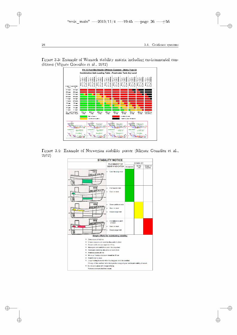
ii


ii

ii


Figure 3.3: Example of Womack stability matrix including environmental con-ditions (Míguez González et al., 2012)

Figure 3.4: Example of Norwegian stability poster (Míguez González et al.,2012)

ii


ii

ii


One example could be the system proposed by the Centre for Marine Tech-nology and Engineering (CENTEC) (Tello, Ribeiro e Silva, & Guedes Soares,2011; Varela et al., 2010). This system has two modules. The rst one com-putes the static stability according to the Torremolinos Convention Criteria forshing vessels and the IMO Severe Wind and Rolling Criteria. The secondmodule considers the eects of the waves and implements the MSC Circ. 707 Revised Guidance to the Master for Avoiding Dangerous Situations in AdverseWeather and Sea Conditions (International Maritime Organization, 2007). Inboth modules the application displays the stability level of the current loadingcondition with some graphs and numerically (See Figure 3.5 and 3.6).

Figure 3.5: SEMPEO, layout of the static stability analysis module Varela etal. (2010)

In Canada, a system that combines Womack matrix with ship motions wasdeveloped. When the amplitude of the motions exceeds a given limit, a warningappears on screen (Deakin, 2005; Míguez González et al., 2012; Varela et al.,2010).

There is another alternative, developed by the Integrated Group for Engi-neering Research and called Safe Skipper, that combines a naval architecturesoftware with a simplied and user-friendly interface. This system provides sta-bility information following a similar coloured approach to the aforementionedstability posters. It is installed on board on a touchable screen PC and, from thehull forms and weight distribution, manually introduced by the crew, performsall necessary calculations regarding to vessel stability. Once calculations aredone, the system generates and displays in a clear and understandable way thecurrent situation of the vessel and her risk level. The values of heel, trim and

ii


ii

ii

28 3.5. Roll natural frequency estimation

Figure 3.6: SEMPEO, layout of the wave safety analysis module Varela et al.(2010)

draft are graphically displayed and the stability level is presented according to acolour scale. If one of the stability criteria are not met, the minimum freeboardis exceeded or watertight or progressive ooding points are immersed an alertmessage appears on the screen. The usability levels of the interface have beentested and veried to guaranteed the easy of use (Míguez González, CaamañoSobrino, Tedín Álvarez, Díaz Casás, & Martínez López, 2010; Míguez Gonzálezet al., 2012).

All the described alternatives rely on the use of data provided by the crew,thus introducing subjectivity and large uncertainties within the stability evalua-tion process. In the case of stability posters, subjectivity and uncertainty appearduring the selection of the loading condition from those included in the posterwhich better resembles the current one. And in the case of computer systems,they appear while introducing the loading condition details which are needed toevaluate the stability level. Those details are basically the approximate locationand the amount of cargo and tank lling levels. Therefore, these systems couldprovide erroneous information if mistaken input data are introduced.

3.5 Roll natural frequency estimation

Most recently, and in order to try to maximize the ease of use and minimizethe crew interaction/interference, a new group of decision support systems hasbeen proposed. The main goal of these systems is to provide an autonomous as-

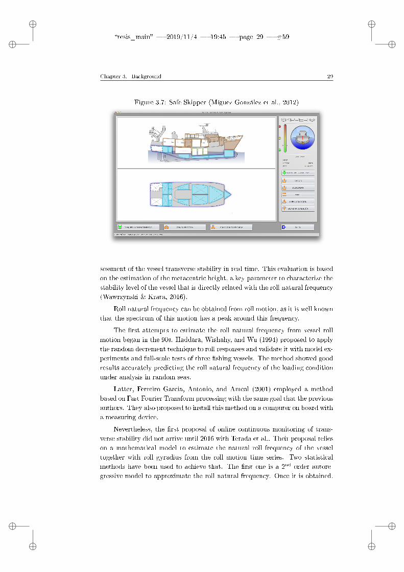
ii


ii

ii


Figure 3.7: Safe Skipper (Míguez González et al., 2012)

sessment of the vessel transverse stability in real-time. This evaluation is basedon the estimation of the metacentric height, a key parameter to characterize thestability level of the vessel that is directly related with the roll natural frequency(Wawrzynski & Krata, 2016).

Roll natural frequency can be obtained from roll motion, as it is well knownthat the spectrum of this motion has a peak around this frequency.

The rst attempts to estimate the roll natural frequency from vessel rollmotion began in the 90s. Haddara, Wishahy, and Wu (1994) proposed to applythe random decrement technique to roll responses and validate it with model ex-periments and full-scale tests of three shing vessels. The method showed goodresults accurately predicting the roll natural frequency of the loading conditionunder analysis in random seas.

Latter, Ferreiro Garcia, Antonio, and Ameal (2001) employed a methodbased on Fast Fourier Transform processing with the same goal that the previousauthors. They also proposed to install this method on a computer on board witha measuring device.

Nevertheless, the rst proposal of online continuous monitoring of trans-verse stability did not arrive until 2016 with Terada et al.. Their proposal relieson a mathematical model to estimate the natural roll frequency of the vesseltogether with roll gyradius from the roll motion time series. Two statisticalmethods have been used to achieve that. The rst one is a 2nd order autore-gressive model to approximate the roll natural frequency. Once it is obtained,

ii


ii

ii

30 3.5. Roll natural frequency estimation

GM and roll gyradius are estimated based on a general state space modellingprocedure. This method has been validated with model and on board experi-ments.

In order to reduce the complexity of this approach, it was further renedin Terada et al. (2018), where a methodology based on the application of aBayesian modelling procedure using the Markov Chain Monte Carlo (MCMC)method with the same purpose. Nonetheless, in both cases authors state thatmore validation work is needed to ensure the reliability of the obtained results.

In this framework is where this PhD thesis is included. It provides newmethodologies for assessing in real-time the stability of the vessel and, at thesame time, the development of a guidance system belonging to the last groupof systems.

ii


ii

ii

Chapter 4

Fundamentals of real-time

stability assessment

4.1 Introduction

This chapter is dedicated to present the basis of the real-time stability eval-uation. It starts describing the involved parameters, how they are related toeach other and how they are traditionally obtained. Then, the proposed proce-dure, the roll motion monitoring and the requirements of real-time estimationare introduced.

4.2 Involved parameters in stability evaluation

Ship stability is governed by many concepts related with geometry, physicalresponses to inclinations or loading condition. As it was mentioned in chapter3, the rst theories or criteria for estimating the stability were based on the def-inition of two parameters: metacentre and righting arm. The rst one is relatedwith the initial stability of the vessel and the second one with the restoringmoment after inclining the vessel a certain heel angle. Both of them are veryimportant and they are connected to each other. At small heel angles there isa direct relationship:

GZ = GM · sin(θ); θ < 100 (4.1)

Being θ the heel angle. And at large heel angles:

ii


ii

ii

32 4.2. Involved parameters in stability evaluation

GZ = KN −KG · sin(θ); θ > 100 (4.2)

WhereKN is the cross curve of stability of the vessel andKG is the verticalposition of the centre of gravity of the ship that can be obtained from the GMvalue as:

KG = KM −GM (4.3)

KM is the distance from the keel to the metacentre.

For this reason, the metacentric height is a key parameter for vessel stabil-ity and its real-time monitoring may be benecial for alerting the crew aboutchanges in stability.

The classical procedure to estimate the stability parameters of a vessel isperforming an inclining experiment. It consists of creating a controlled heelon the vessel by moving some known weights, and then obtaining the resultingmetacentric height through basic initial stability principles. Another way toobtain the metacentric height of a vessel is to carry out a roll decay test and,from the resulting roll motion time series, obtain the roll spectrum. In calmwater conditions and under no external excitation, the location of the peakof the roll spectrum correspond with the roll damped natural frequency. Inthe case of ships, where the damping is usually quite small, this value is veryclose to the vessel roll natural frequency, and both values could be consideredequivalent. Consequently, the metacentric height can be obtained from the rollnatural frequency by:

GM =(Ixx +A44) · ω2

0

g ·∆(4.4)

Where ω0 is the roll natural frequency, g is the acceleration of the gravity,∆ is the vessel mass displacement, Ixx is the ship transverse mass moment ofinertia and A44 is the roll added mass. If the inertia and the added mass areapproximated by the Weiss formula (Krüger & Kluwe, 2008), the GM of thevessel can be obtained as:

GM =k2xx · ω2

0

g(4.5)

Being kxx the roll gyradius of the ship, which is usually taken as 40% ofthe beam of the vessel.

ii


ii

ii

Chapter 4. Fundamentals of real-time stability assessment 33

4.3 Real-time stability estimation

The inclining experiment is the method approved by the International Mar-itime Organization for estimating the vessel lightship parameters (InternationalMaritime Organization, 2008), while the spectral approach is proposed as possi-ble means for carrying out approximate real-time estimates of the vessel stabilitywhile sailing (International Maritime Organization, 1993). However, the resultsof both methodologies are only reliable when the vessel is in sheltered waters,with no waves and no wind. As it is highlighted by IMO (International Mar-itime Organization, 1993), this fact is especially important in the case of thelatter methodology. When an external excitation such as waves and wind ispresent, its eect is perceivable in the roll spectrum.

This dissertation is focused in this specic situation, where the vessel issailing at sea in the presence of wind, waves and currents. Also the loadingcondition changes during the voyage due to the fuel consumption and the catchesstored on board. Hence, the main challenge in this work is to extract the rollnatural frequency from all the information contained in the roll motion in thoseparticular conditions. Once it is obtained, stability of the vessel can be assessedaccording to Equation 4.4. Figure 4.1 summarises the purpose of this PhDthesis, where the black box represents the developed methodology.

Figure 4.1: Summary of the purpose of the thesis.

4.4 Roll motion monitoring

First of all, the departure point of the proposed methodology is the rollmotion that it is measured through an inertial measurement unit (IMU) andstored in a buer by the data acquisition (DAQ) system. The idea of utilizingan IMU comes from one of the main requirements of the guidance systems: lowcost of acquisition, installation and maintenance. Furthermore, the sensor issmall enough to not bother daily operations on board.

ii


ii

ii

34 4.5. Real-time requirements

As a signal, roll motion may be described in terms of dierent parametersand usually each characteristic is described by two variables. One of them isindependent and denes how or when each sample is taken. It is called domainand the most common domains are time, using canonical basis, or frequency,whose base is a sum of harmonic components of dierent frequencies. Theother variable is the actual measurement and it is function of the previous one(Oppenheim, Schafer, & Buck, 1999; Proakis & Manolakis, 1996; Smith, 2002).In this work, roll motion is monitored as a function of time (s) and by measuringthe amplitude (deg).

There are some characteristics or information of the signal that are easierto analyse in one specic domain. However, by the Heisenberg uncertainty prin-ciple it is impossible to locate the signal in time and frequency simultaneously.So that, if the signal is originally acquired as a function of time, a change to fre-quency domain is needed (Proakis & Manolakis, 1996). There are several toolsthat allow time-frequency analysis, but the implementation of an algorithm toestimate the roll natural frequency in an on board stability assessment systemshould guarantee that the results are obtained in real-time.

In this thesis, two dierent approaches for estimating the roll natural fre-quency from the roll motion time series are developed and compared. Therst one is based on analysing the signal in the frequency domain by usingdigital signal processing techniques and the second one in analysing it in thetime domain combining signal processing with statistical change detection tools.Furthermore, both methodologies are validated by dierent ways.

4.5 Real-time requirements

To fulll the real-time estimation requirement a proper buer size to storeroll motion needs to be determined. Wave buoys normally employ 20 minutesintervals for analysing environmental data because it is the minimum amountof time to consider a stationary sea (Pascoal, Guedes Soares, & SoÌºrensen,2007). However, this time window is too large for the case under analysis. In20 minutes, the ship condition could be signicantly modied, even leading toa dangerous situation.

The choice of the batch length has been made assuming a medium sizedshing vessel (the target vessels of this dissertation) and by trading-o amongthe minimum data batch size to achieve a reliable estimate of the roll naturalfrequency and the needed resolution to distinguish between dierent operationalconditions. Therefore, in this work real-time is considered when the results areobtained every 3 minutes.

ii


ii

ii

Chapter 4. Fundamentals of real-time stability assessment 35

Moreover, roll motion is a discrete digital signal and in order to accuratelyreproduce it without aliasing the sampling frequency should be greater thantwice the maximum frequency to be sampled. This state is known as Nyquist-Shannon theorem or Sampling theorem and the limit frequency is called Nyquistfrequency (Medina, 2010; Proakis & Manolakis, 1996; Stearns, 2003):

flim =fs2

=1

2 · Ts(4.6)

Being flim the Nyquist frequency, fs the sampling frequency and Ts thesampling period.

ii


ii

ii

ii


ii

ii

Chapter 5

Fast Fourier Transform based

methodology

5.1 Introduction

In this chapter a methodology for estimating in real-time the ship stabilitybased on the Fast Fourier Transform is presented.

First of all, the use of this tool to obtain the roll natural frequency of thevessel is studied and validated with roll motion time series from towing tanktests of two shing vessels in dierent wave conditions. The constrains of thistool are also introduced.

Once the roll natural frequency is estimated, the metacentric height canbe computed applying Equation 4.4 or 4.5. The implications of utilising oneequation or another and the calculation of the involved parameters are analysed.

Moreover, an uncertainty analysis of the results of the roll natural frequencyand the metacentric height is performed.

Finally, a real-time stability monitoring methodology based on the use ofthe recursive Fast Fourier Transform is described and validated with roll motiontime series from simulations and sea trials of two stern trawlers.

5.2 Fast Fourier Transform based estimation

The rst attempt to estimate the metacentric height from roll motion con-sists of considering Equation 4.4 and obtaining the involved parameters: rollnatural frequency, transverse mass moment of inertia, added mass and ship

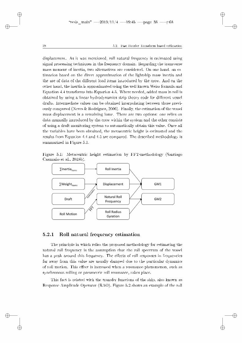
ii


ii

ii

38 5.2. Fast Fourier Transform based estimation

displacement. As it was mentioned, roll natural frequency is estimated usingsignal processing techniques in the frequency domain. Regarding the transversemass moment of inertia, two alternatives are considered. On one hand, an es-timation based on the direct approximation of the lightship mass inertia andthe use of data of the dierent load items introduced by the crew. And on theother hand, the inertia is approximated using the well known Weiss formula andEquation 4.4 transforms into Equation 4.5. Where needed, added mass in roll isobtained by using a linear hydrodynamics strip theory code for dierent vesseldrafts. Intermediate values can be obtained interpolating between those previ-ously computed (Neves & Rodríguez, 2006). Finally, the estimation of the vesselmass displacement is a remaining issue. There are two options: one relies ondata manually introduced by the crew within the system and the other consistsof using a draft monitoring system to automatically obtain this value. Once allthe variables have been obtained, the metacentric height is estimated and theresults from Equation 4.4 and 4.5 are compared. The described methodology issummarized in Figure 5.1.

Figure 5.1: Metacentric height estimation by FFT-methodology (SantiagoCaamaño et al., 2018b).

5.2.1 Roll natural frequency estimation

The principle in which relies the proposed methodology for estimating thenatural roll frequency is the assumption that the roll spectrum of the vesselhas a peak around this frequency. The eects of roll responses in frequenciesfar away from this value are usually damped due to the particular dynamicsof roll motion. This eect is increased when a resonance phenomenon, such assynchronous rolling or parametric roll resonance, takes place.

This fact is related with the transfer functions of the ship, also known asResponse Amplitude Operator (RAO). Figure 5.2 shows an example of the roll

ii


ii

ii

Chapter 5. Fast Fourier Transform based methodology 39

transfer function for a shing vessel in beam seas at zero speed. As it can beseen, roll amplitude is damped for wave frequencies that are far away from thenatural frequency and much larger when they are close. This eect, as it wasmentioned before, is translated into the roll spectrum showing a peak more orless pronounced at this frequency. Thus, it can be expected that in sea stateswhere the wave frequency is far from the roll natural frequency, the identicationof this frequency will be tougher than in situations where resonance appears.

Figure 5.2: Example of a roll transfer function for a shing vessel in beam wavesat zero speed.

Frequency domain describes how much of a signal lies within each givenfrequency band over a range of frequencies. This representation commonly givesa better understanding or characterisation of the behaviour of a physical systemas many parameters are time varying. For example, a system can be described interms of bandwidth, frequency response, gain, phase shift, resonant frequencies,time constant, resonance width, damping factor, Q factor, harmonics, spectrum,power spectral density, eigenvalues, poles, and zeros.

The power spectrum is a characteristic of the signal that shows how itsenergy or power is distributed throughout each component of the frequency.Consequently, it allows to identify the natural frequency of the system underanalysis by determining the frequencies in which the main peak is located. Inorder to be able to compute it, the representation of the signal in the frequencydomain is necessary (Medina, 2010; Stearns, 2003).

There are several tools that permit to change from one domain to another,but keeping in mind the requirement of real-time and because it is the mostcommon way of generating a power spectrum, the Fast Fourier Transform (FFT)was chosen (Medina, 2010; Stearns, 2003).

The FFT is an algorithm to compute the Discrete Fourier Transform (DFT)

ii


ii

ii


faster and more eciently. The DFT is dened as (Oppenheim et al., 1999;Stearns, 2003):

Xm =

N−1∑n=0

xne−j2πmn/N ; m = 0, 1, ..., N − 1 (5.1)

Being N the number of computations of the DFT and xn is the sampledsignal.

The FFT algorithm is based on decomposing the calculation of the DFT ofa vector into the computation of DFTs of smaller vectors. This decompositionavoids redundant complex products contained in the original DFT, and so that,the number of products is reduced from N2 to N

2 log2 (N) (Oppenheim et al.,1999; Stearns, 2003).

To increase the simplicity of the process without degrading the results, thesignal power spectrum S(ω) is computed by multiplying the FFT results (g(ω))by their complex conjugate and averaging it. Thus, the proposed computationis the following:

g(ω) = FFT (φ(t)) (5.2)

S(ω) = |g(ω)| 2n (5.3)

Where φ(t) is the roll motion amplitude.

In S(ω), apart from the roll natural frequency, all the excitations that act onthe ship (such as waves, wind, currents...) are contained. Usually they appear inthe power spectrum as peaks of dierent amplitudes depending on their energycontent, and from all of them it is necessary to identify the roll natural frequency.As there is no more information on board to be able to discern among all thepeaks, the frequency where the largest peak of S(ω) is located is assumed tobe the roll natural frequency of the vessel. This assumption is a bit rough butthe excitation of the vessel herself is usually the most energetic, in particular inthose cases where parametric or pure resonance take place.

5.2.1.1 Limitations of the Fast Fourier Transform

Despite of the simplicity of the calculation of the FFT to install it on anon board guidance system, it has some limitations that have to be mentioned.

The rst thing is that the FFT is performed on a specic set of acquiredtime domain data. In order to have enough data points to get good results

ii


ii

ii


a proper buer size needs to be determined. In this case, the requirement ofreal-time sets the batch length to 3 minutes.

The second thing to keep in mind is the frequency resolution of the FFT(∆F ). When the FFT is calculated from time domain data, it gives amplitudeinformation at discrete frequencies below the Nyquist value. The dierencebetween these frequencies is given by the equation:

∆F =sample rate

FFT record length(5.4)

To get a ner resolution, the signal must be sampled at a slower rate or toincrease its record length.

Finally, as the FFT is applied to signal batches window issues, as for exam-ple spectral leakage, can be introduced and aect the analysis. This last pointis discussed in deep in the following sub-subsection.

5.2.1.2 Windowing

In spectral analysis when a signal is time varying and nitely sampledspectral leakage may appear. This eect is no more than energy dispersion inthe spectrum. Its main cause are the discontinuities that exist at the beginningand the end of the analysed signal and it could degrade the signal-noise ratioand mask other smaller signals at dierent frequencies. The eects of spectralleakage can be reduced decreasing the discontinuities at the edges of the signal(Albrecht, 2001; Harris, 1978; Oppenheim et al., 1999).

A possible solution is to apply a window function. The process consists ofmultiplying the signal by a function that reduces the signal to zero at the edgesand it is known as windowing (Harris, 1978; Oppenheim et al., 1999).

Windows generally cause a reduction in the accuracy of the measured peakamplitude and also introduce damping. Nevertheless, these issues are not rele-vant for this case, as the main objective is to estimate the frequency in whichthe main peak is located and not its amplitude (Harris, 1978; Oppenheim et al.,1999).

There are numerous window functions. In this work for the sake of sim-plicity, only those belonging to cosine-sum family have been considered. Thereasons are that in this window family all are real-valued continuous functions,their rst derivative is also continuous, very simple calculation of the weightingcoecients and easy to identify the properties of their transform. In particularthree members of this family have been used in the study in order to see ifthey improve the estimation of the roll natural frequency in case that spectral

ii


ii

ii


leakage appear: Hanning, Blackman and Blackman-Harris windows (Albrecht,2001; Harris, 1978; Oppenheim et al., 1999). The expressions and the shape ofthe window functions are the followings (Harris, 1978).

Hanning:

wh (n) = 0.5 + 0.5cos

[2n

Nπ

]; (5.5)

n = −N2, ...,−1, 0, 1, ...,

N

2

Blackman:

wb(n) = 0.42 + 0.50cos

[2n

Nπ

]+ 0.08cos

[2n

N2π

]; (5.6)

n = −N2, ...,−1, 0, 1, ...,

N

2

Blackman-Harris:

wbh(n) = 0.35875−0.48829cos

[2n

Nπ

]+0.14128cos

[2n

N2π

]−0.01168cos

[2n

N3π

];

(5.7)

n = 0, 1, ..., N − 1

Figure 5.3: Hanning window

ii


ii

ii


Figure 5.4: Blackman window

Figure 5.5: Blackman-Harris window

5.2.1.3 Roll natural frequency uncertainty analysis

In order to determine the accuracy of the results of natural roll frequencyusing the FFT-based methodology an uncertainty analysis has to be carried out.Considering that the obtained values of the estimated roll natural frequency aredirectly measured quantities, the U95 model for calculating the uncertainty inthe results has been employed (Dieck, 2007).

Uω0= U95 = ±t95[b2 + (

SX√N

)2]12 (5.8)

Where U95 is the 95% condence uncertainty and t95 is a function of νobtained from a Student's table (for ν ≥ 30 t95 = 2.000 ), being ν the degreesof freedom. Regarding b, it is the systematic standard uncertainty (at 68%condence). N is the number of data points in the average calibration constantor the number of data points in the calibration line t. Finally, SX is thestandard deviation of the data under analysis.

ii


ii

ii


5.2.2 Transverse mass moment of inertia

The transverse mass moment of inertia of a vessel can be estimated bythree dierent alternatives.

The rst one is the direct integration. However, this is not a feasible optionconsidering the shape of the vessel and the variation of her mass characteristicsalong the length. Due to this fact, this option is discarded (Aasen & Hays,2010).

There is another alternative of estimating the dry mass moment of iner-tia similar to the previous one but simpler and more common. It consists ofreducing the ship to a single object with a known shape and constant density,or by breaking her down into the most relevant mass items, and approximatingthem to known shapes with constant density (Aasen & Hays, 2010). The latterproposal has been selected, and applied by considering the steel weight, sh inholds, tanks and some specic cargo items which have large inuence in theinertia's value.

The steel weight is supposed to represent the largest percentage of theinertia, and it has been obtained by calculating the transverse inertia of theamidship section using its structural drawings and integrating it along the over-all length using the hull form curve of areas.

Regarding the mass inertia of the tanks, it has been estimated by approxi-mating their shape to a parallelepiped, and taking into account that their llinglevel has to be manually introduced by the skipper or installing tank levels. Thesame approach has been followed to take sh holds into consideration.

Finally, the other relevant load items are the main engine and the shinggear. In both cases, their inertias have been estimated considering their shapesas parallelepipeds, with centres of gravity coinciding with their real locationwithin the vessel, and their real weights. In addition to these, the inertia ofice and sh boxes in the holds has been computed as if these items were pointloads.

Concerning the added mass, it has been computed by using a strip theorycode for dierent values of the vessel draft. Intermediate values for the actualdraft are obtained by lineal interpolation from the precomputed data.

The third and last possible alternative for estimating the transverse massmoment of inertia of the vessel, is by applying the Weiss formula (Krüger &Kluwe, 2008):

Ixx +A44 = k2xx∆ (5.9)

ii


ii

ii


In summary, the transverse mass moment of inertia of the ship is calculatedbreaking her into items and also using the Weiss formula. Both options will becompared in the estimation of the GM .

5.2.3 Displacement

The ship displacement is the last variable involved in Equation 4.4. Thereare two alternatives for obtaining it.

The rst option consists of the summation of the load items considered inthe calculation of the inertia. To be able to do that it is necessary that the crewmanually introduce in the system the approximate weights and their positionson the vessel, including the cargo in holds and lling levels of the tanks. Thiswould require crew interaction and one of the main premises of the guidancesystems would not be fullled.

The other alternative relies on the use of draft sensors to automaticallymonitor this value. This would allow to accomplish with the requirement of nointeraction, but it would increase the cost of the system if they are not alreadyon the vessel.

There is one more solution that is the use of the Weiss formula to computethe transverse mass moment of inertia. Thus, Equation 4.4 becomes Equation4.5 and there is no more dependency on this parameter. However, this optioncan lead to introduce uncertainty in the estimation of the metacentric height.

5.2.4 Metacentric height

As it was described in Chapter 4, the metacentric height can be computedconsidering two alternatives.

The rst one is by Equation 4.4 and the accuracy in the result dependson the values of the roll natural frequency obtained using the FFT, the trans-verse mass moment of inertia calculated applying the breakdown method, theadded mass by strip theory code and the ship displacement. In this case thedisplacement is obtained from data which are introduced by the crew in thesystem.

The second option is by Equation 4.5 that is only related with the rollnatural frequency and the roll gyradius. For the sake of simplicity, the value ofthe roll gyradius is taken from the literature and it is assumed as a 40% of thebeam of the ship.

In order to evaluate which alternative provide better results an uncertaintyanalysis of both of them is carried out. This uncertainty analysis is explained

ii


ii

ii


in deep in the following sub-subsection.

5.2.4.1 Metacentric height uncertainty analysis

As for the estimation of the roll natural frequency of the vessel, the un-certainty in the results of the GM has to be calculated. The GM value hasbeen obtained from the combination of other variables, which have uncertaintythemselves. Due to this fact, the uncertainty is computed carrying out an errorpropagation analysis (Dieck, 2007). Furthermore, this analysis allows to iden-tify which variables have more inuence on the uncertainty of the metacentricheight (vessel displacement, mass moment of inertia or natural roll frequency).

Applying error propagation to Equation 4.4, the uncertainty of the meta-centric height (UGM ) could be related to the estimated parameters by:

U2GM = (

∂GM

∂ω0)2(Uω0)2 + (

∂GM

∂I)2)2(UI)

2 + (∂GM

∂∆)2)2(U∆)2 (5.10)

Where UI is the uncertainty of the total roll inertia and U∆ is the uncer-tainty of the mass displacement.

For Equation 4.5, the uncertainty of the metacentric height can be com-puted in the following way:

U2GM = (

∂GM

∂kxx)2(Ukxx)2 + (

∂GM

∂ω0)2(Uω0)2 (5.11)

Where Ukxx is the uncertainty of the roll gyradius.

5.2.5 Results/Validation

In this subsection the validation of the proposed methodology for estimat-ing the roll natural frequency of the vessel and the metacentric height is carriedout.

In order to do that, roll motion time series from towing tank experimentsof two shing vessels have been used. The rst vessel has been tested in regularand irregular head seas at dierent speeds; while the second one has been testedin regular waves but at zero speed and dierent headings.

The computation of the metacentric height by the two proposed alternativesand the comparison of them are performed in the rst campaign of tank tests.This fact implies also the calculation of the inertia by the two described methods.The second run of experiments has the goal of validating the estimation of the

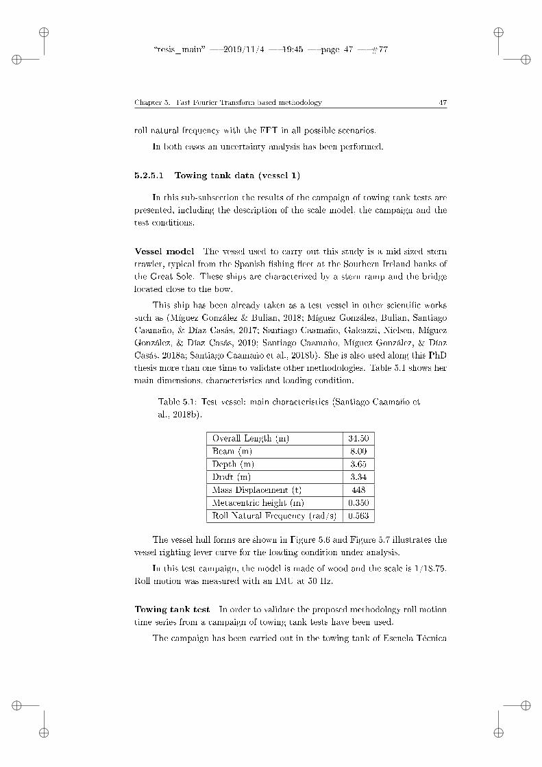
ii


ii

ii


roll natural frequency with the FFT in all possible scenarios.

In both cases an uncertainty analysis has been performed.

5.2.5.1 Towing tank data (vessel 1)

In this sub-subsection the results of the campaign of towing tank tests arepresented, including the description of the scale model, the campaign and thetest conditions.

Vessel model The vessel used to carry out this study is a mid-sized sterntrawler, typical from the Spanish shing eet at the Southern Ireland banks ofthe Great Sole. These ships are characterized by a stern ramp and the bridgelocated close to the bow.

This ship has been already taken as a test vessel in other scientic workssuch as (Míguez González & Bulian, 2018; Míguez González, Bulian, SantiagoCaamaño, & Díaz Casás, 2017; Santiago Caamaño, Galeazzi, Nielsen, MíguezGonzález, & Díaz Casás, 2019; Santiago Caamaño, Míguez González, & DíazCasás, 2018a; Santiago Caamaño et al., 2018b). She is also used along this PhDthesis more than one time to validate other methodologies. Table 5.1 shows hermain dimensions, characteristics and loading condition.

Table 5.1: Test vessel: main characteristics (Santiago Caamaño etal., 2018b).

Overall Length (m) 34.50

Beam (m) 8.00

Depth (m) 3.65

Draft (m) 3.34

Mass Displacement (t) 448

Metacentric height (m) 0.350

Roll Natural Frequency (rad/s) 0.563

The vessel hull forms are shown in Figure 5.6 and Figure 5.7 illustrates thevessel righting lever curve for the loading condition under analysis.

In this test campaign, the model is made of wood and the scale is 1/18.75.Roll motion was measured with an IMU at 50 Hz.

Towing tank test In order to validate the proposed methodology roll motiontime series from a campaign of towing tank tests have been used.

The campaign has been carried out in the towing tank of Escuela Técnica

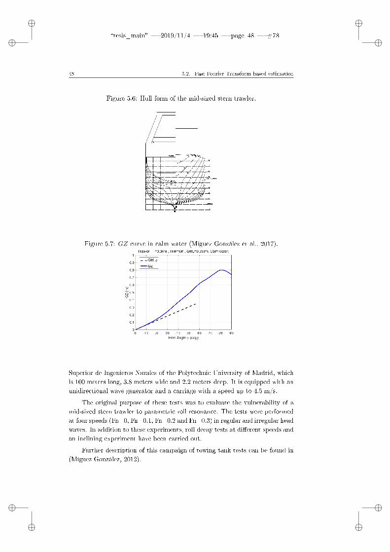
ii


ii

ii


Figure 5.6: Hull form of the mid-sized stern trawler.

Figure 5.7: GZ curve in calm water (Míguez González et al., 2017).

Superior de Ingenieros Navales of the Polytechnic University of Madrid, whichis 100 meters long, 3.8 meters wide and 2.2 meters deep. It is equipped with anunidirectional wave generator and a carriage with a speed up to 4.5 m/s.

The original purpose of these tests was to evaluate the vulnerability of amid-sized stern trawler to parametric roll resonance. The tests were performedat four speeds (Fn=0, Fn=0.1, Fn=0.2 and Fn=0.3) in regular and irregular headwaves. In addition to these experiments, roll decay tests at dierent speeds andan inclining experiment have been carried out.

Further description of this campaign of towing tank tests can be found in(Míguez González, 2012).

ii


ii

ii


Test conditions The test conditions were longitudinal head waves. On theone hand, experiments in regular waves with wave height ranging from 0.497 to1.988 meters and encounter frequency to natural roll frequency ratios (ωe/ω0)varying from 1.7 to 2.3 were performed. On the other hand, irregular wavesusing a Jonswap or TMA spectrum, ωe/ω0 between 1.9 and 2.2 and with signif-icant wave height values from 0.944 to 2.438 meters were also carried out. As itcan be appreciated encounter frequency to natural roll frequency ratios are inthe area where parametric roll may occur.

The detailed wave parameters of each test are shown in Table 5.2 (forregular waves) and Table 5.3 (for irregular waves).

Table 5.2: Test conditions: regular waves.

Experiment Fn ωw (rad/s) ωe (rad/s) ωe/ω0 (rad/s) Hw (m)

1 0 0.957 0.957 1.700 1.000

2 0 1.069 1.069 1.900 1.000

3 0 1.126 1.126 2.000 1.000

4 0 1.013 1.013 1.800 1.491

5 0 1.069 1.069 1.900 0.491

6 0 1.069 1.069 1.900 0.745

7 0 1.182 1.182 2.100 0.745

8 0 1.069 1.069 1.900 0.497

9 0.1 0.965 1.126 2.000 1.491

10 0.1 1.049 1.238 2.200 1.491

11 0.1 1.090 1.294 2.300 1.491

12 0.1 0.965 1.126 2.000 1.000

13 0.1 0.923 1.070 1.900 1.000

14 0.1 1.007 1.182 2.100 1.000

15 0.1 1.049 1.238 2.200 1.000

16 0.1 0.965 1.126 2.000 0.745

17 0.2 0.832 1.069 1.900 1.000

18 0.2 0.867 1.126 2.000 1.491

19 0.2 0.867 1.126 2.000 0.745

20 0.2 0.796 1.013 1.800 1.491

21 0.2 0.971 1.295 2.300 1.491

22 0.2 0.902 1.182 2.100 1.988

23 0.2 0.937 1.238 2.200 1.988

24 0.2 0.937 1.238 2.200 1.000

25 0.3 0.797 1.125 2.000 1.491

26 0.3 0.828 1.182 2.100 1.491

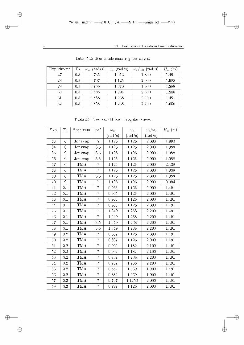
ii


ii

ii


Table 5.2: Test conditions: regular waves.

Experiment Fn ωw (rad/s) ωe (rad/s) ωe/ω0 (rad/s) Hw (m)27 0.3 0.735 1.013 1.800 1.491

28 0.3 0.797 1.125 2.000 1.988

29 0.3 0.766 1.070 1.900 1.988

30 0.3 0.888 1.295 2.300 1.988

31 0.3 0.858 1.238 2.200 1.491

32 0.3 0.858 1.238 2.200 1.000

Table 5.3: Test conditions: irregular waves.

Exp. Fn Spectrum pef ωw(rad/s)

ωe(rad/s)

ωe/ω0

(rad/s)Hw (m)

33 0 Jonswap 5 1.126 1.126 2.000 1.800

34 0 Jonswap 3.5 1.126 1.126 2.000 1.988

35 0 Jonswap 3.5 1.126 1.126 2.000 1.988

36 0 Jonswap 3.5 1.126 1.126 2.000 1.988

37 0 TMA 7 1.126 1.126 2.000 2.438

38 0 TMA 7 1.126 1.126 2.000 1.988

39 0 TMA 3.5 1.126 1.126 2.000 1.988

40 0 TMA 7 1.126 1.126 2.000 0.994

41 0.1 TMA 7 0.965 1.126 2.000 1.491

42 0.1 TMA 7 0.965 1.126 2.000 1.491

43 0.1 TMA 7 0.965 1.126 2.000 1.491

44 0.1 TMA 7 0.965 1.126 2.000 1.491

45 0.1 TMA 7 1.049 1.238 2.200 1.491

46 0.1 TMA 7 1.049 1.238 2.200 1.491

47 0.1 TMA 3.5 1.049 1.238 2.200 1.491

48 0.1 TMA 3.5 1.049 1.238 2.200 1.491

49 0.2 TMA 7 0.867 1.126 2.000 1.491

50 0.2 TMA 7 0.867 1.126 2.000 1.491

51 0.2 TMA 7 0.902 1.182 2.100 1.491

52 0.2 TMA 7 0.902 1.182 2.100 1.491

53 0.2 TMA 7 0.937 1.238 2.200 1.491

54 0.2 TMA 7 0.937 1.238 2.200 1.491

55 0.2 TMA 7 0.832 1.069 1.900 1.491

56 0.2 TMA 7 0.832 1.069 1.900 1.491

57 0.3 TMA 7 0.797 1.1256 2.000 1.491

58 0.3 TMA 7 0.797 1.126 2.000 1.491

ii


ii

ii


Table 5.3: Test conditions: irregular waves.

Exp. Fn Spectrum pef ωw(rad/s)

ωe(rad/s)

ωe/ω0

(rad/s)Hw (m)

59 0.3 TMA 7 0.797 1.126 2.000 1.491

60 0.3 TMA 7 0.797 1.126 2.000 1.491

61 0.3 TMA 7 0.828 1.182 2.100 1.491

62 0.3 TMA 7 0.828 1.182 2.100 1.491

63 0.3 TMA 7 0.828 1.182 2.100 1.491

64 0.3 TMA 7 0.828 1.182 2.100 1.491

pef: Peak Enhancement Factor

Transverse mass moment of inertia In order to compare and choose theless unfavourable alternative, the transverse mass moment of inertia of the testvessel has been computed following two approaches: the breakdown methodand the Weiss formula.

The Weiss formula is based on the traditional values of roll gyradius presentin the literature that keep constant for all loading conditions. So that, to eval-uate the implications of utilising this option instead of the breakdown methodthe inertia of 4 loading conditions has been calculated. The studied loading con-ditions are those included in the stability booklet according to the IMO 2012Cape Town Agreement for the Safety of Fishing Vessels (International MaritimeOrganization, 2012):

1. Departure for the shing grounds with full fuel, stores, ice, shing gear,etc., and no catch.

2. Departure from shing grounds with full catch and shing gear, 35% offuel and stores and no ice.

3. Arrival at home port with full catch and shing gear, 10% of fuel andstores and no ice.

4. Arrival at home port with 20% catch, full shing gear, 10% of fuel andstores and no ice.

The obtained results of applying the breakdown methodology to each load caseare shown in Table 5.4. These values are decomposed into dry and added inertia.The dry inertia is, at the same time, decomposed into the main items of thevessel (steel, tanks, shing gear, main engine, ice in hold, sh boxes, sh cargoin hold, supplies and nets). For computing the value of the inertia of the steelthe curve of areas has been used for each loading condition. An example of

ii


ii

ii


the curve of areas of the test vessel is shown in Figure 5.8 and the amidshipsection in Figure 5.9. It has to be mentioned that the roll inertia has beenestimated for a longitudinal axis passing through the centre of gravity of theship in that specic loading condition. For this reason, the value of the inertiaof non-varying items changes with the loading condition. Regarding the addedroll inertia, it has been computed using a strip theory code.

As it can be seen in Table 5.4, the dierence in the results of the totalinertia among the dierent loading conditions is not very large and it can beconsidered almost constant.

Furthermore, it can also be appreciated that the values of the roll gyradiusin all cases are very close to the reference value in the literature (0.40 for shingvessels (Biran & López Pulido, 2014)). It can be concluded that using a constantroll gyradius value may be a suitable option, in particular if crew interactionwould like to be kept to a minimum. The highest dierence between the realroll gyradius in the loading conditions and the reference value in percentage istaken as the uncertainty of this variable in the uncertainty analysis.

Table 5.4: Roll mass moment of inertia of load items considered inthe breakdown methodology (Santiago Caamaño et al., 2018b).

Loading

condition

1

Loading

condition

2

Loading

condition

3

Loading

condition

4

Dry Roll

Inertia

(t·m2)

Steel 3515.80 3515.50 3520.84 3570.04

Tanks 485.73 178.80 53.43 47.93

Fishing

gear

71.47 71.71 69.40 63.17

Main

engine

8.86 8.93 8.29 6.62

Ice in hold 11.48 0.00 0.00 0.00

Fish boxes 2.30 0.00 0.00 0.00

Fish cargo

in hold

0.00 292.89 262.49 35.69

Supplies 1.94 1.90 2.35 4.19

Nets 346.03 344.64 358.85 404.99

Total Roll Dry Inertia (t·m2) 4443.61 4414.44 4275.66 4132.53

Added Roll Inertia (t·m2) 472.21 471.32 461.5 411.01

Mass Displacement (t) 492 489 465 411

Roll gyradius (kxx/B) 0.395 0.395 0.399 0.416

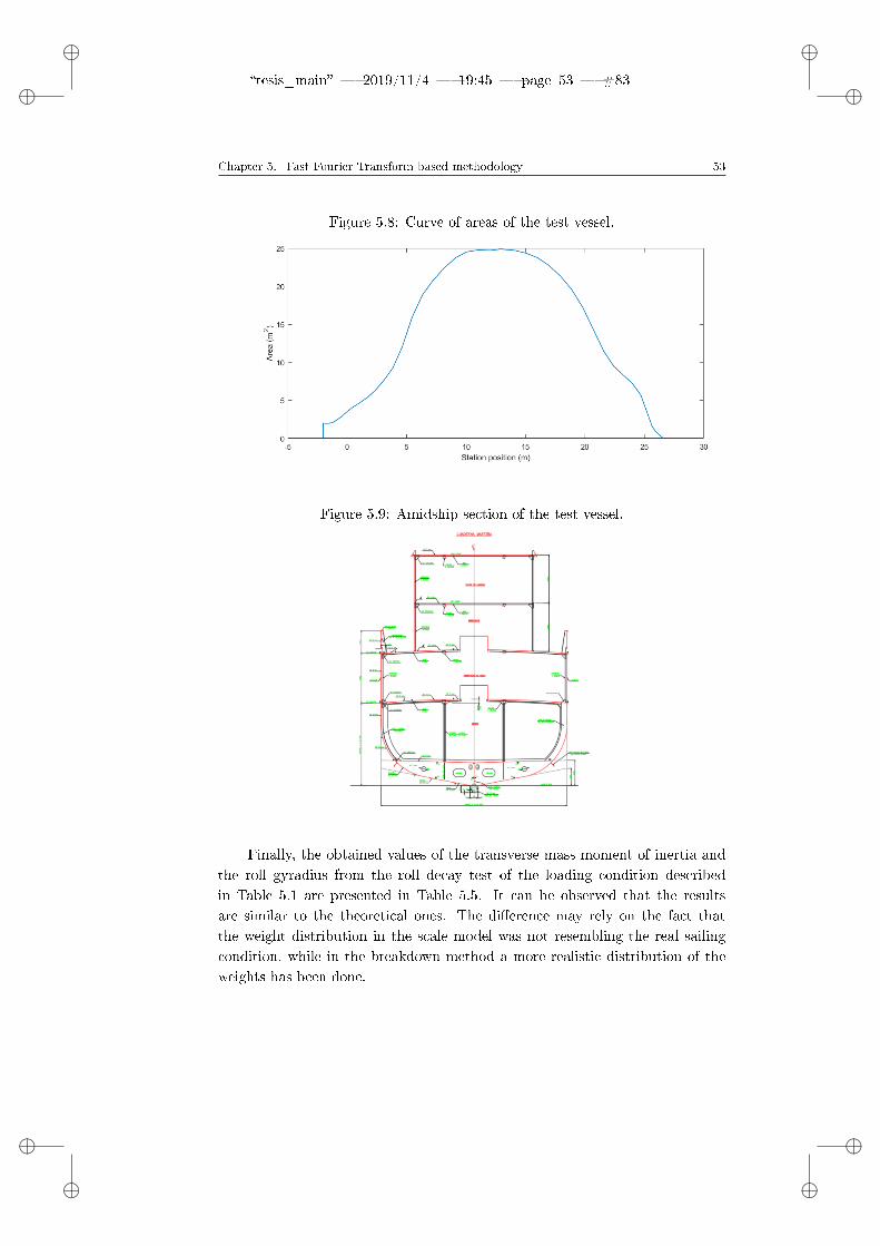
ii


ii

ii


Figure 5.8: Curve of areas of the test vessel.

Figure 5.9: Amidship section of the test vessel.

Finally, the obtained values of the transverse mass moment of inertia andthe roll gyradius from the roll decay test of the loading condition describedin Table 5.1 are presented in Table 5.5. It can be observed that the resultsare similar to the theoretical ones. The dierence may rely on the fact thatthe weight distribution in the scale model was not resembling the real sailingcondition, while in the breakdown method a more realistic distribution of theweights has been done.

ii


ii

ii


Table 5.5: Test vessel mass distribution data. Towing tank tests(Santiago Caamaño et al., 2018b).

∆ (m) 448

ω0 (rad/s) 0.563

GM (m) 0.350

Ixx +A44 (t·m2) 4852.86

A44 (t·m2) 450.66

Ixx (t·m2) 4402.20

kxx/B 0.411

Roll natural frequency In order to show how the FFT-based methodologyworks and how windowing aects the results, four cases (from the 64 tests) areexplained in deep.

Figure 5.10 and 5.11, shows the roll motion time series including the ap-plication of window functions and the roll spectrum corresponding to test case13 in Table 5.2. This test was run in regular waves at Fn=0.1 and parametricresonance took place. As it was expected, in Figure 5.10 the signal is reducedto zero at the edges due to windowing. Regarding the obtained spectrum fromthe application of the FFT (Figure 5.11), it can be observed that most of theenergy is concentrated around the roll natural frequency of the vessel with littlescattering. This dispersion may be motivated by the discontinuities at the edgesof the time series as it is reduced with the use of window functions. In addition,it can be seen that windowing cause damping in the peak of the spectrum andit is more or less pronounced depending on the type of window.

Figure 5.10: Experiment 13. Roll motion time series. Regular waves. Fn=0.1.Parametric roll occurs (Santiago Caamaño et al., 2018b).

ii


ii

ii


Figure 5.11: Experiment 13. Roll spectrum. Regular waves. Fn=0.1. Paramet-ric roll occurs (Santiago Caamaño et al., 2018b).

Figure 5.12 and 5.13 illustrate the time series and the spectrum for regularwaves without parametric rolling (experiment 7 in Table 5.2). Due to the factthat no parametric rolling developed, there is a greater dispersion of the energyand more than one peak appeared. However, roll natural frequency can stillbe identied as it is the peak of the spectrum with higher intensity. The otherpeak corresponds to the wave encounter frequency and it has to be said thatwith the use of windowing this peak is mitigated.

Figure 5.12: Experiment 7. Roll motion time series. Regular waves. Fn=0. Noparametric roll (Santiago Caamaño et al., 2018b).

The results for irregular waves when parametric roll takes place (experiment37 in Table 5.3, Figures 5.14 and 5.15) are very similar to those in regular waves.A single peak appears in the spectrum and the dispersion is negligible, so thatthe roll natural frequency can be clearly recognised.

ii


ii

ii


Figure 5.13: Experiment 7. Roll spectrum. Regular waves. Fn=0. No para-metric roll (Santiago Caamaño et al., 2018b).

Figure 5.14: Experiment 37. Roll motion time series. Irregular waves. Fn=0.Parametric roll occurs (Santiago Caamaño et al., 2018b).

Figure 5.15: Experiment 37. Roll spectrum. Irregular waves. Fn=0. Parametricroll occurs (Santiago Caamaño et al., 2018b).

ii


ii

ii


For irregular waves when no resonance occurs (experiment 46 in Table 5.3,Figures 5.16 and 5.17), the scattering in the energy is much greater although theroll natural frequency still corresponds to the main peak. However, in this casethe use of windowing is not satisfactory as the spectrum presents many peaksmaking impossible to locate the one corresponding to the target value. Thisfact is related with the damping introduced by the window function, reducingthe main peak and making it impossible to be identied among the rest of thepeaks contained in the spectrum.

Figure 5.16: Experiment 46. Roll motion time series. Irregular waves. Fn=0.1.No parametric roll (Santiago Caamaño et al., 2018b).

Figure 5.17: Experiment 46. Roll spectrum. Irregular waves. Fn=0.1. Noparametric roll Santiago Caamaño et al. (2018b).

The results of the roll natural frequency estimates of the 64 roll time seriesfrom the towing tank tests are illustrated in Figures 5.18-5.25. The green dotsrepresent the roll natural frequency estimates in tests where parametric rollresonance did not develop, red triangles indicate the roll natural frequencyestimates in cases in which this phenomenon took place and the dashed blackline represents the target value of the roll natural frequency. As it can be seen

ii


ii

ii


the results look promising as they are close to the target value.

Figure 5.18: Natural roll frequency estimation results. Regular waves. Fn=0(Santiago Caamaño et al., 2018b).

Figure 5.19: Natural roll frequency estimation results. Irregular waves. Fn=0(Santiago Caamaño et al., 2018b).

Figure 5.24: Natural roll frequency estimation results. Regular waves. Fn=0.3(Santiago Caamaño et al., 2018b).

ii


ii

ii


Figure 5.20: Natural roll frequency estimation results. Regular waves. Fn=0.1Santiago Caamaño et al. (2018b).

Figure 5.21: Natural roll frequency estimation results. Irregular waves. Fn=0.1Santiago Caamaño et al. (2018b).

Figure 5.22: Natural roll frequency estimation results. Regular waves. Fn=0.2Santiago Caamaño et al. (2018b).

ii


ii

ii


Figure 5.23: Natural roll frequency estimation results. Irregular waves. Fn=0.2(Santiago Caamaño et al., 2018b).

Figure 5.25: Natural roll frequency estimation results. Irregular waves. Fn=0.3(Santiago Caamaño et al., 2018b).

Furthermore, the numerical results for all experiments with and withoutwindowing are summarised in Tables 5.6-5.13. ω0, ω0h, ω0b and ω0bh are theestimated roll natural frequency without windowing, applying Hanning window,using Blackman window and with Blackman-Harris window respectively.

Table 5.6: Roll natural frequency estimates with and without win-dowing. Regular waves. Fn=0.

Experiment ω0 (rad/s) ω0h (rad/s) ω0b (rad/s) ω0bh (rad/s)

1 0.567 0.567 0.567 0.567

2 0.531 0.531 0.531 0.531

3 0.567 0.567 0.567 0.567

4 0.494 0.494 0.494 0.494

5 0.531 0.531 0.531 0.531

ii


ii

ii


Table 5.6: Roll natural frequency estimates with and without win-dowing. Regular waves. Fn=0.

Experiment ω0 (rad/s) ω0h (rad/s) ω0b (rad/s) ω0bh (rad/s)6 0.531 0.531 0.531 0.531

7 0.602 0.602 0.602 0.602

8 0.531 0.531 0.531 0.531

Table 5.7: Roll natural frequency estimates with and without win-dowing. Regular waves. Fn=0.1.


9 0.567 0.567 0.567 0.567

10 0.602 0.602 0.602 0.602

11 0.638 0.638 0.638 0.638

12 0.567 0.567 0.567 0.567

13 0.531 0.531 0.531 0.531

14 0.602 0.602 0.602 0.602

15 0.567 0.567 0.567 0.602

16 0.567 0.567 0.567 0.567



17 0.531 0.531 0.531 0.567

18 0.567 0.567 0.567 0.567

19 0.567 0.567 0.567 0.567

20 0.567 0.602 0.602 0.602

21 0.602 0.602 0.602 0.602

22 0.602 0.602 0.602 0.602

23 0.602 0.602 0.602 0.602

24 0.602 0.531 0.531 0.531



25 0.602 0.602 0.602 0.602

ii


ii

ii




27 0.567 0.567 0.567 0.567

28 0.567 0.567 0.567 0.567

29 0.531 0.531 0.531 0.531

30 0.638 0.638 0.638 0.638

31 0.602 0.602 0.602 0.602

32 0.567 0.567 0.567 0.567

Table 5.10: Roll natural frequency estimates with and withoutwindowing. Irregular waves. Fn=0.


33 0.567 0.567 0.567 0.567

34 0.567 0.567 0.567 0.567

35 0.602 0.956 0.956 0.956

36 0.567 0.567 0.567 0.567

37 0.567 0.567 0.567 0.567

38 0.567 0.567 0.567 0.567

39 0.531 0.531 0.531 0.531

40 0.567 0.567 0.567 0.567

Table 5.11: Roll natural frequency estimates with and withoutwindowing. Irregular waves. Fn=0.1.


41 0.602 0.602 0.602 0.602

42 0.567 0.567 0.567 0.567

43 0.567 0.567 0.567 0.567

44 0.567 0.638 0.638 0.638

45 0.602 0.531 0.531 0.531

46 0.567 0.071 0.071 0.071

47 0.638 0.638 0.638 0.638

48 0.531 0.496 0.496 0.496

ii


ii

ii




49 0.567 0.531 0.531 0.531

50 0.531 0.461 0.461 0.461

51 0.567 0.531 0.531 0.531

52 0.496 0.496 0.496 0.496

53 0.602 0.602 0.602 0.602

54 0.602 0.602 0.602 0.602

55 0.602 0.602 0.602 0.602

56 0.567 0.567 0.567 0.567



57 0.567 0.567 0.567 0.567

58 0.567 0.567 0.354 0.354

59 0.602 0.638 0.638 0.638

60 0.567 0.567 0.567 0.567

61 0.602 0.602 0.602 0.602

62 0.531 0.177 0.177 0.177

63 0.638 0.673 0.673 0.673

64 0.638 0.638 0.425 0.425

Table 5.14: Uncertainties in percentage of Nominal Level Units(Santiago Caamaño et al., 2018b).

Uncertaintysource

Systematic StandardUncertainty (b)

Random StandardUncertainty (SX)

Uω0/±

ω0 1.857% 0.713% 3.978%

ω0h 1.230% 5.426% 11.128%

ω0b 0.252% 2.373% 4.773%

ω0bh 0.043% 2.554% 5.108%

Finally, the uncertainty in the estimation of roll natural frequency of theship (for windowed and no windowed cases) needs to be calculated followingthe Equation 5.8. Results are included in Table 5.14. As it can be seen theuncertainty levels do not exceed 12%, in fact most of the values are under 6%.

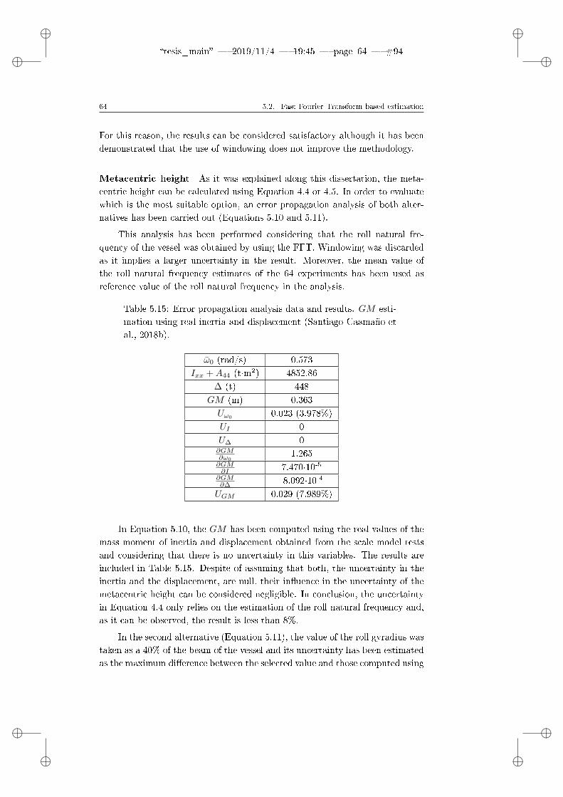
ii


ii

ii


For this reason, the results can be considered satisfactory although it has beendemonstrated that the use of windowing does not improve the methodology.

Metacentric height As it was explained along this dissertation, the meta-centric height can be calculated using Equation 4.4 or 4.5. In order to evaluatewhich is the most suitable option, an error propagation analysis of both alter-natives has been carried out (Equations 5.10 and 5.11).

This analysis has been performed considering that the roll natural fre-quency of the vessel was obtained by using the FFT. Windowing was discardedas it implies a larger uncertainty in the result. Moreover, the mean value ofthe roll natural frequency estimates of the 64 experiments has been used asreference value of the roll natural frequency in the analysis.

Table 5.15: Error propagation analysis data and results. GM esti-mation using real inertia and displacement (Santiago Caamaño etal., 2018b).

ω0 (rad/s) 0.573

Ixx +A44 (t·m2) 4852.86

∆ (t) 448

GM (m) 0.363

Uω00.023 (3.978%)

UI 0

U∆ 0∂GM∂ω0

1.265∂GM∂I 7.470·10-5∂GM∂∆ -8.092·10-4

UGM 0.029 (7.989%)

In Equation 5.10, the GM has been computed using the real values of themass moment of inertia and displacement obtained from the scale model testsand considering that there is no uncertainty in this variables. The results areincluded in Table 5.15. Despite of assuming that both, the uncertainty in theinertia and the displacement, are null, their inuence in the uncertainty of themetacentric height can be considered negligible. In conclusion, the uncertaintyin Equation 4.4 only relies on the estimation of the roll natural frequency and,as it can be observed, the result is less than 8%.

In the second alternative (Equation 5.11), the value of the roll gyradius wastaken as a 40% of the beam of the vessel and its uncertainty has been estimatedas the maximum dierence between the selected value and those computed using

ii


ii

ii


the breakdown method. The results are shown in Table 5.16. The uncertaintyin the metacentric height is slightly larger than in the previous case, but it iskept under reasonable values.

Table 5.16: Error propagation analysis data and results. GM esti-mation using approximate roll gyradius (Santiago Caamaño et al.,2018b).

ω0 (rad/s) 0.573

kxx/B 0.4

GM (m) 0.343

Uω0 0.023 (3.978%)

Ukxx 0.016 (5%)∂GM∂ω0

1.196∂GM∂kxx

0.214

UGM 0.028 (8.163%)

5.2.5.2 Towing tank data (vessel 2)

In this sub-subsection the results of the campaign of towing tank tests arepresented, including the description of the scale model, the campaign and thetest conditions.

Vessel model A new set of experiments has been performed with a secondvessel. Once more, the vessel is a stern trawler but, in this case, she is rep-resentative of the UK shing eet from the 80's. The hull form and maincharacteristics can be found in Figure 5.26 and Table 5.17 respectively.

Table 5.17: Test vessel: main characteristics .

Overall length (m) 25.910

Length between perpendiculars (m) 22.090

Beam (m) 6.680

Depth to main deck (m) 3.350

Draft (m) 2.475

Displacement (t) 170.300

GM (m) 0.436

ω0 (rad/s) 0.913

The test vessel corresponds to the MFV Trident, a shing vessel that sankin Scottish waters in 1974. According to some investigations the cause of the

ii


ii

ii


Figure 5.26: Test vessel: hull form (Míguez González, 2012).

misfortune could be broaching as the vessel was sailing in stern-quartering seas(Grimson, 1975; Paett, 1976; Young, 2011).

This vessel has been part of other scientic research works, mainly focusedon parametric roll resonance in head seas. Some of these studies are MíguezGonzález (2012); Neves, Pérez, and Lorca (2002, 2003); Neves, Pérez, and Va-lerio (1999); Neves and Rodríguez (2005); Neves, Rodríguez, Merino, MañuicoVivanco, et al. (2009); Pérez M. and Sanguinetti (2006); Rodríguez (2010); Ro-dríguez Castillo (2008).

The scale model is made of high density polyurethane covered by breglassand the scale is 1/15. It is selfpropelled and is equipped with an IMU to measureroll motion, a thrust sensor, a revolution and torque sensor, sonars, batteries,Wi-Fi and a computer (Míguez González, Deibe, Orjales, & Priego, 2015).

Figure 5.27: Vessel scale model.

ii


ii

ii


Towing tank test A new campaign of 60 towing tank tests has been carriedout to validate the methodology in dierent wave directions and to study theinuence of the wave encounter frequency in the results. Due to the limitationsof the facilities, experiments were run at zero speed in order to test all wavedirections and compare the results. Roll decay tests and an inclining experimenthave also been done. Roll motion was recorded at 30 Hz.

The experiments have been performed in the University of A Coruña towingtank, which is 56 meters long, 4.20 meters wide and 1.80 meters deep. It isequipped with an unidirectional wave generator and a carriage with a speed upto 3 m/s.

The retaining system consisted in four semielastic ropes. Two ropes xedto the bow and another two xed to the stern. All of them xed at the waterlinelevel and fastened to the sides of the tank. The model arrangement for the caseof head seas can be seen in Figure 5.28.

Figure 5.28: Model arrangement.

Test conditions The test conditions are regular waves with wave encounterfrequency to roll natural frequency ratio from ωe/ω0 = 0.850 to ωe/ω0 = 2.500

and wave directions from 0 to 180 degrees. The purpose is to evaluate the abilityof the methodology to detect the roll natural frequency in the roll spectrum inscenarios where resonance takes place as well as in those in which roll amplitudeis smaller. In this case, the inuence of the wave direction is also studied.

The parameters of the test waves are shown in Table 5.18.

ii


ii

ii


Table 5.18: Test conditions.

Experiment Wave direction ωw (rad/s) ωe/ω0 (rad/s) Hw (m)

1 0 0.776 0.850 1.461

2 0 0.913 1.000 1.056

3 0 1.279 1.400 0.539

4 0 0.776 0.850 1.705

5 0 0.913 1.000 1.232

6 0 1.279 1.400 0.628

7 0 0.776 0.850 2.046

8 0 0.913 1.000 1.478

9 0 1.279 1.400 0.754

10 0 1.369 2.000 0.900

11 0 1.826 1.500 1.650

12 0 2.283 2.500 0.600

13 45 0.776 0.850 1.461

14 45 0.913 1.000 1.056

15 45 1.279 1.400 0.539

16 45 0.776 0.850 1.705

17 45 0.913 1.000 1.232

18 45 1.279 1.400 0.628

19 45 0.776 0.850 2.046

20 45 0.913 1.000 1.478

21 45 1.279 1.400 0.754

22 45 1.369 2.000 0.900

23 45 1.826 1.500 1.650

24 45 2.283 2.500 0.600

25 90 0.776 0.850 1.461

26 90 0.913 1.000 1.056

27 90 1.279 1.400 0.539

28 90 0.776 0.850 1.705

29 90 0.913 1.000 1.232

30 90 1.279 1.400 0.628

31 90 0.776 0.850 2.046

32 90 0.913 1.000 1.478

33 90 1.279 1.400 0.754

34 90 1.369 2.000 0.900

35 90 1.826 1.500 1.650

36 90 2.283 2.500 0.600

37 135 0.776 0.850 1.461

ii


ii

ii


Table 5.18: Test conditions.

Experiment Wave direction ωw (rad/s) ωe/ω0 (rad/s) Hw (m)38 135 0.913 1.000 1.056

39 135 1.279 1.400 0.539

40 135 0.776 0.850 1.705

41 135 0.913 1.000 1.232

42 135 1.279 1.400 0.628

43 135 0.776 0.850 2.046

44 135 0.913 1.000 1.478

45 135 1.279 1.400 0.754

46 135 1.369 2.000 0.900

47 135 1.826 1.500 1.650

48 135 2.283 2.500 0.600

49 180 0.776 0.850 1.461

50 180 0.913 1.000 1.056

51 180 1.279 1.400 0.539

52 180 0.776 0.850 1.705

53 180 0.913 1.000 1.232

54 180 1.279 1.400 0.628

55 180 0.776 0.850 2.046

56 180 0.913 1.000 1.478

57 180 1.279 1.400 0.754

58 180 1.369 2.000 0.900

59 180 1.826 1.500 1.650

60 180 2.283 2.500 0.600

Roll natural frequency The results of the estimation of the roll natural fre-quency using the proposed methodology, including the application of Hanning,Blackman and Blackman-Harris window functions, are summarised in Table5.19.

Furthermore, the values of the total uncertainty and the level of uncertaintyof each wave direction calculated according to Equation 5.8 are presented inTables 5.20-5.25.

Table 5.19: Roll natural frequency estimation results. Target valueω0 = 0.913 (rad/s).


1 0.784 0.784 0.784 0.784

2 0.903 0.903 0.903 0.903

ii


ii

ii




4 0.784 0.784 0.784 0.784

5 0.903 0.903 0.903 0.903

6 0.000 1.260 1.260 1.260

7 0.000 0.784 0.784 0.784

8 0.903 0.903 0.903 0.903

9 1.260 1.260 1.260 1.260

10 0.927 0.927 0.927 0.927

11 0.903 0.760 0.760 0.760

12 0.974 0.974 0.974 0.974

13 0.784 0.784 0.784 0.784

14 0.903 0.903 0.903 0.903

15 1.283 1.283 1.283 1.283

16 0.784 0.784 0.784 0.784

17 0.903 0.903 0.903 0.903

18 1.283 1.283 1.283 1.283

19 0.784 0.784 0.784 0.784

20 0.903 0.903 0.903 0.903

21 1.260 1.260 1.260 1.260

22 1.854 1.854 1.854 1.854

23 1.378 1.378 1.378 1.378

24 2.258 2.281 2.281 2.281

25 0.784 0.784 0.784 0.784

26 0.903 0.901 0.901 0.901

27 1.260 1.260 1.260 1.260

28 0.784 0.784 0.784 0.784

29 0.903 0.903 0.903 0.903

30 1.283 1.283 1.283 1.283

31 0.760 0.760 0.760 0.760

32 0.903 0.903 0.903 0.903

33 1.283 1.283 1.283 1.283

34 1.830 1.830 1.830 1.830

35 1.378 1.378 1.378 1.378

36 0.927 2.281 2.281 2.281

37 0.784 0.784 0.784 0.784

38 0.903 0.903 0.903 0.903

ii


ii

ii




40 0.784 0.784 0.784 0.784

41 0.903 0.903 0.903 0.903

42 1.283 1.283 1.283 1.283

43 0.784 0.784 0.784 0.784

44 0.903 0.903 0.903 0.903

45 1.260 1.260 1.260 1.260

46 0.927 0.927 0.927 0.927

47 1.378 1.378 1.378 1.378

48 2.281 0.166 0.166 2.281

49 0.784 0.784 0.784 0.784

50 0.927 0.927 0.927 0.927

51 1.260 1.260 1.260 1.260

52 0.784 0.784 0.784 0.784

53 0.903 0.903 0.903 0.903

54 1.260 1.260 1.260 1.260

55 0.784 0.760 0.760 0.760

56 0.903 0.903 0.903 0.903

57 1.260 1.260 1.260 1.260

58 0.927 0.927 0.927 0.927

59 0.927 0.927 0.927 0.927

60 0.951 0.951 0.951 0.951

Table 5.20: Uncertainties in percentage of Nominal Level Unitsconsidering all the tests.

Uncertaintysource



Uω0/±

ω0 13% 6% 32%

ω0h 15% 5% 35%

ω0b 15% 5% 35%

ω0bh 17% 9% 39%

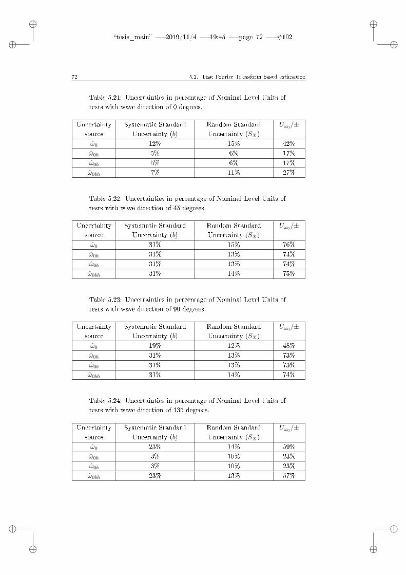
ii


ii

ii


Table 5.21: Uncertainties in percentage of Nominal Level Units oftests with wave direction of 0 degrees.

Uncertaintysource



Uω0/±

ω0 12% 15% 42%

ω0h 5% 6% 17%

ω0b 5% 6% 17%

ω0bh 7% 11% 27%


Uncertaintysource



Uω0/±

ω0 31% 15% 76%

ω0h 31% 13% 74%

ω0b 31% 13% 74%

ω0bh 31% 14% 75%


Uncertaintysource



Uω0/±

ω0 19% 12% 48%

ω0h 31% 13% 73%

ω0b 31% 13% 73%

ω0bh 31% 14% 74%


Uncertaintysource



Uω0/±

ω0 23% 14% 59%

ω0h 3% 10% 23%

ω0b 3% 10% 23%

ω0bh 23% 13% 57%

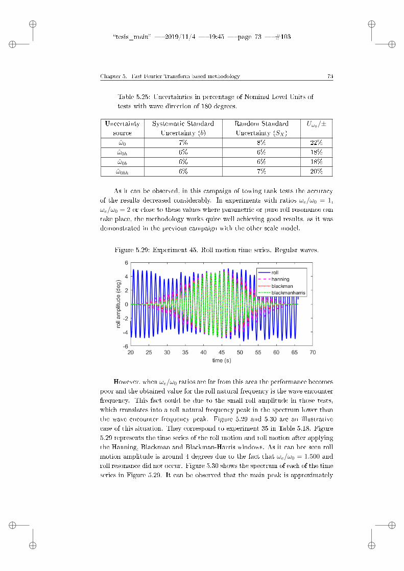
ii


ii

ii



Uncertaintysource



Uω0/±

ω0 7% 8% 22%

ω0h 6% 6% 18%

ω0b 6% 6% 18%

ω0bh 6% 7% 20%

As it can be observed, in this campaign of towing tank tests the accuracyof the results decreased considerably. In experiments with ratios ωe/ω0 = 1,ωe/ω0 = 2 or close to these values where parametric or pure roll resonance cantake place, the methodology works quite well achieving good results, as it wasdemonstrated in the previous campaign with the other scale model.

Figure 5.29: Experiment 45. Roll motion time series. Regular waves.

However, when ωe/ω0 ratios are far from this area the performance becomespoor and the obtained value for the roll natural frequency is the wave encounterfrequency. This fact could be due to the small roll amplitude in those tests,which translates into a roll natural frequency peak in the spectrum lower thanthe wave encounter frequency peak. Figure 5.29 and 5.30 are an illustrativecase of this situation. They correspond to experiment 35 in Table 5.18. Figure5.29 represents the time series of the roll motion and roll motion after applyingthe Hanning, Blackman and Blackman-Harris windows. As it can bee seen rollmotion amplitude is around 4 degrees due to the fact that ωe/ω0 = 1.500 androll resonance did not occur. Figure 5.30 shows the spectrum of each of the timeseries in Figure 5.29. It can be observed that the main peak is approximately

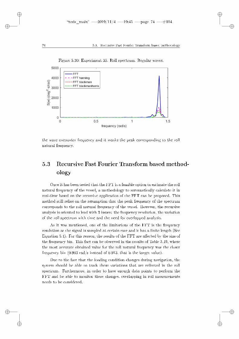
ii


ii

ii

74 5.3. Recursive Fast Fourier Transform based methodology

Figure 5.30: Experiment 35. Roll spectrum. Regular waves.

the wave encounter frequency and it masks the peak corresponding to the rollnatural frequency.

5.3 Recursive Fast Fourier Transform based method-

ology

Once it has been tested that the FFT is a feasible option to estimate the rollnatural frequency of the vessel, a methodology to automatically calculate it inreal-time based on the recursive application of the FFT can be proposed. Thismethod still relies on the assumption that the peak frequency of the spectrumcorresponds to the roll natural frequency of the vessel. However, the recursiveanalysis is oriented to lead with 3 issues: the frequency resolution, the variationof the roll spectrum with time and the need for overlapped analysis.

As it was mentioned, one of the limitations of the FFT is the frequencyresolution as the signal is sampled at certain rate and it has a nite length (SeeEquation 5.4). For this reason, the results of the FFT are aected by the size ofthe frequency bin. This fact can be observed in the results of Table 5.19, wherethe most accurate obtained value for the roll natural frequency was the closerfrequency bin (0.903 rad/s instead of 0.913, that is the target value).

Due to the fact that the loading condition changes during navigation, thesystem should be able to track these variations that are reected in the rollspectrum. Furthermore, in order to have enough data points to perform theFFT and be able to monitor these changes, overlapping in roll measurementsneeds to be considered.

ii


ii

ii


Figure 5.31: Proposed methodology (Míguez González et al., 2017).

Therefore, the proposed methodology, summarised in Figure 5.31, is basedon overlapping roll measures (with a length of analysis time and sampled atsample time) and averaging the obtained roll spectra during a certain aver-aging time. The analysis time has to be set considering the real-time require-ment. The sample time is determined by the speed of the analysis algorithmand the necessity of tracking any change in the roll natural frequency. Finally,the averaging time has to be taken as a balance between not very long to hidepossible changes in the vessel condition nor very short to be aected by poorestimations.

Once the spectrum is obtained, it is rstly smoothed, applying a 5-pointmoving average technique, and then tted with a parametric model to increasethe frequency resolution.

The parametric model used in the tting process has 9 parameters andconsists in the superposition of 3 Gaussian functions corresponding to the rollmotion, wave excitation and wind excitation. This tting process has two steps.The rst one provides an approximation of the tting parameters through aminimization process by applying a genetic algorithm. The second one uses aNonlinear Least Squares Fitting process to determine the nal parameters ofthe tting function. This tting function is the one utilised for the identicationof the maximum peak which is related with the roll natural frequency.

The full description of this methodology can be found in Míguez Gonzálezet al. (2017).

5.3.1 Results and validation

In order to validate the proposed methodology to estimate the roll naturalfrequency of the vessel in real-time, roll motion time series from a mathematical

ii


ii

ii


model (Sub-subsection 5.3.1.1) and sea trials (Sub-subsection 5.3.1.2) have beenemployed.

Two shing vessels have been tested, one in the mathematical model andother one in the sea trials. Both ships are very similar; they are stern trawlerstypical from the Galician shing eet.

The operation of this type of vessels is typically divided in two dierentstages. The rst one includes cruising to and from the shing grounds at mod-erate speeds. And the second one corresponds to the shing manoeuvre, whichis composed of the letting out phase, where the nets are deployed, trawling andreeling in. From these, the most dangerous is usually the last one, as the vesselis sailing at very low forward speed (close to zero) and with reduced course keep-ing capabilities. Under these conditions the vessel may face beam waves whichtogether with possible appearance of roll resonance, reduced damping moments(due to low speed), opened doors and hatches and hanging weights, could easilylead to ooding and/or capsizing. In order to address these conditions, in whichaccidents could be most likely, in the mathematical model zero forward speed,beam waves and lateral wind have been chosen as the operational scenario.

Regarding the sea trials, they have been carried out during a shing cam-paign in the Northwest coast of Spain where these type of ships normally navi-gate.

5.3.1.1 Simulated data

In this sub-subsection the results of the simulated roll motion time seriesare presented, including the description of the test model, the mathematicalmodel and the test conditions.

Test vessel The ship is the same stern trawler presented in Sub-subsection5.2.5.1, although this time has been tested in dierent environmental conditions.Her main characteristics and the loading condition under analysis can be foundin Table 5.1.

Mathematical model Roll motion is simulated by an uncoupled one degree-of-freedom mathematical model, where nonlinear quadratic damping and non-linear restoring based on the vessel restoring arm curve have been considered.This model is dened by the following equation:

φ+ 2υω0φ+ βφ|φ|+ ω20

GZ (φ)

GM= ω2

0mwave (t) + ω20mwind(t) (5.12)

ii


ii

ii


Being φ the roll angle, ν and β the linear and quadratic roll dampingcoecients, GZ(φ) and GM the righting lever curve and the metacentric heightin still water, mwave(t) the non-dimensional wave excitation in irregular beamseas and mwind(t) is the non-dimensional moment due to the eect of lateralwind.

The wave excitation has been modelled through the Absolute Roll AngleModel (Bulian & Francescutto, 2006) according to the following expression

mwave (t) =

n∑i=1

πr (ωi) s (ωi) · cos (ωit+ ξi) (5.13)

where ωi is the frequency of the i-th wave component, r(ωi) is the eectivewave slope coecient, s(ωi) is the wave steepness and ξi is the phase.

Regarding the wind excitation it has been divided into two components.A steady component which is the mean wind speed and it is calculated as afunction of signicant wave height using the relationship in Pierson-Moskowitzspectrum (International Towing Tank Conference, 2002). The other compo-nent is the wind gustiness that has been obtained from Davenport spectrum(Davenport, 1961).

This mathematical model of roll motion is derived from the classical linearmodel of uncoupled roll motion in waves (Bhattacharyya, 1978) and its detaileddescription can be found in Bulian and Francescutto (2004, 2006). In the rstreference, this model is used to estimate the capsize probability of a smallshing vessel and a large passenger ship in irregular beam seas. Meanwhile inthe second one, it is employed to analyse the operability and capsize probabilityof the same shing vessel in regular and irregular beam waves as a function of itsstatic parameters. In addition to these applications, this model has been usedfor characterizing the roll motion of dierent types of multihull vessels in beamwaves and comparing the results with scale model towing tank tests showinggood results (Bulian & Francescutto, 2009).

Table 5.26: Damping coecients of tested shing vessel (MíguezGonzález et al., 2017).

Linear Roll Damping Coecient (ν) 0.0187

Quadratic Roll Damping Coecient (β) 0.3932 rad-1

Purely Linear Roll Damping (νL) 0.0697

The values of the linear and quadratic roll damping coecients for thevessel under analysis can be found in Table 5.26. Moreover, the eective waveslope coecient needed for the computation of the wave exciting moment is

ii


ii

ii


shown in Figure 5.32. This coecient has been obtained by using the linearhydrodynamics alternative as shown in Míguez González and Bulian (2018).

Figure 5.32: Eective wave slope coecient (Míguez González et al., 2017).

Test conditions In order to test the methodology in the most real possiblescenario, the environmental conditions have been selected considering thosemore prone in Galician coast. This is the area where this type of vessels normallyoperates.

The conditions were determined constructing a scatter diagram with thevalues of wind and wave parameters obtained from historical data (from 1997to 2015) of four SeaWave buoys in the area (FOM, 2017). From this diagram,the most probable scenario has been chosen. The values are shown in Table5.27.

Table 5.27: Tested wave and wind conditions (Míguez González etal., 2017).

Signicant wave height (m) 1.971

Peak period (s) 10

Mean wind speed (m/s) 9.375

Results The rened methodology has been tested using simulated roll motiontime series. The time series were obtained running the mathematical model witha 20 Hz sampling rate. Wind and wave moments were generated using 1000components. The analysis time has been set to 3 minutes to accomplish withthe real-time requirement, the sample time is 10 seconds and the averagingtime 120 seconds.

ii


ii

ii


Figure 5.33 shows the obtained roll motion time series under irregular beamwaves and lateral gusty wind. As it can be observed, there is an asymmetryin roll motion due to the eect of mean wind pressure and some low frequencycomponents resulting from wind gustiness. As it was expected roll amplitudeis large because the wave period is close to the roll natural frequency, so thatparametric resonance may appear.

Figure 5.33: Roll motion time series. Irregular beam waves. Lateral gusty wind(Míguez González et al., 2017).

The results of executing the methodology in the time series are presentedin Figure 5.34. The green dots represent the roll natural frequency estimatedevery 10 seconds (sample time) and after averaging the previous spectra (120seconds of averaging time) during 180 seconds (analysis time). In order todiscard possible punctual poor roll natural frequency estimations, a movingmedian of the group of past 12 estimations was calculated. It is represented bythe red dotted line.

Figure 5.34: Left: Roll natural frequency estimates. Right: representation ofestimated roll natural frequency distribution through minimum observed value,5%, 25%, 50% (median), 75% and 95% estimated percentiles, and maximumobserved value (Míguez González et al., 2017).

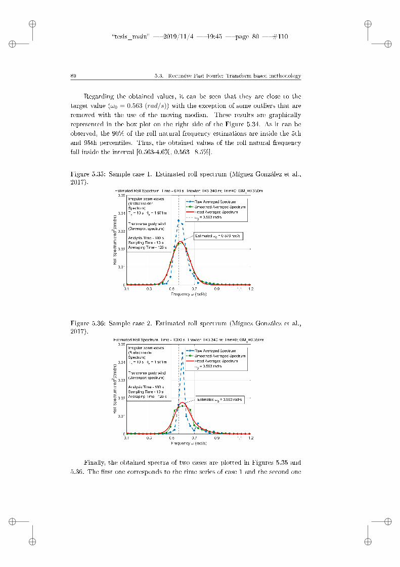
ii


ii

ii


Regarding the obtained values, it can be seen that they are close to thetarget value (ω0 = 0.563 (rad/s)) with the exception of some outliers that areremoved with the use of the moving median. These results are graphicallyrepresented in the box plot on the right side of the Figure 5.34. As it can beobserved, the 90% of the roll natural frequency estimations are inside the 5thand 95th percentiles. Thus, the obtained values of the roll natural frequencyfall inside the interval [0.563-4.6%, 0.563+8.5%].

Figure 5.35: Sample case 1. Estimated roll spectrum (Míguez González et al.,2017).

Figure 5.36: Sample case 2. Estimated roll spectrum (Míguez González et al.,2017).

Finally, the obtained spectra of two cases are plotted in Figures 5.35 and5.36. The rst one corresponds to the time series of case 1 and the second one

ii


ii

ii


to case 2 in Figure 5.33. In both gures, the dashed blue lines represent theraw averaged spectrum, the dotted green lines represent the smoothed spectrumand the red continuous line represents the spectrum obtained after the ttingprocess. As it can be observed, the frequency resolution in the range of interestis quite low and the smoothed spectrum reduces the secondary peaks of the rawspectrum.

5.3.1.2 Sea trials

In this sub-subsection the results of the sea trials are presented, includingthe description of the test model, the shing campaign and the trial conditions.

Test vessel The vessel under analysis is a medium sized stern trawler typicalfrom the Galician shing eet with home port in A Coruña. She is very simi-lar to the one presented in Sub-subsection 5.2.5.1, in both characteristics andoperation. The only dierence is that during the sea trials she works as pairtrawler with her twin, but she can operate as independent stern trawler as well.Her main characteristics and hull form are shown in Table 5.28 and Figure 5.37respectively. Additionally, a picture of the shing vessel is included in Figure5.38. As it can be seen, the superstructure is forward with the working deckand trawl ramp aft.

Figure 5.37: Test vessel: hull form (Míguez González et al., 2018).

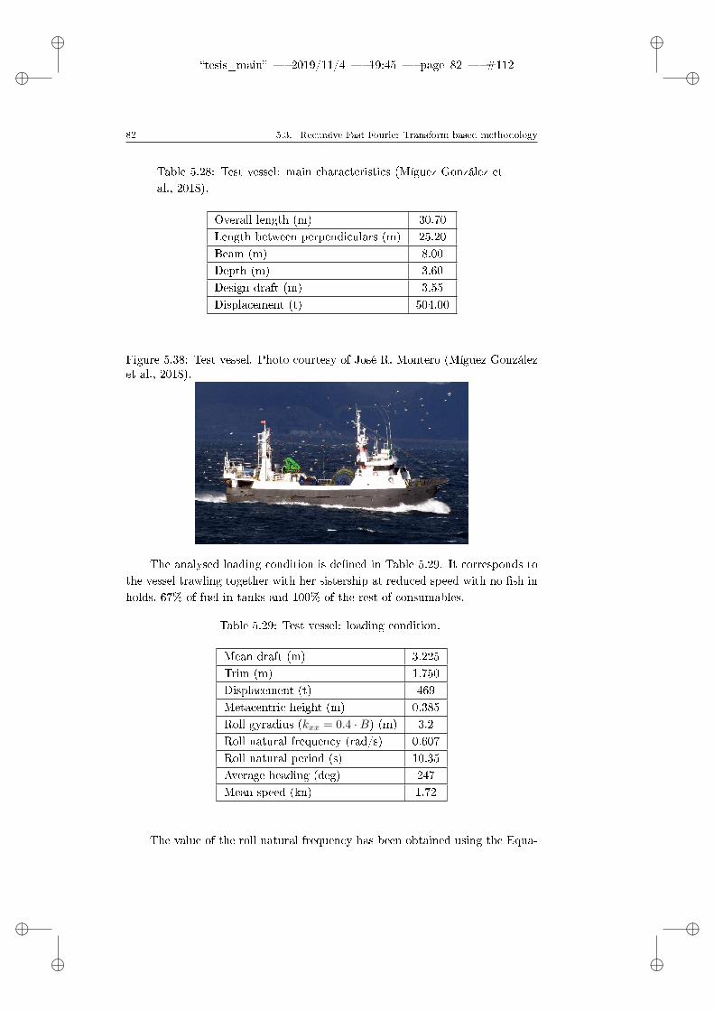
ii


ii

ii


Table 5.28: Test vessel: main characteristics (Míguez González etal., 2018).

Overall length (m) 30.70

Length between perpendiculars (m) 25.20

Beam (m) 8.00

Depth (m) 3.60

Design draft (m) 3.55

Displacement (t) 504.00

Figure 5.38: Test vessel. Photo courtesy of José R. Montero (Míguez Gonzálezet al., 2018).

The analysed loading condition is dened in Table 5.29. It corresponds tothe vessel trawling together with her sistership at reduced speed with no sh inholds, 67% of fuel in tanks and 100% of the rest of consumables.

Table 5.29: Test vessel: loading condition.

Mean draft (m) 3.225

Trim (m) 1.750

Displacement (t) 469

Metacentric height (m) 0.385

Roll gyradius (kxx = 0.4 ·B) (m) 3.2

Roll natural frequency (rad/s) 0.607

Roll natural period (s) 10.35

Average heading (deg) 247

Mean speed (kn) 1.72

The value of the roll natural frequency has been obtained using the Equa-

ii


ii

ii


tion 4.5 with the estimated metacentric height for the loading condition.

Sea trials The sea trials have been carried out during a normal shing cam-paign. The test vessel usually operates on a daily shing with her sistershipin Galician coastal waters. In this case the campaign lasted 19 h and the ves-sel departed from A Coruña port to the shing ground placed in the area ofVillano-Sisargas SeaWatch buoy, which is moored 35 miles o her home port.After 3 hours of sailing, both ships were shing during 10 hours and then returnto port (6 h). The shing area is represented with a red dashed line and theSeaWatch buoy with a red circle in Figure 5.39.

Figure 5.39: Sea trial area and SeaWatch buoy position (Míguez González etal., 2018).

In order to validate the proposed rened methodology the entire trip hasbeen monitored, including the vessel motions, loading condition, heading, speedand sea state. Roll motion has been measured with an IMU and the speed andheading using a GPS. Moreover, tank lling levels, approximate sh weight andlocation, situation and weight of shing nets and other equipment and numberof people on board have been manually monitored.

The analysis of a time series of 2 h 5' of duration, which corresponds withthe vessel parameters showed in Table 5.29, has been included in this disserta-tion.

Trial conditions The meteorological condition has been obtained from theprevailing wave and wind conditions in the area of the Villano-Sisargas buoy.These data are provided by Puertos del Estado and include the signicant wave

ii


ii

ii


height, peak period, mean wave direction and mean wind speed and directionexpressed by hour.

For the time series under analysis the vessel was sailing in slight starboardbeam to quartering forward seas and lateral wind. The parameters of the wavesand wind are shown in Table 5.30.

Table 5.30: Test conditions (Míguez González et al., 2018).

Mean signicant wave height (m) 0.9

Mean wave peak period (s) 10.25

Mean wave direction (deg) 322.5

Mean wind speed (m/s) 1.29

Mean wind direction (deg) 154

Results Figure 5.40 shows the 2 h 5' roll motion time series.

Due to the fact that the wave encounter frequency is not close to the rollnatural frequency, roll resonance did not take place. In consequence, roll ampli-tude is small. It can be observed that there is a point around the time instant3000 s in which the vessel changes the heel angle from 1 degree to starboard sideto 0.5 degrees to port side. As the test vessel was trawling at the port side ofthe couple (see Figure 5.41), a modication of the two trawling vessels headingthat leads to a reduction of the net tension could explain this fact.

Figure 5.40: Roll motion time series (Míguez González et al., 2018).

The results of applying the recursive FFT-based methodology are shown inFigure 5.42. Likewise in the simulated time series, the analysis time, sampletime and averaging time have been set 180, 10 and 120 seconds respectively.The green dots represent the roll natural frequency estimations, the red line

ii


ii

ii


Figure 5.41: Pair trawling (FAO, 2018). Situation of the test vessel is high-lighted.

the median of the last 6 estimations and the dashed black line the target value(ω0 = 0.607 rad/s). As it can be seen, the results during the whole time seriesare close to the target value with a clear tendency to overestimation.

Figure 5.42: Roll natural frequency estimation results (Míguez González et al.,2018).

If the results are numerically analysed with the 5th, 50th and 95th per-centile (Table 5.31), as in the case of simulated data, it can be concluded thatthe error in the estimation remains approximately the same. ω0 estimates fallinside the interval [0.607-5.1%, 0.607+9.89%].

Table 5.31: Estimation results.

Estimated roll natural frequency median (rad/s) 0.629

5% Percentile estimated roll natural frequency (rad/s) 0.576

95% Percentile estimated roll natural frequency (rad/s) 0.667

ii


ii

ii

86 5.4. Discussion

5.4 Discussion

In this chapter the use of the Fast Fourier Transform to estimate the rollnatural frequency has been proposed and validated with towing tank tests. Thenthe calculation of the metacentric height by two dierent alternatives has beenstudied. Finally, a methodology based on the recursive FFT has been developedand validated with simulations and sea trials.

The results of the campaigns of towing tank tests have shown that, in gen-eral, the FFT works better in cases where the ship is in the area where resonancephenomenon can take place. In other situations the ability of detecting the rollnatural frequency is degraded presenting larger uncertainties.

Further research is needed to improve the performance of the FFT in allscenarios. A possible solution is to pre-lter the roll motion in order to removethe wave component, although it would require to estimate at the same timethe wave encounter frequency or, at least, know the wave parameters.

The application of window functions to roll signal to reduce the spectralleakage has been tested. However, no improvement in the results has beenachieved.

Furthermore, the FFT has been tested in dierent wave directions and ves-sel's speed. None of these variables seem to signicantly aect its performance.

Regarding the metacentric height, it has been calculated according to Equa-tion 4.4 and 4.5. In the rst equation the computation of the transverse massmoment of inertia and displacement is necessary. Despite of having lower un-certainty, the calculation of these parameters relies on the inputs manuallyintroduced by the crew.

Equation 4.5 proposes an alternative to avoid those calculations with theWeiss formula to approximate the ship's inertia. It seems a feasible solutionand the uncertainty in the GM does not increase considerably with regard tothe previous alternative.

The last point of discussion is the recursive FFT-based methodology. Fromthe results of the simulations and the sea trials, it can be concluded that it showsa good performance. On the one hand, despite of the overestimation of the rollnatural frequency of the vessel, the values of the estimates are similar to thetarget value. This overestimation could be solved adding a safety margin in thepredictions. Nevertheless, to do that it must be constant in all scenarios.

On the other hand, the smoothing and tting process seem a feasible al-ternative for removing the peaks of the other components in the roll spectrum.

In addition to this, the rened methodology is sensible to the length of

ii


ii

ii


the analysis time and averaging time. Further research would be needed todene the most suitable length of the time series.

Finally, more validation is needed in order to cover all the possible scenariosduring navigation.

ii


ii

ii

ii


ii

ii

Chapter 6

Time domain and change

detection methodology

6.1 Introduction

This chapter is dedicated to present a new methodology with three mainobjectives:

1. To provide a real-time estimate of the vessel's roll natural frequency duringnavigation

2. To track changes in the estimated frequency as a mean to assess the cur-rent level of stability that may occur due to variations in the loadingcondition of the ship

3. To reduce the obtained error in the estimation with regard to the recursiveFFT-based methodology

It consists of time domain techniques to obtain the value of the roll naturalfrequency from the measured roll motion in combination with a detector totrack the changes on this parameter.

The methodology is validated with roll motion time series from simulationsand towing tank tests of a shing vessel.

ii


ii

ii

90 6.2. Architecture

6.2 Architecture

In this second methodology, an estimator-detector architecture is proposedto reliably extract information about the roll natural frequency from the mea-sured roll motion and evaluate when this frequency signicantly deviates overthe time.

The proposal of a statistical change detection technique is not new in themaritime sector and it has proven to be a successful methodology for the designof condition monitoring systems whenever timely decision under uncertaintyand robustness are paramount. Examples of such systems are presented byGaleazzi et al. (2015); Galeazzi, Blanke, and Poulsen (2013) for the real-timemonitoring of parametric roll resonance on merchant vessels; Fang, Blanke, andLeira (2015) for the timely detection of faults in mooring systems of oshoreoating platforms; Willersrud, Blanke, Member, Imsland, and Pavlov (2015)for the robust detection of drillstring washouts during drilling operation foroil and gas; Hansen and Blanke (2014) for the real-time detection of airspeedsensor faults in unmanned aerial vehicles; Ghane, Rasekhi Nejad, Blanke, Gao,and Moan (2018) for wear detection in the downwind main shaft bearing of aspar-type oating wind turbine; Pradhan and Gupta (2017) for the detectionof incoming vessels by measuring the ambient noise to enhance security of portand oshore operations.

In order to fulll the requirements of the guidance systems (already men-tioned in Chapter 3) and to achieve a robust system, the proposed design isvessel model-free and adopts probabilistic methods to discern among dierentoperational conditions. The specic features are the following:

real-time estimation of the roll natural frequency based solely on the mea-sured roll angle, as in the recursive FFT-based methodology

probabilistic model of the roll natural frequency

on-line continuous learning

high sensitivity in discriminating across dierent loading/operational con-ditions

timely detection of unsafe operational conditions

low probability of false alarms

no need of external inputs from the crew

Two dierences from the previous methodology can be highlighted. On theone hand, in the recursive FFT-based method the stability assessment relied

ii


ii

ii

Chapter 6. Time domain and change detection methodology 91

directly in the estimation of the roll natural frequency and, on the other hand,it didn't provide additional information to the crew. Thus, it depended only onthe performance of the frequency estimates.

In this new proposal, the combination of the Empirical Mode Decomposi-tion (EMD) with the Hilbert-Huang Transform (HHT) is used instead of theFFT to better discriminate the oscillatory modes contained in the roll motion,avoiding the tendency of the FFT to condensate information. In addition tothis, the FFT needs a longer data batch to obtain accurate results, which in thecase under analysis may lead to hiding stability failures that take place in veryshort time. Moreover, a detection system based on a probabilistic approachhas been included to distinguish between safe and unsafe situations, increasingrobustness of the stability guidance system.

Figure 6.1: Architecture of the transverse stability monitoring system (SantiagoCaamaño, Galeazzi, Nielsen, et al., 2019).

The proposed system architecture is illustrated in Figure 6.1 and its mainbuilding blocks are:

DAQ roll motion is measured through an inertial measurement unit and storedin a buer by the data acquisition system;

EMD the Empirical Mode Decomposition method (Dätig & Schlurmann, 2004;Gupta, Kumar, & Bahl, 2014; Huang et al., 1998) is applied to decomposethe roll motion signal into its main oscillatory modes;

HHT the Hilbert-Huang Transform is applied to each of the resulting oscil-latory modes to estimate their modal frequency (Dätig & Schlurmann,2004; Huang et al., 1998). Among all of these frequencies, the vessel's rollnatural frequency is selected;

W-GLRT the Weibull based Generalized Likelihood Ratio Test evaluates the

ii


ii

ii


current estimate of the roll natural frequency and decides if the vessel isoperating in a safe or unsafe loading condition. The detector triggers analarm if a safety threshold is crossed;

LPF Low-pass ltering of the measured roll motion is applied when the es-timated roll natural frequency is close to the maximum roll natural fre-quency. When ltering occurs then the ltered signal is processed againthrough the EMD and HHT blocks.

Each building block is described in detail in the next subsections.

6.2.1 Data acquisition

The function of the DAQ is to measure and store in a buer the vessel rollmotion. To fulll the real-time estimation requirement a proper buer size needsto be determined. The choice has been made considering the target eet, thusassuming a medium sized shing vessel. Also, the decision has been made bytrading-o among the minimum data batch size to achieve a reliable estimate ofthe roll natural frequency, the maximum time to detect the transition towards anunsafe operational condition and the needed resolution to distinguish betweendierent operational conditions. As in the FFT-based methodology, the timewindow length has been set to 3 minutes.

In addition to this, a 75% of overlapping between consecutive batches hasbeen taken into account to increase the number of estimations done by timewindow. In this case an estimate is obtained every 45 seconds while in theFFT-based methodology every 10 seconds.

6.2.2 Empirical Mode Decomposition

The Empirical Mode Decomposition is an adaptative time domain tech-nique that allows breaking down a multi-frequency signal into its main oscilla-tory components called Intrinsic Mode Functions (IMFs). The IMF is dened asa function with a time-varying frequency and amplitude and with equal numberof extremes and zero-crossings, and whose envelopes are symmetric with respectto zero (Dätig & Schlurmann, 2004; Gupta et al., 2014; Huang et al., 1998).

The procedure to extract the IMFs is called sifting, which decomposes thesignal from high to low embedded frequency components until a monotonicresidual is obtained. It consists of connecting all the time series maxima witha cubic spline and all the minima with another one and obtaining the meancurve from both splines. If the dierence between the time series and this mean

ii


ii

ii


curve satises the conditions of an IMF (equal number of extremes and zero-crossings and symmetry to zero), it is subtracted from the time series and theprocess is started again, until the result is a monotonic function. If the dierencebetween the data and the mean curve is not an IMF, the sifting continues withthe modied time series until an IMF is obtained or until one of the stoppingcriteria are fullled (Dätig & Schlurmann, 2004; Gupta et al., 2014; Huang etal., 1998). Algorithm 6.1 summarizes the sifting process.

Algorithm 6.1 EMD algorithmInput: φ(t), t ∈ [t− 3 min, t] Input signal1: max_iter = 2000 Maximum number of iterations2: imf_count = 0 Current number of IMFs3: while φ(t) is not monotonic do4: x1(t) = φ(t)5: σ = Inf Standard deviation6: it = 0 Current iteration number7: while σ > 0.1 or x1(t) is not symmetric and it < max_iter do8: get cubic spline of maxima s1(t)9: get cubic spline of minima s2(t)10: x2(t) = x1(t)− (s1(t) + s2(t))/211: σ = sum((x1(t)− x2(t))2)/sum(x2

1(t))12: it = it + 113: end while14: imf_count = imf_count + 115: IMF(imf_count) = x1(t)16: φ(t) = φ(t)− x1(t)17: end while

The main objective of the EMD is decomposing the roll motion time seriesinto its main oscillatory modes for the subsequent application of the HilbertSpectral Analysis. After the application of the EMD the roll motion time seriescan be represented as:

φ (t) =

NIMF∑i=1

IMFi (t) +R (t) , t ∈[t− 3min, t

](6.1)

BeingR(t) a monotonic function, NIMF the total number of IMFs extractedfrom the measured roll motion and t the current time.

In the case of a vessel rolling under the eect of an external excitation suchas waves and wind, the extracted IMFs from the roll motion time series usuallyinclude the oscillatory modes due to this excitation, as well as the mode cor-responding to the vessel roll natural frequency, sensor noise and other possiblecomponents.

ii


ii

ii


6.2.3 Hilbert-Huang Transform

The Hilbert-Huang Transform is a spectral analysis tool that transforms areal-valued function x(t) into a complex one z(t) that is time-variant. This newfunction can be written as (Dätig & Schlurmann, 2004; Huang et al., 1998):

z (t) = x (t) + iy (t) (6.2)

With y(t) being the Hilbert-Huang Transform of x(t).

HHT provides a representation of the signal in the time-frequency-energyparadigm. Another advantage of this method is that the new signal is stronglyanalytical, which means that it can be described in terms of instantaneousamplitude (a(t)), phase (θ(t)) and frequency (ω(t)). The denitions of eachof these parameters are respectively (Dätig & Schlurmann, 2004; Huang et al.,1998):

a (t) ,√x (t)

2+ y (t)

2 (6.3)

θ (t) , arctan

(y (t)

x (t)

)(6.4)

ω (t) ,dθ (t)

dt(6.5)

The HHT is applied to each IMF extracted from the roll motion in orderto compute the associated instantaneous frequency, which in general is timevarying. To obtain a constant frequency estimate for each IMF the mean in-stantaneous frequency is then computed according to Xie and Wang (2006).

ωi =

∑Lφk=1 ωi (k) a2

i (k)∑Lφk=1 a

2i (k)

, i = 1, ..., NIMF (6.6)

Where Lφ is the number of samples included in the time window [t −3 min, t] given the sampling frequency Fs, ωi and ai are the instantaneousfrequency and amplitude of the i-th IMF.

Once the mean instantaneous frequencies (ωj) of all IMFs are estimated,the identication of the roll natural frequency among them is necessary. In thefollowing Sub-subsection the constrains on the roll natural frequency that helpto discriminate it from all of them are presented.

ii


ii

ii


6.2.3.1 Constraints on the roll natural frequency

The roll natural frequency of the vessel varies during shing operationsdue to changes in loading condition (0 ≤ ω0 ≤ ∞). However, this variation canbe delimited inside a more constrained interval, ω0,min ≤ ω0 ≤ ω0,max. Thisinterval is determined by two values, which are indeed vessel specic but easyto compute.

The maximum value of the roll natural frequency (ω0,max) corresponds tothe maximum possible GM of the vessel in all loading conditions, i.e. the largestGM condition contained in the vessel's stability booklet. If there is no otherdata available, it could be estimated by considering that the centre of gravity ofthe vessel is on the base line. Thus, the maximum GM would be equal to themaximum height of the metacentre (KM). KM could be easily obtained byanalysing the hydrostatic values corresponding to all drafts between lightshipand summer draft.

Regarding the minimum roll natural frequency (ω0,min), it has to be takeninto account that ship stability is not only limited by GM and, in fact, ina real seaway large roll angle stability is usually more relevant. Consideringthat according to SOLAS marine engines could stop when static heel is over 15degrees, it could be assumed that a vessel that acquires such an angle under theeect of moderate lateral winds would be hardly able to sail. Thus, ω0,min hasbeen selected as the one corresponding to the minimum GM needed to keep heelangles under 15 degrees under the action of a lateral wind of approximately 30knots. This lateral excitation is computed following the IMO Weather Criterionguidelines (International Maritime Organization, 2012).

These limits provide a conservative view of the whole range of possiblenatural roll frequencies. Nevertheless, further work would be needed to obtainmore realistic values from the real operation of the ships.

According to the signal decomposition strategy of the EMD, the IMFs ex-tracted from the original signal are ranked in relation to the frequency (fromhigh to low) and to the power content associated with the dierent frequenciespresent in the signal. This implies that the rst IMF is a narrow band signalthat retains the higher frequencies of the original signal as well as most of itspower. In consequence, an ordered vector ΩIMF = [ω1, ω2, . . . , ωNIMF

]T is cre-ated where ω1 > ω2 > . . . > ωNIMF . Each element in ΩIMF is then assessed to bein the interval [ω0,min, ω0,max] and the estimates that fall outside are discarded.At this point, it is assumed that the current roll natural frequency is the largestfrequency, i.e. ω0 = maxΩIMF.

When the wave spectrum is well within the roll spectrum most of thesignal power is concentrated around the roll natural frequency. Therefore, the

ii


ii

ii


rst IMF is expected to contain most of the information related to the rollnatural frequency. Conversely, when the wave spectrum falls at the boundariesof the roll spectrum most of the signal power is concentrated around the waveencounter frequency; hence the rst IMF is not expected to be informative aboutthe roll natural frequency, but the second IMF is.

6.2.4 Detector

To take into account the inherent uncertainty of the estimation process, astatistical characterization of the estimated roll natural frequency is pursued byidentifying the parametric probability distribution that best ts the estimatesω0 across dierent loading conditions and sea states.

This implies that data of roll natural frequency estimates are needed. Inthis case, simulated data from Sub-subsection 6.3.1 are used in order to ndthe most suitable probability distribution function. Figure 6.2 shows the prob-ability plot of four distributions (logistic, t-location scale, Weibull and doubleWeibull) tted to a sequence of 90 estimates of roll natural frequency for 3loading conditions (Table 6.3) and Sea State 1 (Table 6.4).

Figure 6.2: Probability plot of the roll natural frequency estimates for loadingconditions LC 1, LC 4 and LC 6, where ω0 = 0.804 rad/s, ω0 = 0.563 rad/sand ω0 = 0.514 rad/s respectively, and Sea State 1. Logistic, t-location scale,Weibull and double Weibull distributions are tted to the data (Santiago Caa-maño, Galeazzi, Nielsen, et al., 2019).

The probability plot shows that the Weibull distribution provides the mostaccurate t to the estimates of the roll natural frequency in all considered cases.

ii


ii

ii


However, although the Weibull is the distribution which better ts the datain the cases under analysis (beam seas and zero forward speed), it has to behighlighted that this could not be necessarily true for other headings or speeds.Further validation in this respect would be needed when the performance ofthe methodology is evaluated under these additional conditions. The Weibulldistribution describing ω0 is given by

W (ω0) =κ

λ

(ω0

λ

)κ−1

exp

(−(ω0

λ

)κ)(6.7)

where κ is the shape parameter and λ is the scale parameter. The prob-abilistic median of the Weibull distribution is a robust estimator of the rollnatural frequency, i.e.

ω0 = λ (ln 2)1κ (6.8)

Furthermore, it is function of both shape and scale parameters whose valueschange with variation in vessel loading condition, as shown in Figure 6.2. Thissuggests that by designing a detector able to trail changes of κ and λ then it ispossible to monitor variations in roll natural frequency. Thereby evaluate thevessel stability condition in real-time.

The detection problem is set up as sequential hypothesis testing, where twocompeting hypothesis are evaluated for each batch of data. The null hypothesisH0 represents the safe condition and the alternative hypothesis H1 correspondsto the unsafe condition.

H0 : λ0 (ln 2)1κ0 ≥ ω0c

H1 : λ1 (ln 2)1κ1 < ω0c

(6.9)

In ship stability, the safety of a loading condition depends on several pa-rameters including GM , the heeling lever curve, the area under this curve, thefreeboard, possible free surfaces, the ship-wave interaction, and few others. Inthis work the distinction between the two scenarios is done only using GM .The limiting GM value between the safe and unsafe case has been taken as0.350 m, which is the minimum required GM for shing vessels according toIMO (International Maritime Organization, 2012). Therefore, using Equation4.5 the critical roll natural frequency of the vessel (ω0c) can be obtained.

Since the median of the Weibull distribution is function of the shape andscale parameters, the detection problem in Equation 6.9 can be rewritten as astandard parameter test.

ii


ii

ii


H0 : θ = θ0

H1 : θ 6= θ0

(6.10)

Where θ = [λ, κ]T is the vector of parameters of the Weibull distributionand θ0 is its representation under the H0 hypothesis.

This corresponds to a composite hypothesis testing problem, since the alter-native hypothesisH1 is not completely dened, as the parameters of the Weibulldistribution which characterise this condition are unknown. In order to decidebetween the two competing hypothesis from a data set, the Generalized Likeli-hood Ratio Test is adopted. It is a statistical test based on the Neyman-Pearsontheorem that maximises the probability of detection for a desired probability offalse alarms (Kay, 1998).

Let Ω0 = [ω0,k−N , . . . , ω0,k]T the vector containing the N latest estimatesof roll natural frequency. Assuming that the elements of Ω0 are independentand identically distributed (i.i.d.), then its distribution reads:

W (Ω0;θ) =( κλκ

)N N−1∏i=0

[Ωκ−1

0,i exp

(−(Ω0,i

λ

)κ)](6.11)

The detector then decides that the current condition corresponds to H1 if:

LG =W(Ω0; θ1,H1

)W (Ω0;θ0,H0)

> γ (6.12)

Where θ1 is the maximum likelihood estimate (MLE) of the parametervector θ under the hypothesis H1 and γ is the threshold for a given probabilityof false alarms.

The MLE of θ1 is obtained maximisingW(Ω0;θ) under the hypothesis H1,that is:

∂ ln(W(Ω0; θ1,H1

))∂θj

= 0 (6.13)

Hence, the parameters λ1 and κ1 can be estimated as:

λ1 =

[1

N

N−1∑i=0

Ωκ10,i

] 1κ1

(6.14)

ii


ii

ii


1

κ1+

1

N

N−1∑i=0

ln (Ω0,i)−∑N−1i=0 Ωκ1

0,i ln (Ω0,i)∑N−1i=0 Ω

κ10,i

(6.15)

The following explicit expression of the detector, can be derived by takingthe natural logarithm of both sides of Equation 6.12:

ln

(κ1

λκ11

)N ∏N−1i=0

[Ωκ1−1

0,i exp

(−(∑N−1

i=0 Ω0,i

λ1

)κ1)]

(κ0

λκ00

)N ∏N−1i=0 Ωκ0−1

0,i exp

(−(∑N−1

i=0 Ω0,i

λ0

)κ0) > γ (6.16)

Simplifying Equation 6.16, the GLRT becomes:

N ln

(κ1λ

κ00

κ0λκ11

)+(κ1 − κ0)

N−1∑i=0

ln (Ω0,i)−

(∑N−1i=0 Ω0,i

λ1

)κ1

+

(∑N−1i=0 Ω0,i

λ0

)> γ′

(6.17)

The threshold γ′ = ln(γ) has been selected to maximise the probability ofdetection, according to the Neyman-Pearson theorem (Kay, 1998):

PFA =

∫Ω0:LG(Ω0)>γ′

W (Ω0; θ0,H0) dx (6.18)

Being PFA the probability of false alarms.

The detector raises an alarm only when the risky condition is met. Toprovide greater awareness to the crew about the current vessel stability con-dition an intuitive situation awareness system is designed. Its objective is toprovide information to the skipper about how far the vessel is from the criti-cal condition, which will help him to adopt corrective measures. The situationawareness system compares the actual robust estimate of the roll natural fre-quency (λ1(ln 2)

1κ1 ) with the frequency ω0c identifying the critical situation.

Thresholds are then established to determine the stability margin of the vessel.In order to simplify even more the information that the skipper is receiving,the situation awareness' output is colour coded from dark green (safe situation)to red (very risky condition). The colour related to each threshold has beendened the following way:

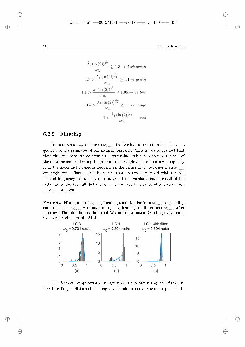
ii


ii

ii


λ1 (ln (2))1κ1

ω0c

≥ 1.3→ dark green

1.3 >λ1 (ln (2))

1κ1

ω0c

≥ 1.1→ green

1.1 >λ1 (ln (2))

1κ1

ω0c

≥ 1.05→ yellow

1.05 >λ1 (ln (2))

1κ1

ω0c

≥ 1→ orange

1 >λ1 (ln (2))

1κ1

ω0c

→ red

6.2.5 Filtering

In cases where ω0 is close to ω0max , the Weibull distribution is no longer agood t to the estimates of roll natural frequency. This is due to the fact thatthe estimates are scattered around the true value, as it can be seen on the tails ofthe distribution. Following the process of identifying the roll natural frequencyfrom the mean instantaneous frequencies, the values that are larger than ω0max

are neglected. That is, smaller values that do not correspond with the rollnatural frequency are taken as estimates. This translates into a cuto of theright tail of the Weibull distribution and the resulting probability distributionbecomes bi-modal.

Figure 6.3: Histograms of ω0. (a) Loading condition far from ω0max ; (b) loadingcondition near ω0max without ltering; (c) loading condition near ω0max afterltering. The blue line is the tted Weibull distribution (Santiago Caamaño,Galeazzi, Nielsen, et al., 2019).

This fact can be appreciated in Figure 6.3, where the histograms of two dif-ferent loading conditions of a shing vessel under irregular waves are plotted. In

ii


ii

ii


Figure 6.3(a), the histogram of the roll natural frequency estimates correspond-ing to a loading condition that is far from the maximum expected frequency isdisplayed. As it can be seen, this histogram ts well with the Weibull proba-bility distribution function. Figure 6.3(b) shows the histogram correspondingto a loading condition that is close to ω0max . As it was mentioned, it can beappreciated that the right tail is smaller and the distribution becomes bi-modal.

In order to correct this issue, a ltering process of the roll motion signal hasbeen designed to reduce the dispersion in the estimates and to retain the validityof the Weibull distribution as statistical model of the roll natural frequenciesestimates across all loading conditions. The employed lter is an eighth orderlowpass Butterworth lter with zero phase distortion. This ltering process isapplied to the stored 3 minutes batches of data, thus allowing the use of zerophase distortion techniques. The cuto frequency is the highest roll naturalfrequency of the loading conditions described in the stability booklet (ω0max).

Figure 6.3(c) shows the eect of ltering on the histogram of the estimatedroll natural frequencies. By comparing with the histogram in Figure 6.3(b) itcan be seen that ltering attenuates signicantly the presence of outliers in theestimates and the Weibull distribution is again a good t to the data.

As ltering is needed only in the described case, it is necessary to dene itsapplication limits. If the histogram in Figure 6.3(a) is taken into consideration,some dispersion can be observed. However, when the current roll natural fre-quency of the loading condition and the maximum expected value (ω0max) areclose to each other, the right tail of the resulting probability distribution startsto be cut and the dispersion in the results becomes larger. Therefore, the limitthat determines the use of ltering or not is dened as:

δ , ω0max −σ2ω0

2(6.19)

where σ2ω0 is the variance of the roll natural frequency estimates.

In conclusion, ltering is applied to the measured roll motion when themedian of the Weibull distribution is greater than δ. In this case, the EMD andHHT have to be applied again to the ltered signal to obtain ω0.

6.3 Results/Validation

To validate the described stability monitoring system and evaluate its per-formance and sensitivity, a set of dierent loading conditions have been analysedand compared. Furthermore, the impact of the sea state on the performance ofthe proposed methodology has been studied by comparing the results obtained

ii


ii

ii

102 6.3. Results/Validation

in dierent wave situations.

Roll motion time series have been obtained by using the 1 degree-of-freedomnonlinear mathematical model (described in Subsection 6.3.1) and from towingtank tests (in Subsection 6.3.2).

It is worth mentioning that the analysis done in this work is at zero forwardspeed and beam waves as it represents the worst operational scenario for ashing vessel. In addition to this, it does not consider the possible dynamicaleects that trawling nets or other phenomena which usually aect shing vessels(for instance, water-on-deck) have in the vessel motions.

6.3.1 Simulated data

In this subsection the results of the simulated roll motion time series arepresented, including the description of the test vessel, the mathematical model,the test conditions and the tunning of the monitoring system.

6.3.1.1 Test vessel

The test vessel is again the one presented in Sub-subsection 5.2.5.1 and hermain dimensions and hull forms are shown in Table 5.1 and Figure 5.6 respec-tively. The minimum and maximum roll natural frequencies for this ship, calcu-lated following the constrains presented in Sub-subsection 6.2.3.1,are includedin Table 6.2. The maximum roll natural frequency is the one that correspondswith the loading condition of highest stability in the stability booklet plus a15% of margin.

Table 6.2: Test vessel: roll natural frequency limits.

Minimum roll natural frequency (ω0min) 0.300 rad/s

Maximum roll natural frequency (ω0max) 0.925 rad/s

In order to verify how the detection system performs and how fast it rec-ognizes possible changes in ship stability, 6 loading conditions were dened. LC1 and LC 2 are two of the mandatory loading conditions contained in the sta-bility booklet. They correspond respectively with Departure from the shinggrounds with full catch and shing gear, 35% of fuel and stores and no ice andArrival at home port with full catch and shing gear, 10% of fuel and storesand no ice. Moreover, LC 1 represents the loading condition with the expectedmaximum roll natural frequency, that is, the one with the highest GM . LC 4is the critical loading condition (the one that corresponds with the minimum

ii


ii

ii


required metacentric height) and LC 3 is an intermediate situation dened bythe authors in Santiago Caamaño, Galeazzi, Nielsen, et al. (2019). All of themare under the H0 hypothesis.

LC 5 and LC 6 loading conditions belong to the alternative hypothesis,i.e., they are unsafe situations because GM values are below the minimumrequired value. Due to the fact that these conditions do not fulll the minimumstability requirements of the IMO for shing vessels (International MaritimeOrganization, 2012) nor they are contained in the compulsory stability booklet,they have been dened by the authors in Santiago Caamaño, Galeazzi, Nielsen,et al. (2019) with the purpose of evaluating if the detector is able to identifythem as dangerous situations and triggers the alarm.

The parameters of each loading condition are shown in Table 6.3 and therighting lever curves in still water for all of them have been computed by usinga naval architecture software and displayed in Figure 6.4.

Table 6.3: Loading condition parameters of the tested vessel (San-tiago Caamaño, Galeazzi, Nielsen, et al., 2019).

Parameter LC 1 LC 2 LC 3 LC 4 LC 5 LC 6

∆ (t) 489 465 489 448 448 448

T (m) 3.295 3.199 3.484 3.340 3.294 3.294

GM (m) 0.659 0.661 0.501 0.350 0.331 0.291

ω0 (rad/s) 0.804 0.798 0.701 0.563 0.548 0.514

kxx 0.395 0.399 0.395 0.411 0.411 0.411

Figure 6.4: GZ curves for the dierent tested loading conditions in calm water(Santiago Caamaño, Galeazzi, Nielsen, et al., 2019).

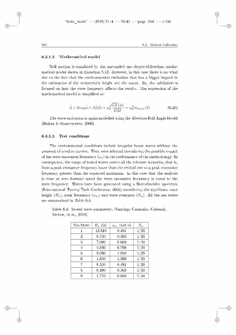
ii


ii

ii


6.3.1.2 Mathematical model

Roll motion is simulated by the uncoupled one degree-of-freedom mathe-matical model shown in Equation 5.12. However, in this case there is no winddue to the fact that the environmental excitation that has a bigger impact inthe estimation of the metacentric height are the waves. So, the validation isfocused on how the wave frequency aects the results. The expression of themathematical model is simplied as:

φ+ 2υω0φ+ βφ|φ|+ ω20

GZ (φ)

GM= ω2

0mwave (t) (6.20)

The wave excitation is again modelled using the Absolute Roll Angle Model(Bulian & Francescutto, 2006).

6.3.1.3 Test conditions

The environmental conditions include irregular beam waves without thepresence of wind or current. They were selected considering the possible impactof the wave encounter frequency (ωe) in the performance of the methodology. Inconsequence, the range of tested waves covers all the relevant scenarios, that is,from a peak encounter frequency lower than the critical one to a peak encounterfrequency greater than the expected maximum. In this case that the analysisis done at zero forward speed the wave encounter frequency is equal to thewave frequency. Waves have been generated using a Bretschneider spectrum(International Towing Tank Conference, 2002) considering the signicant waveheight (Hs), peak frequency (ωw) and wave steepness (Sw). All the sea statesare summarised in Table 6.4.

Table 6.4: Tested wave parameters (Santiago Caamaño, Galeazzi,Nielsen, et al., 2019).

Sea State Hs (m) ωw (rad/s) Sw

1 12.810 0.491 1/20

2 9.720 0.563 1/20

3 7.080 0.660 1/20

4 4.830 0.798 1/20

5 3.030 1.008 1/20

6 1.650 1.369 1/20

7 8.520 0.491 1/30

8 6.480 0.563 1/30

9 4.710 0.660 1/30

ii


ii

ii


Table 6.4: Tested wave parameters (Santiago Caamaño, Galeazzi,Nielsen, et al., 2019).

Sea State Hs (m) ωw (rad/s) Sw10 3.240 0.798 1/30

11 2.010 1.008 1/30

12 1.320 1.369 1/30

13 2.550 0.491 1/100

14 1.950 0.563 1/100

15 1.410 0.660 1/100

16 0.960 0.798 1/100

17 0.600 1.008 1/100

18 0.330 1.369 1/100

6.3.1.4 Tuning of the condition monitoring system

To theoretically determine the threshold γ′ of the detector, the componentsof the vector Ω0 have to fulll the requirement of being i.i.d. If this condition isnot met, the performance of the detector cannot be guaranteed from a theoreti-cal standpoint and empirical methods for tuning should be pursued. Figure 6.5shows the auto-correlation function of Ω0 under the null hypothesis. It can beseen that the data are uncorrelated and therefore the i.i.d. condition is fullled.Furthermore, this condition is also met when ltering is needed.

Figure 6.5: Auto-correlation function of the driving signal (Santiago Caamaño,Galeazzi, Nielsen, et al., 2019).

Considering the Equation 6.18, the threshold for a desired false alarm prob-ability is obtained from:

ii


ii

ii


1− PFA = 1− exp

(−(γ′

λ0

)κ0)

(6.21)

Ordering the previous equation:

γ′ = λ0 (− ln (PFA))1κ0 (6.22)

In this case, for the hypothesisH0 shown in Figure 6.5, the false alarm prob-ability has been set PFA = 0.0000001 and the obtained value for the thresholdis γ′ = 0.8407.

In Sub-subsection 6.2.4 was explained that the W-GLRT is based on theassumption that the hypothesis H0 is already known. However, in this workthis assumption is not true. In fact, it is supposed that when the vessel leavesthe port the monitoring system is started and the loading condition may havechanged from the last time the system was used.

Nevertheless, the key feature of the monitoring system is the ability to op-erate without crew interaction. Due to this fact, an estimation of the parametervector θ0 is done each time the system starts running. So that, two dierentoperation stages of the system can be distinguished.

Estimation stage This stage is designed for estimating θ0 and solving theissue of H0. It takes places immediately after the system is started andideally when the vessel is leaving port in sheltered waters. In this phase,during a time window Test, the system is only collecting roll natural fre-quency estimates. Once this time is over, the parameter vector θ0 iscalculated according to Equations (6.14)-(6.15). If the probabilistic me-dian of the Weibull distribution (λ0(ln 2)

1κ0 ) is lower than ω0c , an alarm

is raised and a message should be displayed to the skipper to inform himabout too low metacentric height for sailing. Conversely, θ0 is stored asthe reference value to be used during sailing.

For the simulated roll motion time series, a Test = 20 min is proposed.The reason is that during this period a suciently number of roll naturalfrequency estimates can be collected. Furthermore, during this time thevessel is leaving the port, and considering that she is not facing a roughweather, the risk of suering stability issues remains lower than in openseas.

Detection stage During this stage, the system is fully operational. H0 is al-ready known and consequently H1 can be evaluated and compared againstit, following the procedure described in Section 6.2.4. As it was previously

ii


ii

ii


done with θ0, another time window (Tdet) is necessary to make the esti-mation of θ1.

During this phase, ensuring the requirement of real-time is crucial. Sothat, a detection time window of Tdet = 5 min has been selected togetherwith a 40% of overlapping between consecutive measurements. This leadsto the GLRT releasing a new value every 3 minutes, thus fullling the real-time requirement and providing enough roll natural frequency estimatesto perform the MLE.

6.3.1.5 Evaluation of the monitoring performance

For each sea state and loading condition, roll motion time series have beengenerated using the mathematical model. Then, in order to evaluate the perfor-mance of the proposed methodology, for each sea state the 6 loading conditionshave been stitched together (ordered from the safest to the most risky one).The result is a long record history (6.75 h) for each sea state where a changein loading condition could be observed approximately after each 4000 seconds.After that, the estimation of the roll natural frequency was done and, at thesame time, the W-GLRT detector was applied.

To address in detail the impact of the wave encounter frequency in the esti-mation and detection performance, two dierent wave situations are explainedin detail.

Figure 6.6 shows the roll motion time series, the roll natural frequency es-timates after applying the EMD+HHT, the output of the W-GLRT detectorand the output of the awareness indicator for Sea State 7. In this case, the waveencounter frequency is below the expected maximum roll natural frequency. Asit can be seen roll amplitude is large along the whole time series and dierencesbetween the dierent loading conditions are not very pronounced. This could bemainly due to the large wave height and period, which induce very large roll mo-ments in the whole range of natural frequencies of all loading conditions. Also,it can be due to the possible inuence of the nonlinear eects of the restoringterm (see Figure 6.4) in the expected maximum roll amplitude frequency.

Regarding the performance of the EMD+HHT, some dispersion aroundthe roll natural frequency for each loading condition can be observed. Thedispersion becomes larger in those loading conditions with a smaller roll naturalfrequency value.

The W-GLRT is quite sensitive and all loading conditions could be per-fectly distinguished without delay looking at its output. Its performance is alsovery good, as all loading conditions are correctly classied and no false alarmsappear or miss-detections take place. It could be also appreciated that the de-

ii


ii

ii


Figure 6.6: Top to bottom. Roll motion time series, natural roll frequency esti-mations, output of the detector and output of the awareness alarm in irregularwaves. Sea State 7. Hs = 8.520 m, ωw = 0.491 rad/s, Sw = 1/30. The orangeline represents the threshold γ′ (Santiago Caamaño, Galeazzi, Nielsen, et al.,2019).

tector confuses the critical loading condition with a situation of danger, andsubsequently triggers the alarm.

Nevertheless, looking at the output of the awareness alarm, the critical con-dition could be clearly dierentiated. In fact, the perception of risk is increasingas advancing through the loading conditions. Then it could be concluded thatthe awareness alarm performs adequately, although in some circumstances morethan one colour appears, which is due to the dispersion of the estimates.

Figure 6.7 illustrates the roll motion time series, the roll natural frequencyestimates, the output of the detector and the output of the awareness alarm,but for Sea State 17 in which the wave encounter frequency is larger than themaximum roll natural frequency. As it can be appreciated the roll amplitudedecreases considerably, as wave height is quite small and the wave frequency isfar from the natural frequency of any of the loading conditions.

The dispersion in the roll natural frequency estimates increases, in partic-

ii


ii

ii


Figure 6.7: Top to bottom. Roll motion time series, natural roll frequency esti-mations, output of the detector and output of the awareness alarm in irregularwaves. Sea State 17. Hs = 0.600 m, ωe = 1.008 rad/s, Sw = 1/100. The orangeline represents the threshold γ′ (Santiago Caamaño, Galeazzi, Nielsen, et al.,2019).

ular in those cases with the smallest rolling amplitudes (LC 4, LC 5 and LC 6).So that, the performance of the EMD+HHT degrades a little bit.

Nonetheless, the performance of the detector is still quite good. It ade-quately identies safe and unsafe situations and no false alarms arise nor miss-detections take place. Special comment about LC 4, as it is recognised by thedetector as a dangerous loading condition.

By contrast, the awareness alarm is not able of correctly recognizing thechanges in loading conditions. It is only able to dierentiate between safe anddangerous situations.

The evaluation of the performance of the frequency estimation subsystem(EMD+HHT) for all loading conditions and sea states has been done by com-puting the median (Medω0

), the standard deviation (σω0) and the 95th and

5th percentiles (P95ω0and P5ω0

) of the roll natural frequency estimates. Theresults are included in Table 6.5. From the data it can be concluded that the

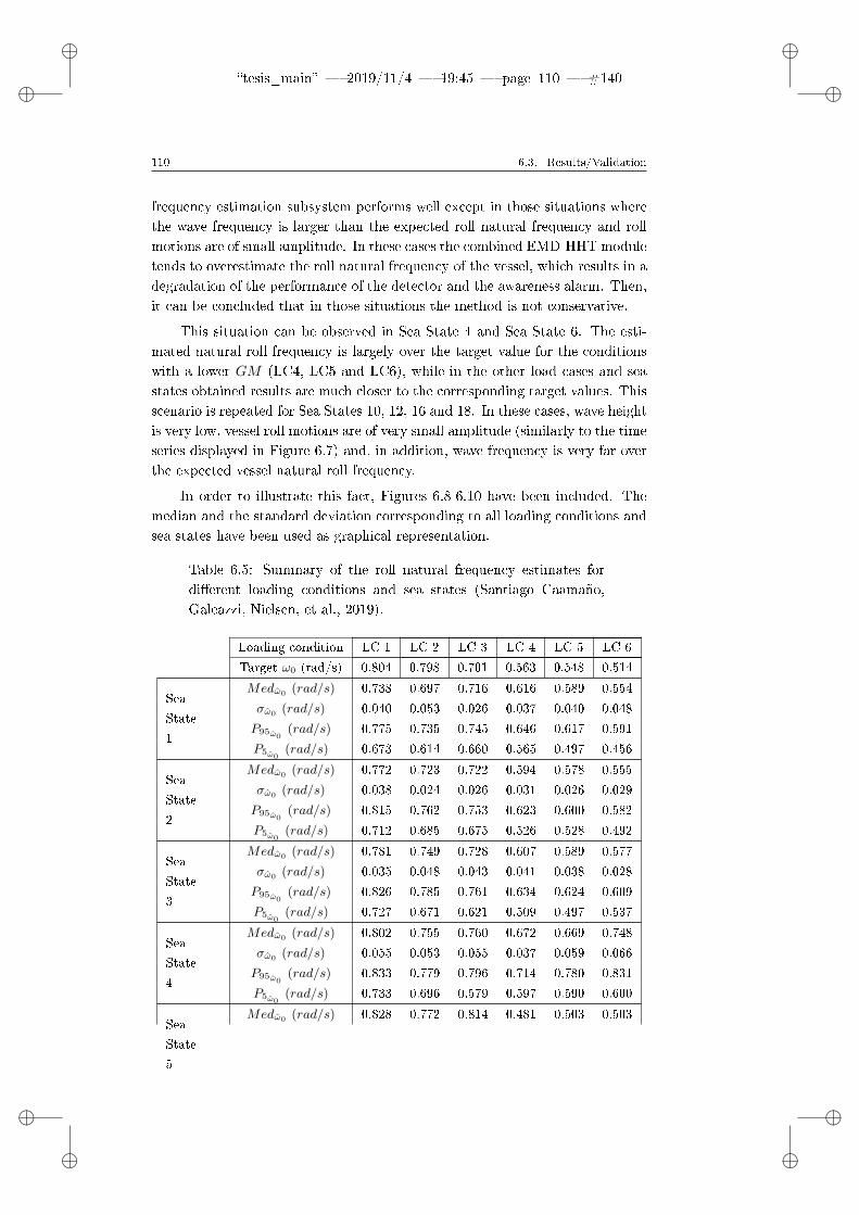
ii


ii

ii


frequency estimation subsystem performs well except in those situations wherethe wave frequency is larger than the expected roll natural frequency and rollmotions are of small amplitude. In these cases the combined EMD-HHT moduletends to overestimate the roll natural frequency of the vessel, which results in adegradation of the performance of the detector and the awareness alarm. Then,it can be concluded that in those situations the method is not conservative.

This situation can be observed in Sea State 4 and Sea State 6. The esti-mated natural roll frequency is largely over the target value for the conditionswith a lower GM (LC4, LC5 and LC6), while in the other load cases and seastates obtained results are much closer to the corresponding target values. Thisscenario is repeated for Sea States 10, 12, 16 and 18. In these cases, wave heightis very low, vessel roll motions are of very small amplitude (similarly to the timeseries displayed in Figure 6.7) and, in addition, wave frequency is very far overthe expected vessel natural roll frequency.

In order to illustrate this fact, Figures 6.8-6.10 have been included. Themedian and the standard deviation corresponding to all loading conditions andsea states have been used as graphical representation.

Table 6.5: Summary of the roll natural frequency estimates fordierent loading conditions and sea states (Santiago Caamaño,Galeazzi, Nielsen, et al., 2019).

Loading condition LC 1 LC 2 LC 3 LC 4 LC 5 LC 6

Target ω0 (rad/s) 0.804 0.798 0.701 0.563 0.548 0.514

Sea

State

1

Medω0 (rad/s) 0.738 0.697 0.716 0.616 0.589 0.554

σω0 (rad/s) 0.040 0.053 0.026 0.037 0.040 0.048

P95ω0(rad/s) 0.775 0.735 0.745 0.646 0.617 0.591

P5ω0(rad/s) 0.673 0.614 0.660 0.565 0.497 0.456

Sea

State

2

Medω0 (rad/s) 0.772 0.723 0.722 0.594 0.578 0.555

σω0 (rad/s) 0.038 0.024 0.026 0.031 0.026 0.029

P95ω0(rad/s) 0.815 0.762 0.753 0.623 0.600 0.582

P5ω0(rad/s) 0.712 0.685 0.675 0.526 0.528 0.492

Sea

State

3

Medω0 (rad/s) 0.781 0.749 0.728 0.607 0.589 0.577

σω0 (rad/s) 0.035 0.048 0.043 0.041 0.038 0.028

P95ω0(rad/s) 0.826 0.785 0.761 0.634 0.624 0.609

P5ω0(rad/s) 0.727 0.671 0.621 0.509 0.497 0.537

Sea

State

4

Medω0 (rad/s) 0.802 0.755 0.760 0.672 0.669 0.748

σω0 (rad/s) 0.055 0.053 0.055 0.037 0.059 0.066

P95ω0(rad/s) 0.833 0.779 0.796 0.714 0.780 0.831

P5ω0(rad/s) 0.733 0.696 0.579 0.597 0.590 0.600

Sea

State

5

Medω0 (rad/s) 0.828 0.772 0.814 0.481 0.503 0.503

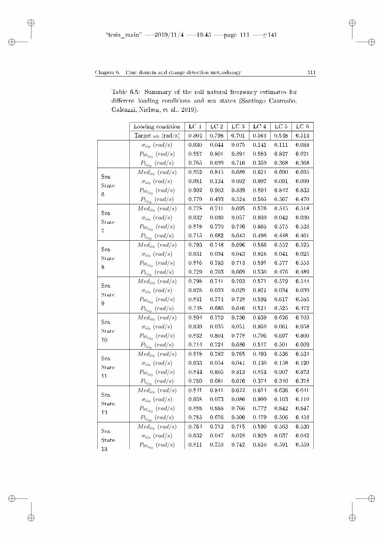
ii


ii

ii




Target ω0 (rad/s) 0.804 0.798 0.701 0.563 0.548 0.514

σω0 (rad/s) 0.030 0.044 0.075 0.141 0.111 0.088

P95ω0(rad/s) 0.857 0.801 0.894 0.883 0.827 0.621

P5ω0(rad/s) 0.765 0.699 0.710 0.359 0.368 0.368

Sea

State

6

Medω0 (rad/s) 0.852 0.845 0.689 0.621 0.690 0.695

σω0 (rad/s) 0.081 0.124 0.092 0.097 0.091 0.099

P95ω0(rad/s) 0.902 0.903 0.839 0.804 0.842 0.833

P5ω0(rad/s) 0.779 0.493 0.524 0.505 0.567 0.470

Sea

State

7

Medω0 (rad/s) 0.778 0.741 0.695 0.576 0.545 0.518

σω0 (rad/s) 0.032 0.030 0.057 0.039 0.042 0.030

P95ω0(rad/s) 0.818 0.770 0.720 0.605 0.575 0.538

P5ω0(rad/s) 0.715 0.682 0.643 0.496 0.448 0.461

Sea

State

8

Medω0 (rad/s) 0.793 0.748 0.696 0.566 0.552 0.525

σω0 (rad/s) 0.031 0.034 0.043 0.018 0.041 0.025

P95ω0(rad/s) 0.816 0.783 0.713 0.591 0.577 0.555

P5ω0(rad/s) 0.729 0.703 0.669 0.530 0.476 0.489

Sea

State

9

Medω0 (rad/s) 0.798 0.741 0.703 0.571 0.579 0.544

σω0 (rad/s) 0.028 0.033 0.029 0.021 0.034 0.039

P95ω0(rad/s) 0.831 0.774 0.728 0.593 0.617 0.585

P5ω0(rad/s) 0.748 0.686 0.646 0.521 0.525 0.472

Sea

State

10

Medω0 (rad/s) 0.804 0.779 0.730 0.639 0.626 0.703

σω0 (rad/s) 0.039 0.035 0.051 0.050 0.061 0.058

P95ω0(rad/s) 0.832 0.804 0.778 0.706 0.697 0.800

P5ω0(rad/s) 0.714 0.724 0.680 0.517 0.501 0.609

Sea

State

11

Medω0 (rad/s) 0.818 0.782 0.765 0.493 0.536 0.534

σω0 (rad/s) 0.033 0.054 0.041 0.130 0.158 0.120

P95ω0(rad/s) 0.844 0.805 0.813 0.853 0.907 0.873

P5ω0(rad/s) 0.750 0.681 0.670 0.374 0.340 0.378

Sea

State

12

Medω0 (rad/s) 0.841 0.841 0.622 0.614 0.636 0.641

σω0 (rad/s) 0.058 0.073 0.080 0.099 0.103 0.110

P95ω0(rad/s) 0.888 0.888 0.766 0.772 0.842 0.847

P5ω0(rad/s) 0.785 0.676 0.500 0.479 0.506 0.458

Sea

State

13

Medω0 (rad/s) 0.764 0.713 0.715 0.590 0.563 0.530

σω0 (rad/s) 0.032 0.047 0.028 0.029 0.037 0.042

P95ω0(rad/s) 0.811 0.753 0.742 0.610 0.591 0.559

ii


ii

ii




Target ω0 (rad/s) 0.804 0.798 0.701 0.563 0.548 0.514

P5ω0(rad/s) 0.701 0.655 0.640 0.518 0.478 0.401

Sea

State

14

Medω0 (rad/s) 0.764 0.724 0.698 0.598 0.581 0.563

σω0 (rad/s) 0.025 0.030 0.031 0.026 0.033 0.034

P95ω0(rad/s) 0.794 0.760 0.716 0.621 0.607 0.588

P5ω0(rad/s) 0.702 0.669 0.628 0.527 0.489 0.478

Sea

State

15

Medω0 (rad/s) 0.790 0.728 0.734 0.607 0.594 0.565

σω0 (rad/s) 0.030 0.037 0.037 0.038 0.034 0.038

P95ω0(rad/s) 0.830 0.765 0.758 0.644 0.622 0.618

P5ω0(rad/s) 0.722 0.665 0.662 0.526 0.516 0.488

Sea

State

16

Medω0 (rad/s) 0.808 0.778 0.741 0.657 0.665 0.720

σω0 (rad/s) 0.027 0.043 0.034 0.049 0.072 0.042

P95ω0(rad/s) 0.834 0.814 0.787 0.739 0.722 0.774

P5ω0(rad/s) 0.748 0.685 0.710 0.585 0.497 0.638

Sea

State

17

Medω0 (rad/s) 0.828 0.780 0.792 0.505 0.494 0.508

σω0 (rad/s) 0.022 0.035 0.035 0.131 0.124 0.092

P95ω0(rad/s) 0.856 0.807 0.825 0.863 0.843 0.715

P5ω0(rad/s) 0.782 0.715 0.738 0.363 0.340 0.417

Sea

State

18

Medω0 (rad/s) 0.855 0.819 0.630 0.644 0.663 0.676

σω0 (rad/s) 0.038 0.045 0.097 0.117 0.095 0.107

P95ω0(rad/s) 0.904 0.871 0.763 0.833 0.804 0.821

P5ω0(rad/s) 0.785 0.729 0.441 0.470 0.490 0.476

ii


ii

ii


Figure 6.8: Median and standard deviation of natural roll frequency estimates.All load cases. Sea States 1 to 6 (Santiago Caamaño, Galeazzi, Nielsen, et al.,2019).

Figure 6.9: Median and standard deviation of natural roll frequency estimates.All load cases. Sea States 7 to 12.

ii


ii

ii


Figure 6.10: Median and standard deviation of natural roll frequency estimates.All load cases. Sea States 13 to 18.

Finally, in order to analyse the performance of the detector, the total num-ber of true detections (TD) and the total number of false detections (FD) foreach loading condition and sea state have been obtained. The results are shownin Table 6.6. These values represent the number of times that the detector isable to adequately recognize if the loading condition under consideration is safeor not (TD) and those in which it is not (FD).

From the obtained results, it could be appreciated that in the two loadingconditions with better stability (LC 1 and LC 2), the detector performs verywell in all sea states and there are no false detections. Results for LC 3 arequite good despite of some false detections took place. Regarding the criticalcondition (LC 4), it is necessary to mention that the detector identied it as riskysituation. This is a conservative approach. Despite of this fact, the detectorworks ne in most of the sea states. In the loading conditions with a stabilitylevel under the standard minimum (LC 5 and LC 6), the performance of thedetector starts decreasing but it still adequately classied the loading conditions,except in Sea State 6, 12 and 18 where a very large number of false detectionstook place. Under these circumstances, as it was previously mentioned, theEMD-HHT module is hardly able to estimate the natural roll frequency and, inconsequence, the performance of the detector gets worse. Despite of this fact,the detector is still able to distinguish between safe and not safe situations witha good accuracy in the vast majority of the cases.

ii


ii

ii


Regarding the critical condition (LC 4), the detector is unable to classifyit as safe in most of the sea states. However, and due to the fact that thissituations represents the border between safe and unsafe, the obtained resultscould be acceptable as they represent a slightly conservative approach.

Table 6.6: Summary of results of the W-GLRT detector (SantiagoCaamaño, Galeazzi, Nielsen, et al., 2019).

Sea

State

LC 1 LC 2 LC 3 LC 4 LC 5 LC 6

Total 16 Total 23 Total 23 Total 23 Total 23 Total 21

TD FD TD FD TD FD TD FD TD FD TD FD

1 16 0 23 0 23 0 13 10 23 0 21 0

2 16 0 23 0 23 0 1 22 23 0 21 0

3 16 0 23 0 23 0 0 23 23 0 21 0

4 16 0 21 2 23 0 2 21 18 5 5 16

5 16 0 23 0 20 3 0 23 23 0 21 0

6 16 0 23 0 23 0 23 0 0 23 0 21

7 16 0 23 0 23 0 0 23 23 0 21 0

8 16 0 23 0 1 22 0 23 23 0 21 0

9 16 0 23 0 23 0 1 22 22 1 21 0

10 16 0 23 0 15 8 0 23 23 0 10 11

11 16 0 23 0 23 0 0 23 23 0 21 0

12 16 0 23 0 18 5 17 6 5 18 3 18

13 16 0 23 0 23 0 0 23 23 0 21 0

14 16 0 23 0 23 0 1 22 23 0 21 0

15 16 0 23 0 23 0 0 23 23 0 21 0

16 16 0 23 0 23 0 2 21 22 1 1 20

17 16 0 23 0 23 0 0 23 23 0 21 0

18 16 0 23 0 23 0 23 0 0 23 0 21

Table 6.7: Confusion matrix for the W-GLRT detector (SantiagoCaamaño, Galeazzi, Nielsen, et al., 2019).

True conditionConditionpositive

Conditionnegative

Predicted Condition positive 1159 178condition Condition negative 371 614

75.8% 77.5%Sensitivity Specicity

ii


ii

ii


As a summary of the performance of the detector, the confusion matrix isshown in Table 6.7. It can be seen that the sensitivity (true positive rate) andthe specicity (true negative rate) are quite good, achieving more than 75% inboth cases.

6.3.2 Towing tank data

In this subsection the results of the campaign of towing tank tests arepresented, including the description of the scale model, the campaign, the testconditions, the design of the lter and the tunning of the monitoring system.

6.3.2.1 Vessel model

The test vessel is the same than in Sub-subsection 5.2.5.1 and 6.3.1. Nev-ertheless, in this test campaign the model is made in breglass with adjustableweights for modifying the loading condition and the scale is 1/30.

The roll motion was measured using an IMU with a sampling frequencyFs = 50 Hz.

Figure 6.11: Ship scale model.

In this case, the tested loading conditions where those that are shown inTable 6.8. As it can be seen, the rst one is very similar to LC 3 in Table 6.3and the second one corresponds to the critical loading condition (LC 4 in Table6.3).

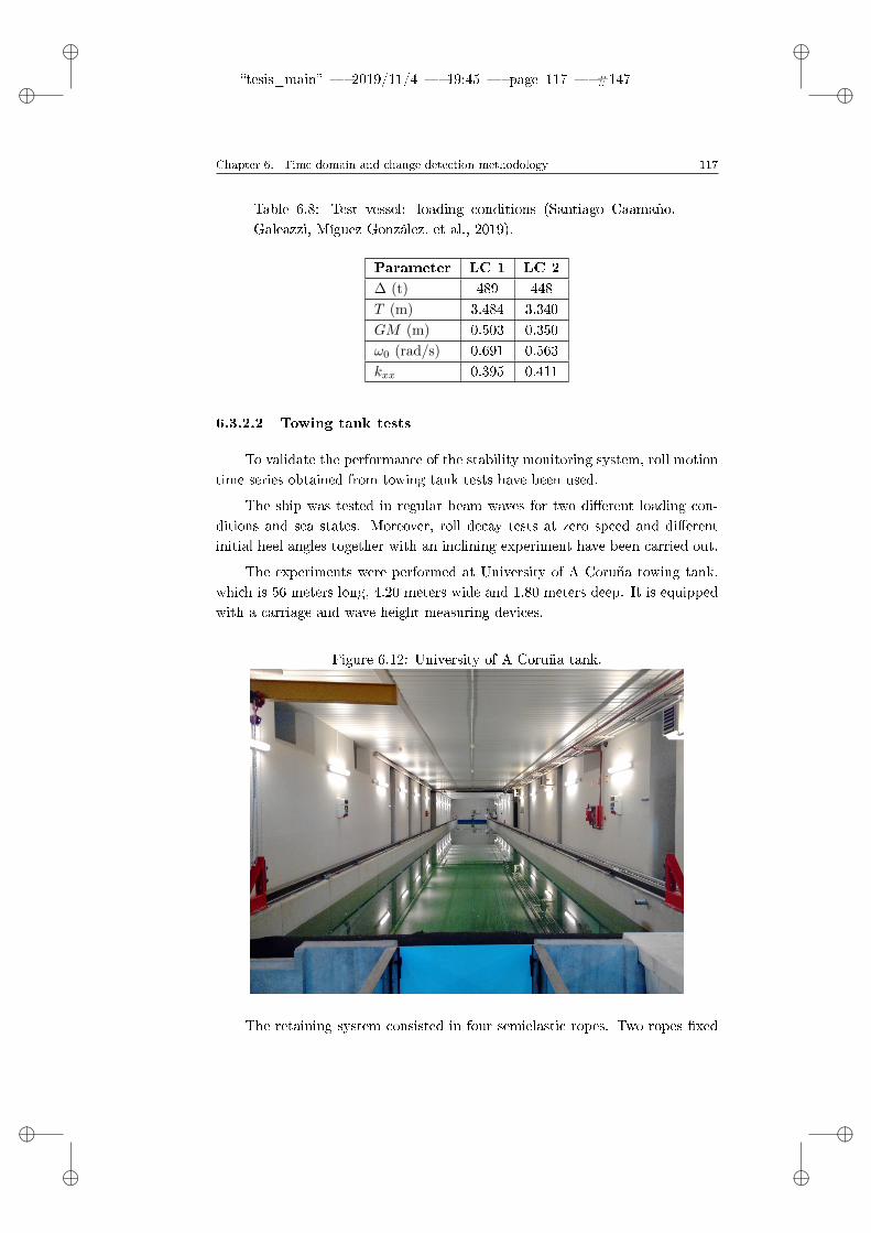
ii


ii

ii


Table 6.8: Test vessel: loading conditions (Santiago Caamaño,Galeazzi, Míguez González, et al., 2019).

Parameter LC 1 LC 2

∆ (t) 489 448

T (m) 3.484 3.340

GM (m) 0.503 0.350

ω0 (rad/s) 0.691 0.563

kxx 0.395 0.411

6.3.2.2 Towing tank tests

To validate the performance of the stability monitoring system, roll motiontime series obtained from towing tank tests have been used.

The ship was tested in regular beam waves for two dierent loading con-ditions and sea states. Moreover, roll decay tests at zero speed and dierentinitial heel angles together with an inclining experiment have been carried out.

The experiments were performed at University of A Coruña towing tank,which is 56 meters long, 4.20 meters wide and 1.80 meters deep. It is equippedwith a carriage and wave height measuring devices.

Figure 6.12: University of A Coruña tank.

The retaining system consisted in four semielastic ropes. Two ropes xed

ii


ii

ii


to the bow and another two xed to the stern. All of them xed at the waterlinelevel and fastened to the sides of the tank.

Figure 6.13: Model arrangement.

Regarding the roll decay tests, the vessel was displaced from its equilibriumposition and then released. During the roll decay the model was completely freein the middle of the tank.

6.3.2.3 Test conditions

Likewise in simulated data, the tested waves were selected considering theimpact of the wave encounter frequency in the performance of the methodology.For the sake of simplicity, only two sea states were tested. One with a waveencounter frequency close to the vessel roll natural frequency and another onewith a wave encounter frequency much higher than the roll natural frequency.The parameters of each sea state are shown in Table 6.9.

Table 6.9: Sea state parameters (Santiago Caamaño, Galeazzi,Míguez González, et al., 2019).

Sea State Hw (m) ωw (rad/s) Sw

1 1.95 0.563 0.01

2 3.03 1.008 0.05

ii


ii

ii


6.3.2.4 Redesigning the lter

The previous low-pass lter design has proved not to be suitable for theexperimental data.

In the experimental roll motion time series, when the wave encounter fre-quency is signicantly larger or smaller than the roll natural frequency, theEMD-HHT has diculties in identifying ω0 among the other components of thesignal. The component with the highest energy content in the time series nor-mally corresponds to the wave excitation and the peak of the spectrum locatedat the wave encounter frequency tends to mask the rest of the components. Thisissue is specially relevant when roll motion has small amplitude.

In this scenario ω0 falls outside the interval [ω0,min ω0,max], hence it isunlikely to be a correct estimate of the roll natural frequency.

In order to remove the possibility that the wave encounter frequency masksthe roll natural frequency, a pass-band lter is applied. The lter is a 5th orderChebychev Type II with an attenuation in the stop band of 20 dB, a lower cut-o frequency of 0.3 rad/s and an upper cut-o frequency of 0.95 rad/s. Thesevalues coincides with ω0,min and a conservative choice of ω0,max.

Thus, the proposed architecture for the stability monitoring system withthe experimental data is the one illustrated in Figure 6.14. As it can be seen,the blocks are the same than in Figure 6.1, except the lter block that it is aband-pass.

Figure 6.14: Architecture of the transverse stability monitoring system (Santi-ago Caamaño, Galeazzi, Míguez González, et al., 2019).

ii


ii

ii


6.3.2.5 Tuning of the condition monitoring system

First of all, in order to determined γ′ it is necessary to verify the i.i.d.assumption. Figure 6.15 shows the auto-correlation function ofΩ0 underH0 andit can be seen that the data are uncorrelated and therefore they are identicallyindependent distributed.

Figure 6.15: Auto-correlation function of Ω0 (Santiago Caamaño, Galeazzi,Míguez González, et al., 2019).

Then, γ′ can be obtained considering the Equation 6.22. PFA has been setconsidering that the desired number of false alarms is one each three months.This value was selected as a compromise between not bothering the crew withfalse alarms and at the same time, guaranteeing their safety. So that, taking intoaccount that an alarm is generated every 3 minutes, PFA = 0.000023 and for theSea State 1 under the hypothesis H0, the value of the threshold is γ′ = 0.6281.

Furthermore, a second threshold γ′′ has been dened as a return-from-alarm criterion. The purpose of this second limit is to ensure that possiblestability overpredictions do not mask real alarms. Therefore, once the alarmis triggered by the detector it will not be withdrawn until a safety margin isreached, i.e., until the detector's output is lower than γ′′. This second thresholdhas been set to γ′′ = γ′/2.

As it was explained before, the detector was designed assuming that theparameters of the H0 hypothesis are known. By contrast, this is not true as theloading condition may change from the last time that the monitoring systemwas used. In consequence, two operational phases for the monitoring systemare dened:

Estimation stage This phase takes place when the vessel leaves the port inprotected waters and the system is started. During this stage the system is

ii


ii

ii


storing roll natural frequency estimates for a time window Test. After that,an estimation of the parameter vector θ0 is done according to Eqs. (6.14)-(6.15). If θ0 fullls the condition of λ0(ln 2)

1κ0 ≥ ω0c , it is stored as the

reference value. Otherwise, an alarm is given to inform the crew aboutthe low stability level of their vessel.

For the experimental data, a Test = 10 min is proposed in order to generatesucient ω0 to achieve a robust statistics of the Weibull distribution.

Detection stage The system fully operates during this stage. H0 is alreadyknown, H1 can be estimated and both values compared according toEq.(6.17). In this phase, another time window (Tdet) is set in order tohave enough estimates of ω0 to estimate θ1.

A time window of Tdet = 4.5 min with a 33% of overlapping betweenconsecutive measurements has been selected in order to fulll the detectionrequirement of the system.

6.3.2.6 Evaluation of the monitoring performance

Due to physical limitations of the towing tank and in order to obtain su-ciently long roll motion time series to validate the performance of the proposedmethodology, each sea state has been tested 4 times for each loading condition.After that, the four time series have been stitched together (previously removedthe transient part) using a smoothing lter around the stitching points to avoidctitious variations within the signals. Then, for each wave case, the roll mo-tion time series of both loading conditions have been stitched ordered from thesafest (LC 1) to the one with the lowest stability (LC 2).

In addition, the roll motion time series have been pre-processed with alow-pass lter with cut-o frequency of 1.75 rad/s to remove components of thesignal not related with the physics of the experiment. These components are aproduct of the experiment itself such as possible rebound of the waves in thetank, wall eects, etc.

Figure 6.16 shows the roll motion time series, the roll natural frequencyestimates, the output of the detector and the output of the awareness indicatorfor Sea State 1. In this case the wave encounter frequency is close to theroll natural frequency for both loading conditions. In fact, there is pure rollresonance in LC 2 as the wave encounter frequency matches the roll naturalfrequency. Furthermore, the energy is largely concentrated around a single peakand thereby the roll natural frequency is accurately estimated. By contrast,there is a clear underestimation of the roll natural frequency in LC 1. This factcould be related with the proximity between wave frequency and roll natural

ii


ii

ii


Figure 6.16: Top to bottom. Roll motion time series, natural roll frequency es-timations, output of the detector and output of the awareness alarm in irregularwaves. Sea State 1. Hs = 1.95 m, ωe = 0.563 rad/s, Sw = 0.01. The orange linerepresents the threshold γ′ and the yellow line γ′′ (Santiago Caamaño, Galeazzi,Míguez González, et al., 2019).

frequency that makes harder its identication. The largest dierence betweenthe median of the estimates of the natural roll frequency and its true value inLC 1 is 17% and in LC 2 is 1.2%.

The performance of the detector is quite good and it is sensitive to changesin loading conditions. When the detector's alarm is triggered it is representedin red colour. In LC 1 a false alarm appeared due to the underestimation of ω0.LC 2, the critical loading condition, is identied as a risky situation most of thetime (there are two miss detections) and the detector subsequently raised thealarm.

The awareness indicator is also sensitive to variations in loading conditionsas LC 2 is plotted in red while LC 1 is plotted in orange.

Figure 6.17 shows the results for Sea State 2, in which the wave frequencyis much higher than the roll natural frequency (ωe ω0). Noteworthy thatin this scenario bandpass ltering was applied to the batches of measured rollmotion. The roll amplitude is small in both loading conditions, although theestimation of ω0 is still good with some dispersion. In this case, the largestdierence between the median and the true value is 9.1% for LC 1 and 3.7% forLC 2.

ii


ii

ii


Figure 6.17: Top to bottom. Roll motion time series, natural roll frequency es-timations, output of the detector and output of the awareness alarm in irregularwaves. Sea State 2. Hs = 3.03 m, ωe = 1.008 rad/s, Sw = 0.05. The orange linerepresents the threshold γ′ and the yellow line γ′′ (Santiago Caamaño, Galeazzi,Míguez González, et al., 2019).

The performance of the detector and the awareness indicator relies quitegood and the transition between the two loading conditions is accurately de-tected most of the time. As in Figure 6.16, there are a few miss detections inLC 2 and the detector identies it as a non safe situation triggering the alarm.

6.4 Discussion

As it was said before, from the results it can be concluded that the stabilitymonitoring system works adequately in most of the situations. It is capable ofalerting about potential risks and giving information about how far the vesselis from the safety limit.

The EMD-HHT is the most vulnerable module. It can estimate the rollnatural frequency of the vessel with an acceptable degree of dispersion, althoughin some cases it is aected by the environmental conditions and the performancedecreases in comparison to others. Usually these situations happen when thewave encounter frequency is outside the interval [ω0,min ω0,max].

A possible explanation for such behaviour may lie in the assumption that

ii


ii

ii

124 6.4. Discussion

the vessel roll natural frequency should be coinciding, or at least very close, tothe roll spectrum peak frequency. As a rule, the ship roll dynamics tend tomitigate the eect of excitation which do not generate motions close to the rollnatural frequency. Nevertheless, when the amplitude of the roll motion is small,the roll spectrum may present additional peaks or even a single peak shifted tothe excitation frequency that, in consequence, mask the expected roll naturalfrequency value.

Filtering has proven to be suitable for mitigating the impact of the en-vironmental conditions, even though under or overestimation of ω0 with somedispersion is still likely to occur in the cases that the wave encounter frequencyis close to the roll natural frequency.

Despite this fact, the detector shows a very good performance and ro-bustness as it is insensitive (in most of the cases) to changes in the sea state.It detects potential unsafe situations in real-time and the percentage of falsealarms generated is quite low.

Regarding the awareness indicator, it is highly dependant on the accuracyof the roll natural frequency estimates. When there is little dispersion in theestimates, the probabilistic median (λ1(ln 2)

1κ1 ) is closer to the real value and

then the situation awareness system is capable of dierentiating changes in theloading condition. However, if the quality of the estimates decreases, the systembecomes insensitive and only identies signicant changes in loading condition.

ii


ii

ii

Chapter 7

Comparison of both

methodologies

7.1 Introduction

In this PhD thesis two methodologies for automatically estimating the rollnatural frequency of the vessel in real-time have been proposed and validated.Both of them rely on the assumption that roll spectrum has a peak around theroll natural frequency. Therefore, solely analysing the roll motion this parametercan be obtained and the stability of the vessel can be assessed.

The rst methodology (described in Chapter 5) analyses the roll signalin the frequency domain with the recursive application of the FFT; while thesecond one (presented in Chapter 6) works in time domain and is based on theapplication of the EMD+HHT and the W-detector.

Apart from taking a dierent approach to extract the information from theroll motion, these methodologies have two main dierences. On the one hand,the recursive FFT-based method only uses the obtained values of ω0 to evaluatethe stability. If for any reason the quality of the predictions is not good, theperformance of the methodology is degraded and could lead to erroneous results.The EMD+HHT have the same mission as the FFT but in the time domain.However, the W-detector is applied to the estimates in order to robustify theoutput of the system and make it more insensitive to the dispersion in ω0. Sothat, poor estimations can be ignored.

On the other hand, the last methodology provides extra information as itincorporates an awareness indicator. The function of this indicator is alertingthe crew about how far the vessel is from the critical condition.

ii


ii

ii

126 7.2. Test case

In this chapter, a test case where both methodologies are analytically com-pared is presented.

7.2 Test case

For the test case the most realistic possible scenario has been chosen. Dueto this fact, the vessel under analysis corresponds to one of the target eet,which is a mid-sized stern trawler.

Furthermore, the roll motion time series have been generated with a mathe-matical model in irregular beam waves with no wind. This is a typical situationthat a shing vessel faces during her normal operation.

The full description of the test vessel and conditions and the results of bothmethodologies can be found in the following subsections.

7.2.1 Test vessel

The test vessel is the same employed for the validation of the methodologiesin Subsections 5.2.5.1, 6.3.1 and 6.3.2. Her main characteristics are presentedin Table 5.1. Two loading conditions (included in Table 7.1) have been testedin order to validate the ability of the methodologies to identify the change inthe roll natural frequency. LC 1 is a safe loading condition as it fullls thestability requirements, while LC 2 is an unsafe situation as the GM is lowerthan 0.350 meters. Both loading condition parameters were dened by theauthors in Santiago Caamaño, Míguez González, Galeazzi, Nielsen, and DíazCasás (2019).

Table 7.1: Test loading conditions (Santiago Caamaño, MíguezGonzález, et al., 2019).

LC 1 LC 2

Displacement (t) 489 448

Metacentric height (m) 0.501 0.331

Roll natural frequency (rad/s) 0.701 0.548

Roll natural period (s) 8.963 11.466

Draft (m) 3.484 3.294

Roll gyradius 0.395 0.411

For the EMD+HHT and change detection methodology the values of themaximum and minimum roll natural frequency can be found in Table 6.2.

ii


ii

ii

Chapter 7. Comparison of both methodologies 127

7.2.2 Test conditions

The sea state has been chosen considering the prevailing conditions in Gali-cian coastal area, where this ship usually shes. Moreover, the waves are irreg-ular generated according to the Bretschneider spectrum and perpendicular tothe course of the vessel (International Towing Tank Conference, 2002). Theirparameters can be seen in Table 7.2.

Table 7.2: Test wave conditions (Santiago Caamaño, MíguezGonzález, et al., 2019).

Signicant wave height (m) 8.520

Peak period (s) 12.8

Regarding the length of the time windows for the analysis of the roll motionin each methodology, the analysis time, sample time and averaging timehave been set 180, 10 and 120 seconds respectively for the recursive FFT-basedmethodology; and Test = 20 min and Tdet = 5 min for the EMD+HHT andchange detection methodology.

7.2.3 Results

Roll motion has been simulated for each loading condition using the math-ematical model dened in Equation 6.20. The length of the time series is 4200seconds. Then, both time series have been stitched together in order to simulatea continuous navigation.

Figure 7.1 shows the results of applying the recursive FFT-based methodol-ogy to the roll motion time series. As it can be seen, the two loading conditionscan be clearly distinguished and there is few dispersion around the target value.

Figure 7.1: Estimations of roll natural frequency from the rened FFT method-ology (Santiago Caamaño, Míguez González, et al., 2019).

Table 7.3 contains the numerical results of the Figure 7.1. As it can beappreciated, the numbers conrm that the deviations from the target value

ii


ii

ii

128 7.2. Test case

are not too large although there is a tendency to overestimate the roll naturalfrequency.

Table 7.3: Results of roll natural frequency estimations. RecursiveFFT-based method (Santiago Caamaño, Míguez González, et al.,2019).

LC 1 LC 2Deviations to target value (%)

LC 1 LC 2

Target ω0 0.701 0.548 - -

Median of ω0 0.725 0.556 3.40 1.45

5th percentile of ω0 0.685 0.516 2.28 5.84


Figure 7.2: Top to bottom. Roll motion time series, natural roll frequencyestimations, output of the detector and output of the awareness indicator. Theorange line represents the threshold γ′ (Santiago Caamaño, Míguez González,et al., 2019).

Figure 7.2 shows the roll motion time series, the results of applying theEMD+HHT, the output of the detector and the output of the awareness indi-cator. As it can be observed, both loading conditions are easily recognised andthe dispersion of the roll natural frequency estimates is low. The performance

ii


ii

ii

Chapter 7. Comparison of both methodologies 129

of the detector is very good; no false alarms appeared nor miss detection tookplace. Regarding the awareness indicator, it adequately classies LC 1 howeverin LC 2 there is some outputs in orange colour. This fact could be caused bythe dispersion in ω0.

The numerical results for the EMD+HHT are included in Table 7.4 and theconfusion matrix of the detector in Table 7.5. As it can be seen, the deviations inthe roll natural frequency estimates are lower than in the previous methodology.Despite of the tendency of the EMD+HHT to underestimate ω0, the predictionskeep under reasonable values and with lower uncertainty than in the previouscase. Regarding the detector, it can be said it perfectly classies the loadingconditions as the values of the sensitivity and specicity are 100%.

Table 7.4: Results of roll natural frequency estimations.EMD+HHT method (Santiago Caamaño, Míguez González, et al.,2019).

LC 1 LC 2Deviations to target value (%)

LC 1 LC 2

Target ω0 0.701 0.548 - -

Median of ω0 0.695 0.545 0.86 0.55



Table 7.5: Confusion matrix of the detector.

True conditionConditionpositive

Conditionnegative

Predicted Condition positive 16 0condition Condition negative 0 22

100% 100%Sensitivity Specicity

7.3 Discussion

In this chapter a numerical comparison of the recursive FFT-based and theEMD+HHT and change detection methodologies has been carried out.

Both methodologies perform very well and the deviations in the estimatesfrom the target value remain under reasonable values. However, from the results

ii


ii

ii

130 7.3. Discussion

it can be concluded that the second methodology estimates more accurately theroll natural frequency than the rst one.

One thing worth mentioning is that the EMD+HHT tends to underestimatethe roll natural frequency. By contrast, the FFT tends to overestimate thisparameter. From a safety point of view, underestimation is less concerningthan overestimation and represents a more conservative approach.

Although the results of the test case are very promising and can help todecide between the methodologies, additional testing is needed to verify thisbehaviour in more wave conditions and vessel speeds and headings.

ii


ii

ii

Chapter 8

Stability assessment system

8.1 Introduction

This chapter is dedicated to present a proposal for a stability guidancesystem. The main objective of the proposed system is to be an alternative forhelping the skippers to objectively assess the stability level of their vessels andto reduce the number of accidents in the shing sector due to stability failures,providing clear and understandable information.

It is based on the one developed by the Integrated Group for EngineeringResearch which was already described in Chapter 3 and consists of a computersoftware with a graphical user interface (GUI) to communicate with the crew.The idea is to install it on a compact computer with a touch screen.

The advantages of the computer-based systems are that the informationthat they contain can be unlimited and they can perform all the calculationsthat are necessary. Moreover, they represent an aordable option and veryeasy to install on board, due to the fact that no modications of the ship arerequired. In addition to this, the GUI with an user-friendly design guaranteesthe usability for the crew.

In this case, the system includes a sensor to monitor the roll motion andadds some new functionalities such as weather forecast and the possibility ofevaluating the Second Generation of Intact Stability Criteria.

Before being installed on board, a conguration le that includes the shipdata is required and has to be dened by the designer.

Apart from introducing the functionalities of the proposed system in thischapter, the description of the graphical user interface and the congurationprocess of the system are included in Appendix A and B respectively.

ii


ii

ii

132 8.2. System description

8.2 System description

The system is an application capable of performing any naval architecturecalculation. For example, hydrostatics, equilibrium of the vessel or stabilitycriteria. At the same time, it incorporates the real-time stability assessmentmethodology described in Chapter 6. The decision of including the methodologybased on the EMD+HHT and change detection has been made consideringthe results of the test case, in which both methodologies have been compared.Nevertheless, any of them could be implemented.

The proposed system is structured in two separated parts: simulation mod-ule and real-time module.

The mission of the rst one is to compute the stability criteria of a ctitiousloading condition and provide information about the stability level. It servesas a test platform for the crew, i.e., if they need to move some weights theycan simulate the loading condition and check the inherit risk level withoutperforming any calculation.

The function of the second module is the real-time evaluation of the stabilityand to give awareness about the safety level of the current situation.

The full description of each module can be found in the following subsec-tions.

8.2.1 Simulation module

This module preserves the functionalities of the original version of the guid-ance system and its look and feel is shown in Figure 8.1. The full descriptionof that system can be found in Míguez González et al. (2010, 2012).

In fact, the objective of this module of the new system is to be used tocalculate the stability level of intermediate loading conditions that does notappear in the stability booklet. Therefore, the need of carrying out the tediousand complex calculations is removed although the performance of this moduleis still dependant on the crew interaction.

The ship conguration data (such as lightweight, hull forms, general ar-rangement and tank and hold capacity and location) is uploaded to the systemby the designer and it can not be modied by the user. If for any reason theship arrangement changes during her life cycle, the data has to be updated.

In order to use this part of the system the skipper only has to manuallyintroduce the approximate weight of the items in each space of the ship to createthe loading condition to analyse.

Once the loading condition is dened, the equilibrium and the stability

ii


ii

ii

Chapter 8. Stability assessment system 133

Figure 8.1: GUI simulation panel.

are computed. After that, the application graphically indicates the equilib-rium parameters (draft, trim and heel) using a diagram of the ship prole andtransverse view. The level of stability is calculated following the criteria pre-sented in Sub-subsection 8.2.1.1. Moreover, a pop-up window containing theinformation about the ship situation and a clear message about the risk level isdisplayed. The severity of the risk is represented with a colour coded stabilityindex (explained in Sub-subsection 8.2.1.2).

8.2.1.1 Stability criteria simulation module

In this module the current intact stability criteria included in the Torre-molinos Protocol without considering severe wind and rolling criterion (weathercriterion) are evaluated. Due to the fact that this protocol is not aimed at shingvessels under 24 meters in length, the Spanish regulation Real Decreto 543/2007has been adopted for those cases (International Maritime Organization, 2012;Ministerio de Fomento, 2007).

In addition to this, a methodology proposed by Deakin is also checked inorder to consider the inuence of the waves and the size of the vessel (Deakin,2005; Wolfson Unit, 2006). It is based on estimating the minimum signicantwave height to capsize (HScrit) taking into account the beam, the residual rangeof positive stability (Range) and the maximum righting moment (RMmax) ofthe vessel, as it reveals the following equation (Wolfson Unit, 2006):

HScrit =Range

√RMmax

20 ·B(8.1)

ii


ii

ii


Then, this value is compared with the IMO reference value (HSIMO ) (Wolf-son Unit, 2006), that is calculated as:

HSIMO =√

1 + 0.4 · LBP − 1 (8.2)

A summary of the stability criteria and their standard values consideredfor the computation of the stability level in this module is included in Table 8.1.

Table 8.1: Stability criteria considered in the simulation module(Santiago Caamaño et al., 2018a).

Criterion Reference Value

Minimum initial GM (m) 0.350

Minimum GZ at a heeling angle of 30 degreesor more (m)

0.200

Minimum heeling angle corresponding tomaximum GZ (deg)

25

Minimum area under GZ curve between 0 and30 degrees (m·rad)

0.055

Minimum area under GZ curve between 0 and40 degrees or ooding angle (m·rad)

0.090

Minimum area under GZ curve between 30and 40 degrees or ooding angle (m·rad)

0.030

Minimum wave height to capsize (m) HSIMO

Apart from the analysis of these criteria, the compliance with the mini-mum required freeboard, the immersion of a downooding point or the weatherdeck, or simply if the vessel is not upright, are also evaluated from the loadingcondition equilibrium data.

8.2.1.2 Stability Index simulation module

In order to represent the stability level of the vessel in a simple and uniqueway, a Stability Index (SI) has been dened. This index is not related withthe awareness indicator nor the alarm of the detector of the EMD+HHT andchange detection methodology.

This index is calculated for each criterion normalising the obtained resultby its standard value.

ii


ii

ii


ithNormalised V alue =ith CriterionLoading Condition V alue

ith Criterion IMOMin.Req. V alue(8.3)

Once all the indexes are computed, the nal value of the SI is obtained asthe minimum of all of them.

SI = MinimumNormalised V alue (8.4)

The normalised value varies form 0 (very high risk) to 1.2 (low risk), themaximum established limit.

At the same time, this index is related to a colour scale that goes fromblack (highest risk) to green (lowest risk). Intermediate states are representedin red and yellow. The colour code is the following:

SI<0.5 At least one of the stability criteria is not fullled by a large margin(more than 50%). In consequence, there is a severe risk of capsizing andthe associated colour is black.

0.5≤SI<1 In this case some of the criteria are not fullled, so that it is a riskyloading condition and the associated colour is red.

1≤SI<1.2 The ship fullls the stability requirements although she is on thelimit. A small modication can lead to a dangerous situation. The asso-ciated risk is moderated and is displayed in yellow.

SI≥1.2 In this situation the ship fullls all the requirements with at least a 20%safety margin. The risk is very low and the associated colour is green.

8.2.2 Real-time module

This module is the most novel and the main one. New functionalities havebeen implemented to achieve a robust system that works without the need ofhuman interaction. Its look and feel is shown in Figure 8.2.

The most relevant improvement is the real-time estimation of the roll nat-ural frequency of the vessel by monitoring roll motion with an IMU, which isconnected to the on board computer. From the two developed methodologies forthe estimation of the roll natural frequency, the one that has been implementedin the system is the EMD+HHT and change detection. This methodology is ex-plained and validated in Chapter 6 and compared with the other one in Chapter7.

ii


ii

ii


Figure 8.2: GUI real-time panel.

Then, the initial intact stability is computed by using Equation 4.5 and therest of the criteria can be evaluated.

The values of ship draft, speed and position are also needed to fully au-tomate the system. Speed and position can be easily obtained from the vesselGPS. Nevertheless, obtaining the draft value is more complicated as the ma-jority of small and medium sized shing vessels are not equipped with draftsensors. The other alternative is that the crew introduce this value into thesystem. This issue has been further discussed in Subsection 5.2.3. In addi-tion, weather forecast is included using an external source to enable some newfunctionalities of the system.

Figure 8.3 shows the work ow of the real-time module.

Figure 8.3: Work ow real-time module.

ii


ii

ii


As it can be seen, the position of the vessel is required to obtain the weatherforecast in the area where the vessel is sailing. The weather forecast is providedby MeteoSIX, an application from MeteoGalicia. The full description of howthe weather forecast is obtained can be found in Sub-subsection 8.2.2.3. Fromthe forecast, wind, wave and tide parameters are obtained.

At the same time, roll and pitch are monitored. From pitch motion thevalue of the trim can be estimated as the median of the time series. Themedian is used instead of the mean because it is not skewed so much by a smallproportion of extremely large or small values. The value of the heel and the rollnatural frequency of the vessel are calculated from roll motion.

Heel, trim and draft dene the equilibrium of the vessel and the panels ofthe interface where these values are shown are be updated. See the descriptionof the graphical user interface in Appendix A.

Once the roll natural frequency is estimated, the metacentric height andthe stability criteria can be computed. The stability criteria under evaluationare, on the one hand, the ones included in the Torremolinos Protocol and,optionally, the Second Generation of Intact Stability Criteria (InternationalMaritime Organization, 2012; International Maritime Organization (IMO) Sub-Committee on Ship Design and Construction, 2018). To asses the last group ofcriteria, wind and wave parameters are necessary. On the other hand, for shingvessels under 24 meters in length Real Decreto 543/2007 is adopted (Ministeriode Fomento, 2007). The detailed description of the criteria is presented in Sub-subsection 8.2.2.1.

Finally, the Stability Index (dened in Sub-subsection 8.2.2.2) is calculatedand displayed. This work ow is repeated every three minutes as the require-ment of real-time sets.

8.2.2.1 Stability criteria real-time module

In this module the Intact Stability Criteria detailed in the TorremolinosProtocol and Real Decreto 543/2007 (for shing vessels under 24 meters inlength) including severe wind and rolling criterion are assessed (InternationalMaritime Organization, 2012; Ministerio de Fomento, 2007). A summary of thestability criteria and their standard values considered for the computation ofthe stability level in this module is included in Table 8.2.

Table 8.2: Stability criteria considered in the simulation module.


Minimum initial GM (m) 0.350

ii


ii

ii


Table 8.2: Stability criteria considered in the simulation module.


Minimum GZ at a heeling angle of 30 degreesor more (m)

0.200

Minimum heeling angle corresponding tomaximum GZ (deg)

25

Minimum area under GZ curve between 0 and30 degrees (m·rad)

0.055

Minimum area under GZ curve between 0 and40 degrees or ooding angle (m·rad)

0.090

Minimum area under GZ curve between 30and 40 degrees or ooding angle (m·rad)

0.030

Minimum wave height to capsize (m) HSIMO

Weather criterion. Area b. Area a

As it was mentioned in Chapter 3, stability failures can be static or dynamicand the previous criteria are focused on preventing the rst ones. For this reasonand in an attempt to to identify if the ship is prone to any of the dynamicstability failure modes recognised by the Administration, the Second Generationof Intact Stability Criteria have also been considered. It is well known thatthey are still under development, they are not aimed at shing vessels and theyare intended to be applied in the design stage (Umeda & Francescutto, 2016),However, they could provide an idea of the probability of suering any of thestability failure modes in the current sailing scenario.

In order to be able to evaluate these criteria in real-time environmentalconditions in the current sailing area have to be taken into account. This issueis solved by connecting the guidance system to a meteorological service that canprovide online weather forecast.

From all the stability failure modes, the ones that are completely developedand that have been implemented in the system are: dead ship condition Level 1criterion, broaching Level 1 and Level 2 criteria and pure loss of stability Level1 and Level 2 criteria. They are calculated according to International MaritimeOrganization (IMO) Sub-Committee on Ship Design and Construction (2018).

Dead ship condition It is applicable to ships above 24 meters in length.

In level 1, the vessel is considered not to be vulnerable in dead ship con-dition when fullling the requirements of the severe wind and rolling cri-terion (weather criterion), but using the value of wave steepness factor,s, from table 4.2.1 in International Maritime Organization (IMO) Sub-Committee on Ship Design and Construction (2018).

ii


ii

ii


Broaching This criteria is applied to all ships of 24 meters in length and above.

In level 1 the vessel is considered not to be vulnerable if Froude number(Fn) is less than or equal to 0.3 or if the length is greater than 200 meters.In order to evaluate the vulnerability of the vessel in the current situation,the Froude number is computed taking into account the real velocity atthe moment of the evaluation of this criteria.

For level 2, the calculation of a parameter, C, based on the probability ofocurrence of a set of short-term sea states is proposed. If C is less than0.005, the ship is considered not to be vulnerable.

Pure loss of stability This failure mode is applicable to vessels with a Froudenumber over 0.24.

In level 1 a vessel is considered not to be vulnerable if the minimumvalue of the metacentric height including the free surface correction isgreater than RPLA. There are two options to calculate the minimumGM depending on the ship conguration. One corresponds to its directcomputation considering a longitudinal wave passing. A set of waves areprovided by the regulation and the minimum metacentric height obtainedfrom all of them should be taken into account. However, only the realscenario is interesting for the system. Due to this fact, current waveparameters supplied by the forecast service are those employed in thecalculation. The second alternative is based on a simple equation.

Level 2 consists of computing CR1 and CR2 and comparing the largestamount with RPL0. If CR1 or CR2 is less than RPL0, the ship is consid-ered not to be vulnerable. CR1 and CR2 are computed as a weightingaverage of the angle of vanishing or the heel angle, respectively, for thewave parameters included in Table 1.3.2 in International Maritime Orga-nization (IMO) Sub-Committee on Ship Design and Construction (2018).

In addition to the criteria shown in Table 8.2, the described criteria andtheir reference values are summarised in Table 8.3.

ii


ii

ii


Table 8.3: Stability criteria considered in the real-time module.


Dead ship condition. Level 1. Minimum valueof area b.

Area a

Broaching. Level 1. Maximum Fn or minimumLBP .

0.3 or 200 m

Broaching. Level 2. Maximum value of C. 0.005

Pure loss of stability. Level 1. Minimum GM

value.RPLA

Pure loss of stability. Level 2. Maximum valueof CR1 or CR2.

RPL0

8.2.2.2 Stability Index real-time module

As in the simulation module, a stability index is calculated to express thesafety level of the current loading condition in a simple and clear way. TheSI is a number that varies from 0 (very high risk) to 1.2 (low risk). It is alsorelated to a colour scale that varies from red (high risk) to green (low risk).This index is computed as the minimum of all indexes obtained as the result ofnormalising each stability criteria by its standard value. Detailed informationabout the index can be found in Sub-subsection 8.2.1.2.

In total, there are two SI in the system. One that indicates the safety levelof the simulation module, and another one for the real-time module.

8.2.2.3 Forecast

The guidance system needs the wave parameters in the current sailing areato evaluate some of the stability criteria in real-time. In particular, broachingand pure loss of stability. These data can be manually introduced by the skip-per by its direct observation of the sea state. However, these are approximatevalues that can lead to uncertainties in the calculation and, ideally, the appli-cation should work automatically. Due to this fact, communication in real-timebetween the system and a weather forecast service is a vital necessity.

There are many forecast servers with local and global coverage and depend-ing on the sailing area of the vessel the most suitable can be chosen. In thiscase, as the vessels under analysis are trawlers from Galician shing eet thatoperates in the coastal area, MeteoSIX API has been integrated in the system.

It is a public web service developed by MeteoGalicia that provides weatherforecast including the sea state. The only requirement is having internet con-

ii


ii

ii


nexion on board and a key to access to the server. MeteoSIX API is basedon a THREDDS (Thematic Realtime Environmental Distributed Data Service)server which is a tool that gives access to a dynamic data base in xml format.

The meteorological and oceanographic data are obtained from dierentnumerical prediction models daily executed by this company. It has to bementioned that these data are predictions for a given time and location andthey are not human supervised. Some dierences between those data and thereal ones may be observed. Real wave values can only be obtained by state-of-the-art very expensive wave radar techniques or by direct observations carriedout by the crew. The provided variables by the numerical models are:

Sky state

Temperature

Wind module and direction

Precipitation amount

Sea water temperature

Signicant wave height

Mean wave direction

Relative wave peak period

Low and high tide time instant and height in the nearest port

Time instant for sunrise, midday and sunset

Duration of solar light

Detailed information about MeteoSIX API can be found in (MeteoGalicia,2014).

The integration of this server with the stability assessment system is veryeasy. Each time that meteorological and oceanographic data are needed a re-quest is made to the server and it returns a le in gml format containing allparameters. In the request the location, the key and the variables of interesthave to be specied.

8.3 Conclusions

In this chapter the architecture of the proposed guidance system has beenpresented. It consists of two modules that work separately: simulation andreal-time.

ii


ii

ii

142 8.3. Conclusions

The simulation module has been designed with the purpose of avoidingthe tedious calculations of intermediate loading conditions from the stabilitybooklet.

The real-time module is the most important and novel as it assess thecurrent level of stability of the vessel with the minimum need of crew interaction.This is possible due to the incorporation of the methodology for estimatingautomatically in real-time the roll natural frequency of the vessel. Position,speed and draft of the ship, required for the calculation of the stability criteria,are still manually introduced but they can be automated when needed.

The level of stability is calculated according to the Intact Stability Criteria.Furthermore, in order to consider the dynamic eects of wind and waves in thevessel, the Second Generation of Intact Stability Criteria are evaluated. Theyare assessed considering the real sea state, so that a weather forecast servicehas also been implemented.

After calculating all the criteria, a stability index is computed and theresult is shown according to a colour scale code. In case of risk an alert messageis displayed in a clear way.

To conclude, the proposed system fulll the three main requirements of theguidance systems as it is aordable, being easy to use and to interact with andminimum need of crew interaction.

ii


ii

ii

Chapter 9

Conclusions and future work

To conclude this dissertation, this chapter is dedicated to present the con-clusions obtained from the results and the future lines of action derived fromthe drawbacks of the proposed methodologies and stability guidance system.

9.1 Conclusions

This PhD. thesis is a contribution to the ship stability eld and to theshing sector with the development of an on board stability assessment system.On the one hand, this system estimates in real-time and with minimum need ofcrew interaction the stability level and provides information about it. On theother hand, it represents an aordable and very easy to use option for the crewof shing vessels, where there is a clear lack of training on this issue, as it is acomputer software with a graphical user interface.

In order to address the real-time stability evaluation, two methodologieshave been developed. They estimate the roll natural frequency of the vessel, andthus the metacentric height, solely from measuring roll motion. They are basedon the statement that roll spectrum has a peak around the roll natural frequency.Nonetheless, this assumption is not totally true as waves, wind or currents arealso contained in the roll motion and hence in its spectrum. Occasionally, thoseexcitations can mask the peak of the roll natural frequency, specially when thereis no pure or parametric resonance and roll motion amplitude is not very large.Digital signal processing techniques have been used to compute the spectrumand identify this peak.

The rst approach to compute the roll spectrum was based on the use of theFFT and the highest peak is selected as the roll natural frequency of the loading

ii


ii

ii

144 9.1. Conclusions

condition under analysis. Previously to develop a methodology, validation workof this tool with and without windowing has been carried out. The results of twodierent campaigns of towing tank tests have demonstrated that the FFT is afeasible alternative to estimate the roll natural frequency of the vessel. However,in some situations the wave encounter frequency, that is also contained in thespectrum, masks the main peak. In conclusion, this approach works betterwhen the ship is in the resonance area. The use of windowing have shown noimprovement in the identication of this parameter.

Due to the fact that the FFT have shown satisfactory results, a methodol-ogy based on its recursive application to automatically estimate the roll naturalfrequency of the vessel in real-time has been developed by Míguez González etal. (2017). It consisted of overlapping subsequent roll measurements, averagingthe obtained roll spectra and then smoothing and tting this spectrum with aparametric model to improve the performance of the raw FFT. This method hasbeen validated with roll motion time series from 1 degree of freedom mathemat-ical model and sea trials. The results were very promising as the roll naturalfrequency was successfully estimated and the error remained under reasonablevalues. Nevertheless, this methodology has a tendency to overestimate the rollnatural frequency.

Despite of FFT-based methodology oers satisfactory results and repre-sents a good improvement in the automatic stability evaluation, a second method-ology based on the same principles of the spectral analysis but with a dierentapproach has been presented. It consisted of two main blocks. The rst one isthe estimation of the roll natural frequency of the vessel using the EMD+HHTand the second one consists of a detection scheme to discriminate between safeand unsafe loading conditions. Moreover, it incorporates an awareness indica-tor to inform the crew about how far the vessel is from a dangerous situation.It has been conrmed that the performance of this methodology is aected bythe wave encounter frequency. In order to remove its dependency on wave pa-rameters a ltering process of roll motion has been integrated for those specicsituations. The method has been validated with simulated roll motion time se-ries and towing tank tests. From the results it can be concluded that the generalperformance is quite good as it is capable of accurate estimating the roll natu-ral frequency, distinguishing among the dierent tested loading conditions andraising an alarm in the risky ones. Special comment to the EMD+HHT moduleas it is the most vulnerable to wave parameters decreasing its performance insome scenarios. However, the detector remains insensitive to those changes androbusties the output of the method. False alarms and miss detections werevery low in all tested cases. It has to be mentioned that the detector classiesthe critical loading condition as a dangerous situation. As it was said before,

ii


ii

ii

Chapter 9. Conclusions and future work 145

this is a conservative approach. Regarding the awareness indicator, it is com-pletely dependant on the results of the rst block. When the dispersion in theestimates is low the indicator appreciates changes in loading conditions showingthe inherit risk level. Otherwise it only recognises two states: safe and unsafe.

Both methodologies have been compared using simulated roll motion timeseries. The results show that the EMD+HHT estimates the roll natural fre-quency of the vessel with lower uncertainty than the recursive FFT, even thoughin some cases it underestimates the value of this parameter. Nevertheless, un-derestimation is less concerning than overestimation as it represents a moreconservative approach. Moreover, the last methodology provides supplemen-tary information to the skipper.

Additionally, two alternatives for computing the metacentric height fromthe estimated roll natural frequency have been considered and compared. Therst one is based on the direct calculation of the ship transverse mass momentof inertia using the breakdown method. However, the weak point of this optionis that it requires that the crew manually introduce in the system the weight ofeach item of the vessel. For this reason, the second alternative has been selectedto be implemented into the system. It consists of approximating the inertia ofthe ship applying the Weiss formula, that only relies in the value of the beam ofthe vessel and the gyradius. The results have demonstrated that the dierencesusing the second alternative are not signicant in comparison with the rst one.

Apart from these methodologies, a stability assessment system, where oneof them is aimed to be implemented, has been presented. Such systems are reallyimportant to shing crews, in particular those of small and medium sized shingvessels, due to the absence of clear and objective stability-related information.

This system calculates the stability level of the vessel in real-time while sheis sailing. It displays all the important stability information in a very simple wayand alert messages are shown in case that there is risk of capsizing. Furthermore,it gives awareness about how far the ship is from a critical condition with anindicator based on a colour scale code.

The computation of the stability level relies on the evaluation of the In-tact Stability Criteria. Additionally, in order to consider the dynamic stabilityfailures the Second Generation of Intact Stability Criteria are included in thesystem. They are assessed considering the real sea state, so that a weatherforecast service has also been implemented.

The proposed system fullls all the main requirements of this kind of sys-tems. It consists of a computer software that performs the stability calculationsand it is connected to a sensor to measure roll motion. Therefore, the requisitesof low cost of acquisition, installation and maintenance are guaranteed.

ii


ii

ii

146 9.2. Future work

Regarding the necessity of crew interaction, it is minimum as the system in-cludes the developed methodology in order to active monitor transverse stability.From the metacentric height the rest of the stability criteria can be computed.At this stage of design, only three inputs are needed: position, speed and draftof the vessel. Position and speed can be easily automated connecting the GPSwith the system. However, draft is still a remaining issue. Draft sensors can beinstalled but it implies a cost and a modication of the vessel.

Finally, the condition of being simple to use and to understand is satisedwith the design of an user-friendly GUI. It is based on a previous prototype ofthe system that achieved good results in the usability test and no major trainingis required to use it.

With regard to the state of development of the system, it is still not readyfor commercial purposes. There are some issues that need further research.First of all, the performance of the methodology needs to be validated in allscenarios to be able to guarantee that no poor estimations will be obtained. Anerror in the prediction of the roll natural frequency could lead to a dangeroussituation and the system needs to be trustworthy for the crew. Otherwise, theywill not utilise it. Moreover, the usability of the application needs to be veried.And last, but not least, all the inputs require to be completely automated inorder to really fulll with the requirements of these systems.

Once all this work is done, the implementation of the system in the shingeet is feasible as no major changes of the vessel are required nor a huge eort bythe crew. It could represent an alternative to the stability booklet. In additionto shing vessels, this system could be adapted to be used on any other type ofship.

Summing-up, in this dissertation a stability assessment system that worksin real-time with almost no human interaction has been proposed and validatedwith the aim of improving the safety of shing vessels.

9.2 Future work

Despite of accomplishing the objectives of this work and presenting inno-vative methodologies in the real-time evaluation of the stability of the vessel,the achieved results lead to the opening of potential improvements for futureresearch.

First of all, the recursive FFT method should be tested in more scenariosthat covered dierent wave directions and ωe/ω0 ratios and more severe seastates. Moreover, the possibility of adding a safety margin in the predictionscould be explored to mitigate the overestimation of the roll natural frequency.

ii


ii

ii

Chapter 9. Conclusions and future work 147

Vary the length of analysis time, averaging time and sample time can beanother alternative to study.

Regarding the EMD+HHT and change detection methodology, the lteringprocess should be revised to obtain more accurate roll natural frequency esti-mates. In particular in those cases where the wave encounter frequency doesnot match the roll natural frequency of the vessel. Modify the length of thetime windows in the detection scheme could also improve the results.

Another point of concern are the constrains of the roll natural frequencyof the vessel imposed in the methodology. Further research could be done toperfectly dene a way to discriminate the target frequency among all the IMFresulting from the decomposition of the signal.

Due to the fact that the output of the awareness indicator depends on thequality of the estimates, the thresholds and how they are calculated should bereformulated to be more solid and insensitive.

Furthermore, experiments in dierent wave directions and frequencies shouldbe carried out to study the possible inuence of these parameters in the perfor-mance of the EMD+HHT and change detection methodology. Dierent vesselspeeds should also be considered.

There is an important fact that has not been tackled in this work and itis the variation of the stability in waves due to nonlinear responses that aectthe roll restoring characteristics of the ship. As a future work, an analysis ofthe stability variations in waves and the impact of this fact may have on theperformance of both methodologies should be carried out.

Another signicant issue is the eect of the nets, when they are deployed,trawling and reeling in, in the behaviour of the methodology. Further studieswould be necessary to analyse the impact of the shing activity or any otherone derived from phenomena such as green water.

Concerning the stability assessment system, the acquisition of the draftvalue in real-time should be implemented. Installing draft sensors seems to bea feasible alternative although any other option could be accepted.

Another aspect that requires attention is the weather forecast. It shouldbe available in the sailing area and feasible to connect with the system. Inrelation with the provided data, most of them are predictions obtained frommathematical models of the sea state. This issue could be addressed through theintegration of sea state estimation systems to determine the wave characteristicsin real-time. This kind of systems are based on the wave buoy analogy andestimate the current sea state from the ship motions. In this manner, the waveparameters in the current sailing area could be obtained without relying on theinformation provided by an external service.

ii


ii

ii

148 9.2. Future work

Finally, an usability test should be performed to verify the design of thegraphical user interface in its current form.

ii


ii

ii

Appendix A

Graphical User Interface

A.1 Description

A graphical user interface has been designed to allow the interaction be-tween the crew and the software. In order to fulll the requirement of beingeasy to understand and to interact with, the design of the GUI has to be userfriendly. In the previous version of the software a usability test was performedto guarantee this point and the results can be seen in Míguez González et al.(2012). Due to this fact, a similar pattern has been adopted in the design ofthe new interface.

Furthermore, the new version has been created with dark colours to avoiddazzle on the bridge at night operation and the ideal screen resolution is 1920x1080pixels. Only elements that have an important mission are highlighted to berecognised with no eort. Warning messages are displayed in bright red colourin a pop-up window, so that they are quickly perceived.

The GUI is composed of two main panels separated by two tabs that favourthe user the navigation from one to another. Each panel corresponds to one ofthe functionalities of the system: simulation module and real-time module.

On the right side of these tabs, in the middle of the screen, a colouredbox symbolising a light is displayed. This light varies its colour depending onthe level of stability of the current loading condition of the vessel. It worksas a visual alarm, that is always perceived independently on the opened panel.Green colour means no risk, yellow indicates moderate risk and red representsa severe danger.

On the top right side of the screen, the logo of the software is displayed.Under the tabs, the content of the selected panel is shown. Both panels are

ii


ii

ii

150 A.1. Description

described in detail in the following sub-sections.

A.1.1 Simulation panel

Figure A.1: GUI simulation panel.

The look and feel of the simulation panel is shown in Figure A.1. As itcan be appreciated, the appearance and the distribution of the elements remainpractically the same with regard to the previous version. Some of the dierencesare the colours that became darker and the shape of some items or the iconsof the buttons that have changed. Regarding the functionalities of this panel,they are identical to the previous version.

On the top left a layout of the general arrangement of the vessel is displayed,including the prole on the top and the selected deck on the bottom. Figure A.2is a zoom of this area. Draft and trim of the loading condition under analysisare drawn in the prole view with a red dashed line and light blue colour underit.

The layout of the general arrangement is iterative. On the one hand, if theuser clicks on one of the decks in the prole view, it will be immediately shownbelow. See the example in Figure A.2, where the bottom deck of the vessel(highlighted in red colour) is selected and it is displayed below.

On the other hand, tanks, compartments and holds can be selected inthe deck view. When the user click on one of them its characteristics (suchas name, content, ll level and weight) are displayed on the right side of thedeck. In Figure A.2, the selected tank is displayed with a dashed line and itscharacteristics are point out in a red square.

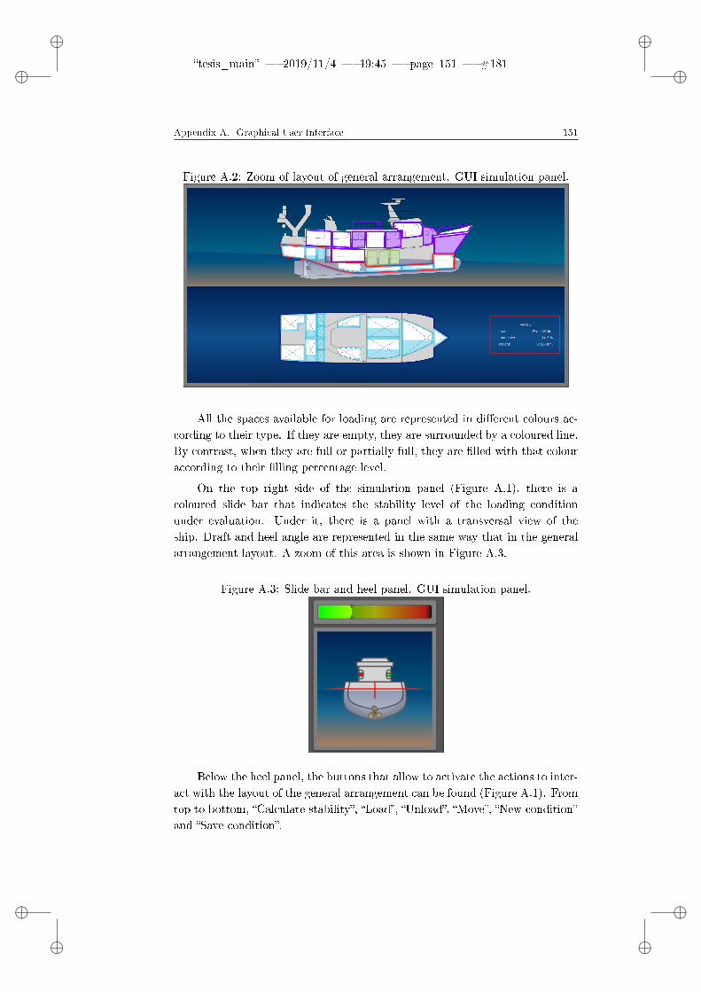
ii


ii

ii

Appendix A. Graphical User Interface 151

Figure A.2: Zoom of layout of general arrangement. GUI simulation panel.

All the spaces available for loading are represented in dierent colours ac-cording to their type. If they are empty, they are surrounded by a coloured line.By contrast, when they are full or partially full, they are lled with that colouraccording to their lling percentage level.

On the top right side of the simulation panel (Figure A.1), there is acoloured slide bar that indicates the stability level of the loading conditionunder evaluation. Under it, there is a panel with a transversal view of theship. Draft and heel angle are represented in the same way that in the generalarrangement layout. A zoom of this area is shown in Figure A.3.

Figure A.3: Slide bar and heel panel. GUI simulation panel.

Below the heel panel, the buttons that allow to activate the actions to inter-act with the layout of the general arrangement can be found (Figure A.1). Fromtop to bottom, Calculate stability, Load, Unload, Move, New conditionand Save condition.

ii


ii

ii


As it is specied in its name, the mission of Calculate stability button isto compute the equilibrium of the loading condition and the stability criteria.Once the calculation is done, a pop-up window is displayed with the results anda clear message about the safety level. An example of this pop-up window whenthere is no risk can be seen in Figure A.4 and an example of a risky situation inFigure A.5. Furthermore, the values of the slide bar, draft, trim and heel angleare updated.

Figure A.4: Stability report no risk. GUI simulation panel.

Figure A.5: Stability report risk. GUI simulation panel.

For a selected tank or compartment, Load button opens a window wherethe weight of the item to load can be introduced. Figure A.6 shows an example

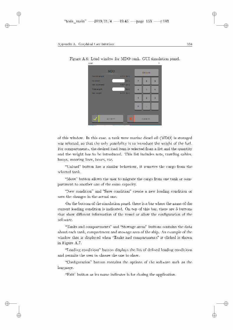
ii


ii

ii


Figure A.6: Load window for MDO tank. GUI simulation panel.

of this window. In this case, a tank were marine diesel oil (MDO) is storagedwas selected, so that the only possibility is to introduce the weight of the fuel.For compartments, the desired load item is selected from a list and the quantityand the weight has to be introduced. This list includes nets, trawling cables,buoys, mooring lines, boxes, etc.

Unload button has a similar behaviour, it removes the cargo from theselected tank.

Move button allows the user to migrate the cargo from one tank or com-partment to another one of the same capacity.

New condition and Save condition create a new loading condition orsave the changes in the actual one.

On the bottom of the simulation panel, there is a bar where the name of thecurrent loading condition is indicated. On top of this bar, there are 5 buttonsthat show dierent information of the vessel or allow the conguration of thesoftware.

Tanks and compartments and Stowage areas buttons contains the dataabout each tank, compartment and stowage area of the ship. An example of thewindow that is displayed when Tanks and compartments is clicked is shownin Figure A.7.

Loading conditions button displays the list of dened loading conditionsand permits the user to choose the one to show.

Conguration button contains the options of the software such as thelanguage.

Exit button as its name indicates is for closing the application.

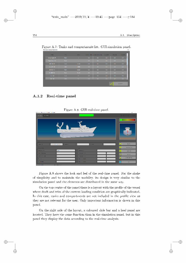
ii


ii

ii


Figure A.7: Tanks and compartments list. GUI simulation panel.

A.1.2 Real-time panel

Figure A.8: GUI real-time panel.

Figure A.8 shows the look and feel of the real-time panel. For the shakeof simplicity and to maintain the usability, its design is very similar to thesimulation panel and the elements are distributed in the same way.

On the top-centre of the panel there is a layout with the prole of the vesselwhere draft and trim of the current loading condition are graphically indicated.In this case, tanks and compartments are not included in the prole view asthey are not relevant for the user. Only important information is shown in thispanel.

On the right side of the layout, a coloured slide bar and a heel panel arelocated. They have the same function than in the simulation panel, but in thispanel they display the data according to the real-time analysis.

ii


ii

ii


Below the layout of the prole view, there are three panels called Inputdata, Wind and waves and Tide.

The rst one contains three variables that are vital for the functionality ofthe real-time module and, in case that they can not be obtained automatically,they have to be manually introduced by the skipper. They are location, speedand draft. As it was mentioned, location and speed are easy to automateconnecting the GPS to the system. Draft is most dicult as usually shingvessels do not have draft sensors.

Wind and waves panel shows numerically the predicted values of wavesand wind parameters obtained from MeteoSIX for that specic location andtime instant. They are wind module, wind direction, signicant wave height,wave peak period and wave direction.

The last panel displays the tide information in the nearest port which isusually needed by the crew for shing purposes.

On the right side of Tide panel, the buttons that activate or deactivatedierent functions of this module can be found. From top to bottom: IMU,Forecast, SGISC and Tide. When this buttons are activated they changetheir state from OFF to ON. There are also two buttons for the congurationof this panel. They are Conguration and Exit.

IMU button is the most important element in this panel. It starts andstops the real-time stability assessment process. Once it is clicked, MeteoSIX iscalled (this option has to be previously activated) and the IMU starts monitoringthe vessel roll motion. Every three minutes the system evaluates the stabilitycriteria, calculates a stability index and the values of trim and heel (obtainedfrom the IMU) are updated in the panels. The alert light and the slide barchange their colours according to the stability index to give awareness to theskipper about the level of stability of the ship. Figure A.9 shows a situationof moderate risk for the vessel. No messages or windows appear to not botherthe crew with an excess of information. As it can be seen the alert light andthe slight bar change their colour to yellow. Only in case of high risk a pop-upwindow with a clear and unequivocal warning message is displayed.

The following buttons (Forecast, SGISC and Tide) enable the Me-teoSIX call, the evaluation of the Second Generation of Intact Stability Criteriaand the tide information. By default, only the Intact Stability Criteria areactivated.

Conguration and Exit buttons have the same function than in simula-tion panel.

Finally, on the bottom of the real-time panel there is a bar where the dateand the temperature is indicated.

ii


ii

ii


Figure A.9: Example of GUI real-time panel in a situation of moderate risk.

ii


ii

ii

Appendix B

Application conguration

B.1 Introduction

One of the requirements of the stability guidance systems is being easy to updateto any modication of the ship structure. Furthermore, in order to guaranteethe low cost of acquisition, installation and maintenance it should be simple toadapt to any other ship design.

The proposed system fulll this requirement as it is an application in whichthe vessel is dened through external conguration les. If these les change, thevessel shown in the application change too. The application was programmedin Java and manages the data base and communicates with the IMU. It readsthe les and generates the model of the vessel. Those les are created by thedesigner and can not be modied by the user. The interaction with the user isexclusively through the graphical user interface.

B.2 Ship denition

The denition of the ship consists of establishing her main characteristics,hull forms, general arrangement and other parameters that may be relevant.The needed conguration les are shown in Table B.1.

Table B.1: Conguration les and their descriptions.

File name Description

condiciones_cargaDirectory where loading conditionswill be saved.

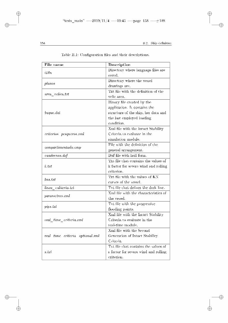
ii


ii

ii

158 B.2. Ship denition



i18nDirectory where language les aresaved.

planosDirectory where the vesseldrawings are.

area_velica.txtTxt le with the denition of thevelic area.

buque.dat

Binary le created by theapplication. It contains thestructure of the ship, her data andthe last employed loadingcondition.

criterios_pesqueros.xmlXml le with the Intact StabilityCriteria to evaluate in thesimulation module.

compartimentado.cmpFile with the denition of thegeneral arrangement.

cuadernas.dxf Dxf le with hull form.

k.txtTxt le that contains the values ofk factor for severe wind and rollingcriterion.

kns.txtTxt le with the values of KNcurves of the vessel.

linea_cubierta.txt Txt le that denes the deck line.

parametros.xmlXml le with the characteristics ofthe vessel.

pips.txtTxt le with the progressiveooding points.

real_time_criteria.xmlXml le with the Intact StabilityCriteria to evaluate in thereal-time module.

real_time_criteria_optional.xmlXml le with the SecondGeneration of Intact StabilityCriteria.

s.txtTxt le that contains the values ofs factor for severe wind and rollingcriterion.

ii


ii

ii

Appendix B. Application conguration 159



s_deadship.txtTxt le that contains the values ofs factor for dead ship criterion.

tipos_carga.xmlXml le with cargo types and theirstowage factor.

tipos_pesos_jos.xmlXml le with a list of the itemsthat can be loaded in the ship.

x1.txtTxt le that contains the values ofx1 factor for severe wind androlling criterion.

x2.txtTxt le that contains the values ofx2 factor for severe wind androlling criterion.

zonas.xmlXml le with the denition of thespaces of the ship.

From all these les only buque.dat is generated by the application andthe others have to be generated by the designer manually or with other tools.Directories have to be created by the designer as well.

All these les have to be saved in a main directory called cong and itsroute has to be introduced in the software as a parameter when it is initialised.

B.2.1 Conguration les characteristics

In this subsection the characteristics of each conguration le are described.

area_velica.txt

This is a txt le with utf8 codication where the coordinates of each pointthat describes the prole view of the vessel are included. The le has twocolumns, the rst one is for the x coordinate (longitudinal position) and thesecond one is the z coordinate (vertical position). The points must be orderedby hull section, starting from the stern to the bow. In addition, they should bewritten from the highest to the lowest zone.

buque.dat

As it was mentioned this le is created by the software and contains allthe needed data of the vessel for its internal operation. If this le does not

ii


ii

ii


exists when the application is executed, it has to be created loading all theparameters of the vessel, creating her structure and dening a default loadingcondition (which is the one corresponding to the lightweight) from the otherles. Otherwise, all the data are read from buque.dat le and the rest areignored.

criterios_pesqueros.xml

This le contain the stability criteria that are evaluated in the simulationmodule. For each criteria their limit standard values and other variables aredened.

compartimentado.cmp

This le should be created in Bentley Maxsurf Stability software and itcontains the denition of the tanks, compartments and stowage areas of thevessel.

cuadernas.dxf

This le should be created in AutoCAD or other similar software and con-tains the curves that dene the hull sections.

k.txt

Txt le with utf8 codication that contains the Table 2.3.4-3 - Values offactor k from International Maritime Organization (2008) for the calculation ofthe severe wind and rolling criterion.

kns.txt

Txt le with utf8 codication that contains the KN curves of the vessel.

linea_cubierta.txt

Txt le with utf8 codication where the deck line is dened. It is composedof three columns, one for each coordinate (x,y,z) of the point.

ii


ii

ii


parametros.xml

It is a xml le that contains the main characteristics of the vessel. Anexample of the structure of this le can be seen in Listing B.1 and the descriptionof each parameter in Table B.2.

Listing B.1: Example of parametros.xml le

<?xml version=" 1 .0 " encoding="UTF−8"?>

<!−−ParÃ½metros d e l buque : pesquero 1Fecha : 29/10/2009−−>

<ship><name>Pesquero 1</name><breadth>6 .2</breadth><depth>2 .9</depth><dra f t>2 .51</ d ra f t><lpp>19</ lpp><sh e l l P l a t t i n g>0 .0</ s h e l l P l a t t i n g><waterDensity>1.025</waterDensity><freeboard>0 .2</ f r e eboard><symmetrical /><xg>9</xg><yg>2</yg><zg>0</zg><weight>80</weight>

</ sh ip>

Table B.2: Parameters description.

Parameter Description

name Name of the vessel

breadth Beam in meters

depth Depth in meters

draft Design draft in meters

lppLength between perpendiculars inmeters

shellPlatting Shell platting coecient

ii


ii

ii


Table B.2: Parameters description.

Parameter Description

waterDensitySea water density in tons per cubicmeters

freeboard Freeboard in meters

symmetricalIf this tag appears it means that thehull sections are symmetric

xgLongitudinal position of the centre ofgravity in meters

ygTransversal position of the center ofgravity in meters

zgVertical position of the center ofgravity in meters

weight Lightweight in tons

pips.txt

Txt le with utf8 codication that contains the progressive ooding points.It has three columns, one for each coordinate (x,y,z).

real_time_criteria.xml

This le contains the Intact Stability Criteria that are evaluated in the real-time module. For each criteria the limit standard values and other variables aredened.

real_time_criteria_optional.xml

This le contains the Second Generation of Intact Stability Criteria thatare evaluated in the real-time module. For each criteria the limit standardvalues and other variables are dened.

s.txt

Txt le with utf8 codication that contains the Table 2.3.4-4 - Values offactor s from International Maritime Organization (2008) for the calculation ofthe severe wind and rolling criterion.

ii


ii

ii


s_deadship.txt

Txt le with utf8 codication that contains the Table 4.2.1 Values ofwave steepness factor from International Maritime Organization (IMO) Sub-Committee on Ship Design and Construction (2018) for the calculation of thedead ship vulnerability level 1.

tipos_carga.xml

Xml le where cargo types and their stowage factor are dened. An exampleof the structure of this le is shown in Listing B.2.

Listing B.2: Example of tiposcarga.xml le.

<t ipos_carga><t ipo><nombre>Ch i l l ed f i s h in wooden boxes</nombre><e s t i b a>0 .7</ e s t i b a></ t ipo><t ipo><nombre>Frozen skinned white f i s h in b locks</nombre><e s t i b a>0.62</ e s t i b a></ t ipo><t ipo><nombre>Frozen white f i s h in boxes</nombre><e s t i b a>0.63</ e s t i b a></ t ipo></ tipos_carga>

This le provides the user the cargo types he can load in each space of thevessel.

tipos_pesos_jos.xml

Xml le with utf8 codication that contains load items of the vessel. Forinstance, nets, trawling cables, trawl doors, buoys, ...

x1.txt

Txt le with utf8 codication that contains the Table 2.3.4-1 - Values offactor X1 from International Maritime Organization (2008) for the calculationof the severe wind and rolling criterion.

ii


ii

ii

164 B.3. Quick guide for conguration

x2.txt

Txt le with utf8 codication that contains the Table 2.3.4-2 - Values offactor X2 from International Maritime Organization (2008) for the calculationof the severe wind and rolling criterion.

zonas.xml

Xml le that numerically denes the spaces of the ship which the user caninteract with. They are:

Selectable decks on the prole view of the vessel in the simulation panel.

Prole view of the vessel for each deck.

Deck views.

Dierent spaces of the vessel with their representation in the prole anddeck views (such as tanks, compartments and holds).

Perpendiculars and base line.

In order to generate this le the images of the prole and deck views are needed.

B.3 Quick guide for conguration

In order to congure a ship in the application it is recommended the fol-lowing steps:

1. Create a directory with the name of the vessel.

2. Create a sub-directory cong.

3. Inside cong folder create planos directory to save there the ship drawings.

4. Inside cong folder create another directory called condiciones_carga forthe future loading conditions.

5. Create the the progressive ooding points le.

6. Create the deck line le.

7. Create les that contains the denition of the hull sections and compart-ments.

ii


ii

ii


8. Copy criterios_pesqueros.xml le in cong directory. This le is only forshing vessels, if a dierent type of vessel is dened in the system it shouldchange for the corresponding stability criteria.

9. Create the le with the load types.

10. Create the le with the ship areas.

11. Create the le with the items that can be load in the vessel.

12. Create the le with the main characteristics of the ship.

13. Execute the application indicating the cong directory. A message sayingthat buque.dat le does not exist and that it will be created will appear.The process can take some time.

ii


ii

ii

ii


ii

ii

Bibliography

Aasen, R., & Hays, B. (2010). Method for nding min and max values of errorrange for calculation of moment of inertia. In 69th Annual Conference ofSociety of Allied Weight Engineers, Inc. Virginia.5.2.2

Albrecht, H.-H. (2001). A family of cosine-sum windows for high-resolutionmeasurements. In Acoustics, Speech, and Signal Processing (pp. 3081 3084).5.2.1.2

Álvarez-Santullano, F. M. (2014). Fishing eort control regulations inuenceon stability, safety and operability of small shing vessels: study of a se-ries of stability related accidents ocurred in Spain between 2004 and 2007(PhD thesis). Escuela Técnica Superior de Ingenieros Navales, Universi-dad Politéctica de Madrid.3.1, 3.3

Antaõ, P., Almeida, T., Jacinto, C., & Soares, C. G. (2008). Causes of occu-pational accidents in the shing sector in Portugal. Safety Science, 46 ,885899. doi: 10.1016/j.ssci.2007.11.0073.2

Ba£kalov, I., Bulian, G., Cichowicz, J., Eliopoulou, E., Konovessis, D., Leguen,J. F., . . . Themelis, N. (2016). Ship stability, dynamics and safety: Statusand perspectives from a review of recent STAB conferences and ISSWevents. Ocean Engineering , 116 , 312349. doi: 10.1016/j.oceaneng.2016.02.0161

Bhattacharyya, R. (1978). Dynamics of marine vehicles. New York: Wiley -Interscience.5.3.1.1

Biran, A., & López Pulido, R. (2014). Ship hydrostatics and stability (2nd ed.).Massachussets, U.S.: Butterworth-Heinemann.5.2.5.1

Bulian, G., & Francescutto, A. (2004). A simplied modular approach for

ii


ii

ii

168 Bibliography

the prediction of the roll motion due to the combined action of wind andwaves. In Proceedings of the Institution of Mechanical Engineers, PartM: Journal of Engineering for the Maritime Environment (Vol. 218, pp.189212). doi: 10.1243/14750900417379585.3.1.1

Bulian, G., & Francescutto, A. (2006). Safety and operability of shing vesselsin beam and longitudinal waves. The Transactions of The Royal Insti-tution Of Naval Architects. Part B, International Journal of Small CraftTechnology , 148 , 116.5.3.1.1, 5.3.1.1, 6.3.1.2

Bulian, G., & Francescutto, A. (2009). Experimental results and numericalsimulations on strongly non-linear rolling of multihulls in moderate beamseas. In Proceedings of the Institution of Mechanical Engineers, Part M:Journal of Engineering for the Maritime Environment (Vol. 223, pp. 189210).5.3.1.1

Bureau of Labor Statistics. (2014). National census of fatal occupational injuriesin 2013 (Preliminary results) (Tech. Rep.). U.S. Department of Labor.3.2

Bye, R., & Lamvik, G. M. (2007). Professional culture and risk perception:Coping with danger on board small shing boats and oshore servicevessels. Reliability Engineering & System Safety , 92 , 17561763. doi:10.1016/j.ress.2007.03.0241, 3.2

Comisión Permanente de Investigación de Siniestros Marítimos. (2012). Memo-ria Anual 2012. Ministerio de Fomento.3.2, 3.4, B.3

Comisión Permanente de Investigación de Siniestros Marítimos. (2017). Memo-ria anual 2017 (Tech. Rep.). Ministerio de Fomento. Gobierno de España.3.2

Dätig, M., & Schlurmann, T. (2004). Performance and limitations of theHilbert-Huang transformation (HHT) with an application to irregular wa-ter waves. Ocean Engineering , 31 , 17831834. doi: 10.1016/j.oceaneng.2004.03.0076.2, 6.2.2, 6.2.3, 6.2.3

Davenport, A. G. (1961). The spectrum of horizontal gustiness near the groundin high winds. Quarterly Journal of the Royal Meteorological Society ,87 (372), 194211. doi: 10.1002/qj.497087372085.3.1.1

Deakin, B. (2005). Development of simplied stability and loading informationfor shermen. RINA, Royal Institution of Naval Architects International

ii


ii

ii

Bibliography 169

Conference - Fishing Vessels, Fishing Technology and Fisheries, 3746.1, 3.2, 3.4, 3.4, 3.4, 8.2.1.1

Dieck, R. H. (2007). Measurement uncertainty. Methods and applications (4thed.). ISA.5.2.1.3, 5.2.4.1

European Commission. (2014). Facts and gures on the Common FisheriesPolicy - 2014 Edition. doi: 10.2771/357453.3, B.3

European Maritime Safety Agency. (2018). Annual overview of marine casual-ties and incidents 2018. European Maritime Safety Agency , 1135.3.2

European Market Observatory for Fisheries and Aquaculture Products. (2018).El mercado pesquero de la UE (Tech. Rep.). Comisión Europea.3.1

European Union. (2002). Commission Directive 2002/35/EC of 25 April 2002amending Council Directive 97/70/EC setting up a harmonised safetyregime for shing vessels of 24 metres in length and over.3.3

Fang, S., Blanke, M., & Leira, B. J. (2015). Mooring system diagnosis and struc-tural reliability control for position moored vessels. Control EngineeringPractice, 36 , 1226. doi: 10.1016/j.conengprac.2014.11.0096.2

FAO. (2018). Fishing techniques. Midwater pair trawling. Rome, Italy.5.41, B.3

Fernández Polo, J. C., & Neves, M. A. S. (2012). Desarrollos recientes de nuevoscriterios de estabilidad intacta de buques en olas. In Simposio Panamer-icano de Ingeniería Naval, Transporte Marítimo e Ingeniería Portuaria(pp. 122). Lima, Perú.3.3

Ferreiro Garcia, R., Antonio, C., & Ameal, F. (2001). Ship stability monitoringby motion frequency analysis. IFAC Proceedings Volumes, 34 (7), 3943.doi: 10.1016/s1474-6670(17)35056-53.5

FOM. (2017). Predicción de oleaje, nivel del mar; boyas y mareógrafos (Tech.Rep.). Ministerio de Fomento, Gobierno de España.5.3.1.1

Francescutto, A. (2013). The evolution of the regulatory stability regime forshing vessels. In International Conference IDS2013 - Amazonia. Iquitos,Perú.3.3

Francescutto, A. (2015). Intact Stability Criteria of ships - past, present and

ii


ii

ii

170 Bibliography

future. In Proceedings of the 12th International Conference on the Stabilityof Ships and Ocean Vehicles. Glasgow, UK.3.3

Francescutto, A., & Papanikolaou, A. D. (2010). Floatability and stabilityof ships: 23 centuries after Archimides. In Proceedings of the Geniusof Archimedes - 23 Centuries of Inuence on Mathematics, Science andEngineering. Syracuse, Italy. doi: 10.1007/978-90-481-9091-13.3

Galeazzi, R., Blanke, M., Falkenberg, T., Poulsen, N. K., Violaris, N., Storhaug,G., & Huss, M. (2015). Parametric roll resonance monitoring usingsignal-based detection. Ocean Engineering , 109 , 355371. doi: 10.1016/j.oceaneng.2015.08.0376.2

Galeazzi, R., Blanke, M., & Poulsen, N. K. (2013). Early detection of parametricroll resonance on container ships. IEEE Transactions on Control SystemsTechnology , 21 (2), 489503. doi: 10.1109/TCST.2012.21893996.2

Gefaell Chamochín, G. (2005). Algunas consideraciones sobre la estabilidady seguridad de los buques pesqueros menores de 24 m de eslora. SectorPesquero.1, 3.2, 3.3, 3.4, 3.4

Ghane, M., Rasekhi Nejad, A., Blanke, M., Gao, Z., & Moan, T. (2018).Condition monitoring of spar-type oating wind turbine drivetrain usingstatistical fault diagnosis. Wind Energy , 21 (7), 575589. doi: 10.1002/we.21796.2

Grimson, G. S. (1975). Report of Court No. S 497. Formal investigation onM.F.V. Trident (on PD111) (Tech. Rep.). London, UK.5.2.5.2

Gudmundsson, A. (2013). The FAO / ILO / IMO safety recommendations fordecked shing vessels of less than 12 metres in length and undecked shingvessels â a major milestone to improve safety for small shing vessels. InProceedings of the 13th International Ship Stability Workshop (pp. 19).Brest.3.1

Gupta, R., Kumar, A., & Bahl, R. (2014). Estimation of instantaneous fre-quencies using iterative empirical mode decomposition. Signal, Image andVideo Processing , 8 , 799812. doi: 10.1007/s11760-012-0305-56.2, 6.2.2

Haddara, M. R., Wishahy, M., & Wu, X. (1994). Assessment of ship's transversestability at sea. Ocean Engineering , 21 (8), 781800.

ii


ii

ii

Bibliography 171

3.5Hansen, S., & Blanke, M. (2014). Diagnosis of airspeed measurement faults for

unmanned aerial vehicles. IEEE Transactions on Aerospace and ElectronicSystems, 50 (1), 224239. doi: 10.1109/TAES.2013.1204206.2

Hanzu-Pazara, R., Duse, Varsami, C., Andrei, C., & Dumitrache, R. (2016).The inuence of ship's stability on safety of navigation. IOP ConferenceSeries: Materials Science and Engineering , 145 . doi: 10.1088/1757-899X/145/8/0820191, 3.2

Harris, F. J. (1978). On the use of windows for harmonic analysis with thediscrete Fourier transform. Proceedings of the IEEE , 66 , 5183. doi:10.1109/PROC.1978.108375.2.1.2

Huang, N., Shen, Z., Long, S., Wu, M., Shih, H., Zheng, Q., . . . Liu, H. (1998).The empirical mode decomposition and the Hilbert spectrum for nonlinearand non-stationary time series analysis. In Proceedings of the Royal SocietyA: Mathematical, Physical and Engineering Sciences (Vol. 454, pp. 903995). doi: 10.1098/rspa.1998.01936.2, 6.2.2, 6.2.3, 6.2.3

International Maritime Organization. (1993). Resolution A.749(18). Code onIntact Stability for all types of ships covered by IMO instruments.4.3

International Maritime Organization. (1995). MSC/Circ.707 Guidance to themaster for avoiding dangerous situations in following and quartering seas.1, 3.3

International Maritime Organization. (2005a). Code of Safety for Fishermenand Fishing Vessels 2005: Part A: Safety and Health Practice.3.3

International Maritime Organization. (2005b). Code of Safety for Fishermenand Fishing Vessels (Part B): Safety and health requirements for the con-struction and equipment of shing vessels.3.3

International Maritime Organization. (2007). MSC.1/Circ.1228 Revised guid-ance to the master for avoiding dangerous situations in adverse weatherand sea conditions.1, 3.3, 3.4

International Maritime Organization. (2008). International Code on IntactStability (2008 IS Code).3.3, 4.3, B.2.1, B.2.1, B.2.1, B.2.1

International Maritime Organization. (2012). Cape Town Agreement of 2012

ii


ii

ii

172 Bibliography

on the implementation of the provisions of the Torremolinos Protocol of1993 relating to the Torremolinos International Convention for the safetyof shing vessels, 1977.1, 3.3, 3.4, 5.2.5.1, 6.2.3.1, 6.2.4, 6.3.1.1, 8.2.1.1, 8.2.2, 8.2.2.1

International Maritime Organization (IMO) Sub-Committee on Ship Design andConstruction. (2018). SDC 6/5 Finalization of second generation intactstability criteria.1, 3.3, 8.2.2, 8.2.2.1, B.2.1

International Towing Tank Conference. (2002). The Specialist Committee onWaves. Final Report and Recommendations to the 23rd ITTC. In Pro-ceedings of the 23rd International Towing Tank Conference. Venice, Italy.5.3.1.1, 6.3.1.3, 7.2.2

Jensen, O. C. C., Petursdottir, G., Holmen, I. M., Abrahamsen, A., & Lincoln,J. (2014). A review of fatal accident incidence rate trends in shing. In-ternational Maritime Health, 65 (2), 4752. doi: 10.5603/IMH.2014.00113.2

Kay, S. M. (1998). Fundamentals of statistical signal proccessing: detectiontheory. Englewood Clis: Prentice-Hall, Inc.6.2.4, 6.2.4

Kobylinski, L. (2012). Stability Criteria - 50 years of Experience and FutureProspects. In Proceedings of the 11th International Conference on Stabilityof Ships and Ocean Vehicles (pp. 91100). Athens, Greece.1, 3.3

Krata, P. (2008). Total losses of shing vessels due to the insucient sta-bility. International Journal on Marine Navigation and Safety of SeaTransportation, 2 (3), 311315.1, 3.2, 3.2, 3.2

Krüger, S., & Kluwe, F. (2008). A simplied method for the estimation of thenatural roll frequency of ships in heavy weather. HANSA InternationalMaritime Journal , 9 .4.2, 5.2.2

Lazakis, I., Kurt, R. E., & Turan, O. (2014). Contribution of human factors toshing vessels accidents and near misses in the UK. Journal of Shippingand Ocean Engineering , 4 , 245261. doi: 10.1037/0033-3204.44.3.01, 3.2, 3.2

Lewis, E. V. (1988). Principles of Naval Architecture (Second Revision), VolumeI - Stability and Strength. Jersey City: Society of Naval Architects andMarine Engineers (SNAME).1

López Sieiro, M. (n.d.). Tipología de Buques Pesqueros, Gestión de Infraestruc-turas Portuarias y Servicios de Pesca. Xunta de Galicia.

ii


ii

ii

Bibliography 173

3.1Lucas, D. L., & Case, S. L. (2018). Work related mortality in the US shing

industry during 2000 2014: New ndings based on improved workforceexposure estimates. American Journal of Industrial Medicine, 61(1), 2131.3.2

Marine Accident Investigation Branch (MAIB). (2008). Analysis of UK FishingVessel Safety 1992 to 2006 (Tech. Rep.). Southampton. Retrieved fromwww.maib.gov.uk

3.2, 3.2, 3.4Medina, J. (2010). Análisis de Fourier para el tratamiento de señales. In XII

Encuentro de Matemáticas y sus Aplicaciones (pp. 139). Quito, Ecuador.4.5, 5.2.1

MeteoGalicia. (2014). MeteoSIX API Documentation version v3 (Tech. Rep.).8.2.2.3

Míguez González, M. (2012). A study of ship parametric roll resonance for theevaluation of preventive strategies (PhD thesis). Universidade da Coruña.5.2.5.1, 5.26, 5.2.5.2, B.3

Míguez González, M., & Bulian, G. (2018). Inuence of ship dynamics modellingon the prediction of shing vessels roll response in beam and longitudinalwaves. Ocean Engineering , 148 , 312330. doi: 10.1016/j.oceaneng.2017.11.0325.2.5.1, 5.3.1.1

Míguez González, M., Bulian, G., Santiago Caamaño, L., & Díaz Casás, V.(2017). Towards real-time identication of initial stability from ship rollmotion analysis. In Proceedings of the 16th International Ship StabilityWorkshop. Belgrade, Serbia.5.2.5.1, 5.7, 5.31, 5.3, 5.26, 5.32, 5.27, 5.33, 5.34, 5.35, 5.36, 9.1, B.3, B.3

Míguez González, M., Caamaño Sobrino, P., Tedín Álvarez, R., Díaz Casás, V.,& Martínez López, A. (2010). Un sistema embarcado de evaluación dela estabilidad y ayuda al patrón de buques de pesca. Ingeniería Naval(Madrid), 79 (880), 9097.3.4, 8.2.1

Míguez González, M., Deibe, Á., Orjales, F., & Priego, B. (2015). An au-tonomous scale ship model for parametric rolling towing tank testing. InR. Duro & Y. Kondratenko (Eds.), Advances in intelligent robotics andcollaborative automation (pp. 4972).5.2.5.2

Míguez González, M., Santiago Caamaño, L., & Díaz Casás, V. (2018). Onthe applicability of real time stability monitoring for increasing the safetyof shing vessels. In Proceedings of the 13rd International Conference on

ii


ii

ii

174 Bibliography

the Stability of Ships and Ocean Vehicles. Kobe, Japan. doi: 10.1016/j.oceaneng.2018.04.0025.37, 5.28, 5.38, 5.39, 5.30, 5.40, 5.42, B.3, B.3

Míguez González, M., Sobrino Caamaño, P., Tedín Álvarez, R., Díaz Casás,V., Martínez López, A., & López Peña, F. (2012). Fishing vessel sta-bility assessment system. Ocean Engineering , 41 , 6778. doi: 10.1016/j.oceaneng.2011.12.0211, 3.2, 3.2, 3.2, 3.4, 3.4, 3.2, 3.4, 3.3, 3.4, 3.7, 8.2.1, A.1, B.3

Ministerio de Agricultura Pesca y Alimentación. (2017). Estadísticas pesqueras(Tech. Rep.). Gobierno de España. Retrieved from http://www.magrama

.gob.es/es/estadistica/temas/estadisticas-pesqueras/

3.1Ministerio de Agricultura Pesca y Alimentación. (2018). Estadísticas Pesqueras

(Tech. Rep.). Gobierno de España. Retrieved from http://www.mapa.gob

.es/es/estadistica/temas/estadisticas-pesqueras/

3.1, 3.1, 3.2, B.3Ministerio de Empleo y Seguridad Social. (2013). Estadísticas de Accidentes

de Trabajo (Tech. Rep.). Gobierno de España. Retrieved from http://

publicacionesoficiales.boe.es/

3.2Ministerio de Fomento. (2007). Real Decreto 543/2007, de 27 de abril, por el que

se determinan las normas de seguridad y prevención de la contaminacióna cumplir por los buques pesqueros menores de 24 metros de eslora (L).3.3, 8.2.1.1, 8.2.2, 8.2.2.1

Molyneux, D. (2008). Tha safety of small boats (including shing boats) againstcapsize: a review. NRC Publications Archive. doi: 10.1016/j.biotechadv.2008.05.0073.3

Moreno Reyes, F. J. (2012). Portal del Sector Marítimo Pesquero. Instituto deSeguridad e Higiene en el Trabajo.3.2

Murdey, D. (2014). International Towing Tank Conference. Retrieved 2019-02-05, from https://ittc.info/

3.3Neves, M. A. S., Pérez, N., & Lorca, O. (2002). Experimental analysis on

parametric resonance for two shing vessels in head seas. In Proceedingsof the 6th International Ship Stability Workshop. Webb Institute, NewYork.5.2.5.2

Neves, M. A. S., Pérez, N., & Lorca, O. (2003). Analysis of roll motion andstability of a shing vessel in head seas. Ocean Engineering , 30 (7), 921

ii


ii

ii

Bibliography 175

935. doi: 10.1016/S0029-8018(02)00066-55.2.5.2

Neves, M. A. S., Pérez, N. A., & Valerio, L. (1999). Stability of small shingvessels in longitudinal waves. Ocean Engineering , 26 (12), 13891419. doi:10.1016/S0029-8018(98)00023-75.2.5.2

Neves, M. A. S., & Rodríguez, C. A. (2005). A coupled third order model of rollparametric resonance. In 12th International Congress of the InternationalMaritime Association of the Mediterranean (IMAM). Lisbon, Portugal.5.2.5.2

Neves, M. A. S., & Rodríguez, C. A. (2006). On unstable ship motions resultingfrom strong non-linear coupling. Ocean Engineering , 33 (14-15), 18531883. doi: 10.1016/j.oceaneng.2005.11.0095.2

Neves, M. A. S., Rodríguez, C. A., & Merino, J. A. (2009). Estabilidad dinámicade buques en olas. Ciencia & Tecnología de buques, 2 , 2336.3.3

Neves, M. A. S., Rodríguez, C. A., Merino, J. A., Mañuico Vivanco, J. E., Vil-lagómez Rosales, J. C., & Agarwal, R. (2009). Efecto de la Aplicación deTanques Estabilizadores Anti-Roll para prevenir la resonancia paramet-rica. In Congreso Panamericano de Ingeniería Naval (COPINAVAL).5.2.5.2

Oliva Remolà, A., & Gudmundsson, A. (2018). Global review of safety atsea in the sheries sector (Tech. Rep.). Rome: Food and AgricultureOrganization.3.2

Oliveira-Goumas, B., & El Houdagui, R. (2000). Information note sh 501 EN:Safety and the causes of accidents in the sheries sector (Tech. Rep.).European Parliament.3.2

Oppenheim, A. V., Schafer, R. W., & Buck, J. R. (1999). Discrete time signalprocessing (2nd ed.). Upper Saddle River, New Jersey: Prentice-Hall, Inc.4.4, 5.2.1, 5.2.1, 5.2.1.2

Paett, J. A. H. (1976). Experiments with a model of MFV Trident and an alter-native round-stern design (Tech. Rep.). Feltham, UK: National MaritimeInstitute (NMI) Ltd.5.2.5.2

Pascoal, R., Guedes Soares, C., & SoÌºrensen, A. J. (2007). Ocean wave spec-tral estimation using vessel wave frequency motions. Journal of OshoreMechanics and Arctic Engineering , 129 (2), 90. doi: 10.1115/1.24269864.5

ii


ii

ii

176 Bibliography

Pérez M., N. A., & Sanguinetti, C. F. (2006). Scale model tests of a shingvessel in roll motion parametric resonance. Síntesis Tecnológica, 3 (1),3337. doi: 10.4206/sint.tecnol.2006.v3n1-045.2.5.2

Petursdottir, G., Hannibalsson, O., & Turner, J. M. M. (2001). Safety at seaas an integral part of sheries management. FAO Fisheries Circular. No.966 .1, 3.2, 3.2, 3.3

Piniella, F., Soriguer, M. C., & Fernández-Engo, M. A. (2007). Artisanal shingin Andalusia: A statistical study of the eet. Marine Policy , 31 (4), 573581. doi: 10.1016/j.marpol.2006.10.0043.1

Pradhan, C., & Gupta, A. (2017). Ship detection using Neyman-Pearson crite-rion in marine environment. Ocean Engineering , 143 (February), 106112.doi: 10.1016/j.oceaneng.2017.03.0086.2

Proakis, J. G., & Manolakis, D. G. (1996). Digital signal processing. Principles,algorithms and applications (3rd ed.). Upper Saddle River, New Jersey:Prentice-Hall, Inc.4.4, 4.5

Roberts, S. E. (2002). Hazardous occupations in Great Britain. Lancet , 360 ,543544. doi: 10.1016/S0140-6736(02)09708-81, 3.2, 3.2

Rodríguez, C. A. (2010). Análise não linear da ressonância paramétrica do bal-anço de navios (Master's thesis). Universidade Federal do Rio de Janeiro,Rio de Janeiro, Brazil.5.2.5.2

Rodríguez Castillo, C. A. (2008). Análisis de la estabilidad de pesqueros en olasregulares de proa (Master's thesis). Universidad Nacional de IngenieríaLima Peru.3.3, 5.2.5.2

Royal Institution of Naval Architects. (2011). RINA Forum on the safety ofsmall shing vessels, 19 July 2011, London (Tech. Rep.). London.1

Santiago Caamaño, L., Galeazzi, R., Míguez González, M., Díaz Casás, V.,& Nielsen, U. D. (2019). Experimental validation of transverse stabilitymonitoring system for shing vessels. In 12th IFAC Conference on ControlApplications in Marine Systems, Robotics and Vehicles. Daejeon, Korea.6.8, 6.9, 6.14, 6.15, 6.16, 6.17, B.3, B.3

Santiago Caamaño, L., Galeazzi, R., Nielsen, U. D., Míguez González, M., &Díaz Casás, V. (2019). Real-time detection of transverse stability changes

ii


ii

ii

Bibliography 177

in shing vessels. Ocean Engineering .5.2.5.1, 6.1, 6.2, 6.3, 6.3.1.1, 6.3, 6.4, 6.4, 6.5, 6.6, 6.7, 6.5, 6.8, 6.6, 6.7,B.3, B.3

Santiago Caamaño, L., Míguez González, M., & Díaz Casás, V. (2018a). Improv-ing the safety of shing vessels trough roll motion analysis. In Proceedingsof the ASME 2018 37th International Conference on Ocean Oshore andArtic Engineering. Madrid, Spain.5.2.5.1, 8.1, B.3

Santiago Caamaño, L., Míguez González, M., & Díaz Casás, V. (2018b). Onthe feasibility of a real time stability assessment for shing vessels. OceanEngineering , 159 , 7687. doi: 10.1016/j.oceaneng.2018.04.0025.1, 5.2.5.1, 5.1, 5.4, 5.5, 5.10, 5.11, 5.12, 5.13, 5.14, 5.15, 5.16, 5.17, 5.18,5.19, 5.24, 5.20, 5.21, 5.22, 5.23, 5.25, 5.14, 5.15, 5.16, B.3, B.3

Santiago Caamaño, L., Míguez González, M., Galeazzi, R., Nielsen, U. D., &Díaz Casás, V. (2019). On the application of change detection techniquesfor the stability monitoring of shing vessels. In Proceedings of the 17thInternational Ship Stability Workshop. Helsinki, Finland.7.2.1, 7.1, 7.2, 7.1, 7.3, 7.2, 7.4, B.3, B.3

Scarponi, M. (2017). Use of the Wolfson stability guidance for appraising theoperational stability of small shing vessels. In Proceedings of the 16thInternational Ship Stability Workshop. Belgrade, Serbia.1, 3.2

Ship Stability Dynamics and Safety (ShipStab). (2019). STAB/ISSW - History.Retrieved 2019-02-05, from http://www.shipstab.org/

3.3Smith, S. W. (2002). Digital signal processing: A practical guide for engineers

and scientists (1st ed.). Newnes.4.4

Stearns, S. D. (2003). Digital signal processing with examples in MATLAB(A. Poularikas, Ed.). CRC Press.4.5, 5.2.1, 5.2.1

Tello, M., Ribeiro e Silva, S., & Guedes Soares, C. (2011). Seakeeping per-formance of shing vessels in irregular waves. Ocean Engineering , 38 ,763773.3.4

Terada, D., Hashimoto, H., Matsuda, A., & Umeda, N. (2018). Direct esti-mation of natural roll frequency using onboard data based on a Bayesianmodeling procedure. In Proceedings of the 13th International Conferenceon the Stability of Ships and Ocean Vehicles. Kobe, Japan.1, 3.5

Terada, D., Tamashima, M., Nakao, I., & Matsuda, A. (2016). Estimation

ii


ii

ii

178 Bibliography

of the metacentric height by using onboard monitoring roll data based ontime series analysis. In Proceedings of the 15th International Ship StabilityWorkshop. Stockholm, Sweden.1, 3.5

Transportation Safety Board of Canada. (2012). Marine investigation report.Safety issues investigation into shing safety in Canada. Report NumberM09Z0001 (Tech. Rep.).3.1, 3.2, B.3

Umeda, N., & Francescutto, A. (2016). Current state of the second generationintact stability criteria achievements and remaining issues. In Proceedingsof the 15th International Ship Stability Workshop (pp. 39).3.3, 8.2.2.1

Varela, S. M., Guedes Soares, C., & Santos, T. (2010). Monitoring systemfor safety of shing vessels subjected to waves. The Portuguese MaritimeSector , 110.3.4, 3.4, 3.5, 3.4, 3.6, B.3

Viggosson, G. (2009). The Icelandic information system on weather and seastate related to shing vessels crews and stability. In World Fishing Ex-hibition. Vigo, Spain.3.4

Wandji, C., Veritas, B., & Corrignan, P. (2012). Test Application of SecondGeneration IMO Intact Stability Criteria on a Large Sample of Ships.Proceedings of the 11th International Conference on Stability of Ships andOcean Vehicles(September), 145155.3.3

Wawrzynski, W., & Krata, P. (2016). Method for ship's rolling period predictionwith regard to non-linearity of GZ curve. Journal of Theoretical andApplied Mechanics, 13291343. doi: 10.15632/jtam-pl.54.4.13291, 3.5

Willersrud, A., Blanke, M., Member, S., Imsland, L., & Pavlov, A. (2015). Drill-string washout diagnosis using friction estimation and statistical changedetection. IEEE Transactions on Control Systems Technology , 23 (5),18861900. doi: 10.1109/TCST.2015.23942436.2

Wolfson Unit. (2004). Research project 530. Simplied presentation of FVstatibility information - phase 1. Final report (Vol. 44; Tech. Rep. No. 4).Univeristy of Southampton.1, 3.2, 3.2, 3.2, 3.4, 3.4, 3.4

Wolfson Unit. (2006). Research Project 560. Simplied presentation of FVstability information for vessels 12 m registered length and over. PhaseII. Final Report (Tech. Rep.). University of Southampton. doi: 10.1787/

ii


ii

ii

Bibliography 179

9789264107687-2-en8.2.1.1, 8.2.1.1

Womack, J. (2003). Small commercial shing vessel stability analysis: Whereare we now? Where are we going? Marine Technology , 40 (4), 296302.3.3, 3.4

Xie, H., & Wang, Z. (2006). Mean frequency derived via Hilbert-Huangtransform with application to fatigue EMG signal analysis. ComputerMethods and Programs in Biomedicine, 82 , 114120. doi: 10.1016/j.cmpb.2006.02.0096.2.3

Young, S. T. (2011). Report on the Rehearing of the formal investigation into theloss of the motor shing vessel "Trident", registered at Peterhead (Ocialnumber PD111) (Tech. Rep.). Aberdeen, UK.5.2.5.2

ii


ii

ii

ii


ii

ii

List of Figures

3.1 Cumulative percentage of fatalities by accident type, 1999-2010(Transportation Safety Board of Canada, 2012) . . . . . . . . . . 14

3.2 Example of Womack stability matrix (Míguez González et al.,2012) . . . . . . . . . . . . . . . . . . . . . . . . . . . . . . . . . . 25

3.3 Example of Womack stability matrix including environmentalconditions (Míguez González et al., 2012) . . . . . . . . . . . . . 26

3.4 Example of Norwegian stability poster (Míguez González et al.,2012) . . . . . . . . . . . . . . . . . . . . . . . . . . . . . . . . . . 26

3.5 SEMPEO, layout of the static stability analysis module Varelaet al. (2010) . . . . . . . . . . . . . . . . . . . . . . . . . . . . . . 27

3.6 SEMPEO, layout of the wave safety analysis module Varela etal. (2010) . . . . . . . . . . . . . . . . . . . . . . . . . . . . . . . 28

3.7 Safe Skipper (Míguez González et al., 2012) . . . . . . . . . . . . 29

4.1 Summary of the purpose of the thesis. . . . . . . . . . . . . . . . 33

5.1 Metacentric height estimation by FFT-methodology (SantiagoCaamaño et al., 2018b). . . . . . . . . . . . . . . . . . . . . . . . 38

5.2 Example of a roll transfer function for a shing vessel in beamwaves at zero speed. . . . . . . . . . . . . . . . . . . . . . . . . . 39

5.3 Hanning window . . . . . . . . . . . . . . . . . . . . . . . . . . . 42

5.4 Blackman window . . . . . . . . . . . . . . . . . . . . . . . . . . 43

5.5 Blackman-Harris window . . . . . . . . . . . . . . . . . . . . . . 43

5.6 Hull form of the mid-sized stern trawler. . . . . . . . . . . . . . . 48

5.7 GZ curve in calm water (Míguez González et al., 2017). . . . . . 48

5.8 Curve of areas of the test vessel. . . . . . . . . . . . . . . . . . . 53

ii


ii

ii

182 List of Figures

5.9 Amidship section of the test vessel. . . . . . . . . . . . . . . . . . 53

5.10 Experiment 13. Roll motion time series. Regular waves. Fn=0.1.Parametric roll occurs (Santiago Caamaño et al., 2018b). . . . . 54

5.11 Experiment 13. Roll spectrum. Regular waves. Fn=0.1. Para-metric roll occurs (Santiago Caamaño et al., 2018b). . . . . . . . 55

5.12 Experiment 7. Roll motion time series. Regular waves. Fn=0.No parametric roll (Santiago Caamaño et al., 2018b). . . . . . . . 55

5.13 Experiment 7. Roll spectrum. Regular waves. Fn=0. No para-metric roll (Santiago Caamaño et al., 2018b). . . . . . . . . . . . 56

5.14 Experiment 37. Roll motion time series. Irregular waves. Fn=0.Parametric roll occurs (Santiago Caamaño et al., 2018b). . . . . 56

5.15 Experiment 37. Roll spectrum. Irregular waves. Fn=0. Para-metric roll occurs (Santiago Caamaño et al., 2018b). . . . . . . . 56

5.16 Experiment 46. Roll motion time series. Irregular waves. Fn=0.1.No parametric roll (Santiago Caamaño et al., 2018b). . . . . . . . 57

5.17 Experiment 46. Roll spectrum. Irregular waves. Fn=0.1. Noparametric roll Santiago Caamaño et al. (2018b). . . . . . . . . . 57

5.18 Natural roll frequency estimation results. Regular waves. Fn=0(Santiago Caamaño et al., 2018b). . . . . . . . . . . . . . . . . . 58

5.19 Natural roll frequency estimation results. Irregular waves. Fn=0(Santiago Caamaño et al., 2018b). . . . . . . . . . . . . . . . . . 58

5.24 Natural roll frequency estimation results. Regular waves. Fn=0.3(Santiago Caamaño et al., 2018b). . . . . . . . . . . . . . . . . . 58

5.20 Natural roll frequency estimation results. Regular waves. Fn=0.1Santiago Caamaño et al. (2018b). . . . . . . . . . . . . . . . . . . 59

5.21 Natural roll frequency estimation results. Irregular waves. Fn=0.1Santiago Caamaño et al. (2018b). . . . . . . . . . . . . . . . . . . 59

5.22 Natural roll frequency estimation results. Regular waves. Fn=0.2Santiago Caamaño et al. (2018b). . . . . . . . . . . . . . . . . . . 59

5.23 Natural roll frequency estimation results. Irregular waves. Fn=0.2(Santiago Caamaño et al., 2018b). . . . . . . . . . . . . . . . . . 60

5.25 Natural roll frequency estimation results. Irregular waves. Fn=0.3(Santiago Caamaño et al., 2018b). . . . . . . . . . . . . . . . . . 60

5.26 Test vessel: hull form (Míguez González, 2012). . . . . . . . . . . 66

5.27 Vessel scale model. . . . . . . . . . . . . . . . . . . . . . . . . . . 66

5.28 Model arrangement. . . . . . . . . . . . . . . . . . . . . . . . . . 67

ii


ii

ii

List of Figures 183

5.29 Experiment 45. Roll motion time series. Regular waves. . . . . . 73

5.30 Experiment 35. Roll spectrum. Regular waves. . . . . . . . . . . 74

5.31 Proposed methodology (Míguez González et al., 2017). . . . . . . 75

5.32 Eective wave slope coecient (Míguez González et al., 2017). . 78

5.33 Roll motion time series. Irregular beam waves. Lateral gustywind (Míguez González et al., 2017). . . . . . . . . . . . . . . . . 79

5.34 Left: Roll natural frequency estimates. Right: representation ofestimated roll natural frequency distribution through minimumobserved value, 5%, 25%, 50% (median), 75% and 95% estimatedpercentiles, and maximum observed value (Míguez González etal., 2017). . . . . . . . . . . . . . . . . . . . . . . . . . . . . . . . 79

5.35 Sample case 1. Estimated roll spectrum (Míguez González et al.,2017). . . . . . . . . . . . . . . . . . . . . . . . . . . . . . . . . . 80

5.36 Sample case 2. Estimated roll spectrum (Míguez González et al.,2017). . . . . . . . . . . . . . . . . . . . . . . . . . . . . . . . . . 80

5.37 Test vessel: hull form (Míguez González et al., 2018). . . . . . . . 81

5.38 Test vessel. Photo courtesy of José R. Montero (Míguez Gonzálezet al., 2018). . . . . . . . . . . . . . . . . . . . . . . . . . . . . . . 82

5.39 Sea trial area and SeaWatch buoy position (Míguez González etal., 2018). . . . . . . . . . . . . . . . . . . . . . . . . . . . . . . . 83

5.40 Roll motion time series (Míguez González et al., 2018). . . . . . . 84

5.41 Pair trawling (FAO, 2018). Situation of the test vessel is high-lighted. . . . . . . . . . . . . . . . . . . . . . . . . . . . . . . . . 85

5.42 Roll natural frequency estimation results (Míguez González etal., 2018). . . . . . . . . . . . . . . . . . . . . . . . . . . . . . . . 85

6.1 Architecture of the transverse stability monitoring system (San-tiago Caamaño, Galeazzi, Nielsen, et al., 2019). . . . . . . . . . . 91

6.2 Probability plot of the roll natural frequency estimates for load-ing conditions LC 1, LC 4 and LC 6, where ω0 = 0.804 rad/s,ω0 = 0.563 rad/s and ω0 = 0.514 rad/s respectively, and SeaState 1. Logistic, t-location scale, Weibull and double Weibulldistributions are tted to the data (Santiago Caamaño, Galeazzi,Nielsen, et al., 2019). . . . . . . . . . . . . . . . . . . . . . . . . . 96

ii


ii

ii

184 List of Figures

6.3 Histograms of ω0. (a) Loading condition far from ω0max ; (b)loading condition near ω0max without ltering; (c) loading condi-tion near ω0max after ltering. The blue line is the tted Weibulldistribution (Santiago Caamaño, Galeazzi, Nielsen, et al., 2019). 100

6.4 GZ curves for the dierent tested loading conditions in calmwater (Santiago Caamaño, Galeazzi, Nielsen, et al., 2019). . . . . 103

6.5 Auto-correlation function of the driving signal (Santiago Caa-maño, Galeazzi, Nielsen, et al., 2019). . . . . . . . . . . . . . . . 105

6.6 Top to bottom. Roll motion time series, natural roll frequencyestimations, output of the detector and output of the awarenessalarm in irregular waves. Sea State 7. Hs = 8.520 m, ωw =

0.491 rad/s, Sw = 1/30. The orange line represents the thresholdγ′ (Santiago Caamaño, Galeazzi, Nielsen, et al., 2019). . . . . . . 108

6.7 Top to bottom. Roll motion time series, natural roll frequencyestimations, output of the detector and output of the aware-ness alarm in irregular waves. Sea State 17. Hs = 0.600 m,ωe = 1.008 rad/s, Sw = 1/100. The orange line represents thethreshold γ′ (Santiago Caamaño, Galeazzi, Nielsen, et al., 2019). 109

6.8 Median and standard deviation of natural roll frequency esti-mates. All load cases. Sea States 1 to 6 (Santiago Caamaño,Galeazzi, Nielsen, et al., 2019). . . . . . . . . . . . . . . . . . . . 113

6.9 Median and standard deviation of natural roll frequency esti-mates. All load cases. Sea States 7 to 12. . . . . . . . . . . . . . 113

6.10 Median and standard deviation of natural roll frequency esti-mates. All load cases. Sea States 13 to 18. . . . . . . . . . . . . . 114

6.11 Ship scale model. . . . . . . . . . . . . . . . . . . . . . . . . . . . 116

6.12 University of A Coruña tank. . . . . . . . . . . . . . . . . . . . . 117

6.13 Model arrangement. . . . . . . . . . . . . . . . . . . . . . . . . . 118

6.14 Architecture of the transverse stability monitoring system (San-tiago Caamaño, Galeazzi, Míguez González, et al., 2019). . . . . 119

6.15 Auto-correlation function of Ω0 (Santiago Caamaño, Galeazzi,Míguez González, et al., 2019). . . . . . . . . . . . . . . . . . . . 120

ii


ii

ii

List of Figures 185

6.16 Top to bottom. Roll motion time series, natural roll frequencyestimations, output of the detector and output of the aware-ness alarm in irregular waves. Sea State 1. Hs = 1.95 m, ωe =

0.563 rad/s, Sw = 0.01. The orange line represents the thresholdγ′ and the yellow line γ′′ (Santiago Caamaño, Galeazzi, MíguezGonzález, et al., 2019). . . . . . . . . . . . . . . . . . . . . . . . . 122

6.17 Top to bottom. Roll motion time series, natural roll frequencyestimations, output of the detector and output of the aware-ness alarm in irregular waves. Sea State 2. Hs = 3.03 m, ωe =

1.008 rad/s, Sw = 0.05. The orange line represents the thresholdγ′ and the yellow line γ′′ (Santiago Caamaño, Galeazzi, MíguezGonzález, et al., 2019). . . . . . . . . . . . . . . . . . . . . . . . . 123

7.1 Estimations of roll natural frequency from the rened FFTmethod-ology (Santiago Caamaño, Míguez González, et al., 2019). . . . . 127

7.2 Top to bottom. Roll motion time series, natural roll frequencyestimations, output of the detector and output of the awarenessindicator. The orange line represents the threshold γ′ (SantiagoCaamaño, Míguez González, et al., 2019). . . . . . . . . . . . . . 128

8.1 GUI simulation panel. . . . . . . . . . . . . . . . . . . . . . . . . 133

8.2 GUI real-time panel. . . . . . . . . . . . . . . . . . . . . . . . . . 136

8.3 Work ow real-time module. . . . . . . . . . . . . . . . . . . . . . 136

A.1 GUI simulation panel. . . . . . . . . . . . . . . . . . . . . . . . . 150

A.2 Zoom of layout of general arrangement. GUI simulation panel. . 151

A.3 Slide bar and heel panel. GUI simulation panel. . . . . . . . . . . 151

A.4 Stability report no risk. GUI simulation panel. . . . . . . . . . . 152

A.5 Stability report risk. GUI simulation panel. . . . . . . . . . . . . 152

A.6 Load window for MDO tank. GUI simulation panel. . . . . . . . 153

A.7 Tanks and compartments list. GUI simulation panel. . . . . . . . 154

A.8 GUI real-time panel. . . . . . . . . . . . . . . . . . . . . . . . . . 154

A.9 Example of GUI real-time panel in a situation of moderate risk. . 156

ii


ii

ii

ii


ii

ii

List of Tables

3.1 Technical characteristics of the Spanish eet by AutonomousCommunity (Ministerio de Agricultura Pesca y Alimentación, 2018) 10

3.2 Number of ships according to their length for each type of gear(Ministerio de Agricultura Pesca y Alimentación, 2018) . . . . . 12

3.3 Distribution of shing vessels by length at European level (Eu-ropean Commission, 2014) . . . . . . . . . . . . . . . . . . . . . . 12

3.3 Distribution of shing vessels by length at European level (Eu-ropean Commission, 2014) . . . . . . . . . . . . . . . . . . . . . . 13

3.4 Number of shing vessels in reported and investigated incidents,by shing gear type and length (Comisión Permanente de Inves-tigación de Siniestros Marítimos, 2012) . . . . . . . . . . . . . . . 15

5.1 Test vessel: main characteristics (Santiago Caamaño et al., 2018b). 47

5.2 Test conditions: regular waves. . . . . . . . . . . . . . . . . . . . 49

5.2 Test conditions: regular waves. . . . . . . . . . . . . . . . . . . . 50

5.3 Test conditions: irregular waves. . . . . . . . . . . . . . . . . . . 50

5.3 Test conditions: irregular waves. . . . . . . . . . . . . . . . . . . 51

5.4 Roll mass moment of inertia of load items considered in the break-down methodology (Santiago Caamaño et al., 2018b). . . . . . . 52

5.5 Test vessel mass distribution data. Towing tank tests (SantiagoCaamaño et al., 2018b). . . . . . . . . . . . . . . . . . . . . . . . 54

5.6 Roll natural frequency estimates with and without windowing.Regular waves. Fn=0. . . . . . . . . . . . . . . . . . . . . . . . . 60

5.6 Roll natural frequency estimates with and without windowing.Regular waves. Fn=0. . . . . . . . . . . . . . . . . . . . . . . . . 61

ii


ii

ii

188 List of Tables

5.7 Roll natural frequency estimates with and without windowing.Regular waves. Fn=0.1. . . . . . . . . . . . . . . . . . . . . . . . 61




5.10 Roll natural frequency estimates with and without windowing.Irregular waves. Fn=0. . . . . . . . . . . . . . . . . . . . . . . . . 62

5.11 Roll natural frequency estimates with and without windowing.Irregular waves. Fn=0.1. . . . . . . . . . . . . . . . . . . . . . . . 62



5.14 Uncertainties in percentage of Nominal Level Units (SantiagoCaamaño et al., 2018b). . . . . . . . . . . . . . . . . . . . . . . . 63

5.15 Error propagation analysis data and results. GM estimation us-ing real inertia and displacement (Santiago Caamaño et al., 2018b). 64

5.16 Error propagation analysis data and results. GM estimation us-ing approximate roll gyradius (Santiago Caamaño et al., 2018b). 65

5.17 Test vessel: main characteristics . . . . . . . . . . . . . . . . . . . 65

5.18 Test conditions. . . . . . . . . . . . . . . . . . . . . . . . . . . . . 68

5.18 Test conditions. . . . . . . . . . . . . . . . . . . . . . . . . . . . . 69

5.19 Roll natural frequency estimation results. Target value ω0 =

0.913 (rad/s). . . . . . . . . . . . . . . . . . . . . . . . . . . . . . 69


0.913 (rad/s). . . . . . . . . . . . . . . . . . . . . . . . . . . . . . 70


0.913 (rad/s). . . . . . . . . . . . . . . . . . . . . . . . . . . . . . 71

5.20 Uncertainties in percentage of Nominal Level Units consideringall the tests. . . . . . . . . . . . . . . . . . . . . . . . . . . . . . . 71

5.21 Uncertainties in percentage of Nominal Level Units of tests withwave direction of 0 degrees. . . . . . . . . . . . . . . . . . . . . . 72

ii


ii

ii

List of Tables 189

5.22 Uncertainties in percentage of Nominal Level Units of tests withwave direction of 45 degrees. . . . . . . . . . . . . . . . . . . . . 72




5.26 Damping coecients of tested shing vessel (Míguez González etal., 2017). . . . . . . . . . . . . . . . . . . . . . . . . . . . . . . . 77

5.27 Tested wave and wind conditions (Míguez González et al., 2017). 78

5.28 Test vessel: main characteristics (Míguez González et al., 2018). . 82

5.29 Test vessel: loading condition. . . . . . . . . . . . . . . . . . . . . 82

5.30 Test conditions (Míguez González et al., 2018). . . . . . . . . . . 84

5.31 Estimation results. . . . . . . . . . . . . . . . . . . . . . . . . . . 85

6.2 Test vessel: roll natural frequency limits. . . . . . . . . . . . . . . 102

6.3 Loading condition parameters of the tested vessel (Santiago Caa-maño, Galeazzi, Nielsen, et al., 2019). . . . . . . . . . . . . . . . 103

6.4 Tested wave parameters (Santiago Caamaño, Galeazzi, Nielsen,et al., 2019). . . . . . . . . . . . . . . . . . . . . . . . . . . . . . . 104

6.4 Tested wave parameters (Santiago Caamaño, Galeazzi, Nielsen,et al., 2019). . . . . . . . . . . . . . . . . . . . . . . . . . . . . . . 105

6.5 Summary of the roll natural frequency estimates for dierentloading conditions and sea states (Santiago Caamaño, Galeazzi,Nielsen, et al., 2019). . . . . . . . . . . . . . . . . . . . . . . . . . 110



6.6 Summary of results of the W-GLRT detector (Santiago Caa-maño, Galeazzi, Nielsen, et al., 2019). . . . . . . . . . . . . . . . 115

6.7 Confusion matrix for theW-GLRT detector (Santiago Caamaño,Galeazzi, Nielsen, et al., 2019). . . . . . . . . . . . . . . . . . . . 115

ii


ii

ii

190 List of Tables

6.8 Test vessel: loading conditions (Santiago Caamaño, Galeazzi,Míguez González, et al., 2019). . . . . . . . . . . . . . . . . . . . 117

6.9 Sea state parameters (Santiago Caamaño, Galeazzi, Míguez González,et al., 2019). . . . . . . . . . . . . . . . . . . . . . . . . . . . . . . 118

7.1 Test loading conditions (Santiago Caamaño, Míguez González, etal., 2019). . . . . . . . . . . . . . . . . . . . . . . . . . . . . . . . 126

7.2 Test wave conditions (Santiago Caamaño, Míguez González, etal., 2019). . . . . . . . . . . . . . . . . . . . . . . . . . . . . . . . 127

7.3 Results of roll natural frequency estimations. Recursive FFT-based method (Santiago Caamaño, Míguez González, et al., 2019).128

7.4 Results of roll natural frequency estimations. EMD+HHTmethod(Santiago Caamaño, Míguez González, et al., 2019). . . . . . . . 129

7.5 Confusion matrix of the detector. . . . . . . . . . . . . . . . . . . 129

8.1 Stability criteria considered in the simulation module (SantiagoCaamaño et al., 2018a). . . . . . . . . . . . . . . . . . . . . . . . 134

8.2 Stability criteria considered in the simulation module. . . . . . . 137

8.2 Stability criteria considered in the simulation module. . . . . . . 138

8.3 Stability criteria considered in the real-time module. . . . . . . . 140

B.1 Conguration les and their descriptions. . . . . . . . . . . . . . 157



B.2 Parameters description. . . . . . . . . . . . . . . . . . . . . . . . 161

B.2 Parameters description. . . . . . . . . . . . . . . . . . . . . . . . 162

Estudio y desarrollo de un sistema de evaluación de la ... - RUC

Documents

Transcript of Estudio y desarrollo de un sistema de evaluación de la ... - RUC