Estimation of brake force on an open wheel racing car using ...
316
Estimation of Brake Force on an Open Wheel Racing Car Using Artificial Neural Networks By Garth Campbell Heron, BEng. (Mech) Hons. Submitted in the fulfilment of the requirements for the Degree of Master of Engineering Science E:: ..... ( . At the ) University of Tasmania (April, 2002)
-
Upload
khangminh22 -
Category
Documents
-
view
1 -
download
0
Transcript of Estimation of brake force on an open wheel racing car using ...

Estimation of Brake Force on an Open Wheel Racing Car Using Artificial Neural
Networks
By
Garth Campbell Heron, BEng. (Mech) Hons.
Submitted in the fulfilment of the requirements for the Degree of
Master of Engineering Science
E:: ..... ~··" ( . ~I At the '~ )
University of Tasmania (April, 2002)

STATEMENT OF O RIGINALITY AND AUTHORITY
OF ACCESS 11
This thesis contains no material that ha been accepted for a degree or diploma by the University of Tasmania or any other institution, except by way of background information and has been duly acknowledged in the thesis, and to the best of the author's knowledge and belief no material has been previously published or written by another person except where due acknowledgment is made in the text of the thesis .
This thesis contains confidential information and is not to be disclosed or made available for loan or copy without the express permission of the University of Tasmania (i). Once released the thesis may be made available for loan and limited copying in accordance with the Copyright Act 1968.
(i) Inquires should be directed to the Research and Development Office.
Dated this tenth day of April 2002
ABSTRACT iii
The nature of automobile dynamics is complex. While they might not be aware of it, the driver of a vehicle is making many complex decisions producing a complex series of actions that effect the motion of the vehicle. Usually the driver can perform a sequence of actions which move the vehicle in a way in which the driver intends, however, occasionally all drivers find themselves having to correct the vehicle in a way that they did not expect.
The problem here is in the control system and the high performance available in the vehicles that are driven on the roads. With the brake pedal linked directly to the force on the brake disks, the driver of the vehicle simply applies pressure that corresponds to the rate at which they intend to stop. At the limits of tyre adhesion this breaks down as more brake pressure fails the slow the vehicle quicker, and the vehicle actually takes longer to stop.
To produce safer vehicles, car developers and manufacturers have developed anti-lock brakes and stability control systems. These state of the art systems monitor driver commands that inherently reflect their intention and the behaviour of the vehicle. When the vehicle behaves in a way that does not follow the driver's intent the system intervenes and selectively applies braking, limits engine power or changes other relevant parameters to assist the driver in retaining control of the vehicle. Systems such as these use mathematical models based on simplified assumptions of vehicle behaviour. Because of this they are built to be robust, commercially available systems fail to capitalise on the full performance potential of the vehicle. Since systems such as these become active in emergency situations, every small gain in performance can make up the difference between life and death.
Neural networks, as emerging decision making tools offer another approach to the problem of modelling non-linear dynamic, multi variable vehicle physics. Neural networks use artificial intelligence to find relationships between inputs and outputs. These relationships are not assumed or based upon a simplified physical analysis, but are built based on the past experiences of the network.
For automobile dynamic prediction a special vehicle 'Intelligent Car' was conceived, constructed and tested in real world driving conditions. Structured driving tests were carried out gathering sufficient data to train ant test the potential of neural networks for the application. The results from these tests represent some of the first outcomes from preliminary research in the 'Intelligent Car' Project.
This study outlines the design and development of the University of Tasmania's Intelligent Car together with results from training various neural network models to predict its brake forces and comparison with measured values.
l V
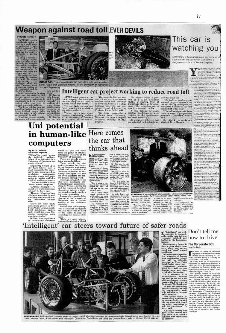
Weapon against road toll .EVER DEVILS This car is watching you ~ A Umvcr51::• ol T c:.smanio project Ila:; wne up w~
c•r!h11tc"lnth·nka.•1dL'Vl!'.'1:.rikF. w. '1:1'\ll o ~ O.v1gc-rou~~1uat.on!11. JOH N VILL •wµor.s. i
r-;:;c.~-~~;;:..,,1~~~~~~~~:?.~1.i~ .I. ~:.:·:::::,·!~·:;;:·::.~ ... 1~u-. ~ >r ,.,h- ol••"' • •• trlo • .:o011 . ...... N l. '\ .. 'l"11
m.t"1.1l.:.•.• · •u-o1tt1· ,.,_,1,,. ... ,W.•.1t• .,. .. . .... ~ ........ .. &.. "
=:":~ ~ ::-':. ':.:: °:"r= ;/~;~::;;.~~~WI~~~~~1~~7::tr~-~t St:hoolofEng/ntMtinf ..__ ,.. - ' ... ' ...... ..._ .. .,.._,I;-;'=_;.~~:::. _.. .. ,,.-..., .. l1!J.u . .u..,. I
~the1 Dr Karri
IAl<hfeobun .~ indudocl networb' wb
Intelligent car project working to reduce road toll ~.~;::~::~::~;~;~~g~:::.~~·~ :' .. ~~:~~:':,'::~~~~·~~:~·:.:...~ :
workinp "'t 5eo.IOI' fwlioo unsafe ~·wuu"i meaaunnc er and brake fOt'I
:fe:1~~ Or Karri•
t.he car alo•
By KA THY GRUBE Education A.porter TASMANIA could bocomo the ArtificiaJ ly lo~Uigeot l1land if an initiative by I'll Un1v~nrity of Tu numia ac•· dcmic take. off.
Enwneen"I lectunr Dr Voshy Kam btJje, there 11
greit potenual for UM: wuver-11ty Lo unite rtlSen.n:hen from poy<hology, maLhemaba,
co~~ : :, •:r1d1u:; rtificia.l inlelligenco p!'Qjec:U. 1betr airo would be to creot.e
"vi rtual human~ computers. .. Artificial intelligence re-
:U~J!:! DrmK!l:~ i~S.'i"ary "11.ow~ver, it hu tradition·
ally bt.-en n!aearched by each d iec1 plinc a1oue without aha rinc infortmu .ion beh 1,•ee.n lhem.
'"11lere a.re eome mullJ·
~~l{~Z ~~ng ~n ~~: ~;11 ~;~~lif.ti:eto pro~ mani:m re archers dOUl.J tomething 11milar."
Dr Karn 1• 11n organiMr of a n ln~~ional __ conference
wards lut gon l And would raite the prome or artificial intelligence re.earch aL the Univen:ily of T mania.
There are already project.a be.ing researched \.here.
Tilcse includ lhe joml project between the Univer-1nty ofTasmnni• engineenng Khool 1t.nd a university io Cenna.ny to develop an arti-
~!,u~~oidn~~:~ :~ :-d ~~ 1.rol iLa aa fe driving speed.
The engin ring Khool hu alao been developina a.rt.i· ficial inte lhgent p rottM modelling fo r Com lco during I.he p35l fh ·e year• ond the achool of c:ompulcr 1cicnoo i1 s tudying neurn1 net.work.I ond how th brnm nH1onalUea.
Profeuor Marimu\.hu Pala· n iawaml, o r Lhe University of Melbourne, wn• a keynote •penker AL the c:onfcrence y~Lcrday
~~~e :r~=-~\li~~~t::: and 88.ld there was no need for the public t.o fear t.he teeh nology JUSL beca.ute of 11..a I name.
'11le.r nre ma ny mlscon· ce Dtioru about what Artificial
,.., ,..,-.r, ... _, ru"r'lllt,•, l'...>l"'IM•• )I ~ " "''"Hl•t..-: .. tr~f'fl" •>I"• "''" ·,,,t ·~ ...... at. . ............ . ' •• 11. ·.11 •• 1 .. ,.,, .:.. .., · .,a1..,..t-:...ou· . ::;n ~:·::.~::.. '.;.::·::-: ·::.~~-~~~.':Ji ~·"•tt t.1.lfl .......... .. ~1 ... 1-·.-. v., w:.Lu l lf'.'f" 1 10\.•h-~,..,. I ' lio~J lrr.•,.« A .... I .. ., • •. he.~,.._ ~ ....... _, , , U"'-lfll •:l 'IDl\..,.ll/l .. >00>1 • .J.. i.oU. lo .., ..... .,,_,,...i. .......... -~·161111°"• ' ... 11 L'UO"kt ..... ,....,.,...,_,., ,~_.-.i..,,-'
' ""''"'--" .......... , .... ""' '" ..... 1_. .. _., , .. h ......... h .. ru.l. .. ~C: ' ,"'!"'1""-t" .. i.. •. h..-.. 1 ·loin"'(
: .:i.. .i1 ; ..... ,....,. ... .,,. • ..,,. ,rr; ...i.wl ... ,,......,, M1 f o"""-"",:_"h10I.:• .. ,~ .. ...... -. l~l ........ l L-hllon...,.W.,1 .. ,,, Ion•-• •-.. · ,~· c-..# .• w. .. .'.:oiuy i..,•
rr..w:._.,,.~.._ ............... &.."""' ... . ...... "
"""!~~;,J~~·:;~::~;~, .. n-·fl ~ UllOJ t fllKl:' a.~r· Ii , .. -"" ;N.1W•1,....~m•U• l,t1 I. 1-J.,•._+1•tl'.
r'U•-~-'..1.l1 1.Jt.:. ... 1...,1.:11L"ti.•: •1r -'fl;l"ltl l U .. ~ ...... r, ,...l.,..t_.., ..... ".__. .... ~ ....... ~ •1..1'• w,n ~" r"-.r••·-:b- -... m nl 01rt · ., .,..•• lh!"'••l •'"IA-..;ut,r l1U. •rr·u 1 .....
i":...:.';i.~ ~ . ·;.i~~:.~·.i:~"l~:,,t~ "'; :~ )'HI' CO ~iJd • tar tb.of ~· .. ~~~:;:~·~:,~~~\~u:-;111 • 4
:d =i:n~: ·~~~~:~:,~,s:::£;?:f..~-- ·-::1L-t~!:=~ll :~l~~·to.:-~;::,3:.:.::.....:! .1 .. ::,. ·.;.
()r Co&. N ici iL WM •d L.- · 111tl ..... ~ =:c=d: ~~Si;~~:.::~~:: o., ~ -::t:: ~~~a·.~~::~Z~:3 bui.do - &Uwut\O~ 11 ~.....,.,..,. .. .,.t ... ,l, ... ...._ • ..w.,i:., J C:::!'t!'°: al't..r .uW ili10°>1Cfi:G,.,.uu'"" ~.,,,..,..
-nw me. th1,. ... ~~~=:.::c~ ... ";:1:::.-
""I'bil JI .-. ~ COIL· Juiw i.odo1t bt&Wt9iTI ..-.hJ.Pi,,_, ._._. tr- •._. =t.·=:Ll~ ouralTCI. We Med lit ;.--::·t>.:1•·11'~1m ....... u.LU Colt .. it ~ .thr rW• ::,u:r~~i:4 ...... ~;~~s~ .. ·.--::.~";_.-~~.:.;~.·-~,~ .. rt.'91tan::b tum. ~r"-~i~~>:!? \0 ....;-• _. - ·n-
"A1 1 r~n1 dt-1..-• r i,~;.1:t~.J~~·~;;:~::!;;!!,.": .. 1:!•~~ ~~~5f~ .nl?'~for~n~it "=~=~~~~~=~~~~kl ~-=·-=·:;.·!1t;;,:K:.~.2..;1., i~'tdt.0.eif 1)1ey =~·~.,~..:.~~: !~~It;:;:· ~ntl~I~ t»t!_:~~:,;;~~I~ ~.i;tlr:ui.o...--,A :k;.~~~~~t~':~'"'f\Y un o:ducarw.h.~ UtO&Ch ~~-~ U. ,,_.~ -...~
~l"\'dopra~n&. o! uln~- ODt can,~l>t tCurn •aJd. !'.:"~~·F~""~ Vl~f!i•ri:.O::ili~-~.\~n;.r!_~ i~L~~ ~~~:J"':r~~ '~~C.:,.:·~~'"';: - • auf.pd.!Uon-fc-r Cf'· 111volH ~1uiid~tUoo ~du!~~ti:'.l ;:'th<l'~~~ h,l!J:. frt,: ~ =~ =~ .. ~~ ~ '!i;~"!1:.~~l :t ,.,, .... __ K ____ .... ___ ·AJ_l_oJw_°"'_~_· ._.. rtaM lucn:tditiou.~ ~ .-i ~ ,,..,tlt 'Ofl'9.i-ri<L_. -- -
'Intelligent' car steers toward future of safer roads AN •lntelllrent" car with tbe pot.entW to dramati· ea.lb' cut the road toll wu
~:d'~r f:'!f..c:!anj~: launch.
V•ln• 1enaon. tho ur bi able to altu •hock pre&· S\l.N!', wbecl and nafne l'peed and -react" to road concUtJona.
lb~ t-:1:er:i~~~?:m'Z ~~· =~ne:!ln~m-:rJfi lau.nc.bed at Wrui Poilll Hotel Cul.no tomorrow. En~ acad.em.lc
X:!fo~:1!!'0 o~~ joyed with the l"ffU1La.
"'It i. (llntaatlC. tt Lt at:ate-ot•th&-art tec.hnol·
:fib-:! a:,.=..':!~ pa.n. a t the Unh•er.lty or Stnt.und," Dr Karri ..Ud.
Re aald the technoloSY
fo~ul!,:!,~~t.\Jr be.~ able nb.lc.1• to lnCJ"eue ..._, ty NJH!C-la.
--rbe ~ t.e.m wou.ld In·
~~=:,!:!fC:i1T;'~~~~~ the car •J>ffd and c.h•nc·
~:ft o::r c::ditloe.:!.'!' t,'; Karri .. 1c1.
'"On dayac.a.rmay eve.n have vltlon ~a..ort that will allow h to avotd a ciol.lilion with another car or obttacle.•
Don ttellm how to dri rhe Corporate Box ronyDe Bo~o
r be bud or a 1cam or dcdk:ated cnainecrs within the faculty of the Hobart-based Univmity of Tu
nanb. look the libcny of "callin& •II :orporations"' this week.
Dr V-1$by Karri of I.he uni\•crsity'1 le~rtmcnl or c-ns:inccrins initiated • M1biic plea for • prospoc:tivc sponsor o assist Mlh the functin&. desi&n and na.nuracture of the world 's fU"lt "artik:iaUy intelligent" race car.
The subsidy tougbt ii tt.latitt.ly talll)' sivco the projccl'1 potential nultimillion-doUar YI.Jue. As Kam aid, " Around $40,000 to $SO.OOO In ponsorship would oenainly aoodentc natttrt eoormoU$ly. In rdUrn, lhe ompany gets to •lian itself with the
~.':~~~d~~ 'etcr Rossnamcn of Gennany'1 worldcnowned Univenity of Stn.lsund cbool of mechanical cnginttrina to tcsisn and build lhc intelligent car. It rill be designed to " think for iuc.1r · nd react to any situation with a ciection of active panmctc~ indud· 111 &boc:k pressure, wbcel and vt&ine pccd. and tyre and bra.kc pruaurc. ttlich can be altcRd to wit drivin& onditions.

ACKNOWLEDGMENTS v
This work was conducted as part of a research team and represents some outcomes from
the collaboration of the 'Intelligent Car' research team here at the University of
Tasmania and colleagues from the University of Stralsund.
Great thanks go to my supervisor Dr Vishy Karri for all of his support and guidance.
His motivation and support has been absolute throughout the course of this research.
I would like to thank David Butler for the dedication, hard work, design talent and
personal sacrifices he has made for this project. From the initial stages of the 'Intelligent
Car' concept David has been there to generate and reflect innovative ideas and designs.
The vehicle is a design success because of his co-operation in the design of the chassis,
suspension, wheel assembly, drivetrain, driver ergonomics, steering system, cooling
system, braking system and many other components too numerous to mention here.
Thanks Dave.
I personally thank the workshop staff and Peter Dove for their assistance in construction
of the 'Intelligent Car' Prototype and the Engineering faculty for making this project
possible. Thanks to Helen Cunningham for her work, dedication and innovative wiring
loom design, Nick Jones and Robert Neben for their great work on the measurement
system, Nick Dwyer for leading the construction of the body work and also Cranston
Polson for his contribution to the engine.
I would like to thank my partner and best friend Anita George for her support,
encouragement and inspiration.
Finally I would like to thank my family for the support throughout my degree and
research work.
CONTENTS VI
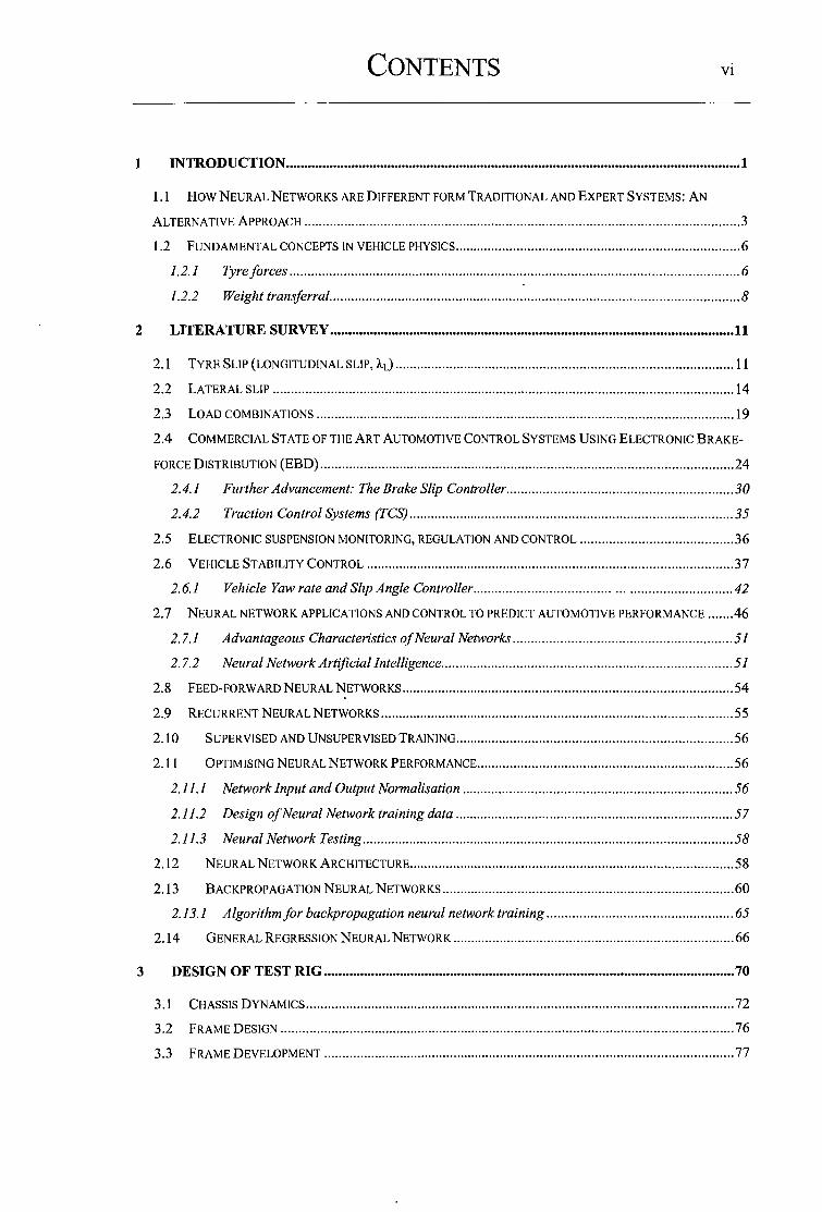
1 INTRODUCTION ............................................................................................................................. 1
1.1 How NEURAL NETWORKS ARE DIFFERENT FORM TRADITIONAL AND EXPERT SYSTEMS: AN
ALTERNATIVE APPROACH ........................................................................................................................ 3
1.2 FUNDAMENTAL CONCEPTS IN VEHICLE PHYSICS .............................................................................. 6
1.2.1 Tyreforces ............................................................................................................................ 6
1.2.2 Weight transferral ................................................................................................................. 8
2 LITERATURE SURVEY ............................................................................................................... 11
2.1 TYRE SLIP (LONGITUDINAL SLIP, A.L) ............................................................................................. 11
2.2 LATERAL SLIP ............................................................................................................................... 14
2.3 LOAD COMBINATIONS ................................................................................................................... 19
2.4 COMMERCIAL STATE OF THE ART AUTOMOTIVE CONTROL SYSTEMS USING ELECTRONIC BRAKE-
FORCE DISTRIBUTION (EBD) .................................................................................................................. 24
2.4.1 Further Advancement: The Brake Slip Controller .............................................................. 30
2.4.2 Traction Control Systems (TCS) ......................................................................................... 35
2.5 ELECTRONIC SUSPENSION MONITORING, REGULATION AND CONTROL .......................................... 36
2.6 VEHICLE STABILITY CONTROL ..................................................................................................... 37
2. 6.1 Vehicle Yaw rate and Slip Angle Controller ...................................... ............................... 42
2. 7 NEURAL NETWORK APPLICATIONS AND CONTROL TO PREDICT AUTOMOTIVE PERFORMANCE ...... .46
2. 7.1 Advantageous Characteristics of Neural Networks ............................................................ 51
2. 7.2 Neural Network Artificial Intelligence ................................................................................ 51
2.8 FEED-FORWARD NEURAL NETWORKS ........................................................................................... 54
2.9 RECURRENT NEURAL NETWORKS ................................................................................................. 55
2.10 SUPERVISED AND UNSUPERVISED TRAINING ............................................................................ 56
2.11 0PTIM ISING NEURAL NETWORK PERFORMANCE ...................................................................... 56
2.11.1 Network Input and Output Normalisation .......................................................................... 56
2.11.2 Design of Neural Network training data ............................................................................ 57
2.11.3 Neural Network Testing ...................................................................................................... 58
2.12 NEURAL NETWORK ARCHITECTURE ......................................................................................... 58
2.13 BACKPROPAGATION NEURAL NETWORKS ................................................................................ 60
2.13.1 Algorithm for backpropagation neural network training ................................................... 65
2.14 GENERAL REGRESSION NEURAL NETWORK ............................................................................. 66
3 DESIGN OF TEST RIG ................................................................................................................. 70
3.1 CHASSIS DYNAMICS ...................................................................................................................... 72
3.2 FRAME DESIGN ............................................................................................................................. 76
3.3 FRAME DEVELOPMENT ................................................................................................................. 77
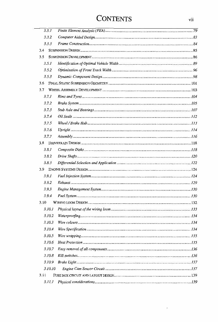
CONTENTS vii
3.3.1 Finite Element Analysis (FEA) ........................................................................................... 79
3.3.2 Computer Aided Design ...................................................................................................... 83
3.3.3 Frame Construction ............................................................................................................ 84
3.4 SUSPENSION DESIGN ..................................................................................................................... 85
3 .5 SUSPENSION DEVELOPMENT ......................................................................................................... 86
3.5.1 Identification of Optimal Vehicle Width ............................................................................. 89
3.5.2 Optimisation of Front Track Width .................................................................................... 96
3.5.3 Dynamic Component Design .............................................................................................. 98
3.6 FINAL STATIC SUSPENSION GEOMETRY ...................................................................................... 101
3.7 WHEELASSEMBLYDEVELOPMENT ............................................................................................ 103
3.7.1 Rims and Tyres ................................................................................................................. 104
3.7.2 Brake System .................................................................................................................... 105
3. 7.3 Stub Axle and Bearings ..................................................................................................... I 07
3.7.4 Oil Seals ........................................................................................................................... 112
3. 7.5 Wheel I Brake Hub ............................................................................................................ 113
3.7.6 Upright ............................................................................................................................. 114
3. 7. 7 Assembly ........................................................................................................................... 116
3.8 DRIVETRAINDESIGN .................................................................................................................. 118
3.8.1 Composite Disks ............................................................................................................... 118
3.8.2 Drive Shafts ...................................................................................................................... 120
3.8.3 Differential Selection and Application ............................................................................. 122
3.9 ENGINE SYSTEMS DESIGN ........................................................................................................... 124
3.9.1 Fuel Injection System ........................................................................................................ 124
3.9.2 Exhaust ............................................................................................................................. 129
3.9.3 Engine Management System ............................................................................................. 130
3.9.4 Fuel System ....................................................................................................................... 130
3.10 WIRING LOOM DESIGN ........................................................................................................... 132
3.10.1 Physical layout of the wiring loom ................................................................................... 133
3.10.2
3.10.3
3.10.4
3.10.5
Waterproofing ................................................................................................................... 134
Wire colours ..................................................................................................................... 134
Wire Specification ............................................................................................................ 134
Wire wrapping .................................................................................................................. 135
3.10.6 Heat Protection ................................................................................................................ 135
3.10.7 Easy removal of all components ....................................................................................... 136
3.10.8 Kill switches ...................................................................................................................... 136
3.10.9 Brake Light ....................................................................................................................... 137
3.J0.10 Engine Cam Sensor Circuit ......................................................................................... 137
3.11 FUSE BOX CIRCUIT AND LAYOUT DESIGN ................................................................................ 139
3.11.1 Physical considerations .................................................................................................... 139
CONTENTS viii
3.11.2 CircuitDesign .................................................................................................................. 139
3.11.3 Physical circuit layout ...................................................................................................... 139
3.11.4 Fuse specification ............................................................................................................. 140
3.12 DASHBOARD-LAYOUT AND CIRCUITRY ............................................................................... 141
3.12.l Physical considerations .................................................................................................... 141
3.12.2 Circuit design ................................................................................................................... 143
3.12.3 Physical layout ................................................................................................................. 143
3.13 ELECTRICAL SYSTEM SPECIFICATIONS ................................................................................... 144
4 INSTRUMENTATION DESCRIPTION .................................................................................... 145
4.1 INPUT TYPE INSTRUMENTATION ................................................................................................. 147
4.1.1 Wheel Speed Hall Effect Sensor ....................................................................................... 148
4.1.2 Three Axis Acceleration & Pitch/Roll/Yaw Angle Measurement: Crossbow DMU
AHRS400CA-200 Sensor ................................................................................................................ 155
4.1.3 Wheel Travel: Gefran PZ12A Linear Potentiometer - 1 OOmm ........................................ 161
4.1.4 Linear Potentiometer Installation and Calibration .......................................................... 164
4.1.5 Steering Angle: MoTeC JO Turn, Gear Driven Rotary Potentiometer ............................ 167
4.1.6 Brake Force: Honeywell Eclipse Hydraulic Pressure Sensor - 2000psi ......................... 171
4.2 DATA ACQUISITION TYPE INSTRUMENTATION ............................................................................ 175
4.2.1 MoTeC Advance Dash Logger (ADL-4) ........................................................................... 175
4.2.2 Wiring Loom ..................................................................................................................... 177
4.2.3 CAN Communication Cable ............................................................................................. 179
4.3 OUTPUT TYPE INSTRUMENTATION .............................................................................................. 180
4.3.1 Research Computer .......................................................................................................... 180
4.3.2 Radio Modems: RFJ-9256 Data Strike Series 3 Spread Spectrum Radio Modem and
Auxiliary Equipment ....................................................................................................................... 181
4.4 THE DEVELOPED MEASURING SYSTEM ....................................................................................... 183
5 TRAINING AND TESTING OFF-LINE NEURAL NETWORK MODELS .......................... 186
5.1 STRATEGY FOR PREDICTION ....................................................................................................... 188
5.2 TYPES OF TRAINING COURSES .................................................................................................... 189
5.3 BACK PROPAGATION NEURAL NETWORK RESULTS .................................................................... 192
5.3.1 Course 1: Straight Line Acceleration and Braking - Front Brake Force Prediction ....... 194
5.3.2 Course 1: Straight Line Acceleration and Braking-Rear Brake Force Prediction ........ 196
5.3.3 Course 2: Figure Eight- Front Brake Force Prediction ................................................. 198
5.3.4 Course 2: Figure Eight - Rear Brake Force Prediction .................................................. 200
5 .4 GENERAL REGRESSION NEURAL NETWORK RESULTS ................................................................. 202
5.5 CONCLUDING REMARKS ............................................................................................................. 202
6 FINAL CONCLUDING REMARKS AND PROPOSED FUTURE WORK .......................... 204
CONTENTS ix
7 REFERENCES .............................................................................................................................. 207
8 APPENDIX A -GENERAL REGRESSION NEURAL NETWORK RESULTS •....•..•........•. 216
9 APPENDIX B -FRAME DESIGN AND FEA .•.................•.•.••.•............•.•.•.•..........•.•..•••......•..... 221
10 APPENDIX C - SUSPENSION DESIGN ...........•.......•.•...................•••..............•..••.•...•............•. 233
11 APPENDIX D - WHEEL ASSEMBLY •.....•..............•.•.•.•............•...••.•.•............••.....•.•.............• 241
12 APPENDIX E-BRAKE PEDAL ASSEMBLY ••.........•.•.•.•.••••.•..•.......•...•.•••......•.....••.••.•.......... 251
13 APPENDIX F - DRIVETRAIN DESIGN .............•.....••.•............•.....•..•......•..•••..•...........•.•.....••.. 253
14 APPENDIX G - ELECTRICAL SYSTEMS DESIGN ........••.•.••••..........•...•....•.........•..•.•.•.•.•.... 261
15 APPENDIX H - TEST RIG SENSOR AND TELEMETRY DESIGN •.•.•.•....••..•.•.•.•.............• 265
16 APPENDIX I- ENGINE SPECIFICATIONS ..•.......•..•.•.............•.•••............•..•..•...............•.•..•• 290
17 APPENDIX J -TESTING DATA •.••.•...............•.••••....................••••..............•.•..............•.•.•......... 294

TABLE OF FIGURES x
Figure 1-1 Characteristics of Neural Network and Traditional Computing Systems . ................................. 3
Figure 1-2 Neural Network and Expert Systems Comparison . .................................................................... 5
Figure 1-3 Tyre pressure distribution. [5] ................................................................................................... 7
Figure 1-4 Moment acting on a braked wheel... ........................................................................................... 7
Figure 1-5 Vehicle in equilibrium [6] .......................................................................................................... 8
Figure 1-6 Weight transferral: (a)under acceleration (b)while turning [6] ............................................... 8
Figure 1-7 Optimal brake force distribution due to weight transferral under braking [7) .......................... 9
Figure 2-1 Friction factor vs slip [ 1] ......................................................................................................... 13
Figure 2-2 Lateral forces during cornering ............................................................................................... 15
Figure 2-3 Lateral force as a function of normal force and slip angle. [9] ............................................... 16
Figure 2-4 Lateral forces generated by the front wheels during vehicle cornering. [9] ............................ 17
Figure 2-5 The friction circle [ 1] ............................................................................................................... 19
Figure 2-6 Total tyre force capability map [9] .......................................................................................... 21
Figure 2-7 Friction circle plot from measured data for a typical sports car [9] ....................................... 22
Figure 2-8 Longitudinal, FL and lateral forces, Fs as a function of slip ratio, AL and Slip angle, a.[8] .... 23
Figure 2-9 Hydraulic circuit of two channel ABS [11] . ............................................................................. 25
Figure 2-10 Three channel ABS Hydraulic circuit.. ................................................................................... 26
Figure 2-11 Four Channel ABS Hydraulic circuit . .................................................................................... 26
Figure 2-12 4 channel ABS Electronic Control Unit (ECU) [12) .............................................................. 27
Figure 2-13 Modern ABS control unit logic [13) ....................................................................................... 28
Figure 2-14 Operational region of ABS allowing for steering input while braking at best efficiency ....... 29
Figure 2-15 Controller structure for the Bosch Brake Slip Controller.[ 14] .............................................. 32
Figure 2-16 ABS in star topology ............................................................................................................... 33
Figure 2-17 The merging of automotive systems. (7) ................................................................................. 34
Figure 2-18 Simplistic view demonstrating active control systems during a cornering manoeuvre .......... 37
Figure 2-19 Bosch/Mercedes-Benz ESP Vehicle Dynamics Control (VDC) system. [14] ......................... 38
Figure 2-20 Bosch-Mercedes Electronic Stability Program (ESP) yaw control using differential
electronic brake force distribution: (a)without ESP, (b) with ESP, (c) Graphical results showing handling
response. [5] ............................................................................................................................................... 40
Figure 2-21 Dynamic vehicle model used in predicting yaw moment changes.[ 14) .................................. 41
Figure 2-22 Bosch vehicle yaw rate and slip angle controller structure. [ 14] .......................................... 44
Figure 2-23 "Automobile Autopilot" modelfreeway used to develop vehicle control Neural Networks .. .48
Figure 2-24 Neural network use in the Automobile Autopilot [ 18) ............................................................ 49
Figure 2-25 The structure of an artificial neuron ..................................................................................... 51
Figure 2-26 Threshold and sigmoidal activation functions ........................................................................ 53
Figure 2-27 Feed forward neural network structure .................................................................................. 55
Figure 2-28 Graphical example of oveifitting on a polynomial approximation.[ 18] ................................ 59
TABLE OF FIGURES xi
Figure 2-29 Backpropagation (multi layered feed forward) neural network architecture with exploded
output layer processing neuron [22] .......................................................................................................... 60
Figure 2-30 Exploded hidden layer processing neuron [Fred Frost 34] [R-ROJAS]. ................................ 62
Figure 2-31 Basic General Regression Neural Network (GRNN) architecture ......................................... 67
Figure 3-1 Vehicle dynamics were found to be influenced by an astoundingly large number of factors.
These pictures were taken during early stages of testing at Baskerville Raceway-Hobart, Tasmania .... 72
Figure 3-2 Mid-mounted engine layout of the test vehicle ......................................................................... 73
Figure 3-3 Reclined driver position of the test car. Note thefar forward driving position ........................ 74
Figure 3-4: PVC mock frame .................................................................................................................... 79
Figure 3-5: FEAframe model [Strand 1] ................................................................................................. 81
Figure 3-6: FEA results for cornering under brakes ................................................................................ 82
Figure 3-7: FEA torsional results under 1 Nm ......................................................................................... 82
Figure 3-8: CAD drawing of the frame ..................................................................................................... 83
Figure 3-9: Mild steel frame ..................................................................................................................... 84
Figure 3-10 Formula SAE vehicles are designed to operate on tight autocross style tracks resulting in
compact design. Photo courtesy of SAE (USA) . ........................................................................................ 86
Figure 3-11 Minimum practical clearances were specified between the seat and engine ......................... 87
Figure 3-12 The lateral distance between wheels, termed track width, is one of the first critical decisions
faced by a vehicle designer ......................................................................................................................... 88
Figure 3-13 Test vehicle during autocross trials . ...................................................................................... 89
Figure 3-14 An experimental slalom course ............................................................................................. 91
Figure 3-15 Identification of experimental slalom course variables ......................................................... 92
Figure 3-16 Geometry of turning vehicle ................................................................................................... 96
Figure 3-17 Pullrod suspension system with inboard coil over shock absorber used on the test vehicle .. 98
Figure 3-18 Keeping the outside wheels vertical during cornering ........................................................... 99
Figure 3-19 The pull-rod suspension . ..................................................................................................... 102
Figure 3-20 Front and rear uprights and bearing arrangements ........................................................... 102
Figure 3-21: Tyre and rim ....................................................................................................................... 104
Figure 3-22 13-inch rims permit the use of larger disk brakes . ............................................................... 105
Figure 3-23: Brake rotor and caliper ...................................................................................................... 106
Figure 3-24: (a) On centre (b) off centre bearings .................................................................................. 107
Figure 3-25: FEA wheel model cross sections (a) with centred bearings (b) with off centre bearings .. 109
Figure 3-26: Stub axle ............................................................................................................................. 112
Figure 3-27: Oil seal ............................................................................................................................... 113
Figure 3-28: Wheel I brake hub .............................................................................................................. 114
Figure 3-29: Upright ............................................................................................................................... 115
Figure 3-30: Wheel assembly .................................................................................................................. 117
Figure 3-31. Kevlar composite disks supplied by GKN motorsport used in the test vehicle transmission .
.................................................................................................................................................................. 118

TABLE OF FIGURES xii
Figure 3-32 Unidirectional Kevlar fibre construction of the composite disks ......................................... I I 8
Figure 3-33 Perfect static alignment of the rear axel is required to keep composite disks from failure .. I I 9
Figure 3-34 Large diameter hollow aluminium drive shafts dominate the rear of the car ...................... 120
Figure 3-35 Aluminium alloy drive shafts bolted directly to the GKN composite disks ........................... 12I
Figure 3-36 Quaife ATE differential with pressed on ball bearings . ....................................................... 122
Figure 3-37 Differential mounting arrangement; a) photo taken during frame construction, b) rear frame
design dominated by differential mounting considerations ...................................................................... 123
Figure 3-38 Differential mounts ............................................................................................................... I23
Figure 3-39 Inlet manifold ....................................................................................................................... I27
Figure 3-40 Exhaust manifold and muffler .............................................................................................. I 29
Figure 3-4I Fuse box location. Note the black wrapped wiring loom located directly above the box ... I 33
Figure 3-42 Conduit, triple insulated wiring loom under nose cone . ...................................................... I 35
Figure 3-43 Kill switches ......................................................................................................................... I 36
Figure 3-44 Location of the engine cam sensor circuit case .................................................................... 138
Figure 3-45 The yellow colour of the automotive fuses ............................................................................ I 40
Figure 3-46 ADL location on dashboard ................................................................................................. I4I
Figure 3-47 Com ports are located on the dashboard for high levels of access during testing and data
transference with the remote PCs ............................................................................................................. I42
Figure 3-48 Rear connection from wiring loom to Com ports ................................................................. I 42
Figure 4-I Research measurand as identified in through the collaboration of Professor Rossmanek and
Dr Karri. .................................................................................................................................................. I45
Figure 4-2 The research measurand depicted on the test rig ................................................................... I46
Figure 4-3 The Input Type Instrumentation Sensors ................................................................................ I47
Figure 4-4 The Honeywell GTI Series Hall Effect Gear Tooth Sensor .................................................... I48
Figure 4-5 Gear tooth sensor construction and wiring diagram ............................................................. I49
Figure 4-6 Hall effect sensor in relation to gear tooth wheel .................................................................. I50
Figure 4-7 Induced voltage changes ........................................................................................................ I50
Figure 4-8 a) Three piece rim, b) outside view of rim bolts, c) inside view of rim bolts .......................... I52
Figure 4-9 Simulation setup used in testing the Hall effect sensor . ......................................................... I 53
Figure 4-I 0 Hall effect sensor mount ....................................................................................................... I 54
Figure 4-I I Dash manager calibration of hall effect sensor ................................................................... I55
Figure 4-12 The DMU AHRS400CA-200 Sensor ..................................................................................... I56
Figure 4-13 Block diagram of the DMU-AHRS sensor ............................................................................ I57
Figure 4-I4 Block diagram depicting the signal conditioning operations ............................................... I59
Figure 4-I5 The DMU-AHRS400CA-200 coordinate system ................................................................... I59
Figure 4-I 6 Error specification of the DMU sensor ................................................................................ I 60
Figure 4-17 Wheel travel linear potentiometer mounted to the test rig ................................................... I6I
Figure 4-I 8 Electrical configuration of the linear potentiometer sensor ................................................. I 62
Figure 4-I9 A representation of a Linear Potentiometer ......................................................................... I63
TABLE OF FIGURES xiii
Figure 4-20 Installation of rear linear potentiometer .............................................. : ............................... I 64
Figure 4-21 calibration curve for front right linear potentiometer .......................................................... I 66
Figure 4-22 The dial height gauge placed underneath the stub axel nut. ................................................. 167
Figure 4-23 Steering Angle Sensor . ......................................................................................................... 168
Figure 4-24 Steering Angle Sensor installed on the test rig ..................................................................... 168
Figure 4-25 a) The protractor clamped to the steering wheel at its zero position, b) the reference pointer
at zero degrees and, c) thirty degrees clockwise ...................................................................................... 170
Figure 4-26 The calibration curve for the steering angle sensor ............................................................. 171
Figure 4-27 The Eclipse Pressure Transducer ......................................................................................... 172
Figure 4-28 Cross-section of a typical quartz pressure sensor ................................................................ 173
Figure 4-29 The calibration curve loaded from the existing index available in the Dash Manager
software . ................................................................................................................................................... 174
Figure 4-30 The MoTeC Advance Dash Logger . ..................................................................................... 176
Figure 4-31 Real Time Clock ................................................................................................................... 178
Figure 4-32 Research Computer .............................................................................................................. 180
Figure 4-33 RFI-9256 Data Strike Series 3 Spread Spectrum Radio Modem .......................................... 181
Figure 4-34 Block diagram of the complete measuring system ................................................................ 184
Figure 4-35 A diagram illustrating the inputs and outputs of the measuring system ............................... 185
Figure 5-1 Test Vehicle gathering data during dynamic vehicle trials .................................................... 186
Figure 5-2 Test courses for neural network training: a) Straight-line acceleration and braking: course 1.
b) Figure eight with hairpin and sweeper: course 2 . ............................................................................... 189
Figure 5-3 Course 1: Straight-line acceleration and braking test photographed during early stages of
testing . ...................................................................................................................................................... 190
Figure 5-4 Course 2: Figure eight test course data generation ............................................................... 191
Figure 5-5 Braking and cornering at different levels of attack producing data sets at different levels of
tyre slip ..................................................................................................................................................... 191
Figure 5-6 Selected backpropagation neural network featuring double layer architecture with seven
hidden layer nodes in each . ...................................................................................................................... 193
Figure 5-7 Front Brake Hydraulic Pressure estimation for test course 1 and calculated absolute error.
Errors for peaks 1, 2 and 4 are not due to the neural network (see text for explanation) ........................ 195
Figure 5-8 Rear Brake Hydraulic Pressure estimation for test course 1 ................................................. 197
Figure 5-9 Figure eight front brake hydraulic pressure estimation by double layer backpropagation
neural network .......................................................................................................................................... 199
Figure 5-10 Figure eight rear brake hydraulic pressure estimation by double layer backpropagation
neural network .......................................................................................................................................... 201

Chapter One - Introduction 1
Chapter One
INTRODUCTION
Accurate dynamic brake pressure information is critical for any sophisticated electronic
driving assistance system. This represents one of the inputs by the driver of the vehicle
along with accelerator and steering wheel position and is used to control and guide a
vehicle in motion.
Driving assistance systems using electronic control and intervention technology are
already standard equipment on many commercially available vehicles, in the medium to
upper market sectors. Advances in vehicle technology ensure that these systems filter
down into lower market sectors as new technology and increased production lowers the
cost.
Consequently there is a need to develop systems that are of higher performance, safer
and cheaper. Development of such systems is recognised as one of the automotive
industry's most important challenges. One method of achieving this is by
understanding the degree of influence of various system parameters on vehicle braking
performance and eliminating those that are non-contributing. This will make the system
robust and efficient for computational purposes.
Further is a need to predict brake force values in advance for use in the intervention
decision making process of driving assistance systems. By predicting brake force
values on line, a brake force controller algorithm coupled with active control systems
could keep these within desired optimum performance limits during braking. This study
is aimed at contributing toward the development of neural network based dynamic
vehicle control systems for predicting braking performance.
Established pressure control methods used in Anti-lock Braking Systems (ABS) have
evolved into sophisticated, well proven designs and are also now commonly
Chapter One - Introduction 2
incorporated into more complete control systems. Driving assistance systems such as
Mercedes-Benz's Electronic Stability Program [l] and BMW's Dynamic Stability
Control [2] assist the driver in avoiding accidents and maintaining control of the vehicle
under normal driving conditions. As these systems are refined, the safe driving
envelope of an average driver is stretched.
Such state of the art designs use a multitude of sensors and control by Expert Systems,
as discussed in the next section, to make decisions on what course of action is required.
However, every control system has strengths, weaknesses and limitations. By their own
admission, the manufacturers of these systems try to find "the best compromise".
In relation to applicability and robustness of the Bosch vehicle dynamic control (VDC)
system, Van Zanten et. al. [3] stated: "Due to th~ design properties of the controller
which is based on physical models a basic application of the controller can be achieved
by a set of parameters for the models which describe the dynamics of the vehicle and
the actuators" . It is these physical models which have been developed to predict, as
close as possible, the physical behaviour of any particular vehicle
Limitations of these systems arise wherever conditions dictate that the physical models
used by the electronic controller do not sufficiently describe the actual behaviour of the
vehicle. Therefore, developers of these brake control systems are using increasingly
complicated Traditional and Expert Systems based models in an attempt to increase
driver control under circumstances where the assumptions made in defining the simpler
physical models are inapplicable.
While many manufacturers are constantly addressing their conventional control
systems, emerging technologies such as neural networks and fuzzy logic are replacing
conventional systems in increasingly complex non-linear dynamic applications. The
following section briefly highlights the major differences between these methods.
Chapter One - Introduction 3
1.1 How N EURAL N ETWORKS ARE D IFFERENT FORM T RADITIONAL
AND E XPERT SYSTEMS: AN A LTERNATIVE A PPROACH
Neural networks offer an alternative way to analyse and develop data into functional
predictive models. Neural Networks are a powerful engineering tool, as they can be
used to recognise patterns in data and later make generalised decisions based on those
patterns.
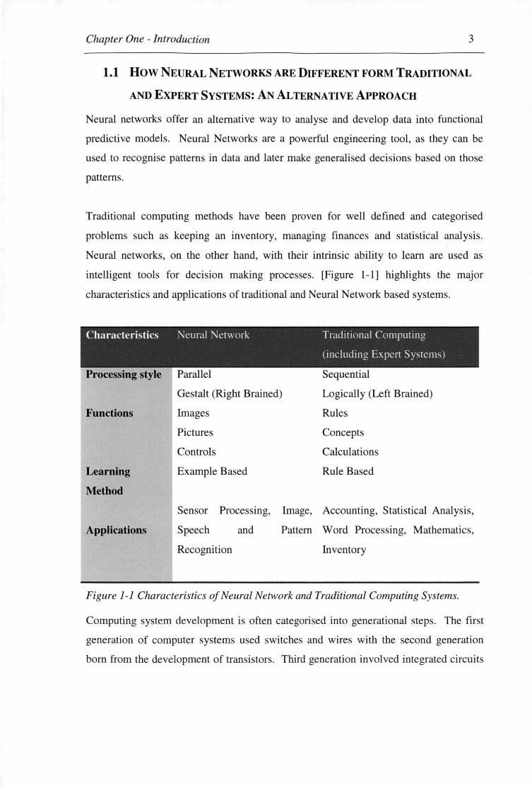
Traditional computing methods have been proven for well defined and categorised
problems such as keeping an inventory, managing finances and statistical analysis.
Neural networks, on the other hand, with their intrinsic ability to learn are used as
intelligent tools for decision making processe . [Figure 1-1] highlights the major
characteristics and applications of traditional and Neural Network based systems.
Characteristics Neural Network Traditional Computing
(including Expert Systems)
Processing style Parallel
Gestalt (Right Brained)
Functions Images
Learning
Method
Pictures
Controls
Example Based
Sequential
Logically (Left Brained)
Rules
Concepts
Calculations
Rule Based
Applications
Sensor Processing, Image, Accounting, Statistical Analysis,
Speech and Pattern Word Processing, Mathematics,
Recognition Inventory
Figure 1-1 Characteristics of Neural Network and Traditional Computing Systems.
Computing sy tern development is often categorised into generational steps. The first
generation of computer systems used switches and wires with the second generation
born from the development of transistors. Third generation involved integrated circuits

Chapter One - Introduction 4
and solid state technology with the use of higher level languages such as FORTRAN, C,
and COBOL. The fourth generation involves end user tools such as "code generators".
The fifth generation of computing, often called Expert Systems use Artificial
Intelligence, commonly in the form of an interference engine, together with a
knowledge base. The generic interference engine handles the user interface, external
files, program access and scheduling. The knowledge base contains all information
specific to the given application allowing a user to define the rules that govern the given
process. Note that the user does not need to know traditional programming techniques
in order fulfil this function.
The user does however need to know both what they want the computer to do and also
how the larger mechanism of the expert system shell works. This shell is part of the
interference engine and directs the computer through the implementation of the user
needs. In this manner, the expert system generates the decision-making programming
for the individual process. The macro program that the expert system uses to create
these process programs develops rules in a complex way.
Efforts to develop a general expert system for the use with various processes have
encountered problems. Increases in system complexity results in the requirement for
greater computing power and the system becomes too slow. The current success. and
feasibility of expert systems is somewhat limited to specific, narrowly confined,
applications.
Sometimes referred to as the sixth generation of computing, artificial neur~ networks
represent a completely different approach to problem solving. Artificial neural
networks do not require assumptions to be made by a programmer in order to model a
system. Instead artificial neural networks can be trained using measured data, as a
result a neural network can be used to find and identify patterns within data that are
previously unidentified.
[Figure 1-2] highlights the different features of neural network and expert systems
characteristics. It can be seen in this Figure that the neural network systems are
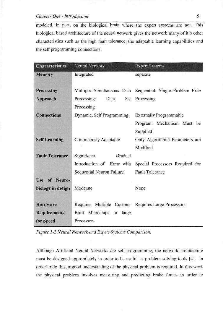
Chapter One - Introduction 5
modeled, in part, on the biological brain where the expert systems are not. This
biological based architecture of the neural network gives the network many of it's other
characteristics such as the high fault tolerance, the adaptable learning capabilities and
the self programming connections.
Characteristics Neural Network Expert Systems
Memory
Processing
Approach
Connections
Self Learning
Integrated separate
Multiple Simultaneous Data Sequential: Single Problem Rule
Processing: Data Set Processing
Processing
Dynamic, Self Programming Externally Programmable
Program: Mechanism Must be
Supplied
Continuously Adaptable Only Algorithmic Parameters are
Modified
Fault Tolerance Significant, Gradual
Introduction of Error with Special Processors Required for
Sequential Neuron Failure Fault Tolerance
Use of Neuro-
biology in design Moderate None
Hardware
Requirements
for Speed
Requires Multiple Custom- Requires Large Processors
Built Microchips or large
Processors
Figure 1-2 Neural Network and Expert Systems Comparison.
Although Artificial Neural Networks are self-programming, the network architecture
must be designed appropriately in order to be useful as problem solving tools [4] . In
order to do this, a good understanding of the physical problem is required. In this work
the physical problem involves mea uring and predicting brake forces in order to
Chapter One - Introduction 6
incorporate these functions into a neural network electronic brake control based driver
assistance system.
In order to identify ways in which an electronic brake control based driver assistance
system could operate, it is imperative to understand the nature in which a vehicle
interacts with its surroundings. The following sections discuss the details of
vehicle/driving environment interaction with particular attention to the most important
dynamic connection between the road/track surface and the tyres.
1.2 FUNDAMENTAL CONCEPTS IN VEIDCLE PHYSICS
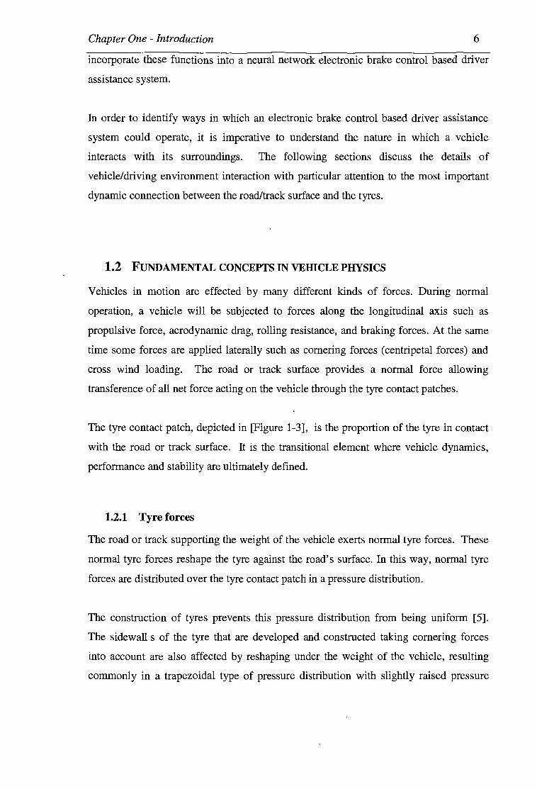
Vehicles in motion are effected by many different kinds of forces. During normal
operation, a vehicle will be subjected to forces along the longitudinal axis such as
propulsive force, aerodynamic drag, rolling resistance, and braking forces. At the same
time some forces are applied laterally such as cornering forces (centripetal forces) and
cross wind loading. The road or track surface provides a normal force allowing
transference of all net force acting on the vehicle through the tyre contact patches.
The tyre contact patch, depicted in [Figure 1-3], is the proportion of the tyre in contact
with the road or track surface. It is the transitional element where vehicle dynamics,
performance and stability are ultimately defined.
1.2.1 Tyre forces
The road or track supporting the weight of the vehicle exerts normal tyre forces. These
normal tyre forces reshape the tyre against the road's surface. In this way, normal tyre
forces are distributed over the tyre contact patch in a pressure distribution.
The construction of tyres prevents this pressure distribution from being uniform [5].
The sidewall s of the tyre that are developed and constructed taking cornering forces
into account are also affected by reshaping under the weight of the vehicle, resulting
commonly in a trapezoidal type of pressure distribution with slightly raised pressure

Chapter One - Introduction 7
points (local maxima) along transitions between sidewalls and tyre tread. The complex
shape of a typical tyre pressure distribution over the contact patch is shown in [Figure 1-
3].
Figure 1-3 Tyre pressure distribution. [5]
Longitudinal forces act on the tyre as it is rolling along the road or track surface. The
net result of these forces is acceleration of the vehicle under power or during braking.
These forces can be seen in [Figure 1-4] where a braking torque is applied to a rolling
wheel.
The magnitude of such a braking force is the product of the torque applied to the wheel
through the brake disk (M8 ) and the radius of the tyre (r). There is, however, a limiting
condition reached when the tyre begins to slip against the road surface. In this case the
accelerating or braking force is equal to the product of the normal tyre force (FN) and
the coefficient of friction of the tyre/surface combination (µ).
Direction
of Motion
Figure 1-4 Moment acting on a braked wheel

Chapter One - Introduction 8
1.2.2 Weight transferral
The value of the normal force on the tyre is dependent on the weight, and is also subject
to acceleration, of the vehicle. [Figure 1-5] shows a vehicle in a steady state with
neutral weight distribution (all four wheels loaded to the same level). In this depiction
the vehicle with neutral weight distribution can either be standing still (static
equilibrium) or at a constant velocity (dynamic equilibrium).
Figure 1-5 Vehicle in equilibrium [6]
In [Figure 1-6 (a)] the same vehicle is depicted under straight-line acceleration. The
acceleration of the car causes transferral of weight from the tyres at the front of the
vehicle to the tyres at the rear. This weight transference can be seen visually as cars
'squat' under power or as drag cars 'wheelie' (extreme case where al l weight is
transferred to the rear tyres) .
(a) (b)
Figure 1-6 Weight transferral: ( a)under acceleration (b )while turning [6]
Chapter One - Introduction 9
In a similar way weight i transferred under cornering and braking. This transference of
weight (changes in normal force) can be seen in [Figure 1-6 (b)].
Weight transferral has the effect of altering the ultimate brake force that can be
transmitted through the tyre contact patch since the limiting condition is reached where
the braking force is equal to the product of the normal tyre force (FN) and the coefficient
of friction of the tyre/surface combination (µ).
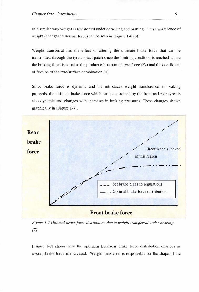
Since brake force is dynamic and the introduces weight transference as braking
proceeds, the ultimate brake force which can be sustained by the front and rear tyres is
also dynamic and changes with increases in braking pressures. These changes shown
graphically in [Figure 1-7].
Rear
brake
force
/." ...(.·=·=···
/. ........ . •.. ... v·
.. ..
.. ···
..... .··
... ··
. .. .. ·· .......
.... ···· .. ·· Rear wheels locked
.... ··· .·· in this region
.... ··· -··-··-··-··-· .. ··.,.,...,. .. ~·· .
Set brake bias (no regulation)
_ •• Optimal brake force distribution
Front brake force
Figure 1-7 Optimal brake force distribution due to weight transferral under braking
[7].
[Figure 1-7] shows how the optimum front:rear brake force distribution changes as
overall brake force is increased. Weight transferral is responsible for the shape of the

Chapter One - Introduction 10
optimum curve where the brake force distribution is the same as the corresponding
normal tyre force distribution.
While braking, weight transfers from the rear wheels to the front. Applying equal (or
even properly adjusted fixed proportional) brake force to front and rear wheels will
eventually cause the rear wheels to lock under hard braking. If the optimal distribution
curve is followed, all four wheels will slip at the same level until locked.
The conventional models used in brake force control systems, with the aid of mechanic
and dynamic testing, get increasingly complex as the number of control parameters are
increased. As discussed earlier neural networks are alternative modeling techniques and
the next section will deal with both conventional and emerging NN attempts in
automotive control. Within the next chapter is a review of state of the art in brake
pressure studies and commercial control systems. There is a need however, in the first
instance to understand and define the terms of vehicle dynamic control and most
importantly the nature of tyre slip that ultimately defines the limit of all automobile
dynamics.
11
Chapter Two
LITERATURE SURVEY
Friction between a vehicle tyre and the road/track surface is used to drive, brake and
steer a vehicle in motion. In order to estimate braking pressures under all conditions it is
necessary to understand the forces transmitted through the contact patch between the
tyres and the road/track.
The problem of estimating and predicting brake forces originates from the complex
nature of tyre slip in both longitudinal and lateral directions simultaneously. The
following parameters are defined:
• Longitudinal Tyre Slip, AL
• Lateral tyre slip
It is also important to understand how these parameters limit and effect the forces
transmitted through the tyre contact patch for all loading (accelerating steering and
braking) combinations. These parameters and their consequences are discussed in this
section.
2.1 TYRE SLIP (LONGITUDINAL SLIP, /....L)
Rather than attempting to actually measure the road coefficient of friction of the
tyre/surface combination (µ) which varies with the conditions, it is convenient to use
longitudinal tyre slip, AL, where µ = f (AL) to describe wheel slip dynamics.
Tyre slip is an expression of the difference between the distance actually covered by the
tyre tread and the distance covered by the vehicle. Whether or not the vehicle in
question is visually spinning the wheels, the inherent flexibility of the tyres on any
driven wheels will give some degree of slip.
Chapter Two - Literature Survey 12
Therefore there is a need to define a measurement scale for slip, traditionally this is in
the form of a slip ratio. This provides a reference for further analysis since the forces
generated at the tyre contact patches are a function of the slip ratio [Equation 2-1].
Where: X1 =vehicle speed
x2 = wheel speed
Equation 2-1 Slip ratio definition [8]
While rolling along any surface of a road or track, a driven or braked wheel is subjected
to deformation while continuously flexing, accepting roughness and irregularities. The
dampening properties of rubber dictate that only part of this deformation energy is
recovered as each portion of the tyre is cycled through the contact patch. Some of this
energy can be observed as the tyres begin to heat up.
Physically the extent of force transfer through to the road or track surface, and hence
acceleration, is dependent on tyre slip rates. The relationship between tyre slip and tyre
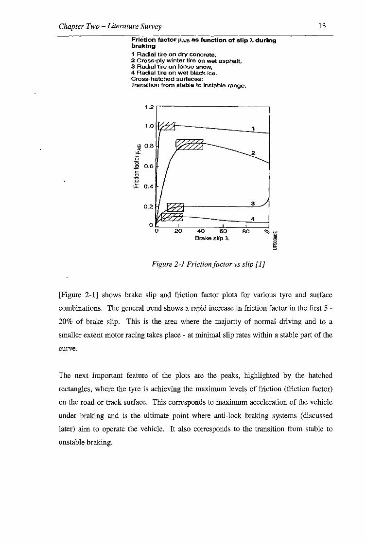
coefficient of friction is the same [ 1] whether the vehicle is braking or accelerating. This
relationship is described in [Figure 2-1].
Chapter Two - Literature Survey
Friction factor µAIB as function of slip A. during braking
1 Radial tire on dry concrete, 2 Cross-ply winter tire on wet asphalt, 3 Radial tire on loose snow, 4 Radial tire on wet black ice. Cross-hatched surfaces: Transition from stable to instable range.
1.2 r-------------~
1.0 1
~ 0.8 ::I.. ..... 0 0
0.6 ~ c: 0 :g if 0.4
0.2 3
4
20 40 60 Brake slip A.
80 0/o LU
Figure 2-1 Frictionfactor vs slip [l]
~ ID LL :::>
13
[Figure 2-1] shows brake slip and friction factor plots for various tyre and surface
combinations. The general trend shows a rapid increase in friction factor in the first 5 -
20% of brake slip. This is the area where the majority of normal driving and to a
smaller extent motor racing takes place - at minimal slip rates within a stable part of the
curve.
The next important feature of the plots are the peaks, highlighted by the hatched
rectangles, where the tyre is achieving the maximum level~ of friction (friction factor)
on the road or track surface. This corresponds to maximum acceleration of the vehicle
under braking and is the ultimate point where anti-lock braking systems (discussed
later) aim to operate the vehicle. It also corresponds to the transition from stable to
unstable braking.

Chapter Two - Literature Survey 14
The remainder of the plots shows a decline in friction factor as the wheels tend toward
fully locked at 100% brake slip. This is the unstable portion of the curve since any
increases in slip generated will lead to full wheel lock typically within tenths of a
second.
An interesting phenomenon is observed in [Figure 2-1, curve 3] where there is a sharp
increase in friction factor in the last 10% as the radial tyre is locked on loose snow.
This is related to geometric changes in tyre/surface interaction. On loose surfaces such
as gravel or snow a locked wheel will gather a pyramid of the surface material from the
leading edge of the contact patch and around the front of the tyre. This pyramid
effectively increases the size of the contact patch and provides additional drag on the
wheel. This phenomena is worth noting as it represents an exception to the general trend
that can not be ignored when applying brake controller systems to off road vehicles.
Perhaps the most relevant observation that can be made from the Radial tyre on dry
concrete plot [Figure 2-1, curve 1] that locking the wheels only reduces the friction
factor and hence braking distance by less than10% of maximum possible values. While
this alone may prevent an accident, it does not seem like enough to warrant such
attention to anti lock systems. The answer to this is due to the lack of directional
control (steering) available while the wheels are locked.
The level of longitudinal slip effects the forces that can be generated laterally by the
tyres. In the case of full wheel lock the lateral (steering) forces obtainable from the
tyres is reduced significantly from free rolling wheels. The following section highlights
the dynamics of lateral tyre force generation and how changing normal forces and
longitudinal slip effects it. Firstly however, lateral slip must be defined.
2.2 LATERAL SLIP
Lateral tyre force experienced by a vehicle during cornering or in a heavy side wind
loading situation causes lateral slip of the tyre. The result of this is that the tyre slips in
a direction other than longitudinal.
Chapter Two - Literature Survey 15
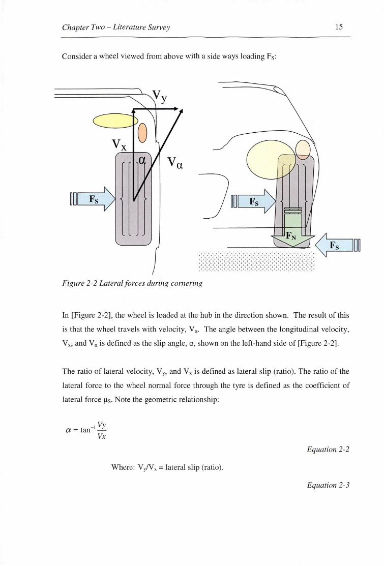
Consider a wheel viewed from above with a side ways loading Fs:
0
~O Fs
Figure 2-2 Lateral forces during cornering
In [Figure 2-2], the wheel is loaded at the hub in the direction shown. The result of this
is that the wheel travels with velocity, Va· The angle between the longitudinal velocity,
V x. and Va is defined as the slip angle, a, shown on the left-hand side of [Figure 2-2].
The ratio of lateral velocity, VY• and V x is defined as lateral slip (ratio). The ratio of the
lateral force to the wheel normal force through the tyre is defined as the coefficient of
lateral force µs. Note the geometric relationship:
- Vy a= tan 1
-Vx
Where: VyN x =lateral slip (ratio).
Equation 2-2
Equation 2-3

Chapter Two - Literature Survey 16
The relationship between lateral force and the wheel normal force is complex. This is
further complicated as slip angle in introduced as a variable. [Figure 2-3] shows the
general trend of the relationship between lateral force and the wheel normal force with
the higher curves on the chart representing greater slip angles.
Lateral
(Side)
Force,
Fs
Normal Force, F N
Figure 2-3 Lateral force as a function of normal force and slip angle. [9]
Slip
Angle,
a
[Figure 2-4] shows the same graphical information as [Figure 2-3] with an example of a
rear wheel drive vehicle' s front wheels during a cornering manoeuvre Imposed on the
Figure. This example is cited in a effort to describe the nature of the Figure and how it
applies to vehicle dynamics.

Chapter Two - Literature Survey
Lateral
(Side)
Force,
Fs
Normal Force, FN
17
Slip
Angle,
a
Figure 2-4 Lateral forces generated by the front wheels during vehicle cornering. [9}
Now it is also important at this stage to consider that the normal force on an individual
wheel will vary as the vehicle is accelerated, steered and braked due to weight
transferral effects as discussed in the introduction.
With reference to Figure 2-4, an analysis will be carried out on a rear wheel drive
vehicle while completing a cornering manoeuvre on a typical test course. This is a
simplified analysis where the front wheels will be followed and the vehicle is driving
within the stable portion of the slip curve [Figure 2-1]. Further geometric complications
related to the level of Ackerman steering [ 10] and smaller geometric effects are omitted.
Before the corner at point a in [Figure 2-4], the vehicle is in dynamic equilibrium (not
accelerating with a constant velocity). Approaching the corner, the vehicle is braked
Chapter Two - Literature Survey 18
until point b, transferring much of the weight of the vehicle onto the front wheels. At
point b the front wheels are steered. The steering angle is slowly increased through
points c1 and c0 until maximum lateral forces and slip angles are reached at points d1 and
d 0 corresponding to the apex of the corner. Here it is clear the normal force on the
inside tyre denoted by di is significantly less than that of the outside tire denoted by d0
due to the weight transference associated with the high lateral acceleration of the
vehicle.
After the apex the steering angle is slowly decreased. Acceleration out of the corner
begins to relieve the front wheels of load through points e1 and e0 • At point f, the
vehicle is exiting the corner and is under pure longitudinal acceleration. The vehicle
eventually reaches terminal speed (dynamic equilibrium) at point g, corresponding to
the condition before the corner, a.
From this example it can be seen that a tyre under normal driving conditions is subject
to both lateral and longitudinal forces simultaneously. The next section looks at this in
detail, as combinations of lateral and longitudinal loads impose limits on the driving
envelope of an automobile.

Chapter Two - Literature Survey 19
2.3 LOAD COMBINATIONS
Loading on a vehicle tyre is very rarely purely longitudinal or lateral. The majority of
the time vehicles are simultaneously steered and braked or accelerated. Since there is
only a finite amount of traction available from the tyres, any vehicle is only able to
brake or accelerate at maximum rates when it is in a straight line. Similarly, to maintain
maximum sideways loading and hence corner speed, a vehicle must not be accelerated
longitudinally.
Accelerating
Non operational region
Turning Left
Non operational region
Braking
Figure 2-5 The friction circle [I}
Longitudinal
Force, FL
Non operational region
Turning Right
Lateral (Side)
Force, Fs
Non operational region
[J Road Car
D Racecar
Chapter Two - Literature Survey 20
Plotting load combinations of all possible lateral and longitudinal force results in a
diagram known as the friction circle that defines the limits of combined acceleration,
braking and cornering.
The friction circle [Figure 2-5] is an expression of the total driving envelope of a
vehicle. On the friction circle plot, a circular or oval shape represents the driving
envelope of any particular vehicle. The operational region inside the circle represents
values of combined loading that are possible for a given vehicle/tyre/surface
combination. The non-operational region represented by the area outside the circle is a
region where the maximum physical forces that can be produced by the tyres as shown
in [Figure 2-1] are exceeded. A vehicle therefore can never operate outside its own
friction circle.
On the friction circle plot [Figure 2-5] is a generalised friction circle plot for a road car
and a generalised plot for a racecar. Racecars typically offer higher performance in the
areas of grip on the road/track surface since they are purpose built or modified to
achieve fast lap or stage times. Thus the friction circle of a racecar is much larger than
that of a typical road car since the racecar can generate greater forces while
accelerating, braking and cornering. Though the driving envelope is larger, a racecar has
a friction circle plot that is similar in shape to the road vehicle since the same limits
apply. Both race tyres and road tyres can only produce their greatest lateral forces while
free wheeling (not accelerating or braking) and their greatest longitudinal forces_ in a
straight line.
Combining the information in [Figure 2-3 (2-4)] and [Figure 2-5] allows gives an
appreciation of individual tyre force capability for each tyre as it is effected by weight
transferral while accelerating, braking and cornering. Thus a map can be created to
express the total tyre force capability of the tyres.
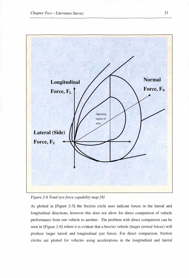
Chapter Two - Literature Survey
Longitudinal
Force, FL
Lateral (Side)
Force, Fs
Figure 2-6 Total tyre force capability map [9]
21
Normal
Force, FN
As plotted in [Figure 2-5] the friction circle axes indicate forces in the lateral and
longitudinal directions, however this does not allow for direct comparison of vehicle
performance from one vehicle to another. The problem with direct comparison can be
seen in [Figure 2-6] where it is evident that a heavier vehicle (larger normal forces) will
produce larger lateral and longitudinal tyre forces . For direct comparison, friction
circles are plotted for vehicles using accelerations in the longitudinal and lateral

Chapter Two - Literature Survey 22
directions, usually expressed in g . [Figure 2-7] [8] is a plot from measured data
showing typical values achieved by a sports car.
1-0.a-0.6-o.4-0.2-0--~
-0.2- ---0.4--o.e--o.s-
-1--1 -0.5 0 0.5
Lateral Acceleration (g)
1
Figure 2-7 Friction circle plot from measured data for a typical sports car [9]
[Figure 2-6] represents the physical limits of forces transmitted through a vehicle tyre
under while subject to changing normal forces due to weight transferral. What the
diagram does not do however, is describe how these physical limits are affected by tyre
slip (A.L) and slip angle (a) defined earlier in this chapter.
When tyres are operated under conditions where both longitudinal and lateral slip is
present any increases in longitudinal slip reduces the lateral force experienced by the
tyre.
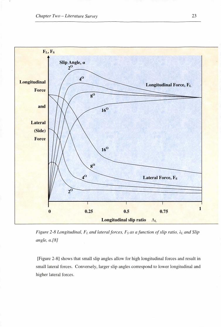
Chapter Two - Literature Survey
Longitudinal
Force
and
Lateral
(Side)
Force
0
Slip Angle, a 20 ~-~
0.25
23
Longitudinal Force, F L
Lateral Force, Fs
0.5 0.75 1
Longitudinal slip ratio J\.L
Figure 2-8 Longitudinal, FL and lateral forces, Fs as a function of slip ratio, AL and Slip
angle, a.[8]
[Figure 2-8] shows that small slip angles allow for high longitudinal forces and result in
small lateral forces . Conversely, larger slip angles correspond to lower longitudinal and
higher lateral forces.
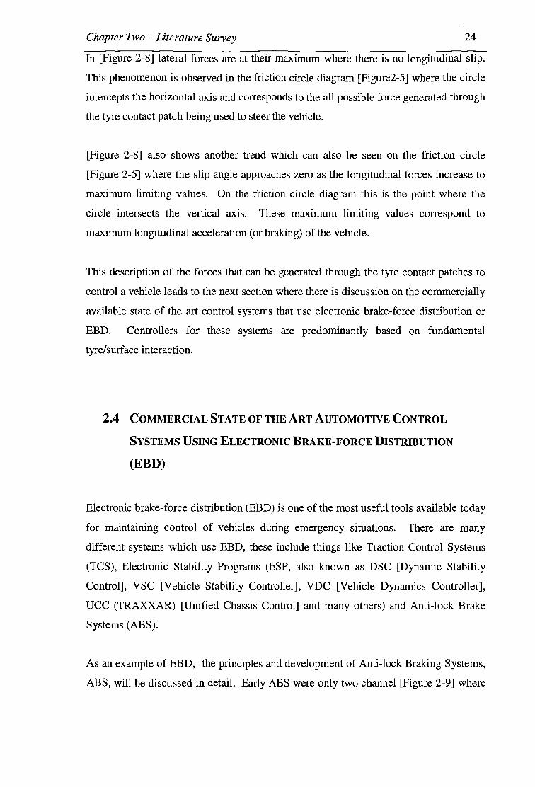
Chapter Two - Literature Survey 24
In [Figure 2-8] lateral forces are at their maximum where there is no longitudinal slip.
This phenomenon is observed in the friction circle diagram [Figure2-5] where the circle
intercepts the horizontal axis and corresponds to the all possible force generated through
the tyre contact patch being used to steer the vehicle.
[Figure 2-8] also shows another trend which can also be seen on the friction circle
[Figure 2-5] where the slip angle approaches zero as the longitudinal forces increase to
maximum limiting values. On the friction circle diagram this is the point where the
circle intersects the vertical axis. These maximum limiting values correspond to
maximum longitudinal acceleration (or braking) of the vehicle.
This description of the forces that can be generated through the tyre contact patches to
control a vehicle leads to the next section where there is discussion on the commercially
available state of the art control systems that use electronic brake-force distribution or
EBD. Controllers for these systems are predominantly based on fundamental
tyre/surface interaction.
2.4 COMMERCIAL STATE OF THE ART AUTOMOTIVE CONTROL
SYSTEMS USING ELECTRONIC BRAKE-FORCE DISTRIBUTION
(EBD)
Electronic brake-force distribution (EBD) is one of the most useful tools available today
for maintaining control of vehicles during emergency situations. There are many
different systems which use EBD, these include things like Traction Control Systems
(TCS), Electronic Stability Programs (ESP, also known as DSC [Dynamic Stability
Control], VSC [Vehicle Stability Controller], VDC [Vehicle Dynamics Controller],
UCC (TRAXXAR) [Unified Chassis Control] and many others) and Anti-lock Brake
Systems (ABS).
As an example of EBD, the principles and development of Anti-lock Braking Systems,
ABS, will be discussed in detail. Early ABS were only two channel [Figure 2-9] where
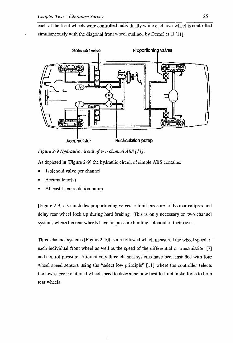
Chapter Two - Literature Survey 25
each of the front wheels were controlled individually while each rear wheel is controlled
simultaneously with the diagonal front wheel outlined by Demel et al [11].
Sof enord valve Proportioning valves
Accumulator Reclrculallon pump
Figure 2-9 Hydraulic circuit of two channel ABS [11].
As depicted in [Figure 2-9] the hydraulic circuit of simple ABS contains:
• lsolenoid valve per channel
• Accumulator( s)
• At least 1 recirculation pump
[Figure 2-9] also includes proportioning valves to limit pressure to the rear calipers and
delay rear wheel lock up during hard braking. This is only necessary on two channel
systems where the rear wheels have no pressure limiting solenoid of their own.
Three channel systems [Figure 2-10] soon followed which measured the wheel speed of
each individual front wheel as well as the speed of the differential or transmission [7]
and control pressure. Alternatively three channel systems have been installed with four
wheel speed sensors using the "select low principle" [11] where the controller selects
the lowest rear rotational wheel speed to determine how best to limit brake force to both
rear wheels.
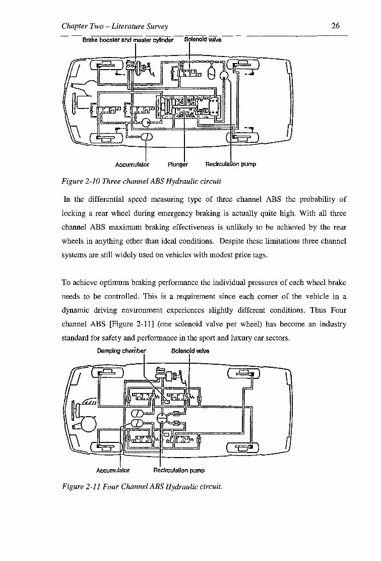
Chapter Two -Literature Survey 26
Brake boosler a11d mas!er cylinder Solenoid valve
Accumulator Plunger Reclrculallon pump
Figure 2-10 Three channel ABS Hydraulic circuit
In the differential speed measuring type of three channel ABS the probability of
locking a rear wheel during emergency braking is actually quite high. With all three
channel ABS maximum braking effectiveness is unlikely to be achieved by the rear
wheels in anything other than ideal conditions. Despite these limitations three channel
systems are still widely used on vehicles with modest price tags.
To achieve optimum braking performance the individual pressures of each wheel brake
needs to be controlled. This is a requirement since each comer of the vehicle in a
dynamic driving environment experiences slightly different conditions. Thus Four
channel ABS [Figure 2-11] (one solenoid valve per wheel) has become an industry
standard for safety and performance in the sport and luxury car sectors.
Damping chamber Solenoid valve
Accumulator Reclrculallon pump
Figure 2-11 Four Channel ABS Hydraulic circuit.

Chapter Two - Literature Survey 27
Solenoid valves or actuators in ABS are controlled by an Electronic Control Unit or
ECU [Figure 2-12]. In the least instance, this unit monitors all wheel speed sensors,
estimates the level of "lock" based upon calculated accelerations of each wheel and is
capable of decreasing and increasing the pressures in the brake lines.
1 Wheel-speed sensors, 2 Diagnosis connection , 3 Battery, 4 Input circuit, 5 Digital electronic controller, 6 Microcontroller, 7 Non-volatile memory, 8 Voltage stabilizer/Error store, 9 Output circuits with driver stages,
10 Solenoid-valve pairs for compressed-air increase/reduction,
11 Relay, 12 Stabilized battery voltage, 13 Check lamp.
Sensors ECU Actuators
Figure 2-12 4 channel ABS Electronic Control Unit (ECU) [ 12)
In more sophisticated ABS [65], the ABS ECU [Figure 2-12] receives the request of the
driver through their application of the brake pedal. The ECU is constantly measuring
the rotational velocity of the wheels and from this can determine the rotational
acceleration of all wheels at any given time. The ECU can then proceed to calculate the
error between the driver request and the actual vehicle dynamics.
Using a pre-programmed model, the ECU knows that the maximum rate of acceleration
under braking is, say, 9.8m/s or lg for the particular vehicle (see friction circle plot for a
typical sports car [Figure 2-7]). By constantly monitoring the wheel speeds, the ECU
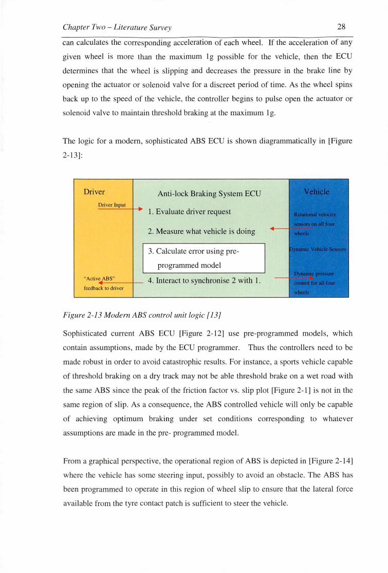
Chapter Two - Literature Survey 28
can calculates the corresponding acceleration of each wheel. If the acceleration of any
given wheel is more than the maximum lg possible for the vehicle, then the ECU
determines that the wheel is slipping and decreases the pressure in the brake line by
opening the actuator or solenoid valve for a discreet period of time. As the wheel spins
back up to the speed of the vehicle, the controller begins to pulse open the actuator or
solenoid valve to maintain threshold braking at the maximum lg.
The logic for a modern, sophisticated ABS ECU is shown diagrammatically in [Figure
2-13]:
Driver
Driver Input
"Acti ve ABS"
feedback to driver
Anti-lock Braking System ECU
1. Evaluate driver request
2. Measure what vehicle is doing
3. Calculate error using pre
programmed model
4. Interact to synchronise 2 with 1.
Figure 2-13 Modern ABS control unit logic [13]
Sophisticated current ABS ECU [Figure 2-12] use pre-programmed models, which
contain assumptions, made by the ECU programmer. Thus the controllers need to be
made robust in order to avoid catastrophic results. For instance, a sports vehicle capable
of threshold braking on a dry track may not be able threshold brake on a wet road with
the same ABS since the peak of the friction factor vs . slip plot [Figure 2-1] is not in the
same region of slip. A a consequence, the ABS controlled vehicle will only be capable
of achieving optimum braking under set conditions corresponding to whatever
assumptions are made in the pre- programmed model.
From a graphical perspective, the operational region of ABS is depicted in [Figure 2-14]
where the vehicle has some steering input, possibly to avoid an obstacle. The ABS has
been programmed to operate in this region of wheel slip to ensure that the lateral force
available from the tyre contact patch is sufficient to steer the vehicle.
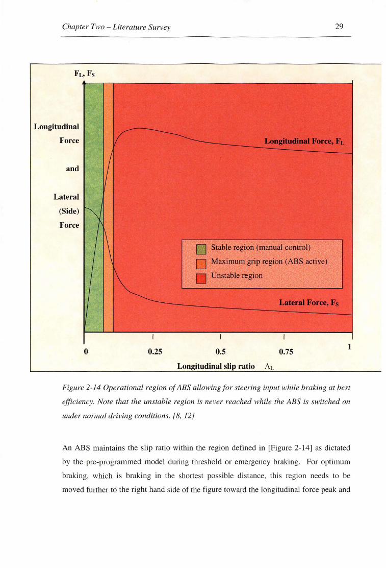
Chapter Two - Literature Survey
Longitudinal
Force
and
Lateral
(Side)
Force
0 0.25
Maximum grip region (ABS active)
Unstable region
0.5 0.75
Longitudinal slip ratio AL
29
1
Figure 2-14 Operational region of ABS allowing for steering input while braking at best
efficiency. Note that the unstable region is never reached while the ABS is switched on
under normal driving conditions. [8, 12)
An ABS maintains the slip ratio within the region defined in [Figure 2-1 4] as dictated
by the pre-programmed model during threshold or emergency braking. For optimum
braking, which is braking in the shortest possible distance, this region needs to be
moved further to the right hand side of the figure toward the longitudinal force peak and

Chapter Two - Literature Survey 30
into the unstable part of the plot. However, in the interests of robustness and
maintenance of sufficient lateral force braking distance is often sacrificed and the active
ABS region is conservatively kept well within the stable zone
To enhance the accuracy and achieve better braking performance it is possible to gain a
better approximation of individual wheel slip than by simply using acceleration based
algorithms. This has been achieved through the inclusion of a brake slip controller
discussed in the next section.
2.4.1 Further Advancement: The Brake Slip Controller
Acceleration based electronic brake control has one major limitation: The controller
assumes that the vehicle can brake at a given maximum rate regardless of conditions.
This can lead to the controller allowing values of wheel slip to extend beyond the 5%-
10% (dry road conditions) that is required for maximum braking effectiveness. In order
to ensure maximum braking effectiveness under all conditions brake slip controllers
have been developed which can "test" the individual tyre slip values. The problem of
measuring tyre slip is, however, extremely complex [13,1,9].
If tire compliance is ignored a linear differential equation can be used as a first
approximation to the actual rotational wheel dynamics. However, the tyre slip is the
basic quantity used in the control process and the equation of motion becomes non
linear after transformation from wheel rotation to tyre slip as a variable [14].
Furthermore the brake force depends non-linearly on the tyre slip.
To make matters even more complicated the brake torque can not be controlled directly
using the current braking systems (disk and drum hydraulic brakes). The system of
activating the brakes once the controller makes a decision involves an intricate series of
events that would be difficult to accurately model and involves many external factors
like brake wear and temperature. For the reasons outlined here, a simple and robust
Proportional-Integral-Differential (PID) [15] controller [Figure 2-15] is often employed.

Chapter Two - Literature Survey 31
It is difficult to directly measure tyre slip under typical road or track conditions since we
require a true measurement of ground speed or free-rolling wheel velocity. An estimate
of this value can be made using a technique where the brake pressure in the
corresponding wheel is relieved to a lesser constant value for sufficient time to test a
stable brake slip value. By using the known tyre stiffness (CA.) as well as estimated
values of tyre normal force (FN) and tyre brake force (F8 ) a nominal free-rolling wheel
velocity is given by:
V Wh/Free = V Whl • F c _ _§_
,i F N
Where: VwhtFree =Nominal free-rolling wheel velocity.
Vwht = Measured wheel velocity.
CA. =Tyre stiffness (known for a given tyre).
F8 = Estimated tyre brake force.
FN = Estimated values of tyre normal force.
Equation 2-4 [ 14], [ 15]
To apply this, the control of wheel slip must be interrupted in order to start the
procedure for the corresponding wheel. This will of course have an effect on the way in
which the vehicle behaves. To minimise the influence of the test procedure:
• Under braking, the relative speed of the wheels is constantly monitored and the
fastest rotating wheel is said to approximate the vehicle velocity.
• The free rolling velocities of the other three wheels are computed from the
approximate vehicle velocity.
• The procedure for determining the free rolling wheel velocity is then initiated for the
wheel in which a reduction of brake pressure would least effect the vehicles
dynamic behaviour.

Chapter Two - Literature Survey 32
The Bosch brake slip controller [13] uses many other parameters in order to achieve its'
aim to test the degree of individual tire slip and decide upon the control action as can be
seen in the controller structure [Figure 2-15].
Vx.
r-------------------------~
:.-----------------, : I I I I
Vy I : McaHalf PCirc FsF ' F;- FN llA. Fs I .~
Estimation of velocity of vehicle center of mass
Vx VWhiFre
Actual slip
slip controller
Mwti1No
Dislnbution of the nominal to es on the wheels
PwhlNo
Inverse model of the hydraulics
ABS - Nominal slip
+
FsF Fs
Brake force
PW hi
Model of the hydraulics
MNoMot UMvaJ
Figure 2-15 Controller structure for the Bosch Brake Slip Controller.[ 14]
Note in [Figure 2-15] that the free rolling wheel velocity, VwhtFree,, in this controller
structure is calculated in the 'Estimation of velocity of vehicle centre of mass' block.
The longitudinal velocity, Vx is estimated in the same block using the free rolling wheel
velocity, VwhtFree,, the estimated lateral velocity, Vy, the measured steering wheel angle, 8,
and the measured yaw velocity, 'I'·
Controllers such as the Bosch brake slip controller [Figure 2-15] are finely tuned in
their operation but still use approximation formulae such as the estimation for free
rolling wheel velocity [Equation 2-4]. Thus even the sophisticated controllers carry
with them assumptions made in these approximations as discussed previously.
To conclude this section on ABS it is important to discuss typical control configuration
and how ABS is incorporated into the overall vehicle control system.
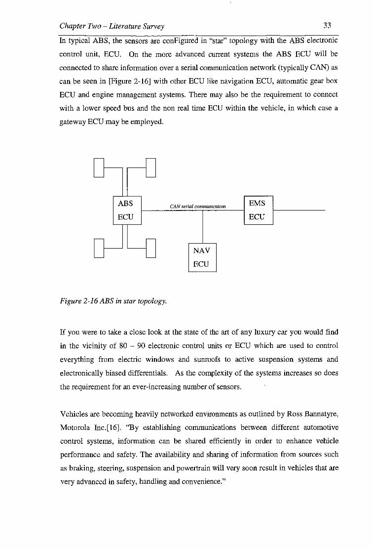
Chapter Two - Literature Survey 33
In typical ABS, the sensors are configured in "star" topology with the ABS electronic
control unit, ECU. On the more advanced current systems the ABS ECU will be
connected to share information over a serial communication network (typically CAN) as
can be seen in [Figure 2-16] with other ECU like navigation ECU, automatic gear box
ECU and engine management systems. There may also be the requirement to connect
with a lower speed bus and the non real time ECU within the vehicle, in which case a
gateway ECU may be employed.
- -.....____
- -
ABS CAN serial cmnmumcatwn EMS
ECU ECU
- -NAV
~ -ECU
Figure 2-16 ABS in star topology.
If you were to take a close look at the state of the art of any luxury car you would find
in the vicinity of 80 - 90 electronic control units or ECU which are used to control
everything from electric windows and sunroofs to active suspension systems and
electronically biased differentials. As the complexity of the systems increases so does
the requirement for an ever-increasing number of sensors.
Vehicles are becoming heavily networked environments as outlined by Ross Bannatyre,
Motorola Inc.[16]. "By establishing communications between different automotive
control systems, information can be shared efficiently in order to enhance vehicle
performance and safety. The availability and sharing of information from sources such
as braking, steering, suspension and powertrain will very soon result in vehicles that are
very advanced in safety, handling and convenience."

Chapter Two - Literature Survey 34
The future is in not just sharing information between systems but in combining these
dynamic control systems into fully integra,ted systems [7]. [Figure 2-17] below indicates
the way in which five different automotive sub systems are being merged. Note that the
central feature in this development is the braking system, which will play a key role in
the highly automated advanced chassis control system.
Steering
Suspension
Braking
Powertrain
Cruise
EHPS
Active Suspension
ABS
Powertrain
Cruise Control
EPS
Adaptive Cnuse
Lateral Stability
Collision Warning
Figure 2-17 The merging of automotive systems. [7]
Collision Avoidance
& Automated Capability
Chapter Two - Literature Survey 35
2.4.2 Traction Control Systems (TCS)
Current traction control systems typically use either Electronic Brake-force Distribution
(EBD), engine power retardation, or a combination of the two. Here we will only
briefly discuss the EBD type since power retardation (engine power limiting) is not part
<;>f the scope of this thesis. EBD traction control works almost exactly the same as ABS
except that the system is in play under acceleration rather than braking. Systems
typically use wheel speed sensors and may or may not utilise the sensors on the non
driven wheels. This is dependant on the application since a Traction Control System
(TCS) designed for a 4x4 all terrain vehicle is likely to be very different from a system
designed for a open wheel racecar in both system design and the sensors used.
Electronic brake-force distribution (EBD) traction control can also, in one sense,
remove the requirement for a limited slip differential. With an open differential the
slipping wheel can be braked transmitting drive through to the wheel(s) with grip.
However there are both advantages and disadvantages to using EBD over mechanical
forms of traction control like limited slip differentials.
In common with ABS the most advanced EBD TCS available today on luxury cars [13]:
1. Evaluates the driver's request as expressed through the accelerator pedal.
2. Measures what the vehicle is doing by through wheel speed sensors.
3. Calculates the "error" using a pre-programmed model of vehicle behaviour.
4. Uses EBD to synchronise 2 with 1.
Quite simply, EBD TCS is ABS under acceleration where, like ABS, the aim is to keep
the driven wheels within the 5%-10% range of slip in order to retain maximum
controllability and acceleration [3].
Chapter Two -Literature Survey 36
2.5 ELECTRONIC SUSPENSION MONITORING, REGULATION AND
CONTROL
While EBD ABS and TCS can make the most of the grip available, they are not direct
methods of increasing the grip or altering the forces developed between the tyre and the
road surface. To achieve this, it is possible to alter the dynamic load on individual
wheels through the means of suspension control. In other words the normal force
between the tyres and the road/track can be distributed actively between the four wheels
or can be instantaneously altered within physical limits.
The suspension on a vehicle can be controlled either directly via means of pneumatic or
hydraulic systems or indirectly through the use of electronically controlled adjustable
dampeners etc. Simple systems do not actually measure the position of the suspension,
thus the system has no means for gathering feedback. The most effective systems do
measure the position of the suspension through the use of linear potentiometers or
similar devices
The use of measuring devices on passive suspension is also becoming popular on luxury
vehicles as part of their dynamic control systems. This provides dynamic information
for wheel loading, which in tum can be used to approximate instantaneous levels of grip
available from each tyre.
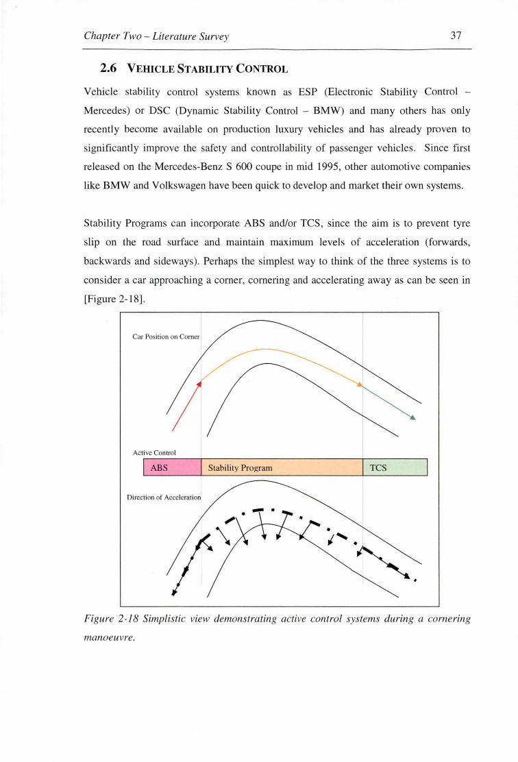
Chapter Two - Literature Survey 37
2.6 VEHICLE STABILITY CONTROL
Vehicle stability control systems known as ESP (Electronic Stability Control -
Mercedes) or DSC (Dynamic Stability Control - BMW) and many others has only
recently become available on production luxury vehicles and has already proven to
significantly improve the safety and controllability of passenger vehicles. Since fust
released on the Mercedes-Benz S 600 coupe in mid 1995, other automotive companies
like BMW and Volkswagen have been quick to develop and market their own systems.
Stability Programs can incorporate ABS and/or TCS, since the aim is to prevent tyre
slip on the road surface and maintain maximum levels of acceleration (forwards,
backwards and sideways). Perhaps the simplest way to think of the three systems is to
consider a car approaching a corner, cornering and accelerating away as can be seen in
[Figure 2-18].
Car Position on Corner
Active Control
I ABS Stability Program TCS
Direction of Acceleration
·~.
Figure 2-18 Simplistic view demonstrating active control systems during a cornering
manoeuvre.

Chapter Two - Literature Survey 38
[Figure 2-18] shows a vehicle cornering on its limits of adhesion. The bar indicates that
the ABS is active on the approach to the corner, the ESP is active through the corner
and the TCS is active while accelerating away from the corner. However this is a
simplistic look at when each system is active, since the exact moment when ABS
becomes ESP and ESP becomes TCS is hard to define, hence the move towards one
integrated system.
The more sophisticated stability programs require more sensors in order to function
properly than simple ABS and TCS systems. Essentially this stems from the
requirement to "know" whether the vehicle is in a state of understeer, oversteer,
sideways drift, or a normal driving attitude.
The Bosch/Mercedes-Benz ESP uses [3]:
1. A steering angle sensor
2. Wheel speed sensors on all four wheels
3. A lateral acceleration sensor
4. A yaw sensor
5. A brake pressure sensor
The Relative positions of these sensors can be seen in [Figure 2-19] where a vehicle slip
controller, as discussed previously, is integrated into the overall Electronic Stability
Program (ESP).
CD Wheel speed sensors
® Brake pressure sensor @ Steering wheel angle sensor
@ Yaw rate sensor
® Lateral accelerabon sensor
@ Brake pressure modulation (f) Engine management
Observer Estimation of state variable values -------,::
f----------1 ------u: Vehicle dynamics controller
Control of yaw rate and vehicle shp angle
Nominal tire shp
Slip controller with interface to VDC
Sensor signals forVDC
Figure 2-19 Bosch/Mercedes-Benz ESP Vehicle Dynamics Control (VDC) system. [14]
Chapter Two - Literature Survey 39
Typically, the information from these sensors [Figure 2-19] is then fed into the ECU
that determines, among other things [ 5]:
1. Where the driver is intending the car to go.
2. At what speed does the driver intend to get there, i.e. are they braking, accelerating
or coasting.
3. The cars status; level of oversteer or understeer, and level of drift/grip
The ESP ECU will then compare this with a stored mathematical reference model and
will apply selective breaking (EBD) in an attempt to match the vehicle's behaviour with
the intended actions of the driver.
The working concept of the most basic function of ESP is actually quite simple. The
sensors determine whether the vehicle is yawing more or less than the driver intends
and applies a corrective moment using different braking forces on either side of the
vehicle.
It has been outlined that longitudinal and lateral forces on a tire (FL, Fs) depend on the
tyre slip (A), the slip angle (a) and the normal tire force (FN) [5]. For a given slip angle
the lateral force generated by a tyre decreases with increasing magnitude of tyre slip. In
other words for a given a, FL decreases as A increases. Stability control systems,
including the Bosch ESP, typically use this fundamental tyre property in order to
specifically control lateral tyre forces and hence the yaw moment on the vehicle. The
effects of stability control systems such as ESP can be seen in [Figure 2-20] where two
vehicles, one with ESP and one without, are steered around a right-left-right-left slalom
type corner combination with the same steering input. Note in this diagram that the
vehicle without ESP becomes increasingly unstable from the first corner.
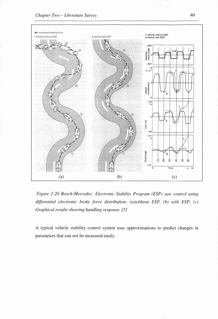
Chapter Two - Literature Survey
.. Increased braking force
1 Vehicle without ESP
(a)
2 Vehicle with ESP
(b)
1 Vehicle without ESP, 2 Vehicle with ESP.
40
+1BO•r-----------,
"' . g. .§ ~ 0 l'--t----11'!---ll---li- +----Hrl !! ~ en !<
m.s-2
-s~-;---+-+--+-+---+----" +30 r---t--+-+--+-+---+--, '/ s
+ 10° r--t----t-- t----+---i-+----, 0
-10' ~o----T~im_e ____ s~14
(c)
Figure 2-20 Bosch-Mercedes Electronic Stability Program (ESP) yaw control using
differential electronic brake force distribution: ( a)without ESP, (b) with ESP, ( c)
Graphical results showing handling response. [5]
A typical vehicle stability control ystem uses approximations to predict changes m
parameters that can not be measured easily.
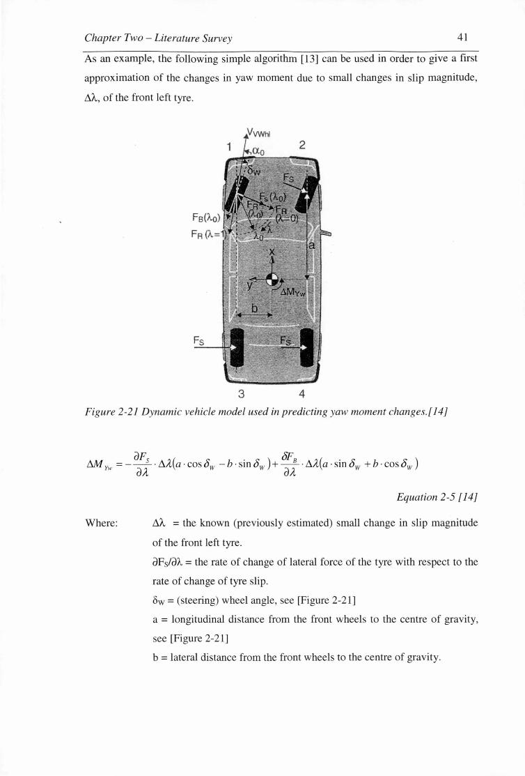
Chapter Two - Literature Survey 41
As an example, the following simple algorithm [13] can be used in order to give a first
approximation of the changes in yaw moment due to small changes in slip magnitude,
f:.,) . ..,, of the front left tyre.
3 4
Figure 2-21 Dynamic vehicle model used in predicting yaw moment changes. [ 14]
M1 =- aFs · lllt(a ·coso -b ·sino )+ 8Fa · lllt(a ·sino +b·coso ) Yw dA W W dA W W
Where:
Equation 2-5 [ 14]
ll'A = the known (previously e timated) small change in slip magnitude
of the front left tyre.
aFsldA = the rate of change of lateral force of the tyre with respect to the
rate of change of tyre slip.
ow= ( teering) wheel angle, see [Figure 2-21]
a = longitudinal distance from the front wheels to the centre of gravity,
see [Figure 2-21]
b = lateral distance from the front wheels to the centre of gravity.
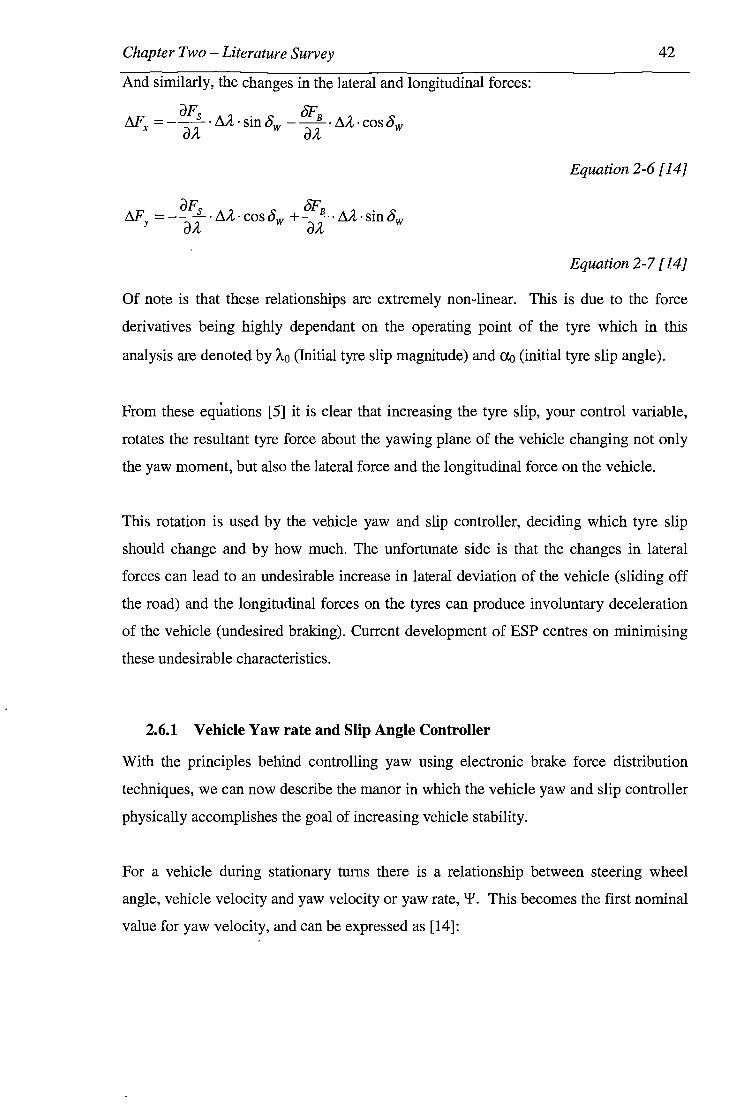
Chapter Two - Literature Survey 42
And similarly, the changes in the lateral and longitudinal forces:
Af' = - dFs · ~A,· sin 8 - §FB ·~A,· cos 8 x a;i w a;i w
Equation 2-6 [14)
dFs ~ s: §FB A ~ • s: Af' = --- · ~J'L,· cosu +--· il/I,' smu y a;i w a;i w
Equation 2-7 [ 14)
Of note is that these relationships are extremely non-linear. This is due to the force
derivatives being highly dependant on the operating point of the tyre which in this
analysis are denoted by A.0 (Initial tyre slip magnitude) and a.a (initial tyre slip angle).
From these equations [5] it is clear that increasing the tyre slip, your control variable,
rotates the resultant tyre force about the yawing plane of the vehicle changing not only
the yaw moment, but also the lateral force and the longitudinal force on the vehicle.
This rotation is used by the vehicle yaw and slip controller, deciding which tyre slip
should change and by how much. The unfortunate side is that the changes in lateral
forces can lead to an undesirable increase in lateral deviation of the vehicle (sliding off
the road) and the longitudinal forces on the tyres can produce involuntary deceleration
of the vehicle (undesired braking). Current development of ESP centres on minimising
these undesirable characteristics.
2.6.1 Vehicle Yaw rate and Slip Angle Controller
With the principles behind controlling yaw using electronic brake force distribution
techniques, we can now describe the manor in which the vehicle yaw and slip controller
physically accomplishes the goal of increasing vehicle stability.
For a vehicle during stationary turns there is a relationship between steering wheel
angle, vehicle velocity and yaw velocity or yaw rate, \f. This becomes the first nominal
value for yaw velocity, and can be expressed as [14]:

Chapter Two - Literature Survey
vx ·bw If/ No = ---"----"---2 -
Where:
v (a+c)(l +~)
VCH
Vx =vehicle velocity in the x (longitudinal) direction
VcH = Characteristic vehicle velocity
8w =(steering) wheel angle, see [Figure 2-21]
43
Equation 2-8 [15]
a = longitudinal distance from the front wheels to the centre of gravity,
see [Figure 2-21]
c = longitudinal distance from the rear wheels to the centre of gravity.
This relationship, however, is not valid if the coefficient of friction of the track surface
is low. Thus, it is necessary to limit this nominal yaw rate:
g lff No.~µ·
V~
Where:µ = Road/tyre combination coefficient of friction.
Equation 2-9 [14]
The problem is not yet complete since the vehicle can still slide excessively sideways
due to the lateral acceleration, which during turns with no wheel slippage is equal to the
product of yaw velocity and vehicle velocity. In a state of excessive sliding the lateral
forces can not be increased any further, so the controller needs to decrease the vehicle
slip angle. By making appropriate decreases in the nominal yaw velocity, creating a
third \J!No, the controller is able to further optimise the Electronic Brake-force
Distribution.
The Bosch Electronic Stability Program, ESP [14][15][1], uses many other parameters
in order to achieve its' aim to maintain higher levels of vehicle control and to decide
upon the control action, as can be seen in the controller structure [Figure 2-22].
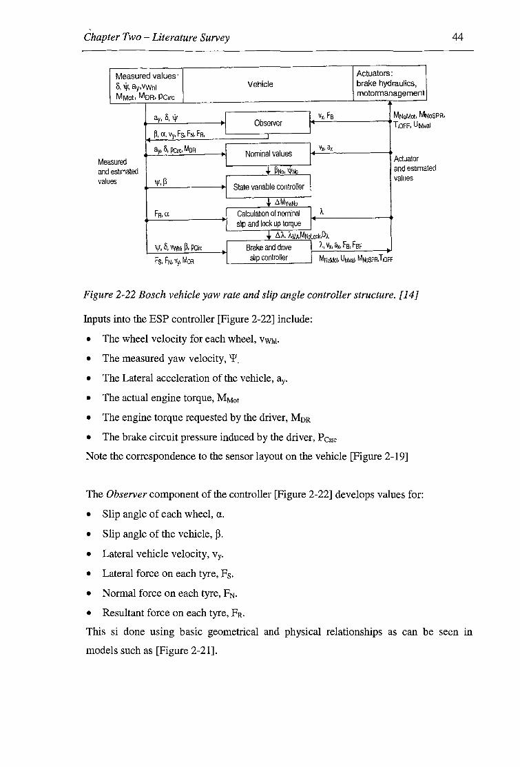
-Chapter Two - Literature Survey
Measured values· Actuators:
o, \jl, ay,VWhl Vehicle brake hydraulics,
MMot. MoR. PC1rc motormanagement ~
ay. o, iV .I I Vx, F0 MNoMot. MN oSPR, al
asured Me and valu
estimated es
p, a, vy. Fs, FN. FR,
ay. o, PC1rc. MoR
ljl,p
FR, u
\jf, O, Vi'lhl> ~. PCirc
Fs, FN, v ' MoR
I
I I
I I
I I
.I 'I
Observer I T10FF. UMv I
Nominal values I Vx, ax
I Actuator
+ PNo. \j/No and es~mat
State vanable controller I values
-t tlMvwNo Calculabon of nominal I f. slip and lock up torque I~
i. tl/.., NAA.MNolcx:k·D).. Brake and dnve I ) ., Vx, ax, Fs, FsF
slip controller I r
MNoMot· UMvaJ, MN0SPR,T10FF
Figure 2-22 Bosch vehicle yaw rate and slip angle controller structure. [14]
Inputs into the ESP controller [Figure 2-22] include:
• The wheel velocity for each wheel, VWhJ·
• The measured yaw velocity, 'I'.
• The Lateral acceleration of the vehicle, ay.
• The actual engine torque, MMot
• The engine torque requested by the driver, MoR
• The brake circuit pressure induced by the driver, Perre
Note the correspondence to the sensor layout on the vehicle [Figure 2-19]
The Observer component of the controller [Figure 2-22] develops values for:
• Slip angle of each wheel, a .
• Slip angle of the vehicle, ~·
• Lateral vehicle velocity, Vy .
• Lateral force on each tyre, Fs .
• Normal force on each tyre, FN .
• Resultant force on each tyre, FR .
ed
44
This si done using basic geometrical and physical relationships as can be seen in
models such as [Figure 2-21].
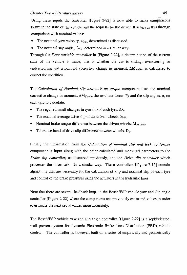
Chapter Two -Literature Survey 45
Using these inputs the controller [Figure 2-22] is now able to make comparisons
between the state of the vehicle and the requests by the driver. It achieves this through
comparison with nominal values:
• The nominal yaw velocity, \j/No .. determined as discussed.
• The nominal slip angle, PNo .. determined in a similar way.
Through the State variable controller in [Figure 2-22], a determination of the current
state of the vehicle is made, that is whether the car is sliding, oversteering or
understeering and a nominal corrective change in moment, ~MYwNo, is calculated to
correct the condition.
The Calculation of Nominal slip and lock up torque component uses the nominal
corrective change in moment, ~MYwNo, the resultant forces FR and the slip angles, a, on
each tyre to calculate:
• The required small changes in tyre slip of each tyre, KA.
• The nominal average drive slip of the driven wheels, AMA·
• Nominal brake torque difference between the driven wheels, MNoLock·
• Tolerance band of drive slip difference between wheels, D1...
Finally the information from the Calculation of nominal slip and lock up torque
component is input along with the other calculated and measured parameters to the
Brake slip controller, as discussed previously, and the Drive slip controller which
processes the information In a similar way. These controllers [Figure 2-15] contain
algorithms that are necessary for the calculation of slip and nominal slip of each tyre
and control of the brake pressures using the actuators in the hydraulic lines.
Note that there are several feedback loops in the Bosch/ESP vehicle yaw and slip angle
controller [Figure 2-22] where the components use previously estimated values in order
to estimate the next set of values more accurately.
The Bosch/ESP vehicle yaw and slip angle controller [Figure 2-22] is a sophisticated,
well proven system for dynamic Electronic Brake-force Distribution (EBD) vehicle
control. The controller is, however, built on a series of empirically and geometrically
Chapter Two -Literature Survey 46
derived approximations as discussed. The system is therefore vulnerable when
conditions arise that are not well described by those approximations.
To prevent the occurrence of catastrophic results under adverse conditions, the
controller is robustly designed. The adverse side to this robustness is that some
performance is sacrifices in the interests of safety. On the subject of applicability and
robustness of the Bosch Vehicle Dynamics Controller, Van Zanten et al (Bosch) [15]:
"To find the best compromise according to the customer demands the system can be
tuned in either direction. For example stopping distances on homogeneous roads for
full braking can be reduced while keeping the vehicle usually stable however, the
manoeuvrability will be reduced." These compromises fail to take full advantage of
Electronic Brake-force Distribution (EBD) under all conditions.
Neural networks offer an alternative approach to empirical/geometrical approximation
based systems and are not subject to the same limitations. Emerging neural network
technology is slowly replacing these types of systems in other fields but is only now
becoming useful for complex automotive control as computing power becomes cheaper
and more compact.
2.7 NEURAL NETWORK APPLICATIONS AND CONTROL TO PREDICT
AUTOMOTIVE PERFORMANCE
Neural networks have been used in a wide range of areas in order to predict the
performance of a given system. In automotive areas of research their use has been
predominantly in engine management systems. A typical example of this is Chris M.
Atkinson's SAE technical paper "Virtual Sensing: a Neural Network-based Intelligent
Performance and Emissions Prediction System for On-Board Diagnostics and Engine
Control" [17].
Atkinson was primarily concerned with the emissions side of things since that is where
legislation (in countries where the biggest automotive markets are) is constantly
applying pressure to the automotive industry. Important as it is, the focus on the

Chapter Two -Literature Survey 47
emission control has put engine control systems in front of dynamic chassis behaviour
control systems in terms of technology, research and development. There is little doubt
that neural network systems have been developed for dynamic chassis behaviour control
by many of the worlds leading automobile producers. The development of such
systems is both expensive and time consuming so it is easy to see why these systems
remain closely guarded secrets.
Many neural network models have been developed for engine control, as it is only a
matter of using the sensors which modem engines already have to control electronic
regulators like fuel injectors, spark plug coils, fly by wire throttles etc. Hence it can be
done for little outlay and is the focus of many academic papers and thesis, which are
freely available and demonstrate the potential for artificially intelligent systems in
engine control. It is only recently that the "sensor explosion" has begun to make its way
into the commercial luxury vehicle chassis.
Following on in this progression, it would seem that the use of neural networks in
vehicle dynamic control systems is the next step. The only questions remaining are how
should these systems be integrated and what types of neural networks are suitable for
dynamic automotive applications.
In the past, development of dynamic automotive neural networks has primarily been
conducted on a theoretical basis by independent and academic researchers since
physical testing for full size self controlled vehicles is costly and can be dangerous.
Despite these and other limitations, some researchers have realised the potential of
Neural Networks in automobile control.

Chapter Two - Literature Survey 48
In 1987 J Shepanski and S.Macy as illustrated in R. Hecht-Nielsen, "Neurocomputing",
[18] developed what they called an "automobile autopilot" through simulation of
"almost real" driving conditions with some restrictions in an effort to make the problem
tractable. Not the least of these restrictions were major assumptions of the road
environment including that the vehicle would only be travelling on a two lane freeway
with wide shoulders (which the vehicle could be driven along) upon which all traffic
was moving in the same direction.
I
Road curvature = C 1
~ = Car driven by neural network
D = Other cars
I
1 Lane i- canter line
Figure 2-23 "Automobile Autopilot" model freeway used to develop vehicle control
Neural Networks in under simplified conditions [18]
The Neural Network driven vehicle can travel in either lane of the freeway where other
simulated cars drive at various speeds and perform certain manoeuvres. In this
simulation, the other cars are pre-programmed and do not deviate if threatened by the
NN controlled vehicle. The researchers justified this by the claim that successful
collision avoidance manoeuvres are uncommon in real world driving situations since
usually the driver does not recognise the threat of a collision until it is too late. This
lack of response by other cars does, however, simplify the problem to what was deemed
a manageable level.
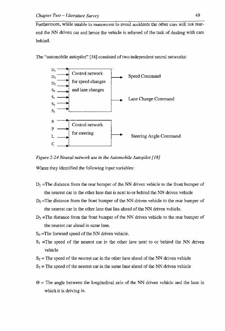
Chapter Two-Literature Survey 49
Furthermore, while unable to manoeuvre to avoid accidents the other cars will not rear
end the NN driven car and hence the vehicle is relieved of the task of dealing with cars
behind.
The "automobile autopilot" [18] consisted of two independent neural networks:
D1
D2
D3 ----So--
S1-
S2
S3
e p
L
c
Control network
for speed changes
and lane changes
Control network
for steering
Speed Command
Lane Change Command
Steering Angle Command
Figure 2-24 Neural network use in the Automobile Autopilot [18]
Where they identified the following input variables:
D1 =The distance from the rear bumper of the NN driven vehicle to the front bumper of
the nearest car in the other lane that is next to or behind the NN driven vehicle
D2 =The distance from the front bumper of the NN driven vehicle to the rear bumper of
the nearest car in the other lane that lies ahead of the NN driven vehicle.
D3 =The distance from the front bumper of the NN driven vehicle to the rear bumper of
the nearest car ahead in same lane.
So =The forward speed of the NN driven vehicle.
S1 =The speed of the nearest car in the other lane next to or behind the NN driven
vehicle
S2 = The speed of the nearest car in the other lane ahead of the NN driven vehicle
S3 = The speed of the nearest car in the same lane ahead of the NN driven vehicle
8 = The angle between the longitudinal axis of the NN driven vehicle and the lane in
which it is driving in.
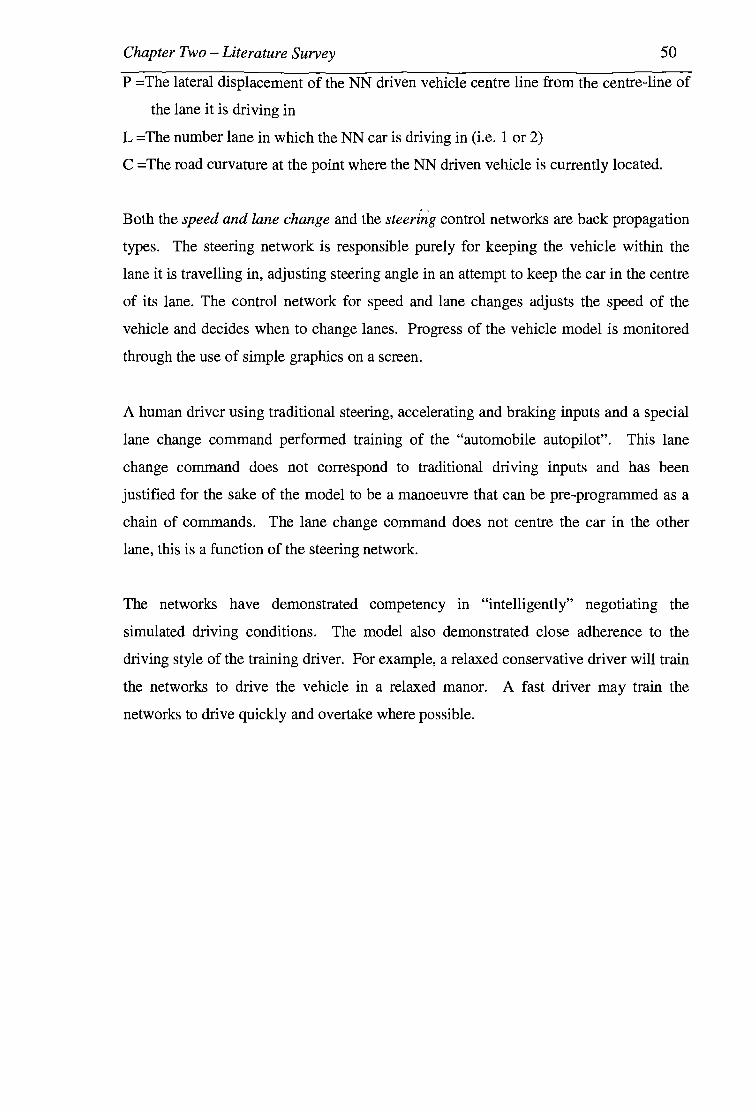
Chapter Two - Literature Survey 50
P =The lateral displacement of the NN driven vehicle centre line from the centre-line of
the lane it is driving in
L =The number lane in which the NN car is driving in (i.e. 1 or 2)
C =The road curvature at the point where the NN driven vehicle is currently located.
Both the speed and lane change and the steeri'rig control networks are back propagation
types. The steering network is responsible purely for keeping the vehicle within the
lane it is travelling in, adjusting steering angle in an attempt to keep the car in the centre
of its lane. The control network for speed and lane changes adjusts the speed of the
vehicle and decides when to change lanes. Progress of the vehicle model is monitored
through the use of simple graphics on a screen.
A human driver using traditional steering, accelerating and braking inputs and a special
lane change command performed training of the "automobile autopilot". This lane
change command does not correspond to traditional driving inputs and has been
justified for the sake of the model to be a manoeuvre that can be pre-programmed as a
chain of commands. The lane change command does not centre the car in the other
lane, this is a function of the steering network.
The networks have demonstrated competency in "intelligently" negotiating the
simulated driving conditions. The model also demonstrated close adherence to the
driving style of the training driver. For example, a relaxed conservative driver will train
the networks to drive the vehicle in a relaxed manor. A fast driver may train the
networks to drive quickly and overtake where possible.

Chapter Two - Literature Survey 51
2.7.1 Advantageous Characteristics of Neural Networks
• Neural Networks are trained or taught rather than programmed. Automated learning
is possible from examples - the need for programmers to make assumptions about
the form of the relationship between input and output is removed.
• Rather than having separate memory, controller and stored external program linking
them (operating system), the operation of neural networks is implicitly controlled.
• The form of a Neural Network gives the system an associative memory. Inherently
the network associates items taught to it, grouping similar items together within the
structure.
• Neural Networks are capable of generalising. This gives the network the ability to
group categories of objects based on a series of examples.
• Neural Networks are robust. Networks will continue to operate after significant
quantities of its neurons and interconnections fail. Performance of the neural
network under these conditions will degrade smoothly with the loss of these
neurons.
• Neural Networks can be structured to be self organising. These networks generalise
from data patterns without requiring specific instructions on what to look for or
what to learn.
2.7.2 Neural Network Artificial Intelligence
In an engineering sense, artificial neural networks are systems that replicate the
principles and functions of a human brain.
Xt~ . Summation • 11
net
X2 ~w L
-~wj,. X1
Activation Function
Processing Unit
Figure 2-25 The structure of an artificial neuron
Output Function
Output
Yk )

Chapter Two - Literature Survey 52
Similar to a biological neuron, an artificial neuron receives inputs from other neurones
within the network, processes those inputs and sends a single output. In this manner,
neurones relate to each other via weighted connections.
In the sketch above, the inputs to the neuron are x1, x2, ..• Xi, the origin of these defined
by the network architecture. The weighted connections are denoted as Wj1,Wj2 ••• Wji
corresponding to these inputs.
The processing capability of an artificial neuron is the combination of three functions:
1. The input function
2. The activation function
3. The output function
The input function multiplies each input by the corresponding weight and sums the
weighted inputs for i number of input neurones. Thus the net input to the /h neuron
activation function, net1, can be described as [19]:
Equation 2-10
The activation function can be any function that is differentiable and monotonically
increasing [20]. The output of the activation function is conventionally limited to
between 0 and 1 or alternatively -1 and +1. The type of activation function used
governs this range. Simple neural network models use step or threshold functions,
popular in early systems. This particular activation function outputs a 1 if the weighted
sum of the inputs is greater than a programmed threshold, if not the output is a zero.
More general non-linear sigmoid (logistic) functions have seen widespread use in more
recent times. Sigmoid functions follow a curve with a continuous positive slope
(derivative is always +ve), contain only real-values and are bound by limits.

Chapter Two - Literature Survey 53
Threshold and Sigmoidal Activation Functions
0.9 .
0.8 .
0.7
--Threshold Function
--Sigmoid Funct ion
0.3
0.2 .
0.1
-7 -5 -3 -1 9
Weighted Sumed Input, netj
Figure 2-26 Threshold and sigmoidal activation functions
The equation governing the sigmoid activation function is given by [21]:
f(net) = I+ exp(-net) Equation 2-11
Hence the derivative can be found simply:
f (net) = f(net) * (1 - f(net)) Equation 2-12
In popular, contemporary neural networks the output from the activation function is
commonly chosen as the output from the neuron. Thus in current practices, the output
function does nothing to alter the value produced by the activation function. It is
important to remember, however, that this is not always the case and under certain
circumstances an effective output function can be very valuable.
Each neuron in a neural network can be thought of as a primitive function, taking a
specific input and producing a defined output. When these are combined in a network,
however, they possess the capability of mapping an n-dimensional real input to an m
dimensional real output. Hence a neural network is often treated by engineers as a
"black box" where the results rather than the process are important.

Chapter Two - Literature Survey 54
A neural network is not programmed to estimate results for specific applications,
instead the network "learns" to solve the problem through a process called 'neural
network training'. This process involves refining the values of the weighted
connections, Wj1,WJ2 ... Wji in our example neuron. These weights are specific to, and
need to be computed for, the application.
There is no direct way to calculate the ultimate weighting. The weighted connections
are continuously adjusted during neural network training using algorithms or 'learning
rules' [18]. The specific learning rule used will depend on what type of neural network
model is being applied.
Neural networks are categorised under two major model classes:
1. Feed-forward Neural Networks
2. Recurrent Neural Networks
Furthermore, methods for neural network training are often broadly categorised into:
1. Supervised training
2. Un-supervised training.
For example, The Perceptron neural network developed by Frank Rosenblatt, in 1962
[22] can be described as a Feed-forward network with supervised training.
2.8 FEED-FORWARD NEURAL NETWORKS
Feed-forward neural networks operate under the principle that the information or input
activity signals propagate in one direction only. Basic or fundamental feed-forward
neural networks consist of a single input layer, numerous hidden layers, and a single
output layer.

Chapter Two -Literature Survey
Input----;, (x,)
Input Layer
Htdden Layer I
Htdden Layer J
Figure 2-27 Feed forward neural network structure
Output Layer
Output (out1)
Output (ou~)
Output (oult)
55
After the input layer, the neurons in each consecutive layer receive an array of data
through network interconnects. This array is then processed within the neuron to
produce a single output, which is fed into every neuron in the next layer. This process
is repeated through the neural network to the output layer.
2.9 RECURRENT NEURAL NETWORKS
All recurrent neural networks posses at least one feedback loop. This means that at least
some activity signals do not follow a straight path through the network, rather the output
from one layer or set of neurones are sent back through some or all of the layers
previously seen. Thus a recurrent neural network is dynamic since the network will
evolve as time elapses for a given initial state.
It is important then that the architecture for a recurrent network is chosen carefully for a
particular application such that the network converges toward a state of equilibrium. If
the recurrent neural network is stable, this can eventually be reached.
Recurrent neural networks are useful for applications involving intensive computational
problems and aiso the in the storage of information (memory applications).

Chapter Two - Literature Survey 56
2.10 SUPERVISED AND UNSUPERVISED TRAINING
Neural networks can be trained using either supervised or unsupervised techniques.
Supervised training is the name given to any neural network training were a teacher
provides input patterns and corresponding output patterns similar to those expected to
be encountered by the network during operation. Using an iterative process the network
dynamically adjusts its weights until the error between the output from the neural
network and the target output reaches a minimum.
Unsupervised training is employed often when only input vectors are available. This
type of training is suited to raw collections of data where the network is used to create
categories by finding similar features and correlations in training input sets. In creating
these categories the network must discover for itself the existence of patterns,
regularities and separating properties.
2.11 OPTIMISING NEURAL NETWORK PERFORMANCE
To achieve optimum performance from a neural network careful consideration is
required in relation to:
• The 'condition' of the network input and target output vectors
• Design of the training data
• Methods for testing and evaluating the network performance
2.11.1 Network Input and Output Normalisation
A Neural Network sees improvements in performance when insignificant characteristics
and information is removed form the input data set. Usually values of standard
deviations and offsets are independent of the important aspects of individual input
vector components. The effect of this type of insignificant data complicates the task of
the Neural Network and decreases the network performance. For this reason the input
vectors to the network are often normalised.

Chapter Two - Literature Survey 57
Normalising involves scaling of the input parameters such that the network sees each
individual component of the input vector as being of equal magnitude. As a
consequence, the network is presented with information that has no implicit bias toward
any given input parameter(s). A side effect of normalisation is increased numerical
stability of the network data process.
In most cases training algorithms minimise the total error of all outputs. Thus if target
output vector components are unequal in magnitude, individual outputs with larger
deviations will be favoured, as they will dominate the error sum. Hence normalisation
of the target output data is critical to achieving true minimisation of total error. This,
however, is often designed into the network through the use of bound activation
functions such as both the threshold and sigmoid types that are usually given and are
therefore limited to a range of between zero and 1, ie. (0:5f(x):5 1).
2.11.2 Design of Neural Network training data
The development of the training set for a Neural Network will dictate its performance.
The size of the training set required to provide the network with adequate training is one
of the most important considerations first encountered by the trainer. However, it has
been proved that the general learning problem for neural networks is intractable [22],
which means that it can not be solved efficiently for every possible input vector. From
an engineering perspective where Neural Networks are used as tools for solving specific
and real problems qualitative decisions need to be made about the size of the training
set.
In order for a trained network to be effective the training set must be large and complete
enough to satisfy at least the following two goals:
• Adequate representation must be given to every variable in the training set. Often
the data used in training will consist of several sub groups having a tendency toward

Chapter Two - Literature Survey 58
a particular trend or pattern. It is important that each of these patterns or classes is
given sufficient representation.
• For each class there must be enough examples to ensure balanced, statistical
variation. In many cases Neural Networks are employed where the data is noisy, that
is they consist of random patterns superimposed on to the actual input values.
Training sets must be large enough to provide sufficient examples in the full range
of likely noise effects.
2.11.3 Neural Network Testing
Once the training of a network has been completed a test set is employed to evaluate
the performance of the network [23]. This is a set of data previously unseen and acts to
test whether or not the network is able to generalise successfully through multi
dimensional interpolation. The results of thorough network testing are a good
indication of how useful the network is as a tool for the application.
2.12 NEURAL NETWORK ARCHITECTURE
Network architecture refers to the structure of the network used. In feed forward neural
networks this refers to the number of neurons in each layer and the number of hidden
layers. Generally the number of neurons in the input layer directly corresponds to the
input vector. Similarly, the set of neurons in the output layer usually corresponds to the
number of outputs required.
That said, the only questions remaining are how many hidden layers are required and
how many neurons are required in each of the hidden layers.
A typical feed forward neural network contains at least one hidden layer but there is no
theoretical upper limit. It has been shown mathematically that at
Least four layers (three hidden layers plus an output layer) are required to solve highly
complex problems. For the vast majority of practical problems it is rarely necessary to
use more than 1 hidden layer [24]. The use of two hidden layers is usually only
necessary when the function learned by the network is discontinuous.

Chapter Two - Literature Survey 59
Increases in the number of hidden layers results in rapid increases in the creation of
localised false minima. This may lead to the network becoming stuck in one of these
minima after many time consuming iterations - resulting in the need to start re-training.
Furthermore the additional layers, through which errors must be back propagated,
makes the gradient of the modelled network unstable. Successful optirii.isation using
gradient-directed optimisation algorithms is dependent on the reasonable stability of the
network gradient. For these reasons it is desirable to use as few hidden layers as is
practical.
Selecting an appropriate number of neurons in the hidden layer is a balancing act
between to few - starving the network of the necessary resources, and to many which
will result in overfitting of data.
computed approximation · ·
I unknown
/function
Figure 2-28 Graphical example of overfitting on a polynomial approximation.[ 18]
As with the number of hidden layers, it is often better to use as few neurons in each
layer as possible to obtain a satisfactory solution.
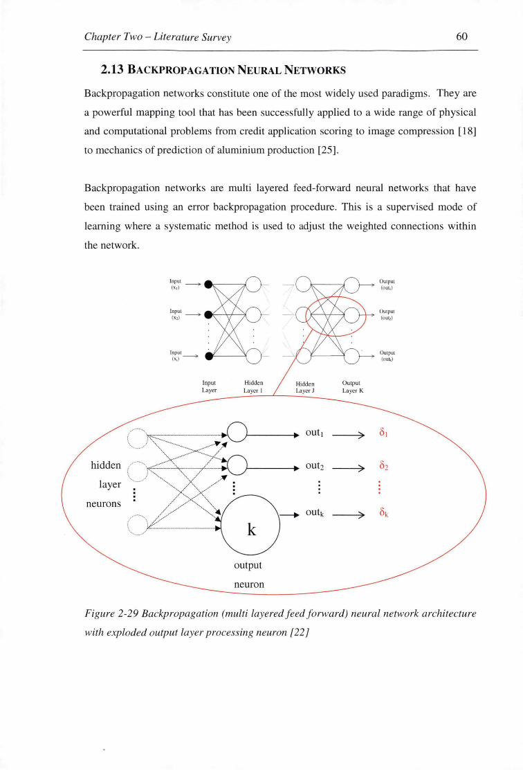
Chapter Two - Literature Survey 60
2.13 BACKPROPAGATION NEURAL NETWORKS
Backpropagation networks constitute one of the mo t widely used paradigms. They are
a powerful mapping tool that has been successfully applied to a wide range of physical
and computational problems from credit application scoring to image compression [18)
to mechanics of prediction of aluminium production [25).
Backpropagation networks are multi layered feed-forward neural network that have
been trained using an error backpropagation procedure. This is a supervised mode of
learning where a systematic method is used to adjust the weighted connections within
the network.
hidden
layer
neurons
Input (xJ ---4
Input Layer
Hidden Layer I
output
neuron
Hidden Layer J
Output Layer K
Output (out,)
Output (out,)
Output (oul<)
---) 82
)
Figure 2-29 Backpropagation (multi layered feed forward) neural network architecture
with exploded output layer processing neuron [22]

Chapter Two - Literature Survey 61
The backpropagation procedure begins with the calculation of error at the output layer.
From each neuron in the output layer a single, real number is output. During training
the output vector provides target outputs for each of these outputs from all neurons in
the layer.
The error, 8ki can then be calculated for neuron kin the output layer:
8k = (tk - ak )J'(netk)
Equation 2-13
Where: f (x) =first derivative of the activation function
netk = the weighted sum of inputs to neuron k
tk = target value for output from neuron k
ak= output value from neuron k
Commonly the activation function used in the backpropagation neural network is the
logistic or sigmoidal function. Recall:
f(net) = I+ exp(-net)
Thus the error is scaled to make a large correction when the weighted sum of the inputs
is small, and a larger correction when the weighted sum of the inputs is large.
Sigmoidal Activation Function and Derivative
--Derivative of Sigmoid
--Sigmoid Function
-7 -5 -3 -1 3 9
Weighted Sumed Input, netj

Chapter Two - Literature Survey 62
The backpropagation procedure continues with the calculation of the error at the hidden
layer, J:
1
2
lnput --3> (x,)
Input Layer
~ Wj2 I
neuron
Hidden Layer I
hidden
layer
neuron
Hidde n Layer J
Output Layer K
neuron
output
O utput (out1)
OuLpul (ou12)
Output (outJ
2 ---7
k ---7
Figure 2-30 Exploded hidden layer processing neuron [Fred Frost 34][R-ROJAS]
For the hidden layer neuron j above the calculation of error involves the weighted sum
of o values from all neurons connected to its output. Thus an equation for the
calculation of Oj [26]:
Where: f (x) = first derivative of the activation function
netj = the weighted sum of inputs to neuron j
Ok = error value calculated for neuron k
Equation 2-14
W ki = weighted connection from hidden layer neuron j to output layer
neuron k
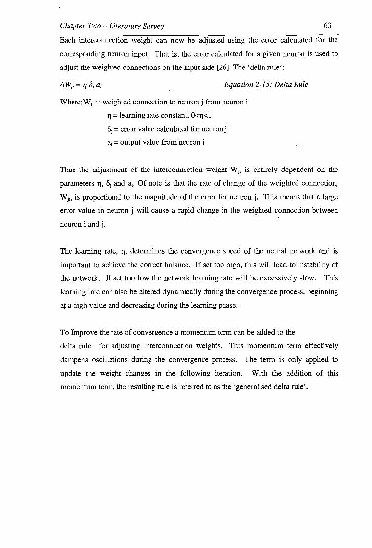
Chapter Two -Literature Survey 63
Each interconnection weight can now be adjusted using the error calculated for the
corresponding neuron input. That is, the error calculated for a given neuron is used to
adjust the weighted connections on the input side [26]. The 'delta rule':
Equation 2-15: Delta Rule
Where: WJi = weighted connection to neuron j from neuron i
11 = learning rate constant, O<ri<l
Oj = error value calculated for neuron j
a1 = output value from neuron i
Thus the adjustment of the interconnection weight WJ1 is entirely dependent on the
parameters 11, OJ and a1• Of note is that the rate of change of the weighted connection,
Wjh is proportional to the magnitude of the error for neuron j. This means that a large
error value in neuron j will cause a rapid change in the weighted connection between
neuron i and j.
The learning rate, 11, determines the convergence speed of the neural network and is
important to achieve the correct balance. If set too high, this will lead to instability of
the network. If set too low the network learning rate will be excessively slow. This
learning rate can also be altered dynamically during the convergence process, beginning
at a high value and decreasing during the learning phase.
To Improve the rate of convergence a momentum term can be added to the
delta rule for adjusting interconnection weights. This momentum term effectively
dampens oscillations during the convergence process. The term is only applied to
update the weight changes in the following iteration. With the addition of this
momentum term, the resulting rule is referred to as the 'generalised delta rule'.
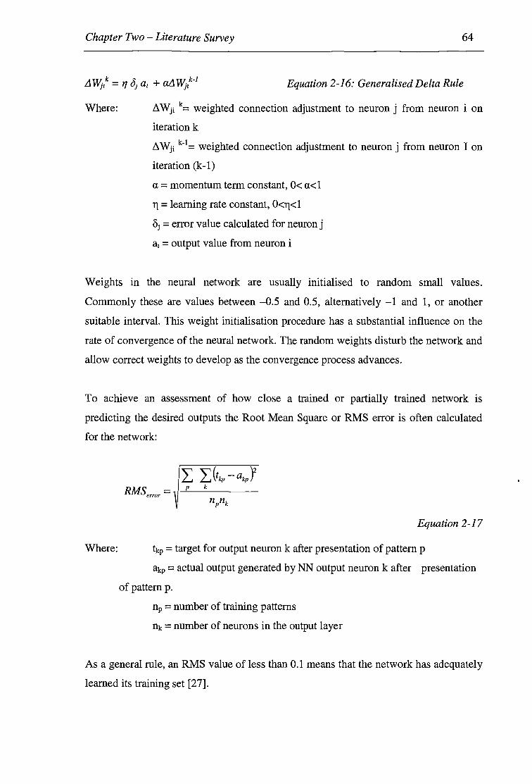
Chapter Two - Literature Survey 64
Where:
Equation 2-16: Generalised Delta Rule
11 Wji k= weighted connection adjustment to neuron j from neuron i on
iteration k
11 Wji k-I= weighted connection adjustment to neuron j from neuron I on
iteration (k-1)
a= momentum term constant, 0< a<l
TJ =learning rate constant, O<ri<l
81 = error value calculated for neuron j
a1 = output value from neuron i
Weights in the neural network are usually initialised to random small values.
Commonly these are values between -0.5 and 0.5, alternatively -1 and 1, or another
suitable interval. This weight initialisation procedure has a substantial influence on the
rate of convergence of the neural network. The random weights disturb the network and
allow correct weights to develop as the convergence process advances.
To achieve an assessment of how close a trained or partially trained network is
predicting the desired outputs the Root Mean Square or RMS error is often calculated
for the network:
Where:
RMSerror =
Equation 2-17
tkp = target for output neuron k after presentation of pattern p
akp = actual output generated by NN output neuron k after presentation
of pattern p.
np = number of training patterns
nk = number of neurons in the output layer
As a general rule, an RMS value of less than 0.1 means that the network has adequately
learned its training set [27].
Chapter Two - Literature Survey 65
2.13.1 Algorithm for backpropagation neural network training
• 1. Initialise all interconnecting weights by assigning small random values.
• 2. Expose the neural network input layer to the first input vector from the training
set and acquire the output vector from the output layer.
• 3. Compare this output vector from the network with the corresponding training set
output vector. Here the error associated with each neuron is calculated using
[Equation 3-4 ]and [Equation 3-5].
• 4. UsingJEquation 3-6], or alternatively [Equation 3-7], the weight adjustment can
be calculated for interconnections between neurons.
• 5. Repeat steps 2,3 and 4 for all input and corresponding output vectors from the
training set
• 6. Test the overall RMS error of the network using [Equation 3-7] for every input
and corresponding output vector within the testing set. This will provide an
indication of the overall predictive capability of the neural network

Chapter Two - Literature Survey 66
2.14 GENERAL REGRESSION NEURAL NETWORK
A GRNN is a memory based feedforward neural network, it responds to an input pattern
by processing the input data from one layer to the next with no feedback paths. GRNNs
feature fast training times, can model nonlinear functions, and have been shown to
perform well in noisy environments given enough data [28].
The primary advantage of the GRNN is the speed at which the network can be trained.
Training a GRNN is performed in one pass of the training data through the network, the
training data values are copied to become the weight vectors between layers. While the
advantages of the GRNN include fast training times, ability to handle both linear and
nonlinear data and the fact that the smoothing parameter is the only adjustable
parameter, thereby making overtraining less likely, the GRNN also has some associated
disadvantages. For example, the GRNN requires many training samples to adequately
span the variation in the data, and it requires that all training samples be stored for
future use. In addition, the GRNN has trouble with irrelevant inputs and there is no
intuitive method for selecting the optimal smoothing parameter.
The architecture of a basic GRNN, shown in [Figure 2-31], has four layers; input,
pattern, summation and output, with weighted connections w1, between the input and
pattern layer and A, and B, between the pattern and summation layer. There are i input
neurons, j pattern neurons, k+ 1 summation neurons and k output neurons.
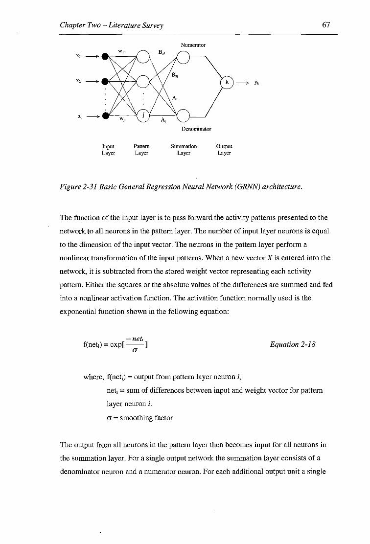
Chapter Two - Literature Survey
Input Layer
Pattern Layer
Numerator
Denominator
Summation Layer
Output Layer
Figure 2-31 Basic General Regression Neural Network (GRNN) architecture.
67
The function of the input layer is to pass forward the activity patterns presented to the
network to all neurons in the pattern layer. The number of input layer neurons is equal
to the dimension of the input vector. The neurons in the pattern layer perform a
nonlinear transformation of the input patterns. When a new vector X is entered into the
network, it is subtracted from the stored weight vector representing each activity
pattern. Either the squares or the absolute values of the differences are summed and fed
into a nonlinear activation function. The activation function normally used is the
exponential function shown in the following equation:
-net, f(neti) =exp[--]
(j
where, f(neti) =output from pattern layer neuron i,
Equation 2-18
net1 = sum of differences between input and weight vector for pattern
layer neuron i.
cr = smoothing factor
The output from all neurons in the pattern layer then becomes input for all neurons in
the summation layer. For a single output network the summation layer consists of a
denominator neuron and a numerator neuron. For each additional output unit a single

Chapter Two - Literature Survey 68
numerator is added. Hence, the summation layer consists of a single denominator unit
and n numerator units, where n equals the number of output neurons. The summation
layer neurons perform a dot product between a weight vector and a vector composed of
the signals from the pattern units. For the denominator summation neuron, the weight
vector is unity, so a simple sum is performed, represented by the following equation:
Equation 2-19
where, denout = output from denominator summation neuron,
f(netJ) =output from pattern layer neuronj, and
AJ = weight connecting denominator summation neuron to all pattern
layer neurons, equal to one for all AJ
For the numerator summation neuron, the weight connecting it to each pattern layer
neuron is equal to the value of the dependent variable for the training case of that
pattern layer neuron [28]. Hence, the numerator summation neuron performs a
computation represented by the following equation:
numouts = Lf(nef.J) * Bs1 Equation 2-20
where, numouts =output from numerator summation neurons,
f(netJ) =output from pattern layer neuronj, and
Bsj = weight connecting numerator summation neuron s to all pattern
layer neurons
The output from the denominator and numerator summation neurons are sent to the
output layer neurons, the function of which is to divide the output of the associated
numerator summation neuron by the output of the denominator summation neuron.
Chapter Two - Literature Survey 69
As a pre-processing step, it is usually necessary to scale all input variables such that
they have approximately the same ranges of variances. The need for this stems from the
fact that the underlying probability density function is to be estimated with a kernel that
has the same width in each dimension
A training algorithm for the general regression neural network:
Step 1. Determine a suitable value for the smoothing parameter, cr.
Step 2. Set input to pattern layer weights, w11 , equal to the values of the independent
variables in the training data set.
Step 3. Set pattern to summation layer denominator weights, A1, equal to a value of
one.
Step 4. Set pattern to summation layer numerator weights, Bs1, equal to the values of
the dependent variables in the training data set.
Step 5. Pass the entire training data set through the network and calculate the
network output in each instance using [Equation 2-18] for the pattern layer neurons, and
[Equation 2-19] and [Equation 2-20] for the summation layer denominator and
numerator neurons, respectively.
Step 6. Calculate network output by dividing the numerator output by the
denominator output fork output neurons.
Step 7. Compute and observe the prediction error of the network by comparing the
predicted output with the target output.
Step 8. If the prediction error is unacceptable, change the value of the smoothing
parameter and repeat Steps 5 to 7.
Step 9. Repeat Step 8 until the prediction error is minimum.

70
Chapter Three
DESIGN.OF TEST RIG
The requirement for a vehicle providing on-line brake-force and dynamic chassis
parameter measurement resulted in the test rig development described within this
chapter.
By developing a vehicle specifically for the purpose of data collection and automotive
Neural Network development inherent problems associated with modifying vehicles
built for other purposes were avoided. Commercial vehicles are designed for specific
markets and not for installations of complex telemetry and dynamic chassis
measurement systems. Further, testing and analysis of a commercial vehicle to gather
data about the design, for instance information about the rigidity of the chassis, is
expensive and time consuming.
From a purely scientific point of view, the development of a specific test vehicle
allowed the removal of as many unknowns as possible. To achieve this, ground-up
design of this vehicle was undertaken. This presented some problems associated with
the complex nature of vehicle design and concerns for driver safety.
In much the same way, driver and general safety concerns in prototype and one off
racing vehicles has lead to the development of rules for racing classes where the
vehicles can be constructed and designed quickly and safely within the guidelines.
Formula SAE is one such class.
The Formula SAE competition was formed in the USA in 1981 and is now also running
in Europe and Australia. The competition is for engineering students to conceive,
design, fabricate, and compete with small formula-style racing cars. The restrictions on
the cars frame and engine are limited so that the knowledge, creativity, and imagination
of the student are challenged. The cars are built with a team effort over a period of

71
about one year and are taken to a host institution (Ford, Toyota, Holden or Mitsubishi)
for judging and comparison with other competitors. The end result is a great experience
for young engineers in a meaningful engineering project as well as the opportunity of
working in a dedicated team effort.
For the purpose of this competition, the students are to assume that a manufacturing
firm has engaged them to produce a prototype car for evaluation as a production team.
The intended sales market is the non-professional weekend autocross racer. Therefore,
the car must have very high performance in terms of its acceleration, braking, and
handling qualities.
The car must be low in cost, easy to maintain, and reliable. In addition, the cars
marketability is enhanced by other factors such as aesthetics, comfort and use of
common parts. The challenge to the design team is to design and fabricate a prototype
car that best meets these goals and intents. Each design will be compared and judged
with other competing designs to determine the best overall car.
The cars are designed entirely by the students and compete for overall supremacy in:
Presentation
Engineering Design
Cost Analysis
Acceleration
Skid-pad performance
Autocross event
Fuel economy event
Endurance event
Incidentally, the prototype race car I test rig which is the subject of this chapter won the
Australasian Acceleration event, won the prize for the best use of innovative electrical
systems, ranked 3rd in Australia overall out of 16 entrants and sixth worldwide in the
2001 International-Australasian Formulae SAE competition. At the Holden proving
grounds in Melbourne, Australia.

Chapter Three - Design of Test Rig 72
3.1 CHASSIS DYNAMICS
The handling of a prototype test/racing car i influenced by an astoundingly large
number of factors. Initially, major factors identified were:
Weight distribution
Position of the centre of gravity
Polar moments of inertia of the vehicle about the three axes
Frame design
Suspension design, wheelbase and track widths
Wheel assembly, brake design and tyre selection
The amount of power driving the rear wheels
The weight distribution of a racecar refers predominantly to the wheel loading. This is
of greatest significance since the tyre contact patches are arguably the biggest factor in
defining the way a racecar will handle. Of cour e, the weight distribution of a car is
dynamic, acceleration in any direction as well as any down force experienced by the
moving vehicle will have an effect on the wheel loading.
Figure 3-1 Vehicle dynamics were found to be influenced by an astoundingly large
number of factors. These pictures were taken during early stages of testing at
Baskerville Raceway - Hobart, Tasmania.

Chapter Three - Design of Test Rig 73
To further complicate matters, the overall weight of the vehicle will change as the fuel
load is burned and, if the fuel tank is not positioned at the centre of gravity, even the
relative wheel loading will change.
The static weight distribution defines the po ition of the centre of gravity in the
horizontal plane. However the position of the centre of gravity vertically will have a
large influence on the overall vehicle handling as well as the weight transfer
characteristics of the car while accelerating. Note that the changing fuel load will again
have an effect on the position of the centre of gravity.
It is worth noting here that for any given class of racecar, as with Formula SAE, the
weight distribution is to a large extent predetermined to quite tight limits. For instance,
if we are adopting a conventional layout (admittedly, there are other options) with a
600cc motorcycle engine and gearbox it means that the engine will be mid mounted
with the driver in front and the drive axel behind. Then the wheelba e will be
somewhere in the vicinity of 1600mm-2000mm and the static weight distribution of the
vehicle will be somewhere between 40160 and 55/45 (Front/Rear).
Figure 3-2 Mid-mounted engine layout of the test vehicle
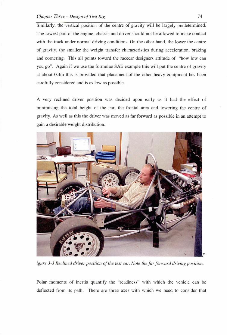
Chapter Three - Design of Test Rig 74
Similarly, the vertical position of the centre of gravity will be largely predetermined.
The lowest part of the engine, chassis and driver should not be allowed to make contact
with the track under normal driving conditions. On the other hand, the lower the centre
of gravity, the smaller the weight transfer characteristics during acceleration, braking
and cornering. This all points toward the racecar designers attitude of "how low can
you go". Again if we use the formulae SAE example this will put the centre of gravity
at about 0.4m this is provided that placement of the other heavy equipment has been
carefully considered and is as low as possible.
A very reclined driver position was decided upon early as it had the effect of
minimising the total height of the car, the frontal area and lowering the centre of
gravity. As well as this the driver was moved as far forward as possible in an attempt to
gain a desirable weight distribution.
igure 3-3 Reclined driver position of the test car. Note the far forward driving position.
Polar moments of inertia quantify the "readiness" with which the vehicle can be
deflected from its path. There are three axes with which we need to consider that

Chapter Three -Design of Test Rig 75
represent the yawing, pitching and rolling actions. Traditionally racecar designers and
drivers are mostly concerned with the yawing polar moment of inertia.
Conceptually a vehicle with the main masses situated towards the ends is considered to
have a high polar moment of inertia in yaw, this means that from a drivers point of view
that the car will respand reluctantly to steering input. Conversely, a vehicle with the
main masses situated very near to the centre of gravity will have a low moment of
inertia in yaw, and will respond quickly to steering input. The high moment of inertia
vehicle will be more reluctant to spin, however once spinning it will take more stopping
than a low moment of inertia vehicle. A low moment of inertia vehicle will exhibit
"twitchy" handling characteristics that require "lightening" quick reflexes on the part of
the drivers.
Very little can be done to affect the polar moments of inertia other that to get the
radiator, fuel tank and other heavy components as close to the centre of gravity as
possible. In practice, other aspects of the car design in effect dictate the polar moments
of inertia and in practice the difference between a high moment of inertia and a low
polar moment of inertia formulae SAE car is very small. However throughout the
history of racing many credible drivers have reported that they can "feel" small
modifications to their cars which race engineers would say are immeasurable.
Because of the windy and slow nature of the Formula SAE race track, the decision was
to make the polar moment of inertia in yaw as small as possible and that meant keeping
as many of the components as close to the centre of the car as possible. This approach
was also consistent with the desire to keep the car as compact and also as light as
possible since wiring, plumbing other connection lengths would be minimised.
The effect this has on the car as a test rig is that the range of acceptable yaw angles
before spin out will be increased. This is a very desirable quality as it increases the
effective/useful resolution of the yaw sensor.

Chapter Three - Design of Test Rig 76
3.2 FRAME DESIGN
The design of the frame presented many challenges since the high performance vehicle
was required to fulfil its specific purpose as a test rig for Neural Network development.
The frame was designed and constructed:
1. To provide stable mounting points for all measurement equipment including the
suspension linear potentiometers, steering wheel position sensor, pitch, roll, yaw
and 3d acceleration sensor.
2. To provide both rigid and stable mounting points for all necessary running gear
including the engine, seat, suspension wishbones, steering, drivetrain, radiator, fuel
tank and pump and filters, harnesses and body work.
3. To conform to the international rules of Formula SAE Competition for driver and
general safety [31].
4. To minimise the forces experienced by the frame, its overall size (especially the
frontal area) and weight and to maximise rigidity particularly torsional to optimise
performance.
The reclined driver position facilitated the placement of the main pitch, roll, yaw and 3d
acceleration sensor at very close to the centre of mass. Ideally this is where it needs to
be located however this is usually within the driver.

Chapter Three-Design of Test Rig 77
3.3 FRAME DEVELOPMENT
A Formula SAE-A racecar must meet an array of design and safety requirements set out
in the competition rules [31]. The design of the frame, being the single largest
component within the car, must consider every specification layed out within the rules,
anticipate the requirements for the installation of each component and allow space for
the addition of various sensors as they are called for. The overall design of the vehicle
revolves around the shape of the frame, and so its construction must consider all aspects
of the intended design. In the interests of high performance it is important to design to
close tolerances, which entails strict identification of the various component positions
and overall design requirements. These requirements include:
Rule Based Requirements:
• Open wheel and open cockpit type vehicle
• Wheel base of at least 1500mm
• Inclusion of front and rear suspension
• Engine size limit of 610cc
• Single seat design (no passengers)
• Front and rear roll over hoop positioning, dimensions and supports
• Side impact protection bar inclusions
• Bulkhead dimensions
• Crush zone dimensions
• Manufacturing materials (or demonstrated equivalence)
Construction Based Requirements:
• Must be as light as possible, while maintaining a long lifetime
• Must be reasonably simple and cheap to construct
• Must strive to make the car as compact as possible
• Must be reasonably ergonomic
• Must encourage component positioning to provide a low centre of gravity,
and approximately 50 I 50 weight distribution between the front and rear
wheels
• Must provided ample stiffness to encourage superior handling

Chapter Three-Design of Test Rig 78
• Must house the following major components in their respective optimum
positions:
Pedals
Seat and harness
Suspension wishbones, springs and pull rod pivots
Steering components
Gear changer mechanism
Fuel Tank
Engine and associated equipment
Differential
Radiator
Bodywork
Electrical equipment (engine management computer, data logger,
radio modem, etc)
Assorted sensors
These rule and construction based requirements form the basis of the design criteria for
the frame. To this end, the frame of choice was decided to be a tubular steel space
frame of varying member diameters and wall thicknesses.
Upon the initial stages of the frame design it was evident that in order for the frame
design to proceed, a general idea of what components were going to be used, and where
they were going to be positioned was required. This mainly included the driver,
suspension, drivetrain and engine positions, and initial designs centred on the respective
positions of each of these. As the frame started to conceptually take shape, other
_ components where included into the design to provide the close tolerances required and
efficient load paths for minimum weight. This required the component selection
process to proceed concurrently with the frame design, with the identification of
appropriate parts often significantly altering the shape and form of the frame.
As such, many frame designs were made, and altered, to suit different component
choices and positions, while also maintaining perceived structural integrity using the
least members possible. As an aid to this process, an easily modifiable PVC piping
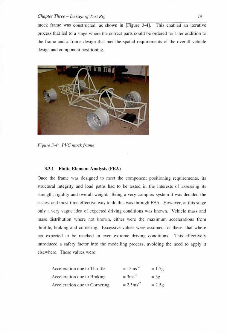
Chapter Three - Design of Test Rig 79
mock frame was constructed, as shown m [Figure 3-4]. This enabled an iterative
process that led to a stage where the correct parts could be ordered for later addition to
the frame and a frame design that met the spatial requirements of the overall vehicle
design and component positioning.
Figure 3-4: PVC mockframe
3.3.1 Finite Element Analysis (FEA)
Once the frame was designed to meet the component positioning requirements, its
structural integrity and load paths had to be tested in the interests of a essing its
strength, rigidity and overall weight. Being a very complex system it was decided the
easiest and most time effective way to do this was through FEA. However, at this stage
only a very vague idea of expected driving conditions was known. Vehicle mass and
mass distribution where not known, either were the maximum accelerations from
throttle, braking and cornering. Excessive value were assumed for these, that where
not expected to be reached in even extreme driving conditions. This effectively
introduced a safety factor into the modelling process, avoiding the need to apply it
elsewhere. These values were:
Acceleration due to Throttle
Acceleration due to Braking
Acceleration due to Cornering
= 15ms-2
= 3ms-2
= 2.5ms-2
= 1.5g
= 3g
= 2.5g

Chapter Three-Design of Test Rig
Acceleration due to Gravity
Vehicle Mass (wet, with driver)
Front I Rear Mass Distribution
= IOms
= 360kg
= 47 I 53
80
=lg
The model was then created in Strand? [23], using only beam elements. This simplified
the model construction and also made the results simple to understand. Material
restrictions and availability were also taken into account and, as a result, only 25mm
OD mild steel tubing of wall thicknesses 2.6mm and l .6mm were chosen for the
construction of the frame.
In an attempt to make the loading on the frame as accurate as possible a number of
measures were taken, and are depicted in [Figure 3-5]. Firstly, a suspension system was
included in the model, the dimensions of which had been under development
concurrently with the frame. This included wishbones that were allowed to freely pivot
on the frame (simulating rod ends) and a pull rod type suspension spring arrangement.
The wishbone ends were then fixed in space to simulate the reactive forces of the
wheels. Secondly, masses were applied to the frame to simulate component masses,
such as the engine and driver. The masses where applied as IOkg 'blocks', each
attached to member intersections distributed throughout the frame, in an attempt to gain
the car's estimated weight distribution and centre of gravity. Thirdly, the frame was
artificially stiffened around the engine mounts with additional members. This was done
because the frame design around that area relies on the engine to act as a sub-member,
increasing stiffness but receiving minimal loads.

Chapter Three - Design of Test Rig
---Wishbones
Figure 3-5: FEAframe model [34)
Wheel
Fixity
81
10 kg Frame
Masses
By altering wheel fixity conditions a number of loading cases were created, each case
using the applicable acceleration values above and are shown in "Appendix B". The
cases were:
• Normal driving
• Hard throttle
• Hard braking
• Hard cornering
• Cornering under throttle
• Cornering under brakes [Figure 3-6]
• Torsional stiffness [Figure 3-7]

Chapter Three - Design of Test Rig
100.IDlxlo"
70.IDJxlo"
40.ooox1o"
10.ooox1o"
-20 .CXXl x108
-50.IDJ x 1 o"
~.ooox1 o"
-110.IDlxl o"
-140.1Dlx1o"
-170.000 x1 o"
-200.1Dlx1 o"
Figure 3-6: FEA results for cornering under brakes
Beam Disp:RXCdeq} sso.ooox1 o-6
61 2.500x10⁻⁶
537.500x1 o-6
462.500x10·6
387.500x1 o-6
312.500x10·6
237.500x1 o-6
162.500x10·6
87.500x10·6
12.SOOx 10·6
-62 .500x10-6
-1.000 x10⁻⁴
Figure 3-7: FEA torsional results under I Nm
82
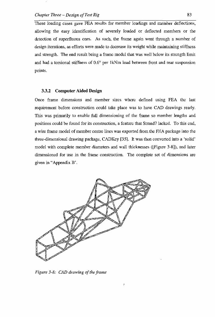
Chapter Three-Design of Test Rig 83
These loading cases gave FEA results for member loadings and member deflections,
allowing the easy identification of severely loaded or deflected members or the
detection of superfluous ones. As such, the frame again went through a number of
design iterations, as efforts were made to decrease its weight while maintaining stiffness
and strength. The end result being a frame model that was well below its strength limit
and had a torsional stiffness of 0.6° per lkNm load between front and rear suspension
points.
3.3.2 Computer Aided Design
Once frame dimensions and member sizes where defined using FEA the last
requirement before construction could take place was to have CAD drawings ready.
This was primarily to enable full dimensioning of the frame so member lengths and
positions could be found for its construction, a feature that Strand? lacked. To this end,
a wire frame model of member centre lines was exported from the FEA package into the
three-dimensional drawing package, CADKey [35]. It was then converted into a 'solid'
model with complete member diameters and wall thicknesses ([Figure 3-8]), and later
dimensioned for use in the frame construction. The complete set of dimensions are
given in "Appendix B'.
Figure 3-8: CAD drawing of the frame

Chapter Three - Design of Test Rig 84
3.3.3 Frame Construction
Frame construction proceeded in a number of step . It was decided from the outset that
the frame was going to be MIG welded due to workshop limitations and that it was
going to be welded using a jig. The form that the jig took was as a steel table from
which many of the members where lightly welded (tacked) into place in their correct
positions. This provided an excellent baseline to work from as well as reducing the
amount that the frame distorted due to residual welding stresses once it was removed
from the jig.
Construction followed a logical sequence. The front and rear roll over hoops where first
bent into shape and construction between them began. Members where cut to the
correct lengths and their ends tapered to ensure a good fit to at the joints, which were
subsequently welded. The front bulkhead was constructed next, followed by the engine
bay and finally the rear most section, ensuring that a sequence of welding was
maintained to minimise buckling due to welding stresses. The frame was then removed
from the jig and all of the final welding was completed with minimal frame distortion.
The complete frame is shown in [Figure Mild steel frame].
The 140 or so mountings for the variou components such as the suspension system, the
engine, the differential and the seat and seat belt were then designed, constructed and
welded to the frame as required. With all of the mountings completed, the frame was
painted using automotive acrylic paint, and assembly began.
Figure 3-9: Mild steel frame

Chapter Three-Design of Test Rig 85
3.4 SUSPENSION DESIGN
As with the frame design, the design of the suspension paid careful consideration to the
vehicle as a test rig for Neural Network Development.
The suspension was designed and constructed:
1. To provide stable mounting points for all measurement equipment.
2. To conform to the international rules of Formula SAE Competition for driver and
general safety.
3. To minimise the forces experienced by the frame.
The major forces on the frame are transmitted through the suspension. The type,
geometry and mounting of the suspension perform a key role in both the kind of
forces experienced by the frame and also the magnitude of those forces.
4. To conform to the chosen optimal suspension geometry and an appropriate level of
strength and serviceability.
5. To minimise the overall size (especially the frontal area) and weight of the
suspension system.
6. To facilitate easy geometric changes, part replacement and "tuning".
7. To use as few parts as possible.
8. To share as many common parts between corners as possible.

Chapter Three - Design of Test Rig 86
3.5 SUSPENSION DEVELOPMENT
The rules and nature of Formula SAE directly specify many of the constraints on the
vehicle's suspension design. On top of this the competition course -type of corners,
general layout and specified surface dictate how the suspension will be required to
operate if the vehicle is to take full advantage of the level of grip available from the
tires. Simply put, the purpose of a suspension ystem is to maximise the amount of
contact between the racecar's tyres and the road urface. However this is not quite the
full story as the dynamic nature of suspension ha the effect of changing the distribution
weight and inertial forces of the vehicle between the four wheel .
One of the first decisions made wa to estimate a suitable wheelbase. The chosen
wheelbase of a racecar has a major effect on the weight transfer characteri ties of the
chassi and will also influence the polar moment of inertia about yaw, high-speed
stability and the turning radius. Since one of the key design motif of the vehicle was to
keep it as compact a practical, the wheelbase estimation stemmed from our decided
driver and engine positions. This worked for the design of this car because it happened
to coincide with it's intended use on tight, windy circuits.
Figure 3-10 Formula SAE vehicles are designed to operate on tight autocross style
tracks resulting in compact design. Photo courtesy of SAE (USA).
With the driver reclined and the engine located midship, minimum practical clearances
were given between the back of the gearbox and the differential spur gear. Since the
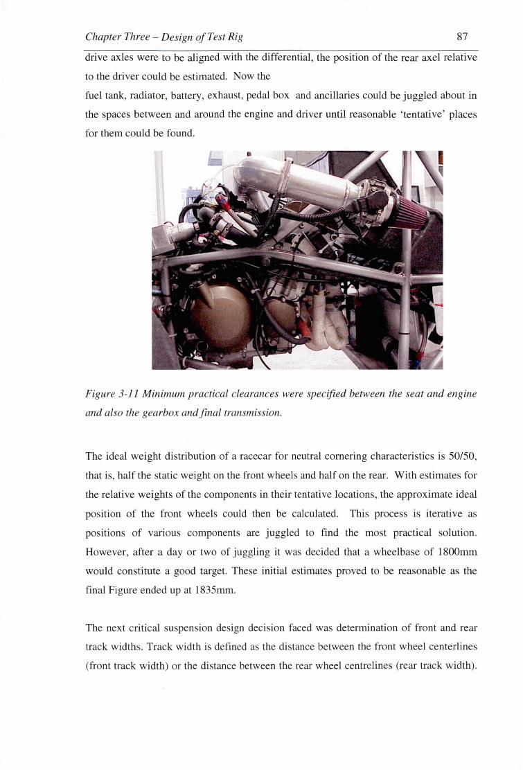
Chapter Three - Design of Test Rig 87
drive axles were to be aligned with the differential, the position of the rear axel relative
to the driver could be estimated. Now the
fuel tank, radiator, battery, exhaust, pedal box and ancillaries could be juggled about in
the spaces between and around the engine and driver until reasonable 'tentative' places
for them could be found.
Figure 3-11 Minimum practical clearances were specified between the seat and engine
and also the gearbox and final transmission.
The ideal weight distribution of a racecar for neutral cornering characteristics is 50/50,
that is, half the static weight on the front wheels and half on the rear. With estimates for
the relative weights of the components in their tentative locations, the approximate ideal
position of the front wheels could then be calculated. This process is iterative as
positions of various components are juggled to find the most practical solution.
However, after a day or two of juggling it was decided that a wheelbase of 1800mm
would constitute a good target. These initial estimates proved to be reasonable as the
final Figure ended up at 1835mm.
The next critical suspension design decision faced was determination of front and rear
track widths. Track width is defined as the distance between the front wheel centerlines
(front track width) or the distance between the rear wheel centrelines (rear track width).

Chapter Three - Design of Test Rig 88
Note that front and rear track widths may or may not be the same, however the track
widths must be decided upon before kinematic analysis of the su pension system can
begin.
Figure 3-12 The lateral distance between wheels, termed track width, is one of the first
critical decisions faced by a vehicle designer.
The decision regarding track widths is critical. During cornering the lateral acceleration
causes an overturning moment corresponding to product of the height of the centre of
gravity from the road surface, the magnitude of the lateral acceleration and the mass of
the vehicle. The track width then directly determines the magnitude of the resisting
force through the tires required to overcome this moment. In other words, the track
width is one way in which a vehicle designer can directly control the extent of lateral
weight transfer.
For this reason the track widths were not as simply arrived at as the wheelbase, since
locating the wheels as close as possible to the chassis would re ult in such a narrow
vehicle that overturning would almost certainly be assured. On the other hand a wide
vehicle carries not just the disadvantages of increased weight and increased frontal area
(drag) over a narrower competitor.
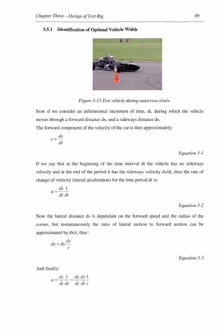
Chapter Three - Design of Test Rig 89
3.5.1 Identification of Optimal Vehicle Width
Figure 3-13 Test vehicle during autocross trials.
Now if we consider an infinitesimal increment of time, dt, during which the vehicle
moves through a forward distance dx, and a sideways distance ds.
The forward component of the velocity of the car is then approximately:
dx v=-
dt
Equation 3-1
If we say that at the beginning of the time interval dt the vehicle has no sideways
velocity and at the end of the period it has the sideways velocity ds/dt, then the rate of
change of velocity (lateral acceleration) for the time period dt is:
ds 1 a= --
dt dt
Equation 3-2
Now the lateral distance ds is dependant on the forward speed and the radius of the
corner, but instantaneously the ratio of lateral motion to forward motion can be
approximated by dx/r, thus :
dx ds=dx
r
And finally:
- dsl dxdx 1 a=--=---
dt dt dt dt r
Equation 3-3

Chapter Three - Design of Test Rig
v2 a=
r
Where: a = lateral acceleration (m/s2)
v = forward velocity of vehicle (m/s)
r = radius of comer (m)
90
Equation 3-4
Thus we have the relationship between lateral acceleration, vehicle velocity and comer
radius. So in order t~ improve out lap times (directly dependant on velocity) we need to
comer at the maximum possible lateral acceleration and choose the straightest racing
lines around the course. This is obvious, but poor choice of vehicle track widths can
prevent the vehicle from physically reaching these limits. Note that down force from
aerodynamic aids will not be considered in this simple analysis since they are not to be
included in the initial stages of development of the research vehicle.
There are two possible physical limits to lateral acceleration:
1. Overturning.
2. The amount of lateral grip which can be provided by the tyres.
During cornering there is an overturning moment caused by the vertical distance
between the centre of gravity (C of G) of the vehicle and the ground, and the cornering
force acting at the friction surface at the tyres. The horizontal distance between the C of
G and the tyre contact patch, and the weight of the vehicle counteracts this moment.
At the limit of cornering the inside wheels have zero load. Thus:
a · g · m · h = m · g . l_ trackwidth 2
a · h = l_ trackwidth 2
Where: a = lateral acceleration (g)
g = acceleration due to gravity
Equation 3-5

Chapter Three - Design of Test Rig 91
h = height of C of G (m)
The amount of lateral grip provided by the tyres provides the other limiting factor for
lateral acceleration. Given that there is no downforce, the maximum lateral acceleration
obtainable from currently available racing slicks is around l.3g. This is based on
skidpan results from some of the top autocross teams.
Wide vehicles have to travel a greater distance around the same circuit than narrow
competitors. This is best illustrated on a slalom or chicane but is true for any corner at
all.
Figure 3-14 An experimental slalom course.
In the slalom cour e above the car is following the ideal line that are perfect arcs where
the maximum lateral acceleration is held for the duration of the slalom changing signs
as each cone is rounded.
The following diagram is used determine the radius and length of the vehicle path:

Chapter Three - Design of Test Rig 92
/// .···[~;· ~~-:·:··,:-·:·:,- ' : I, 0 ~ ...•. · ··.• ..· ' .
.... ·· .. r . ···························· ............... ·················· ············
····························· h
Figure 3-15 Identification of experimental slalom course variables.
From the diagram: li+h=r (a) 2 2 2
h +h =r (b)
Substitute (a) into (b)
(r -11)2 +I} = r2
2 2 2 2 r - 2rl 1 + 11 + h = r
2 2 1 11 +Ji = 2r I
r = (l 12 + h 2) I 211
Equation 3-6
And
arc length = e r
Equation 3-7
Where 8 = 2 Sin-I (}i/r)
Now a perfect time for the slalom course can be established for a given track width and
C of G height.

Chapter Three -Design of Test Rig
Numerical Confirmation
For a course of: 10 cones at 10 m apart for a testing field
Track width = 2m is chosen
C of G height = 0.4m for the test vehicle
The roll over threshold from [Equation 3-5] is:
a · h = ..!.. trackwidth 2
1 a ·0.4 =-· 2
2 a= 3.5g
93
Since the maximum lateral acceleration obtainable from the tyres is about l.3g
(12.8m/s2), this vehicle will spin out rather than roll over when the cornering limit is
exceeded.
To determine the radius of the arc [Equation 3-6]:
r = (112 + lz2) I 211
Where
Thus:
11= 1/2 wheelbase+ cone clearance (say O.lm)
h= Y2 cone spacing
r = (112 + lz2) I 211
r = (1.1 2 + 52) I 2(1.1)
r = ll.9m
And the distance travelled [Equation 3-7]:
arc length = e r Where e = 2 sin-! (h/r)
arc length = 2 sin-1 (5111.9) x 11.9
arc length = 10.32m
distance traveled =arc length x no. of cones= 103.2m

Chapter Three - Design of Test Rig
Thus the maximum speed at which the vehicle can travel [Equation 3-4]:
v2 a=
r
v 2 = 12.753·11.91
v = 12.326m/ s(44.37kml h)
And the minimum time required to complete the course:
t = distance travelled I velocity
t = 103.2112.735
t = 8.37 seconds
94
This analysis was used to create a spreadsheet where varying track widths were tested
and the ideal times for the course can be compared. Of note is that a narrow car (l. lm
track) can complete the course over 2 seconds (over 25%) quicker than a wide car (2m
track) .
Table 1 Spreadsheet Analysis of vehicle width and slalom times.
Slalom vehicle analysis Cof G hei hi = 0.4m
Maximum Lateral Acceleration (g) Track width us slalom course time
Track widl From tyres Maximum Velocity (kmhl Distance travelled Time(s) , .00
2 .00 1 .30 2.50 1 .30 44 .37 103.20 8.37
1 .90 1 .30 2.38 1 .30 45.33 102.91 8 .17 i.so
1 .80 1 .30 2.25 1.30 46.35 102.65 7.97
1 .70 1 .30 2.13 1.30 47.47 102.39 7.77 ~ ~
.!. t.00
1.60 1 .30 2.00 1 .30 48.68 102.15 7.55 ~
1 .50 1.30 1 .88 1 .30 50 .01 101 .92 7.34 j 7.50
1 .40 1 .30 1.75 1 .30 51 .46 101 .70 7 .11 "Cl ~
1 .30 1.30 1.63 1 .30 53.07 101.49 6.88 (Ill
1 .25 1.30 1.56 1 .30 53 .94 101.40 6.77 i l .00
'il 1 .20 1 .30 1.50 1 .30 54 .86 101 .30 6.65
, ,50
1 .15 1 .30 1 .44 1 .30 55.83 101 .21 6 .53
1 .10 1 .30 1 .38 1 .30 56.85 101 .12 6.40 ,,00
1 .05 1.30 1 .31 1 .30 57.94 101 .04 6.28 0.00 0.50 1.00 1.50
1 .00 1 .30 1 .25 1 .25 57.95 100.96 6.27 vehicle track width (m)
0.90 1.30 1.13 1 .13 57.36 100.80 6.33
0.80 1.30 1 .00 1 .00 56.66 100.67 6.40
For the test vehicle geometry corresponding to a track width of 1. lm was chosen. Note
that this is slightly wider than the optimal 1.05m wide car, in the interests of a roll over
safety margin.
l .00

Chapter Three-Design of Test Rig 95
According to this simplified analysis, a car with a 1.0m track width can overturn
without being tripped, while at 1.05 m the car will slide. But these Figures are based
around a maximum l.3g lateral acceleration that may be significantly less than
instantaneous values, which could be attained. This is of importance since the use of
very soft, sticky tyre compounds introduces very complex track surface/tyre contact
patch relationships.
On the other hand, the estimation of the C of G height is on the conservative side since
it is most likely slightly lower in our finished design than the estimated 0.4m.
In the design of the Neural Network development test vehicle, the l. lm track width
represented the upper limit of acceptable risk for vehicle roll over.

Chapter Three -Design of Test Rig 96
3.5.2 Optimisation of Front Track Width
Closer analysis during normal cornering of a vehicle with equal front and rear track
widths reveals that the inside rear wheel limits the approach to the inside of the corner,
for a car experiencing minimal lateral tyre slip.
/
I I
I f
WB
Figure 3-16 Geometry of turning vehicle
\
From the diagram above the following formula can be derived.
Where: r2 = Arc followed by the inner front wheel
r = Arc followed by inner rear wheel
FfW = Front track width
RTW = Rear track width
WB =Wheel Base
\ \ I
\ \ \ \ \
Equation 3-8

Chapter Three-Design of Test Rig 97
Thus from the dimensions of the car (FTW, RTW and WB) and a given comer radius, (
r ), we can determine the radius scribed by the front wheels.
Our purpose for this equation however is to determine the maximum amount that we
can increase the front track width (and hence increase stability) before the front inner
wheel begins to limit our approach to comers. To do this, we need to solve this equation
iteratively:
1. Select an appropriate minimum radius for which the vehicle will be turning
(remember racing lines and comer apexing). This becomes your value for r.
2. Decide on your wheelbase (WB) using packaging or other constraints.
3. Select a rear track width (RTW) as outlined previously.
4. Estimate an initial value for the front track width (FTW), say 10 % larger than the
rear track width.
5. Calculate r2 using [Equation 3-8].
6. If r2 is larger than r, increase the value of FTW. If r2 is smaller than r, decrease the
value of FTW.
7. Repeat steps 4-6 until r2 converges to your chosen r.
Note that this process is easily handled by a spreadsheet where experiments with vehicle
dimensions can be analysed very quickly and easily.
There is one other notable reason, on a rear wheel drive car, to design to a wider front -
narrower rear chassis. By having a narrower rear track the proportion of roll resisted by
the rear tyres is decreased, allowing for increased rear traction while exiting comers.
Effectively this allows using more of the rear tyres (particularly the inside tyre) and as a
side effect causes more even tyre wear, tyre heat and traction on tracks with a comer
bias, i.e. predominantly left-handers or predominantly right-handers. This can be quite
significant as weight transferral ensures rear tyres are working hardest while exiting
corners.

Chapter Three - Design of Test Rig 98
After performing this analysis, it wa decided to increase the front track width to l.2m,
which is perhaps not taking full advantage of the possible gains in stability. This wa
partly to avoid too radical geometry and also partly due to the break down of this simple
analysis once the vehicle begins sliding. We also felt that the chosen track widths
offered enough conservative stability, and compactness was one of our key design
motifs.
3.5.3 Dynamic Component Design
Suspension design is always a compromise. Different suspension systems offer
advantages and disadvantages over others.
Since the vehicle was to be built a part of current investigations without any testing
data and was designed by recent graduates (David Butler and Myself) it was decided
that whatever type of suspension was used would require maximum adjustability for
tuning out any inadequacies which may surface. This was coupled with the general
desire to create a system that could be accurately
modelled before manufacturing and was easy to produce. These desired properties
directed the decision to use a "conceptually conventional" double wishbone suspension.
To rrummise the unsprung weight of the suspension system, pullrod systems were
decided upon front and rear with an inboard coil over shock absorber.
Figure 3-17 Pullrod suspension system with inboard coil over shock absorber used on
the test vehicle.
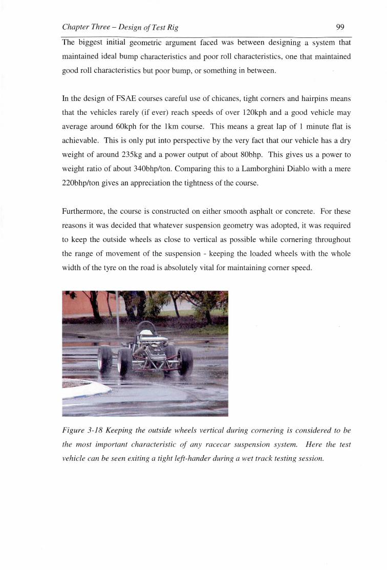
Chapter Three - Design of Test Rig 99
The biggest initial geometric argument faced was between designing a system that
maintained ideal bump characteristics and poor roll characteristics, one that maintained
good roll characteristic but poor bump, or something in between.
In the design of FSAE courses careful use of chicane , tight corners and hairpins means
that the vehicles rarely (if ever) reach speeds of over 120kph and a good vehicle may
average around 60kph for the lkm course. This means a great lap of 1 minute flat is
achievable. This is only put into perspective by the very fact that our vehicle has a dry
weight of around 235kg and a power output of about 80bhp. This gives us a power to
weight ratio of about 340bhp/ton. Comparing this to a Lamborghini Diablo with a mere
220bhp/ton gives an appreciation the tightness of the course.
Furthermore, the course is constructed on either smooth asphalt or concrete. For these
reasons it was decided that whatever suspension geometry wa adopted, it was required
to keep the outside wheels as close to vertical as possible while cornering throughout
the range of movement of the su pension - keeping the loaded wheels with the whole
width of the tyre on the road is absolutely vital for maintaining corner speed.
Figure 3-18 Keeping the outside wheels vertical during cornering is considered to be
the most important characteristic of any racecar suspension system. Here the test
vehicle can be seen exiting a tight left-hander during a wet track testing session.

Chapter Three-Design of Test Rig 100
To achieve vertical outside wheels under maximum expected roll the camber change
properties under centripetal induced deflection need to be carefully considered. Of note
is that when using a double wishbone suspension system the wheels can never remain
vertical through their whole range of motion, but for small levels of roll ( <5°) this can
be controlled by using longer bottom and shorter top suspension arms. A traditional
rule of thumb is that the top suspension arm should be about 2/3 the length of the lower
arm. This is a Figure arrived at as it gives a good compromise between these desired
roll characteristics and also maintaining acceptable geometry in squat/dive under
acceleration.
Empirical Figures such as this, arrived at through years of racing successes,
offered valuable starting points for the suspension design, however finding an optimum
geometry took place through the use of CAD modelling. To minimise the overall width
of the frame (hence frontal area) and still have the necessary length difference between
upper and lower wishbones, the lower wishbones were chosen to meet in the centre of
the vehicle.
This design decision produced many significant packaging problems but was
decided as core to the vehicle design and was not compromised. The upper wishbones
could then be conventionally mounted to the side of the frame which are spaced to suit
with special consideration to driver ergonomics and engine/drivetrain mounting. This
arrangement allowed the achievement of the camber change properties of approximately
half of one degree on the outside wheels under full roll.
Heights of the front and rear roll centres, the point in the transverse plane of the front
(or rear) wheel contact patches about which the sprung mass of the car will rotate under
any disturbing force, were chosen to correspond to the expected mass distribution of the
vehicle. Through FEA modelling, weights were attached to the frame in locations of
major components, and the weight in the plane of the rear contact patch was estimated
to be 49mm above the front.
Positioning of the roll centres is not an exact science, but a matter of opinion since it
effects the extent of vehicle roll. The front roll centre was chosen at ground level based
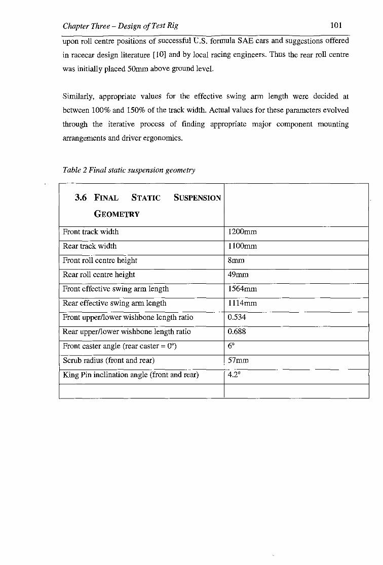
Chapter Three-Design of Test Rig 101
upon roll centre positions of successful U.S. formula SAE cars and suggestions offered
in racecar design literature [10] and by local racing engineers. Thus the rear roll centre
was initially placed 50mm above ground level.
Similarly, appropriate values for the effective swing arm length were decided at
between 100% and 150% of the track width. Actual values for these parameters evolved
through the iterative process of finding appropriate major component mounting
arrangements and driver ergonomics.
Table 2 Final static suspension geometry
3.6 FINAL STATIC SUSPENSION
GEOMETRY
Front track width 1200mm
Rear track width llOOmm
Front roll centre height 8mm
Rear roll centre height 49mm
Front effective swing arm length 1564mm
Rear effective swing arm length 1114mm
Front upper/lower wishbone length ratio 0.534
Rear upper/lower wishbone length ratio 0.688
Front caster angle (rear caster = 0°) 60
Scrub radius (front and rear) 57mm
King Pin inclination angle (front and rear) 4.2°

Chapter Three - Design of Test Rig 102
The suspension system was designed with the concepts of low parts count, simplicity,
compactness, ease of access and widespread use of common parts . All suspension
components are specified for minimum weight and maximum adjustability.
Figure 3-19 The pull-rod suspension provides a progressive spring rate which itself can
be changed through positioning on the rocking supports.
Figure 3-20 Front and rear uprights and bearing arrangements are identical, as is the
whole hub and stub axe/ assembly, allowing for ultra low parts count.

Chapter Three-Design of Test Rig 103
3.7 WHEEL ASSEMBLY DEVELOPMENT
The wheel assembly is defined here as the set of components that link the suspension
wishbones to the road. This includes the wheel rims and tyres, as well as the brake
system, hubs, stub axles, uprights and bearings. The design and integration of these
components had to address the following criteria:
• Be simple and relatively cheap to fabricate
• Be as light as possible without compromising strength or lifetime
• Must house the largest brakes possible
• Must not interfere with rim rotation
• Must mount to the wishbones while ensuring adequate suspension and
steering movement
• Must have a mount for steering linkages
• Must house a wheel speed sensor
• Must allow attachment to the drive axle for the rear wheels
• Should allow significant adjustment in parameters such as camber and caster
to enhance drivability and performance
The same design for the front and rear wheels was also used. The argument for this
addressed a number of points, firstly a common design would enable cheaper and easier
fabrication. Also, the design requirements between the front and rear wheels where
similar. The required mountings for the wishbones were the same front and rear,
identical brakes where going to be used on all four wheels, all of the rims were
matching and wheel loadings were similar. Conversely however, the front wheels
needed to be steered while the rear ones did not, and the rear wheels needed to be driven
while the front ones did not. It was decided that a design that allowed the wheels to be
driven and steered would be best in this situation because, while it increased the
assembly mass, it allowed reduced design and fabrication labour and allowed greater
interchangeability of parts.
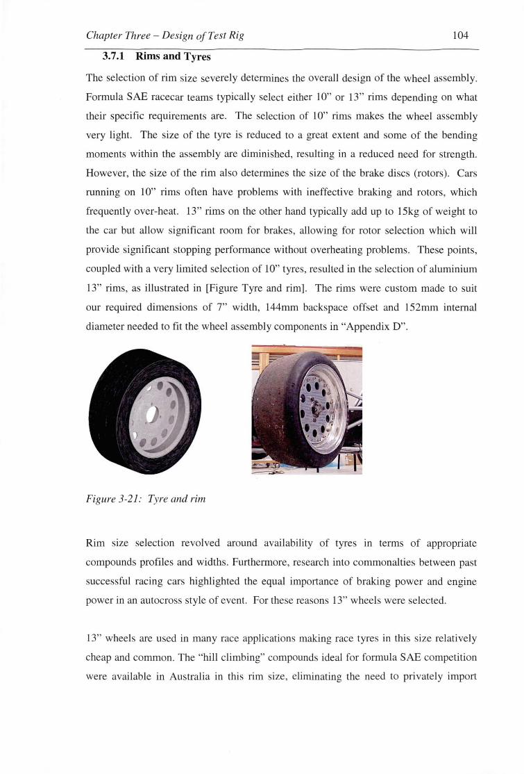
Chapter Three - Design of Test Rig 104
3.7.1 Rims and Tyres
The selection of rim size severely determines the overall design of the wheel assembly.
Formula SAE racecar teams typically select either 10" or 13" rims depending on what
their specific requirements are. The selection of 10" rims makes the wheel assembly
very light. The size of the tyre is reduced to a great extent and some of the bending
moments within the assembly are diminished, resulting in a reduced need for strength.
However, the size of the rim also determines the size of the brake discs (rotors). Cars
running on 10" rims often have problems with ineffective braking and rotors, which
frequently over-heat. 13" rims on the other hand typically add up to 15kg of weight to
the car but allow significant room for brakes, allowing for rotor selection which will
provide significant stopping performance without overheating problems. These points,
coupled with a very limited selection of 10" tyres, resulted in the selection of aluminium
13" rims, as illustrated in [Figure Tyre and rim]. The rims were custom made to suit
our required dimensions of 7" width, 144mm backspace offset and 152mm internal
diameter needed to fit the wheel assembly components in "Appendix D".
Figure 3-21: Tyre and rim
Rim size selection revolved around availability of tyres in terms of appropriate
compounds profiles and widths. Furthermore, research into commonalties between past
successful racing cars highlighted the equal importance of braking power and engine
power in an autocross style of event. For these reasons 13" wheels were selected.
13" wheels are used in many race applications making race tyres in this size relatively
cheap and common. The "hill climbing" compounds ideal for formula SAE competition
were available in Australia in this rim size, eliminating the need to privately import
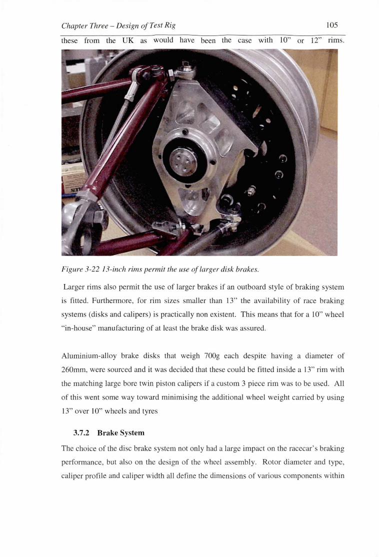
Chapter Three - Design of Test Rig 105
these from the UK as would have been the case with 10" or 12" nms.
Figure 3-22 13-inch rims permit the use of larger disk brakes.
Larger rims also permit the use of larger brakes if an outboard style of braking system
is fitted. Furthermore, for rim size smaller than 13" the availability of race braking
systems (disks and calipers) is practically non existent. This means that for a 10" wheel
"in-house" manufacturing of at least the brake disk was assured.
Aluminium-alloy brake disks that weigh 700g each despite having a diameter of
260mm, were sourced and it was decided that these could be fitted inside a 13" rim with
the matching large bore twin piston calipers if a custom 3 piece rim was to be used. All
of this went some way toward minimising the additional wheel weight carried by using
13" over 10" wheels and tyres
3.7.2 Brake System
The choice of the disc brake system not only had a large impact on the racecar's braking
performance, but also on the design of the wheel assembly. Rotor diameter and type,
caliper profile and caliper width all define the dimensions of various components within
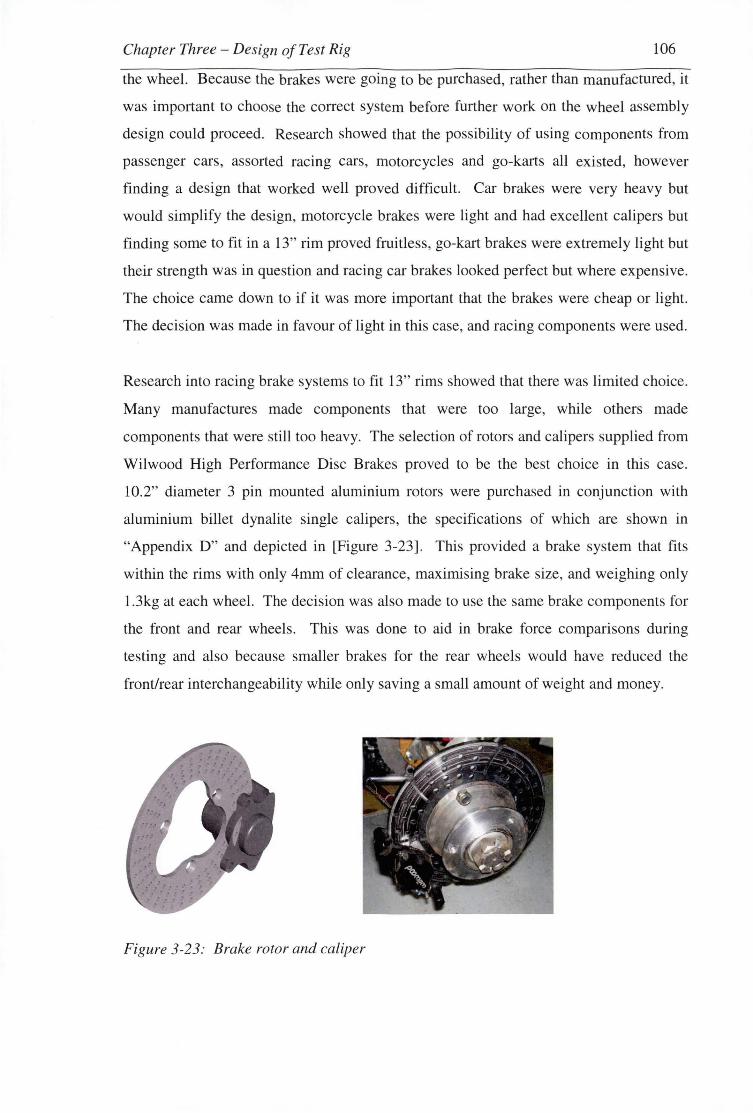
Chapter Three - Design of Test Rig 106
the wheel. Because the brakes were going to be purchased, rather than manufactured, it
was important to choose the correct system before further work on the wheel assembly
design could proceed. Research showed that the possibility of using components from
passenger cars, assorted racing cars, motorcycles and go-karts all existed, however
finding a design that worked well proved difficult. Car brakes were very heavy but
would simplify the design, motorcycle brakes were light and had excellent calipers but
finding some to fit in a 13" rim proved fruitless, go-kart brakes were extremely light but
their strength was in question and racing car brakes looked perfect but where expensive.
The choice came down to if it was more important that the brakes were cheap or light.
The decision was made in favour of light in this case, and racing components were used.
Research into racing brake systems to fit 13" rims showed that there was limited choice.
Many manufactures made components that were too large, while others made
components that were still too heavy. The selection of rotors and calipers supplied from
Wilwood High Performance Disc Brakes proved to be the best choice in this case.
10.2" diameter 3 pin mounted aluminium rotors were purchased in conjunction with
aluminium billet dynalite single calipers, the specifications of which are shown in
"Appendix D" and depicted in [Figure 3-23]. This provided a brake system that fits
within the rims with only 4mrn of clearance, maximising brake size, and weighing only
l .3kg at each wheel. The decision was also made to use the same brake components for
the front and rear wheels. This was done to aid in brake force comparisons during
testing and also because smaller brakes for the rear wheels would have reduced the
front/rear interchangeability while only saving a small amount of weight and money.
Figure 3-23: Brake rotor and caliper
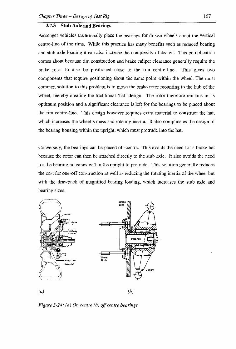
Chapter Three - Design of Test Rig 107
3.7.3 Stub Axle and Bearings
Passenger vehicles traditionally place the bearings for driven wheels about the vertical
centre-line of the rims. While this practice has many benefits such as reduced bearing
and stub axle loading it can also increase the complexity of design. This complication
comes about because rim construction and brake caliper clearance generally require the
brake rotor to also be positioned close to the rim centre-line. This gives two
components that require positioning about the same point within the wheel. The most
common solution to this problem is to move the brake rotor mounting to the hub of the
wheel, thereby creating the traditional 'hat' design. The rotor therefore remains in its
optimum position and a significant clearance is left for the bearings to be placed about
the rim centre-line. This design however requires extra material to construct the hat,
which increases the wheel's mass and rotating inertia. It also complicates the design of
the bearing housing within the upright, which must protrude into the hat.
Conversely, the bearings can be placed off-centre. This avoids the need for a brake hat
because the rotor can then be attached directly to the stub axle. It also avoids the need
for the bearing housings within the upright to protrude. This solution generally reduces
the cost for one-off construction as well as reducing the rotating inertia of the wheel but
with the drawback of magnified bearing loading, which increases the stub axle and
bearing sizes.
(a)
Wheel Studs
(b)
Figure 3-24: (a) On centre (b) off centre bearings
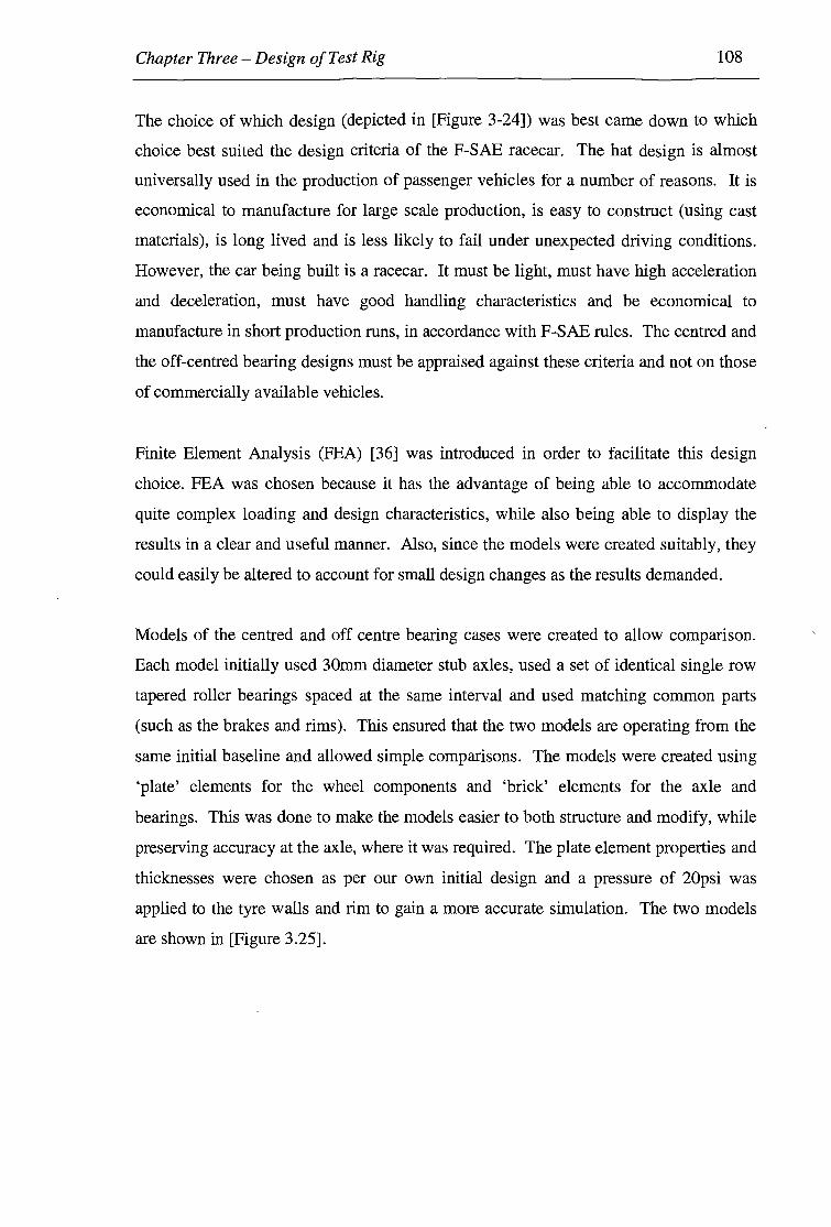
Chapter Three-Design of Test Rig 108
The choice of which design (depicted in [Figure 3-24]) was best came down to which
choice best suited the design criteria of the F-SAE racecar. The hat design is almost
universally used in the production of passenger vehicles for a number of reasons. It is
economical to manufacture for large scale production, is easy to construct (using cast
materials), is long lived and is less likely to fail under unexpected driving conditions.
However, the car being built is a racecar. It must be light, must have high acceleration
and deceleration, must have good handling characteristics and be economical to
manufacture in short production runs, in accordance with F-SAE rules. The centred and
the off-centred bearing designs must be appraised against these criteria and not on those
of commercially available vehicles.
Finite Element Analysis (FEA) [36] was introduced in order to facilitate this design
choice. FEA was chosen because it has the advantage of being able to accommodate
quite complex loading and design characteristics, while also being able to display the
results in a clear and useful manner. Also, since the models were created suitably, they
could easily be altered to account for small design changes as the results demanded.
Models of the centred and off centre bearing cases were created to allow comparison.
Each model initially used 30mm diameter stub axles, used a set of identical single row
tapered roller bearings spaced at the same interval and used matching common parts
(such as the brakes and rims). This ensured that the two models are operating from the
same initial baseline and allowed simple comparisons. The models were created using
'plate' elements for the wheel components and 'brick' elements for the axle and
bearings. This was done to make the models easier to both structure and modify, while
preserving accuracy at the axle, where it was required. The plate element properties and
thicknesses were chosen as per our own initial design and a pressure of 20psi was
applied to the tyre walls and rim to gain a more accurate simulation. The two models
are shown in [Figure 3.25].
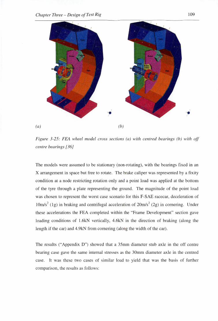
Chapter Three - Design of Test Rig 109
(a) (b)
Figure 3-25: FEA wheel model cross sections (a) with centred bearings (b) with off
centre bearings [36]
The models were assumed to be stationary (non-rotating), with the bearings fixed in an
X arrangement in space but free to rotate. The brake caliper was represented by a fixity
condition at a node restricting rotation only and a point load was applied at the bottom
of the tyre through a plate representing the ground. The magnitude of the point load
was chosen to represent the worst case scenario for this F-SAE racecar, deceleration of
10m/s2 (lg) in braking and centrifugal acceleration of 20m/s2 (2g) in cornering. Under
these accelerations the FEA completed within the "Frame Development" section gave
loading conditions of 1.6kN vertically, 4.6kN in the direction of braking (along the
length if the car) and 4.9kN from cornering (along the width of the car).
The results ("Appendix D") showed that a 35mm diameter stub axle in the off centre
bearing case gave the same internal stresses as the 30mm diameter axle in the centred
case. It was these two cases of similar load to yield that was the basis of further
comparison, the results as follows:

Chapter Three - Design of Test Rig
Table 3:Wheel bearing selection [36]
For Centred Bearings:
Bearing Loads
Fradrnl = 23.lkN
Fax1a1 = 4.9kN
Bearing Parameters
Creq (108 rev) = 43.9kN
Internal Dia. = 30mm
Bearing Choice= FAG 32206A
External Dia. = 62mm
Axle, Bearing & Brake Hat Weight
Wassembly = 2.0kg
Moment of Inertia of Axle & Brake Hat
!assembly = 0.3 lxl0-3 kgm2
Stub Axle Deflection
=0.lmm
110
For Off-Centre Bearings:
Bearing Loads
Frad1al = 33.lkN
Fax1a1 = 4.9kN
Bearing Parameters
Creq (108 rev) = 62.9kN
Internal Dia. = 35mm
Bearing Choice= FAG 32207A
External Dia. = 72mm
Axle, Bearing & Brake Hub Weight
Wassembly = 2.2kg
Moment of Inertia of Axle & Brake Hub
Iassembly = O. l 9x 10⁻³ kgm2
Stub Axle Deflection
=0.5mm
In comparison of the two models it was important to note that the bearing position
would significantly effect the design of surrounding components. The design of the
upright particularly was subject to change since it must house the bearings in their
different respective positions. In the case of the F-SAE racecar, it was found through a
short investigation that the upright weights for both cases would be similar, but
remained very design dependent. A deviation in the above assembly masses of 200g,
while not negligible, can seem less important when considering the design of the
upright as well. A simple calculation considering a 330kg racecar accelerating at
10m/s2 showed that this increase in weight reduces acceleration by 0.02m/s2 while the
increase in moments of inertia account for a completely negligible reduction of
0.0002m/s2•
The last comparison that could significantly affect the wheel assembly performance was
the stub axle deflection. The axle in the off-centre case obviously deflected more than in
the centred case because much more of it was subjected to the maximum stress, and
therefore strain. This small amount of deflection was not a significant problem in the
case of this racecar. It can be shown that the resulting wheel misalignment (0.4° from

Chapter Three-Design of Test Rig 111
vertical) is small when compared to wheel misalignment resulting from car roll and
pitch when cornering and braking. Also, the wheel hub mounting, which was not
considered in this model, further decreases this deflection.
Budgetary constrains had also to be considered. The difference in the cost of
production of the wheel assembly essentially fell to the cost of the upright. This was
because all the other components within each of the assemblies could be made using
very similar methods. The most cost-effective method of producing a lightweight
upright for the very limited number of units required was to machine it out of an
aluminium block. In the case of centred-bearings this would require a very thick and
expensive plate to machine, while the off-centred bearings will require a plate only
about half as thick and much cheaper. Machining the uprights for the off-centred
bearings in this case also requires far less material removal resulting in cheaper
production costs.
In this summary, the centred bearing design proved slightly lighter, showed marginal
increases in handling characteristics and also probably has a longer lifetime due to its
added ability to cope with unexpected driving conditions. Conversely, the off-centre
design revealed itself to be cheaper to construct in 'one off' production, but at a cost of
slightly lower performance and life. The decision was made in favour of the off centre.
case, using a 35rnm stub axle and 35rnm ID and 72rnm OD single row tapered roller
bearings.
The stub axles (show below in [Figure 3-26] and dimensioned in "Appendix D") were
made on a CNC lathe using free machining 709M steel. A thread was also placed on
one end of each, to allow the addition of a castellated nut that would hold the entire
assembly together as well as provide bearing pre-loads. The stub axles were then
moved to a mill where a hole for the castle nut cotter pin was drilled and a grove for the
keyway was cut.
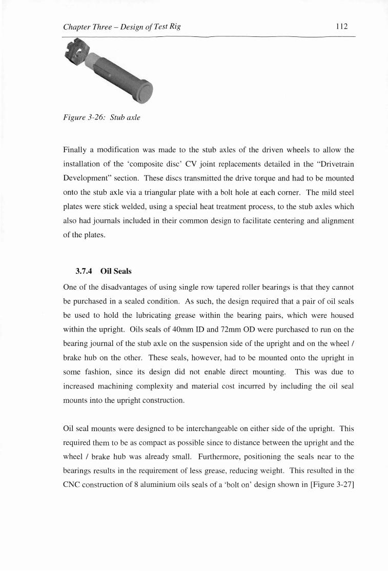
Chapter Three - Design of Test Rig 112
Figure 3-26: Stub axle
Finally a modification was made to the stub axles of the driven wheels to allow the
installation of the 'composite disc' CV joint replacements detailed in the "Drivetrain
Development" section. These discs transmitted the drive torque and had to be mounted
onto the stub axle via a triangular plate with a bolt hole at each corner. The mild steel
plates were stick welded, using a special heat treatment process, to the stub axles which
also had journals included in their common design to facilitate centering and alignment
of the plates.
3. 7 .4 Oil Seals
One of the disadvantages of using single row tapered roller bearings is that they cannot
be purcha ed in a sealed condition. As such, the design required that a pair of oil seals
be used to hold the lubricating grease within the bearing pairs, which were housed
within the upright. Oils seals of 40mm ID and 72mm OD were purchased to run on the
bearing journal of the stub axle on the suspension side of the upright and on the wheel I
brake hub on the other. These seals, however, had to be mounted onto the upright in
some fashion, since its design did not enable direct mounting. This was due to
increased machining complexity and material cost incurred by including the oil seal
mounts into the upright construction.
Oil seal mounts were designed to be interchangeable on either side of the upright. This
required them to be as compact as possible since to distance between the upright and the
wheel I brake hub was already small. Furthermore, positioning the seals near to the
bearings results in the requirement of less grease, reducing weight. This resulted in the
CNC construction of 8 aluminium oils seals of a 'bolt on' design shown in [Figure 3-27]

Chapter Three - Design of Test Rig 113
below, with the bolt holes drilled at even intervals, using the mill dividing head, to
ensure interchangeability and correct alignment.
Figure 3-27: Oil seal
3.7.5 Wheel I Brake Hub
The wheel I brake hub must serve a number of functions. First and foremost it must
provide an attachment for the wheel and the brake rotor to each other, and to the stub
axle. It must also provide a means to allow driven wheel torque to be transferred from
the stub axle to the wheel as well as provide a system to facilitate bearing pre-loading.
Furthermore, a general design had already been established above of a wheel hub plate
and a brake hub plate attached to a shaft. There were also the requirements of the
inclusion of the oil seal running surface and a keyway to the stub axle.
In addition to these requirement, the dimensions where also defined through the overall
assembly design. The position and diameters of wheel mounting was known, as was the
details for the brake mounting. The oil seal journal need to be a specific size and the
diameter of the sleeve to fix the stub axle was defined. The design of this component
was simply focused at producing a component to these very specific requirements that
was both cheap and easy to manufacture, while being as light as possible. The result
being a 2kg mild steel hub manufactured on the a CNC lathe with the keyway cut with a
broach and the bolt holes drilled with a mill with a dividing head, as shown in [Figure
3-28].
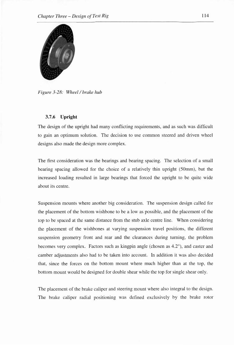
Chapter Three - Design of Test Rig 114
Figure 3-28: Wheel I brake hub
3.7.6 Upright
The design of the upright had many conflicting requirements , and as such was difficult
to gain an optimum solution. The decision to use common steered and driven wheel
designs also made the design more complex.
The first consideration was the bearings and bearing spacing. The selection of a small
bearing spacing allowed for the choice of a relatively thin upright (50mm), but the
increased loading resulted in large bearings that forced the upright to be quite wide
about its centre.
Suspension mounts where another big consideration. The suspension design called for
the placement of the bottom wishbone to be a low as possible, and the placement of the
top to be spaced at the same distance from the stub axle centre line. When considering
the placement of the wishbones at varying suspension travel positions, the different
suspension geometry front and rear and the clearances during turning, the problem
becomes very complex. Factors such as kingpin angle (chosen as 4.2°), and caster and
camber adjustments also had to be taken into account. In addition it was also decided
that, since the forces on the bottom mount where much higher than at the top, the
bottom mount would be designed for double shear while the top for single shear only.
The placement of the brake caliper and steering mount where also integral to the design.
The brake caliper radial positioning was defined exclusively by the brake rotor

Chapter Three - Design of Test Rig 115
diameter, however it could be placed anywhere on that radius, within reason. The best
design, though favours the placement of the caliper as low as possible. This lowers the
centre of gravity, reduces the 'back flow ' of hydraulic fluid that results from caliper
positioning higher than the master cylinder and provides extra strength within the
upright in its lower portion, which is subject to large loads. Further investigation into
the design of the caliper mounting also showed a small alteration would also allow the
integration of the steering mounting into the design with little effort.
Once all of the individual design requirements had been identified a final design for the
upright was produced. Factors such as milling limitations, weight reduction and
appearance where taken as priorities in the design, which also met all other
requirements suitably.
The aluminium uprights were manufactured in a number of steps. The bearing journals
were first lathed out to a J6 clearance, with the upright subsequently CNC machined to
shape. The suspension joint, steering tie rod joint and brake caliper mounting bolt holes
were then manually drilled and taped followed but the drilling of the bolt holes for the
oil sealed in the mill dividing head. The resulting product is illustrated in [Figure 3-29]
and dimensioned in "Appendix D".
Figure 3-29: Upright

Chapter Three - Design of Test Rig 116
3. 7. 7 Assembly
Due to the small clearances within each wheel assembly, they must be assembled in a
specific manner. [Figure 3-30] shows the exploded and cut-away views of the wheel
assemblies, which are put together in the following manner:
1) Press the oil seals into their mountings,
2) Grease the tapered roller bearings,
3) Press and Loctite® the bearing outers into the upright,
4) Slide one of the oil seals along the stub axle to the non threaded end,
5) Press the first bearing inner onto the stub axle and slide it to the journal,
6) Slide the upright over the bearing and bolt and Loctite® the oil seal in place,
7) Press the remaining bearing inner onto the stub axle and bolt and Loctite®
the other oil seal in place,
8) Bolt and lock nut the brake rotor to the hub and slide both onto the shaft with
the keyway key installed,
9) Place the washer and castellated nut onto the tread end of the stub axle,
10) Bolt and Loctite® the bake caliper into place on the upright,
11) Bolt the rim and tyre to the hub,
12) Tighten the castellated nut to pretension the bearings so that the wheel freely
rotates no more than one tum when spun by hand,
13) Insert the cotter pin to stop the castellated nut from loosening,
14) Bolt and Loctite® the suspension and steering rod ends to the upright
utilising the brass spacers to ensure full movement,
15) Bolt the rim to the wheel I brake hub.

Chapter Three - Design of Test Rig 117
Figure 3-30: Wheel assembly

Chapter Three - Design of Test Rig 118
3.8 DRIVETRAIN DESIGN
Fundamental design principles applied to the drivetrain are low rotating mass and
efficient power transmission.
3.8.1 Composite Disks
The drivetrain features extensive use of non-conventional materials. Kevlar composite
disks have been used in place of traditional CV or tripod joints saving a total rotating
mass of around 6kg.
Figure 3-31. Kevlar composite disks supplied by GKN Motorsport used in the test
vehicle transmission.
Figure 3-32 Unidirectional Kevlar fibre construction of the composite disks
The composite disks themselves are made form laminated unidirectional kevlar fibre
and weigh only 55g each despite having a transmission of torque rating of over
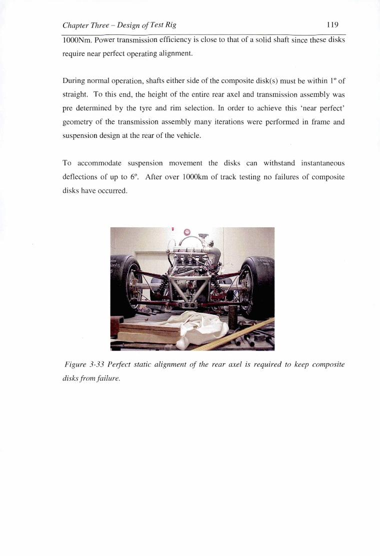
Chapter Three - Design of Test Rig 119
lOOONm. Power transmission efficiency is close to that of a solid shaft since these disks
require near perfect operating alignment.
During normal operation, shafts either side of the composite disk(s) must be within l 0 of
straight. To this end, the height of the entire rear axel and transmission assembly was
pre determined by the tyre and rim selection. In order to achieve this 'near perfect'
geometry of the transmission assembly many iterations were performed in frame and
suspension design at the rear of the vehicle.
To accommodate suspension movement the disks can withstand instantaneous
deflections of up to 6°. After over lOOOkm of track testing no failures of composite
disks have occurred.
Figure 3-33 Perfect static alignment of the rear axel is required to keep composite
disks from failure.
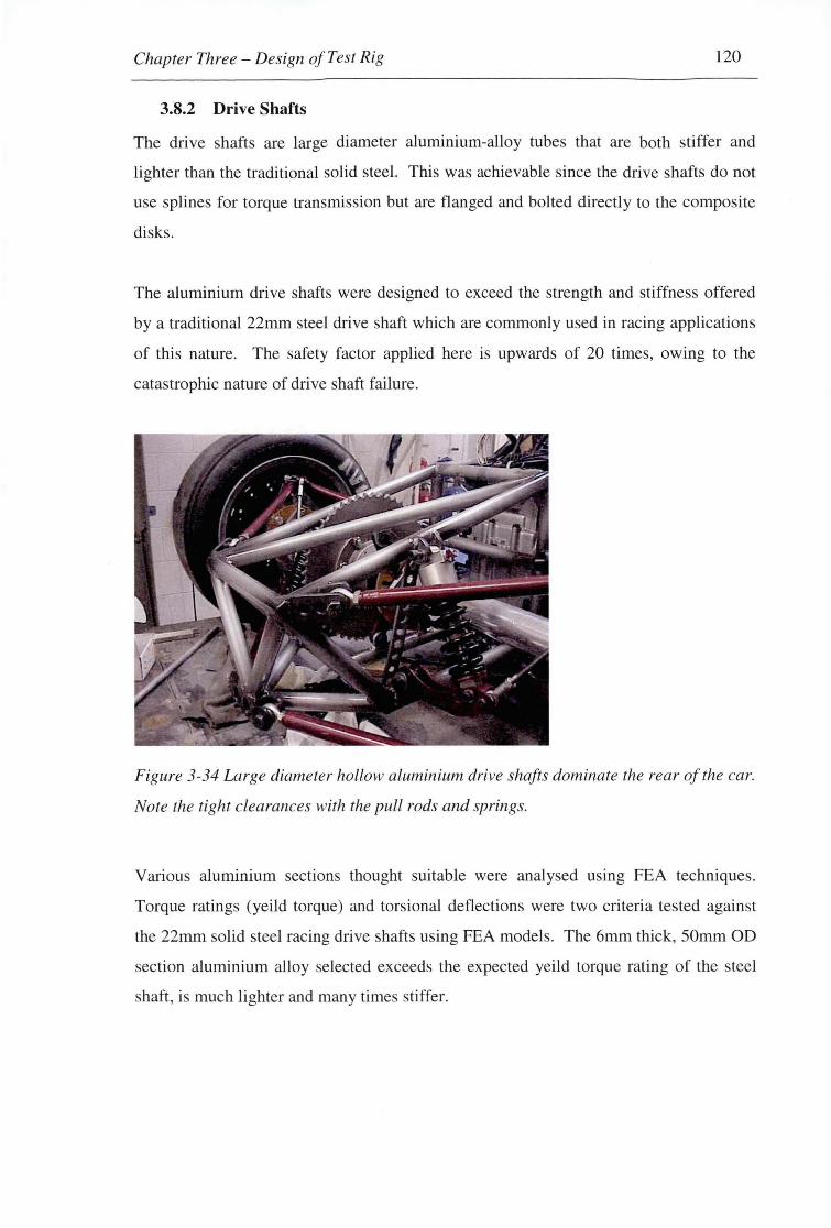
Chapter Three - Design of Test Rig 120
3.8.2 Drive Shafts
The drive shafts are large diameter aluminium-alloy tubes that are both stiffer and
lighter than the traditional solid steel. This was achievable since the drive shafts do not
use splines for torque transmission but are flanged and bolted directly to the composite
disks.
The aluminium drive shafts were designed to exceed the strength and stiffness offered
by a traditional 22mm steel drive shaft which are commonly used in racing applications
of this nature. The safety factor applied here is upwards of 20 times, owing to the
catastrophic nature of drive shaft failure.
Figure 3-34 Large diameter hollow aluminium drive shafts dominate the rear of the car.
Note the tight clearances with the pull rods and springs.
Various aluminium sections thought suitable were analysed usmg FEA techniques.
Torque ratings (yeild torque) and torsional deflections were two criteria tested against
the 22mm solid steel racing drive shafts using FEA models. The 6mm thick, 50mm OD
section aluminium alloy selected exceeds the expected yeild torque rating of the steel
shaft, is much lighter and many times stiffer.
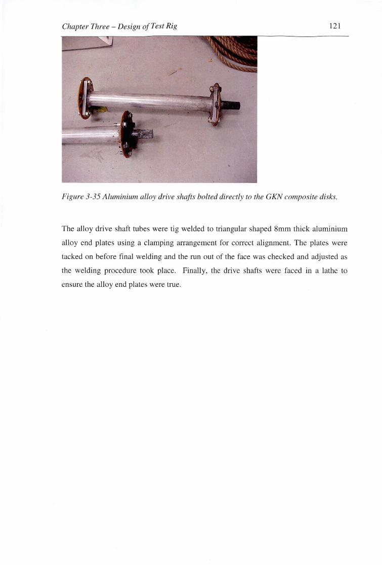
Chapter Three - Design of Test Rig 121
Figure 3-35 Aluminium alloy drive shafts bolted directly to the GKN composite disks.
The alloy drive shaft tubes were tig welded to triangular shaped 8mm thick aluminium
alloy end plates using a clamping arrangement for correct alignment. The plates were
tacked on before final welding and the run out of the face was checked and adjusted as
the welding procedure took place. Finally, the drive shafts were faced in a lathe to
ensure the alloy end plates were true.

Chapter Three - Design of Test Rig 122
3.8.3 Differential Selection and Application
A fully sealed Quaife Automatic Torque Biasing (ATB) differential assists m
maintaining maximum traction during acceleration and cornering. This unit has proved
effective in testing and is the smallest and lightest automatic torque biasing differential
available.
Figure 3-36 Quaife ATE differential with pressed on ball bearings.
The differential unit arrived fully sealed, no modifications were necessary. Blank
sprockets were machined to match the bolt pattern on the existing differential flange .
Ball bearings were selected and pressed on to the differential casing.
The differential mounting arrangement dominates the rear of the frame structure with an
asymmetrical diagonal member supporting the top of the right hand side differential
mount (see [Figure 3-37]) also providing triangulation of the drivetrain frame structure

Chapter Three - Design of Test Rig 123
(a) (b)
Figure 3-37 Differential mounting arrangement; a) photo taken during frame
construction, b) rear frame design dominated by differential mounting considerations
The differential mounts were designed and fabricated out of plain carbon steel and are a
sliding fit over the outside of the differential ball bearings. The two mounts are tripods
in design and mounting is through the use of three bolts each into tabs welded to the
frame
Figure 3-38 Differential mounts shortly after welding mounting tabs to the bare frame
of the test vehicle

Chapter Three-Design of Test Rig 124
3.9 ENGINE SYSTEMS DESIGN
The use of a motorcycle engine as the power plant for a F-SAE racecar is a standard
choice. The 600cc displacement limit imposed by the rules [31] significantly reduces
the possible sources from which an engine can be obtained, and motorcycle engines
offer exceptional performance. They are generally highly tuned and lightweight, and,
coupled with almost universal inclusion of a sequential gearbox, provide significant
power within a compact unit. Most manufactures make a number of such 600cc engines
of varying levels of performance and reliability depending on their application, in this
case it was decided to focus on the high performance end of the market, and a 2000
model Kawasaki Ninja ZX6 engine was chosen.
The Kawasaki ZX6 plant is a high revving in-line 4 cylinder, 4-stroke, water cooled
super-bike engine with double overhead cam. It offered a compression ratio of 11.8: 1
with large low RPM torque and high power within a 55kg (dry) unit with 6 forward
gears. The engine also has, as standard, a deep oil sump (which is needed to ensure oil
flow during high lateral accelerations) and a water jacket style oil cooler integral to the
water cooling system providing a reduction in the overall weight.
3.9.1 Fuel Injection System
The Kawasaki Ninja engine typically runs a carburetted air intake system, with separate
CV carburettors for each cylinder running from a single air box that receives ram air.
This system offers efficient and lightweight fuel control under normal operation, but F
SAE specifications enforce two major limitations. Firstly, all intake air must pass
through a 20mm diameter air restrictor, and secondly, the throttle body must be located
upstream of the restriction. This, coupled with the fact that the carburettors operate with
degraded performance under high lateral accelerations, and their inherent difficulties to
tune, lead to the choice of a fuel injection system.
A well design inlet manifold is of great importance in optimising the airflow to the
engine. Separation and extended boundary layers along with excessive turbulent eddies
are to be avoided where possible. A single plane induction manifold with all intake

Chapter Three-Design of Test Rig 125
runners extending from a common plenum was the design of choice due to the fact that
the open plenum smoothes out the induction pulses better than a dual plane manifold
and can give better top end power.
3.9.1.1 Intake Runner Length
With the engine running both high and low pressure waves move along the intake
plenum due to the opening and closing of the valves (along with air inertia). The idea of
engine tuning is to have the high-pressure wave approach the intake valve just before it
opens hence forcing in a little more air.
For the reasons described above the intake runner length can be optimised for a specific
RPM range making use of the first (or second) set of pressure waves to increase air
induction. The formula for this is:
ECD = 720 - Advance Duration - 30 Equation 3-9
Hence, with advance duration of 305 degrees our ECD becomes 385 degrees:
Intake ram pipe length
ECD = 385°
Advance duration = 305°
Length= 41.66833mm
V = 1300 ft I sec
RV=2
D=0.08m
RPM= 12000
The optimum length is given by
L = (ECD*0.25*V*2)/(rpm*RV)-(1!2D) Equation 3-10

Chapter Three-Design of Test Rig
Where:
ECD = Effective Cam Duration
RV= Reflective Value
D = Runner Length
126
Hence for our engine the effective runner length for the second set of pressure waves is
41.66 mm. This theoretical calculation is an estimate and the only way to fully tune to a
specific rpm is to vary the intake runner lengths whilst observing the torque and power
on a dynamometer or, better still, by track testing with an experienced driver. Peak
power may increase but average power may drop. A balance needs to be found. The
longer the runner, the better torque at lower rpm is a rule of thumb. There obviously
exists a trade off here with specific torque rpm ranges and also average and peak power.
Here in lies the reason for trial and error testing with variable length intake runners.
3.9.1.2 Intake Runner Diameter
This is the easiest to work out due to the fact that the intake air velocity should not
reach over 60 m/s at maximum rpm. The formula for the intake runner diameter is
D = Square root of (Litres*VE*RPM)l(V* 18.5)
Inlet ram diameter
Where:
D = 0.0402227m
Litres= 0.6
VE=0.85
RPM = 12000
v = 105.12
D = Pipe Diameter
Litres = Litres displacement
VE = Volumetric Efficiency
Equation 3-11

Chapter Three - Design of Test Rig 127
V =Velocity in ft/sec
Hence resulting in a 40.22rnrn intake diameter. The inlet ports in the engine actually
already set this but it is always advisable to fully check intake design calculations.
3.9.1.3 Plenum Volume
There never exist a simple answer for a given application and rpm range but a good rule
of thumb is to have the volume at least 50% of the total engine displacement hence
3.6* 10-3 m3 is sufficient.
Plenum Volume (50-60% of total cylinder displacement)
Cylinder displacement = 0.6 L = 0.0006m3
Required volume= 0.00036m3
Plenum volume 0.001705m3
Plenum radius = 0.03755m3
Length = 0.385m3
Figure 3-39 Inlet manifold

Chapter Three - Design of Test Rig 128
3.9.1.4 Restrictor
From basic computational flow theory the best application here to maximise airflow is
the use of a converging diverging nozzle. Once the contraction ratio is chosen 1 the
design criterion becomes the exit flow uniformity, separation, exit boundary layer
thickness and space/cost. The actual design parameters become length, wall shape and
Reynolds number. Manufacturing is obviously also a large consideration.
The maximum mass flow rate at which the nozzle will choke is given by:
-( 2 J 2(r;~~) ( r J . m- -- --PA y+l RT0 °
Equation 3-12
= 0.0745 kg/s which equates to a volumetric flow rate of 0.06535 m3/s. The maximum
airflow velocity is 159.23m/s.
The actual maximum engine air requirement is 3600000 cc per minute that equates to
0.06 m3 /s of air hence the restrictor will not choke at maximum rpm. The air at
maximum rpm has a velocity of 84.88 m/s as it passes through the restrictor.
A matching cubic curve converging section of the nozzle is ideal to minimise separation
and flow non-uniformity's but for ease of manufacture a simple radius was chosen for
the converging section with an optimum 7 degree diverging section. Due to the plenum
diameter the diffuser length is not excessively long to produce undesirably long
boundary layers.
3.9.1.5 Throttle Body and Air Cleaner
The throttle body chosen has an inside diameter of 57 mm which is not excessively
large to decrease throttle response and not too small to restrict flow. The butterfly
placed directly in front of the restrictor intuitively disturbs flow but testing with the
1 Set in our instance from the throttle body diameter and the size of the restriction. =
57/20.

Chapter Three - Design of Test Rig 129
supposedly optimum 0.7* throttle body diameter section in front of the restrictor
surprisingly showed no decrease in average horsepower or torque.
The K&N filter was chosen from the maximum inlet airflow Figures and a cone shape
was chosen for marginal gains due to the ram air effect.
3.9.2 Exhaust
The outlet ports of the engines are 25.4rnm hence the diameter of the extractors was pre
set. Effective length of the outlet pipes 2 was measured from an identical system and
fabricated from stainless steel mandrel bends.
The exhaust was fabricated from stainless steel with a perforated 'straight through' pipe
surrounded by fibreglass packing to severely lower back pressure that a standard baffle
exhaust would otherwise exert on the system. Back-pressure is obviously undesirable,
as it would lower the horsepower of the engine at all rpm's due to the extra energy
required extracting the used gasses. The outlet pipe is a tuned length producing a
standing wave at 9000 rpm. This results in 109 dB of noise 0.5 meters from the exhaust
outlet.
Figure 3-40 Exhaust manifold and muffier
2 To induce the scavenging from the cylinders as the valves are in overlap.

Chapter Three -Design of Test Rig 130
3.9.3 Engine Management System
Extensive research and management system comparisons were conducted and the
MoTeC M4-Pro system was the ideal system for our purpose as it utilises sequential
injection along with 3D-map programming. It also has the option of closed and open
loop operation allowing feedback from the exhaust oxygen sensor.
The system was installed to use either the throttle position sensor (located on the throttle
body) or the manifold air pressure sensor located on the plenum. After extensive tuning
with both sensors it was found that the throttle position sensor provided better throttle
response hence fine-tuning on the dynamometer was conducted using the throttle
position sensor. The MAP sensor is now used to conduct regular manifold pressure
checks.
Sequential injection was desired for fuel efficiency and optimum fuel injection timing
when the inlet valve opens hence a hall effect sensor was installed on the camshaft.
Standard ignition timing is achieved via the factory crank angle sensor.
Other inputs to the ECU are water and air temperature. The water temperature is used
for cold start enrichment and the air temperature for adjusting fuel mixtures depending
on air density.
The engine was tuned for a Lambda reading of 0.89 that equates to an air/fuel ratio of
13.8:1. This provides a balance between the stoichiometric 14.7:1 for fuel economy and
around 13:1 for maximum power. The engine has been tuned both with and without the
restrictor. A very interesting comparison can be shown here as the restrictor provided
very little enrichment of the mixture as expected.
3.9.4 Fuel System
The fuel system was calculated for flow rates and consequently injector sizes. The duty
cycle of an injector is the linear region between 10-90% of the full injector pulse width3.
3 Or opening time.

Chapter Three-Design of Test Rig 131
Injectors that are too large will not allow the engine to idle as their minimum pulse
width will not allow small enough opening times whereas if the injectors are too small
the maximum pulse width will not provide enough fuel at maximum rpm. Low
impedance injectors also provide better idle control.
Due to the fact that we were searching for maximum horsepower at maximum rpm each
cylinder requires 900000 cc per min of air hence the engine consumes 2211 gms/min.
For the required air/fuel ratio an injector that provides between 181 and 221 cc/min of
fuel is sufficient4.
The fuel pump flow rate was calculated to be between 544 cc/min and 665.7 cc/min to
provide enough fuel for the injectors at full rpm when they are virtually always open but
due to rule specifications5 the pump selected is good for 400 horsepower. This simply
means that an excessive amount of fuel is circulated in the system and returned through
the return line. The fuel system runs at 2.5 Bar and the regulator is mounted as close to
the end of the fuel line as possible to minimise transient responses to pressure spikes
and best maintain constant pressure at the injectors.
The injectors are located on the inlet runners at a location so that the spray fires directly
onto the back of the inlet valve when it is closed. This optimises the mixing of the fuel
and air due to the heat of the valve assisting in the atomisation of the fuel even though it
is open at the time of injection.
4 The volumetric efficiency was not known hence maximum and minimum Figures were used. The
density ofunleaded fuel is 0.750g/m3•
5 Threaded or OEM type connections required.

Chapter Three-Design of Test Rig 132
3.10 WIRING LOOM DESIGN
In developing a working electrical system for use in the experimental test vehicle the
following objectives were identified as essential:
1. Open architecture and expansion capability - for further development of on board
electrical systems during automotive Neural Network development.
2. Simplicity - this includes things like minimising the number of wires, using
common parts where feasible and designing straight runs between common points.
3. Ease of fault finding - creating fault finding access locations, common locations of
like components and using fully colour coded looms.
4. Minimal maintenance requirements - the system developed must be robust and
require little maintenance.
5. Neat and aesthetically neutral/appealing.
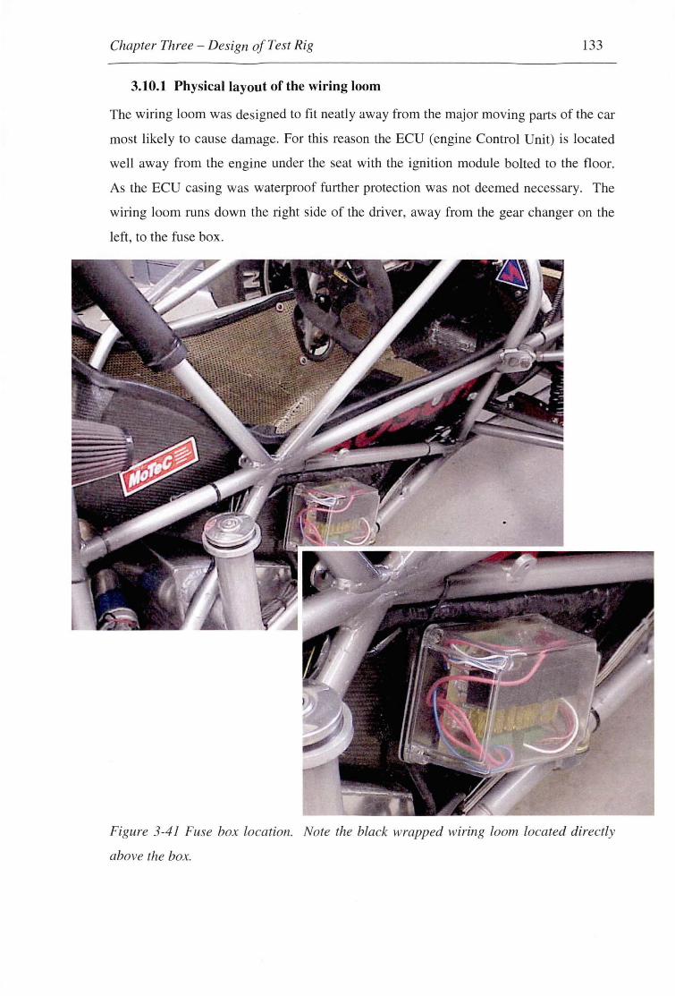
Chapter Three - Design of Test Rig 133
3.10.1 Physical layout of the wiring loom
The wiring loom was designed to fit neatly away from the major moving parts of the car
most likely to cause damage. For this reason the ECU (engine Control Unit) is located
well away from the engine under the seat with the ignition module bolted to the floor.
As the ECU casing was waterproof further protection was not deemed necessary. The
wiring loom runs down the right side of the driver, away from the gear changer on the
left, to the fuse box.
Figure 3-41 Fuse box location. Note the black wrapped wiring loom located directly
above the box.

Chapter Three - Design of Test Rig 134
The fuse box is located in a central position to minimise the length of wiring to and
from it from all locations on the vehicle and for maintenance purposes. The bulk of the
remaining loom continues along this line at a junction with the wiring from the battery
located near the starter motor and alternator on the left hand side of the vehicle. The
original starter motor, alternator and regulator wires have been retained from the
original motorcycle engine loom.
3.10.2 Waterproofing
For reliability during testing it is imperative that the complete wiring loom be
dependable in all weather conditions. The major concern in this case is rain and contact
with water and mud under wet track conditions.
The insulated cables within the wiring loom are further insulated by comprehensive
wrapping in electrical tape in all areas exposed to the elements. The most vulnerable
components of the wiring system are the system of relays and fuses that allow the
MoTeC system to control the higher currents of the engine control system. Hence the
fuse box containing these sensitive components also some and exposed connections
required special attention. The fuse box is carefully sealed to avoid difficulty in this
area.
3.10.3 Wire colours
The design of the wiring loom assigned a unique wire colour to each component for
simplictity of fault finding. Basic electrical conventions were observed as far as
practical (black for earth, white or red for power.) Striped automotive wiring would be
used for production runs of the loom.
3.10.4 Wire Specification
Wire utilised in this design was chosen to withstand the harsh environment of the
automobile. Standard automotive wire has been specifically developed to withstand
bombardment with dirt, oil, heat water and low temperatures and hence was specified
for all wiring connections. Wiring sizes were taken from the largest likely current rating
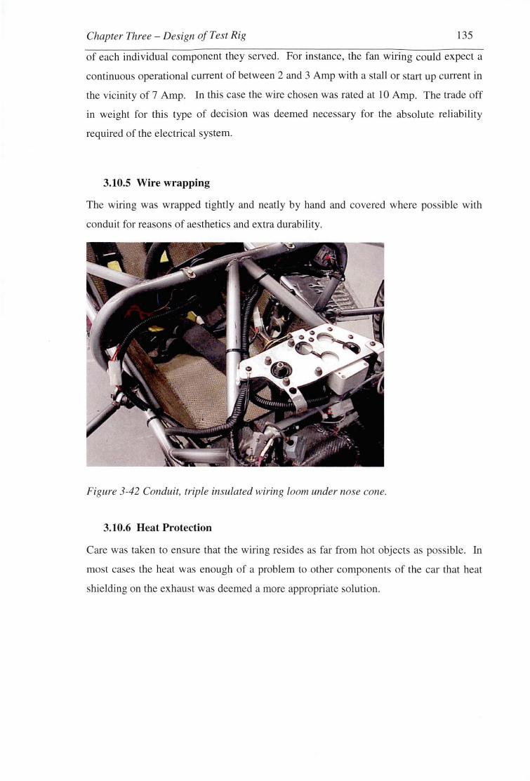
Chapter Three - Design of Test Rig 135
of each individual component they served. For instance, the fan wiring could expect a
continuous operational current of between 2 and 3 Amp with a stall or start up current in
the vicinity of 7 Amp. In this case the wire chosen was rated at 10 Amp. The trade off
in weight for this type of decision was deemed necessary for the absolute reliability
required of the electrical system.
3.10.S Wire wrapping
The wiring was wrapped tightly and neatly by hand and covered where possible with
conduit for reasons of aesthetics and extra durability.
Figure 3-42 Conduit, triple insulated wiring loom under nose cone.
3.10.6 Heat Protection
Care was taken to ensure that the wiring resides as far from hot objects as possible. In
most cases the heat was enough of a problem to other components of the car that heat
shielding on the exhaust was deemed a more appropriate solution.

Chapter Three - Design of Test Rig 136
3.10.7 Easy removal of all components
To ensure easy removal of all components, wires were crimped and not soldered.
Where possible large multiple connectors have been used to eliminate the possibility of
mis-connection upon re-installation.
3.10.8 Kill switches
Power for the entire car may be instantly cut using any one of three kill switches. The
brake over-run switch is located behind the brake pedal and will activate if the brake is
depressed while there is simultaneous fai lure of both independent braking systems.
Figure 3-43 Kill switches
The other two kill switches are located on the dashboard to the driver ' right and
externally next to the head support on the roll bar to the driver's right, in accordance
with best practice international FIA safety standards.

Chapter Three-Design of Test Rig 137
Cutting any one of these switches will deactivate the switch line to the main relay. All
power to components on the vehicle are sourced from this relay or from the switch line
after the kill switches. Both human operated kill switches are clearly labelled with the
international electrical symbol of a red spark on a white-edged blue triangle.
3.10.9 Brake Light
A brake light of 15 watt or equivalent is required by SAE international standards. This
is to be mounted centrally between the wheel centres and the drivers shoulder height at
the rear of the vehicle. For aesthetic reasons a high intensity LED arrangement was
selected. The LEDs are mounted in parallel to prevent failure of the complete brake
light in the event of one LED failing.
3.10.10 Engine Cam Sensor Circuit
The engine cam angle sensor is used by the ECU to determine the location of the
pistons for fuel injection timing. This sensor is a small hall effect type similar in
appearance to a transistor, and is activated by a small permanent magnet mounted in the
cam sprocket. The pulse from the sensor must be amplified to be read by the ECU input.
A simple MOSFET amplification circuit is used for the job. The circuit is built on
printed track circuit board and mounted in a box on the outside of the engine.

Chapter Three - Design of Test Rig 138
The sensor wiring is temperature resistant, Kevlar insulated wire designed for harsh
conditions. The sensor is mounted into the cam sprocket cavity in an aluminium
bracket held by the nearest cam cover bolt. Directions for the setup and calibration of
this sensor are included in the ECU help menus.
Figure 3-44 location of the engine cam sensor circuit case.
Chapter Three-Design of Test Rig 139
3.11 FUSE BOX CIRCUIT AND LAYOUT DESIGN
3.11.1 Physical considerations
In fitting with the major objectives of the electrical system, the original loom design
with in line fuses and multiple bulky relay mountings was re-designed to incorporate a
single fuse and relay box. This box is located in a highly visible, easily accessible
location on the outside of the right hand side of the driver cockpit.
The box itself is made of clear material for reasons of fast identification of loose
connections or burnt out fuses and relays as well as aesthetics. The wires are fed in
groups through the back of the box that allows removal of the box without the loom and
vice versa. Rubber grommets have been used along with a rubber gasket so seal the box
cover in place. The cover is screwed onto the aluminium backing plate that is then
bolted to the frame.
3.11.2 Circuit Design
The circuit for the fuse box was taken almost directly from the MoTeC ECU wiring
diagrams. Major alterations involved the removal of a relay that was redundant in this
particular application and the unification of relay type used throughout the vehicle. The
required diode activated relay was replaced with an in line diode on the circuit to allow
fitment of a standard relay in its place. Extra fuses were included for each of the major
components, allowing for very simple component fault finding.
3.11.3 Physical circuit layout
One of the major objectives of the fuse box was to find a neat and effective way to
mount all the required relays and fuses in one place where they could be easily
accessible to check and change. The ideal situation was chosen to be a set of closely
located relay and fuse sockets joined to plugs as appropriate by a printed circuit board.'
The printed circuit board was layered with solder tracks to increase the current rated
capacity in excess of 12 Amp.

Chapter Three - Design of Test Rig 140
3.11.4 Fuse specification
Load ratings of fuses were selected according to the component they serve. In general
fuses will withstand up to their rated current plus 200% for 2 minutes. The majority of
components have around 7-8 Amp tart up current with a continuous 2-3 Amp while
running. 10 amp fuses are most common in this system. Automotive fuses were
specified for their compactness, physical durability (plastic cases) and ease of mounting.
Figure 3-45 The yellow colour of the automotive fuses within the fuse box indicates a
rating of 10 amp.

Chapter Three - Design of Test Rig 141
3.12 DASHBOARD - LAYOUT AND CIRCUITRY
3.12.1 Physical considerations
The dashboard is the driver control panel. All the information about the engine and
other aspects of the running car is fed to the driver through the Advanced Dash Logger
or ADL. Information about the ADL i contained within the telemetry section of this
document with reference wiring and programming.
Figure 3-46 ADL location on dashboard.
The dash itself is constructed from a composite sandwich of carbon fibre and foam
constructed using vacuum bagging techniques, the fibre was said up on sheets of
window glass to ensure a good finish . Profile cutting, drilling and finishing all
performed after the bonding process. The dashboard attaches to the frame through bolts
and welded tabs.
COM ports featured in the dash are used to facilitate fast and easy connection of the on
board computer systems to an external computing and storage PCs for data logging
sessions. The COM ports connect to plugs behind the dash where the ECU and ADL
are connected facilitating easy removal of individual units. The trackside computer is
simply plugged into the front of the dashboard to down load data or change on-board
programmed settings.
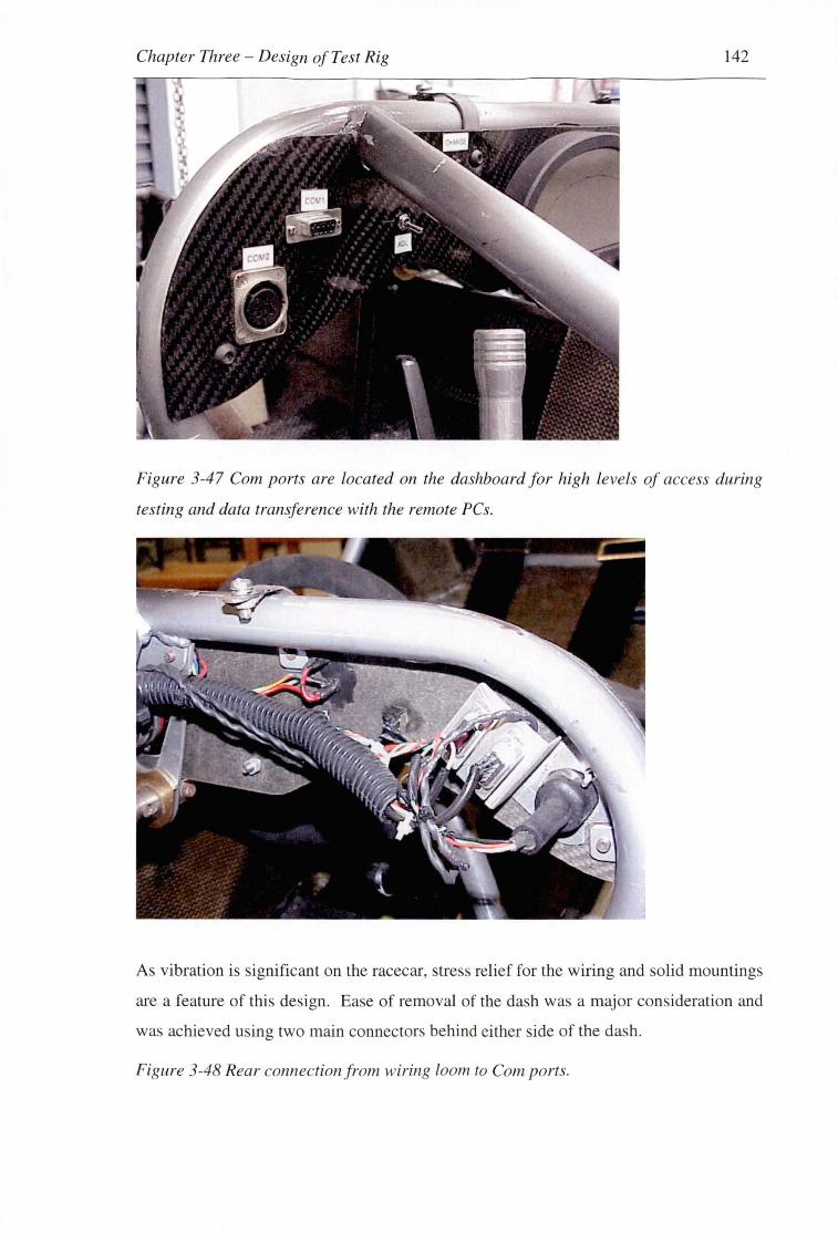
Chapter Three - Design of Test Rig 142
Figure 3-47 Com ports are located on the dashboard for high levels of access during
testing and data transference with the remote PCs.
As vibration is significant on the racecar, stre s relief for the wiring and solid mountings
are a feature of this design. Ease of removal of the dash was a major consideration and
was achieved using two main connectors behind either side of the dash.
Figure 3-48 Rear connection from wiring loom to Com ports.

Chapter Three - Design of Test Rig 143
3.12.2 Circuit design
Once the physical layout of the dashboard was determined, the circuit design was
largely a matter of connecting the components with the main vehicle circuit. Shrink fit
wire covering was used to prevent shorting, and the back of the dash is painted with
liquid electrical tape to ensure water resistance.
3.12.3 Physical layout
Physical layout of the dashboard switches and lights follows a logical progression. The
most important switches are to the right, away from the gear changer. The neutral and
oil warning lights are located close to the ignition switch.

Chapter Three -Design of Test Rig 144
3.13 ELECTRICAL SYSTEM SPECIFICATIONS
Specifications for components of the electrical system are as follows:
Table 4 Electrical system specifications
Item
Battery
Type Gel cell
Capacity 15 Ah
Voltage 12.6 v
Charging System
Type Three Phase AC
Alternator output voltage 45V
Stator coil resistance 0.2-0.6 Ohm
Charging Voltage 14-15 v (regulator I rectifier voltage)
Electric Starter System
Starter motor 12 v Brush length 12111111
Commutator diameter 28mm
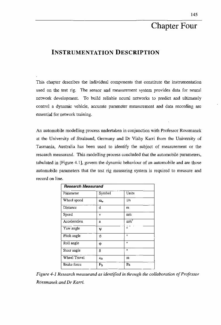
145
Chapter Four
INSTRUMENTATION DESCRIPTION
This chapter describes the individual components that constitute the instrumentation
used on the test rig. The sensor and measurement system provides data for neural
network development. To build reliable neural networks to predict and ultimately
control a dynamic vehicle, accurate parameter measurement and data recording are
essential for network training.
An automobile modelling process undertaken in conjunction with Professor Rossmanek
at the University of Stralsund, Germany and Dr Vishy Karri from the University of
Tasmania, Australia has been used to identify the subject of measurement or the
research measurand. This modelling process concluded that the automobile parameters,
tabulated in [Figure 4.1], govern the dynamic behaviour of an automobile and are those
automobile parameters that the test rig measuring system is required to measure and
record on line.
Research Measurand
Parameter Symbol Units
Wheel speed ffiw 1/s
Distance d m
Speed v m/s
Acceleration a m/SL
Yaw angle "' 0
Pitch angle t} 0
Roll angle <p 0
Steer angle 8 0
Wheel Travel Zst m
Brake force Fa Pa
Figure 4-1 Research measurand as identified in through the collaboration of Professor
Rossmanek and Dr Karri.
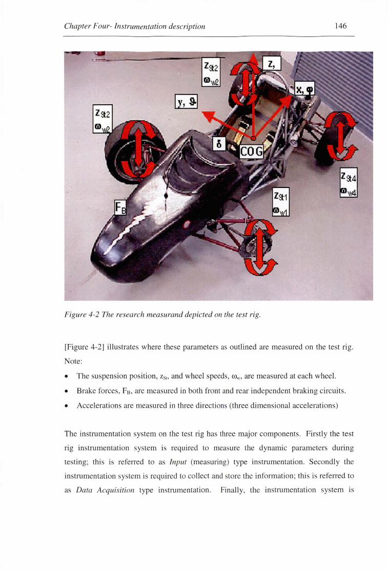
Chapter Four- Instrumentation description 146
z ::t2
Figure 4-2 The research measurand depicted on the test rig.
[Figure 4-2] illustrates where these parameters as outlined are measured on the test rig.
Note:
• The suspension position, z51 , and wheel speeds, COw, are measured at each wheel.
• Brake forces, F8 , are measured in both front and rear independent braking circuits.
• Accelerations are measured in three directions (three dimensional accelerations)
The in trumentation system on the test rig has three major components. Firstly the test
rig instrumentation system is required to measure the dynamic parameters during
testing; this is referred to as Input (measuring) type instrumentation. Secondly the
instrumentation system is required to collect and store the information; this is referred to
as Data Acquisition type instrumentation. Finally, the instrumentation system is
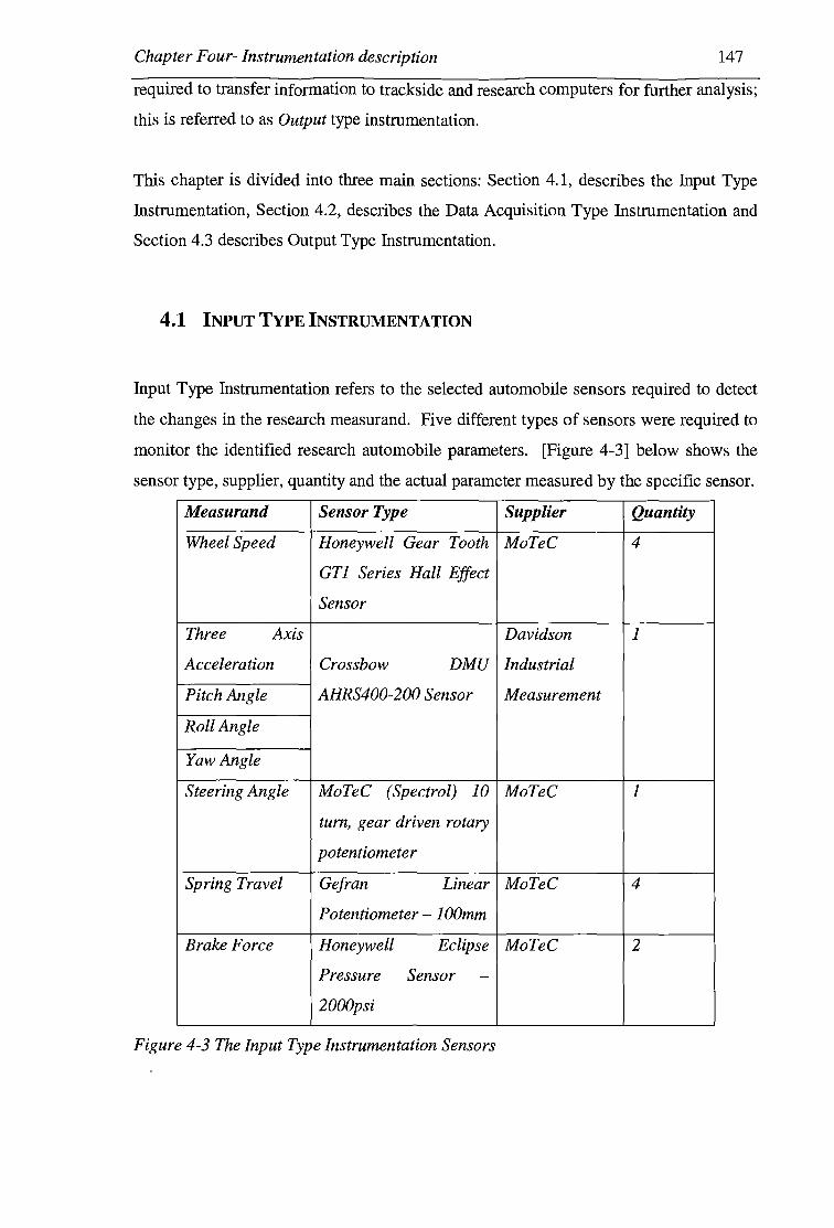
Chapter Four- Instrumentation description 147
required to transfer information to trackside and research computers for further analysis;
this is referred to as Output type instrumentation.
This chapter is divided into three main sections: Section 4.1, describes the Input Type
Instrumentation, Section 4.2, describes the Data Acquisition Type Instrumentation and
Section 4.3 describes Output Type Instrumentation.
4.1 INPUT TYPE INSTRUMENTATION
Input Type Instrumentation refers to the selected automobile sensors required to detect
the changes in the research measurand. Five different types of sensors were required to
monitor the identified research automobile parameters. [Figure 4-3] below shows the
sensor type, supplier, quantity and the actual parameter measured by the specific sensor.
Measurand Sensor Type Supplier Quantity
Wheel Speed Honeywell Gear Tooth MoTeC 4
GTJ Series Hall Effect
Sensor
Three Axis Davidson 1
Acceleration Crossbow DMU Industrial
Pitch Angle AHRS400-200 Sensor Measurement
Roll Angle
Yaw Angle
Steering Angle MoTeC (Spectral) 10 MoTeC 1
tum, gear driven rotary
potentiometer
Spring Travel Gefran Linear MoTeC 4
Potentiometer - 1 OOmm
Brake Force Honeywell Eclipse MoTeC 2
Pressure Sensor -
2000psi
Figure 4-3 The Input Type Instrumentation Sensors
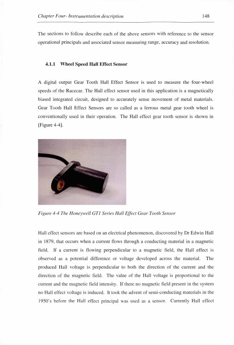
Chapter Four- Instrumentation description 148
The section to follow describe each of the above sensors with reference to the sensor
operational principals and associated ensor measuring range, accuracy and resolution.
4.1.1 Wheel Speed Hall Effect Sensor
A digital output Gear Tooth Hall Effect Sensor is used to measure the four-wheel
speeds of the Racecar. The Hall effect sensor used in this application is a magnetically
biased integrated circuit, designed to accurately sense movement of metal materials .
Gear Tooth Hall Effect Sensors are so called as a ferrous metal gear tooth wheel is
conventionally used in their operation. The Hall effect gear tooth sensor is shown in
[Figure 4-4].
Figure 4-4 The Honeywell GTJ Series Hall Effect Gear Tooth Sensor
Hall effect sensors are based on an electrical phenomenon, discovered by Dr Edwin Hall
in 1879, that occurs when a current flows through a conducting material in a magnetic
field. If a current is flowing perpendicular to a magnetic field, the Hall effect is
observed as a potential difference or voltage developed across the material. The
produced Hall voltage is perpendicular to both the direction of the current and the
direction of the magnetic field . The value of the Hall voltage is proportional to the
current and the magnetic field intensity. If there no magnetic field present in the system
no Hall effect voltage is induced. It took the advent of semi-conducting materials in the
1950's before the Hall effect principal was u ed as a sensor. Currently Hall effect

Chapter Four- Instrumentation description 149
sensors are used to measure rotational speeds of different automotive processes. They
are used in automobile applications such as camshaft and crankshaft speed sensors,
transmission speed sensors, tachometers and are the wheel speed sensors used in ABS
and Traction Control driver supporting facilities.
The Hall effect sensor is composed of an integrated circuit, made up of discrete
capacitors and a bias magnet, that is sealed in a probe type, non-magnetic plastic
package for physical protection and cost effective installation. The Hall effect sensor
consists of three wires. One wire is the power source or voltage, the second wire
supplies the sensor ground and the third wire is the signal wire that provides the output
or measurement sensor reading value. The configuration and wiring diagram is
depicted in [Figure 4-5].
TIMING CAPACITOR
Voltage Regulator t---------f
Hall Sensor Trigger Circuil and
Feedback Ampfifisr
Figure 4-5 Gear tooth sensor construction and wiring diagram
>----+-----1 Vee {+)
. _,..-1__,....-40Utput (O~ Open Collector
As a gear tooth wheel passes the Hall effect sensor face, as depicted in [Figure 4-6], it
concentrates the magnetic flux away from the sensor's in built bias magnet. The sensor
detects the change in magnetic flux level and hence as explained above there is a drop in
the induced voltage across the sensor, which translates into a change in the sensor
voltage output. The digital output switches between the supply voltage when it passes a
gap in the tooth wheel and the saturation voltage (0.4 V) when it passes a tooth. [Figure
4-7] illustrates the drop in induced voltage across the sensor as the gear tooth wheels
teeth move past the face of the Hall Effect sensor.
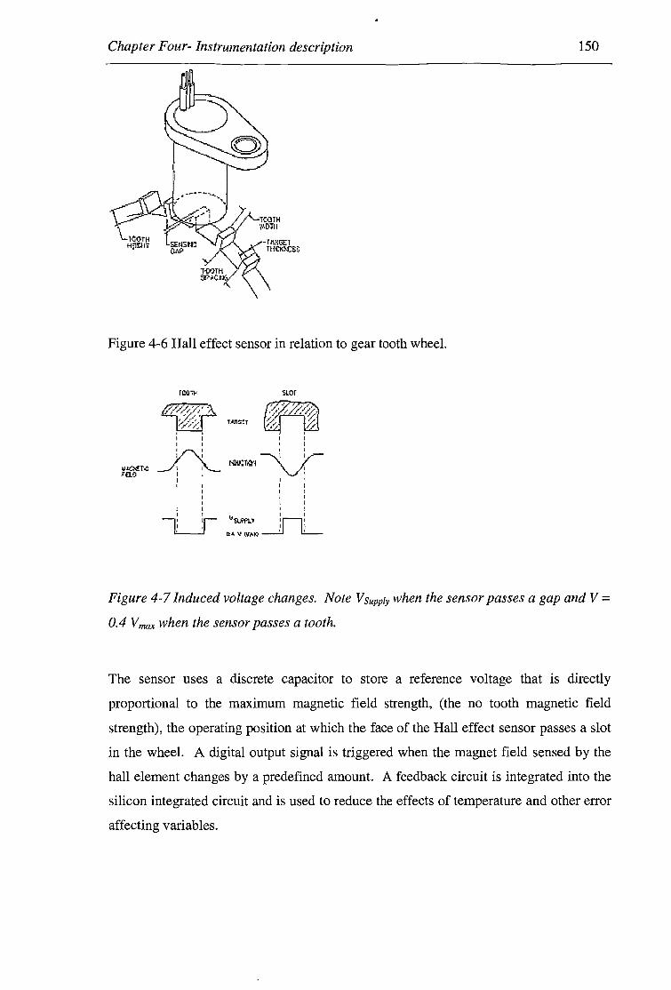
Chapter Four- Instrumentation description
Figure 4-6 Hall effect sensor in relation to gear tooth wheel.
roon-:
I I I I I
1: If"""' lL__j
I I
uor
I l
IW:TIO'l~ I l I I I l I I I I I I
v"5l.A'PI.~ !r-i! n..1, v (lllt.'>J ---1.J Li.__
150
Figure 4-7 Induced voltage changes. Note Vsupply when the sensor passes a gap and V = 0.4 Vmax when the sensor passes a tooth.
The sensor uses a discrete capacitor to store a reference voltage that is directly
proportional to the maximum magnetic field strength, (the no tooth magnetic field
strength), the operating position at which the face of the Hall effect sensor passes a slot
in the wheel. A digital output signal is triggered when the magnet field sensed by the
hall element changes by a predefined amount. A feedback circuit is integrated into the
silicon integrated circuit and is used to reduce the effects of temperature and other error
affecting variables.

Chapter Four- Instrumentation description 151
The Honeywell Gear Tooth (GTl Series) technical specification brochure and the
MoTeC Hall effect sensor CAD drawing are provided in "Appendix H". As the output
from this Hall effect sensor is digital, the accuracy in the sensed measurement is
dependant primarily on how the sensor is positioned with respect to the ferrous metal
gear tooth wheel.
The performance and accuracy of the Hall effect sensors is dependent mainly on the
way the sensors are positioned in relation to the target material6 and also on the
magnetic characteristics of the target. The following variables have been identified to
effect the operation of Hall effect sensors and were considered in combination during
the sensor installation process.
Target material, geometry, and speed
Sensor/target air gap: that is the distance between the sensor and the target material
Operating temperature:
The proximity of magnetic materials to the sensor and target
Initially the installation process required the development of a suitable gear tooth wheel
for sensor operation. However, suitable points of attachment of such a wheel on the test
rig could not be found at all four wheels. It was possible to attach such a device on the
stub axels7 of the front wheels. However, this could not be achieved on the two back
wheels of the automobile, as the drive shaft of the test rig obstructed any available site
of installation. An alternative solution had to be found that involved the use of a
magnetic (metallic) material in a regular repetitive formation, that would provide a
similar output from the Hall effect sensor, as that produced when in use with a gear
tooth wheel.
A solution to this problem was found using the heads of the bolts that hold the
aluminium face plate of the wheels to the rim of the wheels. The bolts, which are
6 Target material refers to the metallic material that concentrates the magnetic flux away from the Hall
effect sensor 7 There are four holes present on the front two stub axels where initially a gear tooth wheel was to be
attached

Chapter Four- Instrumentation description 152
positioned in a uniform circular formation around the face plate, act as the sensor target.
The sensor target is the metallic element necessary to draw the magnetic flux away from
the sensor thus producing a signal output. The wheel rims made from aluminium, a
non-magnetic material behave as the non-target material. [Figure4-8] shows the bolt
arrangement on the in ide of the rims of the wheels. This arrangement with a repetitive
series of targets and non target areas in a circular formation facilitates the same function
in operation as the gear tooth wheel in terms of producing a change in the magnetic flux
of the sensor. In theory this solution is feasible as long as the sensor can be positioned
close enough and in a direct line with the rotating bolt heads on the inside of the wheel.
a c
Figure 4-8 a) Three piece rim, b) outside view of rim bolts, c) inside view of rim bolts .
Testing was required to determine if this unconventional Hall effect sensmg
arrangement would work in practice to confirm if the materials in use as the magnetic
and non-magnetic targets possessed the desirable qualities to produce a reliable signal
from the Hall effect sensor.
Each hall effect sensor required a suitable mounting position to be found close enough
to the inside of the wheel rims to ensure a 1- 2 mm gap between the sensor and the bolt
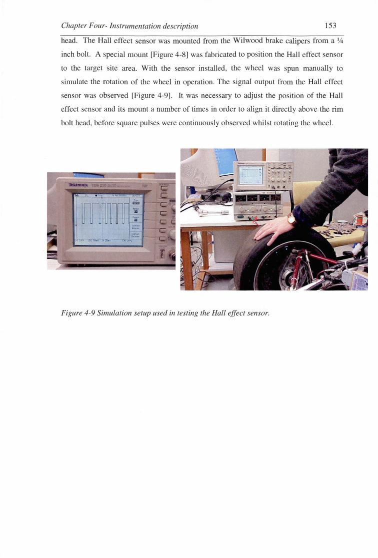
Chapter Four- Instrumentation description 153
head. The Hall effect sensor was mounted from the Wilwood brake calipers from a 1.4
inch bolt. A special mount [Figure 4-8] was fabricated to position the Hall effect sensor
to the target site area. With the sensor installed, the wheel was spun manually to
simulate the rotation of the wheel in operation. The signal output from the Hall effect
sensor was observed [Figure 4-9]. It was necessary to adjust the position of the Hall
effect sensor and its mount a number of times in order to align it directly above the rim
bolt head, before square pulses were continuously observed whilst rotating the wheel.
Figure 4-9 Simulation setup used in testing the Hall effect sensor.

Chapter Four- Instrumentation description 154
Figure 4-10 Hall effect sensor mount.
The calibration function of the Dash Manager [Figure 4-11] software was used to
convert the digital output signal of the Hall effect sensor into a wheel velocity. Sensor
calibration required the wheel speed calculation for one complete revolution of the
wheel, in a single second. One revolution of the wheel is equivalent to eighteen sensor
signal pulses being generated per second, as there are eighteen bolts around each wheel.
To determine the speed of the wheel for one cycle per second the diameter of the wheels
had to be measured and the circumference of each calculated8. This was then entered in
the calibration function in the Dash Manager software, as shown in [Figure 4-11), which
shows the calibration curve of the rear right wheel. A similar calibration curve was
8 The font tyre on the Race Car are sl ightly smaller in size than the back tyres thus. the back and front tyre
diameters had to be individually measured.
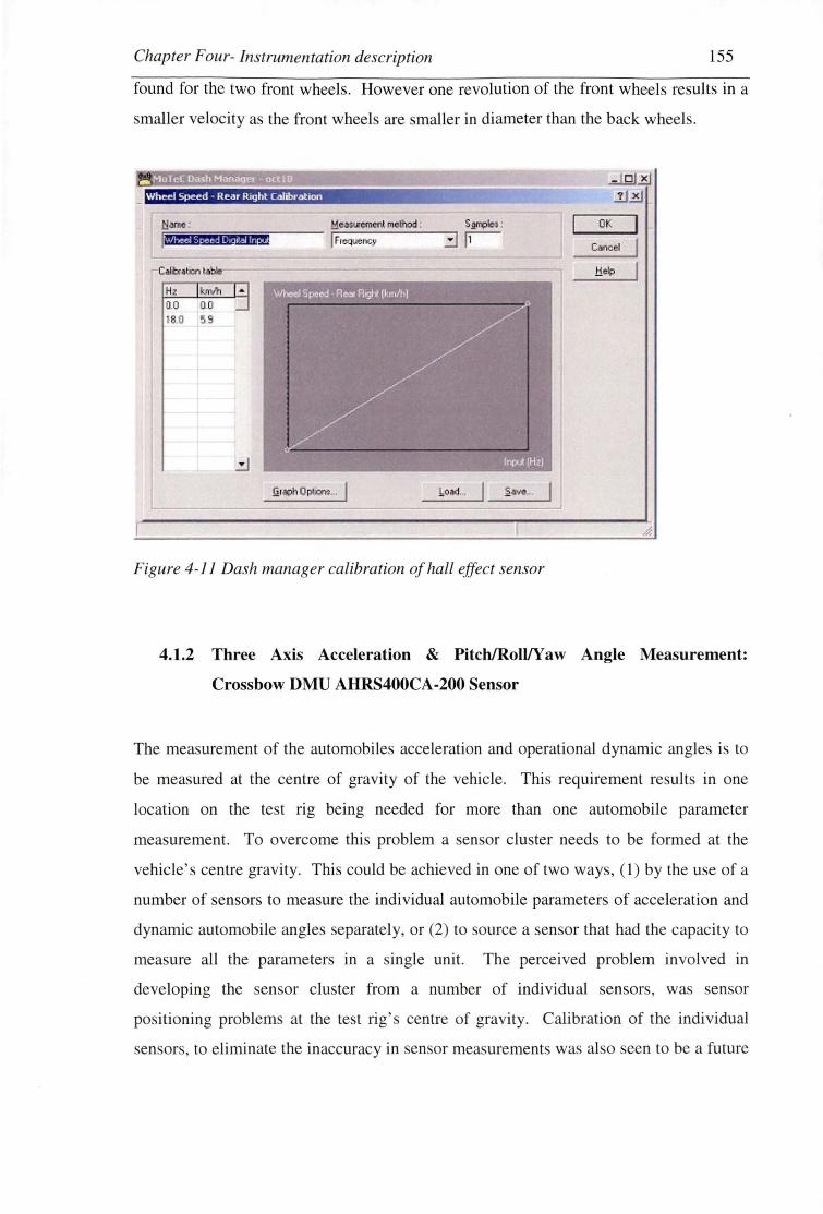
Chapter Four- Instrumentation description 155
found for the two front wheels. However one revolution of the front wheels results in a
smaller velocity as the front wheels are smaller in diameter than the back wheels .
Whoo Speed - Rear Right Calibration ,,t.
0 tjan1e . Me~emcnt method : S,gfll>les~ l.iOiiiiii'iiiiiiiiiiir.iiiiiiiiiii;;;---- .-, ______ ..:J_..... r,--, .
j™"6m:umnn F1equenc - I' Cancel
.!::!ep
- ..
_oad ..
Figure 4-11 Dash manager calibration of hall effect sensor
4.1.2 Three Axis Acceleration & Pitch/Roll/Yaw Angle Measurement:
Crossbow DMU AHRS400CA-200 Sensor
The measurement of the automobiles acceleration and operational dynamic angles is to
be measured at the centre of gravity of the vehicle. This requirement results in one
location on the test rig being needed for more than one automobile parameter
measurement. To overcome this problem a sensor cluster needs to be formed at the
vehicle ' centre gravity. This could be achieved in one of two ways, (1) by the use of a
number of sensors to measure the individual automobile parameters of acceleration and
dynamic automobile angles separately, or (2) to ource a sen or that had the capacity to
measure all the parameters in a single unit. The perceived problem involved in
developing the sensor cluster from a number of individual sensors , was sensor
positioning problems at the test rig 's centre of gravity. Calibration of the individual
sensors, to eliminate the inaccuracy in sensor measurements was also seen to be a future

Chapter Four- Instrumentation description 156
difficulty with this approach. The error in sensor measurement if this approach was
u ed would arise from the sensors being installed at a location near the centre gravity of
the te t rig and not at the exact centre of gravity of the vehicle.
Therefore a single sensor was sought that had the capacity to measure all the measurand
parameters needed to be monitored at the test rig's centre of gravity. The main
advantage of selecting a single sen or for the measurement of the centre of gravity
parameters was identified in the ease of sensor installation and calibration, with the
knowledge of minimising the risk involved in potential installation errors in the sensor
output, compared with installing individual sensors. The Crossbow DMU AHRS400-
CA sensor was identified as being the most appropriate sensor for this application. A
picture of the sensor can be seen below in [Figure 4-12] .
Figure 4-12 The DMU AHRS400CA-200 Sensor
The DMU-AHRS is a sensor clustering measurement system, designed to measure nine
parameters including stabilised pitch, roll and yaw angular rates and angles and three
axis acceleration in a dynamic environment. The DMU-AHRS measures these variables
by using a combination of micro-machined three-axis accelerometers, three-axis
rotational rate sen ors, and three-axis magnetometers. The addition of a three-axis
magnetometer also allows the DMU-AHRS to make a true measurement of magnetic
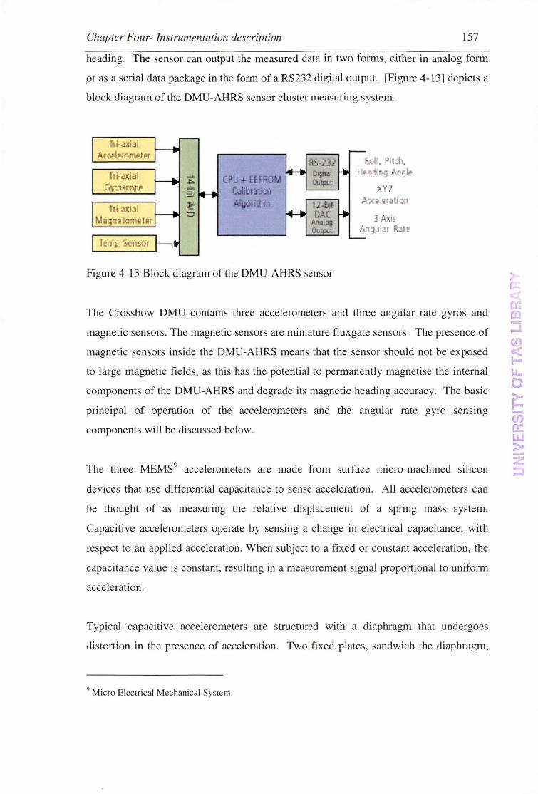
Chapter Four- Instrumentation description 157
heading. The sensor can output the measured data in two forms, either in analog form
or as a erial data package in the form of a RS232 digital output. [Figure 4-13] depicts a
block diagram of the DMU-AHRS sensor cluster measuring ystem.
Figure 4-13 Block diagram of the DMU-AHRS sensor
x· Accle·.a~i ·1
j Ar.is Angular R LI!
The Crossbow DMU contains three accelerometers and three angular rate gyros and
magnetic sensors. The magnetic sensors are miniature fluxgate sensors. The presence of
magnetic sensors inside the DMU-AHRS means that the sensor should not be exposed
to large magnetic fields , as this has the potential to permanently magnetise the internal
components of the DMU-AHRS and degrade its magnetic heading accuracy. The basic
principal of operation of the accelerometers and the angular rate gyro sensing
components will be di cussed below.
The three MEMS9 accelerometers are made from surface micro-machined silicon
devices that use differential capacitance to sen e acceleration. All accelerometers can
be thought of as measuring the relative displacement of a spring mass system.
Capacitive accelerometers operate by sensing a change in electrical capacitance, with
respect to an applied acceleration. When subject to a fixed or constant acceleration, the
capacitance value is constant, resulting in a measurement signal proportional to uniform
acceleration.
Typical capacitive accelerometers are structured with a diaphragm that undergoes
distortion in the presence of acceleration. Two fixed plates, sandwich the diaphragm,
9 Micro Electrical Mechanical System
-..J en t.: LL 0
~ -(/) a: w > -

Chapter Four- Instrumentation description 158
creating the capacitor unit. Changes in acceleration are detected by measuring the
capacitance changes resulting from the separation of the two plates due to a movement
of the diaphragm. The capacitance is inversely proportional to gap distance between the
two plates and therefore the displacement of the diaphragm is a non-linear hyperbolic
function.
The sensor is designed so that the acceleration of the measured medium causes the
diaphragm of the sensor to distort which results in a change in the capacitance of the
sensor, due to a distance change between the two parallel plates that support the
diaphragm. The change in capacitance is used in a bridge circuit that performs signal
conditioning on the sensors' output signal to achieve linearisation and hence an output
signal that is proportional to the input acceleration of the system under investigation.
The three angular rate gyroscopic sensors consist of vibrating ceramic plates that use a
silicon MEMS structure to measure the Coriolis force in order to measure the angular
rotation rate around a given axis. The advantage of this approach is that the output of
the angular rate is independent of the acceleration output. In the l 830's G. Coriolis
discovered that an object moving perpendicular to a rotating frame will cause an
observer on the rotating frame to see an apparent acceleration of the object. The
DMU's angular rate gyros experience a Coriolis acceleration by the angular rotation of
a vibrating silicon MEMS structure induced by the dynamic movement of the testing
apparatus. A change in the direction around one axis of a driving transducer induces a
vibration in a detection transducer on another axis. An oscillator circuit is used to
control the vibration and signal-conditioning converts measurements to an angular rate
output. In general, the apparent Coriolis acceleration A and Force Fis given by:
A= 2mVsin(~) and F = 2mmVsin(~)
where ro is the angular velocity of the rotating axes relative to a fixed set of axes, Vis
the velocity of the bar, and<!> is the angle between the vectors OJ and V.
From observing the above equations it is apparent that the Coriolis force is proportional
to w or angular velocity. The Coriolis force is converted to a voltage by the detector
element and signal conditioning circuitry. As the mass of the structure and the vibration

Chapter Four- Instrumentation description 159
velocity of the sensor components are both known quantities, the angular velocity (J) is
easily derived and provided to the DMU. The sensor integrates the angular velocity
signals with respect to time to convert angular rates, mea ured in °/s into angular 0
outputs. [Figure 4-6] depicts a block diagram illustrating this operation.
Raw Angle
1-----'a.1 Gravity ...---~ Angle
1------ Stabil ized Ang les
Figure 4-14 Block diagram depicting the signal conditioning operations.
The DMU-AHRS sensor has a predefined coordinate system to which the
accelerometers, angular rate sensors and magnetic sensors are aligned. The coordinate
system is shown on a label attached to the connector side of the ensor. The sensor axis
orientation forms an orthogonal right-hand coordinate system with the z-axis defined as
positive in the downward direction. The system is depicted in Figure 4-7.
x
roll
pitch
yaw
z
y
AHRS Top View
x
y
Figure 4-15 The DMU-AHRS400CA-200 coordinate system.

Chapter Four- Instrumentation description 160
The sensors' coordinate system defines a positive acceleration when it is oriented
towards the positive side of the coordinate axis. Therefore if the sensor was only
measuring the effects of gravity it would produce an output in the z axis direction of +g
and would read 0 g for both the acceleration in the x and y directions. The direction of
positive angular rotational rates is defined by the right hand rule. This means a
clockwise motion of the accelerometer when positioned on a horizontal surface would
produce a positive angular rate and yaw angle around the z axis. The x- and y-axis rate
sensors would measure zero angular rates for this operation. The magnetic sensors are
aligned with the same axes definitions and sign as the linear accelerometers.
The Crossbow DMU AHRS400CA-200 technical specification brochure is provided in
"Appendix H". This brochure provides information on the measurement range,
resolution and total accuracy of the angular rates, pitch and roll angles (Altitude) and
yaw angle (Heading) and three-axis acceleration. A summary of these and the
calculated maximum errors associated with measurement is presented below in [Figure
4-16].
Sensor Specification Angular Rates Acceleration
Range ± 200 (0/sec) ± 10 (g)
Resolution < 0.05 (0/sec) < 1.25 (mg)
Bias Error <± 0.05 (0/sec) <±12 (mg)
Non-Linearity (%FS) < 0.3 <1
Scale Factor Accuracy(%) <1 <1
Total Error(%) 1.044 1.458
Maximum Error Value (FS) ± 2. 089 ( 0/sec) ±0.146 (g)
Figure 4-16 Error specification of the DMU sensor.
The DMU measures the parameters at a sampling rate of 75 samples per second. The
sensor also has an on board temperature sensor which is used to monitor the internal
temperature of the DMU for sensor temperature calibration. The DMU-AHRS outputs

Chapter Four- Instrumentation description 161
the yaw angle with referenced to magnetic north 10. The declination 11 needs to be known
in order to translate the DMU-AHRS magnetic heading into a heading referenced to true
north.
4.1.3 Wheel Travel: Gefran PZ12A Linear Potentiometer - lOOmm
A Gefran PZ12A analog linear potentiometer with a 100 mm stroke has been selected to
measure the individual displacement of the four wheels of the test rig during dynamic
trials. The sensor consists of an anodised aluminium cylinder case with an internal
moveable control rod made from stainless steel, with an extension capacity of 100 mm.
At the end of the moveable rod and the bottom of the sensor there are 5 mm diameter
self aligning ball joints used for mounting purposes. The sensor can be seen mounted to
the test rig in [Figure 4-17]
Figure 4-17 Wheel travel linear potentiometer mounted to the test rig.
10 Magnetic north is the direction toward the magnetic north pole; true no1th is the direction towards the true North Pole. 11 The direction of true north varies from magnetic north depending on your location on the globe. The difference between true and
magnetic north is called declination or magnetic variance.
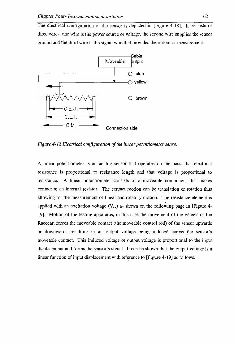
Chapter Four- Instrumentation description 162
The electrical configuration of the sensor is depicted in [Figure 4-18]. It consists of
three wires, one wire is the power source or voltage, the second wire supplies the sensor
ground and the third wire is the signal wire that provides the output or measurement.
~-c.E.u.-~
i--.-- C. E.T. -----i
C.M.
Moveable
blue
yellow
brown
Connection side
Figure 4-18 Electrical configuration of the linear potentiometer sensor
A linear potentiometer is an analog sensor that operates on the basis that electrical
resistance is proportional to resistance length and that voltage is proportional to
resistance. A linear potentiometer consists of a moveable component that makes
contact to an internal resistor. The contact motion can be translation or rotation thus
allowing for the measurement of linear and rotatory motion. The resistance element is
applied with an excitation voltage (Vex) as shown on the following page in [Figure 4-
19]. Motion of the testing apparatus, in this case the movement of the wheels of the
Racecar, forces the moveable contact (the moveable control rod) of the sensor upwards
or downwards resulting in an output voltage being induced across the sensor's
moveable contact. This induced voltage or output voltage is proportional to the input
displacement and forms the sensor's signal. It can be shown that the output voltage is a
linear function of input displacement with ref~rence to [Figure 4-19] as follows.

Chapter Four- Instrumentation description 163
Figure 4-19 A representation of a Linear Potentiometer
Rearranging
as v
___!!__ = cons tan t = c [max
8V = cc5l
The Gefran PZ12A Linear Potentiometer technical specification brochure and the
MoTeC Linear Potentiometer CAD drawing are both provided in "Appendix H". The
resolution of the sensor is infinite according to the Gefran technical specification
brochure. The resolution of the sensor was investigated by connecting the sensor to a
multimeter and manually adjusting the moveable rod to determine the minimum voltage
output from the signal wire of the sensor. The smallest voltage reading the sensor
detected whilst manually adjusting the length of the extension rod was 0.00025 V. This
translates to a resolution of ±5 x 10⁻³ mm as a 8 V corresponds to maximum extension
of 100 mm. The sensor has a linearity accuracy of 0.1 %.
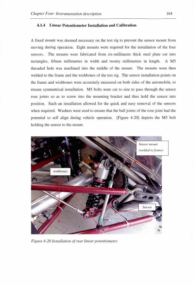
Chapter Four- Instrumentation description 164
4.1.4 Linear Potentiometer Installation and Calibration
A fixed mount was deemed necessary on the test rig to prevent the sensor mount from
moving during operation. Eight mounts were required for the installation of the four
sensors. The mounts were fabricated from six-millimetre thick steel plate cut into
rectangle , fifteen millimetres in width and twenty millimetres in length. A MS
threaded hole was machined into the middle of the mount. The mounts were then
welded to the frame and the wishbones of the test rig. The sen or installation points on
the frame and wishbones were accurately measured on both sides of the automobile, to
ensure symmetrical installation. MS bolts were cut to size to pass through the sensor
rose joints so as to screw into the mounting bracket and thus hold the sensor into
position. Such an installation allowed for the quick and ea y removal of the sensors
when required. Washers were used to ensure that the ball joints of the rose joint had the
potential to self align during vehicle operation. [Figure 4-20] depicts the MS bolt
holding the sensor to the mount.
Figure 4-20 Installation of rear linear potentiometer.
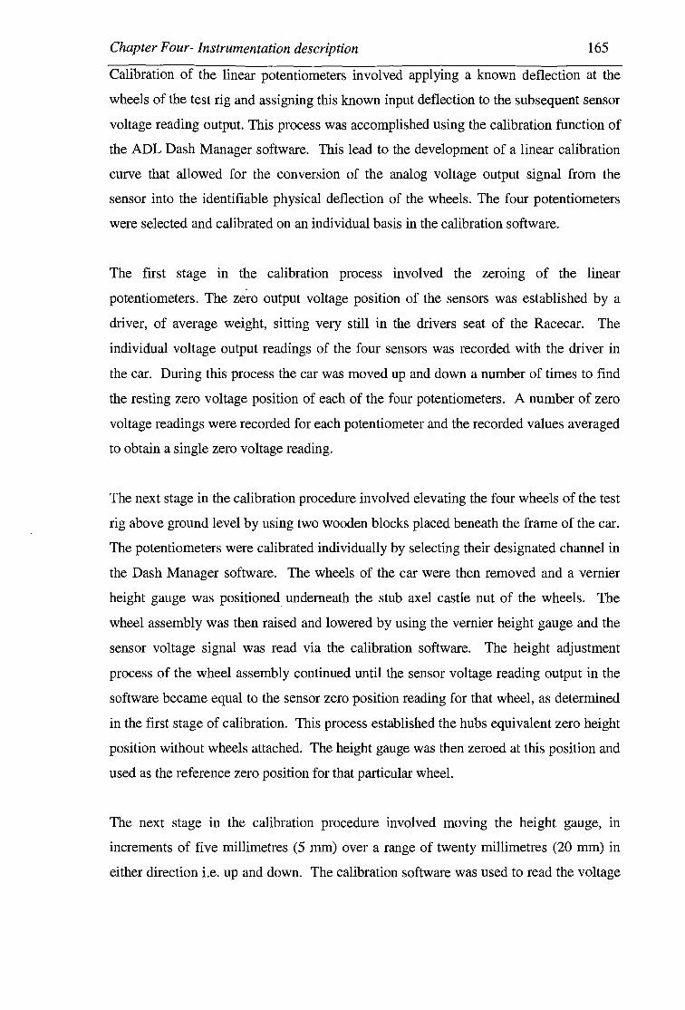
Chapter Four- Instrumentation description 165
Calibration of the linear potentiometers involved applying a known deflection at the
wheels of the test rig and assigning this known input deflection to the subsequent sensor
voltage reading output. This process was accomplished using the calibration function of
the ADL Dash Manager software. This lead to the development of a linear calibration
curve that allowed for the conversion of the analog voltage output signal from the
sensor into the identifiable physical deflection of the wheels. The four potentiometers
were selected and calibrated on an individual basis in the calibration software.
The first stage in the calibration process involved the zeromg of the linear
potentiometers. The zero output voltage position of the sensors was established by a
driver, of average weight, sitting very still in the drivers seat of the Racecar. The
individual voltage output readings of the four sensors was recorded with the driver in
the car. During this process the car was moved up and down a number of times to find
the resting zero voltage position of each of the four potentiometers. A number of zero
voltage readings were recorded for each potentiometer and the recorded values averaged
to obtain a single zero voltage reading.
The next stage in the calibration procedure involved elevating the four wheels of the test
rig above ground level by using two wooden blocks placed beneath the frame of the car.
The potentiometers were calibrated individually by selecting their designated channel in
the Dash Manager software. The wheels of the car were then removed and a vernier
height gauge was positioned underneath the stub axel castle nut of the wheels. The
wheel assembly was then raised and lowered by using the vernier height gauge and the
sensor voltage signal was read via the calibration software. The height adjustment
process of the wheel assembly continued until the sensor voltage reading output in the
software became equal to the sensor zero position reading for that wheel, as determined
in the first stage of calibration. This process established the hubs equivalent zero height
position without wheels attached. The height gauge was then zeroed at this position and
used as the reference zero position for that particular wheel.
The next stage in the calibration procedure involved movmg the height gauge, in
increments of five millimetres (5 mm) over a range of twenty millimetres (20 mm) in
either direction i.e. up and down. The calibration software was used to read the voltage

Chapter Four- Instrumentation description 166
signal output from the sensor at each incremental position of the wheel as embly. The
applied wheel assembly deflection value was then manually typed into the software and
assigned to the recorded analog sensor voltage output. The software assigned positive
deflection for sensor compression, when the height gauge moved the hub upwards and
negative for sensor deflection, for height gauge movement downwards. The zero
reading of each potentiometer was checked when using the gauge in the cross over
region of upward to downward movement or vice versa. With this calibration
information the software has the capacity to graph the relationship between input
deflection and output signal voltage. This calibration procedure was then repeated at
each of the wheels of the Racecar to develop individual calibration curves for each of
the linear potentiometers. [Figure 4-21] is a screen shot of the developed linear
relationship between voltage signal output and input deflection for the front right linear
potentiometer only, similar curves were produced for the other wheels. [Figure 4-14]
shows the test rig during calibration setup used of the linear potentiometers using the
dial height gauge.
Suspensmn Position - Front R Cahbration ·
Name : Measurement method : OK jsusp Front I Ratiometric [5V] 3 Cancel
Calibration table !:ielp
v mm
1.330 200 1.414 15.0 1.495 10.0 1.579 5.0 1.653 0.0 1.752 ·5.0 1.836 ·10.0 1.924 ·15.0 2.008 ·20.0
l:.J Bead Value I graph Options ... If I~:~~; :-. :::::i i ~ave ...
Figure 4-21 calibration curve for front right linear potentiometer.

Chapter Four- Instrumentation description 167
Figure 4-22 The dial height gauge placed underneath the stub axel nut.
4.1.5 Steering Angle: MoTeC 10 Turn, Gear Driven Rotary Potentiometer
The MoTeC steering angle sensor is composed of a Specrol 3 Watt, 10 Turn - 534
Series rotary potentiometer, and two different size gears. The smaller of the two gears
is mounted on the rotating shaft of the potentiometer while the larger of the two gears is
attached to the steering shaft of the automobile. A gear belt connects the gear located
on the steering angle sensor to the gear attached to the steering shaft. As the steering
shaft turns due to rotation of the steering wheel , the shaft on the sensor rotates and this
is detected as a change in steering wheel angle by the synchronised gear movement
arrangement. The steering angle sensor with the two gears is shown in [Figure 4-23]
and [Figure 4-24].

Chapter Four- Instrumentation description
Figure 4-23 Steering Angle Sensor.
Gear Belt
Steering Shaft
Steering Angle
Sensor
Figure 4-24 Steering Angle Sensor installed on the test rig.
168
Gears
This sensor uses the same operational principals as those described previously for the
linear potentiometer. The major difference in operation is that a rotary motion causes
the movement of the resistor contact component instead of linear motion. The resistor
element in a rotary potentiometer is coiled in a circular formation around the inside case
of the sensor. Inside the housing of the sensor there is a slip ring resistor contact slider
that is attached to the shaft of the sensor. As the shaft rotates due to rotation of the
steering column the slip ring slider rotates making contact to the resisting element and
thus changing the voltage output of the sensor. The voltage output is proportion to the
rotation angle of the steering wheel.
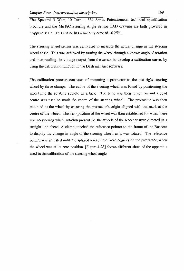
Chapter Four- Instrumentation description 169
The Spectral 3 Watt, 10 Turn - 534 Series Potentiometer technical specification \
brochure and the MoTeC Steering Angle Sensor CAD drawing are both provided in
"Appendix H". This sensor has a linearity error of ±0.25%.
The steering wheel sensor was calibrated to measure the actual change in the steering
wheel angle. This was achieved by turning the wheel through a known angle of rotation
and then reading the voltage output from the sensor to develop a calibration curve, by
using the calibration function in the Dash manager software.
The calibration process consisted of mounting a protractor to the test rig's steering
wheel by three clamps. The centre of the steering wheel was found by positioning the
wheel into the rotating spindle on a lathe. The lathe was then turned on and a dead
centre was used to mark the centre of the steering wheel. The protractor was then
mounted to the wheel by ensuring the protractor's origin aligned with the mark at the
centre of the wheel. The zero position of the wheel was then established for when there
was no steering wheel rotation present i.e. the wheels of the Racecar were directed in a
straight line ahead. A clamp attached the reference pointer to the frame of the Racecar
to display the change in angle of the steering wheel, as it was rotated. The reference
pointer was adjusted until it displayed a reading of zero degrees on the protractor, when
the wheel was at its zero position. [Figure 4-25] shows different shots of the apparatus
used in the calibration of the steering wheel angle.

Chapter Four- Instrumentation description 170
a
b c
Figure 4-25 a) The protractor clamped to the steering wheel at its zero position, b) the
reference pointer at zero degrees and, c) thirty degrees clockwise.
The steering wheel connection to the steering shaft was found to have some movement
and it was determined, from the calibration apparatus configuration, that the steering
wheel had one degree of play. The steering wheel was then turned through increments
of thirty degrees up to one hundred and fifty degrees, in both a clockwise and anti
clockwise direction. Using the calibration function in Dash Manager software the
sensor voltage output was read at each thirty-degree increment rotation of the wheel.
The corresponding actual steering angle position, determined from the pointer position
Chapter Four- Instrumentation description 171
with respect to the protractor, was assigned to the sensor voltage signal for the
development of a calibration curve. [Figure 4-26] below shows the calibration curve for
the steering angle sen or developed in the calibration function in the Dash Manager
software of the ADL.
steeing Wheel Angle Cahbration . "
tjllllle . Me&u1ernent method .
l!i!t!CA0m11aij.paijmCj1ji11r ---- JRoliomc1Jic (SV) 3
y
2.159 2262 2. 0 2.457 2.565 2.ES9 2 774 2.870 2.979 3035 3.1
~
---i··--t----!---i----1----1----t----t---· i -· ···-=--···t····:···-:-···of····i····t·· .. .,. ...
I' t I I I W • t ..... .,,... . . .......... .... .>. ...... J.............. + .................. ...
I I I I I I I t I . . . . . . . . . ................ ... ......... -.......... ...................... .,.. ·-• I I I I I I I I I • f I I • I .................. """".. "-· ................... . I I I I I t I I I
---+---·----1---· ~ --.:----~----1---~----~---
.. ~ .... ; ... : ··+···~····C·-··i···-t···..j. ... I I • I I I l I I
-··t·· : ·-·:---:-··t···:---·:----:····r··----., ...................................................... . . . ' . . . . . . . . . ' ' . . . . Bea;lValue l §1qph Opt>Jm .. boad ...
.=J.gjl!.J .1.12!.1
J OK
Concel
tle~
Figure 4-26 The calibration curve for the steering angle sensor.
4.1.6 Brake Force: Honeywell Eclipse Hydraulic Pressure Sensor - 2000psi
An analog 2000 psi Eclipse OEM pressure transducer was selected to measure the
pressure in both the front and back brake lines of the test rig. The pressure transducer
screws into the brake lines of the automobile and measures the dynarrlic pressure
fluctuations of the brake fluid pressure when brake pressure is applied. The pressure
transducer can be seen in [Figure 4-27] .
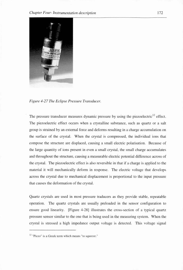
Chapter Four- Instrumentation description 172
Figure 4-27 The Eclipse Pressure Transducer.
The pressure transducer measures dynamic pressure by using the piezoelectric 12 effect.
The piezoelectric effect occurs when a crystalline substance, such as quartz or a salt
group is strained by an external force and deforms resulting in a charge accumulation on
the surface of the crystal. When the crystal is compressed, the individual ions that
compose the structure are displaced, causing a mall electric polarisation. Because of
the large quantity of ions present in even a small crystal, the small charge accumulates
and throughout the structure, causing a measurable electric potential difference across of
the crystal. The piezoelectric effect is also reversible in that if a charge is applied to the
material it will mechanically deform in response. The electric voltage that develops
across the crystal due to mechanical displacement is proportional to the input pressure
that causes the deformation of the crystal.
Quartz crystals are used in most pressure traducers as they provide stable, repeatable
operation. The quartz crystals are usually preloaded in the sensor configuration to
ensure good linearity. [Figure 4-28] illustrates the cross-section of a typical quartz
pressure sensor similar to the one that is being used in the measuring system. When the
crystal is stressed a high impedance output voltage is detected. This voltage signal
12 "Piezo" is a Greek term which means "to squeeze."
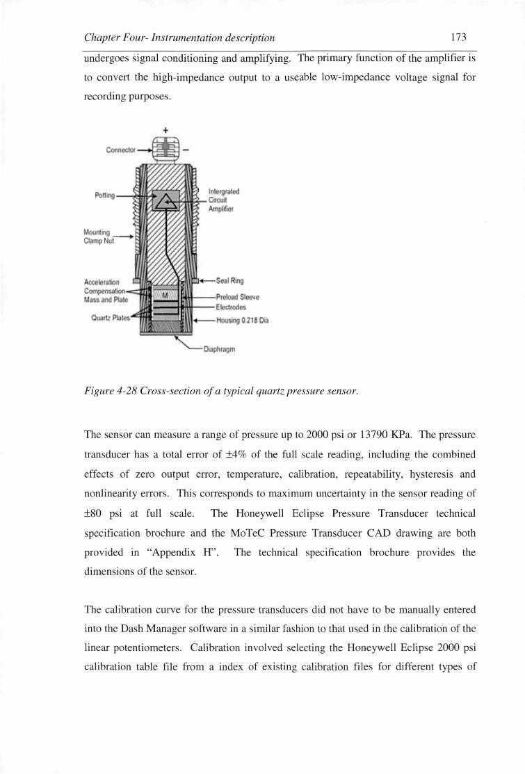
Chapter Four- Instrumentation description 173
undergoes signal conditioning and amplifying. The primary function of the amplifier is
to convert the high-impedance output to a useable low-impedance voltage ignal for
recording purposes.
+
Figure 4-28 Cross-section of a typical quartz pressure sensor.
The sensor can measure a range of pressure up to 2000 psi or 13790 KPa. The pressure
transducer has a total error of ±4% of the full scale reading, including the combined
effects of zero output error, temperature, calibration, repeatability, hysteresis and
nonlinearity errors. Thi s corresponds to maximum uncertainty in the sensor reading of
±80 psi at full scale. The Honeywell Eclipse Pressure Transducer technical
specification brochure and the MoTeC Pressure Transducer CAD drawing are both
provided in "Appendix H". The technical specification brochure provides the
dimensions of the sensor.
The calibration curve for the pres ure transducers did not have to be manually entered
into the Dash Manager software in a similar fashion to that used in the calibration of the
linear potentiometers. Calibration involved selecting the Honeywell Eclipse 2000 psi
calibration table file from a index of existing calibration file for different types of
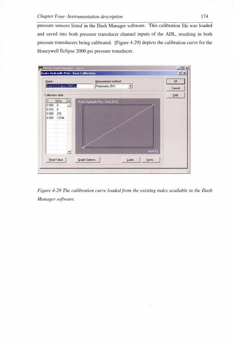
Chapter Four- Instrumentation description 174
pressure sensors listed in the Dash Manager software. This calibration file was loaded
and saved into both pressure transducer channel inputs of the ADL, resulting in both
pressure transducers being calibrated. [Figure 4-29] depicts the calibration curve for the
Honeywell Eclipse 2000 psi pressure transducer.
Brake Hydraulic Pres - Rear Calibration
Name : Measurement method : rr;;limiiiiiiidlliir.i&iiiliiWWW!iliiiiiiiiOiOi.---- I Ratiometric [5V) 3
V kPa 0.500 0 0.570 0 0.580 276 4.500 13794
~
fiead Value I graph Options ... ].oad .. .
DK
Cancel
!!elp
.S.ave ...
Figure 4-29 The calibration curve loadedfrom the existing index available in the Dash
Manager software.

Chapter Four- Instrumentation description 175
4.2 DATA ACQUISITION TYPE INSTRUMENTATION
In this section the various components of the ADL and other items needed for
successful acquisition of all the required data is outlined. Data acquisition type
Instrumentation refers to the actual selected Data Acquisition System and all associated
auxiliary items necessary to connect the automobile sensors and other electrical devices
to the DAS for logging purposes. This instrumentation also facilitates the telemetry
requirement of the measuring system discussed in the next section.
MoTeC was identified as the company that could provide the most suitable data
acquisition instrumentation for automobile testing. The following data acquisiti~n
instrumentation was obtained from MoTeC:
• An Advance Dash Logger
• A basic wiring loom
• A CAN communications cable and telemetry support with remote logging
capabilities.
The components that constitute the data acquisition system will be briefly described in
the following.
4.2.1 MoTeC Advance Dash Logger (ADL-4)
The MoTeC Advanced Dash Logger (ADL-4) is a compact complete data acquisition
system suitable to control the on-board acquisition of data from the automobile sensors ' and the Engine Control Unit (ECU) in the Intelligent Car Project. A picture of the
ADL-4 is provided in [Figure 4-30].

Chapter Four- Instrumentation description 176
Figure 4-30 The MoTeC Advance Dash Logger.
The ADL also serves as the dash display unit for the test rig and has the potential to be
upgraded to 4 Mb of data storage memory capacity. The ADL used in this measuring
system is the basic input output model supporting 10 analog inputs, 8 digital inputs, one
RS232 serial input and 4 auxiliary outputs. The ADL has 1 Mb of memory, which
enables 16 minutes of automobile testing before the ADL data memory bank becomes
full. The advantages of the ADL, compared to other investigated DAS is that it is a
purpose designed automobile testing DAS, with a proven record of operating in similar
automobile dynamic testing conditions 13. The ADL uses a high speed 32 bit
microprocessor to process information.
The ADL consists of two main components. The actual DAS in the form of the dash
display unit and a removable wiring loom that enables data input and output to and from
the ADL. The wiring loom allows sensors and other electrical devices to be connected
to the ADL and also allows for data output from the ADL.
13 The MoTeC ADL is used by a number of Australian V8 Touring Car Teams and many Rally Car
Teams around the globe as a DAS in automobile testing.

Chapter Four- Instrumentation description 177
The ADL display as shown in [Figure 4-30] uses high contrast LCD technology to show
information to the driver of the automobile. The actual display is composed of a 70
segment bar graph, three numeric displays, a centre numeric display and a bottom
alpha/numeric display. The display positions on the ADL face can be set up to show
any information that is sent to the ADL. This includes rpm, gear, engine temperature,
battery voltage etc. The numerical displays all have a different number of display digits
therefore are suited to display different automobile parameters. The configuration of
the display will be discussed in detail in Chapter 6.
4.2.2 Wiring Loom
The ADL uses a 79 pin Auto Sport connector as the wiring loom adaptor. The adaptor
can be twisted to remove it from the back of the ADL, providing easy access to the
wires of the wiring loom. A basic vehicle style-wiring loom was purchased from
MoTeC. The basic wiring loom serves as the interface between the ADL and all
sensors and associated equipment such as the ECU. The sensors purchased from
MoTeC are fully adaptable with this wiring loom.
The ADL comes with Microsoft Windows based software called Dash Manager and
Interpreter. The Dash Manager program is used in the configuration of the sensor and
other instrumentation with the ADL. It is also the means by which logged automobile
data is downloaded from Racecar during testing. The Interpreter software is used to
analyse the logged data from the Racecar. The ADL can collate data on over 200
channels composed of both measured data, in the form of sensor input data to the ADL
and calculated information. The calculated information refers to indirect measurement
of variables that can be quantified mathematically from the direct measurement of other
parameters. This function is being used to calculate the ground speed velocity of the
vehicle and the distance travelled.
There is an inbuilt function in the Dash Manager software that incorporates the use of
two wheel speed sensors in the calculation of ground speed velocity of the Racecar. In
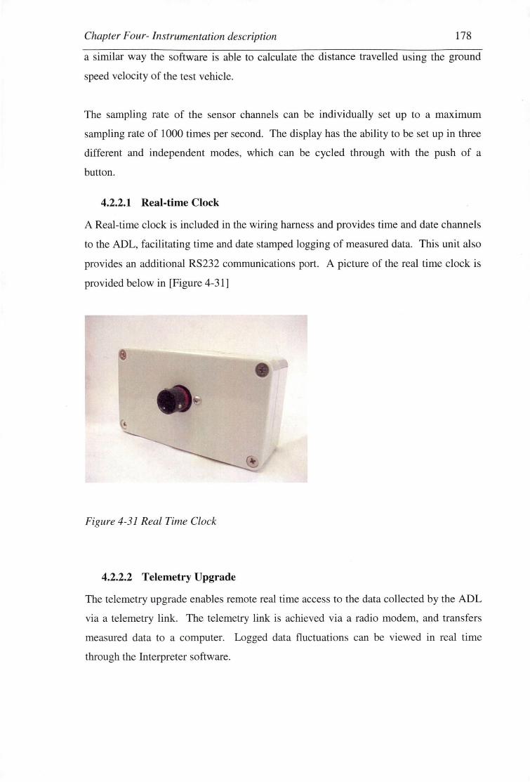
Chapter Four- Instrumentation description 178
a similar way the software is able to calculate the distance travelled using the ground
speed velocity of the test vehicle.
The sampling rate of the sensor channels can be individually set up to a maximum
sampling rate of 1 OOO times per second. The display has the ability to be set up in three
different and independent modes, which can be cycled through with the push of a
button.
4.2.2.1 Real-time Clock
A Real-time clock is included in the wiring harness and provides time and date channels
to the ADL, facilitating time and date stamped logging of measured data. This unit also
provides an additional RS232 communications port. A picture of the real time clock is
provided below in [Figure 4-31]
Figure 4-31 Real Time Clock
4.2.2.2 Telemetry Upgrade
The telemetry upgrade enables remote real time access to the data collected by the ADL
via a telemetry link. The telemetry link is achieved via a radio modem, and transfers
measured data to a computer. Logged data fluctuations can be viewed in real time
through the Interpreter software.
Chapter Four- Instrumentation description 179
4.2.2.3 Remote Logging
Remote logging software is needed as this allows the data received via telemetry to be
stored on the PC for later analysis. The data that is logged by the telemetry equipment
can be independent to the data that is being logged to the ADL. This allows different
parameters to be logged by the ADL and telemetry data storage processes.
ADL Input & Output Requirements and Wiring Diagram
The input output requirements of the ADL unit, the sampling rate of the parameters and
other associated ADL configuration information is provided in "Appendix H". The
wiring diagram of the ADL depicting which sensors are connected to which ADL inputs
and the MoTeC ADL specification brochure are also provided in "Appendix H".
4.2.3 CAN Communication Cable
The CAN communication cable is a high-speed communication cable that enables the
ADL to be connected to the parallel port of a PC. This cable allows the transfer of the
logged data from the ADL to a computer for processing and analysis. The download
speed of logged data from the ADL, using this cable can reach a maximum transfer rate
of 19 seconds per megabyte of data transferred. This cable is addition option to the
basic wiring loom.
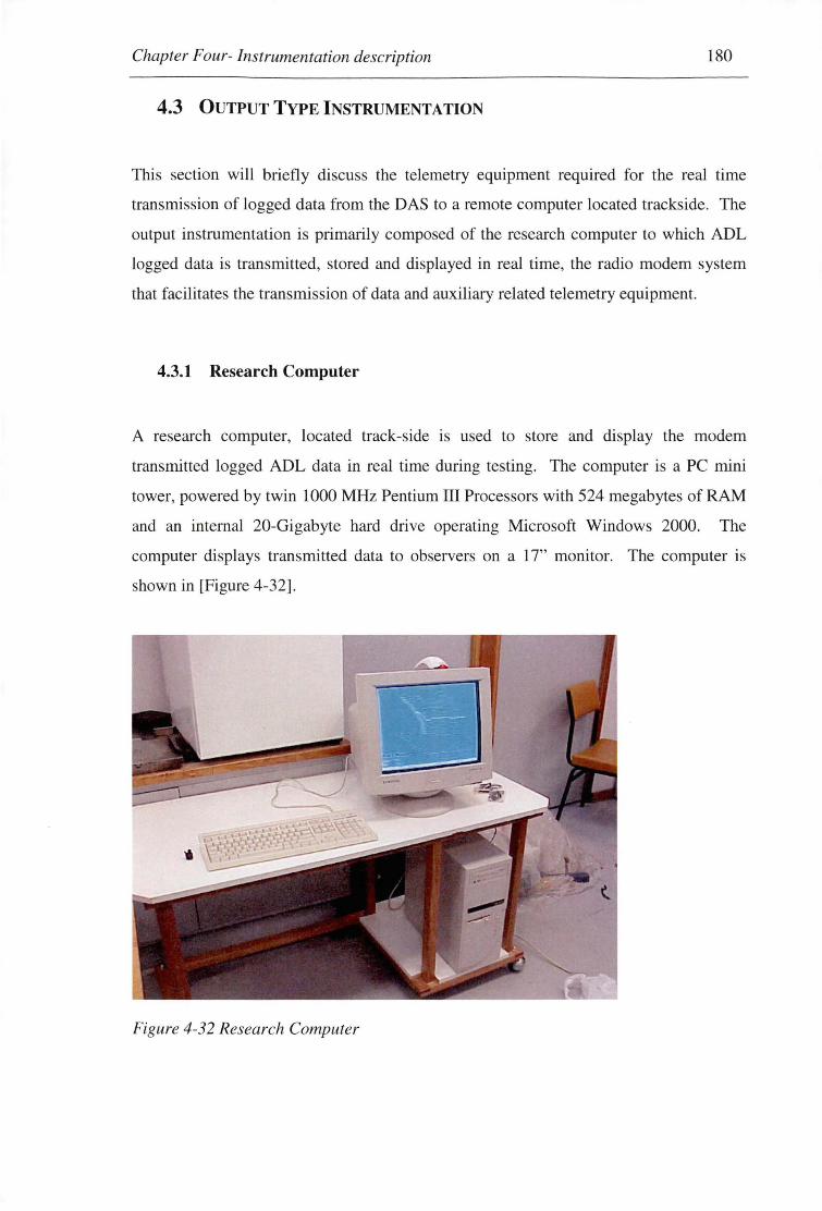
Chapter Four- Instrumentation description 180
4.3 OUTPUT TYPE INSTRUMENTATION
This section will briefly discuss the telemetry equipment required for the real time
transmission of logged data from the DAS to a remote computer located trackside. The
output instrumentation is primarily composed of the research computer to which ADL
logged data is transmitted, stored and displayed in real time, the radio modem system
that facilitates the transmission of data and auxiliary related telemetry equipment.
4.3.1 Research Computer
A research computer, located track-side is used to store and display the modem
transmitted logged ADL data in real time during testing. The computer is a PC mini
tower, powered by twin 1000 MHz Pentium III Processors with 524 megabytes of RAM
and an internal 20-Gigabyte hard drive operating Microsoft Windows 2000. The
computer displays transmitted data to observers on a 17" monitor. The computer is
shown in [Figure 4-32] .
Figure 4-32 Research Computer
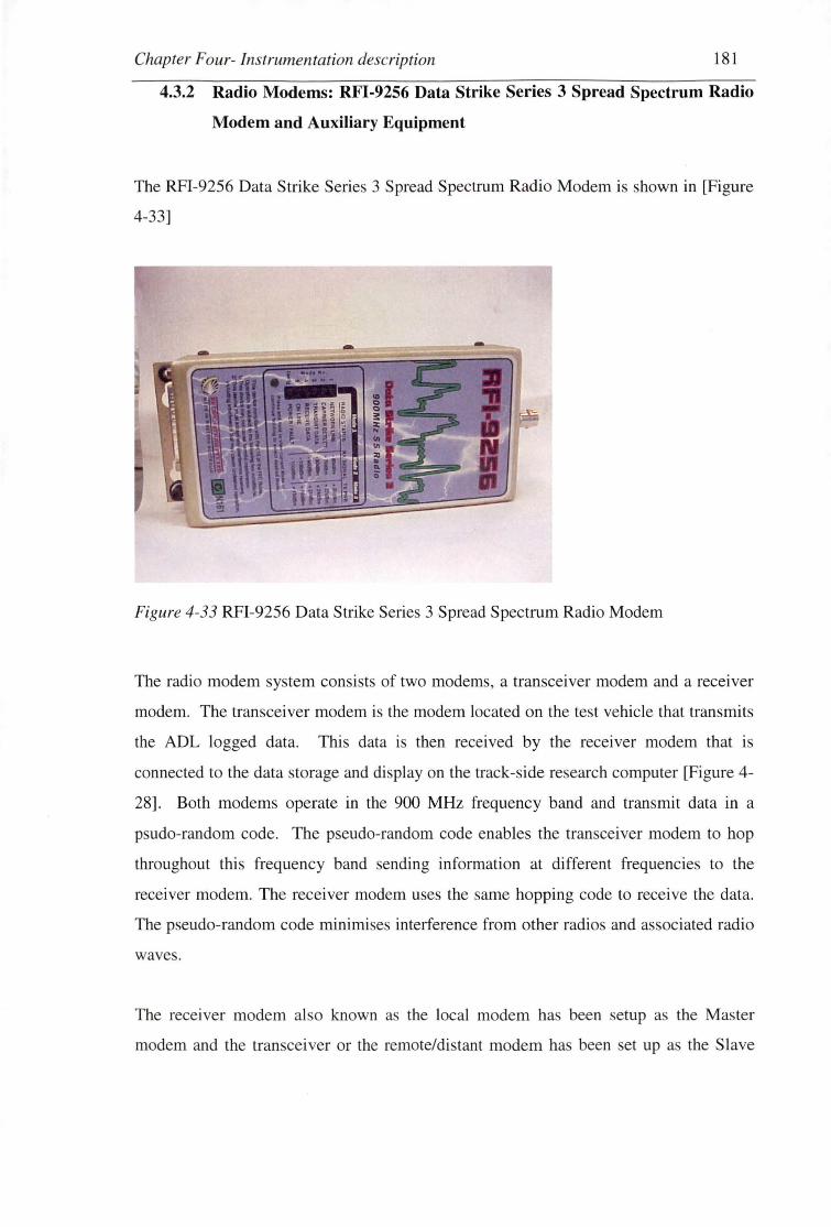
Chapter Four- Instrumentation description 181
4.3.2 Radio Modems: RFI-9256 Data Strike Series 3 Spread Spectrum Radio
Modem and Auxiliary Equipment
The RFI-9256 Data Strike Series 3 Spread Spectrum Radio Modem is shown in [Figure
4-33]
Figure 4-33 RFI-9256 Data Strike Series 3 Spread Spectrum Radio Modem
The radio modem system consists of two modem , a transceiver modem and a receiver
modem. The transceiver modem is the modem located on the test vehicle that transmits
the ADL logged data. This data is then received by the receiver modem that is
connected to the data storage and display on the track-side research computer [Figure 4-
28]. Both modems operate in the 900 MHz frequency band and transmit data in a
psudo-random code. The pseudo-random code enables the transceiver modem to hop
throughout this frequency band sending information at different frequencies to the
receiver modem. The receiver modem uses the ame hopping code to receive the data.
The pseudo-random code minimises interference from other radios and associated radio
waves.
The receiver modem also known as the local modem has been setup as the Master
modem and the transceiver or the remote/distant modem has been set up as the Slave

Chapter Four- Instrumentation description 182
modem. The Master modem is used to synchronise communication, however either
modem and can initiate communication.
The telemetry modems have been linked together in ·a point to point or direct connection
format. Point-to-point communication is similar to a wire that directly connects the
modem devices together for data transfer. Currently data is transferred in one direction
only, from the Racecar to the remote computer. Such data transferral is known as
Simplex communication.
In operation the master modem is connected to the remote computer via Comm Port 2
and also requires an external power supply. The transceiver modem is connected to the
ADL using switch input 4 and an additional Telemetry RS232 output wire that was
acquired through the Telemetry Upgrade from MoTeC. Antennas are connected to both
modems to facilitate data transfer.

Chapter Four- Instrumentation description 183
4.4 THE DEVELOPED MEASURING SYSTEM
The integration of the three different types of instrumentation as described allows for
the development of the test rig's dyriamic measurement system. The integration of the
equipment involves the fusing together of the individual components forming an
instrumentation cluster that allows electrical interaction and communication between
the different components for the successful transmission of measured data to a remote
computer. Combining the instrumentation in order to obtain a reliable measurement
interface involves the physical installation and connection of the components.
The dynamic measurement system can be defined using a block diagram that describes
the function of components in the measuring system. [Figure 4-34] depicts the
measuring system showing the measurand inputs to the DAS and the different forms of
data presentation in block diagram form. [Figure 4-35] shows the measuring system in
a pictorial form, clearly identifying the inputs and outputs of the measuring system.
This chapter has provided a brief description of the operational principals of the
instrumentation that constitutes the measuring system. The next chapter deals with the
results form the physical testing of the vehicle and the use of neural networks as a tool
for predicting dynamic braking pressures in a real world environment.
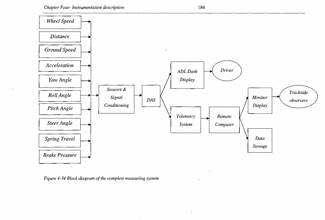
Chapter Four- Instrumentation description 184
Wheel Speed
Distance
Ground Speed
Acceleration ADLDash Driver
Yaw Angle Display
Roll Angle Sensors &
Trackside Signal
DAS Monitor
observers
Pitch Angle Conditioning Display
Telemetry Remote
Steer Angle System Computer
Spring Travel Data
Storage
Brake Pressure
Figure 4-34 Block diagram of the complete measuring system

Chapter Four- Instrumentation description
....... CGnnedor·~ vi.w
L
Sensor
ADL
1 T
Car
Battery
Real Time
Viewing of
ADL logged
Figure 4-35 A diagram illustrating the inputs and outputs of the measuring system
185
RADIO
TRANCE/VER
0
Remote
Computer
MODEM
CAN
cable
T
DATA
RECEIVE
T
Antenna
Data
Transferral
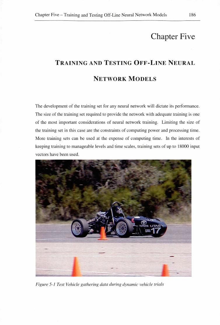
Chapter Five -Training and Testing Off-Line Neural Network Models 186
Chapter Five
TRAINING AND TESTING OFF-LINE NEURAL
NETWORK MODELS
The development of the training set for any neural network will dictate its performance.
The size of the training set required to provide the network with adequate training is one
of the most important considerations of neural network training. Limiting the size of
the training set in this case are the constraints of computing power and processing time.
More training sets can be used at the expense of computing time. In the interests of
keeping training to manageable levels and time scales, training sets of up to 18000 input
vectors have been used.
Figure 5-1 Test Vehicle gathering data during dynamic vehicle trials

Chapter Five - Training and Testing Off-Line Neural Network Models 187
Data measured during dynamic vehicle trials [Figure 5-1] requires sorting into specific
manoeuvres and assembled into training sets capable of providing adequate
representation of all manoeuvre sub groups where there exists a tendency toward
particular trends and patterns. For example, it was found that the brake force pattern
that existed for braking into a tight radius turn was different from braking into a
sweeping comer. In the development of a useful training set it is of great importance to
achieve sufficient representation of all variables in all manoeuvre subgroups.
To accurately estimate and predict the brake forces for a comprehensive range of
braking manoeuvres, the neural network itself must be trained using a statistically
balanced set of input vectors which represent the extent of the predictive capacity
required.
Early testing and recording of data revealed that this statistical variation, especially in
the acceleration data from the test vehicle, is predominantly caused by vibration
(mechanical noise) from the motorcycle power plant. This noise was very prominent in
the data since, as outlined in chapter 3, the motorcycle engine is rigidly connected to the
vehicle frame.
In an attempt to gather data sets with balanced statistical variation and accurate readings
a sampling rate was chosen at 100 Hz for the sensors on the test vehicle. Careful
attention was taken while deciding this rate to avoid resonant and common frequencies
set up in the frame. With several different sampling rates, tests were conducted
throughout the rev range of the motorcycle power plant to locate unacceptable
resonances.
Early tests found that sampling rates significantly higher than the selected lOOHz results
in data sets that are either too large in terms of computational time or too small in terms
of the number of incorporated manoeuvres when used as training inputs to the proposed
neural network models.

Chapter Five - Training and Testing Off-Line Neural Network Models 188
Sampling rates significantly lower than 100 Hz on the other hand, were found to be too
low to accurately follow and represent some of the more rapidly changing parameters
such as the suspension movement.
5.1 STRATEGY FOR PREDICTION
This study is focused around understanding the degree of influence of various process
parameters on predicting brake force and eliminating those that are non-contributing to
develop a reliable neural network based brake force prediction model. The goal of this
study is to have a workable neural network capable of predicting brake force values for
use in the intervention decision making process of driving assistance systems to be later
developed on-line.
As discussed in chapter two, many neural network architecture models are available for
predictive purposes. Out of these, two models were selected for predicting brake forces.
These two models were chosen as the most successful after initial trials with many
different models.
1. Back propagation Neural Network (BP)
2. General Regression Neural Network (GRNN)
Before these networks can be applied, clearly defined training courses must be
identified for generating good training and testing sets. For the purposes of this
research, training sets must be developed that contain sufficient examples of straight
line braking and simultaneous braking and cornering. This lead to the development of
two specific training courses as identified in the following section.

Chapter Five - Training and Testing Off-Line Neural Network Models 189
5.2 TYPES OF TRAINING COURSES
In an effort to achieve reasonable range of braking conditions the following test courses
were laid out [Figure 5-2]:
a) Straight-line acceleration and braking [Figure 5-2, a)]
b) Figure eight with hairpin and sweeper [Figure 5-2, b)]
~ 1 • • • • ......................................................................... ):.
Ji, ~ a
~ ~~---·········~·········-.. ~ ~.... . ........... ............ . ·~···~~.. ~ ..... ~
/r ··········::::··:::::·" ~ j <...,, ........... ............ /~ ················... ~R ./ ~ 1;;;·· .......................... ~
~ b
Figure 5-2 Test courses for neural network training: a) Straight-line acceleration and
braking: course 1. b) Figure eight with hairpin and sweeper: course 2.

Chapter Five -Training and Testing Off-Line Neural Network Models 190
These two test courses [Figure 5-3] and [Figure 5-4] were driven at various speeds close
to the limits of adhesion corresponding to different levels of slip during acceleration,
braking and cornering. This was done in an attempt to gather data sets covering a
reasonable range of tyre slip situations. Training sets were composed of a montage of
these tyre slip levels to include as many varied examples as possible.
Figure 5-3 Course 1: Straight-line acceleration and braking test photographed during
early stages of testing.
Note that the Figure eight [Figure5-2 (b)] and [Figure 5-4] as layed out has a large
radius, R, corner (sweeper) and a tight radius, r, corner (hairpin). The driving approach
and braking for these two types of corner are very different.
In some examples, on the approach to the hairpin, the driver tries to unsettle the test rig
in order to improve turn in and flick the vehicle around the corner. This can be seen in
the data set as a pre-corner steering input or turning of the steering wheel in the opposite
direction to the corner before the corner. This Scandinavian Flick is a manoeuvre
commonly used in racing. In complete contrast, on approach to the sweeper the driver is
smoothly on and off the brakes to avoid upsetting the vehicle's balance.

Chapter Five -Training and Testing Off-Line Neural Network Models 191
Figure 5-4 Course 2: Figure eight test course data generation.
These are two cornering extremes however, since the driver was varying their level of
attack [Figure 5-5] on the test course. The resultant training sets were found to contain
various braking and cornering examples covering the spectrum from below threshold to
complete four wheel locking and sliding.
Figure 5-5 Braking and cornering at different levels of attack producing data sets at
different levels of tyre slip.

Chapter Five -Training and Testing Off-Line Neural Network Models 192
5.3 BACK PROPAGATION NEURAL NETWORK RESULTS
Backpropagation networks are multi layered feed-forward neural networks that have
been trained using an error backpropagation procedure. This is a supervised mode of
learning where a systematic method is used to adjust the weighted connections within
the network.
Various network architectures were trialed in an attempt to find a specific architecture
which best predicted the brake force for the two test courses. To this end, brake
pressures recorded for the Figure eight course (test course 2) data proved more difficult
to predict than the brake pressures for straight line acceleration and braking (test course
1). Inputs to the neural network were chosen as:
1. Yaw Angle 2. Lateral Acceleration 3. Longitudinal Acceleration 4. Distance 5. Steering Wheel Angle 6. Throttle Position 7. Engine RPM 8. Suspension Position:
~ FrontLeft ~ Front Right ~ RearLeft ~ RearRight
9. Wheel Speed: ~ Front Left ~ Front Right ~ RearLeft ~ RearRight
Neural networks were then trained with outputs of front Brake Hydraulic Pressure (BHP
F) and rear Brake Hydraulic Pressure (BHP R).
Combinations of single and double layer backpropagation networks were trialed for
both courses. Many of the single layer backpropagation networks trialed were found to
give good predictions for straight line braking, however the Figure eight test course
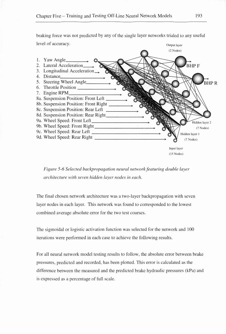
Chapter Five -Training and Testing Off-Line Neural Network Models 193
braking force was not predicted by any of the ingle layer networks trialed to any useful
level of accuracy.
1. Yaw Angle O·...:::----= .. 2. Lateral Acceleration~ 3. Longitudinal Acceleration_ 4. Distance ________ _ 5. Steering Wheel Angle ____ _ 6. Throttle Position ______ _ 7. Engine RPM _ ________ -+
8a. Suspension Position: Front Left ___ _ 8b. Suspension Position: Front Right -----+ 8c. Suspension Position: Rear Left 8d. Suspension Position: Rear Right ______ _ 9a. Wheel Speed: Front Left _________ _ 9b. Wheel Speed: Front Right __________ _
Output layer
(2 Nodes)
(7 odes)
9c. Wheel Speed: Rear Left ---------- --9d. Wheel Speed: Rear Right -------------+ (7 Nodes)
Input layer
( 15 Nodes)
Figure 5-6 Selected backpropagation neural network featuring double layer
architecture with seven hidden layer nodes in each.
The final chosen network architecture was a two-layer backpropagation with seven
layer nodes in each layer. This network was found to corresponded to the lowest
combined average absolute error for the two test courses.
The sigmoidal or logistic activation function was selected for the network and 100
iterations were performed in each case to achieve the following results.
For all neural network model testing results to follow, the absolute error between brake
pressures, predicted and recorded, has been plotted. This error is calculated as the
difference between the measured and the predicted brake hydraulic pressures (kPa) and
is expressed as a percentage of full scale.

Chapter Five - Training and Testing Off-Line Neural Network Models 194
5.3.1 Course 1: Straight Line Acceleration and/Braking - Front Brake Force
Prediction
[Figure 5-7] shows the double layer backpropagation neural network prediction result
from network testing. The network was found to consistently under predict brake line
pressures once a discreet pressure value has been reached. This particular condition was
found to correlate with vehicle dynamics where full wheel lock-up occurred. Full wheel
lockups were found to correspond to peaks 1,2 and 4 of the estimation graph in [Figure
5-6]. This is not a problem with the neural network prediction but is purely related to
the brake hydraulic pressure effect on vehicle dynamics.
Once full wheel lock has occurred the actual value of the hydraulic brake pressure is
arbitrary since increases in brake pressure will not at all effect the vehicle's dynamics.
When the wheels on the test vehicle wheels are fully locked, they have reached a state
where further pressure increase in the brake lines has no effect. Thus the neural
network sees no dynamic change in the behaviour of the vehicle and predicts the
pressures at the constant value where full wheel lockup initially occurs. For this reason
any brake hydraulic pressure information over this full lockup threshold is not useful in
describing any part of the vehicle's dynamics and the neural network should not be
scrutinised for the failure to predict these values.
Therefore, in [Figure 5-7] it is not surprising that the maxim predictive error occurs at
the peak where the brake hydraulic pressure reaches the highest level over and above
the level corresponding to wheel lockup (peak four of the test .data). The peak errors
must be ignored. Far more important features of the straight line prediction are how
closely the neural network estimation follows the measured brake force pressure on the
ramps up to the threshold lockup values and back down to zero pressure. The Absolute
error graph clearly shows that these errors are typically (average) less than 2% and less
than 10% (average) in regions where a typical rate of change of pressure is 4000
kPa/second.
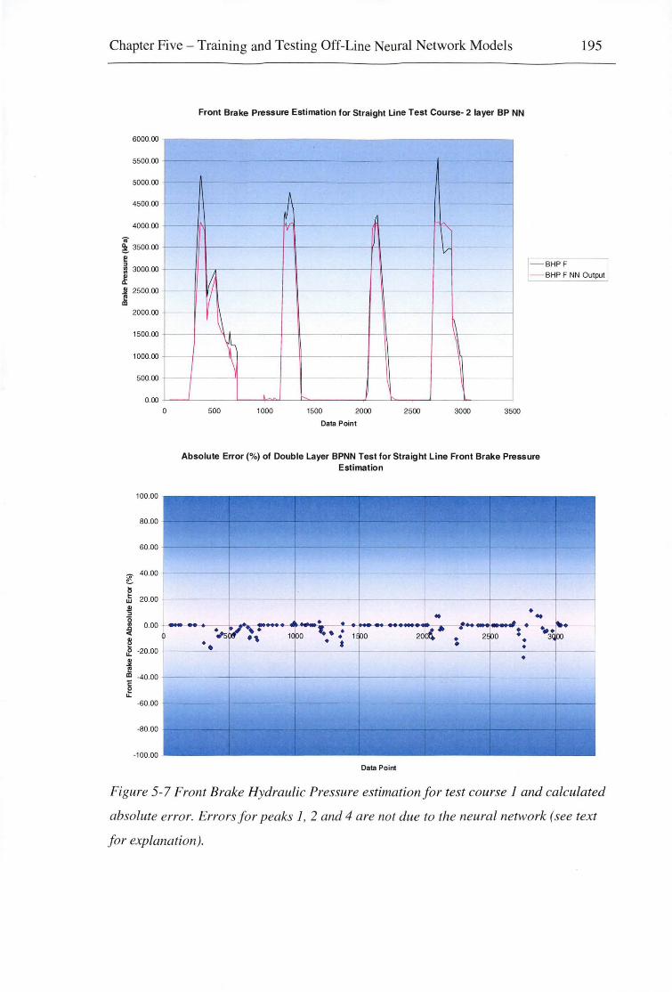
Chapter Five -Training and Testing Off-Line Neural Network Models 195
Front Brake Pressure Estimation for Straight Line Test Course- 2 layer BP NN
6000.00
5500.00 -- -- - - -
5000.00 - - -
-- -- - f- - -L v - '
-
4500.00
4000.00 .. ~ 3500.00 - v -!!! " - BHPF
-:z 3000.00
~ I; - BHP F NN Output
j 2500.00
~ I
2000.00
,\ 1500.00 - --
1000.00
500.00
0.00
0
100.00
80.00
60.00 - -
c 40.00
15 t: 20.00 w s " ~ 0.00 .Q
< ~ if -20.00
"' .., I! Ill E
-40.00
e lL
-60.00
-80.00
-100.00
I
'\
' 500 1000 1500 2000 2500 3000 3500
Data Point
Absolute Error(%) of Double Layer BPNN Test for Straight Line Front Brake Pressure Estimation
---- ------+- -
Data Point
Figure 5-7 Front Brake Hydraulic Pressure estimation for test course 1 and calculated
absolute error. Errors for peaks 1, 2 and 4 are not due to the neural network (see text
for explanation).

Chapter Five - Training and Testing Off-Line Neural Network Models 196
The network here is seen to predict numerically zero brake pressure values to a highly
consistent level and to a greater level of accuracy than the numerical values attained
under braking. Note that the neural network is not directly given any information to
show when the brakes are actually being applied. The network is only given data related
to the dynamic movement of the test rig itself. In this manor the neural network is seen
to be able to differentiate between engine braking, drag forces etc. and braking force
applied through the pressure in the brake lines to an extremely high level of accuracy.
In predicting numerically zero brake pressure values, the network usually has no (0%)
error with only small errors of less than five percent found during transitions between
zero pressure and application of the brake pedal. An example of these errors can be
observed around data point 1000 in [Figure 5-7].
5.3.2 Course 1: Straight Line Acceleration and Braking - Rear Brake Force
Prediction
[Figure 5-8] shows the double layer backpropagation neural network prediction result
for the rear wheel braking under the same test. Similarly to the front brake result, the
network was found to consistently under predict brake line pressures once the complete
wheel lock up·threshold was exceeded. However, the 100% lock up threshold is much
more visually apparent in this result with the broader peaks clearly highlighting the
threshold value determined by the neural network. As before, the predictions are a lot
closer than the quantitative analysis would indicate since beyond 3250 kPa the brake
hydraulic pressure is arbitrary
Again, numerically zero brake pressure information is predicted to a higher level of
accuracy than brake pressures measured under application of the brake pedal. Errors
related to zero pressure in this test are found to be more localised toward the base of
each brake application.
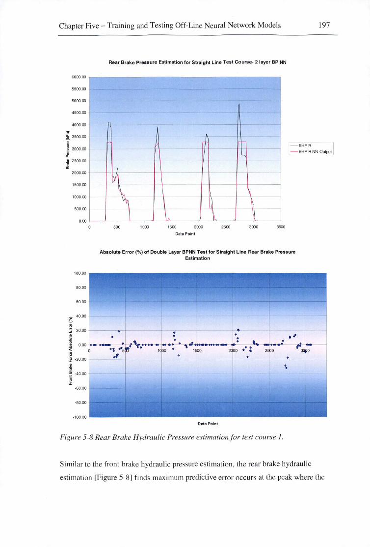
Chapter Five -Training and Testing Off-Line Neural Network Models 197
6000.00
5500.00
5000.00
4500.00
4000.00 ., ! 3500.00
!! :J l:l 3000.00
~ ~ 2500.00
Ji 2000.00
1500.00
1000.00
500.00
0.00
100.00
80.00
60.00
l 40.00
15 t: 20.00 w s :J 0 "' 0.00 .c <(
1l & -20.00
~ e <D -40.00 c: e LL
-60.00
-80 .00
-100.00
Rear Brake Pressure Estimation for Straight Line Test Course- 2 layer BP NN
--- --
-
- - - -- -
• -,_ J_ ~
- BHPA
._ - BHP ANN Output
~ -
+--~
\ ' ~ I
~ u - --
~ 0
'" l 500 1000 1500 2000 2500 3000 3500
Data Point
Absolute Error(%) of Double Layer BPNN Test for Straight Line Rear Brake Pressure Estimation
~ •• --I-----+-------+--- _±_ +-!----- ---l------1
• ~ ·: • • •, I • -i.··----"+-c1-·~··--- ...... ~~----.. ··---.... ·--.-. ~--·-·~j------1
1 OOO • 1500 2doo • • 2500 0
• •
-+--
• • •
~----
l-
~~~,~~~ -:--. lf'"lt,i: 't:"f; ;./>~: "'- k•~. ~I ,~,~J;~•';.I. ,r,~,., •• I {•~--=~,'r~·~·~,:::-: ," J • ,' • \ ' 'r '"'~,' •. •. 1 1· .. ~'t.'( ~
. ' .
Data Point
Figure 5-8 Rear Brake Hydraulic Pressure estimation for test course 1.
Similar to the front brake hydraulic pressure estimation, the rear brake hydraulic
estimation [Figure 5-8] finds maximum predictive error occurs at the peak where the
Chapter Five -Training and Testing Off-Line Neural Network Models 198
rear brake hydraulic pressure is at the maximum level over this wheel lockup threshold.
For reasons discussed, this type of error is to be ignored. The remainder of the absolute
error is on average less than 4%.
The result from rear hydraulic brake pressure estimation is noted to be slightly less
accurate than the front hydraulic brake pressure estimation. This was found consistently
throughout the different courses and models with the rear brake pressure estimation
typically giving higher errors than the corresponding front values.
One possible explanation for this is related to the level of loading of the rear wheels
during braking manoeuvres. As the rear tyres are unloaded, the level of instability
related to tyre flexing increases. Tyre flex rate is progressive with very little force
required to initially cause distortion of the tyre and progressively more force required as
the tyre is loaded. Thus a lightly loaded tyre will move around and change shape due to
surface irregularities, driver inputs and other disruptive external variables more readily
than a heavily loaded tyre. This effectively produces less consistent braking on the rear
wheels of the test rig and is evident when comparing the front [Figure 5-7] and rear
[Figure 5-8] measured brake hydraulic pressure plots.
5.3.3 Course 2: Figure Eight - Front Brake Force Prediction
Wheel locking is not as prevalent in the Figure eight data sets and predictions, [Figure
5-9] and [Figure 5-10]. This is due to the nature of the course, where excessive wheel
locking would result in a lack of directional control and failure of the test rig to follow
the course layout. This is reflected in the results from the neural network testing
[Figure 5-9] where the 100% lock up threshold is only realised in the third peak of the
Figure. At this peak the driver's level of attack is at its maximum and the brakes are
held into the hairpin turn at peak values for the longest amount of time causing locking
of the front wheels which can be seen clearly in [Figure 5-9].
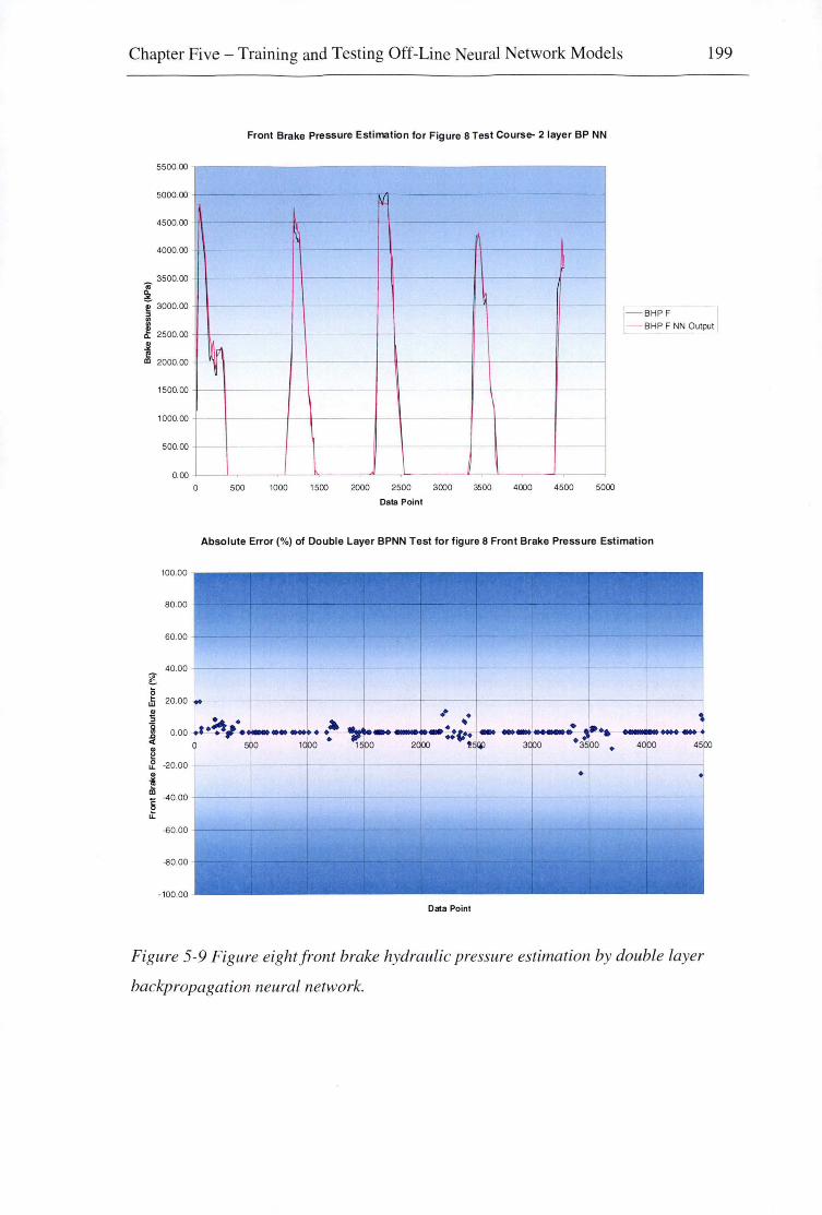
Chapter Five - Training and Testing Off-Line Neural Network Models
5500.00
5000.00
4500.00
4000.00
3500.00 -m ~
-
Front Brake Pressure Estimation for Figure 8 Test Course- 2 layer BP NN
ti -- -
~ f.-- --- -
- -
-
-
199
-e 3000.00 ii: £ 2500.00
~
1-BHPF -i - BHP F NN Output
I!! "' 2000.00
~p ~
1500.00
1000.00 f-----
500.00
0.00
0 500 1000 1500 2000 2500
Data Point
I
3000
-
-
3500 4000 4500 5000
Absolute Error(%) of Double Layer BPNN Test for figure 8 Front Brake Pressure Estimation
100.00
80.00
60.00
40.00
0 .5 20.00
~
" ~ .c <(
~
0.00
--- -
'--- -
~·~i·---r 1000 0 0
--
•• • a. - ~
...... '"'r .. ::tt· • •1 1500 2000
~ -20.00 +------+-----+------!------+----
.; iii 8 -40.00
u: -60.00
-80.00
-100.00
Data Point
--
-µ ~._ •• I ._._..._.
• 3500 • 4000 45100
• j
3000
Figure 5-9 Figure eight front brake hydraulic pressure estimation by double layer
backpropagation neural network.

Chapter Five-Training and Testing Off-Line Neural Network Models 200
Results from testing the front brake pressure prediction by the two layer BP NN model
[Figure 5-9] show that from a purely predictive point of view these brake force
predictions are the closest to the measured values of all models and test courses, with an
average error of less than 2%. This prediction has the least absolute error fC?r testing,
which can be observed in the accompanying error plot.
The Figure eight test course (test course 2) brake hydraulic pressures are consistently
more readily predicted since the information such as lateral acceleration and steering
wheel angle are likely to have a greater influence on the brake pressure.
5.3.4 Course 2: Figure Eight - Rear Brake Force Prediction
[Figure 5-10] shows the double layer backpropagation neural network prediction result
for the rear wheel braking under the same Figure eight test course. Here it can be seen
that the result, rear hydraulic brake pressure estimation, for this test course is
significantly less accurate than the front hydraulic brake pressure estimation [Figure 5-
9].
Here the neural network is seen to slightly under-predict the brake pressure where the
pressures are increasing on peaks 1 and 5, while over predicting brake pressure values
on peaks 2, 3 and 4. However there is still very little bias on the prediction.
It is shown in [Figure 5-10] that predictions for rear brake pressure during cornering
manoeuvres are the most challenging for the neural network, owing to the complex
wheel weight transference and tyre distortion occurring during such a test. However the
neural network is still very accurate in predicting brake values and is seen to be
particularly accurate in predicting occurrences when the brake pressure is numerically
zero.

Chapter Five -Training and Testing Off-Line Neural Network Models 201
., ~
4000.00
3500.00
3000.00
'i 2500.00
~ Q: 2000.00
1500.00 -~-
Rear Brake Pressure Estimation for Figure 8 Test Course- 2 layer BP NN
- ---
- BHPR --i - BHP R NN Output
-
1000.00 ---
~ !5 .!i "' 5 Si .Q <(
"' ~ 0 LL
" : ~ it
500.00 -
100.00
80.00
60.00
40.00
20.00
0.00
-20.00
40.00
.£0.00
-80.00
0 500 1000 1500 2000 2500
Data Point
3000 3500 4000 4500 5000
Absolute Error(%) of Double Layer BPNN Test for Figure 8 Rear Brake Pressure Estimation
+. . .. t : ..... · : .. .:. ..
.$~.: ~ ..... -·~ f!I• •• II I ----·.. --11111 -~·· _. ___ l ,. .. r T , ~ T T ·T ~h- ;i; ... ~
--+-
Data Point
Figure 5-10 Figure eight rear brake hydraulic pressure estimation by double layer
backpropagation neural network

Chapter Five-Training and Testing Off-Line Neural Network Models 202
5.4 GENERAL REGRESSION NEURAL NETWORK RESULTS
The results for brake hydraulic pressure predictions by the General Regression Neural
Network (GRNN) architecture can be seen in "Appendix A". At first glance it is
apparent that the estimations by the GRNN are not nearly as accurate as those by the
Back Propagation Neural Network (BP NN).
The GRNN architecture was trialed in brake force prediction due to the vast reductions
in computational time required by the architecture over the much more accurate BP NN
to predict brake pressure values. Unfortunately the results show that the difference in
performance between the networks far outweighs the computational advantages of
GRNN architecture.
The straight line (test course 1) predictions of the GRNN have greater associated error
than the Figure eight (test course 2) predictions, particularly when the numerical value
of the brake hydraulic pressure is zero. This gives the impression that this network
architecture has difficulty in differentiating between engine braking, drag forces etc. and
the braking force applied though the brake lines.
5.5 CONCLUDING REMARKS
The predictive capabilities of the Back Propagation Neural Network (BP NN) trialed
here far exceeded all expectations relating to accuracy and performance given that the
selection was based on trials of only a small number of architectures. The selection of
the optimum two layer BP NN has not been carried out and the model chosen here has
not been fine tuned. With this in mind, the results from the predictions demonstrate the
massive potential of neural networks as predictive tools for dynamic automobile
performance.
The predictions shown in this chapter have no notable bias. That is that the network is
found to over-predict and under-predict the measured brake force values to the same

Chapter Five - Training and Testing Off-Line Neural Network Models 203
level. This demonstrates the adaptability of neural network processing and indicates
that the networks have received statistically balanced input vectors. However to create
a neural network capable of predicting brake forces under all conditions and for all
manoeuvres the training data would need to be very large and would require excessive
computing power.
Once training has been carried out and network weights have been established the
predictive calculations can be made in feasible timeframes by commercially available
computers. The incorporation of such a computer into the on board electrical system in
the test rig represents the next step in using neural networks to predict brake forces.

Chapter Six - Final Conclusions and Proposed Future work 204
CHAPTER SIX
FINAL CONCLUDING REMARKS AND
PROPOSED FUTURE WORK
The extensive literature review highlighted the need for accurate dynamic brake
pressure in any sophisticated electronic driving assistance system. However, the extent
to which modem automobiles use brake force measurements for electronic brake force
distribution to avoid accidents and overturning is limited form both sensory and
adaptability points of view. In this way current state of the art automotive systems are
reactive to emergency braking situations and systems use robust controllers to alter
brake pressures only once the vehicle is deemed to be 'out of control'. As the future of
brake force control, this work highlights the requirement for accurate quantitative brake
force predictions to determine, in advance, when and how the vehicle will become out
of control given the current course of actions.
Thus development in future electronic brake force controllers will focus around the
ability to predict dynamic performance and make pre-emptive changes to the car
dynamics to avoid instability all together while capable of maintaining threshold
braking much closer to optimum than current, conventional, robust, approaches allow.
While many manufacturers are constantly addressing their conventional control
systems, emerging technologies such as neural networks and fuzzy logic are replacing
conventional systems in increasingly complex non-linear dynamic applications.
Neural network modelling has already proved itself as an accurate and useful
performance estimation tool in manufacturing applications. This report shows, from the
artificial neural network results in this preliminary investigation, the possible
applications of ANN's in dynamic vehicle parameter prediction with the aim of
Chapter Six -Final Conclusions and Proposed Future work 205
providing an effective electronic brake force controller. The results from this
preliminary investigation far exceeded expectations with typical (average) accuracy of
less than 3% full scale absolute error when using the back propagation model, which
could be further improved upon in future development. That said, the results from this
preliminary investigation stand by themselves as predictive tool that could be integrated
almost immediately with current brake force controllers to further improve and develop
current accuracy and performance.
In this work an extensive research is carried out in the design and development of an
open wheel prototype test vehicle. The use of Finite Element Modelling (FEM) and full
3-D CAD modelling in the design are some of the techniques that made possible the
transition from project conception to full size fully operational prototype in the space of
six months. Extensive testing of the vehicle has proved the design with the prototype
having covered over 1600 racing kilometres without the need to alter or redesign any
major components.
Technical aspects covered were the intricate positioning of sensors and allowance in the
overall prototype design to cater for such a position. Some of the more innovative
components of the chassis which have been used to save weight such as the composite
drivetrain and aluminium brake rotors have proven to be very effective from a testing
point of view, pushing the engineering envelope in this innovative prototype. This is a
reflection of the way the dimensional details of each part together with their function
and relation to other components were meticulously documented. The design must of
other systems such as the electrical circuitry, telemetry for data acquisition, and MoTeC
engine management system were coordinated with other research members of the
Intelligent car team.
As part of experimental investigation two testing courses, straight line and Figure eight,
were identified for testing purposes. During this testing many parameters were
measured along with the independent front and rear brake hydraulic pressures. The
level of care directed toward the measuring system featuring telemetry and data
acquisition has resulted in reliable, accurate, quantitative measurements. It is the
- I
Chapter Six - Final Conclusions and Proposed Future work 206
reliability of this data that resulted in the low error neural network modelling and testing
that followed. While the results from the neural networks are encouraging, there is room
for improvement to optimise the networks for input selection accuracy, minimuin
training times and converging rates.
Suggested improvements are in the selection and refinements of sampling rates and
input parameters to enable the compression of the most relevant data into the smallest
usefu~ data sets. This would enable the networks to train themselves more efficiently,
and over a wider range of driving conditions than was possible within the scope of this
work. Refinement in the selection of network architecture is another area were
networks could be further optimised.
It has been shown in these results that the choice of network type and structure can have
a large effect. Therefore future work will involve conducting the testing for a number
of additional ANN models, as well as optimising each by experimentation with different
network configurations and characteristics. This would include trials in properties such
as the number of nodes and their arrangement, trying different training and converging
parameters, altering the number of iterations to convergence and investigating the
effects of different transfer functions. Investigations of this nature have shown to
produce significant improvements in the ANN accuracy far beyond what has been
covered in this work.
In addition to improving the accuracy of the network, further work will need to be
conducted in development of ANN brake force prediction hardware and the interface to
existing electronic brake force control systems. The aim here is to provide a pro-active
brake force controller that reliably and consistently allows for optimum braking
performance under all conditions and surfaces encountered by an automobile.
References 207
REFERENCES
[1] H. Bauer, "ESP - Electronic Stability Program", Robert Bosch GmbH, 1999
[2] BMW World Technology, http://www/bmwworld.com/technology/dsc.htm
[3] A Van Zanten, R Erhardt, K landesfeind and G Pfaff, "VDC Systems
Development and Perspective", Robert Bosch GmbH, Society of Automotive
Engineers, 1998.
[4] R. P. Lippman, "An Introduction to Computing with Neural Nets", IEEE ASSP
Mag. , April 24, 1987.
[5] H. Bauer, "Driving Safety Systems", Robert Bosch GmbH, 1999
[6] B. Heremans "Car Handling" http://www.gallery.uunet.be.heremanss.htm
[7] W. Henke, "Vehicle Dynamics Control - Form ABS to ESP",
http://www.whnet.com/4x4/abs.html
[8] Zhejun Fan, Yoram Koren and David Wehe, "Practical Rule-Based Vehicle
Traction Control", Society of Automotive Engineers ref no. 942402.
[9] D.R. McLellan, J.P. Ryan, E. S. Browalski, J. W. Heinricy, "Increasing the
Safe Driving Envelope - ABS , Traction Control and Beyond", General Motors
Corp., Society of Automotive Engineers, 1992.
[10] C. Campbell, "Design of Racing Sports Cars", 151 edition, Chapman & Hall,
1973
References 208
[11] Alfred Sigl, Herbert Demel, "ABS-Traction Control, State of the Art and Some
Prospects", Society of Automotive Engineers ref no. 900204.
[12] R. K. Jurgen, "Electronic Braking, Traction and Stability Control", Society of
Automotive Engineers, 1999
[13] J. Mack, "ABS -TCS - VDC: Where Will Technology Lead Us", Society of
Automotive Engineers, 1996
[14] R.K. Jurgen, "Automotive Electronics Handbook", 2nd edition, Society of
Automotive Engineers, 1999
[15] Reinhard Auffhammer, Reent Heyken, Harald Roth, "New Driving Stability
Control System with Reduced Technical Effort for Compact and Medium Class
Passenger Cars", BMW AG, Society of Automotive Engineers, 1998.
[16] Ross Bannatyre, "Future Developments in Electronically Controlled Braking
Systems", Transportation Systems Group, Motorola Inc, Society of Automotive
Engineers, 1999.
[17] Chris M Atkinson "Neural Network Engine Control", Society of Automotive
Engineers, 1996.
[18] R. Hecht-Nielsen, "Neurocomputing", Addison-Wesley Publishing Company,
1990.
[19] J.A. Freeman and D.M.Skapura "Neural Networks: Algorithms, Applications
and Programming Techniques", Addison-Wesley Publishing Company Inc.,
1992.

References 209
[20] M. Chow, R.N. Sharpe, J.C. Hung, "On the Application and Design of Artificial
Neural Networks For Motor Fault Detection -Part 1, IEEE Transactions of
Industrial Electronics Vol. 40, No.2 1993. ppl81-188.
[21] L.P. Veelenturf, "Analysis and Applications of Artificial Neural Networks",
Prentice Hall International (UK) Ltd., 1995.
[22] R. Rojas "Neural Networks: A Systematic Introduction", Springer-Verlag, New
York, 1996.
[23] J.E. Dayhoff, "Neural Network Architectures -An Introduction", Van Nostrand
Reinhold, 1990.
[24] M. P. Taylor, W. D. Zhang, V. Willis, S. Schmid, "A Dynamic Model for the
Energy Balance of an Electrolysis Cell" Trans. Institute of Chemical Engineers,
Vol 74, pt.A, Nov. 1996 pp 913-933.
[25] F. Frost "Neural Network Applications to Aluminium Manufacturing", School
of Science and Engineering, University of Tasmania, 2000.
[26] N. Urata, "Magnetics and Metal Pad Instability", Proc. l 141h TMS Annual
Meeting, Atlanta Georgia, Mar 1985, pp. 581-591.
[27] J.M. Zuranda, "Introduction to Artificial Neural Networks", West Publishing
Co., St Paul, 1999.
[28] F. Frost, V. Karri, "Identifying Significant Parameters for Hall-Heroult Process
Modelling using General Regression Neural Network" Proc. 13th International
Conference on Industrial and Engineering Applications of Artificial
Intelligence, New Orleans, USA, Jun. 2000 pp. 73-78.
References 210
[29] F. Frost, V. Karri, "Combined Kohnen and RBF Networks to Predict Electrolyte
Additives in Hall-Heroult Cell" Proc. International Conference on Advances in
Intelligent Systems: Theory and Applications, Canberra, Australia, Feb. 2000
pp. 19-24.
[30] F. Frost, V. Karri, "Intelligent Control of Aluminium Reduction Cells Using
Backpropagation Neural Networks" Proc. International Conference on Advances
in Intelligent Systems: Theory and Applications, Canberra, Australia, Feb. 2000
pp. 350-356.
[31] Formula SAE Rules 2001, SAE International, 2000
[32] K. Singh, "Automobile engineering Vol. 1", 8th edition, A. K. Jain, 2000.
[33] K. Singh, "Automobile engineering Vol. 2", 8th edition, A. K. Jain, 2000
[34] Strand 7 Finite Element Analysis System, G+D Computing, 1999.
[35] CADKEY 98 Release 1 Baystate Technologies, Inc., USA, 1998.
[36] D. Butler, V Karri, "Design Analysis Between On and Off-Centre Bearing for
Racecar Wheel Using Finite Element Method", University of Tasmania, 2001.
[37] Design of Rolling Bearing Mountings Catalogue WL 00 20015 EA, FAG OEM
und Handel AG, 1998.
[38] Technical Information Catalogue WL 43 1190 EA, FAG OEM und Handel AG,
1997.
[39] J. Brandlein, P. Eschmann, L. Hasbargen and K. Weigand, "Ball and Roller
Bearings: Theory, Design and Application", 3rd edition, Wiley.

References 211
[40] K. Jayakumar, K.V.Rajaram and M.A. Faruqi "Machine Intelligence for Crisis
Handling in Navigation Vehicles Using Neuro Controllers", 6 th International
Conference on Neural Information Processing, Institute of Electrical and
Electronics Engineers
[41) E. Gohring, "Electronic Traction Control System ASR and its Integration in the
Anti-Lock Braking Systems ABS to Form a Safety System 'ABS/ASR' for
Commercial Vehicles",", Society of Automotive Engineers ref no. 881137.
[42) James Walker "Chassis controls and their considerations", www.teamscR.com,
SCR Motorsports, 2001
[43) H. Heisler, "Advanced Vehicle Technology", 1st edition, Edward Arnold, 1989
[44) M. Platt, "Elements of Automobile Engineering", 2nd edition, Sir Isaac Pitman
and Sons, 1959
[ 45) T. P. Newcomb, R. T. Spurr, "A Technical History of the Motor Car" 1 st edition,
IOP Publishing, 1989
[46) J . E. Duffy, M. T. Stockel, M. W. Stockel, "Automotive Mechanics
Fundamentals", 1 st edition, Gregory' s Scientific Publications, 1985
[47) L. Terry, A. Baker, "Racing Car Design and Development", 1s1 edition, Robert
Bentley, 1973
[ 48] David Hodges, "A-Z of Formula Racing Cars 1945-1990", 1 st edition, Bay View
Books, 1990
[49) R. L. Norton, "Design of Machinery", 2nct edition mechanical engineering series,
McGraw-Hill, 1999
References 212
[50] Fag Rolling Bearings Catalogue WL 41 520/2 EA, FAG OEM und Handel AG,
1998.
[51] M. Costin, D. Phipps "Racing and Sports Car Chassis Design", 2°d edition, B.
T. Batsford, 1966.
[52] C. P. Nakra, "Basic Automobile Engineering", 81h edition, Dhanpat Rai
Publishing, 1999.
[53] V. V. Vantsevich, M. S. Vysotski, S. V. Kharitont, "Control of wheel
dynamics", International Congress and Exposition, Society of Automotive
Engineers, 1998.
[54] K. C. Check, F. B. Hoogterp, W. K. Fales"Fuzzy Logic Approach to Traction
Control Design", Society of Automotive Engineers ref no.942402, 1998.
[55] K. Lyon, M. Phlipp and E. Grammes, "Traction Control for a Formula 1
Racecar: Conceptual Design, Algorithm Development and Calibration
Methology", Robert Bosch GmbH, Society of Automotive Engineers, 1994.
[56] S. K. Mohan, R. C. Williams, "A Survey of 4WD Traction Control Systems and
Strategies" New Venture Gear, Society of Automotive Engineers, 1995.
[57] A. T. Van Zanten, R. Erhardt, G. Pfaff, "VDC, The Vehicle Dynamics Control
System of Bosch" Robert Bosch GmbH, Society of Automotive Engineers,
1995.
[58] A. T. Van Zanten, R. Erhardt, A. Lutz, W. Neuwald, H. Bartels "Simulation for
the development of the Bosch-VDC" Robert Bosch GmbH, Society of
Automotive Engineers, 1996.
References 213
[59] A. Strickland, K. Dagg, "ABS Braking Performance and Steering Input", Royal
Canadian Mounted Police, Society of Automotive Engineers, 1998.
[60] H. Saito, N. Sasaki, T. Nakamura, M. Kume, H. Takinata, M. Nishikawa,
"Acceleration Sensor for ABS", Sumitomo Electric Industries, Society of
Automotive Engineers, 1992.
[61] D. E. Schenk, R. L. Wells, J.E. Miller, "Intelligent Braking for Current and
Future Vehicles" Delco Chassis, Society of Automotive Engineers, 1995.
[62] G. Mauer, G. Gissinger and Y. Chamaillard, "Fuzzy Logic Continuous and
Quantising control of an ABS Braking System", University of Nevada, Society
of Automotive Engineers, 1994.
[63] L. Evans, "ABS and Relative Crash Risk Under Different Roadway Weather,
and Other Conditions", General Motors Corp, Society of Automotive Engineers,
1995.
[64] T. Bach, H. Schmitt, W. Schwanke, H.J. Tumbrink, '"Roadrunner'- Real Time
Simulation in Anti-Lock Brake System Development" Lucas Braking Systems,
Society of Automotive Engineers, 1995.
[65] M. J. Scheider, "Use of a Hazard and Operability Study for Evaluation of ABS
Control Logic", Ford Motor Company, Society of Automotive Engineers, 1997.
[66] W. Maisch, W. Jonner, R. Mergenthaler, A. Sigl, "ABS5 and ASR5: The New
ABS/ ASR Family to Optimise Direction Stability and Traction" Robert Bosch
GmbH, Society of Automotive Engineers, 1993.
References 214
[67] Thomas G. Beckwith, Roy D. Marangoni, John H. Lienhard V, Mechanical
Measurements, Fifth Edition, Addison-Wesley Publishing Company Inc, 1995, p
4
[68] Ryoji Ohba, F.R.D. Apps, Intelligent Sensor Technology, John Wiley & Sons )
Ltd, 1992 pp.1, 2, 13
[69] H.H. Braess, "Electronics-The Co-Evolution of Intelligence in Automobiles and
Road Traffic", in Proceedings of the 1987 International Conference on
Automotive Electronics 1987, pp. 1-6.
[70] Ross Bannatyne, The Sensor Explosion and Automotive Control Systems
http://sensormag.com/articles/0500/92/main.shtml
[71] Nd Mathews, PE An, M Roberts, CJ Hariss, "A neaurofuzzy approach to future
driver support systems", in Proceedings of the Institute of Mechanicla
Enginneers, London 1998
[72] M. Murayama, "The Situation of Automobile Electronics in Japan", in
Proceedings of the 1987 International Conference on Automotive Electronics .
1987, pp. 7-9.
[73] Introduction to Sensor Fusion
http://lca.kaist.ac.kr/Researches/2000/sensorfusion.html
[74] Delphi Homepage/Products/Intellek Smart Sensors
http:/1164.109.59.132/products/nextech/products/intellek
[75] Dale J. Long, Sensors, An Integral Part of Today's Automobile, Department of
engineering Technology New Mexico State University, 1999
References 215
[76] Peelamedu, S., Naganathan, G. , and Buckley, S. , 1999, "Impact Analysis of
Automotive Structures with Distributed Smart Material Systems", SPIE
Proceedings, Vol. 3667, pp 813-824.
[77] Peelamedu, S. , Naganathan, G, 1999, "Smart automobiles through Smart
Sensors"
[78] Stability Control: Get your Yaws Out
http://www.edmunds.com/oner hip/safety/articles/45992/article.html.
[79] Traction Control
http://www.edmu nds .corn/ onershi p/safety/ articles/ 463 52/ article.html
[80] Ralf Klein, "Antilock-Braking System and Vehicle Speed Estimation using
Fuzzy Logic Fuzzy", in Proceedings of the 1996 Embedding Computer
Conference, 1987
(Http://www.fuzzytech.com/e/e a sie.html)
Appendix A 216
8 APPENDIX A -GENERAL REGRESSION NEURAL
NETWORK RESULTS
A-1: GRNN front brake pressure prediction for Course 1 (straight line) ........................................... 217
A-2: GRNN rear brake pressure prediction for Course 1 (straight line) ............................................. 218
A-3: GRNN front brake pressure prediction for Course 2 (Figure eight) ........................................... 219
A-4: GRNN rear brake pressure prediction for Course 2 (Figure eight) ............................................ 220

Appendix A 217
A-1
Front Brake Pressure Estimation for Straight Line Test Course- GANN
5500.00
5000.00 -
4500.00
4000.00
Ii ~ 3500.00
I!! iil 3000.00
£ ~ 2500.00 e a:i
2000.00
1500.00
1000.00
500.00
0.00
0 500
1
- BHPF
- BHP F NN Output
1000 1500 2000 2500 3000 3500
Data Point
Absolute Error(%) of GANN Estimation for Straight Line Front Brake Pressure Estimation
100.00
80.00
60.00
40.00
0 .ii 20.00
+ t- • • .._ ..... t.
Jt.... .. .,, • o.oo I -·- -•-'"-1.~ .. ----;---
0 • 500 ~· 1000 ~ if -20.00
i a; 6 -40.00
u: -60 .00
-80.00
-100.00
-+- +-
• .... --.- . - -+------+-... ,,. _. _, .. ~
.,.. •• • r -• .• ---+--- -----j-----·'-- .._.
2000 • .:- 2500 • Jooo ~ ._,: ,. 1500
Data Point
•
• •
·~."---+-----!

Appendix A 218
A-2
Rear Brake Pressure Estimation for Straight Line Test Course- GANN
6000.00
5500.00
5000.00
4500.00
4000.00 ,.. :g_ 3500.00
!!! ::J
"' 3000.00 "' £
- BHPR I - BHP ANN Output
" 2500.00 .x e Ill
2000.00
1500.00
1000.00
500.00
0.00
0 500 1000 1500 2000 2500 3000 3500
Data Point
Absolute Error (%)of GANN Estimation for Straight Line Rear Brake Pressure Estimation
~ l5 t:
UJ
s ::J
~ c(
" " l5 u.
" .x e Ill
Ill ~
100.00 -I
80.00 ~:..-~_ ...... :l_ .. ..r_ ... :).~,~~'·~ • .,·· • • .... "' ... __ :,• .-·4. ~
60.00
40.00
20.00
o.oo I ... 0
-20.00
• -40.00
: -80 .00
-80.00
-100.00
T
. I .± • • • \. 4'1111 "· •• ...
• .-~-~·~· 1 - -·~-----·-· ~' • ----i-50~.. 1 OOO • .( 1500 200~ :. 2500
• • •
--- --!--------+--
Data Point
•
-• +

Appendix A
A-3
5500.00
5000.00
4500.00
4000.00
3500.00 -;-~ I!! 3000.00
" "' £ 2500.00
" "' I!! ID 2000.00
1500.00
1000.00
500.00
0.00
100.00
80.00
60.00
40.00 ..... c 0 .li 20.00
" :;
Front Brake Pressure Estimation for Figure 8 Test Course- GANN
-
\ - -\
---
>- --
-f --- - -- -
>- 1- ----- -- ---
iv; v
0
----1i 500 1000
----
--- - -(->-
'-
1500
--- --
- ./'! 2000
......
2500
Data Point
3000
----
3500 4000
~--
--
·-
4500 5000
Absolute Error(%) GANN Estimation for Figure 8 Front Brake Pressure Estimation
~,.:~ ·-'t.!!;.r•'.t •• ,...,.; ..... ~ ~-:- ... -·-t, .. ~, '--~"""'-~- :~.· .... -:- .• ', -.;' •. ~=· . .:.,,1.\i,~
~----+- + ••• --+---- --I-• . .,, •
219
i ;¥ ~
o.oo I • .......... ~__.~ ....... --~'----,--j,._ ....... , ......... . • soo 1 ooo • .. 5-Loo 2001 o • \ •
• 1.r' :••' SOO ~ ~ -- _ __, 1 !00 4000 ~ I & -20.00
.; ~ -40.00
u: -60.00
-80.00
-100.00
·-• • • ••
Data Point

Appendix A 220
A-4
'" !2
4500.00
4000.00
3500.00
3000.00
e- 2500.00
J 2000.00 j! e Ill
1500.00
1000.00
500.00
0.00
100.00
80.00
60.00
40.00
g 20.00 w
~ 0
~ 8 .f "' ~ Ii a:
0.00
-20.00
-40.00
-60.00
-80.00
-100.00
Rear Brake Pressure Estimation for Figure 8 Test Course- GRNN
--- ~
--~
~ \
--- - -- -
l - -- BHPR
- BHP R NN Output I -- - -
-~ -- -
~ - -- -
l J ~
0 500 1000 1500 2000 2500 3000 3500 4000 4500 5000
Data Point
Absolute Error(%) GRNN Estimation for Figure 8 Rear Brake Pressure Estimation
... - , ... ' '. ~.... ~ ' • • - ·"'- ~ • " ~ , L • '' • " . ' ' • ~ ;,.. ~
+-• -+----+- -
• 1 ··--~ - .. ' . , •• ••tt•-~,.. •• ~~ • 500 1000 ~. 1 sb 2000 ..
--•• # 1 • .. I
_j
• •
Data Point
1 ~
-t
~ -----<-----+-• •
+-
•

Appendix B Page 221
9 APPENDIX B -FRAME DESIGN AND FEA
B-1: FEA of frame under normal driving ........................................................................................... 222
B-2: FEA of frame under acceleration ............................................................................................... 222
B-3: FEA of frame under braking ...................................................................................................... 223
B-4: FEA of frame during cornering .................................................................................................. 223
B-5: FEA of frame during cornering under acceleration .................................................................... 224
B-6: FEA of frame during cornering under acceleration .................................................................... 224
B-7: FEA torsional results under 1 Nm .............................................................................................. 225
B-8: Left view of frame (Three Dimensional member lengths) ......................................................... 226
B-9: Top view of frame (first set of dimensions) ............................................................................... 227
B-10: Top view of frame (second set of dimensions) ........................................................................... 228
B-11: Top view of frame (member angles) .......................................................................................... 229
B-12: Top view of frame (member angles of mid-section) .................................................................. 230
B-13: Front view of frame .................................................................................................................... 231
B-14: Roll hoop dimensions ................................................................................................................. 232

Appendix B
B-1: FEA of frame under normal driving
61.ooox10°
55.00Jx1o"
49.00Jx1o"
43.00Jx1o"
37.00Jx1o"
31.00Jx1o"
25.00)x10°
19.000 x10⁸
13.000x1o"
7.00Jx1o"
1.ooox1o"
-5.000x1o"
.11 .ooo x1(fi
-17 .00Jx1o"
-23.000x1o" -25.000x1o"
B-2: FEA of frame under acceleration
aa.ooox10° 79 .000x10°
70.CMXlx10o
s1 .00Jx1o"
52.000x1o"
43.000x10⁸
3• .000x10°
25.000x1o"
16.000x1o"
7 .ooox10°
-2.000 x10⁸
-11 ooo x1o"
.20.ooox1 o0
-29 .00Jx1o"
-3S.ooox1 o0
-47 .000x108
-50 .OOO x 1 OO
Page 222
)
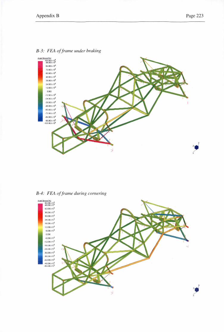
Appendix B
B-3: FEA of frame under braking
64 .00lx1o"
72 .00lx lo"
60 .00J x1o"
46 .00lx1o"
36.00lx1o"
24.00lx1o"
12.00lx lo"
O.OOJ
-12.00J x1o"
-24.00l x1o"
-36 .OOJ x 1 o"
-46 .OOJ x 1 o"
-S0.00J x1o"
-72.00J x 1 o"
-S4 .OOJ x 1 o"
-96.000x10⁸
-100 .00lx1o"
B-4: FEA of frame during cornering
42.0CXl x108
36.CKXl x108
30.000x10⁸
24.0CXl x108
1BJX.()x108
12.00lx1o"
6 .00Jx1o"
O.OOJ
-8.00lx1o"
-12.0CXlx108
-16.000 x10⁸
-24.00lx1o"
-J0.00Jx1o"
-36Jl:Xlx1011
-42.ooox10°
-46.co:lx108
-50.00lx1o"
Page 223
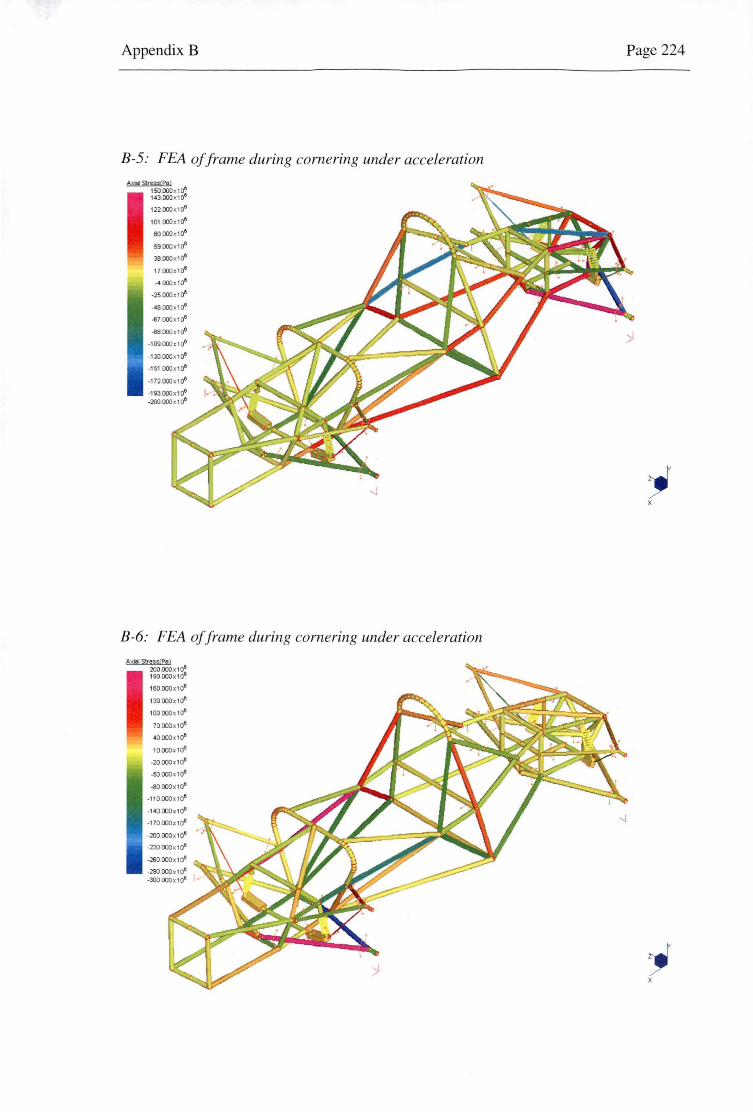
Appendix B
B-5: FEA of frame during cornering under acceleration
101.000x1o"
ao .ooox1o"
59.000x1o"
38.000x1o"
17.000x1o"
-4.000x1o"
-25.000x1o"
-•s.oooxi o"
-67.000x1o"
-88.000x1o"
-109.000x1o"
-130.000 Xl o"
-151 .000 x1 o"
-172.000x1o"
-19J .000x1o" -200.000x1 o"
B-6: FEA of frame during cornering under acceleration
160.000 x10e
130.000x1o"
100 ooox1o"
70 ooox1o"
40000x1o"
10000 x1o"
-20 ooox1o"
-50.000x1 o"
-80000 x1o"
-110000x1o"
Page 224
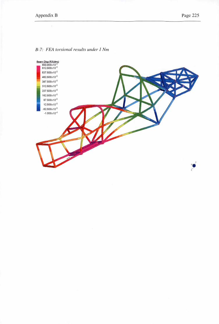
Appendix B
B-7: FEA torsional results under I Nm
Beam Disp:RX(deq} 650.000x10·6
612 .500x10·6
537 .500x1 o-6
462.500x1 o-6
387 .500x10·6
312.500x10⁻⁶
237 .500x1 o-6
162.500x1 o-6
87 .500x10·6
12.500x10·6
-62 .500x1 o-6
-1.ooox1 o-4
Page 225

llTLE Left View - 30 Menber Din. IJMiN BY DAVID BUTLER DATE 4/4/01 \OIGlll. 't
lsrAlE:l: JO ( A3)
Al I nenber lengths or~ 3D
517
224.1 10.0
75.2
~ I
Oo '•
r-< ~ ~ .... (1:>
~
~ ~ ~ ~ (1:> -s. ~ (1:>
~ .... ~ (1:> ;::
"" .... 0 ;:: ~ ..... ~ (1:>
~ <:::l"' (1:> "": ..... (1:> ;::
OQ s. "" --
~ "C (p 1:::1 0.. -· :>< t::C
""O
~ N N 0\
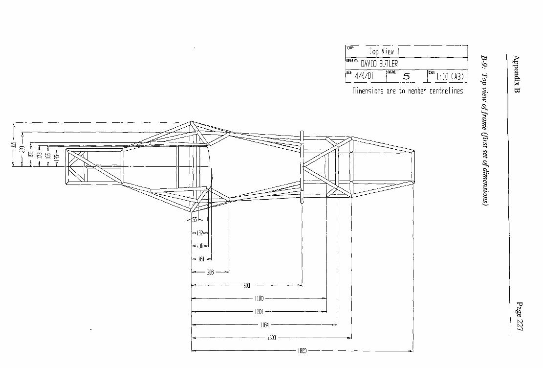
-=== Q
J
--
::>- A
ppendixB
B-9:
Top view o
f frame (first set o
f dimensions)
~
rn
-<:C
~
= ---
-~ ~
lfl O
L
l..LJ
!ii _
_J ~
f--
-=
=
lf'l C
.J c C
.J "-
-!->
c QJ
LJ
"-C
.J -= c:
QJ
c:
Cl
-!->
C.J
"-C
l
=-=
lf'l c C
l C
l f--
1---i
::>-~
=
~
~ ., ~
-= .......... ~ ""'1""
w
O!i
lf'l c C
.J c:
=
Lsu S91 ELI
S61 osc
SSE
=
=
=
Page 227
=
=
=
8 =

Appendix B
P
age 228
B-10:
Top view o
f frame (second set o
f dimensions)
~
,....,, lf1
SLZ
-<:C
~
Q..J
c LZ
= ---
Q..J
5Ec '--
-~ "'I f---
-I->
VEc c Q
..J L
J
~
Q..J
-= c
"° Q
..J c 0
O.<
: !i!
LJ..J
"1
_
J
l§ f--
f---
;;;= =
:i Q
..J =
--
-I->
Q..J ~
0 lf1
=-=
>-----< -
o_
=-=
0
-<:C
'-...
f--
= ~
1;5 ~
c 0 lf1
c Q..J
c .;:;
~ ~
2 =
Lr)
~
r.-.
_J
=
tcl
Lr)
j =
tc
l =
=
=
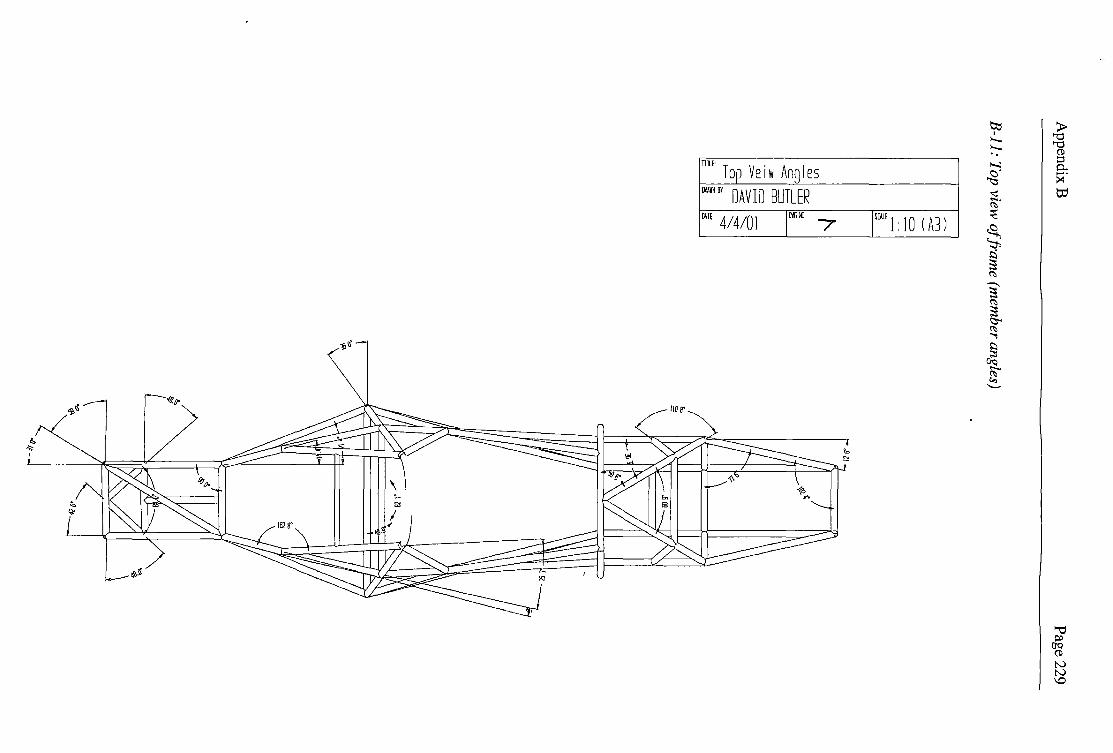
Appendix B
P
age 229
B-11: Top view
of fram
e (mem
ber angles)
~
"" -= ~
= ----~ ~
lfl
" (lJ
C
L
-L
Ll
Si
en
_
_J L
c 1
--
-<C
=
3 =
--
=
(lJ
-
::::>-t--!
::::>-=
C
L
-<C
--......
Cl =
~
1--
'" I;;
"' !
~
~ E!!
.Q /[
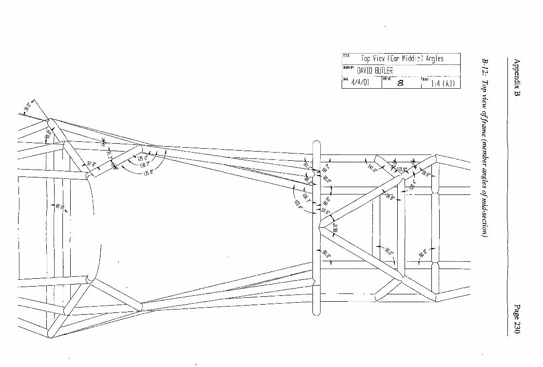
Appendix B
P
age 230
B-12:
Top view o
f frame (m
ember angles o
f mid-section)
"' -:0:::
U"l
QJ
~
en
c: ~
~ Q
J
-0
-0
=
(X) "-C
l l_
J
°"' L
LJ
5!
3'
__
_J
:!l 1
--
-Q
J =
:o
>
=
CL
= >---<
0 :::=-
=
1--
-== "-..
= ~
"-..
"' ~
~ "
~ El!

Appendix B
P
age 231
B-13: F
ront view o
f frame
rrl
-<::C
Ln
Q
_J
LJJ
=:i
-0
~
Q_
J
~ L Q
_J
>-------
-= 1:: Q_
J c C
l
0... -I-=
-
Q_
J L
OL
s;!
a 3
=
LL
I Q
_J
__
J L
_
Ln
1
--
c:
:>-
=
Cl
-I-=-
=
Ln
c: =
c:
Cl
1------l Q
_J
L :>
-=
c
LL
-<::C
"--
=
::::1:: =
i$
~
'°' ~
~ E
6'vBB

If"\
=-0 0 =
Cl
DL
._;_,
~
Ap
pen
dixB
P
age 232
B-14: R
oll hoop dim
ension
s
"' <
:?::
Ln
~ \) -
DL
L
U
Sl
__
J ~
!--
,_______ =
=
=
>--<
=
::>-
<:?::
---.... =
~
;;; "<
;;j-
~ ~
Ln
>--
-= -= QJ
=-__,__.,.
:::i c Q
J
-= 0 __,__.,.
-= Q) Q
J
c If"\ c 0 If"\ c Q
J
c
-= <
:?::
r;t.1
°'I
=
--
--r::-
--
,_
t---------
0'96 __
__
__
_ ____,
i--------8
'9L
---------,
r-------
9'69 ------l
=
------------6
-Ln
~
---
---
-------------~-----~-
~--1 ~-----------~0~1-------------
6~ ~
,__ __
__
__
__
__
__
__
5'6L\ --------------

Appendix C Page 233
lOAPPENDIX C - SUSPENSION DESIGN
C-1: Preliminary front suspension geometry ...................................................................................... 234
C-2: Front suspension geometry ......................................................................................................... 235
C-3: Preliminary rear suspension geometry ....................................................................................... 236
C-4: Rear suspension geometry .......................................................................................................... 237
C-5: 7/16" high capacity rod ends ...................................................................................................... 238
C-6: 1/4" aircraft grade rod ends ........................................................................................................ 239
C-7: Suspension spring specifications ................................................................................................ 240
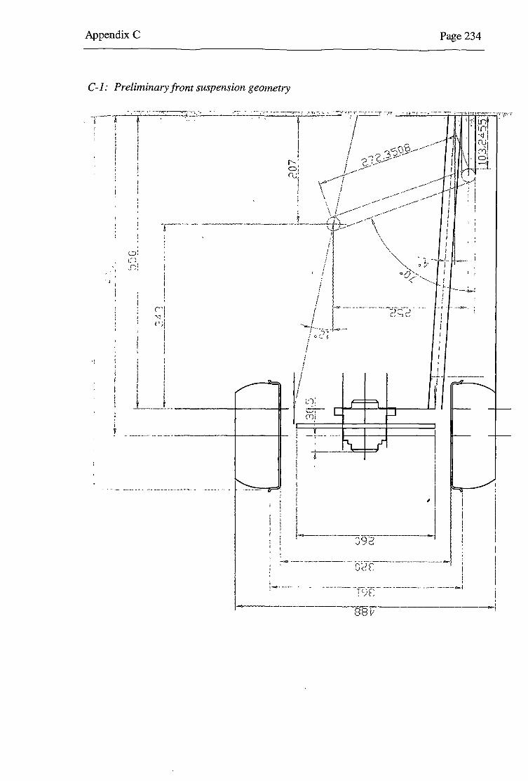
Appendix C
C-1: Preliminary front suspension geometry
~A ---- --
' • J
'l
I _t ____ L __ --i~--
------ -- -- ---- -------t-----11-
, ... ,, --' ...... I
1
---------- -·--·:::r:.:::-:> - ---. .,""I
!""'-:.;-; +~-; IJ (_ i
I
I I
i j
! i I
t:"?; ~ (l")i
J
L_ _____ _ ' :)92
Page 234
i
r I r~ .. -~ I i
-t ---~.
;---- ------------- --- -;..::=-r; ... ----------'°"'"' ~)(, ~-
'
I l
----- -- - --- -- -- -------- -- -----oi-1 T<-)t~
88-V
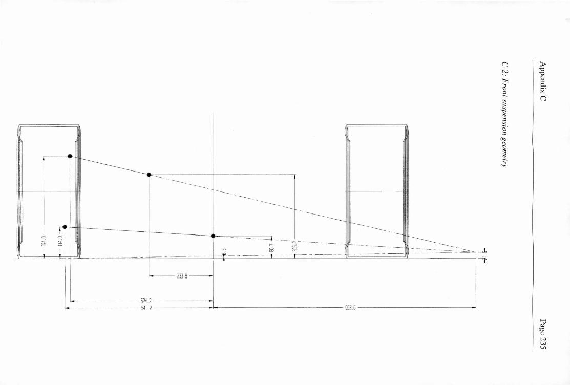
Appendix C
P
age 235
C-2: F
ront suspension geometry
~ 11
//\ I
I
I ( I
I I I
I ! I
I
I /
I
I I I
I j i
u::J ,...., "''
~ -
~
-0
,
I I !
I :
I I
I I
I
f'~~ I
I I
T ,001
I I
I I
I I
I I
I I
EB ~
I I
I I
I I
=
,..., ·~
rv
I I
I I
I '"" ('{,
I •f">
I I I I
--a 1111 -
·
-0 vLE -
•
-
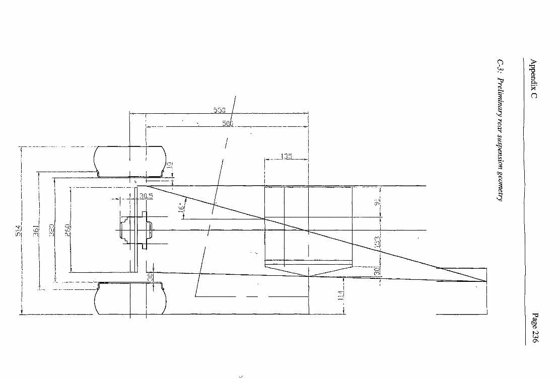
Appendix C
P
age 236
C-3:
Prelim
inary rear suspension geometry
--1
----r -----
1 lfJI
)' I
('")1
-'i t I
-----t I I ' I ' ' I
---
J_
' . ______ ..,.. !? i T
I
~or;~ ,,__ __
l I
--------------r9t:
-~--------9--
1
I !----------------i.1~----------
__ ,...
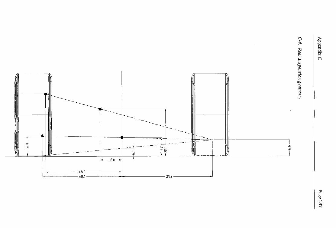
Appendix C
P
age 237
C-4:
Rear suspension geom
etry
I I I\
/ i \ /
/ I l
---f--____,~ 1-tl6c-
/ ' ri--lc
vll-
/ I
/ i \
/ -
1 l'avi.-
' I
\ l \ I \ \ \ l
.. i---QL
ZI-
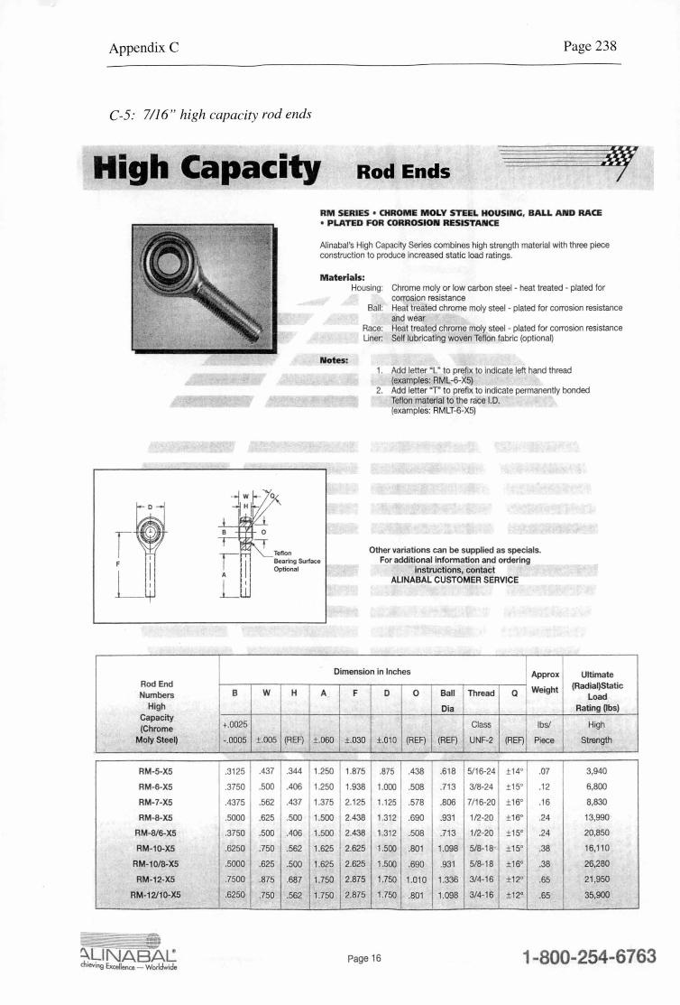
Appendix C Page 238
C-5: 7116 " high capacity rod ends
High Capacity Rod Ends
Rod End Numbers B
High Capacity
+.0025 (Chrome MolySteel) -.0005
RM-5-XS .3125
RM-6-XS .3750
RM-7-XS .4375
RM-8-X5 .5000
RM-8/6-X5 .3750
RM-10-X5 .6250
RM-10/8-XS .5000
RM-12-XS .7500
RM-12/10-X5 .6250
Teflon
RM SERIES • CHROME MOLY STEEL HOUSING, BALL AND RACE • PLATED FOR CORROSION RESISTANCE
Alinabal's High Capacity Series combines high strength material with three piece construction to produce increased static load ratings.
Materials:
Notes:
Housing: Chrome moly or low carbon steel - heat treated - plated for corrosion resistance
Ball: Heat treated chrome moly steel - plated for corrosion resistance and wear
Race: Heat treated chrome moly steel - plated for corrosion resistance Liner: Self lubricating woven Teflon fabric (optionaQ
1. Add letter "L • to prefix to indicate left hand thread (examples: RML-6-X5)
2. Add letter "T" to prefix to indicate permanently bonded Teflon material to the race J.D. (examples: RMLT-6-X5)
Other variations can be supplied as specials. Bearing Surface Optional
For additional infonnation and ordering instructions, contact
ALINABAL CUSTOMER SERVICE
Dimension in Inches I Approx Ultimate
Weight (Radial)Static w H A F D 0 Ball Thread Q Load Dia Rating (lbs)
Class lbs/ High
±.005 (REF) ±.060 ±.030 ±.010 (REF) (REF) UNF-2 (REF) Piece Strength
.437 .344 1.250 1.875 .875 .438 .618 5/16-24 ±1 4° .07 3,940
.500 .406 1.250 1.938 1.000 .508 .713 3/8-24 ±15° .12 6,800
.562 .437 1.375 2.125 1.125 .578 .806 7/16-20 ±1 6° .1 6 8,830
.625 .500 1.500 2.438 1.312 .690 .931 1/2-20 ±16° .24 13,990
.500 .406 1.500 2.438 1.312 .508 .713 1/2-20 ±15° .24 20,850
.750 .562 1.625 2.625 1.500 .801 1.098 5/8-18 ±15° .38 16,110
.625 .500 1.625 2.625 1.500 .690 .931 5/8-18 ±1 6° .38 26,280
.875 .687 1.750 2.875 1.750 1.010 1.336 3/4-16 ±12° .65 21 ,950
.750 .562 1.750 2.875 1.750 .801 1.098 3/4-16 ±12° .65 35,900
Page 16 1-800-254-6763
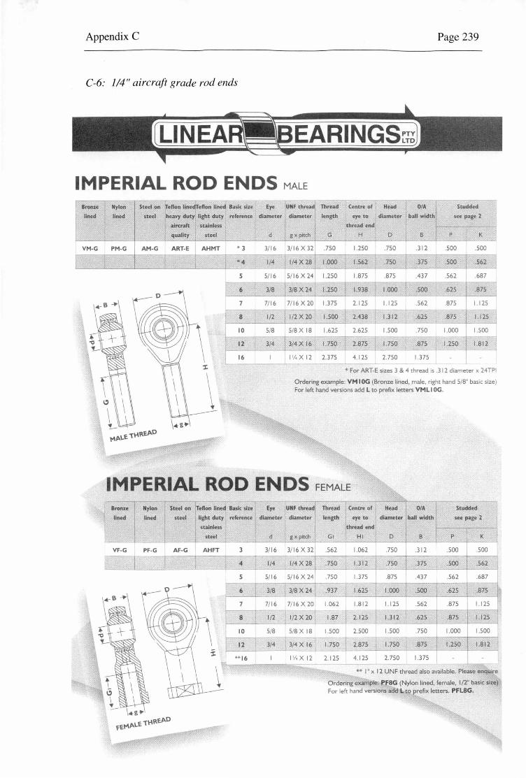
Appendix C Page 239
C-6: 114" aircraft grade rod ends
EARINGSri6
IMPERIAL ROD ENDS MALE
Bronze
lined
VM-G
Steel on eflon linedTeflon line Basic size Eye UNF thread Thread Centre of Head O/A Studded Nylon
lined steel heavy duty llght duty reference diameter diameter length eye to j diameter ball width! see page 2
aircraft stainless
quality steel d
PM-G AM-G ART-E AHMT • 3 3/1 6
4 1/4
s S/ 16
6 3/8
7/ 16
1/2
5/8
3/4
thread endi
g x pitch G H D B p K
3/ 16 X 32 .7SO l .2SO .7SO .3 12 .SOO .SOO
l/4X28 I I.OOO 1.562 .7SO .375 .SOO .562
S/ 16X24 l .2SO l.87S .87S .437 .S62 .687
3/8 x 24 1.250 1.938 I.OOO .SOO .62S .87S
7/16 x 20 I .37S 2. 12S l. 12S .S62 87S I . 12S
1/2 x 20 I.SOO 2.438 1.312 .62S .87S l.12S
S/8 x 18 l .62S 2.62S I.SOO .7SO I.OOO I .SOO
3/4 x 16 l. 7SO 2.87S l.7SO
1 1v. x 12 2.37S 4. 12S 2.7SO l .37S
For ART-E sizes 3 & 4 thread 1s .3 12 diameter x 24TPI
Ordering example: VM I OG (Bronze lined, male, right hand S/8" basic size) For left hand versions add L to prefix letters VML I OG.
IMPERIAL ROD ENDS FEMALE
~;n~ 1 ~;n Steel on Teflon line~ Basic size I Eye UNF thread! Thread j Centre of~ J O/A Studded
lined lined steel light duty reference diameter diameter length eye to 1 diameter ball width see page 2
stainless . h I
.thread end 1 r K --1 steel d gxp1tc GI H I D B p
VF-G PF-G AF-G AHFT 3 3/ 16 3/ 16X 32 .S62 1.062 .7SO .312 .SOO .SOO
4 1/4 1/4 x 28 .750 1.312 .750 .37S .SOO .562
s S/16 S/ 16X24 .7SO I .37S .87S .437 .S62 .687
6 3/8 j 318 x 24 .937 l.62S I.OOO .SOO .62S .875
7 7/ 16 7/ 16 x 20 1.062 1.8 12 l. 12S .562 .87S l.12S
8 1/2 ~ l/2X20 1.87 2. 125 1.312 .62S .87S l . 12S
10 S/8 S/8 x 18 I.SOO 2.SOO I. SOO .7SO I.OOO I.SOO
12 3/4 3/4 x 16 l.7SO 2.87S 1.750 .87S
" 16 IV..X 12 2. 12S 4. 12S 2.7SO I .37S ---~
.. I' x 12 UNF thread also available. Please enquire
Ordering example: PFBG (Nylon lined , female, 1/2" basic size) For left hand versions add L to prefix letters. PFLSG.
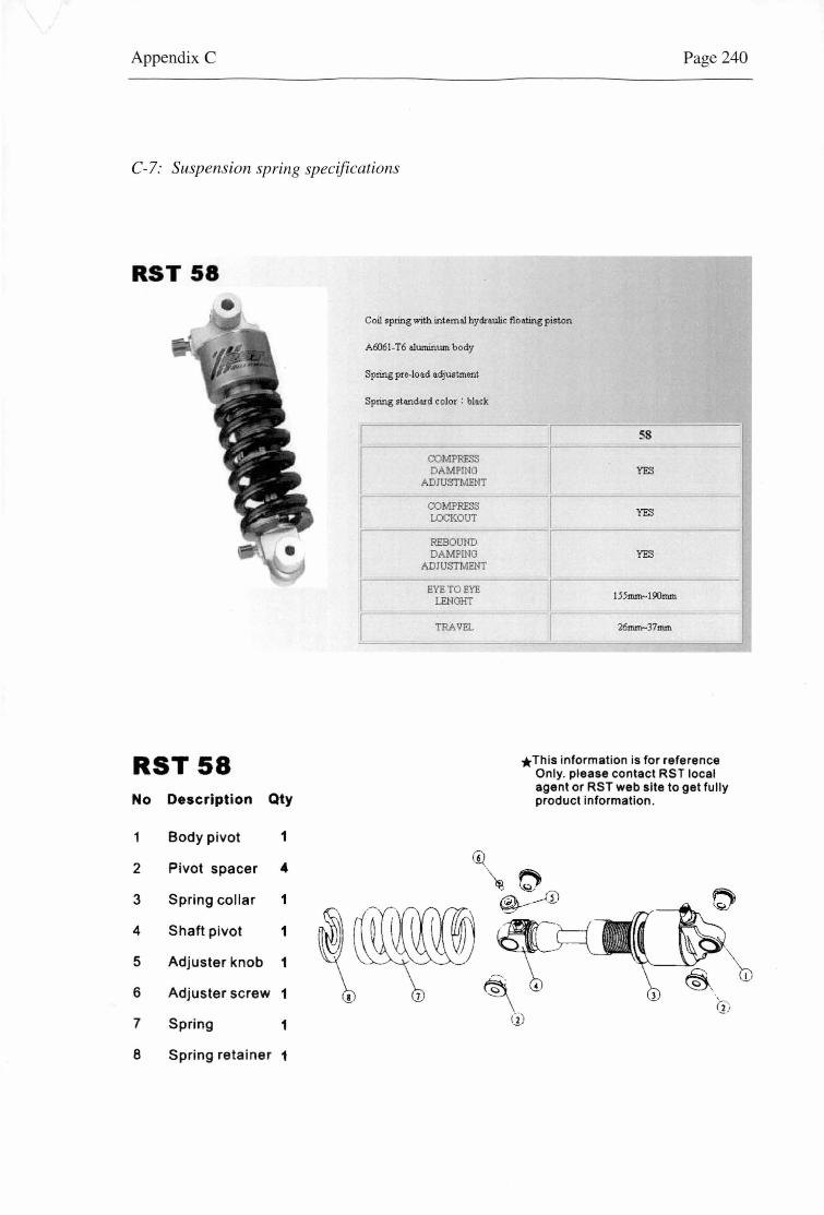
Appendix C
C-7: Suspension spring specifications
RST 58
RST58 No Description Qty
Body pivot 1
2 Pivot spacer .. 3 Spring collar 1
4 Shaft pivot 1
5 Adjuster knob 1
6 Adjuster screw 1
7 Spring 1
8 Spring retainer 1
Coil spring with internal hydraulic fl
A6061-T6 aluminum body
Spring pre-load adjustment
Spring standard color : black
COIVlPRESS LOCKOUT
REBOUND DAMPING
ADJUSTMENT
EYE TO EYE LENGHT
TRAVEL
Page 240
eating piston
- ·---
I 58
I YES
I YES
I YES
I 155=-190mm
r-- 26mrn-37mrn
*This information is for reference Only. please contact RST local agent or RST web site to get fully product information .
Appendix D Page 241
llAPPENDIX D - WHEEL ASSEMBLY
D-1: Brake aluminium rotor dimensions ............................................................................................ 242
D-2: Brake caliper aluminium rotor pad dimensions .......................................................................... 242
D-3: Brake caliper dimensions ........................................................................................................... 243
D-4: Stub axle (30mm dia.) PEA for centred bearing design ............................................................. 244
D-5: Stub axle (35mm dia.) PEA for off centre bearing design .......................................................... 244
D-6: PEA stub axle beanng loads for centred design ......................................................................... 245
D-7: PEA stub axle bearing loads for off centre design ..................................................................... 245
D-8: Upright dimensions ................................................................................................................... 246
D-9: Oil seal dimensions .................................................................................................................... 247
D-10: Stub axle dimensions ................................................................................................................. 248
D-11: Wheel hub dimensions ............................................................................................................... 249
D-12: King pm and caster reference angles .......................................................................................... 250
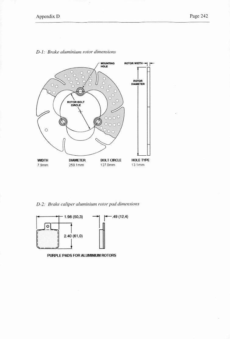
Appendix D
D-1: Brake aluminium rotor dimensions
WIDTH 7.9mm
DIAMETER 259.1 mm
BOLT CIRCLE 127.0mm
ROTOR WIOTH-j r
I ROTOR
DIAMETER
HOLE TYPE 13.1 mm
D-2: Brake caliper aluminium rotor pad dimensions
I
.. · o
. 1.98 (50,3) 1 , .49 (12,4)
PURPLE PADS FOR ALUMINIUM ROTORS
Page 242
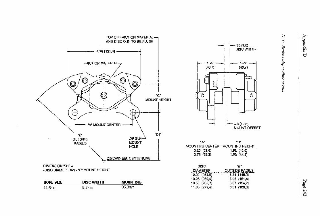
TOP OF FRICTION MATERIAL AND IDJSC 0.0. TO BE FLUSH
i-+----- 4.78(12~.4) -----
FRICTION t.~TERIAL
"C" f.mUNT HEIGHT
~N' MOUNT CENTER
\ .39 (9,9') OUlSlDc "01"
RADIUS "" ~~:T
~ DISCMl!HEEl CENTER LINE
DJMIENS~ON' "D1" = {DISC DJAMETER/2) • '"C" MOUNT HEIGHT
BORE SIZE DISC WIDTH MOUNTING 44.Smm 9.7mm 95.3mm
[ 1.n :43,71
~
"A''
.36 (9,6} DISC WIDTH
©
I
~ .76(19,8) MOUNT OFFSET
MOUNflN"Ci CE:NTER MOUNTING HEIGHr 3.25 (B2,6) 1i.92 (48,8) 3.75 (95,3} i.92 (48,8)
DISC DW,iETEi=l
10.00 (i54;0) 10.25 (260,4} 10.501 (266,7} 1 t.OD (2.79,f.l}
"E" OUTSIDE R.ADtUS
5.84 (148,31 -5.~6 (151,4) 6.07 (154,2) 6.31 (100,3)
t::::i ~ I
~ "O .. CD
O;:i ::i 0..
~ -· :>< ;>;-<
tJ ~ C') ~ --6" ~ ""'! !:)...
§' ~ ;::s
"' .... c::i ;::s
"'
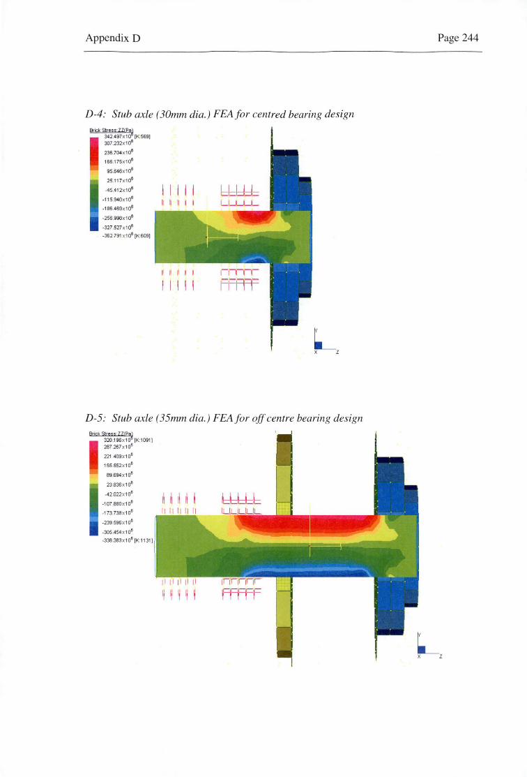
Appendix D
D-4: Stub ax le (30mm dia.) FEAfor centred bearing design 8rjck stress:ZZCP~
342.497 x1 (K:569J 307 .232X1 Oft
236.704 x10ft
166.175x10ft
95.646x10ft
25.117x10ft
-45 .412x10ft
-115.940x10ft
-186 .469x1a8
-256 .998x10ft
-327.527 x10ft
-362 .791 x10ft (K:609J
bbld±
L x z
D-5: Stub axle ( 35mm dia. ) FEAfor off centre bearing design 8rjck stress: ZZCPo~
320 .1ssxrn 1K:10011 287.2t57 x108
221 .409x1 oft
155.552x10ft
89 .694x10ft
23 .836x10ft
-42.022x10ft
-107.880 x10ft
-173.738x10ft
-239 .596 x1 oft
-30S.454 x10ft
-33B .383x1 oft (K:1131 J
1\ 1\ 1\ 1\ ! 111 1111 l
Page 244
L x z

Appendix D Page 245
D-6: FEA stub axle bearing loads for centred design
_, x
D-7: FEA stub axle bearing loads for off centre design
_, x
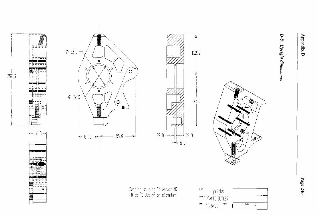
\::) > I "O ~ "O
(1l :::i
~ 0.. CIJ
-· &
>< ""':
0
I
.... Otl 122.2 ;::;-...
~~==3
.... et> ~~ n I
I b.=! u ~-;_-_-_-J - ... .......__~ ~ =-=--=-= 1
~ §" (1:> ;:::: c., cs· ;:::: 257. 3
I c.,
I I
et> 72 'G !45. i
t J 50.0
6\. 0 e. i =- 106.9 22.0
6.0
r:L[ Upright
"''1N
111 DAVID BUTLER 1)11[ lS/S/Ol IDIGIIl. I ISCALE l .2
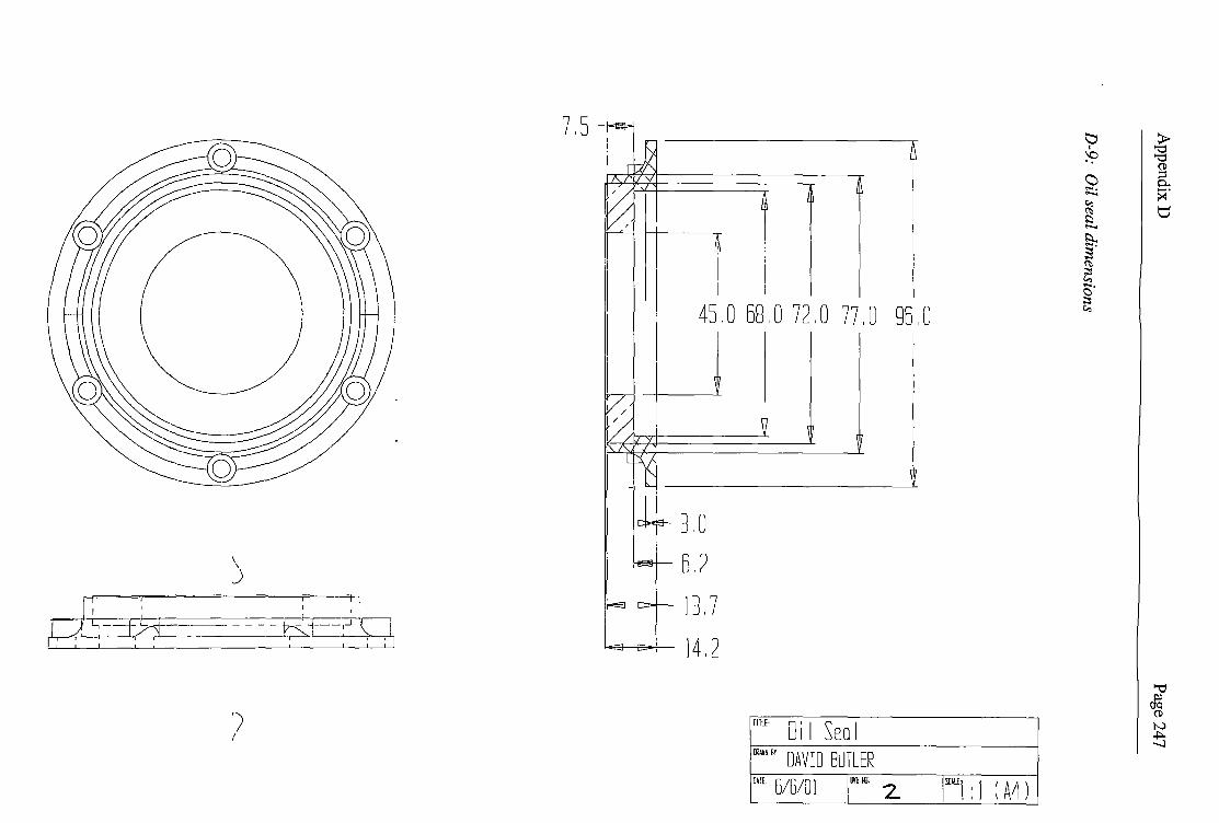
\ )
I (
7.5
I I
45 '0 68' 0 72 '0 77 I 0 96 I 0 I
10 6.2
!i-eEl----1~ i l 7
ka------1=-+--- 14 ' 2
TITLE· Di I Seo I !JIAINBY DAVID BUTLER am. 6/6/0l IDIGtll. 2 IS[llfl : 1 ( A4)
t:i I
\Q .. 0 .... ......

Appendix D
Page 248
D-10:
Stub axle dimen
sions
--
LJ)
~
~
c::::::i -c::::::i
~
ri-L
J)
~1 l
I'll
'tl
--
--~
-
M
:=:l
OL
S
! L
U
-<
:::j-~
_J ~
1--
=
-!-> =
-
= -
c::J, >----< =
_
c
:>-
'-... (/)
<:C
L
Jl
=
'-...
"' L
n
"' r--
~ ~
~ g
j C
LJ
h II -,
·i I I I I I
c::::::i I
-I
=
c::::::i I
Ln
L
J)
Ln
I I I I I
' I I
~ c::::::i -c::::::i I'll
w
I
=

50.0 I
I
63. s
A 11 F 1 I i ets 4nn (con be changed). Keywoy 1s 6~n wide, 3nn deep Mounting hole sizes ore o guide only Hub inner hJle to [leorcnce G6 (obout +O.Oinn on d1Gneter).
I 130.0 '.;4j 7EC 68049.
I I
10.0
I-El---- 72 .3 --=-'
SE[l!!JI A-A
10.0 5.5
1.5
t:H Hub
IJ?Al~o'
DAVID BUTLER OITE 6/6/01 lllUtll.
I 90.0 144.0 \SO l
I
4- ISULE. I: I
\:::) I .......
....... ..
\
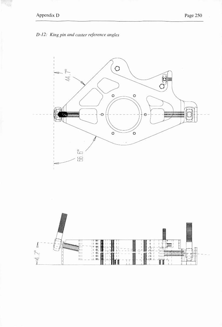
Appendix D
D-12: King pin and caster reference angles
I~
0 LO
LO LO
Page 250

Appendix E Page 251
12APPENDIX E - BRAKE PEDAL ASSEMBLY
E-1: Brake pedal dimensions with balance bar .................................................................................. 251
E-2: Brake master cylinder dimensions .............................................................................................. 252
E-1: Brake pedal dimensions with balance bar
1.10 [28;2)
t
10.24 (260,S)

Appendix E
E-2: Brake master cylinder dimensions
4.65 (1Ul,1)
.75 (19,1)
. U0(41l•l+ I 3.00 (76,21 ~..28 _DIA :_J 1.45
(32,5) (36,8)
--~- 4..63 (117,6) I STROKE
8.86 (225.0}
.40 (10.2) DIA MOUNT HOLE
Page 252
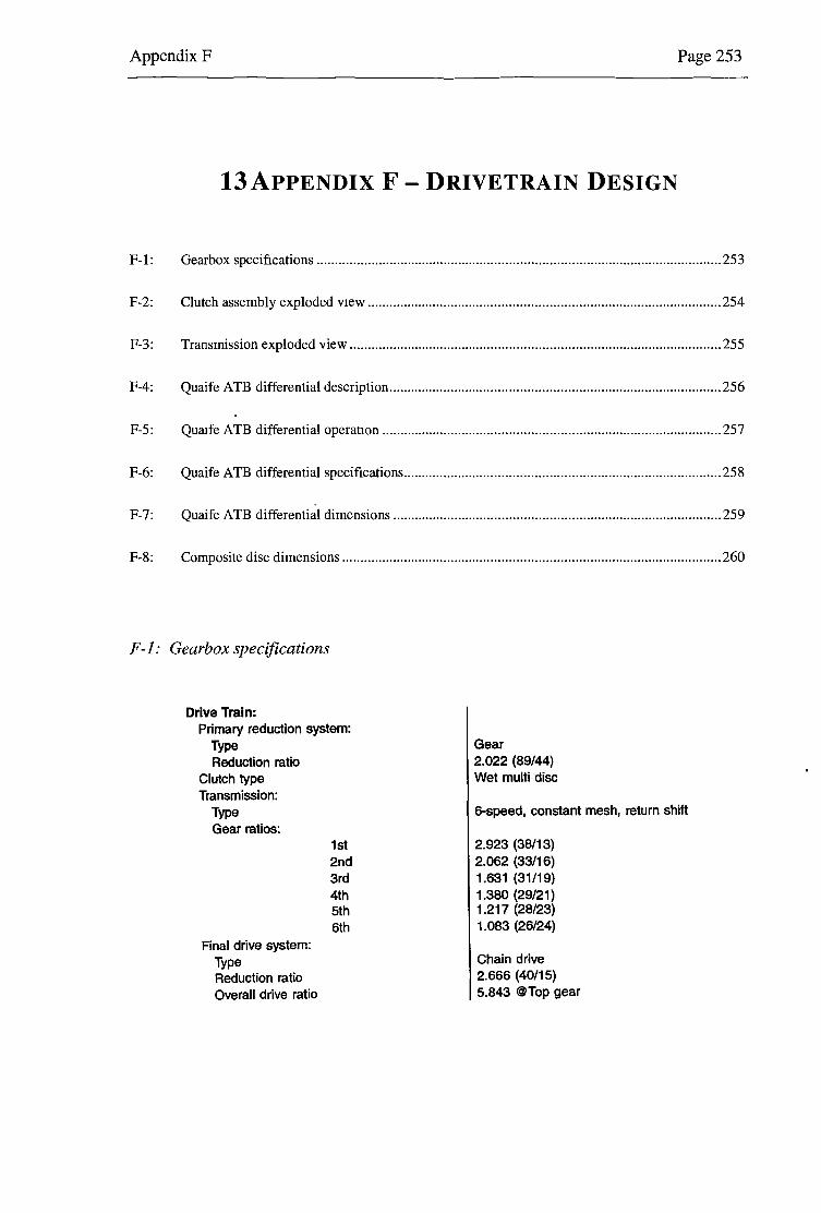
Appendix F Page 253
13APPENDIX F- DRIVETRAIN DESIGN
F-1: Gearbox specifications ............................................................................................................... 253
F-2: Clutch assembly exploded view ................................................................................................. 254
F-3: Transmission exploded view ...................................................................................................... 255
F-4: Quaife ATB differential description ........................................................................................... 256
F-5: Quaife ATB differential operation ............................................................................................. 257
F-6: Quaife ATB differential specifications ....................................................................................... 258
F-7: Quaife ATB differential dimensions .......................................................................................... 259
F-8: Composite disc dimensions ........................................................................................................ 260
F-1: Gearbox specifications
Drive Train: Primary reduction system:
Type Reduction ratio
Clutch type Transmission:
Type Gear ratios:
Final drive system: Type Reduction ratio Overall drive ratio
1st 2nd 3rd 4th 5th 6th
Gear 2.022 (89/44) Wet multi disc
6-speed, constant mesh, return shift
2.923 (38/13) 2.062 (33/16) 1.631 (31/19) 1.380 (29/21) 1.217 (28/23) 1.083 (26/24)
Chain drive 2.666 (40/15) 5.843 @Top gear
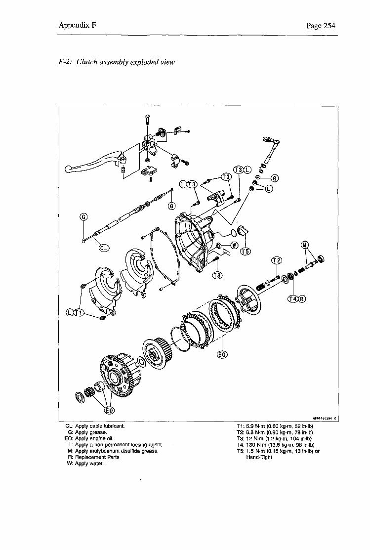
Appendix F
F-2: Cl utch assembl y exploded view
()
~
Page 254
T3 ~ ~- ~
~~® 'l
CL: Appl G· A IY cable lubricant EO: /Py grease. .
L: pply engine oil ·Apply · M· a non-perrna
R; ~~~:~c~olybdenurn n~~~l~~~~ing agent w: A rnent Parts grease.
pply water.
T1· 5 9 T . . N·rn (0.60 k ••••••02u c 2: 8.8 N·rn (0.90 k g·rn, 52 in·lb)
T3: 12 N·rn (1.2 k .g·rn, 78 in·lb) T4. 130 N·rn (13 ~ rn, 104 in·lb) T5: 1.5 N·rn (0.1S kk~·rn, 98 in·lb)
Hand-Tight g rn, 13 in·lb) or
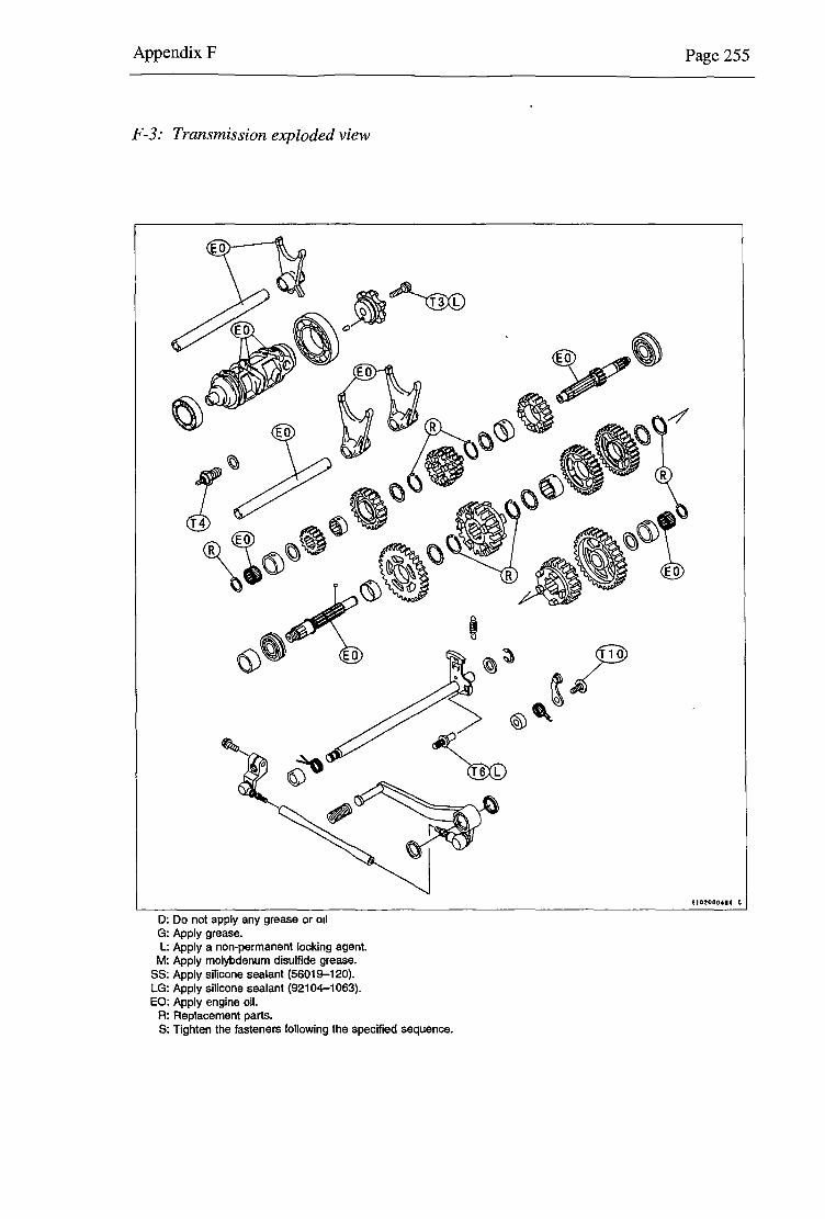
Appendix F
F-3: Transmission exploded view
D: Do not apply any grease or 011
G: Apply grease. L: Apply a non-permanent locking agent.
M: Apply molybdenum disulfide grease. SS: Apply silicone sealant (56019-120). LG: Apply silicone sealant {92104-1063). EO: Apply engine oil.
R: Replacement parts. S: Tighten the fasteners following the specified sequence.
Page 255
a I 02080414 C
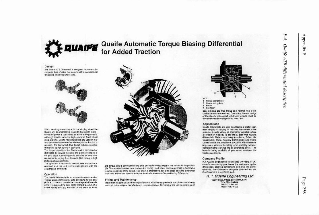
Design 1~,, OJ<til~ Arn Dille; e~li31 is de~ign!ld 10 i:<1r:ert. 11'19 c:orr:p!!te 10.s et drk! ihat oc:cis wnh 1 cort,.•nll:n•I d "!ren1i1I w~'1n one 11·~eel sips.
v.'hi :i.~ requiri.ip .!i.'.lme rnrcue · 1ne SllP',>lng wlla•I me Qualle ur 1 ls pr".grew·1a In attlo1 bul ne-vsr c~s · cowo eo r.ow~r Is irar.Gmlnoo lo all ~10 diivino "tied~ Altho~~~ i.Mlly su11oj lo hlpb•pJworcd f r->n l•wh~el d1'i'lt: $·;$1ern~. 01.r;1 tto AT:l dilrercu\1itsls ore ~d in re-ar and to ~·~'nl!<!I dnve ve id'es "tie •e oplfm1.1m lracton · required. Th9 rou r-Y.h1e1 dn•1e 1ayou1 lnclLdes a centre drttornnllal as woll as ore ' eath axlo Tha :erq'JI) Ciipilcily or lho O.to.dl} 1.nll i~ ~:'\crc;1:;cd OJ dect!~OO lY/ •1itr[tng t."10 ~~ix erd p re~~Lte 3n~Je~ ar eie ge"-r we:h. A c:ornbiiiJ7on I~ ~v~l~~le to rnee1 c~ · requirenont~ iaryirg frcfil Fo1r'l'lultt One racirg to h9h r.u ee91 Atr.br:l:L1te ! _ets. Th! op!r~lie:n is all~CtTH!.~i~. normal .≪le h.i.)rl:e.1i:::n I! retained 011~ IH unll ;,. Iota cnangaa~'e IV•Lll th• cc-1 .. •enll::flaJ dt'arentl31.
Operation ~~Quaile Dillerar:lal ls an &u;c ,.allc gear-o;ieraleo
IOttfJ !!- 9i i1 ~1rg o.r.orcn:i.fll. Sel!I ol r.oiltin;; hcli:al go:u p.n~r.s. i 1) rr.-.>ah t~ pro,·:d! 1ne r.ormaJ sp!ed dlllereo lial w.a io pre-lo<.1 r.ie ~Eilr r"'c~s 1~era Is a e.i!lact!on ol c:G1'l lre ~r ,~ d~:i (2) :n. l;:bl!! In lhn Qvr: ,, 01 v..huL-1
Quaife Automatic Torque Biasing Differential for Added Traction
:lip lorque bias Is ~ene.rated bi ;he a~I ,1n:! r~:!i<! lhrJsts (rod) or lhO Finioru: in tie pccke:~ (J), n o rcsult<on: f.ri ctioi l;rc~ .,..,ob !o~ lh• ~·lvli~ row wh~I ~r.d •ur.·p•er (4) 10 t-ansmit a g r<:•~ •r F"~ott'o d lh• r. ~rq~. Tlli• e~e<:l 15 pto3re:s' :a, ~L1 at ro StaG~ d:es ne d~ere.11ial l::d< ~~ l i:t . 9n:e :1te lrh!r!nl s~!! ty or:t~a OJ la AIJlomatic Torque Ble· i a D e·e <.al.
Fitting and Maintenance fns1" f~1i;111 Is ~E 11 11c~ l to t.1'1 u r:or-nal tiforP.f'IU" · ~t& .... otuir.g pr-! .fO!ld~ :utd piltio;i inesh b!!ing r e~~::i r e d ~~ lnl} ar;·91r.al m&."IU!9tlurer.s> recomrr ndnt"or .... Se"'1lclnp ol lhe unit is slr.ip4e as ttll
XEY 1 ~ - ~r pnbn!.i 'Z C-9-1",ro 'J?r.r.g d_; t.$. 3 PcC.o1 .L Sun Ga:u
~ aar p4r. Ions are tree rlNlnp ar d normal llnal crivo lulvtcafon ells era rala nsd. Due 10 Iha lntG:n~I design ot L e Oual~e dlfturontial, all driving wheel$ ""'"I be tilo·1~IC°d '-"hOn scMdnJ braket, fy rl!!I , elc..
Applications Qvailo di~erer:ial& lll9 usod in i.1 rorm~ or rne<:or •p~r1 irom Cir4;l,Jit l D r~Jlying in IWO .arid iour·wheel d'tiVQ ~)'Sleros. A wd~ ~11.11e1y 01 ~11e:g!~f venlcles, wt.!lr& aU·wealner mo~ll ly Is esaen1laJ, also un Quallo different.al&. Ma.or users te:na l>.Tobulanco. PO--co. HM Coas;:l\J;ird, MOO. forOsli!'/ Cc :t.i.!;sloB and Pub1!: utllli~ where Uie ~ddhiOB ot a OJeile A'iB d1Weren11al Imp ovea \'enlcla ha.ndHng and &lablllly without comprorn sl~g ~erYlcs Ille or opera:lng cos1s. Tno beoerh& t>e lng avallab'.e all yoar ro1nd " QIO•Or !ho raci lcn tood~icns.
Company Prollht A. T. Ouatre E:nglro!er'ng (estatlletied 30 yem UI() manu'acl'Jre& rac no ~ear to«•• (car an~ rnotor ~~-o'o). d 'l&r&c1lill's. &t~o;r.g com;it<ior:s ;i.,,d C:rlvo no power 1.ik.o·;!I~ . TM omoror.tiM d~sign Is ci.1en1e<1 and tne C>J:iiftt n:.l"ne i~ a re~~ered m::rk..
R. T. Quaife Engineering Ltd \'nlry ~~. Otford, Se-nnoake, Ktt"ll,
TK14 5El . EA15land r.1, 01m 1~1144 Fn: 01732 741555

~' eJ, ·~ :.~·~, .. ·-~--' ,,
OperaUon
· fiil!i.:r. ~· ~-~·
1'.he Quaife· Differential Is gew ·Operated and .th.erofOre requires 1)0 _:plates ~vhlch mey wear·or break: The unl\·is smootn in use and requires no special lubricants.-
.SPECIFICATlON
Design The O[Jelfe. Dllfereri:ial'is designed_ to power bo1h ·wheels_· and .eontrol_ Jo5s of drlV\'J. The' · dlHerentlal pro~·Ides constanJ ·and infinitely variable' drive; tracllon being- transferred from !he·splnr.Jng \Vl)eel lo ttie sialfc wheel. autornatlca!)y wl!ho_ut the use' of the 'n_orrtial· 'frlcl[on pads in oih~f des1g~. ·ihe operation . Is fully automatic and requires no manual co'ntrol. The unique design offers full maximum tractron,· _Improves Ji<lh_d!ing · )~nd steering, · and pu!S .the po~~er wl1ere It IS_ needed hiOst. With aJJ \he gear·~ beln'g the_ helical iype, tne· helix ·<lnd pressure _angle .of ~he gea~. teeth . can be:varled 10 rr.~rease or decrease the· to'rque capacity. · ·· ·
SultabllltY -The ciiffere11ua1 is idea11y suitiJ<I to four wheel 'l:lriva appli~ations,· as. well as conip~tiUdn ' vehicles. Can also ~ used ln all four wheel drivo uni1s;~ both front and rear. Even when fitted to front whe'el drive vehicles, there Is no a"dverSe res!s1ance to the steering. .
Fitting and Maintenance Fiuing the Quaife Dlfferen!ia.J_i,s 1he.sama es lnstallir.g tt'ie stahdar;d differential unit; 'An'/ maintenance: cqn ' be carried 'cut by ·a ·competent macharilc am:f·"no·,speclal tools ere "req'uirei:I.
7'J Vi ..

CROU..Jt~ V.lHEEL BOLT PCD Dl .z. 'l."3t:.2.
NO. OF BOLTS .,!5 THREAD I HOLE "'/~ CRO•,.JN WHEEL SPIGOT DIR D2 1t-·lj.8~'l./1t1tm BEARING- DIA D3 1·'1m0 1--;oJ(o
BERRit'JG DISTANCE L1 - "?.·1G>7 SPIGOT LEMGTH L2, -e.·1~ ·r~ OVERALl-_LENGTH L3 s·5o2 BEARD~G/CRO\.JN t•JHEEL L4 -i.oo
BORE 04 1·16\'l, f H•~
·DRIVE SHAFT SPLINE:NO. OF TEETH ~~gH PRESSURE ANGLE
1.°!T ~.._ '2.~ T
'2.l;/'('e Dfl
L2/A
QUA.t'FE FRONT WHEEL DRIVE DIFFER]:NTIAL DESIGN DATA
F1e.z:,rA - 6,SCor;!.T
i=- 7ZS 'bot:.'\.
n I .
QUAIFE DESIGN & DEVELOPMENT
l2/A
.1 I
Ll
Ls
"?j .6" I
0\ '• "d
(I)
ta :::i 0.. ::::: -· ~ :><
S; ~
>Tj
~
~ !::l... § ~
~ ;:::: .... .... ~ ....
{3 ~ (")
S) (") ~ .... .... 0 ;:::: c..,
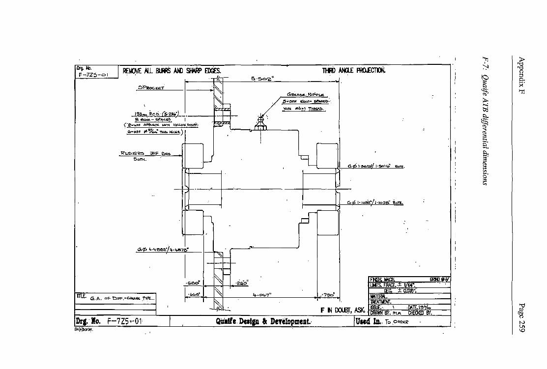
~¥pci.-~·:u<.)_, ___ + s -.:.1 - 5f11"-4!> I
ce-~ .!>!1't. ... ~ ... '1'11 l!oU.0..- __,.,_
- c:.~.:.J~ !6 t}-',,,: 'Mb lt.c..~.)
BoTtL
G11~-Nl?P= :S'-OFF ~.,,_:, ~'.',
lol\T\I "'"'"' 'TliKN>.
-+-+-- ----''-----+--''-------- ---+---- --+-_..;.
Dq;lo. F-7ZS~Ol

Appendix F Page '.260
F-8: Composite disc dimensions
10.04 6 HOLES. sa 10.00 Dr.='lEQ~u'="'=1s~PA~c§~OJ
• iZI 0.05 A
20.10 ES l2S 20. 00
l I I I- I -0 r I
~
~ I I
I • I
T r6140

Appendix G Page 261
14APPENDIX G - ELECTRICAL SYSTEMS DESIGN
G-1: Electrical system specifications ................................................................................ : ................. 261
G-2: Alternator exploded view ........................................................................................................... 262
G-3: Fuse box wiring diagram ............................................................................................................ 263
G-4: Fuse box circuit layout ............................................................................................................... 264
G-1: Electrical system specifications
Battery
Type Gel cell
Capacity 15 Ah
Voltage 12.6 v Charging System
Type Three Phase AC
Alternator output voltage 45V
Stator coil resistance 0.2-0.6 Ohm
Charging Voltage 14- 15 v Electric Starter System
Starter motor 12 v Brush length 12mm

Appendix G
G-2: Alternator exploded view
1 . Starter Lockout Switch 2. Oil Pressure Switch 3. Front Brake Light Switch 4. Neutral Switch L: Apply a non-permanent locking agent.
SS: Apply silicone sealant M: Apply molybdenum disulfide grease. G: Apply grease or engine oil.
Page 262
T1: 3.5 N·m (0.35 kg·m, 30 in·lb) T2: 12 N·m (1.2 kg·m, 104 in·lb) T3: 11 N·m (1.1 kg·m, 95 in·lb) T4: 7 N·m (0.7 kg·m, 62 in·lb) T5: 15 N·m (1 .5 kg·m, 11 .0 ft·lb) T6: 120 N· m (12 kg·m, 87 ft·lb) T7: 1.0 N·m (0.1 kg·m, 9 in·lb) T8: 1.5 N·m (0.15 kg·m, 13 in·lb) T9: 33 N·m (3.4 kg·m, 24 ft·lb)
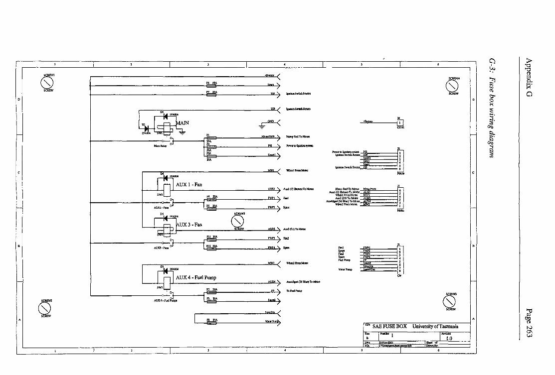
c:i >-I "'O u.i "'O ..
~
G)" <S)' ~ i:l
F6 >lA p.. ..-.
c.., ~ SCREW F7 >lA ~
0
\DI
J,mS.tldiSogn:o SCREW ~ D Cl >-<
JSR ( ,....,.,Wldl._ ~ I
~ ....
14 "':
~ """"" Q;J, s· ~ OQ
FI i::..
::~ &rrJRa!Totdoia:: .... .J IE !:::!
OQ -- Ptiwara> ta=bDl)mD. ~ n
----~ ;: Ipmoa Switch JUrtn 2
>lA l
' \\'!ml From Mon:
1-m Swcli Souite ~ c ''''"'
AUX I -Fan JI AUXI A;mJ (l3 Bron) To MalDi:
-·=i=~ F4 20A :; ... , !:'h~= 4
' I 1::; Ata:411p4 (36 BIQc) To Moue A ~ I ' \lf1ntc2FromMoto; 1 '-I s..,. I -, ...... I I
I I 05
I I UX3-Fan I I
i kW 0.5) To Mota;
Pit 20A :; f'ID1 1:: ""'' ··-· 1L - I s,.., 2
'""' l s..,. ' :: FaclPnmi> ' '""'2Fmm- 6
D3 IN4004 w .... ...,, 7 [[Ji AUX 4 • F"'1 Pmnp ...!... c.
~(J6Biua)ToMoke
sw:i Fl lOA
,:~ AUX4-F~l 1::: TDFud-
cSJ G)" ""C
L :::; ~ SCREW A (Tq .. 20A
~ E3 "" SAE FUSE BOX University ofTasmania N ... N - 0\
w 8 1.0 "'~ :zs.Nov-2001 F c

Battery In
0 lO ro
Mat €:\C Power ...
riux 1
Aux 3 Aux ·4
Motec Wh1 te 2
•
J750 (,-1111)----------
Power to Ignition Syst em ignition Switch Return Spare GND Spar e Ignit ion Switch Source
Fan 1 Spar e Fan 1
Spare Fuel Pump Spar e Spare Water Pump
Appendix H Page 265
15APPENDIX H -TEST RIG SENSOR AND
TELEMETRY DESIGN
H-1: Advanced dash logger - descnption ........................................................................................... 266
H-2: Advanced dash logger - specifications ....................................................................................... 270
H-3: ADL wiring loom ....................................................................................................................... 274
H-4: Radio modem - specifications .................................................................................................... 275
H-5: Radio modem - installation ........................................................................................................ 277
H-6: Wheel speed hall effect sensor - specifications ......................................................................... 278
H-7: Wheel speed hall effect sensor - installation .............................................................................. 280
H-8: Suspension position linear potentiometer - specifications ......................................................... 281
H-9: Suspension position linear potentiometer - installation ............................................................. 284
H-10: Steering angle radial potentiometer - installation ...................................................................... 285
H-11: Brake pressure transducer - specifications ................................................................................ 286
H-12: Brake pressure transducer - installation ..................................................................................... 288
H-13: Attitude & heading reference sensor - specifications and installation ....................................... 289

Appendix H Page 266
H-1 : Advanced dash logger - description
MoTeC Advanced Dash Logger (ADL)
The MoTeC Advanced Dash Logger (ADL) is a fully f eatured and self contained,
programmable logger. The key difference between the MoTeC ADL and other products
is its flexibility to be adapted to any application.
Many vehicle, marine and industrial applicati ons require separate products to perform the logging, controlling and displaying. However, the MoTeC ADL offers seamless integration of all three functions.
All aspects of the ADL are full y conFigureurable, including which sensor is connected to which input, what to log, how fas t to log it, which channels to di splay, warning alarms and contro l outputs.
The MoTeC ADL uses a high speed 32 bit microprocessor and incorporates a 79 pin autosport connector. The ADL is built to internationall y recogni sed quality and manu fac turing standards and is back by a full 2 year worldwide warranty.
15 .1.1.1.1 Data Logging
Data logging allows fo r read ings taken from Analog, Digital, Serial, CAN or Calcul ated channels, to be stored in the ADL fo r later analysis on a computer. The ADL u es permanent non-volatile Flash memory. Data memory may be unloaded at very high speeds (approx. 19 seconds per Mbyte) . Diffe rent logging options allow 384k, 1 MB or the full 8MB to be accessed.
The ADL can store channels at up to 1 OOO times per second per channel, this can be indi vidually set for each channe l. Four logging modes may run concurrenll y (Normal, Fastest Lap and two Burst Modes) each with selectable start and stop logging parameters. Memory can operate in stack or circular buffer mode.
15 . l. l. l.2
1 S .1 .1. I .3 Analog and Digital Channels
In total the ADL can accomm odate over 200 channel derived fro m any mixture of Analog, Digital, RS232 Seri al and CAN bus data channels.
The ADL directl y upport up to 28 analog inputs, 12 digital/speed inputs, 8 auxiliary outputs and 2 high accuracy Wideband Lambda (Air/Fuel ratio) inputs.

Appendix H Page 267
The analog channels sample at up to 1000 samples per second per channel, with a measurement range of 0 to 15 VDC.
Digital inputs are used for state monitoring, counting and pulse width measurement. They accept switch, logic, open collector (Hall Effect), or magnetic signals.
The auxiliary outputs can be conFigured to operate as simple off/on outputs, duty cycle control or frequency based outputs.
15.1.1.1.4
Serial Communications
The RS232 serial port is programmable up to 115k baud and can be used as either a telemetry data output port or serial data input port.
As a telemetry port; devices such as Modems, GSM & Satellite Phones, Radio Modems etc. can be connected to facilitate remote communication.
As a serial data input port; serial communication devices can be connected for displaying and loggmg purposes. These include Engine Management Systems (MoTeC and other), bar code devices, keypads, GPS Systems or other serial communications devices.
15.1.1.1.5
Display
The MoTeC ADL display is a high contrast, high temperature, custom designed reflective LCD. Its unique design makes it viewable in direct sunlight or artificial light.
The display has 3 modes of operation, where each mode is fully programmable and independent of the other. Each mode may be selected by pressing a button or activated by a condition.
The 70 segment bar graph display is programmable to display any channel, with an optional peak hold marker and setpoint marker. Each numerical display item can be programmed to display any channel value as required. The 13 digit alphanumeric display area has 20 lines available to scroll through and may be used to display any channel value or to display warning messages.
Lap times may be displayed when connected to a MoTeC Lap Beacon (or a driver activated switch). Other performance information may be displayed, including mimmum corner and maximum straight speed, fuel used or fuel remaining, and many more.
15.1.1.1.6 Alarms
Warning alarms may be defined for any analog, digital, serial or calculated channel. Alarm limits are fully programmable and may include up to 6 conditions to ensure that the alarms are only activated at the correct time.
When an alarm condition has been detected, a message can be shown on the display and an auxiliary output activated. These outputs can be used for warning lights or the control of other devices.
The alarms remain active until they are acknowledged, either by activating a switch or automatically after a definable period of time.

Appendix H Page 268
15.1.1.1.7
Controller Area Network (CAN)
The CAN bus is a high speed communication standard operating at speeds up to lMbit.
CAN allows many devices to be connected by a common bus, allowing all devices to share information as part of a larger system.
CAN devices include: automatic transmission controllers, sensors, multi-channel input/output modules, engine management systems etc.
15.1.1.1.8 Host Software
The ADL is supplied with software packages for managing the ADL, analysing the logged data and monitoring a telemetry link.
Ease of use is one of the most attractive aspects of the MoTeC ADL software. There is no complex language to learn, just simple menu driven windows.
A full online help system is easily accessible and is integrated throughout the software.
15.1.1.1.9 Dash Manager Software
The Dash Manager Software is used to conFigure the ADL and download logged data. It is logically laid out, giving the user access to the power of the ADL without requiring high levels of computer knowledge or intense training.
15.1.1.1.10/nterpreter Software
The Interpreter software contains predefined configurations for easy data analysis. Screen display formats may be varied to suit all preferences, including user defined graphs, histograms and statistical summaries. By utilising these different display methods, users can view data in many formats to obtain accurate, meaningful analysis.
Data can also be exported into ASCII CSV file format for analysis in other software packages.
The Pro Logging option includes graph overlays, virtual instruments, mathematical functions, XY graphs (scatter plots), track maps (shows minimum and maximum speeds, gear change point and breaking points) and other advanced features.
15.1.1.1.11 Telemetry Monitor (Optional)
The Telemetry Monitor software allows for realtime viewing of the telemetry data either via direct serial communications, modems or radio modems. Data can be viewed in various formats such as charts, bar graphs, dial gauges, numerics, lights, XY graphs and scroll charts. All objects are definable by the user.
15 .1.1.1.12 Upgrades and Accessories

Appendix H Page 269
The MoTeC ADL is completely field updateable by the user. The control software and logged data is stored in FLASH memory. No programming interface is required, simply send to the ADL the new program and the latest features are immediately available.
15.l.1.l.13Upgrade Options
The ADL has field upgradeable options using a password enabling system. Upgrade options include:
Extended inputs & Outputs, Pro Logging (advanced data analysis), Medium Logging (lMbyte), Large Logging (4Mbyte), Telemetry Support, Remote Logging and Wideband Lambda measurement.
Three wiring options are available for the ADL:
Separate I/O Terminal Module with plug-in screw terminals. Includes a Realtime Clock, additional RS232 port and wide ranging power supply.
Standard (vehicle style) wiring loom for specific permanent installations.
Custom wiring looms for complex installations.
15.l.1.l.14Accessories
A wide range of sensors are available for use with the ADL including: hnear position, accelerometers, pressure, resistive and thermocouple temperature sensors, hall and magnetic speed sensors and many others.
The MoTeC Lap Beacon transmitter and receiver has been designed in conjunction with the ADL. It features high channel count (990), improved optics, low power consumption and multi beacon capability.
And for peace of mind the MoTeC ADL offers a full 2 year worldwide warranty.

Appendix H Page 270
H-2: Advanced dash logger - specifications
ADL Specifications
15. l. l. l.15General
• Microprocessor: 32 Bit High Performance • Manufacturing Quality standard to IS09001 • Field updateable Operating System • Non-volatile FLASH memory for data & operating system • High RFI Immunity • Rugged Aluminium Housing (IP-55, NEMA 4) • 79 pin Autosport connector • Operating Temperature: -10 to 70 DegC • Operating Voltage: 7 to 22 VDC • Operating Current: 0.3 A max. • Weight: 385 gms (0.85 lbs) • Size: 180mm x 91mmx18mm (excluding connector) • Reverse Battery and Transient Protection • Warranty: 2 years Parts and Labour
15.l.l.l.16Measurement Inputs
• 28 Analog Inputs (10 Standard): • 20 Analog Voltage (6 Standard) • 8 Analog Temperature (4 Standard) • 12 bit resolution, 0 to 15 VDC range • Update rate (Max. 8 channels): up to 1 OOO times/sec • Other inputs: up to 500 times/sec
• 4 Digital Inputs (2 Standard) • 4 Speed Inputs (2 Standard)
Digital & Speed • Switch to OV, logic signal, open collector (Hall Effect), or Magnetic • State & Counting (1 MHz) • Period (1 micro sec) • Pulse width (1 micro sec)
• 4 Switch Inputs (4 Standard • User definable sensor calibrations
15.1.1.1.17 Auxiliary Outputs
• 8 Digital Outputs (4 standard) • Open Collector (drives to ground) with pullup (1 Ok ohms) to battery
positive • On/Off or Pulse Width Modulation with variable Frequency and Duty
Cycle
15. l. l. l.18Air Fuel Ratio Measurement (Optional)
• 2 high accuracy Wideband Lambda (Air/Fuel ratio) inputs

Appendix H
• Resolution: 0.01 Lambda • Temperature compensated • Range: 0. 75 to 1.2 Lambda
15. l. l. l.19Data Logging
• Memory: 384k, 1 MB, 2MB, 4MB, BMB • Non-volatile FLASH, field upgradeable • Logging of any Analog, Digital, Serial, CAN bus or Calculated channel • Maximum Logging throughput: 201</sec • 2 Burst Logging buffers with pre triggering (Large logging option only) • Typical Unload Speed: 19 sec/MB, using parallel port of PC to CAN bus
RS232 unload rates dependent on baud rate
15. l. l. l .20Calculations
• Timers (0.01 s, 0.1 s, & 1 s resolution) • 2D and 3D Tables • User conditions • Math Functions: Differentiate, Integrate, Absolute, Min/Max • Lap Time and Number • Lap Gain/Loss • Speed and Distance • Gear Detection • Fuel Prediction • Tell-tales • Running Min/Max
15.1.1.1.21 Display
• Custom LCD, High Contrast, High Temperature, Reflective
Page 271
• Display any Analog, Digital, Serial, CAN bus channel or Calculated channel • 3 Display Modes • 70 Segment Bar graph
• Definable Range • Programmable Setpomt and Peak Hold point
• 4 Numeric Display Items • 13 Digit Alpha Numeric Display area, 1,2 or 3 channels per line (20 scrollable
lines per display mode) • Alarm messages • Channel display • Descriptive text
15. l. l. l .22Communication
• Serial RS232 Corns. (1200 to 115k baud) • CAN data link (250Kbit to 1 Mbit) • Telemetry Link output (RS232)
15 .1.1.1.23 Host Software

Appendix H
1. Dash Manager Software 2. Interpreter Analysis Software 3. Telemetry Software (Optional)
Computer Requirements • IBM PC compatible running Windows 95/98 or NT4.0 • Pentium (Min.) 90MHz, 16MB RAM
15.1.1.1.24 Upgrades
The MoTeC ADL in its base configuration includes: • 10 Analog Inputs • 8 Digital Inputs • 4 Digital Auxiliary Outputs • RS232 and CAN bus support • Software: Dash Manager and Interpreter • User's Manual
Upgrades Available (field updateable by the user): • Extended Inputs & Outputs
• 28 Analog Inputs (1 O standard) • 12 Digital Inputs (8 standard) • 8 Digital Auxiliary Outputs (4 standard)
• Pro Logging - Advanced Analysis Software • Graph Overlays • XY Plots • Maths functions • Virtual Instruments display • Track Mapping
• Medium Logging • 384k to 1 MB Memory
• Large Logging (requires Medium Logging Upgrade) • 1 MB to 8MB with Burst mode logging
• Lambda Measurement • 2 Wideband Lambda inputs
• Telemetry • Enables realtime viewing of data via a telemetry link
• Remote Logging (requires Telemetry Upgrade)
Page 272
• Allows Remote Logging via a telemetry link or hand held computer
15. l .1. l.25Accessories
• PC Communications Cable (High Speed CAN) • Wiring Looms • Input/Output Terminal Module • Lambda (Air/Fuel ratio) Sensors and Kits • Telemetry Products
• GSM mobile phones, radio modems etc • Sensors and transducers

Appendix H Page 273
• a full range of sensors, amplifiers, transducers, lights and buttons are available
• Lap Beacon: Transmitter and Receiver (990 channel)

Appendix H
H-3: ADL wiring loom
ADL WIRING
DIAGRAM Digital I Input 2
~--~Whue62 Brown 53 Black 611
SPEED INPUT 1
I HallFR I + WHITE
SIG GREY
62,
63
• RI Af'IC 61
SPEED INPUT 3
I Hall FL I + WHITE 62
SIG VIOLET 65
BLACK 61 -
DIGITAL INPUT 1
I Hall RR I + WHITE 62
SIG RDnWt..t 52
• BLACK 61 -
ANALOGJ{Qh[INPUT1 44 i.--1 -----,1 + RED
Pot. FR . SIG RDnwt..t 45 _ BLACK 43
I
I
I
I
ANALOG VOLT INPUT 2 + RED 44
Pot. FL SIG ORANGE46 - BLACK 43
ANALO<i.YQkI INPUT 3
I + IWHITF 62
Pot. RR SIG YELLOW47
- BLACK 43 -
ANALO~ INPUT 4
I + ,ocn 44
Press. F SIG GREEN 48
- BLACK 43 -
ANALOG VOLT INPUT 5 -+ RED 44
Press. R I SIG BLUE 49
BLACK 43 --
ANALOGVOLTINPUT6
I + RED
Steering SIG VIOLET 44
- BLACK ~
34 43
35 43
57 61
58
59
ANALOG TEMP INPUT 1
GR!=Y SIG BLAC!<I.
Pot. RL
ANALOG TEMP INPUT 2
Vlnl SIG
BLACi<I -
Free
SWITCH INPUT 1
YELLOW BLACKI
Mode Switch
SWITCH INPUT 2 GREEN
Alarm Acknowledge
SWITCH INPUT 3 BLUE
Free
SWITCH INPUT 4
60 ORANG
Violet 67
8
7
RS 232 Grey79
I
Telemetry Modem
RED
BLACK
ECU I
Page 274
AUXILARY OUTPUT 1
9 BROWN
~--11 Free
AUXILARY OUTPUT 2
10 GREEN
__ ___,I SL 1
AUXILARY OUTPUT 3
11 ORANG SL 2 I
NOTE 1: The AUX Outputs can sink a maximum of 0.5 Amps.
NOTE2: The ADL should be wired on Its own power switch.
SWITCH
(FUSE
1 15AMP
BATTERY POSITIVE
CA LE ADL
i--------------~~-------------BLACK '1
EARTH TO DASH 0
MoTeC Title BASIC LOOM (REV B LOOM) Sheet No Drawing No 1--~~~~~~~~.->-~-.-~~~~...L.-~~----1
Dale 0611011999 lorawnST I App I Products ADL 1 of 4 ADL-L 1
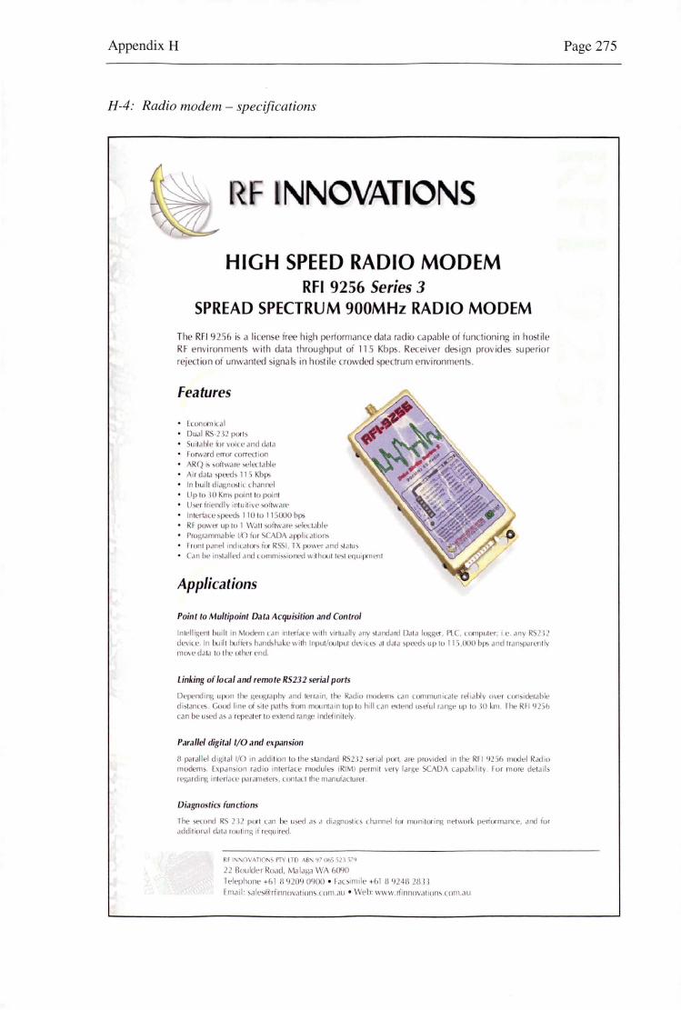
Appendix H
H-4: Radio modem - specifications
NNOVATIONS
HIGH SPEED RADIO MODEM Rf I 9256 Series 3
SPREAD SPECTRUM 900MHz RADIO MODEM
The RFI 9256 i a Ii en;e free high performance data radio apab le of functioni n • in ho;t ile RF environm 111- with data throughput of 11 5 Kbp . R eiver d ign provid uperior rejection oi unwanted ignal in ho til crowded spedrum environment .
Features
lwn0t11K.al DuJI RS -232 porl>
• Su11.1l>lc u11 voice and dJ1.1 Forward rrnr correction
• ARQ >1tilwa1e >elet l a l ~e
Air da1a :.pc od 11 5 KbP> In l>ui ll di.ti;t <»I i< chan11el U1> 10 Ill Knb p< nl lo poml U!14:!1 ioeodly inlu!l 1ve 34Jilwa1e
lnlert3Le 1 ~ 110 lo 115000 bi)> RF Pll\\'tf up lo 1 \ ,111 ;oiM-.Ht' ~it>c 1 .1hll'
• Pro~ramma h , IKl tor CADA applical ons Frcx11 p.uwl md·l1J l or~ ioi RSSI. TX f>O\\l'r .md .., l t1 h1..,
Can be in>lalled and wmmi;,ioned " l hou l le;.1 equ pmen l
Applications
Point to Multipoint Data Acquisition and Control
ln lcll~enl hu1ll m lodcm tan 'nlffiau w11h \Jrll1ally any -1anc!a rd Dala l~g<.f, Pt.C. tompuler, i c any R l 12 de\lce. In bu 1ll bu11er> hand> hake wilh lnput/ou 1pu1 de\ tu" al da1a P"'-od> up 10 11 .OOO b1» and 1ran>paren1 ly n"'"' da1a 10 1hc o1her end
Linking of local and remote RS232 serial ports
Depend111)l upon 11,., 1:eoqr.1pl .rnd lenain, l he Rad"' 11K1denb <Jn <tx11muni<ale rel 1.1 l~y owt ux1'1thal1 , d1>l.tntt'>. Good llfll' tti Ill;' p.11~ irtx1111M)lll11,11n lop lo h1ll totl1 t'\l1;'1td U>t1ul r.Hlgl;' up Ill ll) k111 . n . RFI '125h can be u ~I a a rLpea1er lo cxlcnd ran~' incll1milely
Parallel digital 1/0 and t:'xpansion
!l parallel cli~1 1 al 1/0 in add11ion lo l he landard R51l1 >!enal porl. are I mv1ded m 1he RI I •11 . b model Rad io modem lx1>an>1on radio inleriace module. !RIM) perm11 \ety large SCADA Lapabtl11y I or more delail> rt~1rding mh!1iJ.t.l' 1M r.1111t'ter , LOnl,lt I lhe 1nanui.1LIU1cr
Diagnostics functions
TI~ =*'lond RS i2 p1xl lJll bt:• 11;t'{i .1~ .i di.1gno~I <...> lh..inrwl ior morn l ori~ nt•l\\Ork pl'n.orm.mc...t', ,11l(f ior
addllKJn.11 cla la r11u1 ng '' requircod
Rr l''n\·ATIO' PTY LTD 1\8' 'J7 C>h5 SlJ S.'."ll
22 Bou ler Road, )\.\a ia ~<1 \\'A (,()')0 I elephone +u 1 II '1209 OIJOO • ~al 11nilc +hi II '1243 20 U lmail: '" le>~ri111novat 1 011s wm au • Wei >: \\WW ri11111ov,111on' LOrl1 au
Page 275

AppendixH
Specifications MODEL RFI 9256 Series 3
PHYSICAL
Dimen>1ons ~\leighl Construction
GENERAL
Operating voliage Operating current
Slandby mode fransm1t mode (1 Watt)
Operaling lemperalure range Operaling I lumid11y range PJrameter and mode settings
TRANSMITTER
Oulpul Power Spuriou> emissrons Output protection
RECEIVER
Sen>itiv1tv End to end performance frequency range RSSI d1>play range
DATA SYSTEM
RS 232 handshaking Prolocol modes
Interface dat,1 speed
190mm L x UOmm W x 35mm 11 260grams Alodmed aluminium chas;1s and cover, with intL,;rated display
9 lo 16\IDC negative ground
150 mA Averages 350mr\ -1 0 to .,-60 deg C Up lo 95% non-condensing RI I @ 50 deg C In built >oilware
I mW lo 1 Wan soitware selectable <-&0 dBc Transmrtlcr is fully protected for any load@ full power@ 60 deg C
<· 106d!lrn for B ER 1 p.irl in 10"-4 Beller than 1 in 10"-6 BER for S/N 20 dB or better 915-928 MHz (Australia) 902-928 MHz ffCCl 921-929 MHz (NZ)
-110 to-f10 dllm in 5 dB steps
Hardware/ software/ none software selectable All common varianl> I PLCs supported including point I poinl, point I mullipornt and I layes mode> 110to115,000 bp>, >0ftware selectable all mode>
© RFI 2000 Spetriicat1ons may be ;ubjcct to d1a11ge without notice.
Page 276

Antenna ADL
Digital Modem 09 connector
09 Connector Wiring Details
Male D9 Viewed from loom end
CD Violet
Data::..~G~r~e~e~n'----11--~
0
Motec Part No. 61071
MoTeC
I Data 67 TEL EM 3 pin DTM (male pins)
3 CD 1o----E--12 Data
1 Gnd CD »o--j Note 1
2 +12 Volts
1 Ground
2 pin DTM (male pins) Note 1
The following pins can bo used; Switched Inputs (normally sw4) Speed Inputs, Digital Inputs
ADL Setup
1. Set Input pin's channol to "Carrier Dotcct"
2. Select one of the templates in the RS232 Communications Setup scroen.
NOTE: Tho modem may need configuration before 1t will connect.
Title Di ital Telemet Connection Dal<> 04/03/1999 Drawn ST App Products ADL
~ > "O Vi "O .. (ll
~ l:3 0. $::) .......
$::)... ~ -· :::c: 0
;:;J 0
~ ;:;J I -· ;:::
"" Ei --$::) .... -· 0 ;:::

Appendix H
H-6: Wheel speed hall effect sensor - specifications
Solid State Sensors Hall Effect Gear Tooth Sensors
TYPICAL AP PLICATIONS Au omotive and Heavy Duty Vehicles: • Camshaft d crankshaft speed/
po on • ransmission speed • achnmeters • An -skid/trac on control Industrial: • Sprocket speed • C in Ii k co eyor speed and
distance • Stop motion detec or • High speed low cost proximity • achometers. Co nters
catalog ustmg
~
FEATURES • Senses ferro metal targets • Digital curren si. king o put open
col.ecior) • Better sig al ·lo·noise ro:Jlio than
variab reluc ance sensors, excellent low speed performance, o put ampfl de no! depe dent on RPM
• Sensor eleclronicalty sa/f,adjusts to slight vmiations in runou and variations in temperature. simplifying inst lation and main ten ce
• Fast operating speed over 100 kHz • EMI resist I • Reverse polarity protectio and
tr. sie t protection untegrated in 0
all l. C.) • \t'fJde con nuous operali g
emperalu e r ge ( 40° to I SO"C), short te m to · so•c
MOUNTING DIMENSIONS (For referen oe only}
31,.~
125
I~ 30 4,6
01 1,9
~ . 70
Page 278
GT1 Series
GENERAL INFORMATION 1GT1 Series Gear Too Sensors use a magnetically biased all e eel integrated cir it to ac rate sense movement ot ferrous me al targets. his specially de· signed l.C., wi discrete capacitor and bias magnet. is sealed in OJ probe type package fer physical protectio and cos e: ective installation.
Uni s • II ·unc on 'ram a 4.5 lo 24 VDC power supply. Outp~ is digital , curren sinking (open collector) Reverse polarity pro ection is standard. If power is i dvertently • ·red backwards, the sensor will nol be damaged. 8uill-in protection against uJsed transien s to +60V, 40V is also included.
Optimumse sor perfcrm ceisdepe d· ent on the following variables which mus be considered in combination:
• Target material, geometry d spee-d • Sensor arge gap • Ambie-nt temperalure • Magnetic male ·a1 in close pro mity
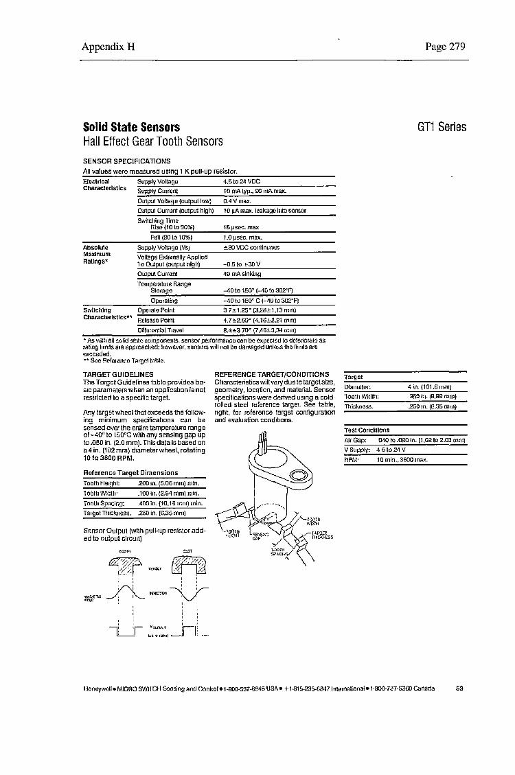
Appendix H
Solid State Sensors Hall Effect Gear Tooth Sensors SENSOR SPECIFICATIONS
All values were measured using 1 K pull-up resistor.
Eleclrtcal Supply VoltaQ£J '1.5 to 24 VDC
Charaelerlsllcs Su)Jply Curr!lnl 10 mA typ .. 20 rnA maK.
Al:lsolule Maximum Ra!lngs~
Ou1pu1 Voliage (oulput low)
0U1J'ul Currant (ou!pul high)
Swi!ching rlma Rise (10 to 90%}
Fall (00 to 103)
Supply Vollllgo (VSJ
Voltage Extm11all1• AppliC!'d lo Oulput {oulpul high)
OU1pul Cur1on1
Tcmp(lraturn Range Stotage
Opmaling
OAVmax.
10 µA rnax. tcakagll Into sensor
15µsc-n.max
1.0 µsec. rnax.
±:la VDC contlnlXIUS
-0.5to +30V
40 mA sinking
-•10 to 150° (-40 !O 302"1')
-·10 to 1 C--0' C (-40 lo 302"F)
Swilchlng Oporatef'oint :i 7±1.25° (3.28.!:1.13 nun)
Character1s11csu Rolnasa Point •l.7±2.so• (4.16.!:2.21 mm)
oarorential Travel 8.4±3 70' (7/l5±3.34 mnl)
·As with an ~lid stato components. sensor performanco can be ox~:HlCtcd to deteroara10 as rating turnls am approached: however. sonsors will not bo darnag<!d unlohs tho nn:1ls are rn<ccaded. •• Seo RC!fornnce Targat ta!J:C.
TARGET GUIDELINES lihe Target Guidelines t:ible prc,1ides ba· sic parameterswlien an applica!Ion is not restricted lo a specific target.
Nly target wheel that exceeds the follow· ing minimum specifica!Ions can be sensed over the entire temperature range of-40' to 150°C with any sensing gap up to .OBO in. (2.0 mm). This data is based on a4 in. (102 mm) diameter wheel, rotating 10 to 3600 RPM.
Reference Target Dimensions
ioo111 Hmnhl: .200 111. (5.0G rnm} min.
ioolll 1.v·rc111· .100 in. (2,54 rnrn) min.
TOCJlh Spacing~ ADD in. (10. lll Irlnl) min.
Target Thickness. 250 In. (G.35 mm)
Sensor Output (wiih pull-up resistor add· ed to output circuit)
rcor ..
~' I
r ' '
' ' r I
' I
---L_j-
I
' ~ y-
rw. '1 r... '"\.../: ' I ' I :
w~,_y ir-LI Q .. '\' IW.11 _.lJ :
REFERENCE TARGET/CONDITIONS Charnc1eristics v.~11 vary due to large! size, geometry, location, and material. Sensor specifications were derived using a cold· rolled steel reference target See table, right, for reference target configuration and evaluation cond1t1ons.
Page 279
GT1 Series
Targll!
DiamotQr: 4111.(101,Gmm)
1'00111 1Nid!tl: 35!> k1. (B.89 mrnj
Thii::k.noss. .25a m. (C!,35 mr11}
Tost Conditions
rur Gap: 040 to.OOO in. {1.0210 2.03 mm)
V Supply: 4 5 to 24 V
RPM· 10 min .. 3500 max.
llonoywell• MICRO SWI fCH Sansing and Conhol •1-800-537-6EM5 USA• +1-B15-235-G<M7ln!ernat1onal•1-800-737-3360 Canada 53

Black/ Red ADL +SV
Operating Temp -40to•150 deg C Black I White Oulput Stales Air : High Sig Metal Low (8 sec Hold Typ) !;Black +8V +8V
ov Sig Speed or Digital Input
NOTE: Shielded Cable should ov OV used to connect sensor.
~ ~ 'l 'rj ..
(ll
~ t::l p..
(1:> ;;;;·
(1:> ::i:: -~
(1:> (1:>
~ ~ ~ --I ECU ~ (1:> r:. ..... c.,
+BV +BV (1:> ;:s
Sensor Sig Digital Input c., c --= ov ~ ov I ....
Tooth Width Tooth Spacing 2.5 mm min Gap 10 mm min
Tooth Height fi 2.0 mm max1/ l 5mmmm
e-= ~ TC MUX (Hall Type)
+8V +8V
;:s c.,
s --~ ..... .... c ;:s
Sig Input
ov - ov Disk Thickness : 6mm minimum
ADL Setup
Speed setup. •fvlal use:J n Tra:;!m Ccru<l ttl9 e:ige.,;1Ji3"1on Of Ute t8E!'l1 mL.t>l t.e less !I~
Select "HALL" Sensor type O 5% (fo gl•e 1 Kl'l I In 200Kl'H a:i:Lla::y)
eg 11 tl13 Edge spocln;i Is 2Dmm tllen 1113 •arl<tJ01 mLE! te less 111'11O1 mm
MoTeC Title GT101 Hall Effect Sensor Sheet No Drawing No
Dato I Drawn ST I App I Products ADL, ECU, TC MUX 1 of 1 X02
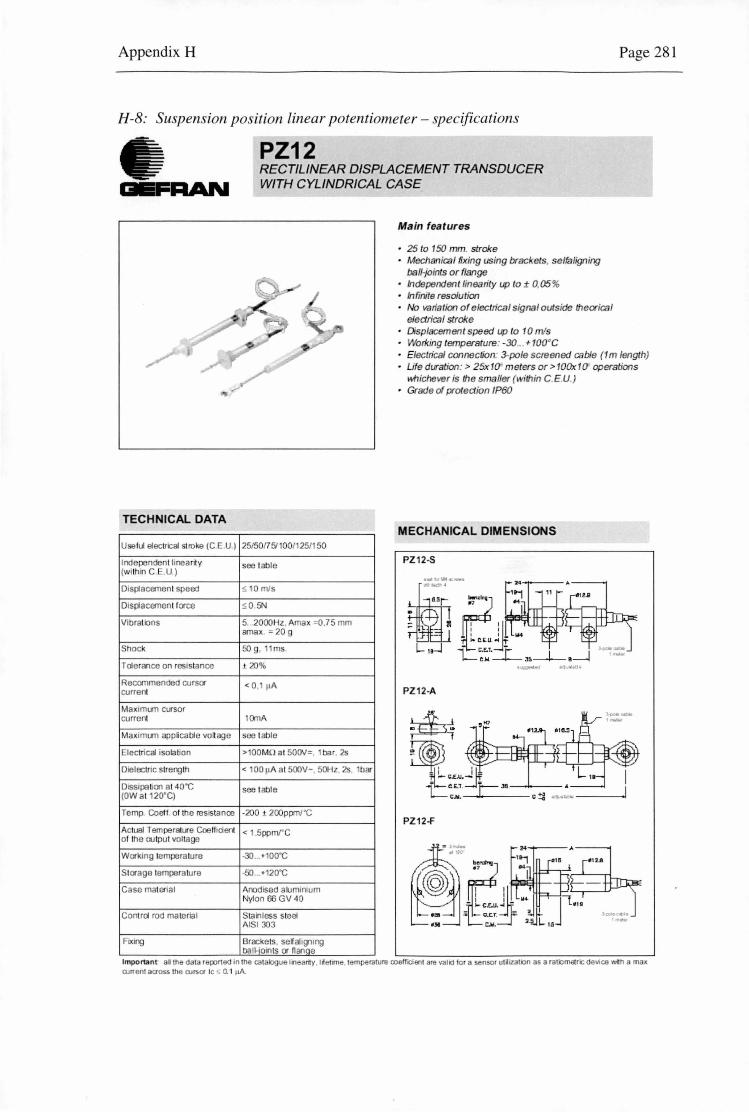
Appendix H Page 28 1
H-8: Suspension position linear potentiometer - specifications
TECHNICAL DATA
Use ful electrical stroke (C E U.J
Ind pendent linc;i rijy (wi th.i C .. U.)
D1spl<icement speed
Displacement force
Vlbral ions
Shock
T oterance on rcsi t;incc
Recanr ended cursor current
Maxlmt.rn CtXsor current
Maximum ;ippie<ible vott<igc
I Electrical isolation
Dielectric strert;ilh
Diss1pat100 al 40 'C (OW al 2o· q
Temp Coetf. or th e resist<inoo
Actual TemperattXe Coetlicienl o f the output voltage
Working temperature
Storage ter perature
Case material
Control rod ma terial
FIXUlQ
PZ12 RECTILINEAR DISPLACEMENT TRANSDUCER WITH CYLINDRICAL CASE
- -
25150({ 51 001 25/ 50
see table
S. 0 m/S
S.0 5N
5 2000Hz. Amax :0,75 mm ama x. = 20g
so g, ms.
?0%
<O, pA
OmA
soo table
> OO MO <i i 500V= . bar, 2s
< 00 uA a t SOOV-. 50Hz. 2s b<r
see table
-200 2ooppm1·c
< 5ppmrc
-30 ... • lOO'C
-50 ... 1 20'C
Arodised atumlrlum Nylon fi6 GV 40
Stainless steel Al 1303
Brackets, se"al1gi1rt;1 balHoints or nanae
Main features
25 to 150 mm. stroke Mechanical fixing using brackets, selfaligning ball-joints or flange Independent linearity up to :t 0,05% Infinite resolution No variation of electrical signal outside theorical electrical stroke Displacement speed up to 10 m/s Working temperature: -30 ... + 1oo•c Electrical connection: 3-pole screened cable (1 m length) Ute duration: > 25x10' meters or >100x10' operations whichever is the smaller (within C.E.U.) Grade of protedion IP60
MECHANICAL DIMENSIONS
PZ12-S
PZ12-A
~~ ~~-1 1'= - c.c.u.-
-1- C.£.1. t:= J6
~ C.N. I--- C ~
PZ12-F
Important' al the data reinrted in the catabgue lilearity . lietime. temperature ooetficient are valid tor a sensor utiizaton as a ratiomSric device ,,._ha max airrent across the rursor le ,; 0.1 µA.
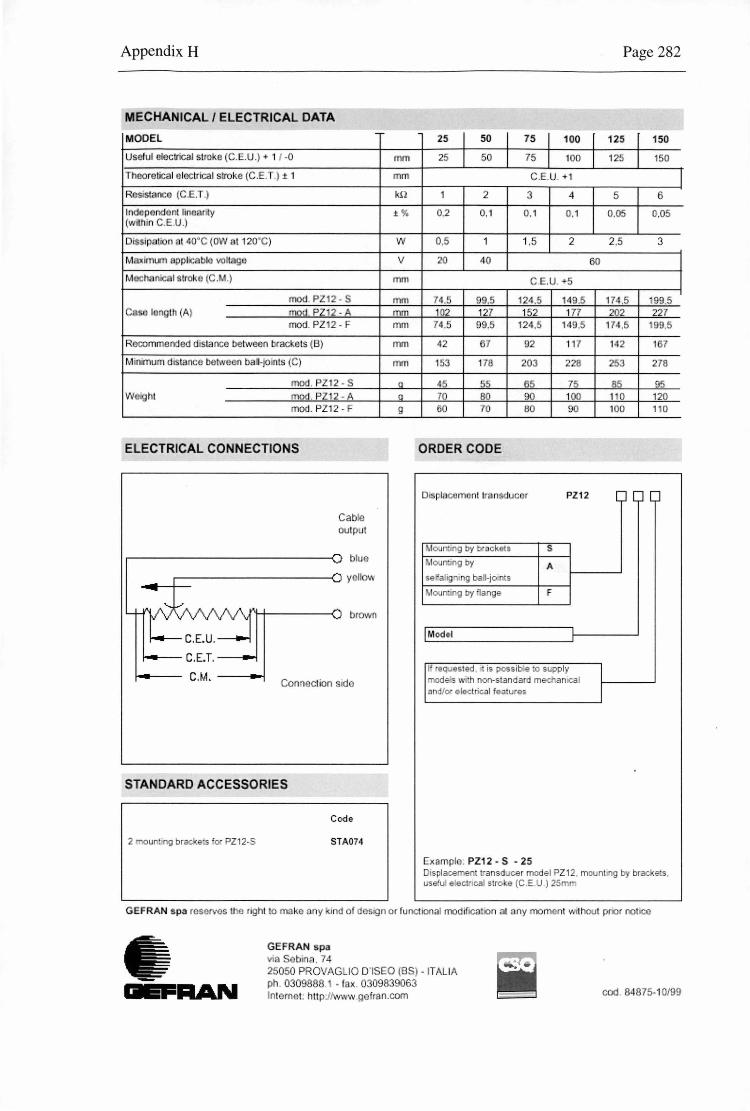
Appendix H
MECHANICAL I ELECTRICAL DATA
MODEL
Useful olec ncaJ . Oko C . . U.) + 1 J -0
n oretical oloc ical s roke (C.E.T.) ± 1
RllSISlanc (C.E.T .)
lndsponderl inoa y (vrilh n C.E.U.)
Dissipation at 4-0•c (OW at 12(). C)
Maxir um applicabl vo age
Mechanicals roko (C . . )
mod. PZ12- S CasG ngth (A) mod. PZ12-A
od. PZ12- F
Rocomr nded tanc bot ~ Ql'I . aclw t · (B)
M ir u ·n distance ootwii n ba ll-;:> IS (C)
moo . PZ12 - S Weig t mO<J. PZ12 -A
moo. PZ12 -F
ELECTRICAL CONNECTIONS
Cable outp
blue
~------------<'. i yellow .... r-r-
-
brown
Coo acl ion sido
STANDARD ACCESSORIES
Code
2 mounting bracl<e!s or PZ 12-S STA074
rrwn
mn1
kn
± %
w v
m
mm mm
ffl
r m
mm
0
0
g
25 I 50 I 75 I 100
25 50 75 100
C.E.U. +1
1 2 3 4
0,2 0. 1 0.1 0.1
0,5 1 1,5 2
20 40
C . . U. 5
74.5 99.5 124.5 149.5 102 127 152 177
74 ,5 99,5 124,5 149,5
42 67 92 117
153 178 203 228
45 55 65 75 10 80 90 100 60 70 80 90
ORDER CODE
DisplaC4lmQnt an ·ducQt PZ12
itoumin9 by b ackets s Mouru:in9 by A se atig mg ball-joints
Mouraing by ·1ange F
Model
I' equeslad , is poosi a 10 supply mode with non-standard mechamcal .and/o electrical fea!ures
Exampl . PZ12 · S - 25
Page 282
r 125 r 150
125 150
5 6
0,05 0,05
2.5 3
60
174.5 199.5 202 227
174.5 1911.5
142 167
253 278
85 95 110 120 100 110
Displacemen: transduc.er model PZ 12. mounLng by brac!o;eis use' e ctrical $1roke (C.E. ) 25
GE.FRAN spa resa os t rlghl to ako any I o closlgn or luncilonal mod flcauoo al any omoot wllhoot pOO( rlOliC
GEFRAN spa ·a S bi a. 74
2 050 PROVAGLIO O"ISEO (BS) - ITAL IA ph. 0309888. - fax. 0309839063 lnt rnet: http:/ vww.ge ran.corn cod. 84875-10199

ADL Setup (to measure distance)
Channel Assignments Assign a dis1ance channel ia: Brake Pedal p:isitbn
Sensor Calibration 1. In Cafibration, select change. 2. Select Ratiometric(5V). 3. In calibration table enter the distance
the pedal has moved and press "Read Value". You will end up with a table like the example.
v mm 1.23 0 1.99 5 2.34 10 2.89 15 3.04 20
Deutsch MT04-3P
SV
Sig
ov
Note 1
ADL
- 18,28,44 5V 5V
Sig Note 1 ov 17,27,43 ov
Analog Voltage (Pins 1,2,3,4,5, 19,20,21,22,23,24,25,26 45,46,47.48,49,50) or Analog Temp ( Pins 34,35,36,37 ,38, 39,41,42 ) input may be used.
Mo T.e C 1--Ti_t1°_L_in_e_a_r--r-P_o_s_i_t~io_n_S_e...,..n_s_o_r _____ ----l Sheet No Drawing No
I ~ Date 21/09/1999 Drawn ST App AD Products ADL 1 of 1 X24
~ > "O \0 "O ..
(D
V:l :;:! :::: p.. ...... {5 ><
Cl:> :::c: ~
"' .... 0 ~
'\:S 0
"' .... ..... .... 0 ~ -.... ~ Cl:> l::l "I
'\:S 0 ~ ~ ..... .... 0 ~ Cl:> ..... Cl:> "I
I s· "' ~ --l::l ..... .... 0 ~

Steering Shaft
+5V:::. ----
SIG -a.-------1
3 Pin Deutsch (mating connector #68052)
RED +SV .--'-~----------< 3
---....-~V_:_:IO::..:L::.:E::..:T:..___....:::S:..:..IG=----1 2
.....,B""l""a""ck=----=-OV_.__---l 1
ADL Setup
Channel Assignments NOTE 1 Assign a Steenng Channel to the appropriate pin
Sensor Calibration Measurement method = Ratiometric Tum wheel to desired angle & enter angle In deg table. Then click on read value to read sensor., Right tum= pos1bve angles Left turn = negative angles Straight = 0 degree
ADL PINS
+ 5V Analog Pins are 18, 28, 44 OV Analog Pins are 17, 27, 33, 40, 43 Analog Volt Input Pins are 1, 2, 3, 4, 5, 19,20,21,22,23,24,25,26,45,46,47 48,49,50
OV::.o---
ADL
Sensor5V NOTE1 Analog Volt Input
SensorOV
Tille MoTeC STEERING ANGLE SENSOR Sheet No Drawing No M 0 Te c f-D-a-te--1-2/-121_2.:_0_DD---,-D-ra_w_n_ST--.-A-pp--r-P-ro-d-uc-!s_A_D_L ____ -I 1 of 1 X21
~ :;.:.. 'O
~ 'O c:;, ('!) .. ::i
V:l 0.. -· ..... ~ (1:) (1:)
~ ""I .... ;::::
OQ
~ ;::::
OQ -(1:)
~ ~ .... ~ -'""C:::I ~ ~ ;:::: ..... .... ~ ;::; (1:) ..... (1:) ""I I ....
;:::: t;.:i
~ -iS"' ..... .... ~ ;::::

Appendix H Page 285
H-11 : Brake pressure transducer - specifications
APPLJCATIONS
HYOAAUUC I P EUMAOC COf\'ffi LS
co,vPRfSSOR E " ATION/
ClllLLERCO TROL
OCE S CON OL
Y lEMS
E GI rco T OLS ANO MO l 0
ECLIPSE®. OEMPRESSURETRANSDUCER
The Eclipse• Is designed for high
volume OEM's needing a low cost pressure
transmitter for Industrial or other heavy
duty applications. The Ecllpse 's combina
tion of rugged packaging, Interna l signal
amplification and price make It Idea l for
many app lications.
The pressure media Is contained by a
brazed assembly of stainless stee l. There
are no hidden 0-rlngs or elastomers
contain ing the media . A plated steel case
protects the Internal electron ics.
It Is available with ellher a 0.5 to 4.5
voll or 4 to 20 mA oulput. The 4 to 20 mA
output Is useful for applications where
electrica l noise may be a concern . Many
units are CE compliant.
FEATURES BENEFITS
• ol1:1gt: 11r currcru o ut put
15 PSIG thrnu!.! h - JOO PSlS r.1ngt:s
• High pcrfo n n:w eat Ju ,, price::
• C:E \ ' tT. i1>1L' J \·ailahlc
• ~ ·at llnpmnf L ypc:: connc::clllr
• Rc,·c::r:. 1m!J rit)' pn>tt:Ulnn
• Low cxc1ta1ion volt:tgt:
• II' l5 sc::akd !'olt:el c.1 ~t'
• FI xlbil ity for th dc:.igner
• .'u.lubh: for n1:U1)' a ppl ication.~
Redu ·cs ( E.\ l S)'Stt'lll co. 1
• Ready fur Elm p t:
High rdiabili ty and Lt c::r f lt:xihi lil)'
0 1 d:uu:1gcd hy r . ,, rscd wiring
• .' ui1ablt: for OR or marine U:.t'
• .o mplc::lt: c::nvironmcntaJ pmtt:ction fi >r d ect r inics
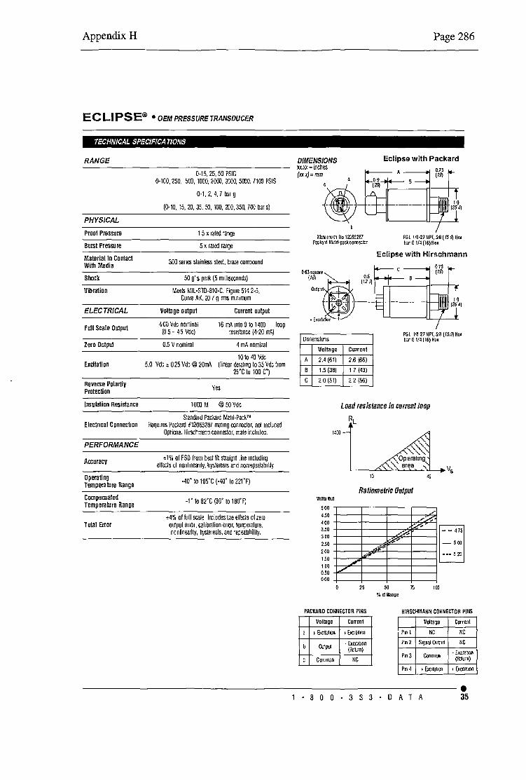
Appendix H
ECLIPSE® • OEM PRESSURE TRANSDUCER
TECHNICAL SPECIFICA nONS
RANGE
PHYSICAL
Proof Pressure
Burst Pressure
Material in Contact With Media
Shock
Vibration
ELECTRICAL
Full Scale Output
Zero Output
Excitation
Reverse Polartiy Protection
Insulation Resistance
0-15, 25, 50 PSIG 0-100, 250, 500, 1000, 2000, JJOO, 5000, 7100 PSIS
0-1, 2, 4, 7 tnr g
(0-10, 15, 20, 35, s:J, 100, 200, 350, 70J bars)
1 5 x rated ran~
5 x rated ran;ie
300 sems stainless steel, braze oomoound
50 g's pea~ (5 m1lhsecond5)
Mee:S MIL-ST0-810-C, Figure 514 2-5, Curve AK, 20 7 g rms minimum
Voltage output
4 00 Vd~ nominal (05- 45 Vdc)
0.5 V nomiml
Current output
16 mA into Oto 1400 loop res1stmce (4-20 mA)
4 mA nominal
10 to u.i \Ide 5.0 VO:: 025 Vd~@ 20mA (llll"..ar rerat11YJ to 35 VO: tram
25'C to 100 C'J
Yes
1000 M @ 50 \Ide
Slandard Packa1d Metrl-Pack™ Electrical Connection Requires Packard #12065287 rmtmg connoctor, no1 mcluded
PERFORMANCE
Accuracy
Operalino Temperature Range
Compensated Temperature Range
Total Error
Optional Huschrmnn connoctor, mate incluJed.
,,1% of FSO from best lit straig;it line mcludi!YJ etlects al nonlmearity, hysteresis and nonrepeatab1lrty
-40" to 10s·c (-40' to 221 'F)
-1' to82'C (30' to 180'F)
,,4% of full scale ln:ludes the ell:cts of zero output error. calibration error, temperature, nonlinearlty, hyste1esls, and repeallbility.
Page 286
DIMENSIONS xx.xx = inches (xxx)~m11
Eclipse with Packard
Mllarni:il !lo 12:165287 l'Jc"1d l.\e!rl-Jllci<COIUle!:l:Jf
P5l 118·27tlPT. 5111 ( 15 9/ Hex bar G 1/4 (16) Hex
Eclipse with Hirschmann
06~~uore. t~z'°il~ 6 Output 1- rr--
? 1 - , ~ --
1 Exaboon ~------1~--/--.L
~lrnenslons PSL 118-27 !IPT, 5.~ (15.9) Hex bar O 114116) H'x
A
B
G
Voltage
2.4 (61)
1.5 {3B)
2 Q (51)
t~Ol
Volts OU!
500 4.5()
400 3.50
Current
2.6 (66)
1 7 {43)
2 2 (56)
load resistance in current loop
RL
Raliometric Output
..
300 2.5()
200 +---t--.,,,...~-~-~P"'-;.;i:"_'_t-_---1 :
·"' ~ 1~0
100 --0.50 OOO
25 50 %of Range
75 10]
PACKARD CONNECTOR PINS HIRSCHMANN CONNECTOR PtllS
Voltage Current Vollaoe Curren!
a '&.cilaloo • E.>olaloo Pm 1 NC NC
b ()JlpUI • [XCilalOll
{l\JIJrn)
c C1JTirn:>n NG
Pm2 S~nal OJ'!mt NC
Pm3 CcmnCJl -fa:itJ!l)n
(llllurn)
Pm•! •bx:illlCil t &CllalOO
------------~~--~-----------~------~ . 1·800-333-DATA 35
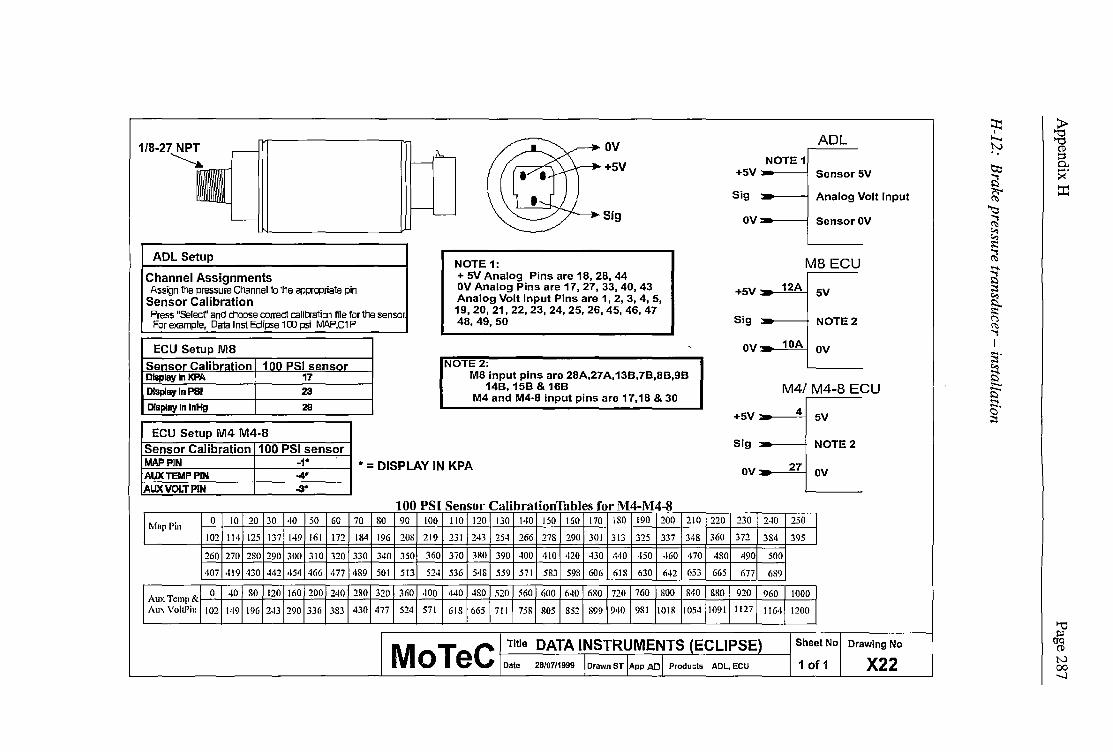
1/8-27 NPT ~
ADL Setup
Channel Assignments Assign 1he pressure Channel to 1he <f.lJ:JqJiia1e pin
Sensor Calibration Press "Select" and choose correct calit::ratim file ror the :sensor For example, Data Inst Eclipse 100 psi MO.P.C1 P
ECU Setup MS Sensor Calibration 100 PSI sensor Display In KPA 17
Dlspley In PSI 23
Dlsplay In lnHg 29
ECU Setup M4 M4-8 Sensor Calibration 100 PSI sensor
NOTE 1:
ov +5V
Sig
+ 5V Analog Pins are 18, 28, 44 OV Analog Pins are 17, 27, 33, 40, 43 Analog Volt Input Pins are 1, 2, 3, 4, 5, 19,20,21,22,23,24,25,26,45,46,47 48,49,50
NOTE2: MB input pins are 28A,27A,138,78,88,98
148, 158 & 168 M4 and M4-8 input pins are 17,18 & 30
MAP PIN -1· * = DISPLAY IN KPA AUXTEMPPIN ""'. AUXVOLTPIN -3"
100 PSl Sensor CalibrationTables for M4-M4-8
MupPin 0 10 20 30 40 50 60 70 80 90 100 110 120 130 140 150 160 170 ISO 190 200 210
102 ll4 125 137 149 161 172 lS4 196 208 219 231 243 25-1 266 278 290 301 313 325 337 348
260 270 280 290 300 310 320 330 340 350 360 370 380 390 ·IOO 410 420 ·130 440 ·150 ·160 470
407 419 430 -142 454 466 477 489 501 513 524 536 548 559 571 583 598 606 618 630 6·12 653
AuxTcmp& 0 -10 80 120 160 200 240 280 320 360 .100 440 -ISO 520 560 600 640 680 720 760 SOO 840
Aux VoltPin 102 149 196 2.13 290 336 383 430 477 524 571 618 665 711 758 805 852 899 940 981 1018 105·1
ADL
NOTE1 +5V Sensor 5V
Slg - Analog Volt Input
ov SensorOV
MBECU
+5V 12A 5V
Sig NOTE2
ov 10A ov
M4/ M4-8 ECU
+5V 4 5V
Slg NOTE2
ov- 27 OV
220 230 2·1D 250
360 372 384 395
480 490 500
665 677 689
880 920 960 1000
1091 1127 1164 1200
M 0 Te C f-T_it_le_D_A_JA_l~N_S_T_R~U_M_E_N_T_S_.__E_C_L_IP_S_E_,__---i 5
1
h
0
eeft1
No DrawXin
2g
2No
Dato 2810711999 Drawn ST App AD Products ADL. ECU
~ ~ "- "O N (1) .. :::s ~ 0..
i:$ $<"
""" :::c: (I)
'T;:! ;-; c., c., :::: ;-; ...... i:$ ;::: c.,
~ ("') (I) "-: I .....
;::: c.,
iS' --~ ...... ..... c:> ;:::

Appendix H
H-13: Attitude & heading ref erence sensor - specifications and installation
AHRS New ...
ATTITUDE & HEADI G REFERENCE Y TEM
"' Roll, Pilch and Heading Angle in Dynamic Environments
"' Enhanced Performance alman Fil ter Algorithm
"' 1gh Stability Mi:MS Sensors
"' High Range Gyro and Accel Options
Applications
"' UAVRPV Control
"' Platform Stab1hzat1on
"' Avionics
JI ..
.... --
AH RS400CA (DMU·HD X·AHRS)
The Crossbow AHRS400CA IS a high performance, solid-state attitude and heading reference sys tem intended for airborne applications such as UAV control. Avionics. and Platform Stab1liza t1on. This high reltabtl1ty, strap-dcmn inertial subsys tem provides attitude and heading measurement With static and dynamic accuracy comparable to trad1uonal spinning mass vertical and d1rect1onal gyros
to determine stab1l1zed roll, pi tch. and heading angles 1n static and dynamics cond1t1ons The Kalman Fil ter implementation resul ts 1n a continuous on-line gyro bias calibra tion. and an adaptive attitude and heading measurement tha t 1s stabilized by the long term gravi ty and magnetic north re ferences Output data 1s provided in both analog and d1g1 tal (RS-232) formats.
Each Ine rtial System comes with a User's Manual offering helpful hints on programming, installa tion, and product information. In add1 t1on, Crossbow's GYRO-VIEW so ftware is included to assist you 1n sys tem development and evaluation. and
Page 288
his A RS400 s ries product builds on the performance of the AHRS300 series tt fea tures higher performance sensors, including silicon MEMS accelerometers and gyroscopes with lower noise and improved bias stability. all ems you to per form data acqu1s1t1on.
---:::. -----tt ... ..L ..... .... •
.. .... ...... ' ~
• ---l •
•
I ... , ... l
he A RS400C A achieves its excellent performance by employing proprietary Kalman Fil ter algorithms
T11 ·a..~I Accele1omae
Ti •ial Magnetometer
Temp Sens01
CPU+ EEPROM Caltbiauon Algorilhm
AHRS Blodc Diagram
crossbow techno logy, one • 41 daggett drive " san 1o se , ea 95134 2109
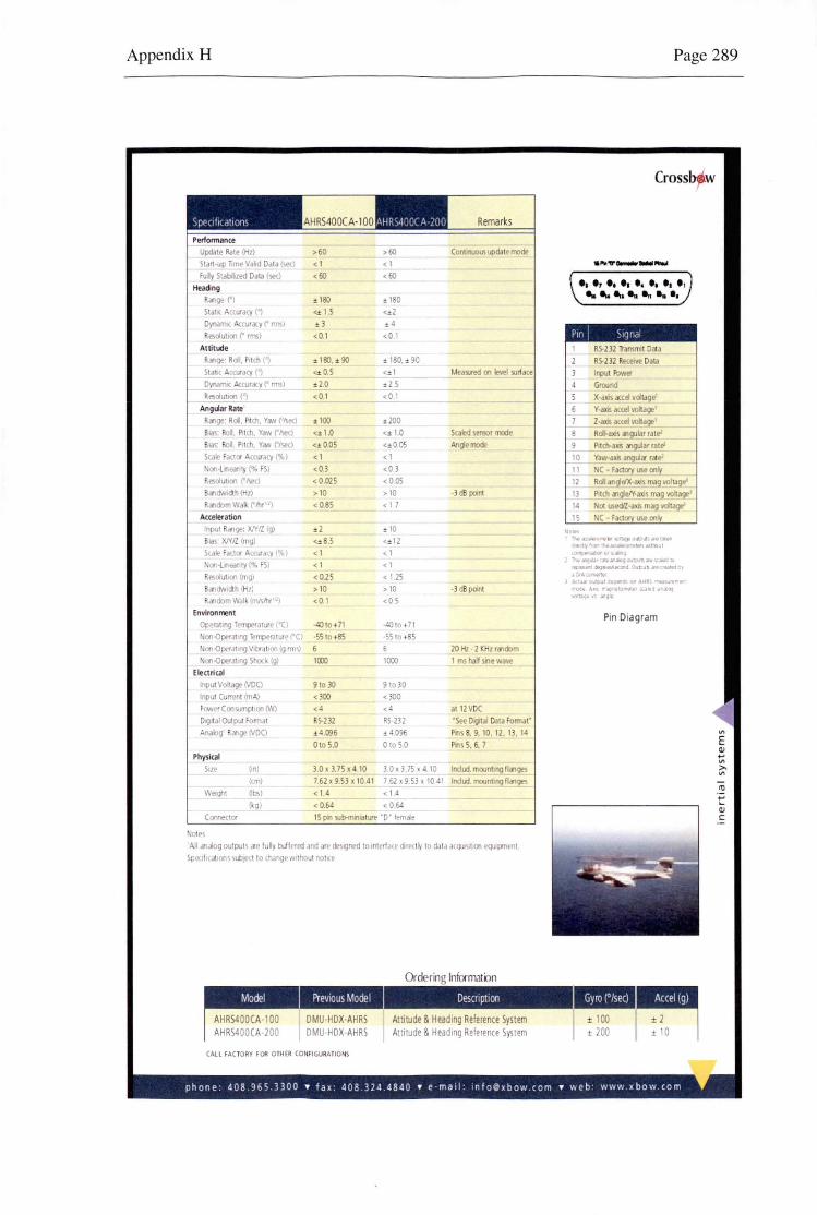
Appendix H
Performance Update Ra_t• I Hz)
Start-up ~me Va d Data (\eel Fuly Stabo zed Data (se<l
Heading Range ri State ~ccu<a<:y (') Dynam - Ac racy r rmsl Resolution r rmsl
Attitude R<rlge: Rol, P.t ii(')
Sta , Accuracy(')
Dynamc "<curacy r rmsl Resol t1on (')
Angular Rate Range Rol , l't · , YiJ11 ('~eel Sias: ~tch, Y;m file<l 8"'· P:lch, Ya.• rise<)
Scale factor ~ccur /% l on-lneanty (% FS)
Resol lltc)
8<11dM (Hz) RandomWa lh< ·)
Acteler ation Input Range: X/Y/Z <gl Bias: X/Y/Z 1mg) Scale tactor A.. :ura %)
on-lnear ty ('lo FS . ResolUllOfl (mgl 8<11d#idt ( zl Random Wal lmM>r 'I
Environment Opera~ng e"'ll"rJt re 'Cl
on-Operat ng ~rature Cl Noo-Operat1ng V11Yat100 {g rm':I)
on-Opera! ng Shoc< (g)
El•ctrical i"I' Voltage NDQ lnp t Curre<lt Im~) Power Consumpt on f\Vl Diglta l Outp format Anabg ange (VDQ
Physical Size (in)
(cm)
We~t Obsl gl
Comecta
ote>
AHRS400C A-1 00
>60 <I
<f>O
± 180 15
±3 <0.1
±180, ±90 <± 0.5 ±20 <01
± 100 <±1.0 <±0.05 < 1 <03 < 0.025 > 10 <085
±2 <±8.5 <1 <1 <0.25 >10 <01
- to•71 -55to•85 6
1000
9to30 <300 <4 RS-232 ±4.0\l6 Oto5.0
3.0xl.75x410 7.62x9.53x 1041
< 1.4 < 0.6J
>f>O
< 1
<f>O
± 180 <±2 ±4 <01
• 180.± 90 <± 1
±2 5 <0 1
±200 <± 1.0 <±0.05 < 1
<03 < 0.05 > 10 < 1 7
± 10 <:t: ll
< 1 < 1
< 1 25 > 10 <05
·" to +71
·55 to • 6 1000
9 to JO <JOO <4
S-232 ±4 096 0 to 50
l.Oxl75x 4. IO 7 62 x 9 53 x 10 41 <14
< 0.6J 15 pn 1Ub-mm1ture ·D· femile
Remarks
Con~ooous updat• mode
Measured on i.v.f IU~ace
Scaled semor mod• Angle mode
-JdB pomt
-JdBpanl
20 Hz - 2 KHz rilldom 1 ms half m•w..,,.
at 12VDC ·s.e Dqtal Data o ar p.,, 8. 9. 10. 12. 13, 14 p.,, 5, 6, 7
lndud. moont ng flan<JO' lnclud. moon\Jng flanges
All .11.iogourputs Jle I ly boffert'd and ,,re de>igned tomterfo<e drecl lo ddld ar""1S•l•on ""'pment Speof <at oos~ub I lo "qew thot.t nol(e
Ordering lnfcrmaton
+;1§1.11%'1' Description
DMU HDX-AHRS DMU-HDX-AHRS
CALL FAC TORY FOR OTHER CO NF IGURATIONS
Attitude & Heading Refeience System Arn ude & Head ing Re'erence Symrn
Page 289
... , ........... . ....................
RS-232 an<mll Data RS-232 e!W Data inputi<>w<J
Groond X·a acco voltaqe' Y·ax!! accel volta(ll'' Z-dlJS accel voltage'
Rol~a 'angular rate' P1tdi-aJa5 angi.iar rate'
I O Yaw-am a"!!ufar rate' 11 C Factory use ont,-12 Rollan1;e'X· s magYOltaq 1l Pitch <rlcJelY·axis mag voltage' 14 ot IM<VZ-a mag ...,iuge'
15 C Factory use ont,-
Pin Diag ram
""·· ..... ~-
--~- · ± 100 ± 2 200 ± '0
"' E QJ .,, "' >-"'
phone 408 965 3300 • fax 408 324 4840 • e mall 1n fo@xbow com • web www xbow com

Appendix I Page 290
16APPENDIX I - ENGINE SPECIFICATIONS
1-1: Engine specifications .................................................................................................................. 291
1-2: Engine top end exploded view ................................................................................................... 292
1-3: Engine crankshaft exploded view ............................................................................................... 293
1-4: ECU installation ......................................................................................................................... 294
1-1: Engine specifications
Engine: Type Cooling system Bore ana stroke Displacement Compression ratio Maximum horsepower
Maximum torque
Carburetion system Starting system Ignition system Timing advance Ignition timing
Spark plug Cylinder numbering method Firing order Valve timing:
Inlet Open
Exhaust
Lubrication system Engine oil:
Grade Viscosity Capacity
Close Durati6n Open Close Duration
4-stroke, DOHC, 4-cylinder Liquid-cooled 66 x 43.8 mm 599 mL 12.8 81.6 kW (111 PS) @12 500 r/min (rpm), (AS) 80.6 kW (109.6 PS) @12 500 r/min (rpm), (PR) 78.2 kW (106.3 PS) @12 500 r/min (rpm), (US) - - -65.6 N·m (6.7 kg·m, 48 ft·lb) @10 OOO r/min (rpm), (AS) 64.6 N-m (6.6 kg·m, 48 ft·lb) @10 OOO r/min (rpm) (FR)(US) - - -Carburetors, Mikuni BDSR 36R x 4 Electric starter Battery and coil (transistorized) Electronically advanced(digital igniter) From 12.5° BTDC @1 300 r/min (rpm) to 42.5° BTDC @5 OOO r/min (rpm) NGK CR9E Left to right, 1-2-3-4 1-2-4-3
56° BTDC 80° ABDC 316° 61° BBDC 33° ATDC 274° Forced lubrication (wet sump with cooler)
SE, SF or SG class SAE10W-40, 10W-50, 20W-40, or 20W-50 3.8 L

Appendix I
1-2: Engine top end exploded view
T1: 9.8 N·m (1.0 kg m, 87 in· lb) T2: 11 N·m (1.1 kg·m, 95 in·lb) T3: 12 N·m (1.2 kg·m, 104 in·lb) T4: 13 N·m (1.3 kg·m, 113 in·lb) T5· 15 N·m (1.5 kg·m, 11.0 ft·lb) T6: 25 N·m (2.5 kg·m, 18.0 ft·lb) T7· 20 N·m (2.0 kg·m, 14.5 ft lb) TB. 49 N·m (5.0 kg·m, 36 ft·lb) T9: 5.9 N·m (0.60 kg·m, 52 in·lb)
T10: 7 8 N·m (0.8 kg·m, 69 in·lb)
Page 291
1. Closed coil end faces downward. L: Apply a non-permanent locking agent.
M: Apply molybdenum disulfide grease. EO: Apply engine oil. SS: Apply silicone sealant.
R: Replacement Parts S: Follow the specific tightening sequence.
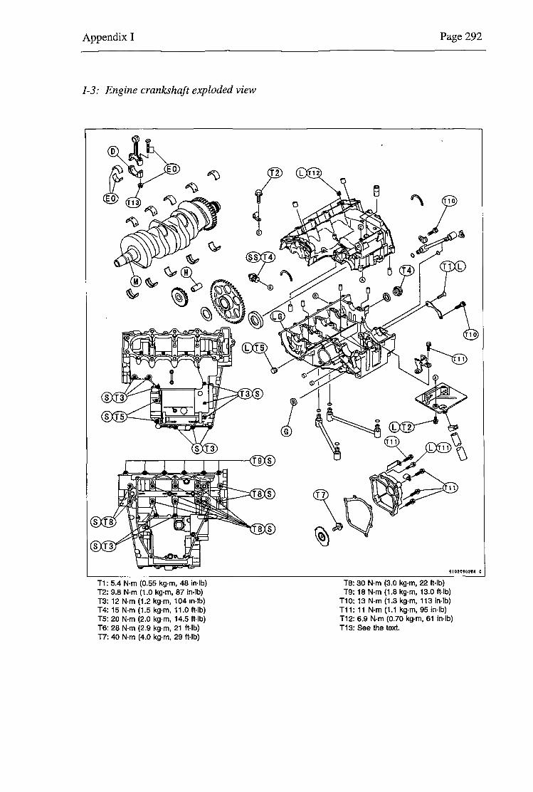
Appendix I
I-3: Engine crankshaft exploded view
T1: 5.4 N·m (0.55 kg·m, 48 in· lb) T2: 9.8 N·m (1.0 kg·m, 87 in·lb) T3: 12 N-m (1.2 kg·m, 104 in·lb) T4: 15 N·m (1.5 kg·m, 11.0 ft·lb) TS: 20 N·m (2.0 kg·m, 14.5 ft·lb) T6: 28 N·m (2.9 kg·m, 21 ft·lb) T7: 40 N·m (4.0 kg·m, 29 ft·lb)
Page 292
Ta: 30 N·m (3.0 kg·m, 22 ft·lb) T9: 18 N·m (1.8 kg·m, 13.0 ft·lb)
T10: 13 N·m (1.3 kg·m, 113 in-lb) T11: 11 N·m (1.1kg·m,95 in·lb) T12: 6.9 N·m (0.70 kg·m, 61 in·lb) T13: See the text.

Appendix I
I-4: ECU installation
Engine Sensors
Red 4
Throttle 16 Position Green Sensor
27 Black
~Red 4 Pressure 17
Sensor enge
27 Black
Engine Temp 28
D==--Purple 27 Sensor Black
Air Temp []==Grey 29
Sensor Black
REF and SYNC Sensors ·" Refer to the detailed drawings for the particular tngger system
Note 3
+8 Volts -- Red REF Sensor - White
0 Volts - Black
3 Core Shielded
Note 3
+8 Volts - Red SYNC Sensor - White
0 Volts - Black
3 Core Shielded
Note AU wires except those marked "Heavy" are 18# (0.85 mm21
Note 1 To avoid the ECU fuse blDwong due to reverse battery polarity use a diode activated relay Bosch 0 332 014 112
Note 2 The Ignition System power should be suphed by the Fuel Pump relay to ensure that the Ignition System power 1s off when the engine 1s stopped This also provides reverse battery protection for the Ignition System
Note 3 Remove the Foil and drain wire DO NOT connect the fool or drain wire to the sensor or to ground
Note4 The Aux Valve wire 1s connected to ECU Aux Output 1-
Note 5 The Fuel Pump wire as connected to ECU Aux Output 4
Note 6 <Refer to the detailed drawings for the particular trigger system)
Looking Into connector on ECU
/
13
36
33
Page 293
Fuel Injectors
Connect in firing sequence for sequential operation
White ---r-:;-::-i White/Blee~
White~2 d White/Red~
White ----f"3-d1 White /Yellow~ J White~ White I Green~
Not used on 2 cyl engines
White--fVI Brown~
Aux Valve Note 4
Yellow
Ignition System
(See Detailed Drawings)
25 Heavy Black
Earth at Engine Block
Chassis
MoTeC [8-=-=-=-=-=TIJ Connector to PC
L03 Sheet No Drawing No
M T". c Title M4 Loom 4 CYLINDER 0 I e Date 19/02/2001 Drawn ST App AD Products 1of1 ECU

Appendix J 294
17 APPENDIX J - TESTING DATA
J- 1: Testing data, logged at the University carpark straight line course ........ .... ........ ...... .. ..... ....... ....... ... 295
J-2: Testing data, logged at the University carpark Figure 8 course ........ .. .............................................. 300
1-1: Testing data, logged at the University carpark straight line course
Straight Line Course - Engine Speed
14000
12000
10000
i' ll. ~ 8000
l "' ~ 0.
6000 c w
4000
2000 -- -
1001 2001 300 1
Data Pattern No.

Appendix J 295
Straight line Course - Gear
2.5
~
2.0 - 1 - -- -- -- -
1.5 ~ -- --- _J - -- - -
: "
1.0 --
I - - ---
0.5 -- --- I - -
I
0.0
1001 200 1 3001
Data Pattern No.
Straight Line Course - Steering Wheel Angle and Throttle Position
120 - Steering
100 +---- - Throttle
BO
60
I 40
"' . 20 :!!. .!! "' . "
-20
-40
-60 +
-BO
Data Pattern No.
Straight line Course - Hydraulic Brake Pressure
7000
6000 - ~ ----+
5000 t n ~ 4000
! , = ! 3000 ..
2000
1000
1001 2001 3001
Data Pattern No.
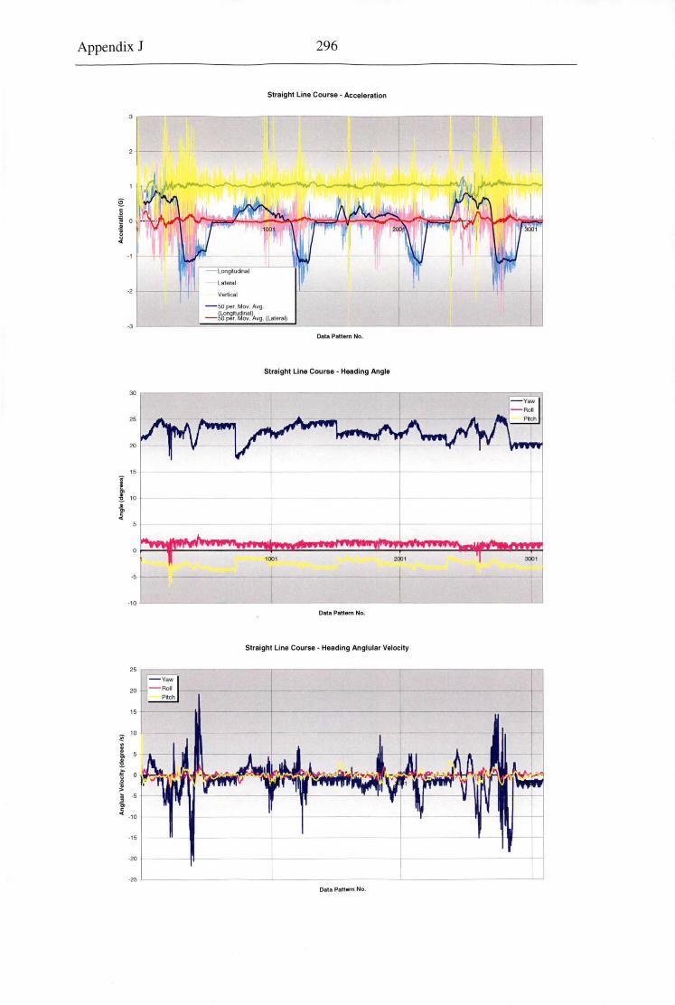
Appendix J 296
Straight Line Course - Acceleration
- so per. Mov. Avg.
-Ro~~~~~:1~vg. (lateraf) -3 L----'==""==:::::i::===:::!_._--------------_u
Data Pattern No.
Straight Line Course - Heading Angle
30
25
20
15
I O> .
10 :!!-
i " ----
0
1001 2Q0 1 3001
-5 I -10
Data Pattern No.
Straight Line Course - Heading Anglular Velocity
20
15
~ 10
i ! f 0
~ ~ -5
g. C( -10
-15
-20
-25
Data Pattern No.
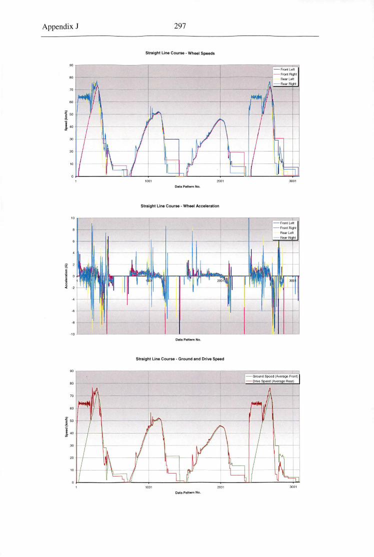
Appendix J 297
Straight Line Course - Wheel Speeds
w r-~~~~~~~~~--,r-~~~~~~~~~ .... ~~~~~~~-;::======~
80
70
60
I 50
l.o -11---+--
"'
20
10
1001 2001
Data Pattern No.
Straight Line Course - Wheel Acceleration
6 --- -i
Data Pattern No.
Straight Line Course - Ground and Drive Speed
80
70 -+- ---
60
I 50
l.o 11---1----t----------flf
"'
20
10
1001 2001
Data Pattern No.
-Front Lett - Front Right
3001
-Front Left ___ _,_ ___ _____, - Front Right
Rear Left - Rear Right
3001
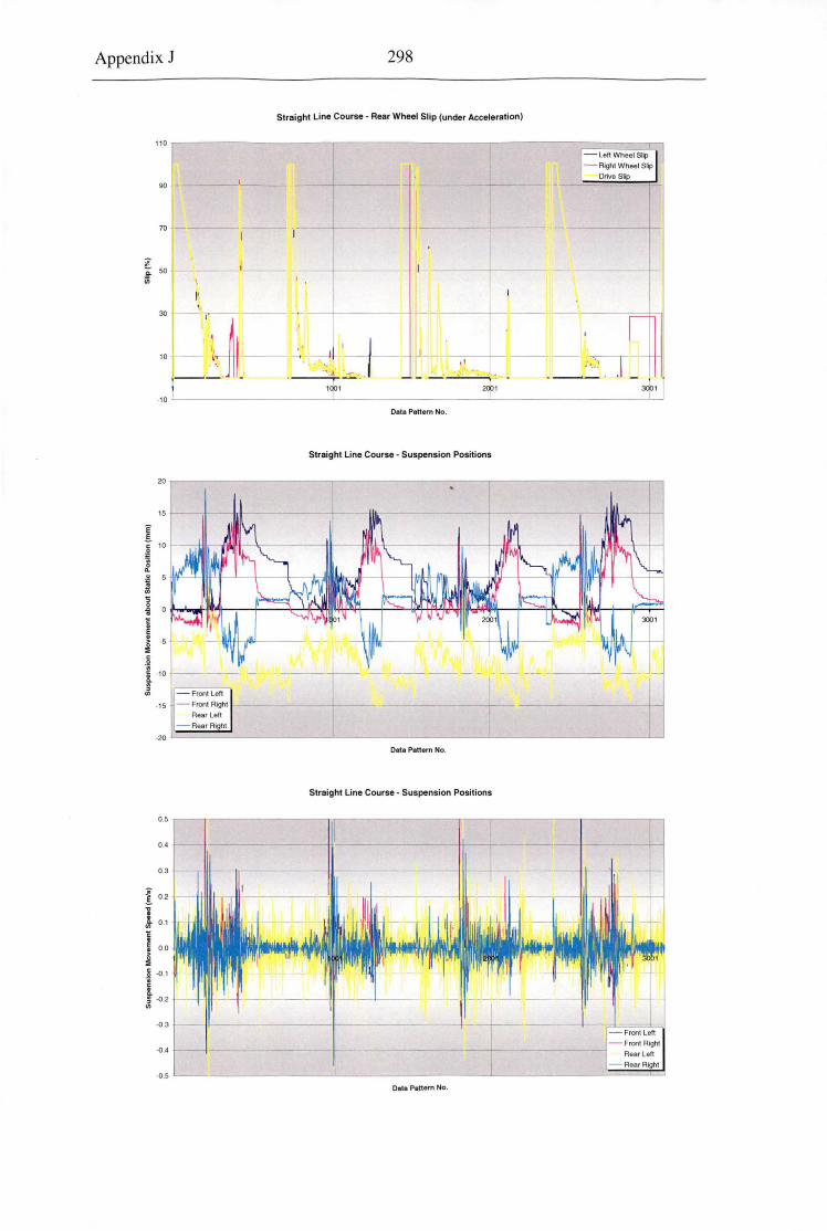
Appendix J 298
Straight Line Course · Rear Wheel Slip (under Acceleration)
110
90 t-70 ~--
~ 50 '--.!!-
'.J-iii
II 30
10 ~t-----~ - --
e ~
15
~ 10
£ .l! ;; iii
i c ~ j -5
·~ 1-10 VJ
Data Pattern No.
Straight Line Course · Suspension Positions
- Left Wheel Slip - Right Wheel Slip
Drive Slip
-15 - Front Right Rear Left
- Rear Right .roi:=::::::::::::=-..~~~~~-1.~~~~~~~~--1~~~~~~~~~........J
0.5
0-4
0 .3
i 0.2
l 0.1 VJ
c . E o_o j .s -0.1
c
~ -0.2 VJ
-0.3
-0-4
-0 .5
Data Pattern No.
Straight Line Course • Suspension Positions
Data Pattern No.
- Front Right Rear Left
- Rear Righi

Appendix J 299
J-2: Testing data, logged at the University carpark Figure 8 course
Figure of Eight Course - Engine Speed
-i 8000
i' .. ~
I 6000
"' ~ ·gi w
4000
2000
1001 2001 3001 4001
Data Pattern No.
Figure of Eight Course - Gear
2.5
I ~
2.0 I
1.5
. . "
1.0
I I
=-t - -
0 .5
0 .0 I I I 1001 2001 3001 4001
Data Pattern No.
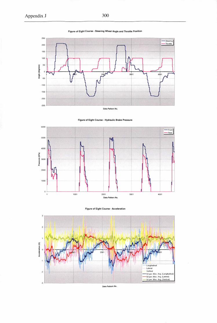
Appendix J 300
Figure of Eight Course - Steering Wheel Angle and Throttle Position
200
150
100
-150 +-----------+----!
-200 +----------+
Data Pattern No.
Figure of Eight Course - Hydraulic Brake Pressure
I ~
~ h -·----+--II- -- ---
· 1
·2
I
I I
1001
- ~----+-
2001
Data Pattern No.
Figure of Eight Course - Acceleration
Data Pattern No.
3001 4001
Vertical - 50 per. MOY. Avg. (longitud"8Q - 50 per. Mov. Avg. (Lateral)
- 50 per. Mov. Avg. (Vertical)

Appendix J
200
150
100
I "' . 50 :!!. ~ c ..
-50
120
100
BO
~
~ "' 60 ! ,. ~ !: 40 . , g. ..
20
,..1
-20
BO
70
60
20
10
1001
301
Figure of Eight Course - Heading Angle
Data Pattern No.
Figure of Eight Course - Heading Anglular Velocity
+-
Data Pattern No.
Figure of Eight Course - Wheel Speeds
-,
2001 3001
Data Pattern No.
---+-
Rear Left
- Rear Right
4001

Appendix J
30
20
10
§: c .2
1 j
-10
-20
-30
ao
70
60
I 50
l 40
30
20
10
50
40
20
10
302
Figure of Eight Course - Wheel Acceleration
Data Pattern No.
Figure of Eight Course - Ground and Drive Speed
1001 2001 3001
Data Pattern No.
Figure of Eight Course - Rear Wheel Slip (under Acceleration)
1001 2001 3001
Data Pattern No.
- Front left - Front Rignl
Rear Lei! - RearRlght
4001
-Left Wheel Slip - Right Wheel Slip
Drive Slip
4001

Appendix J
30
1.0
0 .8
0 .6
i 0.4
l 0.2 VJ
c E o.o j .a -0 .2
~ ~ -0.4
VJ
-0 .6
303
Figure of Eight Course - Suspension Positions
Data Pattern No.
Figure of Eight Course - Suspension Positions
- Front Lett - Front Righi
Rear Left
- Front Lett - Front Righi
Rear Lett - Rear Right
·0 .8 +-----------t-----------+----------+----------+--
Data Pattern No.