Estimating Industry Conduct in Differentiated Products Markets∗

The Evolution of Pricing Behavior in the RTE Cereal Industry

Christian Michel†

Stefan Weiergraeber‡

November 9, 2018

Abstract

We estimate the evolution of competition in the ready-to-eat (RTE) cereal industry.

To separately identify detailed patterns of industry conduct from unobserved marginal

cost shocks, we construct novel instruments that interact data on rival firms’ promo-

tional activities with measures of products’ relative isolation in the characteristics space.

We find strong evidence for partial price coordination among cereal manufacturers in

the beginning of our sample. Manufacturers’ price coordination intensifies following a

horizontal merger in 1993, with median manufacturer margins increasing from 20.8 to

38.1 percent over those implied by multiproduct Bertrand-Nash pricing, but eventually

fully breaks down to multiproduct Bertrand-Nash pricing.

Keywords: Markups, Market Power, Conduct Estimation, Differentiated Products Markets

JEL Classification: L11, L41, C51

∗We thank Daniel Ackerberg, Pierre Dubois, Juan Carlos Escanciano, Federico Ciliberto, Rosa Ferrer, JeremyFox, Amit Gandhi, David Genesove, Gautam Gowrisankaran, Kenneth Hendricks, Jean-Francois Houde, Kyoo-il Kim,Nathan Miller, Massimo Motta, Volker Nocke, Aureo de Paula, Helena Perrone, Barbara Rossi, Philipp Schmidt-Dengler, Johannes Schneider, Alex Shcherbakov, Sandro Shelegia, Andre Stenzel, Yuya Takahashi, Otto Toivanen,Frank Verboven, Matt Weinberg, as well as seminar and conference participants for invaluable comments. Michel grate-fully acknowledges financial support from the Spanish Ministry of Economy and Competitiveness Grant ECO2016-76998 and the Barcelona GSE Seed Grant SG-2017-14. Weiergraeber gratefully acknowledges financial support fromthe IU OVPR Seed Grant 2018.†Department of Economics and Business, Universitat Pompeu Fabra. Email: christian.michel@upf.edu.‡Department of Economics, Indiana University. Email: sweiergr@iu.edu.

1 Introduction

One of the central questions in industrial organization is to what extent firms exert market

power. Product differentiation, as one source of market power, can lead to positive markups

even if firms compete effectively with each other. In many industries, there are concerns that

a low intensity of competition further contributes to high industry markups. Empirically

disentangling legitimate from anti-competitive sources of market power is thus an important

task. This task, however, is very difficult because neither the intensity of competition nor

marginal cost, which is another price determinant, are commonly observed in the data.

A key identification problem in empirical industry models is thus to distinguish whether

firms charge high prices because of anti-competitive behavior or because of high unobserved

cost shocks. To separate the two channels, one needs to find suitable instruments that

are correlated with markups but not with underlying cost shocks. Recently, Berry and Haile

(2014) have shown that it is in principle possible to empirically discriminate between different

oligopoly models by exploiting variation in market conditions.1 In practice, however, many

of the instruments based on this type of variation tend to be weak. The few studies that have

focused on estimating industry conduct, as a measure of an industry’s competitive intensity,

have used alternative identification strategies, such as exploiting plausibly exogenous industry

shocks.2 Such identification strategies can already lead to important insights. However, they

often require the researcher to focus on estimating the conduct of only a subset of firms and

time periods, or to assume that the structure of conduct is invariant across time and firms.

In most cases, it is not clear a priori that the conduct in an industry follows such a pattern.

The level of conduct might not only deviate from competition but also differ substantially

over time and across firms. Not accounting for this heterogeneity can lead to inconsistent

estimates of markups and marginal costs. Allowing for more flexible conduct specifications is

thus likely to lead to more accurate predictions and more effective policy recommendations.

In this paper, we estimate detailed patterns of industry conduct that account for changes

over time and heterogeneity across firms in the US RTE cereal industry. To do so, we

employ a structural differentiated products demand model and a flexible conduct parameter

framework on the supply side. To separately identify industry conduct and manufacturers’

marginal costs, we propose novel instruments that exploit products’ relative proximity in

1Examples of this type of variation are the number of firms, the set of competing products, or functions of theircharacteristics.

2For example, Miller and Weinberg (2017) consider a joint-venture as an exogenous shock to estimate a parameterthat reflects how the behavior between the two leading firms in the US beer industry deviates from Bertrand-Nashpricing once one of them participates in the joint-venture. Ciliberto and Williams (2014) leverage a special feature ofairport gate leasing contracts to estimate conduct as a function of multimarket contact in the airline industry.

1

the characteristics space interacted with information on rival firms’ promotional activities,

which we explain in detail below. Our paper contributes to the literature by incorporating

an identification strategy based on variation in the characteristics space to estimate rich

patterns of industry conduct. We focus on estimating the behavior of firms in the industry

over time, and, in particular, on whether the behavior changes following important industry

events. Specifically, we estimate the levels of conduct between firms before and after the

1993 Post-Nabisco merger, and following a massive wholesale price reduction by most cereal

brands in 1996. Being able to accurately measure and explain the effects of such events is of

key interest for competition policy.

Our results indicate that there are indeed substantial changes in industry conduct over

time. We find partially cooperative levels of conduct between firms in the beginning of our

sample, followed by a further increase in cooperation after the horizontal merger. When

allowing our conduct parameters to differ across firms, we find that the pricing behavior

of the smaller firms during these periods is more cooperative than that of the two market

leaders, Kellogg’s and General Mills. Finally, our estimates are consistent with a drastic

change in industry conduct towards fully competitive behavior three and a half years after

the merger.3

Section 2 introduces our data and provides detailed information about the RTE cereal

industry and important industry events. We use scanner data from the Dominick’s Finer

Food (DFF) database. The database includes detailed information on DFF’s supermarket

stores located in the Chicago metropolitan area. In addition to detailed store-specific data on

quantities, retail prices and temporary promotions, one convenient aspect of our data is that

it contains information on wholesale prices. We analyze a five-and-a-half year span of data

from 1991 until 1996. Our sample period includes several important events, most notably

the Post-Nabisco merger in January 1993 and a period that began in April 1996 in which

manufacturers greatly decreased wholesale prices, which the business press referred to as a

price war. For brevity, we use this terminology for the remainder of this paper.

To motivate our structural model and our identification strategy, we conduct a series

of reduced form regressions. We find that following the horizontal merger, prices increased

significantly for the merging firms as well as for two other firms. However, three-and-a-half

years later, almost all of the manufacturers greatly reduced their wholesale prices within only

a few weeks which translated into shelf-price reductions of up to 18 percent for consumers

3Our results also relate to a long and extensive discussion regarding the underlying sources of market power ofnational cereal manufacturers. For example, Schmalensee (1978) argues that price competition is suppressed althoughfirms might still partially compete via advertising and product entry. In contrast, Nevo (2001) finds that markups inthe industry can be best explained solely by product differentiation and the profit-maximizing behavior of multiproductfirms.

2

(Cotterill and Franklin, 1999). These descriptive statistics provide the first evidence that the

interaction between manufacturers significantly changed over our sample period.

Typically, it is not possible to disentangle the different explanations for the observed

pricing patterns using only reduced form regression methods. Therefore, we introduce a

structural empirical model in Section 3. On the demand side, we use a random coefficients

nested logit (RCNL) model in the style of Berry et al. (1995) (henceforth, BLP) and Nevo

(2001), allowing for detailed consumer heterogeneity. On the supply side, we use a flexi-

ble conduct parameter framework that specifies the degree of cooperation by a matrix of

parameters that capture the degree to which firms internalize their rivals’ profits.

We consider our approach as having significant advantages over simply assuming a par-

ticular form of industry conduct, as is often done in the literature. For example, the most

commonly used assumption in such models is multiproduct Bertrand-Nash pricing. This

form of conduct implies that a firm maximizes the total profits of its own product portfolio

but fully competes with all rival firms’ products. Such a specification limits the heterogene-

ity of markups over time and across firms by assumption. There is a growing interest in

the heterogeneity of markups in both the macroeconomics and the trade literature, which

usually rely on estimating output elasticities using a production function approach; see for

example, De Loecker and Eeckhout (2017). Our approach allows us to estimate whether

there is markup heterogeneity within an industry that can be attributed to heterogeneity in

industry conduct.

Section 4 explains the details of our identification strategy. We exploit variation across

markets in firm’s markup incentives caused by temporary promotions for different products.

The intuition is the following. In many consumer products industries, promotions are agreed

upon between a manufacturer and a retailer several months in advance. This is done for vari-

ous reasons, for example, a sufficient supply of the product must be ensured and promotional

brochures must be printed.4 Therefore, rivals’ promotional activities in a given time period

should be exogenous to innovations in a specific product’s demand and supply shocks. We

provide reduced form evidence that supports the implied timing assumptions. In particular,

we show that wholesale prices react to cost shocks immediately, i.e., in the same month,

whereas the promotional intensity of a product is not affected by contemporaneous shocks.

The promotional intensity of a product 1 to 5 month in the future, however, is significantly

affected by shocks today.

Furthermore, the promotional activities of a rival product will affect a product’s own de-

mand. While promotions typically come with a decrease in the retail price of a product, we

4In both Europe and the US, retailers often establish a planogram of promotions for an entire product categoryseveral months in advance.

3

show in reduced form regressions that –even when controlling for the lower retail price typi-

cally associated with promotional activities– promotions also have additional, nonmonetary

effects on demand, for example, because of an increased coverage in a retailer’s brochures,

better shelf space, or in-store promotional signs for products “on sale”. It is mainly these

types of nonmonetary demand shifts that we exploit for our instruments to identify industry

conduct. The shifts in competitive pressure by these promotion effects will be stronger the

more consumers consider these products as substitutes. Therefore, firms have an incentive

to adjust the markups of all their products accordingly. This is why we interact the num-

ber of rivals’ promotions with the products’ relative proximity in the characteristics space.

The relative proximity feature is shared with the class of differentiation instruments recently

proposed by Gandhi and Houde (2017). In contrast to their approach and to classic BLP

instruments, we do not require product entry or exit to induce variation in the character-

istics space. Instead, we exploit variation in products’ promotional activities as shifters of

firms’ pricing and markup behavior. We conduct a series of weak identification tests for both

our demand and our supply side estimations, and find that our proposed instruments indeed

prove to be very powerful in identifying both consumers’ price elasticities and manufacturers’

industry conduct. The data required to construct our instruments are readily available for

many consumer goods industries, and thus our empirical strategy has broad applicability.

Section 5 presents our main estimation results. We find strong evidence for partial co-

ordination in the beginning of our sample period, and for an additional increase following

the Post-Nabisco merger in 1993. When we restrict the conduct parameters to be equal

across firms, our pre-merger conduct estimate of 0.277 indicates that a firm values US-$ 1

of its rivals’ profits as much as US-$ 0.277 of its own profits. Furthermore, our estimates

reveal that pre-merger, price-cost margins are 25.6 percent higher than under multiproduct

Bertrand-Nash pricing. Following the merger, the estimated conduct increases to 0.454, im-

plying a 42.7 percent median margin over that for multiproduct Bertrand-Nash pricing. Such

an increase is, for example, consistent with a merger further facilitating coordination across

firms in an industry.5 When allowing the conduct parameters to differ across firms, we find

that the small firms’ internalization is higher than that of the two largest firms (Kellogg’s

and General Mills). The overall median margins are slightly lower in this model, at 20.8 and

38.1 percent over multiproduct Bertrand-Nash pricing pre- and post-merger, respectively.

Moreover, towards the end of our sample period, for both specifications, we estimate conduct

parameters close to 0, which is consistent with multiproduct Bertrand-Nash pricing.

5Throughout the paper, we use the term coordination to describe cooperative pricing behavior, in the sense thatfirms’ internalize the effect of their pricing on rival firms’ profits to various degrees. We use this term for conciseness,and do not suggest that our model parameters correspond to anti-competitive behavior in the sense of violatingantitrust laws.

4

As a plausibility check, we compare the implied marginal costs obtained from our conduct

models with those from a hypothetical multiproduct Bertrand-Nash pricing model and the

evolution of several input prices (gas, electricity, various grains) during our sample period.

Most notably, the Bertrand-Nash model predicts that manufacturers’ marginal costs rise

during the first half of our sample period and decrease sharply at the end of our sample

period. This is in contrast to the substantial downward trend in input prices during the first

4 years and the sharp increase in input prices at the end of our sample period. Our conduct

model, however, predicts marginal costs that roughly follow this pattern, in particular, a

downward trend in the post-merger period and a significant increase in marginal costs during

the price war period towards the end of our sample.

Furthermore, we extensively compare our results to those in the existing literature. Our

demand estimates and the implied price elasticities are very much in line with previous studies

on the RTE cereal industry. The key difference between the existing literature and our paper

is that we allow for and find substantial heterogeneity in conduct and markups over time,

especially during a period in our sample that has, to the best of our knowledge, not been

studied using a structural model. We further discuss how our direct conduct estimation can

allow for a more “fine-grained” estimation of markups that can also lead to more accurate

counterfactual predictions and thus better policy recommendations.

We use our parameter estimates to conduct a series of counterfactual exercises in which

we simulate how prices and consumer surplus would have evolved under different levels of

industry conduct. First, if firms had competed via Bertrand-Nash pricing prior to the price

war, consumer welfare would have increased by between US-$ 1.6 and 2.0 million per year for

the markets in our data set. Furthermore, the median wholesale prices would have been 9.5

percent lower during the pre-merger period, and roughly 16.3 percent lower during the post-

merger period. Second, if industry conduct had remained at the post-merger level during the

price war, the median wholesale prices during the actual price war period would have been

between 16.2 and 17.1 percent higher, with substantial heterogeneity across firms.

Our paper relates to several different strands in the literature. First, it relies on the

theoretical literature on the identification of industry conduct and other structural elements

of demand and supply in differentiated products models. Berry and Haile (2014) illustrate

the potential to distinguish different oligopoly models in differentiated products industries

by exploiting variation in market conditions. We show one way in which their arguments can

be applied to real-world industry data and propose specific instruments that we find to be

powerful for identifying detailed industry conduct patterns that are difficult to identify using

established instruments.

5

Early work in the literature on industry conduct has mostly relied on estimating conjec-

tural variations; see, for example Bresnahan (1982) and Lau (1982) for identification results

when estimating conduct for the homogeneous good case. Corts (1999) critically discusses

such approaches. He argues that the estimated parameters usually differ from the “as-if con-

duct parameters” and, therefore, that they do not necessarily reflect the economic parameters

of interest. This critique is not applicable in our case because we estimate a structural model

of the supply side. In a series of seminal papers, Nevo (1998) discusses the advantages and

disadvantages of a direct conduct estimation compared to a non-nested menu approach. He

argues that in practice, estimating detailed industry conduct directly using only a single

demand rotator is impossible, and proposes the use of selection tests for a “menu” of pre-

specified models; see, for example, Gasmi et al. (1992), Rivers and Vuong (1988), and Chen

et al. (2007). One advantage of these approaches compared to a direct conduct estimation

approach is the relatively easy computation of the test statistics. However, in some cases the

statistical power of these tests can be relatively weak and difficult to assess; see, for example,

Shi (2015) for a discussion. This can be especially problematic when several detailed conduct

patterns are tested against each other.

Bresnahan (1987) estimates a structural model for both demand and supply to test

whether multiproduct Bertrand-Nash pricing or full collusion better explains conduct in

the US car industry around a price war in 1955. For 1954 and 1956, his results indicate a

collusive industry outcome, and for 1955, they indicate multiproduct Nash pricing. Nevo

(2001) estimates a detailed differentiated products demand model for the RTE cereal indus-

try, and recovers marginal cost for a menu of pre-specified models, i.e., single-product Nash

pricing, multiproduct Nash pricing, and joint profit maximization. He subsequently compares

the different cost estimates with accounting data to select the most plausible specification,

which he finds to be multiproduct Bertrand-Nash pricing. His sample period partly overlaps

with the pre-merger period in our sample. For this period, our estimates are consistent with

his results but provide additional insights. While our conduct parameters are much closer

to multiproduct Nash than to full collusion, even small differences in conduct can have a

considerable impact on the estimated price-cost margins. We find that under multiproduct

Nash pricing, combined retailer and manufacturer gross margins would be 45%, but that

after allowing for a flexible conduct specification, gross margins are around 55%.

There is a small but growing literature on the estimation of industry conduct in a struc-

tural conduct parameter framework. The two papers most closely related to ours are Miller

and Weinberg (2017), and Ciliberto and Williams (2014).

Miller and Weinberg (2017) assess the effects of a joint-venture on industry pricing behav-

ior in the beer industry. They focus on estimating a conduct parameter that measures the

6

magnitude of mutual profit internalization between Anheuser-Busch InBev (ABI) and Miller-

Coors after the Miller-Coors joint-venture. Their model assumes industry-wide Bertrand-

Nash pricing before the joint-venture for all firms and throughout the sample period for all

firms except ABI and MillerCoors. Their identification strategy exploits the joint-venture as

an exogenous shock together with the assumption that ABI’s marginal costs are not affected

by the MillerCoors joint-venture. They find a positive profit internalization between ABI

and MillerCoors following the joint-venture, indicating that it potentially facilitated price

coordination. Instead of relying on the merger itself as an exogenous instrument, our iden-

tification considers variation in rival firms’ promotional activities and information on the

relative proximity of products in the characteristics space. This allows us to identify a richer

pattern of industry conduct. For example, we are able to quantify changes in conduct over

time and differences across firms without assuming a specific conduct in any time period.

Ciliberto and Williams (2014) estimate industry conduct in the airline industry. Their focus

is on modeling industry conduct as a function of the degree of multimarket contact between

different airlines. They find that firms with a lower degree of multimarket contact cooper-

ate less when setting ticket fares. The identification strategy relies on the probability of a

certain route being served by an airline being correlated with the number of gates an airline

operates at an airport, and the number of gates not being easily adjustable in the short-term.

Their model assumes a time-invariant and proportional relationship between the degree of

cooperation between airlines and their level of multimarket contact.6

2 Data and Industry Overview

In this section, we describe our data and provide background information on the US RTE

cereal industry. In addition, we conduct a series of reduced form regressions to guide our

structural model and motivate the construction of our instruments.

2.1 Data Sources

Our main data consist of scanner data from the DFF database. The database includes

information on DFF supermarkets located in the Chicago metropolitan area and weekly

6Although our paper focuses on estimating industry conduct for general industry settings, it is further related tothe ex-post analysis of mergers. Crawford et al. (2018) analyze the welfare effects of vertical integration in the UScable and satellite industry. They account for internalization effects using a structural bargaining model and find aless than optimal increase in internalization after a merger. Michel (2017) analyzes the internalization of horizontallymerging firms’ pricing externalities in a structural model, and finds a relatively rapid internalization for the first twoyears following the 1993 Post-Nabisco RTE cereal merger. Moreover, there is a growing literature focusing on theimpacts of horizontal mergers on consumer surplus and industry prices; see, for example, Ashenfelter et al. (2013),and Bjornerstedt and Verboven (2016).

7

information on product prices, quantities sold, temporary promotions, and 1990 census data

on demographic variables for each store area. For our analysis, we use data from 58 DFF

stores, which we define as the geographical market and focus on 26 brands from the 6 different

nationwide manufacturers present in the industry from February 1991 until October 1996.

All of the products are offered throughout the whole sample period and at all stores. There

is no persistent entry of new products with a significant market share during our sample

period. Therefore, we do not include these products. The database also includes data on

in-store promotions, which DFF temporarily offers for different products. We explain this

aspect in detail in the next subsection.

We complement the DFF data with input price data from the Thomson Reuters Datas-

tream database and from the website www.indexmundi.com. The data include prices on

commodities needed for the production of cereals such as sugar and various grains, and

data on energy, electricity, and labor costs. Finally, we collect nutrition facts from the web-

site www.nutritiondata.self.com and information on the different production and processing

techniques for the different cereals. Throughout our analysis, we use deflated prices using a

regional consumer price index.

We define a single unit of cereal as a 1 OZ serving of a specific brand. The total overall

market size is defined as one serving per capita per weekday times the mean store-specific

number of total customers.7

We are primarily interested in the interactions among the manufacturing firms. Observing

a wholesale price measure rather than only the retail price allows for more precise inference

regarding the manufacturing firms’ marginal costs and markups. Specifically, we observe the

retailer’s average acquisition costs for each product at a given time. This variable reflects

the inventory-weighted average of the percentage of the retail price that was paid to the

producer. From this variable we compute average wholesale prices for a given period. Note

that this measure gives the weighted average of the wholesale prices for the products in the

inventory; see Chevalier et al. (2003) for a discussion of this variable.8 For our estimation,

the data are aggregated at the monthly level. Consequently, DFF’s inventory stocking at low

7On average, our market size definition is very close to the specification of Meza and Sudhir (2010). We find theempirical results to be robust to using a time-variant market size specification, and to changing the market size byfactors 1

3, 12, 2, and 3, respectively. The implied elasticities from the main model are relatively close to those from

studies using regional level data from the same industry, as, for example, in Nevo (2001). The demand results forthe alternative market specifications are available upon request. We treat our market size number as exogenous tothe RTE cereal prices because cereals only amount to a relatively small fraction of supermarket purchases for mostconsumers.

8DFF uses the following formula to calculate the average acquisition costs (AAC): AAC(t+1) = (Inventory boughtin t) Price paid(t) + (Inventory, end of t-l-sales(t)) AAC(t). From an economic perspective, the variable reflects theweighted profit share for each product in a period, minus the retailer’s costs. Thus, it is a weighted average in termsof the time of purchase of the products in inventory and does not reflect a product’s current replacement value.

8

wholesale prices for later dates should have a negligible effect on our wholesale price measure.

2.2 Industry Overview

The RTE cereal industry has been studied extensively; see, for example, Schmalensee (1978),

Scherer (1979), and Nevo (2000b). At the end of our sample period, the industry had annual

revenues of about US-$ 9 billion, which implies that almost 3 billion pounds of cereals were

sold.

RTE cereals differ with respect to their observed and unobserved product characteristics,

such as sugar and fiber content or package design. In the beginning of our sample period,

the industry comprises 6 large nationwide manufacturers: Kellogg’s, General Mills, Post,

Nabisco, Quaker Oats, and Ralston Purina. It is common to classify the cereals into different

groups, such as adult, family, and kids cereals. Kellogg’s, which is the firm with the biggest

market share, has a strong presence in all segments. General Mills is mainly present in the

family and kids segments, whereas Post and Nabisco are strongest in the adult segment.

The products also differ in the type of main cereal grain and type of processing. The

main types of cereal grains are corn, wheat, rice, and oats. The main production processes

are flaking, puffing, shredding, and baking. We analyze the industry in a very mature state

when no significant technological innovations occurred; therefore, we judge it safe to assume

that production processes are constant over time.

On the retail level, RTE cereal products are primarily distributed via supermarkets. Ac-

cording to Nevo (2000b), more than 200 brands are available to consumers during the time

span we analyze; however, the majority of of sales can be attributed to the 25 most popular

brands. Table 4 in Appendix A summarizes the evolution of manufacturer market shares

over our sample period. Although market shares vary over the different years in our sample,

the industry structure is relatively stable. The two largest firms alone, i.e., General Mills

and Kellogg’s, cover around 75% of the market. The remainder of the market is split among

the substantially smaller firms (Post, Nabisco, Quaker, and Ralston). We do not include

private label products explicitly in our analysis because our main focus is on estimating the

competitive interactions between national cereal manufacturers.9

An important feature of many consumer products industries is the prevalence and impor-

9In principle, it is straightforward to incorporate private label products into our analysis. The main challenge withprivate label products is that one has to model how profits are split in the vertical supply chain of a retailer thatowns the private label products but also benefits from selling the national manufacturer brands. To keep the focusof our analysis on the strategic interaction among national cereal manufacturers, we follow most of the literature andpool private label brands into the outside good. We account for potential changes in the popularity of private labelproducts in a reduced form by incorporating a time trend for the inside goods in the utility function of consumers,see the discussion in Section 4.3.

9

tance of temporary promotions. In our data, we observe four different forms of promotions:

bonus buy, coupon, general, and price reduction. With regard to their effects on prices and

consumer demand, the promotions in our sample can be classified into two different cate-

gories. First, general and explicit price reduction promotions result in lower retail prices

for all consumers and usually, also in a lower wholesale price. To obtain coupon and bonus

buy price reductions, consumers typically must exert extra effort, and these promotions on

average result in a lower price reduction than the other promotions. The different promotion

types are often accompanied by measures that increase consumers’ awareness of a product,

for example, by being included in a retailer’s advertising brochure or because of better shelf

space or additional in-store promotion signs. Both direct price effects and increased prod-

uct exposure typically increase the demand for products “on sale” and tend to temporarily

decrease demand for rival products.10

On November 12, 1992, Kraft Foods made an offer to purchase RJR Nabisco’s RTE cereal

line. The acquisition was cleared by the FTC on January 4, 1993. According to Rubinfeld

(2000), the main concern of the antitrust authority regarding this merger was the strong

substitutability in the adult cereal segment between Post’s Grape Nuts cereal and Nabisco’s

Shredded Wheat, which would give the merging firms a non-trivial incentive to increase

prices unilaterally. The merger did not lead to any product entry or exit or any changes

to existing products. In fact, Nabisco cereals were even sold under the same brand names

and in a packaging very similar to before the merger. Therefore, we abstract from product

repositioning, as, for example, analyzed in Sweeting (2010) and Mazzeo et al. (2013), and

treat the set of products as exogenous.

In April 1996, Post decreased the wholesale prices for its products nationwide by up to

20%, thereby also increasing its market share. This was followed by significant price cuts

a few weeks later by the market leader Kellogg’s and then by General Mills and Quaker.

Cotterill and Franklin (1999) report an average decrease in the wholesale price of 9.66%

across all products in the industry between April and October 1996, and an average 7.5%

decrease in the retail price. These numbers suggest a systematic change in industry pricing

for most products during this period.11 One of the contributions of this paper is that we

structurally estimate how much of the change in industry behavior is due to a breakdown of

10Many of the non-price effects of promotions are likely to be highly correlated with brand-specific advertising,i.e., it is conceivable that promotional activities and advertising capture very similar underlying drivers of consumerdemand. While incorporating detailed advertising data could potentially provide additional insights, such data isunfortunately hard to obtain for a large part of our sample.

11In March 1995, two US congressmen started a public campaign to reduce cereal prices, which received relativelyhigh media attention; this campaign was revived one year later right before the start of the substantial wholesale pricecuts (Cotterill and Franklin, 1999). Although negative publicity and political pressure might be potential reasons forthe price cuts, we remain agnostic about any causes for the price war.

10

coordinated pricing rather than potential shifts in demand or marginal costs.

2.3 Reduced Form Analysis

To investigate whether our data support anecdotal industry evidence and to guide our struc-

tural model, we run a series of reduced form regressions. In particular, we are interested in

whether prices systematically changed following the merger and during the price war, and

whether and how the promotions of rival brands affect manufacturers’ pricing decisions. Fig-

ure 1 in Appendix A illustrates the evolution of wholesale and retail prices averaged over all

stores during our sample period for some important brands.

We analyze the determinants of both wholesale and retail prices by estimating a series of

OLS regressions. The level of observation is a product-store-month combination resulting in

a sample size of 96, 512 observations.12 Our dependent variables is log(pwit), i.e., the logged

wholesale price of brand i for store-market combination t.

The large data set allows us to control for a wide variety of fixed effects such as brand,

store, and time fixed effects. Moreover, we include total market sales to control for overall

industry shocks. For both dependent variables, i.e., wholesale prices and retail prices, our

key regressors of interest are dummy variables for the post-merger and the alleged price war

periods, and variables summarizing a brand’s own and rival firms’ promotional activities in

a specific store and month.

In the baseline specification, we interact a post-merger indicator only with a dummy

for the merging firms and a dummy for the non-merging firms, allowing the merging firms

(Post and Nabisco) to react differently to the merger than the non-merging firms. In more

detailed specifications, we use the post-merger indicator interacted with the dummies for

every post-merger firm (KEL, RAL, QUA, GMI, and POSTNAB).

To motivate our identification strategy for industry conduct, we include several measures

of the firm’s own and rival brands’ promotional activities as additional regressors. First,

we provide descriptive evidence on the distribution of promotions across brands, stores, and

time. Figure 2 in Appendix A reveals that there is significant variation in the number of

promotional activities across time and that different brands tend be on promotion in different

periods. Figure 3 illustrates that, although promotions are positively correlated across stores

in the Chicago metropolitan area, there is also variation across stores. Overall, this rich

pattern of variation is promising for constructing strong instruments.

For our regressions, we disaggregate the total promotional intensity into several variables.

Promo (own brand) captures the number of promotions (general sales or price reduction-

12To investigate UPC-composition effects, we also ran our regressions on the UPC-zone-month level. These regres-sions resulted in very similar results and are available upon request.

11

based sales) conducted for a given brand in a given market. Promo (same firm) indicates the

number of promotions a firm conducted for its products other than brand i in a given store

and month. Promo (rival firm) captures the number of promotions conducted by all rival

firms. Because the reaction to rivals’ promotions is likely to be affected by the prevailing

industry conduct, we allow the effect of rivals’ promotions to differ in the pre-merger, post-

merger, and the price war periods.

We conjecture that general and price reduction sales are typically more visible and appeal

to a broader range of consumers than bonus buy and coupon promotions. Since the latter are

usually more complicated promotions that have more restrictions and often require consumers

to exert extra effort, we suspect their effects to be different from general sales and potentially

much weaker. Therefore, in our baseline specification, we construct promotion regressors

based only on general and price reduction promotions. In the second set of regressions, we

include a measure summarizing bonus buy and coupon promotions conducted by the firm’s

own brand, the firm’s other brands, and rival firms’ brands. Appendix A provides additional

results and presents the estimation equations for the reduced form regressions.

Table 5 in Appendix A summarizes the regression results when the dependent variable

is the logged wholesale price. In the period following the Post-Nabisco merger, the merging

firms increase their wholesale prices by 6% on average. Looking at the non-merging firms’

reaction to the Post-Nabisco merger in detail (column 2), we find that Kellogg’s and Ralston

increase their wholesale prices by almost as much as the merging firms, while Quaker and

General Mills slightly decrease their prices. Furthermore, during the price war period, the

wholesale prices drop substantially for all firms by almost 10% on average.

Not surprisingly, general and price reduction promotions result in a strong decrease in

wholesale prices. An additional promotion on average decreases the wholesale price by ap-

proximately 11%. In contrast, the cross-effects of promoting brands owned by the same

firm are very small but positive, i.e., a brand’s wholesale price increases slightly when other

products owned by the same firm are on promotion. When including regressors that capture

the intensity of bonus buy promotions (columns 3-4), our initial conjecture is confirmed, i.e.,

bonus buy promotions are associated with a substantially smaller (roughly 2%) reduction in

wholesale prices.

Analyzing the effects of the promotions conducted by rival firms over time indicates

important changes in how firms react to each other. In the early periods of our sample (i.e.,

pre-merger), the rival firms’ promotions and wholesale prices for a given brand have a small

but positive correlation both for general and bonus buy promotions. Following the merger,

the effect becomes negative but remains very weak for general promotions, while the effect for

bonus buy promotions remains positive and becomes stronger. During the price war period

12

which starts approximately three and a half years after the merger, both general and bonus

buy promotions have a substantial negative effect on rivals’ wholesale prices.13

This pattern is consistent with significant changes in industry conduct over time. In a

collusive industry, firms internalize each other’s profits. Therefore, rivals’ promotions are not

guaranteed to result in complementary price cuts by a firm’s brands. In contrast, in a com-

petitive environment, prices should be strategic complements: Rivals’ promotions increase

competitive pressure and should go hand in hand with price cuts for a firm’s own brands.

An essential prerequisite for our instruments to be able to work is that promotions affect

demand patterns not only through the retail price but also through other channels, such as

being more salient when being promoted inside a store. To investigate this channel, we regress

the logged quantities sold on a series of brand, store, and time fixed effects, and statistics

of own brand and rival firms’ promotional activities. Table 6 in the Appendix summarizes

the associated results. The main purpose of these quantity regressions is to illustrate that

–even after controlling for the actual retail prices paid by consumers– the pattern of product-

specific promotions in a market has a significant effect on consumer choices. In particular,

both general promotions and bonus buy promotions for a brand increase consumer demand

significantly. We interpret this as strong evidence for the presence of considerable non-

price effects (advertising intensity, brochures, shelf space allocations, or promotional signs

for products on sale) of promotional activities that shift consumer demand.

Overall, our reduced form regressions provide supporting evidence that, in our application,

promotional measures indeed capture relevant shifters of manufacturers’ markups and can

therefore constitute a promising basis for instruments to identify industry conduct.

3 Empirical Model

The reduced form analysis presented in the previous section yields several important insights

into the evolution of the RTE cereal industry in the 1990s. Most importantly, on average,

there is a significant price increase following the Post-Nabisco merger, which is followed by a

dramatic reduction in wholesale prices three-and-a-half years later. There are several poten-

tial reasons for observing this pattern. For example, consumers’ preferences and willingness-

to-pay may have shifted, resulting in changes in market power due to product differentiation.

Alternatively, production costs may have changed over time. In addition, there may have

13The results for retail price regressions using the same specifications as those for wholesale prices are qualitativelysimilar and available on request. Prices increase substantially following the merger. When investigating the post-merger reaction in more detail, the same pattern as for wholesale prices emerges: the retail prices increase for twonon-merging firms (Kellog’s and Ralston) but remain constant for General Mills and Quaker. As expected, bothwholesale and retail prices react strongly to promotions and decrease significantly during the price war period.

13

been changes in industry conduct. Generally, it is extremely difficult to disentangle these

explanations using only reduced form regressions. To gain much more detailed insights into

the different channels, we develop a structural model of the RTE cereal industry.

3.1 Demand Model

On the demand side, we estimate a random coefficients nested logit (RCNL) model with a

specification that is similar to those in Nevo (2001) and Miller and Weinberg (2017). One key

advantage of this model is that it allows for very flexible substitution patterns. An accurate

estimation of own- and cross-price elasticities is crucial in our model since they are the

most important determinants of a firm’s pricing first-order conditions. Consequently, using

incorrect or weakly identified demand estimates is likely to result in confounded estimates of

both marginal costs and industry conduct.

There are J brands available in each market. We denote the number of markets, defined

as a store-month combination, by T . Each market consists of a continuum of individual

consumers. Individual i’s indirect utility from consuming product j in market t is given by

uijt = xjβi + αiprjt + ξjt + εijt, j = 1, .., J ; t = 1, .., T, (1)

where xj denotes a K-dimensional vector of brand j’s observable characteristics (including

several layers of fixed effects), prjt denotes the retail price of product j in market t, and ξjt is a

brand-market specific quality shock that is unobservable to the researcher but observable to

and equally valued by all consumers. In addition, we assume that ξ follows an AR(1)-process

so that

ξjt+1 = ιDξjt + νDjt+1. (2)

This specification allows for persistence in the structural demand error and, most importantly,

enables us to form moment conditions based on the innovations in the process instead of its

levels.

The coefficients βi and αi are individual-specific. They depend on the mean valuations,

a vector of i’s demographic variables, Di, and their associated parameter coefficients Φ, that

14

measure how preferences vary with demographics; therefore,14(αi

βi

)=

(α

β

)+ ΦDi. (3)

Finally, εijt is an iid error term. We model this idiosyncratic error term with a nested

logit structure, such that

εijt = ζigt + (1− ρ)εijt, (4)

where ε is an individual-product-market specific shock that follows an extreme value dis-

tribution, and ζ denotes an individual-product group-market specific shock that is drawn

from the unique distribution that results in the compound error ε to follow an extreme

value distribution. The nesting parameter ρ captures the amount of correlation between the

product-specific shocks within the same product group g. In our application, the main rea-

son for allowing for a nested logit specification is to obtain reasonable substitution patterns

between the inside goods and the outside good. Therefore, we group all inside goods in one

nest and the outside good in a separate nest.

Consumers who do not purchase any cereal product in a period choose the outside good.

The indirect utility of consuming the outside good can be written as ui0t = ξ0 + φ0Di + εi0t.

Because only differences in utility are identified in discrete-choice models, we normalize ξ0 to

zero.

The vector of demand parameters θD consists of a linear part θ1 = (α, β), that affects

each consumer identically, and a nonlinear part θ2 = vec(Φ). Analogously, the indirect

utility of consuming a product can be decomposed into a mean utility δjt and a mean-zero

random component µijt + εijt capturing heterogeneity from demographics and unobserved

taste shocks. The decomposed indirect utility can be expressed as uijt = δjt(xj, prjt, ξjt, θ1) +

µijt(xj, prjt, Di; θ2); with

δjt = xjβ + αprjt + ξjt, (5)

µijt = [prjt, xj]′ ∗ ΦDi, (6)

where [prjt, xj] is a (K + 1)× 1 vector of observable product characteristics.

Consumers buy either one unit of a single brand or take the outside good, and they choose

14In extensive robustness checks, we also experimented with persistent preference heterogeneity in the form of clas-sical normally distributed taste shocks. While these models led to elasticities that were similar to our baseline demandspecifications, the standard errors increased; therefore, we opted for a model with only demographic interactions, as,for example, in Goldberg and Hellerstein (2013) and Miller and Weinberg (2017).

15

the option that yields the highest utility. The model’s market share predictions are obtained

by integrating over all the shock distributions

sjt(x.t, pr.t, δ.t, θ2) =

∫Ajt

dP ∗ε (ε)dP ∗D(D), (7)

where Ajt(x.t, pr.t, δ.t, θ2) = (Di, εit)|uijt ≥ uilt∀l ∈ 0, .., J denotes the set of consumers’

shock realizations for which j yields the highest utility. For our RCNL specification, market

share predictions are then given by

sjt =

∫i

exp((δijt + µijt)/(1− ρ)

)exp

(Iigt/(1− ρ)

) exp(Iigt)

exp(Iit)dPit, (8)

where Iigt and Iit are the inclusive values of consumer i for product group g and all products

respectively, and the integral is taken over the distribution of consumer types in market t, Pit.

The inclusive value of the inside goods is Ii1t = (1− ρ) log(∑J

j=1 exp ((δjt + µijt)/(1− ρ))).

Because of the normalization of the utility of the outside good to zero, Ii0t = 0, so the

inclusive value across all products is given by Iit = log (1 + exp(Ii1t)).

As discussed in Section 2.2, temporary product- and store-specific promotions are impor-

tant determinants of consumers’ cereal choices through both direct price effects and indirect

awareness effects that increase the attractiveness of products ”on sale”. Our model cap-

tures direct price reductions in the observed retail price prjt. For our instruments to work it

is essential that promotions have additional effects on consumer demand that do not work

through the retail price. Our reduced form regressions in Table 6 in Appendix A illustrate

that these effects exist and are significant in the cereal industry. While these effects can be

generated through several channels, for example, retailers’ advertising brochures, better shelf

space because of promotions or in-store promotional signs, we incorporate the indirect effects

of promotions in a relatively parsimonious way by including the number of promotions for

a given brand in a given market as an additional product characteristic in the consumer’s

utility function. Note that our empirical strategy can accommodate that promotions may

work through a variety of channels.15 The essential restriction that we impose is that there

is no direct promotion spillover, i.e., we require that a consumer does not receive a higher

utility from consuming good A if brand B is on promotion. Put differently, while promotions

of rival products affect the demand for a product indirectly by making the rival product

15For example, if one believes that promotions explicitly shift consumers’ awareness of different products, one couldestimate a demand model in the style of Sovinsky Goeree (2008). While the estimation of the demand model becomesmuch more involved and requires more data, for example, on product-market specific advertising expenditure, theestimation of the supply side parameters, which is the focus of this paper, is not fundamentally affected, and ouridentification strategy can be employed in a straightforward way.

16

more attractive –not only because of a lower price but also because of nonmonetary effects of

promotions– rivals’ promotions do not directly affect the utility from consuming a product.

We abstract from dynamic consumer behavior for several reasons. In principle, our sup-

ply model and our identification strategy can be combined with a dynamic demand model

in the style of Hendel and Nevo (2006). However, dynamic models that allow for detailed

high-dimensional heterogeneity are extremely computationally intensive. A dynamic model

would therefore have to heavily compromise in this dimension. In our application, we judge

accounting for detailed consumer heterogeneity to be more important for estimating con-

sumers’ substitution patterns than dynamic storage behavior. We use data at the month

level for which dynamic behavior is arguably much less relevant than for weekly data. To

further support our myopia assumption, we present evidence that storage behavior does not

play a significant role in our sample. Specifically, we regress the quantities sold of a given

brand in a given store-month combination on a brand’s lagged promotional intensity. The

associated results are displayed in column (3) of Table 6 in Appendix A. While current brand-

specific promotions have a large effect on the quantities sold, lagged promotional activities

for the same brand in the same store do not significantly affect demand in the current period.

3.2 Supply Model

The J brands in the industry are produced by R ≤ J firms. Each brand is produced by only

one firm, but each firm can produce multiple brands. We model marginal costs as a linear

function of a battery of fixed effects, observable cost factors wjt, and a brand-market specific

cost shock ωjt that is unobserved by the researcher but known to the firms, so that

mcjt = wjtγ︸︷︷︸mcjt

+ωjt, (9)

where γ is a vector of marginal cost parameters to be estimated, and mcjt denotes the part of

the marginal cost that is attributed to observable cost shifters.16 Analogous to our demand

model, we allow for persistence in the unobserved cost shock and model ω as an AR(1)-process

ωjt+1 = ιSωjt + νSjt+1. (10)

Our baseline cost specification implies that the production processes do not change over

time, resulting in time-invariant marginal cost functions. For our application, we judge this

16For simplicity of notation, we omit index w for wholesale marginal costs.

17

to be a reasonable assumption since no technical innovations or relocations of production

facilities occurred during our sample period. For a discussion on the types of time-varying

cost functions our model can accommodate, for example, because of synergies following the

merger, see Section 4.

In each market, the manufacturing firms set wholesale prices for their products, and the

retailer sets a product-specific retail markup over the wholesale price. We assume linear

wholesale prices that are not contingent on the overall quantity sold in a period. As in

Goldberg and Hellerstein (2013), this results in a model of double marginalization in which

manufacturers set their wholesale prices anticipating that the retailer takes these prices as

given and optimally adjusts its retail prices.17

Focusing on data from a single retailer (DFF) allows us to observe detailed wholesale

price data. The downside of this approach is that we cannot analyze substitution to differ-

ent retailer chains. Given that cereals typically constitute only a small fraction of overall

grocery expenses, we judge this channel to be much less important than the substitutability

of different products within the same store. Slade (1995) finds that 90% of consumers do

not compare the prices of different retailers on a week-to-week basis. Therefore, we do not

expect that excluding other retailers will have a significant effect on our estimation results.

Henceforth, we denote a manufacturing firm simply as a firm. λijt represents the degree to

which brand i takes into account brand j’s profits when setting its wholesale prices in market

t. All λijt can be arranged in an internalization matrix Λt. Consequently, Λt generalizes the

ownership matrix of zeros and ones in classical BLP-models. We follow the literature (Miller

and Weinberg, 2017; Ciliberto and Williams, 2014) in treating the elements of Λ as structural

parameters. Black et al. (2004) and Sullivan (2017) illustrate how these parameters can be

translated into the parameters of an underlying repeated game in which firms maximize

their own discounted lifetime profits. Each λijt is normalized to lie between 0 and 1, where

0 implies no internalization of firm j’s profits by firm i, and 1 implies full internalization.18

17Testing different forms of vertical price-setting behavior, Sudhir (2001) finds evidence for such sequential price-setting behavior between manufacturers and retailers in the industry. Also see Villas-Boas (2007) for a framework totest for different forms of vertical relations using retail and input prices. Our model implies that each manufacturersets store-specific wholesale prices. In principle, it is straightforward to estimate our model under various alternativeassumptions, for example, under the assumption that firms set the same wholesale price for all stores or all storeswithin a pricing zone. We opted for a model of store-specific wholesale prices to capture that in reality, manufacturer-retailer contracts are often very high-dimensional. For example, they may specify additional payments for delivery orshelf space allocations, which are likely to vary across stores.

18Conceptually, our model can also accommodate either λ > 1 or λ < 0. Negative internalization parameters wouldimply that a firm derives a positive utility from “ruining” another firm. In the cereal industry, there is no evidence ofsuch behavior. λ > 1 implies that a firm values its rivals’ profits more than its own, which does not seem reasonablein our application. See Appendix F for the normalization details and for how this affects the computation of standarderrors.

18

The manufacturer’s objective function for product j in market t can be written as

Πjt = (pwjt −mcjt)sjtMt +∑k 6=j

λjkt(pwkt −mckt)sktMt, (11)

where sjt denotes the market share of brand j as defined in Equation (7), Mt denotes the

market size, and pwjt denotes the wholesale price per unit of brand j in market t. Following the

literature, we assume that marginal costs are common knowledge among firms but unobserved

by the researcher.

Therefore, marginal cost must be backed out via the model’s first-order conditions. The

first-order condition for product j with respect to its own price can be written as

sjt +J∑k=1

λjkt(pwkt −mckt)

∂skt∂pwjt

= 0. (12)

Define Ωjkt ≡ −λjkt ∗ ∂skt∂pwjt

, which combines information on consumers’ price elasticities

and firms’ internalization behavior, and let Ωt be the stacked version of Ωjkt with j in the

rows and k in the columns. Given the demand parameters θD, the vector of manufacturers’

marginal costs of production for all products in market t, mc.t, conditional on the ownership

matrix Λt, is

mc.t(θD,Λt, pr.t, p

w.t , x.t) = pw.t − Ω−1

t

(θD,Λt, p

r.t(p

w.t ), x.t

)s.t(θD, p

r.t(p

w.t ), x.t

). (13)

Rearranging and plugging in the marginal cost function from Equation (9) allows us to write

the vector of structural cost shocks for all products in market t, ω.t, as a function of the

model parameters and observed data, so that

ω.t(θD, γ,Λt) = pw.t − mc.t(γ, w.t)− Ω−1t

(θD,Λt, p

r.t(p

w.t ), x.t

)s.t(θD, p

r.t(p

w.t ), x.t

). (14)

This structural cost shock forms the basis of our moment conditions to estimate the supply

parameters.

In most BLP-style models, Λ is fully assumed. One of the key contributions of this paper

is to flexibly estimate industry conduct as captured by the parameters within Λ. In principle,

our empirical strategy is general enough to treat Λ non-parametrically, i.e., let its parameters

vary freely across local markets, time, and products. However, a fully flexible conduct matrix

for a specific market t consists of J2 parameters. To keep the estimation tractable, we restrict

the structure of Λ in an economically reasonable way.

Throughout the paper, we assume that the underlying conduct is identical across all

19

geographical markets for a given time period. This rules out cases in which manufacturing

firms collude in some stores and compete in others. For the cereal industry, we judge this to

be a reasonable restriction, that allows us to focus in detail on variation in conduct over time

and across firms. Moreover, we assume that each firm internalizes all products of a rival firm

equally, so that our internalization parameters are not product- but firm-specific.

One of our primary goals is to quantify the evolution of conduct over time, in particular

over three different periods: the pre-merger period (February 1991 - December 1992), the

post-merger period (January 1993 - April 1996), and the price war period (after April 1996).

Throughout, we estimate conduct parameters that change across but are constant within

periods. We employ the standard assumption that after the merger, merging firms fully

internalize the profits of the other division. In our baseline specification, we assume that all

firms internalize all rivals’ profits to the same degree. In a more detailed specification, we

allow different firms to internalize differently.

Example for Λ: industry with three firms For illustrational purposes, assume that there

are 3 single-product firms. If each firm equally internalizes its pricing externalities on every

rival, the pre-merger conduct matrix is given by

ΛPre =

1 λPre λPre

λPre 1 λPre

λPre λPre 1

.

If firms 1 and 2 merge, the conduct matrix post-merger changes to

ΛPost =

1 1 λPost

1 1 λPost

λPost λPost 1

.

This matrix reflects that the merging firms fully internalize their profits post-merger. More-

over, this specification allows for non-merging firms to change their behavior as well. For

example, if the merger resulted in increased industry-wide price coordination, then we expect

λPost to be higher than λPre. Finally, during the price war period, the conduct matrix evolves

to

ΛPW =

1 1 λPW

1 1 λPW

λPW λPW 1

.

20

If the price war leads firms to price competitively, then we expect λPW to be very close to

zero.

Because we observe a horizontal merger in our sample, it is worth discussing how potential

cost synergies could affect our estimation results. Note that we do not use the ownership

change as an instrument, so that the occurrence of synergies would in principle not pose a

problem. Our identification strategy would lead to biased estimates only if our instruments

are correlated with the innovations in the structural cost shock νS. This would be the

case if there are synergies that are absorbed into the innovations of the unobservable cost

shock and these synergy effects are systematically related to our (promotion and relative

proximity based) instruments for manufacturers’ markups. For example, our instruments

would be invalid if following the merger, Post and Nabisco have systematically lower cost

shock innovations, and rival firms anticipate these future shocks and therefore systematically

change their promotional activities. Given that we include a battery of fixed effects in

the marginal cost function (see Section 4.3) and construct our moments based only on the

innovations instead of the levels of the cost shocks, we argue that our error term νSjt contains

only shocks that are hard for j’s rivals to anticipate when setting their promotions for period

t in period t − 1. Furthermore, we are not aware of any industry evidence for these kinds

of shifts in manufacturers’ strategies after the merger, nor do we find any support for such

behavior in our data.

We have not found evidence suggesting that the Post-Nabisco merger caused significant

marginal cost synergies. Moreover, cost synergy considerations have not been of significant

importance during the merger case.19 In addition, merger-related savings in fixed costs have

no effect on firms’ pricing because fixed costs do not affect the first-order conditions. An

example of such savings is costs for administrative staff or rent for office space. Similarly,

savings in financing costs due to a larger firm size should not affect the marginal costs of

production in the short run.

We explicitly rule out synergies due to the increased bargaining power of the merged

firm with suppliers of inputs. Because the production facilities of the different firms are

geographically separated, the need to use different suppliers of wheat, sugar, and energy

seems reasonable. In addition, there are no factory closures within the first five years of the

merger. Nabisco’s main production facility in Naperville, Illinois, continues to produce the

19See Rubinfeld (2000) for a detailed description of the arguments brought forward in the merger case. Synergiesare not mentioned as an argument in favor of the merger but rather the discussion focused heavily on the consumers’substitution patterns between different cereals, which we estimate in detail. A potential non-synergy rationale for themerger was a reduction in debt for Nabisco’s former parent company, RJR Nabisco. After the 1988 leveraged buyoutof RJR Nabisco, which at this time was the largest leveraged buyout of all time, the ownership group accumulatedsubstantial debt. Divesting different branches of the company such as the RTE cereal branch was thus a strategy toreduce the overall debt level.

21

same products after the merger as before. Moreover, the merging firms’ products use different

production technologies. Post’s products primarily require flaking and baking processes,

while Nabisco’s products mainly rely on shredding.

To address potential remaining concerns about merger-related synergies, we include a

post merger-merging firm dummy in the marginal cost function.20

4 Identification & Estimation

In this section, we describe which variation in the data identifies consumer demand, manu-

facturers’ marginal costs, and industry conduct. Furthermore, we describe how we construct

our instruments and the estimation algorithm.

4.1 Identification of Supply Parameters

Intuitively, one can think of the identification strategy in two steps: first, decomposing ob-

served wholesale prices into a marginal cost term and a markup component, and second, back-

ing out the conduct parameters from the identified vectors of marginal costs and markups.

Once these two vectors are identified, the identification of industry conduct is relatively

straightforward. Intuitively, conduct will be identified from the covariation of manufacturer

markups within a given market and by how this covariation differs across markets with differ-

ent characteristics. Formally, the first step involves decomposing observed prices, such that

pjt = mcjt(wjt, ωjt) + MUjt(It) where MUjt = (pjt −mcjt) denotes the markup of product

j in market t, and It captures all relevant demand and cost shifters that affect the markups

in market t. Suppose for now that we have identified the markup terms for all brands j and

markets t. In the simple case of two firms with one product each, the system of first-order

conditions for market t can be written as

p1 = mc1 +

(∂s1

∂p1

)−1 [s1 + λ12(p2 −mc2)

∂s2

∂p1

]︸ ︷︷ ︸

MU1

(15)

p2 = mc2 +

(∂s2

∂p2

)−1 [s2 + λ21(p1 −mc1)

∂s1

∂p2

]︸ ︷︷ ︸

MU2

. (16)

20As a robustness check, we also estimate our model treating the merging firms’ cost functions as constant overtime. The results for the two specifications are qualitatively identical and quantitatively very similar, see AppendixC.

22

Prices p and market shares s are observed in the data and the partial derivatives of shares with

respect to prices are a function of the demand parameters but not of the supply parameters.

If all marginal costs, or alternatively all markup terms MUjt, are identified, the only unknown

parameters in the system are the conduct parameters λ = (λ12, λ21). The estimation of λ can

then be thought of as picking the parameter values λ such that they solve Equations (15)

and (16) given the values of the demand parameters, prices, shares, and marginal costs.

Therefore, the primary difficulty on the supply side is to separately identify manufac-

turer markups from unobserved marginal cost shocks. Finding good instruments to identify

markups, and therefore industry conduct, is complicated by two factors. First, many in-

struments used in practice turn out to be weak. For example, the classical BLP moment

conditions, which are based on aggregate functions of rival products’ characteristics, are

often too crude and not able to strongly identify conduct parameters. Second, in many ap-

plications, one does not observe variation in the set of products offered which makes many

instruments collinear with brand fixed effects. In the following, we propose a novel set of

instruments that rely only on standard market-level data and help addressing these issues.

To address the problem of weak instruments, we construct measures of products’ relative

isolation in the characteristics space. Gandhi and Houde (2017) illustrate that differentiation

instruments, which exploit products’ relative isolation, perform well in identifying heteroge-

neous consumer preferences. For our application, we find that instruments that are based

on similar proximity measures are also very powerful for identifying industry conduct. More

specifically, we construct several variables that capture how similar the characteristics of two

products are to each other, for example, with respect to their sugar or fiber content.

To overcome the problem of a constant product space, we interact our isolation measures

with information on the promotional activities of rival firms. Intuitively, our instruments

count the number of promotions by rival firms in a given market but only consider those

rival products that are ”close enough” according to our relative proximity measures described

above.

Typically, one can compute several proximity measures, and one often observes several

types of promotions. This allows us to construct multiple instruments for industry conduct.

For example, if we compute 3 different proximity measures and observe 2 types of promotions,

we can rely on 6 different instruments. Appendix B.1 provides the details on how we specify

the instruments in our application.

For our instruments to be valid, they must satisfy two conditions. First, they must be

correlated with the endogenous regressor. When estimating firm conduct, we effectively need

to instrument firms’ markups. How many and which rival products are on promotion affects

the competitive pressure exerted on a product. When any substitute product of j is on

23

sale, consumers become more likely to choose it over product j compared to when there is

no promotion. The firm owning product j should consider this when setting the prices and

markups of its brands. We provide extensive evidence for these effects in Section 3.

Second, the instruments must be exogenous to the structural error used to construct the

moment conditions. Clearly, promotions are chosen by firms and are therefore endogenous.

However, in many industries, including ours, decisions between retailers and manufacturers

regarding whether a promotion for a particular product-store combination will occur in period

t are made in advance, i.e., at the latest in t − 1. Generally, these decisions are unlikely to

be reversed due to operational and logistical issues; for example, advertising brochures have

to be printed, and a higher product supply than usual has to be delivered to the different

stores.21

Note that we include brand, store, and seasonal fixed effects in the marginal cost function

and that we use only the innovation in the structural cost shock to construct our moment

conditions. Therefore, it seems very plausible that the structural supply errors for product j

at time t are unknown and cannot be anticipated by any firm before period t. Consequently,

they should be uncorrelated with other brands’ promotional activities that are decided in

t− 1 at the latest.

The key restriction we make is that while firms decide in period t− 1 or before whether

a promotion occurs in period t, they do not simultaneously determine the wholesale price.

While one could in principle relax this timing assumption, the essential requirement for our

instruments to work is that the promotion patterns are fixed before the wholesale prices are

set.22 Formally, we require that wholesale prices pwjt = f(It), where It denotes all information

available in period t, for example, all contemporaneous demand and cost shifters. In contrast,

the number of promotions in period t Promojt = f(It−1), where It−1 contains only informa-

tion available up to t−1. Shocks that cause It−1 to be different from It provide the variation

in the data necessary to make our instruments for identifying industry conduct work. In all

other regards, we can be agnostic regarding the reason why the retailers and manufacturers

agree to place products on promotion.23 Thus, rival firms’ promotional periods should affect

21This is a pattern observed in many consumer products industries in many different countries. In some countries,it is even known several months in advance at which retailer which brands will be on promotion, and this is commonknowledge across the different manufacturers.

22A subtle additional requirement is that after the promotion pattern for period t is determined, but before thewholesale prices for period t are set, product-specific (demand or supply) shocks occur that lead two firms withidentical promotion patterns today to charge different wholesale prices in the next period. This assumption is similarto common assumptions in the literature on production function estimation; see, for example, the extensive discussionin Ackerberg et al. (2015).

23There is a theoretical literature on why promotions occur in the first place; see, for example, Lal and Matutes(1994) on using promotions as loss-leadership and Varian (1980) and Villas-Boas (1995) for a price-discriminationrationale regarding different consumers.

24

firm j’s pricing but should not be correlated with j’s structural cost shocks.

Because there is little hard evidence on the structure of the contracts between manufac-

turers and retailers, we provide support from the data for these timing assumptions. If our

timing assumptions are satisfied, one would expect that wholesale prices react to demand

and cost shocks immediately. In contrast, if promotions are predetermined, they should not

react to contemporaneous shocks. Instead, one would expect that promotions adjust with

a lag. We investigate these hypotheses in a series of reduced form regressions. Specifically,

we regress wholesale prices on various cost shifters that should affect the pricing decisions of

manufacturers, in particular, input prices for sugar, rice, and corn weighted by the respective

content in a given product, the gasoline price interacted with a production facility’s distance

to the Chicago area, and the electricity price interacted with the main methods of production

(flaking and shredding). Throughout, we control for a series of fixed effects on the brand,

store, and month level. Afterwards, we conduct analogous regressions with the number of

contemporaneous promotions for a given brand in a given market as the dependent vari-

able. Finally, we repeat this regression, replacing the contemporaneous promotion intensity

measure with the number of promotions in future periods (1 to 6 months into the future).

The associated results are summarized in Table 7 in Appendix B.2. Column (1) reveals that

wholesale prices indeed react to shocks in the same month. The weighted grain prices and

gasoline prices significantly affect wholesale prices.24 Column (2) displays that the number

of promotions in the current month is not significantly affected by any of the cost shifters.

Finally, columns (3) to (8) illustrate that the number of promotions in the future is, however,

significantly affected by cost shocks today.

The observed patterns seem reasonable and are consistent with firms being able to react

to different types of shocks in different ways. For example, grain prices today affect the

promotional intensity one and two months in the future, the gasoline price interacted with

factory distances affects promotional intensity 2 to 3 months from today, and electricity

prices have an effect on the number of promotions 3 to 5 months into the future. As another

sanity check, column (8) reveals that the effect of cost shifters on promotions vanishes after

6 months. Overall, we interpret these regressions as providing strong support for the validity

of our timing assumptions. Note that the staggered effect of different cost shifters does not

invalidate our instruments. Instead, all that matters is that it takes time for promotions to

be adjusted so that they are plausibly uncorrelated with the innovations in the structural

cost shock that we use in our moment conditions.

To verify that our supply side instruments are indeed very powerful for identifying the

24The coefficients of electricity prices exhibit high standard errors and are therefore insignificant.

25

conduct parameters, we conduct a series of weak IV and weak identification tests. We report

these results in Appendix B.3.

Several advantages of our identification strategy are noteworthy. First, our instruments do

not require the availability of exogenous industry shocks, such as ownership changes. Second,

they do not rely on variation in the set of products offered or changes in products’ physical

characteristics. Finally, the information necessary to construct our instruments is available in

many data sets used in empirical industrial organization or quantitative marketing; therefore,

our empirical strategy can be easily applied to many consumer products industries.

4.2 Identification of Demand Parameters

Conceptually, our demand model does not differ significantly from most of those used in

the literature. Our primary concern is that the estimated conduct parameters will depend

crucially on the estimated demand elasticities. This results in two challenges for our demand

model. First, we require realistic and flexible substitution patterns among the inside goods

and between the inside goods and the outside good. Therefore, simple logit models are

unlikely to describe the full picture. Second, a recent and growing strand of the literature

has highlighted that many demand instruments commonly used in BLP-type models are

weak. Weak instruments are likely to result in imprecise and very sensitive estimates of

substitution patterns. Because reliable price elasticities and substitution patterns are the

key inputs from the demand side to our supply model, it is extremely important to use

strong instruments.

Our instruments for identifying heterogeneity in consumer preferences and the nesting

parameter are based on the logic of classical BLP instruments. However, we address the

issues of weak instruments by building on the concept of differentiation instruments recently

introduced by Gandhi and Houde (2017). Differentiation instruments, which are a function

of a product’s relative isolation in the physical characteristics space, cannot be employed in

our application since the set of products and their physical characteristics do not vary across

markets. Therefore, we interact measures of products’ relative proximity in the characteristics

space with the number of promotions of rival products.25 The increased promotion intensity

of product j’s rival will make that rival more attractive –not only through a lower price but

also through the advertising and awareness effects that we documented in Section 2.3– and so

shift the markup of product j. Moreover, because of the predetermined nature of promotional

activities, for which we provide evidence in the previous subsection and Appendix B.2, rival

25Essentially, one can interpret the number of market-specific promotions as a nonphysical product characteristicthat varies across markets. Also, see Pinkse and Slade (2004) for a semiparametric approach to estimating demandelasticities using the distance between brands in the characteristics space in the UK beer market.

26

products’ promotions should be uncorrelated with the innovations in the demand shocks

of product j. This logic results in instruments that are conceptually very similar to the

instruments for identifying industry conduct that we described in the previous subsection.

The implied key restrictions are twofold. First, and analogous to our argument on the

supply side, we require that the innovations in the structural demand errors in period t

cannot be anticipated by firms before period t. Given that we include a battery of fixed

effects in the utility function of consumers, it seems reasonable that the innovations in the

demand errors capture only highly idiosyncratic shocks that are hard to anticipate for national

cereal manufacturers. Second, we cannot accommodate promotional spillover effects. These

would occur if the promotions of product j’s rivals affect the utility of product j directly.

Given that promotional activities in the cereal industry are highly brand-specific and do not

reference rival products, it seems very plausible that they affect the demand for product j

only indirectly by making the rival products more attractive.

As instruments for potentially endogenous retail prices in the demand equation, we ex-

ploit input price variation over time interacted with product characteristics. The economic

assumption is that input price variation should be correlated with variation in retail prices

but not with consumers’ preferences for unobservable product characteristics. Because of the

absence of any major variation in the production processes, for example, due to firms’ relo-

cating their production facilities, and because our data covers only one metropolitan area,

the relation between observed cost shifters, such as input prices, and retail prices can be

opaque and statistically weak. Therefore, we exploit data on wholesale prices, as, for exam-

ple, proposed by Chintagunta et al. (2003). We use predicted instead of actual wholesale

prices to account for the possibility that a manufacturer’s wholesale price could be correlated

with a transitory demand shock. We calculate predicted wholesale prices as the fitted values

from a linear regression of observed wholesale prices on a wide variety of fixed effects and

observed demand and cost characteristics. We explain how we construct this regression in

detail in the next subsection.

To ensure the power of our demand instruments, we conduct extensive checks to ensure

that our model does not suffer from weak identification. We run a battery of first-stage

F-tests and rank deficiency tests of the first-stage based on ideas in Cragg and Donald (1993)

and Kleibergen and Paap (2006). The details and results are presented in Appendix B.3.

4.3 Estimation Algorithm

We estimate our model using the generalized method of moments (GMM) similarly to the

seminal work by BLP and the subsequent literature. We estimate demand and supply param-

27

eters in two steps. Given our large data set, we judge the gain in efficiency from estimating

both parts jointly to be less important than the gains in computational speed from estimating

demand and supply separately.

Demand estimation For a given guess of the nonlinear demand parameters, we solve the

BLP contraction mapping to back out the mean utility levels δ for each brand, store and

month to match the model’s predicted market shares to the observed data. Then, we com-

pute the structural demand shocks ξ for a given value of the linear demand parameters.

Afterwards, we regress ξt+1 on ξt using auxiliary OLS regressions to compute the predicted

innovations νD of the ξ-process. Finally, we interact the implied demand shocks with a set of

suitable demand instruments ZD. Based on the identification arguments from the previous

section, we choose ZD such that at the true demand parameter values θD0, the innovations in

the demand shock are uncorrelated with ZD. The moment conditions for the demand model

can be written as

E[Z ′DνD(θ0)] = 0. (17)

In our main specification, ZD contains the following variables. First, we include brand dum-

mies and month-of-the-year (henceforth, month-year) dummies to capture potential seasonal

effects in cereal demand, and the total number of a brand’s promotions in a given market.26 In

addition, X and ZD contain a linear-quadratic time trend that controls for long-term industry

trends. Second, our main specification includes predicted wholesale prices as brand-specific

cost shifters to identify the price coefficient. In our linear hedonic wholesale price regression,

we use the following regressors: brand dummies; month-year dummies; store fixed effects; a

time trend; input prices for wheat, corn, sugar, rice, oats, electricity, and gasoline; and the

number of a brand’s own and rival firms’ promotions. Third, ZD includes instruments based

on the number of rivals’ promotional activities interacted with the relative proximity in the

characteristics space as described in the previous subsection. In particular, we use both the

number of general promotions and bonus buy promotions and interact them with the relative

proximity of the two products with respect to sugar content, fiber content, and sogginess. A

detailed description of how these instruments are computed is provided in Appendix B.1. We

regard these instruments as the most important for identifying the demographic interaction

coefficients.

Our GMM estimate for the demand parameters minimizes the following objective function

26Since in our application, product characteristics do not change across markets, we follow Nevo (2001) and do notinclude exogenous product characteristics x in the estimation directly. Instead, we back out mean preferences for eachtime-invariant product characteristic by regressing the estimated brand fixed effects on these characteristics.

28

θD = arg minθνD(θ)′ZDW

−1D Z ′Dν

D(θ), (18)

where W−1D is an estimate of the efficient weighting matrix

W−1D = E[Z ′Dν

D(θD0)νD(θD0)′ZD]−1

based on parameter estimates obtained from a first-stage estimation with a 2SLS weight-

ing matrix E[Z ′DZD]−1. As proposed by Nevo (2001), we profile out all linear parameters

contained in δ so that we have to optimize numerically only over the nonlinear coefficients.

Supply estimation For the estimation of the marginal cost parameters γ and the conduct

parameters λ, we generalize the algorithm by BLP to allow for the profit internalization

matrix Ω to be estimated rather than assumed.

For a given parameter guess for the supply side parameters θS = (γ, λ), we solve the

stacked first-order conditions, given by Equation (12), for the unobserved cost shock ω for

each brand, store and month

ω(θS, θD) = pw − mc(θS)− Ω−1(θS, θD)s.

Similar to our demand estimation, we exploit orthogonality conditions between the innova-

tions in the structural cost term ω and a set of instruments ZS. We back out the innovations

in the structural cost shocks using auxiliary OLS regressions of ωt+1 on ωt. The moment

conditions of the supply model can then be written as

E[Z ′SνS(θS0, θD)] = 0. (19)

Our supply side instruments consist of the following variables. First, they include brand

dummies, month-year dummies, and store fixed effects to control for persistent cost differ-

ences, for example, due to different delivery costs for different locations or seasonal effects.

Second, we include exogenous cost shifters. In our main model, we include only the electricity

price in the Midwest region to avoid quasi-collinearity problems between different commodity

prices. Finally, we include products’ relative distance in the characteristics space interacted

with rivals’ promotion intensity as discussed in the previous subsection. While the first two

sets of moments identify the parameters of the marginal cost function, the last one identifies

29

the conduct matrix. The objective function of our supply side estimation is given by

θS = arg minθS

νS(θS, θD)Z ′SW−1S Z ′Sν

S(θS, θD), (20)

where WS is an estimate of the asymptotically efficient weighting matrix based on parameters

obtained from the first-stage estimation using the 2SLS weighting matrix. As for the demand

estimation, we profile out the linear parameters contained in the marginal cost function and

search nonlinearly only for the conduct parameters.

5 Results

5.1 Demand Estimates

Table 1 displays the estimation results for our main demand specification. We include mean

parameters for a constant, price, sogginess, sugar content, fiber content, and the total number

of a brand’s promotions in a given market. Furthermore, we interact consumer demographics

with observed product characteristics. Specifically, we interact a dummy for households with

small children (less than 10 years old) with the preference for sugar and a consumer’s income

with preferences for price and fiber content.

Table 1: RCNL Demand Estimates: Main Specification

Mean Children Income

Constant −2.1043***(0.0066)

Price −9.4674*** 0.7491***(0.0967) (0.1825)

Sogginess 0.2202***(0.0018)

Sugar −1.0145*** 3.1400***(0.0048) (0.1456)

Fiber −0.0383*** −0.1074***(0.0022) (0.0299)

Promotions 0.2662***(0.0146)

Nesting parameter 0.4758***(0.0859)

Notes: The estimation includes product- and month-year fixed effectsand a linear-quadratic time trend. Standard errors are in parentheses.Number of observations: 96512.

30

All of our demand coefficients are precisely estimated and highly significant, and the signs

of the estimates for mean preferences seem reasonable. The price coefficient is highly nega-

tive, and ceteris paribus, consumers prefer cereals with higher sugar and less fiber content.

Our estimated price-income coefficient is positive and significant indicating that high-income

consumers are less price-sensitive. Households with small children have a stronger preference

for cereals with a higher sugar content, which is consistent with popular kids’ cereals having

higher sugar content. Finally, the demand for fiber in cereal is negatively correlated with

income and significant, potentially because high-income consumers prefer to consume fiber

from other food sources.

We experimented extensively with alternative demand specifications that include addi-

tional demographic interactions and normally distributed random coefficients. The results

are qualitatively similar. In particular, the implied price elasticities, which are the most

important output of our demand model, are very similar to those of our main specification.

However, larger demand models generally resulted in higher standard errors for some of the

additional parameters, especially for the normally distributed random coefficients.27

Table 11 and Table 12 in Appendix C show the median price elasticities over all markets

for our main demand specification. The own-price elasticities are highly negative for all

products. Moreover, our estimated substitution patterns exhibit significant variation across

brands. The median cross-price elasticities are all positive, which is consistent with products

being imperfect substitutes. Our estimates reveal that the cross-price elasticities tend to

be particularly high among the signature products of Kellogg’s (Corn Flakes and Frosted

Flakes) and General Mills’ (Cheerios and Honey Nut Cheerios). In addition, we generally

observe strong substitution among products with similar characteristics, for example, among

sugary cereals, such as Kellogg’s Frosted Flakes, Kellogg’s Smacks, and Quaker Cap’n Crunch.

Furthermore, our substitution patterns also seem to capture well that consumers may have

a preferred type of cereal so that they substitute more strongly within this type than with

another type of cereal. For example, for the different Raisin Bran brands in our sample

produced by Post, General Mills, and Kellogg’s, the median cross-price elasticities are usually

the highest to the other raisin bran products, which we think is a reasonable pattern.28

Overall, our estimated substitution patterns are relatively similar to those of previous demand

studies on the cereal industry using similar models but different instruments, such as Nevo

(2001).

In general, we judge our model to be economically meaningful and to have a good fit with

27These results are available from the authors upon request.28Specifically, most substitution from Post RB occurs to Kellogg’s RB, substitution from GM RNB is highest to

Post RB, and consumers of Kellogg’s RB are most likely to substitute to Post RB.

31

the observed data. The distribution of implied marginal costs based on the estimated demand

elasticities seems reasonable. For example, under hypothetical multiproduct Bertrand-Nash

pricing our model predicts negative marginal costs only for less than 0.035 percent of our

observations. We further illustrate that the effect of the structural error terms ξ is small and

not systematic. A series of figures in Appendix D shows that in general, when setting the

ξ errors to zero, our model predictions are close to the observed data on several levels. For

example, our graphs suggest that when we predict aggregate sales for the whole Chicago area

or for specific stores or market shares of individual brands, our prediction error is modest

and nonsystematic.

5.2 Supply Estimates

On the supply side, we focus on two different specifications. In our “small” model, we estimate

3 conduct parameters that reflect the level of conduct in each period, i.e., one parameter pre-

merger, one post-merger, and one for the price war period. For this model specification we

impose symmetry across all firms, such that each firm internalizes every rival’s profit to the

same degree. In our “large” model we let the conduct vary across firms. For each period

(pre-merger, post-merger, and price war), we estimate two distinct parameters capturing the

potentially different internalization behavior of the two largest firms, Kellogg’s and General

Mills, and the smaller firms, i.e., Post, Nabisco, Ralston, and Quaker. Consequently, our

large model estimates 6 conduct parameters. This specification allows us to capture the fact

that industry leaders might have very different incentives to internalize rival firms’ profits

than smaller competitors. However, we remain agnostic about which type of firm cooperates

more.

Table 2 presents the estimation results from our main specification, in which we account

for a synergy dummy in the merging firms’ cost function following the merger. The estimates

are very similar to those of the baseline specification that abstracts from cost synergies, see

Table 15 in Appendix C.29

For our small model, there is significant internalization between firms pre-merger, with

an estimate of 0.277. Intuitively, this parameter indicates that a firm values US-$ 1 profit

of a rival firm as much as US-$ 0.277 of its own profits. This parameter further increases to

0.454 following the merger. Consistent with our descriptive evidence, in the price war period,

the industry conduct drastically decreases, with an estimated conduct parameter that is very

close to 0. While the pre- and post-merger conduct parameters are highly significant, the

29When interpreting our results with respect to policy recommendations, two caveats should be noted. First, wedo not suggest that such estimates necessarily provide evidence that cereal manufacturers violated antitrust laws.Second, we do not claim that the merger or the price war actually caused the shifts in industry conduct.

32

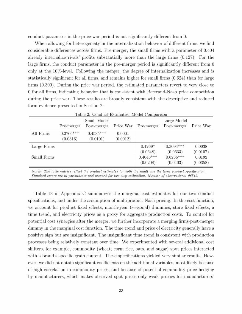
conduct parameter in the price war period is not significantly different from 0.

When allowing for heterogeneity in the internalization behavior of different firms, we find

considerable differences across firms. Pre-merger, the small firms with a parameter of 0.404

already internalize rivals’ profits substantially more than the large firms (0.127). For the

large firms, the conduct parameter in the pre-merger period is significantly different from 0

only at the 10%-level. Following the merger, the degree of internalization increases and is

statistically significant for all firms, and remains higher for small firms (0.624) than for large

firms (0.309). During the price war period, the estimated parameters revert to very close to

0 for all firms, indicating behavior that is consistent with Bertrand-Nash price competition

during the price war. These results are broadly consistent with the descriptive and reduced

form evidence presented in Section 2.

Table 2: Conduct Estimates: Model Comparison

Small Model Large ModelPre-merger Post-merger Price War Pre-merger Post-merger Price War

All Firms 0.2766*** 0.4535*** 0.0001(0.0316) (0.0101) (0.0012)

Large Firms 0.1269* 0.3094*** 0.0038(0.0648) (0.0633) (0.0107)

Small Firms 0.4043*** 0.6236*** 0.0192(0.0208) (0.0403) (0.0358)

Notes: The table entries reflect the conduct estimates for both the small and the large conduct specification.Standard errors are in parentheses and account for two-step estimation. Number of observations: 96512.

Table 13 in Appendix C summarizes the marginal cost estimates for our two conduct

specifications, and under the assumption of multiproduct Nash pricing. In the cost function,

we account for product fixed effects, month-year (seasonal) dummies, store fixed effects, a

time trend, and electricity prices as a proxy for aggregate production costs. To control for

potential cost synergies after the merger, we further incorporate a merging firms-post-merger

dummy in the marginal cost function. The time trend and price of electricity generally have a

positive sign but are insignificant. The insignificant time trend is consistent with production

processes being relatively constant over time. We experimented with several additional cost

shifters, for example, commodity (wheat, corn, rice, oats, and sugar) spot prices interacted

with a brand’s specific grain content. These specifications yielded very similar results. How-

ever, we did not obtain significant coefficients on the additional variables, most likely because

of high correlation in commodity prices, and because of potential commodity price hedging

by manufacturers, which makes observed spot prices only weak proxies for manufacturers’

33

economic marginal cost shifters. The estimates of the post-merger-merging-firms dummy

indicate a very small and insignificant decrease in the merging firms’ marginal cost after the

merger.

Finally, we allow manufacturers’ marginal cost to depend on the number of general promo-

tions and bonus buy promotions as additional cost shifters. These variables should capture

that promotions could, for example, lead to scale economies in shipping, or other types of

cost savings. We find a significant negative effect on manufacturers’ marginal cost for the

number of brand- and market-specific general promotions but only an insignificant negative

effect for the number of bonus buy promotions. Despite of several insignificant coefficients,

our marginal cost specification explains a large portion (73%) of the variation in marginal

costs across brands, stores, and time because most of our fixed effects are large and highly

significant.

For the large specification, the signs and absolute magnitudes of the parameters are similar

to those for the small specification. The cost parameters do not change considerably when

we do not include a synergy dummy for the merging firms following the merger, as shown in

Table 16 in Appendix C. For the small and the large model, we obtain J-statistics of 14.04

and 9.12 respectively, so that the Hansen-Sargent test does not reject the null hypothesis of

the joint validity of the moment conditions at the 1%-level for either model.

A very important and policy-relevant issue is to determine the extent to which industry

conduct translates into the markups of individual products. Table 14 in Appendix C com-

pares product-specific median (across markets) price-cost margins for both of our conduct

specifications. In addition, we compute the implied margins under multiproduct Nash pricing

which we use as a competitive benchmark.30

Both specifications lead to markups that are considerably higher than those implied by

Bertrand-Nash pricing before the price war period. General Mills and Kellogg’s products have

higher markups in the small specification than in the large specification, while the opposite

is true for the smaller firms’ products. Again, this is likely to occur because General Mills

and Kellogg’s internalize their pricing externalities less in the large model than in the small

model, while the opposite is true for the small firms.

The median marginal costs implied by our models are US-$ 0.107 per serving under

multiproduct Nash pricing, US-$ 0.085 for the small conduct specification, and US-$ 0.089

for the large conduct specification. Over the whole sample period, our estimated median

margins are 33 percent (small specification) and 29.4 (large specification) percent higher

than those implied by multiproduct Nash pricing. In the small specification, the median

30Recall that multiproduct Nash pricing implies that each firm maximizes the profits of its own product portfolioand that all of the markups can be attributed to product differentiation rather than to cooperative behavior.

34

margins increase from 25.6 percent over multiproduct Nash pricing in the pre-merger period

to 42.7 percent in the post-merger period. These numbers are slightly lower for the large

model, with an increase in median margins over Nash pricing from 20.8 percent pre-merger

to 38.1 percent in the post-merger period.31 Our estimates imply that, over our whole sample

period, 24.8 percent (small specification) and 22.7 percent (large specification) of the median

markup can be attributed to cooperative industry behavior.32

Table 17 in Appendix C displays the median price-cost margins decomposed for both

different brands and different time periods. Consistent with the model parameter estimates,

markups are very heterogeneous across brands and most products experience considerable

changes in markups over time.

As a final validation of our estimates, we compare marginal cost predictions from our

two conduct models with the ones obtained under the assumption of multiproduct Nash

pricing. Figure 4 in Appendix C illustrates the evolution over time of the median marginal

costs implied by the three different models. Several observations are noteworthy. Under the

assumption of multiproduct Bertrand-Nash pricing, we obtain an inverse u-shaped evolution

of marginal costs. The predicted costs increase during the pre-merger period and for another

year after the merger. They remain roughly constant until shortly before the price war

and decline substantially afterwards. The implied marginal costs from our conduct models

exhibit a different pattern. While they also increase over the pre-merger period, marginal

costs decrease considerably during the post-merger period and increase again during the price

war period, and the qualitative predictions from our small and large models are very similar.

Ideally, one would like to compare these predicted marginal costs to an observed coun-

terpart. Unfortunately, it is extremely hard to obtain such measures from observed data.

Therefore, we plot the evolution of several important input prices (corn, wheat, rice, oat,

sugar, electricity and gasoline) in the bottom panel of Figure 4. Even though input prices

are not a perfect proxy for economic marginal costs, their general development seems much

more consistent with the cost predictions from our conduct models. For example, during most

of the post-merger period, many input prices are considerably lower compared to the pre-

merger and price war periods, and there is a sharp increase in input prices shortly before and

during the price war.33 Overall, these patterns seem difficult to reconcile with the marginal

costs predicted by a multiproduct Nash model. We believe that these results provide further

31We compute the median margin over Nash pricing for a given conduct specification as the difference between themedian margins under this conduct specification and under multiproduct Nash pricing, divided by the median marginunder Nash pricing.

32We compute the fraction of the markups that is attributed to cooperative behavior for a given conduct specificationas the difference between the median margins under this conduct specification and under Nash pricing, divided bythe median margin under the conduct specification.

33Sugar constitutes an exception as its price drops monotonically (except for a short period in 1994).

35

support for our conduct specifications.

Relationship to other industry studies Because the RTE cereal industry has been studied

extensively, it is useful to relate our results to those in the literature. The works of Nevo

(2000b) and Nevo (2001) are of particular interest. Nevo (2000b) simulates the effects of dif-

ferent hypothetical horizontal mergers using only pre-merger data. Assuming multiproduct

Bertrand-Nash pricing before and after the merger, he finds that, in the absence of consider-

able cost synergies for the merging firms, the merger between Post and Nabisco leads to an

increase in prices and a decrease in consumer surplus. Our focus is mainly on estimating the

conduct between different manufacturers over time, and accounting for potential changes in

conduct. Most importantly, in our model specifications, increases in markups can not only be

explained by the “unilateral effects” of the merger but also by a more cooperative industry

conduct in the post-merger period (“coordinated effects”).

Nevo (2001) measures market power in the RTE cereal industry. His sample contains data

from 65 US cities covering a period from 1988 to 1992. Time-wise, this partially overlaps

with our pre-merger period. On the demand side, our estimates of the median own- and

cross-price elasticities are very close to his. This is the case despite his use of Hausman

(1996)-style instruments based on prices from other regions, and different data with a slightly

different product set.34 An additional difference on the demand side is that we use a nested

random coefficient logit model rather than a random coefficient logit model to capture a

richer substitution pattern between the inside products and the outside good. We consider

the similarity of the implied coefficients as an additional validation of our demand estimates.

To select among different forms of industry conduct, Nevo (2001) compares the recovered

marginal cost for different pre-specified conduct assumptions with accounting cost data un-

der the assumption of vertical integration, i.e., joint profit maximization between retailers

and manufacturers. Comparing three different conduct assumptions (single-product Nash,

multiproduct Nash, and joint ownership of all products), he finds that multiproduct Nash

pricing provides the best fit to the industry accounting data, resulting in a combined retailer-

manufacturer price-cost margin of 42.2 percent compared 35.8 percent under single-product

Nash and 72.6 percent under joint ownership of all brands. For the part of our sample period

that overlaps with his sample period, i.e., the pre-merger period, the estimated markups

from both of our conduct models are closer to his multiproduct Nash specification than to

the other two considered options. However, our results indicate a significantly positive but

moderate level of cooperative conduct during this period. For the pre-merger period, we

find implied median gross margins for retailer and manufacturers combined of 53.7 percent

34Most notably, we additionally include products from the manufacturer Ralston.

36

for the small conduct model, and of 52.1 percent for the large model.35 As discussed above,

comparing the implied marginal costs for the different models with input price data yields

supporting evidence that for our sample, our conduct specifications yield a more accurate

industry description than multiproduct Nash pricing.

Comparing our results with those from a pre-specified menu of conduct specifications also

relates to the question of why direct conduct estimation might be useful in the first place.

First, accounting data as a measure of marginal cost is not necessarily very fine-grained,

and it is not always clear how it relates to marginal cost. Thus, while it might enable a

distinction among different relatively distant conduct assumptions, it is more difficult to

use when considering different forms of conduct that are relatively close to each other. For

example, already for a conduct parameter of 0.1, a significant part of the markups can be

due to cooperative behavior between firms. Another alternative to comparing the recovered

marginal cost to accounting data is the use of non-nested statistical tests; see, for example,

Rivers and Vuong (1988), Chen et al. (2007), and Shi (2015). While in principle, it is possible

to compare conduct specifications that are relatively close to each other, the statistical power

of these tests is often hard to assess. This is even more problematic when one is interested in

estimating conduct patterns, that potentially change over time and across firms. For these

reasons, we believe that a direct estimation of industry conduct can contribute to a better

understanding of markups and marginal costs in differentiated products industries.

6 Counterfactual Simulations

In this section, we use our estimated parameters from the structural model to simulate how

two different changes in the underlying industry conduct would affect consumer surplus and

manufacturers’ pricing behavior.

First, we examine how these two measures would change if the firms were competing a

la multiproduct Bertrand-Nash pricing before the price war. Table 3 shows the associated

results. As a measure of consumer surplus, we estimate the compensating variation, i.e.,

the dollar value for which consumers would have been equally well off in both the observed

industry state and the counterfactual simulation. Both the small and large conduct model

35Assuming multiproduct Nash pricing, we find an implied gross margin for the pre-merger period of 45.2 percent,which is slightly higher than Nevo’s (2001) for the same assumption. Note that Nevo recovers the gross marginunder the assumption of joint maximization of retailer and manufacturers profits, while we use the assumption thatmanufacturers and retailers maximize profits independently, which results in double marginalization. This is fullyconsistent with the slightly higher gross margin for our multiproduct Nash specification compared to his in the sametime period. Also note that while the implied margins of both our small and large models are considerably higher thanNevo’s, they still lie within his estimated 95 percent confidence interval for the implied margins under multiproductNash pricing. The lower and upper bound of his 95% confidence interval are 29.1 percent and 55.8 percent respectively.

37

Table 3: Counterfactual Simulation 1: Change to multiproduct Bertrand-Nash pricing

Small Model Large ModelPre-merger Post-merger Pre-merger Post-merger

∆ consumer surplus (in US-$ mio.) 2.3 5.3 3.2 6.3

∆price All Firms (in %) −9.5 −15.7 −9.4 −16.9∆price GM (in %) −8.5 −15.3 −7.6 −14.8∆price RAL (in %) −10.8 −16.8 −25.4 −25.7∆price KEL (in %) −8.3 −13.5 −8.3 −13.8∆price POSNAB (in %) −13.7 −18.6 −27.6 −27.4∆price QUA (in %) −13.5 −22.8 −30.9 −34.1

Notes: The table entries reflect the results from the counterfactual simulations for both the small andthe large conduct specification. The simulations compute the changes in consumer surplus and wholesaleprices before the price war period when all firms play according to multiproduct Nash pricing instead of theestimated conduct.

yield relatively similar results. We find that if firms had played according to multiproduct

Bertrand-Nash pricing instead of our estimated conduct, before the price war, consumers in

our sample would have been between US-$ 1.6 million and US-$ 2.0 million per year better off.

Consistent with the changes in industry conduct over time, the counterfactual simulations

indicate that under multiproduct Nash pricing, the median wholesale prices across all firms

would have been between 9.4 and 9.5 percent lower in the pre-merger period and between

15.7 and 16.9 percent lower in the post-merger period. When considering firm-specific prices,

we find that Kellogg’s would have had the lowest predicted wholesale price decrease, while

the decrease would be the largest for Post-Nabisco and Quaker.

Second, we examine how consumer welfare and pricing would have changed if the price

war had never occurred, i.e., if the conduct had remained the same as before the price war

period. Table 18 in Appendix C shows the associated results. We find that without the price

war, consumers would have been between US-$ 0.7 million and US-$ 0.8 million worse off

during this period, which spans the last 6 months of our sample. The median wholesale price

responses of each manufacturer differ between the small and large conduct models. While

for the small model, the predicted price responses are relatively homogeneous, for the large

model, the wholesale price responses are generally higher for small firms than for large firms.

This is fully consistent with the higher conduct parameters for small firms in the large model.

38

7 Conclusion

In this paper, we estimate the evolution of competition in the RTE cereal industry using

a structural model of demand and supply. Our empirical strategy is flexible enough to

accommodate detailed patterns of industry conduct; in particular, we allow levels of conduct

to vary both across time and firms.

To overcome the identification problem of separating marginal costs from industry con-

duct, we construct novel instruments that interact measures of products’ relative isolation

in the characteristics space with data on rival firms’ temporary and market-specific promo-

tional activities. Intuitively, our identification of the supply parameters is based on the idea

that a firm’s markups react much more strongly to the promotions of a competing product

that is close in the characteristics space than to those of a more distant product; and this

relationship should be stronger the more competitive the industry is.

Our empirical strategy has several attractive features that allow it to be applied to many

other industries. First, it does not rely on exogenous industry shocks, such as ownership

changes, to identify industry conduct. Second, our instruments can be used even if there is

no product entry or exit during the sample period. Third, the required data are available

in many standard data sets for a broad range of consumer goods industries. Finally, a

series of weak identification tests indicates that our instruments indeed are very powerful

for identifying flexible patterns of industry conduct in contrast to many commonly used

BLP-style instruments.

We use our model to shed new light on two important industry events during the 1990s:

first, the Post-Nabisco merger and second, a period of large wholesale price cuts in 1996. Our

estimation results suggest that in the beginning of our sample period in 1991, the industry

was characterized by moderate levels of price coordination which increased significantly for

all firms after the Post-Nabisco merger in January 1993. For the pre-merger and the post-

merger periods, our model predicts price-cost margins that are higher than those implied by

multiproduct Nash pricing by 20.8 and 38.1 percent, respectively. These numbers indicate

that a significant percentage of the markups of national cereal manufacturers during the

first half of the 1990s can be attributed to cooperative industry behavior. Our conduct

estimates for the last months of our sample period are consistent with a shift in firms’ behavior

to multiproduct Nash pricing. Our results thus suggest that while product differentiation

alone can explain the largest portion of the price-cost margins, for a long time cooperative

behavior further increased markups even more. Moreover, we find that such behavior was

more prevalent for small firms than for large firms.

A well-known critique of conduct parameter models in general is that the estimated pa-

39

rameters ultimately constitute only a reduced form approximation to a more structural model

of firm behavior, for example, in the form of a repeated game. While the development of

such a framework goes beyond the scope of this paper, it is a very promising area for future

research. Our empirical strategy and the rich set of instruments that we propose are likely

to be easy to apply and to adapt to these more complicated settings. In particular, a struc-

tural repeated game model is likely to contain more parameters than ours. The empirical

results from our application provide first evidence that our instruments may work very well

for estimating markups in such high-dimensional models.

Recently, there has been an increased interest in the evolution of markups over time

from a macroeconomic perspective. De Loecker and Eeckhout (2017) document a substantial

increase in markups from 1980 onwards for the US economy by using a production func-

tion approach. They attribute this pattern mainly to a sharp increase in the markups of

already high-markup firms within the different industries. Our approach can be seen as com-

plementary to this literature. By focusing on estimating competitive interactions between

firms within an industry, one can gain detailed insights into the extent to which potentially

heterogeneous conduct and differentiated consumer preferences can explain firms’ markups.

Our model can be readily applied to estimate supply side patterns in many important

industries because many standard data sets contain the information required for our esti-

mation strategy. Comparing estimated conduct levels across industries can lead to a better

understanding of the determinants of anti-competitive firm behavior, which is still a relatively

open question with important implications for competition policy.

References

Ackerberg, D. A., Caves, K. and Frazer, G. (2015). Identification properties of recent

production function estimators. Econometrica, 83 (6), 2411–2451.

Angrist, J. D. and Pischke, J.-S. (2008). Mostly harmless econometrics: An empiricist’s

companion. Princeton University Press.

Appel, M., Labarre, R. and Radulovic, D. (2004). On accelerated random search.

SIAM Journal on Optimization, 14 (3), 708–731.

Ashenfelter, O. C., Hosken, D. S. and Weinberg, M. C. (2013). The price effects of

a large merger of manufacturers: A case study of Maytag-Whirlpool. American Economic

Journal: Economic Policy, 5 (1), 239–261.

40

Berry, S., Levinsohn, J. and Pakes, A. (1995). Automobile prices in market equilibrium.

Econometrica, 63 (4), 841–890.

Berry, S. T. and Haile, P. A. (2014). Identification in differentiated products markets

using market level data. Econometrica, 82 (5), 1749–1797.

Bjornerstedt, J. and Verboven, F. (2016). Does merger simulation work? evidence

from the Swedish analgesics market. American Economic Journal: Applied Economics,

8 (3), 125–164.

Black, M., Crawford, G., Lu, S. and White, H. (2004). A virtual stakes approach to

measuring competition in product markets. mimeo.

Bresnahan, T. (1982). The oligopoly solution concept is identified. Economics Letters,

10 (1-2), 87–92.

— (1987). Competition and collusion in the American automobile industry: The 1955 price

war. The Journal of Industrial Economics, 35 (4), 457–482.

Chen, X., Hong, H. and Shum, M. (2007). Nonparametric likelihood ratio model selection

tests between parametric likelihood and moment condition models. Journal of Economet-

rics, 141 (1), 109–140.

Chevalier, J. A., Kashyap, A. K. and Rossi, P. E. (2003). Why don’t prices rise during

periods of peak demand? Evidence from scanner data. American Economic Review, 93 (1),

15–37.

Chintagunta, P. K., Dube, J.-P. and Singh, V. (2003). Balancing profitability and

customer welfare in a supermarket chain. Quantitative Marketing and Economics, 1 (1),

111–147.

Ciliberto, F. and Williams, J. W. (2014). Does multimarket contact facilitate tacit

collusion? Inference on conduct parameters in the airline industry. The RAND Journal of

Economics, 45 (4), 764–791.

Corts, K. (1999). Conduct parameters and the measurement of market power. Journal of

Econometrics, 88 (2), 227–250.

Cotterill, R. and Franklin, A. (1999). An estimation of consumer benefits from the

public campaign to lower cereal prices. Agribusiness, 15 (2), 273–287.

41

Cragg, J. G. and Donald, S. G. (1993). Testing identifiability and specification in in-

strumental variable models. Econometric Theory, 9 (02), 222–240.

Crawford, G., Lee, R., Whinston, M. and Yurukoglu, A. (2018). The welfare effects

of vertical integration in multichannel televistion. Econometrica, 86 (3), 891–954.

De Loecker, J. and Eeckhout, J. (2017). The rise of market power and the macroeco-

nomic implications. NBER Working Paper 23687.

Dube, J.-P., Fox, J. T. and Su, C.-L. (2012). Improving the numerical performance

of static and dynamic aggregate discrete choice random coefficients demand estimation.

Econometrica, 80 (5), 2231–2267.

Gandhi, A. and Houde, J. (2017). Measuring substitution patterns in differentiated prod-

ucts industries. mimeo.

Gasmi, F., Laffont, J. J. and Vuong, Q. (1992). Econometric analysis of collusive

behavior in a soft-drink market. Journal of Economics & Management Strategy, 1 (2),

277–311.

Goldberg, P. K. and Hellerstein, R. (2013). A structural approach to identifying the

sources of local currency price stability. The Review of Economic Studies, 80 (1), 175–210.

Hausman, J. A. (1996). Valuation of new goods under perfect and imperfect competition.

In The economics of new goods, University of Chicago Press, pp. 207–248.

Hendel, I. and Nevo, A. (2006). Measuring the implications of sales and consumer inven-

tory behavior. Econometrica, 74 (6), 1637–1673.

Kleibergen, F. and Paap, R. (2006). Generalized reduced rank tests using the singular

value decomposition. Journal of Econometrics, 133 (1), 97–126.

Knittel, C. R. and Metaxoglou, K. (2014). Estimation of random-coefficient demand

models: Two empiricists’ perspective. Review of Economics and Statistics, 96 (1), 34–59.

Lal, R. and Matutes, C. (1994). Retail pricing and advertising strategies. Journal of

Business, pp. 345–370.

Lau, L. (1982). On identifying the degree of competitiveness from industry price and output

data. Economics Letters, 10 (1-2), 93–99.

Mazzeo, M., Seim, K. and Varela, M. (2013). The welfare consequences of mergers with

product repositioning. mimeo.

42

Meza, S. and Sudhir, K. (2010). Do private labels increase retailer bargaining power?

Quantitative Marketing and Economics, 8 (3), 333–363.

Michel, C. (2017). Estimation of within-firm pricing coordination in differentiated product

industries. mimeo.

Miller, N. H. and Weinberg, M. C. (2017). Understanding the price effects of the

MillerCoors joint venture. Econometrica, 85 (6), 1763–1791.

Nevo, A. (1998). Identification of the oligopoly solution concept in a differentiated-products

industry. Economics Letters, 59 (3), 391–395.

— (2000a). A Practitioner’s Guide to Estimation of Random-Coefficients Logit Models of

Demand. Journal of Economics & Management Strategy, 9 (4), 513–548.

— (2000b). Mergers with differentiated products: The case of the ready-to-eat cereal indus-

try. The RAND Journal of Economics, 31 (3), 395–421.

— (2001). Measuring Market Power in the Ready-to-Eat Cereal Industry. Econometrica,

69 (2), 307–342.

Pinkse, J. and Slade, M. E. (2004). Mergers, brand competition, and the price of a pint.

European Economic Review, 48 (3), 617–643.

Rivers, D. and Vuong, Q. H. (1988). Limited information estimators and exogeneity tests

for simultaneous probit models. Journal of Econometrics, 39 (3), 347–366.

Rubinfeld, D. (2000). Market definition with differentiated products: the post / nabisco

cereal merger. Antitrust Law Journal, 68, 163–185.

Sanderson, E. and Windmeijer, F. (2016). A weak instrument f-test in linear iv models

with multiple endogenous variables. Journal of Econometrics, 190 (2), 212–221.

Scherer, F. M. (1979). The welfare economics of product variety: an application to the

ready-to-eat cereals industry. The Journal of Industrial Economics, pp. 113–134.

Schmalensee, R. (1978). Entry deterrence in the ready-to-eat breakfast cereal industry.

The Bell Journal of Economics, 9 (2), 305–327.

Shi, X. (2015). A nondegenerate Vuong test. Quantitative Economics, 6 (1), 85–121.

Slade, M. E. (1995). Product rivalry with multiple strategic weapons: An analysis of

price and advertising competition. Journal of Economics & Management Strategy, 4 (3),

445–476.

43

Sovinsky Goeree, M. (2008). Limited information and advertising in the us personal

computer industry. Econometrica, 76 (5), 1017–1074.

Stock, J. H., Wright, J. H. and Yogo, M. (2002). A survey of weak instruments and

weak identification in generalized method of moments. Journal of Business & Economic

Statistics, 20 (4), 518–529.

Sudhir, K. (2001). Structural analysis of manufacturer pricing in the presence of a strategic

retailer. Marketing Science, 20 (3), 244–264.

Sullivan, C. (2017). Three Essays on Product Collusion. Ph.D. thesis, University of Michi-

gan.

Sweeting, A. (2010). The effects of mergers on product positioning: evidence from the

music radio industry. The RAND Journal of Economics, 41 (2), 372–397.

Train, K. (2000). Halton sequences for mixed logit. mimeo.

Varian, H. R. (1980). A model of sales. The American Economic Review, 70 (4), 651–659.

Villas-Boas, J. M. (1995). Models of competitive price promotions: Some empirical evi-

dence from the coffee and saltine crackers markets. Journal of Economics & Management

Strategy, 4 (1), 85–107.

Villas-Boas, S. B. (2007). Vertical relationships between manufacturers and retailers:

Inference with limited data. The Review of Economic Studies, 74 (2), 625–652.

Wooldridge, J. M. (2010). Econometric analysis of cross section and panel data. The

MIT Press.

Wright, J. H. (2003). Detecting lack of identification in GMM. Econometric Theory,

19 (02), 322–330.

A Reduced Form Estimations and Additional Details

A.1 Reduced Form Estimation Equations

In this section, we provide the estimation equation for our baseline reduced form regressions

of the log wholesale price log(pwist) in Table 5. PromoG denotes the number of general promo-

tions for a given product in a given market. The superscript indicates which promotions are

included. own considers only promotions for the same product, firm denotes the promotions

44

Figure 1: Evolution of RTE cereal prices

1991 1992 1993 1994 1995 1996 1997

0.08

0.10

0.12

0.14

0.16

Who

lesa

le p

rice

per o

z. (in

US-

$)

Mer

ger

Price

war

Evolution of RTE cereal prices (wholesale)

NAB SWPO RBKEL FFQU CC

1991 1992 1993 1994 1995 1996 1997

0.10

0.12

0.14

0.16

0.18

0.20

0.22

Reta

il pr

ice p

er o

z. (in

US-

$)

Mer

ger

Price

war

Evolution of RTE cereal prices (retail)

NAB SWPO RBKEL FFQU CC

Notes: The two figures display the evolution of the average wholesale and retail prices,respectively, across all stores over time for selected brands. The brands are Nabisco/PostShredded Wheat, Post Raisin Bran, Kellogg’s Frosted Flakes, and Quaker Cap’n Crunch.

45

Table 4: Market share evolution

GMI KEL POS NAB QUA RAL

1991 32.4 46.1 7.9 3.1 7.2 3.41992 30.0 46.3 10.1 3.9 6.6 3.11993 28.9 47.0 11.6 0.0 8.9 3.61994 25.8 48.3 12.3 0.0 10.4 3.31995 31.9 43.8 14.4 0.0 6.8 3.11996 27.5 48.1 13.5 0.0 8.1 2.7

Notes: The table summarizes the firm-specific volume-based market shares (in percent) across all stores in ourdata set for each year. From 1993 onwards, Post’s mar-ket shares include those of Nabisco. GMI stands for Gen-eral Mills, KEL for Kellogg’s, POS for Post, NAB forNabisco, QUA for Quaker, and RAL for Ralston.

of all other products owned by the same firm, and rival captures the number of rival firms’

products’ promotions. We also allow for different rival effects pre-merger (pre), post-merger

before the price war (post), and during the price-war (pw). 1POSNABPost , 1nomergePost , and 1PW

represent dummy variables for the merging firms post-merger, the non-merging firms post-

merger, and a price war dummy for all firms, respectively. Furthermore, Sales Tot indicates

the total quantity of cereals sold in a given store and month. Finally, κi and κs denote

brand and store fixed effects, respectively. Our baseline wholesale price equation can thus be

written as

log(pwist) =β1PromoGownist + β2PromoG

firmist + β3PromoG

riv,preist + β4PromoG

riv,postist

+ β5PromoGriv,pwist + β61

POSNABPost + β71

nomergePost + β81PW

+ β9Sales Totalst + κi + κs + εist

where i, s, and t denote brands, stores, and months respectively. The second column in Table

5 substitutes the post-merger non-merging dummy with firm-specific post-merger dummies.

The last two models add the bonus buy promotion variables, PromoB, in addition to the

general promotion variables. We estimate the same model using the log retail price, log(prist),

as the dependent variable and obtain similar estimates. These results are available upon

request.

A.2 Distribution of Promotional Activities

Figures 2 and 3 illustrate the distribution of the promotional intensity across different brands,

stores, and time. In Figure 2, we plot the total number of promotional activities aggregated

46

Table 5: Reduced form analysis: Wholesale prices(1) (2) (3) (4)

Baseline Firm detailed Baseline w/ BB Firm detailed w/ BB

Promo (own brand) -0.1099∗∗∗ -0.1093∗∗∗ -0.1116∗∗∗ -0.1111∗∗∗

(0.0012) (0.0012) (0.0012) (0.0012)Promo (same firm) 0.0007∗ 0.0009∗∗ 0.0021∗∗∗ 0.0022∗∗∗

(0.0003) (0.0002) (0.0003) (0.0003)Promo pre-merger (rivals) 0.0029∗∗∗ 0.0024∗∗∗ 0.0026∗∗∗ 0.0023∗∗∗

(0.0002) (0.0002) (0.0003) (0.0002)Promo post-merger (rivals) -0.0019∗∗∗ -0.0017∗∗∗ -0.0010∗ -0.0008

(0.0003) (0.0003) (0.0004) (0.0004)Promo price war (rivals) -0.0071∗∗∗ -0.0082∗∗∗ -0.0054∗∗∗ -0.0068∗∗∗

(0.0002) (0.0002) (0.0002) (0.0002)Post-merger non-merging 0.0182∗∗∗ 0.0124∗∗

(0.0022) (0.0046)Post-merger POSTNAB 0.0609∗∗∗ 0.0584∗∗∗ 0.0511∗∗∗ 0.0436∗∗∗

(0.0023) (0.0023) (0.0049) (0.0049)Price war period -0.0983∗∗∗ -0.0936∗∗∗ -0.0869∗∗∗ -0.0854∗∗∗

(0.0015) (0.0015) (0.0017) (0.0017)Post-merger KEL 0.0515∗∗∗ 0.0413∗∗∗

(0.0021) (0.0041)Post-merger RAL 0.0501∗∗∗ 0.0376∗∗∗

(0.0027) (0.0054)Post-merger QUA -0.0176∗∗∗ -0.0273∗∗∗

(0.0026) (0.0052)Post-merger GMI -0.0284∗∗∗ -0.0394∗∗∗

(0.0025) (0.0048)BB (own brand) -0.0217∗∗∗ -0.0220∗∗∗

(0.0009) (0.0009)BB (same firm) 0.0051∗∗∗ 0.0045∗∗∗

(0.0002) (0.0002)BB pre-merger (rivals) 0.0009∗∗∗ 0.0008∗∗∗

(0.0001) (0.0001)BB post-merger (rivals) 0.0014∗∗∗ 0.0018∗∗∗

(0.0003) (0.0003)BB price war (rivals) -0.0053∗∗∗ -0.0040∗∗∗

(0.0003) (0.0003)

Observations 96512 96512 96512 96512R-square 0.76 0.76 0.77 0.77

Notes: All estimations include brand and store fixed effecs. Columns (2) and (4) allow for thepost-merger reaction to differ across firms. Promo (same firm) describes the number of promotionsof other products in a market that belong to the same firm. Promo (rivals) describes the numberof promotions of other products in a market that do not belong to the same firm. Pre, post,and PW stand for pre-merger, post-merger, and price war period, respectively. BB stands forbonusbuy and coupon promotions, while all promo variables without BB reflect general and pricereduction promotions.∗ p < 0.05, ∗∗ p < 0.01, ∗∗∗ p < 0.001

over all 58 stores in our sample for each brand-month combination. In Figure 3 we plot the

total number of promotions for each brand-store combination aggregated over all months

in our sample. In both figures, brighter colors indicate a higher promotional intensity than

darker colors.

47

Figure 2: Distribution of promotional activities I

1 2 3 4 5 6 7 8 9 10 11 12 13 14 15 16 17 18 19 20 21 22 23 24 25 26

brand_id

mon

th

Total promotions monthly (aggregated over stores)

0

50

100

150

200

250

Notes: The figure displays a heatmap of the distribution of the total numberof promotions for each brand over time aggregated over all stores in oursample.

Figure 3: Distribution of promotional activities II

1 2 3 4 5 6 7 8 9 10 11 12 13 14 15 16 17 18 19 20 21 22 23 24 25 26

brand_id

stor

e

Total promotions monthly (aggregated over time)

10

20

30

40

50

60

Notes: The figure displays a heatmap of the distribution of the total numberof promotions aggregated over time for each brand-store combination.

48

Table 6: Reduced form analysis: Quantities sold(1) (2) (3)

Baseline Baseline w/ BB BB & lagged promos

Log Retail Price -1.8089∗∗∗ -1.8139∗∗∗ -1.8393∗∗∗

(0.1230) (0.1231) (0.1258)Promo (own brand) 0.1761∗∗∗ 0.1757∗∗∗ 0.1705∗∗∗

(0.0257) (0.0252) (0.0247)BB (own brand) 0.0861∗∗∗ 0.0848∗∗∗ 0.0845∗∗∗

(0.0093) (0.0096) (0.0082)Promo (same firm) -0.0048 -0.0037 -0.0030

(0.0036) (0.0033) (0.0031)Promo pre-merger (rivals) -0.0085 -0.0034 -0.0008

(0.0059) (0.0033) (0.0039)Promo post-merger (rivals) -0.0072∗∗∗ -0.0070∗∗∗ -0.0073∗∗∗

(0.0017) (0.0017) (0.0015)Promo price war (rivals) -0.0260∗ -0.0253∗ -0.0244∗

(0.0101) (0.0102) (0.0098)BB pre-merger (rivals) -0.0056 -0.0035

(0.0043) (0.0043)BB post-merger (rivals) 0.0021 0.0023

(0.0018) (0.0018)BB price war (rivals) -0.0168 -0.0196

(0.0163) (0.0160)Promo (own brand, lag 1) -0.0200

(0.0108)BB (own brand, lag 1) -0.0092

(0.0076)Promo (own brand, lag 2) 0.0070

(0.0115)BB (own brand, lag 2) 0.0026

(0.0079)Promo (own brand, lag 3) 0.0103

(0.0106)BB (own brand, lag 3) -0.0081

(0.0103)Promo (own brand, lag 4) 0.0029

(0.0120)BB (own brand, lag 4) 0.0059

(0.0064)

Observations 96512 96512 90480R-square 0.83 0.83 0.83

Notes: All estimations include brand, store, and month fixed effecs. Promo (same firm)describes the number of promotions of other products in a market that belong to thesame firm. Promo (rivals) describes the number of promotions of other products ina market that do not belong to the same firm. BB stands for bonusbuy and couponpromotions, while all promo variables without BB reflect general and price reductionpromotions. Column (2) adds rival firms’ BB promotions as regressors. Column (3) addslags of a brand’s promotions as regressors.∗ p < 0.05, ∗∗ p < 0.01, ∗∗∗ p < 0.001

49

B Construction of Instruments and Testing for Weak Identifica-

tion

B.1 Details of Computation of Instruments

Our instruments for manufacturer markups, that identify industry conduct, consist of two

parts. First, we construct proximity measures that describe how close each pair of products

is in the characteristics space. Second, we compute a market-specific measure of the intensity

of each product’s rivals’ promotional activities.

The first component is motivated by the fact that the effect of a rival product’s promotions

on another product’s demand should strongly depend on the proximity of the two products in

the characteristics space. A close rival product going on sale will exert much more competitive

pressure than a very distant product on sale. For example, demand for Post’s Raisin Bran

should be affected much more by promotions of Kellogg’s Raisin Bran than by promotions for

Quaker Oats. For instance, the degree of closeness can be described by whether the difference

between two products in terms of a specific characteristic, for example, sugar content, is in

the first, second, third etc. decile of all differences in terms of that characteristic.36

More specifically, define dxij ≡ xi− xj, i 6= j as the difference in the product characteristic

x between products i and j. Let Cx = cx1 , .., cxυ denote υ equally spaced percentiles of the

entire distribution of characteristics differences dxij with respect to product characteristic x.

The second part of our instruments is motivated by the fact that the pattern of promotions

shifts the competitive pressure in a market. Denote by PROMOGit and PROMOBB

it the

number of general promotions and bonus buy promotions respectively for product i in market

t. We compute our instruments by interacting these promotion measures with our proximity

measures for the corresponding product-pairs. For a continuous product characteristic x, our

instruments zx,k,wjt can then be computed as

zx,k,wjt =∑i 6∈F(j)

1(|dxij,t| < cxk

)· PROMOw

it ,

where k indicates the percentile of closeness, w denotes the type of promotions, i.e., either

general or bonus buy, and F(j) is the product portfolio of the firm owning brand j. This

results in υ ∗ 2 potential instruments per continuous product characteristic x. Intuitively,

our instruments count the number of different types of promotions conducted by rivals in a

given market but only consider promotions of rival products that are close according to our

36Similar ideas underlie the construction of differentiation instruments to identify consumer substitution patternsin Gandhi and Houde (2017).

50

definition above. The analogous instruments for a binary product characteristic, for example,

whether a cereal is soggy in milk or not, can be computed as

zx,k,wjt =∑i 6∈F(j)

1(|dxij,t| = k) · PROMOwit ,

which leads to at most 2 ∗ 2 instruments per binary product characteristic.

In our application, we use sugar and fiber content as continuous characteristics, and

the binary variable sogginess. For the sugar- and fiber-based instruments we use the 33.33

percentile of the respective distribution of characteristic differences as the cutoff value ck.

For the binary variable sogginess, we only consider promotions of rivals that fall in the

same sogginess category, i.e., k = 0. Computing our instruments based on other closeness

definitions, such as using deciles instead of terciles, resulted in very similar estimation results.

B.2 Reduced Form Evidence for Validity of Assumptions

In this appendix, we present reduced form evidence for the timing assumptions that we

employ for our identification strategy. Essentially, we require that wholesale prices in period

t are a function of all information available in period t, so that pwjt = f(It), where It denotes

all information available in period t, i.e., all relevant demand and cost shocks. In contrast, the

number of promotions in period t, Promojt = f(It−1), where It−1 contains only information

available up to t− 1. Shocks that cause It−1 to be different from It provide the variation in

the data necessary to make our instruments for identifying industry conduct work.

Column (1) in Table 7 summarizes the results from regressing logged wholesale prices on

various cost shifters to illustrate that wholesale prices react immediately to contemporaneous

cost shocks. Column (2) highlights that promotions in the current period are not affected

by contemporaneous cost shocks, which provides evidence that promotional activities are

not adjusted immediately. Columns (3) to (7) show that future promotions are affected by

cost shocks today, however. Therefore, while promotions are clearly endogenous, Table 7

provides evidence that they are likely to be sequentially exogenous to future innovations in

manufacturers’ marginal cost shocks.

B.3 Weak Identification

In the following, we illustrate that our instruments have power for identifying both demand

and supply parameters. Compared to traditional first-stage diagnostics for linear IV regres-

sions, testing for weak identification in our model is more complicated for several reasons.

First, our models are highly non-linear and contain multiple endogenous regressors. Second,

51

Tab

le7:

Red

uce

dfo

rmev

iden

cesu

pp

orti

ng

our

tim

ing

assu

mp

tion

s

(1)

(2)

(3)

(4)

(5)

(6)

(7)

(8)

Log

Wh

ole

sale

Pri

ceP

rom

oint

Pro

mo

int

+1

Pro

mo

int

+2

Pro

mo

int

+3

Pro

mo

int

+4

Pro

mo

int

+5

Pro

mo

int

+6

Wei

ghte

dsu

gar

pri

ce1.4

630∗∗∗

-0.9

881

-3.5

065

-5.8

884∗∗

-5.7

979∗∗

-5.1

888∗∗

-4.1

342∗

-2.7

413

(0.5

128)

(1.9

384)

(2.2

934)

(2.3

610)

(2.4

394)

(2.0

418)

(2.0

252)

(2.0

482)

Wei

ghte

dri

cep

rice

0.0

108∗

0.0

264

0.0

315∗

0.0

336∗

0.0

252

0.0

161

0.0

183

0.0

306

(0.0

062)

(0.0

250)

(0.0

176)

(0.0

169)

(0.0

164)

(0.0

190)

(0.0

199)

(0.0

277)

Wei

ghte

dco

rnp

rice

0.0

075∗∗∗

0.0

237

0.0

411∗∗∗

0.0

446∗∗∗

0.0

361

0.0

415∗∗∗

0.0

243∗

0.0

193

(0.0

010)

(0.0

213)

(0.0

092)

(0.0

079)

(0.0

224)

(0.0

091)

(0.0

120)

(0.0

128)

Dis

tan

ceX

gas

pri

ce0.1

013∗∗

0.2

155

0.2

844

0.3

920∗

0.4

732∗∗

0.1

454

0.1

370

0.4

189

(0.0

459)

(0.3

665)

(0.2

615)

(0.2

174)

(0.2

111)

(0.2

307)

(0.2

630)

(0.2

615)

Ele

c.p

rice

XF

lakin

g0.0

414

-0.1

796

0.0

105

0.1

808

0.1

786

0.4

285∗∗

0.2

428

0.0

251

(0.0

397)

(0.1

734)

(0.2

139)

(0.2

613)

(0.1

803)

(0.2

029)

(0.2

088)

(0.2

280)

Ele

c.p

rice

XS

hre

dd

ing

0.0

380

-0.0

474

0.1

271

0.4

349

0.9

905∗∗∗

1.6

795∗∗∗

1.1

773∗∗

0.2

957

(0.0

280)

(0.1

740)

(0.2

998)

(0.3

426)

(0.2

257)

(0.4

951)

(0.5

127)

(0.4

102)

Ob

serv

ati

on

s96512

96512

95004

93496

91988

90480

88972

87464

R-s

qu

are

0.7

80.1

60.1

50.1

60.1

60.1

60.1

50.1

5

Note

s:T

he

table

sum

mari

zes

OL

Sre

sult

sfr

om

regre

ssin

gth

ew

hole

sale

pri

ce(C

olu

mn

1)

and

the

num

ber

of

bra

nd-

and

mark

et-s

pec

ific

pro

moti

ons

at

diff

eren

tp

oin

tsin

tim

e(C

olu

mns

2fo

rco

nte

mp

ora

neo

us

pro

moti

ons,

Colu

mns

3to

8fo

rpro

moti

ons

up

to6

month

sin

toth

efu

ture

)on

vari

ous

conte

mp

ora

neo

us

cost

shif

ters

.A

lles

tim

ati

ons

incl

ude

bra

nd,

store

,and

month

fixed

effec

ts.

∗p<

0.1

0,∗∗p<

0.0

5,∗∗∗p<

0.0

1

52

even if instruments and endogenous regressors are correlated enough to result in a decently

large F-statistic37, the instruments can still be weak enough to result in very sensitive esti-

mates and high standard errors.

In order to overcome the first problem, we adapt a testing procedure recently proposed

by Gandhi and Houde (2017) for demand models. The main idea is to linearize the nonlinear

BLP-model around the estimated parameter values using a first-order Taylor expansion. After

the model is linearized, one can employ generalizations of the well-known F-statistics to test

for identification of single parameters. While traditional F-tests test the null hypothesis of

complete non-identification of a single parameter, rank deficiency tests as developed by Cragg

and Donald (1993) and Kleibergen and Paap (2006) can be adopted to test for alternative

hypotheses, such as underidentification or weak identification of single parameters or the

model as a whole.

General procedure In the following, we describe a general procedure to test for various

degrees of lack of identification and weak instruments based on Gandhi and Houde (2017).

To the best of our knowledge, this procedure has so far not been used to test for weak

identification of conduct parameters.

The starting point is a first-order Taylor expansion of the structural error κ(θ) as a

function of the parameters around the true parameter vector θ0

κjt(θ) = κjt(θ0) +K∑k=1

(θk − θ0k)∂κjt(θ0)

∂θk+ υjt (21)

= κjt(θ0) + Jjt(θ0)b+ υjt (22)

where J denotes the Jacobian stacking all the partial derivatives with respect to each pa-

rameter θk, b stacks the differences θk − θk0 and υ are higher-order residuals. When taking

conditional expectations of the above equation with respect to the proposed instruments Z,

E(κ(θ0)|Z) disappears and when evaluated at θ = θ0 the Jacobian term becomes zero.

In order to have strong identification, we require E(κ(θ)|Z) to be large for θ 6= θ0. There-

fore, we test whether the Jacobian of the objective function reacts strongly to the instruments

(analogous to an F-test in linear GMM). Note that this test can be applied equally well to

both demand and supply models.38 For a given model, we proceed in the following steps.

37A popular rule-of-thumb criterion is that the F-statistic is larger than 10.38We present the test for a general non-linear model and apply the same procedure for testing weak identification

of our demand and supply model. The only difference between the two is in the definition of the structural error κand potentially the choice of the instruments A(Z). In our demand and supply models κ corresponds to νD and νS ,respectively.

53

1. Estimate the model using a set of instruments A(Z) to get the parameter estimates θ.

2. Compute the Jacobian of the structural error κ evaluated at θ. For the linear param-

eters, the derivative has an analytical form. For nonlinear parameters, the derivatives

have to computed numerically.

3. Run a linearized first-stage-regression for each dependent variable, i.e., for each endoge-

nous regressor, on the exogenous regressors X and the excluded instruments A(Z).

∂κjt(θ)

∂θk= Xjtπ1k + Aj(Zt)π2k + εjtk (23)

In our demand model, there are K endogenous variables corresponding to the K partial

derivatives ∂νD

∂θkof the innovations in the structural demand shocks with respect to

the non-linear preference parameters. In our supply model, the number of nonlinear

parameters is equal to the number of estimated conduct parameters.

4. Test joint significance of π2k using an appropriate F-test for each of the K first-stage

regressions. This step is a generalization, of standard F-tests in linear IV regressions.

Wright (2003) shows that at the true parameter value θ0, one can use the same test logic

for the linearized first-stage regressions. Moreover, he shows that the same remains valid

when evaluating the test at θ. For example, the null hypothesis H0 : π2k = 0 corresponds

to complete non-identification of θk.

An important question is which F-test to use in Step 4. Standard F-tests, as reported by

most linear IV regression software packages, can provide a first starting point. However, in

models with multiple endogenous regressors, conventional F-tests can easily result in falsely

rejecting non-identification. Angrist and Pischke (2008) (henceforth, AP) propose a modified

F-statistic that corrects for the presence of multiple endogenous regressors by profiling out the

effects of the other K−1 endogenous regressors and using only the variation in the projection

residual when running the first-stage regression. This test statistic has been further refined

by Sanderson and Windmeijer (2016) (henceforth, SW) and we report their version of the

F-statistic for testing for weak identification of a single regressor in row Robust AP-SW-F-

statistic in Tables 8 to 10.

While single equation F-tests provide insights on whether a particular endogenous regres-

sor is correlated with our instruments, these F-statistics need not be informative about identi-

fication of the model as a whole. In order to test whether all first-stage regressions are jointly

significant, we combine the first-stage coefficients of all K regressions into a dim(A(Z)

)×K

54

matrix Ψ. Underidentification of the model is equivalent to Ψ being rank-deficient. There-

fore, a natural choice for the null hypothesis of underidentification is H0 : rk(Ψ) = K − 1. A

convenient and robust way to test for rank deficiency is to analyze the smallest singular value

of Ψ. If the smallest singular value is statistically different from zero, we can reject under-

identification. This logic has been formalized by Cragg and Donald (1993) and Kleibergen

and Paap (2006) (henceforth, KP). Intuitively, testing the rank of Ψ is equivalent to testing

the local GMM-identification condition, which requires that the K ×K-matrix E [G′0WG0]

with G0 = ∂g(θ0)∂θ

has full rank. Noting that in our models g(θ) = κ(θ) ·Z yields G0 = Z ′ ∂κ(θ)∂θ

.

The matrix of first-stage coefficients Ψ = (Z ′Z)−1Z ′ ∂κ(θ)∂θ

contains the same information as

[G′0WG0] (up to a scaling factor that does not affect the rank). Therefore, testing the rank

of Ψ is equivalent to testing the local identification condition of our GMM model.

Even when we can reject underidentification of our model, i.e., Ψ has full rank, the model

may still be weakly identified. Endogenous regressors and excluded instruments might be

correlated but only weakly, which can result in Ψ having full rank but being close to singular.

In such a case, estimation is likely to perform poorly. For example, estimates will be very

sensitive to the selection of moments and the objective function can have several local minima.

A suitable statistic to examine this type of weak identification of the model is the Cragg-

Donald Wald statistic. Stock et al. (2002) discuss several definitions of performing poorly in

various settings. For our models, we focus on the maximum relative bias as a measure for

the performance of our instruments. If the Cragg-Donald Wald statistic exceeds the critical

value we can reject the null hypothesis that our IV estimator has a bias of more than 5% (or

10%, or 20%) compared to the OLS estimator.39

Weak identification on the demand side Table 8 summarizes the results of our weak

identification tests for the demand model.

All standard first-stage F-statistics are substantially larger than 10. When examining

the robust AP-SW F-test we see a substantial drop in the statistic for the price coefficient

α; therefore, controlling for multiple endogenous regressors is important. All of the test

statistics remain larger than the critical values by at least a factor of 6. The KP-χ2-statistic

for underidentification is very large with a p-value of less than 0.00001. Therefore, we can

strongly reject underidentification of the model. The Kleibergen-Paap F-statistic generalizes

39A minor practical problem is that the critical values tabulated by Stock et al. (2002) are only available for ratherspecial cases such as having only up to 3 endogenous regressors. Both our demand and supply model contain morenonlinear parameters. Therefore, we cannot formally compare our Cragg-Donald Wald statistic to the appropriatecritical values. In our experience, models that seem robust and reasonable, i.e., results in estimates that are notsensitive to minor changes in the moments and that have low standard errors, should result in substantially larger teststatistics than the critical values tabulated by Stock et al. (2002) for one or two endogenous regressors. Therefore,we judge the practical problem of not having the critical values readily available as not crucial.

55

Table 8: Weak IV Tests: Demand Model∂νD

∂α = p ∂νD

∂Π1

∂νD

∂Π2

∂νD

∂Π3

∂νD

∂ρ

Robust F-statistic 193.55 87.05 52.74 71.94 93.16Robust AP-SW-F-statistic 127.88 155.06 65.20 159.80 93.16

KP χ2-statistic 254.16KP χ2-p-value 0.00KP F-statistic 28.53

Notes: The Kleibergen-Paap (KP) χ2-statistic tests the null hypothesis of un-deridentification. The KP F-statistic is a heteroskedasticity-robust version of theCragg-Donald F-statistic testing the null hypothesis of weak identification.

the F-statistic by Cragg and Donald (1993) to models with heteroskedastic error terms.

The KP F-statistic for weak identification exceeds 28. Consequently, we can not only reject

underidentification but also weak identification of our demand model very strongly.

Weak identification on the supply side Table 9 and 10 summarize the results from testing

for weak identification in our supply models. Table 9 focuses on the small specification with

3 conduct parameters. Table 10 displays the results for the more detailed specification with

6 conduct parameters.

Table 9: Weak IV Tests: Supply Model 1∂νS

∂λ1∂νS

∂λ2∂νS

∂λ3

Robust F-statistic 212.87 370.35 195.53Robust AP-SW-F-statistic 120.68 186.12 128.81

KP χ2-statistic 925.67KP χ2-p-value 0.00KP F-statistic 94.85

Notes: The Kleibergen-Paap (KP) χ2-statistic tests the nullhypothesis of underidentification. The KP F-statistic is aheteroskedasticity-robust version of the Cragg-Donald F-statistictesting the null hypothesis of weak identification.

First, we investigate the F-statistic of classical first stage regressions. We regress the

endogenous variables, i.e., the derivatives of the innovations in the structural cost shocks νS

with respect to the nonlinear (conduct) parameters, on our excluded instruments which are

based on rivals’ promotion activities interacted with relative proximity of products in the

characteristics space. In all cases, the F-statistics massively exceed the rule-of-thumb critical

value of 10. Next, we report F-statistics that take into account the presence of multiple

56

Table 10: Weak IV Tests: Supply Model 2∂νS

∂λ1∂νS

∂λ2∂νS

∂λ3∂νS

∂λ4∂νS

∂λ5∂νS

∂λ6

Robust F-statistic 198.07 266.29 226.14 356.56 146.79 115.57Robust AP-SW-F-statistic 43.33 63.32 83.41 62.40 28.22 47.64

KP χ2-statistic 113.36KP χ2-p-value 0.00KP F-statistic 11.17

Notes: The Kleibergen-Paap (KP) χ2-statistic tests the null hypothesis of underidenti-fication. The KP F-statistic is a heteroskedasticity-robust version of the Cragg-DonaldF-statistic testing the null hypothesis of weak identification.

endogenous regressors as initially proposed by Angrist and Pischke (2008) and refined by

Sanderson and Windmeijer (2016). While the F-statistics generally become smaller by a

factor of approximately 2 in the small model and by a factor of 2 to 5 in the large model,

they still consistently exceed the critical values by several orders of magnitude. We take this

as strong evidence that our instruments shift the endogenous regressors substantially and

therefore constitute strong instruments.

Finally, we analyze rank deficiency of the full matrix of first stage coefficients. For both

supply models, we can strongly reject the null hypothesis of underidentification with KP-

statistics of 926 and 113, respectively, resulting in p-values of less than 0.0001 for both

models.

We also look at the KP-F-statistic, which is a heteroskedasticity-robust version of the

Cragg-Donald Wald-statistic for weak identification. For the small model with 3 conduct pa-

rameters the test statistic is 95. This is substantially larger than the critical values computed

by Stock et al. (2002) even in conservative cases such as when we allow for a 5% maximal IV

bias relative to NLS at the 5%-significance level. For our large supply model with 6 conduct

parameters, the KP F-statistic is substantially smaller pointing to more detailed conduct

models being more difficult to identify with a fixed set of instruments. Nonetheless, the test

statistic significantly exceeds the rule-of-thumb critical value of 10. Therefore, we conclude

that even our larger supply model does not suffer from weak identification problems.

57

C Additional Estimation Results

Demand elasticities In our random coefficient nested logit model, consumers’ own- and

cross-price elasticities can be computed according to the following formulas.

ηjkt =

pjtsjt

∫αisijt

(1

1− ρ− sijt −

ρ

1− ρscijt

)dPD(D) for j = k

−pktsjt

∫αi

(sijt +

ρ

1− ρscijt

)siktdPD(D) for j 6= k,

where scijt denotes the market share of product j among consumers of type i conditional on

i choosing one of the inside goods and integration is taken with respect to the distribution

of consumer demographics D.

Market share generation For our estimations, we include all package sizes between 10 and

32 ounces for the different products in our sample, and calculate aggregated quantities and

the average price per ounce for each product. We obtain market shares for the inside goods

by dividing aggregate quantities by our measure of the market size described in the main

text. The remainder, i.e., 1 minus the sum of inside market shares per market, yields the

market share of the outside good. We exclude five weeks in 1995 from our sample because

of a substantial amount of missing data in the DFF database during these weeks.

58

Tab

le11:

Med

ian

Ela

stic

itie

sR

CN

LM

od

el(P

art

1)

NA

BP

OP

OP

OG

MG

MG

MG

MG

MG

MG

MG

MK

EShW

RB

rG

Nu

HC

bR

NB

AC

CW

he

Che

HN

CL

Ch

TC

FT

riF

rL

NA

BShre

dW

hea

t-3

.644

0.0

76

0.0

94

0.0

18

0.0

49

0.0

31

0.0

77

0.2

37

0.1

22

0.0

49

0.0

39

0.0

24

0.0

38

PO

Rais

inB

ran

0.1

15

-3.1

77

0.0

89

0.0

21

0.0

53

0.0

42

0.0

72

0.2

08

0.1

38

0.0

61

0.0

34

0.0

31

0.0

51

PO

Gra

pe

Nuts

0.1

15

0.0

72

-2.6

72

0.0

20

0.0

47

0.0

35

0.0

71

0.2

19

0.1

24

0.0

53

0.0

40

0.0

27

0.0

43

PO

Honey

Com

b0.0

40

0.0

32

0.0

37

-3.0

22

0.0

28

0.0

43

0.0

34

0.1

07

0.1

01

0.0

68

0.0

44

0.0

46

0.0

68

GM

Rais

inN

utB

ran

0.0

91

0.0

64

0.0

72

0.0

23

-3.4

74

0.0

41

0.0

61

0.1

84

0.1

28

0.0

62

0.0

40

0.0

35

0.0

55

GM

ApplC

inC

hee

r0.0

49

0.0

43

0.0

44

0.0

30

0.0

34

-3.0

18

0.0

40

0.1

19

0.1

18

0.0

75

0.0

40

0.0

49

0.0

74

GM

Whea

ties

0.1

04

0.0

64

0.0

79

0.0

20

0.0

45

0.0

35

-3.3

42

0.2

06

0.1

21

0.0

54

0.0

42

0.0

29

0.0

45

GM

Chee

rios

0.0

97

0.0

57

0.0

74

0.0

20

0.0

41

0.0

32

0.0

63

-3.5

20

0.1

13

0.0

52

0.0

45

0.0

28

0.0

42

GM

HonN

ut

Chee

r0.0

71

0.0

53

0.0

59

0.0

25

0.0

39

0.0

44

0.0

52

0.1

58

-3.2

10

0.0

66

0.0

42

0.0

39

0.0

61

GM

Luck

Charm

s0.0

47

0.0

39

0.0

43

0.0

29

0.0

32

0.0

47

0.0

39

0.1

17

0.1

11

-3.2

49

0.0

43

0.0

47

0.0

71

GM

Tot

CoF

lakes

0.0

44

0.0

25

0.0

37

0.0

22

0.0

24

0.0

29

0.0

36

0.1

20

0.0

82

0.0

51

-3.0

71

0.0

32

0.0

46

GM

Tri

x0.0

35

0.0

30

0.0

33

0.0

29

0.0

27

0.0

45

0.0

31

0.0

95

0.1

00

0.0

71

0.0

42

-3.2

25

0.0

73

KE

Fro

ot

Loops

0.0

39

0.0

36

0.0

37

0.0

30

0.0

31

0.0

49

0.0

35

0.1

03

0.1

10

0.0

75

0.0

41

0.0

50

-3.0

37

KE

Sp

ecia

lK

0.0

48

0.0

28

0.0

40

0.0

23

0.0

26

0.0

30

0.0

37

0.1

26

0.0

86

0.0

52

0.0

52

0.0

33

0.0

47

KE

Fro

stF

lakes

0.0

52

0.0

42

0.0

47

0.0

28

0.0

34

0.0

47

0.0

42

0.1

25

0.1

15

0.0

71

0.0

42

0.0

45

0.0

69

KE

Corn

Pops

0.0

32

0.0

30

0.0

31

0.0

31

0.0

27

0.0

49

0.0

30

0.0

88

0.1

02

0.0

75

0.0

40

0.0

52

0.0

79

KE

Rais

inB

ran

0.1

10

0.0

81

0.0

85

0.0

22

0.0

51

0.0

43

0.0

69

0.2

00

0.1

39

0.0

63

0.0

35

0.0

33

0.0

55

KE

Corn

Fla

kes

0.0

84

0.0

50

0.0

65

0.0

21

0.0

38

0.0

34

0.0

57

0.1

80

0.1

10

0.0

54

0.0

47

0.0

30

0.0

46

KE

Honey

Sm

ack

s0.0

39

0.0

46

0.0

40

0.0

34

0.0

36

0.0

60

0.0

36

0.0

96

0.1

30

0.0

89

0.0

35

0.0

58

0.0

91

KE

Cri

spix

0.0

45

0.0

26

0.0

38

0.0

23

0.0

25

0.0

29

0.0

36

0.1

20

0.0

84

0.0

51

0.0

52

0.0

33

0.0

47

KE

Ric

eK

risp

ies

0.0

54

0.0

31

0.0

45

0.0

22

0.0

28

0.0

31

0.0

41

0.1

35

0.0

90

0.0

52

0.0

52

0.0

32

0.0

46

RA

LC

hex

0.0

55

0.0

31

0.0

45

0.0

22

0.0

28

0.0

31

0.0

40

0.1

35

0.0

91

0.0

52

0.0

52

0.0

32

0.0

46

RA

LW

hea

tC

hex

0.1

13

0.0

69

0.0

84

0.0

20

0.0

47

0.0

34

0.0

69

0.2

15

0.1

22

0.0

53

0.0

41

0.0

27

0.0

42

RA

LR

ice

Chex

0.0

43

0.0

24

0.0

37

0.0

22

0.0

24

0.0

28

0.0

34

0.1

16

0.0

80

0.0

49

0.0

52

0.0

31

0.0

45

QU

Quaker

Oats

0.0

95

0.0

65

0.0

75

0.0

23

0.0

45

0.0

41

0.0

63

0.1

89

0.1

28

0.0

61

0.0

40

0.0

34

0.0

53

QU

Capn

Cru

nch

0.0

49

0.0

44

0.0

44

0.0

30

0.0

35

0.0

51

0.0

40

0.1

18

0.1

19

0.0

76

0.0

40

0.0

49

0.0

75

Outs

ide

good

(div

.)0.4

55

0.4

61

0.4

43

0.3

93

0.4

22

0.3

88

0.4

31

0.4

48

0.4

18

0.3

93

0.4

11

0.3

79

0.3

91

No

tes:

Cel

len

trie

si

(in

dex

ing

row

),j

(in

dex

ing

colu

mn

)gi

veth

epe

rcen

tch

an

gein

ma

rket

sha

reo

fbr

an

di

ass

ocia

ted

wit

ha

on

epe

rcen

tch

an

gein

the

pri

ceo

fj.

Ea

chen

try

rep

rese

nts

the

med

ian

of

the

ela

stic

itie

sa

cro

ssth

e3

71

2m

ark

ets.

Th

ela

stro

wd

isp

lays

the

pre

dic

ted

div

ersi

on

toth

eo

uts

ide

good

,i.

e.,

the

perc

enta

geo

fco

nsu

mer

sw

ho

subs

titu

tefr

om

asp

ecifi

cin

sid

ego

odto

the

ou

tsid

ego

od(a

sa

perc

enta

geo

fa

llw

ho

subs

titu

tea

wa

y)w

hen

ap

rod

uct

incr

ease

sit

sp

rice

.

59

Tab

le12:

Med

ian

Ela

stic

itie

sR

CN

LM

od

el(P

art

2)

KE

KE

KE

KE

KE

KE

KE

KE

RA

RA

RA

QU

QU

SpK

FF

lC

Po

RB

rC

Fl

HSm

Cri

RK

rC

he

WC

hR

Ch

QO

CC

r

NA

BShre

dW

hea

t0.0

63

0.1

19

0.0

26

0.1

66

0.1

31

0.0

09

0.0

31

0.1

12

0.0

16

0.0

25

0.0

17

0.0

74

0.0

38

PO

Rais

inB

ran

0.0

56

0.1

48

0.0

37

0.1

87

0.1

19

0.0

17

0.0

28

0.0

99

0.0

14

0.0

23

0.0

15

0.0

78

0.0

52

PO

Gra

pe

Nuts

0.0

64

0.1

28

0.0

31

0.1

58

0.1

24

0.0

12

0.0

32

0.1

12

0.0

16

0.0

23

0.0

18

0.0

70

0.0

43

PO

Honey

Com

b0.0

68

0.1

43

0.0

59

0.0

76

0.0

76

0.0

19

0.0

35

0.1

06

0.0

15

0.0

10

0.0

20

0.0

40

0.0

55

GM

Rais

inN

utB

ran

0.0

64

0.1

45

0.0

41

0.1

46

0.1

11

0.0

16

0.0

32

0.1

09

0.0

15

0.0

19

0.0

18

0.0

65

0.0

52

GM

ApplC

inC

hee

r0.0

63

0.1

63

0.0

63

0.1

03

0.0

81

0.0

23

0.0

32

0.1

00

0.0

14

0.0

12

0.0

17

0.0

49

0.0

64

GM

Whea

ties

0.0

67

0.1

29

0.0

33

0.1

44

0.1

20

0.0

12

0.0

34

0.1

16

0.0

16

0.0

21

0.0

19

0.0

66

0.0

43

GM

Chee

rios

0.0

71

0.1

21

0.0

31

0.1

27

0.1

19

0.0

10

0.0

36

0.1

21

0.0

17

0.0

20

0.0

20

0.0

61

0.0

39

GM

HonN

ut

Chee

r0.0

66

0.1

49

0.0

48

0.1

23

0.0

99

0.0

18

0.0

33

0.1

09

0.0

15

0.0

16

0.0

18

0.0

57

0.0

55

GM

Luck

Charm

s0.0

66

0.1

53

0.0

60

0.0

92

0.0

80

0.0

20

0.0

34

0.1

04

0.0

15

0.0

12

0.0

19

0.0

46

0.0

60

GM

Tot

CoF

lakes

0.0

78

0.1

07

0.0

38

0.0

59

0.0

81

0.0

09

0.0

41

0.1

23

0.0

17

0.0

10

0.0

24

0.0

34

0.0

37

GM

Tri

x0.0

65

0.1

49

0.0

65

0.0

73

0.0

69

0.0

21

0.0

33

0.0

99

0.0

14

0.0

09

0.0

18

0.0

38

0.0

58

KE

Fro

ot

Loops

0.0

63

0.1

58

0.0

66

0.0

84

0.0

73

0.0

23

0.0

32

0.0

97

0.0

14

0.0

10

0.0

18

0.0

43

0.0

63

KE

Sp

ecia

lK

-2.9

60

0.1

11

0.0

39

0.0

66

0.0

86

0.0

10

0.0

40

0.1

24

0.0

17

0.0

11

0.0

24

0.0

37

0.0

38

KE

Fro

stF

lakes

0.0

66

-2.3

86

0.0

58

0.0

99

0.0

85

0.0

20

0.0

34

0.1

06

0.0

15

0.0

13

0.0

19

0.0

49

0.0

59

KE

Corn

Pops

0.0

62

0.1

55

-2.7

79

0.0

73

0.0

65

0.0

23

0.0

32

0.0

93

0.0

13

0.0

08

0.0

17

0.0

38

0.0

62

KE

Rais

inB

ran

0.0

57

0.1

51

0.0

40

-3.0

05

0.1

16

0.0

18

0.0

28

0.1

00

0.0

14

0.0

22

0.0

15

0.0

76

0.0

54

KE

Corn

Fla

kes

0.0

73

0.1

24

0.0

34

0.1

13

-1.9

37

0.0

11

0.0

37

0.1

24

0.0

17

0.0

18

0.0

21

0.0

56

0.0

42

KE

Honey

Sm

ack

s0.0

56

0.1

88

0.0

79

0.1

10

0.0

70

-3.0

08

0.0

28

0.0

85

0.0

12

0.0

10

0.0

15

0.0

51

0.0

77

KE

Cri

spix

0.0

79

0.1

08

0.0

38

0.0

62

0.0

83

0.0

10

-2.8

26

0.1

24

0.0

17

0.0

11

0.0

24

0.0

35

0.0

37

KE

Ric

eK

risp

ies

0.0

79

0.1

13

0.0

37

0.0

73

0.0

92

0.0

10

0.0

41

-2.4

63

0.0

18

0.0

13

0.0

24

0.0

41

0.0

39

RA

LC

hex

0.0

79

0.1

13

0.0

37

0.0

73

0.0

91

0.0

10

0.0

41

0.1

27

-3.2

12

0.0

13

0.0

24

0.0

40

0.0

39

RA

LW

hea

tC

hex

0.0

66

0.1

26

0.0

30

0.1

50

0.1

24

0.0

11

0.0

33

0.1

15

0.0

16

-3.4

15

0.0

18

0.0

69

0.0

41

RA

LR

ice

Chex

0.0

79

0.1

03

0.0

37

0.0

57

0.0

81

0.0

09

0.0

41

0.1

24

0.0

18

0.0

10

-2.8

29

0.0

33

0.0

36

QU

Quaker

Oats

0.0

64

0.1

44

0.0

40

0.1

48

0.1

13

0.0

16

0.0

32

0.1

09

0.0

15

0.0

20

0.0

17

-2.6

23

0.0

51

QU

Capn

Cru

nch

0.0

63

0.1

63

0.0

64

0.1

02

0.0

80

0.0

23

0.0

32

0.0

99

0.0

14

0.0

12

0.0

17

0.0

49

-2.6

76

Outs

ide

good

(div

.)0.4

10

0.4

46

0.3

79

0.4

40

0.4

35

0.3

73

0.4

12

0.4

27

0.4

10

0.4

30

0.4

06

0.4

27

0.4

36

No

tes:

Cel

len

trie

si

(in

dex

ing

row

),j

(in

dex

ing

colu

mn

)gi

veth

epe

rcen

tch

an

gein

ma

rket

sha

reo

fbr

an

di

ass

ocia

ted

wit

ha

on

epe

rcen

tch

an

gein

the

pri

ceo

fj.

Ea

chen

try

rep

rese

nts

the

med

ian

of

the

ela

stic

itie

sa

cro

ssth

e3

71

2m

ark

ets.

Th

ela

stro

wd

isp

lays

the

pre

dic

ted

div

ersi

on

toth

eo

uts

ide

good

,i.

e.,

the

perc

enta

geo

fco

nsu

mer

sw

ho

subs

titu

tefr

om

asp

ecifi

cin

sid

ego

odto

the

ou

tsid

ego

od(a

sa

perc

enta

geo

fa

llw

ho

subs

titu

tea

wa

y)w

hen

ap

rod

uct

incr

ease

sit

sp

rice

.

60

Table 13: Marginal Cost Estimates: Model Comparison

Small model Large model MP Nash

Time Trend 0.0010 −0.0002(0.0392) (0.0585)

Elec. Price 0.0151 0.0134(0.0758) (0.1707)

General Promo −0.1597*** −0.1599***(0.0182) (0.0548)

BB Promo −0.0236 −0.0250(0.0230) (0.0410)

Synergy Dummy −0.0153 −0.0214(0.2632) (0.5758)

Median MC 0.085 0.089 0.107Mean MC 0.081 0.083 0.101

Median PCM 0.439 0.427 0.330Mean PCM 0.439 0.427 0.356Med. PCM pre 0.417 0.401 0.332Med. PCM post 0.468 0.453 0.328Med. PCM pw 0.342 0.345 0.342

Notes: The table entries reflect the marginal cost estimates from our small conductmodel, the large conduct model, and under Bertrand-Nash pricing. For time-specificmedian price-cost margins, pre refers to pre-merger period, post to post-merger period,and pw to price war period. All estimations include brand fixed effects, store fixedeffects, and month-year fixed effects. Standard errors are in parentheses and accountfor two-step estimation. Number of observations: 96512.

61

Table 14: Brand-specific PCM accounting for synergies

Small model Large model MP Nash

NAB Shred Wheat 0.38 0.41 0.25PO Raisin Bran 0.44 0.48 0.30PO Grape Nuts 0.51 0.55 0.35PO Honey Comb 0.37 0.40 0.26GM RaisinNutBran 0.43 0.39 0.32GM ApplCin Cheer 0.45 0.40 0.33GM Wheaties 0.44 0.40 0.33GM Cheerios 0.38 0.34 0.29GM HonNut Cheer 0.43 0.38 0.32GM Luck Charms 0.40 0.36 0.30GM Tot CoFlakes 0.37 0.34 0.29GM Trix 0.37 0.33 0.28KE Froot Loops 0.45 0.42 0.38KE Special K 0.43 0.40 0.36KE Frost Flakes 0.56 0.52 0.47KE Corn Pops 0.47 0.44 0.40KE Raisin Bran 0.51 0.47 0.42KE Corn Flakes 0.71 0.66 0.60KE Honey Smacks 0.52 0.48 0.43KE Crispix 0.46 0.43 0.38KE Rice Krispies 0.51 0.48 0.43RAL Chex 0.34 0.38 0.24RAL Wheat Chex 0.39 0.44 0.26RAL Rice Chex 0.35 0.39 0.26QU Quaker Oats 0.51 0.57 0.34QU Capn Crunch 0.43 0.47 0.31

Notes: The table entries reflect the brand-specific median (across markets) price-cost margins for both the small and large model specification and for multiproductBertrand-Nash pricing.

62

Figure 4: Evolution of predicted marginal costs for different model specifications

1992 1993 1994 1995 1996 1997

0.080

0.085

0.090

0.095

0.100

0.105

0.110

0.115Es

timat

ed m

argi

nal c

ost (

in U

S-$) M

erge

r

Price

war

Evolution of manufacturer marginal cost over time (12-month MA)

Conduct (small model)Conduct (large model)

MP Nash

1992 1993 1994 1995 1996 1997

1.5

1.0

0.5

0.0

0.5

1.0

1.5

2.0

Stan

dard

ized

inpu

t cos

ts

Mer

ger

Price

war

Evolution of input prices over time (12 months-MA)

ElectricityGasoline

SugarCorn

WheatOat

Rice

Notes: The top figure displays the evolution of the estimated manufacturer marginal costsover time predicted by three different models. The figures is based on the median overall brands and stores for a given month and a moving average over a rolling 12-monthswindow. The bottom figure displays the evolution of the 12-months moving average ofvarious input prices over time.

63

Table 15: Conduct Estimation without Synergies: Model Comparison

Small Model Large ModelPre-merger Post-merger Price War Pre-merger Post-merger Price War

All Firms 0.2867*** 0.4409*** 0.0096(0.0219) (0.0061) (0.0072)

Large Firms 0.2178*** 0.3921*** 0.0140(0.0313) (0.0125) (0.0211)

Small Firms 0.6524*** 0.6599*** 0.0032(0.0306) (0.0277) (0.0110)

Notes: The table entries reflect the conduct estimates for both the small and the large conduct specification.Standard errors are in parentheses and account for two-step estimation. Number of observations: 96512.

Table 16: Marginal Cost Estimates without Synergies: Model Comparison

Small model Large model MP Nash

Time Trend 0.0010 0.0020(0.0429) (0.0156)

Elec. Price 0.0123*** 0.0194***(0.0046) (0.0035)

General Promo −0.1589*** −0.1605***(0.0132) (0.0052)

BB Promo −0.0242*** −0.0228***(0.0034) (0.0038)

Median MC 0.085 0.082 0.107Mean MC 0.081 0.076 0.101

Median PCM 0.438 0.463 0.330Mean PCM 0.438 0.463 0.356Med. PCM pre 0.421 0.455 0.332Med. PCM post 0.463 0.481 0.328Med. PCM pw 0.344 0.344 0.342

Notes: The table entries reflect the marginal cost estimates from our small conductmodel, the large conduct model, and under Bertrand-Nash pricing. For time-specificmedian price-cost margins, pre refers to pre-merger period, post to post-merger period,and pw to price war period. All estimations include brand fixed effects, store fixedeffects, and month-year fixed effects. Standard errors are in parentheses and accountfor two-step estimation. Number of observations: 96512.

64

Tab

le17

:T

ime-

Bra

nd

spec

ific

PC

Mw

ith

out

syn

ergi

es

Sm

all

mod

elS

mal

lm

od

elS

mal

lm

od

elL

arge

mod

elL

arge

mod

elL

arge

mod

elM

PN

ash

Pre

-mer

ger

Post

-mer

ger

Pri

ceW

arP

re-m

erge

rP

ost-

mer

ger

Pri

ceW

ar

NA

BS

hre

dW

hea

t0.

36

0.41

0.29

0.46

0.4

80.2

90.2

5P

OR

ais

inB

ran

0.43

0.46

0.40

0.56

0.5

60.4

00.3

0P

OG

rap

eN

uts

0.49

0.54

0.41

0.63

0.6

40.4

00.3

5P

OH

oney

Com

b0.3

60.

380.

300.

470.4

50.2

90.2

6G

MR

ais

inN

utB

ran

0.42

0.46

0.31

0.40

0.4

50.3

10.3

2G

MA

pp

lCin

Chee

r0.4

20.

480.

320.

400.4

70.3

20.3

3G

MW

hea

ties

0.43

0.47

0.29

0.41

0.4

60.2

90.3

3G

MC

hee

rios

0.35

0.41

0.27

0.34

0.4

00.2

70.2

9G

MH

onN

ut

Ch

eer

0.40

0.46

0.30

0.38

0.4

50.3

10.3

2G

ML

uck

Ch

arm

s0.3

80.

420.

290.

370.4

10.2

90.3

0G

MT

otC

oFla

kes

0.36

0.39

0.28

0.35

0.3

80.2

80.2

9G

MT

rix

0.35

0.39

0.28

0.34

0.3

80.2

80.2

8K

EF

root

Loop

s0.

44

0.47

0.43

0.43

0.4

60.4

30.3

8K

ES

pec

ial

K0.

43

0.44

0.36

0.42

0.4

30.3

60.3

6K

EF

rost

Fla

kes

0.5

50.

580.

520.

540.5

70.5

20.4

7K

EC

orn

Pop

s0.4

60.

490.

440.

450.4

80.4

40.4

0K

ER

ais

inB

ran

0.50

0.53

0.45

0.49

0.5

20.4

50.4

2K

EC

orn

Fla

kes

0.73

0.70

0.58

0.71

0.6

90.5

80.6

0K

EH

oney

Sm

acks

0.51

0.52

0.48

0.50

0.5

20.4

80.4

3K

EC

risp

ix0.

46

0.47

0.37

0.45

0.4

60.3

70.3

8K

ER

ice

Kri

spie

s0.

52

0.51

0.43

0.51

0.5

00.4

30.4

3R

AL

Ch

ex0.

34

0.36

0.22

0.45

0.4

20.2

20.2

4R

AL

Wh

eat

Ch

ex0.

38

0.42

0.23

0.53

0.5

10.2

30.2

6R

AL

Ric

eC

hex

0.35

0.37

0.23

0.46

0.4

30.2

30.2

6Q

UQ

uak

erO

ats

0.46

0.56

0.36

0.63

0.6

70.3

60.3

4Q

UC

apn

Cru

nch

0.4

10.

470.

300.

540.5

60.2

90.3

1

No

tes:

Th

eta

ble

entr

ies

refl

ect

the

bra

nd

-spe

cifi

cm

edia

np

rice

-co

stm

arg

ins

for

both

the

sma

lla

nd

larg

em

odel

spec

ifica

tio

nfo

rth

ep

re-m

erge

r,po

st-m

erge

r,a

nd

pri

ce-w

ar

peri

ods,

resp

ecti

vely

,a

nd

for

mu

ltip

rod

uct

Ber

tra

nd

-Na

shp

rici

ng

ove

rth

ew

ho

lesa

mple

.

65

Table 18: Counterfactual Simulation 2: No price war

Small Model Large ModelNo price war No price war

∆ consumer surplus (in US-$ mio.) −0.7 −0.8

∆price All Firms (in %) 16.2 17.1∆price GM (in %) 15.9 14.9∆price RAL (in %) 14.7 23.0∆price KEL (in %) 13.9 14.0∆price POSNAB (in %) 21.7 34.2∆price QUA (in %) 24.2 38.5

Notes: The table entries reflect the results from the counterfactual simulations for both the small and thelarge conduct specification. The simulations compute the changes in consumer surplus and wholesale priceswhen all firms continue to play according to the before price-war conduct instead of changing their conductin the price-war period.

66

D Goodness-of-Fit Graphs

In this appendix, we provide several representative graphs to illustrate that our demand

model fits the data reasonably well. We compare the observed data for market shares to

our model predictions at various levels of aggregation. Our model predictions are computed

using the estimated demand parameters and setting the structural error terms ξ to zero.

Figure 5 displays observed and predicted brand-level market shares for two representative

brands averaged across all stores over time. Figure 6 displays a comparison of predicted

and observed total, i.e., aggregated over all brands, cereal sales for two representative stores

over time.40 In both figures, the prediction error is small and non-systematic. In particular,

we examine whether our demand model is able to capture the effects of promotions on

consumer demand in a reliable and robust way. To do this we construct our goodness-of-fit

graphs separately for promotion and no-promotion periods. For the promotion graphs, we

aggregate our predictions only over observations that indicate a brand-market combination

that is on promotion. For the no-promotion graphs, we only aggregate over brand-market

combinations that are not on promotion. Figures 7 to 10 illustrate that a similar pattern as

for the aggregated figures prevails. Most importantly, the prediction errors for the separate

promotion and no-promotion samples remain small and reasonably non-systematic.

40Additional results, such as the corresponding graphs for other stores or brands, are available from the authorsupon request.

67

Figure 5: Goodness-of-fit: Brand-level market shares

1991 1992 1993 1994 1995 1996 19970.01

0.02

0.03

0.04

0.05

0.06

Mar

ket S

hare

Mer

ger

Price

war

Model Fit: Market Shares for Brand 17

DataModel

1991 1992 1993 1994 1995 1996 1997

0.01

0.00

0.01

Pred

ictio

n er

ror M

erge

r

Price

war

Average Demand Prediction Error for Brand 17

1991 1992 1993 1994 1995 1996 1997

0.005

0.010

0.015

0.020

Mar

ket S

hare

Mer

ger

Price

war

Model Fit: Market Shares for Brand 22

DataModel

1991 1992 1993 1994 1995 1996 1997

0.002

0.000

0.002

0.004

Pred

ictio

n er

ror M

erge

r

Price

war

Average Demand Prediction Error for Brand 22

68

Figure 6: Goodness-of-fit: Store-level sales

1991 1992 1993 1994 1995 1996 1997

0.20

0.25

0.30

Insid

e go

ods'

shar

e Mer

ger

Price

war

Model Fit: Aggregate Cereal Sales for Store 51

DataModel

1991 1992 1993 1994 1995 1996 1997

0.05

0.00

0.05

0.10

Pred

ictio

n er

ror M

erge

r

Price

war

Average Demand Prediction Error for Store 51

1991 1992 1993 1994 1995 1996 1997

0.20

0.25

0.30

Insid

e go

ods'

shar

e Mer

ger

Price

war

Model Fit: Aggregate Cereal Sales for Store 116

DataModel

1991 1992 1993 1994 1995 1996 19970.10

0.05

0.00

0.05

Pred

ictio

n er

ror M

erge

r

Price

war

Average Demand Prediction Error for Store 116

69

Figure 7: Goodness-of-fit: Brand-level market shares (promotion periods)

0.02

0.04

0.06

Mar

ket S

hare

Mer

ger

Price

war

Model Fit: Market Shares for Brand 17 (promotion periods)

DataModel

1991 1992 1993 1994 1995 1996 19970.0150.0100.0050.0000.0050.010

Pred

ictio

n er

ror M

erge

r

Price

war

Average Demand Prediction Error for Brand 17 (promotion periods)

0.005

0.010

0.015

0.020

Mar

ket S

hare

Mer

ger

Price

war

Model Fit: Market Shares for Brand 22 (promotion periods)

DataModel

1992 1993 1994 1995 19960.004

0.002

0.000

0.002

0.004

Pred

ictio

n er

ror M

erge

r

Price

war

Average Demand Prediction Error for Brand 22 (promotion periods)

70

Figure 8: Goodness-of-fit: Brand-level market shares (non-promotion periods)

0.01

0.02

0.03

0.04

0.05

Mar

ket S

hare

Mer

ger

Price

war

Model Fit: Market Shares for Brand 17 (no promotion periods)

DataModel

1991 1992 1993 1994 1995 1996 19970.01

0.00

0.01

Pred

ictio

n er

ror M

erge

r

Price

war

Average Demand Prediction Error for Brand 17 (no promotion periods)

0.005

0.010

0.015

0.020

0.025

Mar

ket S

hare

Mer

ger

Price

war

Model Fit: Market Shares for Brand 22 (no promotion periods)

DataModel

1991 1992 1993 1994 1995 1996 19970.0040.0020.0000.0020.0040.006

Pred

ictio

n er

ror M

erge

r

Price

war

Average Demand Prediction Error for Brand 22 (no promotion periods)

71

Figure 9: Goodness-of-fit: Store-level sales (promotion periods)

0.05

0.10

0.15

0.20

0.25

Insid

e go

ods'

shar

e

Mer

ger

Price

war

Model Fit: Aggregate Cereal Sales for Store 51 (promotion periods)

DataModel

1991 1992 1993 1994 1995 1996 19970.04

0.02

0.00

0.02

0.04

0.06

Pred

ictio

n er

ror M

erge

r

Price

war

Average Demand Prediction Error for Store 51 (promotion periods)

0.05

0.10

0.15

0.20

Insid

e go

ods'

shar

e

Mer

ger

Price

war

Model Fit: Aggregate Cereal Sales for Store 116 (promotion periods)

DataModel

1991 1992 1993 1994 1995 1996 1997

0.02

0.00

0.02

0.04

Pred

ictio

n er

ror M

erge

r

Price

war

Average Demand Prediction Error for Store 116 (promotion periods)

72

Figure 10: Goodness-of-fit: Store-level sales (non-promotion periods)

0.00

0.05

0.10

0.15

Insid

e go

ods'

shar

e

Mer

ger

Price

war

Model Fit: Aggregate Cereal Sales for Store 51 (no promotion periods)

DataModel

1991 1992 1993 1994 1995 1996 19970.04

0.02

0.00

0.02

0.04

Pred

ictio

n er

ror M

erge

r

Price

war

Average Demand Prediction Error for Store 51 (no promotion periods)

0.0

0.1

0.2

0.3

Insid

e go

ods'

shar

e

Mer

ger

Price

war

Model Fit: Aggregate Cereal Sales for Store 116 (no promotion periods)

DataModel

1991 1992 1993 1994 1995 1996 19970.06

0.04

0.02

0.00

0.02

0.04

Pred

ictio

n er

ror M

erge

r

Price

war

Average Demand Prediction Error for Store 116 (no promotion periods)

73

E Numerical Details of the Estimation Algorithm

In this appendix, we provide numerical details about our estimation algorithm and the soft-

ware routines used. We estimate the demand side and the supply side in two steps. In

principle, it is possible to estimate demand and supply jointly, which generally leads to ef-

ficiency gains because it exploits cross-model restrictions and correlations. We choose to

estimate the models separately for several reasons. Joint estimation is computationally more

intensive and with our very large sample we do not suffer from imprecise parameter esti-

mates. Moreover, we found that using different optimization algorithms for demand and

supply resulted in slightly more robust estimates.

Demand side For estimating our demand model, we use the nested fixed point routine

proposed by BLP. Random coefficient demand models can be numerically difficult and com-

putationally intensive to estimate as extensively discussed by Knittel and Metaxoglou (2014).

Appropriate choices of optimizers and tolerance levels for such highly nonlinear models are

crucial, see also the online appendix of Goldberg and Hellerstein (2013). In our baseline

model, we estimate 4 non-linear coefficients capturing heterogeneity across different demo-

graphic consumer types and the nesting parameter. We also estimate much larger demand

models with up to 12 non-linear parameters to perform extensive robustness checks.41

When computing the model’s market share predictions, we simulate 500 consumers per

market using Halton draws. Train (2000) demonstrates that Halton draws can be much

more efficient in simulating the integral over the consumer population than naive random

sampling. In line with the recommendations of Knittel and Metaxoglou (2014) and Dube

et al. (2012), we set the convergence criterion for the contraction mapping very tight. We

stop the mapping, when the sup-norm of the change in the mean utilities δ between two

iterations is less than 10−9.

For minimizing the GMM objective function, we use a Nelder-Mead line search algo-

rithm.42 As stopping criterion for a minimum of the GMM objective function value we set

41Generally, we find that our baseline demand model provides a good fit to the data. The larger models result invery similar price elasticities which are the most important output of the demand estimation. Detailed results areavailable on request.

42Ideally, one would like to use a more efficient gradient-based optimizer. To exploit the full power of gradient-basedoptimization methods, we would have to compute the gradient of the objective function analytically, however. Fora random coefficient model without nests the gradient has a closed-form solution, see, for example, Nevo (2000a).Unfortunately, a nested random coefficient model does not have a tractable closed-form gradient. Among others, weestimated random coefficient models without nests. For these models, we found that the gradient-based optimizerSOLVOPT is very powerful and robust in minimizing the GMM objective function compared to other gradient-and non-gradient based algorithms. In an extensive simulation study, Knittel and Metaxoglou (2014) report similarexperiences.

74

the norm of the gradient of the objective functions to 10−6. By using multiple starting values,

we verify that the obtained minimum of the GMM function is indeed a global minimum.

Supply side For the estimation of the supply model, we generalize the algorithm proposed

by BLP to allow for a flexible ownership/internalization matrix. The algorithm can be

decomposed into four steps (2.-5.) as follows.

1. Estimate the demand parameters θ and compute ∂s()∂p

to compute aggregate

own- and cross-price elasticities as described in the previous paragraph.

2. Pick a guess for the non-linear supply parameters vec(Λ).

3. Back out marginal costs given a guess for vec(Λ), and ∂s()∂p

from the demand

estimation. Combining the price elasticities from Step 1 and the pick of vec(Λ) from

Step 2, we can compute marginal costs for each product and market. Since our marginal

cost functions are linear, we can profile out the marginal cost parameters γ using linear

IV regressions, as suggested by Nevo (2000a) for demand models. This step allows us

to compute the unobservable marginal cost shock ω for each product and market and

obtain the innovations of the shock process, νS, by auxiliary AR(1)-OLS regressions.

4. Compute supply-side GMM objective function. Based on the values for νS

backed out in Step 3, we compute the supply side moments which are based on or-

thogonality conditions between the stacked νS and vectors of appropriate instruments.

Finally, we aggregate the moment conditions to obtain the GMM criterion function for

the parameter guess vec(Λ).

5. Repeat steps 2-4 until GMM objective function is minimized.

Compared to the demand model, the supply side is computationally lighter because it

does not require solving a contraction mapping for every parameter guess. Because we have

to invert the system of firms’ pricing FOCs, the analytical computation of the gradient of

the GMM function is difficult. Since gradient-based optimization easily loses its power when

gradients have to be computed numerically, we revert to non-gradient methods for estimating

our supply model.

We find that a finite-descent accelerated random search (ARS) algorithm, as proposed by

Appel et al. (2004), is very efficient and results in robust estimates in our application. Espe-

cially for our larger supply models with a high number of (non-linear) conduct parameters,

ARS typically outperforms other non-gradient based approaches such as the simplex-based

Nelder-Mead algorithm. For the ARS routine, we use a contraction factor of 2 and a conver-

gence criterion of 10−8.

75

F Standard Error Adjustments

Two-step standard errors adjustment Because we estimate demand and supply in sep-

arate steps, we have to account for the two-step nature of our estimation when computing

the standard errors of the supply parameters. The correction takes into account the sensi-

tivity of the supply moments with respect to the demand estimates and their variance. The

general procedure for obtaining standard errors in this setting is outlined, for example, by

Wooldridge (2010, Chapter 12.5.2). The asymptotic variance-covariance matrix of the GMM

estimator for the supply side parameters θS can be written as

var(θS) =[JS(θS, θD)′WSJS(θS, θD)

]−1

JS(θS, θD)′WSSSWSJS(θS, θD)[JS(θS, θD)′WSJS(θS, θD)

]−1

,

where JS(·) denotes the Jacobian of the l2 supply side moments with respect to the k2

supply parameters, WS is the supply side weighting matrix and SS denotes the l2× l2 matrix

containing the outer product of the l2 supply side moments gνS(·) = νS(θS, θD)ZS.

When demand and supply parameters are estimated in two separate steps, the standard

formula underestimates the variance of the supply side parameters. In order to obtain correct

standard errors, SS has to be modified to take into account the sensitivity of the supply

moments with respect to the demand parameters. In our model, SS has to be replaced with

SS =[gνS(θS, θD) + FgνD(θS, θD)

] [gνS(θS, θD) + FgνD(θS, θD)

]′,

where gνS contains the l2× n supply moments and gνD contains the l1× n demand moments

both evaluated at the estimated parameter values (θD, θS). The sensitivity of the supply

moments with respect to the demand parameters is captured by the l2 × l1 matrix F

F = JSD(θS, θD)[JDD(θS, θD)′WDJDD(θS, θD)

]−1

JDD(θS, θD)′WD,

where JSD(·) contains the derivatives of the l2 supply moment conditions with respect to the

k1 demand parameters evaluated at the estimated demand and supply parameters. JDD(·)denotes the derivatives of the l1 demand moments with respect to the k1 demand parameters

and WD is the l1 × l1 is the weighting matrix used in the demand estimation.

Delta method standard error adjustment We use an exponential transformation to re-

strict our conduct parameters λ to lie between 0 and 1. We estimate a parameter λe such

76

that the actual model parameter is

λ = g(λe) =exp(λe)

1 + exp(λe).

The standard GMM variance formula provides us with an estimate of the standard errors

of λe. In order to compute standard errors for our actual conduct parameters λ, we apply

the delta method which states that the variance of a continuous function g(·) of a random

variable X is given by

var[g(X)

]=[g′(X)

]2var(X).

The derivatives of our functional transformation with respect to the estimated parameter

λe are

g′(θ) =exp(λe)

1 + exp(λe)− exp(λe)

2

[1 + exp(λe)]2=exp(λe) + exp(λe)

2 − exp(λe)2

[1 + exp(λe)]2=

exp(λe)

[1 + exp(λe)]2.

77