Estimación de la distribución estadística de la tasa global de ...

Papeles de Población

ISSN: 1405-7425

[email protected]

Universidad Autónoma del Estado de México

México

Argote Cusi, Milenka Linneth

Estimación de la distribución estadística de la tasa global de fecundidad

Papeles de Población, vol. 13, núm. 54, octubre-diciembre, 2007, pp. 87-113

Universidad Autónoma del Estado de México

Toluca, México

Available in: http://www.redalyc.org/articulo.oa?id=11205405

How to cite

Complete issue

More information about this article

Journal's homepage in redalyc.org

Scientific Information System

Network of Scientific Journals from Latin America, the Caribbean, Spain and Portugal

Non-profit academic project, developed under the open access initiative

http://www.redalyc.org/revista.oa?id=112

http://www.redalyc.org/articulo.oa?id=11205405

http://www.redalyc.org/comocitar.oa?id=11205405

http://www.redalyc.org/fasciculo.oa?id=112&numero=7953

http://www.redalyc.org/articulo.oa?id=11205405

http://www.redalyc.org/revista.oa?id=112

http://www.redalyc.org

76

CIEAP/UAEMPapeles de POBLACIÓN No. 54

Milenka Linneth Argote Cusi

Centro Nacional de Prevención y Atención al VIH/SIDA e ITS

P

Resumen

El método de remuestreo se aplicó para generarla distribución estadística de la tasa global defecundidad con base en los datos de fecundidadde la Encuesta Nacional de Demografía y Saludde Bolivia de 1998, que tiene un diseñoestratificado y bietápico. El test KolmogorovSmirnov de la distribución estadística de laTGF generada en mil réplicas de la muestra nosindica que no existe la evidencia suficiente pararechazar la normalidad de la distribución pormuestreo. Resulta que la tasa global defecundidad es un estimador sesgado; sinembargo, el remuestreo reduce el sesgo (elcoeficiente de variación es mucho mayor alsesgo estandarizado). Si bien la estimación delintervalo de confianza de la TGF bajo elsupuesto de normalidad incluye con altaprobabilidad el valor del parámetropoblacional, la técnica de remuestreo permitióencontrar intervalos menos sesgados.

Palabras clave: técnica de remuestreo,evaluación del sesgo,estimación de la tasaglobal de fecundidad, Bolivia, encuestas pormuestreo.

Abstract

Estimation of the statistical distribution of thetotal fertility rate

Bootstrap method has been applied to generatestatistical distribution of global fertility rate(GFR). In this research the demography andhealth national survey of Bolivia in 1998 wasused as it was the most recent fertility surveyavailable up to February 2005, this survey hasa stratified and bietapic design. AccordingKolmogorov Smirnov test of global fertilityrate statistical distribution there is not enoughevidence to reject normality of resamplingdistribution. The global fertility rate is a biasedestimator but standardized biased is lower thanthe coefficient of variation then it is consistent.The confidence intervals are consistent andshow a convergent tendency. In spite of theGFR confidence interval under normalassumption includes with high probability theparameter value, bootstrap method allowsfinding more accurate estimations. This methodis useful to evaluate sampling error and the biasof estimations.

Key words: bootstrap, bias evaluation,estimation, global fertility rate, Bolivia.

Estimation of the statisticaldistribution of the total fertility rate

Introductionopulations are complex systems whose study is of great interest for socialsciences. The complex systems are characterized by the quantity ofelements and their relations, which are in continuous interchange in time

77 October / December 2007

Estimation of the statistical distribution of the total fertility rate Estimation of the statistical distribution of the total fertility rate Estimation of the statistical distribution of the total fertility rate Estimation of the statistical distribution of the total fertility rate Estimation of the statistical distribution of the total fertility rate /M. Argote

to produce a whole larger than the addition of its parts. One form of studying thecomplexity of the populations is by means of the reconstruction of indicators.When an indicator is calculated from the total population, it receives the nameof parameter, whereas if it is obtained from a sample, it is called statistics (Efronand Tibshirani, 1993). Generally, the parameters of total population are notknown due to the cost of their obtaining, instead, samples are drawn to, fromwhich we make estimations of the parameters. According to the theory ofsampling, since it is only possible to obtain a sample of all the possibilities fromthe total population, the estimations we make from it are subject to samplingerrors and non-sampling ones. Non-sampling errors in a fertility survey are dueto the lack of coverage of all of the selected women, errors in the formulation ofquestions and in the registration of the answers, confusion in the interpretationof the questions, memory problems and codification or processing errors.Sampling error, which is measured by means of standard error, is a measure ofthe variation of the estimator of a parameter in all of the possible samples(Cochran, 1977). In practice, it is not possible to obtain all the possible samplesof a population, in order to solve this problem parametric statistics has constructeda fundamental theoretical base. Large numbers law and the central limit theoryare two basic theorems of the traditional statistic inference that allow us tosuppose a normal distribution of estimators of totals and means, yet, what is thestatistic distribution of an estimator of ratio, such as the global fertility rate? Howcan I estimate the sampling error of an estimator different from a total or a mean?

Parametric inference vs. non-parametric inference

Parametric inference allows us to construct distribution for averages or proportionswith base on the central limit theorem (TLC) and the large numbers law (LNG),which assume a normal distribution of the estimator when the size of the samplegrows infinitely. In the case of a rate (the quotient of the number of eventsoccurred between time of risk exposure), it is a more complex estimator than anaverage or a total.

According to the revised theory, there are not formulae to estimate in ananalytical form the intervals of a rate, however, other methods of varianceestimation have been used for non-linear functions (Taylor series). On the other

78


side, we can add that there is a sample with complex design to estimate TFR.Considering the peculiar characteristics of the estimator, the following questionarises: what is the statistical distribution by sampling of TFR?

The present work states the alternative hypothesis that the TFR distribution,a peculiar estimator, is different from the normal before the void hypothesis thatit is indeed normal, assuming that TGF is similar to a ratio of means, hence, TLCand LNG are applicable. We draw to the bootstraping technique, a non-parametrical statistic technique, to generate the statistic distribution by samplingof the characteristic of interest and, from it, evaluate whether it has a normalbehavior (Cochran, 1977).

The coherence and un-biasing of estimation are a crucial team in statisticinference. If the estimations that are made from the total population samplescannot be adequately interpreted from the statistical point of view, affirmationsthat are not true for total population can be produced and this is the situation whichfrequently the social researcher is exposed to. Nonetheless, what is due theinterest in the estimator of the global fertility rate to?

Importance of fertility

The impact of fertility on the population’s social and economic structure makesthis demographic variable a priority in the sphere of population policies. Sincefertility is an important component of demographic dynamics, it is essential tohave adequate fertility measures, valid interpretations of the trends and differentials,and reasonable conjectures on their future direction (Campbell, 1983). It is worthmentioning that the impact of fertility is not always the one with the mostrelevance in different populations. It can occur that in contexts suffering adisease, such as in Africa, mortality is the demographic phenomenon that definespopulation’s growth. On the other side, nowadays, the volume of migrations hasincreased so much in the last decades that in countries such as Mexico, they havea heavy impact on demographic structure. In Bolivia, the impact of fertility ondemographic growth is heavier than other population-related phenomena. In anexercise of population projection in different sets of fertility, mortality andmigration, fertility’s variations considerably modify population’s structure. Toanalyze the levels and tendencies of fertility in Bolivia, its historic characteristicsmust be considered, which are reflected on a largely indigenous population withpoor schooling levels, widely illiterate and precarious health conditions, mainly in



rural areas. A thorough analysis at more disaggregated levels leads to think thatthis stability would have turned out into the cancelation of two opposedtendencies: a declination of fertility in urban areas and elevation in the rural ones(Carafa et al., 1983). In 2000, TFR is reduced to four and in 2003 a preliminaryTFR of 3.8 by woman is estimated. Even if total fertility has decreased in 2003in the rural area there is a TFR of 5.5 children per woman. Due to this behavior,according to CEPAL, Bolivia changes from ‘incipient transition’ to ‘moderatetransition’, where birth and mortality rates are still high compared to the rest ofLatin American countries.

Hence, it is of great interest to estimate fertility’s indicators that give anaccount of its behavior. Fertility measures are numerous because of the interestin specific demographic groups as well as in the availability of information. Thethree main sources of information are civil registry, censuses and surveys. Insome countries civil registry is reliable, however in countries such as Bolivia, itis not so reliable, so surveys are draw to in order to correct deficiencies.

The measures most used by fertility are specific fertility rates (TEF) byquinquennial age groups, defined by the quotient of births occurred at women ofa group age (Nacx,x+5) divided by the years-person lived in exposure to women’srisk (Temujeresx,x+5) of the same age group, and TFR (the addition of the specificfertility rates multiplied by five) that represents the number of children by womanat the end of their reproductive life, under the supposition that along their life theyfertility will be present. We can also say that TFR is a linear combination of TEFor, from the statistical point of view, it is a linear combination of ratios.

1,5,

1,5,1,

5, ++

+++

+ = ttxx

ttxxtt

xx TemujeresNac

TEF (1)

(2)∑=

++ =7

1

1,1, *5i

tti

tt TEFTGF

80


Data and methods

The present research has used data from the 1998 National Survey onDemography and Health (Encuesta Nacional de Demografía y Salud de1998, Endsa), which is part of the program of Surveys on Demography andHealth (Encuestas de Demografía y Salud, DHS) that Macro InternationalInc. carries out in several developing coutries. Endsa 98 has a probabilisticnational sample, which is stratified and bi-phased. The stratification was carriedout at the level of different geographic subdivisions: geographic regions (highland,valley, plains), by departments in each region and marginalization degree of themunicipalities in each department, according to their poverty levels and abidingzone (urban-rural). Fieldwork began on March 23rd 1998, in the region of LosLlanos and on the 26th in other two regions; it ended on September 15th. In a firstphase, the divisions called areas of censual enumeration were considered as theprimary units of sampling (UPM) out of which 823 were selected in the country.In a second phase, the households listed in the selected UPM were establishedas the secondary units of sampling (USM). For this work’s ends, the units ofanalysis are women in fertile ages and their children’s births in the seletedhouseholds (Endsa, 1998).

To manage databases and implement the resampling algorithm1 the statisticalprogram Stata version 8.0 was used, as it is oriented to surveys by sampling andalso offers functions for non-parametric inference.

Estimation of total fertility rate

Let us begin from the theoretical definition of rate: the quotient of the number ofoccurred events divided by the time of the individuals’ exposure to experiencethe event. Making and analogy, this definition is similar to a poisson process,where we measure for instance, the number of missiles that hit an area or thenumber of times a bus reaches a bus stop in determinate time, etc. The relationof entire units and a continuous value, established through a ratio, is what givesa rate the complexity of representation and interpretation. In Demography thereare several methods to estimate TFR, among them the direct and indirect ones

1 Sequence of steps to obtain a result



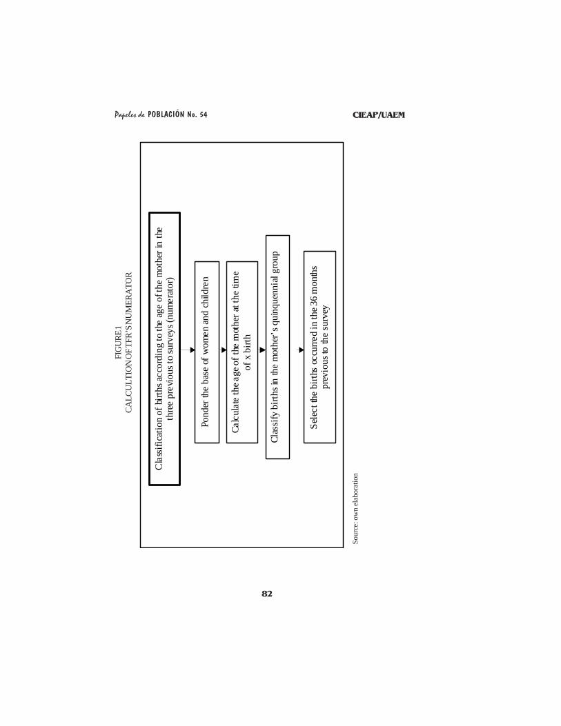
(Campbell, 1983). The methods of TFR estimation applied are summarized infigures 1 and 2.

One of the main factors which had to be controlled was the right classificationof births and time of exposure in the denominator, by quinquennial groups of themother’s age at the time of x children’s birth. Since time of exposure is acontinuous variable, it is possible that the event occurs in the limits of the intervalsof the quinquennial age groups, providing a time of exposure to adjacent groups.

Exposure time is measured in months and once the classification by quinquennialage groups in the three last years (in the last 36 months) prior to the survey iscontrolled, the base is pondered to have as a result a tabulation with the followingcolumns: quinquennial group (categories one to seven), births in each group andexposure time women in each age group provide. From said tabulation thecalculations of the specific fertility rates and the global fertility rate were made.

The procedure to calculate TFR becomes an independent and integral moduleon its own, which is later retaken (referred to) in the resampling executionprogram.

Background of variance estimation

Several methods to estimate variances have been put forward in the literaturefor more complex functions than the total and medians. The most used is themethod for Taylor series that is applied to estimators defined by non-linearfunctions, however, since several derivates are calculated it can be tedious andcomplex to apply (Sul et al., 1989). On the other side, the methods of randomgroups use subsamples, trying as much as possible to preserve the design in theoriginal sample. Indeed, the way to obtain the size of said subsamples is a problemin complex designs (Korn and Graubard, 1999).

A new alternative is given by the methods of resampling and replicas. Theadvantage of these methods is that the units of observation are kept togetherinside a primary unit while it the replicas are constructed, which preservesdependency between the observation units within the same primary unit (Setter,1992a).

Because of this they are applicable to different stratified, poly-phased andprobabilistic designs that have a data distribution that is not identically distributed

82


Cla

ssifi

catio

n of

birt

hs ac

cord

ing

to th

e ag

e of

the

mot

her i

n th

e th

ree

prev

ious

to su

rvey

s (nu

mer

ator

)

Pond

er th

e ba

se o

f wom

en an

d ch

ildre

n

Calc

ulat

e th

e age

of t

he m

othe

r at t

he ti

me

of x

birt

h

Clas

sify

birt

hs in

the

mot

her’

s qui

nque

nnia

l gro

up

Sele

ct th

e bi

rths

occu

rred

in th

e 36

mon

ths

prev

ious

to th

e su

rvey

Sour

ce: o

wn

elab

orat

ion

FIG

URE

1CA

LCU

LTIO

N O

F TFR

’S N

UM

ERA

TOR



Cla

ssif

icat

ion

of e

xpos

ure

time

of w

omen

unt

il bi

rth

(den

omin

ator

)

Add

and

pon

der

the

expo

sure

tim

es

Cal

cula

te th

e ag

e of

wom

en a

t the

tim

e of

the

inte

rvie

w

Acc

ordi

ng to

the

prev

ious

age

, cla

ssif

y w

omen

in

a q

uinq

uenn

ial

grou

p (x

+ 5

)

Cal

cula

te th

e ex

posu

re ti

me

in m

onth

s th

e w

oman

has

in

the

curr

ent g

roup

(x

+ 5)

and

in th

e pr

evio

us g

roup

(x)

at

the

time

of th

e ch

ild’s

bir

th

Cal

cula

te T

EF

and

TF

R

Cla

ssif

y th

e ex

posu

re ti

mes

by

wom

en’s

qui

nque

nnia

l age

gro

ups

Sour

ce: O

wn

elab

orat

ion

FIG

URE

2CA

LCU

LATI

ON

OF T

FR’S

DEN

OM

INA

TOR

84


F

)ˆ(ˆ )(

.,..,2,1,

),...,,( 21

FtFt

nix

xxxF

i

n

==

=

→

θθ

inside a primary unit while it the replicas are constructed, which preservesdependency between the observation units within the same primary unit (Setter,1992a).

Because of this they are applicable to different stratified, poly-phased andprobabilistic designs that have a data distribution that is not identically distributed(Lohr, 2000). The standard resampling method, a method of simple randomsampling with replacement, was proposed by Efron and Tibshirani in 1979; theinterest was mainly in studying standard error and bias in function of samplingvariability. These researchers developed the basic concepts of this techniquefrom the plug-in principle.2 In 1992, Sitter applies bootstrap with replacement(BWR) for stratified random samples and observes that the estimator ofvariance, compared to Cochran’s formula (1977) for the same model, wasbiased. To solve this problem Sitter proposed introducing a correction factor thatadjusts the estimator, yet only for the case of a sample with stratum. In this casethe estimated variance with resampling is consistent and unbiased.

The advances in the technique’s development are related to the desirablepriorities of the estimators (un-biasing and consistency) which are distorted incomplex samples. In this line, resampling methods to estimate variance andconfidence intervals where the sampling occurs without replacement have beenproposed; namely: Jackknife, bootstrap without replacement (BWO), Bootstrap

The function of empirical distribution assigns each realization of the sample a probability 1/n foreach value of

is defined as

When the distribution of probabilities is known, in the case of a census, finding the variance isnot difficult. We do not usually have a census; then we draw to statistical inference that enables us toinfer properties of from a random sample X. “Then is a parameter of , while is a statisticsbased on X. Hence the plug-in estimator of the parameter

2 σFθθ ˆ FF

2 Let us take into account a random sample of size n with a distribution of probabilities .F



stratified designs (Efron, 1982). Another method consists in re-scaling (adjust themediator) the standard method when the estimator is a non-linear function of themeans (Rao and Wu, 1988); in this method, the algorithm is applied with aselected sample size mk not necessarily the size of nh (size of the sample instratum h) and the values of the bootstrap are appropriately re-scaled so as tohave unbiased estimators in the linear case. Since each datum has to be re-scaledin each bootstrap, this process can be complicated in more complex samples.Whereas BWO and BWR are only applicable to simple designs, the version ofbootstrapping with re-scaling is extended to more complex designs for functionsof means and which are more intensive and more difficult to use in a computingmanner.

Applications of bootstrapping methods

The researches carried out by the aforementioned authors have used hypotheticalfinite populations to experiment with the different bootstrapping methods.Attention has been paid to the study of estimations which are linear functions ofmeans; nevertheless, there have been also simulations of the case of estimatorsof ratio, regression coefficients, correlation coefficients and median. It isconcluded that MMB and BWO have an acceptable performance compared toother methods (Sitter, 1992b). In 1994 MMB is applied to a 3-phase stratifieddesign to estimate a ration with acceptable results. Despite more research isnecessary, there is evidence that the estimation of the confidence intervals isappropriated according to the plug-in principle (Robb, 1994). In Australiaseveral bootstrap methods were applied for a ratio estimator (Y: income from thesale of a product; X: quantity of this product) where high biases that can beattributed to the sort of selected estimator were found, however, it is alsosuggested applying more sophisticated bootstrapping methods for bias correction(Davidson and MacKinnon, 1993).

Bootstrapping methods have been mainly applied in the economics’ field. Animportant example is the interest in studying the statistical significance of thechanges in the indicators of inequality and welfare through Gini’s index. If theincome surveys were always based on the same households, temporaryvariations in the inequality and welfare indicators would really reflect changesin income distribution. In reality, it is more frequent to find surveys applied to

86


Bootstrapping methods have been mainly applied in the economics’ field. Animportant example is the interest in studying the statistical significance of thechanges in the indicators of inequality and welfare through Gini’s index. If theincome surveys were always based on the same households, temporary variationsin the inequality and welfare indicators would really reflect changes in incomedistribution. In reality, it is more frequent to find surveys applied to differenthouseholds from one period to another. Thus, the differences in these indicatorscould be simply attributed to the fact that the sample changed, and not to realvariations in inequality of income. For instance, Gini’s coefficient computed inyear t can be superior to that of the year t-1, simply due to sampling phenomena(whether there had been any change in income distribution), so the conclusionthat the distribution has become more inequitable is not necessarily correct(Gasparini and Sosa, 1998).

Characteristics of the bootstrapping model utilized

The theoretical results from the bootstrapping technique were developed fordifferent statistical areas of the surveys by sampling. The extension of bootstrapto complex samples is recent and one of its possible uses is the estimation ofstatistical distribution by sampling an estimator of ratio such as TFR.

In the present work t is an estimator of Bolivia’s total fertility rate in 1998.The only information available comes from a sample with the structure ofhierarchical data, which increases the complexity of the estimations. The objectof interest consists in obtaining a measure of dispersion for F(t) and a confidenceinterval for the punctual estimation of t. The analytical evaluation of thesestatistics requires being aware of F(t) distribution. It is true indeed that thedistribution by sampling of F is not known and the derivation of the standarderror(s) and the confidence interval are analytically complex; the bootstrapmethod, as it has been stated, allows us to approximate F(t) using the empiricaldistribution of the sample F(t).

Bootstrap with replacement is applied considering in the first phase UPM andin the second USM. Bootstrap is less efficient than bootstrap with replacement,nevertheless it is used as it provides facility to choose and analyze the samples.Bootstrap can be applied into sampling by conglomerate in two phases, Robb(1994) finds the contribution of the variance in the second phase will be



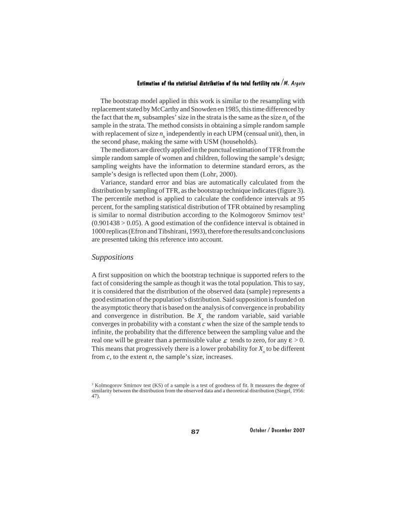
The bootstrap model applied in this work is similar to the resampling withreplacement stated by McCarthy and Snowden en 1985, this time differenced bythe fact that the mh subsamples’ size in the strata is the same as the size nh of thesample in the strata. The method consists in obtaining a simple random samplewith replacement of size nh independently in each UPM (censual unit), then, inthe second phase, making the same with USM (households).

The mediators are directly applied in the punctual estimation of TFR from thesimple random sample of women and children, following the sample’s design;sampling weights have the information to determine standard errors, as thesample’s design is reflected upon them (Lohr, 2000).

Variance, standard error and bias are automatically calculated from thedistribution by sampling of TFR, as the bootstrap technique indicates (figure 3).The percentile method is applied to calculate the confidence intervals at 95percent, for the sampling statistical distribution of TFR obtained by resamplingis similar to normal distribution according to the Kolmogorov Smirnov test3

(0.901438 > 0.05). A good estimation of the confidence interval is obtained in1000 replicas (Efron and Tibshirani, 1993), therefore the results and conclusionsare presented taking this reference into account.

Suppositions

A first supposition on which the bootstrap technique is supported refers to thefact of considering the sample as though it was the total population. This to say,it is considered that the distribution of the observed data (sample) represents agood estimation of the population’s distribution. Said supposition is founded onthe asymptotic theory that is based on the analysis of convergence in probabilityand convergence in distribution. Be Xn the random variable, said variableconverges in probability with a constant c when the size of the sample tends toinfinite, the probability that the difference between the sampling value and thereal one will be greater than a permissible value ε tends to zero, for any e > 0.This means that progressively there is a lower probability for Xn to be differentfrom c, to the extent n, the sample’s size, increases.

3 Kolmogorov Smirnov test (KS) of a sample is a test of goodness of fit. It measures the degree ofsimilarity between the distribution from the observed data and a theoretical distribution (Siegel, 1956:47).

88

CIEAP/UAEMPapeles de POBLACIÓN No. 54FI

GU

RE

3B

OO

TSTR

AP

FOR

STR

ATI

FIED

SA

MPL

ES

Sour

ce: S

itter

(199

2a).

1.

Obt

ener

una

mue

stra

con

reem

plaz

o

hn ihiy

1*

=de

la m

uest

ra o

rigin

al

hn ihiy

1=

inde

pend

ient

emen

te e

n ca

da e

stra

to.

2.

Cal

cula

r

h

hin

iL

hy

s,..

.,2,1

;,..

.,2,1

:*

*=

==

don

de

()

**

ˆˆ

sθ

θ=

3.

Rep

etir

el p

aso

1 un

gra

n nú

mer

o de

vec

es, B

, par

a ob

tene

r *

* 2* 1

ˆ,..

.,ˆ ,

ˆB

θθ

θ.

4.

Estim

ar la

var

( θ) =

()

()(

)2*

*ˆ

ˆ°

−θ

θb

E d

onde

()

()

∑ =

=°

B b

Bb

1

**

/ˆ

ˆθ

θ

5.

Estim

ar el

err

or

()

()[

]2/1

1

2*

*)1

/(ˆ

ˆˆ

⎭⎬⎫

⎩⎨⎧−

°−

=∑ =B b

BB

bes

θθ

6.

Estim

ar e

l ses

go

())ˆ (

ˆF

tbi

asB

−=

∧

oθ

7.

E

stim

ar e

l int

erva

los

de c

onfia

nza

al 9

5%

5.2ˆ

ˆ)

*(in

f=

=α

θθ

avo

per

cent

il de

la d

istrib

ució

n de

*θ

5.97

ˆˆ

)1

*(su

p=

=−α

θθ

avo

per

cent

il de

la d

istrib

ució

n de

*θ

Obt

ain

a sa

mpl

e w

ith re

plac

emen

tof

the

orig

inal

sam

ple

whe

re

3.

R

epea

t ste

p 1

a la

rge

num

ber o

f tim

es, B

, to

obta

in

4.

Estim

ate

the

var

whe

re

5.

Estim

ate

the

erro

r

Estim

ate

bias

Estim

ate

the

conf

iden

ce in

terv

als a

t 95%

2.5th

per

cent

ile o

f dis

tribu

tion

of

97.5

th p

erce

ntile

of t

he d

istri

butio

n of

2. C

alcu

late

inde

pend

ently

in e

ach

stra

tum



Separately, Xn converges in a distribution to a random variable X withaccumulated distribution function F(X), if the difference between the samplingdistribution and the real distribution tends to zero to the extent the size of thesampling does, for all the points of continuity of F(X). These basic concepts fromthe asymptotic theory (Davidson and MacKinnon, 1993) are directly related tothe plug-in principle (Efron and Tibshirani, 1993).

In a second instance it is supposed that the estimator of TFR used in thisresearch is good. For Chou (1977), there are infinite estimators of a parameter;trying all of them out and finding the best is impossible. In this case, the functionused to estimate the total fertility rate we considered a “better” estimator, sincethe theoretical definition of a rate is applied, this is to say, it considers that in thedenominator the time of risk exposure of women in reproductive ages instead ofthe average population of women in reproductive ages that is commonly used.

In relation to the sample, it is supposed that the basic sample that is used tobootstrapping is representative. This concept is crucial in all statistical reasoningand it is understood as the fact that the sample should be similar to the population.It is difficult to secure the representativeness in small samples which have notbeen obtained with random processes. Nonetheless, the law of the large numbersallows us to expect representative samples (Méndez, 2004). The Endsa samplewhich comes from a stratified, bi-phased sampling has a high probability ofbeing representative.

ResultsParametric estimation of the confidence intervals

As a reference point in the first place the method of traditional statisticalinference was applied. The construction of the estimators implies the estimationof totals to the different levels of disaggregation. Finally, the complexity issummarized as the addition of the multiplication of the pondering factors of thedifferent levels, by the TFR (τ ) at the lowest level.

In this exercise a there is a table that contains information of the code thatunivocally identifies each woman, the compensator, the quinquennial groupthey belong to, the exposure time in the respective group and the number ofchildren in the group. Once the time of exposure is annualized (te) the functionof estimation of rates in complex samples that Stata has to estimate specificfertility rates defined by the quotient of children/te in each age group was used.

90

CIEAP/UAEM Papeles de POBLACIÓN No. 54

[ ] [ ] ) ˆ (

) ˆ ( ) ˆ (

2 / 1 t CV t V

t t E ≤

− (3)

Later TFR is calculated through a linear combination of the specific fertility rates (considering the covariances between TEF), the standard error and the confidence intervals are calculated under the supposition of a normal statistical distribution of TFR. For 1998 we consider a TFR of 4.243 children per woman, a datum close to Bolivia’s INE estimation (4.2), and the confidence interval of 95 percent is [4.108, 4.379] (table 1). How certain are these estimations considering that they are obtained from a sample of the total population and that a theoretical distribution, the normal, is assumed to estimate the confidence intervals? TFR’s statistical distribution is not known a priori.

Nonparametrical estimation: simple random bootstrapping

Before the application of bootstrapping considering the complex design of the sample, we experimented with simple random sampling (MAS) to evaluate the behavior of data in relation to the theory by Efron and Tibshirani (1993). By means of the algorithm of TEF and TFR estimation described in the section on the methods we obtained an initial punctual estimation of τ = t( F ˆ ) = 4.228 of TFR (it does not consider the covarianes between TEF). For 1000 replicas we obtain an estimation τ = t( F ˆ ) = 4.327 and a confidence interval of 95 percent of [4.187, 4.474] (table 1). The interval is coherent and includes the estimated value τ (the official TFR in 1998, is closer to the inferior limit). To the extent that the number of replicas increases, the distribution by sampling approaches the normal while ês slightly decreases.

In table 1 we see that the coefficients of variation (CV) are greater than the quotient between the bias and the standard error (with simple random bootstrapping), although not much, this indicates us that the bias of t is consistent as the following inequality, called standardized bias of t , would be proven (Raj, 1968):


Estimation of the statistical distribution of the total fertility rate /M. Argote

where

Bootstrap in a phase of the sample design

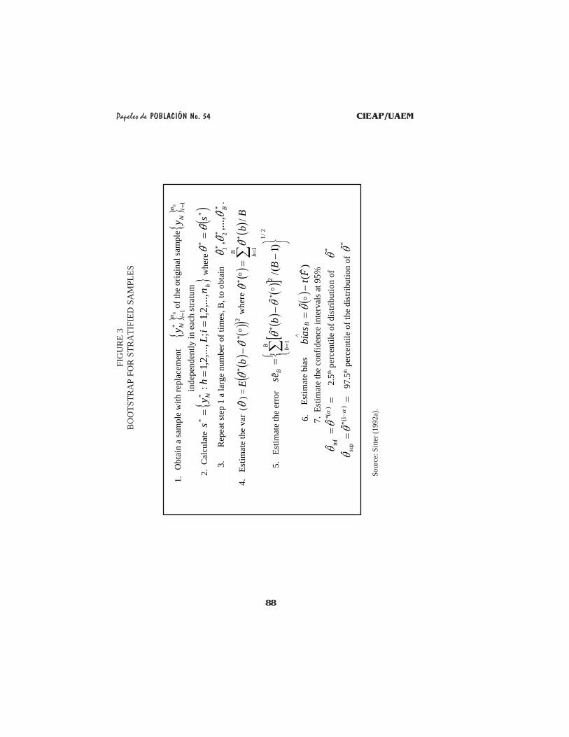
The third phase in the experimentation with bootstrap takes into account a phase; this is partly to verify if actually the standard error from the second phase can be negligible, such as it is indicated in the theory based on Taylor series. Several experiments were run with different numbers of replicas (200, 400, 1000) considering UPM and greater stability of the distribution by sampling of τ was found, being similar to the normal one (figure 4a). The Kolmogorov Smirnov test for 1000 replicas (sig = 0.901438 > 0.05) indicates us that we cannot reject the hypothesis of the normality of the statistical distribution of the total fertility rate of Bolivia in 1998.

It is necessary to point out that this variability is kept in determinate limit, for our case between 0.05525 and 0.05882. We also need to mention that the value of the standard error in 1000 replicas is lower than the standard error with simple random sampling (table 1). This is so because within the strata the variance is lower than the global variance for the design’s ends.

In respect to the behavior of the TFR estimator in function of the number of replicas, we see that there is a tendency toward convergence. For less than 400 replicas the TFR is more fluctuant, whereas for B greater or equal to 400, the estimator becomes more stable. This phenomenon proves the asymptotic theory in the background of the bootstrap method.

Bootstrapping in a phase of the design, as it was expected, allows us to estimate a biased TFR, this is to say, the expected value is different from the parameter that in this case is 4.2, according to INE. Nevertheless, the standardized bias is greater than the variation coefficient, which indicates that bias is not consistent according to equation 4. Otherwise, this can be interpreted as the confidence interval in a phase of the sample design would not be including the complete variability of the estimator. In such sense, in spite theory states that the variance in the second phase is negligible, it was necessary to experiment in a second phase of the sample design.

t s e t CV ˆ ) ˆ ( = (4)

92


Sour

ce: o

wn

calc

ulat

ion

carr

ied

out i

n St

ata,

bas

ed in

End

esa

1998

Estim

atio

ns a

t 100

0 re

plic

as, N

A=

not a

pplic

able

The

offic

ial 1

998

INE

datu

m w

as c

onsi

dere

d as

a p

aram

eter

Ic 9

5%

Es

Med

ian

Para

met

er 1

998

Bia

s B

ias/e

sCV

In

f. Su

p.

KS-

Z Si

g.

Para

met

ric es

timat

ion

of T

FR

0.

069

4.24

4.

230

0.01

3 0.

192

1.63

0 4.

108

4.37

9 N

.A.

N.A

. Si

mpl

e ran

dom

boo

tstra

p

0.07

3 4.

327

4.23

00.

097

1.33

41.

678

4.18

7 4.

474

0.85

6 0.

456

Sing

le b

ootst

rap

in th

e sam

ple

desi

gn

0.05

5 4.

329

4.23

00.

099

1.79

21.

276

4.22

4 4.

437

0.57

0 0.

901

Two-

phas

ed b

ootst

rap

in th

e sam

ple

desi

gn

0.

102

4.32

7 4.

230

0.09

7 0.

952

2.36

4 4.

172

4.49

9 0.

995

0.27

5

TAB

LE I

STA

ND

AR

D E

RR

OR

(ES)

, MED

IAN

, BIA

S, V

AR

IATI

ON

CO

EFFI

CIE

NT

(CV

) AN

D C

ON

FID

ENC

E IN

TER

VA

LS(I

C) E

STIM

ATE

D B

Y P

AR

AM

ETR

IC (1

) AN

D N

ON

-PA

RA

MET

RIC

AL

(2, 3

, 4) I

NFE

REN

CE



4.500 4.438 4.375 4.313 4.250 4.188 4.125

100

80

60

40

20

0

4,688 4,581 4,475 4,368 4,261 4,155 4,048

120

100

80

60

40

20

0

FIGURE 4 STATISTICAL DISTRIBUTION OF TFR FOR THE TOTAL POPULATION

GENERATED IN A THOUSAND REPLICAS OF A) BOOTSTRAP IN A PHASE AND B) BOOTSTRAP IN TWO PHASES

Source: own elaboration based on data from bootstrap.

A B

Bootstrapping in two phases of the sample design

In the first place, it is observed that distribution has a normal behavior (figure 4b). The distribution’s mean does not vary; it remains constant in 4.32 children per women for 1998, a value that is greater than the parametric estimation (method 1 of the figure 5b). The standard error is almost doubled in comparison with the previous method, since besides the variability in UPM, variability in USM is also considered because of this, in this case we will not be able to disregard the standard error in the second phase of the sample design.

The standard error under the supposition of normality (method 1) does not greatly differ from simple random bootstrap (figure 5), it decreases in single phased bootstrapping, yet it increases considering the complete design of the sample (0.102).

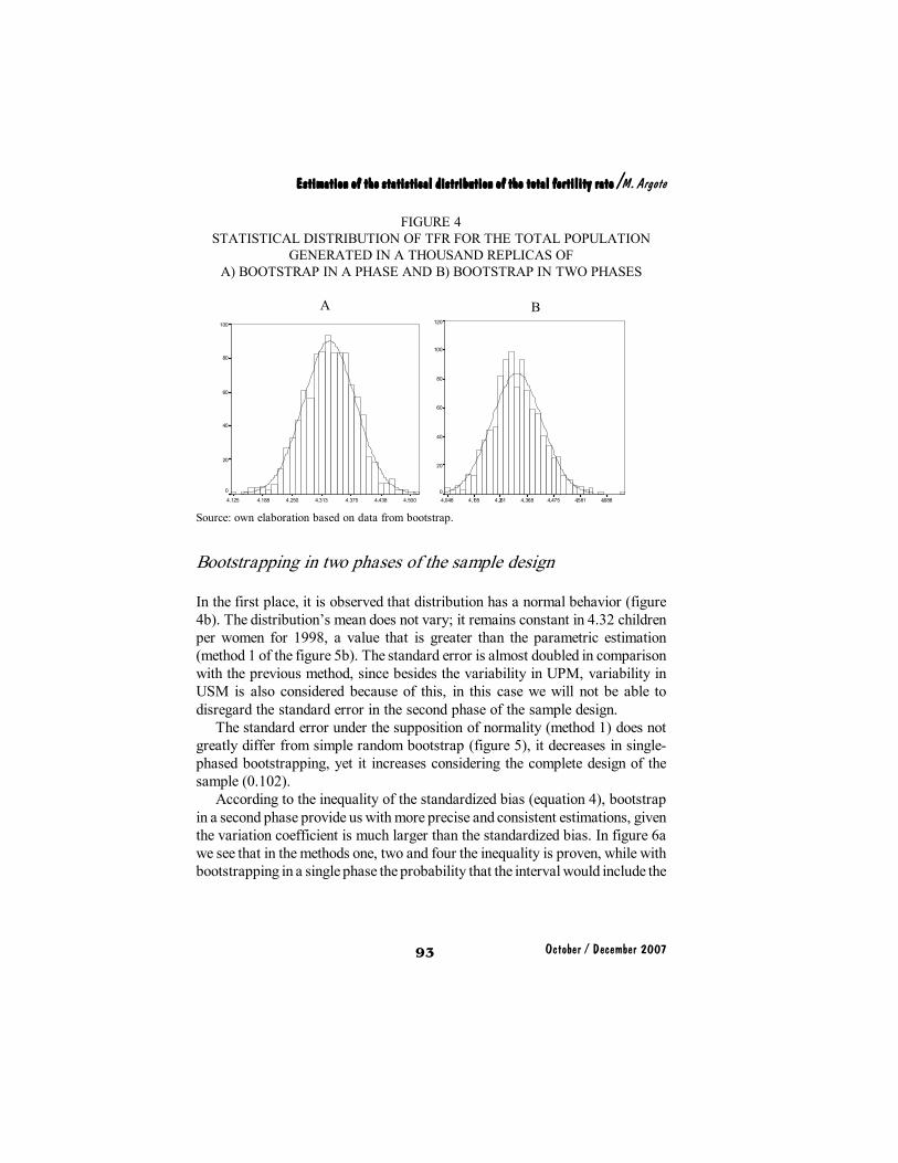
According to the inequality of the standardized bias (equation 4), bootstrap in a second phase provide us with more precise and consistent estimations, given the variation coefficient is much larger than the standardized bias. In figure 6a we see that in the methods one, two and four the inequality is proven, while with bootstrapping in a single phase the probability that the interval would include the

94


real values of TFR was lower, this problem is solved considering the whole design of the sample in bootstrapping.

The confidence intervals of 95 percent, estimated from the different methods, are coherent since they include the different estimations of TFR (figure 6b). Approximately the amplitude of the confidence interval is the same for all of the different methods, with the exception of the third (bootstrap in a single phase) which is lower. Considering that the normality of the statistical distribution by sampling of TFR is accepted, it would be expected that the estimated statistics were similar by means of any method (but the third); nonetheless, the greater difference is to be found on the centrality of the mean by bootstrapping in the different intervals estimated. The mean by bootstrapping (4.32) is above the punctual estimation by parametric inference (4.24), which is closer to the inferior limit of the estimations by resampling. Considering that TFR’s parameter at national level in 1998 is 4.2 children per woman greater but consistent biases were obtained.

It is worth mentioning that, in 2002, the National Institute of Statistics of Bolivia (Instituto Nacional de Estadística de Bolivia) published new estimations of TFR for the 19901995 and 19952000 quinquenniums, whose confection took into account all of the information sources available on fertility thus far (diverse surveys and the 2001 census). For the 19952000 period a TFR of 4.32 children per woman was obtained, precisely the mean of the statistical distribution obtained by bootstrapping in the present work. This is to say, even if the confidence intervals vary in function of the standard error that at the time depends on the sample design, the mean by sampling remains constant and it can be considered as a estimation of lower bias or that it has a greater probability to approach the real value.

The standard error of a statistical estimation, using a multiphased design, such as that used for Endsa 1998, is more complex that the standard error based on simple random sampling and tends to be greater that the standard error produced by a simple random sample. The increment in the standard error from the use of a multiphased design is known as the effect of design and it is defined as the reason between the variance of the estimation with the currently used design and variance of the estimation that would be produced if a simple random sample was used. When it takes the value of one, indicates that the design is as efficient (produces minimal variances) as a simple at random; while a value greater than one, indicates that the design utilized produces a greater variance than that which would be obtained with a simple random sample (Cepep, 2004).



FIGURE 5 COMPARISON OF THE MAIN STATISTICS FROM THE APPLICATION OF

PARAMETRIC AND NONPARAMETRIC ESTIMATION

Source: own calculation based on the statistical distribution generated by bootstrapping.

4.200 4.220 4.240 4.260 4.280 4.300 4.320 4.340

1 2 3 4

Métodos de est imación

0.0 00 0.0 20 0.0 40

0.0 60 0.0 80 0.1 00 0.1 20

1 2 3 4

M ét odo s de e stim ación

A

B

TGF

es

Estimation methods

Estimation methods

TFR

96


FIGURE 6 STANDARDIZED BIAS AND CONFIDENCE INTERVALS ESTIMATED BY

DIFFERENT METHODS

Source: own calculation based on the statistical distribution generated by bootstraping.

3.9 4.0 4.1

4.2 4.3 4.4 4.5 4.6

1 2 3 4

M étodos de e stim ac ión

lim inf lim sup 4.23 (1998) 4.32 (2002)

A

B

Interválos de confianza

0.0

0.5

1.0

1.5

2.0

2.5

1 2 3 4 Métodos de estimación

sesgo/es cv

Sesgo estandarizado

Standardized bias

Estimation methods

Bias/es

Confidence inervals

Estimation methods



In our case an Edis of 1.18 is obtained, proving that it is an efficient sample.

Bootstrapping by residence place

As it was seen, the precision of an estimator through bootstrapping depends on the number of replicas, of the similarity of the bootstrapping with the original sample, of the parameter available for the calculation of bias (in our case 4.2) and ês. In order to contribute to explain ês variations in a bistratified phased design it is interesting to analyze by urban/rural place of residence (figure 6).

It was already mentioned in the introduction that the differences in TFR by residence place in Bolivia are very important, which can influence on an increment or decrement of the total variance, moreover, the analysis by residence place allows us to verify the potential of bootstrapping by subgroups.

According to KolmogorovSmirnov test, the hypothesis of the normality of distribution for both the rural and urban areas cannot be rejected at a significance level of 0.1. Notwithstanding, we have to distinguish that according to statistical evidence the variance in the rural area is greater. This fact is also reflected on the

differences of bias; the estimator’s bias boot τ is lower in the rural area than in the urban one. As bias depends on the extracted sample, the number of cases in each group can be influencing on the differences that are observed (7422 cases in the urban area and 3765 cases in the rural area). This warns us about the attention we should pay to the affirmations when samples of the total population are being worked with, since the changes can be caused by sampling variations and not necessarily by changes in the estimator of the population.

The amplitude of the confidence interval of the rural area is greater than that of the urban area, which indicates a greater dispersion of data from the rural area. This situation was expected, as fertility in urban Bolivia, based on Endsa 1998, is circa three children per woman, conversely, in the rural areas fertility rates are more heterogeneous and higher (approximately six children per woman).

) ˆ ( ) ˆ (

t VAR t VAR

EDIS simple

complejo = (5)

98


FIGURE 7 STATISTICAL DISTRIBUTION OF THE TOTAL FERTILITY RATE

AT A THOUSAND REPLICAS BY PLACE OF RESIDENCE

6 .96 6 .79 6.62 6.45 6. 28 6.1 1 5.94

100

80

60

40

20

0

3 .77 5 3.6 50 3. 525 3.40 0 3.27 5 3. 150 3 .025

10 0

8 0

6 0

4 0

2 0

0

Source: own elaboration with help from the statistical program SPSS.

Urban Rural

Discussion

In regards to the research’s central topic: What is TFR’s statistical distribution? It is concluded that the hypothesis of the normality of its distribution cannot be rejected. KolmogorovSmirnov test indicates us that based on data from the Endsa1998 sample there is not enough evidence to reject the void hypothesis stated. Hence, it is adequate to apply the law of the large numbers and the theorem of central limit in the calculation of the confidence intervals of TFR.

In the present research the supposition of normality and the technique of bootstrap have been applied to estimate the confidence interval of TFR’s estimator. Even if the results show us that when the number of replicas tends to infinite sampling distribution of TFR is similar to the normal, in table I and II we can see there are differences in the estimators’ precision.



Source: own elaboration based on data from

bootstrapping.

TABL

E II

TFR ES

TIMATIONS, STA

NDARD

ERR

OR (ES), B

IAS AND CONFIDEN

CE INTE

RVAL (IC)

BY PLA

CE OF RE

SIDEN

CE, BOLIVIA, 1998

100


Under the supposition of normality of distribution we found that τ n = 4.243, un ês n = 0.069 and a confidence interval of 95 percent [4.108, 4.379]. Bootstrap method in two phases (1000 replicas) gives us a punctual estimation of τ = 4.327 with a confidence interval of 95 percent [4.172, 4.499]. Even if the estimation of the confidence interval of TFR under the supposition of normality includes with high probability the value of the demographic parameter, bootstrapping technique allows us to find more precise confidence intervals. In the case of simple random bootstrapping, such as the bootstrapping of the complex sample, confidence intervals include the official estimations and those from TFR bootstrapping; therefore, the confidence interval estimated by means of bootstrapping is coherent.

In this case the variance in a second phase cannot be considered negligible as the theory indicated; bootstrap in two phases increases the variability of data in as much as twice of a phase’s variability. This increment is coherent since it approaches the variability of simple random bootstrapping (Edis = 1.18), which is a good measure of the efficiency of the sample and that it is correctly reproduced.

The standard error estimated by bootstrapping the complex sample (0.102) has a value greater than the traditional estimation (0.069), reflecting the effect of a sample’s design. The importance of the sample’s design on the statistical inference is verified. So, when statistical model are constructed for samples, the use of functions oriented to complex samples is recommended, such as those of Stata, something that is not standard practice.

We found that TFR is a biased estimator for the sample of Endsa 1998 in Bolivia. This situation was expectable in accordance with the theory of ratio estimation. Based upon the theorems of parametric inference, we can only calculate unbiased indicators for any function of the means, however there are not formulae to calculate unbiased estimators of TFR, unless by means of approximations. Bias indicates us how far our estimation is from the demographic parameter since the fact of considering a sample and a technique of bootstrap allows us to calculate it automatically. The results show us a standardized bias much lower than the coefficient of variation (see figure 6a), which is an important characteristic to evaluate the consistency of estimations.

Finally, we managed to verify that normality of distribution is not rejected for subgroups either, both in the urban and rural areas in the present case, and so we can advance a step on the generalization of the theorem of the central limit



Bibliogr aphy

ANDRÉS, Raquel and Samuel Calonge, 2001, Incidencia de impuestos y prestaciones en España: una evaluación desde la perspectiva de la inferencia estadística, Departamento de Econometría, Estadística y Economía Española, Barcelona. CAMPBELL, Arthur, 1983, Manual of fertility analysis, Center for Population Research/National Institute of Child Health and Human Development/World Health Organization/Churchill Livingstone, Bethesda, Maryland. CARAFA, C., G. Gonzales, V. Ramirez, Pereira and H. Torrez, 1983, Luz y sombra de la vida, mortalidad y fecundidad en Bolivia, Proyecto de Políticas en Población, La Paz. CENTRO PARAGUAYO DE ESTUDIOS DE POBLACIÓN, 2004, Informe final de la Encuesta Nacional de Demografía y Salud Sexual y Reproductiva, Asunción. CHAMBERS, R. and D. Dorfman, 1994, Robust simple survey inference via bootstrapping and bias correction: the case of ratio estimator, Souththampton Statistical Sciences Research Institute, University of Souththampton. COCHRAN, William, 1977, Sampling techniques, Wiley Publications in Statistics, Library of Congress Catalog Card Number: 535412. DAVIDSON, R. and J. MacKinnon, 1993, Estimation and inference in econometrics, Oxford University Press, New York. EFRON, B. and R. Tibshirani, 1993,An introduction to the bootstrap, Chapman & Hall, New York. EFRON, B., 1982,The Jackknife, the bootstrap and other resampling plans, Department of Statistics, Stanford University, CBMSNSF Regional Conference Series in Applied Mathematics, Society for Industrial and Applied Mathematics, Philadelphia. ENDSA, 1998, Informe final, Instituto Nacional de Estadística de Bolivia. FEYERABEND, Paul, 1989, Contra el método: esquema de una teoría anarquista del conocimiento, Editorial Ariel, Barcelona. GASPARINI, Leonardo and Walter Sosa, 1998,Bienestar y distribución del ingreso en Argentina, 19801998,Departamento de Economía, Universidad Nacional de La Plata. KORN, Edward L. and Barry Graubard, 1999, Analysis of health surveys, Wiley Series in Probability and Statistics, Survey methodology section, A WileyInterscience, Publication. LOHR, Sharon, 2000, Muestreo: diseño y análisis, International Thomson Editores, Biblioteca Iberoamericana. Mexico. MCCARTHY, P. and C. Snowden, 1985, “The bootstrap and finite population sampling”, in Vital Health Stat, 2, January (95), Pubmed.

and the law of the large numbers for the estimator of the total fertility rate from a complex sample. Nonetheless, more experimentation with the technique is necessary for other populations with a different fertility pattern.

102


MÉNDEZ, Ignacio, 2004, La estadística, Instituto de Investigación en Matemáticas Aplicadas y Sistemas, UNAM. RAJ, Des, 1968, Sampling theory, Mac Graw Hill. RAO, J. and C. Wu, 1988, “Resampling inference with complex survey data”, in Journal of the American Statistical Association, num. 83. ROBB, William, 1994, Resampling variance estimates for complex survey designs: a simulation study, Macro International Inc., 126 College St., Burlington. SITTER, R. 1992a, “A resampling procedure for complex survey data”, in Journal of American Statistics Associations, num. 87. SITTER, R., 1992b, “Comparing three bootstrap methods for survey data”, in The Canadian Journal of Statistics, num. 20. SUL Lee, Eun, Ronald Forthofer and Ronald Lorimer, 1989,Analyzing complex survey data, Series Quantitative applications in the social sciences, A sage university paper num. 71, The International Professional Publishers, Newbury Park, London, New Delhi. WHITE, H., 1984, Asymptotic theory for econometricians, Academic Press.

Estimación de la distribución estadística de la tasa global de ...

Documents

Transcript of Estimación de la distribución estadística de la tasa global de ...