Establishing Linux Clusters for high-performance computing ...

Calhoun: The NPS Institutional Archive

Theses and Dissertations Thesis Collection

2004-09

Establishing Linux Clusters for high-performance

computing (HPC) at NPS

Daillidis, Christos

Monterey, California. Naval Postgraduate School

http://hdl.handle.net/10945/1445

NAVAL POSTGRADUATE

SCHOOL

MONTEREY, CALIFORNIA

THESIS

Approved for public release; distribution is unlimited

ESTABLISHING LINUX CLUSTERS FOR HIGH-PERFORMANCE COMPUTING (HPC) AT NPS

by

Christos Daillidis

September 2004

Thesis Advisor: Don Brutzman Thesis Co Advisor: Don McGregor

THIS PAGE INTENTIONALLY LEFT BLANK

i

REPORT DOCUMENTATION PAGE Form Approved OMB No. 0704-0188 Public reporting burden for this collection of information is estimated to average 1 hour per response, including the time for review-ing instruction, searching existing data sources, gathering and maintaining the data needed, and completing and reviewing the col-lection of information. Send comments regarding this burden estimate or any other aspect of this collection of information, including suggestions for reducing this burden, to Washington headquarters Services, Directorate for Information Operations and Reports, 1215 Jefferson Davis Highway, Suite 1204, Arlington, VA 22202-4302, and to the Office of Management and Budget, Paperwork Reduction Project (0704-0188) Washington DC 20503. 1. AGENCY USE ONLY (Leave blank)

2. REPORT DATE September 2004

3. REPORT TYPE AND DATES COVERED Master’s Thesis

4. TITLE AND SUBTITLE: Establishing Linux Clusters for High-performance Computing (HPC) at NPS 6. AUTHOR(S) Christos Daillidis

5. FUNDING NUMBERS

7. PERFORMING ORGANIZATION NAME(S) AND ADDRESS(ES) Naval Postgraduate School Monterey, CA 93943-5000

8. PERFORMING ORGANIZATION REPORT NUMBER

9. SPONSORING /MONITORING AGENCY NAME(S) AND ADDRESS(ES)

N/A

10. SPONSORING/MONITORING AGENCY REPORT NUMBER

11. SUPPLEMENTARY NOTES The views expressed in this thesis are those of the author and do not reflect the official policy or position of the Department of Defense or the U.S. Government. 12a. DISTRIBUTION / AVAILABILITY STATEMENT Approved for public release; distribution is unlimited

12b. DISTRIBUTION CODE

13. ABSTRACT Modeling and simulation (M&S) needs high-performance computing resources, but conventional supercomputers are both

expensive and not necessarily well suited to M&S tasks. Discrete Event Simulation (DES) often involves repeated, independent runs of the same models with different input parameters. A system which is able to run many replications quickly is more useful than one in which a single monolithic application runs quickly. A loosely coupled parallel system is indicated.

Inexpensive commodity hardware, high speed local area networking, and open source software have created the potential to create just such loosely coupled parallel systems. These systems are constructed from Linux-based computers and are called Beowulf clusters.

This thesis presents an analysis of clusters in high-performance computing and establishes a testbed implementation at the MOVES Institute. It describes the steps necessary to create a cluster, factors to consider in selecting hardware and software, and de-scribes the process of creating applications that can run on the cluster. Monitoring the running cluster and system administration are also addressed.

15. NUMBER OF PAGES

186

14. SUBJECT TERMS Clusters, Beowulf, HPC, Rocks, HPL, BPS

16. PRICE CODE

17. SECURITY CLASSIFICATION OF REPORT

Unclassified

18. SECURITY CLASSIFICATION OF THIS PAGE

Unclassified

19. SECURITY CLASSIFICATION OF ABSTRACT

Unclassified

20. LIMITATION OF ABSTRACT

UL NSN 7540-01-280-5500 Standard Form 298 (Rev. 2-89) Prescribed by ANSI Std. 239-18

ii


iii

Approved for public release; distribution is unlimited

ESTABLISHING LINUX CLUSTERS FOR HIGH-PERFORMANCE COMPUTING (HPC) AT NPS

Christos Daillidis Major, Hellenic Army

B.S., Hellenic Military Academy, 1989

Submitted in partial fulfillment of the requirements for the degree of

MASTER OF SCIENCE IN COMPUTER SCIENCE

from the

NAVAL POSTGRADUATE SCHOOL September 2004

Author: Christos Daillidis Approved by: Don Brutzman

Thesis Advisor

Don McGregor Thesis Co-Advisor Peter J. Denning Chairman, Department of Computer Science

iv


v

ABSTRACT

Modeling and simulation (M&S) needs high-performance computing resources,

but conventional supercomputers are both expensive and not necessarily well suited to

M&S tasks. Discrete Event Simulation (DES) often involves repeated, independent runs

of the same models with different input parameters. A system which is able to run many

replications quickly is more useful than one in which a single monolithic application runs

quickly. A loosely coupled parallel system is indicated.

Inexpensive commodity hardware, high speed local area networking, and open

source software have created the potential to create just such loosely coupled parallel sys-

tems. These systems are constructed from Linux-based computers and are called Beo-

wulf clusters.

This thesis presents an analysis of clusters in high-performance computing and es-

tablishes a testbed implementation at the MOVES Institute. It describes the steps neces-

sary to create a cluster, factors to consider in selecting hardware and software, and de-

scribes the process of creating applications that can run on the cluster. Monitoring the

running cluster and system administration are also addressed.

vi


vii

TABLE OF CONTENTS I. INTRODUCTION........................................................................................................1

A. PROBLEM OVERVIEW................................................................................1 B. MOTIVATION ................................................................................................1 C. PROBLEM STATEMENT .............................................................................1 D. THESIS ORGANIZATION............................................................................2

II. BACKGROUND AND RELATED WORK ..............................................................3 A. BACKGROUND ..............................................................................................3 B. RELATED WORK ..........................................................................................4

III. LINUX CLUSTERS FOR HPC..................................................................................5 A. BACKGROUND ..............................................................................................5

1. Introduction..........................................................................................5 2. Clusters Defined ...................................................................................5 3. Symmetric Multiprocessing and Clusters..........................................7 4. Primary Benefits ..................................................................................9 5. Applications..........................................................................................9 6. Process Scheduler...............................................................................10 7. Message Passing Interface (MPI) .....................................................11

B. CLUSTER CLASSIFICATIONS.................................................................13 1. Classification by Type of Hardware.................................................13 2. Classification by Network Technology ............................................15 3. Classification by Size .........................................................................15 4. Classification by Shared Resources..................................................16 5. Classification by Cluster Architecture.............................................18

C. CLUSTER OPERATING SYSTEM............................................................18 1. Failure Management..........................................................................18 2. Load Balancing...................................................................................19 3. Parallelizing Computation ................................................................19

a. Parallelizing Compiler ............................................................19 b. Parallelized Application..........................................................19 c. Parametric Computing............................................................19

D. CLUSTER ARCHITECTURE.....................................................................19 E. DIFFERENT CLUSTER INSTALLATIONS.............................................21

1. Windows Cluster Service ..................................................................21 2. Sun Cluster .........................................................................................21 3. Beowulf and Linux Clusters..............................................................22

F. HARDWARE CONSIDERATIONS............................................................24 1. CPU .....................................................................................................25 2. Memory Capabilities, Bandwidth and Latency ..............................28 3. I/O Channels.......................................................................................29

a. PCI and PCI-X........................................................................29 b. AGP..........................................................................................29 c. Legacy Buses ...........................................................................30

4. Motherboard ......................................................................................30 a. Chipsets....................................................................................30

viii

b. BIOS ........................................................................................30 c. PXE (Pre-Execution Environment) .......................................30 d. Linux BIOS .............................................................................31

5. Storage ................................................................................................31 a. Local Hard Disks ....................................................................32 b. RAID........................................................................................33 c. Non Local Storage ..................................................................33

6. Video....................................................................................................33 7. Peripherals..........................................................................................33 8. Case .....................................................................................................34

a. Desktop Cases..........................................................................34 b. Rack-Mounted Cases ..............................................................35 c. Blade Servers...........................................................................36

9. Network...............................................................................................36 a. 10/100/1000 Base T Ethernet .................................................36 b. Myrinet ....................................................................................36 c. Dolphin Wulfkit.......................................................................37 d. Infiniband................................................................................37

10. Heat Management and Power Supply Issues ..................................37 a. Power Consumption................................................................38 b. Thermal Management.............................................................40

G. LINUX OPERATING SYSTEM..................................................................41 H. SUPERCOMPUTER STATISTICS ............................................................42

IV. INSTALLATION OF THE NPS LINUX CLUSTER ............................................45 A. INTRODUCTION..........................................................................................45 B. OPEN-SOURCE CLUSTER SOFTWARE.................................................45

1. Choosing the Software.......................................................................45 a. Rocks........................................................................................45 b. OSCAR ....................................................................................46 c. Scyld.........................................................................................46

2. Cluster Software Selection ................................................................47 C. SELECTING AND EQUIPPING THE HARDWARE ..............................47 D. INSTALLING THE SYSTEM......................................................................50

1. Download the Software......................................................................50 a. Rocks Base...............................................................................51 b. HPC Roll .................................................................................52 c. Grid Engine Roll .....................................................................52 d. Globus Toolkit .........................................................................52 e. Intel Roll..................................................................................53 f. Area51 Roll..............................................................................53 g. SCE Roll ..................................................................................53 h. Java Roll..................................................................................53 i. PBS Roll ..................................................................................54 j. Condor Roll .............................................................................54

2. Installation..........................................................................................55 E. RUNNING THE SYSTEM............................................................................61

ix

1. Cluster Database ................................................................................66 2. Cluster Status (Ganglia) ....................................................................66 3. Cluster Top (Process Viewer) ...........................................................66 4. Proc filesystem....................................................................................66 5. Cluster Distribution ...........................................................................66 6. Kickstart Graph.................................................................................67 7. Roll Call ..............................................................................................67

F. DETAILS ON ROCKS CLUSTER SOFTWARE......................................68 G. PROPOSAL FOR A NEW SYSTEM ..........................................................70

V. PERFORMANCE MEASUREMENTS...................................................................73 A. INTRODUCTION..........................................................................................73 B. PERFORMANCE MEASUREMENTS OVERVIEW ...............................73

1. Benchmarking for Overall System Performance............................73 2. Benchmarking Subsystems for Measuring Subsystem

Performance .......................................................................................74 3. Benchmarking for Incremental Performance Improvements .......75

C. BENCHMARKS ............................................................................................76 D. HIGH-PERFORMANCE LINPACK ..........................................................77

1. Background ........................................................................................77 2. Configuration .....................................................................................77 3. Test Run..............................................................................................81 4. Results .................................................................................................83 5. Benchmarking Cluster with Only One Node...................................89 6. The Ganglia Meta Daemon ...............................................................91 7. To Enter the Top 500.........................................................................92

E. JAVA HIGH-PERFORMANCE LINPACK...............................................92 1. Background ........................................................................................92 2. Test Run..............................................................................................92 3. JAVA Linpack Hall of Fame ............................................................95

F. BEOWULF PERFORMANCE SUITE (BPS).............................................96 1. Background ........................................................................................96 2. BPS Installation..................................................................................96 3. BPS Run and Results .......................................................................101 4. Results in BPS ..................................................................................102

G. LMBENCH 2.0 SUMMARY.......................................................................103

VI. RUNNING APPLICATIONS ON THE CLUSTER.............................................109 A. INTRODUCTION........................................................................................109 B. SYSTEM ADMINISTRATION AND ADDING NEW USERS ..............109 C. MPI................................................................................................................110 D. THE SCHEDULER .....................................................................................113

1. Submit a Simple Job with the Use of the Command qsub ...........114 2. See the Results of the Submitted Job .............................................114 3. Creation of a Shell Script to Submit the Job.................................115 4. Submission of Multiple Jobs ...........................................................116 5. Check the Jobs Status......................................................................116 6. Delete Jobs ........................................................................................117

x

7. MOVES Cluster Experiment ..........................................................117 8. More in Job Submission Scripts .....................................................122

E. THE COMBINATION OF BATCH SYSTEM AND MPI ......................123

VII. FUTURE DEVELOPMENT...................................................................................125 A. INTRODUCTION........................................................................................125 B. IPV6 PROTOCOL.......................................................................................125 C. CLUSTERS AND DATABASES................................................................128

1. Overview ...........................................................................................128 2. DBMS in a Cluster ...........................................................................128 3. MySql ................................................................................................130

D. POTENTIAL MILITARY DEPLOYMENT ............................................130 1. Overview ...........................................................................................130 2. Types of Installations.......................................................................130

E. SECURITY ISSUES....................................................................................132 1. Overview ...........................................................................................132 2. Firewall .............................................................................................132 3. nmap..................................................................................................133

F. WEB SERVICES .........................................................................................137

VIII. CONCLUSIONS AND FUTURE WORK.............................................................141 A. CONCLUSIONS ..........................................................................................141 B. RECOMMENDATIONS FOR FUTURE WORK....................................142

1. IPv6 and the Grid.............................................................................142 2. Acquisition of a New Rack Based System......................................142 4. Simkit ................................................................................................143 5. MPI Programming...........................................................................143 6. Web Services Investigation .............................................................143 7. Database Use Investigation .............................................................144 8. OSCAR Installation.........................................................................144 9. Xj3D Offline Rendering and Physics Interactions........................144

APPENDIX A. DESCRIPTION OF THE HPL.DAT FILE ...........................................145

APPENDIX B. DETAILED RESULTS OF HIGH PERFORMANCE LINPACK (HPL).........................................................................................................................153

LIST OF REFERENCES....................................................................................................159

INITIAL DISTRIBUTION LIST.......................................................................................165

xi

LIST OF FIGURES Figure 1 A simple approach to construct a cluster consisting of one master and two

slave nodes. The master node provides two NIC for the private and external network of the system. .........................................................................6

Figure 2 Classification of Parallel Processors Architectures when is shown the Multiple instruction stream, multiple data stream (MIMD) is the needed Architecture (After Stallings W, Operating Systems, 2001, p. 170) .................9

Figure 3 The Scheduler Functionality with the Submission of the Same Job with Different Parameters Every Time. ...................................................................11

Figure 4 The Message Passing Functionality.................................................................12 Figure 5 A State Diagram of the Message Passing Functionality. The Parallel

Operating Environment (POE) is the one that handles the overall functionality and Partition Manager Daemons (PMDs) are the messages spawn from the system to the nodes. ...............................................................12

Figure 6 Cluster classification by the type of hardware. There are no distinct categories for these clusters. Instead there is a range of possibilities. At one extreme there are the systems built completely from hardware and software products that can be found in any computer store. At the other extreme, there are special products designed and manufactured especially for their deployment and implementation in a cluster. ....................................13

Figure 7 Graph pointing the relation between different metrics in a cluster system. The more special design and implementation for one system the more increased the cost, the complexity, the performance and the reliance on the vendor. .............................................................................................................14

Figure 8 A picture of a node of the earth simulator. It is a system especially constructed for this cluster.( the picture is from www.top500.org).................16

Figure 9 Two Servers – Two Disks Cluster Connected With High-Speed Message Link. (After Stallings W, Operating Systems, 2001, p. 591)...........................17

Figure 10 Two Servers with Shared Disk Cluster Connected With High-Speed Message Link (After Stallings W, Operating Systems, 2001, p. 591).............17

Figure 11 Cluster Architecture (After Stallings W, Operating Systems, 2001, p. 595)...20 Figure 12 Sun Cluster Architecture. (After Stallings W, Operating Systems, 2001, p.

598). .................................................................................................................22 Figure 13 A Beowulf Cluster with Master and Slave Nodes and Network

Connections. The master node with its two NIC is in this case the gateway between the two networks the internal and the external. The slave nodes are connected to the master node with a switch in the internal (private) network..............................................................................................24

Figure 14 Processors Inputs and Outputs with 32-bit and 64-bit. The Inputs are the Instructions and the Data while the Outputs are the Results. Note that in both cases the Instruction set is 32-bit. The one that changes is the Data Set. ...................................................................................................................26

xii

Figure 15 Pre-execution environment (PXE) diagram. The system boots and after a DHCP request receives from the server the data necessary for the start up process..............................................................................................................31

Figure 16 A Typical Diagram of a Cluster System with Mini Tower Cases. There is a hierarchy in the switching scheme, while some computer, not between the nodes have different roles. This is due to easy administration. ................34

Figure 17 Cluster with rack able cases. All the representing parts are shown in this figure, even though some of them may exist in different rack. The keyboard and the monitor are most of the times necessary for troubleshooting. ...............................................................................................35

Figure 18 Supercomputer statistics. The majority of installations are for the industry followed by research and academia. ................................................................43

Figure 19 Graph of HPC locations. About half of the systems are in North America and the other half in the rest of the world. .......................................................44

Figure 20 A view of a dual processor computer (2nd and 3rd Nodes). ..............................49 Figure 21 The results of generating md5summ for Area51 roll. All the file

information is available. This number can be used to be checked against the number that the vendor provides fro the particular piece of software. ......51

Figure 22 The given md5summ for Area51 roll form the download site. This number can be checked against the one that the md5summ program is going to generate for the specific software. ...................................................................51

Figure 23 Installation Process with Problems, Diagnoses and Troubleshooting. ............56 Figure 24 The working area for the MOVES cluster. The nodes are off the rack

during the hardware configuration. A keyboard and a monitor were used for troubleshooting...........................................................................................57

Figure 25 The NPS cluster with all network details (cluster.cs.nps.navy.mil). The host name of the nodes with the relevant IP addresses for the internal (private) cluster network along with the external network data are shown in this figure. ....................................................................................................58

Figure 26 The SSH for MS Windows ready to connect to the cluster. After connect is selected the next screen is asking for the password. ....................................61

Figure 27 Ganglia Monitor, where the state of the system is presented with great detail.................................................................................................................68

Figure 28 The opt directory contents from NPS cluster. All the necessary pieces of software are residing in this directory for the Rocks Beowulf cluster implementation. ...............................................................................................69

Figure 29 One or two processor at work. This part from the Ganglia monitor shows how a compute node with two processors behaves. First, until 16:30 hours, only one processor is used. After that in a new program run starting at about 01:00 hours both processors are engaged. The normal situation for such a machine is to use both processors. The period that only one of them is used is due to insufficient parameters given to the specific program run......................................................................................................79

Figure 30 All nodes are working unevenly. Due to insufficient parameters in the program run the nodes are not working as desired, regarding the CPU load. The front-end colored red in the left, is working more intensively

xiii

while the two nodes in the middle (orange and yellow) are working less intensive. The blue colored node in the right (compute-0-1) is not engaged at all in the run. ..................................................................................86

Figure 31 All Nodes are Working Evenly. Due to sufficient parameters in the program run the nodes are working as desired, regarding the CPU load. All the nodes are colored orange and are engaged with equal amount of CPU power in the run ......................................................................................88

Figure 32 HPL benchmark results graph. The performance is shown for the specific hardware and software configuration and for different parameters in the benchmarking process......................................................................................89

Figure 33 Checking the ganglia monitor, in every step of the process of installing the software, is necessary to be sure that everything works fine. ..........................99

Figure 34 The BPS results in an http page. This is created from a relevant command and provides easy to read data from the benchmark......................................103

Figure 35 Workload during benchmarking. In the system monitor on the right is shown how the CPU and the memory usage are increased during the tests. .105

Figure 36 The results from a desktop PC that it was used during the experiments for a comparison for the MOVES cluster. ...........................................................107

Figure 37 Cluster architecture with each stack in separate server. In this approach each server is taking care of one protocol (IPv4 or IPv6) and routes the incoming traffic to the nodes. All nodes are dual stack................................126

Figure 38 Cluster architecture with both stacks in the same server. In this approach there is one dual stack server that is taking care of both protocols (IPv4 and IPv6) and routes the incoming traffic to the nodes. All nodes are dual stack. ..............................................................................................................126

Figure 39 System on site. The network is wired and all systems are connected to the cluster through this network...........................................................................131

Figure 40 System off site. Because the command was moved to a new position, the network for the system is wireless, and the users are scattered in a small area. ................................................................................................................132

Figure 41 Security level configuration tool in Linux GUI. The firewall can be enabled and trusted services against trusted devices can be combined. ........133

Figure 42 XML Results from Mozilla browser. The browser fails to translate the results. ............................................................................................................138

Figure 43 XML Results from IE browser. The browser translates the results in an efficient way...................................................................................................139

xiv


xv

LIST OF TABLES Table 1 Typical Power Consumption Levels for Computer Parts. ...............................38 Table 2 Cooling Requirements for Computer Room. ...................................................40 Table 3 Different Linux Distributions Available. .........................................................42 Table 4 HPC Usage.......................................................................................................43 Table 5 HPC Locations .................................................................................................44 Table 6 The Hardware Configuration of NPS Cluster..................................................49 Table 7 Front end NIC configuration............................................................................60 Table 8 Private Cluster Network Configuration. ..........................................................60 Table 9 Checklist for Private Cluster Network. ............................................................61 Table 10 Cluster Components in the Rack......................................................................70 Table 11 Example of Benchmark Logging. ....................................................................75 Table 12 HPL Benchmark Results Table........................................................................88 Table 13 JAVA Benchmark Results. ..............................................................................95 Table 14 Basic System Parameters. ..............................................................................103 Table 15 Processor, Processes - Times In Microseconds. ............................................104 Table 16 Context Switching - Times In Microseconds - Smaller Is Better. .................104 Table 17 Local Communication Latencies In Microseconds - Smaller Is Better. ........104 Table 18 File & VM System Latencies In Microseconds - Smaller Is Better. .............104 Table 19 Local Communication Bandwidths In MB/S - Bigger Is Better....................104 Table 20 Memory Latencies In Nanoseconds - Smaller Is Better. ...............................104 Table 21 Stream Benchmark Results. ...........................................................................105 Table 22 Unix Benchmark Results. ..............................................................................106 Table 23 Jobs Submitted Per Node. ..............................................................................121 Table 24 Ports Open in the System...............................................................................135 Table 25 Use of Supercomputers. .................................................................................138

xvi


xvii

ACKNOWLEDGMENTS

I would like to thank Research Associate Don McGregor for introducing me to

the field of high-performance computing and for his professional guidance and direction

during the completion of this thesis at the Naval Postgraduate School. I would also like to

thank my thesis advisor Don Brutzman for his guidance, support and patience.

Their experience and expert knowledge inspired me to reach beyond my previous

limits and capabilities.

In addition, I sincerely thank the Hellenic Army General Staff and especially

Lieutenant General Gerokostopoulos Konstantinos, for sponsoring me for this course and

the entire faculty and staff at the Naval Postgraduate School, for helping me successfully

complete the curriculum.

Last but certainly not least, I am indebted to my loving family, my lovely wife

Akrivi, and my wonderful children, George, Vasilios and Martha, who provided me with

unlimited support and love during this research. Without their support, none of my ac-

complishments would have been possible.

xviii


1

I. INTRODUCTION

A. PROBLEM OVERVIEW

Everyone wants faster computers, and as soon as they arrive still faster ones are

demanded. A great deal of money and effort has been expended to build very fast, spe-

cialized supercomputers. While fast, these machines are often optimized for specific

tasks, are expensive, have unique operating systems and application software that require

personnel trained for that specific platform, and raise issues regarding reliance on ven-

dors that are often small and economically fragile.

Over the last decade huge advances have been made in the personal computer in-

dustry. CPUs have become faster and cheaper, and the hardware industry has become

commoditized, with vendors engaging in cutthroat competition on price. In addition, open

source and free operating systems like Linux have driven down the marginal cost of

software infrastructure to near zero.

A solution to the problem of getting faster computers is to create clusters using

commodity hardware and free operating systems. This can create a high-performance

computing platform for certain classes of applications for a very reasonable price while

avoiding vendor reliance issues.

B. MOTIVATION

Commodity PC hardware combined with commodity, open source, free operating

systems has the potential to create low-cost, high-performance computing clusters that

can be applied to several domains of interest to the MOVES Institute, particularly in

modeling and simulation

C. PROBLEM STATEMENT

In recent years, the fields of meteorology, oceanography, molecular biology, me-

chanical engineering, physics, graphics and many others have taken increasingly compu-

tational and simulation-based approaches to problem solving. These disciplines run

simulation models with a considerable number of calculations, and these simulations

need fast computers on which to run. Hardware and software are each driving advances

in the other-faster computers enable more sophisticated simulations, and more sophisti-

2

cated simulations create a demand for faster hardware. The term High-performance

Computing (HPC) describes the hardware and software designed to solve major computa-

tional problems in these fields.

Some supercomputer architectures are designed to address specific problems in a

domain; the hardware is optimized to solve a problem in a particular field. This approach

has some drawbacks, with cost and heat production being the main concerns. Custom

hardware architectures don’t benefit from the computer industry’s economies of scale.

Usually only a small group of users demand the HPC hardware features specific to a par-

ticular domain, which leads to small production runs and higher costs. In the semiconduc-

tor industry high-volume hardware production runs result in dramatically lower costs on a

per-unit basis.

D. THESIS ORGANIZATION

This thesis is composed of eight chapters. The current chapter provides the prob-

lem overview, motivation and problem statement. Chapter II provides the background

and the related work. Chapter III discusses the implementation of Linux clusters for high-

performance computing. Chapter IV describes the installation of the NPS Linux Cluster.

Chapter V describes the performance measurements procedures for the cluster. Chapter

VI gives an idea of how the applications can run on the cluster. Chapter VII discusses the

potential future development of the project. Chapter VIII provides the conclusions, sum-

mary, and recommendations for future research.

3

II. BACKGROUND AND RELATED WORK

A. BACKGROUND

With the evolution of the inexpensive yet powerful desktop computers a new idea

emerged, that of the cluster. The concept is simple: connect many commodity computers

with a fast network, well-tuned operating systems, some supporting software, and have

all the computers work together as a single machine. Commodity hardware has low

prices due to massive production runs, and market competition has created high-

performance general-purpose CPUs. Clusters take advantage of this by combining many

low-cost, relatively high-performance processors into one virtual computer. In effect, the

general computing market is funding the development and availability of HPC capabili-

ties.

A cluster has been defined as “a set of independent computers, combined into a

unified system through software and networking”[39] . Each element of the cluster is a

computer with its own operating system. Work is distributed throughout the cluster by the

means of software and networking hardware designed for the task.

Clusters have proven useful in three broad categories: scalable performance, high

availability, and resource access. [41]

Scalable performance means that the installation of the system may change with

out major impacts to the functionality. Nodes can be added or removed. Typically more

processors mean more performance. In order to achieve scalable performance for the

Beowulf systems, commodity hardware and open-source software are necessary.

The concept of multiple nodes is creating the high availability. A number of nodes

may be out of the cluster for any reason, but the system will always be available due to

the other nodes. The system understands if a node is out and proceeds with the next

available node. Whenever a node comes into the system again, the system just adds it to

the available nodes and utilizes it.

4

Resource access is related to the availability of the cluster to the users so that they

can run their applications. The application by themselves that are available under a mass

computing power and the ability of the cluster administrator to manage the system creates

the easily accessed resources concept.

B. RELATED WORK

There is a vast amount of effort spent in this direction. All this is under the term

High-performance Computing and Cluster Computing. There are several types of im-

plementation according to the meaning that every one provides to the abovementioned

term.

First there is the academia area where a number of ready to use implementations

can be found. The National Partnership for Advanced Computational Infrastructure

(NPACI) and the San Diego Supercomputing Center (SDSC) distribute the Rocks cluster

package. [15] This is the one that is used for the implementation of the experimental pro-

totype in this thesis. Another resource is the Open-source Cluster Application Resources

(OSCAR) [16].

The vendor area is a very rich one providing a variety of architectures in hard-

ware, software and networking. Scyld is a commercial cluster product based on the open-

source Linux operating system, but with additional value-added commercial software

[34].

5

III. LINUX CLUSTERS FOR HPC

A. BACKGROUND

1. Introduction

In this chapter the concepts regarding a Linux Cluster are examined. Also the

technologies used in the implementation are reviewed. The symmetric multiprocessing

concept is mentioned, along with the actual techniques like the scheduler that make such

a system run and execute programs. An approach for classifying cluster systems is at-

tempted.

The operating system issues and the architectures are examined also. The hard-

ware characteristics is a significant factor, this is why an extend reference to the several

different parts that consist a computer, is given. Also an overview on supercomputer sta-

tistics is given in order to understand how the community is utilizing these systems.

2. Clusters Defined

A cluster built from Commercial-off-the-Self (COTS) inexpensive computer sys-

tems, using LINUX or another open-source operating system whose main purpose is to

achieve computational power, is called a Beowulf cluster. The name Beowulf is a refer-

ence from the earliest surviving English poem of a great hero defeating a monster called

Grendel. It is the same old story repeated throughout history. Just as in the story the hero

Beowulf defeats the monster Grendel, Beowulf clusters defeat the monster called cost.

Beowulf clusters are a type of scalable performance cluster.

The term Beowulf cluster describes a concept rather than a specific collection of

hardware and software. There is no single Beowulf cluster software package or hardware

configuration. Radajewski and Eadline describe Beowulf as “a multi-computer architec-

ture which can be used for parallel computations. It is a system which usually consists of

one server node, and one or more client nodes connected together via Ethernet or some

other network. It is a system built using commodity hardware components, like any PC

capable of running Linux, standard Ethernet adapters, and switches. It does not contain

any custom hardware components and is trivially reproducible” [14].

6

There is no single Beowulf brand software package. There are, however, several

available software packages that can be combined and used to build a Beowulf. They in-

clude MPI, PVM (Parallel Virtual Machine), schedulers, the Linux kernel, and others.

There are also several prefabricated software distributions that gather together the soft-

ware mentioned above and so can be used to create complete Beowulf clusters.

In one popular Beowulf cluster architecture, one of the computers plays the role

of the coordinator (master node or frontend) and the others offer their CPU cycles (slave

or compute nodes). The master usually has at least two network interfaces, one devoted

an internal network that interconnects the compute nodes and one to the external network

from which the external users access the frontend. Each machine is a distinct, separate

computer working in coordination with others. The cluster can have one or many nodes.

Nodes can be added or removed from the cluster during its operation.

Figure 1 illustrates this simple approach to construct a cluster consisting of one

master and two slave nodes.

Switch

Outer network

External

Internal

Master Node

Slave Nodes Figure 1 A simple approach to construct a cluster consisting of one master and two

slave nodes. The master node provides two NIC for the private and external net-work of the system.

7

This is one of the simplest designs and is close to the lower limit of complexity.

The upper limit on the number of slave nodes is determined by practical considerations. It

may be limited by network bandwidth, by physical limits such as power or cooling, or by

physical size.

The master node is visible to the external network while the slave nodes are not.

Traffic on the internal network which may be quite high when the slave nodes are ex-

changing information does not place a load on the external network. Hiding the slave

nodes behind the frontend also simplifies security issues, since the slave nodes cannot be

reached from the outside world without first going through the frontend. Thus the fron-

tend often includes security barriers such as user authentication or a firewall.

It is possible to build clusters using many operating systems, but generally Linux

is preferred. There are no per-node license fees for Linux since it is a free operating sys-

tem, and this is an important consideration when building large clusters. Also, the open-

source Linux environment allows users to make software changes and optimizations to

the operating system itself if needed. Although not often necessary this software-kernel

flexibility can be important if dissimilar hardware or network interfaces are used.

3. Symmetric Multiprocessing and Clusters

Some computers have multiple processors but are not clusters. The distinction is

worth exploring.

According to Stallings [10], a traditional computer system has been viewed as se-

quential machines. In other words, they execute commands one after another. This pro-

vided the basis for hardware and software designers for some time. However, with the

evolution of technology and the drop in the cost of hardware, new concepts emerged. The

most popular are Symmetric multiprocessing (SMP) and clusters. These are two different

approaches. A comparison of the clusters and SMP shows that SMP is easier to manage

and configure, requiring less space and drawing less power. Clusters however are better

for incremental and absolute scalability, and are superior in terms of availability.

In a standalone computer, it is possible to achieve high efficiency with multiple

processors as these processors share the same memory and I/O facilities, inter process

communication is easily established, and all processors perform the same functions.

8

Parallel processing consists of a large set of techniques that are used to provide

concurrent data possessing. There are several types of parallel processing relating to the

processor. However, it is necessary to distinguish the following.

First, it is essential to consider that the normal operation of a computer is to

“fetch” instructions from the memory and to execute them. The sequence of instructions

read from the memory is called the instruction stream. The set of operations performed

on the data is called a data stream.

The classification of architectures according to Flynn [5]is the following:

• Single instruction stream, simple data stream (SISD)

• Single instruction stream, multiple data stream (SIMD)

• Multiple instruction stream, simple data stream (MISD)

• Multiple instruction stream, multiple data stream (MIMD)

SIMD represents a computer that has many processing units, under the supervi-

sion of a common control unit. All processors receive the same instruction but work on

different data.

MIMD signifies the implementation on systems capable of processing several

programs with different data at the same time. Even though the discussion currently con-

cerns processors, it is possible to consider that clusters can be classified in this category

from a more abstract point of view.

9

Parallel processor

SIMD MIMD

Distributed - Memory

(loosely coupled)

Shared - Memory(tightly coupled)

Symmetric Multiprocessors

(SMP)Master/Slave

CLUSTERS

Figure 2 Classification of Parallel Processors Architectures when is shown the Mul-

tiple instruction stream, multiple data stream (MIMD) is the needed Architecture (After Stallings W, Operating Systems, 2001, p. 170)

4. Primary Benefits

According to Brewer [1] and from a more general point of view, some of the

benefits of the clusters are:

• Absolute scalability. It is possible to have dozens of machines, each of which is a multiprocessor.

• Incremental scalability. The cluster is configured in such a way that it is possible to add new systems in small increments. Thus, a cluster can be-gin with a small system and increase its number of nodes without having to replace a system with another newer system.

• High availability. The failure of one node does not mean the loss of ser-vice.

• Superior price/performance. The cluster is constructed from commodity hardware. Therefore, a cluster can have equal or greater computing power than a single large machine at a lower cost.

5. Applications

How a program is executed by a cluster depends on the nature of the application

and the cluster. Some types of applications can be solved with a “divide and conquer”

10

approach, with part of the problem solved on each of the compute nodes. These are called

parallel applications. Other applications run only on one host, and do not communicate

with other hosts during execution or share computation with other machines. When solv-

ing a particular problem if the application must be run many times and each run of the

application does not depend on any other run, the problem is sometimes called “embar-

rassingly parallel.” Each run of the application can be handed off to a different machine,

typically with slightly different input parameters for each run. In this thesis programs that

fit this description are called parametric applications.

Both of these two basic approaches can be accommodated by the cluster’s sup-

porting software.

Parametric applications can be supported by the job scheduler, a system that al-

lows the master node to submit jobs to the slave nodes whenever they are available.

Typically users submit a series of jobs to the front end, which uses the scheduler to parcel

out jobs to the slave nodes. Once the job is on a slave node it runs without communicat-

ing with other slave nodes in the cluster.

Inter-process communication among parallel applications can be accommodated

with the Message Passing Interface (MPI), the name for a set of libraries that assists in

the building and operation of parallel programs. A scheduler again submits jobs to slave

nodes. Once submitted to a slave node, an MPI job typically cooperates with other slave

nodes to solve a problem by passing messages amongst themselves.

6. Process Scheduler

If a program needs to run many times with different parameter values every time

then the actual software may need only minor modifications to run on a cluster. In this

case MPI is no needed but it is necessary to write the scripts and the supporting files for

the scheduler to work. The Scheduler approach is shown in the next diagram.

11

Figure 3 The Scheduler Functionality with the Submission of the Same Job with

Different Parameters Every Time.

7. Message Passing Interface (MPI)

Parallel Virtual Machine (PVM) and MPI are software systems that allow writing

message-passing parallel programs that run on a cluster, such as in FORTRAN and C.

PVM used to be the de facto standard until MPI appeared. However, PVM is still widely

used. MPI is a de facto standard for portable message-passing parallel programs stan-

dardized by the MPI Forum [45] and available on all massively parallel supercomputers.

The design and the use of message passing resulted from the need to implement

the client/server functionality in a network. A client process requires some service, such

as reading a file and sends the request to the server process with a message. The server

12

process sends a message to the client process stating whether or not the request was com-

pleted. A message passing module is used to accomplish this communication. All the re-

lated functions and data are passed as parameters to the module.

Figure 4 The Message Passing Functionality.

The following figure shows a more detailed state diagram of the MPI. The no-

tions of Parallel Operating Environment (POE) and Partition Manager Daemons (PMDs)

are introduced. The POE handles the overall functionality and the PDM are the messages

spawned from the system to the nodes.

Figure 5 A State Diagram of the Message Passing Functionality. The Parallel

Operating Environment (POE) is the one that handles the overall functionality and

13

Partition Manager Daemons (PMDs) are the messages spawn from the system to the nodes.

Another issue is the compiler used to compile the program. Many vendors make

compilers, some of which are capable of automatically parallelizing programs.

Compiled code is typically incompatible with code compiled by (and for) a differ-

ent system.

B. CLUSTER CLASSIFICATIONS

A cluster can be classified in a number of different ways. Some classifications re-

flect managerial or administrative viewpoint, while some others are technical.

1. Classification by Type of Hardware

The most common classification of a cluster results from the parts used to build it.

There are no distinct categories for these clusters. Instead there is a range of possibilities.

At one extreme there are the systems built completely from hardware and software prod-

ucts that can be found in any computer store. At the other extreme, there are special

products designed and manufactured especially for their deployment and implementation

in a cluster. One obvious difference between the left and the right extreme in how the

user goes about acquiring the cluster. This concept appears in the following figure.

Figure 6 Cluster classification by the type of hardware. There are no distinct cate-

gories for these clusters. Instead there is a range of possibilities. At one extreme there are the systems built completely from hardware and software products that can be found in any computer store. At the other extreme, there are special prod-ucts designed and manufactured especially for their deployment and implementa-

tion in a cluster.

The left side shows the simpler approaches to the cluster design with commodity

parts. For example experimental clusters from X-box playing machines have been built.

14

Laptop computers are used in some cases for experimental or instructive reasons. Some-

times a number of common desktop computers (tower boxes) are stacked on the floor.

These machines are connected with a single common Keyboard Video Mouse (KVM)

switch composed of a keyboard, display and mouse, which is necessary to troubleshoot

the nodes. The master node has its own peripherals.

At the other end of the continuum the parts for the cluster are acquired from a

specific vendor and the system is intended to do a specific experimental or business task.

The blade systems appear at this end.

For the ad hoc efforts best solution can usually be found somewhere in the mid-

dle. However, this is a naïve approach because of the phenomenon of the “sliding mid-

dle”, and this middle always slides to the right. This distinction can appear in many dif-

ferent ways.

Cost is a consideration as well as the complexity of the implementation, the per-

formance, and the reliability of the vendor. All these factors vary from little to more.

Also, all these can be considered advantages and disadvantages for a specific implemen-

tation. The following figure demonstrates that a direct connection does exist between all

of them.

COTS Special

Cost

Complexity

Performance

Vendor reliance

Figure 7 Graph pointing the relation between different metrics in a cluster system.

The more special design and implementation for one system the more increased the cost, the complexity, the performance and the reliance on the vendor.

15

The decision rests with the user. Actually, this decision relates to the use of the

cluster, the applications used and the expected gain from the potential investment.

2. Classification by Network Technology

The categorization is defined by the network technology used to connect the hosts

in a cluster. There are three main ways to connect the nodes in the cluster which are

briefly mentioned below. The next chapter further elaborates on these methods concern-

ing the actual build.

• Gigabit Ethernet. It is inexpensive, provides good bandwidth, high la-tency.

• Myrinet (optical). It is expensive, high bandwidth, low latency.

• Infiniband. It is expensive, high bandwidth, very low latency.

3. Classification by Size

The number of nodes is another way to classify a cluster. A node is usually de-

fined as one computer enclosure. A cluster can be said to have 10 or 100 nodes. How-

ever, what if each node in the cluster has two or more processors? Thus, it sometimes

may be more accurate to refer to a cluster class according to its number of processors.

A collection of processors or nodes is sometimes referred to as a farm. Thus, it is

possible to have a “farm” of 500 processors named with a specific name with the DNS

and a specific IP address. This is, of course, the outer network IP address, because in

most of the cases, the inner cluster network uses the IP address from the private IP space.

(10.*.*.* for class A, 176.16.*.* up to 176.21.*.*for class B and 192.168.*.* for class C).

Clusters can be categorized from small to large based on the number of nodes.

• A mini cluster consists of up to 20 nodes.

• A mid-size cluster consists of up to 50 nodes.

• A full cluster consists of more than 50 nodes.

The website www.top500.org provides a better understanding of supercomputers.

Many global supercomputer manufacturers and researchers publish the existence of their

systems on this website according to the number of GFlops the cluster achieved in spe-

cific benchmarks. The fastest current supercomputer has 5,120 CPUs at 500 MHz in 640

nodes (8 CPU per node) according to this website. The overall performance of the sys-

16

tem is 41 Tflop/s. This is the Earth Simulator (ES) in Yokohama, Japan built in 2002.

The main purpose of the system is to run tera-scale simulations for variability studies on

the atmosphere, oceans, and the structure and dynamics of the Earth's interior. The fol-

lowing figure shows the interior of one of the nodes of the ES.

Figure 8 A picture of a node of the earth simulator. It is a system especially con-

structed for this cluster.( the picture is from www.top500.org)

The last one on the list is the “Retailer B” computer in the United States that has

184 CPUs at 1.5 Ghz and a performance of 1.1 Tflop/s.

A widely accepted community benchmark program called Linpack measures this

performance. The chapter on benchmarking discusses the benchmarking process in

greater detail.

4. Classification by Shared Resources

Before discussing the software components, another possible classification of a

cluster exists, which according to Stallings [10], is whether the computers in the cluster

share resources in the same disks. The following figures illustrates the two different cate-

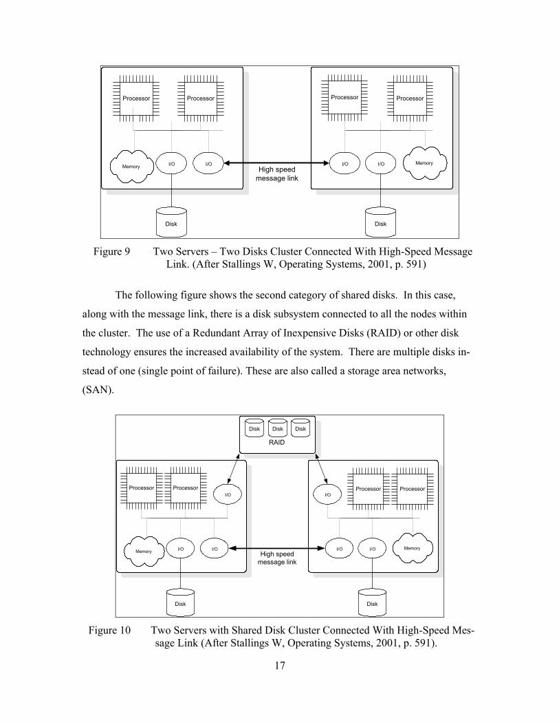
gories. Figure 9 show that the first category is a two-node cluster connected only via a

high-speed message link for coordinating the cluster activity. This message link is the

cluster’s LAN.

17

Disk

Processor Processor

I/O I/OMemory

Disk

Processor Processor

I/OI/O MemoryHigh speed

message link

Figure 9 Two Servers – Two Disks Cluster Connected With High-Speed Message

Link. (After Stallings W, Operating Systems, 2001, p. 591)

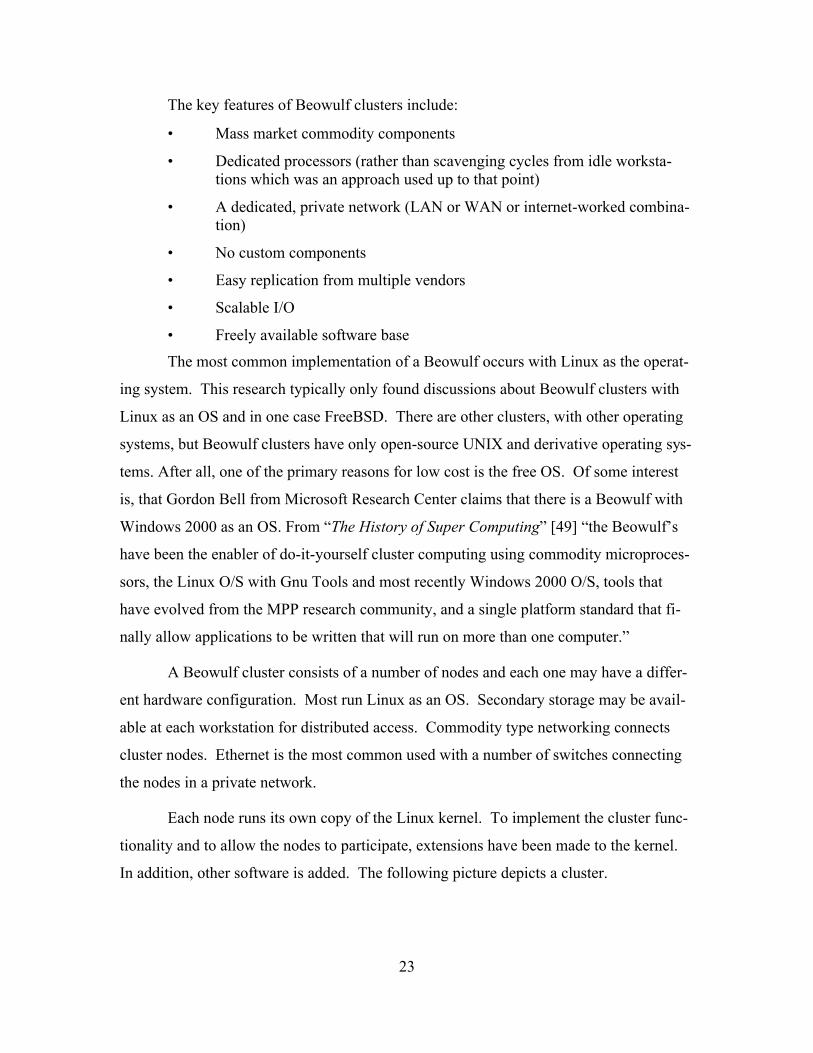
The following figure shows the second category of shared disks. In this case,

along with the message link, there is a disk subsystem connected to all the nodes within

the cluster. The use of a Redundant Array of Inexpensive Disks (RAID) or other disk

technology ensures the increased availability of the system. There are multiple disks in-

stead of one (single point of failure). These are also called a storage area networks,

(SAN).

Disk

Processor Processor

I/O I/OMemory

Disk

Processor Processor

I/OI/O MemoryHigh speed

message link

I/OI/O

Disk Disk Disk

RAID

Figure 10 Two Servers with Shared Disk Cluster Connected With High-Speed Mes-

sage Link (After Stallings W, Operating Systems, 2001, p. 591).

18

5. Classification by Cluster Architecture

Another classification, again according to Stallings [10], for the clusters is the dis-

tinction of separate servers, shared nothing and shared disks according to a more func-

tional point of view.

In separate servers, each computer is a separate server with no shared disks

among the servers. This approach has high availability but requires some management or

scheduling of software to regulate traffic. If one computer fails, another one takes over

and completes the task. This availability is achieved by constantly copying the data be-

tween the servers. This, of course, means that performance is decreased.

To reduce this communication traffic, the servers are connected to common disks.

This is called “shared nothing.” The common disks are partitioned in volumes and each

volume is used by one computer. If a computer fails, another computer obtains owner-

ship of the volume and the cluster continues to work.

The third approach is to have multiple computers share the same disks at the same

time so each computer has access to all the volumes of all the other computers. This ap-

proach is called “shared disks” and requires a mechanism to ensure that the data are ac-

cessed by only one (locking) process.

C. CLUSTER OPERATING SYSTEM

It is clear that the operating system of the cluster must be specific for this special

hardware configuration. Stallings [10] raises the following issues.

1. Failure Management

Resolution of failure management usually follows one of two approaches. The

first is a highly available cluster offering a high probability that all resources will be in

service. If a failure occurs to one node then another one takes over. All the queries and

processes that are in progress are lost in the failed system and there is no guarantee con-

cerning the state of partially executed transactions. This must be taken care of at the ap-

plication or scheduler level.

A fault-tolerant cluster ensures that all resources are always available by using re-

dundant shared disks and mechanisms that maintain the state of the system so that it can

be easily retrieved in case of failure and continued from the point of failure.

19

This has to do with the one of the three primary purposes of clusters the “high

availability” as it was presented previously in this chapter.

2. Load Balancing

This is used for the cluster’s coordinate traffic. When a new computer is added to

the cluster, the load-balancing facility needs to automatically include this computer in

scheduling applications.

3. Parallelizing Computation

At times, it is necessary to execute an application in parallel. According to Kapp

[8][8] there are three different approaches.

a. Parallelizing Compiler

This compiler determines which part of the applications is to be executed

in parallel, which is done in compile time. These parts are then split to be assigned to dif-

ferent computers in the cluster. The performance, of course, depends on the compiler and

how effectively it performs its task.

b. Parallelized Application

In this case, the programmer builds the application in such a way that it

can be executed in a cluster. The programmer uses the message assign interface, a set of

functions and methods to implement the message passing for the demands of the applica-

tion. This is the best approach and provides maximum performance, but, of course,

makes the programming phase more difficult.

c. Parametric Computing

This is different from the two aforementioned categories. It involves an

application that must run some pieces of code many times with different parameters each

time. This refers mostly to simulations that have to repeat different scenarios in order to

return more precise statistical data. For this approach to be effective, extra tools for the

organization and management of the separate jobs are needed, as shown in Figure 4.

D. CLUSTER ARCHITECTURE

The following figure shows typical cluster architecture. There is a connection

with a high speed LAN and each computer is able to operate independently.

An extra module of software is installed in every computer that enables that com-

puter to operate in the cluster operation. This is the cluster middleware. The middleware

20

provides the single system image, ensures availability, individual processor and includes

software tools for enabling the efficient execution of programs that are capable of parallel

execution. This design concept is according to Buyya [2].

PC

Operating System

NIC

PC

Operating System

NIC

PC

Operating System

NIC

PC

Operating System

NIC

Cluster middleware(Single system image)

Parallel programming environment

Parallel application

Sequential application

High speed network/switch Figure 11 Cluster Architecture (After Stallings W, Operating Systems, 2001, p. 595).

As a specific example, the Cluster Single System Image (SSI) middleware pro-

vides the following services and functions, according to Hwang [7]:

• Single entry point. A user logs onto the cluster rather than in every node.

• Single file hierarchy. The user sees one file directory system under the root directory.

• Single control point. The management and control is done by a specific node into the cluster.

• Single virtual network. There may be many physical networks connecting the nodes, but the user (and the cluster) sees only one network within all the nodes, and are connected and function.

• Single memory space. Distributed shared memory enables multiple pro-grams to share variables.

21

• Single job-management system. Under the cluster job scheduler, the user can submit a job without determining which node to execute the job.

• Single user interface. All users have one interface, regardless of the work-station with which they enter the cluster.

• Single I/O space. Any node can access any I/O without knowing its physical location within the cluster resulting in enhanced availability.

• Single process space. A uniform process-identification scheme is used re-sulting in enhanced availability.

• Check pointing. This keeps track of the current state of the cluster to en-sure recovery after failure resulting in enhanced availability.

• Process migration. This function enables load balancing resulting in en-hanced availability.

This is the “ideal” SSI. Implementations may or may not provide all the func-

tionalities mentioned above. For example the NPS exemplar cluster does not use a single

memory space. The SSI is a whole technology and can be found for Linux clusters in

[64].

E. DIFFERENT CLUSTER INSTALLATIONS

Some of the possible cluster implementations with several characteristics and de-

sign issues according to Stallings [10] are mentioned below.

1. Windows Cluster Service

Formerly known as “Wolfpack”, the Windows Cluster Service uses the following

concepts [55]:

• Cluster Service. The collection of the software on each node that manages all the cluster-specific activity.

• Resource. An item is managed by the cluster service.

• Online. A resource is online at a node when it is providing service on that specific node.

• Group. It is a collection of resources managed as a single unit.

2. Sun Cluster

It is based on the Solaris UNIX OS and is a set of extensions to it. It provides the

cluster with a single-system image and the cluster appears to the end user as a single sys-

tem running the Solaris OS [56].

22

The major components are:

• Object and communication support

• Process management

• Networking

• Global distributed file system

DiskI/O

MemorySolaris KernelNetwork

File SystemProcesses

Application

System Call Interface

Cluster framework

Memory

master

slaves

DiskI/O

Memory

Figure 12 Sun Cluster Architecture. (After Stallings W, Operating Systems, 2001, p.

598).

3. Beowulf and Linux Clusters

PC-based clusters began in 1994 when NASA sponsored the project for “Beo-

wulf” clusters under the High-performance Computing and Communications (HPCC)

project, conducted by Dr. Thomas Sterling and Dr. Donald Becker, with the ultimate goal

of reducing the cost of computing power [12] [13]. The http://www.beowulf.org is the

web site providing relevant information.

23

The key features of Beowulf clusters include:

• Mass market commodity components

• Dedicated processors (rather than scavenging cycles from idle worksta-tions which was an approach used up to that point)

• A dedicated, private network (LAN or WAN or internet-worked combina-tion)

• No custom components

• Easy replication from multiple vendors

• Scalable I/O

• Freely available software base

The most common implementation of a Beowulf occurs with Linux as the operat-

ing system. This research typically only found discussions about Beowulf clusters with

Linux as an OS and in one case FreeBSD. There are other clusters, with other operating

systems, but Beowulf clusters have only open-source UNIX and derivative operating sys-

tems. After all, one of the primary reasons for low cost is the free OS. Of some interest

is, that Gordon Bell from Microsoft Research Center claims that there is a Beowulf with

Windows 2000 as an OS. From “The History of Super Computing” [49] “the Beowulf’s

have been the enabler of do-it-yourself cluster computing using commodity microproces-

sors, the Linux O/S with Gnu Tools and most recently Windows 2000 O/S, tools that

have evolved from the MPP research community, and a single platform standard that fi-

nally allow applications to be written that will run on more than one computer.”

A Beowulf cluster consists of a number of nodes and each one may have a differ-

ent hardware configuration. Most run Linux as an OS. Secondary storage may be avail-

able at each workstation for distributed access. Commodity type networking connects

cluster nodes. Ethernet is the most common used with a number of switches connecting

the nodes in a private network.

Each node runs its own copy of the Linux kernel. To implement the cluster func-

tionality and to allow the nodes to participate, extensions have been made to the kernel.

In addition, other software is added. The following picture depicts a cluster.

24

Master node

Switch

External NIC

Internal NIC

WAN

Slave nodes

Figure 13 A Beowulf Cluster with Master and Slave Nodes and Network Connec-

tions. The master node with its two NIC is in this case the gateway between the two networks the internal and the external. The slave nodes are connected to the

master node with a switch in the internal (private) network. F. HARDWARE CONSIDERATIONS

In order to understand better how the different parts of hardware participate in the

overall performance of such a system, it is necessary to examine all these parts sepa-

rately. All the material mentioned in this chapter is referenced from Groop et al. [6] and

from the “Node Hardware” relevant chapter. Due to the actual implementation of the

cluster examined in the following chapters, the author discerned that knowledge about the

hardware sometimes provided answers to configuration problems, mainly in the area of

constructing the nodes.

Several reasons preclude definitive statements in this area. One is that the tech-

nology and the market are changing rapidly and the possible cases to explore are exces-

sive.

Another reason is that different vendors seem to have a greater understanding of

what is appropriate for each application after receiving customer feedback. Therefore,

they build a knowledge database of what is or is not working efficiently. The concept is

that in all the areas using HPC, such as academia, research and others, it is a waste of

time to reinvent the wheel and start the mystifying areas of hardware design from scratch.

25

A better approach is to ask a number of vendors for quotes and afterwards try to decide

the best quote (quality over price) consisting of a number of questions concerning the

technical characteristics on which these quotes differ.

Nevertheless, the actual application environment will be that which results from

the selection of parts.

1. CPU

The nodes’ CPUs execute the application in the cluster. The microprocessor in-

struction set architecture (ISA) dictate the lowest level binary encoding of the instruc-

tions and the actions they perform. The most common ISA is the IA32 or x86. Each

processor has a clock rate that sets the frequency of the execution of the instructions.

Note that the clock rate is not a direct measure of performance. The processor has a theo-

retical peak rate, which is determined by the ISA, the clock rate and components and

technologies included in the processor. One theoretical peak rate can be measured in

flops, floating point operations per second.

The processor constantly retrieves instructions and data with Random Access

Memory (RAM). RAM also has a speed that determines the rate at which the bytes are

moving in and out. The RAM’s speed is also much lower than the processor’s since it of-

ten waits for memory. Thus, the overall speed at which a program is executed depends on

the speed of the processor and memory. The processor, in order to overcome this prob-

lem, has an internal fast memory, called cache (L1, L2 or L3 type), and for most applica-

tions, the larger the cache, the better the performance of the processor.

This concept is better understood by examining how the processor works in more

detail, as demonstrated in the following figure.

26

ProcessorInstuctions Data

Res

ults

3232

32

Single instruction stream, simple data stream (SISD)

ProcessorInstuctions Data

Res

ults

6432

64

Single instruction stream, multiple data stream (SIMD)

Figure 14 Processors Inputs and Outputs with 32-bit and 64-bit. The Inputs are the

Instructions and the Data while the Outputs are the Results. Note that in both cases the Instruction set is 32-bit. The one that changes is the Data Set.

In the both figures, the instruction stream and a data stream are entering and the

result stream is leaving. It is, therefore, possible to state that the instruction stream is

composed of different types of operations and the data stream consists of the data on

which those operations operate.

The data stream is moving to registers in the processor as well as memory loca-

tions. This infrastructure is called a bus. According to the bit-width of these elements, it

is possible to define the processor as 32-bit or 64-bit.

In 32-bit computing, generally four sets of bytes (32-bits) forms a word, defined

as a unit of data that can be addressed and moved between the computer processor and

the storage area. A word may contain a general computer instruction, a storage address,

or any type of data to be manipulated.

Usually, the defined bit-length of a word is equivalent to the width of the com-

puter's data bus so that single operation can move a word from the storage to the proces-

sor registers. Thus, a 64-bit microprocessor has a 64-bit word size.

The presence of these higher-capacity registers translates into more data process-

ing capability and significantly larger amounts of memory access. The 32-bit processors

are capable of addressing up to 4 GB of memory while their 64-bit counterparts can reach

up to 18 billion GB.

27

However, note that these figures concern the quantity of accessible memory and

not outright data processing speeds. Thus, it does not imply that 64-bit processors are

twice as faster as the 32-bit processors.

Also, the 64-bit boost can only be obtained while running a 64-bit application un-

der a 64-bit environment (operating system). In the 32-bit mode, it will operate as a 32-

bit processor and according to the performance boost obtained, due to other architectural

changes such as higher FSB (front side bus) or more L2 cache.

The term “64-bit code”, designates instructions that operate on 64-bit data. The

evolution of the processor technology now provides processors with 64-bit technology, or

the so-called 64-bit computing.

There is a drawback in the 64-bit computing though. The 64-bit pointers that are

used to refer to the 64-bit addressing scheme fill the L1 and L2 cache of the processor in

a larger degree than the 32-bit pointers, and this has an impact in the performance of the

processor.

A description of several processors appears below:

Pentium 4: Intel’s IA32 processor. It produces less computing power per clock

cycle but it is suitable for extremely high frequencies. It implements the SS2 instruction

set and hyper threading. Currently, according to www.top500.org, [35] , out of 500 su-

percomputers (thus 57.4 %), 287 use Intel’s processors. Some are 64-bit ISA as discussed

later.

Athlon: AMD’s IA32 processor is similar to Pentium 4. The performance can be

faster than Pentium 4 but ultimately depends on the application. Currently, according to

www.top500.org, [35] out of 500 supercomputers 34 (8.8 %) use AMD’s processors.

Some of them are 64-bit ISA as discussed later.

Power PC G5: This is an IBM product used for IBM and Apple. The G5 is a 64-

bit architecture, running at 2 GHz. Apple uses G5 in Macs and some clusters use

PowerPC as processors. Mac OS X (a UNIX-like operating system) is the operating sys-

tem used. Currently, according to www.top500.org, [35] out of 500 supercomputers,

three use PowerPC processors.

28

IA64 and Itanium. This is the Intel’s 64-bit architecture and employs the Explic-

itly Parallel Instruction Computing (EPIC) design concerned with impressive results.

The processor, however, produced a larger amount of heat, which created a new problem

with heat management. [This chapter discusses heat management in a subsequent sec-

tion.] Intel released the Itanium 2 to compete directly with AMD's Opteron processor.

The Itanium 2 is a true 64-bit processor that offers larger memory addressable space for

the needs of large memory jobs. Competition has driven down the prices of these proces-

sors, which are Itaniums at 900 MHz, 1.0, 1.3, 1.4 and 1.5 GHz with L3 cache up to 6

MB.

HP Alpha 21264: This is true 64-bit architecture. For years, Alphas were consid-

ered the fastest, and subsequently were used in supercomputers such as the Cray and

Compaq family. Currently, according to www.top500.org, [35] 16 out of 500 supercom-

puters use Alpha processors. Alpha uses the Reduced Instruction Set Computer (RISC)

architecture, and therefore, Alphas are often referred to as RISC processors.

Opteron: This is AMD’s new design in 64-bit architecture, and can support both a

32-bit instruction set along with a 64-bit extension, allowing users to use their 32-bit ap-

plications. Opteron uses three links with the “Hyper Transport” technology. Hyper

Transport technology is AMD's new technology to facilitate high speed communication

between the CPU and the system’s other circuitry. Many options exist. For example, Op-

teron 240 has a 1.4 GHz clock, Opteron 242 has a 1.6 GHz clock, Opteron 244 has a 1.8

GHz clock, Opteron 246 has a 2.0 Ghz clock while Opteron 248 has a 2.2 GHz clock.

Athlon 64 FX is no more than an enhanced version of the AMD Opteron aimed at

desktop computers.

2. Memory Capabilities, Bandwidth and Latency

This is the temporary storage for instructions and data. The speed of the mem-

ory’s Front Side Bus (FSB) varies from 100 MHz up to 1 GHz. Therefore, memory is the

largest obstacle to achieving maximum peak performance. Two characteristics of the FSB

concern performance. The first is the peak memory bandwidth, the burst rate at which the

bytes are copied between the CPU and the memory chips. FSB must be fast enough to

support this rate. The second is memory latency, the amount of time that it takes to move

29

bytes between the CPU and the memory chips. The same bottlenecks are observed, as in

the case when memory must copy bytes to and from another peripheral, such as a perma-

nent storage or network controller.

It is obvious that whenever it is necessary to move data to and from memory, a

reduction in performance occurs. A good solution is, of course, to have all the data sets

of this application stored in memory at all times. For this reason, the amount of memory

is significant to the node of the cluster. Unfortunately many HPC problems of interest re-

quire more memory per processor than is generally available.

A rule of thumb in cluster design is that for every floating point operation per

second, a byte of memory is necessary. For example, a 1 GHz processor, capable of 200

Mflops, must have 200 Mbytes of memory. Memory can be as little as 64 MB per ma-

chine to 8 GB per machine of memory depending upon the requirements. A good choice

is to use Error Correcting (ECC) Memory. Although slightly more expensive (10% to

15% more than non-ECC memory), ECC memory ensures that computations are free of

any fixable computing errors.

Several benchmarks count memory performance and calculate the amount of

memory needed for the cluster, which a later chapter examines.

3. I/O Channels

These are buses that connect peripherals to the main memory. All motherboards

have a bridge mechanism that connects these buses to the main memory. This is the PCI

chipset. Descriptions of the different bus types appear below.

a. PCI and PCI-X

This is the most common bus type in commodity computers. Newer ver-

sions are 64 bit, with a data rate at 66 MHZ or higher. Some good implementations pro-

vide up to 500 MB/s, while the PCI-X that runs at 133 MHz, provides data rates up to

900 MB/s.

b. AGP

Accelerated Graphics Port is used for high-speed graphics adapters and

can access data directly from the main memory. AGP is not a bus like PCI because it can

support only one device with a data rate up to 2.1 GB/s to the main memory (AGP 3.0).

30

c. Legacy Buses

ISA is 8 or 16 bit bus, VESA is 24 bit, while EISA is an extension to ISA,

all of which are now obsolete.

4. Motherboard

After selecting the processor, the most important decision in the design of the

node is the choice of motherboard. It defines the functionality of the node, the range of

performance and the number of subsystems that can be connected. Motherboard manu-

facturers include Gigabyte, Intel, Shuttle, Tyan, Asus, Supermicro, Tyan and many oth-

ers.

a. Chipsets

These implement the functionality of the motherboard. They are bridges

that interconnect the processor, the main memory, the AGP port and the PCI bus (IDE

controller, USB controller).

b. BIOS

BIOS is the software that initializes all system hardware into a state such

that the operating system can boot. Each motherboard has its own BIOS. The BIOS runs

the Power on Self Test (POST) at startup time, in order to locate a drive from which to

boot.

c. PXE (Pre-Execution Environment)

This is a system that allows the nodes to boot from on a network-provided

configuration and boot image, which is necessary for the cluster. The system utilizes two

common network services, DHCP and tftp. The functionality of this PXE system, which

appears to work as a protocol as described in the following figure.

The PXE is a characteristic of the motherboard. It must be in the BIOS

setup when the machine starts its operation in order to utilize it by pressing the appropri-

ate key (usually del or F1) and then navigating to the menu option to choose the location

from which the machine boots. Instead of choosing “floppy” or something similar,

“PXE” is chosen. In actuality, this only occurs with motherboards having integrated

Ethernet controllers. On the motherboards to which are added Ethernet controllers in the

PCI slots, it is necessary to refer to the NIC manufacturer manual to ascertain if and how

31

it is possible to make it work with the “on-card device initialization code.” The results of

the experiments showed that it did not work, and therefore, it was necessary to find an-

other way to boot the nodes. The next chapter examines this situation.

Figure 15 Pre-execution environment (PXE) diagram. The system boots and after a

DHCP request receives from the server the data necessary for the start up proc-ess.

d. Linux BIOS

This is another version of a proprietary BIOS based on the LINUX kernel.

It supports only LINUX and the Windows 2000 operating systems and the greatest bene-

fit is the boot time, which is considerably better than the ordinary BIOS.

5. Storage

The hard disk is used in the node for storage, and depends on the cluster system

utilized as to whether or not a disk is absolutely necessary. The possibility of having “two

servers two disks” or “two server same disk” was mentioned previously. The decision

32

depends on the design. Some slave nodes can be net-booted and do not need a hard disk

at all. Another popular choice is to use a RAID for storing the applications and the data

as well as having a disk in every node for storing only the operating system.

The main characteristics of the disks are capacity, bandwidth, rotations per minute

and latency. The faster the rotation is the higher the bandwidth and the lower the latency.

Another important characteristic is the time between failures.

a. Local Hard Disks

The three most commonly used buses for hard disks currently are IDE

(EIDE or ATA), SCSI and serial ATA.

(1) Integrated Drive Electronics (IDE). These disks are the

most common with the disk controller integrated in the motherboard. The controller pro-

vides two interfaces and up to four (4) IDE disks can be connected to them (two devices

per interface). The data rate is up to 133 MB/s with the use of Ultra DMA 133 (UDMA

133). The majority of CD or DVD drives are currently IDE. If it is necessary to place

more disks in a computer, another controller (with two more interfaces) is required and

must be inserted in an empty PCI slot. It is possible to add four (4) additional disks to this

controller. However, this is disadvantageous because the controller must also be identi-

fied and initialized, which delays the booting of the computer.

These drives are best suited for situations dealing with small files

less than 2 MB. IDE drives are also ideal when transferring many different small files in

small bursts. For most people involved in a cluster computing or stand alone workstation

environment, IDE drives are the better choice.

(2) SCSI. These disks are used in servers. One difference be-

tween IDE and SCSI is that it is possible to add up to 15 disks to a computer. Another is

that they are more expensive and faster. The data rate is up to 350 MB/s.

SCSI hard drives are ideal for transferring large files when transfer

rate needs to be sustained. Clusters typically do not need the sustained speed of SCSI

hard drives because the limiting factor will always be the network connection. Even if the

cluster is equipped with the fastest possible drive, more than likely it does not reach the

full benefits due to the network bottleneck.

33

(3) Serial ATA or SATA. These are an enhanced ATA tech-

nology with a rate up to 150 MB/s.

b. RAID

Redundant Array of Inexpensive Disks are used to aggregate the individ-

ual disks. The RAID disks appear as a single large disk and consist of RAID0 (striping),

RAID1 (mirroring) and RAID5 (striping with parity). RAID is usually used with clusters,

and more typically, on front ends for data storage, but not as often on compute nodes.

c. Non Local Storage

Network File System (NFS) is a protocol and the most popular way to ac-

cess remote file systems. File systems are “mounted” via NFS.

Parallel Virtual File System (PVFS) is another file system designed for

use in high-performance space for parallel applications.

The elaboration of all the relevant UNIX – Linux commands are necessary

to use these file systems. The next chapter examines Linux.

6. Video

Most video adaptors in a commodity computer are connected through the AGP,

and some older models through PCI. In most servers, the video adaptor is built into the

motherboard.

Obtaining a Linux-compatible video card can be problematic. Surprisingly, the 32

MB AGP version of this card is costs roughly the same as the 16 MB card.

For slave nodes not requiring a monitor, a good solution is to use a inexpensive 8

MB video card, which costs less than $20, to ensure proper boot up and ease of mainte-

nance. Many believe that they do not need a video card for a cluster node. The truth is

that most PCs need a video card in order to boot up. Turning on a machine without video

card only results in annoying beeping. The video card also assists in the maintenance of

the PC. In the case of a problem, it is only necessary to attach a monitor in order to diag-

nose the problem. Monitor switches are helpful for racks of “headless” compute nodes.

7. Peripherals

Universal serial Bus (USB) and Firewire are peripheral buses. The most useful is

the USB for connecting the keyboard-mouse in the case of a node debug.

34

8. Case

This is the box that contains all the aforementioned items. The kind of box used

depends mainly on the investment made. The following choices appear below.

a. Desktop Cases

The first clusters consisted of desktop cases. These boxes provide an eco-

nomic solution, are mostly low performance, and used for experimental reasons and by

academia students working on related projects. They are usually stacked on the floor or in

shelves, connected with KVM switches, make considerable noise, draw much power and

produce a lot of heat, and are currently considered satisfactory for experiments.

A standard midi tower case is ideal if plenty of space is available and the

budget is limited. With a power supply of 230W (standard for Intel single processor ma-

chines) or 300W (standard for AMD Athlon Thunderbird or dual processor Intel ma-

chines), the standard midi tower cases provide plenty of reliability and flexibility.

N o d eN o d eN o d eN o d eN o d eN o d e N o d eN o d eN o d eN o d eN o d eN o d eN o d eN o d eN o d eN o d e


N o d eN o d eN o d eN o d eN o d eN o d eN o d eN o d eN o d eN o d eN o d eN o d eN o d eN o d eN o d eN o d e

N o d eN o d eN o d eN o d eN o d eN o d eN o d eN o d eN o d eN o d eN o d eN o d eN o d eN o d eN o d eN o d e



N o d e s 3 * 3 2 = 9 6

S e r v e r

F i rew a ll

G a t e w a y

Pr in te r

K V M s w itch

K V M s w itch

K V M s w itch

48 por t sw i t ch

48 por t sw i t ch

4 8 p o r t s w i tch

25 por t sw i t ch

W A N

Figure 16 A Typical Diagram of a Cluster System with Mini Tower Cases. There is a hierarchy in the switching scheme, while some computer, not between the nodes

have different roles. This is due to easy administration.

35

b. Rack-Mounted Cases

Rack-mounted cases are those that can be mounted on a rack in the com-

puter room. They are 1 U or more wide. One U (Unit) is 1.75 inches in the rack. These

kinds of systems provide high density and good serviceability. Cooling is a considerable

problem with high density. Most come with rack mount rails to assist in the maintenance

of the cluster. The most common format is the 19” rack mount compact size.

The following figure demonstrates the possible configuration of such a

system. The monitor and the keyboard occasionally are incorporated in a separate rack-

able module, when a slideable monitor and a keyboard are available and it is connected to

all the nodes in the rack. With the push of a button, it is possible to see a display and key-

board of a specific node.

A more simplistic, inexpensive solution though is to have a screen and a

keyboard mouse on a wheeled table and connect it at any time to a specific node. Most of

these boxes have display connectors on the front, along with USB connectors for the

keyboard. It is important to note that this is necessary only for debugging reasons since

the normal use of the system is achieved through a SSH network connection.

Keyboard

RAID

Master node

slave node 3

slave node 2

slave node 1

switch

UPS

Figure 17 Cluster with rack able cases. All the representing parts are shown in this

figure, even though some of them may exist in different rack. The keyboard and the monitor are most of the times necessary for troubleshooting.

36

One possible advantage of the rack-mounted systems is that it can be taken

from the cluster and used in another after reconfiguration. Thus, it is considered an excel-

lent solution for experimental use and in academic environments where research may

demand a change in the use of hardware and funding constraints are always a considera-

tion.

c. Blade Servers

Blade servers are the last option. These are actual motherboards mounted

in a module that can be inserted in a case such as a drawer. The front side contains some

connectors (USB) and some LEDs indicating the status, and sometimes contain a hard

disk and/or a power supply. There is an extremely high density of processors per space

unit with this implementation. They are used for a specific blade server and cannot be

used elsewhere as separate computers.

9. Network

A network is among the most important components of a cluster. The perform-

ance of the network results from the selections of network technology, components and

topology. Of course, cost is the main factor that drives all these issues. The TCP/IP pro-

tocol is used to implement the internal network of the Beowulf clusters. One size taken

into consideration is latency. Latency is the amount of time that a message takes to travel

through the network from the sender to the receiver. It can vary typically from 100 to 1

microsecond. As a result, some technical approaches attempt to provide a solution to the

latency problem. A more different metrics is bandwidth, from 100 Mbps to 4 Gbps.

The possible technologies for the network can be the following.

a. 10/100/1000 Base T Ethernet

The 1000 Mbps is the Gigabit Ethernet. This is the most commonly used

network technology.

b. Myrinet

Myrinet is a high-speed local area networking system designed by Myri-

com. Myrinet has much less protocol overhead than standards such as Ethernet, and

therefore, provides much better throughput and less latency. Although it is possible to

use it as a traditional networking system, Myrinet is often used directly by programs that

“know” about it, thereby bypassing a call into the operating system

37

Myrinet physically consists of two fiber optic cables, upstream and down-

stream, connected to the host computers with a single connector. Machines are connected

together via low-overhead routers and switches, as opposed to connecting one machine

directly to another. The first generation provided 512 Mbit/s data rates in both directions,

and later versions supported 1.28 Gbit/s and 2 Gbit/s.

Myrinet's throughput is close to the theoretical maximum of the physical

layer. On the latest 2.0 Gbit/s links, Myranet often runs at 1.98 Gbit/s of sustained

throughput, considerably better than what Ethernet offers, from 0.6 and 1.9 Gbit/s de-

pending on load. [51]

c. Dolphin Wulfkit

This is based on a different standard. It is a relatively economical solution.

The Network Interface Card (NIC) is a PCI with two interfaces that allows special cables

to interconnect in either ring or switched topologies. The bandwidth is measured up to

326 Mbps with 1.4 microseconds latency, the lowest in the market. Its theoretical link

speed is 667 Mbps and 1.333 Gbps in the bi-directional mode.

The Scalable Coherent Interface (SCI) standard achieves this performance,

and bypasses the time-consuming operating system functionalities and protocol software

for the establishment of the networking.

d. Infiniband

InfiniBand is a high-performance, multi-purpose network architecture

based on a switch design often called a “switched fabric.” InfiniBand is designed for use

in I/O networks such as storage area networks (SAN) or in cluster networks. InfiniBand

supports network bandwidth between 2.5 Gbps and 30 Gbps.

Specifications for the InfiniBand architecture span multiple layers of the

OSI model. InfiniBand features physical and data-link layer hardware such as Ethernet

and ATM, although with more advanced technology. [50]

10. Heat Management and Power Supply Issues

Since many machines are connected in a single space, it is necessary to consider

the power consumption and the heat they produce.

38

a. Power Consumption

The power supply of a computer can support a specific number of watts. A

Watt is the measure of power (P=V*I that is Watt=Volt*Amperes), which is consumed

by parts of the computer. The power supply provides the appropriate voltage for each

component. The table below indicates how much power each component needs [68][69].

Component Typical Power Re-quirement

AGP Video Card 20 – 50W

Average PCI Card 5 – 10W

10/100 NIC 4W

SCSI Controller PCI Card 20W

Floppy Drive 5W

DVD-ROM / CD-RW 10 – 25W

7200 rpm IDE Hard Drive 5 – 20W

10,000 rpm SCSI Drive 10 – 40W

Case/CPU Fans 3W (ea.)

Motherboard (without CPU or RAM) 25 – 40W

RAM 8W per 128 MB

Pentium III Processor 550 MHz 30 W

Pentium III Processor 733 MHz 23.5 W

Pentium III Processor 38W

Pentium 4 Processor 70W

AMD Athlon Processor 60W

AMD Opteron 55 W

Intel XEON 77 W

Intel Itanium 65 W

Table 1 Typical Power Consumption Levels for Computer Parts.

39

It is worth nothing that a 400-watt switching power supply will not neces-

sarily use more power than a 250-watt supply. A larger supply may be needed if every

available slot on the motherboard or every available drive bay in the computer case is

used. It is not a good idea to have a 250-watt supply if all the devices total 250 watts

since the supply must not be loaded to 100 percent of its capacity. Computer vendors

usually equip machines economically with the appropriate power supplies and simply try

to cover only the threshold of power consumption needs.

A rule of thumb for estimating the overall power supply wattage is to add

the requirement for each device in the system and then multiply by 1.8. The power sup-

plies are more efficient and reliable when loaded to 30% - 70% of maximum capacity.

All the other components such as switches and disk arrays also produce power consump-

tion.

Some new computers systems, particularly those designed for use as serv-

ers, provide redundant power supplies. In other words, there are two or more power sup-

plies in the system, with one providing power and the other acting as a backup. The

backup supply immediately takes over in the event of a failure by the primary supply.

Then, the primary supply can be exchanged while the other power supply is in use [52]

[53].

The loss of power is one of the main reasons for data loss. For this reason,

every rack also needs to use an Uninterrupted Power Supply (UPS). The characteristic of

the UPS is the power (in VA) that it can support. It is usually a 3000 KVA and must be

enough for seven nodes and the switch when plugged into a 20 AMP (ordinary) circuit.

One characteristic of the UPS’s is the ability they have to shut down the

server that they are connected to. The UPS is connected to the server with a serial or

USB cable to the relevant ports. As soon as the UPS discovers that there is a power fail-

ure, then signals the server to commit a graceful shut down. For this of course a running

daemon in the UNIX system must run. This software is accompanying the UPS hardware

and it must be installed by the system administrator to the server. For the verification

that the system works with out problem a number of tests must be conducted.

40

b. Thermal Management

All these parts, in addition to consuming electrical power, produce heat.

One of the common troubleshooting complaints was that if a personal computer did not

respond well and the programs seemed to be running in a irregular way, then the problem

might be a malfunctioning CPU fan. This type of overheating causes the CPU to work

chaotically. Thus, a CPU with larger power consumption produces a considerable

amount of heat. For this reason, it is necessary to install blowers.

All new processors have a overheating protection. When the temperature

reaches a certain point, all execution in the processor is stopped, until the user resets the

system. For example, the Itanium at 1.5 GHz works from 5 – 85 degrees Celsius.

The computer room housing the clusters must maintain a constant tem-

perature of around 70 degrees F, usually achievable with air-conditioning.

The air-conditioning measurement is in British Thermal Units (BTUs.)

One BTU is the amount of heat required to raise one pound of water one degree Fahren-

heit at one atmosphere pressure. Cooling can be a factor of heat, space, and amount of

heat generating equipment in a room. Air conditioning equipment is usually expressed in

tons, i.e., a one ton air conditioner. One ton of air conditioning is equal to 12,000 BTU's.

The following table [54] provides an idea on what to expect concerning

this issue, and indicates the BTUs needed for a given area in the server room with an av-

erage workload.

Computer room area feet2 Typical BTUs per hour needed

100 to 250

250 to 350

350 to 450

450 to 550

500 to 700

700 to 1000

6,000

8,000

10,000

12,000

14,000

18,000

Table 2 Cooling Requirements for Computer Room.

41

The above amounts must consider the following:

• If the room is heavily shaded / sunny, reduce/increase capacity by 10%.

• If more than two people regularly occupy the room, add 600 Btu/Hr for each additional person.

• For each server add 1200-1500 BTU's.

• For each UPS add 800-1000 BTU's.

Technical solutions exist for almost any topic. Even when it is necessary

to move the computer equipment from one place to another, there are portable systems.

In addition, when in the position to design the hardware for a cluster, it is

then essential to consider the use of the absolutely necessary power supply wattage in

case each machine has its own power supply. In order to reduce power consumption and

heat production, as with blade systems, there can be one power supply for a number of

nodes in the rack. This power supply has many outputs with all the needed power.

Also, consider not using high end graphics cards with 3D processors, extra

hard disks, and anything else that might increase the system’s heat.

G. LINUX OPERATING SYSTEM

It is the author’s opinion that for a cluster to be a Beowulf, Linux is required. The

Linux open-source operating system provides stability, maturity, and straightforward de-

sign. By using Linux, “you are not alone.” The knowledge pool is enormous. Many

types of processors are supported. The kernel of the operating system can be manipu-

lated according to the needs and can “be made small” to fit [6]. [1]

Linux is a clone of the original UNIX operating systems, released in October

1991 by Linus Torvalds, and is one of the most popular operating systems in the world.

The term Linux applies to the UNIX-like kernel. Hence, some vendor companies

incorporated the kernel with a series of supporting software, such as an X Window sys-

tem environment, an installer and several other programs and services. This is a Linux

distribution packed in CD’s or DVD’s and is available for purchase with some manuals.

The following table shows some distribution companies.

42

Distribution company Comments

Red Hat www.redhat.com. Popular for clusters

Turbolinux www.turbolinux.com support in Japanese and Chinese (double byte characters)

Mandrake www.mandrake.org

Debian www.debian.org

SuSE www.suse.com. Good support in German

Slackware www.slackware.com

Table 3 Different Linux Distributions Available.

Linus Torvalds and some core developers maintain the right to make the Linux

kernel releases public, after input received from the Linux community. All improve-

ments, or at least some sent by the global programmers, are incorporated into a “devel-

opment” kernel, which have an odd number such as 2.1 or 2.5. After a period of testing

and debugging, the “development” kernel becomes a “stable” kernel with an even num-

ber such as 2.2 or 2.4.11. The distribution companies on the other hand maintain their

own numbering scheme. They incorporate a given stable kernel with the most recent

supportive software and make public the release number, thus, creating Red Hat 8.0 and

the later 9.0 version.

H. SUPERCOMPUTER STATISTICS

Currently, based on www.top500.org, it is possible to obtain a considerable

amount of information concerning the top 500 computer systems in the world such as ar-

chitecture, processor generation, family and architecture, manufacturer, location of the

cluster in countries and continents and system models. This thesis presents a variety of

summaries information. The majority of the installation types are for industry, followed

by academia.

43

20%

51%

24%

1%

4% Academic

Classified

Government

Industry

Research

Figure 18 Supercomputer statistics. The majority of installations are for the industry

followed by research and academia.

Where number GFlops

Academic 95 19

Classified 19 3.8

Government 3 0.6

Industry 242 48.4

Research 115 23

Vendor 26 5.2

All 500 100 %

Table 4 HPC Usage

The United States possesses the greatest number of supercomputers, with Europe

in second place.

Continent Number

Southern Africa 2

Eastern Europe 5

Australia and New Zealand 11

Central - South America 12

Western - Southern Asia 26

44

Continent Number

Eastern Asia 63

Western - Southern Europe 119

North America 262

Table 5 HPC Locations

0 50 100 150 200 250 300

Southern Africa

Eastern Europe

Australia and New Zealand

Central - South America

Western - Southern Asia

Eastern Asia

Western - Southern Europe

North America

Figure 19 Graph of HPC locations. About half of the systems are in North America

and the other half in the rest of the world.

45

IV. INSTALLATION OF THE NPS LINUX CLUSTER

A. INTRODUCTION

This chapter explains the installation of the hardware and software necessary to

implement the Beowulf cluster considered as a part of this thesis. This chapter also de-

scribes the problems encountered while building the cluster.

The application software used in the cluster is what drives the hardware and over-

all software specifications. In this case and since an investigation and experiment is be-

ing conducted, the specifications on exactly which software to run were not completely

designed in the beginning.

B. OPEN-SOURCE CLUSTER SOFTWARE

1. Choosing the Software

The first problem is the identifying the software needed to implement the cluster.

Linux is the operating system used in most clusters, but additional software is needed to

tie the computers together into a unified whole. The software necessary to create a clus-

ter exists in many forms and is available from many sources. Some cluster distributions

are commercial products, and some are free implementations put together by various or-

ganizations. This section discusses some of the more popular options.

a. Rocks

The National Partnership for Advanced Computational Infrastructure

(NPACI) and the San Diego Supercomputing Center (SDSC) distribute the Rocks cluster

package. Rocks is based on Redhat Linux and is distributed under open-source BSD li-

cense. It is available for download from the web [14]. A manual describes the installation

process step by step, providing screen shots and help files. The most helpful support fea-

ture is the mailing list in which Rocks cluster users help each other with installation, con-

figuration, and operational problems.

The goal of the Rocks distribution is to make clusters easy to deploy,

manage, upgrade, and scale. Many operations are automated, and the install process in-

cludes all the software needed to run a cluster. Installation of a cluster can be as easy as

booting all the machines that will be in the cluster off of a CD. Rocks uses the concept of

a “disposable compute node.” Since installation of a compute node is as simple as boot-

46

ing from an install CD, the easiest way to manage compute nodes is to simply re-install

the operating system if there is ever any doubt about the node’s state. The concept of

“disposable compute nodes” is becoming increasingly popular in large scale clusters be-

cause it is unrealistic to maintain or manually re-install operating system image in large

installations.

The Rocks cluster package includes many of the most popular cluster

software packages including an MPI implementation, Portable Batch System (PBS) and

the Ganglia cluster status program. It includes optional add-on “rolls” for other software

packages, such as Java and Globus.

b. OSCAR

Another solution is the Open-source Cluster Application Resources

(OSCAR) [16]. Like Rocks, the OSCAR cluster package release offers a series of

downloadable CDs used to install the cluster. OSCAR requires that the user first install

Red Hat Linux on the front end node before proceeding with the installation of the add-

on cluster software. Once the OSCAR package is installed on the front end disk images

for the compute nodes can be created. As with Rocks, the images are used to install the

cluster nodes, though usually over the network rather than from CD. Typically the com-

pute nodes are configured to use PXE and boot from the network. The front end receives

the PXE boot request and downloads a system image to the compute node.

One of the main packages included with OSCAR is LAM-MPI, a popular

implementation of the MPI parallel programming paradigm. Another useful program is

the Portable Batch System (PBS), which can be used for scheduling parallel jobs. A MPI

(the MPICH) and a PBS is included in the Rocks package as well, which the next chap-

ters will examine in more detail. In Rocks, the Red Hat Linux is incorporated in the CD

and is installed “as a part” of the cluster software.

c. Scyld

Scyld is a commercial cluster product based on the open-source Linux op-

erating system, but with additional value-added commercial software [34]. Scyld license

fees are based on the front end, plus a fee for each compute node in the cluster, and a

variable fee depending on the type of network interconnection used. Scyld also offers a

full range of professional services, from planning to installation to support and operation.

47

Scyld does its best to present a single system image of the entire cluster.

Many standard Unix utilities have been reworked to make it appear as if all the jobs in

the cluster are running in a single process space on the front end. Running the Unix “ps”

command on the front end, for example, shows all jobs running on all the compute nodes

in the cluster, rather than only the jobs running on the front end.

As with Rocks and OSCAR, the front end can be used to install operating

systems and the necessary software on the compute nodes. Scyld uses a lightweight com-

pute node kernel that can be rapidly re-installed from the front end. Like OSCAR, it typi-

cally relies on PXE on the compute nodes. The PXE boot process installs the kernel on

the compute nodes.

2. Cluster Software Selection

The Rocks package was selected for this thesis. Rocks have an impressive degree

of automation. Installation can be as simple as booting several machines off CD. The in-

stallation of the front end is somewhat simpler than is the case with the OSCAR distribu-

tion. Scyld’s single system image was appealing, but the system requires licensing fees,

which is a significant drawback in academic and military environments.

C. SELECTING AND EQUIPPING THE HARDWARE

This thesis research uses the following configuration. Computers for other uses

were available, which received some modifications for use in building the system. These

include one DELL, 2.4 GHZ Pentium with 1 GB RAM for the front-end, one DELL, 2.4

GHZ Pentium , similar to the front-end, with 1 GB RAM for one node, and two 700 MHz

“no name” Pentiums with two processors each, with 1 GB RAM for two other nodes. A

one Gigabit Ethernet switch will be the internal network switch. At this point, the choice

of Gigabit Ethernet resulted for the simple reason that it is inexpensive and performs well

for the needs of this thesis.

Notice that there is a variety of configurations among the nodes, not only in the

processor speed, but also in the number of processors. This is a good and challenging

opportunity to ascertain how adequately a cluster with different configurations works.

In order to match the specifications, it was necessary to add some components to

the two original equipped manufacturer (OEM), “no name” nodes. These nodes before

48

the beginning of the project were used for other purposes with different configurations. In

order to add them in the cluster, some modifications were required. First, a capable size

hard disk was added to hold the operating system (Linux) along with the swap partition.

Second, a gigabit Ethernet NIC was added for the internal network in a PCI slot. Third, a

CD ROM drive was added because this is helpful to install the Rocks system.

For the CD to be recognized by the system, it was necessary to modify the BIOS

settings. set-up was set to “auto” and 32bit=on. These two little essential adjustments,

among the several combinations possible, were enough to provide one of the first little

frustrations that occurred at the beginning of the project. Also, it was necessary to set the

BIOS boot sequence on the CD ROM to be the first step and the hard drive as the second

step. In addition, another required step was verifying that the “boot without keyboard” se-

lection is checked for the nodes.

The following table shows the hardware configuration:

Front-End & compute-0-3 compute-0-1 & compute-0-2

Type DELL PowerEdge 650, 1 U A no name black rack able box, 2 U

Power sup-

ply

230 W power supply, 100-240V 300 W power supply

Processor One (1) Intel Pentium 4

processor at 2.4 GHz, bus speed

533 MHz, and Level 2 Cache

512 KB

Two (2) Intel Pentium 3 Cop-

permine processors at 701 MHz, and

Level 2 Cache 256 KB

Memory 1024 MB ECC DDR (2 modules

512 each)

1024 MB ECC DDR (4 modules 256

each)

Video Video memory 8 MB SDRM

(Video adapter on board)

Video PCI adapter, with memory 4

MB SDRM

HDD 40 GB Hard disk drive, Seagate

Barracuda, Model # ST

65 GB Hard disk drive, MAXTOR

model # 98196H8 (16383 Cyl, 16

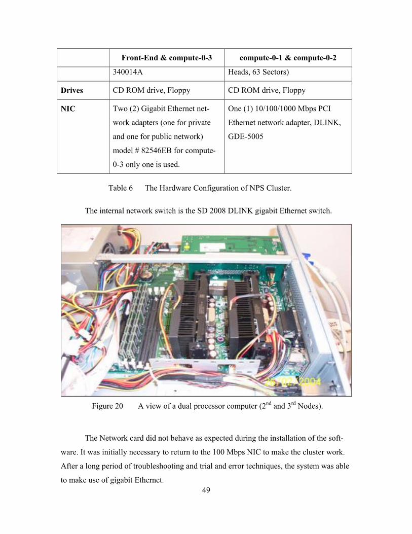
49

Front-End & compute-0-3 compute-0-1 & compute-0-2

340014A Heads, 63 Sectors)

Drives CD ROM drive, Floppy CD ROM drive, Floppy

NIC Two (2) Gigabit Ethernet net-

work adapters (one for private

and one for public network)

model # 82546EB for compute-

0-3 only one is used.

One (1) 10/100/1000 Mbps PCI

Ethernet network adapter, DLINK,

GDE-5005

Table 6 The Hardware Configuration of NPS Cluster.

The internal network switch is the SD 2008 DLINK gigabit Ethernet switch.

Figure 20 A view of a dual processor computer (2nd and 3rd Nodes).

The Network card did not behave as expected during the installation of the soft-

ware. It was initially necessary to return to the 100 Mbps NIC to make the cluster work.

After a long period of troubleshooting and trial and error techniques, the system was able

to make use of gigabit Ethernet.

50

D. INSTALLING THE SYSTEM

1. Download the Software

The software is downloaded from the Rocks web page [14] which contains a cur-

rent “stable release” version of the software. As of this writing the current version is

3.2.0, code-named Shasta. Users may download and print the “Rocks Base” user’s guide

manual as a reference to use while installing. The release notes and errata sections list

any late-breaking news or known problems with the release. The Rocks system also has

add-on rolls. Each roll is a collection of files needed for a particular additional task that

may be useful in the cluster environment.

The Rocks web site provides installation files appropriate for each of the major

hardware architectures including the x86 (Pentium and Athlon), x86_64 (AMD Opteron)

and ia64 (Itanium). The hardware used in this thesis was Pentium-based, so that distribu-

tion was selected.

The software that it is downloaded from the Rocks web page is specific for only

one architecture. So there is not the case that in a Rocks cluster coexist different architec-

tures.

An .iso file contains a CDROM disk image, which is an exact copy of the bits on

a CDROM. The file is saved to disk on a local computer and then burned to read/write

CDROM drive. The .iso file must be installed on the CDROM using the appropriate

software, such as MyDVD, to ensure that the contents of the .iso file are laid out correctly

on the CDROM rather than copied onto the CDROM as a file.

The Rocks website also displays an MD5 hash along with the .iso. This is a

mechanism to check the integrity of the software and ensures that no changes have been

made to the software since the checksum algorithm has run. The following description

explains how to check MD5 hashes on an .iso Image.

MD5 hashes are 32 byte character strings resulting from running the MD5 algo-

rithm against a particular file. Any change to a file results in a different MD5 hash when

the algorithm is run again. If an MD5 hash on the downloaded file matches that displayed

on the web site, then there is a high confidence that the file has not been modified or cor-

rupted.

51

MD5 checksum programs are available for Linux distributions. However, for this

thesis the checksum was run on Windows. This program is not installed as a part of Win-

dows but it can be downloaded from www.md5summer.org. The following figure pro-

vides the shows the MD5 hash for the “Area51 Roll” using the md5summer program.

Figure 21 The results of generating md5summ for Area51 roll. All the file informa-

tion is available. This number can be used to be checked against the number that the vendor provides fro the particular piece of software.

It is then necessary to compare the number with the number provided on the web

site:

Figure 22 The given md5summ for Area51 roll form the download site. This number

can be checked against the one that the md5summ program is going to generate for the specific software.

If the two numbers are identical the file has not been corrupted in the download

process and installers can be reasonably confident that the file has not been modified.

The following software packages and rolls were installed. The Rocks base and

HPC roll are required for a functioning cluster. The other rolls may be installed if needed.

a. Rocks Base

The file name is rocks-disk1-3.2.0.i386.iso. This file provides the basic in-

frastructure of the cluster.

52

b. HPC Roll

The file is named roll-hpc-3.2.0.i386.iso. This package provides MPI

software libraries.

c. Grid Engine Roll

This contains the Grid Engine job queuing system. The Grid Engine is a

Load Management System (LMS) that allocates resources such as processors, memory,

disk-space, and computing time. The Grid Engine, enables transparent load sharing, con-

trols the sharing of resources, and also implements utilization and site policies. It has

many characteristics including batch queuing and load balancing, as well as providing

users the ability to suspend/resume jobs and check the status of their jobs. There are sev-

eral commands for using the grid engine such as qconf, qdel, qhost, qmod, qmon, qstat,

but the most commonly used is the qsub, which is the user interface for submitting a job

to the Grid Engine [17].

The Grid Roll contains the Globus Toolkit, described as follows:

d. Globus Toolkit

The Globus Toolkit is a software collection of useful components that can

be used either independently or together to develop useful grid applications and pro-

gramming tools. For each component, an application programmer interface (API) written

in the C programming language is provided for use by software developers. Command

line tools are also provided for most components, and Java classes are provided for the

most important ones. Some APIs make use of Globus servers running on computing re-

sources. Globus Alliance [19] developed the Globus toolkit. The Globus Alliance is a

research and development project focused on enabling the application of Grid concepts to

scientific and engineering computing.

The Grid refers to an infrastructure that enables the integrated, collabora-

tive use of high-end computers, networks, databases, and scientific instruments owned

and managed by multiple organizations. Grid applications often involve large amounts of

data and/or computing and often require secure resource sharing across organizational

boundaries, and are thus, not easily handled by today’s Internet and Web infrastructures

[19].

53

A large number of individuals, organizations, and projects have developed

higher-level services, application frameworks, and scientific/engineering applications us-

ing the Globus Toolkit. For example, the Condor-G software provides an excellent

framework for high-throughput computing (e.g., parametric studies) using the Globus

Toolkit for inter-organizational resource management, data movement, and security.

e. Intel Roll

The Intel Roll contains the Intel compiler and MPICH built with the Intel

compiler. The MPICH is the Message Passing Interface “Chameleon.” This is a freely

available edition of the MPI, the standard for message-passing libraries, contained in

Rocks. [18]

f. Area51 Roll

This contains system security-related services and utilities. This is soft-

ware packed by the Rocks team for security issues. As with all rolls, it contains a series

of RPMs, each of which is a different program to be installed and contains tripwire.

Tripwire is security software that verifies changes to the system. The program monitors

key attributes of files that might not change, including binary signature, size, expected

change of size, etc. [20]

g. SCE Roll

SCE Roll contains the Scalable Cluster Environment. Kasetsart Univer-

sity, Bangkok, Thailand developed this SCE. They built an easy to use integrated soft-

ware tool for the cluster user community. These software tools, called SCE (Scalable

Computing Environment), consist of a cluster builder tool, a complex system manage-

ment tool (SCMS), scalable real-time monitoring, web-based monitoring software

(KCAP), a parallel Unix command, and a batch scheduler. This software runs on top of

the cluster middleware that provides cluster-wide process control and many services.

MPICH are also included. [21]

h. Java Roll

This contains a Java Virtual Machine (JVM). This roll is optional and in-

stalled when the administrator needs the JVM running in the system. The software is in-

stalled in the /usr/java/j2sdk1.4.2_02 directory. This Rocks release includes the 1.4.2

SDK with all the tools and libraries needed to compile and run JAVA programs.

54

The installation process is invisible to the user. Once the CD is inserted to

the drive the system just copies the relevant files in the /usr/java directory and runs the

JVM in the frontend and to the nodes. There were no problems during the installation and

the use of the JAVA environment.

i. PBS Roll

This contains the Portable Batch System. [22] It is a batch queuing sys-

tem, a mechanism for submitting batch job requests on or across multiple platforms. It is

portable across different UNIX systems such as CRAY's Unicos, IBM's AIX, SGI's Irix,

and so on. It provides the same functionality as the Grid engine. The core of the software

collection is the q-type commands. The PBS is just an initiative by NASA and the grid

engine by Sun. It allows scheduling of job requests among available queues on a given

system according to available system resources and job requirements.

j. Condor Roll

This provides tools for distributed high-throughput computing. Condor is

a specialized workload management system for compute-intensive jobs, such as other

full-featured batch systems. Users submit their serial or parallel jobs to Condor, which

then places them into a queue, chooses when and where to run the jobs based upon a pol-

icy, carefully monitors their progress, and ultimately informs the user upon completion.

[23]

Only a part of this software is required, but for this experiment, all rolls

were installed in order to test different tools to do the same job.

The .iso files on the local disk are burned onto CDs as image files after

download. Thus, a series of CD’s are ready for the installation.

The Rocks naming convention for the computer nodes are: front-end for

the master node and compute-0-1, compute-0-2 and so forth, for the slave nodes. Adding

a second rack with nodes causes the names to be compute-1-1, compute-1-2 and so forth,

which are the names used henceforth.

55

2. Installation

The installation of the cluster required a long period (many weeks) of trouble-

shooting. Most of the delays occurred because of problems with the old machines. Thus,

the following points were discerned after this phase of the installation:

There is no such thing as an easily installed cluster.

The newer and more modern parts are better.

It is generally preferable to have a single, consistent type of computer to use for

all the compute nodes. Hardware differences can lead to hard-to-diagnose problems or

incompatibilities.

In case of an error in the installation not recoverable with the reinstallation of the

front-end or the nodes, the solution is to perform a clean “from the beginning” installa-

tion of Red Hat Linux. This installation will erase all partitions from the cluster and will

format the disk again. The next step is to do a new install from the Rocks CD.

The installation uses the default configuration. However, the manual contains an

alternative option for almost every other step of the installation process. This thesis used

the default options.

The most frustrating error was the one that kept the nodes from being installed

(the two “no name” machines). Instead of continuing the installation, the node returned a

screen with a prompt to …

Select the installation language,

… and afterwards, the process came to a halt. After several days of troubleshoot-

ing, the solution was to reformat the disk.

The following diagram provides an overall idea of the installation process. The

diamonds are the troublesome points.

56

Figure 23 Installation Process with Problems, Diagnoses and Troubleshooting.

One monitor, keyboard and mouse connected to the front-end and one second set

connected to the node to which it was installed was used for the installation. This is only

necessary for troubleshooting. Afterwards, the second set was switched to the next node

57

and so forth. In the end, and after placing the machines into the rack, a monitor, key-

board, mouse connected to the front-end remained beside the rack, and the plugs changed

whenever it was necessary to manipulate a node.

Figure 24 The working area for the MOVES cluster. The nodes are off the rack dur-

ing the hardware configuration. A keyboard and a monitor were used for trouble-shooting.

The following information is required from the network administrator before pro-

ceeding with the installation for this cluster.

• IP address for the external and internal network interfaces and the net masks. This is 131.120.5.50 for the net mask, 255.255.252.0 for the ex-ternal network and 10.1.1.1 for the internal network with net mask 255.0.0.0. Note that in Linux, the NICs are named eth0 for the internal (private) and eth1 for the external (public).

• Name server IP address. This is 131.120.18.40. or .42. This will be the secondary DNS server as the primary will be 127.0.0.1.

• Host name used. This is cluster.cs.nps.navy.mil.

• Local Gateway IP address. This is 131.120.4.1.

• Time Server IP address. The time server is time1.nps.navy.mil with the IP 131.120.254.107. The time server is a minor issue. The IP address might be used instead of the FQDN.

The following figure shows all the networking information.

58

Figure 25 The NPS cluster with all network details (cluster.cs.nps.navy.mil). The

host name of the nodes with the relevant IP addresses for the internal (private) cluster network along with the external network data are shown in this figure.

The DHCP server from the front end was used for the internal (private network).

All others IPs are static.

The installation of the front end is straightforward. The Rocks Base CD is in-

serted into the drive, boots the machine and starts the system. Quickly type the following

in the boot screen:

frontend

The process takes some time. During the installation, it is necessary to insert the

aforementioned network information in several screens along with the partition and

password input. The user’s manual that was previously downloaded and printed de-

scribes the installation process step by step in detail.

Enter MOVES for the cluster name,

Enter N36.3 W 53.3 for Monterey for the Latitude Longitude.

Choose “Autopartition” for the partition part and the system disk is formatted.

Choose “Activate on boot” for both NICs and enter the IP information.

59

The password is the root password used to log into the system later.

At the end, it will ask whether to install a roll. The answer is yes and the CD drive

ejects the CD to insert the HPC roll. The installation continues with all the other rolls.

Note that it is necessary to insert the rolls in the order previously mentioned.

After the installation of the front-end, it is now possible to install the nodes of the

cluster.

The first, step is to log on into the front-end as root. The insert-ethers program is

run to install and add a node. Next, select compute from the menu and wait.

Then, the first node is booted with the same Rocks base CD ROM in the drive. In

the front-end, the “discovered new appliance” and the MAC address of the node appears

and the installation continues from the network (front-end to node). At some point, the

installation finishes and the node reboots. Next, it is essential to remove the Rocks Base

CD ROM from the nodes drive. Not removing it performs a second installation resulting

in innumerable problems.

Every time a node is added to the cluster, a series of files are updated with rele-

vant information. In the previous version of Rocks (3.1.0 named Matterhorn), the

/etc/hosts file had the entries of the nodes with the IP addresses. This does not happen

with the 3.2.0 version.

Note that the DHCP server in Linux, running in the front-end to release IP ad-

dresses to clients, starts the release from the end of the pool. Thus, the first DHCP client

will receive 10.255.255.254, the second 10.255.255.253 and so forth. The Microsoft

DHCP server starts from the beginning of the pool.

To remove a node, for instance, the node compute-0-2 from the cluster in the

front-end, as root user enters:

#insert-ether –remove=“compute-0-2”

In the front-end and after the installation of the system, because the X Windows

environment is not working, it is necessary to use the redhat-config-Xfree86 tool for the

system to recognize the VGA adaptor and the resolution. Simply enter:

60

# redhat-config-Xfree86

To start the X-Window environment, enter startx. It is necessary to remove the

screen saver in order to not receive an annoying message about it. It is now possible to

configure two items from the Windows environment. The first is the time server whose

settings are located at Date/time. Insert the data. The daemon responsible for this is the

NTP. The second is the firewall. The generic Linux firewall is used for the first settings

located at the security level. Enable the firewall to eth1.

If desired, it is possible to give the NIC cards a nickname. Do the following net-

work device control -> configure and assign the:

Interface Nickname IP addr SM

Eth1 External 131.120.5.50 255.255.252.0

Eth0 internal 10.1.1.1 255.0.0.0

Table 7 Front end NIC configuration.

When finished, the following configuration appears.

Hostname IP

CLUSTER.CS.NPS.NAVY.MIL PUBLIC: 131.120.5.50

PRIVATE: 10.1.1.1

COMPUTE-0-1 10.255.255.254

COMPUTE-0-2 10.255.255.253

COMPUTE-0-3 10.255.255.252

Table 8 Private Cluster Network Configuration.

During the installation process of the nodes, the following table was often used to

check network functionality, and whether the ping was done with IP’s or with FQDN as a

result of the unexpected network performance.

61

From

To

front-end Compute-0-1 Compute-0-2 Compute-0-3

front-end X OK IP,

OK name

OK IP,

OK name

OK IP,

OK name

Compute-0-1 OK IP,

OK name

X OK IP,

OK name

Compute-0-2 OK IP,

OK name

OK IP,

OK name

X OK IP,

OK name

Compute-0-3 OK IP,

OK name

OK IP,

OK name

OK IP,

OK name

X

Table 9 Checklist for Private Cluster Network.

E. RUNNING THE SYSTEM

The front-end keyboard is used to log onto the cluster once the aforementioned

software is installed. Use the useradd command to add users once logged on as root.

It is also possible to log into the cluster using the secure shell besides using the

front-end console. Since a MS Windows computer is mostly used, it is necessary to in-

stall the SSH version for Windows, obtainable from www.ssh.org.

.

Figure 26 The SSH for MS Windows ready to connect to the cluster. After connect is selected the next screen is asking for the password.

62

Below is the root logged in the front-end.

Last login: Wed Jul 14 01:16:08 2004 from ras32.ras.nps.navy.mil Rocks 3.2.0 (Shasta) Profile built 22:06 04-May-2004 Kickstarted 22:07 04-May-2004 Rocks Frontend Node [root@frontend-0 root]#

The ifconfig command provides information about the network interfaces.

[root@frontend-0 root]# ifconfig eth0 Link encap:Ethernet HWaddr 00:04:23:5F:7B:50

inet addr:10.1.1.1 Bcast:10.255.255.255 Mask:255.0.0.0 … Interrupt:10 Base address:0xdcc0 Memory:fcfa0000-fcfc0000

eth1 Link encap:Ethernet HWaddr 00:04:23:5F:7B:51 inet addr:131.120.5.50 Bcast:131.120.7.255 Mask:255.255.252.0

… Interrupt:7 Base address:0xdc80 Memory:fcf80000-fcfa0000

lo Link encap:Local Loopback inet addr:127.0.0.1 Mask:255.0.0.0 …

[root@frontend-0 root]#

The cluster-fork command helps to send the command in every node. In the text

below, ps is executed for the front-end, and afterwards for all nodes, and the following

response appears.

[root@frontend-0 root]# ps PID TTY TIME CMD 13415 pts/1 00:00:00 bash 13510 pts/1 00:00:00 ps [root@frontend-0 root]# cluster-fork ps compute-0-1: PID TTY TIME CMD 1 ? 00:00:19 init 2 ? 00:00:00 migration/0 … 2501 ? 00:04:12 sge_commd 20876 ? 00:00:00 sshd 20878 ? 00:00:00 ps compute-0-2: PID TTY TIME CMD 1 ? 00:00:19 init 2 ? 00:00:00 migration/0 … 3046 ? 00:03:57 sge_commd 21407 ? 00:00:00 sshd 21409 ? 00:00:00 ps compute-0-3: PID TTY TIME CMD 1 ? 00:00:04 init 2 ? 00:00:00 keventd … 3230 ? 00:00:00 sge_commd 24096 ? 00:00:00 sshd

63

24098 ? 00:00:00 ps

[root@frontend-0 root]#

To see the procedure for creating a user in the cluster, a user named clusteruser is

created. 411 is a information service that is used securely distributes users and groups

configuration files and password files. It simplifies the administration just as the Net-

work Information Service (NIS). For this reason, the /var/411 is in the output of the

useradd command.

[root@frontend-0 root]# useradd clusteruser Creating user: clusteruser make: Entering directory `/var/411' /opt/rocks/bin/411put --comment=“#” /etc/auto.home 411 Wrote: /etc/411.d/etc.auto..home Size: 676/327 bytes (encrypted/plain) Alert: sent on channel 239.2.11.71 with master 10.1.1.1 /opt/rocks/bin/411put --comment=“#” /etc/passwd 411 Wrote: /etc/411.d/etc.passwd Size: 2662/1797 bytes (encrypted/plain) Alert: sent on channel 239.2.11.71 with master 10.1.1.1 /opt/rocks/bin/411put --comment=“#” /etc/shadow 411 Wrote: /etc/411.d/etc.shadow Size: 1941/1257 bytes (encrypted/plain) Alert: sent on channel 239.2.11.71 with master 10.1.1.1 /opt/rocks/bin/411put --comment=“#” /etc/group 411 Wrote: /etc/411.d/etc.group Size: 1215/725 bytes (encrypted/plain) Alert: sent on channel 239.2.11.71 with master 10.1.1.1 make: Leaving directory `/var/411' [root@frontend-0 root]#

The “channel 239.2.11.71” is within the multicasting IP space.

Next, set the password for this new user.

[root@frontend-0 root]# passwd clusteruser Changing password for user clusteruser. New password: Retype new password: passwd: all authentication tokens updated successfully. [root@frontend-0 root]#

Then connect to a node to see “if the tokens updated successfully”, SSH to the

node compute-0-1, and execute ps.

[root@frontend-0 root]# ssh compute-0-1 Rocks Compute Node [root@compute-0-1 root]# ps PID TTY TIME CMD 20904 pts/0 00:00:00 bash 20959 pts/0 00:00:00 ps

64

Navigate to the etc directory where the password file is located. This file contains

information about the users.

[root@compute-0-1 root]# cd / [root@compute-0-1 /]# cd etc [root@compute-0-1 etc]# cat passwd # $411id: /etc/passwd$ # Retrieved: 29-Jul-2004 05:54 # Master server: 10.1.1.1 # Owner: 0.0 # Name: etc.passwd # Mode: 0100644 root:x:0:0:root:/root:/bin/bash bin:x:1:1:bin:/bin:/sbin/nologin … … clusteruser:x:504:504::/home/clusteruser:/bin/bash [root@compute-0-1 etc]#

Note that at the end, clusteruser appears with user Id 504 and group Id 504.

Next, close and return to the front end. Never forget to close the connections be-

cause the process that was initiated for the connection will always be in the memory of

the client system. When there is no other process related to a forever ongoing process,

then this is an orphan or zombie process.

There is the relation between parent and child process. A zombie process is cre-

ated when the messaging between parent and child processes fails and the system obtains

a list with “defunced” inactive processes. In fact the zombie process is already dead and

so it cannot be killed with the kill command. Thus it does not use any CPU time or

memory. In order to eliminate the zombie processes from the ps command output list a

good idea is to kill the related (parent) process.

[root@compute-0-1 etc]#exit

Switch to clusteruser to see what occurs with the SSH keys.

Connection to compute-0-1 closed. [root@frontend-0 root]# su clusteruser It doesn't appear that you have set up your ssh key. This process will make the files: /home/clusteruser/.ssh/identity.pub /home/clusteruser/.ssh/identity /home/clusteruser/.ssh/authorized_keys Generating public/private rsa1 key pair. Enter file in which to save the key (/home/clusteruser/.ssh/identity):

Simply hit enter for the file.

Created directory '/home/clusteruser/.ssh'.

65

Enter passphrase (empty for no passphrase): Enter same passphrase again:

Simply hit enter for the passphrase.

Your identification has been saved in /home/clusteruser/.ssh/identity. Your public key has been saved in /home/clusteruser/.ssh/identity.pub. The key fingerprint is: a4:fa:61:ee:8b:fc:38:e0:cd:be:bf:89:1c:bf:f1:b7 clusteruser@frontend-

0.public [clusteruser@frontend-0 root]$

Note that the key has been created and saved to the profile files.

From this point, it is possible to SSH to another node, for example, compute-0-2.

[clusteruser@frontend-0 root]$ cd [clusteruser@frontend-0 clusteruser]$ ssh compute-0-2 Warning: Permanently added 'compute-0-2' (RSA1) to the list of known

hosts. Rocks Compute Node [clusteruser@compute-0-2 clusteruser]$ exit logout Connection to compute-0-2 closed. [clusteruser@frontend-0 clusteruser]$

To identify the location of the MPI files:

[root@frontend-0 /]# find . -name mpi* -print | more

./export/home/install/ftp.rocksclusters.org/pub/rocks/rocks-3.2.0/rocks-dist/rolls/hpc/3.2.0/i386/RedHat/RPMS/mpich-eth-mpd-1.2.5.2-1.i386.rpm

…

./usr/src/linux-2.4.21-9.0.1.EL/drivers/message/fusion/lsi/mpi_history.txt

…

./opt/mpich

…

./opt/mpich2-mpd

…

./opt/gridengine/examples/jobs/mpi-cpi.sh

…

./opt/gridengine/mpi

…

./opt/intel_idb_73/bin/mpirun_dbg.idb

Under the ./opt/mpich, a whole structure of files and directories exist with the dif-

ferent implementations of MPI. Linux is now used from this point forward. It is neces-

sary to master the Linux commands and know how to find help in every step, using the

man page or the -help switch to start working with the cluster.

66

A web server runs in the cluster, which is the Apache web server. Opening an

internet browser and entering the cluster Fully Qualified Domain Name (FQDN) in the

address bar returns a page full of utilities for monitoring the cluster. Some of these utili-

ties are not available from a remote system, but only from the front-end keyboard, for se-

curity reasons, with the following options.

1. Cluster Database

From the front-end console, it is possible to manipulate the database of the cluster

and add or remove nodes. Rocks use this database to store data about its configuration,

and information about the nodes in this cluster. Every node in the cluster is described in

the database. The schema of the database can be found in the manual, in UML notation

with descriptions of the data fields and types. MySQL is a freely available Relational

Database Management System (RDBMS) used by Rocks to maintain the database [15].

2. Cluster Status (Ganglia)

The popular tool made it possible to see much information about the cluster such

as CPU usage, network, hard disks, and configuration. The items often used were the

load for the last week or day.

The CPU Usage parameter shows the percentage of CPU that currently is not in

the idle state. For example,

CPU Usage = [(CPU Used by Users + CPU Used by System + CPU Nice) ÷ (CPU Idle +

CPU Used by Users + CPU Used by System + CPU Nice)] × 100

3. Cluster Top (Process Viewer)

This allows a graphical view of information concerning the processes running on

the system, the users that submitted the processes, and the CPU usage among others.

4. Proc filesystem

It is not possible to see this through the network by default. From the front-end

console, it is possible to manipulate the /proc. This is a virtual directory containing in-

formation for every process on the Linux system.

5. Cluster Distribution

From the front-end console, it is possible to manipulate the distribution and have

access to the /install directory.

67

6. Kickstart Graph

This will present a graph with the functioning concept of the cluster from the be-

ginning and the direction of the logical volumes of functions.

7. Roll Call

It is possible to see the installed rolls. The response obtained is:

These rolls have been installed on your Rocks Cluster:

sge 3.2.0 i386

java 3.2.0 i386

intel 3.2.0 i386

grid 3.2.0 i386

hpc 3.2.0 i386

The Rocks Users Guide, Get a License for your Intel Compilers, Make Labels,

and Register Your Cluster, are straightforward options.

The following figure shows the Ganglia monitor with the nodes executing several

programs. This is from a later experiment. Each node, according to its color, is more or

less working. Red means a great deal of work, while green is less. In any case, notice

the CPUs total 6, Nodes up 4 and Nodes Down 0 to the left in the monitor.

68

Figure 27 Ganglia Monitor, where the state of the system is presented with great de-

tail. F. DETAILS ON ROCKS CLUSTER SOFTWARE

Thus, to conclude what a cluster is and what extra software a cluster must have,

these computers need their own operating system. In addition, the following are more or

less necessary:

• A batch system. (grid engine).

• An MPI API. (mpich, etc.).

• A series of compilers for both the above. (intel, etc.).

• A tool to monitor the system. (ganglia and iozone for the graphs.)

• Some benchmarks to measure the performance of the system. (hpl, iperf and stream).

• Tools to implement system specific tasks and communication (rocks con-taining the 411 get and put commands for implementing the interconnec-tion between the nodes).

• A series of tools to utilize the globus-grid, a more extended notion of a cluster through the Internet. (nmi and gpt).

69

In order to demonstrate this, a little navigation into the relevant directories to see

the globus-job-run command and some of the output are presented. It appears to

have the same syntax and parameters as the npirun:

[root@frontend-0 bin]# pwd /opt/nmi/bin [root@frontend-0 bin]# ls … globus-job-get-output globus-job-run globus-job-status globus-job-submit globus-makefile-header globus-domainname globusrun globus-job-cancel globus-job-clean [root@frontend-0 bin]# ./globus-hostname frontend-0.public [root@frontend-0 bin]# globus-job-run -help … … host-clause syntax: { contact string only the hostname is required. [-np N] number of processing elements [-count N] same as -np [-host-count nodes] number of SMP nodes (IBM SP) … … The working directory of the submitted job defaults to $HOME. … … [root@frontend-0 bin]#

All the above are in the /opt directory in the Rocks cluster, shown in the following fig-

ure.

Figure 28 The opt directory contents from NPS cluster. All the necessary pieces of

software are residing in this directory for the Rocks Beowulf cluster implementa-tion.

70

G. PROPOSAL FOR A NEW SYSTEM

After some consideration of the possible needs, a point was reached when it was

necessary to propose a new system as a second cluster across campus, to be intercon-

nected via IPv4 and IPv6. The composition of the proposed system is as follows:

• 1 computer system, 1U, with 2 NICs as a front-end system. This will have 2 AMD opteron 64-bit processors, 4 GB of SDRAM and 200 GB of disk space.

• 6 computer systems, 1U, with 1 NIC as nodes. These will have 2 AMD opteron 64-bit processors at 2.0 GHz clock (this is the Opteron 246), 1 GB of SDRAM and 100 GB of disk space.

• 1 8 port Gigabit Ethernet switch rack able 1U.

• 1 console rack able 1U.

• 1 UPS capable on supporting the above systems, rack able 2U.

• 1 power distribution unit with the miscellaneous power cabling.

• All the necessary networking cabling.

• All the necessary mount assemblies, for the systems to fit in the rack.

• 1 rack 16U, on wheels.

The space in the rack (U’s) is to be distributed as follows:

Item U’s

front-end 1

nodes 6

switch 1

console 1

UPS 2

disk array (future) 2

TOTAL 13

Table 10 Cluster Components in the Rack.

71

Note that no disk array is required in the presence state, and it is assumed that the

storage in each computer is more than adequate. However, the 2 U in the rack is pre-

served, in case this estimation is no longer valid due to future condition changes.

There are a number of vendors:

• www.dell.com provides a rich variety of systems and government pricing.

• www.tyan.com has many systems similar to the needs of this thesis re-search.

• www.infinicon.com provides more information about clusters profile and knowledge.

• www.linuxnetworx.com specializes in clusters.

• www.penguincomputing.com specializes in Linux systems.

• www.appro.com has more blades that rack able computers.

• www.RLX.com has a small interesting set of blades for a cluster.

The pricing is different for every vendor. Only Dell provides an indication of the

price and estimates are possible. A general estimate is close to $10,000.00 for the afore-

mentioned system.

The estimated performance of the system proposed is 48 Gflop. This result is the

output on the registration page on the Rocks cluster system. In this case, it is used as a

“calculator” to provide an estimation of a system with a number of processors of a given

architecture and a given clock rate. As shown in the next chapter, the performance of a

system is an issue requiring further investigation.

Tyan Corporation maintains a repository of specification papers [65] about hard-

ware configurations.

72


73

V. PERFORMANCE MEASUREMENTS

A. INTRODUCTION

Clusters are used to obtain better performance from programs, but in actuality,

better performance is difficult to optimize. Many aspects of a system affect performance.

Some programs will benefit most from a faster CPU, some from a faster network, and

some from better memory I/O.

Benchmarking is the process of characterizing the system as a whole or its various

subsystems in order to understand either its actual or potential performance.

B. PERFORMANCE MEASUREMENTS OVERVIEW

Benchmarking is used, generally speaking, for three purposes: measuring overall

system performance in order to rank-order systems, measuring subsystem performance in

order to make better optimization choices, and before-and-after comparisons to determine

if changes have improved the performance of the system.

1. Benchmarking for Overall System Performance

There are many possible ways to measure the performance of a system. Usually

the best way is to run the actual applications on it in order to see how fast they run. This

is not always possible for a variety of reasons. For example, the programs intended to run

on the system might not yet have been written, or the applications are too numerous to

test. In this situation, even an imperfect measure of expected performance is better than

none at all.

The High-Performance Linpack (HPL) benchmark is often used to characterize

systems. As mentioned in a previous chapter, the top of the list of the top 500 project is

the Earth Simulator supercomputer in Japan. With its Linpack benchmark performance of

35.86 Tflops (trillions of floating-point operations per second), its performance beats that

of the number two machine, the ASCI Q machine at Los Alamos National Laboratory, at

13.88 Tflops by a significant margin.

The number 499 supercomputer is located at the McGill University in Canada. It

is “self-made” with Athlons at 1.6 Ghz and Myrinet and achieves 406 Gflops. This the

same performance of the 500th computer at MTU Aero Engines in Germany, built from

74

Dell computers with P4 Xeons at 2.4 Ghz and Myrinet. The HPL benchmark is being

used to rank-order systems from the most to least powerful. Of course, for any particular

application other than HPL, systems may perform faster or slower. However, the bench-

mark provides an idea of system performance for a broad class of applications.

It is possible to make comparisons with other systems knowing the overall system

performance results, and to see and understand how other implementations are used in the

international community as appeared in the top 500 project. In order to post a supercom-

puter there, according to its performance, administrators have to follow a certain proce-

dure and perform a particular benchmark.

The system for this thesis research has 2.4 GHz and 700 MHz processors, and the

network is Gigabit Ethernet. There are six processors total.

2. Benchmarking Subsystems for Measuring Subsystem Performance

There is a lot of argument about the “one number result” in the benchmarking

process because this number cannot represent the exact picture of all the subsystems

of the system. For this reason, the special benchmarking software is used to measure

the performance of some of the independent assets in the system. These can be:

• I/O (hard disk) performance

• Memory performance

• General network performance

• Processor, Processes – times performance

• Context switching – times performance

• Communication latencies performance

• File and VM system latencies performance

• Communication bandwidths performance

• Memory latencies performance.

The subsystem performance can be used in the next context of benchmarking

for incremental performance improvements. In this manner, administrators have a

way to fine tune a cluster system.

75

3. Benchmarking for Incremental Performance Improvements

In a benchmark, a measurement of the ability of the machine to execute a series of

tests is performed. Next, the result is recorded and used as a reference. Each time an im-

provement or a change in the configuration in hardware and software in the system is

made, the benchmarking is again completed and a detailed conclusion provided if the

change was effective or not. In the case of an improvement, it is checked against the

amount of money spent to invest in new assets.

For example, a system administrator may keep records of system performance by

running benchmarks before and after each change to a system component. Thus, there are

historical data on the changes to the system, a fact that creates a great deal of experience

and knowledge. This knowledge can be used in different ways, but is beyond the scope of

this thesis. A table with the general idea will be provided as an example demonstrating

the “one number result” from the overall benchmark.

Date Action Benchmark Results

Difference Remarks

1/1/2004 Primary installation 100 Gflop 0 Application running

1/3/2004 Memory upgrade 110 Gflop +10 Good

1/4/2004 New switch 112Gflop +2 Rather useless

1/5/2004 Application mod-uleX redesign

100 Gflops -12 Who ordered this??

Table 11 Example of Benchmark Logging.

Another point of view is the desire to not benchmark the system at all. The target

application running on it is the actual referee. It is necessary, of course, to fine tune the

application in order for it to run as optimized as possible. Consider [24] the case of clus-

ter A that runs some benchmark faster than cluster B, but cluster B runs the application

faster than Cluster A. Cluster B will be chosen, all other things being equal.

The benchmarking can be classified as a number of levels [25]. These levels start

from the lower to the upper level are:

76

• The node level whose goal is to measure the node characteristics such as CPU, memory and disk bandwidth and access and other tests.

• The system level benchmarking is the one across the cluster and measures the MPI.

• The application level benchmarking measures the application in the cluster performance.

• The workflow level performance measures a series of applications exe-cuted.

The overall performance is traced for a period of time, from one to several days,

to make it clear when and where a potential bottleneck occurs.

The specific benchmarking of the authors is the one written and run for their spe-

cific needs.

Thus, the levels are additive. In other words, level 2 benchmarking contains level

1 and level 3, for example, contains level 1 and 2. [26]

C. BENCHMARKS

Many benchmarks can be found for clusters. The focus of this thesis will be iden-

tifying a benchmark with the following characteristics:

• Open source

• Free download

• Easy to install and execute

• Widely recognized by the community

The benchmarks used to conduct the performance measurements are described as

follows.

HPL, the High-Performance Linpack benchmark, is the most widely recognized in

the HPC community. The results generated by HPL are expressed in Gflops, and are

widely regarded as the “official” performance benchmark of clusters. In the categoriza-

tion system above, it corresponds to a system level benchmark.

The HPL benchmark will be conducted in several ways. Step one will execute the

original HPL written in FORTRAN. Step two will execute the HPL in Java in order to

understand the differences between the two approaches. The result will demonstrate the

overhead of the JAVA.

77

Step three will execute the PBS. Beowulf Performance Suite is a series of com-

mon UNIX benchmarks for several different areas of performance such as memory and

disk access. PBS can be categorized in the first low level in the benchmarking categoriza-

tion (node level).

D. HIGH-PERFORMANCE LINPACK

1. Background

Linpack is a benchmark that solves a random, dense linear system of equations in

double-precision arithmetic of the form A x = b in parallel. The algorithm is described in

[27].

The benchmark was developed at the Innovative Computing Laboratory at the

University of Tennessee, and is freely available and documented. HPL provides a testing

and timing program to quantify the accuracy of the obtained solution and the time re-

quired to compute it.

The software was obtained from netlib. The Netlib [28] is a repository containing

freely available software, documents, and databases of interest to the numerical, scientific

computing, and other communities. Versions for C and a JAVA are also available.

2. Configuration

HPL can be configured in numerous ways so that a maximum performance result

can be achieved on a variety of computer architectures. HPL requires either the Basic

Linear Algebra Subprograms (BLAS) or the Vector Signal Image Processing Library

(VSIPL), and the Message Passing Interface (MPI) for communications among distrib-

uted-memory nodes. Rocks, as with almost every other cluster implementation, includes

all the necessary files and libraries, and linpack is ready to run. Two files are needed for

this test. The configuration of HPL requires the creation of a file named machines in the

local directory that includes the names of the clusters nodes.

The machines file contains the nodes that will participate in the run. Note that

the front-end (the master node) is not included in the machines file. The parameter –

nolocal in the mpirun command (the command used to run the test) states that it is not

necessary for the front-end to participate in the run. If –nolocal is omitted, then the front-

end will contribute in the run with the CPU cycles.

78

There is a difference in the way that the nodes appear in the machines file. Note

that in the cluster for this research, compute-0-1 and compute-0-2 have two processors

each.

For example, a machines file such as the following will take all the nodes for the

run.

[cdaillid@frontend-0 cdaillid]$ vi machines compute-0-1.local compute-0-2.local compute-0-1.local compute-0-2.local compute-0-3.local ~

Note the order that the nodes appear in the file. They are actually entered as

processors. The above file is different from the following, and has better behavior than

the following file.

[cdaillid@frontend-0 cdaillid]$ vi machines compute-0-1.local compute-0-1.local compute-0-2.local compute-0-2.local compute-0-3.local ~

For example, the following file will enable only one processor from the nodes

compute-0-1 and compute-0-2.

[cdaillid@frontend-0 cdaillid]$ vi machines compute-0-1.local compute-0-2.local compute-0-3.local ~

Notice that a two processor machine is using only the one processor by looking in

the ganglia monitor.

The following figures show that for the period of a week, and for the two proces-

sor node compute-0-2, one CPU was used for some time.

79

Figure 29 One or two processor at work. This part from the Ganglia monitor shows

how a compute node with two processors behaves. First, until 16:30 hours, only one processor is used. After that in a new program run starting at about 01:00

hours both processors are engaged. The normal situation for such a machine is to use both processors. The period that only one of them is used is due to insuffi-

cient parameters given to the specific program run.

Another file, HPL.dat, includes all the necessary parameters the program needs to

run. The three most significant parameters able to be tuned are the problem size, N, the

block size NB, and the process grid ratio, PxQ. It is possible to set the parameters as de-

sired to maximize the performance for the cluster.

N refers to the order of the matrix of the system of linear equations being solved.

Higher order matrices take more time and space to solve. Generally, the problem size

should be small enough to fit in physical memory. Larger problems will cause disk swap-

ping, and the benchmark will become a long-running measure of disk performance rather

than computational performance. This parameter is the most important in determining

the number of calculations performed in the benchmark, and large values may result in

what appears to be a calculation that does not end.

P and Q refer to the process grid size, an abstraction that represents the number of

independent processes working on the problem. For example, if there was a 64 node clus-

ter, but P and Q are specified as 8 and 2, only 16 processors would work on the problem

80

rather than all 64 that are available. Generally, the ratio of P to Q should be between one

and three for maximum performance, with Q as the larger value. The optimum ratio be-

tween the two depends in part on the networking topology used in the cluster, with

switches getting better performance when the ratio between P and Q is close to one, and

hubs or shared media having better results when the ratio is higher.

The block size, NB, is used for data distribution and for computational granular-

ity. A small block size usually results in better load balancing. However, picking too

small a block size increases communications overhead. The optimal values depend on

balance between computational power and communications bandwidth on the system be-

ing tested. Good block sizes typically range from 32 to 256. A block size around 60 is

good for fast Ethernet, and larger values are better for high bandwidth interconnects.

There are guidelines on how to set the parameters in order to succeed the best per-

formance at [32].

The fully detailed explanation of the HPL.dat file, as obtained from netlib [29] is

shown in APPENDIX A. Description of the HPL.dat File

The HPL.dat file listed below was used for one of the tests.

HPLinpack benchmark input file MOVES institute, HPC team HPL.out output file name (if any) file device out (6=stdout,7=stderr,file) 4 # of problems sizes (N) 1500 3000 6000 10000 Ns 2 # of NBs 50 60 NBs 1 # of process grids (P x Q) 1 Ps 1 Qs 16.0 threshold 3 # of panel fact 0 1 2 PFACTs (0=left, 1=Crout, 2=Right) 1 # of recursive stopping criterium 8 NBMINs (>= 1) 1 # of panels in recursion 2 NDIVs 1 # of recursive panel fact. 2 RFACTs (0=left, 1=Crout, 2=Right) 1 # of broadcast 1 BCASTs (0=1rg,1=1rM,2=2rg,3=2rM,4=Lng,5=LnM) 1 # of lookahead depth 1 DEPTHs (>=0) 2 SWAP (0=bin-exch,1=long,2=mix) 80 swapping threshold 0 L1 in (0=transposed,1=no-transposed) form 0 U in (0=transposed,1=no-transposed) form

81

1 Equilibration (0=no,1=yes) 8 memory alignment in double (> 0)

3. Test Run

The program is launched with mpirun. The command to run the benchmark in the

cluster (front-end and the three nodes ) is:

/opt/mpich/gnu/bin/mpirun -np 4 -machinefile machines /opt/hpl/gnu/bin/xhpl

The first part is the full path and the mpirun file.

The –np 4 means the number of processors to run.

The -machinefile machines is the parameter of the machines file that contains the

nodes for the run.

The second part is the path and the actual benchmark file that is the xhpl.

A first taste of the mpirun can be seen by typing.

mpirun –-help

The test and runs possesses many abilities, and during this experiment, some

variations were attempted. However, for this thesis, the traditional run of HPL is used.

Issuing the following command provides an idea of what is being attempted.

pstree –a.

The output can indicate that an ssh connection is established with the nodes and

the job is distributed among them. The PI14558 is a hidden, temporary file created for

helping the run. p4pg and p4wd are switches to the xhpl.

|-gnome-terminal

| |-bash

| | `-mpirun /opt/mpich/gnu/bin/mpirun -np 4 -machinefile machines /opt/hpl/gnu/bin/xhpl

| | `-xhpl -p4pg /home/cdaillid/PI14558 -p4wd /home/cdaillid

| | |-ssh compute-0-1 -l cdaillid -n /opt/hpl/gnu/bin/xhpl frontend-0.public 44956 \-p4amslave \-p4yourname compute-0-1 -p4rmrank 1



| | `-xhpl -p4pg /home/cdaillid/PI14558 -p4wd /home/cdaillid

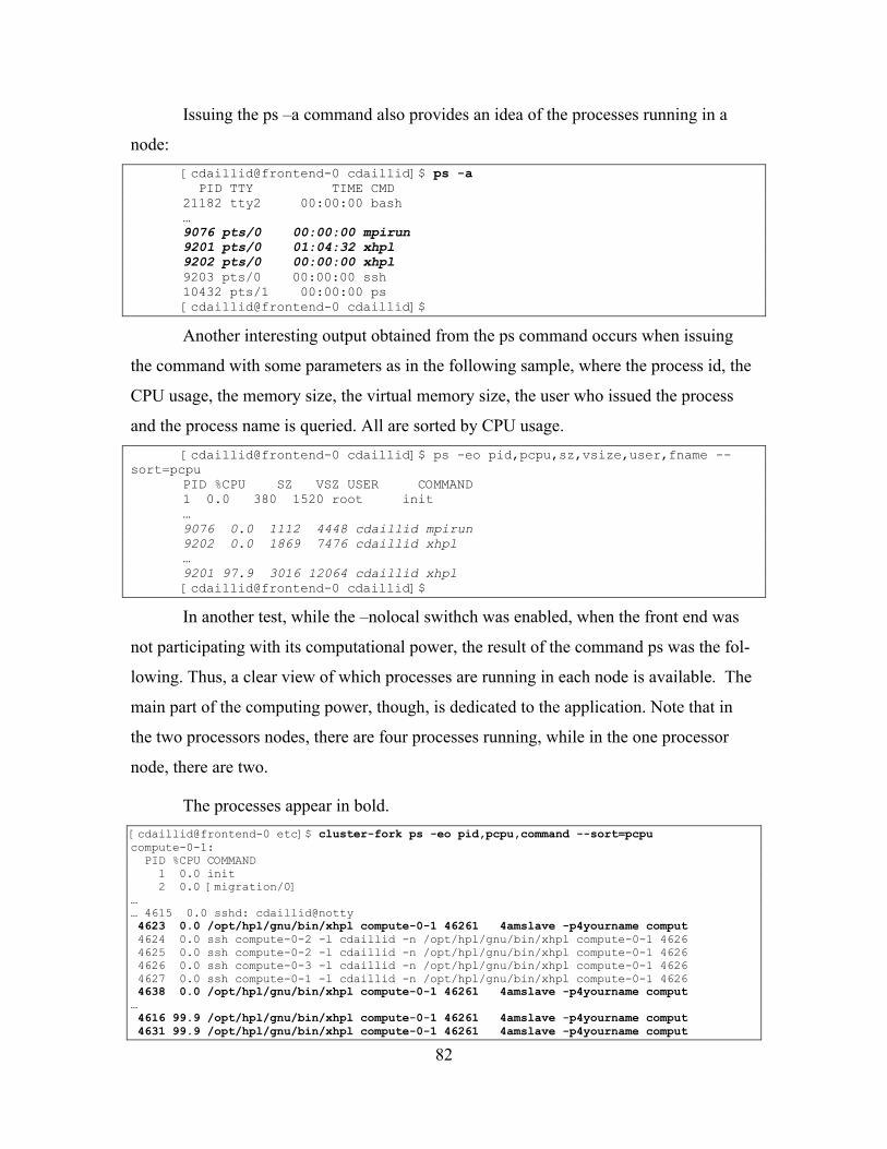
82

Issuing the ps –a command also provides an idea of the processes running in a

node:

[cdaillid@frontend-0 cdaillid]$ ps -a PID TTY TIME CMD 21182 tty2 00:00:00 bash … 9076 pts/0 00:00:00 mpirun 9201 pts/0 01:04:32 xhpl 9202 pts/0 00:00:00 xhpl 9203 pts/0 00:00:00 ssh 10432 pts/1 00:00:00 ps [cdaillid@frontend-0 cdaillid]$

Another interesting output obtained from the ps command occurs when issuing

the command with some parameters as in the following sample, where the process id, the

CPU usage, the memory size, the virtual memory size, the user who issued the process

and the process name is queried. All are sorted by CPU usage.

[cdaillid@frontend-0 cdaillid]$ ps -eo pid,pcpu,sz,vsize,user,fname --sort=pcpu

PID %CPU SZ VSZ USER COMMAND 1 0.0 380 1520 root init … 9076 0.0 1112 4448 cdaillid mpirun 9202 0.0 1869 7476 cdaillid xhpl … 9201 97.9 3016 12064 cdaillid xhpl [cdaillid@frontend-0 cdaillid]$

In another test, while the –nolocal swithch was enabled, when the front end was

not participating with its computational power, the result of the command ps was the fol-

lowing. Thus, a clear view of which processes are running in each node is available. The

main part of the computing power, though, is dedicated to the application. Note that in

the two processors nodes, there are four processes running, while in the one processor

node, there are two.

The processes appear in bold. [cdaillid@frontend-0 etc]$ cluster-fork ps -eo pid,pcpu,command --sort=pcpu compute-0-1: PID %CPU COMMAND 1 0.0 init 2 0.0 [migration/0] … … 4615 0.0 sshd: cdaillid@notty 4623 0.0 /opt/hpl/gnu/bin/xhpl compute-0-1 46261 4amslave -p4yourname comput 4624 0.0 ssh compute-0-2 -l cdaillid -n /opt/hpl/gnu/bin/xhpl compute-0-1 4626 4625 0.0 ssh compute-0-2 -l cdaillid -n /opt/hpl/gnu/bin/xhpl compute-0-1 4626 4626 0.0 ssh compute-0-3 -l cdaillid -n /opt/hpl/gnu/bin/xhpl compute-0-1 4626 4627 0.0 ssh compute-0-1 -l cdaillid -n /opt/hpl/gnu/bin/xhpl compute-0-1 4626 4638 0.0 /opt/hpl/gnu/bin/xhpl compute-0-1 46261 4amslave -p4yourname comput … 4616 99.9 /opt/hpl/gnu/bin/xhpl compute-0-1 46261 4amslave -p4yourname comput 4631 99.9 /opt/hpl/gnu/bin/xhpl compute-0-1 46261 4amslave -p4yourname comput

83

compute-0-2: PID %CPU COMMAND 1 0.0 init 2 0.0 [migration/0] …… 4521 0.0 /opt/hpl/gnu/bin/xhpl compute-0-1 46261 4amslave -p4yourname comput 4532 0.0 /opt/hpl/gnu/bin/xhpl compute-0-1 46261 4amslave -p4yourname comput ... 4514 99.8 /opt/hpl/gnu/bin/xhpl compute-0-1 46261 4amslave -p4yourname comput 4525 99.8 /opt/hpl/gnu/bin/xhpl compute-0-1 46261 4amslave -p4yourname comput compute-0-3: PID %CPU COMMAND 1 0.0 init 2 0.0 [keventd] …… 3943 0.0 /opt/hpl/gnu/bin/xhpl compute-0-1 46261 4amslave -p4yourname comput … 3936 99.9 /opt/hpl/gnu/bin/xhpl compute-0-1 46261 4amslave -p4yourname comput [cdaillid@frontend-0 etc]$

Of course, it is possible to view the node status with the command top.

The PIxxx file provides another way to see which machines participated in the

run. From above, it is known that PI with a number (i.e., PI14558) is a hidden, temporary

file created for helping the run. Samples of this file follow:

compute-0-1.local 1 /opt/hpl/gnu/bin/xhpl compute-0-2.local 1 /opt/hpl/gnu/bin/xhpl compute-0-1.local 1 /opt/hpl/gnu/bin/xhpl compute-0-2.local 1 /opt/hpl/gnu/bin/xhpl compute-0-3.local 1 /opt/hpl/gnu/bin/xhpl

The front end also works even when not using the –nolocal switch in the mpirun:

frontend-0.public 0 /opt/hpl/gnu/bin/xhpl compute-0-1.local 1 /opt/hpl/gnu/bin/xhpl compute-0-2.local 1 /opt/hpl/gnu/bin/xhpl compute-0-1.local 1 /opt/hpl/gnu/bin/xhpl compute-0-2.local 1 /opt/hpl/gnu/bin/xhpl compute-0-3.local 1 /opt/hpl/gnu/bin/xhpl

4. Results

After running the benchmark, an output file named HPL.out is obtained, which is

stored in the local directory. For another run, it is first necessary to rename this file to

some identifiable name, because by the next run, the file will be overwritten. The con-

tents of this file are similar to those appearing below. ============================================================================ HPLinpack 1.0 -- High-Performance Linpack benchmark -- September 27, 2000 Written by A. Petitet and R. Clint Whaley, Innovative Computing Labs., UTK ============================================================================ An explanation of the input/output parameters follows: T/V : Wall time / encoded variant. N : The order of the coefficient matrix A. NB : The partitioning blocking factor. P : The number of process rows. Q : The number of process columns. Time : Time in seconds to solve the linear system. Gflops : Rate of execution for solving the linear system.

84

The following parameter values will be used: N : 1500 3000 6000 10000 NB : 50 60 P : 1 Q : 1 PFACT : Left Crout Right NBMIN : 8 NDIV : 2 RFACT : Right BCAST : 1ringM DEPTH : 1 SWAP : Mix (threshold = 80) L1 : transposed form U : transposed form EQUIL : yes ALIGN : 8 double precision words ---------------------------------------------------------------------------- - The matrix A is randomly generated for each test. - The following scaled residual checks will be computed: 1) ||Ax-b||_oo / ( eps * ||A||_1 * N ) 2) ||Ax-b||_oo / ( eps * ||A||_1 * ||x||_1 ) 3) ||Ax-b||_oo / ( eps * ||A||_oo * ||x||_oo ) - The relative machine precision (eps) is taken to be 1.110223e-16 - Computational tests pass if scaled residuals are less than 16.0 ============================================================================ T/V N NB P Q Time Gflops ---------------------------------------------------------------------------- W11R2L8 1500 50 1 1 1.47 1.531e+00 ---------------------------------------------------------------------------- ||Ax-b||_oo / ( eps * ||A||_1 * N ) = 0.0526934 ...... PASSED ||Ax-b||_oo / ( eps * ||A||_1 * ||x||_1 ) = 0.0234389 ...... PASSED ||Ax-b||_oo / ( eps * ||A||_oo * ||x||_oo ) = 0.0057014 ...... PASSED ============================================================================ ... … … T/V N NB P Q Time Gflops ---------------------------------------------------------------------------- W11R2R8 10000 60 1 1 370.60 1.799e+00 ---------------------------------------------------------------------------- ||Ax-b||_oo / ( eps * ||A||_1 * N ) = 0.0946743 ...... PASSED ||Ax-b||_oo / ( eps * ||A||_1 * ||x||_1 ) = 0.0224027 ...... PASSED ||Ax-b||_oo / ( eps * ||A||_oo * ||x||_oo ) = 0.0050075 ...... PASSED ============================================================================ Finished 24 tests with the following results: 24 tests completed and passed residual checks, 0 tests completed and failed residual checks, 0 tests skipped because of illegal input values. ---------------------------------------------------------------------------- End of Tests.

As can be seen from above, after each run, the relevant parameters are printed

along with the time it took to complete the computations of the test and the performance

in units of Gflops.

The case shown below illustrates an incomplete configuration in the cluster. This

is the HPL.out obtained after the inadequate completion of the benchmark. This particu-

lar instance arose because of the big N size along with the 1x2 of PxQ.

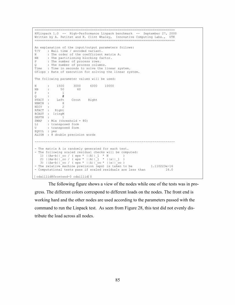
85

============================================================================ HPLinpack 1.0 -- High-Performance Linpack benchmark -- September 27, 2000 Written by A. Petitet and R. Clint Whaley, Innovative Computing Labs., UTK ============================================================================ An explanation of the input/output parameters follows: T/V : Wall time / encoded variant. N : The order of the coefficient matrix A. NB : The partitioning blocking factor. P : The number of process rows. Q : The number of process columns. Time : Time in seconds to solve the linear system. Gflops : Rate of execution for solving the linear system. The following parameter values will be used: N : 1500 3000 6000 10000 NB : 50 60 P : 1 Q : 2 PFACT : Left Crout Right NBMIN : 8 NDIV : 2 RFACT : Right BCAST : 1ringM DEPTH : 1 SWAP : Mix (threshold = 80) L1 : transposed form U : transposed form EQUIL : yes ALIGN : 8 double precision words ---------------------------------------------------------------------------- - The matrix A is randomly generated for each test. - The following scaled residual checks will be computed: 1) ||Ax-b||_oo / ( eps * ||A||_1 * N ) 2) ||Ax-b||_oo / ( eps * ||A||_1 * ||x||_1 ) 3) ||Ax-b||_oo / ( eps * ||A||_oo * ||x||_oo ) - The relative machine precision (eps) is taken to be 1.110223e-16 - Computational tests pass if scaled residuals are less than 16.0 [cdaillid@frontend-0 cdaillid]$

The following figure shows a view of the nodes while one of the tests was in pro-

gress. The different colors correspond to different loads on the nodes. The front end is

working hard and the other nodes are used according to the parameters passed with the

command to run the Linpack test. As seen from Figure 28, this test did not evenly dis-

tribute the load across all nodes.

86

Figure 30 All nodes are working unevenly. Due to insufficient parameters in the

program run the nodes are not working as desired, regarding the CPU load. The front-end colored red in the left, is working more intensively while the two nodes in the middle (orange and yellow) are working less intensive. The blue colored

node in the right (compute-0-1) is not engaged at all in the run.

Another way to see the processes running in the system is with the use of the

command cluster-fork.

[cdaillid@frontend-0 cdaillid]$ cluster-fork ps compute-0-1: PID TTY TIME CMD 1831 ? 00:00:00 sshd 1833 ? 00:00:00 xhpl <defunct> 1841 ? 00:00:00 xhpl 3191 ? 00:00:00 sshd 3192 ? 00:00:00 ps compute-0-2: PID TTY TIME CMD 1713 ? 00:00:00 sshd 1715 ? 16:07:25 xhpl 1723 ? 00:00:00 xhpl 3118 ? 00:00:00 sshd 3119 ? 00:00:00 ps

87

compute-0-3: PID TTY TIME CMD 1235 ? 00:00:00 sshd 1237 ? 16:07:32 xhpl 1245 ? 00:00:00 xhpl 2591 ? 00:00:00 sshd 2592 ? 00:00:00 ps [cdaillid@frontend-0 cdaillid]$

The xhpl process with pid 1833 in the compute-0-1 is <defunced>. For this rea-

son, the node is not using the CPU power to contribute the cluster as shown in Figure 30.

The <defunct> processes are created when one of the child or parent processes is termi-

nated for some reason (probably kernel bug) and the other does not respond to fix it. This

is called a zombie process, which is a process that has completed execution but has not

yet been removed from the kernel’s process table.

A short discussion of the processes from the ps manual concerning the process

state appears below:

• D uninterruptible sleep (usually IO)

• R runnable (on run queue)

• S sleeping

• T traced or stopped

• Z a defunct (“zombie”) process

• W has no resident pages

• < high-priority process

• N low-priority task

• L has pages locked into memory (for real-time and custom IO)

In Figure 31, the test had different parameters and the load balancing was more

even. The actual difference is in the machines file and in the nodes entered there.

88

Figure 31 All Nodes are Working Evenly. Due to sufficient parameters in the pro-

gram run the nodes are working as desired, regarding the CPU load. All the nodes are colored orange and are engaged with equal amount of CPU power in the

run

The results from several tests appear in Appendix B, which were performed in the

experimental Beowulf Linux cluster.

Table 12 summarizes the results for the HPL benchmark with differing values for

NB, the block size, and N, the problem size. The cluster achieves the maximum perform-

ance of 2.6983 Gflop with a problem size of 10000 and block size of 80, and all of them

are in a 1x1 process grid. Note that the above 10000 limit did not produce results due to

inefficiency of the system to handle memory swapping. Also, the results for a grid more

than 1x1 were low.

The following table was created upon completion of all the tests.

NB\N 0 50 100 150 500 1000 1500 3000 6000 10000

50 0 0.2561 0.5217 0.8861 1.0317 1.5310 1.5293 1.4357 1.7093 1.7530

60 0 0.3104 0.5901 0.8612 1.0005 1.1 1.2370 1.6117 1.7590 1.8010

64 0 0.2 0.5889 0.9 1.2883 1.4757 1.5675 1.7535 1.7907 1.8047

70 1.6630 1.8163

80 1.9663 2.2851 2.4730 2.4060 2.6983

85 2.6377

90 2.6200

100 2.5357

Table 12 HPL Benchmark Results Table.

89

The following figure shows the results.

Benchmark results

0

0.5

1

1.5

2

2.5

3

0 50 100 150 500 1,000 1,500 3,000 6,000 10,000

N

Gig

a Fl

ops

50

60

64

70

80

85

90

100

Figure 32 HPL benchmark results graph. The performance is shown for the specific

hardware and software configuration and for different parameters in the bench-marking process.

The detailed results per test appear in Appendix B.

5. Benchmarking Cluster with Only One Node

Another experiment was completed to investigate the performance of one ma-

chine only. It was necessary to include only one machine in the machines file just to en-

sure that nothing unexpected might happen.

[test@frontend-0 test]$ vi machines compute-0-3 ~

The following appear in the HPL.dat.

[test@frontend-0 test]$ vi HPL.dat … 1 # of problems sizes (N) 1000 Ns 1 # of NBs 64 NBs 1 # of process grids (P x Q) 1 Ps 1 Qs

The command to run the benchmark is the following:

90

[test@frontend-0 test]$ /opt/mpich/gnu/bin/mpirun -nolocal -np 1 -machinefile machines /opt/hpl/gnu/bin/xhpl

The results are:

T/V N NB P Q Time Gflops ------------------------------------------------------------------------ W11R2L8 1000 64 1 1 0.49 1.375e+00 ------------------------------------------------------------------------- … T/V N NB P Q Time Gflops ------------------------------------------------------------------------ W11R2C8 1000 64 1 1 0.45 1.494e+00 ------------------------------------------------------------------------ … T/V N NB P Q Time Gflops ------------------------------------------------------------------------ W11R2R8 1000 64 1 1 0.45 1.494e+00 ------------------------------------------------------------------------ …

The average for compute-0-3 is 1.454 Gflops, for N=1000.

Now increase the problem size to 10000 Ns.

[test@frontend-0 test]$ vi HPL.dat … 1 # of problems sizes (N) 10000 Ns

The results are:

[test@frontend-0 test]$ /opt/mpich/gnu/bin/mpirun -nolocal -np 1 -machinefile machines /opt/hpl/gnu/bin/xhpl … N : 10000 NB : 64 P : 1 Q : 1 … T/V N NB P Q Time Gflops ------------------------------------------------------------------------ W11R2L8 10000 64 1 1 370.14 1.802e+00 ------------------------------------------------------------------------ … T/V N NB P Q Time Gflops ------------------------------------------------------------------------ W11R2C8 10000 64 1 1 368.99 1.807e+00 ------------------------------------------------------------------------ … T/V N NB P Q Time Gflops ------------------------------------------------------------------------ W11R2R8 10000 64 1 1 370.64 1.799e+00

Notice that the time is much greater the second time but that the performance is

better. Also note that the compute-0-3 is a 2.4 GHz processor machine, which by itself,

possesses approximately the same performance as the whole cluster.

91

It is then possible to conclude that the two 700 MHz machines do not contribute

greatly to the computing power.

The problem size of 20000 was a disaster. The output is the following:

… N : 20000 NB : 80 P : 1 Q : 1 … HPL ERROR from process # 0, on line 170 of function HPL_pdtest: >>> [0,0] Memory allocation failed for A, x and b. Skip. <<< HPL ERROR from process # 0, on line 170 of function HPL_pdtest: >>> [0,0] Memory allocation failed for A, x and b. Skip. <<< HPL ERROR from process # 0, on line 170 of function HPL_pdtest: >>> [0,0] Memory allocation failed for A, x and b. Skip. <<< 0 tests completed and passed residual checks, 0 tests completed and failed residual checks, 3 tests skipped because of illegal input values.

6. The Ganglia Meta Daemon

A ganglia monitor was used during all these tests to view the load in the cluster.

This was possible because a process named gmetad was running on the compute nodes

and reporting data back to the front end running Ganglia.

By issuing the following command, it is possible to see the purpose of the gmetad,

which helped to complete the task.

#./gmetad --help ganglia-monitor-core 2.5.5 Purpose: The Ganglia Meta Daemon (gmetad) collects information from multiple gmond or gmetad data sources, saves the information to local round-robin databases, and exports XML which is the concatentation of all data sources Usage: ganglia-monitor-core [OPTIONS]... -h --help Print help and exit -V --version Print version and exit -cSTRING --conf=STRING Location of gmetad configuration file (de-fault='/etc/gmetad.conf') -dINT --debug=INT Debug level. If greater than zero, daemon will stay in foreground. (default=0) [cdaillid@frontend-0 sbin]$

92

7. To Enter the Top 500

The table that holds the 500 most powerful commercially available known com-

puter systems includes other data such as the manufacturer, location, the number of proc-

essors, and well as tracks the Rmax, which is the Maximal LINPACK performance

achieved and the Nmax, which is the problem size for achieving Rmax.

E. JAVA HIGH-PERFORMANCE LINPACK

1. Background

The Java HPL implementation was obtained from netlib [31]. It is a command

line utility with all graphical components removed.

Two more editions run as an applet. One is the “simple” and the second is the

“optimized.”

Unfortunately, this test does not utilize MPI, and is run only on a single machine.

To compare the performance under the two benchmarks, two comparisons will be made.

The first directly compares the benchmark by running each on a single node, while the

second estimates the maximum possible performance for the cluster running Java HPL,

and compares this to the actual results achieved by the Fortran HPL benchmark.

2. Test Run

Assuming that cluster performance scales linearly with the performance of each

node in the cluster, overall cluster performance is the sum of the performance of each

node. Even though this approach is not correct, it will provide an estimate of the upper

bound of performance.

This will be compared to the performance that the 2.4 GHz node compute-0-3

achieved in the previous section when running the Fortran HPL benchmark.

As with the Fortran HPL benchmark, the problem solved is a dense 500x500 sys-

tem of linear equations with one right hand side, Ax=b. The matrix is generated randomly

and the right hand side is constructed so the solution has all components equal to one.

The method of solution is based on Gaussian elimination with partial pivoting.

Mflop/s: for this problem there are 2/3 n3 + n2 floating point operations.

Time is the time in seconds to solve the problem, Ax=b.

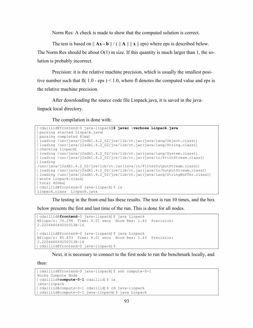
93

Norm Res: A check is made to show that the computed solution is correct.

The test is based on || Ax - b || / ( || A || || x || eps) where eps is described below.

The Norm Res should be about O(1) in size. If this quantity is much larger than 1, the so-

lution is probably incorrect.

Precision: it is the relative machine precision, which is usually the smallest posi-

tive number such that fl( 1.0 - eps ) < 1.0, where fl denotes the computed value and eps is

the relative machine precision.

After downloading the source code file Linpack.java, it is saved in the java-

linpack local directory.

The compilation is done with:

[cdaillid@frontend-0 java-linpack]$ javac -verbose Linpack.java [parsing started Linpack.java] [parsing completed 81ms] [loading /usr/java/j2sdk1.4.2_02/jre/lib/rt.jar(java/lang/Object.class)] [loading /usr/java/j2sdk1.4.2_02/jre/lib/rt.jar(java/lang/String.class)] [checking Linpack] [loading /usr/java/j2sdk1.4.2_02/jre/lib/rt.jar(java/lang/System.class)] [loading /usr/java/j2sdk1.4.2_02/jre/lib/rt.jar(java/io/PrintStream.class)] [loading /usr/java/j2sdk1.4.2_02/jre/lib/rt.jar(java/io/FilterOutputStream.class)] [loading /usr/java/j2sdk1.4.2_02/jre/lib/rt.jar(java/io/OutputStream.class)] [loading /usr/java/j2sdk1.4.2_02/jre/lib/rt.jar(java/lang/StringBuffer.class)] [wrote Linpack.class] [total 400ms] [cdaillid@frontend-0 java-linpack]$ ls Linpack.class Linpack.java

The testing in the front-end has these results. The test is run 10 times, and the box

below presents the first and last time of the run. This is done for all nodes.

[cdaillid@frontend-0 java-linpack]$ java Linpack Mflops/s: 76.296 Time: 0.01 secs Norm Res: 1.43 Precision: 2.220446049250313E-16 … [cdaillid@frontend-0 java-linpack]$ java Linpack Mflops/s: 85.833 Time: 0.01 secs Norm Res: 1.43 Precision: 2.220446049250313E-16 [cdaillid@frontend-0 java-linpack]$

Next, it is necessary to connect to the first node to run the benchmark locally, and

thus:

[cdaillid@frontend-0 java-linpack]$ ssh compute-0-1 Rocks Compute Node [cdaillid@compute-0-1 cdaillid]$ ls java-linpack [cdaillid@compute-0-1 cdaillid]$ cd java-linpack [cdaillid@compute-0-1 java-linpack]$ java Linpack

94

Mflops/s: 29.855 Time: 0.02 secs Norm Res: 1.43 Precision: 2.220446049250313E-16 … [cdaillid@compute-0-1 java-linpack]$ java Linpack Mflops/s: 29.855 Time: 0.02 secs Norm Res: 1.43 Precision: 2.220446049250313E-16 [cdaillid@compute-0-1 java-linpack]$

Then, connecting to node compute-0-2 results in:

[cdaillid@frontend-0 java-linpack]$ ssh compute-0-2 Rocks Compute Node [cdaillid@compute-0-2 cdaillid]$ cd java-linpack [cdaillid@compute-0-2 java-linpack]$ java Linpack Mflops/s: 29.855 Time: 0.02 secs Norm Res: 1.43 Precision:

2.220446049250313E-16 … [cdaillid@compute-0-2 java-linpack]$ java Linpack Mflops/s: 31.212 Time: 0.02 secs Norm Res: 1.43 Precision:

2.220446049250313E-16 [cdaillid@compute-0-2 java-linpack]$

For the node compute-0-3:

[cdaillid@frontend-0 java-linpack]$ ssh compute-0-3 Rocks Compute Node [cdaillid@compute-0-3 cdaillid]$ cd java-linpack [cdaillid@compute-0-3 java-linpack]$ java Linpack Mflops/s: 85.833 Time: 0.01 secs Norm Res: 1.43 Precision:

2.220446049250313E-16 … [cdaillid@compute-0-3 java-linpack]$ java Linpack Mflops/s: 76.296 Time: 0.01 secs Norm Res: 1.43 Precision:

2.220446049250313E-16 [cdaillid@compute-0-3 java-linpack]$

Since the Norm Res value is greater than 1, it is then possible to state that all the

tests were correct, with the results from all the available nodes. It can be assumed that the

computing power of the entire system is the summation of the computing power of the

nodes, and therefore, the computer power of the cluster is derived, which is shown in the

following table.

95

front-end -0-1 -0-2 -0-3 1st run 76.296 29.855 29.855 85.833 2nd run 85.833 31.212 31.212 85.833 3rd run 76.296 31.212 28.611 85.833 4th run 85.833 29.855 29.855 85.833 5th run 85.833 29.855 29.855 76.296 6th run 62.424 29.855 31.212 85.833 7th run 85.833 29.855 28.611 85.833 8th run 68.667 29.855 29.855 85.833 9th run 76.296 29.855 29.855 85.833 10th run 76.296 29.855 29.855 85.833 11th run 85.833 29.855 31.212 76.296 Average for each node 78.67636364 30.10172727 29.99890909 84.099 TOTAL 222.876

Table 13 JAVA Benchmark Results.

Directly comparing the performance of the node compute-0-3 under both the For-

tran and Java benchmarks, the Java performance is much lower. Previously, it was 1.0317

Gflops, for N=500 for the FORTRAN linpack, but it is now 84.099 Mflops, for N=500,

which is a big difference. However, the comparison cannot be considered precise be-

cause the JAVA linpack does not involve the NB factor.

It is possible to see the results from each run, the average for every node and the

total of all nodes. The amount is 222.876 Mflop, which is much less than the 2.9 Gflop

achieved by the FORTRAN linpack.

The conclusion reached is that it is not possible to have comparable results for

these two tests.

3. JAVA Linpack Hall of Fame

There is a web page maintained by [email protected] in which the results

are reported from different individuals conducting the test. The first and the last two ma-

chines from the list are listed below.

2147 Mflop/s; PowerPC 601 Mac OS PowerBooks G3/266; 3/10/04 dcwy 999 Mflop/s; Other Other n0n3; 3/1/03 h?d3nZ0rN … … 0.27 Mflop/s; Intel PIII Windows2000 ; 10/25/02 0.22 Mflop/s; UltraSparc Solaris 2x ; 8/15/00 Barbara 0.17 Mflop/s; UltraSparc Solaris 2x ; 8/16/00 Last updated : Mon Jun 14 00:10:14 EDT 2004

96

F. BEOWULF PERFORMANCE SUITE (BPS)

1. Background

Now, a more simple approach is achieved by using the prepackaged performance

suite from Beowulf, called the Beowulf Performance Suite (BPS). The precompiled soft-

ware can be found at hpc-design [33]. This actually, according to the author of the ex-

planatory paper, is not designed to be benchmark clusters. It is designed to be an analysis

tool for measuring differences that occur when making a hardware or soft ware change in

the cluster.

As previously mentioned, the goal is to log all performance results in a table and

rerun the BPS again after deciding in the future to do some upgrades. Next, the perform-

ance results are simply compared after and before the upgrade. It is possible to state that

the upgrade has positive, negative, or no results at all in the configuration.

The BPS provides a text mode and graphical interface to run the tests. It also pro-

vides a tool for creating web pages with the results of the benchmark so that it is distrib-

uted easily in the net.

The BPS includes the following tools for the benchmarking:

bonnie++: that is a I/O (hard disk) performance

stream: for memory performance

netperf: for general network performance

netpipe: more detailed network performance

unixbench: general Unix benchmarks

LMbench: low level benchmarks

nas: NASA parallel benchmarks.

2. BPS Installation

The aforementioned website provided the source code and the binaries in a RPM.

RPM stands for Red Hat Package Manager

The files are:

bps-1.2-11.i386.rpm is the binaries

97

bps-1.2-11.src.rpm is the source code.

The step-by-step procedure for installing an RPM is described as follows.

First, it is necessary to navigate to the user’s home directory and issue the com-

mand to install the RPM.

[cdaillid@frontend-0 /]$ cd /home/cdaillid [cdaillid@frontend-0 cdaillid]$ ll total 11100 -rw-r--r-- 1 root root 2738286 May 6 09:33 bps-1.2-11.i386.rpm -rw-r--r-- 1 root root 5253075 May 6 09:34 bps-1.2-11.src.rpm [cdaillid@frontend-0 cdaillid]$ rpm -ivh bps-1.2-11.i386.rpm error: Failed dependencies: pygtk is needed by bps-1.2-11 gnuplot is needed by bps-1.2-11 [cdaillid@frontend-0 cdaillid]$

It can be ascertained from the above message that the pygtk and gnuplot are

missing from this system and that they are required by the BPS. All these RPMs can be

found at http://rpmfind.net/linux/RPM/. This is the repository for all RPMs.

The following command is issued to ensure that the RPMs are missing. The grep

command (global regular expression pattern) is a useful find tool for the Unix Linux

world.

[cdaillid@frontend-0 /]$ rpm -qa | grep gnuplot [cdaillid@frontend-0 /]$ cdaillid@frontend-0 /]$ rpm -qa | grep pygtk [cdaillid@frontend-0 /]$

The system responded that none of the desired RPMs are installed. It is first nec-

essary to find the package gnuplot.

The current version is 4.0.0, with a build date of Fri Apr 16 15:59:34 2004 with

the gnuplot-4.0.0-1 RPM for i386.

Gnuplot is a command-line driven, interactive function plotting program espe-

cially suited for scientific data representation. Gnuplot can be used to plot functions and

data points in both two and three dimensions and in many different formats. The next

step is to find the PyGTK. The current version is 0.6.9, with a build date of Apr 9 03:07:18

2002 with the pygtk-0.6.9-3 RPM for i386.

PyGTK is an extension module for Python that provides access to the GTK+ wid-

get set. Almost anything that can be written in C with GTK+ can be written in Python

98

with PyGTK (within reason), but with all of Python's benefits. PyGTK provides an object-

oriented interface at a slightly higher level than the C interface. It is necessary to install

PyGTK to obtain the Python bindings for the GTK+ widget set.

Next, the command to install the PyGTK is issued.

[cdaillid@frontend-0 cdaillid]$ rpm -iv pygtk-0.6.9-3.i386.rpm warning: pygtk-0.6.9-3.i386.rpm: V3 DSA signature: NOKEY, key ID db42a60e error: Failed dependencies: imlib is needed by pygtk-0.6.9-3 libgdk_imlib.so.1 is needed by pygtk-0.6.9-3 libgdk_pixbuf.so.2 is needed by pygtk-0.6.9-3 [cdaillid@frontend-0 cdaillid]$

The attempt to install pygtk shows that it is necessary to find imlib. After

searching again in the RPM repository, it is possible to see that the current version is

1.9.13, with a build date of Aug 14 04:54:52 2002 with the imlib-1.9.13-9 RPM for i386.

Imlib is a display depth independent image loading and rendering library. Imlib

is designed to simplify and accelerate the process of loading images and obtaining X

Window system drawables. Imlib provides many simple manipulation routines, which

can be used for common operations.

Install imlib if it is necessary for an image loading and rendering library for

X11R6, or if installing GNOME. It might also be desirable to install the imlib-cfgeditor

package, which will help in configuring Imlib.

It is then run:

[root@frontend-0 cdaillid]# rpm -iv imlib-1.9.13-9.i386.rpm warning: imlib-1.9.13-9.i386.rpm: V3 DSA signature: NOKEY, key ID db42a60e Preparing packages for installation... imlib-1.9.13-9 /sbin/ldconfig: File /opt/intel_fc_80/lib/libcprts.so is too small, not checked. … … /sbin/ldconfig: File /opt/intel_cc_80/lib/libunwind.so is too small, not checked. [root@frontend-0 cdaillid]#

Next, it is run in order to install PyGTK.

[root@frontend-0 cdaillid]# rpm -iv pygtk-0.6.9-3.i386.rpm warning: pygtk-0.6.9-3.i386.rpm: V3 DSA signature: NOKEY, key ID db42a60e error: Failed dependencies: libgdk_pixbuf.so.2 is needed by pygtk-0.6.9-3 [root@frontend-0 cdaillid]#

Now note that this libgdk_pixbuf is needed.

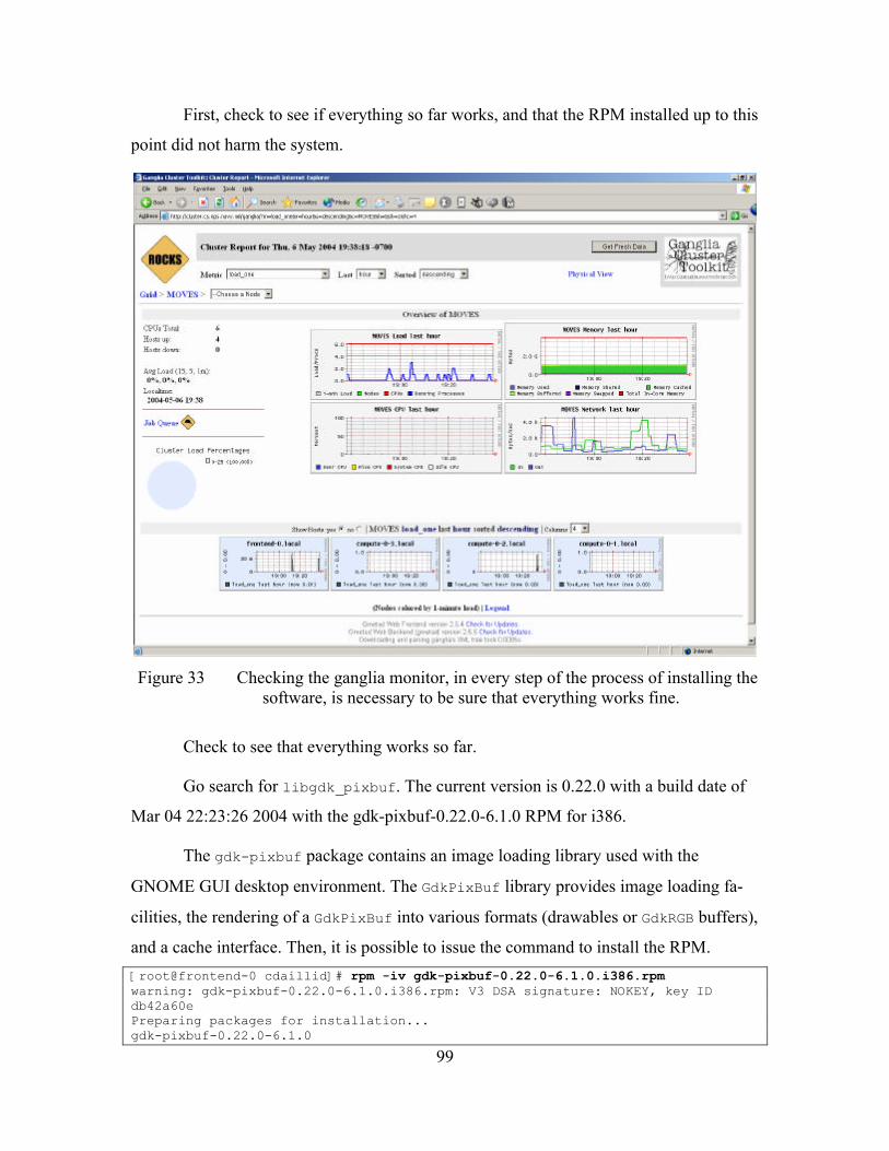
99

First, check to see if everything so far works, and that the RPM installed up to this

point did not harm the system.

Figure 33 Checking the ganglia monitor, in every step of the process of installing the

software, is necessary to be sure that everything works fine.

Check to see that everything works so far.

Go search for libgdk_pixbuf. The current version is 0.22.0 with a build date of

Mar 04 22:23:26 2004 with the gdk-pixbuf-0.22.0-6.1.0 RPM for i386.

The gdk-pixbuf package contains an image loading library used with the

GNOME GUI desktop environment. The GdkPixBuf library provides image loading fa-

cilities, the rendering of a GdkPixBuf into various formats (drawables or GdkRGB buffers),

and a cache interface. Then, it is possible to issue the command to install the RPM.

[root@frontend-0 cdaillid]# rpm -iv gdk-pixbuf-0.22.0-6.1.0.i386.rpm warning: gdk-pixbuf-0.22.0-6.1.0.i386.rpm: V3 DSA signature: NOKEY, key ID db42a60e Preparing packages for installation... gdk-pixbuf-0.22.0-6.1.0

100

/sbin/ldconfig: File /opt/intel_fc_80/lib/libcprts.so is too small, not checked. … … /sbin/ldconfig: File /opt/intel_cc_80/lib/libunwind.so is too small, not checked. [root@frontend-0 cdaillid]#

Install the PyGTK RPM.

[root@frontend-0 cdaillid]# rpm -iv pygtk-0.6.9-3.i386.rpm warning: pygtk-0.6.9-3.i386.rpm: V3 DSA signature: NOKEY, key ID db42a60e Preparing packages for installation... pygtk-0.6.9-3 [root@frontend-0 cdaillid]#

OK and with Python. Now, for the installation of the gnuplot rpm, the following

is run.

[root@frontend-0 cdaillid]# rpm -iv gnuplot-4.0.0-1.i386.rpm warning: gnuplot-4.0.0-1.i386.rpm: V3 DSA signature: NOKEY, key ID e01260f1 Preparing packages for installation... gnuplot-4.0.0-1 [root@frontend-0 cdaillid]#

OK and with gnuplot. Now, for the installation of the bps rpm, the following is

run.

[root@frontend-0 cdaillid]# rpm -iv bps-1.2-11.i386.rpm Preparing packages for installation... bps-1.2-11 [root@frontend-0 cdaillid]#

The files were found at the end. By the way, note that the home directory of the

user (cdaillid up to this point) is also present in the ./export directory of the system.

For this reason, the export directory is available through the network file system. Any-

thing appearing in this directory can be seen from the nodes.

[root@frontend-0 /]# find . -name bps* -print ./export/home/cdaillid/bps-1.2-11.tar ./export/home/cdaillid/bps-1.2-11.i386.rpm ./export/home/cdaillid/bps-1.2-11.src.rpm ./etc/profile.d/bps.csh ./etc/profile.d/bps.sh ./root/daillidis/bps-1.2-11.tar ./usr/share/doc/bps-1.2 ./usr/bps ./usr/bps/bin/bps-html ./usr/bps/bin/bps ./usr/bps/man/man1/bps.1 ./home/cdaillid/bps-1.2-11.tar ./home/cdaillid/bps-1.2-11.i386.rpm ./home/cdaillid/bps-1.2-11.src.rpm [root@frontend-0 /]# cd /usr/bps [root@frontend-0 bps]# ls bin man src [root@frontend-0 bps]# cd bin [root@frontend-0 bin]# ls

101

bonnie++ bps-html netpipe.network_signature_graph.gp netserver sedscr xbps bps netperf netpipe.throughput_vs_blocksize.gp NPtcp stream-wall

It must be mentioned that the packages needed in every instance may differ. This

is one observation. When trying to make the same installation in the cluster that had the

pervious version of Rocks (3.1), that series of packages required was different from the

one required for the second installation done with Rocks 3.2, because each release of

Rocks implements different packages.

The packages needed for the first installation were:

pygtk2-1.99.14-4.i386.rpm

perl-5.8.0-88.i386.rpm

python-2.2.2-26.i386.rpm

gnuplot-3.7.3-2.i386.rpm

expect-5.38.0-88.i386.rpm

3. BPS Run and Results

BPS is installed in the directory /usr/bps. From there and from the folder /bin, the

program is run, and with the appropriate parameter, it is possible to run it.

It is not possible to run the tests as root. It is necessary to switch to a user (here

cdaillid) to run the BPS.

[root@frontend-0 bin]# su cdaillid [cdaillid@frontend-0 bin]$ ./bps Usage: ./bps <OPTIONS> Options: -b bonnie++ -s stream -f <send node>,<receive node> netperf to remote node -p <send node>,<receive node> netpipe to remote node -n <compiler>,<#processors), NAS parallel benchmarks <test size>,<MPI>, compiler={gnu,pgi,intel} <machine1,machine2,...> test size={A,B,C,dummy} MPI={mpich,lam,mpipro} -k keep NAS directory when finished -u unixbench -m lmbench -l <log_dir> benchmark log directory -w preserve existing log directory -i <mboard manufacturer>, machine information <mboard model>,<memory>, <interconnect>,<linux ver> -v show version

102

-h show this help [cdaillid@frontend-0 bin]$

Out of all the tests possible, the only tests completed are the stream (for memory),

the unixbench and the lmbench (for almost everything within the system).

Documentation also does exist for the other tests.

Next, the tests are run.

[cdaillid@frontend-0 bin]$ ./bps -s -u -m Logdir defaulting to ~/bps-logs Note: /home/cdaillid/bps-logs must be mounted on all nodes (i.e. under /home) Running LMBench... Running Stream... Running Unixbench...

All the results from the tests are stored in the user’s local directory and in a direc-

tory is created for this purpose named /bps-logs. It is possible to see the results either by

viewing the relevant .out files (for example, the stream benchmark test creates a file

named stream.log where it saves the results), or by running the ./bps-htmp command. In

this case, the results can be displayed in a web-based form.

4. Results in BPS

After running the command:

[cdaillid@frontend-0 bin]$ ./bps-html /home/cdaillid/ bps-logs Generating: lmbench.log.html Generating: stream.log.html Generating: unixbench.log.html [cdaillid@frontend-0 bin]$

The results are formatted in a series of web pages for readability.

The index page has general information about the date and the machine and links

for the individual test results. There is a row text output available from the program, for

any desired use.

A sample is shown in the following figure.

103

Figure 34 The BPS results in an http page. This is created from a relevant command

and provides easy to read data from the benchmark.

The tests were conducted 12 times to derive the average, but the deviations be-

tween the tests results were insignificant, and note that the tests run only in the front-end.

The results of the tests are descriptive and detail the general idea of the perform-

ance, which will be discussed below. They are the results from the LMbench, the low

level benchmarks. In every case, there is an indication of the number posted. The use of

these numbers can only be compared to another source.

G. LMBENCH 2.0 SUMMARY

Host OS Description Mhz frontend- Linux 2.4.21- i686-pc-linux-gnu 2400

Table 14 Basic System Parameters.

104

Host OS Mhz null call

null I/O

stat open close

selct TCP

sig inst

sig hadl

fork proc

exec proc

sh proc

frontend- Linux 2.4.21-

2400 0.46 0.52 1.90 2.55 5.333 0.79 2.70 122. 501. 2813

Table 15 Processor, Processes - Times In Microseconds.

Host OS 2p/0K

ctxsw 2p/16K ctxsw

2p/64K ctxsw

8p/16K ctxsw

8p/64K ctxsw

16p/16K ctxsw

16p/64K ctxsw


1.130 2.2600 4.8200 2.8700 27.8 6.23000 39.3

Table 16 Context Switching - Times In Microseconds - Smaller Is Better.

Host OS 2p/0K

ctxsw Pipe AF

UNIX UDP RPC/UDP TCP RPC/TCP TCP

conn frontend- Linux

2.4.21- 1.130 5.158 7.55 15.0 21.6 16.8 27.6 51.5

Table 17 Local Communication Latencies In Microseconds - Smaller Is Better.

Host OS 0K File

Create/Delete 10K File Create/Delete

Mmap Latency Prot Fault Page Fault

frontend- Linux 2.4.21- 30.3 / 6.1330 63.1 / 13.8 2150.0 0.740 4.00000

Table 18 File & VM System Latencies In Microseconds - Smaller Is Better. Host OS Pipe AF

UNIX TCP File re-

read Mmap reread

Bcopy (libc)

Bcopy (hand)

Mem read

Mem write


1250 2081 226. 1294.4 1647.3 564.0 572.0 1649 804.5

Table 19 Local Communication Bandwidths In MB/S - Bigger Is Better.

Host OS Mhz L1 $ L2 $ Main mem Guesses frontend- Linux 2.4.21- 2400 0.834 7.6990 120.9

Table 20 Memory Latencies In Nanoseconds - Smaller Is Better.

The following table presents the results of the stream, the memory performance bench-

mark. Note that the “total memory required” is the amount of memory used for the test,

and not a result indicating that the system needs 45.8 MB of memory.

105

Stream Results Summary

Function Rate (MB/s) RMS time Min time Max time Copy 1008.0682 0.0321 0.0317 0.0326 Scale 988.6601 0.0328 0.0324 0.0332 Add 1220.1973 0.0395 0.0393 0.0399 Triad 1222.8653 0.0394 0.0393 0.0397

Array size = 2000000, Offset = 0 Total memory required = 45.8 MB.

Table 21 Stream Benchmark Results.

The following figure shows the memory effects the three times that the memory

benchmark (stream) was run on a desktop computer. These actually are the comparisons

that are possible to make. A run on a desktop computer was also made for some of the

tests. The computer used was a 1.7 GHz Pentium 4 with 750 MB of RAM and a 200 GB

hard disk, having a Fast Ethernet NIC, running Red Hat Linux 9.0.

Note that the cluster’s performance is twice than that of the single machine, in this

benchmark.

Figure 35 Workload during benchmarking. In the system monitor on the right is shown how the CPU and the memory usage are increased during the tests.

The following box shows how to look at the contents of the stream.log file.

106

[cdaillid@frontend-0 bin]$ ./bps -s Logdir defaulting to ~/bps-logs Note: /home/cdaillid/bps-logs must be mounted on all nodes (i.e. under

/home) Running Stream... [cdaillid@frontend-0 bin]$ cat/home/cdaillid/bps-logs/ stream.log [ start stream - Mon Aug 2 01:59:52 PDT 2004 ] ------------------------------------------------------ This system uses 8 bytes per DOUBLE PRECISION word. ------------------------------------------------------ Array size = 2000000, Offset = 0 Total memory required = 45.8 MB. Each test is run 10 times, but only the *best* time for each is used. ------------------------------------------------------ Your clock granularity/precision appears to be 1 microseconds. Each test below will take on the order of 28996 microseconds. (= 28996 clock ticks) Increase the size of the arrays if this shows that you are not getting at least 20 clock ticks per test. ------------------------------------------------------ WARNING -- The above is only a rough guideline. For best results, please be sure you know the precision of your system timer. ------------------------------------------------------ Function Rate (MB/s) RMS time Min time Max time Copy: 951.5328 0.0338 0.0336 0.0342 Scale: 940.8721 0.0343 0.0340 0.0346 Add: 1046.7336 0.0464 0.0459 0.0505 Triad:1047.5567 0.0459 0.0458 0.0461 [ end stream - Mon Aug 2 01:59:54 PDT 2004 ] [cdaillid@frontend-0 bin]$

The following table provides the results from unixbench, which are the general

Unix benchmarks. The “number” for the final score appears.

UnixBench Results Summary

Test Baseline Result Index Dhrystone 2 using register variables 116700.0 3690372.3 316.2 Double-Precision Whetstone 55.0 718.7 130.7 Execl Throughput 43.0 1829.4 425.4 File Copy 1024 bufsize 2000 maxblocks 3960.0 343137.0 866.5 File Copy 256 bufsize 500 maxblocks 1655.0 142054.0 858.3 File Copy 4096 bufsize 8000 maxblocks 5800.0 458698.0 790.9 Pipe-based Context Switching 4000.0 194139.9 485.3 Process Creation 126.0 7957.4 631.5 Shell Scripts (8 concurrent) 6.0 341.4 569.0 System Call Overhead 15000.0 391909.4 261.3 FINAL SCORE 464.9

Table 22 Unix Benchmark Results.

107

The unixbench.log file in the /bps-logs directory provides a much better understanding of

what happened, which allows a lot of granularity about the parameters and the results of

the test. A small portion of this file is shown below.

BYTE UNIX Benchmarks (Version 4.1.0) System -- Linux cluster.cs.nps.navy.mil 2.4.21-4.0.1.EL #1 Sat Nov 29 04:33:14 GMT 2003 i686 i686 i386 GNU/Linux Start Benchmark Run: Wed Apr 21 17:49:31 PDT 2004 … … Process Creation 7957.4 lps (30 secs, 3 samples) Execl Throughput 1829.4 lps (29 secs, 3 samples) … … Arithmetic Test (type = short) 570241.1 lps (10 secs, 3 samples) … … Arithmetic Test (type = double) 535249.2 lps (10 secs, 3 samples) Arithoh 11852738.4 lps (10 secs, 3 samples) C Compiler Throughput 973.5 lpm (60 secs, 3 samples) Dc: sqrt(2) to 99 decimal places 73396.3 lpm (30 secs, 3 samples) Recursion Test--Tower of Hanoi 54721.1 lps (20 secs, 3 samples) … … System Call Overhead 15000.0 391909.4 261.3 ========= FINAL SCORE 464.9

The same test was run on a desktop computer, which was a 1.7 GHz Pentium 4

with 750 MB of RAM and a 200 GB hard disk, having a Fast Ethernet NIC, running Red

Hat Linux 9.0.

Note that the cluster’s performance is almost five times better than the machine’s.

The final score is 464.9 vs. 93.

Figure 36 The results from a desktop PC that it was used during the experiments for

a comparison for the MOVES cluster.

108


109

VI. RUNNING APPLICATIONS ON THE CLUSTER

A. INTRODUCTION

After the performance evaluation of the system, the next step is to run applica-

tions. There are three ways to do this. The first is to use the Message Passing Interface

(MPI), the second to use the scheduler with a series of batch files in the Linux environ-

ment and the third is to use a combination of the two.

These are other issues to consider such as the user, the connectivity between the

nodes and the file and directory structure used for the saving the files with the results.

B. SYSTEM ADMINISTRATION AND ADDING NEW USERS

Adding a new user to the Rocks cluster to allow use of resources is straightfor-

ward. Rocks use software that makes typical system administration tasks easy.

Recall that the cluster is created with a front end, which is visible to the outside

world, and compute nodes, which are hidden in a private network attached to the front

end’s second network card. Running an application on a compute node requires that the

person have an account on that node. However, it may be unworkable to add a new user

manually to each of the nodes in a large cluster. New users must be added to the

/etc/passwd files on every node in the cluster, and for large clusters, this may mean edit-

ing a hundred /etc/passwd files on a hundred different machines. Many other configura-

tion files in the /etc directory also need to be manually maintained on each node. This

may be contrary to the Rocks philosophy of having disposable compute nodes. Any man-

ual configuration will be lost when the node was rebuilt.

Rocks use a system called “411” to avoid these problems. A system administrator

can centrally add new users and centrally manage other files in the /etc directory. The

411 system is similar to the Network Information System (NIS), a popular Sun product

widely used in managing UNIX systems, but 411 adds encryption for confidentiality.

To add a new user, the system administrator simply adds a user on the front-end.

Rocks and the 411 system will automatically push a new /etc/password, /etc/shadow, and

other necessary files out to all the compute nodes. Once this is done, the new user has ac-

cess to all the compute nodes.

110

The user has a home directory created on the front-end. The compute nodes auto-

matically NFS mount that home directory when the user logs on. In other words, the

home directory is shared among all compute nodes plus the front-end. This is important

to keep in mind. The shared home directory allows any data written to it to be shared

among all compute nodes, but may also lead to data file collisions if two compute nodes

attempt to write to a file with the same name.

The cluster administrator creates an account for the user. With this account, the

user has a home directory, which stores the results of the different programs. Also, dif-

ferent environmental variables must be set in order for the path to the directories where

the applications reside to be available to the users. This user must have an e-mail address

available to receive e-mail notification when the submitted job is finished.

The user can logon to the front-end via ssh from the Internet. This is the access

point of the system to all external users. Once logged onto the front end, the user can ssh

into any of the compute nodes. Users cannot directly log onto compute nodes from a ma-

chine on the external network. The compute nodes use a private network in the non-

routable 10.x.x.x IP range. IP numbers in this special range are discarded by routers, so

an attempt to ssh to a 10.x IP number from anywhere other than the cluster front-end will

not result in a connection.

As mentioned in previous chapters, there are two main methods to utilize a cluster

and run programs on it: The MPI and the scheduler. A third method exists. It is a com-

bination of the other two, and is a scheduler submitting MPI enabled jobs. These ap-

proaches will be examined individually.

C. MPI

MPI was used in benchmarking. The command to run MPI structured software is

mpirun. The only thing that may vary is the implementation, or version, release of MPI

held. The Rocks version used for this research contains the MPICH, which will be re-

ferred to throughout this thesis. The command, the compiler and all the libraries are from

MPICH.

111

This approach requires a great burden exists in the software design and develop-

ment. From the site http://www-unix.mcs.anl.gov/mpi/mpich/ it is possible to download,

install and implement MPI enabled programs in the cluster. A fully detailed manual ap-

pears in [44].

No MPI application was used in this experimental cluster. However, in order to

describe the functionality, an explanation is attempted with a simple MPI program,

named mpihello.c. It is written in C and acquired from [44]. This cluster implementation

contains several mpi versions.

[root@frontend-0 /]# find . -name mpicc ./opt/mpich/gnu/bin/mpicc ./opt/mpich/myrinet/gnu/bin/mpicc ./opt/mpich/myrinet/intel/bin/mpicc ./opt/mpich/intel/bin/mpicc ./opt/mpich-mpd/gnu/bin/mpicc ./opt/mpich-mpd/intel/bin/mpicc ./opt/mpich2-mpd/gnu/bin/mpicc

The following steps were followed to complete this example.

Write the software in a programming language using the MPI (libraries, header

files, commands etc.).

#include <stdio.h> #include “mpi.h” main(int argc, char** argv) { int noprocs, nid; MPI_Init(&argc, &argv); MPI_Comm_size(MPI_COMM_WORLD, &noprocs); MPI_Comm_rank(MPI_COMM_WORLD, &nid); if (nid == 0) printf(“Hello world! I'm node %i of %i \n”, nid, noprocs); MPI_Finalize(); }

Compile the software with the mpi compiler. In these implementations with the

MPICH, there are compilers for C (mpicc), C++ (mpiCC), FORTRAN 77 (mpif77) and

FORTRAN 90 (mpif90).

112

$ /opt/mpich/gnu/bin/mpicc -v mpihello.c mpicc for 1.2.5 (release) of : 2003/01/13 16:21:53 Reading specs from /usr/lib/gcc-lib/i386-pc-linux/3.2.3/specs … … Thread model: posix gcc version 3.2.3 20030502 (Red Hat Linux 3.2.3-24) … … #include “...” search starts here: #include <...> search starts here: /opt/mpich/gnu/include /usr/local/include /usr/lib/gcc-lib/i386-pc-linux/3.2.3/include /usr/include End of search list. … … $ ll … … -rwxrwxr-x 1 cdaillid cdaillid 298203 Aug 7 02:04 a.out -rw-r--r-- 1 cdaillid cdaillid 298 Aug 7 01:36 mpihello.c … … $

The gnu release compiler is used, as seen from the path. The intel compiler does

require a license. A message such as the following appears when trying to compile with

the Intel compiler. The site from which to find information also appears. There is aca-

demic prizing, but there is also a download for “non commercial” use after following

some steps for registration.

Error: A license for CCompL could not be obtained (-1,359,2). Is your license file in the right location and readable? The location of your license file should be specified via the $INTEL_LICENSE_FILE environment variable. License file(s) used were (in this order): 1. /opt/intel_cc_80/licenses/*.lic 2. /opt/intel_fc_80/licenses/*.lic 3. /opt/intel_cc_80/licenses/*.lic 4. /opt/intel_cc_80/bin/*.lic Please visit

http://support.intel.com/support/performancetools/support.htm if you require technical assistance.

Create a file, usually named machines, with the entries of all nodes with the host-

names (just like the benchmark).

$ vi machines compute-0-1.local compute-0-2.local compute-0-1.local compute-0-2.local compute-0-3.local ~

Make the run with the mpirun command. The command has a variety of parame-

ters. The most usual is the the –np for the number of processors and the machine file.

113

The output of the program is the response of the nodes with the hello world ex-

pression.

$ /opt/mpich/gnu/bin/mpirun -np 4 -machinefile machines ./a.out Hello world! I'm node 0 of 4 $

D. THE SCHEDULER

The term “scheduler” will no longer be used. The term “the batch system” is used

instead, because the jobs are submitted with the aid of a batch file.

The Grid Engine Enterprise Edition is the toolkit enabled in the cluster. This in-

cludes a series of commands, each one with a large number of parameters for controlling

the submission of jobs. It resides in the /opt/gridengine/bin/glinux in the front-end.

qsub: the dominant command for the batch job submission to the Grid Engine.

qstat: shows all the information about the submitted jobs.

qdel: removes a job from the queue.

qacct: for a report and account of Grid Engine usage

qalter: to modify a pending batch job.

qresub: to submit a copy of an existing job.

qmod: enables users classified as owners of a workstation to modify the state of

Grid Engines queues as well as the state of the jobs.

qconf: allows the system administrator to add, delete, and modify the current Grid

Engine configuration, including queue management, host management, complex man-

agement and user management.

The Portable Batch System (PBP) is another widely known, implementation,

which is an open-source product. This is also a series of commands much the same as the

Grid Engine.

All these commands appear in the following experiment conducted in the cluster.

114

Thus, in order to understand the concept of “running programs with Grid Engine”

in a cluster, a step-bystep approach is followed by moving from the simple to the more

complex.

These steps were also followed during the experiments in the cluster to evaluate

two different programs. One is in Java and the other C++.

These steps are discussed below.

1. Submit a Simple Job with the Use of the Command qsub

The steps in the cluster appear below.

# whoami cdaillid # find . -name qsub … ./opt/gridengine/bin/glinux/qsub … # qsub

The above is the path where all the relevant commands reside, and they are all the

Grid Engine Enterprise Edition.

After typing qsub and pressing the enter key, the cursor goes to the next line and

awaits the commands or the programs to execute.

The following are typed for the examples.

ls hostname echo finiched

Next, in order to submit the job, type <Ctrl>d (The “Ctrl” key held down while

pressing d). Ensure that the <Ctrl>d is executed on an empty line, (i.e., hit Enter after

typing the last line above).

A job identifier number appears, take note of this number.

your job 1 (“STDIN”) has been submitted #

2. See the Results of the Submitted Job

The commands issued within the qsub provide some results. ls lists the current di-

rectory, hostname returns the name of the host stating that the job was submitted and fin-

ished is just an echo.

The results are in the file STDIN.o1 in the HOME directory.

115

-STDIN means Standard Input was used to write the script and PBS assigned that

as the name of the job.

-The “o” stands for Output and the 1 is the job identifier seen when submitting the

job with <Ctrl>d

-There is also a file named STDIN.e1, which contains any errors sent to the shell

while the script executed.

Type:

# cat STDIN.o1

If the system is busy, the job may be in the queue for a while, and therefore, it

will not be possible to see the output files until later.

# cat STDIN.o1 Warning: no access to tty (Bad file descriptor). Thus no job control in this shell. bps-files bps-logs dail … compute-0-1.local finished $

The first two lines are just a warning from the Unix shell and do not affect the

batch job in any way, and are ignored. The next lines are the results of the commands is-

sued through the qsub.

Next, typing

# cat STDIN.e1

will probably take nothing for an answer since the file is of 0 size due to the lack of er-

rors.

3. Creation of a Shell Script to Submit the Job

A file with vi is created.

# vi script1 # -S bin/sh time hostname echo finished ~ “script1” 5L, 41C 3,1 All

The first line tells the script which Unix shell to use. The next lines query for the

time that the next two commands are required to be executed.

116

Ensure the script has executed permissions by typing the following at a Unix

prompt:

# chmod +x script1

Typing ./script1 runs the script in interactive mode, which will only be executed

in the front-end, or in whatever node the users are logged into.

However, it must be running as a batch job. Again, the qsub command is used.

# qsub script1 your job 2 (“script1”) has been submitted $

Note that the output files are not named STDIN. They will have the name of the

script used, i.e., script1.o2 and script1.e2.

4. Submission of Multiple Jobs

Now that a script exists with the commands in it, it is possible to submit the job

multiple times very easily. For this test, enter the qsub script1 command and then press

the up arrow key on the keyboard.

# qsub script1 your job 3 (“script1”) has been submitted $ qsub script1 your job 4 (“script1”) has been submitted $ qsub script1 your job 5 (“script1”) has been submitted $

Each instance of a job will have a unique output and error file, and it is possible to

see the numbers of the jobs in the output.

5. Check the Jobs Status

The command qstat is used to check the job status. Several kinds of information

appear about a job.

[cdaillid@frontend-0 tests]$ qstat job-ID prior name user state submit/start at queue master ja-task-ID ------------------------------------------------------------------------------- 3 0 script1 cdaillid pw 06/07/2004 22:27:25 4 0 script1 cdaillid t 06/07/2004 22:27:26 compute-0-1 MASTER 5 0 script1 cdaillid t 06/07/2004 22:27:27 compute-0-2 MASTER 6 0 script1 cdaillid r 06/07/2004 22:27:27 compute-0-3 MASTER

The state column is the status of whether the job is running or not. A “q” indi-

cates the job is in the queue and waiting for resources to become available to run. An “r”

indicates that the job is running and a “t” that it is stopped.

117

6. Delete Jobs

The qdel command is used to stop a job once it is started and delete it from the

queue. For example, to delete job number 6, type:

[cdaillid@frontend-0 tests]$ qdel 6

7. MOVES Cluster Experiment

The following experiment was done to understand how the system works.

Two simple programs were written: one in JAVA and the other in C++. These

programs are CPU intensive. In other words, the CPU experiences a lot of load for a lim-

ited amount of time.

The C++ program is as follows:

[cdaillid@frontend-0 cpp]$ pwd /home/cdaillid/my-programs/cpp [cdaillid@frontend-0 cpp]$ cat cb.cpp //--------------------------------------------------------- // Fileneme: cb.cpp // Date: 6/6/2004 // This is project test program //--------------------------------------------------------- #include <iostream> using namespace std; int main() { // declare the variables // The numbers for the test double num1=1 , num2=2; int cycles = 1000000000; cout << “Starting calculations”<< “\n”; for (int i=1; i <= cycles; i++) { num1 = num1*2; num1 = num1/2; num1 = num1+1; num1 = num1-1; } cout << “last we have: “ << num1 << “\n”; return 0; } // end main [cdaillid@frontend-0 cpp]$

To compile in Linux and to make the executable out of the source code, type

g++ -o executable inputfile.cpp:

[cdaillid@frontend-0 cpp]$g++ -o cb cb.cpp

The JAVA program is the following:

118

[cdaillid@frontend-0 java]$ cat cb.java /--------------------------------------------------------- // Fileneme: jb.java // Date: 6/6/2004 // This is project test program // Compiler: SDK 1.3.1 //--------------------------------------------------------- public class jb { public static void main (String args []) { double num1=1 , num2=2; int cycles =1000000000; System.out.println( “Starting calculations” ); for (int i=1; i< cycles; i++ ) { num1 = num1*2; num1 = num1/2; num1 = num1+1; num1 = num1-1; //System.out.println( num1); } System.out.println( “last we have: “ + num1 ); System.exit (0); // terminate application } // end method main } // end class

Then, compile with the java compiler to obtain the jb.class file.

[cdaillid@frontend-0 java]$ javac jb.java

First, run the two programs to have an understanding of the two programming

languages. In order to have an more average result, run each program three times. The re-

sults are shown for C++:

[cdaillid@frontend-0 cpp]$ time ./cb Starting calculations last we have: 1 real 1m2.024s user 1m1.760s sys 0m0.010s [cdaillid@frontend-0 cpp]$ time ./cb Starting calculations last we have: 1 real 1m2.466s user 1m1.710s sys 0m0.000s [cdaillid@frontend-0 cpp]$ time ./cb Starting calculations last we have: 1 real 1m1.906s user 1m1.810s sys 0m0.000s

The results are shown for JAVA:

119

[cdaillid@frontend-0 java]$ time java jb Starting calculations last we have: 1.0 real 0m57.946s user 0m57.830s sys 0m0.020s [cdaillid@frontend-0 java]$ time java jb Starting calculations last we have: 1.0 real 0m58.137s user 0m57.770s sys 0m0.030s [cdaillid@frontend-0 java]$ time java jb Starting calculations last we have: 1.0 real 0m57.962s user 0m57.850s sys 0m0.020s

Next, two batch files were created, one for each program. Thus, the vi, the

cpptestscript, and the javatestscript were created in the same manner as script1 in the sev-

eral steps previously. D not forget to change the mode of these files to executables by us-

ing the chmod command.

The shell is set in these files and counts the time for each program and the remain-

ing minor commands. The hostname and echo finished are queried as well, all of which

appear below.

[cdaillid@frontend-0 tests]$ cat javatestscript # -S bin/sh time hostname /home/cdaillid/my-programs/java/java jb echo finished [cdaillid@frontend-0 tests]$ cat cpptestscript # -S bin/sh time hostname /home/cdaillid/my-programs/cpp/./cb echo finished [cdaillid@frontend-0 tests]$

To complete the experiment, each batch file is executed five times to acquire the

time and the node that the job was submitted.

The whole process appears below:

[cdaillid@frontend-0 tests]$ qsub javatestscript your job 66 (“javatestscript”) has been submitted … … [cdaillid@frontend-0 tests]$ qsub javatestscript your job 70 (“javatestscript”) has been submitted [cdaillid@frontend-0 tests]$ qsub cpptestscript your job 71 (“cpptestscript”) has been submitted … …

120

[cdaillid@frontend-0 tests]$ qsub cpptestscript your job 75 (“cpptestscript”) has been submitted

Now, issuing the qstat command will show that the processes are entering a

queue. Every time the qstat command is issued, this queue is changed, and at the end, all

the remaining processes are in the running state. When a process is finished (after the

running state) the process is not shown in the queue and the result is saved to the users

local directory. These results are shown below:

[cdaillid@frontend-0 tests]$ qstat job-ID prior name user state submit/start at queue master ja-task-ID --------------------------------------------------------------------------------------------- 72 0 cpptestscript cdaillid t 06/07/2004 23:23:24 compute-0- MASTER 73 0 cpptestscript cdaillid t 06/07/2004 23:23:24 compute-0- MASTER 71 0 cpptestscript cdaillid t 06/07/2004 23:23:24 compute-0- MASTER 74 0 cpptestscript cdaillid qw 06/07/2004 23:23:28 75 0 cpptestscript cdaillid qw 06/07/2004 23:23:29 [cdaillid@frontend-0 tests]$ qstat job-ID prior name user state submit/start at queue master ja-task-ID --------------------------------------------------------------------------------------------- 74 0 cpptestscript cdaillid t 06/07/2004 23:23:39 compute-0- MASTER 75 0 cpptestscript cdaillid t 06/07/2004 23:23:39 compute-0- MASTER 72 0 cpptestscript cdaillid t 06/07/2004 23:23:24 compute-0- MASTER 73 0 cpptestscript cdaillid t 06/07/2004 23:23:24 compute-0- MASTER 71 0 cpptestscript cdaillid t 06/07/2004 23:23:24 compute-0- MASTER [cdaillid@frontend-0 tests]$ qstat job-ID prior name user state submit/start at queue master ja-task-ID --------------------------------------------------------------------------------------------- 74 0 cpptestscript cdaillid t 06/07/2004 23:23:39 compute-0- MASTER 75 0 cpptestscript cdaillid t 06/07/2004 23:23:39 compute-0- MASTER 72 0 cpptestscript cdaillid t 06/07/2004 23:23:24 compute-0- MASTER 73 0 cpptestscript cdaillid t 06/07/2004 23:23:24 compute-0- MASTER 71 0 cpptestscript cdaillid t 06/07/2004 23:23:24 compute-0- MASTER [cdaillid@frontend-0 tests]$ qstat job-ID prior name user state submit/start at queue master ja-task-ID --------------------------------------------------------------------------------------------- 74 0 cpptestscript cdaillid r 06/07/2004 23:23:39 compute-0- MASTER 75 0 cpptestscript cdaillid r 06/07/2004 23:23:39 compute-0- MASTER 72 0 cpptestscript cdaillid r 06/07/2004 23:23:24 compute-0- MASTER 73 0 cpptestscript cdaillid r 06/07/2004 23:23:24 compute-0- MASTER 71 0 cpptestscript cdaillid r 06/07/2004 23:23:24 compute-0- MASTER [cdaillid@frontend-0 tests]$ qstat job-ID prior name user state submit/start at queue master ja-task-ID --------------------------------------------------------------------------------------------- 74 0 cpptestscript cdaillid r 06/07/2004 23:23:39 compute-0- MASTER 75 0 cpptestscript cdaillid r 06/07/2004 23:23:39 compute-0- MASTER 71 0 cpptestscript cdaillid r 06/07/2004 23:23:24 compute-0- MASTER [cdaillid@frontend-0 tests]$ qstat [cdaillid@frontend-0 tests]$

Unfortunately, the output does not show the compute node indicating that the

program is executed, and in which node it was sent by the scheduler.

It is now possible to understand the status of the cpptestscript as the ‘qw’ state

passes to ‘t’, from there to ‘r’, and from ‘r’ it is lost as done.

The contents of the output files are:

$ cat javatestscript.o66 Warning: no access to tty (Bad file descriptor). Thus no job control in this shell. 0.120u 0.030s 0:00.19 78.9% 0+0k 0+0io 3385pf+0w compute-0-3.local finished

121

$ cat javatestscript.o67 Warning: no access to tty (Bad file descriptor). Thus no job control in this shell. 0.220u 0.190s 0:00.48 85.4% 0+0k 0+0io 3385pf+0w compute-0-2.local finished … … $ cat cpptestscript.o74 Warning: no access to tty (Bad file descriptor). Thus no job control in this shell. 0.300u 0.140s 0:00.48 91.6% 0+0k 0+0io 3258pf+0w compute-0-1.local Starting calculations last we have: 1 finished $ cat cpptestscript.o75 Warning: no access to tty (Bad file descriptor). Thus no job control in this shell. 0.290u 0.140s 0:00.47 91.4% 0+0k 0+0io 3385pf+0w compute-0-1.local Starting calculations last we have: 1 finished $

During the experiments, note is taken of the node that the job was submitted. The

following pattern was discerned. Each number is a job number submitted sequentially

from the front-end.

Compute-0-1 1 4 5 7 8 11 12 16 17 Compute-0-2 2 9 10 13 14 18 19 21 Compute-0-3 3 6 15 20

TOTAL Compute-0-1 22 23 28 29 33 34 38 39 18 Compute-0-2 25 26 30 31 35 36 40 41 16 Compute-0-3 24 27 32 37 42 10

Table 23 Jobs Submitted Per Node.

Thus, from the 42 jobs submitted, 18 were assigned to compute-0-1, 16 to com-

pute-0-2 and 10 to compute-0-3. The following is considered regarding the times of exe-

cution:

The nodes are not of the same processing power (2.4GHz and 700MHz). There-

fore, every time the program is executed in the fast processor node, it takes less time than

when executed in the slow processor node.

122

Execution in the front-end only is considered in order to compare just the two in-

stances of languages.

Consequently, for the simple program to be executed in the front-end memory and

processor, the average time was 58.0588 seconds in JAVA, while the average was

62.0600 seconds in C++.

This is not an important result since it depends on the compiler, the parameters

passed to the compiler to make an optimized work, the libraries coming with each lan-

guage and so forth. However, it is just seen as a result of a “default” use of the two ap-

proaches.

8. More in Job Submission Scripts

The approach above is the simplest script possible. A lot of information can ap-

pear in a script. The most common is to add some parameters in the qsub command. The

next line demonstrates such an example:

$ qsub –l ncpus=4,walltime=00:00:05 –N myjob –m abe –M youremailaddress

The “ –l” line tells the batch system that four processors are needed for the job

and the job needs five seconds to run.

These items help the batch system schedule the job as efficiently as possible

among all the other jobs submitted. The more the walltime, the more efficient the system

can be for everyone involved.

The “–N” line gives the job a name and specifies the name of the output files.

This script will now produce the files: myjob.oJOBID# and myjob.eJOBID#.

The “–m” specifies which job information to email. The a sends an email if the

job is aborted, the b sends an email when the job begins execution, and the e sends an

email when the job terminates. The “–M” specifies the email address to which to send

the notifications. Thus, an email is received when the job starts, and another when the

job finishes. All these are available with the command:

$ man qsub

The Rocks contains a sample batch file in /opt/gridengine/examples/jobs named

sge-qsub-test.sh.

123

E. THE COMBINATION OF BATCH SYSTEM AND MPI

No work has been done towards this task.

This is simply a batch file containing a command of the type for the line of execu-

tion.

mpirun -np 4 -machinefile machines our_MPI_application

124


125

VII. FUTURE DEVELOPMENT

A. INTRODUCTION

This chapter examines a number of possible issues regarding the potential future

expansion of the system was built for this thesis. The IPv6 protocol concerns the connec-

tivity of the cluster with other clusters within the campus and beyond.

A more detailed examination is given on the Rocks cluster software bundle, the

issue of the clusters and their usage in the database utilization. A general assessment of

the potential military deployment of a cluster system ensues.

The security of the “default installation” is examined by conducting an experi-

ment of the installation of the relevant software. Lastly, the important topic of Web ser-

vices is studied via a small experiment in the MOVES cluster.

B. IPV6 PROTOCOL

One of the objectives of this project was to establish a network connection within

the campus based on the IPv6 protocol. This part of the network was to connect the two

computer clusters, one at the MOVES Institute in the Mechanical Engineering building

and the other in the Information Systems Department’s “Gigabit Lab” in Root Hall.

A fiber optic connection was desired in order to ensure high network speed. Also,

the IPIPv6 protocol was to be used in order to explore the capabilities and possible draw-

backs of this protocol. In the event, scheduling problems prevented timely installation of

the fiber optic link. New fiber had to be run between the buildings, and this took longer

than expected. Nonetheless, a solution can be outlined for future work.

The IPv6 implementation to the cluster consists of several steps.

Step one is the general approach used to connect the systems. According to in-

formation presented by Ericsson [59], there are two possible architectures. Figure 37 and

Figure 38 show that the compute nodes are “dual stack”, meaning that they support both

IPv4 and IPv6. The internal network switches that support the internal cluster traffic are

also dual-stack. In Figure 37 there are two master nodes, each supporting a DNS server,

one for IPv4 and one for IPv6. Incoming IPv4 traffic is routed to the IPv4 front end, and

incoming IPv6 traffic is routed to the IPv6 server.

126

Figure 38 shows a second scenario. The front end is also dual-stack, and all in-

coming traffic, both IPv4 and IPv6, is sent to it. It runs a DNS server capable of resolving

both IPv4 and IPv6.

NODESAll nodes are dual stack

IPv6 trafficIPv6

IPv4

Master Node 1IPv6 DNS

Master Node 2IPv4 DNS IPv4 traffic

incoming traffic

Figure 37 Cluster architecture with each stack in separate server. In this approach

each server is taking care of one protocol (IPv4 or IPv6) and routes the incoming traffic to the nodes. All nodes are dual stack.

N O D E SA ll n o d e s a r e d u a l s tack

IPv6

IPv4 M a s ter N o d eI P v 4 D N SI P v 6 D N S

incom ing traf f ic

Figure 38 Cluster architecture with both stacks in the same server. In this approach

there is one dual stack server that is taking care of both protocols (IPv4 and IPv6) and routes the incoming traffic to the nodes. All nodes are dual stack.

127

The second step is to determine whether the operating systems used for both the

front end and the compute nodes in the cluster are “IPv6 ready” and to what extent most

of the operating systems today supports IPv6, including Linux kernel version 2.2 and

above.

Reference [58] has a step by step guide for migration from IPv4 to IPv6 in Linux.

It includes a series of check points that can be run to understand the current situation.

The third step is the installation of IPv6 on the local machine. What are the spe-

cific files and services enabled to support IPv6? What configuration files exist to edit in

order to achieve the nodes “dual stack”, and the front end to be the IPv6 DNS server?

The answer to this question will be provided first by experimentation and the “trial and

error” method, and secondly, by the community and the mailing lists.

The following concerning the Linux distribution in Rocks was discovered after

some investigation.

The kernel is IPv6 capable as discerned from /lib:

Binary file modules/2.4.21-9.0.1.EL/kernel/net/ipv6/…

The files, commands and directories are the following: /bin/netstat /etc/ init.d/network rc.d/rc6.d/ sysconfig/network-scripts/ sysconfig/network-

scripts/network-functions-ipv6

/sbin/ arp depmod ifconfig ifdown ifup ifup insmod insmod.static ip ip6tables ip6tables-restore ip6tables-save ipmaddr iptunnel kallsyms ksyms lsmod modinfo modprobe rmmod route tc

/usr/bin/dig host nslookup nsupdate net-snmp-config php nmap /var/lib/rpm/Providename lib/rpm/Packages lib/rpm/Requirename lib/rpm/Basenames lib/rpm/Name lib/rpm/Dirnames lib/rpm/Sigmd5 lib/rpm/Filemd5s lib/slocate/slocate.db

128

Of course, this is just an indication to show the future potential of adapting IPv6.

C. CLUSTERS AND DATABASES

1. Overview

Many users, consultants, and even vendors are confused about the relationship be-

tween clusters and databases [60]. For instance, database clusters are regularly confused

with other kinds of clusters, such as clusters for hardware and applications.

2. DBMS in a Cluster

It is necessary to make a distinction between the hardware and software cluster.

The kind of cluster built for this thesis is a hardware cluster. This multiple CPU, highly

available system fault tolerant system is a hardware cluster.

The software cluster from the other side is a mid-tier application server that can

cluster multiple instances of an application. This is more a conceptual approach of the

database industry, and thus, such a server may be a database cluster. Here, multiple data-

base servers run instances of a single database. If one database server fails, another can

serve queries and write transactions so that applications depending on the database do not

go down. In this design, the database clusters usually only need two or three nodes. Some

opinions tend to stress scalability as the main advantage while others focus on availabil-

ity.

The way in which database clusters are implemented differs in each case. Using a

Linux cluster to implement a database requires discussions with a database vendor. The

vendor can tie together the cluster operating system, along with the DBMS (Database

Management System). A great deal of effort and knowledge is involved for the DBMS to

setup and manage.

Although Linux clusters are typically not used for database clustering, large ven-

dors have been working on the problem for several years.

It is possible to drop a non-clustered database onto a hardware cluster, and the da-

tabase gains some benefit from the redundant hardware. However, what is really desired

is a database management system that is aware of the hardware cluster and takes full ad-

129

vantage of it. As a result, expect a true database cluster product from a database vendor to

require a hardware cluster. This support (else certification) of one product to the other

and vice versa must be investigated before the acquisition of each.

The entire installation and tune up procedure for the system seems to be difficult

and demands well trained personnel.

In trying to remember the notion of “shared nothing”, it is then possible to see

that, in this case, the database must be partitioned and each partition distributed to a dif-

ferent node. This process is extremely difficult even for an experienced Data Base Ad-

ministrators (DBA).

In the “shared disk” approach, there is a single instance of a database. All data is

in one database instance, which is contrary to most high availability best practices. It is a

single point of failure with no redundancy for quick recovery of the database.

Thus, these two cases of a cluster do not fit in the database world. What it is

done, therefore, is a mixture. There is an up-dated copy of the database on each node of

the cluster. This is somehow hard to do, at least much harder than the solution available

for many years, which is Replication technology. Replication servers are quite a com-

mon thing. As a matter of fact, the database clusters are often combined with a replica-

tion server. The issue has to do with the installation of a data center.

Oracle has a software product (named 10g) in the category Real Application Clus-

ters (RAC) that provide scalability and availability by allowing users to run their data on

a cluster of servers through a single database image. These products support all types of

applications, from update-intensive online transaction processing to read-intensive data

warehousing.

The following from the Oracle corporation, [61] is an example of such a cluster.

Platform: Dell PowerEdge OS: RedHat Linux REL 3.0 RDBMS version: 32-bit Oracle10g RAC (10.1.0.2.0) Cluster Software: Oracle CRS (Cluster Ready Services) Number of Server Nodes: 8 Shared Storage Technology: EMC Symmetrix DMX Series, Symmetrix 8000 Se-

ries and EMC CLARiiON CX Series

130

The unfortunate problem with all the above is that the DBMS vendors require a

lot of money to use the system, because they do their prizing according to the number of

users that use the system. Thus, there is the issue of licensing.

3. MySql

Mysql is a relational database management system that can be downloaded and

installed for free. It has many features of other RDBMS and it is relatively easy to use.

The Rocks cluster has the Mysql installed by default. It maintains the database of

the status of the system, keeping track of the nodes, hostnames and other information.

There is a series of commands to use to manage the database. With the Mysql

RDBMS, it is possible to manage multiple databases in the system. In other words, it is

possible to create a second database, and manipulate it, or moreover, create a series of ac-

tive server pages with the proper connectivity to the Mysql database to manipulate

through the net. Further investigation on this database concept was not conducted.

D. POTENTIAL MILITARY DEPLOYMENT

1. Overview

The question that must be answered in the first place is what kind of applications

is needed to run in the field. Is this application necessary enough, stable and easy to use

in order to travel along with the military forces?

2. Types of Installations

If the answer to the above question is positive then it is possible to state that there

are two different ways of deploying such a system.

• Permanent installation, such as the one on a ship, or mounted in a vehicle, that carries C4I equipment, or in a decision support center on permanent premises.

• Non-permanent installation, meaning that the whole infrastructure has to be set up in a station, work for a period of time and then moved to another location.

There are numerous technical solutions for every case, which will be discussed

below.

131

For the permanent installation, blades servers in a normal 19’’ rack can be used.

The internal and external networks will be the same as in any other installation. Caution

must be given to the noise levels since space restrictions may require personnel to work

nearby.

For the non-permanent installation, a 18 U rack on wheels and capable of moving,

can be used. During the movement, the racks door secures the system from damage.

Blade servers are the most indicated solution. A UPS in a separate unit ensures that the

main box with the nodes is not in a high heat environment. The external network is much

more likely to be a wireless 802.11g based infrastructure. Bluetooth and infrared are not

preferred due to low bandwidth. There is a grid of wireless access points from where the

connection is established. The computers that the users may use to submit the jobs and

administering the cluster are portable (laptops) with PCMCIA NIC. A potable air-

conditioning unit, near the node’s rack, will ensure the necessary working temperature.

As always, there is a third solution. In other words, a system is permanently in-

stalled but there is the capability to move and work on it in another location. The follow-

ing two figures demonstrate such a system working at its main site. There is the capabil-

ity, however, to move and work on it at another location.

Figure 39 System on site. The network is wired and all systems are connected to the

cluster through this network.

132

Figure 40 System off site. Because the command was moved to a new position, the

network for the system is wireless, and the users are scattered in a small area. E. SECURITY ISSUES

1. Overview

The approach of this thesis to the security issue is simply to investigate the vul-

nerabilities of the cluster. The tool provided for a general idea of what is happening is

the firewall form of the Linux GUI.

2. Firewall

The use of the Linux firewall is straightforward. It can be found in the GUI envi-

ronment of the Red Hat under the “System Settings” as “Security Level”. The tool is

named “Security Level Configuration”. It is possible to set the firewall for the available

protocols – services to the available interfaces. The following figure shows the config-

ured firewall.

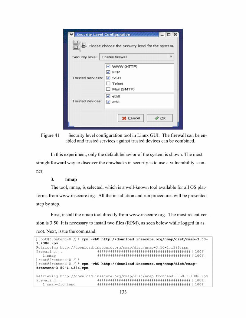
133

Figure 41 Security level configuration tool in Linux GUI. The firewall can be en-

abled and trusted services against trusted devices can be combined.

In this experiment, only the default behavior of the system is shown. The most

straightforward way to discover the drawbacks in security is to use a vulnerability scan-

ner.

3. nmap

The tool, nmap, is selected, which is a well-known tool available for all OS plat-

forms from www.insecure.org. All the installation and run procedures will be presented

step by step.

First, install the nmap tool directly from www.insecure.org. The most recent ver-

sion is 3.50. It is necessary to install two files (RPM), as seen below while logged in as

root. Next, issue the command:

[root@frontend-0 /]# rpm -vhU http://download.insecure.org/nmap/dist/nmap-3.50-1.i386.rpm Retrieving http://download.insecure.org/nmap/dist/nmap-3.50-1.i386.rpm Preparing... ########################################### [100%] 1:nmap ########################################### [100%] [root@frontend-0 /]# [root@frontend-0 /]# rpm -vhU http://download.insecure.org/nmap/dist/nmap-frontend-3.50-1.i386.rpm Retrieving http://download.insecure.org/nmap/dist/nmap-frontend-3.50-1.i386.rpm Preparing... ########################################### [100%] 1:nmap-frontend ########################################### [100%]

134

The following command is issued to ascertain the location of the relevant files in

the directory structure:

[root@frontend-0 /]# find . -name nmap -print ./usr/share/nmap ./usr/bin/nmap

Now, scan the external IP address: –v means Verbose, -sS means TCP SYN

stealth port scan, -sU means UDP port scan. The results follow.

[root@frontend-0 /]# nmap -v -sS -sU 131.120.5.50 Starting nmap 3.50 ( http://www.insecure.org/nmap/ ) at 2004-05-13 11:57 PDT Host cluster.cs.nps.navy.mil (131.120.5.50) appears to be up ... good. Initiating SYN Stealth Scan against cluster.cs.nps.navy.mil (131.120.5.50) at 11:57 … … Interesting ports on cluster.cs.nps.navy.mil (131.120.5.50): (The 3110 ports scanned but not shown below are in state: closed) PORT STATE SERVICE 22/tcp open ssh 25/tcp open smtp 53/tcp open domain 53/udp open domain 67/udp open dhcpserver 69/udp open tftp 80/tcp open http 111/tcp open rpcbind 111/udp open rpcbind 123/udp open ntp 443/tcp open https 514/udp open syslog 535/tcp open iiop 697/udp open unknown 700/tcp open unknown 716/udp open unknown 719/tcp open unknown 818/udp open unknown 2049/tcp open nfs 2049/udp open nfs 3000/tcp open ppp 3306/tcp open mysql 6000/tcp open X11 32768/udp open omad 32771/tcp open sometimes-rpc5 32771/udp open sometimes-rpc6 32773/tcp open sometimes-rpc9 Nmap run completed -- 1 IP address (1 host up) scanned in 11.611 seconds [root@frontend-0 /]# nmap -v -sS -sU 10.1.1.1 Starting nmap 3.50 ( http://www.insecure.org/nmap/ ) at 2004-05-13 11:59 PDT Host frontend-0.local (10.1.1.1) appears to be up ... good. Initiating SYN Stealth Scan against frontend-0.local (10.1.1.1) at 11:59 … … Interesting ports on frontend-0.local (10.1.1.1): (The 3110 ports scanned but not shown below are in state: closed) PORT STATE SERVICE 22/tcp open ssh 25/tcp open smtp … … 32771/tcp open sometimes-rpc5

135

32771/udp open sometimes-rpc6 32773/tcp open sometimes-rpc9 Nmap run completed -- 1 IP address (1 host up) scanned in 11.234 seconds

An explanation will be attempted as to why these ports are open, which will help

clarify how the system works behind the scenes. From the “well known ports list”, [62] it

is possible to discern the following.

Port number service

22/tcp SSH Remote Login Protocol 25/tcp Simple Mail Transfer 53/tcp Domain Name Server 53/udp Domain Name Server 67/udp Bootstrap Protocol Server 69/udp Trivial File Transfer 80/tcp HTTP server - client 111/tcp SUN Remote Procedure Call 111/udp SUN Remote Procedure Call 123/udp Network Time Protocol 443/tcp http protocol over TLS/SSL 514/udp automatic authentication 535/tcp iiop, see below for node 697/udp UUIDGEN generate a Universal Unique Identifier

(UUID) 700/tcp Extensible Provisioning Protocol

716/udp, 719/tcp, 818/udp 713-728 & 811-827 Unassigned 2049/tcp nfs 2049/udp nfs

The following entry records an unassigned but widespread use 3000/tcp RemoteWare Client 3000/tcp ppp 3306/tcp mysql 6000/tcp X Window System

32768/udp omad * 32771/tcp,32771/udp,32773/tcp remote procedure call

Table 24 Ports Open in the System.

Except for the 697-818 range with the unknown indication, the remaining are le-

gitimate ports. This range of TCP and UDP ports is used by the Rocks implementation.

136

For the omad, it was not possible to find anything. The command netstat was

used to resolve this issue, which demonstrates the open ports along with the PID that uses

each port. For the 32768 port, note the presence of a remote procedure call.

[root@frontend-0 root]# netstat --inet -ap Active Internet connections (servers and established) Proto Recv-Q Send-Q Local Address Foreign Address State PID/Program name tcp 0 0 *:32768 *:* LISTEN 1441/rpc.statd … …

The aforementioned method was used to resolve any questions about ports that

are open, and who is using them.

It is now possible to do the scan for the nodes after pinging to reveal the IP’s.

The results show that all of them have TCP ports 22, 80, 111, 199, 443 and 535. No UDP

port is open to the nodes.

The 22 port is used by the ssh, the 80 port by the httpd for the ganglia monitor, the

111 port for rcpbind, the connection for communication between the node and front end,

the 199 port for unknown reasons, the 443 port for secure http, and the 535 port for iiop.

IIOP is the Internet Inter-ORB Protocol, a protocol developed by the industry

consortium known as the Object Management Group (OMG) to implement COBRA solu-

tions over the World Wide Web. IIOP enables browsers and servers to exchange integers,

arrays, and more complex objects, unlike HTTP, which only supports the transmission of

text. COBRA stands for Common Object Request Broker Architecture, an architecture

that enables pieces of programs, called objects, to communicate with one another regard-

less of the programming language in which they were written or on which operating sys-

tem they are running. CORBA was developed by an Object Management Group (OMG).

The results for the sake of space are presented only for one node.

[root@frontend-0 /]# nmap -v -sS -sU 10.255.255.253 Starting nmap 3.50 ( http://www.insecure.org/nmap/ ) at 2004-05-13 12:03 PDT Host compute-0-1.local (10.255.255.253) appears to be up ... good. Initiating SYN Stealth Scan against compute-0-1.local (10.255.255.253) at 12:03 Adding open port 111/tcp Adding open port 443/tcp Adding open port 535/tcp Adding open port 199/tcp Adding open port 22/tcp Adding open port 80/tcp The SYN Stealth Scan took 2 seconds to scan 1659 ports. Initiating UDP Scan against compute-0-1.local (10.255.255.253) at 12:04 Too many drops ... increasing senddelay to 50000 caught SIGINT signal, cleaning up

137

[root@frontend-0 /]# nmap -v -sS -sU 10.255.255.254 Starting nmap 3.50 ( http://www.insecure.org/nmap/ ) at 2004-05-13 12:09 PDT Host compute-0-2.local (10.255.255.254) appears to be up ... good. … … [root@frontend-0 /]# nmap -v -sS -sU 10.255.255.252 Starting nmap 3.50 ( http://www.insecure.org/nmap/ ) at 2004-05-13 12:10 PDT Host compute-0-3.local (10.255.255.252) appears to be up ... good. … …

F. WEB SERVICES

The investigation to ascertain where web services are used in clusters did not pro-

vide many results. Some information about Microsoft clusters using Microsoft products

such as MS SQL server was found, but little was discovered, in particular, about Beowulf

clusters.

The concept is similar for the database server. The application is shared on the

Internet, using a series of active server pages or other similar technology residing on the

front-end. No easy way exists to partition it to take advantage of the computational

power of the nodes.

Another approach was tried to find a site and ascertain its actual use, which is the

application running on the system. The site with the web services application may pro-

vide resources for research. The www.500top.org, unfortunately, does not have specific

uses. There is a general distinction between government or academia or industry but no

details. Another similar site, http://clusters.top500.org/, was found. This is another site

that tries to gather the 500 supercomputers. This site contains a more detailed description

of the 260 computers currently registered. From a query in their database, it is possible to

see that 73 supercomputers do not register their usage. As for the rest, none is used in a

manner in which web services are implemented. Some sample uses are shown in the next

table.

138

Number of computers Application area 12 Academic 1 Artificial Intelligence 4 Astrophysics 10 Bioinformatics 25 Experimental Education 12 Computational Chemistry 10 Meteorological Research 20 Physics 35 Scientific Research

Table 25 Use of Supercomputers.

Only one indicates commercial uses and nothing else.

In order to understand that the system is responding well to a possible web appli-

cation, a small experiment was conducted. A series of XML pages were created where

they were stored in var/www/xmp_test/. These are a project from [4] and concern a “re-

frigerator service office.”

The overall impression, as expected, is that the system responded well and

worked with the application without problems. The results are shown in the following

two figures where two different browsers are used to retrieve the web page. Mozilla fails

to retrieve the results, while Microsoft Internet Explorer has better output.

Figure 42 XML Results from Mozilla browser. The browser fails to translate the re-

sults.

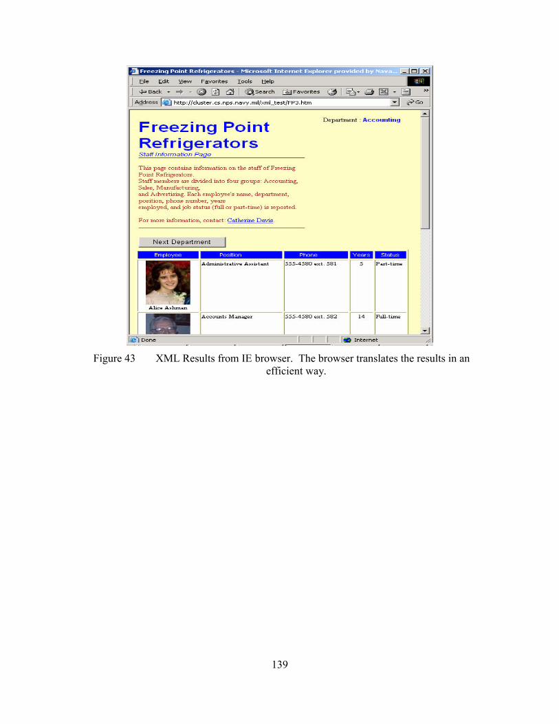
139

Figure 43 XML Results from IE browser. The browser translates the results in an

efficient way.

140


141

VIII. CONCLUSIONS AND FUTURE WORK

A. CONCLUSIONS

Based on the experience gained in setting up this cluster, several conclusions can

be drawn.

The installation of such a system requires significant Linux operating system ex-

pertise. An implementer should also be familiar the accompanying tools and utilities of

the Linux OS. It is difficult for a person not experienced in UNIX to accomplish a com-

pletely correct installation. Solutions for problems are not always instantly available and

time has to be spent searching several resources. The manuals do not cover all possible

problems. Scripting in Linux is difficult for users that are not familiar with it. There are a

lot of information, ideas, and tools to master.

The heterogeneity of our system resulted in a number of problems during the in-

stallation process. It is better to avoid using older or mixed configuration machines to

build a cluster. Using only a limited number of standardized machines—preferably one

type only—simplifies the installation.

When debugging a problem start from the simplest possible cause. For example,

when you do not have connectivity between two nodes instead of using ethereal to check

if the packages depart or arrive, check to see if the cable is securely plugged in.

In the beginning the thesis aspired to cover too many interesting topics. Limit the

scope of the objectives to be achieved in new installations. It will take longer than you

expect to accomplish what you want.

At least some background in programming is necessary to finish the project with

satisfactory results.

142

B. RECOMMENDATIONS FOR FUTURE WORK

1. IPv6 and the Grid

This was one of the goals of our project but due to problems scheduling the instal-

lation of fiber optic cable it was not accomplished. The intent was to connect two NPS

clusters within the campus network. The task could be decomposed into several steps.

First is to establish a connection with native IPv6 traffic across the campus. Second is to

install the dual protocol (IPv4/IPv6) stack on the cluster’s front end. Third is to investi-

gate the grid software and to choose an appropriate tool distribution kit. This last one is a

quite challenging task, because the grid by itself is a cutting-edge technology that re-

quires up to date information and knowledge. While the Rocks cluster software includes

the Globus Grid Toolkit, at least two connected clusters are needed to investigate the

concept.

2. Acquisition of a New Rack Based System

Many vendors are able to provide turn-key cluster systems. During the project an

effort has been made to collect data about a possible system, and have had some contact

with a contractor that installed another cluster on campus. Any new system to implement

a cluster needs to be a rack-based system rather than a blade server.

Rack-mounted units can be redeployed for other uses if the need arises. It is

common for compute clusters to be refreshed with more modern CPUs every few years to

maintain the cluster’s lead over other computing alternatives. When this happens the old

units can be redeployed as web servers, firewalls, routers, fileservers, and other less de-

manding tasks. Or the rack-mounted units can be split into two clusters or moved be-

tween clusters. This flexibility is more difficult to achieve with blade servers.

The students that will deal with this will find it easier to have a well known hard-

ware platform rather than a blade server, which tends to be vendor-specific. (Though re-

cently IBM and Intel recently announced an attempt to standardize blade server inter-

faces.) While in some situations the density of blade servers is an advantage, in a fast-

changing academic environment the disadvantages tend to outweigh the advantages.

143

4. Simkit

Simkit is a Java toolkit for general purpose discrete event simulation. Simkit is

fairly widespread in the academic environment and has been used in some military simu-

lations, such as Combat XXI. During this thesis some small, example Simkit programs

were run on the cluster.

More on this direction could be achieved. Discrete event simulation (DES) can be

an “embarrassingly parallel” application that is well suited for clusters. Most DES ex-

periments involve repeated runs with only parameter changes for random number genera-

tors, slight changes to parameter inputs, and so on. Each of these experimental runs can

be performed on a different compute node of the cluster.

This is a significant application area for the MOVES Institute and for military

simulations. It has the potential to be a very significant new capability in the military

modeling and simulation application domain, and to open new horizons in modeling and

simulation experiments. This project can be done to the current experimental Rocks clus-

ter, or to the possible next acquired cluster.

5. MPI Programming

MPI is a message-passing API for parallel programming. MPI programming re-

quires the programmer to have knowledge of the MPI classes and APIs, and to be aware

of parallel programming concepts. Typically the programming can be done in Fortran, C

or C++. MPI programming requires a significant investment in time to do achieve the

level of competence needed to write significant applications.

6. Web Services Investigation

The web services on clusters are an emerging technology, and the best approach is

probably to experiment with small applications. These could be the use of a “web en-

abled database”. The creation of such a project is possible with a number of ways. The

use of XHTML for the web pages along to access to a PHP-enabled Web server such as

the Apache. Apache is of course the web server running in our cluster. The Mysql could

be enough for database environment. The use of XML is also possible.

But the main purpose is to investigate how the http requests from the clients to the

front-end web server can be distributed to the nodes. So this system could take much

144

more simultaneous http requests and can process them in a more efficient way. Now in

the case that there is a database, this must reside in more than one node. This design is up

to the application and how the load must be distributed.

The web services concept is much more than the above. The possible implemen-

tation depends on a variety of areas of interest.

7. Database Use Investigation

As with web services this is an area that there is not a lot of information. What is

needed is the creation of knowledge with the use of small step by step experiments. This

project could be a part of the web services investigation for utilizing all the nodes of the

cluster to serve a database.

8. OSCAR Installation

Another easy task would be the installation of OSCAR, one of the other open

source software package for implementing a cluster. This could be done in parallel with

the installation of Rocks in a possible new system. OSCAR needs exactly the same

background as Rocks thus the cluster administrator must be proficient in Linux, and must

have a lot of patience.

9. Xj3D Offline Rendering and Physics Interactions

Xj3D is a project of the Web3D Consortium [66] focused on creating a toolkit for

VRML97 and X3D content written completely in Java. VRML stands for Virtual Reality

Modeling Language. Rendering is the result of interpretation of some code, e.g. VRML.

In computer graphics, rendering is the process of producing an image from more abstract

image information, such as 3D computer graphics information (typically consisting of

geometry, viewpoint, texture and lighting information). In order to move in this direction

to the cluster environment the parallel rendering scheme on distributed memory multi-

processors needs to be established. There is a number of sites that started investigating

this concept [67].

145

APPENDIX A. DESCRIPTION OF THE HPL.DAT FILE

The HPL.dat is the file used as an input file for the HPL benchmark. A sample

HPL.dat file with a definition for each line follows. It is the same file from page 78 used

in one of the experiments. HPLinpack benchmark input file MOVES institute, HPC team HPL.out output file name (if any) file device out (6=stdout,7=stderr,file) 4 # of problems sizes (N) 1500 3000 6000 10000 Ns 2 # of NBs 50 60 NBs 1 # of process grids (P x Q) 1 Ps 1 Qs 16.0 threshold 3 # of panel fact 0 1 2 PFACTs (0=left, 1=Crout, 2=Right) 1 # of recursive stopping criterium 8 NBMINs (>= 1) 1 # of panels in recursion 2 NDIVs 1 # of recursive panel fact. 2 RFACTs (0=left, 1=Crout, 2=Right) 1 # of broadcast 1 BCASTs (0=1rg,1=1rM,2=2rg,3=2rM,4=Lng,5=LnM) 1 # of lookahead depth 1 DEPTHs (>=0) 2 SWAP (0=bin-exch,1=long,2=mix) 80 swapping threshold 0 L1 in (0=transposed,1=no-transposed) form 0 U in (0=transposed,1=no-transposed) form 1 Equilibration (0=no,1=yes) 8 memory alignment in double (> 0)

Line 1: (unused) Typically one may use this line for its own good. For example, it may be used to summarize the content of the input file. By default this line reads:

HPL Linpack benchmark input file

Line 2: (unused) same as line 1. By default this line reads:

MOVES institute, HPC team

Line 3: the user can choose where the output might be redirected to. In the case of a file, a name is necessary, and this is the line where one wants to specify it. Only the first name on this line is significant. By default, the line reads:

146

HPL.out output file name (if any)

This means that if one chooses to redirect the output to a file, the file will be called “HPL.out.” The rest of the line is unused, and this space to put some informative comment on the meaning of this line.

Line 4: This line specifies where the output might go. The line is formatted, it must begin with a positive integer, the rest is unsignificant. 3 choices are possible for the positive integer, 6 means that the output will go the standard output, 7 means that the output will go to the standard error. Any other integer means that the output might be re-directed to a file, which name has been specified in the line above. This line by default reads:

6 device out (6=stdout,7=stderr,file)

which means that the output generated by the executable might be redirected to the standard output.

Line 5: This line specifies the number of problem sizes to be executed. This number must be less than or equal to 20. The first integer is significant, the rest is ig-nored. If the line reads:

3 # of problems sizes (N)

this means that the user is willing to run 3 problem sizes that will be specified in the next line.

Line 6: This line specifies the problem sizes one wants to run. Assuming the line above started with 3, the 3 first positive integers are significant, the rest is ignored. For example:

3000 6000 10000 Ns

means that one wants xhpl to run 3 (specified in line 5) problem sizes, namely 3000, 6000 and 10000.

Line 7: This line specifies the number of block sizes to be run. This number must be less than or equal to 20. The first integer is significant, the rest is ignored. If the line reads:

5 # of NBs

this means that the user is willing to use 5 block sizes that will be specified in the next line.

147

Line 8: This line specifies the block sizes one wants to run. Assuming the line above started with 5, the 5 first positive integers are significant, the rest is ignored. For example:

80 100 120 140 160 NBs

means that one wants xhpl to use 5 (specified in line 7) block sizes, namely 80, 100, 120, 140 and 160.

Line 9: This line specifies how the MPI processes may be mapped onto the nodes of your platform. There are currently two possible mappings, namely row- and column-major. This feature is mainly useful when these nodes are themselves multi-processor computers. A row-major mapping is recommended.

Line 10: This line specifies the number of process grid to be runned. This number must be less than or equal to 20. The first integer is significant, the rest is ignored. If the line reads:

2 # of process grids (P x Q)

this means that you are willing to try 2 process grid sizes that will be specified in the next line.

Line 11-12: These two lines specify the number of process rows and columns of each grid you want to run on. Assuming the line above (10) started with 2, the 2 first positive integers of those two lines are significant, the rest is ignored. For example:

1 2 Ps

6 8 Qs

means that one wants to run xhpl on 2 process grids (line 10), namely 1-by-6 and 2-by-8. Note: In this example, it is required then to start xhpl on at least 16 nodes (max of Pi-by-Qi). The runs on the two grids will be consecutive. If one was starting xhpl on more than 16 nodes, say 52, only 6 would be used for the first grid (1x6) and then 16 (2x8) would be used for the second grid. The fact that you started the MPI job on 52 nodes, will not make HPL use all of them. In this example, only 16 would be used. If one wants to run xhpl with 52 processes one needs to specify a grid of 52 processes, for ex-ample the following lines would do the job:

4 2 Ps

13 8 Qs

Line 13: This line specifies the threshold to which the residuals should be com-pared with. The residuals should be or order 1, but are in practice slightly less than this,

148

typically 0.001. This line is made of a real number, the rest is not significant. For exam-ple:

16.0 threshold

In practice, a value of 16.0 will cover most cases. For various reasons, it is possi-ble that some of the residuals become slightly larger, say for example 35.6. xhpl will flag those runs as failed, however they can be considered as correct. A run should be consid-ered as failed if the residual is a few order of magnitude bigger than 1 for example 10^6 or more. Note: if one was to specify a threshold of 0.0, all tests would be flagged as failed, even though the answer is likely to be correct. It is allowed to specify a negative value for this threshold, in which case the checks will be by-passed, no matter what the threshold value is, as soon as it is negative. This feature allows to save time when per-forming a lot of experiments, say for instance during the tuning phase. Example:

-16.0 threshold

The remaining lines allow to specifies algorithmic features. xhpl will run all pos-sible combinations of those for each problem size, block size, process grid combination. This is handy when one looks for an “optimal” set of parameters. To understand a little bit better, let say first a few words about the algorithm implemented in HPL. Basically this is a right-looking version with row-partial pivoting. The panel factorization is matrix-matrix operation based and recursive, dividing the panel into NDIV sub panels at each step. This part of the panel factorization is denoted below by “recursive panel fact. (RFACT).” The recursion stops when the current panel is made of less than or equal to NBMIN columns. At that point, xhpl uses a matrix-vector operation based factorization denoted below by “PFACTs.” Classic recursion would then use NDIV=2, NBMIN=1. There are essentially 3 numerically equivalent LU factorization algorithm variants (left-looking, Crout and right-looking). In HPL, one can choose every one of those for the RFACT, as well as the PFACT. The following lines of HPL.dat allows you to set those parameters.

Lines 14-21: (Example 1)

3 # of panel fact

0 1 2 PFACTs (0=left, 1=Crout, 2=Right)

4 # of recursive stopping criterium

1 2 4 8 NBMINs (>= 1)

3 # of panels in recursion

2 3 4 NDIVs

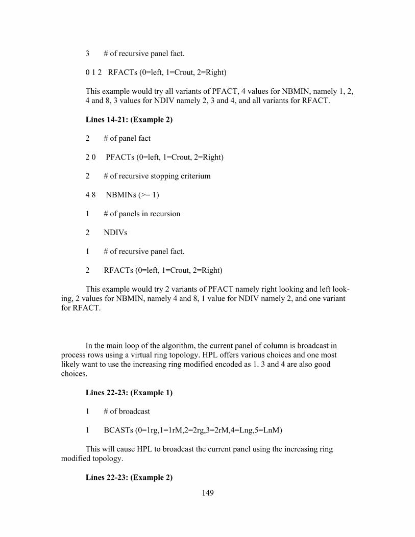
149

3 # of recursive panel fact.

0 1 2 RFACTs (0=left, 1=Crout, 2=Right)

This example would try all variants of PFACT, 4 values for NBMIN, namely 1, 2, 4 and 8, 3 values for NDIV namely 2, 3 and 4, and all variants for RFACT.


2 # of panel fact

2 0 PFACTs (0=left, 1=Crout, 2=Right)

2 # of recursive stopping criterium

4 8 NBMINs (>= 1)

1 # of panels in recursion

2 NDIVs

1 # of recursive panel fact.

2 RFACTs (0=left, 1=Crout, 2=Right)

This example would try 2 variants of PFACT namely right looking and left look-ing, 2 values for NBMIN, namely 4 and 8, 1 value for NDIV namely 2, and one variant for RFACT.

In the main loop of the algorithm, the current panel of column is broadcast in process rows using a virtual ring topology. HPL offers various choices and one most likely want to use the increasing ring modified encoded as 1. 3 and 4 are also good choices.


1 # of broadcast

1 BCASTs (0=1rg,1=1rM,2=2rg,3=2rM,4=Lng,5=LnM)

This will cause HPL to broadcast the current panel using the increasing ring modified topology.


150

2 # of broadcast

0 4 BCASTs (0=1rg,1=1rM,2=2rg,3=2rM,4=Lng,5=LnM)

This will cause HPL to broadcast the current panel using the increasing ring vir-tual topology and the long message algorithm.

Lines 24-25 allow to specify the look-ahead depth used by HPL. A depth of 0 means that the next panel is factorized after the update by the current panel is completely finished. A depth of 1 means that the next panel is immediately factorized after being up-dated. The update by the current panel is then finished. A depth of k means that the k next panels are factorized immediately after being updated. The update by the current panel is then finished. It turns out that a depth of 1 seems to give the best results, but may need a large problem size before one can see the performance gain. So use 1, if you do not know better, otherwise you may want to try 0. Look-ahead of depths 3 and larger will probably not give you better results.

Lines 24-25: (Example 1):

1 # of lookahead depth

1 DEPTHs (>=0)

This will cause HPL to use a look-ahead of depth 1.


2 # of lookahead depth

0 1 DEPTHs (>=0)

This will cause HPL to use a look-ahead of depths 0 and 1.

Lines 26-27 allow specifying the swapping algorithm used by HPL for all tests. There are currently two swapping algorithms available, one based on “binary exchange” and the other one based on a “spread-roll” procedure (also called “long” below). For large problem sizes, this last one is likely to be more efficient. The user can also choose to mix both variants, that is “binary-exchange” for a number of columns less than a threshold value, and then the “spread-roll” algorithm. This threshold value is then speci-fied on Line 27.


1 SWAP (0=bin-exch,1=long,2=mix)

60 swapping threshold

151

This will cause HPL to use the “long” or “spread-roll” swapping algorithm. Note that a threshold is specified in that example but not used by HPL.


2 SWAP (0=bin-exch,1=long,2=mix)

60 swapping threshold

This will cause HPL to use the “long” or “spread-roll” swapping algorithm as soon as there is more than 60 columns in the row panel. Otherwise, the “binary-exchange” algorithm will be used instead.

Line 28 allows to specify whether the upper triangle of the panel of columns should be stored in no-transposed or transposed form. Example:

0 L1 in (0=transposed,1=no-transposed) form

Line 29 allows to specify whether the panel of rows U should be stored in no-transposed or transposed form. Example:

0 U in (0=transposed,1=no-transposed) form

Line 30 enables / disables the equilibration phase. This option will not be used unless you selected 1 or 2 in Line 26. Example:

1 Equilibration (0=no,1=yes)

Line 31 allows to specify the alignment in memory for the memory space allo-cated by HPL. On modern machines, one probably wants to use 4, 8 or 16. This may re-sult in a tiny amount of memory wasted. Example:

8 memory alignment in double (> 0)

152


153

APPENDIX B. DETAILED RESULTS OF HIGH PERFORMANCE LINPACK (HPL)

The following table displays the results of the benchmark runs made to the

MOVES cluster. For every run, an average is computed, and for every series of runs with

the same parameters, a general average is computed as well.

The N is the problem size, the NB is the block size, and the P and Q are the proc-

ess grids.

These results are presented graphically on page 87.

N NB P Q RESULTS Average Average of all tests 100 64 1 1 0.4760

0.5876 0.6359 0.5938 0.5995 0.6353 0.5880

100 64 1 1 0.4807 0.5772 0.6419 0.5917 0.6027 0.6443 0.5898 0.5889

500 64 1 1 1.2780 1.2830 1.2910 1.2960 1.2870 1.2950 1.2883 1.2883

1000 64 1 1 1.3750 1.4940 1.4940 1.4543

1000 64 1 1 1.3850 1.4640 1.4680 1.4390

1000 64 1 1 1.5370

154

N NB P Q RESULTS Average Average of all tests 1.5360 1.5280 1.5337 1.4757

1500 64 1 1 1.5680 1.5550 1.5650 1.5730 1.5720 1.5720 1.5675 1.5675

3000 64 1 1 1.7420 1.7420 1.7340 1.7960 1.7535 1.7535

5000 64 1 1 1.7260 1.7540 1.7470 1.7520 1.7600 1.7490 1.7480

5000 64 1 1 1.7520 1.7560 1.7670 1.7740 1.7660 1.7710 1.7643 1.7562

6000 64 1 1 1.7870 1.7910 1.7940 1.7907 1.7907

10000 64 1 1 1.8020 1.8070 1.7990 1.8027

10000 64 1 1 1.8140 1.8110 1.8090 1.7960 1.7950 1.8050

155

N NB P Q RESULTS Average Average of all tests 10000 64 1 1 1.8250

1.8060 1.8020 1.8020 1.8020 1.8020 1.8065 1.8047

50 50 1 1 0.1580 0.2884 0.3337 0.2600 0.1604 0.2773 0.3190 0.2522 0.2561

100 50 1 1 0.0470 0.6147 0.6810 0.4476 0.5578 0.5928 0.6371 0.5959 0.5217

150 50 1 1 0.8703 0.8667 0.9212 0.8861 0.8861

200 50 1 1 1.0240 1.0140 1.0570 1.0317 1.0317

1000 50 1 1 1.5310 1.5330 1.5290 1.5310 1.5310

1500 50 1 1 1.5310 1.5290 1.5280 1.5293 1.5293

3000 50 1 1 1.6330

156


6000 50 1 1 1.7140 1.7050 1.7090 1.7093 1.7093

10000 50 1 1 1.7540 1.7570 1.7480 1.7530 1.7530

50 60 1 1 0.3088 0.2982 0.3415 0.3162 0.2962 0.2912 0.3262 0.3045 0.3104

100 60 1 1 0.6054 0.6022 0.6027 0.6034 0.5676 0.5671 0.5953 0.5767 0.5901

150 60 1 1 0.8512 0.8461 0.8862 0.8612 0.8612

200 60 1 1 0.9914 0.9912 1.0190 1.0005 1.0005

1500 60 1 1 1.3070 1.3370 1.0670 1.2370 1.2370

3000 60 1 1 1.5200 1.6750 1.6400 1.6117 1.6117

6000 60 1 1 1.7580

157


10000 60 1 1 1.8040 1.8000 1.7990 1.8010 1.8010

6000 70 1 1 1.556 1.722 1.711 1.663 1.6630

10000 70 1 1 1.823 1.823 1.803 1.81633 1.8163

1000 80 1 1 1.974 1.976 1.949 1.96633 1.9663

2000 80 1 1 2.215 2.243 2.241 2.233

2000 80 1 1 2.318 2.314 2.279 2.30367

2000 80 1 1 2.32 2.324 2.312 2.31867 2.2851

3000 80 1 1 2.472 2.477 2.47 2.473 2.4730

4000 80 1 1 2.544 2.551 2.53 2.54167 2.5417

6000 80 1 1 2.164 2.533 2.521 2.406 2.4060

158

N NB P Q RESULTS Average Average of all tests

10000 80 1 1 2.706 2.693 2.696 2.69833 2.6983

10000 85 1 1 2.685 2.623 2.605 2.63767 2.6377

10000 90 1 1 2.623 2.621 2.616 2.62 2.6200

10000 100 1 1 2.548 2.545 2.514 2.53567 2.5357

15000 80 1 1 was never completed

20000 80 1 1 was never completed

50 50 1 2 0.0317 0.0349 0.0367 0.0344 0.0344

50 60 1 2 0.0410 0.0407 0.0417 0.0411 0.0411

159

LIST OF REFERENCES

Books

[1]. Brewer E., Clustering: Multiply and Conquer, Data Communications, July 1997.

[2]. Buyya R., High-performance Cluster Computing, Volume 1: Architectures and Systems, Prentice-Hall, 1999.

[3]. Buyya R. ed., High-performance Cluster Computing, Volume 2: Programming and Applications, Prentice-Hall, 1999.

[4]. Carey P., New Perspectives on XML, Thomson, 2004.

[5]. Flynn M., Computer Organizations and their Effectiveness, IEEE Transactions on Computers, September 1972.

[6]. Gropp W., Ewing L. and Sterling T., Beowulf Cluster Computing with Linux, 2nd Edition, The MIT Press, 2003.

[7]. Hwang, K. et al., Designing SSI Clusters with Hierarchical Check Pointing and Single I/O Space, IEEE Concurrency, January-March 1999.

[8]. Kapp C., Managing Cluster Computers: Dr. Dobb’s Journal, July 2000.

[9]. Kurose, J and Ross, K, Computer Networks: A Top-down Approach Featuring the Internet, Addison-Wesley, 2002.

[10]. Stallings W, Operating Systems, Prentice-Hall, 2001.

[11]. Vrenios A, Linux Cluster Architecture, SAMS, 1st Edition (July 15, 2002).

160

Articles and Papers

[12]. Becker D. J., Sterling T. L., Savarese D. F., Dorband J. E., Ranawak U. A. and Packer C. V., “Beowulf: A Parallel Workstation for Scientific Computation,” Pro-ceedings of the International Conference on Parallel Processing, 1995.

[13]. Becker D. J., Sterling T. L., Savarese D. F., Fryxell B., and Olsen K., “Communi-cation Overhead for Space Science Applications on the Beowulf Parallel Work-station,” Proceedings of the IEEE International Symposium on High Performance Distributed Computing, 1995.

161

Web Sites

[14]. “Radajewski J, Eadline D., Beowulf How To, http://www.ibiblio.org/pub/Linux/ docs/ HOWTO/other-formats/html_single/Beowulf-HOWTO.html, accessed 7/1/2004.

[15]. “Rocks Cluster Distribution,” http://www.rocksclusters.org/Rocks/, accessed 7/27/2004.

[16]. “OSCAR,” http://oscar.openclustergroup.org/tiki-index.php, accessed 7/27/2004.

[17]. “Sun Grid Engine,” http://gridengine.sunsource.net/, accessed 7/28/2004.

[18]. “MPICH,” http://www-unix.mcs.anl.gov/mpi/mpich/, accessed 7/28/2004.

[19]. “Globus Alliance,” http://www.globus.org/, accessed 7/28/2004.

[20]. “Tripwire,” http://www.tripwire.org/qanda/index.php#1, accessed 7/28/2004.

[21]. “Scalable Computing Environnent,” http://mail.nllgg.nl/cola/2001-06/95.html, ac-cessed 7/28/2004.

[22]. “Portable Batch System”,http://www.openpbs.org/, accessed 7/28/2004.

[23]. “Condor”, http://www.cs.wisc.edu/condor/description.html/, accessed 7/28/2004

[24]. Forrest Hoffman, “It’s all about Speed,” www.Extremelinux.com,/, accessed 7/30/2004 .

[25]. “The cluster world benchmark project”, http://www.clusterworld.com/ CWCE2004/ Douglas_Eadline_presentation.pdf, accessed 7/31/2004.

[26]. “SCL Cluster Cookbook,” http://www.scl.ameslab.gov /Projects /ClusterCookbook /, accessed 7/31/2004.

[27]. “The hpl Algorithm,” http://www.netlib.org/benchmark/hpl/algorithm.html, ac-cessed 7/31/2004.

[28]. “High-Performance Linpack (HPL) Benchmark for Distributed-Memory Com-puters,” http://www.netlib.org/benchmark/hpl, accessed 7/30/2004

[29]. “The HPL.dat File,” http://www.netlib.org/benchmark/hpl/tuning.html#tips, ac-cessed 7/30/2004.

[30]. “The Cluster World Benchmark Project,” http://www.clusterworld.com/ CWCE2004/ Douglas_Eadline_presentation.pdf, accessed 7/31/2004.

[31]. “The JAVA Linpack,” http://www.netlib.org/ benchmark/linpackjava/, accessed 7/31/2004.

162

[32]. “Guidelines for HPL,” http://www.netlib.org/benchmark/hpl/faqs.html accessed 7/31/2004.

[33]. “Beowulf Performance Suite (BPS),” http://www.hpc-design.com/down-rep.html, accessed 7/31/2004.

[34]. “The Scyld Beowulf Cluster Operating System,”, http://www.scyld.com/, ac-cessed 7/28/2004.

[35]. The top 500 supercomputers,” http://www.top500.org, accessed 8/15/2004.

[36]. “Beowulf HOWTO,” http://www.linuxdoc.org/HOWTO/Beowulf-HOWTO.html, accessed 6/2/2004.

[37]. “The Beowulf Project at CACR,” http://www.cacr.caltech.edu/research/beowulf/, accessed 6/28/2004.

[38]. “The Beowulf Project at CESDIS,” http://beowulf.gsfc.nasa.gov/beowulf.html, accessed 6/27/2004.

[39]. “Grid Today,” http://www.gridtoday.com/02/1021/100562.html, accessed 8/15/2004.

[40]. “The Grendel Project,” http://www.cacr.caltech.edu /projects/ beowulf/ Grendel-Web/, accessed 8/15/2004.

[41]. “The Scyld Beowulf Cluster System,” by Becker D. http://osdn.jp/ event/ ker-nel2002/ pdf/C04.pdf, accessed 8/15/2004.

[42]. “IEEE Task Force on Cluster Computing,” http://www.dgs.monash.edu.au/ ~rajkumar/ tfcc/index.html, accessed 6/24/2004.

[43]. “Internet Parallel Computing Archive,” http://www.hensa.ac.uk/parallel/ accessed 8/15/2004.

[44]. “The mpi Manual,” http://www-unix.mcs.anl.gov/mpi/mpich/docs/mpichman-chp4.pdf, accessed 8/9/2004.

[45]. “Message Passing Interface (MPI) Forum Home Page,” http://www.mpi-forum.org/, accessed 8/10/2004.

[46]. “MPI -- The Message Passing Interface Standard,” http://www-unix.mcs.anl.gov/mpi/, accessed 8/10/2004.

[47]. “Scientific Applications on Linux,” http://SAL.KachinaTech.COM/, accessed 8/10/2004.

[48]. “SCL Cluster Cookbook,” http://www.scl.ameslab.gov/ Projects/ Cluster Cook-book/, accessed 8/11/2004.

163

[49]. “The Microsoft Corporation Research,” http://research.microsoft.com/ users/ GBell/ Supers/ Supercomputing-A_Brief_History_1965_2002.htm, accessed 8/12/2004.

[50]. “The Infiniband Project,” http://www.infinibandta.org/ibta/, accessed 8/10/2004.

[51]. “Myrinet Definitions,” http://encyclopedia.thefreedictionary.com/Myrinet, ac-cessed 7/25/2004.

[52]. “Contingency Planning,” www.contingencyplanning.com, accessed 7/25/2004.

[53]. “American Power Convention,, www.apcc.com, accessed 7/12/2004.

[54]. “HVAC Resources,” http://www.periphman.com/computer-room-air-conditioners/ room-size-calculator.shtml, accessed 7/14/2004.

[55]. “Microsoft Clusters,” http://www.microsoft.com/ windowsserver2003 /technologies/ clustering/default.mspx, accessed 8/2/2004.

[56]. “Sun Clusters,” http://wwws.sun.com/software/cluster/, accessed 8/2/2004.

[57]. “Beowulf Papers,” http://beowulf.es.embnet.org/papers/papers.html, accessed 8/15/2004.

[58]. “Linux IPv6 HOWTO,” http://www.tldp.org/HOWTO/Linux+IPv6-HOWTO/, accessed 8/12/2004.

[59]. “Linux Clusters,” http://www.linux.ericsson.ca/visibility/ieeecluster2002.pdf, ac-cessed 8/12/2004

[60]. Russom P., http:// www.intelligententerprise.com /online_only /analyst /011212.jhtml, accessed 8/12/2004.

[61]. “Oracle10g Real Application Clusters,” http://www.emc.com/partnersalliances/ partner_pages/ oracle3_rac.jsp, accessed 8/12/2004.

[62]. “Well Known Ports,” http://www.iana.org/assignments/port-numbers, accessed 8/12/2004.

[63]. “Suns Interoperable Systems,” http://www.emc.com/ horizontal/ interoperability/ index.jsp, accessed 8/12/2004.

[64]. “The SSI Resource,” http://openssi.org/, accessed 8/1/2004.

[65]. “TYAN Corporation,” http://www.tyan.com/products/html/gx28b2882_spec.html, accessed 8/1/2004.

[66]. “Web3D Consortium,” http://www.web3d.org/, accessed 9/8/2004.

164

[67]. “Consortium of Naval Libraries,” http://portal.acm.org/portal.cfm, accessed 9/8/2004.

[68]. “The AMD Opteron Processor Power and thermal data sheet”, http://www.amd.com/us-en/ assets/ content_type/ white_papers_and_tech_docs/ 30417.pdf, accesed 9/15/2004.

[69]. “The Intel Itanium quick reference guide”, http://www.intel.com/ business/ bss/ products/ server/itanium2/dp_qrg.pdf, accessed 9/15/2004.

[70]. “The MOVES Open House”, Slide set about High-performance Computing, http://www.movesinstitute.org/OpenHouse2004.html, accessed 9/15/2004.

165

INITIAL DISTRIBUTION LIST

1. Defense Technical Information Center Ft. Belvoir, Virginia

2. Dudley Knox Library

Naval Postgraduate School Monterey, California

3. Don Brutzman

MOVES Institute Naval Postgraduate School Monterey, California

4. Don McGregor

MOVES Institute Naval Postgraduate School Monterey, California

5. Dr. Sue Numrich Defense Modeling and Simulation Office

Alexandria, Virginia 6. Mr. Richard Lee

The Pentagon Washington, DC 7. Mrs. Sue Payton

The Pentagon Washington, DC

8. Dr. Mark Pullen

GMU Arlington, Virginia

9. Dr. Andreas Tolk

VMASC Norfolk, Virginia

10. Research and Informatics Department (DEPLH). Hellenic Army General Staff Athens, Greece

166

11. DI.K.A.T.S.A. Inter-University Center for the Recognition of Foreign Academic Titles Athens, Greece

12. Christos Daillidis 401 General Military Hospital/Compute and Research Office Athens, Greece

Establishing Linux Clusters for high-performance computing ...

Documents

Transcript of Establishing Linux Clusters for high-performance computing ...