ERA - University of Alberta

University of Alberta

Numerical Modeling of Cuttings Transport with Foam in Vertical and HorizontalWells

by

Yibing Li

A thesissubmitted to the Faculty of Graduate Studies and Research

in partial fulfillment of the requirements for the degree of

Doctor of Philosophy

in

Petroleum Engineering

Department of Civil and Environmental Engineering

Edmonton, Alberta

Fall 2004

Reproduced with permission of the copyright owner. Further reproduction prohibited without permission.

1*1 Library and Archives Canada

Published Heritage Branch

Bibliotheque et Archives Canada

Direction du Patrimoine de I'edition

395 Wellington Street Ottawa ON K1A 0N4 Canada

395, rue Wellington Ottawa ON K1A 0N4 Canada

Your file Votre reference ISBN: 0-612-95967-8 Our file Notre reference ISBN: 0-612-95967-8

The author has granted a nonexclusive license allowing the Library and Archives Canada to reproduce, loan, distribute or sell copies of this thesis in microform, paper or electronic formats.

The author retains ownership of the copyright in this thesis. Neither the thesis nor substantial extracts from it may be printed or otherwise reproduced without the author's permission.

L'auteur a accorde une licence non exclusive permettant a la Bibliotheque et Archives Canada de reproduire, preter, distribuer ou vendre des copies de cette these sous la forme de microfiche/film, de reproduction sur papier ou sur format electronique.

L'auteur conserve la propriete du droit d'auteur qui protege cette these. Ni la these ni des extraits substantiels de celle-ci ne doivent etre imprimes ou aturement reproduits sans son autorisation.

In compliance with the Canadian Privacy Act some supporting forms may have been removed from this thesis.

While these forms may be included in the document page count, their removal does not represent any loss of content from the thesis.

Conformement a la loi canadienne sur la protection de la vie privee, quelques formulaires secondaires ont ete enleves de cette these.

Bien que ces formulaires aient inclus dans la pagination, il n'y aura aucun contenu manquant.

CanadaReproduced with permission of the copyright owner. Further reproduction prohibited without permission.

Dedication

To

m y w ife W ensheng Zhang

and

m y parents


ACKNOWLEDGEMENT

I wish to express my sincere gratitude to Dr. Ergun Kuru, for his support and supervision

throughout my Ph.D. thesis research.

I would like to express my sincere appreciation to Dr. Quang Doan, for his effort in

initiating my Ph.D. research project.

Special thanks are expressed to the following senior scholars, Dr. Ramon G. Bentsen,

Dr. Marcel Polikar, Dr. Peter Toma and Dr. S.M. Farouq Ali for their help in the course of

my Ph.D. study.

Sincere gratitude is extended to the Natural Sciences and Engineering Research

Council (NSERC) of Canada for the financial support to this research work.


TABLE OF CONTENTS

1 Introduction.............................................................................................................. 11.1 Overview................................................................................................................. 1

1.2 Statement of Problem............................................................................................ 7

1.3 Objectives of Research......................................................................................... 10

1.4 Scope of Research................................................................................................10

1.5 Methodology of Research..................................................................................... 12

1.6 Expected Contributions of the Current Research..................................................12

1.7 Structure of the Dissertation..................................................................................14

2 Literature Review....................................................................................................162.1 Cuttings Transport with Conventional Drilling Fluids............................................. 16

2.1.1 Cuttings Transport in Vertical Wells............................................................... 16

2.1.1.1 Mechanism of Cuttings Transport in Vertical Wells.................................16

2.1.1.2 Experimental Studies.............................................................................. 20

2.1.2 Cuttings Transport in Horizontal Wells...........................................................22

2.1.2.1 Mechanism of Cuttings Transport in Horizontal Wells............................ 22

2.1.2.2 Experimental Studies.............................................................................. 27

2.1.2.3 Mechanistic and Empirical modeling....................................................... 28

2.2 Underbalanced Drilling (UBD)...............................................................................33

2.2.1 Air/Gas Drilling...............................................................................................33

2.2.2 Gasified Liquid Drilling....................................................................................34

2.3 Cuttings Transport with Foam...............................................................................37

2.3.1 Foam Equation of State..................................................................................37

2.3.1.1 Foam Fluid.............................................................................................. 37

2.3.1.2 Foam Quality.......................................................................................... 37

2.3.1.3 Foam Density..........................................................................................38

2.3.2 Foam Rheology..............................................................................................38

2.3.3 Foam Flow in Pipe and Annulus.....................................................................44

2.3.4 Cuttings Transport with Foam........................................................................ 47

2.3.4.1 Solids Transport with Foam in Vertical Wells........................................47

2.3.4.2 Solids Transport with Foam in Horizontal Wells.................................... 49


2.3.5 Formation Influx Model...................................................................................50

2.4 Summary...............................................................................................................51

3 Numerical Modeling of Cuttings Transport With Foam in Vertical Wells............. 543.1 Model Development.............................................................................................. 54

3.1.1 Continuity and Momentum Equations............................................................ 54

3.1.2 Other Closure Equations................................................................................ 56

3.1.3 Boundary Conditions...................................................................................... 58

3.1.4 Initial Conditions............................................................................................ 58

3.2 Solution.................................................................................................................58

3.2.1 Computational Geometries.............................................................................58

3.2.2 Foam-Cuttings Flow in Drilling Annulus..........................................................59

3.2.3 Foam Flow Across Bit Nozzle.........................................................................60

3.2.4 Foam Flow in Drilling Pipe............................................................................. 60

3.3 Verification of Model Predictions........................................................................... 60

3.3.1 Foam Flow..................................................................................................... 60

3.3.2 Foam Flow with Cuttings................................................................................61

3.4 Sensitivity Analysis - Practical Implications of the New Model............................. 65

3.4.1 Effects of Gas and Liquid Injection Rates on Bottom Hole Pressures........... 65

3.4.2 Effect of Drilling Rate on Bottom Hole Pressures.......................................... 65

3.4.3 Effect of Water Influx on Bottom Hole Pressures........................................... 66

3.4.4 Effect of Gas Influx on Bottom Hole Pressures..............................................67

3.4.5 Transient Bottom Hole Pressures and Cuttings Concentration......................67

3.4.6 Effects of Cuttings Size and Shape on Bottom Hole Pressures..................... 70

4 Numerical Modeling of Cuttings Transport With Foam in Horizontal Wells........ 714.1 Model Development.............................................................................................. 71

4.1.1 Conservation of Mass and Momentum Equations..........................................72

4.1.2 Critical Deposition Velocity Criteria................................................................74

4.1.3 Boundary Conditions...................................................................................... 77

4.1.4 Consideration For Wellbore Geometry...........................................................77

4.1.5 Cuttings Bed Height Prediction...................................................................... 77

4.2 Method of Numerical Solution...............................................................................78

4.3 Results and Discussion......................................................................................... 78


5 Method of Numerical Solution For the Foam-Cuttings Flow Models.................... 845.1 Discretization of the Physical Model...................................................................... 84

5.2 Discretization of Momentum Equations.................................................................84

5.2.1 Discretization of the Momentum Equation of Continuous Phase................... 84

5.2.2 Discretization of the Momentum Equation of Dispersed Phase..................... 86

5.3 Formulation of Velocity-Correction Equations.......................................................87

5.4 Discretization of Continuity Equations.................................................................. 89

5.5 Formulation of Pressure-Correction Equation.......................................................90

5.6 Numerical Method for Transient Foam-Solids Flow Model................................... 93

6 Hydraulic Optimization of Foam Drilling in Vertical Wells.................................... 966.1 Hydraulic Optimization Program........................................................................... 96

6.2 Basic Design Considerations.................................................................................96

6.3 Optimization of Foam Drilling................................................................................97

6.3.1 Critical Foam Velocity.................................................................................... 97

6.3.2 Circulating Bottomhole Pressure....................................................................98

6.3.3 Concept of Optimum Foam Velocity...............................................................98

6.3.4 Concept of Optimum Gas/Liquid Ratio........................................................... 99

6.3.5 Annular Back Pressure versus Critical Gas Liquid Ratio..............................100

6.3.6 Optimum Annular Back Pressure................................................................. 101

6.3.7 Optimum Foam Velocity...............................................................................107

6.3.8 Cuttings Transport Efficiency....................................................................... 108

6.3.9 Bottomhole Pressure and the Liquid Rate Corresponding to the OFV.........110

6.3.10 Summary of Hydraulic Optimization Procedure For Foam Drilling.............112

7 Hydraulic Optimization of Foam Drilling in Horizontal Wells..............................1147.1 Model Description............................................................................................... 114

7.1.1 Proposed Model............................................................................................114

7.1.2 Boundary Conditions.....................................................................................1147.2 Critical Foam Velocity (CFV)............................................................................... 115

7.2.1 Effect of Foam Quality on the CFV.............................................................. 115

7.2.2 Effect of Drilling Rate on the CFV................................................................ 116

7.2.3 Effect of Wellbore Geometry on the CFV.....................................................117

7.2.4 Effect of Bottomhole Pressure on the CFV..................................................118


7.2.5 Effect of Bottom Hole Temperature on the CFV...........................................119

7.2.6 Effect of Horizontal Well Length on the CFV................................................120

7.2.7 Generalized Correlation For the Critical Foam Velocity................................121

7.2.8 Gas and Liquid Volumetric Rates at the Downhole Conditions....................122

7.3 Sample Calculation of the Critical Foam Velocity.............................................. 123

8 Conclusions and Recommendations....................................................................1248.1 Conclusions......................................................................................................... 124

8.1.1 Numerical Modeling of Cuttings Transport with Foam in Vertical Wells...124

8.1.2 Numerical Modeling of Cuttings Transport with Foam in Horizontal Wells...125

8.1.3 Hydraulic Optimization of Foam Drilling in Vertical Wells...........................126

8.1.4 Hydraulic Optimization of Foam Drilling in Horizontal Wells...................... 127

8.2 Recommendations For the Future Studies.......................................................... 128

References................................................................................................................129

Appendix A: Derivation of the Foam-Cuttings Transport Modelfor Vertical Wells.................................................................................141

Appendix B: Derivation of the Foam-Cuttings Transport Modelfor Horizontal Wells............................................................................ 152

Appendix C: Geometrical Equations....................................................................... 158

Appendix D: Derivation of Solids Concentration Equation....................................161


LIST OF TABLES

Table 2.1: Summary of variables effects on cuttings transport........................................22

Table 3.1: Base data used for simulation of foam drilling............................................... 62

Table 3.2: Comparison of models....................................................................................63

Table 4.1: Base data used for sensitivity analyses..........................................................78

Table 6.1: The base data used in Figures 6.5 to 6.9..................................................... 101

Table 7.1: The base data...............................................................................................120


LIST OF FIGURES

Figure 1.1: Consequences of inadequate hole cleaning......................................... 8

Figure 2.1: Forces acting on a solid particle in vertical flow.............................................17

Figure 2.2: Viscous and turbulent velocity distributions (center pipe stationary).............20

Figure 2.3: Forces acting on a particle in horizontal flow................................................23

Figure 2.4: Two-layer model in horizontal pipe............................................................... 29

Figure 2.5: Theoretical foam viscosity............................................................................. 40

Figure 2.6: Correlations for foam flow behavior index and consistency........................ 42

Figure 3.1: Flow geometries in drilling annulus, bit nozzle and drill pipe........................59

Figure 3.2: The comparison of bottom hole pressures predicted by

proposed model and Beyer et al.'s model.................................................... 61

Figure 3.3: The comparison of bottom hole pressure predicted by

proposed model and Beyer et al.'s model....................................................62

Figure 3.4: Comparison of solids friction factors............................................................ 64

Figure 3.5: Bottom hole pressure variation with injection gas and liquid rates.............. 66

Figure 3.6: Bottom hole pressure variation with drilling rates........................................66

Figure 3.7: Bottom hole pressure variation with water influx..........................................67

Figure 3.8: Bottom hole pressure variation with gas influx .................................... 68

Figure 3.9: Transient bottom hole pressure....................................................................68

Figure 3.10: Transient cuttings concentration................................................................. 69

Figure 3.11: Distribution of cuttings concentration along the wellbore............................69

Figure 3.12: Effect of cuttings size on cuttings concentration......................................... 70

Figure 3.13: Effect of cuttings shape (sphericity) on cuttings concentration................... 70

Figure 4.1: Schematic view of two-layer model for cuttings transport

with foam in horizontal wells......................................................................... 72

Figure 4.2: Model prediction of cuttings bed using Oroskar and Turian’s

critical deposition velocity correlation........................................................... 75

Figure 4.3: Model prediction of cuttings bed using modified foam

deposition velocity correlation.......................................................................76

Figure 4.4: Cuttings transport along the wellbore with time........................................... 79

Figure 4.5: Effect of drilling rate on dimensionless cuttings bed height......................... 80

Figure 4.6: Effect of drillpipe eccentricity on dimensionless cuttings bed height........... 80

Figure 4.7: Effect of cuttings size on dimensionless cuttings bed height.......................81


Figure 4.8: Effect of foam quality on dimensionless cuttings bed height....................... 81

Figure 4.9: Effect of foam flow rate on dimensionless cuttings bed height..................... 82

Figure 4.10: Effect of formation gas influx on dimensionless cuttings bed height.......... 82

Figure 4.11: Effect of formation water influx on dimensionless cuttings bed height 83

Figure 5.1: Staggered grid system..................................................................................84

Figure 5.2: Flow diagram for the numerical solution procedure.......................................95

Figure 6.1: Boundary condition for multiphase flow modeling......................................... 97

Figure 6.2: Hydraulically-dominated vs. friction-dominated BHP curves........................ 99

Figure 6.3: Optimum foam velocity................................................................................100

Figure 6.4: Critical GLR at different back pressures......................................................101

Figure 6.5: Optimum back pressure.............................................................................. 102

Figure 6.6: Back pressure vs. bottom hole pressure for different drilling rates..............103

Figure 6.7: Effect of borehole geometry on the optimum back pressure

for 914 m (3000 ft) well............................................................................ ...103

Figure 6.8: Effect of borehole geometry on the optimum back pressure

for 3048 m (10000 ft) well............................................................................104

Figure 6.9: Optimum back pressure for different well depths........................................ 104

Figure 6.10: Optimum back pressure............................................................................ 105

Figure 6.11: Bottom hole foam quality corresponding to the optimum point...................106

Figure 6.12: Bottom hole foam quality for the reduced optimum back pressure...........107

Figure 6.13: Optimum foam velocity............................................................................. 108

Figure 6.14: Bottom hole cuttings concentration........................................................... 109

Figure 6.15: Optimum and minimum velocity, case 1.................................................... 110

Figure 6.16: Optimum and minimum velocity, case II................................................... 110

Figure 6.17: Bottom hole pressures corresponding to the optimum flow

conditions (i.e. minimum BHP and Cs < 4% )........................................... 111

Figure 6.18: Optimum Liquid rates for 914 m (3000 ft) well.......................................... 111

Figure 6.19: Optimum liquid rates for 1828 m (6000 ft) well......................................... 112

Figure 6.20: Optimum liquid rates for 3048 m (10000 ft) well........................................112

Figure 7.1: Schematic view of the horizontal section.................................................... 115

Figure 7.2: Effect of foam quality on the critical foam velocity.......................................116

Figure 7.3: Effect of drilling rate on the critical foam velocity.........................................117

Figure 7.4: Effect of wellbore geometry on the critical foam velocity............................. 117

Figure 7.5: Foam specific gravity change with pressure............................................... 118


Figure 7.6: BHP effect on the critical foam velocity.......................................................119

Figure 7.7: Foam specific gravity change with temperature...........................................119

Figure 7.8: Bottom hole temperature effect on the critical foam velocity..................... 120

Figure 7.9: Foam quality variation along the well (uf=1.8 m/s (6.0 ft/s))........................ 121

Figure 7.10: Effect of the horizontal well length on the critical foam velocity.................121

Figure A-1: Particle velocities across a surface in a control volume..............................142

Figure A-2: Control volume of cuttings flow in vertical well........................................... 144

Figure B-1: Solids deposition in the horizontal well.......................................................154

Figure C-1: Wellbore configuration................................................................................ 158

Figure D-1: Solids concentration in a cylindrical control volume................................... 161


NOMENCLATURE

a, b, c, d coefficients in the OPB correlations

a1t a2, a3, b1, b2, cu c2, dh d2 coefficients in the CFV correlations

a ’ , b’ coefficients in Luo et al.’s correlation

C constant in the reservoir inflow model

a , b * , c , d * coefficients in Martins et al. (2001 )’s correlation

a [ , a ' 2 , b [ , b ' 2 constants in Lourenco et al. (2000)’s foam Theological

correlations

A cross-section area, m2

C concentration (volume fraction), m3/m3

CD drag coefficient, dimensionless

CL lift coefficient, dimensionless

d diameter, m

D diameter of pipe, m

Dh hydraulic diameter of wellbore, m

D0 diameter of outer pipe, m

D, diameter of inner pipe, m

e offset .between centers of inner and outer pipes, m

E expansion ratio, dimensionless

f friction coefficient, dimensionless

fF Fanning friction coefficient, dimensionless

fM Moody friction coefficient, dimensionless

f$d static dry friction coefficient, dimensionless

F force, N

g acceleration constant of gravity, m/s2

gc gravitational constant

hw vertical well depth, m

k geometric average of horizontal and vertical absolute permeabilities (kXi ky)

expressed as (kxky)°-5

K consistency index, sn dyn/cm2

L length of pipe, m

m mass flow rate, kg/s


m mass of single particle, kg

M mass, kg

N total number

modified Reynolds number, dimensionless

n flow behavior index, dimensionless

P pressure in wellbore, Pa

Pb back pressure, Pa

P bh bottomhole pressure, Pa

Pob optimum back pressure, Pa

Prob reduced optimum back pressure, Pa

q flow rate, m3/s

Ap pressure drop, Pa

p i specific productivity index, m2/(Pa s)

P h theoretical productivity index, m3/s/Pa

r radius, m

re radial distance into the reservoir, m

R rate of penetration, m/hr

Re Reynolds number, dimensionless

RSgen generalized Reynolds number, dimensionless

S mass source term, kg/(s m3)

Sf source term of foam due to formation fluid influx, kg/(s m3)

ASf source term of foam due to mass transfer between layers, kg/(s m3)

ASg source term of solids due to mass transfer between layers, kg/(s m3)

sg source term of gas influx, kg/(s m3)

s0 source term of oil influx, kg/(s m3)

sw source term of water influx, kg/(s m3)

Si length of interface between layers, m

Si wetted perimeter of the inner pipe, m

S2 wetted perimeter of the outer pipe, m

S wetted perimeter, m

sk skin factor, dimensionless

t time, sec.

T absolute temperature, K


u velocity, m/s

Uc critical deposition velocity, m/s*

U friction velocity, m/s

<«,> volume-average velocity, m/s

mass-average velocity, m/s

Vs slip velocity between fluid and solids, m/s

Vt terminal settling velocity, m/s

V volume, m3

vA average volume, m3

X length of control volume, m

X coefficient used in the critical velocity correlation, dimensionless

Z gas deviation factor

Pv coefficient accounting for drag force, kg/(s m3)

<2>C critical gas liquid ratio, stm3/stm3

X distance between the bottoms of outer and inner pipes, m

r foam quality, dimensionless

s slip layer thickness, m

a mean diffusion coefficient, dimensionless

s ' local diffusion coefficient, dimensionless

r shear rate, 1/s

X eccentricity, dimensionless

h viscosity of foam, Pa s

Ha apparent viscosity, Pa s

He effective viscosity, Pa s

Hp plastic viscosity, Pa s

e hole inclination angle, degree

p density, kg/m3

p bulk density, kg/m3

a foam critical deposition velocity index, dimensionless

Ty yield strength, Pa

T shear stress, Pa

Tw shear stress in the wall, Pa


co relaxation factor, dimensionless

y/ particle sphericity, dimensionless

es specific volume expansion ratio, dimensionless

Subscriptsac accumulation

an wellbore annulus

b cutting bed

B Bingham plastic

dp drill pipe

d solids deposition

D drag

e foam entrainment

f foam

F friction

9 gas

G gravityh hole

i interface between upper and bottom layer

in injection

k number of particles

1 liquid phase

L lift force

min minimum

nozz bit nozzle

o open flow area of fluid

opt optimum

P particles

P pressure

Pi power-law

re reservoir condition

s dispersed phase (solid particles)

slip slip velocity

w water


x x-direction

1 control surface in the upstream

2 control surface in the downstream

AbbreviationsBHP bottomhole pressure

CBHP circulating bottomhole pressure

CCC critical cuttings concentration

CFQ critical foam quality

CFV critical foam velocity

CGLR critical gas liquid ratio

GLR gas liquid ratio

OBP optimum back pressure

OFV optimum foam velocity

OGLR optimum gas liquid ratio

PI productivity index

PV plastic viscosity

ROBP reduced optimum back pressure

ROP rate of penetration

TVD true vertical depth

UBD underbalanced drilling

YP yield stress


CHAPTER 1

INTRODUCTION

1.1 OverviewThe Alberta Energy and Utilities Board considers underbalanced drilling (UBD) to be

taking place “when the hydrostatic head of a drilling fluid is intentionally designed to be

lower than the pressure of the formation being drilled,” (Ref. 2).

Underbalanced Drilling techniques in various forms have been used for more than 20

years (Cade et al., 2003). Moreover, reservoir drilling employing UBD has steadily

evolved since the beginning of the 1990’s (Giancarlo et al., 2002). This is mainly

because the UBD techniques have many advantages over conventional drilling

operations.

The main advantage of UBD is the ability to successfully minimize the damage to

reservoirs in the vicinity of the wellbore due to the invasion of in-situ fines, clays and

solids in the mud into the formation matrix. This invasive formation damage is easily

caused by conventional overbalanced operations. The underbalanced techniques are

often used with horizontal well drilling because the formation damage becomes a major

concern when the wellbore surface is exposed to the mixture of drilling fluid and solids

for a long time (Bennion et al., 1998).

The direct benefit from the removal or reduction of the formation damage is the

enhancement of the oil and gas productivity and total hydrocarbon recovery of a

reservoir. This benefit usually has substantial impact on the economics of the whole

project, and can be quantified by applying probabilistic approaches to comparing the

underbalanced versus overbalanced actual hydrocarbon production. For example, a

number of case histories of UBD were analyzed by such a simple way to quantify the

incremental reserves, and it was concluded that the incremental reserves that are

attributed to the use of UBD technology can be large (Cade et al., 2003). In an oilfield in

Lithuania, use of UBD technology resulted in a five to ten fold increase in oil production.

Recently, a field test was conducted to compare the impact of conventional and UBD

techniques on the production rate. A horizontal well with five legs was drilled in Saih

l


Rawl in Oman. The first three legs were drilled conventionally overbalanced while the

remaining legs were drilled underbalanced. The analyses of the productivity index (PI)

and early production data indicated a 5% increase of the ultimate oil recovery as a result

of UBD techniques (Culen et al., 2003).

Elimination of drilling fluid loss is another important advantage of UBD. When low

pressure and high permeability reservoirs are drilled using conventional drilling fluids,

the fluid circulation loss can be very high leading to severe formation damage and

increased drilling cost. UBD techniques have been considered as the appropriate way to

reduce the drilling cost and near wellbore formation damage due to the drilling fluid loss.

Park et al. (2001) reported that massive lost circulation (mud losses in excess of 50,000

bbls) occurred while drilling the first horizontal well in the Crisna field in Indonesia, which

became the primary reason to drill the following wells underbalanced.

In UBD, the lower bottom hole circulating pressure not only prevents loss of the drilling

fluid into the formation, but also allows early production of formation hydrocarbons. The

drilling while producing allows significant revenue to be generated during the operation.

For instance, a well was successfully drilled underbalanced in the Degliai Field in

Lithuania in 2001. Later evaluation showed that a total of 6864 m3 (43197 bbl) crude oil

was produced while drilling. The revenue generated during the drilling phase of this well

was sufficient to pay for all the underbalanced drilling services used (Giancarlo et al.,

2002).

Increased rates of penetration (ROP) can be achieved by using UBD techniques. Drilling

faster implies less drilling time and direct savings of drilling costs. Case histories in the

Basalt - Parana basin in Brazil showed that, by using UBD, the drilling rate was

noticeably improved by about a factor of two, compared to the conventional drilling

performance (Negrao et al., 1999). Field application of near-balanced drilling using foam

in western Venezuela showed an average ROP of 8.5 m/hr (28 ft/hr), with a maximum ROP of 36.9 m/hr (121 ft/hr) achieved, which was faster than the average drilling rate

achieved during conventional drilling operations (Rojas et al, 2002). A significant

increase in drilling rate was reported in another case history of UBD (Jaramillo, 2003).

The average drilling rate with conventional drilling was approximately 1.2-1.4 m/hr (4-5

2


ft/hr) in a formation in Texas. After using air/gas as a drilling fluid, the average drilling

rate was increased to 15-18 m/hr (50-60 ft/hr) or more.

The problem of differential pipe sticking usually occurs in the conventional drilling.

However, in UBD, the mechanism of differential drillpipe sticking does not exist, and this

problem can be avoided (Mclennan et al., 1997).

Reservoir evaluation while drilling is considered as a fundamental benefit of UBD as

well. Attempting to test a potential zone with a Drill Stem Test (DST) after drilling

overbalanced often proves fruitless (Hannegan and Divine, 2002). The failure of the

DST’s in an area in Brazil due to the severe formation damages caused by conventional

drilling was also reported (Lage et al., 1996). On the other hand, by using UBD, good

reservoir analysis is possible because the reservoir is producing while drilling

underbalanced. The information can be used to assist in the characterization of reservoir

features that are difficult or impossible to characterize with traditional logging techniques.

Additionally, in reservoirs where horizontal wells have been drilled and seismic data

exist, information can be combined with 3-D seismic to yield a more accurate

interpretation of important reservoir features (Johnson, 2003).

In some cases, a productive hydrocarbon zone could be missed completely while using

overbalanced drilling for reasons such as a lack of shows, little production or nothing in

the tests. In UBD, since formation fluids flow into the wellbore, and are transported to the

surface by the circulating fluids, the new producing zones can be discovered by

observation of the returning drilling fluids. A case history described the discovery of an

entire new producing zone in a field in Lithuania when drilling underbalanced. The new

zone was not thought to be productive before drilling, and also, it was not detected by

drilling when using conventional mud in other wells. However, through the use of UBD in

this zone, 4000 BOPD was produced while drilling. Then, the operation was suspended,

and the well was completed after 5 meters of penetration due to the prolific influx of oil

(Cade et al., 2003). This example illustrates how field development strategies were

achieved more quickly and cost effectively when using production data obtained during

UBD rather than using data from sustained well tests undertaken after the well was

drilled.

3


UBD also has an advantage over the conventional drilling with respect to petrophysical

measurements of the formation. Wireline logging is widely used for evaluating lithology,

formation characteristics and the borehole. High end logs from the logging service

companies are also available for petrophysical evaluation, fluid sampling and analysis,

wellbore seismic, fracture imaging, and so on. However, the potential of logging tools

sticking in an openhole is higher in highly overbalanced wells (Hannegan and Divine,

2002). The mechanism of the logging tool sticking is similar to that of differential drillpipe

sticking.

Due to its significant advantages, underbalanced techniques have been used widely for

drilling different types of reservoirs. Since 1990, UBD techniques have been used to

enhance oil recovery from mature reservoirs, to reduce circulation loss in low pressure

and high transmissibility oil fields, to eliminate formation damage in tight gas fields and

coal-bed methane fields, to improve oil and gas productivity in offshore and deep water

reservoirs, to create underground gas storage and to control the environmental

contamination while drilling.

So far, UBD techniques have been successfully used around the world, including in

Canada, the United States, the North Sea, Russia, Oman, UAE, China, Algeria,

Indonesia, Malaysia and Latin America. These techniques for solving drilling problems

have been applied to tens of thousands of wells since the late 1950s (Johnson, 2003).

Governments and major oil companies have recognized the great impact of

underbalanced drilling on energy development strategy, and have been taking

substantial actions in support of this technology. For instance, Shell has formed a Global

Implementation Team tasked with the introduction of UBD to all applicable global Shell

interests (Culen et al., 2003).

There are many important factors affecting the success of a UBD project. Among them,

downhole pressure management is a key factor. An underbalanced drilling operation must be designed to achieve underbalanced conditions throughout the entire drilling and

completion operation (Wang et al., 1997). To achieve this, drilling fluids should be

carefully screened to meet hydraulic limitations. Normally, air/gas, low-density liquid, or a

combination of air/gas and liquid can be used as the UBD drilling fluid. According to the

4


drilling fluids used, UBD is largely classified into four main categories (Mclennan et al.,

1997):

(1) Air/gas drilling: air, nitrogen and some hydrocarbon gas can be used as the

circulating medium. A well with a very low bottomhole pressure and water sensitive

formations is a good candidate for using air drilling. Additional advantages of air/gas

drilling include the low cost and environmental amiability of the drilling fluid.

(2) Gasified liquid drilling: A gas-liquid two-phase drilling fluid is used in the drilling

operation. There are two basic techniques to inject the gas to mix the liquid: drillpipe

injection and annular gas injection. The flow in the annulus can exhibit various flow

patterns such as bubbly flow, slug flow and annular flow, which makes BHP pressure

control very difficult.

(3) Foam drilling: stable foam is used as the UBD drilling fluid because of its high

viscosity and low density. The high viscosity gives foam superior cuttings transport

ability, and the low density makes the underbalanced condition achievable in almost all

circumstances. The additional benefits of foam drilling include stable flow without

slugging and the ability to lift large quantities of liquid influx from reservoir.

(4) Flow drilling: a fluid with a density below the formation’s hydrostatic gradient is used

as the circulating fluid. The hydrostatic pressure created by a liquid drilling fluid is

necessarily higher than that created by a gaseous or gas-containing drilling fluid, which

requires a higher pore pressure existing in the formation to ensure the drilling is

underbalanced. The additional advantages of flow drilling are that the need for gas

supply system is eliminated, and the conventional mud motor and MWD units can still be

used in the drilling operations.

Out of the four different UBD techniques, only foam drilling is the subject of the current study; therefore, other techniques will not be discussed any further in this thesis.

Foam is agglomerations of gas bubbles separated from each other by thin liquid films

(Bikerman, 1973). An aqueous solution of water and a surface-active agent constitute

5


the continuous phase, with air appearing as discontinuous bubbles (Okpobiri and Ikoku,

1986).

Foam is often used as a circulating fluid in underbalanced drilling operations because of «

its high viscosity and variable density. High effective foam viscosity helps lift the drilled

cuttings and clean the hole efficiently. Laboratory tests illustrate that preformed stable

foam has two to eight times better lifting ability than water (Anderson, 1984). In a pilot

test of foam drilling operation in Western Venezuela, it was seen that solids of 15 g

weight and 2x2 cm of dimensions were successfully carried out of the well by the foam

demonstrating the excellent holding and transport ability of the foamed fluids (Rojas et

al., 2002).

Variable foam density, on the other hand, is beneficial when drilling underbalanced.

Foam density is sensitive to the amount of gaseous phase in the fluid. For example,

foam qualities of 55% and 96% have been considered as the lower bound and the upper

limit to keep foam stable, and controlling the foam quality in this range was

recommended in the drilling operation (Okpobiri and Ikoku, 1986). Based on the above

suggestion, one can estimate that the foam specific gravity (water = 1) could be

anywhere between 0.04 and 0.45 in foam drilling operations.

One of the first applications of stable foam as a drilling fluid was reported by Anderson

(1971) where stable foam was successfully used to improve the penetration rate of large

diameter surface holes drilled through permafrost in Northern Canada. Later, stable

foam was used in drilling in Western Canada to eliminate drilling fluid loss, control

formation damage and give continuous formation evaluation during the drilling (Bentsen

and Veny, 1976). Since then, foam drilling has been increasingly used in highly depleted

or mature reservoirs to develop the fields or to enhance oil recovery (Anderson, 1984;

Giffin and Lyons, 2000; Hall and Roberts, 1984; Kitsios et al., 1994; Negrao et al., 1999;

Robinson et al., 2000; Rojas et al., 2002).

In a field in the Western Canada basin, water-based stable foam was introduced to

successfully solve the drilling problems of poor cuttings transport and highly fluctuating

bottomhole pressure resulting from the use of straight nitrogen-water circulating system

(Teichrob et al, 2000).

6


Despite the fact that the industry use of foam as a drilling fluid has been increasing,

there are still many unanswered questions associated with the application of foam. The

mechanisms involved in foam flow are very complex due to the compressible nature of

the foam, which makes reliable prediction of foam performance very difficult. The

determination of optimum gas/liquid injection rates for effective cuttings transport while

achieving minimum bottomhole pressure is one of the major areas that needs to be

studied.

The following section discusses the problems associated with the use of foam while

explaining the rationale for carrying out this research.

1.2 Statement of ProblemHole cleaning (cuttings transport) is one of the most important factors affecting drilling

cost, time and the quality of the resulting well to produce oil and gas. Inadequate hole

cleaning can result in expensive drilling problems such as pipe sticking, premature bit

wear, slow penetration rate, formation fracturing and high torque and drag. (Figure 1.1)

Cuttings transport is controlled by many variables, such as well geometry (diameter,

inclination, eccentricity), cuttings characteristics (size, shape, porosity of bed), drilling

fluid properties (rheology, density, drag coefficient) and drilling operational parameters

(drilling rate, drilling fluid circulation rate). A good understanding of the mechanics of

cuttings transport is required as an integral component of optimum drilling hydraulics

design.

Advantages of drilling with foam (increased drilling rate, mitigation of formation damage,

reduction of environmental impact, minimized lost circulation, etc.) can be hindered by

inefficient cutting transport to the surface. To make the efficient use of all the benefits of

using compressible fluids, one has to understand the interaction between the foam and

the drill cuttings. Research investigating the complex mechanisms involved in cuttings

transport is traditionally limited to studies of cuttings transport with conventional drilling

fluids. A better understanding of how drilling operational parameters affect cuttings

transport will lead to a more widespread use of foam as a drilling fluid.

7


DrillingFluid choke

Improper hole cleaning- High torque and drag on the drilling string- Premature wear of down hole tools- Slower penetration rate- Formation fracturing- Mechanical pipe sticking

Figure 1.1: Consequences of inadequate hole cleaning

Accurate prediction of the bottomhole pressure (BHP) is as important as the effective

removal of the cuttings for the success of drilling with foam. Maintaining the BHP lower

than the formation pore pressure is the main objective of any UBD operation. In this

regard, accurate modeling’of foam drilling hydraulics is an important step leading to the

efficient management and optimization of the BHP. However, the existing foam hydraulic

models are far from being perfect.

Homogeneous flow models for drilling vertical wells with foam were proposed by Krug

and Mitchell (1972), Okpobiri and Ikoku (1986), Harris et al. (1991), Guo et al. (1995),

Liu and Medley (1996), Valko and Economides (1997) and Owayed (1997). In

homogeneous flow models, particles were considered uniformly dispersed in the foam

and the slip velocity of the solids was neglected in the calculation of pressure drops in

the vertical well. In addition, all the above-mentioned models were derived for the

steady-state condition; therefore, the transient behavior of solids-foam flows can not be

studied using these models. Other aspects such as the friction between the drilled solids

and borehole wall and water and/or gas influx from reservoir were not well addressed in

most of the existing models.

8


For solids transport with foam in horizontal wells, only a few research studies have been

conducted (Thondavadi and Lemlich, 1985; Herzhaft et al., 2000; Martins et al., 2001;

Ozbayoglu et al., 2003). Thondavadi and Lemlich (1985), Herzhaft et al. (2000) and

Martins et al. (2001) mainly presented their experimental results. Ozbayoglu et al. (2003)

presented a 1D three-layer mechanistic model for foam cuttings flow. The model utilized

a lift coefficient and a diffusion coefficient to determine cuttings in-situ concentration.

Since the determination of these coefficients is very difficult, the practical application of

Ozbayoglu et al.’s model is severely limited. In addition, it is a steady state model and,

therefore, the transient nature of foam-cuttings flow in a horizontal well can not be

analyzed by using Ozbayoglu et al’s model. The effect of reservoir fluid influx was not

taken into account in Ozbayoglu et al.’s model either.

An important goal of hydraulics modeling is its application to predicting and optimizing

BHP and hole cleaning in drilling operations.

Most of the previous research on foam drilling hydraulics focused on finding the

minimum volumetric flow rate required for cuttings transport without paying much

attention to the actual value of the circulating bottom hole pressure (CBHP) (Guo et al.,

1995; Krug and Mitchell, 1972; Okpobiri and Ikoku, 1986). Other hydraulic optimization

programs refer to conditions to achieve minimum bottomhole pressure without paying

much attention to the efficiency of the cuttings transport (Tian et al., 2000). Other

problems such as the lack of a criterion for choosing the optimum annular back pressure

and determining the maximum allowable foam flow rate to avoid wellbore instability also

exist.

Optimization of hole cleaning in horizontal wells becomes even more complex when

compressible fluids such as foam and aerated mud are used as drilling fluids. The good

cuttings transport ability of foam has been demonstrated in the field (Rojas et al., 2002),

although formation of stationary cuttings beds has been reported by some experimental

studies (Ozbayoglu et al., 2003; Martins et al., 2001; Saintpere, 1999). For horizontal

wells, no research has been found on the subject of hydraulic optimization of foam

drilling so far.

9


A comprehensive approach to foam drilling optimization considering cuttings transport

efficiency while minimizing CBHP is, therefore, needed.

1.3 Objectives of ResearchThis research will focus on the numerical modeling and optimization studies of foam

drilling hydraulics and cuttings transport in vertical and horizontal wells. The main

objectives of this research include:

(1) Develop 1-D transient mechanistic models of cuttings transport with foam in vertical

and horizontal wells,

(2) Provide numerical solutions of the mechanistic models of foam-cuttings transport in

vertical and horizontal wells,

(3) Develop numerical wellbore simulators that can be used for hydraulic optimization of

foam drilling operations (i.e., effective transport of cuttings while keeping the bottom hole

pressure at a minimum).

(4) Develop guidelines and a series of simplified hole cleaning charts for practical field

applications of foam drilling (i.e., determine optimum values of gas/liquid injection rates

and optimum back pressure values for vertical wells; determine critical foam velocity

required for avoiding cuttings bed formation in horizontal wells).

1.4 Scope of ResearchThe major tasks to be accomplished throughout this research can be summarized as

follows:

(1) A 1-D transient model of solids-foam flow in vertical wells will be developed. This task

requires the formulation of the governing equations for fully suspended solids-foam flow

and the associated boundary conditions within the vertical drilling circulating system.

This task also calls for the selection of closure equations to complete the set of

equations governing the solid and foam phases. The closure equations include the

correlations to calculate the foam rheology and density, foam and solids friction factors and drag coefficients for a power law fluid.

(2) A 1-D transient model of solids-foam flow in horizontal wells will be developed. This

task deals with the formulation of governing equations for fully suspended solids-foam

flow and the associated boundary conditions in horizontal wells. Also included in this

10


task is the selection of closure equations to complete the equations governing the solid

and foam phases. The closure equations include the correlations to calculate the foam

. rheology and density, foam and solids friction factors, drag coefficient for a power law

fluid and the hydraulic diameter of the open flow area. In addition, a method will be

proposed to determine the transient solids bed height which, depending on the drilling

operational parameters (i.e., drilling rate, foam flow rate, etc.), may form at the low side

of the horizontal wellbore.

(3) The proposed models will be solved numerically. The numerical solutions of the

models will be implemented into wellbore simulators. A well-established numerical

method (i.e. SIMPLE, Patankar,1980; Crowe, 1998) for a dilute two-fluid flow model in

fluid mechanics will be adopted, and modified to discretize the governing equations for

foam-solids flow in both vertical and horizontal wells. Numerical wellbore simulators will

be, then, developed by using the proposed numerical method with the Fortran

programming language.

(4) An optimization study of cuttings transport and wellbore hydraulics for a vertical well

will be conducted. Hydraulic optimization of underbalanced drilling with foam is defined

as a problem which requires finding the best combination of annular back pressure, gas

and liquid injection rates which would yield minimum circulating bottomhole pressure and

cuttings concentration while drilling at maximum allowable drilling rates. Effects of key

drilling parameters (i.e. drilling rate, injection gas and liquid rates, back annular pressure,

etc.) on the efficiency of cuttings transport will be investigated. A series of simplified hole

cleaning charts will be developed which enable the optimum hole cleaning parameters to

be determined at the rig site.

(5) The optimization study of cuttings transport and wellbore hydraulics for a horizontal

well will be carried out. A closed form equation for predicting critical foam velocity (CFV)

(i.e., a minimum foam velocity required for preventing the formation of a stationary cuttings bed on the low side of the horizontal wellbore) will be developed. The effects of

foam quality, borehole size, bottomhole pressure, horizontal well length and bottomhole

temperature on the CFV will be analyzed.

l i


1.5 Methodology of ResearchA number of different methodologies will be used to achieve the research objectives. In

order to determine the solids concentration, foam velocity and pressure field in the

wellbore accurately, separate derivations of continuity and momentum equations for the

solid and foam phases are required. For each phase, the continuity equation will be

derived based on the law of mass conservation which states that sum of the

accumulation rate of mass in a mass system and the net efflux of mass through the

system is equal to the mass generated in the system. The momentum equation will be

derived based on Newton’s second law of motion which states that the rate of change of

the momentum of a mass system with time is equal to the total external forces acting on

the system. Mass exchanges (reservoir fluid influx, solids deposited to the stationary

bed, etc.) between inside the flow system and outside the system will be treated as

source terms. After the derivation of the governing equation, appropriate closure

equations will be selected based on the accuracy and applicability of the correlations

through an extensive literature review.

The well-known SIMPLE (semi-implicit pressure-linked equation) method will be adopted

to discretize the system of partial differential equations. This method was initially

developed by Patankar (1980) for single-phase flow, and was modified for dilute two-

phase flow later (Crowe, 1998). The method will be further modified for dilute solids-

foam flow in this research.

Numerical solutions of the cuttings transport models will be used to conduct the

hydraulic optimization studies for foam-cuttings flow in vertical and horizontal wells. To

achieve this goal, the optimum foam drilling conditions will be defined. The effects of

drilling operational parameters (drilling rate, gas and liquid injection rates, back pressure,

etc.) on the optimum conditions will be investigated. Predictive methods estimating the

parameters corresponding to the optimum conditions will be developed in terms of

simplified charts or closed form correlations for field use.

1.6 Expected Contributions of the Current ResearchTo the best of our knowledge, all of the existing models of foam-solids flow in vertical

wells prior to this study treat foam-solids flow as homogeneous slurry flow, which

neglects the slip velocity between the solids and the foam. In one case (Okpobiri and

12


Ikoku, 1986), authors addressed the issue of slip velocity, however, their final

formulation of cuttings concentration did not include the slip velocity effect.

Homogeneous-flow assumption implies that the drag coefficient between the foam and

solids is infinite, which would lead to overestimation of the cuttings transport capacity of

foam. From a practical point of view, homogeneous flow models will predict lower foam

flow rates than actually required to clean the borehole effectively and cause serious

drilling problems due to cuttings accumulation in the borehole.

In order to overcome this deficiency in foam/cuttings transport modeling, this research

will propose two novel mechanistic models for dilute solids-foam flows in vertical and

horizontal wells. The new models will take the slip velocity between phases into account

and will allow more accurate prediction of the solids concentration, foam velocity and

pressure distributions in the wellbore while drilling with foam. The use of the new models

for designing foam drilling operations will help to achieve better control of bottomhole

pressure and effective cuttings transport in field operations.

To the best of our knowledge, all of the existing models prior to this study considered

only the steady state condition for cuttings transport with foam in horizontal wells. Steady

state models have limited applicability since the cuttings transport with foam is a fully

time dependent process. The concentration of cuttings along the well changes not only

with location but also with time. The proposed models will provide transient solutions to

the problem of cuttings transport with foam in vertical and horizontal wells. For instance,

the new horizontal well flow model will be used to predict the evolution of solids bed with

time in the horizontal wellbore section. This information will be very useful for field

personnel to make a decision such as if they need a wiper trip and, if so, how long after

drilling they should stop and apply more aggressive wellbore cleaning.

In addition to the modeling, a contribution will be made also by modifying an existing

numerical solution technique for transient foam-solids flow with formation fluid influx.

When applying the SIMPLE method to the proposed models, new techniques will be

developed to facilitate the convergence of the numerical iterations.

This research presents a comprehensive optimization study of foam hydraulics design in

vertical wells. The proposed optimization concept calls for finding the best combination

13


of the back pressure, the drilling rate and injection gas and liquid rates in order to

achieve minimum bottomhole pressure and cuttings concentration values. Simplified

charts and correlations to find optimum values of back pressure, gas and liquid rates will

be presented. These charts and correlations can be used by field personnel as

guidelines when designing a foam drilling job for minimum bottom hole pressure and

maximum cuttings transport efficiency.

A closed form equation of the critical foam velocity (CFV) for solids transport in

horizontal wells will be developed. The CFV is defined as the minimum foam velocity

needed to prevent the formation of a solids bed at the low side of horizontal wells. The

new CFV correlation will provide important insights into the cuttings transport efficiency

with foam in horizontal wells.

1.7 Structure of the DissertationChapter 1 provides an overview of the research study whose results are presented in

this dissertation, including the background to the problem, the statement of the problem,

the objectives and the scope of the research, methodology of the research and the

expected scientific and industrial contributions of this research.

Chapter 2 gives a comprehensive literature review of the related research areas which

include cuttings transport with conventional drilling fluids in vertical wells and in

horizontal wells, underbalanced drilling with air/gas, underbalanced drilling with gasified-

liquid (or mud) and foam drilling. When reviewing the literature for foam drilling, the

review is focused on the rheology of foam, foam flow in the pipe and in the annulus and

solids transport with foam in vertical wells and in horizontal wells (or pipes).

Chapter 3 presents the development of a mechanistic model of cuttings transport with

foam in vertical wells. It describes the governing equations and boundary conditions,

numerical solution, verification of the model predictions, and the correction of an existing

solids friction factor correlation in a major research in this area. The results of a

sensitivity analysis based on the model are also presented.

Chapter 4 presents the development of a mechanistic model of cuttings transport with

foam in horizontal wells. It also describes the governing equations and boundary

14


conditions, numerical solution and verification of the model predictions. Results of the

sensitivity analysis based on the model are also presented.

Chapter 5 describes the methodology used for numerical solution of the foam-solids flow

models. The numerical method includes the discretization of the momentum equations,

formulations of the velocity-correction equations, discretization of the continuity

equations, formulation of the pressure-correction equations and the derivation of the

foam quality adjustment equation.

Chapter 6 provides the details of the comprehensive optimization study of hole cleaning

in vertical wells using foam. It presents a new definition of the optimum condition and a

summary of the optimization procedure. It also provides simplified charts and

correlations that can be used for field applications.

Chapter 7 presents the results of the study for predicting the critical foam velocity (CFV)

in horizontal well drilling. It provides the definition of the CFV, and analyzes the effects of

key parameters on the CFV. It also provides simplified charts and closed form

correlations that can be used for field applications.

Chapter 8 contains the conclusions of this research and recommendations for future

work. The literature referred to in the thesis is listed right after Chapter 8.

Appendix A provides the detailed derivation of the continuity and momentum equations

for both solids and foam in vertical flow.

Appendix B provides the detailed derivation of the continuity and momentum equations

for both solids and foam in horizontal flow.

Appendix C gives a set of equations to calculate the area open for flow for various pipe

eccentricities and cuttings bed top positions.

Appendix D describes a definition of solids concentration in well drilling.

15


CHAPTER 2

LITERATURE REVIEW

The literature review consists of three major sections, cuttings transport with

conventional drilling fluids, underbalanced drilling and foam drilling. Review of literature

for foam mainly focuses on foam rheology, foam flow and cuttings transport with foam.

2.1 Cuttings Transport with Conventional Drilling Fluids2.1.1 Cuttings Transport in Vertical Wells

2.1.1.1 Mechanism of Cuttings Transport in Vertical Wells

Forces Acting on A Solid Particle. In vertical wells, the drilled cuttings are transported

upwards by the drilling fluid through the annular space between the drillpipe and wall of

the hole. To lift the cuttings continuously, a viscous force exerted on the cuttings by the

drilling fluid should be always higher than the gravity of solids. External forces acting on

the cuttings control cuttings movement in the fluid. Figure 2.1 shows that mainly two

forces, the gravitational force and drag force, are exerted on a solid particle in the

opposite directions when cuttings are transported with drilling fluid in vertical wells. The

cuttings will move upwards if the drag force is higher than the gravitational force (Figure

2.1 (A)), and cuttings will move downwards if the drag force is lower than the

gravitational force (Figure 2.1 (C)). Figure 2.1 (B) represents a critical condition that

forces are balanced over the particle, and its movement is determined by its previous

motion.

Drag Coefficient. The determination of gravitational force is not difficult, while that for

drag force is much more complicated because factors affecting the drag force include

drilling fluid viscosity and density, slip velocity between drilling fluid and solids, particle

density, size and shape. The drag force can be calculated through the use of drag

coefficient (Crowe, 1998):

F D = ^ C D A SP f i Uf - US) - \ Uf - Us\ (2 -1)

16


Figure 2.1: Forces acting on a solid particle in vertical flow

The determination of the drag coefficient has been a research topic since 1851, when

Stokes developed the classic correlation of drag coefficient as a linear function of

particle Reynolds number (Stokes law) for steady creepy flow passing a rigid sphere in

Newtonian fluid (Chhabra, 1993). Clift (1978) recommended the standard correlations for

the calculation of drag coefficients for all the flow regimes in Newtonian fluid.

Experiments were also carried out in order to determine the drag coefficients of solid

particles in different types of non-Newtonian fluids (Shah, 1982; Dedegil, 1987; Peden

and Luo, 1987; Fang, 1992). In the experiments, the terminal settling velocity of a

spherical particle in a fluid is measured, and then the drag coefficient can be calculated

by using equation (2.2):

For fluid without a yield stress:

C D = ^ r g ds { Ps ~ f f ) (2-2-a)3 p fV(

For fluid with a yield stress:

4 d s( p s - p f ) 2 m yC D = ^-g V (2.2-b)

3 p f v, p f v

17


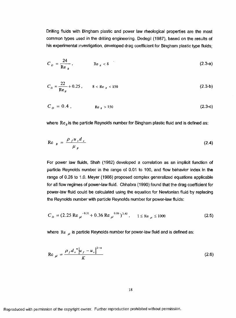
Drilling fluids with Bingham plastic and power law Theological properties are the most

common types used in the drilling engineering. Dedegil (1987), based on the results of

his experimental investigation, developed drag coefficient for Bingham plastic type fluids;

24(2.3-a)

Re BRe B < 8

8 < Re B < 150 (2.3-b)

C D = 0 .4 , Re B > 150 (2.3-C)

where ReB is the particle Reynolds number for Bingham plastic fluid and is defined as:

For power law fluids, Shah (1982) developed a correlation as an implicit function of

particle Reynolds number in the range of 0.01 to 100, and flow behavior index in the

range of 0.28 to 1.0. Meyer (1986) proposed complex generalized equations applicable

for all flow regimes of power-law fluid. Chhabra (1990) found that the drag coefficient for

power-law fluid could be calculated using the equation for Newtonian fluid by replacing

the Reynolds number with particle Reynolds number for power-law fluids:

where Re , is particle Reynolds number for power-law fluid and is defined as:

P f u sd s

Pp(2.4)

C D = (2.25 Re + 0.36 Re / ° 6 ) 345, i < Re pl < 1000 (2.5)

(2.6 )

18


Later, Fang (1992) showed that drag coefficient approached a constant value (s1.0)

when the particle Reynolds number was greater than 100. Chhabra (1993) presented a

comprehensive critical evaluation of the literature available on the particle motion in non-

Newtonian media. Chien (1994) developed a drag coefficient equation for power-law

fluids that can be even used for irregularly shaped cuttings:

30.0 67.289C d = — + - p 3 * T . 0.2 <y/ <1.0 (2.7)

where y denotes sphericity, which is defined as the ratio of the surface area of a

spherical shape having the same volume as the particle and actual surface area of the

particle, and 0.001 < Re < 200,000.

Drilling Fluid Velocity Profile. Mean fluid velocity is normally used to determine the

cuttings transportability although the actual point velocity distribution is not uniform

across the drilling annulus. It is seen from Figure 2.2 that, as the distances increase

along the radial direction, the point velocity increases from zero at the drillpipe wall (if no

wall slip is assumed) to a maximum value near the center of the stream, then decreases

to zero again at the wellbore wall. Since higher fluid velocity yields higher cutting lifting

force (Equation (2.1)), cuttings in the center of the stream are transported faster than

those close to the wall. It is likely that that fluid velocity near the outer boundaries is not

sufficient so that the cuttings would fall back towards the bottom of the hole along the

wall. Two different type of flow regimes, laminar and turbulent, have been identified in

the drilling fluid circulating system. The efficiencies of cuttings transport in laminar flow

and turbulent flow are not the same. As seen in Figure 2.2, the velocity profile in

turbulent flow is flatter than that in laminar flow, which is favorable for the prevention of

cuttings falling in the outer area of the flow stream. Furthermore, in experiments, most

investigators confirmed that turbulent flow has more effective cuttings transport capacity

than laminar flow.

Pipe Rotation Affects Cuttings Trajectory. Drillpipe rotation has positive effect on

cuttings transport through two mechanisms. One is that the rotation aids in creating

turbulence and helps prevent the formation of stagnant, gelled pockets between the

19


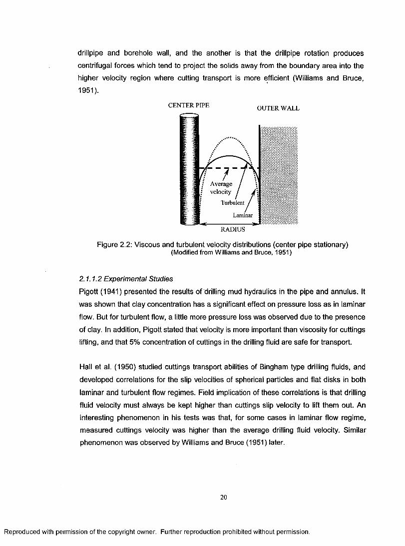
drillpipe and borehole wall, and the another is that the drillpipe rotation produces

centrifugal forces which tend to project the solids away from the boundary area into the

higher velocity region where cutting transport is more efficient (Williams and Bruce,

1951).

CENTER PIPE OUTER WALL

Average / velocity /

Turbulent

Laminar

RADIUS

Figure 2.2: Viscous and turbulent velocity distributions (center pipe stationary)(Modified from Williams and Bruce, 1951)

2.1.1.2 Experimental Studies

Pigott (1941) presented the results of drilling mud hydraulics in the pipe and annulus. It

was shown that clay concentration has a significant effect on pressure loss as in laminar

flow. But for turbulent flow, a little more pressure loss was observed due to the presence

of clay. In addition, Pigott stated that velocity is more important than viscosity for cuttings

lifting, and that 5% concentration of cuttings in the drilling fluid are safe for transport.

Hall et al. (1950) studied cuttings transport abilities of Bingham type drilling fluids, and

developed correlations for the slip velocities of spherical particles and flat disks in both

laminar and turbulent flow regimes. Field implication of these correlations is that drilling

fluid velocity must always be kept higher than cuttings slip velocity to lift them out. An

interesting phenomenon in his tests was that, for some cases in laminar flow regime,

measured cuttings velocity was higher than the average drilling fluid velocity. Similar

phenomenon was observed by Williams and Bruce (1951) later.

20


Williams and Bruce (1951) investigated the minimum velocity required to remove

cuttings successfully and the effects of drilling fluid properties on their carrying capacities

in a 152 m (500 ft) experimental well. In general, it was found that low-gel, low viscosity

muds are better than high-gel, high viscosity muds in cuttings removal. They also found

that pipe rotation has a strong positive impact on cuttings transport. Another

phenomenon of interest was the so-called “reverse order effect”, which was described as

that the large particles reached the surface first although, theoretically, they should

appear the last. The authors finally suggested that mud velocity of 0.51 to 0.64 m/s (100

to 125 ft/min) can be used to keep borehole clean if turbulent flow is maintained.

Hopkin (1967) presented laboratory test results as well as field experiences about the

safe drilling fluid velocity required for hole cleaning. Although laboratory test results

showed a minimum of 0.61 m/s (120 ft/min) velocity required with low viscosity drilling

fluid, the studies of drilling conditions on several wells during fast upper-hole drilling with

water illustrated that 5 percent by volume is a critical concentration in the annulus. This

conclusion supported what has been suggested by Pigott (1941). In addition, Hopkin

reported that high viscosity mud in laminar region is more favorable than lower viscosity

fluid in turbulent flow for hole cleaning, which was not in agreement with Williams and

Bruce’s conclusions.

Zeidler (1972) firstly used a 4.5 m (15 ft) long, 0.08 m (3 in.) ID glass tube to determine

the terminal settling velocity of drilled cuttings, and then employed a large-scale

experimental apparatus, which consisted of a 20 m (65 ft) long wellbore annulus, to

investigate the cuttings transport efficiency with both water and drilling mud. Using

water, he found that even when water velocity is higher than solids terminal settling

velocity, 100% cuttings transport could not be achieved without pipe rotation. Great

improvement in the cuttings transport was observed when pipe rotation was introduced.

The cumulative recovery fraction of the drilled particles in an annulus, which was used to

characterize the transient cuttings transport efficiency, was found to be affected by many factors such as particle mass, fluid velocity, fluid viscosity and drillpipe rotation.

Sifferman et al. (1974) constructed a full-scale experimental apparatus with a 43 m (140

ft) oilfield derrick served as the main frame, which was used to test the steady-state flow

behavior of drilling fluid and cuttings in the annulus. They used the term “cuttings

21


transport ratio”, which was defined as the ratio of net upward velocity of cuttings and the

bulk annular velocity, and plotted it against annular velocity in charts to investigate the

effects of drilling variables.

Table 2.1: Summary of variables effects on cuttings transport

Variable Major Effect Moderate Effect Slight Effect

Annular Velocity X

Rheological Properties X

Cuttings Size X

Fluid Weight X

Rotary Speed X

Feed Concentration X

Annulus Size X

Eccentricity X

(Modified from Sifferman et al., 1974)

2.1.2 Cuttings Transport in Horizontal Wells2.1.2.1 Mechanism of Cuttings Transport in Horizontal Wells

Force Analysis. Figure 2.3 describes an ideal condition of a particle flowing with liquid

in horizontal flow, in which particie-particle interaction and particle-wall interaction is not

illustrated. It is shown that the drag force, FD, which is responsible for the solids

transport, is perpendicular to the gravity force acting on the solid particle, FG. As a result,

the solid particle would still fall down from the flow stream even if the drag force is

greater than the gravitational force. The force that is responsible for cuttings lifting is

referred to as lift force, which acts on the particle in the opposite direction of gravity.

When the lift force, FL, is lower than the gravitational force, the particle will either stay

still on the low side of the wellbore (Figure 2.3-B), or be transported by sliding on the

wall of the wellbore if the dry friction force between the cuttings and the wall is overcome

by the drag force (Figure 2.3-A). When the lift force is higher than the gravitational force,

cuttings are transported in suspension by the viscous drag forces exerted by the

surrounding fluid (Figure 2.3-C). Of all the forces, gravitational force and fluid drag force

can be determined relatively easily. The static dry friction force and fluid lift force acting

22


on a single cuttings resting on the low side of the wall of the wellbore are expressed as follows:

Figure 2.3: Forces acting on a particle in horizontal flow

* > = / ( 2 .8 )

and

~ 2 ^L^sP fuf (2-9)

where fsd is the static dry friction coefficient, and CL is the lift coefficient.

The static dry friction coefficient, fsd, generally can be assumed constant, lyoho (1980)

indicated that when cuttings bed slides down the 60° inclined wellbore, fsd is found to be

about 0.6.

Theoretically, in laminar flow, lift force results from the particle rotation, which may be

caused by a shear gradient, particle-particle interaction or particle-wall interaction.

Crowe (1998) described two types of lift forces; Magnus lift force and Saffman lift force.

The Magnus force is purely due to the rotation of a particle in a uniform velocity field,

which can cause a pressure distribution on the particle. The Saffman lift force is also

generated by the pressure distribution around the particle due to particle rotation.

23


However in the case of Saffman lift force, the particle rotates due to velocity gradient

around the particle. Crowe also presented the correlations to calculate these two forces.

In turbulent flow, the lift force that maintains the solids in suspension may result from the

dissipation of the turbulent eddies. As pointed out by Oroskar and Turian (1980), only

those eddies with instantaneous velocities equal to or higher than the terminal settling

velocities of the solids can create big enough lift force to suspend the solids in the fluid.

But in a real pipe flow, the lift force is hard to be quantified because of the difficulties in

determining the particle rotation, local velocity gradient, particle-particle interaction and

particle-wall interaction.

Mechanism of Solids Displacement. There are mainly two mechanisms, saltation and

sliding, which are responsible for cuttings transport in horizontal well (Gavignet and

Sobey, 1989; Ford et at., 1990). Saltation is described as the lifting of cuttings into the

stream of liquid and being transported. As shown in Figure 2.3-C, the particle is lifted

into the stream of liquid when FL > FG, and transported under the influence of drag force,

Fd. Sliding refers to the case where solids bed resting on the lower part of the wellbore

moves along the well by the interfacial drag force exerted by the upper liquid layer

(Figure 2.3-A). Although particles are observed rolling over the surface of the wall of an

inclined pipe, this transport mechanism is not considered effective for cuttings transport

in horizontal well. If all the transport mechanisms, saltation, sliding and rolling, have

minimal effects for cuttings displacement, a stationary cuttings bed would form on the

low side of the wellbore (Figure 2.3-B).

Flow Patterns. Different physical phenomena of cuttings transport were observed

during the experiments. Ford et al. (1990) identified seven types of flow pattern in slurry

flow, which included homogeneous suspension, heterogeneous suspension,

suspension/saltation, sand cluster, separated moving bed (dunes), continuous moving

bed and stationary bed. Later, Luo et al. (1992) described five types of flow patterns of

cuttings-liquid mixture in the annulus. (1) Heterogeneous Suspension, this type of flow

usually occurs when the fluid velocity is high. In this case, cuttings are fully suspended

by the lift forces created by the high velocity. Usually, there is an asymmetric

concentration distribution along the direction perpendicular to the horizontal wellbore

axis such that more solids stay in the lower half part of the wellbore. The solids

24


concentration distribution can be determined by using the diffusivity model based on the

turbulence theory (Doron, et al., 1987; Martins and Santana, 1992). (2) Separated

Bed/Dunes, in this type of flow, fluid velocity is not high enough to create lift forces to

suspend all the cuttings. Cuttings bed begins to form, but the interface between the

solids bed and carrying fluid is discontinuous. (3) Continuous Moving Bed, if the fluid

velocity is moderate, the lift force would be weak, and the drag force (or interfacial force)

will dominate the transport of solids. Solids deposited at the lower part of the hole will be

moved by the interfacial viscous forces exerted by the liquid layer. (5) Stationary Bed, it

is associated with the low fluid flow rate in horizontal wells, where interfacial force

exerted by upper liquid layer does not have any effects on the movement of the solids

bed.

Critical Conditions For Cuttings Movements Based on Balance of Forces. Two

critical conditions are noticed through analyses of the forces acting on a single particle.

One is the inception of the cuttings sliding on the bed surface (or the wellbore wall), and

another is the inception of the cuttings resuspension from the bed. The drilling fluid flow

rates (or velocities) corresponding to these two critical conditions are of great interest for

field engineer, because, to a large extent, they can be viewed as the lower pump rate

limit for effective cuttings transport. Based on the balance of forces, Ford et al. (1996)

developed a semi-empirical model for the prediction of the minimum transport velocity

(MTV) for both cuttings rolling or sliding along the lower side of the wellbore, and

cuttings suspending and being transported in the slurry.

Critical Deposition Velocity For Cuttings Transport. Even though it gives the physical

meanings of different transport mechanisms involved in the process, the method based

on the balance of forces is not widely used for slurry flow in pipes mainly because of the

uncertainties involved in determining lift forces in a multi-particle system. One of the

most common ways to find the critical conditions is the direct determination of critical

fluid deposition velocity, which is defined as the minimum velocity that can prevent the

formation of a solids bed on the bottom of the horizontal pipe. The critical fluid velocity is

usually determined as a function of fluid properties, solids characteristics and pipe

geometry. Oroskar and Turian (1980) developed such a correlation based on balancing

the energy required to suspend the particle with the effective turbulence energy to

predict the critical velocity. The correlation is:

25


■ = 1.85CS 0 1536 (1 - C J 03564f d

gd,(— ~ 1) P f

y D jN Ke0MX 03 (2 .10)

where N R is a modified Reynolds number defined by equation (2.11):

M V Pf

Oroskar and Turian stated that for the types of slurries they used, the value of X is close

to unity, and proved that their model was superior than all other previously developed

critical velocity correlations.

Critical Solids Concentration For Cuttings Transport. Another way to find the critical

condition is the determination of solids concentration distribution as a function of slurry

velocity, fluid properties, solids characteristics and pipe geometry. The average

concentration calculated from the distribution is viewed as the critical mean

concentration that cannot be exceeded during the period of solids transportation. Doron

et al. (1987) employed the well-known diffusion equation to represent the dispersion

mechanism of solid phase in the fully suspended flow:

, d C ( y ) , d C ( y ) .g V + v a = 0 (2.12)dy 8y

where e ' is the local diffusion coefficient and v' is the particles’ local terminal settling

velocity. When the mean diffusion, s , and terminal settling velocity, vb are applied,

analytical result can be obtained by integrating the diffusion equation twice:

C(y) = Cb exp — (y - hb) €(2.13)

and 6 can be evaluated as:

26


e - 0.026u *D h (2.14)

where u = y fr jp is the shear velocity and D H is hydraulic diameter.

2.12.2 Experimental Studies

lyoho (1980) carried out extensive experiments on investigating the cuttings transport

performances in directional wells by using the test facility built at the University of Tulsa.

The apparatus consisted of a 12.3 m (40 ft) long, 127 mm x 48.3 mm (5 in.x 1.9 in.) test

annulus with the inclination angle varied from zero to 90 degree. It was found that the

major factors affecting cuttings transport were drilling fluid velocity and viscosity,

inclination angle, and drilling rate. Specifically, it was observed that increasing of hole

angle or drilling rate had negative effect on cuttings transport. Higher drilling fluid

viscosity was more favorable than the lower viscosity for cuttings transport within the

same flow regime. Annular eccentricity had moderate effect although the concentric

annulus provided the best transport performance.

Tomren et al. (1986) performed a total of 242 tests by employing the same experimental

facility as used by lyoho in 1980. Comprehensive cuttings transport phenomena were

observed, which included the flow in vertical and near vertical well in both laminar and

turbulence regimes, the flow in low angles of inclination, the flow in the transient or

critical angle inclination, and the flow in high angles of inclination. It was found that, in

inclined annulus, bed formation in high viscosity drilling fluid was slower than that in low

viscosity drilling fluid in laminar flow. It was also found that inner pipe eccentricity has

little effect on cuttings flow behavior in vertical annulus, but for inclined hole, concentric

annulus yields maximum efficiency of cuttings transport.

Okrajni and Azar (1986) particularly investigated the effects of mud rheology on hole

cleaning in directional well. The drilling fluids with yield values within the range of 0.0 to 9.6 Pa (0.0 to 20.0 lbf/100 ft2), and with three values of YP/PV ratio (0.5, 1.0 and 2.0)

were used in the tests. The observations in the preliminary tests had shown that a

drilling fluid velocity lower than 1.02 m/s (3.34 ft/s) was generally insufficient to remove

all the cuttings once a bed formed in the inclined annulus. Further investigation revealed

that drilling fluid rheological properties (yield value and YP/PV ratio) generally did not

27


affect the cuttings transport under turbulent regime although the drilling fluid with higher

yield value yielded better cuttings transport under laminar flow regime. During both the

bed-erosion (annulus-cleaning) and cuttings transport experiments, identical trends were

observed.

Brown, Bern and Weaver (1989) carried out experimental studies in BP Research

Centre to investigate the mechanisms of hole cleaning in deviated wells. The

experiments were performed in a flow loop consisting of a 15.2 m (50 ft) long test section

with a 20.3 cm (8 in.) diameter cased hole and a 12.7 cm (5 in.) diameter drillpipe. They

observed that hole cleaning was more efficient with water in turbulent flow than with

hydroxyethyl cellulose (HEC) based drilling fluid. In addition, they indicated that the

poorest removal rates generally occurred in the critical inclination angle of 50 to 60

degree. At hole angles of 50 degrees and above, the mud velocity of 1.27 m/s (250

ft/min) was insufficient to initiate the cuttings transport.

Ford et al. (1990) performed an experimental study on drilled cuttings transport in

inclined boreholes by using a 6.3 m (21 ft) borehole simulator built within the Department

of Petroleum Engineering at Heriot-Watt University. It was found that cuttings were

removed by two distinct mechanisms including rolling/siding and transport in suspension.

Seven slurry flow patterns were observed including homogeneous suspension,

heterogeneous suspension, suspension/saltation, sand cluster, separated moving bed

(dunes), continuous moving bed and stationary bed. Experimental results showed that

the minimum transport velocities (MTV) corresponding to the two transport mechanisms

were influenced by a variety of variables such as hole angle, fluid viscosity, inner pipe

rotation and cuttings size.

Larsen (1990) carried out more than 700 tests by using the full-scale wellbore simulator

at the University of Tulsa. The effects of almost all the variables on the critical transport

velocity have been investigated. Results indicated that the angle of inclination and drilling flow rate had the most significant effect on hole cleaning.

2.1.2.3 Mechanistic and Empirical Modeling

Doron, Granica and Barnea (1987) established a solids hydraulic transport model with

an assumption that two layers, a heterogeneous suspension at the top and a solids bed

28


at the bottom, exist in the horizontal slurry flow (Figure 2.4). By neglecting the slip

velocity between two phases, two continuity equations was developed for solid phase

and liquid phase, and two force balance equations was developed for upper layer and

lower layer. The well-known diffusion equations (2.12) and (2.13) were used to calculate

the mean solids concentration in the flowing suspension. The cutting bed could be either

stationary or moving, which is controlled by the balance of all forces including pressure

force, interfacial shear force and dry friction force acting on the bed.

Upper Layer

Bottom Layer

Hi. .Hi

Figure 2.4: Two-layer model in horizontal pipe

Gavignet and Sobey (1989) developed a mechanistic model for cuttings transport and

bed thickness prediction in deviated wells. The basic assumptions included a closely

packed cuttings bed existing in the lower part of the wellbore that could be transported

by sliding-up. Simple momentum balance was given for both upper and lower layers,

and the equation that relates wall stresses to interfacial stress was derived:

A , & = - r f S , - r lSl (2.15)

4 ^ = - r ,S ,- r ,S , (2.16)OX

Abr f S f + ATjSj = A0tsSs (2.17)

Solving the above equations requires the determination of hydraulic diameter, frictional

factors for pure liquid and solids, as well as interfacial friction. The sliding friction

29


coefficient, which is directly responsible for the determination of the bed moving velocity

and bed height, was assumed to be equal to 0.2 throughout the paper.

Martins and Santana (1992) developed a two-layer mechanistic model for cuttings-liquid

flow. The lower layer was assumed to be a cuttings bed which can be either stationary or

moving, and the upper layer was assumed to be the drilling fluid with suspended cuttings

in it. The model consisted of two continuity equations for solids and liquid phases, and

two momentum equations for the top layer and bottom layer respectively. Solving the

equations requires the determination of interfacial shear stress and critical cuttings

concentration in the upper layer. The critical cuttings concentration in the flow stream

was determined by the diffusivity equation (Equation 2.13).

Luo, Bern and Chambers (1992) proposed an empirical cuttings-transport model that

can predict the critical flow rate (CFR) required to prevent the formation of stationary

cuttings bed in deviated wells. The model was based on the Buckingham PI theorem,

and four dimensionless groups were derived from seven dimensionless variables. The

simplified CFR correlation, which only included two most important dimensionless

groups, was expressed as:

Empirical coefficients, a' and b' , were obtained from regression analysis. The results

showed that the average percentage difference between the predicted and the

experimental data is 16%. Field data, which have proved adequate hole cleaning during

drilling operations, were also used to validate the model.

Clark and Bickham (1994) presented a mechanistic model by analyzing the particle

settling, rolling and lifting mechanisms to predict the critical fluid velocities that initiate

the cuttings movements. Correlations for the critical velocities were given as a function

of operational parameters, well bore configuration, fluid properties and cuttings

characteristics.

d sg Ps P f sin(6>)

*2

\ (2.18)

30


Campos (1995) presented a two-dimensional mechanistic model that addressed the

effect of pipe eccentricity. Momentum equation for the liquid phase was derived for

turbulent liquid flow, i.e., including an unknown “eddy turbulent diffusivity”. Solids

continuity equation (cuttings concentration equation) was also formulated. A coordinate

transformation technique was employed to simplify the eccentric annular boundary and

generate the grids within a rectangular computational domain.

Ford et al. (1996) developed a mathematical model to predict the minimum transport

velocity (MTV), which is required to initiate the sliding or lifting of drilled cuttings resting

on the low side of the borehole. The model was based on the balance of forces acting on

a single particle, and the determination of lift coefficient, CL, was needed to solve the

model.

Larsen et al. (1997) developed an empirical model based on their experimental results

(Larsen, 1990) to predict the minimum fluid velocity that prevents the formation of a

cuttings bed. They first developed an empirical correlation of cuttings concentration in

terms of drilling rate, and then cuttings transport velocity (CTV) is calculated. The

correction factors of angle of inclination, cuttings size and drilling fluid weight were

introduced and incorporated into the generalized equivalent slip velocity (ESV), which

was added to CTV to obtain the critical transport fluid velocity (CTFV).

Nguyen and Rahman (1998) constructed a three-layer hydraulic model to describe

cuttings transport phenomena in a horizontal well. Three different flow patterns were

assumed to co-exist in the transport process, which included a bed of particles of

uniform concentration at the bottom, a dispersed layer with varied concentration in the

middle and a fluid flow layer with a clear fluid or a turbulent suspension at the top.

However, validation for the model was not provided in the paper.

Kamp and Rivero (1999) proposed a two-layer model for cuttings transport in highly

inclined wellbore. The model consisted of three continuity equations and two momentum

equations for the solids, liquid and cuttings bed. In their model, the prediction of cuttings

bed height was dictated by two terms, (J>s,dep, and <f>SiSUSp, which were referred to as the

mass flux of cuttings that deposited per unit interface and that were resuspended per

31


unit interface, respectively. The former term was determined through the product of

mean cuttings concentration, cuttings density and particle terminal settling velocity. The

latter term was assumed to be directly proportional to the cuttings bed concentration,

cuttings density and friction velocity.

Gillies and Shook (2000) developed a two-layer model for high concentration (up to

35%) settling slurry flow with particle diameter finer than 0.5 mm. The model consisted of

mass balance equations and force balance equations for the two layers. Mass and force

balance equations were then solved to obtain the pressure loss. The kinetic stresses of

the liquid and solids acting at boundaries were calculated using Fanning friction factor. In

addition, the Coulombic friction, which is the resisting force exerted by the wall on those

particles which do not produce kinetic friction, was determined through the correlation

developed by Wilson (1976).

Cho, Shah and Osisanya (2002) proposed a three-layer model for predicting the cuttings

transportability when drilling a deviated well with coiled tubing. The three layers

considered in the model included stationary bed at the bottom, a moving bed above it,

and a heterogeneous suspension layer at the top. Continuity equations for solid phase

and liquid phase, and momentum equations for the top layer (dispersed suspension) and

the middle layer (moving bed) were developed. The well-known diffusion model

(Equation (2.13)) was used for determining solids critical concentration in the

suspension. Through the simulation, the authors recommended that drilling fluid velocity

of 1.0 m/s to 1.2 m/s should be maintained to drill a well having a long horizontal section.

Doan et al. (2003) developed a transient cuttings transport model consisting of three

time-dependant continuity equations and three time-dependant momentum equations for

the deposit cuttings bed, fluid component and cuttings component in the flowing

suspension mixture. The mass transfer between two layers, which dictated the transient

cuttings bed height, were represented by cuttings deposition and entrainment rates, vDEP

and Vent■ Vdep was defined as the hindered terminal settling velocity. vENTv/as assumed

to be a function of interfacial shear velocity.

32


2.2 Underbalanced Drilling (UBD)The research related to UBD has been focusing on the mechanistic modeling of

multiphase flow hydraulics in the wellbore, and the determination of the minimum gas

and/or liquid flow rates required for cuttings transport.

2.2.1 Air/Gas Drilling

Angel (1957) derived an equation for determining the circulation rates necessary to

produce annular velocities that are equivalent in lifting power to some velocity of

standard density air. The equation was solved implicitly to obtain the minimum

circulation rate based on the assumption that the minimum velocity of standard-density

air required to transport the cuttings is 15.2 m/s (3000 ft/min). The effect of slip velocity

between phases was neglected in this study.

Machado and Ikoku (1982) developed a group of empirical correlations to account for

the frictional effects of solids in the annulus by applying linear regression analysis to the

experimental data. Based on the assumption that air/gas velocity must be higher than

the terminal settling velocity of cuttings to keep the drilling safe, minimum volume

requirements were calculated by using trial-and-error method. The minimum gas

injection rate was found to increase with well depth and drilling rate.

Mitchell (1983) carried out a simulation study for air and mist drilling in the geothermal

well. At first, equations of mass balance and momentum balance for compressible gas

flow were derived, then the appropriate modifications necessary to incorporate drilling

cuttings and mist into the air flow model were discussed. Mitchell’s model predicted

higher volumetric requirements than Angel’s model for air drilling.

Sharma and Chowdhry (1986) presented an isothermal 1D steady-state mathematical

model to analyze the fluid dynamic effects of clouds of various size particles, and to

calculate the pressure drop of the mixture. Their model breaks up the annulus into a series of computational cells. Total pressure drop is determined by summing the

individual cell pressure drops.

Wolcott and Sharma (1986) developed a steady-state model for air volume requirement

calculations. Unlike Sharma and Chowdhry’s model, this one can be applied to any

33


isothermal or non-isothermal 1D flow of gas and solids suspension. Effects of solids slip

were considered, and three methods for determining pressure drop due to solids phase

were studied.

Supon and Adewumi (1991) built an experimental wellbore model to simulate the

multiphase flow of compressed air and sand, which occurs in an air drilling process. The

model was designed to control the air volumetric flow rate and sand flow rate through a

transparent annulus. The existence of the minimum pressure drop for annulus flow was

confirmed by the experiments, and an empirical equation was developed for the

minimum annulus pressure drop as a function of the sand flow rate through the system.

Tian and Adewumi (1991) developed a hydrodynamic approach taking into account the

variables including physical properties of solids, two different particle sizes, thermo

physical properties of transporting fluid, penetration rate, geometrical configuration of the

wellbore/drilling string annulus and fluid transport velocity. Three partial differential

equations were formulated to account for the mass balances of gas and two groups of

solids with different sizes, and another three partial differential equations were

formulated to account for the momentum balances of gas and two groups of solids with

different sizes. Incorporating initial and boundary conditions, the model was integrated

by using the numerical method of lines (MOL). The model predictions were compared to

Supon and Adewumi (1991) ’s experimental data, and the agreement was found to be quite good.

2.2.2 Gasified Liquid Driiling

Guo et al. (1996) developed a mathematical model based on the isothermal, steady

state mechanical energy balance for compressible foam flow. The equation was applied

to the multiphase flow of gas, drilling mud and cuttings by assuming a homogeneous

flow in the aerated mud drilling. The model was used to predict the BHP as well as

cuttings concentration in the wellbore.

Wang et al. (1997) developed an unsteady state underbalanced drilling model. The

mass conservations of eight components including the free gas produced from reservoir,

gas injected from drillpipe, gas injected from annulus, dissolved gases, drilling fluid,

formation oil, formation water and drilled cuttings were considered in conjunction with a

34


full conservation of total momentum. A number of submodels to calculate drilling fluid

density, gas density, cuttings velocity, etc. were also developed to close the systems of

continuity and momentum equations.

Bijleveld et al. (1998) developed a steady state UBD model which can be used to

simulate the multiphase flow in drillpipe and annulus. The components of oil, water,

reservoir production, free and dissolved hydrocarbon gases, additional injection gases,

nitrogen, air and cuttings were taken into account to meet the mass balances. To

determine the average mixture density in a calculation block, a two-phase flow model

was used with the consideration of different flow patterns occurring in the wellbore. In

addition, the effects of reservoir fluids influx were incorporated in the model.

Sharma et al. (2000) developed a steady state model to study the multiphase flow of

gas, liquid and solids in conduits. Mass conservation equations for oil, water, mud,

injected gas, formation gas and drilled cuttings, and the momentum conservation

equation for the mixture were given in the model. To solve the model, a homogenous

mixture was assumed in the flow system, and the drilled cuttings were assumed to be

fully suspended in the homogeneous gas/liquid mixture.

Li and Walker (2001) performed 600 tests on solids transport with gas/liquid fluids. They

used a flow loop which consisted of a 6 m (20 ft) transparent Lexan pipe with a 13 cm (5

in.) inner diameter and a 7 cm (2-3/8 in.) steel inner pipe simulating the openhole and

drillpipe respectively. Based on the experimental results, an empirical correlation was

developed to determine the critical deposition velocity that can prevent the formation of a

stationary cuttings bed. It was found the in-situ liquid velocity was the most important

variable affecting cuttings transport in horizontal wells. Other hole cleaning modes, such

as circulation hole cleaning and wiper-trip hole cleaning, were also discussed in the

research.

Martins et al. (2002) investigated the solids return time in aerated fluid drilling by using

the real scale test facility built at PETROBRAS. The facility consisted of a vertical well,

which was cased with 34 cm (13-3/8 in.) casing to 1300 m. Another 18 cm (7 in.) casing

was set at depth. The drill string with size of 9 cm (3-1/2 in.) drillpipe was used in the

experiments. Sand was injected either through the annulus or drillpipe, and the return

35


time was recorded. It was found that liquid flow rate had a major effect on solids return

time.

Naganawa et al. (2002) carried out experiments to investigate the cuttings transport in

aerated mud drilling for inclined annuli with angles between 30° and 90°. The Cuttings

Transport Flow Loop System (CTFLS) used in the tests consisted of a 9 m long test

section with a 13 cm (5 in.) ID transparent acrylic outer pipe and a 5 cm (2.063 in.) OD

steel inner pipe. Three flow patterns including bubbly, churn and slug flows were

observed while transporting cuttings in inclined annuli. In a horizontal annulus, however,

only stratified wavy flow was observed. The injection rate of gas was found to have a

small effect on cuttings transport in horizontal well where wavy stratified flow prevailed.

Sunthankar et al. (2003) carried out an experimental study on aerated mud flow in an

inclined well utilizing a field-scale low-pressure flow loop with a 27 m (90 ft) inclined

section and 20x11 cm (8x4.5 in.) annular geometry. Both bubbly and intermittent flow

regimes were observed in the tests. Experimental results showed that flow pattern

boundaries shifted in the annulus flow as compared to those in pipe flow.

Lage et al. (2003) developed a mathematical model to investigate the transient dynamics

of UBD with gas/liquid two-phase fluids. The model consisted of two continuity equations

for gas and liquid phases and a momentum equation for the mixture. The approach of

drift-flux was adopted to determine the slip velocity between gas and liquid. The system

of conservation equations was solved by an explicit composite scheme, and the model

was validated with full-scale experimental data.

Tellez et al. (2003) developed a comprehensive, mechanistic model that can precisely

predict the wellbore pressure and two-phase flow pattern for UBD. The model consisted

of a number of correlations (or submodels) used to determine the transitions of two-

phase flow patterns and the pressure losses and phase concentrations for particular flow

patterns. The model predictions were validated with actual UBD field data and full-scale

experiments, and an average error of less than 3% was shown by the validation.

36


2.3 Cuttings Transport with Foam2.3.1 Foam Equation of State

2.3.1.1 Foam Fluid

Foam is a dispersion of gas into a liquid phase (water), which is stabilized by surfactant.

In aqueous foam, the gaseous phase appears as bubbles that are separated from each

other by liquid films. Foams having the same gas fraction, (i.e. quality), may have a

different texture (i.e. bubble size and shape) and liquid film thickness depending on the

type of surfactant, mechanism of foam generation, etc. Variation of texture and liquid film

thickness would influence the viscosity of foam. It is, however, practically impossible to

take into account these uncontrollable variables when the rheology of the foam is

studied. As far as drilling engineering applications are concerned, the effect of foam

texture on the foam rheology is neglected. Foam is, therefore, considered as a

macroscopically homogeneous fluid, and from the standpoint of hydraulic design it is

treated as a single-phase compressible fluid.

2.3.1.2 Foam Quality

Foam quality is defined as gas volume ratio to the total volume to foam, i.e. gas volume

fraction of foam:

Vr = — — (2.19)Vg + v t

The value of foam quality varies between zero and unity. Because foam contains a

gaseous component, its quality changes as a function of pressure and temperature. The

real gas law can be used to determine the gas volume ratio at different pressure and

temperature condition,

*1 _ Z1 Po Tx (2 20)VgQ Z 0 p x T0

and to determine the gas density ratio at different pressure and temperature condition:

37


where Z is the gas deviation factor, and is calculated by using a computerized method

(Yarborough and Hall, 1974), subscript 0 and 1 denote two different conditions.

By combining equations (2.19) and (2.20), the equation to calculate foam quality at

different pressure and temperature can be obtained as follows:

r■ = 1 +

f i - r ^ 1 1 0 1 ^

° . E lT ^0

rV 1 o y Po T1 J(2 .22)

2.3.13 Foam Density

Since foam is treated as a homogeneous fluid, the foam density can be calculated by using the equation (2.23):

P f = T P g + ( l ~ T )P i (2.23)

The effects of pressure and temperature on foam density need to be considered. By

combining equations (2.21), (2.22) and (2.23), the following relationship is derived:

PfO

P fl= (i-r0)+r0

\Z\ Po Tx

\ Pi T0 j(2.24)

2.3.2 Foam Rheology

The foam viscosity is generally known to be a strong function of the foam quality.

Einstein (1906) derived a bubble-liquid two-phase viscosity model by the application of hydrodynamic equations as well as an energy conservation equation to the flow of a fluid

around a system of bubbles (Mitchell, 1969). Einstein’s viscosity equation was valid for

foam quality less than 0.52, i.e., dispersed bubble region:

Hf = p ,( l -0 + 2.5T) (2.25)

38


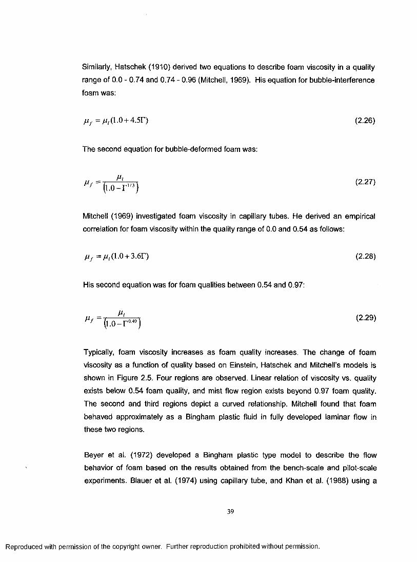
Similarly, Hatschek (1910) derived two equations to describe foam viscosity in a quality

range of 0.0 - 0.74 and 0.74 - 0.96 (Mitchell, 1969). His equation for bubble-interference

foam was:

= ^ ( 1 .0 + 4 .5 0 (2.26)

The second equation for bubble-deformed foam was:

(2.27)

Mitchell (1969) investigated foam viscosity in capillary tubes. He derived an empirical

correlation for foam viscosity within the quality range of 0.0 and 0.54 as follows:

Typically, foam viscosity increases as foam quality increases. The change of foam

viscosity as a function of quality based on Einstein, Hatschek and Mitchell’s models is

shown in Figure 2.5. Four regions are observed. Linear relation of viscosity vs. quality

exists below 0.54 foam quality, and mist flow region exists beyond 0.97 foam quality.

The second and third regions depict a curved relationship. Mitchell found that foam

behaved approximately as a Bingham plastic fluid in fully developed laminar flow in these two regions.

Beyer et al. (1972) developed a Bingham plastic type model to describe the flow

behavior of foam based on the results obtained from the bench-scale and pilot-scale

experiments. Blauer et al. (1974) using capillary tube, and Khan et al. (1988) using a

H f - / / / (1 .0 + 3 .6 F ) (2.28)

His second equation was for foam qualities between 0.54 and 0.97:

(2.29)

39


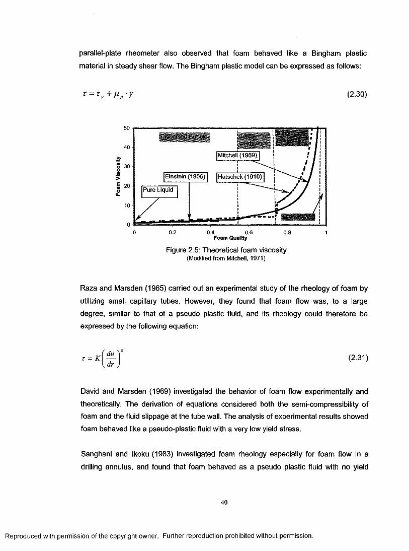
parallel-plate rheometer also observed that foam behaved like a Bingham plastic

material in steady shear flow. The Bingham plastic model can be expressed as follows:

T = Ty+Mp- Y (2.30)

; Bubhip | Interfereno

Mitchell (1969)

Einstein (1906) Hatschek (1910)

0 0.2 0.4 0.6 0.8 1Foam Quality

Figure 2.5: Theoretical foam viscosity (Modified from Mitchell, 1971)

Raza and Marsden (1965) carried out an experimental study of the rheology of foam by

utilizing small capillary tubes. However, they found that foam flow was, to a large

degree, similar to that of a pseudo plastic fluid, and its rheology could therefore be

expressed by the following equation:

f /J \t = K — (2.31)

V dr

David and Marsden (1969) investigated the behavior of foam flow experimentally and

theoretically. The derivation of equations considered both the semi-compressibility of foam and the fluid slippage at the tube wall. The analysis of experimental results showed

foam behaved like a pseudo-plastic fluid with a very low yield stress.

Sanghani and Ikoku (1983) investigated foam rheology especially for foam flow in a

drilling annulus, and found that foam behaved as a pseudo plastic fluid with no yield

40


value. Experimental results were obtained by using a concentric annular viscometer that

could closely simulate actual borehole conditions. Sanghani and Ikoku provided the

values of the flow behavior index, n, and the fluid consistency, K, as functions of foam

quality. There was no correlation available to calculate n and K. In this study,

correlations based on Sanghani and Ikoku’s experimental results were developed

through regression analysis (Figure 2.6). The correlations are:

For T < 0.915:

£ = 0.0074-e3 5163 r (2.32-a)

« = 1.2085-e-1 9897 r (2.32-b)

For 0.98> T > 0.915:

K = -2.1474 T + 2.1569 (2.32-c)

n = 2.5742 T - 2.1649 (2.32-d)

It is interesting to see that there exist two distinct regions which can be expressed by two

different correlations. An exponential relationship exists between K and n and foam

quality when foam quality is less than 0.915, whereas a linear relationship exists at

qualities above 0.915. This is because, for T < 0.915, stable foam prevails, and as foam

quality increases, foam effective viscosity increases, and the deviation from Newtonian

fluid increases. For 0.96> T > 0.915, the stable foam begins to convert to unfavorable

mist which usually has a much lower viscosity than foam. If foam quality is higher than

0.96, mist prevails. The value of 0.96 was recommended as the maximum foam quality

that is allowed in the drilling wellbore annulus (Okpobiri and Ikoku, 1986).

41


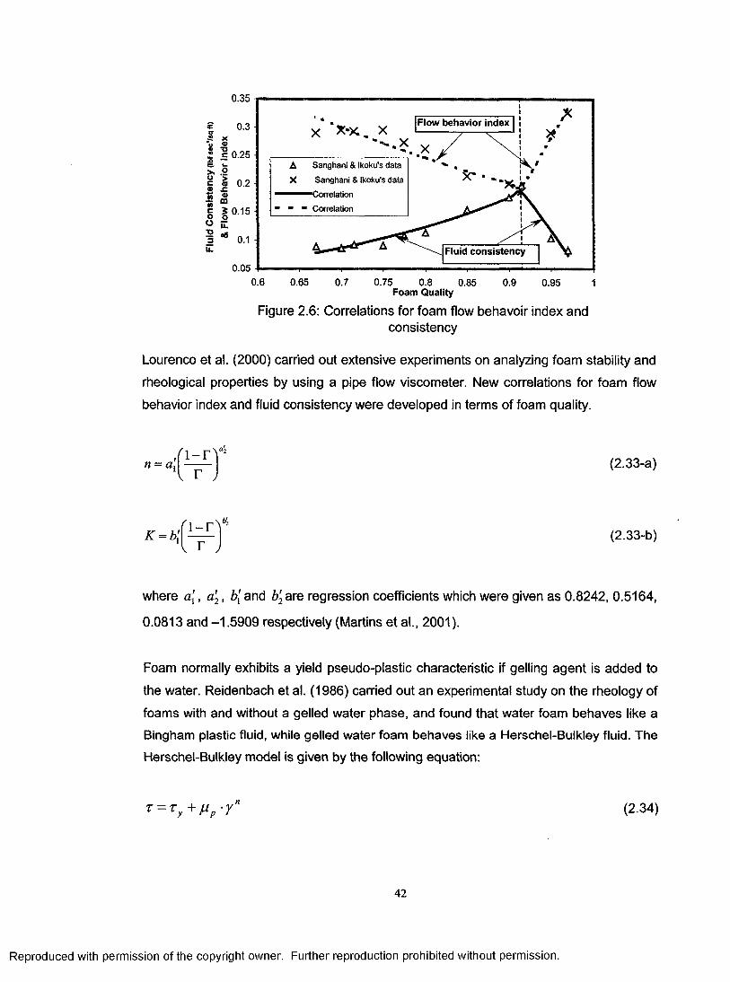
0.35

Flow behavior index i

A Sanghani & Ikoku's data

X Sanghani & Ikoku's data

Correlation

“ ” Correlation

Fluid consistency0.05

0.6 0.65 0.7 0.75 0.8 0.85 0.9 0.95Foam Quality

Figure 2.6: Correlations for foam flow behavoir index andconsistency

Lourenco et al. (2000) carried out extensive experiments on analyzing foam stability and

rheological properties by using a pipe flow viscometer. New correlations for foam flow

behavior index and fluid consistency were developed in terms of foam quality.

where a[ , a'2, b[ and b'2 are regression coefficients which were given as 0.8242, 0.5164,

0.0813 and -1.5909 respectively (Martins et al., 2001).

Foam normally exhibits a yield pseudo-plastic characteristic if gelling agent is added to

the water. Reidenbach et al. (1986) carried out an experimental study on the rheology of

foams with and without a gelled water phase, and found that water foam behaves like a Bingham plastic fluid, while gelled water foam behaves like a Herschel-Bulkley fluid. The

Herschel-Bulkley model is given by the following equation:

n = a (2.33-a)

(2.33-b)

T = Ty + H p - y n (2.34)

42


Reidenbach et al. (1986) also observed that the flow behavior index, n, was

approximately the same as that of the base liquid, and the yield point, ry, and fluid

consistency, K, were exponential functions of foam quality. A series of correlations were

proposed to calculate the ry and K, of nitrogen- and carbon dioxide-based foams.

Later, Harris and Reidenbach (1984) carried out a Theological study of nitrogen-based

foam fracturing fluids at high-temperature. They extended the research of Reidenbach et

al. (1986) by incorporating the effects of high temperature and gelling agent

concentration into the three parameters of the Herschel-Bulkley model (Equation 2.34).

Calvert and Nezhati (1987) modeled foams as a modified Bingham plastic model (Herschel-Bulkley) by analyzing experimental data obtained from a cone and plate

rheometer and pipe flow. They introduced a term “expansion ratio”, which was defined

as the ratio of the volume of a sample of foam to the volume of its base liquid, instead of

“quality” to describe foam properties. It was found that consistency and flow behavior

index were independent of the flow rate and expansion ratio to a large extent, whereas

the yield stress varied much more strongly with both flow rate and expansion ratio.

Saintpere et al. (1999) used a stress-controlled and two velocity-controlled Haake

rheometers to study the rheology of gelled water foam. Results clearly showed that foam

was a pseudo plastic fluid with a yield stress, and behaved like an elastic solid for small

deformations.

Bonilla and Shah (2000) experimentally investigated the rheology of aqueous and gelled

foams by utilizing a loop-type viscometer. All the tests were run under an average

pressure of 6890 kPa (1000 psia) in order to ensure foam quality is constant and

homogeneous inside the loop. They concluded that foam rheology can be adequately

characterized by the Herschel-Bulkley model. Relationships between yield point and

foam quality, and consistency index and foam quality were developed for both aqueous

and gelled foams by applying regression analysis to the experimental data.

Valko and Economides (1992) proposed a novel constitutive equation for foam polymer

solutions based on the principle of volume equalization. They introduced a specific

volume expansion ratio, es, that was defined as the ratio of the specific volume of the

43


foam to the specific volume of the base liquid. The volume-equalized constitutive

equation for Bingham plastic fluid was expressed as:

y = 0 (2.35-a)

x = (2.35-b)v

and for power-law fluid:

x = {K \ r V (2.36)

Ozbayoglu et al. (2002) conducted a comparative study of the foam hydraulic models.

Based on the comparison of the measured frictional pressure drop during the flow of

foam in pipes with model predictions, they have concluded that foams can be treated as

power law fluids when the foam quality is 70-80%, and as a Bingham plastic fluid when

the foam quality is 90%.

2.3.3 Foam Flow in Pipe and Annulus

Beyer et al. (1972) developed a method to calculate pressure drop for foam flow in pipe

and annulus. In the method, total flow rate of foam was composed of a slip component,

qslip, and a fluidity component, qFluidity:

Q ~ Q Slip + # F lu id ity (2-37)

The slip component was calculated by using empirical correlations developed from the

experimental results, and the fluidity velocity was derived from the Buckingham-Reiner equation:

32 n p 3 x w 3 ^ r „ J(2.38)

44


where

Ty

A pD 4 L

(2.39)

They combined equations (2.37), (2.38) and (2.39) to obtain an explicit function for the

pressure gradient vs. total velocity, liquid volume fraction and pipe diameter. The explicit

function was calculated using a finite difference scheme by dividing the pipe into

incremental lengths with small pressure changes. The small pressure changes could be

accumulated to get the total pressure drop. The iteration process was continued until the

sum of the incremental lengths equals to the total length of the pipe:

Blauer et al. (1974) found that frictional pressure loss for foam flow could be determined

as by assuming foam as single-phase fluid and using the conventional Reynolds

number, Moody diagram, and Hagen-Poiseuille law for Newtonian laminar flow. They

suggested to use the effective viscosity of foam instead of single-phase viscosity in the

calculation.

The effective viscosity of the Bingham plastic foam was:

Lord (1981) predicted the pressure loss by solving the isothermal and steady state

mechanical energy balance equation (Equation (2.43)) for compressible fluid flow:

(2.40)

(2.42)

45


udu gdx dp r l u 2dx ° ------- + _ ^ _ + f ------------------ = o

S c S c P f S c D

(2.43)

Sporker et al. (1991) set up a downhole flow loop to investigate foam behavior under

realistic field conditions. A foam flow model for vertical flow of multiphase fluid was

proposed to evaluate the experimental data. This model was an improved version of

Lord’s foam model (1981). Instead of using the real gas law in Lord’s method, the virial

equation was used to describe the gas behavior, which led to considerably different

results.

Calvert (1990) assumed that foam flows as a plug lubricated by a wall slip layer. The

thickness of wall slip layer, which was considered by Calvert as the most important

parameter controlling foam flow, may be estimated from the average bubble diameter

and expansion ratio from experimental analysis:

The author used Herschel-Bulkley model to calculate the slip component, qslip, and

fluidity component, qFluidity, to get the total foam flow rate under certain pressure drop:

6 2 (2.44)d bubble

_ ttS D 2 t w

y sup (2.45)

and

Q Fluidity — 0 , | t | < x y (2.46-a)

Fluidity| t | > t y (2.46-b)

where

46


r = ( i - T v / o (2.47)

Gardiner et ai. (1999) constructed a foam flow model that combined Valko and

Economides’ method (1992) of volume equalization with the effect of foam wall slippage.

They integrated the equation of volume equalization with the wall slip boundary condition

and obtained a velocity profile of power-law foam flow as follows:

q = 7r R slip +3 « + 1

dpdx

R n + 1 e

2 K

1 / ft

(2.48)

2.3.4 Cuttings Transport with Foam2.3.4.1 Solids Transport with Foam in Vertical Wells

Krug and Mitchell (1972) employed a numerical technique, which was based on a

modified Buckingham-Reiner equation, to analyze the wellbore hydraulics for foam

drilling. The following finite difference equations were used to describe foam flow in

pipes and annuli:

P i+1 Pi! = 1 i = l P ig ~

8 Ty , i

8 ju piu(2.49)

3 r

P i +1 - Pii= 1 P ig +

6 r+

(2.50)p i “ f . l

( Z ) 0 - D , . ) ( D ' - D t Y

In equations (2.49) and (2.50), the flowing density, foam quality, and velocity were

adjusted for the presence of drilled cuttings in the foam assuming homogeneous solids- foam flow. Krug and Mitchell used the model to determine the minimum volumes of

water and gas, and hydraulic horse power required for a foam drilling operation.

Okpobiri and Ikoku (1986) developed an iterative procedure to calculate the volumetric

requirements and wellhead injection pressure for power-law foam drilling in vertical well.

Predictive model was established to account for the frictional pressure loss caused by

47


the solid phase and foam. Real gas law was used to determine the density and velocity

of mixture fluid. They treated the foam-cuttings flow as a homogeneous flow, and

suggested that for effective transport of cuttings with foam, fluid velocity at the bottom

should be higher than the cuttings terminal settling velocity by at least 10% at the same

depth. The differential form of their model was:

~ = iCr P / +C,P,)g + ( f , + f w) ^ ^ - (2.51)ox Dh

They were the first investigators incorporating the effect of solids friction force into foam

drilling modeling. The solids friction factor used in equation (2.51) was:

39.36J s

s 2 \ 0.0296 S s 0.1403

Uf

R e /" 07 8ds P fc 03844 (2.52)

Harris et al. (1991) suggested that foam-solids flow for hydraulic fracturing could be

handled as a homogeneous flow. Proppant was treated as an internal phase when

determining rheological properties of proppant-foam mixture. The modified foam quality,

or the total internal phase quality, was the ratio of the volume of gas plus the volume of

sands and the total slurry volume.

Guo et al. (1995) presented a simple analytical model to estimate the bottom hole

pressure when drilling with foam in directional wells. They recognized that the

compressibility of foam could cause the cuttings concentration at a given depth to be

different from that at the surface, rendering inappropriate calculations of the minimum

required cuttings transport velocities.

Liu and Medley (1996) presented a 1-D mechanistic flow model similar to Lord’s (1981) and Sporker et al.’s (1991) to analyze foam drilling performance. Cuttings were

considered homogenously dispersing in the foam, so that the mixture properties were

used to solve equation (2.43). Influx from formation due to the underbalanced condition

was considered in the model.

48


Buslov et al. (1996) developed an iterative computation procedure to calculate pressures

of the flow of foams in well completion process. In the method, compressibility factor was

assumed to be equal to 1.0 for the gaseous phase, and Mitchell’s viscosity model

(Equations (2.28) and (2.29)) was used to determine foam viscosity.

Owayed (1997) developed a 1D steady state computational model for foam drilling. The

main difference between Owayed’s and Okpobiri and Ikoku’s (1986) models was in that

the former took the formation water influx into account while the latter did not.

Valko and Economides (1997) developed a method that combined the principle of

volume equalization (Valko and Economides, 1992) with the method of constant-internal-

phase (Harris et al., 1991) for foam-proppant flow. The combination of these two

methods produced a unified framework for solid-laden foam flow calculations.

2.3.4.2 Solids Transport with Foam in Horizontal Wells

Thondavadi and Lemlich (1985) investigated the flow performance of foam in horizontal

pipes with solid particles. The sizes of solids used in the experiments were 80-120

mesh, finer than 140 mesh and approximately 240 mesh. They observed that foam could

carry up to 35 wt % solids, and the presence of solids had no significant effect on

pressure loss. It was also revealed that most solids were deposited in the Plateau

borders rather than in or on the lamellae by visual inspection, which may explain why

solids-laden foam exhibited nearly the same pressure drop as did solids-free foam.

Herzhaft et al. (2000) experimentally investigated the solids-carrying capacity of foams in

inclined pipes. They observed that efficiency of particles transport increases with the

increase of foam quality, and that the inclined pipes with angles between 40° and 60°

brought up the worst situation for efficient cuttings transport.

Martins et al. (2001) studied the foam ability to transport cuttings in horizontal well by

using a cuttings transport flow loop which consisted of a 12 m long test section of acrylic

pipe with a 10 cm (4 in.) inner diameter. Results indicated that high quality foam had an

excellent transport performance, and that liquid flow rate also played an important role in

cuttings transport. In addition, they proposed an empirical bed erosion model to predict

the bed height:

49


^ - = a - b * ReA

gen (2.53)

where Regen is the generalized Reynolds number for power-law fluid.

Recently, Ozbayoglu et al. (2003) carried out an extensive experimental and modeling

study on solids transport with foam in horizontal wells. Three layers were observed

during the solids-foam flow in the pipe including a bottom stationary bed, a

heterogeneous layer of solids-foam mixture and an upper layer with only foam. They

developed a 1D steady state three-layer model by using the laws of mass conservation

and momentum conservation for solid and foam. The diffusion equation was used in the

model to determine the in-situ cuttings concentration in the second layer.

2.3.5 Formation Influx Model

When drilling with underbalanced conditions, formation fluids (oil, water and gas) will

flow into the borehole. When drilling with foam, inflow of reservoir fluids could cause a

change in the foam texture, and hence influence the rheology of foam. Therefore, effects

of inflow of reservoir fluids should be taken into account when modeling a foam drilling

operation.

Stone (1989) used a fully implicit, 3-D thermal numerical model for simulating flow

through porous media and through wellbore. He considered the inflow from formation as

a boundary condition for the wellbore model, and coupled the reservoir and wellbore

models by using the concept of productivity index, which is defined as the volume flow

rate of the produced fluid per unit pressure drop. The inflow of phase /' was governed by:

Islam and Chakma (1990) presented a horizontal well model and coupled it with a three-

phase compositional, hybrid grid reservoir simulator. Korady et al. (1991) also developed

a compositional numerical reservoir simulator, and his wellbore model was similar to

Equation (2.54).

A = P I t ■ P i ( Pre ~ P i ) - ' = ° -w and 9 (2.54)

50


Because the use of numerical model is often costly and time-consuming, some authors

preferred to use some simple equations to explain the formation fluid inflow behavior.

Vogel (1968) developed an empirical equation relating oil production or reservoir inflow

and bottomhole flowing pressure for solution gas drive reservoir.

Giger (1985) did not consider the effect of wellbore condition, but he developed his

heterogeneous reservoir production model analytically. The productivity indexes of both

short and long horizontal wells were derived based on the assumption that the condition

was similar to that of a fully penetrating vertical fracture.

Dikken (1989) established an analytical method to describe the single-phase production

performance of horizontal wells. Three equations were introduced to represent inflow

performance, volumetric balance and pressure gradient inside horizontal well. The inflow

performance was also expressed as a function of productivity index and pressure drop

across the reservoir. Unlike the other models, Dikken’s inflow model could be

incorporated into the wellbore flowing model analytically resulting in the analytical

solution of production and pressure drop in the horizontal well.

Folefac et al. (1991) also used a simple relationship of inflow rate and productivity index

to couple reservoir and horizontal wellbore models:

2 * k A x -A p (2.55)M ln ( — ) + S k

2.4 SummaryIn this chapter, the literature related to the research of cuttings transport in vertical and

horizontal wells is surveyed. It is noted that the research in drilling fluid hydraulics and

solids transport began in the early 1940s, where the main focus of investigations was on

the experimental studies of solids transport in vertical wells using conventional drilling

fluids (Pigott, 1941; Hall et al., 1950; Williams and Bruce, 1951; Hopkin, 1967; Zeidler,

1972; Sifferman et al., 1974). From the early 1980s, the research interests shifted to the

experimental studies of solids transport in inclined and horizontal wells using

51


conventional drilling fluid (lyoho, 1980; Tomren et al., 1986; Okrajni and Azar, 1986;

Brown et al., 1989; Ford et al., 1990; Larsen, 1990). Later, empirical models were

developed based on the experimental results to predict the critical fluid velocity for

conventional drilling fluid (Luo et al., 1992; Larsen et al., 1997). These experimental

studies, although, are not directly related to the mechanistic modeling of solids transport

with foam, the transport phenomena and mechanisms revealed through these studies

are still very useful for both constructing the governing equations and the corresponding

boundary conditions and interpreting the model simulation results.

The mechanistic modeling of solids transport in horizontal wells has attracted the

interests of many investigators in petroleum engineering since the pioneer work done by

Gavignet and Sobey (1989). Most of such types of studies were focused on building

steady-state layer-models for conventional drilling fluids (Gavignet and Sobey, 1989;

Martins and Santana, 1992; Campos, 1995; Nguyen and Rahman, 1998; Kamp and

Rivero, 1999; Cho et al., 2002; Doan et al., 2003). By using these models, people

performed sensitivity studies of the effects of different drilling variables on the hole

cleaning and drilling hydraulics and conducted comprehensive research on optimizing

the drilling operational parameters without the use of expensive experimental facilities

(Gavignet and Sobey, 1989; Martins and Santana, 1992; Nguyen and Rahman, 1998;

Kamp and Rivero, 1999; Cho et al., 2002). These efforts laid the foundation to model the

cuttings transport in horizontal wells using complex drilling fluids such as gas-liquid and

foam fluids.

Underbalanced drilling (UBD) is an evolving technology gradually in place of the

conventional drilling technique to develop low pressure reservoirs or highly depleted

mature reservoirs. The introduction of gaseous phase to the drilling fluid circulating

system complicates the prediction of drilling hydraulics and solids transport. For gas or

air drilling, investigators mainly concentrated on the mechanistic modeling of gas-solids

flow in vertical wells since this drilling technique is normally used in vertical wells (Angel,

1957; Machado and Ikoku, 1982; Mitchell, 1983; Sharma and Chowdhry, 1986; Wolcott

and Sharma, 1986; Supon and Adewumi, 1991; Tian and Adewumi, 1991). For the UBD

using gasified liquid drilling fluid, the development of the wellbore hydraulics and solids

transport models was mainly focused on the drilling in vertical wells (Guo et al., 1996;

Wang et al., 1997; Bijleveld et al., 1998; Lage et al., 2003; Tellez et al., 2003). Although

52


a number of experimental studies of gas-liquid-solids flow in inclined and horizontal

pipes or annulus were carried out in recent years (Li and Walker, 2001; Naganawa et al.,

2002; Sunthankar et al., 2003), the research in the mechanistic modeling is still in the

infant stage.

One main aspect of the research of foam flow is the characterization of the rheological

properties of foam. It was observed that foam rheology can be described by using three

types of non-Newtonian models such as Bingham plastic (Mitchell, 1969; Beyer et al.,

1972; Blauer et al., 1974; Khan et al., 1988), power law (Raza and Marsden, 1965;

David and Marsden, 1969; Sanghani and Ikoku, 1983; Lourenco et al., 2000) and yield

power law (Reidenbach et al., 1986; Harris and Reidenbach, 1984; Calvert and Nezhati,

1987; Bonilla and Shah, 2000). In addition, some investigators found that foam flow

rheology is a time-dependent variable, and the viscosity of foam decreases continuously

until reaches a constant value after a short period of time (Saintpere, et al., 1999). This

transient behavior, however, is normally neglected in the modeling of foam rheology and

foam-solids flow in the drilling engineering. After determining the foam rheology, the

pressure loss of foam flow in pipes and annulus can then be calculated (Beyer et al.,

1972; Blauer etal., 1974; Lord, 1981; Sporker et al., 1991; Calvert, 1990; Gardiner etal.,

1999).

In the area of UBD using foam, most of the previous research was focused on the

mechanistic modeling of foam-solids flow in vertical wells (Krug and Mitchell, 1972;

Okpobiri and Ikoku, 1986; Liu and Medley, 1996; Owayed, 1997), and the development

of criteria to determine the minimum requirement of gas and liquid injection rates (Krug

and Mitchell, 1972; Okpobiri and Ikoku, 1986; Guo et al., 1995). Most recently, attention

is paid to the experimental study of solids transport in horizontal wells (Herzhaft et al.,

2000; Martins et al., 2001; Ozbayoglu et al., 2003), and also, efforts are being taken to

develop mechanistic model that can predict the transportability of solids with foam in

horizontal wells (Ozbayoglu et al., 2003). The following chapters will present such an effort.

53


CHAPTER 3

NUMERICAL MODELING OF CUTTINGS TRANSPORT WITH FOAM IN

VERTICAL WELLS

A one-dimensional, unsteady state mathematical model is developed to simulate

cuttings transport with foam in vertical wells. The model is solved numerically to predict

average cuttings concentration in the well as a function of the drilling rate, the gas and

the liquid injection rates, the rates of gas and liquid influx from the reservoir, and the

borehole geometry.

Sensitivity analyses are conducted to investigate effects of key drilling parameters (i.e.

gas and liquid injection rates, drilling rate, wellbore geometry, formation fluid influx, and

cuttings size and shape) on the efficiency of cuttings transport with foam in vertical wells.

The detailed description of the model development, numerical solution, verification of the

model predictions using field test data, and results of sensitivity analyses are presented

in this Chapter.

3.1 Model DevelopmentThe following assumptions are made for the development of foam drilling model:

(1) Foam is a homogenous non-Newtonian fluid whose rheological behavior can be

described by power law model.

(2) Drill cuttings have spherical shapes with uniform sizes.

(3) Reservoir fluids flowing into the wellbore commingle with drilling foam completely.

(4) Inflowing reservoir fluids are instantaneously accelerated to mean foam velocity.

3.1.1 Continuity and Momentum EquationsBased on the mass balance and force balance of foam and solids in a control volume,

the continuity and momentum equations for these two phases are derived. The details of

the derivation are given in Appendix A. Equations (3.1) and (3.2) are the continuity

equations representing conservation of mass for foam and drilled solids, respectively

(3.1)

54


Equation (3.3) and (3.4) are conservation of momentum equations for foam and drilled

solids, respectively

( \ ^ / \' f ' fPfuf ] + f Pf uf )= —'C/ - us)~Cf P f g - f i (3.3)

(3.4)

Foam mass flow rate in the annulus would be affected by the influx of formation fluids

when drilling underbalanced condition (i.e. reservoir pressure is higher than flowing

bottom hole pressure). This effect is represented by the source term, sf, in equation

(3.1). The source term is defined as the mass influx rates of water, oil and gas from the

reservoir per unit volume of the wellbore annulus:

where Plj is the specific productivity index, defined as the volumetric flow rate of

formation fluid per unit well length, per unit pressure drop between formation and

wellbore. Equations (3.3) and (3.4) can be added together to eliminate the drag force

between solids and foam.

- _ ^ P j P I M r e ~ P ) f ~ 2 L i A

, j=w, o, and g (3.5)

d_

dt

(3.6)

55


Under a steady-state flow condition, neglecting the acceleration term yields equation

(3.7), which has a similar form to equation (2.51) except that the solids friction factor is

defined slightly differently.

/C/ P f uf | s C sp sus2

2 D h Jp 2 D h ^^ = (C f p f g + C , p , g ) + f M/ (3.7)

\

The solids friction factor, / , in equations (3.6) and (3.7) is normally defined in the same

way as the fluid frictional factor is defined by applying the Fanning equation to the flow of

solids in the pipe (Capes and Nakamura, 1973; Konno and Saito, 1969; Ozbelge, 1984;

Yang, 1978).

As seen in equation (3.7), the steady-state pressure drop mainly consists of two parts,

hydrostatic pressure drop of foam-cuttings mixture and the total frictional pressure drop

caused by foam and solid phases.

3.1.2 Other Closure Equations

Because of the low density and high viscosity of foamed drilling fluids, most of the foam

drilling and cleanout operations can be carried out successfully within, the laminar flow

regime as long as the foam quality is kept higher than 55%. In laminar flow, Moody

friction factor (f=64/Re) is used for foam friction pressure loss calculations. In turbulent

flow, Dodge and Metzner’s expression for the Fanning friction factor is used (Skelland,

1967):

(3.8)

where Ref is the generalized Reynolds number for power law fluids

(3.9)

56


A number of empirical correlations (Capes and Nakamura, 1973; Konno and Saito,

1969; Ozbelge, 1984; Yang, 1978) are available to determine the solids friction factor fP.

Four well-known correlations for solids friction factors are listed below. The correlation

that gives the highest solids frictional pressure drop is used for the model predictions

presented in this thesis.

Konno and Saito’s (Konno and Saito, 1969):

(3 ,0 )

Capes and Nakamura’s (Capes and Nakamura, 1973):

_ 0.206J P ~ 1.22

U* (3.11)

Yang’s (Yang, 1978):

/ = 0 . 0 1 2 6 - ^ CSU,\ -0.979

i U f ~ U . i V / s J (3.12)

Ozbelge’s (Ozbelge, 1984):

/ , =0.02161f Csus )

-0.115r c fUfd, ^

0.339

C fu fV J J J (U f - Us)D (3.13)

In momentum equations (Equation (3.3) and (3.4)), ^ is a coefficient that accounts for

the drag force between foam and solid particles.

3 C——— P fCD ■ (lly ~US)

(3.14)

57


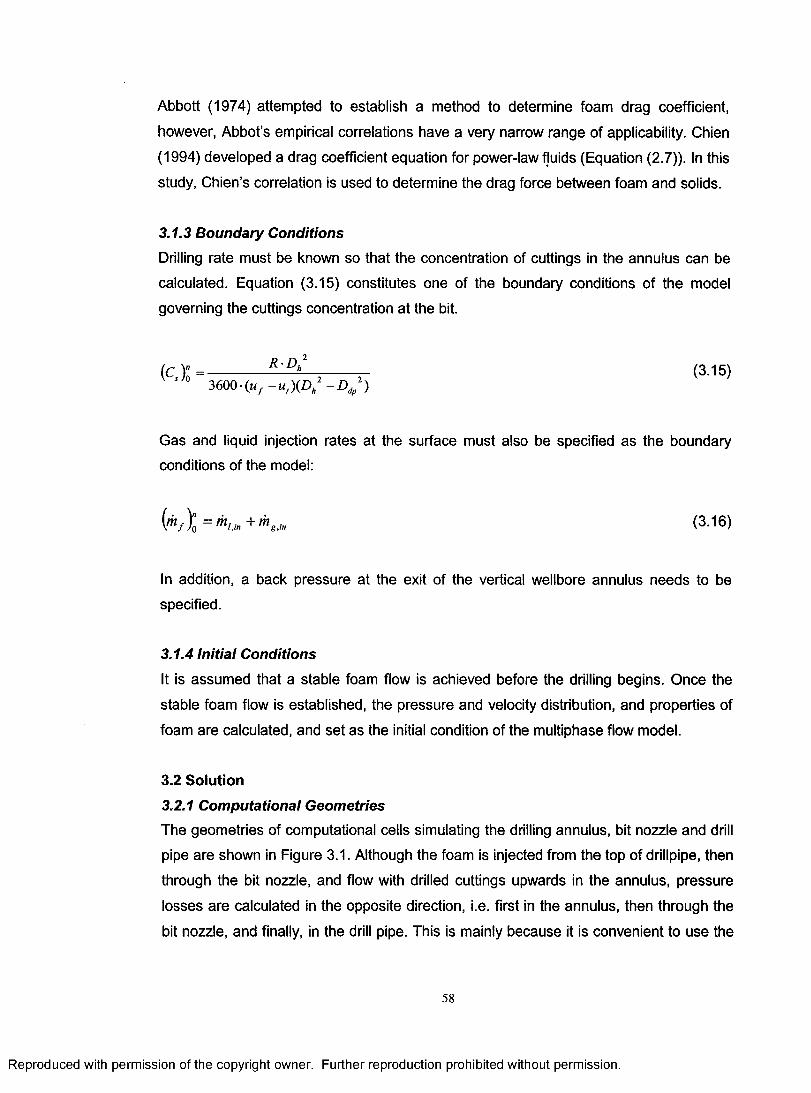
Abbott (1974) attempted to establish a method to determine foam drag coefficient,

however, Abbot’s empirical correlations have a very narrow range of applicability. Chien

(1994) developed a drag coefficient equation for power-law fluids (Equation (2.7)). In this

study, Chien’s correlation is used to determine the drag force between foam and solids.

3.1.3 Boundary ConditionsDrilling rate must be known so that the concentration of cuttings in the annulus can be

calculated. Equation (3.15) constitutes one of the boundary conditions of the model

governing the cuttings concentration at the bit.

Gas and liquid injection rates at the surface must also be specified as the boundary

conditions of the model:

In addition, a back pressure at the exit of the vertical wellbore annulus needs to be

specified.

3.1.4 Initial Conditions

It is assumed that a stable foam flow is achieved before the drilling begins. Once the

stable foam flow is established, the pressure and velocity distribution, and properties of

foam are calculated, and set as the initial condition of the multiphase flow model.

3.2 Solution3.2.1 Computational GeometriesThe geometries of computational cells simulating the drilling annulus, bit nozzle and drill

pipe are shown in Figure 3.1. Although the foam is injected from the top of drillpipe, then

through the bit nozzle, and flow with drilled cuttings upwards in the annulus, pressure

losses are calculated in the opposite direction, i.e. first in the annulus, then through the

bit nozzle, and finally, in the drill pipe. This is mainly because it is convenient to use the

(q \n A ' Uh________sh 3600 ■(uf - u t \ D h1 - D dp1)

(3.15)

(3.16)

58


boundary conditions of the pressure at the outlet, and injection rate of foam at the inlet to

solve the transient foam-solids flow model in the fluid circulating system.

B A C K PRESSURE G A S & L IQ U ID INJ. R A T E

PRESSURE A T D R IL L P IPE

B IT N O ZZL E

B O T T O M H O L E R R E S S U R E

(a) (b)

-#r

i + l -

(C )

Figure 3.1: Flow geometries in drilling annulus, bit nozzle and drill pipe

3.2.2 Foam-Cuttings Flow in Drilling Annulus

Predictions of flowing bottom hole pressure and cuttings concentration along the well

require the numerical solution of equations (3.1)-(3.4) which describe the multiphase

flow in the annulus. Irregular geometry of the annulus is taken care of by using hydraulic

diameter (Appendix C).

Patankar (1980) developed a numerical solution scheme called SIMPLE for single phase

flow by reformulating the continuity equation in terms of pressure. Crowe (1998)

presented a modification of the SIMPLE method to solve steady-state two-phase flow

models. It is generally agreed that a deficiency of SIMPLE method is that it does not

work well for the flow of compressible fluids. However, in this paper, Crowe’s method is

used with some modification to facilitate the convergence of the numerical solution. The

SIMPLE method and the new techniques as applied to the solution of unsteady-state compressible foam flow with and without source term effect is described in Chapter 5.

59


3.2.3 Foam Flow Across Bit Nozzle

The frictional losses and gravity force are negligible in comparison to the acceleration

force when high pressure foam flows through the bit nozzle. Eliminating gravity and

frictional terms, equation (3.3) can be modified into equation (3.17).

Pdp,N ~ Pan,\ + (P fUf )nozz (P fUf )dp,N (3-17)

3.2.4 Foam Flow in Drilling Pipe

Foam flow in the drilling pipe is treated as a steady-state flow of single-phase

compressible fluid in a pipe. The equation (3.18), describing the foam flow in drill pipe,

can be derived from equation (3.3) by equating foam concentration to unity and

changing the sign of gravity term.

The finite difference formulation of equation (3.18) is given as follows:

Pip, = Pdp,M ~AxPf,Mg +r 2 . ^p f uf Ax

2 Du + (P/uf 2)M -(j>f Uf2)i (3.19)

Iterative calculation procedure is required to solve equation (3.19).

3.3 Verification of Model PredictionsAccuracy of the model predictions of flowing bottomhole pressure is verified by using the

data available from the literature. Comparisons are made for two different cases; foam

flow only and foam flow with drilled solids.

3.3.1 Foam Flow

Beyer et al. (1972) presented a model for the prediction of flowing bottomhole pressure

for foam flow in vertical wells. They verified their model by using field data from a “large

well” with 25 cm (9-5/8 in.) casing, 7.3 cm (2-7/8 in.) tubing, and 914 m (3000 ft) depth

which refers to the well geometry normally used in drilling and production-tubing

60


cleanout operations. Beyer et al.’s model underpredicted the flowing bottomhole

pressure by 9%.

The flowing bottomhole pressure predictions of the new model are compared with the

results from Beyer et al.’s model. Figure 3.2 and 3.3 illustrate the bottom hole pressures

predicted from both models for a 914 m (3000 ft) deep vertical well with 18 cm (7 in.)

casing and 7.3 cm (2-7/8 in.) tubing at two different back pressures. In both cases, the

new model predicts an average 5% higher bottom hole pressure than that of Beyer et

al.’s model. Considering the Beyer et al.’s model underpredicts the flowing bottomhole

pressure by 9%, it can be said that new model provides more accurate predictions of

flowing bottomhole pressure for foam flow in vertical wells.

Figures 3.2 and 3.3 also reveal that there is an optimum gas injection rate (~ 4.2

stm3/min or 150 scfm) and any increase in gas injection rate beyond this level has little

effect on flowing bottomhole pressure.

3.3.2 Foam Flow with Cuttings

The model predictions of bottomhole pressure are also compared with data provided by

Okpobiri and Ikoku for foam flow with drilled solids. The input variables included well

depth, drilling rate, back pressure, injection gas and liquid rate. Base data used in this

comparison are listed in Table 3.1.

10000BACK PRESSURE= 0 kPa

ProposedL Beyer etal. (1972)<» 7000

6000 Liquid rate=151 L/min

Liquid rate=76 L/minrate=38 L/min

5 2000

Gas Rate (stm /min)

Figure 3.2: The comparison of bottom hole pressures predicted by proposed model and Beyer et al.’s model

61


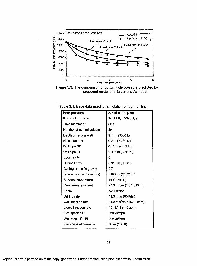
BACK PRESSURE=2068 kPa14000 • Proposed± Beyer etal. (1972)o- 12000

Liquid rate=38 L/minLiquid rate=151 L/min10000

Liquid rate=76 L/min8000

6000

4000

2000

0 3 6Gas Rate (stm3/min)

9 12

Figure 3.3: The comparison of bottom hole pressure predicted by proposed model and Beyer et al.'s model

Table 3.1: Base data used for simulation of foam drilling

Back pressure 276 kPa (40 psia)

Reservoir pressure 3447 kPa (500 psia)

Time increment 50 s

Number of control volume 30

Depth of vertical well 914 m (3000 ft)

Hole diameter 0.2 m (7-7/8 in.)

Drill pipe OD 0.11 m (4-1/2 in.)

Drill pipe ID 0.095 m (3.76 in.)

Eccentricity 0

Cuttings size 0.013 m (0.5 in.)

Cuttings specific gravity 2.7

Bit nozzle size (3 nozzles) 0.022 m (28/32 in.)

Surface temperature 16°C (60 °F)

Geothermal gradient 27.3 mK/m (1.5 °F/100ft)

Foam Air + water

Drilling rate 18.3 m/hr (60 ft/hr)

Gas injection rate 14.2 stm3/min (500 scfm)

Liquid injection rate 151 L/min (40 gpm)

Gas specific PI 0 m2/s/Mpa

Water specific PI 0 m2/s/Mpa

Thickness of reservoir 30 m (100 ft)


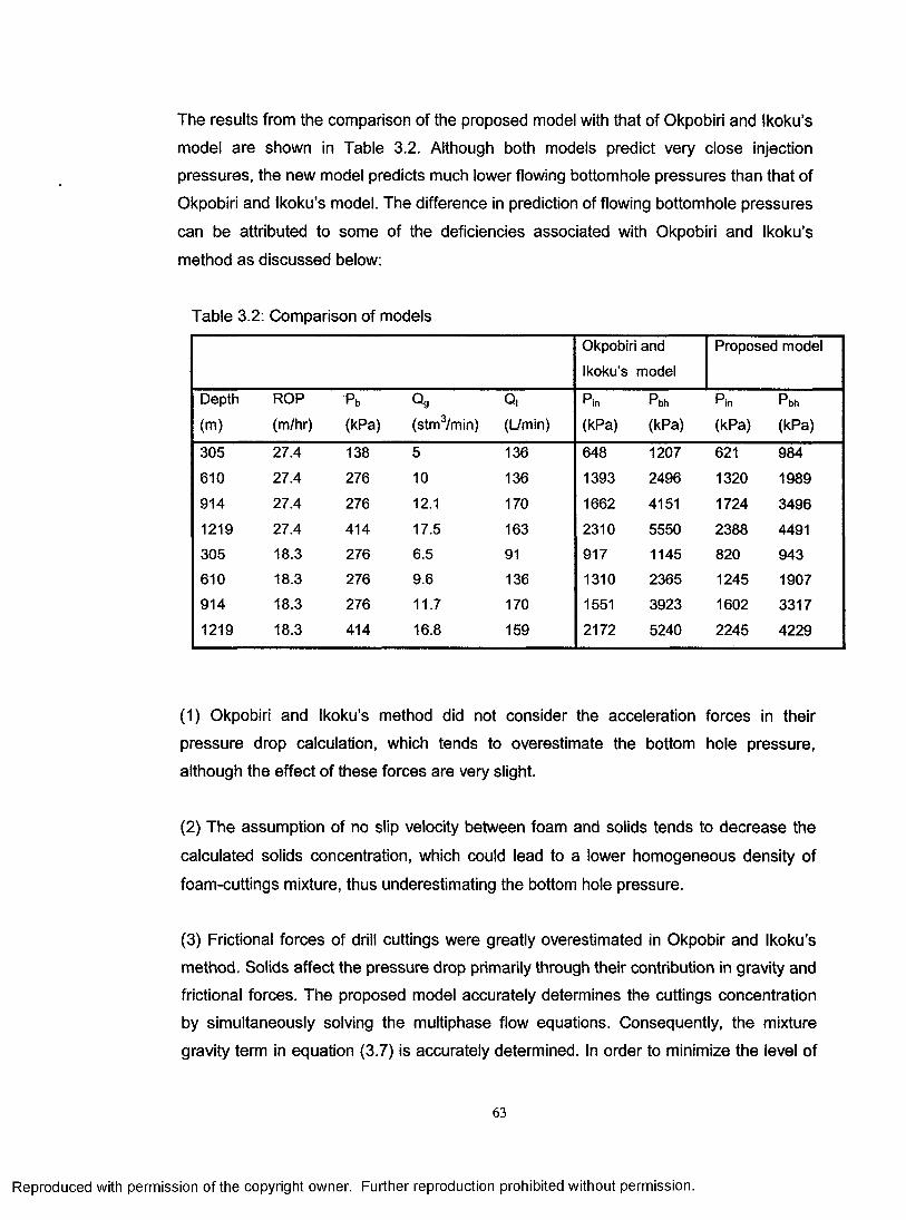
The results from the comparison of the proposed model with that of Okpobiri and Ikoku’s

model are shown in Table 3.2. Although both models predict very close injection

pressures, the new model predicts much lower flowing bottomhole pressures than that of

Okpobiri and Ikoku’s model. The difference in prediction of flowing bottomhole pressures

can be attributed to some of the deficiencies associated with Okpobiri and Ikoku’s

method as discussed below:

Table 3.2: Comparison of models

Okpobiri and

Ikoku’s model

Proposed model

Depth ROP Pb Qg Q. Pin Pbh Pin Pbh

(m) (m/hr) (kPa) (stm3/min) (L/min) (kPa) (kPa) (kPa) (kPa)

305 27.4 138 5 136 648 1207 621 984

610 27.4 276 10 136 1393 2496 1320 1989

914 27.4 276 12.1 170 1662 4151 1724 3496

1219 27.4 414 17.5 163 2310 5550 2388 4491

305 18.3 276 6.5 91 917 1145 820 943

610 18.3 276 9.6 136 1310 2365 1245 1907

914 18.3 276 11.7 170 1551 3923 1602 3317

1219 18.3 414 16.8 159 2172 5240 2245 4229

(1) Okpobiri and Ikoku’s method did not consider the acceleration forces in their

pressure drop calculation, which tends to overestimate the bottom hole pressure,

although the effect of these forces are very slight.

(2) The assumption of no slip velocity between foam and solids tends to decrease the

calculated solids concentration, which could lead to a lower homogeneous density of

foam-cuttings mixture, thus underestimating the bottom hole pressure.

(3) Frictional forces of drill cuttings were greatly overestimated in Okpobir and Ikoku’s

method. Solids affect the pressure drop primarily through their contribution in gravity and

frictional forces. The proposed model accurately determines the cuttings concentration

by simultaneously solving the multiphase flow equations. Consequently, the mixture

gravity term in equation (3.7) is accurately determined. In order to minimize the level of

63


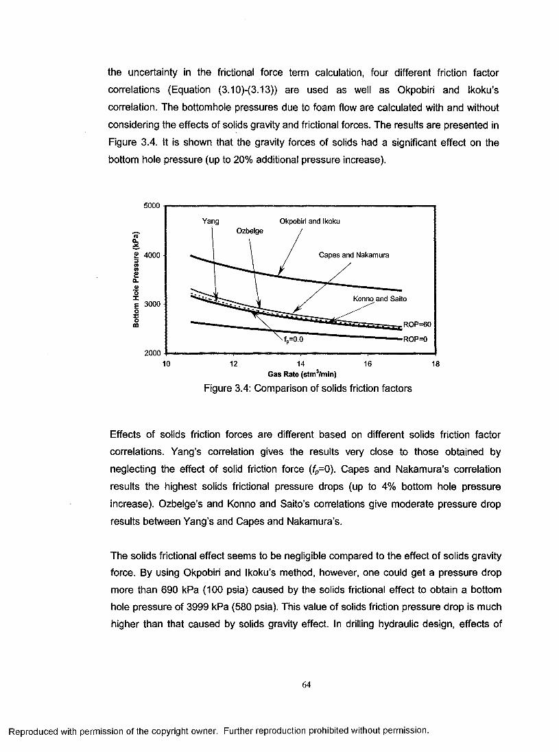
the uncertainty in the frictional force term calculation, four different friction factor

correlations (Equation (3.10)-(3.13)) are used as well as Okpobiri and Ikoku’s

correlation. The bottomhole pressures due to foam flow are calculated with and without

considering the effects of solids gravity and frictional forces. The results are presented in

Figure 3.4. It is shown that the gravity forces of solids had a significant effect on the

bottom hole pressure (up to 20% additional pressure increase).

5000

Yang Okpobiri and IkokuOzbelge

£ 4000 Capes and Nakamura

Konno and SaitoE 3000

ROP=60

f„=o.o ROP=0

200010 12 14 16 18

Gas Rate (stm3/min)

Figure 3.4: Comparison of solids friction factors

Effects of solids friction forces are different based on different solids friction factor

correlations. Yang’s correlation gives the results very close to those obtained by

neglecting the effect of solid friction force (fp=0). Capes and Nakamura’s correlation

results the highest solids frictional pressure drops (up to 4% bottom hole pressure

increase). Ozbelge’s and Konno and Saito’s correlations give moderate pressure drop

results between Yang’s and Capes and Nakamura’s.

The solids frictional effect seems to be negligible compared to the effect of solids gravity force. By using Okpobiri and Ikoku’s method, however, one could get a pressure drop

more than 690 kPa (100 psia) caused by the solids frictional effect to obtain a bottom

hole pressure of 3999 kPa (580 psia). This value of solids friction pressure drop is much

higher than that caused by solids gravity effect. In drilling hydraulic design, effects of

64


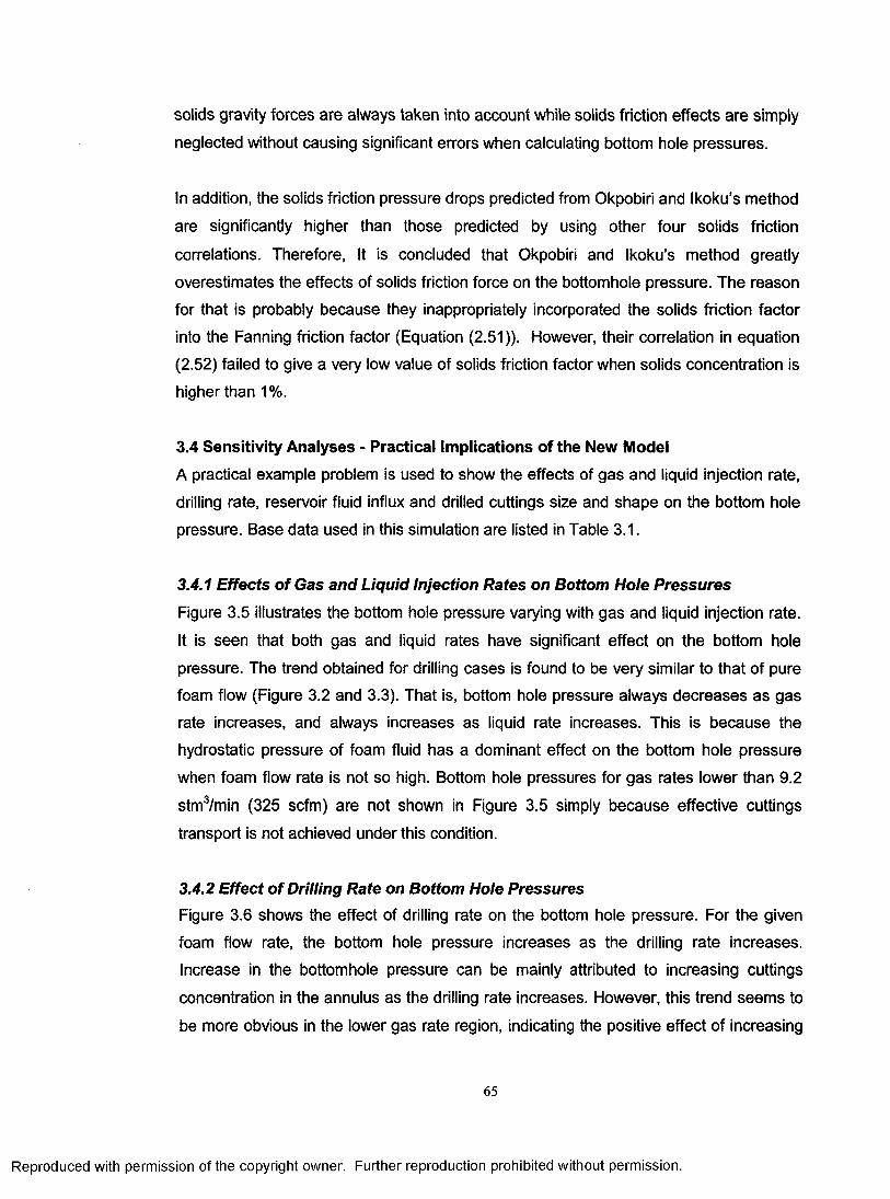
solids gravity forces are always taken into account while solids friction effects are simply

neglected without causing significant errors when calculating bottom hole pressures.

In addition, the solids friction pressure drops predicted from Okpobiri and Ikoku’s method

are significantly higher than those predicted by using other four solids friction

correlations. Therefore, It is concluded that Okpobiri and Ikoku’s method greatly

overestimates the effects of solids friction force on the bottomhole pressure. The reason

for that is probably because they inappropriately incorporated the solids friction factor

into the Fanning friction factor (Equation (2.51)). However, their correlation in equation

(2.52) failed to give a very low value of solids friction factor when solids concentration is

higher than 1%.

3.4 Sensitivity Analyses - Practical Implications of the New ModelA practical example problem is used to show the effects of gas and liquid injection rate,

drilling rate, reservoir fluid influx and drilled cuttings size and shape on the bottom hole

pressure. Base data used in this simulation are listed in Table 3.1.

3.4.1 Effects of Gas and Liquid Injection Rates on Bottom Hole Pressures

Figure 3.5 illustrates the bottom hole pressure varying with gas and liquid injection rate.

It is seen that both gas and liquid rates have significant effect on the bottom hole

pressure. The trend obtained for drilling cases is found to be very similar to that of pure

foam flow (Figure 3.2 and 3.3). That is, bottom hole pressure always decreases as gas

rate increases, and always increases as liquid rate increases. This is because the

hydrostatic pressure of foam fluid has a dominant effect on the bottom hole pressure

when foam flow rate is not so high. Bottom hole pressures for gas rates lower than 9.2

stm3/min (325 scfm) are not shown in Figure 3.5 simply because effective cuttings

transport is not achieved under this condition.

3.4.2 Effect of Drilling Rate on Bottom Hole PressuresFigure 3.6 shows the effect of drilling rate on the bottom hole pressure. For the given

foam flow rate, the bottom hole pressure increases as the drilling rate increases.

Increase in the bottomhole pressure can be mainly attributed to increasing cuttings

concentration in the annulus as the drilling rate increases. However, this trend seems to

be more obvious in the lower gas rate region, indicating the positive effect of increasing

65


gas flow rate on cuttings transport. In other words, the bottom hole pressure at high gas

rate is not so sensitive as the one at low gas rate to the change of drilling rate.

3800

™ 3400

| 30002Q.Oo 2600Eoe£ 2200

1800

189 L/min

151 L/min

114 L/min

9 12 15 18Gas Rate (stm /min)

Figure 3.5: Bottom hole pressure variation with injection gas and liquid rates

3800

“ 3400

2| 3000

CL

0 2600-1Eoo 2200

ROP=27 m/hr

ROP=18 m/hr

ROP=9 m/hr

ROP=0 m/hr

180010 13 16 19

Gas Rate (stm /min)

Figure 3.6: Bottom hole pressure variation with drilling rates

3.4.3 Effect of Water Influx on Bottom Hole Pressures

Figure 3.7 illustrates the effect of reservoir fluid influx on the bottom hole pressure.

Water influx from reservoir instantly decreases foam quality and, therefore, increases the

effective density of the foam which results in an increase in the bottom hole pressure. It

66


should be noted that the increase of bottom hole pressure due to water influx is more

significant at high gas injection rate. A practical implication of this finding is that the

reservoir pressure could be exceeded when high quality foam is used at a relatively high water influx condition.

3800

3600 FORMATION PRESSURE = 3447 kPa3400

Plw=0.0002 m2/s/MPa

Plw=0.0001 m2/s/MPa£ 3200-

3000

« 2800

£ 2600

o 2400

2200

200010 12 14 16 18 20

Gas Rate (stm3/min)

Figure 3.7: Bottom hole pressure variation with water influx

3.4.4 Effect of Gas Influx on Bottom Hole Pressures

The gas influx from reservoir always increases the foam quality in the wellbore, and

therefore, reduces the bottom hole pressure (Figure 3.8). The effect of gas influx is more

significant in the lower gas injection rate region.

3.4.5 Transient Bottom Hole Pressures and Cuttings ConcentrationFigure 3.9 illustrates the transient bottom hole pressure variations at three different

drilling rates. Bottomhole pressure continually increases as a function of time and

reaches a steady state condition. A longer drilling time is needed for the bottom hole

pressure to stabilize as the drilling rate increases. It is important to know the transient

behavior of bottomhole pressure when designing a foam hydraulics program in order to

make sure that the well is drilled at an underbalanced condition.

67


^ 3500 - «TQ.£| 3000 - (0 <A£CL

- I 2500 oX

E o% 2000 - m

1500 ■9 12 15 18

Gas Rate (stm3/min)

Figure 3.8: Bottom hole pressure variation with gas influx

FORMATION PRESSURE = 3447 kPa

PI = 0.0 m2/s/MPa

PL = 0.005 m /s/MPa

Pia = 0.01 m /s/MPa

3200

3100<oa. 3000 ROP = 27 m/hr

2900

8 2800£

ROP = 18 m/hrto£cl 2700

o 2600 xE 2500 oZ 2400 m

2300

ROP = 9 m/hr

22000 10 20 30 40 50 60

Time (min)

Figure 3.9: Transient bottom hole pressure

Figure 3.10 shows the variation of average cuttings concentration in the annulus with

time. Comparison of the Figures 3.9 and 3.10 reveals that the change in bottomhole

pressure as function of time is directly related to change in cuttings concentration in the

annulus as a function of time. It is noted that average solids concentration is a strong

function of the drilling rate at a specific time point.

68


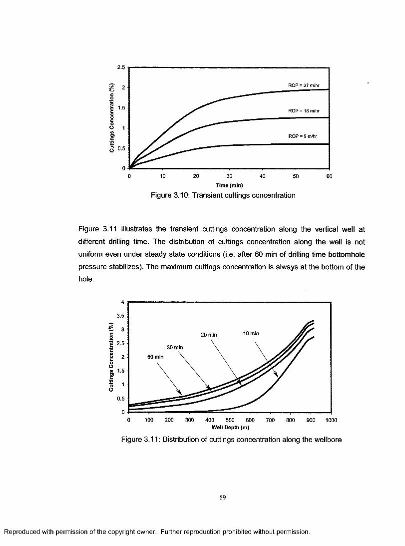
2.5

ROP = 27 m/hr2

1.5 ROP = 18 m/hr

1ROP = 9 m/hr

0.5

00 10 20 30 40 50 60

Time (min)

Figure 3.10: Transient cuttings concentration

Figure 3.11 illustrates the transient cuttings concentration along the vertical well at

different drilling time. The distribution of cuttings concentration along the well is not

uniform even under steady state conditions (i.e. after 60 min of drilling time bottomhole

pressure stabilizes). The maximum cuttings concentration is always at the bottom of the

hole.

3.5

10 min20 min2.5

30 min

60 min

1.5o>

0.5

0 100 200 300 400 500 600 700 800 900 1000Well Depth (m)

Figure 3.11: Distribution of cuttings concentration along the wellbore

69


3.4.6 Effects of Cuttings Size and Shape on Bottom Hole PressuresResults shown in Figure 3.12 indicate that larger cuttings size yields a higher cuttings

concentration. Therefore, assumption of uniform cuttings size is expected to generate

some error in the model predictions.

Figure 3.13 shows that cuttings with irregular shapes (i.e., lower sphericity) lead to lower

cuttings accumulation. Therefore, assumption of uniform spherical (=1) cuttings shape

may lead to overprediction of cuttings concentration.

2.5

ds= 1.52 cm

ds= 1.27 cm

ds = 0.75 cmo>

0.5

0 10 20 30 40 50 60Time (Min)

Figure 3.12: Effect of cuttings size on cuttings concentration

1.6

1.4 Sphericity = 1.0

Sphericity = 0.6

Sphericity = 0.2

0.8

0.6o>0.4

0.2

0 2010 30 40 50 60Time (Min)

Figure 3.13: Effect of cuttings shape (sphericity) on cuttingsconcentration

70


CHAPTER 4

NUMERICAL MODELING OF CUTTINGS TRANSPORT WITH FOAM IN

HORIZONTAL WELLS

A one-dimensional, unsteady state model is developed to simulate cuttings transport

with foam in horizontal wells. The model is solved numerically to predict cuttings bed

height as a function of the drilling rate, the gas and the liquid injection rates, the rates of

gas and liquid influx from the reservoir, and the borehole geometry.

Sensitivity analyses are conducted to investigate effects of key drilling parameters (i.e.

gas and liquid injection rates, drilling rate, wellbore geometry, cuttings size, formation

fluid influx, etc.) on the efficiency of cuttings transport with foam in horizontal wells.

The detailed description of the model development, numerical solution, verification of the

model predictions using experimental data, and results of sensitivity analyses study are

presented in this Chapter.

4.1 Model DevelopmentA two-layer model is developed in order to study factors affecting cuttings transport with

foam in horizontal wells. This approach has been originally used for modeling of slurry

transport in pipes (Doron, 1987; Shook et al., 1991; Wilson, 1976). Several studies in

petroleum drilling engineering on cuttings transport modeling have also used the two-

layer modeling approach (Clark and Bickham, 1994; Gavignet and Sobey, 1989; Kamp

and Rivero, 1999). Existence of layers in the form of stationary beds and heterogeneous

suspension of cuttings have been verified by many experimental studies (lyoho, 1980;

Ford et al., 1990; Luo et al., 1992).

A schematic view of two-layer model for foam-solids flow in a horizontal well is shown in Figure 4.1. The upper layer consists of a foam-cuttings mixture with a low solids

concentration, while the lower layer consists of a stationary bed of cuttings with foam

entrained in the pores.

The following assumptions are made to simplify the case:

(1) Foam is a fluid with a homogeneous property at any cross-sectional area of the well.

71


(2) Drill cuttings have uniform size, shape and velocity at any cross-sectional area of the well.

(3) Formation fluids flowing into the wellbore mix with foam completely.

(4) Influx fluid is accelerated to the mean stream velocity instantaneously.

Formation Influx

Upper LayerMass Transfer

Stationary Bed

t t t t t t t t t t t t t t tFormation Influx

Figure 4.1: Schematic view of two-layer model for cuttings transport

with foam in horizontal wells

4.1.1 Conservation of Mass and Momentum EquationsBased on the mass balance and force balance of foam and solids in a control volume,

the continuity and momentum equations for these two phases are derived. The details of

the derivation are given in Appendix B. Equations (4.1) and (4.2) are the continuity

equations representing conservation of mass for foam and drilled solids, respectively.

-Qj(AoCfP f) + -j£(AoCfP fU f) = Ao(sf - t e f ) (4.1)

£ (A ,C lP l) + £ ( A .C 1p ,u ,)= -A .A s . (4.2)

In equations (4.1) and (4.2), Asf and Ass represent the rates of change of mass of foam

and solid particles per unit volume of the wellbore due to the mass transfer between

layers. Asf and Ass can be determined by using equations (4.3) and (4.4) respectively.

72


where Cb is the concentration of solids in the stationary bed (= 0.52 for cubic packing).

Foam mass flow rate in the upper layer would also be affected by the influx of formation

fluids due to the underbalanced drilling condition (i.e. reservoir pressure is higher than

flowing bottomhole pressure). Mass influx rates of water, oil and gas from the reservoir

per unit volume of the wellbore can be determined by using equations (4.5), (4.6) and

(4.7) respectively.

s PwP Iw(Pre~P) ( 4 5)

PgPIgiPre-P) (4 6)A.

s __PgPIg(Pre~P) (47)

where PI is the specific productivity index, the ratio of volumetric flow rate of formation

fluid per unit horizontal well length and pressure drop between reservoir and wellbore.

The total mass influx from the formation into the wellbore is then given by equation (4.8).

sf = sw+ so+sg (4-8)

Momentum equations for foam and solid phase flowing in horizontal wells are given by

equations (4.9) and (4.10), respectively.

73


Qt {A0Cf P f U f ) + 0x i^oCfPfUf )~ C f Qx A J v (Uf Mj) 2 C f- f fP f u f S0 (4.9)

^ y oCspsu M ^ 0Cspsu ;)= -C s^ l + A0P M f - u s) - \ c j spsus2S0 (4.10)

4.1.2 Critical Deposition Velocity Criteria

The foam velocity must be higher than the critical deposition velocity to convey the

cuttings in suspension. If the foam velocity falls below the critical value, a cuttings bed

forms, and the foam velocity begins to increase in the partially blocked pipe until it

attains the critical value. If the foam velocity is higher than critical velocity, cuttings will

be re-suspended into the flow stream, and the bed height will be decreased until the

dynamic equilibrium condition is achieved.

Shook et al. (1994) suggested that the most suitable critical velocity correlation for high

viscosity liquids is the one from Oroskar and Turian (1980). Shook et al. used Oroskar

and Turian’s correlation (Equation 4.11) to predict the head loss for both laminar and

turbulent flow and concluded that there was a close agreement between the observed

and predicted results.

where jyRe is a modified Reynolds number defined by equation (4.12):

^ = — Jgd,(— ~ 1) <4-12>p V Pf

Shah and Lord (1990) confirmed that this correlation is applicable for solids transport in

a horizontal pipe by using non-Newtonian fluids.

:1.85CJa,I36( i - C J) 0.3564r , n -0.378

(4.11)

In order to introduce the annular geometry into the critical deposition velocity correlation,

a hydraulic diameter that is defined in Appendix C is used to replace pipe diameter, D, in

equations (4.11) and (4.12). Note that the effective viscosity of foam should be used in

equation (4.12). The effective viscosity of power law fluids is given as follows:

74


M e = K3n + l

An

\ n 8 m ,N«-l

(4.13)

Experimental data published by Martins et al. (2001) are used to verify the applicability

of Oroskar and Turian’s critical velocity correlation in modeling of cuttings transport with

foam. The parameters used in Martins et al.’s experiments included pipe length (12 m),

hole diameter (0.1 m), inner pipe OD (0.042 m), eccentricity (1.0), cuttings size (0.6 cm),

cuttings density (2.6 g/cm3), liquid flow rate (20 and 30 L/min), and gas flow rate (60 to

500 L/min). The comparison of the model predictions of dimensionless cuttings bed

height with Martin et al.’s experimental results is shown in Figure 4.2.

SZO)*55X*o4)CD(A<A4)Co’5>c4)£5

0.8

0.6

0.4 -

s 0.2

q(=30 L/minq,=20 L/min

(Data from simulation)

▲ A

A□ □

Oql=20 L/min (data from ref. 86)

A ql =30 L/min (data from ref. 86)

50 100 150 200Gas Rate (L/min)

250 300 350

Figure 4.2: Model prediction of cuttings bed using Oroskar and Turian’s critical deposition velocity correlation

Figure 4.2 shows that the use of Oroskar and Turian’s correlation results in

overpredictions of cuttings bed heights. The difference between the predicted cuttings

bed heights and measured ones is more pronounced at higher gas flow rates. This phenomenon suggests that increasing gas flow rate (or foam quality) decreases cuttings

bed height, however, the effect of foam quality is not included in Oroskar and Turian’s

model. Since the foam quality influences the efficiency of cuttings transport, it needs to

be somehow incorporated into the critical deposition velocity models. Therefore, a new

75


correlation of critical deposition velocity for cuttings transport with foam is proposed as

follows:

*V = « C/ - ( 1 - ] T (4.14)

where ucf is the critical deposition velocity in foam, ucl is the critical deposition velocity

for a liquid, and <ris foam critical deposition velocity index that represents the extent of

the deviation of the critical velocity in foam from the one in liquid.

Based on Martins et al.’s experimental data, it is found that the foam critical deposition

velocity index, a, increases with the increasing liquid flow rate if Oroskar and Turian’s

correlation is used for ucl in equation (4.14). When liquid flow rate is 20 L/min, a

approximately is equal to 0.2, and a becomes very close to 0.3 as liquid flow rate is

increased to 30 L/min. The simulation results using the modified foam critical deposition

velocity correlation are shown in Figure 4.3, which indicates a good agreement between

the predicted and observed cuttings bed height.

qi=30 L/min (o = 0.3)

□ ql=20 L/min (data from ref. 86)

Aql=30 L/min (data from ref. 86)n °'8 o>d>

I 0.6

CO0§ 0.4*55c0)| 0.2

A A

0 50 100 150 200 250 300 350Gas Rate (L/min)

Figure 4.3: Model prediction of cuttings bed using modified foam deposition velocity correlation

The foam critical velocity index, a, does not seem to be influenced by gas flow rates.

However, a is found to be a strong function of the liquid phase flow rate. A logarithmic

relationship between <rand liquid superficial velocity is suggested as follows:

76


a = 0.2466 -ln (w ;) + 0.9314 (4.15)

4.1.3 Boundary Conditions

Cuttings concentration at the drilling bit is determined from drilling rate, R.

(C )" = ---------R'D"2_____ (4.16)3600 • uf (Dh - D dp )

Gas and liquid injection rates must be specified as the boundary conditions of the model:

(mf )no =m Un +mgJn (4.17)

Solution of the problem also requires definition of a back pressure at the exit of the

horizontal wellbore section away from the bit.

4.1.4 Consideration For Wellbore Geometry

Complex wellbore geometry due to the drillpipe eccentricity is taken into account in the

solution of the problem. Considering the relative position of the drillpipe and drilling

fluid/cuttings bed interface, Campos (1995) provided a set of analytical geometry

equations to define the area occupied by the cuttings and fluid in the annulus. In this

study, a modified version of the Campos’ equations is used to define the annular

geometry (Appendix C).

4.1.5 Cuttings Bed Height Prediction

A trial-and-error technique is used to determine the cuttings bed height, hb. Initially,

foam velocity, uf, and cuttings concentration, Cs are determined assuming fully suspended flow of cuttings. The critical velocity, uc, for cuttings’ deposition is then

calculated and compared with uf. If uc is greater than uf then a cuttings bed forms. An

increase in cuttings bed height would influence the flow behavior in the upper layer by

(1) narrowing the upper flow channel area, and (2) reducing the mass flow rate of solid

particles and foam in the main flow stream. In response to the first change, the open flow

area and hydraulic diameter are re-calculated. In response to the second change, the

77


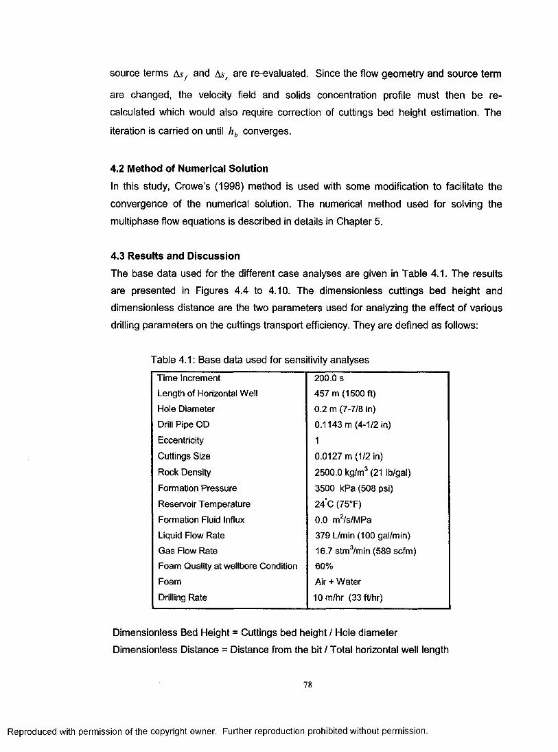
source terms Asf and Ass are re-evaluated. Since the flow geometry and source term

are changed, the velocity field and solids concentration profile must then be re

calculated which would also require correction of cuttings bed height estimation. The

iteration is carried on until hb converges.

4.2 Method of Numerical SolutionIn this study, Crowe’s (1998) method is used with some modification to facilitate the

convergence of the numerical solution. The numerical method used for solving the

multiphase flow equations is described in details in Chapter 5.

4.3 Results and DiscussionThe base data used for the different case analyses are given in Table 4.1. The results

are presented in Figures 4.4 to 4.10. The dimensionless cuttings bed height and

dimensionless distance are the two parameters used for analyzing the effect of various

drilling parameters on the cuttings transport efficiency. They are defined as follows:

Table 4.1: Base data used for sensitivity analyses

Time Increment 200.0 s

Length of Horizontal Well 457 m (1500 ft)

Hole Diameter 0.2 m (7-7/8 in)

Drill Pipe OD 0.1143m (4-1/2 in)

Eccentricity 1

Cuttings Size 0.0127 m (1/2 in)

Rock Density 2500.0 kg/m3 (21 lb/gal)

Formation Pressure 3500 kPa (508 psi)

Reservoir Temperature 24 C(75°F)

Formation Fluid Influx 0.0 m2/s/MPa

Liquid Flow Rate 379 L/min (100 gal/min)

Gas Flow Rate 16.7 stm3/min (589 scfm)

Foam Quality at wellbore Condition 60%

Foam Air + Water

Drilling Rate 10 m/hr (33 ft/hr)

Dimensionless Bed Height = Cuttings bed height / Hole diameter

Dimensionless Distance = Distance from the bit / Total horizontal well length

78


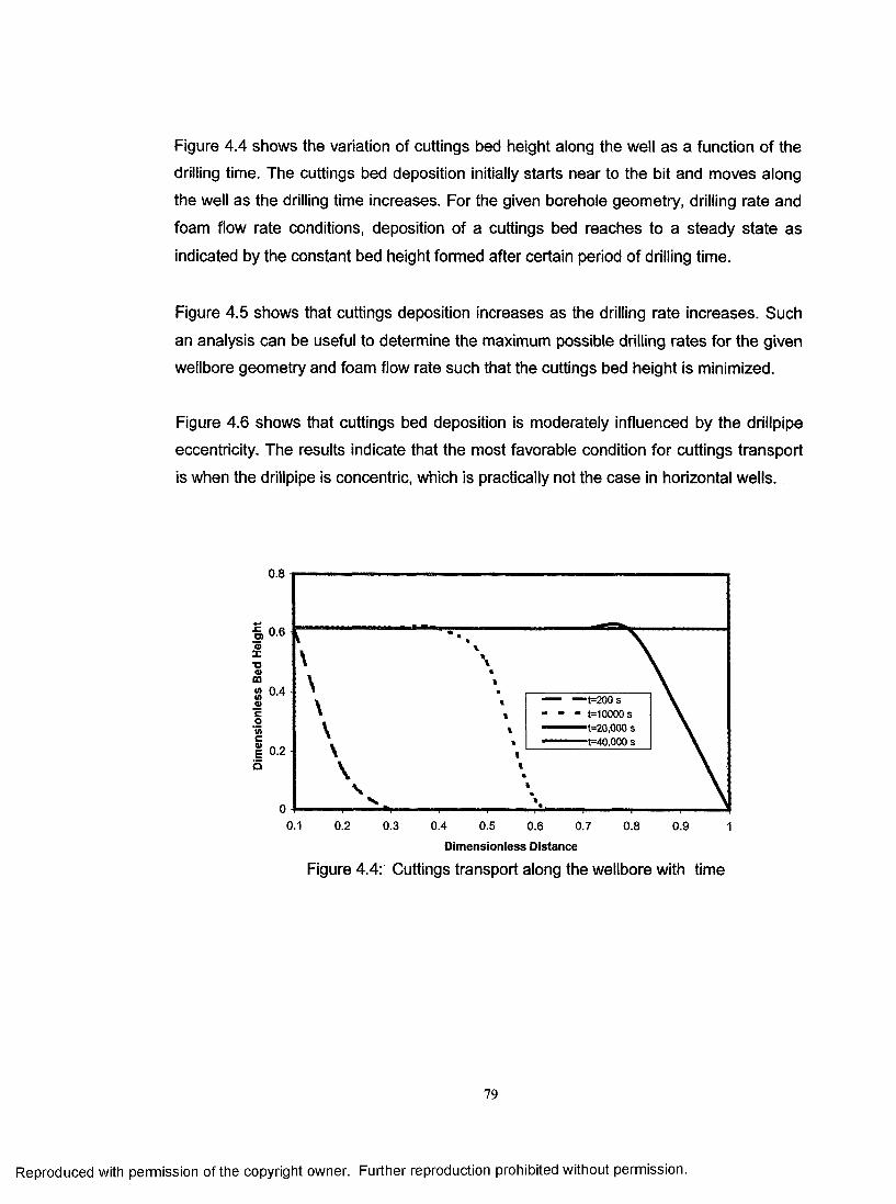
Figure 4.4 shows the variation of cuttings bed height along the well as a function of the

drilling time. The cuttings bed deposition initially starts near to the bit and moves along

the well as the drilling time increases. For the given borehole geometry, drilling rate and

foam flow rate conditions, deposition of a cuttings bed reaches to a steady state as

indicated by the constant bed height formed after certain period of drilling time.

Figure 4.5 shows that cuttings deposition increases as the drilling rate increases. Such

an analysis can be useful to determine the maximum possible drilling rates for the given

wellbore geometry and foam flow rate such that the cuttings bed height is minimized.

Figure 4.6 shows that cuttings bed deposition is moderately influenced by the drillpipe

eccentricity. The results indicate that the most favorable condition for cuttings transport

is when the drillpipe is concentric, which is practically not the case in horizontal wells.

0.8

o> u u*3XT3a>CQ8 04 ® c o

“ —-t=200 s - - t=10000s

t=20,000 s t=40,000 s| 0.2

a

0.1 0.2 0.3 0.4 0.5 0.6 0.7 0.8 0.9 1Dimensionless Distance

Figure 4.4: Cuttings transport along the wellbore with time

79


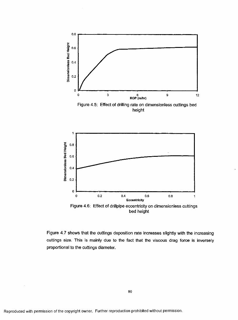
0.8

0.6

0.4

0.2

0 3 6 9 12ROP (m/hr)

Figure 4.5: Effect of drilling rate on dimensionless cuttings bedheight

0.8 -

x(8 0.6<A0)©o 0.4 '#> c 0>E5 0.2

0 0.2 0.4 0.6 0.8 1Eccentricity

Figure 4.6: Effect of drillpipe eccentricity on dimensionless cuttingsbed height

Figure 4.7 shows that the cuttings deposition rate increases slightly with the increasing

cuttings size. This is mainly due to the fact that the viscous drag force is inversely

proportional to the cuttings diameter.

80


1

o ----------- ---------—, ...... ...............1-------- - I ----------- ------------0 0.002 0.004 0.006 0.008 0.01 0.012 0.014

Cuttings Diameter (m)

Figure 4.7: Effect of cuttings size on dimensionless cuttings bed height

Figure 4.8 shows that the cuttings bed height decreases as the foam quality increases

when the liquid rate is kept constant. The increasing foam quality is expected to increase

the flow rate and the effective viscosity of the foam, which enhances the cuttings transport.

0.8

~ 0.6T3

M 0.4

0.6 0.650.55 0.7 0.75 0.8Foam Quality

Figure 4.8: Effect of foam quality on dimensionless cuttings bed

Figure 4.9 shows that as the total foam flow rate increases, the cuttings bed height

decreases. However, for the given wellbore geometry and drilling rate conditions, there

is an upper limit for total foam flow rate that can be injected without exceeding the flowing bottomhole pressure limits set in order to achieve underbalanced condition.

81


0.8

s: at ® 0.6

0.2

1000800 900 1100 1200 1300 1400 1500 1600Foam Flow Rate at Wellbore Condition (L/min)

Figure 4.9: Effect of foam flow rate on dimensionless cuttingsbed height

Figure 4.10 shows that the gas influx from the reservoir enhances cuttings transport

efficiency. This is mainly due to the increase in foam quality with the addition of

formation gas and /or increased total flow rate.

The effect of water influx into the wellbore is shown in Figure 4.11. It is seen that liquid

influx causes a decrease in cuttings bed height. This behavior can be attributed to the

fact that foam density and flow rate are increased with the addition of formation water

influx.

0.8

m‘/s/Mpa Pl=0.00002 m2/s/Mpa

Pl=0.00004 m2/s/Mpa

0.4 0.5 0.6 0.7Dimensionless Distance

Figure 4.10: Effect of formation gas influx on dimensionlesscuttings bed height

82


0.7

^ 0.65JC O)’3= 0.6 TJ <1)CO

8 0.55J3>Coc ^0)£5 0.45

0.40.1 0.2 0.3 0.4 0.5 0.6 0.7 0.8 0.9 1

Dimensionless Distance

Figure 4.11: Effect of formation water influx on dimensionlesscuttings bed height

T “ « "Z T Z “ — —

.................................. ...................................

m2/s/M pa— - — PI0.00001 n^/s/Mpa- - - Pl=0.00002 nf/s/M pa^*****^*131=000003 m2/s/M pa

83


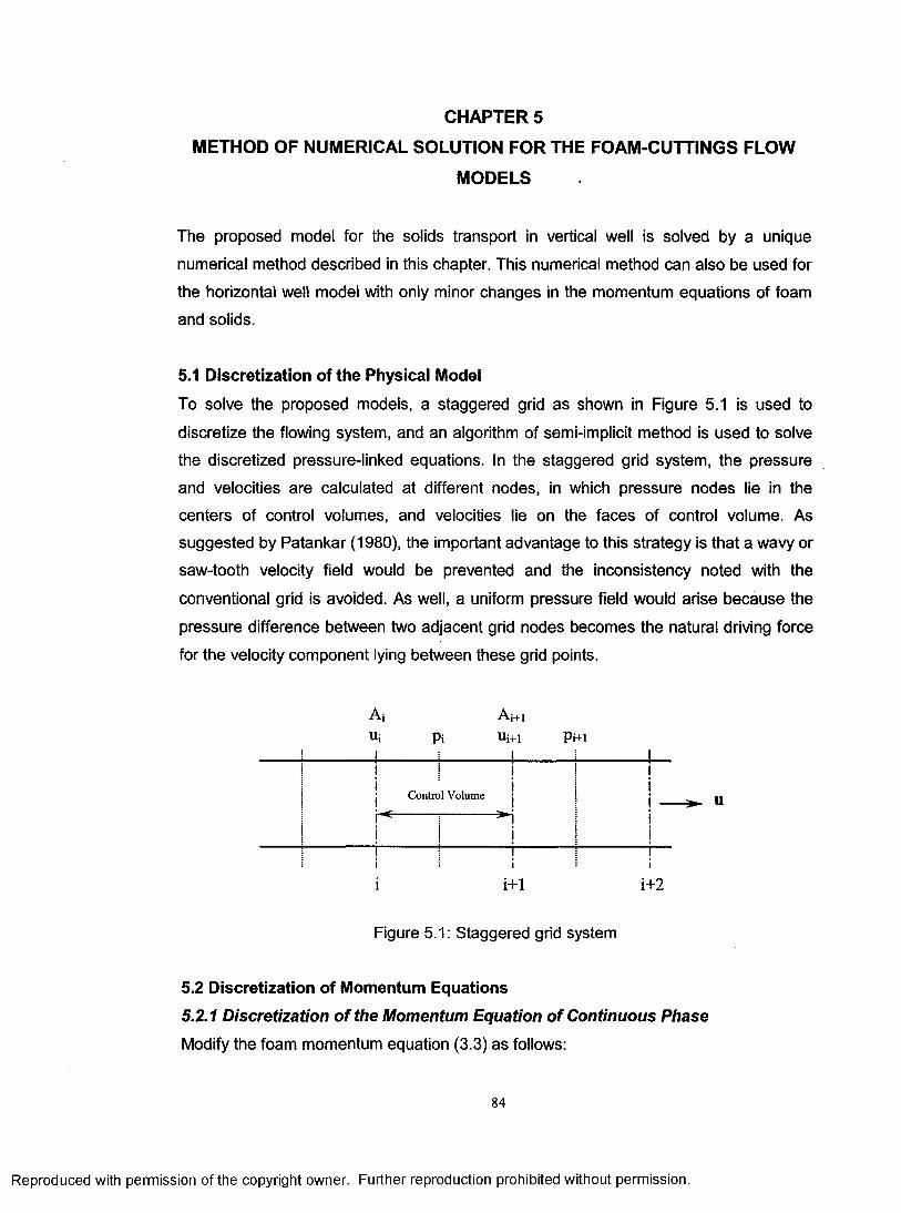
CHAPTER 5

METHOD OF NUMERICAL SOLUTION FOR THE FOAM-CUTTINGS FLOW

MODELS

The proposed model for the solids transport in vertical well is solved by a unique

numerical method described in this chapter. This numerical method can also be used for

the horizontal well model with only minor changes in the momentum equations of foam

and solids.

5.1 Discretization of the Physical ModelTo solve the proposed models, a staggered grid as shown in Figure 5.1 is used to

discretize the flowing system, and an algorithm of semi-implicit method is used to solve

the discretized pressure-linked equations. In the staggered grid system, the pressure

and velocities are calculated at different nodes, in which pressure nodes lie in the

centers of control volumes, and velocities lie on the faces of control volume. As

suggested by Patankar (1980), the important advantage to this strategy is that a wavy or

saw-tooth velocity field would be prevented and the inconsistency noted with the

conventional grid is avoided. As well, a uniform pressure field would arise because the

pressure difference between two adjacent grid nodes becomes the natural driving force

for the velocity component lying between these grid points.

Ai Ai+iU i P i U i+ i P i+ i

I I 1

Contrc 1 Volume--------^ u

ji

i i+1 i+2

Figure 5.1: Staggered grid system

5.2 Discretization of Momentum Equations5.2.1 Discretization of the Momentum Equation of Continuous Phase

Modify the foam momentum equation (3.3) as follows:

84


j - (A C f P f uf ) + j - ( m f uf ) = -Cf A ^ - - A / ] v(uf - u s) - A C f pf g - ^ - f M/ C ~ - f (5.1)

Replacing the derivatives by forward difference approximation implicitly, we get the

numerical expression for equation (5.1) at node i+1 and time step n+1:

(ACf p f uf ) i+l (ACf p f uf ) M (mf uf ) M (mf uf ) i _ +) p"+l - p * ** ” V “'/A J |+ 1At Ax 1 1+1 Ax

■u/},)::: - u c / / v g );*[ <5 .2)

Rearranging equation (5.2) yields:

{AcfP f ) t i + k ) ; : ; + a * ( ^ x . ' + k / m / ^ ) ; ; 11 = ( * / );+, ^ + ( * / «/ ) rV , y,+1 2 D h j

v n + 1 / . , n+1 . * « + l \ / A S '' ^ i a n \ n + l „ „ n + 1+ (Cf A ) ^ ( Pr - p : : il ) -A x - (A C f p f g ) ^ + Ax(Afiv) ^ (5.3)

Setting

-t n+1 Ax

At

Ax

2Dl )■n+1 i+l (5.4)

Then

n+1 =//+1 77 n+lE f i+1 L

Ax( i» /« / ) r + ( * / ) « — +(C/ y4)";i'( Pr )-(4x4C /P /g ) ^ +A x (A P X : <

n+1 n+1/+!

(5.5)

For convenience, equation (5.5) is expressed as:

( C /C»"+1n+1 _ n+1 [ V / J i+l y „n+1 „« + l\“ /;+! “ 2„,i+1 + ^ „+1 (Pi P/+I )£

(5.6)/ / + i

85


where

{t*ACf pfg)^+te(APX (5 .7 )

It should be noted that the gravity term, (axACf p f g), in equation (5.7) must be removed

for the horizontal well flow.

5.2.2 Discretization of the Momentum Equation of Dispersed Phase

The discretized momentum equation for the dispersed phase is obtained by the similar

numerical technique:

(5.8)

Rearranging equation (5.8) yields:

*±{AC,p,)% + { m X l + A x (^ X +11

+ (C,A)%(p?« - p £ ) - ( A x A C sp,g)% +Ax(Aj3v)

= ^ 7 ■ (« ,);♦ .+ (*,o r 1At

(5.9)

Setting

(5.10)

Then

^ ■' H 1 , , n+1E s i+ 1 V

^ ) ”+1 + T : < » X . + ( C sAyi: l ( p r l - p $ ) - ( * x A C , p , g ) % +Ax(A/3v)

(5.11)

86


For convenience, the equation is expressed as:

(5.12)

where

\

J(5.13)

It should be noted that the solids gravity term, (AxACspsg) , in equation (5.13) must be

removed for the horizontal well flow.

5.3 Formulation of Velocity-Correction EquationsThe biggest complexity in the calculation of velocities lies in the unknown pressure field

because the pressure gradient forms a part of the momentum equations. Patankar

(1980) developed a SIMPLE method to overcome this difficulty for a single-phase fluid.

Later, this method is applied to two-phase flow (Crowe, 1998). In the SIMPLE method, a

guessed pressure field is given at first, and the momentum equation is then solved to

obtain the velocity field. This resulting velocity field will not satisfy the continuity equation

unless the correct pressure field is used, so an equation to correct the guessed pressure

field by using the resulting velocity field is needed in the iteration. This pressure-

correction equation can be obtained by substituting the velocity-correction formula into

the continuity equation. Therefore, the velocity-correction equations are formulated firstly

from the momentum equations for both phases.

Assuming that velocity is a function of pressure gradient only, i.e. a function of the two

pressures on each side of the velocity node, one has:

u (5.14)

(5.15)

87


When pressure changes take place at nodes i and i+1, the corresponding velocity

changes can be estimated by applying Taylor series expansion to the velocity-pressure functions:

d n +1 n + \U r , , C U

Au f n + = — ^ - A p , * +I + — (5-16)/ , +i dp*+\ dp.+\ 1

n+1 n + 1A . . ,I+1 _ O U s i + 1 a _ " + 1 . O U s i + 1 a _ « + 1 ^ 1 7 ^

A“ -“ - ~bpU T " 1 ’

Taking the indicated derivatives of equations (5.6) and (5.12), we obtain:

du ri l l ( C f A) t fw e / m

( c , a ) $, fi +1 n +1

' / i+idp? :1 E

and

dus:; i ( c sA ) i : i

w " e s il l

dusill _ (c ,A

(5.18)

(5.19)

(5.20)

(5.21)

Substituting equations (5.18) to (5.21) into equations (5.16) and (5.17), the velocity-

correction formulas for both phases at node i+1 are derived:

a - , : ; ; = - a / o <5-22>E, (//+!


= (C;^ F ' (A p r 1 - * P; : ! ) (5 .23 )-^i+l

Applying equations (5.22) and (5.23) to the velocity changes at node i yields:

A " / ," ' ° (r 5 (ApT-V - A p r1) (5.24)E f ,

A x .r ' = (C: ^ F '-( Ap-V - Ap,"*1) (5.25)E_.

In addition, the mass flow rate of inflow from reservoir changes with wellbore pressure

as follows:

A (5-26)

where C' is a constant calculated from the reservoir inflow model.

5.4 Discretization of Continuity EquationsThe next step is to discretize the continuity equations for foam and solid phases:

{ A C f P f ) Z l - ( A C f P f yM | ( A C f p f u f )Hl - (A C f p f u f )1+x (g 2?r)

At Ax f 1+1

(ACS)%-(ACX> , UCsuX l-(A Csus) f Q (5 28)At Ax

Then the concentrations (volume fractions) for the carrier phase and carried phase are

derived:

c "+1

A vA x ( A s f ):: t + { A C f P f u f )1+x + ^ A C f P f yM

+ ( A p f uf ) %At

89

(5.29)


5.5 Formulation of Pressure-Correction EquationIt is assumed that the concentration at node i+1 is a function of velocities at node i and

i+1 and source term, so the concentration change for each phase can be estimated by

the expansion of a Taylor series:

C = c * A „ A m Af M /i+1 d u r 1 d u f 1+1 dsf M

J i J i + 1 / i+ l

(5.31)

n+1 n+1

r< n+1 _ r ' * n+x , i / + l a . . n + 1 , * i+ l a . . n + 1

C „ + l ~ C s M + — „+- | A » „ + T n + T M J/+1

f a s t d U s M

(5.32)

where the superscript * represents the value from the previous iteration. Taking the

indicated derivatives of the function of concentration and velocity in equations (5.29) and

(5.30), the following equations are obtained:

8C

du

n + 1

f i'+l _n + 1 ~

( ACf P f )T x

f i AxAt

(5.33)( A P / ) £ + ( A P / u f ) £

dC

du

n + 1

/ i + 1 n + 1

/i+i

(AP f Y,:iAx

Ax (As f yt: i + (ac fP fU fy r + — (A c f P f yM(5.34)

A y

^ - ( A P f y :; + (AP fU f) z l

6C

dsf i+1

n+1

/ i + 1

A x (5.35)f U f \ n+1

) i+l

90


d C "+1u^si+i n +1

( a c s):«+i

Ax

A t

(5.36)( A ) £ + (Au, ) %n + 1

8C "+1Sj + 1 n +1

dusi+1

A y

( A c sus) r + ^ ( A c s):+lA t

a ;n+1i+1

AxA t + ( o ;++11

(5.37)

The final equation that needs to be discretized to complete the set of momentum and

continuity equations is that the sum of concentrations equals to unity:

c fn+x + c X! = i/i+l (5.38)

Substituting equations (5.31) and (5.32) of concentrations of foam and solids into

equation (5.38) yields the following equation:

/i+i +-du

n+1 f i r n+I n+1 n+1

au™ +— % a Ufn+! +— ^ r ASfr‘+! +c:::: + ~ ^ r A«?+i =\n+1 f i

f ia . n+1 / i+ 1 ' n+1 iJ J / i + 1 r V 'v 1+1 ' ~ n+1 “ " s i ' - n+1 ,_“ *s i+ louf t as, , du,. du

/ i+ 1 / i+ 1 Si S i+ l

(5.39)

Substituting equations (5.22) to (5.26) and (5.33) to (5.37) into equation (5.39), we

obtain the pressure-correction equation:

(AC f P jY i«+l (c f A ) r iA y r * /IH

— (A P / ) X + ( A p f uf )% E f i(APr ; - APr ) -

(APf):;;A v

Ax(Asf ) £ +(rhf )"+1 + — (AC f P f ) r

A x , , „ n + ] . n+1— (+4p/ ) '!+7 + ( A p f u f ) r

C ’AxA y aPm + ( ^ ) r

'/i+i

( c ^ ) -

(A ^ +i - a k +v ) -

(A^V - A pD -n+ . >A y

— (A )r :+ (A us) i iAt

p n+1 n+1 E e .Sl

91


A y

(ACsus) f + =-UC,YMAt

AnSi;, Ax ,

At + (« X .

(CsA) m (A «+ir, n+1 V * 1si+\

- A p £ ) = l - C Z - Cn+l

/ i + 1

(5.40)

or in a more compact form:

L f a p z - { i f + u f ) A p r x + ( u r l - r 1) ^ 1 = i - c . - c , (5-41)

where

(AcfPlr« (c,A)r (ac,r r (c. )r1 i5.42)i Ay |-« «+l A y

= -{A P f) i z + £ /,- -T7 w ; , 1+At At

si

(APt)%u v

A-v*

At( A p X ! +(Ap/ u/ ) l >

(c,4%

"/(+1

A y

(4C,«x' +-rM cX *At ic5A)nt:i

At+ (uX

(5.43)

T:n+lC &x

Z : (P f )Z l+ {p f u X lAxAt

(5.44)

Equation (5.41) is also called the pressure formulation of the continuity (or

concentration) equation. The tri-diagonal matrix algorithm that was developed by

Thomas can be easily used to solve this equation.

The solutions from equation (5.41) are added to the old pressure values to correct the

pressure field, and are substituted into equations (5.24), (5.25), (5.26), (5.31) and (5.32)

to correct the velocity fields, source term and concentrations. New velocity fields are

obtained by solving the momentum equations again, and concentrations are calculated

92


by equations (5.29) and (5.30). If the continuity condition is met, the calculation will

switch to next time step until specified maximum time is attained.

5.6 Numerical Method for Transient Foam-Solids Flow ModelThe formulation of the SIMPLE method to solve the transient two-phase flow is

described in the above. The following section explains the proposed technique as

applied to the solution of compressible foam flow with and without source term effect.

Case-1: No source term effects

The variable density of foam with pressure has a very strong influence on the

convergence of the solution. It is seen that overall convergence of the solution is

achieved faster if the foam density is adjusted for new pressure condition after obtaining

the convergent solutions of pressure field with a fixed foam density. Furthermore, a

relaxation factor m is introduced and the new foam density is calculated as follows:

Pf = (1 - <»)p/ + <opf (5-45)

The value co is found to be 0.2 for the best convergence.

Case-ll: Source term effects

The source term (i.e. addition of formation fluid) not only affects velocity and pressure

fields, and concentration distribution, but also influences the foam quality distribution

transiently. The foam continuity equation is not sufficient to evaluate this effect even if

the continuity of foam is satisfied using initial foam quality values. In order to solve this

problem, the foam quality is adjusted for new pressure condition after stable solutions for

pressure, velocity, concentration and density were obtained with the effect of source

term sf . The adjusting equation is the gas continuity or liquid continuity equation. The

foam continuity equation (Equation (3.1)) can be re-written as a function of foam quality

by substituting foam density equation (Equation (2.23)) into equation (3.1).

^ { A 0Cf ((\-T)Pl + Ypg))+^-{A0Cf ({\-T)pl +Tp )uf ) = A0(s +s,) (5.46)at ox

93


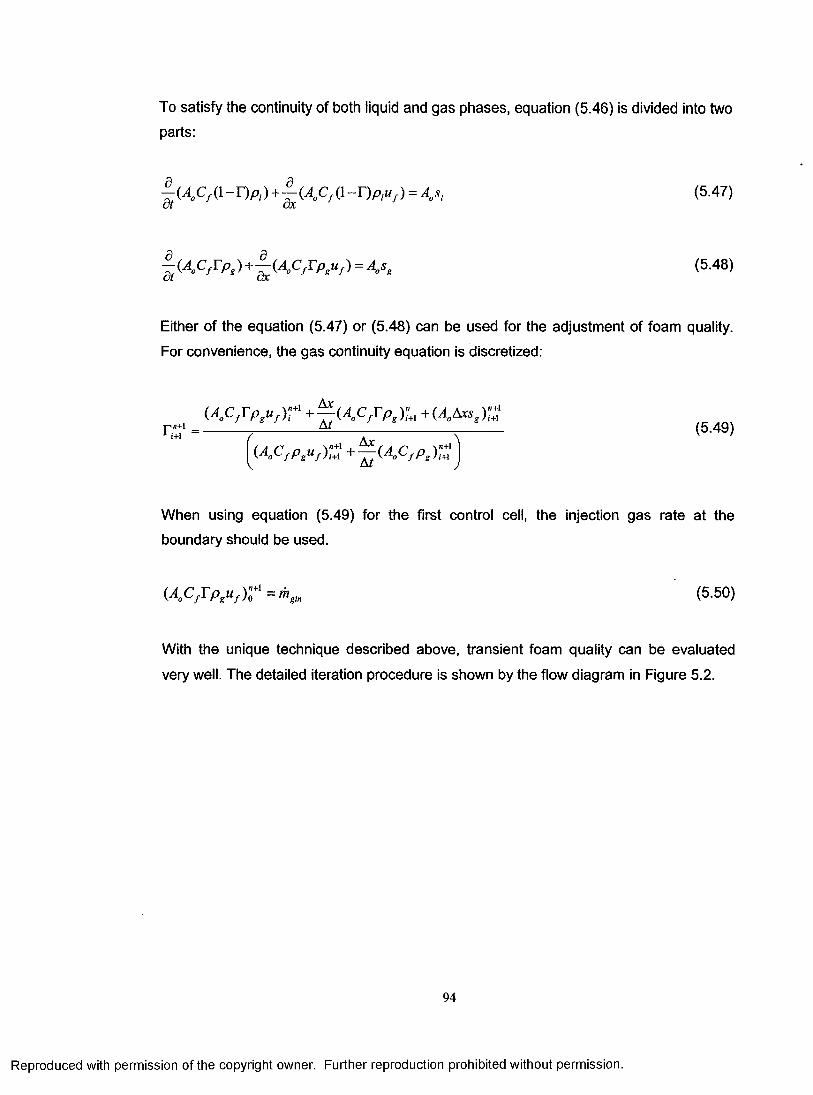
To satisfy the continuity of both liquid and gas phases, equation (5.46) is divided into two parts:

| ( 4 C / ( l- n p , )+ £ ( A C / 0 -O A !< ,) = A*, (547)

| (A,Cf TPt) + jL (A'Cf r Pluf ) = A,s, (5.4«)

Either of the equation (5.47) or (5.48) can be used for the adjustment of foam quality.

For convenience, the gas continuity equation is discretized:

nfl+I L i+1

A y

{A0CfTpguf r l + ^ A 0CfTpg) l x +(A0AxsXl' 7 A y '

(A0c fPgu x : + — (A0c fPx :

(5.49)

When using equation (5.49) for the first control cell, the injection gas rate at the

boundary should be used.

(A0Cf Tpgu X l =thgin (5.50)

With the unique technique described above, transient foam quality can be evaluated

very well. The detailed iteration procedure is shown by the flow diagram in Figure 5.2.

94


Given initial velocity fields forfoam and solids, pressure field,and concentrations in the well.

t=t+At

fUse momentum and continuity equations to calculate uf, us, Cf, and Cs:Eq. (5.6), Eq. (5.12), Eq. (5.29), and Eq.(5.30) Yes

CContinuity satisfied?

No

T,n a x

Use pressure-correct equation to calculate pressure changes and correct pressures. Eq. (5.41)

No

Stop

Use velocity correction equation, concentration correction equation and foam quality correction equation to adjust pressure, velocity, source term, concentration and foam quality.Eq.(5.24), Eq.(5.25), Eq.(5.26), Eq.(5.31), Eq.(5.32), and Eq. (5.49)

Figure 5.2: Flow diagram for the numerical solution procedure

95


CHAPTER 6

HYDRAULIC OPTIMIZATION OF FOAM DRILLING IN VERTICAL WELLS

A mathematical model of the cuttings transport with foam in vertical wells has been

presented in Chapter 3. The new model has been incorporated into a computer program

and is used for optimization of drilling hydraulic parameters (i.e. critical foam flow rate,

back pressure, foam quality, etc.) for effective cuttings transport with foam in vertical

wells.

Effects of key drilling parameters (i.e. drilling rate, annular geometry, formation fluid

influx, etc.) on the efficiency of cuttings transport have also been investigated. A series

of simplified hole cleaning charts have been developed, which enables the optimum hole

cleaning parameters to be determined at the rig site.

Chapter 6 introduces the optimization concepts and summarizes the results of hydraulic

optimization studies for effective cuttings transport with foam in vertical wells.

6.1 Hydraulic Optimization ProgramThe hydraulic optimization program proposed in this study considers the combined

effects of the drilling rate, the annular back pressure, the injection gas and liquid rates on

the circulating bottomhole pressure and the efficiency of cuttings transport. Typical foam

drilling operational practice requires that injection gas and liquid rates and back pressure

be specified (Figure 6.1). The foam velocity at the bottom of the well is used as the

primary term to control the bottom hole pressure, and cuttings concentration is used as

the primary term to evaluate the cuttings transport efficiency. Elements of the

optimization program are explained in the following sections.

6.2 Basic Design ConsiderationsBased on the field practice and the data available from the literature, the following

criteria are used as basic guidelines for the development of foam drilling hydraulic

optimization programs.

96


(1) Friction dominated flow is preferred over hydrostatic pressure dominated flow since

the multi-phase flow in the friction dominated region is more stable when gas rate varies

or when formation gas influx occurs (Saponja, 1998).

n g in andw

| Parameters that need to be : spci tiled as boundaty| conditions ot the multiphase

flow mode)

(1) Injection gas rate, qgin(2) Injection liquid rate, q,ir(3) Back pressure, pb(4) Cuttings rate, qs

Figure 6.1: Boundary conditions for multiphase flow modeling

(2) Back pressure needs to be kept as low as possible to make the control easy

(Saponja, 1998).

(3) Foam velocity should be higher than the terminal settling velocity of cuttings.

(4) A foam quality of 96% is considered as the upper limit of gas fraction (CFQ). Foam

would break up and result in mist flow if foam quality is higher than 96%.

(5) In UBD, 4% is preferred to be the upper limit of solids concentration (CCC) (Guo et

al„ 1995).

(6) Bottom hole foam quality is normally considered to be between 55% and 70%. In this

study, the bottomhole foam quality range is extended to be 50%-80%.

(7) The liquid volumetric flow rate is kept as low as possible to reduce the cost of the

foaming agent (Robinson et al., 2000).

(8) The foam velocity should not be too high to avoid the wellbore erosion.

6.3 Optimization of Foam Drilling6.3.1 Critical Foam VelocityThe critical fluid velocity concept is commonly used for evaluating the effectiveness of

cuttings removal from bottom hole when drilling with conventional drilling fluids. For foam

97


drilling, average cuttings concentration is strongly controlled by the velocity of the foam (Equation (D-11)).

Several critical foam velocity criteria have been suggested by the previous investigators

(Guo et al., 1995; Krug and Mitchell, 1972; Okpobiri and Ikoku, 1986). Krug and Mitchell

(1972) set 0.45 m/s (1.5 ft/s) as the minimum foam velocity at the bottom hole to lift

cuttings. Okpobiri and Ikoku (1986) suggested that foam velocity should exceed the

terminal settling velocity of cuttings by 10% to provide adequate hole cleaning. Guo et al.

(1995) suggested that a critical cuttings concentration (CCC) at the wellbore should be

specified to determine the minimum foam velocity. They used 4% as the CCC in their

study.

6.3.2 Circulating Bottom hole Pressure

Equation (6.1) describes the total pressure drop in the annular section for the flow of

foam with cuttings under steady-state condition.

The numerical analysis of the compressible fluid flow requires the discretization of the

wellbore annulus into small sections, and then the sum of the pressure drop in all

sections will give the total pressure losses in the wellbore. The circulating bottomhole

pressure (CBHP), pBH, can, then, be calculated as follows:

6.3.3 Concept of Optimum Foam Velocity

Saponja (1998) defined the optimal circulating bottomhole pressure as the minimum achievable bottomhole pressure (BHP) for a specific liquid rate in a gas/liquid multiphase

flow system (Figure 6.2). As shown in Figure 6.2, the point of optimum CBHP divides the

curve of BHP vs. gas rate into two regions; the hydrostatic pressure dominated and

friction pressure dominated regions.

bPan =Ax’E (C/ / ,/^ + CS 4 +AX' S /a (6.1)

P m = P b + AP, (6.2)

98


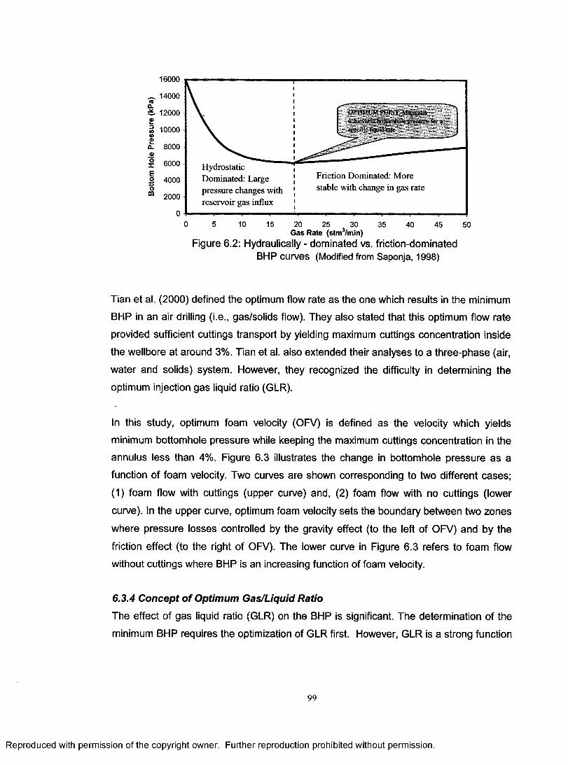
16000

„ 14000

i 12000 - ■H'il‘11 MilI| .1 Nachievable bnttninhole bpccilic liquid rate10000

8000

6000 Hydrostatic Dominated: Large pressure changes with reservoir gas influx

Friction Dominated: More stable with change in gas rate

4000

2000

0 5 10 15 20 25 30Gas Rate (stm3/min)

35 40 45 50

Figure 6.2: Hydraulically - dominated vs. friction-dominated BHP curves (Modified from Saponja, 1998)

Tian et al. (2000) defined the optimum flow rate as the one which results in the minimum

BHP in an air drilling (i.e., gas/solids flow). They also stated that this optimum flow rate

provided sufficient cuttings transport by yielding maximum cuttings concentration inside

the wellbore at around 3%. Tian et al. also extended their analyses to a three-phase (air,

water and solids) system. However, they recognized the difficulty in determining the

optimum injection gas liquid ratio (GLR).

In this study, optimum foam velocity (OFV) is defined as the velocity which yields

minimum bottomhole pressure while keeping the maximum cuttings concentration in the

annulus less than 4%. Figure 6.3 illustrates the change in bottomhole pressure as a

function of foam velocity. Two curves are shown corresponding to two different cases;

(1) foam flow with cuttings (upper curve) and, (2) foam flow with no cuttings (lower

curve). In the upper curve, optimum foam velocity sets the boundary between two zones

where pressure losses controlled by the gravity effect (to the left of OFV) and by the

friction effect (to the right of OFV). The lower curve in Figure 6.3 refers to foam flow

without cuttings where BHP is an increasing function of foam velocity.

6.3.4 Concept of Optimum Gas/Liquid Ratio

The effect of gas liquid ratio (GLR) on the BHP is significant. The determination of the

minimum BHP requires the optimization of GLR first. However, GLR is a strong function

99


of annular back pressure for a given critical (i.e. maximum allowable) foam quality (CFQ)

at the surface (Figure 6.4).

4000 .......... —................... - .....- .— " ' ................. ....................

■S' 3500 0.

1 3000<A(A£o- 2500a>op 2000 TVD = 914m2 I - - - ROP = 0 m/hr D „ - 0 22mE .. Dd„= 011 m“ 1500 m/hr P „=483kP a

GLR = 117

•I000 ' "F...... ..... I........ ....... I ................. ........ ...0 0.2 0.4 0.6 0.8 1 1.2 1.4

Foam Velocity (m/s)

Figure 6.3: Optimum foam velocity

The GLR determined at a specific annular back pressure and for the given CFQ is called

critical GLR (CGLR). Different CGLR values, however, can be obtained for different back

pressures. Therefore, as a first step in optimization of foam drilling hydraulics, finding of

optimum back pressure (OBP) is required. A complete procedure of determining the

OBP, optimum GLR (OGLR), and optimum foam velocity at the bottom of the hole are

given in the following sections.

6.3.5 Annular Back Pressure versus Critical Gas Liquid Ratio

The critical gas liquid ratio (CGLR) is defined as the GLR which would lead to a

maximum foam quality and a minimum circulating pressure at the bottom of the hole for

a given annular back pressure. A CGLR can be determined if the CFQ and the pressure

at the top of the annulus are known. Figure 6.4 reveals that there is a linear relationship

between CGLR, Oc, and back pressure, pb, and the correlation is given below:

® c = a -Pb + b (6-3)

In equation (6.3), a and b are correlation coefficients depending on the value of CFQ and

units of GLR and pressure. If 96% is chosen as CFQ, and strrvVstm3 and kPa as the

units for GLR and pressure respectively, a is found to be equal to 0.2383 and b is found

100

ROP = 0 m/hr

-ROP = 27 m/hr

TVD = 914 m D„ = 0 22 m Ddp= 011 m Pb= 483 kPa GLR = 117

0.2 0.4 0.6 0.8Foam Velocity (m/s)

1.2



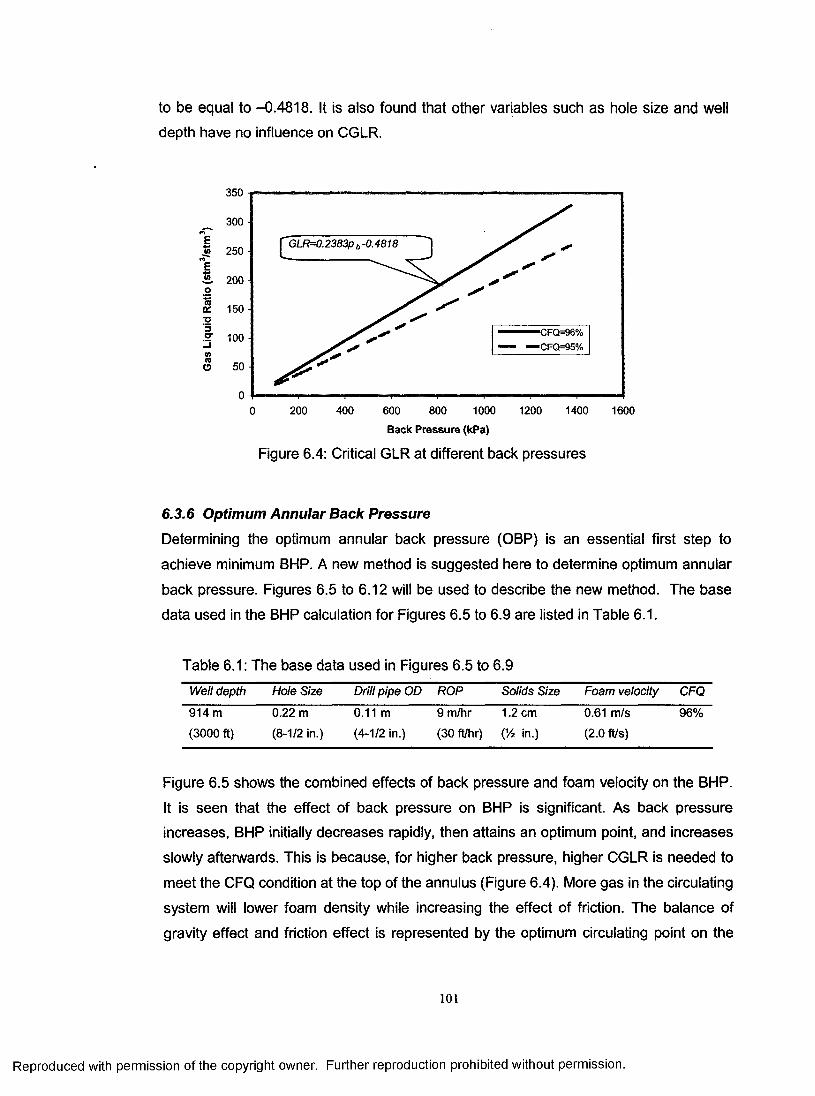
to be equal to -0.4818. It is also found that other variables such as hole size and well

depth have no influence on CGLR.

350

300 ■

E4* GLR=0.2383p b -0.4818250E2 . 200o

150 ■ 2•S' 100inO 50

— CFQ=96% — CFQ=95%

400 800 1000 1200 14000 200 600 1600

Back Pressure (kPa)

Figure 6.4: Critical GLR at different back pressures

6.3.6 Optimum Annular Back Pressure

Determining the optimum annular back pressure (OBP) is an essential first step to

achieve minimum BHP. A new method is suggested here to determine optimum annular

back pressure. Figures 6.5 to 6.12 will be used to describe the new method. The base

data used in the BHP calculation for Figures 6.5 to 6.9 are listed in Table 6.1.

Table 6.1: The base data used in Figures 6.5 to 6.9

Well depth Hole Size Drill pipe OD ROP Solids Size Foam velocity CFQ

914 m 0.22 m 0.11 m 9 m/hr 1.2 cm 0.61 m/s 96%(3000 ft) (8-1/2 in.) (4-1/2 in.) (30 ft/hr) (Yz in.) (2.0 ft/s)

Figure 6.5 shows the combined effects of back pressure and foam velocity on the BHP.

It is seen that the effect of back pressure on BHP is significant. As back pressure

increases, BHP initially decreases rapidly, then attains an optimum point, and increases

slowly afterwards. This is because, for higher back pressure, higher CGLR is needed to

meet the CFQ condition at the top of the annulus (Figure 6.4). More gas in the circulating

system will lower foam density while increasing the effect of friction. The balance of

gravity effect and friction effect is represented by the optimum circulating point on the

101


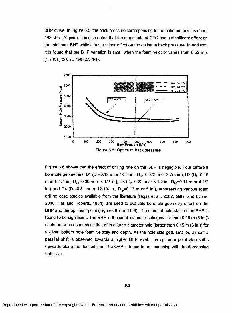
BHP curve. In Figure 6.5, the back pressure corresponding to the optimum point is about

483 kPa (70 psia). It is also noted that the magnitude of CFQ has a significant effect on

the minimum BHP while it has a minor effect on the optimum back pressure. In addition,

it is found that the BHP variation is small when the foam velocity varies from 0.52 m/s

(1.7 ft/s) to 0.76 m/s (2.5 ft/s).

7000

6000<0o.

£ 5000-3(A(A£Q- 4000 o o XE 3000 os“ 2000 -

CFQ = 95% CFQ =

10000 100 200 300 400 500 600 700 800 900

Back Pressure (kPa)

Figure 6.5: Optimum back pressure

Figure 6.6 shows that the effect of drilling rate on the OBP is negligible. Four different

borehole geometries, D1 (Dh=0.12 m or 4-3/4 in., Ddp=0.073 m or 2-7/8 in.), D2 (Dh=0.16

m or 6-1/4 in., Ddp=0.09 m or 3-1/2 in.), D3 (Dh=0.22 m or 8-1/2 in., Ddp=0.11 m or 4-1/2

in.) and D4 (Dh=0.31 m or 12-1/4 in., Ddp=0.13 m or 5 in.), representing various foam

drilling case studies available from the literature (Rojas et al., 2002; Giffin and Lyons,

2000; Hall and Roberts, 1984), are used to evaluate borehole geometry effect on the

BHP and the optimum point (Figures 6.7 and 6.8). The effect of hole size on the BHP is

found to be significant. The BHP in the small-diameter hole (smaller than 0.15 m (6 in.))

could be twice as much as that of in a large-diameter hole (larger than 0.15 m (6 in.)) for

a given bottom hole foam velocity and depth. As the hole size gets smaller, almost a

parallel shift is observed towards a higher BHP level. The optimum point also shifts

upwards along the dashed line. The OBP is found to be increasing with the decreasing

hole size.

102


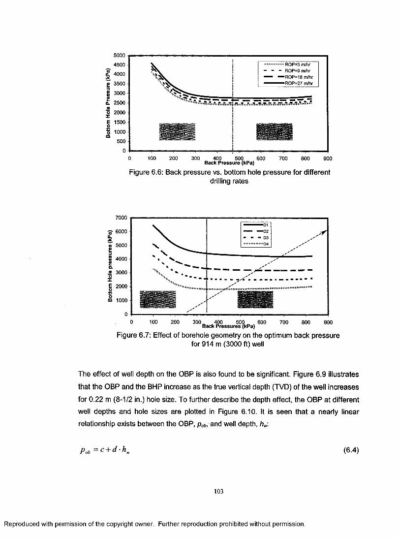
5000

4500

a 4000

gT 3500

1 30002£ 2500

o 2000

E 1500 o? 1000 m

500

00 100 200 300 400 500 600 700 800 900

Back Pressure (kPa)

Figure 6.6: Back pressure vs. bottom hole pressure for differentdrilling rates

7000

6000 ■02D304n 5000

<A 4000

3000

2000Fi (U 1 don na d *1000

0 100 200 300 „ . 400 50(Back Pressures i

600 700 800 900

Figure 6.7: Effect of borehole geometry on the optimum back pressurefor 914 m (3000 ft) well

The effect of well depth on the OBP is also found to be significant. Figure 6.9 illustrates

that the OBP and the BHP increase as the true vertical depth (TVD) of the well increases

for 0.22 m (8-1/2 in.) hole size. To further describe the depth effect, the OBP at different

well depths and hole sizes are plotted in Figure 6.10. It is seen that a nearly linear

relationship exists between the OBP, pob, and well depth, hw\

P o b = c + d ' K (6-4)

103


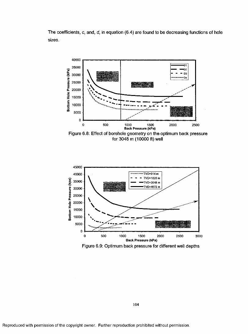
The coefficients, c, and, d, in equation (6.4) are found to be decreasing functions of hole

sizes.

40000

_ 35000 rai . 30000 £3 25000 a!£ 20000

I 15000 E% 10000 oCD

5000

00 500 1000 1500 2000 2500

Back Pressure (kPa)Figure 6.8: Effect of borehole geometry on the optimum back pressure

for 3048 m (10000 ft) well

llydmskitildnminatnu

net on t rii natod

45000 -

40000 -

§. 35000 -

2 30000 -i/i® 25000 -Q.® 20000 - oE 15000- oo 10000- m

5000 -

0 -0 500 1000 1500 2000 2500 3000

Back Pressure (kPa)

Figure 6.9: Optimum back pressure for different well depths

TVD=914 m■ TVD=1828 m —TVD=3048 m — 1VD=4572 m

fyarosutic

104


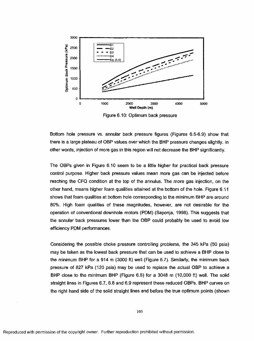
3000

a 2500 — D2

D4Eq. (6.5)2 2000

1500

£ 1000

a 500

00 1000 2000 3000 4000 5000

Well Depth (m)

Figure 6.10: Optimum back pressure

Bottom hole pressure vs. annular back pressure figures (Figures 6.5-6.9) show that

there is a large plateau of OBP values over which the BHP pressure changes slightly. In

other words, injection of more gas in this region will not decrease the BHP significantly.

The OBPs given in Figure 6.10 seem to be a little higher for practical back pressure

control purpose. Higher back pressure values mean more gas can be injected before

reaching the CFQ condition at the top of the annulus. The more gas injection, on the

other hand, means higher foam qualities attained at the bottom of the hole. Figure 6.11

shows that foam qualities at bottom hole corresponding to the minimum BHP are around

80%. High foam qualities of these magnitudes, however, are not desirable for the

operation of conventional downhole motors (PDM) (Saponja, 1998). This suggests that

the annular back pressures lower than the OBP could probably be used to avoid low

efficiency PDM performances.

Considering the possible choke pressure controlling problems, the 345 kPa (50 psia)

may be taken as the lowest back pressure that can be used to achieve a BHP close to the minimum BHP for a 914 m (3000 ft) well (Figure 6.7). Similarly, the minimum back

pressure of 827 kPa (120 psia) may be used to replace the actual OBP to achieve a

BHP close to the minimum BHP (Figure 6.8) for a 3048 m (10,000 ft) well. The solid

straight lines in Figures 6.7, 6.8 and 6.9 represent these reduced OBPs. BHP curves on

the right hand side of the solid straight lines and before the true optimum points (shown

105


by dashed lines) normally have very slow and negative slopes, and the region

represented by these curves are referred as the buffer region. Even though it is

hydrostatically dominated, in the buffer zone, the flow system is quite stable because the

increase of gas rate would decrease the BHP very slightly.

100

g 90

<D 80 _OX 70£oe 60oCQ** 50 •<0£ 40IS3 30oE 20mou. 10

--------------------------------------------- sT

D1- D2 — D3 — 04

1000 2000 3000

Well Depth (m)4000 5000

Figure 6.11: Bottom hole foam quality corresponding to the optimum point

By neglecting the effect of hole size, the reduced OBP (ROBP) can be written in terms of

the well depth as shown by equation (6.5). The ROBP, pmb, can be considered as the

lower limit of the back pressure to be used in any foam drilling operation.

Prob= 138.56 + 0.226 -hw (6.5)

Using the simplified relationship defined by equation (6.5), the foam quality at the bottom

hole is recalculated. Very good foam quality control (around 70%) is obtained at the

bottom of the hole (Figure 6.12). Therefore, the use of ROBPs (dashed line in Figure

6.10), which are as low as about the half of the original OBPs (solid lines in Figure 6.10), is recommended for practical drilling operation.

In foam drilling practice, the calculated OBP should be compared to the maximum

allowable operational pressure at the choke, and then the lower one should be chosen

as the OBP. Once the OBP is estimated (Equation 6.5), optimum foam velocity and

liquid rate can be determined as explained in the following sections.

106


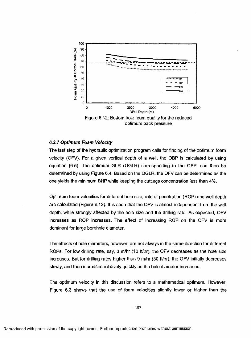
g

100

90

<v 80oX 70Eo£ 60Om 50<3> i 40«3 30oE 20<so 10u .

00

JjilsSiWiiBWiSKyiWj: Q

- - - D2

D4

1000 40002000 3000Well Depth (m)

Figure 6.12: Bottom hole foam quality for the reduced optimum back pressure

5000

6.3.7 Optimum Foam Velocity

The last step of the hydraulic optimization program calls for finding of the optimum foam

velocity (OFV). For a given vertical depth of a well, the OBP is calculated by using

equation (6.5). The optimum GLR (OGLR) corresponding to the OBP, can then be

determined by using Figure 6.4. Based on the OGLR, the OFV can be determined as the

one yields the minimum BHP while keeping the cuttings concentration less than 4%.

Optimum foam velocities for different hole size, rate of penetration (ROP) and well depth

are calculated (Figure 6.13). It is seen that the OFV is almost independent from the well

depth, while strongly affected by the hole size and the drilling rate. As expected, OFV

increases as ROP increases. The effect of increasing ROP on the OFV is more

dominant for large borehole diameter.

The effects of hole diameters, however, are not always in the same direction for different

ROPs. For low drilling rate, say, 3 m/hr (10 ft/hr), the OFV decreases as the hole size increases. But for drilling rates higher than 9 m/hr (30 ft/hr), the OFV initially decreases

slowly, and then increases relatively quickly as the hole diameter increases.

The optimum velocity in this discussion refers to a mathematical optimum. However,

Figure 6.3 shows that the use of foam velocities slightly lower or higher than the

107


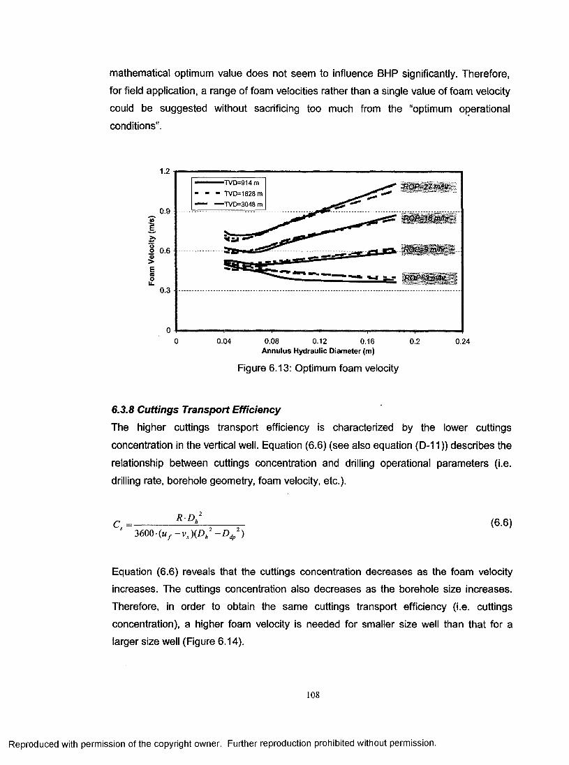
mathematical optimum value does not seem to influence BHP significantly. Therefore,

for field application, a range of foam velocities rather than a single value of foam velocity

could be suggested without sacrificing too much from the “optimum operational

conditions”.

TVD=914m

- - - TVD=1828 m

— — TVD=3048m

ROP=27 m/hr

0.9

>>*-*oO 0.6 , ROH=9 m hr

a - j ROF=j n Inu.

0.3

0.04 0.080 0.12 0.16 0.2 0.24Annulus Hydraulic Diameter (m)


6.3.8 Cuttings Transport Efficiency

The higher cuttings transport efficiency is characterized by the lower cuttings

concentration in the vertical well. Equation (6.6) (see also equation (D-11)) describes the

relationship between cuttings concentration and drilling operational parameters (i.e.

drilling rate, borehole geometry, foam velocity, etc.).

C, = ------------ ^ —2------- r (6.6)3600 •(uf - v s\ D h2 - D dp1)

Equation (6.6) reveals that the cuttings concentration decreases as the foam velocity

increases. The cuttings concentration also decreases as the borehole size increases.

Therefore, in order to obtain the same cuttings transport efficiency (i.e. cuttings

concentration), a higher foam velocity is needed for smaller size well than that for a

larger size well (Figure 6.14).

108


10 1

“ “ Dh=0.11 m (4-1/2 in.), Ddp=0.073 m (2-7/8 in.)

— -Dh=0.22 m (8-1/2 in.), Ddp=0.11 m (4-1/2 in.)

TVD 914 m (3000 ft) ROP 18 m/hr (60 ft/hr) Pt 345 kPa (50 psia)

o>

0.5 0.6 " " "

Foam Velocity (m/s)0.2 0.4 0.60.3 0.7 0.8 0.9

Figure 6.14: Bottom hole cuttings concentration

For low ROP (< 3 m/hr (10 ft/hr)), the 4% concentration limit is easy to accommodate

since the mass flow rate of solids is low. However, when the drilling rate is high, the

ROP has a strong influence on the efficiency of cuttings transport, and two types of

relationships between the minimum foam velocity (required for lifting cuttings), umin, and

the optimum velocity, t/op/,are observed.

For a large size well, foam velocity yielding the minimum BHP is normally higher than

the minimum required foam velocity to keep cuttings concentration below 4% (Figure

6.15). However, when drilling a small diameter hole at a high drilling rate, the cuttings

concentration in the annulus becomes relatively high. Even though there exists an

optimum foam velocity, the solids concentration at the bottom hole may exceed 4% at

this optimum foam velocity (Figure 6.16). In this case, the minimum foam velocity that

keeps the concentration of cuttings equal to 4% should be used as the optimum velocity

to guarantee effective hole cleaning.

109


3000

reCL■SC

2900

<g 2800

2700

Eoo 2600 CD

25000.3 0.4

u mln0.5

TVD 914 m(3000 ft) OD 0 22 m (8-1/2 in ) ID 0 11 m (4-1/2 in ) ROP 18 m/hr (60 ft/hr) Pi, 345 kPa (50 psia)

Cs<4%

0.6 Uopt 0.7 Foam Velocity (m/s)

0.8 0.9

Figure 6.15: Optimum and minimum velocities, case I

5400

5350TD 91 4 m (3000 ft) OD0.11 m (4-1/2 in)ID 0 071 m (2-7/8 In ) ROP. 1 8 m/hr (60 ft/hr) P„ 345 kPa (50 psia)

Cs=4%2 5300

5250

o. 5200 •

X 5150 ■Cs<4%

Cs>4%m

g 5100 -

5050

5000„ _ U min 0.6

**T“0.8

opt0.4 0.5 0.7 0.9Foam Velocity (m/s)

Figure 6.16: Optimum and minimum velocities, case II

6.3.9 Bottomhole Pressure and the Liquid Rate Corresponding to the OFV

The bottom hole pressures corresponding to different hole sizes, well depths and drilling

rates under the optimum hydraulic design conditions (i.e. minimum BHP and Cs<4%) are shown in Figure 6.17. The well depth has the most significant effect while the drilling rate

has the least significant, and hole size has the moderately significant effect on the BHP.

Hence, for a well with a specific vertical depth, the selection of the well size (i.e.

borehole geometry) is the most critical task to be fulfilled in the process of the hydraulic

optimization.

110


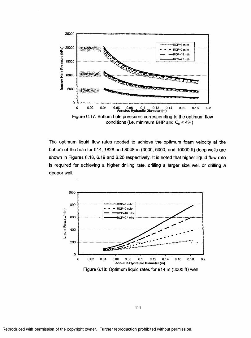
25000

•.S' 20000CL£jf« 15000 <o2Q.a)° 10000Eo%m 5000

00.2

Figure 6.17: Bottom hole pressures corresponding to the optimum flow conditions (i.e. minimum BHP and Cs < 4%)

The optimum liquid flow rates needed to achieve the optimum foam velocity at the

bottom of the hole for 914, 1828 and 3048 m (3000, 6000, and 10000 ft) deep wells are

shown in Figures 6.18, 6.19 and 6.20 respectively. It is noted that higher liquid flow rate

is required for achieving a higher drilling rate, drilling a larger size well or drilling a

deeper well.

1000

ROP=3 m/hr ROP=9 m/hr

-ROP=18 m/hr -ROP=27 m/hr

800 •cE2 , 600 ouK2 4003 O’3

200 • -

0 0.02 0.04 0.06 0.08 0.1 0.12 0.14 0.16 0.18 0.2Annulus Hydraulic Diameter (m)

Figure 6.18: Optimum liquid rates for 914 m (3000 ft) well

i l l


1200

0 |T-'- - | -..... '■•I....... i.,—— — ..... ............................................ ............0 0.02 0.04 0.06 0.08 0.1 0.12 0.14 0.16 0.18 0.2

Annulus Hydraulic Diameter (m)


1200

1000

R0P=3 m/hr

ROP=9 m/hr

'ROP=18 m/hr

■ROP=27 m/hr

| 8002.<D“ 600

2§■ 400

200 ■

0 0.02 0.04 0.06 0.08 0.1 0.12 0.14 0.16 0.18 0.2Annulus Hydraulic Diameter (m)


6.3.10 Summary of Hydraulic Optimization Procedure for Foam Drilling

The hydraulic optimization of foam drilling requires integrated controls of back pressure,

foam quality and gas and liquid rates. The step-by-step procedure for the hydraulic optimization of the foam drilling operation is given as follows:

(1) Specify the critical foam quality (CFQ) at the top of the annulus. Normally, 96% is

used as CFQ.

112


(2) Determine the optimum annular back pressure (OBP). Equation (6.5) is

recommended for the calculation of optimum back pressure.

(3) Determine the optimum gas liquid ratio (OGLR). OGLR can be calculated by using

Equation (6.3).

(4) Determine the optimum foam velocity (OFV), the liquid flow rate and the bottomhole

pressure (BHP). The optimum foam velocity is found by comparing foam velocity

corresponding to the minimum BHP with the foam velocity yielding to the 4% bottomhole

cuttings concentration. Figures 6.13 and 6.17 to 6.20 are recommended to use.

(5) Determine the gas flow rate by multiplying liquid flow rate with the OGLR.

113


CHAPTER 7

HYDRAULIC OPTIMIZATION OF FOAM DRILLING IN HORIZONTAL WELLS

A mathematical model and a numerical analysis of cuttings transport with foam in

horizontal wells have been presented in Chapter 4. In this chapter, the model has been

incorporated into a computer program and used for finding a closed form critical foam

velocity (CFV) correlation.

The new CFV correlation can be used to predict the minimum foam flow rate required to

remove, or prevent the formation of a stationary cuttings bed on the low side of the

highly deviated and horizontal well.

The effects of key drilling parameters (i.e. drilling rate, annular geometry, foam quality,

bottomhole pressure and temperature) on the critical foam velocity have also been

investigated.

Numerical examples are presented to illustrate how the CFV correlation can be used to

determine the required gas and liquid flow rates at the downhole condition.

7.1 Model Description7.1.1 Proposed Model

The model developed in Chapter 4 is used to perform the optimization study of foam-

cuttings flow in horizontal wells. The basic assumption of the model is that a stationary

cuttings bed exists on the low side of the horizontal wellbore if foam velocity is lower

than the critical transport velocity. Oroskar and Turian’s correlation, which is reliable to

use for high viscosity incompressible fluids (Shook et al., 1991; Shah and Lord, 1990), is

modified to determine the CFV by incorporating the effect of foam quality.

7.1.2 Boundary ConditionsMechanisms of cuttings transport in highly deviated and horizontal wells are significantly

different than that of the vertical wells. Therefore, in order to analyze the cuttings

transport in horizontal wells, we have focused only on the horizontal section of the well.

Figure 7.1 shows the geometry of a typical horizontal well section.

114


Pressure Temperature Foam Quality

Horizontal Length

Figure 7.1: Schematic view of the horizontal section

The pressure at the heel of the horizontal wellbore section largely reflects the effect of

the true vertical depth of the well. The numerical solution of the model for horizontal

wells requires that the pressure at the heel of the horizontal wellbore is specified as a

boundary condition. The foam quality at the heel of the horizontal wellbore section

largely reflects the combined effects of injection gas liquid ratio (GLR) and back pressure

at the surface, which also need to be specified to investigate its effect on cuttings

transport.

7.2 Critical Foam Velocity (CFV)The critical foam velocity in a horizontal well is defined as the minimum foam velocity

which yields no cuttings bed deposition. Drilling rate, wellbore geometry, horizontal well

length, foam quality, botomhole pressure and temperature are some of the most

important factors affecting the critical foam velocity.

7.2.1 Effect of Foam Quality on the CFVThe quality of foam controls the foam viscosity and the density, and therefore affects

efficiency of cuttings transport significantly. As the foam quality increases, the foam

viscosity also increases, which is favorable for cuttings removal. On the other hand, the

foam density decreases with increasing foam quality, which is unfavorable for cuttings

transport.

The effect of foam quality on the CFV is shown in Figure 7.2. Generally, the effect of

foam quality on the CFV is negligible when the foam quality is between 50% and 70%.

115


When the foam quality is higher than 70%, the CFV increases noticeably as the foam

quality increases. In this case, the foam density affects the cuttings transport efficiency more than the foam viscosity.

The general relationship between the CFV, ucf, and the foam quality, r , can be described

by a 2nd order polynomial function:

mc/ = al +a2- r+ a 3 T 2 (7.1)

where a#, a2 and a3 are correlation coefficients.

1.4 ................. — ... ....- ...................... ............................. — — .............

(O

o1 I--— ........ I....... ■........... —................... . —...............

30 40 50 60 70 80 90Foam Quality (%)

Figure 7.2: Effect of foam quality on the critical foamvelocity

7.2.2 Effect of Drilling Rate on the CFV

The effect of rate of penetration (ROP) on the critical foam velocity (CFV) for various

wellbore geometries with 60% foam quality and 5861 kPa (850 psi) bottomhole pressure

is shown in Figure 7.3.

Regression analyses have shown that CFV is a logarithmic function of the ROP, R. The general correlation can be written as:

Ucf = b, ln(R) + b2 (7.2)

where b, and b2are correlation coefficients.

116


D2D3'D4

S 0.4-

0 105 15 20 25 30Drilling Rate (m/hr)

Figure 7.3: Effect of drilling rate on the critical foam velocity

7.2.3 Effect of Wellbore Geometry on the CFV

The effect of wellbore geometry on the CFV is shown in Figure 7.4. It is found that CFV

is also a logarithmic function of wellbore hydraulic diameter. The hydraulic diameter, DH,

is defined as the difference between wellbore diameter and the drillpipe outer diameter.

Ucf = d ln(DH) + c2 (7.3)

where Ci and c2are correlation coefficients.

ROP=0.3 m/hr ROP=3 m/hr 'ROP=9 m/hr 'ROP=18 m/hr

tf>

>* o.2 1.2 - -

>£njOU.8 0.8 -

o

0.40.02 0.06 0.080.04 0.1 0.12 0.14 0.16 0.18 0.2

Hydraulic Diameter (m)

Figure 7.4: Effect of wellbore geometry on the critical foam velocity

117


7.2.4 Effect of Bottomhole Pressure on the CFV

Cuttings transport is significantly affected by foam specific gravity (or foam density) since

the terminal settling velocity of solids decreases as the carrier fluid density increases. As

shown in Figure 7.5, for a fixed foam quality (in this case 60 %), the foam specific gravity

increases with the increasing BHP.

0.8“ 20°C

— ---- 100°C>.0.6

Q.

U.

0 5000 10000 15000 20000 25000 30000 35000Pressure (kPa)

Figure 7.5: Foam specific gravity change with pressure

Figure 7.6 illustrates the effect of BHP on the CFV for 60% quality foam. It is seen that a

lower foam velocity is required to remove all the cuttings at higher BHP. This is mainly

due to the fact that bottomhole foam density increases as the BHP increases (Figure

7.5), and the foam with higher density can suspend and transport the cuttings more

effectively.

The general relationship between the CFV and the BHP can be described by a power

law function:

ucf=d\-(PBH)dl (7-4)

where d1 and d2 are correlation coefficients.

118


1.6

0.6 — —

0 5000 10000 15000 20000 25000 30000 35000 40000Bottom Hole Pressure (kPa)

Figure 7.6: BHP effect on the critical foam velocity

7.2.5 Effect o f Bottom Hole Temperature on the CFV

Figure 7.7 shows that for a foam of fixed quality, foam specific gravity decreases slightly

with increasing temperature. For the bottomhole temperature variation between 30 °C to

100°C, the effect of temperature on the CFV is negligible (Figure 7.8). This conclusion is

also supported by the experimental results recently published by Lourenco et al. (2003),

where they found that the rheology of foam (with a fixed foam quality) was not influenced

by increasing temperature.

1

!L® 0.8

$>2o

0.6

oo0)aCO£<oo

£ 0.4

0.2

020

■5516 kPa (800 psia)

■27579 kPa (4000 psia)

30 40 50.. ...60 70

T —80

.. ....90 100

Temperature (°C)

Figure 7.7: Foam specific gravity change with temperature

119


1.:oofl>>E<0O<0o

6

4

2

1

8

6

0.4

■5516 kPa

-27579 kPa

....... .... ...... ...... ... r ~ T ........ .... ..... .......... .....20 30 40 50 60 70 80 90 100

Bottom Hole Temperature (°C)Figure 7.8: Bottom hole temperature effect on the critical

foam velocity

110

7.2.6 Effect of Horizontal Well Length on the CFV

The pressure at the toe of the horizontal well section is higher than the pressure at the

heel of the well. The difference is mainly due to the frictional pressure loss, and the

pressure loss increases as the horizontal well length increases. Therefore, the foam

quality increases as the foam flows away from the bit in the horizontal well section.

By using the base data given in Table 7.1, foam quality changes along the horizontal

wells (with 457 m (1500 ft) length and 1372 m (4500 ft) length, at 1.8 m/s (6.0 ft/s) foam

velocity) are calculated. The results are shown in Figure 7.9.

Table 7.1: The base dataPressure Temperature Hole size Drill pipe Eccentricity ROP Particle Foam Horizontal

OD size quality length

5861 kPa 65.6 °C 0.22 m 0.11 m 1.0 9 m/hr 1.3 cm 60% 457 m(850 psi) (8-1/2 in.) (4-1/2 in.) 1.0 (30 ft/hr) (% in.) (1500 ft)

It is seen that the foam quality variation is very small along the horizontal well. For a 457

m (1500 ft) well, the foam quality increase at the heel is negligible. For a 1372 m (4500

ft) well, less than 2% foam quality increase is observed at the heel of the well.

120


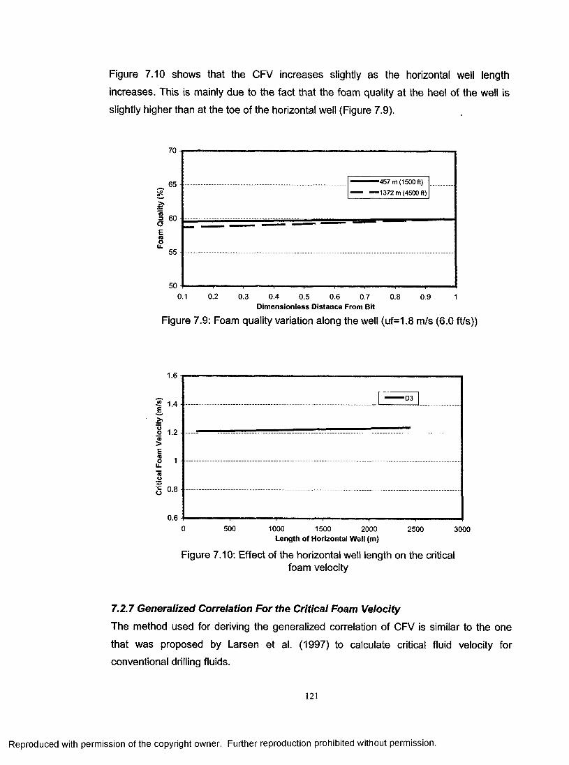
Figure 7.10 shows that the CFV increases slightly as the horizontal well length

increases. This is mainly due to the fact that the foam quality at the heel of the well is

slightly higher than at the toe of the horizontal well (Figure 7.9).

70

65 — ............. -----

50

-457 m (1500 ft)

-1372 m (4500 ft)

0.1 0.2 0.3 0.4 0.5 0.6 0.7Oimensionless Distance From Bit

0.8 0.9

Figure 7.9: Foam quality variation along the well (uf=1.8 m/s (6.0 ft/s))

1.6

mE>.ooID>E<oou.

1.4

1.2

-D3

S 0.8

0.6500 1000 1500 2000

Length of Horizontal Well (m)2500 3000

Figure 7.10: Effect of the horizontal well length on the criticalfoam velocity

7.2.7 Generalized Correlation For the Critical Foam Velocity

The method used for deriving the generalized correlation of CFV is similar to the one

that was proposed by Larsen et al. (1997) to calculate critical fluid velocity for

conventional drilling fluids.

121


Based on the data presented in Figures 7.3 and 7.4, the CFV correlation for 60% foam

quality and 850 psia BHP can be written as follows:

ucf = 0.03383 • (ln(7?) + 7 .976 l)- ( ln fZ )^ ) + 5.951) (7.5)

The value of CFV obtained from equation (7.5) needs to be corrected for bottomhole

pressures other than 5861 kPa (850 psia) and the foam qualities other than 60%.

Based on the CFV vs. BHP relationship shown in Figure 7.6, the regression coefficient,

d 2, in equation (7.4) is found to be equal to -0.0533. The correction factor, C Bhp , for the

effect of BHP other than 5861 kPa (850 psia) on the CFV can be determined as follows:

r =BHP

/ \ -0.0533P b h

5861(7.6)

Based on the CFV vs. foam quality relationship shown in Figure 7.2, regression

coefficients, au a2, and a3 in equation (7.1) are found as 1.4, -0.68, and 0.62

respectively. The correction factor for the effect of foam quality other than 60% on the

CFV can be found by dividing the equation (7.1) with the value of the equation (7.1)

when the foam quality is 60%. The equation (7.7) gives the final form of the correction

factor for the effect of foam quality other than 60% on the CFV.

CQ = 1.15 -0.55r + 0.5 r 2 (7.7)

Finally, the CFV for any BHP other than 5861 kPa (850 psia) and any foam quality other

than 60%, can be calculated by multiplying CFV from equation (7.5) by C Bhp and CQ.

7.2.8 Gas and Liquid Volumetric Rates at the Downhole Conditions

The gas and liquid flow rates corresponding to CFV at the bottomhole conditions can be

calculated by using the definition of foam quality and velocity. The final form of the

equations for downhole gas and liquid flow rates are given by equations (7.8) and (7.9),

respectively.

122


qg = T x u cfxAan (7.8)

qL= ( l.O -r)x UlfxAan • (7.9)

7.3 Sample Calculation of the Critical Foam VelocityWellbore Diameter: 0.2 m (7-7/8 in.)

Drillpipe OD: 0.1 m (4 -1/2 in.)

Bottomhole Pressure: 8274 kPa (1200 psi)

Bottomhole Foam Quality: 60%

Drilling Rate: 12.2 m/s (40 ft/hr)

The CFV corresponding to 60% foam quality and 5861 kPa (850 psia) is calculated from

equation (7.5) as 1.234 m/s (4.06 ft/s).

The correction factor for BHP of 8274 kPa (1200 psia) is calculated from equation (7.6)

as 0.98.

The corrected CFV is calculated as 1.21 m/s (3.99 ft/s). The bottomhole gas and liquid

flow rates are calculated from equations (7.8) and (7.9), as 0.0154 m3/s (33 ft3/min) and

0.0102 m3/s (163 gal/min), respectively.

When the same problem is solved for foam quality of 70%, CFV increased slightly to

1.23 m/s (4.03 ft/s) with corresponding downhole gas and liquid rates of 0.0184 m3/s (39

ft3/min) and 0.0078 m3/s (124 gal/min), respectively.

123


CHAPTER 8

CONCLUSIONS AND RECOMMENDATIONS

8.1 ConclusionsA comprehensive numerical simulation study of cuttings transport with foam in vertical

and horizontal wells has been conducted. New mechanistic models have been

developed and solved numerically to predict efficiency of cuttings transport with foam in

vertical and horizontal wells. The models have also been used for developing new

hydraulic optimization concepts for field application. The following sections summarize

the findings of this study.

8.1.1 Numerical Modeling of Cuttings Transport with Foam in Vertical Wells

A transient 1-D mechanistic model of cuttings transport with foam in vertical wells has

been developed and numerically solved. Model predictions of flowing bottomhole

pressure for foam flow in vertical wells show good agreement with field test data.

The bottomhole pressure does not stabilize immediately after drilling starts. A longer

drilling time is needed for the bottom hole pressure to stabilize as the drilling rate

increases. The transient nature of the bottomhole pressure should, therefore, be taken

into account when designing underbalanced drilling operations using foam.

The distribution of cuttings concentration along the well is not uniform even under steady

state conditions. The maximum cuttings concentration is always at the bottom of the

hole.

Water influx from the reservoir decreases foam quality and, therefore, increases the

flowing bottom hole pressure. The effect of water influx is more pronounced at high gas

injection rates (i.e. high foam quality). A practical implication of this finding is that the

degree of underbalance approaches a minimum (i.e. near-balanced drilling) when foam

is used at a relatively high water influx condition.

Gas influx from the reservoir increases foam quality in the wellbore, which reduces the

bottom hole pressure. The effect of gas influx is more significant in the lower gas

injection rate region.

124


Larger cuttings size leads to higher cuttings concentration. Cuttings with irregular shapes

(i.e. lower sphericity) lead to lower cuttings accumulation.

The model developed in this study can be used to write computer programs for practical

design purposes to determine optimum volumetric gas/liquid flow rates, injection

pressure and the back pressure required for drilling vertical wells. The model could also

be used to develop guidelines for field people to use in operational control of cuttings

transport with foam.

8.1.2 Numerical Modeling of Cuttings Transport with Foam in Horizontal Wells

A transient 1-D mechanistic model of cuttings transport with foam in horizontal wells is

developed. The model is then solved numerically to predict cuttings bed height as a

function of foam quality, total foam flow rate, drilling rate, volume of formation fluid influx

and wellbore geometry.

A new critical deposition velocity correlation for foam-cuttings flow is introduced by

modifying Oroskar and Turian’s correlation.

Results of the sensitivity analyses have shown that the model is capable of predicting

the transient nature of the cuttings transport with foam along the wellbore.

Results have also shown that the increasing drilling rate and drillpipe eccentricity would

increase the cuttings bed height.

It is found that cuttings transport efficiency is increased with increasing foam flow rate.

This suggests that, as long as the equivalent circulating bottomhole pressure stays

below the required limit for underbalance, the maximum possible gas/liquid injection

rates should be used for effective borehole cleaning.

Influx of formation fluid has a positive effect on cuttings transport efficiency as indicated

by reduced cuttings bed height. However, foam stability might be a critical issue when

there is formation fluid influx and therefore, it should be carefully evaluated.

125


The model developed in this study can be used to write computer programs for practical

design purposes to determine optimum volumetric gas/liquid flow rates, injection

pressure, and back pressure required for drilling horizontal wells. The model can also be

used to develop guidelines for field people to use in operational control of cuttings

transport with foam.

8.1.3 Hydraulic Optimization of Foam Drilling in Vertical Wells

A new method has been developed to determine the optimum foam drilling hydraulics

conditions, under which the bottomhole pressure is minimized, foam quality is well

controlled, and cuttings transport efficiency is guaranteed.

For a given critical foam quality specified at the top of the annulus, higher back pressure

is needed as the drilling depth increases. The optimum back pressure increases linearly

with the increasing well depth.

The optimum back pressure decreases with increasing borehole size.

The depth of the well has little impact on the optimum foam velocity.

The borehole size has a significant effect on the optimum foam velocity. The borehole

size effect, however, shows a different trend depending on the drilling rate and the

hydraulic diameter. When the drilling rate is low (i.e., <3 m/hr), the optimum foam

velocity decreases continuously as the hydraulic diameter increases. For higher drilling

rates, however, the optimum foam velocity decreases with increasing hydraulic diameter

at small diameter borehole sizes (i.e. hydraulic diameter < 7.5 cm). For higher drilling

rates in larger wellbores, however, higher optimum foam velocity values are required as

the hydraulic diameter increases.

If the drilling rate is low, its effect on the bottomhole pressure is negligible. If the drilling rate is high, however, the efficiency of the cuttings transport becomes a controlling factor

in a small borehole size, and the drilling rate affects the bottom hole hydraulics

significantly.

126


The well depth has the most significant effect on the bottomhole pressure, while the hole

size has the second most significant effect. Therefore, for a well with a given true vertical

depth, the optimization of wellbore size becomes the most critical task to be fulfilled

when designing a hydraulic program for foam drilling.

Finally, for large diameter wells, the optimum gas and liquid rates may be higher than

the minimum flow rates required for effective cuttings transport. Although the hydraulic

optimization can be achieved by using these higher injection rates, the overall

economics of the well may impose a limit on the liquid volumetric flow rates.

8.1.4 Hydraulic Optimization of Foam Drilling in Horizontal Wells

The critical foam velocity is a strong function of the borehole diameter. A higher foam

velocity is needed to completely remove the cuttings from a larger size wellbore.

The critical foam velocity is also a strong function of the drilling rate. A higher foam

velocity is needed to completely remove the cuttings at higher drilling rates.

The critical foam velocity is moderately affected by the bottomhole pressure. A power

law function can be used to describe the effect of the bottomhole pressure on the critical

foam velocity.

Other variables such as foam quality and bottomhole temperature have negligible effects on the critical foam velocity.

The generalized critical foam velocity correlation presented in this study provides

important insights into the cuttings transport efficiency with foam in horizontal wells.

The generalized critical foam velocity correlation could be conveniently used by a drilling

engineer to determine the required gas and liquid flow rates for effective hole cleaning in horizontal wells using foam.

127


8.2 Recommendations for the Future StudiesThis thesis contains extensive studies on the modeling and optimizing cuttings transport

in vertical and horizontal wells using foam. However, future work may still be needed to

improve or extend the current research in the following areas:

(1) Further verification and calibration of the proposed models by using actual field data.

(2) The incorporation of yield power law rheological model into the simulator.

(3) Modeling of cuttings transport with foam in inclined wells.

(4) Investigation of the effects of different boundary conditions on the cuttings transport

and drilling hydraulics.

128


REFERENCES

1. Abbott, W.K.: “An Analysis of Slip Velocity of Spherical Particles in Foam Drilling

Fluid,” MS thesis, Colorado School of Mines, Golden (1974).

2. Alberta Recommended Practices for Underbalanced Drilling; Interim Directive ID

94-3, Calgary, Canada, July 1994.

3. Anderson, G.W.: “Stable Foam Circulation Cuts Surface Hole Costs,” World Oil

(Sept. 1971), p.39-42.

4. Anderson, G.W.: “Use of Preformed Foam in Low Pressure Reservoir Wells,”

paper SPE 12425, 5th Off-shore South East Asia, Singapore, February 21-24, 1984.

5. Angel, R.R: “Volume Requirements for Air or Gas Drilling,” Petroleum

Transactions (1957), AIME, Vol. 210, p.325-330.

6. Bennion, D.B., Thomas, F.B., Bietz, R.F. and Bennion, D.W.: “Underbalanced

Drilling: Praises and Perils,” SPEDC (Dec. 1998), p.214-221.

7. Bentsen, N.W. and Veny, J.N.: “Preformed Stable Foam Performance in Drilling

And Evaluating Shallow Gas Wells in Alberta,” JPT (October 1976), p. 1237-1240.

8. Beyer, A.H., Millhone, R.S., and Foote, R.W.: “Flow Behavior of Foam as A Well

Circulating Fluid,” paper SPE 3986, the 47th Annual Fall Meeting of the Society of

Petroleum Engineers of AIME, San Antonio, Tex., Oct. 8-11,1972.

9. Bijieveld, A.F., Koper, M. and Saponja, J.: “Development and Application of An

Underbalanced Drilling Simulator,” paper SPE 39303, the 1998 IADC/SPE

Drilling Conference, Dallas, Texas, 3-6 March 1998.

10. Foams, J.J. Bikerman, Springer-Verlag, New York (1973).

H.BIauer, R.E., Mitchell, B.J., and Kohlhaas, C.A.: “Determination of Laminar,

Turbulent, and Transitional Foam Flow Losses in Pipes,” paper SPE 4885, the

1974 SPE Annual California Regional Meeting, San Francisco, California, 4-5

April 1974.

12. Bonilla, L.F. and Shah, S.N.: “Experimental Investigation On the Rheology of Foams,” paper SPE 59752, the 2000 SPE/CERI Gas Technology Symposium,

Calgary, Alberta, Canada, 3-5 April 2000.

13. Brown, N.P., Bern, P.A. and Weaver, A.: “Cleaning Deviated Holes: New

Experimental and Theoretical Studies,” paper SPE 18636, the 1989 IADC/SPE

Drilling Conference, New Orleans, Louisiana, Feb. 28 - Mar. 3, 1989.

129


14. Buslov, R., Towler, B.F. and Amian, A.V.: “Calculation of Pressures for Foams in

Well Completion Process,” paper SPE 36490, the 1996 SPE Annual Technical

Conference and Exhibition, Denver, Colorado, 6-9 October 1996.

15. Cade, R., Kirvelis, R., Nafta, M., and Jennings, J.: “Does Underbalanced Drilling

Really Add Reserves?” Paper SPE 81626, the IADC/SPE Underbalanced

Technology Conference, Houston, March 28-26, 2003.

16. Calvert, J.R. and Nezhati K.: “A Rheological Model for A Liquid-Gas Foam,”

International Journal of Heat and Fluid Flow (September 1986) 7, No.3, p. 164-

168.

17. Calvert J.R.: “Pressure Drop for Foam Flow through Pipes,” International Journal

of Heat and Fluid Flow (September 1990) 11, No.3, p.236-241.

18. Calvert, J.R. and Nezhati K.: “Bubble Size Effects in Foams,” International

Journal of Heat and Fluid Flow (1987) 8, No.2, p. 102-106.

19. Campos, W.: “Mechanistic Modeling of Cuttings Transport in Directional Wells,”

PhD dissertation, University of Tulsa, OK (1995).

20. Capes, C.A. and Nakamura, K.: “Vertical Pneumatic Conveying: An Experimental

Study with Particles in the Intermediate and Turbulent Flow Regimes,” The

Canadian Journal of Chemical Engineering (February 1973), Vol.51, p.31-38.

21 .Bubbles, Drops, and Particles in Non-Newtonian Fluid, Chhabra, R.P., CRC

Press, 1993.

22. Chhabra, R.P.: “Motion of Spheres in Power Law (Viscoinelastic) Fluid at

Intermediate Reynolds Numbers: A Unified Approach”, Chem. Eng. Process.

(1990) 28, 89-94.

23. Chien, S.F.: “Settling Velocity of Irregularly Shaped Particles,” SPEDC

(December 1994).

24. Cho, H., Shah, S.N. and Osisanya, S.O.: “A Three Segment Hydraulic Model for

Cuttings Transport in Coiled Tubing Horizontal and Deviated Drilling,” JCPT

(June 2002), p.32-39.

25. Chung, C.: “Drag on Object Moving through Foam,” PhD dissertation, Iowa State University, Ames, Iowa (1991).

26. Clark, R.K. and Bickham, K.L.: “A Mechanistic Model for Cuttings Transport,”

paper SPE 28306, the SPE 69th Annual Technical Conference and Exhibition,

New Orleans, LA, 25-28 September 1994.

27. Bubbles, Drops, and Particles, R. Clift, Academic Press, New York (1978).

130


28. Multiphase Flow with Droplets and Particles, Crowe, C.T., CRC press (1998).

29. Cuien, M.S., Harthi, S., and Hashimi, H.: “A Direct Comparison Between

Conventional and Underbalanced Drilling Techniques in the Saih Rawl Field,

Oman,” paper SPE 81629, the IADC/SPE Underbalanced Technology

Conference and Exhibition, Houston, Texas, 25-26 March 2003.

30. David, A. and Marsden, S.: “The Rheology of Foam,” paper SPE 2544, the 1969

SPE Annual Fall Meeting, Denver, Colorado, 28 September -1 October, 1969.

31.Dedegil, M.Y.: “Drag Coefficient and Setting Velocity of Particles in Non-

Newtonian Suspensions,” Journal of Fluid Engineering (September 1987) 109.

32. Dikken, B. J.: “Pressure Drop in Horizontal Wells and Its Effect on Their

Production Performance,” paper SPE 19824, the 1989 SPE Annual Technical

Conference and Exhibition, San Antonio, TX, 8-11 October 1989.

33. Doan, Q.T.: “Numerical Simulation of Sand Deposition and Accumulation in A

Horizontal Well,” PhD dissertation, University of Alberta, Alberta, Canada (1995).

34. Doan, Q.T., Oguztoreli, M., Masuda, Y., Yonezawa, T., Kobayashi, A. and Kamp,

A.: “Modelling of Transient Cuttings Transport in Underbalanced Drilling,” SPEJ

(June 2003).

35. Doron, P., Granica, D. and Barnea, D.: “Slurry Flow in Horizontal Pipes -

Experimental and Modeling,” International Journal of Multiphase Flow (1987) 13.

36. Einstein, A: “Eine neue Bestimmung der Molekuldimensionen,” Annalen der Physik (1906) 19, Ser. 5, 289.

37. Fang, G.: “An Experimental Study of Free Settling of Cuttings in Newtonian and

Non-Newtonian Drillings Fluids: Drag Coefficient and Settling Velocity," SPE

26125, 1992.

38. Folefac, A.N., Archer, J.S., Issa, R.I., and Arshad, A.M.: “Effect of Pressure Drop

Along Horizontal Wellbores on Well Performance,” paper SPE 23094, the

Offshore Europe Conference, Aberdeen, 3-6 September 1991.

39. Ford, J.T., Peden, J.M., Oyeneyin, M.B., Gao, E. and Zarrough, R.:

“Experimental Investigation of Drilled Cuttings Transport in Inclined Boreholes,”

paper SPE 20421, the 65th Annual Technical Conference and Exhibition, New

Orleans, LA, September 23-26, 1990.

40. Ford, J.T., Gao, E., Oyeneyin, M.B., Peden, J.M., Larrucia, M.B. and Parker, D.:

“A New MTV Computer Package for Hole-Cleaning Design and Analysis,”

SPEDC (September 1996), p. 168-172.

131


41. Gardiner, B.S., Dlugogorski, B.Z. and Jameson, G.J.: “Prediction of Pressure

Losses in Pipe Flow of Aqueous Foams,” Ind. Eng. Chem. Res. (1999) 38,

p. 1099-1106.

42. Gavignet, A.A. and Sobey, I.J.: “Model Aids Cuttings Transport Prediction,” JPT

(Sept. 1989), Trans., AIME, 287, p.916-920.

43. Giancarlo, P., Fuller, T., Haselton, T. and Kirvelis, R.: “Underbalanced-

Undervalued? Direct Qualitative Comparison Proves the Technique, “Paper SPE

74446, the IADC/SPE Drilling Conference, Dallas, Feb. 26-28, 2002.

44. Giffin, D.R. and Lyons, W.C.: “Case Histories of Design and Implementation of

Underbalanced Wells,” paper SPE 59166, the 2000 IADC/SPE Drilling

Conference, New Orleans, Louisiana, 23-25 February 2000.

45. Giger, F.M.: “Horizontal Wells Production Techniques in Heterogeneous

Reservoirs,” paper SPE 13710, the 1985 SPE Middle East Oil Technical

Conference and Exhibition, Bahrain, March 11-14,1985.

46. Gillies, R.G. and Shook, C.A.: “Modelling High Concentration Settling Slurry

Flows”, The Canadian Journal of Chemical Engineering (Aug. 2000), 78, p.709- 716.

47. Gregory, G.A.: “Foam Flow Modeling for UBD Applications,” JCPT (May 2003)

Vol. 42, No.5, p. 14-19.

48. Guitian, J. and Joseph, D.: “How Bubbles Mixtures Foam and Foam Control

Using A Fluidized Bed,” International Journal of Multiphase Flow (1998) 24, 1,

p. 1-16.

49. Guo, B., Hareland, G. and Rajtar, J.: “Computer Simulation Predictions

Unfavorable Mud Rate and Optimum Air Injection Rate for Aerated Mud Drilling,”

SPEDC (June 1996), p.61-66.

50. Guo, B., Miska, S., Hareland, G.: “A Simple Approach to Determination of Bottom

Hole Pressure in Directional Foam Drilling,” ASME Drilling Technology

Symposium (1995), PD-Vol. 65, p.329-338.

51. Hall, D.L. and Roberts, R.D.: “Offshore Drilling with Preformed Stable Foam,”

paper SPE 12794, the 1984 California Regional Meeting, Long Beech, CA, 11-13

April 1984.

52. Hall, H.N., Thompson, H. and Nuss, F.: “Ability of Drilling Mud to Lift Bit

Cuttings,” Petroleum Transactions, AIME (1950), Vol. 189, p.35-46.

132


53. Hanking, T. and Rappuhn, T.F.: “Case History: Breitbrunn - Horizontal Foam

Drilling Project in An Environmentally Sensitive Area in Bavaria, Germany,” paper

SPE 35068, the IADC/SPE Drilling Conference, New Orleans, Louisiana, 12-15

March 1996.

54. Hannegan, D.M. and Divine, R.: “Underbalanced Drilling - Perceptions and

Realities of Today’s Technology in Offshore Applications,” paper SPE 74448, the

IADC/SPE Drilling Conference, Dallas, Texas, 26-28 Feb. 2002.

55. Harris, P.C. and Reidenbach, V.G.: “High-Temperature Rheologjcal Study of

Foam Fracturing Fluids,” JPT (May 1987), p.613-619.

56. Harris, P.C., Klebenow, D.E. and Kundert, D.P.: “Constant-lnternal-Phase Design

Improves Stimulation Results,” SPEPE (February 1991), 15-22.

57. Hatschek, E.: “Die Viskositat der Dispersoide. I. Suspensoide,” Kolloid Z. (1910)

7, 301.

58. Hatschek, E.: “Die Viskositat der Dispersoide. II. Die Emulsionen und

Emulsoide,” Kolloid Z. (1910) 8, 34.

59. Herzhaft, B., Toure, A., Bruni, F. and Saintpere, S.: “Aqueous Foams for

Underbalanced Drilling: The Question of Solids,” paper SPE 62898, the 2000

SPE Annual Technical Conference and Exhibition, Dallas, Texas, 1-4 October.

60. Hopkin, E. A.: “Factors Affecting Cuttings Removal During Rotary Drilling,” JPT

(June 1967), p.807-814.

61. Islam, M.R. and Chakma, A.: “Comprehensive Physical and Numerical Modeling

of A Horizontal Well,” paper SPE 20627, the 1990 SPE Annual Technical

Conference and Exhibition, New Orleans, LA, September 23-26.

62. lyoho, A.W.: “Drilled-Cuttings Transport by Non-Newtonian Drilling Fluids

Through Inclined, Eccentric Annuli,” Ph.D. dissertation (1980), The University of

Tulsa.

63. Jaramillo, M.: “Bitterweed S. (Caballos) Field: A Case History in Changing

Economics Using Underbalanced Drilling and Open Hole Completions,” paper

SPE 81647, the IADC/SPE Underbalanced Technology Conference and

Exhibition, Houston, Texas, 25-26 March 2003.

64. Johnson, D.: “ Under Pressure to Grow Production”, CADENEWS (October

2003), Vol. 16, No. 8.

133


65. Kamp, A.M. and Rivero, M.: “Layer Modeling for Cuttings Transport in Highly Inclined Wellbores,” paper SPE 53942, the 1999 Latin American and Caribbean

Petroleum Engineering Conference, Caracas, Venezuela, 21-23 April 1999.

66. Khan, S.A., Schnepper, C.A., and Robert, C.: “Foam Rheology: III. Measurement

of Shear Flow Properties,” Journal of Rheology (1988) 32,1, 69-92.

67. Kitsios, E., Kamphuis, H, Quaresma, V., Rovig, J.W. and Reynolds, E.:

“Underbalanced Drilling Through Oil Production Zones with Stable Foam in

Omen,” paper SPE 27525, the 1994 IADC/SPE Drilling Conference, Dallas,

Texas, 15-18 February 1994.

68. Konno, H. and Saito, S.: “Pneumatic Conveying of Solids Through Straight

Pipes,” Journal of Chemical Engineering of Japan (1969), Vol.2, No.2, p.211-217.

69. Korady, V., Renard, G. and Lemonnier, P.: “Modeling of Pressure Drop for

Three-Phase Flow in Horizontal Wells,” paper presented at the 6th European

lOR-Symposium in Stavanger, Norway, May 21-23 1991.

70. Krug, J.A. and Mitchell, B.J.: “Charts Help Find Volume, Pressure Needed for

Foam Drilling,” Oil & Gas J. (7 February 1972).

71. Kuru, E., Miska, S., Pickell, M., Takach, N. and Volk, M.: “New Direction in Foam

and Aerated Mud Research and Development,” paper SPE 53963, the 1999 SPE

Latin American and Caribbean Petroleum Engineering Conference, Caracas,

Venezuela, 21-23 April 1999.

72. Lage, A.C.V.M., Fjelde, K.K and Time, R.W.: “Underbalanced Drilling Dynamics:

Two-Phase Flow Modeling and Experiments,” SPEJ (March 2003), p.61-70.

73. Lage, A.C.V.M., Nakagawa, E.Y., de Souza, A.A., and Santos, M.M.: “Recent

Case Histories of Foam Drilling in Brazil,” paper SPE 36098, the Fourth Latin

American and Caribbean Petroleum Engineering Conference, Port-of-Spain,

Trinidad & Tobago, 23-26 April 1996.

74. Larsen, T.I.: “A Study of the Critical Fluid Velocity in Cuttings Transport for

Inclined Wellbores,” M.S. thesis (1990), The University of Tulsa.

75. Larsen, T.I., Pilehvari, A.A. and Azar, J.J.: “Development of A New Cuttings- Transport Model for High-Angle Wellbores Including Horizontal Wells,” SPEDC

(June 1997), p. 129-135.

76. Latil, M.J., Coffe, G., Lehuen, P., and Renard, G.: “Fast Evaluation of Horizontal

Well Performance,” paper SPE 36930, the 1996 SPE European Petroleum

Conference, Milan, Italy, 22-24 October 1996.

134


77. Liu, G. and Medley, G.H.: “Foam Computer Model Helps in Analysis of

Underbalanced Drilling,” Oil & Gas J. (1 July 1996).

78. Li, J. and Walker, S.: “Sensitivity Analysis of Hole Cleaning Parameters in

Directional Wells,” SPE Journal (Dec. 2001), p.356-363.

79. Lord, D.L.: “Analysis of Dynamic and Static Foam Behavior,” JPT (January

1981).

80. Lourenco, A.M.F., Martins, A.L., Sa, C.H.M, Brandao, E.M. and Shayegi, S.:

“Drilling with Foam: Stability and Rheology Aspects,” Proceedings of

ETCE/OMAE 2000 Joint Conference on Energy for the New Millennium, New

Orleans, LA, February 14-17, 2000.

81. Lourenco, A.M.F., Miska, S.Z, Reed, T.R., Pickell, M.B. and Takach, N.E.: “Study

of the Effects of Pressure and Temperature on the Rheology of Drilling Foams

and Frictional Pressure Losses,” paper SPE 84175, the SPE Annual Technical

Conference and Exhibition, Denver, Colorado, 5-8 October 2003.

82. Luo, Y., Bern, P.A. and Chambers, B.D.: “Flow-Rate Prediction for Cleaning

Deviated Wells,” paper SPE 23884, the 1992 IADC/SPE Drilling Conference,

New Orleans, Louisiana, February 18-21, 1992.

83. Luo, S., Hong, R., Meng, Y., Zhang, L., Li, Y. and Qin, C.: “Underbalanced

Drilling in High-Loss Formation Achieved Great Success - A Field Case Study,”

paper SPE 59260, the 2000 IADC/SPE Drilling Conference, New Orleans,

Louisiana, 23-25 Feb. 2000.

84. Machado, C.J. and Ikoku, C.V.: “Experimental Determination of Solids Fraction

and Minimum Volume Requirements in Air and Gas drilling,” JPT (November

1982), p.2645-2655.

85. Martins, A.L., Lourenco, A.M.F., Andrade, P.H., Silva, V., Silva, P.R.C. and

Nakagawa, E.Y.: “Evaluation of Solids Carrying Capacity in Aerated Fluid Drilling:

Real Scale Tests and Modeling,” paper SPE 74464, the IADC/SPE Drilling

Conference, Dallas, Texas, 26-28 February 2002.

86. Martins, A.L., Lourenco, A.M.F. and de Sa, C.H.M.: “Foam Property Requirements for Proper Hole Cleaning While Drilling Horizontal Wells in

Underbalanced Conditions,” SPEDC (December 2001), p.195-200.

87. Martins, A.L. and Santana, C.C.: “Evaluation of Cuttings Transport in Horizontal

and Near Horizontal Wells - A Dimensionless Approach,” paper SPE 23643, the

135


Second Latin American Petroleum Engineering, Caracas, Venezuela, 8-11 March 1992.

88. Marett, B.P. and Landman, M.J.: “Optimal Perforation Design for Horizontal Wells

in Reservoir Boundaries,” paper SPE 25366, the SPE Asia Pacific Oil and Gas

Conference and Exhibition, Singapore, February 1993.

89. Underbalanced Drilling Manual, Mclennan, J., Carden, R.S., Curry, D., Stone,

C.R. and Wyman, R.E., Gas Research Institute, Chicago, Illinois (1997).

90. Meyer, B.R.: “Generalized Drag Coefficient Application for All Flow Regimes,” Oil

& Gas J. (26 May 1986).

91. Millhone, R.S., Haskin, C.A. and Beyer, A.H.: “Factors Affecting Foam Circulation

in Oil Wells,” paper SPE 3986, the 47th Annual Fall Meeting of the Society of

Petroleum Engineers of AIME, San Antonio, Tex., Oct. 8-11, 1972.

92. Mitchell, B.J.: “Viscosity of Foams,” PhD dissertation, University of Oklahoma

(1969).

93. Mitchell, B.J.: “Test Data Fill Theory Gap on Using Foam as A Drilling Fluid,” Oil

& Gas J. (6 September 1971).

94. Mitchell, R.F.: “Simulation of Air and Mist Drilling for Geothermal Wells,” JPT

(November 1983), p.2120-2126.

95. Naganawa, S., Oikawa, A., Masuda, Y., Yonezawa, T., Hoshino, M. and Acuna,

P.: “Cuttings Transport in Directional and Horizontal Wells While Aerated Mud

Drilling,” paper SPE 77195, the IADC/SPE Asia Pacific Drilling Technology,

Jakarta, Indonesia, 9-11 September 2002.

96. Negrao, A.F., Lage, A.C.V.M. and Cunha, J.C.: “An Overview of Air/Gas/Foam

Drilling in Brazil,” SPEDC (June 1999) 14(2), p.109-114.

97. Nguyen, D. and Rahman, S.S.: “A Three-layer Hydraulic Program for Effective

Cuttings Transport and Hole Cleaning in Highly Deviated and Horizontal Wells,”

SPEDC (September 1998).

98. Okpobiri, G.A. and Ikoku, C.U.: “Volumetric Requirements for Foam and Mist

Drilling Operations,” SPEDE (February 1986).

99. Okrajni, S.S. and Azar, J.J.: “The Effects of Mud Rheology on Annular Hole

Cleaning in Directional Wells,” SPEDE (August 1986), p.297-308.

100. Oroskar, A.R. and Turian, R.M.: “The Critical Velocity in Pipeline Flow of

Slurries,” AlChE Journal (1980), 26, p.550-558.

136


101. Owayed, J.F.: “Simulation of Water Influx During Underbalanced Foam Drilling,”

MS thesis, University of Tulsa, Tulsa, OK (1997).

102. Ozbayoglu, M.E., Kuru, E., Miska, S. and Takach, N.: “A Comparative Study of

Hydraulic Models for Foam Drilling,” JCPT (June 2002), p.52-61.

103. Ozbayoglu, E.M., Miska, S.Z., Reed, T. and Takach, N.: “Cuttings Transport with

Foam in Horizontal & Highly-Inclined Wellbore,” paper SPE 79856, the

SPE/IADC Drilling Conference, Amsterdam, The Netherlands, 19-21 February

2003.

104. Ozbelge, T.A.: “Solids Friction Factor Correlation for Vertical Upward Pneumatic

Conveyings,” International Journal of Multiphase Flow (1984), Vol. 10, No.4,

p.459-465.

105. Park, D., Brand, P.R., Allyson, B. and Sodersano, G.: “Planning and

Implementation of the Repsol-YPF-MAXUS Krisna Underbalanced Drilling

Project,” paper SPE 67689, the SPE/IADC Drilling Conference, Amsterdam, the

Netherlands, 27 Feb. -1 Mar. 2001.

106. Numerical Heat Transfer and Fluid Flow, S.V. Patankar, Hemisphere Publishing

Corporation, New York (1980).

107. Peden, J.M. and Luo, Y.: “Settling Velocity of Variously shaped Particles in

Drilling and Fracturing Fluids,” SPEDE (Dec. 1987).

108. Pigott, R.J.S.: “Mud Flow in Drilling,” Drill, and Prod. Prac., API (1941), p.91-103.

109. Raza, S.H. and Marsden, S.S.: “The Flow of Foam: 1. Rheology and Streaming

Potential,” paper SPE 1205, the 1965 Annual Fall Meeting of SPE, Denver, Oct.

3-6, 1965.

110. Reidenbach, V.G., Harris, P.C., Lee, Y.N. and Lord, D.L.: “Rheological Study of

Foam Fracturing Fluids Using Nitrogen and Carbon Dioxide,” SPEPE (January

1986), p.31-41.

111. Robinson, S., Hazzard, V., Leary, M. and Carmack, C.: “Redeveloping the

Rhourde El Baguel Field with Underbalanced Drilling Operations,” paper SPE

62203, provided to the Society of Petroleum Engineers for distribution and possible publication in an SPE Journal, 2000.

112. Rojas, Y., and Vieira, P., Borrell, M., Blanco, J., Ford, M., Nieto, L., Lopez, G.

and Atencio, B.: “Field Application of Near-Balanced Drilling Using Aqueous

Foams in Western Venezuela,” paper SPE 74449, the IADC/SPE Drilling

Conference, Dallas, Texas, 26-28 February 2002.

137


113. Saintpere, S., Herzhaft, B. and Toure, A.: “Rheological Properties of Aqueous

Foams for Underbalanced Drilling,” paper SPE 56633, the 1999 Annual

Technical Conference and Exhibition, Houston, Texas, 3-6 October.

114. Sanghani, V. and Ikoku, C.U.: “Rheology of Foam and Its Implications in Drilling

and Cleanout Operations,” Journal of Energy Resources Technology (September

1983)105, p.362-371.

115. Saponja, J.: “Challenges with Jointed-Pipe Underbalanced Operations,” SPEDC

(June 1998), p. 121-128.

116. Shah, S.N.: “Proppant Setting Correlations for Non-Newtonian Fluid under Static

and Dynamic Conditions,” SPE Journal (April 1982).

117. Shah, S.N. and Lord, D.L.: “Hydraulic Fracturing Slurry Transport in Horizontal

Pipes,” SPEDE (Sept. 1990), p.225-232.

118. Sharma, M.P. and Chowdhry, D.V.: “A Computational Model for Drilled Cutting

Transport in Air (or Gas) Drilling Operations,” Journal of Energy Resources

Technology (March 1986), Vol. 108, p.8-14.

119. Sharma, Y. and Kamp, A.M., Yonezawa, T., Rivero, L.M., Kobayashi, A. and

Gonzalez, J.: “Simulating Aerated Drilling,” paper SPE 59424, the SPE Asia

Pacific Conference on Integrated Modeling for Asset Management, Yokohama,

Japan, 25-26 April 2000.

120. Shook, C.A., Gillies, R.G., Kristoff, B.J. and Small, M.H.: “Sand Transport

Mechanism in Horizontal Wells,” 4th petroleum Conf. of South Saskatchewan

section, Petroleum society of CIM hold with CANMED, Regina, Saskatchewan,

Canada, Oct.7-9,1991.

121. Sifferman, T.R., Myers, G.M., Haden, E.L. and Wahl, H.A.: “Drill-Cuttings

Transport in Full-Scale Vertical Annuli,” JPT (Nov. 1974), p. 1295-1302.

122. Non-Newtonian Flow and Heat Transfer, Skelland, A.H.P., John Wiley and Sons,

Inc., New York (1967).

123. Sporker, H.F., Trepress, P., Valko, P. and Economides, M.J.: “System Design for

Measurement of Downhole Dynamic Rheology for Foam Fracturing Fluids,”

paper SPE 22840, the 66th Annual Technical Conference and Exhibition of SPE,

Dallas, TX, 6-9 October 1991.

124. Stone, T.W.: “A Comprehensive Wellbore/Reservoir Simulator,” paper SPE

18419, the SPE Symposium on Reservoir Simulation, Houston, TX, 6-8 February

1989.

138


125. Sunthankar, A.A., Kuru, E., Miska, S. and Kamp, A.: “New Developments in

Aerated Mud Hydraulics for Drilling in Inclined Wells,” SPEDC (June 2003),

p. 152-158.

126. Supon S.B. and Adewumi, M.A.: “An Experimental Study of the Annulus

Pressure Drop in A simulated Air-Drilling Operation,” SPEDE (March 1991), p.74-

80.

127. Teichrob, R. and Baillargeon, D.: “The Changing Face of Underbalanced Drilling

Technology Part III — Six-Year Case History of Pressure-Depleted Reservoir

Exploitation in Western Canada and Evolution of Cost-Saving, Integrated UBD

Package,” World Oil (June 2000), p.79-82.

128. Tellez, C.P., Smith, J.R. and Edwards, J.K.: “A New Comprehensive, Mechanistic

Model for Underbalanced Drilling Improves Wellbore Pressure Predictions,”

SPEDC (September 2003), p. 199-208.

129. Tian, S. and Adewumi, M.A.: “Multiphase Hydrodynamic Model Predicts

Important Phenomena in Air-Drilling Hydraulics,” SPEDE (June 1991), p. 145-

152.

130. Tian, S., Medley, G.H. and Stone, C.R.: “Optimizing Circulation while Drilling

Underbalanced,” World Oil (June 2000), p.48-55.

131. Thondavadi, N.N. and Lemlich, R.: “Flow Properties of Foam With and Without

Solid Particles,” Ind. Eng. Chem. Process Des. (1985), p.748-753.

132. Tomren, P.H., lyoho, A.W. and Azar, J.J.: “Experimental Study of Cuttings

Transport in Directional Wells,” SPEDE (February 1986), p.43-56.

133. Valko, P. and Economides, M.J.: “Volume Equalized Constitutive Equations for

Foamed Polymer Solutions,” Journal of Rheology (August 1992), 36(6), p. 1033-

1055.

134. Valko, P. and Economides, M.J.: “Foam-Proppant Transport,” SPEPF (November1997).

135. Vogel, J.V.: “Inflow Performance Relationships for Solution-Gas Drive Wells,”

JPT (January 1968), p.83-92.

136. Wang, Z., Rommetveit, R., Bijleveld, A., Maglione, R. and Gazaniol, D.:

“Underbalanced Drilling Requires Downhole Pressure Management,” Oil & Gas

Journal (June 16,1997), p.54-60.

139


137. Wang, Z., Vefring, E., Rommetveit, R., Bieseman, T., Maglione, R., Lage, A. and

Nakagawa, E.: “Underbalanced Drilling Model Simulates Dynamic Wellbore

Conditions,” Oil & Gas Journal (July 7, 1997), p.62-66.

138. Williams, C.E. and Bruce, G.H.: “Carry Capacity of Drilling Muds,” Petroleum

Transactions, AIME (1951), Vol. 192, p.111-120.

139. Wilson, K.C.: “A Unified Physically-Based Analysis of Solid-Liquid Pipeline Flow,”

Proc., Hydrotransport 4 Conference, BHRA Fluid Engineering, Banff, Canada,

1976.

140. Wolcott, D.S. and Sharma, M.P.: “Analysis of Air Drilling Circulating System With

Application to Air Volume Requirement Estimation,” paper SPE 15950, the SPE

Eastern Regional Meeting, Columbus, November 12-14,1986.

141. Yang, W.C: “A Correlation for Solid Friction Factor in Vertical Pneumatic

Conveying Lines,” AlChE Journal (May 1978), Vol.24, No.3, p.548-552.

142. Yarborough, L. and Hall, K.R.: “How to Solve Equation of State for Z-factors,” Oil

and Gas Journal (February 18, 1974), p.86-88.

143. Zeidler, H.U.: “An Experimental Analysis of the Transport of Drilled Particles,”

SPEJ (Feb. 1972), p.39-49.

140


APPENDIX ADERIVATION OF THE FOAM-CUTTINGS TRANSPORT MODEL FOR VERTICAL

WELLS

In this study, the Eulerian approach is used to derive the governing equations for foam-

cuttings flow. The Eulerian approach treats the cloud of solid particles (drilled cuttings)

as a second fluid that behaves like a continuum (Crowe, 1998). Foam is Theologically

characterized as power law type fluid.

Basic DefinitionsThe bulk density of the dispersed phase is defined as the ratio of the mass of the

dispersed phase to the total volume of the mixture:

_ AId , /Ap s = lim ---- *- (A-1)A K -> A r„ A V

Bulk density is related to the actual density of dispersed phase as:

P s = C s -Ps (A-2)

The concentration (volume fraction) of the solid phase (drilled cuttings) is defined as:

C s = lim ^ (A-3)5 AV-*AV0 A V

where AV0 is the limiting volume that ensures a stationary average, in which the average

would remain unchanged if the volume is changed slightly. Equivalently, the

concentration (volume fraction) of the continuous phase (foam) is defined as:

A^AV-*AV„ A F

C f = lim — 7 7 7 (A-4)

The sum of the concentrations must be equal to unity:

141


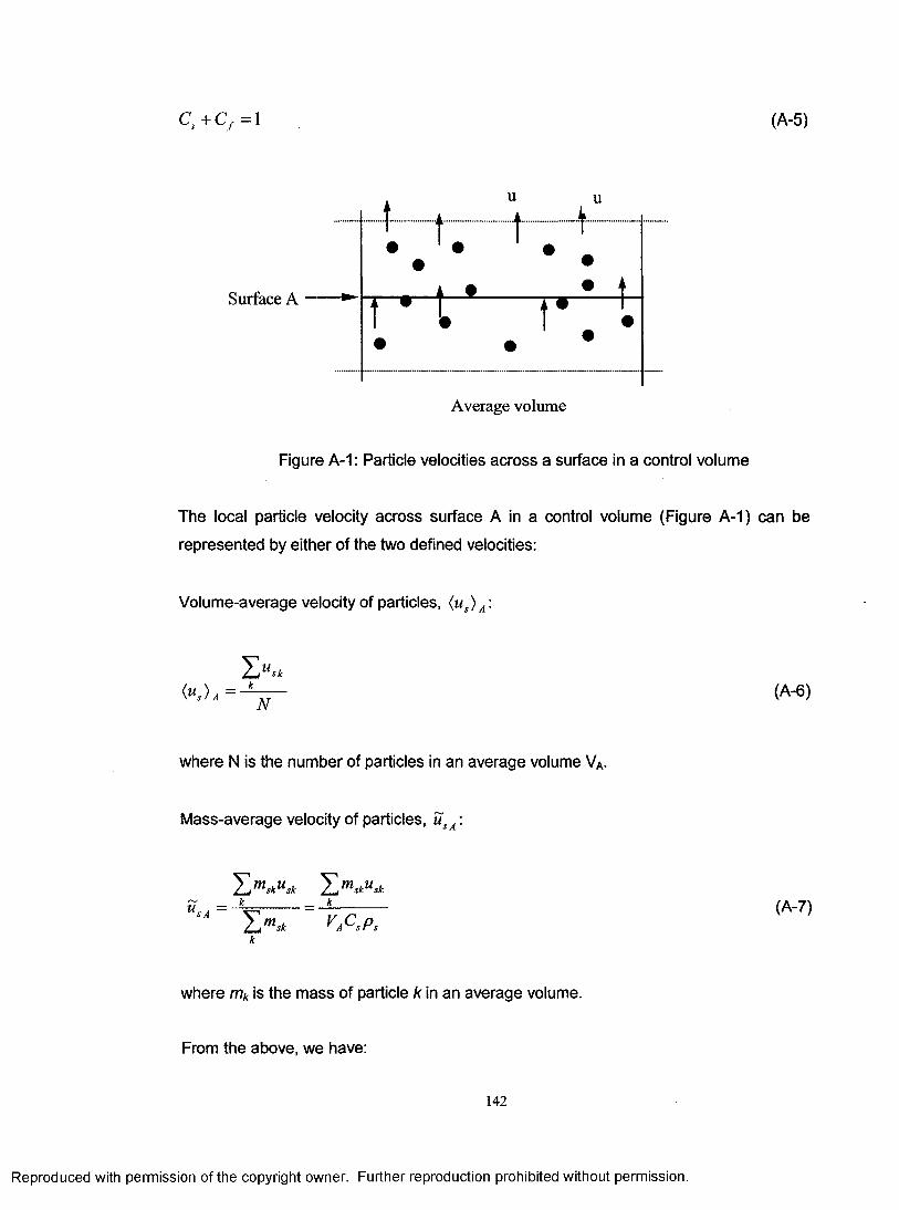
c,+cf =\ (A-5)

Surface A

Average volume

Figure A-1: Particle velocities across a surface in a control volume

The local particle velocity across surface A in a control volume (Figure A-1) can be

represented by either of the two defined velocities:

Volume-average velocity of particles, (us) A:

IX*(A-6)

where N is the number of particles in an average volume VA.

Mass-average velocity of particles, uSA:

u _* * (A-7)

*

where mk is the mass of particle k in an average volume.

From the above, we have:

142


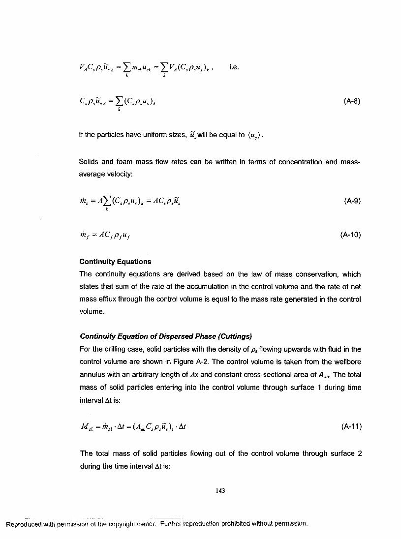
v a C s P s u sA = Y s V s k = X V a ( C s P s^ s ) ic • i-e-k k

c sP f isA = lL ( CsPsus )k (A-8)k

If the particles have uniform sizes, will be equal to (us) .

Solids and foam mass flow rates can be written in terms of concentration and mass-

average velocity:

= aYSP.p."')* = AC'P & (A"9)k

mf =ACf p f uf (A-10)

Continuity EquationsThe continuity equations are derived based on the law of mass conservation, which

states that sum of the rate of the accumulation in the control volume and the rate of net

mass efflux through the control volume is equal to the mass rate generated in the control

volume.

Continuity Equation of Dispersed Phase (Cuttings)

For the drilling case, solid particles with the density of ps flowing upwards with fluid in the

control volume are shown in Figure A-2. The control volume is taken from the wellbore

annulus with an arbitrary length of Ax and constant cross-sectional area of Aan. The total

mass of solid particles entering into the control volume through surface 1 during time

interval At is:

M sl = • At = ( A n C sPsUs)\ ■ At (A-11)

The total mass of solid particles flowing out of the control volume through surface 2

during the time interval At is:

143


X

HU t - t

Inflow A x Inflow

Figure A-2: Control volume of cuttings flow in vertical well

M ,2 = ms2 • At = (.AanCspsus )2 • At

Mass accumulation in the control volume during At is:

(A-12)

At = ^ ^ - . A t = AJ * ^ . A t sac dt dt dt

(A-13)

Since drilling cuttings generated is zero along the wellbore, the continuity equation of

dispersed particle phase is:

M s i - M sl+ M sac=0 (A-14)

(AanCsPSUs)l * At ~ (AnCsPs^s ), 'A t + Am • At = 0dt(A-15)

Both sides are divided by (AanAxAt), and are taken the limit with respect to Ax, the

equation changes into:

d(CMp,u ,) < d(CsPs) dx dt

(A-16)

144


For 1-D foam drilling model, a uniform velocity of cutting across the control surface is

assumed, so the final continuity equation of drilling cutting is:

(A-17)dx dt

Continuity Equation of Continuous Phase (Foam)The principle of the derivation of the continuity equation for foam phase is similar to that

for the dispersed phase except that the mass of fluid inflow from reservoir has to be

incorporated into the source term of the mass conservation equation:

M f 2 ~ M fl + M fac = M re (A-18)

Mass of foam entering the control surface, leaving the control surface, accumulating and

generating in the control volume during time At are:

M fx = mfl ■ At = (AanCf p f uf ) l • At (A-19)

M f2 = mf2 • At = (AanCf p f uf )2 • At (A-20)

ff llf , d(V„C f p f ) d(CfP f )M fac= —‘At = .............. . • At = Aan Ax -At (A-21)

fac dt dt dt

M re = mre • At = (paqre,0 + p wqre,w + p gqre,g ) ■ At (A-22)

Thus, the continuity equation of foam phase is obtained as follows:

d(Cfp f)iAanCfPf uf ) 2 -At-(AanCf p f uf \-A t+ A an Ax -& = (poqre,o +Pwqre,w +Pgqnjl) ' ^ (A'23)

145


Then both sides of equation (A-23) are divided by (AanAxAt), and are taken the limit with

respect to Ax to obtain the differential equation of continuity:

d(Cf P fuf ) t d(Cf P f ) = (p 0qre,0+ p wqre,w+ p gqre,g) dx dt Vm

The source term in equation (A-24) can be represented by sfi which is defined as the

mass rate change per unit control volume:

s = + P w d r e , w + P g < l r e , g ) 25)' A „ - A x

Therefore, equation (A-24) is simplified into equation (A-26):

Momentum Equations Momentum

Momentum is the product of a mass and the velocity of the mass. According to Newton’s

second law of motion, the rate of the momentum change of a mass system with time is

equal to the total external forces acting on the system. The general formula in x-direction

is:

This formula can be applied to the control volume as shown in Figure A-2 during time

interval At:

(C fP f)+ (C y Pj-Uj-) — S f (A-26)

d{M •U) _ 'yi p, dt ~ ^

(A-27)

A(Mu) = A t - ^ F x (A-28)

146


In equation (A-28), the total momentum change of the system is equal to the sum of the

net momentum efflux from the control volume and the accumulation of momentum in the

control volume:

A (Mu) = (Mu) 2 - (Mu)] + (Mu)ac (A-29)

Momentum Equation of Dispersed Phase (Cuttings)The momentum equation for a cloud of particles can be obtained by summing the

momentum equations for all particles in a control volume. During the time At, the total

momentum entering and leaving the control surfaces are:

(M su ,) i = (th ,u ,\ ■At = ( r an'£ (C spsus2)k)i -At (A-30)k

( M s u , ) 2 = (msus)2 -At^ (V an'YJ(Cspsus2)k)2-At (A-31)k

The accumulation of momentum in the control volume during At is:

d Y / a n i C s p su s ) k

CM sUs)ac = Z (™skUsk)ac = - A --------At = — ... At (A-32)* ot at

According to the definition of the mass-average velocity, equation (A-32) can be

simplified as:

= 4 . A ( A - 3 3 )dt

Forces over all the particles in the control volume including pressure force, drag force,

gravity force and frictional force of dispersed phase are taken into account in the

derivation.

147


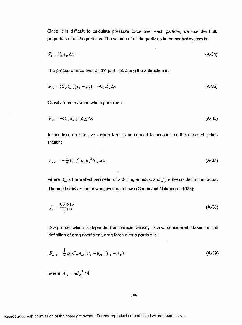
Since it is difficult to calculate pressure force over each particle, we use the bulk

properties of all the particles. The volume of all the particles in the control system is:

Vs = C sAan Ax (A-34)

The pressure force over all the particles along the x-direction is:

F Ps = (CsAan)(px - p 2) = -C sAanAp (A-35)

Gravity force over the whole particles is:

FGs= -(C sAan) -p sg&x (A-36)

In addition, an effective friction term is introduced to account for the effect of solids

friction:

Fr, = - j C , f , P , u , 2Sm&x (A-37)

where san is the wetted perimeter of a drilling annulus, and / is the solids friction factor.

The solids friction factor was given as follows (Capes and Nakamura, 1973):

f s = (A-38)u r

Drag force, which is dependent on particle velocity, is also considered. Based on the

definition of drag coefficient, drag force over a particle is:

F Dsk ~ 2 P f^ ^ A s k I Uf Usk I ( Uf U sk) (A-39)

where Ask =ndsk2 /4

148


The total drag force acting on all the particles is:

^ D s ~ r , P f ^ D ^ j - ^ s k \ U f U sk I ( u f U s k ) (A-40)1 k

By equating the total momentum change to the sum of the external forces over all the

particles in a control volume, the general momentum equation of dispersed phase is obtained as follows:

k k. ut

A tCsAmA p - C sAanp sg A x - ^ C J sp sus2SanAx + ^ p f CD^ A sk \u f - ust \ (u f - usk)

(A-41)

Dividing both sides of equation (A-41) by (AanAxAt) , and taking the limit with respect to

Ax, the differential form of the momentum equation for solid phase is obtained as follows:

t ___________ =dt dx

- c . ~ c , P . g - \ c J . P * , ' ^ + ^ P , c » Y .A* \ « / -« .k ) (A-42)an an

If it is assumed that solid particles have uniform sizes, and have same velocities across

the control surface, the momentum equation is simplified to:

S(CsPsus) | d(CsPsus2) dt dx

- C , ^ - C , p , g - \ c j , p , u , 2^ f - + ^ - p / C[,A ,\u f - u , \ ( u f - « , ) (A-43)dx 2 Aan 2Van

where Ns is the number of particles in a control volume, and can be calculated by:

149


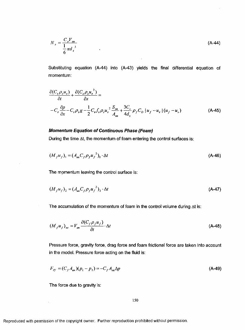
Substituting equation (A-44) into (A-43) yields the final differential equation of

momentum:

d(CsPsus) | d(Cspsus2) _ dt dx

~C, I “ / K«/ (A-45)

Momentum Equation of Continuous Phase (Foam)

During the time At, the momentum of foam entering the control surfaces is:

(M f uf \ = (A anCf p f u / ) x -At (A-46)

The momentum leaving the control surface is:

(M f uf )2 =(AanCf p f u / ) 2 -At (A-47)

The accumulation of the momentum of foam in the control volume during At is:

lM ,u , )„„ = V„ d(-Cf ^ ut ) . a , (A_48)

Pressure force, gravity force, drag force and foam frictional force are taken into account

in the model. Pressure force acting on the fluid is:

Fpf = (Cf Aan)(Pl - p 2) = -C f AanAp (A-49)

The force due to gravity is:

150


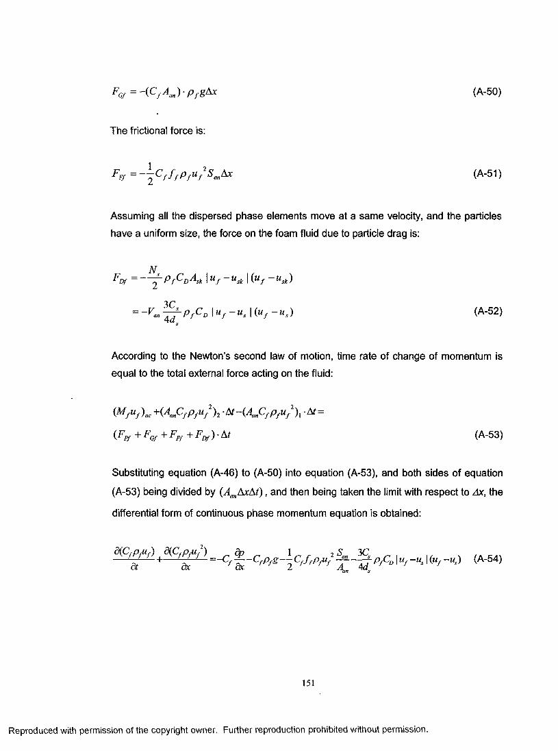
F 0f = H C f A a n ) - p f g & x

The frictional force is:

(A-50)

F t f = ~ C f f f P f U / S anA x (A-51)

Assuming all the dispersed phase elements move at a same velocity, and the particles

have a uniform size, the force on the foam fluid due to particle drag is:

N

FDf = ^ P D^sk I U f ~ U sk I ( M/ ~ Usk)

3 C= - Va n ^ J L P f C D \ Uf - Us \ ( Uf - Us) (A_52)

According to the Newton’s second law of motion, time rate of change of momentum is

equal to the total external force acting on the fluid:

( M f U f ) a c + ( A anC f p f u f ) 2 -A r ( A anC f p f u f ) , -1 s t —

(Fpf + FCf + FFf + FDf)- At (A-53)

Substituting equation (A-46) to (A-50) into equation (A-53), and both sides of equation

(A-53) being divided by (AanAxAt) , and then being taken the limit with respect to Ax, the

differential form of continuous phase momentum equation is obtained:

— I^ U— +— /qx - = - Cf ^ - C f Pf g ~ C f f f p/ uf2^ - ^ - p f CD\uf -us\(uf -us) (A-54)

151


APPENDIX BDERIVATION OF THE FOAM-CUTTINGS TRANSPORT MODEL FOR

HORIZONTAL WELLS

Two-Layer ModelThe cuttings transport in horizontal wells becomes more complicated than that in vertical

wells because of the possibility of the formation of cuttings bed on the lower part of the

wells.

There are two significant differences for modeling cuttings transport in horizontal well: (1)

Cross-section area allowing foam flow along the well would not be constant but change

with time due to the partial blockade of the annulus by solids bed. (2) If a stationary bed

formed, mass flow rate of cuttings along the well would not be always constant but be a

variable changing with time because of the mass exchange between fluid mixture and

stationary bed.

As described in Chapter 2, the main mechanisms responsible for cuttings transport in

horizontal wells are saltation and sliding. The determination of the critical conditions (i.e.

the inception of cuttings bed formation) requires the accurate determinations of forces

exerted on the solid particles. These are solids gravity force, drag force, static dry friction

force and lift force. Of all the forces, lift force is the one that must be known to calculate

the threshold condition. However, so far the knowledge about the lift force is very limited

for a single particle, let alone for multiple particles. To avoid the use of the lift force in the

analysis, investigators developed semi-empirical correlations of the critical solids

deposition velocity based on extensive experimental data. The correlation of Oroskar

and Turian (1980) represented such a method that provides a reliable prediction for

solids transport in horizontal pipe (Equation 2.10).

In this thesis, a modification of this correlation is used to predict the critical foam velocity

which is defined as the minimum foam velocity that prevents the formation of a solids

bed in a wellbore. If the foam flow velocity is dropped below the critical foam velocity,

solids are not transported completely, and a solids bed forms. Therefore, the basic

assumption of a two-layer flow model for solids transport in horizontal wells is needed.

152


Mass Exchange Between Layers (Source Terms)When the foam velocity is not equal to the critical value, cuttings deposition or

resuspension occurs at the interface of fluid and solids bed, which could be viewed as a

source (or sink) term for dispersed phase. If the increase of sediment bed height is Ahb

during At (Figure B-1), for a transient problem, the change of deposition mass flux of

particles per unit volume is:

As * Vj£ l (B-1)(A t-V 0)

where V0 denotes the volume of a control cell, AVb is the volume of settled solid

particles during At in the control cell.

Since AF6and Vacan be expressed as:

AVb = C bAAbAx (B-2)

V0 = A a Ax (B-3)

The change of solid phase source term during time At is:

As. - CbPsAt

r AVV j

(B-4)

where A0 represents the portion of the cross-section area allowing the foam and solids

flow, AAb represents the change of the cross-section area consisting of solids over the

time, and Cb is the concentration of the solids bed deposited at the low side of the hole

(=0.52 for cubic packing).

The drilling fluid (foam) will be entrained in the pores of the sediment solids bed. The

corresponding change of foam mass flow rate per unit volume is:

153


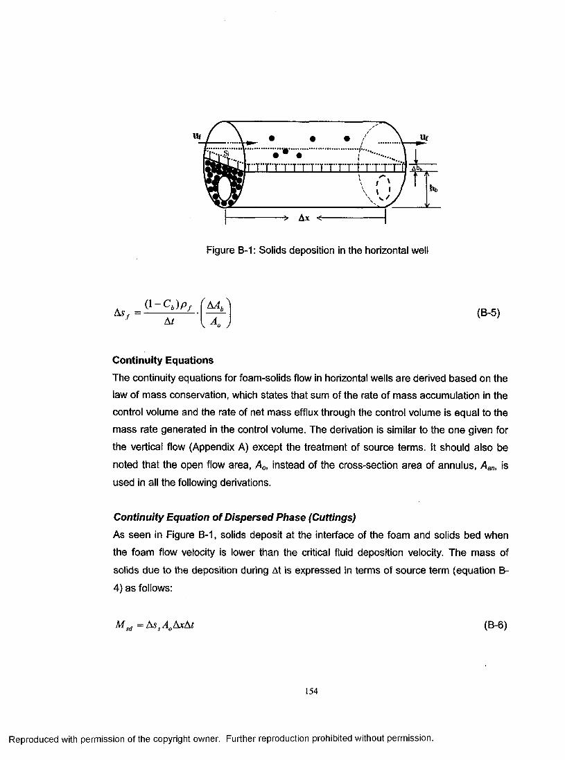
Figure B-1: Solids deposition in the horizontal well

J K t A(B-5)

Continuity EquationsThe continuity equations for foam-solids flow in horizontal wells are derived based on the

law of mass conservation, which states that sum of the rate of mass accumulation in the

control volume and the rate of net mass efflux through the control volume is equal to the

mass rate generated in the control volume. The derivation is similar to the one given for

the vertical flow (Appendix A) except the treatment of source terms. It should also be

noted that the open flow area, A0, instead of the cross-section area of annulus, Aan, is

used in all the following derivations.

Continuity Equation of Dispersed Phase (Cuttings)

As seen in Figure B-1, solids deposit at the interface of the foam and solids bed when

the foam flow velocity is lower than the critical fluid deposition velocity. The mass of

solids due to the deposition during At is expressed in terms of source term (equation B-

4) as follows:

M s d = *s ,A 0Axht (B-6)

154


Adding the solids deposition term (equation B-6) to the left side of equation (A-15), the

mass conservation equation for solids is obtained as follows:

( 4 c ,p A ) 2 -ti- iA C sP sU s)i • Ar + Axd('A°^sPs • At + AssAoAxAt = 0 (B-7)dt

If both sides of the equation (B-7) are divided by (AxAt) and are taken the limit with

respect to Ax, the equation changes into equation (B-8) by assuming a uniform solids

velocity:

5 .A-CM } + S(A£ , P . K - A A s (B-8)dx dt ° 5

Continuity Equation of Continuous Phase (Foam)

The mass of foam entrained in the pore of solids bed due to the deposition of solids

during At is expressed in terms of source term (equation B-5) as follows:

Mfe = As f A0 Ax At (B-9)

Adding the foam entrainment term (equation B-9) to the left side of equation (A-23), the

mass conservation equation for foam is obtained as follows:

d(A0Cfp f )(A0Cf pf uf )2 • At ~(A0Cf p f uf )l -At + Ax At + As f A0 Ax At =

(P o < lre ,o + P v A r e . * + P g < lre ,g ) ’ (B-10)

If both sides of equation (B-10) are divided by (AxAt) and are taken the limit with respect

to Ax, the equation changes into:

-^■(AoCf P f ) + - ^ ( A0Cf P f u/ ) = A0(sf - A s f ) (B-11)

155


Momentum EquationsMomentum Equation of Dispersed Phase (Cuttings)

In this 1-D foam-solids horizontal flow model, the momentum changes and forces (i.e.

pressure force, drag force and frictional force) parallel to the flow direction are

incorporated into the Newton’s second law of motion to derive the momentum equations.

Other forces (gravity force, lifting force, etc) acting perpendicular to the velocity direction

contribute to the cuttings deposition and resuspension, and their effects are incorporated

into the source terms only.

Dropping the gravity force term from equation (A-41), we have:

If we assume a uniform size for all the particles, and both sides of equation (B-12) are

divided by (AxAr) and are taken the limit with respect to Ax, the dispersed phase

momentum equation is simplified to:

Momentum Equation of Continuous Phase (Foam)Substituting equations (A-46) to (A-52) into equation (A-53) and removing the gravity

term yield:

d(A0CsPsus) [ d(A0CsPsu / )+

dt dxdt

(B-13)

d(V0c f P f U f )

1 3 C( - C f A 0 & p - - C f f f P f u f 2 S 0 A x - V 0 - ^ - P f C D | u f - u s \ ( u f - u s ) ) - A t (B-14)

156


If both sides of equation (B-14) are divided by (AxAr) and are taken the limit of Ax, the

continuous phase momentum equation is simplified to:

6 {A 0C f p f u f ) d (A 0C / P f U f )

dt dx

157


(B-15)

APPENDIX C

GEOMETRICAL EQUATIONS

Three different wellbore configurations based on the relative position of the drillpipe and

foam-cuttings bed interface are shown in Figure C-1.

Figure C-1: Wellbore configuration

The inner pipe eccentricity is defined as:

2e

A - A(C-1)

where Da is wellbore diameter, and A i s 'nner diameters, e is the offset between

centers.

The distance between the bottoms of outer and inner pipes is calculated:

0-A X A - A ) (C-2)

To calculate the cross-sectional area consisting of the sediment solid bed, it is convenient to first define an auxiliary function:

f (D ,h ) =D 1 arccos( - ? )

(C-3)

158


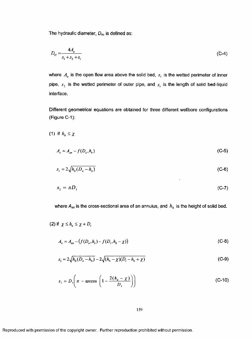
The hydraulic diameter, DH, is defined as:

S , + S 2 + 5 , .(C-4)

where A0 is the open flow area above the solid bed, sx is the wetted perimeter of inner

pipe, s2 is the wetted perimeter of outer pipe, and st is the length of solid bed-liquid

interface.

Different geometrical equations are obtained for three different wellbore configurations

(Figure C-1):

(1) if K <%

where Aan is the cross-sectional area of an annulus, and hb is the height of solid bed.

A = Aan~f(D0,hb) (C-5)

2 4hb{D0 - h b) (C-6)

(C-7)

(2) if x ^ K < x + A

A0=Aan- ( f (D0,hb) - f ( D i,hb- X )) (C-8)

= 2ylhb(D0- h b) - 2 4(hb- x m - h b+ x ) (C-9)

(5, = D t it — arccos 1 - (C-10)

v

159


(3) if x +D , <hb < D a

A o = A an f (D0,hb)7TD;2 ^ (0 -11)

= 2^ hb(D o - hb)

= 0

(C-12)

(0-13)

For all of the three configurations, we have:

*2 ' D0 i t - arccos (C-14)

160


APPENDIX DDERIVATION OF SOLIDS CONCENTRATION EQUATION

The volumetric concentration (volume fraction) was defined in equation (D-1) (Crowe,

1998):

AFCs = lim — (D-1)

S A F -> A F () A F

where AV0 is the limiting volume that ensures a stationary average.

Crowe’s definition of particle concentration is also applicable for solids-fluid flow.

Realistically, however, we need to specify a control volume, AV, and calculate the

average solids concentration in that volume to avoid taking the limit in equation (D-1).

The control volume is assumed to be a cylinder with cross sectional area, A, and height,

AL, (Figure D-1 (A)). It represents a local flow inside a multi-dimensional domain or a

section of a pipe flow. The control volume containing the mixture of solids and fluid in

Figure D-1 (A) can also be represented as the one in Figure D-1 (B) with the total

volume of solids, AVS, and volume of fluid, AVf, separated.

ALAV

(A )

< = ^ > AVf

Figure D-1: Solids concentration in a cylindrical control volume.

161


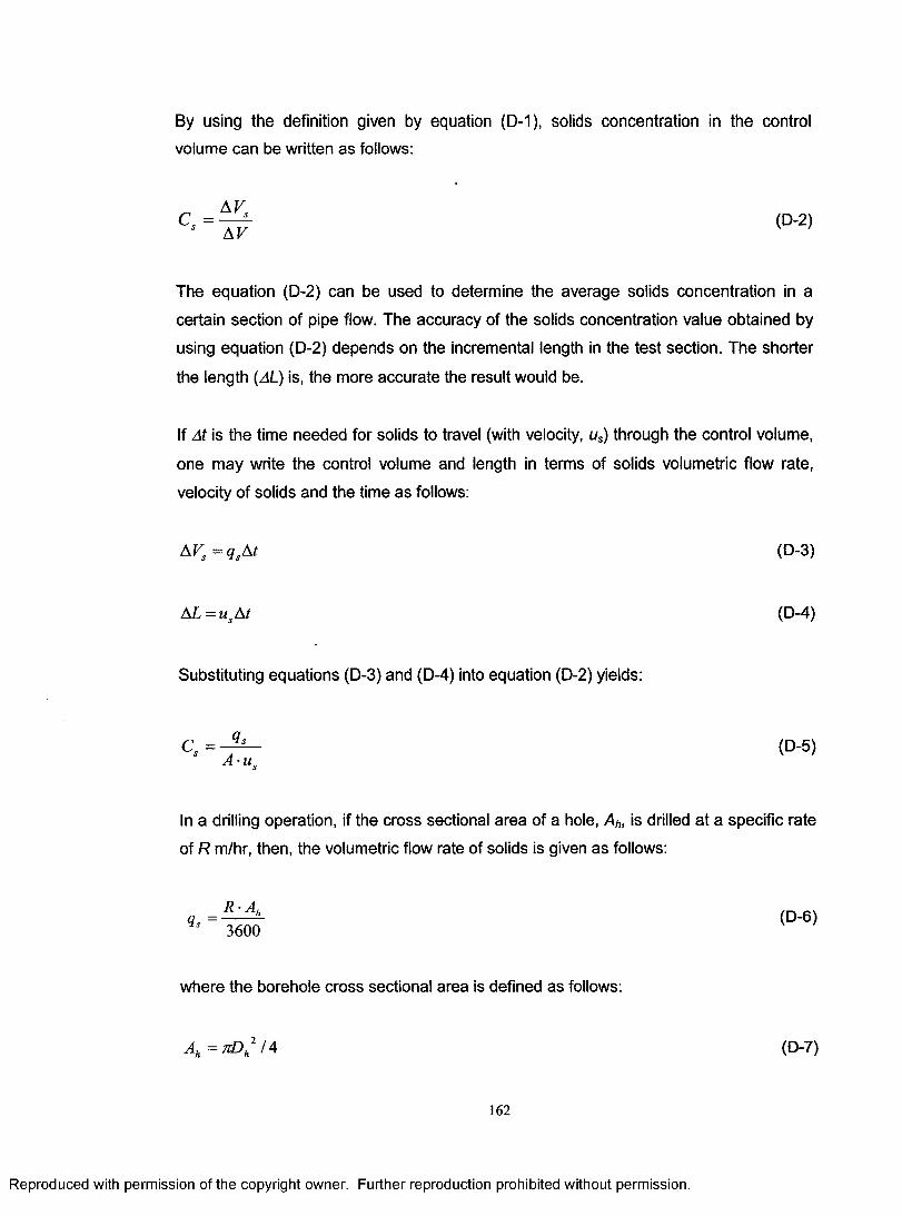
By using the definition given by equation (D-1), solids concentration in the control volume can be written as follows:

(D-2)

The equation (D-2) can be used to determine the average solids concentration in a

certain section of pipe flow. The accuracy of the solids concentration value obtained by

using equation (D-2) depends on the incremental length in the test section. The shorter

the length (AL) is, the more accurate the result would be.

If At is the time needed for solids to travel (with velocity, us) through the control volume,

one may write the control volume and length in terms of solids volumetric flow rate,

velocity of solids and the time as follows:

In a drilling operation, if the cross sectional area of a hole, Ah, is drilled at a specific rate

of R m/hr, then, the volumetric flow rate of solids is given as follows:

where the borehole cross sectional area is defined as follows:

= qsAt (D-3)

AL = u A t (D-4)

Substituting equations (D-3) and (D-4) into equation (D-2) yields:

(D-5)

(D-7)

162


The drilled cuttings are transported through the annular area, Aan, between drillpipe and

the wall of the hole. The annular cross sectional area of the hole can be expressed in

terms of hole diameter, Dh, and drillpipe diameter, Ddp as follows:

A a n = 7 r ( D h 2 - D dp2 ) / 4 (D-8)

By combining equations (D-2) to (D-8), a relationship for cuttings concentration in terms

of drilling rate and borehole geometry is obtained (Equation (D-9)):

c s = ---------------------------------- ( ° - 9 )3600-us(Dh2- D dp2)

Cuttings transport velocity, us, is accurately determined by using the mechanistic foam-

cuttings flow model developed in Appendix A. The us can be expressed as the difference

between drilling fluid velocity, uf, and the slip velocity of the fluid and solids, vs.

u s = u f - v s (D-10)

Therefore, the final form of cuttings concentration equation is given in terms of drilling

rate and fluid velocity as follows:

d r» 2C = -------------------- (D-11)

J 3600-(W/ - v s) ( D h2 - D d 2)

163


ERA - University of Alberta

Documents

Transcript of ERA - University of Alberta