EPSC 233: Earth and Life History
179
EPSC 233: Earth and Life History Galen Halverson Fall Semester, 2014
-
Upload
khangminh22 -
Category
Documents
-
view
3 -
download
0
Transcript of EPSC 233: Earth and Life History

EPSC 233: Earth and Life History
Galen Halverson
Fall Semester, 2014

Contents
1 Introduction to Geology and the Earth System 11.1 The Science of Historical Geology . . . . . . . . . . . . . . . . . . . . . . . . 11.2 The Earth System . . . . . . . . . . . . . . . . . . . . . . . . . . . . . . . . 4
2 Minerals and Rocks: The Building Blocks of Earth 62.1 Introduction . . . . . . . . . . . . . . . . . . . . . . . . . . . . . . . . . . . . 62.2 Structure of the Earth . . . . . . . . . . . . . . . . . . . . . . . . . . . . . . 62.3 Elements and Isotopes . . . . . . . . . . . . . . . . . . . . . . . . . . . . . . 72.4 Minerals . . . . . . . . . . . . . . . . . . . . . . . . . . . . . . . . . . . . . . 92.5 Rocks . . . . . . . . . . . . . . . . . . . . . . . . . . . . . . . . . . . . . . . 10
3 Plate Tectonics 163.1 Introduction . . . . . . . . . . . . . . . . . . . . . . . . . . . . . . . . . . . . 163.2 Continental Drift . . . . . . . . . . . . . . . . . . . . . . . . . . . . . . . . . 163.3 The Plate Tectonic Revolution . . . . . . . . . . . . . . . . . . . . . . . . . 173.4 An overview of plate tectonics . . . . . . . . . . . . . . . . . . . . . . . . . . 203.5 Vertical Motions in the Mantle . . . . . . . . . . . . . . . . . . . . . . . . . 24
4 Geological Time and the Age of the Earth 254.1 Introduction . . . . . . . . . . . . . . . . . . . . . . . . . . . . . . . . . . . . 254.2 Relative Ages . . . . . . . . . . . . . . . . . . . . . . . . . . . . . . . . . . . 254.3 Absolute Ages . . . . . . . . . . . . . . . . . . . . . . . . . . . . . . . . . . . 264.4 Radioactive dating . . . . . . . . . . . . . . . . . . . . . . . . . . . . . . . . 284.5 Other Chronostratigraphic Techniques . . . . . . . . . . . . . . . . . . . . . 31
5 The Stratigraphic Record and Sedimentary Environments 355.1 Introduction . . . . . . . . . . . . . . . . . . . . . . . . . . . . . . . . . . . . 355.2 Stratigraphy . . . . . . . . . . . . . . . . . . . . . . . . . . . . . . . . . . . . 355.3 Describing and interpreting detrital sedimentary rocks . . . . . . . . . . . . 36
6 Life, Fossils, and Evolution 416.1 Introduction . . . . . . . . . . . . . . . . . . . . . . . . . . . . . . . . . . . . 416.2 Fossils . . . . . . . . . . . . . . . . . . . . . . . . . . . . . . . . . . . . . . . 426.3 Biostratigraphy . . . . . . . . . . . . . . . . . . . . . . . . . . . . . . . . . . 446.4 The Geological Time Scale . . . . . . . . . . . . . . . . . . . . . . . . . . . . 456.5 Systematics and Taxonomy . . . . . . . . . . . . . . . . . . . . . . . . . . . 466.6 Evolution . . . . . . . . . . . . . . . . . . . . . . . . . . . . . . . . . . . . . 496.7 Gradualism Versus Punctuated Equilibrium . . . . . . . . . . . . . . . . . . 53
i

ii
7 The Environment and Chemical Cycles 557.1 Introduction . . . . . . . . . . . . . . . . . . . . . . . . . . . . . . . . . . . . 557.2 Ecology . . . . . . . . . . . . . . . . . . . . . . . . . . . . . . . . . . . . . . 567.3 The Atmosphere . . . . . . . . . . . . . . . . . . . . . . . . . . . . . . . . . 577.4 The Terrestrial Realm . . . . . . . . . . . . . . . . . . . . . . . . . . . . . . 617.5 The Marine Realm . . . . . . . . . . . . . . . . . . . . . . . . . . . . . . . . 63
8 Origin of the Earth and the Hadean 668.1 Introduction . . . . . . . . . . . . . . . . . . . . . . . . . . . . . . . . . . . . 668.2 Origin of the Solar System . . . . . . . . . . . . . . . . . . . . . . . . . . . . 668.3 Differentiation and the origin of the Moon . . . . . . . . . . . . . . . . . . . 678.4 The Late Heavy Bombardment . . . . . . . . . . . . . . . . . . . . . . . . . 67
9 Earth’s Earliest Record: the Archean 709.1 The Archean . . . . . . . . . . . . . . . . . . . . . . . . . . . . . . . . . . . 70
10 The Great Oxidation Event 7510.1 The Great Oxidation Event . . . . . . . . . . . . . . . . . . . . . . . . . . . 75
11 Early–Middle Proterozoic Life and Environment 8111.1 The Paleoproterozoic Glaciations . . . . . . . . . . . . . . . . . . . . . . . . 8111.2 Life in the Proterozoic . . . . . . . . . . . . . . . . . . . . . . . . . . . . . . 82
12 Supercontinents and the Assembly of North America 8412.1 Tectonics and the Supercontinental Cycle . . . . . . . . . . . . . . . . . . . 8412.2 The Assembly of North America . . . . . . . . . . . . . . . . . . . . . . . . 85
13 Neoproterozoic Snowball Earth and Rodinia Break-up 8713.1 Introduction . . . . . . . . . . . . . . . . . . . . . . . . . . . . . . . . . . . . 8713.2 Rodinia break-up . . . . . . . . . . . . . . . . . . . . . . . . . . . . . . . . . 8813.3 Geochemical Proxies . . . . . . . . . . . . . . . . . . . . . . . . . . . . . . . 8913.4 Record of Neoproterozoic glaciations . . . . . . . . . . . . . . . . . . . . . . 8913.5 The Snowball Earth hypothesis . . . . . . . . . . . . . . . . . . . . . . . . . 90
14 The Ediacaran Period and the Origin of Animals 9314.1 Introduction . . . . . . . . . . . . . . . . . . . . . . . . . . . . . . . . . . . . 9314.2 Chronology of Early Animal Evolution and Ediacaran Events . . . . . . . . 9514.3 Early Sponges? and the Molecular Clock Record of Metazoan Diversification 9614.4 The Acritarch Extinction and Radiation . . . . . . . . . . . . . . . . . . . . 9614.5 The Ediacara Biota . . . . . . . . . . . . . . . . . . . . . . . . . . . . . . . . 9714.6 Weakly Calcified Metazoa . . . . . . . . . . . . . . . . . . . . . . . . . . . . 100
15 The Cambrian Explosion 10115.1 The Early Cambrian . . . . . . . . . . . . . . . . . . . . . . . . . . . . . . . 10115.2 The Explosion . . . . . . . . . . . . . . . . . . . . . . . . . . . . . . . . . . 10715.3 Cambrian Biodiversity . . . . . . . . . . . . . . . . . . . . . . . . . . . . . . 109
iii
16 The Early Paleozoic: Age of the Invertebrates 11116.1 Orodovician life . . . . . . . . . . . . . . . . . . . . . . . . . . . . . . . . . . 11116.2 Simple animals . . . . . . . . . . . . . . . . . . . . . . . . . . . . . . . . . . 11216.3 The Bilateria . . . . . . . . . . . . . . . . . . . . . . . . . . . . . . . . . . . 11416.4 Colonial Metazoa . . . . . . . . . . . . . . . . . . . . . . . . . . . . . . . . . 119
17 The Early–Middle Paleozoic: Paleogeography, Stratigraphy, and Envi-ronments 12017.1 Paleozoic Tectonics and Paleogeography . . . . . . . . . . . . . . . . . . . . 12017.2 Paleozoic Climate . . . . . . . . . . . . . . . . . . . . . . . . . . . . . . . . . 123
18 Paleozoic Vertebrates and the Origin of Land Plants 12518.1 Origin of the Vertebrates . . . . . . . . . . . . . . . . . . . . . . . . . . . . 12518.2 Fish . . . . . . . . . . . . . . . . . . . . . . . . . . . . . . . . . . . . . . . . 12518.3 Amphibians . . . . . . . . . . . . . . . . . . . . . . . . . . . . . . . . . . . . 12618.4 Reptiles . . . . . . . . . . . . . . . . . . . . . . . . . . . . . . . . . . . . . . 12718.5 Land Plants . . . . . . . . . . . . . . . . . . . . . . . . . . . . . . . . . . . . 128
19 The Late Paleozoic and the Permo-Triassic Extinction 13019.1 Pangaea . . . . . . . . . . . . . . . . . . . . . . . . . . . . . . . . . . . . . . 13019.2 Late Paleozoic Climate . . . . . . . . . . . . . . . . . . . . . . . . . . . . . . 13019.3 Late Paleozoic Life . . . . . . . . . . . . . . . . . . . . . . . . . . . . . . . . 13119.4 Extinctions in the fossil record . . . . . . . . . . . . . . . . . . . . . . . . . 13319.5 The Big Five Mass Extinctions . . . . . . . . . . . . . . . . . . . . . . . . . 134
20 Mesozoic Life 13820.1 Recovery from the Permo-Triassic extinction in the marine realm . . . . . . 13820.2 Life on land in the Mesozoic . . . . . . . . . . . . . . . . . . . . . . . . . . . 14020.3 The End Triassic Mass Extinction . . . . . . . . . . . . . . . . . . . . . . . 143
21 Mesozoic Earth history 14421.1 Breakup of Pangaea . . . . . . . . . . . . . . . . . . . . . . . . . . . . . . . 14421.2 North America in the Mesozoic . . . . . . . . . . . . . . . . . . . . . . . . . 14521.3 Mesozoic Climate . . . . . . . . . . . . . . . . . . . . . . . . . . . . . . . . . 148
22 The Cretaceous-Paleogene Mass Extinction and the Paleogene 15022.1 The K-Pg Extinction . . . . . . . . . . . . . . . . . . . . . . . . . . . . . . . 15022.2 Life in the Paleogene . . . . . . . . . . . . . . . . . . . . . . . . . . . . . . . 15222.3 Paleogene Tectonics . . . . . . . . . . . . . . . . . . . . . . . . . . . . . . . 15522.4 Cenozoic Climate . . . . . . . . . . . . . . . . . . . . . . . . . . . . . . . . . 156
23 The Neogene 15823.1 Introduction . . . . . . . . . . . . . . . . . . . . . . . . . . . . . . . . . . . . 15823.2 Neogene Tectonics . . . . . . . . . . . . . . . . . . . . . . . . . . . . . . . . 15823.3 Neogene Climate . . . . . . . . . . . . . . . . . . . . . . . . . . . . . . . . . 16023.4 Life in the Neogene . . . . . . . . . . . . . . . . . . . . . . . . . . . . . . . . 162
iv
24 Pleistocene Glaciation and Earth System Evolution 16324.1 The Geological Record of Pleistocene Glaciation . . . . . . . . . . . . . . . 16324.2 The Oxygen-Isotopic Record of Glaciation . . . . . . . . . . . . . . . . . . . 16424.3 Milankovitch Cycles . . . . . . . . . . . . . . . . . . . . . . . . . . . . . . . 165
25 Origin and Evolution of Hominoids 16725.1 Early Hominid Evolution . . . . . . . . . . . . . . . . . . . . . . . . . . . . 16725.2 Hominin Evolution . . . . . . . . . . . . . . . . . . . . . . . . . . . . . . . . 167
Chapter 1
Introduction to Geology and theEarth System
1.1 The Science of Historical Geology
Historical geology is the study of the Earth’s past. This includes the evolution of the Earth(including both its surface and interior) and the life that has inhabited it. It also includesevents in the Earth’s history, many of which significantly shaped the course of life, thebiosphere, and more generally, the Earth System. It is virtually impossible to avoid Earthhistory if one work on rocks, because most rocks are old, and discerning their significanceentails knowing how old and in what environment or context they were formed. Earthhistory simply integrates as much information as possible obtained from all the rocks onthe surface of the Earth (and biological and chemical clues they contain) into a narrativeof Earth’s past. As you will appreciate, this is not an easy task and historical geologycourses have no choice but to omit most of the details. Like most Earth history courses,a large component of this course will entail stepping through the geological time scale tounderstand how Earth formed then changed over the course of its 4.56 billion years. Butfirst it will begin with introductions to the the sub-disciplines employed in studying Earth’spast and tools used to interrogate it.
Why study Earth history? To be honest, probably the main reason people do is becauseit is fundamentally interesting. If you are curious about how the Earth came to be theway it us, then you need to know about its past. That is, the only way to appreciate theoxygen in the atmosphere, the diversity of life, and the present geography of the globethat we inhabit is to delve into Earth’s past. Scientists more broadly interested in howplanets evolve are best served to begin with our planet, where we have a rich rock record ofits history. However, Earth history also has certain practical applications. In light of thecurrent challenges humanity faces due to environmental deterioration and global warming,many Earth historians now rationalize their work in terms of the need to predict Earth’sfuture. Although this argument is overplayed in my opinion, it is true that by studying,for example, past global warming episodes, we learn how the Earth System has respondedto global warming, most importantly the rates at which it responded and recovered. Itturns out there were multiple hypothermal episodes of sudden warming over the past 50million years, many if not all of which were driven by rapid input of greenhouse gases intothe ocean-atmosphere system. If we want to learn the consequences and rates of response
1
Chapter 1: Geology and the Earth System 2
to the current episode of fossil-fuel and land-use driven rise in CO2, it is logical to beginby looking at past analogs.
The distribution and extent of petroleum and mineral deposits is also governed by pastgeological events. Consider the source rock (i.e., an organic-rich sedimentary rock) for apetroleum reservoir in a sedimentary basin. By understanding how and under what depo-sitional environment this source rock formed, a petroleum geologist might better predictits distribution in the subsurface and extrapolate these results to other sedimentary basinswhere similar types of rock might be expected to have been deposited.
Earth history can be subdivided into three broad themes: Deep Time, Plate Tectonics,and the Evolution of Life (Levin, 2013). Compared to the human life span, geologicaltime us incomprehensibly vast. Geology has taught us this, and now a important part ofgeology is dating and calibrating Earth’s 4.56 billion-year-old history. Of particular interestis dating major catastrophic events and the the first appearance or occurrence of certainphenomena. Plate tectonics was not fully accepted by the geological community until theearly 1970’s, but now it is and integral component of virtually any study of past geologicalevents (sedimentologists and palaeontologists ignore tectonics at their own peril!). Andthe origins of geology itself are deeply rooted in the study of the fossil record and thedocumentation and interpretation of the evolution of life. Logically, as we dig deeper intoEarth’s past, it becomes more and more difficult to divine its stories. The oldest mineralsthat formed on Earth (that is, after planetary accretion) are about 4.4 billion years old,and the oldest rocks are 4.0 billion years old. Hence, deciphering Earth’s earliest historyrequires a combination of esoteric geochemical techniques, modelling, and an abundanceof creativity.
1.1.1 Geology
Geology is the fundamental tool or approach that is used to study Earth’s past. Geol-ogy encompasses the study of all types of rock found on Earth and on other planetarybodies. The three main rock types are igneous, metamorphic, and sedimentary and allcontain important clues about past geological events. Igneous rocks, for example, indicatepast thermal events that may have been related to subducting plates, rifting, hot spots, orother processes capable of melting the mantle or the crust. Studying metamorphic rockscan reveal key details about ancient mountain building events, hence continent-continentcollisions. The sedimentary record, which comprises both sedimentary rocks and unlithi-fied sediments, also contains important information about past thermal and tectonic events(the weathered detritus from volcanoes and mountain belts is ultimately deposited in sed-imentary basins). Sedimentary rocks are also the only of the three major rock types topreserve fossils. Because the study of ancient life is effectively the core of historical geology,Earth History is based heavily on sedimentary geology and palaeontology.
1.1.2 Application of Scientific Method in Geology
Geology is frequently accused of being unscientific by scientists that do not fully under-stand what geologists do. But it is true that although experimentation is important incertain domains of the Earth sciences, it is not the basis of geology as it is in physics,chemistry, and much of biology. So where is the science in geology, in particular historical
Chapter 1: Geology and the Earth System 3
geology? They way to look at this problem is terms of testing hypotheses. Earth histo-rians effectively formulate ideas about what happened in Earth’s past. Ultimately, thesemodels should offer the most parsimonious explanation of all available data and presentconcrete ways of being tested. For example, some researchers have argued that the Permo-Triassic extinction, like the Cretaceous-Paleogene extinction (formally known as the K-T),was likely triggered by a meteorite impact. Well, lots of other scientists disagree with thismodel, but it is testable, at least in theory, because meteorite impacts leave specific tracesin the sedimentary record, including unusual accumulations of platinum group elementsand unique organic chemicals derived from meteorites.
I find historical geology tricky because it so often lacks definitive answers. Show an outcropof rocks to ten different geologists, and probably you will hear ten different explanationsfor why those rocks are there and what they signify. Likely as not, a few of those geologistswill argue passionately about their hypotheses, even if there seem to be multiple viableexplanations. As a consequence, it is reasonable to question any model that is put forwardto explain Earth’s past. You might ask why bother if geologists cannot be coerced toagree upon any hypotheses anyway. The answer is because as more data are collectedand hypotheses proposed, geologists tend to converge on a given model or hypotheses,to the extent that it then gives way to a theory that is widely accepted by the scientificcommunity.
1.1.3 The Principle of Actualism
The foundation upon which Geology is built is the principle of Actualism, which holdsthat fundamental chemical and physical processes do not change. James Hutton, whohas earned the monicker of “Father of Modern Geology”, and his great promoter CharlesLyell recognized that process on Earth operate slowly and gradually and surmised thatthese same processes occurred throughout the history of Earth, giving rise to the rocksand physiographic features we see today. This concept of uniformitarianism has come todominate geological thought and is nicely encapsulated in the famous lines: “No vestige ofa beginning, no prospect of an end” and ”The present is the key to the past.”
When it was proposed, the idea of uniformitarianism was radical because it contradictedthe prevailing catastrophic theories for the Earth, with obviously immense implications forthe age of the Earth and the legitimacy of the Bible. However, through Charles Lyell’spersuasive arguments, the paradigm shift occurred and uniformitarianism has guided geo-logical thought and research for much of the past two centuries. However, like any greatnew theory in geology, this one was flawed. Specifically, Hutton and Lyell envisioned thatonly those processes witnessed by humans occurred in the past and that all processeswere gradual. Given the immense age of the Earth as compared to the short duration ofhistorical records, this suggestion now seems rather absurd, and it is now well acceptedthat catastrophic events of the sort never witnessed by humans have occurred episodicallythroughout Earth history. Indeed, these episodic events, such as meteorite impacts, andmassive volcanic eruptions, probably play an outsized role in shaping Earth’s surface andthe evolution of life and the environment.
Another important point on which Lyell erred was the idea that the nature of the processesand the rocks they formed have not changed since the Earth was formed. We now know,
Chapter 1: Geology and the Earth System 4
through the study of Earth history, that this is truly not the case. The increase in atmo-spheric oxygen concentrations, influences of life, and cooling of the interior of the Earth,to name but a few examples, have all led to unidirectional changes in geological processesand the types of minerals and rocks that form on Earth’s surface.
1.2 The Earth System
It is in vogue these days to discuss Earth as a system. Indeed, our textbook is called EarthSystem History. So what does this mean? The Earth system concept is rooted in theappreciation that Earth is unique, and the conditions on Earth’s surface that sustain lifeare the result of interaction and balance between various components, or systems, of theEarth, namely the hydrosphere, the atmosphere, the biosphere, the cryosphere the Earth’sinterior, its exterior, and climate. All of these systems can be subdivided into subsystems,which are also interrelated both to each other and to some lesser extent to subsystems ofother systems. You might think of the Earth system concept as a more scientifically palat-able version of the Gaia hypothesis, which holds that all organisms and their inorganicmilieu are integrated to form a single, self-regulating system, not unlike how various celltypes, organs, and bacteria in our bodies all work together and interact to sustain our lives.
Earth’s systems are dynamic and none of them operates in isolation. That is, the systemsare coupled. The habitability of the planet is ultimately maintained by negative feedbackloops that regulate couplings between the systems. A feedback is a response to a pertur-bation or stimulation of a system. For example, if you deprive yourself of food for a longtime, you will become thirsty, which might cause you to take a drink of water to alleviatethat thirst. This is an example of a negative feedback. Negative feedback loops tend todiminish disturbances and to maintain equilibrium states.
Positive feedback loops occur when a disturbance results in a response that amplifies thedisturbance. Unchecked positive feedbacks lead to unstable scenarios and can result in arunaway. For example, consider the situation with Arctic sea ice. It is both graduallythinning and decreasing in aerial extent, due to warming of the Arctic. The more this seaice thins and disappears, the more the ocean can absorb and retain heat energy from thesun, which will make the Arctic warmer and melt more sea ice. Eventually, this feedbackloop, if unchecked by some other negative feedback, will runaway, leaving the Arctic oceansea ice-free.
Equilibrium states may be either stable or unstable. In a stable state, a minor disturbancewill result in a response that returns the state to the original equilibrium. In an unsta-ble state, a disturbance will result in a shift to a new equilibrium state or to disequilibrium.
Earth system history is simply an approach to interpreting Earth’s history that appreciatesthe interconnectedness between the different components of the planet and the inescapablefact that Earth as we know it today is the result of its long and unique history. For exam-ple, mass extinctions have impacts on the oceans, the atmosphere and the biosphere, andmay be triggered by internal Earth processes. Hence, if one wishes to understand massextinctions, it is not enough simply to study the fossil record to determine the pattern ofextinction and recovery. As you will see, mass extinctions are invariably linked to major

Chapter 1: Geology and the Earth System 5
carbon isotope excursions, which illustrates that the they represent perturbances to theglobal carbon cycle. Because Earth’s climate is also coupled to the carbon cycle, massextinctions might be expected to be associated with climate change–either as a trigger, aconsequence, or both. Similarly, the chemistry of the ocean is controlled in part by climateand by the processes that remove CO2 from the atmosphere over geological time. Hence,ocean chemistry also typically changes across mass extinction events. The coupled changesin the atmosphere, oceans, climate, and the biosphere during mass extinctions exemplifythe behaviour of the Earth system and the necessity of considering the systems togetherwhen interpreting Earth’s history, and its future.
From a somewhat philosophic perspective, Earth history has taught us that the Earthsurface environment that we inhabit is both fragile and robust. On relatively short timescales, in can be strongly perturbed with dire consequences for the life that inhabits it.However, life is tenacious and none of these disturbances, from the snowball Earth to hugemeteorite impacts, has been sufficient to eradicate it. Over long (non-human) time scales,the Earth system recovers from perturbations, including the current experiment in rapid,human-induced environmental change.

Chapter 2
Minerals and Rocks: The BuildingBlocks of Earth
Reading: Chapter 2 in Earth System History (Stanley, 3rd edition)
2.1 Introduction
Most of what we know about Earth’s history comes from the study of rocks. The rocksare made up of minerals, which themselves comprise molecules that form from diversecombinations of elements. Hence, it is useful to review the basics of elements, chemicalbonds, minerals, and rocks before jumping into Earth history, which presupposes a certainknowledge of rocks. But even before we begin that discussion, we need to talk about thebasic structure of the Earth in order to frame the discussion of rocks.
2.2 Structure of the Earth
Geologists now have a reasonable grasp on the basic physical and chemical structure of thewhole Earth. We owe much of this knowledge to seismology, through which geophysicistsimage Earth’s interior, via a technique not unlike CT scans used by doctors to imagine thebody. When an Earthquake occurs, it sends seismic waves across and through the Earth,the patterns of which are recorded on a global network of seismographs. Scientists use thisdata to pinpoint the location and magnitude of earthquakes, and as we’ll see later, thecollection of data on the foci of earthquakes was an important piece in the plate tectonicspuzzle. Importantly, these seismic waves are also sensitive to temperature and whetherthe material they pass through is liquid or solid, and hence, reveal the structure of theinterior of the Earth, which is one of abrupt boundaries between liquids and solids anddenser and less dense layers. You will know doubt learn a lot more about seismology andseismic waves in another course.
The average radius of Earth is 6370 km. Earth can be subdivided into four physical layers:
• the solid iron+nickel inner core (6370–5150 km)
• the liquid iron+nickel outer core (5150–2900 km)
• the viscoelastic, silicate asthenosphere (2900 to 40–150 km)
6

Chapter 2: Minerals & Rocks 7
• the elastic lithosphere
Figure 2.1: The components of Earth’s deep interior.
The lithosphere is further subdivided into the crust and the mantle asthenosphere, wherethe mantle encompasses everything from the base of the crust to the top of the outer core(hence the terms mantle and asthenosphere are often interchanged, even though they arenot exactly the same). The boundary between the crust and the mantle is chemically de-fined as is known as the Mohorovicic discontinuity—the Moho for short. Rocks below thisboundary are significantly denser than the rocks above.
The crust is highly variable in thickness. It is thinnest beneath the deep oceans (7–10 km),where it is made up of basalt and has an average density of about 2.9 g/cm3. Continentalcrust has is less dense (∼ 2.7 g/cm3), is compositionally similar to granite (on average),and varies from about 25 to 70 km in thickness. As you know, the continents stand abovethe oceans, and in mountain ranges, far above the ocean floor. The continental crustalso extends well below the oceanic crust. This geometry is explained simply by isostasy,which is the gravitational equilibrium between the lithosphere and the asthenosphere (thatis, think of the lithosphere floating on the asthenosphere). The oceanic crust-continentalcrust dichotomy yields a distinct hypsometry (Fig. 2.2), which sets Earth apart from theother planets and moons in the solar system.
2.3 Elements and Isotopes
In order to understand minerals, it is necessary first to step back and understand elements.

Chapter 2: Minerals & Rocks 8
Figure 2.2: The hypsometric curve of Earth shows two distinct modes of elevation (orbathymetry) relative to see level: low continental interiors and the deep ocean floor. Moun-tains and trenches only cover a small part of Earth’s surface.
2.3.1 Elements
An element consists of a unique kind of atom. Atoms comprise a nucleus of neutrons andprotons(+), each of which has an atomic mass unit of 1, surrounded by shells of electrons(-),which have a minimal mass.
• Elements are distinguished by their number of protons (atomic number)
• Protons and neutrons roughly equal in nucleus
• Electrons form shells around the nucleus, and to a large extent, are responsible forthe chemical behavior of an atom
2.3.2 Isotopes
Although the number of neutrons in the nucleus of a given atom is typically close to thenumber of protons, particularly in lower mass elements, the number of neutrons varies formany elements. So, for example, whose atomic number is 8, may have 8, 9, or 10 neutrons.Each type of oxygen atom (that is, with 8, 9, or 10 neutrons) is called an isotope. Thechemical properties of different isotopes of the same element are identical, but due to theirdifferent masses, they react at slightly different rates. This phenomenon turns out to be
Chapter 2: Minerals & Rocks 9
extremely important and is the basis of stable isotope geochemistry, which will be discussedin more detail later in the course. Another important phenomenon is that some isotopes areinherently unstable, or radioactive. These isotopes decay to form daughter isotopes (whichmay or may not be stable), and in the process, emit energy in the form of radiation. Asyou know, radioactive isotopes are an important source of energy, including that for therover Curiosity which is currently cruising around Gale Crater on Mars. But radioactiveisotopes are also important as a tool for dating geological materials, as will be discussedin detail in a subsequent lecture.
2.3.3 Chemical bonds
Minerals are formed by way of chemical reactions, during which two or more atoms of oneore more elements combine to form a molecule, which is the basic until of a chemical com-pound. As a general rule, compounds behave differently than their constituent elements,because their size, electrical charge, and other characteristics are modified.
Ionic bonds are bonds that involve the transfer of electrons from one to another, typicallyresulting in stable electron shell configurations. This transfer results in opposite electriccharges between the two atoms, and it is the attraction between these two oppositelycharged ions that binds the two elements. The classic example of an ionic bond is NaCl(halite), where sodium gives up one electron from its outer shell and chlorine adds thatelectron to a shell that contained 7 electrons to round it out at eight. Ionic bonds commonlyoccur between metals and non-metals (i.e., between elements on the left and right-handside of the period table, respectively).
Covalent bonds occur where two atoms share pairs of electrons. Common examples includeO2 and CO2. The mineral diamond, in which carbon atoms share electrons on all sides, isan example of a covalently bonded mineral.
Ionic complexes form where two or more atoms bond but do not achieve charge balance.Rather, then retain a charge. For example, the carbonate ion in seawater: (CO3)
2−.
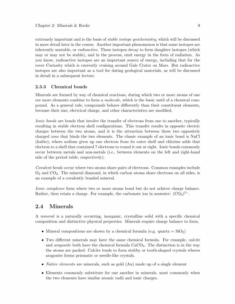
2.4 Minerals
A mineral is a naturally occurring, inorganic, crystalline solid with a specific chemicalcomposition and distinctive physical properties. Minerals require charge balance to form.
• Mineral compositions are shown by a chemical formula (e.g. quartz = SiO2)
• Two different minerals may have the same chemical formula. For example, calciteand aragonite both have the chemical formula CaCO3. The distinction is in the waythe atoms are packed. Calcite tends to form stubby or tooth-shaped crystals wheresaragonite forms prismatic or needle-like crystals.
• Native elements are minerals, such as gold (Au) made up of a single element
• Elements commonly substitute for one another in minerals, most commonly whenthe two elements have similar atomic radii and ionic charges.
Chapter 2: Minerals & Rocks 10
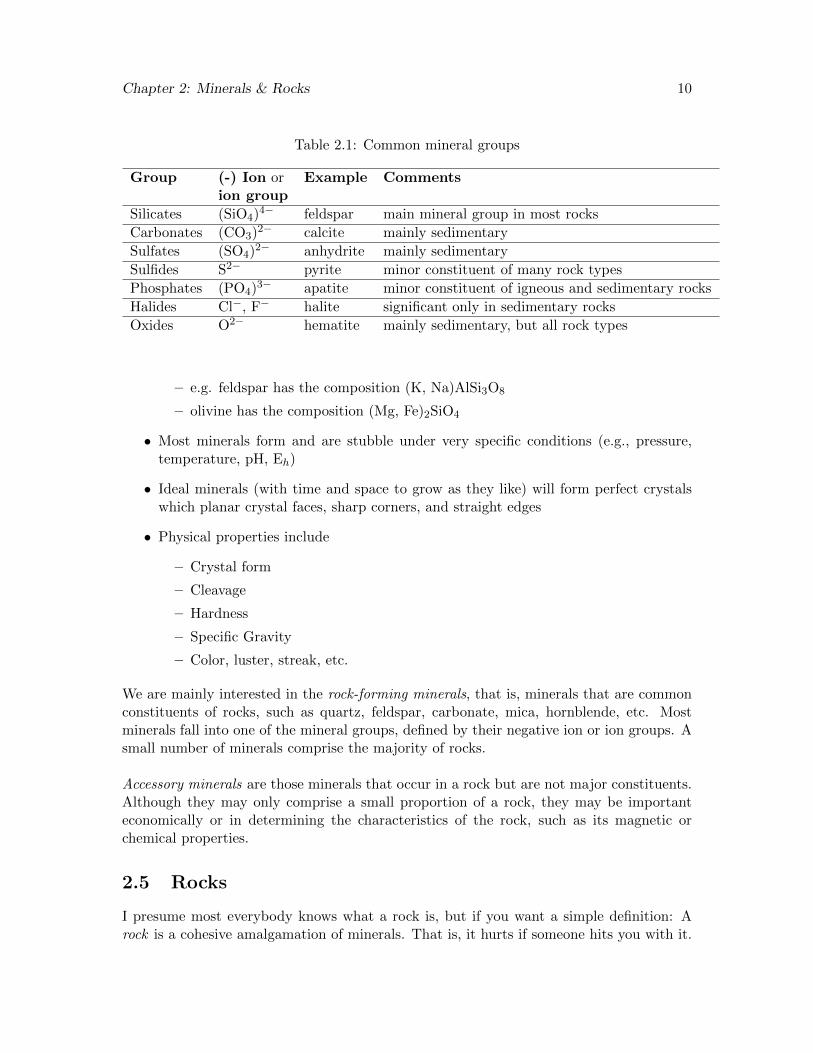
Table 2.1: Common mineral groups
Group (-) Ion or Example Commentsion group
Silicates (SiO4)4− feldspar main mineral group in most rocks
Carbonates (CO3)2− calcite mainly sedimentary
Sulfates (SO4)2− anhydrite mainly sedimentary
Sulfides S2− pyrite minor constituent of many rock types
Phosphates (PO4)3− apatite minor constituent of igneous and sedimentary rocks
Halides Cl−, F− halite significant only in sedimentary rocks
Oxides O2− hematite mainly sedimentary, but all rock types
– e.g. feldspar has the composition (K, Na)AlSi3O8
– olivine has the composition (Mg, Fe)2SiO4
• Most minerals form and are stubble under very specific conditions (e.g., pressure,temperature, pH, Eh)
• Ideal minerals (with time and space to grow as they like) will form perfect crystalswhich planar crystal faces, sharp corners, and straight edges
• Physical properties include
– Crystal form
– Cleavage
– Hardness
– Specific Gravity
– Color, luster, streak, etc.
We are mainly interested in the rock-forming minerals, that is, minerals that are commonconstituents of rocks, such as quartz, feldspar, carbonate, mica, hornblende, etc. Mostminerals fall into one of the mineral groups, defined by their negative ion or ion groups. Asmall number of minerals comprise the majority of rocks.
Accessory minerals are those minerals that occur in a rock but are not major constituents.Although they may only comprise a small proportion of a rock, they may be importanteconomically or in determining the characteristics of the rock, such as its magnetic orchemical properties.
2.5 Rocks
I presume most everybody knows what a rock is, but if you want a simple definition: Arock is a cohesive amalgamation of minerals. That is, it hurts if someone hits you with it.
Chapter 2: Minerals & Rocks 11
2.5.1 Igneous Rocks
Igneous rocks form from cooling magma, which consists of a mixture of molten material(liquid), gas (e.g. H2O, CO2), and minerals. Igneous rocks are crystalline, made up ofinterlocking minerals. As a general rule, igneous rocks that cool quickly are finer grained,and those that cool more slowly are coarser grained.
2.5.2 Extrusive igneous rocks
Volcanic (extrusive) igneous rocks solidify quickly on the surface from lava. They tend tobe mainly aphanitic–that is, very fine grained. However, in some cases, minerals beginto crystallize in the magma chamber and are erupted along with the magma. Volcaniceruptions produce gases, steam, lava, and tephra, which is fragmented material generateby an eruption and includes ash.
• Lava flows
• Obsidian is volcanic glass that forms when a degassed magma cools extremely quickly
• Pumice forms where magmas rich in gases solidify rapidly and contain significantpore space
• Pyroclastic deposits consist of airborne volcanic material. Tuffs are the pyroclasticdeposits consisting mainly of ash.
2.5.3 Intrusive igneous rocks
Plutonic (intrusive) igneous rocks solidify slowly below the surface and are mainly phaner-itic—consisting of visible crystals. Plutonic rock bodies come in many shapes and sizes.
• Pluton is the general term for a larger body of intrusive igneous rock
• Dykes are vertical (relative to the land surface at the time of emplacement) sheets ofintrusive igneous rocks
• Sills are horizontal sheets of intrusive igneous rocks
2.5.4 Classification of igneous rocks
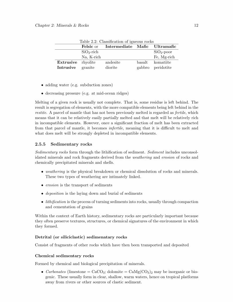
Both extrusive and intrusive igneous rocks are distinguished by their chemical composi-tion, namely by the abundance of SiO2 and other key elements, such as Na, K, Fe, and Mg.However, there are also very important difference in trace elements between these differentrock types. So-called incompatible elements, such as U and the rare earth elements (REEs)tend to be concentrated in felsic (i.e., more silica rich and Fe-, and Mg-poor melts), whereascompatible elements, such as Ni and Ti, are found preferentially in more mafic (silica-poorand Fe-, and Mg- rich) rocks.
The first step in making an igneous rocks is melting existing rocks. Melting is accomplishedby one of three general processes:
• increasing temperature (e.g. mantle plumes)
Chapter 2: Minerals & Rocks 12
Table 2.2: Classification of igneous rocksFelsic or Intermediate Mafic Ultramafic
SiO2-rich SiO2-poorNa, K-rich Fe, Mg-rich
Extrusive rhyolite andesite basalt komatiiteIntrusive granite diorite gabbro peridotite
• adding water (e.g. subduction zones)
• decreasing pressure (e.g. at mid-ocean ridges)
Melting of a given rock is usually not complete. That is, some residue is left behind. Theresult is segregation of elements, with the more compatible elements being left behind in therestite. A parcel of mantle that has not been previously melted is regarded as fertile, whichmeans that it can be relatively easily partially melted and that melt will be relatively richin incompatible elements. However, once a significant fraction of melt has been extractedfrom that parcel of mantle, it becomes infertile, meaning that it is difficult to melt andwhat does melt will be strongly depleted in incompatible elements.
2.5.5 Sedimentary rocks
Sedimentary rocks form through the lithification of sediment. Sediment includes unconsol-idated minerals and rock fragments derived from the weathering and erosion of rocks andchemically precipitated minerals and shells.
• weathering is the physical breakdown or chemical dissolution of rocks and minerals.These two types of weathering are intimately linked.
• erosion is the transport of sediments
• deposition is the laying down and burial of sediments
• lithification is the process of turning sediments into rocks, usually through compactionand cementation of grains
Within the context of Earth history, sedimentary rocks are particularly important becausethey often preserve textures, structures, or chemical signatures of the environment in whichthey formed.
Detrital (or siliciclastic) sedimenatary rocks
Consist of fragments of other rocks which have then been transported and deposited
Chemical sedimentary rocks
Formed by chemical and biological precipitation of minerals.
• Carbonates (limestone = CaCO3; dolomite = CaMg(CO3)2 may be inorganic or bio-genic. These usually form in clear, shallow, warm waters, hence on tropical platformsaway from rivers or other sources of clastic sediment.

Chapter 2: Minerals & Rocks 13
Table 2.3: Classification of detrital sedimentary rocks
Sediment Rock
gravel (grains > 2 mm) conglomerate (rounded), breccia (angular), diamictite (grains in matrix)sand (1/16 - 2 mm) sandstone (quartz sandstone, feldspathic sandstone, lithic sandstone)silt (1/256 - 1/16 mm) siltstonemud (silt + clay) mudstone or shale (finely laminated)clay (< 1/256 mm) claystonemud matrix + sand and/or gravel wacke
• Evaporites, including halite (salt) and gypsum (CaSO4)•2H2O form by evaporation ofconcentrated solutions. Significant evaporite deposits usually form in the subtropics.
• Chert consists of of microcrystalline quartz. Whereas most marine chert that hasformed in the past few hundred millions of years is derived from microscopic, siliceousshells (diatoms or radiolaria) or sponge spicules, older cherts were most likely inor-ganic (although their formation may have been biologically mediated in cases).
• Banded iron formation or BIF, is layered, iron-rich rock
• Coal is the compressed and altered remains of land plants
2.5.6 Metamorphic rocks
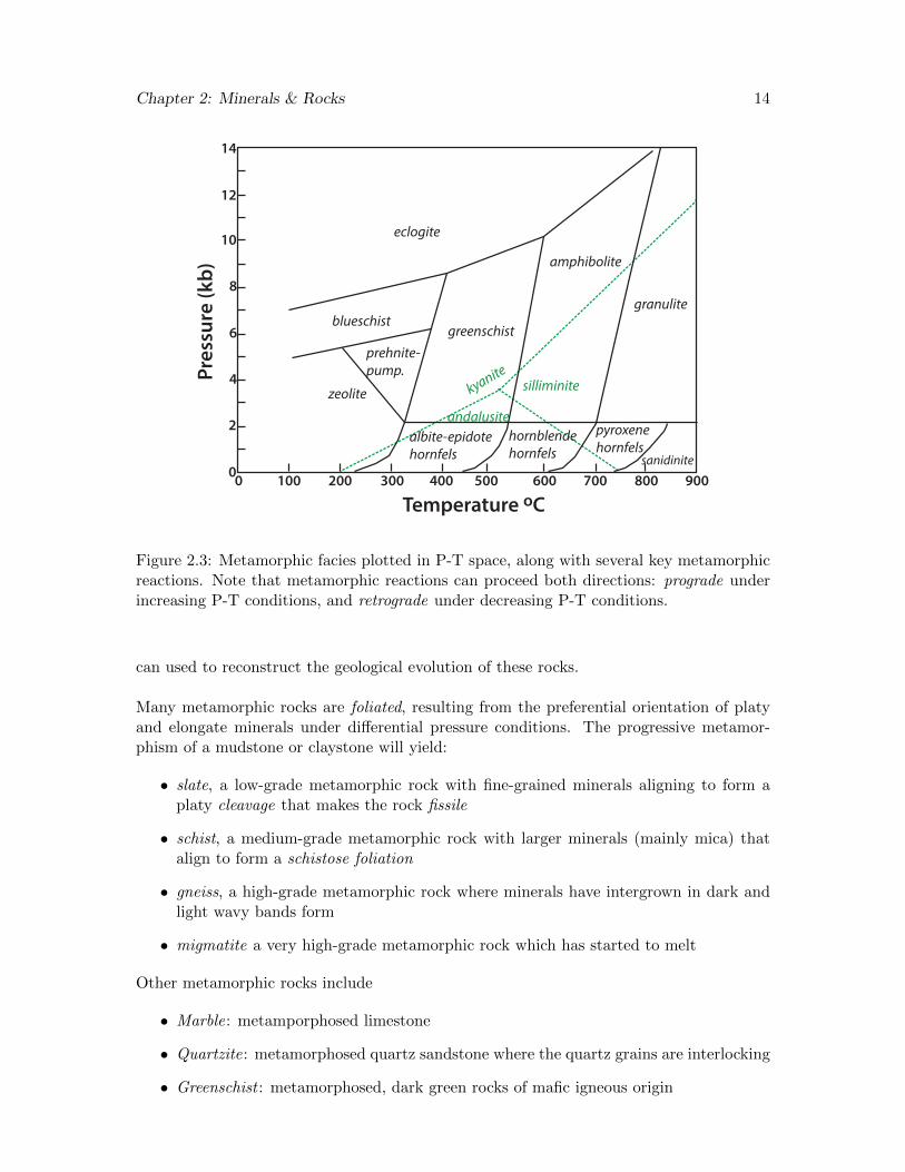
Metamorphic rocks form through the solid state alteration of other rocks (igneous, sedi-mentary, or metamorphic) due to changes in temperature, pressure, and/or fluids. Meta-morphism involves the slow crystallization of new minerals that are thermodynamicallystable under the changed temperature/pressure/fluid conditions. For example, the miner-als muscovite and quartz react under amphibolite facies (see below) pressure-temperature(P-T) conditions to form orthoclase, sillimanite, and water (Fig. 2.3).
KAl3Si3O10(OH)2 + SiO2 = KAlSi3O8 +Al2SiO5 +H2O (2.1)
• Contact metamorphism is driven by heat (± fluids) from an adjacent igneous body
• Burial metamorphism occurs through the depositional burial of sedimentary andvolcanic rocks
• Regional metamorphism effects large areas that are buried and heated, usually inmountain-building events
• Hydrothermal metamorphism is the result of interaction of rocks with hot, percolatingfluids (most commonly on mid-ocean ridges)
• Shock metamorphism occurs when an asteroid impacts Earth
Metamorphism often occurs under differential pressures (i.e. mountain belts), which resultsin the development of distinct textures which, in combination with the mineral assemblages
Chapter 2: Minerals & Rocks 14
silliminite
andalusite
kyanite
Temperature oC
Pres
sure
(kb)
14
12
10
8
6
4
2
00 100 200 300 400 500 600 700 800 900
zeolite
albite-epidotehornfels
hornblendehornfels
pyroxenehornfels
sanidinite
blueschist
eclogite
greenschist
amphibolite
granulite
prehnite-pump.
Figure 2.3: Metamorphic facies plotted in P-T space, along with several key metamorphicreactions. Note that metamorphic reactions can proceed both directions: prograde underincreasing P-T conditions, and retrograde under decreasing P-T conditions.
can used to reconstruct the geological evolution of these rocks.
Many metamorphic rocks are foliated, resulting from the preferential orientation of platyand elongate minerals under differential pressure conditions. The progressive metamor-phism of a mudstone or claystone will yield:
• slate, a low-grade metamorphic rock with fine-grained minerals aligning to form aplaty cleavage that makes the rock fissile
• schist, a medium-grade metamorphic rock with larger minerals (mainly mica) thatalign to form a schistose foliation
• gneiss, a high-grade metamorphic rock where minerals have intergrown in dark andlight wavy bands form
• migmatite a very high-grade metamorphic rock which has started to melt
Other metamorphic rocks include
• Marble: metamporphosed limestone
• Quartzite: metamorphosed quartz sandstone where the quartz grains are interlocking
• Greenschist : metamorphosed, dark green rocks of mafic igneous origin

Chapter 2: Minerals & Rocks 15
• Blueschist : high pressure, moderate temperature, altered basalt (in subduction zones)
• Eclogite: very high pressure, moderate–high temperature
• Granulite: formed under extremely high temperature conditions
Chapter 3
Plate Tectonics
Reading: Chapters 8–9 in Stanley
3.1 Introduction
Plate tectonics describes the motion of Earth’s lithosphere, which is broken into a seriesof plates that move relative to one another. Plate tectonics is driven by mantle convectionand explains many distinct observations that the continents drifted across the globe overgeological time, episodically crashing into one another. A half a century into acceptanceof plate tectonics, it is now almost baffling to think that theory took so long to take hold –one only has to look at a bathymmetric map of the oceans to see the work of plate tectonicsin all of its glory.
3.2 Continental Drift
In 1912, Alfred Wegner, a German meteorologist, proposed the hypothesis of continentaldrift to explain massive evidence the he and previous scientists had assembled that Earth’scontinents had once been part of a single continent (Pangea) that had subsequently brokenapart. British geologist Arthur Holmes and South African geologist Alexander du Toitprovided additional geological and paleontological evidence for continental drift and theancient supercontinent.
• Geography: the shorelines of the continents (in particular eastern South America andwestern Africa) fit together like pieces of a puzzle
• Correlation: sedimentary sequences from many continents now separated from eachother were very similar in composition and age
• Fossils: Many fossils of extinct organisms from scattered continents converged to asingle geographic zone when the continents are restored to their supercontinentalconfiguration
• Paleoclimate: Indicators of ancient ice flow directions related to similar aged glacialdeposits, including in many areas currently outside of the polar latitudes, all consis-tent with a large ice sheet centered on the southern part of the supercontinent. Asimilar pattern is seen in northern hemisphere coal seems.
16
Chapter 3: Plate Tectonics 17
Although a small subset of geologists were convinced by continental drift, most geologistsharshly opposed Wegener’s hypothesis. The prevailing hypothesis to explain the majorstructural features on Earth was through vertical motions in the crust, driven by a coolingand contracting Earth. One of the main reasons typically offered for this refusal of whatin hindsight seems like incontrovertible evidence is that Wegener was not able to furnisha plausible model for why the continents should drift. Wegener died on the Greenlandice sheet in 1930, without having converted many geologists to mobilism. Arthur Holmessubsequently offered a mechanism (mantle convection), but he was a lone voice in thewilderness, and it was not until two decades later that geophysicists furnished enoughevidence in support of continental drift that plate tectonics began to be accepted. It wouldtake longer for many geologists to come around to plate tectonics.
3.3 The Plate Tectonic Revolution
Starting in the late 1940s and continuing through the 1960s, many disparate pieces of evi-dence and new hypotheses began to emerge that supported Wegener’s theory of continentaldrift. Many fixest geologists held out against continent drift. Finally, in 1962, Harry Hesspublished a paper in which he proposed that the entire crust moves, with new oceaniccrust being made at mid-ocean ridges, then spreading away like a conveyer belt. A yearlater, PhD student Fred Vine and Lawrence Morley separately1 found robust evidence forsea-floor spreading in the form of magnetic stripes on the seafloor, providing a resoundinglypositive test of plate tectonic theory. The principle pieces of the puzzle they eventuallycombined to demonstrate plate tectonics include:
• Apparent polar wander
• Magnetic reversals on the seafloor
• The lithology, age, and bathymetry of the ocean basins
• Transform faults
• The location of earthquakes along the mid-ocean ridges and oceanic trenches
3.3.1 Paleomagnetism
Early evidence support plate tectonics and the vindication of the sea floor spreading hy-pothesis were accomplished through paleomagnetism, the study of the record of Earth’smagnetic field as recorded in rocks. Magnetic minerals (mainly iron oxide minerals) tendto align with the Earth’s magnetic field when they crystallize (igneous rocks) or when theyare deposited (sedimentary rocks). Hence, in theory, if we can measure the orientation ofthe magnetic field locked in rocks, we can determine the nature of the magnetic field at thetime they were deposited. In practice, this is more difficult because the magnetic signaturein many rocks has been overprinted during tectonic, hydrothermal, and other events (evenlightning strikes!). But in many places, the original magnetic signal remains, and we can
1Morley, a geologist, submitted his findings first, but they were rejected by both Nature and Journal ofGeophysical Research. Later that year, Vine and Drummond Matthews (Vine’s PhD supervisor) publishedtheir results in Nature. The consequence was that for thirty years or so, Vine and Matthews received muchof the credit for the positive test for plate tectonics. Now that credit is deservedly shared with Morley.
Chapter 3: Plate Tectonics 18
measure both the declination (the deviations from true north) and inclination, the tilt ofthe magnetic mineral. This inclination reflects latitude because magnetic field lines arenormal to the magnetic poles and curve around earth, such that if you use a magneticcompass, the needle will be perfectly horizontal at the (magnetic) equator and vertical atthe magnetic poles. However, the magnetic north and south poles do not align perfectlywith the true axial north and south poles. Furthermore, the magnetic poles migrate aboutthe polar regions. The upshot of this is that over timescales of tens of thousands of years,these wayward magnetic poles average out to be the same as the true poles, a phenomenonknown as the geocentric axial dipole. By the early 1900s, the French scientist and BernardBrunhes and the Japanese geophysicist Matonari Matuyama recognized that two polaritieswere preserved in rocks, suggesting that the earth’s magnetic field had reversed in the past.
In the 1950’s, paleomagnetists noticed that through successively older rocks, the magneticpole (even averaged out) seemed to drift significantly away from the geographic poles. Thispattern was consistent with continental drift, but the entrenched opposition to continentaldrift led scientists at first to suggest that the magnetic pole wandered, i.e., apparent polarwander. However, magnetic evidence mounted against this hypothesis. First, the apparentpolar wander paths from different continents, while suggesting wander, were different. In-stead, the paths are consistent with continents drifting apart from one another, such thatwhen that drift is accounted for and restored, the apparent polar wander paths converge.So in fact, these apparent polar wander paths can be used to deduce when continents col-lide and split up.
The other great victory of paleomagnetism came in the aforementioned magnetic stripeson the seafloor. Because Earth’s magnetic field flips from time to time, the polarity ofmagnetic minerals in rocks also changes. Harry Hess had proposed that new ocean crustwas formed at the mid-ocean ridges and then drifted away as if on a conveyor belt. Theprediction then is that strips of oceanic crust parallel to the mid-ocean ridge should haveeither normal or reversed polarity in their magnetic fields. Vines, Morley, and othersobserved evidence for this be measuring the magnetic field across north-south orientedmid-ocean ridges. What they found were a series of valleys and ridges in field intensity.The ridges were positive anomalies resulting from the addition of the magnetic field fromthe rocks to the Earth’s magnetic field (normal polarity), and the valleys were negativeanomalies resulting from the subtraction of the magnetic field from the Earth’s magneticfield (reversed polarity).
3.3.2 The ocean basins
The ocean basins are underlain by oceanic crust and mantled in sediments. Harry Hesspointed out that if the ocean basins were as old as the Earth, then even assuming a mini-mal sedimentation rate, they should be deeply buried in sediments (up to, say, at least 15km). Not only are they not covered in so much sediment, this mantle of sediments thinstowards the mid-ocean ridges, which is consistent with the mid-ocean ridges being youngand the oceanic crust being no more than several hundred million years old. Various otherlines of evidence, including the profile of the mid-ocean ridges and the formation of guyots,supported the notion that new oceanic crust is made at the ridges and then carried away,as if on a conveyor belt.

Chapter 3: Plate Tectonics 19
Dating of seafloor has beautifully confirmed Harry Hess’s original hypotheses. The youngestand most buoyant oceanic crust is invariably found along the mid-ocean ridge. The oldestoceanic crust in the open oceans is about 180 million years old. Where plate boundariescut across seafloor time lines, that seafloor is being destroyed–in subduction zones.
3.3.3 Transform faults
Canadian geologist and geophysicist J. Tuzo Wilson saw positive evidence for seafloor ev-idence in the transform faults that occur ubiquitously in the ocean basins and offset themid-ocean ridges. It turns out that the relative motion on the segment of the faults betweenmid-ocean ridges is the opposite of the apparent sense of offset between the mid-ocean ridgesegments. Beyond the mid-ocean ridge segments, there is no relative motion on these faults,although the seafloor on either side is at a different depth. These patterns can only beexplained by new oceanic crust forming at the spreading ridges and subsequently driftingaway from the ridges.
The motion of a rigid plate on a sphere is defined by identifying its axis of rotation andangular velocity. The axis of rotation, known as an Euler pole, intersects the surface ofthe Earth in two places. It turns out that we can use the transform faults to identify theEuler pole for the relative movement of oceanic crust on either side of a mid-ocean ridgeby drawing lines tangent to the transform faults: the intersection of these tangent lines isthe Euler pole.
3.3.4 The location of earthquakes
The plate boundaries on Earth can be identified by looking at a map of earthquake sources,because these are tectonically active zones. The Japanese geophysicists Kiyoo Wadatirecognized in the 1930’s that near the deep ocean trenches (the zones of the deepest seaflooron Earth), these earthquakes are also deep and they occur along a line that is inclined awayfrom the trench. Hugo Benioff of CalTech also recognized these earthquake zones and wasthe first to hypothesize that these were zones of descending seafloor—that is, subductionzones.
3.3.5 The Hawaiian-Emperor Seamount
J. Tuzo Wilson also proposed the first way to measure the absolute motion of plates. Henoted that the age of the Hawaiian-Emperor volcanic-seamount chain increased away frompresent day Hawaii, where the volcanoes are still active. This chain is kinked, and the age ofthe seamount at that kink is about 43 million years. The Emperor chain disappears at theAlleution trench, where the seamounts are 75 million years old. This chain of volcanoesformed above a hot spot, which is currently under Hawaii. Hot spots are the surfaceexpression of vertical temperature anomalies in the mantle, which reflect narrow plumesof up going asthenosphere that generate high temperatures melts resulting in volcanism atthe Earth’s surface independent of tectonic boundaries. The chain of volcanoes that hasdrifted across a hot spot is known as a hot spot track, and the ages and distances of this hotspot track can be used to calculate the absolute plate motion (direction and velocity) ofthe Pacific Plate in this case, assuming that the hot spot has remained in the same place.The kink in the hot spot track 43 million years indicates a wholescale shift in the absoluteplate motion
Chapter 3: Plate Tectonics 20
3.4 An overview of plate tectonics
In the simplest of terms, the lithosphere moves laterally as a result of convection withinthe mantle, itself a consequence of the Earth cooling itself off. The lithosphere consistsof a finite number of rigid plates that move relative to one another and whose boundariesare tectonically active: convergent, divergent, and transform boundaries. Ocean floor isrelatively young, is created at mid-ocean ridges (divergent), and is destroyed in subductionzones (convergent).
3.4.1 Folds and faults
The most obvious manifestation of plate tectonics is in the form of folding and faultingof rocks in the lithosphere. Virtually all rocks have experiences some deformation, andknowledge of at least the basic elements of structural geology is necessary if we are goingto discuss the geological record. We can map out the occurrence of folds and faults bymeasuring the attitudes of beds and fault surfaces: that is, their orientation. The strikeof a planar surface is defined as the azimuthal orientation (in degrees) of the intersectionbetween a planar surface and the surface of the earth. The dip of the surface is definedas the angle between it and the horizontal earth surface, such that your bed should dip at0◦ and your walls at 90◦. The dip direction is geometrically constrained to be 90◦ fromthe orientation of the strike. By convention, we define the strike direction such that wearrive at the dip direction by rotating 90◦ clockwise from the strike. This is known as theright-hand rule.
Folds
Most folds form in convergent environments due to compressive forces, just as you mightfold a phonebook (wait, what are those?) by pressing on its two sides. Synclines are bowl-shaped folds, where layers slope downward on both sides to a low point, which lies on thefold axis. Anticlines are roof-shaped folds where layers inline upwards from the two sidesand converge at a high point. Most synclines air paired to an anticline and vice versa. Inmap view, synclines are distinguished as displaying younger strata in their cores, wheresanticlines display older strata.
The fold axes are effectively the horizontal trace of a fold hinge on the earth surface. Mostfolds are not perfectly upright, but rather are tilted such that the hinge lines actuallytilt. The orientation of these hinge lines is called the plunge, which can be measured andrecorded in the same way as strike and dip, but where the dip is measured in the samedirection that the hinge is plunging. In map view, a syncline opens in the direction ofplunge, whereas an anticline closes.
Faults
Faults can be classified as dip-slip, strike-slip, or oblique, where the slip direction is not thesame as either the strike or dip direction. Whereas many faults have an oblique component,we tend to describe them as either dip-slip or strike-slip.
Normal faults are faults that involved down-dip slip, such that the hanging wall drops downrelative to the foot wall. These are also referred to as extensional faults and they juxtapose

Chapter 3: Plate Tectonics 21
younger rocks above on older rocks below (with intervening strata removed locally). Thetotal vertical displacement on a normal fault is known as the throw, whereas the horizontaldisplacement is known as the heave.
Reverse faults are faults in which the hanging wall moves upward relative to the footwall.These juxtapose older rocks on top of younger rocks and so have the effect of duplicatingstratigraphy. Thrust faults are simply low angle reverse faults. These may have heaves ofmany tens or even hundreds of kilometres.
Strike-slip faults are vertical faults where rocks slide past each other horizontally.
3.4.2 Divergent boundaries
You now know that new oceanic crust is made at mid-ocean ridges, or spreading ridges.These spreading ridges are plate boundaries, because the plates on either side are movingapart from each other; that is, they are diverging. These spreading ridges form in themiddle of the oceans basins stand out as underwater mountain ranges because they arebuoyed up by hot, upwelling asthenosphere below. As this new oceanic crust moves awayfrom the spreading center, it gradually cools, and hence ’sinks’. The result is a depth toocean floor which is proportional to
√age.
New oceanic crust formed at spreading ridges has a typical depth profile: the top is sed-iments, followed by pillow basalts, sheeted dikes, and layered gabbro. The base of thelayered gabbro is the base of the crust (the Moho), and is so underlain by mantle.
Continental rifting
Divergence can also occur in continental settings. Rifting is the spreading apart of con-tinental crust. It is the result of tension on the continental crust, which thins the crust.In the upper crust, this thinning is brittle, meaning it is accomplished by a series of faultsknown as normal faults, where one side (the hanging wall slips down relative to other sidefoot wall. At depth, the thinning occurs in a ductile fashion, meaning that the crust ispulled apart like taffy.
This normal faulting gives rise to a series of fault bound rift basins, where the downthrownblocks are the basins and are bound by relatively upthrown blocks, which provide a sourceof sediment to the basins. The East African Rift system is a classic example of a continentalrift. Here, like many places, this rifting is accompanied by upwelling mantle, resulting in abroad topographic high, despite the fact that thinning of the crust alone should lower theelevation of the top of the crust as a result of isostasy. Magmatism is concentrated alongthese faults, and gives rise to bimodal volcanics, comprising mixed basalts and rhyolitesin and adjacent to the rift basins. Continental rift basins are typically filled in by sedi-ments (being derived from nearby highlands), which are often coarse (e.g. conglomeratesand sandstones) and red (due to an arid, continental environment). Alluvial, fluvial, andlacustrine sediments are common, and these sediments tend to be highly discontinuous. Ifrifting continues, the central part of the rift basin may eventually begin to subside belowsea level, in which case they are initially highly restricted seaways where evaporites areprone to be deposited (namely, gypsum and halite).
Chapter 3: Plate Tectonics 22
Passive margins
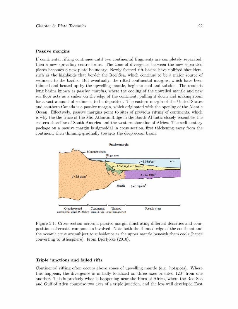
If continental rifting continues until two continental fragments are completely separated,then a new spreading centre forms. The zone of divergence between the now separatedplates becomes a new plate boundary. Newly formed rift basins have uplifted shoulders,such as the highlands that border the Red Sea, which continue to be a major source ofsediment to the basins. But eventually, the rifted continental margins, which have beenthinned and heated up by the upwelling mantle, begin to cool and subside. The result islong basins known as passive margins, where the cooling of the upwelled mantle and newsea floor acts as a sinker on the edge of the continent, pulling it down and making roomfor a vast amount of sediment to be deposited. The eastern margin of the United Statesand southern Canada is a passive margin, which originated with the opening of the AlanticOcean. Effectively, passive margins point to sites of previous rifting of continents, whichis why the the trace of the Mid-Atlantic Ridge in the South Atlantic closely resembles theeastern shoreline of South America and the western shoreline of Africa. The sedimentarypackage on a passive margin is sigmoidal in cross section, first thickening away from thecontinent, then thinning gradually towards the deep ocean basin.
Figure 3.1: Cross-section across a passive margin illustrating different densities and com-positions of crustal components involved. Note both the thinned edge of the continent andthe oceanic crust are subject to subsidence as the upper mantle beneath them cools (henceconverting to lithosphere). From Bjorlykke (2010).
Triple junctions and failed rifts
Continental rifting often occurs above zones of upwelling mantle (e.g. hotspots). Wherethis happens, the divergence is initially localized on three axes oriented 120◦ from oneanother. This is precisely what is happening near the Horn of Africa, where the Red Seaand Gulf of Aden comprise two axes of a triple junction, and the less well developed East
Chapter 3: Plate Tectonics 23
African Rift the third arm. If this rifting continues, and East Africa separates from main-land Africa, then the point where these three spreading centers intersect will become atriple junction. In fact, triple junctions are any points where three plate boundaries inter-section, but triple rifting junctions are arguably the most important and spectacular.
In many cases, the third arm of a triple junction does not continue to completion, in whichcase it becomes a failed rift. These are distinct in the geological record
3.4.3 Convergent boundaries
Convergent plate boundaries are those where two plates collide. There are two types ofconvergent plate boundaries: subduction zones and continent-continent collision zones.Subduction zones occur where an oceanic plate thrusts beneath another plate and into theasthenosphere. The lithosphere of the other plate may be either continental or oceanic.Where a subduction zone occurs beneath continental lithosphere, a continental arc–that is,a chain of volcanoes–develops. This volcanism is the result of melting of the mantle wedgebetween the subducting slab and overlying crust, driven by the release of fluids from theslab. An excellent example of this type of convergent plate boundaries is along the westernmargin of South America, where the Andes are the volcanic arc. Continental arcs tendto be dominated by igneous rocks of intermediate composition, hence the term andesite.However, both felsic and mafic volcanism also occurs in continental arcs. Where oceaniclithosphere subducts underneath oceanic lithosphere, an island arc develops. An exampleis the Aleutian Island arc, where the Pacific plate is subducting underneath the NorthAmerican plate.
Long, linear sedimentary basins form on either side of the volcanic chain of mountains.These basins form as the result of the weight of the volcanic arc and associated fold andthrust belts on the edge of the overriding plate. The basin facing the subducting plateis known as the forearc basin. During the process of subduction, sediments and seafloorfrom the subducting plate are commonly scraped off in the trench and accreted to the mar-gin of the overriding plate, forming accretionary complexes. These accretionary complexestypically mostly comprise a chaotic jumble of metamorphosed and deformed fine-grainedsediments (commonly bedded cherts) and oceanic crust called mmelange. The Franciscancomplex, which makes up much of the west coast of California, is a melange.
Another feature of subducting, convergent margins are ophiolites. Ophiolites are sliversof oceanic upper mantle and crust that have been thrust up on to continental margins.Because oceanic crust is more dense than continental crust, ophiolites are not omnipresenton convergent boundaries. However, where present, they are clear indicator of a convergentboundaries involving at least some oceanic crust.
3.4.4 Transform boundaries
Transform plate boundaries occur where plates slide past one another, without either con-verging or diverging (On plate tectonic scales). Oceanic transform faults are just offsetsof the mid-ocean ridge. Large plate boundaries may occur on the continent, as does theSan Andreas Fault in California. Transform plate boundaries are not as widespread as the
Chapter 3: Plate Tectonics 24
other two types of plate boundaries, but they are nonetheless important. Where there isa sharp jog or offset on a transform fault, it generates either small zone of compression (asmall mountain range) or extension (a strike-slip basin).
3.5 Vertical Motions in the Mantle
Plate tectonics elegantly explains most of the major features on Earth and utterly changedgeology. But like most sweeping theories, it is not perfect an cannot explain all of thefeatures on Earth. Other processes, namely vertical motions in the mantle, may haveprofound effects on the Earth’s surface. We have already discussed hot spot tracks, mostof which appear to record mantle plume volcanism. But upwelling mantle, event withoutvolcanism, may cause the lithosphere to buoy upwards, hence generating 100s to 1000s ofmeters of topographic relief. It is widely believed that the high average elevation of southernAfrica is due to one such upwelling cell of the mantle. Similarly, downwelling mantle canpull the whole lithosphere down with it, even generating new sedimentary basins in theprocess. This dynamic topography is typically transient, because the plates are in motionand eventually drift across and away from these zones of upwelling and downwelling.
Chapter 4
Geological Time and the Age ofthe Earth
Reading: Chapter 3 in Stanley (Chapter 4 in Wiccander and Monroe)
4.1 Introduction
Time is the axis of Earth history. The age of the Earth, as determined by biblical schol-arship, did not allow enough time for either Hutton’s gradualism or Darwin’s evolution.Beginning in the late 1700’s, however, scientists began to experiment with ways of estimat-ing the age of the Earth that invariably led to an older Earth. Today, we have impressivelyprecise means of dating old materials and the know the age of the Earth to be precisely4.54 billion years. The ability to produce absolute ages is a huge boon for Earth scientists(and evolutionary biologists). Even so, geologists are still heavily dependent on the originalframe of reference for dating rocks, which Nicolas Steno first elaborated: relative ages.
4.2 Relative Ages
The earliest stratigrapher (and also a bishop an anatomist), Nicolas Steno, establishedvarious principles with regards to the deposition of strata:
• Principle of superposition
• Principle of original horizontality
• Principle of lateral continuity
Along with the the principle of cross-cutting relationships, these basic laws enable geologiststo work out the relative ages of rocks and geological structures in given region. While simplein essence, these are powerful laws and underlay a large part of what field geologists do.
4.2.1 Principle of faunal succession
In the late 18th century, an English surveyor and engineer by the name of William Smith,who worked to build canals, observed that the suite of fossils within the Paleozoic strata of
25
Chapter 4: Geological Time 26
southern and central England varied up-section, and that this assemblage never repeateditself. Hence he concluded, in what is now the basis of biostratigraphy, that the successionof fossils varies systematically, in a reliable order. This principle of faunal succession is anextraordinarily useful tool for working out the relative ages of rock not just in one region,but between regions and globally. Indeed, this principle is the basis for how the geologicaltime scale was born: the first defined geological intervals were based on the assemblagesof fossils within specific bodies of rock.
4.2.2 The fossil record reveals extinctions
At about the same time that William Smith was working out faunal succession, the in-contournable French anatomist Georges Cuvier was making important discoveries aboutextinction. In dissecting a fossil mammoth, he realized that these bones did not belong toa dead elephant, but rather a mammal that had previously inhabited the Earth, but nolonger does. He also observed evidence for extinctions in the fossil record of the Paris basin.In fact, horizons at which many extinctions occur, and which therefore marked a turnoverin fossil assemblages, have naturally become geological boundaries. Cuvier did not liveto read Darwin’s great treatise and never believed in evolution, but his contributions topaleontology were no less fundamental.
4.2.3 The geological time scale
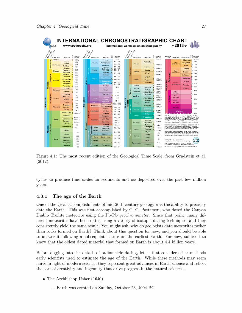
The principal of faunal succession, along with the observation of extinctions, laid thegroundwork for the development of the geological time scale. The basic structure of thegeological time scale was established relatively early on in the history of geology, basedlargely on the fossil record and acceptance of the principal of faunal succession. In thisway, the major systems (rock packages distinguished by their fossil assemblages) of thePhanerozoic were established and themselves subdivided. It was not until much later thatradiometric dating techniques permitted geologists to pin ages on these boundaries (Fig.4.1).
4.3 Absolute Ages
Absolute ages are mostly made thanks to radiometric dating, which exploits the naturaland statistically consistent change of certain intrinsically unstable nuclides into new nu-clides. Once an age has been established in one place, it can, in some instances, be appliedelsewhere through correlation. For example, the principle of faunal succession allows usto identify confidently the Cambrian-Ordivician and Permian-Triassic boundary in succes-sions containing strata of those ages. If that boundary can be dated in one place, thenthat age can be applied elsewhere as well. There are many available tools for correlation,as will be discussed in a subsequent section.
Of course, there are some other ways of determining absolute ages, but these really onlyapply to the fairly recent past. For example, very precise chronologies can be made countingtree rings or layers in ice cores. Another method is through the exploitation of knownperiodic events. For example, it is now well accepted that the Pleistocene ice ages aremodulated by the Milankovitch cycles, whose periodicities are well constrained. Hence,geological records that record these climatic fluctuations can be tuned to the Milankovitch
Chapter 4: Geological Time 27
Figure 4.1: The most recent edition of the Geological Time Scale, from Gradstein et al.(2012).
cycles to produce time scales for sediments and ice deposited over the past few millionyears.
4.3.1 The age of the Earth
One of the great accomplishments of mid-20th century geology was the ability to preciselydate the Earth. This was first accomplished by C. C. Patterson, who dated the CanyonDiablo Troilite meteorite using the Pb-Pb geochronometer. Since that point, many dif-ferent meteorites have been dated using a variety of isotopic dating techniques, and theyconsistently yield the same result. You might ask, why do geologists date meteorites ratherthan rocks formed on Earth? Think about this question for now, and you should be ableto answer it following a subsequent lecture on the earliest Earth. For now, suffice it toknow that the oldest dated material that formed on Earth is about 4.4 billion years.
Before digging into the details of radiometric dating, let us first consider other methodsearly scientists used to estimate the age of the Earth. While these methods may seemnaive in light of modern science, they represent great advances in Earth science and reflectthe sort of creativity and ingenuity that drive progress in the natural sciences.
• The Archbishop Usher (1640)
– Earth was created on Sunday, October 23, 4004 BC
Chapter 4: Geological Time 28
• Georges-Louis Leclerc de Buffon (1774)
– Empirically determined the Earth was 75,000 years old by studying how long ittook iron balls of various sizes to cool off
• Charles Walcott (1893) 35–80 million years
– Time required to deposit the Paleozoic, based on counting layers
• John Jolly (in 1908)
– Estimated age of 90 million years based on concentration of salt in ocean
• Lord Kelvin (William Thompson) (1866)
– Approximately 100 m.y., although he revised it downward
– Based on a heat-loss model (conduction)
– Assumed internal temperature of 3870◦ C
– Surface geothermal gradient of 35◦ C/km
– Thermal diffusivity from experiments (0.01178 cm2/sec)
Lord Kelvin’s estimate of the age of the Earth held incredible sway at the time because hewas a highly respected physicist and had produced the age through rigorous mathematicalcalculations based using the best available empirical data. However, this age was at seriousodds with the prevailing view of geologists at the time, which was that Earth must havebeen much older to explain both the rock record and the patterns of evolution. This tensionbetween physicists and physical geologists has largely persisted since then, with physicistsoften unimpressed by the lack of quantitive support for geological models, and geologistssuspicious of physicists calculations based on unrealistic (not ground-truthed) assumptions.In this particular case, the geologists eventually won the argument. Ernest Rutherford lateroffered the conciliatory explanation to Lord Kelvin that it was because radioactivity hadnot yet been discovered. And in fact, this has been the standard explanation for whyKelvin got it wrong ever since. However, this explanation is wrong.
4.4 Radioactive dating
Building on recent discoveries of the evidence and nature of radioactivity by Roentgen,Becquerel, and the Curies, New Zealander Ernest Rutherford and Englishman FrederickSoddy (both at McGill University at the time) formulated the general theory of radioactivedecay in 1902. The key elements of their theory were
• That radioactivity involves conversion of one element into another
• Radioactivity is proportional to number of parent atoms
• Radioactivity declines exponentially at a time scale determined by a characteristicdecay constant
They identified three types of radioactive decay
Chapter 4: Geological Time 29
• Beta particle decay: neutron converted to proton and an electron emitted
• Electron capture: proton converted into a neutron by capture of an electron
• Alpha particle decay: a particle consisting of two protons and two neutrons (i.e. a4He nucleus) is emitted
Each of these types of decay emits gamma radiation, which is a high frequency, electromag-netic radiation. The gamma rays are what make radioactive minerals potentially dangerousto our health.
4.4.1 The law of radioactive decay
Given that the theory of radioactive decay states that the rate of decay of a radioactiveparent nuclide to a stable daughter product is proportional to the number of parent atomsN, at any time t :
−dNdt
= λN (4.1)
Where λ is the decay constant. This equation can be integrated to yield
N = N0e−λt (4.2)
where N0 is the original number of parent atoms. It is convenient to cast the decay constantin terms of half-life (t1/2), the time required for half of the original parent atoms to decay:
t1/2 =ln(2)
λ(4.3)
Equation 2 can be re-written by substituting the number of daughter atoms (D) andoriginal number of daughter numbers (D0) for N and N0:
D = D0 +N(eλt − 1) (4.4)
This is the fundamental equation used in radioactive dating. Now, let’s consider an actualradioactive decay scheme, such as
87Rb→ 87Sr + β− (4.5)
We can substitute these isotopes into the equation 4:
87Sr = 87Sr0 +87 Rb(eλt − 1) (4.6)
This equation, in theory, is all we need to use the Rb-Sr radioactive decay scheme todate rocks! However, it isn not quite this easy, because it turns out measuring preciseconcentrations of individual nuclides is very difficult. In practice, it is much easier tomeasure ratios. Fortunately, algebra allows us to incorporate this analytical requirementinto the equation, which we do in this case by dividing through by 86Sr:
87Sr86Sr
= (87Sr86Sr
)0 +87Rb86Sr
(eλt − 1) (4.7)

Chapter 4: Geological Time 30
Table 4.1: Commonly used radioactive decay schemes for rocks and minerals
Parent daughter half-life (years) time frame comments
Rubidium-87 Strontium-87 49 x 109 >100 my felsic igneous rocks
Samarium-147 Neodymium-143 110 x 109 >500 my igneous rocks
Uranium-238 Lead-206 4.5 x 10⁹ >50 my widely used
Uranium-235 Lead-207 0.7 x 10⁹ >50 my widely used
Potassium-40 Argon-40 1.3 x 10⁹ >0.1 my widely used
Rhenium-187 Osmium-187 41.6 x 10⁹ >100 my black shales, sulfide ores
Carbon-14 Nitrogen-14 5,370 <40 ky archeology, climatology
4.4.2 U-Pb zircon dating
Of all the geochronometers available to geologists, the U-Pb technique, in particular asapplied to zircons, is the gold standard. One tremendous advantage of the U-Pb methodis that it has two separate decay systems with different decay constants:
23892 U → 206
82 Pb (4.8)
23592 U → 207
82 Pb (4.9)
This duplication of the decay scheme offers a unique way to verify the reliability of data.The mineral zircon (ZrSiO4) is also uniquely well suited for U-Pb radiometric analysis,because it incorporates trace U (which replaces the Zr atom), but does not incorporateany Pb. Furthermore, it is a widely occurring mineral (formed early during the cooling ofintermediate to felsic magmas) and is very robust. Indeed, zircons are retained in sandspopulations (hence sandstone) and commonly used as a way of tracing the source (prove-nance) of sediments. Zircon crystals can now be dated very rapidly by in-situ methods,and this has resulted in the burgeoning of detrital zircon geochronology as a geological toolwith wide-ranging applications (LaMaskin, 2012).
There are three common analytical techniques for measuring zircon minerals, but in allcases, the data are plotted on a concordia diagram, in which the 206Pb/238U are plottedagainst the 207Pb/235U . If zircons remain closed relative to the U-Pb isotope systems,they will evolve along a single curved line on the concordia diagram. If on the other hand,the zircons were perturbed somehow, and either lost or gained Pb or U, then this will beimmediately apparent. But even in this case, not all is lost! Another remarkable thingabout the U-Pb chronometer is that where zircons have only been perturbed once (resultingin lead loss) in their history, we can often not only still date the age of crystallization, butalso the time at which they were disturbed, because a suite of similarly disturbed zirconswill plot along a straight line known as the discordia. The upper intercept of the discordialine and the concordia curve is the age of the zircon, and the lower intercept dates the leadloss event (usually metamorphism).
Chapter 4: Geological Time 31
4.5 Other Chronostratigraphic Techniques
Chronostratigraphy deals with strata with respect to time. That is, it involves dating andcorrelating strata (base on age). Obviously, producing precise ages is the most reliableway of determining the age of a rock, but in most cases, this is not so easy. Fortunately,mother Earth has given us a variety of other ways to determine ages. We have alreadymentioned that we can use certain annual phenomena, such as tree rings and layers andice cores to produce geochronologies. But these have limited applicability to the wholeof Earth history. Most chronostratigraphic techniques that do not involve directly datingrocks entail correlation. We will describe correlation as it pertains to strata more when wediscuss the sedimentary record. Here, we are more concerned with correlation of distinctivepatterns or signatures that can be extracted from stratigraphic records. We will discussjust a few of the more important techniques.
4.5.1 Biostratigraphy
We have talked about biostratigraphy already and we will discuss it in more detail whenwe talk more about the fossil record. Suffice it for now the work of Smith (Priniciple ofFaunal Succession) and Cuvier (extinctions) laid the groundwork for using the fossil recordto make age correlations of fossil-bearing rocks around the world. It goes without sayingthat this method is only widely applied to Phanerozoic and latest Precambrian rocks.
4.5.2 Magnetostratigraphy
As discussed in a previous lecture about the magnetic stripes on the seafloor, Earth’smagnetic field switches polarity from time to time (on average, every million years or so).This can be seen not only in the stripes on the ocean floor, but also in the stratigraphicrecord, because the switch in polarity shows up in the magnetic signatures carried byiron minerals in volcanic and sedimentary rocks. The result is a sort of bar-coding of thegeological record. Because the magnetic polarity record has been precisely calibrated forthe Cenozoic Era (past 65 million years), reasonably calibrated for the Mesozoic Era (c.250 to 65 million years ago), and somewhat calibrated for the Paleozoic Era (541 to 250million years ago), a magnetostratigrapher can in principle date a sequence of strata bymatching the bar coding pattern in those strata with the calibrated reversal record. Youwill be savvy enough to realize that the preservation of similar patterns is dependent on thereliability of the sequence of strata that is being analyzed. For example, where there arehighly variable sedimentation rates, depositional hiatuses, or worse, intervals of erosion,then the magnetic reversal patterns will be heavily distorted. It follows that the mostreliable strata to which to apply magnetostratigraphy are relatively quiet (and preferablydeep) water deposits with slow but regular sedimental accumulation rates.
4.5.3 Sr isotope stratigraphy
We will talk more about isotopes and the Earth system in later lectures. However, stron-tium isotopes are uniquely well suited for determining the age of carbonate (or evaporite)rocks that cannot otherwise be dated reliably. As you already know, radiogenic 87Rb de-cays to the stable nuclide 87Sr. Sr has several stable isotopes, of which 86Sr has a similarabundance as 87Sr. Consequently, the ratio 87Sr/86Sr of the bulk Earth has progressively
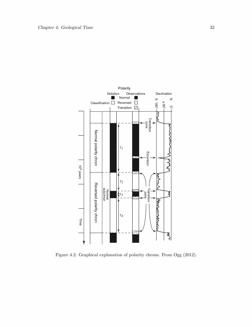
Chapter 4: Geological Time 32
Figure 4.2: Graphical explanation of polarity chrons. From Ogg (2012).

Chapter 4: Geological Time 33
increased over the course of history as a result of radiogenic ingrowth of 87Sr.
Rubidium is a large ion lithophile element, meaning that because of its large atomic ra-dius, it is incompatible and concentrated in the crust. Consequently, basalt has lowerRb concentrations than granite, and so basalts tend to have much lower 87Sr/86Sr ratiosthan granites. The seafloor has 87Sr/86Sr ratios equal to that of the mantle, from whichit is derived. Strontium is reasonably abundant in the oceans, and the 87Sr/86Sr ratio ofseawater largely reflects the balance between low 87Sr/86Sr (unradiogenic) Sr derived formhydrothermal alteration and high 87Sr/86Sr (radiogenic) Sr derived from weathering of thecontinents (delivered via rivers). Hence, at an given time, the 87Sr/86Sr ratio of seawaterreflects the competing influences between hydrothermally derived and continental derivedstrontium, plus the background effect of a gradual increase in the 87Sr/86Sr ratio of thebulk Earth
Strontium is quite similar in ionic radius and charge to Ca, and so is incorporated intoCaCO3 minerals precipitated from seawater, including shells. The 87Sr/86Sr ratio of car-bonates then is a proxy for seawater composition at the time the mineral was precipitated.Compilations of the 87Sr/86Sr of carbonates of different ages show systematic fluctuationsin seawater strontium isotope compositions, most notably a major rise over the past 40m.y. from about 0.7078 to 0.7091 (this may not sound like much, but is in fact one of themost impressive rises in 87Sr/86Sr in Earth’s history). Consequently, if you were to measurethe 87Sr/86Sr ratio of a calcite shell of some critter that lived in the past 40 million years,you could determine its age (in this case, within about 1 million years).
4.5.4 Tephrachronology and event stratigraphy
Felsic volcanic rocks are useful for dating because they often contain the mineral zircon,which you now know is the golden child of Earth’s minerals. However, very young volcanicrocks are difficult to date (because not much Pb has yet evolved), and, as it unfortunatelyturns out, many volcanic rocks do not contain primary zircons (that is, zircons that datefrom the age of the magma). Fortunately, these same volcanic rocks, in particular volcanicashes, can be deposited over vast swaths of land because they erupt high into the atmo-sphere. Huge eruptions are sufficiently rare that such tephra layers can usually be traced toa specific source and correlated, yet sufficiently frequent that you can expect to find a fewof them in sedimentary layers that are being deposited downwind from massive volcanoes.
In the same way that huge volcanic eruptions can be used to establish chronostratigraphicmarker horizons, so too can other catastrophic events in Earth’s history. The most obviousexamples of such events are mass extinctions, which leave an imprint on the fossil andstratigraphic record that can be used to correlate rocks globally. Some mass extinctionsare thought to be linked to meteorite impacts, which leave even better chronostratigraphicmarkers (e.g. impact eject, shocked quartz, chemical anomalies), because these correspondto a geologically instantaneous event, whereas mass extinctions might be more drawn out.

Chapter 4: Geological Time 34
87Sr
/86S
r
0.7050
0.7055
0.7060
0.7065
0.7070
0.7075
0.7080
0.7085
0.7090
0.7095
0.7100
0100200300400500Millions of years ago
Cambrian Ordovic Sil Devonian Carbonifer Permian Triassic CretaceousJurassicCENOZOICPALEOZOIC MESOZOIC
Figure 4.3: The record of seawater 87Sr/86Sr over the past billion years. From Halverson(in press). Strontium isotopes can be a powerful means of dating and correlating rocks,but because most 87Sr/86Sr are non-unique, additional information on the broad age of therocks you are trying to date with this method are required.
Chapter 5
The Stratigraphic Record andSedimentary Environments
Reading: Chapter 5 in Stanley; Chapter 6 in Wiccander and Monroe
5.1 Introduction
Geologists use all rock types to piece together the history of the Earth, but sedimentaryrocks are especially important for several reasons. First, sedimentary rocks cover 75% ofthe continental surface and are highly visible and relevant to geologists. Second, fossils arealmost exclusively preserved in sediments and sedimentary rocks, and hence the history oflife on Earth has largely been extracted from the sedimentary record. Third, sedimentaryrocks archive information about past environments through their physical make-up andstructures, the fossils they contain, and their geochemical signatures.
Sedimentary Geology encompasses any field of science dealing with sediments or sedimen-tary rocks – that is rocks formed by Earth surface processes that include physical settling ofgrains or chemical precipitation of minerals from air or water. Sediments are an archive ofinformation about environmental, tectonic, and biological conditions that prevailed at thetime they were laid down: their very existence in some regions is revealing to the interestedgeologist. Sediments are largely derived from older sedimentary, igneous and metamorphicrocks, and themselves may be metamorphosed or melted to form other rock types. So theyrepresent one arc in the continuous, and long cycle of shaping and reshaping of the earth’slandscape, as envisioned by James Hutton.
5.2 Stratigraphy
Stratigraphy is the study of stratified rocks, which include both sedimentary rocks and lay-ered volcanic rocks. Stratigraphy involves determining the ages (or relative ages), origins,distribution, and lateral relationships of strata.
Steno’s Laws+
• Law of Superposition
35
Chapter 5: Stratigraphy 36
• Law of Original Horizontality and Lateral Continuity
• Law of Cross-cutting Relationships
• Law of Inclusion
5.2.1 Stratigraphic contacts
• conformity
• unconformity
• angular unconformity
• disconformity
• nonconformity
5.2.2 Lithostratigraphic subdivisions
Lithostratigraphy is the study, description, and correlation of layers of rock and usually in-volves identifying individual units based on the physical nature of the sediments comprisingthem (e.g. a sandstone versus a limestone, or a conglomerate versus a shale).The fundamental lithostratigraphic unit is the formation, which is defined as a a mappablebody of rock that is identified by its lithological characteristics and stratigraphic position.But there is a whole hierarchy of lithostratigraphic units that are commonly used:
• Supergroup
• Group
• Formation
• Member
• Bed or Flow
Traditionally, formations and other rock units are defined based on lithology, which is thethe physical nature of the rock (e.g., well-sorted sandstone versus conglomerate or shale).One of the results, as we’ll describe later, is that formation boundaries commonly do notmake very good time boundaries.
5.3 Describing and interpreting detrital sedimentary rocks
5.3.1 Properties of sedimentary rocks
The first step in studying sedimentary rocks is to describe them in the field (or in a corelibrary), followed, often, by observation in thin-section. Of course, some of the easiest thingsto describe are some of the most useful: color (both in fresh and weathered surfaces), theirdegree of induration (how well cemented are they), and how they weather (e.g., blockyor rounded). But most of the important features require a closer look and systematicdescriptions.

Chapter 5: Stratigraphy 37
Composition and texture
• Grain size
• Grain composition
• Grain rounding
• Grain sorting
• Porosity
• Matrix
Bedding and grading
Sedimentary units almost always consist of individual beds that represent a single deposi-tional cycle (perhaps a storm event, high tide, a flood, etc.). Beds are separated by beddingplanes that represent periods of non-deposition or even erosion or a change in depositionalprocess. Features to notice about bedding are
• Thickness of layers (beds vs. laminae)
• Lateral continuity of beds
• Nature of bedding planes (planar, curved, wavy, erosional, etc.)
• Type, if any, of cross-bedding
• Grading
Graded beds are beds that show a systematic variation in grain size through the bed. Bedswhose grain size decreases upsection (i.e., from older to younger) are called normally graded,whereas those that exhibit an increase in grain size are reverse or inverse graded.
5.3.2 Sedimentary structures
Sedimentary structures are physical features in sedimentary rocks that formed during orshortly after deposition and often provide some clue as to the environment in which thesediment was deposited. Some important sedimentary structures are
• ripples (or ripple marks)
– asymmetric ripples (formed in currents)
– symmetric ripples (formed by waves)
• channels
• mud cracks
• halite casts
• sole marks
• biogenic structures (trace fossils)
Chapter 5: Stratigraphy 38
5.3.3 Sedimentary basins
Sediments accumulate in basins, which require some form of subsidence — that is, a meansof creating space for those sediments to fill. That space is referred to as accommodationspace. For example, isostatic considerations tell us that rifting generates subsidence justfrom the thinning of the continental crust. It turns out that isostasy also enables a muchgreater thickness of sediments to accumulate than the original amount of subsidence, be-cause the weight of the sediments (and the water) causes the crust to sink even more.Sediments also compact after they are buried, and this compaction generates additionalspace for sediments to fill. Hence, once accommodation space is produced, it is easier toproduce more space (sort of like having a lot of money makes it easier to make money!).
There are three main ways of generating a basin:
• thinning of the continental crust (rift basins)
• cooling of underlying mantle or crust (passive margin)
• depression of the crust under the weight of mountains (foreland basin)
Another way to produce accommodation space is through eustasy, which is global fluc-tuation in sea level. The best understood way of driving global sea level fluctuation arethrough climate (namely, waxing and waning of glaciers, but also through the effects ofthermal expansion/contraction of seawater), which causes changes on the the time scale of10’s to 100’s of thousands of years. Another commonly invoked means of changing globalsea level is through total volume of the ocean basins, which might change with changingglobally integrated rates of production of oceanic crust.
5.3.4 Depositional environments
Depositional environments are areas of active sediment accumulation characterized by adistinct combination of physical, chemical, and biological processes, that result in a uniquefacies, that is, a suite of sedimentary features that point to a specific depositional envi-ronment. Depositional environments change in space and time due mainly to changes inwater depth, which can be driven by local, basinal factors (such as tectonics or sedimentinfilling) or actual variations in global sea level. Climate and tectonics are the main factorsthat drive these changes in sea level.
By their very nature, shorelines (of lakes or oceans), and the affixed depositional environ-ments, are unstable. Imagine a beach. That beach will only remain in the same geographiclocation over time if the rate of production of accommodation space (basically subsidenceplus space generated or lost by rising or falling sea level) is exactly balanced by sedimentaccumulation rates. Where that balance is not achieved, the shoreline will either migratecontinent-ward, in what is called a transgression, or ocean-ward, in what is known as aregression. Transgressions are associated with an increase in water depth, whereas regres-sions result in a decrease in water depth (or complete exposure of a basin to subaerialweathering and erosion).
Transgressions and regressions result in laterally migrating depositional environments.Walther’s Law states that a vertical succession of facies in a sequence of sedimentary
Chapter 5: Stratigraphy 39
rocks reflects such lateral changes in sedimentary environment. For example, if a beachfacies is overlain by back-beach aeolian facies, this indicates that these two environmentswere juxtaposed and that this sequence experienced a regression. Walther’s Law is the ba-sis by which geologists can convert the sedimentary record into a paleonvironmental mapof a sedimentary basin.
The continental environment
• Fluvial. Commonly coarse-grained channel fill/bars with fine-grained flood-plaindeposits. May be associated with coals. Important archives of terrestrial environ-ments.
• Lacustrine. Varved (rhythmic) laminae common. May be either open or closed,they latter commonly forming chemical precipitates via evaporation.
• Desert.
– alluvial fans are the coarse grained aprons that form on the margins of mountainranges
– dunes are deposited by blowing sand and have characteristic bimodal grain sizedistribution and large-scale cross-bedding
• Soils. Not extremely common in the sedimentary record, but highly informativebecause soil formation is sensitive to so many environmental parameters.
• Glacial. Unsorted tills/morraines (diamictites), ice-sculpted landforms (i.e. drum-lins), striations and grooves
Coast lines
The coast line is the marginal marine environment that occurs along the boundary betweenthe ocean and the continents. It is influenced by a combination of rivers, wind, waves, tides,and other shallow marine processes and can be subdivided into a several sub-environments.
• Deltas. Dominated by sediment supply from rivers. Form prograding lobs of sandand mud, commonly arranged in clinoforms
• Estuaries. Flooded river mouths. Brackish water, significant muds.
• Beaches and barrier islands. Sandy, commonly cross-bedded with heavy minerallaminations, multi-directional currents.
• Tidal flat. Significant muds, commonly mud-cracked, interbedded with sands withdistinct structures and bedding types associated with tidal currents.
The open marine environment
Open marine environments are spatially the most expansive because they include most ofthe continental shelves and the deep ocean basins.
• Continental shelf. Influenced by storm events, pelagic sedimentation
Chapter 5: Stratigraphy 40
• Continental slope. Dominated by gravity flow processes (mud and debris flows,turbidity currents)
• Deep ocean. Pelagic sedimentation: dust and tests of micro-organisms, such asdiatoms and foraminifera.
• Glaciomarine. Heavily controlled by processes at the ice-grounding line. Commonlypoorly stratified sediments with outsized and exotic clasts.
Carbonate platforms
Carbonate sediments preferentially accumulate in shallow, tropical marine settings withlimited siliciclastic sediment input. A carbonate platform is a broad region of shallowwater dominated by carbonate sedimentation. The Bahamas banks off the east coast ofFlorida is a well known example of a carbonate platform. Here, carbonate sands (whichinclude ooids) and lime muds are abundant.
Reefs constitute another important site of carbonate sediment accumulation in the oceans.The most prominent are barrier reefs, such as the Great Barrier Reef off the coast ofnortheastern Australia. Barrier reefs are relatively common in the stratigraphic recordwhere they form the outer edge of a carbonate platform and provide protection to theinner part of the platform (a lagoon), which enables carbonate sediments to accumulate.Whereas most modern reefs consist largely of corals (with significant contributions fromsea grasses and carbonate-secreting algae and cyanobacteria), a variety of different organ-isms have formed reefs throughout Earth history, notably stromatolites in the Precambrian.
Limestone precipitation is concentrated in the tropics because calcium carbonate solubilityis lower in warmer waters. This mineralogically unusual situation arises because of thesomewhat complicated speciation of dissolved inorganic carbon in seawater. But what itboils down to is that processes that remove CO2 from seawater drive those waters towardscarbonate precipitation. Because warmer water can hold less dissolved CO2, this is wherecarbonate precipitation is focused.
• continental
• marine
Carbonates also do occur in the deep sea, but only above the carbonate compensation depth(the depth at which carbonates dissolve in seawater; this will be discussed in more detail ina subsequent chapter). Carbonates found on the deep sea floor are almost entirely derivedfrom the sea surface or from shallow water carbonate platforms and reefs (transported bygravity flows, such as turbidites).
Chapter 6
Life, Fossils, and Evolution
Reading: Chapters 3, 7 in Stanley; Chapter 7 in Wiccander and Monroe
6.1 Introduction
The vestiges of ancient life are called fossils. Fossils come in various forms, includingmoulds, casts, imprints, impressions, burrow traces, recyrstallized shells, and replacedhard and less commonly, soft parts. Molecular fossils (biomarkers) are molecules preservedin the organic matter of sedimentary rocks that can be used indicators of specific groupsof organisms. The study of ancient life is broadly known as paleontology. Though someancient scholars contemplated the meaning of fossils, most did not appreciate what theyrepresented. It was not until William Smith, Georges Cuvier, and a few others in the early19th century began to make sense of the fossil record was the field of paleontology born.Today, this field is broad and includes many subdisciplines, such as evolutionary biology,biostratigraphy, paleoecology, and molecular paleontology, to name but a few. Paleontol-ogy is an increasingly interdisciplinary field, often combining phylogenetics with organicand isotope geochemistry.
The word Paleontology is derived from the Greek palaeo = ancient, ontos = being, andlogos = knowledge. Modern paleontology is the overlap between biology, geology, ecology,paleogeography, geochemistry, and increasingly, molecular biology. It can be defined as thestudy of ancient life in the context of environment and evolution. Classical paleontologyinvolves making many measurements of various dimensions of innumerable fossil specimens(biometrics), then trying to make sense of these data through statistical analyses. We donot have the time to get too deeply involved in this aspect of paleontology.
6.1.1 Subdisciplines of paleontology
• paleozoology
• paleobotony
• invertebrate paleontology
• vertebrate paleontology
41
Chapter 6: Life, Fossils, and Evolution 42
• micropaleontology
The western history of palaeontology, like many sciences, goes back to Aristotle, but reallygot started by Da Vinci. Modern paleontology was born around the end of the 18th century,when geology first took roots. Four 18th and 19th century scientists are largely responsiblefor the development of paleontology and how we read the paleontological record.
• Georges Cuvier (1769–1832) recognized that fossils represented extinct organisms
• William Smith (1769–1839) first applied biostratigraphy
• Charles Darwin (1809–1882) and Alfred Wallace (1823–1913) demonstrated evolutionand proposed the theory of natural selection.
6.2 Fossils
Fossils, quite simply are the preserved remains or traces of organisms in rocks. Fossilsprovide the framework for how we understand ancient life. However, sedimentology, evolu-tionary biology, ecology, and increasingly molecular biology fill in the gaps in this frameworkand by now have provided has with a rich knowledge of ancient life. Almost all fossils arefound in sediments and sedimentary rocks that have not been heavily metamorphosed.
6.2.1 Types of fossils and preservation
Fossils come in many shapes and forms and may be preserved in a variety of manners.
• Various factors favor fossilization:
– abundance of organisms
– minimal disturbance after death
– rapid burial or ’entombment’
– small size
– marine organisms are more likely to be preserved than terrestrial organisms
• Hard parts much more likely to be preserved than soft tissues
– in vertebrates: bone, enamel, keratin (fibrous structural proteins)
– in invertebrates: chitin (a polymer of glucose used, e.g., in exoskeletons), shells(carbonate or silica)
– in plants: cellulose (a polysaccharide) or lignin (a polymer of ring alcohols thatprovides structure to plant cell walls)
6.2.2 Modes of preservation
Soft parts
The soft parts (tissues, hair, etc.) of animals are rarely preserved, but certain exceptions dooccur and unaltered remains are preserved (permafrost, amber, mummification, tar, peat).Invariably, the preservation of soft parts requires a hermetic tomb, that is immediately andpermanently sealed off to oxygen.
Chapter 6: Life, Fossils, and Evolution 43
Molds
Molds are the negative imprint of an organic structure. They commonly arise throughthe dissolution of the structure during diagenesis and require that the space left behindis retained, either permanently, or for long enough for some other material to fill it, andhence preserve the original shape of the structure
Impressions
Impressions are delicate surface markings in soft sediments that preserve the flattenedoutline of certain soft or semi-hard organisms.
Changes to organic components
• carbonization: release of volatile constituents; nearly pure C is left behind as a film
• pyritization: mineral replacement of soft parts
Changes in the inorganic substance of hard parts
• unchanged hard parts are most likely Cenozoic
• recrystallization
• petrifaction (by percolating fluids)
– Most commonly calcite, silica, and iron minerals
• solution of hard parts
– external mold: a shape in the sediment that reflect that outer shape of theorganism. Imagine your footprint in wet sand on the beach.
– internal mold: sediment fills an open cavity in an organism: for example, a clamshell that is filled with sand.
– casts fill molds: e.g. the sediment or minerals that replaces the cavity when aclam shell dissolves
6.2.3 Trace fossils and other indirect fossils
Ichnology is the study of trace fossils - that is, of the tracks, burrows, footsteps and othertraces left behind by organisms.
• Trace fossils are useful biogenic sedimentary structures
– may indicate sedimentary environment/paleodepth
• bioturbation is the burrowing of organisms in unconsolidated sediments
– destroys other sedimentary features, such as bedding and structures
• Often preserved in sediments otherwise not conducive to fossil preservation
• Always in situ

Chapter 6: Life, Fossils, and Evolution 44
• Preserved in various ways
– most commonly as sand or mud cast of a burrow or track
6.2.4 Lagerstatten
A sedimentary deposit that contains exceptional preservation of fossils is referred to as alagerstatte. Lagerstatten (plural) may form by a variety of means and span from the lateNeoprotroterozoic to the present. They commonly (but not always) include fossils of pre-served soft tissues, and so provide extraordinary insight into ancient life. Well known exam-ples of lagerstatte include the Cambrian Burgess Shale in B.C. and the Jurassic Solnhofenlimestone in Germany.
6.2.5 Biomarkers
Biomarkers are molecular fossils. You can think of a biomarker as the altered chemi-cal trace of some previously living organism. Biomarkers can be measured in rocks andsediments, and the key biomarkers are molecules that can be linked to precursor moleculeproduced by a specific organism, only lacking functional groups (which are quickly strippedoff during diagenesis. The field of biomarker geochemistry has largely been developed mythe petroleum industry who use biomarkers to link petroleum to source rocks, among otherapplications.
6.3 Biostratigraphy
Biostratigraphy is the application of the fossil record to stratigraphic correlation and de-termining the relative ages of strata.
• Guided by the principle of faunal succession - the observation that sedimentary rockscontain fossils that succeed one another vertically in a consistent order and that thesesuccessions can be recognized over wide long distances
• Biostratigraphic zonation
• Stages and zonation
– range zone: The body of strata representing the known range of a particulartaxon
– biozone: A body of strata delimited by a characteristic assemblage of taxa
– concurrent range zone: a body of strata in which a specific suite of taxa alloccur (and certain other don’t occur)
– an index fossil is a fossil with a short range and a wide geographic distribution
– first and last appearance of fossils
– The Signor-Lipps effect is the principle that, due to the inherent incompletenessof the fossil record, neither the first nor the last organism of a given taxon willbe preserved in the fossil record.
The text-book demonstration of the Signor-Lipps effect: the coelacanth, thought to havegone extinct in the late Cretaceous (based on last occurrence).
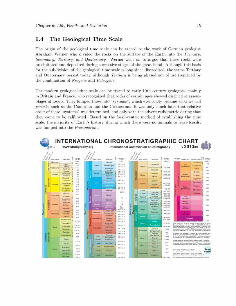
Chapter 6: Life, Fossils, and Evolution 45
6.4 The Geological Time Scale
The origin of the geological time scale can be traced to the work of German geologistAbraham Werner who divided the rocks on the surface of the Earth into the Primary,Secondary, Tertiary, and Quaternary. Werner went on to argue that these rocks wereprecipitated and deposited during successive stages of the great flood. Although this basisfor the subdivision of the geological time scale is long since discredited, the terms Tertiaryand Quaternary persist today, although Tertiary is being phased out of use (replaced bythe combination of Neogene and Paleogene.
The modern geological time scale can be traced to early 19th century geologists, mainlyin Britain and France, who recognized that rocks of certain ages showed distinctive assem-blages of fossils. They lumped these into ”systems”, which eventually became what we callperiods, such as the Cambrian and the Cretaceous. It was only much later that relativeorder of these “systems” was determined, and only with the advent radiometric dating thatthey came to be calibrated. Based on the fossil-centric method of establishing the timescale, the majority of Earth’s history, during which there were no animals to leave fossils,was lumped into the Precambrian.
Pha
nero
zoic
Cen
ozoi
cQ
uate
rnar
y Holocene
Pleistocene
Pliocene
Miocene
Oligocene
Eocene
Paleocene
Neo
gene
Pal
eoge
ne
Upper
Lower
Cre
tace
ous
Mes
ozoi
c
Tria
ssic
Car
boni
fero
usM
esoz
oic
Per
mia
nJu
rass
ic
Upper
Lower
Middle
Upper
Lower
Middle
Lopingian
Guadalupian
Cisuralian
Upper
Lower
Upper
Middle
Middle
Lower
Mis
siss
ippi
anPe
nnsy
lvan
ian
Pal
eozo
ic
MiddleUpper
CalabrianGelasian
PiacenzianZancleanMessinianTortonian
SerravallianLanghian
BurdigalianAquitanianChattian
Rupelian
PriabonianBartonianLutetian
Ypresian
ThanetianSelandian
Danian
Maastrichtian
Campanian
SantonianConiacian
Turonian
Cenomanian
Albian
Aptian
BarremianHauterivianValanginian
Berriasian
Tithonian
Kimmeridgian
OxfordianCallovianBathonianBajocianAalenian
Toarcian
Pliensbachian
SinemurianHettangianRhaetian
Norian
Carnian
LadinianAnisian
OlenekianInduan
ChanghsingianWuchiapingian
CapitanianWordianRoadian
Kungurian
Artinskian
Sakmarian
Gzhelian
Famennian
Frasnian
Givetian
Eifelian
Emsian
PragianLochkovian
LudfordianGorstian
HomerianSheinwoodian
TelychianAeronian
RhuddanianHirnantian
Katian
Sandbian
Darriwilian
DapingianFloian
Tremadocian
Stage 10
JiangshanianPaibian
GuzhangianDrumian
Stage 5
Stage 4
Stage 3
Stage 2
Fortunian
KasimovianMoscovian
Bashkirian
Serpukhovian
Visean
TournaisianTerreneuvian
Series 2
Series 3
Furongian
Cam
bria
n
Upper
Lower
Middle
Llandovery
Wenlock
Ludlow
Pridoli
Upper
Middle
Lower
Silu
rian
Dev
onia
nO
rdov
icia
nP
aleo
zoic
Pha
nero
zoic
Pha
nero
zoic
Asselian
Hadean
Arc
hean
Pre
cam
bria
n Pro
tero
zoic
Neo-proterozoic
Meso-proterozoic
Paleo-proterozoic
Neo-archean
Meso-archean
Paleo-archean
Eo-archean
Ediacaran
Cryogenian
Tonian
Stenian
Ectasian
Calymmian
Statherian
Orosirian
Rhyacian
Siderian
0.01170.1260.781
1.806
2.5883.600
5.333
7.246
11.62
13.82
15.97
20.44
23.03
28.1
33.9
38.041.3
47.8
56.059.2
61.6
66.0
72.1 ±0.2
83.6 ±0.286.3 ±0.5
89.8 ±0.3
93.9
100.5
~ 113.0
~ 125.0
~ 129.4
~ 132.9
~ 139.8
~ 145.0
~ 145.0
152.1 ±0.9
157.3 ±1.0
163.5 ±1.0166.1 ±1.2168.3 ±1.3170.3 ±1.4
174.1 ±1.0
182.7 ±0.7
190.8 ±1.0
199.3 ±0.3201.3 ±0.2
~ 208.5
~ 227
254.14 ±0.07
259.8 ±0.4
265.1 ±0.4268.8 ±0.5
272.3 ±0.5
283.5 ±0.6
290.1 ±0.26
303.7 ±0.1307.0 ±0.1
315.2 ±0.2
323.2 ±0.4
330.9 ±0.2
346.7 ±0.4
358.9 ±0.4
298.9 ±0.15295.0 ±0.18
~ 237
~ 242
247.2251.2
252.17 ±0.06
358.9 ± 0.4
372.2 ±1.6
382.7 ±1.6
387.7 ±0.8
393.3 ±1.2
407.6 ±2.6410.8 ±2.8
419.2 ±3.2
423.0 ±2.3425.6 ±0.9427.4 ±0.5430.5 ±0.7433.4 ±0.8
438.5 ±1.1440.8 ±1.2443.4 ±1.5445.2 ±1.4
453.0 ±0.7
458.4 ±0.9
467.3 ±1.1470.0 ±1.4
477.7 ±1.4
485.4 ±1.9
541.0 ±1.0
~ 489.5
~ 494~ 497
~ 500.5
~ 504.5
~ 509
~ 514
~ 521
~ 529
~ 541.0 ±1.0
~ 635
850
1000
1200
1400
1600
1800
2050
2300
2500
2800
3200
3600
4000
~ 4600
present
Series / Epoch Stage / Agenumericalage (Ma) Eo
noth
em /
Eon
Erat
hem
/ Er
aSy
stem
/ Pe
riod
Series / Epoch Stage / Agenumericalage (Ma) Eo
noth
em /
Eon
Erat
hem
/ Er
aSy
stem
/ Pe
riod
Series / Epoch Stage / Agenumericalage (Ma) System / PeriodErathem / Era
numericalage (Ma)Eo
noth
em /
Eon
Erat
hem
/ Er
aSy
stem
/ Pe
riod
Eonothem / EonG
SS
P
GS
SP
GS
SP
GS
SP
GS
SA
INTERNATIONAL CHRONOSTRATIGRAPHIC CHARTInternational Commission on Stratigraphywww.stratigraphy.org
Coloring follows the Commission for the Geological Map of the World. http://www.ccgm.org
Chart drafted by K.M. Cohen, S. Finney, P.L. Gibbard(c) International Commission on Stratigraphy, January 2013
http://www.stratigraphy.org/ICSchart/ChronostratChart2013-01.pdf
Units of all ranks are in the process of being defined by Global Boundary Stratotype Section and Points (GSSP) for their lower boundaries, including those of the Archean and Proterozoic, long defined by Global Standard Stratigraphic Ages (GSSA). Charts and detailed information on ratified GSSPs are available at the website http://www.stratigraphy.org. The URL to this chart is found below.
Numerical ages are subject to revision and do not define units in the Phanerozoic and the Ediacaran; only GSSPs do. For boundaries in the Phanerozoic without ratified GSSPs or without constrained numerical ages, an approximate numerical age (~) is provided.
Numerical ages for all systems except Permian,Triassic, Cretaceous and Precambrian are taken from ‘A Geologic Time Scale 2012’ by Gradstein et al. (2012); those for the Permian, Triassic and Cretaceous were provided by the relevant ICS subcommissions.
v 2013/01

Chapter 6: Life, Fossils, and Evolution 46
6.5 Systematics and Taxonomy
Systematics is the study of the structure and diversity of life, in particular as it has evolved.Although similar in some aims, it should not be confused with taxonomy, which is morestrictly concerned with the identification, description, and nomenclature of organisms andfossils. Hence, the role of systematics is to understand the pattern presented by taxonomy.
A taxon is any named grouping of organisms. Palaentologists, like biologists, use thelinnaean, binomen hierarchical classification system to name fossil species:
• Superkingdom: Eukarya
• Kingdom: Metazoa
• Phylum: Chordata
• Class: Mammalia
• Order: Primates
• Family (-idae, -aceae): Hominidae
• Genus: Homo
• Species: Homo sapiens
6.5.1 Classification of fossils
Taxonomy is not simple business
• originally classified based solely on morphology and function (that is, phenotypicalexpression
• Evolutionary taxonomy was mainstream in the first two thirds of the 20th century
– Substantially aided by ontogeny : the study of the origin and development ofanimals, with an emphasis on embryonic development. Ontogeny demonstratedclose evolutionary linkages between taxa that are not as obviously similar intheir adult phenotypes
– Phylogeny : The origin and evolution of a set of organisms. This is how we placeorganisms within an evolutionary frameowork
• Numerical taxonomy : use of objective, statistical similarities to develop phylogeneticrelationships
6.5.2 Cladistics
Cladistics is the classification organisms by their evolutionary relationships rather thantheir morphology. While this seems like an obvious way to classify organisms and fossils, itwas not always so. This method was first championed by the German entomologist WilliHennig (1913–1976). The underlying assumption in cladistics is that two taxa share thesame trait because they are both derived from the same ancestor that also had that trait.This is referred to as a primitive trait. Derived traits (synapomorphies) appear later inthe cladistic succession.
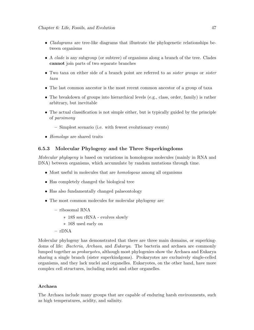
Chapter 6: Life, Fossils, and Evolution 47
• Cladograms are tree-like diagrams that illustrate the phylogenetic relationships be-tween organisms
• A clade is any subgroup (or subtree) of organisms along a branch of the tree. Cladescannot join parts of two separate branches
• Two taxa on either side of a branch point are referred to as sister groups or sistertaxa
• The last common ancestor is the most recent common ancestor of a group of taxa
• The breakdown of groups into hierarchical levels (e.g., class, order, family) is ratherarbitrary, but inevitable
• The actual classification is not simple either, but is typically guided by the principleof parsimony
– Simplest scenario (i.e. with fewest evolutionary events)
• Homologs are shared traits
6.5.3 Molecular Phylogeny and the Three Superkingdoms
Molecular phylogeny is based on variations in homologous molecules (mainly in RNA andDNA) between organisms, which accumulate by random mutations through time.
• Most useful in molecules that are homologous among all organisms
• Has completely changed the biological tree
• Has also fundamentally changed palaeontology
• The most common molecules for molecular phylogeny are
– ribosomal RNA
∗ 18S ssu rRNA - evolves slowly
∗ 16S used early on
– rDNA
Molecular phylogeny has demonstrated that there are three main domains, or superking-doms of life: Bacteria, Archaea, and Eukarya. The bacteria and archaea are commonlylumped together as prokaryotes, although most phylogenies show the Archaea and Eukaryasharing a single branch (sister superkindgoms). Prokaryotes are exclusively single-celledorganisms, and they lack nuclei and organelles. Eukaryotes, on the other hand, have morecomplex cell structures, including nuclei and other organelles.
Archaea
The Archaea include many groups that are capable of enduring harsh environments, suchas high temperatures, acidity, and salinity.
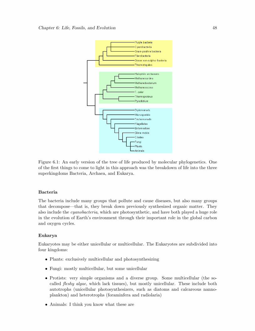
Chapter 6: Life, Fossils, and Evolution 48
Figure 6.1: An early version of the tree of life produced by molecular phylogenetics. Oneof the first things to come to light in this approach was the breakdown of life into the threesuperkingdoms Bacteria, Archaea, and Eukarya.
Bacteria
The bacteria include many groups that pollute and cause diseases, but also many groupsthat decompose—that is, they break down previously synthesized organic matter. Theyalso include the cyanobacteria, which are photosynthetic, and have both played a huge rolein the evolution of Earth’s environment through their important role in the global carbonand oxygen cycles.
Eukarya
Eukaryotes may be either unicellular or multicellular. The Eukaryotes are subdivided intofour kingdoms:
• Plants: exclusively multicellular and photosynthesizing
• Fungi: mostly multicellular, but some unicellular
• Protists: very simple organisms and a diverse group. Some multicellular (the so-called fleshy algae, which lack tissues), but mostly unicellular. These include bothautotrophs (unicellular photosynthesizers, such as diatoms and calcareous nanno-plankton) and heterotrophs (foraminfera and radiolaria)
• Animals: I think you know what these are

Chapter 6: Life, Fossils, and Evolution 49
6.6 Evolution
About half a century before Darwin’s epic voyage aboard the HMS Beagle II, Jean-BaptisteLamarck (1744–1829) proposed the first well-developed hypothesis for evolution. Com-monly referred to as Lamarckian evolution, this hypothesis posits that new traits in organ-isms arise during their lifetime as the result of some need, and these traits can be passedalong to their descendants. We may snicker at the seeming naivety of this idea now, butin fact it was a tremendous leap forward in biology at the time.
6.6.1 Evolution happens
Charles Darwin (1809–1882) and his near contemporary Alfred Wallace (1823–1913) estab-lished that evolution accounts for the origination of new species and the diversity of life onEarth. Charles Darwin was trained in geology and had a copy of the Lyell’s just-publishedPrinciples of Geology. As such, the observations on his voyage on the HMS Beagle II(1831–1836) and the interpretations he made to explain them were framed in a geologicalcontext. Importantly, he not only made observations, but also collected the detailed dataand notes required to convince others of evolution and the theory of natural selection.Some of the bedrock observations that led him to his conclusion:
• The fauna of the Americas was completely different from that of Europe and Africa,even in comparable environments
• Marine species are strikingly dissimilar on either side of the Isthmus of Panama
• Small islands >5000 km from continents lacked endemic land mammals
• Shells of Galapagos tortoises unique on different islands
• Finches most closely resembled those of South America; unique adaptations of beaksto grazing habits
• Similarity in the embryos of vertebrates
• Homology : similar body parts with different functions
• Vestigial organs: organs, such as the appendix, that serve no purpose
Fundamentally, evolution is driven by random mutations that occur during sexual repro-duction. Most such mutations are not advantageous (perhaps why being called a “mutant”is not a compliment) and do not propagate. Where evolution occurs is where a mutationactually imparts an advantage on organism within its milieu. This process is further com-plicated by the fact that environments themselves are not static. So whereas white fur isan evolutionary advantage to polar bears when they are hunting for seals on the sea ice,it will be less of an advantage and probably a disadvantage as they are forced to find foodon bare land.
Much of what Darwin and Wallace observed in the (then) modern world is also observed inthe fossil record. Quite simply, it is unavoidable to conclude that organisms evolve throughtime. Whereas evolution as articulated by Darwin may have qualified as a theory at thetime, it is a well observed fact today, and the “theory of evolution” is not about whetherit occurs but rather why evolution happens.

Chapter 6: Life, Fossils, and Evolution 50
6.6.2 The theory of natural selection
Darwin was well aware that artificial selection, by dog or plant breeders, was capable ofproducing great variability among given species. He was also deeply convinced by Huttonand Lyell’s gradualism, and the enormity of time. The theory of natural selection was per-haps not that great of a leap once he had observed evolution. The challenge in proposingthe theory, and the reason he waited over twenty years to do so following his return fromthe Beagle voyage, was that natural selection is utterly at odds with religion and the notionof a benevolent god. Indeed, it was only the realization that Wallace had also stumbledupon the theory based on his research in southeast Asia that motivated Darwin to publishhis evidence for evolution and theory of natural section to explain it.
The English cleric Thomas Malthus (1766–1834) observed that organisms produce moreoffspring than can survive, as part of a natural impetus to increase population. Both Dar-win and Wallace (1823–1913) recognized that this resulted in competition within speciesto survive. For example, certain species of finches that Darwin observed in the GalapagosIslands bear two chicks, even though only one of those chicks ultimately survives. In fact,in the brutal struggle to survive, the weaker of the two chicks is often killed by his or hersibling. It is in this way that individuals that are stronger or more capable will preferen-tially survive and pass along their genes, while the weakest individuals will be killed off andtheir genes eliminated from the gene pool. This is a brutal, but efficient way for species topropagate and adapt to their environment (given, of course, sufficient time).
In a similar way, different species struggle against one another. They may be in directcompetition for the same resources, or one species may prey on the other, leading to aso-called evolutionary arms race, where one group of organisms will evolve to better preyon another group of organisms, triggering them to evolve better defence mechanisms, andso forth. It has often been argued that the Cambrian Radiation records the first majorevolutionary arms race, after which, effectively all modern body plans had been achieved(at the phylum level) and from there, evolution largely preceded at lesser (order, family,etc.) levels. Under this process of natural selection, taxa evolved gradually (anagenesis)as the result of long-lived environmental pressures.
6.6.3 Patterns and rates in evolution
Evolutionary radiation
Anagenesis is the gradual evolution of one taxon, but we know that taxa also diverge. Thesplitting of a single taxon into multiple taxa (branches), is known as cladogenesis. Bothprocesses are observed in the fossil record, which, despite its inherent weaknesses, providesus a measure of the timing and rates of origination of species (or other clades). Apparentin the fossil record are periods when certain taxa produce many new genera or species.These evolutionary radiations, which include the famous Cambrian radiation, show upspectacularly in the fossil record. These radiation events typically result in certain groupsof organisms adapting to new modes of life, which enable them to expand and populatenew ecospace.
These radiation events may result from the extinction of other taxa that dominate availableenvironments. For example, we now know that mammals coexisted with dinosaurs through
Chapter 6: Life, Fossils, and Evolution 51
much of the Mesozoic, but they remained small and subordinate. Only after extinction ofdinosaurs did mammals flourish. The radiation of mammals over the last 66 million yearshas been nothing short of extraordinary (look at how different bats are from whales, forexample!).
Other radiations were triggered by adaptive breakthroughs, whereby a taxon develops cer-tain features that enable it to survive and thrive in available environments, outcompetingother organisms. One such example are the hexacorals, whose porous structure allows themto grow much quicker than other calcite-secreting sessile organisms because they need muchless CaCO3 per unit volume.
Molecular clocks
A molecular clock is a technique of dating divergence times between different groups ofrelated organisms, based on molecular phylogeny. It is particularly useful for estimatingdivergence times between extant organisms that have left no or incomplete fossils records.But of course, it has wide-ranging applications.
• Needs to be calibrated
• Based on the assumption that rates of divergence are constant (at least betweencalibration points)
• Assumes no lateral gene transfer
• Inherently less reliable the further back in time one goes
Evolutionary convergence
Evolutionary convergence occurs when separate taxa evolve to have similar traits. Com-mon examples of convergence include the various types of anteaters, flying squirrel-likecreatures, and cactus and cactus-like euphorbia. Convergence attests to the strong controlof environment on evolution.
Horizontal gene transfer
In case cladistics and evolution is not sufficiently difficult, it turns out that in some cases,genetic information has been transferred between different species in a process known ashorizontal gene transfer. This usually occurs among prokaryotes as a result of bacteriaor viruses invading a cell of organism, then transferring its genetical material to anothervictim.
Extinction
As mentioned before, the first-order structure of the geological time scale reflect the patternof major extinctions in Earth history, that is intervals marked by the abrupt disappear-ance of fossil taxa. Extinctions result from a variety of factors, including predation, disease,competition for resources, and of course, natural disasters.
Chapter 6: Life, Fossils, and Evolution 52
Figure 6.2: A plot of divergence times versus divergence (nucleotide substitutions) for 17mammalian species illustrates that at lease for this clade, divergence occurs at a constantrate.
Extinction is a normal part of the fossil record, and different taxa exhibit very differentcharacteristic rates of extinctions. For examples, about half of all mammal species goesextinct every million years, whereas among marine molluscs, the rate is an order of mag-nitude slower.
Despite the difference in rates of extinctions among different groups, global trends in extinctare apparent. Specifically, plots of either total number of species, genera, or classes at agiven time, or simply percentage of species or genera going extinct through time highlightseveral mass extinction events, where an unusually large percentage of existing taxa goextinct. The big five of mass extinctions are the
• end-Ordivician event
• late Devonian event
• Permo-Triassic event
• late Triassic event
• Cretaceous-Paleogene event
We will discuss the individual events more in late lectures.
Chapter 6: Life, Fossils, and Evolution 53
Evolutionary trends
Animals evolve towards larger body size. This is mainly a result of competition to breed,with larger males tending to win the fight for females, driving a tendency towards largerand larger animals. This pattern highlights an important point about evolution, which isthat ’more evolved’ does not imply any sort of overall superiority. This tendency among an-imals is fundamentally unsustainable, because animals can grow only so large before theirsize and nutrient requirements become a serious problem. Indeed, this tendency probablycontributes to the high extinction rates among mammals, where it occurs relatively quickly.Large animals, you can imagine, would be highly susceptible to perturbations to the foodchain.
Rates of evolution vary greatly. For the most part, they are slow, with individual speciesranging for millions or tens of millions of years. However, speciation can happen quicklyin cases where a simple genetic changes have major consequences. The fossil record alsoabounds with examples that suggest that taxa experience intervals of stasis, followed byrapid evolutionary expansion, as discussed in the following section.
Finally, evolution is irreversible. Because evolution is the result of a series of geneticchanges, it is effectively impossible to undo, even if subsequent evolution might producea creature that resembles any ancestor. This unidirectionality in evolution is known asDollo’s law.
6.7 Gradualism Versus Punctuated Equilibrium
6.7.1 Phyletic gradualism
Evolution by natural selection, as originally conceived by Darwin and Wallace, occurs grad-ually, requiring vast tracts of geological time. Darwin was very aware of this requirement ofhis theory, and for this reason, was greatly troubled by both Lord Kelvin’s stingy estimateof the age of the Earth (ca. 100 m.y.) and by the Cambrian explosion, which appeared torecord a very sudden initial evolution of animals. In fact, the fossil record shows many caseswhere speciation appears to occur instantaneously, in geological terms, and the question iswhether or not this feature can be accommodated by Darwinian evolution.
• Darwin himself recognized this feature of the fossil record
• But phyletic gradualism reigned as the preferred model for evolution until the latterhalf of the 20th century
In this model, new species evolved largely through anagenesis, the gradual transition ofone species into another. This sort of evolutionary pattern gives rise to pseudo extinctionsin the fossil record, because specific species disappear over time, but because they havechanged not because some catastrophic event or other change in the environment wipedthem out.
6.7.2 Punctuated equilibrium
In the early 1970’s, Niles Eldridge and Stephen Jay Gould published a landmark paper inwhich they argued that most species change little for most of their history (stasis), and

Chapter 6: Life, Fossils, and Evolution 54
when evolution occurs, it does so in rapid branching events (cladogenesis). This hypothesiswas fundamentally rooted in the observation that the fossil record rarely demonstratesgradualistic evolution and that new taxa appear rapidly. The explanation for this patternis based on observations that
• large populations dilute phenotypic changes—that is, changes in the physical mani-festation of the genetic code
• geographically isolated (peripheral) populations are more likely to change and formnew species (allopatric speciation)
• however, because the allopatric species are marginal, these adaptations are usuallywiped out
• the record of speciation is actually very rare in the fossil record—it occurs whenchance changes in environment favor a peripheral population and are detrimental tothe parent population
At its core, the punctuated equilibrium model doesn’t contradict the gradualistic model.Rather, it argues that gradualism alone cannot explain the fossil record. Importantly, thishypothesis emphasizes the importance of ecological context within paleontology.
Chapter 7
The Environment and ChemicalCycles
Reading: Chapter 11 in Stanley; Chapter 4 in Wiccander and Monroe
7.1 Introduction
An important goal in Earth history is reconstructing ancient environments (paleoenviron-ments). Earth historians do this in part because the detective work involved in figuringout past environments is intrinsically interesting. But we do this also to understand howEarth’s surface environment has evolved and responded to major perturbations in the past.Indeed, by studying the history of past climatic perturbations, we gain important insighton how the current Earth system will respond to our current experiment in global warming.
The modern environment is also the best tool we have to understand ancient environments.However, it is insufficient and inaccurate to compare the ancient Earth solely to the modernenvironment, because the Earth has changed considerably over its history, and certainlymany ancient environments have no analog in the present world. For example, we livein a glacial epoch (despite the fact that we are in a glacial minimum), which is relativerare in Earth history. Consequently, the present climate is not comparable to climate thatprevailed through most of Earth’s history.
First order clues of the nature of ancient environments can be obtained directly from thesedimentary record. For example, sedimentologists can readily discern between deltaic,beach, fluvial (rivers), and deep sea environments based the physical characteristics of thestrata. Other important clues may come from the chemistry of the rocks. At the heart ofstudies of paleoenvironments during the Phanerozoic (541 million years ago to the present)is the study of the fossil record. Fossils may serve to help understand a particular environ-ment better (for example, certain types of trace fossils are specific to certain environmentalsettings). In turn, studies of the sediments might help to unravel the environment and lifehabits of the organisms that left certain fossils. And by examining the whole suite of fos-sils within a package of rock, a paleontologist can develop an outline of the entire ecosystem.
Because environments and the behaviour of the modern Earth system are covered in detail
55
Chapter 7: The Environment 56
in many other courses, we will only briefly review modern environments here.
7.2 Ecology
Habitats, as the word implies, are those parts of the Earth’s surface and near surface en-vironments that are inhabited by life. We can broadly break down Earth’s habitats interrestrial, marine, and freshwater.
Most organisms can only live within a relatively limited range of environmental conditions.In order to survive and perpetuate, organisms require a source of food (or energy), andphysical conditions within certain thresholds, which define the limits of its ecological niche.The way that an organism performs its basic functions in that niche, such as feeding andreproduction, is its life habit.
A population is a group of individuals of a species that inhabits a region, and the ensembleof species in that area is a community. The community and the physical environmentit occupies constitute an ecosystem. Most species compete with other species within anecosystem for resources, and many species are a source of food for other species or them-selves eat other species, giving rise to food chains, and the more complex food webs, inwhich multiple species occupy trophic tiers. Diversity in both modern environments andin the geological record refers to the number of species that inhabit a community. Wehave good, if biased records of diversity over the Phanerozoic Eon, that show tremendousfluctuations, but an overall increase in diversity through time. Of course, at present, weare facing potentially catastrophic loss of diversity.
7.2.1 Food webs and nutrient supply
A food webs depicts the feeding connections in an ecological community, and so is a moreholistic depiction of a food chain. The foundation of a food web is made up of the primaryproducers, which are those organisms that harvest sunlight, or less abundantly, chemicalenergy, to survive and build tissue. All other trophic tiers ultimately rely on these pri-mary producers, even if they themselves occupy a lofty tier. That is, a lion is a carnivoreand might eat herbivores like wildebeests and gazelles, and not grass, but without grass,herbivores cannot survive, and so won’t be around to nourish the lions. Parasites areunsavoury members of a food web that feed on living organisms, but do not tend to causedeath because their own life depends on the life of their unwitting host. Scavengers suchas vultures, on the other hand, feed on already dead organisms. All trophic levels in thefood web are subject to disease and will decay after death, with the help of decomposers(mostly, but not entirely, bacteria).
A food web is fundamentally limited by the supply of nutrients to nourish the primaryproducers. The principal macronutrients are C, H, O, P, K, N, S, Ca, Fe, and Mg. Lesseramounts of the micronutrients Si, Cl, Na, Cu, Zn, and Mo are also necessary to sustaina food web. Sunlight (or energy-rich chemical species) can also be considered a sort ofnutrient. In any community, primary production, and hence the biomass of the entire foodweb, is limited by some nutrient or nutrients. In the oceans, for example, iron is the limitednutrients in some regions around the southern ocean, and N can become limiting in anoxic
Chapter 7: The Environment 57
settings. However, ultimately, P is the principal limiting nutrient to primary productivityin the surface ocean over geological time.
Because the primary producers lie at the base of food webs, any perturbation to themwould effect the entire ecosystem. The populations in the upper tier of the food web tendto be larger, have higher energy requirements, and live longer. Hence they take muchlonger to recover (if they recover at all) from any major perturbation to the ecosystem.
7.2.2 Biogeography
The distribution of groups of organisms across the globe is its biogeography. This rangeis limited by a variety of factors, the most important of which is temperature. However,many other factors also control biogeography, such as calcite and aragonite saturation forCaCO3-secreting organisms, availability of fresh water, and nutrient supply. History alsocontrols biogeography, for species that originate in a certain area may be prevented bygeographic barriers or hostile environments from migrating to other areas that have theright conditions for them to survive. Humans, for example, which originated in Africa,migrated into Europe and Asia relatively early on, but only made their way to Australiaand the Americas much later, even though these continents were just as inhabitable asAfrica.
7.3 The Atmosphere
The atmosphere is the thin envelope of gases that surrounds Earth. While there is noclearly delineated upper boundary to the atmosphere, 97% of it is confined to the lower30 km above the Earth’s surface. The atmosphere play two key roles in the Earth system:it regulates climate, and it is a reservoir, or market place if you will, of elements andmolecules that are used by organisms.
7.3.1 Composition
The atmosphere is made up overwhelmingly of nitrogen (N2) and oxygen O2. But manyother gases occur in the atmosphere, a number of which are crucial to life as we knowit (Table 7.3.1). Water is of course an important component of the atmosphere, but itsconcentration is highly variable, and it is generally just treated as being along for the ride.You all know that oxygen is important, but so also are the various greenhouse gases, whichhelp maintain reasonable temperatures on Earth.
7.3.2 Greenhouse gases
The composition of the atmosphere has varied through Earth’s history. For example, earlyin Earth’s history carbon dioxide and methane concentrations were likely much higher.Most Earth scientists agree that CO2 levels have decreased gradually over the planet’shistory to compensate for increasing solar output. That is, solar evolution models predictthat the early Sun was about 30% dimmer than it is today and has increased in luminosityroughly linearly since. The geological record, however, indicates that there has been liquid
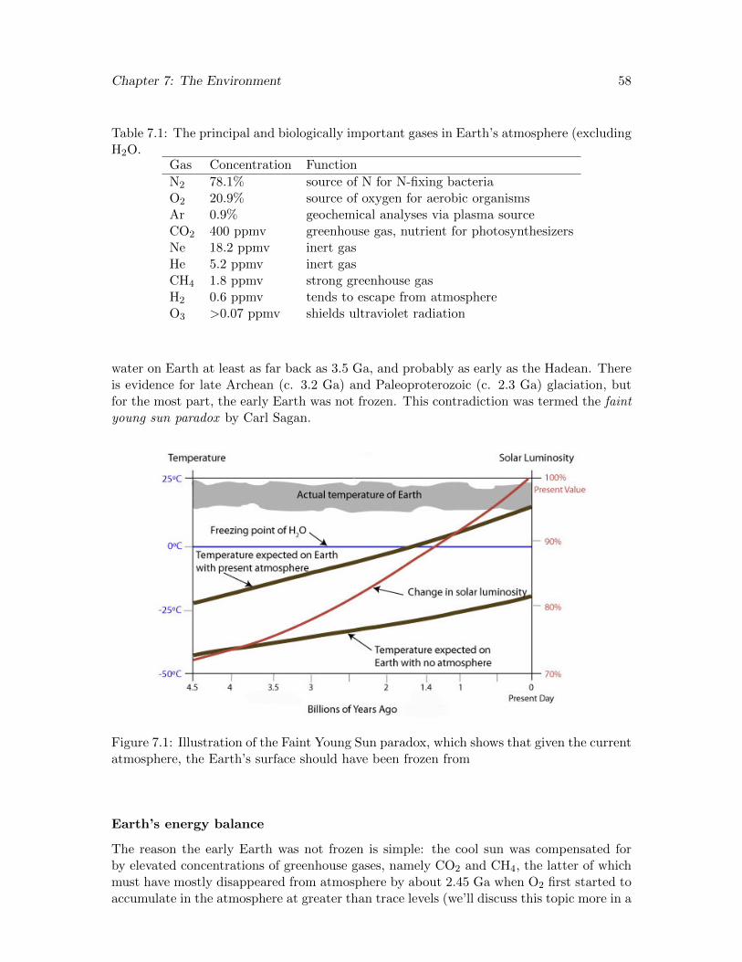
Chapter 7: The Environment 58
Table 7.1: The principal and biologically important gases in Earth’s atmosphere (excludingH2O.
Gas Concentration Function
N2 78.1% source of N for N-fixing bacteriaO2 20.9% source of oxygen for aerobic organismsAr 0.9% geochemical analyses via plasma sourceCO2 400 ppmv greenhouse gas, nutrient for photosynthesizersNe 18.2 ppmv inert gasHe 5.2 ppmv inert gasCH4 1.8 ppmv strong greenhouse gasH2 0.6 ppmv tends to escape from atmosphereO3 >0.07 ppmv shields ultraviolet radiation
water on Earth at least as far back as 3.5 Ga, and probably as early as the Hadean. Thereis evidence for late Archean (c. 3.2 Ga) and Paleoproterozoic (c. 2.3 Ga) glaciation, butfor the most part, the early Earth was not frozen. This contradiction was termed the faintyoung sun paradox by Carl Sagan.
Figure 7.1: Illustration of the Faint Young Sun paradox, which shows that given the currentatmosphere, the Earth’s surface should have been frozen from
Earth’s energy balance
The reason the early Earth was not frozen is simple: the cool sun was compensated forby elevated concentrations of greenhouse gases, namely CO2 and CH4, the latter of whichmust have mostly disappeared from atmosphere by about 2.45 Ga when O2 first started toaccumulate in the atmosphere at greater than trace levels (we’ll discuss this topic more in a

Chapter 7: The Environment 59
subsequent lecture). The role of greenhouse gases and solar luminosity is easily understoodin terms of the Energy Balance Equation:
4fσT 4e = S(1−A) (7.1)
where,
f: greenhouse transmission factor
σ: Stefan-Boltzmann constant
T 4e : Average surface temperature on Earth (in K)
S: Incident solar energy (at the surface of the atmosphere)
A: Average planetary albedo (a number between 0 and 1)
The silicate weathering feedback
CO2 levels are regulated over geological time scales (>10’s or 100’s of thousands of years)by the silicate weathering feedback
• CO2 + H2O → H2CO3
• CaSiO3 + H2CO3 → Ca2+ + 2HCO−3 + SiO2 + H2O
• CO2 regulated through direct temperature effect and indirect precipitation effect onweathering of silicate minerals on the continents
• The geological carbon cycle
– Mantle/metamorphism source of CO2
– Carbonate and sedimentary organic matter ultimate sink
7.3.3 Atmospheric oxygen and organic carbon burial
Earth’s atmosphere did not always contain free oxygen. So where did this lovely O2 comefrom? Most of it came from photosynthesis, which, as you well know, converts CO2 intoreduced C in the form of organic matter, which consists of mainly proteins, lipids, andcarbohydrates. But we are all familiar with the smell of decaying leaves and know thatanimals and bacteria alike eat plants and other animals, resulting in the reoxidation of thatorganic matter through respiration. We can summarize this two way street of C reductionand oxidation as
CO2 +H2O CH2O +O2 (7.2)
You, your dog, trees, and all organic material exposed to the atmosphere are inherentlythermodynamically unstabe—that is, out of equilibrium with a highly oxidizing atmo-sphere, which wants to convert us back into CO2. So how then does O2 manage to accu-mulate in the atmosphere? The answer is in the equation: we need to remove the CH2Ofrom the the cycle. The earth does this for us by burying a very small fraction of allorganic material that is produced (<0.1%) in sediments, mostly in shales. Some of thisorganic matter subsequently reinvents itself as oil or natural gas (collectively known as
Chapter 7: The Environment 60
petroleum), which is why petroleum geologists like shales (think the Bakken and Marcellusshales). Most of this petroleum will eventually be reoxidized, either gradually as it mi-grates through seeps to the oceans or atmosphere, or much more quickly by airplanes andautomobiles. The most recalcitrant of the organic matter remains in sediments as kerogen,and this is really the counterweight to the O2 in our atmosphere.
The O2 content of the atmosphere is strongly regulated by negative feedbacks in the oxygencycle. The more O2 there is around, the harder it is for organic matter to go unnoticed byoxygen and succeed in being buried. If the Earth was to find some way to start pumpingnew O2 into the atmosphere, forests would eventually start to combust spontaneously ! Onthe flip side, if O2 levels go down a bit (as they are currently, due to fossil fuel burning), itbecomes easier to bury organic matter, and hence to build up O2 again. Other importantfeedbacks regulate oxygen through nutrient recycling.
7.3.4 Carbon isotopes
The oxygen cycle and the history of O2 in the atmosphere is both more complicated andmuch more interesting than all of this. We will spend more time discussing atmosphericO2 in subsequent lectures. But before we move on, we should first discuss carbon isotoperatios, which are a powerful tool for querying the ancient carbon cycle, as well as carbonflow at many different spatial scales. Carbon has two stable isotopes: 13C and 12C, ofwhich the latter is by far more abundant. The ratios of 13C/12C are variable in differentC-bearing molecules, and this difference arises through fractionation, whereby a physical,chemical, or biochemical process results in differences in this ratio between one region andanother or between reactants and productions. This fractionation arises because the heav-ier isotope is more sluggish when both isotopes are freely bouncing around, and because italso tends to form stronger bonds that are harder to break.
Life being intrinsically lazy, much prefers to use to use 12C when it synthesizes organicmolecules. The result is a very strong fractionation between the oxidized carbon pool ituses (atmospheric CO2 or dissolved CO2 in waters) and the organic materials it makes.
By convention, we do not refer to carbon isotope by the raw 13C/12C ratios. Rather, we usethe delta notation, through which we normalize them a reference ratios and then multiplyby a thousand, so that we can express them in per mil units. The result is numbers thatare much easier to deal with than the ratios themselves:
δ13CV PDB(h) =
(13C12C sample
/13C12C vpdb
− 1
)× 1000 (7.3)
where VPDB referes to the reference 13C/12C ratio we use for normalization.
Organic matter, such as me and most sedimentary organic matter (SOM), has very lowδ13Cvpdb values (probably about -25h) compared to the average CO2 emitted by volcanoes(the ultimate source of CO2 in the atmosphere-ocean system), which is about -5h. dis-solved inorganic carbon (DIC), in the oceans, which is close to 0h. The reason the oceansare heavier than the source of carbon is that about 20% of the carbon removed from the

Chapter 7: The Environment 61
oceans is SOM, which by virtual of being isotopically so negative, buoys the isotopic com-position of the remaining reservoir DIC. The result of the carbon is removed from theocean as carbonate, which has nearly the same isotopic composition as the seawater fromwhich it precipitates. Consequently, we can measure the δ13C of carbonates as a proxy forthe δ13C of the ancient ocean and broadly track fluctuations in the amount of SOM beingburied.
Changes to the the carbon isotope composition of seawater can be either steady state,result from a change in the parameters controlling the isotopic composition of inflow andout flow of carbon, or non-steady state, in which the volume of the reservoir changes. Theseproduce very different isotopic responses, the former typically being more gradual and thelatter, typically more abrupt, followed by a gradual recovery.
7.3.5 Circulation
Wind happens, which means that the atmosphere is mobile. Wind is the result of pressuredifferences, facilitated by the low density and viscosity of the atmosphere. On a globalscale, circulation is driven by heating in the low-latitudes, which drives air upwards, fol-lowed by cooling and sinking in the higher latitudes. However, the fact that the Earthrotates complicates what would otherwise be a very simple convective cell. Rotation givesrise to the Coriolis effect. Quite simply, this deflects the trajectory of air masses clockwisein the northern hemisphere and counterclockwise in the southern hemisphere. The resultis that the hot air masses that rise in the tropics gradually deflect further and further tothe right as they drift north (and to the left in the southern hemisphere), such that theycannot make it to the poles and instead eventually sink (as cool, dry air) in the sub-tropics.There, the air masses diverge north and south. In the northern hemisphere, the air movingnorth deflects towards the east giving rise to the westerlies in the mid-latitudes, and the airmoving south deflects westwards as it approaches the equator, generating the trade winds.
The combined effect of convection and the Coriolis effect produces a general circulationof the atmosphere dominated by three convective cells in each the northern hemisphereand southern hemisphere, known as Hadley cells. These Hadley cells exert a major controlon climate, accounting for the large amount of rainfall in the tropics in the intertropicalconvergence zone (or ITCZ as it is commonly abbreviated), where warm moist air rises,and the arid conditions in the subtropics, where cool, dry air descends.
7.4 The Terrestrial Realm
As you know from the hypsometric curve, most of the terrestrial realm sits at relativelylow elevations above sea level. One stark feature of the present terrestrial realm is a largetemperature gradient between the poles and the equator. It is this temperature gradientthat gives rise to the atmospheric circulation, but this is not enough to even it out. Thisgradient also begets a diversity of climates. The type and diversity of vegetation is closelycoupled to climate, and because vegetation forms the base of of community food webs,there is a strong geographic control on the major terrestrial communities on Earth:
• Rain forests
Chapter 7: The Environment 62
• Deserts
• Mediterranean; chaparral
• Savannahs
• Temperate grasslands
• Temperate forests
• Mountains (and glaciers)
• Northern coniferous forests
• Arctic tundra
The major atmospheric circulation patters we learned about in the previous section havethe greatest control on precipitation patterns, which along with temperature, control veg-etation types. Hence, the sub-tropics, where dry air descends and warms on its way down,are dominantly desert and largely sparse in vegetation. Most rain forests, on the otherhand, straddle the equator, in the ITCZ.
The other major control on precipitation patterns is mountains, in particular those alongcoast lines. Mountains deflect passing air upwards, causing it to cool and drop its mois-ture. The air then descends down the other side of the mountains, warms up again, andis dry. Hence, rain shadows form on the leeward side of mountain ranges (that is, on thedownwind side). This is why Victoria, BC is relatively dry and sunny compared to Seattleand Vancouver, and why the west side of the Sierra Nevadas are significantly wetter thanthe east side.
Seasons also exert a strong control on precipitation patterns. Mediterranean climates havehot and dry summers and cool and wet winters. Savannahs tend to receive their rainfall inthe warm, summer months, as the ITCZ shifts. Similarly, the great Asian monsoon occursduring the summer, when the ITCZ migrates northward, and prevailing winter air patternof offshore winds shifts to strong onshore winds, that deliver extraordinary amounts ofhumidity that drops as those air masses warm and rise over the continent.
Mountains (or better yet, elevation) also give rise to climatic zonation, that parallels, at amuch smaller scale, the changes in climates from the low to high latitudes. The change intemperature, with elevation, is called the lapse rate, and is about 6.4◦C/km, on average (abit lower under very humid conditions, and a fair bit higher under dry conditions). So youcan see it does not take terribly high mountains to produce arctic-like conditions, even atlow latitudes.
Some of the best clues we have to determining ancient climate zones from the geologicalrecord come from the fossil records of plants. This record only stretches back to the middlePaleozoic, and is only augmented by flowering plants for the past 80 to 90 million years.Nevertheless, plants provide a powerful means of quantifying ancient climates, because theydisplay patterns that are a function of climatic conditions. For example, the percentage ofsmooth leaves (versus jagged-edged leaves) correlates almost perfectly with temperature.Similarly, the size of leaf stomata reflect CO2 abundance and humidity.

Chapter 7: The Environment 63
7.5 The Marine Realm
Most sediments accumulate in the oceans, and those that do accumulate in the oceans havea much better chance of escaping subsequent erosion than do sediments deposited in theterrestrial realm. For this reason, our knowledge of ancient environments and the fossilrecord are heavily skewed towards the marine realm. This said, deep water sediments (i.e.those deposited directly on ocean crust) are not well preserved in the geological record,because they tend to subduct. However, we have access to such sediments dating back toabout 200 Ma through deep sea sediment cores and the odd sliver of deep sea sedimentspreserved elsewhere in mountain belts.
7.5.1 Ocean currents
Surface ocean currents are largely driven by the wind, with modification by the Corioliseffect. For this reason, major ocean currents parallel major wind patterns, with strongeasterly equatorial currents westerly mid-latitude currents. But unlike the atmosphericcirculation, the ocean currents are constrained by the location of continents. Hence, whenthese currents collide with the continents, they deflect counterclockwise in the southernhemisphere and clockwise in the northern hemisphere. They also generate gravitationalcounter currents.
Subtropical gyres form in all of the ocean basins straddling the equator, and their senseof rotation is again governed by the Coriolis effect. The centre of these gyres tend tobe relatively barren, because they are cut off from sources of nutrients. A branch of theNorth Atlantic gyre, known as the Gulf Stream, flows northward towards western Europeand eventually the North Atlantic. The current carries warm, salty water northward andaccounts for the relatively temperate climates in northwestern Europe (compared to equiv-alent latitudes in North America).
The warm, salty water of the Gulf Stream eventually cools off in the polar regions, andbecause it is saltier than surrounding waters, becomes denser and sinks. This formation ofNorth Atlantic Deep Water sets up the great conveyer belt of seawater known as the ther-mohaline circulation, which delivers deep waters throughout the Atlantic Ocean. There isonly week formation of deep waters in the northern Pacific Ocean, and for this reason, thedeep waters in the Pacific are much older (and more acidic) than those in the deep ocean.
The Antarctic Circumpolar Current flows clockwise around Antarctica. This strong currenteffectively cuts of the Southern Ocean from the Atlantic, Indian, and Pacific oceans, whichhelps account for why Antarctica is so much colder than the northern polar region.
7.5.2 Climatic oscillations
Certain quasi-periodic climatic phenomena result from oscillating atmospheric air pres-sures, sometimes coupled to fluctuating oceanic conditions. These are known as oscillationsand can play an important role in regional weather from year to year.
Chapter 7: The Environment 64
El Nino-Southern Oscillation (ENSO)
El Nino refers to an interval of unusually warm surface waters in the eastern tropical pa-cific. It corresponds with high atmospheric pressures in the western tropical Pacific and lowpressures in the eastern Pacific. This pressure gradient drives easterly wind currents thatdrag warm western Pacific water eastward. The result is unusually high temperatures andabnormally high levels of precipitation in the eastern tropical and even sub-tropical Pacific.
La Nina refers to the opposite scenario, where atmospheric pressures are higher over theeastern Pacific, setting up easterly winds. The drag from these winds causes cold, deepPacific water to upwell, resulting in anomalously cool surface waters in the eastern Pacific,and correspondingly cooler weather and lower than average rainfall.
These two states tend to oscillate back and forth with a periodicity of about 5 years, hencethe term oscillation.
North Atlantic Oscillation
Another oscillating climatic phenomenon is the North Atlantic oscillation (NAO), althoughthis is more an atmospheric feature. It is defined by oscillating air pressure differences asrecorded in the Azores and Reykjavık, Iceland, which lie at the centre of permanent airpressure highs and lows, respectively. The NAO results in weakening and intensification ofthis pressure difference with a periodicity of about 10 years. When the pressure differenceare higher, they strengthen the westerlies, which transport warm, most air to westernEurope. The result is milder winters and summers. When the pressure differences diminish,the westerlies diminish, resulting in more extreme weather over western Europe.
7.5.3 Marine environments
We commonly subdivide the marine realm physiographically into the continental shelf, con-tinental slope, continental rise, and abyssal plain, which is the deep sea floor. As you knowthe mid-ocean ridges stand tall above the deep sea floor, and are underwater mountainranges where new oceanic crust is made.
Epicontinental seas are shallow, typically somewhat isolated or restricted seaways thatspread out over large swaths of low-lying continents during period of high sea level. Be-cause we are in a glacial epoch, there are few notable epicontinental seaways. An excellentancient example is the Western Interior Seaway, which covered much of central NorthAmerica about 100–70 million years ago, and connected the Gulf of Mexico to the ArcticOcean.
There are various different zones in the marine realm that are distinguished based on theirhydrographic, biological, and biogeochemical conditions.
• Supratidal zone
• Intertidal zone
• Shallow subtidal zone
Chapter 7: The Environment 65
• Storm wave base
• Below storm wave base
• Photic zone
• Oxygen minimum zone (OMZ)
The photosynthesis that take place in the photic zone is mostly carried out by single-celled,cyanobacteria and algae, that are collectively referred to as phytoplankton, meaning theyare small photosynthesizes that drift in the surface ocean. The production of primarybiomass by photosynthesizers tends to deplete the surface ocean in nutrients. After death,this organic material begins to settle through the water column, effectively exporting car-bon and nutrients to the deeper ocean. Much of this carbon is consumed or decays beforeit reaches the seabed, releasing CO2 and nutrients into the deeper ocean. At the sametime, this decay consumes oxygen, leading to the development of an oxygen minimum zonewhere rates of O2-consumption peak in the water column.
The nutrients released by decaying phyotoplankton and the organisms that consume themare returned to the surface in zones of upwelling. Such upwelling zones, such as the marginoffshore Peru, tend to be highly fertile and productive.
Zooplankton are small animals, including many crustaceans, that drift in the surface oceanand feed upon the phytoplankton. The nekton include the animals that swim, and theseinclude animals that both feed on phytoplankton and on zooplankton. Together, theplankton and nekton constitute the pelagic life in the oceans, mean they live and moveabout in the water column. The group of animals that live on the seafloor (or in shallowsediments) are known as the benthos. These include both mobile organisms, and sessileorganisms, such as sponges and corals, which are attached to the seafloor.
Chapter 8
Origin of the Earth and theHadean
Reading: Chapter 11 in Stanley; Chapter 8 in Wiccander and Monroe
8.1 Introduction
Earth’s history is commonly broadly separated into two temporally unequal halves: thePrecambrian and the Phanerozoic, which roughly correspond to the time before and afterthe first appearance of large eukaryotes. The Precambrian, which is not an official name inthe Geological Time Scale, is subdivided into the Hadean, Archean, and Proterozoic. Whilewhat we know about Earth’s history is overwhelmingly biased towards the Phanerozoic (thepast 541 million years), the Precambrian encompasses the lion’s share of geological time.Before digging into Early Earth’s history, we will begin with a brief review of the origin ofthe solar system.
8.2 Origin of the Solar System
Earlier in this course, we discussed the age of the Earth, which we now know quite pre-cisely from the age of meteorites. These meteorites reveal extraordinary information aboutthe early history of the solar system and Earth’s own early history. For example, somemeteorites show evidence of differentiation, with one class of meteorites representing theiron-rich core of a differentiated body (iron meteorites) and other meteorites more closelyresembling magmatic rocks (stony meteorites). Undifferentiated, chondritic meteorites, onthe other hand, provide an indication of what Earth’s bulk chemical make-up might havebeen like when it formed. Hence, geochemists often compare the geochemistry of certainchemical reservoirs in the Earth or rocks with average chondritic values as a measure ofthe differentiation that has occurred on Earth.
Our sun and the planets in our solar system formed from the leftover material from asupernova, an exploding star that left a wake of material in the form of a slowly rotatingnebula. As this nebula cooled, condensed, and flattened, it began to spin faster due tothe conservation of angular momentum. This rotating disk segregated into a central sunand rings of material that rotated around it and gradually coalesced into planetesimals.
66
Chapter 8: Hadean 67
During this process, the lighter and more volatile elements were concentrated in the outerring, which went on to form the gaseous planets, like Jupiter and Saturn, while the denserand less volatile elements were concentrated in the inner solar system, forming the rockyplanets like Earth and Venus. Based on the abundance of certain daughter isotopes ofshort-lived radioactive isotopes, we know that the the sun and the planets formed withinabout 50 million years of one another, and possibly even less.
8.3 Differentiation and the origin of the Moon
The proto-Earth was a hot place, due to the kinetic energy resulting from the frequentmeteorite impacts as the proto-planet grew, along with the heat released by radioactivedecay, which would have been much greater early in the solar system’s history than it istoday. This heat melted the early Earth, and the denser parts of this melt, most notablyiron and nickel, migrated to the core, while the less dense part rose to the top, forming aproto-mantle. The act of differentiation alone generated enormous amounts of heat throughthe conversion of potential energy, and this helped sustain a molten early Earth.
Earth’s moon is thought to have formed very early in Earth’s history, probably as the resultof a collision with a Mars-sized planet. Such a model conveniently accounts for Earth’sunusually fast spin (for its position in the solar system), and probably remelted Earth,after it cooled initially. We surmise that the moon formed after differentiation, becauseits bulk chemistry and density differ from the bulk composition of Earth, but quite closelyresemble Earth’s mantle. Consequently, it would also have blown away any atmospherethat the Earth and moon might have developed by that time as a result of early coolingand differentiation. Indeed, the near absence of water within the crystal structure of lunarminerals attest to the loss of water during the collision.
Strong support of the impactor hypothesis emerged when Clayton and Mayeda (1996)showed that the oxygen isotopic composition of the moon and Earth are indistinguishable.A recent paper on Zn isotopes in lunar rocks (Paniello et al., 2012) had seemed to haveconfirmed the Mars-impactor hypothesis for the origin of the moon. However, these sim-ilarities are not necessarily consistent with the impactor model after all, based on recentmodelling of the impact scenario, which suggests that significant isotopic variations shouldhave resulted from the standard mars-sized impactor scenario. So this once staid and ac-cepted model for the origin of the moon is again under scrutiny—an excellent example ofhow science and our knowledge of how the Earth and solar system evolved is never settled.
8.4 The Late Heavy Bombardment
The Hadean was originally defined as the period of time dating from the origin of the solarsystem 4.56 Ga to the age of the oldest terrestrial rocks, 3.8 Ga. This time also correspondsto the Late Heavy Bombardment, when frequent large impacts would have remelted mostearly crust that had formed. How do we know that meteorites continue to impact the Earthfor hundreds of millions of years after the moon formed when we have no record of theseimpacts on Earth? The answer is in the moon, which is heavily pock-marked by cratersformed by metrorite impacts. The ages of the largest craters range from 3.8 to about 4.5
Chapter 8: Hadean 68
Ga, and studies of the pockmarks suggest that the rate of impacts was about 1000 timesgreater in the early Hadean than it is today. In fact, we owe it to Jupiter that the Earthand moon were not more thoroughly peppered by meteorites, for it deflects most would-beimpactors of doom. Nevertheless, these impacts were sufficiently large and frequent to addsignificant material and heat to the early Earth, and presumably sterilize it frequently. Itis also due to the early clean-up of meteorites from the solar system that the planets havetilted spin axes.
Rocks and minerals older than 3.8 Ga have now been dated, but we still know very littleabout the first 0.75 Ga of Earth’s history.
8.4.1 Origin of the ocean and atmosphere
The earliest atmosphere was likely composed mostly of H and He (not unlike the sun),but most of these original gasses were lost during meteorite impacts and gradual escape tospace.
• Hydrosphere derived from volcanoes and comets
• Salts derived from weathering of seafloor, then continents
Earth’s earliest ocean was not particularly salty. Modeling suggests that it would havereached roughly modern salinity by the early Archean, and since that time, the flux ofsalts into the ocean has been balanced by the deposition of salts.
• Atmosphere derived from volcanic outgassing
• Early atmosphere largely lost from meteorite impacts
• A reducing atmosphere (H2O, HCl, CO, CO2, N, CH4, NH3)
8.4.2 Origin of continental crust
The earliest ’crust’ that would have formed as the magma ocean cooled at its surface wouldhave been basaltic in composition. This proto-crust was simply cooled from the magmaocean, and so was mafic in composition. Hence, there were no continents initially. Theformation of distinct continental crust required differentiation to form lighter, less dense,felsic rock.
The formation of felsic magmas could only have occurred through the melting of basalt.Hence the the formation of the first continental crust would have resulted from the descentof early, mafic crust back into the mantle—subduction. The earliest evidence for the for-mation of felsic crust comes from the ages of the oldest zircons in the world: the Jack Hillszircons. These zircons, obtained from the Jack Hills of Western Australia, are dated at4.404 Ga and are the oldest Earth materials ever dated (Wilde et al., 2001). These zirconsappear to suggest that proto-plate tectonics had begun within 150 m.y. of the origin ofthe solar system—that is, basaltic crust had begun to subduct and remelt, forming felsicmagmas. The rocks that would have formed from these early felsic melts would have beensodium-rich, because sodium is a highly incompatible element.

Chapter 8: Hadean 69
The earliest bits and pieces of granitic crust would have probably been pushed and shovedabout on the surface of the early ocean by the still vigorously convecting mantle. Over time,they would have begun to coalesce to form protocratons: early, relatively stable continentalcrust that would eventually assemble to form the earliest continents. These Precambrianshields are at the core of all continents.
The Jack Hills zircons are interesting not only because they are really old, but also becausethey contain oxygen isotope signatures that suggest the involvement of water in the meltingof the magmas. Some scientists have argued that this is evidence that an ocean alreadyexisted by about 4.4 Ga, although it is really impossible to constrain what the nature ofthis early ocean might have been like or whether or not it was permanent.
The oldest rock: the Acasta Gneiss vs. the Nuvvuagittuq Greenstone
The oldest actual terrestrial rock ever dated by an uncontroversial method is the AcastaGneiss, which occurs on the Slave craton in northern Canada and was dated by Bowringand Williams (1999).
• Oldest U-Pb zircon discordant age of 4.06 Ga
• A gneiss, so protolith was even older
The same zircons in the Acasta Gneiss that show that the protolith formed from a felsicmagma also record metamorphic events at 3.75 and 3.60 Ga (Bowring and Williams, 1999).Similar aged gneisses occur elsewhere in the world, notably in Issua Greenland, where rocksas old 3.8 Ga preserve what closely resembles modern oceanic crust. Hence, it is clear thatby about 3.8 Ga, not only had continental and oceanic crust similar to that found todayalready begun to form, but also these rocks were participating in collisional events thatdrove regional metamorphism.
The prize for the oldest rocks on Earth was challenged a few years ago when then McGillPhD student, Jonathon O’Neill argued that a patch of rocks in Ungava Quebec might beas old as 4.3 Ga, based on a new dating method that uses an extinct Nd isotope system(O’Neil et al., 2008). This technique and the suggestion that these are the oldest rocks iscontroversial. The oldest zircons in these rocks date to 3.8 Ga, which still means they areextremely old. To the extent that they are in fact older, they provide a rare glimpse intoconditions on the earliest Earth.
It is clear that differentiated continents had already begun to drift about by the late Hadeanor early Archean. Whether or not this constituted plate tectonics as we know it todayremains a hotly debated question. As you will see in the following chapter, certain rockassociations that are common in Archean terranes are in fact quite distinct from those thatoccur in younger rocks. These greenstone belts are one of several lines of evidence thatskeptics of modern-style (horizontal) Archean plate tectonics (e.g., Bedard et al., 2003)highlight in their arguments. In fact, these arguments beg the question: what are theessential criteria for plate tectonics?

Chapter 9
Earth’s Earliest Record: theArchean
9.1 The Archean
The Archean Eon spanned from 3.8 to 2.5 Ga. The Earth’s interior was still very hot duringthis time, and as a consequence, it seems that no large continents like those found today hadformed. Nevertheless, cratons stabilized during this time and recognizable plate tectonicprocesses were active, although noticeably different from those today. The Archean alsopreserves the first putative and first indisputable evidence of life on Earth. The ArcheanEon ended with the Great Oxidation Event, during which free O2 accumulated in theatmosphere for the first time.
9.1.1 Greenstone belts
Greenstone belts are elongated terranes with a synclinal structure that consists of maficto ultramafic volcanic rocks and mafic-derived sedimentary rocks (turbidites and mud-stones), and sometimes banded iron formation (see below) that have been metamorphosedto greenschist facies (hence their name; green, because they contain abundant metamorphicchlorite) and are commonly intruded by granite. Greenstone belts tend to be sandwichedbetween granite-gneiss complexes (typically highly metamorphosed gneiss of granitic ori-gin).
• Restricted to Archean (and possibly Hadean)
• Often occur in parallel belts, perhaps forming in arc, back-arc, or rift settings
• Often include komatiites—ultramafic lava flows, which are rare in post-Archean world
• Reflect hotter interior of the Earth and early version of plate tectonics (althoughprecisely how they formed remains a mystery)
• Earliest record of subaqueous sedimentation
The origin of greenstone belts has long intrigued geologists and continues to be a sourceof much debate. One only has to read several different Earth and Life History textbooksto see the differing views. Whereas Stanley’s book seems to support an intercontinentaldrift model, others advocate for an Arc model to account for greenstone belts. I personally
70
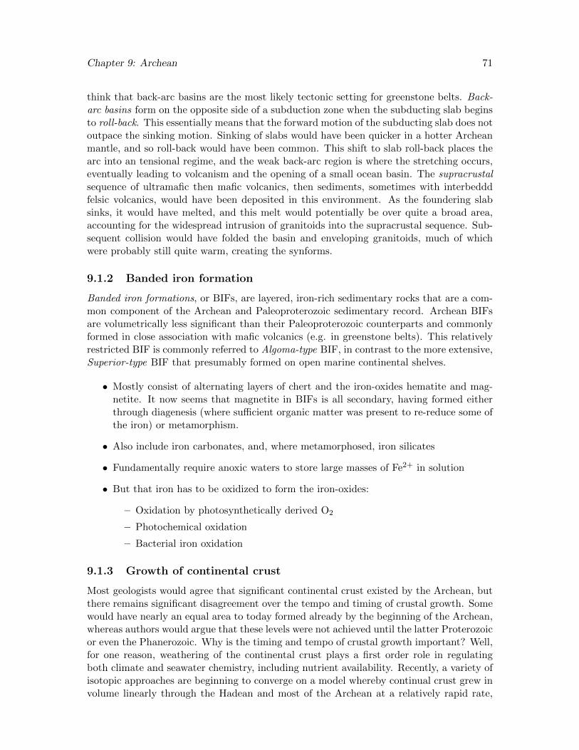
Chapter 9: Archean 71
think that back-arc basins are the most likely tectonic setting for greenstone belts. Back-arc basins form on the opposite side of a subduction zone when the subducting slab beginsto roll-back. This essentially means that the forward motion of the subducting slab does notoutpace the sinking motion. Sinking of slabs would have been quicker in a hotter Archeanmantle, and so roll-back would have been common. This shift to slab roll-back places thearc into an tensional regime, and the weak back-arc region is where the stretching occurs,eventually leading to volcanism and the opening of a small ocean basin. The supracrustalsequence of ultramafic then mafic volcanics, then sediments, sometimes with interbedddfelsic volcanics, would have been deposited in this environment. As the foundering slabsinks, it would have melted, and this melt would potentially be over quite a broad area,accounting for the widespread intrusion of granitoids into the supracrustal sequence. Sub-sequent collision would have folded the basin and enveloping granitoids, much of whichwere probably still quite warm, creating the synforms.
9.1.2 Banded iron formation
Banded iron formations, or BIFs, are layered, iron-rich sedimentary rocks that are a com-mon component of the Archean and Paleoproterozoic sedimentary record. Archean BIFsare volumetrically less significant than their Paleoproterozoic counterparts and commonlyformed in close association with mafic volcanics (e.g. in greenstone belts). This relativelyrestricted BIF is commonly referred to Algoma-type BIF, in contrast to the more extensive,Superior-type BIF that presumably formed on open marine continental shelves.
• Mostly consist of alternating layers of chert and the iron-oxides hematite and mag-netite. It now seems that magnetite in BIFs is all secondary, having formed eitherthrough diagenesis (where sufficient organic matter was present to re-reduce some ofthe iron) or metamorphism.
• Also include iron carbonates, and, where metamorphosed, iron silicates
• Fundamentally require anoxic waters to store large masses of Fe2+ in solution
• But that iron has to be oxidized to form the iron-oxides:
– Oxidation by photosynthetically derived O2
– Photochemical oxidation
– Bacterial iron oxidation
9.1.3 Growth of continental crust
Most geologists would agree that significant continental crust existed by the Archean, butthere remains significant disagreement over the tempo and timing of crustal growth. Somewould have nearly an equal area to today formed already by the beginning of the Archean,whereas authors would argue that these levels were not achieved until the latter Proterozoicor even the Phanerozoic. Why is the timing and tempo of crustal growth important? Well,for one reason, weathering of the continental crust plays a first order role in regulatingboth climate and seawater chemistry, including nutrient availability. Recently, a variety ofisotopic approaches are beginning to converge on a model whereby continual crust grew involume linearly through the Hadean and most of the Archean at a relatively rapid rate,

Chapter 9: Archean 72
and then slowed down, but continued to grow linearly, after about 3 Ga (Dhuime et al.,2012). This model is compelling because various different lines of evidence appear to pointto something rather significant happening in terms of mantle convection and plate tectonicsat this time.Also about 3.0 Ga, the first known cratons began to stabilize.
• cratons are the stable cores of ancient continents
• oldest known stable craton is about 3.0 Ga, represented by mixed carbonate-clasticWitwatersrand and Pongola groups in South Africa and Swaziland. The developmentof a carbonate platform requires a stable carton
• sediments contain abundant structures indicating shallow water and even glacial de-position (oldest evidence of glaciation, c. 2.9 Ga; Young et al., 1998).
Figure 9.1: Various models for the tempo of crustal growth (plotted as fraction of conti-nental crust relative to the present through time), from Taylor and McLennan (1985)
.
Precambrian shields are regions of dominantly Precambrian-aged cratonic rocks exposedat the Earth’s surface. The Canadian Shield is perhaps the most impressive example, andas would be expected for such a large tract of very old rocks, consists mostly of crystallinerocks. The Precambrian shield is stitched together by various ancient orogenic belts, thatrepresent collisions between the ancient cartons.
9.1.4 Archean life
It is impossible to say for certain when life first evolved (some think it may have done somultiple times in the Hadean, only to be annihilated by large meteorite impacts. Beforeeven looking at the evidence for early life, however, it is worth considering what is meantby life.
Chapter 9: Archean 73
• Able to metabolize
• Have some barrier from outside world
• Able to reproduce
• Able to produce complex molecules
This definition of what is required for life leads us to a list of essential components for lifeto originate:
• Amino Acids, which are relative simple organic compounds, which strung togetherform the more complex proteins that are catalyze chemical reactions and act asbuilding materials
• Nucleic acids, large and complex acids: ribonucleic acid (RNA), which is simpler butless stable, and deoxyribonucleic acid (DNA), which is more complex and more stable
• Organic phosphorus compounds. Adenosine triphosphate (ATP) transforms energyfrom light or chemicals into the energy required by cells. Phospholipids providestructure to cell walls and create a semi-permeable membrane
It is conceivable that the building block organic materials required for life to originate weredelivered by comets and meteorites during the Late Heavy Bombardment. Stanley Millershowed in the 1950’s that sparks of electricity could actually stimulate the formation ofamino acids and a variety of other somewhat complex organic molecules from the inorganiccompounds that likely existed in the early atmosphere.
How did amino acids aggregate to poem proteins? Some scientists have suggest that claysprovided a necessary template through the metal ions on their surfaces. These could haveattracted amino acids and arranged them in an orderly way.Many people believe life originated in extreme environments because some extremophilesoccur on the deepest branches of the tree of life. However, others, including Andrew Knoll,think that life most likely originated in ’normal’ environments and later moved into theextreme environments through environmental pressures.
• Required a source of appropriate building blocks for organic molecules
• A source of energy
The earliest indirect evidence for life comes from carbon isotope compositions of concen-trated carbon in a highly metamorphosed gneiss in a 3.8 Ga Akilia Gneiss in southwestGreenland
• Low δ13C values imply organic synthesis
• Debate over whether this is the only process that can produce low carbon isotopevalues
• Debate over whether or not the protolith was sedimentary or granitic
The earliest direct evidence for life on Earth comes from 3.5 Ga stromatolites and micro-fossils in Western Australia
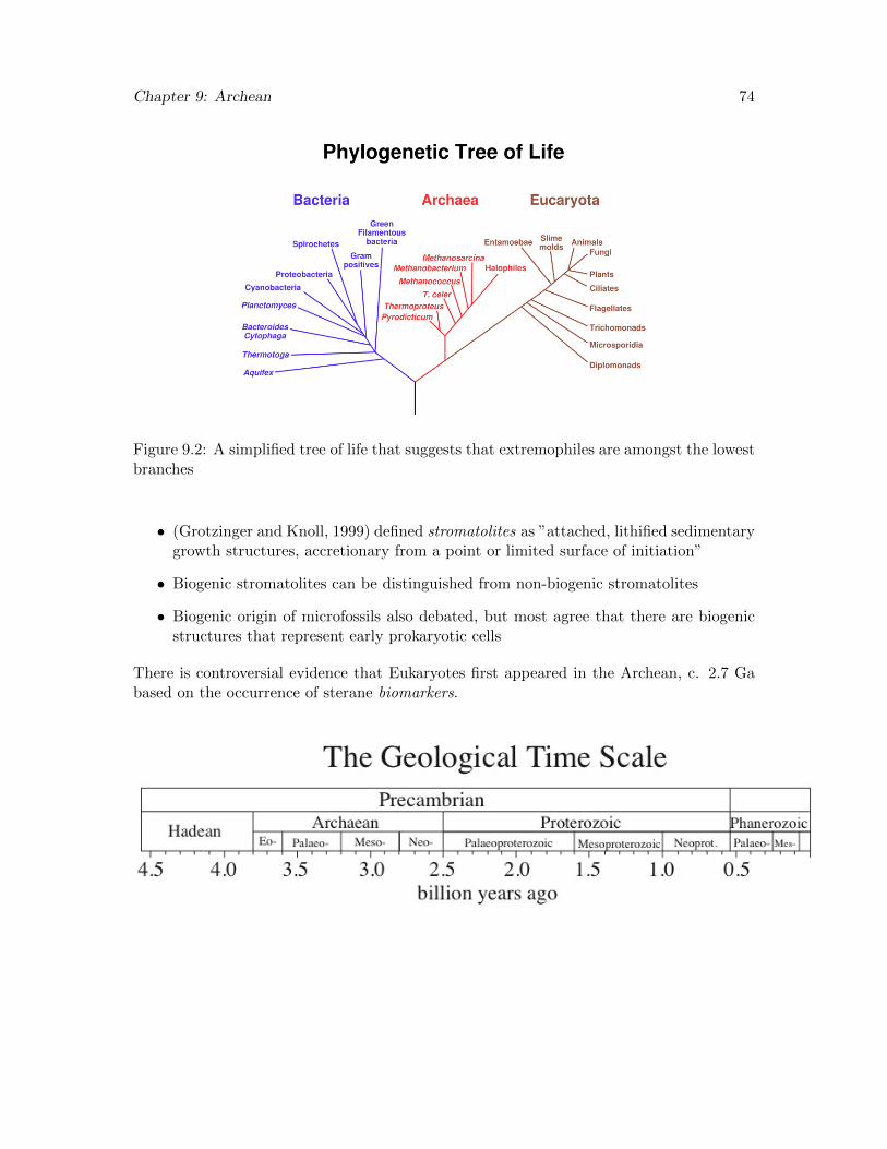
Chapter 9: Archean 74
Figure 9.2: A simplified tree of life that suggests that extremophiles are amongst the lowestbranches
• (Grotzinger and Knoll, 1999) defined stromatolites as ”attached, lithified sedimentarygrowth structures, accretionary from a point or limited surface of initiation”
• Biogenic stromatolites can be distinguished from non-biogenic stromatolites
• Biogenic origin of microfossils also debated, but most agree that there are biogenicstructures that represent early prokaryotic cells
There is controversial evidence that Eukaryotes first appeared in the Archean, c. 2.7 Gabased on the occurrence of sterane biomarkers.

Chapter 10
The Great Oxidation Event
10.1 The Great Oxidation Event
The Great Oxidation Event was the appearance of free oxygen in the atmosphere about2.45–2.35 Ga. Whereas geologists have long recognized this event based on the geologi-cal record (and some theoretical considerations), the onset of this event is now virtuallyunambiguously pinpointed in the stratigraphic record by sulfur isotope data (Fig. 10.2).
10.1.1 Geological evidence for an early anoxic atmosphere
By the late 1950’s, geologists and geochemists like Preston Cloud, Heinrich Holland, andRobert Garrels recognized that the geological record from early Earth’s history was sig-nificantly different from that of later in Earth’s history and that this was due, in part, todifferent atmospheric oxygen levels. The occurrence and pattern of banded iron formationwas an important clue that Earth’s early environment lacked sufficient oxygen to ventilatethe deep oceans. It was the anoxic oceans that permitted ferrous (Fe2+) iron to accumulatein the oceans. Massive iron formation disappeared from the geological record by about 1.8Ga, and it was long argued by Holland and others that this marked the oxygenation of thedeep oceans.
In addition to the BIF record, there is other geological evidence that pointed specificallyto an Archean atmosphere with no free oxygen and geochemical evidence that suggest animportant change in ocean geochemistry sometime in the Paleoproterozoic.
Redox sensitive minerals
Fluvial sediments in the Archean contain certain detrital minerals that are not stableunder an even mildly oxidizing environment: pyrite, siderite, and uraninite. By the earlyProterozoic, these distinctive minerals had disappeared from the sedimentary record.
Soil profiles
Archean soil profiles are noticeably depleted in iron, which could only have occurred ifthere was no free oxygen around. Otherwise, iron would have been retained in the soilsas iron oxide and oxyhydroxide minerals. By the Paleoproterozoic, iron had begun to beretained in soil profiles, indicating free atmospheric O2.
75
Chapter 10: GOE 76
10.1.2 Growth of the marine sulfate reservoir
Sulfate is abundant in the modern ocean, but this has not always been the case. Variouslines of evidence indicate that Proterozoic oceans had much less sulfate overall, and thatthe Archean ocean had almost no sulfate. Geologically, this is seen in the complete absenceof calcium sulfate evaporite deposits (gypsum or anhydrite) of Archean age. The first sig-nificant sulfate deposits are found in the ca. 2.3 billion-year old Gordon Lake Formationin the Huronian Supergroup in Ontario and possibly equivalent rocks in the Lucknow Fm.of South Africa (Rasmussen et al., 2013). However, sulfate deposits remain scarce overallthrough much of the Proterozoic.
In the late 1990’s, Don Canfield published a now famous plot of the sulfur isotopic compo-sition of sulfieds (mainly pyrite) deposited in marine sediments through time. This datasetshowed a substantial increase in the spread of these values around the Archean-Proterozoicboundary. In the modern ocean, large differences in the δ34S values between seawatersulfate and sedimentary pyrites are the result of sulfur isotopic fractionation by bacterialsulfate reducers, which use sulfate as an electron acceptor during metabolism. That is,they reduce the sulfate to sulfide. Oxygen recycling of the reduced sulfur can lead toeven bigger differences between sulfate and sedimentary sulfides. Consequently, Canfieldinterpreted this increased spread in sulfur isotope values around 2.3 billion years ago (Fig.10.1) to herald growth in the marine sulfate reservoir, consistent with higher atmosphericoxygen concentrations and in increase in oxidative weathering on the continents (Canfieldand Teske, 1996).
The Canfield Ocean
Shortly after he published his sulfur isotope curve, Canfield proposed a radical new modelfor deep ocean chemistry during the Proterozoic. He argued that rather than becomingoxygenated following the end of BIF deposition around 1.8 Ga, the oceans instead remainedanoxic, but became sulfidic rather than iron-rich as they had been for the previous twobillion years. The word used to describe such conditions is euxinia, and the possibility ofeuxinic oceans had important implications for seawater chemistry and eukaryotic evolu-tions. The interval of the Canfield Ocean (∼ 1.8 to 0.8 Ga) has otherwise been referredto as the Boring Billion because it lacks both iron formation and significant carbon iso-tope anomalies, reflecting a relatively infertile era in biospheric evolution. The CanfieldOcean model seems at first blush to be consistent with this observation, because euxinicconditions would have resulted in vanishingly low concentrations of Mo and some other keynutrients (Anbar and Knoll, 2002). After Canfield first proposed this model, several differ-ent datasets bearing on the nature of sulfur and iron chemistry in seawater were publishedfrom Mesoproproterozoic (1.6 to 1.0 Ga) which seemed to support the euxinia model (e.g.Shen et al., 2003; Brocks et al., 2005)
The Canfield Ocean understandably received great attention and a large following. How-ever, it has recently been challenged both by new data sets that suggest that some wereferruginous rather than sulfidic (Planavsky et al., 2011), and simple modelling that in-dicates that the low trace metal concentrations observed during this interval in time donot in fact require widespread sulfidic or even anoxic conditions (Reinhard et al., 2013). I
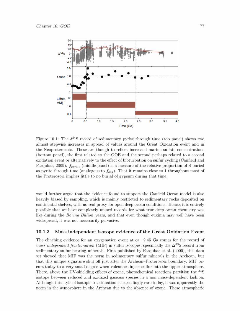
Chapter 10: GOE 77
Figure 10.1: The δ34S record of sedimentary pyrite through time (top panel) shows twoalmost stepwise increases in spread of values around the Great Oxidation event and inthe Neoproterozoic. These are though to reflect increased marine sulfate concentrations(bottom panel), the first related to the GOE and the second perhaps related to a secondoxidation event or alternatively to the effect of bioturbation on sulfur cycling (Canfield andFarquhar, 2009). fpyrite (middle panel) is a measure of the relative proportion of S buriedas pyrite through time (analogous to forg). That it remains close to 1 throughout most ofthe Proterozoic implies little to no burial of gypsum during that time.
would further argue that the evidence found to support the Canfield Ocean model is alsoheavily biased by sampling, which is mainly restricted to sedimentary rocks deposited oncontinental shelves, with no real proxy for open deep ocean conditions. Hence, it is entirelypossible that we have completely missed records for what true deep ocean chemistry waslike during the Boring Billion years, and that even though euxinia may well have beenwidespread, it was not necessarily pervasive.
10.1.3 Mass independent isotope evidence of the Great Oxidation Event
The clinching evidence for an oxygenation event at ca. 2.45 Ga comes for the record ofmass independent fractionation (MIF) in sulfur isotopes, specifically the ∆33S record fromsedimentary sulfur-bearing minerals. First published by Farquhar et al. (2000), this dataset showed that MIF was the norm in sedimentary sulfur minerals in the Archean, butthat this unique signature shut off just after the Archean–Proterozoic boundary. MIF oc-curs today to a very small degree when volcanoes inject sulfur into the upper atmosphere.There, above the UV-shielding effects of ozone, photochemical reactions partition the 33Sisotope between reduced and oxidized gaseous species in a non mass-dependent fashion.Although this style of isotopic fractionation is exceedingly rare today, it was apparently thenorm in the atmosphere in the Archean due to the absence of ozone. These atmospheric

Chapter 10: GOE 78
sulfur gases with the MIF signal were then eventually incorporated into sedimentary sulfurminerals by a combination of biological and non-biological processes.
Because ozone in the upper atmosphere is tied to oxygen concentrations, it stands to reasonthat the MIF sulfur signature is a first-order and unequivocal recorder of an increase inatmospheric oxygen levels beyond some threshold where the MIF signal shuts off. In aclever atmospheric chemistry modelling study, Pavlov and Kasting (2002) showed that thisthreshold is approximately 10−5 times the present atmospheric level (PAL) of O2.
Figure 10.2: The ∆33S record from sedimentary sulfur-bearing minerals shows a rise inPO2 over the critical threshold of 10−5 present levels (Farquhar et al., 2007)
.
Other proxies for oxygen abundance also show increasing oxygenation of Earth’s environ-ment. However, it is currently virtually impossible to quantify PO2 during the Proterozoic.
10.1.4 Source of oxygen and cause of the oxidation event
If the MIF signature in sedimentary sulfur pinpoints where in the geological record oxygenconcentrations rose beyond some key threshold, what drove this rise in oxygen in the firstplace? The most logical answer is that it resulted from the steady production of O2 byphotosynthesizes, who we know inhabited the oceans for at least several hundred millionyears prior to the GOE. Another possible source of atmospheric oxygen was hydrogen es-cape, whereby photodissociation of H2O in the upper atmosphere, followed by escape ofthe light hydrogen left behind a more oxidizing atmosphere (Catling and Claire, 2005).However, whereas these are presumably the source of that oxygen, why did the GOE nothappen earlier?
Once possible answer is that the sinks for oxygen outweighed the input of oxygen fromphotosynthesis and hydrogen escape. We have already learned that banded iron formation(BIF) contains a significant amount of iron oxide and that oxidation of sulfide is the mainsource of sulfate to the oceans. These would have constituted tremendous sinks for oxygen.Another important sink would have been the flux of volcanic gases to the atmosphere fromvolcanoes. Many scientists have argued that the oxidation state of these gases might have
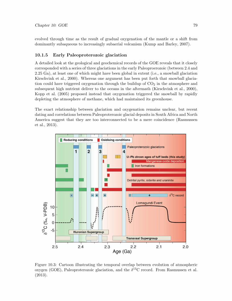
Chapter 10: GOE 79
evolved through time as the result of gradual oxygenation of the mantle or a shift fromdominantly subaqueous to increasingly subaerial volcanism (Kump and Barley, 2007).
10.1.5 Early Paleoproterozoic glaciation
A detailed look at the geological and geochemical records of the GOE reveals that it closelycorresponded with a series of three glaciations in the early Paleoproerozoic (between 2.4 and2.25 Ga), at least one of which might have been global in extent (i.e., a snowball glaciationKirschvink et al., 2000). Whereas one argument has been put forth that snowball glacia-tion could have triggered oxygenation through the buildup of CO2 in the atmosphere andsubsequent high nutrient deliver to the oceans in the aftermath (Kirschvink et al., 2000),Kopp et al. (2005) proposed instead that oxygenation triggered the snowball by rapidlydepleting the atmosphere of methane, which had maintained its greenhouse.
The exact relationship between glaciation and oxygenation remains unclear, but recentdating and correlations between Paleoproterozoic glacial deposits in South Africa and NorthAmerica suggest that they are too interconnected to be a mere coincidence (Rasmussenet al., 2013).
Figure 10.3: Cartoon illustrating the temporal overlap between evolution of atmosphericoxygen (GOE), Paleoproterozoic glaciation, and the δ13C record. From Rasmussen et al.(2013).

Chapter 10: GOE 80
10.1.6 The Lomagundi Event
Shortly after the last Paleoproterozoic glaciation, δ13C values in marine carbonates beganto rise, and they stayed unusually high (> 8h) for about 150 million years (Fig. 10.3. Longintervals of high δ13C are commonly associated with input of oxygen to the atmospheredue to the implied high rates of organic carbon burial. However, it is interesting to notethat the Lomagundi event started after the initiation of the GOE and was over long afterthe GOE had begun. This paradox highlights that fact that it was not increased carbonburial alone that drove the onset of the GOE, and also suggests that just what the GOErepresents perhaps is not so easy to describe or quantify. For example, the MIF-sulfurrecord tells us when pO2 surpassed a certain minimum threshold, but it does not actuallysay anything about continued oxygenation after that. It seems highly likely that oxygenlevels continued to climb after the start of the GOE for some several hundred million years,perhaps approaching levels not dramatically different from those of the late Proterozoicor early Paleozoic. New trace metal data and isotope data also suggest that atmosphericoxygen, and by extension, marine oxygen and sulfate levels may have declined abruptlyfollowing the Lomagundi event (Planavsky et al., 2012; Partin et al., 2013).
Chapter 11
Early–Middle Proterozoic Life andEnvironment
Reading: Chapter 12 in Stanley
The Proterozoic spans from 2.5 to 0.542 Ga and is subdivided rather arbitrarily into thePaleo- (2.5–1.6), Meso- (1.6–1.0), and Neoproterozoic (1.0–0.542 Ga). The onset of the Pro-terozoic conveniently closely corresponds with the so-called Great Oxidation Event, duringwhich time free O2 first accumulated in the atmosphere, and its end closely correspondswith the origin and diversification of animals, which presumably indicates that atmosphericoxygen levels had risen to at least many hundredths, if not, tenths of the modern level.The first indisputable Eukaryotes appear in the Paleoproterozoic, and they diversify in theearly Neoproterozoic, although cyanobacteria (and stromatolites) reigned supreme throughthe Eon. The Earth was glaciated multiple times in the both the Paleoproterozoic and theNeoproterozoic, some of these glaciations being global in extent. Banded iron formation(BIF), which was already being deposited in the Archean, became more widespread inthe early Paleoproterozoic (vast Superior-type BIFs), and all but ended for good by theend of the Paleoproterozoic. Supercontinents were born and died multiple times in theProterozoic.
11.1 The Paleoproterozoic Glaciations
The early Paleoproterozoic was punctuated by a series of glaciations, at least one of whichmay have been global in extent, between 2.45 and 2.2 Ga. Well represented north of LakeHuron within the Huronian Supergroup.
• Closely followed assembly of an early supercontinent (Kenorland)
• PPz glacial deposits found in N. America, Finland, South Africa, and Australia
• In Great Lakes area: Mt. Ramsay, Bruce, and Gowganda formations
• Followed by the Lomagundi Event – high δ13C carbonates – a prolonged carbon burialevent
81

Chapter 11: Proterozoic 82
11.2 Life in the Proterozoic
Andy Knoll has dubbed the Proterozoic the ”Age of Cyanobacteria” because the cyanobac-teria were the dominant life from in terms of energy flow in Proterozoic oceans. They mostcertainly account for the increase in oxygen levels and most organic carbon that was buriedin Proterozoic sediments. However, one of the big questions in Precambrian paleobiologyis when the Eukarya branched from the Archaea. Up until recently, it was believed thatthis branch point was 2.7 Ga or older based on biomarker data, but these data are nowcalled into question. So the best evidence we have is that the earliest eukaryotes appearedin the Proterozoic.
11.2.1 Eukaryotic evolution
Eukaryotic cells are larger and more complex than prokaryotic cells:
• internal nucleus, which store genetic information in chromosomes
• most contain other organelles
Most eukaryotes are aerobes and many are multicellular. Thus, they represent a fundamen-tally huge step in Precambrian evolution. It is widely regarded that Eukaryotes evolved,in part, as the result of symbiosis between different bacteria: an invading or predatorybacteria and a host. Lynn Margulis, who was also known for supporting the Gaia hypoth-esis, was the first biologist to recognize and argue for the symbiotic origin of Eukarya—ahypothesis that is now widely accepted. She argued that the symbiosis eventual resulted independence between the invading and host bacteria, with the invader performing a specificfunction related. For example, mitochondria, which are the engines of eukaryotic cells,resemble certain extant bacteria, and they have distinctive RNA and DNA from the re-mainder of the cell. Similarly, chloroplasts in plants closely resemble certain cyanobacteria,and it has hard to imagine that cyanobacteria and eukaryotes separately evolved such sim-ilar platforms to carry out photosynthesis.
In order to have engulfed bacteria, early eukaryotes must have first evolved a cytoskeleton,which is a set of fibres beneath the outer membrane of the cell that give it rigidity andshape. The timing of the origin of the eukaryotes is a subject of great debate and significantresearch, but as of yet, little consensus.
Was the eukaryotic evolution simply a matter of time or was it nudged along by environ-mental change? Answering that question fundamentally requires knowing when eukaryotesfirst evolved. As discussed earlier, some circumstantial evidence (some of it now discred-ited) has been offered to suggest they evolved in the Archean, prior to the Great OxidationEvent. However, the fossil record does not preserve any unambiguous fossils pre-dating theGEO.
• 2.1 Ga macrofossils of colonial (eukaryotic?) algae, Francevile Series, Gabon
• 2.1 Ga Grypania, a colonial bacteria (or eukaryote?) from Negaunee iron formation,Michigan
• 1.9 Ga Gunflint chert: Microfossils of iron-oxidizing bacteria (i.e, recognizable moderncounterpart)
Chapter 11: Proterozoic 83
• 1.8 Ga oldest acritarchs: ”closed, organic-walled microfossils of uncertain systematicaffinities” (Knoll et al., 2006a), but many are thought to be eukaryotic
• 1.5 Ga Tapannia, an acritarch that likely represents a eukayrote with a complexcytoskeleton (thought by some to be an early fungus)
• 1.2 Ga Bangiomorpha pubescens (bangiophyte red algae) with differentiated holdfasts
• Early Neoproterozoic: Eukaryotic diversification
• c. 0.65 Ga: the first sponges? biomarkers, macrofossils, and molecular clocks
11.2.2 The age of stromatolites
As previously mentioned, life on the Proterozoic Earth was dominated by cyanobacteria,who are the dominant organism involved in the construction of stromatolites. Stroma-tolite diversity peaked in the late Mesoproterozoic, when they were a major componentof carbonates rocks. Throughout the Proterozoic, stromatolites were major reef-builders,filling the biogeochemical-ecological role that corals would eventually occupy. Stromatolitebiodiversity began to decline precipitously in the middle Neoproterozoic and they all butdisappeared by the end of the Ediacaran Period, presumably as the result of the expansionof grazing organisms.
Chapter 12
Supercontinents and the Assemblyof North America
12.1 Tectonics and the Supercontinental Cycle
Archean greenstone belts offer a glimpse of how plate tectonics operated on a much hotterEarth (that is, in the interior). By the 3 Ga, the first modern-scale continents had formed,as represented by the stable continental platform onto which the Witwatersrand and Pon-gola supergroups (South Africa) were deposited.
It was long a matter of debate whether or not modern-style plate tectonics operated at all inthe Precambrian, and many prominent geologists argued that it did not. However, it is nowwell established that plate tectonics resembling the familiar rifting and mountain buildingprocesses taking place today did in fact operate in the Precambrian. Paul Hoffman’spioneering work on the c. 1.9 Ga Wopmay orogen in northern Canada clearly establishedthat the modern mode of tectonics had been established by the late Paleoproterozoic.
12.1.1 Precambrian supercontinents
The cratons appear to assemble periodically into large continents (supercontinents) that in-clude many to most of the cratons. The best known example of a supercontinent is Pangea,which finished assembling the in the late Paleozoic. Not surprisingly, reconstructing oldersupercontinents is difficult business and amounts to putting together highly fragmentedpuzzles with poorly preserved pieces.
• Geological tie point
– lithology
– metamorphic grain
– geochemistry
– geochronology
– stratigraphic architecture (e.g. rift–drift)
• Paleomagnetic data (apparent polar wander paths)
84
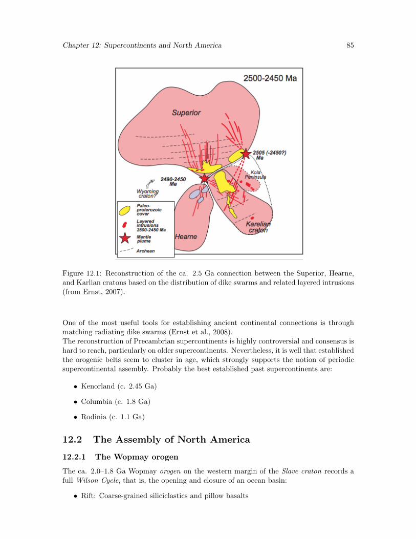
Chapter 12: Supercontinents and North America 85
Figure 12.1: Reconstruction of the ca. 2.5 Ga connection between the Superior, Hearne,and Karlian cratons based on the distribution of dike swarms and related layered intrusions(from Ernst, 2007).
One of the most useful tools for establishing ancient continental connections is throughmatching radiating dike swarms (Ernst et al., 2008).The reconstruction of Precambrian supercontinents is highly controversial and consensus ishard to reach, particularly on older supercontinents. Nevertheless, it is well that establishedthe orogenic belts seem to cluster in age, which strongly supports the notion of periodicsupercontinental assembly. Probably the best established past supercontinents are:
• Kenorland (c. 2.45 Ga)
• Columbia (c. 1.8 Ga)
• Rodinia (c. 1.1 Ga)
12.2 The Assembly of North America
12.2.1 The Wopmay orogen
The ca. 2.0–1.8 Ga Wopmay orogen on the western margin of the Slave craton records afull Wilson Cycle, that is, the opening and closure of an ocean basin:
• Rift: Coarse-grained siliciclastics and pillow basalts
Chapter 12: Supercontinents and North America 86
• Drift: Passive margin, development of a stable carbonate platform
• Collision: Outer metamorphic belt, central fold-thrust belt and foreland basin, inter-nal undeformed craton
12.2.2 Proterozoic evolution of North America (Laurentia)
The core of North America is an ancient continent that consists of Archean cratons suturedby Paleoproterozoic orogens. Precambrian North America is known as Laurentia andincludes Greenland, Svalbard, and northwest Scotland which were separated from NorthAmerica during Cretaceous rifting.
Archean cratons
The Canadian shield comprises at least 7 Archean cratons: Superiour, Wyoming, Nain,Rae, Slave, Hearne, Burwell. These largely assembled between about 2.0 and 1.8 Ga, suchthat the boundaries between the distinct cartons are orogens with associated arcs.
Yavapai-Mazazatl Terranes
Following stabilization of Laurentia, southern and eastern Laurentia was the locus of activecrustal growth from about 1.8 to 1.6 Ga, through the accretion of oceanic terranes and arcvolcanism. This phases of juvenile crustal growth was followed by a prolonged episode ofpost-orogenic igneous activity and emplacement of vast volumes of granite between about1.5 and 1.3 Ga
The Mackenzie Dike Swarm
North America also experienced major plume activity and continental rifting in the Meso-proterozoic. The Mackenzie Dike swarm was emplaced about 1.27 Ga, and is one of thelargest dike swarms known on Earth. Dike swarms are curved or radiating clusters ofmafic dikes that likely formed as the result of plume activity and constitute the roots ofwidespread volcanism. They often all that remains of what are commonly referred to aslarge igneous provinces.
The Mid-continent Rift
Later in the Mesoproterozoic, continental extension began about 1.2 Ga, forming the Kee-weenawan, or mid-continent rift. A series of large grabbens, filled with basalts and sed-iments, formed at this time, but rifting ultimately ceased, and the Laurentian continentremained in tact. Lake Superior roughly occupies one of these former rifts, but the associ-ated volcano-sedimentary succession is exposed on either side of the lake.
Chapter 13
Neoproterozoic Snowball Earthand Rodinia Break-up
Reading: Chapter 12, pages 276-277, in Stanley
13.1 Introduction
The Neoproterozoic Era (1000–542 Ma) experienced many important events and changes.At the onset of the Neoproterozoic, by all counts the biosphere was still rather simple.Cyanobacteria were the dominant primary producer and Eukarya had evolved, but notdiversified. The oceans were largely anoxic, and probably at least in part sulfidic (=euxinic). The continents were arranged in the supercontinent Rodinia, and climate wasprobably fairly steady. By the end of the Neoproterozoic, Rodinia was gone and a new su-percontinent had already begun to form. The Earth had experienced a series of glaciationsso severe that the tropics were covered in ice. Yet Eukarya survived, and by the late Neo-proterozoic (if not somewhat earlier) animals populated at last parts of the oceans. Mostof the major animal phyla may even have already evolved. Oxygen was probably fairlyabundant, even if the deep oceans were not yet entirely oxygenated. Algae had replacedcyanobacteria as the core of the marine food chain. In short, the planet was eminentlyhabitable and had begun to resemble the modern world in many important ways.
• Break-up of the low-latitude supercontinent Rodinia
• onset of amalgamation of the supercontinent Gondwana
• High average δ13C values punctuated by negative excursions
• At least three glaciations, two of which were global in extent
• Reprise of iron formation deposition
• Oxygenation of the environment
• Emergence and diversification of animals
87

Chapter 13: Snowball Earth and Rodinia Break-up 88
Figure 13.1: An early version of the proposed Rodinia supercontinent (Hoffman, 1991),based in large part on the locations of Grenvillian orogens and geological tie points. Addi-tional evidence that Laurentia was at the centre of this supercontinent comes from the factthat it is almost entirely encircled in latest Proterozoic to early Paleozoic passive margins,which require continent rifting and subsequent drift to form.
13.2 Rodinia break-up
The supercontinent Rodinian finished assembling around the end of the Mesoproterozoic,perhaps the earliest Neoproterozoic (Li et al., 2008). It begin to drift towards the lowerlatitudes and show at least initial signs of breaking up around 850–800 Ma. By about 720million years ago, break-up seemed to be well underway and the supercontinents continuedto disintegrate until about 600 Ma with the opening of the Iapetus (Paleo-Atlantic) ocean.
The break-up of Rodinia appears to be closely associated with the emplacement of a largenumber of Large Igneous Provinces (LIPs), which are indicated by a combination of aflood basalt and/or a large radiating dyke swarm. Large LIPs notably occur around 830(Willouran-Guibei), 780 (Gunbarrel), and 720 Ma (Franklin), and much of the evidence forthese is clustered on cratons that are widely thought to have been contiguous in Rodinia:Laurentia, India, Australia, and South China. Hence, it has been proposed that these LIPswere are related to a single super plume event.
Both the emplacement of LIPs and the paleogeography during early break-up would havehad a large influence on global climate, for multiple reasons.

Chapter 13: Snowball Earth and Rodinia Break-up 89
13.2.1 Paleogeographic influence on global climate
Even before the pieces of Rodinia had entirely disaggregated, Gondwana begin to assemblewith continental collisions encircling Africa (the so-called Pan-African orogens).
• Laurentia surrounded by passive margins
• Rifting associated with plumes and emplacement of several large igneous provinces(LIP’s). In North America these include the 780 Ma Gunbarrel event and the 720Ma Franklin event.
• Unique paleogeography played a strong role in regulating climate:
– Response of silicate weathering feedback to low-latitude, rifting continents, abun-dant mafic rocks
– Affect of low-latitudes on albedo
13.3 Geochemical Proxies
13.4 Record of Neoproterozoic glaciations
It has long been recognized that the Earth was glaciated in the late Precambrian. By thelate 19th century, Infracambrian glacial deposits had been documented on several conti-nents. But it was not until two eminent geologists working in the middle of last centurychampioned their existence and pointed out their widespread occurrence did these rockstake on importance in Earth history: the Cantabridgian, Brian Harland worked mainly inEurope, Svalbard, and Greenland, while the erstwhile Antarctic explorer Douglas Maw-son worked in Australia. The Neoproterozoic glacial deposits are now well known, figureprominently in text books, and are the subject of much controversial, but also exciting,interdisciplinary research.
It now seems that there were at least three glacial epochs:
• Sturtian (∼ 720–660 Ma)
• Marinoan (∼645–635 Ma)
• Ediacaran (∼ 580 Ma)
Of these, the first two appear to have been the most severe, with clear evidence that thewere long-lived and entailed low-latitude continental glaciation. These two are hypothe-sized to have been snowball Earth glaciations. Several different observations regarding theglaciations underlie the snowball Earth hypothesis:
• Glaciations widespread (all continents)
• Carbonate platforms glaciated
• Evidence that glaciers reached sea level in the tropics
– Elatina tidal rhythmites
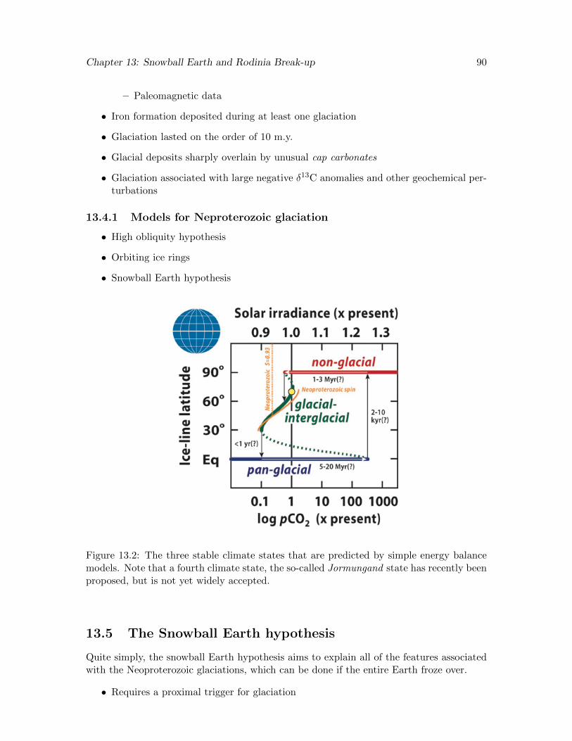
Chapter 13: Snowball Earth and Rodinia Break-up 90
– Paleomagnetic data
• Iron formation deposited during at least one glaciation
• Glaciation lasted on the order of 10 m.y.
• Glacial deposits sharply overlain by unusual cap carbonates
• Glaciation associated with large negative δ13C anomalies and other geochemical per-turbations
13.4.1 Models for Neproterozoic glaciation
• High obliquity hypothesis
• Orbiting ice rings
• Snowball Earth hypothesis
Figure 13.2: The three stable climate states that are predicted by simple energy balancemodels. Note that a fourth climate state, the so-called Jormungand state has recently beenproposed, but is not yet widely accepted.
13.5 The Snowball Earth hypothesis
Quite simply, the snowball Earth hypothesis aims to explain all of the features associatedwith the Neoproterozoic glaciations, which can be done if the entire Earth froze over.
• Requires a proximal trigger for glaciation

Chapter 13: Snowball Earth and Rodinia Break-up 91
• Once glaciers surpass the mid-latitudes, ice-albedo feedback triggers climatic collapse:runaway glaciation
• Hydrological cycle would largely shut down on a frozen-over Earth
• Ocean would be cut off from atmosphere
– Ocean would become anoxic
– CO2 would accumulate in the atmosphere
• Would take about 10 million years to accumulate enough to compensate for highalbedo
• Catastrophic melting: ice-albedo feedback in reverse
• Post-glacial ultra-greenhouse
• Cap carbonates represent flux of alkalinity to the ocean
• Intense silicate weathering draws down CO2 over a few million years
Figure 13.3: The snowball cycle.
13.5.1 Problems with the snowball
• How did life survive (refugia)?
• The glacial record
Chapter 13: Snowball Earth and Rodinia Break-up 92
– Thick glacial deposits reminiscent of Pleistocene glacial deposits
– Evidence of cyclicity
– Evidence of open water
• Issues raised by modeling
13.5.2 Geochemical support for snowball
• Iridium and other platinum group elements
• Spike in Sr isotope ratios after glaciation
• Boron isotopes
• Mass-independent oxygen isotopes (∆17O)
13.5.3 Possible consequences of the snowball
• Trimming the tree of life
• Evolutionary radiation
• Extreme greenhouse, weathering
• Some of the earliest petroleum systems?
Chapter 14
The Ediacaran Period and theOrigin of Animals
14.1 Introduction
The Ediacaran Period was the first named period in the Precambrian
• Just named, with the GSSP in Brachina Gorge, South Flinders (Knoll et al., 2006b)
• Base of the Ediacaran Period is the base of the Nuccaleena Formation
• Base of the Cambrian is formally defined by the first appearance of the trace fossilPhycodes pedum (now known as Treptichnus pedum).
The Ediacaran Period began 635 Ma with the end of the snowball Earth, which by mostaccounts was followed by a catastrophic greenhouse. At this time, no unambiguous animalshad yet populated the Earth, although several lines of circumstantial evidence suggest thatearly animals may have already diverged from the eukaryotic lineage. By the end of theEdiacaran Period (541 Ma), the biosphere was quite diverse and may have included mostif not all of the major animals clades. A lot happened in the 94 million years in between,and so it is not surprising that the Ediacaran Period draws so much attention. One of theprevailing questions among researchers today is the extent to which early animal evolutionwas driven by an increase in oxygen in the environment. The underlying principal behindthis view of permissive evolution is that most large animals require a significant amount ofoxygen to metabolize, and hence could not have evolved until atmospheric oxygen reached areasonably large fraction of present atmospheric level (PAL). The implication is that earlyanimal evolution was sort of waiting around for this oxygenation to occur. This view is atleast partly supported by molecular clock data that place several important early metazoandivergences prior to the Ediacaran Period, 10’s to 100’s of millions of years before the firstmacroscopic animal fossils (Erwin et al., 2011)(Fig. 14.1).
A countervailing view is that early animal evolution was not triggered so much by a chang-ing environment, but by the eventual acquisition of the genetic toolkit that allowed themto evolve, which took hundreds of millions of years (Butterfield, 2009). Proponents of thisview of early animal evolution posit that it was the animals themselves that triggered themajor change in the environment, specifically, oxygenation. That is, animal evolution trig-
93
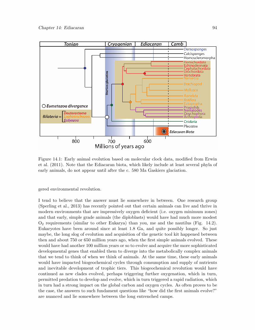
Chapter 14: Ediacaran 94
Figure 14.1: Early animal evolution based on molecular clock data, modified from Erwinet al. (2011). Note that the Ediacaran biota, which likely include at least several phyla ofearly animals, do not appear until after the c. 580 Ma Gaskiers glaciation.
gered environmental revolution.
I tend to believe that the answer must lie somewhere in between. One research group(Sperling et al., 2013) has recently pointed out that certain animals can live and thrive inmodern environments that are impressively oxygen deficient (i.e. oxygen minimum zones)and that early, simple grade animals (the diploblasts) would have had much more modestO2 requirements (similar to other Eukarya) than you, me and the nautilus (Fig. 14.2).Eukaryotes have been around since at least 1.8 Ga, and quite possibly longer. So justmaybe, the long slog of evolution and acquisition of the genetic tool kit happened betweenthen and about 750 or 650 million years ago, when the first simple animals evolved. Thesewould have had another 100 million years or so to evolve and acquire the more sophisticateddevelopmental genes that enabled them to diverge into the metabolically complex animalsthat we tend to think of when we think of animals. At the same time, these early animalswould have impacted biogeochemical cycles through consumption and supply of nutrientsand inevitable development of trophic tiers. This biogeochemical revolution would havecontinued as new clades evolved, perhaps triggering further oxygenation, which in turn,permitted predation to develop and evolve, which in turn triggered a rapid radiation, whichin turn had a strong impact on the global carbon and oxygen cycles. As often proves to bethe case, the answers to such fundament questions like “how did the first animals evolve?”are nuanced and lie somewhere between the long entrenched camps.

Chapter 14: Ediacaran 95
Figure 14.2: Summary of minimum oxygen requirements for two hypothetical last commonancestors of the bilaterians: one in which is limited by diffusion, and another which islimited by the circulatory system. Note that these are quite similar and not that far offfrom the current lower limit for extant mobile bilaterians. From (Sperling et al., 2013).
14.2 Chronology of Early Animal Evolution and EdiacaranEvents
• ∼700 Ma: The earliest sponges?
• 635 Ma: The end of the last global glaciation
• ∼632 Ma: Possible early microscopic animals?
• 595 (?) Ma: The Doushantuo biota (fossilized animal embryos)
• ∼ 590 (?): Acraman impact
• ∼ 590 (?): Turnover in the acritarch record
• 582 Ma: The Gaskiers glaciation
• 580 - 565 (?) Ma: Shuram-Wonoka negative δ13C anomaly
• 575 Ma: first appearance of the Ediacaran biota
• <555 Ma: first appearance of Kimberella (mollusca?) and Dickinsonia
• ∼ 545 Ma: fist appearance of lightly calcified metazoa (LCM)
• 542 Ma: Precambrian-Cambrian boundary: the first animal extinction event?
– Disappearance of the LCM
– Negative δ13C anomaly
– Some Ediacara continue?
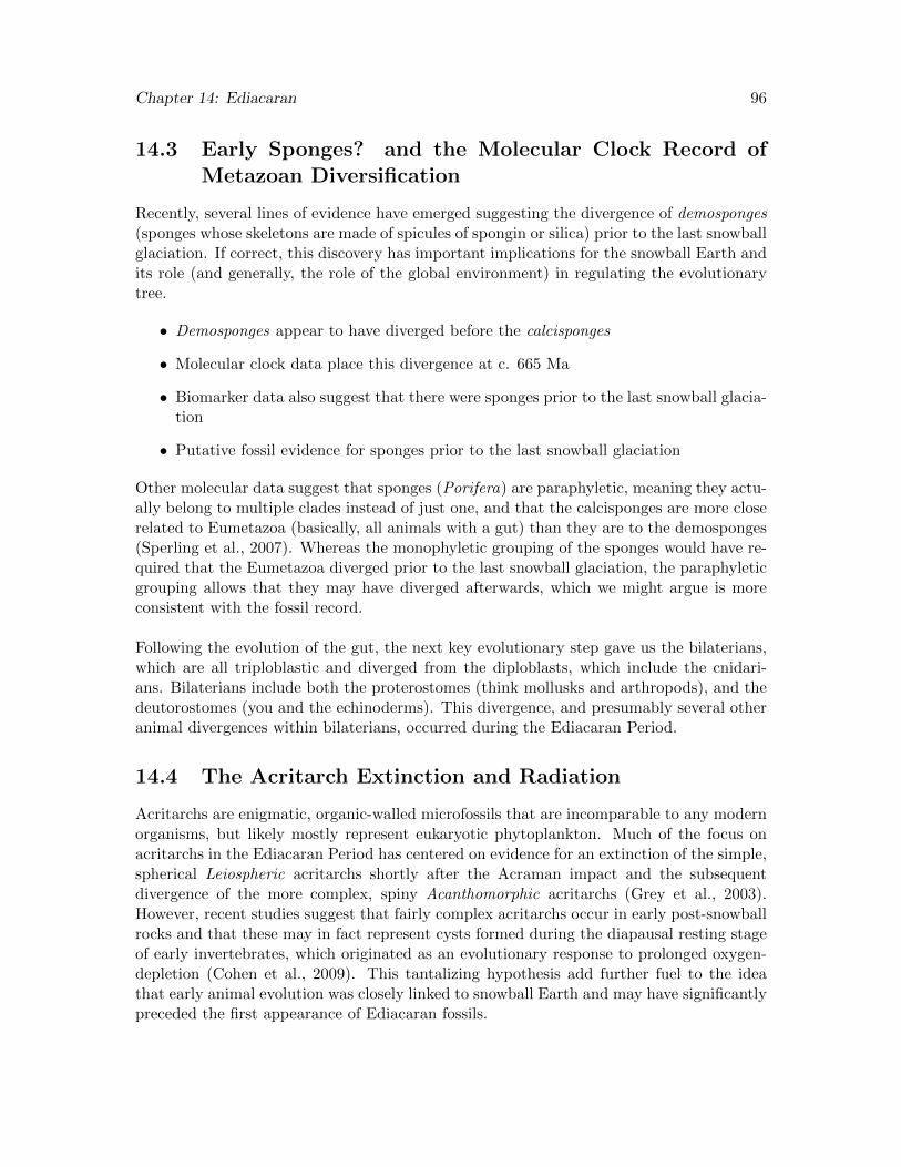
Chapter 14: Ediacaran 96
14.3 Early Sponges? and the Molecular Clock Record ofMetazoan Diversification
Recently, several lines of evidence have emerged suggesting the divergence of demosponges(sponges whose skeletons are made of spicules of spongin or silica) prior to the last snowballglaciation. If correct, this discovery has important implications for the snowball Earth andits role (and generally, the role of the global environment) in regulating the evolutionarytree.
• Demosponges appear to have diverged before the calcisponges
• Molecular clock data place this divergence at c. 665 Ma
• Biomarker data also suggest that there were sponges prior to the last snowball glacia-tion
• Putative fossil evidence for sponges prior to the last snowball glaciation
Other molecular data suggest that sponges (Porifera) are paraphyletic, meaning they actu-ally belong to multiple clades instead of just one, and that the calcisponges are more closerelated to Eumetazoa (basically, all animals with a gut) than they are to the demosponges(Sperling et al., 2007). Whereas the monophyletic grouping of the sponges would have re-quired that the Eumetazoa diverged prior to the last snowball glaciation, the paraphyleticgrouping allows that they may have diverged afterwards, which we might argue is moreconsistent with the fossil record.
Following the evolution of the gut, the next key evolutionary step gave us the bilaterians,which are all triploblastic and diverged from the diploblasts, which include the cnidari-ans. Bilaterians include both the proterostomes (think mollusks and arthropods), and thedeutorostomes (you and the echinoderms). This divergence, and presumably several otheranimal divergences within bilaterians, occurred during the Ediacaran Period.
14.4 The Acritarch Extinction and Radiation
Acritarchs are enigmatic, organic-walled microfossils that are incomparable to any modernorganisms, but likely mostly represent eukaryotic phytoplankton. Much of the focus onacritarchs in the Ediacaran Period has centered on evidence for an extinction of the simple,spherical Leiospheric acritarchs shortly after the Acraman impact and the subsequentdivergence of the more complex, spiny Acanthomorphic acritarchs (Grey et al., 2003).However, recent studies suggest that fairly complex acritarchs occur in early post-snowballrocks and that these may in fact represent cysts formed during the diapausal resting stageof early invertebrates, which originated as an evolutionary response to prolonged oxygen-depletion (Cohen et al., 2009). This tantalizing hypothesis add further fuel to the ideathat early animal evolution was closely linked to snowball Earth and may have significantlypreceded the first appearance of Ediacaran fossils.
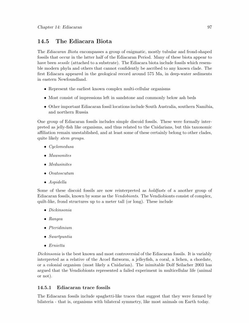
Chapter 14: Ediacaran 97
14.5 The Ediacara Biota
The Ediacaran Biota encompasses a group of enigmatic, mostly tubular and frond-shapedfossils that occur in the latter half of the Ediacaran Period. Many of these biota appear tohave been sessile (attached to a substrate). The Ediacara biota include fossils which resem-ble modern phyla and others that cannot confidently be ascribed to any known clade. Thefirst Ediacara appeared in the geological record around 575 Ma, in deep-water sedimentsin eastern Newfoundland.
• Represent the earliest known complex multi-cellular organisms
• Most consist of impressions left in sandstone and commonly below ash beds
• Other important Ediacaran fossil locations include South Australia, southern Namibia,and northern Russia
One group of Ediacaran fossils includes simple discoid fossils. These were formally inter-preted as jelly-fish like organisms, and thus related to the Cnidarians, but this taxonomicaffiliation remain unestablished, and at least some of these certainly belong to other clades,quite likely stem groups.
• Cyclomedusa
• Mawsonites
• Medusinites
• Ovatoscutum
• Aspidella
Some of these discoid fossils are now reinterpreted as holdfasts of a another group ofEdiacaran fossils, known by some as the Vendobionts. The Vendiobionts consist of complex,quilt-like, frond structures up to a meter tall (or long). These include
• Dickinsonia
• Rangea
• Pteridinium
• Swartpuntia
• Ernietta
Dickinsonia is the best known and most controversial of the Ediacaran fossils. It is variablyinterpreted as a relative of the Acoel flatworm, a jelleyfish, a coral, a lichen, a chordate,or a colonial organism (most likely a Cnidarian). The inimitable Dolf Seilacher 2003 hasargued that the Vendiobionts represented a failed experiment in multicellular life (animalor not).
14.5.1 Ediacaran trace fossils
The Ediacaran fossils include spaghetti-like traces that suggest that they were formed bybilateria - that is, organisms with bilateral symmetry, like most animals on Earth today.

Chapter 14: Ediacaran 98
14.5.2 More complex Ediacaran fossils
Another class of Ediacaran fossils exhibit bilateral symmetry and loosely resemble somePhanerozoic organisms, such as arthropods and molluscs.
• Spriggina (arthropodoid?)
• Praecambridium (arthropodoid)?
• Kimberella (a mollusc?)
• Parvancorina (a stem group trilobites?
Ediacaran fossils can be subdivided into three separate assemblages, which include someoverlapping fossils, but represent somewhat different sedimentary environments and modesof preservation.
14.5.3 The Avalon assemblage
The oldest Ediacaran fossils are found in Newfoundland, in deepwater sediments (tur-bidites, shales, and tuffs) and date as far back as about 580 Ma (Narbonnne and Gehling,2003). These include the frond structures, which appear to have formed relative complex,ecologically tiered communities (Fig. 14.5.3. These fossils are preserved as impressionson bedding planes, commonly draped in volcanic ash (which helps account for the spec-tacular preservation). Whereas some scientists claim these fossils include early animals, itremains to be demonstrated unambiguously that these were early animals. What is certain,however, is that they represent a bold eukaryotic experiment in multicellularity, but onewhich, ultimately, failed because most of these fossils are at best stem groups. Further-more, they inhabited deep waters, which seems to suggest these deeper waters were moreenvironmentally friendly for colonization be early multicullar eukaryotes (maybe animals).
Figure 14.3: Guy Narbonne and colleagues interpret many of these fossils to representorganisms that lived in tiered-communities consisting of sessile organisms attached to theseabed. From (Narbonnne and Gehling, 2003).
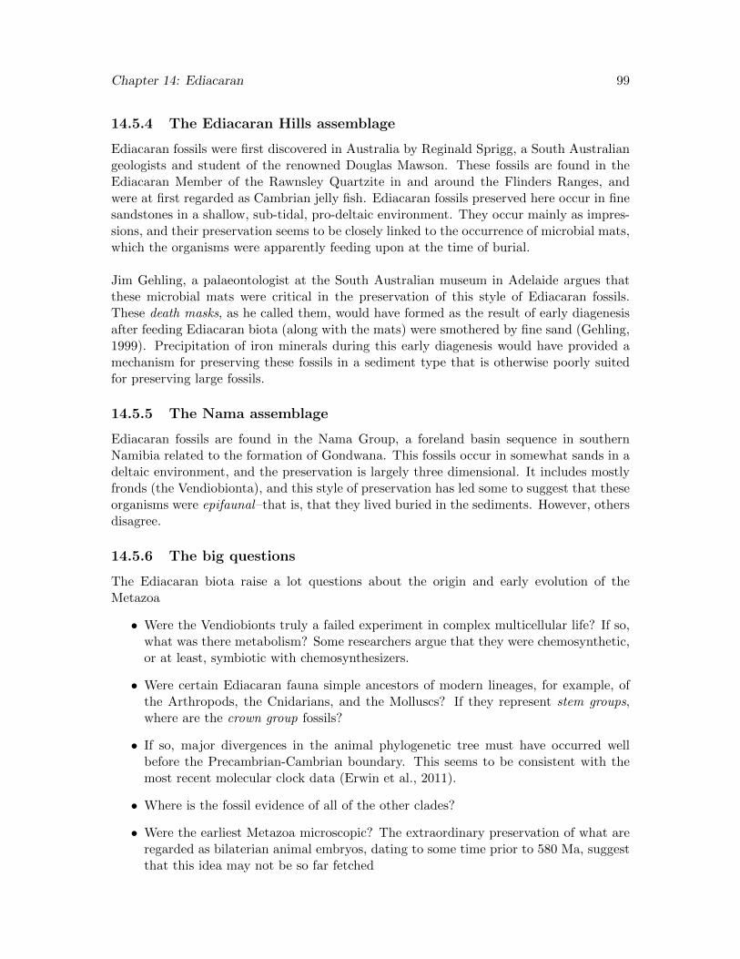
Chapter 14: Ediacaran 99
14.5.4 The Ediacaran Hills assemblage
Ediacaran fossils were first discovered in Australia by Reginald Sprigg, a South Australiangeologists and student of the renowned Douglas Mawson. These fossils are found in theEdiacaran Member of the Rawnsley Quartzite in and around the Flinders Ranges, andwere at first regarded as Cambrian jelly fish. Ediacaran fossils preserved here occur in finesandstones in a shallow, sub-tidal, pro-deltaic environment. They occur mainly as impres-sions, and their preservation seems to be closely linked to the occurrence of microbial mats,which the organisms were apparently feeding upon at the time of burial.
Jim Gehling, a palaeontologist at the South Australian museum in Adelaide argues thatthese microbial mats were critical in the preservation of this style of Ediacaran fossils.These death masks, as he called them, would have formed as the result of early diagenesisafter feeding Ediacaran biota (along with the mats) were smothered by fine sand (Gehling,1999). Precipitation of iron minerals during this early diagenesis would have provided amechanism for preserving these fossils in a sediment type that is otherwise poorly suitedfor preserving large fossils.
14.5.5 The Nama assemblage
Ediacaran fossils are found in the Nama Group, a foreland basin sequence in southernNamibia related to the formation of Gondwana. This fossils occur in somewhat sands in adeltaic environment, and the preservation is largely three dimensional. It includes mostlyfronds (the Vendiobionta), and this style of preservation has led some to suggest that theseorganisms were epifaunal–that is, that they lived buried in the sediments. However, othersdisagree.
14.5.6 The big questions
The Ediacaran biota raise a lot questions about the origin and early evolution of theMetazoa
• Were the Vendiobionts truly a failed experiment in complex multicellular life? If so,what was there metabolism? Some researchers argue that they were chemosynthetic,or at least, symbiotic with chemosynthesizers.
• Were certain Ediacaran fauna simple ancestors of modern lineages, for example, ofthe Arthropods, the Cnidarians, and the Molluscs? If they represent stem groups,where are the crown group fossils?
• If so, major divergences in the animal phylogenetic tree must have occurred wellbefore the Precambrian-Cambrian boundary. This seems to be consistent with themost recent molecular clock data (Erwin et al., 2011).
• Where is the fossil evidence of all of the other clades?
• Were the earliest Metazoa microscopic? The extraordinary preservation of what areregarded as bilaterian animal embryos, dating to some time prior to 580 Ma, suggestthat this idea may not be so far fetched
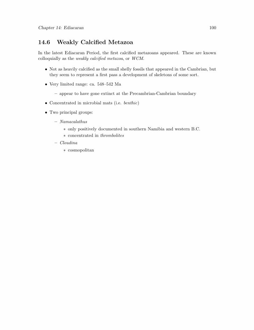
Chapter 14: Ediacaran 100
14.6 Weakly Calcified Metazoa
In the latest Ediacaran Period, the first calcified metazoans appeared. These are knowncolloquially as the weakly calcified metazoa, or WCM.
• Not as heavily calcified as the small shelly fossils that appeared in the Cambrian, butthey seem to represent a first pass a development of skeletons of some sort.
• Very limited range: ca. 548–542 Ma
– appear to have gone extinct at the Precambrian-Cambrian boundary
• Concentrated in microbial mats (i.e. benthic)
• Two principal groups:
– Namacalathus
∗ only positively documented in southern Namibia and western B.C.
∗ concentrated in thrombolites
– Cloudina
∗ cosmopolitan
Chapter 15
The Cambrian Explosion
Reading: Chapter 13 in Stanley; Chapter 10 in Wiccander and Monroe
15.1 The Early Cambrian
The Cambrian and subsequent Ordovician periods were recognized and defined in the 19thcentury in Great Britain. Even before the time scale was formalized, it was recognized fortwo centuries that the fossil record changed abruptly in the early Cambrian, and the so-called Cambrian explosion continues to captivate palaeontologists and be a major topic ofresearch. Charles Darwin was well aware of this feature of the fossil record, which seemed tobe at odds with his own theory of natural selection and gradual evolution. Charles Walcott,a North American geologist who discovered the Burgess Shale, suggested that the apparentabruptness of the Cambrian radiation could be ascribed to failure in the stratigraphic recordto preserve the early evolution of animals; he proposed that a vast stretch of timing wasactually missing from the geological record at the Precambrian-Cambrian boundary (theso-called Lipalian interval). Stephen J. Gould, who was fond of the idea of episodic, veryrapid rates of evolution, believed that the Cambrian radiation represented just that — aburst in evolution due to fortuitous environment conditions. Of course, many geologistsdo not agree with this thesis, and increasingly, even as the Cambrian time-scale is beingshrunk by new radiometric ages, the timing of early animal diversification is being pushedback.
15.1.1 The Cambrian (541–485.4 Ma) Period and Time Scale
The Cambrian is known for the diversification of animal fossils, but if animal fossils date tothe Ediacaran, what sets these two periods apart? Mainly, even though animal fossils dooccur in the Ediacaran, they are limited to a few regions of exceptional preservation, andmany discoveries of these fossils have required extraordinary perseverance by dedicatedpaleontologists. The fossils record in the Cambrian, on the other hand, is widespread,such that you and I could readily identify the remains of what were sure early animals inmany outcrops of Cambrian age across the globe. This great diversification of animal life iseffectively restricted to the oceans. Whereas we cannot rule out the possibility that therewere freshwater early animals, there is no evidence in the sedimentary record to supportthis argument. Even within the oceans, the life habits of the earliest Cambrian animals
101
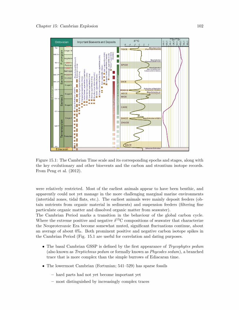
Chapter 15: Cambrian Explosion 102
Figure 15.1: The Cambrian Time scale and its corresponding epochs and stages, along withthe key evolutionary and other bioevents and the carbon and strontium isotope records.From Peng et al. (2012).
were relatively restricted. Most of the earliest animals appear to have been benthic, andapparently could not yet manage in the more challenging marginal marine environments(intertidal zones, tidal flats, etc.). The earliest animals were mainly deposit feeders (ob-tain nutrients from organic material in sediments) and suspension feeders (filtering fineparticulate organic matter and dissolved organic matter from seawater).The Cambrian Period marks a transition in the behaviour of the global carbon cycle.Where the extreme positive and negative δ13C compositions of seawater that characterizethe Neoproterozoic Era become somewhat muted, significant fluctuations continue, aboutan average of about 0h. Both prominent positive and negative carbon isotope spikes inthe Cambrian Period (Fig. 15.1 are useful for correlation and dating purposes.
• The basal Cambrian GSSP is defined by the first appearance of Trycophytes pedum(also known as Treptichnus pedum or formally known as Phycodes sedum), a branchedtrace that is more complex than the simple burrows of Ediacaran time.
• The lowermost Cambrian (Fortunian; 541–529) has sparse fossils
– hard parts had not yet become important yet
– most distinguished by increasingly complex traces
Chapter 15: Cambrian Explosion 103
• The Cambrian radiation really begins in the Stage 2 (latter Terreneuvian Epoch;529–521.1 Ma)
– First appearance and diversification of the Archaeocyathans
– SSF’s diversify
– First Arthropod traces
– The earliest crown group sponges and likely brachiopods
• And explodes in the Atdabanian (521.1–518.7 Ma)
– Trilobites and Echinoderms by the middle Atdabanian
• The Chengjiang fauna span from the late Atdabanian into the early Botomian (521.1–513 Ma)
– Includes most of the animal phyla, e.g. Porifera, Mollusca, Brachiopoda, Arthro-poda, Priapulida, Echinodermata, Annelida, Hemichordata, Chordata
15.1.2 The Early Cambrian substrate revolution
During the Ediacaran Period, microbial mats likely still covered much of the sea floor,providing a sort of protection to the substrate and maintaining a sharp sediment-water in-terface (Bottjer et al., 2000). At the same time, the simple trace fossils suggests there wereno burrowers as yet. This changed rather abruptly in the early Cambrian, when animalsbegan to burrow in a big way and the extent of microbial mats likely dropped precipitouslydue to grazing. It is not clear if the early burrowers were looking for food or escaping frompredators, but the consequences were the same: sediments in habitable parts of the oceanwere irrigated. It is perhaps the destruction of this substrate, which seems to have been soimportant for Edaicaran life habit and fossil preservation, that led to their disappearance(both literally, and in the fossil record).
One clear manifestation of the substrate revolution that accompanied the evolution of ani-mals is the sharp decrease in stromatolite abundance spanning the Precambrian-Cambrianboundary. Stromatolites still formed in the Cambrian, but were restricted to zones notyet inhabited by animals, such as intertidal zones. And many of the microbial build-upsin the Paleozoic lack the well defined laminations of stromatolites. These thrombolites areprobably a close cousin of stromatolites, their difference being that the were subject tograzing and burrowing, which obliterated much of the original texture.
With the advent of burrowing, the uppermost sediment column would have been soupierand the sediment-water interface more diffuse, resulting in a discrete mixed layer betweenseawater and sediments. This would have had a profound impact on early benthic organ-isms, which would have had to seek alternative methods for attachment to substrates (forsessile organisms) and who have adapted to a completely different style of sediments andfood supply. As pointed out by Canfield and Farquhar (2009), the onset of vertical biotur-bation would also have had a profound effect on seawater chemistry by irrigating surfacesediments and introducing oxygenated seawater. These authors argue that the substraterevolution resulted in a sharp decline in the proportional burial of sedimentary pyrite andcompensatory increase in seawater sulfate concentrates and gypsum precipitation. At the
Chapter 15: Cambrian Explosion 104
same time, bioturbation should have made it much harder to sequesterer organic matterin sediments, hence imposing a negative feedback on environmental oxygen abundances.
15.1.3 The Small Shelly Fauna
The first fully shelled metazoans are known as the small shelly fauna (SSF). They appearwithin 5 Ma of the pC-C boundary and gradually radiate through the Nemakit-Daldynian.They are tiny skeleton fragments (1-5 mm diameter), comprising tubes, spines, cones, andplates. Some are actually small shells of animals, whereas other are schlerites, disartic-ulated hard parts of animals. Whereas their affinity had long been mysterious, it nowappears that the oldest SSF schlerites are disarticulated elements of lophotrochozoan affin-ity, likely early molluscs (Caron et al., 2006; Morris and Caron, 2007). The diversity offorms suggest a parallel genetic and phyllogenetic diversity. Importantly, the SSF’s arecommonly phosphatic (although some are also calcitic and others siliceous) and are con-centrated in phosphate deposits. Phosphate deposits are relatively common in both theEdiacaran and the Cambrian, and the temporal restriction of the SSF’s to the Tommotiansuggests that animals did not evolve the capability of building phosphatic skeletons untilthe Cambrian.
15.1.4 The Archaeocyathans
The Archaeocyatha were the first major reef-building Metazoa, although their reefs wererelatively small and patchy compared to later Paleozoic and modern reefs.
• Appeared in Early Cambrian—ca. 530 Ma
• Extinct 10–15 million years later (by the Middle Cambrian)
• Wide geographic distribution. Hence superb index fossil for the early Cambrian
• Built reefs up to 10s of meters tall and hundreds of kilometers wide
• Unknown affinity
– either a separate phylum
– or an extinct lineage of sponge (phylum Porifera)
• Distinctive morphology
– sessile, inverted cone-shape cup
– high Mg calcite skeleton
– double-walled, walls connected by septa
The disappearance of the Archeaocyatha so soon after their appearance on the scene isprobably due to the fact that they appeared during a time of aragonite seas, that is,when Mg/Ca ratios in seawater were relatively high, which is why they evolved to makehigh Mg calcite skeletons. Aragonite seas gave way to calcite seas soon after, and this mostlikely accounts for their sudden decline. Subsequent reef-builders, like the stromatoporoids,calcite sponges, and corals were longer lived, presumably because they could make theirskeletons out of low Mg calcite.
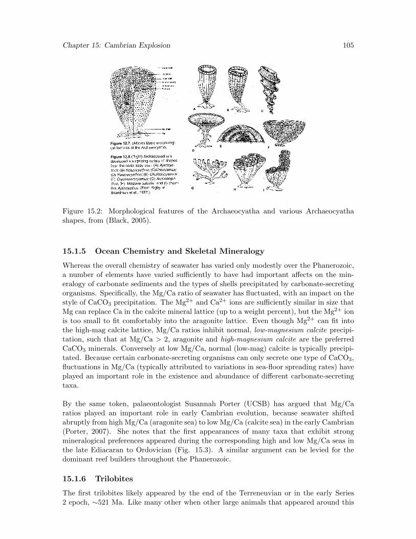
Chapter 15: Cambrian Explosion 105
Figure 15.2: Morphological features of the Archaeocyatha and various Archaeocyathashapes, from (Black, 2005).
15.1.5 Ocean Chemistry and Skeletal Mineralogy
Whereas the overall chemistry of seawater has varied only modestly over the Phanerozoic,a number of elements have varied sufficiently to have had important affects on the min-eralogy of carbonate sediments and the types of shells precipitated by carbonate-secretingorganisms. Specifically, the Mg/Ca ratio of seawater has fluctuated, with an impact on thestyle of CaCO3 precipitation. The Mg2+ and Ca2+ ions are sufficiently similar in size thatMg can replace Ca in the calcite mineral lattice (up to a weight percent), but the Mg2+ ionis too small to fit comfortably into the aragonite lattice. Even though Mg2+ can fit intothe high-mag calcite lattice, Mg/Ca ratios inhibit normal, low-magnesium calcite precipi-tation, such that at Mg/Ca > 2, aragonite and high-magnesium calcite are the preferredCaCO3 minerals. Conversely at low Mg/Ca, normal (low-mag) calcite is typically precipi-tated. Because certain carbonate-secreting organisms can only secrete one type of CaCO3,fluctuations in Mg/Ca (typically attributed to variations in sea-floor spreading rates) haveplayed an important role in the existence and abundance of different carbonate-secretingtaxa.
By the same token, palaeontologist Susannah Porter (UCSB) has argued that Mg/Caratios played an important role in early Cambrian evolution, because seawater shiftedabruptly from high Mg/Ca (aragonite sea) to low Mg/Ca (calcite sea) in the early Cambrian(Porter, 2007). She notes that the first appearances of many taxa that exhibit strongmineralogical preferences appeared during the corresponding high and low Mg/Ca seas inthe late Ediacaran to Ordovician (Fig. 15.3). A similar argument can be levied for thedominant reef builders throughout the Phanerozoic.
15.1.6 Trilobites
The first trilobites likely appeared by the end of the Terreneuvian or in the early Series2 epoch, ∼521 Ma. Like many other when other large animals that appeared around this
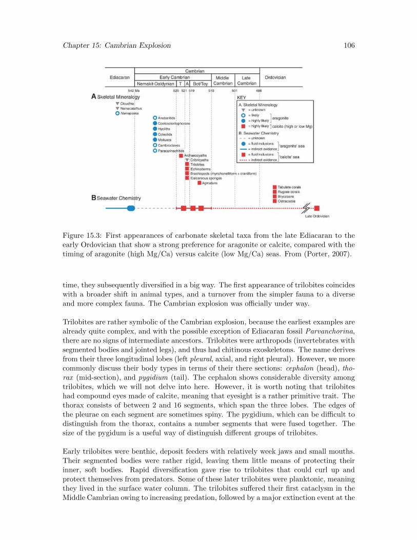
Chapter 15: Cambrian Explosion 106
Figure 15.3: First appearances of carbonate skeletal taxa from the late Ediacaran to theearly Ordovician that show a strong preference for aragonite or calcite, compared with thetiming of aragonite (high Mg/Ca) versus calcite (low Mg/Ca) seas. From (Porter, 2007).
time, they subsequently diversified in a big way. The first appearance of trilobites coincideswith a broader shift in animal types, and a turnover from the simpler fauna to a diverseand more complex fauna. The Cambrian explosion was officially under way.
Trilobites are rather symbolic of the Cambrian explosion, because the earliest examples arealready quite complex, and with the possible exception of Ediacaran fossil Parvanchorina,there are no signs of intermediate ancestors. Trilobites were arthropods (invertebrates withsegmented bodies and jointed legs), and thus had chitinous exoskeletons. The name derivesfrom their three longitudinal lobes (left pleural, axial, and right pleural). However, we morecommonly discuss their body types in terms of their there sections: cephalon (head), tho-rax (mid-section), and pygidium (tail). The cephalon shows considerable diversity amongtrilobites, which we will not delve into here. However, it is worth noting that trilobiteshad compound eyes made of calcite, meaning that eyesight is a rather primitive trait. Thethorax consists of between 2 and 16 segments, which span the three lobes. The edges ofthe pleurae on each segment are sometimes spiny. The pygidium, which can be difficult todistinguish from the thorax, contains a number segments that were fused together. Thesize of the pygidum is a useful way of distinguish different groups of trilobites.
Early trilobites were benthic, deposit feeders with relatively week jaws and small mouths.Their segmented bodies were rather rigid, leaving them little means of protecting theirinner, soft bodies. Rapid diversification gave rise to trilobites that could curl up andprotect themselves from predators. Some of these later trilobites were planktonic, meaningthey lived in the surface water column. The trilobites suffered their first cataclysm in theMiddle Cambrian owing to increasing predation, followed by a major extinction event at the

Chapter 15: Cambrian Explosion 107
end of the Cambrian, which marked a major change in the trilobite record. They sufferedsubsequent major extinctions at the end of the Ordovician and in the late Devonian, afterwhich they were trimmed down to one order (Proetida). They eventually succumbed tocomplete extinction at the end of the Permian.
Figure 15.4: Morphological features of a trilobite.
15.2 The Explosion
The Cambrian Explosion refers to the geologically abrupt appearance in the fossil recordof complex metazoa representing most of the extant phyla. The ’explosion’ is probablyless explosive than once thought, but is still spectacular insofar as the earliest Cambrianwas marked by low diversity and subdued fossil evidence for animals, and by the middleCambrian, diverse and complex animals clearly inhabited the entire ocean.
• Begins in the late Terreneuvian and accelerates early in Series 2
• Documents a massive radiation in hard parts/skeletons—probably partly the reasonfor the abrupt appearance of skeletal fossils in the geological record
• All major body plans were present by this time; 80% of skeletal elements recognizedin modern phyla were present by this time
• Subsequent evolution characterized by diversification at the species to class level
15.2.1 Early-Middle Cambrian Lagerstatte
The Burgess Shale
The Burgess Shale, the most famous lagerstatte, is 505 Ma
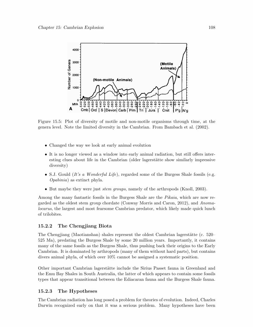
Chapter 15: Cambrian Explosion 108
Figure 15.5: Plot of diversity of motile and non-motile organisms through time, at thegenera level. Note the limited diversity in the Cambrian. From Bambach et al. (2002).
• Changed the way we look at early animal evolution
• It is no longer viewed as a window into early animal radiation, but still offers inter-esting clues about life in the Cambrian (older lagerstatte show similarly impressivediversity)
• S.J. Gould (It’s a Wonderful Life), regarded some of the Burgess Shale fossils (e.g.Opabinia) as extinct phyla.
• But maybe they were just stem groups, namely of the arthropods (Knoll, 2003).
Among the many fantastic fossils in the Burgess Shale are the Pikaia, which are now re-garded as the oldest stem group chordate (Conway Morris and Caron, 2012), and Anoma-locarus, the largest and most fearsome Cambrian predator, which likely made quick lunchof trilobites.
15.2.2 The Chengjiang Biota
The Chengjiang (Maotianshan) shales represent the oldest Cambrian lagerstatte (c. 520–525 Ma), predating the Burgess Shale by some 20 million years. Importantly, it containsmany of the same fossils as the Burgess Shale, thus pushing back their origins to the EarlyCambrian. It is dominated by arthropods (many of them without hard parts), but containsdivers animal phyla, of which over 10% cannot be assigned a systematic position.
Other important Cambrian lagerstatte include the Sirius Passet fauna in Greenland andthe Emu Bay Shales in South Australia, the latter of which appears to contain some fossilstypes that appear transitional between the Ediacaran fauna and the Burgess Shale fauna.
15.2.3 The Hypotheses
The Cambrian radiation has long posed a problem for theories of evolution. Indeed, CharlesDarwin recognized early on that it was a serious problem. Many hypotheses have been
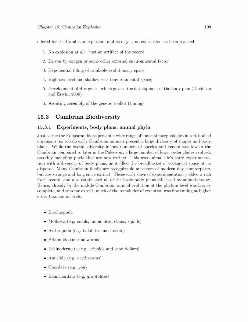
Chapter 15: Cambrian Explosion 109
offered for the Cambrian explosion, and as of yet, no consensus has been reached.
1. No explosion at all—just an artifact of the record
2. Driven by oxygen or some other external environmental factor
3. Exponential filling of available evolutionary space
4. High sea level and shallow seas (environmental space)
5. Development of Hox genes, which govern the development of the body plan (Davidsonand Erwin, 2006)
6. Awaiting assembly of the genetic toolkit (timing)
15.3 Cambrian Biodiversity
15.3.1 Experiments, body plans, animal phyla
Just as the the Ediacaran biota present a wide range of unusual morphologies in soft-bodiedorganisms, so too do early Cambrian animals present a large diversity of shapes and bodyplans. While the overall diversity in raw numbers of species and genera was low in theCambrian compared to later in the Paleozoic, a large number of lower order clades evolved,possibly including phyla that are now extinct. This was animal life’s early experimenta-tion with a diversity of body plans, as it filled the breadbasket of ecological space at itsdisposal. Many Cambrian fossils are recognizable ancestors of modern day counterparts,but are strange and long since extinct. These early days of experimentation yielded a richfossil record, and also established all of the basic body plans still used by animals today.Hence, already by the middle Cambrian, animal evolution at the phylum level was largelycomplete, and to some extent, much of the remainder of evolution was fine tuning at higherorder taxonomic levels.
• Brachiopoda
• Mollusca (e.g. snails, ammonites, clams, squids)
• Arthropoda (e.g. trilobites and insects)
• Priapulida (marine worms)
• Echinodermata (e.g. crinoids and sand dollars)
• Annelida (e.g. earthworms)
• Chordata (e.g. you)
• Hemichordata (e.g. graptolites)
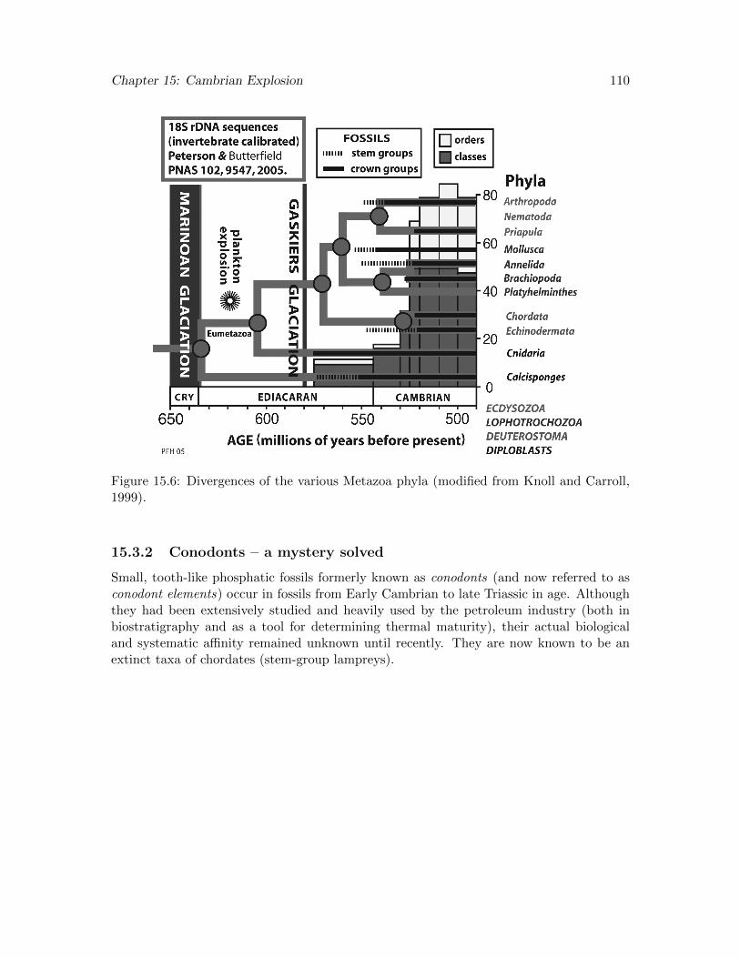
Chapter 15: Cambrian Explosion 110
Figure 15.6: Divergences of the various Metazoa phyla (modified from Knoll and Carroll,1999).
15.3.2 Conodonts – a mystery solved
Small, tooth-like phosphatic fossils formerly known as conodonts (and now referred to asconodont elements) occur in fossils from Early Cambrian to late Triassic in age. Althoughthey had been extensively studied and heavily used by the petroleum industry (both inbiostratigraphy and as a tool for determining thermal maturity), their actual biologicaland systematic affinity remained unknown until recently. They are now known to be anextinct taxa of chordates (stem-group lampreys).
Chapter 16
The Early Paleozoic: Age of theInvertebrates
Reading: Chapter 3 (65-70), Chapter 13 in Stanley; Chapter 12 in Wiccander and Monroe
16.1 Orodovician life
If the Cambrian is known for the incredible radiation in animal life and the emergence ofall extant phyla, the Ordovician Period (485.4 to 443.8 Ma) might be best distinguishedby extraordinary diversification at higher order taxonomic levels and the origin of manyanimal clades that dominated Paleozoic marine life. Even though the early chordates hadappeared already by the middle Cambrian, marine life in the early Paleozoic was dominatedby the invertebrates, which include the proterostomes (lophotrochozoa and ecdyozoa) andthe echinoderms.
The trilobites suffered a major extinction at the end of the Cambrian, but retained a strongfoothold in the benthic marine environment in the early Ordovician. The brachiopods andgastropods, both benthic organisms that originated in the Cambrian, also began to diver-sify at this time. At the same time, in the pelagic environment above, two other groupsthat appeared in the Cambrian also begin to diversify: the nautiloids (cephalopods) andgraptolites (colonial Metazoa).
Although the early Ordovidian saw the start of a recovery from the end Cambrian ex-tinctions, the pace of recovery in overall diversity was slow. It was not until later in theOrdovician that the pace of diversification picked up, and then it did so with a bang. Thenumber of animal families increased by a factor of three as animals ramped up there pres-ence on and within (epifaunal) sediments and in the overlying water column. Reef buildingwent into recession in the latter half of the Cambrian, but reemerged in the Ordovician ina massive way, with corals (rugose and tabulate) and stromatoporoids constructing vastreef tracts.
Stromatolites, which had already suffered great indignities during the Ediacaran and Cam-brian, continued to decline in abundance, and by the end of the Ordovician, were largelyrelegated to the relatively harsh environments (e.g., hypersaline lagoons and lakes) that
111
Chapter 16: Early Paleozoic Life 112
they continue to inhabit today. While microbial life on the sea floor took a major hit,plants did begin to take a foothold on land in the Ordovician.
The great Ordovician diversification was punctuated by a series of extinctions at the closeof the period, collectively known as the late Ordovician mass extinction.
Below is a review of the invertebrate clades the emerged in the Cambrian and OrodivianPeriod.
16.2 Simple animals
16.2.1 Porifera
The phylum Porifera (sponges) is the most primitive (deeply branched) of the multicellulareukaryotes
• Similar to colonial choanoflagellates (flagellate protozoa)
• Sessile, simple organisms - lack tissues
• Filter feeders
• Live in water depths from intertidal down to over 5000m
• Most basic body plan: inverted cup- or vase-shaped
• Commonly with spicules - basis for subdivision into classes
– Calcarea (calcium carbonate) - the simplest form
– Hexactenelida: silica spicules with six rays
– Demospongiae (spongin)
• Probably also include the Archaeocyatha
• Stromatoporoids?
The fossil record of sponges is spotty
• First appeared in the Neoproterozoic?
• few are cosmopolitan
• oldest sponge borings occur in Ordovician
• More prominent than usual in the Devonian, lower Carboniferous, Jurassic, andCretaceous
16.2.2 Stromatoporoids
The stromatoporoids (affinity really unknown) resemble a cross between a stromatolite(morphology) and a tabular coral (laminations). Like both, they were important reefbuilders. Prominent in Ordovician to middle Devonian reefs, but ranged from the Cambriantoe Cretaceous.
Chapter 16: Early Paleozoic Life 113
16.2.3 The Cnidaria
The Cnidaria are also very primitive and represent the next major divergence of the animalbranch
• First appeared in the Ediacaran Period
• Radial symmetry (radiata)
• Single gastrovascular cavity
• Some have have sensory organs
• Stinging cells; feed by catching prey, or through symbiosis (i.e. corals)
• Four main classes:
– Anthozoa (corals)
– Scyphozoa (jelly fish)
– Cuozoa (box jellies)
– Hydrozoa (Portuguese Man o’ War)
Of the four Cnidaria classes, Anthozoa is the most important in terms of the fossil record,because corals secrete calcium carbonate skeletons.
• Always attached to a substrate
• Polyps, either solitary or colonial
• Exclusively marine
• Subdivided into two subclasses
– Alcyonaria (8-way symmetry) (include soft corals and sea pens)
– Zoantharia (6-way symmetry of which three classes are particularly importantin the fossil record
∗ Rugosa (horned corals)
∗ Tabulata (tabulate corals)
∗ Scleractinia (stony corals)
Rugosa
The rugose, or horned-corals, are solitary or compound Palaeozoic corals that went extinctat the P-T extinction
• Calcareous skeleton
• Fossil range from Middle Ordovician to Late Permian
• Widespread by the Silurian
• Important reef builders

Chapter 16: Early Paleozoic Life 114
Tabulata
The Tabulata, or tabulate corals, are almost all colonial and were the major reef builderin the Palaeozoic
• Calcareous skeleton
• Honeycomb-like colonies of individual hexagonal cells (corallites)
• Distinguished by well-developed horizontal partitions
• Smaller than rugose corals, but more variable in morphology
• Ranged from the Late Ordovician to Late Permian; most prominent in the Silurianand Devonian
Scleractinia
The Scleractinia (stony corals) are the most important reef-builders today
• Solitary or colonial aragonitic skeletons
– The colonial scleractinians occur in shallow, tropical waters, build reefs
– The solitary scleractinians do not build reefs, may live in deep and cold waters
• First appeared in middle Triassic
16.3 The Bilateria
16.3.1 Brachiopoda
The brachiopods emerged in the Early Cambrian and persist today.
• solitary, benthic, filter-feeding, marine bilaterians with an external shell of eithercalcite (class Articulata — hinge) or alternating phosphate and chitin (class Innar-ticulata — no hinge)
• distinguished from bivalves by their plane of symmetry, which bisects the valves
Figure 16.1: Bivalve versus brachiopod symmetry.
Brachiopod Morphology
• the shell encloses the body
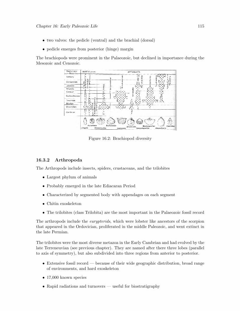
Chapter 16: Early Paleozoic Life 115
• two valves: the pedicle (ventral) and the brachial (dorsal)
• pedicle emerges from posterior (hinge) margin
The brachiopods were prominent in the Palaeozoic, but declined in importance during theMesozoic and Cenozoic.
Figure 16.2: Brachiopod diversity
16.3.2 Arthropoda
The Arthropods include insects, spiders, crustaceans, and the trilobites
• Largest phylum of animals
• Probably emerged in the late Ediacaran Period
• Characterized by segmented body with appendages on each segment
• Chitin exoskeleton
• The trilobites (class Trilobita) are the most important in the Palaeozoic fossil record
The arthropods include the eurypterids, which were lobster like ancestors of the scorpionthat appeared in the Ordovician, proliferated in the middle Paleozoic, and went extinct inthe late Permian.
The trilobites were the most diverse metazoa in the Early Cambrian and had evolved by thelate Terreneuvian (see previous chapter). They are named after there three lobes (parallelto axis of symmetry), but also subdivided into three regions from anterior to posterior.
• Extensive fossil record — because of their wide geographic distribution, broad rangeof environments, and hard exoskeleton
• 17,000 known species
• Rapid radiations and turnovers — useful for biostratigraphy

Chapter 16: Early Paleozoic Life 116
• Both benthic (scavengers, grazers, and filter feeders) and pelagic (eat plankton)
• 9 orders, all but one of which appeared by the late Cambrian
• Numbers began to decrease in Silurian and Devonian (predation by sharks?)
• All but the order Proetida died out during the Late Devonian extinction
• Remaining trilobites went extinct by the Late Permian (Permo-Triassic extinction)
16.3.3 Mollusca
The phyllum Mollusca is diverse and includes many familiar organisms, such as snails,squids, and oysters
• triploblasic protostomes (bilaterians)
• Some 112,000 species
• Closely related to the annelids (sister group)
• Probably first appeared in the late Ediacaran
• Diversified in the early Cambrian
• The most important in the fossil record include the bivalves, gastropods, and cephalopods
Bivalvia
The class Bivalvia evolved by the Middle Cambrian and diversified in the Ordovician
• Distinguished as typically having two shells that are more or less symmetrical
• Calcareous shells
• Filter-feeders: feed and excrete through siphons
• Most groups are either epifaunal or infaunal
• Include oysters, mussels, cockles, and clams
Gastropoda
The class Gastropoda (snails) first appeared in the Late Cambrian and have since been animportant and diverse class of animals
• Highly diverse (over 60,000 known living species)
• Freshwater, marine, and terrestrial
• Includes snails, slugs, abalone, conches
• Most have a coiled or spiraled aragonitic shell
• Fairly robust during mass extinctions
Chapter 16: Early Paleozoic Life 117
• Earliest gastropods were quite distinct from extant gastropods
• Not until the Mesozoic did the ancestors of the modern gastropods appear
• Become especially important in the Cenozoic
Cephalopoda
The class Cephalopoda first appeared in the Late Cambrian and was important amongmarine animals through much of the Paleozoic and Mesozoic
• Distinguished by the large number tentacles that surround the head (e.g. squid,octopus)
• Important fossil groups (subclasses) include the Nautiloidea, Ammonoidea, and Coleoidea
The Nautiloids where the first of the Cephalopods to appear.
• Cone-shaped shell, typically curved or coiled
• Shell made of aragonite
• Consists of a series of chambers used to regulate buoyancy
• Important in the early Paleozoic, when they were the main predatory animals (eatingtrilobites)
• Highly diverse in fossil record, but sparse today
• Sister group to the Ammonoids
The Ammonoids appeared in the late Early Devonian and persisted until the end of theCretaceous
• Very similar morphologically to the Nautiloids
• Planar-spiralled, complexly sutured shells
• May be loosely or tightly coiled
• Aragonite
• Hit hard by extinction events in Late Devonian, Late Permian, Late Triassic
• Extinct at the K-T boundary
The Belmnites are an extinct order of the Subclass Coleoidea, which include the squid andcuttlefish
• Very similar to the cuttlefish
• With notable exception that they contained an internal shell, located at the back endof the creature
• Largest of the belemnites up to 3 meters long
• Appeared in the Early Carboniferous; prominent in Jurassic and Cretaceous
• Extinct at the K-T boundary
• Useful index fossils
Chapter 16: Early Paleozoic Life 118
16.3.4 Echinodermata
The phylum Echinodermata is a diverse phylum that appeared in the fossil record in theEarly Cambrian
• Deuterostomes (sister group of the hemichordates)
• Evolved from animals with bilateral symmetry but have radial symmetry
– larvae are ciliated, bilaterally symmetric, free swimmers
– later develop five-fold symmetry
• All echinoderms have an internal skeletan made of small, calcified plates and spines
– provides structural support within tissues
• Exclusively marine
• Six living classes
– Asteroidea (star fish)
– Concentricycloidea (sea daisies)
– Crinoidea (sea lillies, crinoids)
– Echinoidea (sea urchins, sand dollars)
– Holothuroidea (sea cucumbers)
– Ophiuroidea (brittle stars)
The starfish (or sea stars) (Asteroidea) first appear in the fossil record in the Ordovician
• Possess five or more arms
• Poorly preserved as fossils because they do not posses a coherent skeleton
• Most live on sandy or rocky sea-floors
The echinoids first appeared in the Late Ordovician
• Benthic and gregarious
• Echinoid skeleton is rigid and may be a hemispheroid, disc-shaped, or heart-shaped
• Outer surface covered in spines
The crinoids first appeared in the Middle Cambrian
• Gregarious, live in shallow to deep, cold to warm waters
• Filter-feeders
• Attached to the sea floor by a stem (as juveniles)
• Pieces of the stem, which form disks, are prominent in the fossil record and cancomprise a major component of limestones
• Prominent in the middle Paleozoic
• Suffered a serious die-off during the Permo-Triassic extinction
• Radiated again in the Mesozoic

Chapter 16: Early Paleozoic Life 119
16.4 Colonial Metazoa
16.4.1 The Bryozoa
The phylum Bryozoa, sometimes referred to as the moss animals, appear in the fossil recordin the Early Ordovician
• In the same superphylum as Mollusca and Brachiopoda (Lophotrochozoa)
• Colonial — individual animals (zooids) are tiny and perform specific functions
• Typically form calcareous skeletons
• Most common in warm, tropical waters, where they are important reef-building or-ganisms
• Most are sessile, on hard substrates
• Common constituent of middle Paleozoic limestones
• Many species are short-ranged and cosmopolitan - thus useful index fossils
• Most Palaeozoic orders went extinct during the Permo-Triassic extinction
16.4.2 Graptolites
The Graptolithina are an extinct class of the Hemichordata; they first appeared in thefossil record in Late Cambrian
• Colonial organisms (rhabdosomes), consisting of branches (stipes) emanating from asingle organism (sicula)
• Diverse morphology, but characteristically form hook-like or serrated structures
• Form skeleton of collagen
• Typically preserved in shales, but also in limestones and cherts
• Went extinct in the Carboniferous
• Make superb index fossils
Chapter 17
The Early–Middle Paleozoic:Paleogeography, Stratigraphy, andEnvironments
Reading: Chapters 13 (301–313) and 14 (331–339) in Stanley; Chapters 10 and 11 in Wic-cander and Monroe
The transition from the Precambrian to the Paleozoic is best known for the advent anddiversification of animal life, but it was also an important time tectonically, with the largecontinent Gondwana forming from fragments of other continents. The Cambrian was likelyan unusually warm period in Earth’s history, but Earth experienced a series of glaciationsin the Paleozoic. Some of these are closely connected to impressive mass extinction eventsand tectonic reorganizations, which triggered significant changes to the biosphere.
17.1 Paleozoic Tectonics and Paleogeography
The land masses were largely separated into four continents of variable size in the EarlyPaleozoic, including Gondwana, Laurentia, Baltica, and Siberia. Most, if not all of thecontinental fragments would eventually collide to form the next supercontinent, Pangaea,at the end of the Paleozoic. As we already learned, North America (or Laurentia) was oneof these continents that was freed from the center of Rodinia in the late Proterozoic.
17.1.1 Gondwana
Gondwana was a large, composite continent that formed from several continental fragmentsthat broke out of Rodinia: Australia, India, Antarctica, and most of present day Africaand South America. Just as Rodinia appears to have been centred on Laurentia, so alsowas Gondwana centred on Africa. Gondwana began to form around 600 Ma, through aseries of orogenic events that surround the various cratonic fragments of Africa.
Pan-African Orogenies
These orogenic events are collectively referred to as the Pan-African orogenies, becausethe various cratons that make up present-day Africa were at the centre of Gondwana, and
120
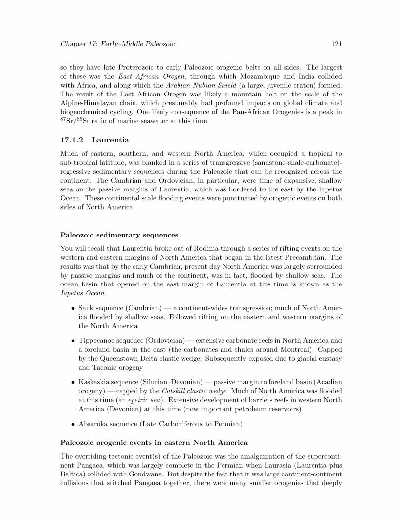
Chapter 17: Early–Middle Paleozoic 121
so they have late Proterozoic to early Paleozoic orogenic belts on all sides. The largestof these was the East African Orogen, through which Mozambique and India collidedwith Africa, and along which the Arabian-Nubian Shield (a large, juvenile craton) formed.The result of the East African Orogen was likely a mountain belt on the scale of theAlpine-Himalayan chain, which presumably had profound impacts on global climate andbiogeochemical cycling. One likely consequence of the Pan-African Orogenies is a peak in87Sr/86Sr ratio of marine seawater at this time.
17.1.2 Laurentia
Much of eastern, southern, and western North America, which occupied a tropical tosub-tropical latitude, was blanked in a series of transgressive (sandstone-shale-carbonate)-regressive sedimentary sequences during the Paleozoic that can be recognized across thecontinent. The Cambrian and Ordovician, in particular, were time of expansive, shallowseas on the passive margins of Laurentia, which was bordered to the east by the IapetusOcean. These continental scale flooding events were punctuated by orogenic events on bothsides of North America.
Paleozoic sedimentary sequences
You will recall that Laurentia broke out of Rodinia through a series of rifting events on thewestern and eastern margins of North America that began in the latest Precambrian. Theresults was that by the early Cambrian, present day North America was largely surroundedby passive margins and much of the continent, was in fact, flooded by shallow seas. Theocean basin that opened on the east margin of Laurentia at this time is known as theIapetus Ocean.
• Sauk sequence (Cambrian) — a continent-wides transgression; much of North Amer-ica flooded by shallow seas. Followed rifting on the eastern and western margins ofthe North America
• Tippecanoe sequence (Ordovician) — extensive carbonate reefs in North America anda foreland basin in the east (the carbonates and shales around Montreal). Cappedby the Queenstown Delta clastic wedge. Subsequently exposed due to glacial eustasyand Taconic orogeny
• Kaskaskia sequence (Silurian–Devonian) — passive margin to foreland basin (Acadianorogeny) — capped by the Catskill clastic wedge. Much of North America was floodedat this time (an epeiric sea). Extensive development of barriers reefs in western NorthAmerica (Devonian) at this time (now important petroleum reservoirs)
• Absaroka sequence (Late Carboniferous to Permian)
Paleozoic orogenic events in eastern North America
The overriding tectonic event(s) of the Paleozoic was the amalgamation of the superconti-nent Pangaea, which was largely complete in the Permian when Laurasia (Laurentia plusBaltica) collided with Gondwana. But despite the fact that it was large continent-continentcollisions that stitched Pangaea together, there were many smaller orogenies that deeply
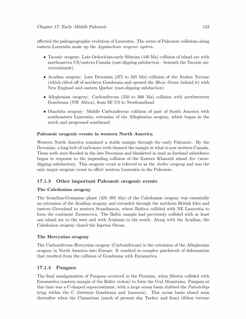
Chapter 17: Early–Middle Paleozoic 122
effected the paleogeographic evolution of Laurentia. The series of Paleozoic collisions alongeastern Laurentia make up the Appalachian orogenic system.
• Taconic orogeny: Late Ordovician-early Silurian (440 Ma) collision of island arc withnortheastern US/eastern Canada (east-dipping subduction—beneath the Taconic mi-crocontinent)
• Acadian orogeny: Late Devonian (375 to 325 Ma) collision of the Avalon Terrane(which rifted off of northern Gondwana and opened the Rheic Ocean behind it) withNew England and eastern Quebec (east-dipping subduction)
• Alleghenian orogeny: Carboniferous (350 to 300 Ma) collision with northwesternGondwana (NW Africa), from SE US to Newfoundland
• Ouachita orogeny: Middle Carboniferous collision of part of South America withsoutheastern Laurentia; extension of the Alleghenian orogeny, which began in thenorth and progressed southward
Paleozoic orogenic events in western North America
Western North America remained a stable margin through the early Paleozoic. By theDevonian, a long belt of carbonate reefs rimmed the margin in what is now western Canada.These reefs were flooded in the late Devonian and blanketed in mud as foreland subsidencebegan in response to the impending collision of the Eastern Klamath island Arc (west-dipping subduction). This orogenic event is referred to as the Antler orogeny and was theonly major orogenic event to effect western Laurentia in the Paleozoic.
17.1.3 Other important Paleozoic orogenic events
The Caledonian orogeny
The Scandian-Grampian phase (425–395 Ma) of the Caledonian orogeny was essentiallyan extension of the Acadian orogeny and extended through the northern British Isles andeastern Greenland to western Scandinavia, where Baltica collided with NE Laurentia toform the continent Euramerica. The Baltic margin had previously collided with at leastone island arc to the west and with Avalonia to the south. Along with the Acadian, theCaledonian orogeny closed the Iapetus Ocean.
The Hercynian orogeny
The Carboniferous Hercynian orogeny (Carboniferous) is the extension of the Alleghenianorogeny in North America into Europe. It resulted in complex patchwork of deformationthat resulted from the collision of Gondwana with Euramerica.
17.1.4 Pangaea
The final amalgamation of Pangaea occurred in the Permian, when Siberia collided withEuramerica (eastern margin of the Baltic craton) to form the Ural Mountains. Pangaea atthis time was a C-shaped supercontinent, with a large ocean basin dubbed the Paleotethyslying within the C (between Gondwana and Laurasia). This ocean basin closed soonthereafter when the Cimmerian (much of present day Turkey and Iran) ribbon terrane

Chapter 17: Early–Middle Paleozoic 123
rifted off of NE Gondwana and collided with Laurasia. The Neotethys ocean basin openedin its wake.
17.2 Paleozoic Climate
The early Paleozoic is distinguished by high pCO2 levels (10–20 × present CO2) and awarm climate that persisted through most of the Cambrian and Ordovian. CO2 haddeclined to more typical Phanerozoic levels by the Carboniferous, and this was closelyrelated to the burial of vast amounts of coal in the Carboniferous and the onset of thePermo-Carboniferous glaciation (discussed in detail in a subsequent chapter), the last andprobably largest of three glacial epochs during the Paleozoic. This carbon burial event isalso clearly revealed in the marine carbon isotope record of the late Paleozoic.
17.2.1 Late Ordovician glaciation
The late Ordovician (Hirnantian) glaciation followed a decline of about 40% in atmosphericCO2 levels. This was probably driven by increased burial of organic carbon, based on acoeval positive excursion in carbonate isotopes. But it appears that CO2 levels were stillvery high, which long posed an enigma to geologists and climate models.
Based on oxygen isotope evidence, the glaciation appears to have lasted only about 1–2million years. Sufficient continental ice formed to lower sea level significantly and bringthe the high sea levels of the Sauk sequence to and end. Global cooling and loss of habitatwere two likely key factors contributing to the first of two phases of the late Ordovicianmass extinction. The second phases, which was not as severe, occurred at the end of theglaciation and was presumably the result of rising temperatures and pCO2.
Ice sheets during the late Ordovician covered what we usually think of as northern Gond-wana (North Africa and northeastern South America), which were likely close to the SouthPole at the time.
17.2.2 Late Devonian glaciation
The Silurian and much of the Devonian were again warm period in Paleozoic Earth history.This is perhaps best seen in the high global sea level and widespread development of reefsystems. However, another glaciation, with ice sheets centred on Brazil, occurred in thelate Devonian.
Like the previous glacial epoch, the late Devonian glaciation appears to have been rela-tively short-lived, and associated with mass-extinction. It may also have occurred duringa time of relatively high pCO2, although carbon dioxide levels must still have declined tohelp trigger the glaciation. The drop in pCO2 is likely related to the early expansion ofland plants. Not only would trees have become an important sink for organic carbon, butalso land plants accelerate silicate weathering in soils by increasing CO2 concentrations inthe soils (via decay of organic detritus) and releasing organic acids, which help to breakdown silicate minerals.

Chapter 17: Early–Middle Paleozoic 124
Like the Orodovician glaciation, the Devonian glaciation appears to have been closelylinked to one of the big five mass extinctions, which will be discussed in more detail in asubsequent chapter.
Chapter 18
Paleozoic Vertebrates and theOrigin of Land Plants
Reading: Chapters 13 and 14 in Stanley; Chapter 13 in Wiccander and Monroe
18.1 Origin of the Vertebrates
As we learned earlier, the recognition that conodonts, dating to the early Cambrian, belongto a group of lampreys, which belong to the phylum chordata, established that chordateshad evolved already by the early Cambrian. Some Ediacaran fossils may represent stemgroup chordates, which would push this divergence back in Earth’s history, consistent withmolecular clock data.
Chordates are animals with a notochord and tail (at least at some point in the their de-velopment. Ontogenetically, chordates are distinguished by radial cell cleavage in earlyembryo development, which contrasts with the spiral cleavage in all invertebrates. It is forthis reason that chordates are closely aligned with the echinoderms (within the deuteros-tomes), who also show radial cleavage.
The vertebrates are a subphylum of the the chordates and dominate the chordata phylumin terms of diversity. They are distinguished as having a backbone. The record of the earlyevolution of the chordates and the divergence of vertebrates is poor, due in large part tothe dominantly soft-bodies of the early chordates. These include both jawless fish and thejawed vertebrates, the group to which we belong.
18.2 Fish
The earliest vertebrates were jawless fish (Agnatha; e.g. lampreys and hagfish), whichfirst appeared in shallow seas in the Late Cambrian. Most were likely bottom dwellers,feeding directly off the seafloor. Fish diversified significantly in the Devonian, which isoften referred to as the Age of Fish.
• The ostracoderms were early, armored, jawless fish that prospered in the Silurian andDevonian but went extinct by the late Devonian extinction
125

Chapter 18: Vertebrates and Land Plants 126
• The jaw was an important evolutionary innovation that fundamentally changed themarine ecosystem and eventually terrestrial ecosystems.
– The jawed fish appeared in the early Silurian
– originated from the first two gill bars, possibly originally for enhanced respiration
– teeth originated from the denticles on the skin that covered the gill bars
• The acanthodians likely gave rise to the armoured jaw fish, cartilaginous (i.e. sharksand rays) and bony fish. They contained several key features that distinguish modernfish, such as paired fins and scales instead of plates.
• Armored jaw-fish (placoderms) fierce predators, abundant in Silurian and Devonian,disappeared in Permian. The placoderm Dunkleosteus grew to be up to 7 m long!
• Cartilaginous fish (chronodytes), which include sharks and rays, appeared in theEarly Devonian
• Bony fish subdivided into the ray-finned and the lobe-finned fish
– Ray-finned (Actinopterygii) fish include most common fish types (i.e. tuna andsalmon); appear to have evolved in fresh waters in the Devonian
– Lobe-finned fish (Sarcopterygii) appeared in the Devonian. Include lungfish andcoelacanths
∗ muscular fins with articulated bones
∗ strong swimmers (perhaps evolved to swim up rivers)
∗ amphibians likely evolved from the crossopteryginians, which had back-bones, limbs that could be used for walking, and primitive lungs
• Appearance of fish likely placed significant evolutionary pressure on invertebrates(for example the trilobites)
18.3 Amphibians
The earliest vertebrates to walk on land were ancestral amphibians that evolved from thelobe-finned fish in the Late Devonian. One important question is why the lobe-finnedfish evolved limbs in the first place. Paleontologists believe they served to help navigateshallow water environments, like tidal flats, streams, and swamps. The earliest land-dwelling animals had to overcome many significant barriers to living out of the water:
• desiccation
• respiration
• gravity
• reproduction
The recently discovered Tiktaalik (”fishapod”) represents the transition between the crossptery-ginians and the earliest tetrapods (the early amphibians).
• 375 Ma
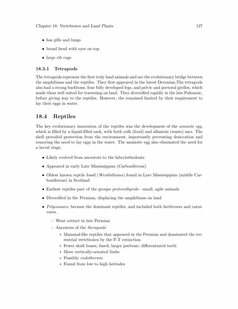
Chapter 18: Vertebrates and Land Plants 127
• has gills and lungs
• broad head with eyes on top
• large rib cage
18.3.1 Tetrapods
The tetrapods represent the first truly land animals and are the evolutionary bridge betweenthe amphibians and the reptiles. They first appeared in the latest Devonian.The tetrapodsalso had a strong backbone, four fully developed legs, and pelvic and pectoral girdles, whichmade them well suited for traversing on land. They diversified rapidly in the late Paleozoic,before giving way to the reptiles. However, the remained limited by their requirement tolay their eggs in water.
18.4 Reptiles
The key evolutionary innovation of the reptiles was the development of the amniote egg,which is filled by a liquid-filled sack, with both yolk (food) and allantois (waste) sacs. Theshell provided protection from the environment, importantly preventing desiccation andremoving the need to lay eggs in the water. The amniotic egg also eliminated the need fora larval stage.
• Likely evolved from ancestors to the labryinthodonts
• Appeared in early Late Mississippian (Carboniferous)
• Oldest known reptile fossil (Westlothiana) found in Late Mississippian (middle Car-boniferous) in Scotland
• Earliest reptiles part of the groupe protorothyrids—small, agile animals
• Diversified in the Permian, displacing the amphibians on land
• Pelycosaurs, became the dominant reptiles, and included both herbivores and carni-vores.
– Went extinct in late Permian
– Ancestors of the therapsids
∗ Mammal-like reptiles that appeared in the Permian and dominated the ter-restrial vertebrates by the P-T extinction
∗ Fewer skull bones, fused; larger jawbone; differentiated teeth
∗ More vertically-oriented limbs
∗ Possibly endothermic
∗ Found from low to high latitudes

Chapter 18: Vertebrates and Land Plants 128
18.5 Land Plants
The first land plants appeared in the middle-late Ordovician and evolved progressivelyfrom a marine to freshwater environment, where they were able to adapt gradually to dif-fering osmotic pressures. They are probably derived from the green algae, which are theonly algae to have colonized fresh water. Land plants subdivided into non-vascular andvascular plants.
Non-vascular land plants include the bryophytes (liverworts and mosses) that are mostlyrestricted to moist environments.
18.5.1 Vascular plants
Vascular plants likely appeared sometime in the Silurian. They are distinguished from thenon-vascular plants in that they have tissues made from specialized cells that enable themto transport water and nutrients and provide rigidity to the plant. Other key innovationsof the vascular plants include
• lignin and cellulose, which provide additional strength
• cutin, which inhibits desiccation, oxidation, effects of ultraviolet light, and parasites
• roots to collect water and nutrients
• leaves for more efficient photosynthesis
Early vascular plants
The earliest vascular plants of the genus Cooksonia date from the Middle Silurian and havesmall, y-shaped stems.
• Seedless
• Lacked a true root system (water and nutrients from the rhyzome)
• Lived in low, marshy, freshwater
• Diversified in the Late Silurian and Early Devonian
• Heterospory—two types of spores that give rise to female and male plants
• Achieved great size (up to 10 m) by the Late Devonian — first forests
• First ferns appeared in Middle Devonian
• Major source of the Carboniferous coal, e.g. lycopsids and sphenospids (rushes)
Chapter 18: Vertebrates and Land Plants 129
Seed-bearing vascular plants
The first seed-bearing plants likely evolved in the Late Devonian. Seeds reduced the needfor plants to remain in moist environments, thus allowing them to diversify and populatedry environments. This key evolutionary innovation led to the first full-fledged forests,which began to spread across the terrestrial landscape in the late Devonian.
Seed ferns appeared in the Carboniferous and eventually gave rise to the gymnosperms(think conifers), which came to be the dominant trees by the late Permian.
18.5.2 Consequences of evolution of land plants
The evolution of land plants and their colonization of the continents had huge implicationsfor the biosphere, climate, and soils.
Land plants spur animal evolution
Early trees would have provided protection from direct sunlight to early animals. Hence,the first amphibians arose about the same time that the first forests spread across thelandscape, in the late Devonian.
18.5.3 Soils and erosion
Root systems provide trees with both better access to water and nutrients in the soil andstabilize that part of the plant the projects upward from the ground surface (big treesneed big root systems). The emergence of root systems had a profound effect on the de-velopment of soils and landscapes, because they anchored soils in place. Hence, richer soilsdeveloped, both because nutrient rich minerals are held in place and because the plantscontribute organic matter to the soil, replenishing nutrients in a more bioavailable package.
Some scientists content that the development of vascular plants and root systems lead to achange in the style of rivers. Whereas rivers appear to have been exclusively braided (thatis, dominated by erosion) prior to the Devonian, meandering rivers emerged afterwards, asthe result of the stabilizing affect of plants.
18.5.4 Climate
The origin of land plants would have also impacted climate in two important ways. First,it would have been a new route for organic carbon to be produced and buried. Evidencefor this new style of carbon burial is seen in the vast coal beds that formed in the latestPaleozoic (the aptly named Carboniferous Period). Two consequences would have beengreater removal of CO2 from the atmosphere and increased O2 concentrations in the at-mosphere.
The development of land plants would also have greatly changed the way silicate weatheringworks. Respiration in soils tends to concentrate CO2 in soils, such that concentrations aremuch higher than in the ambient atmosphere. Plants also produce a variety of organicacids, which took over from CO2 some of the role of driving silicate weathering (hydrolysis)reactions. It is likely no coincidence that two of the Phanerozoic glaciations correspondedto major evolutionary developments in vascular plants.
Chapter 19
The Late Paleozoic and thePermo-Triassic Extinction
Reading: Chapter 14 in Stanley; Chapters 12 in Wiccander and Monroe
19.1 Pangaea
As you will recall from previous lectures, the great Paleozoic landmass Gondwana hadeffectively finished assembling by the early Paleozoic. Throughout the remainder of thePaleozoic, Laurentia grew through accretion of terranes on both the eastern and westernmargins, finally colliding with Baltica (Caledonian orogeny) in the Devonian, to form Eura-sia. Collision between the Siberia and Baltica formed the Urals and gave rise to the largecontinent known as Laurasia.
At about the same time as the collision of Siberia with Baltica, Gondwana began to collidewith Laurasia in what is known as the Alleghenian-Hercynian orogeny (think Appalachi-ans). This resulted in the nearly complete amalgamation of the continents into the su-percontinent Pangaea, which was a C-shaped landmass with a large ocean basin dubbedthe Paleotethys lying within the C (between Gondwana and Laurasia). This ocean basinclosed soon thereafter when the Cimmerian (much of present day Turkey and Iran) ribbonterrane rifted off of NE Gondwana and collided with Laurasia. The Neotethys ocean basinopened in its wake. The Panthalassa ocean bordered the western side of Pangaea.
19.2 Late Paleozoic Climate
19.2.1 Permo-Carboniferous glaciation
The onset of late Paleozoic glaciation in the middle Carboniferous (about 315 Ma) roughlycoincided with the Alleghenian-Hercynian orogenies, but was probably most closely relatedto spread of large vascular land plants in the Carboniferous, including the gymnosperms,which formed immense forests that give rise to vast peat and coal deposits. The combina-tion of CO2 sequestration through the formation of these peat and coasl, and an increasein silicate weathering due to the formation of organic acids by these new vascular plants,
130

Chapter 19: Vertebrates and Land Plants 131
drove CO2 to its lowest levels in the Paleozoic.
Evidence of this ’carbon burial’ event are seen in the unusually high carbon isotope ra-tios in the Carboniferous. This high rate of burial of carbon was balanced by high O2
concentrations—probably the highest in Earth’s history.At the same time, Gondwana drifted over the south pole. The result was the most severeglaciation of the Phanerozoic, lasting 30 million years. Glacial deposition appeared to haveoccurred diachronously on Gondwana as it drifted across the pole, and on Siberia, whichwas in the northern high latitudes at the time.
19.2.2 Carboniferous coal and cyclothems
The Carboniferous, as its name implies, was a time of widespread coal deposition, whichfollowed the spread of large vascular land plants, in particular varieties that had developedthick mantles of bark (lignin), which is difficult to decompose. Carboniferous coals arewidespread in North America and Europe, but also occur in northern Gondwana (wherethey formed just to the north of the limit of continental ice sheets). The vast swamps inwhich the precursor plants to the coal grew probably owed their existence to glaciation,which had lowered sea levels and created vast, lowland swampy regions on the continentalmargins, not unlike the Florida everglades. The Carboniferous coal dominantly occursas seams a few meters thick within cyclothems, which are repetitive, terrestrial-marginalmarine cycles that likely record glacioeustatic fluctuations in sea level.
19.2.3 Late Permian drying
The formation of large, moisture-capturing mountain ranges and a supercontinent withmuch land area far removed from the oceans resulted in aridification of much of interiorPangea. The resulting decrease in coal formation likely contributed to rising pCO2 andthe end of glaciation. Coniferous trees, which are quite tolerant of dry conditions, spreadand floras were generally provincial due to sharp climatic gradients from the coasts toinland. Large volumes of continental red-beds and non-marine and marine (for example,the Zechstein basin) evaporites were deposited during the Permian.
19.3 Late Paleozoic Life
19.3.1 Plants
Plants continued to diversify in the late Paleozoic, and their proliferation accounts for thename of the Carboniferous Period. This was a wet and warm area over much of Pangeaand Laurasia, and newly evolved trees and ferns thrived in the expansive wetlands. Thespore plants, like the lycopods, that had evolved earlier, continued to thrive under theseconditions. Among the spore plants, the segmented sphenopsids were particularly impor-tant. However, both spore-producing and seed ferns also diversified during this time.
The gymnosperms, which include conifers, also diversified during this time and came todominate large vegetation. One group of gymnosperms, the Cordaites, formed large treesthat populated forests in dry regions.
Chapter 19: Vertebrates and Land Plants 132
19.3.2 Animals
Both vertebrates and invertebrates continued to diversify in the late Paleozoic, driven bydiversification and population of new environments by land plants, coupled to high ambientoxygen levels.
19.3.3 Insections
The insects enjoyed a particularly profound role in late Paleozoic ecology, due in large partto the acquisition of flight among some clades. The early flying insects include dragonfliesand mayflies; the latter grew upwards of a meter in wingspan. Indeed, many large insectsevolved at this time. Some millipede-like insects grew to nearly 2.5 m long! And spidersthe size of medium dogs roamed the forests.
By the Permian Period, insects with folding wings (which include most modern flying in-sects) had appeared, indicating a major diversification of insects prior to the end of thePaleozoic.
19.3.4 Amphibians and Reptiles
Amphibians had begun to populate marginal marine/coastal settings and were large crea-tures, compared to those of today. Amphibians were the dominant land animal throughmost of the Carboniferous, but began to give way to the reptiles by the late Carboniferous.One particular advantage that the reptiles evolves was a strong jaw. The were also fasterand generally more agile than the amphibians.
As mentioned, the key innovation in reptiles was the development of the amniote egg, whichallowed reptiles to remain on land when giving birth. Another innovation of later reptileswas a much more advanced, stronger jaw, which along with new blade-like teeth, enabledthem to slice up their pray rather than eat them whole, as early reptiles and amphibianswere forced to do.
The pelycosaurs were a fin-backed reptile that thrived atop the carnivorous food chain inthe Permian. Their skull structures and other skeletal features resemble those of mammals,and they likely gave rise to the therapsids.
19.3.5 Therapsids
The therapsids, the progenitors of mammals, evolved late in the Permian, thus marking abreak from the lineage that would give rise to the dinosaurs. They had legs that sat moresquarely underneath their bodies and developed complex and powerful jaws. Some of thetherapsids may even have been endothermic (warm-blooded). Some appear to have hadhair for insulation. The ectothermic reptiles were likely much slower than their therapsidcousins, and not well adapted to deal with the cooler conditions that prevailed in the lateCarboniferous and Permian.
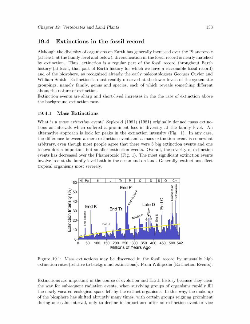
Chapter 19: Vertebrates and Land Plants 133
19.4 Extinctions in the fossil record
Although the diversity of organisms on Earth has generally increased over the Phanerozoic(at least, at the family level and below), diversification in the fossil record is nearly matchedby extinction. Thus, extinction is a regular part of the fossil record throughout Earthhistory (at least, that part of Earth history for which we have a reasonable fossil record)and of the biosphere, as recognized already the early paleontologists Georges Cuvier andWilliam Smith. Extinction is most readily observed at the lower levels of the systematicgroupings, namely family, genus and species, each of which reveals something differentabout the nature of extinction.Extinction events are sharp and short-lived increases in the the rate of extinction abovethe background extinction rate.
19.4.1 Mass Extinctions
What is a mass extinction event? Sepkoski (1981) (1981) originally defined mass extinc-tions as intervals which suffered a prominent loss in diversity at the family level. Analternative approach is look for peaks in the extinction intensity (Fig. 1). In any case,the difference between a mere extinction event and a mass extinction event is somewhatarbitrary, even though most people agree that there were 5 big extinction events and oneto two dozen important but smaller extinction events. Overall, the severity of extinctionevents has decreased over the Phanerozoic (Fig. 1). The most significant extinction eventsinvolve loss at the family level both in the ocean and on land. Generally, extinctions effecttropical organisms most severely.
Figure 19.1: Mass extinctions may be discerned in the fossil record by unusually highextinction rates (relative to background extinctions). From Wikipedia (Extinction Events).
Extinctions are important in the course of evolution and Earth history because they clearthe way for subsequent radiation events, when surviving groups of organisms rapidly fillthe newly vacated ecological space left by the extinct organisms. In this way, the make-upof the biosphere has shifted abruptly many times, with certain groups reigning prominentduring one calm interval, only to decline in importance after an extinction event or vice

Chapter 19: Vertebrates and Land Plants 134
versa. For example, the Trilobites, which were so such an important component of earlyPaleozoic seas, were decimated in the late Devonian extinction and finally went extinctduring the Permo-Triassic extinction.Many extinction events are thought to result from a combination of long-term environmen-tal stress and a proximal trigger, which ultimately kills them off. A significant source ofconfusion when discussing mass extinctions is differentiating between the trigger and thekill mechanisms.
• The trigger mechanism is the geological event that leads to extinction events
• The kill mechanisms is the actual environmental condition (resulting from the triggermechanism) that is responsible for killing off groups of organisms
For example, in the case of an asteroid impact, the impact itself, although it will cer-tainly lead to many extinctions of spatially restricted groups of organisms that might bein the region of the impact, it is the follow on effects from the impact that most likely areresponsible for the majority of extinctions.
19.4.2 Causes of mass extinctions
Identifying the causes of mass extinctions is not easy, for these causes need to be consistentwith available paleontological evidence (e.g., including all groups of organisms that survivedand those that went extinct) and geological evidence (e.g. ocean acidification, fluctuationsin sea level, etc.). Probably, many mass extinctions were the result of multiple overlappingcauses.
• Fall in sea level (exposure of continental shelves)
• Global cooling
• Global warming
• Flood basalt volcanisms
• Meteorite impacts
• Ocean anoxia
• Sulfidic deep waters
19.5 The Big Five Mass Extinctions
Extinction event Genus loss (%) Species loss (%)
End Ordovician 60 85Late Devonian 57 83Permo-Triassic 82 95End Triassic 53 80Cretaceous-Tertiary 47 76
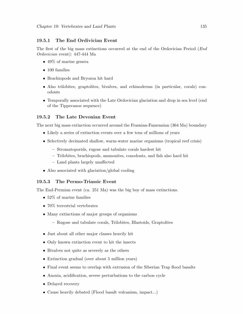
Chapter 19: Vertebrates and Land Plants 135
19.5.1 The End Ordivician Event
The first of the big mass extinctions occurred at the end of the Ordovician Period (EndOrdovician event): 447-444 Ma
• 49% of marine genera
• 100 families
• Brachiopods and Bryozoa hit hard
• Also trilobites, graptolites, bivalves, and echinoderms (in particular, corals) con-odonts
• Temporally associated with the Late Ordovician glaciation and drop in sea level (endof the Tippecanoe sequence)
19.5.2 The Late Devonian Event
The next big mass extinction occurred around the Frasnian-Famennian (364 Ma) boundary
• Likely a series of extinction events over a few tens of millions of years
• Selectively decimated shallow, warm-water marine organisms (tropical reef crisis)
– Stromatoporids, rugose and tabulate corals hardest hit
– Trilobites, brachiopods, ammonites, conodonts, and fish also hard hit
– Land plants largely unaffected
• Also associated with glaciation/global cooling
19.5.3 The Permo-Triassic Event
The End-Permian event (ca. 251 Ma) was the big boy of mass extinctions.
• 52% of marine families
• 70% terrestrial vertebrates
• Many extinctions of major groups of organisms
– Rugose and tabulate corals, Trilobites, Blastoids, Graptolites
• Just about all other major classes heavily hit
• Only known extinction event to hit the insects
• Bivalves not quite as severely as the others
• Extinction gradual (over about 5 million years)
• Final event seems to overlap with extrusion of the Siberian Trap flood basalts
• Anoxia, acidification, severe perturbations to the carbon cycle
• Delayed recovery
• Cause heavily debated (Flood basalt volcanism, impact...)
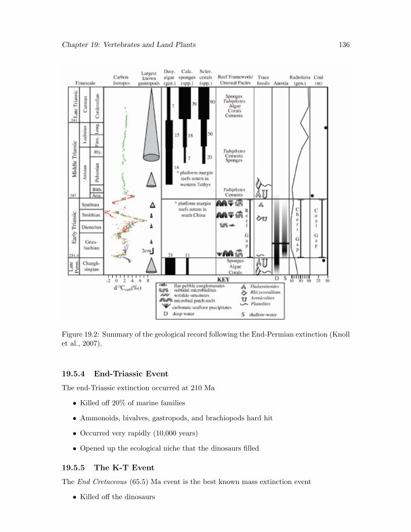
Chapter 19: Vertebrates and Land Plants 136
Figure 19.2: Summary of the geological record following the End-Permian extinction (Knollet al., 2007).
19.5.4 End-Triassic Event
The end-Triassic extinction occurred at 210 Ma
• Killed off 20% of marine families
• Ammonoids, bivalves, gastropods, and brachiopods hard hit
• Occurred very rapidly (10,000 years)
• Opened up the ecological niche that the dinosaurs filled
19.5.5 The K-T Event
The End Cretaceous (65.5) Ma event is the best known mass extinction event
• Killed off the dinosaurs

Chapter 19: Vertebrates and Land Plants 137
• As well as the ammonoids and rudist clams
• Planktonic marine species especially hard hit
• Land plants and many terrestrial vertebrates not heavily affected
• Associated with an immense meteorite impact, but other related kill mechanisms
• The boundary layer - Ir anomaly, shocked quartz, tektites
• The Chicxulub Impact on the Yucatan Peninsula was contemporaneous
Chapter 20
Mesozoic Life
Reading: Chapter 16 in Stanley; Chapter 15 in Wiccander and Monroe
20.1 Recovery from the Permo-Triassic extinction in the ma-rine realm
The biosphere was decimated at the beginning of the Mesozoic as a result of the Permo-Triassic extinction, and life had a distinctly different flavor in the Mesozoic. Recoveryfrom the extinction took many millions of years, probably the result of the continuedinhospitable environment (anoxic, and maybe sulfidic deep oceans) that caused or at leastheavily contributed to the extinction.
• Reef gap delayed recovery of reef-forming organisms
• Coal gap apparently delayed recovery of large trees in swampy areas
• Stromatolites enjoyed a brief resurgence
• Only mollusks and ammonoids reasonably abundant in Early Triassic
By the middle Triassic, the recovery had begun. Whereas many important Paleozoic biotawere lost to extinction (the rugose and tabulate corals, the trilobites, fusilinid foraminifera),other groups thrived in the Mesozoic.
20.1.1 Benthic biota
• Bivalves expanded and became hugely important in the benthic environment
– Rudist bivalves important reef builders (calcite)
– Important diversification in Cretaceous
• Sea urchins thrived after the early Triassic
• Gastropods diverged and took on a more ”modern” appearance, particularly in Cre-taceous with appearance of the Neogastropods
• Early reef builders were sponges and algae
138
Chapter 20: Mesozoic Life 139
– eventually the hexacorals (Scleractinia) took over; at first, small reefs, thenlarge, diverse reefs
– some groups lived in deep waters (i.e., no symbiosis with algae)
• Brachiopods and crinoids declined, particularly in late Mesozoic
20.1.2 Pelagic biota
• Ammonoids thrived after near extinction (just two genera survived)
• Belemnites (evolved in late Paleozoic) diversified and were important predators
• Conodonts disappeared by the Jurassic
• Fish changed dramatically
– Early ray-finned fish still rather primitive compared to most extant examples;they had, for example, triangular, non-overlapping scales.
– Evolution of the swim bladder
– Some modern sharks evolved (e.g. the tiger shark) by early Mesozoic
– Teleost fish, which included many modern fish, evolved by late Cretaceous
∗ Overlapping, circular scales
∗ Symmetric tails and specialized fins
∗ short jaws
• Some reptiles returned to the seas
– nothosaurs
– placodonts
– plesiosaurs
– ichthyosaurs, known as the “fish-lizard” appeared somewhat later in the Meso-zoic and are distinct from the other swimming reptiles in that they gave birthto live young
– Crocodiles also emerged in the Mesozoic, although later than the other groups.Thet diverged from the last common ancestor to the dinosaurs, and hence area sister group to the dinosaurs.
• Dinoflagellates (which include photosynthesizers) and foraminifera (heterotrophicprotists) diversified
• Expansion of calcareous nannoplankton, such as the Coccolithophora, and calcareousforams
– profound influence on carbonate sedimentology
– carbonate precipitation in open ocean (not constrained to shallow water plat-forms); shifted the locus of carbonate deposition away from continental marginsand into the deep sea.
• Diatoms appeared in Cretaceous, with a large impact on the silica cycle. Now un-dersaturated in the surface ocean.
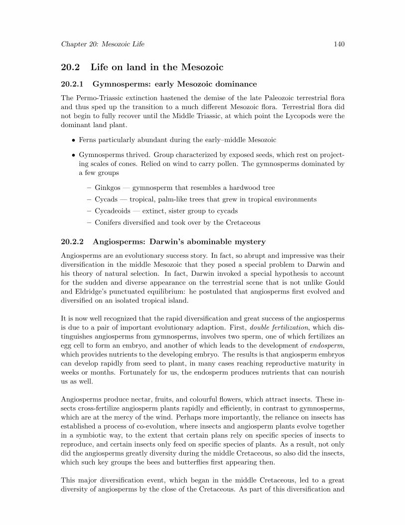
Chapter 20: Mesozoic Life 140
20.2 Life on land in the Mesozoic
20.2.1 Gymnosperms: early Mesozoic dominance
The Permo-Triassic extinction hastened the demise of the late Paleozoic terrestrial floraand thus sped up the transition to a much different Mesozoic flora. Terrestrial flora didnot begin to fully recover until the Middle Triassic, at which point the Lycopods were thedominant land plant.
• Ferns particularly abundant during the early–middle Mesozoic
• Gymnosperms thrived. Group characterized by exposed seeds, which rest on project-ing scales of cones. Relied on wind to carry pollen. The gymnosperms dominated bya few groups
– Ginkgos — gymnosperm that resembles a hardwood tree
– Cycads — tropical, palm-like trees that grew in tropical environments
– Cycadeoids — extinct, sister group to cycads
– Conifers diversified and took over by the Cretaceous
20.2.2 Angiosperms: Darwin’s abominable mystery
Angiosperms are an evolutionary success story. In fact, so abrupt and impressive was theirdiversification in the middle Mesozoic that they posed a special problem to Darwin andhis theory of natural selection. In fact, Darwin invoked a special hypothesis to accountfor the sudden and diverse appearance on the terrestrial scene that is not unlike Gouldand Eldridge’s punctuated equilibrium: he postulated that angiosperms first evolved anddiversified on an isolated tropical island.
It is now well recognized that the rapid diversification and great success of the angiospermsis due to a pair of important evolutionary adaption. First, double fertilization, which dis-tinguishes angiosperms from gymnosperms, involves two sperm, one of which fertilizes anegg cell to form an embryo, and another of which leads to the development of endosperm,which provides nutrients to the developing embryo. The results is that angiosperm embryoscan develop rapidly from seed to plant, in many cases reaching reproductive maturity inweeks or months. Fortunately for us, the endosperm produces nutrients that can nourishus as well.
Angiosperms produce nectar, fruits, and colourful flowers, which attract insects. These in-sects cross-fertilize angiosperm plants rapidly and efficiently, in contrast to gymnosperms,which are at the mercy of the wind. Perhaps more importantly, the reliance on insects hasestablished a process of co-evolution, where insects and angiosperm plants evolve togetherin a symbiotic way, to the extent that certain plans rely on specific species of insects toreproduce, and certain insects only feed on specific species of plants. As a result, not onlydid the angiosperms greatly diversity during the middle Cretaceous, so also did the insects,which such key groups the bees and butterflies first appearing then.
This major diversification event, which began in the middle Cretaceous, led to a greatdiversity of angiosperms by the close of the Cretaceous. As part of this diversification and
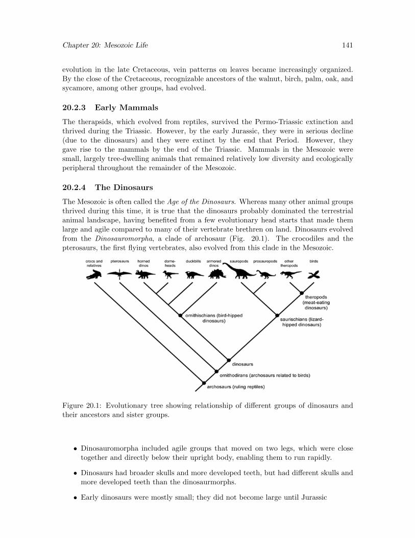
Chapter 20: Mesozoic Life 141
evolution in the late Cretaceous, vein patterns on leaves became increasingly organized.By the close of the Cretaceous, recognizable ancestors of the walnut, birch, palm, oak, andsycamore, among other groups, had evolved.
20.2.3 Early Mammals
The therapsids, which evolved from reptiles, survived the Permo-Triassic extinction andthrived during the Triassic. However, by the early Jurassic, they were in serious decline(due to the dinosaurs) and they were extinct by the end that Period. However, theygave rise to the mammals by the end of the Triassic. Mammals in the Mesozoic weresmall, largely tree-dwelling animals that remained relatively low diversity and ecologicallyperipheral throughout the remainder of the Mesozoic.
20.2.4 The Dinosaurs
The Mesozoic is often called the Age of the Dinosaurs. Whereas many other animal groupsthrived during this time, it is true that the dinosaurs probably dominated the terrestrialanimal landscape, having benefited from a few evolutionary head starts that made themlarge and agile compared to many of their vertebrate brethren on land. Dinosaurs evolvedfrom the Dinosauromorpha, a clade of archosaur (Fig. 20.1). The crocodiles and thepterosaurs, the first flying vertebrates, also evolved from this clade in the Mesozoic.
Figure 20.1: Evolutionary tree showing relationship of different groups of dinosaurs andtheir ancestors and sister groups.
• Dinosauromorpha included agile groups that moved on two legs, which were closetogether and directly below their upright body, enabling them to run rapidly.
• Dinosaurs had broader skulls and more developed teeth, but had different skulls andmore developed teeth than the dinosaurmorphs.
• Early dinosaurs were mostly small; they did not become large until Jurassic

Chapter 20: Mesozoic Life 142
• Diverged into two main groups distinguished by pelvic structure
– Ornithischian (bird-hipped) — herbivores (but do not include the ancestor tothe birds)
– Saurichia (lizard-hipped) — herbivores and carnivores
• Co-existed with therapsids, dinosauromorphs, amphibians, and reptiles until the end-Triassic extinction, at which point the dinosaurs took over the show
• Extinction wiped out the therapsids, opened the ecological door to dinosaurs
• Highly diverse within a 100,000 years of extinction
• Ruled the land until the end of the Mesozoic. Highly successful because
– Many were highly agile
– Complex system of ordering eggs
• Diverse, dinosaur-filled terrestrial ecosystems by the Cretaceous
• Matched in size by other large animals, like crocodiles (up to 15 m in length)
Evidence for endothermy among dinosaurs
In the past 20 years, evidence has mounted that the dinosaurs were not cold-blooded,lumbering creatures as popularly depicted in animations and in older textbooks.
• Must have had high rate of metabolism to suppress mammals for 140 m.y.
• Small percentage of carnivores (high metabolism requires lots of food, can’t supportlarge number of carnivores)
• Active locomotion (versus lumbering)
• Abundance of blood vessels in bones
• Evidence of brooding (like warm-blooded birds)
• High growth rates
• Some dinosaurs had feathers (which would have served to insulate)
• Dinosaurs in the high latitudes
Fly vertebrates
The Pterosaurs include the pterodactyl and other flying dinosaur-like creatures. Despitetheir superficial resemblance to birds, the Pterosaurs branched off the main dinosaur lin-eage prior to crown-group dinosaurs (Fig. 20.1), and hence were not closely related tobirds. The pterosaurs had immense wing spans, and biomechanics studies of their fossilssuggest that they did not regularly flap their wings, but rather most glides on air currents.
Birds emerged from the Saurichia line of dinosaurs, and the evidence for the close link todinosaurs is mounting, with lots of recent evidence for feathered dinosaurs and perhapsflying birds with ostensibly bird-like features.
Chapter 20: Mesozoic Life 143
20.2.5 Frogs and Turtles
These two groups of small vertebrates originated in the Triassic
20.2.6 The Mammals
Mammals evolved from the still reptile-like therapsids in the latest Triassic. The ther-apsids, which had managed to suppress the dinosaurs, went extinct in the End-Triassicextinction. Mammals survived, but they remained small and relatively unimportant inMesozoic ecology due to the subsequent dominance of the dinosaurs.
• earliest mammals resemble the modern shrew
• Key evolutionary changes
– Differentiated and specialized teeth
– Enlarged brain
– Modification of jawbones into ear bones
– Single jawbone
– Secondary palate (to allow continue breathing while eating)
– Suckled young
• Remained small due to predatory pressure by dinosaurs
• Many were nocturnal
• Many were tree dwelling
• First herbivores in the Jurassic
• Differentiated into the placentals and marsupials by the Late Cretaceous
20.3 The End Triassic Mass Extinction
The end-Triassic extinction occurred at 210 Ma and overlaps with the emplacement of theenormous Central Atlantic Magmatic Province (CAMP), which was related to the openingof the central Atlantic ocean.
• Killed off 20% of marine families and half of all genera
• Ammonoids, bivalves, gastropods, and brachiopods hard hit
• Occurred very rapidly (10,000 years)
• Therapsids went extinct
• Opened up the ecological niche that the dinosaurs filled

Chapter 21
Mesozoic Earth history
Reading: Chapters 16 and 17 in Stanley; Chapter 14 in Wiccander and Monroe
At the beginning of the Mesozoic, the continents were mostly amalgamated in the super-continent Pangaea. Sea level was generally high, and carbonates were deposited in muchof Europe. The Tethys Sea was a large, mostly tropical ocean basin the separated easternGondwana from southeastern Asia. The geology of the Mesozoic was dominated by thebreak-up of Pangea, starting in the the Triassic, not long after it finished forming. By theend of the Cretaceous, many of the cratons that had assembled to form Gondwana andLaurasia were again separated. Whereas most of the Paleozoic orogenic events to affectNorth America occurred along its east coast, Mesozoic orogeny exclusively affected westernNorth America. With opening of the Atlantic, the east coast of North America became apassive margin.
21.1 Breakup of Pangaea
Pangaea breakup began in the late Triassic with the onset of rifting between Laurasiaand Gondwana, and proceeded slowly into the Jurassic. Break-up, particularly along theAtlantic margins, was accompanied by extensive plume magmatism
• Opening of the Atlantic basin
• Associated with the 200 Ma Central Atlantic magmatic province (flood basalts)
• Tethys Sea extended between Laurasia and Africa
• Gulf of Mexico opens and North America and South America separated by the LateJurassic
• Pacific, Atlantic, and Tethys connected by deep, narrow basins
• Vast salt deposits, important seals in many petroleum provinces
• Greenland separated from North America by Late Cretaceous
Gondwana began to rift in the Late Triassic and was mostly disaggregated by the end ofthe Cretaceous
144
Chapter 21: The Mesozoic 145
• Antarctica and Australia first separated from South America and Africa; associatedwith emplacement of the Karoo-Ferrar flood basalt (183 Ma)
• India rifted apart from eastern Gondwana and begin to drift to the north
• South America and Africa began to rift apart in the late Jurassic; associated withParana-Etendeka flood basalt (130 Ma)
• Australia and Antarctica rifted in the late Cretaceous
The breakup of Pangaea had profound effects on ocean circulation and regional climate
• Pangaea interior typically arid, global climate dominated by large Pacific ocean
• Tethys realm tropical during the Mesozoic; site of most coral reefs
• Temperature gradients low during first half of Mesozoic – mild climates to 60N
• Drift of continents to the high latitudes increased global temperature gradients
• Rigorous and complex ocean circulation
21.1.1 The Cretaceous
The Cretaceous was a time of continental fragmentation and the development of narrowseaways. Ocean circulation changed, particularly when the Tethys seaway connected to thePacific ocean. Evaporite were deposited on the margins of many of the newly developedseaways.
The Tethys Seaway
The Cretaceous Tethys Seaway was much different from its predecessor, the Tethys Sea,which was a large ocean basin nearly encircled by Pangaea. The trade winds drove a vastocean current through the seaway, distributing the warmth of tropical ocean waters to thesouthern Europe and eastern North America.
21.2 North America in the Mesozoic
In the early Mesozoic, sedimentation in North America was dominated by terrestrial de-position in the continental interior and along the recently formed Appalachians.
21.2.1 East Coast
• Onset of breakup between North America and Africa in Late Triassic
• Deposition of coarse, poorly sorted, red sediments in non-marine rift basins (NewarkGroup)
• Intrusion of dikes and sills (for example the Palisades sill along Hudson River)
• East coast passive margin established by about 180 Ma
• Gulf of Mexico opened as a shallow, restricted basin. Site of thick salt deposits
Chapter 21: The Mesozoic 146
• Opened to ocean and deepened by late Jurrasic
• Widespread rudist (reef-forming bivalves) reefs (superb reservoirs)
21.2.2 West Coast
Sonoman orogeny
A second island arc system collided with western North America around the Permian-Triassic boundary as a result of west-dipping subduction during the Sonoman orogeny.This orogenic event was similar to the Antler orogeny, but in this case, the volcanic arc(the Golconda arc) was formed on the edge of an exotic continental terrane (Sonomia)rather than on oceanic crust (as in the Klamath arc), such that the orogeny added a signif-icant amount of new material to western North America. After this collision, the westernmargin of North America was again a stable, passive margin.
The Classic Model: Subduction polarity switch
Following docking of the Sonoma terrane, the west coast was tectonically quiescent throughthe Triassic. The traditional interpretation of the Mesozoic tectonic evolution of NorthAmerica holds that following the resumption of tectonism in the Jurassic is related tofoundering of the oceanic crust on the trailing (western) margin of Sonomia terrane (nowNorth America), leading to the onset of east-dipping subduction: a subduction polarityswitch. From the Jurassic onward, the west coast was an active continental margin, domi-nated by east-dipping subduction of the Farallon plate (part of the ancestral Pacific oceanbasin) and the accretion of island arcs and microcontinents brought in on the subductingplates. The tectonics of western North America in the Mesozoic mirrored the tectonics ofeastern North America in the middle-late Paleozoic.
Cordilleran orogenesis
The Cordilleran orogeny refers to the series of orogenic events the influenced the westernmargin of North America from the middle Jurassic to the early Cenozoic, after the switchin subduction polarity
• Nevadan orogeny — middle Jurassic to early Cretaceous
– Sierra Nevada arc and widespread, eastward-migrating batholith emplacementin western North America. The present day Sierra Nevadas, which are composedmainly of granodiorite, are an erosional relic of this arc.
– Deposition of Franciscan complex (melange) and Great Valley Group in theforearm
– Addition of a large, composite exotic terrane to western Canada and Alaska
• Sevier orogeny — Cretaceous
– result of ongoing eastward subduction (thus east-west compression of the mar-gin)
– Alaska to Mexico
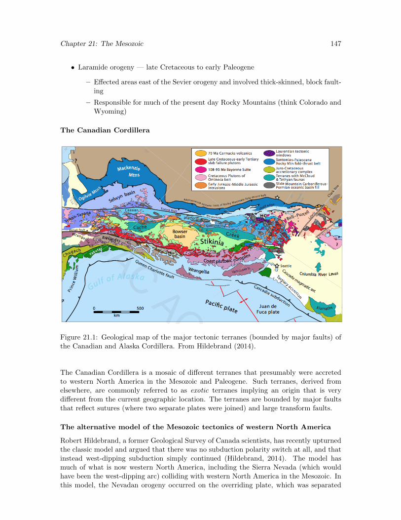
Chapter 21: The Mesozoic 147
• Laramide orogeny — late Cretaceous to early Paleogene
– Effected areas east of the Sevier orogeny and involved thick-skinned, block fault-ing
– Responsible for much of the present day Rocky Mountains (think Colorado andWyoming)
The Canadian Cordillera
Figure 21.1: Geological map of the major tectonic terranes (bounded by major faults) ofthe Canadian and Alaska Cordillera. From Hildebrand (2014).
The Canadian Cordillera is a mosaic of different terranes that presumably were accretedto western North America in the Mesozoic and Paleogene. Such terranes, derived fromelsewhere, are commonly referred to as exotic terranes implying an origin that is verydifferent from the current geographic location. The terranes are bounded by major faultsthat reflect sutures (where two separate plates were joined) and large transform faults.
The alternative model of the Mesozoic tectonics of western North America
Robert Hildebrand, a former Geological Survey of Canada scientists, has recently upturnedthe classic model and argued that there was no subduction polarity switch at all, and thatinstead west-dipping subduction simply continued (Hildebrand, 2014). The model hasmuch of what is now western North America, including the Sierra Nevada (which wouldhave been the west-dipping arc) colliding with western North America in the Mesozoic. Inthis model, the Nevadan orogeny occurred on the overriding plate, which was separated
Chapter 21: The Mesozoic 148
from North America at the time by an ocean basin. This continent grew as a resultof a series of collisions during the middle Mesozoic prior to beginning to collide withwestern North America in the early Cretaceous (Sevier orogeny) and culminated in the lateCretaceous (Laramide orogeny). Many of the terranes that clog up the Canadian Cordillera(Fig. 21.1) then translated northward along a major strike slip system, consistent with theGreat Alaskan Terrane Wreck model proposed by Stephen Johnston (Johnston, 2001),which holds that many of the terranes along the Cordillera are fragmented pieces of singleribbon continent that collides with western North America.
21.2.3 Mesozoic sedimentation
Non-marine sediments were deposited across much of the southwestern US in the first halfof the Mesozoic. These include many of the famous, pastel-colored units found on theColorado Plateau, such as the Moenkopi, Chinle, and Navajo Sandstone formations whichfilled a foreland basin that formed in response to the Nevadan orogeny.
Following brief marine incursions by the Sundance Sea, the colorful late Jurassic MorrisonFormation (∼150 Ma), which is famous for its dinosaur fossils, was deposited across muchof what is now the Rocky Mountain area of the western U.S.
21.2.4 Cretaceous Interior Seaway
Orogenic activity along the Cordillera resulted in the development of a long foreland basinalong the eastern margin of the mountain front. As a result also of long wavelengthsubsidence of interior North America due to the sinking Farallon slab beneath it, the oceantransgressed the mid-continent from the north beginning in the Early Cretaceous. By theLate Cretaceous, this seaway was continuous with the Gulf of Mexico and much of theinterior of the continent was underwater. Widespread late Cretaceous coal was depositedalong coastal plains as the sea retreated in the late Cretaceous.
21.3 Mesozoic Climate
21.3.1 Early Mesozoic
In the Triassic, Pangaea was still largely intact. Much of the continental interior was farfrom a source of moisture, and hence dry. Redbeds and evaporites were deposited in manyregions. This interior realm would have experience significant seasonality, as well, andprobably moisture was heavily dependent on monsoons.
By the Jurassic, Pangaea was fragmenting and the widespread arid climate began to giveway to a warm and broadly equable climate, characterized by relatively low temperaturegradients between low and high latitudes. Nevertheless, coral reefs were largely restrictedto the margins of the Tethys Ocean.
Chapter 21: The Mesozoic 149
21.3.2 Cretaceous
Ocean Anoxic Events
Carbon dioxide concentrations were unusually high during the Cretaceous, which resultedin high average temperatures. One result of this climate was a generally warm, poorlyventilated ocean. At several times during the Cretaceous organic-rich black shales weredeposited globally. The black shales deposited during these ocean anoxic events are im-portant petroleum source rocks.
The Cretaceous ocean anoxic events are closely linked temporally with an intense episodeof oceanic crust production, which was a direct result of break-up of Pangea. At the sametime, Earth’s magnetic field was unusually stable, giving rise to the Cretaceous Superchronnormal polarity interval.
Cretaceous glaciation?
Despite the generally greenhouse climate of the Cretaceous, there are reports of minorglacial episodes, detected mainly in the oxygen isotope records of marine carbonates. How-ever, glaciation, if it did occur, was likely restricted to small areas near the south pole,such as Australia, where some evidence of Cretaceous glacial conditions has been found.

Chapter 22
The Cretaceous-Paleogene MassExtinction and the Paleogene
Reading: Chapters 17 and 18 in Stanley; Chapters 16 and 18 in Wiccander and Monroe
The Cenozoic, which is split into the Paleogene (65.6 to 23 Ma) and Neogene (23 Ma topresent) began 65.5 with the mass extinction event the killed off the dinosaurs, the last ofthe giant, aquatic reptiles, and the ammonoids, and many other animals groups. By thattime, Pangaea had mostly broken up and western North America was undergoing activeorogenesis as the Rocky Mountains were forming along the length of the Cordillera. Mam-mals took over from the dinosaurs as the dominant animals on land and even recolonizedthe oceans. Our records of Cenozoic Earth history are much more detailed, thanks to acombination of deep sea sediment records and many terrestrial environmental records, suchas lake bed sediments and cave deposits.
22.1 The K-Pg Extinction
The End Cretaceous, or K-Pg mass extinction (formerly known as the K-T event, forCretaceous-Tertiary) is the best known mass extinction event because it is the most recentand understood. Most importantly for museums, children’s books, and life as we knowit on Earth, it killed off the dinosaurs, paving the way for an extraordinary radiation ofmammals.
• Dinosaurs, giant aquatic reptiles, and giant turtles went extinct
• Ammonoids went extinct; belemnoids nearly extinct
• Planktonic marine species especially hard hit; 90% of all nannoplankton and plank-tonic foraminifera went extinct
• Land plants, including both gymnosperms and angiosperms, heavily hit, particularlyin North America, but the angiosperms fared better
• Many terrestrial vertebrates not heavily affected
The almost certain cause of the K-Pg extinction was discovered by accident by the NobelPrize-winning physicist Walter Alvarez, and his son, Luis Alvarez. They were analyzing
150

Chapter 22: K-Pg Extinction and the Paleogene 151
Ir concentrations in deep sea clays exposed at Gubbio, Italy for a totally different project(they were trying to constrain sedimentation rates), when they discovered an extraordinarypeak in Ir concentrations at the K-Pg boundary. Ir is rare on Earth’s surface, but relativelyabundant in meteorites, and so, logically, they proposed that the extinction was directlylinked to a meteorite impact. The anomaly has since been found globally, and along withit, three other key ingredients have been found in the K-Pg boundary clay layer aroundNorth and central America that point to a meteorite impact:
• Shocked quartz grains (fractured and welded grains that are formed by a sudden,high pressure shock)
• Microspherules, which are small droplets of glass formed by the rapid cooling ofmolten rock within the atmosphere
• Microdiamonds, which form only in space or through the sorts of shocks generatedby impacts
The K-Pg boundary layer is also found by a high concentration of fern spores, which indi-cate that other plants died off, and ferns opportunistically repopulated much of the landsurface (Vajda et al., 2001). Other evidence in support of the impact hypothesis came fromtsunami deposits and concentrations of soot in the boundary clay. But the true triumphfor the Alvarez family and for geology came when the K-Pg impact crater was discoveredno long afterwards. The Chicxulub crater occurs in the subsurface on the northwesternedge of the Yucatan Peninsula in Mexico, and Ar-Ar dating of glass within impact siteyields an age of precisely 65.5 Ma (within the range of error of the measurements).
If the impact hypothesis has now been largely settled (minus a few stubborn holdouts),the kill mechanism or mechanisms remain debated. Whatever they are, they must accountfor the unique extinction pattern.
• global wildfire triggered by the impact and subsequent heat generated by fallingdebris
• impact winter, results from the immense quantity of dust in the atmosphere
• acid rain, from generation of nitrous oxides in atmosphere and collision with a sulfate-rich target
• global warming, from collision with a carbonate-rich target (evidence for a peak inCO2 concentrations from leaf stomata)
The K-Pg extinction nearly coincided with the emplacement of the Deccan Traps floodbasalt in India, and some scientists, most notably Greta Keller of Princeton Universityargue that this was really the main cause of the extinction, at least of the dinosaurs. Sheargues that dinosaurs appear to started going extinct a few hundred thousand years earlier,and that this is consistent with the volcanic trigger.

Chapter 22: K-Pg Extinction and the Paleogene 152
22.2 Life in the Paleogene
Life on land changed dramatically after the K-Pg extinction, due in large part to theextinction of the dinosaurs and the diminished role of the gymnosperms. Angiospermsflourished in the early Paleogene, and mammals diversified rapidly to fill the many nichesthat the dinosaurs and large reptiles left open.
22.2.1 Marine life in the Paleogene
Benthic life survived the extinction fairly in tact, and the teleost fish, mollusks, and ben-thic foraminifera we see today closely resemble those that existed on the sea floor at thebeginning of the Paleogene. The planktonic foraminifera, on the other hand, suffered im-mensely, and only three species are known to have survived. However, these three speciesdiversified extremely rapidly (due in large part to the empty ecospace in the aftermath ofthe extinction). Likewise, the calcareous nannoplankton diversified rapidly.
The rudist clams died off during the extinction whereas the corals did not. But the coralsdid not immediately rebound to take over reef-building duties in the Paleogene. This mighthave been due to still somewhat low Mg/Ca ratios of seawater. In the Oligocene, afterMg/Ca ratios rose, the hexacorals rebounded and begin to build large reefs again.
Whales
Just as reptiles returned to the sea from land in the Mesozoic, so too did some mammalsreturn to the water in the Cenozoic. The whales evolved from carnivorous land mammals,and in the oceans where other large predators were absent, quickly gained the upper hand.So too did giant sharks become prominent in the early Cenozoic. The cetaceans (whales)are a sister group to the artiodactyla. The earliest whales appeared in the Early Eoceneand still had front limbs that enabled them to support their weight on land.
• Land-dwelling ancestors are the raoellids
• Front limbs modified to flippers
• Rear limbs lost
• Nostrils to top of head
• Large tale fluke
• Baleen and toothed whales appeared by Oligocene
22.2.2 Life on land in the Paleogene
Flowering plants diversified rapidly in the late Mesozoic. One of the keys of their successwas the advent of double fertilization, which produced both a seed and a food supply forthat seed (in contrast to gymnosperm seeds, which require much more time to furnishthese nutrients, hence their slow reproductive cycle). The flowering plants were also ableto attract insects, which helped with fertilization. In fact, the symbiotic relationship thatdeveloped between insects and flowering plants resulted in closely coupled evolution among
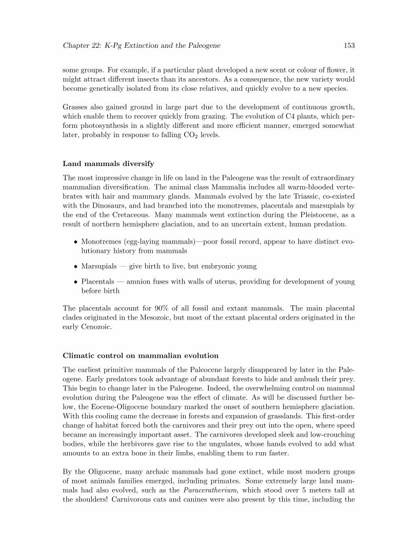
Chapter 22: K-Pg Extinction and the Paleogene 153
some groups. For example, if a particular plant developed a new scent or colour of flower, itmight attract different insects than its ancestors. As a consequence, the new variety wouldbecome genetically isolated from its close relatives, and quickly evolve to a new species.
Grasses also gained ground in large part due to the development of continuous growth,which enable them to recover quickly from grazing. The evolution of C4 plants, which per-form photosynthesis in a slightly different and more efficient manner, emerged somewhatlater, probably in response to falling CO2 levels.
Land mammals diversify
The most impressive change in life on land in the Paleogene was the result of extraordinarymammalian diversification. The animal class Mammalia includes all warm-blooded verte-brates with hair and mammary glands. Mammals evolved by the late Triassic, co-existedwith the Dinosaurs, and had branched into the monotremes, placentals and marsupials bythe end of the Cretaceous. Many mammals went extinction during the Pleistocene, as aresult of northern hemisphere glaciation, and to an uncertain extent, human predation.
• Monotremes (egg-laying mammals)—poor fossil record, appear to have distinct evo-lutionary history from mammals
• Marsupials — give birth to live, but embryonic young
• Placentals — amnion fuses with walls of uterus, providing for development of youngbefore birth
The placentals account for 90% of all fossil and extant mammals. The main placentalclades originated in the Mesozoic, but most of the extant placental orders originated in theearly Cenozoic.
Climatic control on mammalian evolution
The earliest primitive mammals of the Paleocene largely disappeared by later in the Pale-ogene. Early predators took advantage of abundant forests to hide and ambush their prey.This begin to change later in the Paleogene. Indeed, the overwhelming control on mammalevolution during the Paleogene was the effect of climate. As will be discussed further be-low, the Eocene-Oligocene boundary marked the onset of southern hemisphere glaciation.With this cooling came the decrease in forests and expansion of grasslands. This first-orderchange of habitat forced both the carnivores and their prey out into the open, where speedbecame an increasingly important asset. The carnivores developed sleek and low-crouchingbodies, while the herbivores gave rise to the ungulates, whose hands evolved to add whatamounts to an extra bone in their limbs, enabling them to run faster.
By the Oligocene, many archaic mammals had gone extinct, while most modern groupsof most animals families emerged, including primates. Some extremely large land mam-mals had also evolved, such as the Paraceratherium, which stood over 5 meters tall atthe shoulders! Carnivorous cats and canines were also present by this time, including the
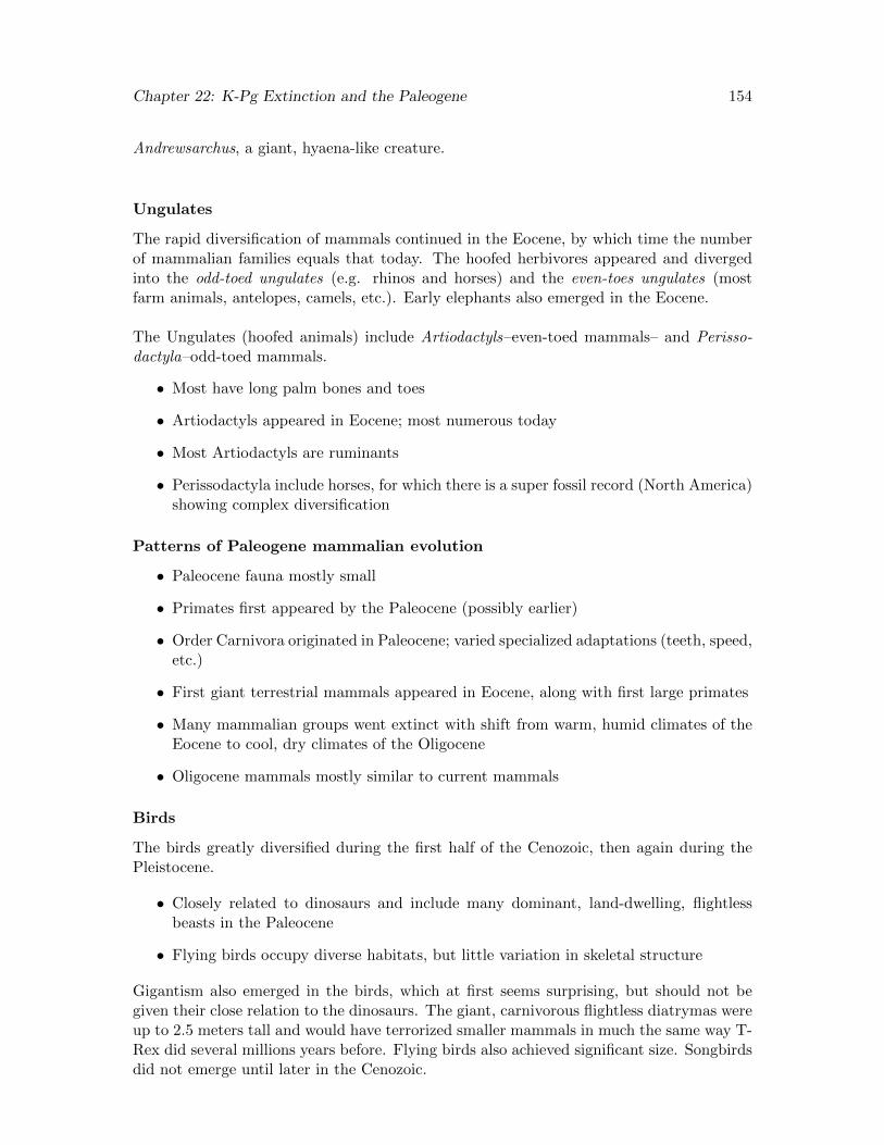
Chapter 22: K-Pg Extinction and the Paleogene 154
Andrewsarchus, a giant, hyaena-like creature.
Ungulates
The rapid diversification of mammals continued in the Eocene, by which time the numberof mammalian families equals that today. The hoofed herbivores appeared and divergedinto the odd-toed ungulates (e.g. rhinos and horses) and the even-toes ungulates (mostfarm animals, antelopes, camels, etc.). Early elephants also emerged in the Eocene.
The Ungulates (hoofed animals) include Artiodactyls–even-toed mammals– and Perisso-dactyla–odd-toed mammals.
• Most have long palm bones and toes
• Artiodactyls appeared in Eocene; most numerous today
• Most Artiodactyls are ruminants
• Perissodactyla include horses, for which there is a super fossil record (North America)showing complex diversification
Patterns of Paleogene mammalian evolution
• Paleocene fauna mostly small
• Primates first appeared by the Paleocene (possibly earlier)
• Order Carnivora originated in Paleocene; varied specialized adaptations (teeth, speed,etc.)
• First giant terrestrial mammals appeared in Eocene, along with first large primates
• Many mammalian groups went extinct with shift from warm, humid climates of theEocene to cool, dry climates of the Oligocene
• Oligocene mammals mostly similar to current mammals
Birds
The birds greatly diversified during the first half of the Cenozoic, then again during thePleistocene.
• Closely related to dinosaurs and include many dominant, land-dwelling, flightlessbeasts in the Paleocene
• Flying birds occupy diverse habitats, but little variation in skeletal structure
Gigantism also emerged in the birds, which at first seems surprising, but should not begiven their close relation to the dinosaurs. The giant, carnivorous flightless diatrymas wereup to 2.5 meters tall and would have terrorized smaller mammals in much the same way T-Rex did several millions years before. Flying birds also achieved significant size. Songbirdsdid not emerge until later in the Cenozoic.

Chapter 22: K-Pg Extinction and the Paleogene 155
22.3 Paleogene Tectonics
22.3.1 Alpine-Himalayan orogen
The Alpine-Himalayan orogenic belt stretches from Spain in the west to southeast Asia.This extensive orogenic belt represent collision of Africa and India with Europe and Asia asthe Tethys ocean basin closed, beginning in the late Mesozoic. The eastern Mediterraneanis a vestige of the former Tethys ocean. The extensive orogenesis is responsible for manyseparate mountain chains, such as:
• Pyrenees
• Alps
• Caucasas
• Zagros
• Hindu Kush
• Pamir
• Himalayas
The Indian plate drifted northward, during the Cenozoic (by as much as 15–20 cm yr−1 inthe early Cenozoic), colliding with the Asian margin beginning about 50 Ma. It was pullednorthward (at least in part) by northward subduction underneath Asia, which resulted inthe emplacement of a large volcanic arc and associated batholiths. Orogeny is ongoing, asseen in the intensity of seismic activity in the region.
22.3.2 Paleogene tectonism in North America
The Laramide Orogen
The semicontinuous mountain building that begin in the early Mesozoic on the westernmargin of North America continued into the Paleogene with the Laramide orogen. Thisalso continued the trend of eastward migration of the orogenic front, which is though bymany to be closely linked to an eastward migration in magmatism. Most likely, this is aresult of a flattening subducting slab, which need to travel further in order to reach thenecessary depth to start melting.
Laramide deformation produced impressive fold and thrust belts in western Canada—thenorthern US (Idaho and Montana) and in southern New Mexico and Mexico. The style ofdeformation in these areas (classic fold and thrust belts) was quite different in the morecentral part of the Rocky Mountains in the US, where it was manifested by broad basementuplifts. These uplifts give rise to adjacent sedimentary basins in which vast volumes of ter-restrial sediment were deposited. The Green River basin is the largest known paleo-lakesystem well represented in the sedimentary record and contains abundant oil shales.
The Laramide orogeny ended by about 50 m.y., at which point the highlands the developedat this time were heavily eroded and planed off, filling the adjacent sedimentary basins.The modern Rocky Mountains reflect subsequent uplift of much of these earlier highlands.

Chapter 22: K-Pg Extinction and the Paleogene 156
Figure 22.1: Cenozoic benthic δ13C δ18O records and major tectonic, climatic, and biolog-ical events (Zachos et al., 2001).
22.3.3 Rifting and volcanism
A continental rift began to form in New Mexico in the late Oligocene. The Rio GrandeRift developed along previously developed Laramide structures, and resulted in massivevolcanic episodes that produced the San Juan Mountains and the famous Bandelier Tuff.
Somewhat earlier, in the Eocene, massive and episodic volcanism began in the area thatis now occupied by Yellowstone Park. The catastrophic eruptions in this region buried asmany as 20 forests in lavas, volcanic ash, and mud, as seen today in the petrified forestsin the region.
22.4 Cenozoic Climate
The Cretaceous is generally regarded as a warm interlude in Earth history (although thereis much debate about a possible series of minor glaciations). Warm conditions continuedinto the early Cenozoic.
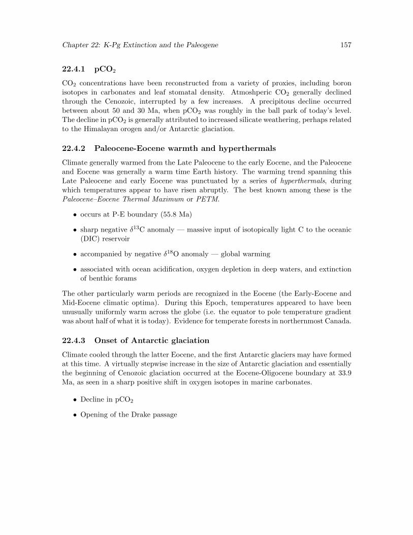
Chapter 22: K-Pg Extinction and the Paleogene 157
22.4.1 pCO2
CO2 concentrations have been reconstructed from a variety of proxies, including boronisotopes in carbonates and leaf stomatal density. Atmoshperic CO2 generally declinedthrough the Cenozoic, interrupted by a few increases. A precipitous decline occurredbetween about 50 and 30 Ma, when pCO2 was roughly in the ball park of today’s level.The decline in pCO2 is generally attributed to increased silicate weathering, perhaps relatedto the Himalayan orogen and/or Antarctic glaciation.
22.4.2 Paleocene-Eocene warmth and hyperthermals
Climate generally warmed from the Late Paleocene to the early Eocene, and the Paleoceneand Eocene was generally a warm time Earth history. The warming trend spanning thisLate Paleocene and early Eocene was punctuated by a series of hyperthermals, duringwhich temperatures appear to have risen abruptly. The best known among these is thePaleocene–Eocene Thermal Maximum or PETM.
• occurs at P-E boundary (55.8 Ma)
• sharp negative δ13C anomaly — massive input of isotopically light C to the oceanic(DIC) reservoir
• accompanied by negative δ18O anomaly — global warming
• associated with ocean acidification, oxygen depletion in deep waters, and extinctionof benthic forams
The other particularly warm periods are recognized in the Eocene (the Early-Eocene andMid-Eocene climatic optima). During this Epoch, temperatures appeared to have beenunusually uniformly warm across the globe (i.e. the equator to pole temperature gradientwas about half of what it is today). Evidence for temperate forests in northernmost Canada.
22.4.3 Onset of Antarctic glaciation
Climate cooled through the latter Eocene, and the first Antarctic glaciers may have formedat this time. A virtually stepwise increase in the size of Antarctic glaciation and essentiallythe beginning of Cenozoic glaciation occurred at the Eocene-Oligocene boundary at 33.9Ma, as seen in a sharp positive shift in oxygen isotopes in marine carbonates.
• Decline in pCO2
• Opening of the Drake passage

Chapter 23
The Neogene
23.1 Introduction
The Neogene Period is the most recent in Earth’s history and spans from just 23 millionyears ago to present. It includes the Miocene, Pliocene, Pleistocene, and Holocene epochs.Earth’s paleogeography has not changed a great deal since the Paleogene, although thewestern coast of North America continued to evolve rapidly, as did the Mediterranean.The present Rocky Mountains and Himalayas also developed during this time. Mammalscontinued to diversify during the Neogene, but the most profound change on Earth hasbeen climatic, with the continuation of cooling that first initiated in the late Eocene.
23.2 Neogene Tectonics
23.2.1 Circum-Pacific orogens
The Pacific ocean is surrounded by orogens — mostly active volcanic arcs where the variousplates that make up the Pacific ocean basin are subducting beneath continents or otherocean basins. A series of trenches is associated with intense volcanic activity:
• Peru-Chile trench (Andes)
• Middle-America trench
• Cascade trend
• Aleutian trench
• Kurile trench
• Japan trench
• Marianas trench
23.2.2 Western North America
The tectonics of western North America changed about 20 Ma with the onset of subductionof a mid-ocean ridge beneath the western margin. There were many results of this tectonicevent, the most important of which was that the western boundary of the North American
158
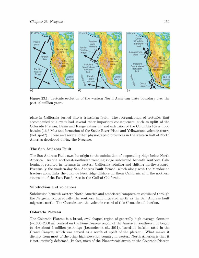
Chapter 23: Neogene 159
Figure 23.1: Tectonic evolution of the western North American plate boundary over thepast 40 million years.
plate in California turned into a transform fault. The reorganization of tectonics thataccompanied this event had several other important consequences, such as uplift of theColorado Plateau, Basin and Range extension, and extrusion of the Columbia River floodbasalts (16.6 Ma) and formation of the Snake River Plane and Yellowstone volcanic centre(hot spot?). These and several other physiographic provinces in the western half of NorthAmerica developed during the Neogene.
The San Andreas Fault
The San Andreas Fault owes its origin to the subduction of a spreading ridge below NorthAmerica. As the northeast-southwest trending ridge subducted beneath southern Cali-fornia, it resulted in terranes in western California rotating and shifting northwestward.Eventually the modern-day San Andreas Fault formed, which along with the Mendocinofracture zone, links the Juan de Fuca ridge offshore northern California with the northernextension of the East Pacific rise in the Gulf of California.
Subduction and volcanoes
Subduction beneath western North America and associated compression continued throughthe Neogene, but gradually the southern limit migrated north as the San Andreas faultmigrated north. The Cascades are the volcanic record of this Cenozoic subduction.
Colorado Plateau
The Colorado Plateau is a broad, oval shaped region of generally high average elevation(∼1800–2000 m) centred on the Four-Corners region of the American southwest. It beganto rise about 6 million years ago (Levander et al., 2011), based on incision rates in theGrand Canyon, which was carved as a result of uplift of the plateau. What makes itdistinct from most of the other high elevation country in western North America is that itis not intensely deformed. In fact, most of the Phanerozoic strata on the Colorado Plateau

Chapter 23: Neogene 160
are flat-lying, with only some minor folds here and there. It appears that the anomalousuplift is the result of progressive, inward delamination of the mantle lithosphere, in part asa result of upwelling asthenosphere and emplacement of dense mafic igneous rocks relatedto mid-Cenozoic volcanism (Levander et al., 2011).
The Basin and Range province
The Basin and Range Province extends from the edge of the Colarado Plateau in the east(effectively the Wasatch Fault in Salt Lake City) to the Sierra Nevada Mountains in thewest. It is distinguished by a series of linear (N-S) mountains and intervening valleys thatformed as the result of extensional block faulting. This arid region of high average elevationformed as the result of doming and extension of the continental crust, beginning about 18million years ago.
The present Sierra Nevadas
Although the Sierra Nevadas comprise mainly igneous rocks formed by middle Mesozoicsubduction beneath North America, their present high elevation is due to the extensionthat generated the Basin and Range province. The eastern edge of the Sierra Nevadas isa major, east-dipping normal fault (the mirror image of the Wasatch Fault in Salt LakeCity).
Columbia River flood basalt and Snake River plain
A hot spot began to spill out large volumes of basalt in the northwest about 17 millionyears ago. This Columbia River Flood Basalt covers large areas of present day easternWashington and Oregon and western Idaho in scablands. Volcanism continued after theinitial flood basalt volcanism, and as North America drifted to the west, this ongoingvolcanism formed the Snake River Plain, which cuts across southern Idaho like a deepwound. The hot spot now sits below Yellowstone Park and is responsible for extraordinaryvolcanic eruptions that occur about once every million years.
23.3 Neogene Climate
The Neogene was generally a time of cooling, marked by expansion of the Antarctic icesheet and onset of northern hemisphere glaciation. However, the late Oligocene and earlyMiocene saw a shrinking of Antarctic ice sheets, and this warm spell peaked in the middleMiocene, prior to rapid cooling and expansion of ice sheets from the late Miocene to thepresent.
23.3.1 Mid-Miocene Climatic Optimum
The Miocene Epoch is also regarded as a generally warm period in recent Earth history, atleast compared with more recent climate. Optimum temperatures occurred around 16 Maand were followed by about 12 million years of generally cooling climate. The Mid-Mioceneclimatic optimum occurred at the same time that the Columbia River flood basalts wereextruded in eastern Canada and Oregon. However, although this warm interval is apparentin oxygen isotope and paleontological records, it is not obvious in paleo-CO2 records.
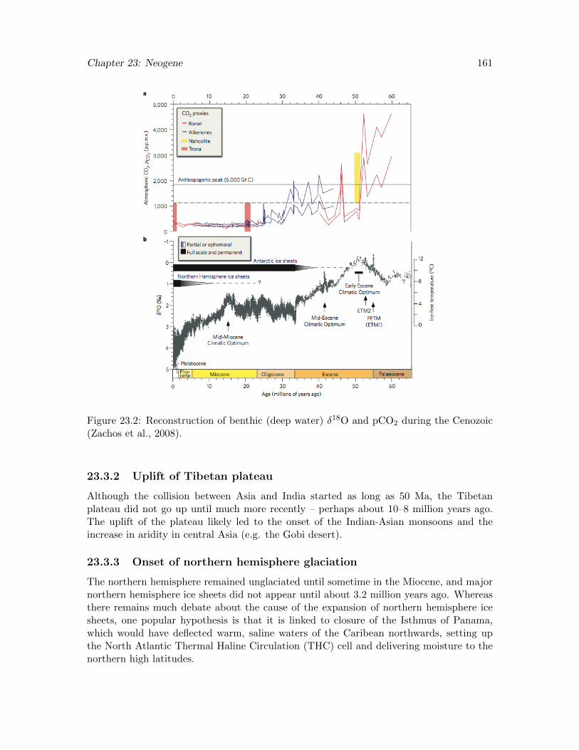
Chapter 23: Neogene 161
Figure 23.2: Reconstruction of benthic (deep water) δ18O and pCO2 during the Cenozoic(Zachos et al., 2008).
23.3.2 Uplift of Tibetan plateau
Although the collision between Asia and India started as long as 50 Ma, the Tibetanplateau did not go up until much more recently – perhaps about 10–8 million years ago.The uplift of the plateau likely led to the onset of the Indian-Asian monsoons and theincrease in aridity in central Asia (e.g. the Gobi desert).
23.3.3 Onset of northern hemisphere glaciation
The northern hemisphere remained unglaciated until sometime in the Miocene, and majornorthern hemisphere ice sheets did not appear until about 3.2 million years ago. Whereasthere remains much debate about the cause of the expansion of northern hemisphere icesheets, one popular hypothesis is that it is linked to closure of the Isthmus of Panama,which would have deflected warm, saline waters of the Caribean northwards, setting upthe North Atlantic Thermal Haline Circulation (THC) cell and delivering moisture to thenorthern high latitudes.
Chapter 23: Neogene 162
23.4 Life in the Neogene
To a large extent, life in the early Neogene was already very similar to that which occurredtoday. Invertebrate animals, in particular, have hardly changed since. However, a fewgroups of land mammals and plants continued to diverge rapidly during this interval.Specifically, both grasses and plants which include weeds and herbs diversified. At thesame time, rats and mice (Muridae), songbirds, and snakes diversified impressively. Ofcourse, from our anthropocentric vantage, the most important evolution was that of theprimates, which we will discuss in more detail in the next chapter.
23.4.1 C4 Plants
A major Cenozoic innovation in plants was the development of a new style of photosyn-thesis. The C4 plants that use this novel form of photosynthesis are much more efficientin their utilization of carbon dioxide. Although the evolution of C4 photosynthesis prob-ably occurred earlier in the Cenozoic, it only became widespread in the Miocene Epoch,almost certainly in response to low CO2 levels. C4 photosynthesis is restricted to the an-giosperms and includes many modern grasses and several important crop plants, such asmaize, sorghum, and millet.
Because C4 plants use more of the CO2 that they incorporate via diffusion through theirstomata, they require fewer stomata than comparable C3 plants. One important side effectof this adaptation is that they are also more tolerant of drier climates, because they do notlose as much water through their stomata. Another side effect is that C4 plants fractionatecarbon isotopes to a lesser extent than C3 plants (about half as much), since they makedo with more of the CO2 available, meaning they are less picky about which isotope theyuse. The expansion of C4 plants in the late Miocene is clearly seen in the carbon isotopiccomposition of pedogenic carbonates and in mammal teeth in Asia and North America, aswell as in the carbon isotope record of marine carbonates.

Chapter 24
Pleistocene Glaciation and EarthSystem Evolution
Reading: Chapter 19 in Stanley; Chapter 17 in Wiccander and Monroe
The Pleistocene Epoch officially began at 1.8 Ma, when continental-scale northern hemi-sphere ice sheets stabilized. However, Northern hemisphere glaciation started earlier thanthis, with alpine glaciers and isolated ice caps dating back as far as the Eocene or Oligoceneaccording to seem researchers. In any case, it appears that northern hemisphere ice sheetsbecame important in global climate starting about 3.2 million years, roughly when the Isth-mus of Panama formed and cut off tropical circulation between the Atlantic and Pacificoceans.
24.1 The Geological Record of Pleistocene Glaciation
Whereas early geologists regarded the unusual deposits and landforms left behind by icesheets in Europe to be the product of the Great Flood, Louis Agassiz, building on the workof a handful of other scientists, began to sway geologists and the public that Europe andmuch of northern North America had been glaciated relatively recently. Evidence for thisglaciation was in fact widespread and is now irrefutable. Is also clear that ice sheets haveexpanded and contracted cyclicly over the past several million years, at least.
• Erratics, drumlins, tills, etc.
• Evidence for shifting geographic distributions of biota
• Evidence of four distinct glacial epochs in till deposits in Europe and in North Amer-ica
– Nebraskan
– Kansan
– Illinoian
– Wisconsonian
• These were just the largest of the glacial advances
163
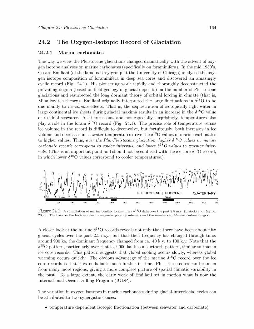
Chapter 24: Pleistocene Glaciation 164
24.2 The Oxygen-Isotopic Record of Glaciation
24.2.1 Marine carbonates
The way we view the Pleistocene glaciations changed dramatically with the advent of oxy-gen isotope analyses on marine carbonates (specifically on foraminifera). In the mid 1950’s,Cesare Emiliani (of the famous Urey group at the University of Chicago) analysed the oxy-gen isotope composition of foraminifera in deep sea cores and discovered an amazinglycyclic record (Fig. 24.1). His pioneering work rapidly and thoroughly deconstructed theprevailing dogma (based on field geology of glacial deposits) on the number of Pleistoceneglaciations and resurrected the long dormant theory of orbital forcing in climate (that is,Milankovitch theory). Emiliani originally interpreted the large fluctuations in δ18O to bedue mainly to ice-volume effects. That is, the sequestration of isotopically light water inlarge continental ice sheets during glacial maxima results in an increase in the δ18O valueof residual seawater. As it turns out, and not especially surprisingly, temperatures alsoplay a role in the foram δ18O record (Fig. 24.1). The precise role of temperature versusice volume in the record is difficult to deconvolve, but fortuitously, both increases in icevolume and decreases in seawater temperatures drive the δ18O values of marine carbonatesto higher values. Thus, over the Plio-Pleistocene glaciation, higher δ18O values in marinecarbonate records correspond to colder intervals, and lower δ18O values to warmer inter-vals. (This is an important point and should not be confused with the ice core δ18O record,in which lower δ18O values correspond to cooler temperatures.)
Figure 24.1: A compilation of marine benthic foraminifera δ18O data over the past 2.5 m.y. (Lisiecki and Raymo,2005). The bars on the bottom refer to magnetic polarity intervals and the numbers to Marine Isotope Stages.
A closer look at the marine δ18O records reveals not only that there have been about fiftyglacial cycles over the past 2.5 m.y., but that their frequency has changed through time:around 900 ka, the dominant frequency changed from ca. 40 k.y. to 100 k.y. Note that theδ18O pattern, particularly over that last 900 ka, has a sawtooth pattern, similar to that inice core records. This pattern suggests that global cooling occurs slowly, whereas globalwarming occurs quickly. The obvious advantage of the marine δ18O record over the icecore records is that it extends back much further in time. Plus, these cores can be takenfrom many more regions, giving a more complete picture of spatial climatic variability inthe past. To a large extent, the early work of Emiliani set in motion what is now theInternational Ocean Drilling Program (IODP).
The variation in oxygen isotopes in marine carbonates during glacial-interglacial cycles canbe attributed to two synergistic causes:
• temperature dependent isotopic fractionation (between seawater and carbonate)
Chapter 24: Pleistocene Glaciation 165
• the ice-volume effect
24.2.2 Ice cores
Like sediment cores, ice cores provide an exceptional record of glacial interglacial cycles,beautifully showing the saw-toothed pattern and interruptions to the warming in oxygenand hydrogen isotope ratios (and many other parameters) during the deglaciations (Fig.2). However, ice core records only go back about a million years for Antarctica, and noteven 100,000 for Greenland.
One important difference in the oxygen isotope record of the waxing and waning of icesheets as seen in ice cores is the oxygen isotope ratios fluctuate much more than they do inmarine carbonates. These fluctuations are controlled mainly by temperature, and in thiscase, the lowest δ18O values correspond to the glacial maxima (so the inverse of marinecarbonates, where it is the highest δ18O that correspond to glacial maxima).
24.3 Milankovitch Cycles
As early as the early 19th century, scientists suspected that variations in Earth’s climatewere systematic and that they might be related to variations in Earth’s orbit. In the early20th century, Milutin Milankovitch both calculated past variations in solar forcing relatedto changes in Earth’s three main orbital parameters and directly linked these variations toclimate.
• Precession (∼20 ky)
• Obliquity (∼40 ky)
• Eccentricity (∼100 and 400 ky)
The answer, it turned out, was in cool northern hemisphere summers (rather than in coldwinters, which were also coupled with hot summers).
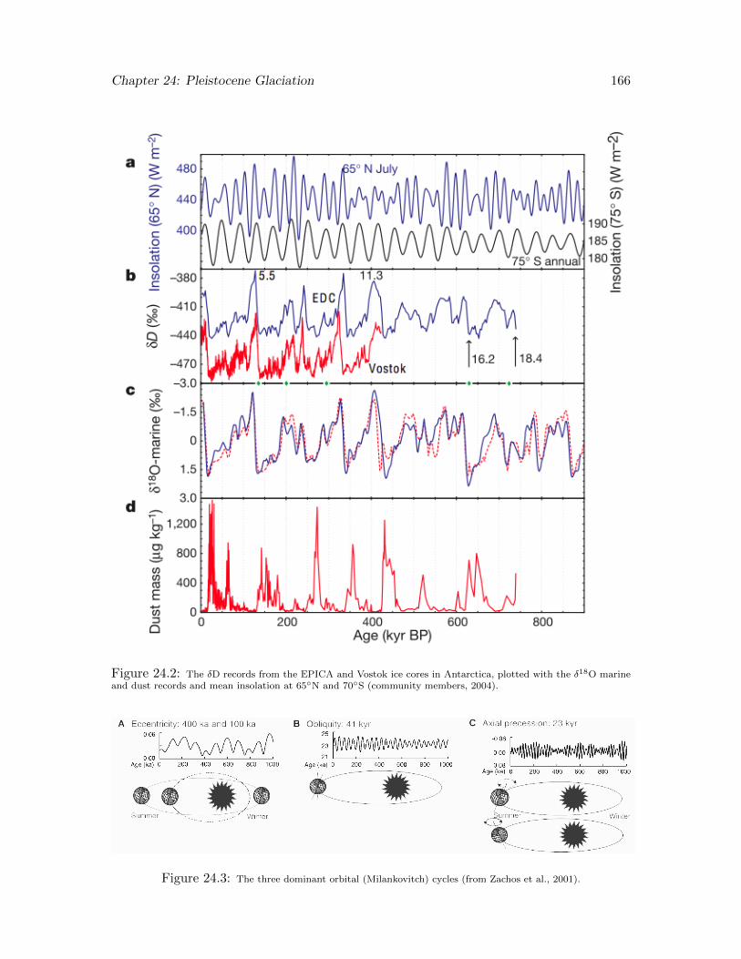
Chapter 24: Pleistocene Glaciation 166
Figure 24.2: The δD records from the EPICA and Vostok ice cores in Antarctica, plotted with the δ18O marineand dust records and mean insolation at 65◦N and 70◦S (community members, 2004).
Figure 24.3: The three dominant orbital (Milankovitch) cycles (from Zachos et al., 2001).
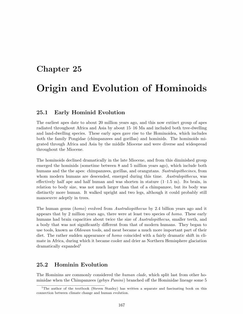
Chapter 25
Origin and Evolution of Hominoids
25.1 Early Hominid Evolution
The earliest apes date to about 20 million years ago, and this now extinct group of apesradiated throughout Africa and Asia by about 15–16 Ma and included both tree-dwellingand land-dwelling species. These early apes gave rise to the Hominoidea, which includesboth the family Pongidae (chimpanzees and gorillas) and hominids. The hominoids mi-grated through Africa and Asia by the middle Miocene and were diverse and widespreadthroughout the Miocene.
The hominoids declined dramatically in the late Miocene, and from this diminished groupemerged the hominids (sometime between 8 and 5 million years ago), which include bothhumans and the the apes: chimpanzees, gorillas, and orangutans. Sustralopithecines, fromwhom modern humans are descended, emerged during this time. Australopithecus, waseffectively half ape and half human and was shorten in stature (1–1.5 m). Its brain, inrelation to body size, was not much larger than that of a chimpanzee, but its body wasdistinctly more human. It walked upright and two legs, although it could probably stillmanoeuvre adeptly in trees.
The human genus (homo) evolved from Australiopithecus by 2.4 billion years ago and itappears that by 2 million years ago, there were at least two species of homo. These earlyhumans had brain capacities about twice the size of Australopithecus, smaller teeth, anda body that was not significantly different from that of modern humans. They began touse tools, known as Oldowan tools, and meat became a much more important part of theirdiet. The rather sudden appearance of homo coincided with a fairly dramatic shift in cli-mate in Africa, during which it became cooler and drier as Northern Hemisphere glaciationdramatically expanded1
25.2 Hominin Evolution
The Hominins are commonly considered the human clade, which split last from other ho-minidae when the Chimpanzees (gebys Panini) branched off the Hominidae lineage some 5
1The author of the textbook (Steven Stanley) has written a separate and fascinating book on thisconnection between climate change and human evolution.
167
Chapter 25: Hominoid Evolution 168
million years ago. Homo erectus was on of the early Homo species, and it closely resembledus. Two important and related difference were that its brain capacity was only about 1000cm (compared to 1200 to 1500 in modern humans), and it had narrower hips. Presumably,these narrow hips prevented it from developing a larger brain. Amazingly, it appears thatHomo erectus co-existed with other humans, including modern humans for a long time;fossils found on an isolated islands in Indonesia are dated at about 50,000–30,000 yearsold. Several other species also co-existed, including Homo heidelbergensis (700,000–200,000years ago) and Homo intercessor, which more closely resembles Homo sapiens than Homoheidelbergensis.
The Neanderthals appeared in Europe by about 200,000 years ago. These creatures wereonce thought to be a early ancestors of modern humans, but appear instead to be a sep-arate species that, based on molecular clock data, diverged from the ancestors of Homosapiens about 500,000 years ago. They did, however, co-exist with humans and lived untilabout the peak of the last ice age maximum, around 28,000 years ago. Homo sapiensappeared about 150,000 ago in Africa and had migrated into Europe by about 40,000 yearsago. This early Cro-Magnon culture incorporated diverse, specialized tools and even rathersophisticated art.
Incredible advances in the study of ancient DNA have revolutionized are understanding ofhominin evolution and co-existence over the past 200 kyr. It is now clear that there were(at least) 3 separate lineages of humans that inhabited Europe and Asia as recently as thelast Pleistocene: modern humans, Neanderthals, and the Denisovans (Prufer and 44 others,2013). The Denisovans have only been discovered recently, based on the genome sequenceof a finger bone from a cave in the Altai Mountains of Siberia! (Reich et al., 2010). TheDenisovans and Neanderthals appear to have branched from the modern human lineageabout 600 ka and from one another about 400 ka. Their DNA also suggest that theyinterbred slightly with one another and with modern humans. Interestingly, they alsoshow evidence of having interbred with a fourth, as yet unknown hominin (Fig. ??), whichmust have persisted at least until 400 ka, since this mysterious DNA does not appear withinthe Neanderthals.
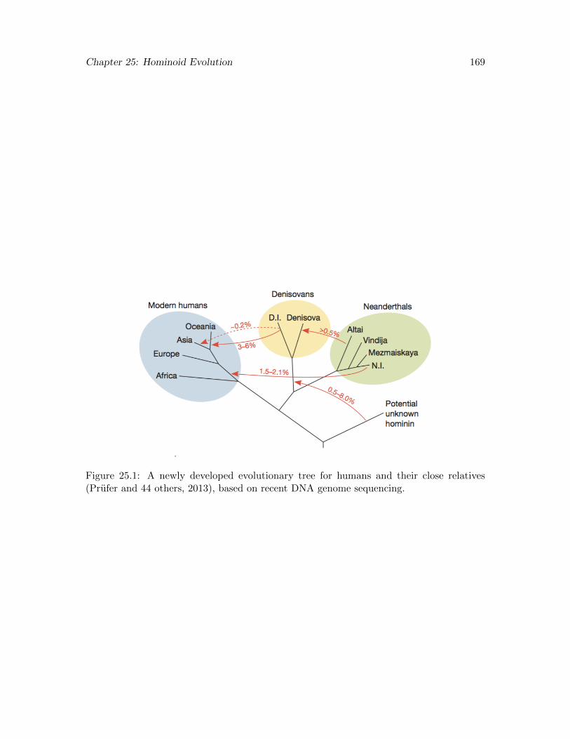
Chapter 25: Hominoid Evolution 169
Figure 25.1: A newly developed evolutionary tree for humans and their close relatives(Prufer and 44 others, 2013), based on recent DNA genome sequencing.
Bibliography
Anbar, A. D., Knoll, A. H., 2002. Proterozoic ocean chemistry and evolution: A bioinor-ganic bridge? Nature 297, 1137–1142.
Bambach, R. K., Knoll, A. H., Sepkoski, J. J., 2002. Anatomical and ecological constraintson Phanerozoic diversity in the marine realm. Proceedings of the National Academy ofSciences 99, 6854–6859.
Bedard, J. H., Brouillette, P., Madore, L., Berclaz, A., 2003. Archaean cratonization anddeformation in the northern Superior Province, Canada: an evaluation of plate tectonicversus vertical tectonic models. Precambrian Research 127, 61–87.
Bjorlykke, K., 2010. Sequence Stratigraphy, Seismic Stratigraphy and Basin Analysis.Springer-Verlag, Berlin-Heidelberg, Ch. 8, pp. 235–251.
Black, R. M., 2005. The Elements of Palaeontology. Cambridge University Press.
Bottjer, D. J., Hagadorn, J. W., Dornbos, S. Q., 2000. The Cambrian substrate revolution.GSA Today 9 (10), 1–7.
Bowring, S. A., Williams, I. S., 1999. Priscoan (4.00-4.03) orthogneisses from northwesternCanada. Contributions to Mineralogy and Petrology 134, 3–16.
Brocks, J. J., Love, G. D., Summons, R. E., Knoll, A. H., Logan, G. A., Bowden, S. A.,2005. Biomarker evidence for green and purple sulphur bacteria in a stratified palaeo-proterozoic sea. Nature 437 (7060), 866–870.
Butterfield, N., 2009. Oxygen, animals and oceanic ventilation: an alternative view. Geo-biology 7, 1–7.
Canfield, D. E., Farquhar, J., 2009. Animal evolution, bioturbation, and the sulfate concen-tration of the oceans . Proceedings of the National Academy of Sciences 106, 8123–8127.
Canfield, D. E., Teske, A., 1996. Late Proterozoic rise in atmospheric oxygen concentrationinferred from phylogenetic and sulphur-isotope studies. Nature 382, 127–132.
Caron, J.-B., Scheltema, A., Schander, C., Rudkin, D., 2006. A soft-bodied mollusc withradula from the middle cambrian burgess shale. Nature 442 (7099), 159–163.
Catling, D. C., Claire, M. W., 2005. How earth’s atmosphere evolved to an oxic state: astatus report. Earth and Planetary Science Letters 237 (1), 1–20.
Clayton, R. N., Mayeda, T. K., 1996. Oxygen isotope studies of achondrites. Geochimicaet Cosmochimica Acta 60, 1999–2017.
170
Chapter 25: Hominoid Evolution 171
Cohen, P. A., Knoll, A. H., Kodner, R. B., 2009. Large spinose microfossils in Ediacaranrocks as resting stages of early animals. Proceedings of the National Academy of Sciences106 (6519-6524).
community members, E., 2004. Eight glacial cycles from an Antarctic ice core. Nature,623–628.
Davidson, E. H., Erwin, D. H., 2006. Gene regulatory networks and the evolution of animalbody plans. Science 311, 796–800.
Dhuime, B., Hawkesworth, C. J., Cawood, P. A., Storey, C. D., 2012. Achange in thegeodynamics of continental growth 3 billion years ago. Science 335, 1334–1336.
Ernst, R. E., 2007. Large igenous provinces in Canada through time and their metallogenicpotential. In: Goodfellow, W. D. (Ed.), Mineral Deposits of Canada: A Synthesis ofMajor Deposit-Types, District Metallogeny, the Evolution of Geological Provinces, andExploration Methods. Geological Association of Canada, pp. 929–937.
Ernst, R. E., Wingate, M. T. D., Buchan, K. L., Li, Z. X., 2008. Global record fo 1600–700Ma Large Igneous Provinces (LIPs): Implications for the reconstruction of hte proposedNuna (Columbia) and Rodinia supercontinents. Precambrian Research 160, 159–178.
Erwin, D. H., LaFlamme, M., Tweedt, S. M., Sperling, E. A., Pisani, D., Peterson, K. J.,2011. The Cambrian conundrum: Early divergence and later ecological success in theearly history of animals. Science 334, 1091–1097.
Farquhar, J., Bao, H., Thiemens, M., 2000. Atmospheric influence of earth’s earliest sulfurcycle. Science 289 (5480), 756–758.
Farquhar, J., Peters, M., Johnston, D. T., Strauss, H., Masterson, A., Wiechert, U., Kauf-man, A. J., 2007. Isotopic evidence for Mesoarchaean anoxia and changing atmosphericsulphur chemistry. Nature 449, 706–710.
Gehling, J. G., 1999. Microbial mats in Terminal Proterozoic siliciclastics: Ediacaran deathmasks. Palaios 14, 40–57.
Gradstein, F. M., Ogg, J. G., Schmitz, M. D., Ogg, G. M., 2012. The Geological TimeScale 2012. Elsevier.
Grey, K., Walter, M., Calver, C., 2003. Neoproterozoic biotic diversification: SnowballEarth or aftermath of the Acraman impact. Geology 31, 459–462.
Grotzinger, J. P., Knoll, A. H., 1999. Stromatolites in Precambrian carbonates: Evolu-tionary mileposts or environmental dipsticks? Annual Review of Earth and PlanetarySciences 27, 313–358.
Halverson, G. P., in press. Seawater Sr curve. In: Rink, W. J., Thompson, J., Jull, A. J. T.,Paces, J. B., Heaman, L. (Eds.), Encyclopedia of Scientific Dating Techniques. Springer.
Hildebrand, R. S., 2014. Geology, mantle tomography, and inclination corrected paleogeo-graphic trajectories support westward subduction during Cretaceous orogenesis in theNorth American Cordillera. Geoscience Canada, 10.12789/geocanj.2014.41.032.

Chapter 25: Hominoid Evolution 172
Johnston, S. T., 2001. The Great Alaskan Terrane Wreck: reconciliation of paleomagneticand geological data in the northern Cordillera. Earth and Planetary Science Letters 193,259–272.
Kirschvink, J. L., Gaidos, E. J., Bertani, L. E., Beukes, N. J., Gutzmer, J., Maepa, L. N.,Steinberger, R. E., 2000. Paleoproterozoic snowball earth: extreme climatic and geo-chemical global change and its biological consequences. Proceedings of the NationalAcademy of Sciences 97 (4), 1400–1405.
Knoll, A. H., 2003. Life on a Young Planet: The First Three Billion Years of Evolution onEarth. Princeton University Press.
Knoll, A. H., Bambach, R. K., Payne, J. L., Pruss, S., Fischer, W. W., 2007. Paleo-physiology and end-Permian mass extinction. Earth and Planetary Science Letters 256,295–313.
Knoll, A. H., Carroll, S. B., 1999. Early animal evolution: Emerging views from compara-tive biology and geology. Science 284, 2129–2137.
Knoll, A. H., Javaux, E. J., Hewitt, D., Cohen, P., 2006a. Eukaryotic organisms in Protero-zoic oceans. Philosophical Transactions of the Royal Society of London 361, 1023–1038.
Knoll, A. H., Walter, M. R., Narbonne, G. M., Christie-Blick, N., 2006b. The Edi-acaran Period: a new addition to the geologic time scale. Lethaia 39, 13–30,10.1080/00241160500409223.
Kopp, R. E., Kirschvink, J. L., Hilburn, I. A., Nash, C. Z., 2005. The paleoproterozoicsnowball earth: a climate disaster triggered by the evolution of oxygenic photosynthe-sis. Proceedings of the National Academy of Sciences of the United States of America102 (32), 11131–11136.
Kump, L. R., Barley, M. E., 2007. Increased subaerial volcanism and the rise of atmosphericoxygen 2.5 billion years ago. Nature 448 (7157), 1033–1036.
LaMaskin, T. A., 2012. Detrital zircon facies of cordilleran terranes in western north amer-ica. GSA Today 22 (3), 4–11.
Levander, A., Schmandt, B., Miller, M., Liu, K., Karlstrom, K., Crow, R., Lee, C.-T.,Humphreys, E., 2011. Continuing colorado plateau uplift by delamination-style convec-tive lithospheric downwelling. Nature 472 (7344), 461–465.
Levin, H., 2013. The Earth Through Time. Wiley.
Li, Z., Bogdanova, S. V., Collins, A. S., Davidson, A., Waele, B. D., Ernst, R. E., Fitzi-mons, I. C. W., Fuck, R. A., Gladkochub, D. P., Jacobs, J., Karlstrom, K. E., Lu, S.,Natapov, L. M., Pease, V., Pisarevsky, S. A., Thrane, K., Vernikovsky, V., 2008. Assem-bly, configuration, and break-up history of Rodinia: a synthesis. Precambrian Research160, 179–210.
Lisiecki, L., Raymo, M., 2005. A pliocene-pleistocene stack of 57 globally distributed ben-thic d18O records. Paleoceanography 20, 1003.
Chapter 25: Hominoid Evolution 173
Morris, S. C., Caron, J.-B., 2007. Halwaxiids and the early evolution of the lophotro-chozoans. Science 315 (5816), 1255–1258.
Narbonnne, G. M., Gehling, J. G., 2003. Life after snowball: The oldest complex Ediacaranfossils. Geology 31, 27–30.
Ogg, J. G., 2012. Geomagnetic polarity time scale. In: Gradstein, F. M., Ogg, J. G.,Schmitz, M. D., Ogg, G. M. (Eds.), The Geological Time Scale 2012. Elsevier, pp. 85–113.
O’Neil, J., Carlson, R. W., Francis, D., Stevenson, R. K., 2008. Neodymium-142 evidencefor Hadean mafic crust. Science 321, 1828–1831.
Paniello, R. C., Day, J. M. D., Moynier, F., 2012. Zinc isotopic evidence for the origin ofthe Moon. nature 490, 376–379.
Partin, C. A., Bekker, A., Planovsky, N. J., Scott, C. T., Gill, B. C., Li, C., Podkovyrov,V., Maslov, A., Konhauser, K. O., Lalonde, S. V., Love, G. D., Poulton, S. W., Lyons,T. W., 2013. Large-scale fluctuations in Precambrian atmospheric and oceanic oxygenlevels from the record of U in shales. Earth and Planetary Science Letters 369, 284–293.
Pavlov, A., Kasting, J., 2002. Mass-independent fractionation of sulfur isotopes in archeansediments: strong evidence for an anoxic archean atmosphere. Astrobiology 2 (1), 27–41.
Peng, S., Babcock, L., Cooper, R., 2012. The cambrian period. The Geologic Time Scale2, 437–488.
Planavsky, N. J., Bekker, A., Hofmann, A., Owens, J. D., Lyons, T. W., 2012. Sulfurrecord of rising and falling marine oxygen and sulfate levels during the lomagundi event.Proceedings of the National Academy of Sciences 109 (45), 18300–18305.
Planavsky, N. J., McGoldrick, P., Scott, C. T., Li, C., Reinhard, C. T., Kelly, A. E., Chu,X., Bekker, A., Love, G. D., Lyons, T. W., 2011. Widespread iron-rich conditions in themid-proterozoic ocean. Nature 477 (7365), 448–451.
Porter, S. M., 2007. Seawater chemistry and early carbonate biomeralization. Science 316,1302.
Prufer, K., 44 others, 2013. The complete genome sequence of a Neanderthal from the AltaiMountains. Nature, doi:10.1038/nature12886.
Rasmussen, B., Bekker, A., Fletcher, I. R., 2013. Correlation of Paleoproterozoic glaciationsbased on U–Pb zircon ages for tuff beds in the Transvaal and Huronian Supergroups.Earth and Planetary Science Letters 382, 173–180.
Reich, D., Green, R. E., Kircher, M., Krause, J., Patterson, N., Durand, E. Y., Viola, B.,Briggs, A. W., Stenzel, U., Johnson, P. L., et al., 2010. Genetic history of an archaichominin group from denisova cave in siberia. Nature 468 (7327), 1053–1060.
Reinhard, C. T., Planavsky, N. J., Robbins, L. J., Partin, C. A., Gill, B. C., Lalonde,S. V., Bekker, A., Konhauser, K. O., Lyons, T. W., 2013. Proterozoic ocean redox andbiogeochemical stasis. Proceedings of the National Academy of Sciences 110 (14), 5357–5362.

Chapter 25: Hominoid Evolution 174
Seilacher, A., Grazhdankin, D., Legouta, A., 2003. Ediacaran biota: the dawn of animallife in the shadow of giant protists. Paleontological Research 7 (1), 43–54.
Sepkoski, J. J., 1981. A factor analytial description of the Phanerozoic marine fossil record.Paleobiology 7, 36–53.
Shen, Y., Knoll, A. H., Walter, M. R., 2003. Evidence for low sulphate and anoxia in amid-Proterozoic marine basin. Nature 423, 632–635.
Sperling, E., Pisani, D., Peterson, K., 2007. Poriferan paraphyly and its implications forPrecambrian palaeobiology. In: Vickers-Rich, P., Komarower, P. (Eds.), The Rise andFall of the Ediacaran Biota. Vol. 286 of Special Publications. Geological Society, London,London, pp. 355–368.
Sperling, E. A., Halverson, G. P., Knoll, A. H., Macdonald, F. A., Johnston, D. T., 2013.A basin redox transect at the dawn of animal life. Earth and Planetary Science Letters371-372, 143–155.
Taylor, S. R., McLennan, S. M., 1985. The continental crust: its composition and evolution.Blackwell.
Vajda, V., Raine, J. I., Hollis, C. J., 2001. Indication of global deforestation at theCretaceous-Tertiary boundary by New Zealand fern spike. Science 295, 1700–1702.
Wilde, S. A., Valley, J. W., Peck, W. H., Graham, C. M., 2001. Evidence from detritalzircons for the existence of continental crust and oceans on the Earth 4.4 Gyr ago. Nature409, 175–178.
Young, G. M., von Brunn, V., Gold, D. J. C., Minter, W. E. L., 1998. Earth’s OldestReported Glaciation: Physical and Chemical Evidence from the Archean Mozaan Group(∼2.9 Ga) of South Africa. The Journal of Geology 106, 523–538.
Zachos, J., Pagani, M., Sloan, L., Thomas, F., Billups, K., 2001. Trends, rhythms, andaberrations in global climate 65 Ma to present. Science 292, 686–693.
Zachos, J. C., Dickens, G. R., Zeebe, R. E., 2008. An early Cenozoic perspective on green-house warming and carbon-cycle dynamics. Nature, 279–283.