Environmental Fate, Aquatic Toxicology and Risk Assessmentof Polymeric Quaternary Ammonium Salts from CosmeticUses

Author

Cumming, Janet L

Published

2008

Thesis Type

Thesis (PhD Doctorate)

School

School of Environment

DOI

https://doi.org/10.25904/1912/2683

Copyright Statement

The author owns the copyright in this thesis, unless stated otherwise.

Downloaded from

http://hdl.handle.net/10072/365855

Griffith Research Online

https://research-repository.griffith.edu.au

Environmental Fate, Aquatic Toxicology and Risk Assessment of Polymeric Quaternary Ammonium Salts from Cosmetic Uses.

Janet L. Cumming B.Sc. (Hons)

Submitted in fulfilment of the requirements of the degree of Doctor of Philosophy

Griffith School of Environment Science, Environment, Engineering and Technology Group

Griffith University

February 2008

Removal Notice

Figure 2.5 (p. 34) has been removed from the digital version of this thesis for copyright reasons. Figure 3.3 (p. 61) has been removed from the digital version of this thesis for copyright reasons. Figures 3.4 & 3.5 (p. 62) have been removed from the digital version of this thesis for copyright reasons.

ii

Synopsis The consumption of household and personal care products in Australia is similar to

that of more highly regulated agricultural and veterinary chemicals. One class of

chemical used in cosmetic applications, polymeric quaternary ammonium salts

(polyquaterniums), is thought to have adverse effects on aquatic organisms. These

polymers belong to a larger class of polymers, cationic polyelectrolytes, that are

widely used in industry, largely for water treatment, and that have been extensively

studied and regulated. The cosmetic polyquaterniums, however, have not been subject

to the same scrutiny, even though differences in, or expectations of, their behaviour

are known to exist.

The aim of this study was to examine the fate and toxicity of some cosmetic

polyquaterniums, and particularly to examine the impact of the presence of the

anionic surfactant, sodium dodecyl sulphate, that is often complexed with the

polyquaterniums in cosmetic formulations on fate and toxicity. The polyquaterniums

studied consisted of six samples of Polyquaternium-10 of provided by Amerchol (The

Dow Chemical Company, Midland, MI U.S.A.), five samples of three

polyquaterniums (Polyquaternium-11, Polyquaternium-28, Polyquaternium-55)

provided by International Specialty Products (ISP, Wayne, New Jersey, USA), and

polydimethyldiallyl ammonium chloride (poly(DADMAC), Polyquaternium-6),

widely used in water treatment but less commonly in cosmetic applications purchased

from Sigma-Aldrich (Castle Hill, NSW, Australia). The four-step risk assessment

paradigm (hazard identification, exposure assessment, hazard assessment, risk

characterisation) provided the framework for this study.

Metachromatic polyelectrolyte titration was used to analyse polyquaterniums in

aqueous solution. Although the method is generally not viable in the presence of other

ions due to interference, it was found to be viable in the presence of the anionic

surfactant sodium dodecyl sulphate. Further, the method was found to work with the

supernatant following a sorption experiment involving humic acid. It was not possible

to titrate solutions following exposure to bentonite, or in solutions prepared for

toxicity tests. Metachromatic Colloid Titration was found to be useful in determining

the charge density of the polyquaterniums, and in measuring the concentration of

polyquaterniums of known charge density.

iii

To establish the extent of exposure of vulnerable aquatic organisms to

polyquaterniums released from cosmetic usage, it is necessary to estimate the

concentration of polyquaterniums in the aquatic environment. The volume usage of

polyquaterniums was estimated from available published data and standard emission

scenarios used in the risk assessment of new and existing chemicals. The partitioning

of the polyquaternium from the aqueous to the biosolid phase from wastewater

treatment plants was estimated from the determination of the partition coefficient

between water and humic acid. The latter was assumed to be a suitable surrogate for

the biosolids. The fate of polyquaterniums in wastewater treatment plants was

modelled using a fugacity approach based on a typical wastewater treatment plant.

The import/manufacture volume of polyquaterniums for cosmetic uses was estimated

to be between 20 and 60 tonnes per annum. The partition coefficient for

polyquaterniums between the aqueous phase and humic acid was lower than expected,

generally between 100 and 1000 for the polyquaterniums in this study. Fugacity

modelling results suggested that the partitioning of polyquaterniums to the solid phase

in wastewater treatment may be less than the default values normally assumed in

regulatory risk assessment. Therefore, the estimate of the predicted environmental

concentration (PEC) of polyquaterniums in Australian waters is between 0.7 µg/L and

40 µg/L depending on the assumptions and methodology used.

Effects assessment, or hazard assessment, is concerned with determining the capacity

of the cosmetic polyquaterniums to cause harm to aquatic organisms in the

environment. In this study, the aim was to determine if the hazard of the

polyquaternium from cosmetic usage is the same as that of the better studied water

treatment polymers; and if the complexing of the polyquaternium with the anionic

surfactant makes any difference to the toxicity. One species from each of three trophic

levels, viz fish, crustacean and algae were selected. Using assessment factors

developed for the risk assessment of new chemicals, the environmental concentration

likely to be hazardous to the most sensitive species was estimated. The

polyquaterniums studied were found to be just as hazardous to the most sensitive

species for a typical cosmetic polyquaternium when complexed with the anionic

surfactant. The lowest concentration at which a toxic effect occurred was for 50%

growth inhibition for algae, 0.3 mg/L for the most toxic polyquaternium. With

assessment factors, and using the concentration at which cosmetic polyquaterniums

iv

were likely to be hazardous to aquatic organisms, the predicted no effect

concentration (PNEC) was estimated to be between 0.3 µg/L and 1.2 µg/L.

The risk characterisation process combines the information obtained from the effects

and exposure assessments to evaluate the nature of the potential risk. Commonly, the

level of risk is estimated based on the PEC/PNEC ratio. In this study, using point

estimates and probabilistic methods (Monte Carlo Simulation), the risk of

polyquaterniums from cosmetic uses was estimated. Based on the behaviour and

toxicity determined in this study, there may be some risk to aquatic organisms from

individual polyquaterniums at even low import volumes. As a class of compounds,

polyquaterniums from cosmetic uses may present a significant risk to environmental

waters in Australia. Sensitivity analysis showed that the prediction of risk was most

sensitive to those parameters for which the least amount of data was available, such as

the import volume and dilution to receiving waters.

A recently developed method of estimating potential risk based on the concept of an

Environmental Threshold of No Concern (ETNC), was applied to the use of cosmetic

polyquaterniums in Australia. Using the fugacity model approach, the usage volume

at which the environmental concentration would exceed the critical threshold was

estimated. The volume was found to be significantly lower than the estimated usage

determined by either of the methods employed in estimating the current usage

volume.

While some problems remain in identifying the risk from polyquaterniums to the

Australian environment, particularly those associated with the difficulties of

quantifying polymers in environmental samples, this thesis has made substantial

progress in the risk assessment. Particularly, it has been shown that the use of default

assumptions that are largely unsubstantiated, and the sensitivity of the methodology to

information that is often unavailable, may result in an estimation of risk that may not

be able to protect vulnerable environments.

v

Acknowledgements This work was supported by the Society of Environmental Toxicology and Chemistry (SETAC)/Procter & Gamble Company Global Fellowship for Doctoral Research in Environmental Science, sponsored by the Procter & Gamble Company. I would like to thank my supervisors, Dr Darryl Hawker, Dr Heather Chapman and Dr Kerry Nugent for their guidance, support and encouragement through all aspects of my candidature. Thank you to the technical and support staff at the Griffith School of Environment, particularly Scott Byrnes and Jane Gifkin for their assistance and support in the laboratory. Thank you to my research assistant, Melanie Crook, for many dedicated hours in the field and the laboratory; Alan and Joyce Hodder for access to their property for collecting Gambusia; and the undergrad students who helped sort the blighters. I would like to acknowledge the CRC for Water Quality and Treatment and the Centre for Environmental Systems Research for financial support and encouragement. Also important were Jenny Stauber and her team at CSIRO for their endeavours in teaching me algal toxicity testing. I am especially grateful to SETAC and Procter & Gamble, whose support made a significant contribution to this research, which might have been barely possible otherwise. Thank you to Fiona de Mestre for the final editing. I would like to thank my fellow candidates at Griffith School of Environment; the friendship and encouragement of peers is invaluable. Finally, a special thank you to my family – my sister Alison, my daughters Jeanne and Heather, their father Fred, and my niece Darcy; with their love and support, anything is possible.

vi

Dedicated to

Alyssa Lenore Hannaford

(8/7/1989 to 16/9/2003)

and

Michael Thomas Wakeham

(8/10/1989 to 9/4/2007)

vii

Declaration of Originality

The experimentation, analysis, presentation and interpretation of results presented in this thesis represent my original work and have not previously been submitted for a degree or diploma in any university. To the best of my knowledge and belief, the thesis contains no material previously published or written by another person except where due reference is made in the thesis itself.

Janet L. Cumming

Publications arising from this work Cumming, J.L. 2007 ‘Polyelectrolytes’. in Chemicals of Concern in Wastewater Treatment Plant Effluent. CRC for Water Quality and Treatment Occasional Paper No 8. Cooperative Research Centre for Water Quality and Treatment, Adelaide.

Cumming, J.L, Hawker D.W., Nugent, K.W. and Chapman, H.F. 2008 Ecotoxicities of Polyquaterniums and their associated polyelectrolyte surfactant aggregates (PSA) to Gambusia holbrooki. Journal of Environmental Science and Health, Part A Toxic/Hazardous Substances and Environmental Engineering, Volume 43 Issue 2, 113

Cumming, J.L, Hawker D.W., Nugent, K.W. and Chapman, H.F. 2006 Toxicity of cosmetic polyquaterniums to Gambusia holbrooki. Oral Presentation, SETAC Asia Pacific, Beijing.

Janet Cumming, 2006 Environmental Fate and Aquatic Toxicology of Polymeric Quaternary Ammonium Salts. Oral Presentation, CRCWQT Postgraduate Students Conference, Melbourne, July 2006.

Janet Cumming, Darryl Hawker, Heather Chapman. 2005 Mitigation of Toxicity of Quaternary Polyelectrolytes – Fact or Fiction? Oral Presentation, Australian Society for Ecotoxicology Conference, Melbourne. Cumming, J.L. Hawker D.W and Chapman, H.F 2005 Polyquaternium Ammonium Salts: Using data obtained in the study of water treatment polyelectrolytes in the risk assessment of cosmetic polymers. Presentation and Paper (peer reviewed) Australian Water Association Contaminants of Concern Conference, Canberra.

viii

Table of Contents Synopsis .....................................................................................................................ii Acknowledgements....................................................................................................v Declaration of Originality ........................................................................................vii Publications arising from this work .........................................................................vii Table of Contents......................................................................................................xi List of Tables ..........................................................................................................xiv List of Figures ...................................................................................................... xviii Abbreviations..........................................................................................................xix Definitions..............................................................................................................xxii

1. Introduction............................................................................................................1 1.1. Non-cosmetic Uses of Polyquaterniums........................................................3 1.2. Regulation of Chemicals in Australia ............................................................7 1.3. The Risk Assessment Framework................................................................11

1.3.1. Hazard Identification ...........................................................................12 1.3.2. Effects Assessment ..............................................................................13 1.3.3. Exposure Assessment...........................................................................13 1.3.4. Risk Characterisation ...........................................................................13 1.3.5. Assessment Reports .............................................................................14 1.3.6. Data Requirements...............................................................................14 1.3.7. Globally Harmonised Labelling...........................................................15 1.3.8. GHS and the Aquatic Environment .....................................................16

1.4. Conclusion ...................................................................................................17 1.4.1. Aims.....................................................................................................18 1.4.2. Structure...............................................................................................18

2. Literature Review.................................................................................................19 2.1. Structure of Polyquaterniums ......................................................................19

2.1.1. Quaternary Ammonium Salts ..............................................................19 2.1.2. Polymers ..............................................................................................19 2.1.3. Polyelectrolytes....................................................................................20 2.1.4. Common Features of Polyquaterniums................................................20 2.1.5. Variation Between Polyquaterniums ...................................................21 2.1.6. Variation Within Polyelectrolytes........................................................23

2.2. Nomenclature...............................................................................................24 2.3. Relevant Polyquaternium Physical-Chemical Properties ............................24

2.3.1. Molecular Weight Distribution ............................................................25 2.3.2. Charge Density.....................................................................................27 2.3.3. Aqueous Solubility...............................................................................29 2.3.4. Biodegradation.....................................................................................31 2.3.5. Chemical/physical Degradation ...........................................................32

2.4. Exposure Assessment (Environmental Fate) ...............................................33 2.4.1. Sorption-desorption..............................................................................33 2.4.2. Sorption of Polymers ...........................................................................33 2.4.3. Sorption of Polyelectrolytes.................................................................35

2.5. Effects Assessment (Aquatic Toxicology)...................................................40 2.5.1. Toxicity of Surfactants.........................................................................40 2.5.2. Toxicity of Polymers............................................................................41 2.5.3. Toxicity of Polyelectrolytes – General Considerations .......................41 2.5.4. Meta-analysis .......................................................................................46 2.5.5. Mechanism...........................................................................................51

ix

2.6. Conclusion ...................................................................................................53 3. Analysis of Polyquaterniums ...............................................................................55

3.1. Introduction..................................................................................................55 3.1.1. Metachromasy......................................................................................56 3.1.2. Colloid Titration...................................................................................56

3.2. Metachromatic Polyelectrolyte Titration .....................................................57 3.2.1. The Titrant – Choice of Chromotropic Polyanion and Cationic

Standard ...............................................................................................58 3.2.2. The Indicator – Choice of Metachromatic Dye ...................................58 3.2.3. Determination of The Visual Endpoint................................................59 3.2.4. Determination of the Endpoint Using Spectrophotometry ..................59 3.2.5. Calculations – Determining Charge Density and/or Concentration ....62 3.2.6. Method Validation ...............................................................................63 3.2.7. Problems and Limitations ....................................................................63 3.2.8. Aims and Objectives ............................................................................65

3.3. Analytical Methods......................................................................................65 3.3.1. Materials ..............................................................................................65 3.3.2. Standardisation of PVSK .....................................................................68 3.3.3. Titration of Polyquaternium Solutions (Visual Endpoint)...................68 3.3.4. Charge Density Determination of Polyquaterniums (Preparation of the

Standard Curve) ...................................................................................69 3.3.5. Titration (Spectrophotometric Endpoint).............................................70

3.4. Results..........................................................................................................71 3.4.1. PVSK ...................................................................................................71 3.4.2. Analysis of Results for Equivalent Weight..........................................72 3.4.3. Titration in the Presence of SDS..........................................................74 3.4.4. Titration (Spectrophotometric Endpoint).............................................74

3.5. Discussion ....................................................................................................76 3.6. Conclusion ...................................................................................................79

4. Chemistry and Fate – Exposure Assessment of Polyquaterniums.......................81 4.1. Introduction..................................................................................................81 4.2. Use patterns and release data .......................................................................82

4.2.1. Emission Scenarios ..............................................................................86 4.3. Environmental Fate......................................................................................87

4.3.1. Partitioning...........................................................................................87 4.3.2. Methods................................................................................................88 4.3.3. Results..................................................................................................90 4.3.4. Discussion ............................................................................................93

4.4. Fate Modelling .............................................................................................96 4.4.1. Partitioning Models..............................................................................96 4.4.2. Model Parameters ................................................................................98 4.4.3. Predicting Extent of Removal of Polyquaternium. ............................100 4.4.4. Results................................................................................................106 4.4.5. Discussion ..........................................................................................107

4.5. Predicted Environmental Concentration ....................................................108 4.6. Conclusion .................................................................................................112

5. Aquatic Toxicology – Effects Assessment of Polyquaterniums........................113 5.1. Introduction................................................................................................113 5.2. Methods......................................................................................................115

5.2.1. Experimental Design..........................................................................115

x

5.2.2. Test Solutions.....................................................................................116 5.2.3. Fish.....................................................................................................116 5.2.4. Brine Shrimp......................................................................................120 5.2.5. Algae ..................................................................................................121

5.3. Results, Observations and Data Analysis ..................................................122 5.3.1. Fish.....................................................................................................122 5.3.2. Brine Shrimp......................................................................................127 5.3.3. Algae ..................................................................................................128

5.4. Discussion ..................................................................................................129 5.4.1. Charge Density...................................................................................133 5.4.2. Polymer-surfactant Complex .............................................................136 5.4.3. Humic Acid........................................................................................137

5.5. PNEC .........................................................................................................139 5.6. Conclusions................................................................................................141

6. Risk Characterisation .........................................................................................142 6.1. Introduction................................................................................................142

6.1.1. Monte Carlo Simulation.....................................................................145 6.2. The Environmental Threshold of No Concern Method .............................146

6.2.1. Method ...............................................................................................147 6.2.2. Results................................................................................................152

6.3. The PEC/PNEC Ratio (The Quotient Method)..........................................154 6.3.1. Method ...............................................................................................155 6.3.2. Results................................................................................................156

6.4. Probabilistic Risk Characterisation............................................................158 6.4.1. Method ...............................................................................................158 6.4.2. Results................................................................................................162

6.5. Discussion ..................................................................................................165 6.5.1. Is This Risk? ......................................................................................165 6.5.2. Uncertainty in PNEC and PEC ..........................................................169 6.5.3. Conservatism and Precaution.............................................................173 6.5.4. Science, Policy, Assessment and Management .................................175 6.5.5. Characterising the Risk to the Aquatic Environment from Cosmetic

Polyquaternium Use in Australia .......................................................178 6.6. Conclusion .................................................................................................181

7. Overall Conclusions and Future Research.........................................................183 7.1. Conclusions................................................................................................183

7.1.1. Analysis..............................................................................................183 7.1.2. Environmental Fate............................................................................183 7.1.3. Toxicology .........................................................................................184 7.1.4. Risk Characterisation .........................................................................185

7.2. Implications and Future Research..............................................................185 7.3. Concluding Comments...............................................................................188

List of References ......................................................................................................189 Appendix 1. Database of cosmetic polyquaterniums..................................................i

Polyquaternium-1....................................................................................................i Polyquaternium-2...................................................................................................ii Polyquaternium-4................................................................................................. iii Polyquaternium-5..................................................................................................iv Polyquaternium-6...................................................................................................v Polyquaternium-7..................................................................................................vi

xi

Polyquaternium-8.................................................................................................vii Polyquaternium-9............................................................................................... viii Polyquaternium-10................................................................................................ix Polyquaternium-11.................................................................................................x Polyquaternium-12................................................................................................xi Polyquaternium-13...............................................................................................xii Polyquaternium-14............................................................................................. xiii Polyquaternium-15/polyquaternium-32..............................................................xiv Polyquaternium-16...............................................................................................xv Polyquaternium-17..............................................................................................xvi Polyquaternium-18.............................................................................................xvii Polyquaternium-19........................................................................................... xviii Polyquaternium-20........................................................................................... xviii Polyquaternium-22..............................................................................................xix Polyquaternium-24...............................................................................................xx Polyquaternium-26...............................................................................................xx Polyquaternium-27..............................................................................................xxi Polyquaternium-28.............................................................................................xxii Polyquaternium-29........................................................................................... xxiii Polyquaternium-30........................................................................................... xxiii Polyquaternium-31............................................................................................xxiv Polyquaternium-34.............................................................................................xxv Polyquaternium-35............................................................................................xxvi Polyquaternium-37...........................................................................................xxvii Polyquaternium-39......................................................................................... xxviii Polyquaternium-42............................................................................................xxix Polyquaternium-43............................................................................................xxix Polyquaternium-44.............................................................................................xxx Polyquaternium-46............................................................................................xxxi Polyquaternium-47...........................................................................................xxxii Polyquaternium-51......................................................................................... xxxiii Polyquaternium-55..........................................................................................xxxiv Dimethylamine-epichlorohydrin copolymer....................................................xxxv Polymethacrylamidopropyltrimonium chloride..............................................xxxvi Guar hydroxypropyltrimonium chloride........................................................xxxvii Other polyquaterniums................................................................................. xxxviii

Appendix 2. Published toxicity values for Cationic Polyelectrolytes......................xli Appendix 3 Partitioning Models......................................................................... xlviii a. Percent Removal Model. ................................................................................. xlviii b. Input Flux Model. ..............................................................................................xlix

xii

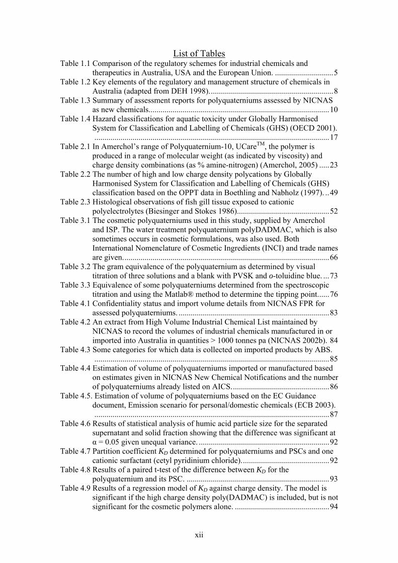
List of Tables Table 1.1 Comparison of the regulatory schemes for industrial chemicals and

therapeutics in Australia, USA and the European Union. .............................5 Table 1.2 Key elements of the regulatory and management structure of chemicals in

Australia (adapted from DEH 1998)..............................................................8 Table 1.3 Summary of assessment reports for polyquaterniums assessed by NICNAS

as new chemicals..........................................................................................10 Table 1.4 Hazard classifications for aquatic toxicity under Globally Harmonised

System for Classification and Labelling of Chemicals (GHS) (OECD 2001)......................................................................................................................17

Table 2.1 In Amerchol’s range of Polyquaternium-10, UCareTM, the polymer is produced in a range of molecular weight (as indicated by viscosity) and charge density combinations (as % amine-nitrogen) (Amerchol, 2005) .....23

Table 2.2 The number of high and low charge density polycations by Globally Harmonised System for Classification and Labelling of Chemicals (GHS) classification based on the OPPT data in Boethling and Nabholz (1997). ..49

Table 2.3 Histological observations of fish gill tissue exposed to cationic polyelectrolytes (Biesinger and Stokes 1986)..............................................52

Table 3.1 The cosmetic polyquaterniums used in this study, supplied by Amerchol and ISP. The water treatment polyquaternium polyDADMAC, which is also sometimes occurs in cosmetic formulations, was also used. Both International Nomenclature of Cosmetic Ingredients (INCI) and trade names are given.......................................................................................................66

Table 3.2 The gram equivalence of the polyquaternium as determined by visual titration of three solutions and a blank with PVSK and o-toluidine blue. ...73

Table 3.3 Equivalence of some polyquaterniums determined from the spectroscopic titration and using the Matlab® method to determine the tipping point......76

Table 4.1 Confidentiality status and import volume details from NICNAS FPR for assessed polyquaterniums. ...........................................................................83

Table 4.2 An extract from High Volume Industrial Chemical List maintained by NICNAS to record the volumes of industrial chemicals manufactured in or imported into Australia in quantities > 1000 tonnes pa (NICNAS 2002b). 84

Table 4.3 Some categories for which data is collected on imported products by ABS......................................................................................................................85

Table 4.4 Estimation of volume of polyquaterniums imported or manufactured based on estimates given in NICNAS New Chemical Notifications and the number of polyquaterniums already listed on AICS.................................................86

Table 4.5. Estimation of volume of polyquaterniums based on the EC Guidance document, Emission scenario for personal/domestic chemicals (ECB 2003)......................................................................................................................87

Table 4.6 Results of statistical analysis of humic acid particle size for the separated supernatant and solid fraction showing that the difference was significant at α = 0.05 given unequal variance. .................................................................92

Table 4.7 Partition coefficient KD determined for polyquaterniums and PSCs and one cationic surfactant (cetyl pyridinium chloride)............................................92

Table 4.8 Results of a paired t-test of the difference between KD for the polyquaternium and its PSC. .......................................................................93

Table 4.9 Results of a regression model of KD against charge density. The model is significant if the high charge density poly(DADMAC) is included, but is not significant for the cosmetic polymers alone. ...............................................94

xiii

Table 4.10 Results of model calculation for proportion of influent polyquaternium removed as a function of various values of KD and solids removal (PST only and with WAS taken into account). .................................................107

Table 4.11 Determination of PEC for environmental risk assessment using NICNAS/DEW method. ..........................................................................109

Table 4.12 Effluent discharge polyquaternium concentrations (µg/L) for a range of import volumes and WWTP removal rates..............................................109

Table 4.13 PECs of polyquaterniums for different import volumes and environmental dilution ratios (µg/L). The effluent concentration would also represent the case where there was zero dilution. .........................................................111

Table 5.1 Water parameters before and after exposure of fish to the polyquaternium of PSC for an acceptable test with G. holbrooki. ...........................................118

Table 5.2 Concentrations of polyquaterniums used in fish toxicity tests. .................119 Table 5.3 Concentration of polyquaternium as polymer-surfactant complex used in the

toxicity tests. ..............................................................................................119 Table 5.4 Concentrations of polyquaterniums, SDS and SDS as polyquaternium-

surfactant complexes used in brine shrimp tests........................................121 Table 5.5 Conditions for the culture and testing of algae. .........................................121 Table 5.6 Test concentrations of chemicals used in algal toxicity tests ....................122 Table 5.7 Result of probit analysis of data from 96 hour fish tests using G. holbrooki

with polyquaterniums and the monoquaternium cetyl pyridinium chloride without surfactant. Where more than one test has been performed, the repeat results are indicated by the letters in parenthesis.......................................125

Table 5.8 Result of probit analysis of data from 96 hour fish tests using G. holbrooki with PSC and the monoquaternium cetylpyridinium chloride and SDS. ..126

Table 5.9 Results of paired t-test for fish toxicity studies. ........................................126 Table 5.10 Results of analysis of data from algal growth inhibition test for

polyquaterniums and for the PSC for UCareTM JR125 only....................128 Table 5.11 Results of statistical test for difference in algal toxicity between the

samples of UCare JR125, JR400 and JR30M (Polyquaternium-10) and Gafquat® 440 and 734 (Polyquaternium-11). .........................................129

Table 5.12 Results of Dunnett's test for difference between test concentrations and controls in algal growth inhibition test. ...................................................129

Table 5.13 Fish Acute Toxicity Syndromes (FATS) as described by McKim et al. (1987) .......................................................................................................130

Table 5.14 Recommended assessment factors to be applied in determining the PNEC are dependent on the confidence that can be attributed to the available data, which is dependent on the amount and types of toxicity data available. .140

Table 6.1 Definitions of risk characterisation published in various guidelines and articles since the introduction of the four-step paradigm in 1983. ............143

Table 6.2 Definitions of risk published in various guidelines and articles since the introduction of the four-step paradigm in 1983. ........................................144

Table 6.3 Estimates of input volume and product usage for various ETNCaq for polyquaterniums, calculated for KD values of 400 (UCareTM JR125) and 1000 (Gafquat® 755) and 10000. ..............................................................153

Table 6.4 Analysis of the PEC/PNEC estimates in NICNAS assessments. Note that different assumptions regarding population size and water use volumes may apply in these assessments. ........................................................................156

xiv

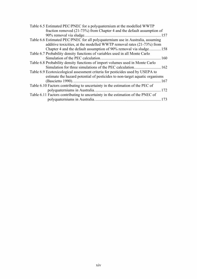
Table 6.5 Estimated PEC/PNEC for a polyquaternium at the modelled WWTP fraction removed (21-73%) from Chapter 4 and the default assumption of 90% removal via sludge.............................................................................157

Table 6.6 Estimated PEC/PNEC for all polyquaternium use in Australia, assuming additive toxicities, at the modelled WWTP removal rates (21-73%) from Chapter 4 and the default assumption of 90% removal via sludge............158

Table 6.7 Probability density functions of variables used in all Monte Carlo Simulation of the PEC calculation.............................................................160

Table 6.8 Probability density functions of import volumes used in Monte Carlo Simulation for three simulations of the PEC calculation...........................162

Table 6.9 Ecotoxicological assessment criteria for pesticides used by USEPA to estimate the hazard potential of pesticides to non-target aquatic organisms (Bascietto 1990). ........................................................................................167

Table 6.10 Factors contributing to uncertainty in the estimation of the PEC of polyquaterniums in Australia. ..................................................................172

Table 6.11 Factors contributing to uncertainty in the estimation of the PNEC of polyquaterniums in Australia. ..................................................................173

xv

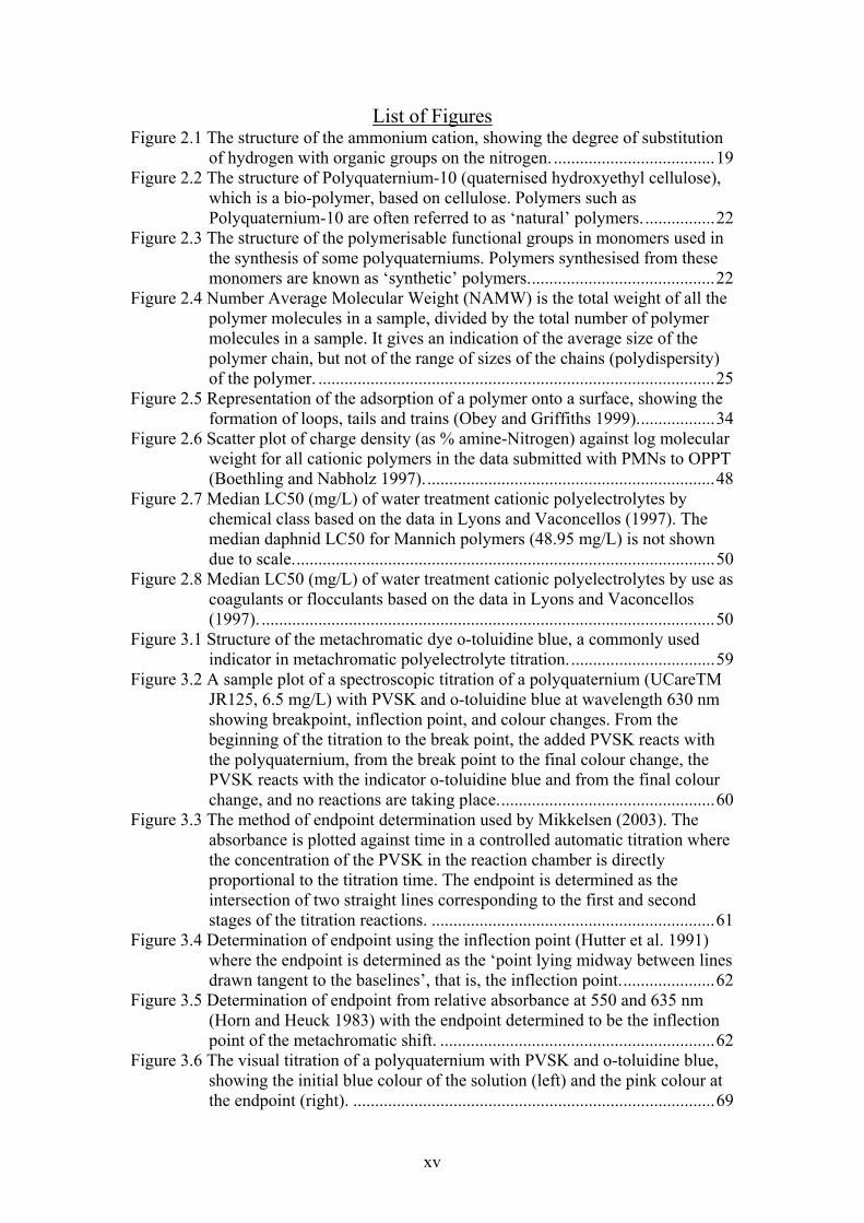
List of Figures Figure 2.1 The structure of the ammonium cation, showing the degree of substitution

of hydrogen with organic groups on the nitrogen. .....................................19 Figure 2.2 The structure of Polyquaternium-10 (quaternised hydroxyethyl cellulose),

which is a bio-polymer, based on cellulose. Polymers such as Polyquaternium-10 are often referred to as ‘natural’ polymers.................22

Figure 2.3 The structure of the polymerisable functional groups in monomers used in the synthesis of some polyquaterniums. Polymers synthesised from these monomers are known as ‘synthetic’ polymers...........................................22

Figure 2.4 Number Average Molecular Weight (NAMW) is the total weight of all the polymer molecules in a sample, divided by the total number of polymer molecules in a sample. It gives an indication of the average size of the polymer chain, but not of the range of sizes of the chains (polydispersity) of the polymer. ...........................................................................................25

Figure 2.5 Representation of the adsorption of a polymer onto a surface, showing the formation of loops, tails and trains (Obey and Griffiths 1999)..................34

Figure 2.6 Scatter plot of charge density (as % amine-Nitrogen) against log molecular weight for all cationic polymers in the data submitted with PMNs to OPPT (Boethling and Nabholz 1997)...................................................................48

Figure 2.7 Median LC50 (mg/L) of water treatment cationic polyelectrolytes by chemical class based on the data in Lyons and Vaconcellos (1997). The median daphnid LC50 for Mannich polymers (48.95 mg/L) is not shown due to scale.................................................................................................50

Figure 2.8 Median LC50 (mg/L) of water treatment cationic polyelectrolytes by use as coagulants or flocculants based on the data in Lyons and Vaconcellos (1997). ........................................................................................................50

Figure 3.1 Structure of the metachromatic dye o-toluidine blue, a commonly used indicator in metachromatic polyelectrolyte titration..................................59

Figure 3.2 A sample plot of a spectroscopic titration of a polyquaternium (UCareTM JR125, 6.5 mg/L) with PVSK and o-toluidine blue at wavelength 630 nm showing breakpoint, inflection point, and colour changes. From the beginning of the titration to the break point, the added PVSK reacts with the polyquaternium, from the break point to the final colour change, the PVSK reacts with the indicator o-toluidine blue and from the final colour change, and no reactions are taking place..................................................60

Figure 3.3 The method of endpoint determination used by Mikkelsen (2003). The absorbance is plotted against time in a controlled automatic titration where the concentration of the PVSK in the reaction chamber is directly proportional to the titration time. The endpoint is determined as the intersection of two straight lines corresponding to the first and second stages of the titration reactions. .................................................................61

Figure 3.4 Determination of endpoint using the inflection point (Hutter et al. 1991) where the endpoint is determined as the ‘point lying midway between lines drawn tangent to the baselines’, that is, the inflection point......................62

Figure 3.5 Determination of endpoint from relative absorbance at 550 and 635 nm (Horn and Heuck 1983) with the endpoint determined to be the inflection point of the metachromatic shift. ...............................................................62

Figure 3.6 The visual titration of a polyquaternium with PVSK and o-toluidine blue, showing the initial blue colour of the solution (left) and the pink colour at the endpoint (right). ...................................................................................69

xvi

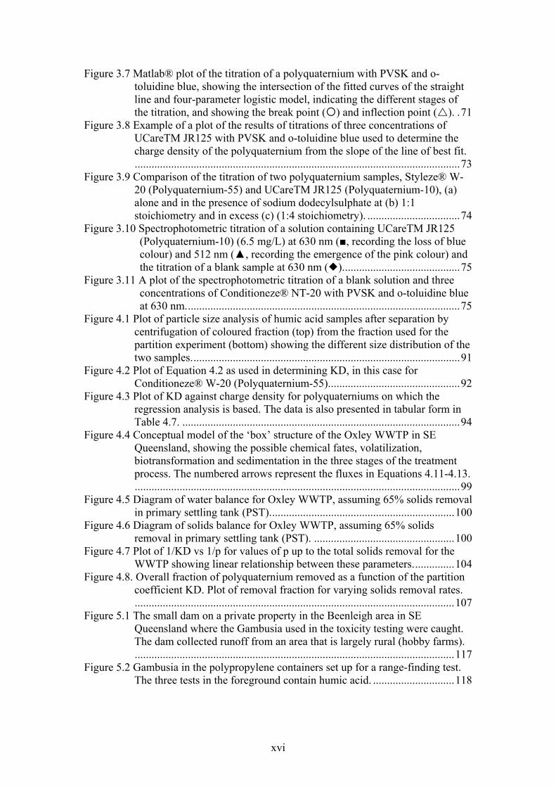
Figure 3.7 Matlab® plot of the titration of a polyquaternium with PVSK and o-toluidine blue, showing the intersection of the fitted curves of the straight line and four-parameter logistic model, indicating the different stages of the titration, and showing the break point ( ) and inflection point ( ). .71

Figure 3.8 Example of a plot of the results of titrations of three concentrations of UCareTM JR125 with PVSK and o-toluidine blue used to determine the charge density of the polyquaternium from the slope of the line of best fit.....................................................................................................................73

Figure 3.9 Comparison of the titration of two polyquaternium samples, Styleze® W-20 (Polyquaternium-55) and UCareTM JR125 (Polyquaternium-10), (a) alone and in the presence of sodium dodecylsulphate at (b) 1:1 stoichiometry and in excess (c) (1:4 stoichiometry). .................................74

Figure 3.10 Spectrophotometric titration of a solution containing UCareTM JR125 (Polyquaternium-10) (6.5 mg/L) at 630 nm (, recording the loss of blue colour) and 512 nm (, recording the emergence of the pink colour) and the titration of a blank sample at 630 nm ( )..........................................75

Figure 3.11 A plot of the spectrophotometric titration of a blank solution and three concentrations of Conditioneze® NT-20 with PVSK and o-toluidine blue at 630 nm..................................................................................................75

Figure 4.1 Plot of particle size analysis of humic acid samples after separation by centrifugation of coloured fraction (top) from the fraction used for the partition experiment (bottom) showing the different size distribution of the two samples................................................................................................91

Figure 4.2 Plot of Equation 4.2 as used in determining KD, in this case for Conditioneze® W-20 (Polyquaternium-55)...............................................92

Figure 4.3 Plot of KD against charge density for polyquaterniums on which the regression analysis is based. The data is also presented in tabular form in Table 4.7. ...................................................................................................94

Figure 4.4 Conceptual model of the ‘box’ structure of the Oxley WWTP in SE Queensland, showing the possible chemical fates, volatilization, biotransformation and sedimentation in the three stages of the treatment process. The numbered arrows represent the fluxes in Equations 4.11-4.13.....................................................................................................................99

Figure 4.5 Diagram of water balance for Oxley WWTP, assuming 65% solids removal in primary settling tank (PST)..................................................................100

Figure 4.6 Diagram of solids balance for Oxley WWTP, assuming 65% solids removal in primary settling tank (PST). ..................................................100

Figure 4.7 Plot of 1/KD vs 1/p for values of p up to the total solids removal for the WWTP showing linear relationship between these parameters...............104

Figure 4.8. Overall fraction of polyquaternium removed as a function of the partition coefficient KD. Plot of removal fraction for varying solids removal rates...................................................................................................................107

Figure 5.1 The small dam on a private property in the Beenleigh area in SE Queensland where the Gambusia used in the toxicity testing were caught. The dam collected runoff from an area that is largely rural (hobby farms)...................................................................................................................117

Figure 5.2 Gambusia in the polypropylene containers set up for a range-finding test. The three tests in the foreground contain humic acid. .............................118

xvii

Figure 5.3 Typical plots of concentration vs. mortality for two polyquaterniums, poly(DADMAC) (a) and Conditioneze® W-20 (Polyquaternium-55) (b) demonstrating the steepness of the curve in this all-or-nothing toxicity. 124

Figure 5.4 Toxicity to Artemia (% mortality) for SDS complexed with UCareTM JR125. The non-standard toxicity curves show a reduced mortality at higher concentrations of the complex. .....................................................127

Figure 5.5 Toxicity (% mortality) for SDS complexed with Gafquat® 734. The non-standard toxicity curves show a reduced mortality at higher concentrations of the complex..........................................................................................128

Figure 5.6 Plot of EC50 for fish in mass units (mg/L) against charge density (eq/g) for eight cosmetic polyquaterniums (Gafquat® 440, 734, and HS100; UCareTM JR125, JR30M, JR400; Styleze® W-20) and polyDADMAC...................................................................................................................134

Figure 5.7 Plot of EC50 for fish in equivalence units (eq/L) against charge density (eq/g) for eight cosmetic polyquaterniums (Gafquat® 440, 734, and HS100; UCareTM JR125, JR30M, JR400; Styleze® W-20) and polyDADMAC.........................................................................................135

Figure 6.1 Representation of the mass balance in the Final Settling Tank of the WWTP. ....................................................................................................149

Figure 6.2 Representation of the mass balance in the bioreactor of the WWTP. ......150 Figure 6.3 Representation of the mass balance in the Primary settling tank of the

WWTP. ....................................................................................................151 Figure 6.4 Probability density function for the input variable partition coefficient KD

used in the Monte Carlo Simulation of the ETNCaq model. ...................154 Figure 6.5 Forecast Probability Density Function (left) and sensitivity analysis (right)

for the influent flux of polyquaternium, from the Monte Carlo simulation of the ETNCaq model. .............................................................................154

Figure 6.6 Probability density functions for variables common to all simulations of probabilistic risk assessment (a) proportion of polyquaternium released to sewer; (b) water use per person; (c) proportion of polyquaternium removed in WWTP; and (d) dilution to receiving waters.......................................160

Figure 6.7 Probability density functions for input volumes for the three simulations of the PEC (a) import volume < 1000 kg; (b) import volume < 16 tonnes; and (c) estimated total import volume for all cosmetic polyquaterniums. .....161

Figure 6.8 Fish probability distribution function from data (a), and assumed for the Monte Carlo Simulation (b) .....................................................................162

Figure 6.9 Probability Density Forecast (left) and sensitivity analysis (right) from a Monte Carlo Simulation of the PEC for a polyquaternium at an import volume of < 1tonne. .................................................................................163

Figure 6.10 Probability Density Function for the PEC input into PEC/PNEC Monte Carlo Simulation for import volume < 1 tonne, a log normal distribution with mean = 0.02; stddv = 0.08..............................................................163

Figure 6.11 Probability density forecast from a Monte Carlo Simulation for the PEC/PNEC for a polyquaternium import volume of < 1 tonne .............163

Figure 6.12 Probability density forecast and sensitivity analysis from the Monte Carlo Simulation of PEC for a polyquaternium at an import volume of 16 tonnes. ....................................................................................................164

Figure 6.13 Probability Density Function for PEC input into Monte Carlo Simulation of the PEC/PNEC for import volume of < 16 tonnes, a log normal distribution with mean = 0.34; stddv = 1.13. .........................................164

xviii

Figure 6.14 Probability density forecast from a Monte Carlo Simulation of PEC/PNEC for polyquaternium at an import volume of < 16 tonnes....164

Figure 6.15 Probability density forecast (right) and sensitivity analysis (left) from a Monte Carlo Simulation of the PEC for an estimated total cosmetic polyquaternium import volume..............................................................165

Figure 6.16 Probability Density Function of PEC for input into PEC/PNEC Monte Carlo Simulation for import volume for all polyquaterniums, a log normal distribution with mean = 1.51; stddv = 1.17. .........................................165

Figure 6.17 Probability density forecast from a Monte Carlo Simulation of the PEC/PNEC for estimated total cosmetic polyquaterniums import volume.................................................................................................................165

Figure 6.18 Decision scheme for aquatic risk characterisation of new chemicals (ECB 2003). The fourth possibility, no further assessment if PEC/PNEC is < 1 is not shown on the diagram. .................................................................168

xix

Abbreviations ABS Australian Bureau of Statistics AETAC acroyloxy ethyl trimethyl ammonium chloride (N,N-

Dimethylaminoethyl Acrylate Methyl Chloride) AICS Australian Inventory of Chemical Substances APVMA Australian Pesticides & Veterinary Medicines Authority ARTG Australian Register of Therapeutic Goods ASCC Australian Safety and Compensation Council CFPA Cationic Flocculant Producers Association CMC Critical Micelle Concentration CofA Commonwealth of Australia CSTEE Committee for Toxicology, Ecotoxicology and the Environment CTE Central Tendency Exposure CTFA Cosmetic Toiletry and Fragrance Association DADMAC Diallyldimethylammonium chloride DEH Department of Environment and Heritage (previous name of

Department of Environment and Water) DEW Department of Environment and Water DOC Dissolved organic carbon EC50 Median Effective Concentration ECB European Chemical Bureau EEC Estimated Environmental Concentration EINECS European Inventory of Existing Commercial Chemical Substances ELINCS European List of Notified Chemical Substances EPA Environmental Protection Agency EPAR European Public Assessment Reports EPI/DMA dimethylamine-epichlorohydrin polymer eq equivalence EQWT Equivalent Weight ErC50 Median Effective Concentration (growth inhibition) ETNC Environmental Threshold of No Concern FATS Fish Acute Toxicity Syndrome FDA Food and Drug Administration (USA) FFDCA Federal Food, Drug and Cosmetic Act (USA) FPR Full Public Report GHS Globally Harmonised System for Classification and Labelling of

Chemicals HVICL High Volume Industrial Chemical List ICNA Industrial Chemicals (Notification and Assessment) Act INCI International Nomenclature of Cosmetic Ingredients IOMC Inter Organisational Program for Sound Management of Chemicals LC50 Median Lethal Concentration LOAEL Lowest Observed Adverse Effect Level LOEC Lowest Observed Effect Concentration LRCC Low Regulatory Concern Chemical MAPTAC methacrylamido propyl trimethyl ammonium chloride (3-

Trimethylammonium propyl methacrylamide chloride) METAC methacroyloxy ethyl trimethyl ammonium chloride MF Melamine-formaldehyde

xx

Mn Number Average Molecular Weight MOA Mode of Action MOU Memorandum of Understanding MSDS Material Safety Data Sheet N Normality NAMW Number Average Molecular Weight NChEM National Framework for Chemicals Environmental Management NICNAS National Industrial Chemical Notification and Assessment Scheme NLM National Library of Medicine NOAEL No Observed Adverse Effect Level NOEC No Observed Effect Concentration NOEL No Observed Effect Level NOHSC National Occupational Health and Safety Commission NRC National Research Council OCDD octochlorodibenzodioxin OECD Organisation for Economic Cooperation and Development OHS Occupational Health and Safety OPPT Office of Pollution Prevention and Toxics (USA) PAA Polyacrylic acid PDAM poly(N,N,-dimethylaminoethyl methacrylate) pdf Probability Distribution Function PEC Predicted Environmental Concentration PI Polydispersity Index PLC Polymer of Low Concern PMN Premanufacture Notice PNEC Predicted No Effect Concentration POP Persistent Organic Pollutant PRA Probabilistic Risk Assessment PSC Polyelectrolyte Surfactant Complex PST Primary Settling Tank PVSK Poly(vinyl sulphate), potassium salt QSAR Quantitative Structure-Activity Relationships REACH Registration, Evaluation and Authorisation of Chemicals RME Reasonable Maximum Exposure SAR Structure Activity Relationship SDS Sodium dodecyl sulphate SOCMA Specialty Organic Chemicals Manufacturers Association SUSDP Standard for Uniform Scheduling of Drugs and Poisons TGA Therapeutic Goods Administration TL50 Median Tolerance Level TOC Total Organic Carbon TSCA Toxic Substances Control Act TTC Threshold of Toxicological Concern UNCED United Nations Conference on Environment and Development USC United States Code USEPA United States Environment Protection Agency WAMW Weight Average Molecular Weight WAS Waste Activated Sludge WWTP Wastewater Treatment Plant

xxi

Definitions Amphoteric surfactants

Surfactant species that can be either cationic or anionic depending on the pH of the solution, including also those which are zwitterionic (possessing permanent charges of each type) (Myers 1999).

Anionic surfactants

Surfactants that carry a negative charge on the active portion of the molecule (Myers 1999).

Antistatic agents Substances which are added to cosmetic products to reduce static electricity by neutralising electrical charge on a surface (Europa 1996).

Assessment factors Assessment factors were developed for the process of reviewing premanufacture notices and are applied to acute toxicity values, and take into account the uncertainties due to such variables as test species’ sensitivities to acute and chronic exposures, laboratory test conditions, and age-group susceptibility (Bascietto 1990).

Bioconcentration An initial measure of the potential for accumulation of chemical residues in the food chain (Jop 1997).

Biodegradability A measure of the ability of a chemical to be degraded to simpler molecular fragments by the action of biological processes, especially by the bacterial processes present in wastewater treatment plants, the soil, and general surface water systems (Myers 1999).

Biodegradation The removal or destruction of chemical compounds through the biological action of living organisms (Myers 1999).

Biopolymers Polymers directly produced by living or once-living cells or cellular components, or synthetic equivalents of such polymers, or derivatives or modifications of such polymers in which the original polymer remains substantially intact (CofA 1989)

Cationic surfactants

Surfactants carrying a positive charge on the active portion of the molecule (Myers 1999).

Cellulosic polymer A polymer having a backbone composed of cellulose.

Central Tendency Exposure

A risk descriptor representing the average or typical individual in a population, usually considered to be the mean or median of the distribution.

Charge Density Proportional weight of cationic (e.g. quaternary ammonium) or anionic (e.g. carboxylate) fragments in the polymer chain (Doi 1997).

Clarification The removal of small amounts of fine (2-100 µm) particulates from liquids (Parke 2003).

Coacervate Complex phase formed by a polyelectrolyte in the presence of an oppositely charged surfactant (Gruber 1999).

Coagulation The neutralisation of the charges on colloidal matter (Kemmer 1987).

xxii

Coalescence The irreversible union of two or more drops (emulsion) or particles (dispersions) to produce a larger unit of lower interfacial area (Myers 1999).

Colloid A system consisting of one substance, the dispersed phase (gas, liquid or solid), finely divided and distributed evenly throughout a second substance, the dispersion medium of continuous phase (gas, liquid or solid) (Myers 1999).

Copolymer A polymer synthesised from two or more distinct monomers.

Counter ion The (generally) non-surface active portion of an ionic surfactant species necessary for maintaining electrical neutrality (Myers 1999).

de minimis A level of risk to small to be concerned about. From de minimis non curat lex, the law is not concerned with insignificant matters.

Desorption The reverse process of sorption (Doi 1997).

dilution deposition The deposition of the conditioning agent on the skin or hair during the rinsing (Gruber 1999).

Dispersion The distribution of finely divided solid particles in a liquid phase to produce a system of very high solid/liquid interfacial area (Myers 1999).

Dissociation Constant(s)

Measure of the degree of ionisation of a polymer, which varies with the pH of the solution (Doi 1997).

EC50 ‘The concentration that immobilises, inhibits growth or causes other sub-lethal effects in 50% of test organisms . . . Used as and effect endpoint in tests with fish, invertebrates and algae.’ (Jop 1997).

Ecological risk assessment

The component of Environmental risk assessment which is concerned with the effects of chemicals on non-human populations, communities and ecosystems (Maltby 2006).

Ecotoxicology ‘… the science of assessing the effects of toxic substances on ecosystems, with the goal of protecting entire ecosystems and not merely isolated components.’ (Jop 1997).

Environmental Risk Assessment

The analysis of information on the environmental fate and behaviour of chemicals in the environment (Maltby 2006)

Emollients Substances which are added to cosmetic products to soften and smoothen the skin (Europa 1996).

Emulsifying agents

Surfactants or other materials added in small quantities to a mixture of two immiscible liquids for the purpose of aiding in the formation and stabilisation of an emulsion.

Emulsion A colloidal suspension of one liquid in another (Myers 1999).

xxiii

Fatty acids A general term for the groups of saturated and unsaturated monobasic aliphatic carboxylic acids with hydrocarbon chains of 6-20 carbons, the name deriving from the original source of such materials, namely animal and vegetable fats and oils (Myers 1999).

Film Formers Substances which are added to cosmetic products to produce, upon application, a continuous film on skin, hair or nails (Europa 1996).

Flocculation The process of agglomerating coagulated particles into settleable flocs, usually of a gelatinous nature (Kemmer 1987).

gram-equivalents The molar mass of a substance divided by the number of charges of the same sign carried by the ions released by a molecule of that substance in an aqueous solution is the gram-equivalent of the substance (Dregrémont 1991).

Grandfathered chemicals

Chemicals added to AICS at the time it was established, and are exempt from the provisions of ICNA.

Head group (surfactant)

A term referring to the portion of a surfactant molecule that imparts solubility to the molecule. Generally used in the context of water solubility (Myers 1999).

homopolymer A polymer synthesised from one monomer only.

Hydrolysis Reaction of a polymer (RX) with water (HOH), with the resultant net exchange of a group (X) from the polymer for the OH group from water at the reaction centre as shown: RX + HOH ---> ROH + HX (Doi 1997).

Hydrophilic (‘water loving’)

A descriptive term indicating the tendency on the part of a species to interact strongly with water (Myers 1999).

Hydrophobic (‘water hating’)

The opposite of hydrophilic, having little energetically favourable interaction with water (Myers 1999).

Interface The boundary between two immiscible phases. The phases may be solids, liquids or vapours, although there cannot be an interface between two vapour phases (Myers 1999).

Isoelectric point The pH value of the dispersion medium of a colloidal suspension at which the colloidal particles do not move in an electric field (McGraw-Hill 2003).

LC50 The median effective concentration that is lethal to 50% of a test population (Jop 1997).

LOEC Lowest Observed Effect Concentration. The lowest concentration that has a statistically significant adverse effect on the test organisms compared to control organisms (Jop 1997).

Macromolecule Very large molecules, including natural and synthetic polymers, proteins, and biomolecules such as nucleic acids, proteins and carbohydrates.

Median Tolerance Level

The concentration at which 50% of test animals were able to survive for a specified period of exposure.

xxiv

Metachromasy Metachromasy is the hypsochromic (shift in absorption to shorter wavelength) and hypochromic (decrease in intensity of colour) exhibited by certain basic aniline dyes in the presence of water and under the following conditions: Increase in dye concentration; temperature decrease; salting out; interaction with certain substances whose metachromatic influence may be due to serially arranged proximate anionic sites (Bergeron and Singer. 1958).

Micelles Aggregated units composed of a number of molecules of a surface active material, formed as a result of the thermodynamics of the interactions between the solvent (usually water) and the lyophobic (or hydrophobic) portions of the molecule (Myers 1999).

monomer A molecule which is capable of combining with like or unlike molecules to form a polymer; the repeating structure within a polymer (McGraw-Hill 2003).

Monte Carlo Simulation

A technique for characterising the uncertainty and variability in risk estimates by repeatedly sampling the probability distributions of the risk equation inputs and using these inputs to calculate a range of risk values (USEPA 2001).

natural polymer A polymer having a polymer backbone of a natural material such as cellulose, guar, or chitin.

NOAEC No Observed Adverse Effect Concentration. An endpoint used in partial or full life-cycle tests for chronic toxicity that is the highest concentration with no adverse effects when compared to control animals.

NOEC No Observed Effect Concentration. An endpoint use in partial or full life-cycle tests for chronic toxicity that is the highest concentration that has no statistically significant effect on the test organisms compared to the control organisms (Jop 1997).

Non-ionic surfactants

Surfactants that carry no electrical charge, their water solubility being derived from the presence of polar functionalities capable of significant hydrogen bonding interaction with water, e.g. polyoxyethylenes and polyglycidols (Myers 1999).

Number average molecular weight

The total weight of all the molecules in a polymer sample divided by the total number of moles present (Doi 1997).

Octanol/water partition coefficient

Ratio of the concentration of any single molecular species in two phases, n-octanol and water, when the phases are in equilibrium with one another and the substance is in dilute solution in both phases (Doi 1997).

oligomer A very low molecular weight polymer, usually with a degree of polymerisation of 10 or less (Winnik 1999).

orthochromasy The absence of colour change when an aniline dye is in solution or bound to a matrix (Bergeron and Singer 1958).

xxv

Parameter A value that characterises the distribution of a random variable. Parameters commonly characterise the location, scale, shape, or bounds of the distribution. For example, a truncated normal probability distribution may be defined by four parameters: arithmetic mean [location], standard deviation [scale], and minimum and maximum. It is important to distinguish between a variable (e.g., ingestion rate) and a parameter (e.g. arithmetic mean ingestion rate) (USEPA 2001).

Personal Care Products

Cosmetics and toiletries that are substances or preparations used externally on the body (including the oral cavity) for the purpose of cleansing, perfuming, protection, or changing appearance (CofA 1989).

Point estimate In statistical theory, a quantity calculated from values in a sample to estimate a fixed but unknown population parameter. Point estimates typically represent a central tendency or upper bound estimate of variability (USEPA 2001).

Point Estimate Risk Assessment

A risk assessment in which a point estimate of risk is calculated from a set of point estimates for exposure and toxicity. Such point estimates of risk can reflect the RME, or bounding risk estimate depending on the choice of inputs

Polydispersity Index

The breadth of the distribution of molecular weights in a polymer (Mw/Mn) (Doi 1997).

polymer A chain of organic molecules produced by the joining of primary units called monomers (Kemmer 1987).

Probabilistic Risk Assessment

A risk assessment that yields a probability distribution for risk, generally by assigning a probability distribution to represent variability or uncertainty in one or more inputs to the risk equation.

Probability Density Function

A function representing the probability distribution of a continuous random variable. The density at a point refers to the probability that the variable will have a value in a narrow range about that point.

Reasonable Maximum Exposure (RME)

The highest exposure that is reasonably expected to occur at a site (USEPA, 1989a). The intent of the RME is to estimate a conservative exposure case (that is, well above the average case) that is still within the range of possible exposures.

Risk Quotient The ratio of the Predicted Environmental Concentration and the Predicted No Effect Concentration, sometimes also called Hazard Quotient.

Safety Factor A safety factor is generally a margin of safety applied to a No Observed effect Concentration to produce a value below which exposures are assumed to be safe (Bascietto 1990).

Sorption The adhesion of molecules to surfaces of solid bodies with which they are in contact (Doi 1997).

xxvi

Substantivity The affinity of a compound for a given substrate. In cosmetics, the affinity of the conditioning agent for skin or hair.

Surface active agent

The descriptive generic term for materials that preferentially adsorb at interfaces as a result of the presence of both lyophobic and lyophilic structural units, the adsorption generally resulting in the alteration of the surface or interfacial properties of the system (Myers 1999).

Surface tension The property of a liquid evidenced by the apparent presence of thin elastic membrane along the interface between the liquid and vapour phase, resulting in the contraction of the interface and the reduction of the total interfacial area. Thermodynamically, the surface excess free energy per unit area of interface resulting from an imbalance in the cohesion forces acting on liquid molecules at the surface (Myers 1999).

Surfactant tail In surfactant science, usually used in reference to the hydrophobic portion of the surfactant molecule (Myers 1999).

Surfactants Contraction for ‘surface active agents’. Substances which are added to cosmetic products to lower the surface tension as well as to aid the even distribution of the cosmetic product, when used (CofA 1989).

synthetic polymer A synthetic polymer that is not a natural polymer, i.e. does not have a backbone composed of a natural material.

Vapour pressure The force per unit area exerted by a gas in equilibrium with its liquid or solid phase at a specific temperature. It can be thought of as the solubility of a substance in air and is dependent on the nature of the compound and the temperature (Doi 1997).

Water solubility The maximum amount of a polymer in solution and at equilibrium with excess compound in the water at specific environmental conditions (that is temperature, atmospheric pressure and pH) (Doi 1997).

Weight average molecular weight

The mean of the weight distribution of molecular weights (Doi 1997).

Zeta potential The difference in voltage between the surface of a diffuse layer surrounding a colloid particle and the bulk liquid beyond (Kemmer 1987).

1

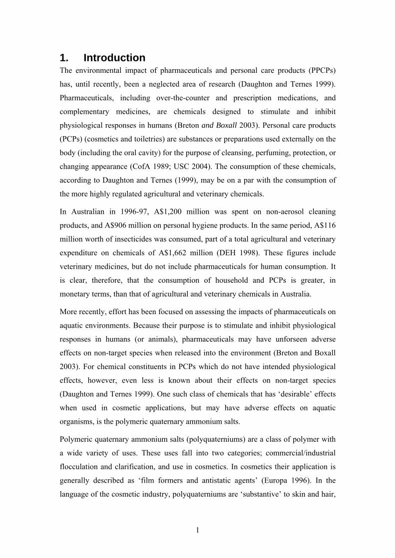
1. Introduction The environmental impact of pharmaceuticals and personal care products (PPCPs)

has, until recently, been a neglected area of research (Daughton and Ternes 1999).

Pharmaceuticals, including over-the-counter and prescription medications, and

complementary medicines, are chemicals designed to stimulate and inhibit

physiological responses in humans (Breton and Boxall 2003). Personal care products

(PCPs) (cosmetics and toiletries) are substances or preparations used externally on the

body (including the oral cavity) for the purpose of cleansing, perfuming, protection, or

changing appearance (CofA 1989; USC 2004). The consumption of these chemicals,

according to Daughton and Ternes (1999), may be on a par with the consumption of

the more highly regulated agricultural and veterinary chemicals.

In Australian in 1996-97, A$1,200 million was spent on non-aerosol cleaning

products, and A$906 million on personal hygiene products. In the same period, A$116

million worth of insecticides was consumed, part of a total agricultural and veterinary

expenditure on chemicals of A$1,662 million (DEH 1998). These figures include

veterinary medicines, but do not include pharmaceuticals for human consumption. It

is clear, therefore, that the consumption of household and PCPs is greater, in

monetary terms, than that of agricultural and veterinary chemicals in Australia.

More recently, effort has been focused on assessing the impacts of pharmaceuticals on

aquatic environments. Because their purpose is to stimulate and inhibit physiological

responses in humans (or animals), pharmaceuticals may have unforseen adverse

effects on non-target species when released into the environment (Breton and Boxall

2003). For chemical constituents in PCPs which do not have intended physiological

effects, however, even less is known about their effects on non-target species

(Daughton and Ternes 1999). One such class of chemicals that has ‘desirable’ effects

when used in cosmetic applications, but may have adverse effects on aquatic

organisms, is the polymeric quaternary ammonium salts.

Polymeric quaternary ammonium salts (polyquaterniums) are a class of polymer with

a wide variety of uses. These uses fall into two categories; commercial/industrial

flocculation and clarification, and use in cosmetics. In cosmetics their application is

generally described as ‘film formers and antistatic agents’ (Europa 1996). In the

language of the cosmetic industry, polyquaterniums are ‘substantive’ to skin and hair,

2

that is, they will sorb to proteinaceous surfaces. This is a very desirable property

providing they also impart cosmetic effects in terms of ‘feel’. This characteristic of

conditioning is subjectively reported by test subjects, and comprises one of four

measures used by cosmetic companies in assessing conditioning of hair. The others

are wet combability, dry combability and curl retention.

Because skin and hair are negatively charged at their surface, ‘conditioning’ has

become synonymous with cationic adsorption agents. Cleaning formulations, such as

shampoos and body scrubs, normally employ anionic (sometimes non-ionic)

surfactants. Without a conditioning agent, these formulations can cause fibre friction,

dryness and the ‘fly-away’ effect of electrostatic charge, conditions generally

regarded as sub-optimal by the cosmetic industry (Goddard 1999).

To overcome these apparent negative effects of anionic cleansing agents, cationic

agents, such as surfactants, but particularly polyelectrolytes, are used in the cosmetic

industry as hair and skin conditioners. The high adsorption efficiency of cationic

polyelectrolytes and the inherent properties of their adsorbed layers make them

particularly suitable as conditioning agents. Cationic polyelectrolytes have a further

advantage in that they can function as conditioners in formulations also containing the

anionic surfactants that would neutralise, and be neutralised by, a cationic surfactant

(Goddard 1999).

The combining of cationic polyelectrolytes and anionic surfactants in formulations is

one of two technologies that led to the development of the 2-in-1 shampoo

conditioner. This was developed and commercialised in the late 1960s and early

1970s, and is still employed. The alternative method involves a micro-suspension of

silicone, and essentially works in the same manner with the anionic surfactant (Burke

2005). Both involve the deposition of the conditioning agent, polyelectrolyte or

silicone, on the hair as the surfactant is rinsed away, a process known as ‘dilution

deposition’ (Gruber 1999).

At the present time all the major manufacturers produce ‘2-in-1’ formulations, and

over 20% of the shampoos sold are of this type (Gray 2003). Paradoxically, the advent

of the 2-in-1 conditioning shampoo has led to an increase in the number of people

using separate step conditioners (Burke 2005). Most shampoos now available have

some conditioning function, and cationic polyelectrolytes are found in a wide variety

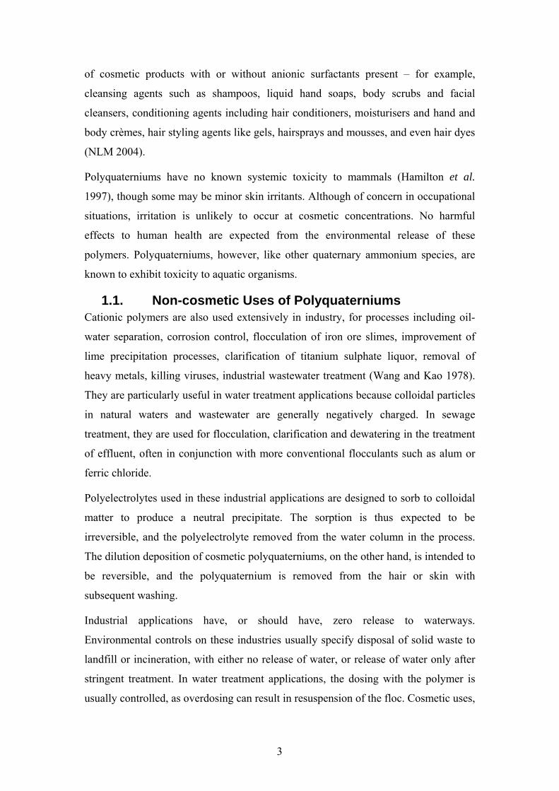
3

of cosmetic products with or without anionic surfactants present – for example,

cleansing agents such as shampoos, liquid hand soaps, body scrubs and facial

cleansers, conditioning agents including hair conditioners, moisturisers and hand and

body crèmes, hair styling agents like gels, hairsprays and mousses, and even hair dyes

(NLM 2004).

Polyquaterniums have no known systemic toxicity to mammals (Hamilton et al.

1997), though some may be minor skin irritants. Although of concern in occupational

situations, irritation is unlikely to occur at cosmetic concentrations. No harmful

effects to human health are expected from the environmental release of these

polymers. Polyquaterniums, however, like other quaternary ammonium species, are

known to exhibit toxicity to aquatic organisms.

1.1. Non-cosmetic Uses of Polyquaterniums Cationic polymers are also used extensively in industry, for processes including oil-

water separation, corrosion control, flocculation of iron ore slimes, improvement of

lime precipitation processes, clarification of titanium sulphate liquor, removal of

heavy metals, killing viruses, industrial wastewater treatment (Wang and Kao 1978).

They are particularly useful in water treatment applications because colloidal particles

in natural waters and wastewater are generally negatively charged. In sewage

treatment, they are used for flocculation, clarification and dewatering in the treatment

of effluent, often in conjunction with more conventional flocculants such as alum or

ferric chloride.

Polyelectrolytes used in these industrial applications are designed to sorb to colloidal

matter to produce a neutral precipitate. The sorption is thus expected to be

irreversible, and the polyelectrolyte removed from the water column in the process.

The dilution deposition of cosmetic polyquaterniums, on the other hand, is intended to

be reversible, and the polyquaternium is removed from the hair or skin with

subsequent washing.

Industrial applications have, or should have, zero release to waterways.

Environmental controls on these industries usually specify disposal of solid waste to

landfill or incineration, with either no release of water, or release of water only after

stringent treatment. In water treatment applications, the dosing with the polymer is

usually controlled, as overdosing can result in resuspension of the floc. Cosmetic uses,

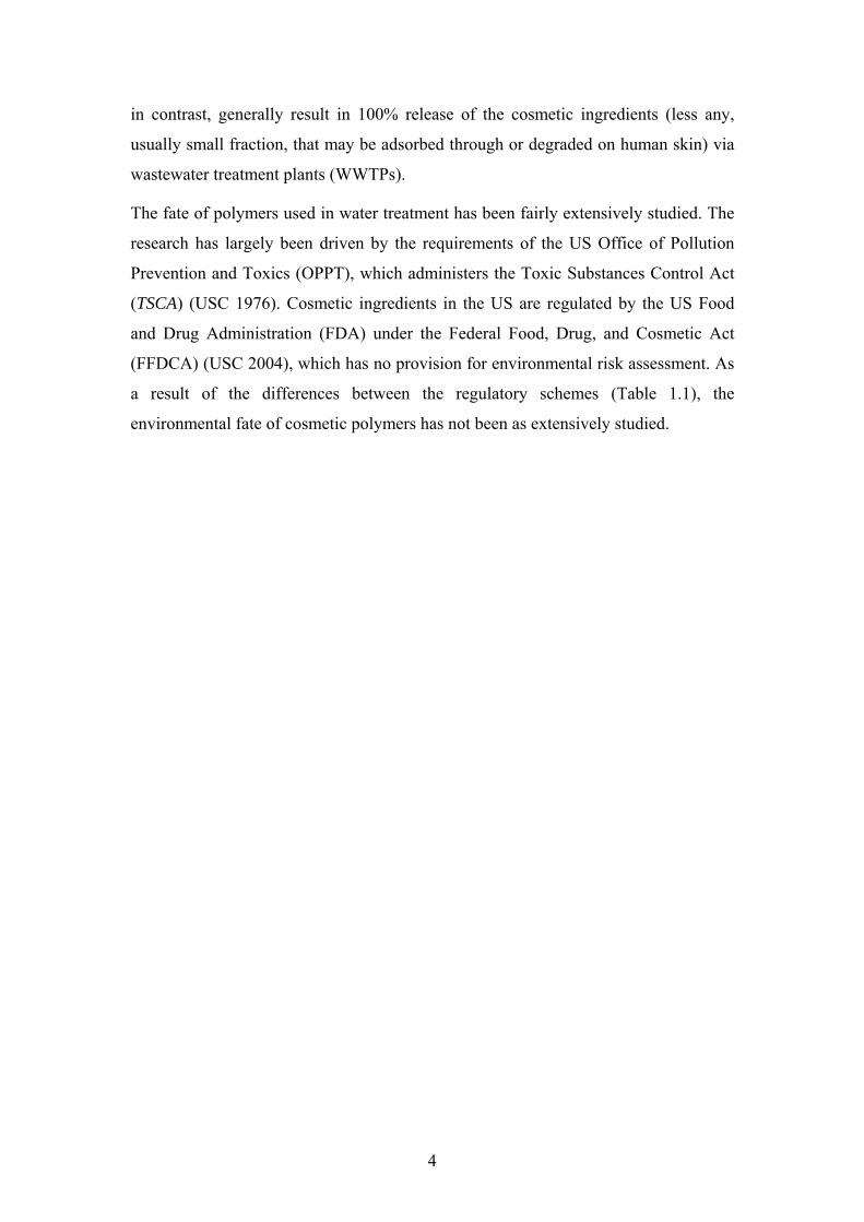
4

in contrast, generally result in 100% release of the cosmetic ingredients (less any,

usually small fraction, that may be adsorbed through or degraded on human skin) via

wastewater treatment plants (WWTPs).

The fate of polymers used in water treatment has been fairly extensively studied. The

research has largely been driven by the requirements of the US Office of Pollution

Prevention and Toxics (OPPT), which administers the Toxic Substances Control Act

(TSCA) (USC 1976). Cosmetic ingredients in the US are regulated by the US Food

and Drug Administration (FDA) under the Federal Food, Drug, and Cosmetic Act

(FFDCA) (USC 2004), which has no provision for environmental risk assessment. As

a result of the differences between the regulatory schemes (Table 1.1), the

environmental fate of cosmetic polymers has not been as extensively studied.

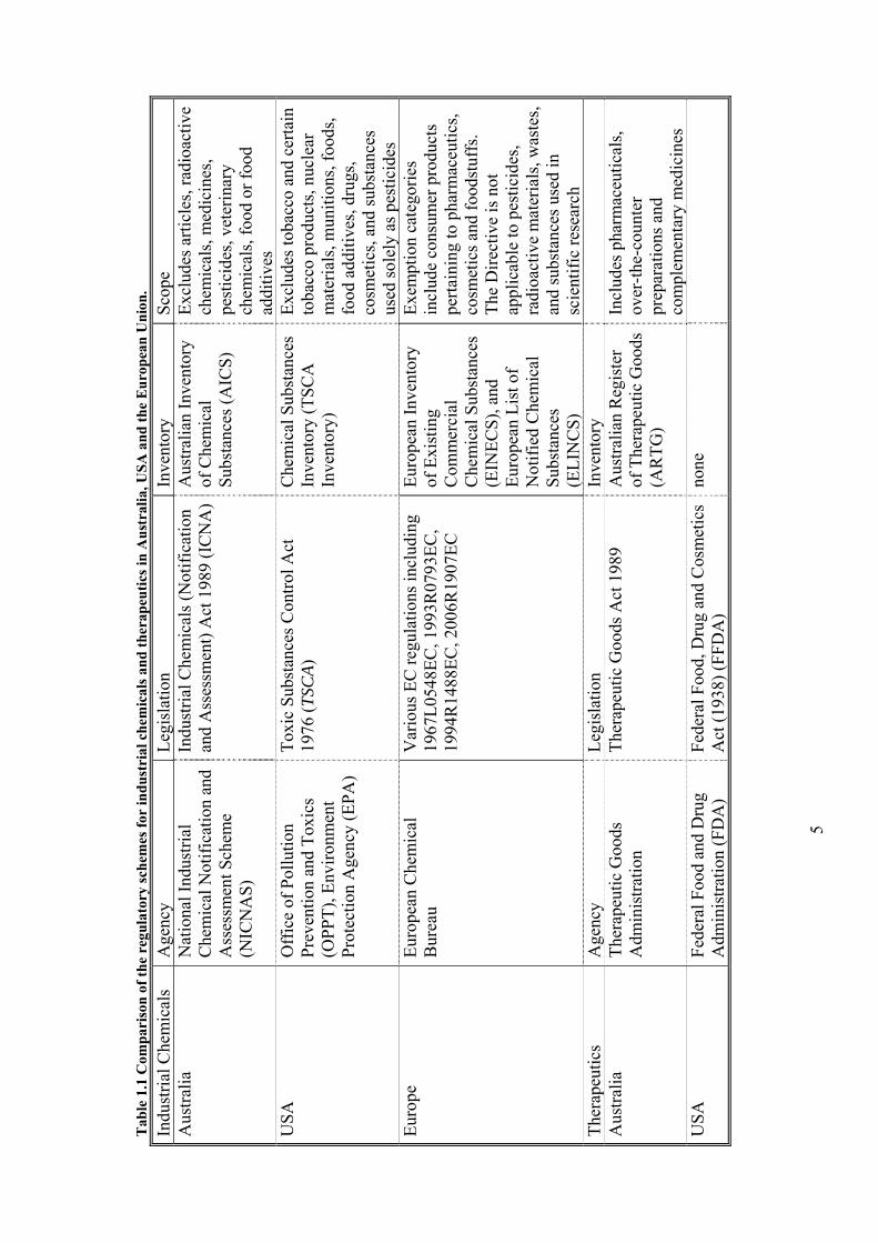
5

Tab

le 1

.1 C

ompa

riso

n of

the

regu

lato

ry sc

hem

es fo

r in

dust

rial

che

mic

als a

nd th

erap

eutic

s in

Aus

tral

ia, U

SA a

nd th

e E

urop

ean

Uni

on.

Indu

stria

l Che

mic

als

Age

ncy

Legi

slat

ion

Inve

ntor

y Sc

ope

Aus

tralia

N

atio

nal I

ndus

trial

C

hem

ical

Not

ifica

tion

and

Ass

essm

ent S

chem

e (N

ICN

AS)

Indu

stria

l Che

mic

als (

Not

ifica

tion

and

Ass

essm

ent)

Act

198

9 (I

CN

A)

Aus

tralia

n In

vent

ory

of C

hem

ical

Su

bsta

nces

(AIC

S)

Excl

udes

arti

cles

, rad

ioac

tive

chem

ical

s, m

edic

ines

, pe

stic

ides

, vet

erin

ary

chem

ical

s, fo

od o

r foo

d ad

ditiv

es

USA

O

ffic

e of

Pol

lutio

n Pr

even

tion

and

Toxi

cs

(OPP

T), E

nviro

nmen

t Pr

otec

tion

Age

ncy

(EPA

)

Toxi

c Su

bsta

nces

Con

trol A

ct

1976

(TSC

A)

Che

mic

al S

ubst

ance

s In

vent

ory

(TSC

A

Inve

ntor

y)

Excl

udes

toba

cco

and

certa

in

toba

cco

prod

ucts

, nuc

lear

m

ater

ials

, mun

ition

s, fo

ods,

food

add

itive

s, dr

ugs,

cosm

etic

s, an

d su

bsta

nces

us

ed so

lely

as p

estic

ides

Eu

rope

Eu

rope

an C

hem

ical

B

urea

u V

ario

us E

C re

gula

tions

incl

udin

g 19

67L0

548E

C, 1

993R

0793

EC,

1994

R14

88EC

, 200

6R19

07EC

Euro

pean

Inve

ntor

y of

Exi

stin

g C

omm

erci

al

Che

mic

al S

ubst

ance

s (E

INEC

S), a

nd

Euro

pean

Lis

t of

Not

ified

Che

mic

al

Subs

tanc

es

(ELI

NC

S)

Exem

ptio

n ca

tego

ries

incl

ude

cons

umer

pro

duct

s pe

rtain

ing

to p

harm

aceu

tics,

cosm

etic

s and

food

stuf

fs.

The

Dire

ctiv

e is

not

ap

plic

able

to p

estic

ides

, ra

dioa

ctiv

e m

ater

ials

, was

tes,

and

subs

tanc

es u

sed

in

scie

ntifi

c re

sear

ch

Ther

apeu

tics

Age

ncy

Legi

slat

ion

Inve

ntor

y

Aus

tralia

Th

erap

eutic

Goo

ds

Adm

inis

tratio

n Th

erap

eutic

Goo

ds A

ct 1

989

Aus

tralia

n R

egis

ter

of T

hera

peut

ic G

oods

(A

RTG

)

Incl

udes

pha

rmac

eutic

als,

over

-the-

coun

ter

prep

arat

ions

and

co

mpl

emen

tary

med

icin

es

USA

Fe

dera

l Foo

d an

d D

rug

Adm

inis

tratio

n (F

DA

) Fe

dera

l Foo

d, D

rug

and

Cos

met

ics

Act

(193

8) (F

FDA

) no

ne

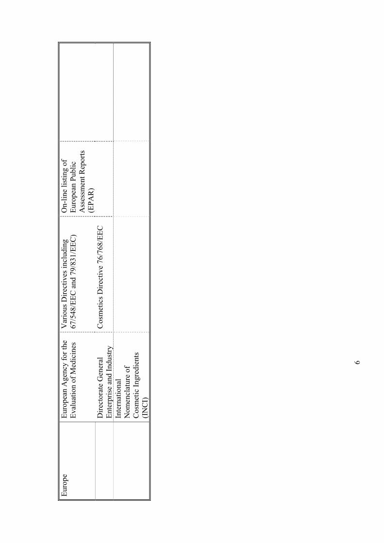
6

Euro

pe

Euro

pean

Age

ncy

for t

he

Eval

uatio

n of

Med

icin

es

Var

ious

Dire

ctiv

es in

clud

ing

67/5

48/E

EC a

nd 7

9/83

1/EE

C)

On-

line

listin

g of

Eu

rope

an P

ublic

A

sses

smen

t Rep

orts

(E

PAR

)

D

irect

orat

e G

ener

al

Ente

rpris

e an

d In

dust

ry

Cos

met

ics D

irect

ive

76/7

68/E

EC

In

tern

atio

nal

Nom

encl

atur

e of

C

osm

etic

Ingr

edie

nts

(IN

CI)

7

1.2. Regulation of Chemicals in Australia In Australia, there are four agencies responsible for the regulation of chemicals. The

responsibilities of each agency are outlined in Table 1.2. The regulation of industrial

chemicals, including cosmetics, is the responsibility of the National Industrial

Chemical Notification and Assessment Scheme (NICNAS), a statutory scheme which

is part of the Therapeutic Goods Administration (TGA) in the portfolio of the Minister

for Health and Ageing. NICNAS undertakes risk assessment in the areas of

Occupational Health and Safety (OHS), public health and environment. The

environmental assessment, generally carried out by the Department of Environment

and Water Resources (DEW), deals only with the non-human environment. Human

health impacts resulting from environmental exposure form part of the public health

assessment. NICNAS maintains an inventory of industrial chemicals approved for use

in Australia, called the Australian Inventory of Chemical Substances (AICS). The

inventory is used to distinguish between new and existing chemicals. A new chemical

is any chemical that is not on the AICS. Companies wishing to import or manufacture

any new chemical (known as ‘notifiers’ in the Industrial Chemicals (Notification and

Assessment) Act (ICNA)) must apply to NICNAS for a certificate or permit before

importing the chemical. Depending on the type of chemical and/or the volume to be

introduced, an assessment process is conducted and an assessment report published.

Existing chemicals include those that were in use in Australia between 1 January 1977

and 28 February 1990, and therefore placed on the inventory when it was established.

These chemicals are sometimes referred to as ‘grandfathered’ chemicals. In addition,

new chemicals are added to AICS after assessment. There are currently over 38,000

chemicals on AICS. All grandfathered chemicals, chemicals which have been

imported under certificate for five years, and chemicals where the notifier requests

early AICS listing comprise AICS. A small proportion of AICS chemicals are held on

a confidential section. Chemicals are introduced under an assessment certificate for

the first five years, unless the notifier requests early AICS listing. These chemicals do

not form part of AICS and are not able to be imported by other companies without

separate notification.

8

Tab

le 1

.2 K

ey e

lem

ents

of t

he r

egul

ator

y an

d m

anag

emen

t str

uctu

re o

f che

mic

als i

n A

ustr

alia

(ada

pted

from

DE

H 1

998)

. El

emen

t In

dust

rial C

hem

ical

s A

gric

ultu

ral a

nd V

eter

inar

y Pr

oduc

ts

Phar

mac

eutic

als

Food

Add

itive

Sche

me

resp

onsi

ble

for

asse

ssm

ent

Nat

iona

l Ind

ustri

al C

hem

ical

s N

otifi

catio

n an

d A

sses

smen

t Sc

hem

e (N

ICN

AS)

Aus

tralia

n Pe

stic

ides

&

Vet

erin

ary

Med

icin

es

Aut

horit

y (A

PVM

A)

Ther

apeu

tic G

oods

A

dmin

istra

tion

(TG

A)

Food

Sta

ndar

ds A

ustra

lia

New

Zea

land

(FSA

NZ)

Min

istry

H

ealth

and

Age

ing

Agr

icul

ture

, Fis

herie

s and

Fo

rest

ry

Hea

lth a

nd A

gein

g H

ealth

and

Age

ing

Ass

essm

ent a

nd/o

r re

gist

ratio

n

All

new

che

mic

als a

re a

sses

sed

befo

re u

se. E

xist

ing

chem

ical

s ar

e re

view

ed o

n a

prio

rity

basi

s.

All

new

pro

duct

s and

new

us

es o

f pro

duct

s mus

t be

asse

ssed

and

regi

ster

ed

befo

re u

se. E

xist

ing

chem

ical

s and

pro

duct

s may

be

revi

ewed

.

All

new

ther

apeu

tic g

oods

m

ust b

e re

gist

ered

on

the

Aus

tralia

n R

egis

ter o

f Th

erap

eutic

Goo

ds.

Stip

ulat

es fo

od st

anda

rds t

o pr

otec

t pub

lic h

ealth

.

Scop

e an

d de

finiti

on

Ass

essm

ent o

f a c

hem

ical

ent

ity

(not

pro

duct

) – a

ny c

hem

ical

th

at h

as a

n in

dust

rial u

se m

ay

be in

clud

ed i.

e., d

yes,

solv

ents

, ad

hesi

ves,

plas

tics,

labo

rato

ry

chem

ical

s, pa

ints

, cle

anin

g pr

oduc

ts, c

osm

etic

s and

to

iletri

es. E

xclu

des a

rticl

es,

radi

oact

ive

chem

ical

s or

chem

ical

s sol

ely

in o

ther

sc

hem

es.

Reg

istra

tion

of p

rodu

cts

incl

udes

: an

agric

ultu

ral

prod

uct u

sed

to st

upef

y,

repe

l, in

hibi

t the

feed

ing

of

or p

reve

nt, p

ests

on

plan

ts

or o

ther

thin

gs; d

estro

y a

plan

t or m

odify

phy

siol

ogy;

or

attr

act a

pes

t to

dest

roy

it.

Vet

erin

ary

prod

uct i

nclu

des

a su

bsta

nce

for p

reve

ntin

g,

diag

nosi

ng c

urin

g or

al

levi

atin

g di

seas

e in

an

imal

s. Ex

clud

es fe

rtilis

ers

Ass

essm

ent a

nd re

gist

ratio

n of

ther

apeu

tic g

oods

C

ontro

l of c

onta

min

ants

and

fo

od a

dditi

ves t

hat a

re

adde

d to

food

to a

ssis

t in

food

pro

cess

ing

or to

ac

hiev

e a

tech

nolo

gica

l pu

rpos

e in

the

food

, for

ex

ampl

e, c

olou

ring

or

flavo

urin

g.

Con

trols

of u

se

If n

ot o

n A

ICS

(or h

as a

n as

sess

men

t cer

tific

ate

or p

erm

it is

sued

) may

not

be

used

co

mm

erci

ally

; may

be

rem

oved

fr

om A

ICS.

App

licat

ion

of

If n

ot re

gist

ered

may

not

be

used

; reg

istra

tion

may

sp

ecify

how

use

d;

regi

stra

tion

can

be

canc

elle

d; u

se c

ontro

lled

by

If n

ot re

gist

ered

, may

not

be

used

. Lic

ensi

ng o

f M

anuf

actu

rer;

Stan

dard

for

Uni

form

Sch

edul

ing

of D

rugs

an

d Po

ison

s (SU

SDP)

;

Food

Sta

ndar

ds C

ode

(A14

); co

ntro

l per

mis

sibl

e ad

ditiv

es, p

rese

rvat

ives

and

co

lour

s; a

pplic

atio

n of

M

axim

um R

esid

ue L

imits

.

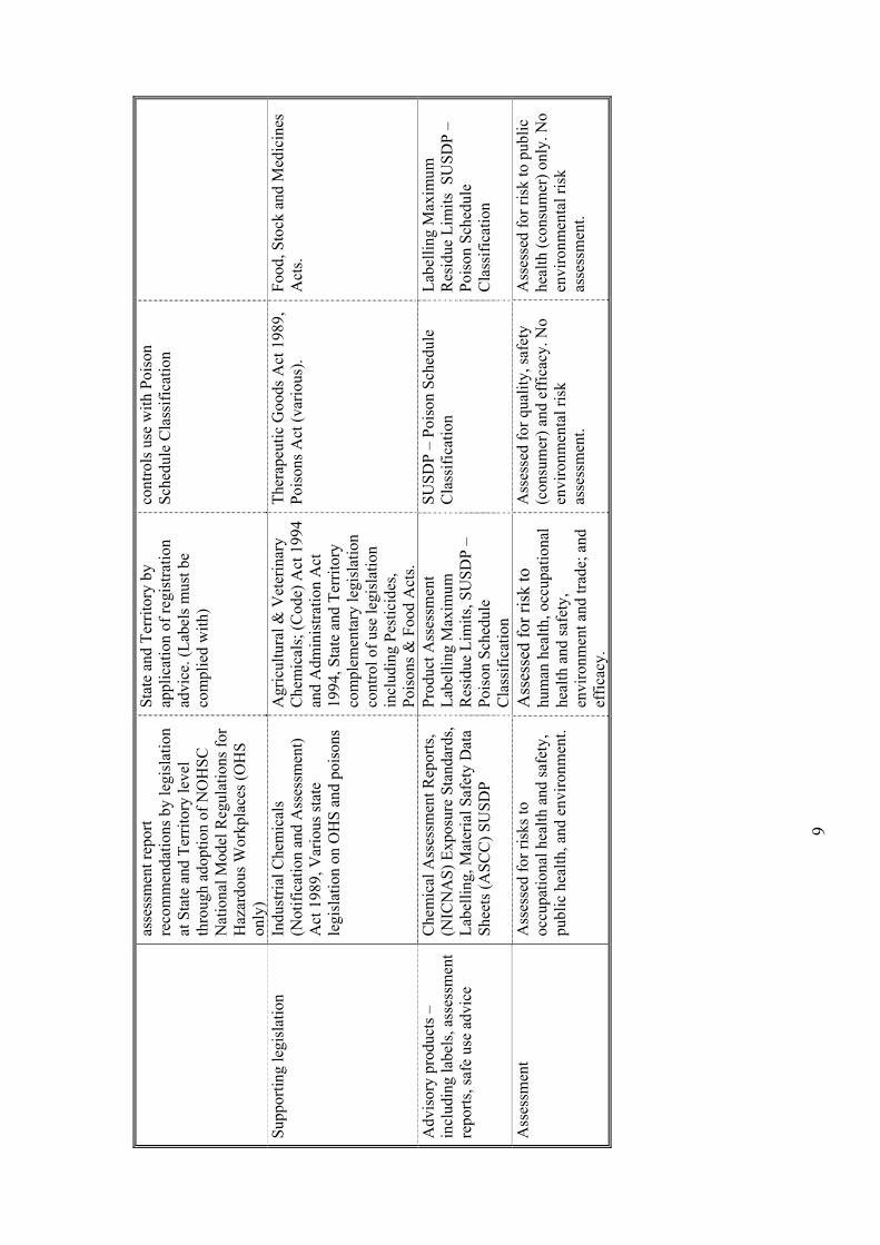
9

asse

ssm

ent r

epor

t re

com

men

datio

ns b

y le

gisl

atio

n at

Sta

te a

nd T

errit

ory

leve

l th

roug

h ad

optio

n of

NO

HSC

N

atio

nal M

odel

Reg

ulat

ions

for

Haz

ardo

us W

orkp

lace

s (O

HS

only

)

Stat

e an

d Te

rrito

ry b

y ap

plic

atio

n of

regi

stra

tion

advi

ce. (

Labe

ls m

ust b

e co

mpl

ied

with

)

cont

rols

use

with

Poi

son

Sche

dule

Cla

ssifi

catio

n

Supp

ortin

g le

gisl

atio

n

Indu

stria

l Che

mic

als

(Not

ifica

tion

and

Ass

essm

ent)

Act

198

9, V

ario

us st

ate

legi

slat

ion

on O

HS

and

pois

ons

Agr

icul

tura

l & V

eter

inar

y C

hem

ical

s; (C

ode)

Act

199

4 an

d A

dmin

istra

tion

Act

19

94, S

tate

and

Ter

ritor

y co

mpl

emen

tary

legi

slat

ion

cont

rol o

f use

legi

slat

ion

incl

udin

g Pe

stic

ides

, Po

ison

s & F

ood

Act

s.

Ther

apeu

tic G

oods

Act

198

9,

Pois

ons A

ct (v

ario

us).

Fo

od, S

tock

and

Med

icin

es

Act

s.

Adv

isor

y pr

oduc

ts –

incl

udin

g la

bels

, ass

essm

ent

repo

rts, s

afe

use

advi

ce

Che

mic

al A

sses

smen

t Rep

orts

, (N

ICN

AS)

Exp

osur

e St

anda

rds,

Labe

lling

, Mat

eria

l Saf

ety

Dat

a Sh

eets

(ASC

C) S

USD

P

Prod

uct A

sses

smen

t La

belli

ng M

axim

um

Res

idue

Lim

its, S

USD

P –

Pois

on S

ched

ule

Cla

ssifi

catio

n

SUSD

P –

Pois

on S

ched

ule

Cla

ssifi

catio

n La

belli

ng M

axim

um

Res

idue

Lim

its S

USD

P –

Pois

on S

ched

ule

Cla

ssifi

catio

n

Ass

essm

ent

Ass

esse

d fo

r ris

ks to

oc

cupa

tiona

l hea

lth a

nd sa

fety

, pu

blic

hea

lth, a

nd e

nviro

nmen

t.

Ass

esse

d fo

r ris

k to

hu

man

hea

lth, o

ccup

atio

nal

heal

th a

nd sa

fety

, en

viro

nmen

t and

trad

e; a

nd

effic

acy.

Ass

esse

d fo

r qua

lity,

safe

ty

(con

sum

er) a

nd e

ffic

acy.

No

envi

ronm

enta

l ris

k as

sess

men

t.

Ass

esse

d fo

r ris

k to

pub

lic

heal

th (c

onsu

mer

) onl

y. N

o en

viro

nmen

tal r

isk

asse

ssm

ent.

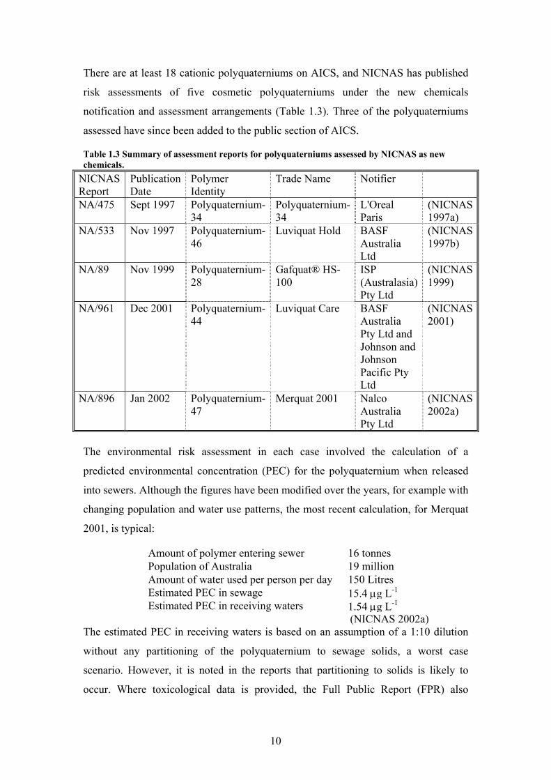
10

There are at least 18 cationic polyquaterniums on AICS, and NICNAS has published

risk assessments of five cosmetic polyquaterniums under the new chemicals

notification and assessment arrangements (Table 1.3). Three of the polyquaterniums

assessed have since been added to the public section of AICS.

Table 1.3 Summary of assessment reports for polyquaterniums assessed by NICNAS as new chemicals.

NICNAS Report

Publication Date

Polymer Identity

Trade Name Notifier

NA/475 Sept 1997 Polyquaternium-34

Polyquaternium-34

L'Oreal Paris

(NICNAS 1997a)

NA/533 Nov 1997 Polyquaternium-46

Luviquat Hold BASF Australia Ltd

(NICNAS 1997b)

NA/89 Nov 1999 Polyquaternium-28

Gafquat® HS-100

ISP (Australasia) Pty Ltd

(NICNAS 1999)

NA/961 Dec 2001 Polyquaternium-44

Luviquat Care BASF Australia Pty Ltd and Johnson and Johnson Pacific Pty Ltd

(NICNAS 2001)

NA/896 Jan 2002 Polyquaternium-47

Merquat 2001 Nalco Australia Pty Ltd

(NICNAS 2002a)

The environmental risk assessment in each case involved the calculation of a

predicted environmental concentration (PEC) for the polyquaternium when released

into sewers. Although the figures have been modified over the years, for example with

changing population and water use patterns, the most recent calculation, for Merquat

2001, is typical:

Amount of polymer entering sewer 16 tonnes Population of Australia 19 million Amount of water used per person per day 150 Litres Estimated PEC in sewage 15.4 μg L-1 Estimated PEC in receiving waters 1.54 μg L-1

(NICNAS 2002a) The estimated PEC in receiving waters is based on an assumption of a 1:10 dilution

without any partitioning of the polyquaternium to sewage solids, a worst case

scenario. However, it is noted in the reports that partitioning to solids is likely to

occur. Where toxicological data is provided, the Full Public Report (FPR) also

11

includes a Predicted No Effect Concentration (PNEC) based on the toxicity of the

polymer to the most sensitive aquatic species. The environmental risk is then

determined as the ratio PNEC/PEC, sometimes called the Risk Quotient or Hazard

Quotient (Q). Only Merquat 2001, with its high import volume, had a PNEC/PEC

value of less than one, indicating a possible environmental risk. However, according

to the report, the partitioning of the polyquaternium to sewage sludge was expected to

fully mitigate the risk.

The expectation of partitioning to sludge is based on references including Nabholz et

al. (1993), and Boethling and Nabholz (1997), which rely on data submitted with

Premanufacture Notices (PMN) under TSCA for their models and assessment of

polyelectrolytes in the environment. As cosmetic polymers in the United States are

not included under the TSCA, but are regulated under the Federal Food, Drug and

Cosmetic Agency, the TSCA data is based upon only water treatment and other

industrial polyelectrolytes, but not cosmetic polymers.

1.3. The Risk Assessment Framework Regulatory risk assessment of chemicals in most jurisdictions follows the framework

developed by the United States Environment Protection Agency (USEPA) in the early

1980s. This process, known as the four-step paradigm, was first outlined by the

National Research Council (NRC) in a 1983 publication known as ‘the red book’,

(NRC 1994). The four steps of the process are:

1. Hazard Identification

2. Dose-Response Assessment

3. Exposure Assessment

4. Risk Characterisation.

Although there are many published versions of the four-step framework for risk

assessment, most are focused on human health impacts, either from direct exposure

(i.e. from food and water consumption) or indirect exposure from the environment

(i.e. air toxics, recreational water use etc). There are fewer examples of guidelines for

risk assessment of chemicals as they affect the health of the environment, or non-

human species. From the basic framework, many variations of the method, and of

terminology, have developed. Much of this variation results from the purpose of the

risk assessment, for example whether the risk assessment is remedial (for

12

contaminated sites) or predictive (for new chemicals) and whether the assessment is

conducted for the purpose of protecting human health, endangered species or

ecosystems.

This study concerns the evaluation of risk from polyquaterniums, both new and

existing, in Australia, and therefore follows the framework of regulatory chemical risk

assessment. There is less variation in the assessment methodology and terminology

across jurisdictions, largely because of the cooperative arrangements that have been

developed, such as the Canada-Australia Bilateral cooperative arrangements and the

Organisation for Economic Cooperation and Development (OECD) New Chemicals

Taskforce on mutual acceptance of assessments (NICNAS 2007). Where alternative

methods and terminology are available, this study will reflect those used in NICNAS

assessment reports.

1.3.1. Hazard Identification The first step in risk assessment is to determine if the chemical is or can be causally

linked to an adverse outcome (NRC 1994) that is, does the chemical have a known

hazard, belong to a class of compounds known to be toxic, or does the chemical have

characteristics that suggest it may be toxic. For existing chemicals, the hazard may be

identified from observed environmental effects in the field. In Australia, the chemical

can be nominated as a candidate for assessment by any person, group or organisation,

but the criteria used by NICNAS to select nominated chemicals for assessment have

not been published and are currently under review (NICNAS 2006). For new

chemicals, identification of a specific hazard is not required, although manufacturers

and importers, are required to have checked the chemical against criteria specified

under various guidelines, for example Approved Criteria for Classifying Hazardous

Substances (NOHSC 1999), and prepared appropriate hazard labelling and safety data

sheets (NICNAS 2004b). The nature of the risk assessment process is determined by

the volume of the chemical to be introduced (< or ≥ 1000 kg) and/or its classification

as a Polymer of Low Concern (PLC). Recent review and amendments of ICNA have

resulted in a new classification of Low Regulatory Concern Chemicals (LRCC),

which will enable manufacturers and importers (known as ‘notifiers’ in ICNA) to

undertake audited self-assessment of chemicals and polymers considered to be of low

hazard or low risk potential.

13

1.3.2. Effects Assessment The second step of the risk assessment, dose-response assessment in the red book

(NRC 1983), is generally called effects assessment in NICNAS assessment reports.

Using available toxicity data, the relationship between the exposure and the outcome

in an exposed population is predicted, generally from the No Observed Effect Level

(NOEL), or the No Observed Adverse Effect Level (NOAEL) in a laboratory study.

Safety margins can be determined from the ratio of the NOAEL and the Lowest

Observed Adverse Effect (LOAEL) (NRC 1994), or from the ratio of chronic to acute

studies (Giolando et al. 1995; Jop 1997). Other factors that may be important in

hazard assessment include the existence of a threshold level (i.e. minimum

concentration below which no effects are expected), the level of uncertainty,

reversibility of effect, interaction between species, host characteristics, reproductive

status, and population characteristics such as mobility.

1.3.3. Exposure Assessment The extent of the exposure of a vulnerable organism to the chemical before or after

application of regulatory controls requires determination of the fate of the chemical

and exposure pathways. Factors that need to be considered include frequency and

duration of exposure, rates of uptake or contact, and rates of absorption (NRC 1994).

Methods and approaches to exposure are medium-specific (air, water, soil), and unless

measured environmental data are available, require transport and fate models (NRC

1994). The models, in turn, rely on specified physicochemical characteristics of the

chemical, such as solubility, vapour pressure, and partition coefficients. Other

important factors in assessing exposure include release patterns, cumulative versus

non-cumulative exposure, persistence, failure of exposure controls, quality of data and

quality of models (EnHealth 2002).

1.3.4. Risk Characterisation The final stage in the risk assessment integrates the information from effects and

exposure assessment (EnHealth 2002) to provide a description of the nature and

magnitude of the risk, including uncertainty. The outcome of the risk assessment can

be qualitative or quantitative. Qualitative risk assessments provide a descriptive

indication of risk (e.g. high, medium, low), usually determined against a pre-existing

set of criteria or guidelines developed for that purpose (NRC 1994). A quantitative

risk assessment, on the other hand, attempts to put a numeric value to the risk, for

example lifetime and population risks that have been determined for some

14

carcinogens. The use of numerical methods in the risk assessment does not, however,

indicate that the outcome will be a quantitative risk assessment, that is a measure of

the risk. For example, the hazard index used for non-carcinogens in humans is a

benchmark used in the estimation of risk, but is not a quantitative measure of risk

(NRC 1994). While weighing the risks against other societal costs and benefits is

often considered an important part of risk assessment, this is not a part of the risk

assessment of industrial chemicals in Australia. Each chemical is assessed on the basis

of its hazard and exposure only. Positive benefits, including the replacement of a more

hazardous chemical, are not considered. The determination of labelling classifications

and recommendations for control are part of the NICNAS risk assessment process. It

should be noted, however, that labelling classifications used in Australia (and

globally) are hazard based, not risk based.

1.3.5. Assessment Reports Unlike in the USA and Canada where the assessment reports remain confidential,

reports of new and existing chemicals assessed by NICNAS are published and freely

available. Although draft guidelines on the assessment process as it is applied have

only recently been published by DEW (Lee-Steere 2007), it can be ascertained from

the published reports that the four-step risk assessment process is used. An assessment

report contains the information on which the assessment is based, under the headings

Process and Release Information, Physical and Chemical Properties and Toxicological

Investigations. The following section of the report, Risk Assessment, is divided into

OHS, public health, and environment, and each of these is further divided into

exposure assessment, effects assessment and risk characterisation. The final section

contains the risk assessment for each category, plus the recommendations for hazard

classification, labelling, and the Material Safety Data Sheet (MSDS). In the FPR,

which is available on the NICNAS website, the data that the notifier has requested be

kept confidential is excluded. If no request is made to keep data confidential, the

Assessment Report and the FPR will be identical.

1.3.6. Data Requirements In chemical assessment, the data that needs to be made available for the risk

assessment is usually determined by the legislation and/or regulations, and may

depend on the type of chemical or polymer and the volume to be manufactured or

imported. The data requirements for new chemical assessment under ICNA are

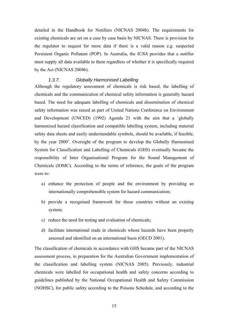
15

detailed in the Handbook for Notifiers (NICNAS 2004b). The requirements for

existing chemicals are set on a case by case basis by NICNAS. There is provision for

the regulator to request for more data if there is a valid reason e.g. suspected

Persistent Organic Pollutant (POP). In Australia, the ICNA provides that a notifier

must supply all data available to them regardless of whether it is specifically required

by the Act (NICNAS 2004b).

1.3.7. Globally Harmonised Labelling Although the regulatory assessment of chemicals is risk based, the labelling of

chemicals and the communication of chemical safety information is generally hazard

based. The need for adequate labelling of chemicals and dissemination of chemical

safety information was raised as part of United Nations Conference on Environment

and Development (UNCED) (1992) Agenda 21 with the aim that a ‘globally

harmonised hazard classification and compatible labelling system, including material

safety data sheets and easily understandable symbols, should be available, if feasible,

by the year 2000’. Oversight of the program to develop the Globally Harmonised

System for Classification and Labelling of Chemicals (GHS) eventually became the

responsibility of Inter Organisational Program for the Sound Management of

Chemicals (IOMC). According to the terms of reference, the goals of the program

were to:

a) enhance the protection of people and the environment by providing an

internationally comprehensible system for hazard communication;

b) provide a recognised framework for those countries without an existing

system;

c) reduce the need for testing and evaluation of chemicals;

d) facilitate international trade in chemicals whose hazards have been properly

assessed and identified on an international basis (OECD 2001).

The classification of chemicals in accordance with GHS became part of the NICNAS

assessment process, in preparation for the Australian Government implementation of

the classification and labelling system (NICNAS 2005). Previously, industrial

chemicals were labelled for occupational health and safety concerns according to

guidelines published by the National Occupational Health and Safety Commission

(NOHSC), for public safety according to the Poisons Schedule, and according to the

16

requirements of the Dangerous Goods Act for transport and storage purposes, but

there was no system for the classification and labelling of environmentally hazardous

chemicals.

1.3.8. GHS and the Aquatic Environment The classification of hazards to aquatic environments under GHS is based on the

impacts of the chemical on aquatic organism and the ecosystems which they inhabit,

and not in terms of public health impacts (OECD 2001). The basic data elements used

in the classification of environmental hazard under the GHS are:

e) acute aquatic toxicity;

f) potential for or actual bioaccumulation;

g) degradation (biotic or abiotic) for organic chemicals;

h) chronic aquatic toxicity.

The hazard classifications for the aquatic environment under the GHS are given in

Table 1.4.

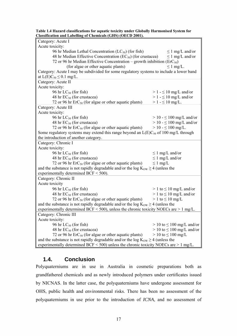
17

Table 1.4 Hazard classifications for aquatic toxicity under Globally Harmonised System for Classification and Labelling of Chemicals (GHS) (OECD 2001). Category: Acute I Acute toxicity: 96 hr Median Lethal Concentration (LC50) (for fish) ≤ 1 mg/L and/or 48 hr Median Effective Concentration (EC50) (for crustacea) ≤ 1 mg/L and/or 72 or 96 hr Median Effective Concentration – growth inhibition ( ErC50) (for algae or other aquatic plants) ≤ 1 mg/L. Category: Acute I may be subdivided for some regulatory systems to include a lower band at L(E)C50 ≤ 0.1 mg/L. Category: Acute II Acute toxicity: 96 hr LC50 (for fish) > 1 - ≤ 10 mg/L and/or 48 hr EC50 (for crustacea) > 1 - ≤ 10 mg/L and/or 72 or 96 hr ErC50 (for algae or other aquatic plants) > 1 - ≤ 10 mg/L. Category: Acute III Acute toxicity: 96 hr LC50 (for fish) > 10 - ≤ 100 mg/L and/or 48 hr EC50 (for crustacea) > 10 - ≤ 100 mg/L and/or 72 or 96 hr ErC50 (for algae or other aquatic plants) > 10 - ≤ 100 mg/L. Some regulatory systems may extend this range beyond an L(E)C50 of 100 mg/L through the introduction of another category. Category: Chronic I Acute toxicity: 96 hr LC50 (for fish) ≤ 1 mg/L and/or 48 hr EC50 (for crustacea) ≤ 1 mg/L and/or 72 or 96 hr ErC50 (for algae or other aquatic plants) ≤ 1 mg/L and the substance is not rapidly degradable and/or the log KOW ≥ 4 (unless the experimentally determined BCF < 500). Category: Chronic II Acute toxicity 96 hr LC50 (for fish) > 1 to ≤ 10 mg/L and/or 48 hr EC50 (for crustacea) > 1 to ≤ 10 mg/L and/or 72 or 96 hr ErC50 (for algae or other aquatic plants) > 1 to ≤ 10 mg/L and the substance is not rapidly degradable and/or the log KOW ≥ 4 (unless the experimentally determined BCF < 500), unless the chronic toxicity NOECs are > 1 mg/L. Category: Chronic III Acute toxicity: 96 hr LC50 (for fish) > 10 to ≤ 100 mg/L and/or 48 hr EC50 (for crustacea) > 10 to ≤ 100 mg/L and/or 72 or 96 hr ErC50 (for algae or other aquatic plants) > 10 to ≤ 100 mg/L and the substance is not rapidly degradable and/or the log KOW ≥ 4 (unless the experimentally determined BCF < 500) unless the chronic toxicity NOECs are > 1 mg/L.

1.4. Conclusion Polyquaterniums are in use in Australia in cosmetic preparations both as

grandfathered chemicals and as newly introduced polymers under certificates issued

by NICNAS. In the latter case, the polyquaterniums have undergone assessment for

OHS, public health and environmental risks. There has been no assessment of the

polyquaterniums in use prior to the introduction of ICNA, and no assessment of

18

polyquaterniums as a chemical class. Further, the risk assessment of the new polymers

does not take into account other ingredients which occur in cosmetic preparations

with polyquaterniums and in particular, the interactions that occur between the

polyquaterniums and anionic surfactants. Little is known about the fate of cosmetic

polyquaterniums. All are released to WWTP where they are assumed to sorb to

sludge. Due to their toxicity to aquatic biota, the release of polyquaterniums into

receiving waters with WWTP effluent could be a potential risk to the environment.

1.4.1. Aims It is the aim of this research to provide reliable data to facilitate the risk assessment

for polyquaterniums used in cosmetics applications. Specifically, this research aims to

a) determine the sorption behaviour of the polyquaternium and the

polyquaternium/surfactant complex (PSC) on environmental surfaces (e.g.

dissolved organic carbon (DOC), humic acid);

b) determine the toxicity of the polyquaternium and the PSC to algae, aquatic

invertebrates and fish;

c) investigate the mitigating effects of humic acids and electrolytes on the

toxicity of polyquaterniums and PSC that are found to be toxic;

d) investigate models and/or predictive tests that may assist in determining the

environmental risk of polyquaterniums of different chemistries, molecular

weights and charge densities.

1.4.2. Structure The four-step risk assessment paradigm described above has been adopted for this

study. In addition to providing a framework for the research on environmental fate

and aquatic toxicology of the polyquaterniums and PSCs, this will facilitate a critique

of the method as it is used for the assessment of new and existing chemicals, and a

review the alternative methods that may be available.

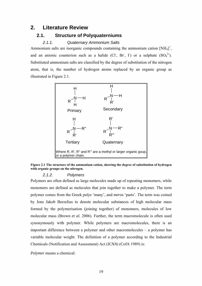
19

2. Literature Review 2.1. Structure of Polyquaterniums

2.1.1. Quaternary Ammonium Salts Ammonium salts are inorganic compounds containing the ammonium cation [NH4]+,

and an anionic counterion such as a halide (Cl-, Br-, I-) or a sulphate (SO42-).

Substituted ammonium salts are classified by the degree of substitution of the nitrogen

atom, that is, the number of hydrogen atoms replaced by an organic group as

illustrated in Figure 2.1.

RN

H

H

H

RN

R'

H

R''

RNR'

H

H

RNR'''

R'

R"

Primary Secondary

Tertiary Quaternary

Where R, R', R'' and R''' are a methyl or larger organic goup,or a polymer chain.

Figure 2.1 The structure of the ammonium cation, showing the degree of substitution of hydrogen with organic groups on the nitrogen.

2.1.2. Polymers Polymers are often defined as large molecules made up of repeating monomers, while

monomers are defined as molecules that join together to make a polymer. The term

polymer comes from the Greek polys ‘many’, and meros ‘parts’. The term was coined

by Jons Jakob Berzelius to denote molecular substances of high molecular mass

formed by the polymerisation (joining together) of monomers, molecules of low

molecular mass (Brown et al. 2006). Further, the term macromolecule is often used

synonymously with polymer. While polymers are macromolecules, there is an

important difference between a polymer and other macromolecules – a polymer has

variable molecular weight. The definition of a polymer according to the Industrial

Chemicals (Notification and Assessment) Act (ICNA) (CofA 1989) is:

Polymer means a chemical:

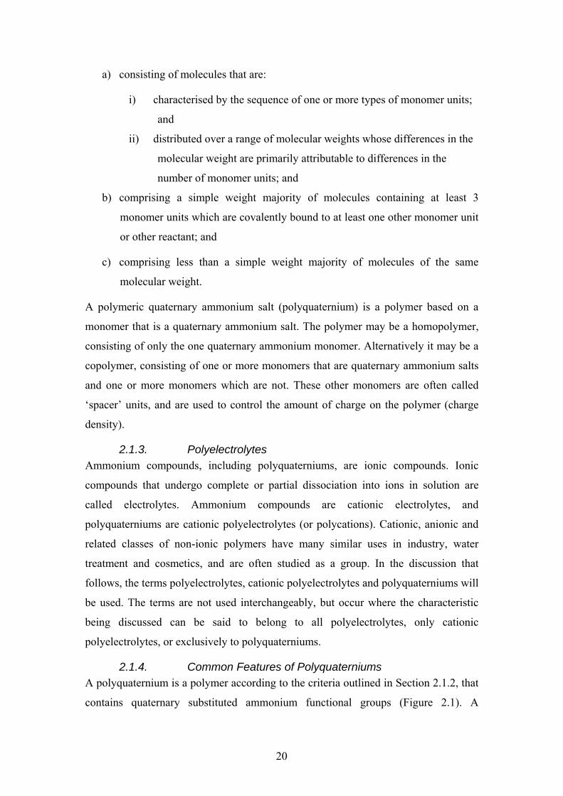
20

a) consisting of molecules that are:

i) characterised by the sequence of one or more types of monomer units;

and

ii) distributed over a range of molecular weights whose differences in the

molecular weight are primarily attributable to differences in the

number of monomer units; and

b) comprising a simple weight majority of molecules containing at least 3

monomer units which are covalently bound to at least one other monomer unit

or other reactant; and

c) comprising less than a simple weight majority of molecules of the same

molecular weight.

A polymeric quaternary ammonium salt (polyquaternium) is a polymer based on a

monomer that is a quaternary ammonium salt. The polymer may be a homopolymer,

consisting of only the one quaternary ammonium monomer. Alternatively it may be a

copolymer, consisting of one or more monomers that are quaternary ammonium salts

and one or more monomers which are not. These other monomers are often called

‘spacer’ units, and are used to control the amount of charge on the polymer (charge

density).

2.1.3. Polyelectrolytes Ammonium compounds, including polyquaterniums, are ionic compounds. Ionic

compounds that undergo complete or partial dissociation into ions in solution are

called electrolytes. Ammonium compounds are cationic electrolytes, and

polyquaterniums are cationic polyelectrolytes (or polycations). Cationic, anionic and

related classes of non-ionic polymers have many similar uses in industry, water

treatment and cosmetics, and are often studied as a group. In the discussion that

follows, the terms polyelectrolytes, cationic polyelectrolytes and polyquaterniums will

be used. The terms are not used interchangeably, but occur where the characteristic

being discussed can be said to belong to all polyelectrolytes, only cationic

polyelectrolytes, or exclusively to polyquaterniums.

2.1.4. Common Features of Polyquaterniums A polyquaternium is a polymer according to the criteria outlined in Section 2.1.2, that

contains quaternary substituted ammonium functional groups (Figure 2.1). A

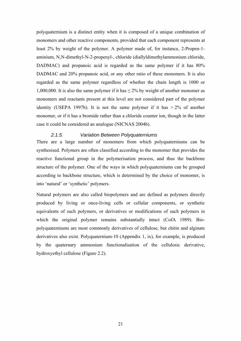
21

polyquaternium is a distinct entity when it is composed of a unique combination of

monomers and other reactive components, provided that each component represents at

least 2% by weight of the polymer. A polymer made of, for instance, 2-Propen-1-

aminium, N,N-dimethyl-N-2-propenyl-, chloride (diallyldimethylammonium chloride,

DADMAC) and propanoic acid is regarded as the same polymer if it has 80%

DADMAC and 20% propanoic acid, or any other ratio of these monomers. It is also

regarded as the same polymer regardless of whether the chain length is 1000 or

1,000,000. It is also the same polymer if it has ≤ 2% by weight of another monomer as

monomers and reactants present at this level are not considered part of the polymer

identity (USEPA 1997b). It is not the same polymer if it has > 2% of another

monomer, or if it has a bromide rather than a chloride counter ion, though in the latter

case it could be considered an analogue (NICNAS 2004b).

2.1.5. Variation Between Polyquaterniums There are a large number of monomers from which polyquaterniums can be

synthesised. Polymers are often classified according to the monomer that provides the

reactive functional group in the polymerisation process, and thus the backbone

structure of the polymer. One of the ways in which polyquaterniums can be grouped

according to backbone structure, which is determined by the choice of monomer, is

into ‘natural’ or ‘synthetic’ polymers.

Natural polymers are also called biopolymers and are defined as polymers directly

produced by living or once-living cells or cellular components, or synthetic

equivalents of such polymers, or derivatives or modifications of such polymers in

which the original polymer remains substantially intact (CofA 1989). Bio-

polyquaterniums are most commonly derivatives of cellulose, but chitin and alginate

derivatives also exist. Polyquaternium-10 (Appendix 1, ix), for example, is produced

by the quaternary ammonium functionalisation of the cellulosic derivative,

hydroxyethyl cellulose (Figure 2.2).

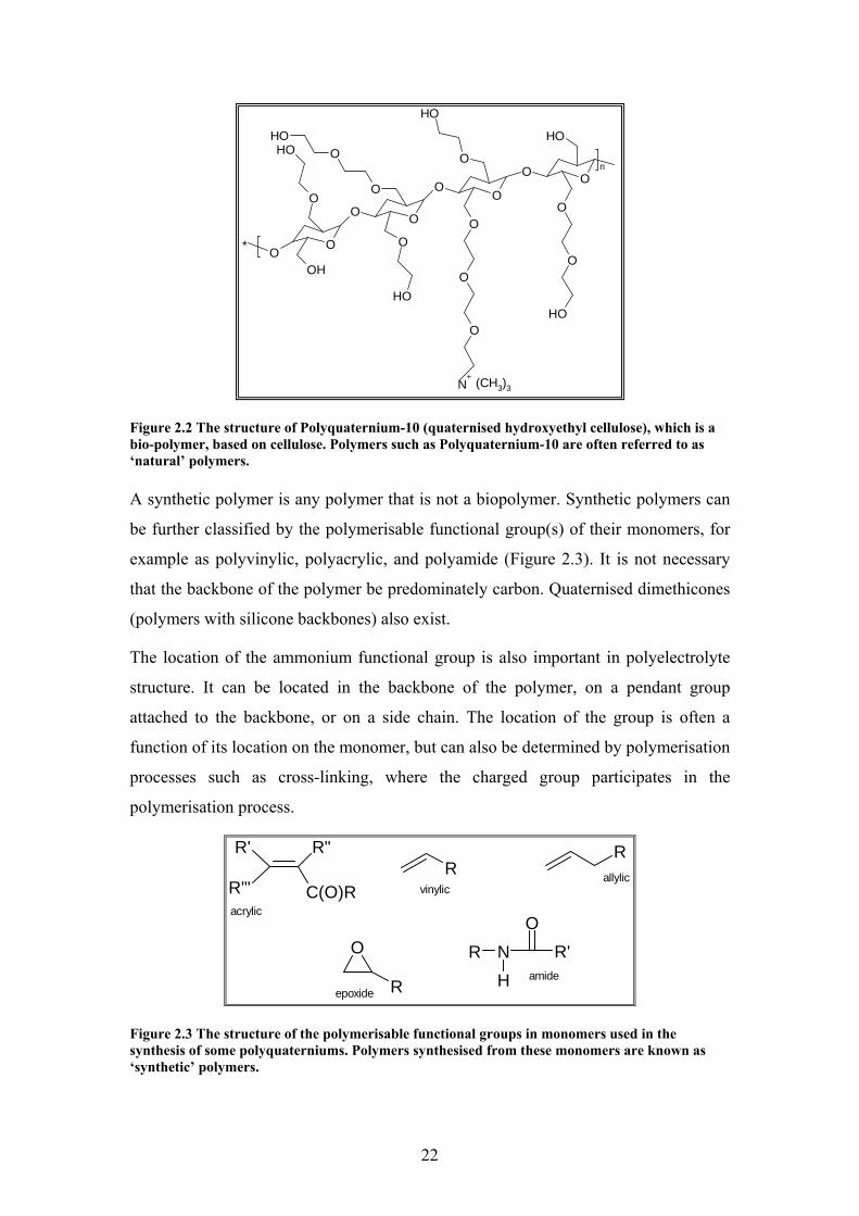
22

n

O

OO

O

OO

O

OH

O

O

O

O

OOH

O

O

OH

O

O*

OH

O

OHOH

O

OH

N+ (CH3)3

Figure 2.2 The structure of Polyquaternium-10 (quaternised hydroxyethyl cellulose), which is a bio-polymer, based on cellulose. Polymers such as Polyquaternium-10 are often referred to as ‘natural’ polymers. A synthetic polymer is any polymer that is not a biopolymer. Synthetic polymers can

be further classified by the polymerisable functional group(s) of their monomers, for

example as polyvinylic, polyacrylic, and polyamide (Figure 2.3). It is not necessary

that the backbone of the polymer be predominately carbon. Quaternised dimethicones

(polymers with silicone backbones) also exist.

The location of the ammonium functional group is also important in polyelectrolyte

structure. It can be located in the backbone of the polymer, on a pendant group

attached to the backbone, or on a side chain. The location of the group is often a

function of its location on the monomer, but can also be determined by polymerisation

processes such as cross-linking, where the charged group participates in the

polymerisation process.

R"

C(O)R

R'

R"'R

R

O

R

R N R'H

Oacrylic

vinylicallylic

epoxideamide

Figure 2.3 The structure of the polymerisable functional groups in monomers used in the synthesis of some polyquaterniums. Polymers synthesised from these monomers are known as ‘synthetic’ polymers.

23

Polyionenes are copolymers that have linkages through cationic and anionic charged

groups, and consequently are cross-linked. The anti-microbial Polyquaternium-1, used

in contact lens solutions, is an example of a polyionene (Appendix 1, i).

2.1.6. Variation Within Polyelectrolytes In addition to the structural variations between polyquaterniums, there is considerable

scope for variation within a given polymer. These variations are brought about by

varying conditions in the polymerisation process. The molecular weight of the

polymer and the percentage of low molecular weight species can be varied depending

on the reaction conditions. Polyquaternium-10, for example, is produced by the Dow

Chemical Company subsidiary Amerchol in a variety of molecular weights in the

UCareTM range (Table 2.1). The number of functional groups in the polymer (except

for homopolymers of monomers with charged groups) can be varied by changing the

ratios of monomers in the reaction. Again, Amerchol’s UCareTM range of

Polyquaternium-10, is produced with a variety of charge densities (Table 2.1).

Table 2.1. In Amerchol’s range of Polyquaternium-10, UCareTM, the polymer is produced in a range of molecular weight (as indicated by viscosity) and charge density combinations (as % amine-nitrogen) (Amerchol, 2005) Trade Name Charge Density Molecular Weight UCareTM JR400 High Low UCareTM JR30M High High UCareTM JR125 High Low UCareTM LR400 Low Low UCareTM LR30M Low High UCareTM LK Low Low

For polymers that are quaternised during or after the manufacture of the polymer, the

degree of quaternisation can be varied, allowing the polymer to be produced with a

mixture of quaternary, tertiary and secondary ammonium groups. Polyquaternium-11

is an example of a polyquaternium produced from a tertiary amine monomer (2-

Propenoic acid, 2-methyl-, 2-(dimethylamino)ethyl ester and quaternised following

polymerisation with diethyl sulphate (Appendix 1, x).

Another important variation in polyelectrolytes is hydrophobic substitution, i.e. the

addition of short or long hydrocarbon side chains to the polymer backbone. The

addition of the chains is usually not enough to make the polymer insoluble, but does

alter other important aspects of solution behaviour. Polyquaternium-24 (Appendix 1,

xx), for example, is a hydrophobically modified version of Polyquaternium-10, and is

24

also produced by Amerchol under the trade name Quatrisoft®. It has an 11-carbon

chain attached to the ammonium functional group.

2.2. Nomenclature Most polymers are named in terms of the monomers from which they are

manufactured. In the nomenclature of the Chemical Abstract Service of the American

Chemical Society, the basic form of the monomer-based name of a polymer is

‘Reactant A, polymer with reactant B and reactant C’. For example, the formal name

for Polyquaternium-13 (Appendix 1, xii) is 2-Propenoic acid, 2-methyl-, 2-

(diethylamino)ethyl ester, polymer with ethyl 2-methyl-2-propenoate and (9Z)-9-

octadecenyl 2-methyl-2-propenoate, compound with dimethyl sulphate (9CI).

Polymers with only one monomer generally have the term ‘homopolymer’ added to

the name, for example, Polyquaternium-6 (Appendix 1, v) is 2-Propen-1-aminium,

N,N-dimethyl-N-2-propenyl-, chloride, homopolymer (9CI). Although this

nomenclature system is required for regulatory purposes, common names for

monomers are still used in naming polymers. Polyquaternium-6 is most often referred

to in both product catalogues and scientific literature as poly(diallyldimethyl

ammonium chloride) or poly(DADMAC).

Polymeric quaternary ammonium salts are recognised by Cosmetic Toiletry and

Fragrance Association US (CTFA) under the label ‘Polyquaternium-X’, where X is

sequentially chosen. This naming system is widely accepted by cosmetic

manufacturers and was adopted by the European Union (96/335/EC) as the common

nomenclature for cosmetic ingredients. It appears on the International Nomenclature

for Cosmetic Ingredients (INCI) and is the name under which these polymers are

listed on product labels in Australia.

2.3. Relevant Polyquaternium Physical-Chemical Properties

Properties that are important in determining the fate of polymers such as

polyquaterniums in the environment include water solubility, molecular weight

distribution, acid dissociation constant(s), degradation half-lives, and sorption-

desorption data. Polymers tend to have low volatility in air and are not generally

absorbed through biological membranes to bioaccumulate in tissues (Doi 1997).

Therefore, the octanol-water partition coefficients and vapour pressures are generally

not considered important for predicting the environmental fate of polymers (Doi

25

1997). The risk assessment of polymers under the Toxic Substances Control Act

(TSCA) focuses on the monomer content of the polymer, molecular weight

distribution, equivalent weight of any reactive functional groups and/or cationic

charge density, properties such as physical form, particle size distribution,

swellability, aqueous solubility and water disposability (Boethling and Nabholz

1997). In the USA, the Office of Pollution Prevention and Toxics (OPPT) has

identified a group of polymers that are believed to pose low or no risk to human

health or environment and exempted them from the notification process (USEPA

1997b). In Australia, the separate notification category, PLC, with a reduced data

requirement, was introduced for these polymers (CofA 1989). Exempt polymers in the

USA, or PLCs in Australia, have to meet particular requirements with regard to

molecular weight and elemental composition. Polymers are excluded from the

category if they contain reactive functional groups, are biodegradable or unstable, are

water absorbing or contain monomers that are not on the respective inventory.

Importantly, polymers that are cationic, potentially cationic, or reasonably anticipated

to be cationic are excluded from the exemption (USEPA, 1997b).

2.3.1. Molecular Weight Distribution Polymers contain mixtures of different size molecules, and individual polymers can

be made in a range of molecular weights. In the case of the Amerchol’s

Polyquaternium-10 range with the trade name UCareTM, the name may give some

indication of the molecular weight (e.g. JR400 ≈ 4 x 105 amu, LR30M ≈ 3 x 107 amu).

However, the classification of polymers as high, medium or low molecular weight is

somewhat arbitrary, and makes comparison between polymers difficult if the actual

molecular weights are not known (Figure 2.4).

NAMW 1 3 10 102 103 104 105 106 107

Monomer OligomerLow Molecular Weight Polymer

Medium Molecular Weight PolymerHigh Molecular Weight Polymer

NAMW 1 3 10 102 103 104 105 106 107

Monomer OligomerLow Molecular Weight Polymer

Medium Molecular Weight PolymerHigh Molecular Weight Polymer

Figure 2.4 Number Average Molecular Weight (NAMW) is the total weight of all the polymer molecules in a sample, divided by the total number of polymer molecules in a sample. It gives an indication of the average size of the polymer chain, but not of the range of sizes of the chains (polydispersity) of the polymer.

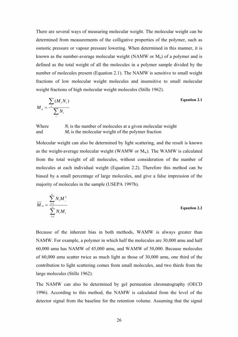
26

There are several ways of measuring molecular weight. The molecular weight can be

determined from measurements of the colligative properties of the polymer, such as

osmotic pressure or vapour pressure lowering. When determined in this manner, it is

known as the number-average molecular weight (NAMW or Mn) of a polymer and is

defined as the total weight of all the molecules in a polymer sample divided by the

number of molecules present (Equation 2.1). The NAMW is sensitive to small weight

fractions of low molecular weight molecules and insensitive to small molecular

weight fractions of high molecular weight molecules (Stille 1962).

∑∑

=

ii

iii

n N

NMM

)(

Equation 2.1

Where Ni is the number of molecules at a given molecular weight and Mi is the molecular weight of the polymer fraction Molecular weight can also be determined by light scattering, and the result is known

as the weight-average molecular weight (WAMW or Mw). The WAMW is calculated

from the total weight of all molecules, without consideration of the number of

molecules at each individual weight (Equation 2.2). Therefore this method can be

biased by a small percentage of large molecules, and give a false impression of the

majority of molecules in the sample (USEPA 1997b).

∑

∑∞

=

∞

==

1

1

2

iii

ii

w

MN

MNM

i

Equation 2.2

Because of the inherent bias in both methods, WAMW is always greater than

NAMW. For example, a polymer in which half the molecules are 30,000 amu and half

60,000 amu has NAMW of 45,000 amu, and WAMW of 50,000. Because molecules

of 60,000 amu scatter twice as much light as those of 30,000 amu, one third of the

contribution to light scattering comes from small molecules, and two thirds from the

large molecules (Stille 1962).

The NAMW can also be determined by gel permeation chromatography (OECD

1996). According to this method, the NAMW is calculated from the level of the

detector signal from the baseline for the retention volume. Assuming that the signal

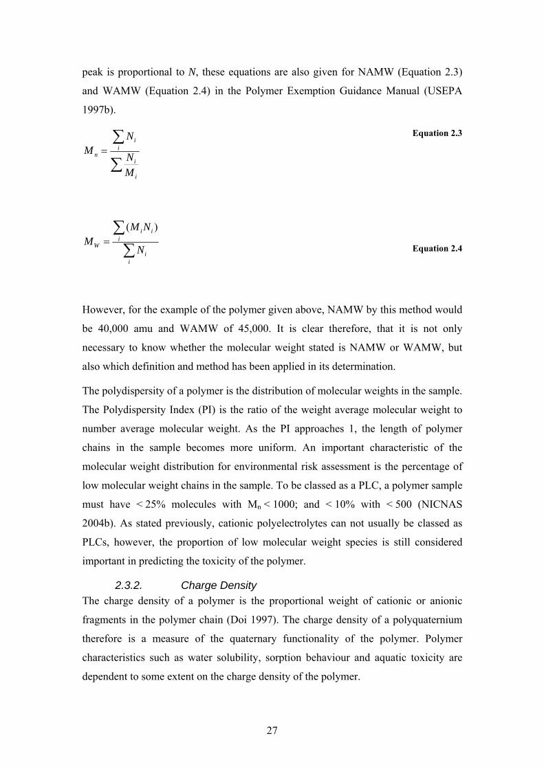
27

peak is proportional to N, these equations are also given for NAMW (Equation 2.3)

and WAMW (Equation 2.4) in the Polymer Exemption Guidance Manual (USEPA

1997b).

∑

∑=

i

i

ii

n

MN

NM

Equation 2.3

∑∑

=

ii

iii

W N

NMM

)(

Equation 2.4

However, for the example of the polymer given above, NAMW by this method would

be 40,000 amu and WAMW of 45,000. It is clear therefore, that it is not only

necessary to know whether the molecular weight stated is NAMW or WAMW, but

also which definition and method has been applied in its determination.

The polydispersity of a polymer is the distribution of molecular weights in the sample.

The Polydispersity Index (PI) is the ratio of the weight average molecular weight to

number average molecular weight. As the PI approaches 1, the length of polymer

chains in the sample becomes more uniform. An important characteristic of the

molecular weight distribution for environmental risk assessment is the percentage of

low molecular weight chains in the sample. To be classed as a PLC, a polymer sample

must have < 25% molecules with Mn < 1000; and < 10% with < 500 (NICNAS

2004b). As stated previously, cationic polyelectrolytes can not usually be classed as

PLCs, however, the proportion of low molecular weight species is still considered

important in predicting the toxicity of the polymer.

2.3.2. Charge Density The charge density of a polymer is the proportional weight of cationic or anionic

fragments in the polymer chain (Doi 1997). The charge density of a polyquaternium

therefore is a measure of the quaternary functionality of the polymer. Polymer

characteristics such as water solubility, sorption behaviour and aquatic toxicity are

dependent to some extent on the charge density of the polymer.

28

There are several methods of measuring charge density.

Charge percent: In this case charge does not refer to the cationic charge, but to the

proportion of the monomer in the polymer mix, and can be applied to any monomer in

a polymer. By this method, a homopolymer, for example, has a charge density of

100% (USEPA 1997b).

Percent amine-nitrogen (% a-N): A measure commonly used by OPPT for cationic

polyelectrolytes is the percentage of amine-nitrogen present in the polymer, as 99% of

cationic polymers have their charge based on nitrogen. It is the percentage of cationic

nitrogen in the polymer (Boethling and Nabholz 1997). This is simple for

homopolymers, but requires information on the charge percentages of the monomers

in the polymer for copolymers (Equation 2.5).

10014% ∗=−mwmonomer

Na Equation 2.5

Equivalent weight (EQWT): The equivalent weight can be calculated for any reactive

functional group in a polymer, and is used by OPPT and the National Industrial

Chemicals Notification and Assessment Scheme (NICNAS) in polymer risk

assessment. Methods of calculating the EQWT are given in the guidelines for polymer

exemption (USEPA 1997b). For polyquaterniums, EQWT can be calculated from

% a-N (Equation 2.6) (Boethling and Nabholz 1997).

NaEQWT

−=

%1400

Equation 2.6

Number of cations per 1000 molecular weight (#C/K): Although not a commonly

used measure of charge density, #C/K can be calculated simply from either % a-N

(Equation 2.7) or EQWT (Equation 2.8) according to Boethling and Nabholz (1997).

714286.0%/# ∗−= NaKC Equation 2.7

EQWTKC 1000/# = Equation 2.8

Gram-equivalents: The molar mass of a substance divided by the number of charges

of the same sign carried by the ions released by a molecule of that substance in an

aqueous solution is the gram-equivalent of the substance. For simple molecules, the

gram-equivalent is the weight of one mole of the substance divided by its valency. For

29

polymers, the gram-equivalent is usually determined by titration of a polymer

solution. The concentration of the polymer (or any molecule) in terms of gram-

equivalents is the normality (N) of the solution (Degrémont 1991). For polymers,

charge density is determined by electrolyte titration of solutions of known

concentration (Dentel 1989).

2.3.3. Aqueous Solubility The low water solubility of the majority of nonionic polymers is due to the

hydrophobicity of the polymer chains. The polyquaternium conditioning polymers

used in cosmetics are, however, highly water soluble (Gruber 1999). The solubility is

largely the result of the charged centre of the amine functional group. In an aqueous

solution, repulsive forces between the cationic amines keep the polymers apart and

dispersed through the solution. Intra-chain repulsion between the charge centres

forces the polyelectrolytes to adopt a stretched conformation (Claesson et al. 2000). In

this conformation, the polymer is often described as resembling a string, but is

perhaps a very loosely coiled globular structure, similar to globular proteins, with the

charged centres facing into the water. This conformation occurs because, like

surfactants, cationic polyelectrolytes consist of two parts with different solubility

characteristics; one part that is soluble in water (a hydrophilic group) and one part that

is not water-soluble (hydrophobic). The hydrophilic group is the charged functional

group, the cationic amine in polyquaterniums. The hydrophobic group section is the

‘tail’ of the surfactant or the polymer backbone for polyelectrolytes. In the coiled

conformation, the hydrophobic domains of the polymer chain, like surfactant tails, are

contained within a micelle-like structure (Fundin et al. 1996).

Although polyquaterniums are surface active, they are only slightly so (Manuszak

Guerrini et al. 1998). When the concentration of surfactants approaches the solubility

limit, the molecules do not precipitate, but form micelles, tiny aggregates of 50 to 100

molecules. The concentration at which micelles begin to form is called the critical

micelle concentration (CMC), and can be detected by subtle changes in surface

tension or light scattering (Connell 1997). Above the CMC, the surface tension

remains fairly constant (Manuszak Guerrini et al. 1998). In a study using Polymer

JR400, Regismond et al. (1999c) reported a slight lowering of surface tension at

concentrations between 0.05 and 0.5% w/w. The amount of reduction in surface

30

tension ranged from 0.1 to 7.4 mJ/m2. However, at the lower concentration of 0.01 %

w/w, the polymer appeared to increase surface tension slightly (0.3 to 0.4 mJ/m2).

When an anionic surfactant is added to a solution with a cationic polyelectrolyte,

several types of behaviour may be seen. The phase diagram shows three distinct

zones, the clear zone, the precipitation zone and the resolubilisation zone. The

transition between stages is marked by changes in the relative concentrations of the

polyelectrolyte and the surfactant. The clear zone occurs where there is an excess of

polyelectrolyte, and the resolubilisation with an excess of surfactant. The precipitation

zone occurs when the stoichiometry of the surfactant and polymer is approximately

1:1 (Leung, et al. 1985).

When the polymer is in excess, the electrostatic salt formation between the charged

head of the surfactant and the charged group on the polymer is followed by the

hydrophobic interaction of the surfactant tails and the hydrophobic segments of the

polyelectrolytes. The interaction begins at low concentrations, below the critical

micelle concentration (CMC) of the surfactant. The concentration at which

complexation begins is called the critical aggregation concentrations (CAC)

(Manuszak-Guerrini et al. 1997). The binding process is cooperative, as the binding of

the polycation-surfactant is more favourable than the aggregation of the surfactant

(Goddard 1999). As the charge is neutralised, hydrophobic interactions between the

surfactant tails and uncharged segments of the polymer lead to further contraction of

the complex. Neutralisation results in reduced water solubility, and the hydrodynamic

radius of the polyelectrolyte-surfactant complex is significantly smaller than that of

the free polymer (Fundin et al. 1996). As the surfactant molecules bind to the charged

centres of the polymer, a change in the conformation of the polymer occurs. The

reduction of the intramolecular repulsion allows the polymer to ‘curl up’ (Leung et al.

1985). As the polyelectrolyte-surfactant complex is formed, there is a synergistic

lowering of surface tension (Regismond et al. 1998).

In a solution with a large excess of surfactant, the complex formed consists of

polyelectrolyte cross-linked or woven through surfactant micelles (Fundin et al. 1996,

Leung et al. 1985). The structure of the surfactant micelle is similar to the structure of

micelles without the polyelectrolyte present (Ananthapadmanabhan et al. 1985). The

binding results from hydrophobic interactions between the neutral complex and the

hydrophobic tails of the surfactant and produces a negatively charged complex. The

31

new complex is larger than the complexes in the previous two zones (Fundin et al.

1996), and is soluble due to the negative charge on the surface. In cosmetic

formulations, the polymer and the surfactant are dissolved in separate components of

the formula and then mixed together. Thus the binding occurs between the formed

surfactant micelle and the polyelectrolyte and results in a viscous solution with a

highly ordered structure (Goddard and Hannan 1976). If a system with excess

surfactant is diluted below the CAC for the polymer/surfactant system, the micelle

structure of the surfactant will break down (Gruber 1999).

2.3.4. Biodegradation Degradation is an important component of the fate of cationic surfactants, but

generally, polymers are considered to be essentially nonbiodegradable. Even modified

natural polymers such as carboxymethylcellulose with an ‘appreciable’ degree of

substitution, regardless of the type of substituent, are not biodegradable. As

environmental fate assessment is commonly limited to the potential for sorption or

precipitation under various conditions, there are few studies on the biodegradability of

commercially available polymers (Boethling and Nabholz 1997).

Some studies have shown that anionic and non-ionic polymers may undergo some

degradation, but that cationic polymers are more resistant. For example, the secondary

nitrogen in anionic and non-ionic polyacrylamides was found to provide a nitrogen

source to bacteria isolated from soil, however cationic polyacrylamide was toxic to

Psuedomonas and strongly inhibited the growth of Desulfovibrio (Grula et al. 1994).

The anionic and non-ionic polyacrylamides did not provide a source of carbon, and

there was no evidence of breakdown of the polymer chain. The ability of soil bacteria

to use anionic polyacrylamide as a nitrogen source, but not as a carbon source, was

confirmed in studies by Kay-Shoemake et al. (1998). Complete removal of pendant

nitrogen from polyacrylamide would leave a residual chain similar to polyacrylic acid

(PAA), which has been shown to be incompletely mineralised by activated sludge

microorganisms even at low molecular weights. Both monomers and dimers of PAA

were completely mineralised, and low molecular weight oligomers of PAA (molecular

weights 500 and 700) were extensively but not completely degraded (Larson et al.

1997).

Cationic poly(acryloyloxyethyltrimethylammonium chloride) (AETAC) copolymer,

Percol (or Zetag) 787 (Polyquaternium-15, Appendix 1, xiv) was found by Chang et

32

al. (2001) to degrade aerobically leaving ammonia, trimethylamine, which is resistant

to further degradation, and a non-fragmented backbone of either polyacrylamide or

PAA. Anaerobically, the pendant ammonium group was also hydrolysed, and

completely degraded following removal. Again there was no evidence of breakdown

of the polymer chain. It should be noted that this test period was considerably longer

than retention times in Wastewater Treatment Plants (WWTPs). Anaerobic

degradation, as measured by increased gas production, was incomplete at the end of

the test period (840 hours). The incubation period prior to this increase in gas

production was 6 days. The authors suggest that ‘hydrolytic release of pendant group

may occur with many common flocculant polymers possessing an ester in the position

immediately adjacent to the main alkyl chain’ (Chang et al. 2001). That ester linkages

or other labile groups in the main chain of natural or synthetic backbone of polymers

may be biodegradable under favourable conditions has also been suggested (Boethling

and Nabholz 1997). Although ester linkages are common in the pendant groups of

natural polyquaterniums, they are much rarer in the synthetic polymer chains.

Quaternary polyesters are not represented in either the cosmetic or flocculant groups

of polyquaterniums.

2.3.5. Chemical/physical Degradation In addition to biodegradation, polyelectrolytes may undergo degradation due to

mechanical wearing of the polymer chains, or by reaction with other chemical species

in the water. As cationic polyelectrolytes are often used in water treatment, of

particular interest is the effect of other water treatment chemicals, such as ozone and

chlorine. The possibility of chemical degradation in effluent is also relevant to

cationic polyelectrolytes used in cosmetics, which are disposed of in sewage.

Ozonation reduced the average molecular weight of several polymers to oligomer size

(250-560 amu) in 2 to 4 hours, but without significant improvement in the

biodegradation of the fragments (Suzuki et al. 1978). Polyvinyl alcohol and

polyvinylpyrrolidone showed no improvement in biodegradability for fragments with

molecular weight > 100. There was no improvement in the degradation of

polyacrylamide even for fragments with molecular weight < 100. Chlorination

reduced the average molecular weight of anionic polyacrylamide from 107 to

approximately 104 in three hours reducing the ability of the polymers to form flocs

(Aizawa et al. 1991).

33

2.4. Exposure Assessment (Environmental Fate) A major problem in the study of environmental fate of polyquaterniums has been the

absence of any method for identifying and quantifying polyelectrolytes in

environmental samples. Although around 6.5 million tons of polyelectrolytes are used

each year in the USA alone in industry and wastewater treatment (Chang et al. 2002),

there is no satisfactory way of quantifying any flocculant residual in the treated water

(Bennett et al. 2000). Although several techniques have been developed for analysing

polyelectrolytes in relatively clean water (Wickramanayake et al. 1987), no

established method is satisfactory in complex mixtures such as wastewater, biosolids

and environmental samples (Chang et al. 2002). The inability to monitor water

concentrations at levels of regulatory concern has been identified as one of the

problems facing the cationic flocculants industry.

2.4.1. Sorption-desorption The partitioning to solids in the waste stream is generally considered the most

significant fate pathway for industrial and cosmetic cationic polyelectrolytes

(Boethling and Nabholz 1997). However, there have been few studies on sorption or

precipitation of cationic polyelectrolytes in the waste stream or in the environment.

Consequently, risk assessments of cationic polyelectrolytes are generally based on

default values for polymers. According to Boethling and Nabholz (1997) ‘non-ionic,

cationic and amphoteric polymers with molecular weight >1000 are assumed to

partition mainly to the solids phase and to be 90% removed relative to the total

influent concentration’. The 90% figure was selected because it represents a typical

level of solids removal in WWTPs (Boethling and Nabholz 1997).

The sorption of low molecular weight organic substances to soils and sediments is

dependent on the aqueous solubility of the substance and is normally proportional to

the organic carbon content of the sorbent. Generally, sorption increases with

decreasing solubility of the substance and with the increasing carbon content of the

sorbent (Podoll and Irwin 1988). Typically, the relationship between the mass of the

chemical adsorbed and the concentration remaining in solution at a given temperature,

the sorption isotherm, is linear or approximately so (Burchill et al. 1981).

2.4.2. Sorption of Polymers For polymers, molecular weight and chemical structure dominate sorption behaviour.

For polydisperse polymers i.e. polymer samples with a wide range of sizes, small

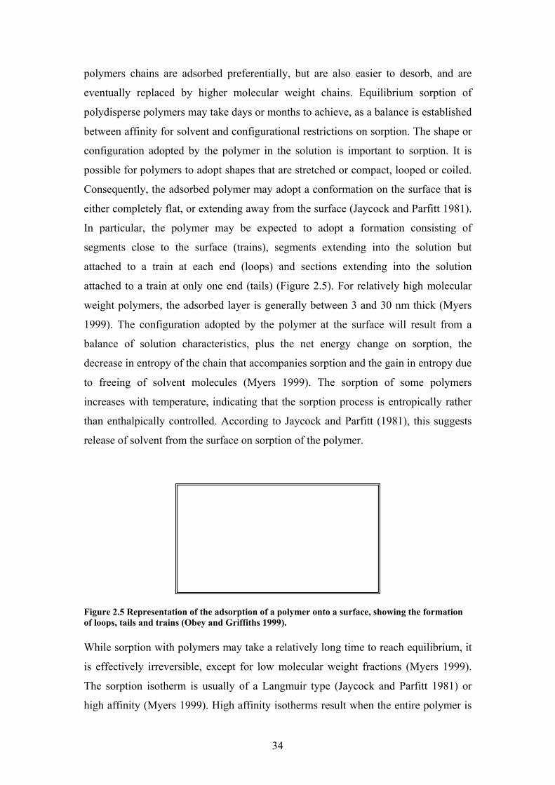
34

polymers chains are adsorbed preferentially, but are also easier to desorb, and are

eventually replaced by higher molecular weight chains. Equilibrium sorption of

polydisperse polymers may take days or months to achieve, as a balance is established

between affinity for solvent and configurational restrictions on sorption. The shape or

configuration adopted by the polymer in the solution is important to sorption. It is

possible for polymers to adopt shapes that are stretched or compact, looped or coiled.

Consequently, the adsorbed polymer may adopt a conformation on the surface that is

either completely flat, or extending away from the surface (Jaycock and Parfitt 1981).

In particular, the polymer may be expected to adopt a formation consisting of

segments close to the surface (trains), segments extending into the solution but

attached to a train at each end (loops) and sections extending into the solution

attached to a train at only one end (tails) (Figure 2.5). For relatively high molecular

weight polymers, the adsorbed layer is generally between 3 and 30 nm thick (Myers

1999). The configuration adopted by the polymer at the surface will result from a

balance of solution characteristics, plus the net energy change on sorption, the

decrease in entropy of the chain that accompanies sorption and the gain in entropy due

to freeing of solvent molecules (Myers 1999). The sorption of some polymers

increases with temperature, indicating that the sorption process is entropically rather

than enthalpically controlled. According to Jaycock and Parfitt (1981), this suggests

release of solvent from the surface on sorption of the polymer.

Figure 2.5 Representation of the adsorption of a polymer onto a surface, showing the formation of loops, tails and trains (Obey and Griffiths 1999). While sorption with polymers may take a relatively long time to reach equilibrium, it

is effectively irreversible, except for low molecular weight fractions (Myers 1999).

The sorption isotherm is usually of a Langmuir type (Jaycock and Parfitt 1981) or

high affinity (Myers 1999). High affinity isotherms result when the entire polymer is

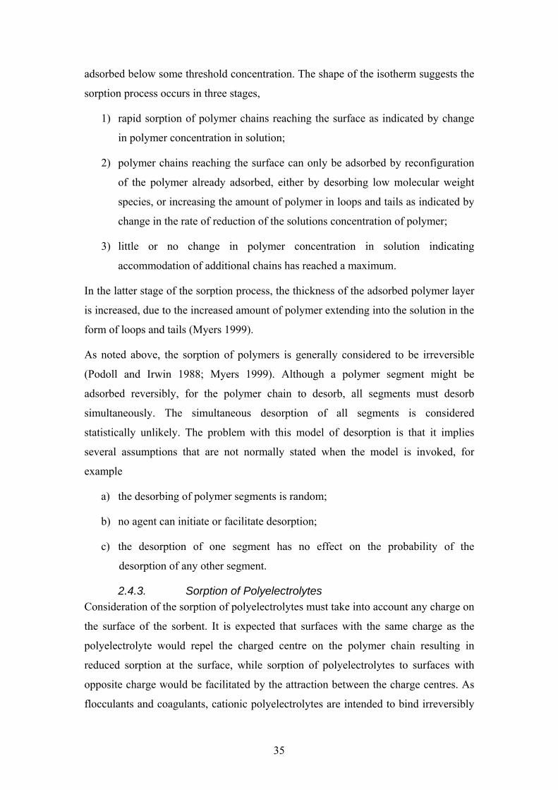
35

adsorbed below some threshold concentration. The shape of the isotherm suggests the

sorption process occurs in three stages,

1) rapid sorption of polymer chains reaching the surface as indicated by change

in polymer concentration in solution;

2) polymer chains reaching the surface can only be adsorbed by reconfiguration

of the polymer already adsorbed, either by desorbing low molecular weight

species, or increasing the amount of polymer in loops and tails as indicated by

change in the rate of reduction of the solutions concentration of polymer;

3) little or no change in polymer concentration in solution indicating

accommodation of additional chains has reached a maximum.

In the latter stage of the sorption process, the thickness of the adsorbed polymer layer

is increased, due to the increased amount of polymer extending into the solution in the

form of loops and tails (Myers 1999).

As noted above, the sorption of polymers is generally considered to be irreversible

(Podoll and Irwin 1988; Myers 1999). Although a polymer segment might be

adsorbed reversibly, for the polymer chain to desorb, all segments must desorb

simultaneously. The simultaneous desorption of all segments is considered

statistically unlikely. The problem with this model of desorption is that it implies

several assumptions that are not normally stated when the model is invoked, for

example

a) the desorbing of polymer segments is random;

b) no agent can initiate or facilitate desorption;

c) the desorption of one segment has no effect on the probability of the

desorption of any other segment.

2.4.3. Sorption of Polyelectrolytes Consideration of the sorption of polyelectrolytes must take into account any charge on

the surface of the sorbent. It is expected that surfaces with the same charge as the

polyelectrolyte would repel the charged centre on the polymer chain resulting in

reduced sorption at the surface, while sorption of polyelectrolytes to surfaces with

opposite charge would be facilitated by the attraction between the charge centres. As

flocculants and coagulants, cationic polyelectrolytes are intended to bind irreversibly

36

to anionic biosolids and separate into the solid phase during effluent treatment. In the

case of cationic polyelectrolytes, the binding is expected to be coulombic (Podoll et

al. 1987).

A major study of the adsorption behaviour of the low molecular weight fraction of

cationic and non-ionic polyelectrolytes was undertaken to assist the OPPT in

assessing the fate of water treatment polymers. These low molecular weight fractions,

or oligomers, are larger than most organic compounds, but smaller than the

commercially used polymers. They are not commercially significant, but are by-

products of the polymer synthesis process and released with the polymer on use

(Podoll et al. 1987).

This study of the sorption/desorption behaviour of oligomers of non-ionic and cationic

water treatment polymers on sediments compared non-ionic poly(ethylene glycol)

(PEG) with molecular weight from 194 (4 repeat units) to 3400 (≈ 77 units);

poly(ethylenimine) (PEI), a branched cationic polymer with primary, secondary and

tertiary substituted amino groups and molecular weight 600, 1200 and 1800 (n = 14-

42) Podoll et al. (1987); and tertiary cationic polymer poly(N,N,-dimethylaminoethyl

methacrylate) (PDAM) molecular weight of 920, 1598 and 4115 (Podoll and Irwin

1988). The sediments had varying compositions of clay, sand and silt, with organic

carbon contents varying from 0.48 – 2.33%, cation exchange capacities (CEC) of

13.5 – 33 mequiv/100 g and pH from 4.3 – 8.25.

All polymers showed strong, site-specific sorption to all sediments. While the sorption

of non-ionic PEG correlated with the clay content of the sediment, and was also

influenced by the pH of the sediment and the solution, the amount of cationic PEI and

PDAM adsorbed correlated with the CEC of the sediment and was independent of pH.

The coulombic interaction between the tertiary nitrogens of PDAM and the cation

exchange sites was found to be weaker than the coulombic interaction of PEI at these

sites.

The sorption isotherms were non-linear for both the non-ionic and the cationic

polymers. A Langmuir isotherm fitted well with cationic PEI and PDAM but less well

with non-ionic PEG. For a given molecular weight and sediment, the extent of

sorption for PEI was greater than for PEG. Sorption increased with molecular weight,

more noticeably for PEG than PEI. The plateau sorption values increased with

37

increasing molecular weight for PEI, but were independent of molecular weight for

PDAM. The number of nitrogens adsorbed per cation exchange site for PEI ranged

from about two to three and increased with increasing molecular weight, indicating

that PEI adsorbs with a significant number of the amino groups in the loops and tails.

PDAM, on the other hand, adsorbed to most soils with a ratio of amino groups to

cation exchange sites close to 1:1, indicating that it probably adsorbs in a train

conformation with almost all nitrogens attached to the sediment. These results suggest

that some flexibility is required to allow all cationic sites on the polymer to interact

with the array of anionic sites on the substrate. For example, if the separation of

anionic sites is greater than the distance between amines in PEI, then not all amines

can coulombically bond. Even if the separation is a little less, it is still difficult to

achieve an arrangement where all amines are associated with anionic sites, because

equilibration would require large amounts of desorption. With a more flexible link,

sectors can loop together and entangle more. The authors state the molecular weight

effect for PEI is mitigated by repulsive force of charged groups in the loops and tails

of the sorbed polymer.

It is possible that the non-ionic binding mechanisms (van der Waals) operating

between PEG and the clays are more sensitive to molecular weight than the charge

density dependent coulombic binding of the cationic PEI. Podoll et al. (1987) also

note that the increase in absorption with increase in molecular weight is greatest in the

lower molecular weight range, and that the rate of increase was expected to diminish

as molecular weight increased above 3400 amu. Sorption isotherms were constructed

and sorption coefficients (slope of the linear section of the isotherm) and the sorption

capacities (plateau value of the isotherm) were calculated for a range of sediments.

Sorption capacities of the sediments ranged from 17.6 mg/g to 142 mg/g and partition

coefficients from 880 to 480,000 mL/g (Podoll et al. 1987; Podoll and Irwin 1988).

Desorption was reported as being < 15% for PDAM at all concentrations, while

desorption for PEI increased with increasing solution concentration, from < 15% to as

high as 50% in the plateau region of the isotherm. However, the actual desorption data

is not published. Looking at desorption for both polymers, it was not below 10% for

any solution concentration tested, and approached 50% as the concentration

approached or exceeded 1000 ppm.

38

When added to humic acid, the water treatment algicide and cationic polymer

poly[oxy-1,2-ethanediyl(dimethyliminio)-1,2-ethanediyl(dimethyliminio)-1,2-

ethanediyl dichloride] (Busan 77, Polyquaternium-42) (Appendix 1, xxix), was found

to form insoluble precipitates with high molecular weight humic acids (Matthews et

al. 1995). The Polyquaternium-42 studied had an average molecular weight of 3900

amu, and molecular weight range from 600 to 5000 amu. However, soluble complexes

were formed with low molecular weight humic acid, with the maximum binding

capacity indicating 1:1 molar binding at saturation. The binding was reversible, and

gave a reasonable fit to a Langmuir isotherm. Between 10% and 20% of the polymer

dose was found to be bound in soluble complexes to naturally occurring humic acid

under expected levels of polymer contamination in aquatic conditions (Matthews et

al. 1995).

While the study of the sorption of polyquaterniums to environmental solids has not

received much attention, the sorptive behaviour in cosmetic applications has received

extensive attention. In addition to studies of the sorption of polyelectrolytes to hair,

various studies have examined the sorption of polyelectrolytes to mica (Fielden et al.

1998; Rojas et al. 2002), glass (Poptoshev and Claesson 2002), cellulose (Rojas et al.

2000) and silica (Samoshina et al. 2005).

Like environmental solids such as humic acid, human hair has a negatively charged

surface. The isolectric point of hair (the pH above which it has a net negative charge)

is 3.67, and its zeta potential is normally about -30 mV. A zeta potential of -25 mV is

needed for molecules to overcome van der Waals attraction. Van der Waals bonding

increases with increasing molecular surface area, and for polymers can approach the

strength of primary valence bonds (Robbins 1994). Studies with monofunctional

quaternary ammonium surfactants show substantivity to hair is only achieved when

there are 8 to 10 carbons in the hydrocarbon tail of the surfactant, indicating that van

der Waals forces in addition to ionic binding contribute to the sorption of quaternary

cationics to hair.

Many studies of the sorption of polyquaterniums to hair have been of the sorption of

the polymer alone to hair. Without the surfactant, the polymer sorbs strongly to hair,

with an excess of positive charges in the loops and tails of the sorbed polymer. The

zeta potential of the hair sample may be increased to 25-30 mV and remains positive

through continuous rinsing with water (Amerchol 2002). The amount of polymer

39

needed to saturate normal hair is 2 mg/g for

poly(methacrylamidopropyltrimethylammonium) chloride (poly(MAPTAC))

(Appendix 1, xxxvi) and 25 mg/g for UCare JR (Polyquaternium-10) (Jachowicz, et

al. 1985).

In the presence of a surfactant, however, only a fraction of the polymer may be

deposited on the hair (André et al. 1999), and the uptake of Polymer JR in the

presence of surfactants used in shampoos may be as low as 1 µg/mg (Goddard et al.

1975). The zeta potential of the hair is increased, but not to positive values, and

according to Hössel et al. (2000), this indicates the deposition of a charge neutral

polymer-surfactant complex. However, it is also possible that the lower deposition

may be responsible for the smaller change in zeta potential.

The addition of a surfactant to a preadsorbed polyquaternium layer has been studied

using mica or gold, as well as hair, as the substrate. For example, in a study of AM-

MAPTAC on gold Plunkett et al.(2002) reported swelling of the adsorbed polymer

when the surfactant, SDS, concentration was 20% of the CMC, with desorption of the

polymer occurring when the concentration was between 60% and 200% of the CMC.

Rojas et al. (2001) reported that low charge density AM-MAPTAC began to desorb

from mica at 0.1% of the CMC of SDS, and desorption increased as the surfactant

concentration was increased. Low charge density polyquaterniums adopt a more

extended conformation on the surface (more polymer in loops and tails), allowing the

association of the polyquaternium and the surfactant on the surface, thus incorporating

negative charges within the previously cationic layer of the double layer (Rojas et al.

2000). Regismond et al. (1999a) demonstrated the desorption of Polymer JR from hair

with SDS using fluorescence microscopy. Hair was treated with the fluorescently

labelled polymer JR 400 for periods ranging from 30 minutes to 12 hours. With SDS

the polyquaternium was completely desorbed from the hair samples treated for the

shorter times. Jachowicz et al. (1985) reported limited desorption of polyMAPTAC

and polyDADMAC with SDS as the polymer-surfactant complex remained bound to

the surface of the hair, however, the sorbed polycations formed complexes with the

anionic polymers PSS and PAA, and were subsequently desorbed from the hair.

Faucher et al. (1977) reported that the deposition of Polymer JR was hindered by the

presence of other electrolytes such as metal salts, with effectiveness being dependant

40

on valency. These metal salts were also able to desorb up to 50% of polymer JR,

however, the effect of valency was only apparent at low concentrations (< 0.01 M).

The studies outlined above would seem to indicate that in the presence of the

oppositely charged surfactant, sorption of the polymer may be reduced, and

desorption increased. Although humic acid has a similar isoelectric point to hair, the

behaviour of the polyquaternium/surfactant complex at infinite dilution is not known.

2.5. Effects Assessment (Aquatic Toxicology) Some of the earliest published fish toxicity data on a cationic polyelectrolyte were

reported by Tooby et al. (1975). The toxicity to Rasbora heteromorpha Duncker of

Busan 77, a Polyquaternium-42 used as a microbicide, was included in a study of the

aquatic toxicity of pesticides. The 24 hour 10th percentile lethal concentration (LC10)

and the median lethal concentration (LC50) were reported as 0.47 and 0.66 mg/L,

respectively; the 48 hour LC10 and LC50 as 0.32 and 0.39 mg/L; and the 96 hour LC50

as 0.17 mg/L. Importantly, this study established that the toxicity of cationic

polyelectrolytes may be similar to that of cationic surfactants (Madsen et al. 2001).

2.5.1. Toxicity of Surfactants As the toxicity of cationic surfactants and cationic polyelectrolytes appear to be

similar, it is useful to look briefly at the toxicity of cationic surfactants. In an

environmental and health assessment of household detergents for the Danish

Environmental Protection Agency, Madsen et al. (2001) reported that cationic

surfactants were very toxic to fish, invertebrates and algae. The LC50 values were

generally ≤ 1.0 mg/L and rarely more than ≥ 10.0 mg/L. Lewis and Suprenant (1983)

studied literature values of LC50 of cationic, anionic and non-ionic surfactants to

aquatic invertebrates. They found that the sensitivity of different species to the same

surfactant, cationic cetyl trimethyl ammonium chloride (CTAC), varied by a factor of

2300, while the sensitivity of the same species (Daphnia magna) to three surfactants

varied by a factor of up to 220. D. magna was the most sensitive species of those

considered to surfactants. The authors also tested three surfactants, CTAC, an anionic

linear alkylbenzene sulphonate and nonionic C14-15 alkyl ethoxylate to six species of

aquatic invertebrates. Clearly, the possession of cationic centres is an important factor

in the toxicity of surfactants, but variability between vulnerable organisms and

between chemical analogues appears to be high.

41

2.5.2. Toxicity of Polymers The toxicity of polymers is generally limited because their high molecular weight and

large steric size limit their ability to cross biological membranes, though chemical

reactivity of functional groups can influence ecotoxicology and fate (Hamilton et al.

1997). According to Jop (1997), with polymer dispersions, polymer toxicity may

result from mechanisms such as inhibition of light penetration or by clogging gills at

high concentrations.

2.5.3. Toxicity of Polyelectrolytes – General Considerations Assessment of the published studies on the toxicity of cationic polyelectrolytes,

mostly for water treatment polymers, can be difficult. The polymers are often

identified only by their trade names, if at all, and the chemical identity or class may be

difficult to establish. Further, molecular weight and charge density of the

polyelectrolytes are not always stated, and it may not be possible to determine if the

charge centre is tertiary or quaternary substituted. When molecular weight and charge

density are given, different methods of reporting them can still make comparisons

difficult. A study by Biesinger et al. (1976), typifies the problems in identifying the

studied polymers. The 5 cationic, one anionic and one non-ionic polyelectrolytes in

the study are identified only by their trade names, Superfloc 330, Calgon M-500,

Gendriv 162, Magnifloc 570C and Magnifloc 521C (all cationic), Dow AP-30

(anionic) and Magnifloc 905N (nonioinc). While it is possible to find Chemical

Abstracts Service (CAS) listings for most of these polymers, details of their structures

are not available. Superfloc is a trade name of Cytec, who make a range of polyamine

and poly(DADMAC) water treatment polymers, however, Superfloc 330 is no longer

listed in the Cytec catalogue. Magnifloc is the trade name for a range of food grade

water treatment polymers also made by Cytec. The Magnifloc range includes both

Polyquaternium-6 (poly(DADMAC)) and Polyquaternium-33 (Appendix 1, xxiv), but

Magnifloc 521C and Magnifloc 570C are not listed as trade names in the CAS listings

for these polymers. Gendriv 162 is a trade name for guar gum, which is not cationic as

stated by the authors. Cationic guar gum (Appendix 1, xxxvii) has a different CAS

number (65497-29-2), and the trade name Gendriv is not listed in its chemical

abstracts listing. However, guar gum, hydroxypropyl guar gum and cationic guar gum

have many similar trade names. In many cases the trade name may still be in use, but

the specific polymer referred to may no longer be in the manufacturer’s catalogue.

42

No further details were given of the structures of the seven polyelectrolytes employed

by Biesinger et al. (1976). As all are flocculants, it is probable that they are high

molecular weight, high charge density polymers. The authors reported the toxicity

values as median tolerance limit, TL50, defined as the concentration at which 50% of

the test animals were able to survive for a specified period of exposure. The exposure

time was 48 hours for Daphnia and 96 hours for fish. The results for cationic

polyelectrolytes were generally less than 10 mg/L, and less than < 1 mg/L for some

species, and only Gendriv, which has a non-synthetic backbone (guar gum) had

relatively low toxicity, with TL50 > 100 mg/L. The authors concluded that ‘some

cationic polyelectrolytes tested were particularly toxic at certain concentrations that

might easily be released into the environment and cause serious problems for aquatic

life’ (Biesinger et al. 1976). They found that the 21 day TL50 for Daphnia was higher

by an order of magnitude than 48 hour TL50, which they attributed to the addition of

food during the test, and adsorption of the test material to the food particles (Biesinger

et al. 1976).

A number of studies have shown that the presence of suspended solids mitigated the

toxicity of cationic polyelectrolytes (Devore and Lyons 1986). For example, four

cationic polylectrolytes, two epichlorohydrin-amine condensates (molecular weight

20,000 and 400,000 amu), an acrylamide-vinyl quaternary amine copolymer

(molecular weight 3,000,000 amu) and poly(DADMAC), with LC50 values to

minnows and Daphnia < 1 mg/L, were tested in synthetic river water containing fixed

amounts kaolinite clay, humic acid and dissolved salts prepared in the laboratory. No

toxicity was evident until the polymer dose exceeded the dose required for

flocculation, around 10 mg/L. The lack of toxicity at concentrations below the

flocculant dose is therefore assumed to result from the lack of free polymer molecules

in the solution. The resuspension of the floc due to overdosing coincided with the

reappearance of free polymer molecules in the supernatant and observed toxic effects

in the test organisms. The mitigating effect of suspended solids has become a major

theme in toxicity studies of cationic polyelectrolytes.

Biesinger and Stokes. (1986) looked at detoxifying effects of anionic polymers and

various clays on cationic polyelectrolytes. Anionic polyelectrolytes were able to

negate the toxic effects of the cationic polyelectrolyte when present in about equal

quantities. The authors report the amounts of clay needed to detoxify a cationic

43

polymer at five times the toxic dose were 80 mg/L for red clay, 160 mg/L for

montmorillonite and 320 mg/L for kaolinite. These concentrations are a useful

indication of the relative adsorptive ability of the various clays. However, it appears

that only one polymer was tested in this manner (‘Polymer O’, Median Effective

Concentration (EC50) 96 hour fish 1.05 mg/l). Of the fifteen polyelectrolytes in this

study, most had effective concentration in tests with daphnids of < 1 mg/L and with

minnows < 10 mg/L, although some had effective concentrations > 100 mg/L for one

or both species. Eight polyelectrolytes were also tested with midges, and 13 with

gammarids. These organisms were less sensitive to the cationic polyelectrolytes than

fish and Daphnia. According to the authors, the ‘large differences in sensitivity

between these species suggest different modes of toxic action’, while the differences

in toxicity between various polymers ‘is probably accounted for by their chemical

structure’ (Biesinger and Stokes 1986). However, no details of the chemical structures

of the polymers in their study are given. Elucidating the structural characteristics that

influence the toxicity is the other major theme in toxicity studies of cationic

polyelectrolytes.

The mitigating effect of humic acid on the toxicity of polyquaterniums was an issue

for industrial manufacturers because of the United States Environment Protection

Agency’s (USEPA) data requirements pre-manufacture notice (PMN) under TSCA.

When acute toxicity studies submitted with a PMN for a chemical had LC50 values

< 1.0 mg/L, additional supporting data including chronic life-cycle studies on two to

three species were required (Cary et al. 1987; Cary et al. 1989). It was suggested that

results of acute toxicity tests ‘may be too stringent for estimating the effects of

cationic polyelectrolytes in receiving waters’ (Cary et al. 1987). This claim was

supported by the study of four quaternary polyelectrolytes of varying chemistries,

molecular weight, charge density and percent quaternisation, all with LC50 values to

three species of fish and Daphnia of < 1 mg/L. The toxicity of the polyelectrolytes

was tested in the presence of suspended solids (bentonite, illite, kaolin and pure silica)

at 50 mg/L, and dissolved organic carbon (DOC) (humic acid, tannic acid, fulvic acid,

lignin, and lignosite) at 10 mg/L. The presence of suspended solids or DOC reduced

the toxicity of the cationic polyelectrolytes regardless of molecular weight or charge

density. The reduction in LC50 was generally one to two orders of magnitude, though

illite, kaolin and silica were less effective (Cary et al. 1987).

44

To address chemical industry concerns regarding the costs of providing the extra data

with PMNs, the Cationic Flocculant Producer Association (CFPA) was formed as a

subgroup of Specialty Organic Chemical Manufacturers Association (SOCMA) (Cary

et al. 1989). The CFPA consisted of American Cyanimid Company, Betz Laboratories

Inc, Calgon Corporation, CPS Chemical Company Inc, Hercules Incorporated, Nalco

Chemical Company and Petrolite Corporation. The purpose of the group was to lobby

USEPA to treat cationic polyelectrolytes as a class of chemicals, rather than treating

each new PMN individually. It was felt that this would lead to lower data

requirements, and hence lower notification costs. Data was collected from members

on 386 toxicity studies of cationic polyelectrolytes. The data included chemical

classification, molecular weight, charge density, test species, toxicity values, water

hardness, suspended solids and type of Total Organic Carbon (TOC) and Suspended

Solids (SS). Sixty percent of the cationic polyelectrolytes had toxicity values between

0.1 and 1.0 mg/L, and only 8% had toxicity values > 10 mg/L. Nine classes of water

soluble cationic polyelectrolytes were identified, though data was collected on only

six of them. No correlation was reported between toxicity and molecular weight,

charge density or water hardness (Cary et al. 1989). The data have not been published.

To further support the case for mitigation, and therefore reduced data requirements for

PMNs, four cationic polyelectrolytes were tested in reconstituted laboratory water

with humic acid, fulvic acid, tannic acid lignin, and lignosite at concentrations of 5,

10, 20 mg/L were used for four compounds (quaternised polyethanolamine, molecular

weight 25,000 amu; poly(dimethylvinyl-pyridinium) chloride, molecular weight

≈ 1,200,000 amu; dimethylamine-epichlorohydrin copolymer, molecular weight

100,000 amu), and 5, 10, 20 mg/L for high charge density polymers

(epichlorohydrin/amine polymer, molecular weight 2-3000 amu). Again, a reduction

in the toxicity of around 2 orders of magnitude was reported. Further, a direct linear

relationship between LC50 and DOC was reported from regression analysis (Cary et

al. 1989). As a result of the efforts by CFPA, test procedures incorporating the

mitigating effect of humic acid were incorporated into the USEPA’s procedure for

environmental impact assessment (Cary et al. 1989). Humic acid was chosen as the

most representative DOC because of its median response and ‘ubiquitous’ nature

(Cary et al. 1989).

45

Having established cationic polyelectrolytes as a distinct class of polymers, further

studies on the toxicity of cationic polyelectrolytes have focused on the relative

toxicity of the polymers based on structural features such as molecular weight and

charge density, that is, within-class variation in toxicity. The results have been

somewhat contradictory. In a study to evaluate the effect of chemistry, charge density

and molecular weight on acute and chronic toxicity (Goodrich et al. 1991) found

useful comparisons were made difficult by variability in replicate data and the small

data sample. The polymers selected for this study included three

epichlorohydrin/dimethylamine polymers of varying molecular weight (up to 250,000

amu), and two acrylamide polymers (acrylamide/2-(N,N,N)-trimethyl ammonium

ethylacrylate chloride) with different charge densities. The polyelectrolytes were all

relatively toxic, with only the low charge density acrylamide polymer having a LC50

> 1.0 mg/L (≈ 1.7 mg/L). The authors did report a tendency of increasing toxicity with

increasing molecular weight. This was most noticeable in the chronic studies, due to

the replicate variability in the acute studies. What is important, however, is the low

acute to chronic LC50 ratios, with most mortality in the long-term test occurring in the

first seven days. The mitigating effects of humic acid were again reported with a 7 to

16-fold decrease in toxicity with as little as 5 mg/L humic acid. Although this study

included chronic studies, the mitigating effect of humic acid was not established in the

chronic tests.

A much larger study of 34 water treatment polymers, including 24 cationic

polyelectrolytes, appears to have been more successful in finding factors controlling

toxicity (Hall and Mirenda 1991). The cationic polyelectrolytes included in the study

were poly(methacryloyloxy ethyltrimethyl ammonium chloride) (METAC), AETAC,

dimethylamine-epichlorohydrin polymer EPI/DMA, poly(DADMAC), Mannich

amine (cationic tertiary amines), and one melamine-formaldehyde (MF) copolymer.

While the METAC, AETAC and DADMAC polymers are expected to be quaternary,

the degree of substitution of the EPI/DMA and MF polymers is not specified. Two

species, Daphnia pulex and Pimephales promelas (fathead minnow) were used in the

tests. There was an apparent increase in toxicity with increasing charge density

evident in the fish data for the METAC and AETAC polymers. The LC50 for fish for

the melamine-formaldehyde copolymer was > 170 mg/L, and this compound was also

only moderately toxic to Daphnia (12.31 mg/L). The Mannich amine polymers were

46

significantly less toxic to Daphnia, (LC50 42-70 mg/L) than to fish (1.1-3.3 mg/L).

The authors suggest that polymer chemistry is the controlling factor in toxicity of the

cationic polyelectrolytes to Daphnia, while toxicity to the minnow appeared to be

related to charge density. However, analysis of this data by Cumming et al. (2005)

using Pearson Correlation Coefficient (SAS 2002) shows that while fish LC50 is

correlated with charge density for AETAC polymers (0.83682, p = 0.0049), it was

less correlated for METAC polymers (0.8077, p = 0.0982) and not at all for all the

cationic polyelectrolytes (0.08799, p = 0.6827). There are two possible explanations

for this outcome. Either chemistry is also important in toxicity of cationic

polyelectrolytes to fish, or toxicity becomes asymptotic relative to charge density

above a certain value.

Further toxicity data for water treatment polymers were reported Beim and Beim.

(1994) and Fort and Stover (1995). In one study higher bioactivity with increasing

charge density was reported for three polymers, but no correlation with molecular

weight. Species including saprophytic bacteria, planaria and gammaridae were found

to be less susceptible than fish and Daphnia (Beim and Beim. 1994). Although LC50

values for algae were not published, they were found to be less sensitive than

Daphnia, but more sensitive than fish. In a comparison of the toxicity of four water

treatment polymers (including 3 polyquaterniums) and two inorganic flocculants,

ferric chloride and aluminium sulphate, to Daphnia, the polymers were found to be

significantly more toxic than the inorganic flocculants (Fort and Stover 1995).

A summary of the published toxicity values for cationic polyelectrolytes is given in

Appendix 2.

2.5.4. Meta-analysis Meta-analysis is a technique of combining independent but related published studies

using statistical methods to synthesise results with the aim of evaluating results in

ways that may not have been possible in the original studies. Published data can also

be re-analysed using statistical techniques that may not have been available or

employed at the time the data as published. Review studies of cationic

polyelectrolytes have been published and provide suitable data for examination of the

role of polymer characteristics in toxicity. Boethling and Nabholz (1997) published

toxicity data for about 50 cationic polyelectrolytes that had been submitted with

47

PMNs to the OPPT under TSCA. Based on their interpretation of this data, the authors

suggested the following:

a) aquatic toxicity is strongly influenced by cationic charge density and type of

polymer backbone;

b) aquatic toxicity increases ‘exponentially’ with higher charge density until

toxicity becomes ‘asymptotic’;

c) aquatic toxicity is not influenced by pH dependence (degree of substitution),

position of cations (backbone or pendant) or molecular weight;

d) effect of molecular weight may be greatest with relatively high surface to

volume ratios of organisms: algae > daphnids > fish (Boethling and Nabholz

1997).

Establishing any relationships between polymer characteristics and toxicity based on

this published data is problematic. The data set is not balanced in terms of treatments

(polymer characteristics) and the data is neither independent nor normally distributed.

It should be possible, however, to determine if the conclusions that have been drawn

from the data are reasonable.

Importantly, it can be shown that there are significant correlations between the

polymer characteristics themselves. For example, in the OPPT data (Boethling and

Nabholz 1997), cationic polylectrolytes with natural (cellulosic) backbones tend to

have medium to high molecular weight and low charge density, while silicone based

polycations have low molecular weights and low charge densities. Synthetic carbon

polymers have an approximately equal distribution of molecular weights and charge

densities. Specifically, using correlation analysis (SAS 2002) it can be shown that

there is a small, but significant, negative correlation (-0.43811, p = 0.0008) between

charge density and molecular weight in the OPPT data. As can be seen from the

simple scatter plot of the two variables in Figure 2.6, the high variability in molecular

weight at low charge density narrows considerably as charge density increases.

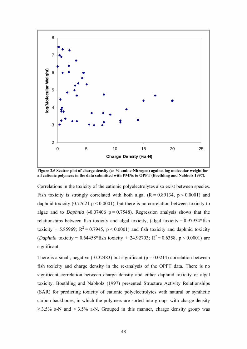
48

2

3

4

5

6

7

8

0 5 10 15 20 25

Charge Density (%a-N)

log(

Mol

ecul

ar W

eigh

t)

Figure 2.6 Scatter plot of charge density (as % amine-Nitrogen) against log molecular weight for all cationic polymers in the data submitted with PMNs to OPPT (Boethling and Nabholz 1997). Correlations in the toxicity of the cationic polyelectrolytes also exist between species.

Fish toxicity is strongly correlated with both algal (R = 0.89134, p < 0.0001) and

daphnid toxicity (0.77621 p < 0.0001), but there is no correlation between toxicity to

algae and to Daphnia (-0.07406 p = 0.7548). Regression analysis shows that the

relationships between fish toxicity and algal toxicity, (algal toxicity = 0.97954*fish

toxicity + 5.85969; R2 = 0.7945, p < 0.0001) and fish toxicity and daphnid toxicity

(Daphnia toxicity = 0.64458*fish toxicity + 24.92703; R2 = 0.6358, p < 0.0001) are

significant.

There is a small, negative (-0.32483) but significant (p = 0.0214) correlation between

fish toxicity and charge density in the re-analysis of the OPPT data. There is no

significant correlation between charge density and either daphnid toxicity or algal

toxicity. Boethling and Nabholz (1997) presented Structure Activity Relationships

(SAR) for predicting toxicity of cationic polyelectrolytes with natural or synthetic

carbon backbones, in which the polymers are sorted into groups with charge density

≥ 3.5% a-N and < 3.5% a-N. Grouped in this manner, charge density group was

49

significant for all species in a nonparametric rank sums (Kruskal-Wallis) test. The

significant correlations in these data sets appear to be the result of a small number of

very low charge density polymers with very low toxicities. Importantly, this data

shows that high charge density polycations are almost always very toxic, but low

charge density polycations are still frequently toxic (Table 2.2). There is a significant

correlation between log molecular weight and acute and chronic algal toxicity

(0.61299, p = 0.0089, n = 17; and 0.61168, p = 0.0118, n = 16 respectively) but not

fish or daphnid toxicity in the TSCA data.

Table 2.2 The number of high and low charge density polycations by Globally Harmonised System for Classification and Labelling of Chemicals (GHS) classification based on the OPPT data in Boethling and Nabholz (1997). >100 mg/L Harmful Toxic Very toxic Total Fish: High charge density Low charge density

1 5

0 5

2 6

21 10

24 26

Daphnia: High charge density Low charge density

0 6

1 6

4 1

10 6

15 19

Algae: High charge density Low charge density

1 2

0 0

0 3

12 4

13 9

Lyons and Vaconcellos (1997) reviewed toxicity data for 61 polycations, drawn from

unpublished studies by Betz Laboratories, and published papers including Hall and

Mirenda (1991), Goodrich et al. (1991) and Cary et al. (1987). In a meta-analysis of

this data (SAS 2002), the relationship between charge density (ionicity) and molecular

weight was found to be significant in a Kruskal-Wallis test (p < 0.0001), and in a

generalised linear model (in which molecular weight is given as a class variable only)

molecular weight was found to account for about 48% of the variation in percent

ionicity. There was no correlation between fish toxicity and daphnid toxicity. There

was a correlation between percent ionicity and daphnid toxicity (r = 0.30772, p = 0.

0265), but not fish toxicity. As the correlation between percent ionicity and daphnid

toxicity is positive, LC50 is increasing, and therefore toxicity decreasing, as charge

density increases. The statistical significance in this data set, in contrast to the OPPT

data, appears to result from a small number of relatively very toxic, high charge

density polymers. Analysis by non-parametric rank (Kruskal-Wallis) indicates a

significant relationship between molecular weight and fish toxicity, but not daphnid

toxicity. Details of the chemistry were not given for the OPPT data, but the

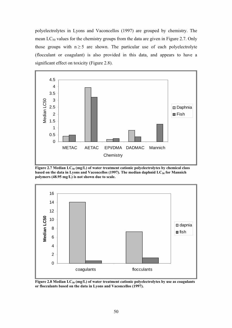
50

polyelectrolytes in Lyons and Vaconcellos (1997) are grouped by chemistry. The

mean LC50 values for the chemistry groups from the data are given in Figure 2.7. Only

those groups with n ≥ 5 are shown. The particular use of each polyelectrolyte

(flocculant or coagulant) is also provided in this data, and appears to have a

significant effect on toxicity (Figure 2.8).

00.5

11.5

2

2.53

3.54

4.5

METAC AETAC EPI/DMA DADMAC Mannich

Chemistry

Med

ian

LC50

DaphniaFish

Figure 2.7 Median LC50 (mg/L) of water treatment cationic polyelectrolytes by chemical class based on the data in Lyons and Vaconcellos (1997). The median daphnid LC50 for Mannich polymers (48.95 mg/L) is not shown due to scale.

0

2

4

6

8

10

12

14

16

coagulants flocculants

Med

ian

LC50

dapniafish

Figure 2.8 Median LC50 (mg/L) of water treatment cationic polyelectrolytes by use as coagulants or flocculants based on the data in Lyons and Vaconcellos (1997).

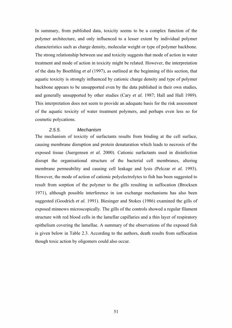
51

In summary, from published data, toxicity seems to be a complex function of the

polymer architecture, and only influenced to a lesser extent by individual polymer

characteristics such as charge density, molecular weight or type of polymer backbone.

The strong relationship between use and toxicity suggests that mode of action in water

treatment and mode of action in toxicity might be related. However, the interpretation

of the data by Boethling et al (1997), as outlined at the beginning of this section, that

aquatic toxicity is strongly influenced by cationic charge density and type of polymer

backbone appears to be unsupported even by the data published in their own studies,

and generally unsupported by other studies (Cary et al. 1987; Hall and Hall 1989).

This interpretation does not seem to provide an adequate basis for the risk assessment

of the aquatic toxicity of water treatment polymers, and perhaps even less so for

cosmetic polycations.

2.5.5. Mechanism The mechanism of toxicity of surfactants results from binding at the cell surface,

causing membrane disruption and protein denaturation which leads to necrosis of the

exposed tissue (Juergensen et al. 2000). Cationic surfactants used in disinfection

disrupt the organisational structure of the bacterial cell membranes, altering

membrane permeability and causing cell leakage and lysis (Pelczar et al. 1993).

However, the mode of action of cationic polyelectrolytes to fish has been suggested to

result from sorption of the polymer to the gills resulting in suffocation (Brocksen

1971), although possible interference in ion exchange mechanisms has also been

suggested (Goodrich et al. 1991). Biesinger and Stokes (1986) examined the gills of

exposed minnows microscopically. The gills of the controls showed a regular filament

structure with red blood cells in the lamellar capillaries and a thin layer of respiratory

epithelium covering the lamellae. A summary of the observations of the exposed fish

is given below in Table 2.3. According to the authors, death results from suffocation

though toxic action by oligomers could also occur.

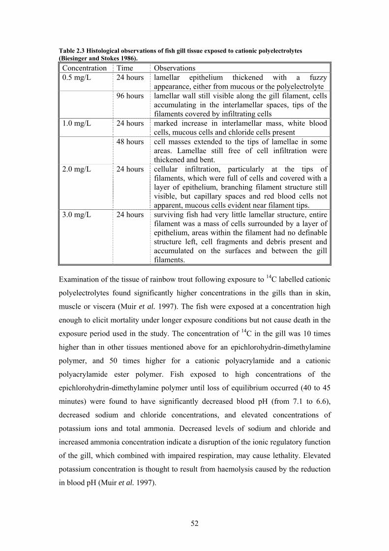
52

Table 2.3 Histological observations of fish gill tissue exposed to cationic polyelectrolytes (Biesinger and Stokes 1986). Concentration Time Observations 0.5 mg/L 24 hours lamellar epithelium thickened with a fuzzy

appearance, either from mucous or the polyelectrolyte 96 hours lamellar wall still visible along the gill filament, cells

accumulating in the interlamellar spaces, tips of the filaments covered by infiltrating cells

1.0 mg/L 24 hours marked increase in interlamellar mass, white blood cells, mucous cells and chloride cells present

48 hours cell masses extended to the tips of lamellae in some areas. Lamellae still free of cell infiltration were thickened and bent.

2.0 mg/L 24 hours cellular infiltration, particularly at the tips of filaments, which were full of cells and covered with a layer of epithelium, branching filament structure still visible, but capillary spaces and red blood cells not apparent, mucous cells evident near filament tips.

3.0 mg/L 24 hours surviving fish had very little lamellar structure, entire filament was a mass of cells surrounded by a layer of epithelium, areas within the filament had no definable structure left, cell fragments and debris present and accumulated on the surfaces and between the gill filaments.

Examination of the tissue of rainbow trout following exposure to 14C labelled cationic

polyelectrolytes found significantly higher concentrations in the gills than in skin,

muscle or viscera (Muir et al. 1997). The fish were exposed at a concentration high

enough to elicit mortality under longer exposure conditions but not cause death in the

exposure period used in the study. The concentration of 14C in the gill was 10 times

higher than in other tissues mentioned above for an epichlorohydrin-dimethylamine

polymer, and 50 times higher for a cationic polyacrylamide and a cationic

polyacrylamide ester polymer. Fish exposed to high concentrations of the

epichlorohydrin-dimethylamine polymer until loss of equilibrium occurred (40 to 45

minutes) were found to have significantly decreased blood pH (from 7.1 to 6.6),

decreased sodium and chloride concentrations, and elevated concentrations of

potassium ions and total ammonia. Decreased levels of sodium and chloride and

increased ammonia concentration indicate a disruption of the ionic regulatory function

of the gill, which combined with impaired respiration, may cause lethality. Elevated

potassium concentration is thought to result from haemolysis caused by the reduction

in blood pH (Muir et al. 1997).

53

The depuration of the polymer, as loss of 14C from the gill, in water following short

one hour exposures then depuration for 6 hours was rapid for both cationic

polyacrylamide (half life 2.8 hours) and cationic polyacrylamide ester (2.6 hours). For

epichlorohydrin-dimethylamine, removal was somewhat slower, with a half life of 5.7

hours. The presence of humic acid in the water during depuration did not significantly

alter the depuration time for the polyacrylamides (3.4 and 3.5 hours respectively), but

removal of epichlorohydrin-dimethylamine was more rapid (half-life 1.2 hours).

There was no accumulation in tissues following three repeat exposures of three hours

followed by 24 hour depuration (Muir et al. 1997).

While it is feasible to extrapolate the mode of action to all organisms that have a gill

structure like fish, cationic polyelectrolytes are also expected to sorb strongly to other

biological membranes that are anionic, such as some bacterial surfaces (Boethling and

Nabholz 1997). However, it has been suggested that other factors may be important

for some smaller organisms. Cary et al. (1987) observed the mechanism of toxicity of

cationic polyelectrolytes to daphnids and reported that Daphnia acted as sites of

flocculation and were physically clumped together or entrapped within the floc.

Consequently, the toxicity did not follow a typical dose-response curve. Survival rates

increase above the optimum treatment dose due to the polymers’ tendency to

resuspend the floc. Mortality due to physical entrapment or clumping of daphnids was

also noted by Hall and Mirenda(1991), who attributed wide confidence intervals

around the LC50 values in this study to this phenomenon.

2.6. Summary The above review shows that unlike compounds used in applications such as water

treatment, polyquaterniums used in cosmetic applications may not be released to

wastewater as a charged polycation. Cosmetic polyquaterniums are formulated in an

excess of anionic surfactant, deposited onto hair or skin as a polymer-surfactant

complex, and are desorbed from the hair or skin in subsequent washing with an

anionic surfactant. The chemical species or form released, therefore, is most likely to

be a charge-neutral polyquaternium/surfactant complex. Unlike water treatment

polycations, this complex is film-forming rather than floc forming and may have very

different environmental characteristics than the charged polycation. In particular, rates

of sorption and desorption may be significantly different for the polymer-surfactant

complex. While anionic species, particularly anionic polymers, have been shown to

54

mitigate the toxicity of some industrial polycations, the toxicity of the

polyquaternium/surfactant complex to aquatic organisms is not known.

55

3. Analysis of Polyquaterniums 3.1. Introduction

Many techniques have been developed for analysing polyelectrolytes in relatively

clean water. These techniques include turbidimetry/nephelometry, spectrofluorometry,

spectrophotometry, viscometry, colloid titration, luminescence titration, gel

permeation chromatography, bromine oxidation of primary amides, and

radioimmunoassay (Wickramanayake et al. 1987). Some of these clean water

analytical techniques are limited by their specificity to certain types of

polyelectrolytes, for example, the bromine oxidation for polyelectrolytes containing

primary amide functional groups, and radioimmunoassay for polyacrylamides. More

recent developments, such as the use of NMR (Chang et al. 2002) are also limited, so

far, to polyelectrolytes with trimethyl quaternary ammonium pendant functional

groups.

Fluorescent tagging, the attaching of a fluorescent chromophore to a polyelectrolyte,

has also been used in some studies of cationic polyelectrolytes. Fluorescently tagged

polyelectrolytes can be detected qualitatively by fluorescent microscopy (Regismond

et al. 1999b) and quantitatively by luminescence spectroscopy (Bennett et al. 2000).

The method has been used to study the sorption of cationic polyelectrolytes on hair

(Regismond et al. 1999b), polymer-surfactant interactions (Ananthapadmanabhan et

al. 1985; Winnik and Regismond 1996; Morishima et al. 1999) and as an indicator in

polyelectrolyte titration (Tanaka and Sakomoto 1993).

Fluorescently tagged poly(DADMAC) has also been suggested for possible use in the

determining of residual polymer after flocculant dosing in water treatment (Bennett et

al. 2000). Unlike the studies of sorption of polyquaterniums on hair using

Polyquaternium-10, which needs no modification prior to the addition of the

fluorescent tag, poly(DADMAC) has to be polymerised with an amine-functional

monomer at 1-2% charge in order to be tagged. This does not, however, amount to a

substantial change to the polymer, and does not change its legal identity. Of two

fluorescent tags trialled in the study by Bennett et al. (2000), one was found to be

quenched by the presence of organic carbon in the water. Many fluorescent indicators

are also quenched by the presence of surfactants, hence their use in the study of

polymer-surfactant interactions, and this may limit the usefulness of the method in

determining residuals following wastewater treatment.

56

3.1.1. Metachromasy The most widely used method of analysis of polyelectrolytes in the literature is colloid

titration, which is based on a phenomenon known as metachromasy. This method

arose from the observation of the behaviour of certain aniline dyes used in the staining

of histological samples (Bergeron and Singer. 1958). A history of the development of

the method in histology is given in Bergeron and Singer. (1958), who proposed the

following definition:

Metachromasy is the hypsochromic (shift in absorption to shorter

wavelength) and hypochromic (decrease in intensity of colour) change in

colour exhibited by certain basic aniline dyes in the presence of water and

under the following conditions:

a) increase in dye concentration;

b) temperature decrease;

c) salting out;

d) interaction with certain substrates whose metachromatic influence may

be due to serially arranged proximate anionic sites.

Metachromasy has been adapted for the measurement of concentration and charge

density of polyelectrolytes when used in conjunction with analytical techniques such

as colloid titration.

3.1.2. Colloid Titration Colloid titration is the name given to the quantitative volumetric analysis of

polyelectrolytes in solution (Terayama 1952). The titration is possible because ionic

reactions between oppositely charged polyelectrolytes in dilute solutions are

stoichiometric by charge and very rapid (Terayama 1952). The endpoint of colloid

titration has been determined by changes in turbidity (Hanasaki et al. 1985),

streaming current detection (Kam et al. 1999), ion-selective electrodes (Séquaris and

Kalabokas et al. 1993), conductometric methods (Ghimici and Dragan 2002), and by

colour change of a metachromatic dye (Wang and Shuster 1975). The method has also

been used for charge determination of proteins (Horn and Heuck 1983) and cell

surfaces (Watanabe and Takesue 1976; Van Damme et al. 1994), as well as for

determining polyelectrolyte concentration in water (Wang and Shuster 1975; Parazak

et al. 1987; Majam and Thompson 2006). In the latter capacity it has also been used

57

for sorption studies. In these, the sorbed concentration was determined by difference

between the starting and equilibrium concentrations Hutter, 1991 #100. However, it

has limitations in some water industry applications due to interference by organics

(Hanasaki et al. 1985) and inorganic ions (Sjöedin and Öedberg 1996).

Cationic metachromatic dyes, for example o-toluidine blue, are useful indicators for

colloid titration as they do not interact with cationic polyelectrolytes due to

electrostatic repulsion, but produce a distinct metachromatic colour shift from blue to

red-violet on binding with anionic polyelectrolytes. The method, therefore, allows for

the direct titration of cationic polyelectrolytes, while anionic polyelectrolytes need to

be back-titrated with a cationic standard (Ueno and Kina 1985). In colloid titration

using a metachromatic dye as an endpoint indicator, the reaction between the cationic

analyte and anionic titrant is favoured over the reaction between the titrant and the

indicator, so the coupled reactions occur consecutively (Horn and Heuck 1983). Once

the cationic polyelectrolyte is reacted, the chromotropic polyanionic titrant begins to

combine with the dye, resulting in a colour change that is clear and instant according

to Terayama (1952).

3.2. Metachromatic Polyelectrolyte Titration While colloid titration with metachromatic dyes has been in use for nearly fifty years,

there are still many unresolved issues in the method. The determination of the

concentration of a polyelectrolyte in water by titration relies on the measurement of

the amount of cationic or anionic functional groups present in the solution, and thus

determines the concentration of the solution in terms of equivalents per litre, i.e. the

normality of the solution. The method has been applied to charge determination not

only of water treatment polyelectrolytes (Dentel 1989; Kam et al. 1999), but also to a

variety of bio-molecules such as bovine pancreatic chymotrypsin A, bovine

ribonuclease A, porcine pepsin, equine heart muscle cytochrome c. (Horn and Heuck

1983), bone cartilage (Van Damme et al. 1992), heparin (Katayama et al. 1978),

together with humic acid and the extracellular polymers of activated sludge

(Mikkelsen 2003). Other colloids whose normality may be determined by colloid

titration include cellulose sulphate, plant mucilages (gum Arabic, gum tragacanth,

agar agar), lignin, and clay, all of which are anionic (Terayama 1952; Ueno and Kina

1985). While there are fewer positively charged colloids, derivatives of chitosan and

58

some proteins, such as clupein and salmine (Terayama 1952) have been measured

with polyelectrolyte titration.

Subsequently, in this work the term Metachromatic Polyelectrolyte Titration will be

used to refer to the analysis of polyelectrolytes using a metachromatic indictor, in

preference to the somewhat misleading term of Colloid Titration (Tanaka and

Sakomoto 1993).

3.2.1. The Titrant – Choice of Chromotropic Polyanion and Cationic Standard

The most commonly used chromotropic polyanion in the literature is the potassium

salt of poly(vinylsulphate) (PVSK, sometimes also abbreviated as PVS-K or KPVS).

Dextran sulphate has also been used (Van Damme et al. 1992). In some cases, PVSK

is used as supplied (Horn and Heuck 1983). However, as commercial PVSK may be

rather impure and can leave some solid residue when dissolved in water (Kam et al.

1999), filtration of the gelatinous residue is recommended (Dentel 1989). If the PVSK

has not been filtered, the equivalence of the PVSK solution can be estimated from the

mass and monomer molecular weight (Horn and Heuck 1983; Ueno and Kina 1985),

however, PVSK does not serve as a good primary standard and standardising the

solution is often recommended. Standardisation is usually performed by titration with

a cationic surfactant such as with Zephiramin (tetradecyltrimethylbenzylammonium

chloride) (Katayama et al. 1978), cetyltrimethylammonium bromide (CTAB) (Kam et

al. 1999), or cetylpyridinium chloride (Ueno and Kina 1985). These cationic

surfactants give reproducible solution concentrations and have a defined molecular

weight, and are therefore used as primary standards.

For the determination of anionic polyelectrolytes by back-titration, the most

commonly used cation is polyDADMAC, (as cat-floc) (Katayama et al. 1978; Horn

and Heuck 1983; Van Damme et al. 1992; Mikkelsen 2003). Protamine sulphate

(Watanabe and Takesue 1976) and 1,5-dimethyl-1,5-diazaundecamethylene

polymethobromine (DDPM) (Wang and Shuster 1975) have also been used.

3.2.2. The Indicator – Choice of Metachromatic Dye The most commonly used indicator in metachromatic polyelectrolyte titration is o-

toluidine blue (Figure 3.1), at a concentration of between 0.01 and 0.1% w/v. Other

metachromatic dyes include brilliant cresyl blue and methylene blue (Terayama

1952). Orthochromatic dyes, which do not change colour, but nevertheless undergo a

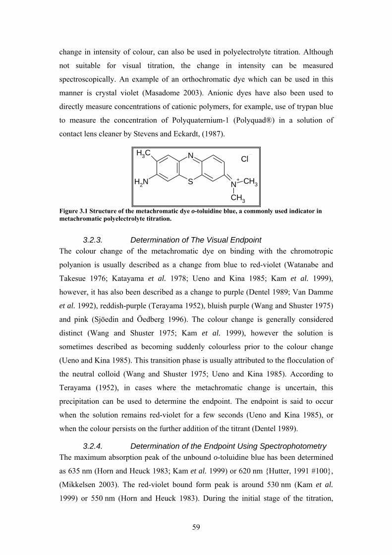
59

change in intensity of colour, can also be used in polyelectrolyte titration. Although

not suitable for visual titration, the change in intensity can be measured

spectroscopically. An example of an orthochromatic dye which can be used in this

manner is crystal violet (Masadome 2003). Anionic dyes have also been used to

directly measure concentrations of cationic polymers, for example, use of trypan blue

to measure the concentration of Polyquaternium-1 (Polyquad®) in a solution of

contact lens cleaner by Stevens and Eckardt, (1987).

S

NCH3

NH2 N+ CH3

CH3

Cl

Figure 3.1 Structure of the metachromatic dye o-toluidine blue, a commonly used indicator in metachromatic polyelectrolyte titration.

3.2.3. Determination of The Visual Endpoint The colour change of the metachromatic dye on binding with the chromotropic

polyanion is usually described as a change from blue to red-violet (Watanabe and

Takesue 1976; Katayama et al. 1978; Ueno and Kina 1985; Kam et al. 1999),

however, it has also been described as a change to purple (Dentel 1989; Van Damme

et al. 1992), reddish-purple (Terayama 1952), bluish purple (Wang and Shuster 1975)

and pink (Sjöedin and Öedberg 1996). The colour change is generally considered

distinct (Wang and Shuster 1975; Kam et al. 1999), however the solution is

sometimes described as becoming suddenly colourless prior to the colour change

(Ueno and Kina 1985). This transition phase is usually attributed to the flocculation of

the neutral colloid (Wang and Shuster 1975; Ueno and Kina 1985). According to

Terayama (1952), in cases where the metachromatic change is uncertain, this

precipitation can be used to determine the endpoint. The endpoint is said to occur

when the solution remains red-violet for a few seconds (Ueno and Kina 1985), or

when the colour persists on the further addition of the titrant (Dentel 1989).

3.2.4. Determination of the Endpoint Using Spectrophotometry The maximum absorption peak of the unbound o-toluidine blue has been determined

as 635 nm (Horn and Heuck 1983; Kam et al. 1999) or 620 nm Hutter, 1991 #100,

(Mikkelsen 2003). The red-violet bound form peak is around 530 nm (Kam et al.

1999) or 550 nm (Horn and Heuck 1983). During the initial stage of the titration,

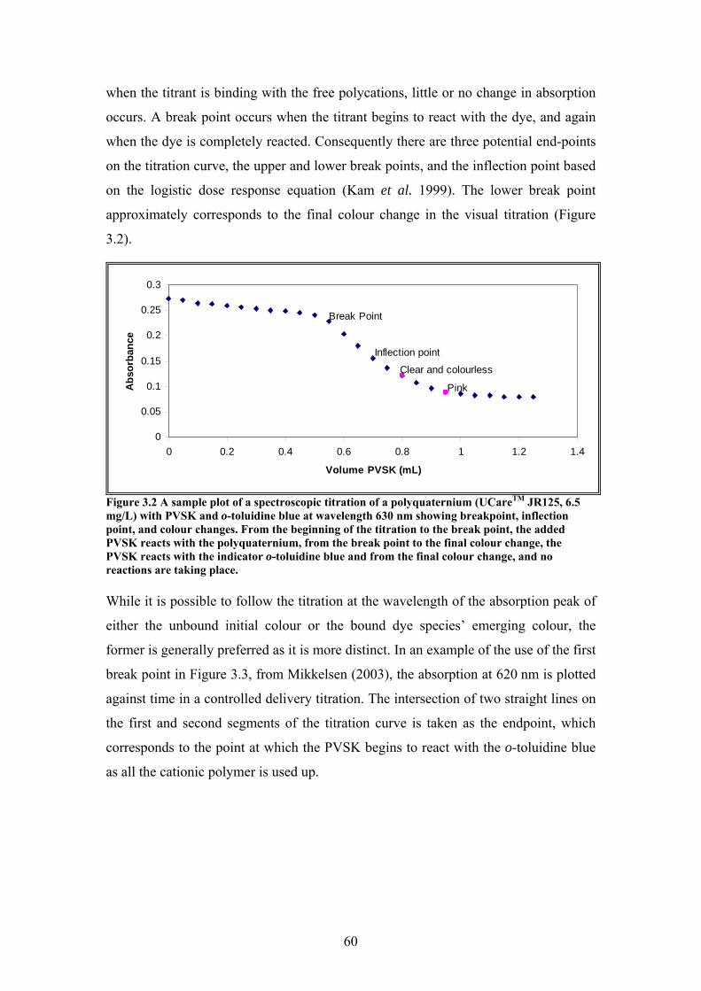
60

when the titrant is binding with the free polycations, little or no change in absorption

occurs. A break point occurs when the titrant begins to react with the dye, and again

when the dye is completely reacted. Consequently there are three potential end-points

on the titration curve, the upper and lower break points, and the inflection point based

on the logistic dose response equation (Kam et al. 1999). The lower break point

approximately corresponds to the final colour change in the visual titration (Figure

3.2).

0

0.05

0.1

0.15

0.2

0.25

0.3

0 0.2 0.4 0.6 0.8 1 1.2 1.4

Volume PVSK (mL)

Abs

orba

nce

Clear and colourless

Pink

Inflection point

Break Point

Figure 3.2 A sample plot of a spectroscopic titration of a polyquaternium (UCareTM JR125, 6.5 mg/L) with PVSK and o-toluidine blue at wavelength 630 nm showing breakpoint, inflection point, and colour changes. From the beginning of the titration to the break point, the added PVSK reacts with the polyquaternium, from the break point to the final colour change, the PVSK reacts with the indicator o-toluidine blue and from the final colour change, and no reactions are taking place. While it is possible to follow the titration at the wavelength of the absorption peak of

either the unbound initial colour or the bound dye species’ emerging colour, the

former is generally preferred as it is more distinct. In an example of the use of the first

break point in Figure 3.3, from Mikkelsen (2003), the absorption at 620 nm is plotted

against time in a controlled delivery titration. The intersection of two straight lines on

the first and second segments of the titration curve is taken as the endpoint, which

corresponds to the point at which the PVSK begins to react with the o-toluidine blue

as all the cationic polymer is used up.

61

Figure 3.3 The method of endpoint determination used by Mikkelsen (2003). The absorbance is plotted against time in a controlled automatic titration where the concentration of the PVSK in the reaction chamber is directly proportional to the titration time. The endpoint is determined as the intersection of two straight lines corresponding to the first and second stages of the titration reactions. In an example of the inflection point method, Figure 3.4, three straight lines have been

drawn on each of the three segments of the titration curve, and the endpoint is taken as

the midpoint on the second line between the intersection with the first and second

points Hutter, 1991 #100. Horn and Heuck (1983) followed the titration at both 550

and 635 nm with a double beam spectrophotometer, and plotted the relative

absorbance of the two wavelengths (Figure 3.5). The inflection point in this plot

corresponds to the point where rate of change between the absorbance at the two

wavelengths is greatest. According to Kam et al. (1999), deduction of a blank is not

required, however, both Hutter et al. (1991) and Mikkelsen et al. (2003) deducted

blanks in their calculations.

62

Figure 3.4 Determination of endpoint using the inflection point (Hutter et al. 1991) where the endpoint is determined as the ‘point lying midway between lines drawn tangent to the baselines’, that is, the inflection point.

Figure 3.5 Determination of endpoint from relative absorbance at 550 and 635 nm (Horn and Heuck 1983) with the endpoint determined to be the inflection point of the metachromatic shift.

3.2.5. Calculations – Determining Charge Density and/or Concentration

The calculation of the concentration of the unknown analyte is based on the known

equivalence of titrant, according to Equation 3.1 (Wang and Shuster 1975).

63

a

PVSKPVSKa V

VNN = Equation 3.1

where Na is the normality of the cationic analyte in eq/L NPVSK is the normality of the titrant in eq/L VPVSK is the volume of the titrant solution to endpoint and Va is the volume of the analyte solution titrated. The charge density of the cationic polymer/colloid can be determined from the

nominal equivalence of the PVSK (6.17 meq/g) if the solution has not been

standardised (Horn and Heuck 1983). This assumes that the PVSK is fully dissociated

and completely dissolved. Alternatively, the equivalence of the PVSK can be

determined by standardisation on titration with a cationic surfactant as mentioned

above (Dentel 1989).

3.2.6. Method Validation The results of charge density determination using metachromatic polyelectrolyte

titration have been found to be within the range of charge density quoted by the

polymer manufacturer (Kam et al. 1999), and consistent with the results from other

methods such as the Zeisel method of hydroxyethyl molar substitution and Kjeldahl

determination of nitrogen content (Hutter et al. 1991), streaming current detection

(Kam et al. 1999), turbidimetric and electrochemical titration (Koetz et al. 1996) and 1H NMR determination of quaternary methyl substituted ammonium functional

groups (Chang et al. 2002). A detection limit of 10-5 eq/g was reported by Mikkelsen

(2003).

In addition, the surface charge determined for proteins using this method has been

shown to have good agreement with the literature values measured by alternative

methods (Van Damme et al. 1992). For the determination of concentration of

polyelectrolyte solutions, metachromatic polyelectrolyte titration has been found to be

suitable for concentration ranges of 10-3–10-4 N (Terayama 1952), and 5 x 10-3 –

2 x 10-4 N (Wang and Shuster 1975). A linear relationship between concentration of

the titrant and amount of polyquaternium was established for concentrations of

polymer between 0.05 and 0.20% w/v, provided the amount of polyquaternium in the

aliquot did not exceed 400 µg (Hutter et al. 1991).

3.2.7. Problems and Limitations For polyquaterniums a constant charge density should be observed across a wide

range of solution pH values (Katayama et al. 1978; Horn and Heuck 1983; Dentel

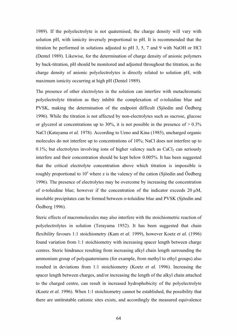
64

1989). If the polyelectrolyte is not quaternised, the charge density will vary with

solution pH, with ionicity inversely proportional to pH. It is recommended that the

titration be performed in solutions adjusted to pH 3, 5, 7 and 9 with NaOH or HCl

(Dentel 1989). Likewise, for the determination of charge density of anionic polymers

by back-titration, pH should be monitored and adjusted throughout the titration, as the

charge density of anionic polyelectrolytes is directly related to solution pH, with

maximum ionicity occurring at high pH (Dentel 1989).

The presence of other electrolytes in the solution can interfere with metachromatic

polyelectrolyte titration as they inhibit the complexation of o-toluidine blue and

PVSK, making the determination of the endpoint difficult (Sjöedin and Öedberg

1996). While the titration is not affected by non-electrolytes such as sucrose, glucose

or glycerol at concentrations up to 30%, it is not possible in the presence of > 0.3%

NaCl (Katayama et al. 1978). According to Ueno and Kina (1985), uncharged organic

molecules do not interfere up to concentrations of 10%; NaCl does not interfere up to

0.1%; but electrolytes involving ions of higher valency such as CaCl2 can seriously

interfere and their concentration should be kept below 0.005%. It has been suggested

that the critical electrolyte concentration above which titration is impossible is

roughly proportional to 10z where z is the valency of the cation (Sjöedin and Öedberg

1996). The presence of electrolytes may be overcome by increasing the concentration

of o-toluidine blue; however if the concentration of the indicator exceeds 20 µM,

insoluble precipitates can be formed between o-toluidine blue and PVSK (Sjöedin and

Öedberg 1996).

Steric effects of macromolecules may also interfere with the stoichiometric reaction of

polyelectrolytes in solution (Terayama 1952). It has been suggested that chain

flexibility favours 1:1 stoichiometry (Kam et al. 1999), however Koetz et al. (1996)

found variation from 1:1 stoichiometry with increasing spacer length between charge

centres. Steric hindrance resulting from increasing alkyl chain length surrounding the

ammonium group of polyquaterniums (for example, from methyl to ethyl groups) also

resulted in deviations from 1:1 stoichiometry (Koetz et al. 1996). Increasing the

spacer length between charges, and/or increasing the length of the alkyl chain attached

to the charged centre, can result in increased hydrophobicity of the polyelectrolyte

(Koetz et al. 1996). When 1:1 stoichiometry cannot be established, the possibility that

there are untitratable cationic sites exists, and accordingly the measured equivalence

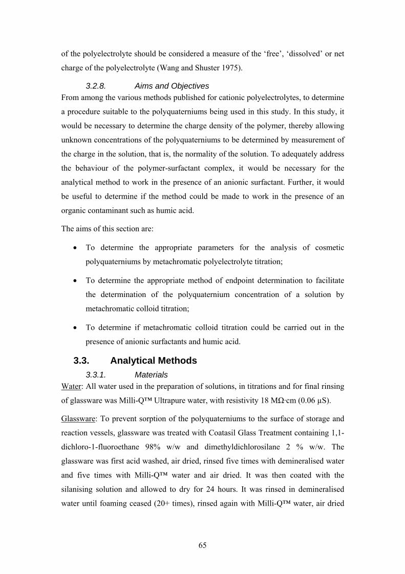
65

of the polyelectrolyte should be considered a measure of the ‘free’, ‘dissolved’ or net

charge of the polyelectrolyte (Wang and Shuster 1975).

3.2.8. Aims and Objectives From among the various methods published for cationic polyelectrolytes, to determine

a procedure suitable to the polyquaterniums being used in this study. In this study, it

would be necessary to determine the charge density of the polymer, thereby allowing

unknown concentrations of the polyquaterniums to be determined by measurement of

the charge in the solution, that is, the normality of the solution. To adequately address

the behaviour of the polymer-surfactant complex, it would be necessary for the

analytical method to work in the presence of an anionic surfactant. Further, it would

be useful to determine if the method could be made to work in the presence of an

organic contaminant such as humic acid.

The aims of this section are:

• To determine the appropriate parameters for the analysis of cosmetic

polyquaterniums by metachromatic polyelectrolyte titration;

• To determine the appropriate method of endpoint determination to facilitate

the determination of the polyquaternium concentration of a solution by

metachromatic colloid titration;

• To determine if metachromatic colloid titration could be carried out in the

presence of anionic surfactants and humic acid.

3.3. Analytical Methods 3.3.1. Materials

Water: All water used in the preparation of solutions, in titrations and for final rinsing

of glassware was Milli-Q™ Ultrapure water, with resistivity 18 MΩ·cm (0.06 µS).

Glassware: To prevent sorption of the polyquaterniums to the surface of storage and

reaction vessels, glassware was treated with Coatasil Glass Treatment containing 1,1-

dichloro-1-fluoroethane 98% w/w and dimethyldichlorosilane 2 % w/w. The

glassware was first acid washed, air dried, rinsed five times with demineralised water

and five times with Milli-Q™ water and air dried. It was then coated with the

silanising solution and allowed to dry for 24 hours. It was rinsed in demineralised

water until foaming ceased (20+ times), rinsed again with Milli-Q™ water, air dried

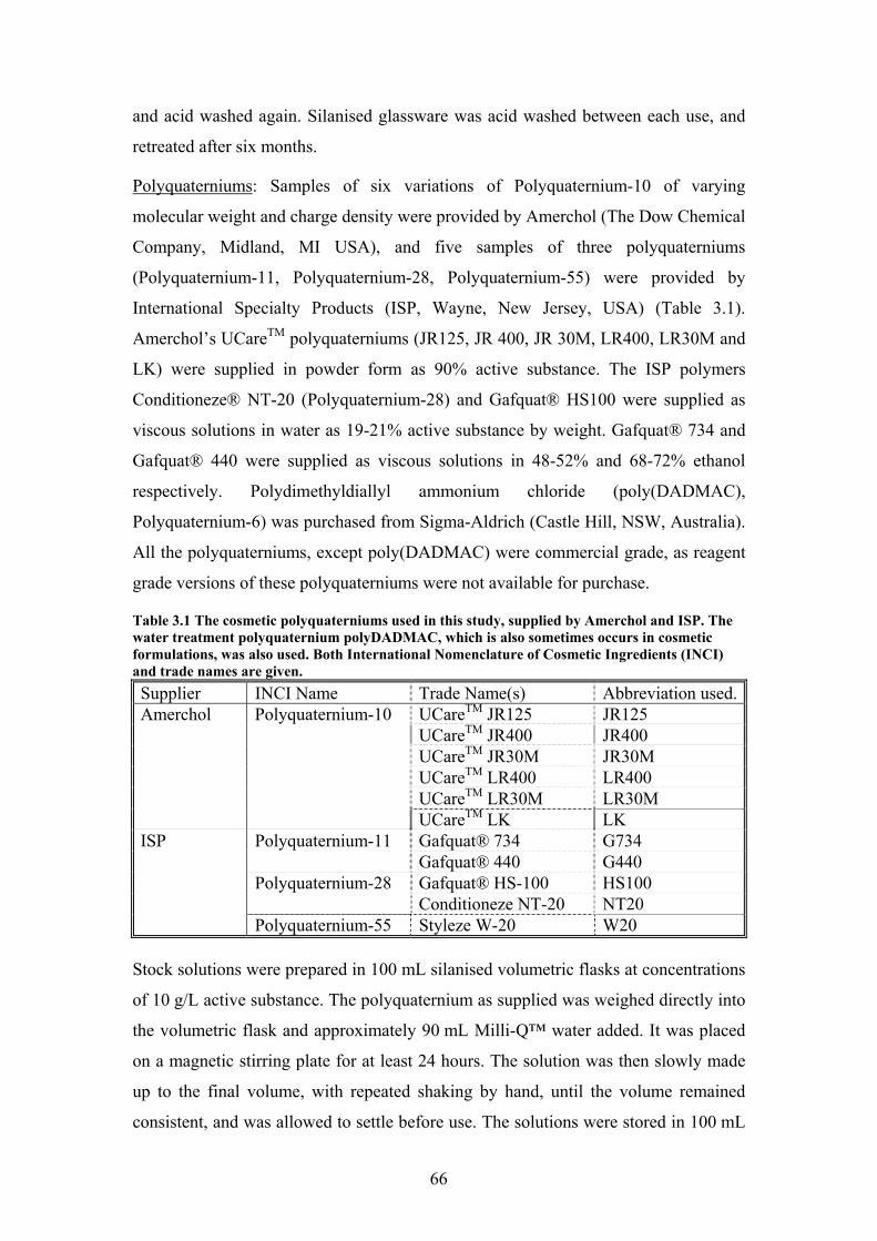
66

and acid washed again. Silanised glassware was acid washed between each use, and

retreated after six months.

Polyquaterniums: Samples of six variations of Polyquaternium-10 of varying

molecular weight and charge density were provided by Amerchol (The Dow Chemical

Company, Midland, MI USA), and five samples of three polyquaterniums

(Polyquaternium-11, Polyquaternium-28, Polyquaternium-55) were provided by

International Specialty Products (ISP, Wayne, New Jersey, USA) (Table 3.1).

Amerchol’s UCareTM polyquaterniums (JR125, JR 400, JR 30M, LR400, LR30M and

LK) were supplied in powder form as 90% active substance. The ISP polymers

Conditioneze® NT-20 (Polyquaternium-28) and Gafquat® HS100 were supplied as

viscous solutions in water as 19-21% active substance by weight. Gafquat® 734 and

Gafquat® 440 were supplied as viscous solutions in 48-52% and 68-72% ethanol

respectively. Polydimethyldiallyl ammonium chloride (poly(DADMAC),

Polyquaternium-6) was purchased from Sigma-Aldrich (Castle Hill, NSW, Australia).

All the polyquaterniums, except poly(DADMAC) were commercial grade, as reagent

grade versions of these polyquaterniums were not available for purchase.

Table 3.1 The cosmetic polyquaterniums used in this study, supplied by Amerchol and ISP. The water treatment polyquaternium polyDADMAC, which is also sometimes occurs in cosmetic formulations, was also used. Both International Nomenclature of Cosmetic Ingredients (INCI) and trade names are given. Supplier INCI Name Trade Name(s) Abbreviation used.

UCareTM JR125 JR125 UCareTM JR400 JR400 UCareTM JR30M JR30M UCareTM LR400 LR400 UCareTM LR30M LR30M

Amerchol Polyquaternium-10

UCareTM LK LK Gafquat® 734 G734 Polyquaternium-11 Gafquat® 440 G440 Gafquat® HS-100 HS100 Polyquaternium-28 Conditioneze NT-20 NT20

ISP

Polyquaternium-55 Styleze W-20 W20 Stock solutions were prepared in 100 mL silanised volumetric flasks at concentrations

of 10 g/L active substance. The polyquaternium as supplied was weighed directly into

the volumetric flask and approximately 90 mL Milli-Q™ water added. It was placed

on a magnetic stirring plate for at least 24 hours. The solution was then slowly made

up to the final volume, with repeated shaking by hand, until the volume remained

consistent, and was allowed to settle before use. The solutions were stored in 100 mL

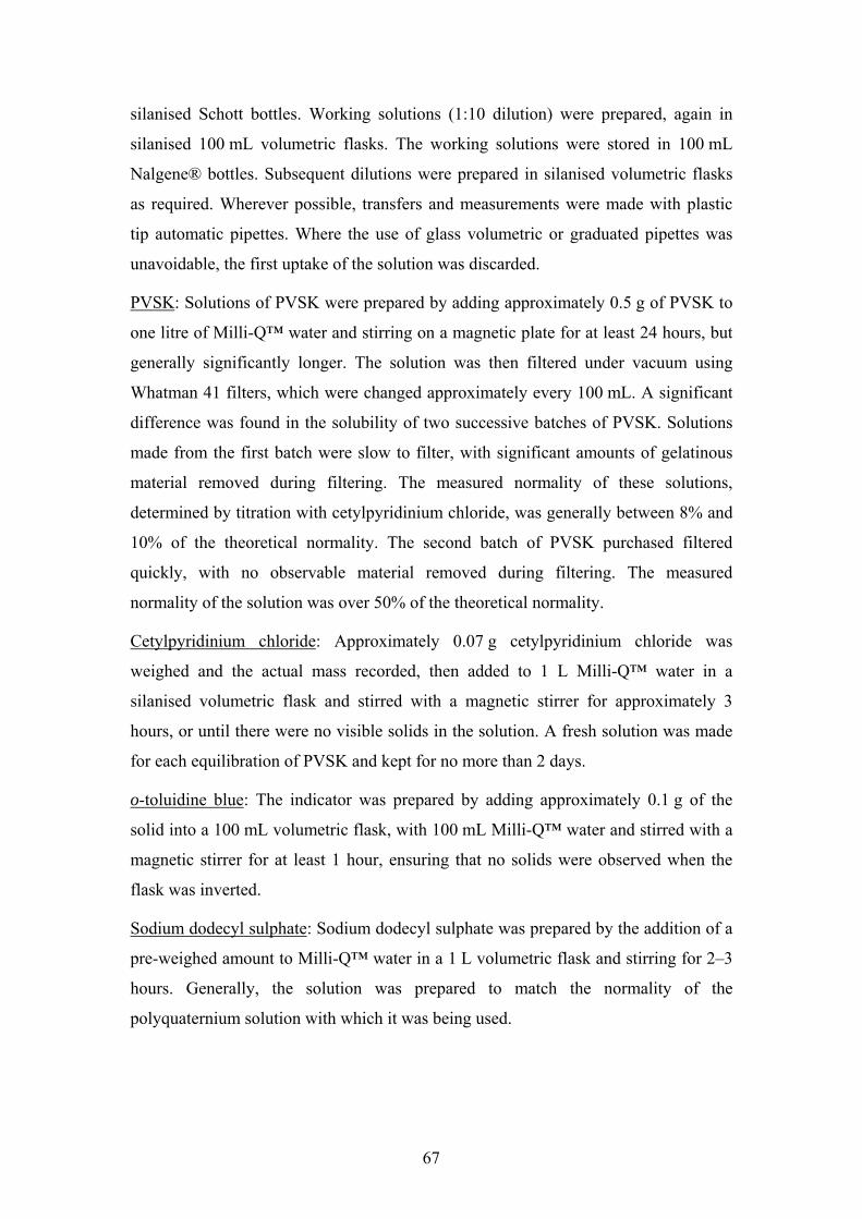
67

silanised Schott bottles. Working solutions (1:10 dilution) were prepared, again in

silanised 100 mL volumetric flasks. The working solutions were stored in 100 mL

Nalgene® bottles. Subsequent dilutions were prepared in silanised volumetric flasks

as required. Wherever possible, transfers and measurements were made with plastic

tip automatic pipettes. Where the use of glass volumetric or graduated pipettes was

unavoidable, the first uptake of the solution was discarded.

PVSK: Solutions of PVSK were prepared by adding approximately 0.5 g of PVSK to

one litre of Milli-Q™ water and stirring on a magnetic plate for at least 24 hours, but

generally significantly longer. The solution was then filtered under vacuum using

Whatman 41 filters, which were changed approximately every 100 mL. A significant

difference was found in the solubility of two successive batches of PVSK. Solutions

made from the first batch were slow to filter, with significant amounts of gelatinous

material removed during filtering. The measured normality of these solutions,

determined by titration with cetylpyridinium chloride, was generally between 8% and

10% of the theoretical normality. The second batch of PVSK purchased filtered

quickly, with no observable material removed during filtering. The measured

normality of the solution was over 50% of the theoretical normality.

Cetylpyridinium chloride: Approximately 0.07 g cetylpyridinium chloride was

weighed and the actual mass recorded, then added to 1 L Milli-Q™ water in a

silanised volumetric flask and stirred with a magnetic stirrer for approximately 3

hours, or until there were no visible solids in the solution. A fresh solution was made

for each equilibration of PVSK and kept for no more than 2 days.

o-toluidine blue: The indicator was prepared by adding approximately 0.1 g of the

solid into a 100 mL volumetric flask, with 100 mL Milli-Q™ water and stirred with a

magnetic stirrer for at least 1 hour, ensuring that no solids were observed when the

flask was inverted.

Sodium dodecyl sulphate: Sodium dodecyl sulphate was prepared by the addition of a

pre-weighed amount to Milli-Q™ water in a 1 L volumetric flask and stirring for 2–3

hours. Generally, the solution was prepared to match the normality of the

polyquaternium solution with which it was being used.

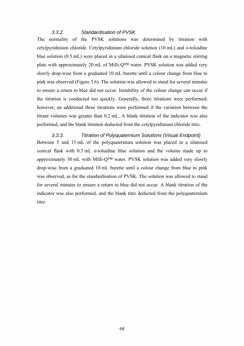
68

3.3.2. Standardisation of PVSK The normality of the PVSK solutions was determined by titration with

cetylpyridinium chloride. Cetylpyridinium chloride solution (10 mL) and o-toluidine

blue solution (0.5 mL) were placed in a silanised conical flask on a magnetic stirring

plate with approximately 20 mL of Milli-Q™ water. PVSK solution was added very

slowly drop-wise from a graduated 10 mL burette until a colour change from blue to

pink was observed (Figure 3.6). The solution was allowed to stand for several minutes

to ensure a return to blue did not occur. Instability of the colour change can occur if

the titration is conducted too quickly. Generally, three titrations were performed;

however, an additional three titrations were performed if the variation between the

titrant volumes was greater than 0.2 mL. A blank titration of the indicator was also

performed, and the blank titration deducted from the cetylpyridinium chloride titre.

3.3.3. Titration of Polyquaternium Solutions (Visual Endpoint) Between 5 and 15 mL of the polyquaternium solution was placed in a silanised

conical flask with 0.5 mL o-toluidine blue solution and the volume made up to

approximately 30 mL with Milli-Q™ water. PVSK solution was added very slowly

drop-wise from a graduated 10 mL burette until a colour change from blue to pink

was observed, as for the standardisation of PVSK. The solution was allowed to stand

for several minutes to ensure a return to blue did not occur. A blank titration of the

indicator was also performed, and the blank titre deducted from the polyquaternium

titre.

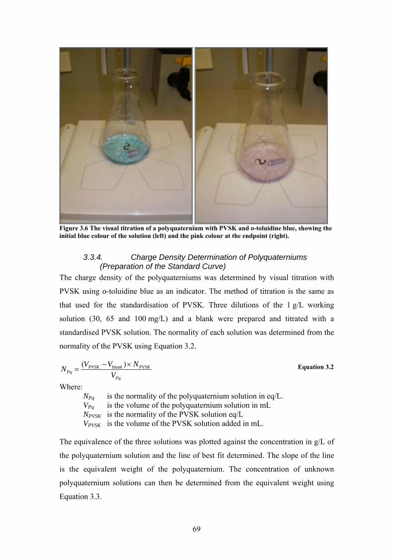
69

Figure 3.6 The visual titration of a polyquaternium with PVSK and o-toluidine blue, showing the initial blue colour of the solution (left) and the pink colour at the endpoint (right).

3.3.4. Charge Density Determination of Polyquaterniums (Preparation of the Standard Curve)

The charge density of the polyquaterniums was determined by visual titration with

PVSK using o-toluidine blue as an indicator. The method of titration is the same as

that used for the standardisation of PVSK. Three dilutions of the 1 g/L working

solution (30, 65 and 100 mg/L) and a blank were prepared and titrated with a

standardised PVSK solution. The normality of each solution was determined from the

normality of the PVSK using Equation 3.2.

Pq

PVSKblankPVSKPq V

NVVN ×−=

)(

Equation 3.2

Where: NPq is the normality of the polyquaternium solution in eq/L. VPq is the volume of the polyquaternium solution in mL NPVSK is the normality of the PVSK solution eq/L VPVSK is the volume of the PVSK solution added in mL. The equivalence of the three solutions was plotted against the concentration in g/L of

the polyquaternium solution and the line of best fit determined. The slope of the line

is the equivalent weight of the polyquaternium. The concentration of unknown

polyquaternium solutions can then be determined from the equivalent weight using

Equation 3.3.

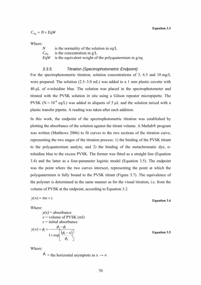
70

EqWNCPq ×= Equation 3.3

Where: N is the normality of the solution in eq/L CPq is the concentration in g/L EqW is the equivalent weight of the polyquaternium in g/eq

3.3.5. Titration (Spectrophotometric Endpoint) For the spectrophotometric titration, solution concentrations of 3, 6.5 and 10 mg/L

were prepared. The solution (2.5–3.0 mL) was added to a 1 mm plastic cuvette with

40 μL of o-toluidine blue. The solution was placed in the spectrophotometer and

titrated with the PVSK solution in situ using a Gilson repeater micropipette. The

PVSK (N ≈ 10-4 eq/L) was added in aliquots of 5 µL and the solution mixed with a

plastic transfer pipette. A reading was taken after each addition.

In this work, the endpoint of the spectrophotometric titration was established by

plotting the absorbance of the solution against the titrant volume. A Matlab® program

was written (Matthews 2006) to fit curves to the two sections of the titration curve,

representing the two stages of the titration process: 1) the binding of the PVSK titrant

to the polyquaternium analyte, and 2) the binding of the metachromatic dye, o-

toluidine blue to the excess PVSK. The former was fitted as a straight line (Equation

3.4) and the latter as a four-parameter logistic model (Equation 3.5). The endpoint

was the point where the two curves intersect, representing the point at which the

polyquaternium is fully bound to the PVSK titrant (Figure 3.7). The equivalence of

the polymer is determined in the same manner as for the visual titration, i.e. from the

volume of PVSK at the endpoint, according to Equation 3.2.

cmxxy +=)( Equation 3.4

Where: y(x) = absorbance x = volume of PVSK (ml) c = initial absorbance

( )⎥⎦

⎤⎢⎣

⎡ −+

−+=

4

3

121

exp1)(

φφφφφ

xxy

Equation 3.5

Where: 1φ = the horizontal asymptote as x → ∞

71

2φ = the horizontal asymptote as x → −∞

3φ = the value of x at the inflection point. (At this value of x the response is midway between the asymptotes) 4φ = a scale parameter on the x axis. (Pinheiro and Bates 2000)

0 0.01 0.02 0.03 0.04 0.05 0.06 0.070

0.05

0.1

0.15

0.2

0.25

0.3

0.35

PVSK (ml)

Abs

orba

nce

experimental datafitted curve

Figure 3.7 Matlab® plot of the titration of a polyquaternium with PVSK and o-toluidine blue, showing the intersection of the fitted curves of the straight line and four-parameter logistic model, indicating the different stages of the titration, and showing the break point ( ) and inflection point ( ).

3.4. Results 3.4.1. PVSK

Solutions of PVSK (Sigma-Aldrich), prepared by dissolving 0.4–0.5 g of the dry

powder in 1 L Milli-Q™ water, have a nominal normality of 2.46–3.85 meq/L.

However solutions prepared from the first batch of PVSK were found to have

normality of between 0.186 and 0.786 meq/L. This was due to the large amount of

gelatinous material removed from the solution during filtration. Solutions prepared

from the second batch of PVSK filtered quickly and no gelatinous material was

observed on the filters, indicating that this batch of PVSK had dissolved more

thoroughly. The normality of these solutions when standardised was found to be

72

between 0.59 and 1.78 meq/L. These solutions were diluted and recalibrated before

use. Solutions of PVSK were found to be very stable. Generally, solutions were used

within one month, with re-calibration indicated if the blank titration varied more than

10% from the initial blank titration. Only one solution was used for more than one

month, and was recalibrated twice. The normality of the solution was found to be

stable over that time.

3.4.2. Analysis of Results for Equivalent Weight Generally, new solutions of polyquaterniums were made for each new experiment.

Where possible, as many experiments as possible were conducted using the same

solution. As can be seen from Table 3.2, subsequent batches of the same

polyquaternium did not always have the same equivalence, although the results were

reasonably consistent given the difficulties in preparing dilutions from highly viscous

solutions. An example of a plot used to determine the equivalent weight of a

polyquaternium sample is shown in Figure 3.8. Analysis of the results using a

generalised linear model with Tukey test for multiple comparisons which included all

samples was significant (F = 20.70, Pr > F <0.0001), with poly(DADMAC) being

significantly different to all the personal care polyquaterniums. Removing

poly(DADMAC), and looking only at the personal care polyquaterniums, the Tukey

test showed a significant difference between Styleze® W-20 and the low charge

density UCareTM LR/LK range, Gafquat® HS100 and Conditioneze® NT-20, and

significant differences also existed between UCareTM LK and the JR polymers, and

between JR30M and LR40M (F = 7.81, Pr > F = 0.0016).

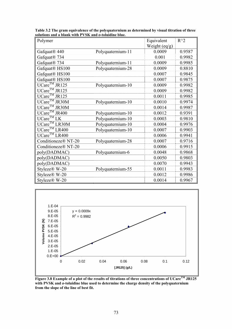
73

Table 3.2 The gram equivalence of the polyquaternium as determined by visual titration of three solutions and a blank with PVSK and o-toluidine blue. Polymer Equivalent

Weight (eq/g) R^2

Gafquat® 440 Polyquaternium-11 0.0009 0.9587 Gafquat® 734 0.001 0.9982 Gafquat® 734 Polyquaternium-11 0.0009 0.9985 Gafquat® HS100 Polyquaternium-28 0.0009 0.8810 Gafquat® HS100 0.0007 0.9845 Gafquat® HS100 0.0007 0.9875 UCareTM JR125 Polyquaternium-10 0.0009 0.9982 UCareTM JR125 0.0009 0.9982 UCareTM JR125 0.0011 0.9985 UCareTM JR30M Polyquaternium-10 0.0010 0.9974 UCareTM JR30M 0.0014 0.9987 UCareTM JR400 Polyquaternium-10 0.0012 0.9391 UCareTM LK Polyquaternium-10 0.0003 0.9810 UCareTM LR30M Polyquaternium-10 0.0004 0.9976 UCareTM LR400 Polyquaternium-10 0.0007 0.9903 UCareTM LR400 0.0006 0.9941 Conditioneze® NT-20 Polyquaternium-28 0.0007 0.9716 Conditioneze® NT-20 0.0006 0.9915 poly(DADMAC) Polyquaternium-6 0.0048 0.9868 poly(DADMAC) 0.0050 0.9803 poly(DADMAC) 0.0070 0.9943 Styleze® W-20 Polyquaternium-55 0.0011 0.9983 Styleze® W-20 0.0012 0.9986 Styleze® W-20 0.0014 0.9967

Figure 3.8 Example of a plot of the results of titrations of three concentrations of UCareTM JR125 with PVSK and o-toluidine blue used to determine the charge density of the polyquaternium from the slope of the line of best fit.

y = 0.0009xR2 = 0.9982

0.E+001.E-052.E-053.E-054.E-055.E-056.E-057.E-058.E-059.E-051.E-04

0 0.02 0.04 0.06 0.08 0.1 0.12[JR125] (g/L)

Volu

me

PVSK

(N)

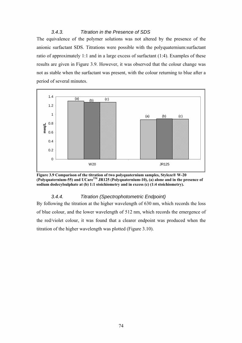
74

3.4.3. Titration in the Presence of SDS The equivalence of the polymer solutions was not altered by the presence of the

anionic surfactant SDS. Titrations were possible with the polyquaternium:surfactant

ratio of approximately 1:1 and in a large excess of surfactant (1:4). Examples of these

results are given in Figure 3.9. However, it was observed that the colour change was

not as stable when the surfactant was present, with the colour returning to blue after a

period of several minutes.

0

0.2

0.4

0.6

0.8

1

1.2

1.4

W20 JR125

meq

/L

(a)

(a)

(b)

(b)

(c)

(c)

Figure 3.9 Comparison of the titration of two polyquaternium samples, Styleze® W-20 (Polyquaternium-55) and UCareTM JR125 (Polyquaternium-10), (a) alone and in the presence of sodium dodecylsulphate at (b) 1:1 stoichiometry and in excess (c) (1:4 stoichiometry).

3.4.4. Titration (Spectrophotometric Endpoint) By following the titration at the higher wavelength of 630 nm, which records the loss

of blue colour, and the lower wavelength of 512 nm, which records the emergence of

the red/violet colour, it was found that a clearer endpoint was produced when the

titration of the higher wavelength was plotted (Figure 3.10).

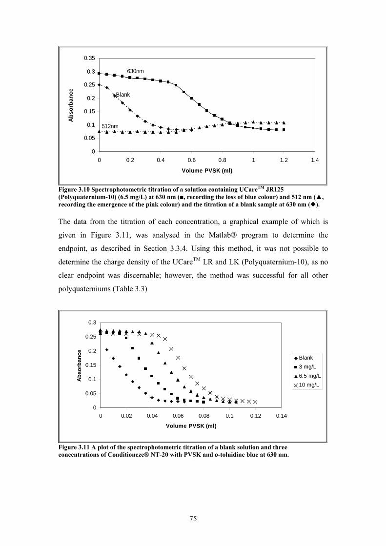
75

0

0.05

0.1

0.15

0.2

0.25

0.3

0.35

0 0.2 0.4 0.6 0.8 1 1.2 1.4

Volume PVSK (ml)

Abso

rban

ce630nm

512nm

Blank

Figure 3.10 Spectrophotometric titration of a solution containing UCareTM JR125 (Polyquaternium-10) (6.5 mg/L) at 630 nm (, recording the loss of blue colour) and 512 nm (, recording the emergence of the pink colour) and the titration of a blank sample at 630 nm ( ). The data from the titration of each concentration, a graphical example of which is

given in Figure 3.11, was analysed in the Matlab® program to determine the

endpoint, as described in Section 3.3.4. Using this method, it was not possible to

determine the charge density of the UCareTM LR and LK (Polyquaternium-10), as no

clear endpoint was discernable; however, the method was successful for all other

polyquaterniums (Table 3.3)

0

0.05

0.1

0.15

0.2

0.25

0.3

0 0.02 0.04 0.06 0.08 0.1 0.12 0.14

Volume PVSK (ml)

Abs

orba

nce

Blank3 mg/L6.5 mg/L10 mg/L

Figure 3.11 A plot of the spectrophotometric titration of a blank solution and three concentrations of Conditioneze® NT-20 with PVSK and o-toluidine blue at 630 nm.

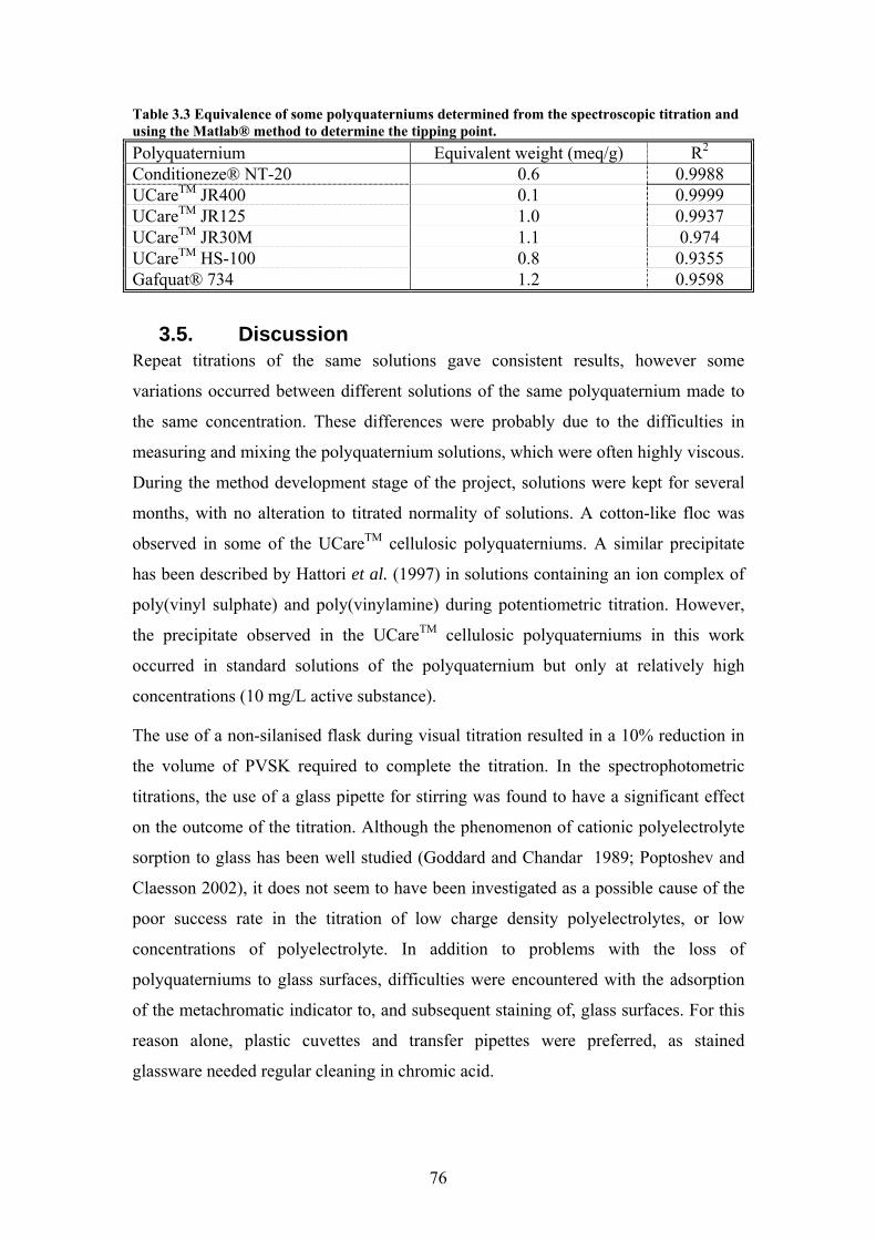
76

Table 3.3 Equivalence of some polyquaterniums determined from the spectroscopic titration and using the Matlab® method to determine the tipping point. Polyquaternium Equivalent weight (meq/g) R2 Conditioneze® NT-20 0.6 0.9988 UCareTM JR400 0.1 0.9999 UCareTM JR125 1.0 0.9937 UCareTM JR30M 1.1 0.974 UCareTM HS-100 0.8 0.9355 Gafquat® 734 1.2 0.9598

3.5. Discussion Repeat titrations of the same solutions gave consistent results, however some

variations occurred between different solutions of the same polyquaternium made to

the same concentration. These differences were probably due to the difficulties in

measuring and mixing the polyquaternium solutions, which were often highly viscous.

During the method development stage of the project, solutions were kept for several

months, with no alteration to titrated normality of solutions. A cotton-like floc was

observed in some of the UCareTM cellulosic polyquaterniums. A similar precipitate

has been described by Hattori et al. (1997) in solutions containing an ion complex of

poly(vinyl sulphate) and poly(vinylamine) during potentiometric titration. However,

the precipitate observed in the UCareTM cellulosic polyquaterniums in this work

occurred in standard solutions of the polyquaternium but only at relatively high

concentrations (10 mg/L active substance).

The use of a non-silanised flask during visual titration resulted in a 10% reduction in

the volume of PVSK required to complete the titration. In the spectrophotometric

titrations, the use of a glass pipette for stirring was found to have a significant effect

on the outcome of the titration. Although the phenomenon of cationic polyelectrolyte

sorption to glass has been well studied (Goddard and Chandar 1989; Poptoshev and

Claesson 2002), it does not seem to have been investigated as a possible cause of the

poor success rate in the titration of low charge density polyelectrolytes, or low

concentrations of polyelectrolyte. In addition to problems with the loss of

polyquaterniums to glass surfaces, difficulties were encountered with the adsorption

of the metachromatic indicator to, and subsequent staining of, glass surfaces. For this

reason alone, plastic cuvettes and transfer pipettes were preferred, as stained

glassware needed regular cleaning in chromic acid.

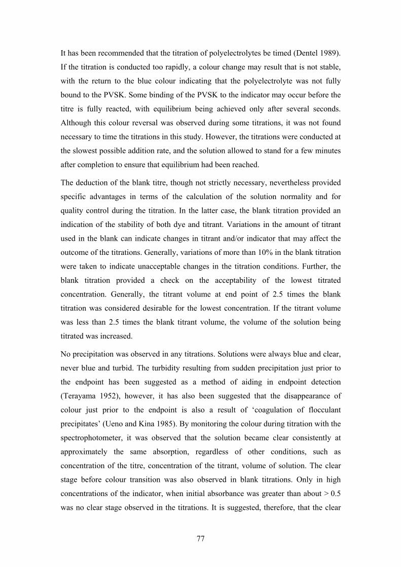
77

It has been recommended that the titration of polyelectrolytes be timed (Dentel 1989).

If the titration is conducted too rapidly, a colour change may result that is not stable,

with the return to the blue colour indicating that the polyelectrolyte was not fully

bound to the PVSK. Some binding of the PVSK to the indicator may occur before the

titre is fully reacted, with equilibrium being achieved only after several seconds.

Although this colour reversal was observed during some titrations, it was not found

necessary to time the titrations in this study. However, the titrations were conducted at

the slowest possible addition rate, and the solution allowed to stand for a few minutes

after completion to ensure that equilibrium had been reached.

The deduction of the blank titre, though not strictly necessary, nevertheless provided

specific advantages in terms of the calculation of the solution normality and for

quality control during the titration. In the latter case, the blank titration provided an

indication of the stability of both dye and titrant. Variations in the amount of titrant

used in the blank can indicate changes in titrant and/or indicator that may affect the

outcome of the titrations. Generally, variations of more than 10% in the blank titration

were taken to indicate unacceptable changes in the titration conditions. Further, the

blank titration provided a check on the acceptability of the lowest titrated

concentration. Generally, the titrant volume at end point of 2.5 times the blank

titration was considered desirable for the lowest concentration. If the titrant volume

was less than 2.5 times the blank titrant volume, the volume of the solution being

titrated was increased.

No precipitation was observed in any titrations. Solutions were always blue and clear,

never blue and turbid. The turbidity resulting from sudden precipitation just prior to

the endpoint has been suggested as a method of aiding in endpoint detection

(Terayama 1952), however, it has also been suggested that the disappearance of

colour just prior to the endpoint is also a result of ‘coagulation of flocculant

precipitates’ (Ueno and Kina 1985). By monitoring the colour during titration with the

spectrophotometer, it was observed that the solution became clear consistently at

approximately the same absorption, regardless of other conditions, such as

concentration of the titre, concentration of the titrant, volume of solution. The clear

stage before colour transition was also observed in blank titrations. Only in high

concentrations of the indicator, when initial absorbance was greater than about > 0.5

was no clear stage observed in the titrations. It is suggested, therefore, that the clear

78

stage observed prior to colour change is the result of the hypochromic shift that occurs

on the binding of PVSK to o-toluidine blue.

The endpoint in all visual titrations in this study is most suitably described as pink,

and followed a stage in which the solution changed from blue to clear. Solutions at all

stages were clear rather than turbid. Of the two breakpoints in the spectroscopic

titration, which coincide with changes in the reaction processes, the first breakpoint

was the more distinct and was used in this study for the determination of the

spectroscopic endpoint. There was good agreement between the endpoint determined

by visual titration with the blank subtracted, and the first break point in the

spectroscopic titration. Both these points represent the stage in the titration where the

polyquaternium and the PVSK are fully reacted, and the PVSK begins to bind with

the indicator, o-toluidine blue. Unlike more conventional acid-base titrations, where

the titration curve is very steep and there is no intermediate stage in the titration, the

inflection point on the polyelectrolyte does not correspond to any significant chemical

process in the titration reaction and is therefore not particularly useful as an endpoint

when there is a better one available.

As previously mentioned, the equivalence of the polyquaternium in this study was

determined from the normality of the titre solutions according to Equation 3.3. An

alternative method, where the amount of polymer is plotted against the volume of the

titrant, and the equivalence determined from the slope of the regression line was used

by Hutter et al. (1991). In addition to being mathematically more complex, this

method allows less flexibility in the titration procedure, as it requires that the volume

of the titre be identical for all concentrations in a series. In the method used in this

study, the volume of the titre could be varied to ensure the lowest concentration was

significantly differentiated from the blank, and the maximum concentration titratable

within the volume of the burette. Consequently, a wider range of concentrations could

be titrated. While it is not strictly necessary to have a wide range of concentrations for

the determination of charge density, such variation can and does occur in the

applications where concentration is being determined for difference studies.

The method of direct titration using trypan-blue (Stevens and Eckardt 1987) was

found to be non-linear and variable at the concentration range required for this study.

Polyquaternium-1, the polyelectrolyte used in the study by Stevens and Eckardt

(1987) is a very high charge density polyelectrolyte, with two charge centres on each

79

monomer, which may account for its titratability at the low concentrations (0.0005 to

0.0015% m/V).

In order to investigate the behaviour of the polyquaternium in the presence of the

surfactant, it was necessary to be able to determine if the metachromatic

polyelectrolyte titration could be performed in the presence of the surfactant. The

presence of SDS, either at 1:1 stoichiometry or in excess, had no effect on the titration

of the polyquaternium with PVSK. The binding of the polyquaternium with PVSK,

and of PVSK with o-toluidine blue, were therefore found to be preferred to

association with the surfactant. However, the colour change in the presence of the

surfactant was not as stable as the colour change in the standard titration (though it

was sufficiently stable for the determination of the endpoint), indicating that some

desorption/dissociation of the polyquaternium and PVSK in the presence of the

surfactant could occur over time. It was possible, therefore, using this method, to

determine the concentration of polyelectrolyte in solution when SDS was present, but

not the extent to which it was complexed with the surfactant.

It was not possible to conduct the titration in solutions of either polyquaterniums that

had been exposed to bentonite clay, or polyquaterniums prepared in a solution

containing tap water, such as the medium used in the fish toxicity tests in Chapter 5.

In each case, no colour change occurred, indicating interference in the reaction

between the PVSK and o-toluidine blue.

3.6. Conclusion Metachromatic polyelectrolyte titration was found to be a reliable method for

determining the charge density of polyquaterniums, and for subsequent determination

of concentration of unknown solutions of polyquaterniums. The most suitable

endpoint in visual titration was found to be the point at which colour change is

complete. With the deduction of a blank titration, this point was consistent with the

first breakpoint in the spectrophotometric titration. In this study, metachromatic

polyelectrolyte titration was effective for concentrations as low as 10-4 N with the

visual endpoint, and 10-5 N with the spectrophotometric endpoint.

The most significant disadvantages of the method are its inability to distinguish

between polyelectrolytes, and the interference of other ions. The method is limited to

solutions in simple matrices, and therefore is not suitable for the determination of

80

polyelectrolytes in environmental samples. While it may be possible to achieve

further improvements in the concentration range for metachromatic polyelectrolyte

titration using automated titration techniques and improved mathematical models for

endpoint detection, the development of methods able to overcome the problems of

electrolyte interference, and to distinguish specific cationic polyelectrolytes, would be

more useful in environmental studies of polyquaterniums. However, metachromatic

polyelectrolyte titration is a useful method for laboratory analysis of polyelectrolytes.

81

4. Chemistry and Fate – Exposure Assessment of Polyquaterniums 4.1. Introduction

In the previous chapter, a method of measuring the concentration of polyquaterniums,

at least in the laboratory, was described. This method can be used to investigate some

aspects of the behaviour of polyquaterniums that may influence their fate in the

environment. As outlined in Chapter 1, the exposure assessment step of the four-step

risk assessment paradigm uses various measurements and/or models to estimate the

contact that may occur between a chemical and a vulnerable organism in the

environment.

Exposure assessment examines the contact between an organism and a chemical in

terms of the intensity, frequency and duration of the contact (USEPA 1998). The site

of interaction between the organism and the chemical is somewhat controversial, and

can be taken to mean either at the outer visible boundary, the visible exterior of the

organism (the skin and openings into the body, such as mouth, nostrils) or the so-

called exchange boundaries where absorption takes place (skin, lung, gastrointestinal

tract) (USEPA 1992). Exposure assessment can also evaluate the rate at which a

chemical crosses the boundary. In the former case, the exposure can be expressed as a

concentration of the chemical in the exposure medium, such as air, or water. In the

latter case, the exposure can only be expressed in terms of dose, and must take into

account the rates of uptake and absorption (USEPA 1992). Generally, the exposure

assessment should be expressed in units that allow it to be combined with the hazard

assessment. If the hazard assessment is expressed in terms of dose or internal

concentration, then the exposure assessment should also be expressed in terms of dose

or internal concentration. Fortunately, aquatic toxicity is usually expressed in terms of

concentration of the chemical in the aquatic environment, and the exposure can thus

be expressed as the aqueous concentration of the chemical in receiving waters.

Where an environmental risk assessment is undertaken in response to an existing

exposure, the extent of the exposure can be directly measured. However, in some

cases, such as the assessment of a new chemical or where analytical methods are not

available, the exposure must be estimated by means of models. Where the exposure is

to be expressed in terms of concentration in the exposure medium, the exposure can

be estimated with fate and transport models based on use and release data and the

82

physico-chemical properties of the chemical. This is the approach adopted by

National Industrial Chemicals Notification and Assessment Scheme/Department of

Environment and Water Resources (NICNAS/DEW) in the assessment of new

chemicals, as can be seen from the published reports (NICNAS 2004b). This

assessment takes into account relevant properties of the chemical that may determine

fate (volatility, aqueous solubility, etc), use patterns and potential release estimates to

predict an environmental concentration. These estimates also take into account basic

(human) population data and the water use patterns of the population.

4.2. Use patterns and release data An important first step in modelling the predicted environmental concentration is to

determine the amount of the chemical being used. However, unless required by

regulation to publish such data, many companies regard volume data as commercially

confidential information. In new chemical notifications to NICNAS, use and

manufacture/import volume is a requirement for all notifications (a Part B data

requirement), however, the guidance notes for notifiers states

‘In some cases, for example, “Maximum Introduction Volume of Notified

Chemical (100%) Over Next 5 Years”, the exact details can be claimed as

confidential; however, a generic or sanitised description is required for the

public report’ (NICNAS undated).

Of the five published assessment reports of polyquaterniums (Table 4.1), only one

claimed confidentiality as evidenced by this standard statement in the Full Public

report (FPR)

The chemical name, CAS number, molecular and structural formulae,

molecular weight, spectral data, details of the polymer composition and

details of exact import volume and uses have been exempted from

publication in the Full Public Report and the Summary Report. (NICNAS

2002a).

The stated import volume in this notification is < 16 tonnes. It may be considerably

less than 16 tonnes, but not less than one tonne, and certainly cannot be more than 16

tonnes. Three of the notifications are ‘limited’ notifications, implying that the import

volume is less than one tonne pa (it cannot exceed one tonne pa without further

notification). The remaining report is a standard notification (volume > 1000 kg), no

83

confidentiality is claimed, and the volume is stated as “up to” 5 tonnes. As the stated

volume is a legal limit imposed by the certificate conditions, the import volume of this

polyquaternium cannot exceed that amount. There are a further 18 polyquaterniums

on the Australian Inventory of Chemical Substances AICS for which no assessment

reports are available, so no import data, ‘generic’ or otherwise, is available on these.

Table 4.1 Confidentiality status and import volume details from NICNAS FPR for assessed polyquaterniums. Notification Product Notifier Confidentiality Maximum

Volume (tonnes pa)

NA89 Polyquaternium-28 (Gafquat® HS100)

ISP Corp No 5

NA475 Polyquaternium-34

L’Oreal Paris No < 1

NA533 Polyquaternium-46

BASF Australia Ltd

No < 1

NA896 Polyquaternium-47 (Merquat 2001)

Nalco Australia Pty Ltd

Yes < 16

NA961 Polyquaternium-44 (Luviquat Care)

Johnson and Johnson Pacific Pty Ltd

No < 1

With respect to existing chemicals, NICNAS is able to acquire import data on

chemicals as part of the evaluation of a potential Priority Existing Chemical

declaration under Section 48 of the Industrial Chemicals (Notification and

Assessment) Act (ICNA). When deciding whether to make a recommendation for the

declaration of a chemical as a Priority Existing Chemicals, the Director may require

additional information. This may include:

a) specified information about a particular chemical, such as use and health

and/or environmental effects;

b) the quantities of the chemical used for a specified purpose in a specified

period, for example, use in cosmetics over the past three years;

c) the quantities of the chemical manufactured or imported in a specified

period (CofA 1989).

Following declaration, information required to be submitted by companies importing

and/or manufacturing, or intending to manufacture or import the chemical, either as is

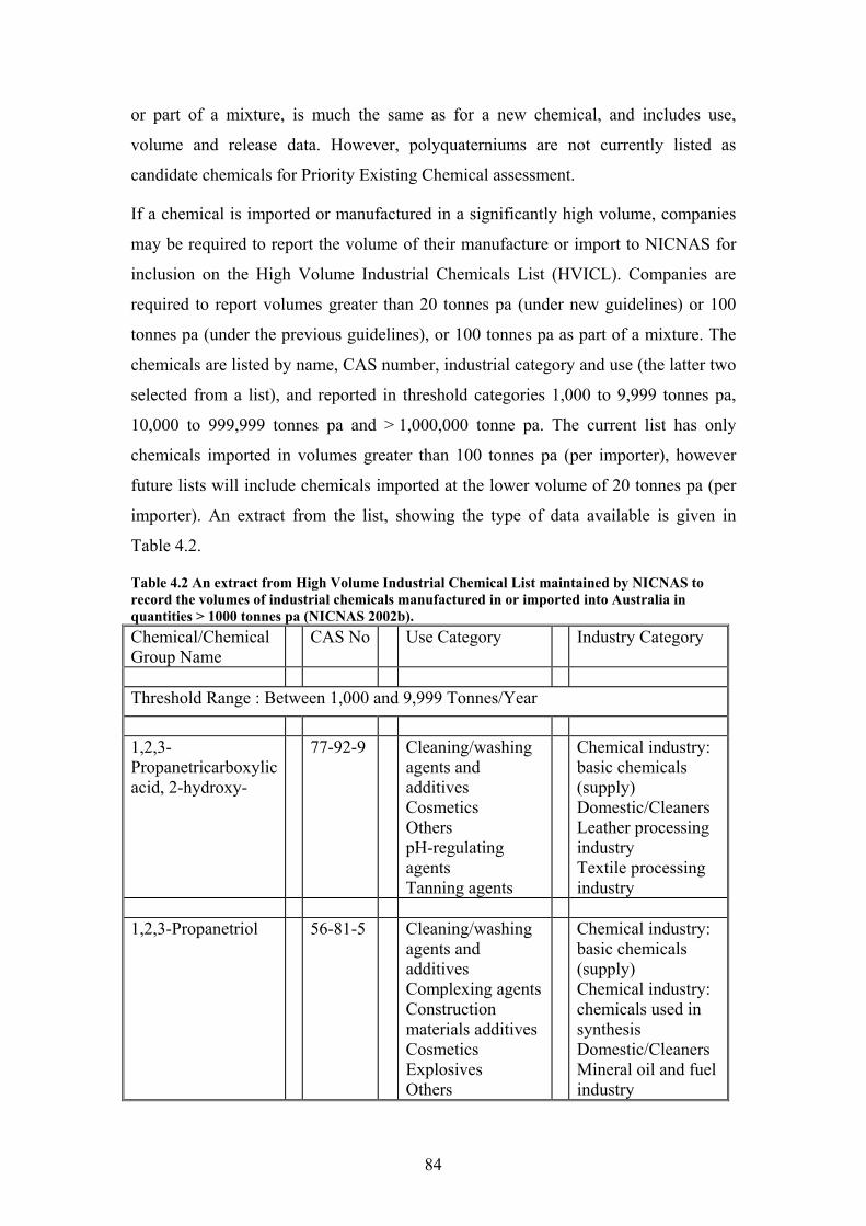
84

or part of a mixture, is much the same as for a new chemical, and includes use,

volume and release data. However, polyquaterniums are not currently listed as

candidate chemicals for Priority Existing Chemical assessment.

If a chemical is imported or manufactured in a significantly high volume, companies

may be required to report the volume of their manufacture or import to NICNAS for

inclusion on the High Volume Industrial Chemicals List (HVICL). Companies are

required to report volumes greater than 20 tonnes pa (under new guidelines) or 100

tonnes pa (under the previous guidelines), or 100 tonnes pa as part of a mixture. The

chemicals are listed by name, CAS number, industrial category and use (the latter two

selected from a list), and reported in threshold categories 1,000 to 9,999 tonnes pa,

10,000 to 999,999 tonnes pa and > 1,000,000 tonne pa. The current list has only

chemicals imported in volumes greater than 100 tonnes pa (per importer), however

future lists will include chemicals imported at the lower volume of 20 tonnes pa (per

importer). An extract from the list, showing the type of data available is given in

Table 4.2.

Table 4.2 An extract from High Volume Industrial Chemical List maintained by NICNAS to record the volumes of industrial chemicals manufactured in or imported into Australia in quantities > 1000 tonnes pa (NICNAS 2002b). Chemical/Chemical Group Name

CAS No Use Category Industry Category

Threshold Range : Between 1,000 and 9,999 Tonnes/Year 1,2,3-Propanetricarboxylic acid, 2-hydroxy-

77-92-9 Cleaning/washing agents and additives Cosmetics Others pH-regulating agents Tanning agents

Chemical industry: basic chemicals (supply) Domestic/Cleaners Leather processing industry Textile processing industry

1,2,3-Propanetriol 56-81-5 Cleaning/washing

agents and additives Complexing agents Construction materials additives Cosmetics Explosives Others

Chemical industry: basic chemicals (supply) Chemical industry: chemicals used in synthesis Domestic/Cleaners Mineral oil and fuel industry

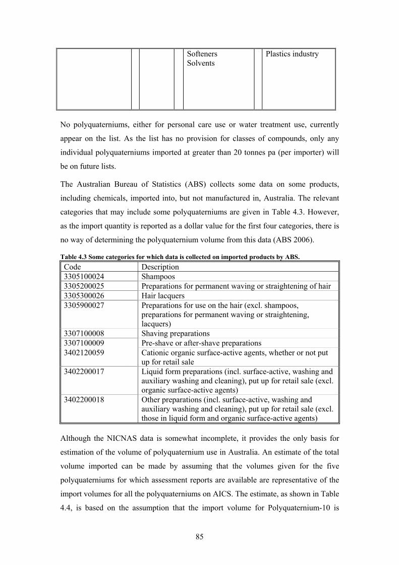
85

Softeners Solvents

Plastics industry

No polyquaterniums, either for personal care use or water treatment use, currently

appear on the list. As the list has no provision for classes of compounds, only any

individual polyquaterniums imported at greater than 20 tonnes pa (per importer) will

be on future lists.

The Australian Bureau of Statistics (ABS) collects some data on some products,

including chemicals, imported into, but not manufactured in, Australia. The relevant

categories that may include some polyquaterniums are given in Table 4.3. However,

as the import quantity is reported as a dollar value for the first four categories, there is

no way of determining the polyquaternium volume from this data (ABS 2006).

Table 4.3 Some categories for which data is collected on imported products by ABS. Code Description 3305100024 Shampoos 3305200025 Preparations for permanent waving or straightening of hair 3305300026 Hair lacquers 3305900027 Preparations for use on the hair (excl. shampoos,

preparations for permanent waving or straightening, lacquers)

3307100008 Shaving preparations 3307100009 Pre-shave or after-shave preparations 3402120059 Cationic organic surface-active agents, whether or not put

up for retail sale 3402200017 Liquid form preparations (incl. surface-active, washing and

auxiliary washing and cleaning), put up for retail sale (excl. organic surface-active agents)

3402200018 Other preparations (incl. surface-active, washing and auxiliary washing and cleaning), put up for retail sale (excl. those in liquid form and organic surface-active agents)

Although the NICNAS data is somewhat incomplete, it provides the only basis for

estimation of the volume of polyquaternium use in Australia. An estimate of the total

volume imported can be made by assuming that the volumes given for the five

polyquaterniums for which assessment reports are available are representative of the

import volumes for all the polyquaterniums on AICS. The estimate, as shown in Table

4.4, is based on the assumption that the import volume for Polyquaternium-10 is

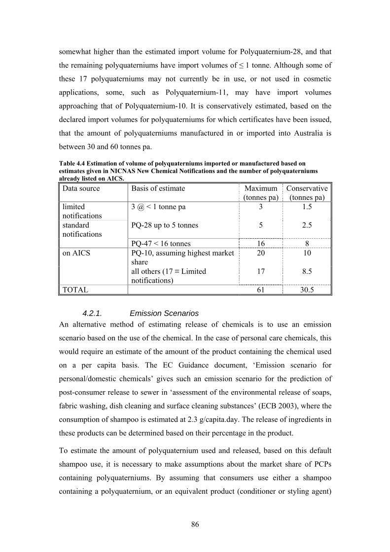
86

somewhat higher than the estimated import volume for Polyquaternium-28, and that

the remaining polyquaterniums have import volumes of ≤ 1 tonne. Although some of

these 17 polyquaterniums may not currently be in use, or not used in cosmetic

applications, some, such as Polyquaternium-11, may have import volumes

approaching that of Polyquaternium-10. It is conservatively estimated, based on the

declared import volumes for polyquaterniums for which certificates have been issued,

that the amount of polyquaterniums manufactured in or imported into Australia is

between 30 and 60 tonnes pa.

Table 4.4 Estimation of volume of polyquaterniums imported or manufactured based on estimates given in NICNAS New Chemical Notifications and the number of polyquaterniums already listed on AICS. Data source Basis of estimate Maximum

(tonnes pa) Conservative(tonnes pa)

limited notifications

3 @ < 1 tonne pa 3 1.5

standard notifications

PQ-28 up to 5 tonnes 5 2.5

PQ-47 < 16 tonnes 16 8 on AICS PQ-10, assuming highest market

share 20 10

all others (17 ≡ Limited notifications)

17 8.5

TOTAL 61 30.5

4.2.1. Emission Scenarios An alternative method of estimating release of chemicals is to use an emission

scenario based on the use of the chemical. In the case of personal care chemicals, this

would require an estimate of the amount of the product containing the chemical used

on a per capita basis. The EC Guidance document, ‘Emission scenario for

personal/domestic chemicals’ gives such an emission scenario for the prediction of

post-consumer release to sewer in ‘assessment of the environmental release of soaps,

fabric washing, dish cleaning and surface cleaning substances’ (ECB 2003), where the

consumption of shampoo is estimated at 2.3 g/capita.day. The release of ingredients in

these products can be determined based on their percentage in the product.

To estimate the amount of polyquaternium used and released, based on this default

shampoo use, it is necessary to make assumptions about the market share of PCPs

containing polyquaterniums. By assuming that consumers use either a shampoo

containing a polyquaternium, or an equivalent product (conditioner or styling agent)

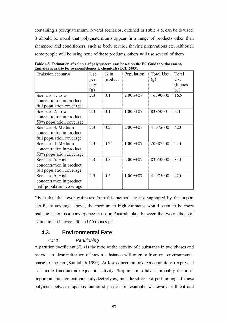
87

containing a polyquaternium, several scenarios, outlined in Table 4.5, can be devised.

It should be noted that polyquaterniums appear in a range of products other than

shampoos and conditioners, such as body scrubs, shaving preparations etc. Although

some people will be using none of these products, others will use several of them.

Table 4.5. Estimation of volume of polyquaterniums based on the EC Guidance document, Emission scenario for personal/domestic chemicals (ECB 2003). Emission scenario Use

per day (g)

% in product

Population Total Use (g)

Total Use (tonnes pa)

Scenario 1. Low concentration in product, full population coverage

2.3 0.1 2.00E+07 16790000 16.8

Scenario 2. Low concentration in product, 50% population coverage

2.3 0.1 1.00E+07 8395000 8.4

Scenario 3. Medium concentration in product, full population coverage

2.3 0.25 2.00E+07 41975000 42.0

Scenario 4. Medium concentration in product, 50% population coverage

2.3 0.25 1.00E+07 20987500 21.0

Scenario 5. High concentration in product, full population coverage

2.3 0.5 2.00E+07 83950000 84.0

Scenario 6. High concentration in product, half population coverage

2.3 0.5 1.00E+07 41975000 42.0

Given that the lower estimates from this method are not supported by the import

certificate coverage above, the medium to high estimates would seem to be more

realistic. There is a convergence in use in Australia data between the two methods of

estimation at between 30 and 60 tonnes pa.

4.3. Environmental Fate 4.3.1. Partitioning

A partition coefficient (KD) is the ratio of the activity of a substance in two phases and

provides a clear indication of how a substance will migrate from one environmental

phase to another (Samiullah 1990). At low concentrations, concentrations (expressed

as a mole fraction) are equal to activity. Sorption to solids is probably the most

important fate for cationic polyelectrolytes, and therefore the partitioning of these

polymers between aqueous and solid phases, for example, wastewater influent and

88

sludges, or wastewater effluent and stream suspended solids is fundamental to

modelling the environmental concentrations of polyquaterniums (Equation 4.1).

W

SD C

CK =

Equation 4.1

where CS is the concentration of the substance on the sorbent CW is the concentration of the substance in the aqueous phase As mentioned in Section 2.5.3, humic acid has been selected by United States

Environmental Protection Agency (USEPA) as representative of dissolved organic

carbon (DOC) sources in natural waters for the purposes of determining the mitigating

effect of dissolved solids on the toxicity of cationic polyelectrolytes (Nabholz 1991).

Humic acid accounts for between 60 and 80% of DOM in surface waters (Matthews et

al. 1995), and between 40 and 60% of wastewater solids (Narkis and Rebhun 1983).

Other components of wastewater solids include fatty acids 8.3%; anionic detergents

13.9%; carbohydrates 11.5%; proteins 22.4%; tannins 1.7% (Narkis and Rebhun

1983). For these reasons, humic acid has been selected in this study to represent the

sorbent in wastewater sludges and surface receiving waters. Humic acid is a high

molecular weight anionic polyhydroxycarboxylate, comprised of polyaromatic and

aliphatic subunits. The degree of ionisation of this anionic polyelectrolyte is governed

by the amount of ionised phenolic and carboxylic groups of the humic core which is

pH dependent (Schmitt-Kopplin et al. 1998). Humic acid and wastewater sludges are

characterised by relatively high negative zeta potential (≈ -25 mV) and low isoelectric

point (Kerr et al. 2000; Mikkelsen 2003).

The aim of the following experimental section, therefore, is to determine the partition

coefficients of the polyquaterniums to humic acid. Polyquaterniums in solution will

be exposed to humic acid, and the uptake of polyquaternium from solution to the solid

phase will be determined by difference, using the metachromatic colloid titration

method described in the previous chapter. In later sections of this chapter, the partition

coefficients will be used in a fugacity model to estimate the partitioning of

polyquaterniums to the solid phase in Wastewater Treatment Plants (WWTPs).

4.3.2. Methods Materials: All chemicals used were as described previously in Section 3.3.1.

89

Preparation of Humic Acid: As commercial humic acid produces a coloured solution

in water, metachromatic colloid titration cannot be used to analyse polyquaternium

concentrations without prior treatment. To separate out the water-colouring material,

the humic acid (Fluka, technical grade) was repeatedly washed in Milli-Q™ water.

When the water appeared clear following centrifugal separation of the water and

solids, the solid residual humic material was collected, filtered and dried, and stored

in an air-tight stoppered glass bottle for use in the partition experiments. The collected

supernatant with the dissolved coloured fraction of the humic acid from the repeated

washings (which was used in the toxicity experiments) and the filtered, dried humic

acid were analysed for particle size and total organic carbon content. Particle size

analysis was performed on a Multisizer™ 3 Coulter Counter.

Preparation of Solutions: A polyquaternium solution at each required concentration

was prepared in Milli-Q™ water. Polyquaternium-surfactant solutions were prepared

by mixing equal volumes of the polyquaternium solution with an SDS solution of the

same equivalence. The resulting solution was gently mixed on a rotary mixer prior to

addition to the exposure container.

Polyquaternium Sorption to Humic Acid: The humic acid (0.02 ± 0.002 g) was

weighed directly into 50 ml centrifuge tubes, and solutions of either polyquaternium,

or polyquaternium and SDS at 1:1 stoichiometry (50 mL) were added. The tubes were

placed on a mixer for 24 hours, centrifuged, and the supernatant analysed for

polyquaternium concentration. Initial polyquaternium concentration of the solutions

ranged from 20 to 160 mg/L. Four concentrations from within this range were

selected, with higher concentrations of polyquaternium being used for lower charge

density polyquaterniums to ensure an analysable supernatant. Blank and control

samples containing 50 mg/L polyquaternium or polyquaternium-surfactant only,

humic acid only, Milli-Q™ water only, and where appropriate, surfactant only, were

also prepared and treated in the same manner as the exposed samples. The amount of

polyquaternium sorbed was calculated from the difference between the initial

concentration and the final concentration following exposure and separation by

centrifugation. The partition coefficient was found from the plot of Equation 4.2

(Vowles and Hawker 1992).

90

w

HAfDfi m

mCKCC ××=− Equation 4.2

where Ci is the initial concentration in water Cf is the concentration in water after exposure to humic acid mHA is the mass of humic acid and mw is the mass of water A selection of humic acid samples exposed to polyquaternium in the sorption

experiment were also analysed for particle size.

4.3.3. Results The total organic carbon TOC level of the humic acid was 54% for the humic acid as

purchased, and 51% for the coloured humic acid fraction removed by centrifugation.

The separation of the humic acid into the coloured and non-coloured fractions

effectively divided the humic acid by particle size. The humic acid in the supernatant

had a mean diameter of 10.6 μm, while the mean diameter of the insoluble fraction

was > 70 μm (Figure 4.1).

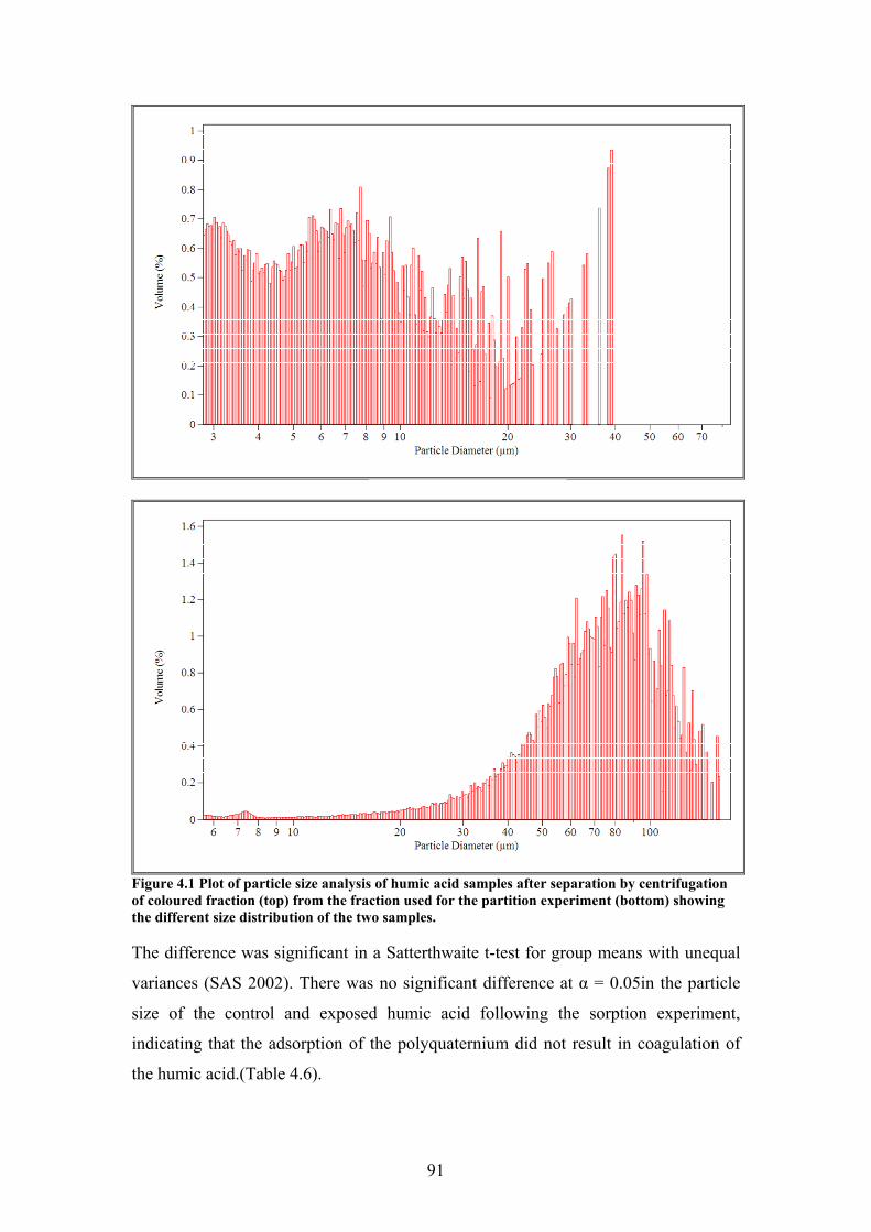
91

Figure 4.1 Plot of particle size analysis of humic acid samples after separation by centrifugation of coloured fraction (top) from the fraction used for the partition experiment (bottom) showing the different size distribution of the two samples. The difference was significant in a Satterthwaite t-test for group means with unequal

variances (SAS 2002). There was no significant difference at α = 0.05in the particle

size of the control and exposed humic acid following the sorption experiment,

indicating that the adsorption of the polyquaternium did not result in coagulation of

the humic acid.(Table 4.6).

92

Table 4.6 Results of statistical analysis of humic acid particle size for the separated supernatant and solid fraction showing that the difference was significant at α = 0.05 given unequal variance. Variable Method Variances DF t Value Pr > |t| Size Pooled Equal 2 34.34 0.0008 Size Satterthwaite Unequal 1.37 34.34 0.0056 Test for Equality of Variances Variable Method Num DF Den DF F Value Pr > F Size Folded F 1 1.37 5.22 0.5252

The calculated KD values are given in Table 4.7, and a sample of the plot of Equation

4.2 as used in determining KD, in this case for Conditioneze W-20 is shown in Figure

4.2.

y = 500.18xR2 = 0.9093

0

2

4

6

8

10

12

14

16

0 0.005 0.01 0.015 0.02 0.025 0.03

Ci-

Cf

Cf*Ms/Mw

y = 500.18xR2 = 0.9093

0

2

4

6

8

10

12

14

16

0 0.005 0.01 0.015 0.02 0.025 0.03

Ci-

Cf

Cf*Ms/Mw

Figure 4.2 Plot of Equation 4.2 as used in determining KD, in this case for Conditioneze® W-20 (Polyquaternium-55). Table 4.7 Partition coefficient KD determined for polyquaterniums and PSCs and one cationic surfactant (cetyl pyridinium chloride). Polyquaternium KD KD with SDS Gafquat® 440 1038 1226 Gafquat® 734 986 1436 Gafquat® HS100 186 80 UCareTM JR125 359 795 UCareTM JR30M 634 1484 UCareTM JR400 440 382 Conditioneze® NT-20 309 168 poly(DADMAC) 2238 3329 Styleze® W-20 500 400 Cetyl pyridinium chloride 55,000 -

In a Paired T-test (SAS 2002), there was no significant difference between the KD

values for the polyquaternium or the polyquaternium-surfactant complex (PSC) at α =

0.05 (Table 4.8).

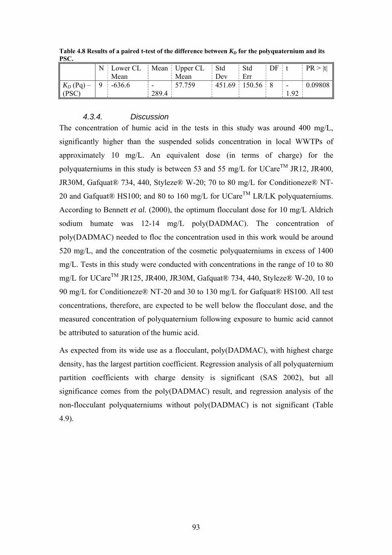
93

Table 4.8 Results of a paired t-test of the difference between KD for the polyquaternium and its PSC. N Lower CL

Mean Mean Upper CL

Mean Std Dev

Std Err

DF t PR > |t|

KD (Pq) –(PSC)

9 -636.6 -289.4

57.759 451.69 150.56 8 -1.92

0.09808

4.3.4. Discussion The concentration of humic acid in the tests in this study was around 400 mg/L,

significantly higher than the suspended solids concentration in local WWTPs of

approximately 10 mg/L. An equivalent dose (in terms of charge) for the

polyquaterniums in this study is between 53 and 55 mg/L for UCareTM JR12, JR400,

JR30M, Gafquat® 734, 440, Styleze® W-20; 70 to 80 mg/L for Conditioneze® NT-

20 and Gafquat® HS100; and 80 to 160 mg/L for UCareTM LR/LK polyquaterniums.

According to Bennett et al. (2000), the optimum flocculant dose for 10 mg/L Aldrich

sodium humate was 12-14 mg/L poly(DADMAC). The concentration of

poly(DADMAC) needed to floc the concentration used in this work would be around

520 mg/L, and the concentration of the cosmetic polyquaterniums in excess of 1400

mg/L. Tests in this study were conducted with concentrations in the range of 10 to 80

mg/L for UCareTM JR125, JR400, JR30M, Gafquat® 734, 440, Styleze® W-20, 10 to

90 mg/L for Conditioneze® NT-20 and 30 to 130 mg/L for Gafquat® HS100. All test

concentrations, therefore, are expected to be well below the flocculant dose, and the

measured concentration of polyquaternium following exposure to humic acid cannot

be attributed to saturation of the humic acid.

As expected from its wide use as a flocculant, poly(DADMAC), with highest charge

density, has the largest partition coefficient. Regression analysis of all polyquaternium

partition coefficients with charge density is significant (SAS 2002), but all

significance comes from the poly(DADMAC) result, and regression analysis of the

non-flocculant polyquaterniums without poly(DADMAC) is not significant (Table

4.9).

94

0

500

1000

1500

2000

2500

0 0.001 0.002 0.003 0.004 0.005 0.006

poly(DADMAC)

Figure 4.3 Plot of KD against charge density for polyquaterniums on which the regression analysis is based. The data is also presented in tabular form in Table 4.7. Table 4.9 Results of a regression model of KD against charge density. The model is significant if the high charge density poly(DADMAC) is included, but is not significant for the cosmetic polymers alone. Regression F Pr > F R2 All polyquaterniums 25.63 0.0015 0.7854 Without poly(DADMAC) 0.08 0.7832 0.0136

The sorption coefficients overall are perhaps lower than expected. For example,

Busan 77 (Polyquaternium-42), a high charge density bactericide homopolymer with

two quaternary ammonium charged centres in each monomeric unit and a nominal

equivalence/gram of 0.00775, has been found to have a log KD between 4.3 and 4.7

(≈ 20,000 – 50,000) when tested with acid-precipitable fraction humic acid (Matthews

et al. 1995). Similarly, when cetylpyridinium chloride was tested in this study using

the same method, the sorption coefficient was found to be 55,000 L/kg. The results

were similar, however, to the results obtained by Podoll and Irwin (1988) for the

tertiary cationic poly(N,N,-dimethylaminoethyl methacrylate) (PDAM) oligomers on

sediments (880 – 4,100 mL/g). One possible reason for an apparently low partition

coefficient could be the lower surface area to mass ratio due to the larger particles of

the humic acid used in the sorption experiment. Roughness of the surface in terms of

pores not accessible to the polyelectrolyte of the large particles may also be a factor in

lower adsorption, as has been suggested for the binding of flocculant polymers to

wastewater sludge (Mikkelsen 2003). Due to this roughness, neutralisation of the

‘polymer accessible surface charges’ would occur at a polymer dose that was below

the zeta potential for full neutralisation.

95

It has been suggested that the calculation of a partition coefficient for highly soluble

substances such as polyquaterniums may not be appropriate, as this model of

environmental behaviour assumes that the binding of the substance is not saturable

(Matthews et al. 1995). Poorly soluble substances form micelle-like structures with

humic acid and the binding capacity is unlimited. There is evidence to suggest,

however, that binding of the polyquaternium to humic acid or suspended solids

continues beyond the flocculant dose, that is, charge neutralisation, to form a stable

dispersion of opposite charge. This phenomenon is seen in the re-suspension of flocs

following over dosing with flocculants in water treatment applications (Narkis and

Rebhun 1983).

Nevertheless, in general, care should be taken in extrapolating from the conditions

pertaining to an experimental sorbent-water partition coefficient derived for highly

soluble substances. The polyquaternium-surfactant complex, however, is insoluble,

and thus this constraint to the use of partition coefficient would not apply.

The observation that binding of the polyquaternium with humic acid is not

significantly affected by the presence of the anionic surfactant is not surprising; as it

is this aspect of the behaviour of these polyelectrolytes that makes them suitable for

use many personal care applications. The zeta potential and isoelectric point of hair (-

30 mV, 3.6) are roughly the same as those of humic acid. In studies of the behaviour

of a polyquaternium acrylamide-methacrylamido propyl trimethyl ammonium

chloride (AM-MAPTAC) and the anionic surfactant SDS at a negatively charged

surface (mica), sorption of a high charge density polymer (10%) was found to be

enhanced at SDS concentrations above one tenth of critical micelle concentration

(CMC) (8 x 10-4 M), and at a maximum at charge neutralisation (Rojas et al. 2004).

Low charge density AM-MAPTAC (1%) began to desorb when surfactant

concentration was one tenth of CMC (Rojas et al. 2001). In terms of the sorption

studies here, the concentration of SDS at charge neutralisation of poly(DADMAC)

was > 0.5 CMC, while for the personal care polymers it was between 0.07 and 0.15

CMC. Therefore, enhanced sorption of the poly(DADMAC) could be expected, and

was observed. The lower partition coefficients observed for the low charge density

polyquaterniums, Conditioneze® NT-20 and Gafquat® HS100, in the presence of the

surfactant could result from desorption.

96

4.4. Fate Modelling Fate modelling of chemical species in an aquatic environment is often thought of in

terms of four pathways – adsorption, biodegradation, chemical degradation and

volatilisation. Two of these, adsorption and volatilisation are transfers of the chemical

of interest from the dissolved phase to another phase. In wastewater treatment, this

generally means transfer to air, sludge, or suspended solids. The remaining two

pathways, chemical degradation and biodegradation involve the transformation of the

chemical of interest into a different chemical, or even a suite of different chemicals.

These pathways are often referred to as ‘removal’ pathways, but from a risk

assessment perspective only complete mineralisation can be regarded as complete

removal.

In the context of chemicals such as polyquaterniums, ‘transfer’ from the water column

to the sludge in the wastewater treatment process has traditionally been regarded as a

‘removal’ process in chemical risk assessment in Australia, for example in the FPR

for Luviquat Care (Polyquaternium-44) (NICNAS 2001). Traditional disposal

methods of wastewater sludges by landfill or incineration were thought to result in

immobilisation of the chemical in the former, and transformation to oxides of carbon

and nitrogen in the latter. However, recent developments in the re-use of sludge in

land applications could result in further mobility of chemicals, and their potential

return to the aquatic environment via leaching and surface water movements.

In the risk assessment of chemicals that are transformed by either biodegradation or

chemical degradation (hydrolysis, photolysis), it must be established in the risk

assessment process that such transformation products are less hazardous than the

original chemical. In the case of polymers, the ability to degrade is not generally

regarded as a favourable outcome, due to the complexity of possible degradation

products, their higher potential for mobility and systemic absorption compared with

the high MW polymer. It is for this reason that biopolymers and other biodegradable

polymers are not considered to be PLCs.

4.4.1. Partitioning Models The environmental fate of chemicals may as a first estimate be considered by

determining the distribution of chemicals between phases or compartments in the

environment based on the thermodynamic principle that the chemical will tend to

reach an equilibrium state between phases or compartments. The operation of such

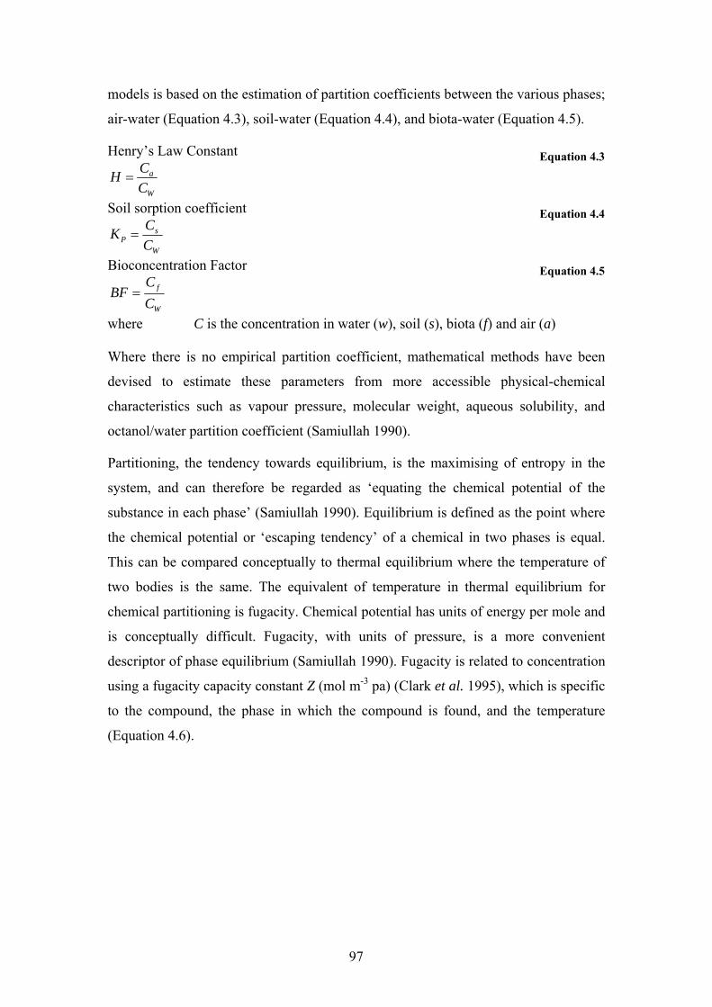
97

models is based on the estimation of partition coefficients between the various phases;

air-water (Equation 4.3), soil-water (Equation 4.4), and biota-water (Equation 4.5).

Henry’s Law Constant

W

a

CCH =

Equation 4.3

Soil sorption coefficient

W

sP C

CK = Equation 4.4

Bioconcentration Factor

W

f

CC

BF = Equation 4.5

where C is the concentration in water (w), soil (s), biota (f) and air (a) Where there is no empirical partition coefficient, mathematical methods have been

devised to estimate these parameters from more accessible physical-chemical

characteristics such as vapour pressure, molecular weight, aqueous solubility, and

octanol/water partition coefficient (Samiullah 1990).

Partitioning, the tendency towards equilibrium, is the maximising of entropy in the

system, and can therefore be regarded as ‘equating the chemical potential of the

substance in each phase’ (Samiullah 1990). Equilibrium is defined as the point where

the chemical potential or ‘escaping tendency’ of a chemical in two phases is equal.

This can be compared conceptually to thermal equilibrium where the temperature of

two bodies is the same. The equivalent of temperature in thermal equilibrium for

chemical partitioning is fugacity. Chemical potential has units of energy per mole and

is conceptually difficult. Fugacity, with units of pressure, is a more convenient

descriptor of phase equilibrium (Samiullah 1990). Fugacity is related to concentration

using a fugacity capacity constant Z (mol m-3 pa) (Clark et al. 1995), which is specific

to the compound, the phase in which the compound is found, and the temperature

(Equation 4.6).

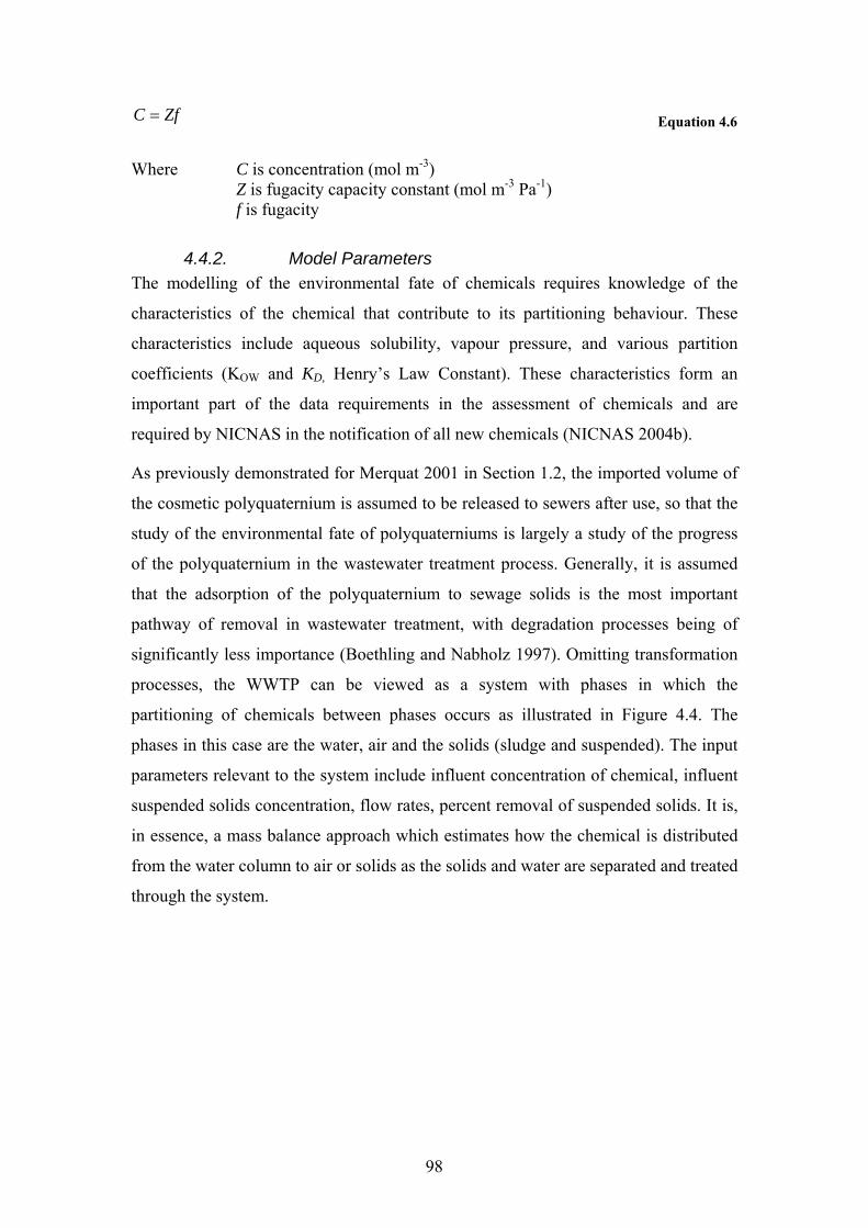
98

ZfC = Equation 4.6

Where C is concentration (mol m-3) Z is fugacity capacity constant (mol m-3 Pa-1) f is fugacity

4.4.2. Model Parameters The modelling of the environmental fate of chemicals requires knowledge of the

characteristics of the chemical that contribute to its partitioning behaviour. These

characteristics include aqueous solubility, vapour pressure, and various partition

coefficients (KOW and KD, Henry’s Law Constant). These characteristics form an

important part of the data requirements in the assessment of chemicals and are

required by NICNAS in the notification of all new chemicals (NICNAS 2004b).

As previously demonstrated for Merquat 2001 in Section 1.2, the imported volume of

the cosmetic polyquaternium is assumed to be released to sewers after use, so that the

study of the environmental fate of polyquaterniums is largely a study of the progress

of the polyquaternium in the wastewater treatment process. Generally, it is assumed

that the adsorption of the polyquaternium to sewage solids is the most important

pathway of removal in wastewater treatment, with degradation processes being of

significantly less importance (Boethling and Nabholz 1997). Omitting transformation

processes, the WWTP can be viewed as a system with phases in which the

partitioning of chemicals between phases occurs as illustrated in Figure 4.4. The

phases in this case are the water, air and the solids (sludge and suspended). The input

parameters relevant to the system include influent concentration of chemical, influent

suspended solids concentration, flow rates, percent removal of suspended solids. It is,

in essence, a mass balance approach which estimates how the chemical is distributed

from the water column to air or solids as the solids and water are separated and treated

through the system.

99

Primary Settling Tank

BioreactorFinal Settling Tank

Volatilization

SedimentationBiotransformation

41 3

25

6Primary Settling Tank

BioreactorFinal Settling Tank

Volatilization

SedimentationBiotransformation

41 3

25

6Primary Settling Tank

BioreactorFinal Settling Tank

Volatilization

SedimentationBiotransformation

41 3

25

6

Figure 4.4 Conceptual model of the ‘box’ structure of the Oxley WWTP in SE Queensland, showing the possible chemical fates, volatilization, biotransformation and sedimentation in the three stages of the treatment process. The numbered arrows represent the fluxes in Equations 4.11-4.13. The application of the fugacity/partition models to WWTP is therefore specific to

particular plants, as the mass balance of each plant will be different. For the purposes

of this study, the model has been applied to Oxley WWTP, a conventional activated

sludge WWTP with a mix of industrial and domestic influent of 240,000 people

equivalents, and typical in configuration of those found in South East Queensland

(Tan et al. 2007). The mass balance of water and solids in the Oxley WWTP is given

in Figure 4.5 and Figure 4.6 respectively (Tan et al. 2007).

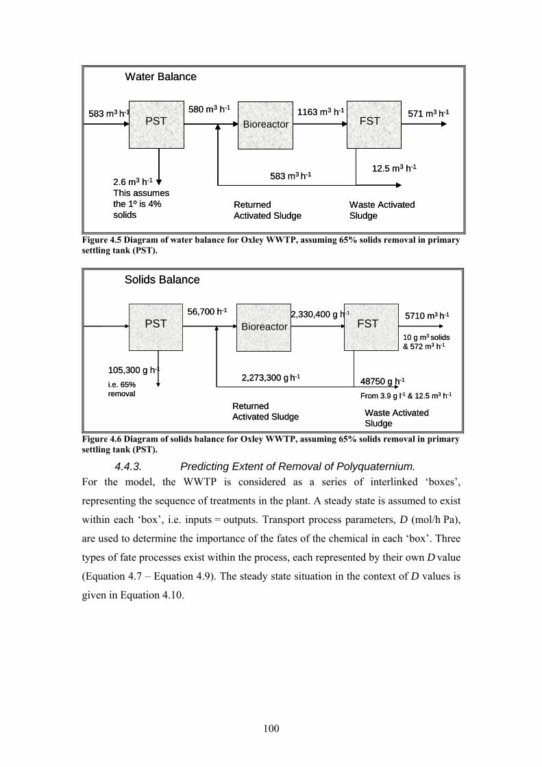
100

583 m3 h-1 580 m3 h-1 1163 m3 h-1

2.6 m3 h-1

This assumes the 1º is 4% solids

571 m3 h-1

12.5 m3 h-1583 m3 h-1

Waste Activated Sludge

Returned Activated Sludge

PST FST

Water Balance

Bioreactor583 m3 h-1 580 m3 h-1 1163 m3 h-1

2.6 m3 h-1

This assumes the 1º is 4% solids

571 m3 h-1

12.5 m3 h-1583 m3 h-1

Waste Activated Sludge

Returned Activated Sludge

PST FST

Water Balance

Bioreactor

Figure 4.5 Diagram of water balance for Oxley WWTP, assuming 65% solids removal in primary settling tank (PST).

56,700 h-1 2,330,400 g h-1

105,300 g h-1

i.e. 65% removal

5710 m3 h-1

48750 g h-1

From 3.9 g l-1 & 12.5 m3 h-1

2,273,300 g h-1

Waste Activated Sludge

Returned Activated Sludge

PST FST

Solids Balance

Bioreactor10 g m3 solids & 572 m3 h-1

56,700 h-1 2,330,400 g h-1

105,300 g h-1

i.e. 65% removal

5710 m3 h-1

48750 g h-1

From 3.9 g l-1 & 12.5 m3 h-1

2,273,300 g h-1

Waste Activated Sludge

Returned Activated Sludge

PST FST

Solids Balance

Bioreactor10 g m3 solids & 572 m3 h-1

Figure 4.6 Diagram of solids balance for Oxley WWTP, assuming 65% solids removal in primary settling tank (PST).

4.4.3. Predicting Extent of Removal of Polyquaternium. For the model, the WWTP is considered as a series of interlinked ‘boxes’,

representing the sequence of treatments in the plant. A steady state is assumed to exist

within each ‘box’, i.e. inputs = outputs. Transport process parameters, D (mol/h Pa),

are used to determine the importance of the fates of the chemical in each ‘box’. Three

types of fate processes exist within the process, each represented by their own D value

(Equation 4.7 – Equation 4.9). The steady state situation in the context of D values is

given in Equation 4.10.

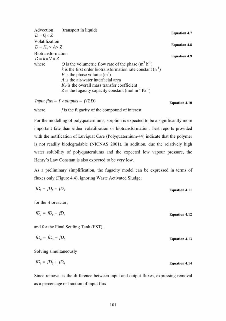
101

Advection (transport in liquid) ZQD ×= Equation 4.7

Volatilization ZAKD V ××= Equation 4.8

Biotransformation ZVkD ××= Equation 4.9

where Q is the volumetric flow rate of the phase (m3 h-1) k is the first order biotransformation rate constant (h-1) V is the phase volume (m3) A is the air/water interfacial area KV is the overall mass transfer coefficient Z is the fugacity capacity constant (mol m-3 Pa-1)

)( DfoutputsffluxInput Σ=×= Equation 4.10

where f is the fugacity of the compound of interest For the modelling of polyquaterniums, sorption is expected to be a significantly more

important fate than either volatilisation or biotransformation. Test reports provided

with the notification of Luviquat Care (Polyquaternium-44) indicate that the polymer

is not readily biodegradable (NICNAS 2001). In addition, due the relatively high

water solubility of polyquaterniums and the expected low vapour pressure, the

Henry’s Law Constant is also expected to be very low.

As a preliminary simplification, the fugacity model can be expressed in terms of

fluxes only (Figure 4.4), ignoring Waste Activated Sludge;

321 fDfDfD += Equation 4.11

for the Bioreactor;

453 fDfDfD += Equation 4.12

and for the Final Settling Tank (FST).

654 fDfDfD += Equation 4.13

Solving simultaneously

621 fDfDfD += Equation 4.14

Since removal is the difference between input and output fluxes, expressing removal

as a percentage or fraction of input flux

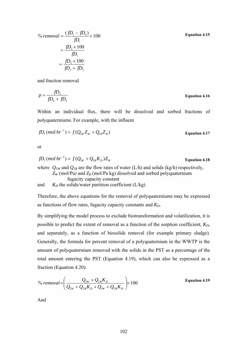
102

100)(%1

61 ×−

=fD

fDfDremoval

1

2 100fD

fD ×=

32

2 100fDfD

fD+×

=

Equation 4.15

and fraction removal

32

2

fDfDfDp+

= Equation 4.16

Within an individual flux, there will be dissolved and sorbed fractions of

polyquaterniums. For example, with the influent

)()( 111

1 BBWW ZQZQfhrmolfD +=− Equation 4.17

or

WDBW ZKQQfhrmolfD )()( 111

1 +=− Equation 4.18

where Q1W and Q1B are the flow rates of water (L/h) and solids (kg/h) respectively, ZW (mol/Pa) and ZB (mol/Pa kg) dissolved and sorbed polyquaternium fugacity capacity constant and KD the solids/water partition coefficient (L/kg) Therefore, the above equations for the removal of polyquaterniums may be expressed

as functions of flow rates, fugacity capacity constants and KD.

By simplifying the model process to exclude biotransformation and volatilization, it is

possible to predict the extent of removal as a function of the sorption coefficient, KD,

and separately, as a function of biosolids removal (for example primary sludge).

Generally, the formula for percent removal of a polyquaternium in the WWTP is the

amount of polyquaternium removed with the solids in the PST as a percentage of the

total amount entering the PST (Equation 4.19), which can also be expressed as a

fraction (Equation 4.20).

100%3322

22 ×⎟⎟⎠

⎞⎜⎜⎝

⎛+++

+=

DBWDBW

DBW

KQQKQQKQQremoval

Equation 4.19

And

103

⎟⎟⎠

⎞⎜⎜⎝

⎛+++

+=

DBWDBW

DBW

KQQKQQKQQp

3322

22 Equation 4.20

where p is the fraction of polyquaternium removed This equation can be rearranged to express the relationship between p and the

partition coefficient KD (Equation 4.21).

( )( )BBB

WWWD QQpQ

QQQpK322

232

+−−+

= Equation 4.21

In the situation under consideration, the flow of water removed with the solids is

significantly less than the flow rate of water to the bioreactor, that is Q2W << Q3W, and

for most WWTPs, it can be expected that Q2W << p(Q2w+Q3W). Taking this

assumption into account, the relationship can be simplified (Equation 4.22), and

rearranged to Equation 4.23 and Equation 4.24, which describes the linear relationship

between 1/KD and 1/p.

( )( )BBB

WWD QQpQ

QQpK322

32

+−+

≈ Equation 4.22

and therefore

( )( )WW

BBB

D QQpQQpQ

K 32

3221+

+−= Equation 4.23

( )( )( )WW

BB

WW

B

D QQQQ

QQpQ

K 32

32

32

21++

−+

= Equation 4.24

If Q2W << Q3W, denominator term may also be approximated as ≈ Q3W.

W

BB

W

B

D QQQ

pQQ

K 3

32

3

21 +−= Equation 4.25

Employing the actual fluxes from Oxley WWTP mass balance data with this equation,

the plot of the inverse of KD and p for values of p up to the maximum solids removal

(65%) for this WWTP (Figure 4.7), demonstrates that as KD becomes larger, the

proportion removed in the primary sludge becomes larger. In fact, as KD → ∞, and

1/KD → 0, 1/p approaches 1/0.65. That is, if KD → ∞ and the polyquaternium were all

sorbed, the maximum proportion of the polyquaternium that could be removed is 0.65

or 65%.

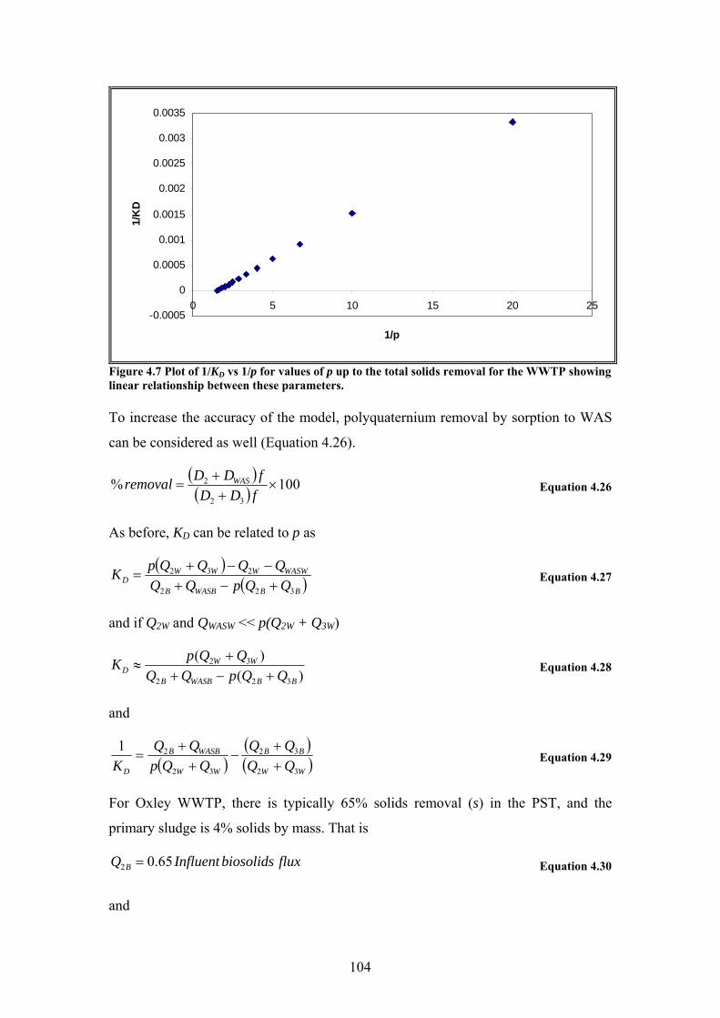
104

-0.0005

0

0.0005

0.001

0.0015

0.002

0.0025

0.003

0.0035

0 5 10 15 20 25

1/p

1/K

D

Figure 4.7 Plot of 1/KD vs 1/p for values of p up to the total solids removal for the WWTP showing linear relationship between these parameters. To increase the accuracy of the model, polyquaternium removal by sorption to WAS

can be considered as well (Equation 4.26).

( )( ) 100%

32

2 ×++

=fDDfDDremoval WAS Equation 4.26

As before, KD can be related to p as

( )( )BBWASBB

WASWWWWD QQpQQ

QQQQpK322

232

+−+−−+

= Equation 4.27

and if Q2W and QWASW << p(Q2W + Q3W)

)()(

322

32

BBWASBB

WWD QQpQQ

QQpK+−+

+≈ Equation 4.28

and

( )( )( )WW

BB

WW

WASBB

D QQQQ

QQpQQ

K 32

32

32

21++

−+

+= Equation 4.29

For Oxley WWTP, there is typically 65% solids removal (s) in the PST, and the

primary sludge is 4% solids by mass. That is

fluxbiosolidsInfluentQ B 65.02 = Equation 4.30

and

105

( )BBB QQQ 322 65.0 += Equation 4.31

Given that the solids level in the primary sludge is 4%, the biosolids and water flow

rate from the PST in the primary sludge can be expressed as a proportion of the total

flow rate

( )WBB QQQ 222 04.0 += Equation 4.32

( )WBW QQQ 222 96.0 += Equation 4.33

From Equation 4.20, the relationship between p and KD can be expressed taking into

account the proportion of solids removal (Equation 4.34).

( ) ( )( ) DBBWW

DBBBB

KQQQQ

KQQsQQs

p3232

3232

04.096.0

+++

+++××

= Equation 4.34

Where: s is the proportion of solids removed Thus for a polyquaternium with KD = 400, when s = 0.65, using the flux values from

Oxley WWTP, the proportion of polyquaternium removed is about 7%. As s → 1, the

equation can be simplified (Equation 4.35) and it can be shown that if KD is 400, and

all biosolids removed as primary sludge, only maximum of 10.6% of the

polyquaternium can be expected to be removed.

( )

( ) DBBWW

BBD

KQQQQ

QQKp

3232

3204.096.0

+++

+⎟⎠⎞

⎜⎝⎛ +

=

Equation 4.35

Where: Q2B = 105 kg/h Q3B = 56.7 kg/h Q2W = 2.6x103 L/h Q3W = 580x103 L/h

( )4007.161106.582

7.161400243 ×+×

+→p

106.01047.61086.6 4

=××

=

To take into account WAS, Equation 4.34 can be expanded to include sorption to

WAS (Equation 4.36).

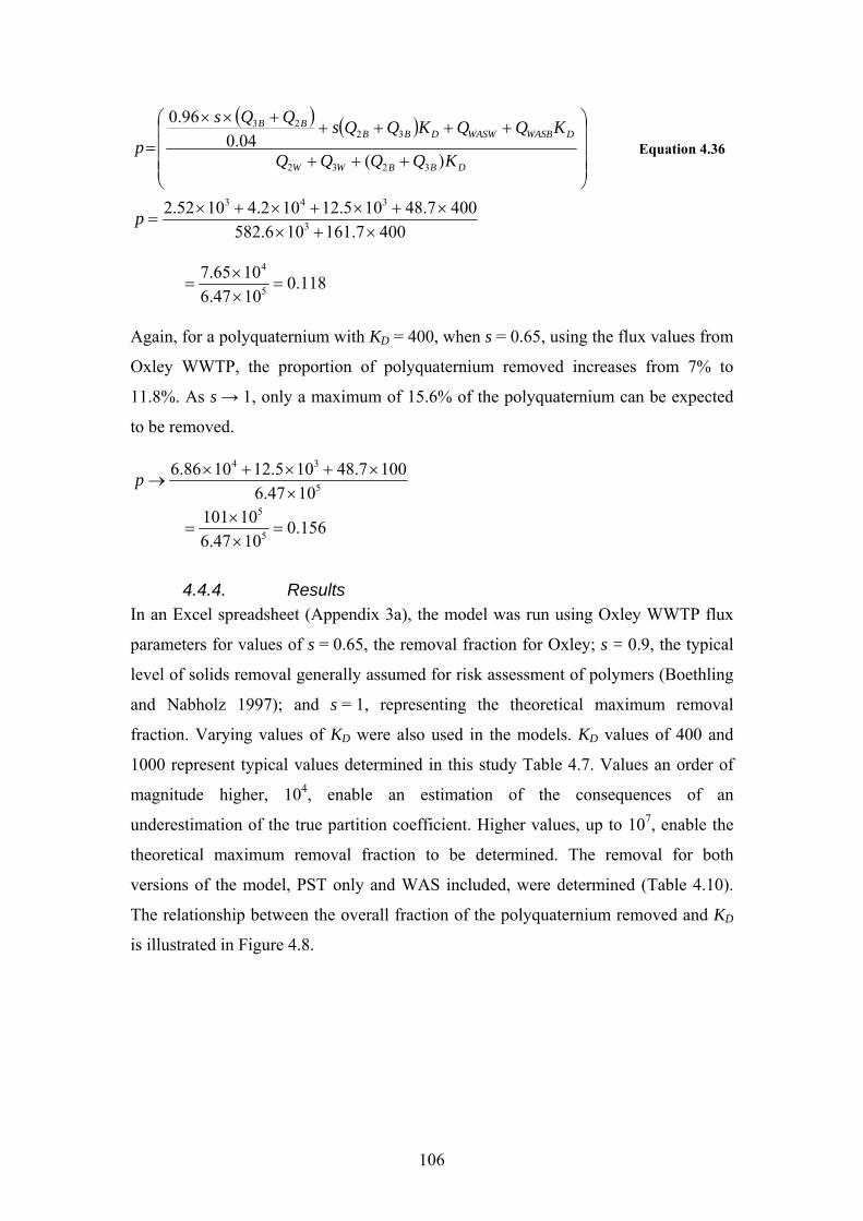
106

( ) ( )

⎟⎟⎟⎟

⎠

⎞

⎜⎜⎜⎜

⎝

⎛

+++

+++++××

=DBBWW

DWASBWASWDBBBB

KQQQQ

KQQKQQsQQs

p)(

04.096.0

3232

3223

Equation 4.36

4007.161106.5824007.48105.12102.41052.2

3

343

×+××+×+×+×

=p

118.01047.61065.7

5

4

=××

=

Again, for a polyquaternium with KD = 400, when s = 0.65, using the flux values from

Oxley WWTP, the proportion of polyquaternium removed increases from 7% to

11.8%. As s → 1, only a maximum of 15.6% of the polyquaternium can be expected

to be removed.

5

34

1047.61007.48105.121086.6

××+×+×

→p

156.01047.610101

5

5

=××

=

4.4.4. Results In an Excel spreadsheet (Appendix 3a), the model was run using Oxley WWTP flux

parameters for values of s = 0.65, the removal fraction for Oxley; s = 0.9, the typical

level of solids removal generally assumed for risk assessment of polymers (Boethling

and Nabholz 1997); and s = 1, representing the theoretical maximum removal

fraction. Varying values of KD were also used in the models. KD values of 400 and

1000 represent typical values determined in this study Table 4.7. Values an order of

magnitude higher, 104, enable an estimation of the consequences of an

underestimation of the true partition coefficient. Higher values, up to 107, enable the

theoretical maximum removal fraction to be determined. The removal for both

versions of the model, PST only and WAS included, were determined (Table 4.10).

The relationship between the overall fraction of the polyquaternium removed and KD

is illustrated in Figure 4.8.

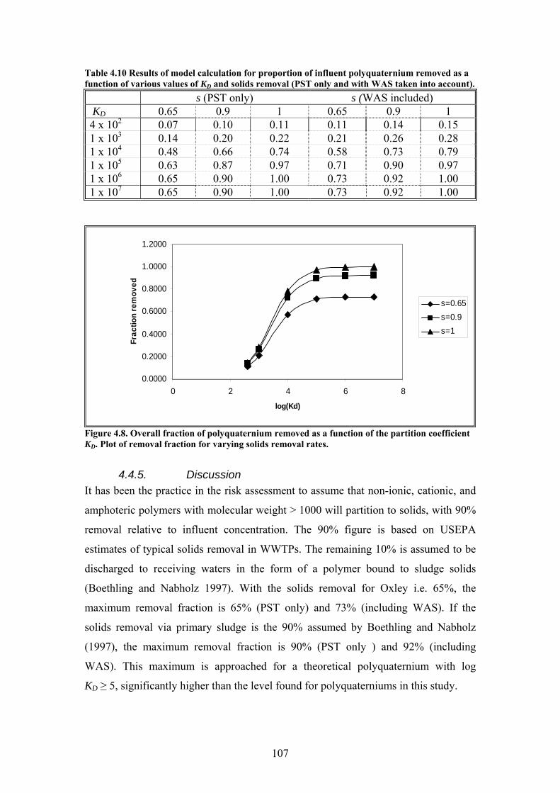
107

Table 4.10 Results of model calculation for proportion of influent polyquaternium removed as a function of various values of KD and solids removal (PST only and with WAS taken into account). s (PST only) s (WAS included) KD 0.65 0.9 1 0.65 0.9 1 4 x 102 0.07 0.10 0.11 0.11 0.14 0.15 1 x 103 0.14 0.20 0.22 0.21 0.26 0.28 1 x 104 0.48 0.66 0.74 0.58 0.73 0.79 1 x 105 0.63 0.87 0.97 0.71 0.90 0.97 1 x 106 0.65 0.90 1.00 0.73 0.92 1.00 1 x 107 0.65 0.90 1.00 0.73 0.92 1.00

0.0000

0.2000

0.4000

0.6000

0.8000

1.0000

1.2000

0 2 4 6 8

log(Kd)

Frac

tion

rem

oved

s=0.65s=0.9s=1

Figure 4.8. Overall fraction of polyquaternium removed as a function of the partition coefficient KD. Plot of removal fraction for varying solids removal rates.

4.4.5. Discussion It has been the practice in the risk assessment to assume that non-ionic, cationic, and

amphoteric polymers with molecular weight > 1000 will partition to solids, with 90%

removal relative to influent concentration. The 90% figure is based on USEPA

estimates of typical solids removal in WWTPs. The remaining 10% is assumed to be

discharged to receiving waters in the form of a polymer bound to sludge solids

(Boethling and Nabholz 1997). With the solids removal for Oxley i.e. 65%, the

maximum removal fraction is 65% (PST only) and 73% (including WAS). If the

solids removal via primary sludge is the 90% assumed by Boethling and Nabholz

(1997), the maximum removal fraction is 90% (PST only ) and 92% (including

WAS). This maximum is approached for a theoretical polyquaternium with log

KD ≥ 5, significantly higher than the level found for polyquaterniums in this study.

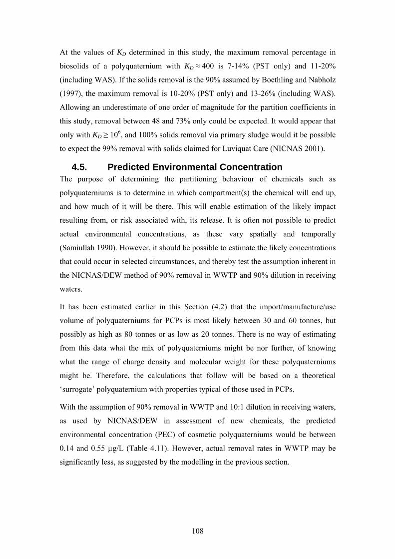
108

At the values of KD determined in this study, the maximum removal percentage in

biosolids of a polyquaternium with KD ≈ 400 is 7-14% (PST only) and 11-20%

(including WAS). If the solids removal is the 90% assumed by Boethling and Nabholz

(1997), the maximum removal is 10-20% (PST only) and 13-26% (including WAS).

Allowing an underestimate of one order of magnitude for the partition coefficients in

this study, removal between 48 and 73% only could be expected. It would appear that

only with KD ≥ 106, and 100% solids removal via primary sludge would it be possible

to expect the 99% removal with solids claimed for Luviquat Care (NICNAS 2001).

4.5. Predicted Environmental Concentration The purpose of determining the partitioning behaviour of chemicals such as

polyquaterniums is to determine in which compartment(s) the chemical will end up,

and how much of it will be there. This will enable estimation of the likely impact

resulting from, or risk associated with, its release. It is often not possible to predict

actual environmental concentrations, as these vary spatially and temporally

(Samiullah 1990). However, it should be possible to estimate the likely concentrations

that could occur in selected circumstances, and thereby test the assumption inherent in

the NICNAS/DEW method of 90% removal in WWTP and 90% dilution in receiving

waters.

It has been estimated earlier in this Section (4.2) that the import/manufacture/use

volume of polyquaterniums for PCPs is most likely between 30 and 60 tonnes, but

possibly as high as 80 tonnes or as low as 20 tonnes. There is no way of estimating

from this data what the mix of polyquaterniums might be nor further, of knowing

what the range of charge density and molecular weight for these polyquaterniums

might be. Therefore, the calculations that follow will be based on a theoretical

‘surrogate’ polyquaternium with properties typical of those used in PCPs.

With the assumption of 90% removal in WWTP and 10:1 dilution in receiving waters,

as used by NICNAS/DEW in assessment of new chemicals, the predicted

environmental concentration (PEC) of cosmetic polyquaterniums would be between

0.14 and 0.55 µg/L (Table 4.11). However, actual removal rates in WWTP may be

significantly less, as suggested by the modelling in the previous section.

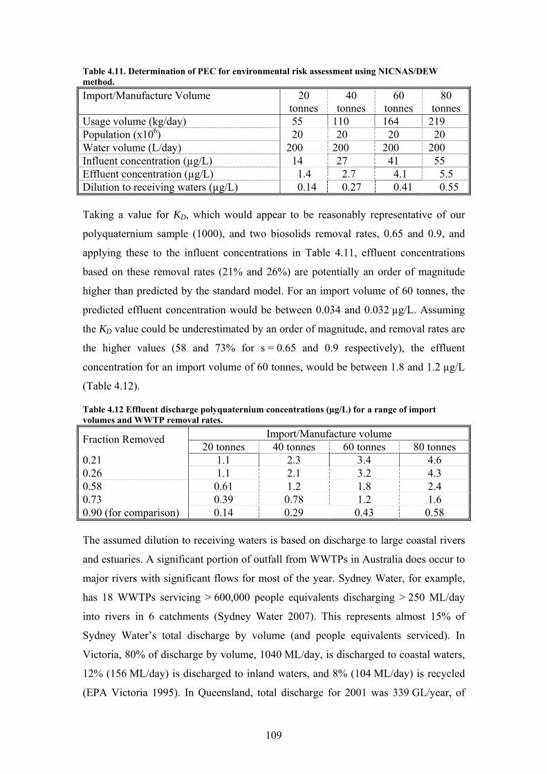
109

Table 4.11. Determination of PEC for environmental risk assessment using NICNAS/DEW method. Import/Manufacture Volume 20

tonnes 40

tonnes 60

tonnes 80

tonnes Usage volume (kg/day) 55 110 164 219 Population (x106) 20 20 20 20 Water volume (L/day) 200 200 200 200 Influent concentration (µg/L) 14 27 41 55 Effluent concentration (µg/L) 1.4 2.7 4.1 5.5 Dilution to receiving waters (µg/L) 0.14 0.27 0.41 0.55 Taking a value for KD, which would appear to be reasonably representative of our

polyquaternium sample (1000), and two biosolids removal rates, 0.65 and 0.9, and

applying these to the influent concentrations in Table 4.11, effluent concentrations

based on these removal rates (21% and 26%) are potentially an order of magnitude

higher than predicted by the standard model. For an import volume of 60 tonnes, the

predicted effluent concentration would be between 0.034 and 0.032 µg/L. Assuming

the KD value could be underestimated by an order of magnitude, and removal rates are

the higher values (58 and 73% for s = 0.65 and 0.9 respectively), the effluent

concentration for an import volume of 60 tonnes, would be between 1.8 and 1.2 µg/L

(Table 4.12).

Table 4.12 Effluent discharge polyquaternium concentrations (µg/L) for a range of import volumes and WWTP removal rates.

Import/Manufacture volume Fraction Removed 20 tonnes 40 tonnes 60 tonnes 80 tonnes

0.21 1.1 2.3 3.4 4.6 0.26 1.1 2.1 3.2 4.3 0.58 0.61 1.2 1.8 2.4 0.73 0.39 0.78 1.2 1.6 0.90 (for comparison) 0.14 0.29 0.43 0.58 The assumed dilution to receiving waters is based on discharge to large coastal rivers

and estuaries. A significant portion of outfall from WWTPs in Australia does occur to

major rivers with significant flows for most of the year. Sydney Water, for example,

has 18 WWTPs servicing > 600,000 people equivalents discharging > 250 ML/day

into rivers in 6 catchments (Sydney Water 2007). This represents almost 15% of

Sydney Water’s total discharge by volume (and people equivalents serviced). In

Victoria, 80% of discharge by volume, 1040 ML/day, is discharged to coastal waters,

12% (156 ML/day) is discharged to inland waters, and 8% (104 ML/day) is recycled

(EPA Victoria 1995). In Queensland, total discharge for 2001 was 339 GL/year, of

110

which 11.2% was recycled and 23 GL (around 8%) was discharged to non-tidal water

bodies (Beeton et al. 2006).

Consequently, between 8 and 15% of total effluent is discharged into vulnerable

inland waterways, where dilution is likely to be less than 10:1. Victorian regulations

require that the dilution be at least 5:1. Queensland and NSW regulations are based on

water quality outcomes and regulated in licensing agreements. Of course, dilution

values could be less than 5:1 or more than 10:1; in fact, for discharge into ocean

outfall (the majority of WWTP discharge in Australia) it will be greater than 10:1.

The range of environmental concentrations likely under 10:1 and 5:1 dilution regimes

is given in Table 4.13. Without even considering the possibility of zero dilution

(effectively the effluent concentration) on discharge, a fifteen-fold difference in the

PEC can occur for some possible import volumes. The application of the model has

produced a range or distribution of possible concentrations. All these concentrations

are lower than the concentrations predicted by the NICNAS/DEW method (Table

4.11), assuming no adsorption in WWTP, but higher that that assumed by adopting

the USEPA default of 90% loss to solids in WWTPs.

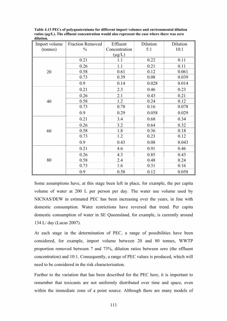
111

Table 4.13 PECs of polyquaterniums for different import volumes and environmental dilution ratios (µg/L). The effluent concentration would also represent the case where there was zero dilution. Import volume

(tonnes) Fraction Removed

% Effluent

Concentration(µg/L)

Dilution 5:1

Dilution 10:1

0.21 1.1 0.22 0.11 0.26 1.1 0.21 0.11 0.58 0.61 0.12 0.061 0.73 0.39 0.08 0.039

20

0.9 0.14 0.028 0.014 0.21 2.3 0.46 0.23 0.26 2.1 0.43 0.21 0.58 1.2 0.24 0.12 0.73 0.78 0.16 0.078

40

0.9 0.29 0.058 0.029 0.21 3.4 0.68 0.34 0.26 3.2 0.64 0.32 0.58 1.8 0.36 0.18 0.73 1.2 0.23 0.12

60

0.9 0.43 0.08 0.043 0.21 4.6 0.91 0.46 0.26 4.3 0.85 0.43 0.58 2.4 0.48 0.24 0.73 1.6 0.31 0.16

80

0.9 0.58 0.12 0.058 Some assumptions have, at this stage been left in place, for example, the per capita

volume of water at 200 L per person per day. The water use volume used by

NICNAS/DEW in estimated PEC has been increasing over the years, in line with

domestic consumption. Water restrictions have reversed that trend. Per capita

domestic consumption of water in SE Queensland, for example, is currently around

134 L/ day (Lucas 2007).

At each stage in the determination of PEC, a range of possibilities have been

considered, for example, import volume between 20 and 80 tonnes, WWTP

proportion removed between 7 and 73%, dilution ratios between zero (the effluent

concentration) and 10:1. Consequently, a range of PEC values is produced, which will

need to be considered in the risk characterisation.

Further to the variation that has been described for the PEC here, it is important to

remember that toxicants are not uniformly distributed over time and space, even

within the immediate zone of a point source. Although there are many models of

112

dilution effects as a function of distance from release, mixing zones and patch effects

can also occur (Spromberg et al. 1998; Landis and McLaughlin 2000). No boundaries

are specified for the PEC, which can be assumed to be applicable only in the

proximity of the WWTP outfall. The process of adsorption of the polyquaternium to

DOM continues to occur once the WWTP effluent has been released to receiving

waters, and removal to sediments in the downstream area will occur. In addition to the

removal of residual cationic polyelectrolytes to DOM and clay in the receiving waters,

removal of soluble polyelectrolyte-DOM complexes by adsorption to clay particles

can occur (Bennett et al. 2000). While these factors are often critical in the assessment

of contaminated sites, they are generally outside the scope of the risk assessment of a

new chemical. However, the partition coefficients determined in this study have

implications for the extent of removal of the polyquaterniums in receiving waters, as

well as the extent of removal in WWTP. Sorption to solids in receiving waters may be

similarly lower than expected.

4.6. Conclusion The import volume for cosmetic polyquaterniums has been estimated using two

different methods. The results of these estimates resulted in a similar range of values.

The experimentally determined KD for the polyquaterniums was less than expected,

and significantly less than that for the monoquaternary surfactant, cetylpyridinium

chloride, that was also tested. Consequently, the fraction removed in WWTP would be

expected to be significantly less than the default value for polymers that is generally

used in the risk assessment of cosmetic polyquaterniums. The PEC calculated has a

range of approximately 0.01 to 1.0 µg/L between the highest and lowest estimates.

Therefore, considerable uncertainty will need to be considered in the risk

characterisation.

113

5. Aquatic Toxicology – Effects Assessment of Polyquaterniums 5.1. Introduction

The assessment of the effects of a chemical is often regarded as comprising two

components; hazard identification and dose (concentration)–response assessment

(ECB 2003). Hazard relates to the capacity of a specific agent to produce a particular

type of adverse health or environmental effect, for example the capacity of benzene to

cause cancer or the capacity of solar radiation to cause skin cancer (EnHealth 2002).

Dose-response assessment explores the relationship between the amount of exposure

to the hazard, and the level of effect observed (Neely 1994), which can be estimated

or determined from toxicological studies, epidemiological studies and, for

environmental impacts, ecological studies. Thus, effects assessment is a two step

process comprising the identification of the hazard, and the capacity of the hazard to

cause the response, that is the level of exposure, or dose required (EnHealth 2002). In

practical terms, a substance is labelled as hazardous if it meets certain criteria. While

these criteria may be based on physico-chemical properties of the chemical, for

example if it is corrosive, determination of a hazard classification is generally

determined by the toxic (dose) response in a standard test (NOHSC 1999, OECD

2001).

In regulatory chemical risk assessment, the identification of the hazard is generally

determined by criteria set out in the appropriate act. The Industrial Chemicals

(Notification and Assessment) Act (ICNA), for example, has previously categorised

polymers according to criteria that determine low concern (Polymers of Low Concern,

PLC), and all other chemicals solely on volume imported or manufactured. More

recently, criteria for identifying all chemicals of low concern have been developed

(Low Regulatory Concern Chemicals, LRCC). The development of such criteria is

usually only possible after years of operation of the assessment process allows the

identification of suitable criteria (NICNAS 2004a). The process, therefore, is not

about identifying a hazard, but of screening out those chemicals that are unlikely to be

hazardous. The data required for assessment is also established in the Act or

regulations. For new chemicals that are regarded as potentially hazardous, the

minimum data requirement for hazard assessment for the aquatic compartment

comprises short-term toxicity data for three species from three trophic levels, algae,

114

Daphnia, and fish, and a bacteria (respiratory inhibition test) for sludge-based

organisms (EC 2003; NICNAS 2004b). However, further information may be

requested by the regulatory authorities, and notifiers are expected to provide all

available information above the minimum requirement if such data exists (NICNAS

2004b). Waivers may also be granted for some or all of the required tests, allowing

substitution of analogue data, or complete waiver in cases where the testing is not

technically possible, for example, readily hydrolysed compounds.

As exposure assessment is the process leading to the predicted environmental

concentration (PEC), for the purposes of this study effects assessment is the process

leading to the establishment of a Predicted No Effect Concentration (PNEC). A PNEC

is regarded as a concentration below which an unacceptable effect will most likely not

occur (ECB 2003). In practice, the PNEC is calculated by dividing the short-term

median effective concentration (EC50) or long-term no observed effect level (NOEC)

value by an appropriate assessment or safety factor. A safety factor is generally a

margin of safety applied to a NOEC level to produce a value below which exposures

are assumed to be safe (Bascietto 1990). Assessment factors were developed for the

process of reviewing premanufacture notices and are applied to acute toxicity values,

and take into account the uncertainties due to such variables as test species’

sensitivities to acute and chronic exposures, laboratory test conditions, and age-group

susceptibility (Bascietto 1990). The EC50 required for the determination of the PNEC

in new chemicals assessment by National Industrial Chemicals Notification and

Assessment Scheme/Department of Environment and Water Resources

(NICNAS/DEW) is minimally required to be the lowest of the three trophic levels

required for regulatory assessment (ECB 2003, NICNAS 2004b). The level of

assessment factors used in determining the PNEC is dependent on the availability of

test results above the minimum requirement. Therefore, in this study, fish,

invertebrate and algae tests are reported. The three species selected were Gambusia

holbrooki, Artemia sp., and Chlorella sp. 12. As polyquaterniums are released with

wastewater across a variety of aquatic environments, relevance of species to the

ecosystem of interest was not critical. However, Gambusia are found widely in

freshwater streams in eastern Australia (McDowall 1996). As large releases of

wastewater to ocean outfall occur in coastal areas, and little data is available on the

toxicity of polyquaterniums to marine species, a marine species was included. As

115

there was little data available on sensitivity of species to suggest whether the species

selected would be sensitive to polyquaterniums, Gambusia and Artemia were chosen

primarily because of their availability and ease of handling.

The aim of the following experimental section is to establish if:

• the cosmetic polyquaterniums are toxic to the three species, G. holbrooki,

Artemia spp. and Chlorella sp12;

• If the polyquaterniums are toxic to any species, to determine if the formation

of the polymer-surfactant aggregate in cosmetic formulations has any impact

on the toxicity;

• If the polyquaterniums are toxic to any species, to investigate if the presence

of humic acid has any effect on the toxicity;

• To use the toxicity data in the hazard assessment of the risk assessment

process.

5.2. Methods 5.2.1. Experimental Design

The initial step in the experimental design was to determine the toxicity of the

cosmetic polyquaterniums to the test species. The toxicity of the anionic surfactant

SDS was also tested. For comparison, the toxicity of the water treatment polymer

poly(DADMAC) and the cationic surfactant cetyl pyridinium chloride were also

tested. As these tests would allow the comparison of the toxicity of the cosmetic

polyquaterniums to the published values for water treatment polycations and other

cationic surfactants, the inclusion of poly(DADMAC) and cetyl pyridinium chloride

would ensure that differences found were not due to the methods adopted in this

study.

If the polyquaternium(s) were toxic to the test species, and the anionic surfactant was

either not classifiable as toxic, or significantly less toxic than the polyquaternium, it

would then be possible to test the toxicity of the polymer-surfactant complex.

In addition to direct comparison of the toxicity of cosmetic polyquaterniums to the

published toxicity values for water treatment, this would determine if any differences

in the toxicity of water treatment polycations and cosmetic polyquaterniums could be

attributed to the factors resulting from the formulation of cosmetic products, that is,

116

the presence of the anionic surfactant. If any of the polyquaterniums were classifiable

as toxic, it was proposed to test the polyquaternium in the presence of

environmentally relevant concentrations of humic acid to determine if this resulted in

any change in the toxicity of the polyquaternium.

As metachromatic colloid titration had not proved amenable to determining the

concentration of polyquaterniums in the test solutions, the concentrations quoted are

nominal rather than actual. However, choice of all equipment in test should take into

account the tendency of polyquaterniums to adsorb to certain surfaces.

At the beginning of testing, it was not known if all polyquaterniums would have

similar toxicities, or if differences in the structure of the polymers would result in

determinable differences in toxicity. As testing was limited to polyquaterniums that

manufacturers were prepared to provide, it was determined that testing would begin

with all polyquaterniums that were obtained. However, if the behaviour of

polyquaterniums were not discernibly different, or if groupings became apparent, the

choice of polyquaterniums for the remaining tests would be refined.

5.2.2. Test Solutions All chemicals used were as described previously in Section 3.3.1. Stock solutions of

polyquaterniums were prepared in Milli-Q water at a concentration of 10 g/l, and

diluted to make working solutions of 1 g/l. For tests with humic acid, the soluble

fraction separated as described in the previous chapter was used. The concentration

was determined from the organic carbon concentration of the supernatant and the

organic carbon content of the humic acid (51%). The humic acid was added to the test

solution before the toxicant, at concentrations of 5 and 10 mg/L humic acid. The

relative concentration was determined from the organic carbon content of the

supernatant and the organic carbon content of the humic acid (51%).

5.2.3. Fish Gambusia holbrooki were trapped in a small dam on a private property in the

Beenleigh area in SE Queensland (Figure 5.1). The dam collects runoff from an area

that is largely rural (hobby farms). Fish were collected on a fortnightly basis, and kept

for a minimum of 12 days prior to testing. G. holbrooki are dimorphic, so only female

fish between 1.5 and 3 cm in length, with no obvious gravid spot, were used in the

test. This group was the most numerous in the field collections in autumn and winter.

Larger female fish are often survivors from the previous season (i.e. were older than

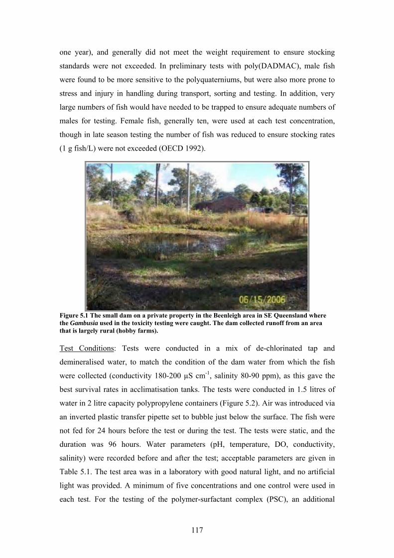
117

one year), and generally did not meet the weight requirement to ensure stocking

standards were not exceeded. In preliminary tests with poly(DADMAC), male fish

were found to be more sensitive to the polyquaterniums, but were also more prone to

stress and injury in handling during transport, sorting and testing. In addition, very

large numbers of fish would have needed to be trapped to ensure adequate numbers of

males for testing. Female fish, generally ten, were used at each test concentration,

though in late season testing the number of fish was reduced to ensure stocking rates

(1 g fish/L) were not exceeded (OECD 1992).

Figure 5.1 The small dam on a private property in the Beenleigh area in SE Queensland where the Gambusia used in the toxicity testing were caught. The dam collected runoff from an area that is largely rural (hobby farms). Test Conditions: Tests were conducted in a mix of de-chlorinated tap and

demineralised water, to match the condition of the dam water from which the fish

were collected (conductivity 180-200 µS cm-1, salinity 80-90 ppm), as this gave the

best survival rates in acclimatisation tanks. The tests were conducted in 1.5 litres of

water in 2 litre capacity polypropylene containers (Figure 5.2). Air was introduced via

an inverted plastic transfer pipette set to bubble just below the surface. The fish were

not fed for 24 hours before the test or during the test. The tests were static, and the

duration was 96 hours. Water parameters (pH, temperature, DO, conductivity,

salinity) were recorded before and after the test; acceptable parameters are given in

Table 5.1. The test area was in a laboratory with good natural light, and no artificial

light was provided. A minimum of five concentrations and one control were used in

each test. For the testing of the polymer-surfactant complex (PSC), an additional

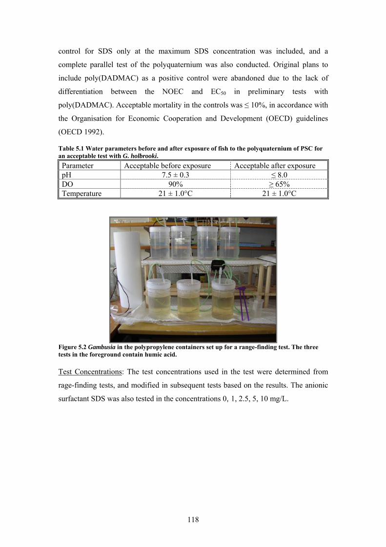
118

control for SDS only at the maximum SDS concentration was included, and a

complete parallel test of the polyquaternium was also conducted. Original plans to

include poly(DADMAC) as a positive control were abandoned due to the lack of

differentiation between the NOEC and EC50 in preliminary tests with

poly(DADMAC). Acceptable mortality in the controls was ≤ 10%, in accordance with

the Organisation for Economic Cooperation and Development (OECD) guidelines

(OECD 1992).

Table 5.1 Water parameters before and after exposure of fish to the polyquaternium of PSC for an acceptable test with G. holbrooki. Parameter Acceptable before exposure Acceptable after exposure pH 7.5 ± 0.3 ≤ 8.0 DO 90% ≥ 65% Temperature 21 ± 1.0°C 21 ± 1.0°C

Figure 5.2 Gambusia in the polypropylene containers set up for a range-finding test. The three tests in the foreground contain humic acid. Test Concentrations: The test concentrations used in the test were determined from

rage-finding tests, and modified in subsequent tests based on the results. The anionic

surfactant SDS was also tested in the concentrations 0, 1, 2.5, 5, 10 mg/L.

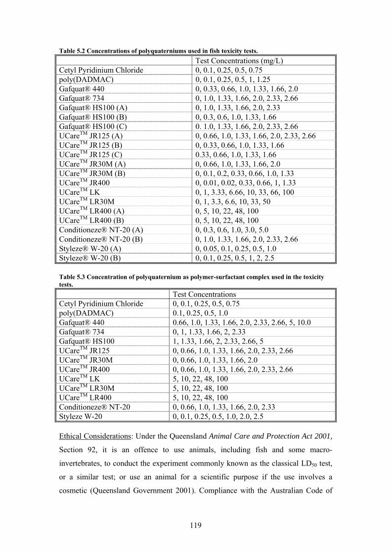
119

Table 5.2 Concentrations of polyquaterniums used in fish toxicity tests. Test Concentrations (mg/L) Cetyl Pyridinium Chloride 0, 0.1, 0.25, 0.5, 0.75 poly(DADMAC) 0, 0.1, 0.25, 0.5, 1, 1.25 Gafquat® 440 0, 0.33, 0.66, 1.0, 1.33, 1.66, 2.0 Gafquat® 734 0, 1.0, 1.33, 1.66, 2.0, 2.33, 2.66 Gafquat® HS100 (A) 0, 1.0, 1.33, 1.66, 2.0, 2.33 Gafquat® HS100 (B) 0, 0.3, 0.6, 1.0, 1.33, 1.66 Gafquat® HS100 (C) 0. 1.0, 1.33, 1.66, 2.0, 2.33, 2.66 UCareTM JR125 (A) 0, 0.66, 1.0, 1.33, 1.66, 2.0, 2.33, 2.66 UCareTM JR125 (B) 0, 0.33, 0.66, 1.0, 1.33, 1.66 UCareTM JR125 (C) 0.33, 0.66, 1.0, 1.33, 1.66 UCareTM JR30M (A) 0, 0.66, 1.0, 1.33, 1.66, 2.0 UCareTM JR30M (B) 0, 0.1, 0.2, 0.33, 0.66, 1.0, 1.33 UCareTM JR400 0, 0.01, 0.02, 0.33, 0.66, 1, 1.33 UCareTM LK 0, 1, 3.33, 6.66, 10, 33, 66, 100 UCareTM LR30M 0, 1, 3.3, 6.6, 10, 33, 50 UCareTM LR400 (A) 0, 5, 10, 22, 48, 100 UCareTM LR400 (B) 0, 5, 10, 22, 48, 100 Conditioneze® NT-20 (A) 0, 0.3, 0.6, 1.0, 3.0, 5.0 Conditioneze® NT-20 (B) 0, 1.0, 1.33, 1.66, 2.0, 2.33, 2.66 Styleze® W-20 (A) 0, 0.05, 0.1, 0.25, 0.5, 1.0 Styleze® W-20 (B) 0, 0.1, 0.25, 0.5, 1, 2, 2.5 Table 5.3 Concentration of polyquaternium as polymer-surfactant complex used in the toxicity tests. Test Concentrations Cetyl Pyridinium Chloride 0, 0.1, 0.25, 0.5, 0.75 poly(DADMAC) 0.1, 0.25, 0.5, 1.0 Gafquat® 440 0.66, 1.0, 1.33, 1.66, 2.0, 2.33, 2.66, 5, 10.0 Gafquat® 734 0, 1, 1.33, 1.66, 2, 2.33 Gafquat® HS100 1, 1.33, 1.66, 2, 2.33, 2.66, 5 UCareTM JR125 0, 0.66, 1.0, 1.33, 1.66, 2.0, 2.33, 2.66 UCareTM JR30M 0, 0.66, 1.0, 1.33, 1.66, 2.0 UCareTM JR400 0, 0.66, 1.0, 1.33, 1.66, 2.0, 2.33, 2.66 UCareTM LK 5, 10, 22, 48, 100 UCareTM LR30M 5, 10, 22, 48, 100 UCareTM LR400 5, 10, 22, 48, 100 Conditioneze® NT-20 0, 0.66, 1.0, 1.33, 1.66, 2.0, 2.33 Styleze W-20 0, 0.1, 0.25, 0.5, 1.0, 2.0, 2.5 Ethical Considerations: Under the Queensland Animal Care and Protection Act 2001,

Section 92, it is an offence to use animals, including fish and some macro-

invertebrates, to conduct the experiment commonly known as the classical LD50 test,

or a similar test; or use an animal for a scientific purpose if the use involves a

cosmetic (Queensland Government 2001). Compliance with the Australian Code of

120

Practice for the Care and Use of Animals for Scientific Purposes (NHMRC 2004) is

also required. The Code requires that death as an endpoint be avoided wherever

possible. To meet the requirements of the Griffith University Animal Ethics

Committee, changes to the standard OECD Test Guideline 203 Fish, Acute Toxicity

Test were made with respect to endpoint and ranging of the test (OECD 1992):

a) a non-lethal endpoint would be used;

b) only environmentally relevant concentrations would be tested.

As the mode of action of polyquaterniums was believed to result from the polymer

binding to the surface of the gill, leading to suffocation, and as Gambusia is able to

gulp air at the water surface in low oxygen situations, it was thought that this gulping

action would be an early indication of respiratory distress and therefore an appropriate

endpoint. Actual environmental concentrations were not known at the time ethics

approval was sought, therefore it was agreed that tests were to be conducted only in

the range that would result in a classification of Acute Toxicity under the Harmonised

Integrated Classification System For Human Health And Environmental Hazards Of

Chemical Substances And Mixtures i.e. up to, and not exceeding, 100 mg/L (OECD

2001).

5.2.4. Brine Shrimp Brine shrimp (Artemia sp.) were purchased from a local supplier < 1week post-

hatching. The shrimp were acclimatised in artificial seawater prepared with

Coralife™ scientific grade marine salt for 24 hours and fed once before testing. Tests

were static and conducted in 100 ml of the same artificial seawater, (salinity

18 ± 0.5 ppk, pH 8.3, temperature 22 ± 1°C) in 250 ml plastic specimen jars. Air was

supplied as a gentle stream to the surface of the container. A minimum of 7

concentrations and a clean water control were used for each test. For tests of the PSC,

additional controls containing only the polyquaternium were included. Two replicates

of 10 shrimp were used for each concentration. The test duration was 48 hours and the

shrimp were not fed during that time. The shrimp were checked every 24 hours for

motility and morbidity, and dead shrimp removed from the container. The number of

surviving shrimp was counted at the end of the test. For a valid test, losses of < 10%

in the controls and DO ≥ 60% were required (OECD 1992).

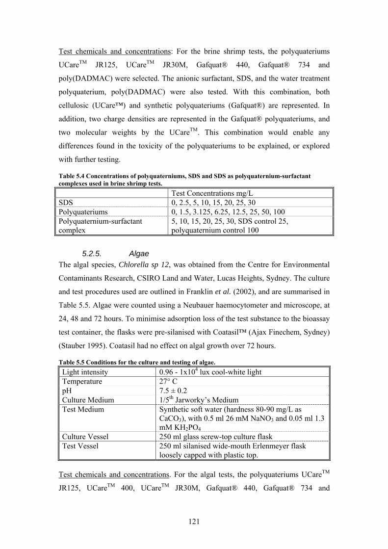
121

Test chemicals and concentrations: For the brine shrimp tests, the polyquateriums

UCareTM JR125, UCareTM JR30M, Gafquat® 440, Gafquat® 734 and

poly(DADMAC) were selected. The anionic surfactant, SDS, and the water treatment

polyquaterium, poly(DADMAC) were also tested. With this combination, both

cellulosic (UCare™) and synthetic polyquateriums (Gafquat®) are represented. In

addition, two charge densities are represented in the Gafquat® polyquateriums, and

two molecular weights by the UCareTM. This combination would enable any

differences found in the toxicity of the polyquateriums to be explained, or explored

with further testing.

Table 5.4 Concentrations of polyquaterniums, SDS and SDS as polyquaternium-surfactant complexes used in brine shrimp tests. Test Concentrations mg/L SDS 0, 2.5, 5, 10, 15, 20, 25, 30 Polyquateriums 0, 1.5, 3.125, 6.25, 12.5, 25, 50, 100 Polyquaternium-surfactant complex

5, 10, 15, 20, 25, 30, SDS control 25, polyquaternium control 100

5.2.5. Algae The algal species, Chlorella sp 12, was obtained from the Centre for Environmental

Contaminants Research, CSIRO Land and Water, Lucas Heights, Sydney. The culture

and test procedures used are outlined in Franklin et al. (2002), and are summarised in

Table 5.5. Algae were counted using a Neubauer haemocytometer and microscope, at

24, 48 and 72 hours. To minimise adsorption loss of the test substance to the bioassay

test container, the flasks were pre-silanised with Coatasil™ (Ajax Finechem, Sydney)

(Stauber 1995). Coatasil had no effect on algal growth over 72 hours.

Table 5.5 Conditions for the culture and testing of algae. Light intensity 0.96 - 1x104 lux cool-white light Temperature 27° C pH 7.5 ± 0.2 Culture Medium 1/5th Jarworky’s Medium Test Medium Synthetic soft water (hardness 80-90 mg/L as

CaCO3), with 0.5 ml 26 mM NaNO3 and 0.05 ml 1.3 mM KH2PO4

Culture Vessel 250 ml glass screw-top culture flask Test Vessel 250 ml silanised wide-mouth Erlenmeyer flask

loosely capped with plastic top. Test chemicals and concentrations. For the algal tests, the polyquateriums UCareTM

JR125, UCareTM 400, UCareTM JR30M, Gafquat® 440, Gafquat® 734 and

122

poly(DADMAC) were selected. The anionic surfactant, SDS, and the water treatment

polyquaterium, poly(DADMAC) were also tested. Again, this combination would

enable any differences found in the toxicity of the polyquateriums to be explained, or

explored with further testing. Only one test was performed with the polyquaternium-

surfactant complex, as the anionic surfactant damages the Coatasil™ surface on the

test containers. It was not possible to test the effect of humic acid on the toxicity of

the polyquaterniums to algae. Humic acid produces a coloured solution which would

interfere with the light, and consequently the growth rate of the algae. Further, the

humic acid would hinder the counting of the algae with a microscope.

Table 5.6 Test concentrations of chemicals used in algal toxicity tests Test Concentrations (mg/L) poly(DADMAC) 0, 0.005, 0.01, 0.04, 0.06, 0.1 UCareTM JR125 0, 0.005, 0.01, 0.05, 0.1, 0.175 UCareTM JR400 0.0, 0.005, 0.01, 0.1, 0.1, 0.2 UCareTM JR30M .000, 0.005, 0.010, 0.050, 0.100, ,175, 0.250 Gafquat® 440 0.000, 0.005, 0.010, 0.050, 0.100, ,175, 0.250Gafquat® 734 .000, 0.005, 0.010, 0.050, 0.100, ,175, 0.250 SDS 0, 0.0013, 0.975, 1.95 UCareTM JR125-SDS Complex 0, 0.01, 0.025, 0.05, 0.1, 1.0

5.3. Results, Observations and Data Analysis 5.3.1. Fish

The expected gulping of air by Gambusia at the surface of the water did not occur,

indicating either that morbidity did not result from suffocation or that this

compensatory mechanism was not invoked in this situation. Gulping is a response to

low oxygen levels in the environment, and has been reported as a response of

Gambusia to the blocking of the uptake of oxygen following exposure to the piscicide

rotenone (Nunes 2005). The signs observed in this work included lethargy (or

quiescence) – the fish ‘rested’ at the bottom of the container, sometimes with the tail

elevated; some bloating of the abdominal area, followed by loss of equilibrium (loe),

characterised by rolling and loss of control of mobility, and death. The lowest

observed effect level (LOEC) was defined as the lowest concentration at which these

symptoms occurred, and mortality greater than the mortality in the control. The

NOEC is thus the concentration immediately below that LOEC (if any). Any fish

displaying loe were removed from the container during inspection. Therefore the

EC50, where it was possible to establish, is defined as the EC50(loe).

123

Acute toxicity curves for Gambusia were very steep. Although the range of

concentrations was generally less than one order of magnitude (commonly 0.66 mg/L

to 2.66 mg/L), the LOEC concentration and the concentration at which ≥ 50%

mortality occurred were often consecutive test concentrations, and even in some

cases, the same concentration. This all-or-none type of lethal toxicity has also been

reported for the cationic surfactant didecyldimethylammonium chloride (DDAC)

(Juergensen et al. 2000), and for quaternary ammonium halides generally (Farrell et

al. 1998).

This steepness of the dose-response curve (Figure 5.3) presents some difficulties for

statistical analysis. The standard method of analysis for typical dose-response curves,

probit, ignores upper and lower concentrations where mortality is 0 or 100%, reducing

the degrees of freedom in the analysis. The data becomes too sparse to test for

goodness of fit, for example with Pearson’s test for chi squared distribution of

deviance (SAS 2002). Nevertheless, probit analysis does give an EC50 in the range

suggested by examination of the data, although fiducial limits (confidence intervals)

were not calculated for all tests. The toxicity (as EC50) of the cosmetic

polyquaterniums ranged from > 100 mg/L for the low charge density cellulosic

polyquaterniums UCareTM LR30M, LR400 and LK, to 0.5 mg/L for the high charge

density polyquaternium Styleze W-20. The latter was the only cosmetic

polyquaternium to have a toxicity approaching that of the water treatment

polyquaternium, pDADMAC and the quaternary surfactant cetyl pyridinium chloride.

For most of the cosmetic polyquaterniums tested, the EC50 was between 1.0 and

2.5 mg/L.

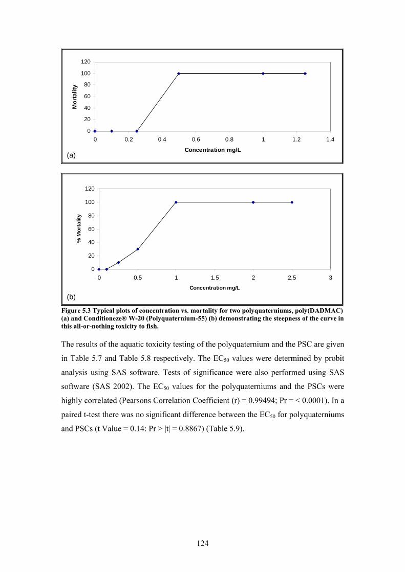
124

0

20

40

60

80

100

120

0 0.2 0.4 0.6 0.8 1 1.2 1.4

Concentration mg/L

Mor

talit

y

(a)

0

20

40

60

80

100

120

0 0.2 0.4 0.6 0.8 1 1.2 1.4

Concentration mg/L

Mor

talit

y

(a)

0

20

40

60

80

100

120

0 0.5 1 1.5 2 2.5 3

Concentration mg/L

% M

orta

lity

(b)

0

20

40

60

80

100

120

0 0.5 1 1.5 2 2.5 3

Concentration mg/L

% M

orta

lity

(b)

Figure 5.3 Typical plots of concentration vs. mortality for two polyquaterniums, poly(DADMAC) (a) and Conditioneze® W-20 (Polyquaternium-55) (b) demonstrating the steepness of the curve in this all-or-nothing toxicity to fish. The results of the aquatic toxicity testing of the polyquaternium and the PSC are given

in Table 5.7 and Table 5.8 respectively. The EC50 values were determined by probit

analysis using SAS software. Tests of significance were also performed using SAS

software (SAS 2002). The EC50 values for the polyquaterniums and the PSCs were

highly correlated (Pearsons Correlation Coefficient (r) = 0.99494; Pr = < 0.0001). In a

paired t-test there was no significant difference between the EC50 for polyquaterniums

and PSCs (t Value = 0.14: Pr > |t| = 0.8867) (Table 5.9).

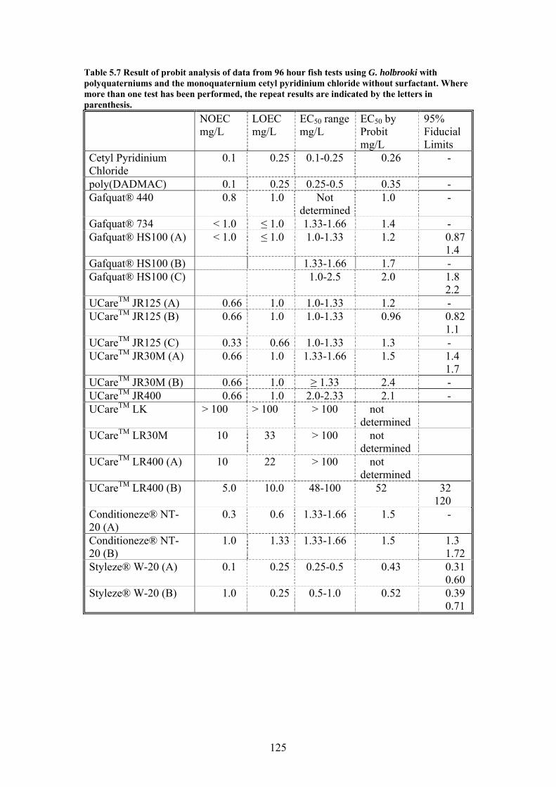
125

Table 5.7 Result of probit analysis of data from 96 hour fish tests using G. holbrooki with polyquaterniums and the monoquaternium cetyl pyridinium chloride without surfactant. Where more than one test has been performed, the repeat results are indicated by the letters in parenthesis. NOEC

mg/L LOEC mg/L

EC50 range mg/L

EC50 by Probit mg/L

95% Fiducial Limits

Cetyl Pyridinium Chloride

0.1 0.25 0.1-0.25 0.26 -

poly(DADMAC) 0.1 0.25 0.25-0.5 0.35 - Gafquat® 440 0.8 1.0 Not

determined1.0 -

Gafquat® 734 < 1.0 ≤ 1.0 1.33-1.66 1.4 - Gafquat® HS100 (A) < 1.0 ≤ 1.0 1.0-1.33 1.2 0.87

1.4 Gafquat® HS100 (B) 1.33-1.66 1.7 - Gafquat® HS100 (C) 1.0-2.5 2.0 1.8

2.2 UCareTM JR125 (A) 0.66 1.0 1.0-1.33 1.2 - UCareTM JR125 (B) 0.66 1.0 1.0-1.33 0.96 0.82

1.1 UCareTM JR125 (C) 0.33 0.66 1.0-1.33 1.3 - UCareTM JR30M (A) 0.66 1.0 1.33-1.66 1.5 1.4

1.7 UCareTM JR30M (B) 0.66 1.0 ≥ 1.33 2.4 - UCareTM JR400 0.66 1.0 2.0-2.33 2.1 - UCareTM LK > 100 > 100 > 100 not

determined

UCareTM LR30M 10 33 > 100 not determined

UCareTM LR400 (A) 10 22 > 100 not determined

UCareTM LR400 (B) 5.0 10.0 48-100 52 32 120

Conditioneze® NT-20 (A)

0.3 0.6 1.33-1.66 1.5 -

Conditioneze® NT-20 (B)

1.0 1.33 1.33-1.66 1.5 1.3 1.72

Styleze® W-20 (A) 0.1 0.25 0.25-0.5 0.43 0.31 0.60

Styleze® W-20 (B) 1.0 0.25 0.5-1.0 0.52 0.39 0.71

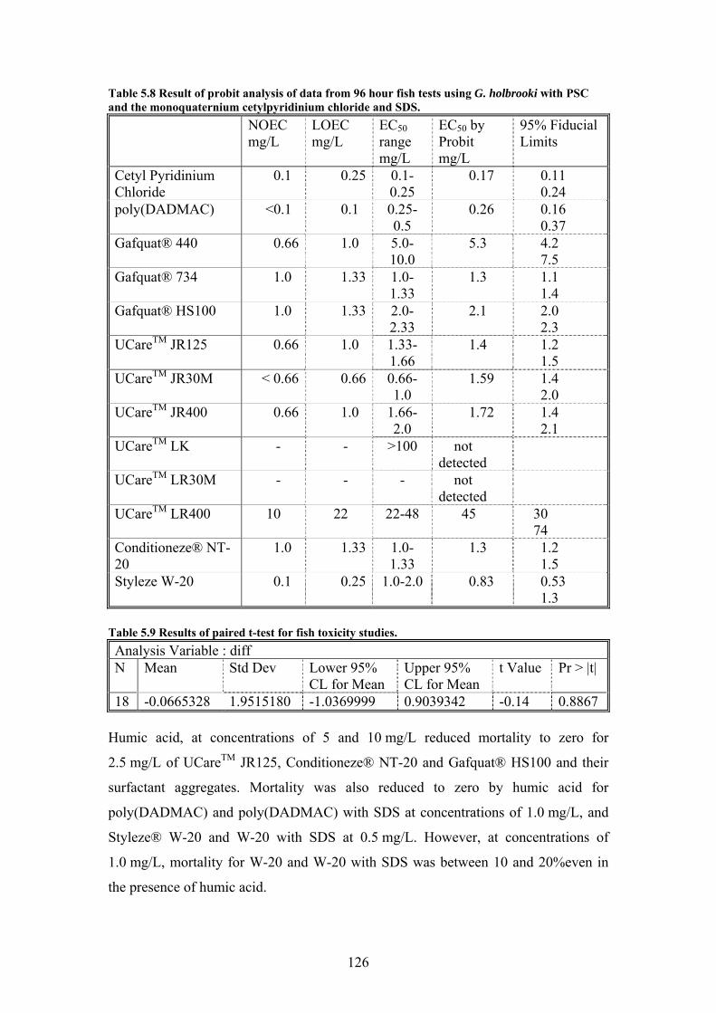
126

Table 5.8 Result of probit analysis of data from 96 hour fish tests using G. holbrooki with PSC and the monoquaternium cetylpyridinium chloride and SDS. NOEC

mg/L LOEC mg/L

EC50 range mg/L

EC50 by Probit mg/L

95% Fiducial Limits

Cetyl Pyridinium Chloride

0.1 0.25 0.1-0.25

0.17 0.11 0.24

poly(DADMAC) <0.1 0.1 0.25-0.5

0.26 0.16 0.37

Gafquat® 440 0.66 1.0 5.0-10.0

5.3 4.2 7.5

Gafquat® 734 1.0 1.33 1.0-1.33

1.3 1.1 1.4

Gafquat® HS100 1.0 1.33 2.0-2.33

2.1 2.0 2.3

UCareTM JR125 0.66 1.0 1.33-1.66

1.4 1.2 1.5

UCareTM JR30M < 0.66 0.66 0.66-1.0

1.59 1.4 2.0

UCareTM JR400 0.66 1.0 1.66-2.0

1.72 1.4 2.1

UCareTM LK - - >100 not detected

UCareTM LR30M - - - not detected

UCareTM LR400 10 22 22-48 45 30 74

Conditioneze® NT-20

1.0 1.33 1.0-1.33

1.3 1.2 1.5

Styleze W-20 0.1 0.25 1.0-2.0 0.83 0.53 1.3

Table 5.9 Results of paired t-test for fish toxicity studies. Analysis Variable : diff N Mean Std Dev Lower 95%

CL for Mean Upper 95% CL for Mean

t Value Pr > |t|

18 -0.0665328 1.9515180 -1.0369999 0.9039342 -0.14 0.8867 Humic acid, at concentrations of 5 and 10 mg/L reduced mortality to zero for

2.5 mg/L of UCareTM JR125, Conditioneze® NT-20 and Gafquat® HS100 and their

surfactant aggregates. Mortality was also reduced to zero by humic acid for

poly(DADMAC) and poly(DADMAC) with SDS at concentrations of 1.0 mg/L, and

Styleze® W-20 and W-20 with SDS at 0.5 mg/L. However, at concentrations of

1.0 mg/L, mortality for W-20 and W-20 with SDS was between 10 and 20%even in

the presence of humic acid.

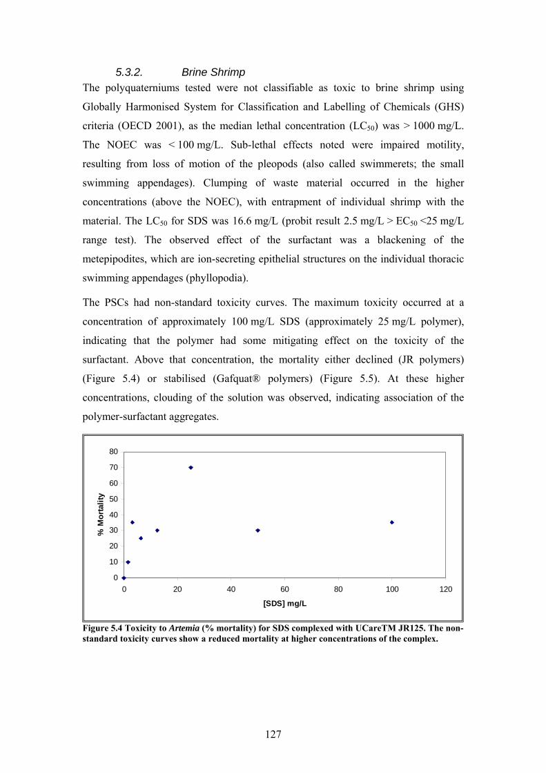
127

5.3.2. Brine Shrimp The polyquaterniums tested were not classifiable as toxic to brine shrimp using

Globally Harmonised System for Classification and Labelling of Chemicals (GHS)

criteria (OECD 2001), as the median lethal concentration (LC50) was > 1000 mg/L.

The NOEC was < 100 mg/L. Sub-lethal effects noted were impaired motility,

resulting from loss of motion of the pleopods (also called swimmerets; the small

swimming appendages). Clumping of waste material occurred in the higher

concentrations (above the NOEC), with entrapment of individual shrimp with the

material. The LC50 for SDS was 16.6 mg/L (probit result 2.5 mg/L > EC50 <25 mg/L

range test). The observed effect of the surfactant was a blackening of the

metepipodites, which are ion-secreting epithelial structures on the individual thoracic

swimming appendages (phyllopodia).

The PSCs had non-standard toxicity curves. The maximum toxicity occurred at a

concentration of approximately 100 mg/L SDS (approximately 25 mg/L polymer),

indicating that the polymer had some mitigating effect on the toxicity of the

surfactant. Above that concentration, the mortality either declined (JR polymers)

(Figure 5.4) or stabilised (Gafquat® polymers) (Figure 5.5). At these higher

concentrations, clouding of the solution was observed, indicating association of the

polymer-surfactant aggregates.

0

10

20

30

40

50

60

70

80

0 20 40 60 80 100 120

[SDS] mg/L

% M

orta

lity

Figure 5.4 Toxicity to Artemia (% mortality) for SDS complexed with UCareTM JR125. The non-standard toxicity curves show a reduced mortality at higher concentrations of the complex.

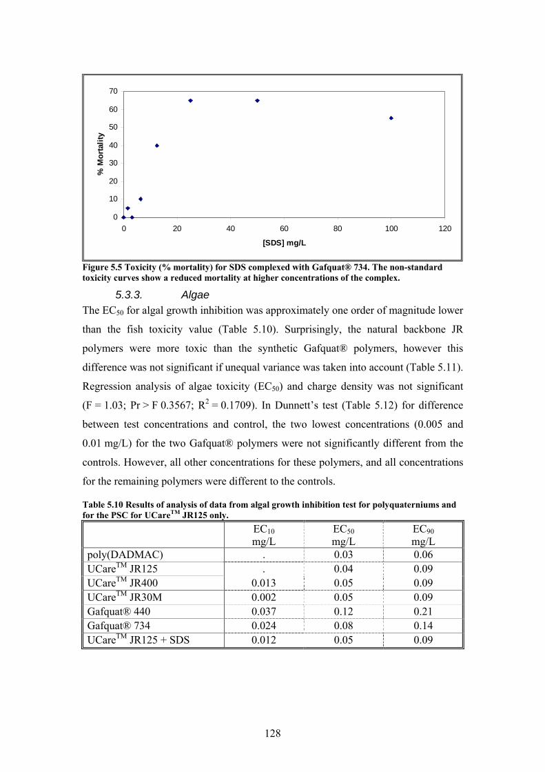
128

0

10

20

30

40

50

60

70

0 20 40 60 80 100 120

[SDS] mg/L

% M

orta

lity

Figure 5.5 Toxicity (% mortality) for SDS complexed with Gafquat® 734. The non-standard toxicity curves show a reduced mortality at higher concentrations of the complex.

5.3.3. Algae The EC50 for algal growth inhibition was approximately one order of magnitude lower

than the fish toxicity value (Table 5.10). Surprisingly, the natural backbone JR

polymers were more toxic than the synthetic Gafquat® polymers, however this

difference was not significant if unequal variance was taken into account (Table 5.11).

Regression analysis of algae toxicity (EC50) and charge density was not significant

(F = 1.03; Pr > F 0.3567; R2 = 0.1709). In Dunnett’s test (Table 5.12) for difference

between test concentrations and control, the two lowest concentrations (0.005 and

0.01 mg/L) for the two Gafquat® polymers were not significantly different from the

controls. However, all other concentrations for these polymers, and all concentrations

for the remaining polymers were different to the controls.

Table 5.10 Results of analysis of data from algal growth inhibition test for polyquaterniums and for the PSC for UCareTM JR125 only. EC10

mg/L EC50 mg/L

EC90 mg/L

poly(DADMAC) . 0.03 0.06 UCareTM JR125 . 0.04 0.09 UCareTM JR400 0.013 0.05 0.09 UCareTM JR30M 0.002 0.05 0.09 Gafquat® 440 0.037 0.12 0.21 Gafquat® 734 0.024 0.08 0.14 UCareTM JR125 + SDS 0.012 0.05 0.09

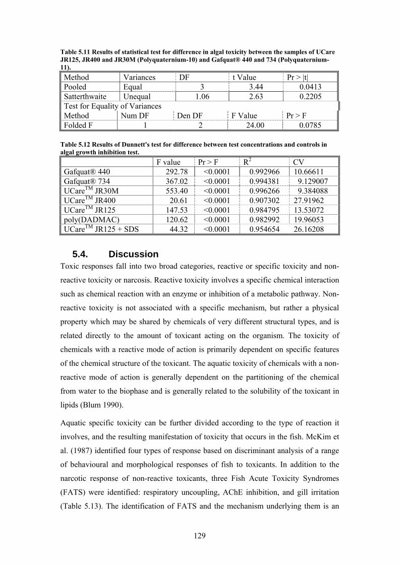
129

Table 5.11 Results of statistical test for difference in algal toxicity between the samples of UCare JR125, JR400 and JR30M (Polyquaternium-10) and Gafquat® 440 and 734 (Polyquaternium-11). Method Variances DF t Value Pr > |t| Pooled Equal 3 3.44 0.0413 Satterthwaite Unequal 1.06 2.63 0.2205 Test for Equality of Variances Method Num DF Den DF F Value Pr > F Folded F 1 2 24.00 0.0785

Table 5.12 Results of Dunnett's test for difference between test concentrations and controls in algal growth inhibition test. F value Pr > F R2 CV Gafquat® 440 292.78 <0.0001 0.992966 10.66611 Gafquat® 734 367.02 <0.0001 0.994381 9.129007 UCareTM JR30M 553.40 <0.0001 0.996266 9.384088 UCareTM JR400 20.61 <0.0001 0.907302 27.91962 UCareTM JR125 147.53 <0.0001 0.984795 13.53072 poly(DADMAC) 120.62 <0.0001 0.982992 19.96053 UCareTM JR125 + SDS 44.32 <0.0001 0.954654 26.16208

5.4. Discussion Toxic responses fall into two broad categories, reactive or specific toxicity and non-

reactive toxicity or narcosis. Reactive toxicity involves a specific chemical interaction

such as chemical reaction with an enzyme or inhibition of a metabolic pathway. Non-

reactive toxicity is not associated with a specific mechanism, but rather a physical

property which may be shared by chemicals of very different structural types, and is

related directly to the amount of toxicant acting on the organism. The toxicity of

chemicals with a reactive mode of action is primarily dependent on specific features

of the chemical structure of the toxicant. The aquatic toxicity of chemicals with a non-

reactive mode of action is generally dependent on the partitioning of the chemical

from water to the biophase and is generally related to the solubility of the toxicant in

lipids (Blum 1990).

Aquatic specific toxicity can be further divided according to the type of reaction it

involves, and the resulting manifestation of toxicity that occurs in the fish. McKim et

al. (1987) identified four types of response based on discriminant analysis of a range

of behavioural and morphological responses of fish to toxicants. In addition to the

narcotic response of non-reactive toxicants, three Fish Acute Toxicity Syndromes

(FATS) were identified: respiratory uncoupling, AChE inhibition, and gill irritation

(Table 5.13). The identification of FATS and the mechanism underlying them is an

130

important step in the development of Quantitative Structure-Activity Relationships

(QSAR) for predicting the toxicology of industrial chemicals. Although QSARs must

be developed for each mode of action, their development allows for rapid predictive

screening of hazardous chemicals for further study (McKim et al. 1987).

Table 5.13 Fish Acute Toxicity Syndromes (FATS) as described by McKim et al. (1987) Mode of Action

Respiratory-cardiovascular Response

Plasma ion regulation

Gill Damage Behavioural Observations

Narcosis Decline in pH, O2; haemocrit and haemoglobin increased (in response to hypoxia

No increase in concentrations of plasma ions

hypoactive, under-reactive to outside stimuli, respiration shallow and rapid, discolouration (dark, blackish)

Respiratory uncouplers

pH, haemocrit, haemoglobin and CO2 remained unchanged

[K+], [Ca2+], and [Mg2+] increased

No gill damage

hyperactive and over-reactive, most die without exhibiting numerous signs of stress

AChE inhibitors

Heart rate and O2 uptake is reduced

[Ca2+] and [Mg2+] increased significantly

No gill damage for 80% of survival time

generally hypoactive; over-reactive to stimuli; high incidence of abnormal swimming; deformities; numerous signs of stress

Gill irritants O2, CO2 and pH decreased; haemocrit increased steadily, haemoglobin remained constant

[Na+] and [Cl-] decreased

Histological damage to gill

initial increase in cough rate, moderate-to-low increase in ventilation rate

In the fish tests with both the polyquaternium and the PSC, no coughing was observed

to indicate mechanical clogging of the gill such as occurs with exposure to suspended

131

solids (Jobling 1995). No respiratory compensation such as gulping at the surface

occurred. This response has previously been reported for rotenone, which reportedly

acts by blockage of cellular oxygen uptake (McKim et al. 1987) in the study of the

toxicity of rotenone to Gambusia spp (Willis and Ling 2000). The reported response

to the rotenone exposure, however, included hyperactivity, stress and colour change

from silver to almost black. The hyperactivity exhibited in response to rotenone

suggests that this compound fits the category of respiratory uncoupler as described by

McKim et al. (1987), and the gulping action observed is a response to this

mechanism.

From the description of gill damage upon exposure to polyquaterniums (Boethling

and Nabholz 1997), the measurement of decreased blood pH (increase in [H+]), and

decreased concentrations of Na+ and Cl- (Muir et al. 1997), it would appear that

polyquaterniums, like many other ionic compounds, are gill irritants. Epithelial and

endothelial integument of the fish is tough and relatively impermeable, so that toxic

substances tend to be taken up by fish either by ingestion or through the gills

(Metcalfe 2000). The gill is the site of transport mechanisms that regulate osmotic and

ionic gradients, plasma pH and nitrogenous waste excretion, and so performs many of

the functions of the kidney in terrestrial animals (Evans et al. 2005). In addition to

entering the body via the gills, toxins can cause damage to the gill membrane itself

(Jobling 1995). Ions cannot diffuse through lipid membranes, and require active

transport via amino acids or protein ligands to penetrate membranes (Metcalfe 2000).

In conjunction with the findings of Muir et al. (1997) it appears the polyquaterniums

exert this toxic action without penetrating beyond the gill membrane. Other chemicals

known to be gill irritants include heavy metals, ozone (Wedemeyer et al. 1979),

acrolein and benzaldehyde (McKim et al. 1987).

All the reactive mechanisms described by McKim et al. (1987) cause alterations to

blood osmolity, but only gill irritation syndrome also results in a decline in blood pH.

That the observed decrease in sodium concentration occurs with increased

concentrations of H+ (decreasing pH) is probably the result of the coupling of Na+

uptake with proton efflux via V-H+-ATPase in the fish brachial epithelium (McKim et

al. 1987). In freshwater teleosts, V-H+-ATPase is located in respiratory pavement

cells of the brachial epithelium (Clairborne et al. 2002), and has also been described

132

for tight epithelia such as frog skin and distal portions of mammalian nephron tissue

(McKim et al. 1987).

The symptoms displayed by Gambusia in tests with polyquaterniums in this study

included lethargy with an onset of < 24 hours, followed by loss of equilibrium and

death, usually between 48 and 72 hours. It is likely, therefore, that the cause of death

was not suffocation, but acidosis resulting from the disruption of sodium uptake, and

consequently, acid-base regulation mechanisms.

The brine shrimp, in contrast to the fish, exhibited a toxic response to the anionic

surfactant SDS rather than to the polyquaterniums. The visible effect was the

discolouration (blackening) of the metepipodites, similar to the staining effect

reported by Holliday et al. (1990) following exposure to silver nitrate. However, as

the observed effect in this study followed exposure to the anionic surfactant SDS, it is

unlikely that the discolouration is associated with sites of chloride efflux as suggested

for silver nitrate staining. The metepipodites function like the gill in marine teleosts,

and have high levels of Na+/K+-ATPase indicating a role in osmoregulation (Holliday

et al. 1990). Although the similarity in function could suggest that marine teleosts

may also be less sensitive than fresh water teleosts, no difference in the sensitivity of

fresh and marine invertebrates and fish was found in a study of the cationic surfactant

ditallowdimethylammonium chloride (Lewis and Wee 1983). In published data by

Beim and Beim. (1994), fresh water shrimp were consistently less sensitive to cationic

polyelectrolytes than fish (or daphnids), with EC50 values of 70, 650 and 1160 mg/L

to three cationic flocculants (Appendix 2). However, shrimp were as sensitive or more

sensitive than fish to one of two cationic polyelectrolytes (Superfloc 330) in Biesinger

et al. (1976), and one of 12 cationic polyelectrolytes in Biesinger and Stokes (1986).

The difference in sensitivity between shrimp and fish to cationic polyelectrolytes

would therefore appear to be the result of differences in structure of the fish gill and

the metepipodite.

Toxicity of the polyquaterniums to algae follows the same steep dose-response curve

as observed for fish, suggesting again that a reactive mechanism of toxicity is

involved. Surfactants are known to bind and denature proteins on the cell wall of

algae, altering the permeability of the membrane to nutrients and chemicals (Pelczar

et al. 1993). Algal cell walls differ in thickness and chemical composition, which can

influence the severity of the toxic response to surface active agents (Lewis 1990).

133

This difference may account for exceptions reported by Boethling and Nabholz (1997)

to the general trend of cationic polyelectrolytes being six times more toxic to algae

than fish. In this study, algal EC50 values were between 2.5 and 11% of the fish EC50,

suggesting that in the case of these two species, Chlorella and Gambusia,

polyquaterniums are approximately an order of magnitude more toxic to the algae

than the fish.

5.4.1. Charge Density The results for fish toxicity give no support to the relationship between charge density

and EC50. Of the polyelectrolytes in this study, only poly(DADMAC) has a charge

density high enough to suggest that it may be asymptotic according to the criteria of

Boethling and Nabholz (1997). Overall, the correlation between fish toxicity and

charge density in the data is not significant (r = -37441, p = 0.2566). The model for

fish toxicity proposed by Boethling and Nabholz (1997) (Equation 5.1 and Equation

5.2) is not particularly successful at predicating the toxicity of the polyelectrolytes in

this study, and especially not for the polyelectrolytes with charge density in the higher

or lower ranges of % a-N. For example, the toxicity of polyelectrolytes UCareTM LK,

LR400 and LR30M is significantly overestimated, while the toxicity of Styleze® W-

20 is underestimated.

Log[fish 96-hour LC50] = 1.209-0.462*% a-N Equation 5.1

for % a-N ≤ 3.5 Fish 96-hour LC50 = 0.28 mg/L Equation 5.2

for %a-N > 3.5 The UCareTM LR/LK polyelectrolytes have both low charge density and low toxicity.

These are cellulosic polyelectrolytes (natural backbone). Their low toxicity accords

with the results for Gendriv 162 (cationic guar gum) in Biesinger et al. (1976), and

with the low toxicity of the low charge density cellulosic polyelectrolytes in the

Office of Pollution Prevention and Toxics (OPPT) data (Boethling and Nabholz 1997)

discussed in Section 2.5.4. Clearly, charge density does not appear to be the

controlling factor here, as UCareTM LR30M and LR400 have similar charge density to

Gafquat® HS100 and 440. Nor does it appear to simply be the result of the cellulosic

backbone, as the higher charge density UCareTM JR polyelectrolytes have similar

toxicity to the synthetic carbon polyelectrolytes with similar charge density. It would

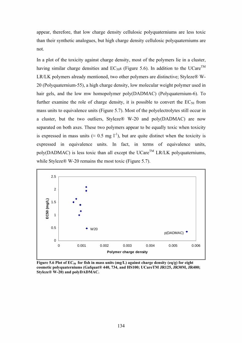
134

appear, therefore, that low charge density cellulosic polyquaterniums are less toxic

than their synthetic analogues, but high charge density cellulosic polyquaterniums are

not.

In a plot of the toxicity against charge density, most of the polymers lie in a cluster,

having similar charge densities and EC50s (Figure 5.6). In addition to the UCareTM

LR/LK polymers already mentioned, two other polymers are distinctive; Styleze® W-

20 (Polyquaternium-55), a high charge density, low molecular weight polymer used in

hair gels, and the low mw homopolymer poly(DADMAC) (Polyquaternium-6). To

further examine the role of charge density, it is possible to convert the EC50 from

mass units to equivalence units (Figure 5.7). Most of the polyelectrolytes still occur in

a cluster, but the two outliers, Styleze® W-20 and poly(DADMAC) are now

separated on both axes. These two polymers appear to be equally toxic when toxicity

is expressed in mass units (≈ 0.5 mg l-1), but are quite distinct when the toxicity is

expressed in equivalence units. In fact, in terms of equivalence units,

poly(DADMAC) is less toxic than all except the UCareTM LR/LK polyquaterniums,

while Styleze® W-20 remains the most toxic (Figure 5.7).

0

0.5

1

1.5

2

2.5

0 0.001 0.002 0.003 0.004 0.005 0.006

Polymer charge density

EC

50 (m

g/L)

p(DADMAC)W20

Figure 5.6 Plot of EC50 for fish in mass units (mg/L) against charge density (eq/g) for eight cosmetic polyquaterniums (Gafquat® 440, 734, and HS100; UCareTM JR125, JR30M, JR400; Styleze® W-20) and polyDADMAC.

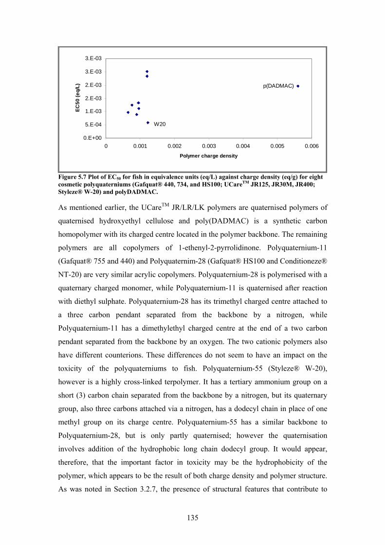
135

0.E+00

5.E-04

1.E-03

2.E-03

2.E-03

3.E-03

3.E-03

0 0.001 0.002 0.003 0.004 0.005 0.006

Polymer charge density

EC50

(eq/

L) p(DADMAC)

W20

Figure 5.7 Plot of EC50 for fish in equivalence units (eq/L) against charge density (eq/g) for eight cosmetic polyquaterniums (Gafquat® 440, 734, and HS100; UCareTM JR125, JR30M, JR400; Styleze® W-20) and polyDADMAC. As mentioned earlier, the UCareTM JR/LR/LK polymers are quaternised polymers of

quaternised hydroxyethyl cellulose and poly(DADMAC) is a synthetic carbon

homopolymer with its charged centre located in the polymer backbone. The remaining

polymers are all copolymers of 1-ethenyl-2-pyrrolidinone. Polyquaternium-11

(Gafquat® 755 and 440) and Polyquaternim-28 (Gafquat® HS100 and Conditioneze®

NT-20) are very similar acrylic copolymers. Polyquaternium-28 is polymerised with a

quaternary charged monomer, while Polyquaternium-11 is quaternised after reaction

with diethyl sulphate. Polyquaternium-28 has its trimethyl charged centre attached to

a three carbon pendant separated from the backbone by a nitrogen, while

Polyquaternium-11 has a dimethylethyl charged centre at the end of a two carbon

pendant separated from the backbone by an oxygen. The two cationic polymers also

have different counterions. These differences do not seem to have an impact on the

toxicity of the polyquaterniums to fish. Polyquaternium-55 (Styleze® W-20),

however is a highly cross-linked terpolymer. It has a tertiary ammonium group on a

short (3) carbon chain separated from the backbone by a nitrogen, but its quaternary

group, also three carbons attached via a nitrogen, has a dodecyl chain in place of one

methyl group on its charge centre. Polyquaternium-55 has a similar backbone to

Polyquaternium-28, but is only partly quaternised; however the quaternisation

involves addition of the hydrophobic long chain dodecyl group. It would appear,

therefore, that the important factor in toxicity may be the hydrophobicity of the

polymer, which appears to be the result of both charge density and polymer structure.

As was noted in Section 3.2.7, the presence of structural features that contribute to

136

hydrophobicity can result in deviations from 1:1 stoichiometry in metachromatic

polyelectrolyte titration, however, it is not clear that a similar mechanism is operating

in the toxic action.

5.4.2. Polymer-surfactant Complex The low rates of deposition of the polyquaterniums on hair in the presence of SDS

reported by Andre et al. (1999) suggests that the aquatic toxicity of the PSC might be

lower than the toxicity of the polyquaternium alone, as mechanism of toxicity is

thought to be binding to the surface of the fish gill (Biesinger et al. 1976). This is

because binding to hair and sorption to gill surfaces are believed to be the result of the

same mechanism, i.e. coulombic binding with anionic sites on the surface of the gill

cells or hair. In addition, it has been suggested that the PSC formed at 1:1

stoichiometry is not as soluble as the polyquaternium alone, or aggregates formed at

other stoichiometries.

Phase diagrams produced by Goddard et al. (1975) suggest a precipitation zone at 1:1

stoichiometry, with areas of cloudiness, slight precipitation or turbidity. Clear zones

occur with either large excess of polyquaternium, or large excess of surfactant. At the

point of phase separation, it has been reported that the surface tension of the solution,

which begins to lower above the CAC of the polymer-surfactant system, continues to

drop, and does not level out until the critical micelle concentration (CMC) of the

surfactant is reached. This accords with the description by Koetz et al. (1996) that a

system in which two ions are of vastly different molecular weights will tend to form

films rather than flocs. The PSC being formed in these systems is surface active and

accumulates at surfaces, continuing to do so until the surfactant in solution begins to

form micelles in the bulk phase.

There was no clouding observed in the solution at the effective concentrations in any

of the fish or algae tests in this investigation. The solution concentration for SDS was

in the range 5 x 10-7 to 1.5 x 10-6 M which was well below the CMC of 8 x 10-3 M,

and possibly below the CAC, expected to be 2-3 orders of magnitude lower than the

CMC. Further, the effective polyquaternium concentration employed here in this work

is 2-3 orders of magnitude below the concentration at which many studies of PSC

behaviour are studied, generally 0.01 to 0.1%. According to Manuszak-Guerrini et al.

(1997), at concentrations less than 0.01%, a fixed concentration of SDS is required to

137

precipitate the complexes. Thus at the effective concentration, below 0.01%

polyquaternium, the neutral PSC may not precipitate.

The results of this work suggest that at the low concentrations which may be found in

the environment, the PSC could remain in solution long enough to effect the toxic

action and no mitigation of the toxicity of the polyquaternium resulting from

precipitation following association with an anionic surfactant such as SDS can be

expected. The toxicity of the monoquaternary surfactant cetylpyridinium chloride was

also unaffected by the presence of SDS at a 1:1 ratio. For the singly charged species,

formation of an ion pair would be expected to decrease the solution activity of the

cationic surfactant, which could be a factor in mitigating toxicity. The lack of effect

on the monoquaternary surfactant indicates that the reduction in solution activity at a

1:1 ratio and environmentally relevant concentrations of the cationic test substances

does not mitigate toxicity, and reduced toxicity may not be expected unless the

anionic surfactant concentration is sufficiently high to lead to precipitation of the

PSC.

5.4.3. Humic Acid The mitigating effect of humic acid on the toxicity of polyquaterniums to fish has

been demonstrated to occur even in the presence of the anionic surfactant SDS. The

full extent of the mitigation was not measured in this work because of ethical

considerations mentioned previously. Qualitatively however, the mitigation is as

expected based on published studies. The extent of the mitigating effect has been

shown to be between one and two orders of magnitude at 10 mg/L humic acid, (Cary

et al. 1987; Goodrich et al. 1991; Hall and Mirenda 1991), and between two and three

orders of magnitude at 50-60 mg/L humic acid (Goodrich et al. 1991; Hall and

Mirenda 1991).

It has been recommended by Nabholz et al. (1993), for regulatory testing, that fish

toxicity tests of cation polyelectrolytes be separately conducted in clean dilution water

with total organic carbon (TOC) < 2 mg/L, and also with 10 and 20 mg/L humic acid.

The toxicity of the polyelectrolyte in the presence of 10 mg/L TOC can then be

determined from regression of the three toxicity values against TOC level. A

‘mitigating factor’ can then be determined by dividing the LC50 in 10 mg/L by the

LC50 in clean water. According to Nabholz et al. (1993), the mitigating factor for

cationic surfactants is expected to be less than 20. Based on an unpublished study of

138

eight polymers, Nabholz et al. (1993) suggested that the reduction in toxicity is about

94 times for high charge density cationic polyelectrolytes (3.3% a-N) in 10 mg/L

TOC equivalent to 27.6 mg/L humic acid, sodium salt (Aldrich).

The need to determine the mitigating effect in terms of TOC rather than humic acid

concentration is apparent due to differences in the TOC content of the humic acids

used in the published studies. The TOC content of humic acid used by Nabholz et al.

(1993) is approximately 37%, whereas Hall and Mirenda (1991) reported a TOC

content of approximately 16%. Neither Cary et al. (1987; 1989) nor Goodrich et al.

(1991) state the TOC content of the humic acid used in their mitigation studies. It has

been suggested that the use of Aldrich humic acid may result in an overestimation of

the effect of dissolved organic matter, as humic substances account for only 50 to

75% of dissolved organic carbon (Haitzer et al. 1998).

The difference in the binding capacity of humic acids of different sources is relevant

because of the assumption that the mitigating effect of humic acid is due to

preferential binding of cationic polyelectrolytes to dissolved organics resulting in

decreased availability of the polyelectrolyte to aquatic organisms (Goodrich et al.

1991). However, Matthews et al. (1995) has suggested that the amount expected to be

bound to humic acid or dissolved humic material may not be enough to explain the

reduction in toxicity. Humic acid has surfactant properties and can affect

physiological responses in living cells. By increasing the permeability of the

membrane in microorganisms, humic acid can result in an increase in

bioconcentration of some organic chemicals (Visser 1985). The mitigating effect of

humic acid on the toxicity of cationic surfactants has been shown to be dependent of

the chain length of the surfactant. According to Versteeg and Shorter, (1992) humic

acid did not affect the toxicity of quaternary ammonium surfactants to fish if the alkyl

chain length of the surfactant was 14 carbons or shorter, suggesting that the

interaction between the cation and humic acid was hydrophobic rather than

coulombic.

The results of this work show that the presence of dissolved organic material such as

humic acid can lead to a reduction in the toxicity of polyquaterniums and other cation

polyelectrolytes and surfactants, and this needs to be considered in the risk assessment

process. However, the determination of mitigation factor for individual polymers and

surfactants based on toxicity levels at various concentrations of humic acid requires a

139

level of testing which is difficult to justify on ethical grounds (let alone economic

ones). As the reduction in toxicity as reported by Hall and Mirenda (1991) and Cary et

al. (1987) seems to be reasonably consistent at between one and two orders of

magnitude regardless of the source of humic material, it may be appropriate to take

this into account when determining the assessment factors used in determining the

PEC, however, the presence of such concentrations of humic acid in natural water

cannot always be assumed, and therefore the use of a mitigation factor may not be

justifiable on environmental grounds.

5.5. PNEC The lowest toxicity values in this study were the EC50 for algal growth inhibition, in

the order of 0.03 to 0.12 mg/L for the polyquaterniums tested. This accords with the

statement by Nabholz et al. (1993) that algae are the most sensitive species to cationic

polyelectrolytes. Although the algal test is technically a chronic test, covering several

generations, it is regarded as an acute test for the purposes of risk assessment (ECB

2003).

A number of uncertainties exist in extrapolating from laboratory toxicity data to

natural ecosystems, and these have been summarised as

a) intra- and inter-laboratory variation of toxicity data;

b) intra- and inter-species variations (biological variance);

c) short-term to long-term toxicity extrapolation;

d) laboratory data to field impact extrapolation (additive, synergistic and

antagonistic effects from the presence of other substances may also play a role

here).

The assessment factors recommended depend on the confidence with which the PNEC

can be derived, and are outlined in Table 5.14. When only short-term data are

available, as in this study, an assessment factor of 1000 will be applied to the lowest

L(E)C50. While the algal growth inhibition test is a multigenerational test, it is treated

as a short-term toxicity value for the purposes of determining appropriate assessment

factors (ECB 2003). Accordingly, the assessment factor to be applied in the

calculation of the PNEC for the polyquaterniums based on this study is 1000.

Applying the assessment factor to the algal EC50, therefore, gives a PNEC of between

0.03 and 0.12 µg/L.

140

Table 5.14 Recommended assessment factors to be applied in determining the PNEC are dependent on the confidence that can be attributed to the available data, which is dependent on the amount and types of toxicity data available. Dataset Assessment Factor At least one acute L(E)C50 from each of the three trophic levels (fish, invertebrates and aquatic plants)

1000x

One chronic NOEC (either fish or invertebrates)

100x

Chronic NOECs from species representing different trophic levels (fish, invertebrates and/or aquatic plants)

50x

Chronic NOECs from at least three species (normally fish, invertebrates and algae) representing three trophic levels

10x

Species sensitivity distribution (SSD) method

5-1 (to be justified case by case)

Field data or model ecosystem review on a case by case basis The mitigating effect of humic acid is generally not taken into account in the

determination of the PNEC. In determining the fate of polyquaterniums, it has been

assumed that the PEC will be fully mitigated by sorption to solids as, for example, in

the assessment of Merquat 2001 (NICNAS 2002a) which states

‘However, receiving waters usually contain suspended colloidal matter of

both mineral and organic origin (for example, humic material), and the

interaction of cationic polymers with this material has been demonstrated

to dramatically reduce the toxicity of the polymers. In addition, most of

the polymer will become associated with sewage sludge during passage

through the sewer mains and the sewage treatment plants and will not be

released to receiving waters.’

However, weight of evidence from published data gives reasonable certainty to a

reduction of one order of magnitude, at environmental concentrations of DOM, at

least in the case of fish. For this reason it may be possible to argue that this should be

taken into account in determining the assessment factors to be applied in determining

the PNEC. Such a strategy would reduce the assessment factors being applied in this

case to 100, and give a PNEC between 0.3 and 1.2 µg/L.

This strategy may be appropriate when the hazard of a group or class of cationic

polyelectrolytes is being considered, as in a Priority Existing Chemical assessment.

However, for the assessment of new cationic polymers, the extrapolation of possible

141

additive effects presents an additional factor that is not generally taken into account,

and the assessment factors based on the available data, without consideration of humic

acid effects, should probably be applied.

5.6. Conclusions The polyquaterniums in this study were toxic to fish and algae. The lowest EC50, for

algae is ≤ 1 mg/L, therefore classification of Acute I under GHS is generally required

for many of these polymers. Establishing toxicity for polymers is made difficult by

the variation that can occur in the structure of the polymer, without changing the

identity of the polymer, as noted in Section 2.5.3. This has been demonstrated here in

the range of EC50 (fish) values for Polyquaternium-10, from 1.2 mg/L for UCareTM

JR125 to > 100 mg/L for UCareTM LK. There was no difference between the toxicity

to fish of a polyquaternium and the corresponding PSC.

The mechanism of toxicity of the polyquaterniums to fish would appear to be

disruption of osmoregulation following binding of the polyquaternium to the gill

surface. Knowledge of the toxic mechanism may be as important as the chemical

structure/behaviour in determining toxic responses, and further knowledge of the

interaction between the polyquaternium and the gill surface may be required before

QSARs can be developed. Further, an understanding of the different interactions that

occur with fresh and marine species may be useful in predicting toxicity in marine

environments.

The characteristic of polyquaterniums which has the most influence on the toxicity of

the chemical would appear to be hydrophobicity. Hydrophobicity is a function of both

the charge density and structural features of the polyquaternium such as chain length.

Greater understanding of the structural elements that contribute to hydrophobicity,

and the role of hydrophobicity in toxicity, may help to clarify some of the apparent

inconsistencies in the published toxicity data on cationic polyelectrolytes, as well as

assist in the development of QSARs.

The PNECs for the cosmetic polyquaterniums examined in this study are in the range

between 0.03 and 0.12 µg/L in the absence of humic acid.

142

6. Risk Characterisation 6.1. Introduction

The risk characterisation process combines the information obtained from the effects

and exposure assessments to evaluate the nature of the potential risk (Molak 1997). It

is the final process of the four-step paradigm as originally described in ‘Risk

Assessment in the Federal Government: Managing the Process’ (NRC 1983),

commonly referred to as ‘the red book’ and further developed in ‘Science and

Judgement in Risk Assessment’ (NRC 1994) (known as ‘the blue book’) as methods

for determining health risks to human populations, and later adapted for ecological

risk assessment. The development of the process of risk characterisation is reflected in

the changing definition of risk characterisation since the original publication of the

red book (Table 6.1).

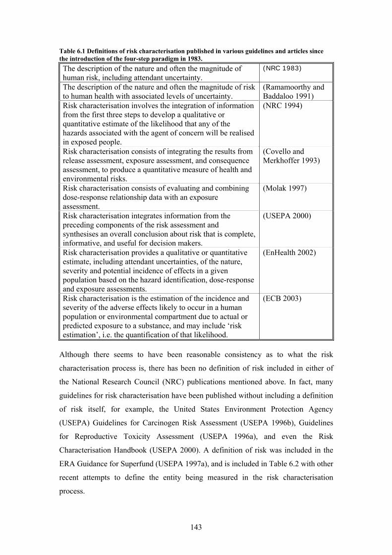
143

Table 6.1 Definitions of risk characterisation published in various guidelines and articles since the introduction of the four-step paradigm in 1983. The description of the nature and often the magnitude of human risk, including attendant uncertainty.

(NRC 1983)

The description of the nature and often the magnitude of risk to human health with associated levels of uncertainty.

(Ramamoorthy and Baddaloo 1991)

Risk characterisation involves the integration of information from the first three steps to develop a qualitative or quantitative estimate of the likelihood that any of the hazards associated with the agent of concern will be realised in exposed people.

(NRC 1994)

Risk characterisation consists of integrating the results from release assessment, exposure assessment, and consequence assessment, to produce a quantitative measure of health and environmental risks.

(Covello and Merkhoffer 1993)

Risk characterisation consists of evaluating and combining dose-response relationship data with an exposure assessment.

(Molak 1997)

Risk characterisation integrates information from the preceding components of the risk assessment and synthesises an overall conclusion about risk that is complete, informative, and useful for decision makers.

(USEPA 2000)

Risk characterisation provides a qualitative or quantitative estimate, including attendant uncertainties, of the nature, severity and potential incidence of effects in a given population based on the hazard identification, dose-response and exposure assessments.

(EnHealth 2002)

Risk characterisation is the estimation of the incidence and severity of the adverse effects likely to occur in a human population or environmental compartment due to actual or predicted exposure to a substance, and may include ‘risk estimation’, i.e. the quantification of that likelihood.

(ECB 2003)

Although there seems to have been reasonable consistency as to what the risk

characterisation process is, there has been no definition of risk included in either of

the National Research Council (NRC) publications mentioned above. In fact, many

guidelines for risk characterisation have been published without including a definition

of risk itself, for example, the United States Environment Protection Agency

(USEPA) Guidelines for Carcinogen Risk Assessment (USEPA 1996b), Guidelines

for Reproductive Toxicity Assessment (USEPA 1996a), and even the Risk

Characterisation Handbook (USEPA 2000). A definition of risk was included in the

ERA Guidance for Superfund (USEPA 1997a), and is included in Table 6.2 with other

recent attempts to define the entity being measured in the risk characterisation

process.

144

Table 6.2 Definitions of risk published in various guidelines and articles since the introduction of the four-step paradigm in 1983. The probability that, in a certain timeframe, and adverse outcome will occur in a person, group of people, plants, animals and/or the ecology of a specified area that is exposed to a particular dose or concentration of a hazardous agent, i.e. it depends on both the level of toxicity of the agent and the level of exposure.

(EnHealth 2002)

Actual risk is the probability or chance of an occurrence of adverse outcomes (sickness or death) to human health or environmental functioning at some frequency and some level of intensity. Perceived Risk is a risk as defined by its importance and significance to individuals, community and society.

(Frantzen and Ackerman 2002)

A measure of the probability of the introduction of an exotic disease and the seriousness of such an outcome in the context of the importance of animal or animal products.

(Molak 1997)

The expected frequency or probability of undesirable effects resulting from exposure to known or expected stressors.

(Molak 1997)

A characteristic of a situation or action wherein two or more outcomes are possible, the particular outcome that will occur is unknown, and at least one of the possibilities is undesired.

(USEPA 1997a)

The probability that a hazard (H) will have the unwanted effect (E) on a vulnerable object (V) under certain given conditions (C), which can be expressed as R(hvec)

Malmfors, 2002 #61

The lack of clarity in the definition of risk is evident in the various meanings that are

assigned to the word risk in the scientific literature, for example: Risk = hazard;

Risk = likelihood, probability; Risk = damage, loss, consequence; Risk = relative

frequency (Malmfors and Rosing 2002). According to Malmfors and Rosing (2002),

this can lead to ambiguity in the outcome of the risk assessment, and difficulties in

interpretation and communication of the risk.

In addition to the problems of defining and identifying risk, measuring risk also

presents difficulties. Generally, it is considered that risk can be characterised

quantitatively (as a number) or qualitatively (in categories, e.g. high, medium, low).

In situations where no toxicological and exposure data are available, only qualitative

estimates of risk are possible. This occurs frequently in Australia in new chemical risk

assessment, where some chemical classes, or chemicals imported at low volumes, are

exempt from providing toxicological data (NICNAS 2004b). An example of this type

of qualitative estimation of risk is the Full Public Report (FPR) for Gafquat® HS-100

(NICNAS 1999).

145

One of the most common methods of risk characterisation is the quotient method, the

ratio between predicted no effect concentration (PNEC) and predicted environmental

concentration (PEC). Often considered a numerical method, descriptions of this

method are given in many risk assessment handbooks. The process of calculating the

quotient is intended to be iterative, with ambiguous results resulting from a quotient

≈ 1 necessitating further investigation of either the toxicology or environmental fate in

order to arrive at a more definitive result. An alternative method, developed to meet

the demand for rapid assessment required for the European Chemicals Bureau (ECB)

review of industrial chemicals, Registration, Evaluation and Authorisation of

Chemicals (REACH) involves a screening process based on an Environmental

Threshold of No Concern (ETNC). The ETNC is a level of environmental exposure to

chemicals below which no significant risk is expected to exist, and may be determined

for chemicals or classes of chemicals (de Wolf et al. 2005). Both these methods

provide a point estimate of risk. A third method, Probabilistic Risk Assessment

(PRA), uses statistical methods to describe the uncertainty in the risk estimate. Using

techniques such as Monte Carlo Simulation, the likelihood of each risk is

quantitatively characterised in the risk estimate (USEPA 2004).

In this chapter, three methods, ETNC, PNEC/PEC ratio, and a probabilistic version of

the PNEC/PEC ratio using Monte Carlo Simulation will be applied to the risk

characterisation of cosmetic polyquaterniums in Australia. Further, the risk

characterisation methods will be reviewed to assist in determining the usefulness,

advantages and shortcomings of the process with respect to the regulatory risk

assessment of new and existing chemicals.

6.1.1. Monte Carlo Simulation Monte Carlo Simulation is a technique for characterising the uncertainty and

variability in risk estimates by repeatedly sampling the probability distributions of the

risk equation inputs and using these inputs to calculate a range of risk values (USEPA

2001). This technique will be used in this thesis to examine the probabilities and

uncertainties in the model presented in Section 6.2, and the risk characterisation in

Section 6.4. In Monte Carlo Simulation, the same calculations used in a point estimate

model are performed many times, with the input variables resampled for each

calculation from a probability distribution selected for each variable. The probability

distribution, or probability density function (pdf) of each variable can either be

146

determined directly from the data if sufficient data points are available, from

statistical parameters such as mean and standard deviation if they are known, or

estimated from the most likely value of the variable, the Central Tendency Estimates

(CTE) and a reasonable worst case or conservative estimate, the Reasonable

Maximum Estimate (RME). The RME is the value most often used in estimates. The

result of the Monte Carlo Simulation is a probability distribution for the output

variable (the forecast). Monte Carlo Simulation thus gives a range of output values,

with their associated probabilities.

6.2. The Environmental Threshold of No Concern Method

One method for evaluating the potential risk of a chemical is the threshold of

toxicological concern (TTC), which is based on establishing an exposure threshold

value below which no significant risk to human health and/or the environment is

expected. In this method, the emphasis is not on the hazard of individual chemicals,

but in establishing a de minimis value for any chemical or class of chemicals that

could be applied even if no toxicological data is available. The method has been

proposed in response to the requirements of the REACH legislation in the EU, and

would allow the legislative requirements to be met while reducing animal testing and

focusing resources on the substances likely to pose the greatest risk (De Wolf et al.

2005).

Specifically for environmental concerns, the TTC takes the form of an Exposure

Threshold of No Concern (ETNC) for each environmental compartment (De Wolf et

al. 2005). In the aquatic compartment, the application of ETNCaq relies on a

classification of chemicals by mode of action as proposed by Verhaar et al. (2000).

Similar to the classification scheme for fish toxicity discussed in Chapter 5, this

scheme has four classifications base on mode of action (MOA): MOA1 inert

chemicals, MOA2 less inert chemicals, MOA3 reactive chemicals, and MOA4

specifically reacting chemicals. The first two of these correspond approximately to the

narcotic and polar narcotic substances of McKim et al. (1987). In the scheme

proposed by Verhaar et al. (2000), the specific mechanism of reactive chemicals is not

considered. Chemicals classed as MOA4 tend to be pharmaceuticals and pesticides

whose toxicity is based on specific interactions with receptor molecules, while those

147

classed as MOA3 react unselectively with certain chemical structures commonly

found in biomolecules or can be metabolised to more toxic species.

It has been suggested, based on analysis of the available toxicity data on the European

Union New Chemicals Database, that there is no evidence to suggest that a de minimis

ETNCaq(MOA1-3) of 0.1 µg/L is an unacceptable value, and that this value can be used

as a first approximation for comparison with PEC values for screening-level risk

assessments (de Wolf et al. 2005). No similar consensus has been reached on a default

value for de minimis ETNCaq(MOA4), (de Wolf et al. 2005), although a value of

0.01 µg/L has been suggested (Straub 2002). In Chapter 5, it was suggested that the

PNEC for polyquaterniums was nominally ≥ 0.01 µg/L, and approximately between

0.01 and 0.1 if a one order of magnitude mitigating effect by DOM was considered.

This result is consistent with polyquaterniums having a specific, targeted mode of

action (MOA4) in vulnerable species. The incorrect classification of an MOA4

chemical as MOA1, MOA2 or MOA3 can lead to the underestimation of its potential

toxicity (De Wolf et al. 2005). However, as the mode of action of polyquaterniums is

not certain, and the mitigating effect of DOM needs to be considered, model estimates

will be derived for concentrations of 0.1 and 0.01 µg/L.

Advocates of the ETNC approach have suggested three areas where the application of

the method may be appropriate:

a) as a first approximation in screening-level assessment by chemical producers

in the early stages of product development;

b) site-specific assessments for downstream users;

c) selecting chemicals for including in environmental monitoring.

The concept is useful in the context of this work too. The model used in Chapter 4 to

predict Wastewater Treatment Plant (WWTP) effluent levels from given influent data

can be reversed to determine an influent concentration corresponding to an ETNCaq if

appropriate physico-chemical data are known or can be estimated. This method allows

the estimation of a trigger value of import/manufacture that would justify further

investigation of the fate and aquatic toxicity of the chemical concerned.

6.2.1. Method Returning to the fugacity model and representative wastewater treatment plant used in

Chapter 4 to determine the PEC, it should be possible to estimate, from the ETNCaq,

148

the input flux that leads to the threshold concentration. For polyquaterniums, as in the

model in Chapter 4, only sorption and advection are considered. However, in contrast

to the simple model in Chapter 4 which required only the partition coefficient and

fluxes, this application of the model requires the determination of the fugacity

capacity constant, Z for dissolved polyquaternium (ZW) and also for polyquaternium

sorbed to biosolids (ZB).

The value for ZW can be estimated from Henry’s Law Constant as

HZW

1= Equation 6.1

where ZW is the fugacity capacity constant for the dissolved polyquaternium in µg/L.Pa H is Henry’s Law Constant and

WCPH = Equation 6.2

where P is pressure and CW is concentration in water. Therefore the fugacity capacity constant is

PaLgP

CZ WW ./μ= Equation 6.3

For the purposes of this exercise, the water solubility is estimated as 107 µg/L, which

is the highest concentration dissolved in preparation of solutions during this project.

The vapour pressure used was 1 x 10-10 Pa, which was one of the lowest measured

vapour pressures found in the literature (for octochlorodibenzodioxin). Therefore, by

Equation 6.2, for a given polyquaternium (PQ-X), HPQ-X = 10-17 L.Pa/µg and by

Equation 6.3, ZW = 1017 µg/L.Pa. This approach of using an arbitrarily small vapour

pressure has previously been employed by Holysh et al. (1986) when investigating the

fate of linear alkylbenzenesulphonate surfactants. It is necessary because

fundamentally, fugacity requires a chemical species to exert a vapour pressure.

Another alternative would be to use the concept of ‘aquivalence’ (Diamond 1999), but

since there was a good precedent for the former approach, it was adopted.

It has been demonstrated (Tan et al. 2007) that the value of ZB changes at various

sequences in the process train, and is concentration dependent. The value of ZB,

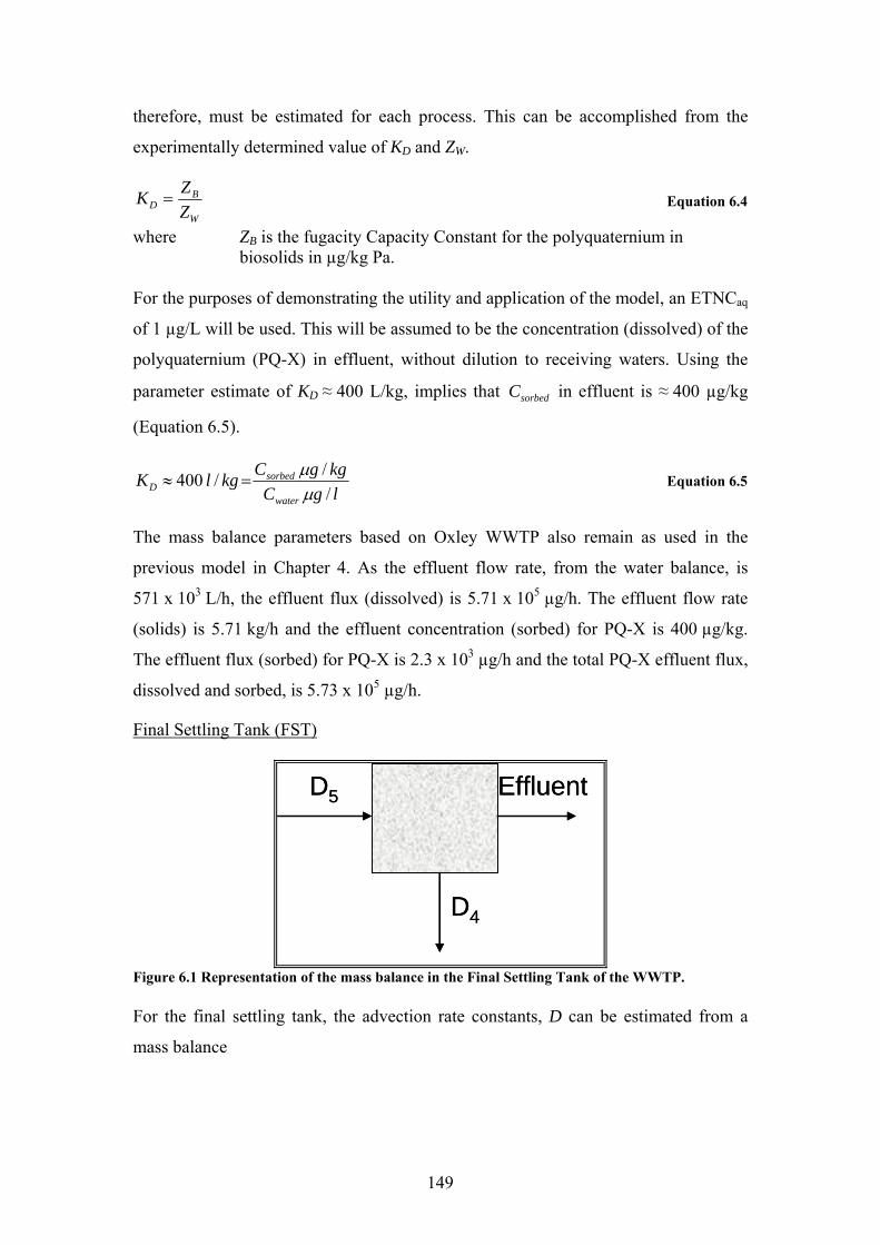
149

therefore, must be estimated for each process. This can be accomplished from the

experimentally determined value of KD and ZW.

W

BD Z

ZK = Equation 6.4

where ZB is the fugacity Capacity Constant for the polyquaternium in biosolids in µg/kg Pa. For the purposes of demonstrating the utility and application of the model, an ETNCaq

of 1 µg/L will be used. This will be assumed to be the concentration (dissolved) of the

polyquaternium (PQ-X) in effluent, without dilution to receiving waters. Using the

parameter estimate of KD ≈ 400 L/kg, implies that sorbedC in effluent is ≈ 400 µg/kg

(Equation 6.5).

lgCkggCkglK

water

sorbedD /

//400μμ

=≈ Equation 6.5

The mass balance parameters based on Oxley WWTP also remain as used in the

previous model in Chapter 4. As the effluent flow rate, from the water balance, is

571 x 103 L/h, the effluent flux (dissolved) is 5.71 x 105 µg/h. The effluent flow rate

(solids) is 5.71 kg/h and the effluent concentration (sorbed) for PQ-X is 400 µg/kg.

The effluent flux (sorbed) for PQ-X is 2.3 x 103 µg/h and the total PQ-X effluent flux,

dissolved and sorbed, is 5.73 x 105 µg/h.

Final Settling Tank (FST)

D5

D4

EffluentD5

D4

Effluent

Figure 6.1 Representation of the mass balance in the Final Settling Tank of the WWTP. For the final settling tank, the advection rate constants, D can be estimated from a

mass balance

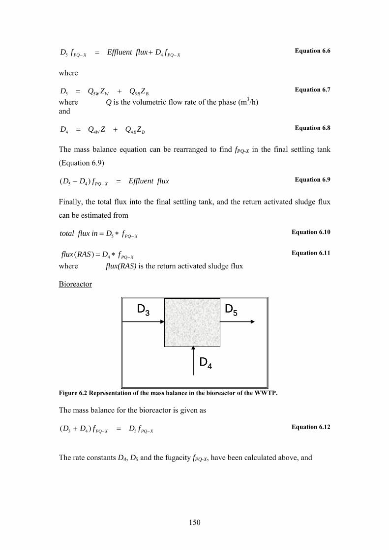
150

XPQXPQ fDfluxEffluentfD −− += 45 Equation 6.6

where

BBWW ZQZQD 555 += Equation 6.7

where Q is the volumetric flow rate of the phase (m3/h) and

BBW ZQZQD 444 += Equation 6.8

The mass balance equation can be rearranged to find fPQ-X in the final settling tank

(Equation 6.9)

fluxEffluentfDD XPQ =− −)( 45 Equation 6.9

Finally, the total flux into the final settling tank, and the return activated sludge flux

can be estimated from

XPQfDinfluxtotal −∗= 5 Equation 6.10

XPQfDRASflux −∗= 4)( Equation 6.11

where flux(RAS) is the return activated sludge flux Bioreactor

D3

D4

D5D3

D4

D5

Figure 6.2 Representation of the mass balance in the bioreactor of the WWTP. The mass balance for the bioreactor is given as

XPQXPQ fDfDD −− =+ 543 )( Equation 6.12

The rate constants D4, D5 and the fugacity fPQ-X, have been calculated above, and

151

BBWW ZQZQD 333 += Equation 6.13

Primary Settling Tank (PST)

D1

D2

D3D1

D2

D3

Figure 6.3 Representation of the mass balance in the Primary settling tank of the WWTP.

The mass balance for the primary settling tank is given by

XPQXPQ fDDfD −− += )( 321 Equation 6.14

The rate constants D3 and the fugacity fPQ-X, have been calculated above, and

BBWW ZQZQD 111 += Equation 6.15

and

BBWW ZQZQD 222 += Equation 6.16

As the sorption-desorption process occurs prior to arrival at the WWTP, the influent

flux can be subdivided into its dissolved and sorbed components (assuming

equilibrium)

sorbedBWW CQCQfluxTotal 11 += Equation 6.17

and

Dwater

sorbed KCC

= Equation 6.18

therefore

152

WDsorbed CKC ∗= Equation 6.19

The model parameters used here are based on the flow rates of only one of four waste

streams in the Oxley WWTP. To convert to a population usage volume for PQ-X, it is

necessary to multiply the influent flux by four (assuming equal flow in all four

streams) before converting to a tonnes per year volume usage. The people equivalent

capacity for Oxley WWTP is 240,000 (Tan et al. 2007). Based on Brisbane water

usage of 62% domestic, a rounded figure of 60% of the people equivalent capacity is

assumed to come from domestic sources. The critical usage volume is calculated from

the Oxley WWTP influent flux in tonnes/year as per Equation 6.20.

populationtotaldfpec

fluxvolumeimportTotal ××

=Equation 6.20

where flux: total influent flux for Oxley pec people equivalent capacity for Oxley WWTP (240,000) df fraction of pec assumed to be from domestic sources (0.6) total population of Australia, 20, 000,000

6.2.2. Results With the assumption that the ETNCaq is an in-stream concentration, diluted by a factor

of 10 from WWTP effluent concentration, and that the partition coefficient for

polyquaterniums is 400 L/kg, the approximate value for the JR polyquaterniums, or

1000 L/kg as for the Gafquat® polyquaterniums, the point estimates of critical usage

volume for risk assessment purposes is approximately 3 tonnes per annum if the mode

of action is non-specific (MOA3) and an order of magnitude less if the mode of action

is targeted (MOA4). This would translate to a personal use of 0.1 and 2.0 grams per

person per day of product containing 0.25% polyquaternium (Table 6.3). For

comparison, the results assuming a KD of 10,000 are also reported. The point estimate

was calculated in an Excel spreadsheet (Appendix 3b).

153

Table 6.3 Estimates of input volume and product usage for various ETNCaq for polyquaterniums, calculated for KD values of 400 (UCareTM JR125) and 1000 (Gafquat® 755) and 10000. ETNCaq µg/L

EffluentConc. µg/L

KD Influent fluxOxley µg/h

Influent flux Oxley

kg/year

National Use Volume tonnes/year

As product at 0.25%

g/person day0.01 0.1 400 2.46E+05 2.16 0.26 0.1 0.1 1 400 2.46E+06 21.59 2.63 1.0 0.01 0.1 1000 2.70E+05 2.36 0.29 0.2 0.1 1 1000 2.70E+06 23.63 2.88 2.0 0.01 0.1 10000 4.81E+05 4.22 0.51 0.3 0.1 1 10000 4.81E+06 42.16 5.13 3.0 In a Monte Carlo simulation of the model using Crystal Ball® (Decisioneering 2007)

the influent concentration was shown to have a lognormal distribution. The model was

run separately for the two values of ETNCaq. The model variable KD was assumed to

have a Maximum Extreme Distribution (Gumbel) with the input parameters, Likeliest

and Scale, set at 1000 and 400 respectively. This setting gave a distribution which

included values up to approximately 3000 in the extreme tail (Figure 6.4), This

positively skewed distribution suggests that while the KD values determined

experimentally in Chapter 4 are the most likely values, higher values such as those

reported by Podoll and Irwin (1988) are also possible. This probability density

function for KD was used in all following simulations. All other parameters relating to

the flows, water and solids balance in Oxley WWTP were assumed to be normally

distributed, as no data was available to suggest an alternative distribution. The results

for sample simulations are given in Figure 6.5. The mean concentration in the

simulation is close to the value determined in the point estimates above, indicating

that the model gives a Central Tendency Estimate of the influent flux. Any

conservatism in the estimate is therefore contained in the estimate of the ETNCaq.

Sensitivity analysis suggests that the modelled influent flux of polyquaternium is most

sensitive to the solids balance in the final settling tank, with KD having a significantly

smaller effect.

The importance of choosing the correct mode of action, and consequently the correct

ETNCaq is apparent in the point estimate result, as shown in both the point estimate

and probabilistic results. The one order of magnitude difference in the ETNCaq

translates directly into an order of magnitude difference in the trigger value for the

import/manufacture. By contrast, an incorrect estimation of the partition coefficient is

far less significant. A change of one order of magnitude in KD results in a difference

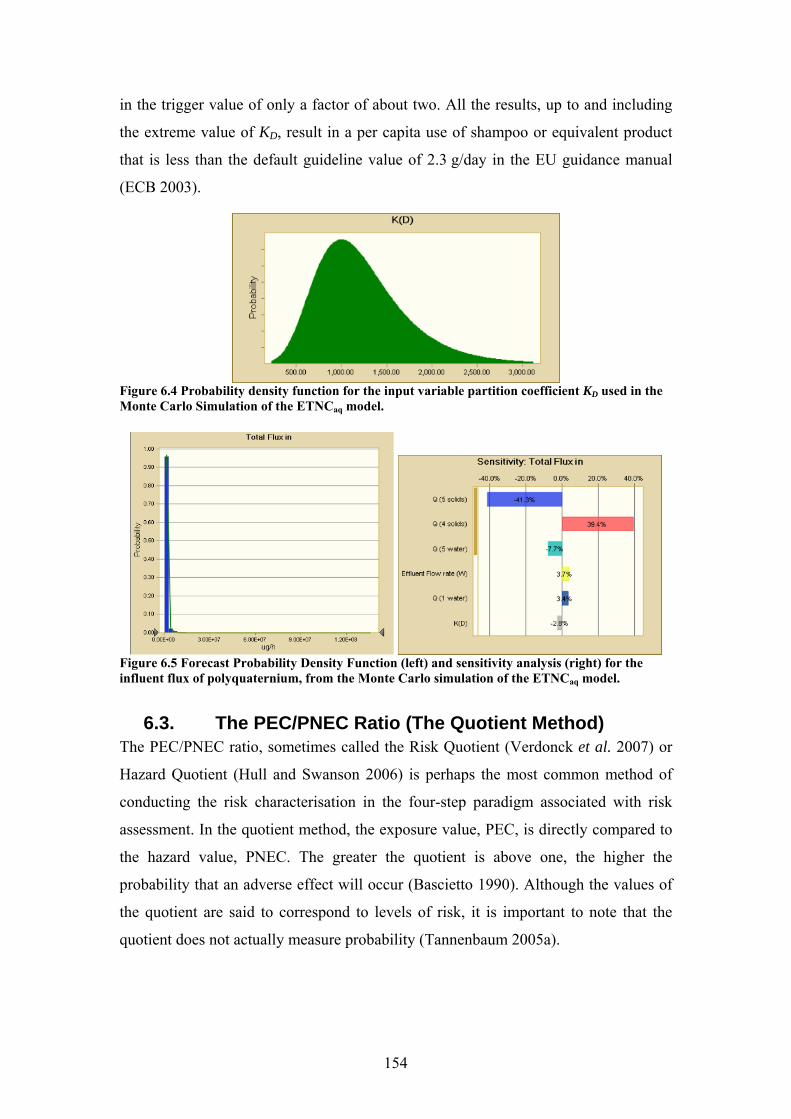
154

in the trigger value of only a factor of about two. All the results, up to and including

the extreme value of KD, result in a per capita use of shampoo or equivalent product

that is less than the default guideline value of 2.3 g/day in the EU guidance manual

(ECB 2003).

Figure 6.4 Probability density function for the input variable partition coefficient KD used in the Monte Carlo Simulation of the ETNCaq model.

Figure 6.5 Forecast Probability Density Function (left) and sensitivity analysis (right) for the influent flux of polyquaternium, from the Monte Carlo simulation of the ETNCaq model.

6.3. The PEC/PNEC Ratio (The Quotient Method) The PEC/PNEC ratio, sometimes called the Risk Quotient (Verdonck et al. 2007) or

Hazard Quotient (Hull and Swanson 2006) is perhaps the most common method of

conducting the risk characterisation in the four-step paradigm associated with risk

assessment. In the quotient method, the exposure value, PEC, is directly compared to

the hazard value, PNEC. The greater the quotient is above one, the higher the

probability that an adverse effect will occur (Bascietto 1990). Although the values of

the quotient are said to correspond to levels of risk, it is important to note that the

quotient does not actually measure probability (Tannenbaum 2005a).

155

6.3.1. Method It was noted in Chapter 4 that it was necessary for the PNEC and PEC to be expressed

in units that allowed their ratio to be determined. Although both have been derived in

units of concentration (mg/L or µg/L), the PEC has been estimated for all cosmetic

polyquaterniums combined, while the PNEC has been estimated for a sub-set of those

polyquaterniums. While there are possible methods of estimating market share, it is

not clear if this will improve the certainty of any predicted PNEC/PEC ratio.

Importantly, it is not known to what degree either the toxicities of, or the risk from,

polyquaterniums may be additive.

The PNEC/PEC ratio has been estimated in only one assessment of new

polyquaterniums by National Industrial Chemicals Notification and Assessment

Scheme/Department of Environment and water Resources (NICNAS/DEW) (Table

6.4), viz the nominally high volume import Merquat 2001 (NICNAS 2002a). In the

assessment of PQ-28 Gafquat® (NICNAS 1999) the import volume is given as 5

tonnes, but the PEC has been calculated on an import volume of 1 tonne. The

remaining assessments are all based on import volumes of less that one tonne per

year, resulting in a PECinfluent of 1 µg/L using the method outlined in Section 1.2. In

only one assessment was the PEC predicted for receiving waters (NICNAS 2002a).

Based on these reports however, data generated in this study can be used to predict a

PNEC/PEC ratio for polyquaterniums in Australia. The calculations will assume that

the volumes in the NICNAS reports, 1, 5 and 16 tonnes are typical

import/manufacture volumes for polyquaterniums. PNEC/PEC ratio will be calculated

for these typical volumes, as an estimate of the possible risk of individual

polyquaterniums. A PNEC/PEC ratio will also be calculated for the total volumes

estimated in Chapter 4, to estimate the risk from polyquaterniums if the toxicities/risk

are additive.

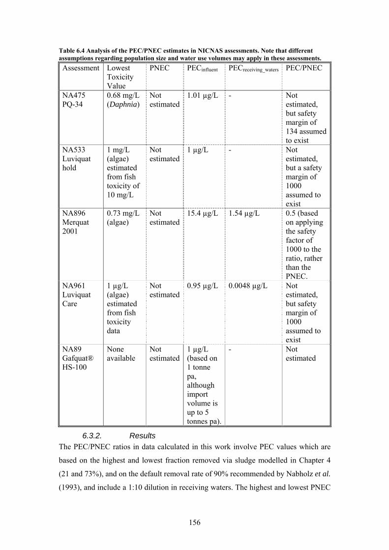
156

Table 6.4 Analysis of the PEC/PNEC estimates in NICNAS assessments. Note that different assumptions regarding population size and water use volumes may apply in these assessments. Assessment Lowest

Toxicity Value

PNEC PECinfluent PECreceiving_waters PEC/PNEC

NA475 PQ-34

0.68 mg/L (Daphnia)

Not estimated

1.01 µg/L - Not estimated, but safety margin of 134 assumed to exist

NA533 Luviquat hold

1 mg/L (algae) estimated from fish toxicity of 10 mg/L

Not estimated

1 µg/L - Not estimated, but a safety margin of 1000 assumed to exist

NA896 Merquat 2001

0.73 mg/L (algae)

Not estimated

15.4 µg/L 1.54 µg/L 0.5 (based on applying the safety factor of 1000 to the ratio, rather than the PNEC.

NA961 Luviquat Care

1 µg/L (algae) estimated from fish toxicity data

Not estimated

0.95 µg/L 0.0048 µg/L Not estimated, but safety margin of 1000 assumed to exist

NA89 Gafquat® HS-100

None available

Not estimated

1 µg/L (based on 1 tonne pa, although import volume is up to 5 tonnes pa).

- Not estimated

6.3.2. Results The PEC/PNEC ratios in data calculated in this work involve PEC values which are

based on the highest and lowest fraction removed via sludge modelled in Chapter 4

(21 and 73%), and on the default removal rate of 90% recommended by Nabholz et al.

(1993), and include a 1:10 dilution in receiving waters. The highest and lowest PNEC

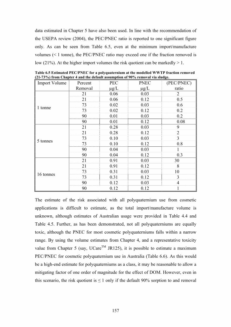
157

data estimated in Chapter 5 have also been used. In line with the recommendation of

the USEPA review (2004), the PEC/PNEC ratio is reported to one significant figure

only. As can be seen from Table 6.5, even at the minimum import/manufacture

volumes (< 1 tonne), the PEC/PNEC ratio may exceed one if the fraction removed is

low (21%). At the higher import volumes the risk quotient can be markedly > 1.

Table 6.5 Estimated PEC/PNEC for a polyquaternium at the modelled WWTP fraction removed (21-73%) from Chapter 4 and the default assumption of 90% removal via sludge.

Import Volume Percent Removal

PEC µg/L

PNEC µg/L

(PEC/PNEC) ratio

21 0.06 0.03 2 21 0.06 0.12 0.5 73 0.02 0.03 0.6 73 0.02 0.12 0.2 90 0.01 0.03 0.2

1 tonne

90 0.01 0.12 0.08 21 0.28 0.03 9 21 0.28 0.12 2 73 0.10 0.03 3 73 0.10 0.12 0.8 90 0.04 0.03 1

5 tonnes

90 0.04 0.12 0.3 21 0.91 0.03 30 21 0.91 0.12 8 73 0.31 0.03 10 73 0.31 0.12 3 90 0.12 0.03 4

16 tonnes

90 0.12 0.12 1 The estimate of the risk associated with all polyquaternium use from cosmetic

applications is difficult to estimate, as the total import/manufacture volume is

unknown, although estimates of Australian usage were provided in Table 4.4 and

Table 4.5. Further, as has been demonstrated, not all polyquaterniums are equally

toxic, although the PNEC for most cosmetic polyquaterniums falls within a narrow

range. By using the volume estimates from Chapter 4, and a representative toxicity

value from Chapter 5 (say, UCareTM JR125), it is possible to estimate a maximum

PEC/PNEC for cosmetic polyquaternium use in Australia (Table 6.6). As this would

be a high-end estimate for polyquaterniums as a class, it may be reasonable to allow a

mitigating factor of one order of magnitude for the effect of DOM. However, even in

this scenario, the risk quotient is ≤ 1 only if the default 90% sorption to and removal

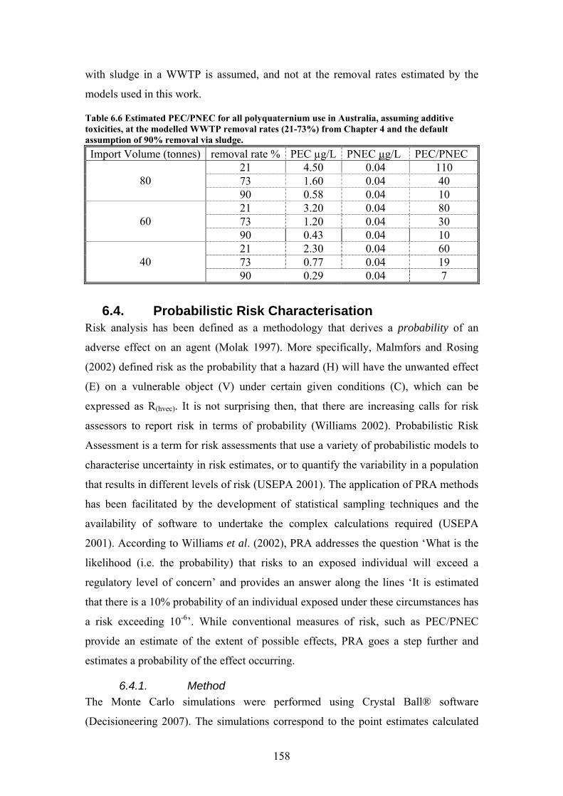
158

with sludge in a WWTP is assumed, and not at the removal rates estimated by the

models used in this work.

Table 6.6 Estimated PEC/PNEC for all polyquaternium use in Australia, assuming additive toxicities, at the modelled WWTP removal rates (21-73%) from Chapter 4 and the default assumption of 90% removal via sludge. Import Volume (tonnes) removal rate % PEC µg/L PNEC µg/L PEC/PNEC

21 4.50 0.04 110 73 1.60 0.04 40 80 90 0.58 0.04 10 21 3.20 0.04 80 73 1.20 0.04 30 60 90 0.43 0.04 10 21 2.30 0.04 60 73 0.77 0.04 19 40 90 0.29 0.04 7

6.4. Probabilistic Risk Characterisation Risk analysis has been defined as a methodology that derives a probability of an

adverse effect on an agent (Molak 1997). More specifically, Malmfors and Rosing

(2002) defined risk as the probability that a hazard (H) will have the unwanted effect

(E) on a vulnerable object (V) under certain given conditions (C), which can be

expressed as R(hvec). It is not surprising then, that there are increasing calls for risk

assessors to report risk in terms of probability (Williams 2002). Probabilistic Risk

Assessment is a term for risk assessments that use a variety of probabilistic models to

characterise uncertainty in risk estimates, or to quantify the variability in a population

that results in different levels of risk (USEPA 2001). The application of PRA methods

has been facilitated by the development of statistical sampling techniques and the

availability of software to undertake the complex calculations required (USEPA

2001). According to Williams et al. (2002), PRA addresses the question ‘What is the

likelihood (i.e. the probability) that risks to an exposed individual will exceed a

regulatory level of concern’ and provides an answer along the lines ‘It is estimated

that there is a 10% probability of an individual exposed under these circumstances has

a risk exceeding 10-6’. While conventional measures of risk, such as PEC/PNEC

provide an estimate of the extent of possible effects, PRA goes a step further and

estimates a probability of the effect occurring.

6.4.1. Method The Monte Carlo simulations were performed using Crystal Ball® software

(Decisioneering 2007). The simulations correspond to the point estimates calculated

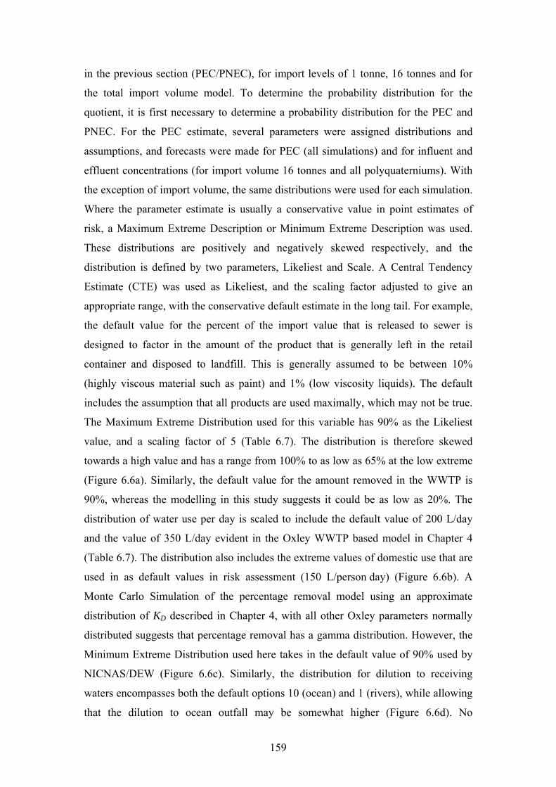
159

in the previous section (PEC/PNEC), for import levels of 1 tonne, 16 tonnes and for

the total import volume model. To determine the probability distribution for the

quotient, it is first necessary to determine a probability distribution for the PEC and

PNEC. For the PEC estimate, several parameters were assigned distributions and

assumptions, and forecasts were made for PEC (all simulations) and for influent and

effluent concentrations (for import volume 16 tonnes and all polyquaterniums). With

the exception of import volume, the same distributions were used for each simulation.

Where the parameter estimate is usually a conservative value in point estimates of

risk, a Maximum Extreme Description or Minimum Extreme Description was used.

These distributions are positively and negatively skewed respectively, and the

distribution is defined by two parameters, Likeliest and Scale. A Central Tendency

Estimate (CTE) was used as Likeliest, and the scaling factor adjusted to give an

appropriate range, with the conservative default estimate in the long tail. For example,

the default value for the percent of the import value that is released to sewer is

designed to factor in the amount of the product that is generally left in the retail

container and disposed to landfill. This is generally assumed to be between 10%

(highly viscous material such as paint) and 1% (low viscosity liquids). The default

includes the assumption that all products are used maximally, which may not be true.

The Maximum Extreme Distribution used for this variable has 90% as the Likeliest

value, and a scaling factor of 5 (Table 6.7). The distribution is therefore skewed

towards a high value and has a range from 100% to as low as 65% at the low extreme

(Figure 6.6a). Similarly, the default value for the amount removed in the WWTP is

90%, whereas the modelling in this study suggests it could be as low as 20%. The

distribution of water use per day is scaled to include the default value of 200 L/day

and the value of 350 L/day evident in the Oxley WWTP based model in Chapter 4

(Table 6.7). The distribution also includes the extreme values of domestic use that are

used in as default values in risk assessment (150 L/person day) (Figure 6.6b). A

Monte Carlo Simulation of the percentage removal model using an approximate

distribution of KD described in Chapter 4, with all other Oxley parameters normally

distributed suggests that percentage removal has a gamma distribution. However, the

Minimum Extreme Distribution used here takes in the default value of 90% used by

NICNAS/DEW (Figure 6.6c). Similarly, the distribution for dilution to receiving

waters encompasses both the default options 10 (ocean) and 1 (rivers), while allowing

that the dilution to ocean outfall may be somewhat higher (Figure 6.6d). No

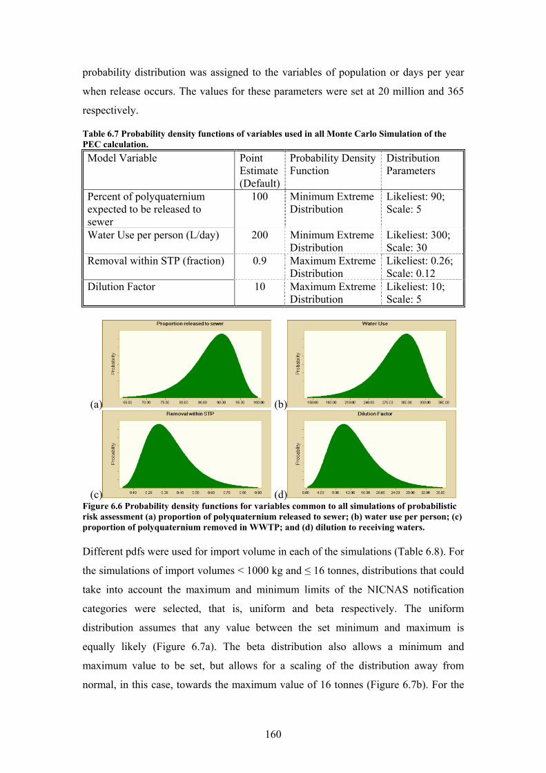
160

probability distribution was assigned to the variables of population or days per year

when release occurs. The values for these parameters were set at 20 million and 365

respectively.

Table 6.7 Probability density functions of variables used in all Monte Carlo Simulation of the PEC calculation. Model Variable Point

Estimate (Default)

Probability Density Function

Distribution Parameters

Percent of polyquaternium expected to be released to sewer

100 Minimum Extreme Distribution

Likeliest: 90; Scale: 5

Water Use per person (L/day) 200 Minimum Extreme Distribution

Likeliest: 300; Scale: 30

Removal within STP (fraction) 0.9 Maximum Extreme Distribution

Likeliest: 0.26; Scale: 0.12

Dilution Factor 10 Maximum Extreme Distribution

Likeliest: 10; Scale: 5

(a) (b)

(c) (d) Figure 6.6 Probability density functions for variables common to all simulations of probabilistic risk assessment (a) proportion of polyquaternium released to sewer; (b) water use per person; (c) proportion of polyquaternium removed in WWTP; and (d) dilution to receiving waters. Different pdfs were used for import volume in each of the simulations (Table 6.8). For

the simulations of import volumes < 1000 kg and ≤ 16 tonnes, distributions that could

take into account the maximum and minimum limits of the NICNAS notification

categories were selected, that is, uniform and beta respectively. The uniform

distribution assumes that any value between the set minimum and maximum is

equally likely (Figure 6.7a). The beta distribution also allows a minimum and

maximum value to be set, but allows for a scaling of the distribution away from

normal, in this case, towards the maximum value of 16 tonnes (Figure 6.7b). For the

161

simulation of all cosmetic polyquaterniums, no minimum or maximum constraint is

set. However, the volume is unlikely to be less than the import volume for any one

polyquaternium. Therefore a log normal distribution was selected (Figure 6.7c),

limiting lower end estimates. The mean and standard deviation (50 and 10 tonnes

respectively) were selected to cover the possible range of import volumes estimated in

Chapter 4.

(a) (b)

(c) Figure 6.7 Probability density functions for input volumes for the three simulations of the PEC (a) import volume < 1000 kg; (b) import volume < 16 tonnes; and (c) estimated total import volume for all cosmetic polyquaterniums. The result of the Monte Carlo Simulation is a pdf for the PEC for each of the three

import scenarios. This pdf was then combined with the pdf determined from the

toxicity data to determine the probability that the PEC/PNEC was ≤ 1. Although algae

were the most sensitive species, there was not sufficient data to create a pdf in Crystal

Ball® for algal toxicity. However, a pdf was created for the fish data, which was

found to have a log normal distribution with a mean of 2.46 µg/L and a standard

deviation of 3.85 µg/L (Figure 6.8a). The toxicity of polyquaterniums to algae was

approximately one order of magnitude higher, and for the purposes of this simulation,

could be assumed to follow the same distribution as fish toxicity. However, the

purpose of risk assessment is to protect vulnerable, not average, species and

individuals, as indicated by the selection of the most sensitive species toxicity value

for the risk characterisation, and the pdf in a includes the values of median effective

concentration (EC50) for the low toxicity polyquaterniums UCareTM LR400 and

LR30M. This inclusion skews the mean toxicity away from values that would protect

sensitive species from more toxic polyquaterniums. The value selected for this

162

variable may still have some uncertainty, however and a probability function can be

estimated. In this case, the extreme maximum distribution was again selected. Based

on the algal data in this study, the Likeliest value was determined to be 0.12 µg/L, and

the scale factor 0.02 selected to include the highest toxicity value (lowest EC50) of

0.03 µg/L, as determined in Chapter 5 (Figure 6.8b). For more general assessments,

the probability function could be set to include the ETNCaq, with 1.0 as Likeliest, and

the scale adjusted to include the MOA4 value of 0.01 in the tail.

Table 6.8 Probability density functions of import volumes used in Monte Carlo Simulation for three simulations of the PEC calculation. Import Volume Probability Distribution

Function Distribution Parameters

<1000 kg Uniform Minimum: 100 kg; Maximum: 1000 kg.

≤ 16 tonnes Beta Minimum: 1 tonne; Maximum: 16 tonnes; α: 4; β: 2

All cosmetic polyquaterniums.

Log normal Mean: 50 Standard deviation: 10

(a) (b) Figure 6.8 Fish probability distribution function from data (a), and assumed for the Monte Carlo Simulation (b)

6.4.2. Results For the simulation of PEC for the < 1 tonne import volume, the probability that the

PEC ≤ 0.03 µg/L is 0.9, at a confidence level of 99% (Figure 6.9). The simulation of

the PEC was most sensitive to the variables import volume (51.3%) and dilution to

receiving waters (-38.3%) (Figure 6.9). The probability distribution function for PEC

input into the Monte Carlo Simulation of the PEC/PNEC was a log normal

distribution with a mean of 0.02 and a standard deviation of 0.08 (Figure 6.10). The

probability that the ratio (PEC/PNEC > 1) was between 0.94 and 0.99, with an

average 0.95 at 95% level of certainty in five successive runs of the simulation. An

example of the output is shown in Figure 6.11.

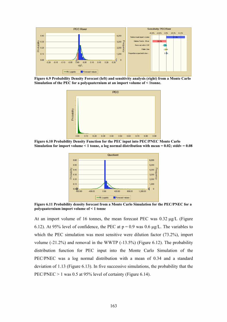
163

Figure 6.9 Probability Density Forecast (left) and sensitivity analysis (right) from a Monte Carlo Simulation of the PEC for a polyquaternium at an import volume of < 1tonne.

Figure 6.10 Probability Density Function for the PEC input into PEC/PNEC Monte Carlo Simulation for import volume < 1 tonne, a log normal distribution with mean = 0.02; stddv = 0.08

Figure 6.11 Probability density forecast from a Monte Carlo Simulation for the PEC/PNEC for a polyquaternium import volume of < 1 tonne At an import volume of 16 tonnes, the mean forecast PEC was 0.32 µg/L (Figure

6.12). At 95% level of confidence, the PEC at p = 0.9 was 0.6 µg/L. The variables to

which the PEC simulation was most sensitive were dilution factor (73.2%), import

volume (-21.2%) and removal in the WWTP (-13.5%) (Figure 6.12). The probability

distribution function for PEC input into the Monte Carlo Simulation of the

PEC/PNEC was a log normal distribution with a mean of 0.34 and a standard

deviation of 1.13 (Figure 6.13). In five successive simulations, the probability that the

PEC/PNEC > 1 was 0.5 at 95% level of certainty (Figure 6.14).

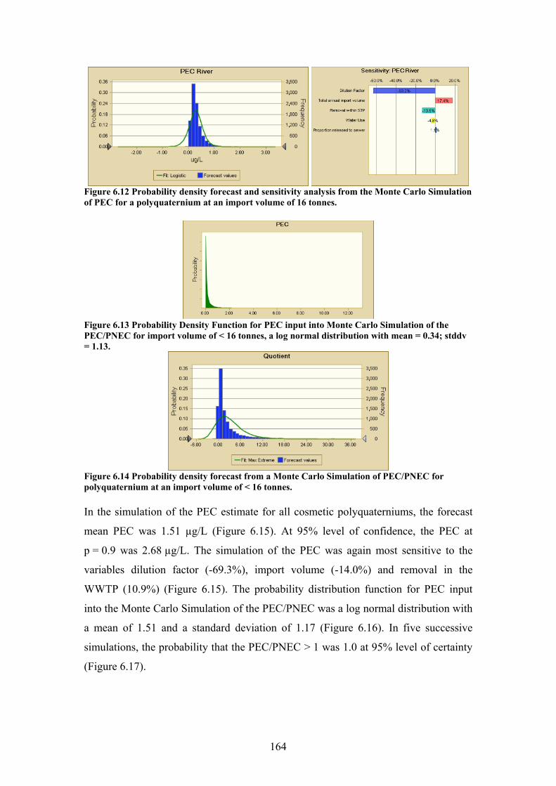
164

Figure 6.12 Probability density forecast and sensitivity analysis from the Monte Carlo Simulation of PEC for a polyquaternium at an import volume of 16 tonnes.

Figure 6.13 Probability Density Function for PEC input into Monte Carlo Simulation of the PEC/PNEC for import volume of < 16 tonnes, a log normal distribution with mean = 0.34; stddv = 1.13.

Figure 6.14 Probability density forecast from a Monte Carlo Simulation of PEC/PNEC for polyquaternium at an import volume of < 16 tonnes. In the simulation of the PEC estimate for all cosmetic polyquaterniums, the forecast

mean PEC was 1.51 µg/L (Figure 6.15). At 95% level of confidence, the PEC at

p = 0.9 was 2.68 µg/L. The simulation of the PEC was again most sensitive to the

variables dilution factor (-69.3%), import volume (-14.0%) and removal in the

WWTP (10.9%) (Figure 6.15). The probability distribution function for PEC input

into the Monte Carlo Simulation of the PEC/PNEC was a log normal distribution with

a mean of 1.51 and a standard deviation of 1.17 (Figure 6.16). In five successive

simulations, the probability that the PEC/PNEC > 1 was 1.0 at 95% level of certainty

(Figure 6.17).

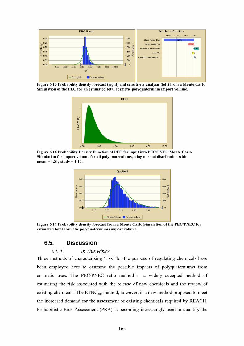
165

Figure 6.15 Probability density forecast (right) and sensitivity analysis (left) from a Monte Carlo Simulation of the PEC for an estimated total cosmetic polyquaternium import volume.

Figure 6.16 Probability Density Function of PEC for input into PEC/PNEC Monte Carlo Simulation for import volume for all polyquaterniums, a log normal distribution with mean = 1.51; stddv = 1.17.

Figure 6.17 Probability density forecast from a Monte Carlo Simulation of the PEC/PNEC for estimated total cosmetic polyquaterniums import volume.

6.5. Discussion 6.5.1. Is This Risk?

Three methods of characterising ‘risk’ for the purpose of regulating chemicals have

been employed here to examine the possible impacts of polyquaterniums from

cosmetic uses. The PEC/PNEC ratio method is a widely accepted method of

estimating the risk associated with the release of new chemicals and the review of

existing chemicals. The ETNCaq, method, however, is a new method proposed to meet

the increased demand for the assessment of existing chemicals required by REACH.

Probabilistic Risk Assessment (PRA) is becoming increasingly used to quantify the

166

uncertainty in risk assessments of contaminated sites by USEPA (USEPA 2001), but

has not yet been applied to regulatory new or existing chemical risk assessment in

Australia. It is necessary to examine, however, exactly how these methods have

characterised the risk, and how they advance the risk assessment process for

regulatory chemical risk assessment.

The ETNCaq, does not combine the PNEC and PEC to produce a single numeric

indicator in the way the ratio method does. It is claimed by its advocates to provide an

indication of risk by purporting to be a critical value of the PEC at which risk

approaches zero. Rather than putting a value on the risk per se, it is intended to be a

screening tool, to determine if further risk assessment is required by identify those

cases in which the risk may be significantly greater than zero. The method, therefore,

has only two possible outcomes. Either the risk approaches zero (negligible risk) or

the risk is not close to zero and therefore further assessment is required. The

application of the method requires, in addition to the ETNCaq, a good estimate of the

usage volumes, and possibly release and fate parameters. In assessment of new

chemicals, the usage volume is known, though fate parameters may not be well

established, and measured environmental concentrations are generally not available

(or at least, not for the jurisdiction under consideration). In assessment of existing

chemicals, usage data can generally be sought under the regulatory framework, but

fate parameters and measured environmental concentrations may or may not be

available. In the proposed application of the method for REACH, if the usage volume

indicated that the PEC may be greater than the ETNCaq, further assessment of the fate

parameters and release data may be required (De Wolf et al. 2005). As it has been

applied here, where actual usage volumes are not known but some information on the

fate parameters is available, it has been used to determine the import/manufacture

volume at which further assessment of the fate of the polyquaternium may need to be

examined, probably around three tonnes per annum.

As the PEC/PNEC ratio gives a numerical result, it is generally regarded to be a

quantitative measure of risk (ECB 2003). However, it has also been suggested that the

PEC/PNEC is not a measure of risk at all (Tannenbaum 2005a), and indeed, it is

sometimes referred to as Hazard Quotient rather than Risk Quotient (DeMott et al.

2005; Hull and Swanson 2006). Further, the quotient method has been criticised for

the tendency of risk assessors to view the value of one as a threshold value, with

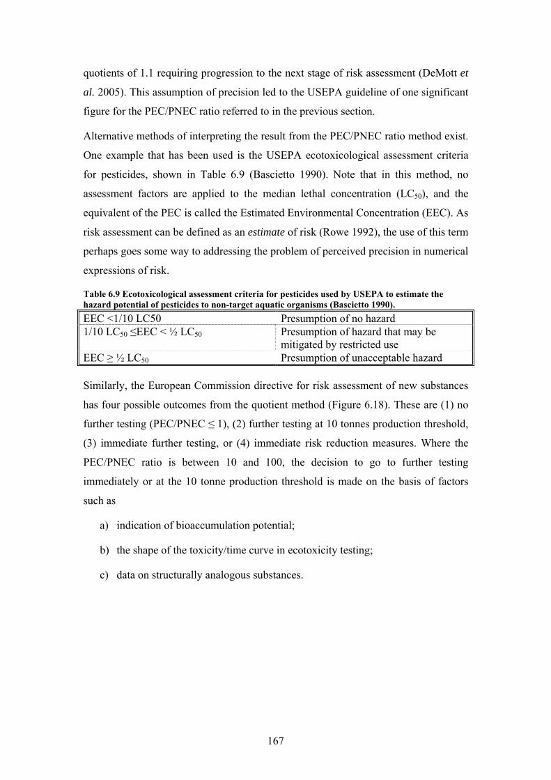
167

quotients of 1.1 requiring progression to the next stage of risk assessment (DeMott et

al. 2005). This assumption of precision led to the USEPA guideline of one significant

figure for the PEC/PNEC ratio referred to in the previous section.

Alternative methods of interpreting the result from the PEC/PNEC ratio method exist.

One example that has been used is the USEPA ecotoxicological assessment criteria

for pesticides, shown in Table 6.9 (Bascietto 1990). Note that in this method, no

assessment factors are applied to the median lethal concentration (LC50), and the

equivalent of the PEC is called the Estimated Environmental Concentration (EEC). As

risk assessment can be defined as an estimate of risk (Rowe 1992), the use of this term

perhaps goes some way to addressing the problem of perceived precision in numerical

expressions of risk.

Table 6.9 Ecotoxicological assessment criteria for pesticides used by USEPA to estimate the hazard potential of pesticides to non-target aquatic organisms (Bascietto 1990). EEC <1/10 LC50 Presumption of no hazard 1/10 LC50 ≤EEC < ½ LC50

Presumption of hazard that may be mitigated by restricted use

EEC ≥ ½ LC50 Presumption of unacceptable hazard Similarly, the European Commission directive for risk assessment of new substances

has four possible outcomes from the quotient method (Figure 6.18). These are (1) no

further testing (PEC/PNEC ≤ 1), (2) further testing at 10 tonnes production threshold,

(3) immediate further testing, or (4) immediate risk reduction measures. Where the

PEC/PNEC ratio is between 10 and 100, the decision to go to further testing

immediately or at the 10 tonne production threshold is made on the basis of factors

such as

a) indication of bioaccumulation potential;

b) the shape of the toxicity/time curve in ecotoxicity testing;

c) data on structurally analogous substances.

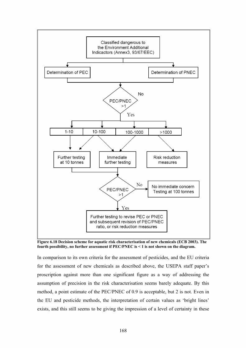
168

Figure 6.18 Decision scheme for aquatic risk characterisation of new chemicals (ECB 2003). The fourth possibility, no further assessment if PEC/PNEC is < 1 is not shown on the diagram. In comparison to its own criteria for the assessment of pesticides, and the EU criteria

for the assessment of new chemicals as described above, the USEPA staff paper’s

proscription against more than one significant figure as a way of addressing the

assumption of precision in the risk characterisation seems barely adequate. By this

method, a point estimate of the PEC/PNEC of 0.9 is acceptable, but 2 is not. Even in

the EU and pesticide methods, the interpretation of certain values as ‘bright lines’

exists, and this still seems to be giving the impression of a level of certainty in these

169

assessments that may not be justified. It is suggested therefore, that although the point

estimate of PEC/PNEC uses numerical methods, it is, in fact, only a qualitative

method of characterising risk, and only three outcomes are possible from this method:

PEC/PNEC << 1 (acceptable risk); PEC/PNEC >> 1 (unacceptable risk); or

PEC/PNEC ≈ 1 (indeterminate risk or risk requiring intervention). The decision of

how much greater or less than one is significant is a policy decision, not a scientific

one, and will be addressed in Section 6.5.4.

In contrast to the point estimate of the PEC/PNEC, the results of the PRA include a

distribution of forecast results, the probabilities associated with the forecast results,

and analysis of the sensitivity of the forecast to each input variable. Not only was it

possible to fit probability distributions to both the PEC and the PNEC, but it was also

possible to determine importance of the variables in determining the forecast. The

essential difference is that with PRA, it can be stated that ‘At the level of 95%

confidence the probability that the PEC/PNEC for an import volume of 16 tonnes will

be < 1 is 0.5’, rather than ‘A conservative estimate is that the PEC/PNEC for an

import volume of 16 tonnes is likely to be < 1’. While the probability estimate, or

more specifically, the sensitivity analysis that accompanies it, is helpful in

determining where it might be necessary to focus further data collection and research,

it does not account for all the uncertainty in the risk characterisation, nor overcome all

the limitations of the PEC/PNEC method. Further, the method has not dealt with the

issue of the appropriateness of the PEC/PNEC as a measure of risk. For example, the

PRA gives us no answer to the problem of the assessment factors used to account for

uncertainties in toxicological methods (effects of incremental dosages, differences

between laboratory test and field populations, indirect effects of toxicant such as food

chain interactions, other ecosystem effects including predator-prey relationships,

community metabolism, structural shifts) (Bascietto 1990). Further, the reliability of

the PRA is dependent to a large extent on the appropriateness and/or suitability of the

pdfs assigned to the variables, which can only be validated by data from field studies.

6.5.2. Uncertainty in PNEC and PEC The red book (NRC 1983) describes uncertainty as ‘pervasive’ and the ‘dominant

analytical difficulty’ in risk assessment. Uncertainty and variability exist in all risk

assessments (USEPA 2004) to an often unknown degree (Malmfors and Rosing

2002). An examination of the sources of uncertainty, either qualitatively or

170

quantitatively, can be a productive means of refining a risk assessment, or to find

solutions to the problems at issue (Verdonck et al. 2007), and is of interest in this

work.

In many discussions of uncertainty and variability in risk characterisation, the

distinction between the two terms is often blurred, and the terms even used

interchangeably. Alternative terms have also been used, for example, Wilson and

Shlyakhter (1997) describes ‘stochastic uncertainties’ and ‘uncertainties of fact’,

while Verdonk et al. (2007) uses ‘epistemological uncertainty’ and ‘ontological

uncertainty’ for uncertainty and variability respectively. Variability (stochastic

uncertainty) is generally considered to be the measured and therefore known variation

among members of a defined population potentially leading to variations in risk

(Wilson and Shlyakhter 1997). For Verdonk et al. (2007), ontological uncertainty

(variability) is the inherent randomness in the parameter, but also includes variability

in human behaviour and variability in societal factors such as the development of

technological systems. Variability is a fundamental property of nature and is

irreducible through further measurement. Uncertainty (epistemological uncertainty,

uncertainty of fact), however, arises from a lack of knowledge which can be reduced

through additional investigation.

In this study, a large amount of the uncertainty in the risk characterisation results

because the import/manufacture volume of the polyquaterniums is unknown and

therefore uncertain (reducible uncertainty). If it was possible to determine the usage

volume by asking the importers and manufacturers how much is manufactured or sold

each year, there would still be variability in the usage volume. The volume may

change from year to year, market share may be won from or lost to alternative

products, formulation of specific products may change, new products may be

developed, all contributing to variation in the usage volume. In new chemicals risk

assessment, the notifier is required to state the maximum annual import volume for

the first five years. There is no uncertainty in this volume; though there may be some

variability (the notifier may not reach their sales target). However, after 5 years, when

the chemical is publicly listed on the Australian Inventory of Chemical Substances

(AICS), no import restrictions exist, and usage volume becomes uncertain and

variable.

171

Increasing the data available for risk assessment, however, does not necessarily

reduce uncertainty. For example, it has been regarded as reasonably certain in risk

assessments by NICNAS/DEW and in the literature that the adsorption of

polyquaterniums in WWTP was close to 100% due to the high affinity of the cationic

sites on the polymer for the anionic sites on biosolids. Based on this assumption, the

default value of 90% reduction in concentration in WWTPs has been used as a

‘conservative’ estimate. However, this work with cosmetic polyquaterniums has

suggested that removal of polyquaterniums in WWTP may be significantly lower, due

to the relatively high aqueous solubility of the cosmetic polyquaterniums and the

relatively low concentrations of solids in wastewater. It has also been assumed that

the desorption of polymers generally, and therefore polyquaterniums, is unlikely to

occur for reasons outlined in Section 2.4.2, and this view has been maintained in risk

assessment, despite some evidence to the contrary. The ability of polyquaterniums to

desorb (as mentioned previously) is considered one of their advantages in hair and

skin care applications, and evidence to this effect is freely available on the

manufacturers’ websites.

Uncertainty in risk assessment can arise from many factors, and has been broadly

classified into three main areas (USEPA 1992):

a) scenario uncertainty, arising from missing or incomplete information e.g.

descriptive errors, aggregation errors, errors in professional judgement, and

incomplete analysis;

b) parameter uncertainty, which affects a particular parameter e.g. measurement

errors, sampling errors, variability, and use of generic or surrogate data;

c) model uncertainty, arising from the scientific theory affecting the ability of a

model to make predictions.

Uncertainty in the derivation of the PEC and PNEC in this study contains

uncertainties that fall into each of these groups. Greater uncertainty exists in the PEC,

the sources of which are described in Table 6.10. In each of the scenarios modelled

(< 1, < 16 and ≈ 50 tonnes import volume), the difference between the CTE (mean

estimate) value and the RME (conservative estimate) was two orders of magnitude. In

sensitivity analysis, several factors were found to contribute significantly to the

uncertainty the PEC, notably import volume, in-stream dilution of WWTP effluent,

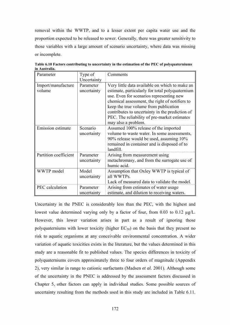
172

removal within the WWTP, and to a lesser extent per capita water use and the

proportion expected to be released to sewer. Generally, there was greater sensitivity to

those variables with a large amount of scenario uncertainty, where data was missing

or incomplete.

Table 6.10 Factors contributing to uncertainty in the estimation of the PEC of polyquaterniums in Australia. Parameter Type of

Uncertainty Comments

Import/manufacture volume

Parameter uncertainty

Very little data available on which to make an estimate, particularly for total polyquaternium use. Even for scenarios representing new chemical assessment, the right of notifiers to keep the true volume from publication contributes to uncertainty in the prediction of PEC. The reliability of pre-market estimates may also a problem.

Emission estimate Scenario uncertainty

Assumed 100% release of the imported volume to waste water. In some assessments, 90% release would be used, assuming 10% remained in container and is disposed of to landfill.

Partition coefficient Parameter uncertainty

Arising from measurement using metachromasy, and from the surrogate use of humic acid.

WWTP model Model uncertainty

Assumption that Oxley WWTP is typical of all WWTPs. Lack of measured data to validate the model.

PEC calculation

Parameter uncertainty

Arising from estimates of water usage estimate, and dilution to receiving waters.

Uncertainty in the PNEC is considerably less than the PEC, with the highest and

lowest value determined varying only by a factor of four, from 0.03 to 0.12 µg/L.

However, this lower variation arises in part as a result of ignoring those

polyquaterniums with lower toxicity (higher EC50) on the basis that they present no

risk to aquatic organisms at any conceivable environmental concentration. A wider

variation of aquatic toxicities exists in the literature, but the values determined in this

study are a reasonable fit to published values. The species differences in toxicity of

polyquaterniums covers approximately three to four orders of magnitude (Appendix

2), very similar in range to cationic surfactants (Madsen et al. 2001). Although some

of the uncertainty in the PNEC is addressed by the assessment factors discussed in

Chapter 5, other factors can apply in individual studies. Some possible sources of

uncertainty resulting from the methods used in this study are included in Table 6.11.

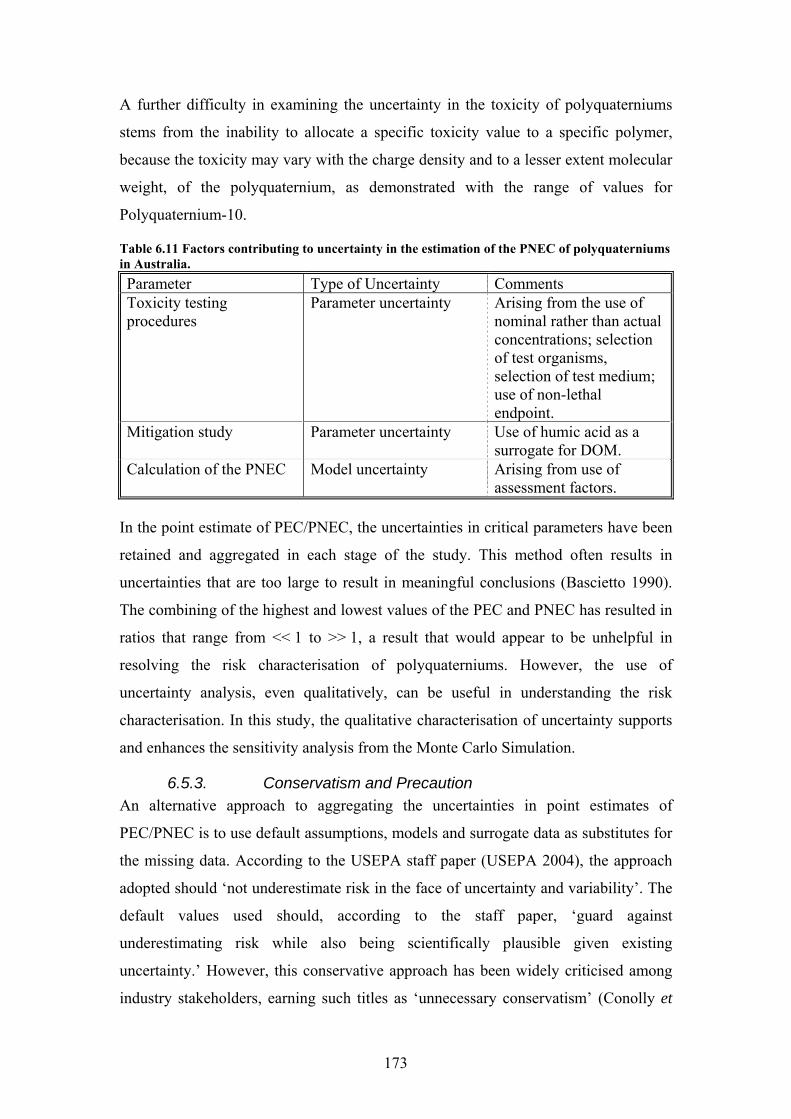
173

A further difficulty in examining the uncertainty in the toxicity of polyquaterniums

stems from the inability to allocate a specific toxicity value to a specific polymer,

because the toxicity may vary with the charge density and to a lesser extent molecular

weight, of the polyquaternium, as demonstrated with the range of values for

Polyquaternium-10.

Table 6.11 Factors contributing to uncertainty in the estimation of the PNEC of polyquaterniums in Australia. Parameter Type of Uncertainty Comments Toxicity testing procedures

Parameter uncertainty Arising from the use of nominal rather than actual concentrations; selection of test organisms, selection of test medium; use of non-lethal endpoint.

Mitigation study Parameter uncertainty Use of humic acid as a surrogate for DOM.

Calculation of the PNEC Model uncertainty Arising from use of assessment factors.

In the point estimate of PEC/PNEC, the uncertainties in critical parameters have been

retained and aggregated in each stage of the study. This method often results in

uncertainties that are too large to result in meaningful conclusions (Bascietto 1990).

The combining of the highest and lowest values of the PEC and PNEC has resulted in

ratios that range from << 1 to >> 1, a result that would appear to be unhelpful in

resolving the risk characterisation of polyquaterniums. However, the use of

uncertainty analysis, even qualitatively, can be useful in understanding the risk

characterisation. In this study, the qualitative characterisation of uncertainty supports

and enhances the sensitivity analysis from the Monte Carlo Simulation.

6.5.3. Conservatism and Precaution An alternative approach to aggregating the uncertainties in point estimates of

PEC/PNEC is to use default assumptions, models and surrogate data as substitutes for

the missing data. According to the USEPA staff paper (USEPA 2004), the approach

adopted should ‘not underestimate risk in the face of uncertainty and variability’. The

default values used should, according to the staff paper, ‘guard against

underestimating risk while also being scientifically plausible given existing

uncertainty.’ However, this conservative approach has been widely criticised among

industry stakeholders, earning such titles as ‘unnecessary conservatism’ (Conolly et

174

al. 1999) and ‘compounding conservatism’ (Stahl et al. 2005). The use of

‘intentionally protective’ assumptions results in ‘biased’ risk characterisation (DeMott

et al. 2005), and has the potential to mask uncertainty in the risk characterisation

(Verdonck et al. 2007). The overstating of risks in conservative risk assessments is

thought to lead to inappropriate risk management decisions (Stahl et al. 2005), unless

risk managers are aware that the risk characterisation is not a real risk measure, but a

measure to avoid false negatives (unsafe chemicals that are assessed as safe)

(Verdonck et al. 2007). Further, the method may lead to more stringent regulatory

controls and standards than are necessary (Conolly et al. 1999). The use of PRA,

however, does not completely overcome the conservatism of most point estimate

calculations, as the conservatism can simply be built into the probability distribution

of the variable.

Other stakeholders may take the position that the conservative approach is not

protective or precautionary enough. As the USEPA acknowledges in the staff paper

(USEPA 2004), it is possible that in individual cases the final overall risk estimate

will underestimate the true risk, even though the tendency is for the estimate to be

higher than the true risk rather than lower. In contrast to the position taken by industry

stakeholders, it has been argued that uncertainty in the data and scientific evidence in

the risk assessment process may create a bias in favour of regulatory inaction (Latin

1997; Wilson and Shlyakhter 1997), as regulators may be reluctant to enforce

restrictions or controls without good science and a degree of certainty.

According to Gullett (2000), a distinction needs to be made between ‘prevention’ and

‘precaution’. While prevention deals with avoiding uncertain outcomes which may or

may not be harmful, precaution, as embodied in the precautionary principle,

encompasses not only the preventative aspects of traditional regulatory approaches,

but also provides justification for acting in advance of knowledge where outcomes are

uncertain. Gullet (2000) defines the central elements of the precautionary principle as:

a) Being confident about predictions of future environmental effects of activities

before allowing them;

b) Not waiting for conclusive proof of environmental harm before adopting

appropriate remedial measures.

175

Although the precautionary principle has been included in some environmental

legislation in Australia, including the Environment Protection and Biodiversity

Conservation Act, (1999), and in amendments to Great Barrier Reef Marine Park Act,

(1975) and the Fisheries Management Act, (1991), the definition of the precautionary

principle in legislation is often problematic and indistinct from the conventional

conservative approach (Gullett 2000). According to the EU, the ‘prudential’

(conservative) approach is an integral part of the scientific opinion delivered by the

risk evaluators, while the precautionary principle becomes a risk management option

‘when scientific uncertainty precludes a full assessment of the risk and when decision-

makers consider that the chosen level of environmental protection or of human,

animal and plant health may be in jeopardy’ (EC 2000).

In the application of new chemicals risk assessment, conservatism does not usually

contribute to a significantly inflated risk. For example, the assumption of 100%

release for dispersed uses such as personal care products, is not particularly inflated

compared to the assumption of between 1% and 10% percent loss (depending on

viscosity) to landfill with the container. In the sensitivity analysis, this variable

contributed only about 1% of uncertainty in the PEC. In other situations, such as the

use of a large volume at an industrial site, however, this variable may contribute more

to uncertainty. According to Stahl et al. (2005), most companies making pre-

manufacture notice (PMN) applications under the Toxic Substances Control Act

(TSCA) are aware of the extrapolations and default assumptions used in the process.

Their preference is for a quick response to the application. If the PMN cannot be

approved due to uncertainty in either the PEC/PNEC ratio or structure-activity

relationships, the decision to generate the required data or withdraw the application is

a business decision, not a scientific one.

However, the conservative approach applied to the point estimate of risk in an

assessment such as this one, where the usage volume is not known, generates a

quotient significantly greater than one, and results in a characterisation of significant

risk. The criticism that high-end estimates mask uncertainty, therefore, would be

applicable in this case.

6.5.4. Science, Policy, Assessment and Management The conservative stance taken by risk assessors in organisations such as USEPA and

NICNAS/DEW is of course, a policy position rather than a scientific one. According

176

to the USEPA staff paper (USEPA 2004), policy provides the fundamental framework

of the risk assessment, and informs the default assumptions used within the

framework. These policy positions are developed outside the risk assessment. An

alternative view, however, would place a greater emphasis on science rather than

policy in determining the risk assessment process. For example Conolly et al. (1999)

suggests that toxicologists should refine existing approaches and develop new tools so

that ‘toxicological science’ rather than ‘science policy’ becomes the primary basis for

risk assessment. Stahl et al. (2005) have argued that a greater reliance on scientific

information, rather than plausible conservatism in selecting defaults should be

possible due to increasing experience in ‘the field’. However, Tannenbaum (2005b)

has suggested that toxicological science lacks the ability to identify true biological

harm when and if it occurs in the field.

It is not universally accepted, however, that the role of policy is one of framing and

informing the risk assessment process, or of filling in the gaps left by scientific

knowledge. Science and policy are sometimes viewed as belonging to risk assessment

and risk management respectively. According to Verdonk et al. (2005), risk

assessment is a science-based process which identifies and characterises hazard,

exposure and risk (including uncertainty), while risk management is a ‘decision-

making process used for deciding between policy alternatives in consultation with

stakeholders, taking into account both the estimated risk and its uncertainty, the

precautionary principle, the cost and other factors (e.g. social, economic and legal

considerations)’. Risk assessments, in this framework, should ‘aspire to the greatest

extent to be objective scientific exercises that seek realistically to estimate risk’ while

subsequent risk management ‘must be fully and transparently distinguished from risk

assessment if the practice of risk assessment is to have scientific credibility’ (ACC

2003). According to Stahl et al. (2005), this position is reflected in the policy directive

from the Executive Office of the President (USA), which stated ‘EPA risk

assessments must not intermingle important policy judgements within the scientific

assessment of risk. Rather, the choice of an appropriate margin of safety should

remain the province of responsible risk-management officials, and should not be pre-

empted through biased risk assessments.’ However, this position does not appear to

have been maintained in subsequent publications from the Executive Office, for

177

example in the Updated Principles of Risk Assessment (EOP 2007), which takes a

position more in line with the traditional USEPA approach.

In the European Union, two separate bodies are involved in the scientific and policy

aspects of risk assessment. The Committee for Toxicology, Ecotoxicology and the

Environment (CSTEE) provides independent advice on scientific issues relevant to

regulatory decision making. After a risk assessment has been peer reviewed by

CSTEE, a separate policy body, Competent Authorities (CA), recommends follow up

to the conclusion of the assessment ( Munn and Hansen 2002). There are three

possible outcomes of the EU risk assessment, viz

a) recommend further information be generated to reduce uncertainties;

b) recommend no further exposure reduction measures, based on the

consideration that an ‘unacceptable risk’ has not been demonstrated;

c) recommend further exposure reduction measures, based on the consideration

that an ‘unacceptable risk’ cannot be ruled out.

According to Munn and Hansen (2002), a science-based conclusion will lean towards

(a) or (b), while a policy-based conclusion will be influenced by socio-economic

factors in the choice between (a) and (c). Assessments that take into account practical

considerations including the scientific uncertainties and the needs of risk managers are

described by Verdonk et al. (2007) as being based on regulatory science rather than

research science. This suggests that the policy-science distinction that plagues the US

system of risk assessment has been resolved in the EU as a science in its own right,

distinct from the normal research science from which it draws much data and

methodology, by its ability to incorporate the social and legal aspects of the risk

assessment, management and communication processes.

The approach adopted by the EU suggests that issues such as evidence and uncertainty

in risk assessment can be treated as they would be in science, and this is, in fact, what

PRA is expected to do. However, the risk assessment process is to a large extent

shaped by the ‘requirements, constraints and adversarial climate of regulation’, rather

that the disciplinary norms of science (Latin 1997), and uncertainty and evidence do

not have the same meaning in law and science (Gawlack et al. 1987). A scientist,

using an uncertainty analysis approach, may view the addition of components, each

with its own uncertainty, as leading to an increase in uncertainty. A lawyer weighing

the same evidence in a ‘sum of evidence’ approach would regard uncertainty as

178

reduced by the addition of each piece of evidence (Gawlack et al. 1987). It should not

be surprising then, that a regulatory risk assessment can be regarded as giving too

little weight to uncertainty by some reviewers, and being too conservative or cautious

by others. The two views represent, according to Gawlack et al. (1987) diverging

scientific and legal opinions.

6.5.5. Characterising the Risk to the Aquatic Environment from Cosmetic Polyquaternium Use in Australia

It is necessary then, to approach the uncertainty in the risk characterisation of

cosmetic polyquaterniums in Australia from the perspective of the applicability of the

questions of science and policy, and risk assessment and risk management. For

example, one major source of uncertainty in the risk characterisation of cosmetic

polyquaterniums identified above is the import volume. There is no system for the

generation of statistics on the production and use of chemicals in Australia that is

nationally uniform, consistent and comparable (DEH 1998). Data collected by the

Australian Bureau of Statistics (ABS) is designed to be useful for the study and

understanding of trade, not safety or environment, as evidenced by the collection of

some categories in terms of monetary value rather than quantity. As mentioned in

Section 4.2, the actual import or manufacture volume of a new chemical can be kept

confidential at the request of the importer. Data on volume and use can be collected

by NICNAS as part of a Priority Existing Chemical assessment, even in the initial

stage of review. However, there are approximately 40,000 existing chemicals on

AICS, and as at September 2007, only 29 Priority Existing Chemical reports have

been produced since the inception of NICNAS in 1989. There are 7 assessments

currently in progress; 43 chemicals are currently on the candidate list of chemicals for

assessment with a further 12 on a standby list. To date, 13 nominated chemicals have

been rejected for assessment. The majority of chemicals nominated as priority

existing chemicals are nominated on public health and occupational health and safety

(OHS) grounds, a priority that is understandable in light of the enormity of the task.

The main reasons stated for the rejection of candidate chemicals are either that

NICNAS was unable to ascertain any usage in Australia, or the usage determined was

very low (<< 1 tonne). However, two assessments currently in progress are based to a

large extent on environmental concerns; Sodium Cyanide, a chemical used in gold

extraction, and Triclosan, an antibacterial agent used in personal care and household

products. The reasons for the nomination of Sodium Cyanide include; widespread use

179

provides a number of ways for the chemical to enter the environment; it is acutely

toxic to animals, fish and birds, may cause death and low growth rates in plants; and

bird kills had been reported following possible exposure at tailings dams (NICNAS

2002c). Triclosan was nominated on the basis of its toxicity to aquatic species,

particularly algae; the number of ways it can enter environment; the possibility that it

may be persistent and bioaccumulate; and because disposal by incineration of wastes

containing Triclosan may result in formation of dioxins (NICNAS 2003).

While the collection of more extensive data on chemical use and release would seem

desirable, considerable obstacles to such collection exist. For example, importers of

household and personal care products may not know the formula of the product; the

number of different products imported is very large; and the collation of the data once

collected is likely to be time consuming and expensive. Further, while standardisation

of names exists for cosmetic products, and for industry applications requiring Material

Safety Data Sheets (MSDS), the same does not apply to ingredients in household and

other consumer products. These problems not only make the collection and collation

of data difficult, they also contribute to difficulties in the enforcement of compliance

with the Industrial Chemicals (Notification and Assessment) Act (ICNA). Although

mandatory reporting of volume is required in some circumstance, for example for

chemicals on the HVICL, and for some categories of permits and certificates, any

attempt to collect usage data on a wider scale is likely to be resisted by industry.

A further source of uncertainty identified above concerned the fate of the

polyquaterniums in WWTPs and dilution to receiving waters. In the risk

characterisation of polyquaterniums by NICNAS/DEW, default assumptions of 90%

removal and 1:10 dilution are used. Although the partitioning behaviour of the

polyquaterniums is an important factor here, also significant is the extent of solids

removal in the WWTP. However, it would appear from this study that these

assumptions, instead of being conservative, may be optimistic. In the risk

characterisation process for new and existing chemicals, where field studies are not

part of the process, assessors are, to a significant degree, reliant on

information/feedback from risk managers for information and updates on the

parameters affecting these variables. In the Australian regulatory system, the risk

assessors, NICNAS/DEW, are departments of the Commonwealth Government, while

the risk managers are the State and Territory departments of environment, health and

180

occupational health and safety (OHS). The relationship between the Commonwealth,

as risk assessor, and the States and Territories, as risk managers, is subject to a

Memorandum of Understanding (MOU), established in 1991. As defined in the MOU,

the role of the States and Territories is to implement recommendations from

assessment reports published by the Director of NICNAS. The States and Territories

must also inform the Director of NICNAS of any consequential action taken in respect

of any recommendations, and can raise issues of concern regarding chemicals with the

Commonwealth agencies. Due to the confidentiality provisions of ICNA, the risk

managers receive the Full Public Report, which may not contain the actual volume. It

is therefore essential that the risk be well characterised within the report. However, it

is not at all clear from the assessments of polyquaterniums that the risk assessors have

adequate information on WWTP processes and receiving waters relevant to

polyquaterniums to make an adequate characterisation of the risk and recommend

adequate control measures. Risk managers may, for example, be better placed to

determine the extent to which the toxicity of polyquaterniums is mitigated by the

presence of solids in the receiving waters into which they discharge, than risk

assessors who can only apply a generalised determination.

In 2007, the States and Commonwealth signed a National Framework for Chemicals

Environmental Management (NChEM), which may well address these issues to some

degree. It includes in its recommendations the investigation of the feasibility of a

centralised national approach to gathering, storing and utilising information on

industrial chemicals that have been made available for use, and consultation with state

departments during the assessment process. The agreement also recommends further

development of the environmental monitoring database to ensure that it incorporates

information on environmental impacts and usage.

However, in order for data on polyquaterniums to be included on a database of

environmental impacts, there must first be some way of measuring such impacts, and

as has been discussed previously, there is no reliable method available for measuring

concentrations of polyquaterniums in environmental matrices such as water or

sediment. The assessment of new chemicals does require that the notifier provide

details on methods of identification of the chemical, for example, an infra-red

spectrum, however, like the import volume, this information is covered by the

confidentiality provisions, and may not be included in the Full Public Report. The

181

purpose of this data requirement is perhaps more to facilitate identification of the

assessed chemical if required in compliance matters. It may be time, however, in the

on-going regulatory review of the Act and its implementation, to consider requesting

that notifiers provide a method of extracting and quantifying the notified chemical in

environmental samples, if release to the environment is likely to occur.

6.6. Conclusion As complex as the chemistry and toxicology of this class of polymers is, the

difficulties faced in this assessment are as much about the process as the subject.

Uncertainty exists in several variables in the risk characterisation – both in the PEC

and PNEC. Further scientific studies may help. For example, further toxicological

studies would be valuable in determining the mechanism of toxicity, species

sensitivity distribution, and polymer architecture effects. Such studies may also help

in further understanding the toxicity of cationic surfactants generally. However,

considerable data already exists, published and unpublished, to establish that, except

in a few cases of very low charge density natural polyquaterniums, these polymers are

very toxic to some aquatic organisms. There is probably already enough information

to begin screening of these polymers on the basis of chemistry, without recourse to

any further toxicity testing. The issue of mitigation by DOM, total organic carbon

(TOC) or humic acid is a wider issue, and needs to be addressed for all organics as

part of the differences between laboratory testing and field effects. Further, it may be

better addressed in risk management than risk assessment. It is difficult, based on the

partitioning results of this study, to make a special case for polyquaterniums. A

method of determining the concentration of polyquaterniums in environmental

samples, particularly water and sediment, would also be useful, as an alternative to a

policy commitment to monitor import volumes. But the development of an analytical

method is likely to be expensive, and the question of who would be responsible for

the development of the method would need to be resolved. To require industry to

provide an appropriate test again requires a policy commitment.

Even assuming the problems of uncertainty in critical variables can be addressed, it is

far from clear that the risk assessment methodology is able to quantify and/or

characterise risk in a way that is meaningful to, and useful for, risk managers. The

methodology adopted in regulatory chemical risk assessment has been adopted from

the methodologies developed for the ecological risk assessment of contaminated sites,

182

where the basis of the risk assessment is measured environmental concentrations

generally taken in response to an observed adverse effect on the site ecology. The

applicability of the method even to contaminated site assessment has been the subject

of some criticism. It has been suggested that ‘ERA, from its inception until the present

day, remains devoid of a risk assessment tool. A greater tragedy may be that

ecological risk assessors and risk managers do not seem to have this realization’

(Tannenbaum 2005a). A review of the methodology, and possible alternatives, for the

environmental risk assessment of new industrial chemicals is needed.

Polyquaterniums, a class of polymer that are known to be toxic in the aquatic

environment, are being introduced into Australia, in unknown quantities, for use in

applications that result in wide, dispersive release through WWTPs. They do not

degrade, but partition between anionic solids (including biota) and water, yet there is

no way of reasonably determining their fate, or of measuring their concentration in

environmental samples. Uncertain and unproven default assumptions are used in

assessing the risk of these compounds in the aquatic environment, and no assessment

has been attempted of possible risk in sediments. Only limited risk assessment is

carried out when new polyquaterniums are introduced, and not in the context of the

total amount of polyquaternium released. This assessment has looked at the risk of

polyquaterniums from only one source, cosmetics, and found that the risk may be

significant.

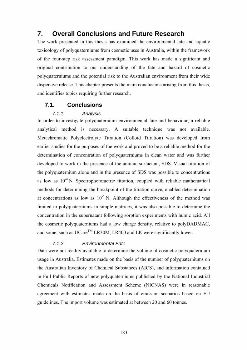
183

7. Overall Conclusions and Future Research The work presented in this thesis has examined the environmental fate and aquatic

toxicology of polyquaterniums from cosmetic uses in Australia, within the framework

of the four-step risk assessment paradigm. This work has made a significant and

original contribution to our understanding of the fate and hazard of cosmetic

polyquaterniums and the potential risk to the Australian environment from their wide

dispersive release. This chapter presents the main conclusions arising from this thesis,

and identifies topics requiring further research.

7.1. Conclusions 7.1.1. Analysis

In order to investigate polyquaternium environmental fate and behaviour, a reliable

analytical method is necessary. A suitable technique was not available.

Metachromatic Polyelectrolyte Titration (Colloid Titration) was developed from

earlier studies for the purposes of the work and proved to be a reliable method for the

determination of concentration of polyquaterniums in clean water and was further

developed to work in the presence of the anionic surfactant, SDS. Visual titration of

the polyquaternium alone and in the presence of SDS was possible to concentrations

as low as 10-4 N. Spectrophotometric titration, coupled with reliable mathematical

methods for determining the breakpoint of the titration curve, enabled determination

at concentrations as low as 10-5 N. Although the effectiveness of the method was

limited to polyquaterniums in simple matrices, it was also possible to determine the

concentration in the supernatant following sorption experiments with humic acid. All

the cosmetic polyquaterniums had a low charge density, relative to polyDADMAC,

and some, such as UCareTM LR30M, LR400 and LK were significantly lower.

7.1.2. Environmental Fate Data were not readily available to determine the volume of cosmetic polyquaternium

usage in Australia. Estimates made on the basis of the number of polyquaterniums on

the Australian Inventory of Chemical Substances (AICS), and information contained

in Full Public Reports of new polyquaterniums published by the National Industrial

Chemicals Notification and Assessment Scheme (NICNAS) were in reasonable

agreement with estimates made on the basis of emission scenarios based on EU

guidelines. The import volume was estimated at between 20 and 60 tonnes.

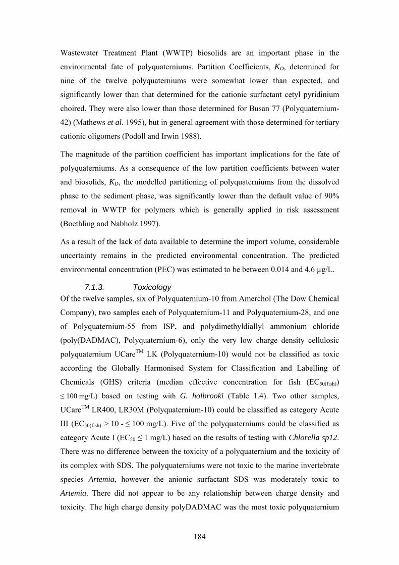
184

Wastewater Treatment Plant (WWTP) biosolids are an important phase in the

environmental fate of polyquaterniums. Partition Coefficients, KD, determined for

nine of the twelve polyquaterniums were somewhat lower than expected, and

significantly lower than that determined for the cationic surfactant cetyl pyridinium

choired. They were also lower than those determined for Busan 77 (Polyquaternium-

42) (Mathews et al. 1995), but in general agreement with those determined for tertiary

cationic oligomers (Podoll and Irwin 1988).

The magnitude of the partition coefficient has important implications for the fate of

polyquaterniums. As a consequence of the low partition coefficients between water

and biosolids, KD, the modelled partitioning of polyquaterniums from the dissolved

phase to the sediment phase, was significantly lower than the default value of 90%

removal in WWTP for polymers which is generally applied in risk assessment

(Boethling and Nabholz 1997).

As a result of the lack of data available to determine the import volume, considerable

uncertainty remains in the predicted environmental concentration. The predicted

environmental concentration (PEC) was estimated to be between 0.014 and 4.6 µg/L.

7.1.3. Toxicology Of the twelve samples, six of Polyquaternium-10 from Amerchol (The Dow Chemical

Company), two samples each of Polyquaternium-11 and Polyquaternium-28, and one

of Polyquaternium-55 from ISP, and polydimethyldiallyl ammonium chloride

(poly(DADMAC), Polyquaternium-6), only the very low charge density cellulosic

polyquaternium UCareTM LK (Polyquaternium-10) would not be classified as toxic

according the Globally Harmonised System for Classification and Labelling of

Chemicals (GHS) criteria (median effective concentration for fish (EC50(fish))

≤ 100 mg/L) based on testing with G. holbrooki (Table 1.4). Two other samples,

UCareTM LR400, LR30M (Polyquaternium-10) could be classified as category Acute

III (EC50(fish) > 10 - ≤ 100 mg/L). Five of the polyquaterniums could be classified as

category Acute I (EC50 ≤ 1 mg/L) based on the results of testing with Chlorella sp12.

There was no difference between the toxicity of a polyquaternium and the toxicity of

its complex with SDS. The polyquaterniums were not toxic to the marine invertebrate

species Artemia, however the anionic surfactant SDS was moderately toxic to

Artemia. There did not appear to be any relationship between charge density and

toxicity. The high charge density polyDADMAC was the most toxic polyquaternium

185

when EC50 was expressed in mass units, but one of the least toxic if EC50 was

expressed in terms of equivalence. It is probable that the toxicity of the

polyquaternium is dependent on hydrophobicity, which is in turn dependent on

multiple structural features of the polymer. Algae were the most sensitive of the three

species tested. With the application of assessment factors, the predicted no effect

concentration (PNEC) for the toxic polyquaterniums was estimated to be 0.03 and

0.12 µg/L. This PNEC does not take into account possible mitigation of the toxicity of

polyquaterniums by humic acid.

7.1.4. Risk Characterisation A PEC/PNEC ratio > 1 is possible at even low volumes if the fraction of

polyquaternium removed in WWTP is in the lower range modelled in this work. At

higher volumes, > 5 tonnes, the PEC/PNEC ratio can exceed 1 even at the default

removal of 90% in WWTPs. Monte Carlo Simulation highlighted the sensitivity of the

calculations to those variables for which a large data gap exists – import volume and

dilution to receiving waters. Consequently, the greatest uncertainty in the risk

characterisation results from those aspects of the PEC calculation.

7.2. Implications and Future Research The most significant difficulty for the risk assessment of polyquaterniums is most

likely the lack of a viable method of identifying and quantifying polyquaterniums

(and cationic polyelectrolytes generally) in environmental samples. However, there

are inherent problems in the analysis of polymers due to their distribution of

molecular size, and in the analysis of cations due to interference of other cations, that

combined make the development of a suitable analytical method difficult. A method

of tagging polyquaterniums, such as that proposed by Bennett et al. (2000) could at

least enable the verification of fate models such as those used in this work, if the

method of tagging can be shown to have no effect on the behaviour of the

polyquaternium in laboratory tests. As an interim measure pending a method of

identification quantification of polyquaterniums in environmental samples, the

tracking of tagged polyquaterniums would be a worthwhile area for future research.

In terms of the ecotoxicology, uncertainty still exists with regard to the mechanism of

toxicity, and species sensitivity distribution. Neither of these is of significant

consequence for the risk assessment process, and further toxicity studies are unlikely

to contribute to the risk characterisation of polyquaterniums. It is not possible to

186

assign a toxicity to a particular polyquaternium in the absence of specific testing, due

to variations in structure that may contribute to toxicity without altering the ‘identity’

of the polymer, nor is it possible to draw generalised conclusions regarding particular

characteristics such as ‘natural’ versus ‘synthetic’ polyquaterniums. However,

sufficient data exists to enable reasonable prediction of toxicity based on chemistry.

While some very low charge density cellulose (and probably guar) based polymers

have significantly lower toxicity than either ‘synthetics’ or higher charge ‘natural’

polyquaterniums, generally polyquaterniums should be assumed to be very toxic to

aquatic organisms. The toxicity of individual polyquaternium samples appears to be

the result of a complex mix of those characteristics that contribute to the

hydrophobicity of the polymer, and this would seem to be a possible direction for

future research.

An understanding of the mechanism of toxicity may be important as part of a more

general understanding of the toxicity of cationic species generally. Further, the

mitigating effect of humic acid needs to be considered in the wider consequence of

the differences between laboratory studies and field effects, and the role of DOM in

mitigating the toxic effects of anthropogenic chemicals. Without addressing wider

questions, such as the release of other toxic cations from DOM on binding of

polyquaterniums, there is little justification for the special treatment of humic acid

mitigation in the risk assessment of cationic polyelectrolytes without reliable

information on DOM concentrations in the receiving environment, and the role of

DOM in the mitigation of toxicity of organic chemicals more generally.

The lack of available data on the volume usage of polyquaterniums (and many other

chemicals) presents a significant challenge for researchers and risk managers. Even

where data is collected, it is not necessarily freely available, such as the confidential

NICNAS data, nor available in a useful format, such as the Australian Bureau of

Statistics (ABS) import figures in dollar values. This deficiency has been critical in

the case of polyquaterniums, where no method of measuring environmental

concentration exists. However, even for other chemicals released with wastewater,

volume usage data may enable issues of spatial and temporal distribution to be

addressed. Without creating additional data collection and collation schemes, the data

available for monitoring and research could be improved by addressing the form in

which data is collected, and the extent to which it is made public.

187

In this study, probability distribution functions were generated using the ‘reasonable’

and ‘conservative’ values that may be used in point estimate risk assessments. The

determination of appropriate distributions of parameters such as per capita water use

and dilution to receiving waters could be better determined if appropriate feedback

from risk managers to risk assessors was available. Much of this data could easily be

generated from information already held by various water authorities and state EPAs.

The collection and collation of this data and the description of realistic pdfs would

greatly assist in any move from point estimate to probabilistic risk assessment of

chemicals in Australia. Further, as hazard assessment endeavours to protect the most

vulnerable species, realistic probability distribution functions would enable

characterisation of the risk to the most vulnerable environments.

Of the scientific and knowledge gaps identified above, NICNAS already has the

authority to collect the information from importers and manufacturers of new and

existing chemicals. Volume data is a requirement for all new chemical notifications

(NICNAS 2004), and can be requested for existing chemicals under Section 48 of the

Industrial Chemicals (Notification and Assessment) Act (ICNA) (CofA 1989).

Notifiers of new chemicals are also required to provide details of a method of

identification of the notified chemical or polymer. The requirement is usually met

with the provision of an infra-red spectrum of the pure substance. As a method of

identification the infra-red spectrum may not be adequate to identify even the

chemical or polymer in the form/matrix in which it is imported into Australia for

regulatory compliance purposes, and even less useful for the monitoring of

environmental, public or occupational health and safety (OHS). It may be more

appropriate in the case of novel chemicals to interpret the data requirement as the

requirement of a method of identification of the chemical/polymer in samples taken

for compliance, environmental, public or health monitoring purposes. However, such

a requirement would be problematic for a class of compound such as

polyquaterniums, where a large number are already widely available. For some data

requirements of ICNA, additional fees are charged where data is either not available or

the notifier otherwise seeks a variation to the data requirements. The decision to

proceed with the notification by meeting the testing requirement, or payment of the

fee, would be a commercial one for the notifier as suggested by Stahl et al. (2005).

The possibility of imposing release controls, which can be applied in the case of

188

industrial chemicals whose use is limited to specific sites, cannot be applied to

cosmetics.

7.3. Concluding Comments Polyquaterniums are a class of polymers with an already extensive use pattern, and in

the case of cosmetic uses, with a dispersive release to the environment through the

wastewater system. The risk assessment of polyquaterniums is characterised by a set

of default assumptions that do not appear to be supported either by limited

environmental studies of their fate, or by studies of the behaviour of polyquaterniums

in cosmetic applications. There is no known method of reliably measuring or

determining the concentration of polyquaterniums in environmental samples. With

few exceptions, polyquaterniums are very toxic to some aquatic species; and tend to

have steep toxicity curves. The extent of polyquaternium usage in cosmetic products

is not known, however, limited available data suggests that sufficient quantities of

polyquaterniums may currently be released through the wastewater system in

Australia to present a significant risk to more vulnerable waterways that receive

WWTP effluent.

189

List of References ABS (2006) Merchandise Import Data by Tariff Code by Calendar Year by Value &

Quantity (2001-2005). Information supplies by Australian Bureau of Statistics, 1/08/2006. Commonwealth of Australia.

ACC (2003). Comments to the Office of Management and Budget. Draft 2003 Report to Congress on the Costs and Benefits of Federal Regulations. Arlington, Virginia, The American Chemistry Council.

Aizawa T, Y Magara and M Musashi (1991). Problems with introducing synthetic polyelectrolyte coagulants into the water purification process. Water Supply 9(1, IWSA/IAWPRC Jt. Spec. Conf. Coagulation, Flocculation, Filtr., Sediment. Flotation, 1990): 27-35.

Amerchol (2002) UCare® Polymers: Cationic conditioners that revitalize hair and skin. http://www.dow.com/PublishedLiterature/dh_0048/0901b80380048858.pdf?filepath=amerchol/pdfs/noreg/324-00004.pdf&fromPage=GetDoc. Accessed 26/5/03.

Ananthapadmanabhan KP, PS Leung and ED Goddard (1985). Fluorescence and solubilization studies of polymer-surfactant systems. Colloids and Surfaces 13(1): 63-72.

André V, R Norenberg, P Hossel and A Pfau (1999). The role of polymer-surfactant interactions in the adsorption process of hair-conditioning polymers. Macromolecular Symposia 145(Polymer Sorption Phenomena): 169-179.

Bascietto J (1990). Ecotoxicology and ecological risk assessment. Environmental Science & Technology 24(1): 10-15.

BASF Akteingesellschaft (1998). ZK 1210-187: Determination of the Absorption on Activated Sludge, Project No. 98/0194/14/1, BASF Experimental Toxicology and Ecology, Ludwigshafen, Germany. (unpublished report) in NICNAS (2001). NA/961 Full Public Report: Luviquat Care (Polyquaternium 44). Sydney, National Industrial Chemicals Notification and Assessment Scheme.

Bhattacharjya SK, VS Gupta and BK Dutta (1975). Industrial application of zeta potential studies: effect of cationic polyelectrolytes on destabilization of clay colloids in synthetic waters. Fertilizer Technology 12(4): 306-11.

Beeton R, KI Buckley, GJ Jones, D Morgan, RE Reichelt, D Trewin and ASotE Committee (2006). Australia State of the Environment Report, 2006, Independent report to the Australian Government Minister for the Environment and Heritage, Canberra. Department of the Environment and Heritage.

Beim AA and AM Beim (1994). Comparative ecological-toxicological data on determination of maximum permissible concentrations (MPC) for several flocculants. Environmental Technology 15(2): 195-8.

Bennett DM, BA Bolto, DR Dixon, RJ Eldridge, NP Le and CS Rye (2000). Determining the fate of flocculants by fluorescent tagging. Chemical Water and Wastewater Treatment VI, Proceedings of the Gothenburg Symposium, 9th, Istanbul, Turkey, Oct. 2-4, 2000: 159-168.

Bergeron JA and M Singer (1958). Metachromasy: An experimental and theoretical reevaluation. Journal of. Cell Biology. 4(4): 433-457.

Biesinger KE, AE Lemke, WE Smith and RM Tyo (1976). Comparative toxicity of polyelectrolytes to selected aquatic animals. Journal - Water Pollution Control Federation 48(1): 183-7.

190

Biesinger KE and GN Stokes (1986). Effects of synthetic polyelectrolytes on selected aquatic organisms. Journal - Water Pollution Control Federation 58(3): 207-13.

Blum DJW (1990). Determining chemical toxicity to aquatic species. Environmental Science & Technology 24(3): 284-293.

Boethling RS and JV Nabholz (1997). Environmental assessment of polymers under the U.S. Toxic Substances Control Act. Ecological Assessment of Polymers: 187-234.

Breton R and A Boxall (2003). Pharmaceuticals and personal care products in the environment: Regulatory drivers and research needs. QSAR & Combinatorial Science 22(3): 399-409.

Brocksen RW (1971). An evaluation of potential sources of toxicity to fish in Martis Creek. SD Army Corps of Engineers, CA: 1-11.

Brown TL, J LeMay, H.E. and BE Bursten (2006). Chemistry: the central science. Upper Saddle River, N.J, Pearson Prentice Hall.

Burchill S, MHB Hayes and DJ Greenland (1981). Adsorption. Chemical Soil Processes. DJ Greenland. Chichester, J. Wiley.

Burke M (2005) Take two bottles into the shower? Chemistry World, Royal Society of Chemistry, January 2005. http://www.rsc.org/chemistryworld/Issues/2005/January/Taketwobottles.asp Accessed 12/6/06

Cary GA, WJ Kuc and JA McMahon (1989). Toxicity of cationic polyelectrolytes to aquatic organisms - the relationship between acute toxicity and dissolved organic carbon. Polymer Preprints (American Chemical Society, Division of Polymer Chemistry) 30(2): 384-5.

Cary GA, JA McMahon and WJ Kuc (1987). The effect of suspended solids and naturally occurring dissolved organics in reducing the acute toxicities of cationic polyelectrolytes to aquatic organisms. Environmental Toxicology and Chemistry 6(6): 469-74.

Chang L-L, D Bruch Martha, J Griskowitz Nancy and K Dentel Steven (2002). NMR spectroscopy for determination of cationic polymer concentrations. Water Research 36(9): 2255-64.

Chang LL, DL Raudenbush and SK Dentel (2001). Aerobic and anaerobic biodegradability of a flocculant polymer. Water Science and Technology 44(2-3, 1st World Water Congress: Operation and Management, Landfill and Sludge Management, 2000): 461-468.

Claesson PM, M Bergstroem, A Dedinaite, M Kjellin, J-F Legrand and I Grillo (2000). Mixtures of cationic polyelectrolyte and anionic surfactant studied with small-angle neutron scattering. Journal of Physical Chemistry B 104(49): 11689-11694.

Clairborne JB, SL Edwards and AI Morrison-Shetlar (2002). Acid-base regulation in fishes: cellular and molecular mechanism. Journal of Experimental Zoology 293: 302-319.

Clark B, GLH Henry and D Mackay (1995). Fugacity analysis and model of organic chemical fate in a sewage treatment plant. Environmental Science and Technology 29(6): 1488-94.

CofA (Commonwealth of Australia) (1989), Industrial Chemicals (Notification and Assessment) Act (C2007C00553)

Connell DW (1997). Basic Concepts of Environmental Chemistry. Boca Raton, Lewis Publishers.

191

Conolly RB, BD Beck and JI Goodman (1999). Stimulating research to improve the scientific basis of risk assessment. Toxicological Sciences 49(1): 1-4.

Covello VT and MW Merkhoffer (1993). Risk Assessment Methods: Approaches for Assessing Health and Environmental Risks. New York, Plenum Press.

Daughton CG and TA Ternes (1999). Pharmaceuticals and personal care products in the environment: agents of subtle change? Environmental Health Perspectives 107 Suppl 6: 907-38.

De Wolf W, A Siebel-Sauer, A Lecloux, V Koch, M Holt, TC Feijtel, M Comber and G Boeije (2005). Mode of action and aquatic exposure thresholds of no concern. Environmental Toxicology and Chemistry 24(2): 479-485.

Decisioneering (2007). Crystal Ball Denver, Decisioneering Inc: Risk Analysis and Forecasting Program.

Degrémont (1991). Water Treatment Handbook. Paris, Degrémont. DEH (Department of Environment and Heritage) (1998). National Profile of

Chemicals Management Infrastructure in Australia, Environment Australia. Department of Environment and Heritage, Canberra

DeMott RP, A Balaraman and MT Sorensen (2005). The future direction of ecological risk assessment in the United States: reflecting on the U.S. Environmental Protection Agency's "Examination of risk assessment practices and principles". Integrated Environmental Assessment and Management 1(1): 77-82.

Dentel S, K. (1989). Procedures for Polymer Selection in Water Treatment Plants, Denver, American Water Works Association.

Devore DI and LA Lyons (1986). Toxicity of Cationic Polyelectrolyte in Water Treatment System Effluents. Environmental Quality and Ecosystem Stability. Y Dubinsky and Y Steinberger. Ramat-Gan, Israel, Bar-Ilan University Press. III A/B: 647-658.

Diamond ML (1999). Development of a fugacity/aquivalence model of mercury dynamics in lakes. Water, Air, & Soil Pollution 111(1-4): 337-357.

Doi J (1997). Overview of Ecological Test Methods. Strategies for product stewardship and regulatory programs. Ecological Assessment of Polymers. JD Hamilton and R Sutcliffe. New York, Van Nostrand Reinhold.

Dragan S, A Maftuleac, I Dranca, L Ghimici and T Lupascu (2002). Flocculation of montmorillonite by some hydrophobically modified polycations containing quaternary ammonium salt groups in the backbone. Journal of Applied Polymer Science 84(4): 871-876.

EPA Victoria (1995). Managing sewage discharges to inland waters. EPA Victoria, Victorian Government. http://epanote2.epa.vic.gov.au/EPA/Publications.nsf/d85500a0d7f5f07b4a2565d1002268f3/f8cdc5444551e42a4a2565fc0008e287/$FILE/473.pdf

European Commission C (2000). Communication from the Commission on the precautionary principle, Commission of the European Communities. Brussels.

European Chemicals Bureau (2003). Technical Guidance Document on Risk Assessment. European Chemicals Bureau. European Communities. Luxembourg.

EnHealth (2002). Environmental Health Risk Assessment. Guidelines for assessing human health risks from environmental hazards. Department of Health and Ageing and enHealth Council, Commonwealth of Australia. Canberra.

192

EOP (2007). Updated Principles for Risk Analysis. Office of Management and Budget and Office of Science and Technology, Executive Office of the President. Washington.

Europa (1996). International Nomenclature Cosmetic Ingredient, European Communities. http://ec.europa.eu/enterprise/cosmetics/inci/inci_2006.pdf

Evans DH, PM Piermarini and KP Choe (2005). The multifunctional fish gill: dominant site of gas exchange, osmoregulation, acid-base regulation, and excretion of nitrogenous waste. Physiological Reviews 85: 97-177.

Farrell AP, CJ Kennedy, A Wood, DJ Blair and WR Bennett (1998). Acute toxicity of didecyldimethylammonium chloride-based wood preservative, Bardac 2280, to aquatic species. Environmental Toxicology and Chemistry 17(8): 1552-1557.

Faucher JA, ED Goddard and RB Hannan (1977). Sorption and desorption of a cationic polymer by human hair: effects of salt solutions. Textile Research Journal 47(9): 616-20.

Fielden ML, PM Claesson and K Schillen (1998). Investigation of a 31% charged cationic polyelectrolyte interacting with sodium dodecyl sulfate in bulk solution and as a preadsorbed layer on mica. low ionic strength. Langmuir 14(19): 5366-5375.

Fort DJ and EL Stover (1995). Impact of toxicities and potential interactions of flocculants and coagulant aids on whole effluent toxicity testing. Water Environment Research 67(6): 921-5.

Franklin NM, JL Stauber, RP Lim and P Petocz (2002). Toxicity of metal mixtures to a tropical freshwater alga (Chlorella sp.): The effect of interactions between copper, cadmium, and zinc on metal cell binding and uptake. Environmental Toxicology and Chemistry 21(11): 2412-2422.

Frantzen KA and J Ackerman (2002). Reality-based Management. Risk-based Analysis for Environmental Managers. KA Frantzen. Boca Raton, Lewis Publishers.

Fundin J, W Brown and MS Vethamuthu (1996). Poly((N,N,N-trimethylammonio)ethyl acrylate chloride salt) (PCMA)-SDS Complex Formation in Dilute Aqueous Solution. Light Scattering and Time-Resolved Fluorescence Quenching Measurements. Macromolecules 29(4): 1195-203.

Gawlack WM and DM Byrd (1987). Divergent Approaches to Uncertainty in Risk Assessment: Mathematical Expression Compared to Circumstantial Evidence. Uncertainty in Risk Assessment, Risk Management, and Decision Making. VT Covello, L Lave, A Moghissi and VRR Uppuluri. New York, Plenum Press.

Ghimici L and S Dragan (2002). Behaviour of cationic polyelectrolytes upon binding of electrolytes: effects of polycation structure, counterions and nature of the solvent. Colloid and Polymer Science 280(2): 130-134.

Giolando ST, RA Rapaport, RJ Larson, TW Federle, M Stalmans and P Masscheleyn (1995). Environmental fate and effects of DEEDMAC: a new rapidly biodegradable cationic surfactant for use in fabric softeners. Chemosphere 30(6): 1067-83.

Goddard ED (1999). Polymer/Surfactant Interactions in Applied Systems. Principles of Polymer Science and Technology in Cosmetics and Personal Care. ED Goddard and JV Gruber. New York, Marcel Dekker, Inc: 181-215.

Goddard ED and P Chandar (1989). Deposition of colloidal silica as an indicator of polymer adsorption on keratin. Colloids and Surfaces 34(3): 295-300.

193

Goddard ED, JA Faucher, RJ Scott and ME Turney (1975). Adsorption of polymer JR on keratinous surfaces - Part ll. Journal of the Society of Cosmetic Chemists 26: 539-550.

Goddard ED and RB Hannan (1976). Cationic polymer/anionic surfactant interactions. Journal of Colloid and Interface Science 55(1): 73-79.

Goodrich MS, LH Dulak, MA Friedman and JJ Lech (1991). Acute and long-term toxicity of water-soluble cationic polymers to rainbow trout (Oncorhynchus mykiss) and the modification of toxicity by humic acid. Environmental Toxicology and Chemistry 10(4): 509-15.

Gray J (2003). The World of Hair, Procter & Gamble. http://www.pg.com/science/haircare/hair_twh_toc.htm

Gruber JV (1999). Synthetic Polymers in Cosmetics. Principles of Polymer Science and Technology in Cosmetics and Personal Care. ED Goddard and JV Gruber. New York, Marcel Dekker, Inc.: 217-274.

Grula MM, M-L Huang and G Sewell (1994). Interactions of certain polyacrylamides with soil bacteria. Soil Science 158(4): 291-300.

Gullett W (2000). The precautionary principle in Australia: policy, law and potential precautionary EIAs. Risk: Health, Safety and Environment 93: 93-124.

Haarhoff J and JL Cleasby (1989). Direct filtration of chlorella with cationic polymer. Journal of Environmental Engineering (Reston, VA, United States) 115(2): 348-66.

Haitzer M, S Hoss, W Traunspurger and C Steinberg (1998). Effects of dissolved organic matter (DOM) on the bioconcentration of organic chemicals in aquatic organisms – a review. Chemosphere 37(7): 1335-62.

Hall WS and LW Hall, Jr. (1989). Toxicity of alum sludge to Ceriodaphnia dubia and Pimephales promelas. Bulletin of Environmental Contamination and Toxicology 42(5): 791-8.

Hall WS and RJ Mirenda (1991). Acute toxicity of wastewater treatment polymers to Daphnia pulex and the fathead minnow (Pimephales promelas) and the effects of humic acid on polymer toxicity. Research Journal of the Water Pollution Control Federation 63(6): 895-9.

Hamilton JD, SR Vasconcellos and RL Keener (1997). Introduction. Ecological Assessment of Polymers. Strategies for Product Stewardship and Regulatory Programs. JD Hamilton and R Sutcliff. New York, Van Nostrand Reinhold.

Hanasaki T, H Ohnishi, A Nikaidoh, S Tanada and K Kawasaki (1985). Determination of trace polymer in wastewater. Bulletin of Environmental Contamination and Toxicology 35(4): 476-81.

Hattori T, K Katai, S Hattori and M Kato (1997). Ion association of protonated poly(vinylamine) and poly(ethylenimine with poly(vinyl sulfate) and dodecylbenzenesulfonate as special reference for colloid titration. Bulletin of the Chemical Society of Japan 70: 359-364.

Holliday CW, DB Roye and RD Roer (1990). Salinity-induced changes in branchial Na+/K+- ATPase activity and transepithelial potential difference in the brine shrimp Artemia s. Journal of Experimental Biology 151: 279-296.

Holysh M, S Paterson and D Mackay (1986). Assessment of the environmental fate of linear alkylbenzenesulphonates. Chemosphere 15(1): 3-20.

Horn D and CC Heuck (1983). Charge determination of proteins with polyelectrolyte titration. Journal of Biological Chemistry 258(3): 1665-70.

194

Hössel P, R Dieing, R Norenberg, A Pfau and R Sander (2000). Conditioning polymers in today's shampoo formulations - efficacy, mechanism and test methods. International Journal of Cosmetic Science 22(1): 1-10.

Hull RN and S Swanson (2006). Sequential Analysis of Lines of Evidence - An Advanced Weight-of-Evidence Approach for Ecological Risk Assessment. Integrated Environmental Assessment and Management 2(4): 302-311.

Hutter JM, MT Clarke, EK Just, JL Lichtin and A Sakr (1991). Colloid titration. A method to quantify the adsorption of cationic polymer by bleached hair. Journal of the Society of Cosmetic Chemists 42: 87-89.

Jachowicz J, M Berthiaume and M Garcia (1985). The effect of the amphiprotic nature of human hair keratin on the adsorption of high charge density cationic polyelectrolytes. Colloid and Polymer Science 263(10): 847-58.

Jaycock MJ and GD Parfitt (1981). Chemistry of Interfaces. Chichester, Halstead Press.

Jobling M (1995). Environmental Biology of Fishes. London, Chapman & Hall. Jop KM (1997). Overview of ecological toxicity test methods. Ecological Assessment

of Polymers; Strategies for Product Stewardship and Regulatory Programs: 17-32.

Juergensen L, J Busnarda, P-Y Caux and R Kent (2000). Fate, behavior, and aquatic toxicity of the fungicide IPBC in the Canadian environment. Environmental Toxicology 15(3): 201-213.

Kam SK and J Gregory (1999). Charge determination of synthetic cationic polyelectrolytes by colloid titration. Colloids and Surfaces, A: Physicochemical and Engineering Aspects 159(1): 165-179.

Katayama T, KI Takai, R Kariyama and Y Kanemasa (1978). Colloid titration of heparin using Cat-Floc (polydiallyldimethyl ammonium chloride) as standard polycation. Analytical Biochemistry 88(2): 382-7.

Kay-Shoemake JL, ME Watwood, RE Sojka and RD Lentz (1998). Polyacrylamide as a substrate for microbial amidase in culture and soil. Soil Biology & Biochemistry 30(13): 1647-1654.

Kemmer FN (1987). The Nalco Water Treatment Handbook. New York, McGraw Hill, Inc.

Kerr KM, RJ Larson and DC McAvoy (2000). Evaluation of an inactivation procedure for determining the sorption of organic compounds to activated sludge. Ecotoxicology and Environmental Safety 47(3): 314-22.

Koetz J, H Koepke, G Schmidt-Naake, P Zarras and O Vogl (1996). Polyanion-polycation complex formation as a function of the position of the functional groups. Polymer 37(13): 2775-2781.

Landis WG and JF McLaughlin (2000). Design criteria and derivation of indicators for ecological position, direction, and risk. Environmental Toxicology and Chemistry 19(4): 1059-1065.

Larson RJ, EA Bookland, RT Williams, KM Yocom, DA Saucy, MB Freeman and G Swift (1997). Biodegradation of acrylic acid polymers and oligomers by mixed microbial communities in activated sludge. Journal of Environmental Polymer Degradation 5(1): 41-48.

Latin H (1997). Science, Regulation, and Toxic Risk Assessment. Fundamentals of Risk Analysis and Risk Management. V Molak. Boca Raton, Lewis Publishers.

Lee-Steere C (2007). Environmental Risk Assessment Guidance Manual for Industrial Chemicals (Draft). Canberra, Environmental Protection Branch, Dept of the

195

Environment and Water Resources. http://www.ephc.gov.au/pdf/EPHC/NChEM_Industrial_manual_Aug_07.pdf

Leung PS, ED Goddard, C Han and CJ Glinka (1985). A study of polycation-anionic-surfactant systems. Colloids and Surfaces 13(1): 47-62.

Lewis MA (1990). Chronic toxicities of surfactants and detergent builders to algae: a review and risk assessment. Ecotoxicology and Environmental Safety 20(2): 123-40.

Lewis MA and D Suprenant (1983). Comparative acute toxicities of surfactants to aquatic invertebrates. Ecotoxicology and Environmental Safety 7(3): 313-22.

Lewis MA and VT Wee (1983). Aquatic safety assessment for cationic surfactants. Environmental Toxicology and Chemistry 2(1): 105-18.

Lucas P (2007). Press Release; Sunday, September 30, 2007. Gardens spared but business must do better. Brisbane, Queensland Government.

Lyons LA and SR Vasconcellos (1997). Water Treatment Polymers. Ecological Assessment of Polymers; Strategies for Product Stewardship and Regulatory Programs. JD Hamilton and R Sutcliffe. New York, Van Nostrand Reinhold.

Madsen T, HB Boyd, D Nylén, AR Pedersen, GI Petersen and F Simonsen (2001). Environmental and Health Assessment of Substances in Household Detergents and Cosmetic Detergent Products. København, Miljøstyrelsen, Danish EPA.

Majam S and PA Thompson (2006) Polyelectrolyte determination in drinking water. Water SA 32, 705-707 DOI:

Malmfors T and H Rosing (2002). Introduction-risk from a philosophy of science point of view. Toxicology 181-182: 109-113.

Maltby L (2006) Environmental Risk Assessment. Chemicals in the Environment Assessing and Managing Risk. RE Hester and RM Harrison. Cambridge, RSC Publishing.

Manuszak-Guerrini M, L Smith-Wright, RY Lochhead and WH Daly (1997). Complexation of aminoalkylcarbamoyl cellulosics and oppositely charged mixed micelles. Journal of the Society of Cosmetic Chemists 48(1): 23-40.

Manuszak Guerrini M, II Negulescu and WH Daly (1998). Interactions of aminoalkylcarbamoyl cellulosics and sodium dodecyl sulfate. I. Surface tension. Journal of Applied Polymer Science 68(7): 1091-1097.

Masadome T (2003). Determination of cationic polyelectrolytes using a photometric titration with crystal violet as a color indicator. Talanta 59(4): 659-666.

Matthews C (2006). MatLab Program for Endpoint Determination. Personal Communication. J Cumming. Brisbane.

Matthews JC, JE Ekuta, KD Drake, CF Watson and WH Benson (1995). Nature and extent of the interactions of humic acids with a water treatment algicide and a fungicide. Chemosphere 30(8): 1565-72.

McDowall, R.M. (Ed) (1996). Freshwater Fishes of South-Eastern Australia. Sydney, Reed Books.

McGraw-Hill (2003) 6th Edition Dictionary of Chemistry. New York, The McGraw-Hill Companies.

McKim JM, SP Bradbury and GJ Niemi (1987). Fish acute toxicity syndrome and their use in the qsar approach to hazard assessment. Environmental Health Perspectives 71(171-186): 172-186.

Metcalfe CD (2000). Toxicology. The Laboratory Fish. GK Ostrander. San Diego, Academic Press.

196

Mikkelsen LH (2003). Applications and limitations of the colloid titration method for measuring activated sludge surface charges. Water Research 37(10): 2458-2466.

Molak V (1997). Introduction and Overview. Fundamentals of Risk Analysis and Risk Management. V Molak. Boca Raton, Lewis Publishers.

Morishima Y, M Mizusaki, K Yoshida and PL Dubin (1999). Interactions of micelles with fluorescence-labelled polyelectrolytes. Colloids and Surfaces, A: Physicochemical and Engineering Aspects 147(1-2): 149-159.

Muir MM, KG Kosteretz and JJ Lech (1997). Localization, depuration, bioaccumulation and impairment of ion regulation associated with cationic polymer exposure in rainbow trout (Oncorhynchus mykiss). Xenobiotica 27(10): 1005-1014.

Munn SJ and BG Hansen (2002). EU risk assessment: science and policy. Toxicology 181-182: 281-285.

Myers D (1999). Surfaces, interfaces and colloids: principles and applications. New York, Wiley-VHC.

Nabholz JV (1991). Environmental hazard and risk assessment under the United States Toxic Substances Control Act. Science of the Total Environment 109-110: 649-65.

Nabholz JV, P Miller and M Zeeman (1993). Environmental Risk Assessment of New Chemicals Under the Toxic Substances Control Act (TSCA) Environmental Toxicology and Risk Assessment. WG Landis, JS Hughes and MA Lewis. Philadelphia, American Society for Testing and Materials.

Nagai K and Y Ohishi (1987). Polymerization of surface-active monomers. II. Polymerization of quaternary alkyl salts of dimethylaminoethyl methacrylate with a different alkyl chain length. Journal of Polymer Science, Part A: Polymer Chemistry 25(1): 1-14.

Narkis N and M Rebhun (1983). Inhibition of flocculation processes in systems containing organic matter. Journal - Water Pollution Control Federation 55(7): 947-55.

Neely WB (1994). Introduction to Chemical Exposure and Risk Assessment. Boca Raton, CRC Press, Inc.

Nguyen Nghi V, DW Cannell, RA Mathews and HHY Oei (1992). Assessment of the substantivity of cationic quaternary compounds to hair by potentiometric titration using the surfactant electrode. Journal of the Society of Cosmetic Chemists 43(5): 259-73.

NHMRC. (2004). Australian Code of Practice for the care and use of animals for scientific purposes. 7th. Retrieved 20/8/06, 2006, from http://www.nhmrc.gov.au/publications/_files/ea16.pdf.

NICNAS (1997a). NA/475 Full Public Report: Copolymer in Polyquaternium-34, Sydney, National Industrial Chemicals Notification and Assessment Scheme.

NICNAS (1997b). NA/533 Full Public Report: Polymer in Luviquat Hold. Sydney, National Industrial Chemicals Notification and Assessment Scheme.

NICNAS (1999). NA/89 Full Public Report: [3-(methacryloyl amino)propyl] trimethyl ammonium chloride, polymer with N-vinyl-2-pyrrolidone. Sydney, National Industrial Chemicals Notification and Assessment Scheme.

NICNAS (2001). NA/961 Full Public Report: Luviquat Care (Polyquaternium 44). Sydney, National Industrial Chemicals Notification and Assessment Scheme.

NICNAS (2002a). Full Public Report: Merquat 2001. Sydney, National Industrial Chemicals Notification and Assessment Scheme.

197

NICNAS (2002b). High Volume Industrial Chemicals List. Dept of Health and Aging, Commonwealth of Australia.

NICNAS (2002c). Chemical Gazette, May 2002. Dept of Health and Aging, Commonwealth of Australia

NICNAS (2003). Chemical Gazette, May 2003. Dept of Health and Aging, Commonwealth of Australia

NICNAS (2004a). Chemical Gazette No. C 8-Special. Dept of Health and Aging, Commonwealth of Australia.

NICNAS (2004b). NICNAS Handbook for Notifiers. Sydney, Dept of Health and Aging, Commonwealth of Australia.

NICNAS (2005). Annual Report 2004-2005. Sydney, Dept of Health and Aging, Commonwealth of Australia.

NICNAS (2006). Promoting safer chemical use: towards better regulation of chemicals in Australia. Existing Chemicals Review Program. Sydney, Dept of Health and Aging, Commonwealth of Australia.

NICNAS (2007). Annual Report 2006-2007. Sydney, Dept of Health and Aging, Commonwealth of Australia.

NICNAS (undated). Guidance Document Non-hazardous chemicals & non-hazardous polymers other than PLC: Self-Assessment. National Industrial Chemicals Notification and Assessment Scheme. http://www.nicnas.gov.au/Forms/New_Chemicals/Self_Assessment/NON_PLC_Self_Assessment_Guidance_PDF.pdf

NLM (2004). Household Products Database, US National Library of Medicine. http://hpd.nlm.nih.gov/

NOHSC (1999). Approved Criteria for Classifying Hazardous Substances. National Occupational Health and Safety Commission, Canberra, Commonwealth of Australia.

NRC (National Research Council) (1983). Risk Assessment in the Federal Government: Managing the Process. Washington, D.C., National Academy Press.

NRC (1994). Science and Judgement in Risk Assessment. Washington, D.C., National Academy Press.

Nunes B (2005). Acute toxicity of widely used pharmaceuticals in aquatic species: Gambusia holbrooki, Artemia parthenogenetica and Tetraselmis chuii. Ecotoxicology and Environmental Safety 61: 413-419.

Obey TM and PC Griffiths (1999) Polymer Adsorption: Fundamentals. Principles of Polymer Science and Technology in Cosmetics and Personal Care. ED. Goddard and JV Gruber. New York, Marcel Dekker, Inc:

OECD (Organisation for Economic Cooperation and Development) (1992). Guidelines for the testing of chemicals No 203 Fish Acute toxicity test. Paris, Organisation for Economic Co-operation and Development

OECD (1996). Determination of the Number-Average Molecular Weight and the Molecular Weight Distribution of Polymers using Gel Permeation Chromatography. Paris, Organisation for Economic Co-operation and Development.

OECD (2001). Harmonised integrated classification system for human health and environmental hazards of chemical substances and mixtures. OECD series on testing and assessment Number 33. e directorate, JMOTCC and PAB the working party on chemicals, Paris, Organisation for Economic Co-operation and Development.

198

Parazak DP, CW Burkhardt and KJ McCarthy (1987). Determination of low levels of cationic polyelectrolytes in water. Analytical Chemistry 59(10): 1444-5.

Parke SP (Ed) (2003) Concise Encylopedia of Science and Technology 3rd Edition. New York, McGraw Hill, Inc.

Pelczar MJ, ECS Chan and NR Kreig (1993). Microbiology. New York, McGraw-Hill.

Pinheiro JC and DM Bates (2000). Mixed-Effects Models in S and S-Plus. New York, Springer Verlag.

Plunkett MA, PM Claesson and MW Rutland (2002). Adsorption of a cationic polyelectrolyte followed by surfactant-induced swelling, studied with a quartz crystal microbalance. Langmuir 18(4): 1274-1280.

Podoll RT and KC Irwin (1988). Sorption of cationic oligomers on sediments. Environmental Toxicology and Chemistry 7(6): 405-15.

Podoll RT, KC Irwin and S Brendlinger (1987). Sorption of water-soluble oligomers on sediments. Environmental Science and Technology 21(6): 562-8.

Poptoshev E and PM Claesson (2002). Weakly charged polyelectrolyte adsorption to glass and cellulose studied by surface force technique. Langmuir 18(4): 1184-1189.

Queensland Government (2001), Animal Care and Protection Act. Ramamoorthy S and E Baddaloo (1991). Evaluation of Environmental Data for

Regulatory and Impact Assessment. Amsterdam, Elsevier. Regismond STA, Y-M Heng, ED Goddard and FM Winnik (1999a). Fluorescence

microscopy observation of the adsorption onto hair of a fluorescently labelled cationic cellulose ether. Langmuir 15(8): 3007-3010.

Regismond STA, YM Heng, ED Goddard and FM Winnik (1999b). Fluorescence microscopy study of the sorption of cationic polymers on hair. ACS Symposium Series 737(Polysaccharide Applications): 276-286.

Regismond STA, Z Policova, AW Neumann, ED Goddard and FM Winnik (1999c). Static and dynamic surface tension of dilute polyelectrolyte solutions. Colloids and Surfaces, A: Physicochemical and Engineering Aspects 156(1-3): 157-162.

Regismond STA, FM Winnik and ED Goddard (1998). Stabilization of aqueous foams by polymer/surfactant systems: effect of surfactant chain length. Colloids and Surfaces, A: Physicochemical and Engineering Aspects 141(2): 165-171.

Robbins CR (1994). Chemical and Physical Behaviour of Human Hair. New York, Springer-Verlag.

Rojas OJ, PM Claesson, KD Berglund and RD Tilton (2004). Coadsorption and surface forces for selective surfaces in contact with aqueous mixtures of oppositely charged surfactants and low charge density polyelectrolytes. Langmuir 20(8): 3221-3230.

Rojas OJ, M Ernstsson, RD Neuman and PM Claesson (2000). X-ray photoelectron spectroscopy in the study of polyelectrolyte adsorption on mica and cellulose. Journal of Physical Chemistry B 104(43): 10032-10042.

Rojas OJ, M Ernstsson, RD Neuman and PM Claesson (2002). Effect of Polyelectrolyte Charge Density on the Adsorption and Desorption Behavior on Mica. Langmuir 18(5): 1604-1612.

Rojas OJ, RD Neuman and PM Claesson (2001). Desorption of low-charge-density polyelectrolyte adlayers in aqueous sodium n-dodecyl sulfate solution. Journal of Colloid and Interface Science 237(1): 104-111.

199

Rowe WD (1992). Risk Analysis: A Tool For Policy Decisions. Risk and Society: The interaction of Science, Technology and Public Policy. M Waterstone. Dordrecht, Kulwer Academic Publishers.

Samiullah Y (1990). Prediction of the Environmental Fate of Chemicals. London, Elsevier Applied Science.

Samoshina Y, T Nylander, P Claesson, K Schillen, I Iliopoulos and B Lindman (2005). Adsorption and aggregation of cationic amphiphilic polyelectrolytes on silica. Langmuir 21(7): 2855-2864.

SAS (2002). SAS Software Program. Cary, NC, USA, SAS Institute Inc. Schmitt-Kopplin P, AW Garrison, EM Perdue, D Freitag and A Kettrup (1998).

Capillary electrophoresis in the analysis of humic substances: Facts and artefacts. Journal of Chromatography A 807(1): 101-109.

Séquaris JM and P Kalabokas (1993). Application of an iodide ion-selective electrode to the determination of anionic polyelectrolytes and colloids with a cationic surfactant. Analytica Chimica Acta 281(2): 341-6.

Sjöedin U and L Öedberg (1996). The influence of metal ions on polyelectrolyte titration. Colloids and Surfaces, A: Physicochemical and Engineering Aspects 116(3): 269-275.

Spromberg JA, BM John and WG Landis (1998). Metapopulation dynamics: indirect effects and multiple distinct outcomes in ecological risk assessment. Environmental Toxicology and Chemistry 17(8): 1640-1649.

Stahl RG, A Guiseppi-Elie and TS Bingman (2005). The U.S. Environmental Protection Agency's Examination of Its Risk Assessment Principles and Practices: A Brief Perspective From the Regulated Community. Integrated Environmental Assessment and Management 1(1): 86-92.

Stauber JL (1995). Toxicity testing using marine and freshwater unicellular algae. Australasian Journal of Ecotoxicology 1(1): 15-24.

Stille JK (1962). Introduction to Polymer Chemistry. New York, Wiley Stevens LE and JI Eckardt (1987). Spectrophotometric determination of

polyquaternium-1 with Trypan Blue by a difference procedure. Analyst (Cambridge, United Kingdom) 112(11): 1619-21.

Straub JO (2002). Environmental risk assessment for new human pharmaceuticals in the European Union according to the draft guideline/discussion paper of January 2001. Toxicology Letters 131(1-2): 137-143.

Suzuki J, K Hukushima and S Suzuki (1978). Effect of ozone treatment upon biodegradability of water-soluble polymers. Environmental Science and Technology 12(10): 1180-3.

Sydney Water (2007). Wastewater Treatment Plants http://www.sydneywater.com.au/OurSystemsandOperations/WastewaterTreatmentPlants/. Accessed December 2007.

Tan BLL, DW Hawker, JF Müller, FDL Leusch, LA Tremblay and HF Chapman (2007). Modelling of the fate of selected endocrine disruptors in a municipal wastewater treatment plant in South East Queensland, Australia. Chemosphere 69 (4) 644-654.

Tanaka H and Y Sakamoto (1993). Polyelectrolyte titration using fluorescent indicator. I. Direct titration of anionic and cationic polyelectrolytes with 10-4N standard solutions. Journal of Polymer Science, Part A: Polymer Chemistry 31(11): 2687-91.

200

Tannenbaum LV (2005a). A critical assessment of the ecological risk assessment process: a review of misapplied concepts. Integrated Environmental Assessment and Management 1(1): 66-72.

Tannenbaum LV (2005b). Letter to editor detoxifying ecological risk assessment. Human and Ecological Risk Assessment 11: 469-472.

Terayama H (1952). Method of colloid titration (a new titration between polymer ions). Journal of Polymer Science 8(2): 243-253.

Tooby TE, PA Hursey and JS Alabaster (1975). Acute toxicity of 102 pesticides and miscellaneous substances to fish. Chemistry & Industry (London, United Kingdom)(12): 523-6.

USC (United States Code) (1976), Toxic Substances Control Act. USC (2004), Federal Food, Drug, and Cosmetic Act. Ueno K and K Kina (1985). Colloid titration - a rapid method for the determination of

charged colloid. Journal of Chemical Education 62(7): 627-9. UNCED (1992). Agenda 21 / United Nations Conference on Environment &

Development. New York. United Nations. http://www.un.org/esa/sustdev/documents/agenda21/english/agenda21toc.htm

USEPA (1992). Guidelines for Exposure Assessment. EPA/600/Z-92/001. Washington DC. US Environmental Protection Agency.

USEPA (1996a). Guidelines for Reproductive Toxicity Risk Assessment. EPA/630/R-96/009. Washington. Risk Assessment Forum, US Environmental Protection Agency.

USEPA (1996b). Proposed Guidelines for Carcinogen Risk Assessment. EPA/600/P-92/003C. Washington DC. Office or Research and Development, US Environmental Protection Agency.

USEPA (1997a). Ecological Risk Assessment for Superfund: Process for Designing and Conducting Ecological Risk Assessment. EPA 540-R-97-006. Washington DC. US Environmental Protection Agency.

USEPA (1997b). Polymer Exemption Guidance Manual. EPA 744-B-97-001. Washington DC. Office of Pollution Prevention and Toxics, Environmental Protection Agency.

USEPA (1998). Guidelines for Ecological Risk Assessment. Federal Register 63(93):26846-26924 Washington, DC, US Environmental Protection Agency.

USEPA (2000). Risk Characterisation Handbook. EPA 100-B-00-002. Washington DC.Science Policy Council, United States Environmental Protection Agency.

USEPA (2001). Risk Assessment Guidance for Superfund: Volume III - Part A, Process for Conducting Probabilistic Risk Assessment. EPA 540-R-02-002. Washington DC.Office of Emergency and Remedial Response., U.S. Environmental Protection Agency.

USEPA (2004). An Examination Of EPA Risk Assessment Principles and Practices. EPA/100/B-04/001. Washington DC. Office of the Science Advisor, U.S. Environmental Protection Agency.

Van Damme M-PI, J Tiglias, N Nemat and BN Preston (1994). Determination of the charge content at the surface of cells using a colloid titration technique. Analytical Biochemistry 223(1): 62-70.

Van Damme MP, ST Blackwell, WH Murphy and BN Preston (1992). The measurement of negative charge content in cartilage using a colloid titration technique. Analytical biochemistry 204(2): 250-7.

201

Verdonck F, A Souren, M van Asselt, P Van Sprang and P Vanrolleghem (2007). Improving Uncertainty assessment in EU risk assessment of chemicals. Integrated Environmental Assessment and Management 3 (3): 333-343.

Verdonck FAM, PA Van Sprang and PA Vanrolleghem (2005). Uncertainty and precaution in European environmental risk assessment of chemicals. Water Science and Technology 52 (6, Uncertainty and Precaution in Environmental Management): 227-234.

Verhaar HJM, J Solbe, J Speksnijder, CJ van Leeuwen and JLM Hermens (2000). Classifying environmental pollutants: Part 3. External validation of the classification system. Chemosphere 40(8): 875-883.

Versteeg DJ and SJ Shorter (1992). Effect of organic carbon on the uptake and toxicity of quaternary ammonium compounds to the fathead minnow, Pimephales promelas. Environmental Toxicology and Chemistry 11(4): 571-80.

Visser SA (1985). Physiological action of humic substances on microbial cells. Soil Biology and Biochemistry 17(4): 457-462.

Vowles PD and DW Hawker (1992). Water Pollution Chemistry Laboratory and Workshop Manual. 3431AES Water Pollution Chemistry. Faculty of Environmental Sciences. Brisbane, Griffith University.

Wang LK and WW Shuster (1975). Polyelectrolyte determination at low concentration. Industrial & Engineering Chemistry Product Research and Development 14(4): 312-14.

Wang MH and J-F Kao (1978). Application and Determination of Organic Polymers. Water, Air, and Soil Pollution 9: 337-348.

Watanabe K and S Takesue (1976). Colloid titration for determining the surface charge of bacterial spores. Journal of General Microbiology 96(1): 221-3.

Wedemeyer GA, NC Nelson and WT Yasutake (1979). Physiological and biochemical aspects of ozone toxicity to rainbow trout (Salmo gairdneri). Journal of the Fisheries Research Board of Canada 35(6): 1979.

Wickramanayake GB, BW Vigon and R Clark (1987). Analytical Techniques for Polyelectrolytes in Wastewater: A review. Flocculation an Biotechnology and Separation Systems. YA Attia. Amsterdam, Elsevier Science Publications.

Williams C (2002). Evolution of the Risk Paradigm. Risk-Based Analysis for Environmental Managers. KA Frantzen. Boza Raton, Lewis Publishers.

Williams C, KA Frantzen and J Vangalio (2002). Interfacing the Assessment, Management and Communication of Risk. Risk-Based Analysis for Environmental Managers. KA Frantzen. Boca Raton, Lewis Publishers.

Willis K and N Ling (2000). Sensitivities of mosquitofish and black mudfish to a piscicide: could rotenone be used to control mosquitofish in New Zealand wetlands? New Zealand Journal of Zoology 27: 85-91.

Wilson R and A Shlyakhter (1997). Uncertainty and Variability of Risk Analysis. Fundamentals of Risk Analysis and Risk Management. V Molak. Boca Raton, Lewis Publishers.

Winnik FM (1999). Elements of Polymer Science. Principles of Polymer Science and Technology in Cosmetics and Personal Care. ED Goddard and JV Gruber. New York, Marcel Dekker, Inc.

Winnik FM and STA Regismond (1996). Fluorescence methods in the study of the interactions of surfactants with polymers. Colloids and Surfaces A: Physicochemical and Engineering Aspects 118(1-2): 1-39.

i

Appendix 1. Database of cosmetic polyquaterniums Registry Number: 75345-27-6 CA Index Name: Poly[(dimethyliminio)-2-butene-1,4-diyl chloride], α-[4-[tris(2-

hydroxyethyl)ammonio]-2-butenyl]-ω-[tris(2-hydroxyethyl)ammonio]-, dichloride (9CI)

Other Names: Onamer M; Onyxsperse 12S; Polidronium chloride; Polyquad; Polyquaternium 1

Formula: (C6 H12 N)n C16 H36 N2 O6 . 3 Cl Alternate Formula: (C6 H12 N . Cl)n C16 H36 N2 O6 . 2 Cl Polymer Class Term: Polyionene INCI Name: POLYQUATERNIUM-1 Function: antistatic agents/film formers Confidentiality Status:

Public

AICS: No Commercial Profile: Onamer M = contact lens solution; Polyquad (in Tears Naturale) Structure:

n

Me

Me

N CH 2CH 2

CH 2

CH 2

CHCH 2

CH 2

CH 2

CHHO

HO

HO

CH 2 N CH 2 CH CH CH 2+ +

Cl -3·

N CH 2

CH 2

CH 2

CH 2

CH 2

CH 2

OH

OH

OH

+

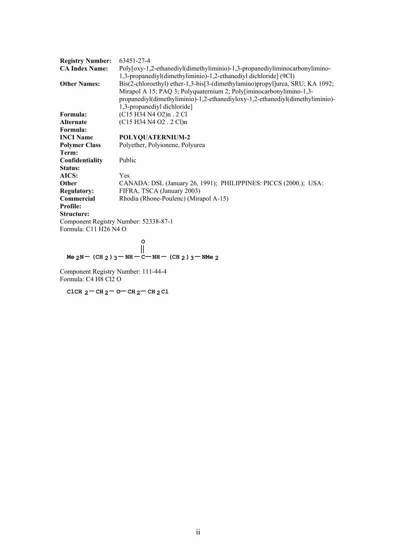
ii

Registry Number: 63451-27-4 CA Index Name: Poly[oxy-1,2-ethanediyl(dimethyliminio)-1,3-propanediyliminocarbonylimino-

1,3-propanediyl(dimethyliminio)-1,2-ethanediyl dichloride] (9CI) Other Names: Bis(2-chloroethyl) ether-1,3-bis[3-(dimethylamino)propyl]urea, SRU; KA 1092;

Mirapol A 15; PAQ 3; Polyquaternium 2; Poly[iminocarbonylimino-1,3-propanediyl(dimethyliminio)-1,2-ethanediyloxy-1,2-ethanediyl(dimethyliminio)-1,3-propanediyl dichloride]

Formula: (C15 H34 N4 O2)n . 2 Cl Alternate Formula:

(C15 H34 N4 O2 . 2 Cl)n

INCI Name POLYQUATERNIUM-2 Polymer Class Term:

Polyether, Polyionene, Polyurea

Confidentiality Status:

Public

AICS: Yes Other Regulatory:

CANADA: DSL (January 26, 1991); PHILIPPINES: PICCS (2000.); USA: FIFRA, TSCA (January 2003)

Commercial Profile:

Rhodia (Rhone-Poulenc) (Mirapol A-15)

Structure: Component Registry Number: 52338-87-1 Formula: C11 H26 N4 O

(CH 2)3(CH 2)3 NMe 2Me 2N NHCNH

O

Component Registry Number: 111-44-4 Formula: C4 H8 Cl2 O

ClCH 2 CH 2ClOCH 2 CH 2

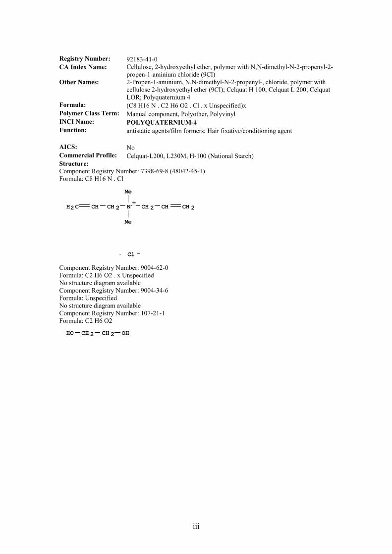
iii

Registry Number: 92183-41-0 CA Index Name: Cellulose, 2-hydroxyethyl ether, polymer with N,N-dimethyl-N-2-propenyl-2-

propen-1-aminium chloride (9CI) Other Names: 2-Propen-1-aminium, N,N-dimethyl-N-2-propenyl-, chloride, polymer with

cellulose 2-hydroxyethyl ether (9CI); Celquat H 100; Celquat L 200; Celquat LOR; Polyquaternium 4

Formula: (C8 H16 N . C2 H6 O2 . Cl . x Unspecified)x Polymer Class Term: Manual component, Polyother, Polyvinyl INCI Name: POLYQUATERNIUM-4 Function: antistatic agents/film formers; Hair fixative/conditioning agent AICS: No Commercial Profile: Celquat-L200, L230M, H-100 (National Starch) Structure: Component Registry Number: 7398-69-8 (48042-45-1) Formula: C8 H16 N . Cl

Me

Me

N CH 2CH 2 CHCH CH 2H2C+

Cl -·

Component Registry Number: 9004-62-0 Formula: C2 H6 O2 . x Unspecified No structure diagram available Component Registry Number: 9004-34-6 Formula: Unspecified No structure diagram available Component Registry Number: 107-21-1 Formula: C2 H6 O2

CH 2 CH 2HO OH

iv

Registry Number: 26006-22-4 CA Index Name: Ethanaminium, N,N,N-trimethyl-2-[(2-methyl-1-oxo-2-propenyl)oxy]-,

methyl sulphate, polymer with 2-propenamide (9CI) Other Names: 2-Propenamide, polymer with N,N,N-trimethyl-2-[(2-methyl-1-oxo-2-

propenyl)oxy]ethanaminium methyl sulphate (9CI); Acrylamide, polymer with choline methyl sulphate methacrylate (8CI); …..Acrylamide-[2-(methacryloyloxy)ethyl]trimethylammonium methyl sulphate polymer; Calgon K 400; Catamer Q; Hercofloc 812; Hercofloc 849; Kayafloc C 599-1F; Polyquaternium 5; Reten 1104; Reten 1105; Reten 1106; Reten 210; Reten 220; Reten 230; Reten 240; Reten 260; Reten 420; Reten SPX 1098

Formula: (C9 H18 N O2 . C3 H5 N O . C H3 O4 S)x Polymer Class Term: Polyacrylic, Polyother INCI Name: POLYQUATERNIUM-5 Function: antistatic agents/film formers AICS: Yes (1996) Other Regulatory: TSCA 2003 (EPA: XU); DSL 1991; ENCS No 6-538; ECL 1997; PICCS 2000 Commercial Profile: Reckitt Benckeser (Calgon); Hercules (Reten 220); Ondeo Nalco (Merquat 5) Structure: Component Registry Number: 79-06-1 Formula: C3 H5 N O

C CHH2N

O

CH 2

Component Registry Number: 6891-44-7 Formula: C9 H18 N O2 . C H3 O4 S No structure diagram Component Registry Number: 33611-56-2 Formula: C9 H18 N O2

Me 3+N MeCH 2 OCH 2 C C

O CH 2

Component Registry Number: 21228-90-0 Formula: C H3 O4 S

Me SO 3-O

v

Registry Number: 26062-79-3 CA Index Name: 2-Propen-1-aminium, N,N-dimethyl-N-2-propenyl-, chloride, homopolymer

(9CI) Other Names: Ammonium, diallyldimethyl-, chloride, polymers (8CI); 261LV; Additol

VXT 3529; Agefloc WT 20; Alcofix; Aronfloc (polymer); Bufloc 536; Calgon, DMDACC, E 904, E 905, E 921; Calgon Polymer 261; Cartafix VXT; Cat-Floc; Certrex 340; CinFix RDF; CM 100; CM 100 (onium compound); Conductive Polymer 261; Croscolor; DADMAC polymer; Danfix 707; Danfix F; Diallyldimethylammonium chloride homopolymer; Diallyldimethylammonium chloride polymer; Dimethyldiallylammonium chloride homopolymer; Dimethyldiallylammonium chloride polymer; E 261; ECCat 2020; Floerger FL; Hydraid 2010, 2020; Jayfloc 842; Kufloc; KZ 106K; KZ 63K; Lectrapel; M 40176; Mackernium 006; Magnafloc 1697, 368; Magnifloc 585C, 587C, 589C, 591C; Merck 261; Merquat 100; Mirapol 100; Mobil ED 87/04; N,N-Diallyl-N,N-dimethylammonium chloride homopolymer; Nalco 2010; PAS 10L; PAS-H 10; PAS-H 10L; PAS-H 1L; PAS-H 35L; PAS-H 35S; PBK 1; PBK 1 (quaternary compound); PCL 2; PDMDAAC; PDMDAC 50; Percol 1620; Percol 1697; Percol 368; Percol 406; Percol 406F; PKB 1;… Poly-DMDAAC; Polydadmac; Polydadmac 570; Polymer 261; Polymer 261LV; Polypure C 318; Polyquat; Polyquaternium 6; Ponilit CP 1; Quaternium 40; Reten 203; Salcare SC 30;

Formula: (C8 H16 N . Cl)x Polymer Class Term: Polyvinyl INCI Name: POLYQUATERNIUM-6 Function: Conditioner, moisturiser (L&G:1999) AICS: Yes Other Regulatory: TSCA 2003 (EPA:XU); DSL 1991; ENCS; ECL 1997; PICCS 2000 Commercial Profile: Ondeo-Nalco (Merquat 100); 3V (Conditioner P6) Structure: Component Registry Number: 7398-69-8 (48042-45-1) Formula: C8 H16 N . Cl

Cl -·

Me

Me

N CH 2CH 2 CHCH CH 2H2C+

vi

Registry Number: 26590-05-6 CA Index Name: 2-Propen-1-aminium, N,N-dimethyl-N-2-propenyl-, chloride, polymer with 2-

propenamide (9CI) Other Names: 2-Propenamide, polymer with N,N-dimethyl-N-2-propenyl-2-propen-1-

aminium chloride (9CI); Acrylamide, polymer with diallyldimethylammonium chloride (8CI); … Acrylamide-DADMAC copolymer; … Agequat 500, 5008, C 3204; Betz 2651; CV 5380; Diallyldimethylammonium chloride-acrylamide copolymer; Dimethyldiallylammonium chloride-acrylamide copolymer; E 949; ECCat 777; Himacs SC 100; Hydraid 777; Kayacryl EC 315, M-N, Resin M-N; Lipoflow MN; Mack K 007; Mackernium 007, 007S; ME Polymer 09W; Merquat 2200, 500, 550, 550L, S; Mirapol 550; Nalco 1470, 8105; PAS-J 11; PAS-J 41; PAS-J 81; PDMDAAC-AM; Poly(acrylamide-dimethyldiallylammonium chloride); Polyquaternium 7; Quaternium 41; Salcare SC 10; Salcare Super 7; WT 2575, 2640, 2860, 5504; XB 54-15-1; XQ 550

Formula: (C8 H16 N . C3 H5 N O . Cl)x Polymer Class Term: Polyacrylic, Polyvinyl INCI Name: POLYQUATERNIUM-7 Function: Function: antistatic agents/film formers; Condition, moisturise, smooth;

rheology builder (L&G:1999) AICS: Yes (1996) Other Regulatory: TSCA 2003 (EPA:XU); DSL 1991; ENCS; ECL 1997; PICCS 2000 Commercial Profile: Ondeo Nalco (Merquat); Rhodia (Mirapol) Structure: Component Registry Number: 7398-69-8 (48042-45-1) Formula: C8 H16 N . Cl

Component Registry Number: 79-06-1 Formula: C3 H5 N O

C CHH2N

O

CH 2

Cl -·

Me

Me

N CH2CH2 CHCH CH2H2C+

vii

Registry Number: 146189-14-2 CA Index Name: 2-Propenoic acid, 2-methyl-, 2-(dimethylamino)ethyl ester, polymer with

methyl 2-methyl-2-propenoate and octadecyl 2-methyl-2-propenoate, compd. with dimethyl sulphate (9CI)

Other Names: 2-Propenoic acid, 2-methyl-, methyl ester, polymer with 2-(dimethylamino)ethyl 2-methyl-2-propenoate and octadecyl 2-methyl-2-propenoate, compd. with dimethyl sulphate (9CI); 2-Propenoic acid, 2-methyl-, octadecyl ester, polymer with 2-(dimethylamino)ethyl 2-methyl-2-propenoate and methyl 2-methyl-2-propenoate, compd. with dimethyl sulphate (9CI); Sulphuric acid, dimethyl ester, compd. with 2-(dimethylamino)ethyl 2-methyl-2-propenoate polymer with methyl 2-methyl-2-propenoate and octadecyl 2-methyl-2-propenoate (9CI); Polyquaternium 8

Formula: (C22 H42 O2 . C8 H15 N O2 . C5 H8 O2)x . x C2 H6 O4 S Polymer Class Term: Polyacrylic INCI Name: POLYQUATERNIUM-8 Function: Function: antistatic agents/film formers Confidentiality Status: Public AICS: No Structure: Component Registry Number: 77-78-1 Formula: C2 H6 O4 S MeO−S(O2)−OMe Component Registry Number: 41510-85-4 Formula: (C22 H42 O2 . C8 H15 N O2 . C5 H8 O2)x Component Registry Number: 32360-05-7 Formula: C22 H42 O2

(CH 2)17 MeMe O C C

O CH 2

Component Registry Number: 2867-47-2 Formula: C8 H15 N O2

MeMe 2N O CCH 2 C

O

CH 2

CH 2

Component Registry Formula: C5 H8 O2Number: 80-62-6

Me OMeCC

OH2C

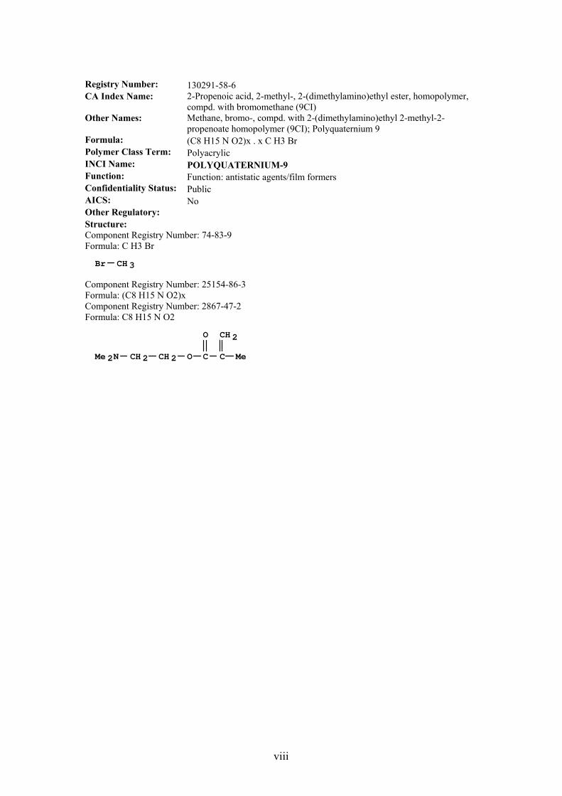
viii

Registry Number: 130291-58-6 CA Index Name: 2-Propenoic acid, 2-methyl-, 2-(dimethylamino)ethyl ester, homopolymer,

compd. with bromomethane (9CI) Other Names: Methane, bromo-, compd. with 2-(dimethylamino)ethyl 2-methyl-2-

propenoate homopolymer (9CI); Polyquaternium 9 Formula: (C8 H15 N O2)x . x C H3 Br Polymer Class Term: Polyacrylic INCI Name: POLYQUATERNIUM-9 Function: Function: antistatic agents/film formers Confidentiality Status: Public AICS: No Other Regulatory: Structure: Component Registry Number: 74-83-9 Formula: C H3 Br

Br CH 3

Component Registry Number: 25154-86-3 Formula: (C8 H15 N O2)x Component Registry Number: 2867-47-2 Formula: C8 H15 N O2

MeMe 2N O CCH 2 C

O

CH 2

CH 2

ix

Registry Number: 81859-24-7 CA Index Name: Cellulose, 2-hydroxyethyl 2-[2-hydroxy-3-

(trimethylammonio)propoxy]ethyl 2-hydroxy-3-(trimethylammonio)propyl ether, chloride (9CI)

Other Names: Amerchol JR 400; Catinal HC 100; Catinal HC 35; Catinal LC 100; Celquat SC 230M; Celquat SC 240C; JR 1; JR 125; JR 30M; JR 400; KG 30M; Leogard G; Leogard GP; Leogard LP; Leogard P; LR 300M; LR 400; Polymer JR 400; Polymer KG 30M; Polymer LR 30M; Polyquaternium 10; Quaternium 19; Ritaquat 3000; Ritaquat 400KG; Ucare JR 125; Ucare JR 400; UCARE Polymer JR; UCARE Polymer JR 125; UCARE Polymer JR 30; UCARE Polymer JR 30M; UCARE Polymer JR 400; UCARE Polymer JR 40M; UCARE Polymer KG 30M; UCARE Polymer LR; UCARE Polymer LR 30M; UCARE Polymer LR 400; UCARE Polymer SR 10

Formula: C8 H20 N O3 . x C6 H16 N O2 . x C2 H6 O2 . x Cl . x Unspecified Polymer Class Term: Manual registration INCI Name: POLYQUATERNIUM-10 Function: antistatic agents/film formers Confidentiality Status: Public AICS: Yes (1996) Other Regulatory: ECL 1997; PICCS 2000; Commercial Profile: Akzo Noble (Leogard); National Starch (Celquat); Amerchol (Dow

Corning) (UCARE) Structure: Component Registry Number: 170553-71-6 Formula: C8 H20 N O3 . x C6 H16 N O2 . x C2 H6 O2 . x Unspecified

Me 3+N CH 2 CH CH 2

OH

O CH 2 CH 2 OH

Component Registry Number: 170344-46-4 Formula: C8 H20 N O3

N+Me 3CH 2CHCH 2

OH

HO

Component Registry Number: 44814-66-6 Formula: C6 H16 N O2 No Structure Diagram Available Component Registry Number: 9004-34-6 Formula: Unspecified Component Registry Number: 107-21-1 Formula: C2 H6 O2

CH 2 CH 2HO OH

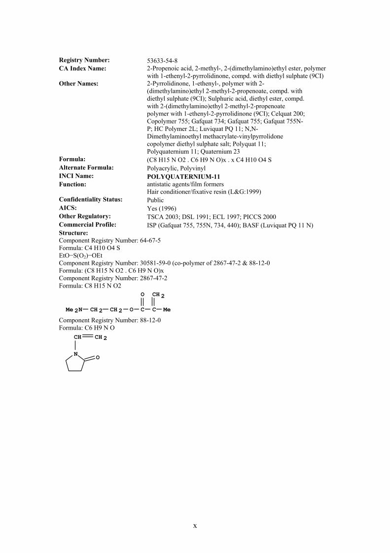
x

Registry Number: 53633-54-8 CA Index Name: 2-Propenoic acid, 2-methyl-, 2-(dimethylamino)ethyl ester, polymer

with 1-ethenyl-2-pyrrolidinone, compd. with diethyl sulphate (9CI) Other Names: 2-Pyrrolidinone, 1-ethenyl-, polymer with 2-

(dimethylamino)ethyl 2-methyl-2-propenoate, compd. with diethyl sulphate (9CI); Sulphuric acid, diethyl ester, compd. with 2-(dimethylamino)ethyl 2-methyl-2-propenoate polymer with 1-ethenyl-2-pyrrolidinone (9CI); Celquat 200; Copolymer 755; Gafquat 734; Gafquat 755; Gafquat 755N-P; HC Polymer 2L; Luviquat PQ 11; N,N-Dimethylaminoethyl methacrylate-vinylpyrrolidone copolymer diethyl sulphate salt; Polyquat 11; Polyquaternium 11; Quaternium 23

Formula: (C8 H15 N O2 . C6 H9 N O)x . x C4 H10 O4 S Alternate Formula: Polyacrylic, Polyvinyl INCI Name: POLYQUATERNIUM-11 Function: antistatic agents/film formers

Hair conditioner/fixative resin (L&G:1999) Confidentiality Status: Public AICS: Yes (1996) Other Regulatory: TSCA 2003; DSL 1991; ECL 1997; PICCS 2000 Commercial Profile: ISP (Gafquat 755, 755N, 734, 440); BASF (Luviquat PQ 11 N) Structure: Component Registry Number: 64-67-5 Formula: C4 H10 O4 S EtO−S(O2)−OEt Component Registry Number: 30581-59-0 (co-polymer of 2867-47-2 & 88-12-0 Formula: (C8 H15 N O2 . C6 H9 N O)x Component Registry Number: 2867-47-2 Formula: C8 H15 N O2

Component Registry Number: 88-12-0 Formula: C6 H9 N O

CH CH 2

N O

MeMe 2N O CCH 2 C

O

CH 2

CH 2

xi

Registry Number: 68877-50-9

CA Index Name:

2-Propenoic acid, 2-methyl-, [(1R,4aR,4bR,10aR)-1,2,3,4,4a,4b,5,6,10,10a-decahydro-1,4a-dimethyl-7-(1-methylethyl)-1-phenanthrenyl]methyl ester, polymer with 2-(diethylamino)ethyl 2-methyl-2-propenoate and ethyl 2-methyl-2-propenoate, compd. with dimethyl sulphate (9CI)

Formula: (C24 H36 O2 . C10 H19 N O2 . C6 H10 O2)x . x C2 H6 O4 S Polymer Class Term: Polyacrylic INCI Name: POLYQUATERNIUM-12 AICS: No Other Regulatory: TSCA 2003 (EPA:XU); NDSL 1998 Structure: Component Registry Number: 77-78-1 Formula: C2 H6 O4 S Component Registry Number: 68877-49-6 Formula: (C24 H36 O2 . C10 H19 N O2 . C6 H10 O2)x Component Registry Number: 68877-48-5 Absolute stereochemistry. Formula: C24 H36 O2

MeO−S(O2)−OMe

Pr-i

Me

MeMe

O

O

CH 2

H

H

R

R

R

R

Component Registry Number: 105-16-8 Formula: C10 H19 N O2

NEt 2Me CH 2CH 2OCC

OH2C

Component Registry Number: 97-63-2 Formula: C6 H10 O2

OEtMe CC

OH2C

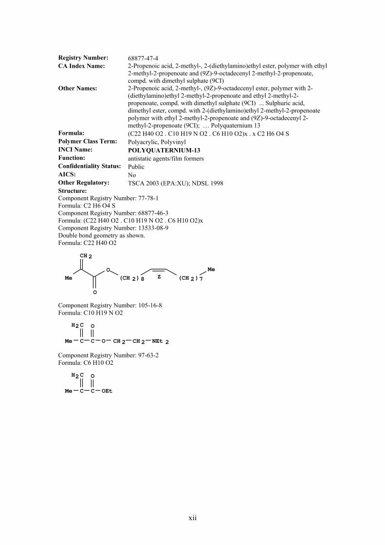
xii

Registry Number: 68877-47-4 CA Index Name: 2-Propenoic acid, 2-methyl-, 2-(diethylamino)ethyl ester, polymer with ethyl

2-methyl-2-propenoate and (9Z)-9-octadecenyl 2-methyl-2-propenoate, compd. with dimethyl sulphate (9CI)

Other Names: 2-Propenoic acid, 2-methyl-, (9Z)-9-octadecenyl ester, polymer with 2-(diethylamino)ethyl 2-methyl-2-propenoate and ethyl 2-methyl-2-propenoate, compd. with dimethyl sulphate (9CI) ... Sulphuric acid, dimethyl ester, compd. with 2-(diethylamino)ethyl 2-methyl-2-propenoate polymer with ethyl 2-methyl-2-propenoate and (9Z)-9-octadecenyl 2-methyl-2-propenoate (9CI); … Polyquaternium 13

Formula: (C22 H40 O2 . C10 H19 N O2 . C6 H10 O2)x . x C2 H6 O4 S Polymer Class Term: Polyacrylic, Polyvinyl INCI Name: POLYQUATERNIUM-13 Function: antistatic agents/film formers Confidentiality Status: Public AICS: No Other Regulatory: TSCA 2003 (EPA:XU); NDSL 1998 Structure: Component Registry Number: 77-78-1 Formula: C2 H6 O4 S Component Registry Number: 68877-46-3 Formula: (C22 H40 O2 . C10 H19 N O2 . C6 H10 O2)x Component Registry Number: 13533-08-9 Double bond geometry as shown. Formula: C22 H40 O2

(CH 2)8 (CH 2)7MeMeO

O

CH 2

Z

Component Registry Number: 105-16-8 Formula: C10 H19 N O2

NEt 2Me CH 2CH 2OCC

OH2C

Component Registry Number: 97-63-2 Formula: C6 H10 O2

OEtMe CC

OH2C

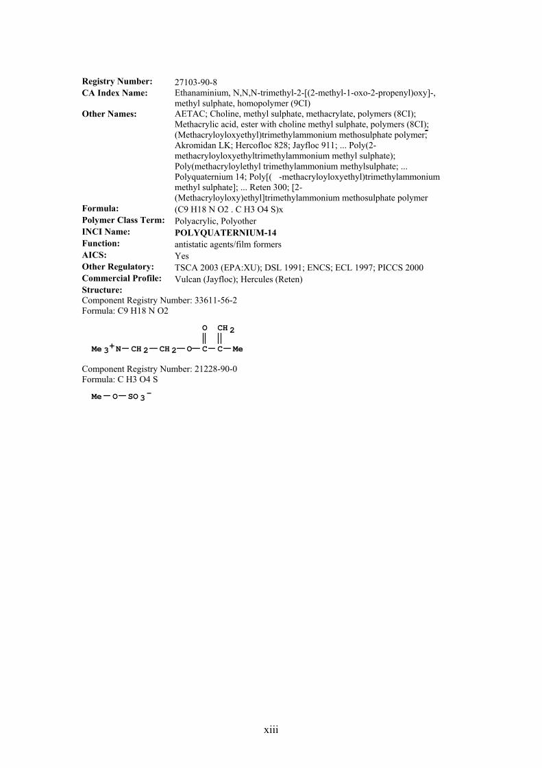
xiii

Registry Number: 27103-90-8 CA Index Name: Ethanaminium, N,N,N-trimethyl-2-[(2-methyl-1-oxo-2-propenyl)oxy]-,

methyl sulphate, homopolymer (9CI) Other Names: AETAC; Choline, methyl sulphate, methacrylate, polymers (8CI);

Methacrylic acid, ester with choline methyl sulphate, polymers (8CI); (Methacryloyloxyethyl)trimethylammonium methosulphate polymer; Akromidan LK; Hercofloc 828; Jayfloc 911; ... Poly(2-methacryloyloxyethyltrimethylammonium methyl sulphate); Poly(methacryloylethyl trimethylammonium methylsulphate; ... Polyquaternium 14; Poly[(-methacryloyloxyethyl)trimethylammonium methyl sulphate]; ... Reten 300; [2-(Methacryloyloxy)ethyl]trimethylammonium methosulphate polymer

Formula: (C9 H18 N O2 . C H3 O4 S)x Polymer Class Term: Polyacrylic, Polyother INCI Name: POLYQUATERNIUM-14 Function: antistatic agents/film formers AICS: Yes Other Regulatory: TSCA 2003 (EPA:XU); DSL 1991; ENCS; ECL 1997; PICCS 2000 Commercial Profile: Vulcan (Jayfloc); Hercules (Reten) Structure: Component Registry Number: 33611-56-2 Formula: C9 H18 N O2

Me 3+N MeCH 2 OCH 2 C C

O CH 2

Component Registry Number: 21228-90-0 Formula: C H3 O4 S

Me SO 3-O

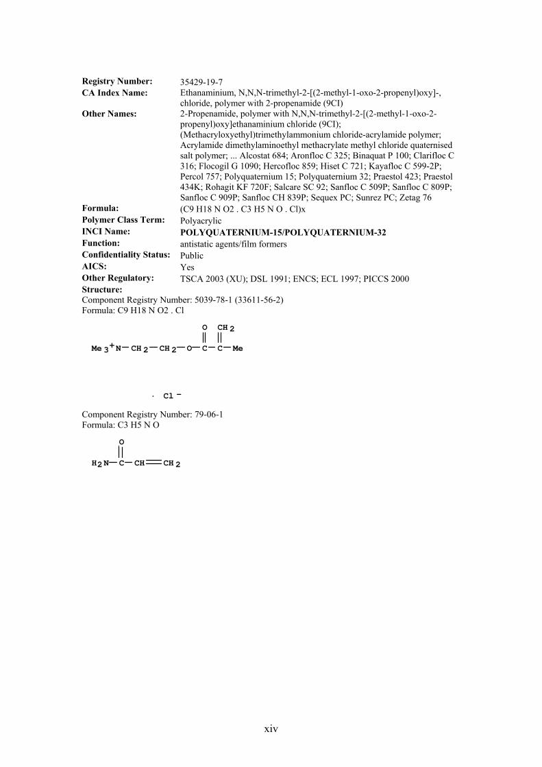
xiv

Registry Number: 35429-19-7 CA Index Name: Ethanaminium, N,N,N-trimethyl-2-[(2-methyl-1-oxo-2-propenyl)oxy]-,

chloride, polymer with 2-propenamide (9CI) Other Names: 2-Propenamide, polymer with N,N,N-trimethyl-2-[(2-methyl-1-oxo-2-

propenyl)oxy]ethanaminium chloride (9CI); (Methacryloxyethyl)trimethylammonium chloride-acrylamide polymer; Acrylamide dimethylaminoethyl methacrylate methyl chloride quaternised salt polymer; ... Alcostat 684; Aronfloc C 325; Binaquat P 100; Clarifloc C 316; Flocogil G 1090; Hercofloc 859; Hiset C 721; Kayafloc C 599-2P; Percol 757; Polyquaternium 15; Polyquaternium 32; Praestol 423; Praestol 434K; Rohagit KF 720F; Salcare SC 92; Sanfloc C 509P; Sanfloc C 809P; Sanfloc C 909P; Sanfloc CH 839P; Sequex PC; Sunrez PC; Zetag 76

Formula: (C9 H18 N O2 . C3 H5 N O . Cl)x Polymer Class Term: Polyacrylic INCI Name: POLYQUATERNIUM-15/POLYQUATERNIUM-32 Function: antistatic agents/film formers Confidentiality Status: Public AICS: Yes Other Regulatory: TSCA 2003 (XU); DSL 1991; ENCS; ECL 1997; PICCS 2000 Structure: Component Registry Number: 5039-78-1 (33611-56-2) Formula: C9 H18 N O2 . Cl

Me 3+N MeCH 2 OCH 2 C C

O CH 2

Cl -·

Component Registry Number: 79-06-1 Formula: C3 H5 N O

C CHH2N

O

CH 2

xv

Registry Number: 95144-24-4 CA Index Name: 1H-Imidazolium, 1-ethenyl-3-methyl-, chloride, polymer with 1-ethenyl-2-

pyrrolidinone (9CI) Other Names: 2-Pyrrolidinone, 1-ethenyl-, polymer with 1-ethenyl-3-methyl-1H-

imidazolium chloride (9CI); 1-Ethenyl-2-pyrrolidinone-imidazolimine compd. with chloromethane; 1-Vinyl-3-methylimidazolinium chloride-1-vinylpyrrolidone copolymer; Luviquat FC 370; Luviquat FC 500; Luviquat FC 550; Luviquat FC 905; Luviquat FC 9059; Luviquat HM 550; Luviquat HM 552; Luviquat SC 370; Polyquaternium 16

Formula: (C6 H9 N2 . C6 H9 N O . Cl)x Polymer Class Term: Polyvinyl INCI Name: POLYQUATERNIUM-16 Function: antistatic agents/film formers; Substantive conditioner, film former Confidentiality Status: Public AICS: Yes Other Regulatory: DSL 1991; ECL 1997; PICCS 2000 Commercial Profile: BASF (Luviquat FC 370, Luviquat FC 550, Luviquat HM 552, Luviquat

style, Luviquat Excellence) Structure: Component Registry Number: 13474-25-4 (45534-45-0) Formula: C6 H9 N2 . Cl *** FRAGMENT DIAGRAM IS INCOMPLETE ***

Me

CH CH 2

N

N

Cl-

Component Registry Number: 88-12-0 Formula: C6 H9 N O

CH CH 2

N O

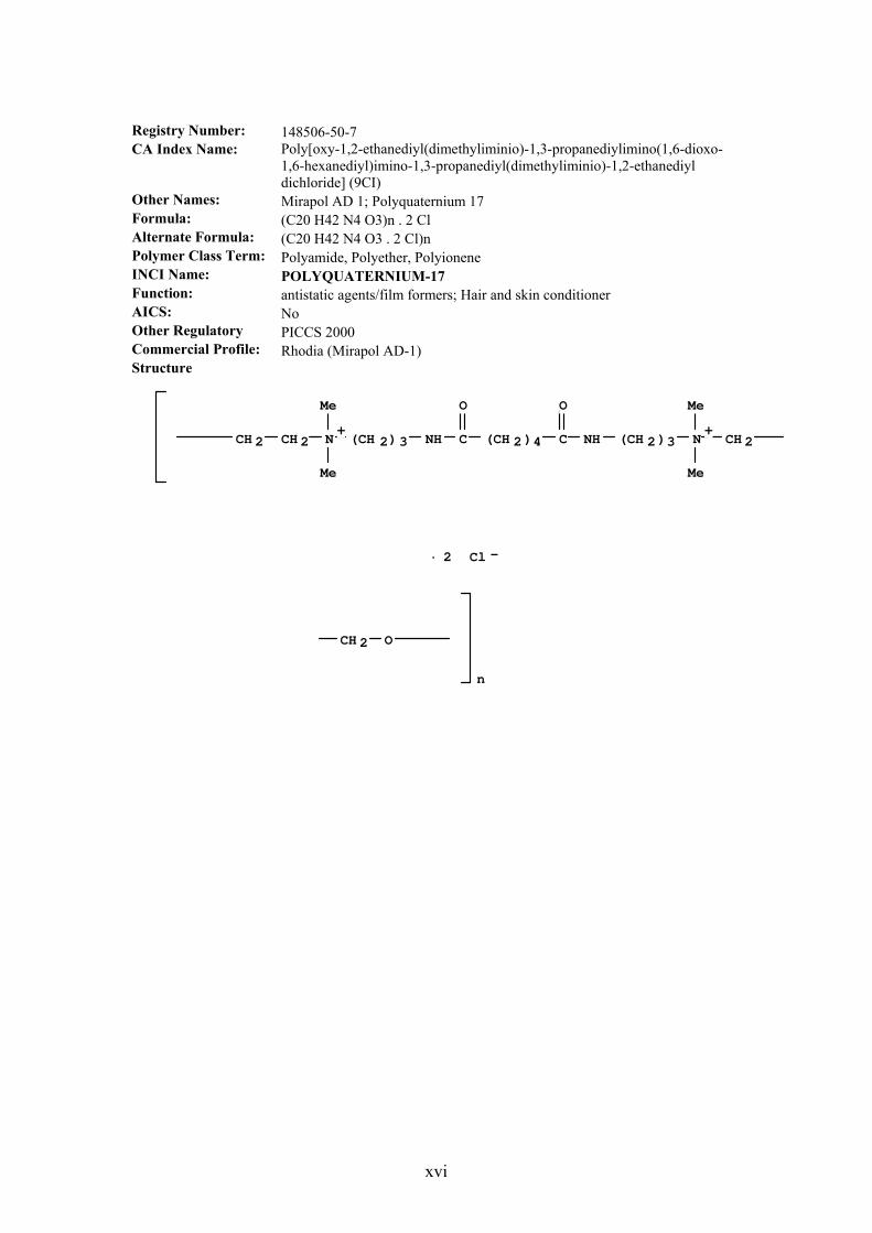
xvi

Registry Number: 148506-50-7 CA Index Name: Poly[oxy-1,2-ethanediyl(dimethyliminio)-1,3-propanediylimino(1,6-dioxo-

1,6-hexanediyl)imino-1,3-propanediyl(dimethyliminio)-1,2-ethanediyl dichloride] (9CI)

Other Names: Mirapol AD 1; Polyquaternium 17 Formula: (C20 H42 N4 O3)n . 2 Cl Alternate Formula: (C20 H42 N4 O3 . 2 Cl)n Polymer Class Term: Polyamide, Polyether, Polyionene INCI Name: POLYQUATERNIUM-17 Function: antistatic agents/film formers; Hair and skin conditioner AICS: No Other Regulatory PICCS 2000 Commercial Profile: Rhodia (Mirapol AD-1) Structure

(CH 2)3(CH 2)4(CH 2)3

Me

Me

Me

Me

NH NC CH 2

O

CNH

O

NCH 2CH 2++

Cl -2·

CH 2 O

n

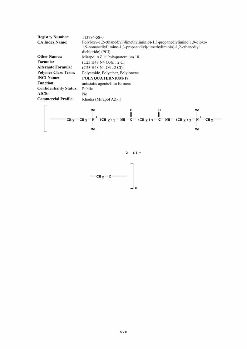
xvii

Registry Number: 113784-58-0 CA Index Name: Poly[oxy-1,2-ethanediyl(dimethyliminio)-1,3-propanediylimino(1,9-dioxo-

1,9-nonanediyl)imino-1,3-propanediyl(dimethyliminio)-1,2-ethanediyl dichloride] (9CI)

Other Names: Mirapol AZ 1; Polyquaternium 18 Formula: (C23 H48 N4 O3)n . 2 Cl Alternate Formula: (C23 H48 N4 O3 . 2 Cl)n Polymer Class Term: Polyamide, Polyether, Polyionene INCI Name: POLYQUATERNIUM-18 Function: antistatic agents/film formers Confidentiality Status: Public AICS: No Commercial Profile: Rhodia (Mirapol AZ-1)

(CH 2)3(CH 2)7(CH 2)3

Me

Me

Me

Me

N CH 2NHC

O

CNH

O

NCH 2CH 2++

Cl -2·

CH 2 O

n

xviii

Registry Number: 110736-85-1 CA Index Name: Polyquaternium 19 (9CI) Other Names: Arlatone PQ 220 Formula: Unspecified Polymer Class Term: Manual Registration INCI Name: POLYQUATERNIUM-19 Function: antistatic agents/film formers Confidentiality Status: Public AICS: No Commercial Profile: Arlatone = Uniqema Structure: No Structure Diagram Available Registry Number: 110736-86-2 CA Index Name: Polyquaternium 20 (9CI) Other Names: Arlatone PQ 225 Formula: Unspecified Polymer Class Term: INCI Name: POLYQUATERNIUM-20 Function: antistatic agents/film formers Confidentiality Status: Public AICS: No Commercial Profile: Arlatone = Uniqema Structure: No Structure diagram available

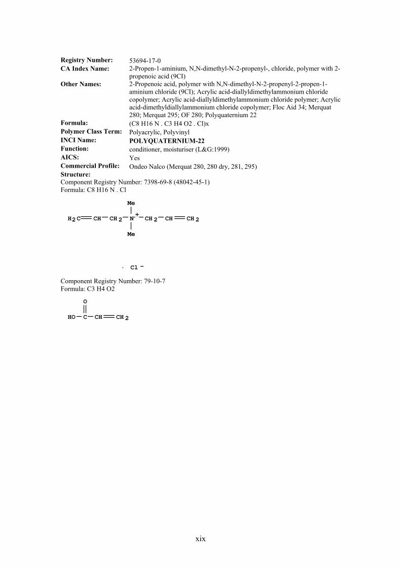
xix

Registry Number: 53694-17-0 CA Index Name: 2-Propen-1-aminium, N,N-dimethyl-N-2-propenyl-, chloride, polymer with 2-

propenoic acid (9CI) Other Names: 2-Propenoic acid, polymer with N,N-dimethyl-N-2-propenyl-2-propen-1-

aminium chloride (9CI); Acrylic acid-diallyldimethylammonium chloride copolymer; Acrylic acid-diallyldimethylammonium chloride polymer; Acrylic acid-dimethyldiallylammonium chloride copolymer; Floc Aid 34; Merquat 280; Merquat 295; OF 280; Polyquaternium 22

Formula: (C8 H16 N . C3 H4 O2 . Cl)x Polymer Class Term: Polyacrylic, Polyvinyl INCI Name: POLYQUATERNIUM-22 Function: conditioner, moisturiser (L&G:1999) AICS: Yes Commercial Profile: Ondeo Nalco (Merquat 280, 280 dry, 281, 295) Structure: Component Registry Number: 7398-69-8 (48042-45-1) Formula: C8 H16 N . Cl

Me

Me

N CH 2CH 2 CHCH CH 2H2C+

Cl -·

Component Registry Number: 79-10-7 Formula: C3 H4 O2

C CH

O

HO CH 2

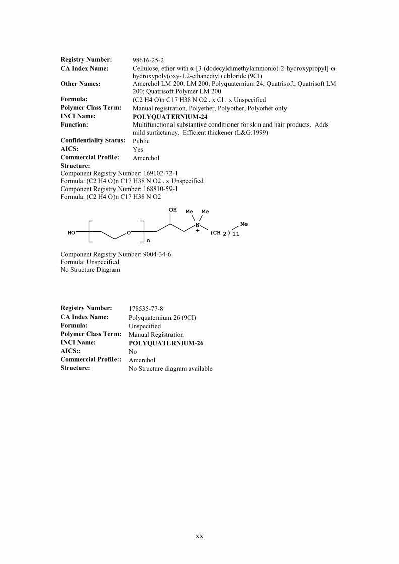
xx

Registry Number: 98616-25-2 CA Index Name: Cellulose, ether with α-[3-(dodecyldimethylammonio)-2-hydroxypropyl]-ω-

hydroxypoly(oxy-1,2-ethanediyl) chloride (9CI) Other Names: Amerchol LM 200; LM 200; Polyquaternium 24; Quatrisoft; Quatrisoft LM

200; Quatrisoft Polymer LM 200 Formula: (C2 H4 O)n C17 H38 N O2 . x Cl . x Unspecified Polymer Class Term: Manual registration, Polyether, Polyother, Polyother only INCI Name: POLYQUATERNIUM-24 Function: Multifunctional substantive conditioner for skin and hair products. Adds

mild surfactancy. Efficient thickener (L&G:1999) Confidentiality Status: Public AICS: Yes Commercial Profile: Amerchol Structure: Component Registry Number: 169102-72-1 Formula: (C2 H4 O)n C17 H38 N O2 . x Unspecified Component Registry Number: 168810-59-1 Formula: (C2 H4 O)n C17 H38 N O2

n(CH 2)11

MeMe

MeN

OH

OHO +

Component Registry Number: 9004-34-6 Formula: Unspecified No Structure Diagram Registry Number: 178535-77-8 CA Index Name: Polyquaternium 26 (9CI) Formula: Unspecified Polymer Class Term: Manual Registration INCI Name: POLYQUATERNIUM-26 AICS:: No Commercial Profile:: Amerchol Structure: No Structure diagram available

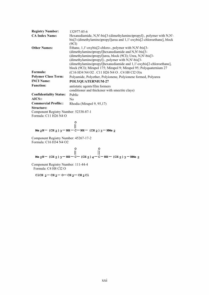
xxi

Registry Number: 132977-85-6 CA Index Name: Hexanediamide, N,N'-bis[3-(dimethylamino)propyl]-, polymer with N,N'-

bis[3-(dimethylamino)propyl]urea and 1,1'-oxybis[2-chloroethane], block (9CI)

Other Names: Ethane, 1,1'-oxybis[2-chloro-, polymer with N,N'-bis[3-(dimethylamino)propyl]hexanediamide and N,N'-bis[3-(dimethylamino)propyl]urea, block (9CI); Urea, N,N'-bis[3-(dimethylamino)propyl]-, polymer with N,N'-bis[3-(dimethylamino)propyl]hexanediamide and 1,1'-oxybis[2-chloroethane], block (9CI); Mirapol 175; Mirapol 9; Mirapol 95; Polyquaternium 27

Formula: (C16 H34 N4 O2 . C11 H26 N4 O . C4 H8 Cl2 O)x Polymer Class Term: Polyamide, Polyether, Polyionene, Polyionene formed, Polyurea INCI Name: POLYQUATERNIUM-27 Function: antistatic agents/film formers

conditioner and thickener with smectite clays) Confidentiality Status: Public AICS:: No Commercial Profile:: Rhodia (Mirapol 9, 95,17) Structure: Component Registry Number: 52338-87-1 Formula: C11 H26 N4 O

(CH 2)3(CH 2)3 NMe 2Me 2N NHCNH

O

Component Registry Number: 45267-17-2 Formula: C16 H34 N4 O2

(CH 2)4 (CH 2)3(CH 2)3 NMe 2Me 2N C NH

O

CNH

O

Component Registry Number: 111-44-4

Formula: C4 H8 Cl2 O

ClCH 2 CH 2ClOCH 2 CH 2

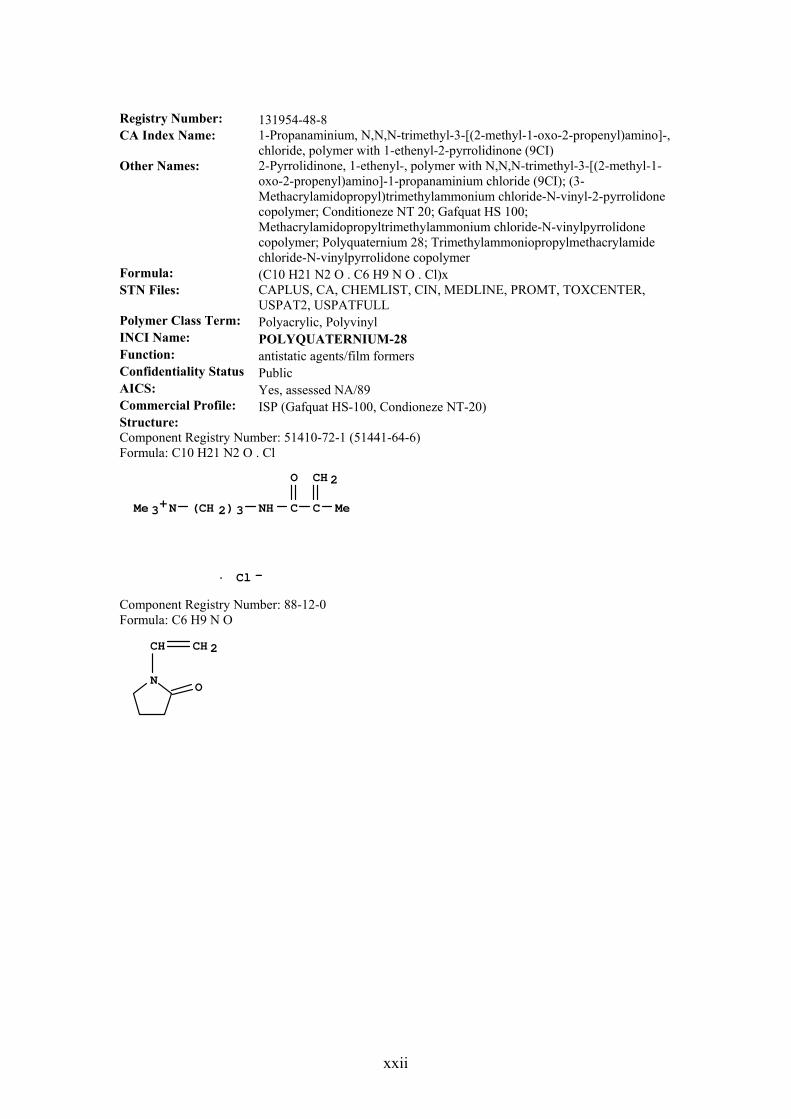
xxii

Registry Number: 131954-48-8 CA Index Name: 1-Propanaminium, N,N,N-trimethyl-3-[(2-methyl-1-oxo-2-propenyl)amino]-,

chloride, polymer with 1-ethenyl-2-pyrrolidinone (9CI) Other Names: 2-Pyrrolidinone, 1-ethenyl-, polymer with N,N,N-trimethyl-3-[(2-methyl-1-

oxo-2-propenyl)amino]-1-propanaminium chloride (9CI); (3-Methacrylamidopropyl)trimethylammonium chloride-N-vinyl-2-pyrrolidone copolymer; Conditioneze NT 20; Gafquat HS 100; Methacrylamidopropyltrimethylammonium chloride-N-vinylpyrrolidone copolymer; Polyquaternium 28; Trimethylammoniopropylmethacrylamide chloride-N-vinylpyrrolidone copolymer

Formula: (C10 H21 N2 O . C6 H9 N O . Cl)x STN Files: CAPLUS, CA, CHEMLIST, CIN, MEDLINE, PROMT, TOXCENTER,

USPAT2, USPATFULL Polymer Class Term: Polyacrylic, Polyvinyl INCI Name: POLYQUATERNIUM-28 Function: antistatic agents/film formers Confidentiality Status Public AICS: Yes, assessed NA/89 Commercial Profile: ISP (Gafquat HS-100, Condioneze NT-20) Structure: Component Registry Number: 51410-72-1 (51441-64-6) Formula: C10 H21 N2 O . Cl

(CH 2)3 MeMe 3+N NH C C

O CH 2

Cl -·

Component Registry Number: 88-12-0 Formula: C6 H9 N O

CH CH 2

N O

xxiii

Registry Number: 148880-30-2 CA Index Name: Polyquaternium 29 (9CI) Other Names: Lexquat CH Formula: Unspecified Polymer Class Term: Manual registration INCI Name: POLYQUATERNIUM-29 Function: antistatic agents/film formers Confidentiality Status Public AICS No Structure No Structure diagram available Registry Number: 147398-77-4 CA Index Name: Ethanaminium, N-(carboxymethyl)-N,N-dimethyl-2-[(2-methyl-1-oxo-2-

propenyl)oxy]-, inner salt, polymer with methyl 2-methyl-2-propenoate (9CI) Other Names: 2-Propenoic acid, 2-methyl-, methyl ester, polymer with N-(carboxymethyl)-

N,N-dimethyl-2-[(2-methyl-1-oxo-2-propenyl)oxy]ethanaminium inner salt (9CI); Mexomere PX; Polyquaternium 30

Formula: (C10 H17 N O4 . C5 H8 O2)x Polymer Class Term: Polyacrylic INCI Name: POLYQUATERNIUM-30 Function: antistatic agents/film formers Confidentiality Status Public AICS No Structure: Component Registry Number: 62723-61-9 Formula: C10 H17 N O4

Me

Me

Me-O2C N CH 2CH 2 CH 2 O C C

O CH 2

+

Component Registry Number: 80-62-6 Formula: C5 H8 O2

Me OMeCC

OH2C

xxiv

Registry Number: 136505-02-7 CA Index Name: 2-Propenenitrile, homopolymer, hydrolysed, block, reaction products with

N,N-dimethyl-1,3-propanediamine, di-Et sulphate-quaternised Formula: Unspecified Polymer Class Term: Manual registration INCI Name: POLYQUATERNIUM-31 Function: antistatic agents/film formers Confidentiality Status: Public AICS: No Structure: No structure diagram available Registry Number: 69418-26-4 CA Index Name: Ethanaminium, N,N,N-trimethyl-2-[(1-oxo-2-propenyl)oxy]-, chloride,

polymer with 2-propenamide (9CI) Other Names: 2-Propenamide, polymer with N,N,N-trimethyl-2-[(1-oxo-2-

propenyl)oxy]ethanaminium chloride (9CI); Acrylamide-(2-acryloxyethyl)trimethylammonium chloride copolymer; ... Acryloyloxyethyltrimethylammonium chloride-acrylamide copolymer; Betz 2680; Himoloc MP 284; Kayafloc C 599-1R; LBN 66; Magnafloc 292; Magnifloc 491C, 492C, 494C, 496C; Nalco 1460; Percol 140; Percol 455; Polyquaternium 33; Salcare SC 93; Zetag 32; Zetag 57, 63, 64, 89; ; Kayafloc C 599-1R; LBN 66; Magnafloc 292; Magnifloc 491C, 494C, 496C; Nalco 1460; Percol 140, 455; Polyquaternium 33; Salcare SC 93; Zetag 32, 57, 63, 64, 89

Formula: (C8 H16 N O2 . C3 H5 N O . Cl)x Polymer Class Term: Polyacrylic INCI Name: POLYQUATERNIUM-33 Function: antistatic agents/film formers Confidentiality Status: Public AICS: Yes Other Regulatory: TSCA 2003 (XU); DSL 1991; ENCS; ECL 1997; PICCS 2000 Commercial Profile: Ciba (Magnafloc); Cytec (Magnifloc); Applied Polymerics (Percol) Structure: Component Registry Number: 44992-01-0 (20284-80-4) Formula: C8 H16 N O2 . Cl

Component Registry Number: 79-06-1 Formula: C3 H5 N O

C CHH2N

O

CH 2

Me 3+N OCH 2 CCH 2 CH

O

CH 2

Cl -·

xxv

Registry Number: 189767-68-8 CA Index Name: Polyquaternium-34 (9CI) Other Names: Formula: Unspecified Polymer Class Term: Manual Registration INCI Name: POLYQUATERNIUM-34 Function: antistatic agents/film formers Confidentiality Status Public AICS No Other Regulatory Structure No Structure diagram available OR?????? Registry Number: 143747-73-7 CA Index Name: Polyquaternium 34 (9CI) Other Names: Formula: Unspecified Polymer Class Term: Manual Registration INCI Name: POLYQUATERNIUM-34 Function: antistatic agents/film formers Confidentiality Status: Public AICS: NA/475

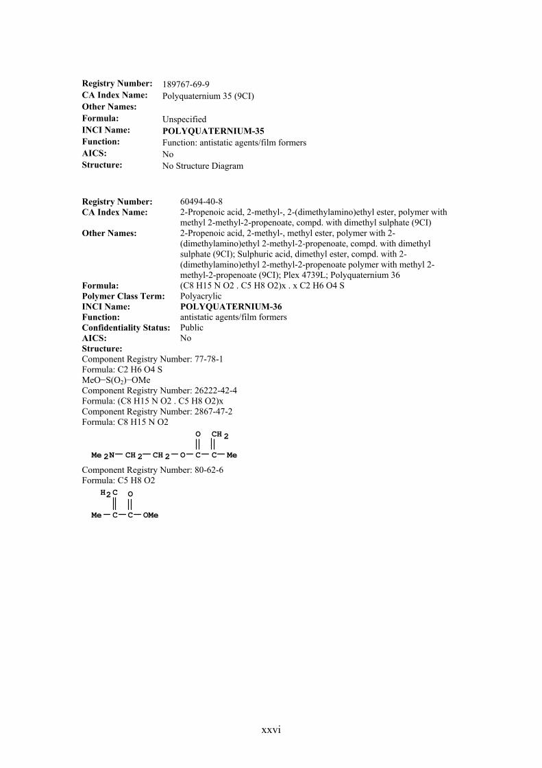
xxvi

Registry Number: 189767-69-9 CA Index Name: Polyquaternium 35 (9CI) Other Names: Formula: Unspecified INCI Name: POLYQUATERNIUM-35 Function: Function: antistatic agents/film formers AICS: No Structure: No Structure Diagram Registry Number: 60494-40-8 CA Index Name: 2-Propenoic acid, 2-methyl-, 2-(dimethylamino)ethyl ester, polymer with

methyl 2-methyl-2-propenoate, compd. with dimethyl sulphate (9CI) Other Names: 2-Propenoic acid, 2-methyl-, methyl ester, polymer with 2-

(dimethylamino)ethyl 2-methyl-2-propenoate, compd. with dimethyl sulphate (9CI); Sulphuric acid, dimethyl ester, compd. with 2-(dimethylamino)ethyl 2-methyl-2-propenoate polymer with methyl 2-methyl-2-propenoate (9CI); Plex 4739L; Polyquaternium 36

Formula: (C8 H15 N O2 . C5 H8 O2)x . x C2 H6 O4 S Polymer Class Term: Polyacrylic INCI Name: POLYQUATERNIUM-36 Function: antistatic agents/film formers Confidentiality Status: Public AICS: No Structure: Component Registry Number: 77-78-1 Formula: C2 H6 O4 S MeO−S(O2)−OMe Component Registry Number: 26222-42-4 Formula: (C8 H15 N O2 . C5 H8 O2)x Component Registry Number: 2867-47-2 Formula: C8 H15 N O2

Component Registry Number: 80-62-6 Formula: C5 H8 O2

Me OMeCC

OH2C

MeMe 2N O CCH 2 C

O

CH 2

CH 2

xxvii

Registry Number: 26161-33-1 CA Index Name: Ethanaminium, N,N,N-trimethyl-2-[(2-methyl-1-oxo-2-propenyl)oxy]-,

chloride, homopolymer (9CI) Other Names: Choline, chloride, methacrylate, polymers (8CI); Methacrylic acid, ester

with choline chloride, polymers (8CI); (Methacryloxyethyl)trimethylammonium chloride polymer; Alcostat 567; Evagrowth C 104G; Flocogil C 4; Himoloc MP 173H; Kayafloc C 599; Methacryloxyethyltrimethylammonium chloride homopolymer; … Praestol 444K; Sanfloc C 009P; Shallol DM 283P, 663P; Synthalen CR; Trimethylaminoethyl methacrylate chloride polymer; Trimethylammonioethyl methacrylate chloride polymer; Zetag 88N; [2-(Methacryloyloxy)ethyl]trimethylammonium chloride polymer

Formula: (C9 H18 N O2 . Cl)x Polymer Class Term: Polyacrylic INCI Name: POLYQUATERNIUM-37 Function: antistatic agents/film formers Confidentiality Status: Public AICS: Yes (1996) Other Regulatory: DSL (1991); ENCS; ECL (1997); PICCS (2000); TSCA (2003) Structure: Component Registry Number: 5039-78-1 (33611-56-2) Formula: C9 H18 N O2 . Cl

Cl -Me 3+N MeCH 2 OCH 2 C C

O CH 2

xxviii

Registry Number: 25136-75-8 CA Index Name: 2-Propen-1-aminium, N,N-dimethyl-N-2-propenyl-, chloride, polymer with 2-

propenamide and 2-propenoic acid (9CI) Other Names: 2-Propenamide, polymer with N,N-dimethyl-N-2-propenyl-2-propen-1-

aminium chloride and 2-propenoic acid (9CI) ... Acrylamide, polymer with acrylic acid and diallyldimethylammonium chloride (8CI); Acrylic acid, polymer with acrylamide and diallyldimethylammonium chloride (8CI); Ammonium, diallyldimethyl-, chloride, polymer with acrylamide and acrylic acid (8CI); … ECCat 7951; Merquat 3300, 3330, 3331, Plus 3300, Plus 3330, Plus 3331; Polyquaternium 39; XQ 3330

Formula: (C8 H16 N . C3 H5 N O . C3 H4 O2 . Cl)x Polymer Class Term: Polyacrylic, Polyvinyl INCI Name: POLYQUATERNIUM-39 Function: antistatic agents/film formers AICS Yes Other Regulatory TSCA 2003; DSL 1998; EPA: XU; EPA Pesticide Inert Ingredients, List 3:

Inerts of unknown toxicity. Structure: Component Registry Number: 7398-69-8 (48042-45-1) Formula: C8 H16 N . Cl

Component Registry Number: 79-10-7 Formula: C3 H4 O2

C CH

O

HO CH 2

Component Registry Number: 79-06-1 Formula: C3 H5 N O

C CHH2N

O

CH 2

Cl -

Me

Me

N CH 2CH 2 CHCH CH 2H2C+

xxix

Registry Number: 31512-74-0 CA Index Name: Poly[oxy-1,2-ethanediyl(dimethyliminio)-1,2-ethanediyl(dimethyliminio)-

1,2-ethanediyl dichloride] (9CI) Other Names: Poly[oxyethylene(dimethyliminio)ethylene(dimethyliminio)ethylene

dichloride] (8CI); Armoblen NPX; BL 2142; Bualta; Bubond 60; Bulab 6002; Busan 1507; Busan 77; KA 1700; MBC 115; Polixetonium chloride; Polyquaternium 42; Poly[oxyethylene(dimethylamino)ethylene(dimethylamino)ethylene dichloride]; TB 66; WSCP

Formula: (C10 H24 N2 O)n . 2 Cl Alternate Formula: (C10 H24 N2 O . 2 Cl)n Polymer Class Term: Polyether, Polyionene INCI Name: POLYQUATERNIUM-42 Function: antistatic agents/film formers, algicide Confidentiality Status Public AICS No Other Regulatory ECL 1997; Giftliste 1 (Toxic Category 4). Commercial Profile Buckman Laboratories (Busan 77); generic contact lense solution

(Polixetonium chloride) Structure:

Registry Number: 336879-27-7 CA Index Name: Polyquaternium 43 (9CI) Formula: Unspecified INCI Name: POLYQUATERNIUM-43 AICS No Structure Diagram available Structure No Structure Diagram available

Cl -2·

Me

Me

Me

Me

N CH 2CH 2 CH 2CH 2 NO CH 2 CH 2+ +

n

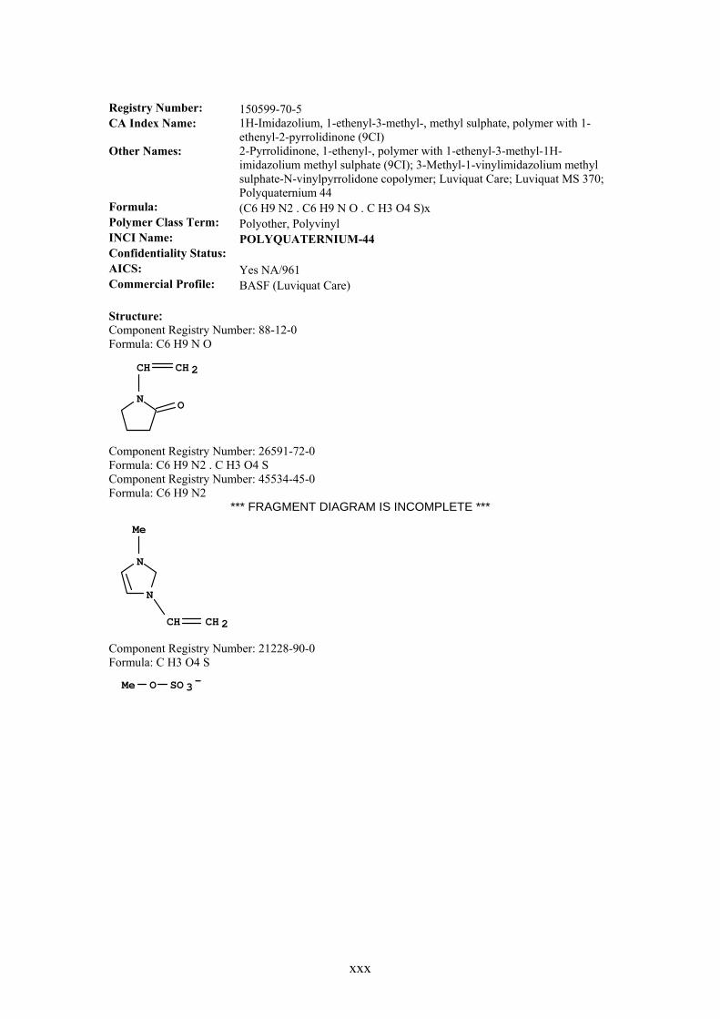
xxx

Registry Number: 150599-70-5 CA Index Name: 1H-Imidazolium, 1-ethenyl-3-methyl-, methyl sulphate, polymer with 1-

ethenyl-2-pyrrolidinone (9CI) Other Names: 2-Pyrrolidinone, 1-ethenyl-, polymer with 1-ethenyl-3-methyl-1H-

imidazolium methyl sulphate (9CI); 3-Methyl-1-vinylimidazolium methyl sulphate-N-vinylpyrrolidone copolymer; Luviquat Care; Luviquat MS 370; Polyquaternium 44

Formula: (C6 H9 N2 . C6 H9 N O . C H3 O4 S)x Polymer Class Term: Polyother, Polyvinyl INCI Name: POLYQUATERNIUM-44 Confidentiality Status: AICS: Yes NA/961 Commercial Profile: BASF (Luviquat Care) Structure: Component Registry Number: 88-12-0 Formula: C6 H9 N O

CH CH 2

N O

Component Registry Number: 26591-72-0 Formula: C6 H9 N2 . C H3 O4 S Component Registry Number: 45534-45-0 Formula: C6 H9 N2

*** FRAGMENT DIAGRAM IS INCOMPLETE ***

Me

CH CH 2

N

N

Component Registry Number: 21228-90-0 Formula: C H3 O4 S

Me SO 3-O

xxxi

Registry Number: 174761-16-1 CA Index Name: 1H-Imidazolium, 1-ethenyl-3-methyl-, methyl sulphate, polymer with 1-

ethenylhexahydro-2H-azepin-2-one and 1-ethenyl-2-pyrrolidinone (9CI) Other Names: 2-Pyrrolidinone, 1-ethenyl-, polymer with 1-ethenylhexahydro-2H-

azepin-2-one and 1-ethenyl-3-methyl-1H-imidazolium methyl sulphate (9CI); 2H-Azepin-2-one, 1-ethenylhexahydro-, polymer with 1-ethenyl-3-methyl-1H-imidazolium methyl sulphate and 1-ethenyl-2-pyrrolidinone (9CI); Luviquat Hold; Polyquaternium 46

Formula: (C8 H13 N O . C6 H9 N2 . C6 H9 N O . C H3 O4 S)x Polymer Class Term: Polyother, Polyvinyl INCI Name: POLYQUATERNIUM-46 AICS: Yes (2003) NA/533 Commercial Profile: BASF (Luviquat Hold) Structure: Component Registry Number: 2235-00-9 Formula: C8 H13 N O

Component Registry Number: 88-12-0 Formula: C6 H9 N O

Component Registry Number: 26591-72-0 Formula: C6 H9 N2 . C H3 O4 S Component Registry Number: 45534-45-0 Formula: C6 H9 N2 *** FRAGMENT DIAGRAM IS INCOMPLETE ***

Me

CH CH 2

N

N

CH CH 2

N O

CH CH 2

NO

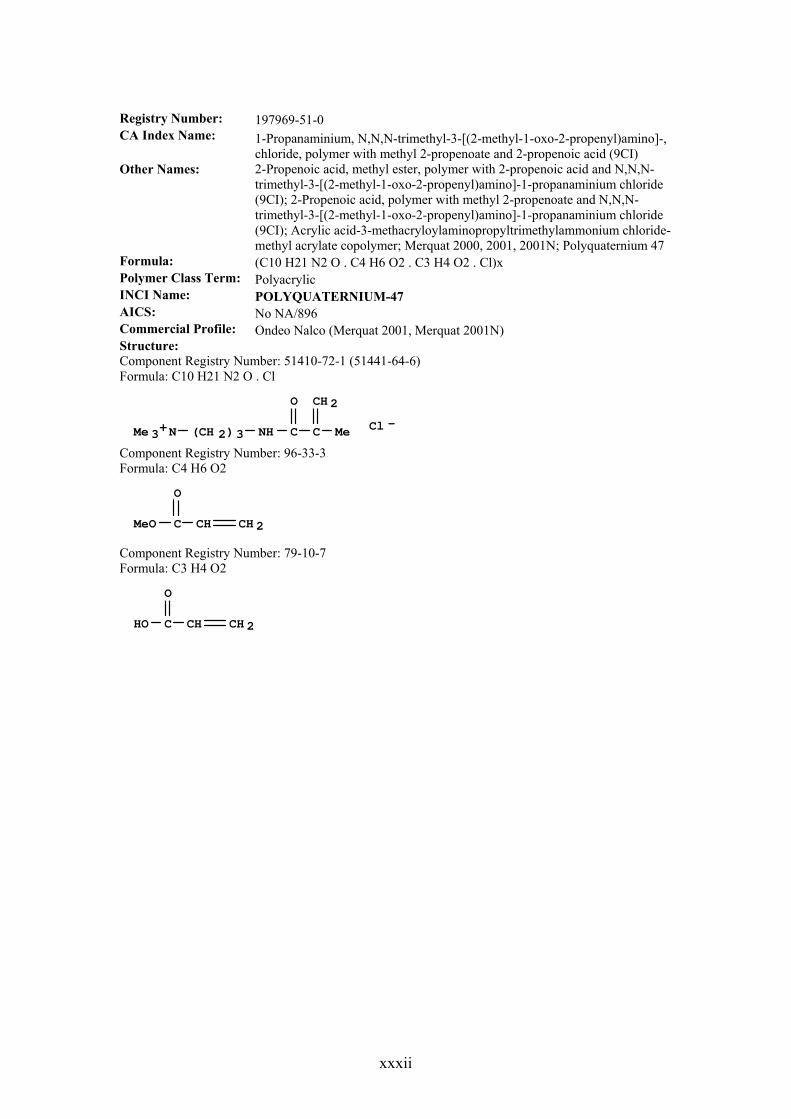
xxxii

Registry Number: 197969-51-0 CA Index Name: 1-Propanaminium, N,N,N-trimethyl-3-[(2-methyl-1-oxo-2-propenyl)amino]-,

chloride, polymer with methyl 2-propenoate and 2-propenoic acid (9CI) Other Names: 2-Propenoic acid, methyl ester, polymer with 2-propenoic acid and N,N,N-

trimethyl-3-[(2-methyl-1-oxo-2-propenyl)amino]-1-propanaminium chloride (9CI); 2-Propenoic acid, polymer with methyl 2-propenoate and N,N,N-trimethyl-3-[(2-methyl-1-oxo-2-propenyl)amino]-1-propanaminium chloride (9CI); Acrylic acid-3-methacryloylaminopropyltrimethylammonium chloride-methyl acrylate copolymer; Merquat 2000, 2001, 2001N; Polyquaternium 47

Formula: (C10 H21 N2 O . C4 H6 O2 . C3 H4 O2 . Cl)x Polymer Class Term: Polyacrylic INCI Name: POLYQUATERNIUM-47 AICS: No NA/896 Commercial Profile: Ondeo Nalco (Merquat 2001, Merquat 2001N) Structure: Component Registry Number: 51410-72-1 (51441-64-6) Formula: C10 H21 N2 O . Cl

Component Registry Number: 96-33-3 Formula: C4 H6 O2

MeO C CH

O

CH 2

Component Registry Number: 79-10-7 Formula: C3 H4 O2

C CH

O

HO CH 2

Cl -(CH 2)3 MeMe 3+N NH C C

O CH 2

xxxiii

Registry Number: 125275-25-4 CA Index Name: 3,5,8-Trioxa-4-phosphaundec-10-en-1-aminium, 4-hydroxy-N,N,N,10-

tetramethyl-9-oxo-, inner salt, 4-oxide, polymer with butyl 2-methyl-2-propenoate (9CI)

Other Names: 2-Propenoic acid, 2-methyl-, butyl ester, polymer with 4-hydroxy-N,N,N,10-tetramethyl-9-oxo-3,5,8-trioxa-4-phosphaundec-10-en-1-aminium inner salt 4-oxide (9CI); 2-Methacryloyloxyethylphosphorylcholine-butyl methacrylate copolymer; Butyl methacrylate-2-(methacryloyloxy)ethyl-2'-(trimethylammonio)ethyl phosphate copolymer; Butyl methacrylate-2-methacryloyloxyethylphosphorylcholine copolymer; Lipidure PMB; n-Butyl methacrylate-2-methacryloyloxyethylphosphorylcholine

Formula: (C11 H22 N O6 P . C8 H14 O2)x Polymer Class Term: Polyacrylic INCI Name: POLYQUATERNIUM-51 Confidentiality Status: Public AICS: No Other Regulatory: TSCA 2003 (EPA:XU); ENCS No.: 6-2367 Structure Component Registry Number: 67881-98-5 Formula: C11 H22 N O6 P

Me 3+N MeO PCH 2 O

O

O

CH 2 CH 2 CH 2 O C C

O CH 2-

Component Registry Number: 97-88-1 Formula: C8 H14 O2

n-BuO MeC C

O CH 2

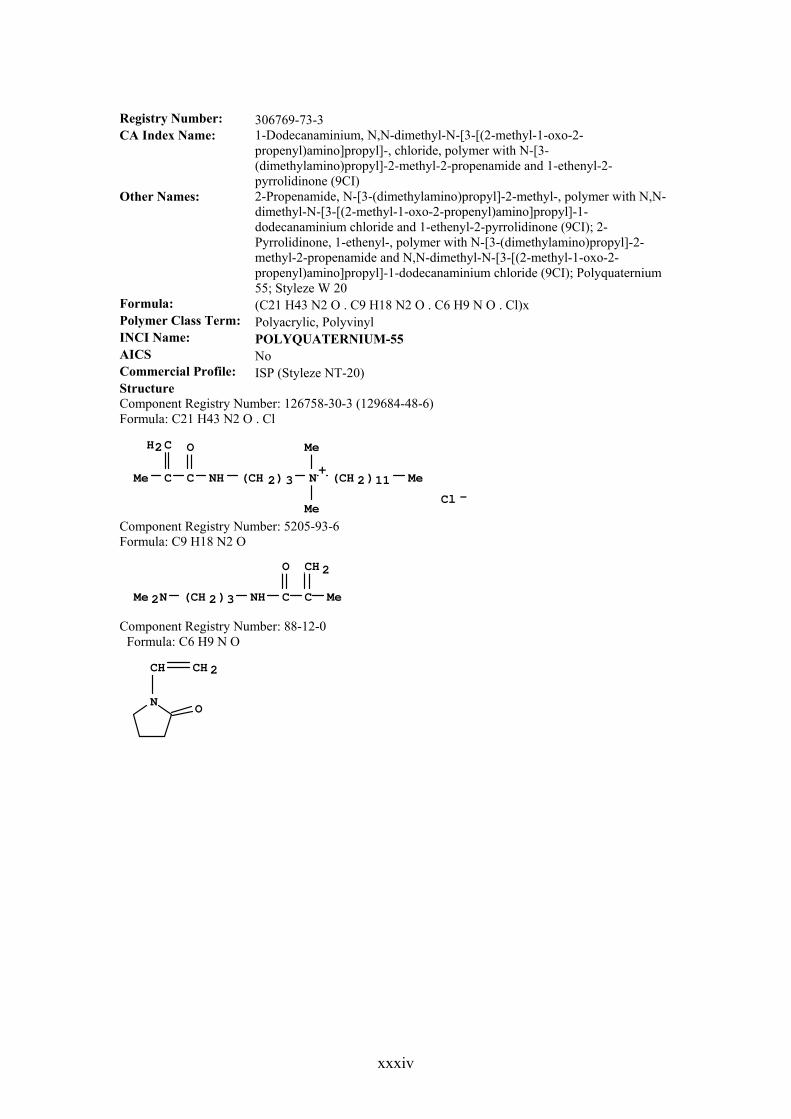
xxxiv

Registry Number: 306769-73-3 CA Index Name: 1-Dodecanaminium, N,N-dimethyl-N-[3-[(2-methyl-1-oxo-2-

propenyl)amino]propyl]-, chloride, polymer with N-[3-(dimethylamino)propyl]-2-methyl-2-propenamide and 1-ethenyl-2-pyrrolidinone (9CI)

Other Names: 2-Propenamide, N-[3-(dimethylamino)propyl]-2-methyl-, polymer with N,N-dimethyl-N-[3-[(2-methyl-1-oxo-2-propenyl)amino]propyl]-1-dodecanaminium chloride and 1-ethenyl-2-pyrrolidinone (9CI); 2-Pyrrolidinone, 1-ethenyl-, polymer with N-[3-(dimethylamino)propyl]-2-methyl-2-propenamide and N,N-dimethyl-N-[3-[(2-methyl-1-oxo-2-propenyl)amino]propyl]-1-dodecanaminium chloride (9CI); Polyquaternium 55; Styleze W 20

Formula: (C21 H43 N2 O . C9 H18 N2 O . C6 H9 N O . Cl)x Polymer Class Term: Polyacrylic, Polyvinyl INCI Name: POLYQUATERNIUM-55 AICS No Commercial Profile: ISP (Styleze NT-20) Structure Component Registry Number: 126758-30-3 (129684-48-6) Formula: C21 H43 N2 O . Cl

Component Registry Number: 5205-93-6 Formula: C9 H18 N2 O

(CH 2)3 MeMe 2N NH C C

O CH 2

Component Registry Number: 88-12-0

Formula: C6 H9 N O

CH CH 2

N O

Cl -

(CH 2)3 (CH 2)11

Me

Me

Me MeNNHCC

OH2C

+

xxxv

Registry Number: 25988-97-0 CA Index Name: Methanamine, N-methyl-, polymer with (chloromethyl)oxirane Other Names: Dimethylamine-epichlorohydrin copolymer

Dimethylamine, polymer with 1-chloro-2,3-epoxypropane (8CI); Oxirane, (chloromethyl)-, polymer with N-methylmethanamine (9CI); Propane, 1-chloro-2,3-epoxy-, polymer with dimethylamine (8CI); Agefloc A 50, A 50LV, B 50, B 50LV; Amerfloc 425E, 485; Bufloc 186; CA 250; CA 260; Callaway 4000; Catiomaster PD 10; Cysep 349, 572, 573, 577;; Dimethylamine-epichlorohydrin polymer; DMA-epichlorohydrin copolymer; ednAgefloc A 50LV; Epichlorohydrin-dimethylamine copolymer; Epichlorohydrin-dimethylamine polymer; Fixogene CXF; Flocmaster 5310; Floxan 5062; Glokill pQ; HP 142A; HP 182A; Jetfix 36N; Kufloc 100A, 200A; Nalco 7655, N 7655; Neofix RE; Polyfix 601, 610; Polyplus 1290; Polypure C 309; Proset 1810, 1820; PRP 2350; PRP 2449; PRP 2850; Refaktan K; Ultrafloc 5000; Weisstex T 101

Formula: (C3 H5 Cl O . C2 H7 N Polymer Class Term: Polyionene, Polyionene formed INCI Name: none AICS Yes Structure Component Registry Number: 124-40-3 Formula: C2 H7 N

NHH3C CH 3

Component Registry Number: 106-89-8 Formula: C3 H5 Cl O

CH 2 Cl

O

xxxvi

Registry Number: 68039-13-4 CA Index Name: 1-Propanaminium, N,N,N-trimethyl-3-[(2-methyl-1-oxo-2-

propenyl)amino]-, chloride, homopolymer (9CI) Other Names: Clairquat 1; Poly MAPTAC;

Poly(methacrylamidopropyltrimethylammonium) chloride; Poly(methacryloylamidopropyltrimethylammonium chloride); Polycare 133; Poly[(3-methacrylamidopropyl)trimethylammonium chloride]; Poly[[3-(2-methylpropenamido)propyl]trimethylammonium chloride]; [(Methacrylamido)propyl]trimethylammonium chloride homopolymer

Formula: (C10 H21 N2 O . Cl)x STN Files: CAPLUS, CA, CHEMCATS, CHEMLIST, CSCHEM,

TOXCENTER, USPATFULL Deleted Registry Number(s): 111547-42-3 Alternate Formula: Polymer Class Term: Polyacrylic INCI Name: POLYMETHACRYLAMIDOPROPYLTRIMONIUM

CHLORIDE Function: Function: antistatic agents/film formers Confidentiality Status Public AICS Yes 1996 Other Regulatory TSCA 2003 (EPS:XU); DSL 1991; PICCS 2000 Structure Component Registry Number: 51410-72-1 (51441-64-6) Formula: C10 H21 N2 O . Cl

(CH 2)3 MeMe 3+N NH C C

O CH 2

Cl -·

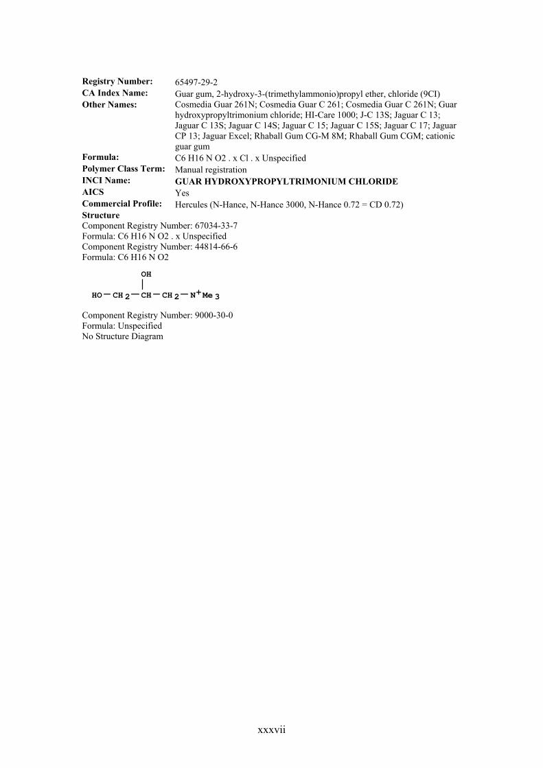
xxxvii

Registry Number: 65497-29-2 CA Index Name: Guar gum, 2-hydroxy-3-(trimethylammonio)propyl ether, chloride (9CI) Other Names: Cosmedia Guar 261N; Cosmedia Guar C 261; Cosmedia Guar C 261N; Guar

hydroxypropyltrimonium chloride; HI-Care 1000; J-C 13S; Jaguar C 13; Jaguar C 13S; Jaguar C 14S; Jaguar C 15; Jaguar C 15S; Jaguar C 17; Jaguar CP 13; Jaguar Excel; Rhaball Gum CG-M 8M; Rhaball Gum CGM; cationic guar gum

Formula: C6 H16 N O2 . x Cl . x Unspecified Polymer Class Term: Manual registration INCI Name: GUAR HYDROXYPROPYLTRIMONIUM CHLORIDE AICS Yes Commercial Profile: Hercules (N-Hance, N-Hance 3000, N-Hance 0.72 = CD 0.72) Structure Component Registry Number: 67034-33-7 Formula: C6 H16 N O2 . x Unspecified Component Registry Number: 44814-66-6 Formula: C6 H16 N O2

N+Me 3CH 2CHCH 2

OH

HO

Component Registry Number: 9000-30-0 Formula: Unspecified No Structure Diagram

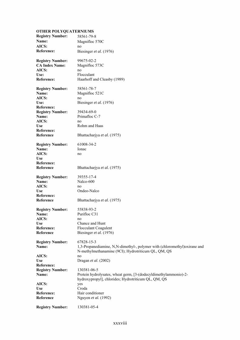
xxxviii

OTHER POLYQUATERNIUMS Registry Number: 58561-79-8 Name: Magnifloc 570C AICS: no Reference: Biesinger et al. (1976) Registry Number: 99675-02-2 CA Index Name: Magnifloc 573C AICS: no Use: Flocculant Reference: Haarhoff and Cleasby (1989) Registry Number: 58561-78-7 Name: Magnifloc 521C AICS: no Use: Biesinger et al. (1976) Reference: Registry Number: 39434-69-0 Name: Primafloc C-7 AICS: no Use Rohm and Haas Reference: Reference Bhattacharjya et al. (1975) Registry Number: 61008-34-2 Name: Ionac AICS: no Use Reference: Reference Bhattacharjya et al. (1975) Registry Number: 39355-17-4 Name: Nalco-600 AICS: no Use Ondeo-Nalco Reference: Reference Bhattacharjya et al. (1975) Registry Number: 55838-93-2 Name: Purifloc C31 AICS: no Use Chance and Hunt Reference: Flocculant Coagulent Reference Biesinger et al. (1976) Registry Number: 67828-15-3 Name: 1,3-Propanediamine, N,N-dimethyl-, polymer with (chloromethyl)oxirane and

N-methylmethanamine (9CI); Hydrotriticum QL, QM, QS AICS: no Use Dragan et al. (2002) Reference: Registry Number: 130381-06-5 Name: Protein hydrolysates, wheat germ, [3-(dodecyldimethylammonio)-2-

hydroxypropyl], chlorides; Hydrotriticum QL, QM, QS AICS: yes Use Croda Reference: Hair conditioner Reference Nguyen et al. (1992) Registry Number: 130381-05-4

xxxix

Name: Protein hydrolysates, wheat germ, [3-(dimethyloctadecylammonio)-2-hydroxypropyl], chlorides; Hydrotriticum QL, QM, QS

AICS: yes Use Croda Reference: Hair conditioner Reference Nguyen et al. (1992) Registry Number: 130381-04-3 Name: Protein hydrolysates, wheat germ, [3-(cocalkyldimethylammonio)-2-

hydroxypropyl], chlorides; Hydrotriticum QL, QM, QS AICS: yes Use Croda Reference: Hair conditioner Reference Nguyen et al. (1992) Registry Number: 124046-49-7 Name: Keratins, hydrolysates, C12-alkyl-quaternised; Croquat WKP AICS: yes Use Croda Reference: Hair conditioner Reference Nguyen et al. (1992) Registry Number: 96526-34-0 Name: 1-Octanaminium, N,N-dimethyl-N-[2-[(2-methyl-1-oxo-2-

propenyl)oxy]ethyl]-, bromide, homopolymer (9CI) AICS: no Use Nagai and Ohishi (1987) Reference: Registry Number: 105058-33-1 Name: 1-Hexadecanaminium, N,N-dimethyl-N-[2-[(2-methyl-1-oxo-2-

propenyl)oxy]ethyl]-, bromide, homopolymer (9CI) AICS: no Use Nagai and Ohishi (1987) Reference: Registry Number: 96526-36-2 Name: 1-Dodecanaminium, N,N-dimethyl-N-[2-[(2-methyl-1-oxo-2-

propenyl)oxy]ethyl]-, bromide, homopolymer (9CI) AICS: no Use Nagai and Ohishi (1987) Reference: Registry Number: 107310-72-5 Name: 1-Butanaminium, N,N-dimethyl-N-[2-[(2-methyl-1-oxo-2-

propenyl)oxy]ethyl]-, bromide, homopolymer (9CI Reference Nagai and Ohishi (1987) Registry Number: 96526-37-3 Name: 1-Tetradecanaminium, N,N-dimethyl-N-[2-[(2-methyl-1-oxo-2-

propenyl)oxy]ethyl]-, bromide, homopolymer (9CI) AICS: no Use Nagai and Ohishi (1987) Reference: Registry Number: 58561-66-3 Name: Superfloc 330 AICS: no Use Cytec Reference: Flocculant Reference Biesinger et al. (1976) Registry Number: 58561-66-3 Name: Calgon M-500

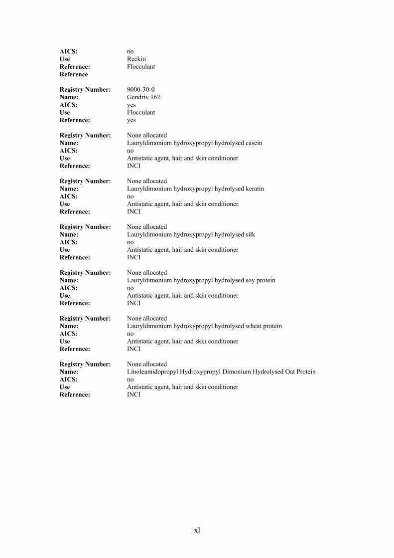
xl

AICS: no Use Reckitt Reference: Flocculant Reference Registry Number: 9000-30-0 Name: Gendriv 162 AICS: yes Use Flocculant Reference: yes Registry Number: None allocated Name: Lauryldimonium hydroxypropyl hydrolysed casein AICS: no Use Antistatic agent, hair and skin conditioner Reference: INCI Registry Number: None allocated Name: Lauryldimonium hydroxypropyl hydrolysed keratin AICS: no Use Antistatic agent, hair and skin conditioner Reference: INCI Registry Number: None allocated Name: Lauryldimonium hydroxypropyl hydrolysed silk AICS: no Use Antistatic agent, hair and skin conditioner Reference: INCI Registry Number: None allocated Name: Lauryldimonium hydroxypropyl hydrolysed soy protein AICS: no Use Antistatic agent, hair and skin conditioner Reference: INCI Registry Number: None allocated Name: Lauryldimonium hydroxypropyl hydrolysed wheat protein AICS: no Use Antistatic agent, hair and skin conditioner Reference: INCI Registry Number: None allocated Name: Linoleamidopropyl Hydroxypropyl Dimonium Hydrolysed Oat Protein AICS: no Use Antistatic agent, hair and skin conditioner Reference: INCI

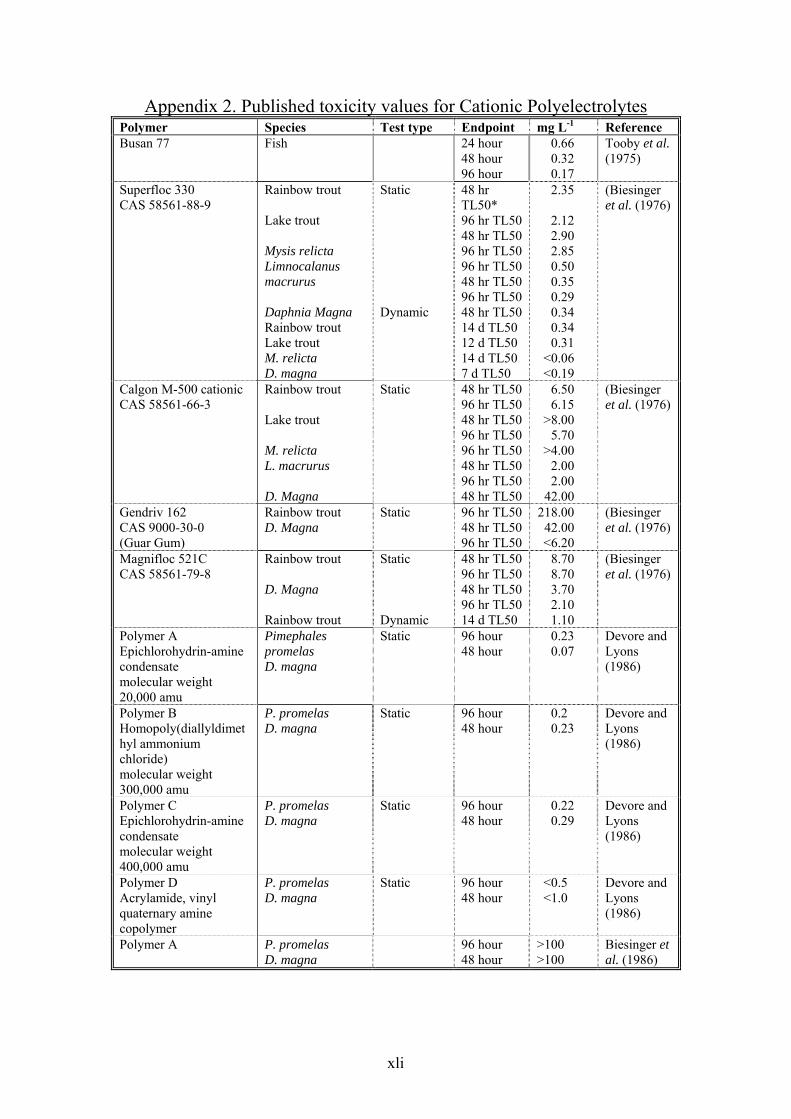
xli

Appendix 2. Published toxicity values for Cationic Polyelectrolytes Polymer Species Test type Endpoint mg L-1

Reference Busan 77 Fish 24 hour

48 hour 96 hour

0.66 0.32 0.17

Tooby et al. (1975)

Superfloc 330 CAS 58561-88-9

Rainbow trout Lake trout Mysis relicta Limnocalanus macrurus Daphnia Magna Rainbow trout Lake trout M. relicta D. magna

Static Dynamic

48 hr TL50* 96 hr TL50 48 hr TL50 96 hr TL50 96 hr TL50 48 hr TL50 96 hr TL50 48 hr TL50 14 d TL50 12 d TL50 14 d TL50 7 d TL50

2.35

2.12 2.90 2.85 0.50 0.35 0.29 0.34 0.34 0.31

<0.06 <0.19

(Biesinger et al. (1976)

Calgon M-500 cationic CAS 58561-66-3

Rainbow trout Lake trout M. relicta L. macrurus D. Magna

Static 48 hr TL50 96 hr TL50 48 hr TL50 96 hr TL50 96 hr TL50 48 hr TL50 96 hr TL50 48 hr TL50

6.50 6.15

>8.00 5.70

>4.00 2.00 2.00

42.00

(Biesinger et al. (1976)

Gendriv 162 CAS 9000-30-0 (Guar Gum)

Rainbow trout D. Magna

Static 96 hr TL50 48 hr TL50 96 hr TL50

218.00 42.00 <6.20

(Biesinger et al. (1976)

Magnifloc 521C CAS 58561-79-8

Rainbow trout D. Magna Rainbow trout

Static Dynamic

48 hr TL50 96 hr TL50 48 hr TL50 96 hr TL50 14 d TL50

8.70 8.70 3.70 2.10 1.10

(Biesinger et al. (1976)

Polymer A Epichlorohydrin-amine condensate molecular weight 20,000 amu

Pimephales promelas D. magna

Static 96 hour 48 hour

0.23 0.07

Devore and Lyons (1986)

Polymer B Homopoly(diallyldimethyl ammonium chloride) molecular weight 300,000 amu

P. promelas D. magna

Static 96 hour 48 hour

0.2 0.23

Devore and Lyons (1986)

Polymer C Epichlorohydrin-amine condensate molecular weight 400,000 amu

P. promelas D. magna

Static 96 hour 48 hour

0.22 0.29

Devore and Lyons (1986)

Polymer D Acrylamide, vinyl quaternary amine copolymer

P. promelas D. magna

Static 96 hour 48 hour

<0.5 <1.0

Devore and Lyons (1986)

Polymer A P. promelas D. magna

96 hour 48 hour

>100 >100

Biesinger et al. (1986)

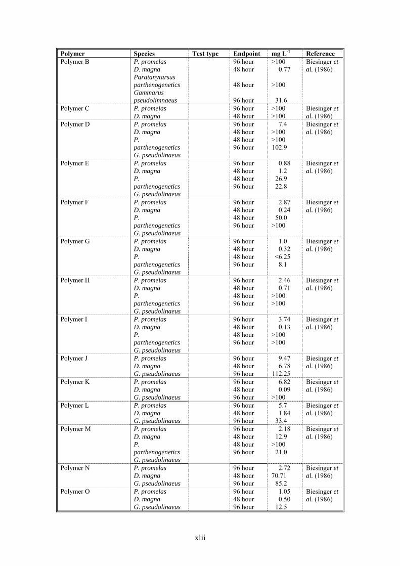
xlii

Polymer Species Test type Endpoint mg L-1 Reference

Polymer B P. promelas D. magna Paratanytarsus parthenogenetics Gammarus pseudolimnaeus

96 hour 48 hour 48 hour 96 hour

>100 0.77

>100

31.6

Biesinger et al. (1986)

Polymer C P. promelas D. magna

96 hour 48 hour

>100 >100

Biesinger et al. (1986)

Polymer D P. promelas D. magna P. parthenogenetics G. pseudolinaeus

96 hour 48 hour 48 hour 96 hour

7.4 >100 >100 102.9

Biesinger et al. (1986)

Polymer E P. promelas D. magna P. parthenogenetics G. pseudolinaeus

96 hour 48 hour 48 hour 96 hour

0.88 1.2

26.9 22.8

Biesinger et al. (1986)

Polymer F P. promelas D. magna P. parthenogenetics G. pseudolinaeus

96 hour 48 hour 48 hour 96 hour

2.87 0.24

50.0 >100

Biesinger et al. (1986)

Polymer G P. promelas D. magna P. parthenogenetics G. pseudolinaeus

96 hour 48 hour 48 hour 96 hour

1.0 0.32

<6.25 8.1

Biesinger et al. (1986)

Polymer H P. promelas D. magna P. parthenogenetics G. pseudolinaeus

96 hour 48 hour 48 hour 96 hour

2.46 0.71

>100 >100

Biesinger et al. (1986)

Polymer I P. promelas D. magna P. parthenogenetics G. pseudolinaeus

96 hour 48 hour 48 hour 96 hour

3.74 0.13

>100 >100

Biesinger et al. (1986)

Polymer J P. promelas D. magna G. pseudolinaeus

96 hour 48 hour 96 hour

9.47 6.78

112.25

Biesinger et al. (1986)

Polymer K P. promelas D. magna G. pseudolinaeus

96 hour 48 hour 96 hour

6.82 0.09

>100

Biesinger et al. (1986)

Polymer L P. promelas D. magna G. pseudolinaeus

96 hour 48 hour 96 hour

5.7 1.84

33.4

Biesinger et al. (1986)

Polymer M P. promelas D. magna P. parthenogenetics G. pseudolinaeus

96 hour 48 hour 48 hour 96 hour

2.18 12.9

>100 21.0

Biesinger et al. (1986)

Polymer N P. promelas D. magna G. pseudolinaeus

96 hour 48 hour 96 hour

2.72 70.71

85.2

Biesinger et al. (1986)

Polymer O P. promelas D. magna G. pseudolinaeus

96 hour 48 hour 96 hour

1.05 0.50

12.5

Biesinger et al. (1986)

xliii

Polymer Species Test type Endpoint mg L-1 Reference

Polymer A molecular weight ≈ 2,000 amu % activity 2.19

P. promelas D. magna

96 hour 48 hour

0.16 0.21

Cary et al. (1987)

Polymer B molecular weight ≈ 1,200,000 amu % activity 0.41

P. promelas D. magna

96 hour 48 hour

0.17 0.08

Cary et al. (1987)

Polymer C molecular weight ≈ 100,000 amu

P. promelas D. magna

96 hour 48 hour

0.25 0.08

Cary et al. (1987)

Polymer D molecular weight ≈ 25,000 amu % activity 0.96

P. promelas D. magna

96 hour 48 hour

0.46 0.20

Cary et al. (1987)

Quaternised polyethanolamine molecular weight ≈ 2000 amu; % activity 2.19

? 0.9 Cary et al. (1989)

Dimethyldiallyl ammonium chloride molecular weight 25,000 amu; % activity 0.96

0.47 Cary et al. (1989)

Poly(dimethylvinyl-pyridinium) chloride molecular weight ≈ 1,200,000 amu; % activity 0.41

0.17 Cary et al. (1989)

Dimethylamine-epichlorohydrin copolymer molecular weight 100,000 amu ; % activity 3.65

0.3 Cary et al. (1989)

Epichlorohydrin/amine polymer molecular weight 2-3000 amu; % activity 3.72

0.24 Cary et al. (1989)

Epichlorohydrin/amine polymer molecular weight 2-3000 amu; % activity 4.53

0.18 Cary et al. (1989)

A-1 Epichlorohydrin/dimethylamine molecular weight 10,000 amu

Rainbow trout Static Dynamic

24 hour 48 hour 72 hour 96 hour 48 hour 72 hour 96 hour 28 day

1.386 0.762 0.646 0.592 0.0544 0.0544 0.0426 0.0017

Goodrich et al. (1991)

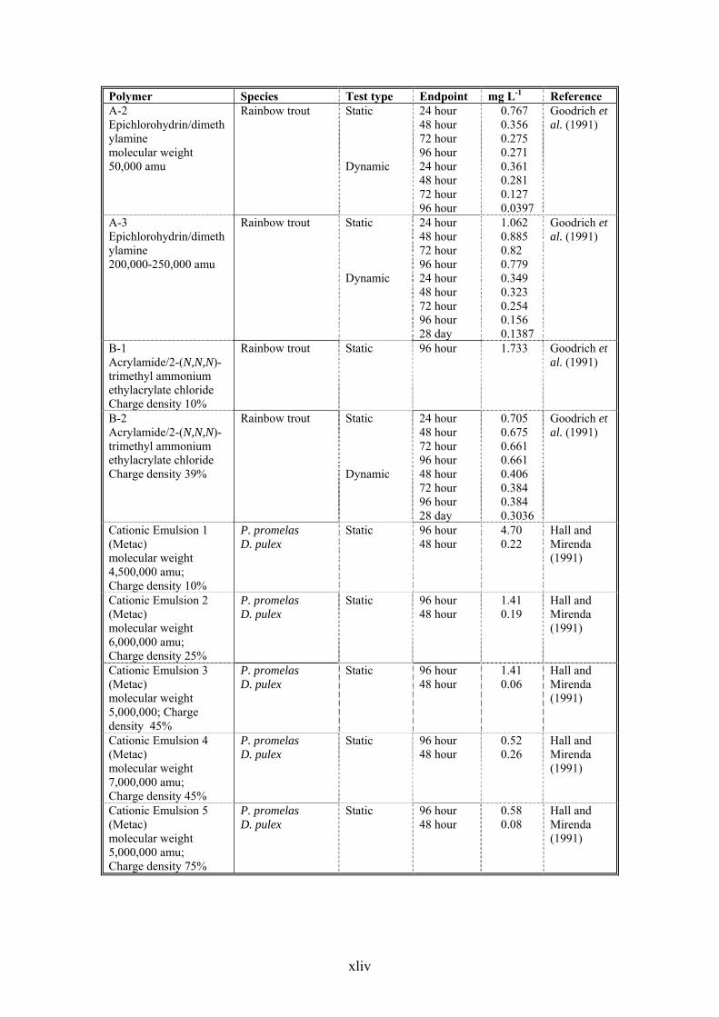
xliv

Polymer Species Test type Endpoint mg L-1 Reference

A-2 Epichlorohydrin/dimethylamine molecular weight 50,000 amu

Rainbow trout Static Dynamic

24 hour 48 hour 72 hour 96 hour 24 hour 48 hour 72 hour 96 hour

0.767 0.356 0.275 0.271 0.361 0.281 0.127 0.0397

Goodrich et al. (1991)

A-3 Epichlorohydrin/dimethylamine 200,000-250,000 amu

Rainbow trout Static Dynamic

24 hour 48 hour 72 hour 96 hour 24 hour 48 hour 72 hour 96 hour 28 day

1.062 0.885 0.82 0.779 0.349 0.323 0.254 0.156 0.1387

Goodrich et al. (1991)

B-1 Acrylamide/2-(N,N,N)-trimethyl ammonium ethylacrylate chloride Charge density 10%

Rainbow trout Static 96 hour 1.733 Goodrich et al. (1991)

B-2 Acrylamide/2-(N,N,N)-trimethyl ammonium ethylacrylate chloride Charge density 39%

Rainbow trout Static Dynamic

24 hour 48 hour 72 hour 96 hour 48 hour 72 hour 96 hour 28 day

0.705 0.675 0.661 0.661 0.406 0.384 0.384 0.3036

Goodrich et al. (1991)

Cationic Emulsion 1 (Metac) molecular weight 4,500,000 amu; Charge density 10%

P. promelas D. pulex

Static 96 hour 48 hour

4.70 0.22

Hall and Mirenda (1991)

Cationic Emulsion 2 (Metac) molecular weight 6,000,000 amu; Charge density 25%

P. promelas D. pulex

Static 96 hour 48 hour

1.41 0.19

Hall and Mirenda (1991)

Cationic Emulsion 3 (Metac) molecular weight 5,000,000; Charge density 45%

P. promelas D. pulex

Static 96 hour 48 hour

1.41 0.06

Hall and Mirenda (1991)

Cationic Emulsion 4 (Metac) molecular weight 7,000,000 amu; Charge density 45%

P. promelas D. pulex

Static 96 hour 48 hour

0.52 0.26

Hall and Mirenda (1991)

Cationic Emulsion 5 (Metac) molecular weight 5,000,000 amu; Charge density 75%

P. promelas D. pulex

Static 96 hour 48 hour

0.58 0.08

Hall and Mirenda (1991)

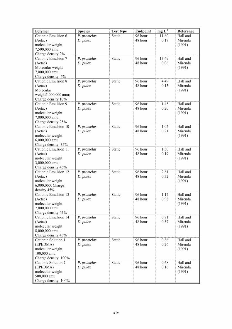
xlv

Polymer Species Test type Endpoint mg L-1 Reference

Cationic Emulsion 6 (Aetac) molecular weight 7,500,000 amu; Charge density 2%

P. promelas D. pulex

Static 96 hour 48 hour

11.60 0.17

Hall and Mirenda (1991)

Cationic Emulsion 7 (Aetac) Molecular weight 7,000,000 amu; Charge density 6%

P. promelas D. pulex

Static 96 hour 48 hour

13.49 0.06

Hall and Mirenda (1991)

Cationic Emulsion 8 (Aetac) Molecular weight5,000,000 amu; Charge density 10%

P. promelas D. pulex

Static 96 hour 48 hour

4.49 0.15

Hall and Mirenda (1991)

Cationic Emulsion 9 (Aetac) molecular weight 7,000,000 amu; Charge density 25%

P. promelas D. pulex

Static 96 hour 48 hour

1.45 0.20

Hall and Mirenda (1991)

Cationic Emulsion 10 (Aetac) molecular weight 6,000,000 amu; Charge density 35%

P. promelas D. pulex

Static 96 hour 48 hour

1.05 0.21

Hall and Mirenda (1991)

Cationic Emulsion 11 (Aetac) molecular weight 3,000,000 amu; Charge density 45%

P. promelas D. pulex

Static 96 hour 48 hour

1.30 0.19

Hall and Mirenda (1991)

Cationic Emulsion 12 (Aetac) molecular weight 6,000,000; Charge density 45%

P. promelas D. pulex

Static 96 hour 48 hour

2.81 0.32

Hall and Mirenda (1991)

Cationic Emulsion 13 (Aetac) molecular weight 7,000,000 amu; Charge density 45%

P. promelas D. pulex

Static 96 hour 48 hour

1.17 0.98

Hall and Mirenda (1991)

Cationic Emulsion 14 (Aetac) molecular weight 8,000,000 amu; Charge density 45%

P. promelas D. pulex

Static 96 hour 48 hour

0.81 0.57

Hall and Mirenda (1991)

Cationic Solution 1 (EPI/DMA) molecular weight 100,000 amu; Charge density 100%

P. promelas D. pulex

Static 96 hour 48 hour

0.86 0.26

Hall and Mirenda (1991)

Cationic Solution 2 (EPI/DMA) molecular weight 500,000 amu; Charge density 100%

P. promelas D. pulex

Static 96 hour 48 hour

0.68 0.16

Hall and Mirenda (1991)

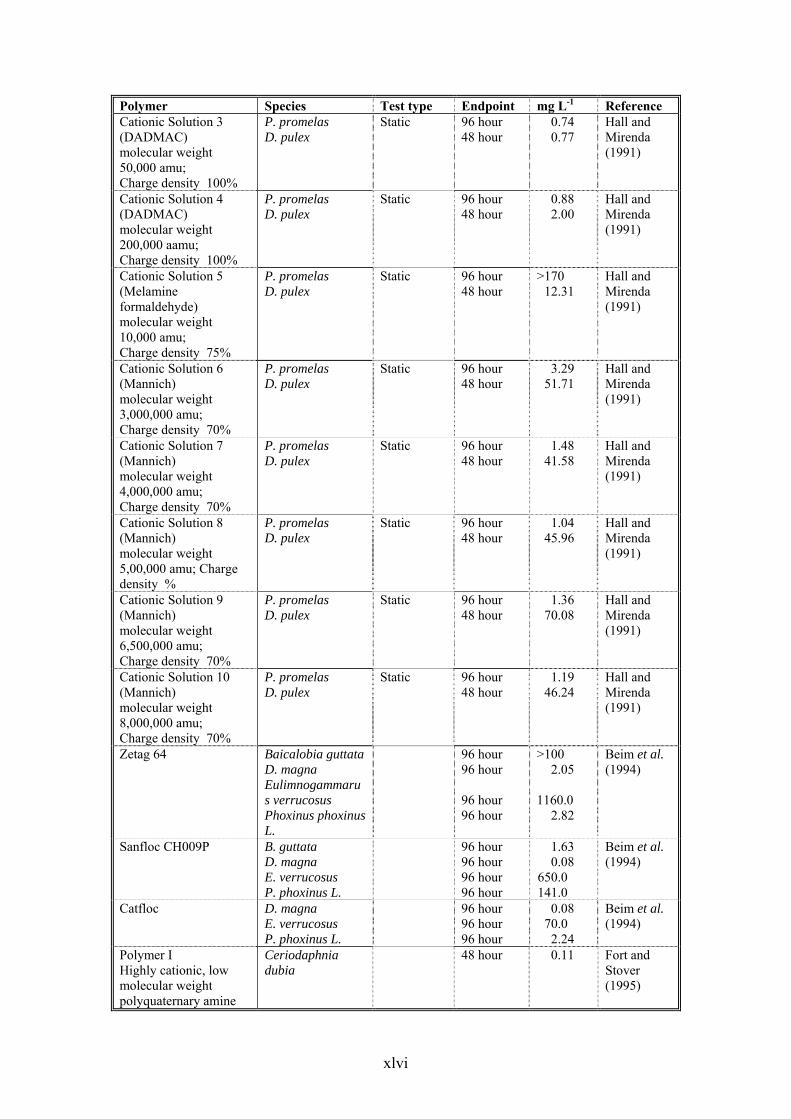
xlvi

Polymer Species Test type Endpoint mg L-1 Reference

Cationic Solution 3 (DADMAC) molecular weight 50,000 amu; Charge density 100%

P. promelas D. pulex

Static 96 hour 48 hour

0.74 0.77

Hall and Mirenda (1991)

Cationic Solution 4 (DADMAC) molecular weight 200,000 aamu; Charge density 100%

P. promelas D. pulex

Static 96 hour 48 hour

0.88 2.00

Hall and Mirenda (1991)

Cationic Solution 5 (Melamine formaldehyde) molecular weight 10,000 amu; Charge density 75%

P. promelas D. pulex

Static 96 hour 48 hour

>170 12.31

Hall and Mirenda (1991)

Cationic Solution 6 (Mannich) molecular weight 3,000,000 amu; Charge density 70%

P. promelas D. pulex

Static 96 hour 48 hour

3.29 51.71

Hall and Mirenda (1991)

Cationic Solution 7 (Mannich) molecular weight 4,000,000 amu; Charge density 70%

P. promelas D. pulex

Static 96 hour 48 hour

1.48 41.58

Hall and Mirenda (1991)

Cationic Solution 8 (Mannich) molecular weight 5,00,000 amu; Charge density %

P. promelas D. pulex

Static 96 hour 48 hour

1.04 45.96

Hall and Mirenda (1991)

Cationic Solution 9 (Mannich) molecular weight 6,500,000 amu; Charge density 70%

P. promelas D. pulex

Static 96 hour 48 hour

1.36 70.08

Hall and Mirenda (1991)

Cationic Solution 10 (Mannich) molecular weight 8,000,000 amu; Charge density 70%

P. promelas D. pulex

Static 96 hour 48 hour

1.19 46.24

Hall and Mirenda (1991)

Zetag 64 Baicalobia guttata D. magna Eulimnogammarus verrucosus Phoxinus phoxinus L.

96 hour 96 hour 96 hour 96 hour

>100 2.05

1160.0

2.82

Beim et al. (1994)

Sanfloc CH009P B. guttata D. magna E. verrucosus P. phoxinus L.

96 hour 96 hour 96 hour 96 hour

1.63 0.08

650.0 141.0

Beim et al. (1994)

Catfloc D. magna E. verrucosus P. phoxinus L.

96 hour 96 hour 96 hour

0.08 70.0 2.24

Beim et al. (1994)

Polymer I Highly cationic, low molecular weight polyquaternary amine

Ceriodaphnia dubia

48 hour 0.11 Fort and Stover (1995)

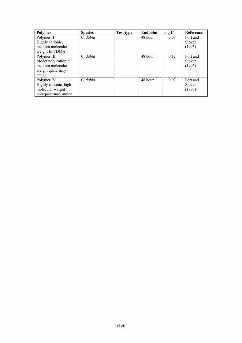
xlvii

Polymer Species Test type Endpoint mg L-1 Reference

Polymer II Highly cationic, medium molecular weight EPI/DMA

C. dubia 48 hour 0.08 Fort and Stover (1995)

Polymer III Moderately cationic, medium molecular weight quaternary amine

C. dubia 48 hour 0.12 Fort and Stover (1995)

Polymer IV Highly cationic, high molecular weight polyquaternary amine

C. dubia 48 hour 0.07 Fort and Stover (1995)

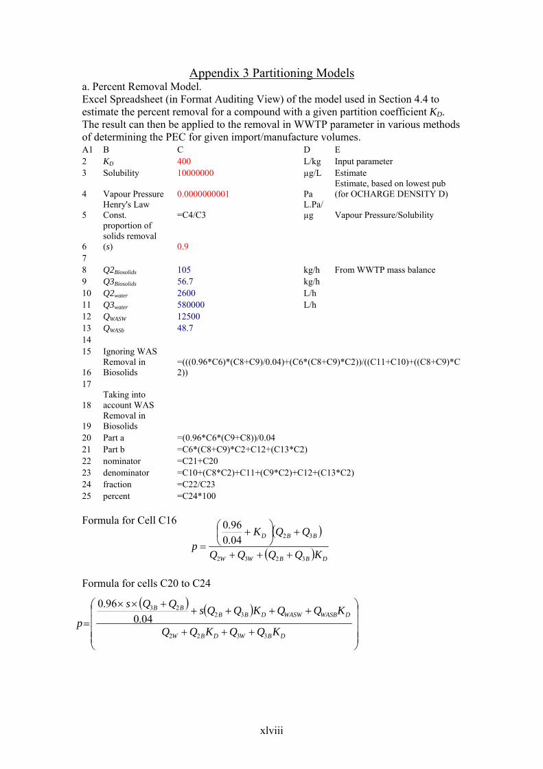
xlviii

Appendix 3 Partitioning Models a. Percent Removal Model. Excel Spreadsheet (in Format Auditing View) of the model used in Section 4.4 to estimate the percent removal for a compound with a given partition coefficient KD. The result can then be applied to the removal in WWTP parameter in various methods of determining the PEC for given import/manufacture volumes. A1 B C D E 2 KD 400 L/kg Input parameter 3 Solubility 10000000 µg/L Estimate

4 Vapour Pressure 0.0000000001 Pa Estimate, based on lowest pub (for OCHARGE DENSITY D)

5 Henry's Law Const. =C4/C3

L.Pa/µg Vapour Pressure/Solubility

6

proportion of solids removal (s) 0.9

7 8 Q2Biosolids 105 kg/h From WWTP mass balance 9 Q3Biosolids 56.7 kg/h 10 Q2water 2600 L/h 11 Q3water 580000 L/h 12 QWASW 12500 13 QWASb 48.7 14 15 Ignoring WAS

16 Removal in Biosolids

=(((0.96*C6)*(C8+C9)/0.04)+(C6*(C8+C9)*C2))/((C11+C10)+((C8+C9)*C2))

17

18 Taking into account WAS

19 Removal in Biosolids

20 Part a =(0.96*C6*(C9+C8))/0.04 21 Part b =C6*(C8+C9)*C2+C12+(C13*C2) 22 nominator =C21+C20 23 denominator =C10+(C8*C2)+C11+(C9*C2)+C12+(C13*C2) 24 fraction =C22/C23 25 percent =C24*100 Formula for Cell C16 Formula for cells C20 to C24

( )

( ) DBBWW

BBD

KQQQQ

QQKp

3232

3204.096.0

+++

+⎟⎠⎞

⎜⎝⎛ +

=

( ) ( )

⎟⎟⎟⎟

⎠

⎞

⎜⎜⎜⎜

⎝

⎛

+++

+++++××

=DBWDBW

DWASBWASWDBBBB

KQQKQQ

KQQKQQsQQs

p3322

3223

04.096.0

xlix

b. Input Flux Model. Excel Spreadsheet (in Format Auditing View) of the model used in Section 6.2 to estimate the input flux resulting in the ETNCaq for a compound with a given partition coefficient KD. The result can then be applied to estimate the import/manufacture volume which may result in the ETNCaq being exceeded.

A B C D 1 ETNC 0.01 Input parameter 2 Effluent =B1*10 µg/L Dilution to receiving waters 3 K(D) 400 L/kg Input parameter 4 Solubility 10000000 µg/L Estimate 5

Vapour Pressure 0.0000000001 Pa Estimate, based on lowest published (for OCHARGE DENSITY D)

6 Henry's Law Const. =B5/B4 L.Pa/µg Vapour Pressure/Solubility 7 8 Effluent 9 Oxley Parameters 10 Effluent Flow rate (W) 571000 L/h From water balance 11 Effluent Flow rate (S) 5.71 kg/h From solids balance 12 Sludge Density 1 Assumed 13 Q5water 1163000 L/h From WWTP mass balance 14 Q5solids 2330 kg/h From WWTP mass balance 15 Q4water 583000 L/h From WWTP mass balance 16 Q4solids 2273 kg/h From WWTP mass balance 17 18 Csorbed =B3*B2 µg/kg from KD = Csorbed/Charge density issolved 19 Effluent Flux (dissolved) =B10*B2 µg/h Cwater * Effluent Flow Rate (W) 20 Effluent Flux (sorbed) =B18*B11 µg/h Csorbed * Effluent Flow Rate (S) 21 Total Effluent Flux =SUM(B19:B20) µg/h Sum of Effluent fluxes 22 23 Zwater =1/B6 µg/L.Pa 1/Henry's Law Constant 24 Zsorbed =B23*B3 µg/kg.Pa From KD = Zsolids/Zwater 25 26 D(5) =(B13*B23)+(B14*B24) μg/h.Pa D = Q*Zwater + Q*Zsorbed 27 D(4) =(B15*B23)+(B16*B24) μg/h.Pa D = Q*Zwater + Q*Zsorbed 28 29 Final Settling Tank 30

ƒ(PQ-X) =B21/(B26-B27) Pa ƒ(PQ-X) - (D5-D4) = Total Effluent Flux

31 Dissolved Flux PQ-X =B30*B26 µg/h D(5) * ƒ(PQ-X) 32 Sorbed Flux PQ-X =B30*B27 µg/h D(4) * ƒ(PQ-X) 33 34 Bioreactor 35 Q3water 580000 L/h From WWTP mass balance 36 Q3solids 56.7 kg/h From WWTP mass balance 37 38 D(3) =(B35*B23)+(B36*B24) μg/h.Pa D = Q * Zwater + Q * Zsorbed 39 40 Dissolved Flux (PQ-X) =B38*B30 µg/h D(3) * ƒ(PQ-X) 41 42 Primary Settling Tank 43 Q1water 583000 L/h From WWTP mass balance 44 Q1solids 162 kg/h From WWTP mass balance 45 Q2water 2630 L/h From WWTP mass balance

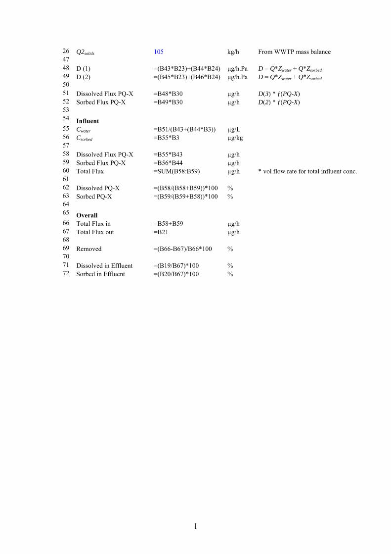
l

26 Q2solids 105 kg/h From WWTP mass balance 47 48 D (1) =(B43*B23)+(B44*B24) μg/h.Pa D = Q*Zwater + Q*Zsorbed 49 D (2) =(B45*B23)+(B46*B24) μg/h.Pa D = Q*Zwater + Q*Zsorbed 50 51 Dissolved Flux PQ-X =B48*B30 µg/h D(3) * ƒ(PQ-X) 52 Sorbed Flux PQ-X =B49*B30 µg/h D(2) * ƒ(PQ-X) 53 54 Influent 55 Cwater =B51/(B43+(B44*B3)) µg/L 56 Csorbed =B55*B3 µg/kg 57 58 Dissolved Flux PQ-X =B55*B43 µg/h 59 Sorbed Flux PQ-X =B56*B44 µg/h 60 Total Flux =SUM(B58:B59) µg/h * vol flow rate for total influent conc. 61 62 Dissolved PQ-X =(B58/(B58+B59))*100 % 63 Sorbed PQ-X =(B59/(B59+B58))*100 % 64 65 Overall 66 Total Flux in =B58+B59 µg/h 67 Total Flux out =B21 µg/h 68 69 Removed =(B66-B67)/B66*100 % 70 71 Dissolved in Effluent =(B19/B67)*100 % 72 Sorbed in Effluent =(B20/B67)*100 %