Environmental decision-making under uncertainty using intuitionistic fuzzy analytic hierarchy...

ORIGINAL PAPER

Environmental decision-making under uncertainty usingintuitionistic fuzzy analytic hierarchy process (IF-AHP)

Rehan Sadiq Æ Solomon Tesfamariam

Published online: 28 November 2007

� Springer-Verlag 2007

Abstract Analytic hierarchy process (AHP) is a utility

theory based decision-making technique, which works on a

premise that the decision-making of complex problems can

be handled by structuring them into simple and compre-

hensible hierarchical structures. However, AHP involves

human subjective evaluation, which introduces vagueness

that necessitates the use of decision-making under uncer-

tainty. The vagueness is commonly handled through fuzzy

sets theory, by assigning degree of membership. But, the

environmental decision-making problem becomes more

involved if there is an uncertainty in assigning the mem-

bership function (or degree of belief) to fuzzy pairwise

comparisons, which is referred to as ambiguity (non-spec-

ificity). In this paper, the concept of intuitionistic fuzzy set

is applied to AHP, called IF-AHP to handle both vagueness

and ambiguity related uncertainties in the environmental

decision-making process. The proposed IF-AHP method-

ology is demonstrated with an illustrative example to select

best drilling fluid (mud) for drilling operations under

multiple environmental criteria.

Keywords Analytic hierarchy process �Intuitionistic fuzzy set � Vagueness � Ambiguity �Drilling fluids � Environmental decision-making

List of symbols

Ai (i = 1, 2,..., m) Possible courses of actions or

alternatives

A, B Intuitionistic fuzzy set (IFS)

a01; b01; c01

� �; lA

� ��;

a1; b1; c1ð Þ; tA½ �iTriangular intuitionistic

fuzzy set

Cj (j = 1, 2, ..., n) Performance criteria or

attributes��FAi Intuitionistic fuzzy AHP score��Gk Intuitionistic fuzzy global

preference weights��J Intuitionistic fuzzy judgment

matrix��jij Pairwise comparison index in

intuitionistic fuzzy judgment

matrix

K Number of levels in a

hierarchical structure

wLIi ;w

UIi

� �Lower and upper interval

weights

ðwiÞLIa ; ðwiÞUI

a Lower and upper normalized

interval weights

W = (w1, w2, ..., wn) Weight vector��W ¼ ð ��wi; i ¼ 1; 2; . . .; nÞ Intuitionistic fuzzy weight

vector

X Universe of discourse

xd Discrete points defined over

the universe of discourse

xij Performance rating of

alternative Ai for criterion Cj

�xðAiÞ Generalized mean of an

alternative Ai (a reduced

fuzzy set)

Dl, DlL and DlU fuzzification factors

px Degree of non-determinacy

tx Non-membership function

of x

R. Sadiq (&) � S. Tesfamariam

Urban Infrastructure Program,

National Research Council Canada—Institute for Research

in Construction, Ottawa, ON, Canada K1A 0R6

e-mail: [email protected]

123

Stoch Environ Res Risk Assess (2009) 23:75–91

DOI 10.1007/s00477-007-0197-z

tA and tB Non-membership function of

IFS A and B

lA and lB Membership function of IFS A

and B

lL and lU Lower and upper bound of

membership function lx

lx Membership function of x

r(Ai) Standard deviation of an

alternative Ai (a reduced

fuzzy set)

1 Introduction

Environmental decision-making is a process of weighting

alternatives and selecting the most appropriate alternative,

by integrating results of risk assessment with social, eco-

nomic, political and engineering data to reach a rigorous

decision. Decision-making tools help in the selection of

prudent, technically feasible, and scientifically justifiable

actions to protect the environment and human health in a

cost-effective way (Sadiq 2001). The main challenge in

environmental decision-making is that alternatives (Ai) are

multiple and diverse in nature, and often have conflicting

criteria. Multiple criteria decision-making (MCDM)

methods are employed where alternatives are predefined

and the decision-maker(s) ranks available alternatives

based on the evaluation of multiple criteria. A typical

MCDM problem with m alternatives and n criteria can be

written as:

C1 C2 … Cn

A1 x11 x12 … x1n

A2 x21 x22 … x2n

M M M M M

Am xm1 xm2 … xmn

(1)

where Ai (i = 1, 2, ..., m) are possible courses of actions or

alternatives; Cj (j = 1, 2, ..., n) are criteria; and xij is a

performance rating of alternative Ai with respect to a cri-

terion Cj. Therefore the environmental decision-making

can be viewed as the process of selecting most appropriate

alternative (A1 or A2 or ... or Am), based on numerous

performance criteria Cj (j = 1, 2, ..., n).

Analytic Hierarchy Process (AHP) is one of the most

commonly used utility-based methods for environmental

decision-making (Sadiq 2001). The AHP uses objective

mathematics to process the subjective and personal pref-

erences of an individual or a group in decision-making

(Saaty 2001). The AHP works on a premise that decision-

making of complex problems can be handled by structuring

it into a simple and comprehensible hierarchical structure.

Once the hierarchical structure is developed, a pairwise

comparison is carried out between two selected criteria.

The levels of the pairwise comparisons may range from 1

to 9, where ‘‘1’’ represents that two criteria are equally

important, while the other extreme ‘‘9’’ represents that one

criterion is absolutely more important than the other

(Table 1). Solution of the AHP hierarchical structure is

obtained by synthesizing local and global preference

weight to obtain the overall priority (Saaty 1980). The AHP

can be summarized into three main steps:

1. Structure the problem into a hierarchy consisting of a

goal (objective), criteria, layers of sub-criteria and

alternatives,

2. Establish pairwise comparisons between elements in

each hierarchal layer, and

3. Synthesize and establish the overall priority to rank

the alternatives.

Uncertainty is an unavoidable and inevitable component

of any environmental decision-making process. The

typology and definition of uncertainty within engineering

community is vast and often conflicting (Parsons 2001).

Klir and Yuan (1995) have broadly categorized uncertainty

into vagueness and ambiguity (Fig. 1). The AHP inherently

involves both vagueness and ambiguity in assigning pair-

wise comparisons and evaluating alternatives. Vagueness

(imprecision) refers to lack of definite or sharp distinction,

Table 1 Linguistic measures of importance used for pairwise com-

parisons (Saaty 1980)

Relative

importance

Importance degree Explanation

1 Equal importance Two activities contribute

equally to objective

3 Weak importance Experience and judgment

slightly favour one activity

over another

5 Essential or strong

importance

Experience and judgment

strongly favour one activity

over another

7 Demonstrated

importance

One activity is strongly

favoured and demonstrated

in practice

9 Extreme importance The evidence favouring one

activity over another is of

highest possible order of

affirmation

2, 4, 6, 8 Intermediate values

between two adjacent

judgments

When compromise is needed

76 Stoch Environ Res Risk Assess (2009) 23:75–91

123

whereas ambiguity is due to unclear distinction of various

alternatives, which is further divided into discord (conflict)

and non-specificity. The taxonomy of uncertainty shown in

Fig. 1, albeit to a different degree, is reflected in the

environmental decision-making process. Henceforth,

both terms ambiguity and non-specificity are used

interchangeably.

Many attempts have been reported in literature to

incorporate different types of uncertainties in the formal

AHP framework. Table 2 provides a summary of various

uncertainty management formulations considered for the

extension of AHP. For example, Ozdemir and Saaty (2006)

accounted for missing information by adding new decision

variable in the pairwise comparison. Beynon et al. (2001)

and Beynon (2002, 2005) proposed the use of Dempster–

Shafer theory in AHP formulation to account for missing

and non-specific information. Yager and Kelman (1999)

proposed the use of ordered weighted averaging (OWA)

operators in AHP, which introduces the dimension of

decision-maker’s attitude in the aggregation. But over the

last 20 years, the most common uncertainty management

formulation used for the extension of AHP is fuzzy logic

(Table 2).

The pairwise comparisons require qualitative assess-

ment of human beings. Consequently, vagueness dominates

the decision making process. The vagueness is best

described by fuzzy set theory (Zadeh 1965). Fuzzy-based

techniques are generalized form of an interval analysis. A

fuzzy number describes the relationship between an

uncertain quantity x and a membership function lx. In the

classical set theory, x is either a member of set A or not,

i.e., {0, 1}, whereas in fuzzy set theory x can be a member

of set A with a certain membership function lx [ [0, 1].

The non-membership is simply a complement of lx, i.e.,

tx = 1 - lx.

A crisp degree of membership lx assigned to any given

value of x over the universe of discourse may also be

subjected to uncertainty. This refers to non-specificity,

which is associated with the membership lx of fuzzy sets.

Zadeh (1975) extended the fuzzy set theory to incorporate

non-specificity through interval-valued fuzzy sets, which

captures non-specificity by an interval [lL, lU], where lL

and lU represent lower and upper bounds of membership

function lx, respectively. Atanassov (1986, 1999) defined a

non-membership function tx in addition to the membership

function lx through an intuitionistic fuzzy set (IFS), such

that the non-specificity (degree of non-determinacy) is an

interval [lx, 1 - tx]. Gau and Buehrer (1993) have

explored similar concept, but called it vague sets (VS).

However recently, Bustince and Burillo (1996) showed that

the vague sets are essentially IFS. Further, Cornelis et al.

(2004) have proved equivalence between interval-valued

fuzzy sets and IFS. Therefore, both vague sets and interval-

valued fuzzy sets can be handled using IFS formulation.

There are some reported applications of IFS in MCDM,

e.g., Liu and Wang (2006), Li (2005), Atanassov et al.

(2002), and Hong and Choi (2000). Recently, Silavi et al.

(2006a, b) have demonstrated the possibility of extending

AHP using IFS.

The main objective of this paper is to quantify vague-

ness and ambiguity uncertainties in AHP using IFS for

environmental decision-making problem. The proposed

technique is used for selecting the best generic drilling fluid

VaguenessThe lack of definite or sharp distinctions

Discord (conflict) Disagreement in choosing among several alternatives

Non-specificity Two or more alternatives are left unspecified

Uncertainty

Ambiguity One-to-many relationships

Fig. 1 Typology of uncertainty (modified after Klir and Yuan 1995)

Table 2 Uncertainty management techniques and formulations used

for the extension of AHP

Techniques References Comments

Fuzzy sets Kreng and Wu (2007),

Arslan and Khisty

(2006), Tesfamariam

and Sadiq (2006),

Bozbura and Beskese

(2006), Yu (2002),

Leung and Cao

(2000), Deng (1999),

Zhu et al. (1999),

Weck et al. (1997),

Levary and Wan

(1998), Chang (1996),

Buckley (1985) and

van Laarhoven and

Pedrycz (1983)

•The vagueness in

pairwise comparisons

is incorporated using

fuzzy numbers. The

standard AHP is

extended using fuzzy

arithmetic operations

• Different ways of

generating fuzzy

weights are illustrated

Intuitionistic

fuzzy sets

Silavi et al. (2006a, b) • Expert provided

membership and non-

membership values

are introduced in the

judgement matrix

Dempster–

Shafer theory

Beynon (2002, 2005)

and Beynon et al.

(2001)

• The incomplete and

partial information

(ambiguity) of

pairwise comparisons

are handled using

belief functions

Interval values Sugihara et al. (2004)

and Wang et al.

(2005)

• The uncertainty in the

pairwise comparison

is defined using

interval values

Ordered

weighted

averaging

operators

(OWA)

Yager and Kelman

(1999)

• Used OWA operators

to incorporate

decision maker’s

attitude

Stoch Environ Res Risk Assess (2009) 23:75–91 77

123

among three available alternatives. The drilling fluid

example used in this paper is modified from Sadiq et al.

(2003), and Tesfamariam and Sadiq (2006), who employed

standard (crisp) AHP and fuzzy AHP (F-AHP), respec-

tively. The remainder of the paper is organized as follows:

Sect. 2 provides background information on intuitionistic

fuzzy arithmetic operations. Section 3 discusses a step-by-

step framework for proposed intuitionistic fuzzy analytic

hierarchy process (IF-AHP). Section 4 discusses the effi-

cacy of IF-AHP through an illustrative case study of

selecting a generic drilling fluid, and finally in Sect. 5

conclusions are presented.

2 Intuitionistic fuzzy sets (IFS)

This section outlays basic definitions of IFS to comprehend

the implementation of IF-AHP, which is described in the

following section. The definitions in this section are mainly

taken from Atanassov (1999). An IFS ‘A’ can be defined as

A ¼ ðx; lx; txÞjx 2 Xf g ð2Þ

The membership (lx) and non-membership (tx) functions

for an element x are defined as:

lx : X ! ½0; 1�; and tx : X ! ½0; 1� ð3Þ

where X defines the possible range of values for a variable

x, and ‘A’ is an IFS defined over X using membership and

non- membership functions [ [0, 1]. For any value of x in

an IFS ‘A’, the expression 0 B (lx + tx ) B 1 holds true.

However, if the expression reduces to (lx + tx ) = 1, the

IFS becomes an ordinary fuzzy set. For IFS, the degree of

non-determinacy px (or non-specificity) of the element x in

IFS ‘A’ is defined as follows:

px ¼ 1� lx � tx; px : X ! ½0; 1� ð4Þ

Therefore, for ordinary fuzzy sets the degree of non-

determinacy px = 0. Figure 2 provides a schematic repre-

sentation of IFS ‘A’.

Now consider two triangular IFS A and B in Fig. 3.

These triangular IFS can be written as A ¼a01; b

01; c01

� �; lA

� �; a1; b1; c1ð Þ; tA½ �

� �and B ¼

a02; b02; c02

� �; lB

� �; a2; b2; c2ð Þ; tB½ �

� �: Three vertices of tri-

angular IFS represented by (ai

0, bi

0, ci

0) and (ai, bi, ci ) are

defined over a universe of discourse X. The three vertices

represent minimum, most likely, and maximum values over

X. Membership lx and non-membership functions tx

belong to the most likely values in triangular IFS, i.e., bi

0

and bi, respectively. The membership functions lA and lB

are used to derive the lower bounds of membership lL for

IFS A and B, where the upper bounds of memberships lU

are derived by taking the compliment of non-membership

functions tA and tB, respectively. Four common arithmetic

operations for intuitionistic fuzzy sets, addition, subtrac-

tion, multiplication and division, are demonstrated using

the triangular IFS A and B (Fig. 3).

2.1 Addition (A + B)

Aþ B ¼ a01; b01; c01

� �; lA

� �; a1; b1; c1ð Þ; tA½ �

� �

þ a02; b02; c02

� �; lB

� �; a2; b2; c2ð Þ; tB½ �

� �

¼ a01 þ a02; b01 þ b02; c

01 þ c02

� �; minðlA; lBÞ

� ��; ;

a1 þ a2; b1 þ b2; c1 þ c2ð Þ; maxðtA; tBÞ½ �i

0

1

X

µ x

1 − νx

µx(xo)

xo

1 − νx(xo)

Fig. 2 An intuitionistic fuzzy set (IFS) (Gau and Buehrer 1993)

X

1 − νB

a1 a'1

µA

1 − νA

b1= b'1

µB

c'1 c1 a2 a'2 b2 = b'2 c'2 c2

Fig. 3 Two triangular intuitionistic fuzzy sets (IFS) A and B


123

2.2 Subtraction (A - B)

A� B ¼ a01; b01; c01

� �; lA

� �; a1; b1; c1ð Þ; tA½ �

� �

� a02; b02; c02

� �; lB

� �; a2; b2; c2ð Þ; tB½ �

� �

¼ a01 � c02; b01 � b02; c

01 � a02


� ��;

a1 � c2; b1 � b2; c1 � a2ð Þ; maxðtA; tBÞ½ �i

2.3 Multiplication (A 9 B)

A� B ¼ a01; b01; c01

� �; lA

� �; a1; b1; c1ð Þ; tA½ �

� �

� a02; b02; c02

� �; lB

� �; a2; b2; c2ð Þ; tB½ �

� �

¼ a01 � a02; b01 � b02; c

01 � c02


� �;

�

a1 � a2; b1 � b2; c1 � c2ð Þ; maxðtA; tBÞ½ �i

2.4 Division (A/B)

A=B ¼ a01; b01; c01

� �; lA

� �; a1; b1; c1ð Þ; tA½ �

� �

� a02; b02; c02

� �; lB

� �; a2; b2; c2ð Þ; tB½ �

� �

¼ a01=c02; b01=b02; c

01=a02


� �;

�

a1=c2; b1=b2; c1=a2ð Þ; maxðtA; tBÞ½ �i

The intuitionistic fuzzy arithmetic operations provided

above can be further simplified if we assume that a1 = a01,

c1 = c01 and a2 = a02, c2 = c02. In this paper, the above

arithmetic operations are used to develop proposed IF-AHP

approach.

3 Intuitionistic fuzzy analytic hierarchy process

(IF-AHP)

A step-by-step approach for the intuitionistic fuzzy analytic

hierarchy process (IF-AHP) is provided in Fig. 4. To

develop the IF-AHP approach, an example for environ-

mental decision-making is provided using four alternatives

(Ai, i = 1, 2, 3, 4). Three performance criteria (Cj, j = 1, 2,

3), namely, environmental impacts (C1), cost (C2), techni-

cal feasibility (C3) are used to evaluate all alternatives and

select the best alternative among them. For each alterna-

tive, assume that the importance rating with respect to each

criterion is obtained from a decision maker in a generalized

linguistic form (Table 3). The reciprocal values of com-

parison are derived from the pairwise comparisons defined

by a decision maker.

3.1 Step 1: Develop a hierarchical structure

In this example, a hierarchical structure consisting of three

levels is developed (Fig. 5). Level 1 represents a goal or an

objective (selecting the best alternative) based on overall

system index (SI). The system index is estimated based on

three criteria (Cj, j = 1, 2, 3), which are shown at Level 2.

There are no sub-criteria defined for any criterion Cj in this

hierarchical structure. Therefore at Level 3, the four alter-

natives (Ai, i = 1, 2, 3, 4) are identified.

3.2 Step 2: Develop pairwise comparisons using

intuitionistic fuzzy judgment matrix

Intuitionistic fuzzy judgment matrix ð ��JÞ is generated using

pairwise comparisons ð ��jijÞ: For example, for a pairwise

comparison between C1 and C2 with respect to the system

index, assume that a decision maker assigns a weak

importance (Table 1), i.e., ‘‘C2 is three times more

important than C1’’. In F-AHP, instead of a ‘‘crisp’’ value

of 3 (as in standard AHP), a triangular fuzzy number (TFN)

expressed by three vertices (a, b, c) can be used. The

vertices of the TFN correspond to (minimum, most likely,

maximum) values over the universe of discourse X (on the

scale of 1–9). Therefore, the weak importance in case of

F-AHP refers to a value, say, between 2.5 and 3.5 with the

Start

End

Step 1: Formulate the hierarchical structure

Step 2: Create intuitionistic fuzzy pairwise comparison matrix JJ

Step 3: Check for consistency index CI for the most likely value

CI < 0.10?No

Yes

Adjust the pairwise comparisons

Step 4: Calculate the intuitionistic fuzzy weights

iwiw

Step 5: Refine intuitionistic fuzzy weights iwiw

Step 6: Establish hierarchical layer sequencing to estimate global weights

Step 7: Determine similarity measures for intuitionistic fuzzy sets

Step 8: Rank the alternatives

AiF

Fig. 4 Proposed step-by-step approach for implementing IF-AHP


123

most likely value being 3. A fuzzy pairwise comparison can

be written as a vector (2.5, 3, 3.5). To generalize this

concept, the vagueness is expressed using a fuzzification

factor Dl. Therefore, the above pairwise comparison can be

generalized as (3 - Dl, 3, 3 + Dl), where Dl = 0.5 is

assumed. The minimum and maximum values of a pairwise

comparison have membership value of zero and the most

likely value has a membership of 1.

In case of IFS, however, an interval-valued member-

ship [lL, lU] needs to be assigned to every point over the

universe of discourse. During the evaluation, in addition

to vagueness, the decision maker can specify his/her

Table 3 Importance matrices used for environmental decision-making

System index C1 C2 C3

C1 Equal importance Equal to weak importance

C2 Weak importance Equal importance Weak importance

C3 Equal importance

C1 A1 A2 A3 A4

A1 Equal importance Weak importance Equal to weak importance

A2 Equal importance Weak to essential importance

A3 Equal to weak importance Equal importance

A4 Equal to weak importance Equal to weak importance Equal importance

C2 A1 A2 A3 A4

A1 Equal importance Equal to weak importance

A2 Equal to weak importance Equal importance Weak importance Equal importance

A3 Equal importance

A4 Weak importance Weak to essential importance Equal importance

C3 A1 A2 A3 A4

A1 Equal importance Equal to weak importance

A2 Weak importance Equal importance Equal to weak importance Weak to essential importance

A3 Equal to weak importance Equal importance Weak importance

A4 Equal importance

Shaded boxes represent that the pairwise comparisons, which are derived based on decision-maker’s evaluations using reciprocal of the provided

pairwise comparison

System index (SI)

Environmental impact (C1) Cost (C2) Technicalfeasibility (C3)

A1 A2 A4A3

Fig. 5 Evaluating system index (SI)—an example of environmental

decision-making, a IFS weight for w2 using arithmetic operations,

b IFS weight w2 after normalization


123

degree of belief for the pairwise comparisons. Assume

that the decision maker’s belief is 80% for his/her eval-

uation of weak importance. This belief is represented by a

membership function lx = lL = 0.80, i.e., a subnormal

fuzzy set. Therefore, the lower bound of triangular IFS

can be written as 3� DlL; 3; 3þ DlL� �

; lx ¼ 0:80� �

: We

assume that the decision-maker does not provide any

further information about his degree of non-belief about

his evaluation. Therefore, for triangular IFS, the non-

membership function tx is assumed to be zero and the

upper bound membership is lU = 1 - tx = 1.0. This

refers to normal fuzzy set. Similarly, a fuzzification factor

DlU is introduced, which may or may not have the same

value as of DlL. Therefore, a pairwise comparison of

weak importance in terms of triangular IFS can be written

as �3. The upper and lower bounds of memberships can be

determined from triangular IFS at any point over the

universe of discourse, i.e., �3 ¼ 3� DlL; 3; 3þ DlL� �

;��

lx ¼ 0:80�; 3� DlU ; 3; 3þ DlU ; tx ¼ 0� �

i: Therefore, at

the most likely value, i.e., 3, the interval-valued mem-

bership is [0.8, 1]. At any other point in the IFS, this

interval-valued membership is determined from two nes-

ted triangles as shown in Fig. 3.

Therefore for n criteria, the intuitionistic fuzzy judgment

matrix ��J can be written as:

��J ¼

��j11��j12 � � � ��j1n

��j21��j22

��j2n

..

. . .. ..

.

��jn1��jn2 � � � ��jnn

2

66664

3

77775ð5Þ

For diagonal entries i ¼ j; ��jij ¼ 1: Upper right-hand

triangle entries ��jij are pairwise comparisons that need to be

defined by a decision maker, whereas lower left-hand

triangle entries are derived taking a reciprocal, i.e.,��jji ¼ 1= ��jij: Through the importance scale given in

Table 1, a pairwise comparison is sought for the SI with

respect to the three criteria, (Cj, j = 1, 2, 3) (Fig. 5).

Assume that the level of importance (or dominance) of C2

over C1 is a triangular IFS �3;C1 over C3 is �2; and C2 over

C3 is �3: Hence the judgment matrix is generated as follows:

C1 C2 C3

��J ¼C1

C2

C3

�1 1=�3 �2

�3 �1 �3

1=�2 1=�3 �1

2

64

3

75

The interpretation of triangular IFS for each ��jij is same

as defined earlier in the discussion. To further simplify the

problem, for each ��jij we assume DlL = 0.50 and DlU = 1

to account for vagueness, and a membership interval of

[0.8, 1.0] to account for non-specificity. Similarly for all

alternatives, the pairwise comparisons are performed for

each criterion based on qualitative importance rating

provided in Table 3.

3.3 Step 3: Check for consistency

Often, the pairwise comparisons in the judgment matrix

are subjected to inconsistency. For example, in a pairwise

comparison, if we say A/B = 2, A/C = 4, therefore it

implies that B/C = 2. However, if the pairwise compari-

son, B/C = 2, there is apparent inconsistency. The AHP

utilizes consistency index (CI) and consistency ratio (CR)

to discern if there is any inconsistency in the fuzzy

judgment matrix ��J: The threshold of the CR is 10%. For

brevity, the calculation procedures are not presented in

this paper.

3.4 Step 4: Calculate the intuitionistic fuzzy set

weights

Various techniques can be used to compute the final

fuzzy weights, such as, computation of the eigenvector,

arithmetic mean, and geometric mean. Preliminary inves-

tigation carried out the authors showed no significant

difference. Consequently, for simplicity, the geometric

mean is used to compute the intuitionistic fuzzy weights.

Appropriate intuitionistic fuzzy arithmetic operations are

used as described earlier. For each row ��Ji; first taking the

geometric mean, and then normalizing it leads to intui-

tionistic fuzzy weights ��wiði ¼ 1 to nÞ :

��Ji ¼ð ��ji1 � � � � � ��jinÞ1=n

��wi ¼ ��Ji � ð ��J1 � � � � � ��JnÞ�1ð6Þ

For each criterion, calculations of the intuitionistic fuzzy

weights ��wi are illustrated below.

��J1¼ð��1�1=��3��2Þ1=3

¼

ð1;1;1:5Þ�1=ð2:5;3;3:5Þ�ð1:5;2;3:5Þð Þ1=3;h

minð0:8;0:80;0:80Þ�;

ð1;1;2Þ�1=ð2;3;4Þ�ð1;2;3Þð Þ1=3;maxð0;0;0Þh i

* +

¼ð1;1;1:5Þ�ð1=3:5;1=3;1=2:5Þ�ð1:5;2;3:5Þð Þ1=3;

h

0:80�; ð1;1;2Þ�ð1=4;1=3;1=2Þ�ð1;2;3Þð Þ1=3;0h i

* +


123

��J2¼ð��3��1��3Þ1=3

¼

ð2:5;3;3:5Þ�ð1;1;1:5Þ�ð2:5;3;3:5Þð Þ1=3;h

minð0:8;0:80;0:80Þ�;

ð2;3;4Þ�ð1;1;2Þ�ð1;2;3Þð Þ1=3;maxð0;0;0Þh i

* +

Thus, the intuitionistic fuzzy weight ��wi can be com-

puted by normalizing the most likely value of ��Ji (Eq. 6)

��w1 ¼ ��J1 � ð ��J1 � ��J2 � ��J3Þ�1

¼ 0:15; 0:25; 0:41ð Þ; 0:80½ �; 0:11; 0:25; 0:54ð Þ; 0½ �h i

��w2 ¼ ��J2 � ð ��J1 � ��J2 � ��J3Þ�1

¼ 0:39; 0:59; 0:88ð Þ; 0:80½ �; 0:28; 0:59; 1:20ð Þ; 0½ �h i

��w3 ¼ ��J3 � ð ��J1 � ��J2 � ��J3Þ�1

¼ 0:09; 0:16; 0:30ð Þ; 0:80½ �; 0:08; 0:16; 0:38ð Þ; 0½ �h i

Sum of the most likely values of intuitionistic fuzzy

weightsP

��wi; equals to 1 (=0.25 + 0.59 + 0.16) at

lx = 0.80 and tx = 0, which complies with the basic

axiom of AHP. The intuitionistic fuzzy weights will reduce

to simple fuzzy weights, if lx = 1.0 and tx = 0, i.e.,

DlL = DlU. It will further reduce to crisp weights,

if lx = 1.0 and tx = 0, and DlL = DlU = 0. Therefore,

both F-AHP and crisp AHP weights become the special

cases of intuitionistic fuzzy weights.

3.5 Step 5: Refine intuitionistic fuzzy weights

The intuitionistic fuzzy weights computed in Step 4, are

normalized based on the most likely values. However, the

fuzzy arithmetic operations generally do not guarantee an

overall normalized TFN. To handle this problem, Wang

and Elhag (2006) have proposed a procedure to check for

normality using Eq. (7). If it is not satisfied, they suggested

a normalization method as provided in Eq. (8). Wang and

Elhag (2006) first performed the normalization for interval

values and extended it to the triangular fuzzy set using the

concept of a-cut. In this paper, the work of Wang and

Elhag (2006) is extended to triangular IFS.

The IFS can be viewed as a nested TFN, such that

normalization is performed on two nested TFNs. For

each weight wi (i = 1,..., n) in a vector W ¼ðw1;w2; . . .;wnÞ; ðwiÞa¼0 ¼ wLI

i ;wUIi

� �and 0�wLI

i �wUIi .

For example, as illustrated in Fig. 6, at a = 0, the lower

and upper interval weights of the IFS are wLIlL;wUI

lL

h i¼

½a; d� ¼ ½0:39; 0:88� and wLIlU;wUI

lU

h i¼ ½b; c� ¼ ½0:28; 1:2�:

��J3 ¼ ð1=��2� 1=��3� ��1Þ1=3

¼1=ð1:5; 2; 2:5Þ � 1=ð2:5; 3; 3:5Þ � ð1; 1; 1:5Þð Þ1=3;minð0:8; 0:80; 0:80Þ

h i;

1=ð1; 2; 3Þ � 1=ð2; 3; 4Þ � ð1; 1; 2Þð Þ1=3;maxð0; 0; 0Þh i

* +

¼ð1=2:5; 1=2; 1=1:5Þ � ð1=3:5; 1=3; 1=2:5Þ � ð1; 1; 1:5Þð Þ1=3; 0:80

h i;

ð1=3; 1=2; 1Þ � ð1=4; 1=3; 1=2Þ � ð1; 1; 2Þð Þ1=3; 0h i

* +

b) IFS weight w2 after normalization

0.0

0.5

1.0

0.0 0.5 1.0 1.5

w2

µ

α a b c d

0.0

0.5

1.0

0.0 0.5 1.0 1.5w2

µ

a) IFS weight for w2 using arithmetic operations

Fig. 6 Illustration of a-cuts on

IFS


123

The check for the normality should satisfy the following

conditions (Wang and Elhag 2006):

Xn

i¼1

wLIi þmax

jwUI

j � wLIj

� �� 1 and

Xn

i¼1

wUIi �max

jwUI

j � wLIj

� �� 1

ð7Þ

If the normality is not satisfied, the following normali-

zation procedure for a dependent fuzzy number can be

adopted (Wang and Elhag 2006):

ðwiÞLIa ¼ max ðwiÞLI

a ; 1�Xn

j 6¼i

ðwiÞUIa

( )

and

ðwiÞUIa ¼ min ðwiÞUI

a ; 1�Xn

j 6¼i

ðwiÞLIa

( ) ð8Þ

First the check for normality Eq. (7), and then perform

normalization using Eq. (8). The above normalization for

upper interval weights wLIlU;wUI

lU

h iof an IFS is described

below. Following IFS weights ��w1; ��w2 and ��w3 were

computed in Step 4 using arithmetic operations:

��w1 ¼ 0:15; 0:25; 0:41ð Þ; 0:80½ �; 0:11; 0:25; 0:54ð Þ; 0½ �h i��w2 ¼ 0:39; 0:59; 0:88ð Þ; 0:80½ �; 0:28; 0:59; 1:20ð Þ; 0½ �h i��w3 ¼ 0:09; 0:16; 0:30ð Þ; 0:80½ �; 0:08; 0:16; 0:38ð Þ; 0½ �h i

At lU = 1 (i.e., tx = 0) and a = 0, the upper interval

weights are ðw1Þa¼0 ¼ 0:11; 0:54½ �; ðw2Þa¼0 ¼ 0:28; 1:20½ �;ðw3Þa¼0 ¼ 0:08; 0:38½ �:

Using Eq. (7), it can be shown that the maxj

wUIj � wLI

j

� �

value is max(0.43, 0.91, 0.30) = 0.91, and the corre-

sponding constraints are:

Xn

i¼1

wLIi þmax

jwUI

j � wLIj

� �

¼ 0:47þ 0:91 ¼ 1:39 [ 1 ðNot satisfiedÞ and

Xn

i¼1

wUIi �max

jwUI

j � wLIj

� �

¼ 2:12� 0:91 ¼ 1:21 [ 1 ðSatisfiedÞ

Since the normality is not satisfied, the upper interval

weights can be normalized using Eq. (8). The final results

are:

ðw1ÞUIa¼0 ¼ 0:54; ðw2ÞUI

a¼0 ¼ 0:81; and ðw3ÞUIa¼0 ¼ 0:38

With this new set of normalized weights, Eq. (7) is satis-

fied:Pn

i¼1 wLIi þmax

jwUI

j � wLIj

� �¼ 0:47þ 0:53 ¼ 1:

Similarly, same procedure is repeated for lower interval

weights. The final normalized IF-AHP weights are:

��w1 ¼ 0:15; 0:25; 0:41ð Þ; 0:80½ �; 0:11; 0:25; 0:54ð Þ; 0½ �h i

Table 4 A intuitionistic fuzzy weights for computing system index and selection of alternatives

SI C1 C2 C3��W1

C1�1 1=�3 �2 ��wC1 ¼ 0:15; 0:25; 0:41ð Þ; 0:80½ �; 0:11; 0:25; 0:54ð Þ; 0½ �h i

C2�3 �1 �3 ��wC2 ¼ 0:39; 0:59; 0:76ð Þ; 0:80½ �; 0:28; 0:59; 0:81ð Þ; 0½ �h i

C3 1=�2 1=�3 �1 ��wC3 ¼ 0:08; 0:16; 0:38ð Þ; 0:80½ �; 0:09; 0:16; 0:30ð Þ; 0½ �h i

C1 A1 A2 A3 A4��W2ðC1Þ

A1�1 �3 �2 1=�2 ��wC1;A1 ¼ 0:18; 0:32; 0:59ð Þ; 0:80½ �; 0:13; 0:32; 0:76ð Þ; 0½ �h i

A2 1=�3 �1 1=�2 �4 ��wC1;A2 ¼ 0:12; 0:22; 0:42ð Þ; 0:80½ �; 0:10; 0:22; 0:52ð Þ; 0½ �h iA3 1=�2 �2 �1 1=�2 ��wC1;A3 ¼ 0:11; 0:21; 0:43ð Þ; 0:80½ �; 0:08; 0:21; 0:55ð Þ; 0½ �h iA4

�2 1=�4 �2 �1 ��wC1;A4 ¼ 0:14; 0:25; 0:41ð Þ; 0:80½ �; 0:10; 0:25; 0:55ð Þ; 0½ �h i


A1�1 1=�2 �2 1=�3 ��W1ðX1

1;0ÞA2

�2 �1 �3 �1 ��wC2;A2 ¼ 0:22; 0:34; 0:52ð Þ; 0:80½ �; 0:15; 0:34; 0:68ð Þ; 0½ �h iA3 1=�2 1=�3 �1 1=�4 ��wC2;A3 ¼ 0:06; 0:10; 0:17ð Þ; 0:80½ �; 0:05; 0:10; 0:21ð Þ; 0½ �h iA4

�3 �1 �4 �1 ��wC2;A4 ¼ 0:27; 0:40; 0:60ð Þ; 0:80½ �; 0:20; 0:40; 0:73ð Þ; 0½ �h i


A1�1 1=�3 1=�2 �2 ��wC3;A1 ¼ 0:09; 0:16; 0:30ð Þ; 0:80½ �; 0:07; 0:16; 0:39ð Þ; 0½ �h i

A2�3 �1 �2 �4 ��wC3;A2 ¼ 0:29; 0:47; 0:69ð Þ; 0:80½ �; 0:21; 0:47; 0:76ð Þ; 0½ �h i

A3�2 1=�2 �1 �3 ��wC3;A3 ¼ 0:16; 0:28; 0:49ð Þ; 0:80½ �; 0:12; 0:28; 0:66ð Þ; 0½ �h i

A4 1=�2 1=�4 1=�3 �1 ��wC3;A4 ¼ 0:05; 0:10; 0:18ð Þ; 0:80½ �; 0:05; 0:10; 0:23ð Þ; 0½ �h i


123

��w2 ¼ 0:39; 0:59; 0:76ð Þ; 0:80½ �; 0:28; 0:59; 0:81ð Þ; 0½ �h i and

��w3 ¼ 0:08; 0:16; 0:38ð Þ; 0:80½ �; 0:09; 0:16; 0:30ð Þ; 0½ �h i

The normalized IFS weights of the hierarchical structure

are given in Fig. 5 and summarized in Table 4.

3.6 Step 6: Establish hierarchical layer sequencing

to estimate global weights

The intuitionistic fuzzy weights at each level are aggre-

gated to obtain final ranking orders for the alternatives.

This computation is carried out from alternatives (bottom

level) to the goal or objective (top level). As shown in

Fig. 5, each of the four alternatives (Ai,; i = 1, 2, 3, 4)

provided at Level 3 are aggregated through Level 2 to Level

1 (goal). Therefore, by following the hierarchical structure

(Fig. 5) at each level l, the intuitionistic fuzzy global

preference weights ð��GlÞ are computed by:

��Gl ¼ ��Wl � ��Gl�1 ð9Þ

The final intuitionistic fuzzy AHP score ð ��FAiÞ; for each

alternative Ai is obtained by carrying out intuitionistic

fuzzy arithmetic sum over each global preference weights

as follows:

��FAi ¼XK

l¼1

��Gl ð10Þ

where K is number of levels in a hierarchical structure.

Consequently, the final IF-AHP scores ð ��FAiÞ are computed

to be:

��FA1¼ 0:071;0:203;0:549ð Þ;0:80½ �; 0:040;0:203;0:828ð Þ;0½ �h i

��FA2 ¼ ð0:129; 0:329; 0:774Þ; 0:80½ �h ;

0:071; 0:329; 1:123ð Þ; 0½ �i��FA3 ¼ ð0:052; 0:153; 0:455Þ; 0:80½ �h ;

0:032; 0:153; 1:714ð Þ; 0½ �i��FA4 ¼ ð0:129; 0:315; 0:678Þ; 0:80½ �h ;

0:072; 0:315; 0:973ð Þ; 0½ �i

The final IF-AHP score for alternative A1ð ��FA1Þ is

plotted in Fig. 7. Similarly, results of the remaining

alternatives can be plotted. To interpret the results and

estimate the ranking order of alternatives, the IF-AHP

scores ð ��FAiÞ are then processed further.

3.7 Step 7: Determine the similarity measures

for intuitionistic fuzzy AHP scores ð ��FAiÞ

The similarity measures can be used to reduce the number

of alternatives by grouping different alternatives into a

single class/cluster when they are ‘‘significantly’’ identical.

This will help reducing the number of possible alternatives

to be ranked. This step is important because of inherent

vagueness and ambiguity in the IF-AHP scores ��FAi: Any

intuitionistic defuzzification method used to find repre-

sentative crisp value of IFS ��FAi does not guarantee the best

ranking order. Therefore, the ranking is performed only for

those alternatives (and/or clusters), which are significantly

different.

A similarity measure is a measure to estimate the degree

of similarity between two (intuitionistic) fuzzy sets.

Therefore, smaller the distance between two IFS, say A and

B, the higher will be the similarity (resemblance) and vice

versa. The proposed similarity measure is used to group

different alternatives into one class when they are ‘‘sig-

nificantly’’ identical. Consequently, the ranking can be

done over the clusters/classes rather than individual

alternatives.

Various techniques are available to determine similarity

measures for IFS (e.g., Hung and Yang 2004). Li et al.

(2007) carried out comparative analyses of 12 different

techniques to determine similarity measures for IFS, and

provided advantages and shortcomings for each technique.

For brevity, the similarity measure S(A,B) between two IFS

is performed as proposed by Li et al. (2007):

SðA;BÞ ¼ 1�Pn

d¼1 SAðxdÞ � SBðxdÞj j4n

�Pn

d¼1 lAðxdÞ � lBðxdÞj j þ mAðxdÞ � mBðxdÞj j4n

ð11Þ

where SA(xd) = lA(xd) - mA(xd) and SB(xd) = lB(xd) -

mB(xd). The xd shown in Eq. (11) represents the values

0.0

0.5

1.0

0.0 0.5 1.0 1.5 2.0

Alternative A1

µ

∆ µU = 1, µ U = 1

Fuzzy set

discretization=0.04

∆ µ L = 0.5, µ L = 0.80

IFS

Fig. 7 Reduction of intuitionistic fuzzy AHP score ��FA1 to a fuzzy set


123

selected through discretization over the universe of

discourse (Fig. 7). The calculated similarity measures

between four alternatives are:

SðA1;A2Þ ¼ 0:961; SðA1;A3Þ ¼ 0:972; SðA1;A4Þ ¼ 0:967

SðA2;A3Þ ¼ 0:960; SðA2;A4Þ ¼ 0:964; SðA3;A4Þ ¼ 0:965

Selecting an acceptable threshold for a similarity

measure is arbitrary and context dependent. In the above

example, to illustrate the use of similarity concept a

threshold value e = 0.97 is selected. Consequently, this

threshold generates three clusters, and suggested that

alternatives A1 and A3 are similar and can be grouped

together. Therefore, ranking should be performed only for

alternatives (or clusters) (A1 or A3), A2 and A4.

3.8 Step 8: Rank the alternatives

The intuitionistic defuzzification entails converting the final

IF-AHP score ��FAi into a crisp value which leads to their

ranking order. A two-step process of intuitionistic defuzz-

ification to determine ranking order is outlined below:

3.8.1 Step (8a): Type reduction of IFS into a fuzzy set

Mendel (2004) proposed a method to reduce IFS into a

fuzzy set by taking an arithmetic mean of interval-valued

memberships [lL, lU] at each xd, representing predefined

discrete points over the universe of discourse. In our

example, the ‘‘reduced fuzzy set’’ FAi is derived by

selecting discrete points xd at an interval of 0.04 (Fig. 7).

3.8.2 Step (8b): Compute mean and standard deviation

of the reduced IFS

Lee and Li (1988) and Chen and Hwang (1992) have

proposed the use of generalized mean and standard devi-

ation to rank fuzzy numbers (sets). In this method, equal

importance is assigned to each vertex of the fuzzy set. The

definitions of generalized mean �xðFAiÞand standard devia-

tion rðFAiÞ are as follows:

�xðFAiÞ ¼R b

a x lFAiðxÞ dx

R b

a lFAiðxÞ dx

ð12Þ

rðFAiÞ ¼R b

a x2 lFAiðxÞ dx

R ba lFAi

ðxÞ dx� �xðFAiÞ� �2

" #1=2

ð13Þ

where a and b are the lower and upper bounds when the

membership is not equal to zero. The denominator in the

above equations accounts for the area under the reduced

fuzzy number FAi: Once �xðFAiÞ and rðFAiÞ are computed,

the ranking orders of alternatives (and/or clusters) can be

determined. The general rule is to rank first with respect to

mean value �xðFAiÞ; but if two mean values are equal, then

rank them based on standard deviation rðFAiÞ (Table 5).

The ranking based on generalized mean �xðFAiÞ and

standard deviation rðFAiÞ is discussed below. On a reduced

fuzzy set FA1; the mean and standard deviation are com-

puted as ð�xðFA1Þ; rðFA1ÞÞ ¼ ð0:350; 0:155Þ using Eqs. 12

and 13, respectively. Similarly, �xðFAiÞ and rðFAiÞ of the

remaining alternatives are obtained and final ranking orders

is derived (Table 6).

4 Hypothetical case study of selecting a generic drilling

fluid—environmental decision making using IF-AHP

Sadiq et al. (2003) formulated a methodology of environ-

mental decision-making for the selection and evaluation of

three generic types of drilling fluids (muds) using the AHP.

Tesfamariam and Sadiq (2006) extended the methodology

to fuzzy AHP (F-AHP) to incorporate vagueness in the

pairwise comparisons. In this paper, the same example is

extended to IF-AHP to incorporate ambiguity (non-speci-

ficity) in addition to vagueness in the pairwise comparisons.

The composition of drilling muds is based on a mixture of

clays and additives in a base fluid. There are three generic

types of base fluids—water-based (WBFs), oil-based

(OBFs), and synthetic-based (SBFs). The composition of

drilling muds used in a particular application depends on the

well conditions and requirements of the environmental reg-

ulatory compliance. Water-based muds or fluids are

Table 5 Ranking technique based on �xðFAiÞ and rðFAiÞ (Chen and

Hwang 1992)

Relation of �xðFAiÞand �xðFAjÞ

Relation of rðFAiÞand rðFAjÞ

Ranking order

�xðFAiÞ[ �xðFAjÞ — Ai [ Aj

�xðFAiÞ ¼ �xðFAjÞ rðFAiÞ\rðFAjÞ Ai [ Aj

Table 6 Ranking orders for final intuitionistic fuzzy set scores ��FAi

Alternatives ð�xðFAiÞ;rðFAiÞÞ Ranking orders

A1 (0.350, 0.155) 3a

A2 (0.496, 0.204) 1

A3 (0.294, 0.137) 3a

A4 (0.447, 0.173) 2

a A1 and A3 both belong to the same cluster and difference between

them is not significant because their similarity measure S(A1, A3) [e = 0.97. Therefore, they are assigned same ranking order


123

relatively environmentally benign, but drilling performance

is better with oil-based fluids. Implementation of advanced

drilling techniques sometimes demands a fluid with better

lubricating characteristics than WBFs can provide. Hence,

this unfolds a typical MCDM problem where the decision

maker has to select among the three alternatives that may

have conflicting criteria, levels of environmental friendliness

and performance enhancement (Sadiq et al. 2003).

Drilling wastes associated with SBFs are less dispersible

in marine water than WBFs and tend to sink to the seafloor

where they pose a potential environmental threat to the

benthic community (settling and dispersion characteristics

depend in part on the relative amount of adhering fluids). It

is believed that environmental impacts include smothering

by the drill cuttings, changes in grain size and composition,

and anoxia caused by the decomposition of organic matter

(US EPA 1999). The environmental impacts associated

with the zero discharge of OBFs can be more harmful than

the discharge of SBFs due to non-water quality environ-

mental impacts, like air pollution and ground water

pollution in the case of incineration and land-based dis-

posal, respectively.

gnillird tseb eht gnitceleS

,epyt diulfX

10 ,1

,seitilibaiL

X ’2

1, 1,stcap

mi lanoitarepO

X 2

1 ,4,stcap

mi cimonoc

EX

’21,2

,stcapmi ecruose

RX

’ 21,3

,gnillirD

X3

4,4

/egrahcsid )erohsffo( etisnO

,lortnoc dilosX

34 ,3

,las opsid erohsnO

X3

4, 1 ,noitatropsnart dna gnidao

LX

34, 2

Occupational, X 416,4

Public, X 415,4

Environmental, X 414,4

Energy use, X 413,4


Public, X 411,3


Energy use, X 4’9,3


Public, X 47,2




Public, X 43,1



Accidents, X524,16

Chemical exposure, X523,16

Air emissions, X522,15


Water column, X516,10

effects

Benthic effects, X514,10

Air emissions, X521,14

Spills, X520,14

Accidents, X519,12

Bioaccumulation and ingestion, X5

17,11

Bioaccumulation, X515,10


Accidents, X513,8

Spill, X59,6

effects

Air emission, X57,6

Water emission, X58,6


Accidents, X56,4

Air emission, X54,3

Ground water contamination, X53,3

Air emission, X52,2

Ground water contamination, X51,2

Water emission, X511,7

Accidents, X510,7

Level 3 Level 4 Level 5 Level 6 (Alternatives)

Level 2Level 1 (Goal)

sF

BO

sF

BW

sF

BS

Fig. 8 Hierarchical structure

for comparing generic drilling

fluids


123

A hierarchical structure of the risks involved in the

selection of three different types of drilling fluids is shown in

Fig. 8. The hierarchical structure is comprised of six levels,

in which the first level (goal) refers to the selection of best

type of generic drilling fluid. At the second level, four major

criteria including operational, resource, economics and lia-

bilities impacts are evaluated. In the next level, only

operational factors are divided into four major impacts (sub-

criteria) including drilling, discharge offshore and onshore,

and loading and transportation. At 4th and 5th levels, each of

these sub-criteria is further divided into basic items. The final

(sixth) level refers to three drilling fluid alternatives, namely,

OBFs, WBFs and SBFs. The nomenclature adopted for each

item in the hierarchical model is Xki,j, where i is the order of

the child at the level/layer k, and j is the parent of the child.

The apostrophe on any intermediate item (element, factor,

sub-criterion) Xi,jk0 indicates that the element does not have

dependent children (Sadiq et al. 2004).

To incorporate vagueness, fuzzification factors DlL and

DlU are assumed equal to 0.5 and 1, respectively. The

ambiguity (non-specificity) is introduced using fixed degree

of belief of 0.8 for all pairwise comparisons. But the

method is general enough to incorporate different degrees

of beliefs for pairwise comparisons. In this example, the

non-specificity is defined by an interval-valued member-

ship function [0.8, 1.0], which corresponds to most likely

values of pairwise comparisons.

After the hierarchical structure is established the IF-

AHP methodology is applied on this case study. For each

alternative and criteria, Sadiq et al. (2003), and Tesfama-

riam and Sadiq (2006) used an approach to derive pairwise

comparisons from associated risks. For brevity the method

is not repeated here. A pairwise comparison of the first

level (X11,0) is summarized in Table 7. At level 2, the

pairwise comparisons are carried out among the criteria,

liability ðX20

1;1Þ; economic impact ðX20

2;1Þ; resource impact

ðX20

3;1Þ and operational impact (X24,1). The corresponding

intuitionistic fuzzy weights are computed and summarized

in Tables 8 and 9. The rest of the judgment matrix com-

parisons are not included in this paper. The corresponding

fuzzy weights, and corresponding intuitionistic fuzzy

weights, ��wi; i ¼ 1; 2. . .5 are summarized in Table 10. The

intuitionistic fuzzy weights are aggregated as outlined in

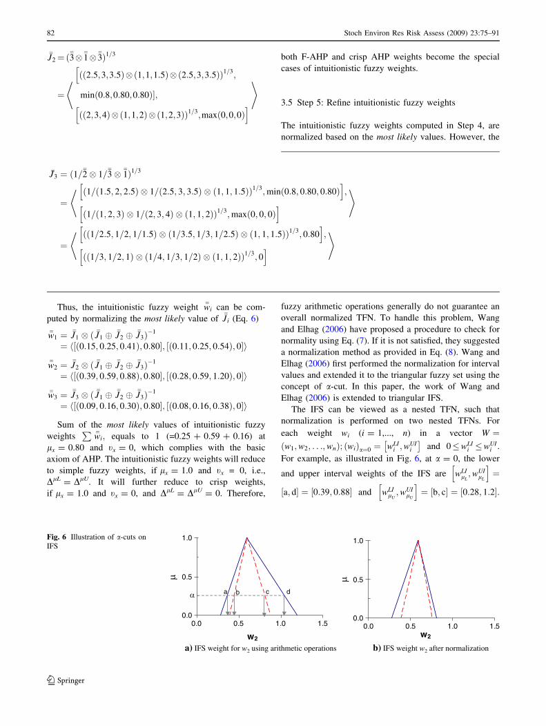
Step 6, and the final results are obtained. The final results

of the three drilling fluids are plotted in Fig. 9. The final IF-

AHP scores ��FAi for OBFs, WBFs and SBFs are:

OBF ¼ 0:067; 0:204; 0:695ð Þ; 0:80½ �;h0:044; 0:204; 1:118ð Þ; 0½ �i

WBF ¼ 0:180; 0:411; 1:091ð Þ; 0:80½ �;h0:127; 0:411; 1:705ð Þ; 0½ �i

SBF ¼ 0:157; 0:370; 1:064ð Þ; 0:80½ �;h0:110; 0:370; 1:614ð Þ; 0½ �i

The sum of the most likely values is equal to one (0.204

+ 0.411 + 0.370), whereas the sum of minimum values

are \ 1 and sum of maximum values are [ 1. The differ-

ence between sum of minimums and sum of maximums

represents the vagueness, and the degree of belief of 0.8

represents ambiguity (non-specificity) in the overall deci-

sion-making process. The similarity measures for the three

alternatives are:

SðOBF;WBFÞ ¼ 0:949; SðOBF; SBFÞ ¼ 0:953;

SðOBF; SBFÞ ¼ 0:955

Since the similarity measure are below the arbitrary

threshold value e = 0.97, each alternative is considered as a

cluster its and required to be ranked separately. The type

reduction of intuitionistic fuzzy set to an ordinary fuzzy set

for all alternatives is shown in Fig. 9. The results of de-

fuzzification are summarized in Table 10. The WBFs are

found to be the most desirable option, followed by SBFs

and OBFs.

In earlier studies by Sadiq et al. (2003) and Tesfama-

riam and Sadiq (2006), the SBF was found to be the most

desirable option. This emphasizes that ambiguity in

assigning degree of beliefs to pairwise comparisons plays

an important role in environmental decision-making. The

authors strongly recommend performing extensive sensi-

tivity analyses before making any final decisions.

5 Conclusions

AHP is inherently a subjective process, which involves

uncertainties in the evaluation and affects the process of

Table 7 A weighting scheme for major impacts ð ��w1Þ

X11,0 X20

1;1 X20

2;1 X20

3;1 X24,1

��W1ðX11;0Þ

X20

1;1�1 �3 �2 �2 ��wX1

1;0;X20

1;1¼ 0:29; 0:43; 0:59ð Þ; 0:80½ �; 0:21; 0:43; 0:64ð Þ; 0½ �h i

X20

2;1 1=�3 �1 �1 �1 ��wX11;0;X20

2;1¼ 0:13; 0:18; 0:23ð Þ; 0:80½ �; 0:13; 0:18; 0:26ð Þ; 0½ �h i

X20

3;1 1=�2 1=�1 �1 1=�2 ��wX11;0;X20

3;1¼ 0:11; 0:16; 0:27ð Þ; 0:80½ �; 0:10; 0:16; 0:31ð Þ; 0½ �h i

X24,1 1=�2 1=�1 �2 �1 ��wX1

1;0;X2

4;1¼ 0:16; 0:23; 0:34ð Þ; 0:80½ �; 0:14; 0:23; 0:41ð Þ; 0½ �h i


123

Ta

ble

8L

ow

erin

terv

alfu

zzy

wei

gh

ts� � w

iði¼

1;2

...5Þ

Lev

el2

W1

Lev

el3

W2

Lev

el4

W3

Lev

el5

W4

W5

(OB

Fs)

W5

(WB

Fs)

W5

(SB

Fs)

X4,1

20

.29

0.4

30

.59

X4,4

30

.28

0.4

20

.60

X16,4

40

.15

0.2

20

.32

X24,1

65

0.4

70

.67

0.7

80

.30

80

.40

00

.49

00

.12

90

.20

00

.36

10

.30

80

.40

00

.49

0

X23,1

65

0.2

20

.33

0.5

30

.12

90

.20

00

.36

10

.30

80

.40

00

.49

00

.30

80

.40

00

.49

0

X15,4

40

.34

0.4

80

.64

X22,1

55

1.0

01

.00

1.0

00

.30

80

.40

00

.49

00

.12

90

.20

00

.36

10

.30

80

.40

00

.49

0

X14,4

40

.14

0.2

00

.27

X21,1

45

0.6

60

.75

0.8

10

.30

80

.40

00

.49

00

.12

90

.20

00

.36

10

.30

80

.40

00

.49

0

X20,1

45

0.1

90

.25

0.3

40

.12

90

.20

00

.36

10

.30

80

.40

00

.49

00

.30

80

.40

00

.49

0

X13,4

40

0.0

70

.11

0.1

90

.30

80

.40

00

.49

00

.12

90

.20

00

.36

10

.30

80

.40

00

.49

0

X3,4

30

.17

0.2

70

.44

X12,3

40

.15

0.2

20

.32

X19,1

25

0.4

70

.67

0.7

80

.12

90

.20

00

.36

10

.30

80

.40

00

.49

00

.30

80

.40

00

.49

0

X18,1

25

0.2

20

.33

0.5

30

.12

90

.20

00

.36

10

.30

80

.40

00

.49

00

.30

80

.40

00

.49

0

X11,3

40

.34

0.4

80

.64

X17,1

15

1.0

01

.00

1.0

00

.37

00

.42

90

.48

80

.10

80

.14

30

.20

20

.37

00

.42

90

.48

8

X10,3

40

.14

0.2

00

.27

X16,1

05

0.3

10

.40

0.4

90

.37

00

.42

90

.48

80

.10

80

.14

30

.20

20

.37

00

.42

90

.48

8

X15,1

05

0.1

30

.20

0.3

60

.37

00

.42

90

.48

80

.10

80

.14

30

.20

20

.37

00

.42

90

.48

8

X14,1

05

0.3

10

.40

0.4

90

.33

30

.33

30

.33

30

.33

30

.33

30

.33

30

.33

30

.33

30

.33

3

X9,3

40

0.0

70

.11

0.1

90

.33

30

.33

30

.33

30

.33

30

.33

30

.33

30

.33

30

.33

30

.33

3

X2,4

30

.10

0.1

60

.28

X8,2

40

.15

0.2

20

.32

X13,8

50

.47

0.6

70

.78

0.0

64

0.0

77

0.1

01

0.5

92

0.6

92

0.7

57

0.1

80

0.2

31

0.3

07

X12,8

50

.22

0.3

30

.53

0.0

81

0.1

11

0.1

68

0.5

33

0.6

67

0.7

59

0.1

60

0.2

22

0.3

10

X7,2

40

.34

0.4

80

.64

X11,7

50

.22

0.3

30

.53

0.1

08

0.1

43

0.2

02

0.3

70

0.4

29

0.4

88

0.3

70

0.4

29

0.4

88

X10,7

50

.47

0.6

70

.78

0.1

62

0.2

00

0.2

56

0.4

88

0.6

00

0.6

76

0.1

62

0.2

00

0.2

56

X6,2

40

.14

0.2

00

.27

X9,6

50

.31

0.4

00

.49

0.0

64

0.0

77

0.1

01

0.5

92

0.6

92

0.7

57

0.1

80

0.2

31

0.3

07

X8,6

50

.13

0.2

00

.36

0.1

08

0.1

43

0.2

02

0.3

70

0.4

29

0.4

88

0.3

70

0.4

29

0.4

88

X7,6

50

.31

0.4

00

.49

0.0

67

0.0

77

0.0

90

0.4

33

0.4

62

0.4

91

0.4

33

0.4

62

0.4

91

X5,2

40

0.0

70

.11

0.1

90

.06

70

.07

70

.09

00

.43

30

.46

20

.49

10

.43

30

.46

20

.49

1

X1,4

30

.10

0.1

50

.23

X4,1

40

.15

0.2

20

.32

X6,4

50

.47

0.6

70

.78

0.0

52

0.0

53

0.0

58

0.4

63

0.4

74

0.4

82

0.4

63

0.4

74

0.4

82

X5,4

50

.22

0.3

30

.53

0.0

67

0.0

77

0.0

90

0.4

33

0.4

62

0.4

91

0.4

33

0.4

62

0.4

91

X3,1

40

.34

0.4

80

.64

X4,3

50

.50

0.5

00

.50

0.0

67

0.0

77

0.0

90

0.4

33

0.4

62

0.4

91

0.4

33

0.4

62

0.4

91

X3,3

50

.50

0.5

00

.50

0.1

08

0.1

43

0.2

02

0.3

70

0.4

29

0.4

88

0.3

70

0.4

29

0.4

88

X2,1

40

.14

0.2

00

.27

X2,2

50

.50

0.5

00

.50

0.0

67

0.0

77

0.0

90

0.4

33

0.4

62

0.4

91

0.4

33

0.4

62

0.4

91

X1,2

50

.50

0.5

00

.50

0.1

08

0.1

43

0.2

02

0.3

70

0.4

29

0.4

88

0.3

70

0.4

29

0.4

88

X1,1

40

0.0

70

.11

0.1

90

.06

70

.07

70

.09

00

.43

30

.46

20

.49

10

.43

30

.46

20

.49

1

X3,1

20

0.1

30

.18

0.2

3

X2,1

20

0.1

10

.16

0.2

7

X1,1

20

0.1

60

.23

0.3

4


123

Ta

ble

9U

pp

erin

terv

alfu

zzy

wei

gh

ts� � w

i(i

=1

,2

...

5)

Lev

el2

W1

Lev

el3

W2

Lev

el4

W3

Lev

el5

W4

W5

(OB

Fs)

W5

(WB

Fs)

W5

(SB

Fs)

X4,1

20

.21

0.4

30

.64

X4,4

30

.20

0.4

20

.69

X16,4

40

.13

0.2

20

.39

X24,1

65

0.3

70

.67

0.7

90

.25

70

.40

00

.58

10

.12

40

.20

00

.40

30

.25

70

.40

00

.58

1

X23,1

65

0.2

10

.33

0.6

30

.12

40

.20

00

.40

30

.25

70

.40

00

.58

10

.25

70

.40

00

.58

1

X15,4

40

.26

0.4

80

.69

X22,1

55

1.0

01

.00

1.0

00

.25

70

.40

00

.58

10

.12

40

.20

00

.40

30

.25

70

.40

00

.58

1

X14,4

40

.12

0.2

00

.32

X21,1

45

0.6

30

.75

0.8

20

.25

70

.40

00

.58

10

.12

40

.20

00

.40

30

.25

70

.40

00

.58

1

X20,1

45

0.1

80

.25

0.3

70

.12

40

.20

00

.40

30

.25

70

.40

00

.58

10

.25

70

.40

00

.58

1

X13,4

40

0.0

60

.11

0.2

20

.25

70

.40

00

.58

10

.12

40

.20

00

.40

30

.25

70

.40

00

.58

1

X3,4

30

.13

0.2

70

.57

X12,3

40

.13

0.2

20

.39

X19,1

25

0.3

70

.67

0.7

90

.12

40

.20

00

.40

30

.25

70

.40

00

.58

10

.25

70

.40

00

.58

1

X18,1

25

0.2

10

.33

0.6

30

.12

40

.20

00

.40

30

.25

70

.40

00

.58

10

.25

70

.40

00

.58

1

X11,3

40

.26

0.4

80

.69

X17,1

15

1.0

01

.00

1.0

00

.33

10

.42

90

.54

40

.10

40

.14

30

.21

60

.33

10

.42

90

.54

4

X10,3

40

.12

0.2

00

.32

X16,1

05

0.2

60

.40

0.5

80

.33

10

.42

90

.54

40

.10

40

.14

30

.21

60

.33

10

.42

90

.54

4

X15,1

05

0.1

20

.20

0.4

00

.33

10

.42

90

.54

40

.10

40

.14

30

.21

60

.33

10

.42

90

.54

4

X14,1

05

0.2

60

.40

0.5

80

.33

30

.33

30

.33

30

.33

30

.33

30

.33

30

.33

30

.33

30

.33

3

X9,3

40

0.0

60

.11

0.2

20

.33

30

.33

30

.33

30

.33

30

.33

30

.33

30

.33

30

.33

30

.33

3

X2,4

30

.10

0.1

60

.33

X8,2

40

.13

0.2

20

.39

X13,8

50

.37

0.6

70

.79

0.0

61

0.0

77

0.1

10

0.5

42

0.6

92

0.7

79

0.1

60

0.2

31

0.3

48

X12,8

50

.21

0.3

30

.63

0.0

76

0.1

11

0.1

86

0.4

52

0.6

67

0.7

92

0.1

32

0.2

22

0.3

64

X7,2

40

.26

0.4

80

.69

X11,7

50

.21

0.3

30

.63

0.1

04

0.1

43

0.2

16

0.3

31

0.4

29

0.5

44

0.3

31

0.4

29

0.5

44

X10,7

50

.37

0.6

70

.79

0.1

53

0.2

00

0.2

79

0.4

42

0.6

00

0.6

93

0.1

53

0.2

00

0.2

79

X6,2

40

.12

0.2

00

.32

X9,6

50

.26

0.4

00

.58

0.0

61

0.0

77

0.1

10

0.5

42

0.6

92

0.7

79

16

00

.23

10

.34

8

X8,6

50

.12

0.2

00

.40

0.1

04

0.1

43

0.2

16

0.3

31

0.4

29

0.5

44

0.3

31

0.4

29

0.5

44

X7,6

50

.26

0.4

00

.58

0.0

66

0.0

77

0.0

93

0.4

10

0.4

62

0.5

18

0.4

10

0.4

62

0.5

18

X5,2

40

0.0

60

.11

0.2

20

.06

60

.07

70

.09

30

.41

00

.46

20

.51

80

.41

00

.46

20

.51

8

X1,4

30

.09

0.1

50

.27

X4,1

40

.13

0.2

20

.39

X6,4

50

.37

0.6

70

.79

0.0

52

0.0

53

0.0

59

0.4

53

0.4

74

0.4

92

0.4

53

0.4

74

0.4

92

X5,4

50

.21

0.3

30

.63

0.0

66

0.0

77

0.0

93

0.4

10

0.4

62

0.5

18

0.4

10

0.4

62

0.5

18

X3,1

40

.26

0.4

80

.69

X4,3

50

.50

0.5

00

.50

0.0

66

0.0

77

0.0

93

0.4

10

0.4

62

0.5

18

0.4

10

0.4

62

0.5

18

X3,3

50

.50

0.5

00

.50

0.1

04

0.1

43

0.2

16

0.3

31

0.4

29

0.5

44

0.3

31

0.4

29

0.5

44

X2,1

40

.12

0.2

00

.32

X2,2

50

.50

0.5

00

.50

0.0

66

0.0

77

0.0

93

0.4

10

0.4

62

0.5

18

0.4

10

0.4

62

0.5

18

X1,2

50

.50

0.5

00

.50

0.1

04

0.1

43

0.2

16

0.3

31

0.4

29

0.5

44

0.3

31

0.4

29

0.5

44

X1,1

40

0.0

60

.11

0.2

20

.06

60

.07

70

.09

30

.41

00

.46

20

.51

80

.41

00

.46

20

.51

8

X3,1

20

0.1

30

.18

0.2

6

X2,1

20

0.1

00

.16

0.3

1

X1,1

20

0.1

40

.23

0.4

1


123

environmental decision-making. The notion of IFS can

handle both vagueness and ambiguity (non-specificity) type

of uncertainties. The use of IF-AHP can help a decision

maker to make more realistic and informed decisions based

on available information, without making strong assump-

tions about the state of knowledge. Concept of IFS in AHP

is introduced through pairwise comparisons. The proposed

IF-AHP methodology is developed using a simple example

of environmental decision-making, which later applied to a

hypothetical case study of drilling fluid selection.

In any MCDM setting, rank preservation and rank

reversal of alternatives is a major concern. Sensitivity

analyses should be carried out to identify the critical factors

in the use of IFS that merit further investigations. The

proposed IF-AHP methodology is demonstrated using fixed

vagueness and ambiguity (non-specificity) in establishing

pairwise comparisons, however, further research is needed

to explore the impact on final decisions using different

values of fuzzification factors and degrees of belief for

different pairwise comparisons.

References

Arslan T, Khisty J (2006) A rational approach to handling fuzzy

perceptions in route choice. Eur J Oper Res 168(2):571–583

Atanassov K (1986) Intuitionistic fuzzy sets. Fuzzy Sets Syst 20:87–

96

Atanassov KT (1999) Intuitionistic fuzzy sets: theory and applica-

tions. Physica-Verlag, Heidelberg

Atanassov K, Pasi G, Yager R (2002) Intuitionistic fuzzy interpre-

tation of multi-person multi-criteria decision making. In: 2002

First International IEEE Symposium ‘‘Intelligent System’’,

pp 115–119

Beynon MJ (2002) DS/AHP method: a mathematical analysis,

including an understanding of uncertainty. Eur J Oper Res

140:148–164

Beynon MJ (2005) A method of aggregation in DS/AHP for group

decision-making with the non-equivalent importance of individ-

uals in the group. Comput Oper Res 32:1881–1896

Beynon MJ, Cosker D, Marshall D (2001) An expert system for multi-

criteria decision making using Dempster Shafer theory. Expert

Syst Appl 20:357–367

Bozbura FT, Beskese A (2006) Prioritization of organizational capital

measurement indicators using fuzzy AHP. Int J Approx

Reasoning 44(2):124–147

0.00.0 1.0 2.0 3.0 4.0

0.5

1.0

OBFs

0.0 1.0 2.0 3.0 4.0

SBFs

0.0 1.0 2.0 3.0 4.0

WBFs

µµ

0.0

0.5

1.0

µ

0.0

0.5

1.0

Fig. 9 Evaluation for drilling

fluids (OBFs, WBFs, SBFs)

using IF-AHP

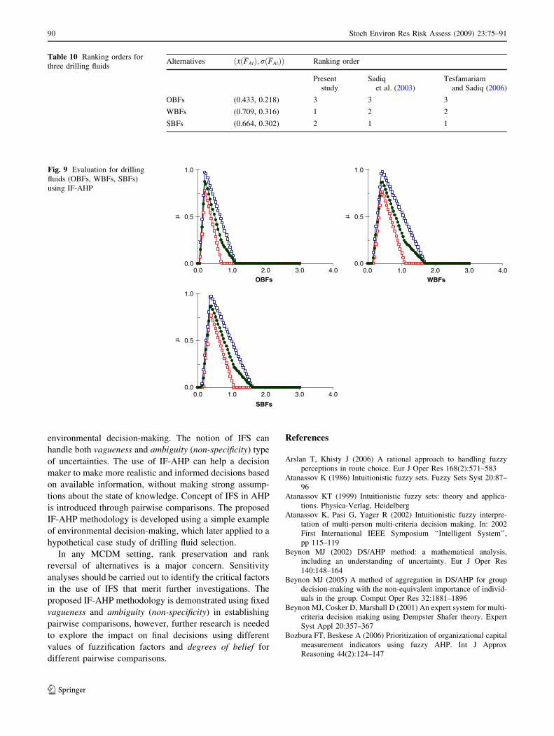
Table 10 Ranking orders for

three drilling fluidsAlternatives ð�xðFAiÞ;rðFAiÞÞ Ranking order

Present

study

Sadiq

et al. (2003)

Tesfamariam

and Sadiq (2006)

OBFs (0.433, 0.218) 3 3 3

WBFs (0.709, 0.316) 1 2 2

SBFs (0.664, 0.302) 2 1 1


123

Buckley JJ (1985) Fuzzy hierarchical analysis. Fuzzy Sets Syst

17:233–247

Bustince H, Burillo P (1996) Vague sets are intuitionistic fuzzy sets.

Fuzzy Sets Syst 79(3):403–405

Chang DY (1996) Application of the extent analysis method fuzzy

AHP. Eur J Oper Res 95:649–655

Chen S-J, Hwang C-L (1992) Fuzzy multiple attribute decision

making: methods and applications. Springer, New York, NY

Cornelis C, Deschrijver G, Kerre EE (2004) Implication in intuition-

istic fuzzy and interval-valued fuzzy set theory: construction,

classification, application. Int J Approx Reasoning 35:55–95

Deng H (1999) Multi-criteria analysis with fuzzy pairwise compar-

ison. Int J Approx Reasoning 21(3):215–231

Gau W-L, Buehrer DJ (1993) Vague sets. IEEE Trans Syst Man

Cyber 23(2):610–614

Hong DH, Choi C-H (2000) Multicriteria fuzzy decision-making

problems based on vague set theory. Fuzzy Sets Syst 114:103–

113

Hung W-L, Yang M-S (2004) Similarity measures of intuitionistic

fuzzy sets based on Hausdorff distance. Pattern Recognit Lett

25:1603–1611

Klir GJ, Yuan B (1995) Fuzzy sets and fuzzy logic: theory and

applications. Prentice Hall International, Upper Saddle River

Kreng VB, Wu C-Y (2007) Evaluation of knowledge portal devel-

opment tools using a fuzzy AHP approach: the case of

Taiwanese stone industry. Eur J Oper Res 176(3):1795–1810

van Laarhoven PJM, Pedrycz W (1983) A fuzzy extension of Saaty’s

priority theory. Fuzzy Sets Syst 11(3):229–241

Lee ES, Li RL (1988) Comparison of fuzzy numbers based on the

probability measure of fuzzy events. Comput Math Appl

15:887–896

Leung LC, Cao D (2000) On consistency and ranking of alternatives

in fuzzy AHP. Eur J Oper Res 124(1):102–113

Levary RR, Wan K (1998) A simulation approach for handling

uncertainty in the analytic hierarchy process. Eur J Oper Res

106(1):116–122

Li D-F (2005) Multiattribute decision making models and methods

using intuitionistic fuzzy sets. J Comput Syst Sci 70:73–85

Li Y, Olson DL, Qin Z (2007) Similarity measures between

intuitionistic fuzzy (vague) sets: a comparative analysis. Pattern

Recognit Lett 28:278–285

Liu H-W, Wang G-J (2006) Multi-criteria decision-making methods

based on intuitionistic fuzzy sets. Eur J Oper Res 179(1):220–

233

Mendel JM (2004) Fuzzy sets for words: why type-2 fuzzy sets should

be used and how they can be used. http://www.fulton.asu.

edu/*nsfadp/ieeecis/Mendel.pdf

Ozdemir MS, Saaty TL (2006) The unknown in decision next term

making what to do about it. Eur J Oper Res 174(1):349–359

Parsons S (2001) Qualitative methods for reasoning under uncer-

tainty. MIT, Cambridge

Saaty TL (1980) The analytic hierarchy process, McGraw-Hill, New

York

Saaty TL (2001) How to make a decision? In: Saaty TL, Vargas LG

(eds) Models, methods, concepts and applications of the analytic

hierarchy process, Chap. 1. Kluwer, Dordrecht

Sadiq R (2001) Drilling Waste discharges in the marine environment:

a risk-based decision methodology. Ph.D. Thesis, Memorial

University of Newfoundland, Canada

Sadiq R, Husain T, Veitch B, Bose N (2003) Evaluation of generic

types of drilling fluid using a risk-based analytical hierarchy

process. Environ Manage 32(6):778–787

Sadiq R, Kleiner Y, Rajani B (2004) Aggregative risk analysis for

water quality failure in distribution networks. J Water Supply

Res Technol-AQUA 53(4):241–261

Silavi T, Delavar MR, Malek MR (2006a) Multicriteria map overlay

in geospatial information system via intuitionistic fuzzy AHP

method. Special Session on ‘‘Soft Computing in Image Process-

ing’’ at the FLINS 2006 Conference, Genova (Italy), August 29–

31, 2006

Silavi T, Delavar MR, Malek MR, Kamalian N, Karimizand K

(2006b) An integrated strategy for GIS-base fuzzy improved

earthquake vulnerability assessment. ISRS-ISPRS TC—IV

International Symposium on ‘‘Geo-information for Disaster

Management (Gi4DM),’’ September 25–26, 2006

Sugihara K, Ishii H, Tanaka H (2004) Interval priorities in AHP by

interval regression analysis. Eur J Oper Res 158(3):745–754

Tesfamariam S, Sadiq R (2006) Risk-based environmental decision-

making using fuzzy analytic hierarchy process (F-AHP).

Stochastic Environ Res Risk Assess 21(1):35–50

U.S. EPA (1999) Development documents for proposed effluent

limitations guidelines and standards for synthetic-based drilling

fluids and other non-aqueous drilling fluids in the oil and gas

extraction point source category, U.S. Environmental Protection

Agency, Washington, DC, EPA-821-B-98–021

Wang Y-M, Elhag TMS (2006) On the normalization of interval and

fuzzy weights. Fuzzy Sets Syst 157:2456–2471

Wang Y-M, Yang J-B, Xu D-L (2005) A two-stage logarithmic goal

programming method for generating weights from interval

comparison matrices. Fuzzy Sets Syst 152:475–498

Weck M, Klocke F, Schell H, Ruenauver E (1997) Evaluating

alternative production cycles using the extended fuzzy AHP

method. Eur J Oper Res 100(2):351–366

Yager RR, Kelman A (1999) An extension of the analytical

hierarchy process using OWA operators. J Intell Fuzzy Syst

7(4):401–417

Yu C-S (2002) A GP-AHP method for solving group decision-making

fuzzy AHP problems. Comput Oper Res 29:1969–2001

Zadeh LA (1965) Fuzzy sets. Inform Control 8(2):338–353

Zadeh LA (1975) The concept of a linguistic variable and its

application to approximate reasoning part I. Inform Sci 8:199–

249

Zhu KJ, Jing Y, Chang D-Y (1999) A discussion on extent analysis

method and applications of fuzzy AHP. Eur J Oper Res 116:450–

456


123

http://www.fulton.asu.edu/$\sim$nsfadp/ieeecis/Mendel.pdf

http://www.fulton.asu.edu/$\sim$nsfadp/ieeecis/Mendel.pdf

Environmental decision-making under uncertainty using intuitionistic fuzzy analytic hierarchy...

Documents

Transcript of Environmental decision-making under uncertainty using intuitionistic fuzzy analytic hierarchy...