Electronic Supplementary Material for “Arroyo del Vizcaino, Uruguay: A fossil-

rich 30 ka megafaunal locality with cut-marked bones”

Richard A. Fariña1,*, P. Sebastián Tambusso1, Luciano Varela1, Ada Czerwonogora1,

Mariana Di Giacomo1, Marcos Musso2, Roberto Bracco3, Andrés Gascue4

1Sección Paleontología, Facultad de Ciencias, Universidad de la República, Iguá 4225,

11400 Montevideo Uruguay

2Sección Geotécnica, Facultad de Ingeniería, Universidad de la República, Julio Herrera

y Reissig 565, 11300 Montevideo, Uruguay

3Laboratorio 14C, Comisión Nacional de Arqueología, Cátedra de Radioquímica,

Facultad de Química, Universidad de la República, Gral. Flores 2124, 11200

Montevideo, Uruguay

4Centro Universitario Regional Este, Universidad de la República, Burnett casi M.

Chiossi (Campus Municipal), 20000 Maldonado, Uruguay

* e-mail: fari~a@fcien.edu.uy

1. SURVEY METHODOLOGY

To resume collection after the drought in January 1997, a secondary course was built to

bypass the site (Figure S1) in July 2009. In February and March 2011 plastic bags were

filled with the dirt removed and then piled up to work as dams on both ends of the site.

The remaining water, along with that continuously supplied by the natural aquifer, was

pumped out all throughout the fieldwork, which took place in late March 2011 and more

recently in late January-early February 2012. In 2011, the site was uncovered and

photographed and bones exposed in an area of about 30 m2 in the streambed, at an

average depth of 2 metres. Those bones regarded as too vulnerable to be left without

risk of loss were collected. A metre grid system was established to map the specimens

(Figure S2). In addition, samples were taken for ongoing analyses, including grain size

and pollen content. In 2012, a more exhaustive collection was performed in an area of

about 12 m2 (Figure S2). Standard techniques have been used for field and quarry

mapping, as well as for excavating and preparing the bones [1].

Figure S1. The power shovel builds a secondary course to bypass the site.

Figure S2. Metre grid system employed to map the specimens.

2. CHRONOLOGICAL, STRATIGRAPHICAL AND

PALAEOENVIRONMENTAL CONTEXT

Radiocarbon dating is based on purified and non-purified bone collagen and on wood.

Table S1 summarizes the radiocarbon dates obtained for Arroyo del Vizcaíno yielded by

samples analysed in the following laboratories: Laboratorio 14C, Comisión Nacional de

Arqueología, Cátedra de Radioquímica, Facultad de Química, Universidad de la

República, Uruguay (URU), Beta Analytic Radiocarbon Dating, Miami FL, USA (Beta)

[2], Oxford Radiocarbon Accelerator Unit, University of Oxford, UK (Ox). Samples

labelled URU 0490, 0493 and 0496 were taken from three ribs belonging to the sloth

Lestodon armatusand sample URU 0574 was taken from a scute belonging to the

glyptodont Panochthus. All of them were pre-treated as follows: the external layers

were mechanically removed and powdered to less than 500 µm. Then, the samples were

washed with distilled water at 80 ºC for 30 minutes, and ultrasonically bathed (4 times).

The inorganic fractions were removed with 8% HCl and the organic fractions were

neutralised washing with successive distilled water washes. They were treated for 24

hours with 0.5 M NaOH and the organic fractions were again neutralised with the same

procedure. Afterwards, the organic fractions of two of the samples (URU 0493 and

URU 0496) were purified as in refs. [3-5]. For control purposes, and to compare with

previous datings of material from the same site [2], the organic fraction of the sample

0490 was not purified. In all cases, the organic fraction recovered was above 8%. The

pieces of wood were pre-trated with HCl (8%)-NaOH (2%)- HCl (2%) and then the

fractions G, H and W were extracted following ref. [6]. Sample OxA-V-2474-10 was

treated following refs.[7-9].

Table S1. Samples dated with radiocarbon techniques. Bones with an asterisk (clavicle [46] and ulna) have marks that show features similar to those made by tools. Ages are given in years before present.

Material

sampled

Laboratory

and sample

number

δ13C C:N

ratio

Percentage

of extracted

collagen

Conventional

radiocarbon

age

Calendar

dates

(Oxcal 4.1)

Lestodon rib URU 0496 -18.5 N/A ≥ 5% 27,000±450 29,696±871

Lestodon rib URU 0490 -18.5 N/A ≥ 5% 27,200±900 30,433±2033

Lestodon rib Beta 204256 -18.6 N/A N/A 28,300±230 30,580±747

Lestodon

clavicle*

Beta 206660 -18.8 N/A N/A 29,150±290 31,895±745

Undetermined

wood

URU 0562 -

25.74

-- -- 29,150±320 31,872±789

Panochthus

scute

URU 0574 -20.6 2.9 ≥ 5% 29,220±300 31,939±728

Undetermined

wood

URU 0561 -

25.74

-- -- 29,350±315 32,009±715

Lestodon rib URU 0493 -18.5 -- ≥5% 30,100±600 32,886±1446

Lestodon

ulna*

OxA-V-

2474-10

-

18.72

3.2 ≥1% 28,760±210 31,561±925

Average 28,692 31,430

Pooled

average

29,000 31759

Median 29,150 31,872

Usual description methods were heeded for the geological setting [10]. The geological

model of the deposits is shown in Figure 1C. Along the stream, ponds are formed as

microbasins excavated by differential erosion on the Mercedes Fm. Cretaceous

sandstones during late Pleistocene. The prevalent climatic conditions must have been

arid to semi-arid. Sediment grain size composition in beds 1 and 2 is similar to that of

the nearby outcrops of Mercedes Fm. (Figure S3). The sediment green-greyish colour of

the bed 2 facies a is attributed to reducing environment and the brownish colour of bed

2 facies b is proposed to have developed by moderate oxidation in post-depositional

events. Still, a more complete understanding of this difference, i.e., whether those facies

correspond to separate events, will be available when larger areas of the site are more

thoroughly excavated.

The depositional environment must have included episodes of different fluvial energy,

capable of carrying pebbles, cobbles and medium to coarse sand. This corresponds to a

flow velocity of 300 to 10 cm s-1 at 1 metre depth to erode and move the particles and a

flow velocity of 100 to 1 cm s-1 to deposit them [11]. Substantial mass flow can be ruled

out as the accumulation agent due to the rather homogeneous grain size, the lack of the

typical size gradient distribution of the remains [12], the lack of predominant orientation

in the material [13] (which is also well preserved) and the very gentle relief in that

region, with just a few metres of height difference in the surrounding area. Besides, the

fossiliferous sediments seem to have been formed in situ, as evidenced by the presence

of intraclasts from the underlying bed in them.

The silicified sandstones of the Mercedes Fm. constitute the palaeorelief as an irregular

plain, with small ponds temporarily flooded. The aquifer must have been already active,

even in times of dry climate between 40 and 30 kybp, which coincides with the final

stages of the marine isotope stage 3. This must have produced reducing conditions in

the base of the fossiliferous bed 2 (facies a) and the relatively more oxidative conditions

in the upper facies b may have been due to postdepositional expositions. The presence

of coarse grains must have been due to high-energy events, and the lack of

intermediately sized grains can be explained by the lack of availability of them in the

Mercedes Fm. regolith. Those pebbles must have transported as bed load together with

the transported bones, perhaps in more than one event. Some of the bones show rather

large clasts (~ 5 cm in diameter) in their natural cavities, such as the spinal canal (Figure

S4). Incidentally, this phenomenon yielded no marks on the bone. Turbulence could

have been present since the deposition took place in an area lateral to the mainstream.

Figure S3. Granulometric analysis of the sediments of the Arroyo del Vizcaíno samples.

Figure S4. Lestodon vertebra showing pebbles in the spinal canal.

3. FAUNAL LIST

Specimens collected

Lestodon armatus: 18 astragali; 183 vertebrae; 2 talus; 15 teeth; 45 metapodials; 3

clavicles; 12 ribs and rib fragments; 14 fragments of skull; 10 scapulae; 31 phalanges;

33 complete or broken femora; 1 hyoid; 5 fibulae; 14 fragments of mandibular rami; 8

teeth; 10 radii or fragment radii; 18 pelvic girdle fragments; 23 complete or broken

tibiae.

Mylodon darwinii: 4 teeth; 1 mandibular ramus; 1 astragalus.

Glossotherium robustum: 2 teeth; 2 vertebrae

Glyptodonts: 1 atlas; 1 calcaneum; 1 fragment of vertebral column; 1 fragment of

cranium; 1 fragment of scapula; 1 femur; 1 humerus; 5 pelvic girdle fragments; 1 tibia;

1 cervical tube; 1 sacral tube; 1 ulnar fragment; 2 vertebrae; 1 trivertebral element; 5

carapace fragments and 3 isolated scutes; 1 cranium and 1 radium assigned to

Glyptodon cf. clavipes; 203 scutes of Glyptodon clavipes, 58 scutes of Doedicurus

clavicaudatus and 26 scutes of Panochthus tuberculatus.

Toxodon platensis:1 vertebra; 1 tibia; 1 cranium; 2 scapulae

Stegomastodon sp.: 1 tooth; 1 fragment of scapula; 1 vertebra; 1 pelvic girdle fragment

Cervidae indet: 1 humerus, 1 calcaneum

Hippidion principale: 1 tooth; 1 astragalum; 1 phalanx; 1 vertebra.

Smilodon populator: 1 canine, 1 cranium fragment

Fossil ground sloths: 1 rib fragment; 2 metapodial; 4 teeth; 2 fragment of scapula; 11

phalanges; 1 fragment of femur; 1 mandibular ramus fragment; 1 patella; 1 tibia

fragment; 4 vertebrae.

Mammaliaidentified specimens not assigned to any species): 110 rib fragments; 11

cranium fragments; 12 fragments of scapula; 21 fragments of femur; 2 of humeri

fragments; 1 mandibular ramus fragment; 2 metapodial; 13 fragments of pelvic girdle; 1

radius fragment; 1 patella fragment; 3 fragments of sacrum; 1 tibia fragment; 4

vertebrae.

Mammalia indet: 34 fragments

4. TAPHONOMY

The biostratinomical characterization of the vertebrate assemblage follows ref. [14]. The

number of specimens (NISP), minimum number of anatomical units (MAU), minimum

number of individuals (MNI) and minimum number of elements (MNE) were

established. Weathering and transport evidence were assessed through macroscopical

analyses. Unless otherwise stated, counts and percentages refer to a total with

glyptodont scutes excluded. The taphonomic features analysed include: number of

specimens and individuals (NISP and MNI counts), number and characterization of the

species represented (see above the faunal list), relative abundance of the species, body

size, age spectra, skeletal articulation, representation of skeletal parts, bone orientation

and bone modifications (this last feature will be detailed in the next section).

In the portion of the bonebed covered in our excavations, the bones were distributed in a

roughly oval pattern and contained more than one thousand elements (see faunal list).

The minimum number of individuals was established as follows: for each skeletal

element (a bone or set of bones, such as the cervical vertebrae), the total number of

identified specimens (NISP) was counted and the number of individual animals (NIA,

or MNI taking only one skeletal portion into account [15]) was calculated. Seventeen

right femora were collected or observed and all of them were assigned to adult or

subadult specimens of Lestodon armatus (hence, MNI=17; table S2). In addition, at

least two juvenile specimens are represented by a hyoid, a mandible, one tibia, four

femora and one rib fragment. The age estimated for the individuals preserved in the

assemblage was classified within three major groups: juveniles (derived from the

absence of the epiphyses), prime adults and old individuals (due to the presence of

osteoarthritical signs).

Table S2. Body mass, NISP (counted as the clearly identifiable specimens), abundance and MNI of the species found in Arroyo del Vizcaíno.

Taxon Body mass

[47,48] NISP

MNI

adults juveniles

Lestodon armatus 4000/1000* 452/5 15 2

Mylodon darwinii 1500 5 1 0

Glossotherium robustum 1500 3 1 0

Glyptodon cf. clavipes 1000† 23/1 0 1

Doedicurus clavicaudatus 1400 1 0

Panochthus tuberculatus 1100 1 0

Toxodon platensis 1100 5 1 0

Stegomastodon sp. 1500* 3 0 1

Hippidion principale 119* 4 0 1

Smilodon populator 400 2 1 0

Cervidae indet. 50 2 1 0

TOTAL MNI 22

(81.5%)

5

(18.5%)

* The elements assigned to these species must have belonged to a juvenile, hence this

mass estimate.

† The juvenile element of a glyptodont counted here is tentatively assigned to

Glyptodon cf. clavipes, but the other two species cannot be ruled out.

The index of anatomical representation [16]indicates the percentage of skeletal elements

preserved in relation to the sum of the total number of elements for all individuals

identified in the assemblage, providing information of the taphonomic biases affecting

the composition of the assemblage. This index (Ir=NISP x 100/MNE x MNI) was

calculated only for L. armatus and also for the glyptodonts, the best represented taxa in

the faunal association. The obtained results, 12.8% for Lestodon armatus and 3.2% for

the glyptodonts, allow the exclusion of catastrophic death or mass mortality event as the

source of the deposit. In those cases, this index would have taken its maximum value for

each represented species (100%) if an immediate burial had occurred, followed by non-

destructive diagenetic conditions [16], which is the case for our site (see below).

The degree of disarticulation and scattering of the bones was analysed in the field

during the collection of the remains. Articulation was considered as “two or more

skeletal elements being in their proper anatomical positions relative to one another, and

within a centimetre of each other if not in fact touching” [17] and scattering as

“increasing the spatial distance between anatomically related bones” [17]. In this sense,

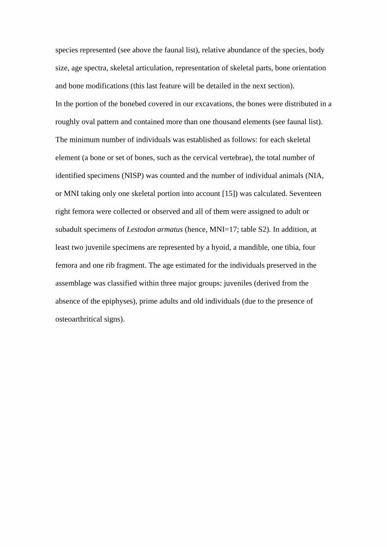
apart from a small group of vertebra and a rib (Figure S5), most of the specimens were

found disarticulated, although in a number of cases bones of similar anatomical regions

were found scattered but in close spatial relation. This is especially true for many bones

of possibly one specimen of Lestodon armatus yet to be collected that are found not

much dispersed from their original arrangement.

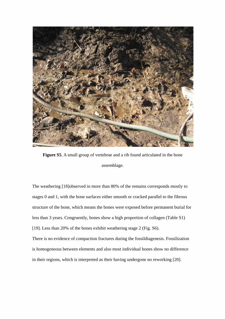
Figure S5. A small group of vertebrae and a rib found articulated in the bone

assemblage.

The weathering [18]observed in more than 80% of the remains corresponds mostly to

stages 0 and 1, with the bone surfaces either smooth or cracked parallel to the fibrous

structure of the bone, which means the bones were exposed before permanent burial for

less than 3 years. Congruently, bones show a high proportion of collagen (Table S1)

[19]. Less than 20% of the bones exhibit weathering stage 2 (Fig. S6).

There is no evidence of compaction fractures during the fossildiagenesis. Fossilization

is homogeneous between elements and also most individual bones show no difference

in their regions, which is interpreted as their having undergone no reworking [20].

Figure S6. A) CAV 16, an astragalus of Mylodon darwinii, showing the usual fine

preservation in the studied site, while B) CAV 369, an astragalus of Lestodon, shows a

weathering stage 2, is cracked mainly in the sticking out regions like the odontoid

process, is rounded and shows some trampling.

To investigate transport due to fluvial action, the relative abundance of Voorhies

Groups [21] was analysed and rose diagrams for orientation of long bones [22,17] were

built up (Figure 2c). In the discrimination of the represented specimens, glyptodont

scutes were not considered in the NISP counts. We found 53% bones belonging to

Group I and 33% and 14% belonging to Groups II and III, respectively. The distribution

and orientation of these bones was quantified on images and direct observations

gathered during fieldwork. No preferential orientation was registered for the long or

elongated bones examined (Figure 2c). Further arguments against major transport [17]

are that most of the bones show no evidence of rolling (88.9%, including glyptodont

scutes in this count, NISP=988) and exhibit minimum abrasion; the state of preservation

is very good and most of the bones are included in fine sediments, composed of clay

and silt (see above: Sediments, profile, environment section). However, the existence of

more than one population of bones cannot be assessed at the present state of knowledge,

as already said. Moreover, in the collected specimens the most transportable elements of

the megamammals are present (Voorhies group I), but not the least transportable

elements of smaller individuals (Voorhies group II and III). Taking into account the

faunal composition of the assemblage, where mostly megamammals are present, it

should be noticed that the fluvial transport index (FTI) calculated from experiments

with individual skeletal elements of an Indian elephant (Elephas maximus) [23] yielded

comparable results to those obtained according to Voorhies Groups [21]

Among the identified specimens (table S3), limb bones and girdles are predominant

(41.1%, including a small number of metapodials, 4.8%), followed by vertebrae

(33.2%), rib portions (15.8%) and cranial fragments (9.2%). These proportions are also

interpreted as the accumulation being autochthonous, as already evidenced by the

Voorhies groups, although some outgoing hydraulic transport might have removed the

lighter elements (scutes, not considered in the proportions of the Voorhies groups, and

metapodials).

The observed frequencies of vertebrae, ribs, limbs and girdle bones, and phalanges,

were compared with the data of different modern and fossil assemblages summarized in

ref. [16] (Figure 3a). The values show the Arroyo del Vizcaíno site very close to the

relative frequencies of the bones exposed in Amboseli [24] and among the group of

values that points out a biogenic accumulation of the bones, in particular, of various

sites associated with human presence: the modern San hunter-gatherer camp and some

of the Plio-Pleistocene archaeological sites at Koobi Fora, Kenya (FxJj50, Olduvai

Gorge, Tanzania, and FLK Zinjantropus site [25, 26]). These African sites had been re-

evaluated from a taphonomic perspective [26], including the comparison with present-

day hunter-gatherers. For example, the Kua San in the East Central Kalahari Desert in

Botswana are known to dismember and transport very large (several hundred kg) entire

carcasses for several kilometres. At FLK Zinjanthropus, the dominant, but not the only

cause of bone accumulation at the site, is the transport and disposal of bones by humans.

However, gnawing by carnivores and small rodents in low proportions (compared to

modern animal dens), removals, and perhaps additions of bones by carnivores, among

biogenic modifications, including trampling, were also present. In the Arroyo del

Vizcaíno site a similar level of taphonomic complexity could be invoked as responsible

for the bone accumulation, excluding the action of carnivores and rodents due to the

absence of these kinds of marks on the bones (see next section).

Likewise, the alternative arguments attributing the observed patterns of skeletal

representation to post-depositional processes (i.e. biogenic accumulation) should be

strengthened with the evidence of subaerial weathering damage on surviving bones [26].

This should be extensive enough to account for the complete disintegration of less

durable (i.e., axial and epiphyseal) elements, thus implying that geological processes

altered the skeletal proportions in the bone assemblage by differential water transport of

certain elements or sediment compaction and differential destruction of buried skeletal

elements [26]. However, it does not seem likely that these processes played a dominant

role in forming the observed patterns of skeletal representation in the Arroyo del

Vizcaíno site. First, the previously-discussed weathering characteristics of the

assemblage indicate a prevalence (more than 80%) of unweathered to moderately

weathered bones, which would be inconsistent withsufficient subaerial exposure to

eliminate less resistant elements [18]. Moreover, the patterns of long bone orientation

and Voorhies groups argue against water transport being a major determinant of skeletal

composition.

In the case of Amboseli [24], the bone sample gives a more accurate representation of

the larger species due to taphonomic biases, with higher representation of animals of

more than 200 kg, as is the case observed for the Arroyo del Vizcaíno site. The

Amboseli bone assemblage reflects the relative numbers of the ten most abundant large

wild herbivores; however, the rhinoceros population show higher than expected values

due to human predation. The body size biases of the smaller bones in this assemblage

are related basically to two factors: more complete initial destruction by carnivores and

scavengers, and more rapid rates of weathering and trampling causing fragmentation

[24]. These biases could account at least partially for the observed bone concentration in

the Arroyo del Vizcaíno site, in particular for the abundance of very large species (see

below).

Table S2 shows the taxonomic composition and relative abundance of the assemblage,

in which herbivores are predominant. The relative abundance was estimated following

ref. [27] and the distributions were corrected to avoid taphonomic biases depending on

body size and differential preservation [28]. The obtained values for linear regressions

of abundance and body mass plots did not fit the expected results for an unbiased

assemblage (y= 0.094x + 2.068, r2 non significant). Most of the represented taxa are

xenarthrans (six out of eleven species), whose body size exceeds the tonne. This faunal

composition resembles the typical association described for the Lujanian (late

Pleistocene) in the current Río de la Plata area, dominated by megamammals

andxenarthrans [29, 30]. Table S3 shows the representation of the anatomical regions,

whose results, as discussed in the main text, are compatible with the removal of

consumable parts.

Finally, the faunal assemblage has little evidence of root etching. If the amount of root

etching is considered a function of the rapidity of burial [31], this evidence is congruent

with a fast burial. Additional evidence suggesting that the bones lay exposed on the

surface for a brief period comes from the absence of modifications by scavengers or

rodents (see below for a detailed characterization of surface modifications on the

bones).

Table S3. Anatomical regions of the specimens represented in the collected material.

Anatomical region Number of elements collected Observed percentage

Skull (including lower jaws and teeth) 75 9.3

Axial skeleton (vertebrae) 274 33.8

Axial skeleton (ribs) 128 11.6

Limb skeleton (including girdles) 294 36.3

Metapodials 39 4.8

Table S4 shows the values of several variables (MNI= minimum number of individuals

based on femora and taking into consideration laterality, size and epiphyses fusion;

MAU= Minimal Animal Units; %MAU= Standardized MAU; Exp. MNE (MNI)=

expected MNE based on MNI; %S= percentage of survival) of the bone representation

belonging to ground sloths, which were used as an input for Fig. 3. In table S5, the

observed frequencies of the remains of the ground sloths are compared with the

frequencies to be expected if all anatomical regions were equally represented. Both Χ2

and G-tests show that there exist significant differences between observed and expected

frequencies. The Χ2 indicates that the main elements contributing to the difference are

femora and tibiae. On the other hand, the values of the G-test show that those elements

present a positive deviation, i.e., they are overrepresented in the sample, while other

elements (in red) show a negative deviation, i.e., they are underrepresented. Those

results are congruent with the survival percentage (%S) and the %MAU (Table S4 and

Fig. 3).

Table S4. Bones assigned to ground sloths (mainly Lestodon armatus) in the bone assemblage of Arroyo del Vizcaíno. Values of %MAU are represented in Fig. 3b. Abbreviations: MNI= Minimum Number of Individuals (Based on femora and taking into consideration laterality, size and epiphyses fusion). MAU= Minimal Animal Units [49].%MAU= Standardized MAU. Exp. MNE (MNI)= expected MNE based on MNI. %S= percentage of survival [50].

Elements NISP MNE MAU %MAU Expected MNE

(MNI) %S

Skulls 25 6 6.00 48.00 17 35.29

Mandibles 20 14 7.00 56.00 17 52.94

Hyoids 2 1 0.50 4.00 34 2.94

Vertebrae (region not

determined)

19

Cervical vertebrae 25 24 3.43 27.43 119 20.17

Dorsal vertebrae 117 70 4.38 35.00 272 25.74

Lumbar vertebrae 11 6 3.00 24.00 34 17.65

Sacra 7 7 7.00 56.00 17 41.18

Caudal vertebrae 83 67 2.68 21.44 425 15.76

Ribs 119 59 2.11 16.86 476 12.39

Ventral Ribs 9 5 0.42 3.33 204 2.45

Sterna 1 1 0.14 1.14 119 0.84

Clavicles 3 3 1.5 12.00 34 8.82

Scapulae 23 8 4.00 32.00 34 23.53

Pelves 25 13 6.50 52.00 17 41.18

Humeri 20 12 6.00 48.00 34 35.29

Radii 11 10 5.00 40.00 34 29.41

Ulnae 10 10 5.00 40.00 34 29.41

Carpals 11 11 0.79 6.29 238 4.62

Metacarpals 14 14 1.40 11.20 170 8.24

Femora 61 25 12.50 100.00 34 73.53

Patellae 6 6 3.00 24.00 34 17.65

Tibiae 28 24 12.00 96.00 34 70.59

Fibulae 5 5 2.50 20.00 34 14.71

Astragali 16 16 8.00 64.00 34 47.06

Calcanei 2 2 1.00 8.00 34 5.88

Tarsals 10 10 1.25 10.00 136 7.35

Metatarsals 8 8 1.00 8.00 136 5.88

1st phalanxes 10 10 0.83 6.67 204 4.90

2nd phalanxes 22 22 2.75 22.00 136 16.18

3rd phalanxes 13 13 1.30 10.40 170 7.65

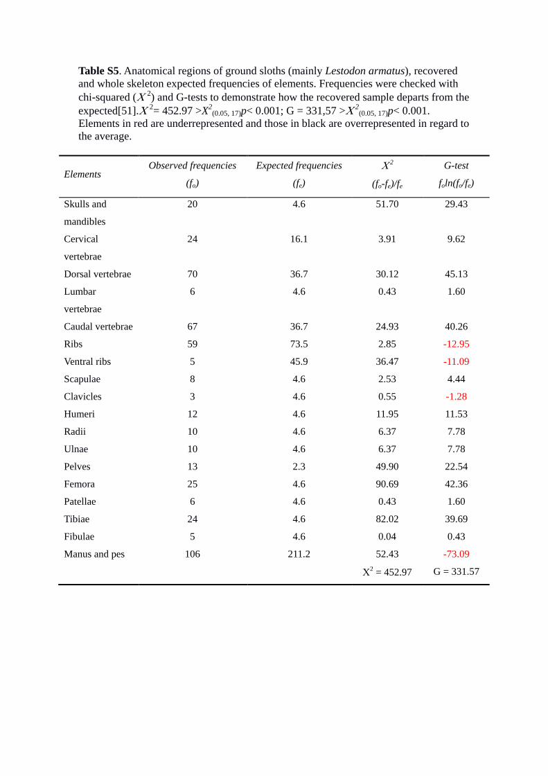
Table S5. Anatomical regions of ground sloths (mainly Lestodon armatus), recovered and whole skeleton expected frequencies of elements. Frequencies were checked with chi-squared (Χ 2) and G-tests to demonstrate how the recovered sample departs from the expected[51].Χ 2= 452.97 >X2

(0.05, 17)p< 0.001; G = 331,57 >Χ 2(0.05, 17)p< 0.001.

Elements in red are underrepresented and those in black are overrepresented in regard to the average.

Elements Observed frequencies

(fo)

Expected frequencies

(fe)

Χ 2

(fo-fe)/fe

G-test

foln(fo/fe)

Skulls and

mandibles

20 4.6 51.70 29.43

Cervical

vertebrae

24 16.1 3.91 9.62

Dorsal vertebrae 70 36.7 30.12 45.13

Lumbar

vertebrae

6 4.6 0.43 1.60

Caudal vertebrae 67 36.7 24.93 40.26

Ribs 59 73.5 2.85 -12.95

Ventral ribs 5 45.9 36.47 -11.09

Scapulae 8 4.6 2.53 4.44

Clavicles 3 4.6 0.55 -1.28

Humeri 12 4.6 11.95 11.53

Radii 10 4.6 6.37 7.78

Ulnae 10 4.6 6.37 7.78

Pelves 13 2.3 49.90 22.54

Femora 25 4.6 90.69 42.36

Patellae 6 4.6 0.43 1.60

Tibiae 24 4.6 82.02 39.69

Fibulae 5 4.6 0.04 0.43

Manus and pes 106 211.2 52.43 -73.09

Χ2 = 452.97 G = 331.57

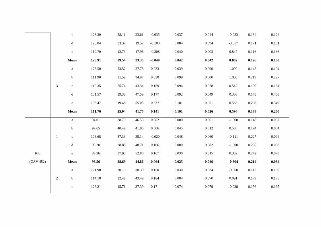
5. SURFACE MODIFICATION ON THE FOSSIL SPECIMENS

Bones were cleaned following the usual procedures [32] and examined under low

magnification using a hand lens to determine the presence of surface

modifications.These were preliminary classified to distinguish trampling from possible

anthropogenic marks [33]. Other, larger bone modifications were analysed visually and

using virtual and plastic models.

(a) Identification and Diagnosis Methods

Further analysis of selected marks was carried out with light microscopy under

magnifications of 20x, 30x and 45x. Following methods based on extended depth-of-

field [34, 35] and, using an Olympus SZ61 stereomicroscope under a magnification of

45x, several photographs of the marks at different focus depth were taken. Helicon

Focus [34] software was used to make a complete in-focus image and a three-

dimensional model of each mark that accurately represents the micromorphology of the

modifications. These models were later processed with the software MeshLab [36] and

at least four perpendicular sections of the grooves were obtained for each mark. In Table

S6 we show the features observed in marks on the surface of several of the bones that

are typical of human-made marks [33, 37-38]:

• Opening angle: angle between left and right slopes at the floor of the cut mark.

• Angle of the Tool Impact Index: angles (σ1 and σ2) between the slopes S1 (left)

and S2 (right) of the cut mark and the unaffected bone surface. Because it is not

possible to determine the left and right side of the mark the ATI Index is

measured as: ((90º – σ1) – (90º – σ2)) / ((90º – σ1) + (90º – σ2)).

• Shoulder Height Index: height of the shoulders formed on either side of the cut

mark (SH1 and SH2). The SH Index is defined as (SH1 – SH2) / (SH1 + SH2).

• Depth of Cut (DC): perpendicular depth of the cut mark in relation to the

unaffected bone surface.

• Floor radius: the radius of circle fitted to the floor of the cut mark profile, with

the floor defined as lying between the two points where the profiles of the slopes

start to converge.

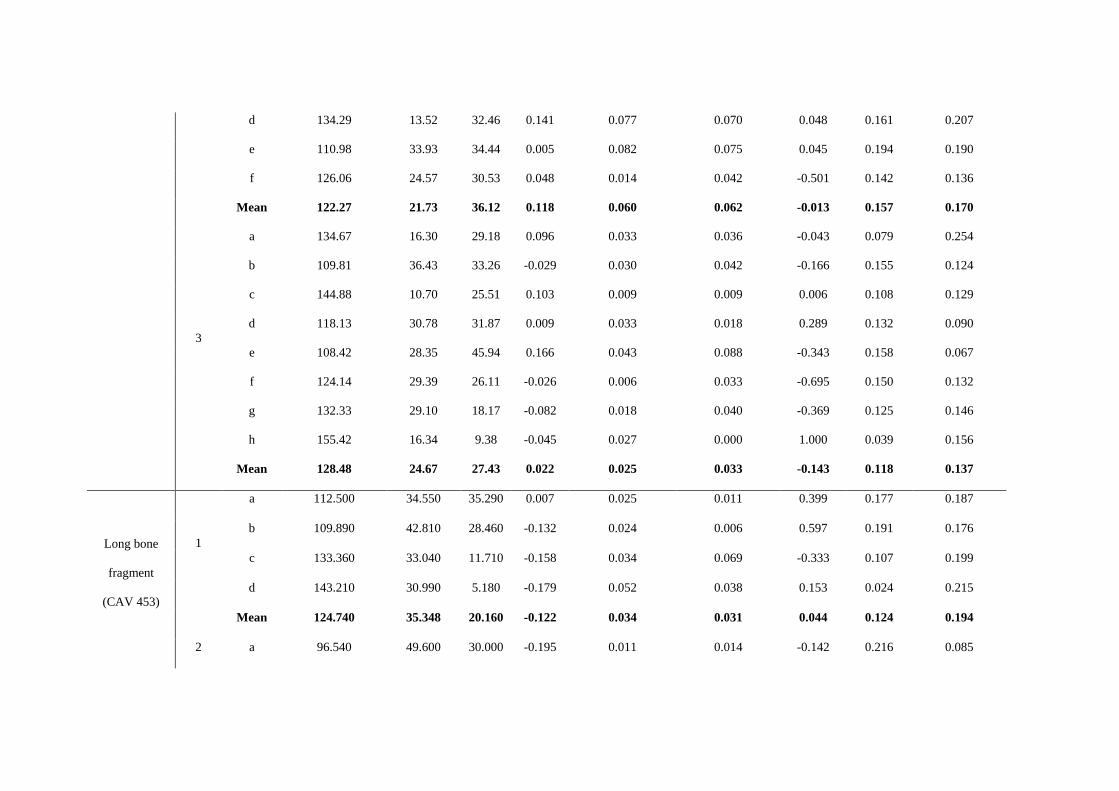
Table S6. Dimensions in the selected marks.

Bone Mark Section Opening Angle σ1 σ2 ATI Shoulder height

left (mm)

Shoulder height

right (mm) SH Index

Depth of

cut (mm)

Floor radius

(mm)

Tibia

(CAV 385)

1

a 100.45 41.98 38.61 -0.034 0.225 0.016 0.865 0.364 0.153

b 102.91 50.64 26.36 -0.2357 0.0114 0.0294 -0.441 0.2708 0.0748

c 91.38 39.11 49.03 0.108 0.025 0.105 -0.617 0.210 0.091

d 101.31 43.07 35.86 -0.0713 0 0.0264 -1.000 0.2458 0.1617

e 131.02 9.48 40.24 0.236 0.022 0.060 -0.467 0.112 0.099

f 129.33 24.69 25.93 0.0096 0 0.001 -1.000 0.1453 0.1407

Mean 109.4 34.83 36.01 0.0108 0.047 0.033 0.176 0.225 0.120

Rib

(CAV 451)

1

a 129.06 16.66 34.69 0.140 0.041 0.010 0.599 0.213 0.459

b 104.26 39.67 36.45 -0.031 0.040 0.030 0.143 0.336 0.473

c 114.20 36.20 29.72 -0.057 0.037 0.017 0.374 0.290 0.469

d 121.37 21.9 34.26 0.100 0.000 0.007 -1.000 0.180 0.167

e 101.88 38.99 39.34 0.003 0.017 0.060 -0.564 0.292 0.188

Mean 114.15 30.68 34.89 0.037 0.027 0.025 0.042 0.262 0.351

2 a 128.80 21.65 29.66 0.062 0.000 0.063 -1.000 0.119 0.149

b 130.90 21.85 25.99 0.031 0.051 0.007 0.763 0.088 0.112

c 128.30 28.11 23.61 -0.035 0.037 0.044 -0.083 0.134 0.124

d 126.84 33.37 19.52 -0.109 0.084 0.094 -0.057 0.171 0.131

e 119.70 42.73 17.96 -0.208 0.040 0.003 0.847 0.116 0.136

Mean 126.91 29.54 23.35 -0.049 0.042 0.042 0.002 0.126 0.130

3

a 128.50 23.52 27.78 0.033 0.039 0.000 1.000 0.148 0.104

b 111.90 31.59 34.97 0.030 0.099 0.000 1.000 0.219 0.227

c 110.35 25.74 43.34 0.159 0.094 0.028 0.542 0.190 0.154

d 101.57 29.38 47.59 0.177 0.092 0.049 0.308 0.173 0.468

e 106.47 19.48 55.05 0.337 0.181 0.051 0.558 0.208 0.349

Mean 111.76 25.94 41.75 0.141 0.101 0.026 0.596 0.188 0.260

Rib

(CAV 452)

1

a 94.01 38.79 46.53 0.082 0.000 0.061 -1.000 0.148 0.067

b 99.65 40.49 41.05 0.006 0.045 0.012 0.580 0.194 0.084

c 106.68 37.33 35.14 -0.020 0.048 0.060 -0.111 0.227 0.094

d 93.20 38.88 48.71 0.106 0.000 0.082 -1.000 0.256 0.098

e 89.26 37.95 52.86 0.167 0.030 0.015 0.332 0.242 0.078

Mean 96.56 38.69 44.86 0.064 0.025 0.046 -0.304 0.214 0.084

2

a 121.90 20.15 38.39 0.150 0.030 0.034 -0.060 0.112 0.150

b 114.18 22.48 43.49 0.184 0.084 0.070 0.091 0.179 0.175

c 126.21 15.71 37.39 0.171 0.074 0.079 -0.038 0.156 0.165

d 134.29 13.52 32.46 0.141 0.077 0.070 0.048 0.161 0.207

e 110.98 33.93 34.44 0.005 0.082 0.075 0.045 0.194 0.190

f 126.06 24.57 30.53 0.048 0.014 0.042 -0.501 0.142 0.136

Mean 122.27 21.73 36.12 0.118 0.060 0.062 -0.013 0.157 0.170

3

a 134.67 16.30 29.18 0.096 0.033 0.036 -0.043 0.079 0.254

b 109.81 36.43 33.26 -0.029 0.030 0.042 -0.166 0.155 0.124

c 144.88 10.70 25.51 0.103 0.009 0.009 0.006 0.108 0.129

d 118.13 30.78 31.87 0.009 0.033 0.018 0.289 0.132 0.090

e 108.42 28.35 45.94 0.166 0.043 0.088 -0.343 0.158 0.067

f 124.14 29.39 26.11 -0.026 0.006 0.033 -0.695 0.150 0.132

g 132.33 29.10 18.17 -0.082 0.018 0.040 -0.369 0.125 0.146

h 155.42 16.34 9.38 -0.045 0.027 0.000 1.000 0.039 0.156

Mean 128.48 24.67 27.43 0.022 0.025 0.033 -0.143 0.118 0.137

Long bone

fragment

(CAV 453)

1

a 112.500 34.550 35.290 0.007 0.025 0.011 0.399 0.177 0.187

b 109.890 42.810 28.460 -0.132 0.024 0.006 0.597 0.191 0.176

c 133.360 33.040 11.710 -0.158 0.034 0.069 -0.333 0.107 0.199

d 143.210 30.990 5.180 -0.179 0.052 0.038 0.153 0.024 0.215

Mean 124.740 35.348 20.160 -0.122 0.034 0.031 0.044 0.124 0.194

2 a 96.540 49.600 30.000 -0.195 0.011 0.014 -0.142 0.216 0.085

b 116.700 42.350 19.050 -0.196 0.069 0.041 0.250 0.083 0.172

c 101.360 47.790 30.780 -0.168 0.006 0.015 -0.426 0.205 0.110

d 102.520 50.330 27.760 -0.221 0.062 0.107 -0.265 0.121 0.228

Mean 104.280 47.518 26.898 -0.195 0.037 0.044 -0.092 0.156 0.149

Rib

(CAV 458)

1

a 129.76 21.91 28.85 0.054 0.0461 0.0049 0.808 0.0485 0.1602

b 110.52 36.92 30.61 -0.056 0.0275 0.0214 0.125 0.0673 0.0917

c 87.66 27.1 64.21 0.418 0.0329 0.1108 -0.542 0.1287 0.0898

d 161.71 11.35 8.53 -0.018 0.0256 0.0128 0.333 0.0417 0.3077

Mean 122.41 24.32 33.05 0.071 0.033 0.037 -0.063 0.072 0.162

Radii

(CAV 459)

1

a 80.580 46.280 53.040 0.084 0.018 0.000 1.000 0.367 0.172

b 112.780 13.780 54.780 0.368 0.099 0.023 0.619 0.257 0.228

c 115.890 17.690 46.770 0.252 0.067 0.015 0.643 0.386 0.231

d 116.220 33.420 27.810 -0.047 0.035 0.012 0.500 0.214 0.254

Mean 106.368 27.793 45.600 0.167 0.055 0.012 0.631 0.306 0.221

Rib

(CAV 475)

1

a 93.33 38.03 47.68 0.102 0.010 0.354 -0.945 0.169 0.071

b 86.73 45.91 47.24 0.015 0.000 0.016 -1.000 0.248 0.102

c 89.10 40.72 49.33 0.096 0.022 0.034 -0.218 0.280 0.081

d 92.80 44.58 42.42 -0.023 0.039 0.046 -0.081 0.283 0.073

Mean 90.49 42.31 46.67 0.048 0.018 0.113 -0.727 0.245 0.082

Hyoid

(CAV 476)

1

a 117.21 28.46 33.06 0.039 0.018 0.044 -0.428 0.153 0.091

b 125.77 24.3 29.67 0.043 0.021 0.050 -0.417 0.178 0.121

c 118.06 23.66 39.14 0.132 0.059 0.044 0.143 0.151 0.142

d 133.65 25.39 20.99 -0.0329 0.0368 0.0245 0.201 0.1133 0.1011

e 125.81 27.64 26.55 -0.0087 0.0421 0.0518 -0.103 0.1618 0.1035

Mean 124.10 25.89 29.88 0.0321 0.035 0.043 -0.099 0.151 0.112

Ulna

(CAV 520)

1

a 86.64 40.84 52.79 0.1384 0 0.0509 -1.000 0.2694 0.0569

b 110.17 26.35 44.26 0.164 0.071 0.000 1.000 0.276 0.100

c 140 16.8 20.43 0.0254 0.1093 0.0109 0.819 0.1011 0.1108

d 95.35 34.24 50.23 0.167 0.031 0.008 0.573 0.239 0.067

Mean 108.04 29.56 41.93 0.1140 0.053 0.018 0.501 0.221 0.084

Mandible

(CAV 897)

1

a 86.46 30.67 62.63 0.3686 0.000 0.132 -1.000 0.293 0.120

b 89.17 45.45 45.39 -0.0007 0.059 0.100 -0.259 0.294 0.091

c 106.55 28.83 44.65 0.1485 0.0134 0.0349 -0.445 0.4294 0.126

d 107.42 32.14 40.99 0.0828 0.0633 0.0495 0.122 0.2091 0.303

Mean 97.4 34.27 48.42 0.1453 0.034 0.079 -0.400 0.307 0.160

(b) Trampling

Two marks on a rib were assigned to trampling (Fig. S7). They were reconstructed using

the procedure described above and showed depths of 81.4 and 93.5 µm, opening angles

of 128º and 144º, and lacked microstriations, Herzian cones, asymmetry and shoulder

effect.

Figure S7. Trampling mark in rib CAV 120 and its section profile for comparison,

showing a smaller depth and lack of shoulders.

(c) Other marks on the bones

A few bones show peculiar indentations whose natural agency is difficult to establish: a

left maxilla (CAV 5, Figure S8) and a calcaneum (CAV 45, Figure S9), both belonging

to Lestodon and in perfect condition, with the outer bone layer well preserved on all

surfaces and lacking other types of possible human-made marks. Casts of the holes in

the bones described below were obtained by filling them with silicon rubber. A catalyser

was added to activate the elastomer. Previously, the inner surfaces of the holes were

cleaned of sediment and then protected with polyethyleneglycol to prevent detachment

of the spongy bone when the casts were extracted. The hole in the calcaneum is on the

lateral surface, while that of the maxilla is right before the first molariform. The casts

can be seen in Figure S10. The puncture in the maxilla is rather shallow, only about one

centimetre deep, and that in the calcaneum is much deeper, about 6.5 cm. The cast from

the calcaneum is interpreted to be double, with both parts at low angles to each other, as

if the object that made it had moved inside the bone after penetration. Otherwise, both

casts are very similar; in lateral view they lack symmetry, as their tips are bevelled.

Observed from the tip, both are laterally symmetrical and about 10 mm thick on average

from right to left and 2 or 3 cm from the thinner bottom to the thicker top. It is

noteworthy that this form does not correspond to that of the canine of a large

carnivoran.

Figure S8. Left maxilla of Lestodon armatus (CAV 5) showing the hole described in the

text.

Figure S9. Left calcaneum of Lestodon armatus (CAV 45) showing the indentation

described in the text.

Figure S10. Casts of the holes in the left maxilla (CAV 5, a) and the left calcaneum

(CAV 45, b) of Lestodon armatus. Black line in B indicates the boundary between each

one of the original dents.

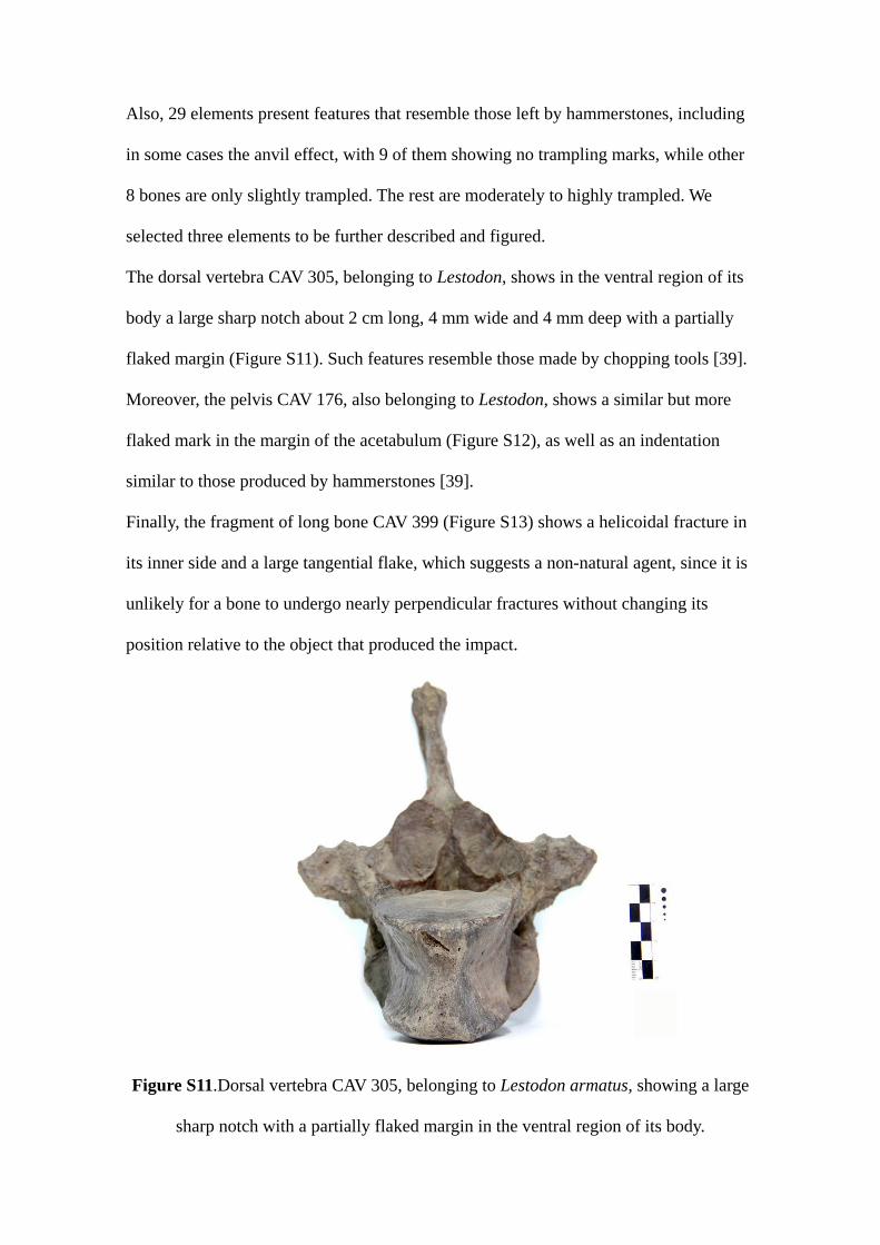
Also, 29 elements present features that resemble those left by hammerstones, including

in some cases the anvil effect, with 9 of them showing no trampling marks, while other

8 bones are only slightly trampled. The rest are moderately to highly trampled. We

selected three elements to be further described and figured.

The dorsal vertebra CAV 305, belonging to Lestodon, shows in the ventral region of its

body a large sharp notch about 2 cm long, 4 mm wide and 4 mm deep with a partially

flaked margin (Figure S11). Such features resemble those made by chopping tools [39].

Moreover, the pelvis CAV 176, also belonging to Lestodon, shows a similar but more

flaked mark in the margin of the acetabulum (Figure S12), as well as an indentation

similar to those produced by hammerstones [39].

Finally, the fragment of long bone CAV 399 (Figure S13) shows a helicoidal fracture in

its inner side and a large tangential flake, which suggests a non-natural agent, since it is

unlikely for a bone to undergo nearly perpendicular fractures without changing its

position relative to the object that produced the impact.

Figure S11.Dorsal vertebra CAV 305, belonging to Lestodon armatus, showing a large

sharp notch with a partially flaked margin in the ventral region of its body.

Figure S12. Flaked mark in the margin of the acetabulum of the pelvis CAV 176

assigned to Lestodon armatus.

Figure S13. Fragment of long bone CAV 399 showing a helicoidal fracture in its inner

side and a large tangential flake.

6. LITHIC MATERIAL.

Lithic material was analysed with the usual techniques [40].In the fieldwork of 2011

and 2012, a total of 105 lithic elements were collected in spatial association with the

bones that precluded recent origin, i.e. they were found immediately below some of the

bones, and beside and above others. After a macroscopical analysis, 10 of them had

some features congruent with anthropic agency, such as flaking events: six possible

flakes (Figure S14), two possible cores and two possible tools on nuclei. One piece of

silcrete was mentioned in the main text to have features compatible with those of a

scraper (Fig. 4 f-g, Fig. S15). Since silcrete is present in the area and given its quality as

a raw material for human tools [41, 42], this quantity is admittedly a scarce

representation of possible lithic tools, although they have not been systematically

searched for in our excavations. The surfaces of these lithic fragments were analysed to

test the hypothesis of their anthropic origin using stereomicroscope at 20x. Nearly all of

them are made of raw material that is present in the surrounding area (quartz, silcrete,

amphibolite and sandstone), i.e. from the Mercedes Fm. [43].

Even though processing this number of giant animals would require a correspondingly

high usage of lithic material, other South American Pleistocene archaeological sites also

show a paucity of such elements [44,45] and only a part of this site has been rather

exhaustively explored.

Figure S14. Broken (above), complete (middle) and fragmentary (below) flakes [52]

found in the Arroyo del Vizcaíno site.

Fig. S15. Further images of the area a of the lithic element illustrated in Fig. 4f.

Scanning electron microphotographs at 2000 and 4300x showing micropolish. The

lighter particle is a piece of fabric left during cleaning.

References

S1. Leiggi, P., Schaff, C. R. & May, P. 1994 Field organization and specimen

collecting. In: Vertebrate Paleontological Techniques (eds. P. Leiggi, P. May), pp. 59-

76. Cambridge: Cambridge Univ. Press.

S2. Fariña, R. A. & Castilla, R. 2007Earliest evidence for human-megafauna interaction

in the Americas. In Human and Faunal Relationships Reviewed: An Archaeozoological

Approach (eds. E. Corona-M. & J. Arroyo-Cabrales), pp. 31-34. Oxford: Archaeopress.

S3. Longin, R. 1971 New method of collagen extraction for radiocarbon dating. Nature

230, 241-242.

S4. Schoeninger, M. & DeNiro, M. 1984 Nitrogen and carbon isotopic composition of

bone collagen from marine and terrestrial animals. Geochim. Cosmochim. Ac. 48, 625–

639.

S5. Higham, T. F. G., Jacobi, R. M. & Bronk Ramsey, C. 2006 AMS radiocarbon dating

of ancient bone using ultrafiltration. Radiocarbon 48, 179–95.

S6. Gupta, S. K. & Polach, H. A. 1985 Radiocarbon Dating Practices at ANU

Handbook Radiocarbon Laboratory Research School of Pacific Studies. Canberra:

ANU.

S7. Bronk Ramsey, C., Higham, T., Bowles, A. & Hedges, R. 2004 Improvements to

the pretreatment of bone at Oxford. Radiocarbon 46,155–63.

S8. Bronk Ramsey, C., Higham, T. & Leach, P. 2004 Towards high-precision AMS:

progress and limitations. Radiocarbon 46,17–24.

S9. Bronk Ramsey, C., Higham, T., Owen, D. C., Pike, W. G. &Hedges, R. 2002

Radiocarbon Dates from the Oxford Ams System: Archaeometry Datelist 31.

Archaeometry 44, 1-149.

S10. Tucker, M. 1982 The Field Description of Sedimentary Rocks. Geological Society

of London Handbook Series, No. 2. Maidenhead: Open University Press.

S11. Michols, G. 2009 Sedimentology and stratigraphy.New York: Wiley-Blackwell.

S12. Major, J. J. 2003 Debris Flow. In Encyclopedia of Sediments and Sedimentary

Rocks (eds. G. V. Middleton, M.J. Church, M. Coniglio, L. A. Hardie, & F.

J.Longstaffe), pp. 186–188. New York: Kluwer Acad. Publ.

S13. Mazza, P. P. A. & Ventra, D. 2011 Pleistocene debris-flow deposition of the

hippopotamus-bearing Collecurti bonebed (Macerata, Central Italy): Taphonomic and

paleoenvironmental analysis. Palaeogeogr. Palaeoclimatol. Palaeoecol. 310, 296-314.

S14. Behrensmeyer, A. K. 1991 Terrestrial Vertebrate Accumulations. In Taphonomy:

Releasing the Data Locked in the Fossil Record (eds. P. Allison & D. E. G. Briggs), pp.

291-335. New York: Plenum.

S15. Bai, B., Wang, Y., Meng, J., Jin, X., Li, Q. & Ping L. 2011 Taphonomic analyses

of an Early Eocene Litolophus (Perissodactyla, Chalicotherioidea) assemblage from the

Erlian Basin, Inner Mongolia, China. Palaios 26, 187–196.

S16. Arribas, A. & Palmqvist, P.1998 Taphonomy and paleoecology of an assemblage

of large mammals: hyaenid activity in the lower Pleistocene site at Venta Micena (Orce,

Guadix-Baza Basin, Granada, Spain). Geobios 31, 3-47.

S17. Lyman, R. L.1994Vertebrate taphonomy. Cambridge: Cambridge Univ. Press.

S18. Behrensmeyer, A. K. 1978 Taphonomic and ecologic information from bone

weathering. Paleobiol. 4, l50-l62.

S19. Czerwonogora, A., Fariña, R. A. & Tonni, E. P. 2011 Diet and isotopes of Late

Pleistocene ground sloths: first results for Lestodon and Glossotherium (Xenarthra,

Tardigrada). Neues Jahrb. Geol. P-A 262, 257-266.

S20. Rogers, R. R. Eberth, D. A. & Fiorillo, A. R. 2007 Bonebeds: Genesis, Analysis,

and Paleobiological Significance. Chicago: Chicago Univ. Press.

S21. Voorhies, M. R. 1969 Taphonomy and population dynamics of an early Pliocene

vertebrate fauna, Knox County, Nebraska. Contrib. Geol. 1, 1-69.

S22. Kreutzer, L. A. 1988 Megafaunal butchering at Lubbock Lake, Texas: a

taphonomic reanalysis. Quaternary Research 30, 221-231.

S23. Frison, G. C. & Todd, L. C. 1986 The Colby mammoth site: Taphonomy and

archaeology of a Clovis kill in northern Wyoming. Albuquerque: Univ. New Mexico

Press.

S24. Behrensmeyer, A. K. & Dechant-Boaz, D. E. 1980 The recent bones of Amboseli

Park, Kenya. In Fossils in the Making (eds. A. K. Behrensmeyer & A. Hill), pp. 72-93.

Chicago: Chicago University Press.

S25. Bunn, H. T. 1982 Meat-eating and human evolution: studies on the diet and

subsistence patterns of Plio-Pleistocene hominids in East Africa. Ph.D. Dissertation.

Berkeley: Univ. of California.

S26. Bunn, H. T. 1986 Patterns of skeletal representation and hominid subsistence

activities at Olduvai Gorge, Tanzania and Koobi Fora, Kenya. J. Hum. Evol. 15, 673–

690.

S27. Damuth, J. 1982 Analysis of the preservation of community structure in

assemblages of fossil mammals. Paleobiol. 8, 434-446.

S28. Behrensmeyer, A. K.,Western, D. & Dechant-Boaz, D. E. New perspectives in

vertebrate paleoecology from a recent bone assemblage. Paleobiol. 5, 12-21.

S29. Tonni, E. P., Prado, J. L., Menegaz, A. N. & Salemme, M. C. 1985 La unidad

mamífero (Fauna) Lujanense. Proyección de la estratigrafía mamaliana al cuaternario de

la región pampeana. Ameghiniana 22, 255-261.

S30. Fariña, R. A., Vizcaíno, S. F. & De Iuliis, G. 2013 Megafauna: Giant Beasts of

Pleistocene South America. Bloomington: Indiana Univ. Press.

S31. Meltzer, D. J. 2006 Folsom: New Archaeological Investigations of a Classic

Paleoindian Bison Kill. Berkeley: University of California Press.

S32. May, P., Reser, P. & Leiggi, P. 1994 Macrovertebrate preparation. In: Vertebrate

Paleontological Techniques (eds. P. Leiggi, P. May), pp. 113-153. Cambridge:

Cambridge Univ. Press.

S33. Domínguez-Rodrigo, M., De Juana, S., Galán, A. B. & Rodríguez, M. 2009 A new

protocol to differentiate trampling marks from butchery cut marks. J. Archaeol. Sci. 36,

2643-2654.

S34. Berejnov, V. V. 2009 Rapid and Inexpensive Reconstruction of 3DStructures for

Micro-Objects Using Common Optical Microscopy. arXiv preprint arXiv:0904.2024.

S35. Hein, L. R. O., de Campos, K. A., Caltabiano, P. C. R de O. & Horovistiz, A. L.

2010 3-D reconstruction by extended depth-of-field in failure analysis – Case study I:

Qualitative fractographic investigation of fractured bolts in a partial valve. Eng. Fail.

Anal. 17, 515–520.

S36. MeshLab. 2009 Open source, portable, and extensible system for the processing

and editing of unstructured 3D triangular meshes. http://meshlab.sourceforge.net/.

S37. Bello, S. M. & Soligo, C. 2008 A new method for the quantitative analysis of

cutmark micromorphology. J. Archaeol. Sci. 35, 1542-1552.

S38.Bello, S. M. Parfitt, S. A.& Stringer, C. 2009 Quantitative micromorphological

analyses of cut marks produced by ancient and modern handaxes. J. Archaeol. Sci. 36,

1869-1880.

S39. Capaldo, S. D. & Blumenschein, R. J. 1994 A quantitative diagnosis of notches

made by hammerstone percussion and carnivore gnawing on bovid long bones. Am.

Antiq. 59, 724-748.

S40. Collins, M. B. 1975 Lithic Technology as a Means of Processual Inference. In

Lithic Technology: Making and Using Stone Tools (ed. E. Swanson), pp. 15-34.

Mouton: The Hague.

S41. Gascue, A. 2009 La tecnología lítica desarrollada por los habitantes prehistóricos

del Arroyo del Perdido (Soriano, Uruguay). Arqueología Prehistórica Uruguaya en el

Siglo XXI, 117-130.

S42. Gascue, A.2009 Tecnología lítica y patrones de asentamiento en la cuenca de

arroyo Grande (Soriano). Arqueología Prehistórica Uruguaya en el Siglo XXI, 133-150.

S43. Spoturno, J., Oyhantçabal, P., Aubet, N., Cazaux, S. & Morales, E. 2004 Carta

Geológica y Memoria Explicativa a Escala 1/100.000 del Departamento de Canelones,

CONICYT. Proyecto 6019. Fondo Clemente Estable. Versión I CD.

S44. Martínez, G. Gutiérrez, M. A. & Tonni, E. P. 2012 Paleoenvironments and faunal

extinctions: Analysis of the archaeological assemblages at the Paso Otero locality

(Argentina) during the Late Pleistocene–Early Holocene. Quat. Int. in press (2013).

S45. Politis, G. & Messineo, P. G. 2008 The Campo Laborde site: New evidence for the

Holocene survival of Pleistocene megafauna in the Argentine Pampas. Quat. Int. 191,

98–114.

S46. Arribas, A., Palmqvist, P., Pérez-Claros, J. A., Castilla, R., Vizcaíno, S. F. &

Fariña, R. A. 2001 New evidence on the interaction between humans and megafauna in

South America. Publ. Semin. Paleon. Zaragoza 5, 228-238.

S47. Fariña, R. A., Vizcaíno, S. F. & Bargo, M. S. 1998 Body size estimations in

Lujanian (Late Pleistocene-Early Holocene of South America) mammal megafauna.

Mastozool. Neotr. 5, 87-108.

S48. Czerwonogora, A. 2010 Morfología, sistemática y paleobiología de los perezosos

gigantes del género Lestodon (Mammalia, Xenarthra, Tardigrada). Ph.D. Dissertation.

La Plata: UNLP.

S49. Binford, L. R. 1984 Faunal Remains from Klasies River Mouth. New York:

Academic Press.

S50. Brain, C. K. 1981. The Hunters or the Hunted? Chicago: University of Chicago

Press.

S51. Sokal, R. R. & Rohlf, F. J. 1981 Biometry, 2nd ed. San Francisco: Freeman.

S52. Sullivan, A. & Rozen, K. 1985 Debitage Analysis and Archaeological

Interpretation. Am. Antiq. 50, 755-779.