arX

iv:h

ep-t

h/92

0308

2v1

30

Mar

199

2

Eikonal Quantum Gravity and Planckian Scattering*

Daniel Kabat and Miguel Ortiz

Center for Theoretical Physics

Laboratory for Nuclear Science

and Department of Physics

Massachusetts Institute of Technology

Cambridge, Massachusetts 02139 U.S.A.

Submitted to: Nuclear Physics B

CTP#2069 March 1992

* This work is supported in part by funds provided by the U. S. Department of Energy(D.O.E.) under contract #DE-AC02-76ER03069.

0

ABSTRACT

Various approaches to high energy forward scattering in quantum gravity are compared

using the eikonal approximation. The massless limit of the eikonal is shown to be equivalent

to other approximations for the same process, specifically the semiclassical calculation due

to G. ’t Hooft and the topological field theory due to H. and E. Verlinde. This comparison

clarifies these previous results, as it is seen that the amplitude arises purely from a linearized

gravitational interaction. The interpretation of poles in the scattering amplitude is also

clarified.

1

I. INTRODUCTION

Quantization of General Relativity leads to a perturbatively non-renormalizeable theory1;

hence the general view that this approach to quantum gravity is without predictive power. It

is therefore interesting that predictive calculations do exist for the two particle forward scat-

tering amplitude at energies of order the Planck scale. G. ’t Hooft2 evaluated the amplitude

semiclassically by solving the Klein-Gordon equation for one particle in the gravitational shock

wave due to the other particle. Since there is no particle production in a shock wave spacetime,

this calculation may also be thought of as solving a free scalar field in the curved background

(Aichelburg–Sexl metric3) arising from a classical ultrarelativistic source4. Subsequently H.

and E. Verlinde5 showed that in this kinematic regime, quantum gravity separates into weakly

and strongly coupled sectors. The weakly coupled sector can be treated classically, while the

strongly coupled sector is a topological theory which may be solved nonperturbatively to

reproduce ’t Hooft’s scattering amplitude.

The eikonal approximation is a technique in quantum field theory for evaluating the

leading behavior of a forward scattering amplitude in the limit of large center of mass energy

by summing an infinite class of Feynman graphs6,7,8. It has been used in string models of

quantum gravity by Muzinich and Soldate9 and by Amati et. al.10 to obtain results similar

to those of ’t Hooft for Planckian scattering (see also Ref. 11). In this paper we apply the

eikonal approximation to linearized quantum gravity. We first use the approximation to derive

an amplitude which is identical to that of Refs. 2, 5. This equivalence has previously been

noted in the context of string theory9,10 and for electromagnetic scattering12. We then show

how, in the massless limit, the summation of Feynman graphs in the eikonal approximation is

2

equivalent to the methods employed by both ’t Hooft and H. and E. Verlinde to evaluate the

Planckian scattering amplitude. The calculation of the eikonal approximation away from the

massless limit allows us to clarify the issue of poles in the scattering amplitude first discussed

by ’t Hooft2,25.

The paper is organized as follows. Part II is a calculation of the eikonal scattering am-

plitude for linearized gravity. Part III shows the equivalence of the eikonal approximation to

’t Hooft’s semiclassical calculation, and part IV discusses the origin of the poles in the scat-

tering amplitude. Finally, part V shows how graviton exchange in the eikonal approximation

is governed by a topological theory in the high energy limit.

II. EIKONAL AMPLITUDE FOR LINEARIZED GRAVITY

We present the eikonal calculation of the two particle scattering amplitude in linearized

gravity. Similar calculations for the scattering of massless particles in a string theory model

of quantum gravity may be found in Refs. 9 and 10.

The action for Einstein gravity coupled to a real scalar field is

S =

∫

d4x√

−detg

{

− 1

16πG

(

R +1

2gµνCµCν

)

− 1

2gµν∂µφ∂νφ − 1

2m2φ2

}

. (2.1)

The metric is to be expanded about a Minkowski background, gµν = ηµν + hµν . The gauge

fixing term is Cµ = ∂νhνµ − 1

2∂µhν

ν ; the ghosts associated with this gauge choice are ignored,

since we expect ghost contributions to be sub-dominant in forward scattering. Expanding in

3

hµν , the leading terms give the action for linearized gravity.

S =

∫

d4x1

16πG

1

8hαβ

[

ηαγηβδ + ηαδηβγ − ηαβηγδ]

2hγδ +1

2φ( 2 − m2)φ

+1

2hµν

[

∂µφ∂νφ − 1

2ηµν

(

∂λφ∂λφ + m2φ2)

]

.

(2.2)

Here and subsequently all indices are to be raised and lowered with ηµν = diag(−1, 1, 1, 1).

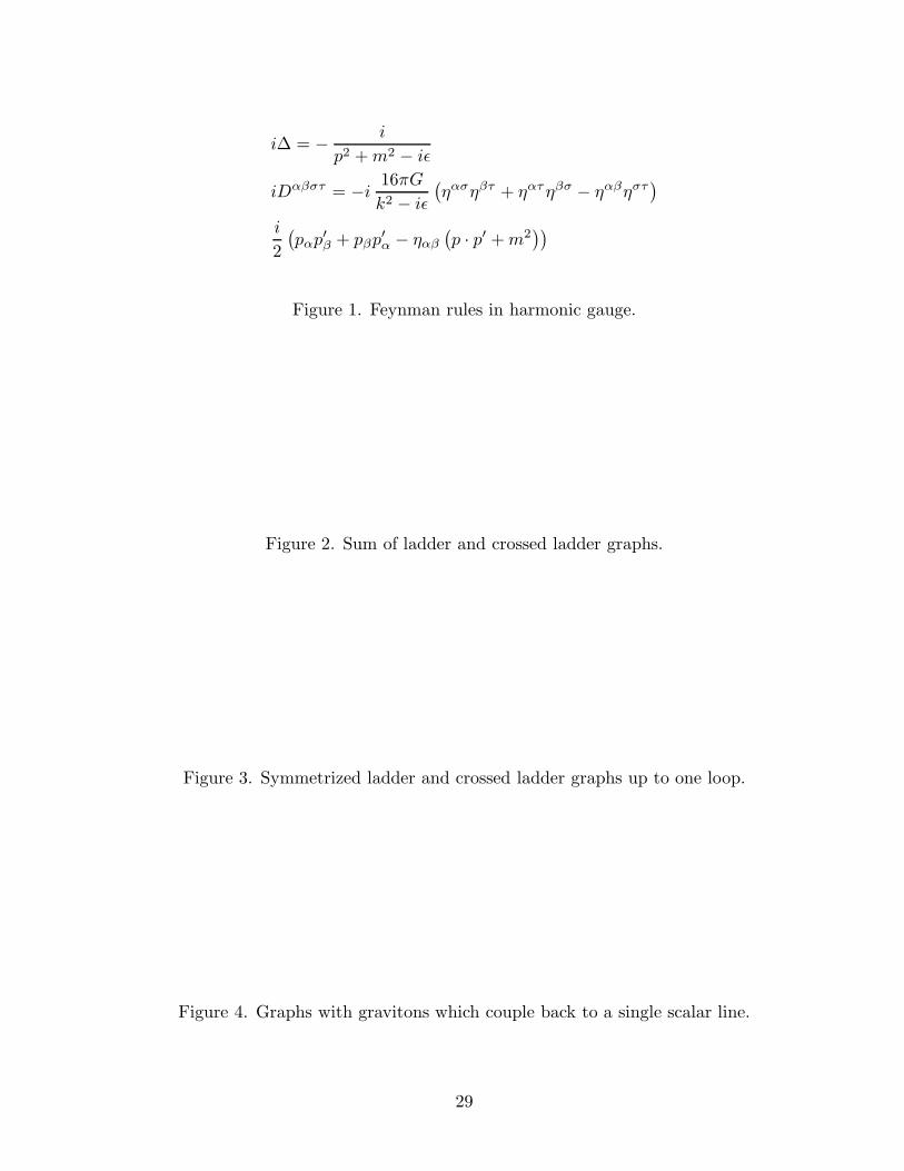
This action leads to the propagators and vertices in Fig. 1.

Perturbative quantum gravity has been investigated by many authors13. It is well known

that the theory suffers from non-renormalizeable infinities, which for the process we are con-

sidering are present even at one loop1,14. Within this approach, the two particle scattering

amplitude may apparently only be calculated in the Born approximation, a calculation which

may be found in De Witt’s seminal paper on quantum gravity13. However, as we shall now

explain, it is possible to go beyond this first order approximation if one wishes to probe only

the leading behaviour of high energy forward scattering.

We are interested in the elastic forward scattering amplitude of two scalar particles with

initial momenta p1, p2 and final momenta p3, p4, in the regime where s/t is large (here s and

t are the usual Mandelstam variables s = −(p1 + p2)2 and t = −(p1 − p3)

2). We proceed to

evaluate the scattering amplitude using the eikonal approximation, which may be described

as follows7. Consider the sum of ladder and crossed ladder graphs (Fig. 2), and make the

following approximations. In evaluating the vertex factors, ignore the recoil of the matter

field,

pµp′ν + pνp′µ − ηµν

(

p · p′ + m2)

≈ 2pµpν .

In the matter propagators, ignore k2 relative to p · k,

1

(p + k)2 + m2 − iǫ≈ 1

2p · k − iǫ.

4

This procedure is expected to give the leading behaviour of the ladder diagrams for large centre

of mass energy15. To preserve Bose symmetry we should include diagrams where p3 and p4

are interchanged, but such diagrams are clearly subdominant. The question of whether the

ladder diagrams dominate over other exchange diagrams in high energy scattering in quantum

gravity is a more subtle question16,17.

We illustrate this procedure order by order (Fig. 3). The Born amplitude is simply

iMBorn = ip1αp1β

−i 16πG

(p1 − p3)2 − iǫ

(

ηαγηβδ + ηαδηβγ − ηαβηγδ)

ip2γp2δ

= i16πGγ(s)1

(p1 − p3)2 − iǫ

where

γ(s) ≡ 2(p1 · p2)2 − m4 =

1

2

[

(

s − 2m2)2 − 2m4

]

.

In terms of the Mandelstam variables, it may be written as

iMBorn =i16πGγ(s)

−t(2.3)

which agrees with the expressions derived by De Witt13 and in a more recent analysis by

Diebel and Schucker18 when t/s → 0.

In the higher order ladder diagrams one has a choice of which graviton momentum to fix

by momentum conservation. We proceed by averaging over this choice, as illustrated in Fig.

5

3. The one loop terms are then

1

2

∫

d4k

(2π)4ip1αp1β

−i16πG

k2 − iǫ

(

ηαγηβδ + ηαδηβγ − ηαβηγδ)

ip2γp2δ

−i

−2p1 · k − iǫ

−i

2p2 · k − iǫ

ip1µp1ν

−i16πG

(p1 − p3 − k)2 − iǫ

(

ηµληνσ + ηµσηνλ − ηµνηλσ)

ip2λp2σ

+ crossed and symmetrized graphs

= (16πG)2γ2(s)

∫

d4k

(2π)41

k2 − iǫ

1

(p1 − p3 − k)2 − iǫ

1

2

[

1

−2p1 · k − iǫ

1

2p2 · k − iǫ+

1

−2p1 · k − iǫ

1

−2p4 · k − iǫ

+1

2p3 · k − iǫ

1

2p2 · k − iǫ+

1

2p3 · k − iǫ

1

−2p4 · k − iǫ

]

.

Note that the eikonal approximation to the one loop integral is finite, as the expected infinity

appears in a portion of the integral sub-dominant in s/t. Now in QED, for example, there is

a well defined procedure for renormalizing the divergent contributions. The absence of such

a procedure in quantum gravity means that we must simply ignore the subdominant terms

and be satisfied with the observation that the leading order terms arise from finite integrals.

To write the amplitude to all orders, we first introduce

−1

k2 − iǫ=

∫

d4xe−ik·x∆(x)

so that the infinite sum of ladder graphs is given by

iM = −16πGγ(s)

∫

d4xe−i(p1−p3)·x∆(x)

{

i − 1

2χ + · · ·

}

where

χ ≡− 16πGγ(s)

∫

d4k

(2π)4eik·x 1

k2 − iǫ[

1

−2p1 · k − iǫ

1

2p2 · k − iǫ+

1

−2p1 · k − iǫ

1

−2p4 · k − iǫ

+1

2p3 · k − iǫ

1

2p2 · k − iǫ+

1

2p3 · k − iǫ

1

−2p4 · k − iǫ

]

.

6

The combinatorics are such that the higher order terms form an exponential series7. Summing

the series gives the eikonal expression for the amplitude,

iM = −16πGγ(s)

∫

d4xe−i(p1−p3)·x∆(x)eiχ − 1

χ. (2.4)

We now make the further approximation of taking p1 ≈ p3, p2 ≈ p4 in χ, so that

χ = −16πGγ(s)

∫

d4k

(2π)4eik·x 1

k2 − iǫ[

1

2p1 · k + iǫ− 1

2p1 · k − iǫ

] [

1

2p2 · k + iǫ− 1

2p2 · k − iǫ

]

= −16πGγ(s)

∫

d4k

(2π)4eik·x 1

k2 − iǫ(−2πi)2δ(2p1 · k)δ(2p2 · k)

=2πGγ(s)

Ep

∫

d2k⊥(2π)2

eik⊥·x⊥1

k2⊥ + µ2 − iǫ

.

This is in the center of mass frame, where pµ1 = (E, 0, 0, p) and pµ

2 = (E, 0, 0,−p). The x⊥

are coordinates in the transverse (x, y) plane, and µ is a graviton mass inserted as an infrared

regulator. The integral over k⊥ may be carried out, yielding

χ =Gγ(s)

EpK0(µx⊥)

≈ −Gγ(s)

Eplog(µx⊥),

for µx⊥ ≪ 1 (with a numerical constant absorbed in µ).

In the eikonal regime, the momentum transfer q = p1−p3 has components predominantly

in the transverse directions. This follows from the on–shell relations q2+2q·p3 = q2−2q·p1 = 0,

and the eikonal kinematics t = −q2 ≪ s = 4E2. Note that

∫

dt dz∆(x) =

∫

d2q⊥(2π)2

eiq⊥·x⊥−1

q2⊥ − iǫ

=−Ep

2πGγ(s)χ

7

so that setting q0 = q3 = 0 in (2.4) gives

iM = 8Ep

∫

d2x⊥e−iq⊥·x⊥

(

eiχ − 1)

.

The integral over x⊥ may be carried out, leading to

iM =8πEp

µ2

Γ(

1 − iGγ(s)2Ep

)

Γ(

iGγ(s)2Ep

)

(

4µ2

q2⊥

)1− iGγ(s)2Ep

where the delta function in iM has been dropped. The final result for the eikonal amplitude

may be rewritten in terms of Lorentz invariant Mandelstam variables:

iM =2π

µ2

√

s(s − 4m2)Γ(1 − iα(s))

Γ(iα(s))

(

4µ2

−t

)1−iα(s)

(2.5)

where

α(s) = G

(

s − 2m2)2 − 2m4

√

s(s − 4m2). (2.6)

This expression is very similar to the electrodynamical eikonal expression19, but with addi-

tional powers of s in α(s) arising from the gravitational couplings. Provided that s > 0 one

may set m = 0 in (2.6) to obtain ’t Hooft’s scattering amplitude2. Note that ’t Hooft scales

µ to unity, and evidently includes a kinematic factor 1/8π2s for the external lines.

The eikonal amplitude may also be written in the form

iM =i16πGγ(s)

−t

Γ(1 − iα(s))

Γ(1 + iα(s))

(

4µ2

−t

)−iα(s)

from which it is evident that iM is just the Born amplitude (2.3) multiplied by

Γ(1 − iα(s))

Γ(1 + iα(s))

(

4µ2

−t

)−iα(s)

.

8

The effect of the additional factor, which is just a phase for α(s) real, is to introduce additional

poles in the scattering amplitude. These poles will be discussed further in section IV.

III. QUANTUM MECHANICS FROM THE EIKONAL

In this section we discuss the relationship between quantum mechanics and the eikonal

approximation in quantum field theory. In the course of our discussion, we shall show that the

technique employed by ’t Hooft for deriving the forward scattering amplitude is completely

equivalent to performing an eikonal approximation. Our approach in this section applies the

work in Refs. 6, 20, and 21 on the QED eikonal approximation to gravity.

Let us begin by writing the four point Green’s function in path integral language:

G(x1, x′1; x2, x

′2) =

∫

Dhµν Dφ1Dφ2 φ1(x1)φ1(x′1)φ2(x2)φ2(x

′2) exp

{

i

∫

d4x√

−detg(h)

[

− 1

16πG

(

R(h) +1

2gµνCµCν

)

− 1

2∇µφi∇µφi −

1

2m2

i φiφi

]}

.

Here i labels the two scalar fields which have been introduced to avoid the unnecessary

complication of identical particles. This may also be written

∫

Dhµν G1(x1, x′1|hµν) G2(x2, x

′2|hµν)

exp

{

i

∫

d4x√

−detg(h)

[

− 1

16πG

(

R(h) +1

2gµνCµCν

)

]}

.

(3.1)

Here G1(x1, x′1|hµν), G2(x2, x

′2|hµν) are two point Green’s functions for scalar fields of mass

m1, m2 respectively in the presence of a background gravitational field hµν .

9

As we are not interested in the full amplitude, we truncate the functional integral (3.1)

to generate only the sum of generalized ladder graphs of Fig. 2. Following Abarbanel and

Itzykson6, first consider the truncation

∫

Dhµν Gc1(x1, x

′1|hµν)Gc

2(x2, x′2|hµν)exp

{

i

∫

d4x1

2hαβ

(

D−1)αβγδ

hγδ

}

(3.2)

where Gci (xi, x

′i|hµν) is the connected part of the two point Green’s function for a free scalar

field in the linearized gravitational background hµν . That is, Gci is simply a Green’s function

for the single particle Klein–Gordon equation in a linearized background metric. In (3.2) we

have eliminated scalar loops and scalar–multi-graviton verticies by taking only the connected

linearized two point functions. We have also eliminated graviton self–couplings by linearizing

the gravitational action, so all that remains are the generalized ladder graphs of Fig. 2, in

which all gravitons are exchanged between the two scalar lines, along with graphs of the type

shown in Fig. 4, in which one or more gravitons couple back to a single scalar line.

Using the identity

∫

DV ei2 V ∆−1V F [V ] = exp

{

i

2

δ

δV∆

δ

δV

}

F [V ]

∣

∣

∣

∣

V =0

we can further rewrite (3.2) as

exp

{

i

∫

d4xd4yδ

δhαβ1 (x)

Dαβγδ(x − y)δ

δhγδ2 (y)

}

Gc1(x1, x

′1|hµν

1 ) Gc2(x2, x

′2|hµν

2 )

∣

∣

∣

∣

∣

h1=h2=0

(3.3)

Here we have introduced distinct hµν1 and hµν

2 to prohibit gravitons from coupling to only one

scalar line, so that (3.3) generates only the sum of generalized ladder graphs. To evaluate

this sum, it remains to determine the two point functions Gci (xi, x

′i|hµν).

10

We proceed by studying the quantum mechanical Green’s function G(x, x′|hµν) for the

linearized, curved space Klein–Gordon equation, along with the free Feynman propagator

∆(x, x′).(

− 2 + m2 + V (x′))

G(x, x′|hµν) = − δ4(x − x′)

(

− 2 + m2)

∆(x, x′) = − δ4(x − x′).

Here V (x′) = hµν(x′) ∂∂x′

µ

∂∂x′

νis the potential in the linearized Klein–Gordon equation in De

Donder gauge, ∂µhµν − 1

2∂νh = 0. Also introduce an auxiliary kernel φ(x, x′) defined by

Gc(x, x′) ≡ ∆−1(G − ∆)∆−1 = V (x′)φ(x, x′).

Gc is the connected amputated Green’s function. It follows that φ obeys the homogeneous

Klein–Gordon equation once the incoming line is put on–shell,

(

−∆−1 + V)

φ = 0.

(Off–shell one has in general(

−∆−1 + V)

φ = −∆−1). Transforming to

φp(x′) =

∫

d4x eip·xφ(x, x′)

we make the eikonal approximation by setting φp(x′) = eip·x′

φp(x′) and assuming that φp(x

′)

is slowly varying compared to eip·x′

. Keeping leading terms in the linearized Klein–Gordon

equation, φp is seen to obey

(2ipµ∂µ + hµνpµpν) φp = 0. (3.4)

This equation may be integrated to give the eikonal wavefunction

φp(x′) = exp

{

i

2m

∫ 0

−∞dτpµpνhµν

(

x′ +p

mτ)

}

.

11

which satisfies the boundary condition φp → 1 in the incoming direction. This is just a

WKB approximation with the particle taken to travel along a straight line. The eikonal

approximation to the amputated momentum space Green’s function is then

Gceik(p, p′) =

∫

d4x′e−ip′·x′

V (x′)φp(x′)

≈ −∫

d4x′e−i(p′−p)·x′

hµνpµpν φp(x′)

=

∫

d4x′e−i(p′−p)·x′

2ipµ ∂

∂xµ′ exp

{

i

2m

∫ 0

−∞dτpµpνhµν

(

x′ +p

mτ)

}

.

(3.5)

Changing variables of integration:

x′ =p

mσ + z,

τ = τ ′ − σ,

(3.5) becomes

Gceik =

p0

m

∫

dσd3z e−i(p′−p)·z2im∂

∂σexp

{

i

2m

∫ σ

−∞dτ ′pµpνhµν

(

z +p

mτ ′)

}

. (3.6)

In the eikonal regime, q = p− p′ has components predominantly in the transverse directions,

so we have dropped the σ contribution to eiq·z in (3.6). Performing the σ integration and

dropping the disconnected piece gives

Gceik = 2ip0

∫

d3zeiq·zexp

{

i

2m

∫ ∞

−∞dτpµpνhµν

(

z +p

mτ)

}

which may be written in the simple form

Gceik = 2ip0

∫

d3zeiq·z exp

{

i

2

∫

d4xTµν(x)hµν(x)

}

where

Tµν(x) =

∫ ∞

−∞dτ

1

mpµpνδ4

(

x − z − p

mτ)

is the classical energy-momentum tensor for a point particle with momentum p.

12

Now return to the truncated four–point function (3.3), and consider the kinematical

regime discussed by ’t Hooft in Ref. 2. The forward scattering process is viewed in a frame in

which particle 1 is highly energetic compared to particle 2, so one may regard the deflection

of particle 1 to be negligible. It is therefore natural in this frame to treat the two point

Green’s function for particle 1 in the eikonal approximation, so we replace Gc1(x1, x

′1) with

Gc1 eik(p1, p

′1) in (3.3). Note that we work in position space for particle 2 and momentum space

for particle 1. Carrying out the functional differentiation in the resulting expression yields

G(p1, p′1 = p1 + q; x2, x

′2) = 2ip0

1

∫

d3zeiq·z Gc2(x2, x

′2|hµν) (3.7)

for the four point Green’s function, where

hµν(x) = −1

2

∫

d4yDµναβ(x − y)Tαβ1 (y)

is the linearized spacetime due to the classical source Tαβ1 . By treating one of the two

point Green’s functions of (3.3) in the eikonal approximation we have therefore rewritten the

four point function in terms of a quantum mechanical Green’s function in a gravitational

background.

Recall that in section II we made the eikonal approximation to both matter lines, which

is equivalent to solving the eikonalized Klein–Gordon equation (3.4) for m2 in the linearized

metric due to m1. However, the eikonal approximation is exact for quantum mechanics in

the 1r

potential of a linearized metric, so the amplitude obtained in section II will agree with

the amplitude we will obtain in section IV by solving the full (non-eikonalized) Klein–Gordon

equation.

13

In the massless case, the 4-momentum of particle 1 is given by pµ1 = (E, 0, 0, E) and hµν is

the Aichelburg-Sexl metric3. Hence ’t Hooft’s approach2 of solving the Klein–Gordon equation

to obtain Gc2(x2, x

′2|hµν) and the scattering amplitude will reproduce the eikonal amplitude

obtained by summing ladder graphs (in the massless limit). Alternatively, one may work in

the rest frame of particle 1, pµ1 = (m1, 0, 0, 0), where one sees that hµν(x) is the linearized

Schwarzschild metric created by a mass m1 located at rest at z, and that Gc2(x2, x

′2|hµν) is

the Green’s function for the Klein–Gordon equation in the metric produced by m1. This is

the calculation we will perform in section IV.

IV. POLES IN THE SCATTERING AMPLITUDE

In this section we proceed to solve the Klein–Gordon equation in a linearized metric. As

expected from section III, the resulting scattering amplitude will exactly reproduce the eikonal

sum of ladder graphs amplitude (2.5). The motivation for this calculation is to understand the

poles in the eikonal amplitude. We shall show in the context of the Klein–Gordon equation

that the physical poles correspond to the bound states expected in the 1r

potential of a

linearized Schwarzschild metric.

We choose to work in the rest frame of a mass M , which gives rise in linearized gravity

to the metric

ds2 =

(

−1 +2GM

r

)

dt2 +

(

1 +2GM

r

)

(

dr2 + r2dθ2 + r2 sin2 θdφ2)

. (4.1)

This is in De Donder gauge, i.e. ∂νhνµ − 1

2∂µhν

ν = 0. The linearized Klein–Gordon equation

describing a particle of mass m is then

((

1 +2GM

r

)

∂2

∂t2−(

1 − 2GM

r

)

∇2 + m2

)

φ = 0. (4.2)

14

Note that a calculation of scattering states will be completely equivalent to ’t Hooft’s,

provided that one is careful in taking the limit M → 0 at the end of the calculation. This

follows from the fact that by boosting the metric (4.1) up to the speed of light and taking the

limit M → 0, one obtains the Aichelburg-Sexl metric that ’t Hooft considers*. The advantage

of working in the rest frame of M rather than on the light cone is that we can have M 6= 0,

which will be necessary to get the correct poles in the scattering amplitude below.

Separate variables φ(t,x) = e−iEtΦ(x), and define

k =√

E2 − m2

α = GM2E2 − m2

√E2 − m2

= G

(

s − m2 − M2)2 − 2m2M2

√

s − (m + M)2√

s − (m − M)2.

The branch cut for the square root is taken to lie just below the real axis, so that k is

positive imaginary for bound states. The resulting cut s plane defines the physical sheet of

the amplitude.

The Klein–Gordon equation is then

(

∇2 + k2 +2αk

r

)

Φ = 0 (4.3)

which has solutions with the asymptotic form24

Φ → ei[kz−α log k(r−z)] + f(k, θ)ei[kr+α log 2kr]

r

f(k, θ) =−i

2k sin2(θ/2)

Γ(1 − iα)

Γ(iα)

(

sin2 θ

2

)iα

.

(4.4)

* Although the Aichelburg–Sexl metric is a solution to the fully non-linear Einstein equa-tions in the presence of a light-like source, it is also co-incidentally a solution for the samesource in the linearized theory, and can therefore be obtained by boosting the linearizedSchwarzschild solution3,23.

15

We may write the amplitude in terms of t = −4k2 sin2(θ/2) instead of the lab frame scattering

angle

f(k, θ) = − i

2k

Γ(1 − iα)

Γ(iα)

(

4k2

−t

)1−iα

. (4.5)

Upon setting M = m, so that α = α, this amplitude equals the previous eikonal result in

(2.5) times a factor 18πm

(

k2

µ2

)−iα

. The 18πm

is a kinematic normalization, while the(

k2

µ2

)−iα

is the infrared regulator which has been absorbed into the asymptotic form of the scattering

wavefunction (4.4).

We now discuss the poles in the eikonal amplitude (2.5) (or (4.5) for M = m). Since

Γ(z) is a nowhere vanishing meromorphic function, poles occur at the poles of the Gamma

function in the numerator, that is at iα = N , N = 1, 2, 3, · · ·. On the physical sheet these

poles are located at

spoleN = 2m2

1 ±

√

√

√

√

1

2+

N2

8G2m4

(

−1 +

√

1 +8G2m4

N2

)

. (4.6)

These are the bound state poles expected in the 1r

potential of linearized gravity. This

interpretation is clear since these poles correspond to normalizeable solutions of the Klein–

Gordon equation (4.2). In (4.6) the + sign yields the two particle bound state poles, and

the − sign yields the particle–antiparticle bound state poles. For the crossed channel the

square of the center of mass energy is redefined as s = −(p1 − p2)2 = 2m2 − 2mE2, and with

this redefinition the particle–antiparticle bound state energies are equal to those for the two

particle bound states as expected. The eikonal has been used previously to determine similar

bound state energies in electrodynamics20,22.

16

Note that the scattering amplitude has zeroes at iα = N , N = 0,−1,−2, · · ·, where the

Gamma function in the denominator has poles. On the physical sheet these zeroes are located

at

szeroN = 2m2

1 ±

√

√

√

√

1

2+

N2

8G2m4

(

−1 −√

1 +8G2m4

N2

)

. (4.7)

By analytically continuing the amplitude on to a second Riemann sheet, the square roots

change sign, and we find that the locations of the poles and zeroes interchange. That is, there

are poles on the second sheet located at szeroN and zeroes located at spole

N .

These second sheet poles do not correspond to physical states. Their occurrence in

linearized gravity may be understood as follows. The potential in the linearized Klein–Gordon

equation (4.3) is

V (r) = −2αk

r= −2GM

r

(

2E2 − m2)

. (4.8)

In the region 2E2 < m2 this potential is repulsive and no physical bound states or resonances

exist. Still, it is scattering in this region that leads to the poles (4.7) on the second sheet. The

reason is that continuing to the second sheet in the amplitude (4.5) changes α(s) → −α(s),

which is equivalent staying on the first sheet but replacing G → −G. This changes the

sign of the potential (4.8) and leads to the poles (4.7). Similar second sheet poles arise in

non–relativistic scattering from a repulsive Coulomb potential26.

Previous discussions of these amplitudes2,5,25 have necessarily worked in the massless

limit from the beginning, and therefore obtained amplitudes with different analyticity prop-

erties. In particular some of the second sheet poles appeared on the physical sheet, and their

significance was somewhat obscure. To correctly obtain the massless limit, one must first

work with m 6= 0.

17

It should be noted that it is perhaps not surprising that the only physical poles in the

scattering amplitude turn out to be no more than the gravitational analogues of the Coulomb

bound states of electromagnetism. We have shown in section II that the eikonal scattering

amplitude (2.5) arises from summing a perturbation expansion in powers of Newton’s constant

G. Non-trivial features of quantum gravity related to black hole formation might be expected

to be non-perturbative in G.

V. TOPOLOGICAL FORMULATION

To complete our investigation of the perturbative approach to high energy forward scat-

tering in quantum gravity, we now show that the massless limit of the eikonal approximation

to linearized gravity may be recast in the form of a topological theory equivalent to the

Verlindes’5. A similar reformulation has been performed in electrodynamics12.

V.1. The boundary action from the eikonal approximation

We start from the functional integral over the linearized Einstein action coupled to a

scalar field,

∫

Dhµν Dφ1Dφ2 φ1(x1)φ1(x′1)φ2(x2)φ2(x

′2)

exp

{

i

∫

d4x1

2hαβ

(

D−1)αβγδ

hγδ +1

2φi

(

2 − m2)

φi +1

2hµνTµν(φi)

} (5.1)

where Tµν(φ) is the energy–momentum tensor of the φ field, and D−1 is i times the inverse of

the graviton propagator. Their explicit forms can be seen by comparing to (2.1). The above

path integral yields the four point Green’s function.

18

As we have seen in section III, we make the eikonal approximation for the matter degrees

of freedom by letting the two particles travel undeflected along straight classical trajectories.

For the massless case considered in Ref. 5, we take the two classical trajectories to be on the

light cone, sayxµ

1 (t) = (t, x1, y1, t)

xµ2 (t) = (t, x2, y2,−t)

so that (5.1) becomes

∫

Dhµνexp

{

i

∫

d4x1

2hαβ

(

D−1)αβγδ

hγδ +1

2hµνTµν

1 +1

2hµνTµν

2

}

. (5.2)

Here Tµν1 and Tµν

2 are the classical energy–momentum tensors for the two particles. In the

center of mass frame, if the particles carry momentum pµ1 = (E, 0, 0, E) and pµ

2 = (E, 0, 0,−E),

they are given by

Tµν1 (t,x) =

1

Epµ1pν

1δ3(x − x1(t))

Tµν2 (t,x) =

1

Epµ2pν

2δ3(x − x2(t)).

(5.3)

Note that we could evaluate the path integral (5.2) explicitly at this stage, which would yield

the massless limit of the eikonal scattering amplitude (2.5), but with an additional dependence

on the background gravitational field in the transverse directions. We proceed somewhat less

directly in order to illustrate the equivalence of (5.2) to a topological theory.

In momentum space, the only non–vanishing light cone components of the scalars’ energy–

momentum tensors are (± ≡ 1√2(0 ± 3))

T++1 (k) = 4πEe−ik⊥·x1⊥ δ

(

k0 − k3)

T−−2 (k) = 4πEe−ik⊥·x2⊥ δ

(

k0 + k3)

.

(5.4)

We see that only the ++ and −− components of hµν are coupled to the sources in this limit.

The values of the other components are determined by the boundary conditions imposed on

19

the path integral. For simplicity we choose boundary conditions that set all components of

hµν except for h++ and h−− equal to zero, which in the language of Ref. 5 means taking Rh

to vanish. The relevant light cone components of the graviton propagator are then (from Fig.

1)

i D++++ = i D−−−− = 0

i D++−− = i D−−++ = −i 16πG2

k2 − iǫ.

The fact that D++++ and D−−−− vanish implies that a graviton cannot be reabsorbed by the

same matter line it was emitted from – it must be exchanged to the other line. This provides

some justification for neglecting gravitons which couple back to a single scalar line (as in

Fig. 4) and considering only the generalized ladder graphs of Fig. 2 when we formulated the

eikonal approximation in sections II and III.

Furthermore, because of the δ-functions δ(

k0 − k3)

and δ(

k0 + k3)

in the sources (5.4),

the exchanged gravitons have k0 = k3 = 0. Restricting our attention to such gravitons, we

may write the effective inverse graviton propagator in position space as

(

D−1)++++

=(

D−1)−−−−

= 0

(

D−1)++−−

=(

D−1)−−++

=1

16πG

1

2∇2

⊥

where ∇2⊥ is the Laplace operator in the two transverse dimensions. Inserting this in (5.2)

the functional integral becomes

∫

Dh++ Dh−− exp

{

i

∫

d4x1

16πG

1

4

(

h++∇2⊥h−− + h−−∇2

⊥h++

)

+1

2h++T++

1 +1

2h−−T−−

2

}

.

(5.5)

20

This is a non–dynamical theory, since there are no longer any time derivatives in the La-

grangian. The h++ and h−− are constrained by the equations of motion

1

16πG∇2

⊥h++ + T−−2 = 0

1

16πG∇2

⊥h−− + T++1 = 0.

These constraints can be immediately integrated.

h++(x) = −16πG

∫

d2x′⊥

1

2πlog |x⊥ − x′

⊥|T−−2 (t,x′

⊥, z)

h−−(x) = −16πG

∫

d2x′⊥

1

2πlog |x⊥ − x′

⊥|T++1 (t,x′

⊥, z)

where we have used 12π

log |x⊥ − x′⊥| as the Green’s function of the Laplace operator in two

dimensions. Solving the constraints evaluates the entire functional integral, as (5.5) now

reduces to

exp

{

−4iG

∫

dt dz d2x⊥ d2x′⊥ T++

1 (t,x⊥, z) log |x⊥ − x′⊥| T−−

2 (t,x′⊥, z)

}

.

Inserting the explicit form of the source current (5.3) yields

e−iGs log |x1⊥−x2⊥|2 .

This is the final result for the two particle S–matrix obtained by H. and E. Verlinde (equation

(6.2) in their paper5). By construction, it is expected to be equivalent to the massless limit

of the amplitudes (2.5), (4.5). This can be checked explicitly by the partial wave analysis of

Ref. 5.

To see how (5.5) reduces to the topological action formulation of Ref. 5, we now gauge

fix explicitly using the De Donder gauge condition

∂µhµν =

1

2∂νh.

21

Since the transverse components of the metric have been eliminated from the problem, it

follows from the gauge condition that

∂+h−− = ∂−h++ = 0.

This allows us to rewrite

h++(x+,x⊥) = ∂+X(+)(x+,x⊥), h−−(x−,x⊥) = ∂−X(−)(x−,x⊥).

Similarly, noting that T++1 depends only on x− and x⊥, while T−−

2 depends only on x+

and x⊥, one may introduce functions P (−) and P (+) defined by T++1 = ∂−P (−)(x−,x⊥) and

T−−2 = −∂+P (+)(x+,x⊥). In terms of the variables X and P , the action in (5.5) is seen to

be a total derivative.

∫

d4x1

16πG

1

4

(

∂+X(+)∇2⊥∂−X(−) + ∂−X(−)∇2

⊥∂+X(+))

+1

2

(

∂+X(+)∂−P (−) − ∂−X(−)∂+P (+))

=

∫

d4x ∂+

[

1

16πG

1

4X(+)∇2

⊥∂−X(−) +1

2X(+)∂−P (−)

]

+ ∂−

[

1

16πG

1

4X(−)∇2

⊥∂+X(+) − 1

2X(−)∂+P (+)

]

.

Upon integrating over the entire transverse x⊥ space and a closed surface in the two dimen-

sional (t, z) Minkowski space, the action is given by the boundary contribution.

∮

dτ

∫

d2x⊥1

64πG

(

X(+)∇2⊥X(−) − X(−)∇2

⊥X(+))

+1

2

(

X(+)P (−) + X(−)P (+))

.

Here all quantities are evaluated along a closed contour (t(τ), z(τ)) bounding the surface in

the (t, z) plane. An overdot denotes τ–differentiation. This is the topological boundary action

of Ref. 5, equation (5.1) with a flat background metric on the transverse (x, y) space.

22

V.2. Linearized gravity from the boundary action

In Ref. 5 this boundary action was derived from the full theory of quantum gravity. We

note that the reduced action derived in Ref. 5 is actually equivalent to the linearized theory

that was our starting point. This can be made evident by observing that the reduced action

is quadratic, indicating that all non-linear terms in the Einstein action have decoupled. In

the notation of Ref. 27, the reduced action takes the form

S = − 1

32πG

∫

(

eIie

JjR

abαβ + 2ea

αeIiR

bJβj

)

εabεIJεijαβ

where I, J, i, j = 1, 2 and a, b, α, β = 0, 3. This simplifies with the use of

eaα = ∂αXa, eI

i = δIi

(we have again assumed that the spacetime transverse to the direction of motion of the

particles is flat), to

S =1

16πG

∫

eaα∇2

⊥ebβεabε

αβ .

From this expression it is easy to see that if we expand the metric about flat space by writing

eaα = δa

α + haα

only quadratic terms in haα contribute. The action, rewritten in terms of ha

α takes precisely

the form in equation (5.5) up to a gauge transformation. Thus the reduction performed

in Ref. 5 implies that only linearized gravitons are exchanged in the kinematical regime

under consideration. This explains how we have arrived at the same answer for the forward

scattering amplitude as Ref. 5 by beginning with the linearized Einstein action (2.2).

23

VI. CONCLUSIONS

To summarize, we have demonstrated the equivalence of three approaches to computing

high energy forward scattering in Quantum Gravity: using the eikonal approximation to sum

ladder graphs, solving the linearized Klein–Gordon equation in the 1r

potential of a linearized

metric, and reformulating the gravity action as an effective topological action for eikonal

scattering of massless particles.

We have not addressed the question of the validity of these approximations in this paper.

The topological formulation has been developed systematically from the full theory of quan-

tum gravity5, and is expected to be valid at energies of order the Planck scale provided the

impact parameter is large enough. One would expect this to be reflected in the dominance

of ladder graphs over other graviton exchanges in a fully non-linear perturbative analysis of

Planckian scattering. However, the effect of scalar loops has not been considered in Ref. 5. It

would be a welcome check to see the eikonal sum of ladder graphs giving the correct asymp-

totic behavior of the full perturbation series for the scattering amplitude 17. Corrections to

the eikonal result have been discussed in string theory10.

Can these results be used as hints toward an understanding of quantum gravity? Note

that all these calculations have been performed purely in the linearized theory. Assuming

that the approximations used above and in Refs. 2 and 5 are valid, it seems that high energy

forward scattering is a regime in which all the complexities of full quantum gravity, as well

as the divergencies of the linearized theory, are subdominant. This allows us, perhaps unex-

pectedly, to make predictive calculations. However, since these calculations do not confront

24

the non-linearities of gravity, they are unlikely to teach us anything about the full theory of

quantum gravity away from this favoured kinematical regime.

ACKNOWLEDGEMENTS

The authors wish to thank Roman Jackiw for bringing the eikonal approach to quantum

gravity to their attention, and for providing many illuminating comments. We also thank

Hung Cheng, Peter Freund, Jaume Garriga, Robert Jaffe, and Francis Low for helpful dis-

cussions, and Katie O’Dwyer for help with drafting the figures. MEO acknowledges financial

support from the SERC, UK. DK is supported in part by an NSF graduate fellowship.

NOTE ADDED

After this work was completed, we received a preprint comparing various approaches to

Planckian scattering: D. Amati, M. Ciafaloni, and G. Veneziano, Planckian Scattering Beyond

the Semiclassical Approximation, CERN preprint CERN–TH.6395.92 (February 1992).

25

REFERENCES

1. See M. H. Goroff and A. Sagnotti, Phys. Lett. 160B, 81 (1985), and references therein.

2. G. ’t Hooft, Phys. Lett. 198B, 61 (1987).

3. P. C. Aichelburg and R. U. Sexl, Gen. Rel. Grav. 2, 303 (1971); T. Dray and G. ’t

Hooft, Nucl. Phys. B253, 173 (1985).

4. C. Klimcik, Phys. Lett. 208B, 373 (1988); J. Garriga and E. Verdaguer, Phys. Rev.

D43, 391 (1991).

5. H. Verlinde and E. Verlinde, Princeton University preprint PUPT–1279 (September

1991), to appear in Nuclear Physics B.

6. H. Cheng and T. T. Wu, Phys. Rev. Lett. 22, 666 (1969); H. Abarbanel and C. Itzykson,

Phys. Rev. Lett. 23, 53 (1969).

7. M. Levy and J. Sucher, Phys. Rev. 186, 1656 (1969).

8. G. W. Erickson and H. M. Fried, J. Math. Phys. 6, 414 (1965).

9. I. J. Muzinich and M. Soldate, Phys. Rev. D37, 359 (1988).

10. D. Amati, M. Ciafaloni, and G. Veneziano, Phys. Lett. 197B, 81 (1987); Int. J. Mod.

Phys. A3, 1615 (1988); Nucl. Phys. B347, 550 (1990).

26

11. H. J. de Vega and N. Sanchez, Nucl. Phys. B317, 706 (1989); ibid. B317, 731 (1989).

12. R. Jackiw, D. Kabat, and M. Ortiz, MIT preprint CTP#2033 (November 1991), to

appear in Phys. Lett. B.

13. B. S. De Witt, Phys. Rev. 160, 1113 (1967); Phys. Rev. 162, 1195 (1967); Phys. Rev.

162, 1239 (1967); M. J. G. Veltman, in Methodes en Theories des Champs, p. 265, eds.

R. Balian and J. Zinn–Justin (North Holland, Amsterdam, 1976).

14. G. ’t Hooft and M. Veltman, Ann. Inst. H. Poincare 20, 69 (1974).

15. G. Tiktopoulos and S. B. Treiman, Phys. Rev. D2, 805 (1970).

16. E. Eichten and R. Jackiw, Phys. Rev. D4, 439 (1971); H. Cheng and T. T. Wu, Expanding

Protons: Scattering at High Energies (MIT Press, Cambridge MA 1987).

17. D. Kabat and M. Ortiz, in preparation.

18. S. Deibel and T. Schucker, Class. Quant. Grav. 8, 1949 (1991).

19. H. M. Fried, Functional Methods and Models in Quantum Field Theory (MIT Press,

Cambridge MA 1972), equation (9.13).

20. E. Brezin, C. Itzykson, and J. Zinn–Justin, Phys. Rev. D1, 2349 (1970).

21. W. Dittrich, Phys. Rev. D1, 3345 (1970).

22. M. Levy and J. Sucher, Phys. Rev. D2, 1716 (1970).

27

23. P. C. Aichelburg and F. Embacher, in Gravitation and Geometry, p. 21, eds. W. Rindler

and A. Trautman (Bibliopolis, Naples, 1987). Also see Aichelburg and Sexl, Ref. 3, as

well as Ref. 12 for the electromagnetic limit.

24. Coulomb scattering is discussed in e.g. J. J. Sakuri, Modern Quantum Mechanics

(Addison–Wesley 1985), section 7.13.

25. G. ’t Hooft, Nucl. Phys. B304, 867 (1988).

26. V. Singh, Phys. Rev. 127, 632 (1962).

27. R. Kallosh, Stanford University Preprint SU-ITP-903 (October 1991).

28

i∆ = − i

p2 + m2 − iǫ

iDαβστ = −i16πG

k2 − iǫ

(

ηασηβτ + ηατηβσ − ηαβηστ)

i

2

(

pαp′β + pβp′α − ηαβ

(

p · p′ + m2))

Figure 1. Feynman rules in harmonic gauge.

Figure 2. Sum of ladder and crossed ladder graphs.

Figure 3. Symmetrized ladder and crossed ladder graphs up to one loop.

Figure 4. Graphs with gravitons which couple back to a single scalar line.

29