AN ABSTRACT OF THE THESIS OF

JULIE ANN CONCANNON for the degree of MASTER OF SCIENCE

in CROP SCIENCE presented on DEC. 4, 1987

Title: EFFECTS OF DENSITY AND PROPORTION ON SPRING

WHEAT AND LOLIUM MULTIFLORUM LAM.

Abstract approved: Redacted for PrivacySteven R. Radosevich

This thesis consists of four chapters. Literature is

reviewed in Chapter 1. Chapter 2 describes an addition

series experiment to determine the influence of species

density and proportion on vegetative and reproductive yield

of spring wheat and Lolium multiflorum. Chapter 3 consists

of a growth analysis experiment to determine whether

proximity factors and time and temperature (incorporated

into growing degree day units) affect the growth rates of

species height, leaf number, tiller number, and leaf area

index. The final chapter contains conclusions drawn from

both experiments.

A review of competition literature indicates that

yield-density relationships can be studied using additive

studies, replacement series, and addition series

experiments. Intra- and interspecific competitive

responses may be quantified best with the latter two

approaches. Additive studies confound variables of species

density and

adequately

Spring

multiflorum

proportion and therefore, do not assess

competitive responses of weed and crop.

wheat (Triticum aestivum) (L.) and Lolium

(Lam.) were grown together in an addition

series to examine the influence of species density and

proportion on vegetative and reproductive biomass. Wheat

grain yields indicated that yield increased with wheat

monoculture density. However, the increase in grain yield

was not linear, indicating that constant final yield

occurred at high wheat monoculture densities. Grain yield

decreased with increasing ryegrass density. These

observations suggest that both intra- and interspecific

competition occurred during the study. Grain yield was

highly correlated with total biomass. Therefore mean plant

biomass was used as a competitive

predictive regression models.

Regression results indicate that wheat was a more

effective competitor than ryegrass over all species

relative and total densities. A model was developed by

regressing mean reciprocal weight as a response to final

densities of both species. Relative competitive abilities

were calculated for each species. The relative competitive

ability of wheat suggests that one wheat plant was as

competitive as 6.7 ryegrass plants. However, wheat also

was more competitive with itself than with ryegrass.

response for developing

Ryegrass relative competitive ability indicated that one

ryegrass plant was as competitive as one wheat or ryegrass

plant.

Species density and proportion and time and

temperature (incorporated in growing degree day units

(GDD)) were included in the regression model as independent

variables to describe relative rates of plant growth for

both species. Growth parameters (seed size, height, leaf

number, tiller number, and leaf area index (LAI)) were

measured throughout the growing season. Analysis of

variance and covariance on relative rates of growth and

seasonal LAI indicated that proximity factors of species

density and proportion influenced relative rates of growth

and seasonal LAI of both species. GDD was usually a

significant variable in the regression equations,

suggesting that time and temperature also influenced rates

of growth.

The regression equations describing relative rates of

growth indicate that wheat, by virtue of a large seed size

and high early season LAI, captured a large share of

resources by germinating fast and quickly overtopping

ryegrass in the mixture. The trend continued throughout

the season. However, suppressed ryegrass plants maintained

a constant rate of growth. Ryegrass eventually grew as

tall or taller than wheat plants and produced a higher LAI

than wheat in mixtures. This may be a growth strategy

which makes ryegrass a persistent weed in spring wheat

cropping systems.

THE EFFECTS OF DENSITY AND PROPORTION

ON SPRING WHEAT AND LOLIUft MULTIFLORUM LAM.

by

Julie Ann Concannon

A THESIS

submitted to

Oregon State University

in partial fulfillment ofthe requirements for the

degree of

Master of Science

Completed Dec. 4, 1987

Commencement June 1988

APPROVED:

Redacted for Privacyi-Professor of Crop Science

in charge of major

Redacted for Privacy

Head of Department of Crop Science

A I

Redacted for PrivacyDean of lraduate School

Date thesis presented Dec. 4, 1987

ACKNOWLEDGMENTS

The first question I asked Dr. Radosevich when we metwas "What is your philosophy about training graduatestudents?" He answered "I train students to be weedscientists". Over the past two years I have had a thoroughtraining from him in logic, organization, and scientificanalysis for which I am truly grateful. He has produced ascientist still filled with enthusiasm for the work whichshe has been trained to do. I consider this a greataccomplishment and thank him for all the time and energywhich he invested in me during these last two years.

Much of the impetus for the problem which Iinvestigated came from the work which Mary Lynn Roush hasdone in the last six years. She walked with me througheach step of my graduate program and helped me in areas ofprofessional as well as personal growth. For her smile,her patience and all her help on those mornings when shereally needed to get work done (but stopped to help me) Ithank her.

Special thanks go the other members of my graduatecommittee. To Dr. Arnold Appleby who taught me thatsilence and listening are truly golden, to Dr. Mark Wilsonwho taught me how to take literary criticism, and to Dr.Richard Dick who took an interest in my study even when itwas in its infant stages.

There are several areas one hopes to improve on duringtheir graduate studies. Bruce Maxwell helped me to seeboth sides of a scientific problem and beyond, by constantthought "provoking" and I thank him for that provoking! Mycomputer skills which were nil when I began, have improvedremarkably because of all the help I received from BobWagner. Tim Harrington provided much needed academic andpersonal support. For those days when I felt the leastconfident, I thank him for his boost of enthusiasm andcaring.

In each persons life there is one person whom theyrely on for the bulk of their emotional support. Myhusband Tom DeMeo supplied all the love and emotionalsupport which I required to make it through this graduateprogram. I thank him for his acceptance of the fact that I

do not do dishes.

This thesis is dedicated to two very special women.First, to Mrs. DeMoss, who stimulated my first scientificthoughts with her "imitation" of a Pronuva moth landing ona yucca plant, in my ninth grade general science course andsecondly, to my mother Margaret Concannon, who continues tomotivate me with her enthusiasm for life and encouragementof my scientific endeavors even if they do take place inthe "dirt".

TABLE OF CONTENTS

Page

CHAPTER 1: INTRODUCTION 1

Methods to Study Competition 2Expanded Reciprocal Yield Approach 5Interaction of Environmental and Biological Factors 7Growth Measurements and Their Implications 9Study Description and Objectives 10

CHAPTER 2: EFFECTS OF SPECIES DENSITY AND PROPORTIONON VEGETATIVE AND REPRODUCTIVE GROWTH OFSPRING WHEAT AND LOLIUM MULTIFLORUM 13

Introduction 13Methods and Materials 15Results and Discussion 20Conclusions 25Chapter 2 References 44

CHAPTER 3: QUANTIFYING GROWTH RESPONSES OF SPRINGWHEAT AND LOLIUM MULTIFLORUM 47

Introduction 47Methods 52Results and Discussion 56Summary 63Chapter 3 References 70

CHAPTER 4: CONCLUSIONS 73

Measuring Competition 73Importance of Competition 77Agricultural Implications 78

BIBLIOGRAPHY 80

APPENDICES 84

Tiller Number 84Individual Plot Measurements 85

LIST OF FIGURES

Figures Page

2.1 Total grain yields/ha resulting from additionseries experiments 36

2.2 Individual wheat plant biomass predicted byexpanded reciprocal approach 38

2.3 Individual ryegrass plant biomass predicted byexpanded reciprocal approach 40

2.4 Individual ryegrass plant biomass predicted byregressing both species densities and a speciesdensity interaction 42

3.1 Wheat and ryegrass height growth ratesplotted against growing degree days 68

a.1 Final mean number of wheat and ryegrasstillers plotted against planted densitiesof both species 101

LIST OF TABLES

Tables Page

2.1 Addition series design 27

2.2 Mean results of 4 replications of spring wheatLollum multiflorum addition series. Totalbiomass and wheat grain yields 28

2.3 Mean results of 4 replications of spring wheatand bolium multiflorum addition series. Speciesmean plant weight and reciprocal weights 30

2.4 Wheat harvest indices calculated for Owensand Waverly spring wheat, describing therelationship between total biomass and grainyield 32

2.5 Reciprocal yield models describing intra-specific competition between wheat andryegrass 33

2.6 Reciprocal yield models describing intra-and interspecific competition of wheat andand ryegrass as influenced by species densityand proportion 34

2.7 Reciprocal yield model predicting ryegrassreciprocal yield with independent variablesof species density and density interaction 35

3.1 Relative height growth rates of ryegrassand wheat explained by independent variablesof proximity factors, growing degree days,and interactions

3.2 Relative leaf initiation rates of ryegrass

65

and wheat explained by independent variablesof proximity factors, growing degree days,and interactions

3.3 Regression equations describing speciesleaf area index with independent variablesof proximity factors, growing degree days,and interactions

66

67

a.1 Relative tillering rates explained byindependent variables of proximity factors,growing degree days, and interactions 86

a.2 1986 spring wheat-Lolium multiflorum additionseries results. Individual plot results oftotal biomass and wheat grain yields 87

a.3 1986 spring wheat-Lolium multiflorum additionseries results. Single plot calculations formean plant weight and reciprocal plant weight....94

The Effects of Density and Proportion On SpringWheat and Lolium multiflorum Lam.

CHAPTER 1: INTRODUCTION

Weeds are unwanted plants that reduce crop yield.

Many experiments have been conducted quantifying grain

losses when weeds invade a fixed crop monoculture. The

most common experimental method to quantify grain loss is

the additive experiment. The total density of the crop and

weeds change in an additive experiment, confounding the

effects of density and proportion (Radosevich and Holt

1984). Density is the number of plants per area.

Proportion is the percentage of species in a mixture. When

these two variables are confounded it is difficult to

assess the influence of competition from the weed

(interspecific) and the crop (intraspecific). Quantifying

plant yield-density relationships between crops and weeds

should lead to better crop management strategies

(Radosevich 1987).

Most of the early work on yield-density relationships

was done with crop monocultures. Shinozaki and Kira (1956)

established a yield-density relationship between reciprocal

plant weight and monoculture density. The curvilinear

relationship that results from plotting individual plant

weight against monoculture density is a negative

rectangular hyperbola. Plant weight decreases

2

asymptotically as monoculture density increases. In order

to linearize this relationship, individual plant weight

often is transformed to its reciprocal and plotted against

species density.

On a population level, total biomass increases with an

increase in density until all available space is occupied.

Constant final yield is then achieved (Harper 1977).

Individual plants in the population often may become large

but only from independent mortality of other plants in the

population (Yoda 1962, Westoby 1981). This information has

been used to study mixed populations under the assumption

that density creates an additive response. Several methods

can be used to quantify yield-density relationships between

weeds and crops in a mixed population. The most frequently

used methods are the additive experiment, replacement

series, and addition series experiments.

Methods to Study Competition

The additive approach has been utilized in weed

control experimentation for the last twenty years.

However, confounding factors of species density and

proportion limit experimental interpretation using this

approach (Radosevich 1987). In addition, Zimdahl (1980)

reviewed many of the additive experiments and concluded

that interpretations of many studies were confounded by

3

site specificity. There has been little effort to separate

site quality factors (e.g. soil bulk density,

precipitation, humidity) from competition factors (e.g.

species density and proportion). Furthermore, in many

experiments, competition from the crop on itself or other

plants has been ignored or underestimated.

Carlson and Hill (1986) attempted to examine the

influence of interspecific (wild oat on wheat) and intra-

specific (wheat on wheat) competition on crop yield in a

comprehensive additive experiment. They observed that wild

oat always decreased the yield of wheat, but that its

influence diminished as total density of the stand

increased. Although Carlson and Hill (1986) were able to

determine a general trend, the competitive responses of the

two species could not be quantified adequately because

variables of density and proportion were varied in an

unsystematic manner (Radosevich 1987). In contrast, many

ecological studies use replacement series experiments which

do systematically vary proportions of two species at a

single total density.

The replacement series approach (de Wit 1960, Harper

1977) traditionally has been used to assess the competitive

influence of two species. Harper (1977) suggests that mean

yield of each species depends on relative proportions of

the species and the total density. Replacement series

4

experiments are interpreted qualitatively with four

possible results (models) representing competition, mutual

antagonism, mutual benefit, and no interaction (Harper

1977). It is possible to determine the relative influence

of intra- and interspecific interference using the

replacement series, but absolute effects cannot be

partitioned (Radosevich 1987). Jolliffe et al. (1984)

attempted to partition intra- and interspecific competition

by incorporating several monoculture densities of the

species proportions into the design. A no-interaction

monoculture line, an interaction monoculture line, and an

inter-specific interaction line were generated (Jolliffe et

al. 1985). By comparing each line, the effects of intra-

and inter-specific competition can be partitioned.

Jolliffe et al. (1984) quantitatively describe data by the

equation:

Rx = (Ym-Yx)/Ym

where Rx is the relative mixture response, Ym is the

experimental yield in monoculture, and Yx is the

experimental yield of at the proportion x. Rx depends on

the particular proportion used. Several replacement series

must be planted in order to assess competition over several

total densities. This requires substantial space and time

to accomplish, a major weakness in using replacement series

5

to assess competitive effects in field experiments. An

addition series can be used to generate a large number of

total and relative densities to assess competitive effects

in the most efficient amount of space.

The addition series approach (Miller and Werner

1987, Radosevich 1987, Roush and Radosevich 1987) generates

a systematically changing array of total and relative

densities in competition experiments, to increase

information which a replacement series is not able to

impart. Although adequate information can be generated

from this method, quantitatively assessing several relative

and total densities of two or more species often has been

difficult (Willey 1979). Few analyses have proven

satisfactory (Willey 1979, Spitters 1983a). Multiple

linear regression can be used to partition intra- and

interspecific competition between two species (Spitters

1983ab, Connolly 1986, Roush and Radosevich 1985).

Absolute effects of competition occurring in an addition

series experiment can be quantified by producing an

expanded reciprocal yield model based on species density

and proportion (Spitters 1983a). Mean reciprocal weights

are regressed as a response to each species density to

produce intra- and interspecific competition coefficients,

which estimate population parameters of species biomass

response to density.

6

The Expanded Reciprocal Yield Approach

The expanded reciprocal yield approach provides a

method to determine resource utilization of each species

according to its relative proportion in the mixture.

Proximity factors, the main factors manipulated by the

farmer, determine the amount of space initially available

to each plant. Space is the composite of all resources

initially available to a plant and the environmental

conditions which a plant experiences (Radosevich and Holt

1984). Total density of a population is assumed equally

additive because initially space is allocated equally by

the planting design in an addition series.

Several assumptions result from the basic premise of

additivity. An expanded reciprocal yield competition model

built from monoculture and mixture densities assumes plants

take up resources additively and equidistant spacing

provides equal allocation of initial available resources.

However, plants may not use resources or compete equally

given an equal amount of space (Watkinson 1980) because of

different germination times or initial plant size.

Incorporating a density interaction term into the model may

facilitate the description of how proportional differences

of each species are affecting the maximum resource uptake

ability of both species.

The expanded reciprocal approach assumes that both

7

species are at maximum resource uptake (Bleasdale 1967,

Spitters 1983ab). If one species is below maximum resource

uptake, the expanded reciprocal yield approach may over-

estimate the biomass response of that species to increasing

species density and proportion. The crop and weed may take

up resources at different efficiencies and the degree of

efficiency also may change with time (Firbank & Watkinson

1987).

The mean reciprocal weight also is assumed to be the

best transformation of the experimental data. Linearizing

the data for regression is one of the most important steps

in building a regression model (Neter and Wasserman 1983)

to describe the influence of intra- and interspecific

competition. Several other factors besides competition

also may influence individual plant weight. Accounting for

unexplained variation in the regression model is important.

Interactions of Environmental and Biological Factors With

Proximity Factors

Modeling individual plant biomass response involves

complex interactions of biological and environmental

factors (Roush and Radosevich 1985, Radosevich 1987) in

addition to yield-density relationships among species. To

quantify interference between crop and weed, as many of

these factors as possible should be determined and

8

controlled.

A model describing plant competition in terms of

biologically meaningful parameters includes biological and

environmental factors such as seasonal differences,

microenvironment and disease. These factors also

ultimately influence plant growth. Seed bank dynamics

including dormancy and survival also may influence initial

germination rates. Germination in turn is influenced by

temperature and degree of disturbance (tillage). All of

these factors and their interactions should be considered

when quantifying yield-density relationships between

plants. Each of these factors and their interactions with

proximity factors of species density and proportion may

contribute to the ability of a species to utilize available

resources.

Hypothetically, plants have available to them a

reservoir of soil- associated resources. The resource pool

in the soil may fall short of the consumption needs of

plants, resulting in competition.

Competition for light differs from competition for

other resources because there is no resource pool from

which the plant can draw light. Light, in the form of

photons, is available only briefly and must be used

immediately or lost (Radosevich and Holt 1984). The

physical position of the plant in the canopy, therefore,

9

becomes an important factor for light interception (Donald

1961, Radosevich and Holt 1984).

Since plants integrate their resources into plant

biomass (Roush and Radosevich 1985), monitoring rate of

plant growth may elucidate how fast resources are being

captured by each species. DeWit (1960) and Harper et

al.(1965) have suggested that a plants ability to capture

resources may impart a competitive advantage. When plant

parameters of LAI, leaf initiation, tiller number, and

height are measured in an addition series, a framework is

established for determining the influence of proximity

factors on both crop and weed growth rates.

Growth Measurements and Their Implications

Weeds, in competing for primary resources of water,

light and mineral nutrients, may cause a reduction in leaf

area of the crop plant (Patterson 1982, Zimdahl 1980,

Harper 1977). Harper et al. (1965) suggests that the

success of weeds is usually due to a weed species becoming

established earlier than crop plants and maintaining a

rapid growth rate. Leaf area, a measurement of the light

gathering capability of a plant has been studied

extensively. Patterson (1982) points out that one of the

factors contributing to the success of agronomic weeds is

the rapid partitioning of plant biomass into leaf area, and

consequently rapid development of canopy shade over the

10

crop. However, crop species also have been shown to

rapidly partition plant biomass into leaf area,

successfully suppressing a weed species. For example,

soybean and peanut were effective in suppressing Henry

crabgrass (Digitaria adscendens H.B.K.), chufa (Cyperus

microiria Steud.), and common purslane (Portulaca oleracea

L.) (Noguchi & Nakayama 1978b).

Several other plant characteristics can be influenced

by species density and proportion. Sestak (1983) suggests

that measuring height, leaf number initiation, and leaf

area index (LAI) could relate how a plant captures

resources over time. Peterson et al. (1982) indicates

that stress also can be measured by the number of tillers

that a plant produces over time. Stress is defined as

external phenomena that limit production, such as reduced

light intensity, water availability, nutrients, or sub-

optimal temperature (Grime 1979).

Study Description and Objectives

Spring wheat (Triticum aestivum) (L.) and Italian

ryegrass (Lolium multiflorum) (Lam.) were chosen to study

the influence of intra- and interspecific competition

between two species using the expanded reciprocal yield

approach. Italian ryegrass is a winter annual grass that

invades winter wheat fields of western Oregon, Washington,

11

and California (Appleby et al. 1976), and reduces wheat

yield. Appleby et al. (1976) indicate that ryegrass may

reduce nitrogen availability to the wheat crop causing

grain yield reductions. However, density and proportion of

the wheat and ryegrass varied in this additive experiment;

thus the influence of intra- and interspecific competition

was confounded. In this thesis, an addition series has

been used to systematically vary the density and proportion

of each species. This experimental approach generates

monoculture and mixture responses of each species in the

experiment. These competitive responses suggest resource

use of each species in the experiment as a response to

variation in species total and relative densities.

Environmental factors such as temperature, light,

water, and nutrients are relatively homogenous and

synchronous in an agricultural system (Roush and Radosevich

1985). Spring wheat and Italian ryegrass are similar C3

grasses that exhibit similar life form, life history, and

phenotypic responses. The species also emerge

simultaneously with cultivation in the spring. By

recognizing environmental and biotic factors that influence

plant growth, this experiment focuses on the proximity

factors of species density and proportion affecting growth

rates and production of both crop and weed.

The primary objective of this study was to quantify

12

antra- and interspecific competition between spring wheat

and Italian ryegrass. A second objective was to elucidate

mechanisms by which ryegrass and wheat might capture

environmental resources. Functional growth analysis (Hunt

1982) was used to compare growth rates of the species in

monoculture and mixture over time.

13

CHAPTER 2: EFFECTS OF SPECIES DENSITY AND PROPORTION ONVEGETATIVE AND REPRODUCTIVE YIELD OF SPRING WHEAT AND

LOLIUM MULTIFLORUM

Introduction

Italian ryegrass (Lolium multiflorum) (Lam.) is an

annual weed that often invades winter wheat fields

throughout western Washington, Oregon, and California

(Appleby et al. 1976). This weed species has been shown to

interfere with wheat, resulting in significant grain loss.

Appleby et al. (1976) demonstrated a decrease in wheat

yields by increasing nitrogen levels and ryegrass density

in an additive experiment. However, the experimental

variables of total plant density, species proportion, and

resource availability (nitrogen levels) were confounded in

this experiment (Harper 1977, Radosevich and Holt 1984,

Radosevich 1987), making the relative contributions of

intra- and interspecific competition and resource

availability difficult to assess.

Carlson and Hill (1986) examined the influence of wild

oat (Avena fatua) on wheat yields by varying the densities

of both crop and weed. They observed that wild oat reduced

wheat yield at each crop density. However, the influence

of wild oat on wheat yield declined as the total density of

the stand increased. Although the approach of Carlson and

Hill (1986) diminished the influence of two simultaneously

varying factors in their experiment, it was difficult to

14

distinguish adequately between the influence of intra- and

interspecific competition (Carlson and Hill 1986,

Radosevich 1987). The distinction between intra- and

inter-specific influence is necessary to establish

biological and economic thresholds for crop and weed

species (Radosevich 1987, Spitters 1983ab, Cousens 1986).

Multiple linear regression has been proposed as a

method to assist in the quantification of intra- and inter-

specific competition between weed and crop species

(Spitters 1983ab, Firbank and Watkinson 1987). In this

approach, the influence of competition is assessed by

producing an expanded reciprocal yield model based on final

densities and proportions of each species. Reciprocal

weights are regressed as a response to the densities of

both species to produce intra- and interspecific

competition coefficients, which indicate competitive

ability. The approach provides a means to assess the

influence of each species on crop or weed yield according

to their proportions (relative densities) in the

association (Spitters 1983ab, Roush and Radosevich 1987,

Radosevich 1987).

The primary objective of this study was to develop a

gradient of interference between spring wheat and Italian

ryegrass by systematically varying densities and

proportions of each species in monocultures and mixtures.

15

The second objective was to partition intra- and inter-

specific effects between the two species using an expanded

reciprocal yield approach and multiple linear regression.

The final objective was to describe the relative

competitive abilities of the two species given changes in

both density and proportion of the plants.

Materials and Methods

Experimental Approach

Two cultivars of soft white spring wheat (Triticum

aestivum (L.) var. Owens (Sunderman) and var. Waverly

(Konzak) were selected to determine the competitiveness of

Italian ryegrass Lolium multiflorum (Lam.) var. Marshals.

Waverly and Owens wheat cultivars have height potentials of

84 and 94 cm, respectively.

An addition series experiment was used to

systematically combine six monoculture densities of wheat

with six corresponding monocultures of ryegrass, resulting

in 36 relative and total densities (Miller and Werner 1987,

Radosevich 1987, Roush and Radosevich 1987). The

monoculture densities were 0, 9, 36, 61, 220, and 440

plants per m2 for each species. These monoculture

densities and their combinations created an array of total

densities and species proportions with 36 total densities

ranging from 0 to 880 plants/m2 (Table 2.1).

16

Two experiments were established, one for each wheat

variety. Each experiment was conducted as a split-strip

design. Species densities (treatments) were planted in

strips established in opposite directions (Little and Hills

1978). Each experiment was replicated four times.

Individual plots were 1.44 m2. The outer 0.50 m 2

of each

plot represented a border area between adjacent treatments.

One block, ie. replicate, encompassed 8.5 m2

.

The study was conducted at the Oregon State University

Hyslop Crop Science Field Laboratory, near Corvallis,

Oregon. The soil was a sandy clay loam. Annual

precipitation for the year was 108 cm. Major rains

occurred in mid-February, early May, and early July. The

mean daily minimum and maximum temperatures for the growing

season were 8.3 and 22.8 C , respectively, averaging

slightly higher than the 100-year mean for the Corvallis

area. Wheat was hand-planted using a template to maintain

equidistant spacing among individual plants (seeds). Wheat

was planted to an excess of 20 percent to obtain 100

percent germination. Ryegrass, at the appropriate density,

was hand-sprinkled uniformly over each plot containing that

species. Total germination was 99-100 percent for each

species. Following emergence, wheat was thinned to the

appropriate density. The site was fertilized with 50 kg/ha

ammonium nitrate, disked into the soil prior to planting.

17

An additional 15 kg/ha ammonium sulfate was applied at the

end of May. The experiment was irrigated to field capacity

at the "boot stage" of wheat on June 3, and one week later.

Removal of other weed species was performed by hand

throughout the growing season.

Data Collection

Plants were harvested 110 days after emergence from a

0.75 m2area in the center of each plot. Individuals of

each species were counted, and actual species densities and

proportions were determined (Table 2.2). Total plant

biomass was removed at soil level, and plants were

separated by species. Whole plants were dried to constant

weight at a temperature of 15.6 C for 48 h, and total

biomass for each plot was weighed. Wheat and ryegrass

plants were threshed, and seed weights were recorded (Table

2.2).

Total biomass for each wheat variety was regressed

against total wheat grain yield to obtain a wheat harvest

index. The wheat harvest index provided a basis for using

biomass as criteria for assessing the affect of competition

on grain yields.

Model Development

Developing a regression model to describe mean

reciprocal yield based on species density and proportion

18

required several steps. Individual plant yield should

decrease asymptotically as a population reaches constant

final yield. If individual plant biomass response forms a

negative rectangular hyperbola with density, the reciprocal

transformation of mean biomass can be used to perform

multiple linear regression (Neter and Wasserman 1983).

Both wheat and ryegrass mean weights were plotted against

final species densities in monoculture and mixture. Both

species data resembled a negative rectangular hyperbola.

However, the ryegrass data displayed a large amount of

variation at high densities. The high degree of variation

in mean plant weight occurring in the higher densities, as

suggested by the residual error terms of each regression

equation, indicated that some of the variation in mean

reciprocal ryegrass weight was not explained by the species

densities. The reciprocal transformation of mean plant

biomass was used when comparing the relative competitive

abilities of each species.

The following reciprocal yield model was used to

describe intraspecific competition when plants were grown

in monoculture:

1/w = b10 1311N1-

The mean reciprocal weight (1/W) is described by the

intercept bio, the theoretical reciprocal weight of a plant

19

growing without competition and the regression coefficient

b11 which describes the degree of intraspecific competition

resulting from additional plants (N) to the population.

The intraspecific competitive ability of each species was

calculated by the ratio b0 /b1. If the addition of plants

to a monoculture influences the reciprocal weight (1 /W)

additively then adding plants of another species (given an

equal amount of space) should affect the reciprocal weight

in a similar manner (Bleasdale 1967, Spitters 1983ab). An

expanded reciprocal model that included both species was

developed to describe the effects of intra- and

interspecific competition:

1/W = b10 b11N1 b12N2

The coefficients b10 and b11 are as described earlier. The

regression coefficient b12 describes interspecific

competition occurring with each additional plant of the

"competing" species. A value for the relative competitive

ability (RCA) of each species was obtained by dividing the

coefficient of intraspecific competition (b11) by the

coefficient of interspecific competition, b12.

An all possible R 2procedure (SAS 1986) and stepwise

regression (SAS 1986) were performed to determine the

importance of the independent variables of species density

and proportion used to describe mean reciprocal plant

20

weight for both species. Finally, analysis of covariance

was performed using the wheat varieties, experimental

variables, and interactions to describe the reciprocal

weight of both species. The wheat varieties were used as

covariants in the analyses. However, since there were no

significant reciprocal biomass differences between

varieties in monoculture or mixture, the data were pooled

to create a regression model quantifying intra- and inter-

specific competition.

Results and Discussion

Total Grain Yields

Total grain yield per plot increased with increasing

wheat monoculture density (Table 2.2 and Figure 2.1).

However, the increase in total grain produced was not

linear. These data indicate that wheat densities became

saturated at 220-440 plants/m 2when constant final yield

occurred. Mean plant yield decreased as total wheat

density increased (Table 2.3), but total wheat grain yield

(Table 2.2) continued to increase due to large increases in

monoculture density. The short wheat variety (Waverly)

yielded less than the tall wheat variety (Owens) (Figure

2.1).

As ryegrass was added to the population, grain yields

decreased (Figure 2.1 and Table 2.2). However, the

21

decrease in grain yield between that of the highest wheat

density monoculture and the highest total density (880

plants/m2) was not proportional to the species density in

mixture. Furthermore, when wheat density was low and

ryegrass density was high in mixture, a significant

decrease in wheat grain yield was observed. These data

indicate that intra- and interspecific competitive

responses change with species density and proportion.

Systematic varying of species density and proportion

demonstrates the influence of both weed and crop on each

species.

These results support the observation that wheat

plants at the high densities acted as an overstory

population that suppressed ryegrass. However, wheat plants

also competed with other wheat plants, decreasing

individual wheat yield.

Wheat Harvest Index

To develop a relationship between total biomass and

total grain yield, a harvest index was developed for each

variety. Total biomass was regressed against total grain

yield (Table 2.4). Wheat grain yield (Kg) was determined

from an intercept value, plus a regression coefficient

which calculated the percent of grain yield obtained for

each kilogram of wheat total biomass (Table 2.3). The high

22

coefficient of determination observed between wheat biomass

and grain yield (R2 = 0.92 and 0.98) provided the basis

for using biomass as a means of relating species density

and proportion to individual plant grain yield.

Describing Individual Plant Weight

As each species total density increased in

monoculture and mixture, the mean weight per plant of each

species decreased (Table 2.3). The intraspecific

competition models predicting reciprocal plant weight (1/W)

for each species (based on data from Table 2.3) are

presented in (Table 2.5). Ryegrass intraspecific

competition (b0 /b1) was 3.5 times greater than wheat

intraspecific competition when grown in monoculture.

Ryegrass competed strongly with itself, indicating that

ryegrass plant weight was strongly influenced by its own

species in a mixed population. Wheat did not compete as

strongly with itself as did the ryegrass.

The expanded reciprocal yield models for each species

predicting reciprocal plant weight are presented in Table

2.6. The relative competitive ability (intraspecific

competition coefficient/interspecific competition

coefficient) for ryegrass in mixture indicates that

interspecific competition was only slightly more important

than intra-specific competition. On a relative basis, a

ryegrass plant competed with another ryegrass plant as

23

aggressively as one wheat plant.

The model predicting reciprocal wheat yield indicates

that a single wheat plant was as competitive as 6.7

ryegrass plants. Wheat was the superior competitor against

ryegrass, reducing ryegrass biomass significantly at high

wheat densities and proportions. Predicted wheat biomass

also was reduced by wheat neighbors in mixture (Figure

2.2). The reciprocal weights of the wheat monocultures

differed slightly from those in mixtures until 200 to 400

ryegrass plants/m 2were added to the mixture. The weight

of ryegrass plants, however, was rapidly reduced when wheat

or ryegrass were added to the mixture (Figure 2.3). The

greatest reduction in predicted ryegrass weight was due to

increasing wheat density. The coefficient of determination

(R2

) for the expanded reciprocal model of wheat indicates

that 90 percent of the variation in wheat reciprocal weight

(R2=0.90) was explained by the final densities of both

species (Table 2.6). However, only 43 percent of the

variation in ryegrass reciprocal weight (R 2=0.43) was

explained by the final species densities (Table 2.6),

suggesting that interactions of experimental variables may

have affected ryegrass in the mixtures. Therefore, a more

complete model for ryegrass biomass yield was built, using

the main experimental variables and their interactions.

24

Full Model Describing Ryegrass Reciprocal Plant Weight

Fifty-nine percent of the variation (R 2=0.59) in

reciprocal ryegrass weight was described by the final

densities of both species (p=0.05) and a density

interaction (p < 0.01) (Table 2.7). The significant

interaction of ryegrass and wheat densities indicates that

species proportion was an important variable determining

ryegrass yield (partial R2=0.57). The significant density

interaction suggests that as total density increased, its

influence was multiplicative, rather than additive (Figure

2.4).

Importance of Competition Factors on Both Species

Ninety percent of the reciprocal weight of wheat

(R2=0.90) was described by the final densities of wheat and

ryegrass (Table 2.6). Because wheat was such a formidable

competitor, it appears that wheat plants were influenced

predominantly by other wheat plants in the two-species

mixture. These data suggest that increasing wheat density

to decrease the effect of ryegrass density may not have a

beneficial effect on individual wheat yield. Appleby et

al. (1976) indicated that a reduction in total grain yield

was attributed to ryegrass alone. However, our study

suggests that wheat yield is a function of the ratio of

wheat and ryegrass with a major reduction of "potential"

wheat yield resulting from intraspecific competition as

25

suggested by the grain yields which resulted in

monocultures in the experiment (Figure 2.1). Potential

yield may defined as the greatest yield possible from one

plant given optimum conditions and available resources.

The greatest reduction in total wheat grain yield from

interspecific competition of ryegrass should occur when

wheat densities are low and ryegrass densities are high

(Figure 2.1).

Conclusions

An addition series and the expanded reciprocal

approach was used to determine the relative competitive

abilities of spring wheat and Italian ryegrass. This

procedure was the first step in identifying important

factors affecting spring wheat cropping systems. This

experiment demonstrated that species density and proportion

influenced intra- and interspecific competitive responses

of both species. Therefore, species density and proportion

should be included in more extensive models to predict crop

yield losses resulting from weeds.

Economic risk is an important factor to consider in a

farming program. Thus, being able to reduce risk or

improve yields are objectives for most agricultural

experimentation. The regression models produced in this

experiment, to examine wheat and ryegrass competition can

26

be used to assess the risk associated with direct weed

control and other management tactics in that cropping

system. The competitive ability of both species over a

range of species densities and proportions was confirmed.

Such information is important to manipulate crop and weed

densities in the field. By relating the biological

information obtained from this type of experiment with

other information concerning management and economics, the

economic risk may be lowered.

Table 2.1. An addition series used to generate monocultures and mixture densities ofspring wheat (W) and Lolium multiflorum (R) resulting in systematically hanging speciesrelative and total densities. Total densities range from 0-880 plants/m , and relativedensities from 0-440 plants/m . The density of spring wheat increases along the verticalaxis. Density of Lolium multiflorum increases along the horizontal axis. 1:1 ratios of thetwo species extend along the underlined diagonal.

Addition Series Experiment

W/R W/R W/R W/R W/R W/R

0/0 9/0 36/0 61/0 220/0 441/0

0/9 9/9 36/9 61/9 220/9 441/9

0/36 9/36 36/36 61/36 220/36 441/36

0/61 9/61 36/61 61/61 220/61 441/61

0/220 9/220 36/220 61/220 220/220 441/220

0/441 9/441 36/441 61/441 220/441 441/441

28

Table 2.2. Mean results from 4 replications of 1986spring wheat-Lolium multiflorum addition series exper-ments. Wheat and ryegriss planting density/m (WTR, RTR)and final density/.75 m (FWD, FRD). Biomass (RB, WB),,and wheat reproductive yield (WGY) measured as kg/.75Two varieties of spring wheat were grown with Marshalsryegrass to determine competitive response of both species.

Wheat WTR RTR FWD FRD RB WB WGYVariety

Owens 0 0 0.0 0.00 9 0.0 9.7 0.123 0.0000 36 0.0 27.7 0.238 0.0000 61 3.7 43.2 0.277 0.0000 220 0.0 99.5 0.437 0.0000 440 0.0 189.0 0.490 0.0009 0 0.6 0.0 0.000 0.146 0.04309 9 0.7 5.2 0.153 0.094 0.02709 36 31.2 15.2 0.161 0.058 0.02029 61 1.5 30.2 0.283 0.099 0.01059 220 0.7 84.7 0.446 0.074 0.01379 440 2.0 136.5 0.514 0.074 0.0195

36 0 10.5 0.0 0.000 0.403 0.156536 9 12.7 10.5 0.042 0.521 0.222036 36 14.2 34.2 0.228 0.419 0.170036 61 14.2 28.2 0.215 0.416 0.148636 220 12.0 91.6 0.321 0.285 0.111336 440 14.5 116.0 0.357 0.285 0.104761 0 21.2 0.0 0.000 0.758 0.304661 9 24.0 5.7 0.054 0.647 0.266061 36 25.2 25.0 0.077 0.620 0.253761 61 22.0 40.5 0.164 0.495 0.171061 220 24.2 92.7 0.228 0.450 0.161261 440 88.0 101.7 0.238 0.423 0.1562

220 0 54.7 0.0 0.000 0.819 0.3440220 9 45.2 11.0 0.025 0.791 0.2940220 36 51.5 16.2 0.032 0.809 0.3417220 61 54.0 24.2 0.080 0.760 0.3067220 220 43.7 72.0 0.114 0.700 0.2710220 440 49.6 150.3 0.205 0.634 0.2433440 0 201.2 0.0 0.000 0.923 0.3707440 9 227.0 6.6 0.022 0.944 0.3743440 36 201.7 18.2 0.023 0.832 0.3485440 61 201.0 27.0 0.029 0.857 0.3490440 220 194.5 49.5 0.029 0.826 0.3267440 440 205.2 133.7 0.063 0.782 0.3015

29

Table 2.2. cont.

Wheat WTR RTR FWD FRD RB WB WGYVariety

Waverly 0 0 0.0 0.00 9 0.0 5.0 0.101 0.0000 36 0.0 17.5 0.211 0.0000 61 0.0 36.7 0.277 0.0000 220 0.0 75.7 0.351 0.0000 440 0.0 157.0 0.456 0.0709 0 1.5 0.0 0.000 0.236 0.03139 9 2.0 14.7 0.131 0.083 0.01669 36 3.0 32.2 0.256 0.147 0.05029 61 1.0 36.0 0.295 0.045 0.01509 220 1.6 81.3 0.411 0.052 0.01409 440 2.2 105.5 0.385 0.073 0.017336 0 10.0 0.0 0.000 0.477 0.186036 9 13.2 8.5 0.047 0.501 0.200536 36 10.2 21.2 0.070 0.407 0.167536 61 12.2 15.5 0.109 0.438 0.173036 220 29.2 63.7 0.240 0.242 0.106736 440 12.2 144.2 0.368 0.240 0.092761 0 26.0 0.0 0.000 0.650 0.281361 9 26.0 13.5 0.050 0.640 0.267061 36 28.2 23.0 0.072 0.559 0.208561 61 23.2 30.0 0.100 0.544 0.208761 220 21.2 93.7 0.327 0.460 0.1830

61 440 20.6 148.0 0.344 0.278 0.1176220 0 57.7 0.0 0.000 0.686 0.2843220 9 52.7 10.7 0.017 0.760 0.3215220 36 61.3 24.0 0.060 0.557 0.2700220 61 29.5 31.2 0.102 0.621 0.2220220 220 46.0 93.2 0.124 0.497 0.1817220 440 51.0 158.5 0.251 0.492 0.1860440 0 169.7 0.0 0.000 0.738 0.3020440 9 188.7 3.0 0.010 0.896 0.3375440 36 173.7 9.6 0.007 0.802 0.3032440 61 179.2 22.7 0.023 0.848 0.3355440 220 178.7 51.2 0.047 0.796 0.3030440 440 193.0 84.0 0.074 0.681 0.2512

30

Table 2.3. Mean individual plant responses calculated asmeans from four replications of the 1986 springwheat-Lolium multiflorum addition seriesexperiments. Two wheat varieties (VAR) were grownwith Marshals ryegrass. Mean plant responses (g /plantwere calculated by dividing total species biomass/.75m bythe final species density. Mean reciprocal weight(1/giplant) was used in the multiple linear regressionmodels as a competitive response to species density andproportion. Treatments in the addition series included6 densities of wheat (WTR) combined with correspondingdensities of ryegrass (RTR).

VAR

'

plants/m2

Wheat Ryegrass

g/plant

Wheat Ryegrass

1/g/plant

Wheat Ryegrass

Owens 0 9 . 18.4260 . 0.07030 36 9.2413 . 0.12410 61 0.000 7.3228 . 0.16430 220 4.7157 . 0.23850 440 . 2.6387 . 0.44179 0 164.000 . 0.006249 9 89.667 36.5937 0.01156 0.04479 36 50.227 13.4847 0.49977 0.07769 61 88.333 10.2000 0.01519 0.10969 220 66.667 5.6902 0.01652 0.19209 440 33.000 3.8100 0.03304 0.2633

36 0 38.786 0.0262936 9 40.590 6.8570 0.02503 0.274736 36 32.520 7.5522 0.03380 0.214536 61 30.168 5.9287 0.03571 0.178936 220 23.795 4.6730 0.04227 0.292436 440 20.486 3.2210 0.05076 0.324361 0 28.563 0.03566 .

61 9 27.120 9.2160 0.03745 0.170461 36 24.719 3.3603 0.04066 0.324161 61 22.561 4.1857 0.04562 0.253561 220 18.939 2.7815 0.05402 0.432161 440 12.406 2.4213 0.21839 0.4352

220 0 15.230 0.06664 .

220 9 17.494 3.6813 0.05753 0.4058220 36 15.825 2.5328 0.06413 0.4728220 61 14.693 2.3163 0.07255 0.4636220 220 20.158 1.8175 0.06524 0.5935220 440 13.041 1.5773 0.07978 0.7785440 0 4.588 . 0.21822 .

440 9 4.301 4.2853 0.23430 0.6247

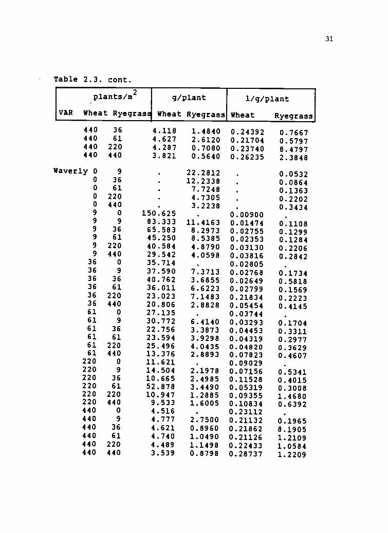
31

Table 2.3. cont.

plants/m2

VAR Wheat Ryegrass

g/plant

Wheat Ryegrass

lig/plant

Wheat Ryegrass

440 36 4.118 1.4840 0.24392 0.7667440 61 4.627 2.6120 0.21704 0.5797440 220 4.287 0.7080 0.23740 8.4797440 440 3.821 0.5640 0.26235 2.3848

Waverly 0 9 22.2812 0.05320 36 . 12.2338 0.08640 61 . 7.7248 0.13630 220 . 4.7305 0.22020 440 . 3.2238 . 0.34349 0 150.625 . 0.00900 .

9 9 83.333 11.4163 0.01474 0.11089 36 65.583 8.2973 0.02755 0.12999 61 45.250 8.5385 0.02353 0.12849 220 40.584 4.8790 0.03130 0.22069 440 29.542 4.0598 0.03816 0.2842

36 0 35.714 . 0.0280536 9 37.590 7.3713 0.02768 0.173436 36 40.762 3.6855 0.02649 0.581836 61 36.011 6.6223 0.02799 0.156936 220 23.023 7.1483 0.21834 0.222336 440 20.806 2.8828 0.05454 0.414561 0 27.135 . 0.0374461 9 30.772 6.4140 0.03293 0.170461 36 22.756 3.3873 0.04453 0.331161 61 23.594 3.9298 0.04319 0.297761 220 25.496 4.0435 0.04820 0.362961 440 13.376 2.8893 0.07823 0.4607

220 0 11.621 . 0.09029 .

220 9 14.504 2.1978 0.07156 0.5341220 36 10.665 2.4985 0.11528 0.4015220 61 52.878 3.4490 0.05319 0.3008220 220 10.947 1.2885 0.09355 1.4680220 440 9.533 1.6005 0.10834 0.6392440 0 4.516 . 0.23112 .

440 9 4.777 2.7500 0.21132 0.1965440 36 4.621 0.8960 0.21862 8.1905440 61 4.740 1.0490 0.21126 1.2109440 220 4.489 1.1498 0.22433 1.0584440 440 3.539 0.8798 0.28737 1.2209

32

Table 2.4. Wheat harvest indices for Owens and Waverlywheat varieties were calculated. Total wheat weights/0.75 m

2

were regressed against total grain weights (kg grain) (Table2.2). The indices were calculated to develop a relationshipbetween total wheat yield and reproductive yield. The coeffi-cients of determination indicate that 92 to 98 percent of thevariation in grain weight was described by wheat biomass.Biomass was therefore used as a competitive response in the1986 spring wheat-Lolium multiflorum competition experiment.

Wheat Variety b0

bl

Owens Kg grain = -0.1458 + 0.4183 (Kg biomass) 0.98

b0

b1

R2

Waverly Kg grain = 0.0005 + 0.3933 (Kg biomass) 0.92

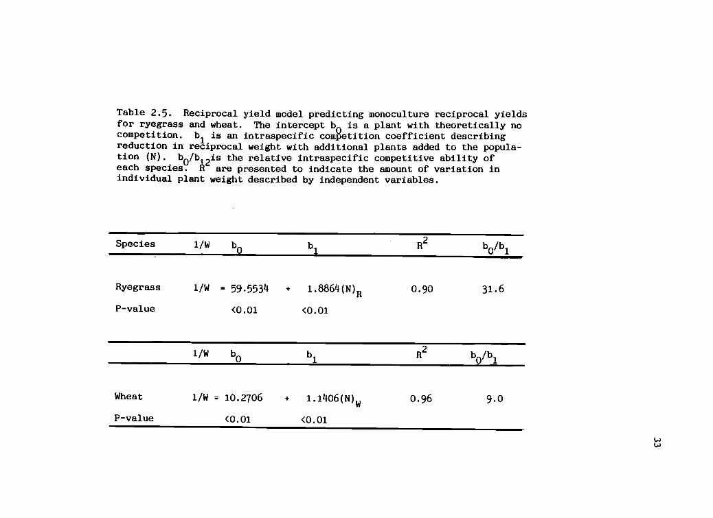
Table 2.5. Reciprocal yield model predicting monoculture reciprocal yieldsfor ryegrass and wheat. The intercept b0 is a plant with theoretically nocompetition. 1)1 is an intraspecific competition coefficient describingreduction in reciprocal weight with additional plants added to the popula-tion (N). b

0/b

12is the relative intraspecific competitive ability ofeach species. A are presented to indicate the amount of variation inindividual plant weight described by independent variables.

Species 1/W b0

b1

R2

b0/b

1

Ryegrass 1/W = 59.5534 + 1.8864(N)R 0.90 31.6

P -value <0.01 <0.01

1/W b0

b1

R2

b0/b

1

Wheat 1/W = 10.2706 1.1406(N)w 0.96 9.0

P-value <0.01 <0.01

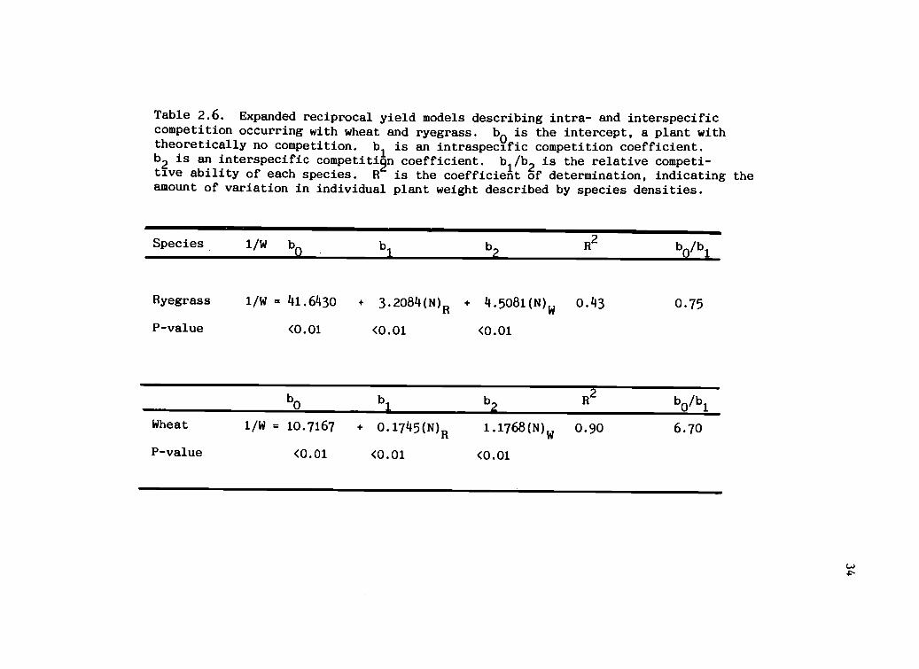
Table 2.6. Expanded reciprocal yield models describing intra- and interspecificcompetition occurring with wheat and ryegrass. bo is the intercept, a plant withtheoretically no competition. bl is an intraspecific competition coefficient.b2

is an interspecific competiti9n coefficient. b1/b

2is the relative competi-

tive ability of each species. R is the coefficient of determination, indicating theamount of variation in individual plant weight described by species densities.

Species. 1/W bo b1

b2

R2

Ryegrass 1/W = 41.6430 + 3.2084(N)R + 4.5081(N) 0.43 0.75

P-value <0.01 <0.01 <0.01

b0

b1

b2

R2

b0/b

1

Wheat 1/W = 10.7167 + 0.1745(N)R 1.1768(N)w 0.90 6.70

P-value <0.01 <0.01 <0.01

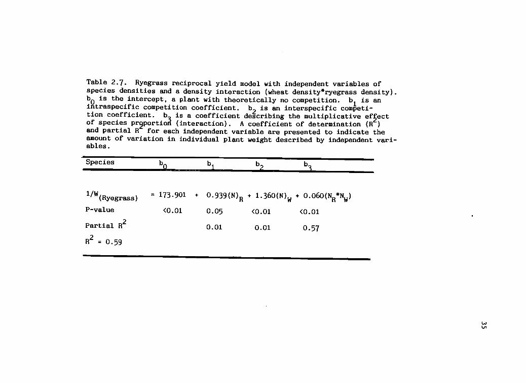
Table 2.7. Ryegrass reciprocal yield model with independent variables ofspecies densities and a density interaction (wheat density*ryegrass density).b0 is the intercept, a plant with theoretically no competition. b

1is an

intraspecific competition coefficient. 132 is an interspecific competi-tion coefficient. b is a coefficient degcribing the multiplicative effectof species prportiod (interaction). A coefficient of determination (R )

and partial R for each independent variable are presented to indicate theamount of variation in individual plant weight described by independent vari-ables.

Species b0

b1

b2

b

1/W(Ryegrass)

P-value

Partial R2

= 173.901

<0.01

+ 0.939(N)R

0.05

0.01

+ 1.360(N)w + 0.060(NR*Nw)

<0.01 <0.01

0.01 0.57

R2

= 0.59

36

Figure 2.1. Total grain yields/ha resulting from each experimentof Owens and Waverly wheat varieties planted2with Lolium multiflorumin addition series. The planted densities /m' of wheat and ryegrassare plotted along the x-axis. The resulting grain yields are plottedalong the y-axis. As wheat density increased, grain yield increased.However, the grain increase in monocultures was not linear, suggestingconstant final yield occurred at higher densities. Adding ryegrass tothe mixture slightly decreased yield. Intra- and interspecific competi-tion were responsible for grain decreases.

OWENS WHEAT GRAIN YIELDkg/hec

WAVERLY WHEAT GRAIN YIELD kg/hec

38

Figure 2.2. Individual plant biomass predicted for wheat by the expandedreciprocal yield regression equation (Table 2.6). Individual wheat biomasswas more significantly reduced by increasing wheat density than by ryegrassdensity.

PREDICTED WALLY -WHEAT G/FLANT

b1 /b2ratb2Species 1/W b0 b1

Wheat 1/W = 10.7167 + 1.1768(N)w + 0.1745(N)R .90 6.70p-value <.01 <.01 <.01

40

Figure 2.3. Individual plant biomass predicted for ryegrass by the expandedreciprocal yield regression equation. Independent variables used were speciesdensities. As total density and proportion of wheat increased, ryegrass biomasswas reduced (Table 2.6).

RYEGRASS RECITED BIOMASS YODEL

sI4-

os

G/PLANT

0411111101"

40"-011m's

Species 1/W b0 b2 ra 2

Ryegrassp-value

1/W = 41.6430 + 3.2084(N)R + 4.5081(N)w .43 0.75<.01 <.01 <.01

42

Figure 2.4. Individual plant biomass predicted for ryegrass by the expandedreciprocal yield equation, using independent variables of species density andspecies density interaction. The significant density interaction suggests thatadding plants to the mixtures has a multiplicative effect. As total density in-creased, the weight of ryegrass was reduced (Table 2.7).

PREDICTED RYEGRO BIOMNTERKIION

6.0G/PLANT

llllll

Species b0 b1 b2 b3

1/W (ryegrass)

p-value

partial r2

ra2=.59

= 173.901

<.01

+ 0.939(N)R

=.05

.01

+ 1.360(N)w

<.01

.01

+ 0.060(NR*Nw)

<.01

.57

44

Chapter 2 References

Appleby, A.P., P.D. Olson, and D.R. Colbert. 1976.Winter wheat reduction from interference by Italianryegrass. Agron. J. Vol. 68:463-466.

Bleasdale, J.K.A. 1967. Systematic designs for spacingexperiments. Exper. Agric. 3:73-85.

Carlson, H.L. and J.E. Hill. 1986. Wild oat (Avena fatua)competition with spring wheat:effects of nitrogenfertilization. Weed Sci 34:29-33.

Cousens, R.D. 1986. The use of population models in thestudy of the economics of weed control. Proc. EWRSSymposium, 1986. Economic Weed Control, 269-276.

de Wit, C.T. 1960. On Competition. No. 66.8 WageningenThe Netherlands: Center for Agricultural Pulications andDocumentation.

Donald, C.M. 1963. Competition for light in crops andpasture. La: Mechanisms in Biological Competition. Soc.Expmt. Biol., Symposium XV. Combridge Press. London. pp.283-313.

Firbank, L.G. and A.R. Watkinson. 1987. On the analysisof competition within two-species mixtures of plants. J.Appl. Ecol. 22:503-517.

Grime, J.P. 1973. Plant Strategies am Vegetationprocesses. John Wiley and Sons, N.Y. 222 p.

Harper, J.L. 1977. Population Biology fa Plants.Academic Press, New York. 892 pp.

Harper, J.L., J.T. Williams, and G.R. Sagar. 1965. Thebehavior of seeds in soil. I. The heterogeneity of soilsurfaces and its role in determining the establishment ofplants from seed. J. Ecol. 53:273-286.

Hunt, R. 1982. Plant Growth Curves. The, functionalapproach g. plant Growth analysis. Baltimore. UniversityPark Press. 248 p.

Jolliffe, P.A., A.N. MinJas, and V.C. Runeckles. 1984. Areinterpetation of yield relationships in replacementseries experiments. J. of Appl. Ecol., 21:227-243.

Jewiss, O.R. and Woledge, J. 1967. The effect of age on

45

the rate of apparent photosynthesis in leaves of tallfescue (Festyca arundinacea Schreb.). Ann. Bot. 31:661-671.

Little, T.M. and F.J. Hills. 1978. AgriculturalExperimentation:Design and Analysis. John Willey and SonsInc. Canada.

Miller, T.E. and P.A. Werner. 1987. Competitive effectsand responses in plants. Ecology (in press).

Neter, J., W. Wasserman, and M.H. Kutner, 1983.AgpliedLinear Regression Models Richard D. Irwin Inc. Illinois.

Newman, E.J., 1983. Interactions between plants. In:Encyclopedia of Plant Physiology New Series Volume 12 C.O.L. Lange, P.S. Nobel, C.B. Osmond, and H. Ziegler (Eds.).Springer-Verlag Berlin/New York. pp. 679-771.

Noguchi, K. and K. Nakayama. 1978a. Jap. J. Crop sci.47:48-55.

Patterson, D.T. 1982. Effects of light and temperature onweed/crop growth and competition. ja:Biometerology inI.P.M. Academic Press.

Peterson, C.M., B. Klepper, and R.W. Rickman, 1982.Tiller development at the coleoptilar node in winter wheat.Agronomy J.74:781-784.

Radosevich, S.R. 1987 (in press). Experimental methodsto study crop and weed interactions. In:Altieri, M.A., M.Z.Liebman (Eds). Plant Competition and Other EcologicalApproaches to Weed Control in Agriculture. CRC Press.

Radosevich, S.R. and J.S. Holt. 1984. WeedEcology:;mplications for, Management. John Wiley and SonsInc. New York. 300 pp.

Roush, M.L. and S.R. Radosevich. 1985. Relationshipsbetween growth and competitiveness of four annual weeds.J. of Appl. Ecol. 22:895-905.

Roush, M.L. and S.R. Radosevich. 1987. A weed communitymodel of germination, growth, and competition of annualweed species. WSSA abstracts. St. Louis.

SAS Institute. SAS/STAT Guide for Personal computers,Version 6 Edition, 1985. Cary, N.C.:SAS Institute Inc.

46

SAS Institute. SAS/System for Linear Models. 1986, Cary,N.C.:SAS Institute Inc.

Sestak, Z. 1983. Photosynthesis During Leaf development.Dr. W. Junk Publ., Dordrecht/Boston. 396 p.

Shinozaki,K. and T. Kira. 1956. Intraspecificcompetition among higher plants. V11. Logistic theory ofthe C-D effect. J. of the Inst. of Polytechnics, Osaka CityUniversity, 7:35-72.

Spitters, C.J.T. 1983 a. An alternative approach to theanalysis of mixed cropping experiments. I. Estimation ofcompetition effects. Netherlands J. of Agr. Sci. 31:1-11.

Spitters, C.J.T. 1983 b. An alternative approach to theanalysis of mixed cropping experiments. II. Marketableyield. Netherlands J. of Agr. Sci. 31:143-155.

Tilman, D. 1982. Re*ource competition and, communityStructure.Princeton University Press. Princeton, NewJersey.

Watkinson, A.R. 1980. Density-dependence in single-species populations of plants. J. Teor. Biol. 83:345-357.

Westoby, M. 1981. The place of the self thinning rule inpopulation dynamics. Am. Nat. 118, pp. 581-587.

Willey. R.W. 1985. Evaluation and presentation ofintercropping advantages. Expl. Agric. 21:119-133.

Yoda, K., T. Kira, H. Ogawa, and H. Hozumi. 1963. Self-thinning in overcrowded pure stands under cultivated andnatural conditions. J. Biol. Osaka City University. 14:107-129.

Zimdahl, R.H. 1980. Weed-crop Competition:A Review.International Plant Protection Center, Corvallis, OR. 196pp.

47

CHAPTER 3: QUANTIFYING GROWTH RESPONSES OF SPRING WHEATTRITICUM AESTIVUM (L.) VAR. OWENS (SUNDERMAN), VAR.

WAVERLY (KONZAK), AND LOLIUM MULTIFLORUM (LAM.)

Introduction

Relative growth rate is a measure of how successfully

a plant captures resources relative to its original size

(Roush and Radosevich 1985). Numerous studies have

demonstrated that a rapid growth rate can be advantageous

in resource capture for both weeds and crops (Patterson

1982). Relative rate of growth is dependent on

intraspecific as well as interspecific competition when

crops and weeds occur together in mixture. In experiments

containing two or more species, separating these two types

of competition has been difficult (Spitters 1983a) when

variables of species density and proportion were not

systematically varied (Radosevich 1987). Species density

and proportion along with spacing, are proximity factors

determining the nearness and identity of neighboring

plants.

Individual plant growth also is influenced by

biological traits such as genetic capability (e.g. seed

size) seed bank dynamics (e.g. seed survival) and

phenotypic factors (e.g. emergent size). Furthermore, life

history traits of the crop and weed, such as annuality

versus perenniality also may contribute to the ability of a

plant to usurp resources (Roush and Radosevich, in

48

progress). However, in annual cropping systems, the life

history traits of a weed and crop usually parallel one

another. Agricultural systems also are influenced strongly

by disturbance (Grime 1979) and resource availability. Any

or all of these factors interact with one other to

determine plant emergence and growth in mixtures.

A plant that emerges first in a mixture is likely to

usurp a disproportionate amount of the available resources

throughout the season (Radosevich and Holt 1984), growing

larger than surrounding neighbors and retaining a dominant

role in the mixture. If emergence of both species is

simultaneous (or controlled) in an experiment, then seed,

and consequently germinant size, may play an important role

in determining the relative growth rate of a plant in

mixture.

Ultimate plant size is determined by the amount of

resources which a plant obtains and uses during the growing

season. "Space" is considered to be a unit of resource

uptake, as influenced by environmental conditions, such as

temperature (Radosevich and Holt 1984). Varying the

proximity factors of species density and proportion

systematically in an addition series (Miller and Werner

1987, Roush and Radosevich 1987, Radosevich 1987), while

maintaining equidistant spacing, initially allocates

resources equally to each neighboring plant.

49

Plant size also is dependent on plant structure. Plant

structure (especially flowers and leaves) depends on a set

of morphological repeating units. The size and form of

these units is tightly controlled by genetically inherent

properties. The relative initiation rate of the

morphological units varies with different levels of

competition (Harper 1977). Harper (1977) also suggests

that the number of units and consequently, the size of the

whole plant may vary with age and environmental conditions

throughout the growing season. For instance, the relative

rate of initiation of leaves, tillers, and flowers may be

cued by temperature and light. Alternatively, these

initiation rates may vary with different levels of

competition for resources.

Plant competition occurs when resources become

limiting. Harper (1977) suggests that plants in mixtures

begin to compete early for available resources. When

stores of soil-associated resources (e.g. nutrients and

water) fall short of plant population needs, competition

for these resources begins.

Above-ground competition for light resources differs

from below-ground resource competition. Light is available

briefly and cannot be stored (Radosevich and Holt 1984).

In below-ground resource competition space capture occurs

by root expansion. In above-ground resource competition

50

the position of a plant becomes an important factor for

light interception (Donald 1963, Radosevich and Holt 1984).

Thus, the rate at which plants integrate resources may

elucidate strategies by which antra- and interspecific

plant neighbors pre-empt available resources.

Firbank and Watkinson (1987) categorize the pre-

emption of resources as either "one-sided" or "two-sided"

competition. One-sided competition occurs when plants grow

larger and faster in the population, over-topping smaller

and slower growing plants. Thus, one competitor (overstory

plants) influences its neighbor (understory plants) but is

not in turn influenced by that neighbor. This phenomenon

can occur when seed sizes, times of germination, or growth

rates differ among the individuals in a mixture. When

seeds are allowed to emerge simultaneously, large seed size

and phenotypically larger plant emergents are considered

advantageous when competing for available resources

(Radosevich and Holt 1984).

Two-sided competition occurs when plants emerge

simultaneously, pre-empting space proportional to their

size, until all space around each plant is occupied by

other plants. Further development is dependent on vertical

growth (Ross and Harper 1972, Firbank and Watkinson 1987).

In a plant mixture, two-sided competition usually occurs

between plants in the upper canopy which have emerged and

51

grown faster than the lower canopy plants. These upper

canopy plants continue to capture space in a uniform

fashion until all available upper canopy space is occupied.

The relative size of a plant at emergence may

determine the type of competition it experiences from

neighboring plants. A larger seed containing a large

endosperm supply usually grows faster and larger in the

first few days than a smaller seed requiring photosynthetic

processes (Esau 1978). Seed or emergent size is accounted

for when relative growth rate measurements begin.

Monitoring changes in plant relative rates of growth

may better define the period when competition between crops

and weeds begins. Furthermore, monitoring growth rate

changes in systematically varying levels of competition

produces a predictive method of assessing competition.

Plant allometry, the study of change in growth of various

plant parts from those more easily measured, utilizes this

method of monitoring plant growth. Plant allometry is

already widely used in forestry (Grier et al. 1984, Bold

and Radosevich 1987). For example, timber stand volume can

be predicted from basal area and height of individual

trees. Simple agronomic plant 'mAasurements such as plant

height and tiller number, measured over time can be used to

determine relative growth rates and predict desired

parameters such as grain yield. Furthermore, data taken

52

Methods

Plant material, planting methods, and cultural

practices were those described in Chapter 2. One

individual of each species was tagged in each plot. Plant

height, leaf number, tiller number, and leaf area index

(LAI) were measured.

The 100-seed weight of each wheat variety and Italian

ryegrass was weighed and recorded. Plant height was

measured from the soil line to the tip of the longest leaf.

The number of leaves was recorded, with the coleoptile

designated as the zero leaf. Subsequent leaves were

numbered 1 to 9. Numbers of tillers and subtillers were

considered equally when counted. Measurements were taken

weekly.

A point frame was constructed with eight aluminum

sliding points spaced 6.5 cm. apart for measuring LAI. LAI

was measured 5 times during the season, beginning in the

middle of the season when average LAI values for both

species exceeded 2. Species LAI was determined by

calculating the average percentage of species hits for the

eight sliding points. Individual plants measured for

height, leaf number, and tiller number were harvested

separately from the total plot harvest described in Chapter

2. Plants were dried to constant weight (15.6 C, 48 h),

and weights were included in biomass determination.

53

Growing Degree Day Units. Planting of the addition series

experiment required ten days. Plants in the first

replication were, therefore, planted ten days before those

in the fourth replication. Plants of equal GDD accumulate

similar developmental time (integrated temperature and

time) despite variation in chronological time (Peterson

1982). Therefore, GDD was used as the time variable in all

analyses of growth.

Ambient air temperatures were collected by the Oregon

State University Climatic Research Institute at Hyslop Crop

Science Field Laboratory, near Corvallis. GDD were

calculated from daily maximum and minimum temperatures

using a baseline growth temperature of 3 C (Klepper

personnel communication).

Calculations. Instantaneous relative growth rates were

calculated for plant height, leaf number and tiller number

(Hunt 1982). The log transformation of primary growth data

was regressed in a stepwise procedure (SAS 1985) against

the variables of GDD, polynomial transformations of GDD

(GDD2, GDD

3), and the log of GDD. These transformations

were used to fit the functional curve of growth data that

may have changed with each relative and total density in

the addition series. The lowest mean square error (MSE) (P

< 0.15), and appropriate residual diagrams were used for

54

determining the best independent variables to describecurves of the log of plant growth. The relative growthrates-are the slopes of the log (growth) versus the GDDcurves. Regression models describing relative rates ofgrowth were constructed for each total density treatment inthe addition series. The appropriate regression equationfor each treatment were then

differentiated, creatinginstantaneous relative growth rate equations for individualplants in each addition series treatment (Hunt 1978).Finally, the acquired GDD for each measurement time wasinput into these equations for

instantaneous plant relativegrowth rates.

Statistical Analysis. Analysis of variance was performedon the final set of plant growthmeasurements to partitionthe seasonal variation among observations into portions

associated with treatmentvariables of replication, wheatvariety, wheat density, ryegrass density, and variable

interactions.

Analyses of variance and covariance to test thehomogeneity of slopes were performed on instantaneousrelative growth rates of plant height, leaf number, andtiller number. Wheat varieties were used as covariants.Independent variables used to describe instantaneousrelative rates of growth were replication, wheat variety,

55

wheat density, ryegrass density, GDD, and interactions of

these variables. Regression variables were chosen based on

significance of independent variables (P < 0.07), largest

coefficient of determination (R 2), lowest mean square error

(MSE), appropriate residual diagrams, and lowest possible

multicolinearity. The maximum variance inflation factor

(VIF) was 6. This value occurred when GDD was selected by

the stepwise regression procedure as the most significant

variable as determined by the partial R2. Relative growth

rates were calculated from descriptive variables of GDD and

transformations of GDD. Transformations of GDD such as log

and cubic, describe accelerations and decelerations of

growth rate. The differences in changes of growth rate

were attributed to proximity factors of species density and

proportion when analyzed with analysis of variance and

covariance. Growth rates which were not affected by

proximity factors followed a linear pattern during the

season. Therefore, these growth rates were highly

correlated with GDD, the variable which was used to

calculate the growth rates and also describe them in the

analysis of variance and covariance.

Analyses of variance and covariance were performed on

species LAI. The continuous measurement of LAI was

described by independent variables of replication, wheat

variety, wheat density, ryegrass density, ODD, and all

56

interactions of these variables. Again, wheat varieties

were chosen as covariants. Criteria used to select

independent variables to explain instantaneous relative

growth rates of plant height, leaf number, and tiller

number also were used to select variables to describe

species LAI.

Results and Discussion

Wheat seed was 15-18 times larger than that of

ryegrass. Furthermore, Owens wheat seed was 16 percent

larger than that of Waverly. The large seed size of wheat

could impart an advantage over ryegrass at the beginning of

the season since both species emerged simultaneously (Esau

1978, Harper 1977). Wheat plants emerged 1-2 days earlier

than the ryegrass over all densities and were

phenotypically larger plants. Thus, wheat plants began as

larger emergents than ryegrass and had an advantage in

usurping resources early in the season.

Height. Plant height is a genetic attribute bred into

grain crops. In this experiment, both wheat varieties were

semi-dwarfs with a 10 cm potential difference. Mean

heights calculated for both varieties in each addition

series indicated that a 10 cm difference existed between

the varieties in the same treatment plots. Analysis of

variance performed on final wheat heights for both

57

varieties indicated that identical variables affected both

varieties. A significant amount of the variation in wheat

height was attributed to wheat density and replication (P <

0.01). However, analysis of variance performed on final

ryegrass heights suggested that both proximity variables of

species density and proportion influenced ryegrass height.

Variation in final ryegrass heights was attributed to wheat

density, ryegrass density, replication, and wheat variety

(P < 0.01).

To describe when and how proximity variables

influenced plant height rates of each species, analyses of

variance and covariance were performed on the instantaneous

height growth rates. Fifty-two percent of the variation in

ryegrass height growth rates (R2 = 0.52) was explained by

independent variables of wheat density (P = 0.02), GDD (P <

0.01), and the interactions of GDD*wheat density (P <

0.01), and wheat density*wheat variety (P = 0.03) (Table

3.1).

The rate of ryegrass height growth does not appear to

differ from either wheat variety. Both species grew at a

constant rate until the .boot stage of wheat when 850 GDD

were accumulated. At this point, both species growth rates

slowed but ryegrass maintained a higher rate of growth than

wheat. This general trend occurred regardless of density

or mixture (Figure 3.1). This suggests that ryegrass

58

plants, grown in mixture with tall wheat plants (10 cm

taller), are experiencing one-sided competition from taller

and phenotypically larger wheat which formed an overstory

(Firbank and Watkinson 1987) for the first half of the

growing season. However, the height growth rates of

ryegrass which increased over the wheat growth rates for

the latter half of the growing season may have compensated

for

the

the overstory competition

beginning of the season.

Analyses of variance and

from wheat for resources at

covariance on wheat height

growth rates indicated that 77 percent of the variation of

height growth rates (R2 = 0.77) was explained by wheat

variety, GOD, and the interactions of GDD*wheat density and

wheat density*ryegrass density (P < 0.01) (Table 3.1).

These interactions suggest that after emergence, the wheat

varieties achieved their overall heights through

differences in growth rates created by variations in growth

response to plant density.

The large intercept, which was significant (P < 0.01)

in both species regression equations, suggests that height

growth rate at emergence also was important in describing

how the species achieved their heights. Though wheat was a

formed an overstory above ryegrass from emergence, ryegrass

maintained a constant rate of height growth. Evidence from

Chapter 2 suggests that ryegrass plant weight was more

59

adversely affected by the overstory competition from wheat

than ryegrass height growth rates. The tall variety of

wheat (Owens) produced higher grain yields than the short

variety of wheat (Waverly) (Figure 2.1).

Leaf Number. Although height is a vertical measure of

space capture, the horizontal level is occupied by layers

of leaves (LAI). Therefore, leaf number initiation rates

and LAI were monitored for each species to elucidate

mechanisms of above-ground resource capture, with respect

to light.

Both wheat and ryegrass normally initiate 9 major

leaves, but stress may deter leaf initiation (Peterson et

al. 1982). The number of leaves initiated often indicates

the environment to which a plant has been subjected (Newman

1986). The greater the number of leaves initiated by the

end of the season, allows a larger source of carbohydrate

for translocation into grain.

Wheat plants initiated all 9 leaves regardless of

density treatment, as indicated by an analysis of variance

performed on the final number of leaves per wheat plant.

However, analysis of variance performed on the final number

of ryegrass leaves indicated that variation in ryegrass

leaf number was attributed to interactions of ryegrass

density*replication (P = 0.03) and replication*wheat

variety (P < 0.01). These interactions suggest that the

60

number of ryegrass leaves per plant resulted from different

levels of ryegrass competition that changed over

replication. Furthermore, ryegrass leaf initiation

differed depending on which variety the ryegrass was grown

with.

The rate at which leaves of each species were

initiated also was an important factor to consider in

assessing above-ground space capture during the season.

When analyses of variance and covariance were performed on

each of the species leaf initiation rates (Table 3.2), the

same independent variables were selected to describe leaf

initiation rates. Wheat density, GDD, and the interaction

of wheat density*CDD (P < 0.01) described 78 percent of the

variation (R2 = 0.78) in wheat leaf initiation rates and 72

percent of the variation (R2 = 0.72) in ryegrass leaf

initiation rates. Furthermore, a stepwise regression

performed on each species using the independent variables

described above, indicated that almost 100 percent of the

coefficient of determination (R 2) was taken up by GDD

(Table 3.2). This indicates that the proximity factors did

not strongly influence leaf initiation rates of either

species and that these rates are probably internally

controlled and cued by temperature over time (GDD).

61

Leaf Area Index. Klepper (personal communication)

hypothesized that size of a plant part (e.g. leaves or

tillers), as opposed to the number of plant parts, may be a

conclusive measure of stress. The size of a leaf is

measured by its area. Leaf area usually is a destructive

measurement; LAI, an indirect measurement of leaf area, was

therefore determined for each species.

LAI is a three-dimensional measurement of the space

captured in each plot as opposed to the actual number of

leaves initiated. LAI was most descriptive of how the

vertical layers of the plant canopy within the plot were

occupied by each species throughout the season.

At emergence, wheat was taller than ryegrass. Wheat

leaves also were wider and spanned a greater distance than

those of ryegrass, but wheat leaves also began to overlap

each other earlier at the highest wheat densities.

Analyses of variance and covariance performed on

measurements of wheat LAI indicate that 49 percent of

variation (R2 = 0.49) was explained by independent

variables of wheat density, ryegrass density, GDD, and

interactions of GDD*wheat density, GDD*ryegrass density,

and wheat density*wheat variety (P < 0.01) (Table 3.3).

LAI of each species was influenced by proximity

factors throughout the season. Wheat LAI increased with

wheat density. However, the increase in wheat LAI differed

62

between wheat varieties. Gradual seasonal decreases in

wheat LAI also varied among the wheat densities. For

instance, wheat growing in high total densities increased

LAI at a greater rate than in low densities at the

beginning of the season. However, wheat in high total

densities decreased LAI faster at the end of the season

than low total densities.

Analyses of variance and covariance performed on

measurements of ryegrass LAI indicate that 48 percent of

variation in LAI was explained by independent variables of

ryegrass density, wheat density, and interactions of

GDD*ryegrass density and wheat density*ryegrass density (P

< 0.01) (Table 3.3). Ryegrass LAI increased with

increasing ryegrass density. However, ryegrass LAI was

adversely affected by increasing density and proportion of

wheat. Also, as the season progressed, LAI of high

ryegrass densities decreased faster than low ryegrass

densities.

The most informative independent variable in both

species' predictive LAI equations was wheat density.

Ryegrass LAI decreased with increasing wheat density in the

mixtures, but the same variable in the wheat LAI equation

increased wheat LAI. This information suggests that

ryegrass was dominated by wheat for the first half of the

season. Furthermore, ryegrass experienced one-sided

63

competition from wheat in mixture, with respect to light

resources (Firbank and Watkinson 1987). Thus, competition

resulted in reduced ryegrass competitive ability (Chapter

2). However, as the season progressed and wheat plants

matured and senesced (fastest in the high total densities),

light became available to suppressed ryegrass plants. LAI

and height of ryegrass plants then increased as these

plants completed their life-cycle, and dispersed seed.

This growth pattern may be one of the strategies that

contributes to the persistence of Italian ryegrass in

spring wheat cropping systems.

Tiller Number. A small amount of variation in tiller

initiation rates was explained by proximity variables or

GDD, and this information was therefore included in the

appendices only.

Summary

Monitoring relative growth rates of plant parameters

has elucidated possible mechanisms that both species

utilize in capturing available resources. Wheat emerged

first in the mixture, growing taller and larger than

ryegrass and capturing vertical space. Wheat plants

continued to expand in LAI, also capturing the horizontal

layers of above-ground space with respect to light

resources. Wheat remained the dominant canopy plant until

64

after "boot stage" (GDD = 850-1200). Wheat then began to

mature and its LAI declined. Presumably, greater light

resources then were made available to the ryegrass.

Before the boot stage of wheat (GDD 850-1200),

ryegrass was suppressed in the mixture. Analyses indicated

that wheat height, leaf initiation, and LAI were not

adversely affected by ryegrass plants in the mixture until

the latter part of the growing season when wheat LAI

declined. However, as density and proportion of wheat

increased, all measured growth rates of ryegrass decreased.

Although rates of height, leaf number, and tiller

growth may be influenced by proximity factors of species

density and proportion, other plant traits such as biomass

and yield appear to be better indicators of competitive

ability (Chapter 2).

Table 3.1. Height growth rates (GR) described by several proximity variables of wheatdensity (N)W, growing degree days (GDD), and the interactions of wheat*density*GDD(GDW), wheat variety*wheat density (VarW), and wheat variety*GDD (VGDD). Wheatvariety did not vary significantly among the ryegrass height growth rates but wassignificantly different among wheat height growth rates. Analysis of variance andcovariance indicated that intercept values for each wheat ariety height (GR) weresignificantly different. Coefficients of determination (R ) are presented to indi-cate the amount of variation described by independent variables.

Species b0

b1

b2

b3

b4

Ryegrass Height (GR) = 0.0059 + 3.3-7 (N)w

- 2.8-6

(GDD) - 1.0-7 (GDW) + 3.3-6

(VarW)

P-value <0.01 <0.01 <0.01 <0.01 <0.01

R2

= 0.52

b0b1

b2

b3

b4

Wheat Height (GR) =

Variety 1 = 0.0050 + 3.9-6 (GDD) + 6.0-6

(VGDD) + 1.9-6

(VarW) + 2.4-8

(GDW)Variety 2 = 0.0048

P-value

R2

= 0.76

<0.01 <0.01 <0.01rn

<0.01 <0.01 Ui

Table 3.2. Leaf number initiation rates (IR)factors of wheat density (N)w, growing degreethese two variables (wheat density*GDD (GDW))strate the large amount of variation attachedtemperature on leaf initiation rate.

described by several proximitydays (GDD) 2and the interaction of

. Partial .R s are included to demon-to GDD, indicating the importance of

Species b0 b1

b2

b3

Ryegrass Leaf IR = 0.0209 - 1.5-5(N)w - 1.4-5(GDD) + 1.0-7(GDW)

P-value <0.01 <0.01 <0.01 <0.02

Partial R2

0.003 0.71 0.003

R2

= 0.72

b0 b1

b2

b3

Wheat Leaf (IR) = 0.0205 - 7.0-6

(N) - 1.5-5 (GDD) + 1.0-7 (GDR)

P-value <0.01 <0.01 <0.01 <0.01

Partial R2

0.0006 0.77 0.008

R2

= 0.78

Table 3.3. Regression equations describing species leaf area index (RLAI)(WLAI) with independent variables of wheat density (N)W, ryegrass density (N)R, andinteractions of wheat density*ryegrass density (INT), ryegrass density*GDD GDR),

wheat density*GDD (GDW), and wheat variety*wheat density (VarW). Partial R aredisplayed to indicate most influential variables determining canopy leaf area index.

Ryegrass (RLAI)P-valuePartial R

2

= 0.6734<0.01

+ 0.0309(N)R<0.010.33

- 0.0030(N)w<0.010.07

- 4.0E-4(INT) - 8.0E-5(GDR)<0.01 <0.01

0.01 0.05

R2

= 0.47

b0

b1

b2

b b4

Wheat (WLAI) = 0.7010 + 0.216(N) - 1.0E-4(GDW) - 1.0E-5(GDR) + 0.0020(VarW)P-value

2<0.01 <0.01 W <0.01 <0.01 <0.01

Partial R 0.20 0.22 0.02 0.003

R2

= 0.46

68

Figure 3.1. Height growth rates are plottedagainst growing degree days (GDD) for Owensspring wheat and Lolium multiflorum.Plants which were growing in addition seriestreatments with 1:1 proportions are representedin the diagram.

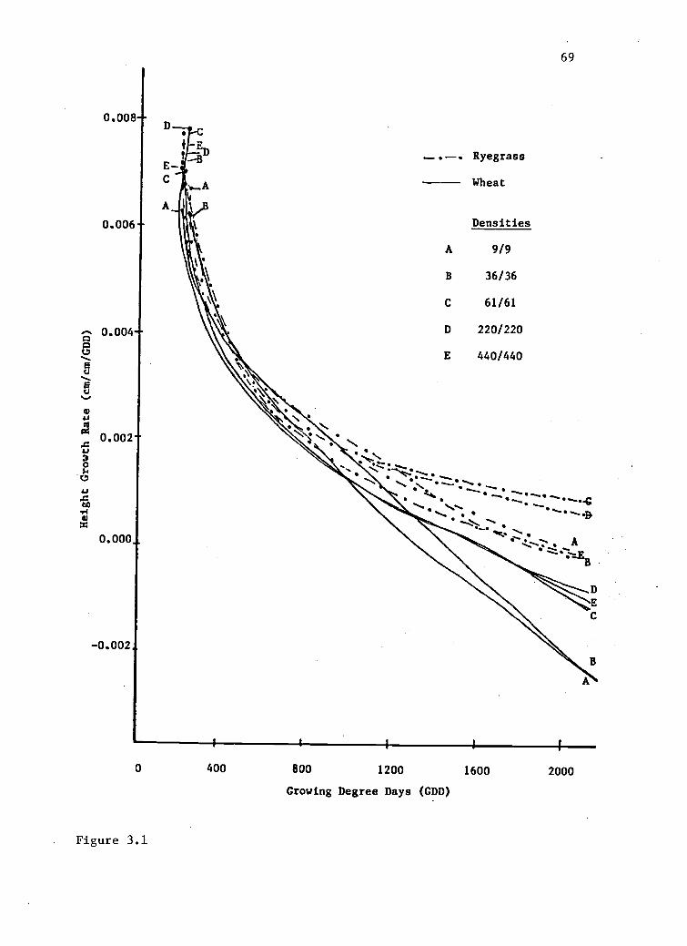
0.008--D

E-C

0.006-

a 0.004 -aLI

iiu

0u

......

'd0.002 -4

4.,

3o

04.,

X140=

0.000_

-0.002_

I E

IN. ..,

69

-_.--. Ryegrass

Wheat

Densities

A 9/9

B 36/36

C 61/61

D 220/220

E 440/440

:".. .....,

....;"'. ....op..... 0S....

-.... 44. .....-... . ...

. ..,..-.4 .V. ....s.'

\Zs:Z. , ,A

i'AEB

E

i 1

0 400 800 1200 1600 2000

Growing Degree Days (GOD)

Figure 3.1

70

Chapter 3 References

Appleby, A.P., P.D. Olson, and D.R. Colbert. 1976.Winter wheat reduction from interference by Italianryegrass. Agron. J. Vol. 68:463-466.

Baker, H.G. 1974. The Evolution of Weeds. Annual Reviewof Ecology and Systematics.

Baskerville, G.L. 1972. Dry-matter production inimmature balsam fir stands:Roots, lesser vegetation, andtotal stand. Forest Science. 12:49-53.

Black, J.N. 1958. Competition between plants ofdifferent initial sizes in swards of subterranean clover(Trifolium. subterranean L.) with particular reference toleaf area and light microclimate. Aust. J. Agric. Res9:299-318.

Cooke, P.T. and S.R. Radosevich. 1987. The Role ofDensity and Proportion In Allometric Equations of Douglas-fir and Red Alder Seedlings. M.S. Thesis. Oregon StateUniversity. Corvallis OR.

Donald, C.M. 1963. Competition for light in crops andpasture. La: Mechanisms in Biological Competition. Soc.Expmt. Biol., Symposium XV. Combridge Press. London. p.283-313.

Esau, K. 1977. Anatomy at Seed Plants. John Wiley andSons, New York, 550 pp.

Firbank, L.G. and A.R. Watkinson. 1987. On the analysisof competition within two-species mixtures of plants. J.Appl. Ecol. 22:503-517.

Grier, C., KI. Lee, and R. Archibald. 1984. Effect ofurea fertilization on allometric relations in youngDouglas-fir trees. Can. J. of For. Res. 14(6):900-904.

Grime, J.P. 1979. Plant Strategies and VegetationProcesses. John Wiley and Sons. 222 pp.

Grime, J.P., J.C. Crick, and J.E. Rincon. 1986. Theecological signifigance of plasticity. Great Britain CSoc. for Ex. Biol.

Gunst, R.F. and R.L. Mason. 1980. Regression Analysis amlLts_ application: g Data-orientated Approach. New York:Marcel Dekker Inc.

71

Harper, J.L. 1977. Population Biology Qj plants. NewYork: Academic Press, 892 pp.

Hunt, R. 1978. Plant Growth Analysis. Inst. Biol.Studies. 96. Edward Arnold. London. 63 pp.

Hunt, R. 1982. Plant Growth Curves. The, Functionalapproach ta Plant Growth Analysis. Baltimore: UniversityPark Press. 248 pp.

Miller, T.E. and P.A. Werner. 1987. Competitive effectsand responses in plants. Ecology (in press).

Newman, E.J. 1983. Interactions between plants.La:Encyclopedia of Plant Physiology New Series Volume 12 C.0.L Lange, P.S Noble, C.B. Osmond, and H. Ziegler (Eds.)Springer-Verlag Berlin/New York. pp. 679-771.

Patterson, D.T. 1982. Effects of light and temperatureon weed/crop growth and competition. _La: Biometerology inI.P.M Academic Press.

Peterson, C.M., B. Klepper, and R.W. Rickman. 1982.Tiller development at the coleoptilar node in winter wheat.Agronomy J. Vol. 74:781-784.

Radosevich, S.R. and J.S. Holt. 1984. WeedEcology:Implications for Management. John Wiley and SonsInc. New York. 300 pp.

Ross, M.A. and J.L. Harper. 1972. Occupation ofbiological space during seedling establishment. J. of Appl.Ecol. 60:77-88.

Roush, M.L. and S.R. Radosevich. 1985. Relationshipsbetween growth and competitiveness of four annual weeds.Journal of Appl. Ecol. 22:895-905.

Roush, M.L. and S.R. Radosevich. 1987. A weed communitymodel of germination, growth, and competitin of annual weedspecies. WSSA abstracs. St.Louis.

SAS Institute. SAS/STAT Guide for Personal computers,Version 6 Edition, 1985. Cary, N.C.:SAS Institute Inc.

SAS Institute. SAS/System for Linear Models. 1986, Cary,N.C.:SAS Institute Inc.

Sestak, Z. 1983. photosynthesis During Leaf Development.

72

Dr. W. Junk Publ., Dordrecht/Boston. 396 pp.

Spitters, C.J.T. 1983 a. An alternative approach to theanalysis of mixed cropping experiments. I. Estimation ofcompetition effects. Netherlands J. 0 Agr. Sci. 31:1-11.

Welden, C.W. and W.L. Slauson. 1986. The intensity ofcompetition versus its importance:an overlooked distinctionand some implications. Quart. Rev. Biol. 61:23-44.

73

CHAPTER 4: CONCLUSIONS

Measuring Competition

Intra- and interspecific competitive biomass responses

were generated in a systematic fashion by using an addition

series. These data were assessed by regressing the

reciprocal transformation of mean plant biomass against

both species densities. A regression model predicting

reciprocal plant weight was produced for each species.

The predictive model for reciprocal wheat biomass and

consequently, wheat yield, indicated that wheat was the

dominant species in mixtures with ryegrass. The relative

competitive ability of wheat suggested that one wheat plant

was as competitive as six to seven ryegrass plants.

The growth analysis experiment confirmed that wheat

was a highly competitive plant in mixture with ryegrass.

The large seed size and consequently large emergent size of

wheat allow this species to rapidly capture above ground

resources. Wheat maintained a dominant role in the

mixtures by producing a higher LAI than ryegrass for the

first half of the season. Wheat LAI also increased faster

in high wheat densities and proportions, suppressing

ryegrass plants in the mixture. However, wheat LAI also

decreased faster at the end of the season in the high wheat

densities. This release of light resources presumably

allowed ryegrass plants to grow and disperse seed

74

maintaining a persistent, though not dominant role in

spring wheat cropping systems.

The final regression model produced to predict

ryegrass reciprocal weight indicated that the interaction

of both species densities described the largest amount of

variation in ryegrass reciprocal weight (R 2= 0.57). The

significant interaction of species densities suggested that

adding plants to a mixture produced an multiplicative

affect on ryegrass reciprocal weight, as well as an

additive one. Biologically, this interaction may be caused

by differences in above-ground competition by larger wheat

plants early in the season or below-ground competition

between both species throughout the season.

If the influence of density is multiplicative, the

strict assumption of additivity on yield-density

relationships is incorrect. Furthermore, if the influence

of density is not additive, then plants in the mixture may

not take up resources or compete equally given an equal

amount of space. This violates a second assumption

(Spitters 1983a) of the expanded reciprocal approach; i.e.

that both species are at maximum resource uptake at

harvest. Thus, biomass predictions may have been over-

estimated if this assumption is not true.

The species density interaction term observed for

ryegrass also may result from a regression model generated

75

from inadequately transformed data. In this experiment,

the best transformation of mean biomass depended on the

degree of variability that each species displayed at

varying density and proportion. Ryegrass, the "loser" over

all densities and proportions, displayed the most variable

reciprocal weights as indicated by the residual plots. The

log transformation which is better able to account for

variance (Satoo and Madgwick 1982) may have been the

correct transformation. However, logarithmic equations are

not linear. Distribution of In (Y), at (X) which is normal

skews the distribution of (Y). The antilog of In (Y) used

to convert the transformed yield, resulting from the

regression equation, back to predictive yield, becomes the

median of the skewed distribution which is not the mean of

biomass (Baskerville, 1972).

Perhaps linear regression is not the most precise

method of assessing competitive biomass response. Mean

yield per plant (W) has universally been modeled as a

rectangular hyperbolic response to density (N) (Watkinson

1980, Bleasdale and Nelder 1960).

W = A + BN

The weight of an individual plant (W) raised to the

exponent (9) is a linear function of density (N). This

exponent (0) has been assumed as 1.0. The use of -1.0

for the exponent (5) led to the Reciprocal Yield Law:

76

1/W = A + BN.

8 may not approach the value of -1.0 in many situations

(Watkinson 1980, Firbank and Watkinson 1985) therefore,

linear regression may not be suitable for assessing density

responses. Non-linear regression has been suggested to

estimate the value of the exponent (9) and also the values

of other linear parameters in such equations (Watkinson

1980, Firbank and Watkinson 1985, Roush and Radosevich (in

preparation)) when one or more species in the mixture has

not attained maximum resource utilization.

Firbank and Watkinson (1987) proposed a

reparameterization of the reciprocal yield regression

equation:

W = Wm (1 + aN) b

The exponent b -1is equivalent to ( 8 of reciprocal yield

equation). The exponent b describes the curvilinear

response of species mean individual plant biomass to

species density. This may be interpreted as the resource

uptake capability of a species in monoculture or mixture

(Watkinson 1980, Firbank and Watkinson 1985, Roush and

Radosevich (in preparation)). (Wm) defines the maximum

size of a plant without competition. The parameter (a)

describes the affect of density (N) on mean plant biomass

and is an actual area necessary to avoid interaction with

other neighboring plants (Roush and Radosevich, in

77

preparation).

The Importance of Competition

Intra- and interspecific competition were important

factors influencing both species biomass yields as was

indicated by the coefficients of determination for the

final regression models (Table 2.6, Table 2.7). However,

only 59 percent of the variation in ryegrass reciprocal

weight was explained by intra- and interspecific

competitive responses. Several alternative factors could

have accounted for some of the unexplained variation. For

instance, gopher predation on wheat and ryegrass plants was

observed in the low total densities in the field (personal

observation). Downy mildew also existed in the high total

densities on both species (personal observation). A larger

amount of disturbance also seemed to play a role in

determining the competitive relationships in this

experiment. Seeds sown in the highest density of wheat

(440 plants/m2

) germinated one day earlier than in the

other densities in all cases. This early germination may

have determined competitive relationships from the

beginning of the season. Predation, disease and

disturbance are factors which may interact with proximity

factors and should also be included in predictive plant

growth models. Future experimentation should be conducted

78

to determine the role of these factors on plant growth.

Agricultural Implications

Wheat is a strong competitor against ryegrass in

mixture. However, this experiment also implicated wheat

neighbors in the populations as the strongest competitors

for resources against other wheat plants. Wheats

competitive nature can be more detrimental to "potential"

grain yield than ryegrass at high wheat densities (220-440

plants/m2).

The timing of germination also was very important in

spring wheat cropping systems. When wheat germinates with

or before ryegrass, the crop maintains an efficient

relative competitive ability. The constant rate of growth

that ryegrass displayed in most measured plant parameters

indicated that ryegrass could be a formidable competitor,

if allowed to germinate before the wheat crop.

Though this study was an empirical one, the regression

models and the growth analysis experiment revealed several

testable hypotheses concerning the mechanisms by which both

species capture available resources in time and space:

1. Light may be the limiting resources for ryegrass at the

beginning of the season, as suggested by the wheat LAI

measurements taken throughout the season. This suggests

that increasing wheat density above 440 plants/m2, which is

79

the normal planting density for Oregon farmers, may suppress

ryegrass weed growth. However, the second application of

nitrogen (applied in split-application) may be the most

limiting factor for both species during the latter half of

the season. Ryegrass may compete quite effectively for

nitrogen in the latter half of the season with the wheat

plants in the mixture, reducing wheat grain yield. The

persistence of Italian ryegrass in spring wheat cropping

systems suggests that competition in the latter half of the

growing season needs to be further examined.

2. Wheat varieties should be selected which have an

inherently larger height than ryegrass. Earlier

germinating varieties also would be advantageous for wheat

to maintain the dominant role in the mixture during the

growing season. Owens spring wheat produced higher grain

yields than Waverly throughout the addition series

experiment. The 10 cm difference appears to have made a

competitive difference.

80

BIBLIOGRAPHY

Appleby, A.P., P.D. Olson, and D.R. Colbert. 1976.Winter wheat reduction from interference by Italianryegrass. Agron. J. Vol. 68:463-466.

Baker, H.G. 1974. The Evolution of Weeds. Annual Reviewof Ecology and Systematics.

Baskerville, G.L. 1972. Dry-matter production inimmature balsam fir stands: Roots, lesser vegetation, andtotal stand. Forest Sci. 12:49-63.

Black, J.N. 1958. competition between plants ofdifferent initial sizes in swards of subterranean clover(Trifolium subterranean) with particular reference to leafarea and light microclimate. Aust. J. Agric. Res. 9:299-318.

Bleasdale, J.K.A., and J.A. Nelder. 1960. Plantpopulation and crop yield. Nature, 188, p. 342.

Bleasdale, J.K.A. 1967. Systematic designs for spacingexperiments. Experimental Agriculture, 3:73-85.

Carlson, H.L. and J.E. Hill. 1986. Wild oat (Avena fatua)competition with spring wheat:effects of nitrogenfertilization. Weed Sci 34:29-33.

Connolly, J. 1986. On difficulties with replacementseries methodology in mixture experiments. J. of AppliedEcology, 23:125-137.

Cooke, P.T. and S.R. Radosevich. 1987. The Role ofDensity and Proportion In Allometric Equations of Douglas-fir and Red Alder Seedlings. M.S. Thesis. Oregon StateUniversity. Corvallis OR.

Cousens, R.D. 1986. The use of population models in thestudy of the economics of weed control. Proc. EWRSSymposium, 1986. Economic Weed Control, 269-276.

de Wit, C.T. 1960. On Competition. No. 66.8 WageningenThe Netherlands: Center for Agricultural Publications andDocumentation.

Donald, C.M. 1963. Competition for light in crops andpasture. La: Mechanisms in Biological Competition. Soc.Expmt. Biol., Symposium XV. Combridge Press. London. pp.283-313.

81

Esau, K. 1977. Anatomy Q. Seed Plants. John Wiley andSons, New York, 550 pp.

Firbank, L.G. and A.R. Watkinson. 1985. On the analysisof competition within two-species mixture of plants. J. ofApplied Ecology, 22:503-517.

Firbank, L.G. and A.R. Watkinson. 1987. On the analysisof competition within two-species mixtures of plants. J.Appl. Ecol. 22:503-517.

Grime, J.P. 1979. Plant Strategies aaa VegetationProcesses. John Wiley and Sons, N.Y. 222 p.

Gunst, R.F. and R.L. Mason. 1980. Rearession Analysisand Itg Application: g Data- orientated Approach. New York:Marcel Dekker Inc.

Harper, J.L. 1977. Population Biology af. Plants.Academic Press, New York. 892 pp.

Harper, J.L., J.T. Williams, and G.R. Sagar. 1965. Thebehavior of seeds in soil. I. The heterogeneity of soilsurfaces and its role in determining the establishment ofplants from seed. J. Ecol. 53:273-286.

Hunt, R. 1978. Plant Growth, Analysis. Inst. Biol.Studies 96. Edward Arnold. London. 63 pp.

Hunt, R. 1982. Plant Growth Curves. The FunctionalApproach la Plant Growth Analysis. Baltimore. UniversityPark Press. 248 p.

Jolliffe, P.A., A.N. Minjas, and V.C. Runeckles. 1984. Areinterpetation of yield relationships in replacementseries experiments. J. of Appi. Ecol., 21:227-243.

Jewiss, O.R. and J. Woledge. 1967. The effect of age onthe rate of apparent photosynthesis in leaves of tallfescue (Pestucl arundinacea Schreb.). Ann. Bot. 31:661-671.

Little T.M. and F.J. Hills. 1978. AgriculturalExperimentation:Design and Analysis. John Willey and SonsInc. Canada.

Miller, T.E. and P.A. Werner. 1987. Competitive effectsand responses in plants. Ecology (in press),

82

Neter, J., W. Wasserman, and M.H. Kutner. 1983.AooliedLinear Regression Models Richard D. Irwin Inc. Illinois.

Newman, E.J. 1983. Interactions between plants. fin:

Encyclopedia of Plant Physiology New Series Volume 12 C.O.L. Lange, P.S. Nobel, C.B. Osmond, and H. Ziegler (Eds.).Springer-Verlag Berlin/New York. pp. 679-771.

Noguchi, K. and K. Nakayama. 1978a. Jap. J. Crop sci.47:48-55.

Patterson, D.T. 1982. Effects of light and temperature onweed/crop growth and competition. Ia:Biometerology inI.P.M. Academic Press.

Peterson, C.M., B. Klepper, and R.W. Rickman. 1982.Tiller development at the coleoptilar node in winter wheat.Agronomy J. 74:781-784.

Radosevich, S.R. 1987 (in press). Experimental methodsto study crop and weed interactions. Ia:Altieri, M.A., M.Z.Liebman (Eds). Plant Competition and Other EcologicalApproaches to Weed Control in Agriculture. CRC Press.

Radosevich, S.R. and J.S. Holt. 1984. WeedEcology:Imolications for. Management. John Wiley and SonsInc. New York. 300 pp.

Ross, M.A. and J.L. Harper. 1972. Occupation ofbiological space during seedling establishment. J. ofAppl. Ecol. 60:77-88.

Roush, M.L. and S.R. Radosevich. 1985. Relationshipsbetween growth and competitiveness of four annual weeds.J. of Appl. Ecol. 22:895-905.

Roush, M.L. and S.R. Radosevich. 1987. A weed communitymodel of germination, growth, and competition of annualweed species. WSSA abstracts. St. Louis.

SAS Institute. SAS/STAT Guide for Personal computers,Version 6 Edition, 1985. Cary, N.C.:SAS Institute Inc.

SAS Institute. SAS/System for Linear Models. 1986, Cary,N.C.:SAS Institute Inc.

Satoo, T. and H.A.I. Madgewick. 1982. Forest biomass.The Hague, Netherlands: Martinus Nijhoff. 152 pp.

Sestak, Z. 1983. photosynthesis During Leaf, development.

83

Dr. W. Junk Publ., Dordrecht/Boston. 396 pp.

Shinozaki, K. and T. Kira. 1956. Intraspecificcompetition among higher plants. V11. Logistic theory ofthe C-D effect. J. of the Inst. of Polytechnics, Osaka CityUniversity, 7:35-72.

Spitters, C.J.T. 1983 a. An alternative approach to theanalysis of mixed cropping experiments. I. Estimation ofcompetition effects. Netherlands J. of Aqr. Sci. 31:1-11.

Spitters, C.J.T. 1983 b. An alternative approach to theanalysis of mixed cropping experiments. II. Marketableyield. Netherlands J. of Agr. Sci. 31143-155.

Tilman, D. 1982. Resource competition and communityStructure.Princeton University Press. Princeton, NewJersey.

Watkinson, A.R. 1980. Density-dependence in single-species populations of plants. J. Theor. Biol. 83:345-357.

Welden, C.W. and W.L. Slauson. 1986. The intensity ofcompetition versus its importance:an overlooked distinctionand some implications. Quart. Rev. Biol. 61:23-44.

Westoby, M. 1981. The place of the self thinning rule inpopulation dynamics. Am. Nat. 118, pp. 581-587.

Willey. R.W. 1985. Evaluation and presentation ofintercropping advantages. Expl. Agric. 21:119-133.

Yoda, K., T. Kira, H. Ogawa, and H. Hozumi. 1963. Self-thinning in overcrowded pure stands under cultivated andnatural conditions. J. Biol. Osaka City University. 14:107-129.

Zimdahl, R.H. 1980. Weed-crop Competition:A Review.International Plant Protection Center, Corvallis, OR. 196pp.

APPENDI CES

84

APPENDICES

Tiller Number

An analysis of variance performed on final number ofryegrass and wheat tillers, in the two variety experiments,indicated that variation in species tiller number wasattributed to ryegrass density (p < 0.01),

wheat density (p< 0.01), and interaction of species densities (p < 0.01).Number of ryegrass and wheat tillers

decreased with anincrease in species relative and total density. Finalnumber of tillers produced by wheat and ryegrass plants inthe addition series (Table 2.1) were influenced byproximity factors of species density and proportion (Figurea.1).

Analyses of variance and covariance performed onrelative rates of ryegrass tillering suggests that 15percent of variation in rates (r2 = 0.15) was explained byindependent variables of wheat variety (p < 0.01), wheatdensity (p < 0.01), ryegrass density (p < 0.01), GDD (p <0.01), and

interactions of GDD*wheat variety (p < 0.01),GDD*wheat density (p < 0.01),

GDD*ryegrass density (p <0.01), and wheat

density*ryegrass density (p < 0.01) (Tablea.1).

Analyses of variance and covariance performed on wheat

85

relative tillering rates indicates that 21 percent ofvariation in rates (r

2= 0.21) was explained by independent

variables of wheat variety (p < 0.01), wheat density (p <0.01), and ryegrass density (p < 0.01), GDD (P < 0.01), andthe interactions of wheat variety*GDD (p < 0.01), GDD*wheatdensity (p < 0.01), GDD*ryegrass density (p < 0.01), andryegrass density*wheat density (p < 0.01) (Table a.1).

Final number of ryegrass and wheat tillers (Figurea.1) resemble total grain yield (Figure 2.1). These datasuggest that tiller relative growth rate (tiller biomass)would have been a better indicator of competitive response.

Individual Plot Measurements

Individual plot measurements from the addition seriesexperiments have been included in Table a.2 and Table a.3.

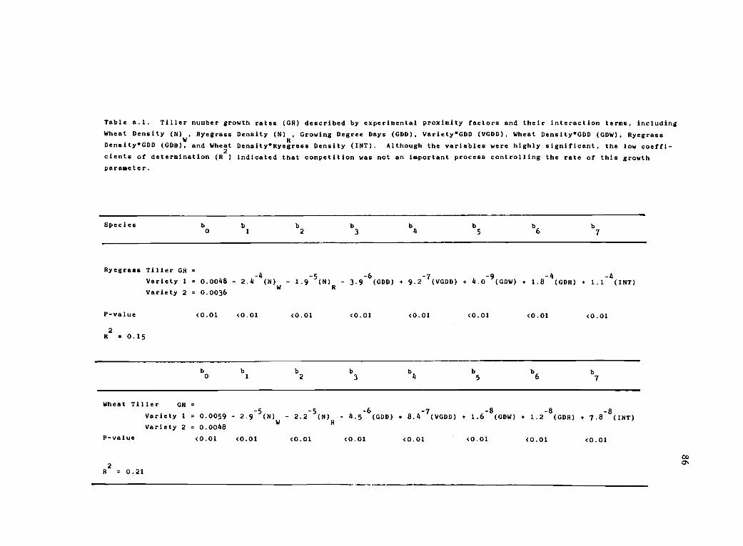
Table a.l. Tiller number growth rates (GR) described by experimental proximity factors and their interaction terms, including

Wheat Density (N)W

, Ryegrass Density (N)R

. Growing Degree Days (GDD), VarietyGDD (VGDD), Wheat Density*GDD (GDW), Ryegrass

Density`GDD (GD0). and Whea2 t Density`Ryegrass Density (INT). Although the variables were highly significant, the low coeffi-

ciente of determination (R ) indicated that competition was not an important process controlling the rate of this growth

parameter.

Species b b0 1

b b b b b b2 3 4 5 6 7

Ryegrass Tiller GR

Variety 1 - 0.0048 - 2.4-4

(N) - 1.9-5

(N) - 3.9-6

(GDD) 9.2-7

(VGDD) + 4.0-9

(GDw) + 1.8-4

(GDR) + 1.1-4

(INT)W R

Variety 2 . 0.0036

P-value

2B . 0.15

<0.01 <0.01 <0.01 <0.01 <0.01 <0.01 <0.01 <0.01

b b b b b0 1 2 3 4

b b b5 6 7

Wheat Tiller GR =

P-value

2R = 0.21

Variety 1 = 0.0059 - 2.9-5

(N) - 2.2-5

(N) - 4.5-6

(GOD) + 8.4-7

(VGDD) + 1.6-8

(GDw) + 1.2-8(GDR) + 7.8

-8(INT)

W RVariety 2 = 0.0048

<0.01 <0.01 <0.01 <0.01 <0.01 <0.01 <0.01 <0.01

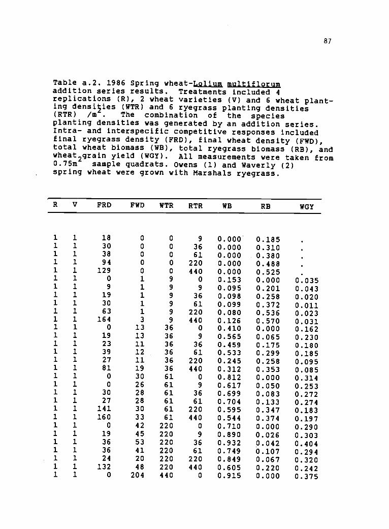
87

Table a.2. 1986 Spring wheat-Lolium multiflorumaddition series results. Treatments included 4replications (R), 2 wheat varieties (V) and 6 wheat plant-ing densiies (WTR) and 6 ryegrass planting densities(RTR) /m . The combination of the speciesplanting densities was generated by an addition series.Intra- and interspecific competitive responses includedfinal ryegrass density (FRD), final wheat density (FWD),total wheat biomass (WB), total ryegrass biomass (RB), andwheat

2grain yield (WGY). All measurements were taken from

0.75m sample quadrats. Owens (1) and Waverly (2)spring wheat were grown with Marshals ryegrass.

R V FRD FWD WTR RTR WB RB WGY

1 1 18 0 0 9 0.000' 0.1851 1 30 0 0 36 0.000 0.3101 1 38 0 0 61 0.000 0.3801 1 94 0 0 220 0.000 0.4881 1 129 0 0 440 0.000 0.5251 1 0 1 9 0 0.153 0.000 0.0351 1 9 1 9 9 0.095 0.201 0.0431 1 19 1 9 36 0.098 0.258 0.0201 1 30 1 9 61 0.099 0.372 0.0111 1 63 1 9 220 0.080 0.536 0.0231 1 164 3 9 440 0.126 0.570 0.0311 1 0 13 36 0 0.410 0.000 0.1621 1 19 13 36 9 0.565 0.065 0.2301 1 23 11 36 36 0.459 0.175 0.1801 1 39 12 36 61 0.533 0.299 0.1851 1 27 11 36 220 0.245 0.258 0.0951 1 81 19 36 440 0.312 0.353 0.0851 1 0 30 61 0 0.812 0.000 0.3141 1 0 26 61 9 0.617 0.050 0.2531 1 30 28 61 36 0.699 0.083 0.2721 1 27 28 61 61 0.704 0.133 0.2741 1 141 30 61 220 0.595 0.347 0.1831 1 160 33 61 440 0.544 0.374 0.1971 1 0 42 220 0 0.710 0.000 0.2901 1 19 45 220 9 0.890 0.026 0.3031 1 36 53 220 36 0.932 0.042 0.4041 1 36 41 220 61 0.749 0.107 0.2941 1 24 20 220 220 0.849 0.067 0.3201 1 132 48 220 440 0.605 0.220 0.2421 1 0 204 440 0 0.915 0.000 0.375

88

Table a.2. cont.

R V FRD FWD WTR RTR WB RB WGY

1 1 22 210 440 9 0.944 0.017 0.3821 1 32 209 440 36 0.889 0.4021 1 61 266 440 61 0.942 0.035 0.3871 1 61 176 440 220 0.891 0.002 0.3251 1 135 220 440 440 0.885 0.045 0.3432 1 2 0 0 9 0.000 0.0662 1 24 0 0 36 0.000 0.2652 1 24 0 0 61 0.000 0.2532 1 68 0 0 220 0.000 0.4892 1 124 0 0 440 . . .

2 1 0 0 9 0 . . .

2 1 3 1 9 9 0.068 0.0352 1 8 122 9 36 0.083 0.135 0.0332 1 23 2 9 61 0.096 . 0.0142 1 48 1 9 220 0.079 0.281 0.0032 1 142 1 9 440 0.020 0.549 0.0092 1 0 11 36 0 0.498 0.000 0.2282 1 20 14 36 9 0.562 0.043 0.2642 1 31 16 36 36 0.565 0.485 0.2242 1 45 13 36 61 0.398 0.190 0.1612 1 88 7 36 220 0.152 0.369 0.0612 1 148 16 36 440 0.265 0.383 0.0982 1 0 22 61 0 0.748 0.000 0.3142 1 4 24 61 9 0.718 0.072 0.3402 1 7 30 61 36 0.731 0.030 0.3102 1 52 23 61 61 0.382 0.216 0.1372 1 40 17 61 220 0.395 0.187 0.1622 1 67 271 61 440 0.395 0.225 0.1462 1 0 51 220 0 0.875 0.000 0.3552 1 2 42 220 9 0.679 0.015 0.2502 1 10 46 220 36 0.810 0.036 0.3192 1 29 51 220 61 0.765 0.070 0.3052 1 77 46 220 220 0.645 0.124 0.2372 1 98 57 220 440 0.575 0.225 0.2182 1 0 216 440 0 1.035 0.000 0.4012 1 2 274 440 9 1.038 0.020 0.4062 1 10 216 440 36 0.959 0.020 0.3742 1 20 180 440 61 0.909 0.030 0.3652 1 29 184 440 220 0.809 0.036 0.3202 1 111 196 440 440 0.745 0.085 0.3013 1 0 0 0 0 . .

3 1 9 0 0 9 . .

3 1 18 0 0 36 0.000 0.1983 1 65 15 0 61 0.000 0.2553 1 130 0 0 220 0.000 0.4603 1 224 0 0 440 0.000 0.513

89

Table a.2. cont.

R V FRD FWD WTR RTR WB RB WGY

3 1 0 1 9 0 0.200 0.000 0.0323 1 1 1 9 9 0.106 0.189 0.0193 1 18 1 9 36 0.052 0.180 0.0163 1 57 2 9 61 0.072 0.343 0.0113 1 130 1 9 220 0.041 0.593 0.0113 1 155 3 9 440 0.120 0.595 0.0253 1 0 9 36 0 0.380 0.000 0.1303 1 0 13 36 9 0.596 0.015 0.2393 1 56 24 36 36 0.445 0.124 0.1793 1 0 21 36 61 0.485 0.2013 1 160 18 36 220 0.460 0.338 0.1783 1 125 14 36 440 0.351 0.332 0.1383 1 0 4 61 0 .

3 1 11 22 61 9 0.682 0.069 0.2603 1 29 24 61 36 0.536 0.123 0.1973 1 37 20 61 61 0.484 0.183 0.1023 1 95 28 61 220 0.438 0.248 0.1533 1 83 21 61 440 0.355 0.184 0.1323 1 0 64 220 0 0.830 0.000 0.3373 1 7 45 220 9 0.792 0.027 0.2803 1 11 58 220 36 0.765 0.026 0.3123 1 0 70 220 61 0.655 0.093 0.2783 1 116 61 220 220 0.696 0.166 0.2903 1 . . 220 440 . . .

3 1 0 175 440 0 0.817 0.000 0.3363 1 6 215 440 9 0.908 0.021 0.3613 1 0 198 440 36 0.736 0.020 0.3173 1 5 163 440 61 0.734 0.026 0.3063 1 74 206 440 220 0.865 0.050 0.3503 1 82 178 440 440 0.697 0.075 0.2814 1 0 0 0 0 . . .4 1 10 0 0 9 0.000 0.120 .

4 1 39 0 0 36 0.000 0.179 .

4 1 46 0 0 61 0.000 0.222 .4 1 106 0 0 220 0.000 0.312 .

4 1 279 0 0 440 0.000 0.434 .

4 1 0 1 9 0 0.139 0.000 0.0514 1 8 0 9 9 0.110 0.187 0.0194 1 16 1 9 16 0.000 0.073 0.0124 1 11 1 9 61 0.130 0.134 0.0064 1 98 0 9 220 0.099 0.376 0.0184 1 85 1 9 440 0.030 0.345 0.0134 1 0 9 36 0 0.325 0.000 0.1064 1 3 11 36 9 0.362 0.045 0.1554 1 27 6 36 36 0.207 0.128 0.0974 1 29 11 36 61 0.248 0.171 0.100

90

Table a.2. cont.

R V FRD FWD WTR RTR WB RB WGY

4 1 89 11 36 220 0.282 0.252 0.1174 1 110 9 36 440 0.215 0.361 0.0984 1 0 29 61 0 0.714 0.000 0.2864 1 8 24 61 9 0.572 0.027 0.2114 1 34 19 61 36 0.517 0.073 0.2364 1 46 17 61 61 0.413 0.125 0.1714 1 95 22 61 220 0.375 0.131 0.1474 1 97 27 61 440 0.399 0.172 0.1504 1 0 62 220 0 0.861 0.000 0.3944 1 16 49 220 9 0.805 0.032 0.3434 1 8 49 220 36 0.731 0.024 0.3324 1 32 54 220 61 0.872 0.050 0.3504 1 71 48 220 220 0.612 0.102 0.2374 1 221 44 220 440 0.723 0.170 0.2704 1 0 210 440 0 0.925 0.000 0.3714 1 12 192 440 9. 0.887 0.025 0.3564 1 31 184 440 36 0.747 0.030 0.3014 1 22 195 440 61 0.844 0.025 0.3384 1 34 212 440 220 0.740 0.030 0.3124 1 207 227 440 440 0.804 0.050 0.2811 2 0 0 0 0 . .

1 2 4 0 0 9 0.000 0.1541 2 22 0 0 36 0.000 0.3051 2 35 0 0 61 0.000 0.3651 2 96 0 0 220 0.000 0.4091 2 190 0 0 440 0.000 0.635 .

1 2 0 2 9 0 0.195 0.000 0.0531 2 31 5 9 9 . 0.157 0.0161 2 31 3 9 36 0.181 0.261 0.0461 2 30 1 9 61 0.034 0.305 0.0071 2 82 1 9 220 0.065 0.477 0.0131 2 93 3 9 440 0.119 0.340 0.0271 2 . 0 36 0 . . .

1 2 2 15 36 9 0.725 0.030 0.2861 2 23 9 36 36 0.511 0.014 0.2201 2 37 14 36 61 0.462 0.185 0.2031 2 95 14 36 220 0.312 . 0.1141 2 85 16 36 440 0.180 0.408 0.0641 2 0 25 61 0 0.760 0.000 0.3171 2 6 29 61 9 0.765 0.050 0.2841 2 21 23 61 36 0.611 0.102 0.2221 2 40 25 61 61 0.644 0.139 0.2511 2 84 23 61 220 0.408 0.255 0.1421 2 87 . 61 440 . 0.476 .

1 2 0 98 220 0 0.819 0.000 0.3391 2 3 53 220 9 0.951 0.018 0.395

91

Table a.2. cont.

R V FRD FWD WTR RTR WB RB WGY

1 2 23 56 220 36 0.847 0.060 0.3441 2 44 5 220 61 0.839 0.144 0.3201 2 93 47 220 220 0.568 0.155 0.2091 2 165 59 220 440 0.702 0.298 0.2761 2 0 189 440 0 0.815 0.000 0.3521 2 5 188 440 9 0.994 0.020 0.3791 2 . 179 440 36 0.905 0.3531 2 27 192 440 61 0.910 0.013 0.3591 2 89 213 440 220 0.870 0.071 0.3361 2 72 186 440 440 0.745 0.091 0.2732 2 0 0 0 0 .

2 2 4 0 0 9 0.000 0.0872 2 12 0 0 36 0.000 0.1382 2 30 0 0 61 0.000 0.2402 2 72 0 0 220 0.000 0.441 .

2 2 163 0 0 440 0.280 0.421 .

2 2 0 2 9 0 0.490 0.0002 2 8 1 9 9 0.095 0.152 0.0222 2 29 3 9 36 0.225 0.225 0.0952 2 29 1 9 61 0.035 0.314 .

2 2 60 3 9 220 0.050 0.391 0.0202 2 64 3 9 440 0.105 0.446 .

2 2 0 14 36 0 0.525 0.000 0.2022 2 4 14 36 9 0.524 0.020 0.2032 2 12 10 36 36 0.462 0.076 0.2132 2 15 11 36 61 0.446 0.103 0.1932 2 66 9 36 220 0.290 0.210 0.1072 2 161 10 36 440 0.301 0.381 0.1332 2 0 32 61 0 . . .

2 2 11 19 61 9 0.665 0.045 0.2952 2 22 40 61 36 0.585 0.050 0.1872 2 26 24 61 61 0.597 0.084 0.2452 2 149 25 61 220 0.501 0.330 0.2012 2 100 19 61 440 0.185 0.252 0.1192 2 0 40 220 0 .

2 2 12 49 220 9 0.788 0.016 0.3042 2 20 75 220 36 0.704 0.047 0.2842 2 25 38 220 61 0.584 0.072 0.2502 2 56 47 220 220 0.413 0.015 0.1452 2 110 54 220 440 0.400 0.190 0.1352 2 0 187 440 0 0.670 0.000 0.3532 2 2 198 440 9 0.945 0.000 0.3622 2 16 165 440 36 0.843 0.001 0.3032 2 24 194 440 61 0.940 0.045 0.3822 2 39 162 440 220 0.830 0.025 0.2982 2 90 190 440 440 0.566 0.070 0.226

92

Table a.2. cont.

R V FRD FWD WTR RTR WB RB WGY

3 2 0 0 0 0 . . .

3 2 8 0 0 9 0.000 0.1013 2 15 0 0 36 0.000 0.230 .

3 2 37 0 0 61 0.000 0.255 .

3 2 53 0 0 220 0.000 0.265 .

3 2 71 0 0 440 0.000 0.348 .

3 2 0 1 9 0 0.200 0.000 0.0323 2 10 1 9 9 0.115 0.130 .

3 2 27 1 9 36 0.113 0.314 0.0303 2 44 1 9 61 0.050 0.359 0.0143 2 102 1 9 220 0.043 0.366 0.0093 2 152 1 9 440 0.016 0.470 0.0063 2 0 14 36 0 0.499 0.000 0.2173 2 19 14 36 9 0.385 0.100 0.1523 2 21 13 36 36 0.375 0.095 0.1133 2 10 12 36 61 0.451 0.080 0.1183 2 78 7 36 220 0.254 0.274 0.1033 2 138 11 36 440 0.247 0.400 0.0793 2 0 22 61 0 0.624 0.000 0.2813 2 11 16 61 9 0.495 0.075 0.2123 2 30 24 61 36 0.507 0.096 0.1863 2 13 18 61 61 0.455 0.088 0.1343 2 64 11 61 220 0.540 0.585 0.2153 2 142 20 61 440 0.320 0.338 0.1063 2 0 41 220 0 0.519 0.000 0.1823 2 24 53 220 9 0.698 0.035 0.3013 2 33 52 220 36 0.701 0.088 0.2633 2 41 37 220 61 0.559 0.122 0.1013 2 89 38 220 220 0.493 0.206 0.1823 2 187 40 220 440 0.342 0.307 0.1153 2 0 120 440 0 0.745 0.000 0.2723 2 3 159 440 9 0.791 0.021 0.2883 2 8 173 440 36 0.711 0.021 0.2513 2 14 151 440 61 0.740 0.015 0.2963 2 67 172 440 220 0.742 0.071 0.2693 2 114 190 440 440 0.754 0.100 0.2744 2 0 0 0 0 . . .

4 2 4 0 0 9 0.000 0.065 .

4 2 21 0 0 36 0.000 0.1734 2 45 0 0 61 0.000 0.251 .4 2 82 0 0 220 0.000 0.290 .

4 2 204 0 0 440 0.000 0.422 .

4 2 0 1 9 0 0.060 0.000 0.0094 2 10 1 9 9 0.040 0.086 0.0124 2 42 5 9 36 0.070 0.226 0.0304 2 41 1 9 61 0.062 0.205 0.024

93

Table a.2. cont.

R V FRD FWD WTR RTR WB RB WGY

4 2 69 3 9 220 0.113 0.248 0.0364 2 113 2 9 440 0.055 0.285 0.0194 2 0 12 36 0 0.408 0.000 0.1394 2 9 10 36 9 0.371 0.038 0.1614 2 29 9 36 36 0.281 0.095 0.1244 2 0 12 36 61 0.395 0.070 0.1784 2 16 87 36 220 0.113 0.236 0.1034 2 193 12 36 440 0.233 0.283 0.0954 2 0 25 61 0 0.566 0.000 0.2464 2 26 40 61 9 0.635 0.030 0.2774 2 19 26 61 36 0.535 0.040 0.2394 2 41 26 61 61 0.480 0.092 0.2054 2 78 26 61 220 0.393 0.139 0.1744 2 263 23 61 440 0.331 0.312 0.1284 2 0 52 220 0 0.720 0.000 0.3324 2 4 56 220 9 0.606 0.000 0.2864 2 19 57 220 36 0.266 0.045 0.2634 2 15 38 220 61 0.503 0.070 0.2174 2 135 52 220 220 0.517 0.122 0.1914 2 172 51 220 440 0.524 0.211 0.2184 2 0 183 440 0 0.725 0.000 0.2314 2 2 210 440 9 0.855 0.000 0.3214 2 5 178 440 36 0.749 0.000 0.3064 2 26 180 440 61 0.805 0.020 0.3054 2 10 168 440 220 0.745 0.021 0.3094 2 60 206 440 440 0.660 0.036 0.232

94

Table a.3. Single plot values resulting from the 1986spring wheat-Lolium multiflorumaddition seriesexperiment. Mean plant weight (g/plant) of wheat (MEANW)and ryegrass (MEANR) were transformed into species reci-procal plant weight (INVW (INVR). Reciprocal plant weightwas regressed against final densities (Table a.2) of wheatand ryegrass to assess intra- and interspecific competi-tive responses of both species. As total planting densityof wheat (WTR) and ryegrass (RTR) increased, mean plantweight decreased. Therefore, the plant reciprocal weightincreased. Mean and reciprocal weights calculated from0.75m plots. Experimental treatments included 4replications (R) and 2 wheat varieties (V). Variety 1= Owens and Variety 2 = Waverly.

R V WTR RTR MEANW MEANR INVW INVR

1 1 0 9 10.278 0.09731 1 0 36 10.333 0.09681 1 0 61 10.000 0.10001 1 0 220 5.191 0.19261 1 0 440 4.070 0.24571 1 9 0 153.000 0.006541 1 9 9 95.000 22.333 0.01053 0.04481 1 9 36 98.000 13.579 0.01020 0.07361 1 9 61 99.000 12.400 0.01010 0.08061 1 9 220 80.000 8.508 0.01250 0.11751 1 9 440 42.000 3.476 0.02381 0.28771 1 36 0 31.538 0.031711 1 36 9 43.462 3.421 0.02301 0.29231 1 36 36 41.727 7.609 0.02397 0.13141 1 36 61 44.417 7.667 0.02251 0.13041 1 36 220 22.273 9.556 0.04490 0.10471 1 36 440 16.421 4.358 0.06090 0.22951 1 61 0 27.067 0.036951 1 61 9 23.731 0.042141 1 61 36 24.964 2.767 0.04006 0.36141 1 61 61 25.143 4.926 0.03977 0.20301 1 61 220 19.833 2.461 0.05042 0.40631 1 61 440 16.485 2.337 0.06066 0.42781 1 220 0 16.905 0.059151 1 220 9 19.778 1.368 0.05056 0.73081 1 220 36 17.585 1.167 0.05687 0.85711 1 220 61 18.268 2.972 0.05474 0.33641 1 220 220 42.450 2.792 0.02356 0.35821 1 220 440 12.604 1.667 0.07934 0.60001 1 440 0 4.485 0.222951 1 440 9 4.495 0.773 0.22246 1.29411 1 440 36 4.254 0.23510

95

Table a.3. cont.

R V WTR RTR MEANW MEANR INVW INVR

1 1 440 61 3.541 0.574 0.28238 1.74291 1 440 220 5.062 0.033 0.19753 30.50001 1 440 440 4.023 0.333 0.24859 3.00001 2 0 9 38.500 0.02601 2 0 36 13.864 0.07211 2 0 61 10.429 0.09591 2 0 220 4.260 0.23471 2 0 440 3.342 0.29921 2 9 0 97.500 0.010261 2 9 9 5.065 0.19751 2 9 36 60.333 8.419 0.01657 0.11881 2 9 61 34.000 10.167 0.02941 0.09841 2 9 220 65.000 5.817 0.01538 0.17191 2 9 440 39.667 3.656 0.02521 0.27351 2 36 0

1 2 36 9 48.333 15.000 0.02069 0.06671 2 36 36 56.778 0.609 0.01761 1.64291 2 36 61 33.000 5.000 0.03030 0.20001 2 36 220 22.286 0.044871 2 36 440 11.250 4.800 0.08889 0.20831 2 61 0 30.400 0.032891 2 61 9 26.379 8.333 0.03791 0.12001 2 61 36 26.565 4.857 0.03764 0.20591 2 61 61 25.760 3.475 0.03882 0.28781 2 61 220 17.739 3.036 0.05637 0.32941 2 61 440 5.471 0.18281 2 220 0 8.357 0.119661 2 220 9 17.943 6.000 0.05573 0.16671 2 220 36 15.125 2.609 0.06612 0.38331 2 220 61 167.800 3.273 0.00596 0.30561 2 220 220 12.085 1.667 0.08275 0.60001 2 220 440 11.898 1.806 0.08405 0.55371 2 440 0 4.312 0.231901 2 440 9 5.287 4.000 0.18913 0.25001 2 440 36 5.056 0.197791 2 440 61 4.740 0.481 0.21099 2.07691 2 440 220 4.085 0.798 0.24483 1.25351 2 440 440 4.005 1.264 0.24966 0.79122 1 0 9 33.000 0.03032 1 0 36 11.042 0.09062 1 0 61 10.542 0.09492 1 0 220 7.191 0.13912 1 0 4402 1 9 02 1 9 9 68.000 11.667 0.01471 0.08572 1 9 36 0.680 16.875 1.46988 0.0593

96

Table a.3. cont.

R V WTR RTR MEANW MEANR INVW INVR

2 1 9 61 48.000 0.02083 .

2 1 9 220 79.000 5.854 0.01266 0.17082 1 9 440 20.000 3.866 0.05000 0.25872 1 36 0 45.273 0.02209 .

2 1 36 9 40.143 2.150 0.02491 0.46512 1 36 36 35.312 15.645 0.02832 0.06392 1 36 61 30.615 4.222 0.03266 0.23682 1 36 220 21.714 4.193 0.04605 0.23852 1 36 440 16.562 2.588 0.06038 0.38642 1 61 0 34.000 0.02941 .

2 1 61 9 29.917 18.000 0.03343 0.05562 1 61 36 24.367 4.286 0.04104 0.23332 1 61 61 16.609 4.154 0.06021 0.24072 1 61 220 23.235 4.675 0.04304 0.21392 1 61 440 1.458 3.358 0.68608 0.29782 1 220 0 17.157 0.058292 1 220 9 16.167 7.500 0.06186 0.13332 1 220 36 17.609 3.600 0.05679 0.27782 1 220 61 15.000 2.414 0.06667 0.41432 1 220 220 14.022 1.610 0.07132 0.62102 1 220 440 10.088 2.296 0.09913 0.43562 1 440 0 4.792 0.208702 1 440 9 3.788 10.000 0.26397 0.10002 1 440 36 4.440 2.000 0.22523 0.50002 1 440 61 5.050 1.500 0.19802 0.66672 1 440 220 4.397 1.241 0.22744 0.80562 1 440 440 3.801 0.766 0.26309 1.30592 2 0 9 21.750 . 0.04602 2 0 36 11.500 . 0.08702 2 0 61 8.000 . 0.12502 2 0 220 6.125 . 0.16332 2 0 440 2.583 . 0.38722 2 9 0 245.000 0.00408 .

2 2 9 9 95.000 19.000 0.01053 0.05262 2 9 36 75.000 7.759 0.01333 0.12892 2 9 61 35.000 10.828 0.02857 0.09242 2 9 220 16.667 6.517 0.06000 0.15352 2 9 440 35.000 6.969 0.02857 0.14352 2 36 0 37.500 0.026672 2 36 9 37.429 5.000 0.02672 0.20002 2 36 36 46.200 6.333 0.02165 0.15792 2 36 61 40.545 6.867 0.02466 0.14562 2 36 220 32.222 3.182 0.03103 0.31432 2 36 440 30.100 2.366 0.03322 0.42262 2 61 0 . . .

2 2 61 9 35.000 4.091 0.02857 0.2444

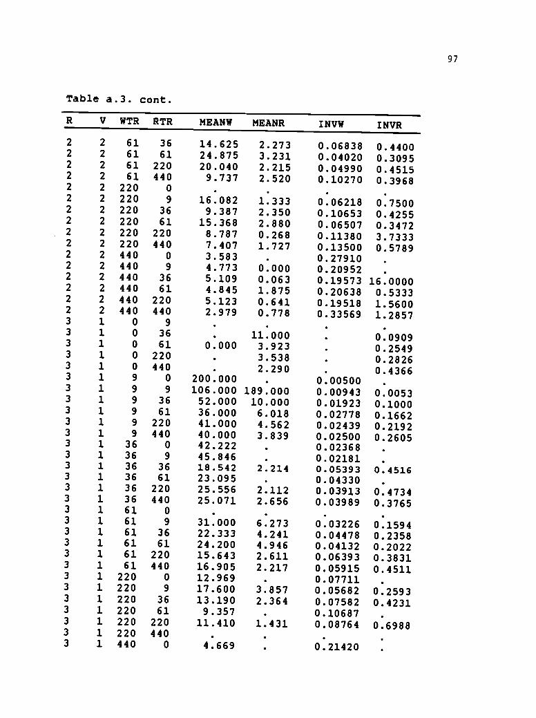
97

Table a.3. cont.

R V WTR RTR MEANW MEANR INVW INVR

2 2 61 36 14.625 2.273 0.06838 0.44002 2 61 61 24.875 3.231 0.04020 0.30952 2 61 220 20.040 2.215 0.04990 0.45152 2 61 440 9.737 2.520 0.10270 0.39682 2 220 02 2 220 9 16.082 1.333 0.06218 0.75002 2 220 36 9.387 2.350 0.10653 0.42552 2 220 61 15.368 2.880 0.06507 0.34722 2 220 220 8.787 0.268 0.11380 3.73332 2 220 440 7.407 1.727 0.13500 0.57892 2 440 0 3.583 0.279102 2 440 9 4.773 0.000 0.209522 2 440 36 5.109 0.063 0.19573 16.00002 2 440 61 4.845 1.875 0.20638 0.53332 2 440 220 5.123 0.641 0.19518 1.56002 2 440 440 2.979 0.778 0.33569 1.28573 1 0 93 1 0 36 11.000 0.09093 1 0 61 0.000 3.923 0.25493 1 0 220 3.538 0.28263 1 0 440 2.290 0.43663 1 9 0 200.000 0.005003 1 9 9 106.000 189.000 0.00943 0.00533 1 9 36 52.000 10.000 0.01923 0.10003 1 9 61 36.000 6.018 0.02778 0.16623 1 9 220 41.000 4.562 0.02439 0.21923 1 9 440 40.000 3.839 0.02500 0.26053 1 36 0 42.222 0.023683 1 36 9 45.846 0.021813 1 36 36 18.542 2.214 0.05393 0.45163 1 36 61 23.095 0.043303 1 36 220 25.556 2.112 0.03913 0.47343 1 36 440 25.071 2.656 0.03989 0.37653 1 61 03 1 61 9 31.000 6.273 0.03226 0.15943 1 61 36 22.333 4.241 0.04478 0.23583 1 61 61 24.200 4.946 0.04132 0.20223 1 61 220 15.643 2.611 0.06393 0.38313 1 61 440 16.905 2.217 0.05915 0.45113 1 220 0 12.969 0.077113 1 220 9 17.600 3.857 0.05682 0.25933 1 220 36 13.190 2.364 0.07582 0.42313 1 220 61 9.357 0.106873 1 220 220 11.410 1.431 0.08764 0.69883 1 220 4403 1 440 0 4.669 0.21420

98

Table a.3. cont.

R V WTR RTR MEANW MEANR INVW INVR3 1 440 9 4.223 3.500 0.23678 0.28573 1 440 36 3.717 0.269023 1 440 61 4.503 5.200 0.22207 0.19233 1 440 220 4.199 0.676 0.23815 1.48003 1 440 440 3.916 0.915 0.25538 1.09333 2 0 9 12.625 0.07923 2 0 36 15.333 0.06523 2 0 61 6.892 0.14513 2 0 220 5.000 0.20003 2 0 440 4.901 0.20403 2 9 0 200.000 0.005003 2 9 9 115.000 13.000 0.00870 0.07693 2 9 36 113.000 11.630 0.00885 0.08603 2 9 61 50.000 8.159 0.02000 0.12263 2 9 220 43.000 3.588 0.02326 0.27873 2 9 440 16.000 3.092 0.06250 0.32343 2 36 0 35.643 0.028063 2 36 9 27.500 5.263 0.03636 0.19003 2 36 36 28.846 4.524 0.03467 0.22113 2 36 61 37.583 8.000 0.02661 0.12503 2 36 220 36.286 3.513 0.02756 0.28473 2 36 440 22.455 2.899 0.04453 0.34503 2 61 0 28.364 0.035263 2 61 9 30.937 6.818 0.03232 0.14673 2 61 36 21.125 3.200 0.04734 0.31253 2 61 61 25.278 6.769 0.03956 0.14773 2 61 220 49.091 9.141 0.02037 0.10943 2 61 440 16.000 2.380 0.06250 0.42013 2 220 0 12.659 0.079003 2 220 9 13.170 1.458 0.07593 0.68573 2 220 36 13.481 2.667 0.07418 0.37503 2 220 61 15.108 2.976 0.06619 0.33613 2 220 220 12.974 2.315 0.07708 0.43203 2 220 440 8.550 1.642 0.11696 0.60913 2 440 0 6.208 0.161073 2 440 9 4.975 7.000 0.20101 0.14293 2 440 36 4.110 2.625 0.24332 0.38103 2 440 61 4.901 1.071 0.20405 0.93333 2 440 220 4.314 1.060 0.23181 0.94373 2 440 440 3.968 0.877 0.25199 1.14004 1 0 9 12.000 0.08334 1 0 36 4.590 0.21794 1 0 61 4.826 0.20724 1 0 220 2.943 0.33974 1 0 440 1.556 0.64294 1 9 0 139.000 0.007194 1 9 9 23.375 0.0428

99

Table a.3. cont.

R V WTR RTR MEANW MEANR INVW INVR

4 1 9 36 0.000 4.562 0.21924 1 9 61 130.000 12.182 0.00769 0.08214 1 9 220 3.837 0.26064 1 9 440 30.000 4.059 0.03333 0.24644 1 36 0 36.111 0.027694 1 36 9 32.909 15.000 0.03039 0.06674 1 36 36 34.500 4.741 0.02899 0.21094 1 36 61 22.545 5.897 0.04435 0.16964 1 36 220 25.636 2.831 0.03901 0.35324 1 36 440 23.889 3.282 0.04186 0.30474 1 61 0 24.621 0.040624 1 61 9 23.833 3.375 0.04196 0.29634 1 61 36 27.211 2.147 0.03675 0.46584 1 61 61 24.294 2.717 0.04116 0.36804 1 61 220 17.045 1.379 0.05867 0.72524 1 61 440 14.778 1.773 0.06767 0.56404 1 220 0 13.887 0.072014 1 220 9 16.429 2.000 0.06087 0.50004 1 220 36 14.918 3.000 0.06703 0.33334 1 220 61 16.148 1.563 0.06193 0.64004 1 220 220 12.750 1.437 0.07843 0.69614 1 220 440 16.432 0.769 0.06086 1.30004 1 440 0 4.405 0.227034 1 440 9 4.620 2.083 0.21646 0.48004 1 440 36 4.060 0.968 0.24632 1.03334 1 440 61 4.328 1.136 0.23104 0.88004 1 440 220 3.491 0.882 0.28649 1.13334 1 440 440 3.542 0.242 0.28234 4.14004 2 0 9 16.250 0.06154 2 0 36 8.238 0.12144 2 0 61 5.578 0.17934 2 0 220 3.537 0.28284 2 0 440 2.069 0.48344 2 9 0 60.000 0.016674 2 9 9 40.000 8.600 0.02500 0.11634 2 9 36 14.000 5.381 0.07143 0.18584 2 9 61 62.000 5.000 0.01613 0.20004 2 9 220 37.667 3.594 0.02655 0.27824 2 9 440 27.500 2.522 0.03636 0.39654 2 36 0 34.000 0.029414 2 36 9 37.100 4.222 0.02695 0.23684 2 36 36 31.222 3.276 0.03203 0.30534 2 36 61 32.917 0.030384 2 36 220 1.299 14.750 0.76991 0.06784 2 36 440 19.417 1.466 0.05150 0.68204 2 61 0 22.640 0.04417

100

Table a.3. cont.

R V WTR RTR MEANW MEANR INVW INVR

4 2 61 9 15.875 1.154 0.06299 0.86674 2 61 36 20.577 2.105 0.04860 0.47504 2 61 61 18.462 2.244 0.05417 0.44574 2 61 220 15.115 1.782 0.06616 0.56124 2 61 440 14.391 1.186 0.06949 0.84294 2 220 0 13.846 0.072224 2 220 9 10.821 0.000 0.092414 2 220 36 4.667 2.368 0.21429 0.42224 2 220 61 13.237 4.667 0.07555 0.21434 2 220 220 9.942 0.904 0.10058 1.10664 2 220 440 10.275 1.227 0.09733 0.81524 2 440 0 3.962 0.252414 2 440 9 4.071 0.000 0.24561 .

4 2 440 36 4.208 0.000 0.23765 .

4 2 440 61 4.472 0.769 0.22360 1.30004 2 440 220 4.435 2.100 0.22550 0.47624 2 440 440 3.204 0.600 0.31212 1.6667

FINAL NUMBEROFT TILLERS

181I- 4-120

101

WAVERLY VARIETY

eQ.

10e

C417:-1'

FINAL NUMBER OF SAT TIM

16141206

OWENS VARIETY6

1.

/aC

110u 1111, II ..1111

A01.10II 11111110

Iii1111.11

Figure a.l. Final mean number of wheat and ryegrass tillers plottedagainst the planted densities of wheat and ryegrass in addition series.Increasing species density and proportion decreased tillers of bothspecies. The effect of increasing wheat density and proportion was moreinfluential than increasing ryegrass density, however.

102

FINAL NUMBER OF REM TILLERS

0068

WAVERLY VARIETY

20e.

FINAL. NUMBER OF RYEGRASS MIMS OWENS VAR=

201 e128

Figure a.l. Cont.