July 11, 2011 15:35 Inverse Problems in Science and Engineering pa-per192˙forIPSE˙LazarCiuprinaIoan

Inverse Problems in Science and EngineeringVol. 00, No. 00, January 2008, 1–11

RESEARCH ARTICLE

Effective extraction of accurate reduced order models for HF-ICs

using multi-CPU architectures

Ioan-Alexandru Lazar, Gabriela Ciuprina∗ and Daniel Ioan

”Politehnica” University of Bucharest, Electrical Engineering Faculty, Numerical

Methods Lab., Spl. Independentei 313, 060042, Bucharest, Romania

(received April 2011)

In this paper a fast, accurate and robust parallel algorithm for the extraction of reduced ordermodels for passive parts of high frequency integrated circuits is proposed. The core of the re-duction procedure is based on Vector Fitting rational approximation of the circuit functions,which are obtained by Finite Integration Technique. In order to reduce the global computa-tional effort, an original Adaptive Frequency Sampling is used to generate an optimal list offrequency samples. The computationally intensive part of algorithm is efficiently mapped ona hierarchical multiprocessor architecture. The goal is to reduce the extraction time and tocontrol the accuracy of the extracted reduced order model.

Keywords: Adaptive Frequency Sampling (AFS), Electronic Design Automation (EDA),Finite Integration Technique (FIT), High Performance Computing (HPC), Model OrderReduction (MOR), Vector Fitting (VF)

AMS Subject Classification: 30E10, 65M22, 65F05, 65Y05

1. Introduction

In the design of today’s high frequency integrated circuits (HF-ICs) electromagneticfield effects are too relevant to be neglected. Electromagnetic (EM) field modelsthat take into account skin effect, dielectric losses, wave propagation, etc. leadto models that may have over one million degrees of freedom even in the caseof simple passive components such as spiral inductors, meander resistors, on-chipcapacitors or metallic interconnects. Since the simulation of the complete IC is doneby aggregating its constitutive parts, a model order reduction (MOR) technique,which transform these huge models to much smaller ones, more or less equivalent,but easy to simulate is required.One of the most successful MOR algorithms for this class of problems proved to

be Vector Fitting (VF) [1]. The VF algorithm, as proposed in [2] by Gustavsen andSemlyen and further refined in [3],[4] starts from the values of the transfer functionin a set of given frequency samples and finds the best rational approximation of thisfrequency characteristic. The accuracy of the models extracted by VF depends onthe number and distribution of frequency samples. For the problems we consider,there is no prior knowledge of the frequency characteristic. That is why a highaccuracy requires a large number of samples to be used. However, each sample iscostly because it needs a full-wave EM simulation. So, without an accuracy control

∗Corresponding author. Email: gabriela@lmn.pub.ro

ISSN: 1741-5977 print/ISSN 1741-5985 onlinec© 2008 Taylor & FrancisDOI: 10.1080/1741597YYxxxxxxxxhttp://www.informaworld.com

July 11, 2011 15:35 Inverse Problems in Science and Engineering pa-per192˙forIPSE˙LazarCiuprinaIoan

2 Taylor & Francis and I.T. Consultant

the computation time may increase uncontrollably in the case of over-sampling orthe extracted model may be poor in the case of local under-sampling. Therefore, amethod to generate an optimal list of samples, by Adaptive Frequency Sampling(AFS), aiming to minimize the approximation error, is expected to improve therobustness and efficiency of a MOR procedure based on VF.Various AFS techniques were proposed even since 1990. The goal was the same:

to minimize the number of costly data samples so that an accurate model for alarge frequency range is obtained with an acceptable effort [5]. All of them usevarious approximation techniques, mainly based on least squares (LS), to obtaina rational approximation of the model. In 2004, Deschrijver and Dhaene proposedan AFS algorithm combined with VF, much stable than traditional LS approaches,which moreover, minimizes passivity violations within the frequency range [5]. Inthis AFS algorithm multiple rational models are built, ranked and the best two areretained. The fitting error is based on the difference between these two models andnew samples are generated so that this fitting error is minimized. In order to avoidthe premature convergence, some heuristic rules are also introduced. In [6] thistechnique is used in combination with PEEC to generate rational macromodels ofEM systems with a reduced cost.The AFS technique we propose uses a different fitting error. The accuracy of

the VF reduced model is estimated in a set of ”test frequencies” interleaved among”sample frequencies”. By controlling the accuracy in the intervals between samples,the total number of frequencies is kept at the lowest level, thus reducing the modelextraction effort. We applied this AFS technique for EM models generated withthe Finite Integration Technique (FIT), originally proposed by Weiland [7] andimproved as in [8] and [9]. Finally, the algorithm is implemented as it is describedbelow on a cluster with multicore CPUs, which further decreases the total extrac-tion time. The intrinsic granulation of our algorithm allows the communicationoverhead to be kept at a minimum level, while exploiting the maximum resourcesof the multicore nodes.

2. Problem formulation

The EM field effects at high frequency are quantified by Maxwell’s equations infull wave regime. Therefore, the first level of approximation consists of modeling apassive device as an EM field problem with particular, appropriate boundary andinitial conditions. This EM field problem defines a consistent input/output systemwhich has a well defined response, described by the unique output signals, for anyinput signals applied as terminal excitations. The most appropriate formulationfor passive devices with distributed parameters, compatible with external electricand magnetic circuits is the Electro-Magnetic Circuit Element (EMCE) [10]. Thenext modeling step is done by applying the Finite Integration Technique (FIT) todiscretize the continuous model defined above. Subsequently, a semi-state spacemodel is obtained [10], [11]:

Cdx(t)

dt+Gx(t) = Bu(t), y(t) = Lx(t). (1)

where, x ∈ IRn is the state space vector, a column vector of size n - the initialnumber of degrees of freedom (DoFs), u ∈ IRm is the vector of input quantities, acolumn vector of size m - the number of floating terminals of the EMCE model,and y ∈ IRm is the vector of output quantities. Each of these m terminals intro-duces exactly one input and one output signal. The matrices C,G ∈ IRn×n are real,

July 11, 2011 15:35 Inverse Problems in Science and Engineering pa-per192˙forIPSE˙LazarCiuprinaIoan

Inverse Problems in Science and Engineering 3

square, sparse matrices, whereas B ∈ ZZn×m and L ∈ ZZm×n are selection, sparsematrices, and in particular cases, B = LT [11]. The relationship between the com-plex representations of the input/output signals is given in the frequency domainby the transfer matrix

HFIT(ω) = L(G+ jωC)−1B. (2)

Thus, to compute (2), an algebraic system of n linear complex equations, havingG + jωC as coefficient matrix and the matrix B as right hand side, has to besolved for each frequency. The size of the system depends on the fineness of theFIT discretization grid (which may contain a huge number of nodes), and on thenumber of terminals which gives the number of right hand side terms. Model orderreduction is necessary.The VF order reduction procedure uses as input a set of values (ωk,H(ωk)),k =

1, . . . , F where F is the number of frequency samples and it identifies the poles pi(which are scalar, real or complex conjugate pairs), the residual matrices Ki ∈ ICn×n

and the constant terms K∞,K0 ∈ IRm×m of the rational approximation

HVF(ω) =

q∑

i=1

Ki

jω − pi+K∞ + jωK0 (3)

forHFIT(ω). Here q is the order of the reduced system (q ≪ n), automatically foundby including the VF function into a loop that increases q until a given thresholdεVF is reached [1].The problem to be solved is the following:

Given n - the size of the initial model,m - the number of input/output signals, thesemi-state space matrices C,G ∈ IRn×n, B ∈ ZZn×m, and L ∈ ZZm×n, the frequencyrange [ωmin, ωmax]Find a minimal set of frequencies S = ωk,k = 1, . . . , F distributed in the

frequency range, so that the relative error ‖HFIT(ω′

i) − HVF(ω′

i)‖/‖HFIT(ω′

i)‖computed for every ω′

i ∈ S ′ is smaller than an imposed threshold εAFS. HereS ′ = ω′

k,k = 1, . . . , F ′, is a set of frequencies: ωk < ω′

k < ωk+1, interleavedamong the samples S.

3. Algorithm

The basic idea of the algorithm is to generate the frequency response HVF(ω) byusing the VF algorithm applied on a set of sampling frequencies S = ω1, . . . , ωF ,which is successively refined.The generation of S depends on how the fitted response matches the real re-

sponse in the test frequencies S ′. The transfer matrix H(ω) in both sets of testand sampling frequencies are computed by numerical solving with FIT the EMfield problem in the analyzed device with EMCE boundary conditions. The set Sis used for fitting, whereas S ′ only for validation.The algorithm is an 8-steps procedure which can be described as follows:

• Step 1. Generate the semi-state space model (1), by using FIT for the EMCEformulation of the EM field problem and distribute it to all computational nodes.

• Step 2. Choose an initial set of F sampling frequencies S (e.g. S = ωmin, (ωmin+ωmax)/2, ωmax) and flag them all as unmarked. Optimal value of F is between2 and the halved number of computational nodes.

July 11, 2011 15:35 Inverse Problems in Science and Engineering pa-per192˙forIPSE˙LazarCiuprinaIoan

4 Taylor & Francis and I.T. Consultant

• Step 3. Choose an initial set of test frequencies S ′ consisting of F ′ = F − 1frequencies interleaved among the sampling frequencies and flag them all asunmarked.

• Step 4. Compute HFIT(S) and HFIT(S′) with (2). This is achieved by solving,

in parallel, the complex linear systems (G + jωC)x = B for all unmarked fre-quencies ω in the sample set S and in the test set S ′, flagging each frequency as”marked” after its associated system has been solved.

• Step 5. Apply VF to HFIT(S), computed at the previous step, and obtainthe characteristic parameters of the rational approximation (3): poles, residualsand constant terms. The order q is successively increased until the fitting errorbecomes acceptable: ‖HFIT(ωk)−HVF(ωk)‖/‖HFIT(ωk)‖ < εVF.

• Step 6. Compute HVF(S′) and evaluate the relative error εi = ‖HFIT(ω

′

i) −HVF(ω

′

i)‖/‖HFIT(ω′

i)‖ for every test frequency ωi ∈ S ′.

• Step 7. If εi < εAFS - the imposed threshold, for every ωi ∈ S ′, then stop.Otherwise, move the test frequencies where the error is larger than εAFS fromS ′ to S and interleave a new set of test frequencies in the new intervals thuscreated. The new test frequencies are appended to S ′ and they are flagged asunmarked.

• Step 8. If none of the other stopping criteria are met (e.g. F > Fmax), repeatfrom Step 4. Otherwise, stop.

Numerical experiments have shown that if the imposed error εAFS is too lowand the number of maximum allowed samples Fmax is too high, the algorithm doesnot stop even if there is no major change in the reduced model obtained. As aconsequence, the stopping criterion is enhanced by adding a heuristic rule whichchecks the poles reallocation in two consecutive iterations that yielded models ofthe same order. Therefore, if at the i-th iteration, ‖Pi − Pi−1‖/‖Pi‖ < εp, withPi being the vector of poles at iteration i, and εp a user supplied tolerance, it canbe assumed that the precision of the model will not be improved any further andthat the computation can be stopped.The convergence of the algorithm and the quality (order and passivity) of the

reduced-order model are also influenced by the choice of εVF. Typically, choosingεVF = εAFS/10 is sufficient for the fitting to be stiff enough to provide both highprecision and quick convergence.There are several methods to interleave the test frequencies. The simplest method

with acceptable results for most problems is to choose as test node the midpointbetween two successive sampling frequencies. When the frequency range is verylarge (more than 3-4 decades), a geometric mean instead the arithmetic averagetends to give better results. Random distribution of test frequencies is anotherpossible option.

4. Implementation on multi-CPU architectures

4.1. Hierarchical parallel architectures

4.1.1. Hardware

In the last years, the most prevalent form of high-scale parallel architecture hasbeen that of the Beowulf cluster. Such cluster is comprised of several individualcomputers called nodes, linked in a computer network. Communication networkcomprises typically a high speed switch (e.g. using low latency Infiniband technol-ogy) and a Network Interface Card (NIC) for each node. The nodes can thereforecommunicate between each other, but they do not share their resources; the only

July 11, 2011 15:35 Inverse Problems in Science and Engineering pa-per192˙forIPSE˙LazarCiuprinaIoan

Inverse Problems in Science and Engineering 5

Figure 1. Typical hierarchical multi-CPU architecture.

exception is, in some cases, the file-system (e.g. NFS), which can be virtuallycommon (although files belong to several HDD/Controllers), in order to make de-velopment and administration easier. This provides a first level of granularity (thecoarsest one) at which an algorithm can be parallelized.With the advent of multicore CPUs on the popular x86 64 architecture, it is

becoming more and more common for the nodes in a cluster to have several multi-cores CPUs (Fig. 1). Essentially, every core is an individual microprocessor, andseveral cores are grouped on a multichip (CPU) module; each core has its own cachememories, but the main memory (RAM) is shared among cores. This provides asecond level of granularity for algorithm parallelization.Every level of hierarchy has specific demands when it comes to performance.From the first level point of view, since the nodes in a Beowulf cluster do not share

resources, the only way to share data is by message passing, by means of NICs.This can be fairly slow even when using specialized protocols like Infiniband.As to the the second level of architectural hierarchy, since the cores in a multicore

CPU share the main memory, communication is faster. However, since accessingthe main memory is significantly slower than accessing the cache and since thedata bus to RAM is also shared by cores, efficient use of the cache memory is vitalfor speed.

4.1.2. Software

From the software point of view, the basic unit of execution is the process. Aprocess consists of a sequence of instructions and a set of reserved resource whichis managed by the operating system. Using a feature called CPU affinity; a processcan be assigned to run on a certain set of cores in a multicore system. Therefore, anode will run at least one process, which can use all of its cores, or several processes,each of them having assigned a subset of the node’s cores.A process can have several execution threads. An execution thread is also a se-

quence of instructions, but unlike processes, threads do not have their own, separatememory space. Instead, they all share the memory space of their parent process.However, using CPU affinity methods, threads can be confined to run on a cer-tain core from those assigned to their parent processes, which is typically efficientbecause transferring threads between cores is costly.

July 11, 2011 15:35 Inverse Problems in Science and Engineering pa-per192˙forIPSE˙LazarCiuprinaIoan

6 Taylor & Francis and I.T. Consultant

4.2. Parallel/distributed implementation of algorithm

The algorithm described in section 3 was carefully mapped on this hierarchicalarchitecture, according to its intrinsic granularity structure.The most computationally intensive task of the algorithm is in step 4, which

requires the solving of large, non-symmetric, very sparse and ill-conditioned linearsystems of complex equations. The contribution of the boundary conditions gener-ates a particular structure of the system matrix, very difficult to be factorized. Thatis why, only this solving was parallelized among several cores of a node, whereasthe rest of algorithm was distributed to several nodes, as an embarrassingly parallelapplication.The program is run by a master process, and at step 4, the computation is

distributed by MPI (Message Passing Interface) to worker processes. Each workerprocess is thus responsible for the solving of a subset of the unmarked (i.e. unsolved)frequencies needed by the AFS iteration and it is assigned to run on a single node,with a number of threads equal to the number of cores of that node.The first level of granularity is achieved by the master process, which distributes

the unmarked frequencies to worker processes (called briefly ”workers”). By usingthe shared file system, the semi-state space matrices are available to each nodedirectly, so that only the frequencies have to be communicated over the networkby message passing.Once all new frequencies have been distributed, the second level of granularity is

exploited by each worker process which is mapped only a single node, which solvesin parallel the linear system associated to the frequency assigned to it, employingthe maximum available number of computational threads (one for each core innode) and shared memory computational model. The parallel linear solving routinewas a sparse, direct one, namely the UMFPACK [12], compiled against AMD’sAdvanced Core Math Library (ACML) with OpenMP, which provides the high-performance parallel BLAS functions. The motivation of this choice will be thescope of another paper.Finally, by using MPI the results are collected by the node that runs the master

process, which performs vector fitting and the error control.

5. Numerical results and validations

5.1. Validation of the AFS algorithm

The first ”toy” test case was a simple circuit with a RC tree structure with 100segments. The values used are: each segment has a rezistance of 0.772 Ω and acapacitance of 0.644 pF, the source is voltage excited, with a inner resistance of 5

Table 1. AFS validation for a simple RC tree test,

2 starting frequencies.

εAFS Convergence

10−4 iteration 1 2 3 4 5 6order 2 3 4 6 9 9F + F ′ 3 5 9 15 27 35

10−3 iteration 1 2 3 4 5order 2 3 4 6 9F + F ′ 3 5 9 15 23

10−2 iteration 1 2 3 4 5order 2 3 4 6 8F + F ′ 3 5 9 13 17

Table 2. AFS convergence for two U-shaped

coupled inductors test, 4 starting frequencies.

εAFS Convergence

10−4 iteration 1 2 3 4 5order 6 5 5 6 6F + F ′ 7 13 25 49 91

10−3 iteration 1 2 3 4order 6 5 5 6F + F ′ 7 13 19 31

10−2 iteration 1 2order 6 5F + F ′ 7 13

July 11, 2011 15:35 Inverse Problems in Science and Engineering pa-per192˙forIPSE˙LazarCiuprinaIoan

Inverse Problems in Science and Engineering 7

104

106

108

1010

1012

1014

0

10

20

30

40

50

60

70

80

Frequency [Hz]

Pha

se (

degr

ee)−

−−

Y

reference3 AFS points at iteration 2VF approximation of order 3

(a)

104

106

108

1010

1012

1014

0

10

20

30

40

50

60

70

80

Frequency [Hz]

Pha

se (

degr

ee)−

−−

Y

reference15 AFS points at iteration 5AFS approximation of order 9

(b)

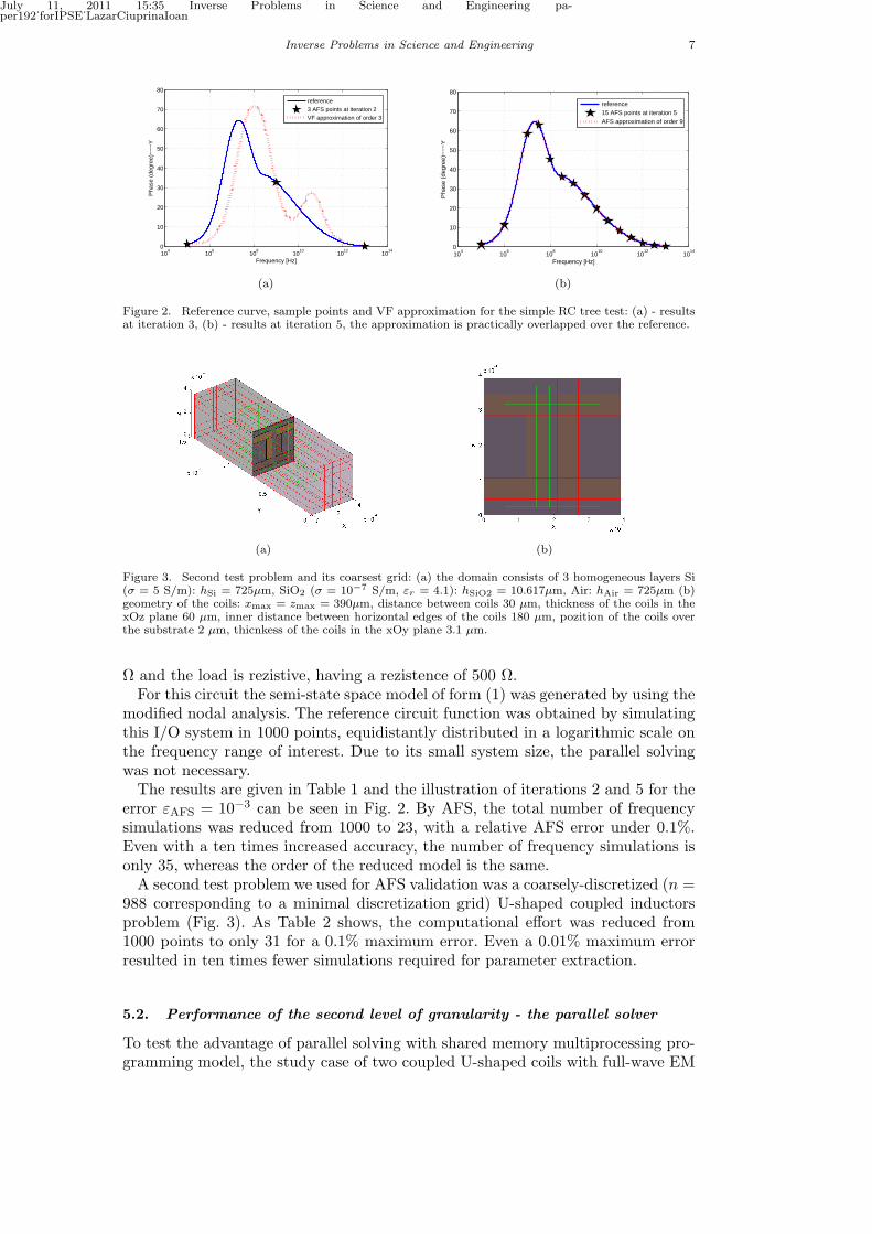
Figure 2. Reference curve, sample points and VF approximation for the simple RC tree test: (a) - resultsat iteration 3, (b) - results at iteration 5, the approximation is practically overlapped over the reference.

(a) (b)

Figure 3. Second test problem and its coarsest grid: (a) the domain consists of 3 homogeneous layers Si(σ = 5 S/m): hSi = 725µm, SiO2 (σ = 10−7 S/m, εr = 4.1): hSiO2 = 10.617µm, Air: hAir = 725µm (b)geometry of the coils: xmax = zmax = 390µm, distance between coils 30 µm, thickness of the coils in thexOz plane 60 µm, inner distance between horizontal edges of the coils 180 µm, pozition of the coils overthe substrate 2 µm, thicnkess of the coils in the xOy plane 3.1 µm.

Ω and the load is rezistive, having a rezistence of 500 Ω.For this circuit the semi-state space model of form (1) was generated by using the

modified nodal analysis. The reference circuit function was obtained by simulatingthis I/O system in 1000 points, equidistantly distributed in a logarithmic scale onthe frequency range of interest. Due to its small system size, the parallel solvingwas not necessary.The results are given in Table 1 and the illustration of iterations 2 and 5 for the

error εAFS = 10−3 can be seen in Fig. 2. By AFS, the total number of frequencysimulations was reduced from 1000 to 23, with a relative AFS error under 0.1%.Even with a ten times increased accuracy, the number of frequency simulations isonly 35, whereas the order of the reduced model is the same.A second test problem we used for AFS validation was a coarsely-discretized (n =

988 corresponding to a minimal discretization grid) U-shaped coupled inductorsproblem (Fig. 3). As Table 2 shows, the computational effort was reduced from1000 points to only 31 for a 0.1% maximum error. Even a 0.01% maximum errorresulted in ten times fewer simulations required for parameter extraction.

5.2. Performance of the second level of granularity - the parallel solver

To test the advantage of parallel solving with shared memory multiprocessing pro-gramming model, the study case of two coupled U-shaped coils with full-wave EM

July 11, 2011 15:35 Inverse Problems in Science and Engineering pa-per192˙forIPSE˙LazarCiuprinaIoan

8 Taylor & Francis and I.T. Consultant

Table 3. Time [s] required to solve a linear system for

a single frequency (U-shaped coils test).

No. of threads System size n6317 17069 42269 56927

1 0.41 3.14 25.79 50.062 0.35 2.07 15.15 28.534 0.29 1.56 9.76 17.686 0.28 1.45 8.14 14.408 0.28 1.37 7.24 12.60

0 1 2 3 4 5 6

x 104

1

1.5

2

2.5

3

3.5

4

System size n

Spe

edup

vs.

ser

ial

2 threads4 threads6 threads8 threads

(a)

0 1 2 3 4 5 6

x 104

0

10

20

30

40

50

60

System size n

Sol

ving

tim

e [s

]

1 thread2 threads4 threads6 threads8 threads

(b)

Figure 4. (a) Relative speed-up over serial solving of one system; (b) Total time required for one frequency.

field was considered again. By using several FIT discretization grids with increasedrefinement, a series of state space models having several sizes were obtained. Table3 holds the time necessary to solve one system with n equations by using variousnumber of threads (mapped on the cores of a single node).It can be seen that increasing the number of threads gives a consistent time

improvement in solving the linear system. As expected, the speed-up increases withthe size of the system (Fig. 4). It can be noted that the speed-up obtained with 8threads is about 4 in the case of the largest system tested. It seems that it is a bitlow, but other trials, e.g. with solvers such as SuperLU Dist or PARDISO, failedfrom the accuracy point of view and SuperLU MT was slower than UMFPACK.

5.3. Overall performance of the distributed/parallel AFS algorithm

The total computational type mainly depends on the number of iterations of theAFS algorithm and on the number of systems to be solved. In each iteration, theunmarked frequencies are distributed to the computational workers (mapped onnodes) and each worker solves its frequencies one after the other. Each linear systemsolving is carried out in parallel by a number of threads equal to the number ofcores of that node.The systems are identical in structure, so every system can be solved in

roughly the same amount of time if the cluster has identical nodes. Therefore,if communication time is neglected, the total time required for extraction isT = Ts

∑Ni=1Ceil[Ni/Nn], where Ni is the number of unmarked frequencies at

each iteration i, Nn is the number of nodes, Ts is the time required to solve onesystem, and N is the number of iterations. If enough nodes are provided so that,at each iteration there are fewer unmarked frequencies than nodes, then every it-eration requires a time of exactly Ts to complete. In this case, if communicationand overhead time is neglected, the extraction procedure can be carried out in atime T = NTs.

July 11, 2011 15:35 Inverse Problems in Science and Engineering pa-per192˙forIPSE˙LazarCiuprinaIoan

Inverse Problems in Science and Engineering 9

0 1 2 3 4 5 6

x 104

0

100

200

300

400

500

600

700

800

System size n

Sol

ving

tim

e [s

]

Serial1 worker2 workers3 workers4 workers

(a)

0 1 2 3 4 5 6

x 104

0

5

10

15

20

25

System size n

Spe

edup

vs.

ser

ial

1 worker2 workers3 workers4 workers

(b)

Figure 5. Overall performance for the U-shaped coils device: (a) solving time vs. system size; (b) speedupvs. serial execution.

In order to study the overall performance of the algorithm, we have consideredtwo benchmark problems. The first one is the two coupled U-shaped coils describedabove.The U-coupled device shows an excellent performance improvement (Table 4).

More refined grids give a speedup of almost 3 for 4 workers, which is with 25%less than the ideal value of 4. As the size of the system increases and most of thecomputational work is spent on solving systems rather than message-passing, I/Oand memory management operations, it is expected that the speed improvementincreases .Using 4 workers (mapped on 4 nodes, so using a total number of 32 cores), the

time required to extract the parameters is almost 23 times smaller than in the caseof serial execution. The total speed-up does depend on the system size; for smallgrids (less than 50000 equations), the speedup is considerably lower (Fig. 5).The second benchmark (CHRF 201) is more complicated. It consists of two cou-

pled coils as well (Fig. 6), but with a more difficult geometry. It is a test structureexperimentally characterized, that is even more computationally-challenging, be-cause of its high memory requirements, even for the minimal discretization gridwhich yielded a semi-state space system of 104102 degrees of freedom. This bench-mark is a real one, such a device being a component of a low noise amplifier.A significant performance improvement was obtained for this problem as well, the

results being summarized in Table 5 and Fig. 7. The reference curve was obtainedby over-sampling i.e. by simulating the field problem in 100 uniformly distributed

Table 4. Total model extraction times [s] and speed-up for the U-

shaped coils with an εAFS = 10−3, parallel computation with 8 threads

for each solving, and 4 starting frequencies.

No. of System size nworkers 6317 17069 42269 56927

Time [s] 1 9.83 25.44 103.05 96.22 8.45 16.51 59.69 58.213 7.71 13.69 44.38 43.934 7.5 12.35 37.63 32.25

Speed-up w.r.t 1 1 1 1 1one worker 2 1.16 1.54 1.73 1.65

3 1.28 1.86 2.32 2.194 1.31 2.05 2.74 2.98

Speed-up w.r.t 1 1.21 2.02 2.96 7.47serial computation 2 1.41 3.12 5.11 12.35

3 1.55 3.76 6.87 16.364 1.6 4.15 8.1 22.28

July 11, 2011 15:35 Inverse Problems in Science and Engineering pa-per192˙forIPSE˙LazarCiuprinaIoan

10 Taylor & Francis and I.T. Consultant

0

0.5

1

x 10−3

0

0.5

1

1.5

x 10−3

0

2

4

6

x 10−4

XY

z

Figure 6. CHRF 201 - computational domain.

109

1010

1011

−5

−4

−3

−2

−1

0

1x 10

−6

Frequency [Hz]

Rea

l par

t−−

−Y

12

referenceAFS pointsVF approximation of order 5

Figure 7. CHRF201-reference and reduced model.

Table 5. CHRF201 model extraction time with 8 threads/solving, 4 starting frequen-

cies, εAFS = 10−3.

No. of. workers 1 2 3 4 5 Serial execution

Solving time [s] 291.19 165.4 120.29 98.5 97.3 1110.37Speed-up 3.81 6.71 9.23 11.27 11.41 1

frequencies in the range 1-60 GHz. By using AFS, only 13 simulation were enough toextract a reduced-order model with order q = 5 and an error under 0.1%. By using 5workers, the extraction process is 11 times faster than the serial extraction with onenode and one thread. Considering that only 13 points are required (instead of the100 required for oversampling) and taking into account the speed improvement dueto parallelization, the proposed AFS algorithm was more than 80 times faster thanthe serial, oversampling-based implementation, which was our initial, referencecode.All tests described above were run on a cluster which has in each node two

INTEL Xeon Nehalem quad-core CPUs at 2.66GHz, 8MB cache and 24GB RAM.

6. Conclusions

The algorithm proposed in this paper is based on a new method for model ex-traction of HF-ICs passive components, which is a basic issue for many problemsencountered in the EDA industry. The novelty of our approach is due to the com-bination of three techniques: FIT, VF and AFS used for electromagnetic modelingand order reduction. Its robustness is given by the VF algorithm, which behavesbetter for the tested structures than other model order reduction techniques. Thenovelty related to AFS is given by the estimation of the extracted model accuracy,by using a set of test points interleaved among the frequency samples used by VFin the fitting process. By controlling the accuracy in the intervals between samples,the total number of frequencies is kept at a low level, thus the computational cost ofthe model extraction, specifically the number of EM field simulations is reduced.Considering all HF field effects described by Maxwell equations, the devices aremodeled with an extremely high accuracy. FIT discretization of these equationswith their appropriate boundary conditions yields finite but still accurate models,which were experimentally validated [8],[11].From the implementation point of view, the algorithm is tailored so as to ex-

ploit the computational resources of a hierarchical parallel architecture, typical fortoday’s HPC clusters, in an efficient manner. Our implementation use both dis-tributed and shared memory programming models as well as industry-standardsoftware tools and technologies that allowed an efficient cache and CPU use on

July 11, 2011 15:35 Inverse Problems in Science and Engineering pa-per192˙forIPSE˙LazarCiuprinaIoan

REFERENCES 11

individual nodes and minimal communication between nodes.The algorithm we propose for model extraction is structured into two levels of

granularity, each of them being mapped on a suitable component of the computingarchitecture. The two granularity levels of the algorithm do not inherently dependon each other: it is possible to apply it in a cloud or grid environment without losingefficiency, and different linear solvers can be used, depending on the problem athand.In brief, this approach combines the efficient exploitation of modern high-

performance computer architectures with the high accuracy of a FIT and VF+AFS-based modeling and order-reduction technique.

Acknowledgements

The authors gratefully acknowledge the financial support offered during sev-eral years by the following complementary projects: FP6/Chameleon-RF,FP5/Codestar, CNCSIS-UEFISCDI project number PNII-IDEI 609/2008. Thework has been co-funded as well by the Sectoral Operational Programme HumanResources Development 2007-2013 of the Romanian Ministry of Labour, Family andSocial Protection through the Financial Agreement POSDRU/89/1.5/S/62557.

References

[1] D. Ioan and G. Ciuprina. Model reduction of interconnected systems. In W.H.A Schilders, Henkvan der Vorst, and J. Rommes, editors, Model Order Reduction: Theory, Research Aspects and Ap-plications, volume 13 of Mathematics in Industry, pages 447–467. Springer Berlin Heidelberg, 2008.

[2] B. Gustavsen and A. Semlyen. Rational approximation of frequency domain responses by vectorfitting. IEEE Transactions on Power Delivery, 14(3):1052–1061, 1999.

[3] B. Gustavsen. Improving the pole relocating properties of vector fitting. IEEE Transactions onPower Delivery, 21(3):1587–1592, 2006.

[4] D. Deschrijver, M. Mrozowski, T. Dhaene, and D. De Zutter. Macromodeling of multiport systemsusing a fast implementation of the vector fitting method. IEEE Microwave and Wireless ComponentsLetters, 18(6):383–385, 2008.

[5] D. Deschrijver and T. Dhaene. Passivity-based sample selection and adaptive vector fitting algorithmfor pole-residue modeling of sparse frequency-domain data. In Proc. of the 2004 IEEE Int. BehavioralModeling and Simulation Conference, pages 68–73, 2004.

[6] A. Antonini, D. Deschrijver, and T. Dhaene. Broadband rational macromodeling based on the adaptivefrequency sampling algorithm and the partial element equivalent circuit method. IEEE Transactionson Electromagnetic Compatibility, 50(1), 2008.

[7] M. Clemens and T. Weiland. Discrete electromagnetism with the finite integration technique. Progressin Electromagnetics Research (PIER), 32:65–87, 2001.

[8] D. Ioan, G. Ciuprina, Radulescu. M., and E. Seebacher. Compact modeling and fast simulation ofon-chip interconnect lines. IEEE Transactions on Magnetics, 42(4):547–550, 2006.

[9] D. Ioan, G. Ciuprina, and W. Schilders. Parametric models based on the adjoint field technique forRF passive integrated components. IEEE Transactions on Magnetics, 44(6):1658–1661, 2008.

[10] D. Ioan, W. Schilders, G. Ciuprina, N. van der Meijs, and W. Schoenmaker. Models for integratedcomponents coupled with their environment. COMPEL- The International Journal for Computationand Mathematics in Electrical and Electronic Engineering, 27(4):820–829, 2008.

[11] G. Ciuprina, D. Ioan, D. Mihalache, and E. Seebacher. Domain partitioning based parametric modelsfor passive on-chip components. In J. Roos and L. Costa, editors, Scientific Computing in Electri-cal Engineering SCEE 2008, volume 14 of Mathematics in Industry, pages 37–44. Springer BerlinHeidelberg, 2010.

[12] T.A. Davis. Algorithm 832: Umfpack, an unsymmetric-pattern multifrontal method. ACM Transac-tions on Mathematical Software, 30(2):196–199, 2004.