Effect of electrode geometry on high energy spark discharges ...
216
Purdue University Purdue e-Pubs Open Access eses eses and Dissertations Spring 2015 Effect of electrode geometry on high energy spark discharges in air Mounia Belmouss Purdue University Follow this and additional works at: hps://docs.lib.purdue.edu/open_access_theses Part of the Aerospace Engineering Commons is document has been made available through Purdue e-Pubs, a service of the Purdue University Libraries. Please contact [email protected] for additional information. Recommended Citation Belmouss, Mounia, "Effect of electrode geometry on high energy spark discharges in air" (2015). Open Access eses. 556. hps://docs.lib.purdue.edu/open_access_theses/556
-
Upload
khangminh22 -
Category
Documents
-
view
1 -
download
0
Transcript of Effect of electrode geometry on high energy spark discharges ...

Purdue UniversityPurdue e-Pubs
Open Access Theses Theses and Dissertations
Spring 2015
Effect of electrode geometry on high energy sparkdischarges in airMounia BelmoussPurdue University
Follow this and additional works at: https://docs.lib.purdue.edu/open_access_theses
Part of the Aerospace Engineering Commons
This document has been made available through Purdue e-Pubs, a service of the Purdue University Libraries. Please contact [email protected] foradditional information.
Recommended CitationBelmouss, Mounia, "Effect of electrode geometry on high energy spark discharges in air" (2015). Open Access Theses. 556.https://docs.lib.purdue.edu/open_access_theses/556


i
EFFECT OF ELECTRODE GEOMETRY ON HIGH ENERGY SPARK DISCHARGES
IN AIR
A Thesis
Submitted to the Faculty
of
Purdue University
by
Mounia Belmouss
In Partial Fulfillment of the
Requirements for the Degree
of
Master of Science in Aeronautics and Astronautics
May 2015
Purdue University
West Lafayette, Indiana

ii
For my mama, Fatima Anezid.

iii
ACKNOWLEDGEMENTS
First, I would like to acknowledge the help, patience and guidance from my
advisor, Dr. Sally Bane. I am very lucky and extremely thankful to have her as my
advisor. This thesis, my years of research and overall experience of graduate school at
Purdue would not have been anywhere as enriching or even possible without her presence.
It is thanks to all her advice, expertise and the amount of time she has invested in guiding
me that I am even here today. She sets a perfect example as an inspiring mentor and
teacher through her friendship, evident dedication and care for all members of the
research group. I cannot thank her enough and I am especially grateful for the confidence
and knowledge she has helped me develop to become a better scientist and engineer.
I would like to acknowledge and thank my amazing parents, for whom I am
eternally grateful. Their acts of love, encouragement, support and sacrifice have allowed
me to be where I am today. Thank you, Mom and Dad.
I would also like to thank the members of my committee, Dr. Gregory Blaisdell
and Dr. John Sullivan, for so kindly agreeing to serve on my committee. I would like to
thank Dr. Gregory Blaisdell for being an inspiring and supportive professor and for all his
help throughout my years of education at Purdue. I would also like to thank Dr. John
Sullivan for his enthusiasm and encouragement. I would like to thank John Philips and

iv
Robin Snodgrass for their help.
I would also like to thank the members of the research group and all my friends
for providing advice and support throughout my education. They have made my
experience as a student at Purdue unforgettable.


vi
Page
2.1 Plasma Discharge Characterization .................................................................... 28
2.2 Diagnostics ......................................................................................................... 31
2.2.1 Schlieren Visualization ............................................................................... 31
2.2.2 Schlieren Image Velocimetry (SIV) Commercial PIV software ............. 32
2.3 Electrical Measurements .................................................................................... 33
CHAPTER 3. RESULTS & ANALYSIS: KERNEL EVOLUTION ELECTRICAL
CHARACTERISTICS ...................................................................................................... 34
3.1 Electrical Energy and Power Measurements ...................................................... 35
3.2 Effect of Discharge Energy on the Structure of the kernel ................................ 49
CHAPTER 4. RESULTS & ANALYSIS: KERNEL EVOLUTION SIV
....................................................................................................... 56
4.1 Point-to-Point Electrodes .................................................................................... 58
4.2 Flat-to-Point Electrodes ...................................................................................... 81
4.3 Blunt-to-Blunt Electrodes ................................................................................. 104
CHAPTER 5. CONCLUSION ................................................................................. 125
5.1 Electrical Characteristics .................................................................................. 126
5.2 Plasma Channel Evolution ............................................................................... 129
CHAPTER 6. FUTURE WORK .............................................................................. 134
REFERENCES ............................................................................................................... 137
APPENDICES ................................................................................................................ 148
Appendix A - Velocity Vector Plots .......................................................................... 148
Appendix B - Vorticity Contour Ploots ..................................................................... 172

vii
LIST OF TABLES
Table .............................................................................................................................. Page
Table 3.1: Discharge characteristics for different electrode configurations. .................... 37
Table 3.3: Plasma channel radii at two different spark energies ...................................... 54
Table 3.4: Breakdown energy and dissipation times across different electrode
configurations ................................................................................................................... 55

viii
LIST OF FIGURES
Figure ............................................................................................................................. Page
Figure 1.1: Current-voltage characteristics of the different types of discharges in gases
[37] .................................................................................................................................... 15
Figure 1.2: : Propagation of (a) an electron avalanche, (b) a positive streamer and (c) a
negative streamer [37, 45]; t1 and t2 are two instants in the same propagation phase. ...... 18
Figure 2.1: Schematic of the high-energy spark discharge circuit.................................... 29
Figure 2.2: Point-to-point electrode configuration in Teflon fixture ................................ 29
Figure 2.3: Schlieren system used for spark discharge visualization. Note that the spark
gap was located between the achromatic lens and flat mirror. ......................................... 32
Figure 3.1: Breakdown voltage of different electrode configurations ............................. 37
Figure 3.2: High-energy discharge current and voltage waveforms for the point to point
electrodes with gap lengths of (a) 2mm, (b) 5mm, and (c) 10 mm................................... 39
Figure 3.3. Calculated power and energy for the point to point electrodes with gap
lengths of (a) 2mm, (b) 5mm, and (c) 10 mm. .................................................................. 40
Figure 3.4: High-energy discharge current and voltage waveforms for blunt-to-blunt
electrodes with gap lengths of (a) 2mm, (b) 5mm, and (c) 10 mm................................... 41
Figure 3.5: Calculated power and energy for the blunt-to-bunt electrodes with gap
lengths of (a) 2mm, (b) 5mm, and (c) 10 mm. .................................................................. 42

ix
Figure ............................................................................................................................. Page
Figure 3.6: High-energy discharge current and voltage waveforms for the flat-to-point
electrodes with gap lengths of (a) 2mm, (b) 5mm, and (c) 10 mm................................... 43
Figure 3.7: Calculated power and energy for the flat-to-point electrodes with gap lengths
of (a) 2mm, (b) 5mm, and (c) 10 mm. .............................................................................. 44
Figure 3.8. High-energy discharge current and voltage waveforms for the blunt-to-point
electrodes with gap lengths of (a) 2mm, (b) 5mm, and (c) 10 mm................................... 45
Figure 3.9: Calculated power and energy for the blunt-to-point electrodes with gap
lengths of (a) 2mm, (b) 5mm, and (c) 10 mm. .................................................................. 46
Figure 3.10: High-energy discharge current and voltage waveforms for the boxlike
electrodes with gap lengths of (a) 2mm, (b) 5mm, and (c) 10 mm................................... 47
Figure 3.11: Calculated power and energy for the boxlike electrodes with gap lengths of
(a) 2mm, (b) 5mm, and (c) 10 mm. ................................................................................... 48
Figure 3.12: Schlieren visualization of the flow field following a spark using blunt-to-
blunt electrodes at a gap length of (a) 2 mm and (b) 5 mm .............................................. 53
Figure 3.13: Plasma channel radii (blunt-to-blunt electrodes) at two different spark
energies ............................................................................................................................. 54
Figure 4.1: Schlieren visualization of the flow field following a spark using point-to-point
10 mm gap electrodes ....................................................................................................... 59
Figure 4.2: Schlieren visualization of the flow field following a spark using point-to-point
electrodes with a 10 mm gap length. ................................................................................ 63
Figure 4.3: Unicolor velocity vector field from SIV and a schlieren image depicting the
discharge axis and outer regions of the plasma ................................................................ 63

x
Figure ............................................................................................................................. Page
Figure 4.4: Velocity vector field from SIV at 0-100 μs .................................................... 64
Figure 4.5: Zoom-in of velocity vector field at the left electrode from SIV at 0-100 μs 64
Figure 4.6: Vorticity contour plot from SIV at 0-100 μs .................................................. 65
Figure 4.7: Schlieren visualization of the flow field following a spark using point to point
electrodes with a 10 mm gap length ................................................................................. 67
Figure 4.8: Velocity vector field from SIV at t = 400-500 μs. ......................................... 68
Figure 4.9: Vorticity contour plot from SIV at t = 400 -500 μs. ...................................... 68
Figure 4.10: Velocity vector field from SIV at t = 600 -700 μs. ...................................... 69
Figure 4.11: Velocity vector field from SIV at t = 800 -000 μs ....................................... 69
Figure 4.12: Velocity vector field from SIV at t = 1000- ................................... 70
Figure 4.13: Schlieren visualization of the flow field following a spark using point to
point electrodes with a 10 mm gap length ........................................................................ 71
Figure 4.14: Velocity vector field from SIV at t = 2600-2700 .................................... 71
Figure 4.15: Vorticity contour plot from SIV at t = 2600-2700 μs................................... 72
Figure 4.16: Velocity vector field from SIV at t = 3800-3900 ................................... 72
Figure 4.17: Vorticity contour plot from SIV at t = 2600 2700 μs ................................ 73
Figure 4.18: Schlieren visualization of the flow field following a spark using point-to-
point electrodes. ................................................................................................................ 76
Figure 4.19: Velocity vector field from SIV at t = 0-100 μs ............................................ 77
Figure 4.20: Vorticity contour plot from SIV at t = 0-100 ............................................... 77

xi
Figure ............................................................................................................................. Page
Figure 4.21: Schlieren visualization of the flow field following a spark using point-to-
point electrodes with a 5mm gap length. .......................................................................... 78
Figure 4.22: Velocity vector field from SIV at t = 800- ...................................... 78
Figure 4.23: Velocity Vector Field from SIV at t = 1600- ................................. 79
Figure 4.24: Vorticity contour plot from SIV at t = 1600- ................................... 79
Figure 4.25: Schlieren visualization of the flow field following a spark using point-to-
point electrodes with a 5 mm gap length .......................................................................... 80
Figure 4.26: Schlieren visualization of the flow field following a spark using point-to-
point electrodes with a 2 mm gap length. ......................................................................... 80
Figure 4.27: Schlieren visualization of the flow field following a spark using flat-to-point
10 mm gap electrodes. ...................................................................................................... 81
Figure 4.28: Schlieren visualization of the flow field following a spark using flat-to-point
electrodes with a 10 mm gap length. ................................................................................ 84
Figure 4.29: Schlieren visualization of the flow field following a spark using flat-to-point
electrode ............................................................................................................................ 85
Figure 4.30: Vorticity contour plot from SIV at t = 0- ........................................... 85
Figure 4.31: Close-up view of vorticity contour plot from SIV at t = 0-100 .............. 86
Figure 4.32: Schlieren visualization of the flow field following a spark using flat-to-point
electrodes with a 10 mm gap. ........................................................................................... 88
Figure 4.33: Velocity vector field from SIV at t = 400-500 ....................................... 88
Figure 4.34: Vorticity contour plot from SIV at t = 400- ....................................... 89
Figure 4.35: Velocity Vector Field from SIV at t = 600- ....................................... 89

xii
Figure ............................................................................................................................. Page
Figure 4.36: Vorticity contour plot from SIV at t = 600- ...................................... 90
Figure 4.37: Velocity Vector Field from SIV at t=1000- .................................... 90
Figure 4.38: Vorticity contour plot from SIV at t = 1000- .................................. 91
Figure 4.39: Schlieren visualization of the flow field following a spark using flat-to-point
electrodes with a 10 mm gap length ................................................................................. 92
Figure 4.40: Velocity vector field from SIV at t=2200- ...................................... 92
Figure 4.41: Velocity vector field from SIV at t = 2800-2900 ................................... 93
Figure 4.42: Schlieren visualization of the flow field following a spark using flat-to-point
electrodes with a 2mm gap length. ................................................................................... 94
Figure 4.43: Vorticity contour plot from SIV at t = 0-100 ........................................... 95
Figure 4.44: Schlieren visualization of the flow field following a spark using flat-to-point
electrodes with a 2 mm gap. ............................................................................................. 96
Figure 4.45: Velocity vector field from SIV at t = 600 -700 µs ....................................... 97
Figure 4.46: Schlieren visualization of the flow field following a spark using flat-to-point
electrodes with a gap length of 2mm. ............................................................................... 97
Figure 4.47: Schlieren visualization of the flow field following a spark using flat-to-point
electrodes with a gap length of 5mm. ............................................................................. 100
Figure 4.48: Vorticity contour plot from SIV at t = 2600- ................................ 101
Figure 4.49: Schlieren visualization of the flow field following a spark using flat-to-point
5 mm gap electrodes. ...................................................................................................... 101
Figure 4.50: Velocity vector field from SIV at t = 200-300 µs ...................................... 102
Figure 4.51: Velocity vector field from SIV at t = 600-700 µs ...................................... 102

xiii
Figure ............................................................................................................................. Page
Figure 4.52: Velocity vector field from SIV at t = 1000-1100 µs. ................................. 103
Figure 4.53: Schlieren visualization of the flow field following a spark using flat-to-point
electrodes with a 5mm gap length. ................................................................................. 103
Figure 4.54: Schlieren visualization of the flow field following a spark using blunt-to-
blunt 10 mm gap electrodes ............................................................................................ 104
Figure 4.55: Schlieren visualization of the flow field following a spark using blunt-to-
blunt 10 mm gap electrodes. ........................................................................................... 108
Figure 4.56: Schlieren visualization of the flowfield following a spark using blunt-to-
blunt electrodes ............................................................................................................... 108
Figure 4.57: Velocity vector field from SIV at t = 0- .......................................... 109
Figure 4.58: Vorticity contour plot from SIV at t = 0- ......................................... 109
Figure 4.59: Schlieren visualization of the flow field following a spark using blunt-to-
blunt electrodes with a 10 mm gap. ................................................................................ 111
Figure 4.60: Velocity vector field from SIV at t = 200- ..................................... 112
Figure 4.61: Vorticity contour plot from SIV at 200- .......................................... 112
Figure 4.62: Vorticity contour plot with velocity vectors from SIV at (a) 200-
(b) 400- ................................................................................................................. 113
Figure 4.63: Velocity vector field from SIV at t = 800- ..................................... 113
Figure 4.64: Velocity vector field from SIV at t = 1600- ................................. 114
Figure 4.65: Velocity vector field from SIV at t = 2200- .................................. 114
Figure 4.66: Schlieren visualization of the flow field following a spark using blunt-to-
blunt electrodes with a 10 mm gap length. ..................................................................... 115
xiv
Figure ............................................................................................................................. Page
Figure 4.67: Velocity vector field from SIV at t = 3800- .................................. 116
Figure 4.68: Vorticity contour plot from SIV at t = 3800- ................................. 116
Figure 4.69: Velocity vector field from SIV at t = 5400- .................................. 117
Figure 4.70: Vorticity Contour plot from SIV at t = 5400- ................................ 117
Figure 4.71: Schlieren visualization of the flow field following a spark using blunt-to-
blunt electrodes with a 2 mm gap length ........................................................................ 121
Figure 4.72: Velocity vector field from SIV at t = 0-100 µs .......................................... 122
Figure 4.73: Vorticity contour plot from SIV at t = 0-100 µs ........................................ 122
Figure 4.74: Velocity vector field from SIV at t = 200-300 µs ..................................... 123
Figure 4.75: Velocity vector field from SIV at t = 1600-1700 µs ................................. 123
Figure 4.76: Vorticity Contour plot from SIV at t = 1600-1700 µs................................ 124
Figure 4.77: Schlieren visualization of the flow field following a spark using blunt-to-
blunt 5 mm gap electrodes .............................................................................................. 124
Figure 6.1: Schlieren visualization of the flow field following a spark using sunken
point-to-point electrodes with a 2 mm gap length .......................................................... 135
Figure 6.2: Schlieren visualization of the flow field following a spark using sunken
point-to-point electrodes with a 10 mm gap length ........................................................ 136
Figure 6.3: Schlieren visualization of the flow field following a spark using sunken
point-to-point electrodes with a 15 mm gap length ........................................................ 136
Appendix Figure Page
Figure A.1: Velocity vector plots of the 2 mm point-to-point electrode gap at: (a) 0-100
μs, (b) 200-300 μs, (c) 400-500 μs, (d) 600-700 μs, (e) 800-900 μs, and (f) 1000-1100 μs
......................................................................................................................................... 148
xv
Appendix Figure Page
Figure A.2: Velocity vector plots of the 2 mm point-to-point electrode gap at: (a) 1200-
1300 μs, (b) 1400-1500 μs, (c) 1600-1700 μs, (d) 1800-1900 μs, (e) 2000-2100 μs, and (f)
2200-2300 μs .................................................................................................................. 149
Figure A.3: Velocity vector plots of the 5 mm point-to-point electrode gap at: (a) 0-100
μs, (b) 200-300 μs, (c) 400-500 μs, (d) 600-700 μs, (e) 800-900 μs, and (f) 1000-1100 μs
......................................................................................................................................... 150
Figure A.4: Velocity vector plots of the 5 mm point-to-point electrode gap at: (a) 1200-
1300 μs, (b) 1400-1500 μs, (c) 1600-1700 μs, (d) 1800-1900 μs, (e) 2000-2100 μs, and (f)
2200-2300 μs .................................................................................................................. 151
Figure A.5: Velocity vector plots of the 5 mm point-to-point electrode gap at: (a) 2300-
2400 μs, (b) 2500-2600 μs, (c) 2700-2800 μs, (d) 2900-3000 μs, (e) 3100-3200 μs, and (f)
3300-3400 μs .................................................................................................................. 152
Figure A.6: Velocity vector plots of the 10 mm point-to-point electrode gap at: (a) 0-100
μs, (b) 200-300 μs, (c) 400-500 μs, (d) 600-700 μs, (e) 800-900 μs, and (f) 1000-1100 μs
......................................................................................................................................... 153
Figure A.7: Velocity vector plots of the 10 mm point-to-point electrode gap at: (a) 1200-
1300 μs, (b) 1400-1500 μs, (c) 1600-1700 μs, (d) 1800-1900 μs, (e) 2000-2100 μs, and (f)
2200-2300 μs, ................................................................................................................. 154
Figure A.8: Velocity vector plots of the 10 mm point-to-point electrode gap at: (a) 2300-
2400 μs, (b) 2500-2600 μs, (c) 2700-2800 μs, (d) 2900-3000 μs, (e) 3100-3200 μs, and (f)
3300-3400 μs, ................................................................................................................. 155

xvi
Appendix Figure Page
Figure A.9: Velocity vector plots of the 2 mm flat-to-point electrode gap at: (a) 0-100 μs,
(b) 200-300 μs, (c) 400-500 μs, (d) 600-700 μs, (e) 800-900 μs, and (f) 1000-1100 μs 156
Figure A.10: Velocity vector plots of the 2 mm flat-to-point electrode gap at: (a) 1200-
1300 μs, (b) 1400-1500 μs, (c) 1600-1700 μs, (d) 1800-1900 μs, (e) 2000-2100 μs, and (f)
2200-2300 μs, ................................................................................................................. 157
Figure A.11: Velocity vector plots of the 5 mm flat-to-point electrode gap at: (a) 0-100
μs, (b) 200-300 μs, (c) 400-500 μs, (d) 600-700 μs, (e) 800-900 μs, and (f) 1000-1100 μs
......................................................................................................................................... 158
Figure A.12: Velocity vector plots of the 5 mm flat-to-point electrode gap at: (a) 1200-
1300 μs, (b) 1400-1500 μs, (c) 1600-1700 μs, (d) 1800-1900 μs, (e) 2000-2100 μs, and (f)
2200-2300 μs .................................................................................................................. 159
Figure A.13: Velocity vector plots of the 5 mm flat-to-point electrode gap at: (a) 2300-
2400 μs, (b) 2500-2600 μs, (c) 2700-2800 μs, (d) 2900-3000 μs, (e) 3100-3200 μs, and (f)
3300-3400 μs .................................................................................................................. 160
Figure A.14: Velocity vector plots of the 10 mm flat-to-point electrode gap at: (a) 0-100
μs, (b) 200-300 μs, (c) 400-500 μs, (d) 600-700 μs, (e) 800-900 μs, and (f) 1000-1100 μs
......................................................................................................................................... 161
Figure A.15: Velocity vector plots of the 10 mm flat-to-point electrode gap at: (a) 1200-
1300 μs, (b) 1400-1500 μs, (c) 1600-1700 μs, (d) 1800-1900 μs, (e) 2000-2100 μs, and (f)
2200-2300 μs .................................................................................................................. 162

xvii
Appendix Figure Page
Figure A.16: Velocity vector plots of the 10 mm flat-to-point electrode gap at: (a) 2300-
2400 μs, (b) 2500-2600 μs, (c) 2700-2800 μs, (d) 2900-3000 μs, (e) 3100-3200 μs, and (f)
3300-3400 μs .................................................................................................................. 163
Figure A.17: Velocity vector plots of the 2 mm blunt-to-blunt electrode gap at: (a) 0-100
μs, (b) 200-300 μs, (c) 400-500 μs, (d) 600-700 μs, (e) 800-900 μs, and (f) 1000-1100 μs
......................................................................................................................................... 164
Figure A.18: Velocity vector plots of the 2 mm blunt-to-blunt electrode gap at: (a) 1200-
1300 μs, (b) 1400-1500 μs, (c) 1600-1700 μs, (d) 1800-1900 μs, (e) 2000-2100 μs, and (f)
2200-2300 μs .................................................................................................................. 165
Figure A.19: Velocity vector plots of the 5 mm blunt-to-blunt electrode gap at: (a) 0-100
μs, (b) 200-300 μs, (c) 400-500 μs, (d) 600-700 μs, (e) 800-900 μs, and (f) 1000-1100 μs
......................................................................................................................................... 166
Figure A.20: Velocity vector plots of the 5 mm blunt-to-blunt electrode gap at: (a) 1200-
1300 μs, (b) 1400-1500 μs, (c) 1600-1700 μs, (d) 1800-1900 μs, (e) 2000-2100 μs, and (f)
2200-2300 μs .................................................................................................................. 167
Figure A.21: Velocity vector plots of the 5 mm blunt-to-blunt electrode gap at: (a) 2300-
2400 μs, (b) 2500-2600 μs, (c) 2700-2800 μs, (d) 2900-3000 μs, (e) 3100-3200 μs, and (f)
3300-3400 μs .................................................................................................................. 168
Figure A.22: Velocity vector plots of the 10 mm blunt-to-blunt electrode gap at: (a) 0-
100 μs, (b) 200-300 μs, (c) 400-500 μs, (d) 600-700 μs, (e) 800-900 μs, and (f) 1000-
1100 μs ............................................................................................................................ 169

xviii
Appendix Figure Page
Figure A.23: Velocity vector plots of the 10 mm blunt-to-blunt electrode gap at: (a)
1200-1300 μs, (b) 1400-1500 μs, (c) 1600-1700 μs, (d) 1800-1900 μs, (e) 2000-2100 μs,
and (f) 2200-2300 μs ....................................................................................................... 170
Figure A.24: Velocity vector plots of the 10 mm blunt-to-blunt electrode gap at: (a)
2300-2400 μs, (b) 2500-2600 μs, (c) 2700-2800 μs, (d) 2900-3000 μs, (e) 3100-3200 μs,
and (f) 3300-3400 μs ....................................................................................................... 171
Figure B 1: Vorticity contour plots of the 5 mm point-to-point electrode gap at: (a) 0-100
μs, (b) 200-300 μs, (c) 400-500 μs, (d) 600-700 μs, (e) 800-900 μs, and (f) 1000-1100 μs
......................................................................................................................................... 172
Figure B 2: Velocity vector plots of the 10 mm point-to-point electrode gap at: (a) 1200-
1300 μs, (b) 1400-1500 μs, (c) 1600-1700 μs, (d) 1800-1900 μs, (e) 2000-2100 μs, and (f)
2200-2300 μs .................................................................................................................. 173
Figure B 3: Vorticity contour plots of the 10 mm point-to-point electrode gap at: (a) 0-
100 μs, (b) 200-300 μs, (c) 400-500 μs, (d) 600-700 μs, (e) 800-900 μs, and (f) 1000-
1100 μs ............................................................................................................................ 174
Figure B 4: Vorticity contour plots of the 10 mm point-to-point electrode gap at: (a)
1200-1300 μs, (b) 1400-1500 μs, (c) 1600-1700 μs, (d) 1800-1900 μs, (e) 2000-2100 μs,
and (f) 2200-2300 μs ....................................................................................................... 175
Figure B 5: Vorticity contour plots of the 2 mm flat-to-point electrode gap at: (a) 0-100
μs, (b) 200-300 μs, (c) 400-500 μs, (d) 600-700 μs, (e) 800-900 μs, and (f) 1000-1100 μs
......................................................................................................................................... 176
xix
Appendix Figure Page
Figure B 6: Vorticity contour plots of the 2 mm flat-to-point electrode gap at: (a) 1200-
1300 μs, (b) 1400-1500 μs, (c) 1600-1700 μs, (d) 1800-1900 μs, (e) 2000-2100 μs, and (f)
2200-2300 μs .................................................................................................................. 177
Figure B 7: Vorticity contour plots of the 5 mm flat-to-point electrode gap at: (a) 0-100
μs, (b) 200-300 μs, (c) 400-500 μs, (d) 600-700 μs, (e) 800-900 μs, and (f) 1000-1100 μs
......................................................................................................................................... 178
Figure B 8: Vorticity contour plots of the 5 mm flat-to-point electrode gap at: (a) 1200-
1300 μs, (b) 1400-1500 μs, (c) 1600-1700 μs, (d) 1800-1900 μs, (e) 2000-2100 μs, and (f)
2200-2300 μs .................................................................................................................. 179
Figure B 9: Vorticity contour plots of the 10 mm flat-to-point electrode gap at: (a) 0-100
μs, (b) 200-300 μs, (c) 400-500 μs, (d) 600-700 μs, (e) 800-900 μs, and (f) 1000-1100 μs
......................................................................................................................................... 180
Figure B 10: Vorticity contour plots of the 10 mm flat-to-point electrode gap at: (a)
1200-1300 μs, (b) 1400-1500 μs, (c) 1600-1700 μs, (d) 1800-1900 μs, (e) 2000-2100 μs,
and (f) 2200-2300 ........................................................................................................... 181
Figure B 11: Vorticity contour plots of the 10 mm flat-to-point electrode gap at: (a)
2300-2400 μs, (b) 2500-2600 μs, (c) 2700-2800 μs, (d) 2900-3000 μs, (e) 3100-3200 μs,
and (f) 3300-3400 μs ....................................................................................................... 182
Figure B 12: Vorticity contour plots of the 2 mm blunt-to-blunt electrode gap at: (a) 0-
100 μs, (b) 200-300 μs, (c) 400-500 μs, (d) 600-700 μs, (e) 800-900 μs, and (f) 1000-
1100 μs ............................................................................................................................ 183

xx
Appendix Figure Page
Figure B 13: Vorticity contour plots of the 2 mm blunt-to-blunt electrode gap at: (a)
1200-1300 μs, (b) 1400-1500 μs, (c) 1600-1700 μs, (d) 1800-1900 μs, (e) 2000-2100 μs,
and (f) 2200-2300 ........................................................................................................... 184
Figure B 14: Vorticity contour plots of the 5 mm blunt-to-blunt electrode gap at: (a) 0-
100 μs, (b) 200-300 μs, (c) 400-500 μs, (d) 600-700 μs, (e) 800-900 μs, and (f) 1000-
1100 μs ............................................................................................................................ 185
Figure B 15: Vorticity contour plots of the 5 mm blunt-to-blunt electrode gap at: (a)
1200-1300 μs, (b) 1400-1500 μs, (c) 1600-1700 μs, (d) 1800-1900 μs, (e) 2000-2100 μs,
and (f) 2200-2300 ........................................................................................................... 186
Figure B 16: Vorticity contour plots of the 5 mm blunt-to-blunt electrode gap at: (a)
2300-2400 μs, (b) 2500-2600 μs, (c) 2700-2800 μs, (d) 2900-3000 μs, (e) 3100-3200 μs,
and (f) 3300-3400 μs ....................................................................................................... 187
Figure B 14: Vorticity contour plots of the 10 mm blunt-to-blunt electrode gap at: (a) 0-
100 μs, (b) 200-300 μs, (c) 400-500 μs, (d) 600-700 μs, (e) 800-900 μs, and (f) 1000-
1100 μs ............................................................................................................................ 188
Figure B 15: Vorticity contour plots of the 10 mm blunt-to-blunt electrode gap at: (a)
1200-1300 μs, (b) 1400-1500 μs, (c) 1600-1700 μs, (d) 1800-1900 μs, (e) 2000-2100 μs,
and (f) 2200-2300 ........................................................................................................... 189
Figure B 16: Vorticity contour plots of the 10 mm blunt-to-blunt electrode gap at: (a)
2300-2400 μs, (b) 2500-2600 μs, (c) 2700-2800 μs, (d) 2900-3000 μs, (e) 3100-3200 μs,
and (f) 3300-3400 μs ....................................................................................................... 190
xxi
ABSTRACT
Belmouss, Mounia. M.S.A.A., Purdue University, May 2015. Effect of Electrode Geometry on High Energy Spark Discharges. Major Professor: Sally P. M. Bane.
The government, aerospace, and transportation industries are deeply invested in
developing new technologies to improve the performance and maneuverability of current
and future aircraft while reducing aerodynamic noise and environmental impact. One of
the key pathways to meet these goals is through aerodynamic flow control, which can
involve suppressing or inducing separation, transition and management of turbulence in
boundary layers, increasing the lift and reducing the drag of airfoils, and gas mixing to
control fluctuating forces and aerodynamic noise [1]. In this dissertation, the complex
flow field following a spark discharge is studied for a range of geometries and discharge
characteristics, and the possibilities for using the induced flow for aerodynamic control
are assessed. This work shows the influence of the electrode configuration on the fluid
dynamics following the spark discharge and how the hot gas evolution gives rise to
various physical phenomena (i.e. generation of turbulence, inducing vorticity, and gas
mixing) that can be used to modify the flow-field structure near the boundary layer on an
aerodynamic surface.
1
CHAPTER 1. INTRODUCTION
1.1 Motivation
The government, aerospace, and transportation industries are deeply invested in
developing new technologies to improve the performance and maneuverability of current
and future aircraft while reducing aerodynamic noise and environmental impact. One of
the key pathways to meet these goals is through aerodynamic flow control, which can
involve suppressing or inducing separation, transition and management of turbulence in
boundary layers, increasing the lift and reducing the drag of airfoils, and gas mixing to
control fluctuating forces and aerodynamic noise [1]. Hence, new aerodynamic control
techniques are of tremendous importance and necessary for flight capabilities to continue
to improve and evolve.
Since the last decade, attention has shifted towards active flow control techniques
that involve energy addition to the flow by an actuator [2]. They can be turned off when
not needed, are adaptable to changing flight conditions and incur fewer drag penalties [2].
Recent developments in this field include non-thermal plasma-based actuators, the most
popular being the dielectric barrier discharge (DBD) plasma actuator. Wang et al. [3]
present a review that discusses the latest developments of DBD plasma actuators and the
recent trends of other plasma actuator designs that are currently being studied.
2
These include plasma synthetic jet actuators, plasma spark jet actuators, three
dimensional plasma actuators and plasma vortex generators [3]. In general, DBD
actuators are simple to implement and operate over a large range of frequencies. The
mechanism of flow control is the generation of a body force on the ambient air that
couples with the momentum giving rise to a wall jet effect that is benefical in preventing
flow separation. The main disadvantage of DBDs however is that they have a limited
velocity and momentum transfer output [2]; the maximum induced flow velocity
tangential to the surface is on the order of 5-10 m/s, even with multiple actuators. Plasma
synthetic jet actuators combine the features of both plasma actuators and synthetic jets [3]
and have been found to induce flow characteristics (e.g. maximum axial velocity across
time and trajectory of the vortex core) very similar to those of mechanical synthetic jet
actuators [3]. Like DBD actuators, however, plasma synthetic jets have a limited velocity
output but can be increased by combining the actuators in series. Three-dimensional
plasma actuators introduce three-dimensional effects on the flow field, the most popular
being the serpentine configuration which has been found to combine the characteristics of
a plasma synthetic jet actuator and a DBD plasma actuator [3]. Plasma vortex generators
are DBD actuators but effect the flowfield differently than conventional DBD actuators.
They create streamwise vortices that induce high momentum fluid from the outer flow
into the near-wall region which re-energizes the boundary layer [3]. They operate in the
exact same way that mechanical vortex generators do but without adding device drag [3].
The work done on flow control using thermal plasmas, such as electric sparks,
consists of the SparkJet device (also known as the plasma spark jet actuator) and arc
filament actuators which were developed specifically for high-speed flow control
3
applications. The SparkJet device operation cycle consists of energy deposition that
causes a plasma discharge inside a small cavity which rapidly heats the gas causing a
pressure rise that pushes gas out of the cavity through a small orifice producing a jet flow
of high velocity [3]. The major drawback of the SparkJet device, however, is that it is
limited to low frequencies [2]. The research work done on arc filament actuators focuses
on the use of localized energy input of the plasma to increase the local temperature and
pressure waves to successfully control higher Reynolds number jet flows. In this
dissertation, spark plasmas are revisited as potential flow control devices. The complex
flow field following a spark discharge is studied for a range of geometries and discharge
characteristics, and the possibilities for using the induced flow for aerodynamic control
are assessed.
1.2 Literature Review
1.2.1 Flow Control Applications
Collis et al. [2] provides a suitable definition for flow control that is broad enough
to include any concept that has been given the label of flow control in literature Flow
control attempts to alter a natural state or development path (transients between states)
into a more desired state (or development path; e.g. smoother, faster transients) . Flow
control strategies are categorized as passive flow control methods or active flow control
methods. The classification is based on energy addition, the type of control loop (steady
vs. unsteady energy input) and on parameters (e.g. an oscillation frequency) that can be
modified after the system is built. Energy addition, however, is the recommended
approach in determining if a flow control technique is active or passive [2]. Passive flow

6
efficient. This is due to airport regulations and aircraft noise certification requirements
[17].
A number of flow control approaches have been applied to suppress jet noise, one
of the dominant sources of noise in modern jet aircraft due to their very high exhaust
velocities [19, 20]. Jet exhaust noise is caused by the turbulent mixing of the exhaust
gases with the freestream. Instability is created by shear layers that develop due to the
velocity differences between the exhaust jet and the freestream. The instability consists
of vortex rollups followed by a transition to turbulence, generating non-equilibrium
pressure fluctuations which are radiated as sound [19]. Amongst commercial airlines,
one of the simplest and most common approaches to jet noise mitigation is the
application of chevrons to the trailing edge that shed counter-rotating vortex pairs that
accelerate the mixing between the flows. This creates low-shear in the surrounding
flowfield reducing the overall level of noise produced [19]. However, the use of
chevrons is not without its disadvantages. Chevrons protrude into the flow which induces
thrust loss. This is an acceptable cost at take-off but not at cruise where the need for
noise reduction is decreased [19]. An alternative noise reduction method which has
shown potential is the introduction of similar streamwise vortices by injecting or blowing
air into the shear layers of the main flow. Examples of this control method include
steady and pulsed blowing approaches and different chevron geometries that are being
tested and evaluated by the aeroacoustic group of The University of Cincinnati [19]
working in collaboration with GE Aviation and GE Global research.


8
dynamics phenomena [1]: laminar-to-turbulent transition, boundary layer separation, and
turbulence. The type of control strategy used is strongly dependent on the flow dynamics.
For example, using steady momentum injection into a separating boundary layer in a
high-lift system is of interest at high Reynolds numbers. It enhances the aerodynamic
performance near the stall angle by adding momentum directly into the retarded flow
near the surface which prevents flow separation. Conversely, at low Reynolds numbers,
the boundary layer separation is prevented by disturbing the upstream boundary layer
instead of momentum injection. Flow control methods can be categorized as either
passive or active.
Common passive flow control methods include vortex generators (VGs), wing
leading edge (LE) slats, LE protuberances and flaps. These devices aim to modify the
shape of the vehicle so as to act directly on its aerodynamic coefficients [25] (e.g. lift
coefficient at a given angle of attack). Vortex generators, one of the simplest methods,
were first developed by Taylor in 1947 [26] and proposed at the United Aircraft
Corporation. They consist of thin plates projecting normal to the surface at a small angle
of attack to the incoming flow. They behave like half wings [27], generating strong
vortices from their tips that propagate downstream and enhance the mixing of the
boundary layer with the free stream flow. This re-energizes the boundary layer so that,
despite the adverse pressure gradient, it is able to remain attached to the airfoil surface
delaying aerodynamic stall. In regards to slotted and multi-element airfoils,
combinations of slots and slot locations were examined where it was found that slots near
the leading edge (i.e. slats) of a wing is an aerodynamically optimal configuration [28].
Adding slats to a single-element wing provides a substantial improvement in
9
aerodynamic performance including stall margin increase and larger lift coefficients at
high angles of attack allowing the aircraft to fly at slower speeds and take off and land in
shorter distances.
The idea of leading edge (LE) protuberances was inspired by the work of marine
29]. Fish
et al. [29] explained how the agility of their large and rigid bodes can be attributed to the
irregular leading edge protuberances on their flippers. Since then, there has been an
extensive amount of research on using LE protuberances as flow control devices for
aircraft, helicopters and wind turbines. In particular, the ability of LE protuberances to
delay stall, reduce drag, and enhance the lift of airfoils has been demonstrated. For
example, sinusoidal LE protuberances [30] have been shown to create 3D vortical flow
structures which re-energize the boundary layer in the pressure recovery region [1] and
thus delays stall.
There is a great deal of ongoing research on the development of high-performance
actuators that will enhance aircraft/airfoil performance while remaining energy efficient
and easy to implement. Active flow control literature includes numerous types of
actuators, but the present discussion will be limited to the most popular actuators for
aerodynamic flow control. These include fluidic actuators, suction and blowing actuators,
and non-thermal plasma actuators.
Fluidic actuators modify the main flow around the aircraft by injecting a
secondary flow [25]. Examples of fluidic actuators include Zero-Net Max-Flux (ZNMF)
actuators, pulsed macro and microjets, piezoelectric flaps, and vortex generating jets
(VGJs) [26-31]
10
flow source but its peak velocities are limited to low to moderate subsonic speeds. Pulsed
jets, in contrast to ZNMF actuators, require an external flow source but are capable of
high velocities with either fast time response or high frequency response [3]. Pulsed
microjets, which were discussed previously as devices applicable to supersonic
impinging jets and high-speed jet noise, are also used to control boundary layer
separation.
Flaps, in general, are installed to improve the performance an aircraft by
modifying the maximum lift and stall characteristics. The lift at a given angle of attack
can be increased by increasing camber, but the maximum achievable lift is limited by
flow separation [28]; trailing edge (TE) flaps are an example of a conventional and
common solution to prevent flow separation. Although effective, they are not without
their drawbacks; mechanical devices, in general, are complicated, add volume and weight,
and are sources of noise and vibration [1]. Piezoelectric flaps (an actuator model) are
more attractive than traditional TE flaps for flow control applications since they are easy
to construct, responsive to different frequency ranges, and consume small amounts of
power [31]. They are generally used to control flow separation and excitation of
instabilities in free shear flows [2, 31].
Vortex Generating Jets (VJGs) are another popular flow control method that has
been applied and studied extensively in literature. They produce co-rotating streamwise
vortices that stay within the boundary layer and inhibit separation via momentum
exchange inside the boundary layer. Streamwise vortices are a primary mechanism for
redistribution of the streamwise momentum such that the pressure field could be affected.
It is important to point out that streamwise vortices play an important role in the flow

11
evolution and momentum transfer mechanisms and their affect on the pressure field
around the body is a research area that is in full expansion [2].
Another form of flow control that prevents boundary layer separation via the
addition of energy into the boundary layer is mass injection or blowing. The most
recent and promising control involves injecting high velocity air in a direction
tha It re-energizes the boundary layer which
results in either delaying or eliminating flow separation. Suction flow control is a similar
technique but different in that it attempts to remove the boundary layer from the surface
before it can separate. This technique has been done using porous materials, multiple
narrow slots, or small perforations [2, 28] in the wings surface. For highly swept wings,
which are usually required for flight at high subsonic and supersonic speeds, suction is
used to control sweep-induced disturbances that promote boundary-layer transition from
laminar to turbulent.
The potential benefits of plasma actuators for flow control are widely recognized
in literature. They utilize plasma that is produced by a high-voltage gas discharge and/or
high-temperature flow conditions to effect the surrounding flow field via momentum and
heat transport phenomena [1, 2, 31, 32]. In the present work, attention is restricted to the
most popular type: non-thermal plasma actuators. Non-thermal plasma actuators have
the advantage of being able to modify flow near atmospheric conditions, and they also
provide rapid time response (on the order of 10 kHz) since they have no moving parts [2].
Examples of non-thermal plasma actuator categories were previously discussed in
Section 1.1.

13
thermodynamic equilibrium where the average temperature of the electrons (Te) in the
plasma is equal to the average ion temperature (Ti) or thermodynamic gas temperature
(Tg
species (i.e. atoms, molecules, and ions) at all degrees of freedom. In addition to this
equilibrium, all of the plasma properties are explicit functions of temperature where the
velocity of its species follows a Maxwell-Boltzmann distribution. The simplest and
traditional way of generating thermal plasma is through an electric arc discharge [35].
Electric arc discharges provide high power for thermal plasma generation at atmospheric
pressure, using DC power supplies that allow for low maintenance costs [35].
Non-thermal plasmas, on the other hand, are not in thermodynamic equilibrium.
These plasmas are popular i
because they meet the parameters and properties demanded by actuators to perform at an
efficient level and with a reduction in maintenance costs [35]. Their non-thermal nature
allows more energy to be channeled into specific excitations and reactions. Examples
include the optimization of the pulsed power source for ozone generation in streamer
corona reactors and dual frequency RF-generated plasmas [36]. In non-thermal plasmas
the average temperature of the electrons (Te) exceeds the average ion temperature (Ti) or
the thermodynamic gas temperature (Tg), and/or the velocity distribution of one or more
of its species does not follow the Maxwell-Boltzmann distribution. There are a large
variety of non-thermal plasmas including, but not limited to, dielectric barrier discharge
(DBD) discharges, glow discharges, corona discharges, and microwave discharges. As
was previously mentioned, the scope of this work deals with non-thermal plasmas.

15
1. 10-8 A) [37]. This type
of discharge can only be sustained over a limited range of gas pressure and
electric field intensity [35-39].
2. Glow discharge: operates at low pressure (~0.001 bar) [36], low current (~10-2 A)
and a moderately high voltage (1 kV) [37]. The glow plasma is a luminous and
weakly ionized discharge.
3. Corona discharge: operates at atmospheric pressure and low current (~10-6 A)
[36]. The corona plasma is a weak luminous discharge that usually develops near
sharp points, edges or thin wires in a strong electric field [38-40].
4. Arc discharge: operates at high current (~ 100 A), low voltage (~ 10V) and has a
bright light emission [37]. There are many theories and models concerning
vacuum and atmospheric arcs [35] but due to their extreme complexity it is a
poorly understood area. For example, arcs erode cathodes by leaving small
craters on their surfaces [37] and this cathode phenomena is problematic and still
not yet understood.
Figure 1.1: Current-voltage characteristics of the different types of discharges in gases [37]
16
The focus of the current work is on spark plasma discharges. A spark discharge is
an unstable transition state of limited lifetime (i.e. a transient process) towards a more
stable regime [35]. Non-thermal discharges are almost always transient [35]. The spark
plasma channel is highly ionized, electrically conductive and has the capability to sustain
a large amount of current (~104 A) [35, 37]. The discharge is accompanied with a bright
flash and a cracking noise. This cracking noise is from a shock wave that is created by
the rapid heating and high pressure rise in the plasma channel. Typically, the
temperature of the spark is around 20,000 K and the electron density on the order of 1017
cm-3 [35-37]. Due to the shock wave, the temperature and pressure of the channel
increases initially as the plasma channel expands radially with time. If a powerful power
supply [37] is used, then the discharge current will be maintained or delivered over a
longer duration which will cause the spark to naturally transform into an arc. However,
transitions into arcs are usually purposefully prevented since they can lead to plasma
actuator damage through a material erosion. In this work, as can be viewed in the
voltage and current traces (Figure 3.2, Figure 3.4, Figure 3.6, Figure 3.8 and Figure 3.10)
in Section 3, the spark discharge does not transition into an arc. Otherwise, after
breadown the current trace would have been increasing towards a final steady value as
the voltage trace decreased.
The spark formation process is a complex phenomenon [37]. The primary feature
of the breakdown process is the rapid development of thin, weakly ionized channels
called streamers between two electrodes. To initiate electron avalanches, the electric
field must be greater than a threshold value known as the conventional breakdown

17
threshold field1 [43]. Free electrons are accelerated from the cathode towards the anode
in the field. Collisions take place with the atoms which result in excitations and
ionizations, creating an electron avalanche (Figure 1.2 (a)). The free electrons continue
to ionize and excite the molecules until they reach the anode where they are collected
[44]. If the number of free electrons in an electron avalanche reaches a critical value
[43], the space-charge field becomes comparable to or exceeds the electric field and the
streamer is initiated. The propagation speed of the streamer can reach up to 106 m/s and
follows a zigzag path [37]. The streamer is classified as positive (Figure 1.2 (b)) or
negative (Figure 1.2 (c)) depending on the direction of the propagation or the polarity of
the charge in the streamer head [43]. The direction of the streamer propagation depends
on the gap distance and voltage [37]. In small gaps with moderate voltages, the streamer
is only initiated after the electron avalanche has crossed the entire electrode gap [37, 39].
The free electrons are rapidly attracted into the streamer leaving behind the positive ions
of the aval This is because ions are practically immobile
when compared to the speed of electrons. For such cases the streamer starts from the
anode with positive heads (as be seen in Figure 1.2 (b)) and grows towards the cathode.
This is known as a positive streamer. In large gaps and/or with high voltages, the
streamer is created even before reaching the anode [37]. The electron avalanche
transitions to a streamer in the gap and grows towards the anode; this is a negative
streamer [37].
1 [42].

18
Figure 1.2: : Propagation of (a) an electron avalanche, (b) a positive streamer and (c) a negative streamer [37, 45]; t1 and t2 are two instants in the same propagation phase.
The breakdown phase is complete when the streamer has bridged the electrode
gap. The transition from a streamer to a spark (a highly ionized channel) is poorly
understood [37, 41]. One possibility is that the formation of the spark channel might be
due to the huge intensity of electrons that are accelerated towards the anode after the
electrode gap has been bridged by the streamer [40, 45].
1.2.3 Electrode Materials and Geometry Background
Several studies [36, 41-42] have demonstrated that streamer velocities and diameters
can vary substantially between different electrode geometries and electric circuits. Only
a limited amount of work exists, however, where the effect of different electrode
materials or geometries on the discharges has actually been examined in detail [44]. A
few studies [44-49] have varied the distance between the top and bottom electrodes of
DBD actuators and some effort has been spent on investigating the effect of the dielectric
thickness. Yoon and Han [46] experimentally investigated the induced thrust and suction
forces of DBD actuators with top electrodes of varying geometry (line type, saw type,
and mesh type). They found that the mesh type top electrode generated the most
19
thrust/suction forces, showing that a larger border area of the electrodes enhances the
performance of the actuator at a limited power. Barckmann et al. [47] investigated the
width, length, electrode spacing, and dielectric thickness of spanwise acting plasma
actuators where the streamwise length of the electrodes used was significantly longer
than in previous studies. These types of actuators are known to influence the size and the
vertical and horizontal position of the produced vortex cores for turbulent separation
control. They found that extending the electrode length in the streamwise direction at
constant operating voltage yields a higher degree of turbulence. Abe et al. [48] found
that the electric field can be increased either by shortening the electrode gap or by
changing the shape of the electrodes. This is an important finding since a stronger
electric field (for the same applied voltage) has been shown to increase actuator
efficiency [49].
In spite of these recent studies, the effect of electrode geometry and material on
plasma discharges is not well understood and represents a critical area for further study in
order to improve actuator design.
1.2.4 Schlieren Image Velocimetry (SIV)
Flow visualization is one of the most important and widely used tools in
fluid mechanics research. For more than a century, significant effort [50, 52, 56]
has been devoted to developing flow visualization techniques with high speed,
resolution, and precision to enable understanding of fluid flow complexities.
Qualitative interpretation of recorded images allows for an understanding of the
flow properties but lacks quantitative details on important parameters such as

20
velocity fields or turbulence intensities [50]. Point measurement tools, such as
anemometers, Laser Doppler Velocimetry (LD), and pitot-static tubes [50, 51] are
instead used provide these details. The major limitation of these tools is that they
can only provide information at a single point in space. Furthermore, they are not
useful for determining an unsteady flow since they cannot detect flow reversal
(unless a Bragg cell that creates a moving fringe pattern is used).
To achieve an accurate, quantitative measurement of fluid velocity vectors
at a large number of points simultaneously, a non-intrusive diagnostic technique
called Particle Image Velocimetry (PIV) was developed [52]. In PIV, is
seeded with smoke, dye, or particles which are assumed to follow the flow
perfectly, and the motion of these tracers is tracked using a series of digital image
pairs to determine local flow velocities. The motion of the tracers does not always
follow the motion of the neighboring fluid, however, and thus requires seeding the
[50, 53, 54] leading to further measurement
di culties. The seeding may also alter results [50] since the large amount of
seeding particles may change the flow dynamics. This is especially an issue if the
seeding particles are not neutrally buoyant of the fluid in order to avoid
gravitational forces [55]. Arnaud et al. [50] explains that the experiment set up,
adjustment of the seeding concentration and other experimental procedures are
tedious tasks in many large facilities and thus PIV is a technique that is mainly
adapted for tests in small closed loops wind tunnels.
The various complexities associated with PIV motivated the examination of
strategies that can be used to generate quantitative measurements of unseeded


23
on the correlation of the motion of turbulent structures where the lack of these
structures is analogous to inadequate seeding in standard PIV [55, 59]. Jonassen et
al. [55] combined PIV equipment and software with a standard optical schlieren
system to yield valid velocimtery data, within certain limits, for a helium jet in air
and a supersonic turbulent boundary layer [55].
Hargather et al. [59] also used this technique as one of their SIV methods
for the seedless velocimetry of subsonic and supersonic turbulent boundary layers,
PIV software from IDT and TSI [59] for the analysis of the schlieren image pairs.
The commercial software packages yielded only limited success, as they calculated
an average velocity that was significantly lower than measured pitot results. In
their case, the SIV technique failed because the schlieren images of the turbulent
structures were of low contrast and lacked sufficient fine-scale turbulence to allow
the commercial PIV algorithm to correlate properly [59].
The PIV software/schlieren image technique was also used by Sosa et al. [53]
to estimate the motion of fluid flows driven by electro hydrodynamic forces.
Using SIV, they calculated a velocity modulus that was four times smaller than the
velocity measured with a pitot tube [53]. They do not mention or discuss reasons
as to why their results were significantly smaller but this could either be due to the
lack of turbulent structures in their schlieren images or their small interrogation
window size. They used an adjustable interrogation window from an initial size of
32 x 32 pixels2 to a final size of 16 x 16 pixels2. Some commercial PIV packages
only allow a maximum interrogation window size of tens of pixels in area to
24
extract displacements from image pairs. This is because they are written to
correlate relatively small interrogation windows containing clearly defined
particles on a uniform background field, whereas schlieren images typically use a
larger interrogation window (hundreds of pixels in area) [59]. Small interrogation
windows in SIV are good in that they ensure high resolution of the velocity field
but as Jonassen et al. [55] mentions small windows produce errors that result in
velocity underestimation. Examples of these errors include spatial averaging of
velocity gradients and loss of pairing [55].
In general, however, prior works [55, 59] where this technique was used
appropriately have demonstrated that commercial PIV software packages perform
considerably well when processing schlieren images that have large, distinct, high-
contrast turbulent structures.
(2) Image Correlation Methods:
The measurement of the displacement field between the images, along with the
known time separation, provides an estimate of the flow-velocity field [56]. This
approach forms the basis for image-correlation velocimetry measurements. There
are several methods for estimating the displacement field between an image pair
[56, 64, 65]. The simplest methods utilize a type of cross-correlation function
calculated between fixed-size interrogation windows in a pair of time-separated
images [56]. A few authors [53, 59] have used codes based on the standard
MATLAB function normxcorr2 to obtain a normalized cross-correlation between
an identified interrogation window and a second image, and this method was found
to produce accurate results.
25
Another type of analysis that fits under this general category of methods and
that can be used with schlieren images is manual PIV [59, 66]. This technique
involves identifying a turbulent structure, for example, in two successive frames by
eye and manually extracting the pixel shift directly from the images [59].
Although this process can be accurate, it is time-consuming and prone to
subjective human estimation error [59]. It is recommended, however, to use as a
images [59].
Most of the recent studies on estimating velocity fields from schlieren images
rely on methods based on image correlation measurements [50]. This method
suffers from the limitation that the results are sensitive to the size of the correlation
window [66]. Despite their limitations, however, image correlation methods show
promise in yielding valid velocimetry data.
(3) Fluid Motion and Dense Motion Estimation Methods
This is a relatively new method that proposes a sound energy based estimator
dedicated to extracting velocity fields from schlieren images of fluid flows [50]. It was
proposed in an effort to eliminate the limitations associated with methods that use image
correlation measurements. This technique has been used to successfully estimate
vorticity maps and displacement fields from images with low brightness and contrast that
would have been very hard to analyze with any image correlation method [50]. To the
literature so far but has shown very promising results [66].
26
1.3 Problem Statement
Given the lack of research work in this area, the primary goals of this dissertation are to:
(1) Investigate the effect of electrode geometry on the electrical parameters and
fluid mechanics following the spark discharge.
(2) Identify mechanisms of the spark discharge effect on the gas parameters and
flow structure that can be used to modify the flowfield structure near the
boundary and how these vary with the different electrode configurations.
1.4 Thesis Outline
Chapter 1 provided background information on flow control applications, plasma
physics and the basic breakdown process, Schlieren Image Velocimetry (SIV) and
electrode materials and geometry used in recent plasma actuators.
Chapter 2 presents the experimental setup which describes the diagnostic approach
used to study the plasma channel propagation and its induced flow characteristics. The
first section describes the high-energy spark discharge circuit and the various electrode
configurations used to generate the spark discharges. The second section presents the
Schlieren visualization setup used to visualize the fluid mechanics following the spark
discharge. The third section describes Schlieren Image Velocimetry (SIV), the technique
that was used to generate quantitative measurements of the schlieren images.
Chapter 3 presents the electrical results of the spark discharges generated using the
five different electrode geometries across three different gap lengths. These results are
discussed and compared, followed by a brief discussion on the effect of discharge energy.
Chapter 4 presents the schlieren images obtained experimentally and the SIV results for

27
three different electrode geometries with three different gap lenghts. The major
conclusions drawn from Chapters 3-4 and possible future work are discussed in Chapter 5.
28
CHAPTER 2. EXPERIMENTAL SETUP
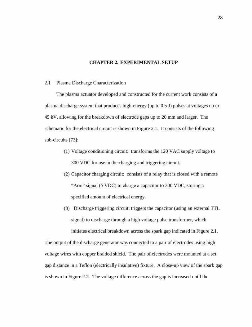
2.1 Plasma Discharge Characterization
The plasma actuator developed and constructed for the current work consists of a
plasma discharge system that produces high-energy (up to 0.5 J) pulses at voltages up to
45 kV, allowing for the breakdown of electrode gaps up to 20 mm and larger. The
schematic for the electrical circuit is shown in Figure 2.1. It consists of the following
sub-circuits [73]:
(1) Voltage conditioning circuit: transforms the 120 VAC supply voltage to
300 VDC for use in the charging and triggering circuit.
(2) Capacitor charging circuit: consists of a relay that is closed with a remote
capacitor to 300 VDC, storing a
specified amount of electrical energy.
(3) Discharge triggering circuit: triggers the capacitor (using an external TTL
signal) to discharge through a high voltage pulse transformer, which
initiates electrical breakdown across the spark gap indicated in Figure 2.1.
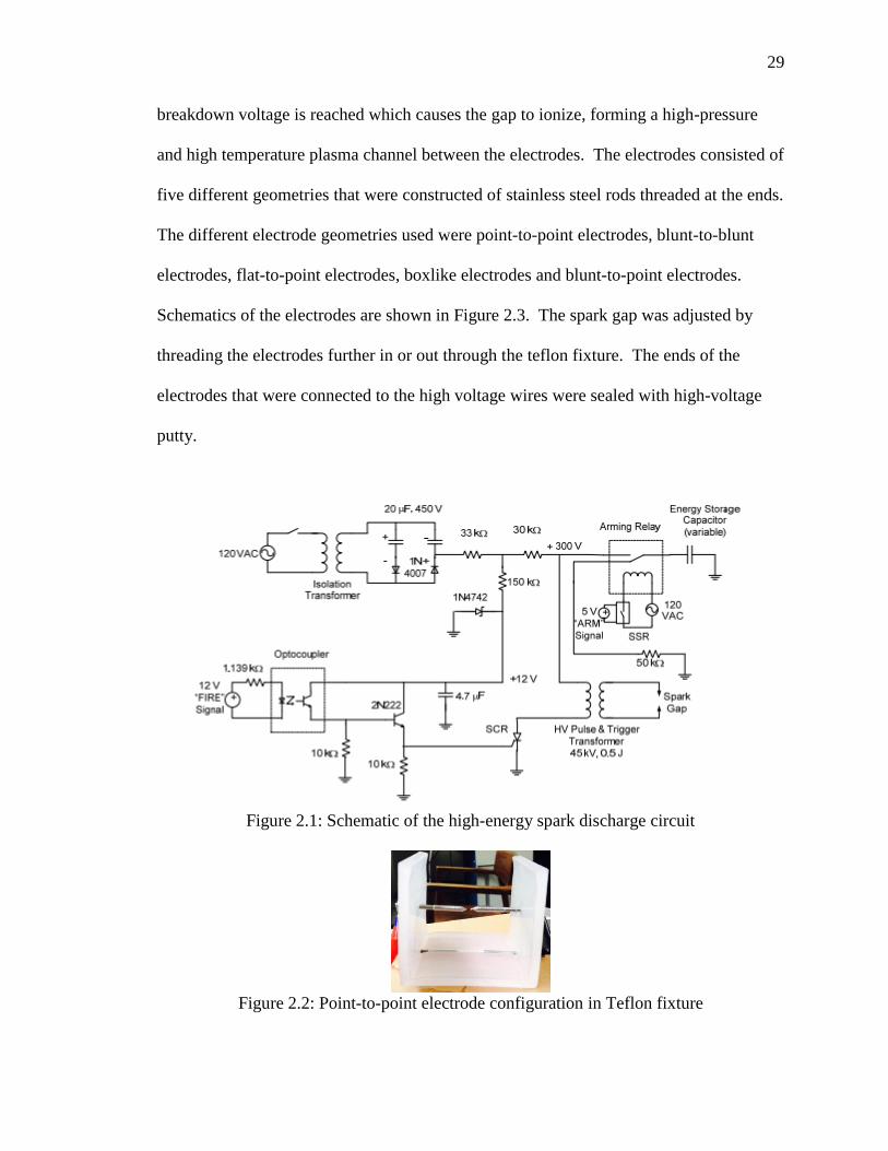
The output of the discharge generator was connected to a pair of electrodes using high
voltage wires with copper braided shield. The pair of electrodes were mounted at a set
gap distance in a Teflon (electrically insulative) fixture. A close-up view of the spark gap
is shown in Figure 2.2. The voltage difference across the gap is increased until the
29
breakdown voltage is reached which causes the gap to ionize, forming a high-pressure
and high temperature plasma channel between the electrodes. The electrodes consisted of
five different geometries that were constructed of stainless steel rods threaded at the ends.
The different electrode geometries used were point-to-point electrodes, blunt-to-blunt
electrodes, flat-to-point electrodes, boxlike electrodes and blunt-to-point electrodes.
Schematics of the electrodes are shown in Figure 2.3. The spark gap was adjusted by
threading the electrodes further in or out through the teflon fixture. The ends of the
electrodes that were connected to the high voltage wires were sealed with high-voltage
putty.
Figure 2.1: Schematic of the high-energy spark discharge circuit
Figure 2.2: Point-to-point electrode configuration in Teflon fixture

30
(e)
Figure 2.3: The five electrode configurations used for this work consist of (a) point-to-point electrodes, (b) blunt-to-blunt electrodes, (c) blunt-to-point electrodes, (d) boxlike electrodes and, (e) flat-to-point electrodes.
(a)
(b)
(c)
(d)
31
2.2 Diagnostics
2.2.1 Schlieren Visualization
Schlieren imaging allows for visualization of the variations in the refractive index
caused by density gradients. This visualization can be used to observe the spark
discharge and the evolution of the heated gas kernel. A schlieren optical system (Figure
2.3) was thus developed for the work in this dissertation. The light from a 150 W Oriel
xenon arc lamp was focused onto an iris (to approximate a point light source) by a 60 mm
focal length condenser lens. A 250 mm focal length achromatic doublet lens (3 inches in
diameter) was used to collimate the light and produce a small field of view approximately
18.4 mm diameter with the electrode spark gap in the center. A flat mirror was used to
direct the light towards a 60 inch focal length concave mirror which focused the light
onto an iris. The iris was used as the schlieren knife-edge where it was positioned at the
focal point of the concave mirror blocking out about half the light to resolve gradients in
all directions. The final image was focused onto the CMOS sensor of a Photron
FASTCAM SA4 high-speed camera. The camera, which has a maximum resolution of
1024 x 1024 at 3,600 fps, was used to record the flow field induced by the spark
discharge at frame rates of 10,000 fps at reduced resolution,

32
Figure 2.3: Schlieren system used for spark discharge visualization. Note that the spark gap was located between the achromatic lens and flat mirror. 2.2.2 Schlieren Image Velocimetry (SIV) Commercial PIV software
For the analysis of the schlieren image pairs, the LaVision FlowMaster Software
was used. The average velocity calculated by the software compared well to velocity
calculations obtained using manual PIV. As mentioned in Section 1.2.4, manual PIV is
eck on the SIV results obtained.
This section will briefly present the chosen settings of the cross-correlation PIV
algorithm used to process the schlieren images. First, to improve the quality of the
results, artifacts were removed and a background subtraction with a length scale of 16
pixels was applied to the images. For vector calculation, the time series of single frames
operation was selected. This operation allows the cross-correlation to work on two
consecutive frames of one recorded time-series [75]. A geometric mask was defined
using polygons to mask the electrodes for each frame set per electrode configuration.
The vector field was calculated using the multi pass (decreasing size) parameter where
the adaptive interrogation window was determined based on the size of the coherent

33
structures in the images that will correlate the movement from frame to frame. Once the
vector field was calculated, a vector validation algorithm (median filter) [75] was applied
to prevent erroneous vectors.
2.3 Electrical Measurements
The discharge current and voltage waveforms were measured simultaneously using
a Bergoz CT-D1.0 current transformer and a Tektronix P6015 high-voltage probe
digitized by a Tektronix DS09104A 1GHz oscilloscope at a sampling rate of 50 MS/s.
The current and voltage waveforms were used to calculate the instantaneous discharge
power and energy. The instantaneous power is the product of the voltage and current at
each time step. The total energy in the discharge is calculated by integrating the product
of the voltage and current over the discharge time (Equation 2.1).
(2.1)
34
CHAPTER 3. RESULTS & ANALYSIS: KERNEL EVOLUTION ELECTRICAL CHARACTERISTICS
Plasma formation is influenced by the discharge energy, power, frequency, and
actuator configuration. The actuator configuration is characterized by the electrode gap
length, geometry and material. The different configurations of the electrodes were
characterized using voltage and current measurements of discharges at varying gap
lengths. From these measurements, the discharge lasts between 1000 µs to 1200 µs,
depending primarily on the circuit capacitance, electrode geometry and gap length, and
any resistance in series with the discharge gap [74]. Each of the electrode geometries
presented in Section 2.1 were tested for electrode gap lengths of 2 mm, 5 mm, and 10 mm,
which produced variations in the breakdown voltage and subsequent discharge energy.
In this section, typical discharge waveforms are presented and discussed, and the
discharge energy and power is calculated for the various configurations.
First, the effect of the electrode geometry on the discharge voltage and current at
varying gap lengths (2 mm, 5 mm, and 10 mm) is briefly discussed, and the current and
voltage waveforms for each electrode configuration are presented. The instantaneous
discharge energy and power results are then calculated from the collected voltage and
current waveforms. Measurements of the discharge power and energy are essential for
the physical understanding of the plasma kernel development process. It is also critical in
understanding how the different electrode geometries used in this work effect the
35
behavior of the voltage and current at varying gap lengths. Understanding these effects
will provide a greater fundamental understanding of the primary fluid dynamic
Studying the effect
of the electrode geometry on the breakdown voltage, for example, is of particular
importance since a high breakdown voltage corresponds to high discharge energy and
hence more energy is deposited in the plasma. The effect of the discharge energy on the
plasma channel radius and spatial evolution is presented in this section as well.
3.1 Electrical Energy and Power Measurements
For all the electrode configurations, it was observed that the primary effect of
varying the gap length was on the breakdown voltage as the gap increased, so did the
breakdown voltage and hence also the discharge energy [4]. This is because as the
distance between the pair of electrodes increased the (non-uniform) electric field
decreased, resulting in a higher breakdown voltage. It was also observed that there was
not one electrode configuration that consistently yielded the highest or lowest breakdown
voltage across all the gap lengths. As can be seen in Table 3.1.1 and Figure 3.2, the
highest breakdown voltage at each gap length is obtained with different electrode
geometries. Table 3.1.2 shows that the breakdown voltage does not increase at an equal
rate across the gap lengths. At gap lengths of 2 mm and 5 mm, the breakdown voltage
was highest for the blunt-to-point electrodes, and at a gap length of 10 mm the
breakdown voltage was highest for the point-to-point electrodes. In general, the gradient
of the electrostatic equipotential (i.e. the electric field) is highest in the area between
sharp tips and weakest between tips with the highest radius of curvature. It was,
36
therefore, expected that the blunt-to-blunt electrodes would have the highest breakdown
voltage across all the gap lengths. Instead, however, the electrode configurations that had
the lowest increase in the breakdown voltage when the gap length was increased from 2
mm to 5 mm had a consistent tendency of having the highest breakdown voltage increase
when the gap length was increased from 5 mm to 10 mm. This trend is shown in table
3.1.2. This shows that the electrode geometries used here at small gap lengths (i.e. ~2 to
5 mm) have the inverse effect on the electric field when compared to the same set of
electrode geometries at larger gap lengths ( i.e. ~5 to 10 mm). It also suggests that
depending on the gap length, there are certain electrode geometries that may be more
efficient to use (i.e. higher energy deposition) for changing the flow field.
In general the breakdown voltage is affected by many factors in addition to the electrode
geometry, such as the physical and atomic nature of the electrode surfaces (e.g. surface
finish, grain size and surface hardness). Surface contamination (e.g. dust particles) that
comes into play during the course of the data collection process affects the breakdown
performance as well. While the electrode geometry has a significant effect on breakdown,
it is not possible to ascribe the differences in the observed breakdown voltage solely to
the electrode geometry.
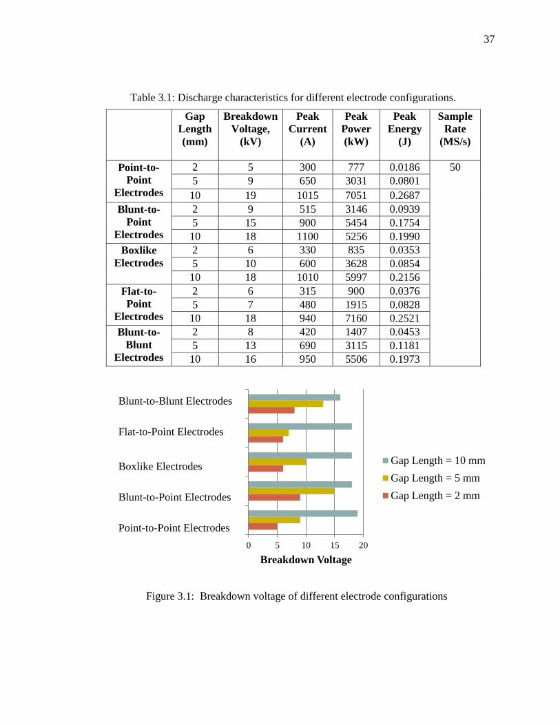
37
Figure 3.1: Breakdown voltage of different electrode configurations
0 5 10 15 20
Point
Spherical-Point
Box Electrodes
Flat-PointElectrodes
Spherical-PointElectrodes
Breakdown Voltage
Gap Length = 10 mm
Gap Length = 5 mm
Gap Length = 2 mm
Table 3.1: Discharge characteristics for different electrode configurations.
Gap Length
(mm)
Breakdown Voltage,
(kV)
Peak Current
(A)
Peak Power (kW)
Peak Energy
(J)
Sample Rate
(MS/s)
Point-to-Point
Electrodes
2 5 300 777 0.0186 50 5 9 650 3031 0.0801
10 19 1015 7051 0.2687 Blunt-to-
Point Electrodes
2 9 515 3146 0.0939 5 15 900 5454 0.1754 10 18 1100 5256 0.1990
Boxlike Electrodes
2 6 330 835 0.0353 5 10 600 3628 0.0854 10 18 1010 5997 0.2156
Flat-to-Point
Electrodes
2 6 315 900 0.0376 5 7 480 1915 0.0828 10 18 940 7160 0.2521
Blunt-to-Blunt
Electrodes
2 8 420 1407 0.0453 5 13 690 3115 0.1181 10 16 950 5506 0.1973
Blunt-to-Blunt Electrodes
Flat-to-Point Electrodes
Boxlike Electrodes
Blunt-to-Point Electrodes
Point-to-Point Electrodes
38
The current and voltage traces for the different electrode geometries and three gap
lengths are shown in Figure 3.2, Figure 3.4, Figure 3.6, Figure 3.8, and Figure 3.10. The
breakdown voltage is defined as the maximum voltage at time t = 0. The calculated
power and energy for these cases have been calculated and are also shown in Figure 3.3,
Figure 3.5, Figure 3.7, Figure 3.9, and Figure 3.11. The maximum instantaneous power
for the point-to-point electrodes at a gap length of 10 mm is extremely large,
approximately 7000 kW. The maximum instantaneous discharge power for these
electrode geometries is so large because of the high current drawn by the very low
resistance of the ionized air in the gap. The discharge energies for the blunt-to-point
electrodes and point-to-point electrodes at a gap length of 10 mm are between 0.20 J and
0.27 J. The discharge energies for all the electrode geometries tested at the varying gap
lengths are between 0.03 J to 0.26 J. After the voltage breaks down and ionizes the gas in
the electrode gap, electrical energy is deposited into the plasma. Energy deposition
results in a high-temperature and high pressure region between the electrodes. The heat
transfer to the electrode surfaces is limited since the plasma channel is in contact with the
electrodes only for a short duration. These results confirm that the energy deposited in
the plasma is dependent on the gap length and electrode geometry combinations. The
duration of the energy deposition is also dependent on the gap length and electrode
geometry as demonstrated by the varying lengths of the voltage and current traces. As
will be discussed in Section 3.2, the plasma kernel growth and dissipation duration is
primarily controlled by the energy deposited in the discharges.

39
(a) (b)
(c)
Figure 3.2: High-energy discharge current and voltage waveforms for the point to point electrodes with gap lengths of (a) 2mm, (b) 5mm, and (c) 10 mm.
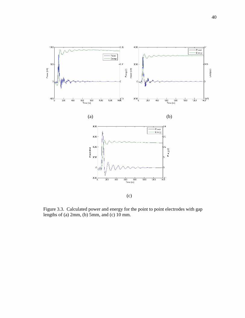
40
(a) (b)
(c)
Figure 3.3. Calculated power and energy for the point to point electrodes with gap lengths of (a) 2mm, (b) 5mm, and (c) 10 mm.
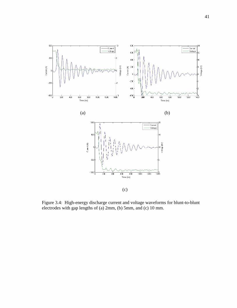
41
(a) (b)
(c)
Figure 3.4: High-energy discharge current and voltage waveforms for blunt-to-blunt electrodes with gap lengths of (a) 2mm, (b) 5mm, and (c) 10 mm.
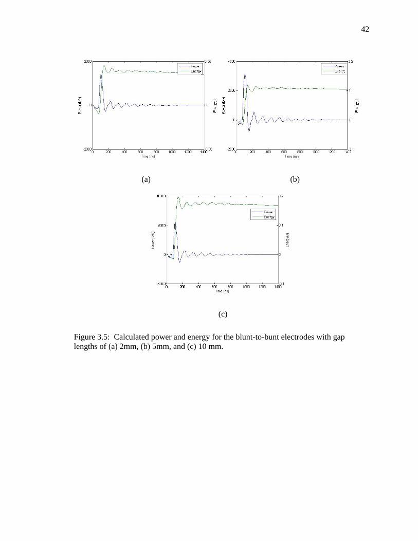
42
(a) (b)
(c)
Figure 3.5: Calculated power and energy for the blunt-to-bunt electrodes with gap lengths of (a) 2mm, (b) 5mm, and (c) 10 mm.
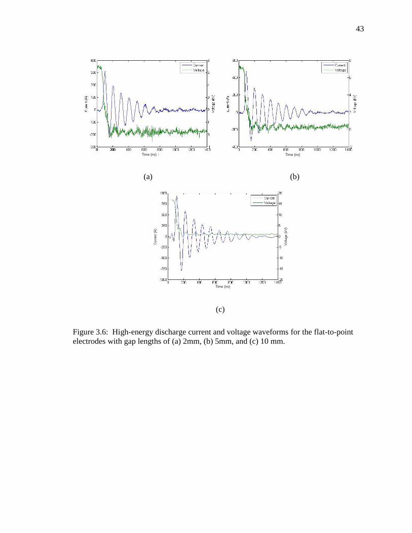
43
(a) (b)
(c)
Figure 3.6: High-energy discharge current and voltage waveforms for the flat-to-point electrodes with gap lengths of (a) 2mm, (b) 5mm, and (c) 10 mm.
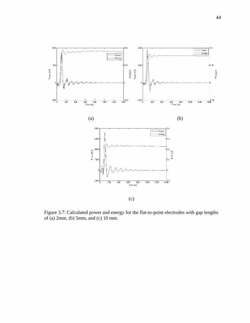
44
(a) (b)
(c)
Figure 3.7: Calculated power and energy for the flat-to-point electrodes with gap lengths of (a) 2mm, (b) 5mm, and (c) 10 mm.
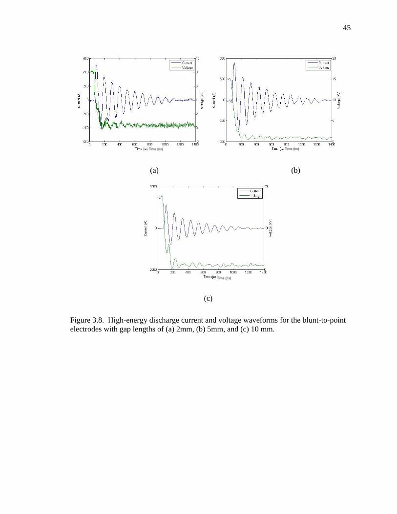
45
(a) (b)
(c)
Figure 3.8. High-energy discharge current and voltage waveforms for the blunt-to-point electrodes with gap lengths of (a) 2mm, (b) 5mm, and (c) 10 mm.

46
(a) (b)
(c)
Figure 3.9: Calculated power and energy for the blunt-to-point electrodes with gap lengths of (a) 2mm, (b) 5mm, and (c) 10 mm.
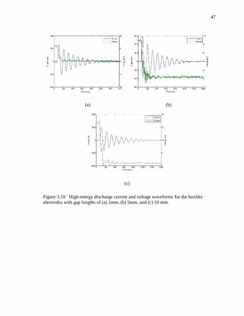
47
(a) (b)
(c)
Figure 3.10: High-energy discharge current and voltage waveforms for the boxlike electrodes with gap lengths of (a) 2mm, (b) 5mm, and (c) 10 mm.

48
(a) (b)
(c)
Figure 3.11: Calculated power and energy for the boxlike electrodes with gap lengths of (a) 2mm, (b) 5mm, and (c) 10 mm.
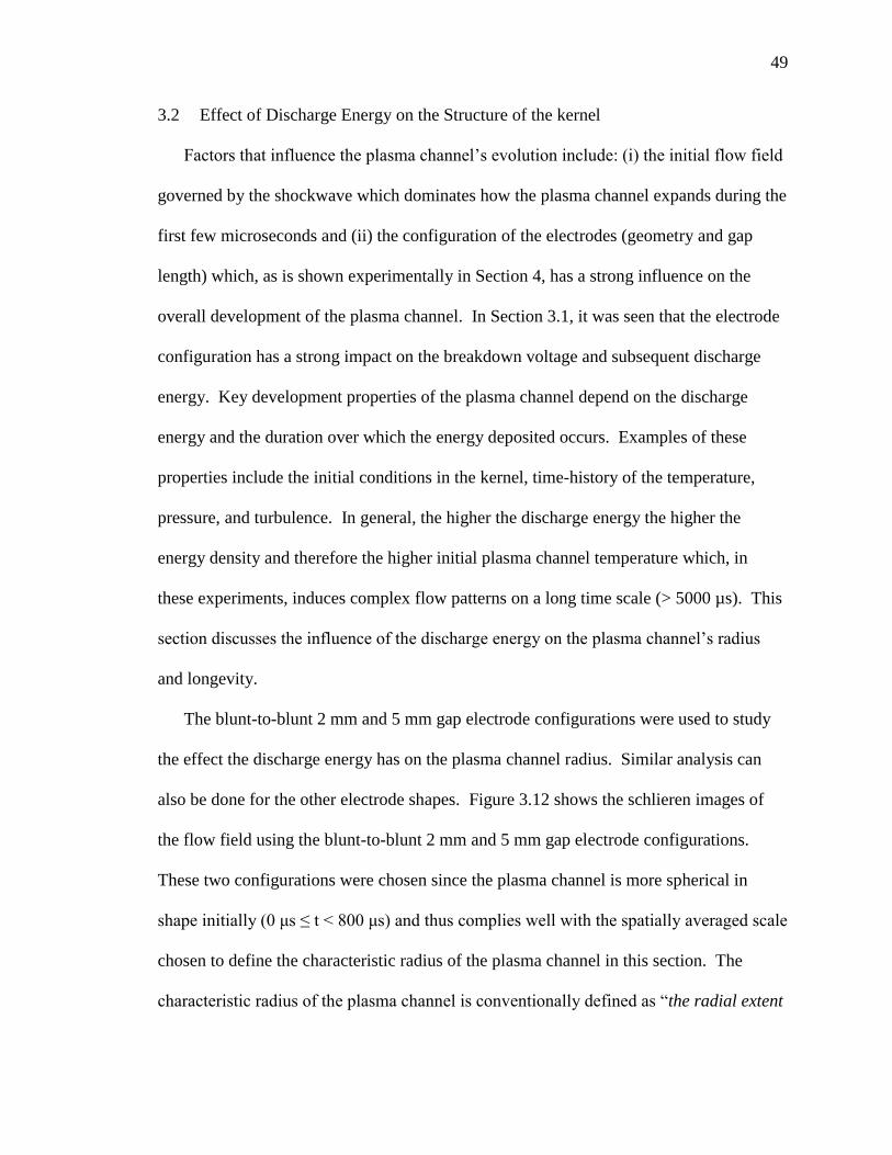
49
3.2 Effect of Discharge Energy on the Structure of the kernel
governed by the shockwave which dominates how the plasma channel expands during the
first few microseconds and (ii) the configuration of the electrodes (geometry and gap
length) which, as is shown experimentally in Section 4, has a strong influence on the
overall development of the plasma channel. In Section 3.1, it was seen that the electrode
configuration has a strong impact on the breakdown voltage and subsequent discharge
energy. Key development properties of the plasma channel depend on the discharge
energy and the duration over which the energy deposited occurs. Examples of these
properties include the initial conditions in the kernel, time-history of the temperature,
pressure, and turbulence. In general, the higher the discharge energy the higher the
energy density and therefore the higher initial plasma channel temperature which, in
these experiments, induces complex flow patterns on a long time scale (> 5000 µs). This
and longevity.
The blunt-to-blunt 2 mm and 5 mm gap electrode configurations were used to study
the effect the discharge energy has on the plasma channel radius. Similar analysis can
also be done for the other electrode shapes. Figure 3.12 shows the schlieren images of
the flow field using the blunt-to-blunt 2 mm and 5 mm gap electrode configurations.
These two configurations were chosen since the plasma channel is more spherical in
chosen to define the characteristic radius of the plasma channel in this section. The
the radial extent
50
of the heated zone in a plane placed in the center of the spark and perpendicular to the
el [76] and is evaluated assuming that the kernel is spherically symmetric [76].
The discharge energy for the 2 mm and 5 mm gaps is approximately 0.0453 J and 0.1181
J, respectively. In these configurations, the energy is transferred to the gas in less than
1400 µs. The metrics used to define this duration (i.e. discharge current and voltage
waveforms for the blunt-to-blunt 2 mm and 5 mm gap electrodes) was presented in
Section 3.1. Table 3.2 and Figure 3.13 show the measured plasma channel radii as a
function of time for the two different spark energies. At very early times (t < 300 μs) the
plasma channel with the lower discharge energy, 0.04531 J, has a larger plasma channel
radius than the channel with the higher discharge energy (and thus a higher initial
temperature) of 0.1181 J. It is observed that the plasma channel radii increase
significantly with time, independent of the discharge energy. The final values do
increase slightly (by an average of ~240 µm every 100 µs) with increasing discharge
energy.
It is important to note, though, that the discharge energy is larger than the
deposited energy (i.e. the amount of electrical energy converted into thermal energy in
the flow). This is because the discharge energy is not just dissipated solely into the
plasma channel. The energy is dissipated in the anode and cathode by conduction and
through radiation losses as well. The fraction of the discharge energy dissipated into the
electrodes by conduction depends on the duration of the spark (i.e. the duration that the
hot plasma channel is in contact with the electrodes). A study by Singh [77], who
examined electric arc behavior in open air, reported that heat loss due to radiation is not a
significant factor for spark discharges in atmospheric air pressure since it only contributes
51
to 1% of the total heat loss. In general, though, it is very difficult to measure the amount
of energy dissipated into the plasma [78].The energy deposited within the plasma channel
depends on time-varying parameters such as the temperature of the flow upstream of the
electrodes and the temperature and velocity of the flow downstream of the electrodes.
The downstream temperature and velocity would have to be measured at multiple points
to characterize the non-uniform flow. In addition, the temperature data would have to be
collected at a high enough repetition rate to ensure accurate energy results. The
efficiency of the energy deposition ( ) can be defined as
= (Eq. 1)
and the values reported in literature are often around 60% [79]. As was previously
mentioned, however, the spark discharge duration is the dominating factor in how well
the measurements of electrical energy supplied to the electrodes compare to the thermal
energy deposited in flow. This is exemplified in recent experimental data [80] which
showed a deposition efficiency that exceeded 90% for a high energy (~0.25 J) spark
kernel created by a short duration (< 1µs) breakdown between the ends of co-linear
cylindrical copper electrodes in uniform airflow.
The data in Table 3.3 demonstrate the effect of the discharge energy on the hot
gas/turbulence dissipation times. It is expected that the higher the discharge energy and
hence the higher the initial temperature, then the larger the dissipation time. As was
discussed in Section 3.1, for gap lengths of 2 mm and 5 mm, the breakdown energy was
highest for the blunt-to-point electrodes, and at a gap length of 10 mm the breakdown
energy was highest for the point-to-point electrodes. For gap lengths of 2 mm and 5 mm,
the breakdown energy was lowest for the point-to-point electrodes and at a gap length of
52
10 mm the breakdown energy was lowest for the blunt-to-blunt electrodes.
Contradictorily, as can be seen in Table 3.3, for gap lengths of 2 mm and 5 mm, the
evity is shortest for the blunt-to-point electrode. For gap lengths of
10 mm the dissipation times are longest for the boxlike electrodes and flat-to-point
electrodes. The breakdown energy for the boxlike electrodes and flat-to-point electrodes
are 0.2156 J and 0.2521 J, respectively. The experimental results summarized in Table
3.3 show that the dissipation time does in fact increase with increasing discharge
energy/gap length for a given electrode configuration. However, there is no apparent
trend between the breakdown energy and the dissipation times across the different
configurations. It is not surprising that there is no trend observed between the varying
electrode configurations, since these are plasma channels that last on a long enough time
scale (> 5000µs) after the discharge for many other factors to come into play that could
accelerate or decelerate the decay depending on the geometry of the electrodes.
Examples of these factors include the rapid entrainment of air into the plasma channel
which lowers the high temperatures and affects the dynamics (e.g. the generation and
interaction of vortical structures) throughout the plasma channel.
In summary, two primary conclusions are drawn from the analysis of the hot gas
dissipation time vs. the discharge energy. First, it was seen that a plasma channel with a
higher spark energy results in a smaller channel radius initially (<400 µs) which over
time grows larger in comparison to a channel with a lower spark energy. In general, one
would expect the higher the discharge energy the larger the heated volume and thus the
larger the channel radius. The results obtained in this section, however, highlight that the
plasma channel radius is a complex parameter that is influenced by a number of different
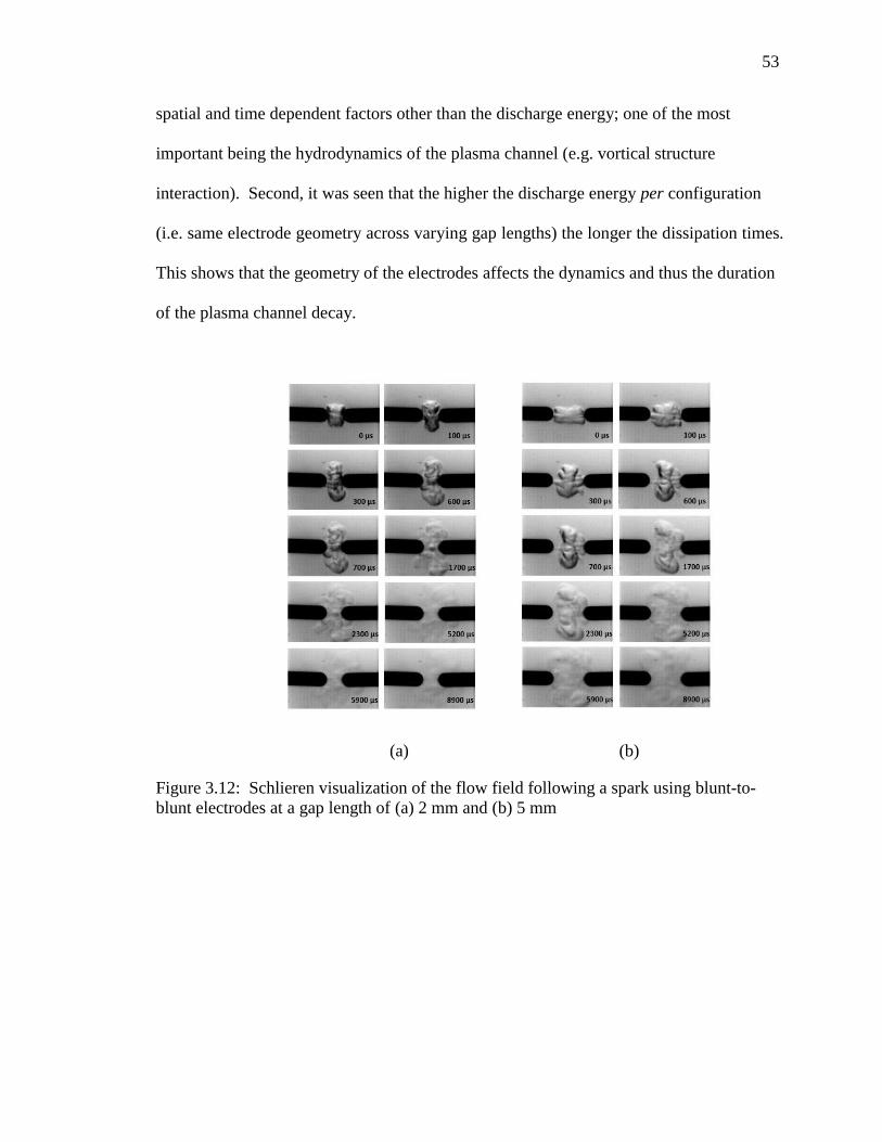
53
spatial and time dependent factors other than the discharge energy; one of the most
important being the hydrodynamics of the plasma channel (e.g. vortical structure
interaction). Second, it was seen that the higher the discharge energy per configuration
(i.e. same electrode geometry across varying gap lengths) the longer the dissipation times.
This shows that the geometry of the electrodes affects the dynamics and thus the duration
of the plasma channel decay.
(a) (b)
Figure 3.12: Schlieren visualization of the flow field following a spark using blunt-to-blunt electrodes at a gap length of (a) 2 mm and (b) 5 mm
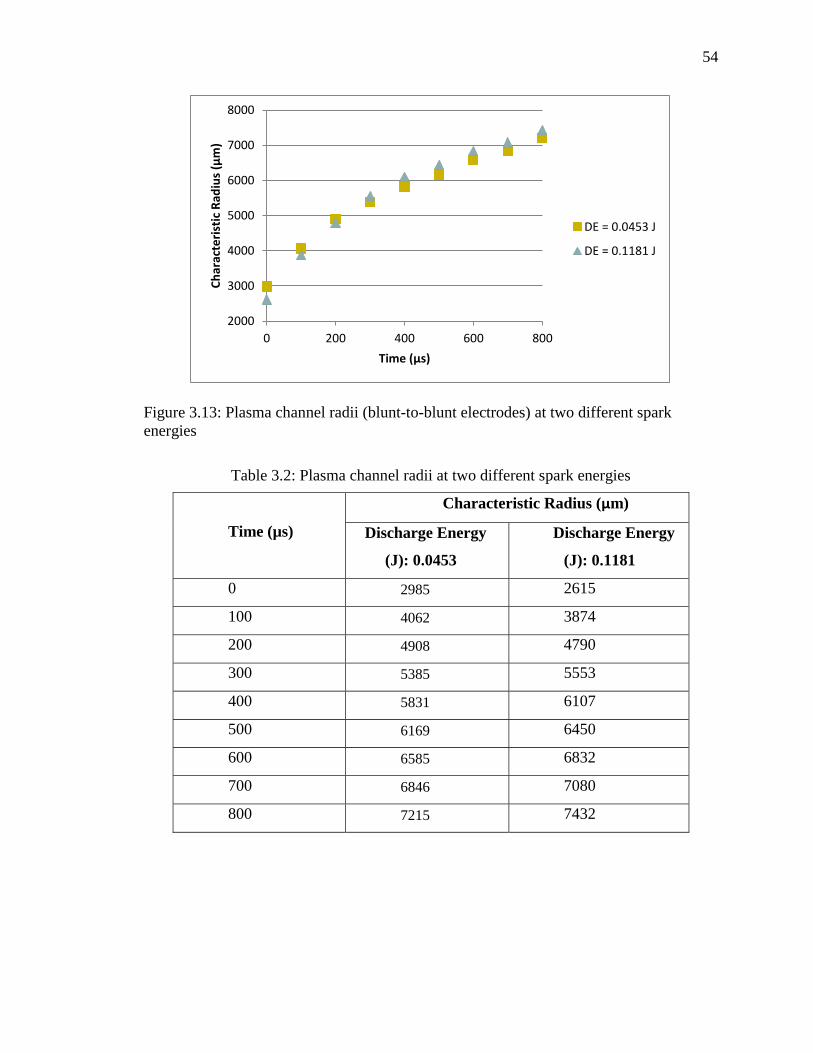
54
Figure 3.13: Plasma channel radii (blunt-to-blunt electrodes) at two different spark energies
Table 3.2: Plasma channel radii at two different spark energies
Time (µs)
Characteristic Radius (μm)
Discharge Energy
(J): 0.0453
Discharge Energy
(J): 0.1181
0 2985 2615
100 4062 3874
200 4908 4790
300 5385 5553
400 5831 6107
500 6169 6450
600 6585 6832
700 6846 7080
800 7215 7432
2000
3000
4000
5000
6000
7000
8000
0 200 400 600 800
Char
acte
rist
ic R
adiu
s (μ
m)
Time (μs)
DE = 0.0453 J
DE = 0.1181 J

55
Table 3.3: Breakdown energy and dissipation times across different electrode configurations
Gap
Length
(mm)
Peak
Energy (J) Dissipation
time (μs)
Point-to-point electrodes
2 0.0186 9,100
5 0.0801 11,500
10 0.2687 27,000
Blunt-to-point electrodes
2 0.0939 6,100
5 0.1754 7,100
10 0.1990 17,800
Boxlike electrodes
2 0.0353 11,600
5 0.0854 17,100
10 0.2156 30,000
Flat-to-point electrodes
2 0.0376 12,400
5 0.0828 22,000
10 0.2521 40,000
Blunt-to-blunt electrodes
2 0.0453 9,200
5 0.1181 20,400
10 0.1973 22,100
.
56
CHAPTER 4. RESULTS & ANALYSIS: KERNEL EVOLUTION SIV ANALYSIS
Flow separation occurs either due to a strong adverse pressure gradient or a drastic
change in the geometry of the surface. Pressure induced separation is not only dependent
on the local pressure gradient but also on the local boundary state [81]. One primary goal
of aerodynamic flow control is to delay or prevent flow separation from aerodynamic
surfaces. The new method of flow control explored in this work modifies the flow-field
structure near the boundary by means of several mechanisms which strongly depend on
the predefined electrode parameters (i.e. electrode geometry and gap length) and
discharge characteristics. The mechanisms of the spark discharge effect on the gas
parameters and flow structure can be summarized as the following:
(1) Pressure gradients are established by local gas heating.
(2) A blast wave forms at the initial stage of the spark discharge process and
propagates outward from the electrode gap during the first several nanoseconds.
Generated by the rapid heating and high pressure rise in the plasma channel, its
departure increases the local temperature and pressure and intensifies the
expansion of the channel.
(3) After the blast wave decay, the hot gas kernel created by the spark plasma
evolves, generating vorticity and/or turbulent gas motion.

57
motion is desirable in that it can be used to trip a laminar boundary layer at a point prior
to the location of laminar separation. A turbulent boundary layer contains more
energy/momentum and has a fuller velocity profile that is able to withstand the strong
adverse pressure gradients longer. This effectively moves the separation point
downstream on the body or even eliminates it. However, since a turbulent boundary
layer has a fuller velocity profile than a laminar boundary layer, it has a higher velocity
gradient at the wall and thus more skin friction is generated in transitioning to turbulent
flow. In general, though, the overall drag is decreased since the drag associated with
separation is much larger and in this case the pressure drag is reduced due to the delay in
boundary layer separation [81].
Generating vorticity may be desirable because it can also have a significant effect
on separation. For example, generating a vortex near a surface draws energetic, rapidly
moving outside air into the slow-moving boundary layer in contact with the surface. This
shifts high momentum fluid from the upper region of the boundary layer to the surface
allowing the flow to withstand a greater pressure rise before separation occurs. This is
the flow control method used by passive vortex generators. Another method for
controlling the flow using vorticity is exciting the local instabilities within the boundary
layer, leading to early transition to turbulence.
Both mechanisms (generation of vortices and turbulence) described above promote
efficient gas mixing which transports kinetic energy from the edge of the boundary layer
to the low momentum flow at the near-wall region or solid surface (e.g. wing). This

58
prevents the flow separation that would occur for a laminar boundary layer under the
same conditions.
4.1 Point-to-Point Electrodes
Figure 4.1 shows a series of schlieren images of the flow following a spark
discharge across an unconfined 10 mm point-to-point electrode gap. The first image is
taken less than 20 µs after the spark breakdown and for this work corresponds to time t =
Figure 4.1 that the evolution of the hot gas kernel created by the
spark is highly complex and persists for several milliseconds after the discharge. The
details of this flow field will be analyzed and discussed in this section. The velocity and
vorticity data presented in this section were obtained using SIV analysis on the schlieren
images.

59
Figure 4.1: Schlieren visualization of the flow field following a spark using point-to-point 10 mm gap electrodes
Immediately after the spark breakdown a very thin plasma channel (diameter on
the order of 10- at high temperature and pressure is created. At very early times,
the post-discharge channel looks like a cylinder of hot gas. This is illustrated in Figure
4.2 which shows the first stage of expansion at which the plasma channel has
frame. Figure 4.3 shows the location of the discharge axis and the outer regions of the
plasma which will be referred to frequently for this discussion. Figure 4.4 shows the
corresponding velocity vector field from SIV. The localized energy deposited in the
channel leads to a high temperature and pressure rise on the discharge axis. This is
followed by rapid gas expansion and causes the region around the discharge axis to act
60
like a piston [81], pushing the gas outwards. This external motion of the gas being
pushed outwards cannot be seen in the schlieren or SIV images since the schlieren
method only allows for the visualization of density gradients. It is also expected that if
the plasma channel that forms is symmetric about the discharge axis then the initial flow
field will also be symmetric. It is important to note, though, that the variability caused by
electrodynamics (such as plasma instabilities and cathode effects) [82] may cause the
plasma channel evolution to exhibit slightly altered characteristics from the ones
mentioned above. The variability of the channel geometry may result in flow field
expansion that is not symmetric about the discharge axis and/or variations along the
channel length from nonhomogeneous energy deposition. The hot gas evolution is
divided into three distinct phases based on the differences in the main flow features
observed: first stage of expansion ( ), second stage of expansion
and the decay or dissipation process (t ). The flow features that
characterize each of these phases are discussed below in detail.
As discussed, immediately after the discharge the plasma channel expands a
shockwave propagates outward from the channel. The shock wave is initially cylindrical
except near the electrode surfaces, where it is spherical. This description of the shock
wave geometry is discussed in the work of Bane et al [83]. They studied the influence of
the electrode geometry on the fluid dynamics following the spark discharge and provided
new insight on the roles of various physical phenomena (viscosity, pressure gradients,
electrode geometry and hot gas confinement) in the spark channel evolution. They
observed that the pressure gradient behind the cylindrical portion of the shock wave is
smaller than that following the spherical shock wave, resulting in a higher pressure in the

61
middle of the channel than near the electrodes. This causes the channel to expand
outwards towards the electrode surfaces as shown in Figure 4.2 at t = 0 µs. Because of
the inertia of the gas accelerated during the fast initial expansion, a decreased pressure
zone is formed on the discharge axis [84]. This halts the outward flow after some time
period and induces an inflow along the electrodes instead as can be observed near the
electrode tips in the SIV vector field in Figure 4.4.
Red circles are drawn on the velocity vector field (Figure 4.4) and vorticity
contour plot (Figure 4.6) to emphasize the swirling directions and the corresponding
vorticity that is present in the flow at t = 100 µs. As can be observed in Figure 4.4, the
inflow along the electrodes is the dominant phenomenon and the primary source of the
big vortex-bumps profile seen visually in Figure 4.2 at t = 100 µs near the left electrode.
The inflow on the left electrode generates vorticity by creating a shear layer with the fluid
expanding outwards. As can be viewed in Figure 4.6, this vorticity is positive (counter-
clock wise vortex) and negative (clockwise vortex) near the corner of the top and bottom
of the left electrode tip, respectively. Shurupov et al. studied the gas dynamic
instabilities during the decay of a submicrosecond high-voltage spark discharge and
explained that the gasdynamic effects of the after-spark channel is strongly dependent on
the different geometric heterogeneities of the discharge channel [84]. This is exemplified
here in how there is no significant inflow on the right electrode due to the asymmetry in
the channel, and therefore the vorticity is much lower near the right electrode tip. On the
top of the right electrode corner, low-magnitude negative vorticity is observed. Both
positive and negative low vorticity is observed near the bottom corner of the right
electrode. The vortices that form on the top of the electrode tips propagate upwards
62
towards the ambient air. In a similar manner, those that form on the bottom of the
electrode tips propagate downwards from the discharge channel.
Figure 4.4 and Figure 4.6 also show the jet flows that develop as a result of the
instabilities along the length of the channel. Similar to how Shurupov et al. explain that
the development of instabilities (i.e. large-scale vortex and jet flows) leads to the
appearance of differently directed gas flows, the localized jets here direct the flow in
different directions as well at a higher velocity (~2 m/s) than the surrounding plasma
regions. These jets can be seen in Figure 4.4. The vorticity that develops throughout the
plasma
within the flow. In summary, as can be observed from both Figure 4.4 and Figure 4.6,
the channel at this stage contains vorticity due to two major shear-layer instability effects:
(i) the inflow along the electrodes generating strong vortex pairs and (ii) instabilities
along the length of the channel that create localized jets.
Figure 4.4 shows the distribution of the velocity across the plasma channel during
travels at a higher velocity (maximum velocity of 6.3 m/s) than the edge along the right
electrode (maximum velocity of 2 m/s). This can also be observed in the schlieren image
in Figure 4.2 by visually comparing the axial distances travelled by each vertical edge
from the electrode tips. This indicates that the plasma region near the left electrode had
a higher energy density which had generated a much stronger shockwave leading to the
faster expansion. Figure 4.8 also shows how the top portion of the channel continues to
expand upwards at a maximum expansion speed of approximately 6 m/s.
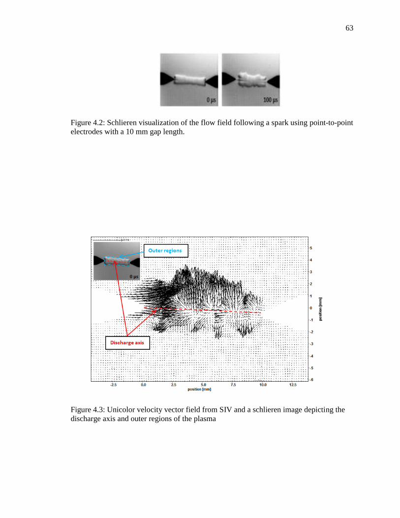
63
Figure 4.2: Schlieren visualization of the flow field following a spark using point-to-point electrodes with a 10 mm gap length.
Figure 4.3: Unicolor velocity vector field from SIV and a schlieren image depicting the discharge axis and outer regions of the plasma

64
Figure 4.4: Velocity vector field from SIV at 0-100 μs
Figure 4.5: Zoom-in of velocity vector field at the left electrode from SIV at 0-100 μs
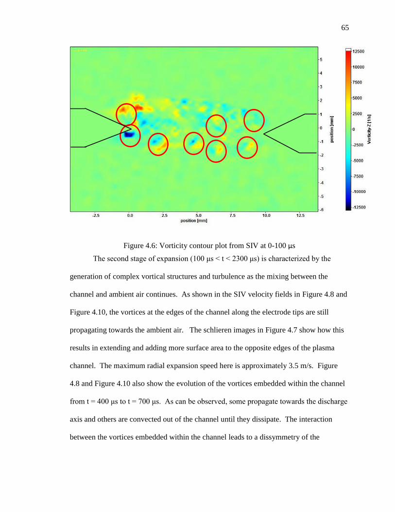
65
Figure 4.6: Vorticity contour plot from SIV at 0-100 μs
generation of complex vortical structures and turbulence as the mixing between the
channel and ambient air continues. As shown in the SIV velocity fields in Figure 4.8 and
Figure 4.10, the vortices at the edges of the channel along the electrode tips are still
propagating towards the ambient air. The schlieren images in Figure 4.7 show how this
results in extending and adding more surface area to the opposite edges of the plasma
channel. The maximum radial expansion speed here is approximately 3.5 m/s. Figure
4.8 and Figure 4.10 also show the evolution of the vortices embedded within the channel
axis and others are convected out of the channel until they dissipate. The interaction
between the vortices embedded within the channel leads to a dissymmetry of the
66
expansion process and the appearance of differently directed gas flows. The result is the
appearance of a chaotic or turbulent channel visually as seen in the schlieren images in
Figure 4.7. Each moving vortex overtakes or influences the motion of its neighboring
vortices. The magnitude of the vorticity associated with these vortices dissipates over
time as shown in Figure 4.6 and Figure 4.9 . The distribution and longevity of the
vortices in the second stage of expansion can be further viewed in Appendix B. By t =
away from the discharge axis towards the ambient air (Figure 4.11 and Figure 4.12). As
a result, the channel continues expanding radially both upwards and downwards at a
maximum expansion speed of approximately 2.5 m/s.
The schlieren images in Figure 4.7 also show that the volume of turbulent gas
increases over time. The turbulent gas motion is likely a result of the Kelvin-Helmholtz
(K-H) instability [85, 86, 87] of the shear layers that develop between regions of different
densities moving at various speeds. Disturbances on the interface are amplified, inducing
mixing between the fluid layers and eventually the whole channel becomes fully
As was observed previously from the inflow along the electrodes in Figure 4.4,
ambient air is drawn into the channel as early as the first stage of expansion which
increases the cooling rate [84] and fluid mixing. The arising turbulent motion in the
second stage of expansion intensifies the mixing of the ambient air within the channel. It
replaces molecular heat conduction as the dominant mechanism of heat transfer, which
results in an even further increase in the rate of cooling [88]. The expansion speeds and,
thus, expansion process of the channel at this stage are lower than the first stage of

67
expansion. Note that in terms of the average velocities over a timescale of 2300 µs (i.e.
throughout the first and second stages of expansion) the average radial velocity is always
greater than the average axial velocity which plays a dominant role in the plasma
Figure 4.7: Schlieren visualization of the flow field following a spark using point to point electrodes with a 10 mm gap length
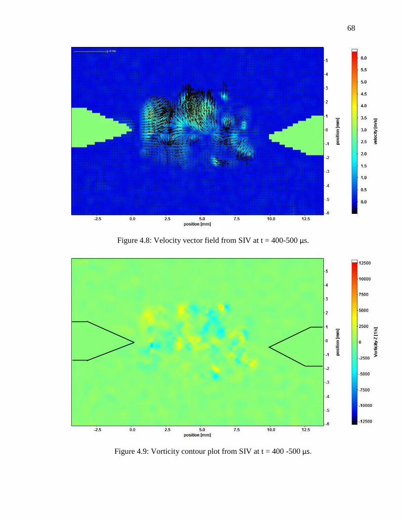
68
Figure 4.8: Velocity vector field from SIV at t = 400-500 μs.
Figure 4.9: Vorticity contour plot from SIV at t = 400 -500 μs.
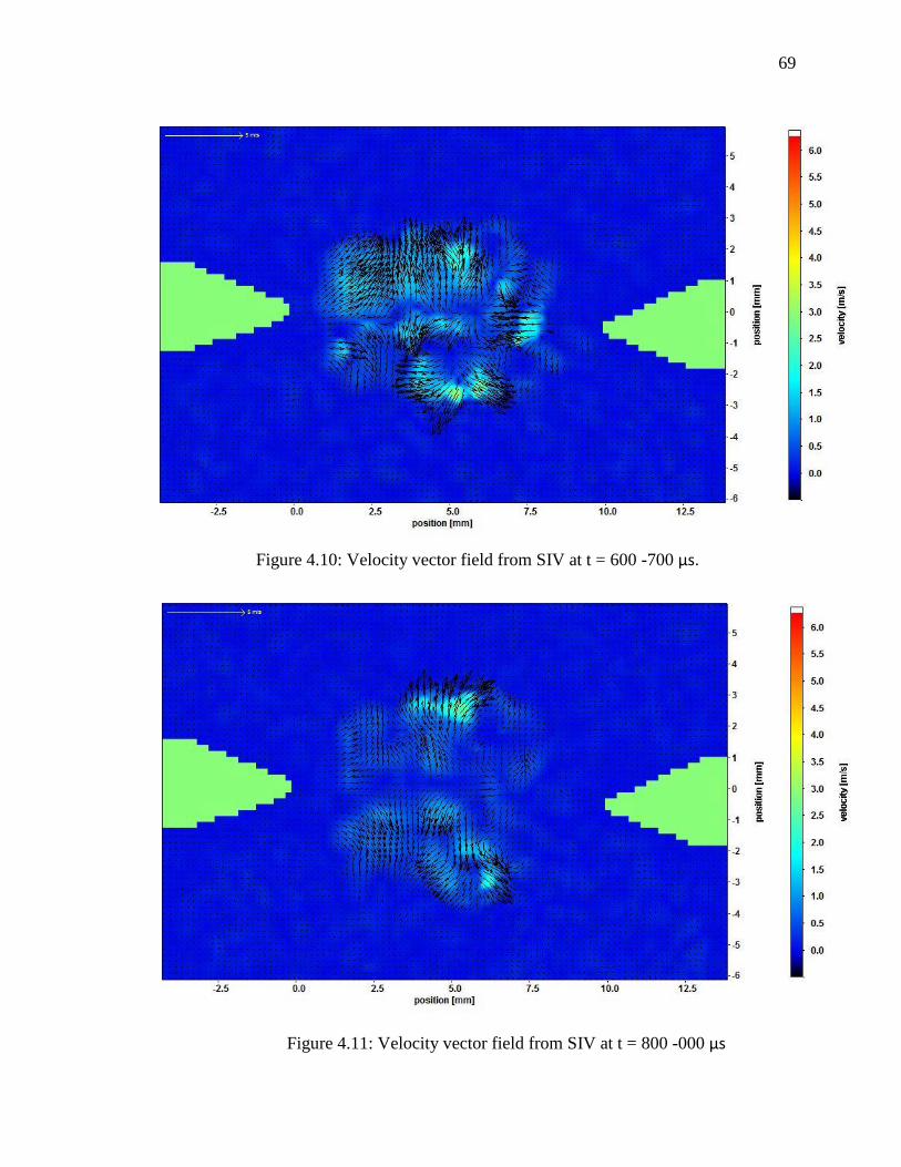
69
Figure 4.10: Velocity vector field from SIV at t = 600 -700 μs.
Figure 4.11: Velocity vector field from SIV at t = 800 -000 μs
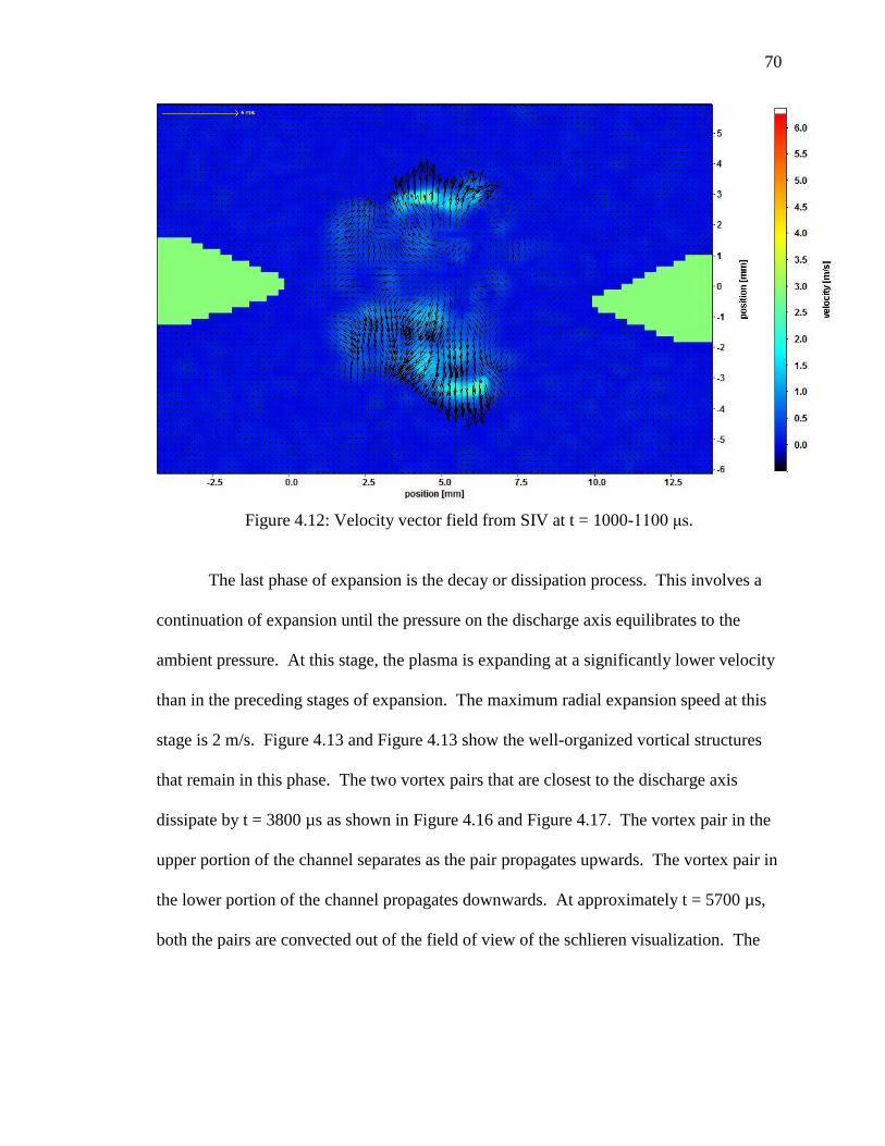
70
Figure 4.12: Velocity vector field from SIV at t = 1000- .
The last phase of expansion is the decay or dissipation process. This involves a
continuation of expansion until the pressure on the discharge axis equilibrates to the
ambient pressure. At this stage, the plasma is expanding at a significantly lower velocity
than in the preceding stages of expansion. The maximum radial expansion speed at this
stage is 2 m/s. Figure 4.13 and Figure 4.13 show the well-organized vortical structures
that remain in this phase. The two vortex pairs that are closest to the discharge axis
dissipate by t = 3800 µs as shown in Figure 4.16 and Figure 4.17. The vortex pair in the
upper portion of the channel separates as the pair propagates upwards. The vortex pair in
the lower portion of the channel propagates downwards. At approximately t = 5700 µs,
both the pairs are convected out of the field of view of the schlieren visualization. The
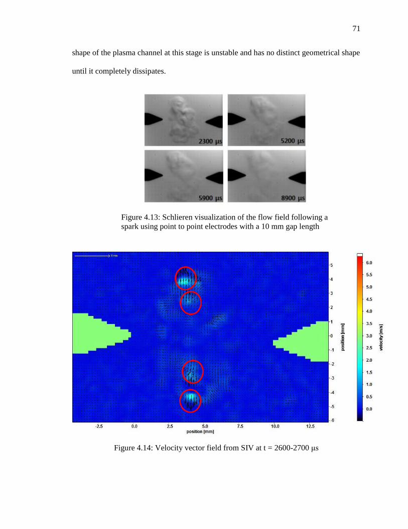
71
shape of the plasma channel at this stage is unstable and has no distinct geometrical shape
until it completely dissipates.
Figure 4.14: Velocity vector field from SIV at t = 2600-2700
Figure 4.13: Schlieren visualization of the flow field following a spark using point to point electrodes with a 10 mm gap length
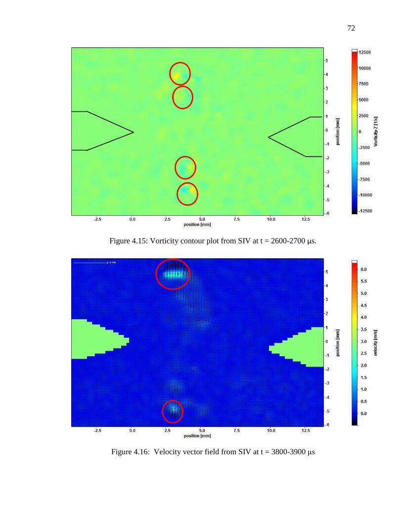
72
Figure 4.15: Vorticity contour plot from SIV at t = 2600-2700 μs.
Figure 4.16: Velocity vector field from SIV at t = 3800-3900
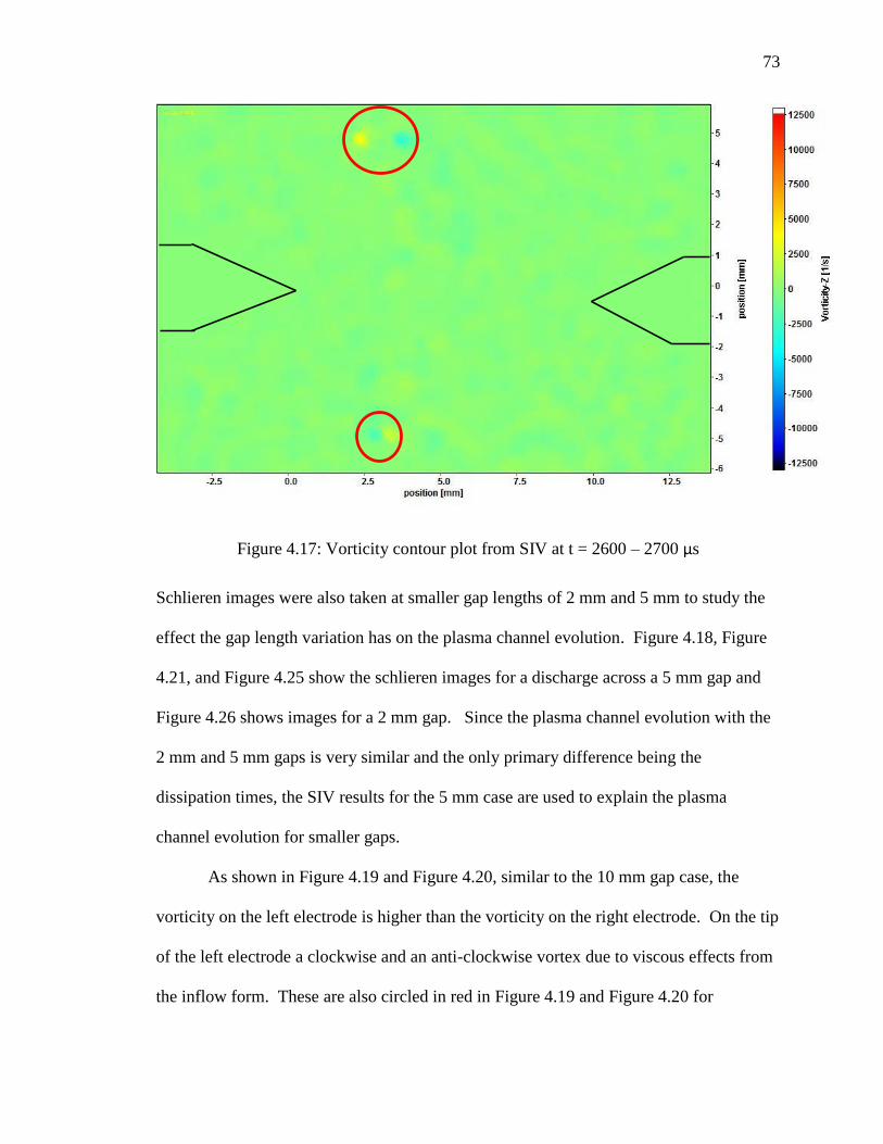
73
Figure 4.17: Vorticity contour plot from SIV at t = 2600 2700 μs
Schlieren images were also taken at smaller gap lengths of 2 mm and 5 mm to study the
effect the gap length variation has on the plasma channel evolution. Figure 4.18, Figure
4.21, and Figure 4.25 show the schlieren images for a discharge across a 5 mm gap and
Figure 4.26 shows images for a 2 mm gap. Since the plasma channel evolution with the
2 mm and 5 mm gaps is very similar and the only primary difference being the
dissipation times, the SIV results for the 5 mm case are used to explain the plasma
channel evolution for smaller gaps.
As shown in Figure 4.19 and Figure 4.20, similar to the 10 mm gap case, the
vorticity on the left electrode is higher than the vorticity on the right electrode. On the tip
of the left electrode a clockwise and an anti-clockwise vortex due to viscous effects from
the inflow form. These are also circled in red in Figure 4.19 and Figure 4.20 for
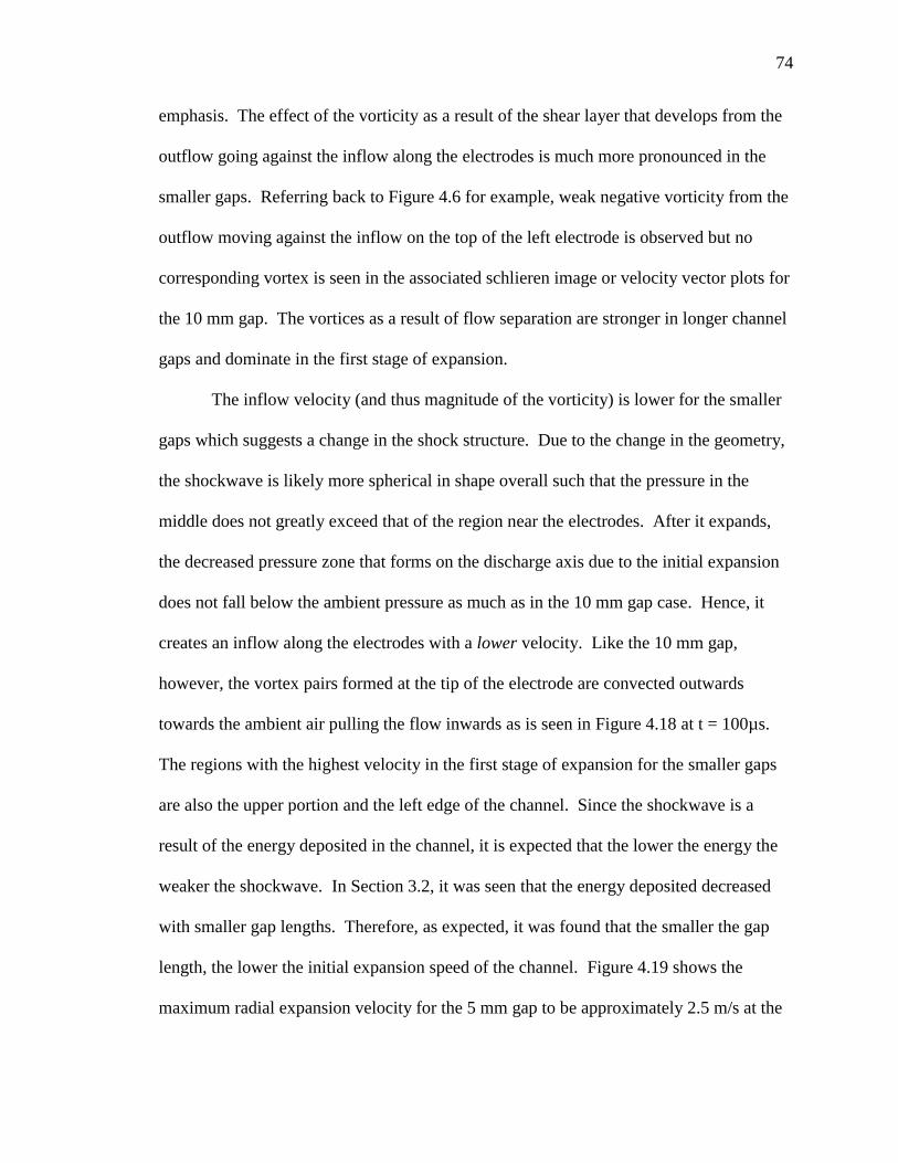
74
emphasis. The effect of the vorticity as a result of the shear layer that develops from the
outflow going against the inflow along the electrodes is much more pronounced in the
smaller gaps. Referring back to Figure 4.6 for example, weak negative vorticity from the
outflow moving against the inflow on the top of the left electrode is observed but no
corresponding vortex is seen in the associated schlieren image or velocity vector plots for
the 10 mm gap. The vortices as a result of flow separation are stronger in longer channel
gaps and dominate in the first stage of expansion.
The inflow velocity (and thus magnitude of the vorticity) is lower for the smaller
gaps which suggests a change in the shock structure. Due to the change in the geometry,
the shockwave is likely more spherical in shape overall such that the pressure in the
middle does not greatly exceed that of the region near the electrodes. After it expands,
the decreased pressure zone that forms on the discharge axis due to the initial expansion
does not fall below the ambient pressure as much as in the 10 mm gap case. Hence, it
creates an inflow along the electrodes with a lower velocity. Like the 10 mm gap,
however, the vortex pairs formed at the tip of the electrode are convected outwards
towards the ambient air pulling the flow inwards as is seen in Figure 4.18 at t = 100µs.
The regions with the highest velocity in the first stage of expansion for the smaller gaps
are also the upper portion and the left edge of the channel. Since the shockwave is a
result of the energy deposited in the channel, it is expected that the lower the energy the
weaker the shockwave. In Section 3.2, it was seen that the energy deposited decreased
with smaller gap lengths. Therefore, as expected, it was found that the smaller the gap
length, the lower the initial expansion speed of the channel. Figure 4.19 shows the
maximum radial expansion velocity for the 5 mm gap to be approximately 2.5 m/s at the
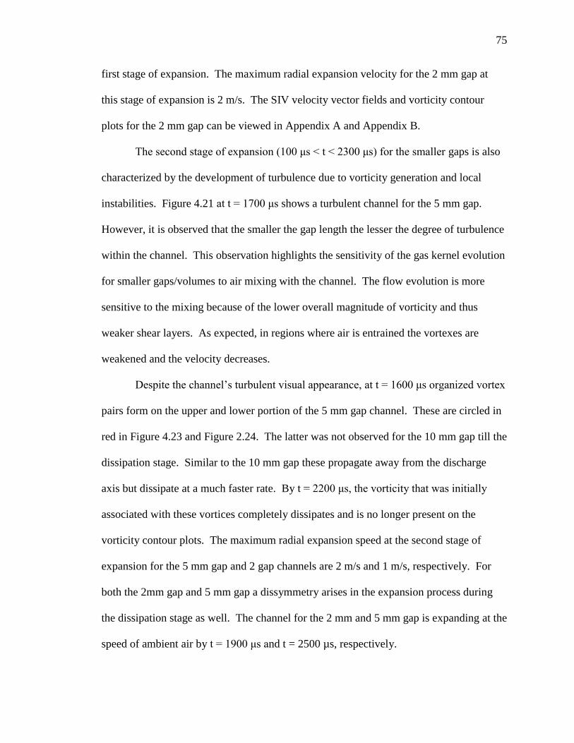
75
first stage of expansion. The maximum radial expansion velocity for the 2 mm gap at
this stage of expansion is 2 m/s. The SIV velocity vector fields and vorticity contour
plots for the 2 mm gap can be viewed in Appendix A and Appendix B.
gaps is also
characterized by the development of turbulence due to vorticity generation and local
instabilities. Figure 4.21 shows a turbulent channel for the 5 mm gap.
However, it is observed that the smaller the gap length the lesser the degree of turbulence
within the channel. This observation highlights the sensitivity of the gas kernel evolution
for smaller gaps/volumes to air mixing with the channel. The flow evolution is more
sensitive to the mixing because of the lower overall magnitude of vorticity and thus
weaker shear layers. As expected, in regions where air is entrained the vortexes are
weakened and the velocity decreases.
pairs form on the upper and lower portion of the 5 mm gap channel. These are circled in
red in Figure 4.23 and Figure 2.24. The latter was not observed for the 10 mm gap till the
dissipation stage. Similar to the 10 mm gap these propagate away from the discharge
axis but dissipate at a much faster rate. By
associated with these vortices completely dissipates and is no longer present on the
vorticity contour plots. The maximum radial expansion speed at the second stage of
expansion for the 5 mm gap and 2 gap channels are 2 m/s and 1 m/s, respectively. For
both the 2mm gap and 5 mm gap a dissymmetry arises in the expansion process during
the dissipation stage as well. The channel for the 2 mm and 5 mm gap is expanding at the
speed of ambient air by nd t = 2500 µs, respectively.

76
As was mentioned in Section 3.2, after breakdown the initial flow field governed
by the shockwave dominates how the plasma channel expands during the first few
microseconds. As was seen above, these flow characteristics induced by the shockwave
also have a major influence on how the channel evolves in the following expansion stages.
It is concluded that the major differences between the 10 mm gap and the smaller gaps
observed in the first stage of expansion are primarily a result of the change in the shock
structure and the decrease in energy deposition which results in a weaker shockwave
overall. Summarizing the differences discussed above, the plasma channel generated in
the smaller gaps of the point-to-point electrode geometry is characterized by a lower
inflow velocity along the electrodes (and thus lower vorticity) during the first stage of
expansion, a lower expansion speed across all the stages of expansion, and a lower degree
of turbulence before it dissipates.
Figure 4.18: Schlieren visualization of the flow field following a spark using point-to-point electrodes.
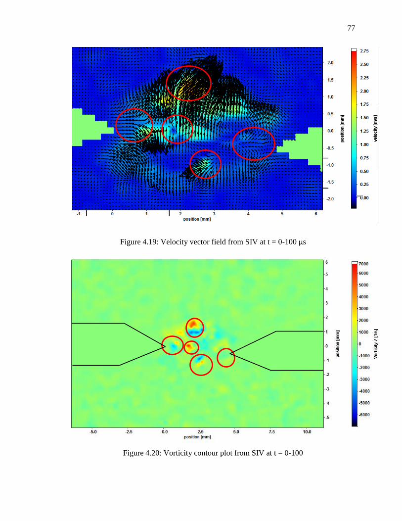
77
Figure 4.19: Velocity vector field from SIV at t = 0-100 μs
Figure 4.20: Vorticity contour plot from SIV at t = 0-100

78
Figure 4.21: Schlieren visualization of the flow field following a spark using point-to-point electrodes with a 5mm gap length.
Figure 4.22: Velocity vector field from SIV at t = 800- s.

79
Figure 4.23: Velocity Vector Field from SIV at t = 1600-17 .
Figure 4.24: Vorticity contour plot from SIV at t = 1600-17
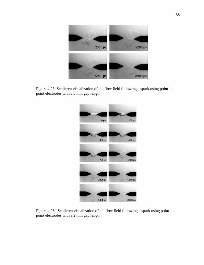
80
Figure 4.25: Schlieren visualization of the flow field following a spark using point-to-point electrodes with a 5 mm gap length
Figure 4.26: Schlieren visualization of the flow field following a spark using point-to-point electrodes with a 2 mm gap length.
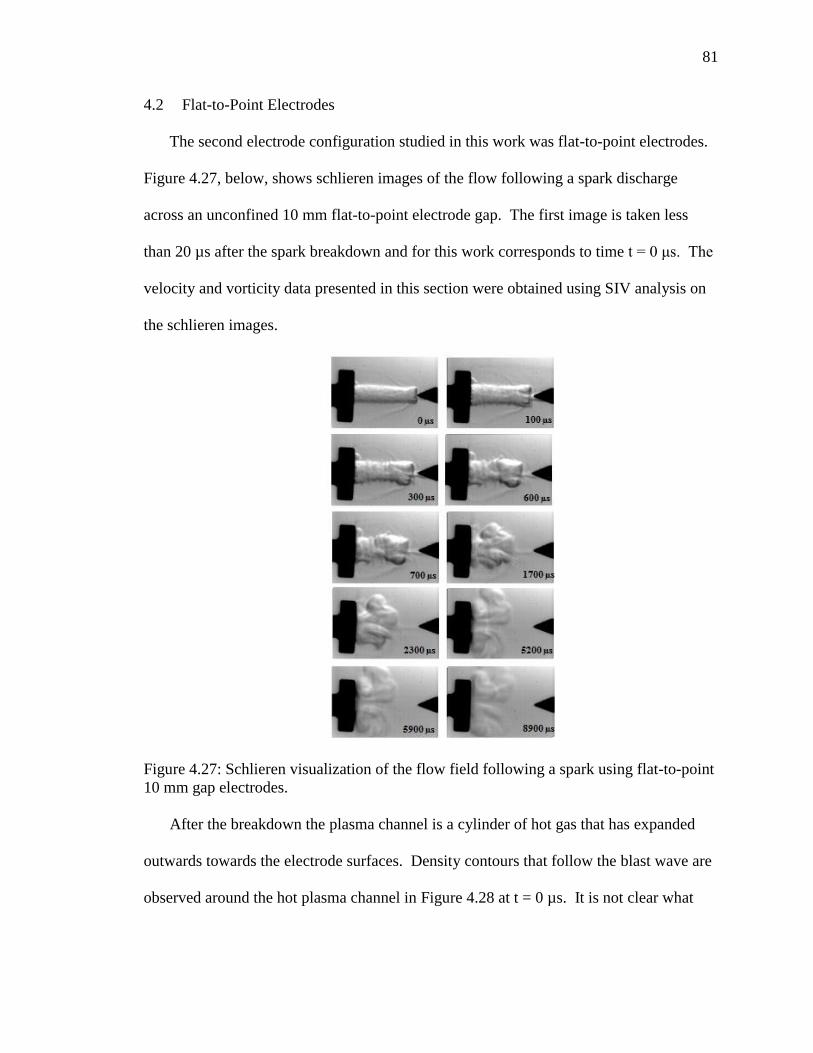
81
4.2 Flat-to-Point Electrodes
The second electrode configuration studied in this work was flat-to-point electrodes.
Figure 4.27, below, shows schlieren images of the flow following a spark discharge
across an unconfined 10 mm flat-to-point electrode gap. The first image is taken less
than 20 µs after the spark breakdown and for this work corresponds to time
velocity and vorticity data presented in this section were obtained using SIV analysis on
the schlieren images.
Figure 4.27: Schlieren visualization of the flow field following a spark using flat-to-point 10 mm gap electrodes.
After the breakdown the plasma channel is a cylinder of hot gas that has expanded
outwards towards the electrode surfaces. Density contours that follow the blast wave are
observed around the hot plasma channel in Figure 4.28 at t = 0 µs. It is not clear what
82
these are but it is suspected that they are a result of multiple streamer discharges that
occurred simultaneously with the main spark. They are only seen in this electrode
geometry in the schlieren visualization of both the first and second stage of expansion for
the 10 mm gap and in the first stage of expansion for the 5 mm gap (Figure 4.47).
The flow in the velocity vector field from SIV in Figure 4.29 is a result of the
structure of the shockwave generated in this configuration. The shockwave is nearly a
pure cylindrical wave except for very close to the point electrode surface, where the wave
is spherical. As was discussed in Section 4.1, the pressure gradient following a
cylindrical shock wave is smaller than that following a spherical shockwave, hence the
pressure is higher throughout the channel than the region close to the point electrode.
This causes the plasma channel to rapidly expand outwards towards the point electrode
surface. Similar to the point-to-point electrode configuration, the inertia of the gas (near
the point electrode) accelerated during the fast initial expansion creates a decreased
pressure zone on the discharge axis (near the point electrode) which halts the outward
flow and induces the strong inflow along the surface of the point electrode as is clearly
indicated in Figure 4.29. The density gradients on the plasma edge by the point electrode
tip seen in the schlieren image at t = 100 µs (Figure 4.28) show that the inflow results in
entrainment of the surrounding atmospheric air. In general, the higher the density
gradients of the plasma channel the higher the entrainment of air [89]. This is because
when air is entrained it creates velocity and temperature differences in the channel which
are reflected as density gradients in the schlieren images.
Figure 4.29 and Figure 4.30 show the velocity vector field and vorticity countour plot
from SIV at t = 0-100 µs. The vorticity in the channel is primarily generated near the
83
point electrode tip which is dominated by the complex pressure gradients produced by the
shock wave. Figure 4.31 shows a close-up view of the vorticity contour plot with
velocity vectors near the point electrode tip; regions of significant vorticity are circled in
black. The red arrows represent the direction of air entrainment as a result of the rotating
vortices that were created due to the airflow along the electrodes. A clockwise vortex
(negative vorticity) and a counter-rotating vortex pair are observed near the top surface of
the point electrode whereas a single anti-clockwise vortex (negative vorticity) is observed
near the bottom surface of the same electrode tip. The clockwise vortex on top and the
anti-clockwise vortex on the bottom pull the right edge of the hot gas channel away from
the electrode as can be seen at t = 100 µs in Figure 4.28. The counter-rotating vortex pair
on the top surface of the point electrode that was previously mentioned is a result of the
shear layer that develops from the inflow moving against the outflow. The inflow and
outflow at this stage of expansion have an average axial velocity of 2.5 m/s and 1.75 m/s,
respectively. In addition to the vortices near the electrode surface, a clockwise vortex in
the lower portion of the channel and a strong counter-rotating vortex pair embedded in
the upper portion of the channel are observed. These are circled in white and are a result
of the strong shear layers within the channel. The origin of these shear layers is not
immediately obvious, but is likely a combination of the complex pressure gradients
produced by the shock wave and hydrodynamic instability of the channel. The left edge
of the plasma channel stays attached to the flat electrode and expands radially (both
upwards and downwards) along its surface as the diameter of the channel increases from
2810 µm to 3007 µm (Figure 4.28) within 100 µs.
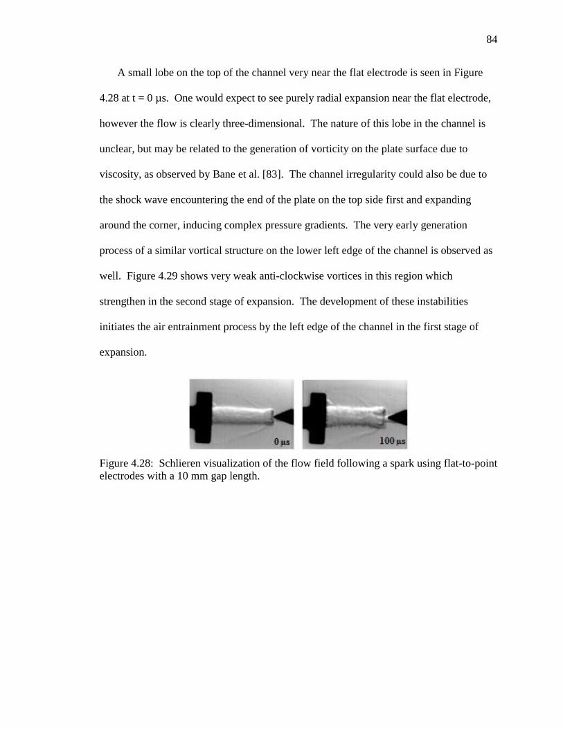
84
A small lobe on the top of the channel very near the flat electrode is seen in Figure
4.28 at t = 0 µs. One would expect to see purely radial expansion near the flat electrode,
however the flow is clearly three-dimensional. The nature of this lobe in the channel is
unclear, but may be related to the generation of vorticity on the plate surface due to
viscosity, as observed by Bane et al. [83]. The channel irregularity could also be due to
the shock wave encountering the end of the plate on the top side first and expanding
around the corner, inducing complex pressure gradients. The very early generation
process of a similar vortical structure on the lower left edge of the channel is observed as
well. Figure 4.29 shows very weak anti-clockwise vortices in this region which
strengthen in the second stage of expansion. The development of these instabilities
initiates the air entrainment process by the left edge of the channel in the first stage of
expansion.
Figure 4.28: Schlieren visualization of the flow field following a spark using flat-to-point electrodes with a 10 mm gap length.

85
Figure 4.29: Schlieren visualization of the flow field following a spark using flat-to-point electrode
Figure 4.30: Vorticity contour plot from SIV at t = 0-

86
Figure 4.31: Close-up view of vorticity contour plot from SIV at t = 0-100
The second stage of expansion is characterized by an
organized set of vortical structures propagating towards one another from the electrodes
at different speeds, resulting in significant asymmetry of the hot gas kernel. The vortical
structure on the left upper edge of the channel propagates upwards along the surface of
the flat electrode with an initial velocity of 1.75 m/s. This can be seen in the schlieren
images in Figure 4.32 and the velocity vector fields from SIV circled in red in Figure
4.33-Figure 4.37 below. The corresponding vorticity plots are presented in Figure 4.34-
Figure 4.43. The vortical structure constitutes of an anti-clockwise vortex that remains
attached to the electrode surface and constitutes of very weak vorticity. Visually, it
corresponds to a growing lobe structure on the channel (Figure 4.32). As the channel
expands, the vortex gets convected upstream. Another vortical structure on the lower left
edge of the channel is seen in the figures circled in red below as well. It is an anti-
clockwise vortex that was generated in the first stage of expansion as was briefly

87
mentioned. It is a result of the vorticity produced from the airflow that was pulled
upwards along the lower tip of the flat electrode surface. The schlieren images in Figure
4.32 show that it has the appearance of a protrusion-like structure rather than the lobe-
like appearance of the previously discussed vortex. As it gets convected in the direction
of the surrounding propagating flow (i.e. axially inwards) it pulls the lower portion of the
channel downwards along the electrode surface with hot gas trapped within.
A clockwise vortex below the lobe-like structure is generated as a result of the
combined influence of the anti-clockwise motion of the lobe-like vortical sturucture and
the inflow propagating towards the point electrode. It is circled in white in the figures
below and as can be seen from the corresponding vorticity contour plots, it is associated
with very little vorticity. This vortex traps hot gas within and is convected in the
direction of the propagating flow towards the point electrode. A downward flow of air
entrainment is induced between the counter-rotating vortexes at the left upper edge of the
channel. Similarly, on the lower left edge an upward flow of air is induced near the flat
electrode surface between the anti-clockwise vortex and the flow propagating towards the
point electrode.
The flow near the point electrode tip is moving inwards at a higher average
velocity (~2.5 m/s vs. 1 m/s) than the flow moving inwards from the flat electrode. The
portion of the channel near the flat electrode consists mainly of stagnant hot gas with
only the vortexes propagating. As can be seen in the SIV velocity vector fields (Figures
Figure 4.33-Figure 4.37) below, the vortical structures circled in black propagate away
from the point electrode towards the flat electrode at a much faster rate, leading to
significant shrinking of the hot gas kernel in the axial direction.

88
Figure 4.32: Schlieren visualization of the flow field following a spark using flat-to-point electrodes with a 10 mm gap.
Figure 4.33: Velocity vector field from SIV at t = 400-500
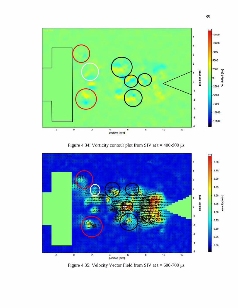
89
Figure 4.34: Vorticity contour plot from SIV at t = 400-
Figure 4.35: Velocity Vector Field from SIV at t = 600-7
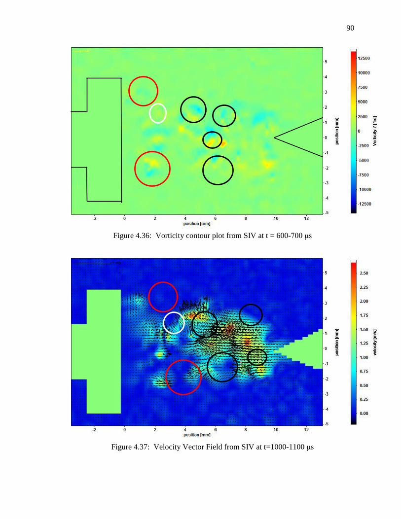
90
Figure 4.36: Vorticity contour plot from SIV at t = 600-
Figure 4.37: Velocity Vector Field from SIV at t=1000-11

91
Figure 4.38: Vorticity contour plot from SIV at t = 1000-
The dissipation stage consists of a horizontally symmetric expansion about the
discharge axis as shown in Figure 4.39. Unlike the point-to-point electrode configuration,
a distinct shape is observed as the channel expands and equilibrates to the ambient air
pressure. At t = 2200-
propagating from different ends meet to move upwards and downwards, respectively.
This occurs at approximately 3.8 mm away from the flat electrode and can be viewed in
Figure 4.40. The vortices that move upwards coalesce with the clockwise vortex circled
in red. The vortices that move downwards interact to form an anti-clockwise vortex.
This strong vortex pair pulls
flat electrode causing an axial expansion outwards along the electrode surface. A flow of
air entrainment is also induced between the vortex pair resulting in the appearance shown
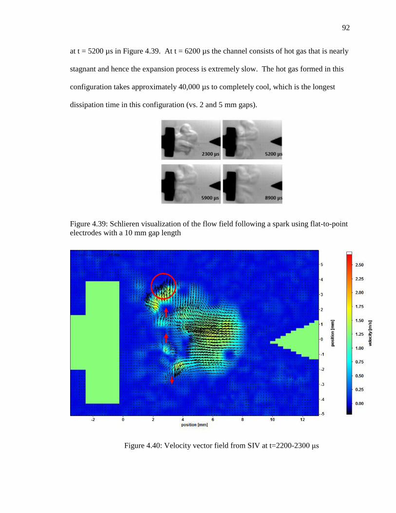
92
at t = 5200 µs in Figure 4.39. At t = 6200 µs the channel consists of hot gas that is nearly
stagnant and hence the expansion process is extremely slow. The hot gas formed in this
configuration takes approximately 40,000 µs to completely cool, which is the longest
dissipation time in this configuration (vs. 2 and 5 mm gaps).
Figure 4.39: Schlieren visualization of the flow field following a spark using flat-to-point electrodes with a 10 mm gap length
Figure 4.40: Velocity vector field from SIV at t=2200-23

93
Figure 4.41: Velocity vector field from SIV at t = 2800-2900
The initial vortex formation process for the 2mm and 5mm gaps follows the same
trend that was observed and discussed for the 10 mm gap first stage of expansion. This
was observed in the results of the schlieren visualization and SIV which can also be
viewed in Appendix A and Appendix B. Figure 4.42 shows the shockwave propagation
and the plasma channel as it expands on the electrode surfaces at t = 0 µs in a 2mm gap.
At t = 100µs, the right edge of the channel is pulled inwards in the precise manner that
was described for the 10mm gap. Again, a clockwise vortex on the upper-left edge of the
channel forms and propagates upwards while an anticlockwise vortex on the lower-left
edge of the channel forms and propagates downwards on the surface of the flat electrode.
The clockwise vortex and anti-clockwise vortex are associated with a positive and
negative time-averaged vorticity, respectively. As can be viewed in the velocity vector
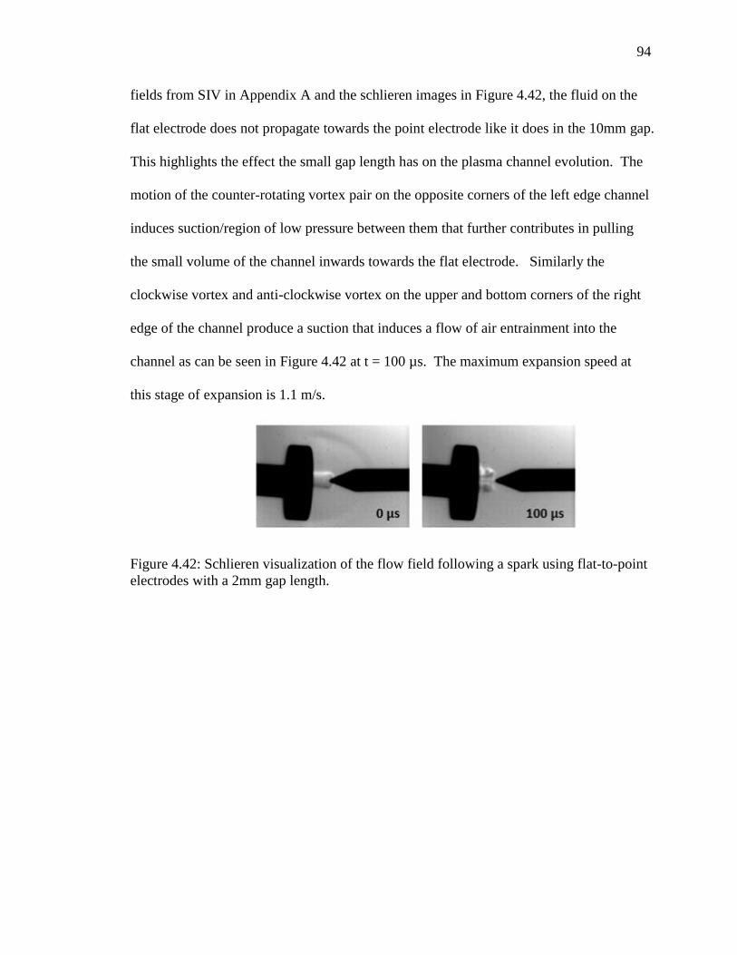
94
fields from SIV in Appendix A and the schlieren images in Figure 4.42, the fluid on the
flat electrode does not propagate towards the point electrode like it does in the 10mm gap.
This highlights the effect the small gap length has on the plasma channel evolution. The
motion of the counter-rotating vortex pair on the opposite corners of the left edge channel
induces suction/region of low pressure between them that further contributes in pulling
the small volume of the channel inwards towards the flat electrode. Similarly the
clockwise vortex and anti-clockwise vortex on the upper and bottom corners of the right
edge of the channel produce a suction that induces a flow of air entrainment into the
channel as can be seen in Figure 4.42 at t = 100 µs. The maximum expansion speed at
this stage of expansion is 1.1 m/s.
Figure 4.42: Schlieren visualization of the flow field following a spark using flat-to-point electrodes with a 2mm gap length.
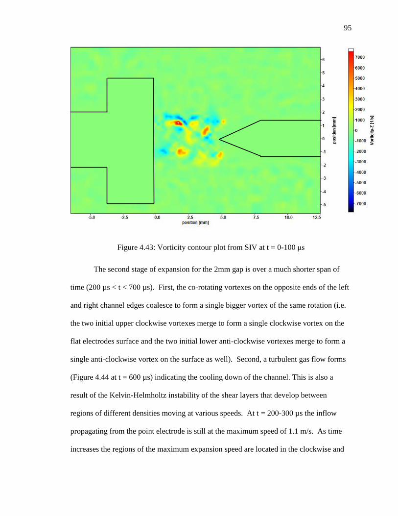
95
Figure 4.43: Vorticity contour plot from SIV at t = 0-100
The second stage of expansion for the 2mm gap is over a much shorter span of
time (200 µs < t < 700 µs). First, the co-rotating vortexes on the opposite ends of the left
and right channel edges coalesce to form a single bigger vortex of the same rotation (i.e.
the two initial upper clockwise vortexes merge to form a single clockwise vortex on the
flat electrodes surface and the two initial lower anti-clockwise vortexes merge to form a
single anti-clockwise vortex on the surface as well). Second, a turbulent gas flow forms
(Figure 4.44 at t = 600 µs) indicating the cooling down of the channel. This is also a
result of the Kelvin-Helmholtz instability of the shear layers that develop between
regions of different densities moving at various speeds. At t = 200-300 µs the inflow
propagating from the point electrode is still at the maximum speed of 1.1 m/s. As time
increases the regions of the maximum expansion speed are located in the clockwise and
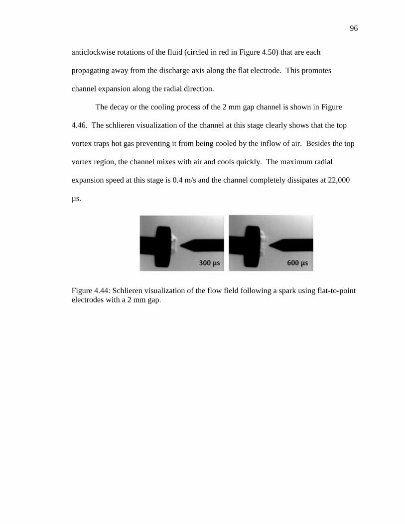
96
anticlockwise rotations of the fluid (circled in red in Figure 4.50) that are each
propagating away from the discharge axis along the flat electrode. This promotes
channel expansion along the radial direction.
The decay or the cooling process of the 2 mm gap channel is shown in Figure
4.46. The schlieren visualization of the channel at this stage clearly shows that the top
vortex traps hot gas preventing it from being cooled by the inflow of air. Besides the top
vortex region, the channel mixes with air and cools quickly. The maximum radial
expansion speed at this stage is 0.4 m/s and the channel completely dissipates at 22,000
µs.
Figure 4.44: Schlieren visualization of the flow field following a spark using flat-to-point electrodes with a 2 mm gap.

97
Figure 4.45: Velocity vector field from SIV at t = 600 -700 µs
Figure 4.46: Schlieren visualization of the flow field following a spark using flat-to-point electrodes with a gap length of 2mm.
98
The schlieren visualization of the first stage of expansion for the 5 mm gap can be
viewed in Figure 4.47. Similar to the 10 mm gap, a faint contour that follows the blast
wave is observed below the hot plasma channel in Figure 4.28 during the first stage of
expansion. As was previously mentioned, however, it is not clear what these are but it is
suspected that they are a result of multiple streamer discharges that occurred
simultaneously with the main spark. The first stage of the 5 mm gap expansion process
mimics that of the 10mm gap. The exception being that of the 2 mm gaps, vorticity here
is generated throughout the channel (Figure 4.48). The maximum expansion speed at this
stage for the 5 mm gap is 2 m/s.
Figure 4.49 shows the major features of the flowfield that characterize the second
stage of expansion (200 µs < t < 2300 µs) for the 5 mm gap. The expansion process is
axially symmetric with clear and organized vortex structures. The speed at which the
channel propagates is equally distributed across the inflows. This can be seen in the
velocity vector field at t = 200-300 µs in Figure 4.50. Again, the clockwise vortex on the
upper-left edge of the channel is propagating vertically upwards on the flat electrode
surface while the anti-clockwise vortex on the lower-left edge of the channel is
propagating vertically downwards on the same electrode surface. The vortices
propagating from opposite ends meet at t = 200-300 µs, approximately 2.4 mm away
from the flat electrode as is shown in Figure 4.50. This is unlike the 10 mm gap where
the vortex flows do not encounter one another until the dissipation stage (i.e. t > 2300 µs).
This is due to the fact that a longer gap length equates to a longer path of travel along the
discharge axis despite the higher propagation speed. The vortices that encounter one
another interact to form counter rotating vortex pairs. These are circled in red for
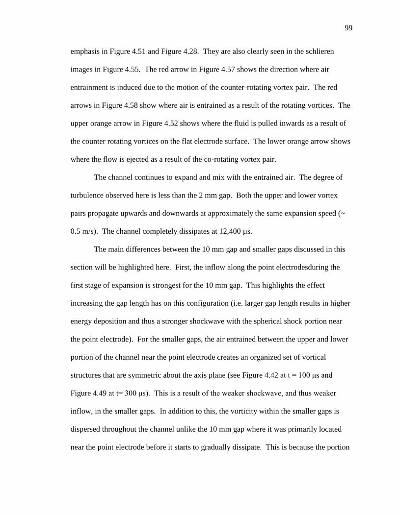
99
emphasis in Figure 4.51 and Figure 4.28. They are also clearly seen in the schlieren
images in Figure 4.55. The red arrow in Figure 4.57 shows the direction where air
entrainment is induced due to the motion of the counter-rotating vortex pair. The red
arrows in Figure 4.58 show where air is entrained as a result of the rotating vortices. The
upper orange arrow in Figure 4.52 shows where the fluid is pulled inwards as a result of
the counter rotating vortices on the flat electrode surface. The lower orange arrow shows
where the flow is ejected as a result of the co-rotating vortex pair.
The channel continues to expand and mix with the entrained air. The degree of
turbulence observed here is less than the 2 mm gap. Both the upper and lower vortex
pairs propagate upwards and downwards at approximately the same expansion speed (~
0.5 m/s). The channel completely dissipates at 12,400 µs.
The main differences between the 10 mm gap and smaller gaps discussed in this
section will be highlighted here. First, the inflow along the point electrodesduring the
first stage of expansion is strongest for the 10 mm gap. This highlights the effect
increasing the gap length has on this configuration (i.e. larger gap length results in higher
energy deposition and thus a stronger shockwave with the spherical shock portion near
the point electrode). For the smaller gaps, the air entrained between the upper and lower
portion of the channel near the point electrode creates an organized set of vortical
structures that are symmetric about the axis plane (see Figure 4.42
Figure 4.49
inflow, in the smaller gaps. In addition to this, the vorticity within the smaller gaps is
dispersed throughout the channel unlike the 10 mm gap where it was primarily located
near the point electrode before it starts to gradually dissipate. This is because the portion
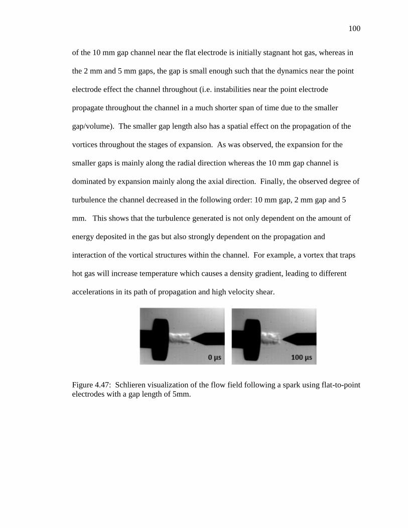
100
of the 10 mm gap channel near the flat electrode is initially stagnant hot gas, whereas in
the 2 mm and 5 mm gaps, the gap is small enough such that the dynamics near the point
electrode effect the channel throughout (i.e. instabilities near the point electrode
propagate throughout the channel in a much shorter span of time due to the smaller
gap/volume). The smaller gap length also has a spatial effect on the propagation of the
vortices throughout the stages of expansion. As was observed, the expansion for the
smaller gaps is mainly along the radial direction whereas the 10 mm gap channel is
dominated by expansion mainly along the axial direction. Finally, the observed degree of
turbulence the channel decreased in the following order: 10 mm gap, 2 mm gap and 5
mm. This shows that the turbulence generated is not only dependent on the amount of
energy deposited in the gas but also strongly dependent on the propagation and
interaction of the vortical structures within the channel. For example, a vortex that traps
hot gas will increase temperature which causes a density gradient, leading to different
accelerations in its path of propagation and high velocity shear.
Figure 4.47: Schlieren visualization of the flow field following a spark using flat-to-point electrodes with a gap length of 5mm.
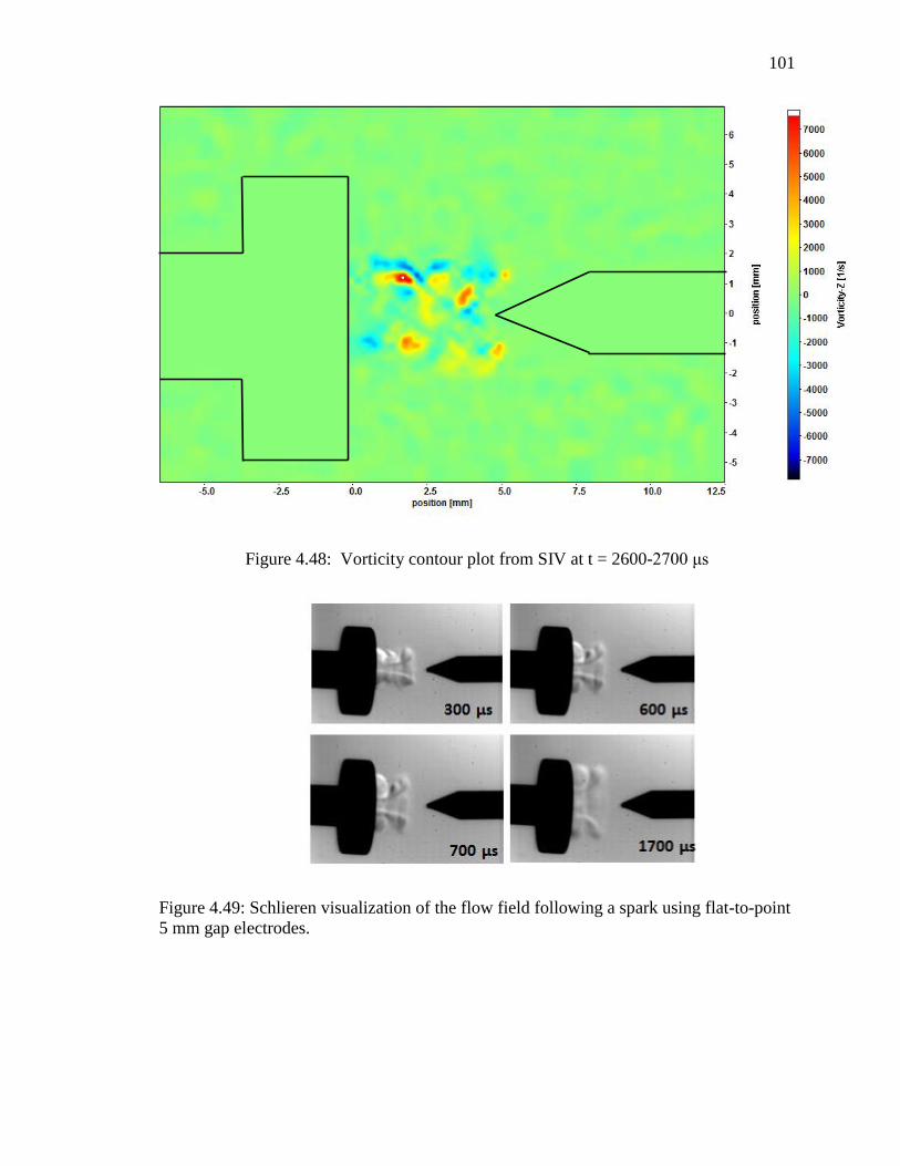
101
Figure 4.48: Vorticity contour plot from SIV at t = 2600-
Figure 4.49: Schlieren visualization of the flow field following a spark using flat-to-point 5 mm gap electrodes.
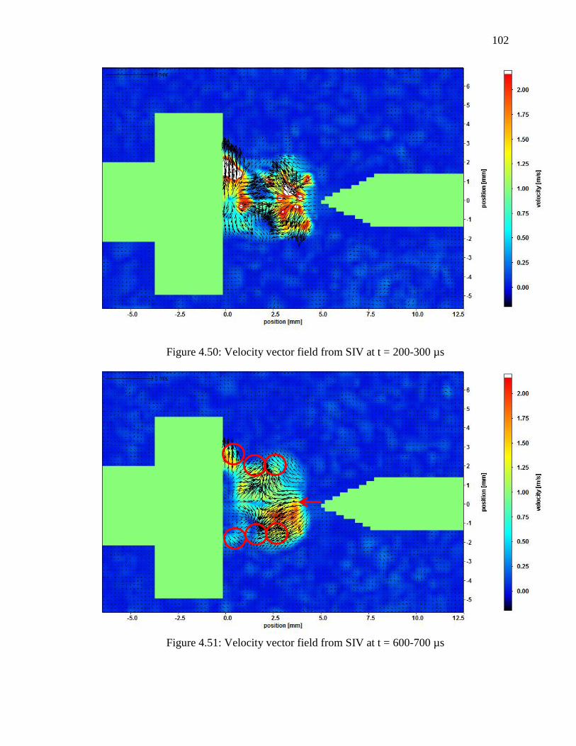
102
Figure 4.50: Velocity vector field from SIV at t = 200-300 µs
Figure 4.51: Velocity vector field from SIV at t = 600-700 µs
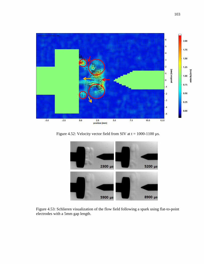
103
Figure 4.52: Velocity vector field from SIV at t = 1000-1100 µs.
Figure 4.53: Schlieren visualization of the flow field following a spark using flat-to-point electrodes with a 5mm gap length.

104
4.3 Blunt-to-Blunt Electrodes
The third and final configuration considered in this work is the blunt-to blunt
electrodes. Figure 4.54 shows schlieren images of the flow induced by a spark discharge
across a 10 mm gap with blunt-to-blunt electrodes. Like with all electrode configurations,
the first image is taken less than 20 µs after the spark breakdown and for this work
SIV and are discussed in this section.
Figure 4.54: Schlieren visualization of the flow field following a spark using blunt-to-blunt 10 mm gap electrodes

105
Figure 4.55, Figure 4.59 and Figure 4.66 show schlieren images of the first stage of
expansion ( ), second stage of expansion and the decay or
dissipation process (t ), respectively. The velocity and vorticity data from SIV
during the first stage of expansion is shown in Figure 4.57 and Figure 4.58. The plasma
channel in the first stage of expansion for the blunt-to-blunt configuration is characterized
by vortical structure formation and an expanding diameter. This can clearly be seen in
the schlieren visualization in Figure 4.55. Similar to the point-to-point and flat-to-point
electrode configurations at t = 0 µs, the post-discharge channel looks like a cylinder of
hot gas. Unlike the two previously studied configurations, however, there is no evident
high-velocity inflow of ambient gas along the electrodes, which was the primary source
of vorticity for the flow near the point electrodes. There is, however, strong vorticity
throughout the entire channel, shown in Figure 4.58. Therefore, it is speculated that the
vorticity for the 10 mm blunt-to-blunt gap configuration is mainly due to the shear layers
that develop from instabilities in the channel (Figure 4.57). In addition to this difference,
unlike the other configurations, the outward flow of the spark kernel itself is not shown in
the SIV results in this case. For the other electrode configurations, the outward
expansion of the kernel, specifically in regions near the electrodes where it was moving
against the inflow, was observed in the SIV results. In this configuration, however, we
only see the channel compressing inwards. This suggests that the pressure along the axis
of the channel (or the central region of the blast wave) may decrease below the ambient
pressure at a much faster rate in the 10 mm blunt-to-blunt gap configuration. In other
words, the inward gas flow could have potentially occurred before the first schlieren
image was recorded (where t = 0 µs).
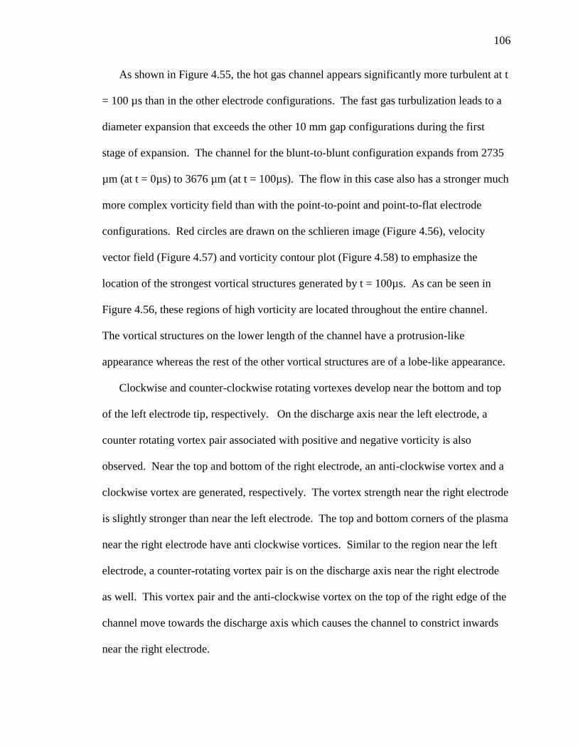
106
As shown in Figure 4.55, the hot gas channel appears significantly more turbulent at t
= 100 µs than in the other electrode configurations. The fast gas turbulization leads to a
diameter expansion that exceeds the other 10 mm gap configurations during the first
stage of expansion. The channel for the blunt-to-blunt configuration expands from 2735
µm (at t = 0µs) to 3676 µm (at t = 100µs). The flow in this case also has a stronger much
more complex vorticity field than with the point-to-point and point-to-flat electrode
configurations. Red circles are drawn on the schlieren image (Figure 4.56), velocity
vector field (Figure 4.57) and vorticity contour plot (Figure 4.58) to emphasize the
location of the strongest vortical structures generated by t = 100µs. As can be seen in
Figure 4.56, these regions of high vorticity are located throughout the entire channel.
The vortical structures on the lower length of the channel have a protrusion-like
appearance whereas the rest of the other vortical structures are of a lobe-like appearance.
Clockwise and counter-clockwise rotating vortexes develop near the bottom and top
of the left electrode tip, respectively. On the discharge axis near the left electrode, a
counter rotating vortex pair associated with positive and negative vorticity is also
observed. Near the top and bottom of the right electrode, an anti-clockwise vortex and a
clockwise vortex are generated, respectively. The vortex strength near the right electrode
is slightly stronger than near the left electrode. The top and bottom corners of the plasma
near the right electrode have anti clockwise vortices. Similar to the region near the left
electrode, a counter-rotating vortex pair is on the discharge axis near the right electrode
as well. This vortex pair and the anti-clockwise vortex on the top of the right edge of the
channel move towards the discharge axis which causes the channel to constrict inwards
near the right electrode.

107
On the upper and lower boundary of the plasma channel there are two almost
evenly-spaced vortical structures. These are circled in white in Figure 4.56, Figure 4.57
and Figure 4.58. These figures clearly show the plane of symmetry about the axis plane
between the upper and lower length of the channel. On the upper length of the channel
circled in red from the left to the right, is an anti-clockwise vortex and a clockwise vortex.
Similarly, on the lower length of the channel circled in red from the left to right, is a
clockwise vortex and an anti-clockwise vortex. The associated vorticity with these
vortices can be viewed in Figure 4.58. The vortex pairs on the discharge axis are circled
in grey. The two main embedded counter-rotating vortex pairs with the highest velocities
are circled in black and can be viewed in the figures below. The red dotted circles on
Figure 4.56, Figure 4.57 and Figure 4.58 show the locations where the flows from the
opposite (electrode) ends meet, generating vorticity of opposite signs.
Figure 4.57 shows the distribution of the velocity across the plasma channel
during the first stage of expansion. The velocity (2 m/s) appears to be fairly uniform on
the edge of the channel along the left electrode. The velocity field of the edge along the
right electrode, however, has a high-velocity region of 4.2 m/s where the anti-clockwise
vortex is located. The vortical structure regions in the upper and lower portion of the
plasma (circled in white) have the maximum axial speed, 5 m/s, at this stage of expansion.

108
Figure 4.55: Schlieren visualization of the flow field following a spark using blunt-to-blunt 10 mm gap electrodes.
Figure 4.56: Schlieren visualization of the flowfield following a spark using blunt-to-blunt electrodes
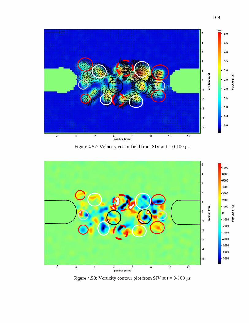
109
Figure 4.57: Velocity vector field from SIV at t = 0-1
Figure 4.58: Vorticity contour plot from SIV at t = 0-

110
The second stage of expansion is characterized by the
propagation and generation of complex vortical structures as the mixing between the
channel and ambient air continues. As can be seen in Figure 4.59, circled in red is the
clockwise vortex near the top of the left electrode which propagates towards the
discharge axis while the anti-clockwise vortex on the bottom propagates downwards
towards the ambient air. At 400-500 , this anti-clockwise vortex separates from the
flow as shown in the close-up view of the vorticity field in Figure 4.62 (a) and (b). After
it separates, it cools and trails behind the channel until it completely dissipates at 3000 .
The counter-rotating vortex pair on the discharge axis near the left electrode from the first
stage of expansion interacts with the vortex motion above and below it to form a
localized jet that moves upwards at a relatively low speed (0.5 m/s). Both the anti-
clockwise and clockwise vortex along the right electrode move towards the discharge
axis. The two embedded vortical structures which are circled in black in Figure 4.60
propagate towards one another along the discharge axis. The vortices that are on the
upper and lower length of the channel propagate towards the plane at r = 5mm to move
upwards and downwards, respectively. The two latter vortex motions described lead to
enhanced airflow towards the center of the gap (i.e. the plane at r = 5mm). By 200-300
(Figure 4.67) the vorticity is inhomogeneously dispersed throughout the channel as a
result of the vortex behavior.
The maximum expansion speed in the second stage of expansion is 4 m/s. Figure
4.63 shows that at 800- expansion in
a direction traverse to the electrodes (i.e. the upper and lower portion of the channel
propagating upwards and downwards, respectively) at an average expansion velocity of

111
2.8 m/s. The vortices in the second stage of expansion entrain a significant amount of air
increasing the cooling rate and air mixing in the flow around them. As a result, after
1000 µs new small scale vortices form on both the upper and lower portion of the channel.
These can be observed in the circulating regions indicated by the velocity vector field at t
= 1600- Figure 4.64. The vortices generated in the upper channel propagate
upwards and those that are generated in the lower channel propagate downwards. This
ion in
geometry. Figure 4.65 shows the velocity vector field at the end of the second stage of
expansion (i.e. 2200- The two main regions of vorticity have been circled in red
and consist of counter-rotating vortex pairs on the upper and lower channel, which persist
onto the last stage of expansion. The other regions of vorticity formed in the initial
expansion stage dissipate by 400 s.
Figure 4.59: Schlieren visualization of the flow field following a spark using blunt-to-blunt electrodes with a 10 mm gap.

112
Figure 4.60: Velocity vector field from SIV at t = 200-3 .
Figure 4.61: Vorticity contour plot from SIV at 200-3

113
(a) (b) Figure 4.62: Vorticity contour plot with velocity vectors from SIV at (a) 200-3 and (b) 400-500
Figure 4.63: Velocity vector field from SIV at t = 800-9 .
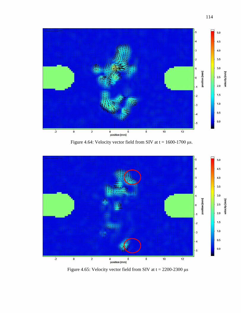
114
Figure 4.64: Velocity vector field from SIV at t = 1600-17 .
Figure 4.65: Velocity vector field from SIV at t = 2200-23
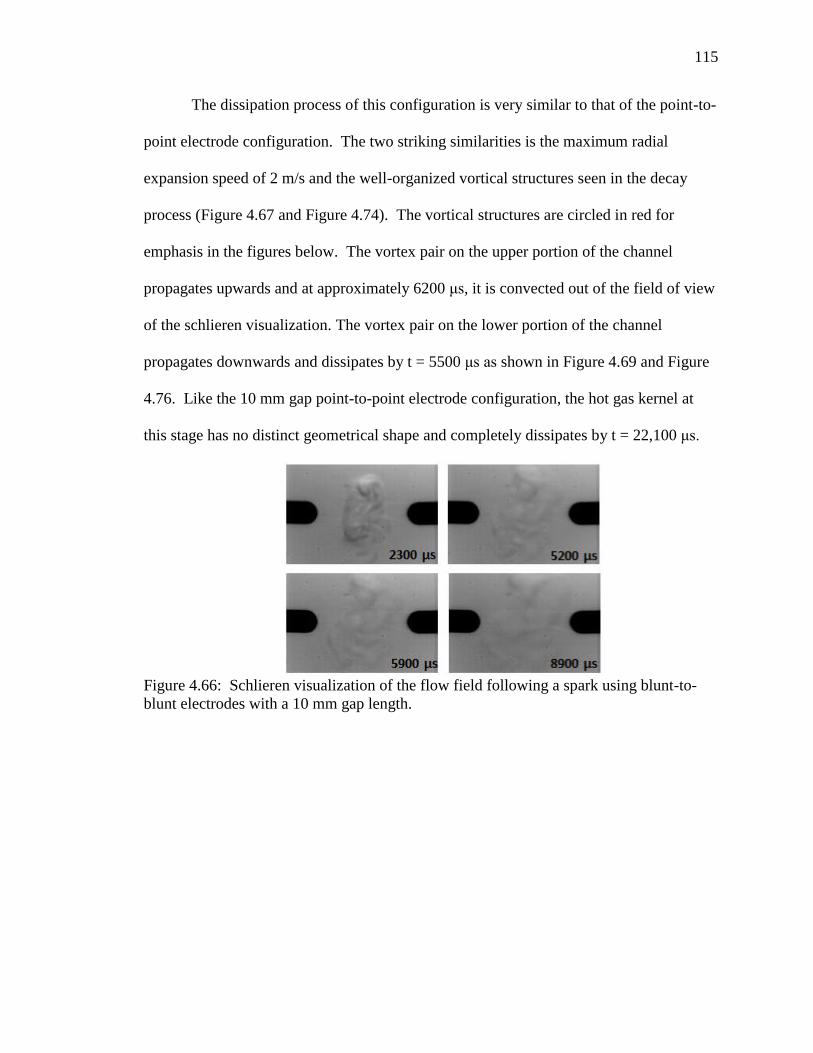
115
The dissipation process of this configuration is very similar to that of the point-to-
point electrode configuration. The two striking similarities is the maximum radial
expansion speed of 2 m/s and the well-organized vortical structures seen in the decay
process (Figure 4.67 and Figure 4.74). The vortical structures are circled in red for
emphasis in the figures below. The vortex pair on the upper portion of the channel
propagates upwards and at approximately 6200 , it is convected out of the field of view
of the schlieren visualization. The vortex pair on the lower portion of the channel
propagates downwards and dissipates by t = 5500 shown in Figure 4.69 and Figure
4.76. Like the 10 mm gap point-to-point electrode configuration, the hot gas kernel at
this stage has no distinct geometrical shape and completely dissipates by t = 22,100
Figure 4.66: Schlieren visualization of the flow field following a spark using blunt-to-blunt electrodes with a 10 mm gap length.

116
Figure 4.67: Velocity vector field from SIV at t = 3800-39
Figure 4.68: Vorticity contour plot from SIV at t = 3800-39
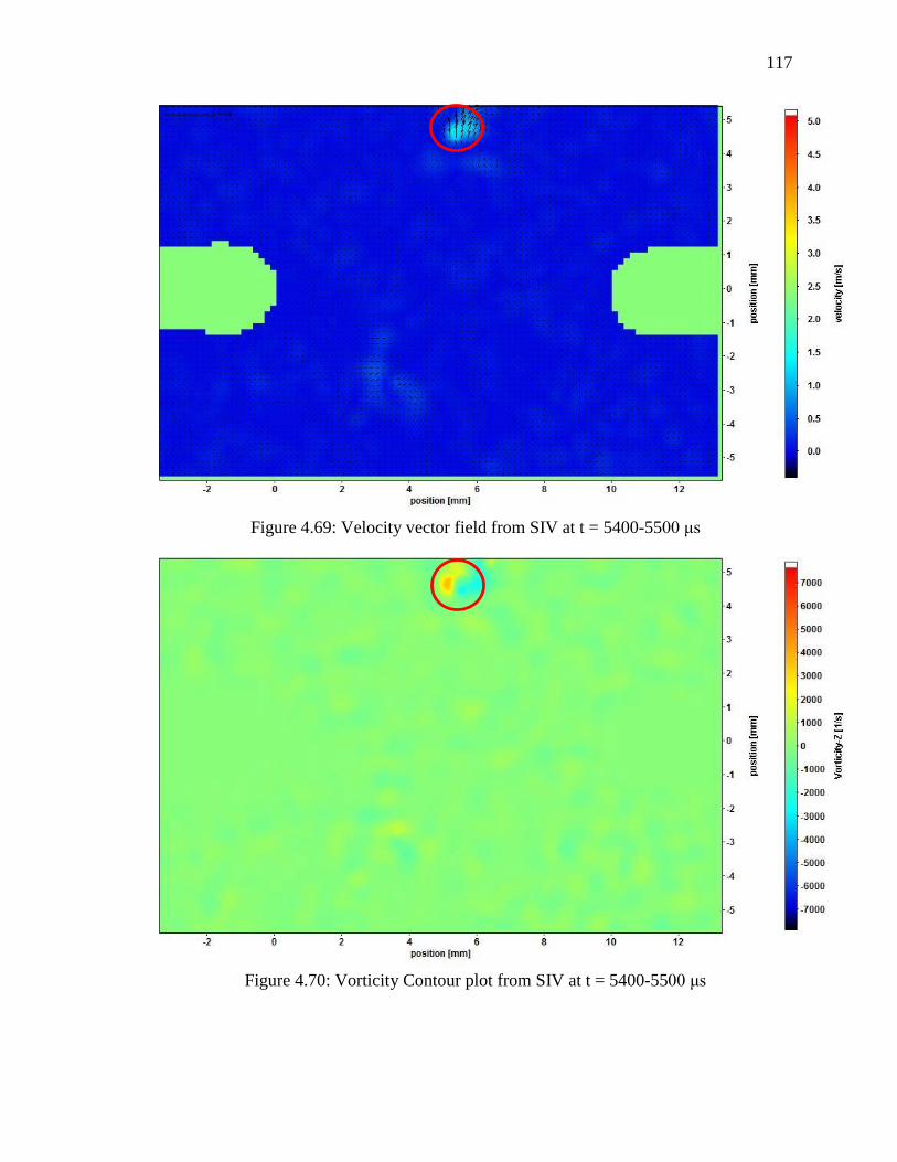
117
Figure 4.69: Velocity vector field from SIV at t = 5400-55
Figure 4.70: Vorticity Contour plot from SIV at t = 5400-55
118
The three stages of expansion for the 2 mm and 5 mm gaps are very similar, therefore
results from the 2 mm gap case will be used in this discussion to represent both smaller
gaps. Significant differences observed in the stages of expansion between the 2 mm and
5mm gap cases will be noted, and the complete SIV results for the 5 mm gap are given in
Appendix A and Appendix B. Figure 4.72 and Figure 4.73show the velocity vector field
and vorticity contour plot of the initial expansion stage for the 2 mm gap. An
anticlockwise vortex (top corner) and a clockwise vortex (bottom corner) are generated
on the left electrode. The anti-clockwise vortex propagates upwards and the clockwise
vortex downwards. The schlieren visualization in Figure 4.65 clearly shows a symmetry
of expansion about the r = 0 plane. And thus, as expected, Figure 4.67 and Figure 4.68
indicate a clockwise vortex (top corner) and an anti-clockwise vortex (bottom corner) on
the right electrode. The clockwise vortex propagates upwards and the anticlockwise
vortex propagates downwards. The effect of these vortices is that they pull the fluid
inwards from the electrodes as can be seen at t = 0- Figure 4.71 (Figure 4.77 for
the 5mm gap). Like the 10 mm gap, there is an anti-clockwise vortex pair on the
discharge axis on the front of each electrode surface. The clockwise vortex of each pair
turns vertical and propagates upwards. The anti-clockwise vortex of the pairs turns
vertical as well and propagates downwards. This vortex behavior can be seen in Figure
4.72 and Figure 4.74. Figure 4.71 and Figure 4.77 clearly show vortical structures with
larger density gradients, sugge
that the degree of mixing with cold ambient air increases with gap distance.
During the first stage of expansion the 5 mm gap channel, unlike the 2 mm gap, also
has embedded vortices (i.e. vorticies within the channel besides ones on edges) that

119
propagate in the same manner as discussed for the 10 mm gap (see Appendix A and
Appendix B). The maximum radial expansion speed during the first stage of expansion
for the 2 mm gap and 5 mm gap case is 3.0 m/s and 6.6 m/s, resepectively. For the 2 mm
gap the channel diameter expands from 2985 µm (t = 0 µs) to 4062 µm (t = 100 µs)
within the first stage of expansion. The 5 mm gap expands from a diameter of 2615 µm
to 3874 µm within the first stage of expansion.
characterized by the formation of small-scale vortices within the channel as a result of
fluid entrainment from the first stage of expansion. The propagation of these vortices
follows the same trend that was discussed for the 10 mm gap where the vortices that are
above the discharge axis propagate upwards and those that are below the discharge axis
propagate downwards. Unlike the other configurations studied, it was observed that the
smaller the gap length the stronger the vortices formed and thus the higher the degree of
organized vortex pairs form on the upper and lower portion of the 2 mm gap channel.
These are circled in red in Figure 4.75 and Figure 4.76. The latter was not observed for
the 10 mm gap until the dissipation stage. Similar to the 10 mm gap, however, these
vortices propagate away from the discharge axis but dissipate at a much faster rate. The
vorticity contour plots in Appendix B show that the vorticity in these flow regions
completely dissipates by t = 4400- maximum radial expansion speed at the
second stage of expansion for the 2 mm gap and 5 mm gap channels are 1 m/s and 2 m/s,
respectively. Like the other configurations at all gap lengths, the channel does not grow
120
in a completely spherical manner but expands more in the transverse direction to the
electrode axis and less in the axial direction.
In summary it was observed that throughout the stages of expansion the
propagation of the vortices in the smaller gaps follows the same trend as the 10 mm gap
but dissipate at a much faster rate. In addition it was observed that the expansion is
stronger in the radial direction as the gap length decreased. Across all the gap lengths in
this configuration, in the second stage of expansion the vortices entrain a significant
amount of air, thus increasing the cooling rate and air mixing in the flow around them.
This leads to the formation of small scale vortices within the channel. It was observed
that the strength of these small scale vortices increased with a decreasing gap length.
This caused the degree of turbulence to increase as the gap length decreased. This trend
across the varying gap lengths is unlike what was observed for the other electrode
configurations. Complex vorticity fields were generated for all three gap lengths and
the vorticity was dispersed throughout the entire channel, an observation that was unique
to the blunt electrodes. In the other electrode configurations, the vorticity was much
more localized; for example, in the 10 mm flat-to-point electrode case, the vorticity was
primarily concentrated near the point electrode.
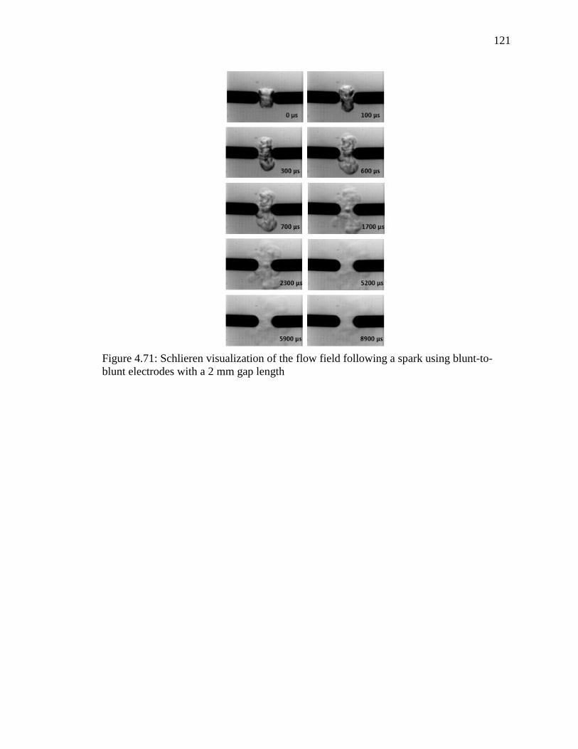
121
Figure 4.71: Schlieren visualization of the flow field following a spark using blunt-to-blunt electrodes with a 2 mm gap length

122
Figure 4.72: Velocity vector field from SIV at t = 0-100 µs
Figure 4.73: Vorticity contour plot from SIV at t = 0-100 µs

123
Figure 4.74: Velocity vector field from SIV at t = 200-300 µs
Figure 4.75: Velocity vector field from SIV at t = 1600-1700 µs

124
Figure 4.76: Vorticity Contour plot from SIV at t = 1600-1700 µs
Figure 4.77: Schlieren visualization of the flow field following a spark using blunt-to-blunt 5 mm gap electrodes
125
CHAPTER 5. CONCLUSION
The work in this dissertation was motivated by the lack of available research
explaining the flow dynamics induced by a spark discharge and how it varies with
different electrode configurations. Analysis on the dischar
and fluid mechanics is important since spark plasmas have the potential to be used as a
method of aerodynamic flow control and thus improve the performance and
maneuverability of current and future aircraft. In this section a brief summary of the
diagnostics developed and tests carried out is first presented. Second, conclusions
relating to the electrical characteristics of the different electrode configurations and the
effect of discharge energy will be discussed. Finally, the critical conclusions regarding
plasma channel evolution in the varied electrode configurations are presented.
In the current work, a very simple plasma actuator was constructed for generating
spark-induced flow fields. The actuator consisted of an electrical discharge system
connected to a spark gap. The discharge system was constructed to produce high-energy
(up to 0.5 J) pulses at voltages up to 45 kV, allowing for the breakdown of electrode gaps
up to 20 mm and larger. For the spark gap, five different electrode geometries were used:
point-to-point electrodes, blunt-to-blunt electrodes, blunt-to-point electrodes, boxlike
electrodes and flat-to-point electrodes. The electrical parameters (voltage and current
waveforms) were measured simultaneously and used to calculate the power and energy
126
results for all the electrode geometries across three varying gap lengths (2 mm, 5 mm and
10 mm).
A schlieren system was also designed and built for visualization of the plasma
channel evolution following the shockwave with three different electrode geometries
(point-to-point electrodes, flat-to-point electrodes, and blunt-to-blunt electrodes) at three
varying gap lengths (2 mm, 5 mm, and 10 mm). The schlieren system was designed to
have a small field of view so that images of the flow evolution could be obtained with
high spatial and temporal resolution. Quantitative data (i.e. velocity vectors and vorticity
contour plots) from the schlieren images was generated using schlieren image
velocimetry (SIV) analysis.
5.1 Electrical Characteristics
Across all the electrode geometries, it was observed that as the gap increased, so did
the breakdown voltage and hence also the discharge energy. This effect of the gap length
on the breakdown electric field is due to the fact that as the distance between the pair of
electrodes increases the electric field decreases, resulting in a higher breakdown voltage.
It was also expected that the blunt-to-blunt electrodes would have the highest breakdown
voltage and that the point-to-point electrodes would have the lowest breakdown voltage
across all the gap lengths. This expectation was based on the simple idea that as the
radius of curvature decreases, the local electric field strength increases. However, not
one electrode configuration consistently yielded the highest or lowest breakdown voltage
across all the gap lengths. In fact, the highest breakdown voltage at each gap length was
obtained with different electrode geometries. At gap lengths of 2 mm and 5 mm, the
127
breakdown voltage was highest for the blunt-to-point electrodes (9 kV and 15 kV) and at
a gap length of 10 mm the breakdown voltage was highest for the point-to-point
electrodes (19 kV). For gap lengths of 2 mm and 5 mm, the breakdown voltage was
lowest for the point-to-point electrodes and at a gap length of 10 mm the breakdown
voltage was lowest for the blunt-to-blunt electrodes. These results demonstrate that while
the electrode geometry may have a significant effect on the breakdown, it is not possible
to ascribe the differences in the observed breakdown voltage (and thus subsequent
discharge energy) solely to the electrode geometry. From these results it can be inferred
that the additional influence of the physical and atomic nature of the electrode surfaces
(e.g. surface roughness) and impurities (e.g. dust particles) affect the performance of the
breakdown voltage significantly. Hence it is important, to take into account the
combined influence of these factors in addition to the electrode geometry when making
comparisons between experimental electrical data and theoretical predictions.
It was also found that the electrode configurations that had the lowest increase in the
breakdown voltage when the gap length was increased from 2 mm to 5 mm had a
consistent tendency of having the highest breakdown voltage increase when the gap
length was increased from 5 mm to 10 mm. This shows that the electrode geometries (in
addition to the combined influence of the previously mentioned physical factors) used at
small gap lengths have the inverse effect on the electric field when compared to the same
set of electrode geometries at larger gap lengths. This work, therefore, suggests that
depending on the gap length, there are certain electrode geometries that may be more
efficient to use (i.e. higher energy deposition) for changing the flow field.
128
Higher discharge energy leads to higher energy density and therefore higher
initial plasma channel temperature/pressure. It is this elevated temperature and pressure
that induces as revealed by the
experiments performed in this work. Key characteristics of the hot gas evolution depend
on the discharge energy, including the initial conditions in the plasma channel and time-
history of the temperature, pressure and turbulence. In this work the effect of the varying
spark energies on the hot gas kernel radius and longevity were compared. It was seen
that for a given electrode geometry, the dissipation time increased with an increasing
discharge energy/gap length but there was no apparent trend observed between the
discharge energy/gap length and the dissipation times across the different electrode
configurations. This was of no surprise, however, since the hot gas persists for a
sufficiently long
into play that could accelerate or decelerate the decay depending on the geometry of the
electrodes. For gap lengths of 2 mm and 5mm, the pla
for the blunt-to-point electrode. For gap lengths of 10 mm the dissipation times are
longest for the boxlike electrodes and flat-to-point electrodes.
To investigate the effect of discharge energy on the temporal growth of the
plasma kernel radius, results using two spark energies (0.1181 J and 0.0453 J) were
compared. It was observed that a plasma channel with a higher spark energy results in a
smaller channel radius initially (t r in comparison
to a channel with lower spark energy. Although the after-spark channel radius is
primarily affected by the discharge energy, this comparison suggests a more complex
competition between various secondary factors (i.e. factors that are dependent on the
129
These secondary factors include the hydrodynamics of the plasma channel, such as
instabilities or vortical flows which are dependent on the initial flow field that is
governed by the shock wave generated. Therefore, the hot gas channel radius is a
complex parameter that depends on a number of spatially-dependent and time-dependent
variables. This conclusion is further exemplified by the observation that initially (t < 400
hot gas channel radii increase significantly with time, independent of the
discharge energy.
5.2 Plasma Channel Evolution
The initial flow field governed by the shockwave dominates how the plasma channel
expands during the first few microseconds. The electrode configuration (geometry and
gap length) has a strong influence on the strength and structure of the shockwave in
addition to the overall development of the plasma channel. This is because the
shockwave is a result of the energy deposited in the gas which is strongly dependent on
the gap length and geometry of the electrodes. Three mechanisms of the spark discharge
effect on the gas parameters and flow structure were identified. First, pressure gradients
are established by local gas heating. Second, a blast wave forms at the initial stage of the
spark discharge process and propagates outward from the electrode gap during the first
several nanoseconds. Generated by the rapid heating and high pressure rise in the plasma
channel, its departure increases the local temperature and pressure and intensifies the
expansion of the channel. Finally, after the blast wave decay, the hot gas kernel created
by the spark plasma evolves, generating vorticity and/or turbulent gas motion. The work
130
in this dissertation focused on the latter mechanism. The influence of three different
electrode geometries (point-to-point electrodes, flat-to-point electrodes, and blunt-to-
point electrodes) across three varying gap lengths (2 mm, 5mm, and 10 mm) on the fluid
dynamics following the spark discharge were studied.
For all the electrode configurations, the hot gas evolution was divided into three
distinct phases based on the observed differences in the main flow features: first stage of
expan
). Immediately after the spark breakdown a very thin
plasma channel (diameter on the order of 10- is
created. At very early times, the post-discharge channel looks like a cylinder of hot gas.
The localized energy deposited in the channel leads to a high temperature and pressure
causes a shockwave to propagate
outwards from the channel. The structure and strength of the shockwave is dependent on
the electrode geometry and gap length.
For the point-to-point and blunt-to-blunt electrode configurations the shockwave is
initially cylindrical except near the electrode surfaces, where it is spherical. The pressure
gradient behind the cylindrical portion of the shockwave is smaller than that following
the spherical shock wave, resulting in a higher pressure in the middle of the channel than
near the electrodes. This causes the channel to expand outwards towards the electrode
surfaces. A decreased pressure zone is formed on the discharge axis due to the inertia of
the gas accelerated during the fast initial expansion. This halts the outward flow after
some time period and induces inflow along the electrodes. However, in the first stage of
expansion for the 10 mm gap blunt-to-blunt electrodes there is no evidence of high-
131
velocity inflow of ambient gas along the electrodes. Instead, the mechanism that follows
it (i.e. inward expansion of channel) is observed initially. Since at a gap length of 10 mm,
the blunt-to-blunt electrode has the lowest discharge energy (and thus a weaker
shockwave) amongst all the electrode configurations, it is possible that weaker inflow
took place at an earlier time than when the first schlieren image was taken in these
experiments. The flow for the blunt-to-blunt electrode configuration is characterized by a
much more complex vorticity field than with the point-to-point and point-to-flat electrode
configurations. For the point-to-point electrode configuration the vorticity is initially
strongest along the surface of the electrodes as a result of the inflow. The flow for the
blunt-to-blunt electrode configuration is also characterized by vortices that entrain a
significant amount of air increasing the cooling rate and air mixing in the flow around
them. This mixing leads to the formation of small scale vortices within the channel that
give rise to a higher degree of turbulence as the gap length decreases.
For smaller gaps in the point-to-point and blunt-to-blunt electrode geometries the
shockwave structure is more spherical and the shockwave strength is weaker due to the
lower discharge energy. As a result, the flow field generated in smaller gaps with the
point-to-point electrodes is characterized by a lower inflow velocity along the electrodes
(and thus lower vorticity) during the first stage of expansion, a lower expansion speed
across all stages of expansion and a smaller degree of turbulence before it dissipates. The
plasma channel generated in smaller gaps for the blunt-to-blunt electrodes is
characterized by a higher degree of turbulence (due to the increased localized mixing
described above) and a lower expansion speed across all stages of expansion.
132
For the flat-to-point electrode configuration, the shockwave is nearly a pure
cylindrical wave except for very close to the point electrode surface, where the shock
wave is spherical. The shock structure initiates a complicated flow field but overall, the
pressure throughout the channel is higher than in the region close to the point electrode,
causing the plasma channel to rapidly expand outwards towards the point electrode
surface. Similar to the point-to-point and blunt-to-blunt electrode configurations, the
inertia of the gas (near the point electrode) that is accelerated during the fast initial
expansion creates a decreased pressure zone on the discharge axis in the region near the
point electrode. This halts the outward flow and induces strong inflow along the surface
of the point electrode. Similar to the point-to-point electrode geometry, the vorticity for
the flat-to-point electrode at a 10 mm gap length is mainly localized around the point
electrode as a result of the inflow. At smaller gap lengths with this electrode geometry,
the shockwave is more spherical and is weaker overall. These changes in the shock wave
result in flow field characterized by lower inflow velocity along the point electrode,
vorticity that is dispersed throughout the entire channel and lower turbulence that is
strongly dependent on the propagation and interaction of the vortical structures.
This work showed the influence of the electrode configuration on the fluid dynamics
following the spark discharge and how the hot gas evolution gives rise to various physical
phenomena that can be used to modify the flow-field structure near the boundary layer on
an aerodynamic surface. These physical phenomena include:
(1) Generation of turbulence can be used to move the separation point
downstream or even eliminate it. When the flow turbulizes it gains more
momentum (and thus energy) creating a fuller velocity profile in the boundary

133
layer which makes it able to withstand stronger/more sustained adverse
pressure gradients.
(2) Inducing vorticity gives rise to and distributes vortices, turbulence, and energy
within the boundary layer, and thus can induce desired changes in the local
boundary state that result in delaying flow separation and aerodynamic
stalling. Depending on the formation, strength, propagation and interaction of
vortices, they may effect the flow in many ways including: entraining heated
fluid, distributing vorticity within the flow, entrainment of ambient air,
turbulence generation which generally increases the cooling rate, and gas
mixing. The formation of jets seen in the point-to-point electrode
configuration can also be used to add momentum/energy into the boundary
layer. The presence of vorticity does not imply the presence of vortices (e.g.
vorticity as a result of shear layers) but in general it leads to the formation of
local instabilities within the flow.
(3) Gas mixing which is a result of turbulence, vortices and air entrainment and
can be used for cross-stream mixing air at the edge of the boundary layer
(which has more kinetic energy) with the low momentum flow at the near-
wall region (e.g. wing) of the boundary layer. This mixing re-energizes the
boundary layer and keeps the flow attached.
134
CHAPTER 6. FUTURE WORK
For experimental work, the next step would be to record the flow field induced by
the spark discharge for the same electrode configurations used in this work at a much
faster frame rate (e.g. 50,000 fps). This will allow for schlieren visualization of the flow
within microseconds of the breakdown. The current study focuses on the hot gas
evolution from approximately 20 μs after the breakdown up until the hot gas channel
fully dissipates (t 50,000 μs). Obtaining a qualitative and quantitative interpretation on
the flow as the shockwave propagates would be both beneficial in further understanding
the influence of the shockwave and the initial flowfield of the spark discharge described
in this work.
The next recommended future work would be to perform SIV analysis on videos of
spark discharges across sunken electrodes (i.e. electrodes flush with the surface) that
were also recorded as part of this work. These videos were taken for the point-to-point
electrodes, blunt-to-blunt electrodes and boxlike electrodes at gap lengths of 2 mm, 5mm,
10 mm and 15 mm. Examples of the schlieren images from these videos can be seen
below in Figure 6.1, Figure 6.2, and Figure 6.3. These figures show the spark discharges
across the sunken pont-to-point electrodes at a gap length of 2 mm, 5 mm, and 15 mm
respectively.

135
Finally, future work to improve the circuit used in this work is recommended as
well. The circuit designed for this work produces high-energy, high-power discharges
over a wide range of electrode gaps but the discharge frequency is limited to less than
100 Hz. Developing a discharge circuit that generates high-energy discharges over a
much wider range of frequencies (e.g. less than 1 Hz up to 10 kHz or higher) would allow
for analysis of the effect varying electrode configurations would have on the induced
flow field and electrical characteristics of a circuit that combines both the capabilities of
high energy and wide range of frequencies.
Figure 6.1: Schlieren visualization of the flow field following a spark using sunken point-to-point electrodes with a 2 mm gap length

136
Figure 6.2: Schlieren visualization of the flow field following a spark using sunken point-to-point electrodes with a 10 mm gap length
Figure 6.3: Schlieren visualization of the flow field following a spark using sunken point-to-point electrodes with a 15 mm gap length

REFERENCES

137
REFERENCES
[1 - Journal of
Applied Physics D: Applied Physics, Vol. 40, 605-36.
Progress in Astronautics and Aeronautics. Vol. 231, 90-233
[3] Wang, J. J., Choi, K. S., Feng, L. H., Jukes, T. N., & Whalley, R. D. (2013). Recent
developments in DBD plasm Progress in Aerospace Sciences. Vol. 62,
52-78.
[4] W. J. Chyu, M. J. Rimlinger, & T. I.-P. Shih. (1995). "Control of shock-
wave/boundary-layer interactions by bleed AIAA Journal, Vol. 33, 1239-1247.
[5] Babinsky, H., Li,Y., & Ford, C. W. Pitt. (2009). "Microramp Control of Supersonic
Oblique Shock-Wave/Boundary-Layer Interactions," AIAA Journal, Vol. 47, 668-675.
[6] Holden, H., &
Normal Shock/Boundary Layer In Journal of Aircraft, Vol. 44(1), 170-174.
[7] Syberg, J., & Koncsek, J. L. (1973). "Bleed System Design Technology for
Supersonic Inlets," Journal of Aircraft, Vol. 10(7), 407-413.
[8] Harloff, G.J., & -Inlet Boundary-
AIAA Journal, Vol. 34(4), 778 785

138
[9] Hirt, S.M., &
of Microramp Flow Control to an Oblique Shock Interaction, 47th AIAA Aerospace
Sciences Meeting including The New Horizons Forum and Aerospace Exposition, AIAA
Paper 2009-919.
[10] Scroggs, S. D. &
Experiments in Fluids, Vol. 21(6), 401-409.
[11] F. S. Alvi, C. Shih, R. Elavarasan, G. Garg, & A. Krothapalli. (2003). "Control of
Supersonic Impinging Jet Flows Using Supersonic Microjets", AIAA Journal, Vol. 41(7),
1347-1355.
[12] B. T. Beck, A. D. Cutler, J. P. Drummond, & S. B. Jones. (2004).
Pulse Detonation Actuator for High- 11th
International Symposium On Flow Visualization.
[13] Kalra, C. S., S. H. Zaidi, R. B. Miles, & S. O. Macheret. (2011). "Shockwave-
Turbulent Boundary Layer Interaction Control Using Magnetically Driven Surface
Discharges," Experiments in Fluids, Vol. 50, 547-59.
[14] Zwaba, R., Flaszynskip P. Szumski J., & Telega J. boundary
layer interaction control by air- Proceedings of the Eighth
International Symposium on Experimental and Computational Aerothermodynamics of
Internal Flows, Vol. 2, 541-547.
[15] ntrol
mechanism of plasma actuators in a shock wave- 51st AIAA
Aerospace Sciences Meeting including the New Horizons Forum and Aerospace
Exposition, AIAA Paper 2013-402.

139
[16] Grossman, K. R., Cybyk, B. Z., & VanWie
AIAA Paper 2003-57.
[17] Port of Oakland ,
Update.
[18] Rask, O., Harrison, S., Munday, D., Harris, C., Mihaescu, M., & Gutmark, E.
AIAA Paper 2007-5631.
[19] Cican, G., Stanciu, V., &
INCAS Bulletin, 6(1).
[20] Hudson, G., &
Holder Aerospace Technical Paper.
[21] Yoshino, T., Fujino, T., & Ishikawa, M. (2009). "Possibility of Thermal Protection
in Earth Re-entry Flight by MHD Flow Control with Air-Core Circular Magnet," IEEJ
Transactions on Electrical and Electronic Engineering, Vol. 4(4), 510-517.
[22] - Progress in
Aerospace Sciences, Vol. 37(1), 1-20.
[23]
15th AIAA Space Planes and
Hypersonic Systems and Technologies Conference, Vol. 28, 1-36
[24] Luo, L., & Schuster, E. (2009). Mixing enhancement in 2D magnetohydrodynamic
channel flow by ex American Control Conference,
2009. ACC'09, 1530-1535.

140
[25] Ternoy, F., Dandois, J., & or
Active Journal Aerospace Lab, Vol. 6, 1-14.
[26 -Induced Boundary Layer Separation at
PhD thesis, University of London.
[27 tex Generators for Small
NASA Contractor Report 179514.
[28]
Courier Coporation.
[29] Johari, H., Henoch, C. W., Custodio, D., & Levshin, A. (2007). Effects of leading-
edge protuberances on airfoil performance. AIAA Journal, Vol. 45(11), 2634-2642.
[30 active flow control solutions for wind
(TU) Berlin.
[31] Mathew, J., Song, Q., Sankar, B. V., Sheplak, M., & Cattafesta, L. N. (2006).
Optimized design of piezoelectric flap actuators for active flow control. AIAA journal,
Vol. 44(12), 2919-2928.
[32] Cho, Y- -Reynolds Number Adaptive Flow Control Using Dielectric
.
[33] Budtz-Jorgensen, C-
thesis, Aarhus University.
[34] Luo, Q- & Merlino, R. L.
Physics of Plasmas, Vol. 5 (8), 2868-2870.
[35] Fridman, A., & Kennedy, L. A. (2004). Plasma Physics and Engineering, CRC press.

141
[36] Nijdam, S., Veldhuizen, E., Bruggeman, P., & a Chemistry
Wiley-VCH Verlag GmbH & Co. KGaA, Vol. 1, 1-
44.
[37
.
[38] Meek, J. M., & Craggs, J. D. (1978 John Wiley
and Sons, Vol. 20.
[39
Encyclopedia of Physics, Vol. 4 (22), 445-530
[40 -thermal atmospheric
Journal of Physics D: Appl. Phys., Vol. 38 (2), R1.
[41] Briels, T. M. P., Kos, J., van Veldhuizen, E.N., &
dependence of the dia Journal of Physics D:
Appl. Phys., Vol. 39(24), 5201.
[42 -diameter
Phys. Rev. E, Vol. 79 (5), 057401.
[43] Liu, N., Kosar, B., Sadighi, S., Dwyer, J.R, &
American Physical Society, Vol. 109, 1-5.
[44] Hurtig, T., Larsson, A., & odynamic Flow
Control Swedish Defense Research Agency, 1-39.
[45] Raizer, Y. P, & Allen, J. E. (1991) Gas discharge physics, Springer-Verlag, Vol. 1.

142
[46] Yoon, J-S., & Han, J-
51st
AIAA Aerospace Sciences Meeting Including The New Horizons Forum and Aerospace
Exposition (Dallas, Texas, 07-10 January 2013), AIAA Paper 2013-0348.
[47
using Dielectric- 51st AIAA Aerospace Sciences Meeting
Including The New Horizons Forum and Aerospace Exposition (Dallas, Texas, 07-10
January 2013) AIAA Paper 2013-0899.
[48
45th AIAA Aerospace Sciences Meeting and Exhibit (Reno,
Nevada, 8-11 January 2007) AIAA Paper 2007-187.
[49] Enloe, C.L., McLaughlin, T.E., VanDyken, R.D., & Kachner, K. D. (2004).
AIAA Journal, Vol. 42(3), 595-604.
[50] Arnaud, E., Mémin, E., Sosa, R., & A fluid motion estimator for
Computer Vision ECCV 2006, Vol. 3951, 198-210.
[51] Stainback, P.C., & Nagabushana, K. A. (1993). -wire anemometry
Thermal Anemometry ASME, Vol. 167, 93-
133.
[52] Adrian, R. J. (2005). Experiments in
Fluids, Vol. 39(2), 159-169.

143
[53] Sosa, R., Arnaud, E., Memin, E., & Artana, G. (2006). Schlieren Image
Velocimetry applied to EHD flows Proc. of the Int. Symposium on
Electrohydrodonamics (ISEHD), 331-334.
[54]
Vibration Handbook (2010), pp. 29.1-29.64
[55] Jonassen, D. R., Settles, G. S., &
ers in Engineering, Vol. 44(3), 190 207.
[56] Kegerise, M.A., & Settles, G.S Schlieren image-correlation velocimetry
and its application to free- Int. Symp. on Flow Visualization.
27th AIAA Aerodynamic Measurement Technology and Ground Testing
Conference (Chicago, IL, 28 June - July 2010) AIAA Paper 2010-4206.
[58]
J. Phys. Chem., 13132-13147.
[59] Hargather, M.J., Lawson, M.J., Settles G.S., & Weinstein L.M. (2011). Seedless
Velocimetry Measurements by AIAA Journal, Vol. 49(3),
611-620.
[60] Settles, G.S., Hackett, E.B., Miller, J.D., Full-scale
Flow Visualization VII. 2 13.
[61] Settles, G.S. The penn state full-scale schlieren system Proceedings of
the 11th International Symposium on Flow Visulaization (Notre Dame, IN, 9-12 August,
2004).

144
[62] Klebanoff, P. S. (1955). with
NACATR 1247.
[63] Tokumaru, P. T., & Dimotakis, P. E. (1995). Image correlation velocimetry
Experiments in Fluids, Vol 19(1), 1-15.
[64]
Optics and Lasers in Engineering 44.3, 190-207.
[65] Papamoschou, D., (1989). -Spark Schlieren System for Very-High Velocity-
Experiments in Fluids, Vol. 7-5, 354 356.
[66] Corpetti, T., M´emin, E., P´erez, P.
Pattern Analysis and Machine Intelligence (PAMI), Vol. 24, 365 380.
[67] Settles, G.S., Hackett, E.B., Miller, J.D., Weinstein, L.M. (1995). Full-scale
Flow Visualization VII. 2 13.
[68] Settles, G.S.: The penn state full-scale schlieren system. In: Int. Symp. on Flow
Visualization. (2004)
[69] Goldstein, R.J.,
Shadowgraph, schlieren, and interferometric technique Fluid Mechanics Measurement.
Taylor and Francis, 451 508.
[ Schlieren and shadowgraph techniques: visualizing
Springer Science & Business Media, 2001.
[71] Fu, S., Wu, Y., Kothari, R., Flow visualization using the
negative-positive grid s Symposium on Flow
Visualization.

145
[72] Horn, B.K., & Schunck, B. (1981).
Symposium East, 319-331.
[73] Black, M., & Anandan, P. The robust estimation of multiple motions:
Parametric and piecewise- Computer vision and image understanding,
Vol. 63(1), 75-104
Control of Combustion Instability in a Lean Direct Injection Gas Turbine Combustor
52nd Aerospace Sciences Meeting, AIAA paper 2014-0622.
[76] Xu, D. A., Lacoste, D. A., Rusterholtz, D. L., Elias, P. Q., Stancu, G. D., & Laux, C.
O. (2011). Experimental study of the hydrodynamic expansion following a nanosecond
repetitively pulsed discharge in air. Applied Physics Letters, 99(12), 121502.
[77]
Thesis, Aalto University.
[78] Eisazadeh-
Combustion and Flame, 157(12),
2211-2221.
[79] Liu, J., Wang, F., Lee, L., Theiss, N., Ronney, P., & Gundersen, M. (2004) Effect
of discharge energy and cavity geometry on fla AIAA
Paper, 1011, 5-8.
[80] Sforzo, B., Lambert, A., Kim, J., Jagoda, J., Menon, S., & Seitzman, J. (2015).
Post discharge evolution of a spark Combustion and Flame, Vol. 162(1),
181-190.

146
[81] Clauser, F. H. (2012). "Turbulent
Journal of the Aeronautical Sciences, Vol. 21, No. 2, 91-108.
Experimental and Numerical Investigation with
electrode geometry on spark ignition Combustion and Flame, Vol. 162(2), 462-469.
[84] Shurupov, M. A., Lenov, S.B., Firsov, A. A., Yarantsev, D. A., & Isaenkov, Yu. I.
(2014
Channel, High Temperature, Vol. 52(2), 169-178.
[85] Zhang, P., Zhou, Y., Alam, &
Joint ERCOFTAC/PLASMAERO Workshop (Toulouse, 10 12 December
2012).
[86] Leroy, A., Audier, P., & Control Using DBD
Joint
ERCOFTAC/PLASMAERO Workshop (Toulouse, 10 12 December 2012).
[87] Chen, P., Chappell, X., Zhang, Z. C. & Angland
Aerodynamic Generated Sound from an Airfoil Equipped with a High- Joint
ERCOFTAC/PLASMAERO Workshop (Toulouse, 10 12 December 2012) .
[88] Leonov, S. B., Isaenkov, Y.I., Firsov, A. A. & Yarantsev, D. A. (2010). High-
Power Filamentary Pulse Discharge in Supersonic Flow 48th AIAA Aerospace Sciences
Meeting Including the New Horizons Forum and Aerospace Exposition (Orlando,
Florida, 4 7 January 2010), AIAA Paper 2010-259.

147
[89] Kavka, Mgr. (2006). Study of Thermal Plasma Jets Generated by DC Arc Plasma
Torches used in Plasma Spraying Applications, Ph. D. Thesis, Charles University in
Prague.

148
APPENDICES

148
Appendix A Velocity Vector Plots
(a) (b)
(c) (d)
(e) (f)
Figure A.1: Velocity vector plots of the 2 mm point-to-point electrode gap at: (a) 0-100 μs, (b) 200-300 μs, (c) 400-500 μs, (d) 600-700 μs, (e) 800-900 μs, and (f) 1000-1100 μs

149
(a) (b)
(c) (d)
(e) (f)
Figure A.2: Velocity vector plots of the 2 mm point-to-point electrode gap at: (a) 1200-1300 μs, (b) 1400-1500 μs, (c) 1600-1700 μs, (d) 1800-1900 μs, (e) 2000-2100 μs, and (f) 2200-2300 μs
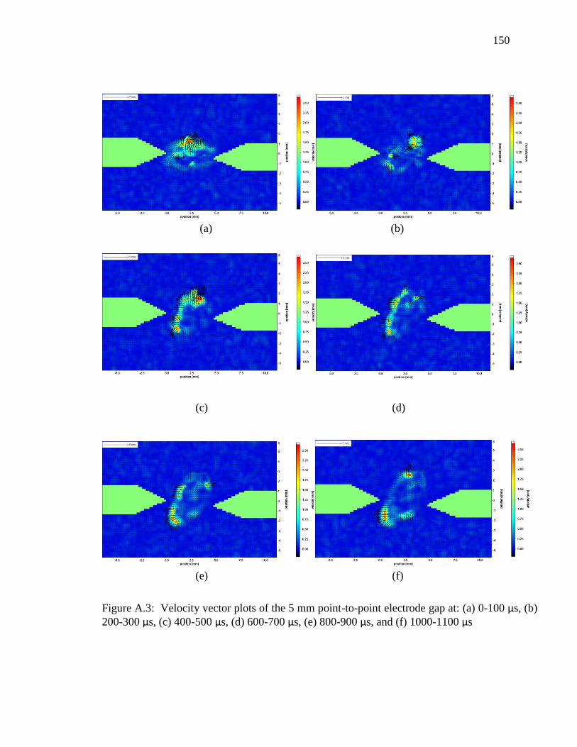
150
(a) (b)
(c) (d)
(e) (f)
Figure A.3: Velocity vector plots of the 5 mm point-to-point electrode gap at: (a) 0-100 μs, (b) 200-300 μs, (c) 400-500 μs, (d) 600-700 μs, (e) 800-900 μs, and (f) 1000-1100 μs
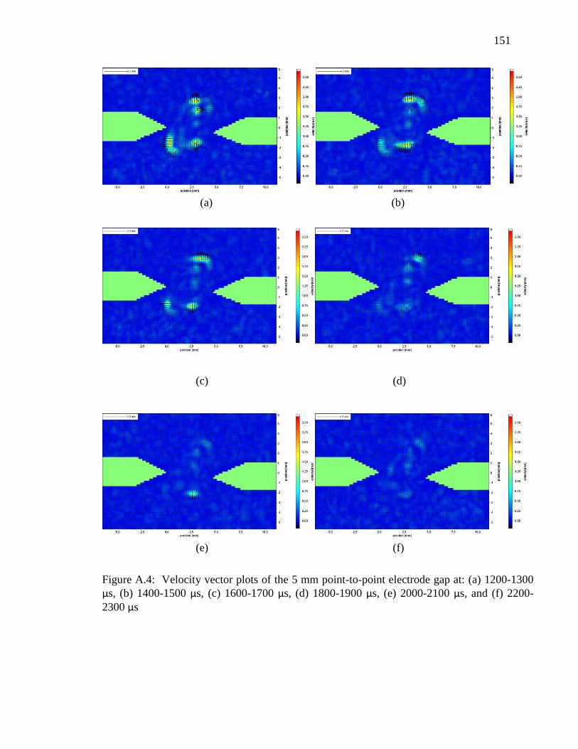
151
(a) (b)
(c) (d)
(e) (f)
Figure A.4: Velocity vector plots of the 5 mm point-to-point electrode gap at: (a) 1200-1300 μs, (b) 1400-1500 μs, (c) 1600-1700 μs, (d) 1800-1900 μs, (e) 2000-2100 μs, and (f) 2200-2300 μs
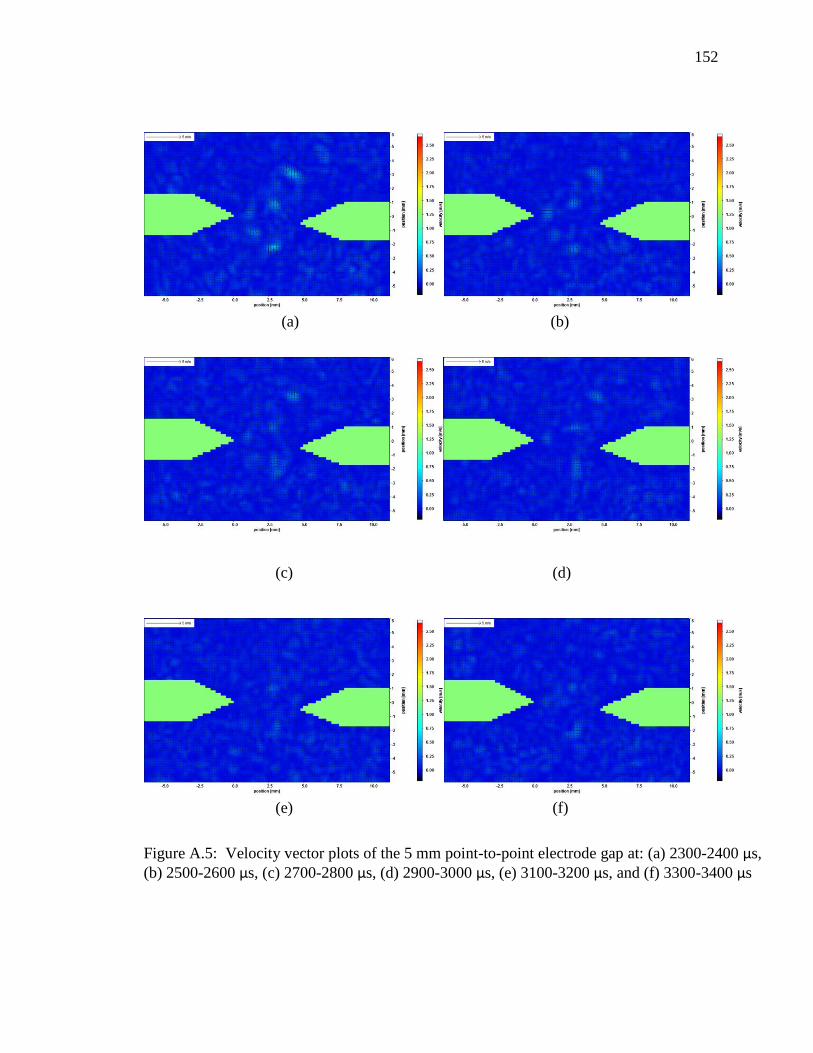
152
(a) (b)
(c) (d)
(e) (f)
Figure A.5: Velocity vector plots of the 5 mm point-to-point electrode gap at: (a) 2300-2400 μs, (b) 2500-2600 μs, (c) 2700-2800 μs, (d) 2900-3000 μs, (e) 3100-3200 μs, and (f) 3300-3400 μs
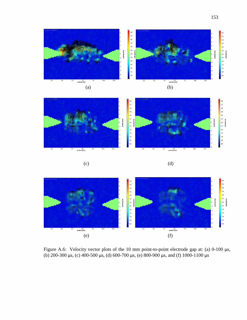
153
(a) (b)
(c) (d)
(e) (f)
Figure A.6: Velocity vector plots of the 10 mm point-to-point electrode gap at: (a) 0-100 μs, (b) 200-300 μs, (c) 400-500 μs, (d) 600-700 μs, (e) 800-900 μs, and (f) 1000-1100 μs

154
(a) (b)
(c) (d)
(e) (f)
Figure A.7: Velocity vector plots of the 10 mm point-to-point electrode gap at: (a) 1200-1300 μs, (b) 1400-1500 μs, (c) 1600-1700 μs, (d) 1800-1900 μs, (e) 2000-2100 μs, and (f) 2200-2300 μs,

155
(a) (b)
(c) (d)
(e) (f)
Figure A.8: Velocity vector plots of the 10 mm point-to-point electrode gap at: (a) 2300-2400 μs, (b) 2500-2600 μs, (c) 2700-2800 μs, (d) 2900-3000 μs, (e) 3100-3200 μs, and (f) 3300-3400 μs,

156
(a) (b)
(c) (d)
(e) (f)
Figure A.9: Velocity vector plots of the 2 mm flat-to-point electrode gap at: (a) 0-100 μs, (b) 200-300 μs, (c) 400-500 μs, (d) 600-700 μs, (e) 800-900 μs, and (f) 1000-1100 μs
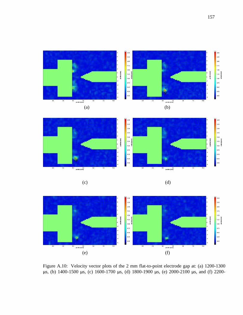
157
(a) (b)
(c) (d)
(e) (f)
Figure A.10: Velocity vector plots of the 2 mm flat-to-point electrode gap at: (a) 1200-1300 μs, (b) 1400-1500 μs, (c) 1600-1700 μs, (d) 1800-1900 μs, (e) 2000-2100 μs, and (f) 2200-2300 s,
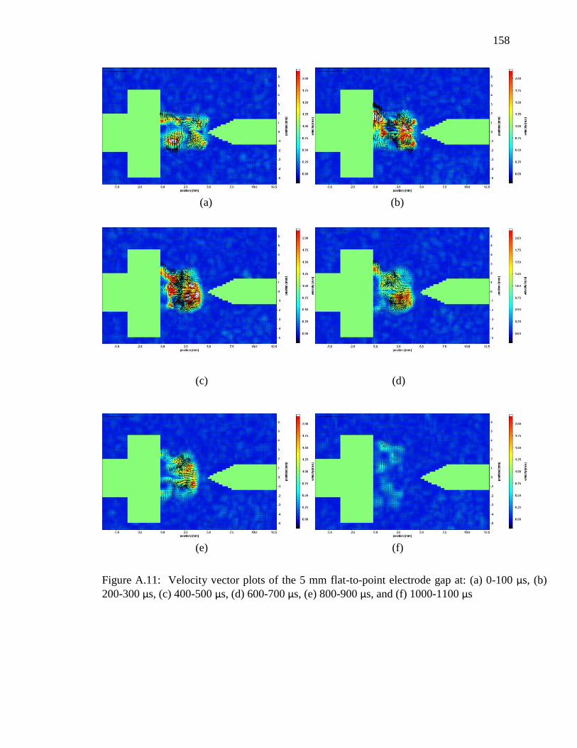
158
(a) (b)
(c) (d)
(e) (f)
Figure A.11: Velocity vector plots of the 5 mm flat-to-point electrode gap at: (a) 0-100 μs, (b) 200-300 μs, (c) 400-500 μs, (d) 600-700 μs, (e) 800-900 μs, and (f) 1000-1100 μs
s,
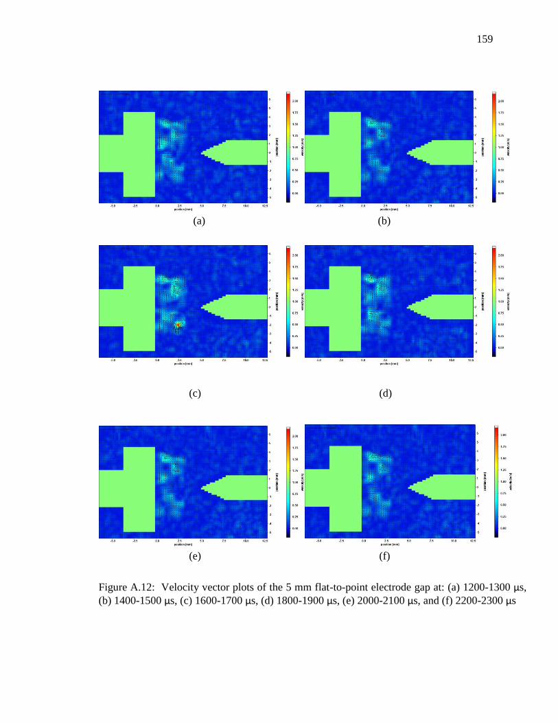
159
(a) (b)
(c) (d)
(e) (f)
Figure A.12: Velocity vector plots of the 5 mm flat-to-point electrode gap at: (a) 1200-1300 μs, (b) 1400-1500 μs, (c) 1600-1700 μs, (d) 1800-1900 μs, (e) 2000-2100 μs, and (f) 2200-2300 μs
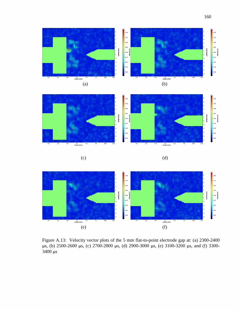
160
(a) (b)
(c) (d)
(e) (f)
Figure A.13: Velocity vector plots of the 5 mm flat-to-point electrode gap at: (a) 2300-2400 μs, (b) 2500-2600 μs, (c) 2700-2800 μs, (d) 2900-3000 μs, (e) 3100-3200 μs, and (f) 3300-3400 μs

161
(a) (b)
(c) (d)
(e) (f)
Figure A.14: Velocity vector plots of the 10 mm flat-to-point electrode gap at: (a) 0-100 μs, (b) 200-300 μs, (c) 400-500 μs, (d) 600-700 μs, (e) 800-900 μs, and (f) 1000-1100 μs

162
(a) (b)
(c) (d)
(e) (f)
Figure A.15: Velocity vector plots of the 10 mm flat-to-point electrode gap at: (a) 1200-1300 μs, (b) 1400-1500 μs, (c) 1600-1700 μs, (d) 1800-1900 μs, (e) 2000-2100 μs, and (f) 2200-2300 μs
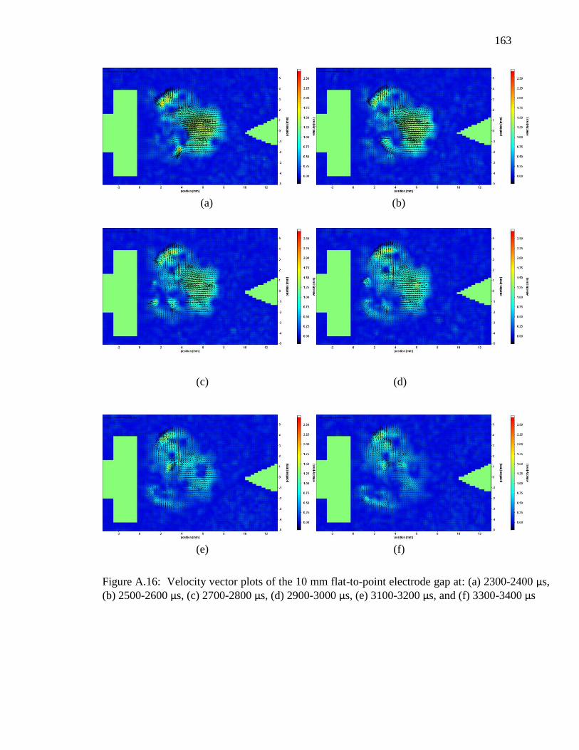
163
(a) (b)
(c) (d)
(e) (f)
Figure A.16: Velocity vector plots of the 10 mm flat-to-point electrode gap at: (a) 2300-2400 μs, (b) 2500-2600 μs, (c) 2700-2800 μs, (d) 2900-3000 μs, (e) 3100-3200 μs, and (f) 3300-3400 μs

164
(a) (b)
(c) (d)
(e) (f)
Figure A.17: Velocity vector plots of the 2 mm blunt-to-blunt electrode gap at: (a) 0-100 μs, (b) 200-300 μs, (c) 400-500 μs, (d) 600-700 μs, (e) 800-900 μs, and (f) 1000-1100 μs
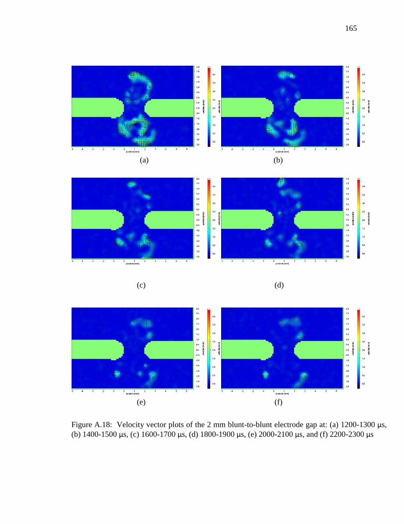
165
(a) (b)
(c) (d)
(e) (f)
Figure A.18: Velocity vector plots of the 2 mm blunt-to-blunt electrode gap at: (a) 1200-1300 μs, (b) 1400-1500 μs, (c) 1600-1700 μs, (d) 1800-1900 μs, (e) 2000-2100 μs, and (f) 2200-2300 μs
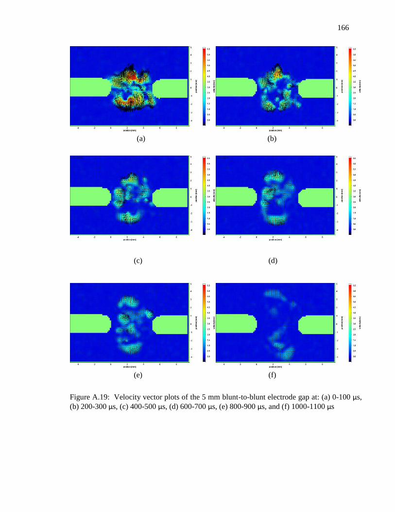
166
(a) (b)
(c) (d)
(e) (f)
Figure A.19: Velocity vector plots of the 5 mm blunt-to-blunt electrode gap at: (a) 0-100 μs, (b) 200-300 μs, (c) 400-500 μs, (d) 600-700 μs, (e) 800-900 μs, and (f) 1000-1100 μs

167
(a) (b)
(c) (d)
(e) (f)
Figure A.20: Velocity vector plots of the 5 mm blunt-to-blunt electrode gap at: (a) 1200-1300 μs, (b) 1400-1500 μs, (c) 1600-1700 μs, (d) 1800-1900 μs, (e) 2000-2100 μs, and (f) 2200-2300 μs
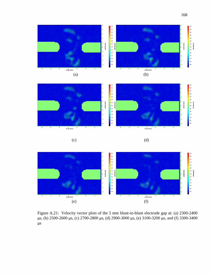
168
(a) (b)
(c) (d)
(e) (f)
Figure A.21: Velocity vector plots of the 5 mm blunt-to-blunt electrode gap at: (a) 2300-2400 μs, (b) 2500-2600 μs, (c) 2700-2800 μs, (d) 2900-3000 μs, (e) 3100-3200 μs, and (f) 3300-3400 μs
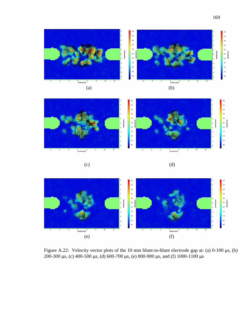
169
(a) (b)
(c) (d)
(e) (f)
Figure A.22: Velocity vector plots of the 10 mm blunt-to-blunt electrode gap at: (a) 0-100 μs, (b) 200-300 μs, (c) 400-500 μs, (d) 600-700 μs, (e) 800-900 μs, and (f) 1000-1100 μs

170
(a) (b)
(c) (d)
(e) (f)
Figure A.23: Velocity vector plots of the 10 mm blunt-to-blunt electrode gap at: (a) 1200-1300 μs, (b) 1400-1500 μs, (c) 1600-1700 μs, (d) 1800-1900 μs, (e) 2000-2100 μs, and (f) 2200-2300 μs
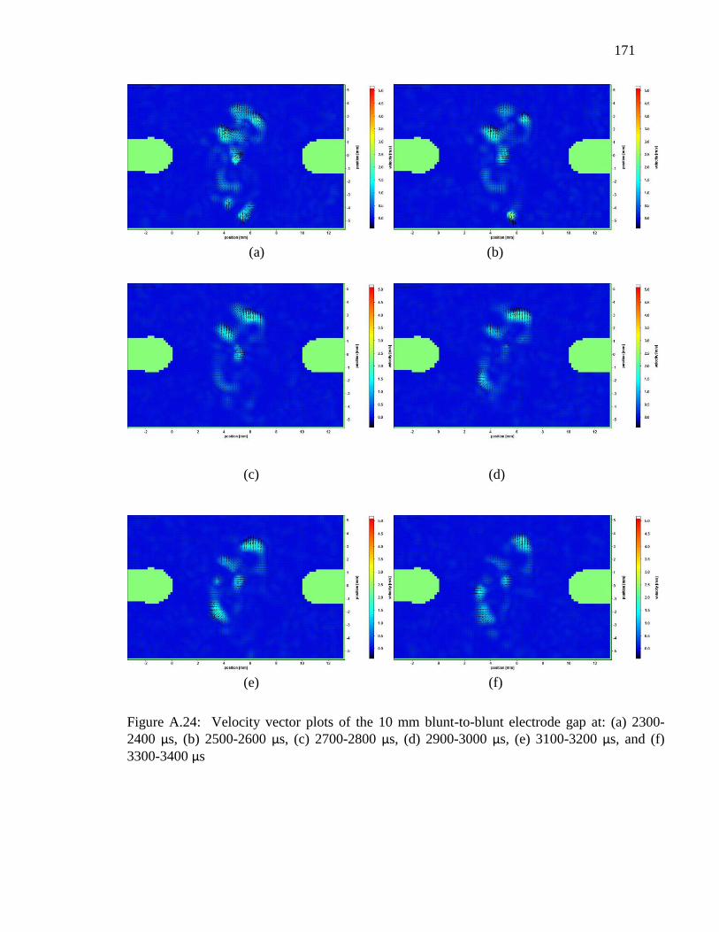
171
(a) (b)
(c) (d)
(e) (f)
Figure A.24: Velocity vector plots of the 10 mm blunt-to-blunt electrode gap at: (a) 2300-2400 μs, (b) 2500-2600 μs, (c) 2700-2800 μs, (d) 2900-3000 μs, (e) 3100-3200 μs, and (f) 3300-3400 μs

172
Appendix B Vorticity Contour Plots
(b) (b)
(d) (d)
(e) (f)
Figure B 1: Vorticity contour plots of the 5 mm point-to-point electrode gap at: (a) 0-100 μs, (b) 200-300 μs, (c) 400-500 μs, (d) 600-700 μs, (e) 800-900 μs, and (f) 1000-1100 μs
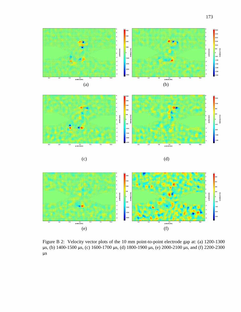
173
(a) (b)
(c) (d)
(e) (f)
Figure B 2: Velocity vector plots of the 10 mm point-to-point electrode gap at: (a) 1200-1300 μs, (b) 1400-1500 μs, (c) 1600-1700 μs, (d) 1800-1900 μs, (e) 2000-2100 μs, and (f) 2200-2300 μs

174
(a) (b)
(c) (d)
(e) (f)
Figure B 3: Vorticity contour plots of the 10 mm point-to-point electrode gap at: (a) 0-100 μs, (b) 200-300 μs, (c) 400-500 μs, (d) 600-700 μs, (e) 800-900 μs, and (f) 1000-1100 μs
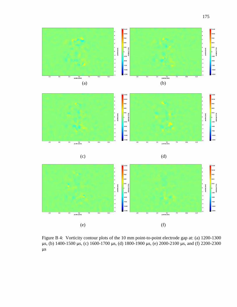
175
(a) (b)
(c) (d)
(e) (f)
Figure B 4: Vorticity contour plots of the 10 mm point-to-point electrode gap at: (a) 1200-1300 μs, (b) 1400-1500 μs, (c) 1600-1700 μs, (d) 1800-1900 μs, (e) 2000-2100 μs, and (f) 2200-2300 μs

176
(b) (b)
(c) (d)
(e) (f)
Figure B 5: Vorticity contour plots of the 2 mm flat-to-point electrode gap at: (a) 0-100 μs, (b) 200-300 μs, (c) 400-500 μs, (d) 600-700 μs, (e) 800-900 μs, and (f) 1000-1100 μs

177
(a) (b)
(c) (d)
(e) (f)
Figure B 6: Vorticity contour plots of the 2 mm flat-to-point electrode gap at: (a) 1200-1300 μs, (b) 1400-1500 μs, (c) 1600-1700 μs, (d) 1800-1900 μs, (e) 2000-2100 μs, and (f) 2200-2300 μs
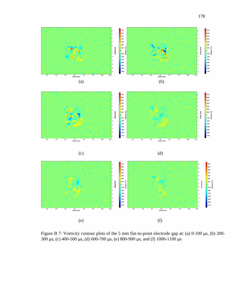
178
(a) (b)
(c) (d)
(e) (f)
Figure B 7: Vorticity contour plots of the 5 mm flat-to-point electrode gap at: (a) 0-100 μs, (b) 200-300 μs, (c) 400-500 μs, (d) 600-700 μs, (e) 800-900 μs, and (f) 1000-1100 μs
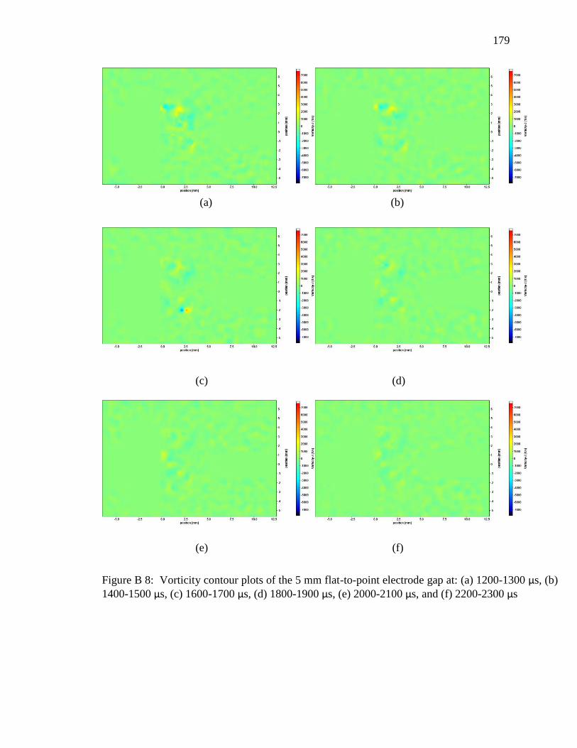
179
(a) (b)
(c) (d)
(e) (f)
Figure B 8: Vorticity contour plots of the 5 mm flat-to-point electrode gap at: (a) 1200-1300 μs, (b) 1400-1500 μs, (c) 1600-1700 μs, (d) 1800-1900 μs, (e) 2000-2100 μs, and (f) 2200-2300 μs
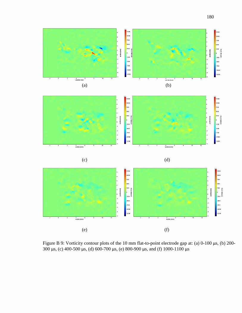
180
(a) (b)
(c) (d)
(e) (f)
Figure B 9: Vorticity contour plots of the 10 mm flat-to-point electrode gap at: (a) 0-100 μs, (b) 200-300 μs, (c) 400-500 μs, (d) 600-700 μs, (e) 800-900 μs, and (f) 1000-1100 μs
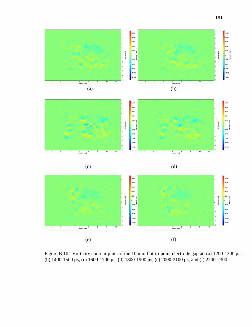
181
(a) (b)
(c) (d)
(e) (f)
Figure B 10: Vorticity contour plots of the 10 mm flat-to-point electrode gap at: (a) 1200-1300 μs, (b) 1400-1500 μs, (c) 1600-1700 μs, (d) 1800-1900 μs, (e) 2000-2100 μs, and (f) 2200-2300

182
(a) (b)
(c) (d)
(e) (f)
Figure B 11: Vorticity contour plots of the 10 mm flat-to-point electrode gap at: (a) 2300-2400 μs, (b) 2500-2600 μs, (c) 2700-2800 μs, (d) 2900-3000 μs, (e) 3100-3200 μs, and (f) 3300-3400 μs

183
(a) (b)
(c) (d)
(e) (f)
Figure B 12: Vorticity contour plots of the 2 mm blunt-to-blunt electrode gap at: (a) 0-100 μs, (b) 200-300 μs, (c) 400-500 μs, (d) 600-700 μs, (e) 800-900 μs, and (f) 1000-1100 μs
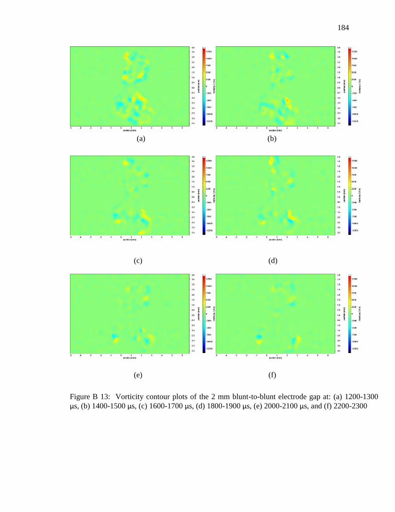
184
(a) (b)
(c) (d)
(e) (f)
Figure B 13: Vorticity contour plots of the 2 mm blunt-to-blunt electrode gap at: (a) 1200-1300 μs, (b) 1400-1500 μs, (c) 1600-1700 μs, (d) 1800-1900 μs, (e) 2000-2100 μs, and (f) 2200-2300
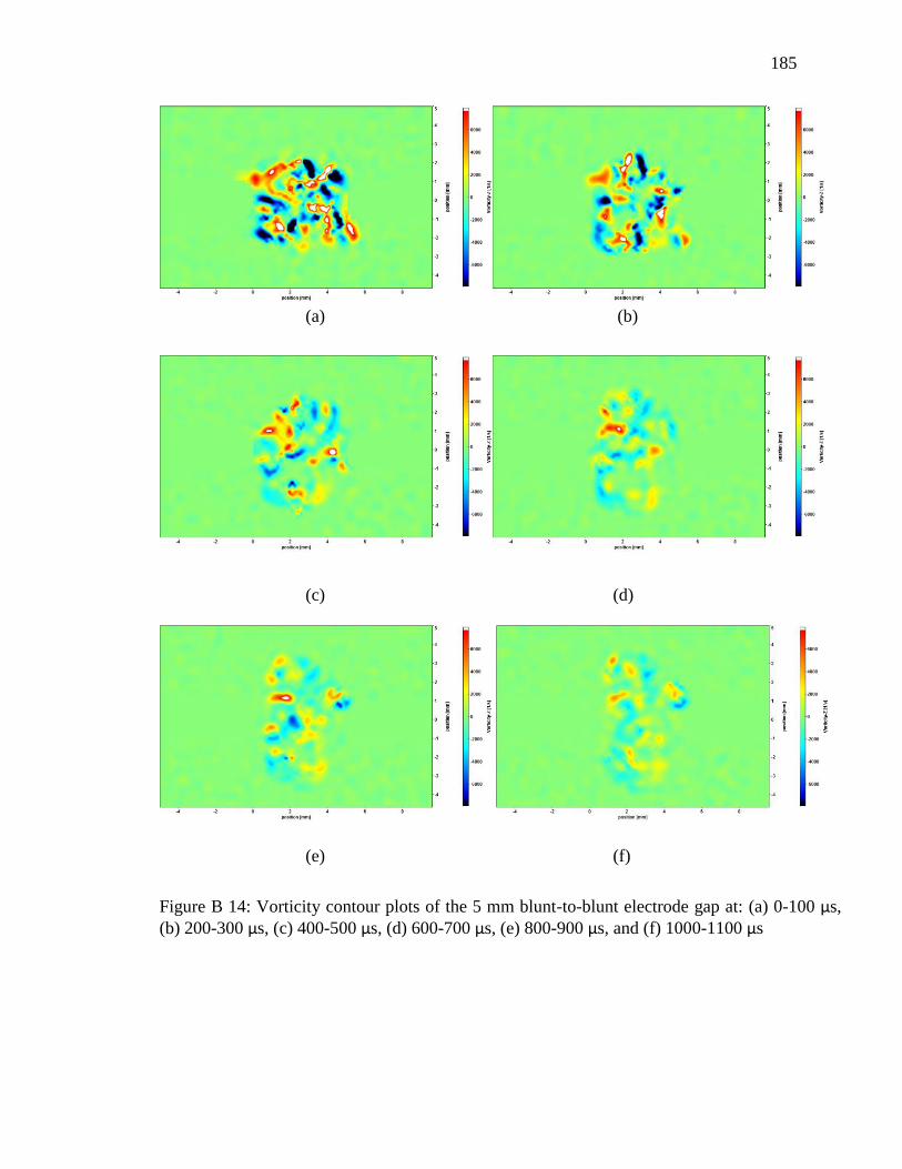
185
(a) (b)
(c) (d)
(e) (f)
Figure B 14: Vorticity contour plots of the 5 mm blunt-to-blunt electrode gap at: (a) 0-100 μs, (b) 200-300 μs, (c) 400-500 μs, (d) 600-700 μs, (e) 800-900 μs, and (f) 1000-1100 μs
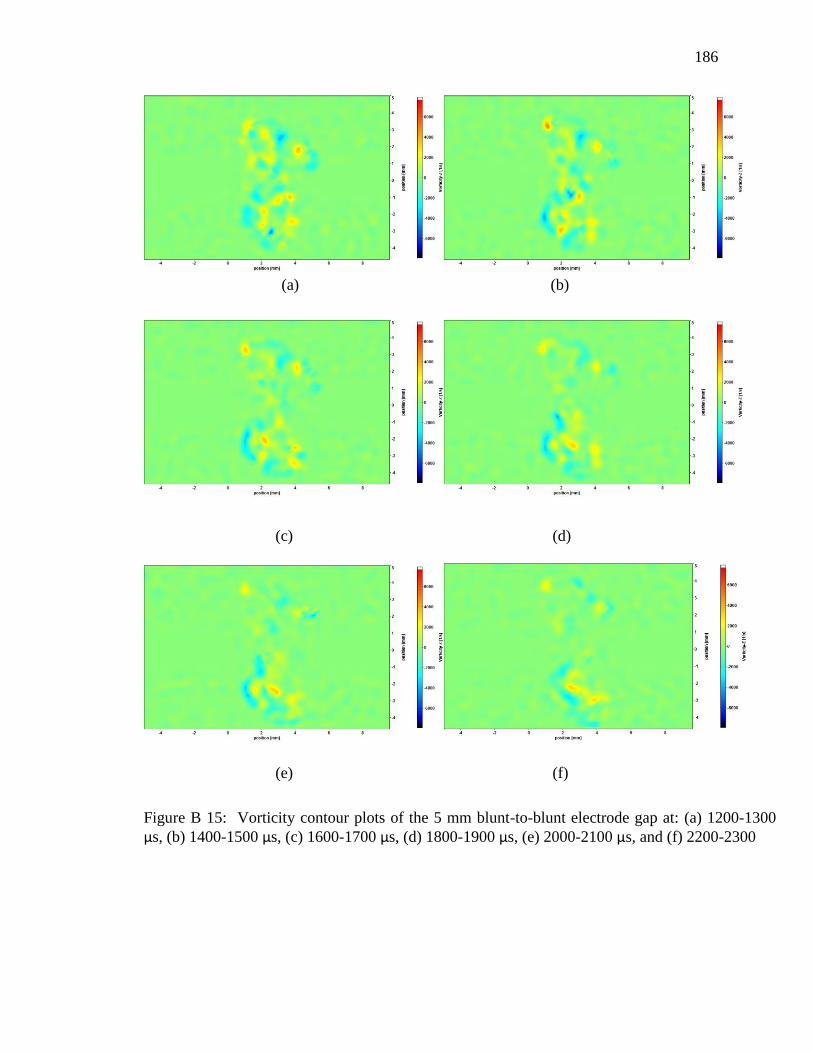
186
(a) (b)
(c) (d)
(e) (f)
Figure B 15: Vorticity contour plots of the 5 mm blunt-to-blunt electrode gap at: (a) 1200-1300 μs, (b) 1400-1500 μs, (c) 1600-1700 μs, (d) 1800-1900 μs, (e) 2000-2100 μs, and (f) 2200-2300
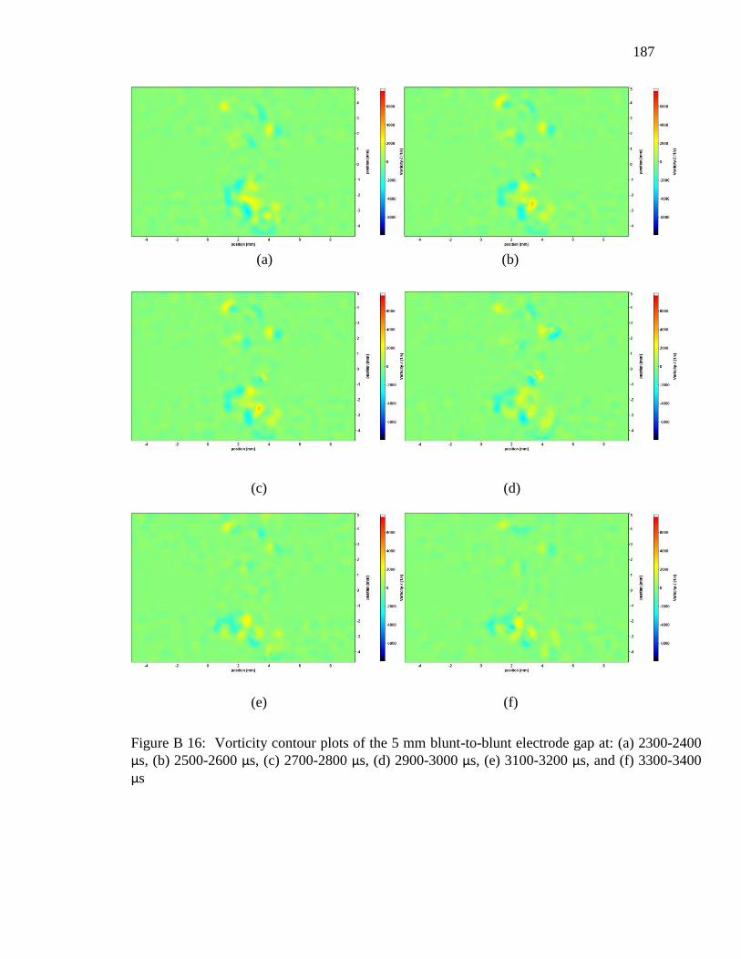
187
(a) (b)
(c) (d)
(e) (f)
Figure B 16: Vorticity contour plots of the 5 mm blunt-to-blunt electrode gap at: (a) 2300-2400 μs, (b) 2500-2600 μs, (c) 2700-2800 μs, (d) 2900-3000 μs, (e) 3100-3200 μs, and (f) 3300-3400 μs

188
(a) (b)
(c) (d)
(e) (f)
Figure B 17: Vorticity contour plots of the 10 mm blunt-to-blunt electrode gap at: (a) 0-100 μs, (b) 200-300 μs, (c) 400-500 μs, (d) 600-700 μs, (e) 800-900 μs, and (f) 1000-1100 μs
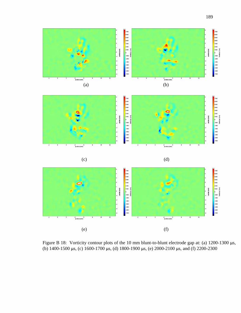
189
(a) (b)
(c) (d)
(e) (f)
Figure B 18: Vorticity contour plots of the 10 mm blunt-to-blunt electrode gap at: (a) 1200-1300 μs, (b) 1400-1500 μs, (c) 1600-1700 μs, (d) 1800-1900 μs, (e) 2000-2100 μs, and (f) 2200-2300

190
(a) (b)
(c) (d)
(e) (f)
Figure B 19: Vorticity contour plots of the 10 mm blunt-to-blunt electrode gap at: (a) 2300-2400 μs, (b) 2500-2600 μs, (c) 2700-2800 μs, (d) 2900-3000 μs, (e) 3100-3200 μs, and (f) 3300-3400 μs
μs