EFFECT OF SOCIO-ECONOMIC STRATIFICATION ON HOUSE VALUE IN BOGOTÁ

24/12/2016

N° 2016/19

EFFECT OF SOCIO-ECONOMIC STRATIFICATION ON HOUSE VALUE IN BOGOTÁ

Gallego, Juan Montoya, Sergio Sepúlveda, Carlos

2 EFFECT OF SOCIO-ECONOMIC STRATIFICATION ON HOUSE VALUE IN BOGOTÁ

EFFECT OF SOCIO-ECONOMIC STRATIFICATION ON

HOUSE VALUE IN BOGOTÁ

Gallego, Juan

Montoya, Sergio

Sepúlveda, Carlos

CAF – Working paper N° 2016/19

24/12/2016

ABSTRACT This paper investigates the impact of urban fiscal policies on housing value. We use a focalization system in Bogotá where certain subsidies and taxes are targeted based on a classification of houses according to external conditions and urban surroundings (socioeconomic stratification). We use a regression discontinuity design, and a rich dataset on cadastre appraisal and housing characteristics, to assess whether a higher tax burden affects the property value. Our results suggest that the usual (negative) capitalization effect is compensated by other channels. We show evidence that as stratum increases, investment on the house maintenance improve. Small sections of text, that are less than two paragraphs, may be quoted without explicit permission as long as this document is stated. Findings, interpretations and conclusions expressed in this publication are the sole responsibility of its author(s), and it cannot be, in any way, attributed to CAF, its Executive Directors or the countries they represent. CAF does not guarantee the accuracy of the data included in this publication and is not, in any way, responsible for any consequences resulting from its use. © 2016 Corporación Andina de Fomento

3 EFFECT OF SOCIO-ECONOMIC STRATIFICATION ON HOUSE VALUE IN BOGOTÁ

EL EFECTO DE LA ESTRATIFICACIÓN SOCIO-

ECONÓMICA SOBRE EL VALOR DE LA VIVIENDA EN

BOGOTÁ

Gallego, Juan

Montoya, Sergio

Sepúlveda, Carlos

CAF - Documento de trabajo N° 2016/19

24/12/2016

RESUMEN

Este artículo investiga cómo el diseño de políticas fiscales urbanas afecta el valor de la vivienda. Estudiamos el caso de la ciudad de Bogotá, donde la tarifa de diversos impuestos y subsidios varía de acuerdo a un sistema de focalización que agrupa las viviendas según sus condiciones exteriores y su entorno urbano (estratificación socioeconómica). Usamos un diseño de regresión discontinua, y una completa base datos de avalúos catastrales y características de las viviendas, para establecer cómo una mayor carga fiscal afecta el valor de la propiedad. Nuestros resultados sugieren que la capitalización del impuesto, que debería generar menores valores de la vivienda, se ve compensada por otros canales. Presentamos evidencia de que uno de estos es que los propietarios reaccionan a la clasificación en estratos altos con mayor inversión en conservación de la vivienda. Small sections of text, that are less than two paragraphs, may be quoted without explicit permission as long as this document is stated. Findings, interpretations and conclusions expressed in this publication are the sole responsibility of its author(s), and it cannot be, in any way, attributed to CAF, its Executive Directors or the countries they represent. CAF does not guarantee the accuracy of the data included in this publication and is not, in any way, responsible for any consequences resulting from its use. © 2016 Corporación Andina de Fomento

Effect of socio-economic stratification on house valuein Bogota∗

Final Report

Juan Gallego† Sergio Montoya‡ Carlos Sepulveda§

December 24, 2016

1 Introduction

Capitalization of fiscal policies on housing prices is a central question in urban andpublic economics. Taxes affecting housing markets can distort different household de-cisions, through channels (and magnitude of impact) depending on the structure andscope of these policies. Housing prices can be altered, for instance, by decisions toinvest on the house (property materials); or household mobility to run away (or lookfor) taxes (or subsidies); or neighborhood spillover effects (public goods provision andhabitat investment); or efficiency on the provision of specific public goods. Such chan-nels emerge from the taxes design and their scope, as they can be focused con housingincome, property taxes, or transaction costs (Bergantino et al., 2013; Gould, 2008; BCE,2003; Oates, 1969).

We use a unique focalization system in Colombia where subsidies and taxes onutilities are targeted based on dwelling external conditions and habitat surroundings.All houses are classified in six groups called stratums; the lower ones (1, 2 and 3)received subsidies on the utilities bill (at a decreasing rate) and the higher (5 and 6)are affected by a consumption tax (at an increasing rate). This stratification has alsoan impact on property taxes. From this classification and a rich data set on cadastre,dwelling quality, urban context and appraisal value, we study the aggregate impact of

∗This document constitutes the Final Report to the CAF research project on Habitat and UrbanDevelopment. We thank Pablo Sanguineti, Dolores de la Mata, Juan Vargas and all participants at theCAF meeting held in Buenos Aires in March 2016 for insightful comments. We thank the SecretarıaDistrital de Planeacion in Bogota, for data and technical support, particularly Ariel Carrero and MariaEsperanza Corredor.†Department of Economics, Universidad del Rosario, Bogota-Colombia‡Department of Economics, Universidad del Rosario, Bogota-Colombia§Department of Economics, Universidad del Rosario, Bogota-Colombia

1

such tax policy on housing prices in Bogota, and explore possible channels that mighttake into place.

The “socioeconomic stratification”, targeting houses instead of families, might gen-erate significant distortion on housing values. The potential buyer of a house with ahigh classification in the stratification scale would expect higher future expendituresin public utilities, and some portion of this future flow of contributions is expectedto be subtracted from the selling or rental price, unless there is a completely inelasticsupply. On the other hand, houses with lower strata are favored with subsidies onutility payments that could also be anticipated and capitalized, with a positive impacton their prices. Since every sequential increase in strata means a decrease in subsidiesor an increase in contributions, the effect of the capitalization would be the reductionof values for every strata addition.

The traditional explanation ignores the possibility of second order effects. Builders,for instance, can shift up markets (Ihlanfeldt, 2007), increasing the quality of housing totarget a population less interested in subsidies. If the price-elasticity of demand is higherfor better quality houses, it would be easier to transfer the value of the contribution tothe buyer (or renter). In this scenario, given the lower capitalization and the increasein quality, the housing value could actually rise.

From a different perspective, there could be negative incentives to quality differ-entiation among strata. Lower strata residents could prevent urban improvements toreduce the risk of reclassification. Since the size of the subsidy/contribution is linked tothe consumption of public utility services, and its weigth on total expenditure decreasesas stratum rises, the relevance of the subsidy for lower groups would be significant togenerate (negative) spillover on the neighborhood.

We use a Regression Discontinuity Design (RDD) that exploits the threshold be-tween two different strata with similar score on the continuous variable that ranks thecharacteristics of each house in a low and high stratum. Through a hedonic pricingmodel, we are able to find positive effects of taxes on housing prices, which would sug-gest that the usual (negative) capitalization effect is compensated by other channels.We show evidence that as stratum increases (higher taxes), investment on the housematerials improve.

2 Conceptual Framework

This paper is related to the literature on tax capitalization of local government pro-grams. The seminal work of Tiebout (1956) hypothesized that property taxes shouldbe capitalized, i.e., that the houses’ values should decline with higher tax rates. Anal-ogously, bigger local spending should increase property values. Around the local provi-sion of public education on the U.S., Oates (1969) and Rosen and Fullerton (1977) findpartial or closer to complete capitalization of public spending on housing values. Insame line, Bergantino et al. (2013) show evidence of parcial capitalization of efficiencyimprovement in the local government for Italy.

2

One empirical challenge is to disentangle the effect of tax capitalization from theimpact of local services financed by those taxes. From a natural experiment in Cali-fornia, Rosen (1982) estimates direct and positive taxes capitalization effects of a taxcut on land values. Lang and Jian (2004) used a change in state level regulation inMassachusetts that limits the capacity of municipalities to raise property taxes. Theyfound that the communities that could increase more rapidly his property tax rate alsosaw rapid increases in property values. However, they were not able to isolate thesecond order effect that the restrictions on property taxing has on expenditure and onother taxes.

Bai et al. (2014) uses counterfactual analysis to assess the impact of trial propertytaxes in Chongqing and Shanghai. They found that new taxes increased the growthin property prices in Chongqing, but decreased it in Shanghai. The later result iscoherent with the capitalization hypothesis. The former is explained by the tax design:only high-end houses (single family’s) were subject to taxes and a part of the propertywas excluded from the them. Therefore, people willing to buy high-end houses beforethe tax implementation could change their minds and buy at the low-end distributionto avoid the tax. In the same direction, they could look for a property smaller thanthe tax-except size. These changes in demand can decrease the growth at the high-endprices and rise it at the low end. If the second effect dominates, the overall effect is afaster overall growth of prices. Du and Zhang (2015) uses the same natural experimentwith a different identification strategy. They found no significant impact on propertyprices in Shanghai, with a low proportion of taxable homes. In Chongqing the presenceof a trial property tax reduced the growth in property prices.

Another empirical methodology that takes advantage of Tiebout framework is re-lated with the implementation of hedonic price models (Bergantino et al., 2013). Ih-lanfeldt (2007) studied the effect of land regulations on property prices. These regu-lations increase the cost of building, and are partially incorporated in housing prices.But, additionally, the house size in zones with heavier regulations is greater –Buildersshift up the market. The explanation is that elasticity of demand decreases with housesize, so the higher cost are more easy to transfer to the buyer.

A few efforts in Colombia try to explore the relationship between taxes and housingprices. Medina and Morales (2007) start with a similar question than ours for 2003data, and found greater housing prices for subsidized strata compared with similarhomes in unsubsidized ones, by an amount they considered almost full capitalizationof the present value of future subsidies. However, their empirical approach does nottake into account urban characteristics of Bogota and the presence of micro-segregation(Aliaga and Alvarez, 2010), having a transition between different socioeconomic levelsnot smooth around the city. More recently, Casas (2014) studies the impact of subsi-dies for energy consumption on the demand for rental housing in Bogota in 2003 andfound an effect on housing size demand, which is interpreted as a signal distortion thatsubsidies impose on the rental market.

3

3 Data and identification strategy

3.1 Data

The data comes from the Special Administrative Department of City Real State Ap-praisal in Bogota (UAECD for its acronym in Spanish), the office in charge of realestate appraisal used for the land property tax, and the District Planning Department(SDP for its acronym in Spanish), in charge of stratification. The UAECD’s datasetfor 2012 contains the inputs to estimate property values, such as location, land use,size of the property, built area, and materials and condition of the facade, ceilings,floors, kitchen and bathroom, among others. They also provide estimations of land andstructure values per square meter, with which the total appraisal value of the propertyis estimated. We include in our sample only the dwellings that are zoned by the city’sland authority for residential use. Table 1 presents the mean land, structure and totalappraisal values1 per m2 for each strata. It is evident that higher strata are associatedwith higher property values, as expected.

Table 1: Mean land, building and appraisal value per m2 by strata

Stratum Land Structures Appraisal

1 273 146 1202 577 321 3583 844 466 6004 1,251 809 9755 1,378 838 1,2536 1,663 963 1,730Total 1,075 575 751

Source: Own calculations, UAECD

The dependent variables are the property values (land, structure and total), whichdetermine the amount of the property tax, and are meant to resemble market prices. Inthe UAECD’s method, first, a sample of different points in the city is selected. Then,expert appraisers are sent to assess the land and structures. Later, those assessmentsare matched with the information the UAECD have about houses’ and neighborhoods’characteristics to run hedonic price models. Subsequently, the models fitted for thissample are applied to the whole universe of houses in Bogota, in order to get predictedvalues (the total appraisal value is the sum of both land and structure). There is a draw-back: the stratification itself is included in the prediction models. We run estimationswith a different set of structure and total appraisal values, calculated by Gallego et al.(2014), with the same data and methodology as the UAECD, but excluding stratifica-tion as explicative variable in the appraisal model. Most of our results are qualitativelysimilar with or without this adjustment.

1Appraisal value per m2 is computed as total appraisal value of the property divided by the builtarea.

4

The second set of data is the one with which the SDP makes the strata assignment.It contains information about exterior physical characteristics of the houses in each sideof each block with buildings in the city. Each block is classified in ’habitat zones’, whichare areas with homogeneous urban characteristics. The dataset is for 1997, when thecurrent model of stratification was first applied, and 2009, where the strata classificationin force in 2011 was issued. Figure 1 shows the spatial distribution of strata and habitatzones in Bogota. There is a lot of concentration in both cases. Most of the blocks inthe lowest strata are in the south and the west of the city, whilst more of the blocks inthe highest strata are in the north-east of the city. The same applies to habitat zones(there is an ordering in the codification of habitat zones, being 1 the neighborhoodsassociated with poverty, and 17 the low-density residential zones; 18 to 20 are blockswith green areas, institutional buildings or unbuilt, see table A3)

Figure 1: Stratification and ’habitat zones’ in Bogota

(a) Spatial distribution of ’Habitat zones’ (b) Stratification in Bogota – 2015

3.2 Identification strategy

Stratification and assignment method

The stratification model applied in Bogota assumes that the quality of housing is agood proxy for household’s permanent income. Because of considerations of ease in

5

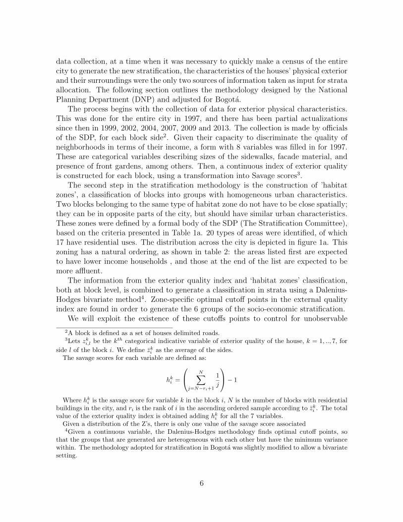
data collection, at a time when it was necessary to quickly make a census of the entirecity to generate the new stratification, the characteristics of the houses’ physical exteriorand their surroundings were the only two sources of information taken as input for strataallocation. The following section outlines the methodology designed by the NationalPlanning Department (DNP) and adjusted for Bogota.

The process begins with the collection of data for exterior physical characteristics.This was done for the entire city in 1997, and there has been partial actualizationssince then in 1999, 2002, 2004, 2007, 2009 and 2013. The collection is made by officialsof the SDP, for each block side2. Given their capacity to discriminate the quality ofneighborhoods in terms of their income, a form with 8 variables was filled in for 1997.These are categorical variables describing sizes of the sidewalks, facade material, andpresence of front gardens, among others. Then, a continuous index of exterior qualityis constructed for each block, using a transformation into Savage scores3.

The second step in the stratification methodology is the construction of ’habitatzones’, a classification of blocks into groups with homogeneous urban characteristics.Two blocks belonging to the same type of habitat zone do not have to be close spatially;they can be in opposite parts of the city, but should have similar urban characteristics.These zones were defined by a formal body of the SDP (The Stratification Committee),based on the criteria presented in Table 1a. 20 types of areas were identified, of which17 have residential uses. The distribution across the city is depicted in figure 1a. Thiszoning has a natural ordering, as shown in table 2: the areas listed first are expectedto have lower income households , and those at the end of the list are expected to bemore affluent.

The information from the exterior quality index and ‘habitat zones’ classification,both at block level, is combined to generate a classification in strata using a Dalenius-Hodges bivariate method4. Zone-specific optimal cutoff points in the external qualityindex are found in order to generate the 6 groups of the socio-economic stratification.

We will exploit the existence of these cutoffs points to control for unobservable

2A block is defined as a set of houses delimited roads.3Lets zki,l be the kth categorical indicative variable of exterior quality of the house, k = 1, .., 7, for

side l of the block i. We define zki as the average of the sides.The savage scores for each variable are defined as:

hki =

N∑j=N−ri+1

1

j

− 1

Where hki is the savage score for variable k in the block i, N is the number of blocks with residential

buildings in the city, and ri is the rank of i in the ascending ordered sample according to zki . The totalvalue of the exterior quality index is obtained adding hk

i for all the 7 variables.Given a distribution of the Z’s, there is only one value of the savage score associated4Given a continuous variable, the Dalenius-Hodges methodology finds optimal cutoff points, so

that the groups that are generated are heterogeneous with each other but have the minimum variancewithin. The methodology adopted for stratification in Bogota was slightly modified to allow a bivariatesetting.

6

variables when estimating the effect of stratification on housing prices. Two housesmay have very similar values in the exterior quality index, but lie on different sidesof the cutting point (at arbitrarily short distances). Each house will be classified indifferent strata, with impact on subsidies and taxation5. Imagine two houses withsimilar surroundings, with the same zoning (‘consolidate residential’, for example), butone was classified in stratum 3 and the other in 4. The first will receive a subsidy in thetariff for public utilities, while second will pay the cost-recovery price. Additionally,stratification in Bogota functions as a signal of quality of housing and neighborhood.These two situations generate opposite effects on the demand for each house, with anunclear result for prices. However, the jump in the stratum assignment allows us to usea regression discontinuity design (RDD) to identify the total effect. In this environment,the treatment would be being in a higher stratum compared to the stratum immediatelybelow, and the running variable would be the exterior quality index.

Empirical model

The main challenge for the identification of the impact of socio-economic stratificationon housing prices is unobserved heterogeneity. On the one hand, a family with highincome is expected to buy or rent a house with characteristics that simultaneouslygenerates a high price and a high stratum, so we will observe a positive correlationbetween stratification and housing prices. Some of these characteristics of the houseare easily observed, like the exterior features of the houses in the block (from thestratification census) or the construction characteristics of the house (from the cadasterdatabase). But some other characteristics are not equally easy to observe, especiallythose related to the interior of the house or subjective assessments of the quality of theneighborhood.

On the other hand, the stratification is a focalization mechanism of many publicprograms. Among others, families living in a house classified in strata 1, 2 or 3 canaccess to subsidies on public services payments; one living in stratum 4 pays the cost-recovery price; and one living in strata 5 or 6 pays an additional contribution to financethe subsidies of the lower strata. Given that this flow of subsidies or contributions canbe anticipated by the seller and the buyer (since the stratification of a house rarelychanges), or the lessee and the lessor, this would likely affect the market prices.

We are interested in the possible distorting effect of attaching the focalization mech-anism to the house, instead of attaching it to the household. But we need a way to con-trol for the unobserved heterogeneity affecting the prices. As described in the previoussection, the allocation mechanism for stratification suggests the possibility of applyinga regression discontinuity design (RDD). The assignment mechanism uses a continuousvariable, the exterior quality index, which determines the allocation of strata by the

5Table A4 presents the percentage of the full tariff that is paid by each household in each stratumwith respect to the neutral stratum (stratum 4) in the different utilities (water/sewerage, gas andenergy). The table discriminates by fixed tariff and variable tariff. The strata-specific tariffs forproperty tax are presented in table A5

7

definition of intervals –specific to each habitat zone– corresponding to each stratum.The cutoff points defining these intervals come to be a discontinuity in the allocation:around them there will be houses that obtained a similar score, but were classified indifferent strata. Our identification strategy will be a hedonic prices model with regres-sion discontinuity design. The scale of 6 strata generates 5 discontinuities that can beanalyzed.

For each block in the city we observe its classification in one of the 17 types ofhabitat zones, z, and the values of the exterior quality index, hz. The discontinuitieswill be defined for each pair of consecutive strata l ∈ {(1, 2), (2, 3), (3, 4), (3, 5), (5, 6)}and each type of habitat zone z. In this way we would be comparing the price of homeswith similar external physical characteristics belonging to urban areas with the samecharacteristics.

For each strata pair l we can define the treatment variable as:

Dl,i =

{1 si hi ≥ hl,z

0 si hi < hl,z

Where Dl,i is equal to 1 if the house i exceeds the threshold hl,z required to beranked in the upper stratum within the pair l in the habitat zone z, and 0 otherwise(e.g. for the pair (3,4), Dl,i = 1 if the house is stratum 4 and Dl,i = 0 if the house is instratum 3).

Our reduced form for the house value, specific to each pair l, will be:

Vi = α +Xiβ + f(hi) + dziλ+Dl,iφ+ εi (1)

For all i such that |hi − hl,z| ≤ ε

Where Vi is the housing value; Xi is a vector of house characteristics; F () is apolynomial of order n of the running variable hi; d

zi is a set of fixed effects by habitat

zone; ε is a bandwidth that ensures that houses in both side of the threshold arecomparable; and φ is our parameter of interest, which captures the distorting effect ofstratification.

Identification rests on two assumptions:

• Subsidies, signaling and segregation effects change discontinuously in the cutoffs,which is granted by the design of the allocation mechanism.

• The characteristics of housing, and households living in them, do not jump in thecutoffs. That is, for sufficiently close intervals around the cutoffs, it is possible toassume that the houses are similar and comparable.

Discontinuity in strata assignment

To avoid manipulation of the strata assignment, both by the households or by the localauthorities, the values of the exterior quality index, the exact formula to aggregate the

8

7 exterior quality variables into the index and the intervals defining each stratum ineach zone (and therefore the cutoff points) are not posted nor recorded, and not evenobserved by the SDP, the public office in charge of stratification. The officials in SDPenter the raw data (exterior quality variables and zonification) in an encrypted softwarethat only reports the final strata assignment by block. Therefore, we had to recoverthe formula by replicating the methodology used in 1997 (savage score transformation)with the data they used to calibrate the formula (the database of Bogota’s decree 009of 1997). We used the actual final strata assignment to locate the cutoffs. With theaggregation formula and the cutoffs recovered in this way we were able to replicate the1997 stratification in 99.91% of the cases.

Since 1997 there has been six actualization to the strata classification in Bogota6,made with the purpose of taking into account the changes in the predominant featuresof some blocks and include neighborhoods recently developed. We observe land pricesin 2011, so we should use the stratification in force in that time, corresponding to theactualization made in 2009. We can only observe the value of the exterior quality indexin 1997, but most blocks haven’t been part of any of the actualization so far. In fact,60% of the blocks in the 2009 dataset haven’t been affected by any actualization. Thisis the sample we will be able to use in our estimation.

Table 2: Strata by ’habitat zone’

Zone Stratum1 2 3 4 5 6 Total

1 173 0 0 0 0 0 1732 3,783 52 0 0 0 0 3,8353 0 29 0 0 0 0 294 0 3,864 0 0 0 0 3,8645 0 7,249 0 0 0 0 7,2496 0 144 0 0 0 0 1447 0 28 117 0 0 0 1458 0 264 2,961 0 0 0 3,2259 0 7 6,467 0 0 0 6,47410 0 11 694 0 0 0 70511 0 0 233 0 0 0 23312 0 0 14 425 0 0 43913 0 0 8 1,449 0 0 1,45714 0 0 0 0 37 0 3715 0 0 0 103 751 0 85416 0 0 0 0 46 557 60317 0 0 1 2 11 108 122Total 3,956 11,648 10,495 1,979 845 665 29,588

The strata assignment is the result of both the exterior quality index and the ’habitat

6In 1999, 2002, 2004, 2007, 2009 and 2013.

9

zone’ classification, and the later is the most influential variable of the two. As shownin table 2, being classified in certain habitat zones almost determines the final strataallocation. For instance, all blocks in zone 1 are classified in stratum 1, and all blockin zone 14 are classified in stratum 5 (see table A3 in the apedix for the descriptionsof the zones). This also implies that we will have observations near the cutoff point forspecific combinations of strata changes and zones. In particular:

• For the change form stratum 1 to 2, we only will observe properties in zone 2,associated with poverty.

• For the change from stratum 2 to 3 we will observe properties in zones 7, 8, 9 and10, associated with industrial areas and neighborhood of consolidated progressivedevelopment.

• For the change from stratum 3 to 4 we will observe properties in zones 12 and 13,associated with intermediate residential neighborhoods.

• For the changes from stratum 4 to 5 and 5 to 6, we will observe only properties inzones 15 and 17, which are exclusive residential or low-density residential zones.

Although the methodology adopted for stratification in Bogota allowed for multiplethreshold points for each strata transition, depending on the habitat zone, in practicethe thresholds coincide within each strata transition7. This will allow us to avoidtransformations in the running variable for the RDD. There is, however, an additionalissue with the discontinuities: the density surrounding the threshold for the stratatransitions 1 to 2 is not enough to make a appropriate estimation.

4 Results

4.1 Basic results

Table 3 presents the RD estimates of the effect of an stratum increase on housing valua-tions. With six groups in the stratification in Bogota, we analyze five strata transitions.Since the boundary between strata is determined by specific conditions in terms of ex-ternal quality index and membership of certain habitat zones, we have no prior reasonto assume that the effect is homogeneous between different strata. Additionally, eachstratum is different in terms of the magnitude of the subsidy/contribution assigned,and an upward reclassification would imply different increases in the fare paid for pub-lic utilities. The income of the families living in different strata is also different, so thesubsidy/contribution would affect differentially the housing demand. Because of theseconsiderations, we present estimation separately for four counterfactual strata transi-tions. The first strata transition, from 1 to 2, was excluded from the analysis becausethere was not enough observations to carry on the analysis.

7This is not a coincidence, but a consequence of the discrete nature of the Dalenius-Hodges method-ology an its adaptation for stratification in Bogota

10

Figure 2: Location of blocks used for RDD

Table 3: RDD estimates on housing values

Appraisal Land Structure ObservationsJump 2 to 3 0.170*** 0.191*** 0.148*** (Left=3252)

(0.035) (0.059) (0.033) (Right=8575)Jump 3 to 4 0.176** 0.678*** 0.363*** (Left=1432)

(0.075) (0.194) (0.119) (Right=3514)Jump 4 to 5 0.256*** 0.240* 0.331*** (Left=4139)

(0.069) (0.138) (0.072) (Right=2475)Jump 5 to 6 -0.031 -0.170 0.098 (Left=1199)

(0.065) (0.212) (0.107) (Right=964)

Standard errors in parentheses, *** p<0.01, ** p<0.05, * p<0.1.Jumtp 2 to 3: Cutoff is -2.155. Optimal bandwidth is 0.601.Blocks tothe left of the BW: 99. Blocks to the right of the BW: 343.Jumtp 3 to 4: Cutoff is 3.019. Optimal bandwidth is 1.295.Blocks tothe left of the BW: 14. Blocks to the right of the BW: 75.Jumtp 4 to 5: Cutoff is 8.216. Optimal bandwidth is 0.646.Blocks tothe left of the BW: 42. Blocks to the right of the BW: 60.Jumtp 5 to 6: Cutoff is 15.210. Optimal bandwidth is 0.528.Blocks tothe left of the BW: 15. Blocks to the right of the BW: 15.

11

We find significant and positives effects of an upward strata reclassification. Thefirst row of table 3 shows that a house in stratum 3 would cost 17% more per squaremeter of building than a similar one in stratum 2. This effect can be decomposed in a19% increase in land value, and a 15% increase in structures value. For the jump fromstratum 3 to 4 we observe similar increases in the appraisal value; a house in stratum4 would cost 18% more per square meter of construction, the structures would cost36% more, and the land would cost almost 68% more. An upward reclassification ofa property in stratum 4 would increase the property value per built square meter inabout 26% and the structures value in 33%; the land value per square meter wouldincrease in 24%, but only statistic significant at 10 %. In the transition from stratum5 to stratum 6 we found a decrease in value, the results are somehow negative, but nosignificantly different from zero, which means that a reclassification to stratum 6 wouldneither increase or decrease the housing value.

Comparing the changes in along the strata, we can see some important effects. Bothlowering subsidies and having (or) increasing contributions have positive final effect onhousing values. This shows the significant impact of indirect effects of taxes. The effectin lower stratums (2 to 3) is smaller than other transitions (i.e. 3 to 4 or 4 to 5). Thepotential explanation for this effect is based in the fact that the monetary value ofsubsidies on water, sewage and energy represents around 7% in stratum 1 and 3.5% instratum 2 from the family income. In this sense the direct (and negative) effects of taxeson house value should be higher impact for households in low socioeconomic strata. Inaddition, a direct (an negative) effect of increasing taxes might be important as well onhigher stratums (5 to 6) since the aggregate change in prices is non-significant. As thetaxes on electricity and on gas consumption are the same for both stratums, this resultmight be driven by house taxes or water sewage’s contributions. In particular propertytaxes as percentage of family income are higher at stratum 6 than 58.

An additional result worth highlighting is the impact of a change from stratum 3to 4. Relative to other possible transitions, moving upwards within these strata wouldhave a quite significant increase in the land price (this is similar than the effect of thestructure value along other changes). Stratum 3 is the last group receiving utilitiessubsidies, so we can think as transition from industrial areas with emerging but stilldisadvantage parts of the city to more residential ones. In general, the city is usuallydivided into two main groups (1, 2 and 3 as subsidized or “lower stratums” or 4, 5and 6 as “higher stratums”). This division reflects an inequality in terms of bothamenities and household income. The price of land reveals the conditions of the housesurroundings (paving, security, mobility and other amenities), so either the signaling orthe segregation channels might be taking place in this group (prices in structure reflectmainly house materials, so the investment theory most probably enters into play forthis).

Figure 3 shows the mean property values –VUI– around the discontinuity threshold,

8Table A5 presents the average subsidy (contribution) and average taxes on property and thepercentage of those values with respect to family income for the year 2011 in Bogota.

12

within the optimal bandwidth9. A visual inspection reveals patterns similar to whatis obtained in table 3: higher values to the right of the cutoff for strata transitions 2to 3, 3 to 4 and 4 to 5, and no discernible difference for strata transition 5 to 6. Thisvisual examination, however, do not take into account the controls used in the RDDregression, and this difference accounts for small discrepancies between the table andthe figure (like strata transition 4 to 5 having the biggest impact in the regression, butnot so clearly in the figure).

Figure 3: Discontinuity in property values.

Note: The figure only includes observations within the optimal bandwidth. Bins overthe exterior quality index are calculated using the IMSE-optimal quantile-spaced

method with polynomial regression. The fitting lines are calculated using linear localregressions with a triangular kernel.

9The graph divides the observations within the optimal bandwidth in bins calculated with theIMSE-optimal quantile-spaced method using polynomial regression, and presents the averages.

13

4.2 Mechanism linking stratification and housing values

Property tax/subside capitalization

A large body of literature has studied the capitalization in house prices of local publicgoods (like school or public spaces) and property taxes. One of the first theoreticalfinding was that the portion of the tax applicable to land would be absorbed by theland owner, in the form of lower land rents and therefore lower land prices (this is thecapitalization of the tax). But the part of the tax applicable to structures would, in thelong run, be transferred to the purchasers, because the tax would reduce the return oninvestments in construction, this would reduce the supply of structures in the future,and would generate higher prices Oates (1969).

The effect of a property tax depends on whether it is ‘onerous’, in the sense thatthere is not a local expenditure compensating the increased tributary burden, or ‘remu-nerative’, this is, if the tax is accompanied by benefits. In the former case, the houseprice is expected to decline. But in the later, property prices could actually rise. Thetaxes linked to stratification are likely to be classified as onerous, because the there isnot a direct local benefit attached to the contribution, and as consequences the impactof higher strata should be expected negative on house value if capitalization is the onlymechanism, however as results on table 3 shows other potential channels explainningthose impacts.

Investment distortions

The expectation to receive subsidies / pay contributions associated with the classifica-tion of properties can change other decisions, besides prices. The Tiebout-Oates modelpredicts that the supply of structures could decrease in the long run in areas with higherproperty tax rates. Nevertheless, Aliaga and Alvarez (2010) maintain that stratificationin Bogota has augmented the residential density in higher strata10.

One of the distortions that stratification generates on investment is that peoplewould avoid to make housing improvements that would likely change their classifica-tion (because that would have a cost in terms of public utility payments or in terms ofsocioeconomic reputation). Even efforts by local public authorities, like the improve-ment of roads in recently settled neighborhoods, have been boycotted by the beneficiarycommunity, to avoid upward strata reclassification11. People already in the next stra-tum have not this concern, so they have not incentives to refrain from investment.Therefore, two properties that were similar at the moment of the first stratification,but were assigned to different strata, would have different land ans structures valuetoday, because of the post-stratification differences in housing investment.

10Data from Bogota’s Cadaster shows that blocks with lower stratum have fewer properties. In oursample, the average block in stratum 1 have 22 properties, in stratum 2 have 49, in stratum 3 have151, in stratum 4 have 236, in stratum 5 have 169 and in stratum 6 have 141

11We would like to thank Denis Lopez to bringing this to our attention

14

Subsidies and contribution can play an important role in this mechanism. If tenantscan rent a place in stratum 3 with subsidies or a similar place in stratum 4 withoutthem, then they would prefer the former option, unless there is a compensation forthe lack of subsidy. It could be a lower price for properties in stratum 4, as in thecapitalization mechanism, but it could be also an improvement in some feature of thehouse (like interior materials and conditions). In this scenario the owner, instead ofreducing his asking price, would make additional investments to compensate for thelack of the subsidy.

The DAECD evaluates the conservation status of the kitchen, bathrooms, buildingfinishes and structures, each with a scale of 1 to 4. For each property in our sample, wegenerated a aggregate index of conservation as the sum of these four individual items(so our scale if from 1 to 16). We use the same regression discontinuity design as beforeto assess the impact of stratification on the conservation status of the properties. Table4 shows our results.

In absence of investment distortions, we would expect no effect of a hypotheticalupward reclassification on conservation status; in other words, the owner of a house in ahigher stratum would have no reason to make a greater effort to maintain his property.Data suggest the opposite, higher stratum is associated with better conservation status,which is evidence of a systematic increase in maintenance efforts by owners of propertiesin higher classifications.

Table 4: Differences in conservation across strata

Jump 2 to 3 0.544**(0.226)

Jump 3 to 4 3.480***(0.759)

Jump 4 to 5 1.011*(0.565)

Jump 5 to 6 2.147***(0.802)

Standard errors in parentheses*** p<0.01, ** p<0.05, * p<0.1

Stratification and residential segregation

Several studies have found evidence of residential segregation in Bogota (Aliaga andAlvarez, 2010; SDP-UN, 2011). Aliaga and Alvarez suggests that one of the causes ofthis segregation is the socio-economic stratification. On the one hand, it increases thedensity of the more affluent neighborhoods of the city. On the other hand, the divisionin strata is already assimilated in the culture. Moving to a neighborhood with a lowerstratification is seen as downward social mobility, whilst moving to a neighborhood witha higher stratification is not necessarily seen as upward social mobility, and people be-longing to the same stratum recognize themselves as member of the same socioeconomic

15

group. A survey in Bogota revealed that 58% of the residents of the city wouldn’t moveto a neighborhood with higher strata, should they turn rich (Uribe, 2008). This resultcould suggest a relation between stratification and taste for segregation.

Lets assume that people like to live in neighborhoods with similar levels of incomeor education. One way of imposing the separation of neighborhoods is through prices(valuations), so that certain neighborhoods are only accessible to families above certainincome level. Local public goods can generate these kind of price differentials, but it isalso dependent on the preferences of the families on the provision of said public good.On the other hand, it is possible that the price differential is motivated by a purelyarbitrary feature of the neighborhood. Stratification could serve this purpose. Maybethe valuation of houses in higher strata is higher, not because they believe those housesto be better or that the neighborhood has more amenities, but because they know thatthose neighborhoods will have certain level of income, given the extra expenditure ofthe price differential caused by the stratification.

Stratification as signaling

Let’s assume that potential buyers of real state have uncertainty about the quality ofthe houses that they can buy, but the sellers have certainty about its features. Thebuyers would search for any signals of the quality of the house, and they know that thelocal authorities make an evaluation of the exterior characteristics and urban contextof each property, and classified them publicly in six groups. Therefore, stratificationcan be used as a signal of quality.

If stratification indeed functions as a signal of housing quality, we would expectthis signal to be more informative in contexts with more uncertainty. We can usedispersion (variance) in house quality as a proxy for uncertainty. However, if the featuresmeasured by our proxy are observable, even an area with a lot of dispersion could havelow uncertainty. Therefore, we would like to use a measure of house or neighborhoodquality that is difficult to observe for the house buyers. The classification in habitatzones is a good option: it is the assessment of an expert, so the house buyer probablylacks the required information and skills to extract this information with accuracy.

Since habitat zones are a qualitative classification of the blocks of the city, morethan a quantitative proxy, we will use the inverse of the Herfindahl–Hirschman index asa measure of dispersion 12. A neighborhood with high concentration (i.e. a low value inthe inverse HH index), is one in which most of the houses belong to the same habitatzone; we would say that this neighborhood is homogeneous according to our metric,so there should be low uncertainty. On the other hand, in a neighborhood with lowconcentration (i.e. high value in the inverse HH index) the houses are evenly distributedamong several habitat zones; there is heterogeneity in our metric of quality.

If the houses in strata 2 and 3, for instance, have a huge dispersion in quality,there could be a source of uncertainty that motivate buyers to read stratification as a

12Inverse HH index = (∑

i pi)−1, where pi is the proportion of properties in the sample belonging

to habitat zone i.

16

Table 5: Zone habitat concentration and RDD effects

Inv. HH RatioBoth Low High IHHl

IHHIHHh

IHHDiff. RDD

Jump 2-3 3.70 2.08 1.92 0.56 0.52 0.04 0.170Jump 3-4 3.13 1.92 1.69 0.62 0.54 0.07 0.176Jump 4-5 2.50 1.69 1.23 0.68 0.49 0.18 0.256Jump 5-6 2.22 1.23 1.14 0.56 0.51 0.04 -0.031

signal. However, the dispersion within strata also affect the usefulness of the signalingmechanism. If the dispersion within strata is the same as the total dispersion, then thesignal is not informative. Therefore, we should look at the ratio of the within stratadispersion to the total dispersion. As it goes to 1 the signal is less informative, and asit goes to 0 the signal is more informative.

Table 5 shows the calculations of the inverse HH indexes for each stata jump inour sample, and within each strata (for the lower and the higher strata of each dyad).The ratio of the within strata dispersion to the total dispersion in that strata jumpis also reported. The last column shows the estimated effect of belonging to a higherstrata, as seen previously in table 3. We would expect more informative signals to beassociated with higher impacts on land prices. However, either a higher or a lowerstratum could be an informative signal, and they have opposite impacts in land prices.So, the comparison of our measure of informativeness and our RDD estimations is notstraightforward. However, the difference among the lower and the higher strata in ourmeasure of informativeness, do have an straightforward interpretation. If the higherstrata is more informative than the lower strata, we should expect higher housingvalues for these houses with an informative signal of good quality. This is what wecan observe in the table: the strata increase in which the higher strata has the biggestinformativeness advantage is the one with the biggest impact on housing prices.

4.3 Validity of the RDD

Sensibility analysis

The optimal bandwidths for all the former estimations have been computed using theMSE-optimal criterion (Imbens and Kalyanaraman, 2011). Even so, to show that theprevious results are not dependent on the bandwidth choice, we have run the sameregressions, expanding and contracting the size of the bandwidth. Table 6 presentsthe results for a bandwidth 120% and 80% the size of the original. For the jumpsfrom stratum 2 to 3 and from 5 to 6, the change in the bandwidth do not generateimportant changes in the estimates, and the significances are preserved. For the jumpfrom stratum 4 to 5, the result for total appraisal is stable; the significance of the effecton the structure value is preserved, but there are important variations in magnitudes(however, they fall inside the 95% confidence interval of the original estimation); for

17

land, nevertheless, the significance is lost, but the change in magnitudes is not large.Finally, for the jump from strata 3 to strata 4, we found that an increase in the sizeof the bandwidth preserves the results, but a decrease in the size generate incoherentestimations. This is a consequence of the number of observations in the bandwidth,which do not allow for reductions without relying in a excessively small sample.

Table 6: Sensitivity analysis on Bandwidth size

Jump 2 to 3Appraisal Land Structure

With pptimal BW 0.170*** 0.191*** 0.148***(0.035) (0.059) (0.033)

With 120% optimal BW 0.171*** 0.214*** 0.126***(0.028) (0.048) (0.028)

With 80% optimal BW 0.182*** 0.203*** 0.154***(0.038) (0.064) (0.036)

Jump 3 to 4Appraisal Land Structure

With pptimal BW 0.176** 0.678*** 0.363***(0.075) (0.194) (0.119)

With 120% optimal BW 0.203*** 0.757*** 0.394***(0.061) (0.197) (0.108)

With 80% optimal BW -0.140 -0.367 -0.345(0.155) (0.434) (0.281)

Jump 4 to 5Appraisal Land Structure

With pptimal BW 0.256*** 0.240* 0.331***(0.069) (0.138) (0.072)

With 120% optimal BW 0.235*** 0.165 0.270***(0.062) (0.136) (0.068)

With 80% optimal BW 0.233** 0.276 0.370***(0.091) (0.171) (0.097)

Jump 5 to 6Appraisal Land Structure

With pptimal BW -0.031 -0.170 0.098(0.065) (0.212) (0.107)

With 120% optimal BW -0.027 -0.154 0.083(0.067) (0.203) (0.104)

With 80% optimal BW -0.043 -0.192 0.140(0.068) (0.233) (0.110)

18

Placebo test

We did a placebo test estimating the jump in land, structures and property values atnon-discontinuity points. Ideally, we would like to run a placebo for each side of thecutoff value. However, our sample do not have enough density of values in the regionsbelow the thresholds (see figure 4), so we can only use the subsamples of observationsabove it. Following Imbens and Lemieux (2008), we test for jumps at the median valuesof the subsample. We found no jumps in any of the housing value variables for any ofthe subsamples (7).

Figure 4: Distribution of external quality index

Table 7: Placebo test, with artificial cutoff points

Appraisal Land Structure ObservationsJump 2 to 3 Above 0.023 0.021 0.022 (Left=24085)

(0.021) (0.036) (0.018) (Right=29254)Jump 3 to 4 Above -0.011 0.015 -0.002 (Left=34507)

(0.027) (0.046) (0.029) (Right=38100)Jump 4 to 5 Above 0.012 0.027 -0.031 (Left=1722)

(0.048) (0.089) (0.037) (Right=1947)Jump 5 to 6 Above 0.068 -0.049 0.068 (Left=1435)

(0.087) (0.124) (0.081) (Right=9503)

19

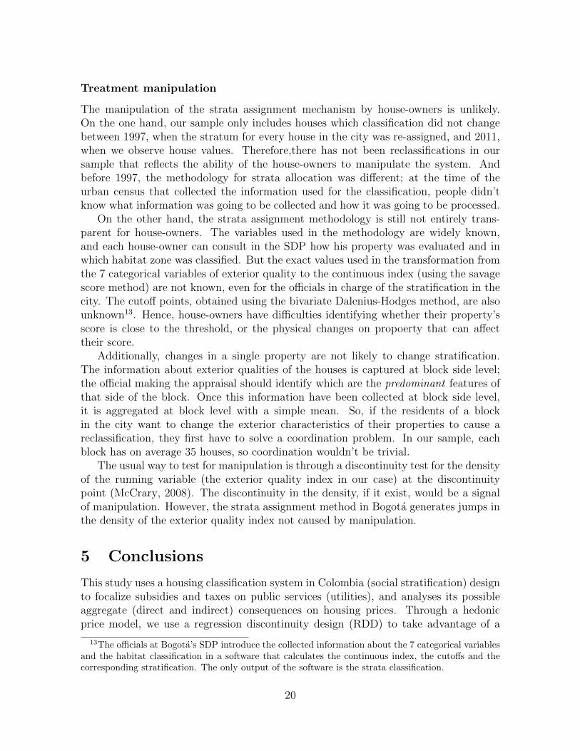
Treatment manipulation

The manipulation of the strata assignment mechanism by house-owners is unlikely.On the one hand, our sample only includes houses which classification did not changebetween 1997, when the stratum for every house in the city was re-assigned, and 2011,when we observe house values. Therefore,there has not been reclassifications in oursample that reflects the ability of the house-owners to manipulate the system. Andbefore 1997, the methodology for strata allocation was different; at the time of theurban census that collected the information used for the classification, people didn’tknow what information was going to be collected and how it was going to be processed.

On the other hand, the strata assignment methodology is still not entirely trans-parent for house-owners. The variables used in the methodology are widely known,and each house-owner can consult in the SDP how his property was evaluated and inwhich habitat zone was classified. But the exact values used in the transformation fromthe 7 categorical variables of exterior quality to the continuous index (using the savagescore method) are not known, even for the officials in charge of the stratification in thecity. The cutoff points, obtained using the bivariate Dalenius-Hodges method, are alsounknown13. Hence, house-owners have difficulties identifying whether their property’sscore is close to the threshold, or the physical changes on propoerty that can affecttheir score.

Additionally, changes in a single property are not likely to change stratification.The information about exterior qualities of the houses is captured at block side level;the official making the appraisal should identify which are the predominant features ofthat side of the block. Once this information have been collected at block side level,it is aggregated at block level with a simple mean. So, if the residents of a blockin the city want to change the exterior characteristics of their properties to cause areclassification, they first have to solve a coordination problem. In our sample, eachblock has on average 35 houses, so coordination wouldn’t be trivial.

The usual way to test for manipulation is through a discontinuity test for the densityof the running variable (the exterior quality index in our case) at the discontinuitypoint (McCrary, 2008). The discontinuity in the density, if it exist, would be a signalof manipulation. However, the strata assignment method in Bogota generates jumps inthe density of the exterior quality index not caused by manipulation.

5 Conclusions

This study uses a housing classification system in Colombia (social stratification) designto focalize subsidies and taxes on public services (utilities), and analyses its possibleaggregate (direct and indirect) consequences on housing prices. Through a hedonicprice model, we use a regression discontinuity design (RDD) to take advantage of a

13The officials at Bogota’s SDP introduce the collected information about the 7 categorical variablesand the habitat classification in a software that calculates the continuous index, the cutoffs and thecorresponding stratification. The only output of the software is the strata classification.

20

Figure 5: Distribution of external quality index within the optimal bandwidth

discontinuity change in stratums (6 stratums based on houses exterior quality materials)over a continued quality index and compare, on average, prices of nearly equal housesallocated in two different stratums. The main direct effect explores by the literature isthe property tax/subsidy capitalization which predicts a negative (positive) impact oftaxes (subsidies) on housing prices; but important indirect effect might arise (investmentdistortions in housing or public goods, segregation, or signaling of urban context orhouse quality), all of which predict positive effect of taxes on prices.

Taking a rich data set on housing for Bogota (property value, quality material andhabitat surroundings) we find that on aggregate, there are positive effects of an upwardstrata classification on the prices of housing, suggesting the important roll of indirecteffects, especially in the transition of intermediate stratums. The evidence suggeststhat one indirect mechanism that is taking into place is the improvement of the housingquality to compensate the fall of prices given the taxes. Further analysis need to bemade to explore the possibility of signaling or segregation because the stratificationmechanisms.

21

References

Aliaga, L. and Alvarez, M. (2010). Segregacion residencial en bogota a traves del tiempoy diferentes escalas. Documento de Trabajo de Lincoln Institute of Land Policy.

Bai, C., Li, Q., and Ouyang, M. (2014). Property taxes and home prices: A tale of twocities. Journal of Econometrics, 180(1):1–15.

BCE (2003). Structural factors in the eu housing markets. Frankfurt: Europa CentralBank.

Bergantino, A. S., Porcelli, F., et al. (2013). Housing market prices: capitalisationof efficiency in local public service provision. an application with data on italianurban transport related expenditures. Technical report, Southern Europe Researchin Economic Studies.

Casas, C. (2014). Subsidies to electricity consumption and housing demand in bogota.Technical report, Banco de la Republica.

Du, Z. and Zhang, L. (2015). Home-purchase restriction, property tax and housingprice in china: A counterfactual analysis. Journal of Econometrics, 188(2):558–568.

Gallego, J. M., Lopez, D., and Sepulveda, C. E. (2014). Los lımites de la estratificacion.En busca de alternativas. Universidad del Rosario.

Gould, I. (2008). Prepared for revisiting rental housing: A national policy summit.Revisiting Rental Housing: Policies, Programs, and Priorities, pages 144–158.

Ihlanfeldt, K. R. (2007). The effect of land use regulation on housing and land prices.Journal of Urban Economics, 61(3):420–435.

Imbens, G. and Kalyanaraman, K. (2011). Optimal bandwidth choice for the regressiondiscontinuity estimator. The Review of economic studies, page rdr043.

Imbens, G. W. and Lemieux, T. (2008). Regression discontinuity designs: A guide topractice. Journal of econometrics, 142(2):615–635.

Lang, K. and Jian, T. (2004). Property taxes and property values: evidence fromproposition 212. Journal of Urban Economics, 55(3):439–457.

McCrary, J. (2008). Manipulation of the running variable in the regression discontinuitydesign: A density test. Journal of Econometrics, 142(2):698–714.

Medina, C. and Morales, L. (2007). Stratification and public utility services in colombia:Subsidies to households or distortion of housing prices? Economia, 7(2):41–86.

22

Oates, W. E. (1969). The effects of property taxes and local public spending on propertyvalues: An empirical study of tax capitalization and the tiebout hypothesis. Journalof political economy, 77(6):957–971.

Rosen, H. S. and Fullerton, D. J. (1977). A note on local tax rates, public benefit levels,and property values. Journal of Political Economy, 85(2):433–440.

Rosen, K. T. (1982). The impact of proposition 13 on house prices in northern califor-nia: A test of the interjurisdictional capitalization hypothesis. Journal of PoliticalEconomy, 90(1):191–200.

SDP-UN (2011). Segregacion Socioeconomica en el Espacios Urbano de Bogota D.C.CID-Universidad Nacional.

Tiebout, C. M. (1956). A pure theory of local expenditures. The journal of politicaleconomy, pages 416–424.

Uribe, C. (2008). Estratificacion social en bogota: de la polıtica publica a la dinamicade la segregacion social. universitas humanıstica, 65(65).

23

Appendix

Table A1: Descriptive statistics

Mean SD Min Max ObsAppraisal value m2 (log) 14.06 0.58 11.75 15.73 751,636Building value m2 (log) 13.56 0.76 9.39 15.58 751,636Land value m2 (log) 13.25 0.60 8.35 15.36 751,636Built area 132.61 112.14 1.10 19862.95 751,636Land area 80.77 135.44 0.33 68544.12 751,636Cadastre score 46.00 16.48 0.00 98.00 751,636Year of construction 1986 13 1910 2011 751,636Co-ownership 0.45 0.50 0 1 751,636Exterior quality index 3.68 6.47 -5.61 22.36 751,636

Habitat type 7 0.00 0.04 0 1 751,636Habitat type 8 0.13 0.33 0 1 751,636Habitat type 9 0.29 0.45 0 1 751,636Habitat type 10 0.01 0.10 0 1 751,636Habitat type 12 0.03 0.17 0 1 751,636Habitat type 13 0.12 0.32 0 1 751,636Habitat type 15 0.07 0.25 0 1 751,636Habitat type 16 0.06 0.25 0 1 751,636Habitat type 17 0.00 0.07 0 1 751,636

Source: Own calculations, SDP, DAECD.

24

Table A2: OLS estimates

Habitat zones in sampleAppraisal Land Structures Observations

Jump 2 to 3 0.110*** 0.190*** 0.051*** 318,510(0.013) (0.022) (0.016)

Jump 3 to 4 0.138** 0.804*** 0.143 119,308(0.066) (0.207) (0.098)

Jump 4 to 5 0.084*** 0.016 0.102*** 50,422(0.028) (0.053) (0.032)

Jump 5 to 6 0.293*** 0.497*** 0.269*** 52,274(0.041) (0.084) (0.051)

All habitat zonesAppraisal Land Structures Observations

Jump 2 to 3 0.098*** 0.202*** 0.022 538,546(0.014) (0.022) (0.015)

Jump 3 to 4 0.129** 0.742*** 0.206 439,204(0.057) (0.189) (0.140)

Jump 4 to 5 0.054** 0.107** 0.099*** 163,866(0.025) (0.045) (0.028)

Jump 5 to 6 0.175*** 0.304*** 0.185*** 95,139(0.038) (0.081) (0.047)

25

Table A3: Number of stratified blocks by ’habitat zone’ in 2009

Criteria Zone Zone description # Blocks Proportion1 1 Poverty (-) 387 1.0%

2 Poverty (+) 6,607 17.3%2 3 Tolerance zone 67 0.2%3 4 Unconsolidated progressive development (-) 5,004 13.1%

5 Unconsolidated progressive development (+) 9,733 25.4%4 6 Urban decay 152 0.4%5 7 Industrial 168 0.4%6 8 Consolidated progressive development (-) 3,901 10.2%

9 Consolidated progressive development (+) 7,037 18.4%7 10 Predominant commercial (-) 748 2.0%

11 Predominant commercial (+) 262 0.7%8 12 Residential intermediate (-) 605 1.6%

13 Residential intermediate (+) 1,621 4.2%9 14 Commercial compatible 52 0.1%10 15 Exclusive residential (-) 1,000 2.6%

16 Exclusive residential (+) 656 1.7%11 17 Low-density residential 295 0.8%12 18 Institutional - -

19 Lot without houses - -20 Green area - -

Total 38,295 100.0%

Source: SDP

26

Table A4: Structure of tariffs in domestic public services

Water/SewerageStratum Fixed tarif Variable Tarif Variable Tarif

(<20M3) (>20M3)1 30% 30% 100%2 60% 60% 100%3 86% 86% 100%4 100% 100% 100%5 249% 151% 151%6 346% 161% 161%

EnergyVariable Tarif Variable Tarif(<130Kwh) (>130Kwh)

1 - 42% 100%2 - 52% 100%3 - 85% 100%4 - 100% 100%5 - 120% 120%6 - 120% 120%

GasVariable Tarif Variable Tarif

(<20M3) (>20M3)1 0% 50% 100%2 0% 63% 100%3 100% 100% 100%4 100% 100% 100%5 120% 120% 120%6 120% 120% 120%

Source: Own calculations

27

Table A5: Public utility services and contributions, and property tax

Average subsidy or contribution by services Tax property Average incomeStratum Water/Sewerage Energy Gas All1 2011 ($) $ 37,724 $ 23,059 $ 9,225 $ 70,008 $ 1,610 $ 1,057,081

% of Income 3.6% 2.2% 0.9% 6.6% 0.2%2 2012 ($) $ 20,959 $ 19,105 $ 6,829 $ 46,893 $ 3,387 $ 1,345,689

% of Income 1.6% 1.4% 0.5% 3.5% 0.3%3 2013 ($) $ 7,583 $ 5,906 $ - $ 13,488 $ 13,557 $ 2,290,080

% of Income 0.3% 0.3% 0.0% 0.6% 0.6%4 2014 ($) $ - $ - $ - $ 38,183 $ 5,026,124

% of Income 0.0% 0.0% 0.0% 0.0% 0.8%5 2015 ($) $ (47,177) $ (13,159) $ (6,901) $ (67,238) $ 85,397 $ 6,501,345

% of Income 0.7% 0.2% 0.1% 1.0% 1.3%6 2016 ($) $ (64,189) $ (17,252) $ (5,571) $ (87,012) $ 124,973 $ 8,510,986

% of Income 0.8% 0.2% 0.1% 1.0% 1.5%Total 2017 ($) 10823.38 10344.86 2921.102 24089.35 16128.46 2413764Bogota % of Income 0.4% 0.4% 0.1% 1.0% 0.7%

28