An Investigation of Goodman's Addictive Disorder Criteria in Eating Disorders
Upload
khangminh22Category
view
0download
0
UNIVERSITY OF SOUTHAMPTON
FACULTY OF SOCIAL SCIENCES
Department of Economics
Eating Disorders Studied over Online Social Networks
by
Tao Wang
Thesis for the degree of Doctor of Philosophy
May 2019


UNIVERSITY OF SOUTHAMPTON
ABSTRACT
FACULTY OF SOCIAL SCIENCES
Department of Economics
Doctor of Philosophy
EATING DISORDERS STUDIED OVER ONLINE SOCIAL NETWORKS
by Tao Wang
Eating disorders are complex mental disorders and responsible for the highest mortality
rate among mental illnesses. Traditional research methods on these diseases mainly
rely on personal interview and survey, which are often expensive and time-consuming to
reach large populations. Recent studies show that user-generated content on social media
provides useful information in understanding these disorders. However, most previous
studies focus on analyzing content posted by people who discuss eating disorders on
social media. Few studies have explored social interactions among individuals who suffer
from these diseases over social media, while social networks play an important role in
influencing and shape individual behavior and health.
This thesis aims to provide insights into eating disorders and their related communities
from a network perspective, particularly to understand how individuals interact with one
another, and the interplays between online social networks and individual behaviors. To
this end, we first develop a snowball sampling method to automatically gather individ-
uals who self-identify as eating disordered in their profile descriptions, as well as their
social connections on Twitter, and verify the effectiveness of our sampling method by
both computational analysis and manual validation. Second, we examine a large com-
munication network of individuals suffering from eating disorders on Twitter to explore
how social media shape community structures and facilitate interactions between com-
munities with different health-related orientations. Third, we propose to use multilayer
networks to model multiplex interactions among individuals and explore how activities
of a set of actors in one type of communication correlate and influence activities of the
actors in other types of communication. Finally, leveraging the longitudinal data on
posting activities in our user samples spanning 1.5 year, we investigate characteristics of
dropout behaviors among eating disordered individuals on Twitter and to estimate the
causal effects of personal emotions and social networks on dropout behaviors. Our find-
ings contribute to understanding of development and maintenance of healthy behaviors
and cognition online, and have practical implications for designing network interventions
that can promote organizational well-being in online health communities.


Contents
Declaration of Authorship xiii
Acknowledgements xv
1 Introduction 1
1.1 Motivation . . . . . . . . . . . . . . . . . . . . . . . . . . . . . . . . . . . 1
1.2 Research Objectives . . . . . . . . . . . . . . . . . . . . . . . . . . . . . . 3
1.3 Thesis Structure . . . . . . . . . . . . . . . . . . . . . . . . . . . . . . . . 4
2 Background 7
2.1 Eating Disorders . . . . . . . . . . . . . . . . . . . . . . . . . . . . . . . . 7
2.1.1 Clinical Knowledge . . . . . . . . . . . . . . . . . . . . . . . . . . . 7
2.1.2 Social Impacts . . . . . . . . . . . . . . . . . . . . . . . . . . . . . 8
2.1.3 Challenges in ED Prevention . . . . . . . . . . . . . . . . . . . . . 9
2.2 Social Media and Well-being . . . . . . . . . . . . . . . . . . . . . . . . . . 10
2.2.1 Risk Detection . . . . . . . . . . . . . . . . . . . . . . . . . . . . . 11
2.2.2 Online Intervention . . . . . . . . . . . . . . . . . . . . . . . . . . . 13
2.2.3 Strengths and Weaknesses . . . . . . . . . . . . . . . . . . . . . . . 14
2.3 ED Research over Social Media . . . . . . . . . . . . . . . . . . . . . . . . 15
2.3.1 Qualitative Analysis . . . . . . . . . . . . . . . . . . . . . . . . . . 16
2.3.2 Quantitative Analysis . . . . . . . . . . . . . . . . . . . . . . . . . 18
2.4 Research Gaps . . . . . . . . . . . . . . . . . . . . . . . . . . . . . . . . . 19
2.5 Social Interaction Theories . . . . . . . . . . . . . . . . . . . . . . . . . . 21
2.5.1 Two-step Flow of Communication . . . . . . . . . . . . . . . . . . 21
2.5.2 Incentive Theory . . . . . . . . . . . . . . . . . . . . . . . . . . . . 22
2.5.3 Social Norms . . . . . . . . . . . . . . . . . . . . . . . . . . . . . . 23
2.5.4 Social Influence . . . . . . . . . . . . . . . . . . . . . . . . . . . . . 24
2.5.5 Homophily . . . . . . . . . . . . . . . . . . . . . . . . . . . . . . . 25
2.6 Content Analysis . . . . . . . . . . . . . . . . . . . . . . . . . . . . . . . . 26
2.6.1 Topic Detection . . . . . . . . . . . . . . . . . . . . . . . . . . . . . 26
2.6.2 Sentiment Analysis . . . . . . . . . . . . . . . . . . . . . . . . . . . 28
2.6.3 Language and Psychology . . . . . . . . . . . . . . . . . . . . . . . 29
2.7 Network Analysis . . . . . . . . . . . . . . . . . . . . . . . . . . . . . . . . 30
2.7.1 Graph Representation . . . . . . . . . . . . . . . . . . . . . . . . . 30
2.7.2 Null Models . . . . . . . . . . . . . . . . . . . . . . . . . . . . . . . 31
2.7.3 Multilayer Networks . . . . . . . . . . . . . . . . . . . . . . . . . . 31
2.8 Statistical Techniques . . . . . . . . . . . . . . . . . . . . . . . . . . . . . 33
v
vi CONTENTS
2.8.1 Classification Analysis . . . . . . . . . . . . . . . . . . . . . . . . . 33
2.8.2 Clustering Analysis . . . . . . . . . . . . . . . . . . . . . . . . . . . 34
2.8.3 Instrumental Variables Estimation . . . . . . . . . . . . . . . . . . 36
2.8.4 Survival Analysis . . . . . . . . . . . . . . . . . . . . . . . . . . . . 37
2.9 Summary . . . . . . . . . . . . . . . . . . . . . . . . . . . . . . . . . . . . 38
3 Data Collection 41
3.1 Introduction . . . . . . . . . . . . . . . . . . . . . . . . . . . . . . . . . . . 41
3.2 Related Work . . . . . . . . . . . . . . . . . . . . . . . . . . . . . . . . . . 43
3.3 Data . . . . . . . . . . . . . . . . . . . . . . . . . . . . . . . . . . . . . . . 44
3.3.1 Collecting ED Data . . . . . . . . . . . . . . . . . . . . . . . . . . 44
3.3.1.1 Filtering Self-reported ED Diagnoses . . . . . . . . . . . 45
3.3.1.2 Snowball Sampling ED Communities . . . . . . . . . . . 46
3.3.2 Collecting Reference Data . . . . . . . . . . . . . . . . . . . . . . . 47
3.4 User Characterization . . . . . . . . . . . . . . . . . . . . . . . . . . . . . 49
3.4.1 Measures . . . . . . . . . . . . . . . . . . . . . . . . . . . . . . . . 49
3.4.1.1 Social Status . . . . . . . . . . . . . . . . . . . . . . . . . 49
3.4.1.2 Behavioral Patterns . . . . . . . . . . . . . . . . . . . . . 49
3.4.1.3 Psychometric Properties . . . . . . . . . . . . . . . . . . 50
3.4.2 Classification Framework . . . . . . . . . . . . . . . . . . . . . . . 51
3.5 Community Characterization . . . . . . . . . . . . . . . . . . . . . . . . . 51
3.5.1 Network Characterization . . . . . . . . . . . . . . . . . . . . . . . 52
3.5.2 Homophily Analysis . . . . . . . . . . . . . . . . . . . . . . . . . . 52
3.6 Results . . . . . . . . . . . . . . . . . . . . . . . . . . . . . . . . . . . . . . 53
3.6.1 ED Validation with Bio-information . . . . . . . . . . . . . . . . . 53
3.6.2 Comparisons of User Features . . . . . . . . . . . . . . . . . . . . . 54
3.6.3 Classification Performance . . . . . . . . . . . . . . . . . . . . . . . 56
3.6.4 Characteristics of Networks . . . . . . . . . . . . . . . . . . . . . . 57
3.6.5 Patterns of Homophily . . . . . . . . . . . . . . . . . . . . . . . . . 58
3.7 Conclusion . . . . . . . . . . . . . . . . . . . . . . . . . . . . . . . . . . . 59
4 Social Structures 63
4.1 Introduction . . . . . . . . . . . . . . . . . . . . . . . . . . . . . . . . . . . 63
4.2 Methods . . . . . . . . . . . . . . . . . . . . . . . . . . . . . . . . . . . . . 65
4.3 Results . . . . . . . . . . . . . . . . . . . . . . . . . . . . . . . . . . . . . . 69
4.3.1 User Groupings . . . . . . . . . . . . . . . . . . . . . . . . . . . . . 69
4.3.2 Network Structures . . . . . . . . . . . . . . . . . . . . . . . . . . . 71
4.3.3 Behavioral Characteristics . . . . . . . . . . . . . . . . . . . . . . . 73
4.3.4 Community Norms . . . . . . . . . . . . . . . . . . . . . . . . . . . 75
4.4 Discussion . . . . . . . . . . . . . . . . . . . . . . . . . . . . . . . . . . . . 76
5 Information Flows 79
5.1 Introduction . . . . . . . . . . . . . . . . . . . . . . . . . . . . . . . . . . . 79
5.2 Data . . . . . . . . . . . . . . . . . . . . . . . . . . . . . . . . . . . . . . . 81
5.2.1 Collecting user sample . . . . . . . . . . . . . . . . . . . . . . . . . 81
5.2.2 Tracking interpersonal conversations . . . . . . . . . . . . . . . . . 82
5.3 Analyses . . . . . . . . . . . . . . . . . . . . . . . . . . . . . . . . . . . . . 82

CONTENTS vii
5.3.1 Content analysis . . . . . . . . . . . . . . . . . . . . . . . . . . . . 83
5.3.2 Network analysis . . . . . . . . . . . . . . . . . . . . . . . . . . . . 86
5.3.2.1 Structures of single-layer networks . . . . . . . . . . . . . 86
5.3.2.2 Dependencies of inter-layer networks . . . . . . . . . . . . 90
5.3.3 Dynamic analysis . . . . . . . . . . . . . . . . . . . . . . . . . . . . 93
5.3.3.1 Transition of engagement activities . . . . . . . . . . . . 95
5.3.3.2 Stability of communities . . . . . . . . . . . . . . . . . . . 98
5.4 Discussion . . . . . . . . . . . . . . . . . . . . . . . . . . . . . . . . . . . . 100
6 Behavioral Change 103
6.1 Introduction . . . . . . . . . . . . . . . . . . . . . . . . . . . . . . . . . . . 104
6.2 Methods . . . . . . . . . . . . . . . . . . . . . . . . . . . . . . . . . . . . . 107
6.2.1 Data Collection . . . . . . . . . . . . . . . . . . . . . . . . . . . . . 107
6.2.2 Estimation Framework . . . . . . . . . . . . . . . . . . . . . . . . . 108
6.2.3 Measures . . . . . . . . . . . . . . . . . . . . . . . . . . . . . . . . 109
6.2.3.1 Dropout Outcomes as Dependent Variables . . . . . . . . 109
6.2.3.2 Emotions and Network Centrality as Main ExplanatoryVariables . . . . . . . . . . . . . . . . . . . . . . . . . . . 110
6.2.3.3 Aggregated Emotions and Network Centrality of Friendsas Instrumental Variables . . . . . . . . . . . . . . . . . . 111
6.2.3.4 Estimation Covariates . . . . . . . . . . . . . . . . . . . . 111
6.2.4 Model Estimations . . . . . . . . . . . . . . . . . . . . . . . . . . . 112
6.2.4.1 IV Estimation in Linear Regression Model . . . . . . . . 112
6.2.4.2 IV Estimation in Survival Model . . . . . . . . . . . . . . 113
6.3 Results . . . . . . . . . . . . . . . . . . . . . . . . . . . . . . . . . . . . . . 113
6.3.1 Descriptive Statistics . . . . . . . . . . . . . . . . . . . . . . . . . . 113
6.3.2 Estimation Results of Linear Probability Models . . . . . . . . . . 113
6.3.3 Estimation Results of Survival Models . . . . . . . . . . . . . . . . 115
6.3.4 Underlying Connection between Emotions and Dropout . . . . . . 116
6.4 Discussion . . . . . . . . . . . . . . . . . . . . . . . . . . . . . . . . . . . . 118
7 Conclusion 121
7.1 Contributions and Implications . . . . . . . . . . . . . . . . . . . . . . . . 121
7.1.1 Data Collection . . . . . . . . . . . . . . . . . . . . . . . . . . . . . 122
7.1.2 Social Structures . . . . . . . . . . . . . . . . . . . . . . . . . . . . 123
7.1.3 Information Flows . . . . . . . . . . . . . . . . . . . . . . . . . . . 124
7.1.4 Behavioral Change . . . . . . . . . . . . . . . . . . . . . . . . . . . 125
7.2 Future Work . . . . . . . . . . . . . . . . . . . . . . . . . . . . . . . . . . 127
7.2.1 Characterizing Patterns of Information Diffusion . . . . . . . . . . 127
7.2.2 Identifying Mechanisms of Peer Effects . . . . . . . . . . . . . . . . 129
7.2.3 Distinguishing Influence and Homophily Processes . . . . . . . . . 130
7.3 Further Challenges . . . . . . . . . . . . . . . . . . . . . . . . . . . . . . . 131
7.3.1 Ethical Issues . . . . . . . . . . . . . . . . . . . . . . . . . . . . . . 131
7.3.2 Data Biases . . . . . . . . . . . . . . . . . . . . . . . . . . . . . . . 131
7.3.3 Gap between Online and Offline Behaviors . . . . . . . . . . . . . 132
A Appendix: Supporting Information for Chapter 2 135
A.1 Basic Concepts in Network Analysis . . . . . . . . . . . . . . . . . . . . . 135

viii CONTENTS
A.2 Common Network Properties . . . . . . . . . . . . . . . . . . . . . . . . . 136
B Appendix: Supporting Information for Chapter 4 139
B.1 Data Details . . . . . . . . . . . . . . . . . . . . . . . . . . . . . . . . . . 139
B.1.1 Sampling Disordered Users . . . . . . . . . . . . . . . . . . . . . . 140
B.1.2 Filtering ED-related Tweets . . . . . . . . . . . . . . . . . . . . . . 140
B.1.3 Constructing Communication Network . . . . . . . . . . . . . . . . 142
B.2 User Clustering Analysis . . . . . . . . . . . . . . . . . . . . . . . . . . . . 142
B.2.1 Hashtag Clustering . . . . . . . . . . . . . . . . . . . . . . . . . . . 142
B.2.2 User Profiling . . . . . . . . . . . . . . . . . . . . . . . . . . . . . . 143
B.2.3 User Clustering . . . . . . . . . . . . . . . . . . . . . . . . . . . . . 144
B.3 Community Identification . . . . . . . . . . . . . . . . . . . . . . . . . . . 145
B.3.1 Posting Interests . . . . . . . . . . . . . . . . . . . . . . . . . . . . 145
B.3.2 Attitudes on ED-related Content . . . . . . . . . . . . . . . . . . . 146
B.3.3 Manual Annotation . . . . . . . . . . . . . . . . . . . . . . . . . . 147
B.4 Emotional Interactions . . . . . . . . . . . . . . . . . . . . . . . . . . . . . 147
B.5 Measures on User Characteristics . . . . . . . . . . . . . . . . . . . . . . . 149
B.5.1 Social Activities . . . . . . . . . . . . . . . . . . . . . . . . . . . . 149
B.5.2 Language Use . . . . . . . . . . . . . . . . . . . . . . . . . . . . . . 149
B.6 Community Norms . . . . . . . . . . . . . . . . . . . . . . . . . . . . . . . 150
B.6.1 Characterizing Social Norms . . . . . . . . . . . . . . . . . . . . . 150
B.6.2 Regression Models . . . . . . . . . . . . . . . . . . . . . . . . . . . 151
C Appendix: Supporting Information for Chapter 5 163
C.1 ED-related hashtags . . . . . . . . . . . . . . . . . . . . . . . . . . . . . . 163
C.2 Statistics of conversations . . . . . . . . . . . . . . . . . . . . . . . . . . . 163
C.3 Statistics of topics . . . . . . . . . . . . . . . . . . . . . . . . . . . . . . . 164
C.4 Null models for testing inter-layer correlations . . . . . . . . . . . . . . . . 165
C.5 Statistics of temporal multilayer networks . . . . . . . . . . . . . . . . . . 166
D Appendix: Supporting Information for Chapter 6 169
D.1 Data Statistics . . . . . . . . . . . . . . . . . . . . . . . . . . . . . . . . . 169
D.2 Instrumental Variable Estimation . . . . . . . . . . . . . . . . . . . . . . . 172
D.3 Survival Analysis with IV . . . . . . . . . . . . . . . . . . . . . . . . . . . 172
D.4 Null Model . . . . . . . . . . . . . . . . . . . . . . . . . . . . . . . . . . . 174
D.5 Specifications of Data Censoring Methods . . . . . . . . . . . . . . . . . . 174
D.6 Posting Interests of Users . . . . . . . . . . . . . . . . . . . . . . . . . . . 175
References 179

List of Figures
3.1 Distributions of ages and BMIs. . . . . . . . . . . . . . . . . . . . . . . . . 53
3.2 ROC curves of classifications with different types of features. . . . . . . . 56
4.1 User clustering and group-identity investigation. . . . . . . . . . . . . . . 70
4.2 Interactions of pro-ED and pro-recovery communities. . . . . . . . . . . . 72
4.3 Social norms in pro-ED and pro-recovery communities. . . . . . . . . . . . 75
5.1 Topics in hashtag co-occurrence networks. . . . . . . . . . . . . . . . . . . 83
5.2 Numbers of tweets on mental and thinspo per month . . . . . . . . . . . . 85
5.3 Multilayer communication network. . . . . . . . . . . . . . . . . . . . . . . 87
5.4 Distributions of in-/out-strength of single-layer networks. . . . . . . . . . 87
5.5 Deviations of empirical pairwise correlations of inter-layer networks tonull models. . . . . . . . . . . . . . . . . . . . . . . . . . . . . . . . . . . . 92
5.6 Temporal multilayer communication networks. . . . . . . . . . . . . . . . 94
5.7 Transitions of engagement in different topics. . . . . . . . . . . . . . . . . 96
5.8 Mean entropy of topics in tweets over time. . . . . . . . . . . . . . . . . . 98
5.9 Overlaps of users in temporal networks. . . . . . . . . . . . . . . . . . . . 99
6.1 The who-follows-whom network among ED users on Twitter. . . . . . . . 114
B.1 Diagram of analysis . . . . . . . . . . . . . . . . . . . . . . . . . . . . . . 139
B.2 Topic clusters in core ED users’ tweets . . . . . . . . . . . . . . . . . . . . 141
B.3 Degree distributions of communication networks . . . . . . . . . . . . . . 142
B.4 Topic clusters in ED-related tweets . . . . . . . . . . . . . . . . . . . . . . 144
B.5 Statistics of users and tweets related to ED-related themes . . . . . . . . . 146
B.6 Statistics of users and links in intra- and inter-community interactions . . 148
B.7 Distributions of centralities . . . . . . . . . . . . . . . . . . . . . . . . . . 150
C.1 Aggregating conversations and distribution of conversation sizes . . . . . . 164
C.2 Characterization of the 26 topics found in hashtag co-occurrence networks 165
C.3 Statistics of temporal multilayer networks . . . . . . . . . . . . . . . . . . 166
D.1 Diagram of data collection and analysis procedures. . . . . . . . . . . . . 169
D.2 Number of users along with time points when users created a Twitteraccount and posted the last tweet. . . . . . . . . . . . . . . . . . . . . . . 170
D.3 Demographics of ED users. . . . . . . . . . . . . . . . . . . . . . . . . . . 171
D.4 Kaplan-Meier estimations of survival time. . . . . . . . . . . . . . . . . . . 175
D.5 The co-occurrence network of the most popular hashtags used by ED users.176
ix

List of Tables
2.1 Contingency table of inputs and outputs in binary classification. . . . . . 34
3.1 Examples of self-reported ED diagnoses. . . . . . . . . . . . . . . . . . . . 45
3.2 Keywords used used for filtering ED users. . . . . . . . . . . . . . . . . . . 46
3.3 Data statistics . . . . . . . . . . . . . . . . . . . . . . . . . . . . . . . . . 48
3.4 Statistics of bio-information in ED users. . . . . . . . . . . . . . . . . . . . 53
3.5 Statistics of measures characterizing differences of ED, Random and Youngerusers. . . . . . . . . . . . . . . . . . . . . . . . . . . . . . . . . . . . . . . 55
3.6 Performance of user classifications. . . . . . . . . . . . . . . . . . . . . . . 56
3.7 Statistics of networks between ED users. . . . . . . . . . . . . . . . . . . . 57
3.8 Percentages of assortatively mixed features at different significance levels. 59
3.9 Examples of assortative mixing by features. . . . . . . . . . . . . . . . . . 60
4.1 Statistics of the communication networks among pro-ED and pro-recoverycommunities. . . . . . . . . . . . . . . . . . . . . . . . . . . . . . . . . . . 71
4.2 Comparisions of communities in social activities and language use. . . . . 74
5.1 Statistics of single-layer networks and the aggregated network. . . . . . . 88
5.2 Null hypotheses on correlations of individuals’ activities and roles. . . . . 91
6.1 Control variables used in estimations. . . . . . . . . . . . . . . . . . . . . 112
6.2 Estimated effects of emotions on dropout using OLS and IV models. . . . 115
6.3 Estimated effects of emotions and centrality on survival time using Aalen’sadditive hazards modelsa. . . . . . . . . . . . . . . . . . . . . . . . . . . . 116
6.4 Correlations between pairwise lists of hashtags posted by different users. . 117
B.1 Prominent hashtags in two clusters of users . . . . . . . . . . . . . . . . . 145
B.2 Most frequent pro-ED and pro-recovery hashtags. . . . . . . . . . . . . . . 146
B.3 Sentiments of users on themes of content . . . . . . . . . . . . . . . . . . . 147
B.4 Sentiments of users’ interaction messages . . . . . . . . . . . . . . . . . . 148
B.5 Centrality as a function of body and covariates . . . . . . . . . . . . . . . 152
B.6 Centrality as a function of ingest and covariates . . . . . . . . . . . . . . . 153
B.7 Centrality as a function of health and covariates . . . . . . . . . . . . . . . 154
B.8 Centrality as a function of i and covariates . . . . . . . . . . . . . . . . . 155
B.9 Centrality as a function of we and covariates . . . . . . . . . . . . . . . . 156
B.10 Centrality as a function of social and covariates . . . . . . . . . . . . . . . 157
B.11 Centrality as a function of swear and covariates . . . . . . . . . . . . . . . 158
B.12 Centrality as a function of negate and covariates . . . . . . . . . . . . . . 159
B.13 Centrality as a function of posemo and covariates . . . . . . . . . . . . . . 160
xi

xii LIST OF TABLES
B.14 Centrality as a function of negemo and covariates . . . . . . . . . . . . . . 161
B.15 Centrality as a function of prostrr and covariates . . . . . . . . . . . . . . 162
C.1 Examples of hashtags used to filter ED-related content . . . . . . . . . . . 163
D.1 Descriptive statistics of users by dropout and non-dropout states. . . . . 170
D.2 The most popular hashtags used by ED users, grouped by users’ dropoutstates. . . . . . . . . . . . . . . . . . . . . . . . . . . . . . . . . . . . . . . 176
D.3 The most popular hashtags used by ED users, grouped by users’ emotionalstates. . . . . . . . . . . . . . . . . . . . . . . . . . . . . . . . . . . . . . . 177

Declaration of Authorship
I, Tao Wang , declare that the thesis entitled Eating Disorders Studied over Online
Social Networks and the work presented in the thesis are both my own, and have been
generated by me as the result of my own original research. I confirm that:
• this work was done wholly or mainly while in candidature for a research degree at
this University;
• where any part of this thesis has previously been submitted for a degree or any
other qualification at this University or any other institution, this has been clearly
stated;
• where I have consulted the published work of others, this is always clearly at-
tributed;
• where I have quoted from the work of others, the source is always given. With the
exception of such quotations, this thesis is entirely my own work;
• I have acknowledged all main sources of help;
• where the thesis is based on work done by myself jointly with others, I have made
clear exactly what was done by others and what I have contributed myself;
• parts of this work have been published as: [Wang et al., 2017] (Chapter 3), [Wang
et al., 2018a] (Chapter 4), [Wang et al., 2019] (Chapter 5)and [Wang et al., 2018b]
(Chapter 6).
Signed:.......................................................................................................................
Date:..........................................................................................................................
xiii


Acknowledgements
First of all, I would like to thank my supervisors, Antonella Ianni, Markus Brede and
Emmanouil Mentzakis, for giving me the opportunity to do this interesting project,
but also for their continuous support, guidance and valuable feedback throughout my
PhD. Special thanks to Dr. Robert Ackland, Prof. Leslie Carr, Dr. Jonathon Hare,
Dr. Carmine Ornaghi and Dr. Hctor Calvo Pardo for their very helpful comments and
suggestions. I would also like to thank the Alan Turing Institute for offering me a one-
year placement, allowing me to continue my research in a multidisciplinary environment.
Last but by no means least, I would like to thank my family for all their support and
encouragement, especially my loving and supportive wife, Dandan Shi. Dandan has
been my best friend and greatest companion, loved, supported, encouraged, inspired,
entertained and helped me get through this agonizing period in the most positive way.
xv


Chapter 1
Introduction
1.1 Motivation
Eating disorders (ED), such as anorexia nervosa and bulimia nervosa, are complex men-
tal illnesses that are characterized by abnormal eating habits and excessive concerns
about body weight and shape [Association et al., 2013]. These diseases can negatively
affect people’s physical and psychological health, with the highest mortality rate of any
mental illness [Arcelus et al., 2011; National Institute of Mental Health, 2016]. Apart
from serious health consequences, ED have become increasingly prevalent over recent
years, particularly in adolescent populations [Abebe et al., 2012]. More than 725,000
people in the UK are reported to develop an ED at some stage in their lifetime, and the
trend is indicated in increasing prevalence over time: approximately 7% increase each
year since 2005-06 [Beat, 2015]. Given these negative impacts on both individuals and
society, ED have been a major public health concern. While various treatments of ED
have emerged over recent years [Corstorphine, 2006], individuals with ED often attempt
to conceal their symptoms and many never seek support or treatment from professionals
[Rich, 2006; Swanson et al., 2011], mainly because of the denial of illness, social stigma
of being mentally ill and lack of health awareness [Guarda, 2008; Swan and Andrews,
2003]. This leads to a lack of quantifiable information on individuals’ behaviors to iden-
tify the occurrences or severities of ED, and brings a significant challenge for health
professionals to understand ED and develop effective treatment programs.
As the emergence of social media services such as Twitter, Facebook and Instagram over
recent years, people are increasingly using social media to record details of everyday life,
exchange information and seek social support, as well as to manage their chronic health
conditions [Fergie et al., 2015]. This provides a new opportunity to study individuals’
health-related behaviors, such as concerns, emotions, activities and socialization, by
analyzing their data generated on social media. Recent studies have shown that user-
generated data online can indeed reveal their mental health states, such as feelings of
1

2 Chapter 1 Introduction
worthlessness, depression, helplessness, anxiety, self-hatred, suicidal ideation and con-
cerns of body image [Chancellor et al., 2016a; Coppersmith et al., 2014; De Choudhury
et al., 2013c; De Choudhury and Kıcıman, 2017; Juarascio et al., 2010]. Moreover, en-
gagement in online ED communities is common among people with ED and has recently
been suggested as a screening factor for ED [Campbell and Peebles, 2014]. Thus, a
growing body of research has focused on using social media data to improve our under-
standing of disordered eating behaviors [Arseniev-Koehler et al., 2016; Chancellor et al.,
2016a; Juarascio et al., 2010; Syed-Abdul et al., 2013; Yom-Tov et al., 2018].
Previous ED studies based on social media data are mainly carried out by psychologists
and clinicians [Arseniev-Koehler et al., 2016; Branley and Covey, 2017; Juarascio et al.,
2010; Wick and Harriger, 2018; Wilson et al., 2006; Wolf et al., 2013]. These studies
often rely on surveys or interviews in data collection [Ransom et al., 2010; Wilson et al.,
2006] and human coding in content analysis [Branley and Covey, 2017; Juarascio et al.,
2010; Wick and Harriger, 2018]. Although in most cases these methods can provide
reliable and valid measures, they often involve intensive manual labor, making previous
studies be limited by small sample sizes. For example, Arseniev-Koehler et al. [2016]
studied socialization of an ED community based on 45 users on Twitter and Wick and
Harriger [2018] analyzed thinspiration content based on 222 images and text posts on
Tumblr. Given the explosive growth of information online, there is therefore a need to
develop more effective techniques to extend these efforts.
Recently, some computational methods have been proposed to study ED and other men-
tal illnesses based on social media data [Chancellor et al., 2016a,c,d; Coppersmith et al.,
2014; De Choudhury, 2015; De Choudhury et al., 2013b, 2014; Harman, 2014]. By lever-
aging users’ content and behaviors generated online, researchers have explored to iden-
tify risks of individuals being affected by ED [Chancellor et al., 2016c; De Choudhury,
2015], depressions [De Choudhury et al., 2014, 2013c; Harman, 2014; Park et al., 2013;
Schwartz et al., 2014; Tsugawa et al., 2015], addictions [MacLean et al., 2015; Murnane
and Counts, 2014], suicidal ideation [De Choudhury and Kıcıman, 2017; De Choudhury
et al., 2016a] and other health conditions [Coppersmith et al., 2015, 2014; Jamison-
Powell et al., 2012; Mitchell et al., 2015]. However, previous studies have often focused
on content analysis [Wongkoblap et al., 2017]. For example, in ED-related studies,
De Choudhury [2015] compared the differences of pro-anorexia and pro-recovery posts,
and Chancellor et al. [2016c] further explored to predict the likelihood of a user in recov-
ery from ED based on users’ posts on Tumblr. Other studies also examined the severity
of ED based on tags posted by users [Chancellor et al., 2016a], characterisitics of re-
moved ED-related tags [Chancellor et al., 2016b], and lexical variations of ED-related
tags [Chancellor et al., 2017, 2016d] on Instagram. While most social media platforms
offer multiple ways (such as “follow” on Twitter) for users to interact with one another,
few studies have explored social ties and interactions among disordered peers online.

Chapter 1 Introduction 3
In fact, social dimension captured by social networks plays an important role in un-
derstanding lifestyle related conditions like ED [Chen, 2013], as our interests, concerns
and behaviors are strongly influenced by the network of people with whom we interact
[Fiori et al., 2006; Kawachi and Berkman, 2001; Paxton et al., 1999]. Previous studies
on offline social networks have shown that various health-related attributes, such as obe-
sity [Christakis and Fowler, 2007], happiness [Fowler and Christakis, 2008], and smoking
[Christakis and Fowler, 2008], are affected by individuals’ attributes but also by their
social networks. Detailed records of individuals’ interactivity on social media provide
a great opportunity to extend these studies and explore the nature and extent of the
person-to-person spread of disordered behaviors through online social networks. More-
over, unlike offline social networking data that is often collected via surveys, online social
networking data is recorded in real time. The availability of such temporal data enables
us to clarify the ordering of individuals’ connections to different people and examine
behavioral changes before and after the formation of a connection, which can help to
extend our understanding on the relations (e.g., co-evolution) between social networks
and individual behaviors. A deeper understanding of these relations can have practi-
cal implications in disease prevention and online intervention to improve organizational
well-being over online social networks [Latkin and Knowlton, 2015; Valente, 2012].
1.2 Research Objectives
The main objective of this thesis is to explore characteristics of social interactions
in online ED communities from a network perspective and examine interplays
between online social networks and individual health attributes. Given this
principal objective, we pursue the following subsidiary objectives:
• To develop a data collection method that can gather a large set of individuals
affected by ED on social media (e.g., Twitter) and track their posting activities
and social networking data online (Chapter 3).
• To characterize structural properties of online social interactions among individuals
with ED by using network analysis methods (Chapter 3).
• To determine groups of individuals with a similar stance on ED (e.g., pro-recovery
or anti-recovery) in an online ED community and how individuals with different
stances interact with one another (Chapter 4).
• To establish the associations between individuals’ positions in a social network and
their behaviors online (Chapter 4).
• To analyze how different types of information (e.g., healthy and harmful content)
flow through interpersonal communication networks in an online ED community
and how these information flows correlate and influence one another (Chapter 5).

4 Chapter 1 Introduction
• To estimate the effects of social networks and individual attributes on behavioral
change, e.g., dropout from a harmful online community (Chapter 6).
1.3 Thesis Structure
The remainder of this thesis is organized as follows.
In Chapter 2, we first introduce background on the research in this thesis and provide
a comprehensive overview of related work. Then, we formulate our research questions
by identifying research gaps in previous studies. Finally, we introduce key theories and
methods that can be used to address these research questions.
In Chapter 3, our focus is to collect interaction data in online ED communities. We
first present a snowball sampling method to sift ED individuals and their social net-
works on Twitter. We verify the effectiveness of this method by both computational
algorithms and human annotations. Then, we characterize structural properties of social
connections among ED individuals through various types of interactions (e.g., “follow”,
“retweet” and “mention”) on Twitter and explore the presence of homophily in online
ED communities. The main part of this chapter was published on [Wang et al., 2017].
In Chapter 4, our focus is to identify distinct subgroups of actors in an online ED
community and examine how different subgroups of actors interact. We first present an
automated approach that integrates topic modeling and clustering analysis to find groups
of users sharing similar interests in online ED communities. Then, we use sentiment
analysis techniques to identify the stances of each group of users towards ED and examine
the differences of groups of users in social activities and psychometric properties. Finally,
we explore the associations between individuals’ positions in a social network and their
behaviors by studying social norms [Parsons, 1937] in different groups. The main part
of this chapter was published on [Wang et al., 2018a].
In Chapter 5, our focus is to identify distinct types of content spread through an online
ED community and examine the correlations among different types of information flows.
We first use topic modeling methods to detect the types of content shared in interper-
sonal conversations within an online ED community. Then, we propose a multilayer
network representation [Boccaletti et al., 2014; Kivela et al., 2014] to model individu-
als’ interactions in communicating different types of content and demonstrate how this
representation can facilitate analyzing the difference and correlations among different
information flows. To better understand underlying processes that lead to the correla-
tions of different information flows, we further investigate dynamics of the multilayer
communication networks over time. The main part of this chapter was published on
[Wang et al., 2019].

Chapter 1 Introduction 5
In Chapter 6, our focus is to explore how online social networks can lead to behavioral
changes, particularly on discontinuation of engagement and dropout on Twitter. We
first identify users’ dropout behaviors by observing their posting activities on Twitter
over 1.5 years. Then, we base the incentive theory [Kollock, 1999] and establish the
causal effects of individual emotions and positions in social networks on their dropout
behaviors (e.g., the probability of dropout and the time to dropout). The main part of
this chapter was published on [Wang et al., 2018b].
In Chapter 7, we conclude the work in this thesis. We first summarize the main contri-
butions in this thesis and discuss their implications for public health. Then, we propose
several directions and open challenges for further research.


Chapter 2
Background
Social media facilitate access to social support and heath-related communication for
people affected by health problems. User-generated data on social media, particularly
health-related data, provides unprecedented opportunities to understand and prevent
challenging health problems at a large scale. This thesis presents studies on eating
disorders over social media. This section reviews four essential elements of background
material for these studies, including (1) knowledge on eating disorders, (2) link between
social media and health, (3) previous health-related research based on social media data,
and (4) key theories and methods used in this thesis.
2.1 Eating Disorders
2.1.1 Clinical Knowledge
In standard medical manuals, such as Diagnostic and Statistical Manual of Mental Dis-
orders (DSM-5) [Association et al., 2013] and International Statistical Classification of
Diseases and Related Health Problems (ICD-10) [Organization, 1993], eating disorders
(ED) are defined as mental illnesses characterized by abnormal attitudes towards food
and unusual eating behaviors. The most common forms of ED are anorexia nervosa
where sufferers restrict their eating to keep low weight, binge ED where sufferers ingest
a large amount of food in a short period of time, and bulimia nervosa where sufferers
repeat cycles of binge eating and purging [Association et al., 2013; Organization, 1993].
Exact causes of ED are still unclear; all biological (genetic effects), psychological (body
image disturbance and personality traits), developmental (childhood sexual abuse), and
sociocultural factors (idealization of thinness) can contribute to the development of these
complex disorders [Rikani et al., 2013]. Symptoms of ED vary according to the nature
and severities of disease [Strumia, 2005]. Common physical symptoms of ED include
7

8 Chapter 2 Background
weakness, fatigue, weigh loss and growth failure [Association et al., 2013; Fairburn and
Harrison, 2003; Pritts and Susman, 2003]. Also, due to the widespread use of starva-
tion, vomiting, medicines (e.g., laxatives and diuretics) to lose weigh, ED sufferers often
exhibit many complications like delayed puberty, dental enamel erosion [Pritts and Sus-
man, 2003], neurologic and skin problems [Strumia, 2005]. Apart from these medical
manifestations, people affected by ED often display abnormal behaviors, such as secret
eating, strict rules on eating, repeated weighing, and highly driven, intense exercising of
a compulsive nature [Fairburn and Harrison, 2003].
As a mental disease, ED are not only about eating behaviors and physical activity —
psychological and emotional issues lie at the core of ED [Corstorphine, 2006; Harrison
et al., 2009]. Difficulties in processing emotional states, particularly on negative emo-
tions such as depression and anxiety, are implicated in the aetiology and maintenance
of disordered eating behaviors [Hambrook et al., 2011]. Esplen et al. [2000] found that a
lower level of soothing receptivity was correlated with a decreased capacity of evocative
memory in bulimia nervosa patients, and highlighted the importance of understanding
affect regulation and loneliness experience in developing treatment to ED. Swan and
Andrews [2003] also evidenced that individuals with ED scored significantly higher than
non-clinical controls on all shame areas; eating disordered women including those recov-
ered scored higher than controls on shame around eating, bodily and characterological
shame. A longitudinal study on 3,150 bulimic suffers followed for 11 years at three
times further demonstrated that appearance satisfaction, and symptoms of anxiety and
depression are associated with the development of bulimic symptoms in both males and
females [Abebe et al., 2012]. In fact, learning how to recognize, regulate and healthfully
express emotions is an essential step in ED recovery [Corstorphine, 2006; Hambrook
et al., 2011].
Health care professionals use several methods to assess individuals with ED, where the
primary methods include interviews, self-reported questionnaires, and physical assess-
ment [Fairburn and Beglin, 1994]. Once diagnosed, treatment of ED can involve multiple
formats of therapies [HALMI, 2005]. The widely used therapy approaches include family
therapy which focuses on obtaining cooperation from family members, examining family
attitudes on an individual’s symptoms, and developing healthy eating patterns in family
members [Johnston et al., 2015], and cognitive emotional behavioral therapy which aims
to help individuals to evaluate the basis of their emotional distress and hence reduce the
need for associated dysfunctional coping behaviors, such as binging, purging, restriction
of food intake, and substance abuse [Corstorphine, 2006; Slyter, 2012].
2.1.2 Social Impacts
ED have serious impacts on individuals’ health including the highest mortality rate of
any mental illness, with 5.86 and 1.93 deaths per 1,000 per year for anorexia and bulimia

Chapter 2 Background 9
respectively, and 20% of all deaths from anorexia are the result of suicide [Arcelus et al.,
2011]. Despite the seriousness of these diseases, ED have become increasingly prevalent
over recent years, particularly among adolescence and young people in western countries
[Abebe et al., 2012]. As estimated by the National Institute of Mental Health, 2.7% of
adolescents aged 13 to 18 years had manifested ED in the US [Merikangas et al., 2010].
More than 725,000 people in the UK are reported to develop ED at some stage in their
lifetime, and the trend is indicated in increasing prevalence over time: approximately
7% increase per year since 2005-06 [Beat, 2015]. More than 85% of those suffering are
below the age of 19 and 95% of sufferers are females. These widespread negative effects
of ED on individuals further lead to a great burden on the society. As estimated by
Beat in 2015, the UK’s leading charity supporting people with ED, a direct financial
burden was between £2.6 billion and £3.1 billion on sufferers per year, total treatment
costs to the National Health Service (NHS) is between £3.9 billion and £4.6 billion and
lost income to the economy is between £6.8 billion and £8 billion [Beat, 2015].
2.1.3 Challenges in ED Prevention
To reduce these negative impacts, clinicians have made ongoing efforts on preventing
the occurrence of ED and delivering early interventions to ED sufferers [Council et al.,
2009]. However, it remains several challenges in ED prevention.
• Hard-to-reach population: People affected by ED are often hard to reach via
traditional health care services [Swanson et al., 2011]. Sufferers often conceal their
symptoms and many never seek help or treatment from health care professionals
[Rich, 2006; Swanson et al., 2011], likely due to social stigma of illness, shame
or fear of stigmatization, and lack of awareness of ED [Guarda, 2008; Swan and
Andrews, 2003]. In a survey conducted by Beat, over half of ED sufferers waited
more than a year after recognizing symptoms of ED before seeking help [Beat,
2015]. This results in delays in receiving diagnosis and effective treatment, which
further leads to a greater severity and long-term suffering of ED. Moreover, this
hard-to-reach nature can lead to a big challenge for researchers to obtain quantifi-
able data that is representative for the whole population through traditional data
collection methods such as interview and survey in ED research.
• Social contagion: Unhealthy eating behaviors and concerns are socially conta-
gious and can spread from people with ED to those without ED through social
contracts [Crandall, 1988; Page and Suwanteerangkul, 2007]. Since Crandall [1988]
first evidenced social contagion of binge eating by showing that an individual’s
binge eating being predictable from the binge eating level of their friends, the ef-
fects of social contagion to eating behaviors have been observed across populations
in different regions and cultures. Based on survey data from 31 middle and high

10 Chapter 2 Background
schools in Minnesota, USA, Eisenberg et al. [2005] found that social norms in one’s
peer group could affect unhealthy weight-control behaviors, particularly for girls
with average weight. In a sample of 2,519 Thai adolescents, Page and Suwan-
teerangkul [2007] found significant associations between friends’ dieting behaviors
and an ego’s dieting behaviors, body mass index (BMI), weight satisfaction, and
frequency of thinking about wanting to be thinner. While these findings emphasize
the importance of social interactions in ED research, individuals’ social network
information is often absent in clinical data, making it difficult for clinicians to
appropriately identify and track the transmission of ED in populations.
• Uncertain outcomes of treatment: Due to the complexity of ED, achieving
full recovery from these diseases can take a long time period, with 57-79 months for
anorexia [Strober et al., 1997]. This long period of treatment can in turn increase
the chance of interruption of treatment and relapse. Indeed, dropout is common
in the treatment of ED, with up to 70% of ED patients dropping out of outpatient
treatment [Fassino et al., 2009], and relapse rates in ED patients are high, with
32.6% for anorexia and 37.4% for bulimia within 2.5 years [Richard et al., 2005].
Various factors such as high work stress, pressures from society and friendship,
as well as other occurrences of negative stressful life events, can increase risk for
relapse and weaken treatment outcomes [Grilo et al., 2012]. This indicates that,
apart from clinical characteristics, information on individuals’ feelings, thoughts,
behaviors and social interactions may provide useful insights into how and why
people choose a healthy or unhealthy lifestyle.
Over recent years, the widespread use (among the general population and discorded in-
dividuals) of social media services, such as Facebook and Twitter, to exchange thoughts
and document details of daily life provides a new opportunity which can potentially
complement traditional methods based on clinical data to address these challenges.
Growing evidence has shown that user-generated data on social media provides rich,
high-resolution records of people’ feelings, thoughts, behaviors and social interactions
that can help to understand complex mental disorders, such as depression, suicide and
ED, at a large scale [De Choudhury et al., 2014, 2013c; Homan et al., 2014; Rice et al.,
2016; Schwartz et al., 2014; Tsugawa et al., 2015; Yom-Tov et al., 2012]. Next, we
introduce the research of human health based on social media data.
2.2 Social Media and Well-being
Social media are Internet-based services that allow people to express and exchange
thoughts, develop social networks and relationships, and document details of daily life.
[Buettner, 2016; Kaplan and Haenlein, 2010]. There are diverse forms of social media,

Chapter 2 Background 11
including social networking (Facebook and LinkedIn), microblogging (Twitter and Tum-
blr), social search (Google and Ask.com), photo sharing (Flickr and Instagram), video
sharing (YouTube), instant messaging (Skype and WhatsApp) and social gaming (World
of Warcraft) [Aichner and Jacob, 2015]. Relying on mobile and Web-based technologies,
these services have revolutionized the way people communicate and socialize in both the
online and offline worlds [Kietzmann et al., 2011]. The popularity of social media has
continued to increase steadily over recent years. According to statistics, more than 2.14
billion users, accounted for 64% of all Internet users, use social media services online in
2015 [Statista Inc, 2016b]. The number of social network users will continue to increase,
estimated about 2.95 billion around the world in 2020 [Statista Inc, 2016a].
Given the pervasiveness of social media in modern life, using social media as key health
information source and tool to manage chronic conditions has also increased steadily,
particularly among young people [Fergie et al., 2015]. More than 30% of U.S. Inter-
net users have participated in a medical or health-related community online [Johnson
and Ambrose, 2006]. In a telephone survey of 1,745 adults, 31.58% of respondents re-
ported using social media for seeking health-related information [Thackeray et al., 2013].
This provides new opportunities to learn more about challenging health problems on a
large scale by studying people’s thinking, emotions, concerns, activities and socialization
based on user-generated data on social media [De Choudhury et al., 2014, 2013c; Homan
et al., 2014; Schwartz et al., 2014; Tsugawa et al., 2015]. Next, we first introduce how
social media can promote public well-being (particularly in risk detection and online
intervention), and then discuss the strengths and challenges of using social media data
in health care research.
2.2.1 Risk Detection
Social media have relevance to public health primarily through their functions on early
risk detection, at both individual and population levels [De Choudhury et al., 2013c,
2016a; Homan et al., 2014; Schwartz et al., 2014; Tsugawa et al., 2015]. At the individ-
ual level, psychologists first observed the presence of abnormal language use in personal
writing of students who scored highly on depression scales [Chung and Pennebaker, 2007;
Rude et al., 2004]. They found that depressed people had more frequent usage of first
person singular pronouns and more frequently expressed negative emotion words [Chung
and Pennebaker, 2007; Rude et al., 2004]. Other studies further found that language
people used online captured diagnostic information on a wide range of psychiatric dis-
orders, such as depression and post traumatic stress disorder (PTSD), [Alvarez-Conrad
et al., 2001; D’Andrea et al., 2012; He et al., 2012; Rude et al., 2004]. Recent work
extended these studies by applying language-analysis methods to social media data and
found differences of language use between disordered and control groups on social me-
dia, such as content discussed in chat rooms among individuals with bipolar disorders

12 Chapter 2 Background
[Kramer et al., 2004] and forum posts of depression [Ramirez-Esparza et al., 2008]. To
date, researchers have shown the potential to learn about individuals’ health and well-
being through their linguistic and behavioral attributes online [De Choudhury et al.,
2013c, 2016a; Harman, 2014; Homan et al., 2014; Schwartz et al., 2014; Tsugawa et al.,
2015], such as identifying risk factors of harmful behaviors (like suicide) [De Choudhury
et al., 2016a], onset of disease [De Choudhury et al., 2013c; Harman, 2014; Tsugawa
et al., 2015], severity of illness [Chancellor et al., 2016a,c; Schwartz et al., 2014] and
outcomes of treatment [Ernala et al., 2017].
On the other hand, social media have potential in population-level surveillance (or sen-
tinel surveillance), an important task in public health that aims to continuously mon-
itor the trends of common diseases in population [Paul and Dredze, 2011; Pfaller and
Diekema, 2002]. Conventionally, monitoring data is collected from health care facilities
or by using surveys, a well-known example being the Behavioral Risk Factor Surveil-
lance System (BRFSS) administered by the Centers for Disease Control and Prevention
(CDC) [CDC, 2014]. Every few years, this system conducts surveys via telephone to es-
timate the rates of some diseases among U.S. adults. Despite with a national-scale effort,
many surveys have limited numbers of participant responses (often in the thousands).
Moreover, the large temporal gaps between these measurements make it hard for profes-
sionals to timely track and identify disease-related risk factors, and to design effective
prevention programs [De Choudhury et al., 2013b]. As an alternative, researchers have
explored to use social media as a source of syndromic surveillance, providing data on
a larger scale but at lower cost [Culotta, 2014; Ginsberg et al., 2009]. One well-known
example is the Google Flu Trends (GFT) which detected the activity of influenza using
query logs, with a reporting up to 7-10 days earlier than CDC’s FluView [Carneiro and
Mylonakis, 2009; Ginsberg et al., 2009], although other studies have shown that the
validity and reliability of GFT are questionable [Lazer et al., 2014]. The trends analyses
of influenza have also been explored based on Twitter temporal streams [Broniatowski
et al., 2013; Smith et al., 2015]. Apart from influenza, Paul and Dredze [2011] employed
topic modeling on health-related tweets to detect references of ailments such as allergies,
obesity and insomnia. They also incorporated prior knowledge into this model for track-
ing illness activities over times, identifying behavioral risk factors, localizing geographic
regions of illness occurring, and measuring symptoms. De Choudhury et al. [2013b] pre-
sented a population-level analysis of depression by leveraging signals of social activity,
emotion, and language manifested on Twitter. Culotta [2014] performed a large-scale
linguistic analysis on tweets posted from the top 100 most populous counties in the U.S.,
and found that Twitter information has a significant correlation with 6 of the 27 health
statistics, including obesity, health insurance coverage, ingestion of healthy foods, and
teen birth rates. Population-level food consumption and dietary choices have been in-
vestigated based on social media data as well [Abbar et al., 2015; De Choudhury et al.,
2016b].

Chapter 2 Background 13
2.2.2 Online Intervention
In addition to identifying people at risk of diseases, social media also provide an op-
portunity to enhance individuals’ health through online intervention [Dolemeyer et al.,
2013; Hay and Claudino, 2015; Latkin and Knowlton, 2015; Rice et al., 2016; Valente,
2012; Wicks et al., 2010]. Online interventions can be delivered in a variety of different
ways, from screening assessments to structured programs on managing health condi-
tions, and from guided self-help to expert-system-based treatments [Dolemeyer et al.,
2013; Latkin and Knowlton, 2015; Saddichha et al., 2014; ter Huurne et al., 2017]. To
date, the most widely used approach is building online self-help (peer-to-peer) commu-
nities on general social media platforms like Twitter and Facebook, either by health care
professionals/organizations or by sufferers. These online communities play a range of
roles in improving ailment recovery and coping with health problems, e.g., sharing infor-
mation that promotes a healthy lifestyle [De Choudhury, 2015; Johnson and Ambrose,
2006], facilitating communication among sufferers with similar health conditions (as well
as health care professionals) in exchanging opinions on treatment options [Eysenbach
et al., 2004; Hartzler and Pratt, 2011; Skeels et al., 2010], offering cognitive and affective
support for sufferers to reduce sufferers’ stress and isolation [Grimes et al., 2010; Johnson
and Ambrose, 2006], enabling a management on chronic medical conditions [Fergie et al.,
2015; Huh and Ackerman, 2012; Huh et al., 2014; Mankoff et al., 2011], collective sense-
making and constructing health knowledge [Mamykina et al., 2015]. Also, there exist
some expert-system-based interventions with targeted clients and structured programs,
such as Student Bodies which uses cognitive-behavioral principle to educate individuals
at risk of ED with tailored content and monitor individuals’ behaviors, so as to improve
their body image and reduce ED symptoms [Saekow et al., 2015].
Another potential use of social media for online interventions is to exploit social network
data to promote behavior change at a community scale. Given the fact that social me-
dia facilitate social connections among disordered peers [Mabe et al., 2014; Syed-Abdul
et al., 2013], and growing evidence on offline social networks showing that people can
be influenced by their social networks to adopt new behaviors that effect their personal
health [Christakis and Fowler, 2007, 2013], an area that has attracted increasing atten-
tion over recent years is community-oriented network interventions which exploit social
networks among individuals to accelerate their behavior change and promote organiza-
tional well-being [Latkin and Knowlton, 2015; Valente, 2012]. A widely used approach in
these network interventions is to identify community opinion leaders based on network
attributes, such as those with a large number of ties or high centrality, and train these
opinion leaders as change agents to promote behavior change in the whole community
[Latkin and Knowlton, 2015; Valente and Pumpuang, 2007].
However, using online communities to develop and deliver successful interventions re-
quires stability and frequency of interactions within these communities themselves [Cobb

14 Chapter 2 Background
et al., 2010; Latkin and Knowlton, 2015]. For communities with a very high dropout
rate, it is unlikely that members will have adequate opportunity to promote a target
behavior change. Attrition (i.e. participants stopping usage or are lost in follow-ups)
has been identified as a crucial issue in the efficacy of online interventions [Eysenbach,
2005; Laranjo et al., 2014; Williams et al., 2014], since cost-effectiveness is largely re-
duced for population-level interventions as the number of people reaping their benefits
goes down [Vinkers et al., 2013]. A meta-analysis of 22 studies found that all stud-
ies suffered from decreased participation throughout the intervention period, with 12
studies reporting rates of more than 20% [Williams et al., 2014]. Despite such high at-
trition rates, characteristics that differentiate dropouts from completers at various time
points in an online intervention are still unknown in the literature [Gow et al., 2010;
Harvey-Berino et al., 2004], even under-explored in the research on traditional face-to-
face interventions on various behavior-related conditions, such as obesity, smoking and
alcohol misuse [Jiandani et al., 2016; Vinkers et al., 2013].
2.2.3 Strengths and Weaknesses
Social media data can potentially complement conventional data in health care studies
through several strengths. First, data on social media is routinely recorded and preserved
in general, and hence analysis based on such data alleviate the hindsight bias in retro-
spective analyses [De Choudhury et al., 2016a]. Second, a rich repository of social media
data provides a large amount of finer-grained longitudinal features which are useful for
identifying, tracking and predicting health risks for large populations [De Choudhury
et al., 2013c]. Third, the (semi-)anonymous nature of social media platforms encourages
people to naturally socialize and self-disclose [Bazarova and Choi, 2014], which allows
professionals to study individuals’ health problems by utilizing naturally occurring data
in a non-reactive way. Finally, as fresh data is generating on social media in real time,
automated processing on social media data can facilitate population-level health analysis
in a cost-effective and time-saving way, while traditional methods for this purpose are
often expensive, time-consuming and showing a significant delay [Harman, 2014].
Also, social media data has weaknesses in health care research. First, the use of social
media to disclose individuals’ health information may have the potential for negative
repercussions due to the breaches of patients’ confidentiality and privacy [Von Muhlen
and Ohno-Machado, 2012]. Some users may leave social media platforms, enable a higher
privacy setting or maliciously produce misleading information after they are aware of
the risks of disclosing personal information. Second, due to a substantial amount of
noise in user-generated content, health information collected from social media and
other online sources often has quality concerns and a lack of reliability [Moorhead et al.,
2013]. Third, given the virtual nature of social media, there often exists a challenge
to verify how correctly the information found online reflects individuals’ offline health
Chapter 2 Background 15
states and how effectively social media tools influence users’ behavioral changes and
contagion in the real world. Finally, while anticipation in online health communities is
increasingly common among people with health problems, the population of social media
users with a health problem is likely to be a subset of the whole population affected by
the health problem. Individuals with some attributes may be more likely to be observed
and sampled by researchers, which can lead to selection bias and make a obtained sample
not representative of the whole population. For example, people who are older, male
and have lower socioeconomic status were less likely to use online resources for health
care [Kontos et al., 2014]; those who were exposed to less emotional support were more
likely to drop out from an online community [Wang et al., 2012].
2.3 ED Research over Social Media
It comes as no surprise that growing research has focused on using social media data to
study ED, as researchers in this area have a long-standing interest in the effect of mass
media (such as magazines, television shows, movies and Internet) on body image and
eating behaviors [Hogan and Strasburger, 2008; Polivy and Herman, 2002; Reel, 2018].
Past studies have shown that the media play an outstanding role in shaping cultural
stereotypes about the aesthetics of body image [Hogan and Strasburger, 2008; Perloff,
2014]. In particularly, advertising slim physical shape of celebrities (such as ultra-thin
models) in the media motivates or even forces people to accept the thin-idealized body
images as normative [Polivy and Herman, 2002]. Internalization of these distorted images
can increase people’s dissatisfaction with their bodies, and further drive them to adopt
disordered eating behaviors [Perloff, 2014; Polivy and Herman, 2002]
As social media are emerging and replacing traditional mass media as a key source
through which people seek information, the role of social media on the development of
negative body image and disordered eating behaviors is becoming an increasing focus
of research. Compared to traditional mass media, social media platforms have several
distinctive attributes (such as interactivity, enhanced sense of presence of users, and
visual content) that can lead to higher rates of image internalization and body dissat-
isfaction [Perloff, 2014; Reel, 2018]. In fact, people affected by ED have a high level of
engagement in online ED communities on social media [Wilson et al., 2006]. Thus, active
participation in pro-ED online communities has been suggested as a screening factor for
ED recently [Campbell and Peebles, 2014]. Such evidence highlights the importance of
understanding disordered individuals’ engagement on social media.
To date, researchers have carried out studies of ED based on social media data. Accord-
ing to the methods in use, previous studies can be classified into qualitative studies and
quantitative studies. Next, we discuss these studies in detail.

16 Chapter 2 Background
2.3.1 Qualitative Analysis
Psychologists and clinicians have long studied ED based on user-generated data online
[Borzekowski et al., 2010; Chesley et al., 2003; Giles, 2006; Wilson et al., 2006]. The
focus in this area has often been on pro-ED (e.g., pro-anorexia or pro-ana) communities
which are featured by a stance to glorify ED (anorexia in particular) as a legitimate
lifestyle choice rather than a dangerous illness [Mulveen and Hepworth, 2006; Overbeke,
2008; Wilson et al., 2006]. A systematic content analysis shown that members of these
pro-ED communities actively engaged in sharing “thinspiration” (combined by “thin”
and “inspiration”, or short as “thinspo”) materials that are designed to inspire people
to lose weight and become unrealistically thin [Borzekowski et al., 2010]. Other stud-
ies extend such analysis on various social media platforms such as Facebook, Tumblr,
YouTube and Twitter [Branley and Covey, 2017; Juarascio et al., 2010; Sowles et al.,
2018; Syed-Abdul et al., 2013; Wick and Harriger, 2018], confirming the widespread
presence of such content online. By interviewing individuals who engaged in an pro-
ED community, researchers further established that exposure to thinspo content can
exacerbate risk factors of ED [Overbeke, 2008; Ransom et al., 2010; Wilson et al., 2006]
including reinforcement of individuals’ identity on ED [Giles, 2006; Maloney, 2013], poor
body image and thinness adoration [Bardone-Cone and Cass, 2006, 2007], learning and
subsequently executing unhealthy methods for weight loss [Norris et al., 2006; Overbeke,
2008; Ransom et al., 2010; Wilson et al., 2006], and maintaining disordered eating [Mabe
et al., 2014].
One might wonder why do ED sufferers often engage in pro-ED communities, even
though knowing their serious harmfulness. This can be explained by Goffmans’ theory
of stigma [Goffman, 1959]. Unlike physical disabilities, there is a negative social stigma
about mental illnesses. People affected by a mental illness are often perceived to have
control of their disabilities and being responsible for causing them [Corrigan and Wat-
son, 2002]. A majority of the general public did not sympathize those affected by a
mental disorder, instead reacting to mental disability with anger and believing that help
is not deserved [Socall and Holtgraves, 1992], though these attitudes have changed due
to a better understanding of these disorders obtained over recent years. To minimize
stigma, individuals often deny their illnesses and never seek help from health care profes-
sionals [Swanson et al., 2011]. As an alternative way, many sufferers seek social support
and health-related information from anonymous online communities [Arseniev-Koehler
et al., 2016; Gavin et al., 2008; Ransom et al., 2010; Swanson et al., 2011]. According
to Goffmans’ theory [Goffman, 1959], in groups of people who share the same social
stigma, members tend to create a positive self-perception and normalize behaviors in
spite of their harmful nature. Acceptance from peers can act as an extrinsic (external)
motivation/reward to reinforce members continuously engaging in these groups [Kollock,
1999]. As more new members join, these groups can develop into larger communities
and subcultures [Gailey, 2009].

Chapter 2 Background 17
One might also wonder how does exposure to thinspo content affect people’s health. The
negative effects of exposure to thinspo content often arise from the processes of social
comparison [Levine and Murnen, 2009; Tiggemann and Zaccardo, 2015]. In social com-
parison theory [Festinger, 1954], there are two types of social comparisons: downward
comparisons and upward comparisons. A downward comparison occurs when people
compare to those who are less capable or fortunate than themselves, which can make
people to feel better or relieved and thankful for their current states but can also lead to
arrogance and selfishness [Wills, 1981]. In contrast, an upward comparison occurs when
people compare to those who are more capable or superior than themselves, which can
drive people to self-improve but can also lead to lower mood and self-esteem [Collins,
1996]. For most people, exposure to thinspo content can trigger an upward comparison,
as people evaluate their appearances by comparing themselves to the cultural ideals of
beauty and thinness in the media [Levine and Murnen, 2009]. This is confirmed by ex-
perimental evidence that viewing thin ideal images can promote body dissatisfaction and
body-focused anxiety [Tiggemann and Polivy, 2010; Tiggemann and Zaccardo, 2015].
Social media can facilitate these social comparisons and reinforce poor body image for
several reasons. First, most social media platforms provide a rich body of interfaces
for people interact with one another, which largely increases the chance for ready and
multiple comparisons [Tiggemann and Zaccardo, 2015]. Second, according to social
comparison theory [Festinger, 1954], people tend to compare with those who are similar
rather than dissimilar to themselves. Hence, peers appear to be more intended targets
than celebrities or models for an appearance comparison [Heinberg and Thompson, 1995].
Past studies have shown that females exposed to photos of attractive peers has lower self-
evaluations of their own attractiveness than those exposed to the same photos presented
as professional models [Cash et al., 1983]. Social media platforms do not allow people to
actively seek peer targets via a search engine, but also routinely recommend potential
targets for people by recommendation algorithms. Finally, social media offer greater
visibility to popular users and content that received more followers, likes and comments.
Thus, people tend to overestimate the prevalence of a risky behavior based on the local
observations of their social contacts while without global knowledge of the states of
others, which can accelerate the spread of social contagions [Lerman et al., 2016].
In fact, online pro-ED communities have become a public concern and draw widespread
criticism, particularly by so-called pro-recovery communities that aim to raise awareness
of ED and offer support for people to recover [Branley and Covey, 2017; Lyons et al.,
2006; Yom-Tov et al., 2012]. Under pressures from these pro-recovery communities
and the general public, several social media platforms have adopted censorship-based
interventions for pro-ED communities, e.g., banning pro-ED content and user accounts
on Tumblr1 and Instagram2 [Casilli et al., 2013; Chancellor et al., 2017, 2016d].
1https://staff.tumblr.com/post/18563255291/follow-up-tumblrs-new-policy-against2http://instagram.tumblr.com/post/21454597658/instagrams-new-guidelines-against-self-harm

18 Chapter 2 Background
Despite providing useful insights into online ED communities, these qualitative studies
involve intensive manual labor in data collection and validation, e.g., manually coding
online content and using surveys or interviews to assess individual behaviors. However,
the volume of user-generated content online is explosively increasing, and this trend is
likely to continue in the future. Thus, there is a need to devise more effective techniques
to boost these analyses on the large and rapidly increasing amount of data. Next, we
review prior studies on developing computational techniques to automatically detect and
quantitatively analyze ED-related content online.
2.3.2 Quantitative Analysis
The research of ED using quantitative methods originates from the literature of psy-
cholinguistics. Lyons et al. [2006] observed different linguistic markers in Internet self-
presentation between self-identified pro-anorexics and self-identified anorexics in recov-
ery. They found that pro-anorexia writers used more positive emotions, lower anxiety, a
lower degree of cognitive reflection, and lower levels of self-directed attention than those
in recovery. Despite the small sample sizes of the study and lack of a neutral control
group, it provides preliminary evidence for distinctive language patterns used by people
with different psychological conditions online. These differences were also observed in
offline writing tasks. Wolf et al. [2007] implemented a journaling exercise in ED inpa-
tients and found that inpatients used more self-related words, negative emotion words
and less positive emotion words. By introducing a control group, Wolf et al. [2013]
further confirmed that computerized quantitative text analysis can offer a novel and
reliable tool to study people’s psychological conditions.
Recently, researchers have extended these studies by using larger datasets and examin-
ing a wider range of behaviors on various social media sites. By using several keywords,
De Choudhury [2015] collected several thousand of ED-related posts on Tumblr and
characterized different patterns of language use between pro-anorexia and pro-recovery
communities. Chancellor et al. [2016c] further explored to predict the likelihood of a user
in the recovery from ED based on their posts on Tumblr. Yom-Tov and Boyd [2014]
found an association between the Internet searching activities on celebrities suffering
from anorexia and the searching activities of anorexic practices. Another study ex-
amined the differences between pro-ED communities in language use, search behaviors,
self-reported weight statues and mood [Yom-Tov et al., 2016]. Very recently, the content
of tags on Instagram has been widely used in ED research, e.g., Chancellor et al. [2016a]
quantified the severity of ED among pro-ED users based on their usages of ED-related
tags; Chancellor et al. [2017, 2016d] examined the content moderation and lexical vari-
ation in ED-related content; Chancellor et al. [2016b] measured the characteristics of
removed content about ED on Instagram. Furthermore, a randomized controlled trial
based on the Bing Ads system revealed that referring users interested in ED-related
Chapter 2 Background 19
content to specific pro-ana communities might lessen their maladaptive online search
behavior [Yom-Tov et al., 2018].
In addition to content analysis, researchers also explored interpersonal interactions
among online ED communities. Oksanen et al. [2015] examined emotional reactions
to pro-anorexia and anti-pro-anorexia online content on YouTube using sentiment anal-
ysis. They found that anti-pro-anorexia videos gained more positive feedback and com-
ments than pro-anorexia videos. Yom-Tov et al. [2012] studied interactions between
pro-anorexia and pro-recovery groups via photo sharing on Flickr. They found that
pro-recovery groups tended to post comments on pro-ED content as an intervention for
pro-ED groups. Moessner et al. [2018] demonstrated using topic modeling and network
analysis methods to analyze communication patterns of a pro-ED community on Reddit,
and Tiggemann et al. [2018] studied re-tweeting networks of pro-ED tweets on Twitter.
2.4 Research Gaps
While much progress has been made in ED research based on social media data, there
are several research gaps that need to be filled in order to achieve a better understanding
of ED and reduce the negative effects of harmful pro-ED content online.
Data Collection: Although recent studies have largely extended traditional data col-
lection methods (e.g., surveys) to gather large samples, the mainstream approach of data
collection in these studies is to filter users who post content containing a pre-defined
set of keywords related to ED [Chancellor et al., 2016c; De Choudhury, 2015; Oksanen
et al., 2015; Yom-Tov et al., 2012]. However, a relatively small set of keywords can
hardly characterize the entire community, as people can use a wide range of lexical vari-
ants to express the same content online [Chancellor et al., 2017, 2016d; Stewart et al.,
2017; Weng and Menczer, 2015]. Even in cases where a complete set of pattern match-
ing rules can be obtained, people who talk about ED online may not suffer from the
disease. Thus, these content-filtering based data collection methods often suffer from
poor quality of data and can lead to misleading results. In this thesis, we explore an
alternative approach to sample people affected by ED on social media.
Social Interactions: Prior studies largely focus on analysis of user-generated content
online. Few studies have considered social interactions among individuals. However,
social networks play an important role when interpreting health-related behaviors, as
our concerns, behaviors and health states are influenced by the network of people with
whom we interact [Fowler and Christakis, 2008]. In fact, an inherent nature of social
media is interactivity, which allows users create content, conduct conversations with
other, and build social relationships. Thus, studying social interactions is an important
aspect of the research based on social media data. While recent studies have examined
interactions in online ED communities [Moessner et al., 2018; Tiggemann et al., 2018;

20 Chapter 2 Background
Yom-Tov et al., 2012], what dictates the interactions of individuals having different
stances on ED is still under-explored. In this thesis, we explore this question by examine
social norms in different ED-related communities.
Community Structures: ED-related communities in prior work are confined to groups
of users who post certain content that researchers are interested in [Chancellor et al.,
2016c; De Choudhury, 2015; Oksanen et al., 2015; Yom-Tov et al., 2012]. This leads
to a systematic exclusion of certain individuals who did not post such content from
research. So far, the natural groupings among individuals affected by ED online remains
unclear. In this thesis, we identify communities of users based on the similarity of users
posting interests using unsupervised clustering algorithms, without assuming a priori
that communities are featured by a certain posting pattern.
Multiplex Communication: Prior studies either focus solely on a single type of com-
munication (e.g., sharing pro-ED content [Tiggemann et al., 2018]) or do not distinguish
different types of information shared in online ED communities [Arseniev-Koehler et al.,
2016; Moessner et al., 2018; Yom-Tov et al., 2012]. Yet, few studies have explored in-
terdependencies among different types of communication. Insights into these patterns
can help to understand how different information flows co-exist in a community (e.g.,
a competitive or cooperative co-existence) [Freilich et al., 2011]. This can further fa-
cilitate predictions of the community’s responses to internal and external perturbations
on an information flow [Connor et al., 2017], e.g., estimating if banning communication
on a type of content would promote/suppress the communication on other content. In
this thesis, we address this gap by characterizing multiplex and dynamic patterns of
communication in online ED communities.
Community Attrition: Previous studies have largely focused on examining how peo-
ple engage in and maintain an online health community, while little is known about
how people drop out of such a community. As a dynamic process, people who join and
actively engage in a community at earlier stages can have less participation and drop out
of the community at later stages. Understanding what determines and accelerates the
dropouts of individuals can enhance our knowledge of the dynamics in online communi-
ties and facilitate prediction of an community’s growth or attrition. In fact, as explained
in Chapter 6, studying the attrition process of a harmful or healthy community also has
practical implications for disease prevention and online interventions [Eysenbach, 2005;
ter Huurne et al., 2017]. In this thesis, we systematically characterize the determinants
of dropout behaviors in online ED communities.
In the following, we introduce the theories and techniques that we used to address these
research gaps.

Chapter 2 Background 21
2.5 Social Interaction Theories
2.5.1 Two-step Flow of Communication
The two-step flow of communication hypothesis is one of the most applied theories in
the impact of social interactions on decision making, which has been rigorously verified
in various empirical settings [Brosius and Weimann, 1996; Choi, 2015; Valente and Saba,
1998]. This hypothesis was first proposed by Lazarsfeld et al. [1944] in a voting study
finding that personal influence, derived from people’s social contacts and friendship
networks, strongly affected their voting decisions. This finding led to the two-step flow
of communication hypothesis, stating that people are indirectly influenced by mass media
through the personal influence of opinion leaders. That is, ideas first flow from the media
to opinion leaders and then spread from these leaders to a wider population. This is
different from the traditionally one-step flow of the hypodermic needle model [Lasswell
et al., 1927] in which people are assumed to be directly influenced by the media.
The original formulation of the two-step flow of communication hypothesis was then re-
fined by Katz [1957]. By reviewing several empirical studies in communication research,
Katz [1957] elaborated three aspects of this hypothesis. First, the impact of personal
influence can be stronger than that of the mass media, particularly in the case of those
who changed their minds during the process of decision-making. Second, opinion leaders
are not fixed in a certain group of the population, e.g., opinion leadership in marketing
often occurs among older women with larger families, while those in fashions and movie-
going were in young, unmarried girls. That is, opinion leaders differ across different
social groups and a leader in one domain is unlikely to be influential in another unre-
lated domain, showing local leadership or domain-specific leadership. Finally, opinion
leaders tend to be those who are more exposed to the mass media, and serve to guide
their groups to relevant parts of the outside world.
A central concept in the two-step flow of communication is opinion leaders, a set of indi-
viduals influential in a specific domain [Katz et al., 2017; Liu et al., 2017b]. Identifying
opinion leaders has attracted considerable interest over recent years [Aral and Walker,
2012; Valente and Pumpuang, 2007], often along with three lines formulated by Katz
[1957]: who one is, individual personification of certain values, such as charisma, person-
ality traits, or socioeconomic and demographic features; what one knows, professional
competence of individuals, such as their knowledge, expertise, or ability to offer infor-
mation or support on an issue; and whom one knows, attributes about an individual’s
position in the social network of a group. That is, individuals can be opinion leaders not
only because they have certain characteristics but also because they locate in a proper
network position that allows them to effectively spread information [Liu et al., 2017b].
Moreover, due to different interface settings on various social media platforms (e.g.,
whether friendships are directed or undirected), the characteristics of opinion leaders

22 Chapter 2 Background
can be different across platforms, leading to more diverse measures of opinion leaders
in online social networks than traditional offline social networks. Although individual
characteristics related to opinion leadership can be measured in various ways [Aral and
Walker, 2012; Matous and Wang, 2019; Rose and Kim, 2011], centrality measures, such
as degree, closeness and betweenness [Freeman, 1978], have been particularly useful for
identifying leaders based on their positions in social networks [Liu et al., 2017b; Valente
and Pumpuang, 2007].
2.5.2 Incentive Theory
Incentive theory is a theory of motivation used to explain the reasons for people’s needs,
desires and actions in psychology [Ryan and Deci, 2000a,b]. In this theory, people’s
actions are driven by a desire for reinforcement or incentives. Such incentives can come
from different sources and can be categorized in different ways. The most basic cat-
egorization is between intrinsic incentives, which refers to an action that is driven by
personal interests and internal emotions of actors in doing the action itself, and extrinsic
incentives, which refers to an action that is driven by external factors, such as a certain
outcome, reward, recognition or avoiding punishment [Ryan and Deci, 2000a]. While
the two types of incentives contradict each other, they often work together to motivate
a person’s actions, specifically in cases of continual actions being observed.
Incentive theory has been also widely used to explain people’s participation in online
communities, such as behaviors on commitment to an online community, coordination or
interaction, and member recruitment [Kollock, 1999; Malinen, 2015]. Previous studies
have shown that the decision of participation or dropout in online communities can be
driven by factors, including personality traits [Orr et al., 2009], interests [Casalo et al.,
2013], recognition in a community [Cook et al., 2009; Garcia et al., 2017; Tausczik and
Pennebaker, 2012], informational [Xing et al., 2018] and emotional support [Budak and
Agrawal, 2013; Wang et al., 2012] from other peers. Orr et al. [2009] performed online
questionnaires among 103 students and found that shyness was significantly positively
associated with the time spent on Facebook and significantly negatively correlated with
the number of Facebook friends. Tausczik and Pennebaker [2012] combined responses
to a survey and data on users’ behaviors collected online. They found that users with
more expertise had higher motivation to help others than those with less expertise,
which [Cook et al., 2009] reported that professionals had lower incentives to contribute
to a community than amateurs. By considering a user to drop out from a group if the
user failed to post within 12 weeks, and measuring the amounts of exposure of the user
to content on emotional (i.e., providing understanding, encouragement or caring) and
informational support (i.e., providing advice, knowledge or referrals) respectively, Wang
et al. [2012] found that users who had more exposure to emotional support were less
likely to drop out while exposure to informational support did not show strong effects

Chapter 2 Background 23
on dropout. Using a similar way, Xing et al. [2018] found that exchanging informational
support with peers with different social roles effect individuals commitment in online
health communities via different ways, e.g., requests from periphery users were related
to higher community commitment while those from core users were not. Garcia et al.
[2017] also suggested that periphery users are more likely to become inactive than core
users in online communities.
2.5.3 Social Norms
In sociology, social norms play a critical role in understanding what dictates the interac-
tions of people in social encounters and promotes the creation of roles in society so that
people from different levels of social class structure function properly [Parsons, 1937;
Scott and Marshall, 2009]. Social norms are often defined as informal rules that guide
the behaviors of members in a society [Scott and Marshall, 2009]. In other words, norms
are collective representations of acceptable group behavior and individual perceptions of
particular group behavior [Lapinski and Rimal, 2005]. These rules can be cultural prod-
ucts such as values, customs and traditions [Sherif, 1936] that characterize individuals’
basic understanding of what others do and think that they should do [Cialdini, 2003].
Norms can differ across different groups. Certain norms that run counter to the be-
haviors of the overarching society or culture may be developed and maintained within
a particular subgroup of society. For example, Crandall [1988] found that groups like
cheerleading squads, dance troupes, sports teams, sororities had a higher rate of bulimia
than society as a whole. To characterize different patterns of norms, according to a
psychological definition of social norms’ behavioral component [Jackson, 1965], norms
can be measured in two dimensions: how much a behavior is exhibited, and how much
the group approves of that behavior. To explain social norms from a more theoretical
respective, the return potential model (RPM), which plots the change of the amount of
group acceptance or approval with the amount of behavior exhibited, has been widely
used [Jackson, 1965]. However, the RPM is primarily a descriptive model; it can hardly
assess the statistical significance of a acceptance pattern [Nolan, 2015]. Another general
framework that can be used to study social norms is the repeated game of game theory
[Voss, 2001; Zhang et al., 2010]. Relying on simulations, game-theory based modes pro-
vide a powerful and flexible way to test different and complex scenarios. A big challenge
of these models is that their built-in assumptions and formulations may not provide
an accurate description of the system and result in inaccurate conclusions [Law et al.,
1991]. For example, players in a game are often treated as opponents [Martin, 1978;
Rubinstein, 1991]. However, the situations in reality can be more complicated, e.g.,
some players with different interests and motivations may be opponents while others
with similar interests may play cooperatively.

24 Chapter 2 Background
2.5.4 Social Influence
Social influence (or peer influence) is the effect of peers on people, particularly describing
the impact on individuals who attempt to follow their peers by changing their emotions,
opinions and behaviors to conform and gain acceptance or recognition from their peer
groups [Brown et al., 1986; Kelman, 1958]. Impacts of peer influence in shaping indi-
viduals’ behaviors have been examined in various real-world contexts, from academic
achievement [Coleman, 1960], personal aspirations [Duncan et al., 1968], job attainment
[Granovetter, 1973] to health-related behaviors and outcomes [An, 2015; Christakis and
Fowler, 2007, 2008; Costa-Font and Jofre-Bonet, 2013; Fowler and Christakis, 2008].
Beyond in-person interactions, prior studies also suggested the presence of peer influence
in online interactions on social media across various domains such as political voting
[Bond et al., 2012], viral marketing [Bakshy et al., 2011; Cha et al., 2010], psychological
and health outcomes [Jang et al., 2016; Kramer et al., 2014; Liu et al., 2017a]. Notably,
Kramer et al. [2014] conducted a controlled experiment that manipulated the extent
to which a sample of users were exposed to emotional expressions on Facebook. Their
results shown a significantly positive correlation between emotions expressed by others
and egos’ emotions online, though this experiment raised ethical concerns. Rather than
manipulating content exposed to users, Ferrara and Yang [2015] compared the differences
of the average sentiments of tweets preceding a positive, negative or neutral tweet and
used a null model which reshuffled the tweets that users were exposed to before posting
their own tweets to determine the effect size of emotional contagion. Their findings also
shown a positive correlation between average sentiments of tweets users were exposed to
and those they produced. Other studies also proposed to use weather such as rainfall as
an exogenous instrument to people’s behaviors such as expressing emotional content and
outdoor exercise, and used instrumental variable estimation (which will be introduced
below) to quantify the strength of effect of friends’ behaviors on an ego’s behavior [Aral
and Nicolaides, 2017; Coviello et al., 2014].
Also, a large number of studies of peer influence on social media have focused on quan-
tifying influence and identifying influentials [Cha et al., 2010; Garcia et al., 2017; Kwak
et al., 2010; Tang et al., 2009], often with a hypothesis that individuals who are more
popular or more likely to affect others to adopt certain behaviors have higher social
influence. Cha et al. [2010] compared three measures of influence by using the numbers
of followers, retweets, and mentions respectively. Results of these measures shown little
overlap in top influentials, suggesting that different measures captured different aspects
of social influence. Their findings also suggested that influence was not gained spon-
taneously or accidentally, but through long-term efforts in building reputation focusing
on a single topic. Apart from measuring individuals’ positions in social networks [Cha
et al., 2010; Garcia et al., 2017; Kwak et al., 2010; Suh et al., 2010], prior studies have
proposed to identify influential individuals through other dimensions, such as seeding

Chapter 2 Background 25
large cascades [Bakshy et al., 2011; Kitsak et al., 2010], information forwarding activity
[Romero et al., 2011], and topical interests [Tang et al., 2009; Weng and Menczer, 2015].
For example, Bakshy et al. [2011] defined social influence as a user’s ability to post new
content that can produce large cascades of reposts, precisely quantified as the number
of users who subsequently repost such content. Then, future influence of a user was
predicted according to individual features and her/his past influence. They found that
it is hard to predict which user and content would produce large cascades. Weng et al.
[2010] suggested that social influence is topic-sensitive and proposed a PageRank-based
algorithm, TwitterRank, to incorporate both the topical similarity and the link struc-
ture between users. Other studies found that people had different levels of influence on
different topics [Tang et al., 2009], and highly topical diversity helped a hashtag grow
popular but did not help an individual to gain social influence on Twitter [Weng and
Menczer, 2015].
2.5.5 Homophily
While the theory of social influence (or contagion) argues that social connections lead
to similarity among friends, there is another theory claiming that similarity breeds con-
nections [McPherson et al., 2001]. This theory is known as homophily (also known as
selection in sociology and assortative mixing in network science [Newman, 2002]), which
refers to the tendency of individuals to connect with others who share similar char-
acteristics [McPherson et al., 2001]. In this theory, people tend to interact and form
social relationships with others who have already shared common attributes, such as
geographical locations, demographics, interests, attitudes and values, with them. The
presence of homophily in social networks has been discovered in a range of observational
and experimental studies [Aiello et al., 2012; Aral et al., 2009; Fiore and Donath, 2005;
Gallos et al., 2012; Maldeniya et al., 2017; McPherson et al., 2001; Simsek and Jensen,
2008; Zhou et al., 2018]. As identified by Manski [1993], influence and homophily are
two common hypotheses explaining that individuals belonging to the same group tend
to behave similarly3.
However, fully distinguishing homophily and influence is hard in social network studies,
as both two processes are often mixed together [Aral et al., 2009; Crandall et al., 2008;
Lewis et al., 2012; Shalizi and Thomas, 2011]. To separate the effects of homophily from
those of influence, Aral et al. [2009] used the propensity score estimation [Rosenbaum
and Rubin, 1983] based on a large set of an individual’s personal and network attributes
to match pairs of users who shared similar attributes. Then, the difference of paired
individuals in adoption of a produce was assumed to solely associate to the presence
3Manski [1993] categorized homophily effects into two sub-types: correlated effects which appear whenindividuals in the same group behave similarly because they share similar individuals characteristics,and contextual effects which appear when individuals behave similarly because their groups share similarcharacteristics. We here do not distinguish these sub-types for simplicity.

26 Chapter 2 Background
of an individual being exposed to their friends’ adoption behaviors, which allows for
an estimate of the proportion of association that is caused by influence, but excluding
the proportions attributable to homophily. Although the authors included a large set of
observed covariates to control the effects of homophily, their efforts may be inadequate if
any unobserved factors can influence both tie formation and produce adoption. Another
notable work [Lewis et al., 2012] employed an stochastic actor-based model [Snijders
et al., 2010] to examine the effects of homophily and influence on the Facebook activity
among college students over 4 years, while this method is applicable in principle to small
networks with a relatively small number of nodes (about 1,000) [Snijders et al., 2010].
2.6 Content Analysis
2.6.1 Topic Detection
Understanding what people talk about on social media is a first step to assess the effects
of online information on people’s health. By meking personal contacts with several
pro-anorexia groups on Facebook and MySpace to obtain access to analyze the content
generated in these groups, Juarascio et al. [2010] found that social support and ED
specific content were two main themes emerged from the content analysis. Wolf et al.
[2013] analyzed pro-ED, recovery and control blogs relying, finding that ED-related blogs
have a stronger occupation with food, weight, and body shape, but with less references
to other areas of life, e.g., school. Recent studies [Sowles et al., 2018; Wick and Harriger,
2018] further shown that concerns on eating and body shape were the most prevalent
topics in the content of online pro-ED community and such content often displayed guilt
about eating, secretive eating and feeling fat. These methods however often involve
intensive manual labor to code the themes of content, which can hardly deal with a
large body of data and obtain a large-scale view on the content shared in online ED
communities. In this thesis, we explore using computational methods to automatically
extract topic structures from online content.
A common approach for detecting topics in texts is topic modeling, a statistical technique
to extract latent topics from a collection of documents [Blei, 2012]. The oldest topic
modeling approach is the Latent Semantic Analysis (LSA) which decomposes document-
term matrix X into a product of two low rank matrices X = U × V using singular
value decomposition (SVD) [Dumais, 2004]. A major limitation of this approach is
that the generated topics are not interpretable, e.g., decomposed components might be
negative. To track the problem, the Probabilistic Latent Semantic Analysis (PLSA) uses
a probabilistic model to characterize the relations among words, topics and documents
[Hofmann, 2017]. Unlike LSA that downsizes the occurrence tables based on linear
algebra, PLSA models the probability of each co-occurrence (w, d) between words w
and document (d) as a mixture of conditionally independent multinomial distributions:

Chapter 2 Background 27
P (w, d) =∑
c P (c)P (d|c)P (w|c) = P (d)∑
x P (c|d)P (w|c), where c denotes the topic
of word w. For each document d, a latent topic is chosen according to P (c|d) and a
word is then generated from the topic according to P (w|c). These probabilities can be
learned using the Expectation-Maximization (EM) algorithm [Dempster et al., 1977].
However, PLSA is not a generative model of new documents, as the prior probability
of a document P (d) is pre-determined in a dataset. To address this limitation, Latent
Dirichlet allocation (LDA) uses a Dirichlet prior on the document-topic and word-topic
distributions, which enable this model to have better generalization, particularly on
generating new documents [Blei et al., 2003]. LDA is a flexible model and can be
easily extended, e.g., including a correlation structure of topics [Blei and Lafferty, 2006],
modeling topics in a hierarchy way [Shu et al., 2009], and nonparametric extensions of
LDA [Paisley et al., 2015]. Despite the wide use in text mining, most topic models are
proposed for processing documents that are sufficiently long to extract robust contextual
statistics. Prior studies [Alvarez-Melis and Saveski, 2016; Hong and Davison, 2010;
Steinskog et al., 2017] have shown that topic models lead to topics that are uninformative
and hard to interpret when applied on short documents.
A second method for topic detection is document clustering [DeMasi et al., 2016; Ferrara
et al., 2013; Ifrim et al., 2014; Petrovic et al., 2010], in which a document is represented
as a vector of features (such as the frequency of a term in a document [Petrovic et al.,
2010], n-grams [Aiello et al., 2013], metadata like hashtags [Ferrara et al., 2013]) and
documents with similar features are grouped into a topic by clustering algorithms such
as k-means [DeMasi et al., 2016; Ferrara et al., 2013]. Conventionally, each term is
represented as a unique one-hot vector and each document is represented as a bag-of-
words (BOW). However, this method often suffers from the problems of data sparsity,
and it fails to capture the semantic relatedness between words, such as polysemy and
synonymy. Text embedding methods have been shown to be effective to address these
problems by learning low-dimensional representations for words and documents, such
that semantically similar words and documents have similar representations [Le and
Mikolov, 2014; Mikolov et al., 2013b]. Moreover, embedding models leverage the word
co-occurrences within small sliding windows for representation learning, which further
enables these models to (at least partially) capture the information on word orders, in
the same way as n-gram models. Currently, continuous bag-of-words and skip-gram are
two widely used embedding models, where CBOW predicts a target word from a window
of surrounding context words while SG uses the target word to predict context words
[Mikolov et al., 2013b]. Due to the unsupervised learning manner, embedding methods
are generic and have boosted the performance of many natural language processing
tasks, such as latent semantic analysis [Mikolov et al., 2013a], syntactic parsing [Socher
et al., 2013] and machine translation [Zhao et al., 2015]. The word embedding models
have been extended to go beyond word level and learn sentence-level or document-
level representations [Le and Mikolov, 2014; Socher et al., 2013]. Also, some supervised

28 Chapter 2 Background
embedding methods that incorporate the label information of training data have been
proposed [Kuang and Davison, 2017; Li et al., 2016; Nam et al., 2016; Tang et al., 2015].
Another approach identifies topics by detecting densely connected clusters in a graph of
correlated keywords that are extracted from documents [Agarwal et al., 2012; Tang et al.,
2009; Weng and Menczer, 2015]. This approach builds on the topic locality (or topicality)
assumption which refers to the phenomenon that most Web pages are likely to link with
related content in the Web context [Davison, 2000]. The effect of topic locality is used
in collaborative filtering [Goldberg et al., 1992], topical/focused crawlers [Menczer and
Belew, 1998], Web page classification and tagging [Qi and Davison, 2009; Schifanella
et al., 2010]. In the context of social media like Twitter, topic locality describes the
hypothesis that semantically similar tags tend to be used in the same posts and hence
to be close to one another in the tag co-occurrence network [Weng and Menczer, 2015].
2.6.2 Sentiment Analysis
Past work on anorexia-related misinformation propagated through YouTube videos found
that pro-anorexia videos were less common than informative videos, while pro-anorexia
content was highly favored and rated by its viewers [Syed-Abdul et al., 2013]. This
finding highlighted the effects of audience’ attitudes on the diffusion of health-related
information. To quantify people’s attitudes, a common approach is sentiment analysis
(also known as opinion mining) which applies natural language processing (NLP), text
analysis and computational linguistics to identify opinionated information from user-
generated content and determine the opinion or sentiment polarity of a author towards
some topics [Pang and Lee, 2008]. Sentiment analysis within social media can capture
the public attitudes on political issues like election [Tumasjan et al., 2010] and public
health issues like adverse drug reactions [Korkontzelos et al., 2016], even though handling
negations, jokes, exaggerations, and sarcasm are still challenging in such a analysis.
Existing methods for sentiment analysis on social media can be classified into four classes,
i.e., machine learning, lexicon-based, hybrid (machine learning and lexicon based), and
graph-based methods [Giachanou and Crestani, 2016]. Most machine learning methods
built supervised classifiers that predict the polarity of a given text based on a set of
features extracted from the textual content [Aston et al., 2014; Da Silva et al., 2014;
Go et al., 2009; Hassan et al., 2013; Kiritchenko et al., 2014]. These classifiers are
often trained via a training dataset in which each textual document is labeled with a
polarity on a multi-way scale (such as positive and negative, or rating scales). Recently,
researchers have intensively exploited deep learning techniques which use a deep neural
network with multiple processing layers to model high-level abstractions of data [LeCun
et al., 2015], so as to enhance the performance of opinion mining tasks [Tang et al., 2014;
Vo and Zhang, 2015]. The lexicon-based methods infer the polarity of sentiment based
on a manually or automatically built dictionary of positive and negative words [Ding

Chapter 2 Background 29
et al., 2008; Thelwall et al., 2010; Turney, 2002]. Some widely used sentiment lexicons
include SentiStrength [Thelwall et al., 2010], SentiWordNet [Baccianella et al., 2010],
AFINN [Nielsen, 2011] and MPQA [Wiebe et al., 2005]. Hybrid approaches combine
machine learning and lexicon-based methods [Ghiassi et al., 2013; Khan et al., 2014;
Kumar and Sebastian, 2012]. For example, Ghiassi et al. [2013] used a n-grams model
to develop a Twitter-specific lexicon and then incorporated this lexicon into a dynamic
artificial neural network to perform sentiment classification. Khan et al. [2014] presented
a hybrid method combining emoticon and lexicon-based classifier.
Rather than exploiting textual data, the graph-based methods exploit social relations to
perform sentiment analysis, based on the assumption that people influence one another
[Cui et al., 2011; Speriosu et al., 2011; Tan et al., 2011]. A representative work in this
line [Speriosu et al., 2011] leveraged label propagation over a graph that model users,
tweets, word unigrams, word bigrams, hashtags, and emoticons as nodes, in which users
are connected based on the Twitter follower graph, users are also connected to the
tweets they created, and tweets are connected to the unigrams, bigrams, hashtags and
emoticons they contain. Before label propagation, the graph is seeded with several
sources of prior information, including the polarity values in the OpinionFinder system
[Wilson et al., 2005], the known polarity of emoticons, and automatically assigned labels
that are trained by a maximum entropy classifier. Tan et al. [2011] used graphical models
incorporating social network information and demonstrated that information of social
relationships can be used to improve user-level sentiment analysis, compared with a
method only using textual information.
2.6.3 Language and Psychology
Language is one of the most common ways for people to translate their internal thoughts
and emotions into a form that others can understand [Tausczik and Pennebaker, 2010].
That is, the usage of language in people’s talks and writings provides a window into their
emotional and cognitive worlds [Pennebaker et al., 2007]. Over the last several decades,
researchers have shown that the language people use is strongly correlated with their
physical and mental health [Gottschalk and Gleser, 1969; Stone et al., 1966]. More
recently, a rich body of research has provides useful insights into human psychology by
examining language use [Pennebaker et al., 2003; Schwartz et al., 2013; Tausczik and
Pennebaker, 2010]. A typical approach to measure psychological attributes based on
language involves counting word usage over pre-defined categories of language [Schwartz
et al., 2013]. For example, we can categorize “dish”, “eat”, and “pizza” into a ingestion
lexicon, and count how often words in the lexicon are used by two different individuals
in order to examine who talks more about the ingestion. The most widely used lexicon
is Linguistic Inquiry and Word Count or LIWC, developed by human judges designing
categories for common words over decades [Tausczik and Pennebaker, 2010]. The 2007

30 Chapter 2 Background
version of LIWC (used in this thesis) contains 80 output variables including 4 general
descriptor categories (total count of words, number of words per sentence, percentage
of words captured by the lexicon, and percent of words longer than six letters), 22
standard linguistic dimensions (e.g., percentage of words that are pronouns, articles,
auxiliary verbs, etc.), 32 word categories tapping psychological constructs (e.g., affect,
cognition, and biological processes), 7 personal concern categories (e.g., work, home, and
leisure activities), 3 paralinguistic dimensions (assents, fillers, and nonfluencies), and 12
punctuation categories (periods, commas, etc.) [Pennebaker et al., 2007].
Pennebaker and King [1999] performed one of the first applications of LIWC by exam-
ining words in a variety of contexts including diaries, writing assignments, and journal
abstracts. Their results shown good internal consistency across these contexts, reveal-
ing patterns such as neurotic people using more negative emotion words and agreeable
individuals using more articles. By examining essays written by students with differ-
ent levels of depression, Rude et al. [2004] found similar results to Pennebaker and King
[1999] and that depressed people used more first-person singular and more negative emo-
tion words than non-depressed individuals. Recently, the emergence of social media has
provided a rich body of personal discourse on everyday concerns [Schwartz et al., 2013],
which allows the applications of LIWC to go beyond laboratory studies. Researchers
have applied LIWC to examining personality traits based on people’s language use in
online blogs [Yarkoni, 2010], text messages [Holtgraves, 2011] and posts on Facebook
[Sumner et al., 2011]. Findings of these studies largely confirmed past results of LIWC
over offline writing data, but also shown new results such as neurotic individuals us-
ing more acronyms online [Holtgraves, 2011]. Other studies further demonstrated that
LIWC outputs capture diagnostic information about a range of psychological states such
as psychiatric disorders [De Choudhury et al., 2013b, 2014; Harman and Dredze, 2014]
and suicidal ideation [De Choudhury and Kıcıman, 2017].
2.7 Network Analysis
2.7.1 Graph Representation
A social network is a social structure comprising a set of social actors (e.g., individuals
and organizations), and sets of dyadic ties or social interactions among actors [Wasser-
man, 1994]. Generally, social networks are represented as a graph G = (V,E), where V
denotes a set of nodes and E denotes a set of edges [Newman, 2010]. Each node in V
denotes an object of interest, such as an individual in a social network. Each edge in
E = {ei,j |i, j ∈ V } denotes a relation that node i connects to node j, such as individual
i befriending individual j in a social network (and hence E ⊆ V × V ). A graph is
undirected if its edges have no orientation, while a graph is directed if each of its edges

Chapter 2 Background 31
is associated with a direction. For an efficient computation, graphs are typically rep-
resented by an adjacency matrix A, where each entry Ai,j (row i, column j) annotates
the number of edges from node i to node j. For special cases where Ai,j ∈ {0, 1}, a
graph is called unweighed graph, and weighted graph otherwise. In undirected graphs,
Ai,j = Aj,i, while Ai,j 6= Aj,i in directed graphs. Basic concepts in network analysis are
introduced in Appendix A.
2.7.2 Null Models
In network analysis, null models are in particular important as they are useful to eval-
uate non-trivial network properties that cannot be quantified directly because of the
complexity of a system in question [Karrer and Newman, 2011; Maslov and Sneppen,
2002; Newman et al., 2001; Zhai et al., 2018]. A widely used null model of a network is
the configuration model, which generates random networks by keeping the same degree
of all nodes in the original network, while rewiring the edges among nodes at totally
random [Maslov and Sneppen, 2002]. Measuring a particular property of these random-
ized networks allows to obtain the average expectation and the standard deviation for
the property. Then, the relevance of this network property can be quantified by com-
paring the difference between the quantity observed in the original network and those
observed in the randomized networks. This null model has been widely used in quan-
tifying complex network characteristics such as community structure [Newman, 2006a],
assortativity [Newman, 2003], and motif detection [Schlauch and Zweig, 2015].
The concept of null model has been generalized to be a randomized version of a network
that matches the original network in some of its structure features, while that is otherwise
taken to be an instance of a random network [Newman and Girvan, 2004]. Various null
models have been proposed to evaluate different network properties of interest. For
example, Opsahl et al. [2008] proposed several null models for weighted networks to
quantify the tendency of prominent elements to form clubs with exclusive control over
the majority of a system’s resources. Croft et al. [2011] used a node-label permutation
model to test whether some individuals were more likely to occupy some specific positions
in a network than expected. A generalization of random geometric graphs was proposed
to model disease propagation on populations [Estrada et al., 2016]. Thus, null models
have been a powerful tool in analyzing the structures and dynamics of complex networks.
2.7.3 Multilayer Networks
As big and multidimensional data sets become growingly available in recent years, partly
because they are increasingly collected through cheap and numerous information-sensing
devices such as mobile devices and Internet-service logs, there are increasingly attempts
to use more complicated but more realistic network frameworks (beyond a single graph)

32 Chapter 2 Background
to model information in different dimensions and represent real-world systems [Kivela
et al., 2014; Mondragon et al., 2018]. One of the most popular frameworks is so-called
multilayer networks, in which a set of nodes are connected in different layers by links
denotes interactions of different types [Boccaletti et al., 2014; Kivela et al., 2014].
Unlike traditional monolayer networks in which actors are connected by a single type of
ties [Newman, 2010], multilayer networks explicitly incorporate multiple channels of con-
nectivity and provide a natural way to describe systems interconnected through different
types of ties [Boccaletti et al., 2014]. For example, in social networks, two individuals
know each other because they are friends, while two other individuals know each other
because they co-work in the same octogenarian. To fully represent the complexity of
this social network, we can categorize ties based on the nature of the relationships and
represent each type of relationships in a different layer [Kivela et al., 2014]. In contrast,
ignoring the difference of relationships and aggregating all types of relationships into a
single-layer network can lead to a substantial loss of information [De Domenico et al.,
2015]. This multilayer network framework has been provides useful insights into systems
such as social [Nicosia and Latora, 2015], biological [Bentley et al., 2016], infrastructure
[Buldyrev et al., 2010] and transportation [De Domenico et al., 2014] networks.
Following Nicosia and Latora [2015]’s notation, a multilayer network consists of N nodes
and M layers, which can be described by a set of M adjacency matrices (i.e., a tensor),
one for each layer, G = [A[1], A[2], ..., A[M ]] ∈ RN×N×M . Each layer A[α] is a directed
or undirected, weighted or unweighted network, in which a link a[α]ij runs from node i
to node j if i connects with j at layer α and a node is said to be active at a layer if it
connects with at least one other node at this layer. Based on this notation, traditional
metrics that are used to characterize the structural properties of a monolayer network
can be extended to the context of multilayer networks. For example, the degree of a
node i in a multilayer networks is the vector ki = (k[1]i , ..., k
[M ]i ) [Battiston et al., 2014;
De Domenico et al., 2013]. By aggregating the vector-type degree of a node, we obtain
the overlapping degree of node i, as oi =∑M
α=1 k[α]i [Battiston et al., 2014]. Similar
to a monolayer network, a geodesic between two nodes i and j in a multilayer network
is one of the shortest path that connects i and j, while a path in multilayer networks
can contain two types of links, namely interlayer and interlayer links [Berlingerio et al.,
2011]. De Domenico et al. [2013] introduced a definition of modularity for multilayer
networks in which a null model is obtained by randomly rewiring connections in a tensor.
One of the most important tasks in multilayer-network analysis is to measure corre-
lations of structural properties of networks across different layers. These correlations
make multilayer networks encode more information than single layers taken in isolation
[Boccaletti et al., 2014]. As not all nodes are active in all layers, a first correlation is
the pairwise multiplexity [Nicosia and Latora, 2015] which quantifies the correlations of
activities of nodes across layers by the fraction of nodes that are active at pairwise layers

Chapter 2 Background 33
in all nodes of a multilayer network. A second type of correlations that are widely con-
sidered is inter-layer degree correlations. These correlations are used to identify whether
hubs in one layer are also the hubs, or low-degree nodes, in another layer, which can be
quantified by the Pearson, the Spearman or the Kendalls correlation coefficients between
the degree sequences {k[α]i } and {k[β]
i } in two layers α and β [Nicosia and Latora, 2015].
A third correlation is link overlap which is to capture whether the connectivity patterns
in different layers are correlated. For example, we may have a number of friends with
which we communicate through several channels such as emails and phones, which in-
dicates that the email social network has a overlap with the phone network [Boccaletti
et al., 2014]. The link overlap can be quantified by several ways, such as the absolute
number of links present at the same time in two different layers [Bianconi, 2013] and the
Jaccard index of links in two layers [Szell et al., 2010]. In weighted multilayer networks,
the weights of links in different layers can also be correlated with one anther [Menichetti
et al., 2014; Mollgaard et al., 2016]. These correlations can be measured by the pairwise
Pearson correlation coefficients of links weights at two layers [Mollgaard et al., 2016] or
the distribution of strengths that a node has in different layers [Menichetti et al., 2014].
2.8 Statistical Techniques
2.8.1 Classification Analysis
In statistics and machine learning, classification is a task of automatically categorizing
new objects, on the basis of a training set of objects with known category memberships.
As a supervised learning approach, classification requires a set of pre-defined categories
and labeled observations beforehand to train a classification model or classifier. For
example, given a set of users belonging to two classes, either disordered or healthy,
predicting if a new user is disordered or healthy lays out a classification task. Common
classifiers include Support Vector Machines [Cortes and Vapnik, 1995], Naive Bayes
[Russell et al., 2003], Maximum Entropy [Malouf, 2002], k-Nearest Neighbors [Altman,
1992], etc. To obtain a generalizable evaluation, a classifier often runs with k-fold cross
validation. The training data is randomly divided into k fold and each fold contains
approximately the same percentage of observations in each class. At each run, the
classifier is trained on k-1 folds and tested on the rest one. Repeating this process k
times until each fold has been tested, the final evaluation is the average results of k runs.
Given a collection of objects with observed class labels C ∈ {c1, c2, ..., cn} and corre-
sponding predicted labels P ∈ {p1, p2, ..., pn}. Accuracy is the ratio of correctly predicted
objects in all tested objects.
accuracy =1
n|{ci|ci = pi, 1 ≤ i ≤ n}| (2.1)

34 Chapter 2 Background
Table 2.1: Contingency table of inputs and outputs in binary classi-fication.
Observed positive Observed negative
Predicted positive True positive (TP) False positive (FP)
Predicted negative False negative (FN) True negative (TN)
For binary classification (with two classes of positive and negative classes), we can con-
struct a contingency table between inputs and outputs, as shown in Table 2.1. TP , FP ,
FN and TN are the numbers of intersections between objects from a corresponding row
and objects from a correspoding column respectively. Based on these indexes, we can
compute precision and recall, two most common evaluating measures for classification.
precision =TP
TP + FP(2.2)
recall =TP
TP + FN(2.3)
Typically, high precision is often achieved at cost of low recall. F1 score is the harmonic
mean to combine precision and recall.
F1 = 2× precision× recallprecision+ recall
(2.4)
When the discrimination threshold of a classifier is not determined, we can obtain a
set of model outcomes at various threshold settings and use the receiver-operating-
characteristic (ROC) analysis to select an optimal model. The ROC curve illustrates the
discriminative ability of a classifier by plotting the true positive rate (TPR = TPTP+FN )
against the false positive rate (FPR = FPFP+TN ). A curve closer to the top left indicates
better performance of classification. The ROC plot can be summarized by the area
under the ROC curve (AUC) into a single number from 0 (worst) to 1 (best).
2.8.2 Clustering Analysis
Clustering is a task of grouping a set of objects into several clusters such that objects
in the same cluster are more similar to one another than those in different clusters
[Anderberg, 1973]. As an unsupervised learning approach, clustering does not require
pre-defined classes and labeled data for training models. Common clustering algorithms
can be categorized into content-based methods, such as hierarchical clustering, k-means,
PCA and the expectation-maximization algorithm [Bishop, 2006], and link-based models
such as communication detection methods discussed in Section A.2. The content-based
methods often represent an object as a vector of features and group objects based on the

Chapter 2 Background 35
similarities of vectors. In these methods, objects sharing similar trails are grouped in
the same cluster, and the relationships among different objects are often unknown before
the clustering algorithms execute. By contrast, the link-based methods often represent
objects as nodes in a graph and cluster nodes based on the structural connections (repre-
senting known relationships beforehand) of nodes, although the content-based clustering
algorithms can be also used for such purposes. For instance, in a link community detec-
tion method, a content-based hierarchical clustering algorithm is used after similarities
between pairs of edges in a network are computed [Ahn et al., 2009].
The results of clustering algorithms can be evaluated in two ways: internal evaluation
and external evaluation [Pfitzner et al., 2009]. The internal evaluation quantifies a
clustering result based on the data that was clustered itself. Methods for such evaluation
often assign the best score to the algorithm that generate clusters with high similarity in
a cluster and low similarity between clusters, such as the DaviesBouldin index [Davies
and Bouldin, 1979], Dunn index [Dunn, 1973] and silhouette coefficient [Rousseeuw,
1987]. Take the widely used silhouette coefficient for example. Given a set of data
points {x1, x2, ..., xn}, the average silhouette coefficient is:
s =1
n
∑i
bi − aimax{bi, ai}
, (2.5)
where ai is the mean distance between a sample xi and all other points in the same
cluster. bi is the mean distance between xi and all other points in the next nearest
cluster. This coefficient measures how appropriately the data have been clustered by
computing how similar an object is to its own cluster compared to other clusters. The
score ranges between -1 and 1, where a high value indicates a better clustering.
In external evaluation, clustering results are assessed based on data that was not used in
clustering, such as pre-classified observations or benchmark classes created by human.
Clustering algorithms are assigned with a high score if they can produce similar clus-
tering structures to these benchmark classes. Common measures for external evaluation
include purity [Liu, 2012], F-measure, Dice index [Schutze et al., 2008] and Rand index
[Hubert and Arabie, 1985]. Take the Rand index for example. This measure comput-
ers how similar the clusters (obtained by a clustering algorithm) are to the benchmark
classes, defined as:
RI =TP + TN
TP + FP + FN + TN, (2.6)
where TP , FP , FN and TN are elements in a contingency table between clusters and
benchmark classes, as shown in Table 2.1 but replacing predicted results with clustered
results. The adjusted Rand index is the corrected-for-chance version for the Rand index.

36 Chapter 2 Background
2.8.3 Instrumental Variables Estimation
In statistics and econometrics, instrumental variables (IV) approach is widely used to
achieve consistent estimates in a causal model containing endogenous variables, where
an variable is said to be endogenous if it is correlated with the error term in a regression
model [An, 2015; Angrist and Imbens, 1995; Cawley and Meyerhoefer, 2012]. Such cor-
relation can appear when (i) a change in the dependent variable can change the value
of any independent variable (simultaneous causality); (ii) there are omitted (or con-
founding) variables that affect both the dependent and independent variables; or (iii) an
accurate measure of one of the independent variables is unavailable (measurement error)
[Wooldridge, 2015]. In any of these situations, ordinary least squares (OLS) produces
biased and inconsistent estimates [Angrist and Imbens, 1995]. However, achieving con-
sistent estimates may be possible if one has an instrumental variable (or instrument for
short) that does not itself belong in the explanatory equation but is correlated with the
endogenous explanatory variables, conditional on other covariates. Given a linear model,
Y = β1E + β2X + U for example, a valid instrument Z must satisfy two conditions:
• Relevance Condition: Z must be correlated with the endogenous explanatory
variables E, conditional on the other covariates X, e.g., cov(Z,E) 6= 0. If this cor-
relation is highly statistically significant, then Z is said to be a strong instrument.
• Exclusion Condition: Z cannot be correlated with the error U in the explana-
tory equation, conditional on the other covariates, i.e., cov(Z,U) = 0. In other
words, Z cannot suffer from the same problem as the original predictors.
A common method to compute IV estimates is two-stage least squares (2SLS or TSLS).
In the first step, an auxiliary linear regression of the instruments and exogenous variables
on the endogenous variables runs.
E = γ0 + γ1Z + γ2X + V, (2.7)
where Z denotes the instruments, γs are estimable parameters and V is an error term.
In the second step, predicted values for E are obtained (i.e. E = γ0 + γ1Z + γ2X) and
are used to replace the original endogeneous variables E.
Y = β′0 + β
′1E + β
′2X + U, (2.8)
Intuitively, E capturers the variation of Y due to the shifts of E only induced by Z, not
accounted for confounding bias. Since cov(Z,U) = 0, we yield cov(E, U) = cov(γ0 +
γ1Z + γ2X,U) = 0. In words, there is no endogeneity issue when estimating the effect
of E on Y . Thus, β′1, for sufficiently large samples, delivers consistent estimates of
the effects of interest. IV approach has been widely used to estimate causal effects
when it is unfeasible to conduct a randomized controlled trial in which treatments are
Chapter 2 Background 37
randomly assigned by investigators and undertaking an treatment or not is the only
thing that differs among different individuals or groups (mainly because of ethical and
practical issues) [Chalmers et al., 1981], such as estimating peer effects [An, 2015; Aral
and Nicolaides, 2017; Coviello et al., 2014] and medical care costs of health problems
[Cawley and Meyerhoefer, 2012].
2.8.4 Survival Analysis
Survival analysis methods are often used to analyze the expected duration of time until
an event of interest occurs, such death or failure [Machin et al., 2006; Miller Jr, 2011;
Richards, 2008]. A key component in performing such analysis is defining duration or
survival time. Taking death as an “event” for example, the survival time of a sample is
considered to be the duration from the beginning of an observation to the occurrence
of death. However, samples might not experience death during the entire observation
period, or samples are lost to follow up during the study [Machin et al., 2006; Richards,
2008]. In these cases, we know that the event of death did not happen when a sample is
under observation, while we do not know her/his exact survival time. The survival time
of such sample is said to be censored.
To model such information, survival analysis often involves two-variable outcomes (δi, ti)
for each sample, where δi is the censoring variable denoting whether the event of interest
occurs and ti is the survival time denoting the length of time until the occurrence of
an event. To quantify the proportion of a population that will survive after a certain
time, we can define a survival function S(t) characterizing the probability that a sam-
ple will survive (i.e., not experience a “death event”) beyond any give specified time
P (T > t), i.e., S(t) = P (T > t) = 1 − F (t), where T ∈ [0,∞) is a random variable
on the survival time with cumulative distribution function F (T ). The nonparametric
Kaplan-Meier estimator [Kaplan and Meier, 1958] is often used to estimate and graph
the survival function. This estimator gives univariate descriptive statistics for survival
data, including survival curves and the median survival time at which one half of the
entire cohort experiences an event. To assess overall differences between the estimated
survival curves for different groups of samples, the log-rank test can be used [Peto and
Peto, 1972].
Apart from descriptive statistics, survival analysis can be also used for predictive analy-
sis, i.e., exploring what and how particular characteristics can increase and decrease the
probability of survival [Aalen, 1989; Cox, 1992]. One of the most popular techniques for
such purpose is the Cox proportional hazards regression model [Cox, 1992] which relates
individual characteristics to a hazard function. A hazard function (or hazard rate) is the
instantaneous risk per unit time for an event to occur, given an object has survived up
to time t, i.e., h(t) = lim∆t→0S(t)−S(t+∆t)
∆tS(t). The validity of this model however largely
relies on the proportional hazards assumption that the ratios of hazard functions (i.e.,

38 Chapter 2 Background
hazard ratios) for different strata are constant over time. One data does not satisfy this
assumption, the proportional hazards model may give misleading results.
The Aalens additive hazards model offers a flexible alternative for modeling associations
on the hazard scale [Aalen et al., 2008; Aalen, 1989]. Unlike the proportional hazards
model that estimates the hazard ratio, the additive model estimates hazard differences,
i.e., the change in hazards due to the change of values for an explanatory variable. The
hazards difference is measured in an additive way, which leads to two notable advantages.
First, covariates act in additive manner on an unknown baseline hazard function, which
can recover a marginal additive hazards model under fairly reasonable assumptions and
lend the regression results to a natural interpretation as the excess hazards due to the
effect of a covariate. Second, the computational methods for fitting additive hazards
regression make it relatively easy to model effects of covariates over time [Aalen et al.,
2008]. The additive hazards model has gained increasing attention and has been widely
used in survival analysis across different fields [Kim et al., 2016; Tchetgen et al., 2015;
Yin, 2007]. Suppose that one has observed independent and identically distributed data
on (T , E,X) for n users, where E is the endogenous variables, X is the control variables,
and T is the time to event outcome. Let U denote the unobserved error terms. Then,
an additive hazards model that estimates the effect of E on T is:
h(t|E,X,U) = β0(t) + βe(t)E + βx(t)X + βu(U |E,X, t), (2.9)
where h(t|E,X,U) is the hazard function of T evaluated at t, conditional on E, X and
U . β0(t) is the unknown baseline hazard function, while βe(t), βx(t) and βu(U |E,X, t)are regression functions that measure the effects of their corresponding covariates. All of
these functions are allowed to vary freely over time. The model posits that conditional
on X and U , the effect of E on T is linear in E for each t, although, the effect size βe(t)
may vary with t. A sub-model is the partially-constant hazards model which can be
obtained by setting βe(t) = βe, where βe is an unknown constant. However, similar to
general regression models, the endogeneity problems can also bias the estimates of an
additive hazards model [Chan, 2016; Li et al., 2015; Tchetgen et al., 2015]. To obtain
consistent estimates, Tchetgen et al. Tchetgen et al. [2015] proposed a method that
incorporates IV estimation in the survival context.
2.9 Summary
In this chapter, we have reviewed previous studied related to this thesis, including the
background of ED research, applications of social media in health care research, and
the state-of-the-art studies on online ED communities. Generally, most previous studies
focus on examining individuals’ behaviors in isolation, and largely ignore their social
interactions. However, both theoretical analysis and empirical evidence suggested that
Chapter 2 Background 39
social interactions are important in understanding people’s behavior and health statuses,
but also can have practical implications in effective interventions. This thesis attempts
to fill in such research gap by performing the following technical tasks.
• Developing an effective data collection method to anatomically sample individuals
with ED on social media (e.g., Twitter), as well as their social networking data.
• Characterizing community structures in ED populations on social media and social
norms in each community.
• Exploring interdependencies of different types of communication in online ED com-
munities.
• Investigating how personal attributes and social networks can influence individuals’
participation in online ED communities.
In the next chapter, we shall introduce our methods for collecting and characterizing
ED communities on social media.


Chapter 3
Data Collection
Eating disorders are complex mental disorders and responsible for the highest mortality
rate among mental illnesses. Recent studies reveal that user-generated content on so-
cial media provides useful information in understanding these disorders. Most previous
studies focus on studying communities of people who discuss eating disorders on social
media, while few studies have explored community structures and interactions among
individuals who suffer from this disease over social media. In this chapter, we first de-
velop a snowball sampling method to automatically gather individuals who self-identify
as eating disordered in their profile descriptions, as well as their social network connec-
tions with one another on Twitter. Then, we verify the effectiveness of our sampling
method by: 1. quantifying differences between the sampled eating disordered users and
two sets of reference data collected for non-disordered users in social status, behavioral
patterns and psychometric properties; 2. building predictive models to classify eating
disordered and non-disordered users based on the assumption that the predictive models
could achieve good performance if disordered and non-disordered users display much dif-
ferent attributes on Twitter. Finally, leveraging the data of social connections between
eating disordered individuals on Twitter, we present the first homophily study among
eating-disorder communities on social media, showing a potential to leverage online so-
cial networks to reach eating disordered populations that are often hard to reach via
traditional health care services. Our findings shed new light on how an eating-disorder
community develops on social media.
3.1 Introduction
Eating disorders (ED) are mental disorders characterized by abnormal attitudes towards
food and unusual eating habits [Association et al., 2013; National Institute of Mental
Health, 2016]. The most common ED are anorexia nervosa where sufferers restrict their
eating to keep low weight, and bulimia nervosa where people repeat cycles of binge eating
41
42 Chapter 3 Data Collection
and purging [Association et al., 2013]. ED can negatively affect a person’s physical,
psychological and social health. Symptoms of ED include self-starvation, laxative abuse,
anxiety, depression, or other extreme behavioral and emotional responses to eating food
and gaining weight [National Institute of Mental Health, 2016]. Specifically, ED exhibit
the highest mortality rate of any mental illness and 20% of all deaths from anorexia are
the result of suicide [Arcelus et al., 2011]. Recently, prevalence of ED has significantly
grown, with a 2015 report from the ED charity Beat estimating more than 725,000
people in the UK are eating disordered (ED), in a trend that is increasing over time
[Beat, 2015]. More than 85% of those suffering are below the age of 19 and 95% of
sufferers are females.
To date, numerous studies in psychiatry, psychology and medicine have been carried
out to identify and understand ED [Abebe et al., 2012; Esplen et al., 2000; Swan and
Andrews, 2003]. However, these clinical studies are typically carried out by means of
surveys and interviews, and these methods are known to present several limitations.
First, the denial of illness, ambivalence towards treatment and high drop-out rates make
ED populations hard to detect and reach [Guarda, 2008]. Even in cases where data can
be collected, participants may conceal their condition and/or its extent, largely reducing
the response accuracy and reliability of the data. Second, most of these surveys and
interviews are conducted within small groups of individuals in a temporal granularity,
which may not be representative of large populations and miss finer-grained longitudinal
data [De Choudhury et al., 2013c]. Finally, pre-defined questionnaires alone may be
insufficient to reveal the physical and psychological states of individuals.
The usage of social media services, such as Twitter, Facebook and Instagram, to express
and exchange thoughts or to document details of daily life has increased steadily over re-
cent years, particularly in young populations. Previous studies have shown that people’s
behaviors and content generated on social media can indeed be used to infer their mental
health states [Chancellor et al., 2016a; Coppersmith et al., 2014; Juarascio et al., 2010].
In this chapter, we show that using analyses based on social media data can help to
overcome the limitations of traditional surveys in ED studies, by providing finer-grained
features of ED with a large number of samples. Besides, the (semi-)anonymous nature
of social media encourages people to naturally socialize and self-disclose [Bazarova and
Choi, 2014], and this allows us to study ED by utilizing naturally occurring data in a
non-reactive way. Thus, social media data may complement conventional data and help
estimating the offline occurrences of ED.
Some computational methods have been proposed to study ED and other mental ill-
nesses over social media recently [Chancellor et al., 2016a,c,d; Coppersmith et al., 2014;
De Choudhury, 2015; De Choudhury et al., 2013b, 2014; Harman, 2014]. Most previ-
ous studies focus on identifying signs of a mental illness from user-generated content on
social media. However, few studies have explored social ties and interactions between
mentally ill peers over social media. A rich body of psychological literature shows that

Chapter 3 Data Collection 43
people’s concerns and behaviors can be influenced by peer pressure [Paxton et al., 1999].
Evidence suggests that the social dimension captured by social networks plays an im-
portant role in the studies of life-style related conditions, such as ED and other mental
disorders [Kawachi and Berkman, 2001]. In this chapter, we explore an alternative and
complementary method to detect ED communities and characterize social interactions
among ED peers on social media, focusing on Twitter.
3.2 Related Work
Most previous studies of ED based on social media data come from the psychological
and medical communities. Juarascio et al. [Juarascio et al., 2010] make personal con-
tacts with several pro-ED groups on Facebook and MySpace to get access to observe
and analyze the groups’ content. Wolf et al. [Wolf et al., 2013] analyze pro-ED, recovery
and control blogs relying on quantitative text analyses. Syed-Abdul et al. [Syed-Abdul
et al., 2013] study anorexia-related misinformation propagated through YouTube videos.
Arseniev-Koehler et al. [Arseniev-Koehler et al., 2016] find that many followers of pro-
ED users also self-identify with ED by studying 45 pro-ED users on Twitter. Most of
these studies use qualitative methods and involve intensive manual labor in data collec-
tion and validation. This work contributes to this literature by developing computational
techniques to automatically detect and quantitatively analyze ED communities on social
media platforms.
In the social computing community, research on ED over social media is limited, espe-
cially on Twitter. Twitter, which was created in 2006 and is used by more than 33% of
US teens [Arseniev-Koehler et al., 2016], provides rich and public information of users’
social and behavioral context. Analyzing such information can offer a deep insight into
ED individuals. Moreover, while many sites such as Facebook and Instagram have taken
steps to counteract the diffusion of pro-ED content [Chancellor et al., 2016d], Twitter
has taken no actions to limit such content [Arseniev-Koehler et al., 2016]. The latter
feature makes Twitter a unique online social media platform to study ED. A recent work
measures the psychological features in a “pro-anorexia” community on Twitter [Wood,
2015]. However, the community studied in this work is a group of users who talk about
ED in their tweets, and this typically includes not only people who are really affected
by the condition, but also a large number of people who casually discuss the disease on
a one-off basis. By contrast, in what follows, we study the community of people who
self-identify with ED in their profile descriptions, and we show that such information is
more reliable to filter users affected by ED on Twitter.
Research on ED has also been carried out on social media platforms other than Twit-
ter. The differences of pro-anorexia and pro-recovery posts on Tumblr are studied in
[De Choudhury, 2015]. Another work further explores to predict the likelihood of a
44 Chapter 3 Data Collection
user in the recovery from ED on Tumblr [Chancellor et al., 2016c]. Very recently, re-
searchers study ED from the content of tags on Instagram: [Chancellor et al., 2016a]
quantifies the severity of ED for a collection of users who post ED-related tags; [Chan-
cellor et al., 2016d] examines the content moderation and lexical variation in ED-related
users; [Chancellor et al., 2016b] measures the characteristics of removed content about
ED. While the findings in these studies are insightful, they are mostly confined to the
study on individuals’ behavioral patterns in isolation, without their mutual interactions.
This work extends prior work by studying social interactions in ED groups on social me-
dia. The work of [Yom-Tov et al., 2012] is the most closely related to ours, as the authors
examine the interactions between pro-anorexia and pro-recovery communities on Flickr.
We extend this research by exploring individuals’ attributes that can facilitate the social
interactions in ED communities on social media.
3.3 Data
Our study protocol was approved by the Ethics Committee at the University of Southamp-
ton. All data we gathered is public information on Twitter, and available via the official
Twitter API. Any data that has been set as private is not included in our study.
3.3.1 Collecting ED Data
A big challenge faced by research on ED and on other mental illnesses from social
media is how to gather a sufficient number of reliable sample individuals with an ill-
ness (i.e., positive samples). To date, researchers seek positive samples mainly relying
on users’ self-reported diagnoses [Chancellor et al., 2016a; Coppersmith et al., 2014;
De Choudhury, 2015; De Choudhury et al., 2013b]. The methods of collecting self-
reports are broadly classified into two categories. One category is survey based methods,
in which self-reports are gathered by surveys (via personal contacts or crowd-sourcing)
[De Choudhury et al., 2013b, 2014; Juarascio et al., 2010]. Typically, survey based meth-
ods are time-consuming and expensive to create a large sample set, and often suffer from
small sample sizes. This feature may in fact undermine the statistical significance of the
results obtained by these methods. Although some approaches have been proposed to
address small sample problems [McNeish, 2016], most surveys have a reactive element
which can cause a reaction on some individuals being studied in such a way that the data
are affected [Bailey, 2008]. The other category is information filtering based methods, in
which self-reports are filtered from public information available online by using compu-
tational techniques [Chancellor et al., 2016a,b; Coppersmith et al., 2014; De Choudhury,
2015; Harman, 2014]. Most filtering methods use a set of keywords as search queries to
filter users whose posts on social media (e.g., tweets on Twitter) contain these keywords.
Due to pervasive noise in online information, these methods often suffer from low quality

Chapter 3 Data Collection 45
of data. Moreover, existing data collection methods mainly focus on gathering positive
individuals, but missing the data of social network connections between individuals.
3.3.1.1 Filtering Self-reported ED Diagnoses
To retrieve reliable ED samples, we draw self-reported diagnoses from users’ profile
descriptions on Twitter, i.e., the user-defined texts describing their accounts below profile
images. This is based on two observations. First, a profile description is often regarded
as the biography of a user, while many statements in tweets are less trustworthy. Second,
users’ personal profiles always pertain to themselves, while people often comment on (or
refer to) others in tweets. Thus, the information in profiles can be more indicative of
the most genuine aspect of a user than that in tweets [Culotta, 2014]. Table 3.1 shows
some examples of diagnostic statements in tweets and profile descriptions. We see that
people who talk about ED in tweets may not be affected by ED. It may be difficult to
identify a user as ED positive based on one of their posts.
Table 3.1: Examples of self-reported ED diagnoses.
Diagnostic Statements in TweetsJoke My mom and brother thinks I have a eating disorder cause I don’t eat
a lot and when I do eat my mom tells me ‘good girl’.Reference If you’re saying @USER has an eating disorder, please unfollow me.
Diagnostic Statements in Profile DescriptionsED-related User Project HEAL Toronto Chapter! Promoting Eating Disorder Aware-
ness, Positive Body Image, & Scholarships for Those Battling ED.ED User 16 years old. Ednos. Not skinny enough for anorexia. 128 lbs 5 foot
7 inch / Yes i look and feel like a wale. I will reach my UGW; 99 lbs.
Based on the above considerations, we assume that users self-identify as being diag-
nosed with ED, for the purposes of our study, if their profile descriptions display any
ED-diagnosis keyword listed in Table 3.2. These keywords are initialized with the seman-
tically related words of “eating disorder” in the Urban Dictionary1. Urban Dictionary is
a crowd-sourced online dictionary of slang words and phrases, which is useful to find the
words that are currently popular on the Internet. Then, we finalize the ED-diagnosis
keywords with the following processing.
1. Remove words that are generic to use in various non-ED contexts, such as “food”,
“fat” and “self-harm”.
2. Remove words that are the abbreviations of ED and ED-related symptoms but have
ambiguity, such as “ed” (may denote the past-tense suffix of verbs), “ana” and “mia”
(may be a person’s name).
3. Track the tweet stream with the keywords after the above refinements via the Twitter
Public API, and add words, which have high co-occurrences with the refined keywords
1http://www.urbandictionary.com, retrieved January 2016.
46 Chapter 3 Data Collection
in the crawled tweets and can directly map to ED, into the ED-diagnosis keyword
set.
However, users whose profile descriptions display ED-related keywords may be thera-
pists, institutes or other organizations related to ED rather than genuine ED sufferers
(see Table 3.1 for example). To filter out these ED-related but non-ED users and obtain
higher-quality samples, we further add another filtering constraint by requiring that
users’ profile descriptions should also contain some personal biological information (bio-
information), such as body weight. As organizations have no such bio-information and
ED therapists are unlikely to disclose bio-information in their profiles, this constraint
can help to refine our ED samples. Since ED sufferers generally focus excessively on
their body weight [Association et al., 2013; National Institute of Mental Health, 2016],
most bio-information keywords we used are weight-related words. Table 3.2 lists the
bio-information keywords we used and their descriptions. Some of these words are the
acronyms of ED glossary2 and the remainder are the units of weight (e.g., lbs and kg).
Profile descriptions are considered to disclose bio-information if they contain any of these
bio-information keywords. We identify a user as ED positive if their Twitter profile de-
scriptions contain both ED-diagnosis information and personal bio-information.
Table 3.2: Keywords of ED diagnoses and bio-information used forfiltering ED users.
Category KeywordsED diagnosis eating disorder, eatingdisorder, anorexia, anorexic, anorexia nervosa, bu-
limia, bulimic, bulemia, bulimia nervosa, ednos, edprob, proana, promia,anamia, askanamia, purge, binge, thinspo, bonespo, legspo.
Bio-information BMI (Body Mass Index), CW (Current Weight), UGW (UltimateGoal Weight), GW (Goal Weight), HW (Highest Weight), LW (Low-est Weight), lbs, kg.
3.3.1.2 Snowball Sampling ED Communities
To obtain a larger number of ED users and their social connections, we develop a user
collection method based on snowball sampling. In brief, we start from a small set of
seed users and expand the user set by a snowball sampling method based on users’ fol-
lowing networks on Twitter. Both seed users and users collected in snowball sampling
procedures are those who self-identified as disordered in their Twitter profile descrip-
tions. Algorithm 1 shows the detailed steps of this method. The sampling is carried
out via breadth-first search. Line 1 to line 5 show the initialization of seed users. Line
6 to line 13 show the snowball sampling to collect ED communities. Publishers(T )
denotes the set of unique users who published the set of initial tweets T . Function
ED check(ui,Kd,Kb) returns true if the profile description of user ui contains at least
2http://glossary.feast-ed.org/

Chapter 3 Data Collection 47
one ED-diagnosis keyword in Kd and one bio-information keyword in Kb. V(l) denotes
the subset of users sampled at level l. Friends(ui) denotes ui’s friends on Twitter,
including followers and followees. In the updates of edges E (line 12), add e(ui, uj) if
uj is one of ui’s followers, and add e(uj , ui) if uj is one of ui’s followees. Our crawler
implemented based on Algorithm 1 stops after six rounds of snowballing in February
2016. At each sampling stage, we filter out non-English speaking accounts and finally
obtain 3,380 unique users.
Algorithm 1: Snowball sampling framework for collecting ED communities onTwitter.
Input: Community graph G = (V,E) with user set V and directed follow edge set E; setof ED-diagnosis keywords Kd; set of bio-information keywords Kb.
Output: G.1 (V,E)← (∅, ∅);2 Track initial tweet stream T with Kd;3 for ui ∈ Publishers(T ) do4 if ED check(ui,Kd,Kb) then5 V (0) ← V (0) + {ui};
6 l← 0;
7 while V (l) 6= ∅ do8 for ui ∈ Vl do9 for uj ∈ Friends(ui) do
10 if ED check(uj ,Kd,Kb) and uj /∈ V then11 V (l+1) ← V (l+1) + {uj};12 E ← E + {e(ui, uj)|e(uj , ui)} ;
13 l← l + 1;
14 return G ;
To inspect the quality of our collected ED data, we develop a labeling system by which
the Twitter homepage of each user is automatically downloaded for inspectors. Inspec-
tors annotate each user as to whether a user is suspected of having ED according to
their posted tweets, images and friends’ profiles. Our annotation results on 1,000 sam-
ples randomly selected from our entire user set (N = 3,380) show that almost all of the
checked samples are suspected of having ED and 95.2% of the samples are labeled as
being highly likely to have ED. This illustrates that the proposed data collection method
provides a set of relatively high-quality ED positive samples. Moreover, in the following
section, we further use classifiers to verify the reliability of our data collection method.
All the 3,380 users are used as ED-positive samples. For each ED user, we download up
to 3,200 (the limit returned from Twitter official API) of their most recent tweets.
3.3.2 Collecting Reference Data
To validate our sampled ED data, we collect two sets of reference data as negative
samples. The first set of data is used to compare the differences between ED users

48 Chapter 3 Data Collection
and the general population on Twitter, which is built by selecting a set of users at
random, labeled as Random data. The second set of data is used to compare the
differences between ED users and young females, labeled as Younger data. As ED
develop predominantly in young females [Abebe et al., 2012; Association et al., 2013],
the effects of demographics (i.e., age and gender) can be further controlled in comparing
ED and Younger users, which helps to explore the key differences between ED and
non-ED users.
Random Data. We construct Random data as follows. First, 252,970 initial tweets are
randomly sampled via the Twitter Public API. To avoid biases of sampling tweets about
specific topics or from specific communities, we collect these tweets in three phases over
two weeks. In each phase, only tweets written in English are collected. Second, from
the unique users who posted these initial tweets, 3,380 (the same number of ED users)
users are randomly selected. Third, to avoid another bias of preferentially sampling
users that are very active on Twitter, we further crawl the friends (including followees
and followers) of the 3,380 seed users, resulting in 11,102,079 users. Finally, we retrieve
historical tweets for these users. Due to the huge number of tweets, we stop this collection
process after one-month running, yielding 60,774,175 tweets of 30,684 users.
Younger Data. To target young female populations on Twitter, we use the names of
14 popular artists, ranked by Billboard3 in 2016, as keywords to track an initial tweet
stream of candidate users. This is motivated by the observation that popular music is
always a hot topic discussed among young people on Twitter. The initial tweets are also
filtered in three phases. Then, we refine the candidate users by filtering female users.
To this end, we follow the widely used method in previous work [De Choudhury et al.,
2013a; Rao et al., 2010], i.e., 1. select the candidate users that have given a full name
in their profiles; 2. perform a lexicon-based method that identifies matches of the first
name of each selected user to a dictionary of first names. Our name dictionary is built
with the top 200 most popular first names for girls born in 2000s, obtained from the US
Social Security Administration4. Also, we filter out the accounts that have been verified
to exclude celebrity friends of the listed artists. Next, we select 3,380 refined users as
seed users and crawl their friends (only the non-verified users with a female name are
collected). Finally, we randomly select 37,983 users and download their most recent
tweets to finalize Younger data (also collected in one-month running of crawler).
Table 3.3: Statistics of numbers of users, numbers of tweets, andaverage numbers of tweets per user.
Dataset #Users #Tweets #T/UED 3,380 1,797,239 531.73Random 30,684 60,774,175 1,980.65Younger 37,983 57,253,947 1,507.36
3http://www.billboard.com/artists/top-100/20164https://www.ssa.gov/oact/babynames/decades/names2000s.html

Chapter 3 Data Collection 49
Table 3.3 lists the statistics on the three sets of data. There are no pairwise intersections
between all of the user sets.
3.4 User Characterization
3.4.1 Measures
We first present three types of measures to characterize differences between ED and
non-ED users on Twitter.
3.4.1.1 Social Status
Engagement. We define three engagement measures based on the overall volumes of
users’ followees, tweets and followers respectively, to assess users’ states of being engaged
on Twitter. However, previous studies report that many statistics of users on Twitter
obey power-law distributions [Lerman et al., 2015; Myers et al., 2014]; some Twitter
users have posts and social connections that greatly exceed the average. To reduce the
skewness towards large values, we employ logarithmic scales and define the engagement
degree of user u in terms of statistic s as:
Engagement(u, s) = log (1 + #su) , (3.1)
where s ∈ {Followees, Tweets, Followers}, and #su denotes the count of s that u has.
The constant 1 is added to avoid infinite values in logarithmic scales.
Activity. Similarly, we use the average normalized numbers of followees, tweets and
followers per day to measure the activity of a user on Twitter. The activity degree of
user u in terms of statistics s is defined as:
Activity(u, s) = log
(1 +
#sutu
), (3.2)
where tu denotes the number of days from the date of u joining Twitter to the date of
u’s last post.
3.4.1.2 Behavioral Patterns
Tweeting Preference. We use the proportions of tweets that involve different types of
behaviors in a user’ most recent tweets to measure users’ tweeting preferences. The be-
haviors of interest are: three manners of publishing posts (i.e., originally tweet, re-tweet

50 Chapter 3 Data Collection
and quote5); two forms of interacting with others (i.e., mention and reply); following the
discussions of public topics (i.e., use hashtags); and sharing external links (i.e., append
URLs). Note that we only count the mentions that are directly made by users. Any
mentions in the original tweets that users re-tweeted are ignored.
Interaction Diversity. We also quantify the ways in which users interact with the
external world, specifically on examining whether a user tends to follow a variety of topics
or a specific set of topics; whether she/he prefers to interact with various individuals or
certain specific individuals. For this purpose, we employ entropy, which is widely used
in previous studies [Eagle et al., 2010; Weng and Menczer, 2015], as a diversity measure.
Given a user u, we track the sequence of targets of interest to u (e.g., hashtags u used or
other users u re-tweeted in the past), denoted as Tu. The interest diversity of u in terms
of a type of interactions I is computed by calculating the entropy of such interactions
with different targets v ∈ Tu:
H(u, I) = −∑v∈Tu
p(Iv) log p(Iv), (3.3)
where I ∈ {Hashtag,Re-tweet,Mention,Reply}, and p(Iv) = #Iv∑j∈Tu
#Ij. #Iv is the
number of interactions I with target v, e.g., using hashtag v or re-tweeting user v.
Larger entropy values indicate a higher diversity of interests that a user has.
3.4.1.3 Psychometric Properties
We use the Linguistic Inquiry and Word Count (LIWC) lexicon [Tausczik and Pen-
nebaker, 2010] to distill a set of variables that relate to health statistics from users’
posts on Twitter. LIWC is composed of 80 psychologically-relevant categories and about
4,500 word patterns6. Each word pattern is associated with one or more categories, cor-
responding to different emotions, linguistic styles, personal concerns, etc. Given a text
file, LIWC computes the percentage of words that match each of these built-in cate-
gories, and hence produces a quantitative summary of 80 dimensions for the textual
data. This lexicon has been widely used to capture people’s psychological and health
states from the words they use [Coppersmith et al., 2014; Culotta, 2014; De Choudhury
et al., 2014].
To facilitate this analysis, we combine the collection of posts generated by each user
together as a document. Users’ re-tweets are also used in this analysis, as the content
users re-tweeted can indicate their interests as well [Metaxas et al., 2015]. Then, we
remove mentions, hashtags, URLs and the prefixes of re-tweets (i.e., “RT”). Finally, the
pruned documents are split into tokens by white-space characters and the documents
5Add comments before re-tweeting to make it a quote tweet.6The version used in this work is LIWC2007.

Chapter 3 Data Collection 51
that have more than 50 tokens are processed with LIWC, resulting in a vector of category
percentages for each user.
3.4.2 Classification Framework
Next, we follow prior studies [Coppersmith et al., 2014; Harman, 2014] that use classifiers
to further verify the reliability of data sampling method. If the labels of ED users are
reliable (i.e., largely different from non-ED users), we expect that the performance of
classifying ED and non-ED users would be better than that of classifying two sets of
non-ED users.
We build separate binary classifiers to predict the classes of ED, Random and Younger
users. Each user is represented as a vector of 97 features obtained from the above mea-
sures (6 social-status features; 11 behavioral features; 80 psychometric features). To
boost the performance of classification, we standardize the values of each feature by
subtracting the corresponding mean and dividing by the corresponding standard devi-
ation. To determine the optimal classification algorithm, we compare several different
parametric classifiers and non-parametric classifiers, such as Naive Bayes, Support Vec-
tor Machine (SVM) with linear, RBF, Sigmoid and Polynomial (degree=3) kernels and
k -Nearest Neighbors with different settings on number of neighbors and distance func-
tions, in our preliminary experiments. The best performing classifier we found is the
linear SVM with the default settings in Scikit-learn 0.17 package7. As the samples are
unbalanced across positive and negative classes, we adjust the regularization constants
of different classes with the weights that are inversely proportional to class sizes in the
training data [Raskutti and Kowalczyk, 2004]. To obtain more generalizable evaluations,
all results are obtained with 5-fold cross validation. Each fold contains approximately
the same percentage of users of each class.
3.5 Community Characterization
Individuals connect/interact with others and form communities on Twitter primarily
by four ways: “follow”, “re-tweet”, “reply” and “mention”. According to follow, re-
tweet, reply and mention ties between users (e.g., who-follows-whom ties), we build
four types of weighted and directed networks among ED users, i.e., follow, re-tweet,
reply and mention networks, respectively. The re-tweet, reply and mention ties are
extracted from users’ most recent posts we retrieved. Typically, users establish different
types of relational ties for different purposes, e.g., follow others to maintain a long-term
friendship; re-tweet someone to diffuse information; mention and reply to a user for
creating temporary conversations. Hence, different types of networks can have different
7http://scikit-learn.org/stable/index.html#
52 Chapter 3 Data Collection
topologies and reflect the features of a community from different perspectives [Conover
et al., 2011]. Next, we investigate the characteristics of ED communities based on these
networks.
3.5.1 Network Characterization
We first examine the topological features of different types of networks built above.
We measure networks by using nine widely used metrics: 1. total number of nodes
(i.e., users); 2. total number of edges; 3. edge density (the ratio of number of edges
to maximum possible number of edges); 4. average shortest path length of connected
node pairs; 5. total number of weakly connected components; 6. fraction of nodes in
the giant weak component; 7. global clustering coefficient (the probability that two
neighbors of a node are connected); 8. reciprocity (the likelihood of nodes with mutual
links); 9. assortativity coefficient of degree (the preference for nodes to link to others
with similar degree values) [Newman, 2003]. Note that directed networks are considered
as undirected ones in measuring global clustering coefficient, and the degree assortativity
measured here are the correlations between source in-degree and destination out-degree
[Myers et al., 2014].
3.5.2 Homophily Analysis
Homophily (known as assortative mixing in network science) is the tendency of individ-
uals to connect with others who share similar characteristics [McPherson et al., 2001].
The properties of homophily can help understand the way a community develops.
To explore homophily in ED communities, we study assortative mixing in their networks
built above, focusing on mixing according to social-status, behavioral and psychometric
features measured in Section 3.4.1. We quantify the assortativity coefficients of different
types of networks by each of these features [Newman, 2003]. To further test the statistical
significance of these assortativity outcomes, for each feature, we randomly shuffle users’
feature values and re-measure assortativity coefficients based on the shuffled values. We
repeat this procedure 3,000 times to yield the simulated distributions of assortativity
coefficients for each feature. Finally, we use two-tailed hypothesis tests to assess how
significantly the assortativity outcomes differ from the simulated distributions.

Chapter 3 Data Collection 53
Table 3.4: Statistics of bio-information in ED users.
Category Indicator #Users %UsersAge 1,030 30.47%Height 1,401 41.45%
Observed GW 2,781 82.28%Information CW 2,238 66.21%
LW 466 13.79%HW 1,296 38.34%
Inferred GBMI 1,168 34.56%Information CBMI 1,025 30.33%
12 14 16 18 20 22 24 26 280.00
0.05
0.10
0.15
0.20
0.25
0.30
0.35
0.40
0.45
Mean
Age
(a) Age
0 5 10 15 20 25 30 350.00
0.02
0.04
0.06
0.08
0.10
0.12
0.14
0.16
TUMO
CBMIGBMI
(b) BMIs
Figure 3.1: Probability density functions of ages and BMIs. “T”,“U”, “M” and “O” mark thinness, underweight, median and over-weight cut-offs from WHO.
3.6 Results
3.6.1 ED Validation with Bio-information
We first validate our ED data from users’ bio-information. We build several regular
expressions to extract ED users’ bio-information, such as age, height, GW, CW, LW
and HW (see Table 3.2 for notations), from their profile descriptions. According to the
values of CW, GW and height, we further infer users’ goal BMI (GBMI) and current
BMI (CBMI) values respectively. Table 3.4 shows the number and percentage of users
that have information related to each indicator. We see that the proposed data collection
method has harvested a large amount of bio-information for ED users.
Next, we discuss these indicators in detail. Figure 3.1 shows the distributions of age
and BMIs values of ED users. Consistent with the findings in clinical studies [Abebe
et al., 2012; Association et al., 2013], most targeted ED users are teenage, concentrated
in the age range of [14, 20], and the average age is 18. Comparing the curves of BMIs,
we see that the GBMI values of this group of users are smaller than their CBMI values.
This indicates that most of these users wish to lose weight, an important signal of ED

54 Chapter 3 Data Collection
[Association et al., 2013]. Also, we obtain the reference figures of BMI for 18-year-
old girls from WHO8. The dotted lines in Figure D.3 mark the reference cut-offs of
thinness, underweight, median and overweight. We see that most ED users have CBMI
values lower than normal and their GBMI values are around the clinically underweight
cut-off. These evidences demonstrate the effectiveness of our method in targeting ED
populations on Twitter.
3.6.2 Comparisons of User Features
We now present some descriptive analyses on the differences of ED and non-ED users,
based on the measures we used in user characterization. Table 3.5 lists the mean and
standard deviation values of some representative measures. We use the Kolmogorov-
Smirnov (KS) test [Lilliefors, 1967] to evaluate the statistical significance of differences
between two sets of users, and use the Bonferroni correction to counteract the problem
of multiple comparisons [Frane, 2015]. We see that most measures can distinguish well
between ED and non-ED users. Comparing the KS statistics of different sets of users,
the differences of ED and non-ED users are generally larger than those of Random and
Younger users. This indicates that the sampled ED users are significantly different from
the general population on Twitter.
For social status, ED users show the least social engagement, indicating that they have
smaller #followees, #tweets and #followers than non-ED users (see Eq. 3.1). However,
ED users do not show the least activity in the three sets of users. Basically, activity
measures are the ratios of #followees, #tweets or #followers to active-period lengths
(see Eq. 3.2). We thus conclude that ED users are generally active on Twitter over a
relatively shorter time period. For behavioral patterns, we find that ED users prefer
to post original tweets (i.e., %tweet) rather than re-tweeting others’ tweets (i.e., %re-
tweet and %quote). Besides, ED users have less interactions with other users (e.g.,
%mention and %reply) and follow fewer public topics (e.g., %hashtag and %URL);
their interactions with the external world are less diverse than those of non-ED users.
These results align with evidence that individuals affected by ED tend to suffer from
social anxiety and they are likely to shy to interact with others [Juarascio et al., 2010].
For psychometric properties, we see that ED users use more of the 1st person singular
(i.e., “I”) and less of the 1st person plural (i.e., “we”), reflecting ED users’ loneliness,
self-focused attention and psychologically distancing from others [De Choudhury et al.,
2013b]. Also, ED users express less positive emotion but more negative emotion (e.g.,
anger and sadness) in their posts, which may reflect their tendencies for depression,
mental instability and irritability. Most of these indications are the common symptoms
of ED [Juarascio et al., 2010]. Finally, we see that ED users are more concerned about
body image and ingestion, which is another important signal of ED [Abebe et al., 2012;
8http://www.who.int/growthref/who2007_bmi_for_age/en/

Chapter 3 Data Collection 55
Tab
le3.5
:S
tati
stic
sof
measu
res
chara
cte
rizin
gd
iffere
nces
of
ED
,R
an
dom
an
dY
ou
nger
use
rs.
Resu
lts
of
Kolm
ogoro
v-
Sm
irn
ov
test
scom
pari
ng
each
pair
of
use
rse
ts(s
ign
ifican
ce
levels
wit
hB
on
ferr
on
icorr
ecti
on
:*p<
0.01/m
;**
p<
0.0
01/m
;***p<
0.000
1/m
wh
ere
m=
97).
Maxim
um
valu
es
of
each
row
are
show
nin
bold
.
Cate
gory
Measu
reE
D(c
1)
Ran
dom
(c2)
You
nger
(c3)
ks(c 1,c
2)
ks(c 1,c
3)
ks(c 2,c
3)
Ch
ara
cte
rist
ics
of
Socia
lS
tatu
s#
Fol
low
ees
4.86(σ
=1.2
9)
6.5
6(σ
=2.0
3)
6.1
7(σ
=1.3
6)
0.4
2***
0.4
1***
0.1
4***
En
gage
men
t#
Tw
eets
5.20(σ
=1.8
5)
7.9
5(σ
=2.4
3)
6.7
2(σ
=2.4
4)
0.5
3***
0.3
7***
0.2
4***
#F
ollo
wer
s4.
53(σ
=1.5
2)
7.5
4(σ
=2.8
2)
5.7
6(σ
=1.8
3)
0.5
3***
0.3
3***
0.2
8***
#F
ollo
wee
s/d
ay1.1
1(σ
=1.0
2)
1.1
1(σ
=1.2
9)
0.7
6(σ
=1.0
2)
0.1
2***
0.2
5***
0.1
5***
Act
ivit
y#
Tw
eets
/day
1.22(σ
=0.8
4)
1.9
2(σ
=1.3
6)
1.0
5(σ
=0.9
3)
0.2
6***
0.1
3***
0.3
1***
#F
ollo
wer
s/d
ay0.
91(σ
=0.8
6)
1.8
0(σ
=1.9
2)
0.6
0(σ
=0.8
1)
0.2
3***
0.2
5***
0.3
2***
Ch
ara
cte
rist
ics
of
Beh
avio
ral
Patt
ern
s%
Tw
eet
0.7
4(σ
=0.2
1)
0.6
6(σ
=0.2
9)
0.6
9(σ
=0.2
7)
0.1
5***
0.0
9***
0.0
6***
%R
e-tw
eet
0.26(σ
=0.2
1)
0.3
4(σ
=0.2
9)
0.3
1(σ
=0.2
7)
0.1
5***
0.0
9***
0.0
6***
Tw
eeti
ng
%Q
uot
e0.
00(σ
=0.0
1)
0.0
3(σ
=0.0
7)
0.0
1(σ
=0.0
4)
0.5
4***
0.4
7***
0.1
0***
Pre
fere
nce
%M
enti
on0.
27(σ
=0.1
9)
0.4
2(σ
=0.2
8)
0.4
4(σ
=0.2
6)
0.2
9***
0.3
3***
0.0
7***
%R
eply
0.08(σ
=0.0
9)
0.1
3(σ
=0.1
6)
0.1
8(σ
=0.1
6)
0.1
7***
0.3
5***
0.1
9***
%H
ashta
g0.
14(σ
=0.1
5)
0.2
3(σ
=0.2
7)
0.2
3(σ
=0.2
1)
0.1
9***
0.2
4***
0.1
1***
%U
RL
0.03(σ
=0.0
9)
0.2
6(σ
=0.2
8)
0.2
5(σ
=0.2
6)
0.6
4***
0.6
3***
0.0
2***
∆R
e-tw
eet
2.90(σ
=1.4
7)
4.3
9(σ
=1.5
8)
3.9
1(σ
=1.5
1)
0.4
1***
0.3
1***
0.1
7***
Inte
ract
ion
∆M
enti
on2.
06(σ
=1.2
4)
3.3
7(σ
=1.4
6)
3.3
5(σ
=1.4
4)
0.4
1***
0.4
1***
0.0
1D
iver
sity
∆R
eply
1.94(σ
=1.2
7)
3.3
3(σ
=1.5
3)
3.1
4(σ
=1.4
1)
0.4
0***
0.3
7***
0.0
6***
∆H
ashta
g2.
65(σ
=1.3
1)
3.8
5(σ
=1.5
1)
4.1
6(σ
=1.6
4)
0.3
8***
0.4
6***
0.1
2***
Ch
ara
cte
rist
ics
of
Psy
chom
etr
icP
rop
ert
ies
Lin
guis
tic
1st
per
ssi
ngu
lar
0.1
0(σ
=0.0
3)
0.0
4(σ
=0.0
3)
0.0
5(σ
=0.0
3)
0.7
6***
0.7
4***
0.2
1***
Sty
les
1st
per
sp
lura
l0.
00(σ
=0.0
0)
0.0
1(σ
=0.0
1)
0.0
1(σ
=0.0
1)
0.6
1***
0.6
2***
0.0
8***
Pos
itiv
eem
otio
n0.
04(σ
=0.0
1)
0.0
5(σ
=0.0
2)
0.0
6(σ
=0.0
2)
0.3
5***
0.4
9***
0.1
4***
Aff
ecti
veN
egat
ive
emot
ion
0.0
4(σ
=0.0
2)
0.0
2(σ
=0.0
1)
0.0
2(σ
=0.0
1)
0.5
4***
0.6
4***
0.1
1***
Pro
cess
esA
nge
r0.0
2(σ
=0.0
1)
0.0
1(σ
=0.0
1)
0.0
1(σ
=0.0
1)
0.3
8***
0.5
3***
0.1
5***
Sad
nes
s0.0
1(σ
=0.0
1)
0.0
0(σ
=0.0
0)
0.0
0(σ
=0.0
0)
0.6
4***
0.6
2***
0.0
6***
Bio
logi
cal
pro
cess
es0.0
7(σ
=0.0
2)
0.0
3(σ
=0.0
2)
0.0
3(σ
=0.0
1)
0.7
9***
0.8
4***
0.0
9***
Bio
logi
cal
Bod
y0.0
2(σ
=0.0
1)
0.0
1(σ
=0.0
1)
0.0
1(σ
=0.0
1)
0.6
2***
0.6
8***
0.0
7***
Pro
cess
esH
ealt
h0.0
2(σ
=0.0
1)
0.0
1(σ
=0.0
1)
0.0
1(σ
=0.0
1)
0.7
3***
0.8
1***
0.1
4***
Inge
stio
n0.0
4(σ
=0.0
2)
0.0
0(σ
=0.0
1)
0.0
1(σ
=0.0
1)
0.8
6***
0.8
5***
0.1
5***
Per
son
alW
ork
0.01(σ
=0.0
1)
0.0
2(σ
=0.0
1)
0.0
2(σ
=0.0
1)
0.4
1***
0.5
5***
0.1
4***
Con
cern
sL
eisu
re0.
01(σ
=0.0
1)
0.0
2(σ
=0.0
2)
0.0
2(σ
=0.0
1)
0.3
9***
0.6
2***
0.2
6***

56 Chapter 3 Data Collection
Table 3.6: Performance of predicting the classes of ED, Random (RD)and Younger (YG) users.
Measure ED-RD ED-YG RD-YGAccuracy .972(σ=.036) .982(σ=.011) .793(σ=.029)Precision .982(σ=.017) .986(σ=.007) .797(σ=.028)Recall .972(σ=.036) .982(σ=.011) .793(σ=.029)F1 .975(σ=.031) .983(σ=.010) .791(σ=.029)
Association et al., 2013]. In contrast, non-ED users care more about work and leisure
than ED users.
3.6.3 Classification Performance
0.0 0.2 0.4 0.6 0.8 1.0False Positive Rate
0.0
0.2
0.4
0.6
0.8
1.0
Tru
e P
ositi
ve R
ate
Soc. (area = 0.79)Beh. (area = 0.84)Psy. (area = 0.97)All. (area = 0.98)
(a) ED-Random Classification
0.0 0.2 0.4 0.6 0.8 1.0False Positive Rate
0.0
0.2
0.4
0.6
0.8
1.0
Tru
e P
ositi
ve R
ate
Soc. (area = 0.77)Beh. (area = 0.88)Psy. (area = 0.98)All. (area = 0.98)
(b) ED-Younger Classification
0.0 0.2 0.4 0.6 0.8 1.0False Positive Rate
0.0
0.2
0.4
0.6
0.8
1.0
Tru
e P
ositi
ve R
ate
Soc. (area = 0.69)Beh. (area = 0.65)Psy. (area = 0.73)All. (area = 0.79)
(c) Random-Younger Classification
Figure 3.2: ROC curves of classifications with different types of fea-tures. The larger area under the curve (AUC) indicates the betterperformance. Gray dotted lines denote chance performance.
Next, we assess the ability of using the above features to classify ED and non-ED users.
Table 3.6 lists the mean and standard deviation values of four metrics for classification
evaluations. We see that ED users are clearly distinguishable from non-ED users. No-
tably, the classification accuracy is above 97%, significantly higher than those in prior
studies (e.g., 72% in predicting depression [De Choudhury et al., 2013c]). There are two
main reasons for such enhanced accuracy. First, self-reported diagnoses in users’ profiles
are more useful to accurately target positive users than identification on the basis of
posts in prior studies [Coppersmith et al., 2014]. Second, our sampling method enabled
us to construct significantly more training samples than prior methods (e.g., 171 positive
users in [De Choudhury et al., 2013c]). These results further confirm the effectiveness
of our method in sampling ED users on Twitter. Due to different sampling methods
in use, we see that Random and Younger users can also be classified well, but with an
accuracy lower than those in classifying ED and non-ED users. Another finding is that
the differences of ED and Younger users (with classification accuracy of 98%) are a bit
larger than those of ED and Random users (with classification accuracy of 97%), which
is against our expectation. We conjecture the reason is because we gather Younger users
by starting from popular artists. This may cause sampling biases and hence collect a

Chapter 3 Data Collection 57
set of users from some specific communities that are more different from ED users than
Random users.
We further examine the importance of each type of features in predicting ED users. We
train one classifier each using: 1. social status; 2. behavioral patterns; 3. psychomet-
ric properties; 4. all features. Figure 3.2 shows the Receiver Operating Characteristic
(ROC) curves generated by classifiers with different types of features. Comparing dif-
ferent classifications, we see that the differences between ED and non-ED users are
consistently larger than those between Random and Younger users measured by each
type of features. Comparing different types of features, although the best performance
in each classification is achieved by using all features, psychometric properties alone are
the best to distinguish different classes of users, particularly, achieving almost the same
performance as using all features in classifying ED and non-ED users. This illustrates
that: 1. the words people used in tweets are effective to reflect their mental health
states; 2. we have sampled ED users that are easily distinguishable from non-ED users,
so that using fewer features seems good enough to classify them well.
3.6.4 Characteristics of Networks
We now discuss the characteristics of different networks in ED users. Table 3.7 lists the
statistics of follow, re-tweet, reply and mention networks among ED users. Each network
is constructed by ED users who have at least one corresponding link to other ED users
in our dataset, e.g., at least one who-follows-whom link in the follow network. All loop
edges are ignored. Note that, due to the settings of Twitter API, all re-tweeters of a
tweet in each cascade are directly linked to the tweet’s author in the re-tweet network.
For example, if Bob re-tweets Andy and then Cole re-tweets Bob, both Bob and Cole
are linked to Andy, even though Cole has not re-tweeted Andy directly. As most re-
tweeting cascades are fairly shallow [Bakshy et al., 2011], all re-tweeters of a tweet can
be regarded as direct re-tweeters approximately [Weng and Menczer, 2015].
Table 3.7: Statistics of networks between ED users.
Measure Follow Re-tweet Reply Mention#Nodes 3,143 2,128 1,403 941#Edges 52,982 11,338 4,344 1,408Density 0.005 0.003 0.002 0.002Avg. Path 3.156 4.398 5.030 5.258#Components 2 10 22 37%Giant Comp. 99.9 99.1 96.9 91.9Clustering Coef. 0.122 0.089 0.052 0.029Reciprocity 0.556 0.098 0.570 0.091Degree Ass. -0.105 0.002 -0.017 -0.199
Since Twitter follow networks have been intensively studied in the previous work [Bild
et al., 2015; Kwak et al., 2010; Myers et al., 2014], we first compare our feature statistics

58 Chapter 3 Data Collection
on the follow network with those in the literature. The average shortest path lengths in
the ED follow network is 3.156 which is smaller than 4.05 and 4.8, the reference average
shortest path lengths in the Twitter follow network reported in [Myers et al., 2014] and
[Bild et al., 2015] respectively. This may indicate that ED users connect one another
through a relatively short path. As reported in [Kwak et al., 2010], the reciprocity in
the Twitter follow network is low at 0.221. In contrast, the reciprocity in the ED follow
network is 0.556, significantly higher than the reference reciprocity. This illustrates that
ED users have a relatively high density of social ties and have formed a tightly linked
community. From the values of degree assortativity, we see that the follow network is
disassortative by degree, i.e., users who have many followees are unlikely to be followed
by others who have many followers, which aligns with the results in prior studies [Bild
et al., 2015; Myers et al., 2014]. Moreover, the degree assortativity in ED users (i.e.,
-0.105) is smaller than that in the general population (e.g., -0.0089 in [Bild et al., 2015]).
This means that the more people an ED user follows, the less popular the user tends to
be.
We then explore the features of other ED networks. From the reciprocity of the reply
network, we find that frequent mutual communications occur in tightly knit groups.
These findings indicate that ED users tend to engage in socializing and communicating
with other ED users on Twitter. In conjunction with our previous findings that ED
users like to express negative emotions and discuss about body image and ingestion, we
conjecture that ED users may use Twitter to seek social support from other ED peers
and exchange ED-specific information [Juarascio et al., 2010]. Similar to the follow
network, the reply and mention networks are also disassortative by degree. However, we
find that the re-tweet network is assortative, i.e., users who have been re-tweeted a lot
tend to re-tweet others who often re-tweet, which is in line with the results in [Bild et al.,
2015]. That is, popular re-tweeters often seek information from other active re-tweeters.
This sounds reasonable, as we can easily understand why information could propagate
through Twitter by re-tweeting based on this [Taxidou and Fischer, 2014]. Note that the
statistics discussed above are potentially biased due to the bias of the data we collected
via the snowball sampling methods [Illenberger and Flotterod, 2012; Lee et al., 2006]
and hence may not be generalized to all other online ED communities.
3.6.5 Patterns of Homophily
Next, we present the results of homophily analysis in these networks. According to the
significance test results of assortativity by each of 97 features, we list the percentages
of features by which networks are assortatively mixed at different significance levels in
Table 3.8. We see that various networks of ED users are significantly assortative by
most features, especially in the follow, re-tweet and reply networks. For example, for
85.6% of features, users with high feature values significantly tend to be connected to

Chapter 3 Data Collection 59
others with high feature values in the follow network, at significance level of 0.05. This
indicates the presence of homophily in ED communities. This, in turn, illustrates the
feasibility of our snowball sampling ED users through their follow networks.
Table 3.8: Percentages of assortatively mixed features at differentsignificance levels.
Sig. Level Follow Re-tweet Reply Mentionp < 0.05 85.6% 83.5% 75.3% 46.4%p < 0.01 79.4% 78.4% 58.8% 30.9%p < 0.001 68.0% 69.1% 47.4% 17.5%
For a more detailed discussion, we rank these features by their values of z-score: z =
(r− µ)/σ, where r is the assortativity coefficient of networks by a feature, and µ and σ
are the mean and standard deviation of the randomly simulated assortativity coefficients
by the feature respectively. Table 3.9 shows the statistics of features ranked in the top
5 for each network. An interesting finding is that the feature “parenth”, which denotes
the percentage of using parentheses (e.g., ‘(’, ‘)’), is ranked very highly across different
networks. To investigate this, we go through the posts of some users. We find that
most parentheses are used to represent emoticons, such as “:))”, “:((”. That is, users
who like to use emoticons tend to connect with others who also like to use emoticons.
This means that ED users have similar habits in using language. Other significantly
assortative features include tweeting preferences (e.g., %tweet and %quote), diversities
of using hashtags, concerns of death, and emotion (e.g., sad).
Moreover, we employ a similar method to investigate the homophily of ED users in terms
of their bio-information indicators (in Table 3.4). The results are listed in the bottom
of Table 3.9. We find that ED users tend to follow others who have similar HW or
LW, and tend to reply to others who have similar CW. In other words, ED users often
seek acquaintances with others who have similar experiences on weight management,
while they communicate with others who are in a similar situation at present. Thus,
we suppose that ED users follow others to seek a sense of community identity and
peer support, and reply to others perhaps to discuss weight loss or other contingent
information.
3.7 Conclusion
In this chapter, we study to detect and characterize ED communities on social media.
We first present a snowball sampling method to automatically sift ED individuals and
their community structures from Twitter data. We then compare ED and two sets of
non-ED users in social status, behavioral patterns and psychometric properties, and find
that ED users show young ages, prevailing urges to lose weight even if being clinically
underweight, high social anxiety, intensive self-focused attention, deep negative emotion,

60 Chapter 3 Data Collection
Table 3.9: Examples of assortative mixing by features, ranked by theabsolute values of z-score. Statistical significance tests are based ontwo-tailed hypothesis tests (* p < 0.05; ** p < 0.01; *** p < 0.001).
Network Feature r µ σ z p
User CharacteristicsParenth .13 .00 .005 24.87 .0***%Quote .12 .00 .005 24.63 .0***
Follow Death .11 .00 .005 20.71 .0***%Tweet .10 .00 .005 19.88 .0***%Re-tweet .10 .00 .005 19.85 .0***∆Hashtag .20 .00 .009 20.81 .0***%Quote .16 .00 .009 18.29 .0***
Re-tweet Parenth .17 .00 .010 17.50 .0***Sad .17 .00 .010 17.29 .0***SemiC .13 .00 .009 14.25 .0***%Quote .21 .00 .016 13.42 .0***Parenth .24 .00 .019 13.10 .0***
Reply %Tweet .18 .00 .019 9.61 .0***%Re-tweet .18 .00 .019 9.52 .0***Death .15 .00 .019 8.02 .0***Parenth .25 .00 .028 8.84 .0***%Re-tweet .22 .00 .028 7.94 .0***
Mention %Tweet .22 .00 .028 7.89 .0***%Quote .16 .00 .023 6.67 .002**%Reply .16 .00 .028 5.66 .0***
Bio-indicatorsFollow HW .05 .00 .013 4.00 .001***
LW .09 -.01 .038 2.66 .021*Reply CW .06 .00 .029 2.21 .038*
increased mental instability, and excessive concerns of body image and ingestion on
Twitter. We further build classifiers to classify ED and non-ED users, and show that
Twitter data can help estimating the occurrence of ED. Finally, we leverage the social
networking data among ED users, and present the first empirical homophily analysis of
ED communities on social media. We find that: 1. ED users have significant assortative
mixing patterns in tweeting preferences, language use, concerns of death and emotions
etc.; 2. ED users tend to follow and reply to other ED users having similar body
weight. Our findings indicate that ED individuals primarily use social media for a sense
of community identity and mutual social support online. Moreover, the presence of
homophily in ED communities and the accuracy of more than 97% in predicting ED users
show the feasibility of develop computational methods to detect larger ED communities
on Twitter, beyond those that have self-identified. For example, we can reach larger ED
communities through users’ social networks online and identify users potentially at risk
of ED using predictive models trained based on users’ tweeting patterns as we used in
this chapter, even if these users did not self-identify as disordered online.
The results presented in this chapter show that we are highly likely to have detected a
set of individuals affected by ED on Twitter. As reported in previous qualitative studies,

Chapter 3 Data Collection 61
a notable characteristic of online ED communities is that their members differ widely in
their stances on ED, where some of them treat ED as an illness and help one another to
recover while some others instead promote ED as a legitimate lifestyle [Bardone-Cone
and Cass, 2006; Harper et al., 2008; Mabe et al., 2014; Overbeke, 2008; Wilson et al.,
2006]. To learn more about social structures of these communities, in the next chapter,
we explore to use computational methods to distinguish individuals’ stances on ED and
examine how groups of users with a different stance interact.


Chapter 4
Social Structures
Online health communities facilitate communication among people with health problems.
Most prior studies focus on examining characteristics of these communities in sharing
content, while limited work has explored social interactions between communities with
different stances on a health problem. In this chapter, we analyze a large communi-
cation network of individuals affected by eating disorders on Twitter and explore how
communities of individuals with different stances on the disease interact online. Based
on a large set of tweets posted by individuals who self-identify with eating disorders
online, we establish the existence of two communities: a large community reinforcing
disordered eating behaviors and a second, smaller community supporting efforts to re-
cover from the disease. We find that individuals tend to mainly interact with others
within the same community, with limited interactions across communities and inter-
community interactions characterized by more negative emotions than intra-community
interactions. Moreover, by studying the associations between individuals’ behavioral
characteristics and interpersonal connections in the communication network, we present
the first large-scale investigation of social norms in online eating disorder communities,
particularly on how a community approves of individuals’ behaviors. Our findings shed
new light on how people form online health communities and can have broad clinical
implications on disease prevention and online intervention.
4.1 Introduction
As discussed in Chapter 2, not all the online communities offer healthy advice and
recovery-oriented support. Some communities in fact promote harmful content and
health-threatening behaviors, which has been a public health concern [Oksanen et al.,
2015; Overbeke, 2008; Wilson et al., 2006; Yom-Tov et al., 2012]. One area that is
receiving increasing attention in public health research is identifying the characteristics
and relationships of online communities with different stances on health problems, which
63
64 Chapter 4 Social Structures
has many applications in enhancing positive and reducing negative impacts of these
communities, disease prevention, and online intervention [Latkin and Knowlton, 2015;
Valente, 2012; Valente and Pumpuang, 2007].
Psychologists and clinicians have long studied online eating disorder (ED) communities
[Borzekowski et al., 2010; Chesley et al., 2003; Giles, 2006; Wilson et al., 2006]. The
focus in this area has often been on pro-ED (e.g., pro-anorexia or pro-ana) communities
which are featured by a stance to glorify ED (anorexia in particular) as a legitimate
lifestyle choice rather than an illness [Mulveen and Hepworth, 2006; Overbeke, 2008;
Wilson et al., 2006]. These communities engage in disseminating content that encour-
ages an unrealistic ideal of thinness and inspires people to lose weight, as well as tips on
how to become and stay extremely thin [Borzekowski et al., 2010; Giles, 2006; Juaras-
cio et al., 2010; Overbeke, 2008; Wilson et al., 2006]. Members of these communities
display a more negative perception of body image, a higher drive for losing weight, and
an increased likelihood to adopt disordered eating behaviors and maintain ED, which
has become a major public health concern [Bardone-Cone and Cass, 2006; Harper et al.,
2008; Mabe et al., 2014; Overbeke, 2008; Rodgers et al., 2012; Wilson et al., 2006]. More
recently, attention has been turned from pro-ED communities to others that treat ED
simply as an illness online, one typical example being so-called pro-recovery communities
where members share treatment advice and provide support for people moving towards
recovery [Chancellor et al., 2016c; De Choudhury, 2015; Lyons et al., 2006]. The focus
in this research has often been on the characterization and comparison of content posted
by different communities online, e.g., demonstrating that pro-ED and pro-recovery in-
dividuals have distinct linguistic styles and language usages in online self-presentation
[De Choudhury, 2015; Lyons et al., 2006], pro-recovery content received more positive
comments than pro-ED content on YouTube [Oksanen et al., 2015], individuals’ lan-
guage use provides useful diagnostic information (e.g., emotional states and thoughts)
for their severities of ED [Chancellor et al., 2016a; Wolf et al., 2007] and indicates signs
of recovery [Chancellor et al., 2016c].
Despite providing useful insights, previous studies have several limitations. First, most
previous studies focus on analysis of user-generated content online; few studies have
considered social interactions among individuals. However, social networks play an im-
portant role when interpreting health-related behaviors, as our concerns, behaviors and
health states are influenced by the network of people with whom we interact [Fowler
and Christakis, 2008], although there is still considerable dispute concerning the causal
effects of social networks on human health [Cohen-Cole and Fletcher, 2008]. One pi-
oneering study has examined interactions between 491 pro-ED and pro-recovery users
via photo sharing on Flickr [Yom-Tov et al., 2012]. Yet, what dictates the interactions
of individuals having different stances on ED is still under-explored. Second, a com-
mon approach for collecting data in previous studies is filtering users who post content
containing a pre-defined set of keywords that relate to ED [Chancellor et al., 2016c;

Chapter 4 Social Structures 65
De Choudhury, 2015; Oksanen et al., 2015; Yom-Tov et al., 2012]. However, a relatively
small set of keywords can hardly characterize the entire community, as people can use a
wide range of lexical variants to express the same content online [Chancellor et al., 2017,
2016d; Stewart et al., 2017; Weng and Menczer, 2015]. Even in cases where a complete
set of pattern matching rules can be obtained, people who talk about ED online may
not suffer from the disease. Thus, these content-filtering based data collection methods
often suffer from poor quality of data and can lead to misleading results. Finally, online
ED communities studied in prior work are confined to groups of users who post certain
content that researchers are interested in [Chancellor et al., 2016c; De Choudhury, 2015;
Oksanen et al., 2015; Yom-Tov et al., 2012]. This leads to a systematic exclusion of cer-
tain individuals from research. So far, the natural groupings among individuals affected
by ED online remains unclear.
In this chapter, we explore how individuals with different stances on ED interact and
associate with different communities online. Studying the interactions among different
communities of individuals can enhance our understanding of the affiliations of individ-
uals in communities through the characteristics of relations between and within com-
munities, instead of the characteristics of each community in isolation. To this end, we
collect a large set of individuals who self-identified with ED in their Twitter profile de-
scriptions using a snowball sampling method [Wang et al., 2017] and study individuals’
direct conversations through “reply” and “mention” interactions on Twitter. We focus
on the Twitter platform due to its anonymous and pervasive nature, along with its very
limited attempts to censor content on ED [Arseniev-Koehler et al., 2016]. This allows
us to study online ED communities in a non-reactive way.
4.2 Methods
To analyze social interactions in online ED communities, we have gathered a large set
of conversations between individuals who self-identified with ED in their Twitter profile
descriptions and their Twitter friends (including followees and followers). Each Twitter
conversation comprises a sequence of tweets, where each tweet is a message used by a user
to reply to or mention others. In this work, we focus on studying users’ conversations
around ED. By projecting these conversations onto the users who send and receive a
message, we build a directed, weighted social network connecting 6,169 users with 11,056
edges. An edge ei,j runs from a node representing user i to a node representing user j
if i mentions or replies to j in a tweet, indicating that information propagates from i
to j. The interaction strength of an edge ei,j is weighted by the count of mentions and
replies from user i to user j.
Data Collection. We collect a set of users who have self-identified with ED in their
Twitter profile descriptions and their Twitter friends (n = 208, 065) using a snowball

66 Chapter 4 Social Structures
sampling approach [Wang et al., 2017]. For each user, we collect up to 3,200 (the
limit returned from Twitter APIs) historical tweets, resulting in a corpus of tweets
(n = 241, 243, 043) in March 2016. From this corpus, we extract 633,492 ED-related
tweets posted by 41,456 unique users by checking the occurrences of ED-related hashtags
(e.g., “#thinspo” and “#edproblems”) in tweets. The ED-related hashtags we used
are obtained by: (i) applying Infomap [Rosvall and Bergstrom, 2008], an established
method for community detection, to the co-occurrence networks of hashtags posted by
self-identified ED users, resulting in topic clusters of semantically related hashtags; (ii)
selecting ED-related topics based on prior evidence of ED-related content on social media
[Chancellor et al., 2016c; De Choudhury, 2015; Juarascio et al., 2010]; (iii) removing
generic hashtags (e.g., “#skinny” and “#food”) from the selected topics.
Based on users’ mentioning and replying relationships in these ED-related tweets, we
build a communication network comprising 13,139 non-isolated nodes and 21,761 edges
to represent users’ interactions in ED-related conversations. All mentions in re-tweets
are excluded, as these mentions are used by the original author of a re-tweet, not by
the users who re-tweeted this tweet. To filter out noise, e.g., users who occasionally
mention ED, we exclude users who have less than three distinct ED-related tweets.
The resulting network contains 6,775 nodes and 11,405 edges, where the largest weakly
connected component has 6,169 nodes and 11,056 edges, with 7 nodes in the second-
largest component. We focus on analyzing the largest component due to its dominance
(see Appendix B, Sect. 1).
User Profiling and Clustering. We profile each user by their interests in posting
different ED-related hashtags, as the social signal of posting specific tags on social media
has been shown to strongly indicate the tendency of an individual for a healthy or un-
healthy lifestyle [Arseniev-Koehler et al., 2016; Chancellor et al., 2016c; De Choudhury,
2015; Oksanen et al., 2015; Syed-Abdul et al., 2013; Yom-Tov et al., 2012]. Since multi-
ple duplicate hashtags can represent the same event, theme or object, we shift attention
from single tags, as widely used in prior work [Chancellor et al., 2017, 2016c; De Choud-
hury, 2015; Yom-Tov et al., 2012], to more general categories, i.e., topics of semantically
related tags. We identify the topics of hashtags by constructing a co-occurrence network
of hashtags in the ED-related tweets, and detecting dense clusters in the network using
the Infomap algorithm. Then, we track the sequence of hashtags that a user used in
the ED-related tweets, and profile the user by a vector that consists of proportions of
usage of these hashtags across the topics found above. Finally, we apply the k-means
clustering algorithm on these vectors to group users who have similar posting interests
into the same community. To identify the natural number of communities in data, we
run k-means with different values of k and select the value of k that maximizes the
average Silhouette coefficient over all samples [Rousseeuw, 1987]. To ensure the robust-
ness of the results, we repeat these analyses 100 times with k ∈ [2, 20] and observe high
consistency in the results (see Appendix B, Sect. 2).

Chapter 4 Social Structures 67
Sentiment Analysis. To examine users’ attitudes to pro-ED and pro-recovery content,
we measure their sentiments expressed in pro-ED and pro-recovery tweets. We categorize
pro-ED and pro-recovery tweets based on the occurrence of a pro-ED or pro-recovery
hashtag in a tweet. The pro-ED and pro-recovery hashtags we used are obtained by
(i) identifying pro-ED and pro-recovery topics from the topics of hashtags found in the
ED-related tweets, based on previous studies on the language use in online pro-ED and
pro-recovery communities [Chancellor et al., 2016c; De Choudhury, 2015; Oksanen et al.,
2015; Yom-Tov et al., 2012]; (ii) removing generic hashtags such as “#ana” and “#ed”
(Appendix B, Sect. 3).
SentiStrength [Thelwall et al., 2010] is used to measure sentiments as: (i) it is designed
for short informal texts with abbreviations and slang, and thus suitable to process tweets;
(ii) it accounts for linguistic rules of negations, amplifications, booster words, emoticons,
spelling corrections, showing good performance in sentiment analysis [Ferrara and Yang,
2015; Thelwall et al., 2010]. This tool assigns two values to each tweet: Sp which mea-
sures positive sentiment, ranging from 1 (not positive) to 5 (extremely positive), and
Sn which measures negative sentiment, ranging from -1 (not negative) to -5 (extremely
negative). Due to the paucity of information conveyed in short texts (up to 140 char-
acters in tweets), previous studies suggest that measuring the overall sentiment is more
accurate than measuring the two dimensions of sentiment separately [Ferrara and Yang,
2015; Thelwall et al., 2010]. Following this research, we capture the sentiment polarity
of each tweet with one single measure, i.e., S = Sp + Sn, in the range of [−4, 4] where
0 indicates a neutral opinion. All hashtags, URLs, re-tweet and mention marks are
removed before sentiment analysis. The same pre-processing is used in measuring the
sentiments of tweets that are associated with intra- and inter-community interactions
(see Appendix B, Sects. 3 and 4).
Null Model. We use a null model [Newman and Girvan, 2004] to evaluate the nor-
malized modularity (or assortativity coefficient) [Newman, 2003] of the communication
network by users’ community labels that are assigned by the clustering algorithm based
on users’ posting interests. We randomly shuffle users’ community labels and re-measure
assortativity by the shuffled labels. Repeating this procedure 3,000 times, we obtain an
empirical distribution of assortativity by users’ community labels, with the mean value
of assortativity coefficients µ = 0 and the standard deviation σ = 0.01. Using this
distribution as a baseline, we measure the deviation of the actual assortativity A from
randomness via a z-score: z = (A− µ)/σ. The result is z = 90.88, showing that the ac-
tual value of assortativity is larger than the random values of assortativity, significantly
at p� 0.001 in a two-tailed test.
Characterizing Language Use. We adopt the psycholinguistic lexicon LIWC [Tausczik
and Pennebaker, 2010] to characterize content and language use in tweets. This tool
reads a given text and counts the percentages of words that reflect different emotions,

68 Chapter 4 Social Structures
thinking styles, and social concerns; it has been widely used to capture people’s psy-
chological and health states from the words they used [Chancellor et al., 2017, 2016c;
De Choudhury, 2015]. For a more reliable evaluation, we combine all historical tweets
of each user as a document. All re-tweets are excluded, since they reflect cognitive
attributes of their original authors rather than those of re-tweeters. After removing
mention marks, hashtags and URLs, each document is split into tokens by white-space
characters. Only documents containing more than 50 tokens are processed with LIWC
for more trustworthy results (see Appendix B, Sect. 5).
Characterizing Social Norms. We measure the two dimensions of social norms by
(i) the amounts of language reflecting different psychological attributes (e.g., concerns
and emotions) in a user’s tweets and (ii) the centrality of the user in the social network
within a community. We measure the PageRank centrality [Page et al., 1999] due to
its several advantages over other centralities (e.g., degree and eigenvector centrality):
(i) it accounts for the centralities of a node’s neighbours, and (ii) it is insensitive to
spammers with a large number of out-links. Due to the dominance of the giant weakly
connected component in the intra-community networks and incomparable PageRank
values of nodes across disconnected components, we focus on users within the giant
components in the analysis of social norms. For validation, we perform the same analyses
using other centrality metrics for directed, weighted networks — hubs and authorities
[Kleinberg, 1999]. The results are similar (see Appendix B, Sect. 6.1).
To explain social norms from a more theoretical respective, a common method is the
RPM, which plots the change of the amount of group acceptance with the amount of
an attribute exhibited [Jackson, 1965]. However, the RPM is primarily a descriptive
model; it can hardly quantify the strength of a relation between two dimensions of
social norms. Here, we follow the framework of RPM and build linear regression models
to quantify these relations. Each model predicts a user’s centrality in a network based
on an attribute of the user (such as concern on body or positive emotions) and covariates
including the numbers of followers, tweets, followers that the user has, the fractions of
tweets mentioning and replying to others, and the number of the historical tweets that
the user has in our data. Given the long tailed distributions of centrality values, we
use robust linear regression models, which are less sensitive to outliers or influential
observations [Andersen, 2008], to achieve robust estimations on the relations between
individuals’ psychological attributes and centralities in social networks (see Appendix B,
Sect. 6.2).

Chapter 4 Social Structures 69
4.3 Results
Based on the dataset collected above, we have performed the following analyses. First,
we explore natural groupings of users who engage in ED-related conversations on Twit-
ter and identify the stances of different groups/communities of users on ED. Second,
we characterize interactions of these communities by measuring structures of commu-
nication networks among users within the same community and across communities.
Third, to obtain a more in-depth analysis of these interaction patterns, we measure in-
dividuals’ behavioral characteristics online. Finally, we explore the associations between
individuals’ behavioral attributes and the organizational structure of a community by
explicitly characterizing social norms within the community, focusing on how a commu-
nity approves of individuals’ behavioral attributes [Jackson, 1965]. Below, we present
our findings in detail.
4.3.1 User Groupings
We profile each user by a vector that characterizes their preferences in posting content
on different ED-related topics, and perform the k-means clustering algorithm on these
vectors to find the natural groupings of users that share similar posting interests (see
Methods). Fig. 4.1(a) shows results of k-means with different values of k. The algo-
rithm consistently produces the highest Silhouette scores [Rousseeuw, 1987] at k = 2
(with µ = 0.803 and σ = 0.001), revealing that two natural groups of users with similar
characteristics are present in the sample. By inspecting content discussed in each group,
we further find that these groups show two distinctive perspectives on ED. Users in
group A (n = 5, 708) focus on posting “thinspirational” content such as “#thinspo”,
“#weightloss” and “#proana” (Fig. 4.1(b)). Such content has been well-known to pro-
mote unhealthy ideals of thinness and encourage people to maintain ED as a lifestyle
choice [Juarascio et al., 2010; Norris et al., 2006; Overbeke, 2008]. In contrast, users in
group B (n = 461) often discuss mental health problems and post recovery-oriented con-
tent like “#mentalhealth” and “#edrecovery” (Fig. 4.1(c)), indicating their intentions
in promoting recovery from ED [Chancellor et al., 2016c; De Choudhury, 2015; Yom-Tov
et al., 2012]. These results show that users involved in the ED-related discussions on
Twitter can be divided into two natural groups that are likely to have a pro-ED and
pro-recovery tendency respectively.
To verify whether a group indeed has pro-ED or pro-recovery stance, we measure sen-
timents expressed by each group of users in commenting on pro-ED and pro-recovery
content (see Methods). Fig. 4.1(d) shows the average sentiments of the two groups of
users towards content on different themes, where the results are normalized based on
the mean sentiment and standard deviation of a whole group expressed in all the ED-
related tweets (so called relative sentiments, see Appendix B). The two groups of users

70 Chapter 4 Social Structures
2 3 4 5 6 7 8 9 10 11 12 13 14 15 16 17 18 19 20K
0.4
0.5
0.6
0.7
0.8A
vera
ge
Silh
ou
ett
e
thinspiration
edproblems
proana
ed
ana
edprobs
weightloss
skinny skinny4xmas
thinspo
thighgap
eatingdisorder
eatingdisorder
eatingdisorders
anorexia
bodyimage
bulimia
mentalhealth
recovery
edrecovery
edawareness
recoverywarriors
ed
internationaledmeetup
Pro ED Pro Rec. Mixed Unspecified
Theme
−0.5
0.0
0.5
Rel
ativ
e S
entim
ent
Group A
Group B
(a) (b)
(c)(d)
Figure 4.1: (a) Distributions of average Silhouette scores with differ-ent k values in k-means. Each box shows the quartiles of the scoresobtained in 100 rounds running, and the whiskers show the rest of adistribution. (b) and (c) The most frequent hashtags and their co-occurrence networks used by two groups of users in ED-related tweetsrespectively. Each node is a hashtag and its size is proportional tothe frequency of the tag used in a group. Edge width is proportionalto the number of co-occurrences of two hashtags in tweets. (d) Aver-age relative sentiments of two groups on different themes: “pro-ED”where each tweet contains a pro-ED hashtag without pro-recoverytags; “pro-recovery” where each tweet has a pro-recovery hashtagwithout pro-ED tags; “mixed” where a tweet has both pro-ED andpro-recovery tags; and “unspecified” where a tweet has neither a pro-ED nor a pro-recovery tag. Error bars denote 95% CI. Mann-WhitneyU tests are used to assess the differences of sentiments between twogroups on each theme. All p-values for “pro-ED”, “pro-recovery”and “unspecified” themes are p < 0.001, while no significant differenceoccurs for the “mixed” theme (see Appendix B).
show clearly different stances on ED. Users in group A have positive comments (i.e.,
using words containing positive sentiment) on “pro-ED” content and relatively negative
comments (i.e., using words containing negative sentiment) on “pro-recovery” content,
revealing that these users typically promote negative body image and disordered eating
behaviors. In contrast, users in group B have a negative view on “pro-ED” content
and a positive view on “pro-recovery” content, showing that these users oppose pro-ED
behaviors and encourage people to recover from ED. These results confirm that group
A can be identified as a pro-ED community while group B can be identified as a pro-
recovery community. To ensure the reliability of our results, we also manually annotate

Chapter 4 Social Structures 71
the presence of a pro-ED or pro-recovery tendency for a random set of users. Our an-
notations show very good agreement with the assignments produced by the algorithms
(Cohen’s κ = 0.85, see Appendix B).
4.3.2 Network Structures
Based on users’ community memberships identified above and their direct communica-
tion, we visualize the communication network between pro-ED and pro-recovery com-
munities in Fig. 4.2(a). One clear feature shown in this figure is a division of the
network into two densely connected sub-graphs, where each sub-graph consists primar-
ily of users belonging to the same community. We measure the strength of division of
the communication network into the pro-ED and pro-recovery communities (as assigned
based only on users’ posting interests without considering their structural connections
in the previous section) by Newman’s normalized modularity [Newman, 2003]. We find
that the communication network is highly segregated by users’ community identities,
with the normalized modularity r = 0.88 (z = 90.88, p � 0.001 compared to a null
model, see Methods). The segregated social circles are likely associated with the dis-
agreement or conflict between these communities. We illustrate this in Fig. 4.2(b) which
compares average sentiments expressed in intra- and inter-community messages, S� and
Sy. All results are normalized based on the mean sentiment and standard deviation of
all messages sourced from a whole community (see Appendix B). In both pro-ED and
pro-recovery communities, inter-community interactions Sy carry more negative emo-
tions than intra-community interactions S�, strongly demonstrating the disagreement
between the two communities.
Table 4.1: Statistics of the communication networks among pro-EDand pro-recovery communities. Total number of nodes (N); numberof edges (E); average degree per node (〈k〉); average shortest pathlength of connected node pairs (L); number of weakly connected com-ponents (#Comp.); ratio of nodes in the giant connected component(GCR); reciprocity measuring the likelihood of nodes with mutuallinks (R); global clustering coefficient (or transitivity) measuring theprobability that two neighbours of a node are connected (C); assor-tativity coefficient of degree measuring the preference for nodes tolink to others with similar degree values (A). Degree assortativitymeasured here are the correlations between source out-degree anddestination in-degree [Newman, 2003], and zX denotes the z-score ofa property X observed in an empirical network compared to thoseobserved in null models, i.e., randomized networks by preserving thedegrees of the empirical network [Newman and Girvan, 2004].
Network N E 〈k〉 L #Comp. GCR R C A zR zC zAPro-ED 5,708 9,023 1.58 10.76 114 97.8% 0.03 0.01 -0.13 90.45 0.33 -12.16Pro-Rec. 461 1,666 3.61 3.95 62 84.2% 0.16 0.19 -0.13 20.12 10.62 -5.57Entire 6,169 11,056 1.79 10.20 1 100.0% 0.05 0.03 -0.14 113.41 32.14 -14.45

72 Chapter 4 Social Structures
SED↻
® SED↷
® SRec↻
® SRec↷
®
® ® ® ®
(a) (b)
−0.5
−0.4
−0.3
−0.2
−0.1
0.0
0.1
Re
lativ
e S
en
time
nt
Figure 4.2: (a) The communication network of users in pro-ED andpro-recovery communities, laid out by ForceAtlas2 [Jacomy et al.,2014]. Each node represents a user and edges represent mentioningor replying relationships. Red nodes (on the left side) denote pro-EDusers and blue nodes (on the right side) denote pro-recovery users.Node size is proportional to in-degree. (b) Average relative senti-ments of intra- and inter-community messages 〈S�〉 and 〈Sy〉 sourcedfrom pro-ED (ED) and pro-recovery (Rec) communities respectively.Error bars denote 95% CI. Differences between S� and Sy are signif-icant (p < 0.01) in U tests in both two communities.
We next examine the network structures of pro-recovery and pro-ED communities in
more detail. Table 4.1 shows the statistical properties of intra- and inter-community
networks among pro-ED and pro-recovery users. The size of the network among pro-ED
users (accounting for 93% of the whole user sample in our data) is larger than that
among pro-recovery users. However, pro-recovery users have more dense connections
(see 〈k〉), as compared to pro-ED users. The smaller value of average path length
(see L) in the pro-recovery network implies that pro-recovery users are more closely
connected with one another. While the two communities have several disconnected
components (see #Comp.), most users (97.8% pro-ED users and 84.2% pro-recovery
users) are connected in the giant components (see GCR). The results of reciprocity R
and clustering coefficient C indicate that pro-recovery users are more likely to reciprocate
the interactions they have received from others and cluster together. Both reciprocity
and transitivity occur more than expected by chance in each community (see zR and
zC). Aligning with evidence on most online social networks [Hu and Wang, 2009], both
communities show disassortative mixing by degree, i.e., high-degree nodes or hubs tend
to be attached to low-degree or peripheral nodes. Compared to random networks, the
pro-ED network shows stronger dissortativity than the pro-recovery network (see zA),
indicating that the pro-ED community has a more pronounced core-periphery network
organization. Due to the dominant number of pro-ED users in the user sample, the
inter-community (i.e., entire) network show similar topological characteristics to the

Chapter 4 Social Structures 73
intra-community network of pro-ED users. These comparisons of network properties
emphasize that pro-ED and pro-recovery users have different interaction patterns online
and have formed communities with different organizational structures.
4.3.3 Behavioral Characteristics
To understand users’ interaction patterns, we conduct a detailed analysis and comparison
of behaviors of the pro-ED and pro-recovery users on Twitter. We focus on characterizing
users’ behaviors on social activities and language use in tweets which have been well
examined in previous studies [Chancellor et al., 2016c; De Choudhury, 2015; Yom-Tov
et al., 2012]. A summary of behavioral characteristics of users in each community is
reported in Table 4.2. We see that pro-ED and pro-recovery individuals display clearly
distinctive behaviors online. Compared to pro-recovery users, pro-ED users are less
active in socializing (see #followees) and generating content (see #tweets); posts of pro-
ED users receive less audience (see #followers) on Twitter. Similar findings have been
reported for other platforms like Tumblr [De Choudhury, 2015]. The results on average
activities per day show that pro-ED users are more active in following and tweeting
per day, while pro-recovery users tend to attract more audience per day. Further, pro-
ED users prefer to re-tweet others (see %re-tweet) and interact less with others by
mentions and replies (see %mention and %reply); they tend to re-tweet content from a
wider variety of people (see H(re-tweet)) but mention and reply to only a specific set
of users (see H(mention) and H(reply)). As re-tweeting is a key part of the process
of community formation and information diffusion on Twitter [Boyd et al., 2010], these
results show that pro-ED users use Twitter as a community engagement tool rather than
a communication tool.
From the psychometric properties reflected by users’ language use in tweets, we find that
pro-ED users are more concerned about body image (see body in Table 4.2) and inges-
tion (see ingest), which is an important signal of ED [Abebe et al., 2012]. Also, pro-ED
users typically use the 1st person singular (see I ), reflecting their loneliness, self-focused
attention and psychological distancing from others [De Choudhury et al., 2013b]. In con-
trast, pro-recovery users often use the 1st person plural (see we), showing their social
embedding within the group. These results are confirmed by that pro-ED users have less
social concerns (see social). This can be due to feelings of social isolation and rejection,
or due to the lack of social support for those suffering from mental illness [De Choud-
hury, 2015; Lyons et al., 2006]. Further, pro-ED users use more swear (see swear) and
negation words (see negate) in their discourse on Twitter, reflecting their aggression and
refusal/contradiction [Tausczik and Pennebaker, 2010]. Pro-ED users also manifest less
positive emotions (see posemo) but more negative emotions (e.g., sadness, anxiety and
anger, see negemo), indicating their tendencies for depression, mental instability and
irritability. The typically negative tone of pro-ED users also reflects a lowered sense of

74 Chapter 4 Social Structures
Tab
le4.2
:C
om
parin
gcom
mu
nitie
sin
socia
lactiv
ities
an
dla
ngu
age
use
,w
here
measu
res
on
lan
gu
age
use
cou
nt
the
perc
enta
ges
of
word
sth
at
refl
ect
diff
ere
nt
psy
chom
etric
pro
pertie
s,su
chas
con
cern
s,em
otio
ns
an
dth
inkin
gsty
les,
ina
use
r’sh
istoric
al
tweets.
Tw
o-sid
ed
Man
n-W
hitn
eyU
tests
evalu
ate
diff
ere
nces
betw
een
gro
up
s,sig
nifi
can
ce
levels
with
Bon
ferro
ni
corre
ctio
n:
*p<
0.05/m
;**p<
0.01/m;
***p<
0.001/mw
here
m=
22.
Mea
sure
Descrip
tion
Pro
-ED
(µ±σ
)P
ro-R
ec.(µ±σ
)z
p
Socia
lA
ctiv
ities
#F
ollow
eesN
um
ber
of
totalfo
llowees
543.7
0±
1,0
96.0
91,561.58
±4,022.53
-14.820.000
***#
Tw
eetsN
um
ber
of
totaltw
eets2,5
73.0
3±
6,5
15.8
35,485.02
±10,166.14
-9.240.000
***#
Follow
ersN
um
ber
of
totalfo
llowers
1,3
39.1
1±
27,3
84.3
716,299.21
±128,844.20
-17.520.000
***#
Follow
ees/day
Average
nu
mb
erof
follow
eesp
erd
ay2.2
2±
7.2
31.72
±6.18
3.360.001
*#
Tw
eets/d
ayA
veragenu
mb
erof
tweets
per
day
5.4
8±
9.0
14.13
±8.73
7.690.000
***#
Follow
ers/day
Average
nu
mb
erof
follow
ersp
erd
ay2.4
1±
12.3
67.51
±46.21
-3.810.000
**%
Re-tw
eetR
atioof
re-tweets
inh
istorica
lp
osts
0.3
0±
0.2
00.21
±0.18
9.760.000
***%
Men
tion
Ratio
of
posts
with
men
tion
s0.3
1±
0.1
70.36
±0.20
-5.080.000
***%
Rep
lyR
atioof
posts
with
replies
0.1
0±
0.0
90.15
±0.13
-7.100.000
***H
(Re-tw
eet)E
ntro
py
ofre-tw
eeting
oth
ers4.2
8±
1.2
03.36
±1.08
16.970.000
***H
(Men
tion)
Entro
py
ofm
ention
ing
oth
ers2.3
3±
1.0
92.91
±1.04
-11.760.000
***H
(Rep
ly)
Entro
py
ofrep
lyin
goth
ers2.7
1±
1.2
12.87
±1.05
-3.090.002
*L
an
gu
age
Use
Bod
yC
on
cerns
ofb
od
yim
age
0.0
2±
0.0
10.01
±0.01
25.680.000
***In
gestC
on
cerns
ofin
gestio
n0.0
3±
0.0
20.02
±0.02
13.410.000
***H
ealthC
on
cerns
ofh
ealth
0.0
2±
0.0
10.02
±0.01
0.970.334
I1st
perso
nal
singu
lar
use
0.1
1±
0.0
30.04
±0.03
30.940.000
***W
e1st
perso
nal
plu
ral
use
0.0
0±
0.0
00.01
±0.01
-25.520.000
***S
ocia
lS
ocial
con
cerns
0.0
8±
0.0
20.11
±0.03
-19.780.000
***S
wea
rA
bu
sivela
ngu
age
0.0
1±
0.0
10.00
±0.00
28.840.000
***N
egateN
egation
use
0.0
3±
0.0
10.02
±0.01
25.860.000
***P
osemo
Positive
emotio
ns
0.0
5±
0.0
10.06
±0.02
-18.340.000
***N
egemo
Neg
ative
emotio
ns
0.0
4±
0.0
10.02
±0.01
26.140.000
***

Chapter 4 Social Structures 75
self-esteem, likely due to normative dissatisfaction with one’s body weight and shape
[Wolf et al., 2007]. Moreover, these results hint that users’ psychological properties are
likely to shape their social networks online, e.g., less social concern and more refusal of
others among pro-ED users may explain their fewer interconnections, less likelihood to
cluster together and a lower reciprocity in the communication network (see Table 4.1).
−0.0006
0.0000
0.0006
Pro
-ED * * *
*
*
** * *
*
Body Ingest
Health I
WeSoci
alSwear
Negate
Posemo
Negemo
Prostr
−0.06
−0.03
0.00
0.03
Pro
-Rec
.
*
*
*
*
*
*
Figure 4.3: Parameters estimates β and 95% confidence intervals foreffects of an attribute on PageRank centralities in pro-ED and pro-recovery communities, estimated using robust linear models with con-trols on social capital covariates (see Methods). Coefficients at sig-nificance level p < 0.05 are labelled with an asterisk. (Prostr) is thestrength that a user promotes a pro-ED or pro-recovery tendency,measured by the average sentiment of the user on pro-ED or pro-recovery content in tweets (see Appendix B).
4.3.4 Community Norms
Next, we present a more systematic exploration of the associations between individuals’
behavioral characteristics and the collective network structure of a community. We
establish the links between individual characteristics and organizational structures from
a sociological perspective and situate our analysis in the context of social norms, i.e.,
how a group approves of individuals’ behavioral attributes. According to the classic
definition of social norms in psychological studies [Jackson, 1965], we assume that social
norms have two dimensions: (i) how much an attribute of an individual is exhibited, and
(ii) how much the group approves of that attribute. We focus on users’ psychological
attributes (e.g., concerns and emotions) reflected by their behaviors in language use, as
these attributes are more related to psychometric indexes of ED than others [Association
et al., 2013]. We measure the amount of an attribute exhibited by the percentage of words
related to the attribute in a user’s tweets (i.e., in the same way as measured in Table 4.2)
and measure the amount of group acceptance by the user’s PageRank centrality [Page
et al., 1999] in an intra-community network. PageRank centrality quantifies how focal
or popular an individual is in a network by considering all connections in the network;

76 Chapter 4 Social Structures
people who receive a greater amount of attention (e.g., in-links) have a higher centrality.
Compared to other centrality measures (e.g., degree centrality), PageRank centrality can
capture the heterogeneity of links, i.e., people who are connected by many well connected
peers are more central than those who are connected by the same number of poorly
connected peers. In other words, individuals who receive attention/links from popular
people will tend to be more central than those who receive attention from the unpopular.
In this light, the centrality metric can effectively capture the structural properties of a
network, but can also be interpreted as a good measure of acceptance of an individual
in a group. Then, we use the classic Return Potential Model (RPM) [Jackson, 1965] to
explain social norms, and build regression models which use the amount of an attribute
exhibited to predict the amount of group acceptance to evaluate the strength of a norm
(see Methods).
Fig. 4.3 shows estimated correlations between psychological attributes and network cen-
tralities of individuals in different communities. We find that users with more concerns
about body image tend to be located more centrally in the pro-ED community. In con-
trast, users with more concerns about body image tend to be more peripheral in the
pro-recovery community. Users who talk more about ingestion tend to be more central
in both two communities. Interestingly, pro-ED users who share more information on
medication and health-related materials tend to be more focal (see health in Fig. 4.3); a
cause may be that pro-ED individuals often share/seek advice on using medications (e.g.,
diuretics, enemas and laxatives) to lose weight or inhibit appetite in online communities
[Campbell and Peebles, 2014]. Consistent with studies in social psychology [Pope and
Bierman, 1999], people who exhibit less self-focused attention (using less I and more
we) are more popular in a social community. Also, people with more negative emotions
tend to be located in the periphery of their communities. This finding aligns with pre-
vious findings in offline social networks that happy people are likely to be located in the
center of their local social networks [Fowler and Christakis, 2008], and also confirms the
positive role of optimism in social network development [Brissette et al., 2002]. Finally,
users who show a stronger pro-ED or pro-recovery tendency tend to be more popular
in the corresponding communities, emphasizing their roles as opinion leaders [Katz and
Lazarsfeld, 1966; Valente and Pumpuang, 2007].
4.4 Discussion
In this chapter, we have explored ED-related communities on Twitter and their in-
teractions via Twitter conversations. We have shown that participants in ED-related
conversations on Twitter can be divided into two main communities: a pro-ED commu-
nity which promotes disordered eating behaviors; and a pro-recovery community which
encourages people to recover from the disease. Consistent with prior studies of these
communities on other platforms like Flickr and YouTube [Oksanen et al., 2015; Yom-Tov

Chapter 4 Social Structures 77
et al., 2012], we find that people tend to interact almost exclusively with others in the
same community, with extremely limited interactions between communities on Twitter.
That is, people sharing similar interests and stances on ED tend to be connected within
the communication network on Twitter, expressed by the presence of strong homophily
[McPherson et al., 2001]. This is of particular importance in reaching larger populations
affected by ED through online social networks. Beyond that, our findings shed new
light on the role of emotional interactions in the segregation between the two communi-
ties in social networks, i.e., more negative emotions in inter-community interactions can
intensify the split in affiliation between different communities [Oberschall, 2007; Yardi
and Boyd, 2010], whereas more positive emotions in intra-community interactions can
enforce social ties and strengthen pre-existing identities of members within the same
community [Chmiel et al., 2011; Oksanen et al., 2015].
We find that users in the two communities display distinctive social behaviors and psy-
chological properties on Twitter. Compared to pro-recovery users, pro-ED users exhibit
an excessive focus on body image and food ingestion, increased feelings of social iso-
lation and self-occupation, heightened aggression and refusal, more negative emotions
and less positive emotions, showing greater risk of ED and poorer mental health. These
results are compatible with prior evidence that pro-ED communities exacerbate risk of
ED [Overbeke, 2008; Wilson et al., 2006] through an unrealistically thin ideal [Bardone-
Cone and Cass, 2006; Mabe et al., 2014], reinforcement of an ED identity [Giles, 2006;
Maloney, 2013], or exposing and adopting harmful weight loss practices [Overbeke, 2008;
Wilson et al., 2006]. Also, our results show that the negative impact of pro-ED com-
munities tends to self-reinforce through very active Twitter engagement (e.g., actively
following, tweeting and re-tweeting behaviors). Similar findings that pro-ED groups
are more active than pro-recovery groups have been reported for other platforms like
Facebook [Teufel et al., 2013].
We further find that individuals’ psychological characteristics can shape their social
networks on Twitter. Characteristics that benefit community development (e.g., less
self-focused attention and lowered negative tones) and behaviors that strongly indicate
a community identity (e.g., actively sharing content on body image and making positive
comments on pro-ED or pro-recovery content) tend to attract more attention and help
actors to be more central in a social network. While our data do not allow us to identify
the actual causal mechanisms of network dynamics, our results provide new insights
into how people maintain order in these online communities. Our findings also indicate
that central individuals in a social community are likely to act as opinion leaders in the
community [Katz and Lazarsfeld, 1966; Winter and Neubaum, 2016]. These individuals
actively promote information on a specific lifestyle (e.g., pro-ED or pro-recovery) and
their central positions can further make them a credible, easily-assessable source of
information. In this light, these central individuals can be more influential than others
to shape health-related opinions in a community.

78 Chapter 4 Social Structures
In summary, this chapter presents a first study of online ED communities that analyses
their social interactions and norms based on a large sample of data. It provides a new
perspective to understand how people form and maintain online health communities.
Notably, we have observed that pro-ED and pro-recovery communities are connected
within the same social network, although this network is a highly segregated by commu-
nity identity. A natural question is whether individuals change their participation from
a community to the other and how individuals’ activities in one community affect their
engagement in the other. This will be further discussed in the next chapter.

Chapter 5
Information Flows
Recent studies have shown that social media facilitate diffusion of both pro-recovery
and anti-recovery information among people affected by mental health problems, while
little is known about the associations of people’s activities in sharing different types
of information. Our work explores this question by analyzing a large set of Twitter
conversations among users who self-identified as eating disordered. We use clustering
algorithms to identify topics shared in online conversations and represent interpersonal
interactions by a multilayer network in which each layer represents user-to-user com-
munication on a different topic. By measuring structural properties of the multilayer
network, we find that (i) the same set of users form social networks with different struc-
tures in communicating different types of information and (ii) exposure to content on
body image can reinforce individual engagement in anti-recovery communication and
weaken engagement in pro-recovery communication. By measuring structural changes
in a sequence of temporal, multilayer networks built based on users’ conversations over
time, we further find that (i) actors previously engaged in pro-recovery communication
are likely to engage in anti-recovery communication in the future and (ii) actors in anti-
recovery communication have frequent entries into and exits from such communication
system. Our results shed light on the organization and evolution of communication in
online eating disorder communities.
5.1 Introduction
As a public concern, pro-ED (or pro-eating disorder) communities draw widespread crit-
icism, particularly by so-called pro-recovery communities that aim to raise awareness of
ED and offer support for people to recover [Chancellor et al., 2016c; De Choudhury, 2015;
Lyons et al., 2006; Oksanen et al., 2015; Wang et al., 2018a]. Under pressures from these
pro-recovery communities and the general public, several social media platforms have
adopted censorship-based interventions for pro-ED communities, e.g., banning pro-ED
79

80 Chapter 5 Information Flows
content and user accounts on Tumblr1 and Instagram2 [Casilli et al., 2013; Chancellor
et al., 2017, 2016d]. However, the efficacy of these interventions is still uncertain. Con-
cerns about this are heightened by recent findings that censoring pro-ED content leads
to a wide spread of more harmful alternatives to such content (e.g., content sharing self-
harm) [Chancellor et al., 2017, 2016d], and banning pro-ED users makes these individuals
more “invisible”, less reachable by health care providers and recovery-oriented informa-
tion [Casilli et al., 2013]. These findings highlight the importance of understanding how
different types of information (not only pro-ED content but also ED-related content
more generally) flow through an online ED community and how these information flows
correlate with one another, before introducing interventions.
However, our understanding of information flows in online ED communities is limited,
as prior studies in this field have often focused on content analysis and largely ignored
interaction patterns. Examples of these analyses are examining the types of content
shared in online ED communities [Borzekowski et al., 2010; Branley and Covey, 2017;
Juarascio et al., 2010; Sowles et al., 2018; Teufel et al., 2013; Wick and Harriger, 2018],
characterizing linguistic styles of individuals in online self-presentation [De Choudhury,
2015; Lyons et al., 2006], identifying diagnostic information from language use in pro-
ED content [Chancellor et al., 2016a,c], detecting lexical variation of pro-ED content
[Chancellor et al., 2017, 2016d], and measuring people’s attitudes on pro-ED and pro-
recovery information based users’ emotional expressions in online comments [Oksanen
et al., 2015; Syed-Abdul et al., 2013]. Yet, social interactions in information exchange
and the resulting communication networks have been largely under-explored. As a re-
sult, little is known about the organizational structure of communication in online ED
communities and the functional roles of individuals in communicating different types of
information.
Although recent studies have turned attention from content analysis to network analysis
[Arseniev-Koehler et al., 2016; Moessner et al., 2018; Tiggemann et al., 2018; Yom-Tov
et al., 2012], they either focus solely on a single type of communication (e.g., sharing
pro-ED content [Tiggemann et al., 2018]) or do not distinguish different types of infor-
mation shared in online ED communities [Arseniev-Koehler et al., 2016; Moessner et al.,
2018; Yom-Tov et al., 2012]. It remains unclear how different types of communication
correlate with one another in these communities. Insights into the correlations among
different types of communication can facilitate predictions of an community’s responses
to interventions. For example, if users’ activities in two types of communication have a
highly positive correlation, blocking one type of communication is likely to promote the
other type of communication.
In this chapter, we address these research gaps by using a multilayer network approach
to systematically characterizing communication networks for a broad range of types of
1https://staff.tumblr.com/post/18563255291/follow-up-tumblrs-new-policy-against2http://instagram.tumblr.com/post/21454597658/instagrams-new-guidelines-against-self-harm

Chapter 5 Information Flows 81
content in an online ED community. We analyze a large set of Twitter conversations (i.e.,
tweets with a “mention” or “reply”) among individuals who self-identified by having ED
in their Twitter profile descriptions and their online friends, involving 2,206,919 tweets
posted by 55,164 users over 7 years (from March 2009 and March 2016). Three major
research questions guide our analysis: (i) what types of content are often discussed in an
online ED community? (ii) how do different types of content flow through interpersonal
communication networks? and (iii) whether and how do different types of communication
correlate with one another?
5.2 Data
Our dataset is collected from Twitter, a microblogging platform that allows millions
of people to interact by exchanging short tweet messages. Whereas many social media
sites restrict pro-ED content [Chancellor et al., 2016d], Twitter has not yet enforced any
restrictions [Arseniev-Koehler et al., 2016]. This makes Twitter a unique platform to
examine communication naturally happening within online ED communities in a non-
reactive way. All data used in this chapter is publicly accessible information on Twitter;
no personally identifiable information is used. Next, we provide details about the dataset
we used.
5.2.1 Collecting user sample
We use a snowball sampling method [Wang et al., 2017] to gather data about individuals
affected by ED on Twitter. We first search for ED-related tweets by a set of keywords
(e.g., “eating disorder”, “anorexia” and “bulimia”) via the Twitter APIs. From authors
of 1,169 ED-related tweets, we identified 33 users who self-reported both ED-diagnosis in-
formation (e.g., “eating disorder”, “edprob” and “proana”) and personal bio-information
(e.g., height and weight) in their Twitter profile descriptions. Starting with these seed
users, we use a snowball sampling procedure through users’ who-follows-whom networks
to expand the user set. This results in 3,380 ED users who self-identified as disordered
in their profile descriptions. Our data validations show that 95.2% of the ED users
are likely to be affected by ED (i.e., a high precision, see [Wang et al., 2017] for more
details). However, the above process does not ensure a high recall, as we miss users who
did not disclose their disorders in Twitter profile descriptions.
To obtain a more representative sample of online ED communities (i.e., including those
who did not disclose their disorders in Twitter profile descriptions), we further collect
ED users’ Twitter friends (including followees and followers) who posted ED-related
content in tweets. To this end, we first crawl all friends of each ED user on Twitter,
yielding 208,065 users (including the 3,380 ED users). For each user, we retrieve up to

82 Chapter 5 Information Flows
3,200 (the limit returned from the Twitter APIs) of their most recent tweets, resulting in
241,243,043 tweets. This collection process finished on March 2, 2016. Then, we search
for users who posted an ED-related hashtag in their historical tweets (see Appendix C,
Section 1 for details), resulting in 41,456 ED-related users.
5.2.2 Tracking interpersonal conversations
The other task of our data collection is to track interpersonal communication of ED-
related users. We focus on users’ communication via the “mention” and “reply” inter-
actions as these interactions are the two main ways to conduct direct communication
on Twitter. Also, as users can discuss a topic by sending and replying to tweets over
several rounds, a single tweet message often cannot provide complete context to under-
stand human communication. For example, it may be hard to recognize that user A
might dissuade user B from committing suicide based on a single tweet “@XXX please
don’t do it, I love you so much!”, without considering that this tweet is user A’s reply
to user B’s tweet “9 30pm on the 8th of July 2012 I will hopefully die, so n/r going to
write my suicide note”. Thus, to obtain a relatively complete context in a discussion, we
shift attention from single tweets to conversations, i.e., aggregations of successive tweets
in a discussion [Alvarez-Melis and Saveski, 2016].
Specifically, for each user, we search for their tweets that contain a mention or reply.
Then, we aggregate tweets into conversations based on the “in reply to status id” field
returned by the Twitter APIs. Each conversation consists of a seed tweet, all tweets
in reply to it, and replies to the replies, which can involve several tweets and users.
Mentions that do not receive any replies are considered as individual conversations. We
obtain 1,044,573 conversations consisting of 2,206,919 tweets. All re-tweets are excluded,
since the mentions or replies in a re-tweet are conducted by the original author of the
re-tweet, not by users who re-tweet it. Detailed statistics of these conversations are
presented in Appendix C, Section 2.
5.3 Analyses
In this section, we present our analyses of Twitter conversations in online ED communi-
ties. These analyses involve three steps: (i) characterizing the types of content in users’
conversations; (ii) examining how different types of content flow through interpersonal
interactions and measuring structural correlations among different types of communi-
cation; and (iii) exploring how different types of communication correlate by analyzing
temporal information.

Chapter 5 Information Flows 83
5.3.1 Content analysis
Common methods for characterizing the types of textual content are topic modeling (e.g.,
latent Dirichlet allocation models [Alvarez-Melis and Saveski, 2016; Blei et al., 2003]) and
content-based clustering methods (e.g., bag-of-words and word/document embeddings
[Le and Mikolov, 2014; Mikolov et al., 2013a]). However, these methods generated topics
that were hard to interpret in our preliminary experiments. Previous studies have shown
that these methods perform poorly when applied to short and noisy tweets [Alvarez-
Melis and Saveski, 2016]. Although we aggregate short tweets into a conversation, most
conversations are still short (on average 21.9 words in each conversation) and they are
often dominated by general chats (e.g., “why do you follow me?”). Inspired by prior
work [Weng and Menczer, 2015], we here characterize the types of users’ conversations
by identifying topics of hashtags used in these conversations. As hashtags are often
used to annotate the theme of a tweet, these clusters of hashtags have been shown to
effectively indicate the underlying topics in tweets [Steinskog et al., 2017; Wang et al.,
2014; Weng and Menczer, 2015].
● ●●
●
●
●
●
●
●
eatingdisorders
bellletstalk
mentalhealth
recovery
mentalillnessnedawareness
depression
aedchat
bpd
bpdchat
hopesharedhere
(a)
●
●
●
●
●
●
●
●
●
●
ff
followfriday
raw
rhony
love
thankyou
periscope
gratitude
music
loveit
teamfollowback
(b)
● ●
●
●●
●
●
●
●
●
health fitness
repost
workoutfollow
fitfam
nutrition
inspiration
eatclean
fitfamlove
tweetwhatyoueat(c)
●
● ●
●●
●
●
●
●
●
quote
sorrynotsorry truth
selfharmfailure
fat
progress
picslip
fml
bodyslip
legslip
(d)●
●
●
●
●
●
●
●
●
proana
thinspo
staystrong
eatingdisorder
anorexia
motivation
edskinny4xmas
thinspiration
ana
edproblems
(e)
●
●
●●
●
rdchat
Mental
Social
Fitness
fitspo
votedemilovatomarijuana
Body
replytweet
Thinspo(f)
Figure 5.1: Topics in hashtag co-occurrence networks. (a-e) Co-occurrence networks of the most frequent hashtags in each of thefive popular topics, where each node denotes a hashtag. The size ofa node is proportional to the number of tweets with a hashtag andedge width is proportional to the number of co-occurrences betweentags. (f) Co-occurrences of popular topics involving more than 1,000users, where each node denotes a topic as labeled. The node sizeis proportional to the number of tweets mentioning a topic and edgewidth is proportional to the ratio of the number of tweets mentioningboth topics over the number of tweets mentioning at least one topic.
We detect topics of hashtags by performing community detection in co-occurrence net-
works of hashtags. We build an undirected, weighted hashtag network based on the co-
occurrences of hashtags in the tweets of users’ conversations, where an edge is weighted

84 Chapter 5 Information Flows
by the co-occurrence count of hashtags. To filter out noise, only tags used by more
than three distinct users and used in more than three tweets are considered. The re-
sulting network contains 65,756 nodes and 109,663 edges, partitioned in 672 connected
components, where 5,791 nodes are in the giant component and 4 in the second largest
component. Due to the dominance, we focus on analyzing the giant component and
obtain 26 topic clusters of hashtags by applying the Louvain method [Blondel et al.,
2008] to this network3. The resulting modularity is Q = 0.51 (z = 6.63 compared to
a random configuration model [Newman and Girvan, 2004], p < 0.001 in a two-tailed
test), indicating a clustered topic structure in the hashtag co-occurrence network. By
examining the numbers of tweets and users related to each of the 26 topics identified
above, we find that users have consistently high levels of engagement in five topics with
IDs 2, 4, 8, 16 and 22 respectively, whereas other topics are much less popular (see
Appendix C, Section 3). To avoid analyzing topics of interest to a specific subgroup of
online ED communities, we focus on the five popular topics in this chapter.
Figures 5.1(a-e) show the most frequent hashtags and their co-occurrence networks for
each of the five popular topics. As shown in Figure 5.1(a), topic 2 is dominated by “#eat-
ingdisorders”, “#mentalhealth”, “#recovery” and “#bellletstalk”4, showing a clear ten-
dency to support recovery from ED and promote mental health [Chancellor et al., 2016c;
Yom-Tov et al., 2012]. We label this topic mental. In contrast, topic 4 (Figure 5.1(b))
is dominated by a single tag “#ff” which is likely to be an abbreviation of “#followfri-
day”, given frequent co-occurrences between the two tags. These tags are often used
in a weekly social events where people recommend their followers to follow more people
on Twitter5. We thus label this topic social. Figure 5.1(c) shows that topic 8 is mainly
concerned with fitness activities and diet (thus labeled fitness). Topic 16 (Figure 5.1(d))
is about “#picslip” which is often used by users to post a picture of themselves6. Other
tags that highly co-occur with “#picslip” are “#bodyslip”, “#fat”, “#selfharm” and
“#failure”, indicating a theme of body image and body dissatisfaction, thereby labeled
body. As shown in Figure 5.1(e), topic 22 is mainly about thinspiration (or pro-ED)
content (e.g., “#thinspo” and “#proana”) which is designed to inspire people to lose
weight and stay extremely thin [Borzekowski et al., 2010; Juarascio et al., 2010]. We
label this topic thinspo. Moreover, to illustrate the relationships of these popular topics,
we visualize a co-occurrence network of popular topics in Figure 5.1(f).
To ensure the validity of our results, we check the reliability of the topic structure found
in users’ conversations. First, we check if the relationships of topics aligns with findings
3We also tried other well-established methods for community detection in networks, e.g., the Infomapalgorithm [Rosvall and Bergstrom, 2008]. These methods produced comparable results in our preliminaryanalysis. In this chapter, we use the Louvain method due to its efficiency of processing large-scalenetworks [Blondel et al., 2008].
4An annual campaign on social media to break the silence around mental illness and support mentalhealth: https://letstalk.bell.ca/en/
5https://www.urbandictionary.com/define.php?term=followfriday6https://www.urbandictionary.com/define.php?term=picslip

Chapter 5 Information Flows 85
in prior qualitative studies on online ED content [Borzekowski et al., 2010; Juarascio
et al., 2010]. To this end, we project hashtags to their associated topics and measure
the relatedness of topics based on the co-occurrences of topics in tweets, where topics
often co-occurring in the same tweets tend to correlate [Weng and Menczer, 2015]. To
avoid bias that popular topics tend to have frequent co-occurrences, we quantify the
relatedness of pairwise topics using the Jaccard coefficient, i.e., the ratio of the number
of tweets mentioning both topics over the number of tweets mentioning at least one
topic, rather than the absolute numbers of co-occurrences. Figure 1(f) of the main text
shows relatedness of topics, where we notice that the thinspo topic is highly related to
the body and fitness topics. This confirms prior qualitative studies showing that pro-
ED content often contains graphic material inspiring the adoration of a thin body, and
exercising or dieting tips on losing weight [Borzekowski et al., 2010; Juarascio et al.,
2010]. In contrast, the mental topic is less related to body and more related to rdchat
which is about online charting on nutrition with registered dietitians7. This confirms
the recovery-oriented feature of mental, as a shift of focus from physical appearance
to healthy diet is an important movement into ED recovery [Shapiro et al., 2007] and
talking to professionals is a useful way to cope with the disease [Linville et al., 2012].
0
500
1000
1500
2009−12 2010−12 2011−12 2012−12 2013−12 2014−12 2015−12
Date
#Tw
eets
Topic Mental Thinspo
Figure 5.2: Numbers of tweets on mental and thinspo per month.
Second, we check if these topics cover real world events in ED communities. Two well-
known events are “Eating Disorders Awareness Week (EDAW)”, a campaign run by
pro-recovery communities to raise awareness of risks of ED from February to March8,
and the “Skinny4Xmas” challenge which is run by pro-ED communities to achieve a net
calorie goal (i.e., the total number of calories consumed minus that burned by exercises)
from October to December9. Inspecting the numbers of tweets on mental and thinspo
7https://www.symplur.com/healthcare-hashtags/rdchat/8https://www.beateatingdisorders.org.uk/edaw9http://letters-from-ana.blogspot.co.uk/2013/10/skinny4xmas.html

86 Chapter 5 Information Flows
topics over time (Figure 5.2), we find that our identified topics indeed relate to these
two events, as a large number of tweets on mental appear around March (i.e., the
time period of “EDAW”) and many tweets on thinspo appear around October (i.e.,
the period of “Skinny4Xmas”). This further confirms that the topics found by the
clustering algorithms give a reliable picture on the types of content discussed in online
ED communities.
5.3.2 Network analysis
We proceed to explore how different types of content flow through interpersonal interac-
tions using network analysis methods. To do this, we first categorize users’ conversations
based on the topics of hashtags found above. Given a conversation document, we track
the sequence of hashtags used in the conversation and annotate the topics of this conver-
sation with the topic labels of these hashtags. To avoid ambiguous annotations, we only
consider conversations that are labeled with only one unique topic; those with multiple
topics or without a hashtag are excluded in our analysis10. This results in 102,554 con-
versations consisting of 201,155 unique tweets. Then, we represent information about
who interacts with whom and on which topic in users’ conversations via a multilayer
network with N = 55, 164 nodes representing users and M = 5 layers representing top-
ics. The multilayer network can be described by a set of M adjacency matrices, one for
each layer, G = [A[1], A[2], ..., A[M ]] ∈ RN×N×M . As shown in Figure 5.3, each layer A[α]
is a directed, weighted network, in which a link a[α]ij runs from a node representing user
i to a node representing user j if i mentions or replies to j in the conversations on topic
α = 1, 2, ...,M , weighted by the frequency of these mentions and replies.
Based on this multilayer representation, we characterize communication patterns in on-
line ED communities by quantifying structural properties of the multilayer network.
First, we measure structural properties of single-layer networks (i.e., each layer is con-
sidered as a separated network) to examine organizational features of each type of com-
munication. Second, we measure inter-layer dependencies in the multilayer network (i.e.,
structural correlations between inter-layer networks) to explore associations of different
types of communication.
5.3.2.1 Structures of single-layer networks
We first examine structures of single-layer networks to explore the organization of an
online ED community in a type of communication. Figure 5.4 shows cumulative in- and
10 While this process reduces the size of our raw data, it can avoid biased results. For example, onecould build classifiers based on content features (e.g., bag-of-words [Sriram et al., 2010]) in conversationslabeled with a single topic to predict the most likely topic for conversations labeled with multiple topicsand conversations without a hashtag. This however can introduce classification errors and noise data.

Chapter 5 Information Flows 87
Alice Bob
Carol Dan
Bob
DanAlice
Carol
Bob
DanAlice
Carol
Thinspo
Mental
(b)(a)
Figure 5.3: Multilayer communication network. (a) The informationflows of exchanging content on mental health (solid lines) and thinspo(dotted lines) within four users. (b) Representation of different typesof communication in a multilayer network, where each node denotesa user and each layer denotes a topic as labeled. Links in the samelayer are the communication connections of the corresponding topicand links across layers align users.
out-strength distributions of each single-layer network, and Table 5.1 gives details about
structural properties of these networks. The key results are as follows.
sin sout
Mental
In: 2.17±0.04 (0.04)
Out: 2.02±0.01 (0.00)10−4
10−3
10−2
10−1
100
100 100.5 101 101.5 102 102.5 103
s
P(s)
(a)
Social
In: 2.38±0.02 (0.00)
Out: 2.07±0.03 (0.00)10−4
10−3
10−2
10−1
100
100 100.5 101 101.5 102 102.5 103
s
P(s)
(b)
Fitness
In: 2.31±0.03 (0.16)
Out: 2.09±0.01 (0.00)10−4
10−3
10−2
10−1
100
100 100.5 101 101.5 102 102.5
s
P(s)
(c)
Body
In: 2.41±0.02 (0.00)
Out: 3.20±0.11 (0.01)10−4
10−3
10−2
10−1
100
100 100.5 101 101.5 102
s
P(s)
(d)
Thinspo
In: 2.30±0.03 (0.00)
Out: 2.94±0.28 (0.89)
10−4
10−3
10−2
10−1
100
100 100.5 101 101.5 102 102.5 103
s
P(s)
(e)
AGG.
In: 2.50±0.16 (0.21)
Out: 1.90±0.00 (0.00)
10−4
10−3
10−2
10−1
100
100 100.5 101 101.5 102 102.5 103
s
P(s)
(f)
Figure 5.4: Distributions of in-/out-strength (sin/sout) at each layerand the full aggregated network (AGG.). All values of s are shiftedby 1 to account for nodes with zero values on the log-log plots. Linesfit a power-law distribution P (s) = s−λ using the maximum likelihoodestimator and a p-value for the goodness of fit is obtained using abootstrapping procedure [Clauset et al., 2009]. The mean values andstandard deviations of exponents λ are shown in the legends, andp-values obtained via 1,000 bootstrap replications are reported inparenthesis.
Users’ engagement levels in posting harmful content have skewed distribu-
tions. Figures 5.4(a-e) show two distinct behaviors in in- and out-strength (sin and
sout) distributions of single-layer networks. Specifically, the distributions of sin are more

88 Chapter 5 Information Flows
Table 5.1: Statistics of single-layer networks and the aggregated(AGG.) network, including 1. the number of active nodes N [α], i.e.,nodes that are connected by at least one in-/out-link [Nicosia and La-tora, 2015]; 2. the total number of edges E[α]; 3. the average strength〈s[α]〉; 4. density D[α] measuring the ratio of the number of edgesto maximum possible number of edges; 5. fraction of nodes in thegiant weakly connected component %G[α]; 6. reciprocity r[α] quanti-fying the likelihood of nodes with mutual links; 7. the Kendall’s τ
correlation between in- and out-strengths τ(s[α]in , s
[α]out). 8. global clus-
tering coefficient C [α] which measures the extent that two neighbors
of a node are connected; 9. assortativity coefficient by strength A[α]s ,
i.e., the correlation between the out-strengths of source nodes andthe in-strengths of destination nodes [Newman, 2003]. Values of z(x)are z-scores for the empirical results based on null models. For eachproperty x of a network, we generate 1,000 randomized networks viathe configuration model [Newman and Girvan, 2004] and measurethe property in these randomized networks. Then, the deviation of xfrom randomness is quantified by a z-score: z(x) = (x− 〈x〉)/σx, where〈x〉 is the mean value of the property in randomized networks and σxis the standard deviation.
Network Mental Social Fitness Body Thinspo AGG. (all αs)
N [α] 9,381 28,959 17,689 11,199 14,156 55,164E[α] 17,306 54,609 34,040 17,881 27,807 140,330〈s[α]〉 3.55 2.89 2.94 2.46 2.96 4.32D[α] 1.97×10⁻⁴ 6.51×10⁻⁵ 1.09×10⁻⁴ 1.43×10⁻⁴ 1.39×10⁻⁴ 4.61×10⁻⁵
%G[α] 76.55% 89.17% 83.84% 73.87% 88.87% 95.67%r[α] 0.24 0.19 0.36 0.45 0.33 0.29
τ(s[α]in , s
[α]out) -0.06 -0.04 0.09 0.21 0.13 0.11
C [α] 0.06 0.04 0.03 0.03 0.01 0.03z(C [α]) 40.70 198.96 61.25 109.21 6.29 160.67
A[α]s -0.08 -0.07 -0.1 -0.02 -0.08 -0.1
z(A[α]s ) -10.64 -17.24 -19.05 -4.60 -14.04 -37.80
skewed than those of sout in the mental, social and fitness layers, while the distribu-
tions of sout are more skewed in the body and thinspo layers. These behaviors can be
quantified by fitting a power-law function P (s) = s−λ. We find that all networks have
comparable values of λ in sin distributions, indicating similar patterns of popularity
ranking for actors in different interactions. However, the sout distributions in the body
and thinspo layers (λ ≈ 3) have a larger value of λ than those in the mental, social and
fitness layers (λ ≈ 2). As exposure to thin-ideal content (thinspo and body) is associated
with higher risks of ED [Hargreaves and Tiggemann, 2003; Yu, 2014], this implies that
the fractions of users who actively post harmful content are relatively small.
Private communication takes place in small groups. As shown in Table 5.1,
mental and body layers have lower fractions of nodes in the giant weakly connected com-
ponent %G[α] than other layers, revealing that users tend to form smaller communities

Chapter 5 Information Flows 89
when discussing mental health and body image. This may be related to the private na-
ture of these topics—due to fear of rejection and feelings of shame [Becker et al., 2010;
Swanson et al., 2011], people are more likely to talk about their illnesses and body image
to someone they can trust rather than any friends online.
Interactions related to body image are reciprocal. Table 5.1 shows that interac-
tions on body image and appearance management (fitness, body and thinspo) have higher
degrees of reciprocity r[α] than those on other types of content (mental and social). A
strong tendency to reciprocate the interactions received from others can reward and
reinforce these interactions [Fehr and Gachter, 2000]. The high degrees of reciprocity of
interactions in the fitness, body and thinspo layers are confirmed by positive correlations
between in- and out-strengths (τ > 0), while τ < 0 implies a suppression of reciprocity
in the mental and social layers. These results imply that online ED communities tend
to mutually exchange information about body image, which align with psychological
evidence that body image issues (including both positive and negative ones) are at the
core of ED [Thompson et al., 1999].
Users in general communication cluster. While the clustering coefficients C [α] are
low in each network (Table 5.1), the value of z(C [α]) in general communication (social)
is larger than those in communication on specific topics (thinspo and mental). Higher
values of z(C [α]) indicate that users are more likely to cluster together, compared to a
baseline of random clustering. Such high value of z(C [α]) in general communication may
be due to the fact that more general topics tend to be of interest to a wider variety of
individuals, and a higher level of individuals sharing common interests leads to a more
cohesive social community [Lim and Datta, 2013].
Private communication forms a weakly disassortative network. As Table 5.1
shows, all networks are characterized by disassortative mixing by strength (A[α]s < 0),
i.e., hubs tend to be attached to peripheral nodes, which aligns with prior evidence on
online social networks [Hu and Wang, 2009]. Compared to null models, the disassortative
strengths in private communication (body and mental) are relatively weaker than those
in other communication (social, fitness and thinspo). This implies that people tend
to discuss private topics with others who have similar social-status characteristics in a
community, aligning with the social penetration theory [Altman and Taylor, 1973] which
argues that similar individuals are more likely to self-disclose more widely (i.e., a wider
range of topics in discussion) and deeply (i.e., a higher degree to which the information
revealed is private or personal).
The independent analysis of single-layer networks described above shows different or-
ganizational structures in different types of communication, highlighting the multiplex
nature of human interactions [Lewis et al., 2012; Szell et al., 2010]. To demonstrate the
disadvantage of not distinguishing types of communication, we include the statistics for
the aggregated network (i.e., aggregating all single-layer networks in a single network) in

90 Chapter 5 Information Flows
Figure 5.4 and Table 5.1. We see that ignoring the differences of interactions can lead to
the loss of essential information and a misrepresentation of the system, e.g., losing infor-
mation on differential network structures between harmful and healthy communication
(as shown in Figure 5.4).
5.3.2.2 Dependencies of inter-layer networks
We next extend the independent analysis of single-layer networks to analysis of inter-
dependencies between these networks. The aim of this interdependency analysis is to
examine the correlations of individuals’ activities and their functional roles in different
types of communication. We consider the following measures.
Activity correlation: the tendency of users to be involved in one type of communica-
tion if they are involved in another type of communication. This can be measured
by multiplexity, namely the fraction of nodes that are active (i.e., having at least
one connection with other nodes) at both layers α and β in all nodes of a multilayer
network [Nicosia and Latora, 2015].
Role correlation: the extent to which hubs (e.g., those users who have high popularity
or active engagement) in one type of communication are also hubs in another type
of communication. We measure this by the Kendall’s τ rank correlations of nodes’
in-/out-strengths between two layers of the multilayer communication network. To
avoid bias due to a low degree of multiplexity in real-world networks [Nicosia and
Latora, 2015], we only consider nodes that are active in both layers.
Link overlap: the tendency that user i connects to user j in both types of communi-
cation. This can be measured by the Jaccard coefficient between two sets of links
(binary links) at two layers [Szell et al., 2010].
Link-strength correlation: the extent to which user i has frequent interactions with
user j in two types of communication. We measure this by Kendall’s τ correlation
of link strengths between two layers. Due to the sparseness of connections in real-
world networks (see Table 5.1), we only consider links between two nodes that are
present in the two layers.
These measures alone, however, are not adequate for evaluating inter-layer correlations.
This is because the values of these measures are influenced by the size and connectivity
of each single-layer network, which can be related to the processes of data collection
and content categorization discussed in the previous sections. For a reliable evaluation,
we need to assess the statistical significance of a correlation result. A standard statisti-
cal approach for distinguishing patterns of networks from those generated by chance is
null models [Connor et al., 2017; Newman and Girvan, 2004]. A null model generates
Chapter 5 Information Flows 91
patterns by randomizing an observed network many times under proper constraints; an
observed pattern that differs from the distribution of randomly generated patterns is po-
tentially derived from meaningful processes rather than chance [Gotelli and Ulrich, 2012;
Paul and Chen, 2016]. According to the null hypothesis in question, null models can
have different constraints and randomization processes, such that randomized networks
preserve structural features of an original network but have a random distribution for
a property of interest, e.g., interactions. Here, we consider four null models for testing
hypotheses of interest (see Table 5.2). In each model, randomized networks in each layer
have the same sizes (i.e., the numbers of active nodes and edges) as the original ones, so
as to control for the effects of data collection and content categorization on inter-layer
correlations. Details of these null models are introduced in Appendix C, Section 5.
Table 5.2: Null hypotheses on correlations of individuals’ activitiesand roles in types of communication.
Correlation Null hypothesis Null modelActivity correlation The activities of users in a type of com-
munication are unrelated to those in othertypes of communication.
Hypergeometric model[Nicosia and Latora, 2015]
Role correlation The roles of users in a type of communica-tion (i.e., their positions in a type of com-munication network) are unrelated to thosein other communication.
Independent multilayernode-permutation model[Croft et al., 2011]
Link overlap Users’ interconnections in one type of com-munication are unrelated to those in othercommunication.
Independent multilayerconfiguration model [Pauland Chen, 2016]
Link-strength cor-relation
The strength/frequency of interactions be-tween two users in one type of communica-tion is unrelated to those in other commu-nication.
Independent directed-weight reshuffling model[Opsahl et al., 2008]
We generate 1,000 randomized multilayer networks for each null model, and measure
a z-score for the empirical value of an inter-layer correlation measured in the original
network x as z(x) = (x−〈x〉)/σx, where 〈x〉 and σx are the mean and standard deviation
of the values of x measured in randomized networks respectively. The results are shown
in Figure 5.5, which can be summarized as follows.
Activity correlation: social networks in the body layer bridge those in the
mental and thinspo layers. Figure 5.5(a) shows z-scores of inter-layer multiplexity
compared to a hypergeometric model [Nicosia and Latora, 2015]. The largest z-score
occurs between body and thinspo layers, indicating that the correlation of users’ activities
in sharing thinspo and body topics is much stronger than expected at random. On the
other hand, while the overlap of actors in mental and thinspo layers is not significantly
different from randomness, actors in the mental layer have a pronounced overlap with
those in the body layer. These results imply that the group of users who engage in
sharing body may bridge two groups who engage in sharing mental health and thinspo
content. This may not be surprise because body image issues are at the core of both

92 Chapter 5 Information Flows
0
−34.21
−10.32
7.21
−1.01
−34.21
0
−45.79
−15.17
−43.53
−10.32
−45.79
0
26.17
1
7.21
−15.17
26.17
0
69.59
−1.01
−43.53
1
69.59
0
Mental
Social
Fitness
Body
Thinspo
Mental Social Fitness Body Thinspo
α
β
−25
0
25
50
Multip.
(a)
0
10.22
2.88
1.72
4.85
10.22
0
21.8
13.96
11.59
2.88
21.8
0
14.79
6
1.72
13.96
14.79
0
17.3
4.85
11.59
6
17.3
0
Mental
Social
Fitness
Body
Thinspo
Mental Social Fitness Body Thinspo
sinα
s inβ
0
5
10
15
20
S.Corr.
(b)
0
5.01
1.33
1.27
2.79
5.01
0
11.13
7.94
4.87
1.33
11.13
0
11.14
2.57
1.27
7.94
11.14
0
13.73
2.79
4.87
2.57
13.73
0
Mental
Social
Fitness
Body
Thinspo
Mental Social Fitness Body Thinspo
soutα
s outβ
0
5
10
S.Corr.
(c)
0
4.24
−0.36
3.1
5.82
3.82
0
12.26
12.8
8.48
−0.29
9.86
0
13.35
3.74
−0.31
4.76
7.64
0
11.81
1.45
3.34
1.43
12.87
0
Mental
Social
Fitness
Body
Thinspo
Mental Social Fitness Body Thinspo
sinα
s outβ
0
5
10
S.Corr.
(d)
0
327.12
288.01
365.19
240.71
327.12
0
498.21
425.43
372.31
288.01
498.21
0
351.99
357.04
365.19
425.43
351.99
0
246.67
240.71
372.31
357.04
246.67
0
Mental
Social
Fitness
Body
Thinspo
Mental Social Fitness Body Thinspo
α
β
0
100
200
300
400
Overlap
(e)
0
1.9
0
1.3
4.24
1.9
0
9.12
4.7
3.13
0
9.12
0
6.13
4.88
1.3
4.7
6.13
0
6.47
4.24
3.13
4.88
6.47
0
Mental
Social
Fitness
Body
Thinspo
Mental Social Fitness Body Thinspo
α
β
0.0
2.5
5.0
7.5
LS.Corr.
(f)
Figure 5.5: Deviations of empirical pairwise correlations of inter-layernetworks to null models. (a) Multiplexity, (b-d) in-/out-strengthcorrelations, (e) link overlaps and (f) correlations of link strengths,where p < 0.05 when z < −1.96 or z > 1.96 with assumptions of nor-mality.
the development and recovery of ED, where negative body image contributes to the
development of ED while positive body image can be helpful for ED recovery [Thompson
et al., 1999].
Role correlations: actors play different roles in healthy and harmful commu-
nication. Figures 5.5(b-d) show z-scores for in- and out-strength correlations of nodes
in pairwise layers, as compared to an independent multilayer node-permutation model
[Croft et al., 2011]. In most pairwise layers, nodes with higher in-/out-strengths in a
layer tend to have higher in-/out-strengths in the other layer (Figures 5.5(b-c)), which
indicates that popular/active users in a field are likely to be popular/active in the other
field. However, nodes’ positions in the mental layer are not significantly correlated with
those in the body layer, implying that actors may play a different role in these types
of communication. Surprisingly, this pattern is absent between the mental and thinspo
layers, i.e., nodes’ positions in these layers are significantly correlated. A possible reason
for such correlations is that pro-recovery users who actively post mental health may send
healthy information to pro-ED users who post thinspo content as interventions [Yom-
Tov et al., 2012]. This can be illustrated by the results in Figure 5.5(d) that nodes with
higher out-strengths in the thinspo layer are likely to have higher in-strengths in the
mental layer. That is, users who post more thinspo content tend to receive more content
on mental health. Figure 5.5(d) also reveals users’ responses when receiving different
content. For example, nodes with higher in-strengths in the fitness and body layers tend
to have higher out-strengths in the thinspo layer and lower out-strengths in the mental
layer. This indicates that receiving more fitness and body content may reinforce users’

Chapter 5 Information Flows 93
engagement in posting thinspo content and reduce their engagement in posting mental
health. A possible explanation is that exposure to fitness and body content may trig-
ger body comparison which can promote body dissatisfaction and body-focused anxiety
[Tiggemann and Polivy, 2010; Tiggemann and Zaccardo, 2015]. Such dissatisfaction and
anxiety can further motivate people engage more in pro-ED conversations and less in
pro-recovery conversations.
Link overlap: people often connect to the same friends in different types of
communication. Figure 5.5(e) shows z-scores for overlaps of links in pairwise layers,
as compared to an independent multilayer configuration model [Paul and Chen, 2016].
We see that high z-scores show in each pair of layers, indicating that users generally
tend to connect to the same friends when discussing different topics. This aligns with
prior evidence that people are often surrounded by a relatively stable social network
[Viswanath et al., 2009].
Link-strength correlation: strengths of interactions on mental health gener-
ally have no significant correlations with those on other content. Figure 5.5(f)
shows z-scores for correlations of link strengths, compared to an independent directed-
weight reshuffling model [Opsahl et al., 2008]. A notable pattern is that users who often
exchange content of mental health have no significant tendencies to frequently discuss
other topics such as social, fitness and body. This can arise from two different processes:
(i) actors in the mental layer exclusively focus on discussing mental health, while largely
ignoring interactions on other topics; and (ii) actors who previously engaged in other
topics are less likely to engage in discussing mental health later. Distinguishing the
two processes requires detailed time information on different interactions, which will be
discussed in the next section.
5.3.3 Dynamic analysis
To better understand the relationships among different types of communication, we
consider the time dimension of Twitter conversations and examine the dynamics of
communication networks over time. Compared to the above analysis on static networks,
dynamic analysis on temporal networks allows to explore how users start/stop to engage
in a topic and change interests from one topic to others, yielding further insights into
the correlation patterns of different types of communication.
To this aim, we represent temporal information about who interacts with whom on which
topic and when in Twitter conversations using temporal multilayer networks. Specif-
ically, we divide users’ conversations into multiple sub-sets over time periods 1, ..., T ,

94 Chapter 5 Information Flows
Thinspo
Social
Mental
t=1 t=2 t=3Figure 5.6: Temporal multilayer communication networks. Each nodedenotes a user and each layer denotes a topic as labeled. Links in thesame layer are the communication connections on the correspondingtopic and links across layers align the same users. The red colormarks active nodes in each layer α at time t.
based on the posting timestamp of a tweet. To reduce potential bias due to intermit-
tent posting activities of users and temporal popularity of topics online11, we build
temporal networks by a fixed number of tweets instead of a fixed time interval. We
rank all tweets by a chronological ordering and partition the tweets into subsets with a
fixed number of tweets. The number of subsets is estimated by the Freedman-Diaconis
rule which is widely used to select the width of the bins in a histogram [Freedman
and Diaconis, 1981], resulting in 55 subsets. As shown in Figure 5.6, for conver-
sations in a subset at period t ∈ [1, ..., T ], we build a temporal multilayer network
Gt = [A[1]t , A
[2]t , ..., A
[M ]t ] ∈ RN×N×M in the same way that we build the static multilayer
network, where M layers representing M topics and N nodes representing N users are
fixed over time. Detailed statistics for these temporal multilayer networks are reported
in Appendix C, Section 6.
Based on these temporal networks, we study the dynamics for users’ communication in
two ways. First, we measure the likelihood of users engaging in a type of communi-
cation given that they have engaged in other types of communication. Clarifying such
likelihood is not only useful to understand how the above correlation patterns appear
among different types of communication, but also helps to identify signs suggestive of
engagement in a type of communication, e.g., risk factors for engaging in harmful com-
munication. Second, we examine the stability of a community of users who engage in a
type of communication over time, particularly on investigating the presence of hardcore
actors who have long-standing involvement in a type of communication. Evidence from
this investigation can give clues about what strategies are likely to achieve quality, cost-
effective outcomes in interventions. For example, if a type of communication is mainly
carried out by a fixed set of hardcore actors, banning a small number of these actors can
lead to serious damage to the connectivity of the communication network [Kirman and
11As shown in Figure C.2(d), users are highly active in posting tweets at some time periods, e.g.,in 2013. This can be related to several factors, e.g., users in our sample might have high levels ofengagement at these periods (i.e., sampling bias), or some topics were highly popular online at theseperiods (i.e., environmental factors).

Chapter 5 Information Flows 95
Lawson, 2009] and reduce the efficacy of the network in shaping individual cognition
and behavior [Kilduff et al., 2006], while banning a larger number of actors at random
may have limited influence on the network [Albert et al., 2000].
5.3.3.1 Transition of engagement activities
We first examine how users change their engagement between types of communication by
measuring transitions of nodes’ activities across layers in temporal multilayer networks.
As users can engage in discussing multiple topics at the same time period, following prior
work [Nicosia and Latora, 2015], we represent the activity state of node i across layers
at time t by a node-activity vector bi,t = (b[1]i,t , ..., b
[M ]i,t ), where b
[α]i,t = 1 if node i is active
at layer α of Gt (i.e., user i engages in topic α at time t) and b[α]i,t = 0 otherwise. For
computational efficiency, each binary vector bi,t = (b[1]i,t , ..., b
[M ]i,t ) is encoded as a decimal
integer Ri,t =∑M
m=1 b[m]i,t ·2M−m, where Ri,t = 0 indicates that node i has no interaction
with others at time t and Ri,t = 2M − 1 indicates that node i interacts with others in
discussing all topics at time t. Then, we measure the transitions of users’ engagement
from a set of topics to another set by the period-to-period transition probability of node
i from state Rt = x to state Rt+1 = y12 as:
P (Rt+1 = y|Rt = x) =
∑T−1t=1
∑Ni=1 I(Ri,t = x,Ri,t+1 = y)∑T−1t=1
∑Ni=1 I(Ri,t = x)
. (5.1)
where I(Ri,t = x,Ri,t+1 = y) is an indicator function denoting whether node i has both
an activity state Ri,t = x at time t and a state Ri,t+1 = y at t+ 1, defined as:
I(Ri,t = x,Ri,t+1 = y) =
1 if Ri,t = x and Ri,t+1 = y
0 otherwise.(5.2)
Similarly, I(Ri,t = x) = 1 if node i has an activity state Ri,t = x at time t and
I(Ri,t = x) = 0 otherwise.
Figure 5.7(a) shows results of transition probabilities P (Rt+1|Rt) in our data, where we
only consider nodes that are active in at least one of the two successive periods, i.e.,
Ri,t +Ri,t+1 > 0. These results reveal the following patterns.
Users tend to shift engagement from healthy communication to other com-
munication. One notable pattern in Figure 5.7(a) is that the probability values in
region I, namely P (Rt+1 > 16|Rt < 16), are smaller than those in other regions. Since
Rt ≥ 16 and Rt < 16 denote whether nodes are active in the mental layer or not
respectively13, this result indicates that users who previously engaged in other top-
ics are less likely to discuss mental health subsequently. In contrast, the values of
12For simplicity, we assume that the conditional probability for engagement at the next period dependsonly on the current state of engagement and not on the states of engagement at previous periods.
13If Rt ≥ 16, b[1]t = 1. In contrast, b
[1]t = 0 if Rt < 16.

96 Chapter 5 Information Flows
I II
III IV0
4
8
12
16
20
24
28
0 4 8 12 16 20 24 28
Rt
Rt+
1
0.0
0.2
0.4
0.6
P(Rt+1|Rt)
(a)
0.4
0.18
0.17
0.17
0.17
0.12
0.46
0.21
0.22
0.18
0.11
0.22
0.49
0.23
0.18
0.1
0.19
0.18
0.5
0.22
0.1
0.18
0.17
0.26
0.54
Mental
Social
Fitness
Body
Thinspo
Mental Social Fitness Body Thinspoα
β
0.1
0.2
0.3
0.4
0.5
P(β|α)
(b)
I
II1
5
9
13
17
21
25
29
1 5 9 13 17 21 25 29
Rb
Re
0.00.10.20.30.40.5
P(Re|Rb)
(c)
Figure 5.7: Transitions of engagement in different topics. (a) Transi-tion probabilities of topic engagement in two subsequent observationsRt and Rt+1; (b) Fractions of users who posted content on topic α ear-lier will post β later (note that
∑β P (β|α) is not necessarily equal to
1 as a user can post multiple different topics β after posting α); (c)Transition probabilities of topic engagement at the beginning Rb andthe end Re of participation.
P (Rt+1 < 16|Rt > 16) in region IV are relatively high, showing that users who previ-
ously talked about mental health tend to change to talk about other topics like thinspo
(i.e., Rt+1 = 1). Together, these results imply that users are more likely to shift engage-
ment from pro-recovery to pro-ED communication than vice versa.
To reinforce the above argument on users’ engagement between pro-recovery and pro-
ED communication, we inspect users’ historical tweets and compute the probability that
users post content on topic β after posting content on topic α. The results are shown
in Figure 5.7(b). We see that 17% of users who posted mental earlier will post thinspo
later, while only 10% of users who posted thinspo earlier will post mental later, which
confirms that users are more likely to shift engagement from pro-recovery to pro-ED
communication. Also, the probabilities in the last row of Figure 5.7(b) are relatively
low, indicating that users previously engaged in posting other content are less likely to
engage in posting mental health. This explains why the link strengths in the mental
layer are less correlated with those at other layers (Figure 5.5(f)). Moreover, the highest
probability occurs when users post body content after posting thinspo. This explains the
significant inter-layer correlations between body and thinspo (Section 5.3.2.2), and also
confirms that individuals are likely to engage in comparison of body image after viewing
thinspo content [Bardone-Cone and Cass, 2007].
Users interested in a specific topic earlier tend to engage in the same topic
later. Another notable pattern in Figure 5.7(a) is the relatively high values of P (Rt+1|Rt =
0) at Rt+1 = 1, 2, 4, 8, 16. Since Rt = 0 denotes users having no engagement in the com-
munication system at time t and Rt+1 = 1, 2, 4, 8, 16 denotes users engaging in a single
topic at t+ 1, this result suggests that new users (and those who restore to active state
after an inactive period) often join the communication system by discussing a single
topic. Similarly, the results of P (Rt+1 = 0|Rt) show the statues of users’ engagement
in topics before they leave the system. We see that the values of P (Rt+1 = 0|Rt) at

Chapter 5 Information Flows 97
Rt = 1, 2, 4, 8, 16 are generally high, indicating that users have high dropout rates when
discussing only a single topic. Thus, a natural question is whether users have con-
stant interests in the same topics at the beginning and the end of participation in the
communication system.
To explore this question, we use the same method described above to measure the
beginning-to-end transition probabilities P (Re|Rb), where Rb and Re are nodes’ activi-
ties across layers at the beginning and the end of participation, respectively. To avoid
overestimation of P (Re|Rb) for users who are observed only in one time period14, we
only consider nodes that are active at least in two different temporal networks (i.e.,
1 ≤ b < e ≤ T ). The results are shown in Figure 5.7(c). As expected, high probabilities
of P (Re|Rb) appear when Re = Rb (highlighted in a red line) and Rb = 1, 2, 4, 8, 16,
indicating that users who engage in a single topic earlier are more likely to engage in
the same topic later. However, this pattern is absent when users engage in more than
one topic at an early stage, i.e., Re = Rb but Rb 6= 1, 2, 4, 8, 16. Measuring Cohen’s κ
between Ri,b and Ri,e for each user i confirms that the consistency between the begin-
ning and end of participation for users with Ri,b = 1, 2, 4, 8, 16 (κ = 0.34) is higher than
that with Ri,b 6= 1, 2, 4, 8, 16 (κ = 0.01).
The diversity of users’ interests decreases over time. We also notice that the
probabilities in region II of Figure 5.7(c) are higher than those in region I. In region II,
Rb > Re, meaning that users who engage in a wide range of topics at the beginning of
participation tend to focus on a small number of specific topics at the end of participa-
tion. To verify this pattern, we measure the diversity of users’ interests in tweets over
sliding windows. Again, we set sliding windows by a fixed number of tweets rather than
a fixed time interval. This is to avoid bias from intermittent activities of users, e.g., as
a user becomes less active in posting content, the number of tweets posted in a fixed
time interval decreases and the diversity of topics in these tweets will also decrease over
time. Given user u posting n distinct tweets on topics T1, ..., Tn (with repetition), the
diversity of posting interests of u in window i ∈ [1, n−k+ 1] is measured by the entropy
of topics Ti, ..., Ti+k:
Hi(u) = −∑
Tj∈Tu,i
P (Tj) logP (Tj), (5.3)
where Tu,i is the set of distinct topics among Ti, ..., Ti+k. P (Tj) = C(Tj)/k in which
C(Tj) counts the frequency of Tj in Ti, ..., Ti+k. A larger value of Hi(u) indicates a higher
degree of diversity in users’ interests. In a similar way, we also measure the diversity of
user interests based on tweets that are received from other users.
Figure 5.8 shows the mean entropy 〈Hi〉 and 95% confidence intervals (CI) of topics in
tweets posted and received by users over sliding windows, where a window size of k = 10
is used. Inactive users who have posted or received less than 20 tweets are excluded
14For a user i who is observed once, the initial state of participation Ri,b and the final state ofparticipation Ri,e are the same, leading to P (Ri,e|Ri,b) = 1.

98 Chapter 5 Information Flows
B = − 0.00275, P = 0
0.0
0.2
0.4
0.6
0.8
100 100.5 101 101.5 102 102.5
Posted Tweets in Window i
<H
i>(a)
B = − 0.00073, P = 0
0.0
0.2
0.4
0.6
0.8
100 100.5 101 101.5 102 102.5
Received Tweets in Window i
<H
i>
(b)
Figure 5.8: Mean entropy 〈Hi〉 and 95% CI of topics in (a) postedand (b) received tweets over sliding windows with a size of k = 10.CI become wider due to the decreased sample sizes of users having alarge number of tweets. Legends report estimated coefficients B andp-values in a linear regression model: 〈Hi〉 = Bi+ ε, where estimationsare based on windows over i ∈ [1, 150] due to relatively small meanerrors in this range.
to avoid noise. Both plots show that the diversity of user interests has a decreasing
trend over time. Results of linear regression models that relate 〈Hi〉 to a function of
i confirm negative correlations between 〈Hi〉 and i, with p < 0.001 in both models.
Robustness checks using other window sizes and thresholds for excluding inactive users
produce similar results. These findings strongly support the hypothesis that users tend
to focus on a small number of specific topics as they engage more online. Moreover,
the diversity of interests in received tweets declines more slowly, as compared to that
in posted tweets. This hints a time-lag between the two trends, likely because a user
might continue to receive information on a topic from other users even when the user
loses interests in posting the topic.
5.3.3.2 Stability of communities
We now turn our focus from analyzing changes in topics of conversations to studying
stability of a community of users involved in a type of communication. We measure the
stability of a community by overlaps of users who engage in the same type of communi-
cation over time, i.e., the overlaps of active nodes in the same layer α in different pairs
of temporal multilayer networks Gt and Gt+∆t. This can be computed by the Jaccard
similarity of nodes that are active in G[α]t and G
[α]t+∆t as:
J [α](t, t+ ∆t) =N
[α]11
N[α]01 +N
[α]11 +N
[α]10
, (5.4)
where ∆t ∈ [1, T − 1] is the time interval between two networks Gt and Gt+∆t. N[α]11
is the number of nodes that are active at both G[α]t and G
[α]t+∆t, N
[α]01 is the number of

Chapter 5 Information Flows 99
nodes that are active at G[α]t+∆t but not in G
[α]t , and N
[α]10 is the number of nodes that are
active at G[α]t but not in G
[α]t+∆t. Then, we calculate the mean similarity across intervals
∆t, and can obtain the overlaps of actors as a function of ∆t:
O[α](∆t) =1
T −∆t
T−∆t∑t=1
J [α](t, t+ ∆t). (5.5)
10−2.5
10−2
10−1.5
10−1
100 100.5 101 101.5
∆t
O(∆
t)
Layer
Mental
Social
Fitness
Body
Thinspo
(a)
1.6
1.8
2.0
2.2
Mental Social Fitness Body Thinspo
Topic
Ave
rage
num
ber
of p
ostin
g pe
riods
(b)
Figure 5.9: (a) Mean overlaps of active users in temporal networksacross interval ∆t. Error bars give 95% CI and yellow region high-lights the stable stages in the mental, social and fitness layers. (b)Average numbers of periods that users post content on each topic.Error bars show 95% CI.
Figure 5.9(a) shows results of O[α](∆t) in each layer of temporal networks. As only a
small number of observations are available for large values of ∆t, we only consider results
of ∆t ∈ [1, 40] to reduce noise. The key findings are summarized as follows.
Limited numbers of hardcore members engage in harmful communication.
As shown in Figure 5.9(a), users engaged in discussing mental health have the largest
overlaps over time, indicating strong stability of pro-recovery communities. Moreover,
the overlaps of actors in the mental, social and fitness layers tend to be relatively stable
(see the highlighted region in Figure 5.9(a)), suggesting the presence of a large set of
hardcore users who have a constantly high level of engagement in exchanging these types
of content. In contrast, the overlaps in the thinspo and body layers continue to decline
as the interval ∆t increases. This indicates that members of pro-ED communities have
frequent entries into and exits from the system, revealing a high level of fluctuation in
these communities.
Individuals engage in harmful communication while organizations engage
in healthy communication. To better understand the results in Figure 5.9(a), we
examine users’ posting activities in more detail and compute the number of time periods
that a user posts a topic. Figure 5.9(b) shows the average number of posting time periods
of users on each topic. We see that users on average share body and thinspo content
in 1.63 and 1.74 time periods respectively, less frequently than sharing other content.

100 Chapter 5 Information Flows
This aligns with our results that active nodes in the body and thinspo layers are highly
fluctuating in Figure 5.9(a). Inspecting the most active users in sharing each topic, we
find that active users in sharing mental health are often charities and organizations that
devote to preventing ED and mental illnesses, such as @HealingFromBPD, @beatED and
@NEDAstaff. Similarly, active users in sharing social and fitness often show a brand-
promoting or marketing purpose, e.g., @WWE for social and @Reebok for fitness. In
contrast, most active users in sharing thinspo and body content tend to be personal
users. Compared to professional organizations and marketing accounts, personal users
are less likely to keep continuously active engagement online due to their limited time
and attention. Thus, it is not surprising that the thinspo and body layers have less
overlaps of active nodes over time than other layers. This may also explain why the
thinspo and body layers have a more skewed distribution of nodes’ out-strengths than
other layers in Figures 5.4(d-e).
5.4 Discussion
In this chapter, we have investigated patterns of communication revolved around topics
in online ED communities through a large set of conversations among users who self-
identified with ED and their friends on Twitter. Applying clustering algorithms to
textual content of these Twitter conversations, we find that members of online ED
communities are interested in discussing specific topics. By projecting interpersonal
interactions in exchanging different topics into a multilayer communication network,
we show that different types of communication have distinct network structures and
people play different roles in different types of communication. We further incorporate
an additional dimension, namely time, into the multilayer network and reveal dynamic
characteristics of multiplex communication in online ED communities.
We show that online ED communities largely focus on discussing mental health, gen-
eral social activities, fitness, body image and thinspo content, which aligns with previous
qualitative studies on the content in these communities [Borzekowski et al., 2010; Juaras-
cio et al., 2010; Tiggemann et al., 2018]. Beyond such content analysis, we further find
that different types of content are diffused in different ways, e.g., conversations on pri-
vate content often take place within small groups and actors in sharing general topics
tend to cluster. This multiplex feature of communication cannot be observed through a
single-layer network obtained by aggregating all different types of communication, high-
lighting the importance of considering multiplex patterns in studying human interactions
[Nicosia and Latora, 2015; Szell et al., 2010].
In line with evidence on other social media platforms [Borzekowski et al., 2010; Chancel-
lor et al., 2016c; De Choudhury, 2015; Yom-Tov et al., 2012], we find the presence of two
communities with distinct stances on Twitter: (i) a pro-recovery community in which

Chapter 5 Information Flows 101
members discuss their health problems and support sufferers to recover from ED and (ii)
a pro-ED community in which members often encourage people to lose weight and stay
thin. We observe that a small number of users engage in exchanging both pro-ED and
pro-recovery content, as indicated by the low value of multiplexity between mental and
thinspo layers. This aligns with prior evidence that social networks of pro-ED commu-
nities have small overlaps with those of pro-recovery communities on Flickr [Yom-Tov
et al., 2012] and YouTube [Oksanen et al., 2015]. Despite these small direct overlaps,
our results suggest that both pro-ED and pro-recovery communities have pronounced
overlaps with communities of users who engage in exchanging content on body image,
reveling an indirect connection of social networks between pro-ED and pro-recovery
communities. Moreover, we find that users who receive more content on body image are
likely to post more thinspo content and less content on mental health. This confirms a
conceptual model based on social comparison theory [Yu, 2014] where people who are
exposed to images of others’ bodies tend to compare their appearance with others, which
can lead to a negative view of their own bodies and social pressures to have a thin body
that can promote the development of ED.
Our results show that users are more likely to engage in pro-ED communication after
pro-recovery communication than vice versa. A possible reason for this is that pro-
recovery communities tend to post comments on pro-ED content as an intervention for
pro-ED communities [Yom-Tov et al., 2012]. We also find that people tend to focus their
communication on narrow, specific topics over time. This can be explained as follows:
an individual’s time and attention are finite resources, and hence each individual must
make a choice about how best to use them given the priority of personal preferences,
interests and needs [Goncalves et al., 2011]. Prior studies have shown that focusing on
a single topic and posting creative or insightful content on the topic can help people
to gain influence online [Cha et al., 2010], and the perception of being valued and
respected by others can further motivate people to do so [Ryan and Deci, 2000a]. The
settings on social media platforms, such as recommendation systems on Twitter, could
also filter topics that less interest a user and reinforce the user to engage in a small
set of topics. Moreover, our results suggest that pro-ED communities have a limited
number of hardcore actors, with strongly fluctuating membership in the periphery of
the communities. This unstable community structure aligns with views of the pro-
ED communities as hidden, secretive groups with frequent migrations [Casilli et al.,
2013], which can make it hard to monitor and track the positions/roles of individuals
(e.g., influential cores) in these communities [Sekara et al., 2016]. Such fluctuating
characteristics is likely to be reinforced by the banning actions of pro-ED content [Casilli
et al., 2013; Tiggemann et al., 2018], making pro-ED communities less reachable by
health care professionals on social media sites.
In conclusion, our investigation of communication behaviors in online ED communities
has uncovered distinct patterns in different types of communication on Twitter. The rich

102 Chapter 5 Information Flows
information in our data allows us to explore the effects of multi-dimensional interactions
on the structure and evolution of a large-scale social network, thereby establishing the
first empirical basis for modeling multiplex and dynamic communication in online health
communities. Moreover, the findings in this chapter suggest that individuals vary in
levels of engagement in online ED communities. In the next chapter, we will investigate
characteristics of individuals’ online engagement in detail.

Chapter 6
Behavioral Change
The use of social media as key health-information source has increased steadily among
people affected by eating disorders. Intensive research has examined characteristics of
individuals engaging in online communities, while little is known about discontinuation
of engagement and the phenomenon of participants dropping out of these communities.
This chapter aims to investigate characteristics of dropout behaviors among eating disor-
dered individuals on Twitter and to estimate the causal effects of personal emotions and
social networks on dropout behaviors. Using a snowball sampling method, we collected
a set of individuals who self-identified with eating disorders in their Twitter profile de-
scriptions, as well as their tweets and social networks, leading to 241,243,043 tweets from
208,063 users. Individuals’ emotions are measured from their language use in tweets us-
ing an automatic sentiment analysis tool, and network centralities are measured from
users’ following networks. Dropout statuses of users are observed in a follow-up period
1.5 years later (from Feb. 11, 2016 to Aug. 17, 2017). Linear and survival regression
instrumental variables models are used to estimate the effects of emotions and network
centrality on dropout behaviors. The average levels of attributes among an individual’s
followees (i.e., people who are followed by the individual) are used as instruments for
the individual’s attributes.
We find that eating disordered users have relatively short periods of activity on Twitter,
with one half of our sample dropping out at 6 months after account creation. Active users
show more negative emotions and higher network centralities than dropped-out users.
Active users tend to connect to other active users, while dropped-out users tend to clus-
ter together. Estimation results suggest that users’ emotions and network centralities
have causal effects on their dropout behaviors on Twitter. More specifically, users with
positive emotions are more likely to drop out and have shorter-lasting periods of activity
online than users with negative emotions, while central users in a social network have
longer-lasting participation than peripheral users. Findings on users’ tweeting interests
further show that users who attempt to recover from eating disorders are more likely to
drop out than those who promote eating disorders as a lifestyle choice. Thus, presence
103

104 Chapter 6 Behavioral Change
in online communities is strongly determined by individual’s emotions and social net-
works, suggesting that studies analyzing and trying to draw condition and population
characteristics through online health communities are likely to be biased. For example,
users with positive emotions in online ED communities tend to drop out of Twitter and
these users, as well as their characteristics, are less likely to be observed by researchers.
Future research needs to examine in more detail the links between individual charac-
teristics and participation patterns if better understanding of the entire population is
to be achieved. At the same time, such attrition dynamics need to be acknowledged
and controlled for when designing online interventions so as to accurately capture their
intended populations.
6.1 Introduction
As discussed in Chapter 4, one notable characteristic of online eating disorder (ED)
communities is their participants having widely different stances on ED [Lyons et al.,
2006; Wilson et al., 2006; Yom-Tov et al., 2012]. Some communities encourage members
to discuss their struggles with ED, share treatment options and offer support towards
recovery from ED, so called pro-recovery communities [Lyons et al., 2006; Wolf et al.,
2013; Yom-Tov et al., 2012]. There are also many anti-recovery or pro-ED communities
in which members often deny ED being a disorder and instead promote ED as a healthy
lifestyle choice [Borzekowski et al., 2010; Wilson et al., 2006]. These pro-ED communi-
ties can negatively affect health and quality of life among people with and without ED,
through reinforcing an individual’s identity around ED [Maloney, 2013], promoting thin
ideals [Bardone-Cone and Cass, 2006], and disseminating harmful practices for weight
loss [Wilson et al., 2006]. Recent studies have shown that individuals’ language use
online strongly indicate their pro-ED or pro-recovery stances [Chancellor et al., 2016c;
De Choudhury, 2015; Lyons et al., 2006], as well as emotions of depression, helpless-
ness and anxiety that reflect their mental disorders [Chancellor et al., 2016a]. Other
studies have also examined interactions between pro-ED and pro-recovery communities
on Flickr [Yom-Tov et al., 2012], anorexia-related misinformation [Syed-Abdul et al.,
2013], sentiments of comments on ED-related videos on YouTube [Oksanen et al., 2015],
characteristics of removed pro-ED content [Chancellor et al., 2016b] and lexical varia-
tion of pro-ED tags on Instagram [Chancellor et al., 2017, 2016d]. Yet, prior studies
have largely focused on examining how people engage in and maintain an online ED
community, while little is known about how people drop out of such a community. As a
dynamic process, people who join and actively engage in a community at earlier stages
can have less participation and leave the community at later stages. Understanding the
attrition processes of online communities can enhance our knowledge of the dynamics in
these communities.

Chapter 6 Behavioral Change 105
Studying the attrition process of an online community can also have practical impli-
cations for disease prevention and health interventions. Given the ease of accessibility
of social media for many individuals (e.g., via mobile devices), increasing attention has
focused on using online communities to deliver health interventions [Casilli et al., 2013;
Laranjo et al., 2014; Latkin and Knowlton, 2015; Maher et al., 2014; McLean et al.,
2017; Stapleton et al., 2018; Williams et al., 2014]. One of the most popular approaches
is to deliver health lessons and behavior-change instructions via an online community
[Laranjo et al., 2014; Latkin and Knowlton, 2015; Maher et al., 2014; McLean et al.,
2017; Stapleton et al., 2018; Williams et al., 2014]. Although pilot studies based on small
samples have demonstrated the effectiveness of this approach in reducing body dissat-
isfaction and disordered eating [McLean et al., 2017; Stapleton et al., 2018], evidence
from interventions for a variety of health behaviors (e.g., smoking, diet, exercise and
sexual health) suggests that attrition (i.e., participant loss) is one of the most common
challenges in online interventions [Laranjo et al., 2014; Williams et al., 2014]. This is
known as the “law of attrition” of online interventions [Eysenbach, 2005]. A recent study
has shown a high attrition rate in an online intervention for ED [ter Huurne et al., 2017],
though this intervention is delivered via a purposely designed website rather than a gen-
eral social media site. Thus, an important goal in conducting successful interventions
via online communities is to improve members’ retention, as members who remain longer
are more likely to receive these interventions and have more opportunities to promote a
target behavior change. To achieve this goal, a critical first step is to understand what
factors influence members’ retention in an online community.
Prior studies have shown that people’s decisions of retention or dropout in online com-
munities are associated with a variety of factors [Kollock, 1999; Malinen, 2015], including
personality traits (e.g., shyness and the Big-Five traits) [Hughes et al., 2012; Orr et al.,
2009], interests [Casalo et al., 2013], recognition in a community [Chiu et al., 2006; Cook
et al., 2009; Lai and Chen, 2014; Nahapiet and Ghoshal, 2000] and support from others
[Wang et al., 2012; Xing et al., 2018]. However, such an association is not adequate
to establish a relationship that changing an individual’s attribute affects her/his online
participation, i.e., casual relationships [Angrist et al., 1996; Stovitz et al., 2017]. This is
because an association can arise from non-causal relationships. For example, most prior
studies focus on the use of self-reported surveys and rely on participants’ reports of their
own personality, concerns and behaviors [Chiu et al., 2006; Orr et al., 2009; Tausczik and
Pennebaker, 2012]. This can introduce considerable retrospective bias and measurement
errors, leading to a coincidental association between two unrelated variables. Even if
variables are measured rather than self-reported [Wu, 2018; Xing et al., 2018], participa-
tion in an online community is inherently self-selected (e.g., sharing common interests)
and members can drop out for many different reasons (e.g., effect of an online or offline
event). Thus, unobservable factors (i.e., confounding variables) may affect both a main
predictor and participation outcomes, causing a spurious association. Moreover, in some
cases reverse causality can lead to an association, e.g., prior studies suggest that feelings

106 Chapter 6 Behavioral Change
of social isolation are linked to frequent social media use [Orr et al., 2009; Sheeks and
Birchmeier, 2007] whereas recent studies indicate that social media use is linked to in-
creased feelings of social isolation [Primack et al., 2017]. Technically speaking, the issues
of measurement errors, confounding variables and reverse causality can cause endogene-
ity which refers to an explanatory variable of interest being correlated with the error
term in a regression model [Angrist et al., 1996]. In these cases, traditional methods
such as ordinary least squares (OLS) give biased and inconsistent estimates of the effect
of interest. It is therefore not surprising that mixed results exist in prior studies, e.g., a
positive association between individuals’ expertise and online participation was found in
[Tausczik and Pennebaker, 2012] while a negative association was found in [Cook et al.,
2009].
This chapter aims to estimate determinants of dropout in an online ED community,
while addressing the endogeneity issues by using an instrumental variables (IV) ap-
proach [Angrist et al., 1996]. Specifically, we analyze tweeting activities of a large set
of individuals who self-identified with ED on Twitter over 1.5 years and identify the
presence of dropout if a user ceased to post tweets in the observation period. We ex-
plore determinants of a user’s dropout based on incentive theory [Kollock, 1999; Ryan
and Deci, 2000a] which argues that people’s engagement in an activity can be driven
by (i) intrinsic motivation which refers to doing something because it is interesting or
enjoyable, and (ii) extrinsic motivation which refers to doing something because it earns
an external reward. We here focus on the intrinsic motivation captured by personal
emotions and the extrinsic motivation captured by sociometric status in an online peer-
to-peer community. Rather than using self-reports [Chiu et al., 2006; Orr et al., 2009;
Tausczik and Pennebaker, 2012], we measure users’ emotions based on their emotional
expressions in tweets using sentiment analysis techniques [Thelwall et al., 2010] and
quantify users’ sociometric statuses by network centrality [Friedkin, 1991] in the social
network of an ED community on Twitter. Based on these measured variables, IV esti-
mators both for the decision to drop out and for the time to dropout are implemented to
achieve consistent estimates of the effects of personal emotions and network centrality
on dropout in an online ED community. To better understand the estimation results, we
further examine the relations of posting interests among users who have different values
of independent and dependent variables respectively. To our knowledge, this study is
the first to systematically characterize the determinants of dropout behaviors in online
ED communities. Three research questions are examined: (i) what are the general char-
acteristics of the attrition process in an online ED community, (ii) how do intrinsic (i.e.,
personal emotions) and extrinsic factors (i.e., social networks) affect the decision of an
individual to drop out of the community, (iii) how do these factors affect the duration
of time until the occurrence of dropout?

Chapter 6 Behavioral Change 107
6.2 Methods
6.2.1 Data Collection
Our data is collected from Twitter, a microblogging platform that allows millions of users
to self-disclose and socialize. As many social media platforms like Facebook and Insta-
gram have taken moderation actions to counteract pro-ED content and user accounts
[Chancellor et al., 2016d], Twitter has not yet enforced actions to limit such content until
the period of our data collection [Arseniev-Koehler et al., 2016]. This makes Twitter a
unique platform to study the attrition process naturally happening in an online ED com-
munity and allows us to examine individuals behaviors in a non-reactive way. Our study
protocol was approved by the Ethics Committee at the University of Southampton. All
data used in our study is public information on Twitter and available through the Twit-
ter APIs (application programming interfaces). No personally identifiable information
is used in this study. Our data collection process includes three phases.
• First, we collect a set of individuals who self-identified with ED on Twitter using
a snowball sampling approach. Specifically, we track the public tweet stream
using “eating disorder”, “anorexia”, “bulimia” and “EDNOS” from Jan. 8 to
15, 2016. This results in 1,169 tweets that mention ED. From the authors of
these tweets, we identify 33 users who self-reported both ED-related keywords
(e.g., “eating disorder”, “anorexia” and “bulimia”) and personal bio-information
(e.g., body weight and height) in her profile descriptions (i.e., a sequence of user-
generated text describing their accounts below profile images). Starting from these
seed users, we expand the user set using snowball sampling through their social
networks of followees/followers. At each sampling stage, we filter out non-English
speaking accounts and finally obtain 3,380 unique ED users who self-report ED-
related keywords and bio-information in their profile descriptions. Note that our
focus in this work is studying individuals who are affected by ED rather than
those who are related to ED. The inclusion of bio-information in user sampling
allows us to filter out ED-related therapists, institutes or organizations, as these
users often display ED-related keywords but do not show bio-information in their
Twitter profile descriptions. Details about the data collection of ED users can be
found in our prior work [Wang et al., 2017].
• Then, we collect all friends (including followees and followers) of each ED user,
leading to a large social network consisting of 208,063 users. For each user, we
retrieve up to 3,200 (the limit returned from Twitter APIs) of their most recent
tweets and obtain 241,243,043 tweets in total. The data collection process finished
on Feb. 11, 2016.
108 Chapter 6 Behavioral Change
• Finally, we open a follow-up observation period for all users on Aug. 17, 2017
to obtain measurements on users’ activities online. In the second observation, we
only collect users’ profile information which includes users’ last posted statuses.
To verify the quality of our collected sample, two members of the research team classified
a random sample of 1,000 users on whether they were likely to be a true ED user based
on their posted tweets, images and friends’ profiles. Users are classified as “disordered” if
they frequently and intensively post their body weights, details of their dietary regimen
(e.g., calories), struggles with eating (e.g., “I want to eat but cannot”), pictures of
themselves, self-reports of being disordered or in recovery in tweets and follow ED-
related friends (e.g., user profiles with ED-related keywords). The process revealed a
95.2% match between the identified ED individuals in the data collection stage and those
classified as ED during inspection. Although it is impossible to diagnose individuals’
disorders based on their online behaviors, this inspection provides a strong indication
that the collected users are likely to be affected by ED rather than those who merely
talk about ED online. See [Wang et al., 2017] for details of data validation.
6.2.2 Estimation Framework
Two different models are specified to estimate the effects of emotions and network cen-
trality on dropout. First, we specify a linear probability model on the whole sample
to estimate the effects of individuals’ characteristics observed in the first-observation
period on the probability of dropping-out in the second-observation period. Second, we
estimate survival models to explore the effects of individuals’ characteristics observed in
the first observation on the time to dropout in the second observation (i.e., the duration
from our first observation to the dropout in our second observation). However, like all
social media studies, only a limited number of individuals’ characteristics are available
for our estimations and these are mostly observed through user-generated data online.
This leads to confounding variable bias, since unobservable factors can be correlated
with both the main explanatory variables (i.e., emotions and network centrality) and
dropout outcomes. For example, undergoing hospital treatment which may not be able
to be observed via social media data can simultaneously affect a person’s emotional state
and the use of social media. Further, prior studies have shown that social media use
is associated with increased depression [Lin et al., 2016], social anxiety [Primack et al.,
2017] and body dissatisfaction [de Vries et al., 2016; Mabe et al., 2014], implying an
effect of online participation on individuals’ emotions (i.e., reverse causality). Both con-
founding variables and reverse causality result in biased and inconsistent estimates of the
effects of emotions and network centrality on dropout. This problem can be addressed
by using a randomized controlled trial, where emotions or network centralities are ran-
domly assigned to users by researchers [Kramer et al., 2014]. Such a trial, however, is
not always feasible, due to ethical and practical limitations [Coviello et al., 2014].

Chapter 6 Behavioral Change 109
Here, we propose an alternative approach for estimating the effects of interest that
is based on instrumental variables (IV) regression, an econometric technique to infer
causal relations from observational data [Angrist et al., 1996]. This technique has been
applied to a variety of contexts, from identifying the causal effect of education on earning
[Card, 1999], the effect of a health treatment [Tchetgen et al., 2015], to estimating social
contagion effects on both online [Coviello et al., 2014] and offline behaviors [Aral and
Nicolaides, 2017]. Formally, consider a model Y = β1X1 + β2X2 + u, where X1 is
endogenous, X2 is exogenous, u is a random error term and βs are effects to be estimated.
IV methodology uses an instrument Z (which is (i) not contained in the explanatory
equation, (ii) correlated with X1, i.e., cov(Z,X1) 6= 0, and (iii) uncorrelated with u, i.e.,
cov(Z, u) = 0, conditional on the other covariates such as X2) and runs a first stage
reduced-form regression X1 = γ1Z + γ2X2 + v, where v is a random error. The causal
effect of X1 on Y is then given in a second stage regression Y = β1X1 +β2X2 +u, where
X1 is the predicted values of X1 from the first stage. For more details please see [Angrist
et al., 1996].
6.2.3 Measures
A number of variables are needed for estimations. All independent variables and IV
are measured in the first-observation period (unless otherwise stated), while dependent
variables are measured in the second-observation period.
6.2.3.1 Dropout Outcomes as Dependent Variables
Following previous studies [Wang et al., 2012; Xing et al., 2018], we identify the presence
of dropout if a user ceases to post tweets. Specifically, in the linear probability models,
we encode the dropout status of a user as 0 (denoting non-dropout) if the user has
updated posts in our second observation, and 1 (denoting dropout) otherwise.
In the survival models, each user has a two-variable outcome: (i) a censoring variable
denoting whether the event of dropout occurs, and (ii) a variable of survival time denot-
ing the duration of time until the occurrence of dropout. We censor the occurrence of a
“dropout event” in two ways. First, users are said to drop out if they have not posted
tweets for more than a fixed threshold interval π before our second observation (so called
identical-interval censoring). As people use social media platforms with different activ-
ity levels, e.g., some users post every several hours while other users only post once every
couple of days, our second censoring method further accounts for personalized posting
activities of individuals (called personalized-interval censoring). In this method, users
are said to drop out if they have not posted tweets for more than a variate threshold
interval λπ + (1 − λ)Ii before our second observation, where π is a fixed threshold, Ii
is the average posting interval of individual i in our first observation period, and λ is a

110 Chapter 6 Behavioral Change
tunable parameter to control the effects of individual activities. We tune the parame-
ters by maximizing the agreement between the estimated dropout states based on users’
activities in our first observation and the observed states in our second observation. See
Appendix D for details. For users who are censored as dropped-out, we set their survival
times as the durations from our first observation to their last postings in our second
observation. For those who are censored as non-dropped-out, we set their survival times
as the whole time period between our two observations.
6.2.3.2 Emotions and Network Centrality as Main Explanatory Variables
Individuals’ emotions are measured through their language used in tweets. There is
a variety of sentiment analysis algorithms to measure emotional expressions in texts
[Goncalves et al., 2013; Thelwall et al., 2010]. In this study, we use SentiStrength [Thel-
wall et al., 2010] as (i) it has been used to measure the emotional content in online
ED communities and shown good inter-rater reliability [Oksanen et al., 2015]; (ii) it
is designed for short informal texts with abbreviations and slang, and thus suitable to
process tweets [Thelwall et al., 2010]. After removing mention marks, hashtags and
URLs, each tweet is assigned a scaled value in [−4, 4] by SentiStrength, where nega-
tive/positive scores indicate the strength of negative/positive emotions respectively, and
0 denotes neutral emotions. We quantify a users emotional state by the average score
of all tweets posted by the user. All re-tweets are excluded, as re-tweets reflect more
the emotions of their original authors than those of their re-tweeters. For robust results
from the language processing algorithms, we only consider users who have more than 10
tweets and post more than 50 words.
Network centrality measures the importance of a person in a social network; people well-
recognized by their peers often have high centralities in a group [Friedkin, 1991]. To
measure a user’s centrality in the ED community, we build a who-follows-whom network
among ED users and their friends, where a directed edge runs from node A representing
user A to node B representing user B if A follows B on Twitter. While there are
various measures of network centrality, we focus on coreness centrality [Seidman, 1983]
as it has been shown to outperform other measures such as degree and betweenness
centrality [Friedkin, 1991] in detecting influential nodes in complex networks [Kitsak
et al., 2010] and cascades of users leaving an online community [Garcia et al., 2017,
2013]. We measure the sociometric status of a user in the ED community by the in-
coreness centrality [Giatsidis et al., 2013] of a node in the generated network using the
package igraph 0.7.0 [Csardi and Nepusz, 2006].

Chapter 6 Behavioral Change 111
6.2.3.3 Aggregated Emotions and Network Centrality of Friends as Instru-
mental Variables
As IV for a user’s attributes, we use average emotions and network centrality over all
followees of the user, i.e., people who are followed by the user. The choice of these IV
are based on the following considerations. First, we consider the relevance assumption of
our instruments requiring that the characteristics of followees are correlated to the user’s
characteristics, i.e., cov(Z,X1) 6= 0. We expect that followees’ updates act as information
sources for a user, and followees’ behaviors as well as emotions manifested in their
tweets can influence the user. Prior work [Wang et al., 2017] has shown the presence of
homophily among ED users on Twitter suggesting that users who share similar emotional
and network attributes tend to follow one another. Further, the empirical existence and
strength of the relevance property are tested in a first stage regression and presented
along with the structural estimates of the models. This reduces the possibility that our
IVs affect directly on a user’s drop-out while have no effects on the user’s emotions and
centrality.
Second, we examine the exogeneity requirement (i.e., cov(Z, u) = 0), where followees’
emotions and centrality must not be have a direct effect on the drop-out decision of
the user other than through their effect on the user’s emotions. While we take such
assumption to be reasonable, we identify a pathway through which direct links could
arise. Followees’ attributes (e.g., emotions) could affect a user’s dropout through their
effects on followees’ own dropouts, e.g., followees’ emotional states may affect their own
dropouts, and a feeling of loneliness due to friends’ leaving may then drive the target
user to drop out. To control for this channel, we measure the proportion and durations of
followees that remain active in our second observation (regardless of whether the target
user drops out or not). Further, we change the definition of followees (that are used to
create the instruments) to those who are followed by a user but do not follow the user
back (called single-way followees). Since users’ dropouts are less likely be observed by
single-way followees, the reverse causality of a user’s dropout on followees’ attributes is
nullified in this setting, which strengthens the exogeneity assumption on IV and controls.
6.2.3.4 Estimation Covariates
Our estimates control for several covariates that may affect users’ tweeting activities.
Details of these covariates are shown in Table 6.1. We first measure users’ social capi-
tal on Twitter (e.g., the numbers of social connections and the levels of engagement in
sharing content) to capture effects that people with different levels of popularity may
have different tendencies to share content online [Wasko and Faraj, 2005]. Note that,
although the numbers of followees and followers can regarded as the in- and out-degree
centralities of a user in the whole social network on Twitter (i.e., the “global” social cap-
ital), we are interesting in the “local” network centrality that is measured from the social

112 Chapter 6 Behavioral Change
Table 6.1: Control variables used in estimations.
Controleffect
Covariate Description
Social capital#Followees Number of total followees#Posts Number of total posts, including tweets and re-tweets#Followers Number of total followers
Activity levelActive days Number of days from account creation to last posting#Followee/day Average number of followees per day#Posts/day Average number of posts per day#Followers/day Average number of followers per day
Observational bias#Tweets in use Number of tweets in use to measure emotions#Followees in use Number of followees whose attributes are used as instruments
Alternative causal channel%Active followees Proportion of followees being active between two observations〈Followeedurations〉
Average days of followees being active between two observa-tions
networks within the ED-specific communities. Second, previous studies have shown that
social media use is significantly associated with increased depression [Lin et al., 2016].
We thus measure historical activity levels of users (i.e., active days) to capture effects
that previous engagement may relate to both users’ emotions and their future engage-
ment. We also measure users’ activity frequencies (e.g., posting frequency) to capture
their patterns of Twitter usage. Third, the covariates on observational bias are used to
control for effects caused by incomplete observations, e.g., a limited number of tweets
are retrieved and used to measure emotions for a user. All variables on social capital,
activity level and observational bias are measured from users’ profile information and
tweets collected in our first observation. Moreover, as discussed above, we include the
proportion and average durations of followees that are active in our second observation
to capture the channel that followees’ emotions affect a user’s dropout through their
effects on followees’ own dropouts.
6.2.4 Model Estimations
6.2.4.1 IV Estimation in Linear Regression Model
We use standard two-stage least squares (2SLS) estimators for linear probability models
(LPM). We here use LPM rather than non-linear models such as logistic regression
because the IV estimating procedure cannot be simply extended to non-linear models
[Foster, 1997], making it hard to consistently estimate the effects of interest. In the
first stage, we run an auxiliary regression and predict the endogenous variables (i.e.,
an individual’s emotional state and network centrality) based on IV and exogenous
covariates. In the second stage regression, we substitute the endogenous variables of

Chapter 6 Behavioral Change 113
interest with their predicted values from the first stage. Estimation is conducted through
the AER package [Kleiber and Zeileis, 2008] and robust standard errors are computed.
6.2.4.2 IV Estimation in Survival Model
We use a Kaplan-Meier estimator [Kaplan and Meier, 1958] to estimate the survival func-
tion from data. Aalen’s additive hazards model [Aalen et al., 2008] is used to estimate
the effects of users’ attributes on the time to dropout. Compared to the proportional
hazards models in which the ratios of hazard functions (i.e., hazard ratios) for different
strata are assumed to be constant over time [Cox, 1992], the additive model is more
flexible and applies under less restrictive assumptions. To compute an IV estimator in
an additive hazards model, we use a control-function based approach which is proposed
by Tchetgen et al. [Tchetgen et al., 2015]. The TIMEREG package [Scheike and Zhang,
2011] is used for the implementation of the estimation algorithm. Standard errors are
obtained through non-parametric bootstrap.
6.3 Results
6.3.1 Descriptive Statistics
We obtain 2,906 users who posted more than 10 tweets (excluding re-tweets) and 50
words in our data, where 2,459 (85%) users had no posting activities during our two
observation periods. Based on the timestamps of account creation and last posting, we
use the Kaplan-Meier estimator to estimate the “lifetime” of a user on Twitter, i.e.,
the duration from account creation to the last posting. The estimated median lifetime
of these users on Twitter is 6 months, i.e., one half of the entire cohort drops out at
6 months after creating an account. Figure 6.1 visualizes the social network between
dropouts and non-dropouts among ED users. We note that users with the same dropout
states tend to cluster together. Computing Newman’s homophily coefficient r [Newman,
2003] of this network by users’ dropout states, we find r = 0.09 (z = 16.84 and P < .001
compared to a null model, see Appendix D), suggesting that users with the same dropout
states tend to befriend one another. See Appendix D for details of data statistics.
6.3.2 Estimation Results of Linear Probability Models
Table 6.2 shows estimated results in the linear models with two different IV specifica-
tions. In the first specification, we use all followees of a user to create IV for the user’s
attributes. The results are given in columns 2-3, in which both OLS and IV estima-
tors show that positive emotions are associated with a higher probability of dropout

114 Chapter 6 Behavioral Change
Figure 6.1: The who-follows-whom network among ED users on Twit-ter, laid out by the Fruchterman-Reingold algorithm [Fruchtermanand Reingold, 1991]. Node colors represent dropout statues, wherethe red color denotes dropout and the green color denotes non-dropout. Node size is proportional to the in-coreness centrality.
(β = 0.044, P = .007 and β = 0.29, P < .001, respectively), with largely comparable co-
efficients for covariates. Compared to the OLS estimator, the IV estimator of the effect
of emotions on dropout is remarkably stronger. The Wu-Hausman test further shows
a significant difference between the OLS and IV estimators (P < .01), suggesting the
presence of endogeneity. These results indicate that ignoring endogeneity in the OLS es-
timation leads to an underestimation of the effect of interest. Moreover, the F -statistics
in the first stage regressions show that the relevance of IV exceeds the conventional
standard of F = 10 [Stock et al., 2002], indicating the validity of our IV.
Columns 4-5 show results of the second IV specification in which only single-way fol-
lowees are used to create IV. Users who have no any single-way followees are excluded
as instruments for these users’ attributes are not available. Thus, the number of obser-
vations decreases as compared to that in the first IV specification. Moreover, as data
on a smaller number of friends is used in the second IV specification, the relevance of
IV becomes weaker but still passes the conventional test in the first stage regression.
Despite such changes, the two specifications produce largely similar results. Comput-
ing Wald tests of equality of coefficients between the two IV models, we find that the

Chapter 6 Behavioral Change 115
Table 6.2: Estimated effects of emotions on dropout using OLS and IV models.
All followees Single-way followeesOLS IV OLS IVβ Pc β P β P β P
Emotions 0.044 .005 0.290 <.001 0.064 <.001 0.304 <.001#Followees −0.0004 .01 −0.0002 .18 −0.0001 .11 −0.0001 .22#Posts −0.00000 .18 −0.00000 .35 −0.00001 .06 −0.00001 .14#Followers 0.00001 .53 0.00001 .58 0.00001 .7 0.00000 .82Active days −0.0003 <.001 −0.0003 <.001 −0.0003 <.001 −0.0003 <.001#Followee/day 0.001 .01 0.002 <.001 0.001 .03 0.002 .003#Posts/day 0.0002 .72 −0.001 .38 0.0001 .85 −0.001 .32#Followers/day −0.003 .01 −0.005 <.001 −0.003 .02 −0.004 .002#Tweets in use −0.00004 .002 −0.00004 .003 −0.00003 .03 −0.00003 .03#Followees in use 0.0004 .03 0.0002 .38 0.00000 .96 −0.0001 .41%Active followees −1.159 <.001 −0.812 <.001 −0.939 <.001 −0.655 <.001〈Followee durations〉 0.001 .004 0.001 .16 0.001 .005 0.0005 .19Constant 1.270 <.001 1.273 <.001 1.246 <.001 1.251 <.001
Observations 2,906 2,906 2,898 2,898First-stage F -statistica 440.26 (P < .001) 158.21 (P < .001)Wu-Hausman testb 42.24 (P < .001) 14.54 (P < .001)
aF -statistic tests the significance of the instrument from a first-stage regression of a user’s emotions onfollowees’ emotions (i.e. the instrument) and the rest of the covariates.bTest the difference in estimates between OLS and IV; rejecting the null hypothesis suggests the presenceof endogeneity.cP -values are computed based on heteroscedasticity-consistent standard errors.
estimated effects of emotions on dropout are statistically the same across different IV
specifications (P = .8), potentially suggesting robustness of the results.
Note that network centrality is excluded from the linear models. This is because, as
shown in Figure 2, Appendix D, many users had dropped out long before our first obser-
vation, and the social networks of such users might largely change from the dates of their
dropouts to our first observation, e.g., a user might be followed by new followers when
these followers were unaware of the dropout of this user. That is, network centralities in
the future are used to explain dropouts in the past for these users, which can produce
misleading results in the linear models. Nevertheless, including network centrality and
instrumenting for it return statistically insignificant effect of centrality on the dropout
decision, confirming our argument above on the irrelevance of centrality on this binary
decision to drop out or not.
6.3.3 Estimation Results of Survival Models
In the survival models, we only consider users who were active past our first observation
period, so as to examine the effect of network centralities in our first-observation on
users activities in the second-observation period. Table 6.3 shows mean coefficients of
emotions and network centrality in the survival models. Following [Tchetgen et al.,
2015], the effects of all covariates are assumed to be time dependent in estimations.
Both the standard and IV models on the identical-interval censored data show that (i)
positive emotions lead to a shorter survival time (P < .05 in the IV model), and (ii) a
core position in social networks is associated with a longer survival time (P < .05 in both

116 Chapter 6 Behavioral Change
Table 6.3: Estimated effects of emotions and centrality on survival time usingAalen’s additive hazards modelsa.
All followees Single-way followeesStandard (95%CIb)
IV (95% CI) Standard (95% CI) IV (95% CI)
Identical-interval censoringEmotions -0.018 (-0.037,
0.0002)-0.043 (-0.083, -0.004)
-0.018 (-0.036,0.0006)
-0.061 (-0.116, -0.011)
Centrality 0.001 (0.0008,0.0011)
0.001 (0.0007,0.0011)
0.001 (0.0008,0.0011)
0.001 (0.0006,0.0011)
Personalized-interval censoringEmotions -0.016 (-0.034,
0.0031)-0.038 (-0.08,0.002)
-0.015(-0.034,0.0026)
-0.056 (-0.115, -0.007)
Centrality 0.001 (0.0008,0.0011)
0.001 (0.0008,0.0012)
0.001 (0.0008,0.0011)
0.001 (0.0007,0.0011)
Observations 447 447 445 445First-stage F -statisticc
66.11 (P < .001) 34.99 (P < .001)
First-stage F -statisticd
27.85 (P < .001) 12.62 (P < .001)
aAll models are estimated controlling for the full list of covariates but are omitted from the tables dueto space concerns. Results are available from the authors.bConfidence intervals (CI) for coefficients are obtained from 1,000 bootstrap replicates. A coefficient issignificant at P < .05 if 0 is not in 95% CI.cF -statistic tests the joint significance of the two instruments from a first-stage regression of a user’semotions on followees’ emotions and followees’ centralities (i.e. the instruments) plus the rest of thecovariates.dF -statistic tests the joint significance of the two excluded instruments from a first-stage regression ofa user’s centrality on followees’ emotions and followees’ centralities (i.e. the instruments) plus the restof the covariates.
models). Estimations on the personalized-interval censored data and using different IV
specifications give similar results. The strong relevance of IV in the first stage regressions
confirms the validity of IV across different models. A comparison of results between the
linear and survival models further shows that these models have compatible estimators
for the effect of emotions on dropout, i.e., positive emotions increase the likelihood to
drop out.
6.3.4 Underlying Connection between Emotions and Dropout
While the positive association between network centrality and duration to dropout found
above can be explained by prior evidence that core, centralized individuals in a social
network act as a critical mass to sustain the network and maintain the network’s use-
fulness by continuously contributing knowledge to others (i.e., actively sharing content)
[Wasko and Faraj, 2005], it is unclear why individuals with positive emotions are more
likely to drop out than those with negative emotions.
To better understand the relationships between emotions and dropout, we examine post-
ing interests among users with different dropout statuses (447 non-dropout and 2,459
dropout users) and emotional states (spitted into 3 equal subsets and each contains
about 968 users) based on hashtags used in users’ tweets (see Appendix D for details).

Chapter 6 Behavioral Change 117
We find non-dropouts are interested in advocating a thin ideal (e.g., using hashtags
“mythinspo” and “skinny4xmas”) and promoting a pro-ED identity (e.g., “edlogic” and
“beautiful”). In contrast, dropouts engage in discussing their health problems (e.g.,
“selfharmprobz”, “bulimicprobz” and “anorexicprobz”) and offering emotional support
for others (e.g., “anasisters” and “stayingstrong”), which implies a tendency of these
users to recover from disorders [Lyons et al., 2006; Wolf et al., 2013; Yom-Tov et al.,
2012]. Similarly, we split all ED users into three equal-size sets based on their emotional
scores and examine hashtags used by each set of users. We find that users with nega-
tive emotions often engage in promoting thin ideals (e.g., “bonespo” and “mythinspo”)
[De Choudhury, 2015], showing largely overlapping interests with the non-dropouts. In
contrast, users with neutral and positive emotions are more interested in discussing their
health problems (e.g., “anorexicprobz” and “bulimicprobz”), opposing pro-ED promo-
tions (e.g., “reversethinspo”) and encouraging healthier body image and behaviors (e.g.,
“fitfam” and “fitness”), showing similar interests with the dropouts. See Appendix D
for more detailed lists of hashtags.
Table 6.4: Spearman rank correlations between pairwise lists of hash-tags posted by users with a given dropout state and by users with agiven emotional state respectivelya.
Negative (n = 61b) Neutral (n = 108) Positive (n = 110)Non-dropout (n = 54b) 0.36 (P = .003)c -0.21 (P = .03) -0.66 (P < .001)Dropout (n = 227) -0.33 (P < .001) -0.04 (P = .57) 0.12 (P = .07)
aAll tags in two lists li and lj are considered in computing the correlation ρ(li, lj). Tags in eachlist are ranked by TF-IDF scores [Sparck Jones, 1972] and the TF-IDF score of tag t in list li is0 if li does not contain i.bThe number of hashtags posted by users with a given state.cThe Spearman correlations r of hashtags posted by users with different dropout and emotionalstates, where ρ ∈ [−1, 1] with 0 indicating no correlation. P−values testing for non-correlationare reported in parentheses.
Measuring the Spearman rank correlation ρ between pairwise lists of hashtags posted by
users with a given state (e.g., dropped-out or not, and positive or negative), we find a
positive correlation between negative users and non-dropouts in hashtag usage (ρ = 0.36,
P = .003 in Table 6.4), indicating similar posting interests among these users. A sim-
ilar pattern occurs between positive users and dropouts. In contrast, users with other
pairs of states show a negative correlation or non-correlation in hashtag usage, indicat-
ing their discrepancies in posting interests. These results reveal a possible underlying
connection between positive emotions and dropout. Compared to users with positive
emotions, those with negative emotions have more similar interests to active members
(i.e., non-dropouts) in the ED community. Finding similarities with other members in a
community can enhance a sense of belonging to the community and positively increase
intention to engage in community activities [Casalo et al., 2013; Malinen, 2015]. There-
fore, it is not surprising that negative users are less likely to drop out than positive users
in our estimations.
118 Chapter 6 Behavioral Change
6.4 Discussion
This chapter provides the first estimates of the effects of personal emotions and inter-
personal social networks on dropout in online ED communities. The present work has
several strengths. First, we base our analysis on incentive theory to explore determi-
nants of users online behaviors (i.e., dropout), allowing us to study users behaviors in
a more systematic way than most prior studies that often focus on a single type of
determinant (e.g., individual attributes [Hughes et al., 2012; Orr et al., 2009] or social
attributes [Garcia et al., 2017; Wang et al., 2012; Xing et al., 2018]). Second, we use
automated sentiment analysis techniques to measure users emotions and network anal-
ysis methods to quantify users sociometric statuses in an online community, leading to
higher efficiency than traditional research methods such as surveys [Casalo et al., 2013;
Chiu et al., 2006; Lai and Chen, 2014; Orr et al., 2009; Sheeks and Birchmeier, 2007].
Third, we apply an IV approach to both linear probability and survival models, which
enables us to achieve a more consistent estimate of human behavior in online settings
than traditional methods (e.g., OLS) used in prior studies [Chiu et al., 2006; Lai and
Chen, 2014; Wu, 2018]. Overall, we find that positive emotions increase the likelihood of
dropout in ED individuals and accelerate the dropout process on Twitter. In contrast, a
central position in the social network of ED individuals at an earlier stage is associated
with prolonged participation of an individual at a later stage. These findings are verified
across a variety of robustness checks. Next, we present a detailed discussion about these
findings.
Despite differences in methodology, our findings align with prior studies in psychological
and social media research [Corstorphine, 2006; Malinen, 2015; Orr et al., 2009]. Our
results suggest that ED users with negative emotions have high levels of participation
on Twitter. This aligns with prior survey studies on social media use (e.g., Facebook
use), where people with social anxiety and shyness (i.e., personality traits that are often
correlated with multiple negative emotions such as feeling lonely, isolated and unhappy
[Farmer and Kashdan, 2012]) are found to spend more time online [Amichai-Hamburger
et al., 2016; Orr et al., 2009; Sheeks and Birchmeier, 2007]. An explanation for this is the
online disinhibition effect [Suler, 2004], i.e., because of anonymity in online interactions,
people with social inhibitions (e.g., those who are socially anxious or shy and those
with a stigmatized health problem [Lapidot-Lefler and Barak, 2015]) might be more
willing share personal feelings and reveal themselves in online interactions than offline
interactions, in order to meet their social and intimacy needs [Sheeks and Birchmeier,
2007]. Additional analyses on users’ posting interests reveal that users with negative
emotions share similar interests with active users. This allows us to confirm the validity
of our results via the social capital theory [Chiu et al., 2006; Nahapiet and Ghoshal,
2000], i.e., sharing common attributes (e.g., interests and vision) with other members
can enhance a sense of belonging and positive feeling toward a community, which drives
people to actively engage in the community.

Chapter 6 Behavioral Change 119
Consistent with positive associations between network centrality and active participa-
tion in other online communities [Garcia et al., 2017; Wasko and Faraj, 2005], we find
that central users in the social network of an ED community tend to have a longer-
lasting participation in the community. This result is to be expected for several reasons.
First, users who are centrally embedded in a group have a relatively high number of
social ties to other members, which can lead these users to feel being socially accepted
and approved, as well as a strong sense of belonging to the group. Prior studies have
consistently shown that recognition from other members and identification within an
online community increase an individual’s commitment to the community [Chiu et al.,
2006; Kollock, 1999; Lai and Chen, 2014; Nahapiet and Ghoshal, 2000]. Second, in-
formation shared by central users is likely to spread to the majority of a community
through social ties, and their central positions in the community may promote other
members to trust such information [Wasko and Faraj, 2005]. This implies that central
users have a greater potential than peripheral users in influencing members’ opinions,
emotions and behaviors in online communities [Tang and Li, 2015]. Thus, compared to
peripheral users, feeling influential may provide an additional incentive for central users
to continue participating.
In line with prior studies on online ED communities [Chancellor et al., 2016c; De Choud-
hury, 2015; Yom-Tov et al., 2012], we find that ED users on Twitter have different stances
on ED, where users with negative emotions often share pro-ED content and those with
positive emotions often share pro-recovery content. As pro-ED content often contains
thin-ideal images and harmful tips for weight loss/control [Bardone-Cone and Cass,
2006; Maloney, 2013; Wilson et al., 2006], this result aligns with clinical evidence on ED
treatment showing that more emotional distress is associated with a higher risk to learn
and develop dysfunctional coping behaviors among ED sufferers [Corstorphine, 2006].
Thus, as suggested by prior studies [Mulveen and Hepworth, 2006], engaging in pro-ED
content may serve as a coping mechanism to deal with emotional pressures and stress
of ED. A possible explanation for the association between engaging in harmful online
content and coping with stress is sensation seeking [Zuckerman, 2008], a basic person-
ality trait defined as the seeking of varied, novel, complex and intense sensations and
experiences, and the willingness to take risks. Several studies have shown that sensation
seeking is prominent in adolescence (i.e., the age that disordered eating often develops
[Association et al., 2013]) and closely related to pathological Internet use, such as use
of violent sites [Slater, 2003] and Internet dependence [Lin and Tsai, 2002].
Our study also offers new insights into online ED communities. First, ED users have a
high dropout rate (85% in our sample) and a short lifespan between an account creation
to lost posting on Twitter (with 6 months of median time to drop out). This aligns
with views of online ED communities as hidden, secretive groups [Casilli et al., 2013],
but also indicates the dynamic characteristics of these communities. Second, users who
discuss their health problems and share pro-recovery content (i.e., pro-recovery users)

120 Chapter 6 Behavioral Change
have lower levels of posting activities (i.e., a higher dropout rate) than those who share
pro-ED content (i.e., pro-ED users) on Twitter. This can be explained as follows. Due
to common interests in ED, pro-recovery and pro-ED groups are likely to be connected
in the same social networks, and content shared within a group is hence likely to be
visible to the other group. However, exposure to content from the antagonist group can
have distinct effects in pro-ED and pro-recovery groups. Exposure to pro-ED content
is harmful for pro-recovery users and can impede their recovery process [Campbell and
Peebles, 2014; Maloney, 2013], while exposure to pro-recovery content can instead stimu-
late harmful behaviors in pro-ED users (e.g., actively sharing pro-ED content) [Yom-Tov
et al., 2012]. Thus, pro-recovery users might tend to leave such an online community
to avoid a risk of further deterioration or relapse. Our finding may also explain why
pro-ED content is found being more pervasive than pro-recovery content across social
media sites [Chancellor et al., 2016c; De Choudhury, 2015; Yom-Tov et al., 2012], e.g.,
almost five times in terms of unique publishers on Tumblr [De Choudhury, 2015]. Third,
ED users tend to connect with others with the same dropout states on Twitter. This im-
plies that whether an individual drops out from online communities depends on whether
others in the individuals social networks drop out. In other words, dropout in online
ED communities is not only a function of individual experience or individual choice but
also a property of group interactions, e.g., homophily [McPherson et al., 2001] and social
contagion effects [Coviello et al., 2014].
To conclude, this chapter presents a systematic characterization of attrition in an ED
community on Twitter. Our analysis offers the first attempt towards the estimators of
the effects of personal emotions and network centrality on dropout behaviors in individ-
uals affected by ED on Twitter. Our results provide new insights into the trajectories
that ED communities develop online, which can help public health officials to better un-
derstand individual needs in using online ED communities and provide tailored support
for individuals with different needs.

Chapter 7
Conclusion
Social media provide a non-judgmental environment for people with a stigmatized health
condition, such as eating disorders (ED), to discuss their illnesses and to seek health-
related information, but also facilitate social interactions among individuals with similar
or common health-related interests. These online interactions allow us to study online
health communities as a connected whole rather than isolated individuals, and to sought
explanations for human behavior from the network of people with whom an individual
interacts more than the individual alone. Insights into the patterns of social networks can
provide a better understanding of organizational behavior in an online health community
and guide novel interventions that promote organizational well-being.
In this thesis, we study online ED communities from a network perspective. Our methods
follow the typical steps of data analysis and involve data collection, pattern exploration
and statistical modeling. First, we develop a data collection method to gather individu-
als affected by ED and their social networks on Twitter. Second, we explore community
structures in online ED communities and characterize social norms in groups of individ-
uals with a different stance of ED. Third, we explore the relationships among different
types of communication took place within online ED communities. Finally, we model the
effects of personal attributes and social networks on individuals’ participation in online
ED communities. We believe that our findings shed new light on how people form online
health communities and can have broad clinical implications on disease prevention and
online intervention. In this chapter, we summarize the contributions of each part in this
thesis and their implications, and then discuss our future work and challenges.
7.1 Contributions and Implications
The contributions and implications of each part in the thesis are summarized as follows.
121

122 Chapter 7 Conclusion
7.1.1 Data Collection
In Chapter 3, we explore how to detect individuals affected by ED and collect their
online social networks on Twitter. The main contributions of this chapter are:
• We present a snowball sampling method to sift ED individuals and their social
networks from Twitter. Unlike prior methods that gather data by surveys or by
filtering users who post ED-related content [Chancellor et al., 2016c; De Choud-
hury et al., 2013b; Wood, 2015], we sample individuals who self-identify as ED in
their profile descriptions on Twitter and expand the sample group with snowball
sampling through their social networks of followees/followers, thereby recovering
connected communities of individuals who are likely to display ED on Twitter.
• Comparing the differences between ED and two sets of non-ED users in social
status, behavioral patterns and psychometric properties, we show that our sampled
ED dataset captures key characteristics of ED, e.g., young ages, prevailing urges
to lose weight even if being clinically underweight, high social anxiety, intensive
self-focused attention, deep negative emotion, increased mental instability, and
excessive concerns of body image and ingestion.
• We show that users’ behaviors and content generated on Twitter can help to
identify whether or not a user is affected by ED by training SVM classifiers to
distinguish between ED and non-ED users. The classifiers have achieved an ac-
curacy of more than 97%, and the differences of ED and non-ED users are more
easily distinguishable than those between two sets of non-ED users. This further
confirms the reliability of our sampling method in targeting ED populations on
Twitter.
• Using the social networking data between ED users, we investigate the social in-
teractions among ED peers and explore the presence of homophily in the ED
communities on Twitter. We find that ED users who show similar tweeting pref-
erences, concerns about death, habits in using language and body weight tend to
preferentially interact with one another.
These findings can help to understand the way an ED community develops on social me-
dia and have several implications for public health. First, while individuals affected by
a socially stigmatized health problem are often hard-to-reach through traditional health
care services, social media provide a non-judgmental environment for these individuals to
naturally disclose their illnesses and interact with others. Thus, self-reported health in-
formation on social media may help health care professionals to reach disordered people.
Second, we find the presence of homophily in online ED communities, i.e., individuals
with similar heath states tend to connect with one another on social media. This sheds
light on developing automated techniques to sample data for larger communities with

Chapter 7 Conclusion 123
a health problem through individuals’ online social networks, going beyond those who
have self-identified as disordered online. Finally, individuals’ behaviors displayed on so-
cial media can indicate their health conditions. Thus, analyzing user-generated data on
social media may be useful for health care professionals to timely track and identify risk
factors of health problems, particularly for lifestyle-related conditions.
7.1.2 Social Structures
In Chapter 4, we examine how individuals with different stances on ED interact with
one another and how individuals’ psychological properties can be associated with their
positions in the social network of an online community. The main contributions of this
chapter are as follows.
• We present a clustering analysis based on users’ posting interests to explore natural
groupings of users affected by ED online. We find that two natural communities
of users are present among those who engage in sharing ED-related content on
Twitter. Rather than assuming a priori that communities are featured by a certain
posting pattern in prior studies [Chancellor et al., 2016c; De Choudhury, 2015;
Oksanen et al., 2015; Yom-Tov et al., 2012], this unsupervised approach finds
communities of users based on the similarity of users’ posting interests.
• We develop an automated approach based on sentiment analysis techniques [Thel-
wall et al., 2010] to identify the stance of an online community on a health prob-
lem like ED. We show that the two communities found above have a pro-ED and
pro-recovery tendency respectively. Compared to previous qualitative methods
[Arseniev-Koehler et al., 2016; Borzekowski et al., 2010; Giles, 2006; Maloney,
2013], this approach is more effective to handle large volumes of user-generated
data online.
• We represent users’ interactions through Twitter conversations by a directed,
weighted communication network and measure the network structures to reveal
how different communities of users interact with one another. We find that in-
dividuals tend to interact with others in the same community, with extremely
limited interactions across communities. The segregation between communities in
social networks is likely to be reinforced by negative emotions in inter-community
interactions.
• We explore the underlying mechanisms that dictate users’ social interactions by
studying users’ behavioural characteristics (e.g., social activities and language use
online) and social norms within an online community [Jackson, 1965]. We find
that users’ psychological properties reflected by their behaviours of language use in
tweets can strongly shape their social interactions online and affect their positions

124 Chapter 7 Conclusion
in social networks, in different ways in communities that have different social
norms.
These findings provide a new perspective to understand how people maintain online ED
communities and can have relevance for public health. First, social media are not only
a valuable medium for reaching individuals who are affected by ED, but also for identi-
fying larger groups who seek recovery from ED and would benefit more from treatment.
Second, automated analysis on social media data can complement self-report based psy-
chiatric assessments on ED and help to tailor specific interventions for pro-ED and
pro-recovery individuals through non-reactive and non-intrusive measurements of their
behaviours online. Third, while online support groups have been increasingly used for
promoting health behaviour change [Latkin and Knowlton, 2015], here we find that the
influence of these groups may be limited due to the network organization. A strong
segregation between groups in social networks might undermine behavioural contagion
across groups [Jackson and Lopez-Pintado, 2013]. Thus, health interventions over sup-
port groups may need to account for the fact that structures and dynamics of individuals’
social networks can affect the intervention outcomes. Finally, as health promotion pro-
grams become more community oriented, community opinion leaders have been widely
used in public health to promote organizational well-being [Valente, 2012; Valente and
Pumpuang, 2007]. Traditional methods for identifying effective opinion leaders primarily
rely on surveys and interviews [Valente and Pumpuang, 2007]. However, these methods
are often time-consuming and hard to implement in large communities. The observa-
tions from our study complement previous work on opinion-leader identification through
analysing naturally occurring data on social media.
7.1.3 Information Flows
In Chapter 5, we explore how different types of information flow through an online
ED community and how indivxiduals’ activities in communicating different types of
information influence one another. The main contributions of this chapter are as follows.
• We demonstrate the use of unsupervised clustering methods to identify the types of
content discussed in online ED communities. Unlike previous studies that assume
a type of content with predetermined features (e.g., a set of keywords) [Arseniev-
Koehler et al., 2016; Chancellor et al., 2016c; De Choudhury, 2015; Oksanen et al.,
2015; Syed-Abdul et al., 2013; Tiggemann et al., 2018; Yom-Tov et al., 2012], our
approach allows themes of content to emerge from the data, which can reduce bias
due to predetermined assumptions and provide an overall view of the full range of
topics discussed in an online ED community.
• We propose to represent types of communication in online ED communities by a
multilayer network in which each layer is a network representing interactions among
Chapter 7 Conclusion 125
the same set of users in discussing a specific topic. Compared to traditional mono-
layer networks [Newman, 2010], multilayer networks provide (i) a more natural
representation of a communication system by capturing the multiplex nature of
human interactions [Boccaletti et al., 2014; Kivela et al., 2014; Nicosia and Latora,
2015], and (ii) a more elegant and flexible way for incorporating multidimensional
information. Based on this multilayer representation, we (i) characterize different
types of communication by measuring structures of single-layer networks in the
multilayer communication network, and (ii) examine interdependencies of differ-
ent communication by measuring structural correlations of inter-layer networks.
• We study dynamics of user communication and reveal underlying processes that
lead to correlations of communication on different topics. By measuring structural
changes and stability in a sequence of temporal, multilayer networks that are built
based on users’ conversations over time, we find that (i) actors previously engaged
in pro-recovery communication are likely to engage in pro-ED communication in
the future and (ii) actors engaged in sharing pro-ED content have frequent entries
into and exits from the corresponding communication network.
These findings provide new insights into the multiplex and dynamic interactions in an
online ED community. They can have the following implications for public health. To
prevent ED and minimize the negative impact of pro-ED content online, many social
media sites have begun to ban thinspo content. Our results show that pro-ED commu-
nities may engage in disseminating other content that is related to thinspo but has not
been banned online, e.g., body image. Exposure to such content can potentially reinforce
individuals’ engagement in pro-ED communication and weaken their engagement in pro-
recovery communication, which may be used as alternatives to the thinspo content to
avoid censorship [Boepple et al., 2016; Chancellor et al., 2016d]. Thus, to enhance health
outcomes, content-based interventions should account for the relationships of types of
content which can be extracted automatically as we did in this study. Another common
intervention strategy in public health is network-based intervention which focuses on
using social network data to promote organizational well-being [Valente, 2012]. One
typical approach in this strategy is identifying community opinion leaders to accelerate
behavior change [Laranjo et al., 2014; Valente and Pumpuang, 2007]. We show that
people can have different roles in different types of interactions and these roles can
change over time. Thus, network-based interventions should account for the multiplex
and dynamic nature of social interactions for identifying appropriate opinion leaders for
a targeted community.
7.1.4 Behavioral Change
In Chapter 6, we investigate the characteristics of dropout behaviors among ED com-
munities on Twitter and estimate the causal effects of personal emotions and social

126 Chapter 7 Conclusion
networks on dropout behaviors. The main contributions of this chapter are as follows.
• Leveraging the longitudinal data on posting activities of ED users spanning 1.5
year, we find that ED users have relatively short periods of activity on Twitter,
with one half of our sample dropping out at 6 months after account creation.
Unlike previous studies that focus on examining how people engage in an online
ED community [Chancellor et al., 2017, 2016d; Oksanen et al., 2015; Syed-Abdul
et al., 2013; Yom-Tov et al., 2012], we first systematically characterize the dropout
behaviors in online ED communities, allowing us to gain a more comprehensive
understanding of people’s participation in these communities.
• Based on the incentive theory [Kollock, 1999], we explore the effects of individuals’
emotions, network centralities in a community on their activities of engagement
in the community. Using an instrumental variable (IV) approach [Angrist et al.,
1996] and survival analysis [Miller Jr, 2011] methods, we show that individuals’
emotions and network centralities at a earlier stage strongly affect their dropout
states at a later stage. Based on evidence on emotional contagion and social
influence [Aral and Nicolaides, 2017; Coviello et al., 2014; Ferrara and Yang, 2015;
Kramer et al., 2014], we use the attributes of an individuals followees (i.e., people
who are followed by the individual) as instruments of the individuals attributes.
We find that users with positive emotions are more likely to drop out and have
shorter-lasting periods of activity online than users with negative emotions, while
central users in a social network have longer-lasting participation than peripheral
users.
• By inspecting tweeting interests among users with different levels of emotions, as
well as among users with and without dropout, we further find that users who seek
recovery from ED tend to have more positive emotions and are more likely to drop
out, while those who promte ED as a lifestyle choice tend to have more negative
emotions and are less likely to drop out on Twitter.
Our findings reveal the determinants of dropout behaviors in online ED communities
and are of practical relevance to the promotion of public health over social media. First,
the decision to maintain active participation in an online community can be caused by
intrinsic and extrinsic characteristics/traits of the participants, e.g., personal emotions,
interests and social networks. Such self-selection bias can lead to the sample not being
representative of the whole population, and hence researchers need to consider both
active and dropped-out users for a well-rounded picture of online health communities.
This is particularly important for public health officials to make special efforts to reach
these dropouts and offer more intensive support when they are trying to recover. Sec-
ond, high attrition rates are often regarded as negative outcomes in online interventions,

Chapter 7 Conclusion 127
particularly in those delivered over a purposely designed website [Eysenbach, 2005; Ma-
her et al., 2014; ter Huurne et al., 2017]. However, this may or may not be the case in
interventions over general social media sites (e.g., Twitter) depending on how targeted
populations use these sites. For example, when an intervention is delivered in an on-
line community in which members often shared harmful content, a high attrition rate
(i.e., members dropping out of the harmful community) may not be a negative outcome.
Using automated data-mining techniques to track users’ behaviors (e.g., emotions and
posting interests), as used in this work, can provide more detailed information about
people’s use of online health communities and improve our understanding of attrition
in online interventions. Third, interventions that recommend content containing posi-
tive emotions to ED users (not limited to ED-related content but more general content
containing happiness and inspiration) may reduce their engagement in a harmful on-
line community. This aligns with Fredrickson’s broadenandbuild model which argues
that cultivating positive emotions is useful to prevent and treat mental health prob-
lems [Fredrickson, 2000]. Finally, intervention strategies could be tailored for different
individuals depending on their positions in the social network of an online community.
For example, identifying central individuals as change agent might enhance the efficacy
and cost effectiveness of an intervention, due to their greater influence potential through
larger numbers of social ties [Valente, 2012], but also their longer-lasting effects through
longer-term participation in the community.
7.2 Future Work
The presented work in this thesis can be extended in several ways. We take three for
example, with operational difficulties from easy to hard. All the proposed future work
revolves how to use social networks to gain useful insights into online health communities,
so as to develop effective programs for disease prevention and online intervention.
7.2.1 Characterizing Patterns of Information Diffusion
In Chapter 5, we observe that different types of information are diffused through online
ED communities in different ways. We can obtain a better understanding of these pat-
terns based on the theory of innovation diffusion, a theory that aims to explain how,
why and at what rate new information, ideas, practices and technology spread through
a population. Rogers [2010] formally defined diffusion as a process in which an inno-
vation is communicated through certain channels over time among the members of a
social system. According to this definition, four elements affect the spread of an inno-
vation, namely the innovation itself, communication channels, time and a social system.
In particular, the network structure of a social system usually plays a crucial role in

128 Chapter 7 Conclusion
information diffusion [Dobbins et al., 2001; Peres et al., 2010], and the majority of infor-
mation spreads in populations through weak ties of a social network [Granovetter, 1973].
Early studies on innovation diffusion often focused on developing theoretical models or
characterizing a diffusion process in empirical data from a macroscopic point of view,
such as measuring the rate of adoption; the rate of adoption over time (often showing
a S-shaped curve [Rogers, 2010]); the stages in the adoption process (including stages
of knowledge, persuasion, decision, implementation, and confirmation); and the modifi-
cation of the innovation [Valente, 1996]. However, empirical studies from a microscopic
view (such as predictive models) are limited, mainly because prior studies often collected
data via survey and lacked detailed temporal information on a diffusion process.
Over the past decades, the development of information techniques, such as social media
and mobile devices, has facilitated the accessibility to rich data of an individual’s daily
experience and largely accelerated the research of innovation diffusion based on empirical
data. Innovation diffusion over networks has been a fundamental research topic in net-
work science and received intensive attention from many fields such as physics, biology,
and computer science [Guille et al., 2013; Li et al., 2017]. Recent studies on informa-
tion diffusion over social media focus on the following questions. The first one is what
information, events or topics are popular and spread widely [Cai et al., 2015; Lu and
Yang, 2012; Takahashi et al., 2014]. Lu and Yang [2012] predicted the trends of topics
on Twitter based on Moving Average Convergence-Divergence, a tendency indicator for
technical analysis of stocks [Appel, 2005], measured from users’ textual content. Beyond
the textual information, Takahashi et al. [2014] proposed a probability model to ana-
lyze a user’ mentioning behavior in social networks and detected the emergence of a new
topic based on the anomalies measured in the model. The second question is how and via
which patterns or paths such information is diffusing, and will be diffused in the future
[Bourigault et al., 2014; Guille and Hacid, 2012; Leskovec et al., 2007; Rodriguez et al.,
2011]. Leskovec et al. [2007] employed the classic SIS (Susceptible-Infected-Susceptible)
model for epidemics [Bailey et al., 1975] to explore topological patterns of information
propagation cascades in blog graphs. In contrast, Bourigault et al. [2014] formulated
information diffusion as a process in a continuous space and presented a new class of
information diffusion models based on the heat diffusion kernel. Finally, who or which
factors affect the diffusing process is another hot topic in the literature [De Choud-
hury et al., 2010; Romero et al., 2011]. Romero et al. [2011] proposed a method that
quantifies the influence and passivity of users based on their information forwarding
activity. De Choudhury et al. [2010] argued that sampling methods considering both
network topology and users attributes (such as activity) estimate information diffusion
with lower error, compared to random or activity-only based sampling.
We plan to explore the patterns of information diffusion in ED communities over social
media in terms of the above questions. Exploring the first question is valuable to under-
stand the interests and preferences of disordered populations on social media. Although

Chapter 7 Conclusion 129
this question has been partially explored in Chapter 5 by detecting popular topics dis-
cussed in Twitter conversations, we shall examine whether we can observe similar topics
in other types of activities on information sharing on social media, such as retweeting
on Twitter. Exploring the second question is useful to predict the transmission intensity
of different pieces of information such as “pro-ED” or “pro-recovery” messages in these
communities, and approximately estimate the potential influence of a health-related pro-
motion message. Exploring the last question can provide clues to quantify the influence
and passivity of disordered individuals in spreading given information, so as to design
effective intervention methods that promote the diffusion of healthy information and
suppress the spread of harmful information over social media.
7.2.2 Identifying Mechanisms of Peer Effects
In Chapter 6, we find that recognition from peers can influence an individual’s behavior
online. Social media provide vast information on individuals’ social relationships, which
allows us to further model and clarify how peer effects work in an online health com-
munity. In traditional models of peer influence, peers’ behaviors are often regarded as
a social norm, imposing a cost if individuals deviate from the majority of their peers
[Balsa and Dıaz, 2018]. Technically, the marginal utility to an individual to perform an
behavior can be modeled as a function of the average amount of the behavior taken by
peers [Boucher et al., 2014; Glaeser and Scheinkman, 2000; Manski, 1993]. Given each
peer with an identical effort, the effect of peers’ behaviors on individual outcomes is
homogeneous across members in a group, expressed by a local-average effect. However,
recent evidence has suggested that peer effects can be heterogeneous across individuals
who have different levels of exposure to others in a group, i.e., occupying different posi-
tions in a social network [Ajilore et al., 2014; Ballester et al., 2006; Ghiglino and Goyal,
2010; Liu et al., 2014]. People who have more friends engaged in a specific action are
more likely to be exposed to and engage in the action, which can be captured by the
sum of peer efforts, so called a local-aggregate effect. The difference between the average
and aggregate effects is whether network positions affect peer effects.
Despite a minor change between these alternative models, they have largely different
policy implications [Ghiglino and Goyal, 2010; Liu et al., 2014]. If the local-average
effects matter, group-level policies are in need to change the norm in a group, i.e., the
group’s perception on what should be regarded as a normal behavior. In contrast, if the
local-aggregate effects matter, individual-level policies should focus on those who have
a large number of social ties. This is not only because these individuals are risky due to
high exposure to others’ behaviors, but also because they are effective to create a high
level of strategic complementarities where the efforts of two or more agents in a social
group can mutually reinforce one another [Bulow et al., 1985]. The latter factor can
further lead to a social multiplier where a policy applied to an individual can lead to

130 Chapter 7 Conclusion
a greater impact on the entire peer group than on the individual [Glaeser et al., 2003].
The average and aggregate effects have been examined in several contexts [Ajilore et al.,
2014; Liu et al., 2014]. Liu et al. [2014] proposed a unified model incorporating both
local-aggregate and local-average effects. They used network intransitivity properties
[Bramoulle et al., 2009] to identify each effect and found that the average effects ex-
plained peer effects in study effort while both two effects explained peer effects in sport
activities. Ajilore et al. [2014] used a similar method to examine peer effects in obesity
and overweight. They found that peer effects in BMI can be explained by both average
and aggregate effects, while those in overweight operate mainly via the aggregate effects.
So far, little is known about how the average and aggregate peer effects work in online
social networks and whether they did in the same ways as in offline social networks.
We would like to follow prior studies and use advanced statistical models to identify the
mechanisms of peer effects in online ED communities.
7.2.3 Distinguishing Influence and Homophily Processes
In Chapters 3 and 4, we observe that people with similar attributes are often connected
together in online ED communities. A fundamental question in social network analysis
is to understand the interplay between similarity and social connections [Crandall et al.,
2008]. The similarity of friends in a social network can be due to two reasons. First,
people tend to form new ties to others who are already similar to them, i.e., homophily
or selection. Second, people and their friends influence one another so that they become
similar after building social connections, i.e., social influence. Disentangling the effects
of homophily and contagion has practical significance in the research of public health.
In a social network of disordered individuals, if the social network is contagion-driven
over health conditioning features, then the influential individuals should be identified
and intervened to promote the health states of other members in the community. In
contrast, if the social network is homophily-driven, then larger disordered populations
can be reached through the social networks starting from a small seeding sample, and
all individuals should be provided equal attentions in an intervention.
Following prior studies [Aral et al., 2009; Lewis et al., 2012], we have tracked day-by-day
activities of users in an ED community for more than 2 years to gain their longitudinal
behavioral, social networking and self-reported health-related data on Twitter. Based
on such information, statistical models such as stochastic actor-based modeling [Lewis
et al., 2012; Snijders et al., 2010], sample-matched estimation method [Aral et al., 2009]
and IV estimation approach [Angrist et al., 1996] will be tried to distinguish the effects
of homophily and contagion in the online ED community.

Chapter 7 Conclusion 131
7.3 Further Challenges
Apart from new opportunities, the use of social media data has several challenges in the
research on public health. Below, we discuss three challenges related to this thesis.
7.3.1 Ethical Issues
The first and most important challenge is ethics. User-generated data on social media
provides vast recodes on individuals’ everyday lives, ranging from their physical activ-
ities, social events, discussions of politics to psychological processes and conversations
on private matters. A big concern in using social media data for research purposes is
whether such data should be considered private or public [Moreno et al., 2013; Townsend
and Wallace, 2016]. A common standard is: if users have agreed with a term that their
data may be accessed by third parties in a social media platform, the data can be con-
sidered public [Townsend and Wallace, 2016]. For example, most social media platforms
allow users to choose their privacy settings—users can set their profile information as
private (i.e., limiting profiles assess to certain approved friends), or pubic (i.e., allowing
anyone access to their profiles) [Moreno et al., 2013]. However, these privacy settings
might change when users were aware of their participation in a study without informed
consent, and these changes are often hard to be noticed by researchers. This is different
from traditional data collection methods such as surveys, in which informed consent is
usually built in the research design and participants are required to sign a consent form.
Even if informed consent can be acquired, key aspects of such consent, such as the right
to withdraw, are highly complicated in social media research, e.g., whether deleting a
post or account means a withdraw from research [Hewson and Buchanan, 2013]. An-
other important ethical issue is anonymity, particularly when data is shared outside of
a research team [Townsend and Wallace, 2016].
In this thesis, our study protocol was approved by the Ethics Committee at the Uni-
versity of Southampton. All data we collected is public information on Twitter and
available via the Twitter APIs. In each part of this thesis, any data that has been set
as private is excluded from our study. No personally identifiable information is used in
this study and all results are anonymized before publishing.
7.3.2 Data Biases
The second challenge is data biases which can arise from several sources. We list the
following sources of biases for example.
Selection bias in using social media. In this thesis, we study ED based on social
media data. However, the populations using social media may be different from the

132 Chapter 7 Conclusion
general population. For example, the results in Chapter 3 show that the major of our
ED users are younger based on their self-reported information. Also, in Chapter 6,
we observe that ED users with more positive emotions tend to drop out on Twitter.
Thus, the focus of social media, and data collected from these platforms can introduce
biases towards individuals with specific demographic attributes or personality traits,
making the collected samples not representative of the entire population affected by ED.
Moreover, users of different social media platforms may be different from one another, as
users of the same platform may share similar preferences in user-interaction interfaces.
For example, people interact mainly by sharing textual tweets on Twitter and by sharing
photos on Instagram. Thus, the studies in this thesis are limited to ED communities on
Twitter and their results cannot be generalized to other social media platforms.
Sampling bias in data collection. So far, the mainstream approach to sample popu-
lations affected by a health problem on social media is filtering users who self-reported a
diagnosis of illness online [Chancellor et al., 2016a; Coppersmith et al., 2014; De Choud-
hury, 2015; De Choudhury et al., 2013b]. However, self-diagnosis information may be
itself self-censored by users to align with their personality traits and perceptions of their
audience on a platform. Some sufferers may not self-report their experience of illness
and would be excluded by these collection methods. Such sampling bias is also un-
avoidable in our data collection methods. For example, while our computational and
manual validations show that we are highly likely to have collected a set of individu-
als suffered from ED (high precision) in Chapter 3, our samples do not guarantee high
recall—we missed populations that were not identified by our collection methods. This
problem in data collection may also bias our analyses on online ED communities. For
example, in Chapter 4, we observe that the number of pro-ED users is larger than that
of pro-recovery users, which aligns with prior evidence that pro-ED communities are
more common than pro-recovery communities on social media [Chancellor et al., 2016c;
De Choudhury, 2015; Yom-Tov et al., 2012]. However, this may be caused by the fact
that pro-recovery users have a broader range of posting interests (not limited to ED-
related topics) while pro-ED users strongly focus on sharing “thinspiration” content
[Yom-Tov et al., 2012]. Thus, we are likely to miss pro-recovery/recovered users who
did not post any ED-related content in their recent tweets.
7.3.3 Gap between Online and Offline Behaviors
People’s behaviors online may not fully reflect who they are and what they do in real
world. To attract attention from other users, individuals may create fake profiles that
reflect their “ideal self” [Ellison et al., 2006] and manage their online self-presentations
[Magdy et al., 2017]. Such gap between online presentations and offline behaviors can
also arise in the studies of this thesis. For example, like other health-related studies based
on social media data [Chancellor et al., 2017, 2016c; De Choudhury, 2015; De Choudhury

Chapter 7 Conclusion 133
et al., 2013b], we measure users’ health states based on their presentations online (in
Chapters 3 and 4). We do not have any clinical indication on their actual states. Such
ground-truth data is often hard to obtain because of ethical concerns and privacy issues,
making it difficult to verify the reliability of these online presentations. Even if people
disclose reliable information on social media, some offline behaviors are missing and not
captured in user-generated data online, such as viewing behaviors. Thus, for instance,
we miss users who actively browse content but never post online, even though these
users may indeed have learned disordered behaviors from such content in real world. In
addition to technical issues in recording users’ behaviors, the absence of offline behaviors
in online data can also arise from users’ usages of social media tools. As social media
profiles are not identical and nonrenewable identifiers, people may have multiple profiles
on the same social media platform or other platforms, and use each profile at different
time periods for different purposes (e.g., personal and business accounts). Thus, activ-
ities of an user account online may merely reflect parts of a person’s offline behaviors.
For example, in Chapter 6, users dropped out from an online community may have other
profiles online, and we cannot be sure whether they will engage in the same or a similar
community using a different user account.


Appendix A
Appendix: Supporting
Information for Chapter 2
A.1 Basic Concepts in Network Analysis
Basic concepts that often occur in social network analysis are introduced below.
Degree: For a node i, degree is the number of edges connected to i, noted as ki. In a
directed graph, we can define in-degree kini as the number of edges connecting to i
and out-degree kouti as those from i to others. In this case, we have ki = kini +kouti .
Weight: Each edge ei,j can ba assigned with an numerical value wi,j . The interpretation
of these weights depends on the properties of the network at hand. For example,
the weight of an edge may refer to as the number of mentions that one user has
conducted to the other in a mention graph on Twitter; in a geographic graph, the
weight might refer to as the distance between two cities.
Strength: The sum of the weights of all edges associated with a given node i, noted as
si. Similar to in- and out-degree, we can define in-strength sini and out-strength
souti in a directed graph, and si = sini + souti .
Density: The fraction of links in a network relative to the maximal number of possible
links.
Distance: The distance between two nodes in a graph is the minimum number of edges
one needs to go through, if traveling from one node to the other.
Centrality: Centrality measures the importances of nodes in a graph, such as identi-
fying the most influential individuals in a social network. Centrality has a wide
number of meanings, leading to many different definitions of centrality and differ-
ent measures that capture network attributes in different ways [Borgatti, 2005].
135

136 Appendix A Appendix: Supporting Information for Chapter 2
The simplest measure of centrality is counting the number of neighbors (known as
“degree” centrality), where nodes with more neighbors tend to be more central.
Other popular measures of centrality include closeness, betweenness [Freeman,
1978], eigenvector centrality [Newman, 2010], PageRank centrality [Page et al.,
1999], hubs and authorities measured via the HITS algorithm [Kleinberg, 1999].
Connected Component: A connected component in undirected graphs is a sub-graph
in which any two nodes are connected to one another, and has not connections
to additional nodes in the super-graph. A component that contains a significant
proportion of all the nodes is called a giant component. In a directed network,
we can differentiate two types of components: strongly connected components and
weakly connected components. A strongly connected component is a maximum
set of nodes such that for each pair of nodes i and j, a direct edge from i to j
always co-exist with a direct reverse edge from j to i. On the other hand, in a
weakly connected component each node can reach any others by edges regardless
of their directions.
Assortativity: A preference for nodes in a network to connect to others that are similar
[Newman, 2002, 2003]. Assortativity in terms of nodes’ degree are often measured
in network science, i.e., quantifying if nodes tend to connect with other nodes with
similar degree, though the similarity can be measured in terms of other attributes of
nodes [Newman, 2010]. The most common measure is the assortativity coefficient
which is the Pearson correlation coefficient of degree between pairs of linked nodes
[Newman, 2002].
A.2 Common Network Properties
Several properties are found to appear commonly in the study of social networks. A first
typical property is the small-world property, which describes that the average distance
between nodes in a network is short, typically scaling logarithmically with the total
number of nodes [Watts and Strogatz, 1998]. A second property is the heavy-tailed
degree distributions, stating that many nodes in a network have low degree while a
small number of nodes have high degree, with a distribution following a power-law (or
exponential) format [Barabasi and Albert, 1999]. This property is often examined by
inspecting the fraction P (k) of nodes in the network that have a particular degree k, as:
P (k) ∼ k−γ , (A.1)
where γ is a parameter and 2 < γ < 3 in most social networks [Clauset et al., 2009].
A third property is clustering, or network transitivity, which describes that two nodes
connecting with the same third node have a high probability of connect with each other
[Girvan and Newman, 2002; Watts and Strogatz, 1998]. In social networks, two of one’s

Appendix A Appendix: Supporting Information for Chapter 2 137
friends are more likely to know each other than two people chosen at random from
the population. This property can measured by the clustering coefficient C [Watts and
Strogatz, 1998]:
C =3× number of triangles
number of all triplets. (A.2)
Precisely, C is the probability that two of one’s friends are friends themselves [Girvan
and Newman, 2002]. Another property that many networks commonly have is com-
munity/modular structure [Girvan and Newman, 2002; Newman, 2010], stating that a
network can be partitioned into clusters (or subsets) of nodes with dense connections
internally and sparser connections across clusters. Communities in a social network
may be real social groupings, by factors such as common location, interests or family
memberships among individuals [Fani and Bagheri, 2017]. To date, there are various
methods to detect communities in a network [Girvan and Newman, 2002; Newman and
Girvan, 2004], such as Newman’s leading eigenvector method [Newman, 2006a], modu-
larity optimization [Clauset et al., 2004; Newman, 2004; Newman and Girvan, 2004], the
Lounvain method [Blondel et al., 2008], random works [Pons and Latapy, 2005], label
propagation [Raghavan et al., 2007] and Infomap [Rosvall and Bergstrom, 2008]. The
methods used this thesis are as follows.
Lounvain method: This method searches for a partition of a network that maximizes
modularity using a greedy optimization approach. Modularity is a measure to qualify
how well a partition is by evaluating the density of links within the same community
compared with those across different communities [Newman, 2006b]. For a weighted
graph, modularity is defined as:
Q =1
2m
∑i,j
[Ai,j −
kikj2m
]σ(ci, cj), (A.3)
where Ai,j is the edge weight between nodes i and j, and m is the sum of all edge
weights. ki and kj are the sum of edges associated with i and j, respectively.kikj2m gives
the expected weight of edge between i and j. ci and cj denote communities of i and
j respectively. Function σ(ci, cj) equals to 1 if ci = cj and 0 otherwise. The values
of Q ranges [−0.5, 1), where a positive value indicates that the number of edge within
clusters exceeds the expected number by chance. The Lounvain method optimizes Q by
two phrases: first, it finds small communities that optimize local modularities; then each
small community is grouped into one node, and forming a new network. The two phrases
are repeated until an optimal modularity is achieved, generating a hierarchical structure
of communities [Blondel et al., 2008]. A notable feature of the Lounvain method is its
high efficiency, compared to other methods [Clauset et al., 2004; Pons and Latapy, 2005;
Wakita and Tsurumi, 2007]. However, like other modularity-optimization based methods
such as the Girvan-Newman algorithm [Newman and Girvan, 2004] and greedy modu-
larity optimization methods [Clauset et al., 2004; Newman, 2004], the Lounvain method
often suffers from a problem called the resolution limit [Fortunato and Barthelemy,

138 Appendix A Appendix: Supporting Information for Chapter 2
2007]. A method is considered to have a resolution limit if it fails to identify modules
smaller than a scale in large networks so that well-defined modules are merged together.
Infomap: The Infomap algorithm finds community structures in networks by minimiz-
ing the description length of a random walkers movements on a network. The basic
assumption is that a random walker tends to be trapped in communities than to move
across communities. This approach searches for a module partition M of n nodes into
m modules that minimizes the expected description length of a random walker. Given
a partition M, the average description length of a single step is:
L(M) = qyH(L) +m∑i=1
pi�H(pi), (A.4)
where qy is the probability that random walker switches communities and H(L) is the
entropy of module names in M. pi� is the fraction of within-module movements in module
i and the probability of existing module i. H(pi) is the entropy of the within-module
movements. The first part of Eq. A.4 measures the entropy of inter-module movements,
and the second part describes the entropy of intra-module movements [Rosvall and
Bergstrom, 2008]. Compared with other methods such as modularity optimization,
Infomap is less likely to suffer from the resolution limit and is more capable to resolve a
large number of finer-grained modules [Kawamoto and Rosvall, 2015].

Appendix B
Appendix: Supporting
Information for Chapter 4
B.1 Data Details
We analyse a dataset collected from Twitter, a social media platform that allows millions
of users to post and interact with short messages (“tweets”). Users can “follow” others
to receive their updates, forward (“re-tweet” and “RT”) tweets to their own followers, or
mention and reply to (“@”) others in tweets. People can also label tweets with hashtags
(“#”) to makes it easier for users to find tweets with a specific theme or topic. All data
used in our analysis is public information, available via the Twitter APIs. As shown in
Fig. D.1, we build our dataset in the following phases.
Core ED Users
ED-related Users
TweetsTweet Corpus
ED-related Tweets
ED-related Conversations
Posting Mentions or RepliesPosting
ExtendingSocial Network
Analysis
User Clustering and Identification
ED-related Hashtags
Data Filtering
Figure B.1: Diagram representing the data flow and analysis processin our study.
139

140 Appendix B Appendix: Supporting Information for Chapter 4
B.1.1 Sampling Disordered Users
To sample individuals with eating disorders (ED) on Twitter, we adopt an approach
used in previous work for detecting ED-related communities from social media sites like
Twitter [Wang et al., 2017]. We begin by tracking the public tweet stream using “eating
disorder”, “anorexia”, “bulimia” and “EDNOS” from Jan. 8 to 15, 2016, leading to
1,169 tweets that mention common ED. From the authors of these tweets, we obtain 33
seed users who self-diagnosed with ED. We identify users as ED-diagnosed if they self-
report both ED-diagnosis information (e.g., “eating disorder”, “edprob” and “proana”)
and personal bio-information (e.g., body weight) in their Twitter profile descriptions
(i.e., a sequence of user-generated text describing their accounts below profile images).
Then, we expand the set of seed users by using a snowball sampling through users’ social
networks of followees/followers on Twitter. At each sampling stage, we filter out non-
English speaking accounts and finally obtain 3,380 unique users (called core ED users).
Our annotation results on randomly selected 1,000 users from the core ED sample show
that almost all of the checked users are suspected of having ED and 95.2% of the users
are labelled as being highly likely to have ED (see [Wang et al., 2017] for more details
on data collection and validation). We further collect all followees and followers of these
core ED users, leading to a large sample of ED-related users (n = 208, 065). For each
user, we retrieve up to 3,200 (the limit returned from Twitter APIs) of their most recent
tweets, resulting in a corpus of 241,243,043 tweets. The retrieval process finished on
Mar. 2, 2016.
B.1.2 Filtering ED-related Tweets
To examine users’ conversations on ED, we extract ED-related messages from our tweet
corpus by searching for tweets that contain at least one ED-related hashtag. To identify
an appropriate set of ED-related hashtags and avoid introducing bias, we detect ED-
related topics from hashtags used by the core ED users. We consider hashtags posted
only by the core ED users rather than those posted by the whole user sample, since the
whole sample contains a large number of users who have only weak connections to ED
(e.g., celebrities and marketing accounts). Not all topics collected based on hashtags
used by the whole user sample are directly related to ED, thus making it harder to
identify ED-related topics.
Based on the topic locality assumption that semantically similar hashtags tend to appear
in the same tweets together, and hence similar hashtags are likely to be densely connected
in their co-occurrence networks [Davison, 2000; Weng and Menczer, 2015], we construct
an undirected, weighted hashtag co-occurrence network. In this network, each edge runs
between two nodes representing two hashtags if the two hashtags co-occur in a tweet
posted by the core ED users, with a weight counting the number of tweets containing

Appendix B Appendix: Supporting Information for Chapter 4 141
the two attached hashtags. To filter out noise, we only consider hashtags used by more
than three distinct users and observed in more than three tweets. The resulting network
contains 4,915 nodes and 34,121 edges. Then, we detect densely connected clusters in
this network by using the Infomap algorithm [Rosvall and Bergstrom, 2008] which finds
cluster structures by minimizing the description length of a random walkers movements
on a network. We obtain 1,200 clusters, where 872 topic clusters have only a single
hashtag and 328 clusters have more than one hashtags. Fig. B.2 shows the largest topic
clusters in the hashtag co-occurrence network. From these generated topic clusters, we
select ED-related topics (e.g., “ED”) based on previous studies on ED-related content
on social media [Chancellor et al., 2016c; De Choudhury, 2015; Juarascio et al., 2010].
After removing generic tags such as “#skinny” and “#staystrong”, we obtain 375 unique
ED-related hashtags such as “#thinspo”, “#edproblems” and “#proana”. Finally, we
search for tweets containing any of these tags in our tweet corpus, yielding 633,492 public
ED-related tweet messages posted by 41,456 unique users.
ED
Body-image
Psychopathology
Ingestion
Fitness
Help-seeking
Topic Example #HashtagsED thinspo, edproblems, thinspiration, proana, ana, skinny, staystrong,
thighgap, edprobs, ed, eatingdisorder.Body-image picslip, fat, fml, failure, fatass, progress, fuck, ugh, reversethinspo, fatty,
ugly, gross, ew, disgusting, fail.Ingestion myfitnesspal, tweetwhatyoueat, twye, eatclean, healthy, yum, vegan,
calories, breakfast, food, yummy.Psychopathology selfharm, depression, depressed, anxiety, sad, suicide, cutting, triggering,
selfharmproblems, suicidal.Fitness fitfam, fitness, workout, getchallenged, exercise, fitfeb, noexcuses, fit,
health, gym, fitfamlove, skinnyteams.Help-seeking replytweet, help, please, confused, curious, anafam, advice, previoust-
weet, lasttweet, now, prettyplease.
Figure B.2: Top plot shows the largest topic clusters in the co-occurrence network of hashtags posted by the core ED users. Eachnode is a cluster of hashtags on the topic as labelled. Node sizeis proportional to the total frequency of all hashtags in the cluster,and edge width is proportional to the co-occurrences between tagsfrom two attached clusters. Bottom table lists example hashtags ofclusters, ranked by their frequencies.

142 Appendix B Appendix: Supporting Information for Chapter 4
B.1.3 Constructing Communication Network
We track user-user conversations/communication on ED by searching for the ED-related
tweets in which authors mention or reply to other users. Since a user can join a Twitter
conversation by either mentioning or replying to others in a tweet 1, we do not dis-
tinguish the two types of interactions in this analysis. Compared with other types of
interactions such as who-follows-whom and who-retweets-whom relationships on Twit-
ter, the direct interactions through Twitter conversations have been shown to exhibit
more similar characteristics to real person to person social interactions [Goncalves et al.,
2011; Huberman et al., 2008]. Based on the reciprocal mentioning and replying rela-
tionships between users in these conversations on ED, we build a directed, weighted
communication network to describe how users interact with one another. Bidirectional
edges denote mutual interactions, with larger weights indicating more frequent or per-
sistent interactions between two individuals. We only consider the interactions that
both senders and recipients exist in our data. All of our analyses focus on the users
connected in the communication network. Fig. B.3 shows the degree distributions of
communication networks among pro-ED and pro-recovery communities.
10−3
10−2
10−1
100
100 100.5 101 101.5 102 102.5
kin
P(x
≥k i
n)
NetworkPro−ED
Pro−Rec.
Entire
(a)
10−3
10−2
10−1
100
100 100.5 101 101.5 102
kout
P(x
≥k o
ut)
NetworkPro−ED
Pro−Rec.
Entire
(b)
Figure B.3: (a) In-degree and (b) out-degree distributions of commu-nication networks. We add 1 to all values of degrees to account fornodes with zero-degrees.
B.2 User Clustering Analysis
B.2.1 Hashtag Clustering
We characterize users’ interests in ED based on their usages of hashtags in the ED-related
tweets. However, multiple hashtags can be developed to represent the same event, theme
or object on Twitter, e.g., both “#thinspo” and “#proana” refer to the promotion of
1https://help.twitter.com/en/using-twitter/mentions-and-replies

Appendix B Appendix: Supporting Information for Chapter 4 143
behaviours related to anorexia nervosa and encouraging people to lose weight. To capture
the semantic relatedness of hashtags, we shift attention from single hashtags to more
general categories, i.e., clusters of semantically related hashtags. Similar to our previous
method on identifying ED-related hashtags, we construct hashtag co-occurrence network
from the ED-related tweets and use Infomap to detect finer-grained sub-topics on ED.
After removing hashtags with low frequencies (occurring in more than 3 tweets) and
engagement (used by more than 3 distinct users), the resulting network contains 5,732
nodes and 126,635 edges. We detect 140 topic clusters from the network. Fig. B.4 shows
the most frequent topic clusters in the hashtag co-occurrence network of the ED-related
tweets.
Note that, although topics in Fig. B.4 can be regarded as the sub-concepts of the “ED”
topic in Fig. B.2, the network in Fig. B.4 is not a subgraph of the network in Fig.
B.2. This is because these networks are built based on tweets posted by two different
sets of users, where the network in Fig. B.2 is built from all tweets posted by the core
ED users, while the network in Fig. B.4 is built from ED-related tweets posted by the
whole user sample (see Fig. D.1). Moreover, an ED-related tweet can contain both an
ED-related hashtag identified in Fig. B.2 and other hashtags. Thus, the size of hashtag
co-occurrence network in Fig. B.4 is not necessary smaller than that in Fig. B.2.
B.2.2 User Profiling
We profile users by their interests in these ED-related sub-topics found above. Given a
user u, we track the sequence of nu hashtags (with repetition) that she/he used in the
ED-related tweets, (h1, h2, ..., hnu). Each hashtag hi is attached to a topic T (hi) as:
T (hi) =
C(hi) if hi exists in the hashtag co-occurrence network
T|C|+1 otherwise(B.1)
where C(h) is a sub-topic containing h and |C| is the number of clusters found in the
hashtag co-occurrence network. T|C|+1 is a dummy topic to host all hashtags that are
not in the co-occurrence network (e.g., low-frequency tags). Each user is represented as
a vector which is constructed by computing the proportions of hashtags across different
sub-topics:
~u =(P (T1), P (T2), ..., P (T|C|+1)
)(B.2)
where
P (Tj) =
∑1≤i≤nu
I(hi, Tj)
nu, (B.3)

144 Appendix B Appendix: Supporting Information for Chapter 4
Thinspiration
ED-recovery
Psychopathology
ED-event
ED-confession
Cluster Example #HashtagsThinspiration thinspo, thinspiration, edproblems, skinny, ana, proana, eatingdisorder,
thighgap, anorexia, ed, edprobs.ED-recovery eatingdisorders, edrecovery, recovery, mentalhealth, bodyimage, recov-
erywarriors, edawareness.Psychopathology depression, selfharm, depressed, anxiety, suicide, suicidal, sad, quotes,
cutting, alone, cut, cat, broken.ED-confession bulimicprobz, anorexicprobz, edprobz, awkward, willbeskinny, selfharm-
probz, wasted, noselfcontrol, noforreal.ED-event internationaledmeetup, edsoldiers, australia, melbourne, australianeat-
ingdisorders, aussie, pink, pinkribbon.
Figure B.4: Top plot shows the largest topic clusters in the hashtagco-occurrence network of the ED-related tweets. Each node is a clus-ter of hashtags on the topic as labelled. Node size is proportional tothe total frequency of all hashtags in the cluster, and edge width isproportional to the co-occurrences between between tags from twoattached clusters. Bottom table lists example hashtags of clusters,ranked by their frequencies.
and I(hi, Tj) is a function indicating whether hashtag hi is associated with topic Tj ,
defined as:
I(hi, Tj) =
1 if T (hi) = Tj
0 otherwise.(B.4)
B.2.3 User Clustering
We perform the k-means clustering algorithm on these vectors to partition users into k
clusters. To identify an appropriate number of clusters in the data, we run k-means by
setting different values of k (a parameter specifying the number of expected clusters)
and select the value of k that maximizes the average Silhouette coefficient [Rousseeuw,
1987]. The Silhouette coefficient is a measure of how appropriately the data have been
clustered by computing how similar an object is to its own cluster compared to other
clusters. Given a set of samples {x1, x2, ..., xn}, the average Silhouette score over all
samples is:
s =1
n
∑i
bi − aimax{bi, ai}
, (B.5)

Appendix B Appendix: Supporting Information for Chapter 4 145
where ai is the mean distance between a sample xi and all other samples in the same
cluster. bi is the mean distance between xi and all other samples in the next nearest
cluster. We use the Euclidean distance to measure the distance between two samples.
The Silhouette score ranges from -1 to 1, where a high value indicates a better clustering
and scores in the range between 0.71 to 1.0 indicate a strong structure in data [Kaufman
and Rousseeuw, 2009]. The value of k that maximizes the Silhouette score is often
regarded as the natural number of clusters in data. To obtain a reliable estimation
on the cluster number, we run the pipeline of hashtag clustering, user profiling and
clustering 100 times. In each run, we calculate the average Silhouette scores given
different values of k ∈ [2, 20].
B.3 Community Identification
To investigate the identities for the two groups of users found above, we (i) examine users’
posting interests in the ED-related tweets, (ii) measure users’ attitudes on different types
of ED-related content, and (iii) manually check a random sample of users in the two
groups.
B.3.1 Posting Interests
Table B.1: The most prominent hashtags used by two groups of users,ranked by NPMI.
Group #HashtagsA thinspo, thinspiration, edproblems, skinny, proana, thighgap, skinny4xmas, ana, edprobs,
anasisters, weightloss, proed, thin, hipbones, fitspo, diet, bonespo, mia, ribs, anafamily,thinkthin, perfection, legs, edgirlprobs, collarbones, edlogic, bones, staystrong, legspo,picslip, skinny4xmastips, mythinspo, mustbethin, edthoughts
B eatingdisorders, edrecovery, recovery, bodyimage, mentalhealth, recoverywarriors, mar-chagainsted, edawareness, mentalillness, endstigma, bellletstalk, ended, eds, aedchat,hope, nedawareness, annawestinact, adiosed, endthestigma, rdchat, carers, treatment,eatingdisorder, annaslaw, skinnygirl, selflove, skinnygirlproblems, endthewait
We examine hashtags that each group of users post in the ED-related tweets to study
their posting interests. We have shown the most frequent hashtags and their co-occurrence
networks used by each group of users in the main text. In order to filter out common
terms and obtain a more intuitive comparison, we here use Normalized Pointwise Mutual
Information (NPMI ) [Bouma, 2009], an information theoretical association measure, to
rank the relative prominence of a hashtag in a group of users. Given f(h, g) is the fre-
quency of hashtag h used by users from group g ∈ {A,B}, the NPMI between h and g
is computed as:
NPMI(h, g) =
(log
P (h, g)
P (h)P (g)
)/ (− logP (h, g)) =
(log
f(h, g)N
f(h)f(g)
)/
(− log
f(h, g)
N
)(B.6)

146 Appendix B Appendix: Supporting Information for Chapter 4
where f(h) =∑
g f(h, g) is the frequency of a tag used by all users from both two groups,
and f(g) =∑
h f(h, g) is the total frequency of all hashtags used by users in group g.
N =∑
g
∑h f(h, g) is the total frequency of all tags used by all users. Table B.1 shows
hashtags that have the largest NPMI values in the two groups of users respectively,
where NPMI is computed only for hashtags that are used in more than three tweets and
by more than three distinct users.
B.3.2 Attitudes on ED-related Content
We categorize the ED-related tweets into “pro-ED”, “pro-recovery”, “mixed” and “un-
specified” themes based on the concurrences of hashtags indicative of a pro-ED and
pro-recovery tendency in tweets. Based on previous studies on characterizing pro-ED
and pro-recovery content on social media [Arseniev-Koehler et al., 2016; Chancellor
et al., 2016c; De Choudhury, 2015; Oksanen et al., 2015; Syed-Abdul et al., 2013; Yom-
Tov et al., 2012], we identify two clusters of hashtags that are indicative of pro-ED and
pro-recovery tendencies respectively from the topic clusters of hashtags found in the ED-
related tweets (see Fig. B.4). After removing generic tags, we obtain 134 pro-ED and
39 pro-recovery tags. Table B.2 lists examples of the pro-ED and pro-recovery hashtags
we used.
Table B.2: Most frequent pro-ED and pro-recovery hashtags.
Topic #Hashtags
Pro-ED thinspo, thinspiration, proana, bonespo, proed, legspo, mythinspo, pro-mia, thinspiraton, thinsporation, thinspogoals, thinspos, thinspothurs-day, thinspoquotes, proanamia, thinsperation, bonesspo, thinspira-tionoftheday, thinsp, proanatips, thinspoooo
Pro-recovery edrecovery, recovery, recoverywarriors, ended, treatment, anorexiarecov-ery, prorecovery, recoveryispossible, eatingdisorderrecovery, anarecovery,recover, recoverywarrior, edtreatment, recoveryisworthit, teamrecovery,bulimiarecovery, recoveryninjas
ProED ProRec. Mixed Unspecified
Theme
0.0
0.2
0.4
0.6
0.8
1.0
User Proportion
Group A
Group B
(a)
ProED ProRec. Mixed Unspecified
Theme
0.0
0.2
0.4
0.6
Tweet Proportion Group A
Group B
(b)
Figure B.5: (a) Proportions of users engaged in different themes fromeach group. (b) Proportions of tweets involved in different themesposted by each group.

Appendix B Appendix: Supporting Information for Chapter 4 147
Table B.3: Sentiments of two groups of users on different themesof content. “All” denotes all content regardless of their assignedthemes. Two-sided MannWhitney U tests evaluate the differences ofmeans between groups, significance levels: * p < 0.05; ** p < 0.01; ***p < 0.001.
Theme Group A (µ± σ) Group B (µ± σ) z p
Pro-ED 0.52 ± 1.20 -0.30 ± 1.28 11.39 0.00 ***Pro-Rec. 0.14 ± 1.35 0.31 ± 1.25 -3.45 0.00 ***Mixed 0.23 ± 1.20 0.50 ± 1.36 -0.68 0.50Unspecified -0.13 ± 1.39 0.17 ± 1.30 -38.12 0.00 ***
All 0.18 ± 1.34 0.21 ± 1.29 -4.92 0.00 ***
Fig. B.5 shows the statistics of users and tweets involved in different themes from the
two groups. Table B.3 reports the statistics of sentiments (measured by SentiStrength
[Thelwall et al., 2010]) that the two groups of users express in tweets on different themes.
In the main text, we normalize the sentiment scores with z-scores. Given a tweet i posted
by user u from group g with a sentiment score Su,i, the z−score for this sentiment score
zu,i is
zu,i =Su,i − Sgσ(Sg)
, (B.7)
where Sg and σ(Sg) are the mean sentiment of all tweets posted by users from group g
and the standard deviation respectively (i.e., items in the “all” line in Table B.3).
B.3.3 Manual Annotation
To verify our results, we go through the Twitter homepages of a random sample of 100
users, where 50 users are from group A and 50 users are from group B. Based on users’
posted tweets, images and friends’ profiles, we annotate each user into three categories:
pro-ED, pro-recovery and not-sure. We observe that 83 users manifest a pronounced
pro-ED or pro-recovery tendency on Twitter, with 39 users from group A and 44 users
from group B. If we assume the group A as a pro-ED cohort and the group B as a pro-
recovery cohort, the Cohens κ between our manual annotation and the above clustering
analysis on these 83 users is κ = 0.85.
B.4 Emotional Interactions
We measure sentiments in inter- and intra-community tweet messages to examine emo-
tional interactions. Based on the community labels of source and target nodes, we
categorize interaction links in the communication network into four types: links within
the pro-ED community (LED� ), links from the pro-ED community to the pro-recovery
community (LEDy ), links within the pro-recovery community (LRec� ), and links from the
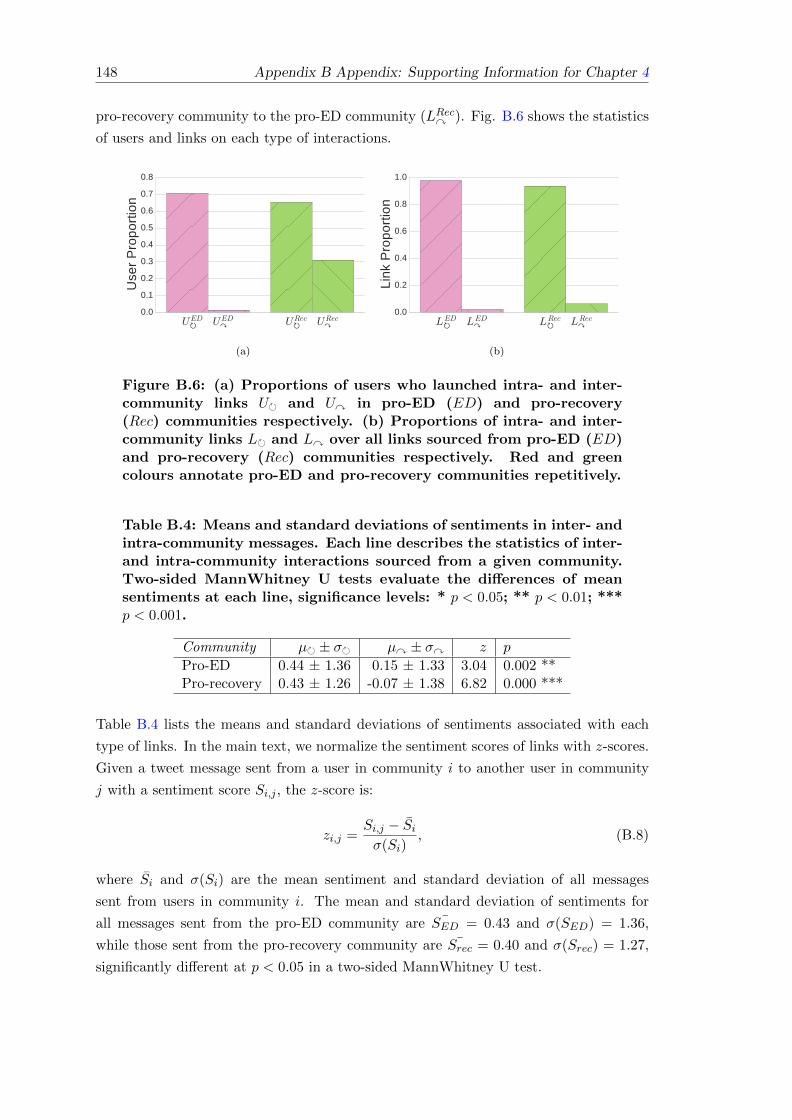
148 Appendix B Appendix: Supporting Information for Chapter 4
pro-recovery community to the pro-ED community (LRecy ). Fig. B.6 shows the statistics
of users and links on each type of interactions.
UED↻ UED↷ URec↻ URec↷0.0
0.1
0.2
0.3
0.4
0.5
0.6
0.7
0.8
Use
r P
ropo
rtio
n
(a)
LED↻ LED↷ LRec↻ LRec↷0.0
0.2
0.4
0.6
0.8
1.0
Link
Pro
port
ion
(b)
Figure B.6: (a) Proportions of users who launched intra- and inter-community links U� and Uy in pro-ED (ED) and pro-recovery(Rec) communities respectively. (b) Proportions of intra- and inter-community links L� and Ly over all links sourced from pro-ED (ED)and pro-recovery (Rec) communities respectively. Red and greencolours annotate pro-ED and pro-recovery communities repetitively.
Table B.4: Means and standard deviations of sentiments in inter- andintra-community messages. Each line describes the statistics of inter-and intra-community interactions sourced from a given community.Two-sided MannWhitney U tests evaluate the differences of meansentiments at each line, significance levels: * p < 0.05; ** p < 0.01; ***p < 0.001.
Community µ� ± σ� µy ± σy z p
Pro-ED 0.44 ± 1.36 0.15 ± 1.33 3.04 0.002 **Pro-recovery 0.43 ± 1.26 -0.07 ± 1.38 6.82 0.000 ***
Table B.4 lists the means and standard deviations of sentiments associated with each
type of links. In the main text, we normalize the sentiment scores of links with z-scores.
Given a tweet message sent from a user in community i to another user in community
j with a sentiment score Si,j , the z-score is:
zi,j =Si,j − Siσ(Si)
, (B.8)
where Si and σ(Si) are the mean sentiment and standard deviation of all messages
sent from users in community i. The mean and standard deviation of sentiments for
all messages sent from the pro-ED community are ¯SED = 0.43 and σ(SED) = 1.36,
while those sent from the pro-recovery community are ¯Srec = 0.40 and σ(Srec) = 1.27,
significantly different at p < 0.05 in a two-sided MannWhitney U test.

Appendix B Appendix: Supporting Information for Chapter 4 149
B.5 Measures on User Characteristics
We consider 22 measures on social activities and language use in tweets to characterize
users’ social behaviours and psychometric properties exhibited on Twitter.
B.5.1 Social Activities
The measures on social activities include:
Social Capital. We measure users’ social capital by their overall numbers of followees,
tweets and followers observed from their profile information respectively.
Activity. We use the average numbers of followees, tweets and followers per day (from
the date of account creation to the date of last post in our observation) to measure the
activity of a user.
Interaction Preference. We measure the proportions of tweets that involve different
types of interactions (i.e., re-tweeting, mentioning and replying) in a user’s most recent
tweets we collected. We only consider the mentions that are directly used by a user; any
mentions in an original tweet that users re-tweeted are ignored.
Interaction Diversity. We also measure whether a user tends to interact with various
individuals or certain specific people. Following previous studies [Eagle et al., 2010;
Weng and Menczer, 2015], we use entropy as a diversity measure. Given a user u, we
track the sequence of people interacted by u (denoted as Tu) in u’s historical tweets.
The interaction diversity of u in terms of a type of interactions I is measured by the
entropy of such interactions with different targets v ∈ Tu:
H(u, I) = −∑v∈Tu
p(Iv) log p(Iv), (B.9)
where I ∈ {re-tweet,mention, reply}, and p(Iv) = #Iv∑j∈Tu
#Ij. #Iv is the number of
interactions I with target v. Larger entropy values indicate a higher diversity of interests
that a user has.
B.5.2 Language Use
We adopt the psycholinguistic lexicon LIWC [Tausczik and Pennebaker, 2010] to charac-
terize users’ language use in tweets. This lexicon decomposes text data into 80 psycho-
logically relevant variables, corresponding to different emotion, linguistic styles, personal
concerns, and so on. Based on the cognitive behavioural theory of ED [Fairburn et al.,
1999], we frame 5 types of variables that measure cognitive attributes and thought pat-
terns associated with ED from LIWC outcomes: (1) concerns of body image, eating

150 Appendix B Appendix: Supporting Information for Chapter 4
behaviours and health, comprising body and ingest and health; (2) interpersonal aware-
ness and focus, comprising 1st personal singular (I) and 1st personal plural (we); (3)
social concern, encoded by social ; (4) abusive language and negation use, measured by
swear and negate; (5) affective processes, comprising positive emotion (posemo) and
negative emotion (negemo).
B.6 Community Norms
B.6.1 Characterizing Social Norms
0
3
6
9
1e−04 1e−03 1e−02
PD
F (
in P
ro−
ED
Com
mun
ity)
0.0
0.1
0.2
1e−12 1e−08 1e−04 1e+00
0.00
0.05
0.10
0.15
0.20
1e−12 1e−08 1e−04 1e+00
0
1
2
0.001 0.010
PageRank
PD
F (
in P
ro−
Rec
. Com
mun
ity)
0.00
0.05
0.10
1e−14 1e−10 1e−06 1e−02
Authority
0.00
0.04
0.08
0.12
1e−15 1e−10 1e−05 1e+00
Hub
Figure B.7: Probability density functions of PageRank, authority andhub centralities measured in pro-ED and pro-recovery communities.The values of centralities are logarithmic scaled (base=10).
In addition to users’ attributes measured by LIWC, we define a metric to measure the
tendency that a use promote a pro-ED or pro-recovery tendency (called pro-strength).
The basic ideal of this metric is that continuously making highly positive comments
on pro-ED or pro-recovery content in tweets indicates a strong tendency of a user to
promote a pro-ED or pro-recovery lifestyle and behaviour. Given user u who belongs
to a community c ∈ {pro-ED,pro-recovery}, has totally Nu tweets in our tweet corpus,
and posts a set of tweets Tc each of which contains one or more c-related hashtags, the
pro-strength of u is:
Prostr(u) =
∑Su(t|t ∈ Tc)Nu
, (B.10)

Appendix B Appendix: Supporting Information for Chapter 4 151
where Su(t) is the sentiment of u in tweet t. Note that we use the total number of tweets
Nu instead of the number of Tc(i.e., |Tc|) in the denominator of the above equation, in
order to capture the tendency that a user posts pro-ED or pro-recovery content in her/his
all tweets.
Fig. B.7 shows the distributions of PageRank [Page et al., 1999], authority and hub
centralities (produced by the HITS algorithm [Kleinberg, 1999]) that are measured from
the intra-community communication networks among pro-ED and pro-recovery users
respectively. Since PageRank gives a constant weight to nodes without any in-degree,
the distributions of PageRank centralities are smoother than those of HITS centralities
(i.e., without multiple peaks). Note that the ranges of centralities are different across
networks with different sizes.
B.6.2 Regression Models
We use linear robust regression models since these models require less restrictive as-
sumptions, as compared with the least squares regression [Andersen, 2008]. Each model
predicts the centrality of a user in a communication network based on an attribute of the
user (such as concerns on body or positive emotion), along with several covariates that
may affect a user’s mention and reply interactions on Twitter or the process of measuring
network centrality. These covariates include the total numbers of followers (#followees),
tweets (#tweets), followers (#followers) that a user has, fractions of historical tweets
that the user mentions (%mention) and replies to (%reply) others, and the number of
historical tweets that the user has in our data (#historical tweets). Robust regression
can be estimated by the iterated re-weighted least squares (IRLS), in which the influence
of outliers (i.e., observations that do not follow the pattern of the other observations)
are down-weighted to provide a better fit to the majority of the data. There are several
weighting functions that can be used for IRLS. We use the Huber’s weighting function
[Huber et al., 1964] in our analysis. The complete lists of variables and their coefficients
in each model are reported in Tables B.5-B.15. Note that we only consider users who
are within the giant weakly connected components of the intra-community networks,
due to the dominance of the giant components and incomparable PageRank values of
nodes across disconnected components. Thus, the numbers of users/observations in the
regression analysis are smaller than those reported in the main text.

152 Appendix B Appendix: Supporting Information for Chapter 4
Table B.5: Coefficients estimated for centrality as a function of bodyand covariates. Parentheses refer to standard errors.
Dependent variable:
(PageRank) (Authority) (Hub)
Pro-ED Pro-Rec. Pro-ED Pro-Rec. Pro-ED Pro-Rec.
Body 0.0001∗∗ −0.018∗ 0.00001∗∗∗ −0.015 0.00001 −0.019(0.00005) (0.008) (0.00000) (0.011) (0.00003) (0.032)
#Followees −0.00001∗∗∗ −0.0001∗∗∗ −0.00000∗∗∗ −0.0001 0.00000∗∗ 0.0002(0.00000) (0.00004) (0.00000) (0.0001) (0.00000) (0.0002)
#Tweets −0.00000∗∗∗ 0.0002∗ −0.00000∗∗∗ 0.0002 0.00000∗∗∗ −0.0004(0.00000) (0.0001) (0.00000) (0.0001) (0.00000) (0.0003)
#Followers 0.00002∗∗∗ 0.0002∗∗∗ 0.00000∗∗∗ 0.0002∗∗ −0.00000∗∗∗ −0.0002(0.00000) (0.00003) (0.00000) (0.0001) (0.00000) (0.0001)
%Mention −0.00002∗∗∗ 0.0005∗ −0.00000∗∗∗ 0.0003 0.00000 0.004∗∗∗
(0.00000) (0.0002) (0.00000) (0.0003) (0.00000) (0.001)
%Reply 0.00003∗∗∗ −0.0001 −0.00000 −0.001∗ −0.00000 −0.001(0.00000) (0.0003) (0.00000) (0.0005) (0.00000) (0.001)
#Historical Tweets 0.000∗∗∗ −0.00000 0.000∗∗∗ −0.00000 −0.000 0.00000∗
(0.000) (0.00000) (0.000) (0.00000) (0.000) (0.00000)
Constant 0.0001∗∗∗ −0.0004 0.00000 −0.001 0.00000 0.003(0.00000) (0.0004) (0.00000) (0.001) (0.00000) (0.002)
Observations 5,584 388 5,584 388 5,584 388
Note: ∗p<0.05; ∗∗p<0.01; ∗∗∗p<0.001
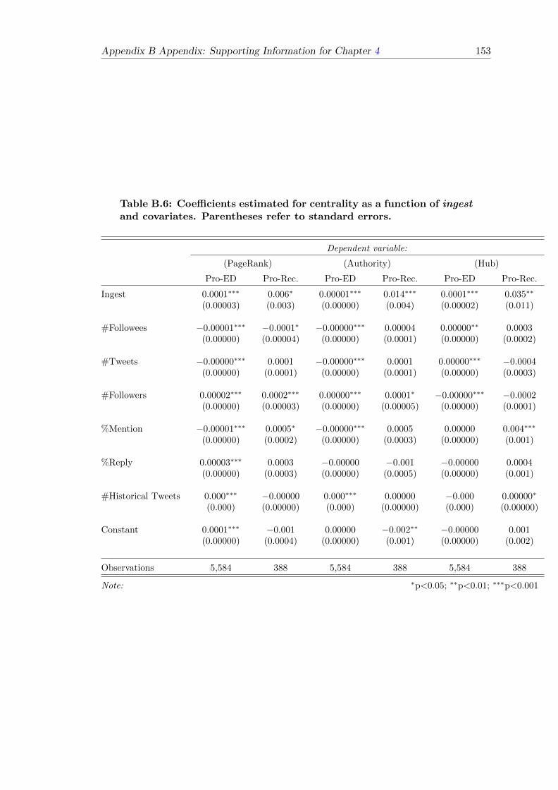
Appendix B Appendix: Supporting Information for Chapter 4 153
Table B.6: Coefficients estimated for centrality as a function of ingestand covariates. Parentheses refer to standard errors.
Dependent variable:
(PageRank) (Authority) (Hub)
Pro-ED Pro-Rec. Pro-ED Pro-Rec. Pro-ED Pro-Rec.
Ingest 0.0001∗∗∗ 0.006∗ 0.00001∗∗∗ 0.014∗∗∗ 0.0001∗∗∗ 0.035∗∗
(0.00003) (0.003) (0.00000) (0.004) (0.00002) (0.011)
#Followees −0.00001∗∗∗ −0.0001∗ −0.00000∗∗∗ 0.00004 0.00000∗∗ 0.0003(0.00000) (0.00004) (0.00000) (0.0001) (0.00000) (0.0002)
#Tweets −0.00000∗∗∗ 0.0001 −0.00000∗∗∗ 0.0001 0.00000∗∗∗ −0.0004(0.00000) (0.0001) (0.00000) (0.0001) (0.00000) (0.0003)
#Followers 0.00002∗∗∗ 0.0002∗∗∗ 0.00000∗∗∗ 0.0001∗ −0.00000∗∗∗ −0.0002(0.00000) (0.00003) (0.00000) (0.00005) (0.00000) (0.0001)
%Mention −0.00001∗∗∗ 0.0005∗ −0.00000∗∗∗ 0.0005 0.00000 0.004∗∗∗
(0.00000) (0.0002) (0.00000) (0.0003) (0.00000) (0.001)
%Reply 0.00003∗∗∗ 0.0003 −0.00000 −0.001 −0.00000 0.0004(0.00000) (0.0003) (0.00000) (0.0005) (0.00000) (0.001)
#Historical Tweets 0.000∗∗∗ −0.00000 0.000∗∗∗ 0.00000 −0.000 0.00000∗
(0.000) (0.00000) (0.000) (0.00000) (0.000) (0.00000)
Constant 0.0001∗∗∗ −0.001 0.00000 −0.002∗∗ −0.00000 0.001(0.00000) (0.0004) (0.00000) (0.001) (0.00000) (0.002)
Observations 5,584 388 5,584 388 5,584 388
Note: ∗p<0.05; ∗∗p<0.01; ∗∗∗p<0.001

154 Appendix B Appendix: Supporting Information for Chapter 4
Table B.7: Coefficients estimated for centrality as a function of healthand covariates. Parentheses refer to standard errors.
Dependent variable:
(PageRank) (Authority) (Hub)
Pro-ED Pro-Rec. Pro-ED Pro-Rec. Pro-ED Pro-Rec.
Health 0.0001∗ −0.003 0.00000 −0.003 0.00004 0.003(0.0001) (0.004) (0.00000) (0.006) (0.00004) (0.016)
#Followees −0.00001∗∗∗ −0.0001∗∗ −0.00000∗∗∗ −0.00004 0.00000∗∗ 0.0002(0.00000) (0.00004) (0.00000) (0.0001) (0.00000) (0.0002)
#Tweets −0.00000∗∗∗ 0.0001∗ −0.00000∗∗∗ 0.0002 0.00000∗∗∗ −0.0004(0.00000) (0.0001) (0.00000) (0.0001) (0.00000) (0.0003)
#Followers 0.00002∗∗∗ 0.0002∗∗∗ 0.00000∗∗∗ 0.0002∗∗ −0.00000∗∗∗ −0.0002(0.00000) (0.00003) (0.00000) (0.0001) (0.00000) (0.0001)
%Mention −0.00002∗∗∗ 0.0004 −0.00000∗∗∗ 0.0003 0.00000 0.004∗∗∗
(0.00000) (0.0002) (0.00000) (0.0003) (0.00000) (0.001)
%Reply 0.00003∗∗∗ −0.00002 −0.00000∗ −0.001∗ −0.00000 −0.0005(0.00000) (0.0004) (0.00000) (0.001) (0.00000) (0.001)
#Historical Tweets 0.000∗∗∗ −0.00000 0.000∗∗∗ −0.00000 −0.000 0.00000∗
(0.000) (0.00000) (0.000) (0.00000) (0.000) (0.00000)
Constant 0.0001∗∗∗ −0.001 0.00000 −0.001∗ 0.00000 0.002(0.00000) (0.0004) (0.00000) (0.001) (0.00000) (0.002)
Observations 5,584 388 5,584 388 5,584 388
Note: ∗p<0.05; ∗∗p<0.01; ∗∗∗p<0.001

Appendix B Appendix: Supporting Information for Chapter 4 155
Table B.8: Coefficients estimated for centrality as a function of i andcovariates. Parentheses refer to standard errors.
Dependent variable:
(PageRank) (Authority) (Hub)
Pro-ED Pro-Rec. Pro-ED Pro-Rec. Pro-ED Pro-Rec.
I −0.00004∗ −0.005∗ −0.00000∗ −0.011∗∗ −0.00001 −0.024∗∗
(0.00002) (0.002) (0.00000) (0.003) (0.00001) (0.008)
#Followees −0.00001∗∗∗ −0.0001∗∗ −0.00000∗∗∗ −0.00004 0.00000∗∗ 0.0002(0.00000) (0.00004) (0.00000) (0.0001) (0.00000) (0.0002)
#Tweets −0.00000∗∗∗ 0.0002∗ −0.00000∗∗∗ 0.0003∗ 0.00000∗∗∗ −0.0002(0.00000) (0.0001) (0.00000) (0.0001) (0.00000) (0.0003)
#Followers 0.00002∗∗∗ 0.0002∗∗∗ 0.00000∗∗∗ 0.0001 −0.00000∗∗∗ −0.0004∗
(0.00000) (0.00004) (0.00000) (0.0001) (0.00000) (0.0001)
%Mention −0.00002∗∗∗ 0.0003 −0.00000∗∗∗ 0.0001 0.00000 0.003∗∗∗
(0.00000) (0.0002) (0.00000) (0.0004) (0.00000) (0.001)
%Reply 0.00002∗∗∗ 0.0003 −0.00000∗∗ −0.001 −0.00001 0.001(0.00000) (0.0003) (0.00000) (0.001) (0.00000) (0.001)
#Historical Tweets 0.000∗∗ −0.00000 0.000∗∗∗ −0.00000 −0.000∗ 0.00000∗
(0.000) (0.00000) (0.000) (0.00000) (0.000) (0.00000)
Constant 0.0001∗∗∗ −0.0004 0.00000∗∗ −0.001 0.00000 0.003(0.00000) (0.0004) (0.00000) (0.001) (0.00000) (0.002)
Observations 5,584 388 5,584 388 5,584 388
Note: ∗p<0.05; ∗∗p<0.01; ∗∗∗p<0.001

156 Appendix B Appendix: Supporting Information for Chapter 4
Table B.9: Coefficients estimated for centrality as a function of weand covariates. Parentheses refer to standard errors.
Dependent variable:
(PageRank) (Authority) (Hub)
Pro-ED Pro-Rec. Pro-ED Pro-Rec. Pro-ED Pro-Rec.
We 0.0004∗ 0.009∗ −0.00001 0.007 −0.00001 0.014(0.0002) (0.004) (0.00001) (0.006) (0.0001) (0.015)
#Followees −0.00001∗∗∗ −0.0001∗∗ −0.00000∗∗∗ −0.00004 0.00000∗∗ 0.0002(0.00000) (0.00004) (0.00000) (0.0001) (0.00000) (0.0002)
#Tweets −0.00000∗∗∗ 0.0002∗ −0.00000∗∗∗ 0.0002 0.00000∗∗∗ −0.0003(0.00000) (0.0001) (0.00000) (0.0001) (0.00000) (0.0003)
#Followers 0.00002∗∗∗ 0.0002∗∗∗ 0.00000∗∗∗ 0.0001∗ −0.00000∗∗∗ −0.0003(0.00000) (0.00004) (0.00000) (0.0001) (0.00000) (0.0001)
%Mention −0.00002∗∗∗ 0.0004 −0.00000∗∗∗ 0.0003 0.00000 0.003∗∗∗
(0.00000) (0.0002) (0.00000) (0.0003) (0.00000) (0.001)
%Reply 0.00002∗∗∗ 0.0001 −0.00000∗ −0.001∗ −0.00001 −0.0005(0.00000) (0.0003) (0.00000) (0.0005) (0.00000) (0.001)
#Historical Tweets 0.000∗∗∗ −0.00000 0.000∗∗∗ −0.000 −0.000 0.00000∗
(0.000) (0.00000) (0.000) (0.00000) (0.000) (0.00000)
Constant 0.0001∗∗∗ −0.001 0.00000∗ −0.001∗ 0.00000 0.002(0.00000) (0.0004) (0.00000) (0.001) (0.00000) (0.002)
Observations 5,584 388 5,584 388 5,584 388
Note: ∗p<0.05; ∗∗p<0.01; ∗∗∗p<0.001
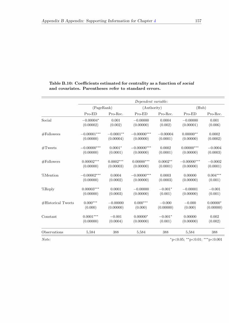
Appendix B Appendix: Supporting Information for Chapter 4 157
Table B.10: Coefficients estimated for centrality as a function of socialand covariates. Parentheses refer to standard errors.
Dependent variable:
(PageRank) (Authority) (Hub)
Pro-ED Pro-Rec. Pro-ED Pro-Rec. Pro-ED Pro-Rec.
Social −0.00004∗ 0.001 −0.00000 0.0004 −0.00000 0.001(0.00002) (0.002) (0.00000) (0.002) (0.00001) (0.006)
#Followees −0.00001∗∗∗ −0.0001∗∗ −0.00000∗∗∗ −0.00004 0.00000∗∗ 0.0002(0.00000) (0.00004) (0.00000) (0.0001) (0.00000) (0.0002)
#Tweets −0.00000∗∗∗ 0.0001∗ −0.00000∗∗∗ 0.0002 0.00000∗∗∗ −0.0004(0.00000) (0.0001) (0.00000) (0.0001) (0.00000) (0.0003)
#Followers 0.00002∗∗∗ 0.0002∗∗∗ 0.00000∗∗∗ 0.0002∗∗ −0.00000∗∗∗ −0.0002(0.00000) (0.00003) (0.00000) (0.0001) (0.00000) (0.0001)
%Mention −0.00002∗∗∗ 0.0004 −0.00000∗∗∗ 0.0003 0.00000 0.004∗∗∗
(0.00000) (0.0002) (0.00000) (0.0003) (0.00000) (0.001)
%Reply 0.00003∗∗∗ 0.0001 −0.00000 −0.001∗ −0.00001 −0.001(0.00000) (0.0003) (0.00000) (0.001) (0.00000) (0.001)
#Historical Tweets 0.000∗∗∗ −0.00000 0.000∗∗∗ −0.000 −0.000 0.00000∗
(0.000) (0.00000) (0.000) (0.00000) (0.000) (0.00000)
Constant 0.0001∗∗∗ −0.001 0.00000∗ −0.001∗ 0.00000 0.002(0.00000) (0.0004) (0.00000) (0.001) (0.00000) (0.002)
Observations 5,584 388 5,584 388 5,584 388
Note: ∗p<0.05; ∗∗p<0.01; ∗∗∗p<0.001

158 Appendix B Appendix: Supporting Information for Chapter 4
Table B.11: Coefficients estimated for centrality as a function of swearand covariates. Parentheses refer to standard errors.
Dependent variable:
(PageRank) (Authority) (Hub)
Pro-ED Pro-Rec. Pro-ED Pro-Rec. Pro-ED Pro-Rec.
Swear −0.0002∗ −0.009 −0.00000 −0.048 −0.0001 −0.241∗∗
(0.0001) (0.022) (0.00000) (0.033) (0.00004) (0.090)
#Followees −0.00001∗∗∗ −0.0001∗∗ −0.00000∗∗∗ −0.00004 0.00000∗∗ 0.0002(0.00000) (0.00004) (0.00000) (0.0001) (0.00000) (0.0002)
#Tweets −0.00000∗∗∗ 0.0001∗ −0.00000∗∗∗ 0.0002 0.00000∗∗∗ −0.0003(0.00000) (0.0001) (0.00000) (0.0001) (0.00000) (0.0003)
#Followers 0.00002∗∗∗ 0.0002∗∗∗ 0.00000∗∗∗ 0.0001∗ −0.00000∗∗∗ −0.0003∗
(0.00000) (0.00004) (0.00000) (0.0001) (0.00000) (0.0001)
%Mention −0.00002∗∗∗ 0.0004 −0.00000∗∗∗ 0.0003 0.00000 0.003∗∗∗
(0.00000) (0.0002) (0.00000) (0.0003) (0.00000) (0.001)
%Reply 0.00002∗∗∗ 0.0001 −0.00000∗ −0.001∗ −0.00001∗ −0.0003(0.00000) (0.0003) (0.00000) (0.0005) (0.00000) (0.001)
#Historical Tweets 0.000∗∗∗ −0.00000 0.000∗∗∗ 0.000 −0.000 0.00000∗
(0.000) (0.00000) (0.000) (0.00000) (0.000) (0.00000)
Constant 0.0001∗∗∗ −0.001 0.00000∗ −0.001 0.00000 0.003(0.00000) (0.0004) (0.00000) (0.001) (0.00000) (0.002)
Observations 5,584 388 5,584 388 5,584 388
Note: ∗p<0.05; ∗∗p<0.01; ∗∗∗p<0.001

Appendix B Appendix: Supporting Information for Chapter 4 159
Table B.12: Coefficients estimated for centrality as a function ofnegate and covariates. Parentheses refer to standard errors.
Dependent variable:
(PageRank) (Authority) (Hub)
Pro-ED Pro-Rec. Pro-ED Pro-Rec. Pro-ED Pro-Rec.
Negate −0.0001∗ −0.011 −0.00001∗∗ −0.017 −0.00003 −0.044(0.0001) (0.006) (0.00000) (0.010) (0.00003) (0.025)
#Followees −0.00001∗∗∗ −0.0001∗∗ −0.00000∗∗∗ −0.00004 0.00000∗∗ 0.0002(0.00000) (0.00004) (0.00000) (0.0001) (0.00000) (0.0002)
#Tweets −0.00000∗∗∗ 0.0002∗ −0.00000∗∗∗ 0.0002 0.00000∗∗∗ −0.0003(0.00000) (0.0001) (0.00000) (0.0001) (0.00000) (0.0003)
#Followers 0.00002∗∗∗ 0.0002∗∗∗ 0.00000∗∗∗ 0.0001∗ −0.00000∗∗∗ −0.0003∗
(0.00000) (0.00004) (0.00000) (0.0001) (0.00000) (0.0001)
%Mention −0.00002∗∗∗ 0.0004 −0.00000∗∗∗ 0.0002 0.00000 0.003∗∗∗
(0.00000) (0.0002) (0.00000) (0.0004) (0.00000) (0.001)
%Reply 0.00002∗∗∗ 0.0001 −0.00000∗∗ −0.001∗ −0.00001 −0.0004(0.00000) (0.0003) (0.00000) (0.001) (0.00000) (0.001)
#Historical Tweets 0.000∗∗∗ −0.00000 0.000∗∗∗ −0.00000 −0.000∗ 0.00000∗
(0.000) (0.00000) (0.000) (0.00000) (0.000) (0.00000)
Constant 0.0001∗∗∗ −0.0004 0.00000∗∗ −0.001 0.00000 0.003∗
(0.00000) (0.0004) (0.00000) (0.001) (0.00000) (0.002)
Observations 5,584 388 5,584 388 5,584 388
Note: ∗p<0.05; ∗∗p<0.01; ∗∗∗p<0.001

160 Appendix B Appendix: Supporting Information for Chapter 4
Table B.13: Coefficients estimated for centrality as a function ofposemo and covariates. Parentheses refer to standard errors.
Dependent variable:
(PageRank) (Authority) (Hub)
Pro-ED Pro-Rec. Pro-ED Pro-Rec. Pro-ED Pro-Rec.
Posemo −0.00002 −0.004 0.00000 −0.005 −0.00003 0.0004(0.00003) (0.003) (0.00000) (0.004) (0.00002) (0.011)
#Followees −0.00001∗∗∗ −0.0001∗∗ −0.00000∗∗∗ −0.00003 0.00000∗∗ 0.0002(0.00000) (0.00004) (0.00000) (0.0001) (0.00000) (0.0002)
#Tweets −0.00000∗∗∗ 0.0002∗ −0.00000∗∗∗ 0.0002 0.00000∗∗∗ −0.0004(0.00000) (0.0001) (0.00000) (0.0001) (0.00000) (0.0003)
#Followers 0.00002∗∗∗ 0.0002∗∗∗ 0.00000∗∗∗ 0.0002∗∗ −0.00000∗∗∗ −0.0002(0.00000) (0.00004) (0.00000) (0.0001) (0.00000) (0.0001)
%Mention −0.00002∗∗∗ 0.001∗ −0.00000∗∗∗ 0.0004 0.00000 0.003∗∗∗
(0.00000) (0.0002) (0.00000) (0.0003) (0.00000) (0.001)
%Reply 0.00003∗∗∗ 0.0002 −0.00000∗∗ −0.001 −0.00000 −0.001(0.00001) (0.0004) (0.00000) (0.001) (0.00000) (0.001)
#Historical Tweets 0.000∗∗∗ −0.00000 0.000∗∗∗ −0.00000 −0.000 0.00000∗
(0.000) (0.00000) (0.000) (0.00000) (0.000) (0.00000)
Constant 0.0001∗∗∗ −0.001 0.00000 −0.001 0.00000 0.002(0.00000) (0.0004) (0.00000) (0.001) (0.00000) (0.002)
Observations 5,584 388 5,584 388 5,584 388
Note: ∗p<0.05; ∗∗p<0.01; ∗∗∗p<0.001

Appendix B Appendix: Supporting Information for Chapter 4 161
Table B.14: Coefficients estimated for centrality as a function ofnegemo and covariates. Parentheses refer to standard errors.
Dependent variable:
(PageRank) (Authority) (Hub)
Pro-ED Pro-Rec. Pro-ED Pro-Rec. Pro-ED Pro-Rec.
Negemo −0.0001∗∗ −0.013∗∗ −0.00001∗∗∗ −0.018∗ −0.0001∗∗∗ −0.066∗∗∗
(0.00003) (0.005) (0.00000) (0.008) (0.00002) (0.020)
#Followees −0.00001∗∗∗ −0.0001∗∗ −0.00000∗∗∗ −0.00005 0.00000∗∗ 0.0002(0.00000) (0.00004) (0.00000) (0.0001) (0.00000) (0.0002)
#Tweets −0.00000∗∗∗ 0.0001∗ −0.00000∗∗∗ 0.0002 0.00000∗∗∗ −0.0004(0.00000) (0.0001) (0.00000) (0.0001) (0.00000) (0.0003)
#Followers 0.00002∗∗∗ 0.0002∗∗∗ 0.00000∗∗∗ 0.0001∗ −0.00000∗∗∗ −0.0003∗
(0.00000) (0.00003) (0.00000) (0.0001) (0.00000) (0.0001)
%Mention −0.00002∗∗∗ 0.0003 −0.00000∗∗∗ 0.0002 0.00000 0.003∗∗∗
(0.00000) (0.0002) (0.00000) (0.0004) (0.00000) (0.001)
%Reply 0.00002∗∗∗ 0.00001 −0.00000∗∗∗ −0.001∗ −0.00001∗∗ −0.001(0.00000) (0.0003) (0.00000) (0.001) (0.00000) (0.001)
#Historical Tweets 0.000∗∗ −0.00000 0.000∗∗∗ 0.00000 −0.000∗ 0.00000∗
(0.000) (0.00000) (0.000) (0.00000) (0.000) (0.00000)
Constant 0.0001∗∗∗ −0.0001 0.00000∗∗ −0.001 0.00000 0.005∗
(0.00000) (0.0004) (0.00000) (0.001) (0.00000) (0.002)
Observations 5,584 388 5,584 388 5,584 388
Note: ∗p<0.05; ∗∗p<0.01; ∗∗∗p<0.001

162 Appendix B Appendix: Supporting Information for Chapter 4
Table B.15: Coefficients estimated for centrality as a function ofprostrr and covariates. Parentheses refer to standard errors.
Dependent variable:
(PageRank) (Authority) (Hub)
Pro-ED Pro-Rec. Pro-ED Pro-Rec. Pro-ED Pro-Rec.
Prostrr 0.0001∗∗∗ 0.004∗ 0.00001∗∗∗ 0.004 −0.00000 0.039∗∗∗
(0.00001) (0.002) (0.00000) (0.002) (0.00001) (0.006)
#Followees −0.00001∗∗∗ −0.0001∗∗∗ −0.00000∗∗∗ −0.0001 0.00000∗∗ 0.0001(0.00000) (0.00004) (0.00000) (0.0001) (0.00000) (0.0002)
#Tweets −0.00000∗∗∗ 0.0002∗ −0.00000∗∗∗ 0.0002 0.00000∗∗∗ −0.0003(0.00000) (0.0001) (0.00000) (0.0001) (0.00000) (0.0003)
#Followers 0.00002∗∗∗ 0.0003∗∗∗ 0.00000∗∗∗ 0.0002∗∗ −0.00000∗∗∗ −0.0002(0.00000) (0.00004) (0.00000) (0.0001) (0.00000) (0.0001)
%Mention −0.00002∗∗∗ 0.0005∗ −0.00000∗∗∗ 0.0004 0.00000 0.004∗∗∗
(0.00000) (0.0002) (0.00000) (0.0003) (0.00000) (0.001)
%Reply 0.00003∗∗∗ 0.0001 −0.00000∗ −0.001∗ −0.00001 −0.0003(0.00000) (0.0003) (0.00000) (0.001) (0.00000) (0.001)
#Historical Tweets 0.000∗∗ −0.00000 0.000∗∗∗ −0.00000 −0.000 0.00000∗
(0.000) (0.00000) (0.000) (0.00000) (0.000) (0.00000)
Constant 0.0001∗∗∗ −0.001 0.00000 −0.002∗ 0.00000 0.002(0.00000) (0.0004) (0.00000) (0.001) (0.00000) (0.002)
Observations 5,584 388 5,584 388 5,584 388
Note: ∗p<0.05; ∗∗p<0.01; ∗∗∗p<0.001

Appendix C
Appendix: Supporting
Information for Chapter 5
C.1 ED-related hashtags
We identify ED-related users by searching for users who posted an ED-related hashtag
in tweets. The ED-related hashtags are obtained by (i) detecting clusters of hashtags
that frequently co-occur in a tweet posted by 3,380 ED users, using a similar method
that we used to detect topics of conversations in the main text; (ii) selecting ED-related
clusters of tags based on prior evidence from language use in online ED-related content
[Chancellor et al., 2016c; De Choudhury, 2015; Yom-Tov et al., 2012]; and (iii) removing
generic tags (e.g., #skinny and #food) from the selected clusters. Ref. [Wang et al.,
2018a] for details. We obtain 375 ED-related hashtags in total and Table C.1 lists
examples of these hashtags.
Table C.1: Examples of hashtags used to filter ED-related content.
thinspo, edproblems, thinspiration, proana, ana, thighgap, edprobs, ed, eatingdisor-der, anorexia, mia, skinny4xmas, bonespo, hipbones, proed, bulimia, ednos, edfam-ily, edlogic, thinkthin, legspo, promia, edthoughts, mythinspo, anorexic, edgirlprobs,edprobz, anamia, eatingdisorders, internationaledmeetup, edlife
C.2 Statistics of conversations
Figure C.1(a) shows an example how we aggregate tweets into conversations. We obtain
1,044,573 conversations consisting of 2,206,919 tweets. The average number of tweets
in a conversation is 2.11, with a standard deviation of 1.93. Figure C.1(b) shows the
distribution of numbers of tweets |Ci| in each conversation Ci. We see that many con-
versations contain a small number of tweets while a few have very large numbers of
163

164 Appendix C Appendix: Supporting Information for Chapter 5
10−6
10−5
10−4
10−3
10−2
10−1
100
100 100.5 101 101.5 102 102.5
|Ci|
P(|Ci|)
(a) (b)
Figure C.1: (a) Aggregating tweets by conversations. If user ui poststweet message mi,1 at time t0, user uj posts tweet mj,1 at time t1 toreply to mi,1, and the two users further have two subsequent inter-actions through mi,2 and mj,2, then the conversation Di between uiand uj is represented as Di = 〈mi,1,mj,1,mi,2,mj,2〉. (b) Distributionof conversation sizes. The red line fits a power-law distribution withexponent λ = 3.65± 0.04.
tweets, suggesting the heterogeneity of conversation sizes. Also, the straight line on the
logarithmic histogram indicates a power law in the distribution [Barabasi and Albert,
1999]. To quantify this pattern, we fit a power-law function P (|Ci|) = |Ci|−λ using
the maximum likelihood estimator and calculate p-value for the goodness of fit via a
bootstrapping procedure [Clauset et al., 2009]. From N = 1, 000 bootstrap replications,
we obtain the fitted values of exponent λ with the mean value µ = 3.65 (σ = 0.04) and
p = 0.18, confirming a power-law distribution in the sizes of conversations. This may
imply a preferential attachment process that people tend to follow hot conversations in
which many users have already involved.
Note that about 7% of tweets in the 1,044,573 conversations had already been deleted
at the time of our data collection. Only content of 2,062,690 tweets were retrieved and
used in the content analysis of main text. Moreover, these tweets are posted by 66,316
distinct users, where 24,860 users are absent in our user sample of 41,456 ED-related
users. Although not all the new users are strongly related to ED, to preserve the integrity
of communication flow, we included these new users in the network analysis of the main
text.
C.3 Statistics of topics
Figure C.2 gives descriptive statistics for the 26 topics identified above. As shown in
Figure C.2(a), most hashatags (83%) are classified into five topics with IDs 2, 4, 8, 16
and 22 respectively. These topics have been talked about by a large number of users in
tweets (Figures C.2(b) and (c)), indicating their popularity among users. By inspecting

Appendix C Appendix: Supporting Information for Chapter 5 165
the numbers of tweets that contain a hashtag labeled with a topic per month, we find
that users have consistently high levels of engagement in sharing these five topics over
time (Figure C.2(d)). In contrast, other topics are much less popular. To avoid analyzing
topics of interest to a specific subgroup of online ED communities, we focus on analyzing
the five popular topics.
0
500
1000
1500
0 10 20
Topic ID
#Has
htag
(a)
0
10000
20000
30000
40000
50000
0 10 20
Topic ID
#Tw
eet
(b)
0
10000
20000
0 10 20
Topic ID
#Use
r
(c)
0
2000
4000
6000
2009−10
2010−10
2011−10
2012−10
2013−10
2014−10
2015−10
Date
#Tw
eet
(d)
Figure C.2: Characterization of the 26 topics found in hashtag co-occurrence networks. (a) The numbers of hashtags in each topiclabeled by an ID in x-axis. (b) The number of tweets containing ahashtag in each topic. (c) The number of users who posted a hashtagof each topic. (d) The numbers of tweets on the five most populartopics per month.
C.4 Null models for testing inter-layer correlations
We use the following null models to evaluate the significance of inter-layer correlations.
Hypergeometric model: a null model testing the correlations of nodes’ activities
across layers in a multilayer network [Nicosia and Latora, 2015]. In this model,
the number N [α] of active nodes at each layer α is fixed to be that in the original
multilayer network and N [α] nodes are randomly sampled to be active at a layer α
by a uniform probability from all N nodes of the network. The null hypothesis of
this model is that the activity of a node at a layer is uncorrelated from its activities
at other layers. We use this model to assess the correlations of users’ activities in
different communication, i.e., empirical results of multiplexity.
Independent multilayer node-permutation model: an extension of the node-label
permutation model [Croft et al., 2011], in which we randomly reshuffle the iden-
tities of nodes (i.e., IDs of the corresponding users) while keeping the topology
(i.e., the degrees of nodes, the edges and the weights attached to edges) at a layer
α intact. However, reshuffling the identities of all nodes (i.e., both active and
inactive nodes) at a layer can lead to variations in the activities of nodes at the
layer, which makes randomized networks not comparable to the original multilayer
network. To maintain the activities of nodes across layers, we only reshuffle nodes
that are active at each layer of the original multilayer network. The null hypothesis
is that individuals can occupy any network position at a layer and their positions
at the layer are unrelated to those at other layers. We use this model to evaluate

166 Appendix C Appendix: Supporting Information for Chapter 5
the correlations of users’ roles in different communication, i.e., empirical results of
in-/out-strength correlations of nodes across layers.
Independent multilayer configuration model: a model testing the relations of link
structures across layers in a multilayer network [Paul and Chen, 2016]. In this
model, we fix the degree sequences of nodes at each layer α and randomly rewire
the edges at α. The null hypothesis is that nodes’ interconnections at a layer are
independent from those at other layers. We use this model to assess the correlations
of users’ connectivities in different communication, i.e., empirical results of link
overlaps.
Independent directed-weight reshuffling model: an extension of the directed-weight
reshuffling model [Opsahl et al., 2008]. For each layer α, we fix the network struc-
ture at α (i.e., the degrees of nodes and the links), and reshuffle weights locally
for each node across its out-links. That is, weights are reshuffled within links
sourced from the same node at each layer. In this way, randomized networks pre-
serve not only nodes’ activities and contacts, but also their engagement levels (i.e.,
out-strengths) across layers in the original multilayer network. The null hypoth-
esis is that the strength of a link between two nodes at a layer is unrelated to
those at other layers. We use this model to test the correlations of users’ interac-
tion strengths in different communication, i.e., empirical results of link strengths
across layers.
C.5 Statistics of temporal multilayer networks
LayerMental
Social
Fitness
Body
Thinspo
AGG.
100
400
700
1000
1300
1600
1900
2200
2500
2800
0 5 10 15 20 25 30 35 40 45 50t
#Act
ive
Nod
es
(a)
100
600
1100
1600
2100
2600
3100
3600
4100
4600
5100
0 5 10 15 20 25 30 35 40 45 50t
#Edg
es
(b)
Figure C.3: Statistics of temporal multilayer networks. (a) Numbersof active nodes and (b) numbers of directed links at each individuallayer of a temporal multilayer network and the aggregated networkof all layers (AGG.) at time t.

Appendix C Appendix: Supporting Information for Chapter 5 167
Figure C.3 shows the numbers of active nodes and edges at each layer of the generated
temporal multilayer networks, as well as the numbers of nodes and edges in the aggre-
gated networks over time. While different single-layer networks show different trends
in the numbers of active nodes and links, the total numbers of actors and connections
in each temporal multilayer network (i.e., statistics for the aggregated networks) are
sufficiently large to provide reasonably statistical power.

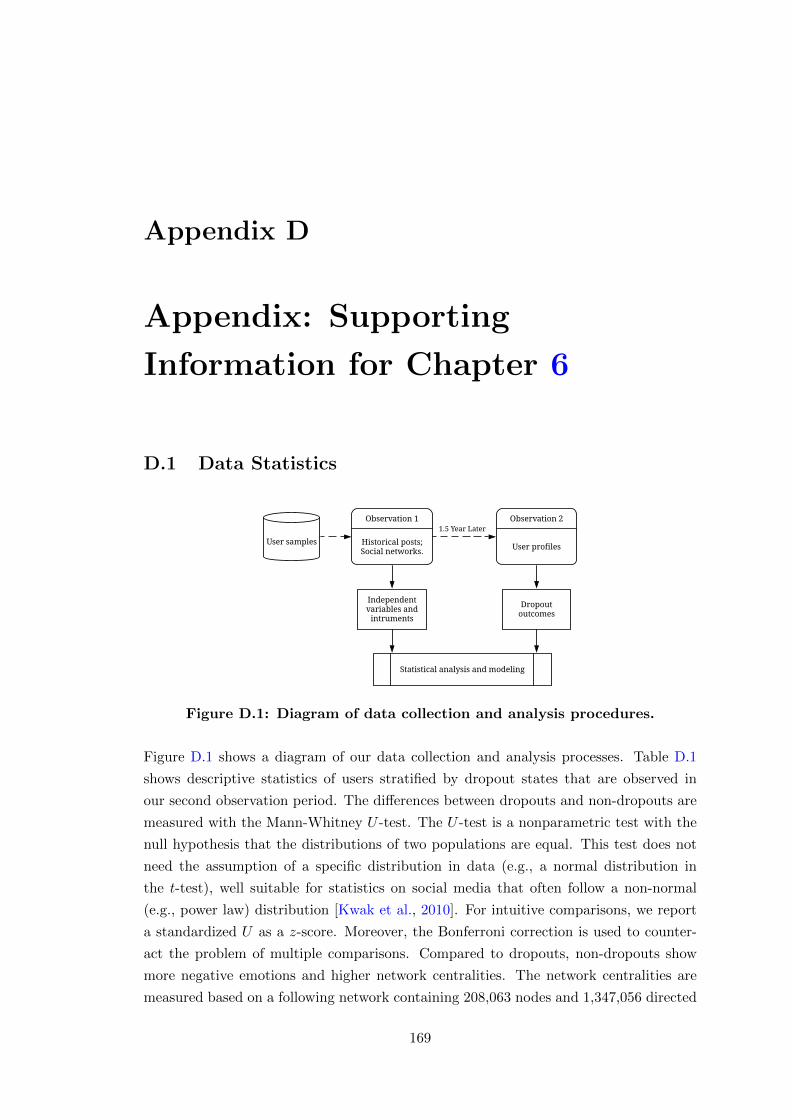
Appendix D
Appendix: Supporting
Information for Chapter 6
D.1 Data Statistics
Figure D.1: Diagram of data collection and analysis procedures.
Figure D.1 shows a diagram of our data collection and analysis processes. Table D.1
shows descriptive statistics of users stratified by dropout states that are observed in
our second observation period. The differences between dropouts and non-dropouts are
measured with the Mann-Whitney U -test. The U -test is a nonparametric test with the
null hypothesis that the distributions of two populations are equal. This test does not
need the assumption of a specific distribution in data (e.g., a normal distribution in
the t-test), well suitable for statistics on social media that often follow a non-normal
(e.g., power law) distribution [Kwak et al., 2010]. For intuitive comparisons, we report
a standardized U as a z-score. Moreover, the Bonferroni correction is used to counter-
act the problem of multiple comparisons. Compared to dropouts, non-dropouts show
more negative emotions and higher network centralities. The network centralities are
measured based on a following network containing 208,063 nodes and 1,347,056 directed
169

170 Appendix D Appendix: Supporting Information for Chapter 6
Table D.1: Descriptive statistics of users by dropout and non-dropoutstates.
Attributes All (n = 2, 906) Non-dropout (n = 447) Dropout (n = 2, 459) U -testMean SD Mean SD Mean SD zb P c
Emotions -0.09 0.36 -0.13 0.33 -0.08 0.37 -3.06 .03Centrality 29.35 16.22 35.89 15.25 28.16 16.11 9.26 <.001#Followees 309.34 483.29 533.19 862.29 268.64 360.69 10.32 < .001#Posts 899.62 2225.44 2298.01 4566.24 645.42 1281.62 16.02 <.001#Followers 308.15 752.74 656.25 1422.54 244.87 525.09 13.64 <.001Active days 348.20 403.06 732.17 524.86 278.40 332.03 18.43 <.001#Followee/day 4.16 19.07 1.75 4.87 4.60 20.60 -8.69 <.001#Posts/day 4.41 7.54 3.85 5.82 4.51 7.81 -1.13 1#Followers/day 2.66 8.23 1.57 3.03 2.85 8.84 -4.97 <.001#Tweets in use 614.43 827.33 1244.17 1078.79 499.96 715.65 16.47 <.001#Followees in use 242.13 366.69 405.27 639.19 212.47 280.92 9.56 <.001%Active followees 0.43 0.16 0.53 0.17 0.41 0.15 13.70 <.001〈Followee durations〉a 193.18 83.24 243.42 89.64 184.05 78.65 13.23 <.001〈Followee emotions〉a 0.06 0.16 0.01 0.16 0.07 0.16 -8.75 <.001〈Followee centralities〉a 29.38 9.04 28.04 8.70 29.62 9.08 -3.65 .004a〈Followee x〉 denotes the average values of a user’s followees in terms of statistics x.bA z-score measures the extent of a variable in non-dropout group being larger than that in dropout group.cP -values for two-tailed tests with Bonferroni correction.
edges. All nodes are connected in a single weakly connected component and the average
degree of the network is 6.5.
0
25
50
75
100
2010 2012 2014 2016 2018
Year
Num
ber
of U
sers
Type Account Created Time Last Posting Time
Figure D.2: Number of users along with time points when users cre-ated a Twitter account and posted the last tweet.
Figure D.2 shows details on dates when users joined and dropped out on Twitter. Most
users were active during 2012 to 2014, during which 1,944 users (67%) joined Twitter.
Two notable peaks in the curve of last posting time occur at the dates of our two
observations. The first peak indicates that some users were lost to follow up (e.g.,
accounts were deleted), and the second peak indicates that many users were still actively
posting tweets until our observations ended.
Figure D.3 shows demographic information of ED users, extracted from users’ Twitter
profile descriptions using regular expressions. To avoid noise (i.e., extremely small or

Appendix D Appendix: Supporting Information for Chapter 6 171
large values), we only consider users whose values are in the 95% confidence intervals
of the whole distribution of a statistic (except for gender). We obtain 357 users who
self-reported gender information and 84% of these users (n = 300) are female (see Figure
D.3(a)). There are 1,030 users who reported their ages in total. After excluding those
with extremely small and large values of age, Figure D.3(b) shows the distribution of
age among ED users (n = 1, 015), and the mean age of these users is 17.3. The majority
of females and young ages in the ED users align with clinical evidence that ED are often
developed among young females [Abebe et al., 2012; Association et al., 2013]. Figures
D.3(c) and (d) further show the distributions of height (with the mean of µ = 165.1cm)
and weights (µ = 57.6kg for current weight and µ = 49.4kg for goal weight) among ED
users. Comparing the distributions of weights, we see that the values of goal weights
are smaller than those of current weights. This implies that most ED users attempt
to lose weight. Moreover, we calculate BMI (Body Mass Index) for users who reported
information about both height and weight. Figure D.3(e) shows the distributions of
users’ current (µ = 21.1) and goal (µ = 18.4) BMIs. Compared to the reference values
of BMI for girls at the age of 17.3 years from World Health Organization (WHO)1, we
find that 58% of users (n = 574 among 991 users) have a current BMI lower than 21.1
(the reference value of median BMI), and 55% of users (n = 619 among 1,123 users) have
a goad BMI lower than 18.5 (the reference BMI for underweight). Note that we do not
include users’ demographic attributes in our estimation models due to a low fraction of
users who have these attributes (e.g., only 357 of 3,380 users with gender information).
0
100
200
300
F M
Gender (n=357)
Nu
mb
er o
f U
sers
(a)
0
50
100
150
10 15 20 25 30
Age (n=1,015)
Nu
mb
er o
f U
sers
(b)
0
100
200
300
150 160 170 180
Height (in cm, n=1,399)
Nu
mb
er o
f U
sers
(c)
0
100
200
300
400
500
25 50 75 100
Weight (in kg)
Nu
mb
er o
f U
sers
TypeCurrent Weight (n=2,189)
Goal Weight (n=2,670)
(d)
0
50
100
150
10 20 30
BMI
Nu
mb
er o
f U
sers
TypeCurrent BMI (n=991)
Goal BMI (n=1,123)
(e)
Figure D.3: Demographics of ED users, extracted from users’ self-reports in their Twitter profile descriptions. A dotted line marks themean of a corresponding statistic and the sample size for a statisticis reported in parentheses.
1http://www.who.int/growthref/bmifa_girls_5_19years_z.pdf?ua=1

172 Appendix D Appendix: Supporting Information for Chapter 6
D.2 Instrumental Variable Estimation
Suppose that one has observed independent and identically distributed data on (Y,E,X)
for n users, where Y denotes the occurrence of dropout (1 for dropout and 0 for non-
dropout), E denotes endogenous variables (i.e., users’ emotions), and X denotes exoge-
nous variables (i.e., covariates). We can specify a linear model to relate a decision to
dropout with users’ attributes on Twitter, as
Y = β0 + β1E + β2X + U, (D.1)
where U is an unobserved error term and βs are parameters to be estimated. As discussed
previously, endogeneity issues, i.e., cov(E,U) 6= 0, can bias such estimates when using
ordinary least squares (OLS). To produce consistent estimates, an instrumental variable
(IV) estimation computed through a two step approach called 2SLS is used. In the first
step, an auxiliary linear regression of instruments (i.e., the average level of emotions of
a user’s followees) and exogenous variables on endogenous variables runs.
E = γ0 + γ1Z + γ2X + V, (D.2)
where Z denotes the instruments, γs are estimable parameters and V is an error term.
Following the estimation, predicted values for E are obtained via E = γ0 + γ1Z + γ2X,
and used in the second step to replace the original endogeneous variables E.
Y = β′0 + β
′1E + β
′2X + U, (D.3)
The 2SLS estimation with IV has been well studies and can be carried out by the R
package AER2.
D.3 Survival Analysis with IV
We build an additive hazards model as follow. Suppose that one has observed indepen-
dent and identically distributed data on (T , E,X) for n users, where E is the endogenous
variables (i.e., emotion and centrality), X is the control variables, and T is the time to
dropout. Let U denote the unobserved error terms. Then, an additive hazards model
that estimates the effect of E on T is:
h(t|E,X,U) = β0(t) + βe(t)E + βx(t)X + βu(U |E,X, t), (D.4)
where h(t|E,X,U) is the hazard function of T evaluated at t, conditional on E, X and
U . β0(t) is the unknown baseline hazard function, while βe(t), βx(t) and βu(U |E,X, t)2https://cran.r-project.org/web/packages/AER/index.html

Appendix D Appendix: Supporting Information for Chapter 6 173
are regression functions that measure the effects of their corresponding covariates. All of
these functions are allowed to vary freely over time. The model posits that conditional
on X and U , the effect of E on T is linear in E for each t, although the effect size βe(t)
may vary with t. A sub-model is the partially-constant hazards model which can be
obtained by setting βe(t) = βe, where βe is an unknown constant. Following [Tchetgen
et al., 2015], we use this sub-model to measure and compare the effects of E on T in
different groups of users.
Similar to general regression models, the endogeneity problems can also bias the esti-
mates of an additive hazards model [Chan, 2016; Li et al., 2015; Tchetgen et al., 2015].
To obtain consistent estimations, we again use an IV method where user’s emotions and
network centralities are instrumented by the average levels of these attributes of user’s
followees. To compute an IV estimator in the survival context, we use a method devel-
oped by [Tchetgen et al., 2015]. This method is based on the control-function approach.
Like 2SLS, it also has two separated steps, but adds the residual from a first-stage re-
gression of the exposure on the IV to the additive hazards model. Specifically, similar
to 2SLS, the first-step regression model is:
E = γ0 + γ1Z + γ2X + V, (D.5)
where Z is the IV, γs are model parameters and V is the error term. Once we estimate
the model parameter γ, we compute the residual errors as V = E − γ0 + γ1Z + γ2X.
Then, we specify the linear projection of the error U in Eq. D.4 on V as:
βu(U |E,X, t) = ρ(t)V + ε(t) (D.6)
where ρ(t) is the regression coefficient, and ε(t) is a random error independent of (V,Z).
The model makes explicit the dependence between V and U , encoded in a non-null value
of ρ(t) 6= 0, and induces confounding bias. The residual error ε(t) introduces additional
variability to ensure that the relation between U and V is not assumed determinis-
tic. Apart from independence with (V,Z), the distribution of ε(t) is unrestricted. Let
h(t|E,X,Z,U) denote the observed hazard function of T given (E,X,Z), evaluated at
t. Then, we plug Eq. D.6 into Eq. D.4 and have the following result:
h(t|E,X,Z,U) = β′0(t) + β
′e(t)E + β
′x(t)X + ρ(t)V + ε(t), (D.7)
where β′0(t) is a baseline hazard function, while β
′e(t) and β
′x(t) are regression functions.
Intuitively, the residual V captures any variation in the hazard function due to unob-
served correlates of E, not accounted for in γ0 +γ1Z+γ2X. These unobserved correlates
must include any confounders of the association between E and T , and so V can be used
as a proxy measure of unobserved confounders. For this reason, ρ(t)V is referred to as a
control function. For estimation, we use V as an estimate of the unobserved residual V
that we use to fit an additive hazards model, with regressors (E,X, V ) under Eq. D.7.

174 Appendix D Appendix: Supporting Information for Chapter 6
Thus, in the second stage, we use Aalen’s least-squares to estimate the following hazard
model:
h(t|E,X,U) = β′0(t) + β
′e(t)E + β
′x(t)X + ρ(t)V + ε(t) (D.8)
Inference about B(t) = (β′0(t), β
′e(t), β
′x(t), ρ(t))
Tfor such a model has been well studied
and can be obtained using the R package TIMEREG3. However, the standard errors
and confidence intervals obtained in the package fail to appropriately account for the
additional uncertainty induced by the first-stage estimation of V . We can use the non-
parametric bootstrap for the whole estimation produce (including both the first-step and
second-step regressions) to produce more accurate estimates of standard errors [Petrin
and Train, 2010].
D.4 Null Model
We use a null model [Newman and Girvan, 2004] to test the statistical significance of
the homophily pattern. Specifically, we randomly shuffle users’ dropout states and re-
measure homophily coefficients r [Newman, 2003] based on the shuffled states. These
coefficients can be viewed as observed values of a random variable. Repeating this
procedure 3,000 times, we yield the empirical distribution of homophily coefficients with
a mean of µ = 0 and a standard deviation of σ = 0.005. The z-score for the observed
homophily (i.e., r = 0.09 in the main text) under this baseline distribution is z = 16.84
and P < .001, suggesting the presence of homophily.
D.5 Specifications of Data Censoring Methods
We tune the parameters of our data censoring methods based on users’ activities be-
fore and after our first observation. We apply each censoring method with different
parameters to data on users activities before our first observation to estimate users
dropout states, and choose parameters that achieve the best agreement between the
estimated dropout states and the observed states in our second observation. By set-
ting π ∈ [1, 300] days in the identical-interval censoring method, we find the optimal
parameter being π = 101, with Cohens κ = .68 of the estimated dropout states and the
observed dropout states of users. Such good agreement illustrates the effectiveness of the
censoring approach. Similarly, by searching in a parameter space of π ∈ [0, 200] days and
λ ∈ [0, 1], we find the optimal parameters in the personalized-interval censoring method
being π = 161 and λ = 0.6, with Cohens κ = .68 as well. We use these parameters cen-
sor the dropout states of users who were active in the second observation. Figure D.4
shows the Kaplan-Meier curves of users’ survival time from our first observation until
our second observation using the two censoring methods. The median survival time of
3https://cran.r-project.org/web/packages/timereg/index.html
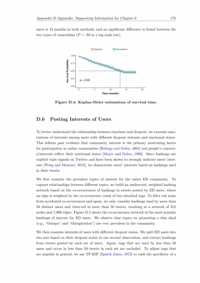
Appendix D Appendix: Supporting Information for Chapter 6 175
users is 13 months in both methods, and no significant difference is found between the
two types of censorships (P = .93 in a log-rank test).
+ ++ +
p = 0.93
0.00
0.25
0.50
0.75
1.00
0 5 10 15 20
Time (months)
Surv
ival
Pro
babi
lity
+ +
Figure D.4: Kaplan-Meier estimations of survival time.
D.6 Posting Interests of Users
To better understand the relationship between emotions and dropout, we examine asso-
ciations of interests among users with different dropout statuses and emotional states.
This follows past evidence that community interest is the primary motivating factor
for participation in online communities [Ridings and Gefen, 2004] and people’s concern-
s/interests reflect their emotional states [Mayer and Geher, 1996]. Since hashtags are
explicit topic signals on Twitter and have been shown to strongly indicate users’ inter-
ests [Weng and Menczer, 2015], we characterize users’ interests based on hashtags used
in their tweets.
We first examine the prevalent topics of interest for the entire ED community. To
capture relationships between different topics, we build an undirected, weighted hashtag
network based on the co-occurrences of hashtags in tweets posted by ED users, where
an edge is weighted by the co-occurrence count of two attached tags. To filter out noise
from accidental co-occurrences and spam, we only consider hashtags used by more than
50 distinct users and observed in more than 50 tweets, resulting in a network of 312
nodes and 7,906 edges. Figure D.5 shows the co-occurrence network of the most popular
hashtags of interest for ED users. We observe that topics on promoting a thin ideal
(e.g., “thinspo” and “thinspiration”) are very prevalent in the community.
We then examine interests of users with different dropout states. We split ED users into
two sets based on their dropout states in our second observation, and extract hashtags
from tweets posted by each set of users. Again, tags that are used by less than 50
users and occur in less than 50 tweets in each set are excluded. To adjust tags that
are popular in general, we use TF-IDF [Sparck Jones, 1972] to rank the specificity of a

176 Appendix D Appendix: Supporting Information for Chapter 6
proana
myfitnesspalthinspo
edproblems
hipbonesthighgap
skinny
thinspiration
ana
ed
bulimia
diet
weightloss
eatingdisorder
proed
anorexia
picslip
mia
skinny4xmas
motivation
ff
edprobs
thin
fitspo
anasisters
staystrong
fat perfection
bellletstalk
bonespo
Figure D.5: The co-occurrence network of the most popular hashtagsused by all ED users. Each node is a hashtag, and node size is pro-portional to the number of users who posted the tag. Node color isassigned based on the frequency of a tag so that high frequency isdarker and low frequency is lighter. Edge width is proportional tothe number of co-occurrences of two attached tags in tweets.
Table D.2: The most popular hashtags used by ED users, grouped by users’dropout states.
Dropout states Hashtagsa
Non-dropout legspo, mythinspo, skinny4xmas, bonespo, goals, edlogic, eatingdisorders,edthoughts, ribs, bones, depressed, depression, edprobs, collarbones, bulimia,promia, replytweet, beautiful, anorexia, thin, hipbones, legs, ednos, ed, thigh-gap, weightloss, skinny, proed, selfharm, perfection, mia, thinspiration, perfect,proana, diet, eatingdisorder
Dropout goaway, stopbullying, worthless, selfharmprobz, ew, anasisters, yay, one-day, reasonstobefit, bulimicprobz, anorexicprobz, fact, disgusting, thankgod,willpower, tweetwhatyoueat, wow, toofat, jealous, thankyou, true, anasister,anafamily, starveon, gross, teamfollowback, fuck, icandothis, tired, edfamily,relapse, stayingstrong
aTags for each state are ranked in a decreasing order based on the TF-IDF score of a tag, which is calculatedby the ratio of the number of users who post the tag and have a given dropout state to the number of userswho post the tag in the whole user sample (i.e., regardless of users’ dropout states).
tag in each set of users. Table D.2 lists the most representative hashtags in each user
set, in which we find that users with different dropout states display distinct interests
online. Non-dropouts are interested in advocating a thin ideal (e.g., “mythinspo” and
“skinny4xmas”) and reinforcing a pro-ED identity (e.g., “edlogic” and “beautiful”). In
contrast, dropouts engage more in discussing their health problems (e.g., “selfharm-
probz”, “bulimicprobz”, “anorexicprobz” and “relapse”) and offering emotional support
for others (e.g., “anasisters” and “stayingstrong”), which implies a tendency of these
users to recover from disorders [Lyons et al., 2006; Wolf et al., 2013; Yom-Tov et al.,
2012]. Together, these results imply that pro-recovery users are more likely to drop out
than pro-ED users. A comparison of interests between each individual set and the entire
community (see Figure D.5) further shows that the non-dropouts have dominated the

Appendix D Appendix: Supporting Information for Chapter 6 177
Table D.3: The most popular hashtags used by ED users, grouped by users’emotional states.
Emotionalstates
Hashtagsa
Negative bonespo, mythinspo, edlogic, bulimia, depression, starve, eatingdisorders, anxi-ety, anorexia, skinny4xmas, depressed, edprobs, proed, ribs, bones, edproblems,thinspo, edthoughts, thinspiration, selfharm, fuck, goals, thin, edgirlprobs, fat,sad, skinny, ednos, realityproject, ana, eatingdisorder, fatass, hipbones
Neutral awkward, anorexicprobz, fast, mylife, bulimicprobz, please, sorry, fuckyou, my-fitnesspal, ew, skinny4xmas, legspo, edfamily, gross, anafamily, ugh, ednos,workout, goals, replytweet, tmi, fatass, reversethinspo, edprobz, anaproblems,failure, flatstomach, fact, binge, fatty, fasting, suicide, depressed
Positive eatclean, fitfam, inspiration, reasonstobefit, ff, noexcuses, fitness, loveit, win-ning, anasister, tweetwhatyoueat, twye, keepgoing, success, jealous, want, fit-spo, beforeandafter, retweet, excited, proud, reasonstoloseweight, abcdiet, fail,justsaying, rt, motivated, workout, stayingstrong, love, myfitnesspal
aTags for each state are ranked in a decreasing order based on the TF-IDF score of a tag, which is calculatedby the ratio of the number of users who post the tag and have a given emotional state to the number ofusers who post the tag in the whole user sample (i.e., regardless of users’ emotional states).
topics of discussions within the community. This is expected because the non-dropouts
have prolonged participation, with 732.17 active days on average compared to 278.40
days of the dropouts (see Table D.1).
Similarly, we split ED users into three equal-size sets based on their emotional scores
and obtain the most representative hashtags among each set of users in Table D.3. The
results show that users with negative emotions more engage in promoting thin ideals
(e.g., “bonespo” and “mythinspo”), showing largely overlapping interests with the non-
dropouts. In contrast, users with neutral and positive emotions are more interested in
discussing their health problems (e.g., “anorexicprobz” and “bulimicprobz”), opposing
pro-ED promotions (e.g., “reversethinspo”) and encouraging healthier body image and
behaviors (e.g., “fitfam” and “fitness”), showing similar interests with the dropouts.
To further quantify the similarity (or association) of posting interests between users
with a dropout state and those with a emotional state (as identified in Tables D.2 and
D.3), we measure the Spearman rank correlation r between pairwise lists of hashtags
posted by users with a given state (e.g., dropped-out or not, and positive or negative).
We use the Spearman correlation because (i) it is more robust to scaling of data than
other measures (e.g., cosine similarity) and (ii) it does not assume that datasets follow a
specific distribution (e.g., a normal distribution in the Pearson correlation). The results
of correlations are shown in Table 4 of the main text.


References
Aalen, O., Borgan, O., and Gjessing, H. (2008). Survival and event history analysis: a
process point of view. Springer Science & Business Media.
Aalen, O. O. (1989). A linear regression model for the analysis of life times. Statistics
in medicine, 8(8):907–925.
Abbar, S., Mejova, Y., and Weber, I. (2015). You tweet what you eat: Studying food
consumption through twitter. In Proceedings of the 33rd Annual ACM Conference on
Human Factors in Computing Systems, pages 3197–3206. ACM.
Abebe, D. S., Lien, L., and von Soest, T. (2012). The development of bulimic symp-
toms from adolescence to young adulthood in females and males: A population-based
longitudinal cohort study. International Journal of Eating Disorders, 45(6):737–745.
Agarwal, M. K., Ramamritham, K., and Bhide, M. (2012). Real time discovery of dense
clusters in highly dynamic graphs: identifying real world events in highly dynamic
environments. Proceedings of the VLDB Endowment, 5(10):980–991.
Ahn, Y.-Y., Bagrow, J. P., and Lehmann, S. (2009). Link communities reveal multiscale
complexity in networks. arXiv preprint arXiv:0903.3178.
Aichner, T. and Jacob, F. (2015). Measuring the degree of corporate social media use.
International Journal of Market Research, 57(2):257–275.
Aiello, L. M., Barrat, A., Schifanella, R., Cattuto, C., Markines, B., and Menczer, F.
(2012). Friendship prediction and homophily in social media. ACM Transactions on
the Web (TWEB), 6(2):9.
Aiello, L. M., Petkos, G., Martin, C., Corney, D., Papadopoulos, S., Skraba, R., Goker,
A., Kompatsiaris, I., and Jaimes, A. (2013). Sensing trending topics in twitter. IEEE
Transactions on Multimedia, 15(6):1268–1282.
Ajilore, O., Amialchuk, A., Xiong, W., and Ye, X. (2014). Uncovering peer effects
mechanisms with weight outcomes using spatial econometrics. The Social Science
Journal, 51(4):645–651.
179

180 REFERENCES
Albert, R., Jeong, H., and Barabasi, A.-L. (2000). Error and attack tolerance of complex
networks. nature, 406(6794):378.
Altman, I. and Taylor, D. A. (1973). Social penetration: The development of interper-
sonal relationships. Holt, Rinehart & Winston.
Altman, N. S. (1992). An introduction to kernel and nearest-neighbor nonparametric
regression. The American Statistician, 46(3):175–185.
Alvarez-Conrad, J., Zoellner, L. A., and Foa, E. B. (2001). Linguistic predictors of
trauma pathology and physical health. Applied Cognitive Psychology, 15(7):S159–
S170.
Alvarez-Melis, D. and Saveski, M. (2016). Topic modeling in twitter: Aggregating tweets
by conversations. ICWSM, 2016:519–522.
Amichai-Hamburger, Y., Gazit, T., Bar-Ilan, J., Perez, O., Aharony, N., Bronstein,
J., and Dyne, T. S. (2016). Psychological factors behind the lack of participa-
tion in online discussions. Computers in Human Behavior, 55:268–277. [DOI:
10.1016/j.chb.2015.09.009].
An, W. (2015). Instrumental variables estimates of peer effects in social networks. Social
science research, 50:382–394.
Anderberg, M. R. (1973). Cluster analysis for applications. Technical report, Office of
the Assistant for Study Support Kirtland AFB N MEX.
Andersen, R. (2008). Modern methods for robust regression. Number 152. Sage.
Angrist, J. and Imbens, G. (1995). Identification and estimation of local average treat-
ment effects.
Angrist, J. D., Imbens, G. W., and Rubin, D. B. (1996). Identification of causal ef-
fects using instrumental variables. Journal of the American statistical Association,
91(434):444–455. [DOI: 10.2307/2291629].
Appel, G. (2005). Technical analysis: power tools for active investors. FT Press.
Aral, S., Muchnik, L., and Sundararajan, A. (2009). Distinguishing influence-based
contagion from homophily-driven diffusion in dynamic networks. Proceedings of the
National Academy of Sciences, 106(51):21544–21549.
Aral, S. and Nicolaides, C. (2017). Exercise contagion in a global social network. Nature
communications, 8:14753.
Aral, S. and Walker, D. (2012). Identifying influential and susceptible members of social
networks. Science, 337(6092):337–341.

REFERENCES 181
Arcelus, J., Mitchell, A. J., Wales, J., and Nielsen, S. (2011). Mortality rates in pa-
tients with anorexia nervosa and other eating disorders: a meta-analysis of 36 studies.
Archives of general psychiatry, 68(7):724–731.
Arseniev-Koehler, A., Lee, H., McCormick, T., and Moreno, M. A. (2016). # proana:
Pro-eating disorder socialization on twitter. Journal of Adolescent Health, 58(6):659–
664.
Association, A. P. et al. (2013). Diagnostic and statistical manual of mental disorders
(DSM-5 R©). American Psychiatric Pub.
Aston, N., Liddle, J., and Hu, W. (2014). Twitter sentiment in data streams with
perceptron. Journal of Computer and Communications, 2014.
Baccianella, S., Esuli, A., and Sebastiani, F. (2010). Sentiwordnet 3.0: An enhanced
lexical resource for sentiment analysis and opinion mining. In LREC, volume 10, pages
2200–2204.
Bailey, K. (2008). Methods of social research. Simon and Schuster.
Bailey, N. T. et al. (1975). The mathematical theory of infectious diseases and its appli-
cations. Charles Griffin & Company Ltd, 5a Crendon Street, High Wycombe, Bucks
HP13 6LE.
Bakshy, E., Hofman, J. M., Mason, W. A., and Watts, D. J. (2011). Everyone’s an
influencer: quantifying influence on twitter. In Proceedings of the fourth ACM inter-
national conference on Web search and data mining, pages 65–74. ACM.
Ballester, C., Calvo-Armengol, A., and Zenou, Y. (2006). Who’s who in networks.
wanted: The key player. Econometrica, 74(5):1403–1417.
Balsa, A. and Dıaz, C. (2018). Social interactions in health behaviors and conditions.
Barabasi, A.-L. and Albert, R. (1999). Emergence of scaling in random networks. science,
286(5439):509–512.
Bardone-Cone, A. M. and Cass, K. M. (2006). Investigating the impact of pro-anorexia
websites: A pilot study. European Eating Disorders Review.
Bardone-Cone, A. M. and Cass, K. M. (2007). What does viewing a pro-anorexia
website do? an experimental examination of website exposure and moderating effects.
International Journal of Eating Disorders, 40(6):537–548.
Battiston, F., Nicosia, V., and Latora, V. (2014). Structural measures for multiplex
networks. Physical Review E, 89(3):032804.
Bazarova, N. N. and Choi, Y. H. (2014). Self-disclosure in social media: Extending the
functional approach to disclosure motivations and characteristics on social network
sites. Journal of Communication, 64(4):635–657.

182 REFERENCES
Beat (2015). The costs of eating disorders: Social, health and economic
impacts. From https://www.b-eat.co.uk/assets/000/000/302/The_costs_of_
eating_disorders_Final_original.pdf?1424694814, 2015-02.
Becker, A. E., Hadley Arrindell, A., Perloe, A., Fay, K., and Striegel-Moore, R. H.
(2010). A qualitative study of perceived social barriers to care for eating disorders:
perspectives from ethnically diverse health care consumers. International Journal of
Eating Disorders, 43(7):633–647.
Bentley, B., Branicky, R., Barnes, C. L., Chew, Y. L., Yemini, E., Bullmore, E. T.,
Vertes, P. E., and Schafer, W. R. (2016). The multilayer connectome of caenorhabditis
elegans. PLoS computational biology, 12(12):e1005283.
Berlingerio, M., Coscia, M., Giannotti, F., Monreale, A., and Pedreschi, D. (2011).
Foundations of multidimensional network analysis. In Advances in Social Networks
Analysis and Mining (ASONAM), 2011 International Conference on, pages 485–489.
IEEE.
Bianconi, G. (2013). Statistical mechanics of multiplex networks: Entropy and overlap.
Physical Review E, 87(6):062806.
Bild, D. R., Liu, Y., Dick, R. P., Mao, Z. M., and Wallach, D. S. (2015). Aggregate
characterization of user behavior in twitter and analysis of the retweet graph. ACM
Transactions on Internet Technology (TOIT), 15(1):4.
Bishop, C. M. (2006). Pattern recognition and machine learning. springer.
Blei, D. and Lafferty, J. (2006). Correlated topic models. Advances in neural information
processing systems, 18:147.
Blei, D. M. (2012). Probabilistic topic models. Communications of the ACM, 55(4):77–
84.
Blei, D. M., Ng, A. Y., and Jordan, M. I. (2003). Latent dirichlet allocation. Journal of
machine Learning research, 3(Jan):993–1022.
Blondel, V. D., Guillaume, J.-L., Lambiotte, R., and Lefebvre, E. (2008). Fast unfold-
ing of communities in large networks. Journal of statistical mechanics: theory and
experiment, 2008(10):P10008.
Boccaletti, S., Bianconi, G., Criado, R., Del Genio, C. I., Gomez-Gardenes, J., Romance,
M., Sendina-Nadal, I., Wang, Z., and Zanin, M. (2014). The structure and dynamics
of multilayer networks. Physics Reports, 544(1):1–122.
Boepple, L., Ata, R. N., Rum, R., and Thompson, J. K. (2016). Strong is the new
skinny: A content analysis of fitspiration websites. Body image, 17:132–135.

REFERENCES 183
Bond, R. M., Fariss, C. J., Jones, J. J., Kramer, A. D., Marlow, C., Settle, J. E., and
Fowler, J. H. (2012). A 61-million-person experiment in social influence and political
mobilization. Nature, 489(7415):295–298.
Borgatti, S. P. (2005). Centrality and network flow. Social networks, 27(1):55–71.
Borzekowski, D. L., Schenk, S., Wilson, J. L., and Peebles, R. (2010). e-ana and e-mia:
A content analysis of pro–eating disorder web sites. American journal of public health,
100(8):1526–1534.
Boucher, V., Bramoulle, Y., Djebbari, H., and Fortin, B. (2014). Do peers affect student
achievement? evidence from canada using group size variation. Journal of applied
econometrics, 29(1):91–109.
Bouma, G. (2009). Normalized (pointwise) mutual information in collocation extraction.
In Proceedings of the Biennial GSCL Conference, volume 156.
Bourigault, S., Lagnier, C., Lamprier, S., Denoyer, L., and Gallinari, P. (2014). Learning
social network embeddings for predicting information diffusion. In Proceedings of the
7th ACM international conference on Web search and data mining, pages 393–402.
ACM.
Boyd, D., Golder, S., and Lotan, G. (2010). Tweet, tweet, retweet: Conversational
aspects of retweeting on twitter. In System Sciences (HICSS), 2010 43rd Hawaii
International Conference on, pages 1–10. IEEE.
Bramoulle, Y., Djebbari, H., and Fortin, B. (2009). Identification of peer effects through
social networks. Journal of econometrics, 150(1):41–55.
Branley, D. B. and Covey, J. (2017). Pro-ana versus pro-recovery: A content analytic
comparison of social media users communication about eating disorders on twitter
and tumblr. Frontiers in psychology, 8:1356.
Brissette, I., Scheier, M. F., and Carver, C. S. (2002). The role of optimism in social
network development, coping, and psychological adjustment during a life transition.
Journal of personality and social psychology, 82(1):102.
Broniatowski, D. A., Paul, M. J., and Dredze, M. (2013). National and local influenza
surveillance through twitter: an analysis of the 2012-2013 influenza epidemic. PloS
one, 8(12):e83672.
Brosius, H.-B. and Weimann, G. (1996). Who sets the agenda: Agenda-setting as a
two-step flow. Communication Research, 23(5):561–580.
Brown, B. B., Clasen, D. R., and Eicher, S. A. (1986). Perceptions of peer pressure, peer
conformity dispositions, and self-reported behavior among adolescents. Developmental
psychology, 22(4):521.

184 REFERENCES
Budak, C. and Agrawal, R. (2013). On participation in group chats on twitter. In
Proceedings of the 22nd international conference on World Wide Web, pages 165–176.
ACM.
Buettner, R. (2016). Getting a job via career-oriented social networking sites: The
weakness of ties. In 2016 49th Hawaii International Conference on System Sciences
(HICSS), pages 2156–2165. IEEE.
Buldyrev, S. V., Parshani, R., Paul, G., Stanley, H. E., and Havlin, S. (2010). Catas-
trophic cascade of failures in interdependent networks. Nature, 464(7291):1025.
Bulow, J. I., Geanakoplos, J. D., and Klemperer, P. D. (1985). Multimarket oligopoly:
Strategic substitutes and complements. Journal of Political economy, 93(3):488–511.
Cai, H., Huang, Z., Srivastava, D., and Zhang, Q. (2015). Indexing evolving events from
tweet streams. IEEE Transactions on Knowledge and Data Engineering, 27(11):3001–
3015.
Campbell, K. and Peebles, R. (2014). Eating disorders in children and adolescents: state
of the art review. Pediatrics, 134(3):582–592.
Card, D. (1999). The causal effect of education on earnings. In Handbook of labor
economics, volume 3, pages 1801–1863. Elsevier. [DOI: 10.1016/S1573-4463(99)03011-
4].
Carneiro, H. A. and Mylonakis, E. (2009). Google trends: a web-based tool for real-time
surveillance of disease outbreaks. Clinical infectious diseases, 49(10):1557–1564.
Casalo, L. V., Flavian, C., and Guinalıu, M. (2013). New members’ integration: Key fac-
tor of success in online travel communities. Journal of Business Research, 66(6):706–
710. [DOI: 10.1016/j.jbusres.2011.09.007].
Cash, T. F., Cash, D. W., and Butters, J. W. (1983). ” mirror, mirror, on the wall...?”
contrast effects and self-evaluations of physical attractiveness. Personality and Social
Psychology Bulletin, 9(3):351–358.
Casilli, A. A., Pailler, F., Tubaro, P., et al. (2013). Online networks of eating-disorder
websites: why censoring pro-ana might be a bad idea. Perspectives in public health,
133(2):94–95.
Cawley, J. and Meyerhoefer, C. (2012). The medical care costs of obesity: an instru-
mental variables approach. Journal of health economics, 31(1):219–230.
CDC (2014). Behavioral risk factor surveillance system survey data. atlanta, ga: Us
department of health and human services, centers for disease control and prevention.
Cha, M., Haddadi, H., Benevenuto, F., and Gummadi, P. K. (2010). Measuring user
influence in twitter: The million follower fallacy. ICWSM, 10(10-17):30.

REFERENCES 185
Chalmers, T. C., Smith, H., Blackburn, B., Silverman, B., Schroeder, B., Reitman, D.,
and Ambroz, A. (1981). A method for assessing the quality of a randomized control
trial. Controlled clinical trials, 2(1):31–49.
Chan, K. C. G. (2016). Instrumental variable additive hazards models with exposure-
dependent censoring. Biometrics.
Chancellor, S., Kalantidis, Y., Pater, J. A., De Choudhury, M., and Shamma, D. A.
(2017). Multimodal classification of moderated online pro-eating disorder content. In
Proceedings of the 2017 CHI Conference on Human Factors in Computing Systems,
pages 3213–3226. ACM.
Chancellor, S., Lin, Z., Goodman, E. L., Zerwas, S., and De Choudhury, M. (2016a).
Quantifying and predicting mental illness severity in online pro-eating disorder com-
munities. In Proceedings of the 19th ACM Conference on Computer-Supported Coop-
erative Work & Social Computing, pages 1171–1184. ACM.
Chancellor, S., Lin, Z. J., and De Choudhury, M. (2016b). this post will just get
taken down: Characterizing removed pro-eating disorder social media content. In
Proceedings of the 2016 CHI Conference on Human Factors in Computing Systems,
pages 1157–1162. ACM.
Chancellor, S., Mitra, T., and De Choudhury, M. (2016c). Recovery amid pro-anorexia:
Analysis of recovery in social media. In Proceedings of the 2016 CHI Conference on
Human Factors in Computing Systems, pages 2111–2123. ACM.
Chancellor, S., Pater, J. A., Clear, T., Gilbert, E., and De Choudhury, M. (2016d). #
thyghgapp: Instagram content moderation and lexical variation in pro-eating disorder
communities. In Proceedings of the 19th ACM Conference on Computer-Supported
Cooperative Work & Social Computing, pages 1201–1213. ACM.
Chen, M. K. (2013). The effect of language on economic behavior: Evidence from sav-
ings rates, health behaviors, and retirement assets. The American Economic Review,
103(2):690–731.
Chesley, E. B., Alberts, J., Klein, J., and Kreipe, R. (2003). Pro or con? anorexia
nervosa and the internet. Journal of Adolescent Health, 32(2):123–124.
Chiu, C.-M., Hsu, M.-H., and Wang, E. T. (2006). Understanding knowledge sharing
in virtual communities: An integration of social capital and social cognitive theories.
Decision support systems, 42(3):1872–1888. [DOI: 10.1016/j.dss.2006.04.001].
Chmiel, A., Sienkiewicz, J., Thelwall, M., Paltoglou, G., Buckley, K., Kappas, A., and
Ho lyst, J. A. (2011). Collective emotions online and their influence on community
life. PloS one, 6(7):e22207.

186 REFERENCES
Choi, S. (2015). The two-step flow of communication in twitter-based public forums.
Social Science Computer Review, 33(6):696–711.
Christakis, N. A. and Fowler, J. H. (2007). The spread of obesity in a large social
network over 32 years. New England journal of medicine, 357(4):370–379.
Christakis, N. A. and Fowler, J. H. (2008). The collective dynamics of smoking in a
large social network. New England journal of medicine, 358(21):2249–2258.
Christakis, N. A. and Fowler, J. H. (2013). Social contagion theory: examining dynamic
social networks and human behavior. Statistics in medicine, 32(4):556–577.
Chung, C. and Pennebaker, J. W. (2007). The psychological functions of function words.
Social communication, pages 343–359.
Cialdini, R. B. (2003). Crafting normative messages to protect the environment. Current
directions in psychological science, 12(4):105–109.
Clauset, A., Newman, M. E., and Moore, C. (2004). Finding community structure in
very large networks. Physical review E, 70(6):066111.
Clauset, A., Shalizi, C. R., and Newman, M. E. (2009). Power-law distributions in
empirical data. SIAM review, 51(4):661–703.
Cobb, N. K., Graham, A. L., and Abrams, D. B. (2010). Social network structure of
a large online community for smoking cessation. American journal of public health,
100(7):1282–1289.
Cohen-Cole, E. and Fletcher, J. M. (2008). Is obesity contagious? social networks vs. en-
vironmental factors in the obesity epidemic. Journal of health economics, 27(5):1382–
1387.
Coleman, J. S. (1960). The adolescent subculture and academic achievement. American
Journal of Sociology, 65(4):337–347.
Collins, R. L. (1996). For better or worse: The impact of upward social comparison on
self-evaluations. Psychological bulletin, 119(1):51.
Connor, N., Barberan, A., and Clauset, A. (2017). Using null models to infer microbial
co-occurrence networks. PloS one, 12(5):e0176751.
Conover, M., Ratkiewicz, J., Francisco, M. R., Goncalves, B., Menczer, F., and Flam-
mini, A. (2011). Political polarization on twitter. ICWSM, 133:89–96.
Cook, E., Teasley, S. D., and Ackerman, M. S. (2009). Contribution, commercialization
& audience: understanding participation in an online creative community. In Pro-
ceedings of the ACM 2009 international conference on Supporting group work, pages
41–50. ACM. [DOI: 10.1145/1531674.1531681].
REFERENCES 187
Coppersmith, G., Dredze, M., Harman, C., and Hollingshead, K. (2015). From adhd
to sad: Analyzing the language of mental health on twitter through self-reported
diagnoses. In Proceedings of the 2nd Workshop on Computational Linguistics and
Clinical Psychology: From Linguistic Signal to Clinical Reality, pages 1–10.
Coppersmith, G., Harman, C., and Dredze, M. (2014). Measuring post traumatic stress
disorder in twitter. In ICWSM.
Corrigan, P. W. and Watson, A. C. (2002). Understanding the impact of stigma on
people with mental illness. World psychiatry, 1(1):16.
Corstorphine, E. (2006). Cognitive–emotional–behavioural therapy for the eating dis-
orders: Working with beliefs about emotions. European Eating Disorders Review,
14(6):448–461.
Cortes, C. and Vapnik, V. (1995). Support-vector networks. Machine learning,
20(3):273–297.
Costa-Font, J. and Jofre-Bonet, M. (2013). Anorexia, body image and peer effects:
evidence from a sample of european women. Economica, 80(317):44–64.
Council, N. R. et al. (2009). Institute of medicine.(2009). preventing mental, emotional,
and behavioral disorders among young people: Progress and possibilities. Board on
Children, Youth, and Families, Division of Behavioral and Social Sciences and Edu-
cation. The National Academies Press, Washington, DC.
Coviello, L., Sohn, Y., Kramer, A. D., Marlow, C., Franceschetti, M., Christakis, N. A.,
and Fowler, J. H. (2014). Detecting emotional contagion in massive social networks.
PloS one, 9(3):e90315. [PMID: 24621792] [DOI: 10.1371/journal.pone.0090315].
Cox, D. R. (1992). Regression models and life-tables. In Breakthroughs in statistics,
pages 527–541. Springer.
Crandall, C. S. (1988). Social contagion of binge eating. Journal of personality and
social psychology, 55(4):588.
Crandall, D., Cosley, D., Huttenlocher, D., Kleinberg, J., and Suri, S. (2008). Feedback
effects between similarity and social influence in online communities. In Proceedings
of the 14th ACM SIGKDD international conference on Knowledge discovery and data
mining, pages 160–168. ACM.
Croft, D. P., Madden, J. R., Franks, D. W., and James, R. (2011). Hypothesis testing
in animal social networks. Trends in Ecology & Evolution, 26(10):502–507.
Csardi, G. and Nepusz, T. (2006). The igraph software package for complex network
research. InterJournal, Complex Systems, 1695(5):1–9.

188 REFERENCES
Cui, A., Zhang, M., Liu, Y., and Ma, S. (2011). Emotion tokens: Bridging the gap among
multilingual twitter sentiment analysis. In Asia Information Retrieval Symposium,
pages 238–249. Springer.
Culotta, A. (2014). Estimating county health statistics with twitter. In Proceedings of
the 32nd CHI conference, pages 1335–1344. ACM.
Da Silva, N. F., Hruschka, E. R., and Hruschka, E. R. (2014). Tweet sentiment analysis
with classifier ensembles. Decision Support Systems, 66:170–179.
D’Andrea, W., Chiu, P. H., Casas, B. R., and Deldin, P. (2012). Linguistic predictors
of post-traumatic stress disorder symptoms following 11 september 2001. Applied
Cognitive Psychology, 26(2):316–323.
Davies, D. L. and Bouldin, D. W. (1979). A cluster separation measure. IEEE transac-
tions on pattern analysis and machine intelligence, (2):224–227.
Davison, B. D. (2000). Topical locality in the web. In Proceedings of the 23rd annual
international ACM SIGIR conference on Research and development in information
retrieval, pages 272–279. ACM.
De Choudhury, M. (2015). Anorexia on tumblr: A characterization study. In Proceedings
of the 5th International Conference on Digital Health 2015, pages 43–50. ACM.
De Choudhury, M., Counts, S., and Horvitz, E. (2013a). Major life changes and behav-
ioral markers in social media: case of childbirth. In Proceedings of the 2013 conference
on Computer supported cooperative work, pages 1431–1442. ACM.
De Choudhury, M., Counts, S., and Horvitz, E. (2013b). Social media as a measurement
tool of depression in populations. In Proceedings of the 5th Annual ACM Web Science
Conference, pages 47–56. ACM.
De Choudhury, M., Counts, S., Horvitz, E. J., and Hoff, A. (2014). Characterizing and
predicting postpartum depression from shared facebook data. In Proceedings of the
17th ACM conference on Conference on Computer-Supported Cooperative Work and
Social Computing (CSCW), pages 626–638. ACM.
De Choudhury, M., Gamon, M., Counts, S., and Horvitz, E. (2013c). Predicting depres-
sion via social media. In ICWSM.
De Choudhury, M. and Kıcıman, E. (2017). The language of social support in social
media and its effect on suicidal ideation risk. In Proceedings of the... International
AAAI Conference on Weblogs and Social Media. International AAAI Conference on
Weblogs and Social Media, volume 2017, page 32. NIH Public Access.
De Choudhury, M., Kiciman, E., Dredze, M., Coppersmith, G., and Kumar, M. (2016a).
Discovering shifts to suicidal ideation from mental health content in social media. In

REFERENCES 189
Proceedings of the 2016 CHI Conference on Human Factors in Computing Systems,
pages 2098–2110. ACM.
De Choudhury, M., Lin, Y.-R., Sundaram, H., Candan, K. S., Xie, L., Kelliher, A., et al.
(2010). How does the data sampling strategy impact the discovery of information
diffusion in social media? ICWSM, 10:34–41.
De Choudhury, M., Sharma, S., and Kiciman, E. (2016b). Characterizing dietary choices,
nutrition, and language in food deserts via social media. In Proceedings of the 19th
ACM Conference on Computer-Supported Cooperative Work & Social Computing,
pages 1157–1170. ACM.
De Domenico, M., Nicosia, V., Arenas, A., and Latora, V. (2015). Structural reducibility
of multilayer networks. Nature communications, 6:6864.
De Domenico, M., Sole-Ribalta, A., Cozzo, E., Kivela, M., Moreno, Y., Porter, M. A.,
Gomez, S., and Arenas, A. (2013). Mathematical formulation of multilayer networks.
Physical Review X, 3(4):041022.
De Domenico, M., Sole-Ribalta, A., Gomez, S., and Arenas, A. (2014). Navigability of
interconnected networks under random failures. Proceedings of the National Academy
of Sciences, 111(23):8351–8356.
de Vries, D. A., Peter, J., de Graaf, H., and Nikken, P. (2016). Adolescents social net-
work site use, peer appearance-related feedback, and body dissatisfaction: Testing a
mediation model. Journal of youth and adolescence, 45(1):211–224. [PMID: 25788122]
[DOI: 10.1007/s10964-015-0266-4].
DeMasi, O., Mason, D., and Ma, J. (2016). Understanding communities via hashtag
engagement: A clustering based approach. In ICWSM, pages 102–111.
Dempster, A. P., Laird, N. M., and Rubin, D. B. (1977). Maximum likelihood from
incomplete data via the em algorithm. Journal of the royal statistical society. Series
B (methodological), pages 1–38.
Ding, X., Liu, B., and Yu, P. S. (2008). A holistic lexicon-based approach to opinion
mining. In Proceedings of the 2008 international conference on web search and data
mining, pages 231–240. ACM.
Dobbins, M., Cockerill, R., and Barnsley, J. (2001). Factors affecting the utilization of
systematic reviews: A study of public health decision makers. International journal
of technology assessment in health care, 17(2):203–214.
Dolemeyer, R., Tietjen, A., Kersting, A., and Wagner, B. (2013). Internet-based in-
terventions for eating disorders in adults: a systematic review. BMC psychiatry,
13(1):207.

190 REFERENCES
Dumais, S. T. (2004). Latent semantic analysis. Annual review of information science
and technology, 38(1):188–230.
Duncan, O. D., Haller, A. O., and Portes, A. (1968). Peer influences on aspirations: A
reinterpretation. American Journal of Sociology, 74(2):119–137.
Dunn, J. C. (1973). A fuzzy relative of the isodata process and its use in detecting
compact well-separated clusters.
Eagle, N., Macy, M., and Claxton, R. (2010). Network diversity and economic develop-
ment. Science, 328(5981):1029–1031.
Eisenberg, M. E., Neumark-Sztainer, D., Story, M., and Perry, C. (2005). The role
of social norms and friends influences on unhealthy weight-control behaviors among
adolescent girls. Social Science & Medicine, 60(6):1165–1173.
Ellison, N., Heino, R., and Gibbs, J. (2006). Managing impressions online: Self-
presentation processes in the online dating environment. Journal of computer-mediated
communication, 11(2):415–441.
Ernala, S. K., Rizvi, A. F., Birnbaum, M. L., Kane, J. M., and De Choudhury, M.
(2017). Linguistic markers indicating therapeutic outcomes of social media disclosures
of schizophrenia. Proc ACM Hum-Comput Interact, 1(1):43.
Esplen, M. J., Garfinkel, P., and Gallop, R. (2000). Relationship between self-soothing,
aloneness, and evocative memory in bulimia nervosa. International Journal of Eating
Disorders, 27(1):96–100.
Estrada, E., Meloni, S., Sheerin, M., and Moreno, Y. (2016). Epidemic spreading in
random rectangular networks. Physical Review E, 94(5):052316.
Eysenbach, G. (2005). The law of attrition. Journal of medical Internet research, 7(1).
Eysenbach, G., Powell, J., Englesakis, M., Rizo, C., and Stern, A. (2004). Health related
virtual communities and electronic support groups: systematic review of the effects
of online peer to peer interactions. Bmj, 328(7449):1166.
Fairburn, C. G. and Beglin, S. J. (1994). Assessment of eating disorders: Interview or
self-report questionnaire? International journal of eating disorders, 16(4):363–370.
Fairburn, C. G. and Harrison, P. J. (2003). Eating disorders. The Lancet, 361(9355):407–
416.
Fairburn, C. G., Shafran, R., and Cooper, Z. (1999). A cognitive behavioural theory of
anorexia nervosa. Behaviour Research and Therapy, 37(1):1–13.
Fani, H. and Bagheri, E. (2017). Community detection in social networks. Encyclopedia
with Semantic Computing and Robotic Intelligence, 1(01):1630001.

REFERENCES 191
Farmer, A. S. and Kashdan, T. B. (2012). Social anxiety and emotion regulation in
daily life: Spillover effects on positive and negative social events. Cognitive behaviour
therapy, 41(2):152–162. [PMID: 22428662] [DOI: 10.1080/16506073.2012.666561].
Fassino, S., Piero, A., Tomba, E., and Abbate-Daga, G. (2009). Factors associated with
dropout from treatment for eating disorders: a comprehensive literature review. BMC
psychiatry, 9(1):67.
Fehr, E. and Gachter, S. (2000). Fairness and retaliation: The economics of reciprocity.
Journal of economic perspectives, 14(3):159–181.
Fergie, G., Hilton, S., and Hunt, K. (2015). Young adults’ experiences of seeking online
information about diabetes and mental health in the age of social media. Health
Expectations.
Ferrara, E., JafariAsbagh, M., Varol, O., Qazvinian, V., Menczer, F., and Flammini, A.
(2013). Clustering memes in social media. In Advances in social networks analysis
and mining (ASONAM), 2013 IEEE/ACM international conference on, pages 548–
555. IEEE.
Ferrara, E. and Yang, Z. (2015). Measuring emotional contagion in social media. PloS
one, 10(11):e0142390.
Festinger, L. (1954). A theory of social comparison processes. Human relations, 7(2):117–
140.
Fiore, A. T. and Donath, J. S. (2005). Homophily in online dating: when do you like
someone like yourself? In CHI’05 Extended Abstracts on Human Factors in Computing
Systems, pages 1371–1374. ACM.
Fiori, K. L., Antonucci, T. C., and Cortina, K. S. (2006). Social network typologies and
mental health among older adults. The Journals of Gerontology Series B: Psycholog-
ical Sciences and Social Sciences, 61(1):P25–P32.
Fortunato, S. and Barthelemy, M. (2007). Resolution limit in community detection.
Proceedings of the National Academy of Sciences, 104(1):36–41.
Foster, E. M. (1997). Instrumental variables for logistic regression: an illustration. Social
Science Research, 26(4):487–504.
Fowler, J. H. and Christakis, N. A. (2008). Dynamic spread of happiness in a large
social network: longitudinal analysis over 20 years in the framingham heart study.
Bmj, 337:a2338.
Frane, A. V. (2015). Are per-family type i error rates relevant in social and behavioral
science? Journal of Modern Applied Statistical Methods, 14(1):5.

192 REFERENCES
Fredrickson, B. L. (2000). Cultivating positive emotions to optimize health and well-
being. Prevention & Treatment, 3(1):1a.
Freedman, D. and Diaconis, P. (1981). On the histogram as a density estimator: L 2
theory. Zeitschrift fur Wahrscheinlichkeitstheorie und verwandte Gebiete, 57(4):453–
476.
Freeman, L. C. (1978). Centrality in social networks conceptual clarification. Social
networks, 1(3):215–239.
Freilich, S., Zarecki, R., Eilam, O., Segal, E. S., Henry, C. S., Kupiec, M., Gophna, U.,
Sharan, R., and Ruppin, E. (2011). Competitive and cooperative metabolic interac-
tions in bacterial communities. Nature communications, 2:589.
Friedkin, N. E. (1991). Theoretical foundations for centrality measures. American
journal of Sociology, 96(6):1478–1504. [DOI: 10.1086/229694].
Fruchterman, T. M. and Reingold, E. M. (1991). Graph drawing by force-
directed placement. Software: Practice and experience, 21(11):1129–1164. [DOI:
10.1002/spe.4380211102].
Gailey, J. A. (2009). starving is the most fun a girl can have: The pro-ana subculture
as edgework. Critical Criminology, 17(2):93–108.
Gallos, L. K., Rybski, D., Liljeros, F., Havlin, S., and Makse, H. A. (2012). How people
interact in evolving online affiliation networks. Physical Review X, 2(3):031014.
Garcia, D., Mavrodiev, P., Casati, D., and Schweitzer, F. (2017). Understanding popu-
larity, reputation, and social influence in the twitter society. Policy & Internet.
Garcia, D., Mavrodiev, P., and Schweitzer, F. (2013). Social resilience in online com-
munities: The autopsy of friendster. In Proceedings of the first ACM conference on
Online social networks, pages 39–50. ACM. [DOI: 10.1145/2512938.2512946].
Gavin, J., Rodham, K., and Poyer, H. (2008). The presentation of pro-anorexia in online
group interactions. Qualitative health research, 18(3):325–333.
Ghiassi, M., Skinner, J., and Zimbra, D. (2013). Twitter brand sentiment analysis: A
hybrid system using n-gram analysis and dynamic artificial neural network. Expert
Systems with applications, 40(16):6266–6282.
Ghiglino, C. and Goyal, S. (2010). Keeping up with the neighbors: social interaction in
a market economy. Journal of the European Economic Association, 8(1):90–119.
Giachanou, A. and Crestani, F. (2016). Like it or not: A survey of twitter sentiment
analysis methods. ACM Computing Surveys (CSUR), 49(2):28.

REFERENCES 193
Giatsidis, C., Thilikos, D. M., and Vazirgiannis, M. (2013). D-cores: measuring collab-
oration of directed graphs based on degeneracy. Knowledge and information systems,
35(2):311–343. [DOI: 10.1109/icdm.2011.46].
Giles, D. (2006). Constructing identities in cyberspace: The case of eating disorders.
British journal of social psychology, 45(3):463–477.
Ginsberg, J., Mohebbi, M. H., Patel, R. S., Brammer, L., Smolinski, M. S., and Brilliant,
L. (2009). Detecting influenza epidemics using search engine query data. Nature,
457(7232):1012–1014.
Girvan, M. and Newman, M. E. (2002). Community structure in social and biological
networks. Proceedings of the national academy of sciences, 99(12):7821–7826.
Glaeser, E. L., Sacerdote, B. I., and Scheinkman, J. A. (2003). The social multiplier.
Journal of the European Economic Association, 1(2-3):345–353.
Glaeser, E. L. and Scheinkman, J. (2000). Non-market interactions. Technical report,
National Bureau of Economic Research.
Go, A., Bhayani, R., and Huang, L. (2009). Twitter sentiment classification using distant
supervision. CS224N Project Report, Stanford, 1:12.
Goffman, E. (1959). The presentation of self in everyday life. New York.
Goldberg, D., Nichols, D., Oki, B. M., and Terry, D. (1992). Using collaborative filtering
to weave an information tapestry. Communications of the ACM, 35(12):61–70.
Goncalves, B., Perra, N., and Vespignani, A. (2011). Modeling users’ activity on twitter
networks: Validation of dunbar’s number. PloS one, 6(8):e22656.
Goncalves, P., Araujo, M., Benevenuto, F., and Cha, M. (2013). Comparing and com-
bining sentiment analysis methods. In Proceedings of the first ACM conference on
Online social networks, pages 27–38. ACM. [DOI: 10.1145/2512938.2512951].
Gotelli, N. J. and Ulrich, W. (2012). Statistical challenges in null model analysis. Oikos,
121(2):171–180.
Gottschalk, L. A. and Gleser, G. C. (1969). The measurement of psychological states
through the content analysis of verbal behavior. Univ of California Press.
Gow, R. W., Trace, S. E., and Mazzeo, S. E. (2010). Preventing weight gain in first
year college students: an online intervention to prevent the freshman fifteen. Eating
behaviors, 11(1):33–39.
Granovetter, M. S. (1973). The strength of weak ties. American journal of sociology,
pages 1360–1380.

194 REFERENCES
Grilo, C. M., Pagano, M. E., Stout, R. L., Markowitz, J. C., Ansell, E. B., Pinto, A.,
Zanarini, M. C., Yen, S., and Skodol, A. E. (2012). Stressful life events predict eating
disorder relapse following remission: Six-year prospective outcomes. International
Journal of Eating Disorders, 45(2):185–192.
Grimes, A., Landry, B. M., and Grinter, R. E. (2010). Characteristics of shared health
reflections in a local community. In Proceedings of the 2010 ACM conference on
Computer supported cooperative work, pages 435–444. ACM.
Guarda, A. S. (2008). Treatment of anorexia nervosa: insights and obstacles. Physiology
& Behavior, 94(1):113–120.
Guille, A. and Hacid, H. (2012). A predictive model for the temporal dynamics of
information diffusion in online social networks. In Proceedings of the 21st international
conference on World Wide Web, pages 1145–1152. ACM.
Guille, A., Hacid, H., Favre, C., and Zighed, D. A. (2013). Information diffusion in
online social networks: A survey. ACM SIGMOD Record, 42(2):17–28.
HALMI, K. A. (2005). The multimodal treatment of eating disorders. World Psychiatry,
4(2):69.
Hambrook, D., Oldershaw, A., Rimes, K., Schmidt, U., Tchanturia, K., Treasure, J.,
Richards, S., and Chalder, T. (2011). Emotional expression, self-silencing, and distress
tolerance in anorexia nervosa and chronic fatigue syndrome. British Journal of Clinical
Psychology, 50(3):310–325.
Hargreaves, D. and Tiggemann, M. (2003). Longer-term implications of responsiveness to
thin-idealtelevision: support for a cumulative hypothesis of body image disturbance?
European Eating Disorders Review: The Professional Journal of the Eating Disorders
Association, 11(6):465–477.
Harman, G. and Dredze, M. H. (2014). Measuring post traumatic stress disorder in
twitter. In ICWSM.
Harman, G. C. M. D. C. (2014). Quantifying mental health signals in twitter. ACL
2014, page 51.
Harper, K., Sperry, S., and Thompson, J. K. (2008). Viewership of pro-eating disorder
websites: Association with body image and eating disturbances. International Journal
of Eating Disorders, 41(1):92–95.
Harrison, A., Sullivan, S., Tchanturia, K., and Treasure, J. (2009). Emotion recognition
and regulation in anorexia nervosa. Clinical psychology & psychotherapy, 16(4):348–
356.

REFERENCES 195
Hartzler, A. and Pratt, W. (2011). Managing the personal side of health: how patient
expertise differs from the expertise of clinicians. Journal of medical Internet research,
13(3):e62.
Harvey-Berino, J., Pintauro, S., Buzzell, P., and Gold, E. C. (2004). Effect of internet
support on the long-term maintenance of weight loss. Obesity, 12(2):320–329.
Hassan, A., Abbasi, A., and Zeng, D. (2013). Twitter sentiment analysis: A bootstrap
ensemble framework. In Social Computing (SocialCom), 2013 International Confer-
ence on, pages 357–364. IEEE.
Hay, P. J. and Claudino, A. M. (2015). Bulimia nervosa: online interventions. BMJ
clinical evidence, 2015.
He, Q., Veldkamp, B. P., and de Vries, T. (2012). Screening for posttraumatic stress
disorder using verbal features in self narratives: A text mining approach. Psychiatry
research, 198(3):441–447.
Heinberg, L. J. and Thompson, J. K. (1995). Body image and televised images of
thinness and attractiveness: A controlled laboratory investigation. Journal of social
and clinical psychology, 14(4):325–338.
Hewson, C. and Buchanan, T. (2013). Ethics guidelines for internet-mediated research.
The British Psychological Society.
Hofmann, T. (2017). Probabilistic latent semantic indexing. In ACM SIGIR Forum,
volume 51, pages 211–218. ACM.
Hogan, M. and Strasburger, V. (2008). Body image, eating disorders, and the media.
Adolescent medicine: state of the art reviews, 19(3):521–46.
Holtgraves, T. (2011). Text messaging, personality, and the social context. Journal of
research in personality, 45(1):92–99.
Homan, C. M., Lu, N., Tu, X., Lytle, M. C., and Silenzio, V. (2014). Social structure and
depression in trevorspace. In Proceedings of the 17th ACM conference on Computer
supported cooperative work & social computing, pages 615–625. ACM.
Hong, L. and Davison, B. D. (2010). Empirical study of topic modeling in twitter. In
Proceedings of the first workshop on social media analytics, pages 80–88. ACM.
Hu, H.-B. and Wang, X.-F. (2009). Disassortative mixing in online social networks. EPL
(Europhysics Letters), 86(1):18003.
Huber, P. J. et al. (1964). Robust estimation of a location parameter. The Annals of
Mathematical Statistics, 35(1):73–101.
Huberman, B. A., Romero, D. M., and Wu, F. (2008). Social networks that matter:
Twitter under the microscope.

196 REFERENCES
Hubert, L. and Arabie, P. (1985). Comparing partitions. Journal of classification,
2(1):193–218.
Hughes, D. J., Rowe, M., Batey, M., and Lee, A. (2012). A tale of two sites: Twitter vs.
facebook and the personality predictors of social media usage. Computers in Human
Behavior, 28(2):561–569.
Huh, J. and Ackerman, M. S. (2012). Collaborative help in chronic disease management:
supporting individualized problems. In Proceedings of the ACM 2012 conference on
Computer Supported Cooperative Work, pages 853–862. ACM.
Huh, J., Liu, L. S., Neogi, T., Inkpen, K., and Pratt, W. (2014). Health vlogs as social
support for chronic illness management. ACM Transactions on Computer-Human
Interaction (TOCHI), 21(4):23.
Ifrim, G., Shi, B., and Brigadir, I. (2014). Event detection in twitter using aggressive
filtering and hierarchical tweet clustering. In Second Workshop on Social News on the
Web (SNOW), Seoul, Korea, 8 April 2014. ACM.
Illenberger, J. and Flotterod, G. (2012). Estimating network properties from snowball
sampled data. Social Networks, 34(4):701–711.
Jackson, J. M. (1965). Structural characteristics of norms. Current studies in social
psychology, pages 301–309.
Jackson, M. O. and Lopez-Pintado, D. (2013). Diffusion and contagion in networks with
heterogeneous agents and homophily. Network Science, 1(1):49–67.
Jacomy, M., Venturini, T., Heymann, S., and Bastian, M. (2014). Forceatlas2, a contin-
uous graph layout algorithm for handy network visualization designed for the gephi
software. PloS one, 9(6):e98679.
Jamison-Powell, S., Linehan, C., Daley, L., Garbett, A., and Lawson, S. (2012). I
can’t get no sleep: discussing# insomnia on twitter. In Proceedings of the SIGCHI
Conference on Human Factors in Computing Systems, pages 1501–1510. ACM.
Jang, K., Park, N., and Song, H. (2016). Social comparison on facebook: Its antecedents
and psychological outcomes. Computers in Human Behavior, 62:147–154.
Jiandani, D., Wharton, S., Rotondi, M. A., Ardern, C. I., and Kuk, J. L. (2016). Pre-
dictors of early attrition and successful weight loss in patients attending an obesity
management program. BMC obesity, 3(1):14.
Johnson, G. J. and Ambrose, P. J. (2006). Neo-tribes: The power and potential of online
communities in health care. Communications of the ACM, 49(1):107–113.
REFERENCES 197
Johnston, J. A., O’Gara, J. S., Koman, S. L., Baker, C. W., and Anderson, D. A. (2015).
A pilot study of maudsley family therapy with group dialectical behavior therapy skills
training in an intensive outpatient program for adolescent eating disorders. Journal
of clinical psychology, 71(6):527–543.
Juarascio, A. S., Shoaib, A., and Timko, C. A. (2010). Pro-eating disorder communities
on social networking sites: a content analysis. Eating disorders, 18(5):393–407.
Kaplan, A. M. and Haenlein, M. (2010). Users of the world, unite! the challenges and
opportunities of social media. Business horizons, 53(1):59–68.
Kaplan, E. L. and Meier, P. (1958). Nonparametric estimation from incomplete obser-
vations. Journal of the American statistical association, 53(282):457–481.
Karrer, B. and Newman, M. E. (2011). Stochastic blockmodels and community structure
in networks. Physical review E, 83(1):016107.
Katz, E. (1957). The two-step flow of communication: An up-to-date report on an
hypothesis. Public opinion quarterly, 21(1):61–78.
Katz, E. and Lazarsfeld, P. F. (1966). Personal Influence, The part played by people in
the flow of mass communications. Transaction Publishers.
Katz, E., Lazarsfeld, P. F., and Roper, E. (2017). Personal influence: The part played
by people in the flow of mass communications. Routledge.
Kaufman, L. and Rousseeuw, P. J. (2009). Finding groups in data: an introduction to
cluster analysis, volume 344. John Wiley & Sons.
Kawachi, I. and Berkman, L. F. (2001). Social ties and mental health. Journal of Urban
health, 78(3):458–467.
Kawamoto, T. and Rosvall, M. (2015). Estimating the resolution limit of the map
equation in community detection. Physical Review E, 91(1):012809.
Kelman, H. C. (1958). Compliance, identification, and internalization: Three processes
of attitude change. Journal of conflict resolution, pages 51–60.
Khan, F. H., Bashir, S., and Qamar, U. (2014). Tom: Twitter opinion mining framework
using hybrid classification scheme. Decision Support Systems, 57:245–257.
Kietzmann, J. H., Hermkens, K., McCarthy, I. P., and Silvestre, B. S. (2011). Social
media? get serious! understanding the functional building blocks of social media.
Business horizons, 54(3):241–251.
Kilduff, M., Tsai, W., and Hanke, R. (2006). A paradigm too far? a dynamic stability
reconsideration of the social network research program. Academy of Management
Review, 31(4):1031–1048.

198 REFERENCES
Kim, S., Cai, J., and Couper, D. (2016). Improving the efficiency of estimation in
the additive hazards model for stratified case–cohort design with multiple diseases.
Statistics in medicine, 35(2):282–293.
Kiritchenko, S., Zhu, X., and Mohammad, S. M. (2014). Sentiment analysis of short
informal texts. Journal of Artificial Intelligence Research, 50:723–762.
Kirman, B. and Lawson, S. (2009). Hardcore classification: Identifying play styles in
social games using network analysis. In International Conference on Entertainment
Computing, pages 246–251. Springer.
Kitsak, M., Gallos, L. K., Havlin, S., Liljeros, F., Muchnik, L., Stanley, H. E., and
Makse, H. A. (2010). Identification of influential spreaders in complex networks.
Nature Physics, 6(11):888.
Kivela, M., Arenas, A., Barthelemy, M., Gleeson, J. P., Moreno, Y., and Porter, M. A.
(2014). Multilayer networks. Journal of complex networks, 2(3):203–271.
Kleiber, C. and Zeileis, A. (2008). Applied econometrics with R. Springer Science &
Business Media. [ISBN: 978-0-387-77318-6].
Kleinberg, J. M. (1999). Authoritative sources in a hyperlinked environment. Journal
of the ACM (JACM), 46(5):604–632.
Kollock, P. (1999). The economies of online cooperation. Communities in cyberspace,
220. [DOI: 10.4324/9780203194959].
Kontos, E., Blake, K. D., Chou, W.-Y. S., and Prestin, A. (2014). Predictors of ehealth
usage: insights on the digital divide from the health information national trends survey
2012. Journal of medical Internet research, 16(7).
Korkontzelos, I., Nikfarjam, A., Shardlow, M., Sarker, A., Ananiadou, S., and Gonzalez,
G. H. (2016). Analysis of the effect of sentiment analysis on extracting adverse drug
reactions from tweets and forum posts. Journal of biomedical informatics, 62:148–158.
Kramer, A. D., Fussell, S. R., and Setlock, L. D. (2004). Text analysis as a tool for
analyzing conversation in online support groups. In CHI’04 Extended Abstracts on
Human Factors in Computing Systems, pages 1485–1488. ACM.
Kramer, A. D., Guillory, J. E., and Hancock, J. T. (2014). Experimental evidence of
massive-scale emotional contagion through social networks. Proceedings of the Na-
tional Academy of Sciences, page 201320040.
Kuang, S. and Davison, B. D. (2017). Class-specific word embedding through linear com-
positionality. In International Workshop on Mining Actionable Insights from Social
Networks, volume 6, page 19.

REFERENCES 199
Kumar, A. and Sebastian, T. M. (2012). Sentiment analysis on twitter. IJCSI Interna-
tional Journal of Computer Science Issues, 9(4):372.
Kwak, H., Lee, C., Park, H., and Moon, S. (2010). What is twitter, a social network
or a news media? In Proceedings of the 19th international conference on World wide
web, pages 591–600. ACM.
Lai, H.-M. and Chen, T. T. (2014). Knowledge sharing in interest online communities:
A comparison of posters and lurkers. Computers in Human Behavior, 35:295–306.
[DOI: 10.1016/j.chb.2014.02.004].
Lapidot-Lefler, N. and Barak, A. (2015). The benign online disinhibition effect: Could
situational factors induce self-disclosure and prosocial behaviors? Cyberpsychology:
Journal of Psychosocial Research on Cyberspace, 9(2). [DOI: 10.5817/CP2015-2-3].
Lapinski, M. K. and Rimal, R. N. (2005). An explication of social norms. Communication
theory, 15(2):127–147.
Laranjo, L., Arguel, A., Neves, A. L., Gallagher, A. M., Kaplan, R., Mortimer, N.,
Mendes, G. A., and Lau, A. Y. (2014). The influence of social networking sites
on health behavior change: a systematic review and meta-analysis. Journal of the
American Medical Informatics Association, 22(1):243–256.
Lasswell, H. D. et al. (1927). Propaganda technique in the world war. MIT press Cam-
bridge, MA.
Latkin, C. A. and Knowlton, A. R. (2015). Social network assessments and interventions
for health behavior change: a critical review. Behavioral Medicine, 41(3):90–97.
Law, A. M., Kelton, W. D., and Kelton, W. D. (1991). Simulation modeling and analysis,
volume 2. McGraw-Hill New York.
Lazarsfeld, P. F., Berelson, B., and Gaudet, H. (1944). The people’s choice.
Lazer, D., Kennedy, R., King, G., and Vespignani, A. (2014). The parable of google flu:
traps in big data analysis. Science, 343(6176):1203–1205.
Le, Q. and Mikolov, T. (2014). Distributed representations of sentences and documents.
In Proceedings of the 31st International Conference on Machine Learning (ICML-14),
pages 1188–1196.
LeCun, Y., Bengio, Y., and Hinton, G. (2015). Deep learning. Nature, 521(7553):436–
444.
Lee, S. H., Kim, P.-J., and Jeong, H. (2006). Statistical properties of sampled networks.
Physical Review E, 73(1):016102.
Lerman, K., Yan, X., and Wu, X.-Z. (2015). The majority illusion in social networks.
arXiv preprint arXiv:1506.03022.

200 REFERENCES
Lerman, K., Yan, X., and Wu, X.-Z. (2016). The” majority illusion” in social networks.
PloS one, 11(2):e0147617.
Leskovec, J., McGlohon, M., Faloutsos, C., Glance, N. S., and Hurst, M. (2007). Patterns
of cascading behavior in large blog graphs. In SDM, volume 7, pages 551–556. SIAM.
Levine, M. P. and Murnen, S. K. (2009). everybody knows that mass media are/are not
[pick one] a cause of eating disorders: A critical review of evidence for a causal link
between media, negative body image, and disordered eating in females. Journal of
Social and Clinical Psychology, 28(1):9–42.
Lewis, K., Gonzalez, M., and Kaufman, J. (2012). Social selection and peer influence in
an online social network. Proceedings of the National Academy of Sciences, 109(1):68–
72.
Li, J., Fine, J., and Brookhart, A. (2015). Instrumental variable additive hazards models.
Biometrics, 71(1):122–130.
Li, M., Wang, X., Gao, K., and Zhang, S. (2017). A survey on information diffusion in
online social networks: models and methods. Information, 8(4):118.
Li, Y., Zheng, R., Tian, T., Hu, Z., Iyer, R., and Sycara, K. (2016). Joint embedding of
hierarchical categories and entities for concept categorization and dataless classifica-
tion. In The 26th International Conference on Computational Linguistics (COLING).
Lilliefors, H. W. (1967). On the kolmogorov-smirnov test for normality with mean and
variance unknown. Journal of the American Statistical Association, 62(318):399–402.
Lim, K. H. and Datta, A. (2013). A topological approach for detecting twitter com-
munities with common interests. In Ubiquitous Social Media Analysis, pages 23–43.
Springer.
Lin, L. Y., Sidani, J. E., Shensa, A., Radovic, A., Miller, E., Colditz, J. B., Hoffman,
B. L., Giles, L. M., and Primack, B. A. (2016). Association between social media
use and depression among us young adults. Depression and anxiety, 33(4):323–331.
[PMID: 26783723] [DOI: 10.1002/da.22466].
Lin, S. S. and Tsai, C.-C. (2002). Sensation seeking and internet dependence of tai-
wanese high school adolescents. Computers in human behavior, 18(4):411–426. [DOI:
10.1016/S0747-5632(01)00056-5].
Linville, D., Brown, T., Sturm, K., and McDougal, T. (2012). Eating disorders and social
support: perspectives of recovered individuals. Eating Disorders, 20(3):216–231.
Liu, B. (2012). Sentiment analysis and opinion mining. Synthesis lectures on human
language technologies, 5(1):1–167.

REFERENCES 201
Liu, Q.-Q., Zhou, Z.-K., Yang, X.-J., Niu, G.-F., Tian, Y., and Fan, C.-Y. (2017a). Up-
ward social comparison on social network sites and depressive symptoms: A moderated
mediation model of self-esteem and optimism. Personality and Individual Differences,
113:223–228.
Liu, W., Sidhu, A., Beacom, A. M., and Valente, T. W. (2017b). Social network theory.
The international encyclopedia of media effects, pages 1–12.
Liu, X., Patacchini, E., and Zenou, Y. (2014). Endogenous peer effects: local aggregate
or local average? Journal of Economic Behavior & Organization, 103:39–59.
Lu, R. and Yang, Q. (2012). Trend analysis of news topics on twitter. International
Journal of Machine Learning and Computing, 2(3):327.
Lyons, E. J., Mehl, M. R., and Pennebaker, J. W. (2006). Pro-anorexics and recovering
anorexics differ in their linguistic internet self-presentation. Journal of psychosomatic
research, 60(3):253–256.
Mabe, A. G., Forney, K. J., and Keel, P. K. (2014). Do you like my photo? facebook use
maintains eating disorder risk. International Journal of Eating Disorders, 47(5):516–
523.
Machin, D., Cheung, Y. B., and Parmar, M. (2006). Survival analysis: a practical
approach. John Wiley & Sons.
MacLean, D., Gupta, S., Lembke, A., Manning, C., and Heer, J. (2015). Forum77: An
analysis of an online health forum dedicated to addiction recovery. In Proceedings
of the 18th ACM Conference on Computer Supported Cooperative Work & Social
Computing. ACM.
Magdy, W., Elkhatib, Y., Tyson, G., Joglekar, S., and Sastry, N. (2017). Fake it till you
make it: Fishing for catfishes. In Proceedings of the 2017 IEEE/ACM International
Conference on Advances in Social Networks Analysis and Mining 2017, pages 497–504.
ACM.
Maher, C. A., Lewis, L. K., Ferrar, K., Marshall, S., De Bourdeaudhuij, I., and Van-
delanotte, C. (2014). Are health behavior change interventions that use online social
networks effective? a systematic review. Journal of medical Internet research, 16(2).
Maldeniya, D., Varghese, A., Stuart, T. E., and Romero, D. M. (2017). The role of
optimal distinctiveness and homophily in online dating. In ICWSM, pages 616–619.
Malinen, S. (2015). Understanding user participation in online communities: A system-
atic literature review of empirical studies. Computers in human behavior, 46:228–238.
[DOI: 10.1016/j.chb.2015.01.004].

202 REFERENCES
Maloney, P. (2013). Online networks and emotional energy: how pro-anorexic websites
use interaction ritual chains to (re) form identity. Information, Communication &
Society, 16(1):105–124.
Malouf, R. (2002). A comparison of algorithms for maximum entropy parameter esti-
mation. In proceedings of the 6th conference on Natural language learning-Volume 20,
pages 1–7. Association for Computational Linguistics.
Mamykina, L., Nakikj, D., and Elhadad, N. (2015). Collective sensemaking in online
health forums. In Proceedings of the 33rd Annual ACM Conference on Human Factors
in Computing Systems, pages 3217–3226. ACM.
Mankoff, J., Kuksenok, K., Kiesler, S., Rode, J. A., and Waldman, K. (2011). Com-
peting online viewpoints and models of chronic illness. In Proceedings of the SIGCHI
Conference on Human Factors in Computing Systems, pages 589–598. ACM.
Manski, C. F. (1993). Identification of endogenous social effects: The reflection problem.
The review of economic studies, 60(3):531–542.
Martin, B. (1978). The selective usefulness of game theory. Social studies of science,
8(1):85–110.
Maslov, S. and Sneppen, K. (2002). Specificity and stability in topology of protein
networks. Science, 296(5569):910–913.
Matous, P. and Wang, P. (2019). External exposure, boundary-spanning, and opinion
leadership in remote communities: A network experiment. Social Networks, 56:10–22.
Mayer, J. D. and Geher, G. (1996). Emotional intelligence and the identification of
emotion. Intelligence, 22(2):89–113.
McLean, S. A., Wertheim, E. H., Masters, J., and Paxton, S. J. (2017). A pilot evalua-
tion of a social media literacy intervention to reduce risk factors for eating disorders.
International Journal of Eating Disorders, 50(7):847–851. [PMID: 28370321 ] [DOI:
10.1002/eat.22708].
McNeish, D. (2016). On using bayesian methods to address small sample problems.
Structural Equation Modeling: A Multidisciplinary Journal, 23(5):750–773.
McPherson, M., Smith-Lovin, L., and Cook, J. M. (2001). Birds of a feather: Homophily
in social networks. Annual review of sociology, 27(1):415–444.
Menczer, F. and Belew, R. K. (1998). Adaptive information agents in distributed textual
environments. In Proceedings of the second international conference on Autonomous
agents, pages 157–164. ACM.
Menichetti, G., Remondini, D., Panzarasa, P., Mondragon, R. J., and Bianconi, G.
(2014). Weighted multiplex networks. PloS one, 9(6):e97857.

REFERENCES 203
Merikangas, K. R., He, J.-p., Burstein, M., Swanson, S. A., Avenevoli, S., Cui, L., Benjet,
C., Georgiades, K., and Swendsen, J. (2010). Lifetime prevalence of mental disorders
in us adolescents: results from the national comorbidity survey replication–adolescent
supplement (ncs-a). Journal of the American Academy of Child & Adolescent Psychi-
atry, 49(10):980–989.
Metaxas, P. T., Mustafaraj, E., Wong, K., Zeng, L., O’Keefe, M., and Finn, S. (2015).
What do retweets indicate? results from user survey and meta-review of research. In
ICWSM, pages 658–661.
Mikolov, T., Chen, K., Corrado, G., and Dean, J. (2013a). Efficient estimation of word
representations in vector space. arXiv preprint arXiv:1301.3781.
Mikolov, T., Sutskever, I., Chen, K., Corrado, G. S., and Dean, J. (2013b). Distributed
representations of words and phrases and their compositionality. In Advances in neural
information processing systems, pages 3111–3119.
Miller Jr, R. G. (2011). Survival analysis, volume 66. John Wiley & Sons.
Mitchell, M., Hollingshead, K., and Coppersmith, G. (2015). Quantifying the language
of schizophrenia in social media. NAACL HLT 2015, page 11.
Moessner, M., Feldhege, J., Wolf, M., and Bauer, S. (2018). Analyzing big data in social
media: Text and network analyses of an eating disorder forum. International Journal
of Eating Disorders.
Mollgaard, A., Zettler, I., Dammeyer, J., Jensen, M. H., Lehmann, S., and Mathiesen, J.
(2016). Measure of node similarity in multilayer networks. PloS one, 11(6):e0157436.
Mondragon, R. J., Iacovacci, J., and Bianconi, G. (2018). Multilink communities of
multiplex networks. PloS one, 13(3):e0193821.
Moorhead, S. A., Hazlett, D. E., Harrison, L., Carroll, J. K., Irwin, A., and Hoving,
C. (2013). A new dimension of health care: systematic review of the uses, benefits,
and limitations of social media for health communication. Journal of medical Internet
research, 15(4).
Moreno, M. A., Goniu, N., Moreno, P. S., and Diekema, D. (2013). Ethics of social media
research: common concerns and practical considerations. Cyberpsychology, behavior,
and social networking, 16(9):708–713.
Mulveen, R. and Hepworth, J. (2006). An interpretative phenomenological analysis of
participation in a pro-anorexia internet site and its relationship with disordered eating.
Journal of health psychology, 11(2):283–296.
Murnane, E. L. and Counts, S. (2014). Unraveling abstinence and relapse: smoking
cessation reflected in social media. In Proceedings of the 32nd annual ACM conference
on Human factors in computing systems, pages 1345–1354. ACM.

204 REFERENCES
Myers, S. A., Sharma, A., Gupta, P., and Lin, J. (2014). Information network or
social network?: the structure of the twitter follow graph. In Proceedings of the 23rd
International Conference on World Wide Web, pages 493–498. ACM.
Nahapiet, J. and Ghoshal, S. (2000). Social capital, intellectual capital, and the organi-
zational advantage. In Knowledge and social capital, pages 119–157. Elsevier. [DOI:
10.2307/259373 ].
Nam, J., Mencıa, E. L., and Furnkranz, J. (2016). All-in text: learning document, label,
and word representations jointly. In Proceedings of the Thirtieth AAAI Conference
on Artificial Intelligence, pages 1948–1954. AAAI Press.
National Institute of Mental Health (2016). Eating disorders. Retrieved from http://
www.nimh.nih.gov/health/topics/eating-disorders/index.shtml 2016-06-30.
Newman, M. (2010). Networks: an introduction. Oxford university press.
Newman, M. E. (2002). Assortative mixing in networks. Physical review letters,
89(20):208701.
Newman, M. E. (2003). Mixing patterns in networks. Physical Review E, 67(2):026126.
Newman, M. E. (2004). Fast algorithm for detecting community structure in networks.
Physical review E, 69(6):066133.
Newman, M. E. (2006a). Finding community structure in networks using the eigenvectors
of matrices. Physical review E, 74(3):036104.
Newman, M. E. (2006b). Modularity and community structure in networks. Proceedings
of the national academy of sciences, 103(23):8577–8582.
Newman, M. E. and Girvan, M. (2004). Finding and evaluating community structure
in networks. Physical review E, 69(2):026113.
Newman, M. E., Strogatz, S. H., and Watts, D. J. (2001). Random graphs with arbitrary
degree distributions and their applications. Physical review E, 64(2):026118.
Nicosia, V. and Latora, V. (2015). Measuring and modeling correlations in multiplex
networks. Physical Review E, 92(3):032805.
Nielsen, F. A. (2011). A new anew: Evaluation of a word list for sentiment analysis in
microblogs. arXiv preprint arXiv:1103.2903.
Nolan, J. M. (2015). Using jacksons return potential model to explore the normativeness
of recycling. Environment and Behavior, 47(8):835–855.
Norris, M. L., Boydell, K. M., Pinhas, L., and Katzman, D. K. (2006). Ana and the
internet: A review of pro-anorexia websites. International Journal of Eating Disorders,
39(6):443–447.

REFERENCES 205
Oberschall, A. (2007). Conflict and peace building in divided societies: Responses to
ethnic violence. Routledge.
Oksanen, A., Garcia, D., Sirola, A., Nasi, M., Kaakinen, M., Keipi, T., and Rasanen, P.
(2015). Pro-anorexia and anti-pro-anorexia videos on youtube: Sentiment analysis of
user responses. Journal of medical Internet research, 17(11).
Opsahl, T., Colizza, V., Panzarasa, P., and Ramasco, J. J. (2008). Prominence and
control: the weighted rich-club effect. Physical review letters, 101(16):168702.
Organization, W. H. (1993). The ICD-10 classification of mental and behavioural disor-
ders: diagnostic criteria for research, volume 2. World Health Organization.
Orr, E. S., Sisic, M., Ross, C., Simmering, M. G., Arseneault, J. M., and Orr,
R. R. (2009). The influence of shyness on the use of facebook in an undergradu-
ate sample. CyberPsychology & Behavior, 12(3):337–340. [PMID: 19250019] [DOI:
10.1089/cpb.2008.0214].
Overbeke, G. (2008). Pro-anorexia websites: Content, impact, and explanations of
popularity. Mind Matters: The Wesleyan Journal of Psychology.
Page, L., Brin, S., Motwani, R., and Winograd, T. (1999). The pagerank citation
ranking: Bringing order to the web. Technical report, Stanford InfoLab.
Page, R. M. and Suwanteerangkul, J. (2007). Dieting among thai adolescents: hav-
ing friends who diet and pressure to diet. Eating and Weight Disorders-Studies on
Anorexia, Bulimia and Obesity, 12(3):114–124.
Paisley, J., Wang, C., Blei, D. M., and Jordan, M. I. (2015). Nested hierarchical
dirichlet processes. IEEE Transactions on Pattern Analysis and Machine Intelligence,
37(2):256–270.
Pang, B. and Lee, L. (2008). Opinion mining and sentiment analysis. Foundations and
trends in information retrieval, 2(1-2):1–135.
Park, M., McDonald, D. W., and Cha, M. (2013). Perception differences between the
depressed and non-depressed users in twitter. In ICWSM.
Parsons, T. (1937). The structure of social action. Sociology. Thought and Action,
1(1):32–46.
Paul, M. J. and Dredze, M. (2011). You are what you tweet: Analyzing twitter for
public health. ICWSM, 20:265–272.
Paul, S. and Chen, Y. (2016). Null models and modularity based community detection
in multi-layer networks. arXiv preprint arXiv:1608.00623.
206 REFERENCES
Paxton, S. J., Schutz, H. K., Wertheim, E. H., and Muir, S. L. (1999). Friendship
clique and peer influences on body image concerns, dietary restraint, extreme weight-
loss behaviors, and binge eating in adolescent girls. Journal of abnormal psychology,
108(2):255.
Pennebaker, J. W., Chung, C. K., Ireland, M., Gonzales, A., and Booth, R. J. (2007).
The development and psychometric properties of liwc2007. Technical report.
Pennebaker, J. W. and King, L. A. (1999). Linguistic styles: Language use as an
individual difference. Journal of personality and social psychology, 77(6):1296.
Pennebaker, J. W., Mehl, M. R., and Niederhoffer, K. G. (2003). Psychological aspects of
natural language use: Our words, our selves. Annual review of psychology, 54(1):547–
577.
Peres, R., Muller, E., and Mahajan, V. (2010). Innovation diffusion and new product
growth models: A critical review and research directions. International Journal of
Research in Marketing, 27(2):91–106.
Perloff, R. M. (2014). Social media effects on young womens body image concerns:
Theoretical perspectives and an agenda for research. Sex Roles, 71(11-12):363–377.
Peto, R. and Peto, J. (1972). Asymptotically efficient rank invariant test procedures.
Journal of the Royal Statistical Society. Series A (General), pages 185–207.
Petrin, A. and Train, K. (2010). A control function approach to endogeneity in consumer
choice models. Journal of marketing research, 47(1):3–13.
Petrovic, S., Osborne, M., and Lavrenko, V. (2010). Streaming first story detection with
application to twitter. In Human language technologies: The 2010 annual conference
of the north american chapter of the association for computational linguistics, pages
181–189. Association for Computational Linguistics.
Pfaller, M. and Diekema, D. (2002). Role of sentinel surveillance of candidemia: trends
in species distribution and antifungal susceptibility. Journal of Clinical microbiology,
40(10):3551–3557.
Pfitzner, D., Leibbrandt, R., and Powers, D. (2009). Characterization and evaluation
of similarity measures for pairs of clusterings. Knowledge and Information Systems,
19(3):361–394.
Polivy, J. and Herman, C. P. (2002). Causes of eating disorders. Annual review of
psychology, 53(1):187–213.
Pons, P. and Latapy, M. (2005). Computing communities in large networks using random
walks. In International symposium on computer and information sciences, pages 284–
293. Springer.

REFERENCES 207
Pope, A. W. and Bierman, K. L. (1999). Predicting adolescent peer problems and
antisocial activities: The relative roles of aggression and dysregulation. Developmental
psychology, 35(2):335.
Primack, B. A., Shensa, A., Sidani, J. E., Whaite, E. O., yi Lin, L., Rosen, D., Colditz,
J. B., Radovic, A., and Miller, E. (2017). Social media use and perceived social
isolation among young adults in the us. American journal of preventive medicine,
53(1):1–8. [PMID: 28279545] [DOI: 10.1016/j.amepre.2017.01.010].
Pritts, S. D. and Susman, J. (2003). Diagnosis of eating disorders in primary care.
American Family Physician, 67(2):297–314.
Qi, X. and Davison, B. D. (2009). Web page classification: Features and algorithms.
ACM computing surveys (CSUR), 41(2):12.
Raghavan, U. N., Albert, R., and Kumara, S. (2007). Near linear time algorithm to
detect community structures in large-scale networks. Physical review E, 76(3):036106.
Ramirez-Esparza, N., Chung, C. K., Kacewicz, E., and Pennebaker, J. W. (2008). The
psychology of word use in depression forums in english and in spanish: Texting two
text analytic approaches. In ICWSM.
Ransom, D. C., La Guardia, J. G., Woody, E. Z., and Boyd, J. L. (2010). Interpersonal
interactions on online forums addressing eating concerns. International Journal of
Eating Disorders, 43(2):161–170.
Rao, D., Yarowsky, D., Shreevats, A., and Gupta, M. (2010). Classifying latent user
attributes in twitter. In Proceedings of the 2nd international workshop on Search and
mining user-generated contents, pages 37–44. ACM.
Raskutti, B. and Kowalczyk, A. (2004). Extreme re-balancing for svms: a case study.
ACM Sigkdd Explorations Newsletter, 6(1):60–69.
Reel, J. (2018). Eating Disorders: Understanding Causes, Controversies, and Treatment.
ABC-CLIO, LLC.
Rice, S., Robinson, J., Bendall, S., Hetrick, S., Cox, G., Bailey, E., Gleeson, J., and
Alvarez-Jimenez, M. (2016). Online and social media suicide prevention interventions
for young people: a focus on implementation and moderation. Journal of the Canadian
Academy of Child and Adolescent Psychiatry, 25(2):80.
Rich, E. (2006). Anorexic dis (connection): managing anorexia as an illness and an
identity. Sociology of Health & Illness, 28(3):284–305.
Richard, M., Bauer, S., and Kordy, H. (2005). Relapse in anorexia and bulimia nervosaa
2.5-year follow-up study. European Eating Disorders Review, 13(3):180–190.

208 REFERENCES
Richards, S. (2008). Applying survival models to pensioner mortality data. British
Actuarial Journal, 14(02):257–303.
Ridings, C. M. and Gefen, D. (2004). Virtual community attraction: Why people hang
out online. Journal of Computer-Mediated Communication, 10(1):00–00.
Rikani, A. A., Choudhry, Z., Choudhry, A. M., Ikram, H., Asghar, M. W., Kajal, D.,
Waheed, A., and Mobassarah, N. J. (2013). A critique of the literature on etiology of
eating disorders. Annals of neurosciences, 20(4):157.
Rodgers, R. F., Lowy, A. S., Halperin, D. M., and Franko, D. L. (2016). A meta-
analysis examining the influence of pro-eating disorder websites on body image and
eating pathology. European Eating Disorders Review, 24(1):3–8.
Rodgers, R. F., Skowron, S., and Chabrol, H. (2012). Disordered eating and group
membership among members of a pro-anorexic online community. European Eating
Disorders Review, 20(1):9–12.
Rodriguez, M. G., Balduzzi, D., and Scholkopf, B. (2011). Uncovering the temporal
dynamics of diffusion networks. arXiv preprint arXiv:1105.0697.
Rogers, E. M. (2010). Diffusion of innovations. Simon and Schuster.
Romero, D. M., Galuba, W., Asur, S., and Huberman, B. A. (2011). Influence and pas-
sivity in social media. In Proceedings of the 20th international conference companion
on World wide web, pages 113–114. ACM.
Rose, P. and Kim, J. (2011). Self-monitoring, opinion leadership and opinion seeking: a
sociomotivational approach. Current Psychology, 30(3):203.
Rosenbaum, P. R. and Rubin, D. B. (1983). The central role of the propensity score in
observational studies for causal effects. Biometrika, 70(1):41–55.
Rosvall, M. and Bergstrom, C. T. (2008). Maps of random walks on complex net-
works reveal community structure. Proceedings of the National Academy of Sciences,
105(4):1118–1123.
Rousseeuw, P. J. (1987). Silhouettes: a graphical aid to the interpretation and validation
of cluster analysis. Journal of computational and applied mathematics, 20:53–65.
Rubinstein, A. (1991). Comments on the interpretation of game theory. Econometrica:
Journal of the Econometric Society, pages 909–924.
Rude, S., Gortner, E.-M., and Pennebaker, J. (2004). Language use of depressed and
depression-vulnerable college students. Cognition & Emotion, 18(8):1121–1133.
Russell, S. J., Norvig, P., Canny, J. F., Malik, J. M., and Edwards, D. D. (2003).
Artificial intelligence: a modern approach, volume 2. Prentice hall Upper Saddle
River.

REFERENCES 209
Ryan, R. M. and Deci, E. L. (2000a). Intrinsic and extrinsic motivations: Classic
definitions and new directions. Contemporary educational psychology, 25(1):54–67.
Ryan, R. M. and Deci, E. L. (2000b). Self-determination theory and the facilitation
of intrinsic motivation, social development, and well-being. American psychologist,
55(1):68.
Saddichha, S., Al-Desouki, M., Lamia, A., Linden, I. A., and Krausz, M. (2014). Online
interventions for depression and anxiety–a systematic review. Health Psychology and
Behavioral Medicine: an Open Access Journal, 2(1):841–881.
Saekow, J., Jones, M., Gibbs, E., Jacobi, C., Fitzsimmons-Craft, E. E., Wilfley, D., and
Taylor, C. B. (2015). Studentbodies-eating disorders: A randomized controlled trial of
a coached online intervention for subclinical eating disorders. Internet Interventions,
2(4):419–428.
Scheike, T. H. and Zhang, M.-J. (2011). Analyzing competing risk data using the r
timereg package. Journal of statistical software, 38(2). [DOI: 10.18637/jss.v038.i02].
Schifanella, R., Barrat, A., Cattuto, C., Markines, B., and Menczer, F. (2010). Folks in
folksonomies: social link prediction from shared metadata. In Proceedings of the third
ACM international conference on Web search and data mining, pages 271–280. ACM.
Schlauch, W. E. and Zweig, K. A. (2015). Influence of the null-model on motif detection.
In Advances in Social Networks Analysis and Mining (ASONAM), 2015 IEEE/ACM
International Conference on, pages 514–519. IEEE.
Schutze, H., Manning, C. D., and Raghavan, P. (2008). Introduction to information
retrieval, volume 39. Cambridge University Press.
Schwartz, H. A., Eichstaedt, J., Kern, M. L., Park, G., Sap, M., Stillwell, D., Kosinski,
M., and Ungar, L. (2014). Towards assessing changes in degree of depression through
facebook. In Proceedings of the Workshop on Computational Linguistics and Clinical
Psychology: From Linguistic Signal to Clinical Reality, pages 118–125. Citeseer.
Schwartz, H. A., Eichstaedt, J. C., Kern, M. L., Dziurzynski, L., Ramones, S. M.,
Agrawal, M., Shah, A., Kosinski, M., Stillwell, D., Seligman, M. E., et al. (2013).
Personality, gender, and age in the language of social media: The open-vocabulary
approach. PloS one, 8(9):e73791.
Scott, J. and Marshall, G. (2009). A dictionary of sociology. Oxford University Press,
USA.
Seidman, S. B. (1983). Network structure and minimum degree. Social networks,
5(3):269–287.

210 REFERENCES
Sekara, V., Stopczynski, A., and Lehmann, S. (2016). Fundamental structures of dy-
namic social networks. Proceedings of the national academy of sciences, 113(36):9977–
9982.
Shalizi, C. R. and Thomas, A. C. (2011). Homophily and contagion are generically
confounded in observational social network studies. Sociological methods & research,
40(2):211–239.
Shapiro, J. R., Berkman, N. D., Brownley, K. A., Sedway, J. A., Lohr, K. N., and
Bulik, C. M. (2007). Bulimia nervosa treatment: a systematic review of randomized
controlled trials. International Journal of Eating Disorders, 40(4):321–336.
Sheeks, M. S. and Birchmeier, Z. P. (2007). Shyness, sociability, and the use of computer-
mediated communication in relationship development. CyberPsychology & Behavior,
10(1):64–70. [PMID: 17305450] [DOI: 10.1089/cpb.2006.9991].
Sherif, M. (1936). The psychology of social norms.
Shu, L., Long, B., and Meng, W. (2009). A latent topic model for complete entity resolu-
tion. In Proceedings of the 2009 IEEE International Conference on Data Engineering,
pages 880–891. IEEE Computer Society.
Simsek, O. and Jensen, D. (2008). Navigating networks by using homophily and degree.
Proceedings of the National Academy of Sciences.
Skeels, M. M., Unruh, K. T., Powell, C., and Pratt, W. (2010). Catalyzing social
support for breast cancer patients. In Proceedings of the SIGCHI Conference on
Human Factors in Computing Systems, pages 173–182. ACM.
Slater, M. D. (2003). Alienation, aggression, and sensation seeking as predictors of ado-
lescent use of violent film, computer, and website content. Journal of communication,
53(1):105–121. [DOI: 10.1111/j.1460-2466.2003.tb03008.x].
Slyter, M. (2012). Treating eating disorders with the buddhist tradition of mindfulness.
Ideas and Research You Can Use: VISTAS, 32(1):1–12.
Smith, M. C., Broniatowski, D. A., Paul, M. J., and Dredze, M. (2015). Towards
real-time measurement of public epidemic awareness: Monitoring influenza awareness
through twitter.
Snijders, T. A., Van de Bunt, G. G., and Steglich, C. E. (2010). Introduction to stochastic
actor-based models for network dynamics. Social networks, 32(1):44–60.
Socall, D. W. and Holtgraves, T. (1992). Attitudes toward the mentally ill: The effects
of label and beliefs. Sociological Quarterly, 33(3):435–445.

REFERENCES 211
Socher, R., Perelygin, A., Wu, J. Y., Chuang, J., Manning, C. D., Ng, A. Y., Potts, C.,
et al. (2013). Recursive deep models for semantic compositionality over a sentiment
treebank. In Proceedings of the conference on empirical methods in natural language
processing (EMNLP), volume 1631, page 1642. Citeseer.
Sowles, S. J., McLeary, M., Optican, A., Cahn, E., Krauss, M. J., Fitzsimmons-Craft,
E. E., Wilfley, D. E., and Cavazos-Rehg, P. A. (2018). A content analysis of an online
pro-eating disorder community on reddit. Body image, 24:137–144.
Sparck Jones, K. (1972). A statistical interpretation of term specificity and its applica-
tion in retrieval. Journal of documentation, 28(1):11–21.
Speriosu, M., Sudan, N., Upadhyay, S., and Baldridge, J. (2011). Twitter polarity
classification with label propagation over lexical links and the follower graph. In
Proceedings of the First workshop on Unsupervised Learning in NLP, pages 53–63.
Association for Computational Linguistics.
Sriram, B., Fuhry, D., Demir, E., Ferhatosmanoglu, H., and Demirbas, M. (2010). Short
text classification in twitter to improve information filtering. In Proceedings of the 33rd
international ACM SIGIR conference on Research and development in information
retrieval, pages 841–842, Geneva, Switzerland. ACM.
Stapleton, J. L., Manne, S. L., Day, A. K., Levonyan-Radloff, K., and Pagoto, S. L.
(2018). Healthy body image intervention delivered to young women via facebook
groups: Formative study of engagement and acceptability. JMIR research protocols,
7(2). [PMID: 29463495 ] [DOI: 10.2196/resprot.9429].
Statista Inc (2016a). Number of social network users worldwide from
2010 to 2020. Retrieved from http://www.statista.com/statistics/278414/
number-of-worldwide-social-network-users/ 2016-08-19.
Statista Inc (2016b). Statistics and market data on social media and user-generated
content. Retrieved from https://www.statista.com/markets/424/topic/540/
social-media-user-generated-content/ 2016-08-19.
Steinskog, A. O., Therkelsen, J. F., and Gamback, B. (2017). Twitter topic modeling
by tweet aggregation. In Proceedings of the 21st Nordic Conference on Computational
Linguistics, NoDaLiDa, 22-24 May 2017, Gothenburg, Sweden, number 131, pages
77–86. Linkoping University Electronic Press.
Stewart, I., Chancellor, S., De Choudhury, M., and Eisenstein, J. (2017). # anorexia,#
anarexia,# anarexyia: Characterizing online community practices with orthographic
variation. arXiv preprint arXiv:1712.01411.
Stock, J. H., Wright, J. H., and Yogo, M. (2002). A survey of weak instruments and weak
identification in generalized method of moments. Journal of Business & Economic
Statistics, 20(4):518–529.

212 REFERENCES
Stone, P. J., Dunphy, D. C., and Smith, M. S. (1966). The general inquirer: A computer
approach to content analysis.
Stovitz, S. D., Verhagen, E., and Shrier, I. (2017). Distinguishing between causal and
non-causal associations: implications for sports medicine clinicians. [PMID: 29162620]
[DOI: 10.1136/bjsports-2017-098520].
Strober, M., Freeman, R., and Morrell, W. (1997). The long-term course of severe
anorexia nervosa in adolescents: Survival analysis of recovery, relapse, and outcome
predictors over 10–15 years in a prospective study. International Journal of Eating
Disorders, 22(4):339–360.
Strumia, R. (2005). Dermatologic signs in patients with eating disorders. American
journal of clinical dermatology, 6(3):165–173.
Suh, B., Hong, L., Pirolli, P., and Chi, E. H. (2010). Want to be retweeted? large
scale analytics on factors impacting retweet in twitter network. In Social computing
(socialcom), 2010 ieee second international conference on, pages 177–184. IEEE.
Suler, J. (2004). The online disinhibition effect. Cyberpsychology & behavior, 7(3):321–
326. [PMID: 15257832] [DOI: 10.1089/1094931041291295].
Sumner, C., Byers, A., and Shearing, M. (2011). Determining personality traits &
privacy concerns from facebook activity. Black Hat Briefings, 11:197–221.
Swan, S. and Andrews, B. (2003). The relationship between shame, eating disorders and
disclosure in treatment. British journal of clinical psychology, 42(4):367–378.
Swanson, S. A., Crow, S. J., Le Grange, D., Swendsen, J., and Merikangas, K. R.
(2011). Prevalence and correlates of eating disorders in adolescents: Results from the
national comorbidity survey replication adolescent supplement. Archives of General
Psychiatry, 68(7):714–723.
Syed-Abdul, S., Fernandez-Luque, L., Jian, W.-S., Li, Y.-C., Crain, S., Hsu, M.-H.,
Wang, Y.-C., Khandregzen, D., Chuluunbaatar, E., Nguyen, P. A., et al. (2013).
Misleading health-related information promoted through video-based social media:
anorexia on youtube. Journal of medical Internet research, 15(2):e30.
Szell, M., Lambiotte, R., and Thurner, S. (2010). Multirelational organization of large-
scale social networks in an online world. Proceedings of the National Academy of
Sciences, 107(31):13636–13641.
Takahashi, T., Tomioka, R., and Yamanishi, K. (2014). Discovering emerging topics
in social streams via link-anomaly detection. IEEE Transactions on Knowledge and
Data Engineering, 26(1):120–130.

REFERENCES 213
Tan, C., Lee, L., Tang, J., Jiang, L., Zhou, M., and Li, P. (2011). User-level sentiment
analysis incorporating social networks. In Proceedings of the 17th ACM SIGKDD
international conference on Knowledge discovery and data mining, pages 1397–1405.
ACM.
Tang, D., Wei, F., Yang, N., Zhou, M., Liu, T., and Qin, B. (2014). Learning sentiment-
specific word embedding for twitter sentiment classification. In ACL (1), pages 1555–
1565.
Tang, J. and Li, J. (2015). Semantic mining of social networks. Synthe-
sis Lectures on the Semantic Web: Theory and Technology, 5(2):1–205. [DOI:
10.2200/S00629ED1V01Y201502WBE011].
Tang, J., Qu, M., and Mei, Q. (2015). Pte: Predictive text embedding through large-scale
heterogeneous text networks. In Proceedings of the 21th ACM SIGKDD International
Conference on Knowledge Discovery and Data Mining, pages 1165–1174. ACM.
Tang, J., Sun, J., Wang, C., and Yang, Z. (2009). Social influence analysis in large-
scale networks. In Proceedings of the 15th ACM SIGKDD international conference on
Knowledge discovery and data mining, pages 807–816. ACM.
Tausczik, Y. R. and Pennebaker, J. W. (2010). The psychological meaning of words: Liwc
and computerized text analysis methods. Journal of language and social psychology,
29(1):24–54.
Tausczik, Y. R. and Pennebaker, J. W. (2012). Participation in an online mathe-
matics community: differentiating motivations to add. In Proceedings of the ACM
2012 conference on computer supported cooperative work, pages 207–216. ACM. [DOI:
10.1145/2145204.2145237].
Taxidou, I. and Fischer, P. M. (2014). Online analysis of information diffusion in twitter.
In Proceedings of the 23rd International Conference on World Wide Web. ACM.
Tchetgen, E. J. T., Walter, S., Vansteelandt, S., Martinussen, T., and Glymour, M.
(2015). Instrumental variable estimation in a survival context. Epidemiology (Cam-
bridge, Mass.), 26(3):402.
ter Huurne, E. D., Postel, M. G., de Haan, H. A., van der Palen, J., and DeJong, C. A.
(2017). Treatment dropout in web-based cognitive behavioral therapy for patients
with eating disorders. Psychiatry research, 247:182–193.
Teufel, M., Hofer, E., Junne, F., Sauer, H., Zipfel, S., and Giel, K. E. (2013). A
comparative analysis of anorexia nervosa groups on facebook. Eating and Weight
Disorders-Studies on Anorexia, Bulimia and Obesity, 18(4):413–420.
Thackeray, R., Crookston, B. T., and West, J. H. (2013). Correlates of health-related
social media use among adults. Journal of medical Internet research, 15(1).

214 REFERENCES
Thelwall, M., Buckley, K., Paltoglou, G., Cai, D., and Kappas, A. (2010). Sentiment
strength detection in short informal text. Journal of the Association for Information
Science and Technology, 61(12):2544–2558.
Thompson, J. K., Heinberg, L. J., Altabe, M., and Tantleff-Dunn, S. (1999). Exacting
beauty: Theory, assessment, and treatment of body image disturbance. American
Psychological Association.
Tiggemann, M., Churches, O., Mitchell, L., and Brown, Z. (2018). Tweeting weight
loss: A comparison of# thinspiration and# fitspiration communities on twitter. Body
image, 25:133–138.
Tiggemann, M. and Polivy, J. (2010). Upward and downward: Social comparison pro-
cessing of thin idealized media images. Psychology of Women Quarterly, 34(3):356–
364.
Tiggemann, M. and Zaccardo, M. (2015). exercise to be fit, not skinny: The effect of
fitspiration imagery on women’s body image. Body image, 15:61–67.
Townsend, L. and Wallace, C. (2016). Social media research: A guide to ethics. Uni-
versity of Aberdeen, pages 1–16.
Tsugawa, S., Kikuchi, Y., Kishino, F., Nakajima, K., Itoh, Y., and Ohsaki, H. (2015).
Recognizing depression from twitter activity. In Proceedings of the 33rd Annual ACM
Conference on Human Factors in Computing Systems, pages 3187–3196. ACM.
Tumasjan, A., Sprenger, T. O., Sandner, P. G., and Welpe, I. M. (2010). Predicting
elections with twitter: What 140 characters reveal about political sentiment. Icwsm,
10(1):178–185.
Turney, P. D. (2002). Thumbs up or thumbs down?: semantic orientation applied to
unsupervised classification of reviews. In Proceedings of the 40th annual meeting on as-
sociation for computational linguistics, pages 417–424. Association for Computational
Linguistics.
Valente, T. W. (1996). Network models of the diffusion of innovations. Computational
& Mathematical Organization Theory, 2(2):163–164.
Valente, T. W. (2012). Network interventions. Science, 337(6090):49–53.
Valente, T. W. and Pumpuang, P. (2007). Identifying opinion leaders to promote be-
havior change. Health Education & Behavior, 34(6):881–896.
Valente, T. W. and Saba, W. P. (1998). Mass media and interpersonal influence in a
reproductive health communication campaign in bolivia. Communication Research,
25(1):96–124.
REFERENCES 215
Vinkers, C. D., Adriaanse, M. A., and de Ridder, D. T. (2013). In it for the long haul:
characteristics of early and late drop out in a self-management intervention for weight
control. Journal of behavioral medicine, 36(5):520–530.
Viswanath, B., Mislove, A., Cha, M., and Gummadi, K. P. (2009). On the evolution
of user interaction in facebook. In Proceedings of the 2nd ACM workshop on Online
social networks, pages 37–42. ACM.
Vo, D.-T. and Zhang, Y. (2015). Target-dependent twitter sentiment classification with
rich automatic features. In Proceedings of the Twenty-Fourth International Joint
Conference on Artificial Intelligence (IJCAI 2015), pages 1347–1353.
Von Muhlen, M. and Ohno-Machado, L. (2012). Reviewing social media use by clinicians.
Journal of the American Medical Informatics Association, 19(5):777–781.
Voss, T. (2001). Game-theoretical perspectives on the emergence of social norms.
Wakita, K. and Tsurumi, T. (2007). Finding community structure in mega-scale social
networks. In Proceedings of the 16th international conference on World Wide Web,
pages 1275–1276. ACM.
Wang, T., Brede, M., Ianni, A., and Mentzakis, E. (2017). Detecting and characterizing
eating-disorder communities on social media. In Proceedings of the Tenth International
Conference on Web Search and Data Mining (WSDM) 2017, pages 91–100. ACM.
Wang, T., Brede, M., Ianni, A., and Mentzakis, E. (2018a). Social interactions in online
eating disorder communities: A network perspective. PloS one, 13(7):e0200800.
Wang, T., Brede, M., Ianni, A., and Mentzakis, E. (2019). Characterizing dynamic
communication in online eating disorder communities: a multiplex network approach.
Applied Network Science, 4(1):12.
Wang, T., Mentzakis, E., Brede, M., and Ianni, A. (2018b). Estimating determinants of
attrition in online eating disordered communities: an instrumental variable approach.
Journal of Medical Internet Research.
Wang, Y., Liu, J., Qu, J., Huang, Y., Chen, J., and Feng, X. (2014). Hashtag graph
based topic model for tweet mining. In Data Mining (ICDM), 2014 IEEE International
Conference on, pages 1025–1030. IEEE.
Wang, Y.-C., Kraut, R., and Levine, J. M. (2012). To stay or leave?: the relationship of
emotional and informational support to commitment in online health support groups.
In Proceedings of the ACM 2012 conference on Computer Supported Cooperative Work,
pages 833–842. ACM.
Wasko, M. M. and Faraj, S. (2005). Why should i share? examining social capital and
knowledge contribution in electronic networks of practice. MIS quarterly, pages 35–57.
[DOI: 10.2307/25148667].

216 REFERENCES
Wasserman, S. (1994). Advances in social network analysis: Research in the social and
behavioral sciences. Sage.
Watts, D. J. and Strogatz, S. H. (1998). Collective dynamics of small-worldnetworks.
nature, 393(6684):440.
Weng, J., Lim, E.-P., Jiang, J., and He, Q. (2010). Twitterrank: finding topic-sensitive
influential twitterers. In Proceedings of the third ACM international conference on
Web search and data mining, pages 261–270. ACM.
Weng, L. and Menczer, F. (2015). Topicality and impact in social media: Diverse
messages, focused messengers. PloS one, 10(2):e0118410.
Wick, M. and Harriger, J. (2018). A content analysis of thinspiration images and text
posts on tumblr. Body image, 24:13–16.
Wicks, P., Massagli, M., Frost, J., Brownstein, C., Okun, S., Vaughan, T., Bradley, R.,
and Heywood, J. (2010). Sharing health data for better outcomes on patientslikeme.
Journal of medical Internet research, 12(2).
Wiebe, J., Wilson, T., and Cardie, C. (2005). Annotating expressions of opinions and
emotions in language. Language resources and evaluation, 39(2-3):165–210.
Williams, G., Hamm, M. P., Shulhan, J., Vandermeer, B., and Hartling, L. (2014).
Social media interventions for diet and exercise behaviours: a systematic review and
meta-analysis of randomised controlled trials. BMJ open, 4(2):e003926.
Wills, T. A. (1981). Downward comparison principles in social psychology. Psychological
bulletin, 90(2):245.
Wilson, J. L., Peebles, R., Hardy, K. K., and Litt, I. F. (2006). Surfing for thinness: A
pilot study of pro–eating disorder web site usage in adolescents with eating disorders.
Pediatrics, 118(6):e1635–e1643.
Wilson, T., Hoffmann, P., Somasundaran, S., Kessler, J., Wiebe, J., Choi, Y., Cardie,
C., Riloff, E., and Patwardhan, S. (2005). Opinionfinder: A system for subjectivity
analysis. In Proceedings of hlt/emnlp on interactive demonstrations, pages 34–35.
Association for Computational Linguistics.
Winter, S. and Neubaum, G. (2016). Examining characteristics of opinion leaders in so-
cial media: A motivational approach. Social Media+ Society, 2(3):2056305116665858.
Wolf, M., Sedway, J., Bulik, C. M., and Kordy, H. (2007). Linguistic analyses of nat-
ural written language: Unobtrusive assessment of cognitive style in eating disorders.
International journal of eating disorders, 40(8):711–717.

REFERENCES 217
Wolf, M., Theis, F., and Kordy, H. (2013). Language use in eating disorder blogs:
Psychological implications of social online activity. Journal of Language and Social
Psychology, page 0261927X12474278.
Wongkoblap, A., Vadillo, M. A., and Curcin, V. (2017). Researching mental health
disorders in the era of social media: Systematic review. Journal of Medical Internet
Research, 19(6).
Wood, I. (2015). Using topic models to measure social psychological characteristics in
online social media. In International Conference on Social Computing, Behavioral-
Cultural Modeling, and Prediction, pages 308–313. Springer.
Wooldridge, J. M. (2015). Introductory econometrics: A modern approach. Nelson
Education.
Wu, B. (2018). Patient continued use of online health care communities: Web mining of
patient-doctor communication. Journal of medical Internet research, 20(4). [PMID:
29661747 ] [DOI: 10.2196/jmir.9127].
Xing, W., Goggins, S., and Introne, J. (2018). Quantifying the effect of informational
support on membership retention in online communities through large-scale data an-
alytics. Computers in Human Behavior, 86:227–234.
Yardi, S. and Boyd, D. (2010). Dynamic debates: An analysis of group polarization over
time on twitter. Bulletin of Science, Technology & Society, 30(5):316–327.
Yarkoni, T. (2010). Personality in 100,000 words: A large-scale analysis of personality
and word use among bloggers. Journal of research in personality, 44(3):363–373.
Yin, G. (2007). Model checking for additive hazards model with multivariate survival
data. Journal of Multivariate Analysis, 98(5):1018–1032.
Yom-Tov, E. and Boyd, D. M. (2014). On the link between media coverage of anorexia
and pro-anorexic practices on the web. International Journal of Eating Disorders,
47(2):196–202.
Yom-Tov, E., Brunstein-Klomek, A., Hadas, A., Tamir, O., and Fennig, S. (2016).
Differences in physical status, mental state and online behavior of people in pro-
anorexia web communities. Eating behaviors, 22:109–112.
Yom-Tov, E., Brunstein-Klomek, A., Mandel, O., Hadas, A., and Fennig, S. (2018).
Inducing behavioral change in seekers of pro-anorexia content using internet adver-
tisements: Randomized controlled trial. JMIR mental health, 5(1).
Yom-Tov, E., Fernandez-Luque, L., Weber, I., and Crain, S. P. (2012). Pro-anorexia and
pro-recovery photo sharing: a tale of two warring tribes. Journal of medical Internet
research, 14(6):e151.

218 REFERENCES
Yu, U.-J. (2014). Deconstructing college students perceptions of thin-idealized ver-
sus nonidealized media images on body dissatisfaction and advertising effectiveness.
Clothing and Textiles Research Journal, 32(3):153–169.
Zhai, X., Zhou, W., Fei, G., Liu, W., Xu, Z., Jiao, C., Lu, C., and Hu, G. (2018). Null
model and community structure in multiplex networks. Scientific reports, 8(1):3245.
Zhang, Y., Park, J., and van der Schaar, M. (2010). Social norms for online communities.
arXiv preprint arXiv:1101.0272.
Zhao, K., Hassan, H., and Auli, M. (2015). Learning translation models from monolin-
gual continuous representations. In Proc. NAACL.
Zhou, Z., Xu, K., and Zhao, J. (2018). Homophily of music listening in online social
networks of china. Social Networks, 55:160–169.
Zuckerman, M. (2008). Sensation seeking. The International Encyclopedia of Commu-
nication. [DOI: 10.1002/9781405186407.wbiecs029].
Copyright © 2022 FDOKUMEN


![ES[S]PRIT – an Internet-based programme for the prevention and early intervention of eating disorders in college students](https://static.fdokumen.com/doc/165x107/631c013c93f371de19013afa/essprit-an-internet-based-programme-for-the-prevention-and-early-intervention.jpg)