Earnings management and the performance of seasoned equity offerings 1 I gratefully acknowledge the...

Journal of Financial Economics 50 (1998) 101—122

Earnings management and the performance of seasonedequity offerings1

Srinivasan Rangan*Graduate School of Management, University of California at Davis, Davis, CA 95616, USA

Received 18 December 1995; received in revised form 27 January 1998

Abstract

Recent studies document that firms conducting seasoned equity offerings experiencepoor stock price and earnings performance in the post-offering period. I investigatewhether earnings management around the time of the offering can explain a portion ofthe poor performance. Consistent with this explanation, I show that earnings manage-ment during the year around the offering predicts both earnings changes and market-adjusted stock returns in the following year. These findings suggest that the stock markettemporarily overvalues issuing firms and is subsequently disappointed by predictabledeclines in earnings caused by earnings management. ( 1998 Elsevier Science S.A. Allrights reserved.

JEL classification: G14; G32; M41

Keywords: Seasoned equity offerings; Earnings management; Market efficiency

*Corresponding author. Tel.: 530/752-0911; fax: 530/752-2924; e-mail: [email protected].

1 I gratefully acknowledge the comments and suggestions of Philip Berger, Patricia Dechow,Kenneth Gaver (the referee), Robert Holthausen, Wayne Mikkelson (the editor), and RichardSloan. I also thank Andrew Alford, Brad Barber, Randolph Beatty, Ilia Dichev, Paul Fisher,Gary Gorton, Paul Griffin, David Larcker, Mark Low, Patricia O’Brien, Madhav Rajan,Jay Ritter, Mark Vargus, Robert Verrecchia, Franco Wong, and workshop participantsat the 1996 American Accounting Association meetings, Columbia University, Emory University,INSEAD, London Business School, MIT, New York University, Northwestern University, PurdueUniversity, University of California at Davis, University of Chicago, University of Michigan,University of Minnesota, University of Pennsylvania, and Yale University for useful comments. I amindebted to Mark Vargus for access to his FORTRAN sub-routines. Errors and omissions are myresponsibility.

0304-405X/98/$19.00 ( 1998 Elsevier Science S.A. All rights reservedPII S 0 3 0 4 - 4 0 5 X ( 9 8 ) 0 0 0 3 3 - 6

1. Introduction

The poor stock price performance of firms that raise capital through seasonedequity offerings is one of the important anomalies of financial markets. Recentstudies by Loughran and Ritter (1995) and Spiess and Affleck-Graves (1995)document significant negative abnormal returns for large samples of issuingfirms for up to five years after the offering date. For example, Loughran andRitter (1995) show that the average annual stock return of issuing firms is about8% less than that of size-matched nonissuing firms over a five-year period afterthe offering.

I investigate whether investors’ inability to unravel earnings managementaround the time of the offering can explain the subsequent poor stock priceperformance. If issuing firms manage earnings upward in order to increase theoffering proceeds, and the market fails to understand that the earnings manage-ment represents transitory increases in earnings, these firms will be overvalued.Subsequently, when earnings management reverses and issuing firms recordearnings declines in the post-offering period, the market is disappointed anddownwardly revises its valuation. Consistent with this explanation, I find thatearnings management around the offerings can reliably predict subsequentstock returns for a sample of 230 seasoned equity offerings in the years1987—1990. A one-standard-deviation increase in earnings management duringthe year around the offering is associated with a decline in market-adjustedreturns in the following year of about 10%. I conclude that pre-offering share-holders of issuing firms benefit from misvaluations of share price that are causedby earnings management.

To measure earnings management, I use discretionary accounting accrualscomputed using methods developed in Jones (1991) and Dechow et al. (1995).I find that discretionary accruals are most significant in the quarter in which theoffering is announced and in the following quarter. My interpretation is thatissuing firms actively manage earnings in these two quarters. An alternative, butnot mutually exclusive, interpretation is that issuing firms are simply timingtheir offerings after quarters of high earnings and are not manipulating earnings.I present evidence that the significant discretionary accruals are not just theconsequence of a timing decision and that at least a portion of the discretionaryaccruals represents deliberate earnings management.

My study adds to the evidence on operating performance following seasonedofferings. Hansen and Crutchley (1990) and Loughran and Ritter (1997) docu-ment that seasoned offerings are followed by significant earnings declines.I show that discretionary accruals in the year around the offering are reversed inthe following year, thereby explaining a portion of the earnings declines in thatyear. However, the reversal of discretionary accruals is concentrated in the yearfollowing the offering year. Earnings changes in the second and third year afterthe offering year are unrelated to offering-year discretionary accruals.

102 S. Rangan/Journal of Financial Economics 50 (1998) 101–122

My study also contributes to a growing body of evidence that the stockmarket can be temporarily optimistic about firms’ prospects and thereforeovervalues shares. Lakonishok et al. (1994) find that firms that have experiencedhigh earnings growth and sales growth, or glamour stocks, initially tend to havehigh valuations, but perform poorly subsequently.2 Sloan (1996) documents thatthe stock market initially overvalues firms that have high levels of accountingaccruals but subsequently lowers its valuation of these firms. I add to thisevidence by showing that the market temporarily overvalues intentional earn-ings management by firms conducting seasoned offerings. My research impliesthat issuing firms use earnings management to temporarily manipulate stockprices.

Two contemporaneous studies also conclude that post-offering abnormalstock returns reflect market inefficiency. Loughran and Ritter (1997) find thatsales growth and capital expenditure growth in the offering year predict mar-ket-adjusted returns averaged over the five-year post-offering period. Teoh et al.(1998) report that discretionary accruals in the year before the offering arenegatively related to abnormal stock returns over the four-year post-offeringperiod. My paper differs from Teoh et al. (1998) in that I examine discretionaryaccruals during the year around the offering. Further, unlike Loughran andRitter (1997), and Teoh et al. (1998), who predict stock returns over five-year andfour-year periods, I predict stock returns in the year following the offering yearalone, because earnings declines related to discretionary accruals are concen-trated in this year.

2. Testable hypotheses

Several practitioners, such as Kellogg and Kellogg (1991), argue that man-agers of publicly traded firms manipulate reported earnings to increase thefirm’s stock price. The incentive to manage reported earnings is especiallyimportant around the time of a seasoned equity offering. Current shareholdersof the issuing firm benefit if earnings management influences market perceptionsof the value of the firm. Specifically, they can raise capital at more favorableterms than if earnings were not managed. However, the benefit of earningsmanagement is partially offset by its expected costs to issuing firms and theirmanagers if earnings management were discovered. Under current securities

2Dechow and Sloan (1997) find that the stock market does not naively extrapolate past sales andearnings growth. Rather, the market naively relies on long-term earnings growth forecasts of securityanalysts, although these forecasts are biased. While their results contradict the findings ofLakonishok et al. (1994), Dechow and Sloan (1997) also conclude that the stock market is optimisticabout firms’ growth prospects.

S. Rangan/Journal of Financial Economics 50 (1998) 101–122 103

laws, investors could sue firms and their managers for misleading disclosures oruntrue statements in offering materials filed with the Securities and ExchangeCommission. Additionally, the discovery of earnings management could reducethe credibility of issuing firms’ financial statements and hence impair theirsubsequent ability to raise capital at favorable terms.

My first hypothesis concerns the timing of earnings management by issuingfirms’ managers. If the decision to issue equity and the public announcement ofthe offering are within a quarter of each other, the earliest quarter in whichearnings management is likely to occur is the quarter immediately preceding theoffering announcement. If their decision to issue equity occurred well before theannouncement of the offering, managers would choose to manipulate earningsand influence investors’ expectations over an extended time before the offeringannouncement. Even in this case, the incentives to manipulate will be strongestin the quarter immediately preceding the offering announcement, because this isthe quarter in which they would want the firm to be most overvalued. Further,the nature of the accounting process makes earnings management for severalquarters implausible. Hence, I predict that the earliest quarter in which earningsmanagement is likely to occur is the quarter immediately preceding the offeringannouncement.

I expect that managers will continue to manage earnings in the quarters afterthe offering announcement for two reasons. First, an earnings reversal immedi-ately after the offering and the associated price drop could precipitate lawsuitsagainst the firm and its managers (see Francis et al., 1994; Skinner, 1994).Second, firms enter into ‘lock-up agreements’ with their underwriters thatprevent insiders at issuing firms from selling their holdings until 90 to 180 daysafter the offering date (see Gutterman, 1994). Insiders who wish to sell shares atthe end of this lock-up period clearly have incentives to support the stock priceof the firm. Hence, they will manage earnings until the end of this period. In mysample, the average time lag between the announcement and the execution ofthe offering is 35 days. This 35-day interval together with a 180-day lock upperiod could include a maximum of three quarterly earnings announcementssubsequent to the announcement of the offering. Therefore, I expect thatearnings management is most likely in the quarter immediately preceding, thequarter of, and the two quarters subsequent to the offering announcement.I define this four-quarter period as year 0.

Earnings management is typically accomplished by shifting income fromfuture periods. In particular, without violating current accounting rules, firmscan accelerate the recognition of revenues and defer the recognition of certainexpenses.3 If offering firms borrow future income to manage earnings in year 0,

3Kellogg and Kellogg (1991), and Mulford and Comiskey (1996) discuss several methods thatfirms use to manage net income, without violating generally accepted accounting principles.


then earnings will increase in year 0 and decrease subsequently. Hence, I predicta negative relation between earnings management in year 0 and subsequentearnings changes.

If the stock market prices earnings growth associated with earnings manage-ment in year 0 as if such growth is permanent, offering firms will be overvalued.Subsequently, when the reversal of earnings associated with earnings manage-ment takes place, the valuation errors are corrected. Therefore, I expect a nega-tive relation between year 0 earnings management and subsequent stockreturns.

3. Sample

I obtained an initial sample of 712 seasoned equity offerings from the semi-annual editions of the Directory of Corporate Financing and the RegisteredOfferings Statistics tape of the Securities Exchange Commission for the years1987—1990. The sample includes all registered firm-commitment offerings ofstock made by US firms in that period. The initial sample does not include shelfofferings, offerings of shares with warrants, and offerings where debt and equityare issued on the same date. I excluded these offerings to achieve a homogenoussample.

From the initial sample I excluded 171 offerings by firms that are not listed onthe 1993 Quarterly Primary, Supplemental, Tertiary, or Full Coverage Compus-tat files. I also excluded 94 offerings by financial services firms because thenature of the accruals of these firms is very different from that of industrial firms.Further, if a firm made multiple issues in the sample period, I retained the firstissue alone in order to reduce problems of cross-sectional dependence in theempirical analysis. To measure earnings management, I compute discretionaryaccruals using methods developed in Jones (1991) and Dechow et al. (1995).I dropped 149 firms that did not have sufficient data to compute discretionaryaccruals in the period surrounding the offering. Finally, I dropped six firms thatdid not have stock return or earnings data needed for some of my tests.

The final sample that remains after the above exclusions consists of 230offerings. Issuers that are not listed on Compustat and issuers with insufficientdata to estimate discretionary accruals are relatively young and small in terms ofmarket capitalization. Hence, by excluding them I tilt my final sample towardolder and larger firms.4

4Of the firms with insufficient data to estimate discretionary accruals, only 25% had traded for atleast 2 years at the offering date. Similarly, 50% of the firms excluded for not being on Compustathad traded for less than 2 years at the offering date. In contrast, 97% of the firms in my final samplehad been trading for more than 2 years at the offering date.


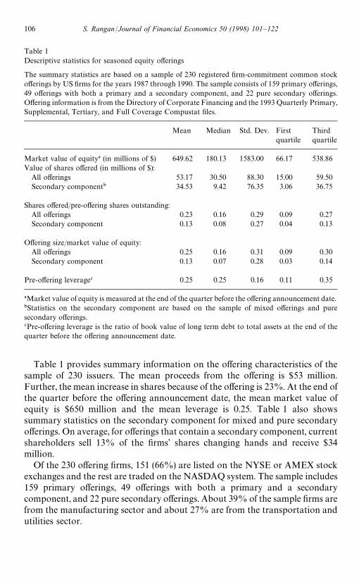
Table 1Descriptive statistics for seasoned equity offerings

The summary statistics are based on a sample of 230 registered firm-commitment common stockofferings by US firms for the years 1987 through 1990. The sample consists of 159 primary offerings,49 offerings with both a primary and a secondary component, and 22 pure secondary offerings.Offering information is from the Directory of Corporate Financing and the 1993 Quarterly Primary,Supplemental, Tertiary, and Full Coverage Compustat files.

Mean Median Std. Dev. Firstquartile

Thirdquartile

Market value of equity! (in millions of $) 649.62 180.13 1583.00 66.17 538.86Value of shares offered (in millions of $):

All offerings 53.17 30.50 88.30 15.00 59.50Secondary component" 34.53 9.42 76.35 3.06 36.75

Shares offered/pre-offering shares outstanding:All offerings 0.23 0.16 0.29 0.09 0.27Secondary component 0.13 0.08 0.27 0.04 0.13

Offering size/market value of equity:All offerings 0.25 0.16 0.31 0.09 0.30Secondary component 0.13 0.07 0.28 0.03 0.14

Pre-offering leverage# 0.25 0.25 0.16 0.11 0.35

!Market value of equity is measured at the end of the quarter before the offering announcement date."Statistics on the secondary component are based on the sample of mixed offerings and puresecondary offerings.#Pre-offering leverage is the ratio of book value of long term debt to total assets at the end of thequarter before the offering announcement date.

Table 1 provides summary information on the offering characteristics of thesample of 230 issuers. The mean proceeds from the offering is $53 million.Further, the mean increase in shares because of the offering is 23%. At the end ofthe quarter before the offering announcement date, the mean market value ofequity is $650 million and the mean leverage is 0.25. Table 1 also showssummary statistics on the secondary component for mixed and pure secondaryofferings. On average, for offerings that contain a secondary component, currentshareholders sell 13% of the firms’ shares changing hands and receive $34million.

Of the 230 offering firms, 151 (66%) are listed on the NYSE or AMEX stockexchanges and the rest are traded on the NASDAQ system. The sample includes159 primary offerings, 49 offerings with both a primary and a secondarycomponent, and 22 pure secondary offerings. About 39% of the sample firms arefrom the manufacturing sector and about 27% are from the transportation andutilities sector.


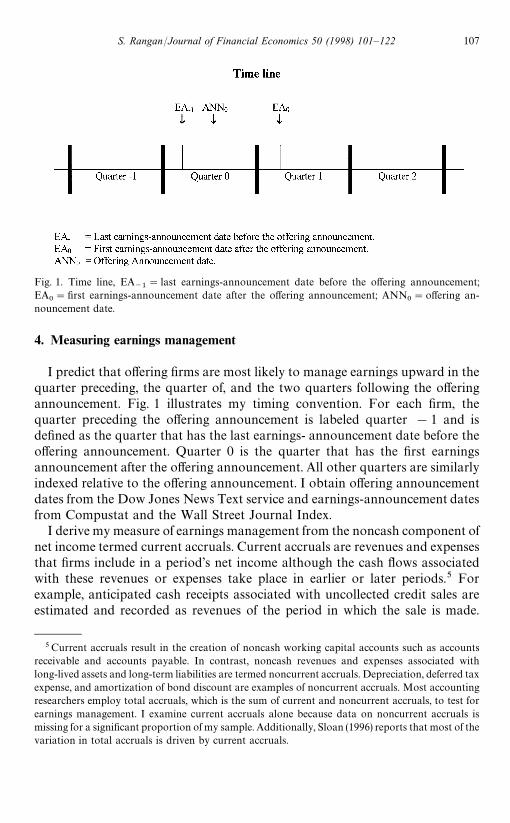
Fig. 1. Time line, EA~1

"last earnings-announcement date before the offering announcement;EA

0"first earnings-announcement date after the offering announcement; ANN

0"offering an-

nouncement date.

4. Measuring earnings management

I predict that offering firms are most likely to manage earnings upward in thequarter preceding, the quarter of, and the two quarters following the offeringannouncement. Fig. 1 illustrates my timing convention. For each firm, thequarter preceding the offering announcement is labeled quarter !1 and isdefined as the quarter that has the last earnings- announcement date before theoffering announcement. Quarter 0 is the quarter that has the first earningsannouncement after the offering announcement. All other quarters are similarlyindexed relative to the offering announcement. I obtain offering announcementdates from the Dow Jones News Text service and earnings-announcement datesfrom Compustat and the Wall Street Journal Index.

I derive my measure of earnings management from the noncash component ofnet income termed current accruals. Current accruals are revenues and expensesthat firms include in a period’s net income although the cash flows associatedwith these revenues or expenses take place in earlier or later periods.5 Forexample, anticipated cash receipts associated with uncollected credit sales areestimated and recorded as revenues of the period in which the sale is made.

5Current accruals result in the creation of noncash working capital accounts such as accountsreceivable and accounts payable. In contrast, noncash revenues and expenses associated withlong-lived assets and long-term liabilities are termed noncurrent accruals. Depreciation, deferred taxexpense, and amortization of bond discount are examples of noncurrent accruals. Most accountingresearchers employ total accruals, which is the sum of current and noncurrent accruals, to test forearnings management. I examine current accruals alone because data on noncurrent accruals ismissing for a significant proportion of my sample. Additionally, Sloan (1996) reports that most of thevariation in total accruals is driven by current accruals.


Similarly, anticipated cash payments associated with warranty costs are esti-mated and recorded as expenses in the period in which the sale is made. As theseexamples indicate, current accruals reflect subjective estimates and can conse-quently be used to manage net income. For example, without violating currentaccounting rules, firms can accelerate the recognition of credit sales and under-estimate warranty expenses. However, accruals-based earnings managementincreases net income only temporarily and its correction in subsequent periodscauses net income to decline.

Current accruals are reflected as increases or decreases in the balances ofvarious noncash current asset and current liability accounts. Continuing withthe above examples, uncollected credit sales are reflected as an increase inaccounts receivable and unpaid warranty expenses are reflected as an increase incurrent liabilities. Hence, current accruals for a period are obtained by subtract-ing the change in current liabilities from the change in noncash current assets forthat period. Accordingly, I define current accruals as:

ACC"(*CA!*CASH)!(*CL!*STD), (1)

where

*CA "change in current assets (Compustat d40),*CASH"change in cash and short-term investments (Compustat d36),*CL "change in current liabilities (Compustat d49),*STD "change in current portion of long-term debt (Compustat d45).I exclude the current portion of long-term debt from current liabilities becausechanges in this account do not affect the calculation of net income. If *STD ismissing, I set it to equal zero. To simplify exposition, for the remainder of thepaper I use the term accruals when referring to current accruals.

To measure accruals-based earnings management, I use an event-studymethod first proposed by Jones (1991). Following this method, accruals in theevent period of interest are assumed to consist of a discretionary (or managed)component and a nondiscretionary (or unmanaged) component. Nondiscretionaryaccruals are computed as forecasts from a linear regression of accruals on certainexplanatory variables fitted over an estimation period. Discretionary accruals in theevent period equal the difference between realized accruals and predicted nondis-cretionary accruals. Test statistics based on these discretionary accruals are used todraw conclusions about the existence of earnings management.6

6Guay et al. (1996) question whether discretionary accruals computed in this manner can be usedto detect earnings management. Most of their analysis is based on a broad cross-section of firms. Insuch a sample, alternative motives for recording discretionary accruals such as income smoothing orimproving earnings as a performance measure are bound to be present. The presence of thesealternative motives confounds and reduces their ability to detect opportunistic earnings manage-ment. In contrast, I study a setting in which such alternative motives are less plausible and henceincrease the likelihood of detecting opportunistic earnings management. I thank the referee formaking this point.


To implement the above procedure, I begin by estimating firm-specific regres-sions to model accruals unrelated to earnings management. Firms that experi-ence growth in either sales or expenses are likely to require additionalinvestment in working capital items such as receivables and inventories. There-fore, to measure the effect of growth on accruals, I estimate the followingregression over a pre-event estimation period for each firm:

ACCit"b

0i#b

1i*REV

it#b

2i*COGS

it#e

it, (2)

where

*REVit

"change in revenue for firm i in quarter t (Compustat d2),*COGS

it"change in cost of goods sold for firm i in quarter t (Compustat

d30).7I estimate the regression only for those firms that have at least six consecutivequarterly observations immediately prior to quarter !4. While the estimationperiod ends in quarter !5 for all firms, it begins at different quarters fordifferent firms. For the 230 firms that meet the minimum data requirements,the estimation period length averages 14 quarters and ranges from 6 to 27quarters.8

Next, I define the event period as quarter !4 to quarter 3. To predictnondiscretionary accruals in the event period, I use the coefficient estimatesfrom the first-stage regression, Eq. (2), and the values of change in revenueand change in cost of goods sold in the event period. As suggested by Dechowet al. (1995), I adjust change in revenue by subtracting change in accountsreceivable from it. The adjustment is intended to remove the effects ofmanagerial discretion over credit sales from nondiscretionary accruals,thereby improving the likelihood of detecting revenue-based earnings manage-ment. Thus, discretionary accruals for each quarter p in the event period isdefined as:

DISCip"ACC

ip!(b

0i#b

1i[*REV

ip!*REC

ip]#b

2i*COGS

ip), (3)

where b0i, b

1i, and b

2iare the estimated coefficients from the first-stage

regression and *RECip

is the change in accounts receivable for firm i inquarter p.

7Kang and Sivaramakrishnan (1995) recommend the use of total expense, in addition to revenues,as an explanatory variable for accruals. Because data on cost of goods sold is missing less often thandata on total expense, to maximize sample size I use change in cost-of-goods-sold expense.

8 I also estimated Eq. (2) with all the variables scaled by beginning assets. The basic conclusions ofthe paper remain unchanged for this specification.


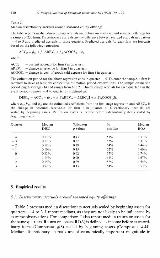
Table 2Median discretionary accruals around seasoned equity offerings

The table reports median discretionary accruals and return on assets around seasoned offerings fora sample of 230 firms. Discretionary accruals are the difference between realized accruals in quarters!4 to 3 and predicted accruals in those quarters. Predicted accruals for each firm are forecastsbased on the following regression:

ACCit"b

0i#b

1i*REV

it#b

2i*COGS

it#e

it,

where

ACC*5

"current accruals for firm i in quarter t;*REV

*5"change in revenue for firm i in quarter t;

*COGS*5"change in cost-of-goods-sold expense for firm i in quarter t.

The estimation period for the above regression ends in quarter !5. To enter the sample, a firm isrequired to have at least six consecutive estimation period observations. The sample estimationperiod length averages 14 and ranges from 6 to 27. Discretionary accruals for each quarter p in theevent period (quarter !4 to quarter 3) is defined as:

DISCip"ACC

ip!(b

0i#b

1i[*REV

ip!*REC

ip]#b

2i[*COGS

ip]),

where b0i, b

1i, and b

2iare the estimated coefficients from the first stage regression and *REC

ipis

the change in accounts receivable for firm i in quarter p. Discretionary accruals arescaled by beginning assets. Return on assets is income before extraordinary items scaled bybeginning assets.

Quarter Median Wilcoxon % MedianDISC p-values positive ROA

!4 0.13% 0.43 51% 1.37%!3 0.17% 0.37 52% 1.31%!2 0.19% 0.29 54% 1.44%!1 0.10% 0.15 52% 1.60%

0 0.83% 0.02 57% 1.74%1 1.15% 0.00 61% 1.67%2 0.15% 0.29 52% 1.54%3 0.52% 0.13 54% 1.53%

5. Empirical results

5.1. Discretionary accruals around seasoned equity offerings

Table 2 presents median discretionary accruals scaled by beginning assets forquarters !4 to 3. I report medians, as they are not likely to be influenced byextreme observations. For comparison, I also report median return on assets forthe same quarters. Return on assets (ROA) is defined as income before extraord-inary items (Compustat d8) scaled by beginning assets (Compustat d44).Median discretionary accruals are of economically important magnitude in


quarters 0 and 1, being more than half the median ROA in those quarters.Further, they are statistically significant at the 5% level based on theWilcoxon signed rank test. The proportion of issuers recording positive dis-cretionary accruals also peaks in quarters 0 and 1. In the other two quarters forwhich I predict earnings management, quarters !1 and 2, median discretion-ary accruals are quite small and are less than 10% of the median ROA.Discretionary accruals are statistically significant at the 10% level only inquarters 0 and 1.

The unusually positive discretionary accruals in quarter 0 are consistent withtwo alternative, but not mutually exclusive, interpretations. The first interpreta-tion is that issuing firms use discretionary accruals to manage earnings deliber-ately. Alternatively, issuing firms could be timing their offerings to follow veryhigh accruals in this quarter.9

To distinguish these two interpretations, I model the equity issue decisionand quarter 0 accruals as jointly endogenous variables in a two-equationsystem. I estimate the two equations for a cross-sectional sample thatconsists of issuing firm-quarters from quarter 0 and nonissuing firm-quarters. Issuing firms that have data in quarter 0 for all variables in thetwo equations enter the sample. Nonissuing firms are defined as Compustat-listed firms that did not make a seasoned equity offering or an initialpublic offering in the years 1987—1990. Nonissuing firm-quarters from the years1987—1990 with data for all variables enter the sample. The sample consists of165 issuing firm-quarters and 23,552 nonissuing firm-quarters that have therequired data.

Specifically, I estimate the following two equations simultaneously:

ACCit"b

0#b

1[*REV

it!*REC

it]#b

2*COGS

it#b

3DUM

it#l

1it,

(4)

DUMit"c

0#c

1ACC

it#c

2PRE

it#c

3MB

it#c

4LIQ

it#c

5LEV

*5

#c6POST

it#c

7CF

it#l

2it. (5)

In the first equation, I regress accruals on change in revenue less change inaccounts receivable, change in cost of good sold, and a dummy variable codedone for issuing firms and zero for nonissuing firm-quarters. In the secondequation, the dependent variable is the equity issue dummy and the independent

9Because 224 out of my 230 sample firms execute their offerings before the earnings announce-ment for quarter 1, the timing interpretation is not relevant for the unusually high accruals inquarter 1.


variables are accruals and other variables that prior research suggests as likelyto influence the probability of an equity issue.10

If issuing firms deliberately manipulate accruals, the coefficient on the equityissue dummy in Eq. (4) should be positive. In Eq. (5), accruals should beara positive coefficient if firms time their offerings after unusually high accruals inquarter 0. Thus, by estimating the two equations jointly, I can test for earningsmanagement in quarter 0 after controlling for the timing explanation. I use aninstrumental variable procedure described in Heckman (1978) to carry out theestimation.

I find, but do not report in tables, that, consistent with a timing explanation,the equity issue dummy and accruals are positively related in the secondequation. The coefficient on accruals is 2.71 with a t-statistic of 4.75. To obtainan elasticity interpretation for this coefficient, I transformed it in the mannersuggested by Judge et al. (1985). The resulting elasticity equals 0.06, implyingthat a 10% increase in accruals in quarter 0 increases the likelihood of equityissuance by a mere one half of a percent. In support of the earnings managementhypothesis, I find that the equity issue dummy enters positively and significantlyin the first equation. The coefficient estimate on the equity issue dummy is 0.31with a t-statistic of 9.5, implying that a 10% increase in the probability of equityissuance is associated with an increase of current accruals of 3 cents per dollar ofassets in quarter 0. Hence, the results suggest that issuing firms manage earnings

10The other variables I include are pre-offering returns (PRE), market-to book ratio (MB),leverage (LEV), a variable measuring cash constraints (LIQ), post-offering returns (POST), andoperating cash flows (OCF). In include pre-offering returns (PRE) because Korajczyk et al. (1990)and several others have documented that firms are likely to issue equity after a stock price run up.For issuing firms, I measure pre-offering returns as the continuously compounded return calculatedover a one-year period ending on the offering announcement date. I calculate ‘pre-offering returns’for nonissuing firm-quarters with the same metric but use the last day of the quarter as a proxy forthe offering announcement date. Issuing firms normally raise equity capital to exploit investmentopportunities, to reduce liquidity constraints, or to improve their debts capacity by using theproceeds to retire existing debt. To capture these motivations, I employ proxies for investmentopportunities, liquidity constrints, and debt capacity. I measure investment opportunities as theratio of the market value of equity to book value of equity at the end of the quarter (MB). FollowingDechow et al. (1996), I measure liquidity constrints (LIQ) by calculating the difference betweenoperating cash flows and capital expendilturers over a one-year period ending with the quarter ofinterest and deflating this difference by the current assets at the beginning of that year. I measuredebt capacity (LEV) as the ratio of long-term debt to total assets at the end of the quarter. Thetiming hypothesis suggested by Loughran and Ritter (1995) predicts that issuing firms will time theiroffering to take advantage of overvaluation and that consequently their post-offering returns will belower than that of nonissuing firms. I measure issuing firm post-offering returns (POST) as thecontinuously compounded return over a two-year period beginning 181 days after the offering date.For nonissuing firm-quarters, I calculate the post-offering return over a two-year period beginningwith the day after the last day of the quarter. Finally, because firms could time the offering aftera quarter of high cash flows, I include quarterly operating cash flows (CF) as an explanatory variablefor the equity issue dummy.


in quarter 0 after controlling for the possibility that they time the offering aftera quarter of high accruals.

To summarize, the evidence indicates that issuing firms deliberately manipu-late earnings in quarters 0 and 1. The magnitude of the earnings management inthese quarters is both economically and statistically significant. Further, theunusually positive accruals in quarter 0 represent earnings management and arenot just the consequence of issuing firms timing the offering after high accrualsin that quarter. Contrary to my prediction, I do not find evidence of significantearnings management in either quarter !1 or quarter 2.

5.2. Discretionary accruals and post-offering earnings performance

If offering firms use discretionary accruals to shift income from the future,I expect a negative relation between discretionary accruals around the offeringand subsequent earnings changes. To test this prediction, I use annual measuresof discretionary accruals and earnings changes constructed by aggregatingquarterly data. Aggregated annual measures contain less measurement errorthan individual quarterly measures and hence enhance the power of my tests.

Specifically, I sum discretionary accruals over quarters !1 to 2 (year 0) andscale the sum by assets at the beginning of the four-quarter period. I define thisannual number as DISC

0. Similarly, I construct ROA for year 0 by summing

income before extraordinary items over quarters !1 to 2 and scaling the sumby assets at the beginning of the four-quarter period. I sum earnings over fourquarter intervals before and after year 0 to construct ROA for years !2 to 3.I first-difference annual ROA to compute changes in ROA (*ROA).

Panel A of Table 3 presents median changes in ROA for years !2 to 3.Consistent with the findings of Hansen and Crutchley (1990) and Loughran andRitter (1997), issuing firms experience earnings increases up to year 0 andearnings declines in subsequent years. Median *ROA is negative and statist-ically significant in each of years 1—3. Further, the proportion of issuers withnegative earnings changes increases from 46% in year 0 to 64% in year 1.Thereafter, it declines but remains greater than 50% in the next two years.11

11As suggested by Barber and Lyon (1996), I control for the normal amount of mean reversion inROA by deducting the change in ROA of a size-matched and performance-matched nonissuing firmfrom the change in ROA of each issuing firm in years 1—3. Specifically, from the nonissuing firmswhose assets are within 90% and 110% of an issuer’s assets at the end of the fiscal year before theoffering, I pick the one whose ROA is closest to that of the issuer in absolute terms. I definenonissuing firms as Compustat-listed firms that did not make an initial public offering or seasonedequity offering in the 1987-1990 period. The pattern of post-offering earnings declines remains forthis measure. The median performance adjusted earnings changes are !0.81%, !1.03%, and!0.78% for years 1, 2, and 3 and are each significant at the 5% level.


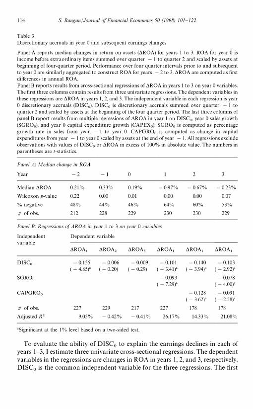
Table 3Discretionary accruals in year 0 and subsequent earnings changes

Panel A reports median changes in return on assets (*ROA) for years 1 to 3. ROA for year 0 isincome before extraordinary items summed over quarter !1 to quarter 2 and scaled by assets atbeginning of four-quarter period. Performance over four quarter intervals prior to and subsequentto year 0 are similarly aggregated to construct ROA for years !2 to 3. *ROA are computed as firstdifferences in annual ROA.Panel B reports results from cross-sectional regressions of *ROA in years 1 to 3 on year 0 variables.The first three columns contain results from three univariate regressions. The dependent variables inthese regressions are *ROA in years 1, 2, and 3. The independent variable in each regression is year0 discretionary accruals (DISC

0). DISC

0is discretionary accruals summed over quarter !1 to

quarter 2 and scaled by assets at the beginning of the four quarter period. The last three columns ofpanel B report results from multiple regressions of *ROA in year 1 on DISC

0, year 0 sales growth

(SGRO0), and year 0 capital expenditure growth (CAPEX

0). SGRO

0is computed as percentage

growth rate in sales from year !1 to year 0. CAPGRO0

is computed as change in capitalexpenditures from year !1 to year 0 scaled by assets at the end of year !1. All regressions excludeobservations with values of DISC

0or *ROA in excess of 100% in absolute value. The numbers in

parentheses are t-statistics.

Panel A: Median change in ROA

Year !2 !1 0 1 2 3

Median *ROA 0.21% 0.33% 0.19% !0.97% !0.67% !0.23%

Wilcoxon p-value 0.22 0.00 0.01 0.00 0.00 0.07

% negative 48% 44% 46% 64% 60% 53%

d of obs. 212 228 229 230 230 229

Panel B: Regressions of DROA in year 1 to 3 on year 0 variables

Independent Dependent variablevariable

*ROA1

*ROA2

*ROA3

*ROA1

*ROA1

*ROA1

DISC0

!0.155 !0.006 !0.009 !0.101 !0.140 !0.103(!4.85)! (!0.20) (!0.29) (!3.41)! (!3.94)! (!2.92)!

SGRO0

!0.093 !0.078(!7.29)! (!4.00)!

CAPGRO0

!0.128 !0.091(!3.62)! (!2.58)!

d of obs. 227 229 217 227 178 178

Adjusted R2 9.05% !0.42% !0.41% 26.17% 14.33% 21.08%

!Significant at the 1% level based on a two-sided test.

To evaluate the ability of DISC0

to explain the earnings declines in each ofyears 1—3, I estimate three univariate cross-sectional regressions. The dependentvariables in the regressions are changes in ROA in years 1, 2, and 3, respectively.DISC

0is the common independent variable for the three regressions. The first


three columns of panel B of Table 3 report these regressions. To reduce the effectof outliers, I excluded observations with values of *ROA or DISC

0greater than

100% in absolute value.When *ROA in year 1 is the dependent variable, the coefficient on DISC

0is

!0.16 with a t-statistic of !4.85. To assess economic significance, I calculatethe one-standard-deviation impact of DISC

0by multiplying its coefficient

estimate by its sample standard deviation. The coefficient estimate implies thata one-standard-deviation increase in DISC

0, which is 17% for my sample, is

associated with an earnings decline of 2.6 cents per dollar of assets in year 1.Hence, DISC

0is associated with both economically and statistically significant

earnings declines in year 1. Although DISC0

is negatively related to *ROA inyears 2 and 3, the coefficient estimates are not statistically or economicallyimportant. Thus, most of the earnings reversals associated with DISC

0are

concentrated in year 1.The above results suggest that earnings management in year 0 causes earnings

to decline in the following year. However, these earnings declines could also berelated to growth in assets or sales. For issuing firms that invest in projects thatgenerate profits only from year 2 onward, the increase in assets in year 0 willinduce mechanical declines in profitability in year 1. Issuing firms that experi-ence rapid sales growth are likely to attract new entrants into their industries.The consequent increase in competition could cause issuing firms to experienceprofitability declines in year 1. Indeed, Loughran and Ritter (1997) find thatissuers that are growing rapidly in terms of sales and capital expenditures in theyear of the offering experience larger post-offering earnings declines than slowlygrowing issuers. Therefore, as a robustness check, I include year 0 sales growth(SGRO

0) and year 0 capital expenditure growth (CAPGRO

0) as additional

explanatory variables for year 1 *ROA. SGRO0

is computed as percentagegrowth rate in sales from year !1 to year 0. CAPGRO

0is computed as change

in capital expenditures from year !1 to year 0 scaled by assets at the end ofyear !1.

The last three columns of panel B of Table 3 report results from multipleregressions of *ROA in year 1 on DISC

0and the two growth variables included

individually and jointly. The regressions that have CAPGRO0

as an indepen-dent variable have fewer observations because this variable is often missing onthe quarterly Compustat files. The coefficient on DISC

0remains negative and

statistically significant in all three regressions. Hence, even after controlling theeffects of sales growth and capital expenditure growth in year 0, DISC

0is

associated with significant earnings declines in year 1. Consistent with thefindings of Loughran and Ritter (1997), both SGRO

0and CAPGRO

0are

negatively related to earnings changes in the following year.Again, to assess economic significance, I calculate the one-standard-deviation

impact of the independent variables on the dependent variable. For example,consider the regression in which all three variables are included. The sample


standard deviations of DISC0, SGRO

0, and CAPGRO

0for the 174 firms used in

this regression are 18%, 35%, and 18%. Therefore, a one- standard-deviationincrease in DISC

0implies an earnings decline of 1.9 cents per dollar of assets in

year 1. Similarly, a one-standard-deviation increase in year 0 sales growthimplies an earnings decline of 2.7 cents per dollar of assets and a one-standard-deviation increase in year 0 capital expenditure growth implies a decline ofabout 1.6 cents. These results suggest that both discretionary accruals and firmgrowth in year 0 are associated with economically important earnings declinesin the following year.

5.3. Discretionary accruals and post-offering stock performance

If the market prices the portion of the growth in year 0 earnings that reflectsearnings management as if such growth is permanent, offering firms will beovervalued. Subsequently, when the reversal of earnings associated with earn-ings management takes place, the valuation errors are corrected. Hence, I expecta negative relation between DISC

0and subsequent stock returns. Because

earnings declines associated with DISC0

are concentrated in year 1, I focus onstock returns in that year.

I compute the full-year return for year 1 over a holding period that spans thefour quarters over which earnings information is released. For each quarter,I assume that earnings information is released over the period starting from theday after the earnings announcement for the previous quarter and ending on theday of the earnings announcement for the quarter. Hence, the full-year return foryear 1, which consists of quarters 3—6, is computed from the day after theearnings announcement for quarter 2 to the day of the earnings announcementfor quarter 6.

I define abnormal returns as market-adjusted returns using the return on theCRSP value-weighted market index as the market return. Returns are com-pounded daily over the holding period described above. I considered, butrejected, subtracting the return on a size-matched control firm from issuing firmreturns because this adjustment produces abnormal returns of less than!100% for a significant fraction of my sample. Twenty-one firms in my sampleof 230 firms record year 1 abnormal returns of less than !100% using thisprocedure.12 I did not consider matching on both size and book-to-marketratio, as recommended by Barber and Lyon (1997), as this would reduce mysample size considerably. However, I do control for the effects of size andbook-to-market ratio by including them as explanatory variables for returns inmy regression-based tests.

12Details of the procedure used to select control firms of similar size are available from the authoron request.


Because firms release a significant proportion of earnings-related informationat earnings-announcement dates, in addition to returns over the entire year,I also examine abnormal returns around earnings announcements in year 1.Earnings-announcement abnormal returns are calculated by compounding thereturns over the four earnings-announcement periods in year 1 and subtractingthe return on the value-weighted market portfolio that is compounded similarly.I define an announcement period as the two-day period beginning the daybefore the Compustat earnings-announcement date. Hence, the earnings-announcement abnormal return for year 1 is measured over eight tradingdays.

Panel A of Table 4 reports median abnormal returns in year 1. Issuing firmsunderperform the market by significant magnitudes both over the entire yearand over earnings- announcement periods. The median market-adjusted returnfor the entire year is !7.4% and is significant at the 1% level based ona two-sided Wilcoxon test. Further, about 60% of the issuing firms recordnegative abnormal returns in this year. The median earnings-announcementabnormal return in year 1 is !1.3% and is statistically significant at the 1%level. Because announcement periods (eight days) constitute only about 3% ofthe average number of trading days in year 1 (252 days), earnings-announcementreturns clearly account for a disproportionate share of year 1 underperfor-mance.13

Next, I examine whether year 0 discretionary accruals can explain the poorstock price performance in year 1. To accomplish this, I link year 1 abnormalreturns with year 1 earnings changes and year 0 discretionary accruals usinga framework similar to Bernard and Thomas (1990). From the results in Table 3,we know that earnings changes in year 1 are negatively related to year 0 dis-cretionary accruals:

*ROA1"a

0#a

1DISC

0#l

1, a

1(0. (6)

Suppose the stock market does not understand this negative relation andassumes that earnings follow a random walk. In that case, unexpected earningsin year 1 equal earnings changes in that year. To model this, I express abnormalreturns in year 1 (AR

1) as a function of *ROA

1:

AR1"b

0#b

1*ROA

1#e

1. (7)

13 In results not reported in tables here, I find that the median full-year abnormal return isnegative in both years 2 and 3 but statistically significant in year 2 alone. Median market-adjustedreturns equal !8.0% (p-value"0.01) in year 2 and !4.6% (p-value"0.46) in year 3, respectively.Median earnings-announcement abnormal return in year 2 equals !0.72%, but is not statisticallysignificant (p-value "0.35). In year 3, median market-adjusted return equals 1.32% (p-value"0.02)indicating that there is no underperformance in that year.


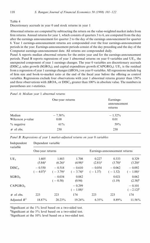
Table 4Discretionary accruals in year 0 and stock returns in year 1

Abnormal returns are computed by subtracting the return on the value-weighted market index fromfirm returns. Annual returns for year 1, which consists of quarters 3 to 6, are computed from the dayafter the earnings announcement for quarter 2 to the day of the earnings announcement for quarter6. Year 1 earnings-announcement returns are compounded over the four earnings-announcementperiods in the year. Earnings-announcement periods consist of the day preceding and the day of theCompustat earnings-announcement date. All returns are compounded daily.Panel A reports median abnormal returns for the entire year and for the earnings-announcementperiods. Panel B reports regressions of year 1 abnormal returns on year 0 variables and UE

1, the

unexpected component of year 1 earnings changes. The year 0 variables are discretionary accruals(DISC

0), sales growth (SGRO

0), and capital expenditure growth (CAPGRO

0). UE

1is the residual

from a regression of year 1 earnings changes (*ROA1) on year 0 variables. All regressions include log

of firm size and book-to-market ratio at the end of the fiscal year before the offering as controlvariables. Regressions exclude four observations with year 1 abnormal returns greater than 150%and three observations with *ROA

1or DISC

0greater than 100% in absolute value. The numbers in

parentheses are t-statistics.

Panel A: Median year 1 abnormal returns

One-year returns Earnings-announcementreturns

Median !7.38% !1.32%Wilcoxon p-value 0.00 0.01

% negative 61% 59%

d of obs. 230 230

Panel B: Regressions of year 1 market-adjusted returns on year 0 variables

Independent Dependent variablevariable

One-year returns Earnings-announcement returns

UE1

1.605 1.883 1.708 0.227 0.333 0.329(5.84)! (6.26)! (4.98)! (2.81)! (3.70)! (3.20)!

DISC0

!0.550 !0.518 !0.610 !0.054 !0.062 !0.092(!4.07)! (!3.79)! (!3.74)! (!1.37) (!1.52) (!1.88)#

SGRO0

!0.034 0.082 0.021 0.062(!0.58) (0.94) (1.19) (2.38)"

CAPGRO0

!0.299 !0.101(!1.88)# (!2.12)"

d of obs. 223 223 174 223 223 174

Adjusted R2 18.87% 20.23% 19.24% 6.35% 8.89% 11.56%

!Significant at the 1% level based on a two-sided test."Significant at the 5% level based on a two-sided test.#Significant at the 10% level based on a two-sided test.


By substituting the expression for *ROA1

in Eq. (6) into Eq. (7), I can testwhether the market is surprised when earnings declines related to DISC

0take

place. Carrying out the substitution, we get:

AR1"(b

0#b

1a0)#b

1l1#a

1DISC

0#e

1. (8)

Simplifying Eq. (8) and writing l1

as UE1

gives us:

AR1"c

0#c

1UE

1#c

2DISC

0#e

1. (9)

Eq. (9) forms the basis for the empirical tests. It defines year 1 abnormalreturn as a function of two components. The first component, UE

1, is the

estimated residual from the regression of year 1 earnings changes on DISC0and

represents unexpected earnings for year 1. The second component, DISC0, is

information available at the beginning of the period over which AR1

is com-puted. In an efficient market, the market would react only to the unexpectedcomponent of earnings and not to DISC

0. Hence, if the market correctly

processes the implications of DISC0

for *ROA1, the coefficient on DISC

0should be zero. However, if the market fails to understand that DISC

0will be

associated with earnings declines in year 1, c2

will be negative.Because sales growth and capital expenditure growth in year 0 are also

negatively related to *ROA1, I evaluate the stock market’s ability to anticipate

the earnings declines associated with these variables as well. To do so, I includethem as additional explanatory variables in both the earnings change and thestock return regressions that are specified by Eq. (6) and Eq. (7). Several studiesdocument that firm size and book-to-market ratio predict subsequent stockreturns. Hence, I include the log of market capitalization and book-to-marketratio at the beginning of the offering year as control variables in all regressions.However, to conserve space, I do not report or discuss coefficient estimates andt-statistics for these two control variables.

Panel B of Table 4 reports the results from regressions of year 1 abnormalreturns on DISC

0and the two year-0 growth variables. To reduce the effect of

outliers in the regressions, I exclude four observations with values of abnormalreturns greater than 150% and 3 observations with absolute values of *ROA

1or DISC

0greater than 100%. When the full-year return is the dependent

variable, the coefficient on DISC0

is !0.55 with a t-statistic of !4.1. Thecoefficient estimate implies that if DISC

0increases by one standard deviation

(18%), market-adjusted returns will decrease by about 10% in year 1. DISC0

isa significant predictor of the full-year return even when sales growth and capitalexpenditure growth are included as explanatory variables.

To obtain an alternate economic interpretation of the above results, I placedDISC

0in quartiles (1 to 4), subtracted one from it, and divided it by three so that

it ranges from 0 to 1. The coefficient in a regression of stock returns on therank-transformed DISC

0can be interpreted as the difference between the mean

market-adjusted return of the top DISC0

quartile issuers and that of the bottom


DISC0

quartile issuers. I estimated the regressions reported in the first threecolumns of panel B with the rank-transformed DISC

0instead of the original

variable. In results not reported in tables here, I find that the coefficient onDISC

0ranges from !0.07 to !0.09 with a t-statistic of !2.9 for all three

regressions. These estimates imply that high discretionary-accrual issuers under-perform low discretionary-accrual issuers by 7% to 9% in year 1 abnormalstock returns.

When the dependent variable is earnings-announcement abnormal returns foryear 1, DISC

0is negative and significant at the 10% level when all three

variables are included in the regression. Its coefficient estimates range from!0.05 to !0.09 across the three regressions. These imply that a one-stan-dard-deviation increase in DISC

0is associated with a decline in market-ad-

justed returns of 0.9% to 1.5% around earnings announcements in year 1.The coefficients on sales growth when the full-year return is the dependent

variable are generally small. When the earnings-announcement return is thedependent variable, the coefficient is surprisingly positive and significant at the5% level in the regression in which all three variables are included. In contrast,Loughran and Ritter (1997) report that sales growth in the year of the offering isreliably and negatively related to subsequent stock returns. I conjecture that ourresults differ because we use different dependent variables. I examine returnsover a one-year period shortly after the offering date, whereas Loughran andRitter (1997) examine the average five-year post-offering return. The coefficienton capital expenditure is negative and statistically significant in both thefull-year return and earnings-announcement regressions. For example, when thefull-year return is the dependent variable, the coefficient estimate equals !0.30with a t-statistic of !1.88. This implies that a one-standard-deviation increasein CAPGRO

0(18%) lowers market-adjusted returns in year 1 by 5.5%. This

result is consistent with that of Loughran and Ritter (1997), who find thatissuing firms with rapid capital expenditure growth in the year of the offeringperform more poorly then slowly-growing issuers.

In sum, the results indicate that earnings management over a one-year periodaround the offering is reliably and negatively related to market-adjusted returnsin the following year. Further, this finding is robust to the inclusion of otherexplanatory variables for returns such as firm size, book-to-market ratio, andsales and capital expenditure growth.

6. Conclusions

Recent studies document that firms conducting seasoned equity offeringsexperience significant earnings declines and negative abnormal stock returns inthe post-offering period. This study shows that discretionary accounting ac-cruals in the period surrounding the offering predict a portion of the subsequent


poor earnings and stock price performance. For a sample of 230 seasonedofferings from the years 1987—1990, I find that discretionary accruals during theyear around the offering are negatively correlated with earnings changes in thefollowing year. A one-standard-deviation increase in discretionary accruals isassociated with an earnings decline of about two to three cents per dollar ofassets. Discretionary accruals around the offering also predict market-adjustedstock returns in the following year. A one-standard-deviation increase in dis-cretionary accruals is associated with a decline in market-adjusted stock returnsof about 10%. The ability of discretionary accruals to predict stock returns isrobust to the inclusion of sales growth, capital expenditure growth, firm size,and book-to-market ratio as additional predictors.

I conclude that the stock market does not correctly value the implications ofdiscretionary accruals for subsequent earnings. Rather, the market appears toextrapolate earnings growth associated with discretionary accruals and henceovervalues issuing firms. Subsequent to the offerings, when the reversal ofdiscretionary accruals causes earnings to decline, the market is surprised andcorrects its valuation errors. Because at least some of the discretionary accrualsreflect deliberate earnings management, I conclude that issuing firms can ma-nipulate their stock price by managing earnings.

References

Barber, B., Lyon, J., 1996. Detecting abnormal operating performance: the empirical power andspecification of test-statistics. Journal of Financial Economics 41, 359—399.

Barber, B., Lyon, J., 1997. Detecting long-run abnormal stock returns: the empirical power andspecification of test-statistics. Journal of Financial Economics 43, 341—372.

Bernard, V., Thomas, J., 1990. Evidence that stock prices do not fully reflect the implications ofcurrent earnings for future earnings. Journal of Accounting and Economics 13, 305—340.

Dechow, P., Sloan, R., 1997. Returns to contrarian investment strategies: tests of naı̈ve expectationshypotheses. Journal of Financial Economics 43, 3—27.

Dechow, P., Sloan, R., Sweeney, A., 1995. Detecting earnings management. The Accounting Review70, 193—225.

Dechow, P., Sloan, R., Sweeney, A., 1996. Causes and consequences of earnings manipulations: ananalysis of firms subject to enforcement actions by the SEC. Contemporary Accounting Re-search 13, 1—36.

Francis, J., Philbrick, D., Schipper, K., 1994. Determinants and outcomes in class action securitieslitigation. Unpublished working paper. University of Chicago, Chicago.

Guay, W., Kothari, S., Watts, R., 1996. A market-based evaluation of discretionary-accrual models.Journal of Accounting Research 34 (Suppl.), 83—105.

Gutterman, A., 1994. The Legal Considerations in Business Financing. Quorum Books, Westport.Hansen, R., Crutchley, C., 1990. Corporate earnings and financings: an empirical analysis. Journal of

Business 63, 347—371.Heckman, J., 1978. Dummy endogenous variables in a simultaneous equation system. Econometrica

46, 931—961.Jones, J., 1991. Earnings management during import relief investigations. Journal of Accounting

Research 29, 193—228.


Judge, G., Griffiths, W., Hill, R., Lutkepohl, H., Lee, T., 1985. The Theory and Practice ofEconometrics. Wiley, New York.

Kang, S., Sivaramakrishnan, K., 1995. Issues in testing earnings management and an instrumentalvariable approach. Journal of Accounting Research 33, 353—368.

Kellogg, I., Kellogg, L., 1991. Fraud, Window Dressing, and Negligence in Financial Statements.Shepard’s/McGraw Hill, Colorado Springs.

Korajczyk, R., Lucas, D., McDonald, R., 1990. Understanding stock price behavior around the timeof equity issues. In: Hubbard, R. (Ed.), Asymmetric Information, Corporate Finance, andInvestments. University of Chicago Press, Chicago, pp. 257—277.

Lakonishok, J., Shleifer, A., Vishny, R., 1994. Contrarian investment, extrapolation, and risk.Journal of Finance 49, 1541—1578.

Loughran, T., Ritter, J., 1995. The new issues puzzle. Journal of Finance 50, 23—51.Loughran, T., Ritter, J., 1997. The operating performance of firms conducting seasoned equity

offerings. Journal of Finance 52, 1823—1850.Mulford, C., Comiskey, E., 1996. Financial Warnings. John Wiley and Sons, Inc., New York.Skinner, D., 1994. Empirical evidence on the relation between earnings disclosures, firm character-

istics, and stockholder lawsuits. Unpublished working paper. University of Michigan, AnnArbor.

Sloan, R., 1996. Do stock prices fully reflect information in accruals and cash flows about futureearnings? Accounting Review 71, 289—315.

Spiess, D., Affleck-Graves, J., 1995. Under-performance in long-run stock returns following seasonedequity offerings. Journal of Financial Economics 38, 243—267.

Teoh, S., Welch, I., Wong, T., 1998. Earnings management and the under-performance of seasonedequity offerings. Journal of Financial Economics 50, 63—99 (this issue).


Earnings management and the performance of seasoned equity offerings 1 I gratefully acknowledge the...

Documents

Transcript of Earnings management and the performance of seasoned equity offerings 1 I gratefully acknowledge the...