e-CLV: A Modeling Approach for Customer Lifetime Evaluation in e-Commerce Domains, with an...

Information Systems Frontiers 7:4/5, 421–434, 2005C© 2005 Springer Science + Business Media, Inc. Manufactured in The Netherlands.

e-CLV: A Modeling Approach for Customer LifetimeEvaluation in e-Commerce Domains, with an Applicationand Case Study for Online Auction

Opher Etzion, Amit Fisher and Segev WasserkrugIBM Research, Laboratory in Haifa, IsraelE-mail: [email protected]: [email protected]: [email protected]

Abstract. e-Commerce companies acknowledge that customersare their most important asset and that it is imperative to estimatethe potential value of this asset.

In conventional marketing, one of the widely accepted meth-ods for evaluating customer value uses models known as Cus-tomer Lifetime Value (CLV). However, these existing models suf-fer from two major shortcomings: They either do not take intoaccount significant attributes of customer behavior unique toe-Commerce, or they do not provide a method for generatingspecific models from the large body of relevant historical datathat can be easily collected in e-Commerce sites.

This paper describes a general modeling approach, basedon Markov Chain Models, for calculating customer value in thee-Commerce domain. This approach extends existing CLV mod-els, by taking into account a new set of variables required forevaluating customers value in an e-Commerce environment. Inaddition, we describe how data-mining algorithms can aid in de-riving such a model, thereby taking advantage of the historicalcustomer data available in such environments. We then present anapplication of this modeling approach—the creation of a modelfor online auctions—one of the fastest-growing and most lucra-tive types of e-Commerce. The article also describes a case study,which demonstrates how our model provides more accurate pre-dictions than existing conventional CLV models regarding thefuture income generated by customers.

Key Words. customer lifetime value, e-commerce recencyfrequency monetary, markov chain

1. Introduction

Currently, there is an escalating demand for webservices and web applications, along with continu-ous growth in worldwide commercial application. E-Commerce companies are beginning to realize that theymust be able to measure the value of their web cus-tomers, i.e. the expected profit that will be derived from

the relationship with web customers from the presentuntil a specified period in the future.

The ability to accurately predict the value of a com-pany’s customers has a large impact on the ability tointelligently influence both business process policiesand IT related decisions pertaining to a company. Sev-eral examples of possible influences are:

1. Companies will know how much they can affordto spend in order to get the first sale. This meanscompanies can take the short term risks necessaryto achieve long-term gain.

2. Marketing managers can develop different offers fordifferent customers, based on the estimated contri-bution of such customers in the future.

3. Stock exchange analysts can use the company’s cus-tomer value in order to evaluate its worth to potentialinvestors.

4. Customer value can serve as the basis for decisionsregarding new campaigns, allocation of retention vs.acquisitions budgets, etc.

5. A company can make better decisions regarding itspromotional budget. For example: Should the com-pany establish a close relationship with only the top10% of its customers or should the same amountbe invested in every customer when providing cus-tomer service?

6. The value of customers can serve as the basis forcustomer prioritization. Profit-generating customersegments can be prioritized over low or negativerevenue generators.

7. A variety of additional uses in the e-Commerce do-main. These include:

421

422 Etzion, Fisher and Wasserkrug

a. Customer value can be used to prioritize incom-ing HTTP requests.

b. IT resource allocation decisions can be basedon customer value. An example of such a deci-sion is whether a server should be dedicated toa specific group of customers.

From the above examples, it is clear that the ability tointelligently make such decisions based on the actualvalue of the customers can help a company achievecompetitive gains over other market players. Therefore,e-Commerce companies require models that enable theaccurate calculation of their customers’ value.

In the field of direct marketing, the term used formeasuring such customer value is customer lifetimevalue, or CLV. There are already well known modelsfor calculating CLV. However, in the e-Commerce do-main, there are several unique attributes of customerbehavior that impact this value, which are not takeninto account by the existing CLV models. An exampleof such an attribute is the division of customer interac-tions with an e-Commerce site into sessions (Menasceand Almeida, 2000). Therefore, in this paper, wepresent a general modeling approach, which we terme-CLV, for creating CLV models in the e-Commercedomain. These models can take into account all thekey factors required to calculate customer value in thisdomain.

Another unique characteristic in the e-Commercedomain is the availability of a large body of historicaldata regarding the customers’ behavior. It seems rea-sonable to assume that the customer value can be in-ferred, at least to some degree, from the customer’s pastbehavior. Therefore, in this paper, we also provide analgorithm for the derivation of the e-CLV model fromsuch data. This algorithm both ensures that the mod-eled customer value is influenced by past behavior, andprovides an automated methodology for creating suchmodels.

This paper also describes the creation of a specificmodel, based on the general modeling approach men-tioned above, for online auction sites. We demonstratethat our model performs well in predicting customervalue by describing a case study carried out on one ofthe largest auction sites in Israel.

The rest of this paper is organized as follows:Section 2 discusses existing models used to calculatethe value of customers in the realm of conventionalbusinesses. Section 3 details the general e-CLV mod-eling approach, and Section 4 describes the specific

model for online auctions. Section 5 describes the casestudy conducted on a popular web auction site in Israel.The results and conclusions are discussed in Section 6.Finally, in Section 7 we close with possible for futurework.

2. Related Work

To the best of our knowledge, no existing work ad-dresses the calculation of customer value in the e-Commerce domain. However, some methods related toconventional marketing are relevant, and are reviewedhere. These works include: CLV models—used to cal-culate the value of customers in conventional business;RFM models—models that take into account behav-ioral characteristics of customers, including purchasefrequency, monetary amount spent, and the time of in-teraction between the customers and the site, in orderto predict short-term future customer behavior, such asthe next purchase date; and models that combine thetwo approaches, by using behavioral characteristics tocalculate the customer value. These works are reviewedin the following sub-sections.

2.1. CLV modelsCustomer Lifetime Value (CLV) models are used inthe field of marketing to evaluate the lifetime value ofcustomers in conventional businesses. A complete CLVmodel must address the following two main questions:What are the set of attributes of customer behavior thatare relevant to the customer’s value, and how to usethese variables to predict the customer value. Someworks (e.g., Rust et al., 2000) address the first questionand only define a set of relevant variables.

Other works focus both on the model and the rel-evant variables. In Berger and Nasr (1998) an equa-tion for calculating the CLV was defined. However,this equation was based on several assumptions, suchas (1) sales take place once a year and (2) revenuesper customer, per year, are constant. These are very re-strictive, and hence render this model impractical forthe e-Commerce domain.

A more general model, that places its emphasis onthe precise specification of the inputs required for prof-itability analysis, was suggested in Mulhern (1999).This model incorporates profit resulting from a cus-tomer over a series of discrete time periods, using thefollowing technique: For each period, the contributionmargin for all purchases is computed, and the variable

e-CLV: A Modeling Approach for Customer Lifetime 423

marketing costs are identified. All of these revenuesand costs are then adjusted to remove the time valueof money (by using the discount rate factor) and thensummed together to provide the lifetime value of a cus-tomer.

Even more complex models, with less restrictive as-sumptions were presented in Berger and Nasr (1998).These models relax several assumptions such as fre-quency of purchase (by considering periods other thanone year), thereby allowing to take into account grosscontribution and promotional cost (by addressing situa-tions in which those values are non-constant over time),and allow continuous cash flow rather than discretecash flow. Another generalized CLV model (Hoekstraand Huizingh, 1999) takes into account additionalfactors, such as customer share, which presents theamount spent by the customer with regards to his/hertotal spending, and supplier-customer potential, whichrefers to forecasts on the future activities of the sup-plier/customer, such as the predictions of a customer’sprofit potential. In this work, the past contribution ofcustomers is also considered, by taking into accountthe revenue that was generated from a customer fromhis/her first transaction until the time that the CLV wascalculated.

However, non of the above models provide methodsfor deriving the model’s parameters and the requiredcompound data for the generation of such models; thisshortcoming, together with their restrictive assump-tions, renders the creation and use of these impracticalmodels in many applications and domains.

Several methods (Gupta, Lehmann, Stuart; Stahl,Matzler, and Hinterhuber, 2002) are used to calcu-late the average CLV value of a company’s customers.However, as such models cannot distinguish betweenthe values of different customers within a company;they cannot provide many of the advantages mentionedin the introduction to this paper.

2.2. RFM methodologyRFM (recency, frequency, monetary) analysis is a mar-keting technique used for predicting the short-term fu-ture behavior of a customer. This short-term future be-havior of a customer describes the probability that acustomer will buy from the company during the nexttime period, given his/her past behavior. These worksbase their predictions on the following attributes of cus-tomer behavior: recency—the time that passed since thelast date the customer requested a service; frequency—the number of times the customer made a purchase; and

monetary—the total dollar amount a customer spenton purchases from the company. The use of these vari-ables as predictors was justified in several works, whichdemonstrated that recency, frequency, and monetaryvalues are good predictors for the probability of pur-chase in the next period.

Several approaches exist for creating such short-term predictive models by using data mining tech-niques. Examples of such approaches are: NeuralNetworks (NN) (Baesens et al., 2002; Kim et al.,2001), Support Vector Machine (SVM) (Viaene et al.,2001) and RFM-based clustering techniques (Kaymak,2001). Therefore, one main advantage of such modelsis the ability to create them based on historical customerdata.

2.3. CLV models based on RFM variablesRFM models are intended to predict only the cus-tomer’s short-term behavior, but can be produced inpractice using data mining techniques. The CLV mod-els presented previously attempt to address the needfor long term prediction, but either entail very restric-tive assumptions regarding customer behavior, or don’tprovide a method for calculating the model’s parame-ters. The shortcomings of both reviewed approaches,as well as their respective strengths, suggest that byintegrating RFM-based prediction capabilities into acomprehensive CLV model, a model can be definedthat both allows for long-term prediction and that canbe derived in practice.

The idea of combining the two approaches by mod-eling customer relations using Markov Chain Mod-els (MCM) was introduced in Pfeifer and Carraway(2000). In general, an MCM is a finite state machinewith a probability measure assigned to each transition.The authors presented the idea of using RFM variablesas a foundation for the definition of MC states, where astate is defined for each distinct set of possible valuesfor these variables.

Because MCM is a finite state machine, only a fi-nite number of values are allowed for each variable.Therefore, all continuous variables, such as the recencyvariable that describes the time, must be discretized.Moreover, the value of all variables must be bound.An example for variable discritization is dividing thecontinuous time line into “time intervals”, which de-fine the discrete values for measuring the time in theMC model, as well as setting a value for the maximumnumber of values. This discretizing can be domain, oreven customer specific. For example, in the domain of


Fig. 1. State transitions in the MCM

e-banking, one can consider a one month period as atime interval; this means that only after each month,the recency value is updated.

The probability transition between states reflects theprobability that future customer behavior will cause thecustomer to migrate from one state to the other. Anexample of such an MCM appears in Fig. 1.

In addition, in Pfeifer and Carraway (2000) a rewardvector (R) that estimates the contribution and costs ofeach state was defined as follows:

R =

NC − M if r = 1−M if 1 < r < max value0 if r == max value

(1)

where NC is the net contribution, i.e. the average con-tribution of the customer in each purchase and M isthe marketing expenditures, i.e. the average marketingexpense per customer over a defined time period.

The MCM theory provides two basic equations(Eqs. (2) and (3)) for calculating the value of eachstate, while considering the time value of money, bydiscounting from the future value to present value us-ing the capitalization factor d . Each equation provides avector (V ) that defines the CLV of each state. In Eq. (2)a finite time horizon is considered (i.e., the CLV iscalculated for the next T time periods), while Eq. (3)enables the calculation of the infinite time horizon. InEq. (3), I is the identity matrix.

V T =T∑

t=0

[(1 + d)−1 P]t R (2)

V = limT →∞

V T = {I − (1 + d)−1 P}−1 R (3)

Because these equations provide a value for each state,and each customer can be assigned to a state based onhis/her history, this model provides a method for calcu-lating the value of each customer. That is, for each set ofRFM variables, it is possible to estimate the customervalue.

The most significant shortcoming of this model withregards to e-Commerce is that the RFM variables arenot sufficient to accurately predict the customer’s value.Furthermore, this method does not provide a techniquefor calculating the transition probabilities.

3. General e-CLV Modeling Approach

To address the shortcomings of existing models for thee-Commerce domain, we developed a general mod-eling approach, e-CLV that extends the MCM modelpresented. This MCM model was chosen as the ba-sis for e-CLV modeling for the following reasons: (1)This theory enables a simple method for describing cus-tomer migration and customer retention rate; (2) Theprobabilistic nature of MCM can account for the inher-ent stochastic nature of customer behavior; (3) MCMpresents the least restrictive approach with regards toassumptions about customer’s behavior.

In Section 3.1 we present the general e-CLV mod-eling approach and in Section 3.2, we describe a tech-nique for deriving the MCM from historical data.

3.1. Constructing the e-CLV modelTo model customer behavior in e-Commerce, we ex-pand the model in two significant ways:

1. We consider variables that are unique for electroniccommerce, in addition to the conventional ones. Ex-amples of such unique variables are session-relatedvariables. This extension is detailed below.

2. We updated the CLV calculation as follows: We ex-tended the definition of the capitalization factor tofit economic markets that are strongly influencedby inflation. In the vector R, defined in Eq. (1),the value is calculated using the net cash flow thateach state provides to the vendor. The average netcontribution (NC) per purchase and the average ex-pense (M) per period are defined in present nominalvalue. When considering future income, two factorsmust be taken into account to calculate the presentvalue of future inflows: (1) i-Consumer Price Index


(which was not taken into account in the capital-ization factor of the model in Section 2.3); and (2)r-Capital price (vendor’s interest for capital enlist-ment) (r > i). To take these factors into account,when calculating the net present value of each cashflow that will be given after t time periods, the cashamount must be multiplied by:

(1 + i

1 + r

)t

(4)

or

(1 + d)−t where d =(

r − i

1 + i

)

(5)

where d is a positive scalar representing the capitaliza-tion factor for the future cash flow.

The general modeling approach to create an ex-tended MCM model for e-Commerce is as follows:

1. Define the candidate variables for the definition ofthe MCM’s states. It is necessary to define the setof variables that may be relevant to CLV calcula-tion in any particular e-Commerce domain. Thisis necessary as e-Commerce includes many dif-ferent trade mechanisms (online auctions, catalogbased sales, etc.). Thus, particular variables uniqueto each mechanism must be considered. An exam-ple for such variables for e-Auctions appears inSection 4.1.

2. Choose the variables that represent the state spacefrom the set of candidate variables. This may be asubset of the candidate variables, since not all vari-ables of the candidate set may indeed be useful forprediction. The procedure of selecting the variablesubset must combine statistical methods and previ-ous knowledge regarding the variables’ predictioncapabilities in any particular domain. When a vari-able is potentially significant in describing the cus-tomer’s behavior, it is included in the model andits actual predictive significance can be evaluatedby the learning algorithm, described in Section 3.2.The process of variable selection is presented inFig. 2.

3. A general set of restrictions on possible values maybe defined. These restrictions define the possiblechanges in the variable’s value. An example of sucha restriction is that the recency value of a purchaseis incremented after each time period, and can de-crease only when the customer makes a purchase.

Fig. 2. Selection process for variables.

4. A general set of transition restrictions can be speci-fied. Some transitions may be impossible due to thesemantic meaning of the variables that define theMCM states. For example, because the monetaryvalue represents the total expenses on merchandise,this value can never decrease.

5. The subset of actual variables must be chosen, andthe possible values of their variables must be dividedinto discrete levels and bounded (as explained inSection 2.3). These variables, along with their dis-crete scales and maximum values, should be chosento optimize the predictive capabilities of the e-CLVmodel. An iterative approach for generating suchscales and bounds appears in Section 3.2.3

6. Define the transition probabilities. A learning algo-rithm, defined in Section 3.2.2 derives these proba-bilities.

3.2. Deriving the MCMAfter defining the state’s variables and the variables’discrete scales, the state’s transition probabilities mustbe estimated. Two main approaches are available forthis task: (1) These probabilities can be evaluated bythe company’s managers who are familiar with thisdomain; (2) Data mining techniques can be used toretrieve the probabilities.

We choose the second alternative for our model, be-cause the evaluation of such probabilities is expectedto be a complex task, even for experienced managers.This section presents a data mining algorithm that re-trieves these probabilities from the past behavior of thecustomers, as well as a process for discretizing the vari-ables values. Section 3.2.1 describes the necessary datafor the algorithm, Section 3.2.2 details the algorithmand Section 3.2.3 describes the variables’ discretiza-tion process.


3.2.1. Input. The required input for our model is thehistory dataset for the past behavior of customers. Thisdata must include values for all variables that were se-lected as candidate variables in the model, and shouldbe as large as possible. In addition, our algorithm as-sumes that the customers’ past behavior is a good in-dicator of their future behavior. Therefore, if futurecustomer behavior changes significantly for some rea-son, the generated model will not be able to predict thisbehavior.

3.2.2. Learning algorithm. The learning algorithmcreates the transition probability matrix (P) as follows:

1. A transition matrix is initialized to contain zeroes inall locations.

2. For each customer that transitions from state i tostate j, the appropriate place in the transition matrixis incremented.

3. After going over the entire dataset, each line is nor-malized to 1, in order to get the transitions’ proba-bilities.

3.2.3. Variables discretization. An iterative processis defined, based on standard learning algorithm prac-tices. This serves to find the subset of actual predictivevariables and the discrete breakdown of their values.

In this process, the data set is divided into two parts:a training data set and a testing set. Next, the iterativeprocess is carried out, where a candidate set of vari-ables, discretization of the values of these variables,and a maximum bound on these variables is chosen.After such a choice has been made, the training datasetis used to calculate the MC state’s transitions probabil-ities and the CLVs. The testing set provides the actualvalue of customers used to measure the predictive capa-bility of the derived model, by comparing the estimatedvalue of each state (i.e., the e-CLV) and the average ac-tual contribution from each state as calculated by thetest set. This comparison can be carried out using sta-tistical methods. Once a sufficiently predictive modelis obtained, the algorithm terminates.

4. E-CLV Model for Online AuctionDomains

Although the e-CLV approach is a general one, theattributes relevant to the prediction of customers’ be-havior are different for every e-Commerce domain. In

this section, we describe the derivation of a model forthe domain of auction sites: one of the most lucrativeand fastest growing e-Commerce domains. Section 4.1describes the candidate variables for the online auc-tion domain. Sections 4.2 and 4.3 detail the restrictionson the variables’ values and the states’ transitions, re-spectively. Section 4.4 explains how we implement ourlearning algorithm in this domain. In Section 4.5, aset of possible transitions is demonstrated via a simpleexample.

4.1. Candidate variables for the e-auction domainThe ideal model should be able to include the uniquecharacteristics of online auction mechanisms. In par-ticular, for electronic web auctions, the following datais available:

1. Customer’s sessions: In each session only “search”and “browse” requests are generated. In addition,each session may also lead to either a bid or a pur-chase.

2. Customer’s bids: Bids for specified good in an elec-tronic auction.

3. Customer’s purchases: Actual purchases of prod-ucts after winning an auction.

This data is used to define the following candidate vari-ables:

Therefore, the state in an MCM model for an e-Commerce site will consist of a set of values for asubset of the following variables:

State = (Rbuy, Fbuy, Rs, Fs, M, Rbet, Fbet, Mbet).

4.2. General restrictions on the variable valuesAs mentioned in Section 3.1, once the candidate vari-ables have been defined, general restrictions can beplaced on their value. For the candidate values of onlineauction sites defined in Section 4.1, these restrictionsare as follows:

1. For each of the three frequency variables, the valueof 0 indicates that the customer has not made anypurchase/bet/session. The maximum value for thefrequency variables indicates that the customer hasmade that amount of purchases/bets/sessions ormore.

2. For the frequency variables, the value of 0 indi-cates that no purchases/bets/sessions were made.The value of 1 indicates that there was a pur-chase/bet/session in the recent period and the valueof n indicates that the last purchase/bet/session was


made n time periods before the current time. Whenthe customer didn’t buy anything in the last n timeperiods and when n is equal to or greater than themaximum value for Rbuy, this customer is con-sidered as “lost for good” (i.e., the company ter-minates its relationship with the customer and as-sumes that no future revenue is expected from thatcustomer).

3. For the monetary variables, the amount is brokeninto a discrete scale by breaking the continuousmonetary value into equal intervals and a maxi-mum amount is defined. If the monetary value ofa customer reaches the maximum amount value (orhigher), this maximum value is assigned to the valueof M/Mbet. If no buys/bets were made, the mon-etary value is set to its first discrete value, whilethe value on n indicates that the total amount is atlevel n (i.e., the value lies somewhere in the nthinterval).

4. The Mbet value of each auction is calculated bytaking into account only the maximum bet madeby the customer in that auction, and smaller bidsby that customer in the same auction are ignored.For example, if John Doe participates in a specificauction and initially bids n′ dollars, after which heraises his bid to n′′ (n′′ > n′) dollars, only n′′ is takeninto account.

4.3. General restrictions on state transitionsThis section specifies the set of restraints on state tran-sitions and emphasizes several important issues regard-ing these transitions:

1. A transition is not possible from a state in whichRbuy �= 0 to states in which Rbuy = 0. Once a pur-chase has been made, the customer can never returnto a state that indicates no purchase.

2. A transition is not possible from a state in whichRbet �= 0 to a state in which Rbet = 0. Once a bethas been made, the customer can never return to astate that indicates no bets.

3. There are no transitions from a state where Rbuy =maximum value. These states are absorbing states(customer “lost for good”).

4. A transition from states in which Rbuy = x to statesin which Rbuy = x + 1, represent “no buy” duringa period.

5. A transition from a state in which Rbet = x to a statein which Rbet = x + 1, represents “no bets” in aperiod.

6. A transition from any given state to a state in whichRbuy = 1, represents a “buy” in the recent timeperiod.

7. A transition from any given state to a state in whichRbet = 1, represents a bid in the last period.

8. Each session sets the Rs value to 1.9. A transition from a state in which Fbuy = x to states

in which Fbuy = x + 1, represents an additionalpurchase during this time period.

10. A transition from a state in which Fbet = x to a statein which Fbet = x + 1, represents an additional betmade by the customer.

11. When the number of purchases reaches its maximumvalue, additional purchases don’t increase the Fbuyvalue.

12. When the number of purchases reaches its maximumvalue, additional bets do not increase the Fbet value.

13. A transition from a state in which Fs = x to statesin which Fs = x + 1, occurs when the customerinitiates an additional session.

14. When the number of sessions reaches its maximumvalue, additional sessions do not increase the Fsvalue.

15. A transition from the state in which M = x to statesin which M = x + 1, occurs when the purchaseamount of a customer crosses the boundary of aninterval in the set of intervals that define the discretemonetary scale.

16. A transition from the state in which Mbet = x tostates in which Mbet = x + 1, occurs when theamount of a customer’s bet crosses the boundaryof an interval in the set of intervals that define thediscrete monetary scale for bets.

17. A purchase does not necessarily increase the valueof M . The value of M is incremented only if themonetary value crosses the boundary of an intervaldefined by the discrete monetary scale.

18. A bet does not necessarily increase the value ofMbet. The value of Mbet is incremented only if themonetary value for bets crosses the boundary of aninterval defined by the discrete monetary scale forbets.

19. When M reaches its maximum value, additionalbuys don’t increase the value of M .

20. When Mbet reaches its maximum value, additionalbets don’t increase the value of Mbet.

4.4. Input required by learning algorithmFor the set of variables (Rbuy, Fbuy, Rs, Fs, M,Rbet, Fbet, Mbet) defined as candidate variables, the


historical data for customers in such domains must becomprised of a set of rows describing sessions of cus-tomers that participate in auctions. Each such row mustcontain the following fields:

1. Id—customer’s unique identification (can be IP oruser-name)

2. Time—start time of this session3. Buy—indicates whether a purchase was carried out

in this session4. Bet—indicates whether the customer bid in this ses-

sion5. BuyAmount—if there was a purchase at this session,

this is the amount spent by the customer6. BetAmount—maximum bet amount in this session,

if such an amount exists

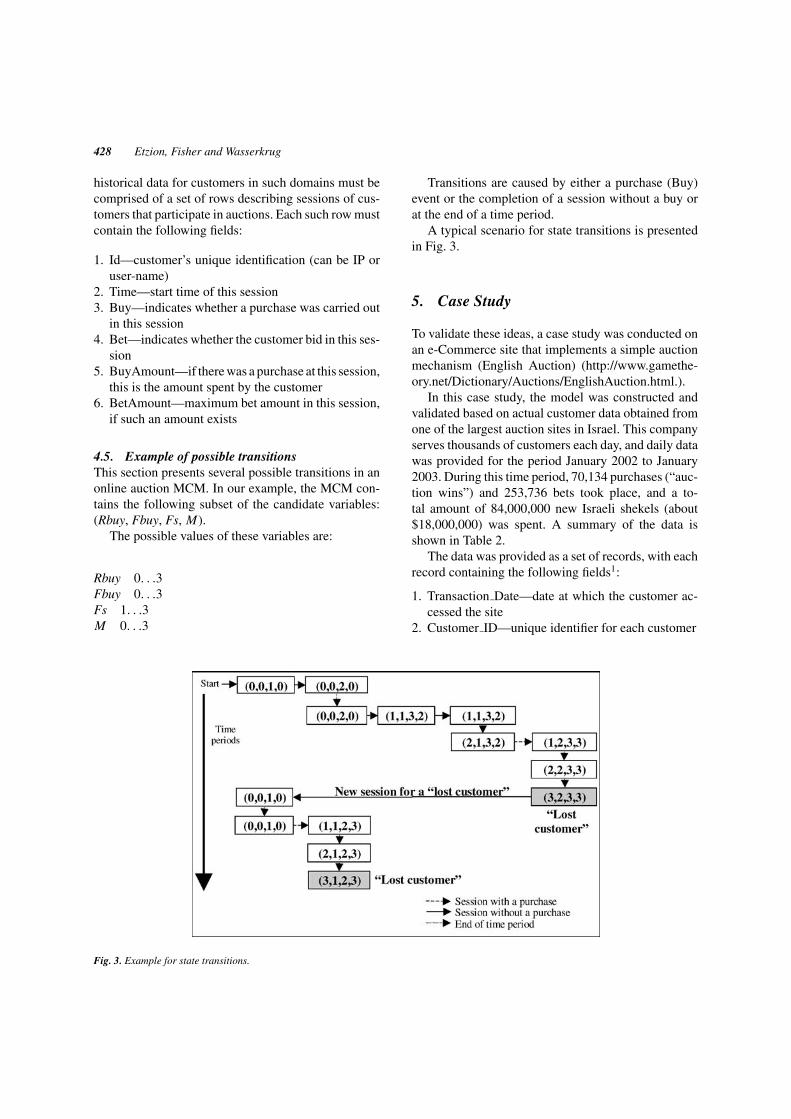
4.5. Example of possible transitionsThis section presents several possible transitions in anonline auction MCM. In our example, the MCM con-tains the following subset of the candidate variables:(Rbuy, Fbuy, Fs, M).

The possible values of these variables are:

Rbuy 0. . .3Fbuy 0. . .3Fs 1. . .3M 0. . .3

Fig. 3. Example for state transitions.

Transitions are caused by either a purchase (Buy)event or the completion of a session without a buy orat the end of a time period.

A typical scenario for state transitions is presentedin Fig. 3.

5. Case Study

To validate these ideas, a case study was conducted onan e-Commerce site that implements a simple auctionmechanism (English Auction) (http://www.gamethe-ory.net/Dictionary/Auctions/EnglishAuction.html.).

In this case study, the model was constructed andvalidated based on actual customer data obtained fromone of the largest auction sites in Israel. This companyserves thousands of customers each day, and daily datawas provided for the period January 2002 to January2003. During this time period, 70,134 purchases (“auc-tion wins”) and 253,736 bets took place, and a to-tal amount of 84,000,000 new Israeli shekels (about$18,000,000) was spent. A summary of the data isshown in Table 2.

The data was provided as a set of records, with eachrecord containing the following fields1:

1. Transaction Date—date at which the customer ac-cessed the site

2. Customer ID—unique identifier for each customer


Table 1. Variables definitions

Symbol Name Description

Rbuy Recency of last buy The time elapsed since the last purchase the customer made at the site.Fbuy Frequency of “buys” Represents the total number of customer’s purchases at the site.Rs Recency of last session The time elapsed since the last session the customer had at the site.Fs Frequency of sessions Represents the total number of customer’s sessions at the siteM Total amount spent on merchandise Represents the total amount spent by the customers in the site, in a discrete scale.Rbet Recency of last bets Represents the time elapsed since the last auction in which the customer participated.Fbet Frequency of bets Represents the total number of auctions in which the customer participated.Mbet Total amount on bets Represents the total amount of money the customer bet on, in a discrete scale

Table 2. Data summary

Q1/2002 Q2/2002 Q3/2002 Q4/2002 01/2002 total

Number of purchases 8,624 13,764 17,382 21,688 8,676 70,134Number of bets 39,981 60,930 61,235 65,863 25,717 253,726Mean buy amount 1358.55 1304.53 1177.62 1092.09 1136.39 1193.23Std. Dev. of buy amount 1652.95 1725.91 1754.16 1598.75 1642.43 1678.26Total income 11,716,180 17,955,598 20,469,510 23,685,343 9,859,388 83,686,019

3. Bet Amount—maximum amount of money a cus-tomer bet in a single auction

4. Win Indicator—indicates whether the bet was awinning bet, i.e., the customer purchased the itemas a result of his bet amount

5. Catalog Price—catalog price of the good

5.1. Validation methodologyIn order to show that our model provides an accu-rate CLV estimation for this site, it must be shownthat our model provides accurate estimations of theactual customers’ values. In order to test this, the datawas divided into a training set and a test set, as de-fined in Section 3.2.3. This division was carried outby chronologically dividing the data into two time pe-riods. A point in time was chosen, and the data upto this point in time was used as the training set. Alldata from that point onwards was used as the test set.The CLV was created from the data on the first timeperiod. Next, the profitability ranking of customers,which is the ranking of customers according to theirCLV value, was compared to the actual profitabilityranking, which is the ranking of customers accordingto their true contribution to the company in the sec-ond time period. The actual Net Present Value (NPV)of each customer was calculated from the test data inorder to find the true contribution of customers. NPVis the approach used for discounting future values intothe present value, thereby providing the present valueof all future incomes generated from a customer and

thus representing his/her true contribution to the com-pany. The NPV was calculated in the case study asfollows:

1. Each outflow that was produced after t time periodssince the data split is multiplied by (1 + d)−t to findthe present value of that amount.

2. For each customer, we totaled these present valueamounts and got an NPV value.

5.1.1. Variable selection. The general process ofvariable selection was described in Section 3.2.3. Thesame process was used in our case study to find the sub-set of predictive variables and the discrete breakdown,and was carried out as follows: Whenever the inclusionof a candidate variable improved the model accuracy,this variable was added to the subset. Whenever theinclusion of a variable worsened the model accuracy,this variable was omitted from the subset. This processconverged into a final collection of variables subsets.The final subsets were tested under different variablescales, and the outcomes of those configurations werecalculated.

In all iterations, a time period equal to one monthwas chosen, and the maximum value for monetaryvalue (for calculating M and Mbet scale) was set to 500NIS. We chose the one month interval due to the dy-namic nature of the Internet, which suggests that shorttime periods should be addressed. The amount of 500NIS as the maximum value for the monetary variables


values was reached based on statistical tests carried outon the actual data.

5.1.2. Testing prediction quality. In order to com-pare the CLV as calculated by the model and theNPV, the, Spearman correlation (StatSoft Inc., 1984–2003) between CLV and NPV was computed. TheSpearman correlation was used as no assumptionscould be made regarding the prior distribution onthe CLVs and NPVs, and the Spearman correlationis a nonparametric correlation that makes no as-sumption about the distribution of the values (as op-posed to the Pearson correlation that assume thatboth variables values are sampled from a Gaussiandistribution).

Furthermore, two types of correlation tests were car-ried out. The first type was one correlation value calcu-lated for the complete ranking. The second test dividedthe classes of customers generated by our model intosubgroups, and then compared the correlations betweenthese subgroups.

In the second type of correlation, the MCM statesdefined by the model were divided into categories ac-cording to the observed number of clients in each state.The Spearman correlation was used to find the cor-relation among states in these categories. States weredivided into the following categories:

1. “Over 1000”—includes states with more than 1,000customers in the training set

2. “100–1000”— includes states with more than 100and less than 1,000 customers in the training set

3. “10–100”—includes states with more than 10 andless than 100 customers in the training set.

4. “3–10” –includes states with more than 3 and lessthan 10 customers in the training set

Table 3. Correlation results

Iteration Rbuy Fbuy M Rbet Fbet Mbet Correlation

1 10 1 5 10 3 5 0.672 10 2 10 10 3 10 0.613 10 5 10 5 5 0.64 10 5 10 5 10 0.65 10 5 10 5 3 0.66 15 3 10 15 5 0.577 10 2 5 10 3 5 0.568 20 5 20 5 0.559 15 5 15 5 5 0.55

10 10 10 10 10 5 0.5511 10 1 5 0.48

5. “2”—includes states that contain exactly 2 cus-tomers in the training set

6. “1”—includes states that contain exactly 1 customerin the training set

These groups were selected to differentiate between“very popular states”, “popular states” and “unpopularstates”. We decided to differentiate between the lasttwo groups (“1” and “2”) because of the relatively highnumber of states in each group.

5.2. ResultsTable 3 presents the main results for the overallcorrelation.

It can be seen from Table 3 that the best correlationwas achieved using the following variables and scales:The possible values of Rbuy are 1. . .10, the possiblevalues of Fbuy are 0. . .10, the possible values of M areto 0. . .5, the possible values of Rbet are to 0. . .10, andthe possible values of Fbet are to 0. . .3 In this case, thetotal correlation value was 0.67 which indicates thatthe model indeed captures a significant majority of therelevant customer behavior.

It can be seen from the above table that using con-ventional RFM variables (iteration 11) is far less accu-rate than the e-CLV model, resulting in a correlationvalue of only 0.48.

While comparing the total correlation is simple, it isnot trivial to create one measure that summarizes theseresults for the group correlation, and several options ex-ist for comparison criteria. The option that was chosenby us was to focus on the correlation for the most pop-ulated categories, i.e., the correlation values among thestates belonging to the “over 1000” category. However,other, more complex correlation ranking measures mayalso be defined. Figure and Figure introduce the group


correlation results for the first and the second best it-erations according to this criterion. It can also be seenfrom Figs. 4 and 5 that it is indeed not trivial to comparestates.

For the second correlation test, the results fromthe standard RFM model were also significantly in-ferior to the results from our enhanced model. Figure6 shows the comparison between iteration 1 and iter-ation 11. The enhanced model achieves significantlybetter correlation results for the most populated groups(i.e., “over 1000” to “10-100”). For the least populatedgroups, the models performs almost the same, exceptfor the fact that in iteration 11 a relatively high numberof “1” states were observed. Because the most popu-lated groups give better estimations for the model accu-racy (because more data was available for those states),we can conclude that our enhanced model performs sig-nificantly better when larger datasets are available.

5.3. ConclusionsOur case study shows that by fitting the model variablesand variable’s scale, and by using our e-CLV model fore-Commerce auction sites, a high degree of predictionaccuracy can be achieved with regards to the futurecontribution of customers (CLV).

1. The strong correlation between customer classesgenerated by the e-CLV model and the NPV valueshows that the e-CLV model indeed ranks customersaccording to their value. The comparison with theconventional RFM model shows that the enhancedmodel provides a much higher degree of accuracyfor the e-Commerce domain.

2. A high correlation is achieved for state categories,for which the number of observation per state ishigh. This value decreases as the number of statesdecrease. This is consistent with the assumption thatonce an appropriate learning algorithm is chosen,larger datasets will yield more accurate results.

3. We cannot decisively conclude which parametersgive the best results. However, several criteria (suchas the one described in Section 5.2) may be defined.In addition, such criteria may be site specific.

4. In our data sample, most iteration mapped a largepercentage of the customers to a small percent ofthe states. This might lead to the conclusion that ine-Commerce, a large amount of customers behavein almost the same manner, while a small percentof the customers display a significantly differentbehavior.

6. Summary

In this paper we present e-CLV, a modeling ap-proach for the calculation of customer value in the e-Commerce realm, and a learning algorithm that aids ingenerating this model. In addition, we present a spe-cific model for auction site mechanisms, along with acase study on an auction site in Israel, which showsthat our model performs well in that domain. Ourmodel succeeded in predicting the future income gen-erated from customers by successfully ranking thesecustomers with a high degree of accuracy. In addition,it was shown that the larger the dataset used for learn-ing, the higher the expected accuracy.

The model shown here does not only improve theprediction accuracy in e-Commerce domains, but alsooffers a complete method for learning the e-customer’sbehavior and calculating his/her lifetime value. To thebest of our knowledge, this is the first work that at-tempts to develop and validate a customer value modelfor e-Commerce domains. Such models are essential inorder to support the continuing growth in demand forcommercial web applications.

7. Future Work

One possible extension is the creation of specific mod-els for additional e-Commerce domains. Examples ofsuch domains include catalog sale sites, B2B mecha-nisms, Request For Proposals (RFP) methods, etc. Anexample for such a model which has been consideredby us is a model for catalog sale sites. Our proposedextension includes the following additional candidatevariables:

a. Rsc—time periods that passed since the last itemwas added to the shopping cart

b. Fsc—number of items added to the shopping cartc. Msc—total value of goods added to the shopping

cart

Another possible extension to the model is the ad-dition of general (i.e., non-domain specific) predic-tion variables that are not necessarily determined bythe customer, but nonetheless influence the customer’sbehavior. We have studied the possibility of addingvariables such as Quality of Service (QoS) measureslike server’s response time (RT) and Service LevelAgreement (SLA) constraints, and created a com-pound model that includes these variables. However,


Fig. 4. Best iteration results—categories correlation.

Fig. 5. Second best iteration results–categories correlation.

Fig. 6. Comparison between iteration 1 and 11.


the addition of additional variables can also bestudied.

In this paper, we present the subsets of model’s vari-ables that provide the most accurate model for a spe-cific e-Auction site in Israel. However, the open ques-tion remains whether model creation is site specific, orwhether general domain models can be created.

The variable selection process described in Sec-tion 5.1.1 uses a “local changes” technique. It would beuseful to define a more formal approach for the defini-tion of the candidate variables. One possible improve-ment is the use of heuristic algorithms (such as hillclimbing, simulated annealing etc. (Russel and Norvig,1995)).

The use of e-CLV for the creation of advancedscheduling mechanisms could also be studied. Thiswould offer new approaches for resource scheduling ine-Commerce websites to try and optimize the site’s rev-enue and profitability. These approaches often requireknowing how valuable the customer is when decidingthe QoS that will be provided to that customer. Currentwork we are carrying out in this area shows promisingresults. In this work, prioritizing customers accordingto their CLV value generated results far superior to thedefault First Come First Serve (FCFS) policy currentlyin place for most HTTP sites. However, a more intel-ligent use of the e-CLV model for scheduling couldpotentially result in far greater improvements.

Appendix A—Efficient Computation

As was presented in Eq. (3), to calculate the vector V,it is necessary to derive the inverse of a matrix of sizen2, where n is the size of the state’s space. The besttime complexity of existing algorithms for inverting amatrix is O(n2.7). This time complexity is impracticalfor our purpose, as the size of the matrix can be quitelarge. For example, for correlation 1 in table, n is equal

Fig. 7. Jacobi approximation algorithm.

to 34,848, and the complexity of the inversion processis O(1012). Therefore, rather than calculate the exactvalue, the Jacobi approximation method (Fig. 7) wasused in the case study to solve the CLV equations

Note

1. No data was available regarding the customer sessions for thissite. Therefore, the session variables could not be considered inthe case study.

References

Baesens B, Viaene S, Van den Poel D, Vanthienen J, Dedene G.Bayesian neural networking learning for repeat purchase modelingin direct marketing. European Journal of Operational Research,2002:191–211.

Berger PD, Nasr NI. Customer lifetime value: Marketing models andapplications. Journal of Interactive Marketing 1998:17–30.

“English Auction” definition from URL: http://www.gametheory.net/Dictionary/Auctions/EnglishAuction.html

Gupta, S., Lehmann, DR, and Stuart, JA. “Valuing Vustomers.”Working E-commerce.

Hoekstra JC, Huizingh EKRE. The lifetime value concept incustomers-based marketing. Journal of Marketing Focused Man-agement, 1999:257–274.

Kaymak U. Fuzzy target selection using RFM variables, In: Pro-ceedings of Joint 9th IFSA World Congress and 20th NAFIPSInternational Conference, Vancouver, Canada, 1038–1043;2001.

Kim Y, Street WN, Russel GJ, Menczer F. Customer targeting: Aneural network approach guided by genetic algorithms, 2001.

Menasce DA, Almeida VAF. Scaling for E-Business, Prentice Hall,2000, ISBN 0-13-086328-9.

Mulhern Francis J. Customer profitability analysis: Measurement,concentration, and research direction. Journal of Interactive Mar-keting 1999:25–40.

Pfeifer PE, Carraway RL. Modeling customers relationship asmarkov chains, Journal of Interactive Marketing, Spring 2000.

Russell SJ, Norvig P. Artificial intelligence: A Modern Approach.Prentice Hall, 2nd edn., ISBN: 0137903952, 1995.

Rust RT, Zeithaml VA, Lemon KN. Driving Customer Equity: HowCustomers Lifetime Value Is Reshaping Corporate Strategy, TheFree Press, 2000.

StatSoft Inc., 1984–2003 URL: http://www.statsoftinc.com/textbook/stathom.html

Stahl H ., Matzler K, Hinterhuber HH. Linking customer lifetimevalue with shareholder value. Industrial Marketing Management,2002:1–13

Viaene S, Baesens B, Van Gestel T, Suykens JAK, Van den PoelD, Vanthienen J, De Moor B, Dedene G. Knowledge discoveryusing least squares support vector machine classifiers: A directmarketing case. Management Science, 2001.

Opher Etzion is a research staff member and themanager of the active management technology group


in IBM Research Laboratory in Haifa, Israel, anda visiting research scientist at the Technion—IsraelInstitute of Technology. He received BA degree inPhilosophy from Tel-Aviv University and Ph.D. degreein Computer Science from Temple University, Prior tojoining IBM in 1997, he has been a faculty memberat the Technion, where he has served as the found-ing head of the information systems engineering areaand graduate program. Prior to his graduate studies, heheld professional and managerial positions in indus-try and in the Israel Air-Force, receiving the air-forcehighest award in 1982. His research interests includeactive technology (active databases and beyond), tem-poral databases, middleware systems and rule-base sys-tems. He is a member of the editorial board of the IIETransactions Journal, was a guest editor in the Jour-nal of Intelligent Information Systems in 1994, and aguest editor in the International Journal of CooperativeInformation Systems (2001). He served as a coordi-nating organizer of the Dagstuhl seminar on Temporaldatabases in 1997, has been the coeditor of the book“Temporal Databases—Research and Practice” pub-lished by Springer-Verlag, in 2000 he has been pro-gram chair of CoopIS’2000, and demo and panel chairof VLDB’2000. He also served in many conferencesprogram committees (e.g. VLDB, ICDE, ER) as well as

national committees and has been program and generalchair in the NGITS workshop series.

Amit Fisher is a research staff member in the activemanagement technology group in IBM Research Lab-oratory in Haifa, Israel. He received B.Sc. degree inIndustrial Engineering and Management and M.Sc.degree in Information System Engineering from theTechnion—Israel institute of Technology.

Prior to joining IBM research, Amit held a profes-sional position in Israel Air-Force. He’s research inter-ests include Customer Behavior Analysis, CRM, DataMining and Business Process Management.

Segev Wasserkrug is a research staff member at IBM’sHaifa Research lab (HRL). He has a M.Sc. in computerscience, in the area of neural networks. In addition,he has significant experience in modeling of varioustypes, automatic model derivation, and optimization,gained from leading the development of a technologyin HRL that deals with optimization of an IT infras-tructure according to business objectives. He is alsocurrently studying towards a Ph.D. in information sys-tems at the Technion, Israel Institute of Technology,in the area of uncertainty handling, based on Bayesiannetwork techniques

e-CLV: A Modeling Approach for Customer Lifetime Evaluation in e-Commerce Domains, with an...

Documents

Transcript of e-CLV: A Modeling Approach for Customer Lifetime Evaluation in e-Commerce Domains, with an...