Dynamic Galois Theory
14
Journal of Symbolic Computation 45 (2010) 1316–1329 Contents lists available at ScienceDirect Journal of Symbolic Computation journal homepage: www.elsevier.com/locate/jsc Dynamic Galois Theory ✩ G.M. Diaz-Toca a,1 , H. Lombardi b a Dpto. de Matemática Aplicada, Universidad de Murcia, 30100 Murcia, Spain b Laboratoire de Mathématiques, UMR CNRS 6623, Université de Franche-Comté, 25030 Besançon, France article info Article history: Received 31 August 2009 Accepted 23 April 2010 Available online 22 June 2010 Keywords: Effective Galois Theory Dynamic evaluation abstract Given a separable polynomial over a field, every maximal idempotent of its splitting algebra defines a representation of its splitting field. Nevertheless such an idempotent is not computable when dealing with a computable field if this field has no factorization algorithm for separable polynomials. Moreover, even when such an algorithm does exist, it is often too heavy. So we suggest to address the problem with the philosophy of lazy evaluation: make only computations needed for precise results, without trying to obtain a priori complete information about the situation. In our setting, even if the splitting field is not computable as a static object, it is always computable as a dynamic one. The Galois group has a very important role in order to understand the unavoidable ambiguity of the splitting field, and this is even more important when dealing with the splitting field as a dynamic object. So it is not astonishing that successive approximations to the Galois group (which is again a dynamic object) are a good tool for improving our computations. Our work can be seen as a Galois version of the Computer Algebra software D5 (Della Dora et al., 1985). © 2010 Elsevier Ltd. All rights reserved. 0. Introduction This work is a continuation and improvement of Diaz-Toca (2006). Given a separable polynomial f (T ) over a discrete field K, we want to run computations in the splitting field in an exact way with ✩ This work is partially supported by the MICINN project MTM2008-04699-C03-03. E-mail addresses: [email protected] (G.M. Diaz-Toca), [email protected] (H. Lombardi). URLs: https://webs.um.es/gemadiaz/ (G.M. Diaz-Toca), http://hlombardi.free.fr/ (H. Lombardi). 1 Tel.: +34 868 88 7612; fax: +34 868 88 4151. 0747-7171/$ – see front matter © 2010 Elsevier Ltd. All rights reserved. doi:10.1016/j.jsc.2010.06.012
Transcript of Dynamic Galois Theory

Journal of Symbolic Computation 45 (2010) 1316–1329
Contents lists available at ScienceDirect
Journal of Symbolic Computation
journal homepage: www.elsevier.com/locate/jsc
Dynamic Galois Theory
G.M. Diaz-Toca a,1, H. Lombardi ba Dpto. de Matemática Aplicada, Universidad de Murcia, 30100 Murcia, Spainb Laboratoire de Mathématiques, UMR CNRS 6623, Université de Franche-Comté, 25030 Besançon, France
a r t i c l e i n f o
Article history:Received 31 August 2009Accepted 23 April 2010Available online 22 June 2010
Keywords:Effective Galois TheoryDynamic evaluation
a b s t r a c t
Given a separable polynomial over a field, every maximalidempotent of its splitting algebra defines a representation of itssplitting field. Nevertheless such an idempotent is not computablewhen dealing with a computable field if this field has nofactorization algorithm for separable polynomials. Moreover, evenwhen such an algorithm does exist, it is often too heavy. Sowe suggest to address the problem with the philosophy of lazyevaluation: make only computations needed for precise results,without trying to obtain a priori complete information about thesituation. In our setting, even if the splitting field is not computableas a static object, it is always computable as a dynamic one. TheGalois group has a very important role in order to understandthe unavoidable ambiguity of the splitting field, and this is evenmore important when dealing with the splitting field as a dynamicobject. So it is not astonishing that successive approximations tothe Galois group (which is again a dynamic object) are a good toolfor improving our computations. Our work can be seen as a Galoisversion of the Computer Algebra software D5 (Della Dora et al.,1985).
© 2010 Elsevier Ltd. All rights reserved.
0. Introduction
This work is a continuation and improvement of Diaz-Toca (2006). Given a separable polynomialf (T ) over a discrete field K, we want to run computations in the splitting field in an exact way with
This work is partially supported by the MICINN project MTM2008-04699-C03-03.E-mail addresses: [email protected] (G.M. Diaz-Toca), [email protected] (H. Lombardi).URLs: https://webs.um.es/gemadiaz/ (G.M. Diaz-Toca), http://hlombardi.free.fr/ (H. Lombardi).
1 Tel.: +34 868 88 7612; fax: +34 868 88 4151.
0747-7171/$ – see front matter© 2010 Elsevier Ltd. All rights reserved.doi:10.1016/j.jsc.2010.06.012

G.M. Diaz-Toca, H. Lombardi / Journal of Symbolic Computation 45 (2010) 1316–1329 1317
theminimumeffort.We propose to address the problemwith the philosophy of lazy evaluation:makeonly computations needed for an asked result, without trying to compute a priori a representation ofthe splitting field.
Our goal here is to introduce lazy algorithms for computations in a splitting field of f (T ), someof them with no factorization assumptions for the given computable field. In what follows, AK,f willdenote the splitting algebra associated to f (T ). A splitting field can be defined by an ideal generated byamaximal idempotent e ofAK,f (the quotientAK,f /⟨e⟩ is a splitting field). In some important particularcases, computational methods for the construction of this ideal are known (see for example Renaultand Yokoyama (2006) and for implementations, Bosma et al. (1997)). However these methods workonly for polynomials over the rationals or over number fields. In fact there is no algorithm to computesuch an idempotent in the general situation. For example, computing a splitting field for T 2
− a incharacteristic = 2 requires us to know if a is a square in the base field. And there is clearly no generalalgorithm testing the squares in a computable field. In a similar way, even when T 3
+pT +q is knownto be irreducible, the computation of a splitting field in characteristic =2, 3 requires us to know if thediscriminant is a square.
Instead we propose the following idea: consider the splitting algebra as a lazy approximation tothe splitting field and start computing. If when calculating, we find an element z indicating that thesplitting algebra is not really a field, then we will react by applying our algorithms to construct a newalgebra where z will behave in a correct way. Thus, we will consider this new algebra as our newsplitting field, go on computing and proceed in the same way if we find another element indicatingthat this new algebra is not a field. Moreover, each time we improve our knowledge of the splittingfield, we are able to improve also our knowledge of the Galois group. For this reason, the splitting fieldand Galois group are ‘‘dynamic objects’’.
In fact, all the successive algebras appearing as lazy splitting fields of f (T ) areGalois quotients of thesplitting algebra. These quotients are defined by Galois ideals whose stabilizers define our ‘‘dynamicGalois groups’’.
Wewould like to emphasize that thismanner of proceeding, based on the D5 philosophy (see DellaDora et al., 1985), is important from a theoretical point of view, since when no factorization algorithmis available for separable polynomials, the splitting field cannot exist as a computable static object.It is also important from a practical point of view. Indeed even when a factorization algorithm doesexist, it is often too heavy.
The D5 philosophy allows us to give a clear computational content for the splitting field andthe Galois group: even when they are not computable static objects, they are always computabledynamic objects. This also gives for example a clear status to the separable closure of a discrete fieldin constructive mathematics. This separable closure is in fact a dynamic computable object.
Another ‘‘dynamic’’ approach is introduced in Steel (2002, 2010), where a scheme is presented forconstructing algebraic extensions of Q as needed during a computation. The techniques described inthese articles provide a dynamic algebraic closure of Q. However they are different from ours becauseon the one hand, the Galois structure of AK,f is not used and on the other hand, they are based onmodular evaluation techniques and require factorization algorithms. These smart techniques cannotbe generalized to an arbitrary computable field.
This paper is organized as follows. Section 1 recalls basic facts about the splitting algebra of apolynomial. Section 2 introduces the definition and properties of Galois quotients. In Section 3, wepresent the algorithms and emphasize the dynamic aspect of our methodology with examples.
1. Splitting algebras
Let K be a computable field. Let f (T ) ∈ K[T ] be a separable monic polynomial, given by
f = T n+
n−k=1
(−1)kakT n−k.
Given the polynomial ring K[X1, . . . , Xn] and the ideal J(f ) generated by the symmetric functionson the roots of f (T ),

1318 G.M. Diaz-Toca, H. Lombardi / Journal of Symbolic Computation 45 (2010) 1316–1329
J(f ) =
a1 −
n−i=1
Xi, a2 −
−1≤i<j≤n
XiXj, . . . , an −
n∏i=1
Xi
,
the splitting algebra of f (T ), denoted by AK,f , is defined as the following quotient ring
AK,f = K[X1, . . . , Xn]/J(f ) = K[x1, . . . , xn].
In this algebra the polynomial f (T ) totally splits
f (T ) =
n∏i=1
(T − xi).
This factorization of f (T ) is known as the universal decomposition of f (T ). Moreover the CauchyModules polynomials associated to f (T ) define a triangular Gröbner basis for the ideal J(f ) (seeValibouze, 1995 for more details).
Let Sn be the symmetric group of degree n. It is well known that if we make Sn to act onK[X1, . . . , Xn], then we have that
∀ σ ∈ Sn, ∀ P ∈ J(f ), σ (P) ∈ J(f ).
Consequently, Sn acts on AK,f and actually, can be seen as a first approximation to the Galois group off (the group of K-automorphisms of the splitting field of f (T )).
In order to recall the main properties of AK,f , we first introduce some definitions. If G denotes agroup acting on a K-finite dimensional algebra B and a ∈ B, then
• the stabilizer of a under the action of G is a subgroup of G defined by
StabG(a) = g ∈ G such that g(a) = a ;
• if G1 ⊆ G, then the subalgebra of the elements fixed by G1 is given by
FixB(G1) = a ∈ B such that g(a) = a, ∀g ∈ G1;
• for a ∈ B, G.a denotes the orbit of a under the action of G;• for a ∈ B, Mina(T ) denotes its minimal polynomial over K;• given G.a = a1, . . . , ak (without repetition), and assuming that FixB(G) = K, the resolvent of a is
a polynomial in K[T ] given by
RvG,a(T ) =
k∏i=1
(T − ai).
Recall that if e is an idempotent in a ring R then the ideal eR can be considered as a ring with e asa unit and then the canonical map eR → R/⟨1 − e⟩ is an isomorpism.
A nonzero idempotent e in a ring is said to be minimal (or indecomposable) when for any otheridempotent e′ one has ee′
= 0 or ee′= e (in other words e is minimal among the nonzero
idempotents).Following the previous notations, the splitting algebra verifies the following well known
properties.
Theorem 1.
(1) AK,f is a K-vector space of dimension n!(2) A basis is given by the monomials xd11 · · · xdn−1
n−1 , dk ≤ n − k.(3) When Sn acting on AK,f , J(f ) is fixed by Sn and Fix(Sn) = K.(4) AK,f is separable (and so, etale, that is, finite dimensional and separable) overK, which implies reduced.(5) Given a ∈ AK,f , its minimal polynomialMina(T ) is the squarefree part of the resolvent RvSn,a(T ).(6) Every ideal is generated by an idempotent. Moreover we can compute the idempotent if we have a
finite generator system of the ideal.(7) If g is a minimal idempotent,

G.M. Diaz-Toca, H. Lombardi / Journal of Symbolic Computation 45 (2010) 1316–1329 1319
• AK,f /⟨1 − g⟩ =: L splitting field of f ,• G = StabSn(g) acts on L as a Galois group of f ,• AK,f =
σ∈Sn/G σ(g)AK,f ≃ Lm where m = (Sn : G).
For more detail see Bourbaki (1981, Chapter IV, Section 5), Ducos (1997, Chapter II) and Pohst andZassenhaus (1989, Chapter 2).
Remark that all these results do have an algorithmic content when the arithmetic operations in Kare computable and there is an explicit test of whether an element is zero. When these hypothesesare satisfied, we will say that K is a discrete field. Hereafter, we suppose that K is discrete.
2. Galois quotients
Next we introduce the definition of Galois idempotents and Galois quotients.
Definition 2.
• A family of nonzero idempotent elements r1, . . . , rm in a commutative ring R is a Basic Systemof Orthogonal Idempotents if
∑mi=1 ri = 1 and rirj = 0 for 1 ≤ i < j ≤ m. This means that
R =m
i=1 riR.• An idempotent in AK,f is said to be a Galois idempotent of (AK,f , Sn) when its orbit is a basic system
of orthogonal idempotents. More generally if H is a group acting on the ring R, a Galois idempotentof (R,H) is an idempotent e whose orbit is a basic system of orthogonal idempotents. This meansthat R is the direct sum
e′∈H.e e
′R.• A Galois ideal of (R,H) is an ideal (1 − e)R, where e is a Galois idempotent.• A Galois quotient of (R,H) is given by the pair (B,G), where
B := R/⟨1 − e⟩, G := StabH(e), e a Galois idempotent of (R,H).
Observe that if e is a Galois idempotent of (R,H), then, for every σ ∈ H , we have either eσ(e) = e,which means that σ(e) = e, or eσ(e) = 0.
A minimal idempotent in AK,f is an example of Galois idempotent and the corresponding Galoisquotient provides a representation of the splitting field and the Galois group of f (T ).
2.1. Properties of Galois idempotents
The following theorem states some useful equivalences for an idempotent written as a sum ofconjugates of a Galois idempotent.
Theorem 3. Let g be aGalois idempotent of (AK,f , Sn) and an idempotent e such that e = g+σ2(g)+· · ·+
σr(g) with g, σ2(g), . . . , σr(g) pairwise distinct. Let σ1 = Id ∈ Sn, G = StabSn(g) and E = StabSn(e).The following assertions are equivalent.
(1) e ∈ AK,f is a Galois idempotent.(2) G ⊆ E and e =
∑σ∈E/G σ(g).
(3) |E| = r · |G|.(4) dim(eAK,f ) = |E|.
Proof. Let σ1, . . . , σm be a system of representants for Sn/G, Gi = σiG and gi = σi(g). So Sn.g =
g1, . . . , gm and Sn acts on Sn.g in the same way as on G1, . . . ,Gm.Since AK,f =
mi=1 giAK,f we have
dim(giAK,f ) =n!m
=|Sn|
(Sn : G)= |G|.
The Boolean algebra generated by Sn.g is made of the idempotents gI =∑
i∈I gi for all subsets I of1, . . . ,m, and it is isomorphic to the Boolean algebra of subsets of 1, . . . ,m (or if one prefers thesubsets of Sn.g). Moreover gIAK,f =
i∈I giAK,f , so
dim(gIAK,f ) = |I| dim(gAK,f ) = |I| · |G|.

1320 G.M. Diaz-Toca, H. Lombardi / Journal of Symbolic Computation 45 (2010) 1316–1329
Let us denote J = 1, . . . , r, we get e = gJ and dim(eAK,f ) = r · |G|.This shows that 3. ⇔ 4.For σ ∈ Sn we have σ(g)AK,f ⊆ σ(e)AK,f , so
AK,f =
−σ∈Sn
σ(g)AK,f =
−σ∈Sn
σ(e)AK,f =
−σ∈Sn/E
σ(e)AK,f =
−h∈Sn.e
hAK,f .
Hence the sum∑
h∈Sn.e hAK,f is a direct sum iff |Sn.e| · dim(eAK,f ) = |Sn|, which is the same thing asdim(eAK,f ) = |E|. Moreover the sum is direct iff e is a Galois idempotent.This shows that 1. ⇔ 4.We have σ ∈ E iff σ(g1, . . . , gr) = g1, . . . , gr. Thus let us consider E as acting on g1, . . . , gr. Wehave
r ≥ |E.g| = (E : E ∩ G) =|E|
|E ∩ G|.
So the equality |E| = r · |G| is equivalent to |E ∩ G| = |G| (which means G ⊆ E) and r = |E.g| (whichmeans, when G ⊆ E, e =
∑σ∈E/G σ(g)).
This shows that 2. ⇔ 3.
Note that for a given idempotent e of AK,f , any minimal idempotent g verifies the hypothesis ofTheorem 3.
Observe also that if you have an idempotent e and a Gröbner Basis for the ideal ⟨1 − e⟩, then thepoint 4 provides a method to check if an idempotent is Galois or not, even if we do not know anyminimal idempotent g .
As far as Galois quotients are concerned, we can deduce from Theorems 1 and 3 these properties.
Corollary 1. Let e be a Galois idempotent of AK,f , B = AK,f / ⟨1 − e⟩, E = StabSn(e) and r = |Sn.e|. Then
(1) The Galois quotient B is a K-vector space of dimension |E|.(2) AK,f ≃ Br .(3) The group E acts on B ≃ eAK,f and FixB(E) = K.(4) Let g be a minimal idempotent such that G = StabSn(g) ⊆ E and e =
∑σ ∈ E/G σ(g). Let k = (E : G).
Then
B ≃ eAK,f ≃
σ ∈ E/G
σ(g)AK,f ≃ Lk.
Thus, knowing a Galois idempotent e involves getting closer to the splitting field and Galois groupof the given polynomial. Furthermore, we have the following result.
Proposition 4. Let e be a Galois idempotent of (AK,f , Sn), B = AK,f / ⟨1 − e⟩ and E = StabSn(e). Let e′ be
a Galois idempotent of (B, E). Let x ∈ AK,f , x = e′ in B. Then
(1) ex is a Galois idempotent of AK,f .(2) B/⟨1 − e′
⟩ = AK,f /⟨1 − e, 1 − x⟩ = AK,f /⟨1 − ex⟩.(3) StabSn(ex) = StabE(e′).(4) If g ′
∈ B is a minimal idempotent, G′= StabE(g ′) and m = (E : G′), then
(a) B/1 − g ′
=: L splitting field of f ,
(b) G′ acts on L as a Galois group of f ,(c) B =
σ∈E/G′ σ(g ′)B ≃ Lm.
Proof. 1. Since x is an element of AK,f such that x = e′ in B, we have x2 = x in B, that is ex2 = ex inAK,f . Thus,
ex ex = e e x2 = e e x = e x in AK,f
and so ex is an idempotent of AK,f .The fact that e and e′ are Galois idempotents of AK,f and B respectively implies that ex is also a Galoisidempotent in AK,f .
G.M. Diaz-Toca, H. Lombardi / Journal of Symbolic Computation 45 (2010) 1316–1329 1321
2.We have B/⟨1− e′⟩ = AK,f /⟨1− e, 1− x⟩ by definition. AK,f /⟨1− e, 1− x⟩ = AK,f /⟨1− ex⟩ because
⟨1 − e, 1 − x⟩ = ⟨1 − e, 1 − x, x − xe⟩ = ⟨1 − xe, 1 − e, x − xe⟩ = ⟨1 − xe, 1 − e⟩and
⟨1 − xe, 1 − e⟩ = ⟨1 − xe2⟩ = ⟨1 − xe⟩.3. Let σ ∈ StabSn(ex). If σ(e) = e in AK,f , since e is Galois idempotent, σ(e) e = 0,
ex = σ(ex) and ex = e2x = eσ(e)σ (x) = 0 ⇒ x = e′= 0 in B,
which yields a contradiction. Then σ(e) = e. Furthermoreσ(ex) = ex = σ(e)σ (x) = eσ(x) ⇒ e′
= x = σ(x) = σ(e′) in B.
So σ ∈ StabE(e′).Let σ ∈ StabE(e′), then σ(e) = e and so
σ(ex) = ex in B ⇒ eσ(ex) = e2x ⇒ σ(ex) = ex.So σ ∈ StabSn(ex).4. Since g ′ is aminimal idempotent inB, the idempotent eg ′ is aminimal idempotent inAK,f . The resultfollows from Property 7 of Theorem 1.
We have shown that Galois quotients have the same good properties as the splitting algebra.Furthermore, the new Galois quotient (B/⟨1 − e′
⟩, StabE(e′)) is closer to the splitting field and Galoisgroup than (B, E) (E = StabSn(e)).
2.2. Galois quotients in the literature
The concept of splitting algebra is already mentioned in Drach (1898), Martens (1902) and Vessiot(1904) and there is a large literature on it, see for example Aubry and Valibouze (2000), Bourbaki(1981, Chapter IV, Section 5), Diaz-Toca et al. (2006), Ducos (1997, Chapter II), Ekedahl and Laskov(2005) and Pohst and Zassenhaus (1989). As far as Galois quotients are concerned, we are not the firstto introduce them. In Ducos (2000), Galois quotients are introduced as Galois algebras over a field.Definition 5 (Chase et al. (1965)). Let A ⊆ B be two commutative rings and G a finite group ofautomorphisms of B. The pair (B,G) is said a Galois algebra over A of group G if FixB(G) = A and forevery α = Id in G, 1 is in the ideal generated by the image of α − Id.
The K-algebra AK,f is an example of a Galois algebra over a field K of group Sn. Recall that f (T ) issupposed to be separable through the paper.Definition 6 (Ducos (2000)). Let B be a Galois algebra over a field K of group G. A proper ideal of B,denoted by I , is a Galois ideal if the residual quotient B/I is a Galois algebra over K of group StabG(I).
Moreover, in Ducos (2000) there is a proposition asserting that an ideal is a Galois ideal if and onlyif for every σ ∈ G, either I = σ(I) or I + σ(I) = B. This result shows the equivalence between ourGalois ideals and Galois ideals as Definition 6.
Another very different point of view is presented in Valibouze (1999), where the followingdefinitions can be found.Definition 7. A proper ideal ofK[X1, . . . , Xn] is aGalois ideal if it contains the idealJ(f ). A Galois idealI ⊂ K[X1, . . . , Xn] is said pure if its injector in the relations ideal is a group.
For details of this definition, see publications of A. Valibouze from 1999.In Valibouze (1999) one can also find that a Galois ideal I is pure if and only if |StabSn(I)| =
dim(K[X]/I), which shows that their pure Galois ideals are our Galois ideals. However, theirmethodology is quite different from ours.
In Pohst and Zassenhaus (1989, Chapter 2, section 6, p. 148) Galois idempotents appear inProposition 10.18 which describes a method for determining the Galois group.
Let us finish the section mentioning that one of the most important properties of Galois (pure)ideals is that their Gröbner basis are triangular. This property independently appears in both Aubryand Valibouze (2000) and Ducos (2000). A generalization of this property appears in Diaz-Toca et al.(2006).

1322 G.M. Diaz-Toca, H. Lombardi / Journal of Symbolic Computation 45 (2010) 1316–1329
3. Dynamic computation
Our goal is to be able to do computations into the splitting field of f (T ). By computations wemeanaddition, subtraction, multiplication and computation of inverses. We first consider AK,f and pretendit to be a splitting field. Thus, AK,f and Sn will be our first dynamic splitting field and Galois grouprespectively denoted by Cd = AK,f , Gd = Sn.
If when computing, we find out an element z ∈ Cd indicating that Cd is not a field, we get a newdynamic splitting field and Galois group, defined by a Galois ideal and its stabilizer, where z behavescorrectly, and go on computing.
These elements z are said odd elements and must verify at least one of these properties,
(i) they are neither null nor invertible (T divides Minz(T )).(ii) degree(Minz(T )) < degree(RvGd,z(T )),(iii) Minz(T ) = R1(T ) R2(T ), with deg(R1) ≥ 1 and deg(R2) ≥ 1.
In the process, we are gradually obtaining a family of successive Galois quotients. However, sinceour goal is not to obtain an exact representation of the splitting field but to compute into it, we onlyreduce our dynamic splitting field if it is necessary.
The Boolean algebra defined by idempotents in the splitting algebra contains a finite number ofpathswhich lead to splitting the field andGalois group of the givenpolynomial. The successive verticesof such paths are descending chains of Galois idempotents (in other words, ascending chains of Galoisideals). Every time we get a Galois ideal, we are choosing a vertex, getting closer to the splitting field.Hence, we dynamically approach the splitting field of the given polynomial by making all oddities wefind in the successive detected Galois quotients disappear.
Note that when doing the usual computations in (successive approximations of) the splitting field,only computations of inverses lead to finding odd elements. Nevertheless, if one wants to computebetter approximations of the splitting field, a possibility is to compute systematically the minimalpolynomial of each new element appearing in the computations, in order to find possible oddities.Indeed minimal polynomials lead to oddities not only by (ii) but also by (iii) and possible factorsof a minimal polynomial can be found either through the squarefree decomposition (if the field isperfect) or through gcd computations (e.g., computing the gcd of distinct minimal polynomials). Nosophisticated factorization algorithm of polynomials over the base field is needed for this job; gcdcomputations are sufficient.
Next we are to describe the algorithms to obtain a Galois quotient from an odd element. Suchalgorithms have been implemented in Magma (see Bosma et al., 1997).
3.1. How to get Galois quotients
Let (Cd, Gd) be a dynamic splitting field. Let z ∈ Cd be an odd element.
• If z verifies either property (i) or (iii), obviously there exist polynomials P(T ) and K(T ),degree(P(T )) ≥ 1, degree(K(T )) ≥ 1, such that Minz(T ) = P(T )K(T ).
• If z verifies property (ii), there exists a conjugate of z under the action ofGd, σ(z), such that z−σ(z)is a zero divisor (for proof, see Diaz-Toca, 2006) and verifies (i). Substitute z − σ(z) for z in whatfollows.
Then, let P(T ) and K(T ) such that Minz(T ) = P(T )K(T ).
3.1.1. From idempotentsBy Bezout’s Identity, there are U(T ) and V (T ) verifying P(T )U(T ) + K(T )V (T ) = 1. Consider
the element e defined by e := P(z)U(z). Observe that e is idempotent and we compute its orbitGd.e = σ1(e) = e, . . . , σk(e). It is possible to compute an element e1 = 0 written as a product
e1 := eσj1(e) · · · σjt (e),
such that for 1 ≤ ℓ ≤ k, either e1σℓ(e) = 0 or e1σℓ(e) = e1.

G.M. Diaz-Toca, H. Lombardi / Journal of Symbolic Computation 45 (2010) 1316–1329 1323
Proposition 8. The element e1 is a Galois idempotent. Moreover e is a sum of conjugates of e1.
Thus we have the following algorithm presented in Diaz-Toca (2006) to compute Galois quotients,
(1) compute e1,(2) compute StabGd(e1),(3) compute the Gröbner basis of ⟨1 − e1⟩.
However, from a practical point of view, this is not the most efficient way to obtain a Galois quotientbecause it requires first the computation of Galois idempotent, second the computation of thestabilizer and finally the Gröbner Basis. Furthermore, the experience tells us that Galois idempotentsare usually very large.
It would be a good idea if the stabilizer and the Galois ideal were got at the same time. In fact, it isnot necessary to obtain a Galois idempotent to obtain a Galois ideal since
⟨1 − e1⟩ = ⟨1 − e, . . . , 1 − σjt (e)⟩.
Moreover once obtained L = id, σj1 , . . . , σjt , the stabilizer of e1 under the action of Gd is givenby the next identity
StabGd(e1) = x ∈ Gd | ∀i ∈ L, ∃j ∈ L such that i x j−1∈ StabGd(e).
For proof, see Diaz-Toca (2006).This reasoning yields Algorithm 3.1.
Algorithm 3.1 (Galois Quotient from idempotents).Input: Idempotent e, Cd, Gd;Output: New Galois quotient (Cd, Gd);Local variables : S, C , Ω;Start S := StabGd(e); C := Cosets(Gd/S); Ω := [ ];
for σ in C doif σ(e) = 0 then
Append( Ω, σ );Cd := Cd/⟨1 − σ(e)⟩;
end if;end for;Gd := x ∈ Gd such that ∀i ∈ Ω, ∃j ∈ Ω with i x j−1
∈ S;return Cd, Gd;
End.
3.1.1.1. Modular algorithms. The performance of Algorithm 3.1 can be affected by the calculationof several Gröbner bases during the process because the computation of Gröbner bases can becomputationally expensive. However, we can usemodular algorithms to deal with this problemwhenK = Q in the following way.
Following the notation of Algorithm 3.1, supposewe have a Galois ideal I , its stabilizerG, triangularGröbner basis Gb of I and an idempotent e ∈ Q[X]/I with its orbit O = G.e = e, σ2(e), . . . , σk(e) asinput.
Let pbe aprime such that gcd(p,discriminant(f ))= 1. If e1 := eσj1(e) · · · σjt (e) is amaximal nonzeroproduct of conjugates of e modulo p, then e1 = 0 in characteristic zero and so
I + ⟨1 − e, 1 − σj1(e), . . . , 1 − σjt (e)⟩ ⊆ J
where J is the Galois ideal we want to compute.Hence, once we obtain the list 1 − e, 1 − σj1(e), . . . , 1 − σjt (e), we check if the ideal I + ⟨1 −
e, 1 − σj1(e), . . . , 1 − σjt (e)⟩ is a Galois ideal in K[X] by applying point (4) of Theorem 3.We remark that similar modular algorithms can be designed in more general situations.

1324 G.M. Diaz-Toca, H. Lombardi / Journal of Symbolic Computation 45 (2010) 1316–1329
3.1.2. From zero divisorsWhen we find an odd element z in a Galois quotient, we can obtain a zero divisor in an easy way.
If Minz(T ) = P(T )K(T ), with P(T )U(T ) + K(T )V (T ) = 1, P(z) and K(z) are both zero divisors.Indeed, if we apply Algorithm 3.1 with e := P(z)U(z), making e be 1 implies making K(z) be 0 in
the next Galois quotient. Moreover if y := K(z), observe that ⟨y⟩ = ⟨1 − e⟩ because y = (1 − e)y andy V (z) = 1 − e. Therefore ⟨σ(y)⟩ = ⟨1 − σ(e)⟩ for all σ in Gd.
Thus the ideal I = ⟨y, σi1(y), . . . , σit (y)⟩ such that 1 /∈ ⟨y, σi1(y), . . . , σit (y)⟩ and 1 ∈
⟨y, σi1(y), . . . , σit (y), σ (y)⟩ for σ(y) = σij(y), j ≤ t , defines a Galois ideal. This yields the followingalgorithm.
Algorithm 3.2 (Galois Quotient from Zero Divisors).Input: Zero divisor y, Cd, Gd;Output: New Galois quotient (Cd, Gd);Local variables : S, C , Ω;Start S:=StabGd(y); C:=Cosets(Gd/S);
Cd := Cd/⟨y⟩; Ω:=[ ];for σ in C do
if not IsUnit(σ (y)) thenAppend( Ω, σ );Cd := Cd/⟨σ(y)⟩;
end if;end for;Gd := x : x ∈ Gd such that ∀i ∈ Ω, ∃j ∈ Ω with i x j−1
∈ S;return Cd, Gd;
End.
We remark that using zero divisors, we can also use modular algorithms.We would like to emphasize that we require neither a complete factorization of resolvents or
minimal polynomials, nor conditions on the stabilizer of z.In practice, given z ∈ Cd, we start computing its minimal polynomial Mz(T ). If Mz(T ) has a root
a in K, we run Algorithm 3.2 on z − a. If Mz(T ) is not equal to the resolvent, there exists zj ∈ Gd.zsuch that z − zj is a divisor of zero (for proof, see Diaz-Toca, 2006) and we run Algorithm 3.2 on z − zj.If Mz(T ) = g1(T )g2(T ), we run either Algorithm 3.2 on g1(z) or Algorithm 3.1 on the idempotent1−g2(z)p2(z), with g1(T )p1(T )+g2(T )p2(T ) = 1. Otherwise, the element z behaves as in the splittingfield.
Suppose that z is odd. Observe that this hypothesis implies that any element of Gd.z is odd too.We compute a new Galois quotient. It may happen that in this new quotient, either z or some of itsconjugates do not behave as in a field (in other words, some oddities may appear when examiningthese elements) and consequently we must run our algorithms again until obtaining a good quotient,our new dynamic field, where all elements of Gd.z behave as in a field.
Moreover, observe that our methods allow us to partially factorize minimal polynomials andresolvents. If Gd.z = z, . . . , αr(z), then it may happen that the minimal polynomials of z, . . . , αr(z)in the new dynamic field provide a new factorization of the minimal polynomial of z in the previousone.
3.2. Explicit computations
In this section we describe what happens when we reduce the dynamic field. It is well known inGalois theory that given z ∈ AK,f , if Minz(T ) = RvSn,z(T ) and RvSn,z(T ) has a simple root a in K, thenthe Galois group of f (T ) is contained in a conjugate to StabSn(z). This means that z−a is a zero divisorof AK,f such that the pair (AK,f /⟨z − a⟩ , StabSn(z)) defines a Galois quotient of the splitting algebra(see for example Stauduhar, 1973). The next proposition generalizes this result and explains whathappens when we run Algorithm 3.2.

G.M. Diaz-Toca, H. Lombardi / Journal of Symbolic Computation 45 (2010) 1316–1329 1325
Proposition 9. Let (B,G) be a Galois quotient. Let y ∈ B, G.y = y1, . . . , yr with y = y1 andg(T ) = RvG,y(T ).
(1) Let a ∈ K be a simple root of g(T ) (g(a) = 0 and g ′(a) = 0). Then:(a) b = ⟨y − a⟩B is a Galois ideal.(b) Let β : B → C = B/b be the natural homomorphism and H = StabG(b). Then β(y1) = a and for
j = 1, RvH,yj divides g(T )/(T − a).(2) Let a ∈ K be a root of g(T ) of multiplicity k. Then:
(a) There exist j2, . . . , jk ∈ [2..r] such that b = ⟨y1 − a, yj2 − a, . . . , yjk − a⟩ is a minimal element ofthe set of Galois ideals containing y − a. Let j1 = 1. For j = j1, . . . , jk, yj − a is invertible modulob.
(b) Let β : B → C = B/b be the natural homomorphism and H = StabG(b). Then β(yj1) = · · · =
β(yjk) = a and for j = j1, . . . , jk, the polynomial RvH,yj divides g(T )/(T − a)k.(3) Let b be a Galois ideal of B such that StabG(b) ⊆ StabG(y). Then g(T ) has a root in K.
Proof. 1a.Weneed to prove ⟨y1 − a⟩+yj − a
= ⟨1⟩ for j = 2, . . . , r . In the quotientB/⟨y1−a, y2−a⟩
the polynomial (T − a)2 divides g(T ) =∏
(T − yj) and then g ′(a) = 0. However, since g ′(a) ∈ K, itis invertible and we have 0 = 1 in the quotient.
1b. One easily sees that H = StabG(y1). Thus H acts on β(y2), . . . , β(yr). Since g(T )/(T − y1) =∏rj=2(T − yj) in B, g(T )/(T − a) =
∏rj=2(T − β(yj)) in C.
2a. The element y1 − a is a zero divisor of B. We obtain a minimal Galois ideal b containing y1 − aby adding a maximal number of conjugates of y1 − a on condition that 1 is not in the ideal. Thus aconjugate of y1 − a is either 0 or invertible in B/⟨b⟩.It follows that there exists a subset J ⊆ [1..r] such that the ideal b is equal to
yj − a | j ∈ J
. Let’s see
|J| = k. Since g(T ) =∏
j(T − β(yj)) and a has multiplicity k, the number of j such that β(yj) = a isequal to k because g(a) = g ′(a) = · · · = g(k−1)(a) = 0 and g(k)(a) invertible.
2b.We follow the same reasoning as 1b.
3. By assumption (B/b, StabG(b)) is a Galois quotient and y1 ∈ Fix(StabG(b)). It follows that y1 ∈ K.Thus g(T ) =
∏j(T − yj) in B/b with g(y1) = 0, y1 ∈ K.
Thus, if y is a zero divisor, i.e. RvG,y = T kQ (T )with Q (0) = 0, Proposition 9 asserts that k elementsof G.y define a newGalois quotient. However, in practice, the Galois ideal is usually reached by addingup less than k conjugates although there are exactly k conjugates becoming zero (see Example 1below).
Next we introduce the constructive version of Theorem 4.7 in Ducos (2000), Proposition 1 inSoicher andMcKay (1985) and (the generalization) of Theorem 15 in Arnaudiés and Valibouze (1997).
Proposition 10. Let y ∈ B and G.y = y1, . . . , yr. Assume that RvG,y = Miny. Let Miny = R1 · · · Rℓ bethe irreducible factorization ofMiny over K[T ]with ℓ > 1. Then there exists a Galois quotient (C,H), withβ : B → C = B/b as the natural homomorphism and H = StabG(b) (b Galois ideal), such that for everyyi ∈ G.y, there exists j with Minβ(yi) = Rj. The group H acts on β(y1), . . . , β(yr) and the length of theorbits are d1 = deg(R1), . . . , dℓ = deg(Rℓ). Moreover, this result is repeated in every Galois quotient of(C,H).
Let us add that another interesting result involving factors of resultants can be found in Valibouze(2007).
Finally when the minimal polynomial is different from the resolvent, we have the following.
Proposition 11. Let y ∈ B, G.y = y1, . . . , yr and let g(T ) = RvG,y(T ) = Rp11 · · · Rpℓ
ℓ = Miny(T ) =
R1 · · · Rℓ. Then there exists a Galois quotient (K, C,H) with β : B → C = B/b as the naturalhomomorphism, such that for every yi ∈ G.y, there exists j with Minβ(yi) = Rj. Moreover, for everyβ(yt) ∈ H.β(yi), the length of β−1(β(yt)) is pj.

1326 G.M. Diaz-Toca, H. Lombardi / Journal of Symbolic Computation 45 (2010) 1316–1329
3.3. Note about the minimal polynomial and Gröbner basis
In our work the computation of minimal polynomials is crucial. In Magma it is done with thefunction MinimalPolynomial. On the other hand, an efficient algorithm based on the Berlekamp–Massey algorithm can be found in Wiedemann (1986).
It is also possible to compute it via Gröbner basis. Let Z be a new variable. Given y ∈ Cdand the Galois ideal which defines Cd, denoted by b, the Gröbner basis of the elimination ideal(b + ⟨Z − y⟩) ∩ K[Z] returns the minimal polynomial of y.
However, we can get more information about Cd from the Gröbner basis of b + ⟨Z − y⟩. LetGb = GroebnerBasis(b + ⟨Z − y⟩) with Z < Xn < · · · < X1. If Gb is not triangular, then Cd isnot a field. Suppose that P(T , Xn, . . . , Xi) is a polynomial in Gb such that its leading coefficient withrespect to the variable Xi is another polynomial in Z, Xn, . . . , Xi+1. Then such a leading coefficient is azero divisor of Cd from which we obtain a new dynamic field where y behaves as in a field.
3.4. Examples
Example 1. This example illustrates Proposition 9.We consider f (T ) = T 6−3T 5
+T 4+10T 2
−9T+3.We are computing in a Galois quotient of dimension 48. Theminimal polynomial of x3+x4x6 factorizesinto two coprime factors, Minx3+x4x6(T ) = g1(T )g2(T ). Let y = g1(x3 + x4x6) be a zero divisor. So werun Algorithm 3.2 on y in Magma (see Bosma et al., 1997) and obtain a new Galois quotient. In thiscase, this new Galois quotient gives the splitting field and the Galois group.
In this example, the resolvent of y has 0 as a root of multiplicity 12, so 12 conjugates generate thenew quotient. In practice, however, two conjugates were enough to generate it.
> z:=x_3 + x_4 x_6;> g1:=Factorization(MinimalPolynomial(z))[1][1];> y:=Evaluate(g1,y);> Algorithm 3.2(y);
Affine Algebra of rank 6 over Rational FieldLexicographical OrderVariables: x1, x2, x3, x4, x5, x6Quotient relations:[
x1 + 8/33*x5*x6^5 - 23/33*x5*x6^4 + 1/33*x5*x6^3 - 4/33*x5*x6^2 + 32/11*x5*x6 -9/11*x5 - 7/33*x6^5 + 16/33*x6^4 - 5/33*x6^3 + 20/33*x6^2 - 17/11*x6 + 1/11,
x2 - 8/33*x5*x6^5 + 23/33*x5*x6^4 - 1/33*x5*x6^3 + 4/33*x5*x6^2 - 32/11*x5*x6 +9/11*x5 + 8/33*x6^5 - 23/33*x6^4 + 1/33*x6^3 - 4/33*x6^2 + 32/11*x6 - 20/11,
x3 + 7/33*x6^5 - 16/33*x6^4 + 5/33*x6^3 - 20/33*x6^2 + 17/11*x6 - 12/11,x4 + x5 - 8/33*x6^5 + 23/33*x6^4 - 1/33*x6^3 + 4/33*x6^2 - 21/11*x6 - 2/11,
x5^2 - 8/33*x5*x6^5 + 23/33*x5*x6^4 - 1/33*x5*x6^3 + 4/33*x5*x6^2 - 21/11*x5*x6 -2/11*x5 + 31/33*x6^5 - 85/33*x6^4 + 8/33*x6^3 + 1/33*x6^2 + 102/11*x6 - 61/11,
x6^6 - 3*x6^5 + x6^4 + 10*x6^2 - 9*x6 + 3]
Permutation group g3 acting on a set of cardinality 6Order = 12 = 2^2 * 3
(1, 2)(4, 5)(1, 4)(2, 5)(3, 6)(1, 5, 3, 4, 2, 6)
Example 2. This example illustrates Propositions 10 and 11. We consider f (T ) = T 6− 4T 3
+ 7. Weare computing in a dynamic field, defined by a Galois quotient of dimension 72. The resolvent of
y = x1x22 + x2x23 + x21x3 + x4x25 + x5x26 + x6x24
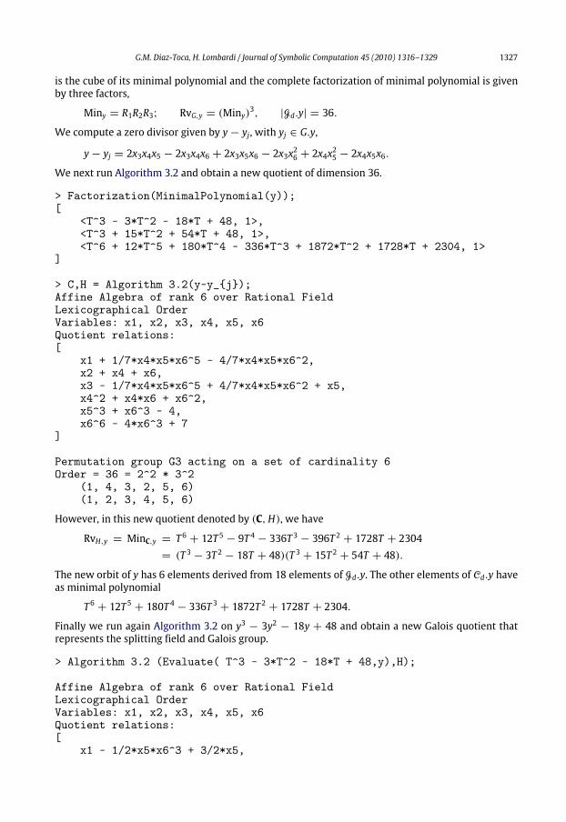
G.M. Diaz-Toca, H. Lombardi / Journal of Symbolic Computation 45 (2010) 1316–1329 1327
is the cube of its minimal polynomial and the complete factorization of minimal polynomial is givenby three factors,
Miny = R1R2R3; RvG,y = (Miny)3, |Gd.y| = 36.
We compute a zero divisor given by y − yj, with yj ∈ G.y,
y − yj = 2x3x4x5 − 2x3x4x6 + 2x3x5x6 − 2x3x26 + 2x4x25 − 2x4x5x6.
We next run Algorithm 3.2 and obtain a new quotient of dimension 36.
> Factorization(MinimalPolynomial(y));[
<T^3 - 3*T^2 - 18*T + 48, 1>,<T^3 + 15*T^2 + 54*T + 48, 1>,<T^6 + 12*T^5 + 180*T^4 - 336*T^3 + 1872*T^2 + 1728*T + 2304, 1>
]
> C,H = Algorithm 3.2(y-y_j);Affine Algebra of rank 6 over Rational FieldLexicographical OrderVariables: x1, x2, x3, x4, x5, x6Quotient relations:[
x1 + 1/7*x4*x5*x6^5 - 4/7*x4*x5*x6^2,x2 + x4 + x6,x3 - 1/7*x4*x5*x6^5 + 4/7*x4*x5*x6^2 + x5,x4^2 + x4*x6 + x6^2,x5^3 + x6^3 - 4,x6^6 - 4*x6^3 + 7
]
Permutation group G3 acting on a set of cardinality 6Order = 36 = 2^2 * 3^2
(1, 4, 3, 2, 5, 6)(1, 2, 3, 4, 5, 6)
However, in this new quotient denoted by (C,H), we have
RvH,y = MinC,y = T 6+ 12T 5
− 9T 4− 336T 3
− 396T 2+ 1728T + 2304
= (T 3− 3T 2
− 18T + 48)(T 3+ 15T 2
+ 54T + 48).
The new orbit of y has 6 elements derived from 18 elements of Gd.y. The other elements of Cd.y haveas minimal polynomial
T 6+ 12T 5
+ 180T 4− 336T 3
+ 1872T 2+ 1728T + 2304.
Finally we run again Algorithm 3.2 on y3 − 3y2 − 18y + 48 and obtain a new Galois quotient thatrepresents the splitting field and Galois group.
> Algorithm 3.2 (Evaluate( T^3 - 3*T^2 - 18*T + 48,y),H);
Affine Algebra of rank 6 over Rational FieldLexicographical OrderVariables: x1, x2, x3, x4, x5, x6Quotient relations:[
x1 - 1/2*x5*x6^3 + 3/2*x5,

1328 G.M. Diaz-Toca, H. Lombardi / Journal of Symbolic Computation 45 (2010) 1316–1329
x2 + 1/2*x6^4 - 1/2*x6,x3 + 1/2*x5*x6^3 - 1/2*x5,x4 - 1/2*x6^4 + 3/2*x6,x5^3 + x6^3 - 4,x6^6 - 4*x6^3 + 7
]
Permutation group acting on a set of cardinality 6Order = 18 = 2 * 3^2
(1, 3, 5)(2, 6, 4)(1, 2, 3, 4, 5, 6)
Example 3. This example illustrates the idea of Section 3.3. Let f (T ) = T 8− 5T 5
− 3T 4− 5T 3
+ 1 ,Cd = AQ,f , Gd = S8 and y = x8x7x6 ∈ Cd. TheGröbner basis of ⟨z − x8x7x6⟩ Cd is not triangular, has 12polynomials, Gb = P1(z, x8, . . . , x1), . . . , P11(z, x8), P12(z) and provides the following information.(1) P12(z) is the minimal polynomial of y,(2) the leading coefficient of P11(z, x8) is a zero divisor, factor of P12(z),(3) the leading coefficient of P8(z, x8, x7), equal to x8 − z, is another zero divisor.Example 4. This example shows how dynamic our methodology is. Let f (T ) = T 8
+ 12T 6+ 42T 4
+
36T 2+ 4 and the goal is to correctly compute in the splitting field of f (T ). So our first dynamic field
is Cd = AQ,f joint with Gd = S8 . We consider the element z = x8 + x7 ∈ AQ,f and observe that
• 25 = degree(Minz(T )) < degree(Rv(T )) = 28,• z is a zero divisor.
Thus, there are two ways of proceeding.(1) We compute a zero divisor given by z − zj, with zj ∈ Gd.z,
z − zj = x8 + x7 − x5 − x6.Let y = z − zj. We next run Algorithm 3.2 on y and obtain a new quotient of dimension 384.In this new quotient the minimal polynomial of −x2 − 2x4 − x6, the image of a conjugate ofy, factorizes into two polynomials, so we run again Algorithm 3.2, obtaining a new quotient ofdimension 128. In this new quotient, the minimal polynomial of −x2 + x4 + x6 + x8, also theimage of another conjugate of y, factorizes into two polynomials, so we run Algorithm 3.2 againgetting a representation of the splitting field a Galois group.
(2) We run Algorithm 3.2 on z and obtain a new quotient of dimension 384. In this new quotient theminimal polynomial of −x2 − x8, the image of a conjugate of z, factorizes into two polynomials,so we run again Algorithm 3.2, obtaining a new quotient of dimension 128.In this new quotient, z and its conjugates behave as in a field. However, we want to takeadvantage of all the information provided by z. Thus, we must consider the element y and seeif y and its conjugates behave as in a field. The answer is not because the minimal polynomialof x6 + x8 − x2 + x4 factorizes into two polynomials. Then we run Algorithm 3.2 again getting arepresentation of the splitting field a Galois group.
Conclusion
We conclude this paper by emphasizing the ideawe have developed here. Ourmethodologymakesit possible to compute in an exact way the splitting field of a polynomial dynamically. We are able totake advantage of any signal which shows that our dynamic field is given (at a certain moment of thecomputation) by an algebra which is not a field. We improve the algebra representing the splittingfield only when it is required.
In future work, it should be interesting to study what kind of oddities can happen
• when trying to make explicit the fact that the Galois correspondence has to be bijective (if ourapproximation is not a field, this can fail),
• when trying to compute a normal basis.

G.M. Diaz-Toca, H. Lombardi / Journal of Symbolic Computation 45 (2010) 1316–1329 1329
Acknowledgements
We are grateful to the anonymous referees for their careful reading of our work and their veryprecise suggestions to improve our presentation.
References
Arnaudiés, J.M., Valibouze, A., 1997. Lagrange resolvents. J. Pure Appl. Algebra 117 & 118, 23–40.Aubry, P., Valibouze, A., 2000. Using Galois ideals for computing relative resolvents. J. Symbolic Comput. 30, 635–651.Bosma, W., Cannon, J., Playoust, C., 1997. The Magma algebra system I: the user language. J. Symbolic Comput. 24 (3), 235–265.
URL: http://www.magma.maths.usyd.edu.au.Bourbaki, N., 1981. Algèbre. Masson, Paris (Chapitres 4 à 7).Chase, S., Harrison, D., Rosenberg, A., 1965. Galois Theory and Galois cohomology of commutative rings. Mem. Amer. Math. Soc.
52, 15–33.Drach, J., 1898. Essai sur la théorie générale de l’itération et sur la classification des transcendantes. Ann. Sci. École Norm. Sup.
3 (15), 243–384.Della Dora, J., Dicrescenzo, C., Duval, D., 1985. About a new method for computing in algebraic number fields. In: Caviness, B.F.
(Ed.), EUROCAL’85. In: Lecture Notes in Computer Science, vol. 204. Springer, pp. 289–290.Diaz-Toca, G.M., 2006. Galois Theory, splitting fields and computer algebra. J. Symbolic Comput. 41, 1174–1186.Diaz-Toca, G.M., Lombardi, H., Quitté, C., 2006. Universal decomposition algebra. In: Proceedings of Transgressive Computing
2006, pp. 169–184.Ducos, L., Effectivité en théorie de Galois. Sous-résultants. Université de Poitiers, Thèse doctorale. Poitiers, 1997.Ducos, L., 2000. Construction de corps de décomposition grâce aux facteurs de résolvantes (Construction of splitting fields in
favour of resolvent factors). Comm. Algebra 28 (2), 903–924 (in French).Ekedahl, E., Laskov, D., 2005. Splitting algebras, symmetric functions and Galois Theory. J. Algebra Appl. 4 (1), 59–76.Martens, F., 1902. Ein Beweis des Galois’schen fundamentalsatzes. Sitzungsberichte der Akademie der Wissensch. in Wien,
Math.-naturw. Kl. Abt. IIa, Bd. 111, 17–37.Pohst, M.E., Zassenhaus, H.J., 1989. Algorithmic Algebraic Number Theory. Cambridge University Press, ISBN: 0521596696.Renault, G., Yokoyama, K., 2006. A modular method for computing the splitting field of a polynomial. In: Proceedings of the 7th
International Symposium on Algorithmic Number Theory. In: Lecture Notes In Computer Science, vol. 4076. pp. 124–140.Soicher, L., McKay, J., 1985. Computing Galois groups over the rationals. J. Number Theory 20, 273–281.Stauduhar, R., 1973. The determination of Galois groups. Math. Comp. 27, 981–996.Steel, A., 2002. A new scheme for computingwith algebraically closed fields. In: Proceedings of the 5th International Symposium
on Algorithmic Number Theory. In: Lecture Notes in Computer Science, vol. 2369. pp. 491–505.Steel, A., 2010. Computing with algebraically closed fields. J. Symbolic Comput. 45, 342–372.Valibouze, A., 1995. Modules de Cauchy, polynômes caractéristiques et résolvantes. Rapport LITP. 95-62.Valibouze, A., 1999. Étude des relations algébriques entre les racines d’un polynôme d’une variable. Bull. Belg. Math. Soc. 6,
507–535.Valibouze, A., 2007. Classes doubles, idéaux de Galois et résolvantes. Rev. Roumaine Math. Pures Appl. 52 (1), 95–109.Vessiot, E., 1904. Sur la théorie de Galois et ses diverses généralisations. Ann. Sci. École Norm. Sup. 3ème série 21, 9–85.Wiedemann, D., 1986. Solving sparse linear systems over finite fields. IEEE Trans. Inf. Theory IT-32, 54–62.