HAL Id: hal-01071543https://hal.archives-ouvertes.fr/hal-01071543

Submitted on 6 Oct 2014

HAL is a multi-disciplinary open accessarchive for the deposit and dissemination of sci-entific research documents, whether they are pub-lished or not. The documents may come fromteaching and research institutions in France orabroad, or from public or private research centers.

L’archive ouverte pluridisciplinaire HAL, estdestinée au dépôt et à la diffusion de documentsscientifiques de niveau recherche, publiés ou non,émanant des établissements d’enseignement et derecherche français ou étrangers, des laboratoirespublics ou privés.

Dynamic Behaviour of a Flexible Yacht Sail PlanBenoit Augier, Patrick Bot, Frédéric Hauville, Mathieu Durand

To cite this version:Benoit Augier, Patrick Bot, Frédéric Hauville, Mathieu Durand. Dynamic Behaviour of a FlexibleYacht Sail Plan. Ocean Engineering, Elsevier, 2013, 66, pp.32-43. �10.1016/j.oceaneng.2013.03.017�.�hal-01071543�

Science Arts & Métiers (SAM)is an open access repository that collects the work of Arts et Métiers ParisTech

researchers and makes it freely available over the web where possible.

This is an author-deposited version published in: http://sam.ensam.euHandle ID: .http://hdl.handle.net/10985/8689

To cite this version :

Benoit AUGIER, Patrick BOT, Frédéric HAUVILLE, Mathieu DURAND - Dynamic Behaviour of aFlexible Yacht Sail Plan - Ocean Engineering - Vol. 66, p.32-43 - 2013

Any correspondence concerning this service should be sent to the repository

Administrator : archiveouverte@ensam.eu

Dynamic Behaviour of a Flexible Yacht Sail Plan

Benoit Augier♥ , Patrick Bot♥ , Frederic Hauville♥ , Mathieu Durand♥♣

♥Naval Academy Research Institute - IRENAV CC600, 29240 BREST Cedex 9, France

♣K-Epsilon Company, 1300 route des Cretes - B.P 255 06905 Sophia Antipolis Cedex,France

Abstract

A numerical investigation of the dynamic Fluid Structure Interaction

(FSI) of a yacht sail plan submitted to harmonic pitching is presented to

address both issues of aerodynamic unsteadiness and structural deformation.

The FSI model — Vortex Lattice Method fluid model and Finite Element

structure model — has been validated with full-scale measurements. It is

shown that the dynamic behaviour of a sail plan subject to yacht motion

clearly deviates from the quasi-steady theory. The aerodynamic forces pre-

sented as a function of the instantaneous apparent wind angle show hysteresis

loops, suggesting that some energy is exchanged by the system. The area

included in the hysteresis loop increases with the motion reduced frequency

and amplitude. Comparison of rigid versus soft structures shows that FSI

increases the energy exchanged by the system and that the oscillations of

aerodynamic forces are underestimated when the structure deformation is

not considered. Dynamic loads in the fore and aft rigging wires are domi-

nated by structural and inertial effects. This FSI model and the obtained

Email address: patrick.bot@ecole-navale.fr Tel:+33 2 98 23 39 86 (PatrickBot♥)

Preprint submitted to Ocean Engineering April 8, 2013

results may be useful firstly for yacht design, and also in the field of auxiliary

wind assisted ship propulsion, or to investigate other marine soft structures.

Keywords:

Fluid Structure Interaction, Dynamic behaviour, Yacht Sails, Soft

Membrane, Unsteady, Numerical/experimental comparison

2

Nomenclature

A deg pitching oscillation amplitude

C m sail plan chord at za (from head-sail leading edge

to mainsail trailing edge)

Cx - driving force coefficient

Cy - heeling force coefficient

fr - flow reduced frequency

S m2 total sail area

T s pitching oscillation period

VAW m.s−1 apparent wind speed

VTW m.s−1 true wind speed

Vr - flow reduced speed

za m height of the centre of aerodynamic force

F - force vector

R - residual vector

u m position vector

[C] - damping matrix

[K] - stiffness matrix

[M ] - inertia matrix

βAW deg apparent wind angle

βeff deg effective wind angle

βTW deg true wind angle

φ deg heel angle

θ deg trim angle

ρ kg.m−3 fluid density

τ s phase shift

3

1. Introduction

It is now well-known that deformations actively or passively endured by

aerodynamic and hydrodynamic lifting bodies have a significant effect on the

flow dynamics and the performance of the system. A huge amount of work

has been devoted to insects’ and birds’ flight, (?) or to fishes swim (?, ?), for

example for applications in Micro Air Vehicles (MAV) and more generally in

the bio-mimetic field (for a review, see ?). From this abundant literature, it

has been shown that the dynamic behaviour of the flow and the structural de-

formation must be considered to better understand the mechanisms involved

in lifting and propulsive performances (?). For example in the field of insect

flight, ? have underlined the necessity to consider the dynamic phenomena

to properly estimate aerodynamic coefficients.

Fluid structure interaction is also of interest for some compliant marine

structures, such as wave attenuation systems (?) or in the field of Ocean

Thermal Energy Conversion (OTEC) where soft ducts made of a membrane

and stiffeners may be interesting for the cold water pipe (?, ?). To reduce

fuel consumption and emissions in maritime transport, wind assisted propul-

sion is more and more considered for ships (?, ?, ?).

When analysing the behaviour of yacht sails, an important difficulty

comes from the Fluid Structure Interaction (FSI) of the air flow and the

sails and rig (?, ?, ?). Yacht sails are soft structures whose shapes change

according to the aerodynamic loading. The resulting modified shape affects

the air flow and thus, the aerodynamic loading applied to the structure. This

4

Fluid Structure Interaction is strong and non-linear, because sails are soft

and light membranes which experience large displacements and accelerations,

even for small stresses. As a consequence, the actual sail’s shape while sailing

— the so-called flying shape — is different from the design shape defined by

the sail maker and is generally not known. Recently, several authors have

focused on the Fluid Structure Interaction (FSI) problem to address the is-

sue of the impact of the structural deformation on the flow and hence the

aerodynamic forces generated (?, ?).

Another challenging task in modelling racing yachts is to consider the

yacht behaviour in a realistic environment (?, ?, ?, ?). Traditional Velocity

Prediction Programs (VPPs) used by yacht designers consider a static equi-

librium between hydrodynamic and aerodynamic forces. Hence, the force

models classically used are estimated in a steady state. However, in realistic

sailing conditions, the flow around the sails is most often largely unsteady

because of wind variations, actions of the crew and more importantly be-

cause of yacht motion due to waves. To account for this dynamic behaviour,

several Dynamic Velocity Prediction Programs (DVPPs) have been devel-

oped, e.g. by ?, ?, ?, ? which need models of dynamic aerodynamic and

hydrodynamic forces. While the dynamic effects on hydrodynamic forces

have been largely studied, the unsteady aerodynamic behaviour of the sails

has received much less attention. ? first developed an unsteady aeroelastic

model in potential flow dedicated to flexible membranes but neglected the

inertia. In a quasi-static approach, a first step is to add the velocity induced

by the yacht’s motion to the steady apparent wind to build an instantaneous

5

apparent wind (see ?, ?) and to consider the aerodynamic forces correspond-

ing to this instantaneous apparent wind using force models obtained in the

steady state. In a recent study, ? developed an analytical model to predict

the unsteady aerodynamics of interacting yacht sails in 2D potential flow and

performed 2D wind tunnel oscillation tests with a motion range typical of

a 90-foot (26m) racing yacht (International America’s Cup Class 33). Re-

cently, ?, ?, and ? studied the aerodynamics of model-scale rigid sails in a

wind tunnel, and showed that a pitching motion has a strong and non-trivial

effect on aerodynamic forces. They showed that the relationship between in-

stantaneous forces and apparent wind deviates — phase shifts, hysteresis —

from the equivalent relationship obtained in a steady state, which one could

have thought to apply in a quasi-static approach. They also investigated soft

sails in the same conditions to highlight the effects of the structural defor-

mation (?).

To better understand the aeroelastic behaviour, a numerical investigation

is achieved with a simple harmonic motion to analyse the dynamic phenom-

ena in a well-controlled situation. This paper addresses both issues of the

effects of unsteadiness and structural deformation on a yacht sail plan with

typical parameters of a 28-foot (8m, J80 class) cruiser-racer in moderate sea.

An unsteady FSI model has been developed and validated with experiments

in real sailing conditions (?, ?, ?). Calculations are made on a J80 class yacht

numerical model with her standard rigging and sails designed by the sail

maker DeltaVoiles. The dynamic results are compared with the quasi-steady

assumption and the dynamic force coefficients are also compared with the

6

experimental results obtained by ? for a rigid sail plan of a 48-foot (14.6m)

cruiser-racer model. The FSI model is presented in section 2, and the experi-

mental validation is presented in section 3. The methodology of the dynamic

investigation is given in section 4. The core of the paper (section 5) presents

and analyses the simulation results regarding variation of force coefficients

and loads in the rig due to pitching. In the last section, some conclusions of

this study are given, with ideas for future work.

2. Numerical model

To numerically investigate aero-elastic problems which can be found with

sails, the company K-Epsilon and the Naval Academy Research Institute have

developed the unsteady fluid-structure model ARAVANTI made by coupling

the inviscid flow solver AVANTI with the structural solver ARA. The AR-

AVANTI code is able to model a complete sail boat rig in order to predict

forces, tensile and shape of sails according to the loading in dynamic condi-

tions. The numerical models and coupling are briefly described below. For

more details, the reader is referred to ? for the fluid solver AVANTI and to

? and ? for the structural solver ARA and the FSI coupling method.

2.1. The inviscid fluid solver: AVANTI

Flow modelling is based on the Vortex Lattice Method (VLM). This

method is suitable for external flows where vorticity exists only in the bound-

ary layers on the lifting surface and its wake. In the lifting surface model,

the vorticity is represented by a non-planar doublet distribution along the

7

lifting surface and the wake formed by the vortex shedding at the trailing

edge is represented by a vortex sheet. This method is basically made up of

two parts: a lifting body problem and a wake problem. These two problems

are coupled by means of a kind of Kutta condition that has been derived

from the kinematic and dynamic conditions along the separation lines. Usu-

ally, these lines are reduced to the trailing edges although more complicated

situations have sometimes been considered. Except when writing this Kutta

condition, the flow is assumed to be inviscid. The lifting problem is solved by

means of a boundary integral method: the surface of the body is represented

using panels of rectangular shape which are used to satisfy the potential slip

condition. Specifically, a doublet strength is associated with each panel, and

the strength of the doublet is adjusted by imposing that the normal velocity

component at the surface of the body must vanish at control points. The

aerodynamic force is computed with the doublet strength and local fluid ve-

locity thanks to the doublet/vorticity equivalence introduced by ? (see also

?). The wake is modelled by means of the particles method itself developed

by ? and then ?. According to this method, the vorticity distribution within

the wake is described by means of virtual particles carrying vortices. The

motion of particles is computed in a Lagrangian framework. The vorticity

on each particle has to satisfy the Helmholtz equation. Dissipation of the

wake is modelled by damping the particles’ intensity in time — empirically

adjusted, see ? — and neighbour particles of small intensity are merged. In

practice, there are very few particles downstream a distance of four chord

lengths from the trailing edge.

8

For the incoming flow, the true wind is defined with the velocity at 10m

height and an atmospheric wind gradient is considered. Boat speed and mo-

tion are then considered to determine the apparent wind. This fluid model

has been largely used and validated (?). As the fluid is supposed to be invis-

cid, the validity of the model is obviously limited to mostly attached flows,

as it is the case for a sailing yacht on a close hauled course, where the sails’

curvature and incidence are moderate. The viscous drag is not considered in

the simulations.

2.2. The structural software: ARA

The structural model is a finite element model composed of beams (spars

and battens), cables (wires and running rigging) and membranes (sails). The

sail model is based on CST (Constant Strain Triangles) membrane model ele-

ments extended in 3 dimensions. Despite its simplicity, this choice has proven

to give a good ratio of accuracy to computing power. The assumptions im-

posed inside this element are constant stresses, constant strains and uniform

stiffness of the material. Non-linearities coming from the geometry and com-

pression are taken into account. The non-linear finite element formulation

based on the virtual work equation links the variation of forces to the vari-

ation of displacement. The Newmark-Bossak Interaction scheme (temporal

discretisation) is based on a prediction-correction iterative method.

(F inertial + F damping + F stiffness) + F external = R (1)

9

Deriving these as a function of position, speed and acceleration results in

a Newton-type scheme:

[M ] u+ [C] u+ [K] u = R (2)

The Newmark scheme puts position, speed and acceleration in the fol-

lowing relation:

[K∗]u = R (3)

[K∗] = [M ]1

ξ∆t2+ [C]

γ

ξ∆t+ [K] (4)

Where [M] is the inertia matrix (mass and added mass), [C] is the damp-

ing matrix and [K] is the stiffness matrix. In the stress-strain relationship

of the sail fabric, an anisotropic composite material is considered and the

properties of several layers may be superimposed in the matrix [K] (films

and strings for example).

The sail structure and panelling are imported from the sail designer soft-

ware Sailpack which was used to make the sails, and the structural mesh is

built according to the sail design. Mechanical properties of every component

of the structure have been measured experimentally.

10

2.3. AVANTI/ARA coupling

The effects of the interaction are translated into a coupling of the kine-

matic equation (continuity of the normal component of the velocity at the in-

terface between fluid and structure geometrical domains) and dynamic equa-

tions (continuity of the normal component of the external force, pressure

forces, on the contact surface of the sail with the fluid). An implicit iterative

algorithm (see Figure 1) is used to coordinate the data exchanges between

the fluid and structure solvers and to obtain a stable coupling. Two different

meshes are used to satisfy the quality criteria of fluid mesh on one side and

structural mesh on the other side. The deformation from the structural com-

putation is introduced into the fluid mesh. Then, new forces from the fluid

computation are interpolated in the structural code by a consistent method.

In a previous study, much attention was devoted to validation of this FSI

model with respect to full-scale experiments (?). A summary of the valida-

tion results is presented below.

3. Experimental validation

Numerical and experimental comparisons with the model ARAVANTI are

based on measurements at full scale on an instrumented 28-foot yacht (J80

class, 8m). The time-resolved sails’ flying shape, loads in the rig, yacht’s mo-

tion and apparent wind have been measured in both sailing conditions of flat

sea and moderate head waves. The comparisons are limited to upwind sailing

conditions, as the flow model validity is limited to mostly attached flows. At

first, the computed sail flying shape and loads in the rig were compared with

11

the measurements in a steady state corresponding to flat sea. The predicted

flying shape is in very good agreement with the measured one, as shown on

Figure 2. Comparison of the computed and experimentally-measured pa-

rameters of the aerodynamic profiles — namely camber, draft, twist angle

— shows a mean relative error of 2.5% and a maximum error of 6% in the

worst case. The loads in the rig are also well predicted with less than 8%

discrepancy for side stays and backstay, and 10% for the forestay (see Figure

3). More detailed description of the experimental system and methods and

the quantitative comparison are given in ?, ? and ?.

For the dynamic regime, a yacht sailing upwind in a short swell with

a constant true wind of 7m.s−1 (14kts) is considered. The apparent wind

variations are assumed to come only from the boat’s motion. Recorded atti-

tudes, from the motion sensors, are implemented as inputs in the simulation.

Time series of some experimental and calculated loads are represented for a

20 s recording in Figure 4. The simulation resolves the dynamic behaviour

of the loads consistently with the experimental measurements. The mean

load value is slightly overestimated in the backstay and underestimated in

the forestay, but the oscillations are reproduced well. The normalised inter-

correlation function between measured and computed time series shows a

maximum value higher than 0.8 with a phase shift lower than 0.1s. For more

details on the model validation with full-scale experiments, the reader is re-

ferred to ?.

The code has shown its ability to simulate the rig’s response to yacht

12

motion forcing, and to correctly estimate the loads. The small observed

discrepancies were mainly attributed to difficulties to determine precisely the

environmental conditions and some inaccuracies in the mechanical properties

of the structural elements. Thereby, ARAVANTI is a reliable tool to study

the dynamic behaviour of a sail plan subject to pitching motion.

4. Simulation Procedure

The yacht motion in waves induces unsteady effects in the sails’ aerody-

namics. In this paper we will study separately one degree of freedom, by

applying simple harmonic pitching. The reference frame and the coordinate

system attached to the yacht are illustrated in Figure 5.

4.1. Reference steady case

First, the reference steady case is computed with the following para-

meters: true wind speed at 10m height VTW=6.7 m.s−1 (a logarithmic verti-

cal wind profile is imposed with a roughness length of 0.2mm (?)), true wind

angle βTW=40˚, boat speed VBS=2.6 m.s−1 , heel angle φ=20˚and trim

angle θ=0˚. This first computation yields the converged steady flow, the rig

and sails’ flying shape, and enables the steady state aerodynamic forces and

centre of effort to be determined. This converged steady state is used as the

initial condition for the computations with pitching forcing. The height za

of the centre of aerodynamic forces is used to define the flow characteristic

quantities: apparent wind speed VAW , apparent wind angle βAW and sail

plan chord C defined as the distance from the head-sail leading edge and the

mainsail trailing edge at za. Corrections of the apparent wind angle βAW due

13

to constant heel φ (first introduced by ?) and trim θ are considered through

the use of the effective apparent wind angle βeff (see ? for heel effect, and ?

for pitch effect):

βeff = tan−1(

tan βAW

cos θcosφ

)(5)

4.2. Harmonic pitching

The unsteady computations consist of a 20s run, with forced harmonic

pitching being imposed on the rig, characterised by the oscillation amplitude

A and period T (equation 6), other parameters being constant and equal to

those of the reference state.

θ(t) = A cos

(2π

Tt

)(6)

To avoid discontinuities in the accelerations, the beginning of motion is

gradually imposed by applying a ramp which increases smoothly from 0 to 1

during the first 3s of imposed motion (see first period in Figure 7).

The investigation has been made with variables in the range A=3 to 6˚, and

T=1.5 to 6s, corresponding to the typical environmental conditions encoun-

tered, as shown in the experiment of ?. The unsteady character of a flow is

characterized by a dimensionless parameter defined by the ratio of the mo-

tion period T to the fluid advection time along the total sail plan chord C.

Similarly to the closely related literature (?, ?), this parameter is called the

flow reduced velocity Vr (or the inverse: the reduced frequency fr) defined by:

14

Vr =VAWT

C= f−1r (7)

The case Vr � 1 (fr � 1) corresponds to quasi-steady aerodynamic

conditions. The pitching period values investigated correspond to a reduced

velocity Vr from 2 to 8.5 (reduced frequency fr from 0.12 to 0.47), which

positions this numerical study in a similar dynamic range to the experiments

of ? where Vr was from 2.3 to 56 (reduced frequency fr from 0.02 to 0.43)

corresponding to typical conditions encountered by a 48-foot yacht (14.6m).

The computed cases are summarised in Table 1.

When the yacht is subjected to pitching motion, the apparent wind is pe-

riodically modified as the rotation adds a new component of apparent wind

which varies with height. Following the analysis of ?, the apparent wind

and pitch-induced velocity are considered at the centre of aerodynamic force

height za. This centre of effort is actually moving due to pitch oscillation, but

variations are small enough to be ignored, and the reference height computed

in the steady state is used. This yields time dependent apparent wind speed

and angle, given by:

VAW (t) =((VTW sin βTW )2

+(VTW cos βTW + VBS + zaθ(t))2) 1

2

βAW (t) = sin−1(VTW sin βTW

VAW (t)

) (8)

And hence the time-dependent effective wind angle:

15

βeff (t) = tan−1(

tan βAW (t)

cos θ(t)cosφ

)(9)

Figure 6 illustrates the dynamic vector composition for pitching velocities

θ=θmax, 0 and θmin, and Figure 7 shows the resulting dynamic apparent wind

velocity and angle computed with equations 8 and 9. As shown in Figure 7,

the apparent wind angle variations are in phase opposition with the apparent

wind speed.

4.3. Heeling and driving force coefficients

Aerodynamic forces are calculated by the code at the sail plan’s centre of

effort. Forces are written in the inertial reference frame, in order to get Fx and

Fy, the driving and the heeling forces. Driving and heeling force coefficients

are obtained by the normalisation with the product of the instantaneous

apparent dynamic pressure and the total sail area S:

Cx(t) =Fx

0.5ρV 2AW (t)S

(10)

Cy(t) =Fy

0.5ρV 2AW (t)S

(11)

5. Results

From the unsteady FSI simulations, the aerodynamic forces and loads

in the rig are determined and their dynamic evolution is analysed with re-

spect to the instantaneous effective wind angle βeff (t) and pitching velocity

θ(t). Figure 8 shows an example of the computed results, with snapshots of

16

the pressure distribution and the particles modelling the wake for a pitch-

ing oscillation amplitude A=5˚and a period T=3s. The unsteady behaviour

is illustrated by the evolution of the pressure distribution on sails and the

emitted particles’ streaklines. The pressure field is presented in Figure 8.b

and 8.d for the extreme values of apparent wind angle βeff (t), i.e. at trim

angle θ=0˚, increasing and decreasing. Notice also in Figure 8.a and 8.c the

different pressure distributions observed for the same value of apparent wind

angle βeff (t) but with opposite trim angles.

5.1. Simulation with different reduced velocities Vr and amplitudes A

Calculations are made with a fixed pitching amplitude A=5˚and different

periods, and with different amplitudes for a given period as illustrated in

Table 1. Figure 9 shows the evolution of aerodynamic coefficients Cx(t)

and Cy(t) with the instantaneous apparent wind angle βeff (t) for different

values of the reduced velocity. From the initial condition corresponding to

the reference steady state at βeff (0)=27.8˚, the system oscillates under the

forced pitching with a periodic behaviour as shown by the quasi-elliptic limit

cycle drawn in the figure. The initial peak at the beginning of the run is

due to imperfection in the restart by the dynamic computation scheme from

the reference steady state. It is noticeable that the periodic behaviour is

obtained after a short transient time of the order of the smoothing ramp

applied on the motion initiation. The evolution of Cx and Cy with βeff in

a steady case, obtained from steady computations for different βeff is also

shown for comparison.

The periodic oscillation of the aerodynamic forces plotted as a func-

17

Table 1: Reduced velocity Vr, reduced frequency fr, phase delay τ and hysteresis loop

area∫TCx dβeff for Cx and apparent wind angle βeff corresponding to the different

tested pitch amplitudes A and periods T.

T A Vr fr τ 2πτ/T Loop area

s deg - - s rad deg

1.5 5 2.13 0.47 0.1 0.42 2.12

3 5 4.27 0.23 0.3 0.63 0.82

5 5 7.11 0.14 0.6 0.75 0.42

6 5 8.53 0.12 0.75 0.79 0.36

T A Vr fr τ 2πτ/T Loop area

s deg - - s rad deg

5 3 7.11 0.14 0.6 0.75 0.15

5 5 7.11 0.14 0.6 0.75 0.42

5 6 7.11 0.14 0.6 0.75 0.61

18

tion of the instantaneous effective wind angle is loop-shaped in the plane

(Cx,y(t),βeff (t)). To better understand this behaviour and the origin of

these loops, the phase shift τ between the signals was determined by cross-

correlation, and the aerodynamic coefficients Cx,y(t) were plotted versus the

time-delayed wind angle βeff (t+τ). In these new plots, the area enclosed

inside the loops is lower than in the former plots but does not vanish, and

the loops do not collapse into a single line as would be the case for simply

phase-shifted signals. Hence, this behaviour is the signature of an hysteresis

phenomenon between the dynamic forces and the apparent wind angle. The

phase delay and the hysteresis loop area are tabulated in Table 1. The phase

delay increases with the reduced velocity (with the motion period) but is not

affected by the oscillation amplitude.

As the reduced velocity decreases (shorter period), the area of the hys-

teresis loop increases importantly (Table 1), as the range of wind angles

swept under pitching ( ∆βeff ) gets wider, and the slope of the hysteresis

loop decreases.

Figure 10 shows the evolution of the aerodynamic coefficients Cx(t) and

Cy(t) with the instantaneous effective wind angle βeff (t) for different values

of the pitching amplitude. The area of the hysteresis loop is increased notice-

ably by the higher pitching amplitude. Although the reduced velocity is not

changed, the amplitude has a strong effect on the unsteady character of the

system as the rotation velocity is directly linked to the oscillation amplitude.

Tables 2 and 3 show the mean value and variation range for each variable

19

Table 2: Mean value and variation range of force coefficients and βeff (t) for a pitching

period variation

A5T1.5 A5T3 A5T5 A5T6

Cx 0.38 0.36 0.36 0.36

∆Cx 0.39 0.21 0.16 0.15

Cy −1.21 −1.16 −1.14 −1.14

∆Cy 0.93 0.46 0.37 0.35

βeff (˚) 28.84 28.03 27.81 27.79

∆βeff (˚) 16.22 7.77 4.62 3.84

during one period of pitching. It may be noticed that the average effective

wind angle varies with the pitching amplitude and period, even if the yacht

is pitching around the same mean trim θ=0˚, because of the non-linearity of

equation 9. The pitching period also has an influence on the hysteresis loop

thickness and its centre, as illustrated in Table 2.

Increasing the pitch period moves the ellipse centre slightly towards lower

values of βeff (t) and force coefficients (in absolute value). The pitch am-

plitude also has a great influence on the hysteresis loop’s enclosed area.

When the pitching amplitude is increased, the variation range of aerody-

namic forces, the variation range of βeff (t) and the mean value of βeff (t)

increase, as tabulated in Table 3.

These results are very similar to the experimental results obtained by ?.

20

Table 3: Mean value and variation range of force coefficients and βeff (t) for a pitching

amplitude variation

A3T5 A5T5 A6T5

Cx 0.36 0.36 0.36

∆Cx 0.13 0.16 0.19

Cy −1.14 −1.14 −1.14

∆Cy 0.30 0.37 0.40

βeff (˚) 27.7 27.8 27.8

∆βeff (˚) 2.8 4.6 5.6

Limit cycles show the same trends, centred on the steady state trend, with

an increasing driving force and an increasing heeling force in absolute value

(Cy <0) when βeff (t) is increasing.

5.2. Effect of the structural deformation

To assess the contribution of the structural behaviour on the system’s

response, results computed with the Fluid Structure Interaction (FSI) sim-

ulations presented above have been compared to fluid-only simulations con-

sidering a rigid structure.

The rigid structure (sails and rig) is the converged flying shape calculated

from the FSI steady simulation (section 4.1), frozen into a fixed geometry

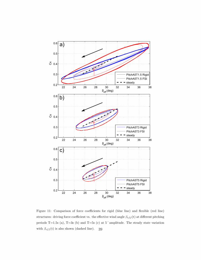
for the unsteady fluid-only simulation with pitching forcing. Figure 11 shows

the evolution of the calculated driving force coefficient Cx(t) for both FSI

and rigid simulations. The enclosed area is smaller and the loop axis slope

21

is slightly lower in the rigid structure case. Rigid structure calculations un-

derestimate the hysteresis phenomenon and the stress variation. The same

behaviour is observed for the side force coefficient Cy(t) (not shown here).

Table 4 summarizes the mean values and the range of force coefficients and

effective wind angle for several values of the pitching period. The variation

range of the aerodynamic coefficients is underestimated by the fluid-only cal-

culation, highlighting the importance of FSI simulation in the case of sails.

Table 4: Comparison between mean value and range of force coefficients and βeff (t) from

Fluid only (rigid structure) and FSI (flexible structure) calculations

A5T1.5 A5T1.5 A5T5 A5T5

Rigid FSI Rigid FSI

Cx 0.38 0.38 0.37 0.36

∆Cx 0.31 0.39 0.13 0.16

Cy −1.22 −1.21 −1.16 −1.14

∆Cy 0.76 0.93 0.32 0.37

βeff (˚) 28.8 28.8 27.8 27.8

∆βeff (˚) 16.2 16.2 4.6 4.6

5.3. Loads in the rig

The ARAVANTI code simulates the full rigging and gives access to the

load experienced by the rig wires and sail vertices. Figure 12 shows the vari-

ations of load in the forestay, backstay and main sheet due to the pitching

oscillation for various reduced velocities, tuned by the pitching period, as

22

a function of effective wind angle βeff (t). A hysteresis loop is observed, as

for the aerodynamic coefficients. The steady state trend is also shown for

comparison, computed from steady simulations with different values of βeff .

The steady state trend is easily explained by the increase in loading of the

rig with increase in the static angle of attack. In a quasi-static approach the

same trend could be expected for the dynamic loads with βeff (t). However,

the general trend shown by the main axis of the hysteresis loop is the op-

posite for the forestay and the main sheet: the load decreases for increasing

βeff (t) which shows a phase opposition.

Actually, it is worth noticing that βeff (t) is itself in phase opposition to

the pitching velocity θ(t) (see Figure 7). In other words, the pitching veloc-

ity is maximal when βeff (t) is minimal. Hence, the general trend of load in

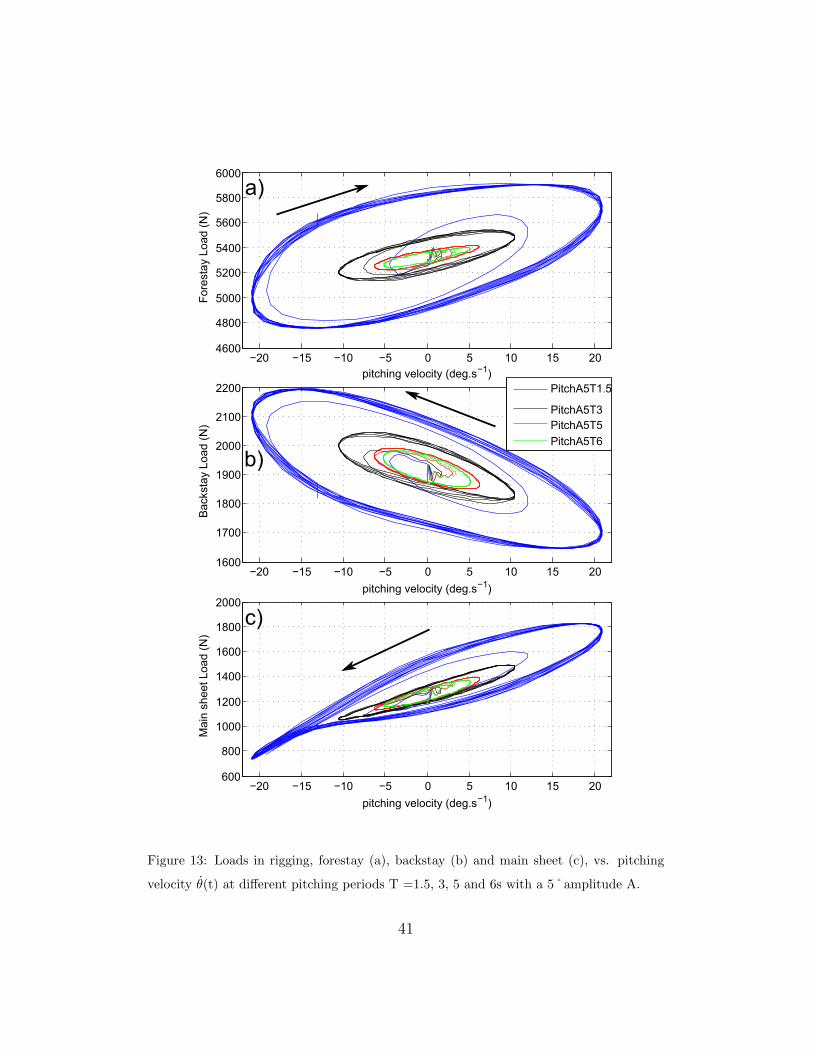
the forestay is an increase with increasing θ(t) as shown on Figure 13. This

observation suggests that the variations in the forestay load are governed

by structural behaviour from the inertia of the rigging, rather than by the

aerodynamic behaviour. Indeed, the motion is imposed on the hull by the

effect of waves and when the yacht’s bow is diving (θ(t)>0), the forestay

pulls the mast forward and the load increases. The opposite holds for the

backstay, which explains the general trend observed in Figure 13: the back-

stay load increases with the negative of the pitching velocity (−θ(t): stern

diving). The forces of inertia from the mast were estimated from the mast

moment of inertia and angular acceleration, and projected along the forestay

and the backstay. The resulting amplitude of inertial loads is the same order

of magnitude as the load variations obtained from the FSI simulation for the

23

forestay and the backstay. It may be concluded that the structural effect

on the forestay and backstay loads is predominant in pitching motion. The

influence of pitching velocity dominates the influence of the angle of attack.

The main sheet’s loop axis slope has the same trend as that of the forestay,

whereas the main sheet pulls the mast backwards as the backstay does. The

load does not increase with βeff (t), but increases with pitching velocity θ(t).

A possible explanation may be that load variations in the main sheet are

governed by the apparent wind speed VAW (t). Variations of the apparent

wind speed are due to pitching, so are in phase opposition with βeff (t). A

maximum θ(t)>0 — and minimum θ(t)<0 — corresponds to a maximum

— and minimum — of VAW (t). The amplitude of inertial forces from the

boom is one order of magnitude lower than the variations in main sheet

load. Therefore, the boom inertia is not predominant in the main sheet load

variations, and the effects of the whole rig inertia and apparent wind speed

VAW (t) may play a significant role.

5.4. Loads in the rig measured in full-scale experiments

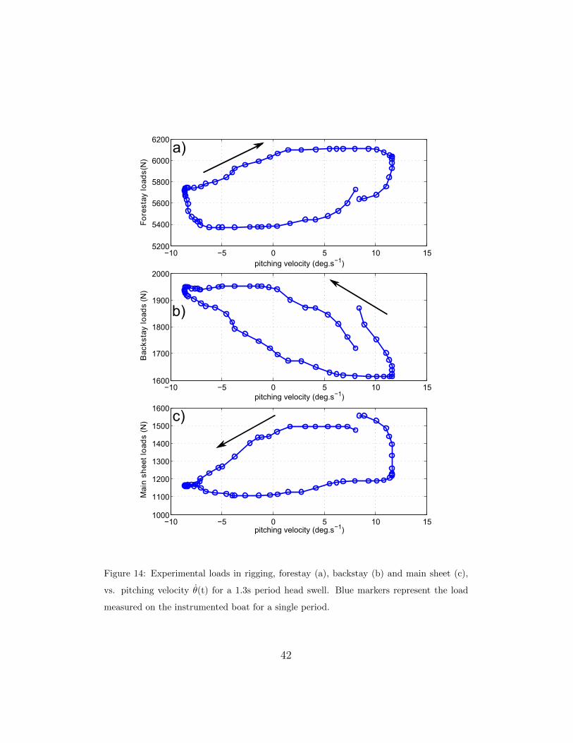
The full-scale experiment described in section 3 enabled the loads in the

rig to be measured. Figure 14 presents the experimental load variations

versus the pitching velocity θ(t) recorded at sea with the instrumented boat.

The pitching period is 1.3s (one period is shown) and the amplitude is around

2˚. Even when the pitching is perturbed by the general boat motion in these

real conditions (more complex than a pure harmonic pitching only), a hys-

teresis loop can be observed. The loop axis slopes for the forestay, backstay

24

and main sheet confirm the trends observed in the simulation results, which

supports the analysis put forth in the previous section. The enclosed area

is smaller in the experimental set because the pitching amplitude is smaller

than in the simulation.

6. Conclusions

The unsteady fluid structure interaction of the sails and rig of a 28-foot

(8m) yacht under harmonic pitching motion has been investigated in order to

highlight both contributions of the dynamic behaviour and the fluid structure

interaction on a sail plan in realistic conditions. The ARAVANTI model is

based on an implicit unsteady coupling between a vortex lattice fluid model

and a finite element structural model, and has been validated with full-scale

experiments in upwind real conditions (?). The contribution of pitching

to the apparent wind has been analysed and the time-dependent apparent

wind speed and angle were derived, in the framework of the effective wind

angle (?) and the sail plan centre of effort velocity induced by pitching

(?). Similar to the experimental results of ? obtained in a wind tunnel

on the rigid sail plan model of a 48-foot (14.6m) yacht, the aerodynamic

coefficients plotted against the instantaneous apparent wind angle show an

hysteresis loop, which indicates that unsteady conditions lead to aerodynamic

equivalent damping and stiffening effects. Further simulations and analysis

are underway to interpret this phenomenon in terms of energy exchanged by

the aeroelastic system.

These results confirm that the dynamic behaviour of a sail plan subjected

to yacht motion deviates from quasi-steady theory. Oscillations of the aero-

25

dynamic forces show phase shifts and hysteresis loops which increase with

the reduced frequency and amplitude of the motion. These conclusions differ

from the results of ? who concluded to small unsteady lift amplitudes for the

sails of a 90-foot (26m) International America’s Cup Class yacht. Besides

differences in the models, the higher variations shown here in the case of a 28-

foot (8m) cruiser-racer in a moderate sea are mainly due to a higher forcing

amplitude. The pitching motion induces an apparent wind velocity relative

amplitude up to 30%, compared to less than 7% in ?, and a wind-normal

motion of the sails at the centre of effort height up to 10% of the total chord

length at the same height, compared to less than 1% in ?.

Thanks to simulations with both rigid and flexible structures (sails and

rig), the particular effect of the fluid structure interaction has been high-

lighted. Interestingly, the aerodynamic force amplitudes are greater in the

case of the flexible structure considered here than for a rigid structure. For

further work, it would be interesting to address this issue for different struc-

ture stiffness characteristics. Indeed, the dynamic FSI model may be used

to study the effect of different tensions in the rig for various dynamic sailing

conditions, which may prove to be very useful for rig design and rig tuning

purposes. The simulation tool developed and the results of this work can be

used by rig and sail designers to estimate the dynamic loads in the structure.

The implications towards performance prediction and performance enhance-

ment of yachts are not straightforward and a thorough analysis with an expert

designer would be of great interest.

26

As the fluid model is an inviscid VLM, the flow is assumed to be at-

tached over the whole sail. However, there may be some non-negligible flow

separation when soft sails are submitted to a pitching motion, as suggested

by ?. This issue needs more investigation, and further developments are in

progress to couple the structural model ARA with a RANSE solver.

The load oscillations in the rig under forced pitching have been analysed.

A similar hysteresis loop has been found but the general trend for the forestay

and backstay is related better to the pitching velocity than to the dynamic

apparent wind. This suggests that the dynamic tensions in the rig are dom-

inated by the effects of structural dynamics and rig inertia, compared to the

aerodynamic effects. Understanding the behaviour of the load in the main

sheet is less intuitive and requires more investigation. Both structural and

aerodynamic behaviours may play significant roles.

This study opens up a large area for further work to better understand

the FSI dynamics of yacht sails and rigs. In particular, more simulations

and experimental work are needed to investigate the relative contributions

of aerodynamics and structural dynamics in more detail. Furthermore, it

would be interesting to explore a wider range of forced oscillation periods

and amplitudes, as well as other excitations such as roll and yaw motion.

This work has shown the importance of accounting for the Fluid Structure

Interaction and dynamic behaviour of a soft structure in an oscillatory flow in

general. The model developed and the outcomes of this work may be useful

27

for ship auxiliary wind-assisted propulsion and to investigate other marine

soft structures.

Acknowledgements

The authors wish to thank Prof. Fossati of Politecnico di Milano for valu-

able discussions. His pioneering work on the subject strongly inspired the

present study and analysis. The authors are grateful to the K-Epsilon com-

pany for continuous collaboration. This work was supported by the French

Naval Academy.

28

initialisation

ARA solver

mesh deformation

AVANTI solver(one non linear iteration)

CV2

CV1

structure deformation

boundary condition

flow

t t+dt

temporal loop

FSI loop

structure loop

Convergence teston structure residuals

Convergence teston fluid residuals

fluid forces

-

Figure 1: Implicit FSI coupling diagram

29

Figure 2: Superposition of the flying shape of the experimental sails and the numerical

result on a yacht sailing upwind in a steady state. The picture and grey visualisation

stripes show the measured flying shape; the blue thick lines show the computed position

of the beams in the model (mast, boom, spreaders, battens); the light blue lines show the

computed sail outline and the visualisation stripes.

30

0

1000

2000

3000

4000

5000

6000

Lo

ads

(N)

Numerical

Experimental

V1

V2

D1

For

esta

y

Bac

ksta

y

Mai

n S

heet

Figure 3: Experimental and numerical comparison on loads at steady state. Comparison

is shown for the fore, aft and three windward side stays holding the mast, and for the

mainsail sheet. V1 is the outer and longer side stay running from the mast top down to

the yacht’s deck ; V2 is the intermediate side stay running from two thirds of the mast

height down to the yacht’s deck ; D1 is the inner and shorter side stay running from one

third of the mast height down to the yacht’s deck.

31

time in s

0 2 4 6 8 10 12 14 16 18 205000

5500

6000

6500Lo

ad (

N)

0 2 4 6 8 10 12 14 16 18 201600

1800

2000

2200

Load

(N

)

0 2 4 6 8 10 12 14 16 18 20

Load

(N

)

1000

1500

2000

backstayEx

backstayNum

forestayEx

forestayNum

main sheetNum

main sheetEx

a)

b)

c)

Figure 4: Comparison of load variations in forestay (a), backstay (b) and main sheet (c)

due to pitch forcing between the measured (Ex-thin line) and calculated (Num-bold line)

signals.

32

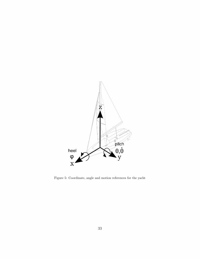
Figure 5: Coordinate, angle and motion references for the yacht

33

BS

x

βAWθ

βAWθ

βAW

min

max

y

VTW

VAW

zaθ<0

zaθ>0

Figure 6: Dynamic effect of pitching on the wind triangle (top view). ~V is the wind

velocity, BS is the boat speed, z is the height of the aerodynamic centre of effort, θ is the

pitching velocity, β is the apparent wind angle, subscripts TW and AW stand for True

and Apparent wind

34

0 2 4 6 8 10 12 14 16 18 207.7

8.2

8.7

9.2

9.7

10.2w

ind

spee

d (m

/s)

t (s)

VAW

steady

VAW

(t) pitch

0 2 4 6 8 10 12 14 16 18 20

24

26

28

30

32

34

Win

d an

gle

(°)

t (s)

βAW

steady

βAW

(t) pitch

βeff

a

b

c

d

a

b

c

d

(t)

a)

b)

Figure 7: Time dependent apparent wind speed VAW (a) ; apparent wind angle βAW and

effective wind angle βeff (b) resulting from pitching oscillation with period T=3s and

amplitude A=5˚. Letters on the signals refer to the snapshots of figure 8

35

Pa

a b

c dθ=0

θ=0

20 -20

-60

-100

-140

-180

βeff=28° θ=+5°

βeff=28° θ=-5° βeff=24.3° θ=0°

βeff=32.1° θ=0°

Figure 8: Pressure jump distribution and wake due to a pitching oscillation with 5˚ampli-

tude and 3s period. The time of each snapshot is indicated on Figure 7. Arrows represent

the pitching direction. θ is the trim angle, θ is the pitching velocity, βeff is the effective

wind angle.

36

20 22 24 26 28 30 32 34 36 38 40 420.2

0.25

0.3

0.35

0.4

0.45

0.5

0.55

0.6

0.65

βeff

Cx

20 22 24 26 28 30 32 34 36 38 40 42−1.8

−1.7

−1.6

−1.5

−1.4

−1.3

−1.2

−1.1

−1

−0.9

−0.8

βeff

Cy

PitchA5T1.5

PitchA5T3

PitchA5T5PitchA5T6

steady

a)

b)

(deg)

(deg)

Figure 9: Driving (a) and heeling (b) force coefficients vs. the effective wind angle βeff (t)

at different pitching periods T=1.5, 3, 5 and 6s with a 5˚amplitude. The rotation direction

is shown by the arrows. The steady state variation with βeff (t) is also shown (dashed

line).

37

25 26 27 28 29 30 310.26

0.28

0.3

0.32

0.34

0.36

0.38

0.4

0.42

0.44

0.46

βeff

Cx

25 26 27 28 29 30 31−1.35

−1.3

−1.25

−1.2

−1.15

−1.1

−1.05

−1

−0.95

−0.9

βeff

Cy

PitchA6T5

PitchA5T5PitchA3T5

steady

a)

b)

(deg)

(deg)

Figure 10: Driving (a) and heeling (b) force coefficients vs. the effective wind angle βeff (t)

at different pitching amplitudes A=3, 5 and 6˚with a 5s period T. The rotation direction

is shown by the arrows. The steady state variation with βeff (t) is also shown (dashed

line).

38

22 24 26 28 30 32 34 36 380.2

0.3

0.4

0.5

0.6

Cx

PitchA5T1.5 Rigid

PitchA5T1.5 IFSsteady

22 24 26 28 30 32 34 36 380.2

0.3

0.4

0.5

0.6

Cx

22 24 26 28 30 32 34 36 380.2

0.3

0.4

0.5

0.6

βeff

Cx

(deg)

βeff (deg)

βeff (deg)

a)

b)

c)

PitchA5T3 Rigid

PitchA5T3 FSIsteady

PitchA5T5 Rigid

PitchA5T5 FSIsteady

FSI

Figure 11: Comparison of force coefficients for rigid (blue line) and flexible (red line)

structures: driving force coefficient vs. the effective wind angle βeff (t) at different pitching

periods T=1.5s (a), T=3s (b) and T=5s (c) at 5˚amplitude. The steady state variation

with βeff (t) is also shown (dashed line). 39

22 24 26 28 30 32 34 36 384600

4800

5000

5200

5400

5600

5800

6000

βeff

For

esta

y Lo

ad (

N)

22 24 26 28 30 32 34 36 381600

1700

1800

1900

2000

2100

2200

βeff

Bac

ksta

y Lo

ad (

N)

PitchA5T1.5

PitchA5T3

PitchA5T5PitchA5T6

steady

22 24 26 28 30 32 34 36 38600

800

1000

1200

1400

1600

1800

2000

βeff

Mai

n sh

eet L

oad

(N)

(deg)

(deg)

(deg)

c)

b)

a)

Figure 12: Loads in rigging, forestay (a), backstay (b) and main sheet (c), vs. the effective

wind angle βeff (t) at different pitching periods T =1.5, 3, 5 and 6s with a 5˚amplitude

A. The steady state variation with βeff (t) is also shown (dashed line).

40

−20 −15 −10 −5 0 5 10 15 204600

4800

5000

5200

5400

5600

5800

6000

For

esta

y Lo

ad (

N)

−20 −15 −10 −5 0 5 10 15 201600

1700

1800

1900

2000

2100

2200

Bac

ksta

y Lo

ad (

N)

PitchA5T1.5

PitchA5T3PitchA5T5

PitchA5T6

−20 −15 −10 −5 0 5 10 15 20600

800

1000

1200

1400

1600

1800

2000

pitching velocity (deg.s−1)

Mai

n sh

eet L

oad

(N)

a)

b)

c)

pitching velocity (deg.s−1)

pitching velocity (deg.s−1)

Figure 13: Loads in rigging, forestay (a), backstay (b) and main sheet (c), vs. pitching

velocity θ(t) at different pitching periods T =1.5, 3, 5 and 6s with a 5˚amplitude A.

41

−10 −5 0 5 10 155200

5400

5600

5800

6000

6200F

ore

stay

load

s (N

)

−10 −5 0 5 10 151600

1700

1800

1900

2000

Bac

ksta

y lo

ads

(N)

−10 −5 0 5 10 151000

1100

1200

1300

1400

1500

1600

Mai

n s

hee

t lo

ads

(N)

a)

b)

c)

pitching velocity (deg.s−1)

pitching velocity (deg.s−1)

pitching velocity (deg.s−1)

Figure 14: Experimental loads in rigging, forestay (a), backstay (b) and main sheet (c),

vs. pitching velocity θ(t) for a 1.3s period head swell. Blue markers represent the load

measured on the instrumented boat for a single period.

42