download - Federation of Myanmar Engineering Societies

January 16, 2020

NATIONAL CONFERENCE ON ENGINEERING RESEARCH

IN

COMMEMORATION OF ANNUAL GENERAL MEETING OF

FEDERATION OF MYANMAR ENGINEERING SOCIETIES


Preface for AGM Proceeding

The First National Conference on Engineering Research has been organized by

Annual General Meeting Paper Committee of Federation of Myanmar Engineering Societies

(Fed.MES). The Conference will be held in Fed.MES Building on 16th January 2020.

The Conference intends to being together Engineers, Researchers form Education and

Industry to Share and Exchange their Knowledge, Experience, Information and Research on

Engineering and Technology.

The First National Conference on Engineering Research will be held in accordance

with the objectives of Fed.MES as:

1. To develop the Engineering Profession

2. To Raise the competitiveness of Myanmar Engineers

3. To lift the work of Human Resource Development and Capacity Building

4. To enhance the infrastructure and industrial development to the nation.

The aim and objective of the papers for various engineering field, will be discussed at

this conference and those who are interested in Engineering are warmly welcome to

participate in this conference. Participants are sincerely requested to put up the questions

related to concern Engineering Fields. But it should be notice that it would be allow 5 min

for each paper.

This National Conference would encourage Researchers and Engineers to present and

discuss the recent advances in engineering fields. The paper committee of this National

Conference has collected papers of various Engineering fields as: Civil, Engineering

Education, Electrical Power, Engineering Geology, Information Technology, Mechatronics,

Mechanical, Metallurgy, Mining, Petroleum Engineering, Renewable Energy,

Environmental Engineering, and Earthquake Engineering.

The AGM Paper Committee of Fed.MES assures the participants to gain very

informative and invaluable knowledge and information.

1 Fed.MES.Conf.2020-001

Development of Flood Inundation Map for Upper Chindwin River Basin By

Using HEC-HMS and HEC-RAS

Khaing Chan Myae Thu

1


Effect of Lime Content and Curing Condition on Strength Development of

Lime-Stabilized Soil in Bogalay Township, Ayeyarwaddy Region

Aung Aung Soe

8


Investigation on Performance Level of 10-storey R.C Building with Pushover

Analysis

Tin Tin Wai

14

4 Fed.MES.Conf.2020-004 Project Management and Construction Method for Different Types of Bridge

in Various Locations of Myanmar. (From Naung Moon to Kawthaung)

Kyaw Myo Htun

19

5 Fed.MES.Conf.2020-005Integrated Water Resources Management Plans for Sittaung River Basin

Shwe Pyi Tan26


Assessment of Crop and Irrigation Water Requirements for Some Selected

Crops in Chaung Gauk Irrigation Scheme

Ei Khaing Zin Than

31


Comparative Study on Soft Storey Effect at Different Levels in Reinforced

Concrete Buildings

Aye Thet Mon

37


Design of Water Distribution System Using Hydraulic Analysis Program

(EPANET 2.0) for Tatkon Town in Myanmar

Aung Myo Wai

44


Study on the Behavior of Spun Pile Foundation Becoming Due to Seismic

Loading

Chan Myae Kyi

51

10 Fed.MES.Conf.2020-010Mathematical Analysis of Reservoir Flood Routing

Hla Tun59

11 Fed.MES.Conf.2020-011Key Factors for the Successful Construction of Tunnels and Shafts

Tun Min Thein62

12 Fed.MES.Conf.2020-012Transition of Urban Sustainability Approach

Thi Thi Khaing68

13 Fed.MES.Conf.2020-013Earthquake Safety Assessment of RC Buildings in Myanmar

Wai Yar Aung73


Towards Understanding Water Governance for Sustainable Urban Water

Management in Yangon City

May Myat Mon

186


COMMEMORATION OF ANNUAL GENERAL MEETING OF FED.MES

Civil Engineering

Contents

16-1-2020

BUILDING OF FEDERATION OF MYANMAR ENGINEERING SOCIETIES



Maritime Education, Training and Capacity Building in Myanmar Mercantile

Marine College

Khin Hnin Thant

75

2 Fed.MES.Conf.2020-016Capacity Building for Future-Oriented Education in Myanmar

Thu Thu Aung78

Electrical Power Engineering

1 Fed.MES.Conf.2020-017Implementation of SCADA System for Hydropower Station Based on IOT

Aung Kyaw Myint84


Simulation and Analysis on Power Factor Improvement and Harmonic

Reduction of High-voltage, High-frequency Power Supply for Ozone

Generator

Nw'e Ni Win

89

Engineering Geology


Microtremor Measurement at Some sites in Mandalay City, Myanmar, for

Earthquake Disaster Mitigation

Yu Nanda Hlaing

96

1 Fed.MES.Conf.2020-021Secure and Authenticated Data Hiding using Edge Detection

Zin Mar Htun102


Mathematical Approach to Stable Hip Trajectory for Ascending Stairs Biped

Robot

Dr.Aye Aye Thant

107

3 Fed.MES.Conf.2020-023Modeling Information Security System using Huffman Coding

Khaing Thanda Swe114

4 Fed.MES.Conf.2020-024Performance Evaluation for Classification on Dengue Fever

Dr.Phyo Thu Zar Tun119


The Optimal Cost of an Outpatient Department by Using Single and Multiple

Server System

Dr.Win Lei Lei Aung

173

Mechatronic Engineering

1 Fed.MES.Conf.2020-025Implementation of Sliding Mode Controller for Mobile Robot System

Zin Thu Zar Naing124

Mechanical Engineering


Theoretical and Numerical Modal Analysis of Six Spokes wheel’s rim using

ANSYS

Dr.Htay Htay Win

128

2 Fed.MES.Con.2020-035

Analysis of Forecasting Techniques of Instant Noodle Manufacturing

Company

Hsu Myat Tin

179

Engineering Education

Information Technology Engineering

Metallurgical Engineering


Synthesis, Characterization and Application of Carbon Nanotubes for

Conductive Ink Application

Dr.Htein Win

135


Effect of Sintering Time on Properties and Shape Memory Behavior of Cu-Zn-

Al Shape Memory Alloy

Dr.Saw Mya Ni

142


Recovery of Cobalt Metal From Spent LI-ION Battery by Combination

Method of Precipitation and Reduction

Dr.Myat Myat Soe

147

Mining Engineering


Assessment of Surface and Ground Water Quality around the Kyinsintaung

Mine, Myanmar

Myint Aung

152

Petroleum Engineering

1 Fed.MES.Conf.2020-031Water Management for Waterflooding in Mature Field

Thaw Zin157

Renewable Energy

1 Fed.MES.Conf.2020-032Promote the Development of Renewable Energy in Myanmar

Khin Thi Aye162

2 Fed.MES.Conf.2020-033Transition of University to Prosumer Consortium Energy Model

Min Set Aung168

Appendix -1

Program of National Conference on Engineering Research 192

Appendix -2

Floor Plan of Rooms for Paper Reading Session 198

Development of Flood Inundation Map for Upper Chindwin River Basin

By Using HEC-HMS and HEC-RAS

Khaing Chan Myae Thu 1,

1 Building Engineering Department, Nay Pyi Taw Development Committee,

Nay Pyi Taw City , Myanmar

*[email protected]

Abstract — Flood is one of the natural disasters

which occur in Myanmar every year. Flooding of

rivers has caused many humans and financial

losses. Flood inundation mapping is an essential

component of flood risk management because

flood inundation maps not only provide accurate

geospatial information about the extent of floods,

but also, can help decision-makers extract other

useful information to assess the risk related to

floods such as human loss, damages, and

environmental degradation. Chindwin River

Basin is located in the western part of Myanmar

and floods often occur seriously in monsoon

season. In order to perform river flood inundation

mapping, HEC-HMS and HEC-RAS were utilized

as hydrological and hydraulic models,

respectively. The model consists of a rainfall–

runoff model (HEC-HMS) that converts

precipitation excess runoff, as well as a hydraulic

model (HEC-RAS) that models unsteady state

flow through the river channel network based on

the HEC-HMS-derived hydrograph. Three flood

events were applied to calibrate and validate the

results. The highest depth of inundation can

seriously affect the Homalin and Mawlaik and U

Yu tributary.

Keywords: Flood Inundation Map, HEC-HMS,

HEC-RAS

I. INTRODUCTION

Flooding is hazardous natural phenomenon

happening worldwide and often causes a lot of

damages on the earth’s surface including human lives

and infrastructure. Floods become the most significant

natural disaster in Myanmar in terms of the population

increased and the disruption to socio-economic

activities. In the rainy season of Myanmar, the

flooding in the river devastates the lives of the

inhabitants and causes the socio-economic losses. The

flood estimation that involves the development of

hydrologic and hydraulic models may help to reduce

the amount of damages incurred.

Besides, future flood-prone areas are identified,

flood inundation maps are also useful in rescue and

relief operations related to flooding. As floods are

becoming an increasing menace throughout the world,

it has become clearly that the problem has to be

assessed at a river basin scale. This requires the

evaluation of various hydrological and hydraulic

parameters. Geographic Information System (GIS)

linked the hydraulic numerical models that can

provide the functionality capable of assessing and

analyzing these parameters and visualization of the

results.

The Chindwin River is naturally configured with

tremendous segments of rivulets, streamlets and

tributaries. It represents typical basins and flood plains

that are prone to annual monsoon floods in Myanmar.

Chindwin River Basin is blessed with abundance of

rainfall that contributes to an average of 670 mm to

4200 mm a year. With an exception of extreme

events, the annual average may exceed the above

average. Heavy rainfall due to cyclonic storm crossing

Myanmar and Bangladesh coasts during pre-monsoon

and post-monsoon. The present condition of the

Chindwin river basin is featured by its abundance of

river water, large difference in rainfall, runoff and

water level in a year, swift currents and whirlpools in

the rainy season and chronic flood damages in the

rainy season. In view of the above and severity of the

damages caused by extreme events, it is therefore

necessary to establish a hydrologic model to simulate

flood levels [1].

In order to address this issue, hydrologic and

hydrodynamic models and generated flood inundation

1 of 198

maps for the Chindwin River Basin are applied.

Although this study is not new, this study is one of

very few to be analyzed the flood inundation area in

Myanmar. Furthermore, this study is significant

because a local climate and hydrological dataset, as

well as a topographic dataset, were used to assess the

possible flood inundation in the data-scarce country of

Myanmar. In this study, the HEC-RAS model was

used for flood hazard map development.

II. LOCATION OF STUDY AREA

The Chindwin River is the biggest tributary of

the Ayeyarwady River System and is located in the

western part of Myanmar as shown in Figure 1. It is

located between 21°30'N and 27°15'N latitudes and

between 93°30'E and 97°10'E longitudes. The

source of Chindwin radiates from the Kachin

Plateau. The Saramali which is the second-highest

mountain in Myanmar is also located on the upper

Chindwin catchment area. Since it passes through

the mountain region, there were numerous sterams,

which is flowing into the Chindwin River. The

important tributaries of Chindwin River is U Yu and

Myitha, where U Yu flows into Chindwin near

Homalin and Myithat near Kalewa respectively [2].

Figure 1. Location of Chindwin River Basin,

Myanmar

III. METHODOLOGY

In this study, HEC-HMS and HEC-RAS were

utilized as the hydrologic and hydrodynamic models

using HEC-Geo HMS and HEC-Geo RAS for linking

to a GIS environment. The procedure for developing

the flood inundation maps consisted of four steps: (i)

extraction of geospatial data, (ii) development of design

flood hydrographs, (iii) computation of water surface

profiles and (iv) flood Inundation mapping and

visualization. The overall methodology is shown in

Figure2.

The flood events were applied to the HEC-HMS

model using calibration and validation approaches. The

design flow hydrographs were generated by HEC-

HMS. Water surface profiles were generated by HEC-

RAS. The flood inundation map was generated for the

along upper Chindwin River especially Homalin and

Mawlaik. Three statistical criteria were used to evaluate

the calibrated and validated model performance,

namely Coefficient of determination (R2), Coefficient

of correction(R), and Nash and Sutcliffe model

efficiency (ENS). Flood inundation maps were

developed for different return periods-2, 5, 10, 25, 50

and 100 year as future scenarios [3].

Figure 2. Overall methodology

2 of 198

Table 1 Sources of data

IV. HYDROLOGIC MODELLING

The Hydrologic Modelling System (HEC-HMS)

is designed to simulate the rainfall-runoff process of

watershed systems. It is designed to be applicable in

a wide range of geographic areas to solve the widest

possible range of problems [4]. HEC-HMS is

physically based on a conceptual semi-distributed

model design to simulate the rainfall-runoff processes

in a wide range of geographic areas such as large

river basin, water supply, and flood hydrology to

small urban and natural watershed runoff. The basic

components of the HEC-HMS are the basin model,

meteorological model, control specifications, time-

series data and pair data. The basin model is the

physical representation of the watershed, the sub-

basins, outlets, and river segments. Computation

proceeded from the upstream elements in a

downstream direction. The basin model has four

basic components: Loss model, Direct runoff model,

Base flow model and Routing model. These four

methods are (1) loss method demonstrates the

infiltration rate into the soil profiles, (2), runoff

method represents the transformation of excess

rainfall in the surface, (3) base flow method indicates

the conveying groundwater into the stream and (4)

routing method represents the conveying

groundwater into the stream.

Initial and constant and SCS unit hydrograph

were selected for the loss and transform methods,

respectively. Recession and lag methods were

assigned for the base-flow and routing methods [5].

The time of concentration was 4 hours, with the

model parameter set optimized using individual

event. In the calibration procedure, seven parameters

which include initial loss, constant rate, impervious,

base-flow initial flow rate, recession constant, base

flow threshold ratio and SCS lag were adjusted. In

this study, two flood events of 2011 and 2013 were

selected for the calibration process and 2011

calibration result is shown in Figure3. 2015 and

2018 flood events were used for validation.

Design storms with different return periods were

estimated from an intensity-duration-frequency curve

as shown in Figure 5. Then design flood with

different return periods were generated in HEC-

HMS.

Figure 3. Observed and

simulated hydrographs

after calibration process for

the 2011 flood event

Figure 4. Observed and

simulated hydrographs

after the validation process

for the 2015 flood event

Figure 5. Intensity-Duration-Frequency Curve of

Chindwin River Basin

V. HYDROLOGIC MODELLING

The Hydraulic Engineering Center-River

Analysis System is a hydraulic modeling tool which

is used to determine the flow behavior down a

channel. HEC-RAS system includes steady flow

water surface profile computations, unsteady flow

simulation, sediment transport computations and

water quality analysis. HEC-RAS application

includes flood plain management studies, bridge,

and culvert analysis and design, and channel

modification studies [5].

The hydraulic model requires as input the output

hydrography from HMS; its parameters are

representative cross-sections for each sub-basin,

including left and right bank locations, roughness

coefficients (Manning’s n) and contraction and

Used Dataset Source

Digital Elevation Model SRTM 30m https://earthexplorer.usgs.gov/

MODIS Land Coverhttps://doi.org/10.5067/MODIS/MC

D12Q1.006

(SSURGO) Soil Map https://www.nrcs.usda.gov/

Daily precipitation (1967-2018)

Daily Discharge (2011-2018)

Daily Water Level (1967-2018)

Rating Cuve Homalin Station

PALSAR Satellite Imagery image of

Advanced Land and Observing Satellite

(ALOS) [2013]

https://scihub.copernicus.eu/dhus

Sentinel 1 Satellite Imagery (2015 &

2018)

Department of Metrology and

Hydrology (DMH)

3 of 198

expansion coefficients. Roughness coefficients,

which represent a surface’s resistance to flow and

are integral parameters for calculating water depth,

were estimated by combining land use data with

tables of Manning’s n value such as that found in

[6]. As present engineering studies are completed

throughout the basin, more detailed cross-sectional

data will be incorporated into the model. Due to the

regional scale of the model, channel geometry was

considered Chindwin mainstream and U Yu

Tributary. In order to use the RAS model to develop

floodplain maps, it must be geo-referenced to the

basin.

a. RAS Geometric Data Creation

In ArcGIS, the DEM was converted into a TIN

format file by using the 3 D analyst toolbox. RAS

geometric data such as stream centerlines, bank

lines, flow path lines, and XS cut lines were created

using the TIN as base layer data in HEC-GeoRAS

and delineated by enabling Editor Tool in ArcGIS.

River reach name and flow pathname were also

assigned. Finally, stream centerline attributes and

XS cut line attributes were also generated. Created

Geometric data was exported as RAS data to be

used in HEC-RAS for modelling

b. Unsteady Flow Analysis Unsteady flow analysis was done in HEC-RAS

software based on the open flow channel. Boundary

conditions at Hkanmti and Mawlaik station, the

upstream end of the river system and U Yu,

tributary were assigned to define flow hydrograph.

The Mawlaik station, at the downstream end of the

river system was assigned to define the normal

depth and assume the friction slope of downstream.

The simulated flow data with time series of flood

events were used for calibrating the model [8].

c. Inundation Mapping

After steady flow analysis is being done in

HEC-RAS, GIS data was exported and imported

into ArcGIS for inundation analysis using RAS

Mapping. Imported GIS data need to be converted

from SDF format into XML format [8]. The

calibration process was undertaken 2011 flood

event and the result was shown in Figure6. The

model was validated with the two different flood

events of 2015 and 2018. The validated result of

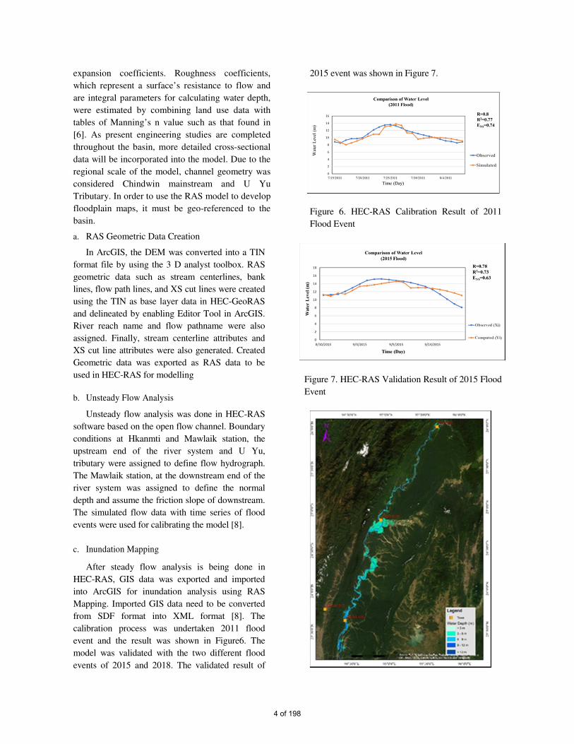
2015 event was shown in Figure 7.

Figure 6. HEC-RAS Calibration Result of 2011

Flood Event

Figure 7. HEC-RAS Validation Result of 2015 Flood

Event

4 of 198

Simulated by

HEC-RAS Model

Estimate by

Satellite Image

Ober-lapped

Area

Over Estimated

by model

Under Estimated

by model

Percentage (%)

(2011)71.6 24.9 3.5

Inundation Area (km2)

(2015)

Percentage (%) (2015)

Inundation Area (km2)

(2018)

Percentage (%)

(2018)76.8 21.2 2

75 22.8 2.2

1097 892.7 842.3 232.8 21.9

57.3

1701 1380.4 1275 388.6 37.4

1613.7 1393.2 1155.2 401.3Inundation Area (km

2)

(2011)

Figure 8. Simulated flood inundation depth and

area for the 2011 flood event

Table2. Comparison of Flood Inundation Area of

Simulated Result and Satellite Images

VI. RESULT AND DISSCUSSION

The HEC-HMS model was calibrated for

different flood events approach in order to determine

the best fit between the model and observation. The

model couldn't simulate well continuous flow of a

one-year period for the Chindwin river catchment.

HEC-HMS has an optimization feature that can be

used to match the simulated flow with observed flow.

The optimization feature was used to carry out the

calibration process. Once the calibration was

completed with two selected flood events, then the

calibrated final parameters were taken as input in the

selected two storms flood events of (2015 and 2018)

for the model validation.

The validated result of 2015 flood event is shown

in Figure 4. The coefficient of determination (R2) and

Nash Sutcliffe efficiency (ENS) and coefficient of

correlation (R) values are obtained as 0.794, 0.89 and

0.403 respectively for the 2015 flood event. The

coefficient of determination (R2) and Nash Sutcliffe

efficiency (ENS) and coefficient of correlation (R)

values are obtained as 0.6, 0.76 and 0.51 respectively

for the 2018 flood event. These results are close and

good correlation between the observed and

simulated flow.

In HEC-RAS model, the simulated flood

inundation maps for the 2011 flood event was

validated by comparing the actual flood area derived

by ALOS PALSAR images. Validation of results for

2015 and 2018 flood events were undertaken by

comparing the model output with sentineal-1 image.

Simulated flood inundation depth and area for

2011and 2015 flood events are shown in Figures 8

and 9.

Figure 9. Simulated flood inundation depth and area

for the 2015 flood event

Table3. Flood Inundation area with classified water

depths in various return periods

Comparison of the predicted flood inundation

area for 2011, 2015 and 2018 events are shown in

Table 2.

For the inundation map of 100year flood

frequency, the maximum depth of flood is extended

to low terrain land and flood plain areas, especially in

Homalin and some villages of Mawlaik Township.

According to the result, the most flooded in 100 years

return period is expended to the area of mid-stream

Water

Depth

(m)

2 Year Flood 10 Year Flood 50 Year Flood 100 Year

Flood

Area

(km2) %

Area

(km2) %

Area

(km2) %

Area

(km2) %

< 3 m 585.2 33.2 626.1 33.0 650.2 30.6 728.7 28.8

3 - 6 m 650.7 36.9 698.6 36.8 672.5 31.7 822.3 32.5

6 - 9 m 261.0 14.8 298.2 15.7 405.2 19.2 446.1 17.6

9 - 12 m 86.2 4.9 89.5 4.7 128.0 6.0 153.2 6.0

> 12 m 176.6 10.0 183.5 9.6 263.9 12.4 375.2 14.8

Total 1760 100 1896 100 2120 100 2526 100

5 of 198

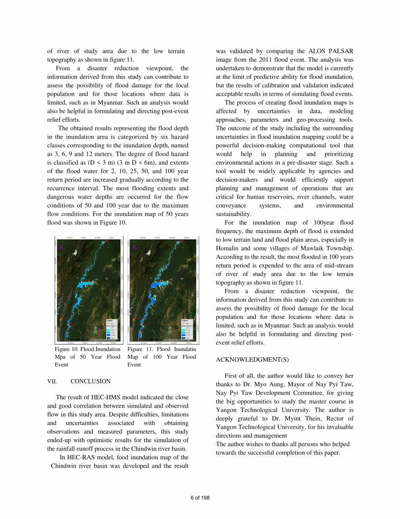
of river of study area due to the low terrain

topography as shown in figure 11.

From a disaster reduction viewpoint, the

information derived from this study can contribute to

assess the possibility of flood damage for the local

population and for those locations where data is

limited, such as in Myanmar. Such an analysis would

also be helpful in formulating and directing post-event

relief efforts.

The obtained results representing the flood depth

in the inundation area is categorized by six hazard

classes corresponding to the inundation depth, named

as 3, 6, 9 and 12 meters. The degree of flood hazard

is classified as (D < 3 m) (3 m D < 6m), and extents

of the flood water for 2, 10, 25, 50, and 100 year

return period are increased gradually according to the

recurrence interval. The most flooding extents and

dangerous water depths are occurred for the flow

conditions of 50 and 100 year due to the maximum

flow conditions. For the inundation map of 50 years

flood was shown in Figure 10.

VII. CONCLUSION

The result of HEC-HMS model indicated the close

and good correlation between simulated and observed

flow in this study area. Despite difficulties, limitations

and uncertainties associated with obtaining

observations and measured parameters, this study

ended-up with optimistic results for the simulation of

the rainfall-runoff process in the Chindwin river basin.

In HEC-RAS model, food inundation map of the

Chindwin river basin was developed and the result

was validated by comparing the ALOS PALSAR

image from the 2011 flood event. The analysis was

undertaken to demonstrate that the model is currently

at the limit of predictive ability for flood inundation,

but the results of calibration and validation indicated

acceptable results in terms of simulating flood events.

The process of creating flood inundation maps is

affected by uncertainties in data, modeling

approaches, parameters and geo-processing tools.

The outcome of the study including the surrounding

uncertainties in flood inundation mapping could be a

powerful decision-making computational tool that

would help in planning and prioritizing

environmental actions in a pre-disaster stage. Such a

tool would be widely applicable by agencies and

decision-makers and would efficiently support

planning and management of operations that are

critical for human reservoirs, river channels, water

conveyance systems, and environmental

sustainability.

For the inundation map of 100year flood

frequency, the maximum depth of flood is extended

to low terrain land and flood plain areas, especially in

Homalin and some villages of Mawlaik Township.

According to the result, the most flooded in 100 years

return period is expended to the area of mid-stream

of river of study area due to the low terrain

topography as shown in figure 11.

From a disaster reduction viewpoint, the

information derived from this study can contribute to

assess the possibility of flood damage for the local

population and for those locations where data is

limited, such as in Myanmar. Such an analysis would

also be helpful in formulating and directing post-

event relief efforts.

ACKNOWLEDGMENT(S)

First of all, the author would like to convey her

thanks to Dr. Myo Aung, Mayor of Nay Pyi Taw,

Nay Pyi Taw Development Committee, for giving

the big opportunities to study the master course in

Yangon Technological University. The author is

deeply grateful to Dr. Myint Thein, Rector of

Yangon Technological University, for his invaluable

directions and management

The author wishes to thanks all persons who helped

towards the successful completion of this paper.

Figure 10. Flood Inundation

Mpa of 50 Year Flood

Event

Figure 11. Flood Inundatin

Map of 100 Year Flood

Event

6 of 198

REFERENCES [1] Thet Hnin Aye, “Development of Flood

Inundation Map for the Bago River Basin”,

International Journal of Innovative Research in

Multidisciplinary Field, Jan 2017, Volume 3,

Issue 1, ISSN 2455-0620.

[2] Department of Meteorology and Hydrology. 2004.

"Meteorological and Hydrological Data

Agricultural Atlas of the Union of Myanmar".

Department of Meteorology and Hydrolog, Food

and Agriculture Organization of the United

Nations.

[3] Zin, W. W. (2015). "River Flood Inundation

Mapping in the Bago River Basin, Myanmar."

Hydrological Research Letter 9 (4), 97-102

(2015). DOI:10.3178/hrl.9.

[4] Yusop, Z., Chan, C. & Katimon, A., 2007. Runoff

characteristics and application of HEC-HMS for

modelling stormflow hydrograph in an oil palm

catchment. Water Science and Technology, 56,

41-48.

[5] Chen, Y., Xu, Y. & Yin, Y.,2009. Impacts of land

use change scenarios on storm-runoff generation

in Xitiaoxi basin, China. Quaternary International,

208, 121-128.

[6] Horritt MS, Bates PD.2002.Evaluation of 1D and

2D numerical models for predicting river flood

inundation, Journal of Hydrology 268 (1-4), 87-89

[7] HEC,2002. River Analysis System: Hydraulic

Reference Manual.US Army crops of engineers

Hydrologic Engineering Center, Davis, CA.

[8] PANAGOULIA, D., MAMASSIS, N. and

GKIOKAS, A., 2013. Deciphering the Floodplain

Inundation Maps in Greece. In 8th International

Conference Water Resource s Management in an

Interdisciplinary and Changing Context, Porto,

Portugal, European Water Resources Association.

7 of 198

Effect of Lime Content and Curing Condition on Strength Development of Lime-

Stabilized Soil in Bogalay Township, Ayeyarwaddy Region

AUNG AUNG SOE*1

, Y. YAMADA2, N. NAKAJIMA

3 and PHYU PHYU

4

1 PhD, Engineering Secretary, FUKKEN Co., Ltd. (Yangon Branch)

2 PhD, General Manager, FUKKEN Co., Ltd. (Yangon Branch) 3 Chief Engineer, Twister Sector, Civil Engineering Department, JDC Corporation

4 Deputy Director, R & D Section, Department of Highways, Ministry of Construction

*Corresponding author – AUNG AUNG SOE, [email protected]

Abstract - Slaked lime was used to stabilize the

cohesive soil, found in Bogalay Township to upgrade

the rural road construction technique in Ayeyarwaddy

Region, Myanmar. To achieve the stabilization

purpose, this cohesive soil is mixed with slaked lime

in different proportions, followed by different curing

periods. The unconfined compression tests were

conducted to investigate the strength characteristics of

lime-stabilized clay soil, with respect to the lime

content and the curing periods. From the test results,

the strength of the lime-stabilized soil increases with

the increase in lime content and curing period.

However, the curing condition has the significant

influence on the strength development of the lime-

stabilized soil.

Keywords - Lime stabilization, cohesive soil and

unconfined compressive strength.

I. INTRODUCTION

Ayeyarwaddy is one of the regions where play an

important role for the development of Myanmar. To

promote the development in this region, road

networks are of importance. Originally, the region is

covered by the alluvial deposit, which is soft cohesive

soil containing clay minerals. For the road

construction, this clay soil is not suitable as a

foundation subgrade layer. One optimal solution is to

improve the strength of cohesive soil by means of

lime stabilization. According to National Lime

Association [1], the effect of lime on soil can be

generally categorized as (1) soil drying: a rapid

decrease in soil moisture content due to chemical

reaction between water and quicklime, (2) soil

modification: modification of soil properties such as

plasticity, density, compactability, etc., and (3) soil

stabilization: production of long-term strength and the

permanent reduction in shrinking, swelling, and soil

plasticity. Regarding lime-soil mixture, a variety of

proportioning procedures have evolved from various

agencies, often reflecting local conditions and

experience [2]. Therefore, due to the heterogeneous

nature of soil, it needs to examine the local cohesive

soil in Ayeyarwaddy Region and its reacting

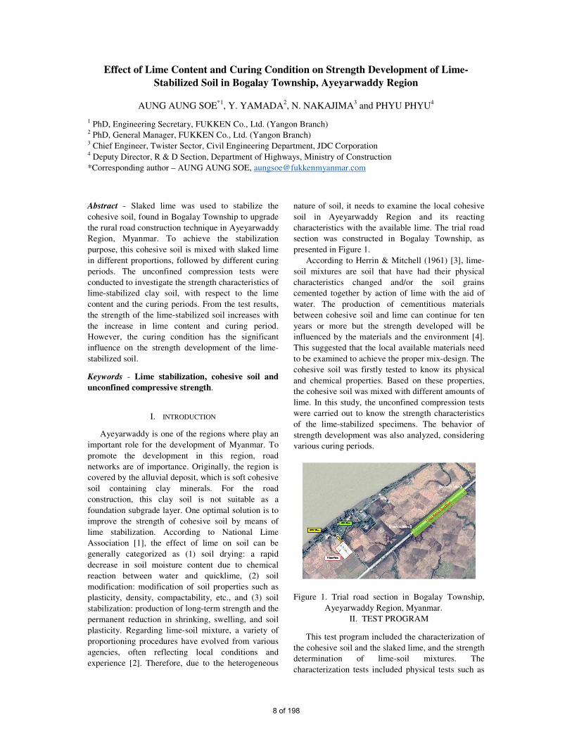
characteristics with the available lime. The trial road

section was constructed in Bogalay Township, as

presented in Figure 1.

According to Herrin & Mitchell (1961) [3], lime-

soil mixtures are soil that have had their physical

characteristics changed and/or the soil grains

cemented together by action of lime with the aid of

water. The production of cementitious materials

between cohesive soil and lime can continue for ten

years or more but the strength developed will be

influenced by the materials and the environment [4].

This suggested that the local available materials need

to be examined to achieve the proper mix-design. The

cohesive soil was firstly tested to know its physical

and chemical properties. Based on these properties,

the cohesive soil was mixed with different amounts of

lime. In this study, the unconfined compression tests

were carried out to know the strength characteristics

of the lime-stabilized specimens. The behavior of

strength development was also analyzed, considering

various curing periods.

Figure 1. Trial road section in Bogalay Township,

Ayeyarwaddy Region, Myanmar.

II. TEST PROGRAM

This test program included the characterization of

the cohesive soil and the slaked lime, and the strength

determination of lime-soil mixtures. The

characterization tests included physical tests such as

8 of 198

moisture content, Atterberg’s Limit, Grain Size

Analysis, Specific Gravity, Sulfate Content, pH and

Lime Demand. Based on the index properties of

cohesive soil, the slaked lime was added by weight

percentages of 3%, 5%, 7%, 9% and 11%. For the

strength determination, the unconfined compression

tests were carried out after the curing periods of 7

days, 14 days, 21 days, and 28 days. The variation in

the unconfined strength of lime-stabilized soil is

analyzed with respect to the lime content and curing

period.

III. MATERIALS

III-A. Cohesive Soil

The local cohesive soil was taken from the site in

Bogalay Township, where a rural road will be

constructed on the soft clay deposit. Laboratory tests

were conducted to examine the index properties of

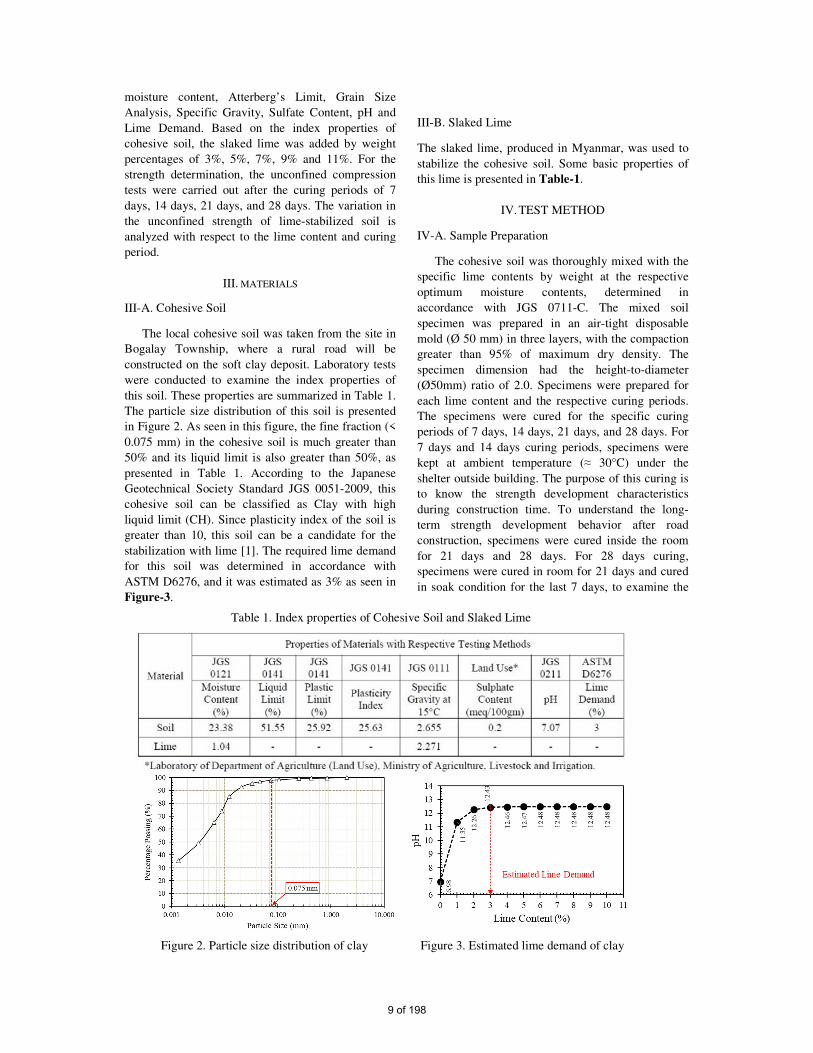
this soil. These properties are summarized in Table 1.

The particle size distribution of this soil is presented

in Figure 2. As seen in this figure, the fine fraction (<

0.075 mm) in the cohesive soil is much greater than

50% and its liquid limit is also greater than 50%, as

presented in Table 1. According to the Japanese

Geotechnical Society Standard JGS 0051-2009, this

cohesive soil can be classified as Clay with high

liquid limit (CH). Since plasticity index of the soil is

greater than 10, this soil can be a candidate for the

stabilization with lime [1]. The required lime demand

for this soil was determined in accordance with

ASTM D6276, and it was estimated as 3% as seen in

Figure-3.

III-B. Slaked Lime

The slaked lime, produced in Myanmar, was used to

stabilize the cohesive soil. Some basic properties of

this lime is presented in Table-1.

IV. TEST METHOD

IV-A. Sample Preparation

The cohesive soil was thoroughly mixed with the

specific lime contents by weight at the respective

optimum moisture contents, determined in

accordance with JGS 0711-C. The mixed soil

specimen was prepared in an air-tight disposable

mold (Ø 50 mm) in three layers, with the compaction

greater than 95% of maximum dry density. The

specimen dimension had the height-to-diameter

(Ø50mm) ratio of 2.0. Specimens were prepared for

each lime content and the respective curing periods.

The specimens were cured for the specific curing

periods of 7 days, 14 days, 21 days, and 28 days. For

7 days and 14 days curing periods, specimens were

kept at ambient temperature (≈ 30°C) under the

shelter outside building. The purpose of this curing is

to know the strength development characteristics

during construction time. To understand the long-

term strength development behavior after road

construction, specimens were cured inside the room

for 21 days and 28 days. For 28 days curing,

specimens were cured in room for 21 days and cured

in soak condition for the last 7 days, to examine the

Figure 2. Particle size distribution of clay Figure 3. Estimated lime demand of clay

Table 1. Index properties of Cohesive Soil and Slaked Lime

9 of 198

long-term strength behavior in severe weather

condition.

IV-B. Testing Instrument and Test Procedure

To conduct the unconfined compression test,

Humboldt Master Loader HM-5030 (50 kN Capacity)

was used for loading. The deformation of the

specimen was recorded by a displacement transducer.

The cured specimen was firstly placed on the

pedestal, followed by adjusting the loading arm to

keep just in contact with specimen. The unconfined

compression test was then carried out in accordance

with the test procedure, described in ASTM D2166

standard. Once the specimen was ready to be tested,

the loading was gradually increased in the strain

controlled manner (1%/min) until the recorded load

decreased with increasing strain or the strain reached

15%. The variations of load and deformation were

recorded by the Humboldt mini-logger (HM-2325A).

The schematic view of the unconfined compression

test is illustrated in Figure 4.

V. TEST RESULTS AND DISCUSSION

V-A. Effect of Lime Content on Unconfined

Compressive Strength

The variation in strength behavior of the lime-

stabilized soil was analyzed with respect to the added

lime contents. For the analysis of the short-term and

the long-term strength development, the effect of lime

content was examined for curing periods of 7 days

and 28 days. The variations of stress-strain curve are

presented in Figure 5 and Figure 6. The repeated

curves show a good agreement with their respective

curves, implying the reproducibility of the test

specimens.

As seen in Figure 5, the stresses abruptly

increased within 0.5% to 0.7% strains, with

increasing strains. The peak strength generally

increased with the lime content, greater than

minimum lime demand (3%). The similar

characteristics can be observed in Figure 6. In both

curing cases, the curves of 11% lime content show

insignificant increase in strength, compared to 9%

lime content. This suggested that the upper limit of

lime content might be 9% for the given cohesive soil.

It is noticed that the curves of the larger lime content

cases rapidly decrease after they had reached peak

stresses. In case of high lime content, the amount of

coarser particles might have been created due to

flocculation, agglomeration and solidification

processes. This would increase the resistance to the

shearing. After it had reached to the peak, the

interlocking between the coarser particles might have

been reduced, forming shearing plane with low

cohesion. According to Overseas Road Note 31 [4],

the stabilized material will generally be non-plastic or

only slightly plastic if the amount of lime added

exceeds the initial consumption of lime. Here, this

consumption was 3%.

Figure 4. Schematic view of UCT

0

200

400

600

800

1000

0.0 0.5 1.0 1.5 2.0 2.5

Com

pre

ssiv

e S

tres

s (k

Pa)

Strain (%)

3% 5% 7% 7%-R 9% 11%

7-Day Curing

Figure 5. Stress-strain curves (7-day curing)

10 of 198

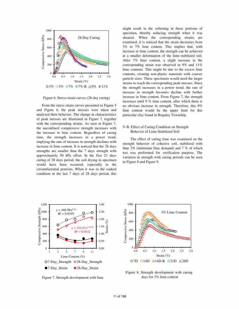
Figure 6. Stress-strain curves (28-day curing)

From the stress-strain curves presented in Figure 5

and Figure 6, the peak stresses were taken and

analyzed their behavior. The change in characteristics

of peak stresses are illustrated in Figure 7, together

with the corresponding strains. As seen in Figure 7,

the unconfined compressive strength increases with

the increase in lime content. Regardless of curing

time, the strength increases in a power trend,

implying the rate of increase in strength declines with

increase in lime content. It is noticed that the 28 days

strengths are smaller than the 7 days strength with

approximately 50 kPa offset. In the first 21 days

curing of 28 days period, the soil drying in specimen

would have been occurred, especially in the

circumferential portions. When it was in the soaked

condition in the last 7 days of 28 days period, this

might result in the softening in these portions of

specimen, thereby reducing strength when it was

sheared. When the corresponding strains are

examined, it is noticed that the strain decreases from

3% to 7% lime content. This implies that, with

increase in lime content, the strength can be achieved

at a smaller deformation of the lime-stabilized soil.

After 7% lime content, a slight increase in the

corresponding strain was observed in 9% and 11%

lime contents. This might be due to the excess lime

contents, creating non-plastic materials with coarser

particle sizes. These specimens would need the larger

strains to reach the corresponding peak stresses. Since

the strength increases in a power trend, the rate of

increase in strength becomes decline with further

increase in lime content. From Figure 7, the strength

increases until 9 % lime content, after which there is

no obvious increase in strength. Therefore, this 9%

lime content would be the upper limit for this

particular clay found in Bogalay Township.

V-B. Effect of Curing Condition on Strength

Behavior of Lime-Stabilized Soil

The effect of curing time was examined on the

strength behavior of cohesive soil, stabilized with

lime 3% (minimum lime demand) and 7 % of which

test was performed for verification purpose. The

variation in strength with curing periods can be seen

in Figure 8 and Figure 9.

0

200

400

600

800

1000

0.0 0.5 1.0 1.5 2.0 2.5 3.0

Com

pre

ssiv

e S

tres

s (k

Pa)

Strain (%)

3% 5% 7% 7%-R 9% 11%

28-Day Curing

Figure 7. Strength development with lime

y = 446.98x0.33

R² = 0.9395

y = 324.61x0.4092

R² = 0.9432

0.00

0.50

1.00

1.50

2.00

2.50

3.00

0

200

400

600

800

1000

1200

1 3 5 7 9 11

Str

ain (

%)

Co

mp

ress

ive

Str

ength

(kP

a)

Lime Content (%)

7-Day_Strength 28-Day_Strength

7-Day_Strain 28-Day_Strain

0

200

400

600

800

1000

0.0 0.5 1.0 1.5 2.0 2.5 3.0

Co

mp

ress

ive

Str

ess

(kP

a)

Strain (%)

7D 14D 14D-R 21D 28D

3% Lime Content

Figure 8. Strength development with curing

days for 3% lime content

11 of 198

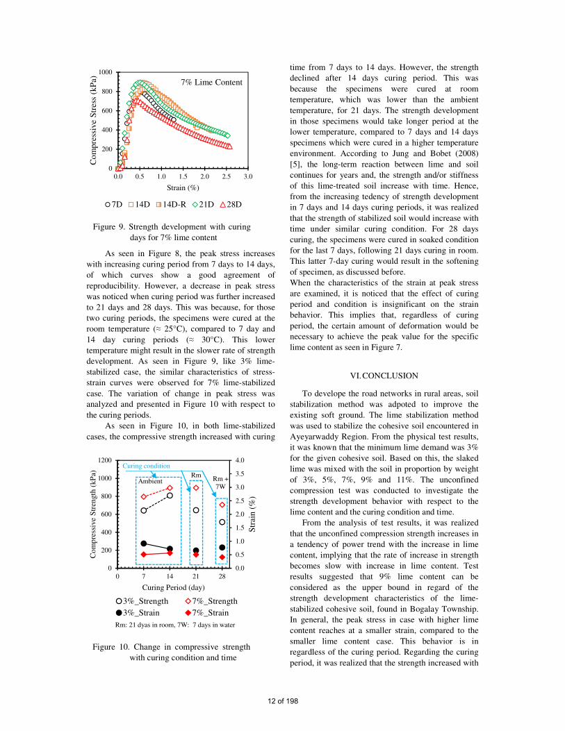
As seen in Figure 8, the peak stress increases

with increasing curing period from 7 days to 14 days,

of which curves show a good agreement of

reproducibility. However, a decrease in peak stress

was noticed when curing period was further increased

to 21 days and 28 days. This was because, for those

two curing periods, the specimens were cured at the

room temperature (≈ 25°C), compared to 7 day and

14 day curing periods (≈ 30°C). This lower

temperature might result in the slower rate of strength

development. As seen in Figure 9, like 3% lime-

stabilized case, the similar characteristics of stress-

strain curves were observed for 7% lime-stabilized

case. The variation of change in peak stress was

analyzed and presented in Figure 10 with respect to

the curing periods.

As seen in Figure 10, in both lime-stabilized

cases, the compressive strength increased with curing

time from 7 days to 14 days. However, the strength

declined after 14 days curing period. This was

because the specimens were cured at room

temperature, which was lower than the ambient

temperature, for 21 days. The strength development

in those specimens would take longer period at the

lower temperature, compared to 7 days and 14 days

specimens which were cured in a higher temperature

environment. According to Jung and Bobet (2008)

[5], the long-term reaction between lime and soil

continues for years and, the strength and/or stiffness

of this lime-treated soil increase with time. Hence,

from the increasing tedency of strength development

in 7 days and 14 days curing periods, it was realized

that the strength of stabilized soil would increase with

time under similar curing condition. For 28 days

curing, the specimens were cured in soaked condition

for the last 7 days, following 21 days curing in room.

This latter 7-day curing would result in the softening

of specimen, as discussed before.

When the characteristics of the strain at peak stress

are examined, it is noticed that the effect of curing

period and condition is insignificant on the strain

behavior. This implies that, regardless of curing

period, the certain amount of deformation would be

necessary to achieve the peak value for the specific

lime content as seen in Figure 7.

VI. CONCLUSION

To develope the road networks in rural areas, soil

stabilization method was adpoted to improve the

existing soft ground. The lime stabilization method

was used to stabilize the cohesive soil encountered in

Ayeyarwaddy Region. From the physical test results,

it was known that the minimum lime demand was 3%

for the given cohesive soil. Based on this, the slaked

lime was mixed with the soil in proportion by weight

of 3%, 5%, 7%, 9% and 11%. The unconfined

compression test was conducted to investigate the

strength development behavior with respect to the

lime content and the curing condition and time.

From the analysis of test results, it was realized

that the unconfined compression strength increases in

a tendency of power trend with the increase in lime

content, implying that the rate of increase in strength

becomes slow with increase in lime content. Test

results suggested that 9% lime content can be

considered as the upper bound in regard of the

strength development characteristics of the lime-

stabilized cohesive soil, found in Bogalay Township.

In general, the peak stress in case with higher lime

content reaches at a smaller strain, compared to the

smaller lime content case. This behavior is in

regardless of the curing period. Regarding the curing

period, it was realized that the strength increased with

Figure 9. Strength development with curing

days for 7% lime content

0

200

400

600

800

1000

0.0 0.5 1.0 1.5 2.0 2.5 3.0

Co

mp

ress

ive

Str

ess

(kP

a)

Strain (%)

7D 14D 14D-R 21D 28D

7% Lime Content

Figure 10. Change in compressive strength

with curing condition and time

0.0

0.5

1.0

1.5

2.0

2.5

3.0

3.5

4.0

0

200

400

600

800

1000

1200

0 7 14 21 28

Str

ain (

%)

Co

mp

ress

ive

Str

ength

(kP

a)

Curing Period (day)

3%_Strength 7%_Strength

3%_Strain 7%_Strain

AmbientRm

Rm +

7W

Curing condition

Rm: 21 dyas in room, 7W: 7 days in water

12 of 198

the increase in curing period. However, the condition

of curing has significant influence on the strength

development behavior. It is recommended to

investigate this behavior more in detail as a further

study.

ACKNOWLEDGEMENTS

This study was conducted at the Soil Laboratory

of FUKKEN Co., Ltd. with the supports of JDC

Corporation. This work is a part of the program

conducted under the Collaboration Program with

JICA and MOC. Authors would like to express their

sincere thanks and acknowledge the concerned parties

and individuals for their continuous supports and

help.

REFERENCES

[1] NLA, "Mixture design and testing procedures for

lime stabilized soil," Technical brief, pp. 1-6,

October 2006.

[2] TRB, "State of the Art Report 5 - Lime

Stabilization," Transportation Research Board,

1987.

[3] M. Herrin and H. Mitchell, "Lime-soil

mixtures," in 40th Annual Meeting of the

Highway Research Board, Washington DC,

1961.

[4] TRL, "Overseas road note 31: A guide to the

structural design of bitumen-surfaced roads in

tropical and sub-tropical countries," Overseas

Center, Transport Research Laboratory,

Crowthorne, Berkshire, United Kingdom, 1993.

[5] C. Jung and A. Bobet, "Post-construction

evaluation of lime-treated soils,"

FHWA/IN/JTRP-2007/25, Indianapolis, IN

46204, 2008.

[6] JGS 0141, "Test method for liquid limit and

plastic limit of soils," in Laboratory testing

standards of geomaterials (Vol. 1), Japanese

Geotechnical Society, 2009.

[7] JGS 0111, "Test method for density of soil

particles," in Laboratory testing standards of

geomaterials (Vol.1), Japanese Geotechnical

Society, 2009.

[8] JGS 0211, "Test method for ph of suspended

soils," in Laboratory testing standards of

geomaterials (Vol.3), Japanese Geotechnical

Society, 2009.

[9] JGS 0121, "Test method for water content of

soils," in Laboratory Testing Standards of

Geomaterials (Vol.1), Japanese Geotechnical

Society, 2009.

[10] JGS 0051, "Method of classification of

geomaterials for engineering purposes," in

Laboratory testing standards of geomaterials

(Vol.1), Japanese Geotechnical Society, 2009.

[11] JGS 0711, "Test method for soil compaction

using a rammer," in Laboratory testing

standards of geomaterials (Vol.1), Japanese

Geotechnical Society, 2009.

[12] ASTM D6276, "Standard test method for using

pH to estimate the soil-lime proportion

requirement for soil stabilization," American

Society for testing and materials, 2006.

[13] ASTM D2166, "Standard test method for

unconfined compressive strength of cohesive

soil," American society for testing and materials,

2006.

13 of 198

Investigation on Performance Level of 10-storey R.C Building with Pushover

Analysis Tin Tin Wai

1, Win Zaw

2, Ohnmar Khaing

3

1Master Candidate, Department of Civil Engineering, Technologic University (Taunggyi)

Taunggyi, Myanmar 2Professor, Department of Civil Engineering, Technologic University (Taunggyi)

Taunggyi, Myanmar 3Lecturer, Department of Civil Engineering, Technologic University (Mandalay)

Mandalay, Myanmar

[email protected],[email protected],[email protected]

ABSTRACT

This paper presents investigation on seismic

performance of a 10-storeyed R.C building in

Taunggyi region, southern Shan State. The main

objective of this paper is to investigate their seismic

performance levels, damage probabilities of proposed

buildings under strong earthquake shaking. Taunggyi

is located in MNBC Seismic Zone-4 and R.C type

residential buildings are the most popular types. Its

height is 110ft above ground level. The total length

and width are 84ft and 54ft respectively. Basic wind

speed 80 mph is used. This structure is composed of

special moment resisting frame. Dead loads and live

loads are used according to ACI code. The load

combinations required for the whole structure is used

according to UBC-97. This paper is an approach to

do nonlinear static analysis in simplify and effective

manner. This method determines the base shear

capacity of the building and performance levels of

each part of building under varying intensity of

seismic force. The results of effects of different plan

on seismic response of buildings have been presented

in terms of displacement, base shear and plastic hinge

pattern. The performance of the buildings is then

assessed with the ATC 40 and FEMA 356 building

acceptance criteria. From pushover analysis, the

capacity curves for each building in two directions of

the earthquake are obtained. The modeling and

analysis is done by ETABS 9.7.1 software. The

displacement control analysis is used and its value is

2% of total structure height. The lateral displacement

of 2.48ft is subjected to roof level .After pushover

analysis has been carried out, capacity spectrum

curve is demonstrated in acceleration-displacement

format. The graphical intersection of the two curves

(capacity spectrum curve and demand curve)

approximates the performance point of the structure.

Based on analysis results, it was needed to strengthen

for resisting up to earthquake shaking.

Keywords:R.C Building, Performance level,

Displacement and base shear, Nonlinear static

(Pushover) analysis and ETABS.

I.INTRODUCTION

Nowadays, Myanmar is still a developing country and

there is a tendency to raise population in future. So, the

high-rise building is the only answer to solve the problem

of population dense. Buildings are commonly designed for

lateral forces due to wind and earthquake. The primary

objective of earthquake resistant design is to prevent

buildings collapse during earthquake. structure must

be safe against collapse and consequences of failure.

So, the proposed building is intended to resist the level of

LS during strong earthquake. Thus the performance based

seismic design is a process that permits design of new

buildings or upgrade of existing buildings with a realistic

understanding of the risk of life, occupancy and economic

loss that may occur as a result of future earthquakes .When

structures are subjected to strong earthquake ground

motion, safety of structures in the inelastic range, structural

stability and nonlinear behaviour have to be carefully

examined. The nonlinear pushover analysis is becoming a

popular tool for seismic performance evaluation of existing

and new structures. . In highly seismic area, it is important

to design the building that will withstand moderate

earthquakes without damage and serve earthquakes

without collapse.

II.BACKGROUND THEORY

Linear

-Structure return to original form

-No change in loading direction or magnitude

-Material properties do not change

-Small deformation and strain

Nonlinear

-Geometry changes resulting in stiffness change

-Material deformation that may not return to original form

-Support changes in loading direction and constraint

location

-Support of nonlinear load curves.

Pushover analysis

-Gravity analysis is force controlled.

14 of 198

-Pushover analysis is a displacement controlled.

-Behavior of structure characterized by capacity

curve(base shear force vs roof displacement)

Nonlinear is subdivided by two classes.

Material Nonlinearity

a. Permanent Deformation

b. Cracking

c. Beam rotation

d. Energy dissipation

Geometric Nonlinearity

a. P-Delta analysis

Methods

-Capacity Spectrum method

-Displacement

-Modal plastic method

Control Case

-Brittle action(load 2ft from roof level)

-Ductile action(displacement 2% of overall height)

Methods of Analysis

Generally for analyzing the structure the following

analysis methods are used depending upon the

requirements.

(1)Linear static procedure

(2)Linear dynamic procedure

(3)Nonlinear static procedure

1.Pushover analysis

2.Capacity spectrum method

(4)Nonlinear dynamic procedure

1.Time history analysis

A pushover analysis to perform non-linear analysis is

considered.

The analysis in ETABS 9.7.1 involves the following

four steps. 1) Modeling, 2) Static analysis, 3) Designing

4)Pushover analysis. Steps used in performing a

pushover analysis of a simple three-dimensional building.

1. Creating the basic computer model (without the

pushover data) in the usual manner.

2. Define properties and acceptance criteria for the

pushover hinges. The program includes several built-in

default hinge properties that are based on average values

from ATC-40 for concrete members and average values

from FEMA-356 for steel members. These built in

properties can be useful for preliminary analyses, but

user defined properties are recommended for final

analyses.

3. Locate the pushover hinges on the model by selecting

one or more frame members and assigning them one or

more hinge properties and hinge locations.

4. Define the pushover load cases. In ETABS 9.7 more

than one pushover load case can be run in the same

analysis. Also a pushover load case can start from the

final conditions of another pushover load case that was

previously run in the same analysis.

Typically a gravity load pushover is force controlled

and lateral pushovers are displacement controlled.

5. Run the basic static analysis and, if desired, dynamic

analysis. Then run the static nonlinear pushover analysis.

6. Display the pushover curve and the table.

7. Review the pushover displaced shape and sequence of

hinge formation on a step-by-step basis.

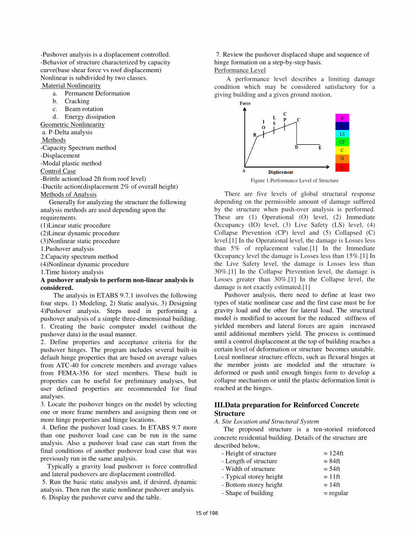
Performance Level

A performance level describes a limiting damage

condition which may be considered satisfactory for a

giving building and a given ground motion.

Figure 1.Performance Level of Structure

There are five levels of global structural response

depending on the permissible amount of damage suffered

by the structure when push-over analysis is performed.

These are (1) Operational (O) level, (2) Immediate

Occupancy (IO) level, (3) Live Safety (LS) level, (4)

Collapse Prevention (CP) level and (5) Collapsed (C)

level.[1] In the Operational level, the damage is Losses less

than 5% of replacement value.[1] In the Immediate

Occupancy level the damage is Losses less than 15%.[1] In

the Live Safety level, the damage is Losses less than

30%.[1] In the Collapse Prevention level, the damage is

Losses greater than 30%.[1] In the Collapse level, the

damage is not exactly estimated.[1]

Pushover analysis, there need to define at least two

types of static nonlinear case and the first case must be for

gravity load and the other for lateral load. The structural

model is modified to account for the reduced stiffness of

yielded members and lateral forces are again increased

until additional members yield. The process is continued

until a control displacement at the top of building reaches a

certain level of deformation or structure becomes unstable.

Local nonlinear structure effects, such as flexural hinges at

the member joints are modeled and the structure is

deformed or push until enough hinges form to develop a

collapse mechanism or until the plastic deformation limit is

reached at the hinges.

III.Data preparation for Reinforced Concrete

Structure A. Site Location and Structural System

The proposed structure is a ten-storied reinforced

concrete residential building. Details of the structure are described below,

- Height of structure = 124ft

- Length of structure = 84ft

- Width of structure = 54ft

- Typical storey height = 11ft

- Bottom storey height = 14ft

- Shape of building = regular

15 of 198

- Location = seismic zone 4

- Type of occupancy = Residential

B. Material Properties

Material properties for structural data are;

- Concrete cylinder strength = 3ksi

- Yield strength of main reinforcement = 50ksi

- Yield strength of shear reinforcement = 50 ksi

- Modulus of elasticity for concrete = 3122 ksi

C. Loading consideration

The applied loads are dead loads, live loads,

earthquake load and wind load. Dead loads consist of the

weight of all materials and fixed equipment incorporated

into the building. Floor finishing, ceiling, partitions are

considered as superimposed dead loads. Loads that are

almost always applied horizontally are called lateral

loads.

For dead load,

- Unit weight of concrete = 150 pcf

- 9" thick brick wall = 100 psf

- 4.5" thick brick wall = 55 psf

- Superimposed dead load = 20psf

For live load,

- Live load on floor = 40 psf

- Live load on stair case = 60 psf

- Live load on roof = 20 psf

-Weight of lift = 2 tons

-Weight of water = 62.4 psf

For earthquake load,

An earthquake level is defined with a probability of

being exceeded in a specified period .The following three

levels are commonly defined for buildings with a design

life of 50 years by ATC 40: Serviceability Earthquake (SE): Ground motion with

a 50 percent chance of being exceeded in a 50- years

Design Earthquake (DE): Ground motion with a 10

percent chance of being exceeded in a 50- years

Maximum Considered Earthquake (MCE): Ground

motion with a 2 percent chance of being exceeded in

a 50-years[3].

Mostly, the seismic hazard levels are determined by

the probabilistic seismic hazard analysis (PSHA).The

calculated results of the seismic hazards for Taunggyi

city are;

- SE =0.22g

- DE =0.46g

- MCE =0.71g

- Soil profile type =SD

- Seismic important factor (I) =1

- Ct value = 0.03

- Seismic source type = A

1. Modeling Aspects of building elements:

Type of proposed building is ten storeyed rectangular

shaped RC building and type of residential which is

located in seismic zone 4. Typical story height and bottom

story height are 11ft and 14ft. Total height of the whole

building is 124ft. X direction length and Y direction length

are 84ft and 54ft respectively. The material properties of

structure are the strength of concrete is 3000 psi and yield

strength of steel is 50000 psi. The plan view, elevation and

3D view of building is shown in figure 2, 3 and

4.Nonlinear plastic hinges are assigned to all of the

primary elements. Default moment hinges (M3) are

assigned to beam elements and default axial moment2-

moment3 hinges (PMM) are assigned to column elements.

The column sizes are defined as 20”x20”, 18”x18’,

16”x16”, 14”x14”, the beams are 12”x14”, 10”x12”,

10”x10” and shear wall is 12” and Stair thickness is 5”.

The design load combinations are used from UBC-

97specification.

Fig-2, TYPICAL FLOOR PLAN

Fig-3, ELEVATION VIEW OF MODEL

16 of 198

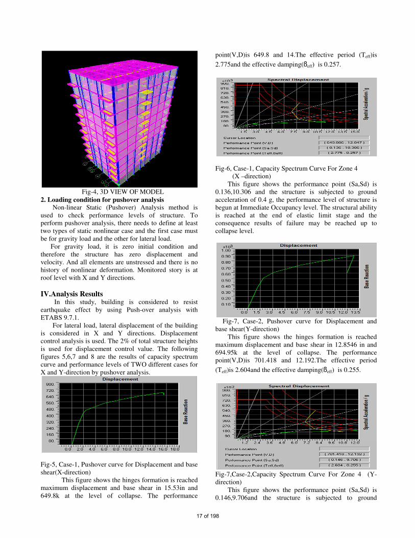
Fig-4, 3D VIEW OF MODEL

2. Loading condition for pushover analysis

Non-linear Static (Pushover) Analysis method is

used to check performance levels of structure. To

perform pushover analysis, there needs to define at least

two types of static nonlinear case and the first case must

be for gravity load and the other for lateral load.

For gravity load, it is zero initial condition and

therefore the structure has zero displacement and

velocity. And all elements are unstressed and there is no

history of nonlinear deformation. Monitored story is at

roof level with X and Y directions.

IV.Analysis Results In this study, building is considered to resist

earthquake effect by using Push-over analysis with

ETABS 9.7.1.

For lateral load, lateral displacement of the building

is considered in X and Y directions. Displacement

control analysis is used. The 2% of total structure heights

is used for displacement control value. The following

figures 5,6,7 and 8 are the results of capacity spectrum

curve and performance levels of TWO different cases for

X and Y-direction by pushover analysis.

Fig-5, Case-1, Pushover curve for Displacement and base

shear(X-direction)

This figure shows the hinges formation is reached

maximum displacement and base shear in 15.53in and

649.8k at the level of collapse. The performance

point(V,D)is 649.8 and 14.The effective period (Teff)is

2.775and the effective damping(ßeff) is 0.257.

Fig-6, Case-1, Capacity Spectrum Curve For Zone 4

(X –direction)

This figure shows the performance point (Sa,Sd) is

0.136,10.306 and the structure is subjected to ground

acceleration of 0.4 g, the performance level of structure is

begun at Immediate Occupancy level. The structural ability

is reached at the end of elastic limit stage and the

consequence results of failure may be reached up to

collapse level.

Fig-7, Case-2, Pushover curve for Displacement and

base shear(Y-direction)

This figure shows the hinges formation is reached

maximum displacement and base shear in 12.8546 in and

694.95k at the level of collapse. The performance

point(V,D)is 701.418 and 12.192.The effective period

(Teff)is 2.604and the effective damping(ßeff) is 0.255.

Fig-7,Case-2,Capacity Spectrum Curve For Zone 4 (Y-

direction)

This figure shows the performance point (Sa,Sd) is

0.146,9.706and the structure is subjected to ground

17 of 198

acceleration of 0.4 g, the performance level of structure is

begun at Immediate Occupancy level. The structural

ability is reached at the end of elastic limit stage and the

consequence results of failure may be reached up to

collapse level.

V. DISCUSSIONS AND CONCLUSIONS

In this paper, the proposed building is ten-

storeyed rectangular shaped RC building and it is located

in seismic zone 4. The design codes used in this paper are

the UBC-97 and ACI 318-05. Structural analysis and

design is done by using ETABS software.

By the studying of plastic hinge mechanism of the

structure, the structural performance levels and the first

failed parts of the structure can be known. Total hinges

formation of 3868 occurs in each case. The comparison

of case 1 and case 2 are as follows:

In case1, when the displacement reaches at

15.2574 in, the structure reaches at collapse

prevention stage.

In case 2, when the displacement reaches at

12.8546 in, the structure reaches at collapse

prevention stage.

To compare this stage, the structural capacity of

Y-direction is less than in X-direction.

Both case 1 and 2,more plastic hinges are found

in beam than column face.

Moreover, according to figures the effective period

(Teff)and the effective damping(ßeff) are in Case 1 is more

than Case 2.This mean that Case 1 is safer than Case

2.S0,The weak points of structural elements in the

building can be determined and The weak-beam &

strong- column concept can be maintained. So, it can be

concluded that the structure can resist high seismic force

even in high seismic zone-4 according to the above

results.

ACKNOWLEDGMENT

The author wishes to express her deep gratitude

to his Excellency, Minister Dr.Myo Thein Gyi, Ministry

of Education. The author is very grateful thanks to

Dr.San San Yee, Rector of Technological University

(Taunggyi), for her permission. The author would like to

express deeply thanks to Dr.Win Zaw, Professor and

Head, Department of Civil Engineering, Technological

University (Taunggyi), for his guidance. The author is

highly grateful to her co-supervisor, Daw Ohnmar

Khaing, Lecturer, Department of Civil Engineering,

Technological University(Taunggyi), for her keen

interest, necessary advice, careful guidance and kindness.

The author is very grateful thanks to all her teachers,

Department of Civil Engineering, Technological

University (Taunggyi), for helpful suggestions and

necessary advices. Moreover, the author expresses the

greatest thanks to her parents and friends for their support

and encouragement. Finally, the author is very thankful

to all teachers who taught her everything since her

childhood.

REFERENCES

[1] ATC 40-“Seismic Evaluation and Retrofit of Concrete

Buildings”,Applied Technology Council, November

1996.

[2] Chopra AK. Dynamics of Structures: theory and

applications to earthquake engineering. Englewood

Cliffs, NJ; 1995.

[3] Federal Emergency Management Agency, FEMA-356,

“Prestandard and Commentary for Seismic

Rehabilitation of Buildings”, Washington, DC, 2000.

[4] ETABS User’s Manual, “Integrated Building Design

Software”,Computer and Structures Inc. Berkeley,

USA.

[5] IS 1893(Part1):2002, Criteria for earthquake resistant

design of structures.

[6] MNBC , Myanmar National Building Code(2016) Part

3 “Structural Design.”

[7] Uniform Building Code(UBC),Vol-1and 2,1997

edition, Published by International Concrete of

Building Officials.

18 of 198

Project Management and Construction Method for Different

Types of Bridge in Various Locations of Myanmar.

(From Naung Moon to Kawthaung)

Kyaw Myo Htun

Department of Bridge, Ministry of Construction

Naypyidaw, Myanmar

E-mail - [email protected]

Abstract — This paper illustrates the duties &

responsibilities of Ministry of Construction and

especially describes the construction of bridges in

Myanmar. Department of Bridge implements different

types of bridges which were appropriated to related

location. Due to the topography of Myanmar, northern

part occupies mountains with cold & rainy weather,

central lowlands have mostly flat terrain with hot &

dry and southern coastal area with tropical weather.

This paper presents how to plan and manage for bridge

construction projects in various topography and

weather of Myanmar and how to choose type of bridge

with appropriate foundations and construction method

to achieve successful outcomes.

Keywords: Plan, Project, Construction Method, Types of

Bridge, Topography, Foundation.

I. INTRODUCTION

Ministry of Construction is a focal Ministry for

infrastructure development in the whole country. There are

five departments in MOC , i.e Department of Building,

Department of Highways, Department of Bridge,

Department of Rural Road Development and Department

of Urban and Housing Development. Among the

Departments, Department of Bridge (DOB) implements the

bridge infrastructures in Myanmar by 20 bridge

construction units. Myanmar have many kinds of terrain

such as mountain, hilly, flat and coastal with winter,

summer & rainy seasons. Therefore type of bridges and

construction method of bridges are varies depend on

location of project site. This paper illustrates about the

construction of some bridges which were located in Kachin

State, Mandalay Region and Tanintharyi Region with

mountainous and cold, flat & dry and hilly coastal area

closed to Equator.

II. BRIDGE CONSTRUCTION PROJECT

Fig.1 Location Map of Bridge Projects

There are many bridge infrastructure projects which

are implemented by DOB in Myanmar and among them,

the five projects described in Fig.1 are selected to study

the project management and construction method.

According to the location of that projects, they were

constructed in different topography and weather with

different condition of transportation to access project site.

19 of 198

Fig.2 Flow Chart of Project Sequences

III. PROJECT PLANNING & FEASIBILITY STUDY

1. Htikha Bridge Project

Hitkha bridge is located on Machanbough-Hprukha-

Naung Moon road and constructed crossed the Htikha

creek. The local people across the Htikha creek with

temporary suspension bridge with limited loading

capacity. To reduce the poverty and upgrade the living

standard of local people, the permanent bridge was need to

construct to develop socioeconomic of this region.

1.1 Soil Investigation

Soil from surface to 10ft depth is silt trace clay &

below 10ft depth is sandstone. N value is 44 at depth of

12ft.

1.2 Topography

Htikha creek is located in the valley of mountainous

area, water level is decrease in summer, increase in rainy

season with very rough flow velocity.

1.3 Transportation Condition

Htikha bridge is located in Northern part of Kachin

State near Naung Moon town, the existing road is not all

weathered road and automobile cannot travel in rainy

season. Major Construction materials and equipments were

supplied from Myikyina through Sumprabom-Putao road

by using of two or three crown vehicle. Heavy

construction machines could not be used because of road

and weather condition.

2. Machanbough Bridge Project

Machanbough bridge is existed at starting mile post of

Machanbough-Hprukha-Naung Moon road and acrossed

Malikha river. There was a existing temporary suspension

bridge which could be passed only small vehicle of less

than one ton in weight. The asphalt pavement road form

Putao to Machanbough was ended at Maylikha river and

from river to Naung Moon was not all weathered road at

that time. To developed socioeconomic of people who

lived in upper region of Machanbough, the new bridge was

needed which can carry more capacity than existing one.


Soil from surface to 20ft depth is sand with gravel and

below 20ft are mostly Grey and Yellowish brown sand

trace silt clay. N value is 65 at depth of 25ft.

2.2 Topography

Maylika river where the bridge constructed location is

existed in valley and level of banks are high from low

water level, but water level is flooded and flow velocity is

also high in rainy season.


Machanbough bridge is located near Machanbough

town, logistics condition is similar to Htikha bridge.

3. Pakokku Bridge Project

The Country is divided into east and west major

portion by Ayeyarwaddy river which started from north of

country and ended Ayeyarwaddy Region. The cities in east

bank portion of Ayeyarwaddy were more developed than

that of west bank because of good development of road

infrastructure network. Bagan and Naung Oo are ancient

cities and they are major tour destination of Myanmar and

Pakokku town in a largest city in west bank of

Ayeyarwaddy river which occupied many agricultural

products especially onions, bean and cooking oil. The

cargo vehicles, passenger vehicles and people crossed

Ayeyarwaddy river with Z-Craft before Pakokku bridge

was constructed and it took about 1:30 hours for one way

trip excluding waiting time to aboard. Pakokku bridge was

need to build to develop Pakokku town and also to develop

west bank of Ayeyarwaddy river including Monywa town,

Sagaing Region and Chin State.


There are mostly sand some silt and clay up to 85ft

depth and below 85ft are Grey Sand trace gravel and silt.

N=45 at depth 85ft.

3.2 Topography

Ayeyarwaddy river of bridge constructed area is

located in flat and steady flow in summer and high

currents velocity in rainy season. The island is existed near

Implementation

Stage

Project

Outcomes

Detail

Feasibility

Study

Project

Planning

Stage

Design

Stage

20 of 198

Pakokku bank and temporary sand dunes are formed near

Letpanchaepaw bank in summer.


Pakokku bridge is located in middle partion of

Myanmar and having good road network for transportation

of all materials, equipments and machines.

4. Thamote-Lutlut Bridge Project

Thamote-Lutlut bridge project which crossed Thamote

river near Myeik is ongoing project and it is located on

Dawei-Myeik-Tanintharyi-Kawthaung Road. (D-M-T-K)

Road is No.1 National Highway (NH1) and (D-M-T)

portion is also part of No.112 Asian Highway (AH112).

Along this highway, Thamote-Lutlut bridge is only one

bridge which remained to construct on NH1, also AH112.

Therefore the regional governor proposed the plan to

Union Government to implement Thamote-Lutlut bridge

project in 2017-18 fiscal year. After the approval of Union

Government, the project had been started on 1.8.2017.


Soil from river bed surface to 10ft depth is brownish

grey clayey & sandy silt some gravel and below 10ft are

light grey weathered GRANITE. N=66 at depth 12ft.

4.2 Topography

The bridge is being constructed near the end of

Thamote river which flows to Andaman Sea. Therefore

there are two tidal period by mean of sea water. The flow

is rough in the case of tide water raised.


The bridge is located on NH1 and so there is good road

network for transportation. The coastal marine

transportation can be used for large and heavy construction

machines and equipment.

5. Pulone Tonetone Bridge Project

Pulone Tonetone bridge project is ongoing project and

which is existed on Kawthaung-Pulone Tonetone island

road acrosses the Andaman sea. Kawthaung is

mountainous and narrow spaced border city near Ranong

city of Thailand. Pulone Tonetone island occupies small

beach which is most visited by local people and Thai

people by being passed through over the existing timber

bridge. The island also occupies fisherman village and so,

many sea products are unloading at that Pulone Tonetone

village and then deliver to Kawthaung. Due to the load

limit of timber bridge they carry fishery products from

village and ice and other supporting materials from

Kawthaung by using three wheel motorbike on the bridge.

Due to existing of small beach and hilly terrain, the island

can be developed into recreation area and tour destination

by providing new bridge across the shallow sea between

mainland and island.


Soil from bed level to 30ft depth are clayey silt some

gravel some sand and below 45ft are Quartzose Sandstone

and weathered Granite. N=63 at depth 40ft.

5.2 Topography

The bridge is being constructed in the Andaman Sea

which will be connected Pulone Tonetone island to main

land. The sea is shallow at the bridge project site and

therefore there are no ship and large boat cross the bridge

except small boat. Freeboad of existing timber bridge is

1m.


The bridge is located near NH1 and 4 mile away from

Kawthaung. The access road to project site is in good

condition. The marine transportation can also be provided

for large & heavy construction machines & equipment.

Fig.3 Soil Investigation Data

21 of 198

Fig.4 Soil Investigation Data

IV. DESIGN STAGE

When data were collected, the construction teams and

designer made many discussions and site visits to provide

most suitable conceptual design for projects. They

reviewed about that, which materials could be got in local

area, how to transport construction machines, equipments

and major materials, which type of bridge is suitable for

related project site, what kind of foundation would be

defined and financial condition; etc.

After that, the designer proposed conceptual drawing

with suitable spans arrangement and then the construction

team set the layout at the project site to know that

conceptual design is constructable or not. Designer

provided complete detail design for the projects if

conceptual is constructable and change alternative design

when conceptual is not constructable. When deisngers and

construction teams made final decisions, types of bridges,

kinds of foundation, span length and span arrangement are

designed as table (1).

Table-1 Design of Bridge Projects

Sr

Name of Brdige

Span Type of Bridge

Location Foundation Substructure Superstructure

1

2

3

4

5

Htikha Bridge

Machanbough

Bridge

Pakokku Bridge

Thamote-Lutlut

Bridge

Pulone Tonetone

Bridge

400 ft

(100' x 4)

840 ft

(50 + 70 +

600 + 70 +

50)

4126 m

Motor

Way

6278 m

Rail Way

1287'

2400'

Caisson

4'Ø Spun pipe

Bored Pile

(Cast in situe

pile)

Bored Pile

Bored Pile

R.C.C

R.C.C

R.C.C

R.C.C

R.C.C

Steel Plate Girder

& R.C.C Decking

R.C.C Land Span

and Bailey

Suspension Main

bridge

P.C Girder &

R.C.C Decking

Approach Bridge,

Steel Truss &

R.C.C Decking

Main Bridge

P.C Girder, Steel

Box Girder & R.C

Decking

R.C.C, P.C Girder

& R.C.C Decking

Machanbough-

Hprukha-Naung

Moon Road.

(Naung Moon

Twonship)

Machanbough-

Hprukha-Naung

Moon Road.

(Machanbough

Twonship)

Nyaung Oo-

Pakokku Road

Dawei-Myeik-

Kawthaung Road.

(Myeik Township)

Kawthaung-Pulone

Tonetone Island

Road.

Fig.5 Conceptual Design Drawings

22 of 198

Fig.6 Conceptual Design Drawing

V. IMPLEMENTATION STAGE

Construction method and project management is very

important in implementation stage to achieve successful

outcomes. Therefore project director of each construction

team need to do proper management on time, quality, cost

and safety including project schedule, quality management

system (QMS), cost control, safety measures, resources

(human, material, machines, equipment), logistics, weather

condition and communication; etc. Engineers in

construction sites need to understand Standard Operation

Procedure (SOP) of all kinds of works in implementation

stage.

1. Htikha Bridge Project

Heavy machines and equipments were not available

according to the difficulty of transportation. Therefore

reinforced concrete caisson foundation type was chosen

and provided by manpower by using of water pumps and

concrete mixers only. Project Director carefully managed

to maintain adequate human resources for foundation work

which required to finish before rain fall in that region. 100

ft span steel plate girder type was chose to reduce number

of pier and also no need to use scaffold for girder

installation, it would be installed by launching method

with less machines requirement. Therefore, experienced

engineers and skill workers were required to complete this

project successfully.

Fig.7 Recorded Photo of Htikha Bridge

Fig.8 Recorded Photo of Htikha Bridge

2. Machanbough Bridge Project

This bridge is bailey suspension bridge with steel pipe

pylon. Foundation are 4'Ø spun pipe pile and therefore

would be provided by manpower. Mobile Crane was

required to install pylon of main bridge and bailey girder,

therefore 15 tons mobile crane was delivered from

Myitkyina in dry season through the Myitkyina-

Sumprabom-Putao road. That delivery process took about

45 days to reach Machanbough bridge project site. Project

director carefully managed to reach major construction

material such as cement, M.S rods, bailey parts, main

cable; etc in time. Project can be delayed if supply of

material delayed. To collect or to get local labours was

very difficult in Putao district and so engineers managed to

maintain the adequate labours including skill labours in

work site by being supplying from Myitkyina base camp.

In this type of bridge, installation process of main

cable, suspender and baily girders were complicated to

understand for unexperienced engineer and labours.

Therefore project engineer explained method of statement

or construction method to all participants and made many

discussions to understand how to do without accident.

Safety is very important in installation of suspension

bridge because most workers would be worked on height

places and narrow space.

Fig.9 Recorded Photo of Machanbough Bridge

23 of 198

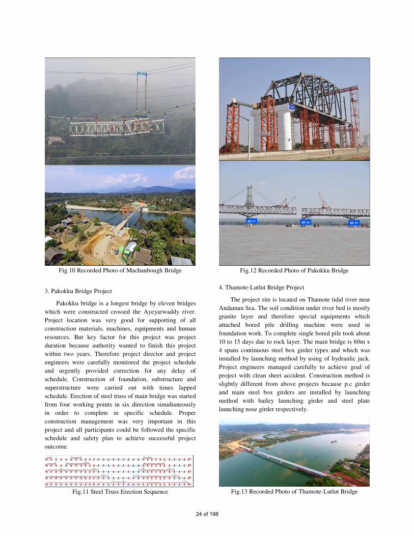
Fig.10 Recorded Photo of Machanbough Bridge

3. Pakokku Bridge Project

Pakokku bridge is a longest bridge by eleven bridges

which were constructed crossed the Ayeyarwaddy river.

Project location was very good for supporting of all

construction materials, machines, equipments and human

resources. But key factor for this project was project

duration because authority wanted to finish this project

within two years. Therefore project director and project

engineers were carefully monitored the project schedule

and urgently provided correction for any delay of

schedule. Construction of foundation, substructure and

superstructure were carried out with times lapped

schedule. Erection of steel truss of main bridge was started

from four working points in six direction simultaneously

in order to complete in specific schedule. Proper

construction management was very important in this

project and all participants could be followed the specific

schedule and safety plan to achieve successful project

outcome.

Fig.11 Steel Truss Erection Sequence

Fig.12 Recorded Photo of Pakokku Bridge

4. Thamote-Lutlut Bridge Project

The project site is located on Thamote tidal river near

Andaman Sea. The soil condition under river bed is mostly

granite layer and therefore special equipments which

attached bored pile drilling machine were used in

foundation work. To complete single bored pile took about

10 to 15 days due to rock layer. The main bridge is 60m x

4 spans continuous steel box girder types and which was

installed by launching method by using of hydraulic jack.

Project engineers managed carefully to achieve goal of

project with clean sheet accident. Construction method is

slightly different from above projects because p.c girder

and main steel box girders are installed by launching

method with bailey launching girder and steel plate

launching nose girder respectively.

Fig.13 Recorded Photo of Thamote-Lutlut Bridge

24 of 198

Fig.14 Recorded Photo of Thamote-Lutlut Bridge

5. Pulone Tonetone Bridge Project

This bridge is bent pile type bridge with two 1.5mØ

bored piles at each pier and 90ft girder 24 spans with 60ft

R.C.C girder 2 spans at each side. In the middle spans of

bridge, P12-P13-P14-P15-P16 Spans are designed innovatively

with view deck and decorative archs for the purpose of

visitors to feel relaxation by seeing open sea view with

fresh breeze across the sea. There is no water in low tide

level and the water depth become 3~4.5m at high tide level

because of flat bed level and shallow portion of sea with

mangrove trees. Construction method of foundation is

different from other bored pile foundation in this bridge,

because the ordinary working barge cannot carry bored

pile machine and other loading without floating in water.

Therefore coastal landing craft which can carry working

bored pile machines on shore was used for foundation

work. After that, prefabricated pre stressed concrete

girders were installed in position by using of modified

steel truss launching girder. Project director and engineers

take care all steps of construction sequence not to deviate

from schedule and quality and not to happen any accident.

Fig.15 Recorded Photo of Pulone Tonetone Bridge

Fig.16 Recorded Photo of Pulone Tonetone Bridge

VI. CONCLUSIONS

By studying the bridge projects at different locations of

Myanmar which were implemented by Department of

Bridge, Myanmar engineers can construct any type of

bridge with any kind of foundation by applying

appropriate construction management knowledge. The

constructors and engineers should consider proper

alternative designs to comply with available resources.

There are different construction methods for various

topography of project location, the engineers should apply

proper method to achieve successful outcomes.

Modernized engineering technology, construction

machines & equipments, safety rules & regulations and

construction management knowledge should be studied

and applied in all engineering societies to become our

bright future Nation.

ACKNOWLEDGEMENT

Author would like to thank Director General U Shwe

Lay for his kind advice to prepare this paper. Special

thanks to U Saw Zarni Hla, U Myint Naing Oo, U Aung

Kyaw Soe and U Wai Phyo for their kind support to

collect required data for bridge projects. Also thanks to

office staff of Bridge Construction (4) for their kind

support during the period of this paper and the people who

helped directly and indirectly to complete successfully this

paper.

REFERENCES

(1) Construction Report of Pakokku Bridge, 2012.

(2) Completion Report of Machanbough Bridge, 2017.

(3) Construction Record of Htikha Bridge, 2019.

(4) Construction Record of Thamote-Lutlut Bridge and

Pulone Tonetone Bridge, 2019.

25 of 198

INTEGRATED WATER RESOURCES MANAGEMENT

PLANS FOR SITTAUNG RIVER BASIN

Shwe Pyi Tan 1, Toshio KOIKE

2,3 , Mohamed RASMY

2,3

1Irrigation and Water Utilization Management Department, Myanmar

2 International Centre for Water Hazard & Risk Management (ICHARM) under auspices

of UNESCO, Public Works Research Institute (PWRI), Japan

3 National Graduate Institute of Policy Studies, Japan

Abstract - Sittaung River Basin (SRB) is one of the

water-related hazards affected basins in Myanmar.

To prevent and reduce socio-economic losses, both

structural and non-structural countermeasures need

to be considered in this basin. The overall objective of

the research is to improve flood and drought analysis

system in Myanmar using advanced spatial

technologies, to understand on the past and future

climate and to examine the effectiveness of existing

and proposed countermeasures. In this study, past

hydro-meteorological data analyzes by the

Standardized Precipitation Index (SPI) method was

used to understand the significant changes of hydro-

meteorological condition of the area. The outputs of

six models selected from the Coupled Model Inter-

comparison Project Phase 5 (CIMP5) were used to

identify signals of climate change. The Water and

Energy based Rainfall-Runoff-Inundation (WEB-

RRI) Model was used to estimate flood inundations

and discharges, to analyze the effectiveness of existing

countermeasures, and to propose new mitigation

measures for future development works. The result of

the assessment indicated that the discharge control by

modifying the existing reservoir operations should be

applied to an adequate water level to mitigate flood

and drought damage. The proposed countermeasures

can contribute to reduce the peak-inundation depth

and thus reduce the agricultural damages.

Keywords: Flood Mitigation, CIMP5, Sittaung

River Basin (SRB), SPI,WEB-RRI

model

I. INTRODUCTION

The Sittaung River Basin (SRB) is the 4th

largest river in Myanmar and is located in the east-

central zone, originating in Mandalay Region on the

edge of the Shan Plateau and flowing south before it

runs out into the Gulf of Martaban of the Andaman

Sea. The catchment area of the Sittaung River is

34950 km2 and it runs 450 km from upstream to the

outlet. Every year, a monsoon rainfall event triggers

a flood disaster. A state of emergency declared in

the five regions; Bago, Taungoo, Phyu, Madauk and

Shwegyin where devastated disasters often happen.

Once a flood occurs, the agricultural fields are

inundated, the major network of motor roads and

railways passes through this region are blocked by

flooding. Not only severe flooding but also drought

is a major problem at some places. During the dry

period, the amount of reservoir storage water

decreases associated with climate change. The

region often faces the shortage of water supply for

hydro-power generation, the farmland and drinking

water. Although local people encounter huge losses

almost every year, there are lacks of systematic

activities to prevent and mitigate of these damages.

There are very few records for floods and no

historical records for droughts and dam operations

exist in this basin. An optimization-based approach

for a multi-reservoir system operation is needed to

mitigate flood damage and support stable water

supply. Therefore, an integrated research is

necessary to analyze climate change scenarios and

seek lasting solutions for the flood and drought

induced problems.

II. METHODS

The overall objectives are to analyze the changes

in precipitation and floods and water scarcity in the

past, to develop the countermeasures considering

future climate change impact based on the flood and

drought impact assessment and to integrate the

efficient water allocation method by modifying the

dam operation. Schematic diagram of the study

Figure 1 Topography of Myanmar and Location of SRB

26 of 198

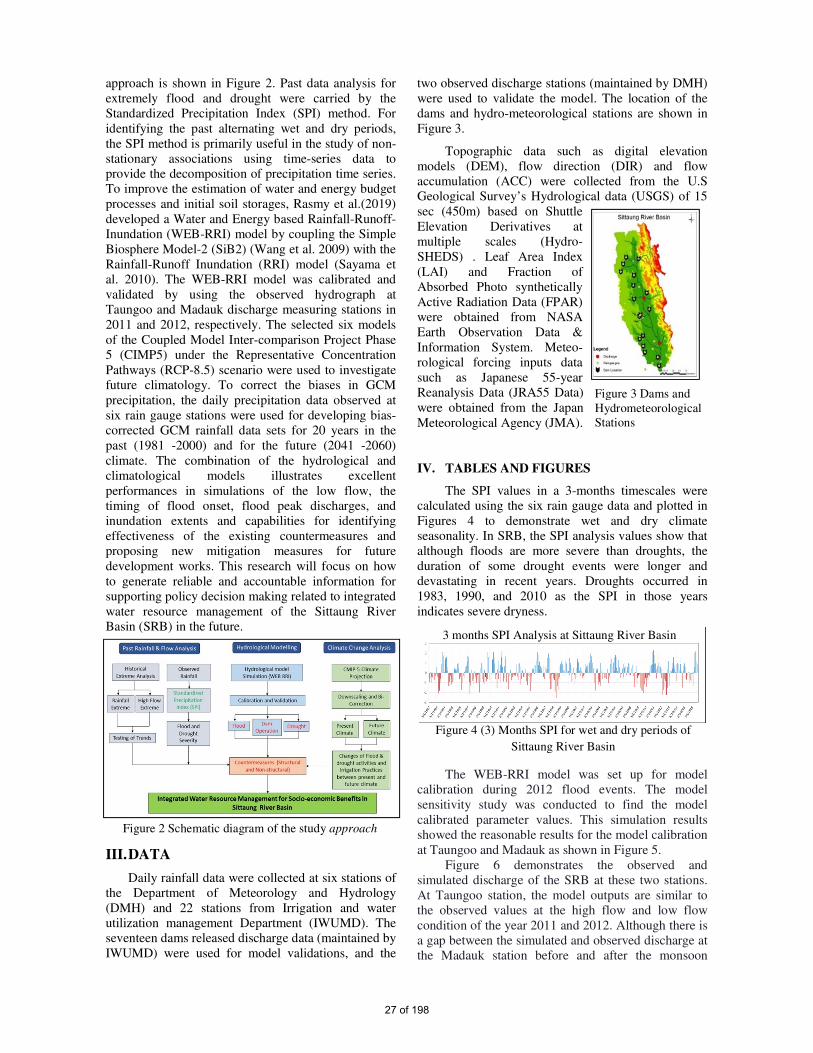
Figure 3 Dams and

Hydrometeorological

Stations

3 months SPI Analysis at Sittaung River Basin

Figure 4 (3) Months SPI for wet and dry periods of

Sittaung River Basin

approach is shown in Figure 2. Past data analysis for

extremely flood and drought were carried by the

Standardized Precipitation Index (SPI) method. For

identifying the past alternating wet and dry periods,

the SPI method is primarily useful in the study of non-

stationary associations using time-series data to

provide the decomposition of precipitation time series.

To improve the estimation of water and energy budget

processes and initial soil storages, Rasmy et al.(2019)

developed a Water and Energy based Rainfall-Runoff-

Inundation (WEB-RRI) model by coupling the Simple

Biosphere Model-2 (SiB2) (Wang et al. 2009) with the

Rainfall-Runoff Inundation (RRI) model (Sayama et

al. 2010). The WEB-RRI model was calibrated and

validated by using the observed hydrograph at

Taungoo and Madauk discharge measuring stations in

2011 and 2012, respectively. The selected six models

of the Coupled Model Inter-comparison Project Phase

5 (CIMP5) under the Representative Concentration

Pathways (RCP-8.5) scenario were used to investigate

future climatology. To correct the biases in GCM

precipitation, the daily precipitation data observed at

six rain gauge stations were used for developing bias-

corrected GCM rainfall data sets for 20 years in the

past (1981 -2000) and for the future (2041 -2060)

climate. The combination of the hydrological and

climatological models illustrates excellent

performances in simulations of the low flow, the

timing of flood onset, flood peak discharges, and

inundation extents and capabilities for identifying

effectiveness of the existing countermeasures and

proposing new mitigation measures for future

development works. This research will focus on how

to generate reliable and accountable information for

supporting policy decision making related to integrated

water resource management of the Sittaung River

Basin (SRB) in the future.

III. DATA

Daily rainfall data were collected at six stations of

the Department of Meteorology and Hydrology

(DMH) and 22 stations from Irrigation and water

utilization management Department (IWUMD). The

seventeen dams released discharge data (maintained by

IWUMD) were used for model validations, and the

two observed discharge stations (maintained by DMH)

were used to validate the model. The location of the

dams and hydro-meteorological stations are shown in

Figure 3.

Topographic data such as digital elevation

models (DEM), flow direction (DIR) and flow

accumulation (ACC) were collected from the U.S

Geological Survey’s Hydrological data (USGS) of 15

sec (450m) based on Shuttle

Elevation Derivatives at

multiple scales (Hydro-

SHEDS) . Leaf Area Index

(LAI) and Fraction of

Absorbed Photo synthetically

Active Radiation Data (FPAR)

were obtained from NASA

Earth Observation Data &

Information System. Meteo-

rological forcing inputs data

such as Japanese 55-year

Reanalysis Data (JRA55 Data)

were obtained from the Japan

Meteorological Agency (JMA).

IV. TABLES AND FIGURES

The SPI values in a 3-months timescales were

calculated using the six rain gauge data and plotted in

Figures 4 to demonstrate wet and dry climate

seasonality. In SRB, the SPI analysis values show that

although floods are more severe than droughts, the

duration of some drought events were longer and

devastating in recent years. Droughts occurred in

1983, 1990, and 2010 as the SPI in those years

indicates severe dryness.

The WEB-RRI model was set up for model

calibration during 2012 flood events. The model

sensitivity study was conducted to find the model

calibrated parameter values. This simulation results

showed the reasonable results for the model calibration

at Taungoo and Madauk as shown in Figure 5. Figure 6 demonstrates the observed and

simulated discharge of the SRB at these two stations.

At Taungoo station, the model outputs are similar to

the observed values at the high flow and low flow

condition of the year 2011 and 2012. Although there is

a gap between the simulated and observed discharge at

the Madauk station before and after the monsoon

Figure 2 Schematic diagram of the study approach

27 of 198

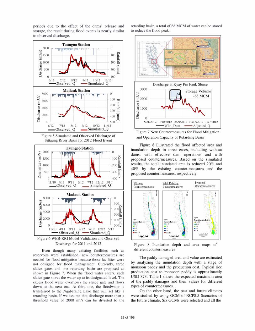
0

100

200

300

400

5000

2000

4000

6000

8000

6/12 7/12 8/12 9/12 10/12 11/12

Madauk Station

0

100

200

300

4000

500

1000

1500

2000

6/12 7/12 8/12 9/12 10/12 11/12

Taungoo Station

Figure 5 Simulated and Observed Discharge of

Sittaung River Basin for 2012 Flood Event

0

100

200

300

4000

500

1000

1500

2000

11/10 4/11 9/11 2/12 7/12 12/12 5/13

0

100

200

300

400

5000

2000

4000

6000

8000

11/10 4/11 9/11 2/12 7/12 12/12 5/13

Figure 6 WEB-RRI Model Validation and Observed

Discharge for 2011 and 2012

0

1000

2000

3000

5/21/2012 7/10/2012 8/29/2012 10/18/2012 12/7/2012

Discharge at Kyay Pin Pauk Sluice

With_Dam Adjusted_Q

Figure 7 New Countermeasures for Flood Mitigation

and Operation Capacity of Retarding Basin

Figure 8 Inundation depth and area maps of

different countermeasures

periods due to the effect of the dams’ release and

storage, the result during flood events is nearly similar

to observed discharge.

Even though many existing facilities such as

reservoirs were established, new countermeasures are

needed for flood mitigation because those facilities were

not designed for flood management. Currently, three

sluice gates and one retarding basin are proposed as

shown in Figure 7. When the flood water enters, each

sluice gate stores the water up to its designated level. The

excess flood water overflows the sluice gate and flows

down to the next one. At third one, the floodwater is

transferred to the Ngabataing Lake that will act like a

retarding basin. If we assume that discharge more than a

threshold value of 2000 m3/s can be diverted to the

retarding basin, a total of 68 MCM of water can be stored

to reduce the flood peak.

Figure 8 illustrated the flood affected area and

inundation depth in three cases, including without

dams, with effective dam operations and with

proposed countermeasures. Based on the simulated

results, the total inundated area is reduced 20% and

40% by the existing counter-measures and the

proposed countermeasures, respectively.

The paddy damaged area and value are estimated

by analyzing the inundation depth with a stage of

monsoon paddy and the production cost. Typical rice

production cost to monsoon paddy is approximately

USD 373. Table.1 shows the expected maximum area

of the paddy damages and their values for different

types of countermeasures.

On the other hand, the past and future climates

were studied by using GCM of RCP8.5 Scenarios of

the future climate, Six GCMs were selected and all the

Dis

char

ge

(m3/s

)

Rain

fall (mm

) R

ainfall (m

m)

Simulated_Q Observed_Q

Observed_Q

Observed_Q Simulated_Q

Simulated_Q

Dis

char

ge

(m3

/s)

Dis

char

ge

(m3

/s)

Rain

fall (mm

) R

ainfall (m

m)

Madauk Station

Storage Volume

-68 MCM

Observed_Q Simulated_Q

Taungoo Station

Dis

char

ge

(m3/s

)

Dis

char

ge

(m3/s

)

28 of 198

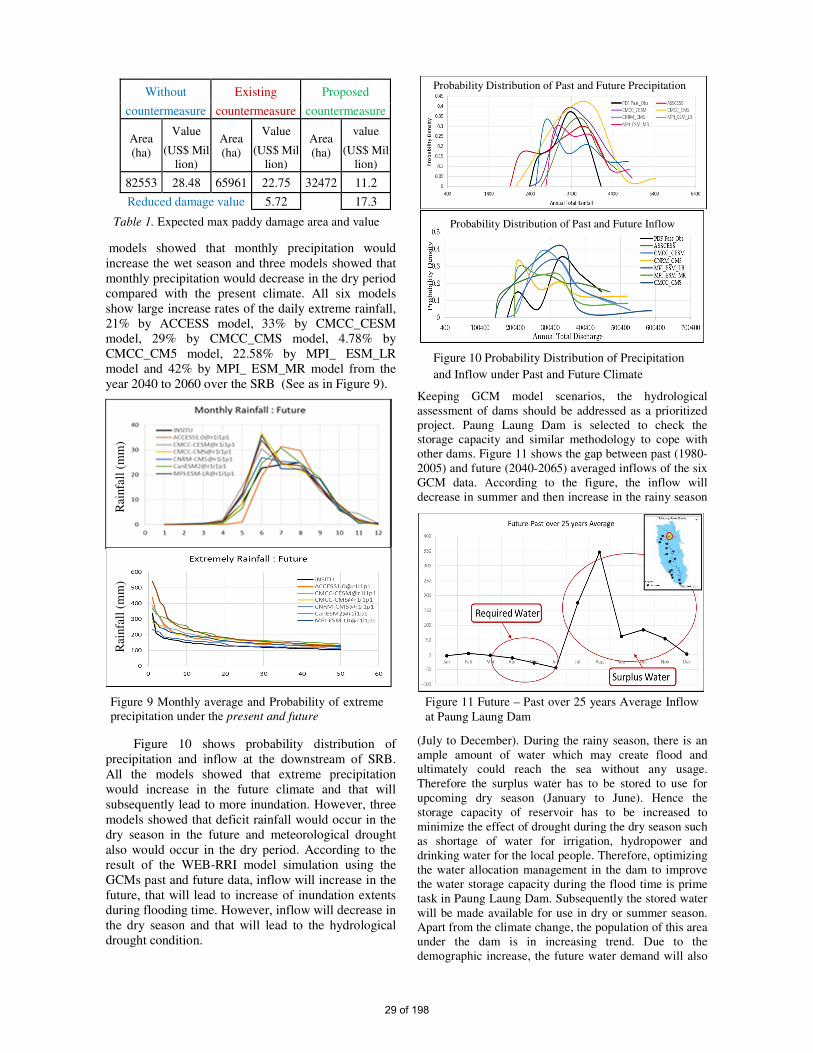
Without Existing Proposed

countermeasure countermeasure countermeasure

Area

(ha)

Value Area

(ha)

Value Area

(ha)

value

(US$ Mil

lion) (US$ Mil

lion) (US$ Mil

lion)

82553 28.48 65961 22.75 32472 11.2

Reduced damage value 5.72 17.3

Table 1. Expected max paddy damage area and value

Figure 11 Future – Past over 25 years Average Inflow

at Paung Laung Dam

Figure 10 Probability Distribution of Precipitation

and Inflow under Past and Future Climate

models showed that monthly precipitation would

increase the wet season and three models showed that

monthly precipitation would decrease in the dry period

compared with the present climate. All six models

show large increase rates of the daily extreme rainfall,

21% by ACCESS model, 33% by CMCC_CESM

model, 29% by CMCC_CMS model, 4.78% by

CMCC_CM5 model, 22.58% by MPI_ ESM_LR

model and 42% by MPI_ ESM_MR model from the

year 2040 to 2060 over the SRB (See as in Figure 9).

Figure 10 shows probability distribution of

precipitation and inflow at the downstream of SRB.

All the models showed that extreme precipitation

would increase in the future climate and that will

subsequently lead to more inundation. However, three

models showed that deficit rainfall would occur in the

dry season in the future and meteorological drought

also would occur in the dry period. According to the

result of the WEB-RRI model simulation using the

GCMs past and future data, inflow will increase in the

future, that will lead to increase of inundation extents

during flooding time. However, inflow will decrease in

the dry season and that will lead to the hydrological

drought condition.

Keeping GCM model scenarios, the hydrological

assessment of dams should be addressed as a prioritized

project. Paung Laung Dam is selected to check the

storage capacity and similar methodology to cope with

other dams. Figure 11 shows the gap between past (1980-

2005) and future (2040-2065) averaged inflows of the six

GCM data. According to the figure, the inflow will

decrease in summer and then increase in the rainy season

(July to December). During the rainy season, there is an

ample amount of water which may create flood and

ultimately could reach the sea without any usage.

Therefore the surplus water has to be stored to use for

upcoming dry season (January to June). Hence the

storage capacity of reservoir has to be increased to

minimize the effect of drought during the dry season such

as shortage of water for irrigation, hydropower and

drinking water for the local people. Therefore, optimizing

the water allocation management in the dam to improve

the water storage capacity during the flood time is prime

task in Paung Laung Dam. Subsequently the stored water

will be made available for use in dry or summer season.

Apart from the climate change, the population of this area

under the dam is in increasing trend. Due to the

demographic increase, the future water demand will also

Figure 9 Monthly average and Probability of extreme

precipitation under the present and future

Probability Distribution of Past and Future Precipitation

Probability Distribution of Past and Future Inflow

Rai

nfa

ll (

mm

) R

ainfa

ll (

mm

)

29 of 198

increase. In that sense, irrigation, hydropower, drinking

water, sanitation and industrial water usages will

increase. Hence, the optimization of water usages is

essential for decision makers of the SRB and this

research will support them for timely decision making.

V. CONCLUSIONS

According to the SPI analysis, in most of the years,

severe floods were recorded in the Sittaung River Basin.

But some drought events were prominent and they lasted

for long period of time in recent years. For the future

climate assessments, the GCM rainfall data bias-

corrected by using the in-situ data and indicated an

increasing trend in the wet season and a decreasing trend

in the dry period in the SRB. Therefore, the increasing

precipitation will result in increasing water levels, and

discharges during the wet season and vice versa in the dry

season.

In this study, WEB-RRI modeled hydrographs

showed acceptable performance in simulating flooding

events, and the modeled discharge hydrographs

correlated well with the observed discharge hydrographs.

This study also examined the effectiveness of

countermeasures for scenario flood events to minimize

severe inundation damages by extreme rainfall events

derived from the climate scenarios. To reduce the flood

inundation area and inundation depth, the proposed

cascade flood gate operations and diverting a peak

discharges to the retention basin can reduce the flood

damages during the rainy season, significantly.

As the SRB also plays an important role for the

national agriculture production and hydropower

generation, the projected water demand and seasonal

water availability in dams for the future should be

considered based on the present demand to improve the

dam operation system. These outputs of this research,

which based on natural science and advanced method of

technology, can support policy and decision making to

optimize the future water resources of the basin in an

integrated approach.

ACKNOWLEDGMENTS

I would like to express my gratitude to my respected

supervisor, Professor Koike and my co-supervisor,

Associate Professor Dr.Mohamed Rasmy, for having time

to supervise my research through his valuable comments,

guidance and support. Also, I am grateful to Mr.Sawano,

Dr.Shrestha and Dr.Takeda for their insightful comments

and encouragement.

REFERENCES

[1] IPCC, 2007. Climate Change 2007: The Physical

Science Basis. Contribution of Working Group I to

the 4th Assessment Report of the IPCC, Cambridge,

UK/New York, USA: Cambridge University Press.

[2] Yang, J. et al., 2008. Comparing uncertainty analysis

techniques for a SWAT application to the Chaohe

Basin in China. Journal of Hydrology, Volume 358,

pp. 1-23.

[3] SAYAMA, Takahiro. Rainfall-Runoff-Inundation

(RRI) Model User's Manual. Tsukuba: International

Center for Water Hazard and Risk Management

(ICHARM), 2013.

[4] United Nations. Report on Sittaung Valley Water

Resources Development (Technical Report):

Rangoon, Burma, 1964; (retrieved from the

Irrigation Department, Myanmar on 2015)

30 of 198

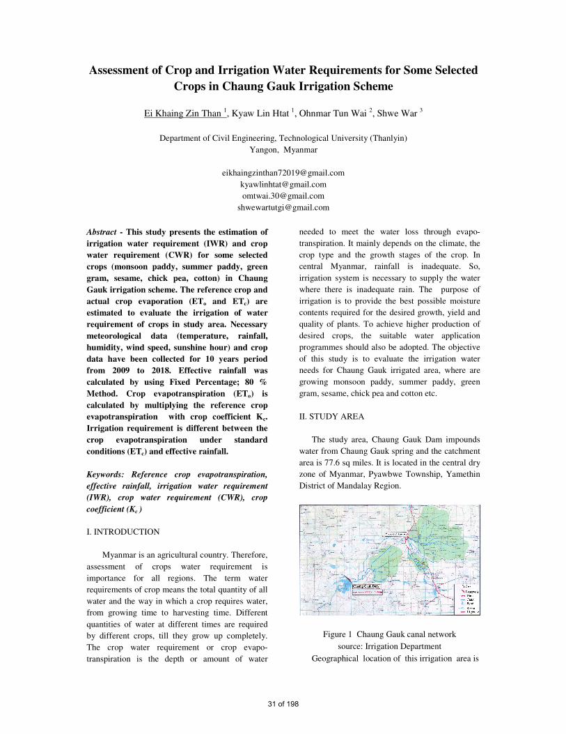
Assessment of Crop and Irrigation Water Requirements for Some Selected

Crops in Chaung Gauk Irrigation Scheme

Ei Khaing Zin Than 1, Kyaw Lin Htat 1, Ohnmar Tun Wai 2, Shwe War 3

Department of Civil Engineering, Technological University (Thanlyin)

Yangon, Myanmar

[email protected]

[email protected]

[email protected]

[email protected]

Abstract - This study presents the estimation of

irrigation water requirement (IWR) and crop

water requirement (CWR) for some selected

crops (monsoon paddy, summer paddy, green

gram, sesame, chick pea, cotton) in Chaung

Gauk irrigation scheme. The reference crop and

actual crop evaporation (ETo and ETc) are

estimated to evaluate the irrigation of water

requirement of crops in study area. Necessary

meteorological data (temperature, rainfall,

humidity, wind speed, sunshine hour) and crop

data have been collected for 10 years period

from 2009 to 2018. Effective rainfall was

calculated by using Fixed Percentage; 80 %

Method. Crop evapotranspiration (ETo) is

calculated by multiplying the reference crop

evapotranspiration with crop coefficient Kc.

Irrigation requirement is different between the

crop evapotranspiration under standard

conditions (ETc) and effective rainfall.

Keywords: Reference crop evapotranspiration,

effective rainfall, irrigation water requirement

(IWR), crop water requirement (CWR), crop

coefficient (Kc )

I. INTRODUCTION

Myanmar is an agricultural country. Therefore,

assessment of crops water requirement is

importance for all regions. The term water

requirements of crop means the total quantity of all

water and the way in which a crop requires water,

from growing time to harvesting time. Different

quantities of water at different times are required

by different crops, till they grow up completely.

The crop water requirement or crop evapo-

transpiration is the depth or amount of water

needed to meet the water loss through evapo-

transpiration. It mainly depends on the climate, the

crop type and the growth stages of the crop. In

central Myanmar, rainfall is inadequate. So,

irrigation system is necessary to supply the water

where there is inadequate rain. The purpose of

irrigation is to provide the best possible moisture

contents required for the desired growth, yield and

quality of plants. To achieve higher production of

desired crops, the suitable water application

programmes should also be adopted. The objective

of this study is to evaluate the irrigation water

needs for Chaung Gauk irrigated area, where are

growing monsoon paddy, summer paddy, green

gram, sesame, chick pea and cotton etc.

II. STUDY AREA

The study area, Chaung Gauk Dam impounds

water from Chaung Gauk spring and the catchment

area is 77.6 sq miles. It is located in the central dry

zone of Myanmar, Pyawbwe Township, Yamethin

District of Mandalay Region.

Figure 1 Chaung Gauk canal network

source: Irrigation Department

Geographical location of this irrigation area is

31 of 198

20.88º North (latitude) and 95.86º East (longitude)

at an elevation of 244 meters. The type of dam is

Earth. Its length is about 6800 ft and its height is 74

ft. Full tank capacity is 26,000 ac-ft and dead

storage capacity is 5,000 ac-ft. Average annual

rainfall is 33 inches. Chaung Gauk Dam project

intends to provide the water for the 6493 acres

irrigable area. Location of the reservoir and canal

network system is shown in Figure 1.

III. METHODOLOGY

1. Collection of Meteorological Data

In this study a long recorded 2009 to 2018

(10years) meteorological data collected from

Meiktila Station. These data are;

• Maximum Temperature and Minimum

Temperature (Celsius)

• Mean Relative Humidity (%)

• Wind Speed (kmph)

• Sunshine Hours (Hrs)

The respective climatic data were collected

from the Department of Meteorology and

Hydrology under the Ministry of Transport and

Communication.

2. Crop Stage Data

The major cultivated in study area are summer

paddy, monsoon paddy, green gram, chick pea,

sesame and cotton, etc. Crop coefficient values

(Kc); rooting depth; length of plant growth stages;

planting date and allowable depletion are taken

from FAO Paper 56.Kc values for initial, mid and

late growth stages of crops are used. Yield response

factor for crops are taken from FAO paper 33.

(i) Crop coefficient (Kc)

Crop coefficient (Kc) varies during the growing

period. As the crop develops, the ground cover,

crop height and the leaf area change. Due to

differences in evapotranspiration during the various

growth stages, the Kc for a given crop will vary

over the growing period. The changing

characteristics of the crop over the growing season

also affect the Kc coefficient.

(ii) Rooting depth (D)

The depth of soil water can be used effectively

by the crop, defined as the Really Available Soil

Moisture (RAM), depends directly on the rooting

depth of the crop.

Two values are required;

- Rooting depth of initial stage normally

taken as 0.25-0.3m, representing the

effective soil depth from which the small

seedling abstracts its water.

- Rooting depth at full development at start

of mid-season. For most irrigated field

crops values vary between land 1.4,

vegetable crops 0.5-1.0.

Rooting depth at development and late

season are interpolated values and no

input is required.

(iii) Allowable depletion (p)

Allowable depletion (p) represents the critical

soil moisture level where first drought stress occurs

affecting evapotranspiration and crop production.

Values are expressed as a fraction of total available

soil moisture and normally vary between 0.4 and

0.6, with lower values taken for sensitive crops

with limited root systems under high evaporative

conditions, and higher values for deep and densely

rooting crops and low evapotranspiration rates.

(iv) Yield response factor (Ky)

Yield Response Factor (Ky) to estimate yield

reductions due to drought stress; yield response

factor have to be given for each growth stages.

3. Reference Crop Evapotranspiration (ETo)

The reference crop evapotranspiration ETo was

calculated by FAO Penman-Monteith method,

using decision support software CROPWAT 8.0

developed by FAO, based on FAO Irrigation and

Drainage Paper 56. The Penman-Monteith equation

integrated in the CROPWAT program is expressed

by equation (1).

ETo =)u 0.34(1

)( 273

900 )( 408.0

2

2

++∆

−+

+−∆

γ

γ asn eeuT

GR

(1)

Where,

ETo = reference crop evapotranspiration(mm/day-1

)

Rn = net radiation at the crop surface (MJm-2day-1)

G = soil heat flux density (MJm-2

day-1

)

T = mean daily air temperature at 2m height ºC

32 of 198

U2 = wind speed at 2 m height (ms-1

)

es = saturation vapor pressure (kpa)

ea = actual vapor pressure (kpa)

D = slope vapor pressure curve

γ = psychometric pressure curve (kPa/ ºC)

The FAO CROPWAT program incorporates

calculation procedures for reference crop evapo-

transpiration and crop water requirements. The

program allows the simulation of crop water use

under various climate and crop conditions.

Meteorological parameters used for calculation

of ETo were latitude, longitude and altitude of the

station, maximum and minimum temperature C,

relative humidity (%), wind speed (km/day) and

sunshine hours.

4. Effective Rainfall

Effective Rainfall defined as that part of the

rainfall which is effectively used by the crop after

rainfall losses due to surface runoff and deep

percolation have been accounted for. The effective

rainfall is the rainfall ultimately used to determine

the crop irrigation requirements. To know the

irrigation requirement, amount of effective rainfall

data is needed.

5. Crop Evapotranspiration ( ETc)

The crop water need or actual crop

evapotranspiration is defined as the depth or

amount of water needed to meet the water losses

through evapotranspiration which is calculated by

multiplying ETo by Kc as follow;

ETc = Kc x ETo (2)

Where,

ETc = crop evapotranspiration under standard

conditions

Kc = crop coefficient

ETo = reference crop evapotranspiration

IV. RESULTS AND DISCUSSION

1. Reference Crop Evapotranspiration of the study

Area

The results obtained when a ten years period

was used with the FAO – Penman Monteith

method to determine the reference crop evapo-

transpiration (ETo).The table shows that ETo varied

from a minimum value of (2.98 mm/day) in

January to the maximum value of (6.17 mm/day) in

April. From the results, it can be seen that ETo is

the lowest during the peak of the rainy season and

changes to the highest during the peak of dry

season.

Table 1 Average reference crop evapotranspira-

tion from the year 2009 to 2018

Month

Min

Tem

p

(°C

)

Max

Tem

p

(°C

)

Hum

idit

y (

%)

Win

d S

pee

d

(km

/ day

)

Su

nsh

ine

(Hrs

)

Rad

iati

on

(MJ/

m2/d

ay)

ET

o (

mm

/day

)

Jan 15.1 30 74 94 7.4 15.6 2.98

Feb 17 34 59 109 7.9 18.1 4.03

Mar 21.5 36.9 57 163 7.7 19.8 5.37

Apr 25.3 38.4 63 195 7.9 21.4 6.17

May 25.8 35.7 71 207 7.2 20.7 5.66

June 24.9 33.2 81 248 5.7 18.5 4.65

July 24.7 32.8 81 249 4.4 16.4 4.26

Aug 24.5 32.3 84 187 4.8 16.8 3.97

Sept 24.5 33 83 142 5.9 17.5 4.04

Oct 23.4 32.2 83 96 5.9 15.8 3.5

Nov 20.3 31.9 77 115 7.0 15.5 3.41

Dec 16.5 29.5 76 128 6.9 14.4 3.0

Avg 22 33.3 74 161 6.6 17.5 4.25

2. Calculation Results of Effective Rainfall

The table 2 shows that the estimated rainfall

and effective rainfall of the selected area for a ten

year period. The maximum effective rainfall is

149.8 mm in September.

Table 2 Total effective rainfall data from the year

2009 to 2018

Month Rainfall Effective Rainfall

mm mm

January 8.8 7.0

February 0.9 0.7

March 5.3 4.2

April 33.9 27.1

May 116.4 93.1

June 125.9 100.7

July 84.4 67.5

August 140.2 112.2

33 of 198

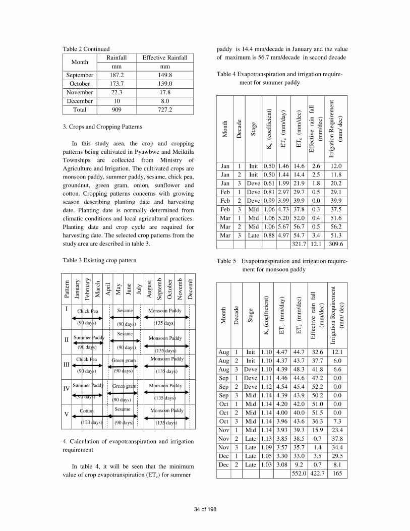
Table 2 Continued

Month Rainfall Effective Rainfall

mm mm

September 187.2 149.8

October 173.7 139.0

November 22.3 17.8

December 10 8.0

Total 909 727.2

3. Crops and Cropping Patterns

In this study area, the crop and cropping

patterns being cultivated in Pyawbwe and Meiktila

Townships are collected from Ministry of

Agriculture and Irrigation. The cultivated crops are

monsoon paddy, summer paddy, sesame, chick pea,

groundnut, green gram, onion, sunflower and

cotton. Cropping patterns concerns with growing

season describing planting date and harvesting

date. Planting date is normally determined from

climatic conditions and local agricultural practices.

Planting date and crop cycle are required for

harvesting date. The selected crop patterns from the

study area are described in table 3.

Table 3 Existing crop pattern

Pat

tern

Jan

uar

y

Feb

ruar

y

Mar

ch

Apri

l

May

June

July

Au

gu

st

Sep

tem

b

Oct

ober

Novem

b

Dec

emb

I

II

III

IV

V

4. Calculation of evapotranspiration and irrigation

requirement

In table 4, it will be seen that the minimum

value of crop evapotranspiration (ETc) for summer

paddy is 14.4 mm/decade in January and the value

of maximum is 56.7 mm/decade in second decade

Table 4 Evapotranspiration and irrigation require-

ment for summer paddy

Mon

th

Dec

ade

Sta

ge

Kc

(co

effi

cient)

ET

c (

mm

/day

)

ET

c (m

m/d

ec)

Eff

ecti

ve

rai

n fa

ll

(mm

/dec

)

Irri

gat

ion R

equ

irem

ent

(mm

/ dec

)

Jan 1 Init 0.50 1.46 14.6 2.6 12.0

Jan 2 Init 0.50 1.44 14.4 2.5 11.8

Jan 3 Deve 0.61 1.99 21.9 1.8 20.2

Feb 1 Deve 0.81 2.97 29.7 0.5 29.1

Feb 2 Deve 0.99 3.99 39.9 0.0 39.9

Feb 3 Mid 1.06 4.73 37.8 0.3 37.5

Mar 1 Mid 1.06 5.20 52.0 0.4 51.6

Mar 2 Mid 1.06 5.67 56.7 0.5 56.2

Mar 3 Late 0.88 4.97 54.7 3.4 51.3

321.7 12.1 309.6


ment for monsoon paddy

Month

Dec

ade

Sta

ge

Kc

(coef

fici

ent)

ET

c (

mm

/day

)

ET

c (m

m/d

ec)

Eff

ecti

ve

rai

n

fall

(mm

/dec

)

Irri

gat

ion R

equir

emen

t

(mm

/ dec

)

Aug 1 Init 1.10 4.47 44.7 32.6 12.1

Aug 2 Init 1.10 4.37 43.7 37.7 6.0

Aug 3 Deve 1.10 4.39 48.3 41.8 6.6

Sep 1 Deve 1.11 4.46 44.6 47.2 0.0

Sep 2 Deve 1.12 4.54 45.4 52.2 0.0

Sep 3 Mid 1.14 4.39 43.9 50.2 0.0

Oct 1 Mid 1.14 4.20 42.0 51.0 0.0

Oct 2 Mid 1.14 4.00 40.0 51.5 0.0

Oct 3 Mid 1.14 3.96 43.6 36.3 7.3

Nov 1 Mid 1.14 3.93 39.3 15.9 23.4

Nov 2 Late 1.13 3.85 38.5 0.7 37.8

Nov 3 Late 1.09 3.57 35.7 1.4 34.4

Dec 1 Late 1.05 3.30 33.0 3.5 29.5

Dec 2 Late 1.03 3.08 9.2 0.7 8.1

552.0 422.7 165

(120 days)

Cotton

(90 days)

(90 days)

Green gram

Green gram

Chick Pea

Sesame

(90 days) (90 days)

Chick Pea

Monsoon Paddy

(135 days)

Monsoon Paddy

(135 days)

Monsoon Paddy

(135 days)

Monsoon Paddy

(135 days)

Monsoon Paddy

(135 days)

(90 days)

Summer Paddy

Summer Paddy

(90 days)

Sesame

(90 days)

(90 days)

Sesame

(90 days)

34 of 198

of March. Also, the highest requirement of

irrigation is 56.2 mm/ decade and the lowest is 11.8

mm/decade just before the harvesting.

There is no irrigation requirement for monsoon

paddy in August and September and the most

irrigation requirement is 37.8 mm/decade at the

second decade of November as shown in table 5.

The table shows that the crop evapotranspiration

changes from the maximum value of 48.3

mm/decade at the initial stage to the minimum

value of 9.2 mm/decade.

For green gram, there is no irrigation

requirement at the second stage of July shown in

table 6. The maximum irrigation requirement is

21.9 mm/decade. The crop evapotranspiration

varies from 55.6 mm/decade at the beginning of

middle stage to 6.5 mm/decade at the end of late

stage.


ment for green gram

Mon

th

Dec

ade

Sta

ge

Kc

(coef

fici

ent)

ET

c (

mm

/day

)

ET

c (m

m/d

ec)

Eff

ecti

ve

rai

n

fall

(mm

/dec

)

Irri

gat

ion R

equir

emen

t

(mm

/ dec

)

Apr 2 Init 0.40 2.51 15.0 4.2 11.5

Apr 3 Init 0.40 2.42 24.2 15.0 9.2

May 1 Deve 0.45 2.64 26.4 25.5 0.9

May 2 Deve 0.69 3.91 39.1 33.8 5.3

May 3 Mid 0.95 5.05 55.6 33.7 21.9

June 1 Mid 1.03 5.15 51.5 34.0 17.5

June 2 Mid 1.03 4.80 48.0 35.5 12.6

June 3 Late 0.96 4.32 43.2 31.2 12.0

July 1 Late 0.69 3.02 30.2 23.8 6.5

July 2 Late 0.51 2.17 6.5 5.7 0.0

339.8 242.4 97.3

For sesame, there is no irrigation requirements

at the first stage of May and second stage of July

shown in table 7. The maximum irrigation

requirement is 19.3 mm/decade. The crop

evapotranspiration varies from 2.2 mm/decade at

the initial stage to 53.3 mm/decade at the mid

season stage.


ment for sesame

Month

Dec

ade

Sta

ge

Kc

(co

effi

cient)

ET

c (

mm

/day

)

ET

c (m

m/d

ec)

Eff

ecti

ve

rai

n fa

ll

(mm

/dec

)

Irri

gat

ion R

equ

irem

ent

(mm

/ dec

)

Apr 2 Init 0.35 2.19 2.2 0.7 2.2

Apr 3 Init 0.35 2.12 21.2 15.0 6.2

May 1 Deve 0.40 2.34 23.4 25.5 0.0

May 2 Deve 0.63 3.55 35.5 33.8 1.8

May 3 Deve 0.88 4.70 51.7 33.7 18.0

June 1 Mid 1.07 5.33 53.3 34.0 19.3

June 2 Mid 1.08 5.01 50.1 35.5 14.6

June 3 Mid 1.08 4.87 48.7 31.2 17.5

July 1 Late 0.92 4.05 40.5 23.8 16.7

July 2 Late 0.44 1.89 15.1 15.1 0.0

341.7 248.3 96.3


ment for chick pea

Mon

th

Dec

ade

Sta

ge

Kc

(co

effi

cient)

ET

c (

mm

/day

)

ET

c (m

m/d

ec)

Eff

ecti

ve

rai

n fa

ll

(mm

/dec

) Ir

rigat

ion

Req

uir

emen

t (m

m/

dec

)

Jan 1 Init 0.40 1.17 11.7 2.6 9.1

Jan 2 Init 0.40 1.15 11.5 2.5 9.0

Jan 3 Deve 0.52 1.70 18.7 1.8 16.9

Feb 1 Deve 0.73 2.70 27.0 0.5 26.4

Feb 2 Mid 0.93 3.76 37.6 0.0 37.6

Feb 3 Mid 1.01 4.50 36.0 0.3 35.7

Mar 1 Mid 1.01 4.95 49.5 0.4 49.0

Mar 2 Mid 1.01 5.40 54.0 0.5 53.4

Mar 3 Late 0.68 3.82 42.0 3.4 38.6

287.8 12.1 275.7

35 of 198

For Chick pea, crop evapotranspiration (ETc)

and crop water requirements are varied from 11.5

mm/decade to 54 mm/decade and 9.0 mm/decade

to 53.4 mm/decade respectively in table 8.


ment for cotton

Month

Dec

ade

Sta

ge

Kc

(c

oef

fici

ent)

ET

c (

mm

/day

)

ET

c (m

m/d

ec)

Eff

ecti

ve

rai

n f

all

(mm

/dec

)

Irri

gat

ion R

equir

emen

t

(mm

/ dec

) Jan 1 Init 0.35 1.02 10.2 2.6 7.6

Jan 2 Init 0.35 1.01 10.1 2.5 7.5

Jan 3 Deve 0.51 1.67 18.3 1.8 16.6

Feb 1 Deve 0.79 2.92 29.2 0.5 28.7

Feb 2 Mid 1.06 4.27 42.7 0.0 42.7

Feb 3 Mid 1.16 5.18 41.4 0.3 41.1

Mar 1 Mid 1.16 5.70 57.0 0.4 56.5

Mar 2 Mid 1.16 6.21 62.1 0.5 61.6

Mar 3 Late 1.14 6.42 70.6 3.4 67.3

Apr 1 Late 1.02 6.09 60.9 5.2 55.7

Apr 2 Late 0.89 5.58 55.8 7.0 48.7

Apr 3 Late 0.76 4.61 46.1 15.0 31.0

504.5 39.3 465.1

For cotton, the most irrigation requirement is

67.3 mm/decade at the third decade of March as

shown in table 9.The table show that the crop

evapotranspiration changes from the maximum

value of 70.6 mm/decade at the late season stage to

the minimum value of 10.1 mm/decade.

V. CONCLUSION

The study mainly estimates the CWR and IWR

for some selected crops as well as developing

cropping pattern for the study area. The result

shows that reference and crop evapotranspiration

(ETo and ETc) were higher for crops with longer

growing season than for those with shorter ones.

Also ETo and ETc were more during the dry season

than the rainy season. The maximum water

requirement of crop is monsoon paddy and the

minimum water requirement of crop is chick pea.

ACKNOWLEDGMENT

The author is deeply grateful to Dr. Nyan

Phone, Professor and Head, Department of Civil

Engineering, Technological University (Thanlyin),

for his guidance. The author is sincerely thank to

Dr. Kyaw lin Htat, Professor, Department of Civil

Engineering , Technological University (Thanlyin),

for his skillful guidance, helpful suggestions and

editing of this paper. The author is profoundly

grateful to Daw Ohnmar Tun Wai, Lecturer,

Department of Civil Engineering , Technological

University (Thanlyin), for her encouragement,

helpful suggestion, true-line guidance and

comment for preparing paper. The author would

like to express her special thank to her co-

supervisor Daw Shwe War, Assistant Lecturer,

Department of Civil Engineering , Technological

University (Thanlyin), for her support and

invaluable comments.

REFERENCES

[1] FAO.1977.Crop Water Requirements: FAO

Irrigation and Drainage Paper 24. Food and

Agricultural Organization of the United

Nation.

[2] FAO. 1998. Crop Evapotranspiration:

Guidelines for Computing Crop Water

Requirements, Irrigation and Drainage

Paper 56. Food and Agricultural

Organization of the United Nation.

[3] Smith, M,2006. Example of the Ues of

CROPWAT 8.0. Food and Agricultural

Organization of the United Nation.

36 of 198

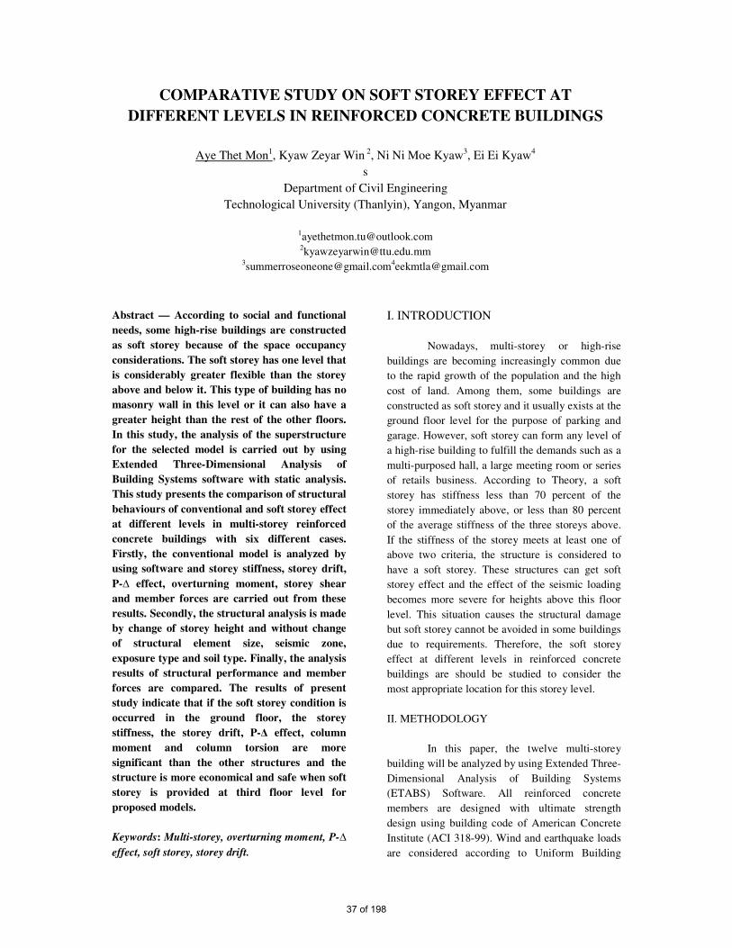
Abstract — According to social and functional

needs, some high-rise buildings are constructed

as soft storey because of the space occupancy

considerations. The soft storey has one level that

is considerably greater flexible than the storey

above and below it. This type of building has no

masonry wall in this level or it can also have a

greater height than the rest of the other floors.

In this study, the analysis of the superstructure

for the selected model is carried out by using

Extended Three-Dimensional Analysis of

Building Systems software with static analysis.

This study presents the comparison of structural

behaviours of conventional and soft storey effect

at different levels in multi-storey reinforced

concrete buildings with six different cases.

Firstly, the conventional model is analyzed by

using software and storey stiffness, storey drift,

P-∆ effect, overturning moment, storey shear

and member forces are carried out from these

results. Secondly, the structural analysis is made

by change of storey height and without change

of structural element size, seismic zone,

exposure type and soil type. Finally, the analysis

results of structural performance and member

forces are compared. The results of present

study indicate that if the soft storey condition is

occurred in the ground floor, the storey

stiffness, the storey drift, P-Δ effect, column

moment and column torsion are more

significant than the other structures and the

structure is more economical and safe when soft

storey is provided at third floor level for

proposed models.

Keywords: Multi-storey, overturning moment, P-∆

effect, soft storey, storey drift.

I. INTRODUCTION

Nowadays, multi-storey or high-rise

buildings are becoming increasingly common due

to the rapid growth of the population and the high

cost of land. Among them, some buildings are

constructed as soft storey and it usually exists at the

ground floor level for the purpose of parking and

garage. However, soft storey can form any level of

a high-rise building to fulfill the demands such as a

multi-purposed hall, a large meeting room or series

of retails business. According to Theory, a soft

storey has stiffness less than 70 percent of the

storey immediately above, or less than 80 percent

of the average stiffness of the three storeys above.

If the stiffness of the storey meets at least one of

above two criteria, the structure is considered to

have a soft storey. These structures can get soft

storey effect and the effect of the seismic loading

becomes more severe for heights above this floor

level. This situation causes the structural damage

but soft storey cannot be avoided in some buildings

due to requirements. Therefore, the soft storey

effect at different levels in reinforced concrete

buildings are should be studied to consider the

most appropriate location for this storey level.

II. METHODOLOGY

In this paper, the twelve multi-storey

building will be analyzed by using Extended Three-

Dimensional Analysis of Building Systems

(ETABS) Software. All reinforced concrete

members are designed with ultimate strength

design using building code of American Concrete

Institute (ACI 318-99). Wind and earthquake loads

are considered according to Uniform Building

COMPARATIVE STUDY ON SOFT STOREY EFFECT AT

DIFFERENT LEVELS IN REINFORCED CONCRETE BUILDINGS

Aye Thet Mon1, Kyaw Zeyar Win 2, Ni Ni Moe Kyaw3, Ei Ei Kyaw4

s

Department of Civil Engineering

Technological University (Thanlyin), Yangon, Myanmar

[email protected] [email protected]

[email protected]

[email protected]

37 of 198

Code (UBC-1997). Exposure type (B) and soil type

(D) are considered with design wind velocity 100

mph. Structural system is considered by concrete

intermediate moment-resisting frame with over-

strength factor 5.5. According to CQHP guide

lines, static design load combinations are used. The

proposed model is statically analyzed and the

results are carried out for the superstructure and

then these are compared.

1. Types of structure

The twelve storey reinforced concrete

models are considered as a conventional structure

and soft storey structures due to change of wall

height. Table 1 shows different cases of six models

for this study.

Table 1 Different cases of six models

Model-1 Conventional

Model-2 Soft storey at ground floor

Model-3 Soft storey at first floor

Model-4 Soft storey at second floor

Model-5 Soft storey at third floor

Model-6 Soft storey at fourth floor

2. Data preparation

The following Tables describe the analysis

data for one conventional and five soft storey

reinforced concrete models. Table 2 shows material

specifications, Table 3 shows structural

configurations and Table 4 shows structural

element sizes. In this study, Table 5 shows storey

heights of different configuration and M-1 is

referred to conventional model. M-2, M-3, M-4, M-

5 and M-6 are referred to soft storey models with

soft storey effect at ground, first, second, third and

fourth floor level respectively.

Table 2 Material specifications

Concrete compressive strength (fc’) 4 ksi

Bending reinforcing yield stress (fy) 50 ksi

Shear reinforcing yield stress (fys) 50 ksi

Modulus of elasticity 3605 ksi

Poisson’s ratio 0.2

Table 3 Structural configurations

Number of stories 12

Width of structure 68ʹ-0″

Length of structure 95ʹ-0″

Total height of structure 148ʹ-0″

Number of bay’s along X 8

Number of bay’s along Y 6

Table 4 Structural element sizes

Column sizes 22″x22″, 20″x20″,

18″x18″, 16″x16″

Beam sizes for

proposed buildings

18″x20″, 16″x18″ ,

14″x18″, 12″x18″,

12″x14″, 10″x12″

Table 5 Storey heights of different configuration

Storey

Height (ft)

Model Model Model Model Model Model

M-1 M-2 M-3 M-4 M-5 M-6

RT-1 10 10 10 10 10 10

RT 10 10 10 10 10 10

11F 10 10 10 10 10 10

10F 10 10 10 10 10 10

9F 10 10 10 10 10 10

8F 11 10 10 10 10 10

7F 11 10 10 10 10 10

6F 11 10 10 10 10 10

5F 11 10 10 10 10 18

4F 11 10 10 10 18 10

3F 11 10 10 18 10 10

2F 11 10 18 10 10 10

1F 11 18 10 10 10 10

GF 10 10 10 10 10 10

Total

height 148 148 148 148 148 148

3. Model description

Figures 1 and 2 show the architectural

floor plans and Figures 3 to 8 show the elevation of

proposed models respectively.

38 of 198

Figure 1 Typical floor plan for proposed model.

Figure 2 Soft storey floor plan for proposed model.

Figure 3 Elevation of (M-1). Figure 4 Elevation of (M-2).



4. Load combination

According to CQHP guide lines, the

considerations of static design load combination

are shown in Table 6.

Table 6. Load combination for proposed models

1 1.4DL + 1.4SDL

2 1.4DL + 1.4SDL + 1.7LL

3,4 1.05DL + 1.05SDL + 1.275 LL ±

1.275WX

5,6 1.05DL + 1.05SDL + 1.275 LL ±

1.275WY

7,8 0.9DL + 0.9SDL ± 1.3WX

9,10 0.9DL + 0.9SDL ± 1.3WY

11,12 1.05DL + 1.05SDL + 1.28LL ± EQX

13,14 1.05DL + 1.05SDL + 1.28LL ± EQY

15,16 0.9DL + 0.9SDL ± EQX

17,18 0.9DL + 0.9SDL ± EQY

19,20 1.27DL + 1.27SDL + 1.28LL ± EQX

21,22 1.27DL + 1.27SDL + 1.28LL ± EQY

23,24 0.68DL + 0.68SDL ± 1.02EQX

25,26 0.68DL + 0.68SDL ± EQY

III. RESULTS AND DISCUSSIONS

In this section, the results obtained from

the analysis of one conventional and five soft

storey reinforced concrete models using ETABS

software have been tabulated and compared. The

performance of structures on different criteria have

39 of 198

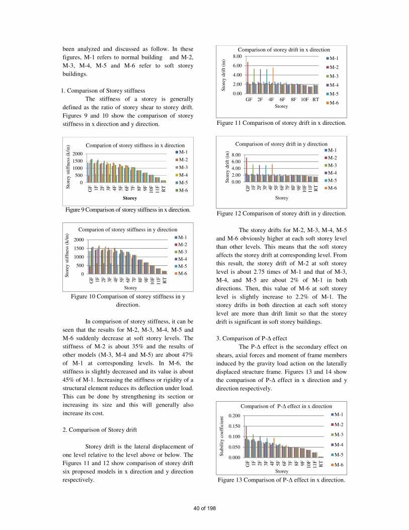
been analyzed and discussed as follow. In these

figures, M-1 refers to normal building and M-2,

M-3, M-4, M-5 and M-6 refer to soft storey

buildings.

1. Comparison of Storey stiffness

The stiffness of a storey is generally

defined as the ratio of storey shear to storey drift.

Figures 9 and 10 show the comparison of storey

stiffness in x direction and y direction.

Figure 9 Comparison of storey stiffness in x direction.

Figure 10 Comparison of storey stiffness in y

direction.

In comparison of storey stiffness, it can be

seen that the results for M-2, M-3, M-4, M-5 and

M-6 suddenly decrease at soft storey levels. The

stiffness of M-2 is about 35% and the results of

other models (M-3, M-4 and M-5) are about 47%

of M-1 at corresponding levels. In M-6, the

stiffness is slightly decreased and its value is about

45% of M-1. Increasing the stiffness or rigidity of a

structural element reduces its deflection under load.

This can be done by strengthening its section or

increasing its size and this will generally also

increase its cost.

2. Comparison of Storey drift

Storey drift is the lateral displacement of

one level relative to the level above or below. The

Figures 11 and 12 show comparison of storey drift

six proposed models in x direction and y direction

respectively.

Figure 11 Comparison of storey drift in x direction.

Figure 12 Comparison of storey drift in y direction.

The storey drifts for M-2, M-3, M-4, M-5

and M-6 obviously higher at each soft storey level

than other levels. This means that the soft storey

affects the storey drift at corresponding level. From

this result, the storey drift of M-2 at soft storey

level is about 2.75 times of M-1 and that of M-3,

M-4, and M-5 are about 2% of M-1 in both

directions. Then, this value of M-6 at soft storey

level is slightly increase to 2.2% of M-1. The

storey drifts in both direction at each soft storey

level are more than drift limit so that the storey

drift is significant in soft storey buildings.

3. Comparison of P-∆ effect

The P-∆ effect is the secondary effect on

shears, axial forces and moment of frame members

induced by the gravity load action on the laterally

displaced structure frame. Figures 13 and 14 show

the comparison of P-∆ effect in x direction and y

direction respectively.

Figure 13 Comparison of P-Δ effect in x direction.

0

500

1000

1500

2000

GF

1F

2F

3F

4F

5F

6F

7F

8F

9F

10

F

11

F

RTS

tore

y s

tiff

nes

s (k

/in

)

Storey

Comparion of storey stiffness in x direction

M-1

M-2

M-3

M-4

M-5

M-6

0

500

1000

1500

2000

GF

1F

2F

3F

4F

5F

6F

7F

8F

9F

10

F

11

F

RT

Sto

rey s

tiff

nes

s (k

/in

)

Storey

Comparion of storey stiffness in y direction

M-1

M-2

M-3

M-4

M-5

M-6

0.00

2.00

4.00

6.00

8.00

GF 2F 4F 6F 8F 10F RT

Sto

rey d

rift

(in

)

Storey

Comparison of storey drift in x direction

M-1

M-2

M-3

M-4

M-5

M-6

0.00

2.00

4.00

6.00

8.00

GF

1F

2F

3F

4F

5F

6F

7F

8F

9F

10

F11

FR

T

Sto

rey d

rift

(in

)

Storey

Comparison of storey drift in y directionM-1

M-2

M-3

M-4

M-5

M-6

0.000

0.050

0.100

0.150

0.200

GF

1F

2F

3F

4F

5F

6F

7F

8F

9F

10

F

11

F

RT

Sta

bil

ity c

oef

fici

ent

Storey

Comparison of P-Δ effect in x direction

M-1

M-2

M-3

M-4

M-5

M-6

40 of 198

Figure 14 Comparison of P-Δ effect in y direction.

In comparison, the stability coefficient of

P-Δ effect at soft storey level in each model is

significantly higher than other levels. It can be seen

that the stability coefficient of M-2 and M-3 in both

directions and that of M-4 in x direction are more

than allowable limit. However, the coefficient of

M-4 in y direction and that of M-1, M-5 and M-6 in

both directions are lower than allowable limit. The

P-Δ effect results in additional forces and moment

increases storey displacement and overturning

moment and this effect influence at lower levels.

4. Comparison of Overturning moment

The summation of moments due to the the

distributed lateral forces is the overturning moment

and these values are shown in Figures 15 and 16.

Figure 15 Comparison of overturning moment in x

direction.

Figure 16 Comparison of overturning moment in y

direction.

In this comparison, overturning moment

of proposed models in x direction and y direction

are nearly similar and it is decreasing from bottom

to top. The overturning moment will increase the

compressive stress in outer columns on the

opposite side of the buildings. The safety factors of

overturning moment for all models are greater than

1.5. Therefore, the overturning moment is no effect

on soft storey for these proposed models.

5. Comparison of Storey shear

Storey shear is the summation of

design lateral forces above the storey under

consideration and the comparison of this

value in x direction and y direction are shown

in Figures 17 and 18.

Figure 17 Comparison of storey shear in x

direction.

Figure 18 Comparison of storey shear in y

direction.

From these comparisons, it can be seen

that the storey shear is larger in bottom and then

declines gradually to top. The results of proposed

models are nearly equal in x direction and y

direction and this value of M-1 is slightly larger at

each level of other models. The results of all

models other than M-1 at corresponding levels are

nearly similar in both directions.

6. Structural member forces in Columns

Structural member forces in columns such

as moment and torsion are shown in Figures 19 and

20 respectively.

0.000

0.050

0.100

0.150

0.200

GF

1F

2F

3F

4F

5F

6F

7F

8F

9F

10

F

11

F

RT

Sta

bil

ity c

oef

fici

ent

Storey

Comparison of P-Δ effect in y direction

M-1

M-2

M-3

M-4

M-5

M-6

0

20000

40000

60000

80000

100000

GF

1F

2F

3F

4F

5F

6F

7F

8F

9F

10

F

11

F

RTO

vert

urn

ing m

om

ent(

k-f

t)

Storey

Comparison of overturning moment in x

direction

M-1

M-2

M-3

M-4

M-5

M-6

0

20000

40000

60000

80000

100000

GF

1F

2F

3F

4F

5F

6F

7F

8F

9F

10

F

11

F

RTO

ver

turn

ing m

om

ent(

k-f

t)

Storey

Comparison of overturning moment in y

direction

M-1

M-2

M-3

M-4

M-5

M-6

0

200

400

600

800

1000

GF

1F

2F

3F

4F

5F

6F

7F

8F

9F

10

F

11

F

RT

Sto

rey S

hea

r (k

ip)

Storey

Comparison of storey shear in x direction

M-1

M-2

M-3

M-4

M-5

M-6

0

200

400

600

800

1000

GF

1F

2F

3F

4F

5F

6F

7F

8F

9F

10

F

11

F

RT

Sto

rey S

hea

r (k

ip)

Storey

Comparison of storey shear in y direction

M-1

M-2

M-3

M-4

M-5

M-6

41 of 198

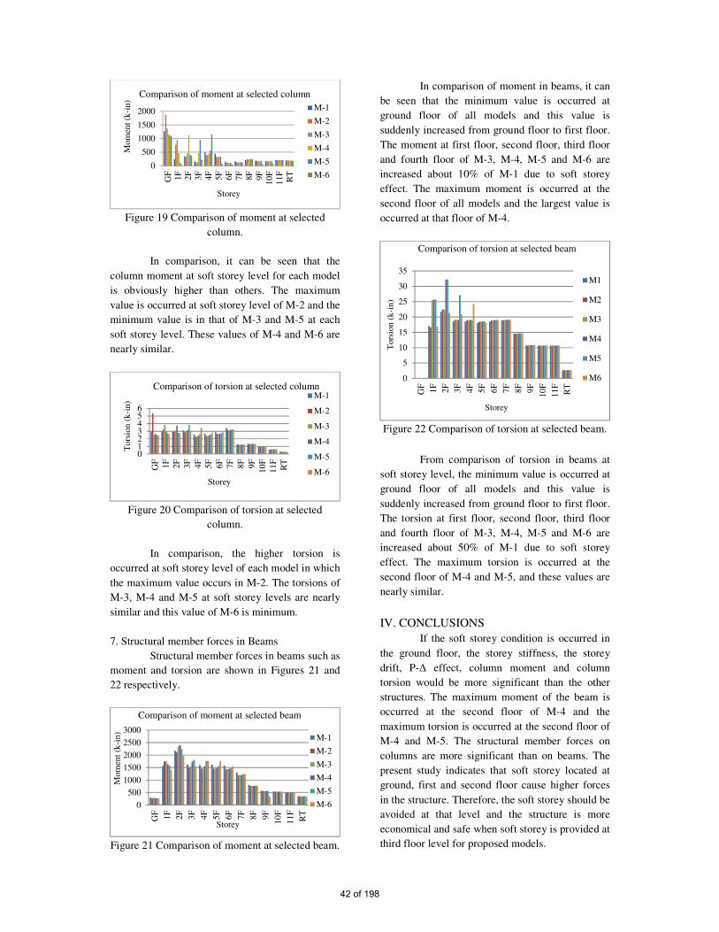
Figure 19 Comparison of moment at selected

column.

In comparison, it can be seen that the

column moment at soft storey level for each model

is obviously higher than others. The maximum

value is occurred at soft storey level of M-2 and the

minimum value is in that of M-3 and M-5 at each

soft storey level. These values of M-4 and M-6 are

nearly similar.

Figure 20 Comparison of torsion at selected

column.

In comparison, the higher torsion is

occurred at soft storey level of each model in which

the maximum value occurs in M-2. The torsions of

M-3, M-4 and M-5 at soft storey levels are nearly

similar and this value of M-6 is minimum.

7. Structural member forces in Beams

Structural member forces in beams such as

moment and torsion are shown in Figures 21 and

22 respectively.

Figure 21 Comparison of moment at selected beam.

In comparison of moment in beams, it can

be seen that the minimum value is occurred at

ground floor of all models and this value is

suddenly increased from ground floor to first floor.

The moment at first floor, second floor, third floor

and fourth floor of M-3, M-4, M-5 and M-6 are

increased about 10% of M-1 due to soft storey

effect. The maximum moment is occurred at the

second floor of all models and the largest value is

occurred at that floor of M-4.

Figure 22 Comparison of torsion at selected beam.

From comparison of torsion in beams at

soft storey level, the minimum value is occurred at

ground floor of all models and this value is

suddenly increased from ground floor to first floor.

The torsion at first floor, second floor, third floor

and fourth floor of M-3, M-4, M-5 and M-6 are

increased about 50% of M-1 due to soft storey

effect. The maximum torsion is occurred at the

second floor of M-4 and M-5, and these values are

nearly similar.

IV. CONCLUSIONS

If the soft storey condition is occurred in

the ground floor, the storey stiffness, the storey

drift, P-Δ effect, column moment and column

torsion would be more significant than the other

structures. The maximum moment of the beam is

occurred at the second floor of M-4 and the

maximum torsion is occurred at the second floor of

M-4 and M-5. The structural member forces on

columns are more significant than on beams. The

present study indicates that soft storey located at

ground, first and second floor cause higher forces

in the structure. Therefore, the soft storey should be

avoided at that level and the structure is more

economical and safe when soft storey is provided at

third floor level for proposed models.

0

500

1000

1500

2000

GF

1F

2F

3F

4F

5F

6F

7F

8F

9F

10

F

11

F

RT

Mom

ent

(k-i

n)

Storey

Comparison of moment at selected column

M-1

M-2

M-3

M-4

M-5

M-6

0123456

GF

1F

2F

3F

4F

5F

6F

7F

8F

9F

10

F

11

F

RT

Tors

ion

(k

-in

)

Storey

Comparison of torsion at selected columnM-1

M-2

M-3

M-4

M-5

M-6

0

500

1000

1500

2000

2500

3000

GF

1F

2F

3F

4F

5F

6F

7F

8F

9F

10

F

11

F

RT

Mom

ent

(k-i

n)

Storey

Comparison of moment at selected beam

M-1

M-2

M-3

M-4

M-5

M-6

0

5

10

15

20

25

30

35

GF

1F

2F

3F

4F

5F

6F

7F

8F

9F

10

F

11

F

RT

Tors

ion

(k

-in

)

Storey

Comparison of torsion at selected beam

M1

M2

M3

M4

M5

M6

42 of 198

ACKNOWLEDGMENT(S)

The author wishes to express grateful

thanks to Dr. Theingi, Rector of Technological

University (Thanlyin). The author wishes to

express the deepest thanks and gratitude to her

supervisor Dr. Kyaw Zeyar Win, Professor of Civil

Engineering Department of Technological

University (Thanlyin). The author special thanks go

to her co-supervisor Dr. Ni Ni Moe Kyaw, Lecturer

of Civil Engineering Department of Technological

University (Thanlyin), for her invaluable advice

and effective suggestion throughout the study. The

author would like to express her thanks to her

teacher Daw Ei Ei Kyaw, Assistant Lecturer of

Civil Engineering Department of Technological

University (Thanlyin), for her valuable comments

and indispensable guidance during this study.

Finally, her special thanks to all who helped her

towards the successful completion of this study.

REFERENCES

[1] IS 1893 2002, “Indian Standard Criteria for

Earthquake Resistance Design of Structures

Part I General Provisions and Buildings”

Bureau of Indian Standard, New Delhi, 2002.

[2] American Concrete Institute Committee,

“Building Code Requirements for Structural

Concrete, ACI-99,” 1999.

[3] International Conference of Building Officials,

Uniform Building Code, Vol II”, Structural

Engineering Design Provision, UBC-97, 1997

[4] Dogan, Mizan, Kirac, Nevzat and Gonen, “Soft

Storey Behaviour in Earthquake and Samples,”

August, 2012.

[5] Murty, C.V.R. “Why are Open Ground Storey

Buildings Vulnerable in Earthquakes,” August

2012.

[6] Committee for Quality Control of High-Rise

Building Construction Projects, 2017.

43 of 198

Design of Water Distribution System Using Hydraulic Analysis Program

(EPANET 2.0) for Tatkon Town in Myanmar

Aung Myo Wai 1, Haicheng Liu

2

1 Engineering Department (Water and Sanitation)

Naypyidaw Development Committee, Naypyidaw - 15011, Myanmar

2 School of Environmental Science and Engineering

Suzhou University of Science and Technology, Suzhou - 215000, People’s Republic of China

1 [email protected],

2 [email protected]

Abstract - Water is one of the plentiful things in

the world. If the water cannot be available, the

living things cannot grow and live. It is a basic

requirement and it influences social, economic and

living standard of human beings. Nowadays

Sustainable development is a major interest. High-

quality infrastructure of water system takes part

in a key role for any kind growth of a city. Here in

this paper, medium town in Naypyidaw of

Myanmar, Tatkon has been emphasized for design

purpose. Although new towns in Naypyidaw have

proper water supply system for inhabitants, there

is no strategic plan yet to develop the water supply

system for that town. Supply water distribution

network of Tatkon town area was selected for

detail analysis and design. The area has been

modeled using EPANET software on the basis of

data surveyed by Tatkon TDC. Assessment of

required pressure head, velocity coverage, water

age and residual chlorine (chemical) concentration

has been done. In addition, the design is made

keeping in view of the population growth rate, and

the developing town up to 2048. Finally, this paper

offers a modeling strategy of Tatkon town which

intends at proposing solutions to the challenges of

lacking proper water supply system and reducing

menace associated with waterborne disease.

Keywords: EPANET software, network analysis,

pressure head, residual chlorine (chemical)

concentration, velocity, water distribution system.

1. INTRODUCTION

Water and related services must be as part of the

economic development business. Many of the major

problems that humanity is facing in the twenty-first

century are related to water quantity and/or water

quality issues, and which currently affects more than

a third of the people in the world (Schwarzenbach et

al., 2010). In developing countries, where most of the

sewage is discharged without treatment, the

improvement of sanitation and access to safe drinking

water are primarily important. In the report of

Myanmar demographic and health survey (2015-

2016), 80% of all households have access to an

improved drinking water source, as do 89% of urban

households and 77% of rural households. However,

distribution of households by the source of drinking

water is only 6% of Myanmar’s population as safe

and piped water into their residence (MOHS, 2017).

Water distribution networks play an important

role in modern societies being its proper operation

directly related to the resident. Naypyidaw, capital

city of Myanmar, is very imperative in modern

society to insure the availability of potable water and

to plan and design for a sustainable economic

suitable pipe network system or water supply

schemes. Tatkon town is an inaccessible water supply

area of Naypyidaw and people use only tube well or

insufficient water supply system. With the aim of

understanding the nature of progress, looking

carefully is important of the way that improvements

in water and sanitation have benefited different

socioeconomic groups.

44 of 198

At the present time, marketable computer

software applications are accessible to characterize

configuration of distribution system and pipe network

where detailed information with the pipe properties

like “Diameter, Length, Pipe material etc.” and

devices like “Pumps, Valves etc.” are provided.

The analysis of design is done by using the

software EPANET. It is such a computer based

program that performs extended period simulation of

hydraulic and water quality behavior within

pressurized pipe networks. The overall objective of

this project is to construct a distribution system

model using EPANET and assesses system criteria

and limitations. The main objective of water

distribution system is to supply water at acceptable

pressure and velocity to meet the requirement. In

support of suitable assessment of a distribution

system computation of flow, velocity and pressure is

essential. These parameters can be calculated

competently with the aid of EPANET. Despite the

fact that EPANET has some limitations, such as it

does not account phenomena such as water hammer,

pipe bursting, behavior of non-return valves and

starting a pump or stopping it.

The primary goal of the distribution systems is to

maintain adequate water pressure at various points

i.e., at the consumer's tap and the selection of the

distribution and its elevation regarding the location of

the water treatment plants.

2. STUDY AREA

Tatkon is located on the central basin of

Myanmar. It is about 60 km far from Naypyidaw

(capital city of Myanmar) and 422 km from Yangon.

It is located between 19°- 55′ and 20°-21′ of North

latitude and 95°-20′ and 96°-30′ of East longitude and

at the altitude of 2250′ above sea level. Location map

of Tatkon is shown in figure 1.2. Located to the

South of the town is Pobbathiri (Naypyidaw), to the

North is Yamethin (Mandalay Region), to the West is

Myothit (Magway Region) and to the East is

Pinlaung (Shan State). It includes 5 Numbers of

District Meter Area (DMA) which is mainly central

part of Tatkon starting from Moekaung pagoda and

ending to township football field.

Fig.1 Location Map of Tatkon in Naypyidaw

Fig.2 Map of Study Area

2.1 Data collection

The data was provided by Tatkon Township

Development Committee (TDC). Data of individual

ID and Labels of Pipes along with specified length,

diameter& material was obtained. Data of individual

Nodes with specified elevation and demand was also

provided.

45 of 198

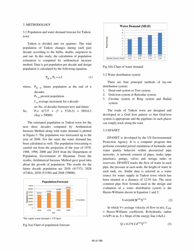
3. METHODOLOGY

3.1 Population and water demand forecast for Tatkon

town

Tatkon is divided into six quarters. The total

population of Tatkon changes during each past

decade according to the births, deaths, migration in

and out. In this study, the calculation of population

estimation is computed by arithmetical increase

method. Data is got population per decade and design

population is calculated by the following equation.

Pn = P0 + n I (1)

where, Pn = future population at the end of n

decades

P0 = present population

I = average increment for a decade

n= No. of decades between now and future

So, P3= 41737 + (3 x 5726.5) = 58916.5

(Say = 59000)

The estimated population in Tatkon town for the

next three decades computed by Arithmetical

Increase Method along with water demand is plotted

in Figure-3. The population was forecasted up to the

year of 2048. For the same the water demand has

been calculated as well. The population forecasting is

carried out from the projection of the year of 1978,

1988, 1998, 2008 and 2018 from the Department of

Population, Government of Myanmar. From the

results, Arithmetical Increase Method gave good idea

about the growth of population. The results for the

future decade population are 2018 (41737), 2028

(47464), 2038 (53190) and 2048 (59000).

*Per capita water demand = 135 lpcd

Fig.3(a) Chart of population forecast

Fig.3(b) Chart of water demand

3.2 Water distribution system

There are four principal methods of lay-out

distribution system:

1. Dead-end system or Tree system,

2. Grid-iron system or Reticular system,

3. Circular system or Ring system and Radial

system.

The roads of Tatkon town are designed and

developed in a Grid Iron pattern so that Grid-iron

system is appropriate and the pipelines in such places

can simply track along the road.

3.3 EPANET

EPANET is developed by the US Environmental

Protection Agency. It is a computer program that

performs extended period simulation of hydraulic and

water quality behavior within pressurized pipe

networks. A network consists of pipes, nodes (pipe

junctions), pumps, valves and storage tanks or

reservoirs. EPANET tracks the flow of water in each

pipe, the pressure at each node, the height of water in

each tank, etc. Sinthe dam is selected as a water

source for water supply in Tatkon town which has

been situated at a distance of 12.93 km. The most

common pipe flow formula used in the design and

evaluation of a water distribution system is the

Hazen-Williams shown in Equation 1 and 2:

V=0.849CR0.63

S0.54

(2)

In which V= average velocity of flow in m/s, CHW

= Hazen-Williams coefficient, R=hydraulic radius

(=A/P) in m, S = Slope of the energy line (=hf/L).

Q = 0.278 Cd0.63

S0.54

(3)

46 of 198

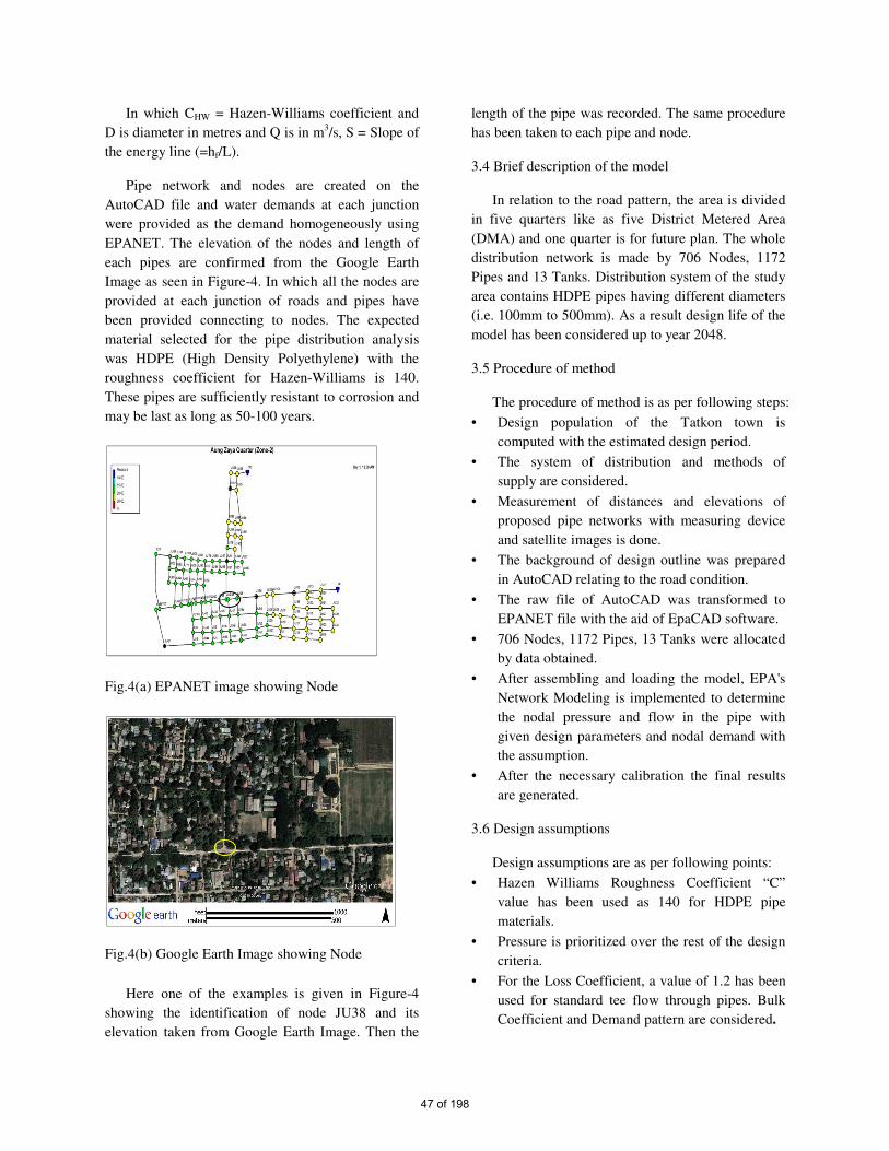
In which CHW = Hazen-Williams coefficient and

D is diameter in metres and Q is in m3/s, S = Slope of

the energy line (=hf/L).

Pipe network and nodes are created on the

AutoCAD file and water demands at each junction

were provided as the demand homogeneously using

EPANET. The elevation of the nodes and length of

each pipes are confirmed from the Google Earth

Image as seen in Figure-4. In which all the nodes are

provided at each junction of roads and pipes have

been provided connecting to nodes. The expected

material selected for the pipe distribution analysis

was HDPE (High Density Polyethylene) with the

roughness coefficient for Hazen-Williams is 140.

These pipes are sufficiently resistant to corrosion and

may be last as long as 50-100 years.

Fig.4(a) EPANET image showing Node

Fig.4(b) Google Earth Image showing Node

Here one of the examples is given in Figure-4

showing the identification of node JU38 and its

elevation taken from Google Earth Image. Then the

length of the pipe was recorded. The same procedure

has been taken to each pipe and node.

3.4 Brief description of the model

In relation to the road pattern, the area is divided

in five quarters like as five District Metered Area

(DMA) and one quarter is for future plan. The whole

distribution network is made by 706 Nodes, 1172

Pipes and 13 Tanks. Distribution system of the study

area contains HDPE pipes having different diameters

(i.e. 100mm to 500mm). As a result design life of the

model has been considered up to year 2048.

3.5 Procedure of method

The procedure of method is as per following steps:

• Design population of the Tatkon town is

computed with the estimated design period.

• The system of distribution and methods of

supply are considered.

• Measurement of distances and elevations of

proposed pipe networks with measuring device

and satellite images is done.

• The background of design outline was prepared

in AutoCAD relating to the road condition.

• The raw file of AutoCAD was transformed to

EPANET file with the aid of EpaCAD software.

• 706 Nodes, 1172 Pipes, 13 Tanks were allocated

by data obtained.

• After assembling and loading the model, EPA's

Network Modeling is implemented to determine

the nodal pressure and flow in the pipe with

given design parameters and nodal demand with

the assumption.

• After the necessary calibration the final results

are generated.

3.6 Design assumptions

Design assumptions are as per following points:

• Hazen Williams Roughness Coefficient “C”

value has been used as 140 for HDPE pipe

materials.

• Pressure is prioritized over the rest of the design

criteria.

• For the Loss Coefficient, a value of 1.2 has been

used for standard tee flow through pipes. Bulk

Coefficient and Demand pattern are considered.

47 of 198

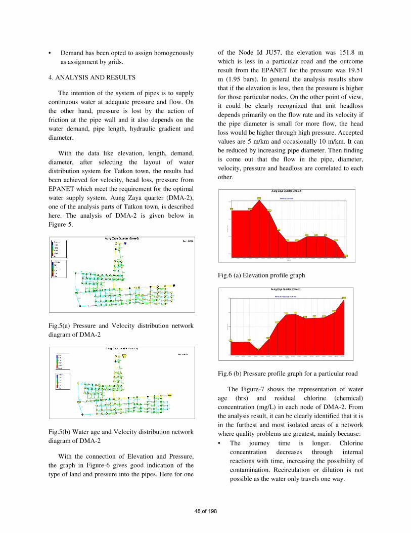
• Demand has been opted to assign homogenously

as assignment by grids.

4. ANALYSIS AND RESULTS

The intention of the system of pipes is to supply

continuous water at adequate pressure and flow. On

the other hand, pressure is lost by the action of

friction at the pipe wall and it also depends on the

water demand, pipe length, hydraulic gradient and

diameter.

With the data like elevation, length, demand,

diameter, after selecting the layout of water

distribution system for Tatkon town, the results had

been achieved for velocity, head loss, pressure from

EPANET which meet the requirement for the optimal

water supply system. Aung Zaya quarter (DMA-2),

one of the analysis parts of Tatkon town, is described

here. The analysis of DMA-2 is given below in

Figure-5.

Fig.5(a) Pressure and Velocity distribution network

diagram of DMA-2

Fig.5(b) Water age and Velocity distribution network

diagram of DMA-2

With the connection of Elevation and Pressure,

the graph in Figure-6 gives good indication of the

type of land and pressure into the pipes. Here for one

of the Node Id JU57, the elevation was 151.8 m

which is less in a particular road and the outcome

result from the EPANET for the pressure was 19.51

m (1.95 bars). In general the analysis results show

that if the elevation is less, then the pressure is higher

for those particular nodes. On the other point of view,

it could be clearly recognized that unit headloss

depends primarily on the flow rate and its velocity if

the pipe diameter is small for more flow, the head

loss would be higher through high pressure. Accepted

values are 5 m/km and occasionally 10 m/km. It can

be reduced by increasing pipe diameter. Then finding

is come out that the flow in the pipe, diameter,

velocity, pressure and headloss are correlated to each

other.

Fig.6 (a) Elevation profile graph

Fig.6 (b) Pressure profile graph for a particular road

The Figure-7 shows the representation of water

age (hrs) and residual chlorine (chemical)

concentration (mg/L) in each node of DMA-2. From

the analysis result, it can be clearly identified that it is

in the furthest and most isolated areas of a network

where quality problems are greatest, mainly because:

• The journey time is longer. Chlorine

concentration decreases through internal

reactions with time, increasing the possibility of

contamination. Recirculation or dilution is not

possible as the water only travels one way.

48 of 198

Some of link results and node results of DMA-2

are as shown in Table-1 and Table-2.

Fig.7 (a) Water age contour graph

Table-1: Link Results

Fig.7 (b) Chemical contour graph for DMA-2

Table-2: Node Results

5. CONCLUSION

The projected distribution network of Tatkon

town consists of five zones. This network is arranged

according to those days’s requirement to the future

(2048) needs and demands. The design capacity of

the distribution network is 11.43 MLD which is

sufficient for the future design demand of 2048.

Hence the 13 elevated tanks (452.6 m3) must support

a capacity to suppress the future demand. So a new

network is to be designed to meet future demands and

to reach the user’s door step. The new network is

placed according to the road pattern using master

plan in view of the town in future.

Main problems to be paid attention to when using

the software are to meet all design criteria for

optimization and to define phases like as net tracing

and dimensioning the elements. The deficiency of

software is to leave out phenomena such as water

hammer, pipe bursting, behavior of non-return valves

and starting a pump or stopping it. But this work

hopes to be a good step toward further understanding

of comprehensive design and research.

The design of water distribution system of Tatkon

town showed suitable and provides minimum head

loss, maximum pressure and efficient diameter. The

49 of 198

results of the analysis are confirmed by hydraulic

equations. Finally, this study would assist the water

supply engineers in saving time under one umbrella

because this process is fast, more attractive, easy to

integrate the changes.

ACKNOWLEDGEMENTS

I would like to express my gratitude to my

supervisor, Associated Professor Haicheng Liu,

School of Environmental Science and Engineering,

Suzhou University of Science and Technology,

Suzhou, China for supporting me in completing my

work successfully by providing the required facilities

and advices. I am also grateful to our School of

Environmental Science and Engineering for their

cooperation during my academic days and providing

guidance. I would like to thank The Chinese Ministry

of Commerce, Chinese Government Scholarships to

students from developing countries, for providing me

the necessary fund for the paper. Special thanks are

due to Naypyidaw Development Committee and

Yangon Technological University for encouragement

of the study. Finally, I am grateful to my family for

their kind support and encouragement.

REFERENCES

[1] Anisha, G., Kumar, A., Kumar, J. A., & Raju, P.

S. (2016). Analysis and Design of Water

Distribution Network Using EPANET for

Chirala Municipality in Prakasam District of

Andhra Pradesh. International Journal of

Engineering and Applied Sciences, 3(4).

[2] Dave, B. H., Rajpara, G., Patel, A., & Kalubarme,

M. H. Analysis of Continuous Water

Distribution System in Gandhinagar City Using

EPANET Software: A Case Study of Sector-8.

[3] Ministry of Health and Sports. (2017).

Demographic and Health Survey Myanmar

2015-2016. Ministry of Health and Sports,

Naypyitaw, The Republic of the Union of

Myanmar.

[4] Montasir, M., Abrar, A. C., Rifat, M., &

Mahommad, S. R. (2015). Water Distribution

System Modelling By Using EPA-NET Software.

In International Conference on Recent

Innovation in Civil Engineering for Sustainable

Development, Gazipur, Bangladesh (pp. 960-

964).

[5] Muranho, J., Ferreira, A., Sousa, J., Gomes, A.,

& Marques, A. S. (2014). Technical performance

evaluation of water distribution networks based

on EPANET. Procedia Engineering, 70, 1201-

1210.

[6] Ramesh, H., Santhosh, L., & Jagadeesh, C. J.

(2012, January). Simulation of hydraulic

parameters in water distribution network using

EPANET and GIS. In International Conference

on Ecological Environmental and Biological

Sciences (ICEEBS’2012) Jan (pp. 7-8).

[7] Rossman, L. A. (2000). EPANET 2 users manual,

water supply and water resources

division. National Risk Management Research

Laboratory, US Environmental Protection

Agency, Cincinnati, Ohio.

[8] Schwarzenbach, R. P., Egli, T., Hofstetter, T. B.,

Von Gunten, U., & Wehrli, B. (2010). Global

water pollution and human health. Annual

Review of Environment and Resources, 35, 109-

136.

50 of 198

STUDY ON THE BEHAVIOR OF SPUN PILE FOUNDATION

DUE TO SEISMIC LOADING

Chan Myae Kyi#1

, Dr.Nyan Phone#2

, Myat Thidar Tun#3

Department of Civil Engineering

Technological University (Thanlyin), Yangon, Myanmar

Abstract- This aim of the paper is the study on

the behavior of spun pile foundation due to

effect of seismic loading. This foundation

describes the lateral deflection and settlement

due to seismic load by applying static load

case and dynamics load case. These results are

described by using ETABS software. To

design the foundation, the super structure of

sixteenth storeyed R.C building with basement

is analyzed by applying static load case and

dynamics load case of ETABS software. The

two results of unfactored load are used to

study the behavior of spun pile by applying the

superstructure from two different load

combinations. According to the result of

unfactored load of superstructure, the same

number of pile is divided into three groups.

Allowable bearing capacity is gained from the

soil report of Inya Lake Residence Project in

Yangon. The allowable bearing capacity of

soil is calculated by Terzaghi based on

Meyerhof’s Method. The smallest area of spun

pile foundation is used. The size of spun pile is

outside diameter 400 mm and thickness 75mm

slender shape. The pile working load from

materials for spun pile is 54 tons. The required

length for 54 tons spun pile regard to 85 ft

according to calculation of the allowable

bearing capacity .The analyzing results of

deflection and settlement for spun pile are

within allowable limits. The results of

deflection and settlement of spun pile

foundation due to the effect of two load

combinations are compared.

I. INTRODUCTION

Pile foundation is the part of a

structure used to carry the applied column load

of a super structure to the allowable bearing

capacity of the ground surface at the same

depth. The common used shape of pile is

rectangular and slender which applied the load

to the stratum of high bearing capacity. In the

case of heavy construction, the bearing

capacity of shallow soil will not be

satisfactory; the construction should be built

on pile foundation. It is used where soil having

low bearing capacity respect to loads coming

on structure or the stresses developed due to

earthquake cannot be accommodated by

shallow foundation. To obtain the most

economical and durable foundation, the

engineers have to consider the super structure

loads, the soil condition and desired to

tolerable settlement. Pile foundations are

convened to construct the multi-storeyed

building and work for water, such as jetties as

bridge pier. The types of prestressed concrete

pile are usually of square, triangular, triangle,

circle and octagonal section which are

produced in suitable length in one meter

interval between 3 and 13 meters. Nowadays,

most people use spun pile foundation one of

the most prestressed concrete pile to construct

most of the buildings and bridges. Spun piles

are widely used in construction. Prestressed

concrete cylinder pile is a special type of

precast concrete pile with a hollow circular

cross section. Advantage of using spun pie are

spun pile is less permeable than reinforced

concrete pile, thus it has a good performance

in marine environment. So the design of spun

pile foundation can be based on the deflection

and settlement due to earthquake.

II.PREPARATION DATA FOR ANALY-

SICS OF SPUN PILE FOUNDATION

Information of structure and material

properties is prescribed as follows. Dead load,

live load, wind load and earthquake loads are

considered in proposed building. The typical

beam plans and 3D view of the proposed

buildings from ETABs software are shown in

Figure 1 and Figure 2.

A. Site location and Profile of structure

Type of structure: 16th storyed R.C Building

51 of 198

Location : Seismic zone (4)

Soil Type : Silty Sand, SD

Type of Occupancy : Residential

Shape of Building : Rectangular shape

Size of Building : Length = 81 ft

: Width = 65 ft

: Height =162 ft

Height of Building: Typical story height = 10ft

Bottom story height = 12ft

B. Design Codes

Design code applied for superstructure

are ACI (318-99) and UBC-97 There are 26

numbers of load combinations which are

accepted for beam, column and slab etc

(1)Material Properties

Analysis property data

Weight per unit volume of concrete= 150 pcf

Modulus of elasticity = 3.12 x 10⁶

Poisson’s ratio = 0.2

Design property data

Reinforcing yield stress (fy) = 50000 psi

Shear reinforcing yield stress (fy) = 50000 psi

Concrete strength (f′c) = 3000 psi

Concrete cylinder strength (f′c) = 3500 psi

C. loading Considerations

The applied loads are dead loads, live loads,

earthquake load and wind load.

(1) Gravity Loads: Data for dead loads which

are used in structural analysis are as follows;

Unit weight of concrete = 150 pcf

4½ inches thick wall weight = 50 psf

9 inches thick wall weight = 100psf

Light partition weight = 20 psf

Finishing Weight = 20 psf

Weight of elevator = 2 ton

Data for live loads which are used in structural

analysis are as follows:

Live load on slab = 40 psf

Live load on lift = 100 psf

Live load on stairs = 100 psf

Live load on corridors = 60 psf

Live load on roof = 20 psf

Weight of water = 2ton

(2)Lateral loads: Data for wind loads which

are used in structural analysis are as follows;

Exposure Type = B

Basic wind velocity =100mph

Important factor, Iw = 1.0

Windward Coefficient = 0.8

Leeward Coefficient = 0.5

Data for earthquake load are as follows:

Soil profile type = SD

Seismic Zone = 2B

Seismic Zone Factor = 0.2

Building period coefficient, Ct = 0.03

Important Factor, I = 1

Seismic coefficient, Ca = 0.28

Seismic coefficient, Cv = 0.4

The magnitude of earthquake loading

depends upon the weight or mass of building,

dynamic properties of the building and

difference in stiffness of adjacent floors along

with the intensity and duration of the

earthquake.

(3)Lateral Load Combination: According to

(ACI 318-99) codes, the design of load

combination are as follows

52 of 198

Table 1 Load Combination for Static

No Load Combination

1 1.4 DL

2 1.4 D + 1.7 LL

3 1.05DL + 1.275LL + 1.275WX

4 1.05DL + 1.275LL – 1.275 WX

5 1.05DL + 1.275LL + 1.275 WY

6 1.05DL + 1.275LL - 1.275 WY

7 0.9DL + 1.3 WX

8 0.9DL -1.3 WX

9 0.9DL + 1.3 WY

10 0.9DL - 1.3 WY

11 1.05DL + 1.28LL + EX

12 1.05DL + 1.28LL - EX

13 1.05DL + 1.28LL + EY

14 1.05DL + 1.28LL - EY

15 0.9DL + 1.02 EX

16 0.9DL - 1.02 EX

17 0.9DL + 1.02 EY

18 0.9DL - 1.02 EY

19 1.16DL + 1.28 LL + EX

20 1.16DL + 1.28 LL - EX

21 1.16DL + 1.28 LL + EY

22 1.16DL + 1.28 LL – EY

23 0.79DL + 1.02 EX

24 0.79DL - 1.02 EX

25 0.79DL + 1.02 EY

26 0.79DL - 1.02 EY

Table 2 Load Combination for Dynamics

No Load Combination

1 1.4 DL

2 1.4 D + 1.7 LL

3 1.05DL + 1.275LL + 1.275WX

4 1.05DL + 1.275LL – 1.275 WX

5 1.05DL + 1.275LL + 1.275 WY

6 1.05DL + 1.275LL - 1.275 WY

7 0.9DL + 1.3 WX

8 0.9DL -1.3 WX

9 0.9DL + 1.3 WY

10 0.9DL - 1.3 WY

11 1.05DL + 1.28LL + 1 SPEC X

12 1.05DL + 1.28LL – 1 SPEC X

13 1.05DL + 1.28LL + 1 SPEC Y

14 1.05DL + 1.28LL – 1 SPECY

15 0.9DL + 1.02 SPEC 1

16 0.9DL - 1.02 SPEC 1

17 0.9DL + 1.02 SPEC 2

18 0.9DL - 1.02 SPEC 2

19 1.16DL + 1.28 LL + SPEC X

20 1.16DL + 1.28 LL – SPEC X

21 1.16DL + 1.28 LL + SPEC Y

22 1.16DL + 1.28 LL – SPEC Y

23 0.79DL + 1.02 SPEC X

24 0.79DL - 1.02 SPEC X

25 0.79DL + 1.02 SPEC Y

26 0.79DL - 1.02 SPEC Y

III.DESIGN RESULTS OF PROPOSED

BUILDING

The design results of beam and column for

proposed building are described.

Table 3. Design Results for Column, Beam and

Slab

Section Size (Static) Size (Dynamics)

Column (12″ × 12″)

(14″× 14″ )

(16″ × 16″)

(18″ × 18″)

(20″ × 20″)

(22″ × 22″)

(24″ × 24″)

(26″ × 26″)

(28″ × 28″)

(14″× 14″ )

(16″ × 16″)

(18″ × 18″)

(20″ × 20″)

(22″ × 22″)

(24″ × 24″)

(26″ × 26″)

(28″ × 28″)

(30″ × 30″)

Beam (9″ × 9″)

(9″ × 12″)

(12″ × 16″)

(12″ × 18″)

(12″ × 20″)

(14″ × 18″)

(14″ × 20″)

(9″ × 9″)

(9″ × 12″)

(10″ × 12″)

(12″ × 16″)

(12″ × 18″)

(12″ × 20″)

(14″ × 18″)

(14″ × 20″)

Slab 4 ″, 4.5″, 5″ 4 ″, 4.5″, 5″

Wall 8″, 12″ & 16″ 8″, 12″ & 16″

Figure.1 3D Model of Proposed Building

53 of 198

IV. STABILITY OF THE

SUPERSTRUCTURE CHECKING

The design superstructure is checked for

(1) Overturning,

(2) Story Drift

(3) Torsional Irregularity

(4) P-∆ Effect

Table 4. Stability Checking

static

load

case

Checking

X-

Direc:

Y-

Direc:

Limit

OTM Static 20.08 14.39 >1.5

Dynamics 33.91 33.92 >1.5

Story

Drift

Static 0.59 0.7 <2.4

Dynamics 0.92 1.2 <2.4

Torsion Static 1 1 <1.2

Dynamics 1 1 <1.2

P-∆

Effect

Static 0.002 0.031 >0.1

Dynamics 0.025 0.035 >0.1

All checking for stability of

superstructure are within the limits. The results

of unfactored load are received by applying

ETAB software. The base point levels of super

structure are described in Figure2.

Figure2. Point Levels Layout Plan

V. PILE WORKING FROM MATERIAL

Shear reinforcing yield stress (fy) = 50000 psi

Concrete cylinder strength (f′c) = 3500 psi

Modulus of elasticity = 3.37 x10⁶

фPT = 0.7 ( 0.33 f′c Ac + 0.39

fyAst)(ACI318-99)

= 0.7 (0.33 × 3500 × 122+ 0.39 ×

50000 × 10 × 0.31)

= 140952 lbs.

= 62 Tons

0.86фPT= 0.86 × 62

= 54.11 Tons (Use 54 Tons)

VI. CALCULATION ALLOWABLE

BEARING CAPACITY

According to CQHP Guideline

Up to 10,000 ft² Area – one bore hole for

2,500 ft²(min)

≥ Two bore hole

For this project,

Project area = 81′-0″ × 65′-0″

= 5265 ft²

Three bore holes are adequate.

For the evaluation of bearing capacity

of pile foundation, the formula for calculation

of bearing capacity of two pile foundations,

derived from “A modified version of the

Terzaghi bearing capacity equation for pile

design” would be applied for this analysis

Table6. Allowable Bearing Capacity

Name Qb

(KN)

Qs

(KN)

Qall

(KN)

F.S Qult

(Ton)

BH1 146.9 1343.5 1490.4 3 49.7

BH2 154.7 1363.1 1517.7 3 50.6

BH3 193.4 1637.5 1830.9 3 61.0

Average Allowable Bearing Capacity 54

VII. ANALYSIS RESULTS OF SPUN PILE

FOUNDATION

The used number of spun pile are

described in the following by analyzing and

design due to static and dynamics of ETABS

54 of 198

software. These numbers of spun pile are

justified to resist the superstructure.

Figure 3. Spun Pile Layout Plan (Static Load

Case)

Figure4. Spun Pile Layout Plan (Dynamics

Load Case)

The group 1,2,3 are considered from the

total unfactored load of point 1, point 24 and

Point 30+31+53+54+55 of shear wall loading

because of applying the reaction of

superstructure by two load cases. These

groups are compared to study the behavior of

spun pile due to apply the two types of load

combinations. The used number of pile and the

size of pile cap are described in table 6 and 7.

Table6. Required Number Pile Cap Size

Name No of

pile

L(m) B(m) H(m)

GP1 6 1.68 2.44 0.91

GP2 9 2.44 2.44 1.22

GP3 66 6.7 3.66 1.52

Table7. Required Number Pile Cap Size

Name No of

pile

L(m) B(m) H(m)

GP1 9 2.44 2.44 1.22

GP2 9 2.44 2.44 1.22

GP3 66 6.7 3.66 1.52

Figure5. 3D Modeling for Combination of

Superstructure and Substructure

The results of spun pile foundation are

described in figure 6, 7, 8, 9, 10 and 11 by

applying two load cases.

Comparison of deflection due to seismic load

in X-direction (For Group 1)

Figure 6. Deflectionalong Spun Pile

-33-31.5

-30-28.5

-27-25.5

-24-22.5

-21-19.5

-18-16.5

-15-13.5

-12-10.5

-9-7.5

-6-4.5

-3

-10 0 10 20 30

Static

Dynamics

Deflection in X- direction (mm)

55 of 198

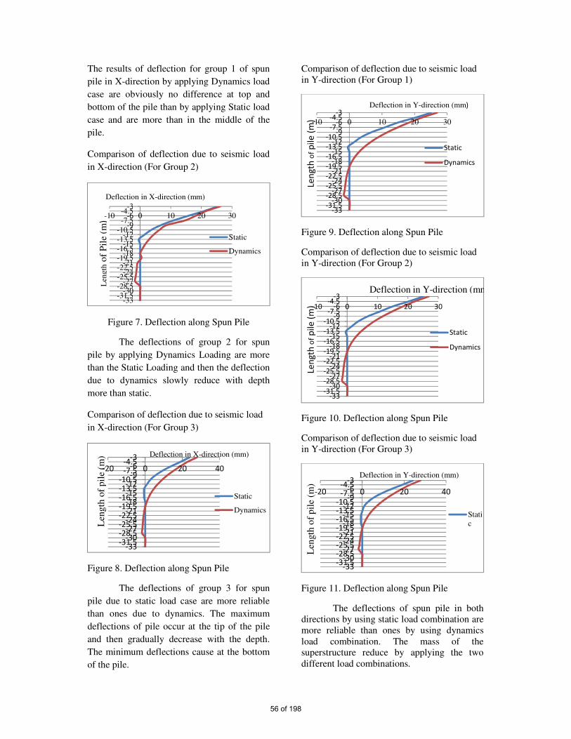
The results of deflection for group 1 of spun

pile in X-direction by applying Dynamics load

case are obviously no difference at top and

bottom of the pile than by applying Static load

case and are more than in the middle of the

pile.



Figure 7. Deflection along Spun Pile

The deflections of group 2 for spun

pile by applying Dynamics Loading are more

than the Static Loading and then the deflection

due to dynamics slowly reduce with depth

more than static.




The deflections of group 3 for spun

pile due to static load case are more reliable

than ones due to dynamics. The maximum

deflections of pile occur at the tip of the pile

and then gradually decrease with the depth.

The minimum deflections cause at the bottom

of the pile.


in Y-direction (For Group 1)








The deflections of spun pile in both

directions by using static load combination are

more reliable than ones by using dynamics

load combination. The mass of the

superstructure reduce by applying the two

different load combinations.

-33-31.5

-30-28.5

-27-25.5

-24-22.5

-21-19.5

-18-16.5

-15-13.5

-12-10.5

-9-7.5

-6-4.5

-3

-10 0 10 20 30

Static

Dynamics

Deflection in X-direction (mm)

Len

gth

of

Pil

e (m

)

-33-31.5

-30-28.5

-27-25.5

-24-22.5

-21-19.5

-18-16.5

-15-13.5

-12-10.5

-9-7.5

-6-4.5

-3

-20 0 20 40

Static

Dynamics

Deflection in X-direction (mm)

Len

gth

of

pil

e (m

)

-33-31.5

-30-28.5

-27-25.5

-24-22.5

-21-19.5

-18-16.5

-15-13.5

-12-10.5

-9-7.5

-6-4.5

-3

-10 0 10 20 30

Static

Dynamics

Deflection in Y-direction (mm)

Len

gth

of

pil

e (

m)

-33-31.5

-30-28.5

-27-25.5

-24-22.5

-21-19.5

-18-16.5

-15-13.5

-12-10.5

-9-7.5

-6-4.5

-3

-10 0 10 20 30

Static

Dynamics

Deflection in Y-direction (mm

Len

gth

of

pil

e (

m)

-33-31.5

-30-28.5

-27-25.5

-24-22.5

-21-19.5

-18-16.5

-15-13.5

-12-10.5

-9-7.5

-6-4.5

-3

-20 0 20 40

Stati

c

Deflection in Y-direction (mm)

Len

gth

of

pil

e (m

)

56 of 198

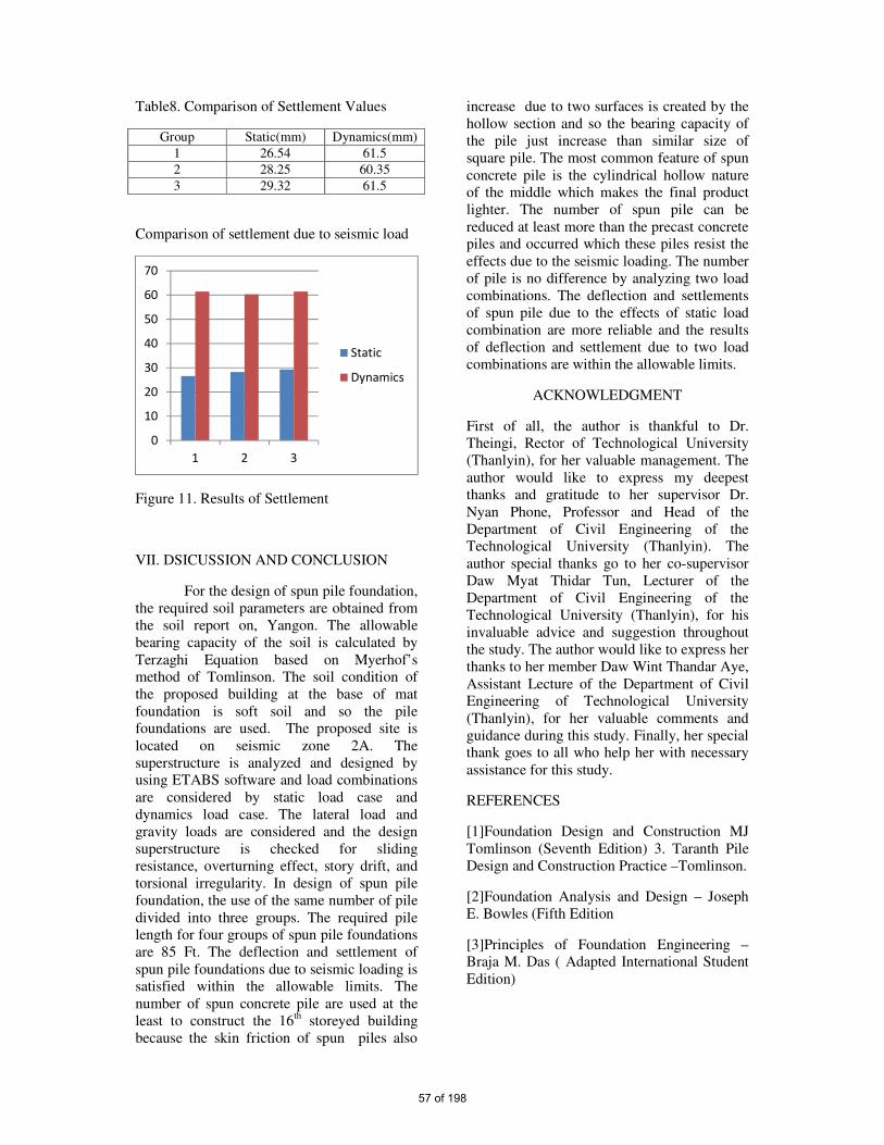
Table8. Comparison of Settlement Values

Group Static(mm) Dynamics(mm)

1 26.54 61.5

2 28.25 60.35

3 29.32 61.5

Comparison of settlement due to seismic load

Figure 11. Results of Settlement

VII. DSICUSSION AND CONCLUSION

For the design of spun pile foundation,

the required soil parameters are obtained from

the soil report on, Yangon. The allowable

bearing capacity of the soil is calculated by

Terzaghi Equation based on Myerhof’s

method of Tomlinson. The soil condition of

the proposed building at the base of mat

foundation is soft soil and so the pile

foundations are used. The proposed site is

located on seismic zone 2A. The

superstructure is analyzed and designed by

using ETABS software and load combinations

are considered by static load case and

dynamics load case. The lateral load and

gravity loads are considered and the design

superstructure is checked for sliding

resistance, overturning effect, story drift, and

torsional irregularity. In design of spun pile

foundation, the use of the same number of pile

divided into three groups. The required pile

length for four groups of spun pile foundations

are 85 Ft. The deflection and settlement of

spun pile foundations due to seismic loading is

satisfied within the allowable limits. The

number of spun concrete pile are used at the

least to construct the 16th storeyed building

because the skin friction of spun piles also

increase due to two surfaces is created by the

hollow section and so the bearing capacity of

the pile just increase than similar size of

square pile. The most common feature of spun

concrete pile is the cylindrical hollow nature

of the middle which makes the final product

lighter. The number of spun pile can be

reduced at least more than the precast concrete

piles and occurred which these piles resist the

effects due to the seismic loading. The number

of pile is no difference by analyzing two load

combinations. The deflection and settlements

of spun pile due to the effects of static load

combination are more reliable and the results

of deflection and settlement due to two load

combinations are within the allowable limits.

ACKNOWLEDGMENT

First of all, the author is thankful to Dr.

Theingi, Rector of Technological University

(Thanlyin), for her valuable management. The

author would like to express my deepest

thanks and gratitude to her supervisor Dr.

Nyan Phone, Professor and Head of the

Department of Civil Engineering of the

Technological University (Thanlyin). The

author special thanks go to her co-supervisor

Daw Myat Thidar Tun, Lecturer of the

Department of Civil Engineering of the

Technological University (Thanlyin), for his

invaluable advice and suggestion throughout

the study. The author would like to express her

thanks to her member Daw Wint Thandar Aye,

Assistant Lecture of the Department of Civil

Engineering of Technological University

(Thanlyin), for her valuable comments and

guidance during this study. Finally, her special

thank goes to all who help her with necessary

assistance for this study.

REFERENCES

[1]Foundation Design and Construction MJ

Tomlinson (Seventh Edition) 3. Taranth Pile

Design and Construction Practice –Tomlinson.

[2]Foundation Analysis and Design – Joseph

E. Bowles (Fifth Edition

[3]Principles of Foundation Engineering –

Braja M. Das ( Adapted International Student

Edition)

0

10

20

30

40

50

60

70

1 2 3

Static

Dynamics

57 of 198

[4]Geotechnical Engineering Calculations and

Rules of Thumb Nilson, A.H., and Winter,

G.1991

[5]Das,BrajaM.1998.″Principles of Foundation

Engineering″. Fourth Edition. United State of

America.

[6]Day,R.W: Foundation Engineering

Handbook, Design and Construction with the

2006 International Building Code, The

McGraw- Hill Companies, Inc, (2006).

[7]FHWA HI 97-013,Design and Construction

Driven Pile Foundation.

58 of 198

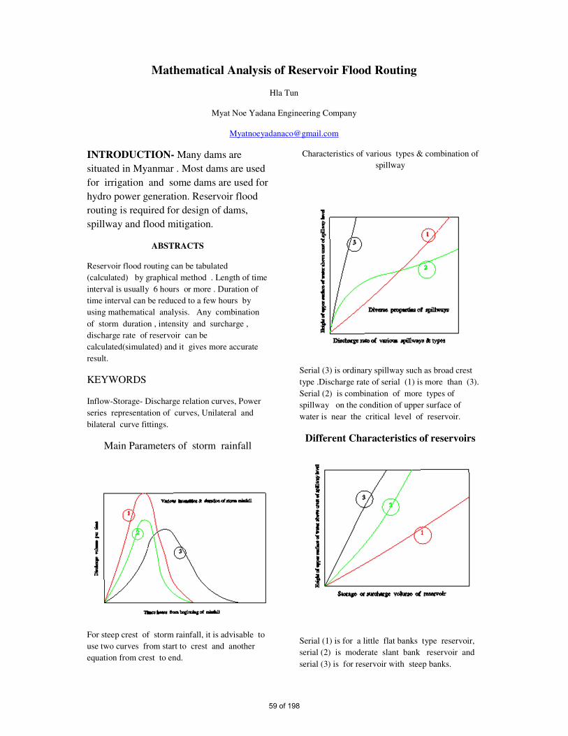
Mathematical Analysis of Reservoir Flood Routing

Hla Tun

Myat Noe Yadana Engineering Company

[email protected]

INTRODUCTION- Many dams are

situated in Myanmar . Most dams are used

for irrigation and some dams are used for

hydro power generation. Reservoir flood

routing is required for design of dams,

spillway and flood mitigation.

ABSTRACTS

Reservoir flood routing can be tabulated

(calculated) by graphical method . Length of time

interval is usually 6 hours or more . Duration of

time interval can be reduced to a few hours by

using mathematical analysis. Any combination

of storm duration , intensity and surcharge ,

discharge rate of reservoir can be

calculated(simulated) and it gives more accurate

result.

KEYWORDS

Inflow-Storage- Discharge relation curves, Power

series representation of curves, Unilateral and

bilateral curve fittings.

Main Parameters of storm rainfall

For steep crest of storm rainfall, it is advisable to

use two curves from start to crest and another

equation from crest to end.

Characteristics of various types & combination of

spillway

Serial (3) is ordinary spillway such as broad crest

type .Discharge rate of serial (1) is more than (3).

Serial (2) is combination of more types of

spillway on the condition of upper surface of

water is near the critical level of reservoir.

Different Characteristics of reservoirs

Serial (1) is for a little flat banks type reservoir,

serial (2) is moderate slant bank reservoir and

serial (3) is for reservoir with steep banks.

59 of 198

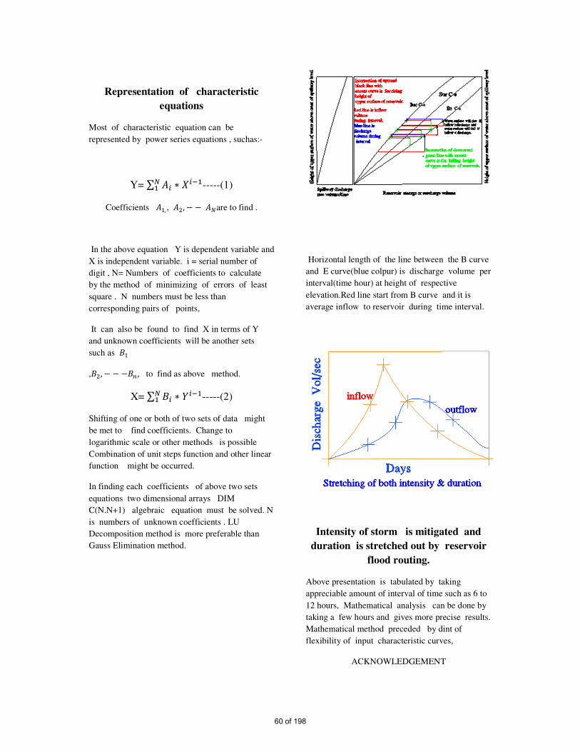
Representation of characteristic

equations

Most of characteristic equation can be

represented by power series equations , suchas:-

Y= ∑ ∗ -----(1)

Coefficients ,, , are to find .

In the above equation Y is dependent variable and

X is independent variable. i = serial number of

digit , N= Numbers of coefficients to calculate

by the method of minimizing of errors of least

square . N numbers must be less than

corresponding pairs of points,

It can also be found to find X in terms of Y

and unknown coefficients will be another sets

such as

, , , to find as above method.

X= ∑ ∗ -----(2)

Shifting of one or both of two sets of data might

be met to find coefficients. Change to

logarithmic scale or other methods is possible

Combination of unit steps function and other linear

function might be occurred.

In finding each coefficients of above two sets

equations two dimensional arrays DIM

C(N.N+1) algebraic equation must be solved. N

is numbers of unknown coefficients . LU

Decomposition method is more preferable than

Gauss Elimination method.

Horizontal length of the line between the B curve

and E curve(blue colpur) is discharge volume per

interval(time hour) at height of respective

elevation.Red line start from B curve and it is

average inflow to reservoir during time interval.

Intensity of storm is mitigated and

duration is stretched out by reservoir

flood routing.

Above presentation is tabulated by taking

appreciable amount of interval of time such as 6 to

12 hours, Mathematical analysis can be done by

taking a few hours and gives more precise results.

Mathematical method preceded by dint of

flexibility of input characteristic curves,

ACKNOWLEDGEMENT

60 of 198

This paper is written to submit at Federation of

Myanmar Engineering Societies, Annual

General Assembly ,National Conference on

Engineering Research to promote harnessing

methods of dams and affiliated structures.

REFERENCES

[1] Creager W.P & Justin J D . Engineering for

Dams Vol-1 John Wiley & Sons,Inc.1966.PP

195-202

[2]Creager W.P & Justin J D. Hydro Electric

Handbook 2nd edition , John Wiley &

Sons,Inc1950.

[3]Conte S D. Elementary Numerical Analysis

Mc-Graw Hill Company

[4]Scarborough J B. Numerical Mathematical

Analysis .Oxford Book Company.

61 of 198

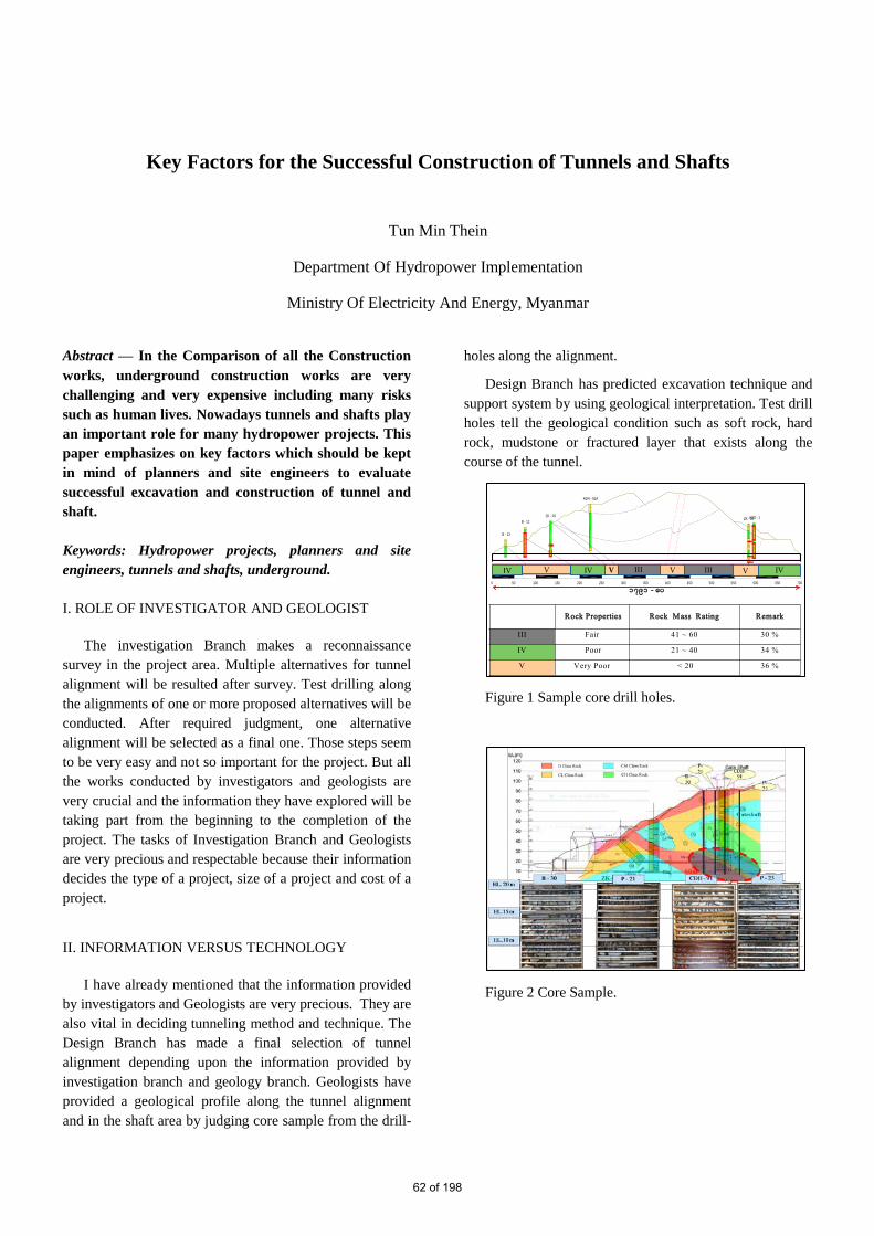
Key Factors for the Successful Construction of Tunnels and Shafts

Tun Min Thein

Department Of Hydropower Implementation

Ministry Of Electricity And Energy, Myanmar

Abstract — In the Comparison of all the Construction

works, underground construction works are very

challenging and very expensive including many risks

such as human lives. Nowadays tunnels and shafts play

an important role for many hydropower projects. This

paper emphasizes on key factors which should be kept

in mind of planners and site engineers to evaluate

successful excavation and construction of tunnel and

shaft.

Keywords: Hydropower projects, planners and site engineers, tunnels and shafts, underground. I. ROLE OF INVESTIGATOR AND GEOLOGIST

The investigation Branch makes a reconnaissance

survey in the project area. Multiple alternatives for tunnel

alignment will be resulted after survey. Test drilling along

the alignments of one or more proposed alternatives will be

conducted. After required judgment, one alternative

alignment will be selected as a final one. Those steps seem

to be very easy and not so important for the project. But all

the works conducted by investigators and geologists are

very crucial and the information they have explored will be

taking part from the beginning to the completion of the

project. The tasks of Investigation Branch and Geologists

are very precious and respectable because their information

decides the type of a project, size of a project and cost of a

project.

II. INFORMATION VERSUS TECHNOLOGY

I have already mentioned that the information provided

by investigators and Geologists are very precious. They are

also vital in deciding tunneling method and technique. The

Design Branch has made a final selection of tunnel

alignment depending upon the information provided by

investigation branch and geology branch. Geologists have

provided a geological profile along the tunnel alignment

and in the shaft area by judging core sample from the drill-

holes along the alignment.

Design Branch has predicted excavation technique and

support system by using geological interpretation. Test drill

holes tell the geological condition such as soft rock, hard

rock, mudstone or fractured layer that exists along the

course of the tunnel.

Figure 1 Sample core drill holes.

Figure 2 Core Sample.

ZK - 03

B - 12

B - 13

ADH - 91A

ADD - 1ZK - 04

IV V IV V III V III V IV

0 50 100 150 200 250 300 350 400 450 500 550 600 650 700

Rock Properties Rock Mass Rating Remark

III Fair 41 ~ 60 30 %

IV Poor 21 ~ 40 34 %

V Very Poor < 20 36 %

V V VVIV IV IVIII III

၁၇၉၁ - ပ

62 of 198

Figure 3 Excavation Methods.

Figure 4 Support Systems.

III. TUNNELING KIT FOR SITE ENGINEERS

The most important fact for a tunnel or shaft engineer is

to be very familiar with geological condition along the

tunnel or shaft. Site engineers must study the geological

profile thoroughly so that they can make necessary

preparation for each sectional excavation.

Figure 5 Geological Profile

Figure 6 Tunneling Method Selection by geology.

Depending upon the excavation method, required

machinery, material and equipment will be different.

Tunnel engineers must study all the tunneling methods

especially the most adaptable methods for each respective

project. For soft rock tunneling, support systems are vital in

addition to excavation method.

Figure 7 Tunneling Kit.

Water supply system, drainage and dewatering system,

ventilation system and electricity supply system need to

meet the necessary workability and safe standards. Tunnel

engineers and workers must follow safety precaution and

must wear the respective PPE for each construction site.

Figure 8 Power supply and ventilation system

Figure 9 Tunnel excavation and shotcret1ng

IV. TUNNELING METHODS APPLYING IN

MYANMAR HYDROPOWER PROJECTS

NATM (New Austrian Tunneling Method) and

conventional methods are generally applied for Myanmar

Hydropower Projects. NATM is best suited for medium to

hard rock excavation and combination of NATM and

conventional method is applicable for soft rock and poor

geological conditions. Depending upon the size of the

tunnel and encountering geology, bench cut method or drift

63 of 198

method or other suitable methods can be applied.

Figure 10 NATM procedures.

Figure 11 Ring cutting method.

Figure 12 Ring cutting method.

Figure 13 Supporting methods in weak and loosen zone.

Precision in survey is vital for hydropower tunnels

because the hydropower tunnels include many turnings and

difference in elevations. The tunnels are excavated from

up-stream and down-stream in parallel. A small mistake in

elevation reading may lead deviation of upstream and

downstream tunnel excavations, resulting oversized

breakthrough.

Figure 14 Missing at breakthrough by level error.

Angular and distance reading mistakes may lead

deviation of excavation fronts resulting in two tunnels

unfortunately.

Figure 15 Missing at Breakthrough Because of

Alignment Error

Therefore both skilled surveyor and modernized and

précised survey equipment are very important for

hydropower structures because their locations and

elevations are linked with each other from upstream to very

far downstream of the Project.

64 of 198

Figure 14 Measuring Instrument

Figure 16 Surveying

V. SUPPORT SYSTEMS FOR TUNNEL AND SHAFT

Flexible support system is the main concept of NATM.

Excavated Surface is secured by Shotcrete first to prevent

falling of Loosen stone and to reinforce weaken disturbed

surface. Quick rock bolt system adds another dimension to

the reinforcement purpose and maintains probable falling

blocks of stone and fractured layer in their positions firmly.

If more reinforcement is needed, steel rib supports may be

applied.

Figure 17 Shotcreting, rockbolting, steel-rib supporting.

Fore poling is necessary for excavation through soft

and fractured rock zone. For the shaft support system, ring

grouting around the circumference of the shaft is

recommendable.

Figure 18 Ring grouting pattern.

Figure 19 Ring grout for Shaft

Shotcrete, wire-mesh and rock-bolts are normally

applied in the shaft support system. When the excavation

diameter is large and geology of the shaft is not very good,

steel rib supports and primary RC concrete support work

effectively in the support system.

Figure 20 Steel-ribs and primary lining supporting.

VI. ACCIDENTS IN TUNNELS AND SHAFTS

For a developing country like Myanmar, there are many

challenges and risks in tunnel and shaft construction

including risk of lives. Lives and property of tunnel

workers and operators mainly depend upon the action and

decision of tunneling Staff officers and SAEs (Sub

Assistant Engineers) because they are always closely

supervising and operating the tunneling 24/7. Efficient

water supply system is very important to prevent much

65 of 198

water leakage and over feeding to the machines and

equipment using in the tunnel. Systematic dewatering and

drainage system is important to eliminate very muddy

tunnel access and provide favourable work-way in the

tunnel for promoting morale standards of the tunnel

workers.

Figure 21 Muddy access and clean access in tunnels.

High voltage Cables must be installed high enough for

the safety of the workers. Emergency breakers must be

installed according to specified standards and no leakage in

the cables and wire connections must be allowed. Most of

the workers get electrified in the tunnel because of Leakage

in the wire or they do not wear respective PPE such as

gloves and safety shoes. Accidents concerning with heavy

machine occur after blasting circle while there is still some

dust in the tunnel and at night because the workers do not

wear PPE such as safety vest with reflection or machine

operators are drunk at night.

Figure 22 Night operations.

VI. CONCLUSION

Most of the tunnel collapse occurs during night time

due to lack of supervision of night shift supervisor or not

enough supervisors for the whole night shift.

Recommendation is to locate the tunnel engineers’ unit

nearest to the tunnel. Site engineer need to know the

respective roles of Investigation Branch. Site engineers

must value the data and information provided by those

branches and have to study them carefully and thoroughly.

No perfect victory will be gained without considering key

factors. Tunnel portal and slope collapse occurred twice at

Thahtay Hydropower Project due to insufficient geological

investigation and proper judgment of site engineer.

Figure 23 Tunnel portal and slope collapse occurred twice.

Tunnel collapse in the crown portion of Diversion

Tunnel No.(2) outlet in Thahtay Hydropower Project

occurred due to improper support system and lack of proper

monitoring system.

Figure 24 Improper support system.

Adit-2 tunnel of Kun Hydropower Project was finally

backfilled and closed because of wrong excavation

technique and support system.

Figure 25 Collapse of wrong excavation technique.

There are many risks in tunneling work such as electric

shock, machinery accidents, minor failure and major failure

of tunnel and so on. Without considering key factors, we

will experience loss of time, money, dignity and lives. That

is why we need to emphasize on these key factors if we are

going to dig a tunnel or shaft. Tunnel engineers have to

compromise between safety and progress in balance. A

tunnel engineer must be able to make quick and right

decision when facing a problem with the tunnel. A lot of

lives and property depend upon the action and decision of a

tunnel engineer. This paper provides a helpful hand for all

66 of 198

the tunnel engineers so that they may become not only

skillful but also accountable tunnel engineers of DHPI

(Department of Hydropower Implementation).

ACKNOWLEDGEMENT

The author is grateful to Deputy Director General of

Department of Hydropower Implementation for giving

such opportunity to prepare this paper. Thanks are also due

to Director of Construction No.(4) for his encouragement in

preparing this paper.

REFERENCES;

Proceedings Papers

[1] Tun Min Thein. Problems and Solutions of Tunneling

at PHYU Hydropower Project.

[2] Tun Min Thein. Big Shaft Excavation in Poor Geology.

[3] Tun Min Thein. Large Tunnels and Shaft Excavation in

Geological Risky Region.

U Tun Min Thein, BE (Civil) is a Civil Engineer

Graduated from Yangon Institute of Technology in

2002. He joined the Government service in 2004 as a

Staff Officer in Ministry of Electric Power. He

worked at Phyu Hydropower Project in Tunnel, Shaft,

Penstock and Switchyard Constructions. In 2014, He

was transferred to Tha-htay Hydropower Project as

an Assistant Director responsible for Tunnels, Shaft

and Power Station up to now. His Foreign experience

includes training and study visits to China, Japan, Lao

PDR, Sweden, Vietnam, Singapore and Indonesia.

67 of 198

Transition of Urban Sustainability Approach

Thi Thi Khaing

1

Deputy Director, Department of Urban and Housing Development, Ministry of Construction, Office No.40,

NayPyiTaw1

Email: [email protected]

Abstract – One of the greatest challenges in our

society is climate change as extremely going up

temperature within a decade. In this paper, why

innovative urban infrastructure should adopt

designing focused on ecosystem and nature – based

engineering solutions. This paper is composed of

two parts, how the cities are facing the threat of

socio-economic impacts due to vulnerable

conventional infrastructure and ecosystem based

nature solution could particularly keep to be urban

sustainability. The current situation of water

management in Yangon city, the more urbanization

is faster, the more water demand is higher in future.

The provision of surface water is very limited up to

demand. The subsidence rate of Yangon city is

getting worse due to extracting of underground

water. Consequently, the salt water intrusion into

the aquifer occurring can be noticed when the

water table is getting low. This is leading to address

not only water shortage happening but also flooding

in vulnerable areas. Likewise, the solid waste

management is needed a proper technology to

dispose at the final dumping site to keep surface

and ground water quality. There is no systematic

way on disposal of solid waste like an opened final

dumping site at surrounding of people living areas

which cannot control a highly contaminated liquid

called a leachate percolate into the aquifer. This is

also potential to impact on ground and surface

water contamination and make shorter life

expectancy and the conventional drainage system is

often flooded as well. Moreover, the innovative

infrastructure adoption is very important to adapt

the climate change and urban sustainability. This

paper illustrates not only about the impacts of

conventional infrastructure with low technology is

highlighted but also will make effort to overcome

these challenges adopting innovative infrastructure

based on ecosystem function nature based solutions.

Keywords – Conventional infrastructure,

Sustainable Urban Drainage

System(SUDS), Nature based

solution(NBS).

I. INTRODUCTION

Nowadays, the world is facing more challenges

from urbanization and climate change due to

increasing greenhouse gases which consequently

happens the Global warming. A Half of the earth’s

population currently lives in Urban areas that is

expected to be getting increased up to 66% in mid of

this century. In Myanmar, 70% of people are living in

Rural areas and the rest of the people in urban areas

which is rapidly growing especially in Yangon city.

Expansions of Urban area are getting increased size of

the city which dramatically effects on destroying

natural resources, open spaces and will have various

impacts on ecosystem functioning. Consequently, the

cities would be faced so many challenges that concerns

climate change issues such as increasing temperatures,

heat waves, heavy rain fall, Floods and droughts. This

is potential to cause not only economic losses but also

effect on social health and human well-being.

The objectives of the paper are as follow; (1) To

provide urban policy making process (2) To adopt

innovative urban infrastructure based on nature based

solutions. (3) To address the socio-economic impacts

upgrading technology (4) To keep the benefits of

ecosystem functioning (5) To adapt climate change

mitigation (6) To reduce the rehabilitation cost of

capital (7) To enhance the public health and well-being.

II. CONVENTIONAL URBAN INFRASTRUCTURE

In the past, urban infrastructure ideas in land and

resource management have relied on conventional

engineering solutions but there is still necessary to

include a holistic approach of ecosystem functioning to

lead urban sustainability. Some infrastructures in

Yangon city involving Housing, Road, Drainage

system, parking and landscape, green space should be

designed based on ecosystem and be created all

inclusive ideas connecting each of its concepts.

1. The Water Management

In the current situation of water supply in Yangon

city, the domestic water for a half of city population is

supplied from reservoirs managed by the city

Development Committee while the rest of water

demand for people living in Yangon city is extracted

from aquifers drilling tube wells nearby their houses

where this is leading to occur a subsidence. Therefore,

flooded events and seawater intrusion in Yangon areas

are often occurring and vulnerable due to the effects of

subsidence by extracting of underground water.

Making assessment of surface deformation

measurements were performed using Synthetic

Aperture Radar interferometry (InSAR) with data from

the recently launched Sentinel-1, the subsidence rate

up to 9mm/y were found by a mapping through water

extractions onto the Yangon City.

68 of 198

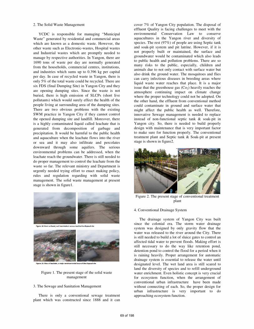
2. The Solid Waste Management

YCDC is responsible for managing “Municipal

Waste” generated by residential and commercial areas

which are known as a domestic waste. However, the

other waste such as Electronic-wastes, Hospital wastes

and Industrial wastes which are promptly needed to

manage by respective authorities. In Yangon, there are

1690 tons of waste per day are normally generated

from the households, commercial centres, institutions,

and industries which sums up to 0.396 kg per capital

per day. In case of recycled waste in Yangon, there is

only 5% of the total waste could be recycled. There are

six FDS (final Dumping Site) in Yangon City and they

are opening dumping sites. Since the waste is not

buried, there is high emission of SLCPs (short live

pollutants) which would surely effect the health of the

people living at surrounding area of the dumping sites.

There are two obvious problems with the existing

SWM practice in Yangon City if they cannot control

the opened dumping site and landfill. Moreover, there

is a highly contaminated liquid called leachate that is

generated from decomposition of garbage and

precipitation. It would be harmful to the public health

and aquaculture when the leachate flows into the river

or sea and it may also infiltrate and percolates

downward through some aquifers. The serious

environmental problems can be addressed, when the

leachate reach the groundwater. There is still needed to

do proper management to control the leachate from the

waste so far. The relevant ministry and Department is

urgently needed trying effort to enact making policy,

rules and regulation regarding with solid waste

management. The solid waste management at present

stage is shown in figure1.

Figure 1. The present stage of the solid waste

management

3. The Sewage and Sanitation Management

There is only a conventional sewage treatment

plant which was constructed since 1888 and it can

cover 7% of Yangon City population. The disposal of

effluent Quality is facing challenges to meet with the

environmental Conservation Law to conserve

aquacultures in the Yangon river and diversity of

species. The rest (97%) of people are using Septic tank

and soak-pit system and pit latrine. However, if it is

not properly built or maintained, the surface and

groundwater would be contaminated which also leads

to public health and pollution problems. There are so

many risks to the public, especially, children and

animals due to not only contact with surface water but

also drink the ground water. The mosquitoes and flies

can carry infectious diseases in breeding areas where

liquid waste water reaches that place. It is a major

issue that the greenhouse gas (Co2) heavily reaches the

atmosphere continuing impact on climate change

where the proper technology could not be adopted. On

the other hand, the effluent from conventional method

could contaminate in ground and surface water that

might affect the public health as well. Therefore,

innovative Sewage management is needed to replace

instead of non-functional septic tank & soak-pit in

Yangon city. So, there is needed to build properly

design with maintenance that is very important factor

to make sure for function properly. The conventional

treatment plant and Septic tank & Soak-pit at present

stage is shown in figure2.

Figure 2. The present stage of conventional treatment

plant

4. Conventional Drainage System

The drainage system of Yangon City was built

since the colonial era. The storm water drainage

system was designed by only gravity flow that the

water was released to the river around the City. There

is still needed to build a lot of sluice gates to control an

affected tidal water to prevent floods. Making effort is

still necessary to do the way like retention pond,

detention pond to control the flood for a period when it

is raining heavily. Proper arrangement for automatic

drainage system is essential to release the water until

designated level. The wet land area is still scared to

land the diversity of species and to refill underground

water enrichment. Even holistic concept is very crucial

for ecosystem function, when the arrangement of

conventional urban infrastructure have been made

without connecting of each. So, the proper design for

urban infrastructure is very important to do

approaching ecosystem function.

69 of 198

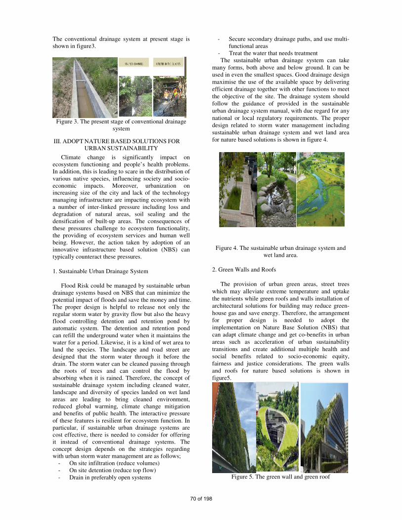
The conventional drainage system at present stage is

shown in figure3.

Figure 3. The present stage of conventional drainage

system

III. ADOPT NATURE BASED SOLUTIONS FOR

URBAN SUSTAINABILITY

Climate change is significantly impact on

ecosystem functioning and people’s health problems.

In addition, this is leading to scare in the distribution of

various native species, influencing society and socio-

economic impacts. Moreover, urbanization on

increasing size of the city and lack of the technology

managing infrastructure are impacting ecosystem with

a number of inter-linked pressure including loss and

degradation of natural areas, soil sealing and the

densification of built-up areas. The consequences of

these pressures challenge to ecosystem functionality,

the providing of ecosystem services and human well

being. However, the action taken by adoption of an

innovative infrastructure based solution (NBS) can

typically counteract these pressures.

1. Sustainable Urban Drainage System

Flood Risk could be managed by sustainable urban

drainage systems based on NBS that can minimize the

potential impact of floods and save the money and time.

The proper design is helpful to release not only the

regular storm water by gravity flow but also the heavy

flood controlling detention and retention pond by

automatic system. The detention and retention pond

can refill the underground water when it maintains the

water for a period. Likewise, it is a kind of wet area to

land the species. The landscape and road street are

designed that the storm water through it before the

drain. The storm water can be cleaned passing through

the roots of trees and can control the flood by

absorbing when it is rained. Therefore, the concept of

sustainable drainage system including cleaned water,

landscape and diversity of species landed on wet land

areas are leading to bring cleaned environment,

reduced global warming, climate change mitigation

and benefits of public health. The interactive pressure

of these features is resilient for ecosystem function. In

particular, if sustainable urban drainage systems are

cost effective, there is needed to consider for offering

it instead of conventional drainage systems. The

concept design depends on the strategies regarding

with urban storm water management are as follows;

- On site infiltration (reduce volumes)

- On site detention (reduce top flow)

- Drain in preferably open systems

- Secure secondary drainage paths, and use multi-

functional areas

- Treat the water that needs treatment

The sustainable urban drainage system can take

many forms, both above and below ground. It can be

used in even the smallest spaces. Good drainage design

maximise the use of the available space by delivering

efficient drainage together with other functions to meet

the objective of the site. The drainage system should

follow the guidance of provided in the sustainable

urban drainage system manual, with due regard for any

national or local regulatory requirements. The proper

design related to storm water management including

sustainable urban drainage system and wet land area

for nature based solutions is shown in figure 4.

Figure 4. The sustainable urban drainage system and

wet land area.

2. Green Walls and Roofs

The provision of urban green areas, street trees

which may alleviate extreme temperature and uptake

the nutrients while green roofs and walls installation of

architectural solutions for building may reduce green-

house gas and save energy. Therefore, the arrangement

for proper design is needed to adopt the

implementation on Nature Base Solution (NBS) that

can adapt climate change and get co-benefits in urban

areas such as acceleration of urban sustainability

transitions and create additional multiple health and

social benefits related to socio-economic equity,

fairness and justice considerations. The green walls

and roofs for nature based solutions is shown in

figure5.

Figure 5. The green wall and green roof

70 of 198

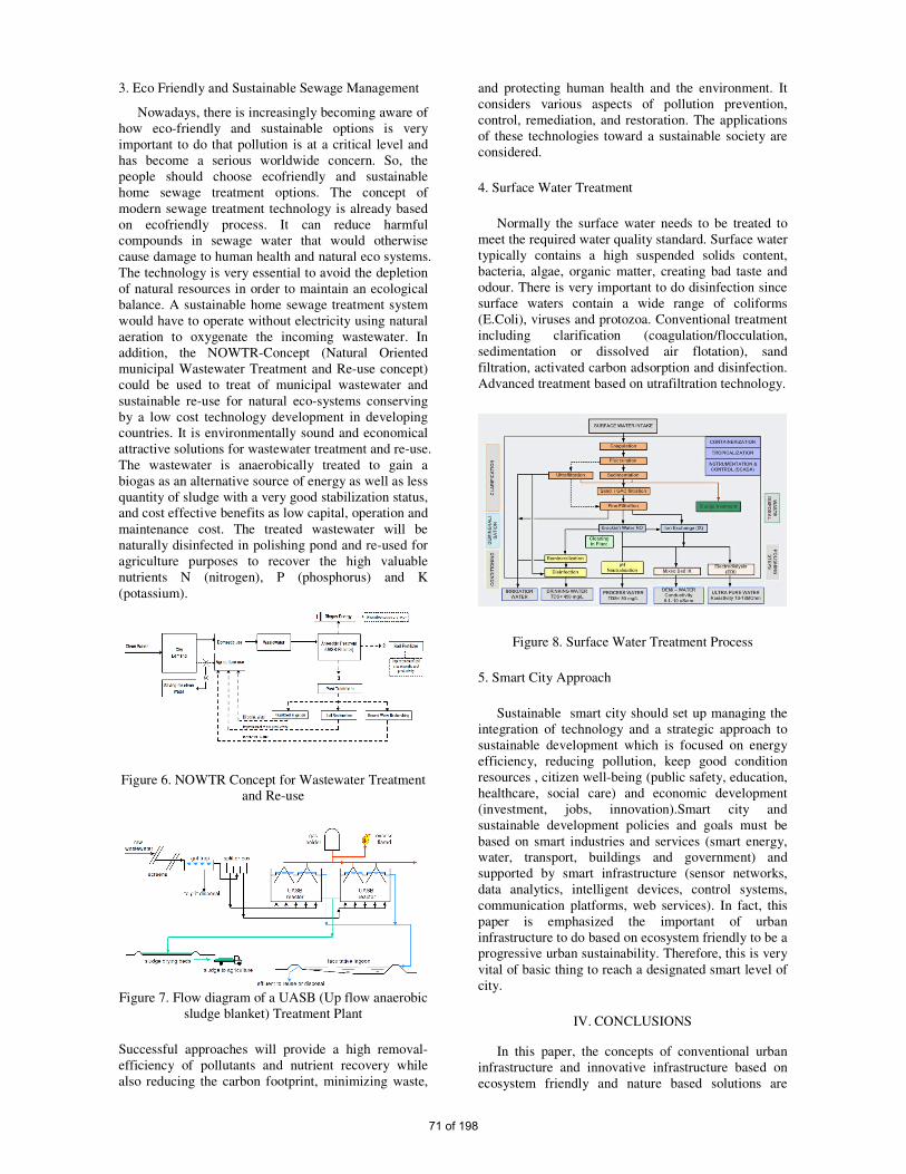
3. Eco Friendly and Sustainable Sewage Management

Nowadays, there is increasingly becoming aware of

how eco-friendly and sustainable options is very

important to do that pollution is at a critical level and

has become a serious worldwide concern. So, the

people should choose ecofriendly and sustainable

home sewage treatment options. The concept of

modern sewage treatment technology is already based

on ecofriendly process. It can reduce harmful

compounds in sewage water that would otherwise

cause damage to human health and natural eco systems.

The technology is very essential to avoid the depletion

of natural resources in order to maintain an ecological

balance. A sustainable home sewage treatment system

would have to operate without electricity using natural

aeration to oxygenate the incoming wastewater. In

addition, the NOWTR-Concept (Natural Oriented

municipal Wastewater Treatment and Re-use concept)

could be used to treat of municipal wastewater and

sustainable re-use for natural eco-systems conserving

by a low cost technology development in developing

countries. It is environmentally sound and economical

attractive solutions for wastewater treatment and re-use.

The wastewater is anaerobically treated to gain a

biogas as an alternative source of energy as well as less

quantity of sludge with a very good stabilization status,

and cost effective benefits as low capital, operation and

maintenance cost. The treated wastewater will be

naturally disinfected in polishing pond and re-used for

agriculture purposes to recover the high valuable

nutrients N (nitrogen), P (phosphorus) and K

(potassium).

Figure 6. NOWTR Concept for Wastewater Treatment

and Re-use

Figure 7. Flow diagram of a UASB (Up flow anaerobic

sludge blanket) Treatment Plant

Successful approaches will provide a high removal-

efficiency of pollutants and nutrient recovery while

also reducing the carbon footprint, minimizing waste,

and protecting human health and the environment. It

considers various aspects of pollution prevention,

control, remediation, and restoration. The applications

of these technologies toward a sustainable society are

considered.

4. Surface Water Treatment

Normally the surface water needs to be treated to

meet the required water quality standard. Surface water

typically contains a high suspended solids content,

bacteria, algae, organic matter, creating bad taste and

odour. There is very important to do disinfection since

surface waters contain a wide range of coliforms

(E.Coli), viruses and protozoa. Conventional treatment

including clarification (coagulation/flocculation,

sedimentation or dissolved air flotation), sand

filtration, activated carbon adsorption and disinfection.

Advanced treatment based on utrafiltration technology.

Figure 8. Surface Water Treatment Process

5. Smart City Approach

Sustainable smart city should set up managing the

integration of technology and a strategic approach to

sustainable development which is focused on energy

efficiency, reducing pollution, keep good condition

resources , citizen well-being (public safety, education,

healthcare, social care) and economic development

(investment, jobs, innovation).Smart city and

sustainable development policies and goals must be

based on smart industries and services (smart energy,

water, transport, buildings and government) and

supported by smart infrastructure (sensor networks,

data analytics, intelligent devices, control systems,

communication platforms, web services). In fact, this

paper is emphasized the important of urban

infrastructure to do based on ecosystem friendly to be a

progressive urban sustainability. Therefore, this is very

vital of basic thing to reach a designated smart level of

city.

IV. CONCLUSIONS

In this paper, the concepts of conventional urban

infrastructure and innovative infrastructure based on

ecosystem friendly and nature based solutions are

71 of 198

highlighted in order to reduce greenhouse gas and get

low impact development. The green spaces and

sustainable urban drainage systems including detention

ponds to prevent the floods that should be considered

in making urban planning process in future. The

sustainable waste water treatment systems should

do consider the appropriate technology for the culture,

land, and climate. In addition to cost and treatment

performance energy aspects, recycling and social

issues are important when evaluating sustainability of a

wastewater treatment system in which the design

criteria must be focused on environmentally friendly

ecosystem. This requires a multidisciplinary approach

where engineers cooperate with social scientists,

economists, biologists, health officials and the public.

In surface water treatment process, the sediment or

sludge produced in this process could be used in

agricultural fields after proper composting. The

technology is very thoughtful to be simple,

inexpensive and ecofriendly method could be used for

urban sustainability. In particular, there is needed to

create wet land areas to land diversity of species. The

interaction of linkage between clean water, clean air

and different species can occur an ecosystem function.

Consequently, there are some benefits such as life

expectancy, symbolic values, landscaping, increased

bio-diversity and bio-resilience, drainage, resource-

efficiency and cost efficiency by keeping ecosystem

function. In addition, functioning ecosystem can

ensure human societies against external disturbance

and these habitats need to be resilient themselves in the

face of future disturbances. Therefore, special attention

is very crucial to do design urban infrastructure based

on ecosystem friendly focusing nature based solution

(NBS) have transformative social impact contributing

to social innovation in cities. Particularly, the practices

of urban infrastructure can be transition initiatives in

cities can get scaled up and hence contributing to

accelerating sustainability. To hope, the concept of this

paper shows how to lead urban sustainability and a

level of smart city.

ACKNOWLEDGEMENTS

The author wishes to express her deep gratitude to

his Excellency, U Min Htein, Director General, Urban

and Housing Development, Ministry of Construction,

for valuable permission and kind support in carrying

out this research work. The author wishes to record her

thanks to Claus Pedersen, Programme Director for

Urban WASH capacity building in Asia (SUWAS ITP

Asia), for his guidance, suggestions and necessary

advice. The author also wishes to thank all her friends

for their helps and advices on her studying. Finally, the

author would like to express grateful thanks to all

teachers and parents for their supports, kindness and

unconditional love.

REFERENCES

[1] Nadja Kabisch, Horst Korn, Jutta Stadler, Aletta Bonn

“Nature-based Solutions to Climate Change Adaptation in Urban Areas”

[2] Henrik Alm, “Sustainable Stormwater Management”,

Stockholm Royal Seaport. [3] Tim Van Der Horst, “Sinking Yangon; Detection of subsidence

caused by groundwater extraction using SAR interferometry

and PSI time-series analysis for Sentinel-1data”

72 of 198

Earthquake Safety Assessment of RC Buildings in Myanmar

Wai Yar Aung1, Technical Research Engineer, Myanmar Earthquake Committee

INTRODUCTION

Before 1988, Yangon does not have many tall

buildings. However, after 1988, due to economic

changes, there was abrupt rise in housing demand and

many mid-rise reinforced concrete buildings around six

to eight storied reinforced concrete buildings were built

concentrating in some crowed townships without

considering earthquake risks until 2002. Therefore, it is

necessary to investigate the actual condition of existing

buildings. Therefore, this study focused on evaluating

earthquake safety assessment of the existing buildings

in Yangon, which buildings are located in high

population density.

OBJECTIVES

For this study, 3 townships from urban areas and 1

township from sub-urban area of Yangon are selected to

study. The main objectives of this study are:

• To assess the seismic risks of existing RC

buildings.

• To calculate the structural capacity of the

selected RC buildings.

• To evaluate the seismic performance and

recommendation for further actions.

RESULTS

Generally, earthquake safety assessment of existing

buildings is carried out in three steps as below.

• Step 1: Rapid Visual Screening

• Step 2: Numerical Evaluation

• Step 3: Detailed Analysis and Retrofitting

Design

Step 3, Detailed analysis and retrofitting design, is not

included in this study. Only Step 1 and Step 2

assessments were carried out based.

In addition to Step 1 and Step 2 assessments,

Microtremor measurements were conducted to

determine the dynamic response of the buildings and

soil conditions.

Firstly, rapid visual assessment was conducted to

identify the deficiencies of the building before

conducting detailed analysis. Numerical evaluation was

carried out for 12 buildings which having the score

lower than the required cut-off score.

Step 1: Rapid Visual Screening

Rapid Visual Screening (RVS) is a rapid way of

assessing the building vulnerability based on visual

inspection, seismicity of the location, and vulnerable

features of the building using standard survey form.

Based on the RVS score, the vulnerability of the

building can be estimated, and decisions can be made

on whether further detail assessment is required or not.

According to the RVS results, 56% of all buildings are

reinforced concrete buildings without considering

earthquake risks. Average storey number is between 4

to 8 stories. These buildings are built between 1984 to

2005. Average RVS Score of RC buildings in selected

area is 1.67 and collapse probability is 2%.

Step 2: Numerical Evaluation

Seismic hazard level considered in this evaluation is

225-year return period with 20% of probability of

exceedance in 50 years. “Life Safety” structural

performance level is considered in this evaluation.

Based on the initial RVS assessment and potential

deficiencies, numerical evaluation was performed by

calculating the internal forces of primary members and

expected capacities according to the specified

performance level and seismic input.

In this study, 10 Pre-Code RC Buildings and 2 Post

Code Buildings are selected to evaluate Shear Stress in

Concrete Columns, Overturning, Storey Drift are

checked according to MNBC and ASCE 41-13.

Rebound Hammer and Ultrasonic Pulse Velocity Test

were conducted and Microtremor measurement was

conducted and check to understand potential resonance

effect according to Gosar, 2010.

This table and Chart Below shows the summary of

earthquake safety of selected RC Buildings.

Interpretation of table and chart is that the higher the

index rate of particular section, the higher the

vulnerability rate. PC means Pre-Code building and PB

means Post Code Buildings. “F” means particular floor

level.

Table (1) shows the summary of earthquake safety of

selected RC Buildings

Building

name RVA Shear Overturning Strength Drift Average

1BPC2F 0.41 0.11 0.07 0.11 0.13 0.82

73 of 198

2BPC5F 0.20 0.07 0.10 0.07 0.06 0.50

3BPC2F 0.30 0.08 0.08 0.13 0.05 0.63

4BPC2F 0.41 0.10 0.08 0.09 0.07 0.76

5BPC3F 0.30 0.13 0.08 0.11 0.10 0.72

6BPC6F 0.41 0.11 0.13 0.08 0.05 0.77

7BPC4F 0.20 0.10 0.10 0.08 0.06 0.54

8BPC2F 0.20 0.04 0.11 0.10 0.06 0.51

9BPC4F 0.21 0.09 0.10 0.07 0.06 0.53

10BPC2F 0.50 0.06 0.07 0.11 0.03 0.77

11BPB2F 0.20 0.06 0.06 0.09 0.02 0.43

12BPB6F 0.21 0.06 0.08 0.08 0.02 0.44

Figure (1) shows summary of earthquake safety of selected RC buildings accordance with recommended safety level

CONCLUSION

It could be clearly observed that seismic performance of

pre-code RC buildings are lower than lower than

Recommended Safety level because none of these

buildings are designed for seismic resistance. At that

time, construction technology is adequately low and

quality control for construction materials were

questionable. However, in Post code new buildings it

could found that seismic demands were lower than Pre-

Code buildings due to its good material strength and

strong structural capacity of important members.

More importantly that there are a lot of RC buildings

(56% of pre-code RC buildings as mentioned above)

were built without considering earthquake risks.

Therefore, the risks of Yangon of could be expected to

high in the case of strong earthquake.

REFERENCES

Guidelines of Rapid Visual Screening of Buildings for

Potential Seismic Hazards, FEMA-154P

Seismic Evaluation and Retrofi t of Existing Buildings,

ASCE/SEI 41-13

Guidelines for seismic evaluation and retrofitting of

existing buildings in Myanmar, Myanmar Earthquake

Committee

2014-Myanmar Population and Housing Census,

Yangon Region Report

Myanmar National Building Code (2016)

0.00

0.50

1.00

1BPC2F2BPC5F3BPC2F4BPC2F5BPC3F6BPC6F7BPC4F8BPC2F9BPC4F10BPC2F11BPB2F12BPB6F

Final Score

RVA Shear Overturning

Strength Drift Moderate Degree of Vulnerability

High Degree of Vulnerability

74 of 198

MARITIME EDUCATION,TRAINING AND CAPACITY BUILDING IN

MYANMAR MERCANTILE MARINE COLLEGE

KHIN HNIN THANT

Marine Engineering Department,

Myanmar Mercantile Marine College (MMMC), Yangon, Myanmar

Email: [email protected]

Abstract — In this paper, maritime education,

training and capacity building process of

Myanmar Mercantile Marine College at

present time is introduced in specific details.

The main theme of this paper is to present the

effort how to improve the maritime capacity

building and how to create a change in

maritime education and training from skill

based to education research based approach.

MMMC is always finding the ways and means

to deal with the change and progress of

maritime education and training. Research and

development is one of the central components

and also the sustainable root cause for the

improvement of every educational institution.

The strategies and procedures to upgrade and

enhance the maritime education research

capacity building of MMMC are also discussed

in this paper. Finally, the difficulties and

challenges faced by MMMC to full-fill and

align the demands from regional and

international engineering accreditation bodies

and awarding authorities. Thus, this paper

intends to present the trend and progress of

enhancing maritime education capacity

building in MMMC.

Keywords: Maritime Education and Training,

Maritime Research Capacity Building,

Engineering Accreditation

I. INTRODUCTION

Training and Development is the heart of

a continuous effort designed to improve employee

competency and organizational performance.

Training provides learners with knowledge and

skill needed for their present jobs. Myanmar

seamen have enjoyed working in international

maritime service with well-known attributes of

competence, sense of responsibilities and

discipline. Therefore, Myanmar needs to make

endeavors in order to become a maritime nation

that ensures the all-round development of maritime

workers and that produced greater numbers of

capable and competent seafarers, so that Myanmar

will be competitive in maritime labor markets, not

only in terms of quality but also in terms of

quantity. For that reason, the government has

upgraded with both the quality and quantity of the

production of international level officers and

engineers for maritime commerce through the

development of human resources competent in

maritime activities at the Maritime Institute.

Maritime Education and Training systems for

seafarers in Myanmar includes maritime education

and training units and maritime administration.

Myanmar MET has a concrete foundation and has

developed rapidly in these years.

Myanmar government has also

encouraged of research study of Maritime

Education. Maritime Education and Training

(MET) System is actually needed for the

75 of 198

development of Myanmar economy because of the

growth of working onboard ships in Myanmar has

paralleled with the increase in seaborne trade.

1. Objective

The objective of this paper is to present

Maritime Education, Training and Capacity

Building process in MMMC.

2. Method and Scope of the Study

The method of this study is descriptive method.

The information, facts and figures used in this

study are secondary data obtained from the

Department of Marine Administration, Myanmar

Mercantile Marine College and Universities

Research Capacity Building Committees.

II. MARITIME INSTITUTION TRAINING

Maritime Institutions in Myanmar can be

classified into government owned and private

owned institutions. The two major institutions;

Myanmar Maritime University and Myanmar

Mercantile Marine College are government owned

institutions and are playing the vital role in the

maritime education and training sectors in

Myanmar. Myanmar Maritime University is mainly

focus on maritime engineering education and

Myanmar Mercantile Marine College is mainly for

marine vocational training and education trend at

present. They both are playing the vital role in the

maritime education sectors in Myanmar. Moreover,

there are also 10 private owned training institutions

in maritime vocational training field. All maritime

institutions are well organized and perform the

requirements of Department of Marine

Administration in Myanmar and International

Maritime Organization (IMO).

III. MARITIME EDUCATION AND TRAINING

IN MYANMAR MERCANTILE MARINE

COLLEGE

Myanmar Mercantile Maritime College is well-

known and well-organized government owned

institution since 1974. MMMC mainly provides

Teaching and Training Services for seafarers such

as Ship Masters, Chief Engineers, Nautical and

Marine Engineer Officers, Electro Technical

Officers, Cadets and Ratings to serve on board

Foreign-Going and Near Costal Voyage vessels

and crafts. The training courses conducted in the

MMMC are designed not only to provide training

in relevant fields but also to give emphasizes on

discipline and formation of responsible mariners to

meet with the requirements of International

Convention on Standard of Training, Certification

and Watch keeping for Seafarers, 1978 as

amended (SCTW Convention). MMMC selects

and provides the trainings for seafarers in

accordance to the requirements of the Department

of Marine Administration (DMA) and the

applicable STCW 95 requirements as amended.

Upon completion of Training and passing the

relevant examination from the DMA they will

possess certificates and qualifications that conform

to the requirements of National and International

Regulations or to the requirements stipulated by

the Flag states; etc., and shall be eligible to service

Worldwide.

1. Teaching and Training Aids

The Teaching and Training Services for ship’s

personnel, provided by MMMC do not use all their

own designed syllabi, but uses syllabi that have

been designed by an outside party such as

International Maritime Organization (IMO) and

approved by the department of Marine

Administration. The teaching Aids and Simulators

programs are provided by the manufacturers as

software. All teaching and Training Requirements

such as Teaching and Training syllabi and

Training Course requirements and guides, to be in

compliance with the SCTW 95 (requirements as

amended). All the teaching syllabus in use by the

MMMC are reviewed and approved by the

Department of Marine Administration. The

teaching and learning process, course conducted

and training process are described in specific

details MMMC website. Furthermore, we are

trying our best to upgrade and full-fill with our

MMMC diploma holders both COC requirements

and engineering accreditation because the teaching

hours, credit units and other academic requirements

76 of 198

of MMMC marine engineering cadet course and

marine electro technology cadet course are full-fill

and align with the requirements of higher education

system and the demands from regional and

international engineering accreditation bodies and

awarding authorities.

2. Training of Trainers

It is the known fact the driving force of training

activities is teaching staffs. Presently, the strength

of academic staff including visiting lecturers is

about 50 and 80 other staffs. To ensure the

outcome of training courses meeting with SCTW

requirements, strengthening of training for

teaching staffs is essential. MMMC provides the

teaching staffs from academic field to attend the

Master Degree and Ph.D. courses related to their

first degree. The teaching staffs of this institute

consists mainly of professionals who have sea

going experience as well as high academic and

internationally recognized qualifications. Most of

teachers and assessors are trained from the

Maritime Universities from all over the world such

as World Maritime University, Shanghai Maritime

University, Korea Maritime University and Tokyo

University of Marine Science and Technology.

Furthermore, all academic teachers have

successfully completed of the STCW Convention

and based on the IMO Model Course 6.09,

Training of Trainers (TOT Course) and

Assessment, Examination and Certification of

Seafarers in accordance with the requirements of

the STCW Convention based on the IMO Model

Course 3.12 (Administrators, Trainers and

Assessors Course).

3. Quality Management System

MMMC has been accredited with certification

by Lloyd’s Register Quality Assurance (LRQA)

and United Kingdom Accreditation Service

(UKAS) from 6th July, 2007 to July, 2019.

MMMC got its ISO certificate from Lloyd’s for its

well-habited Quality Management System.

MMMC was intensively checked and inspected by

Lloyd’s within its certified period. Now MMMC

got ABS Accreditation Service since August 1,

2019.

IV. MARITIME RESEARCH AND CAPACITY

BUILDING IN MMMC

MMMC is always finding the ways and means

to deal with the change and progress of maritime

education and training. MMMC tries to improve

the maritime capacity building and to create a

change in maritime education and training from

skill based to education research based approach.

Research and development is one of the central

components and also the sustainable root cause for

the improvement of every educational institution.

1. Building Research Capacity

Vision of MMMC Research Building Capacity

is to become the Vocational Training Centre of

Excellence in Maritime Education, Training and

Research field. Our mission is to produce ethically

minded, and technically competent Marine officers

and seafarers who have the will and ability for the

maritime field. Moreover, MMMC intends to help

conduct the National Maritime Education and

Research and to collaborate with international

Maritime Societies to share information and

knowledge.

2. Ethics and Research Committee (ERC)

Ethics and Research Committee is formed in

MMMC by Principal and Heads of Academic

Departments. There are internal members and also

external members in ERC. External members are

visiting professors, lectures and experts from

maritime field. The duties and responsibilities of

ERC’s is to enhance for the quality of research

based on research ethic, scientific validity, impact

on maritime industry and social contribution. As

capacity assessment, identifying the main strengths

and weakness of research and institutional

framework at the individual, organizational level

and institution level.

3. Research Training Activities

MMMC conduct Research Training Activities

such as Research Ethics and Responsible conduct

of Research Workshop, Short course on Research

Methodology for teachers, Paper Writing

77 of 198

Workshop; etc. Besides, MMMC urge to do

departmental research with international

collaboration, maritime education research and

students group term papers as the teaching &

learning based research approach. Presently, we

are strategic trying to prepare research oriented

teaching, balancing teaching and research papers,

creation of small research grants, creation of

related research resources and creation of research

database system. The challenges in building

research capacity faced by MMMC are upgrading

Research skill including language, Peer review and

ISBN, ISSN recognition, internal and external

funding, technological barriers, data collection,

ICT infrastructure, online digital library,

inadequate time for research, etc. We are trying to

develop and reform from teaching to learning

organization to create the progress of research

capacity.

V. CONCLUSIONS

In this paper, we present the current situation of

Maritime Education and Training Procedures and

the functions of Building Research Capacity of

MMMC. We also present how MMMC serves to

stimulate improvement of MET standards. The

goals and aims of the Maritime Education and

Training in Myanmar need to be modified to meet

with the challenges and opportunities in the

international shipping world. Furthermore, we

discuss the difficulties and challenges faced by

MMMC to full-fill and align the demands from

regional and international engineering accreditation

bodies and awarding authorities. We try our best to

upgrade and full-fill with our MMMC diploma

holders both COC requirements and engineering

accreditation. Finally, we illustrate the strategies

and procedures of building research capacity in

MMMC.

ACKNOWLEDGMENT(S)

This research was financially supported by the

Myanmar Mercantile Marine College Research and

Academic Fund.

REFERENCES

[1]. Tin Oo, The Asia Maritime & Fisheries

Universities Forum 2013. Proceedings 12th

The Asia Maritime & Fisheries Universities

Forum 2013, Far Eastern State Technical

Fisheries University, Russia, 2013. pp. 170-

177.

[2]. Dr.G.Thiruvasagam, Maritime Education on

India, A Study on Productivity Enhancement,

The Asia Maritime & Fisheries Universities

Forum 2017. Proceedings 16th

The Asia

Maritime & Fisheries Universities Forum

2017, Ho Chi Minh University of Transport,

Vietnam, 2013. pp. 19-25.

[3]. Guideline for Establishing Research Centers

at the University of Malaya.

[4]. Peter Sigmund, Good and Bad Scientific

Practice, Department of Physic and

Chemistry, University of Southern Denmark,

Odense, June 5, 2011

[5]. Policies and Guidelines for Establishment of

Research Center, Hindustan Institute of

Technology and Science.

[6] Available online at

http://www.mmmc.edu.mm

[7]. Building Research Capacity in Education,

Evidence from recent initiatives in England,

Scotland and Wales

https://www.researchgate.net/publication

78 of 198

CAPACITY BUILDING FOR FUTURE-ORIENTED EDUCATION IN MYANMAR

Thu Thu Aung

Department of Computer Engineering and Information Technology , Yangon Technological University, Yangon, 11012, Myanmar

[email protected]

Abstract— Capacity building is the phenomenon by

which individuals and organizations obtain, improve

and retain the skills, knowledge and other resources

needed to do their jobs competently. Capacity building

in the context of developing function, solving problems

within a sustainable manner involves awareness, skills,

knowledge, motivation, commitment and confidence.

Capacity building framework is not only for teachers

but also for students. In this framework, there is a need

to be synchronized with system policies and

performance management. Moreover teacher

improvement is based on student improvement and

student outcomes. This paper aims to focus on

improving effective teaching and professional learning.

Professional learning without depth in evidence or

theories or feedback does not enable effective growth

or change that, in turn, builds capacity and develops

quality in achieving student learning outcomes. Future-

oriented education is important for all teachers and

instructors. In addition, future-oriented education

system of a country is needed to plan and to be higher

education system. Because helping students developed

a future-oriented perspective allows them to manage

the uncertainly of the future logically in academic

settings. In this paper, it intends to explore the

perception of teachers and students for future-oriented

education. Surveys and assessments are used as

research tool from one Myanmar University included

as population for future-oriented education. Some

attributes such as learning outcomes and assessments

include in this paper. In this study, achievements of

students are mainly analyzed on two academic years.

According to the basis of findings, the conclusions can

be drawn. So it is very important to prepare for future

needs and challenges of higher education. Capacity

building and planning should be carried out better

future-oriented education.

Keywords: Capacity building, future-oriented education,

learning outcomes, professional learning

I. INTRODUCTION

Higher education system of a country depends on the

history, the culture, the economics and the growth

potential of that country. There can measure whether a

country develops or not with an effective education

system. Education system is a lead role in the development

of a country. In 21st century, the challenges become more

and more. The influencing of universities will also have

the impact of education. Higher education reflects directly

with the development of economic, human beings and

modern societies.

Higher education is very important for a developing

country as Myanmar. Higher education promotes the

economic knowledge, richer culture and intellectualism in

a country. Some developed countries already planned for

future perspectives of higher education and attained the

futurology. A country with sustainable higher education

enhances over the world.

Now a day, the progress level of a country cannot

assure without training and research on higher education.

The new touchstones of quality of a higher education are

not only its human resource development, but also its

moral commitment to society for desirable social change

or progress through modernization, even strategic

factorization [1].

Today, higher education is the important role of

developing country like Myanmar to manage the demands

and to solve the challenges of present time. So, we have to

prepare ourselves for future needs, demands and challenges

of higher effective education. Preparation for the future has

been a primary function of education. Planning should be

made about what may be expected future of higher

education and how may be constructed the capacity

buildings for teachers and students of effective professional

79 of 198

teaching and learning.

II. CAPACITY BUILDING

Ensuring capacity for lasting improvement is critical to

address challenges of quality and equality [2]. The general

orientation is towards addressing sets of improvement-

related capacities. Especially the changing teaching and

learning is absolutely needed fundamental to

improvement.

Capacity building is an extremely complex endeavor.

In capacity building for future-oriented education, the

sustainable teaching and learning is the core for school,

college and universities. Life-long learning based on

higher effective education of a country, continuous

learning of teachers and institutions itself for the purpose

of enhancing students learning, influenced by individual

teachers within an institution of that country.

So today building capacity for future-oriented

education is facing on as a challenge of country

improvement. Capacity building also needs to provide

support for and development of a wider workforce. Several

countries have adapted to this agenda by developing

integrated community schools and services [2].

In a rapidly changing world, capacity building needs to

address both the present and the future. A recent widening

of the educational agenda to include, among important

outcomes, involving both internally and supporting them

externally of teachers and students.

A large body of education improvement literature

highlights generic features of improvement, frequently

citing the following: a focus on learning and teaching;

using data to help guide improvement efforts; high quality

professional development, embedded within professional

learning communities [2].

In this paper, framework is provided by analysis of

improvement and effectiveness based on research, practice

and strategies as evaluation tools worked with university

to support and quality assure self evaluation efforts.

Capacity building for future-oriented education

approaches different countries strategies of education.

There are also efforts in several other countries to find

ways to help build capacity in universities facing

significant challenges where student achievement is poor,

including government initiatives in their own system.

Improving what goes on in the classroom was

synonymous with instructional improvement; finding out

what instructional strategies were linked with better

student outcomes and thinking of ways to build teachers‟

capacity to use these strategies [2].

In many cases, curriculum, learning and teaching

strategies can offer to success the future-oriented education.

So learning outcomes and assessments of teachers and

students are analyzed to forecast and prepare for future

education in this paper.

III. OBJECTIVES OF THE STUDY

The major objectives of the study are the following:

To focus on improving and effective

teaching and professional learning in Myanmar,

To intend to perception of teachers and

students for future-oriented education in

Myanmar,

To prepare achievement on teachers and

students capacity needing for future higher

education,

To fill the demands based on teachers

and students suitable on education environment

and society in Myanmar country.

IV. DATA COLLECTION

In this study, some course information, learning

outcomes and assessments of teachers and students from

Computer Engineering and Information Technology

Department on Yangon Technological University in

Myanmar were collected as input data. Out of the whole

population, students’ achievement and assessments on

each subject and individual teachers included on academic

year. In compliance with the university's guidelines

regarding classroom research, all the study materials were

reviewed to the implementation of the study. Data were

collected in a class which had the second, third, fourth and

fifth year students on CEIT 2nd

batch course files.

V. METHODS AND PROCEDURES

This paper was descriptive research in nature. A class

which a subject on one academic year consists of course

information and mapping. According to relevant subjects,

different course information and mapping. But a class met

fifty minutes per session, at least three days a week. This

survey based on different subjects in one academic year.

Assessment is a process of measuring and collecting the

data (mark/score) in a manner that enable to analyze the

achievement of the intended learning outcomes and the

effectiveness of the learning activities.

80 of 198

Figure 1 The steps of assessment plan

In step 1, course outcomes (CO) description was

mainly based on syllabus; topics and level of difficulty and

graduate attributes (GA) have twelve types of assessments

such as engineering knowledge, problem analysis and life-

long learning etc. CO description and GA are connected as

a mapping.

In step 2, assessment planning, course works marks

such as assignments, tutorial, practical and exam marks are

connected with GA.

In assessment contribution, CO distributions and GA

distributions are calculated based on assessment items

such as course work and final exam.

In assessment collecting, the percentage of course work

and exam for each student is calculated based on CO and

GA distributions.

In assessment calculating, the achievements of each

student are calculated based on CO and GA distributions.

Then grading of each student is got and the numbers of

students got different grading are calculated.

In step 6, course outcomes achieved by students with

KPI (Key Performance Indicator). In KPI, excellent is

noted by pass 100% with minimum 20% A, good is more

than 80% pass, fair is more than 60% pass and bad is more

than 40% fail.

In finally, overall GA analysis included GA mapping,

GA marks distribution and student achievements with KPI

are achieved for each course/subject on one academic year.

VI. EXPERIMENTS

According to assessments, the achievements of

students on each course for each year in one academic year

can be calculated.

For example, the student achievement of one subject

for second year student in one academic year can be found

in Table 1.

Table 1 The sample of student achievement

Subject- Introduction to Computer System

Overall GA Analysis

Engineering

Knowledge

Modern Tool

Usage

GA 1 GA 5

GA- Mapping CO (1,2,4) CO 3

GA-

Mark Distribution

71.0 29.0

GA-

Student

Achievement

69 66

KPI : above 60% GA Achievement

Student Achievement : GA 1 and 5 above 60%

In Table 2, the achievement of third year student can

be found on one subject in one academic year.

The student achievements of fourth and fifth year on

one course can also be found in one academic year in

Table 3 and 4.

The following Table can also describe the KPI based

on the GA achievement. Therefore, according to the KPI

and student achievement, it can know and study how the

capacity building is raised for the next academic year. So

assessment calculating, CLO and PLO mapping, KPI and

achievements support to improve for future education.

Assessment Collecting

Assessments Calculating

Analyzing

Overall GA Analysis

(Students Final Achievements)

Assessment Contribution

Assessment Planning

CO, GA Mapping

81 of 198

Table 2 The sample of achievement for third year

student on one course

Subject – Operating System I

Overall GA Analysis

Engineering

Knowledge

Problem

Analysis

Investigation

GA 1 GA 2 GA 4

GA-

Mapping

CO 1 CO 2 CO (3,4)

GA-

Mark

Distribution

30.0 12.0 58.0

GA-

Student

Achievement

72 78 58


Student Achievement : GA 1 and 2 above 60% ,

GA 4 under 60%

Table 3 The sample of achievement for fourth year student

on one subject

Subject – Software Engineering

Overall GA Analysis

Engineering

Knowledge

Problem

Analysis

GA 1 GA 2

GA- Mapping CO 1 CO (2,3,4)

GA-

Mark

Distribution

27.0 73.0

GA-

Student

Achievement

73 80


Student Achievement : GA 1 and 2 above 60% ,

Table 4 The sample of achievement for fifth year student

on one course

Subject – Artificial Intelligent

Overall GA Analysis

Engineering

Knowledge

Problem

Analysis

Investigation

GA 1 GA 3 GA 4

GA-

Mapping

CO 1 CO (3,4) CO 2

GA-

Mark

Distribution

33.0 42.0 25.0

GA-

Student

Achievement

85 78 79


Student Achievement : GA 1, 3 and 4 above 60%

VII. CONCLUSIONS

According to the final achievement results, teachers

can prepare their course and teaching techniques for next

academic year. In addition, planning can draw the better

teaching and learning strategies and then their capacity can

also be built on future-oriented education for their students

and learners to improve.

ACKNOWLEDGMENT(S)

The author would like to acknowledge the support

of Myanmar Engineering Council and Society. And

then I would like to thank the Rector and the teachers

from Yangon Technological University.

REFERENCES

Journal Papers

[1] Saima Rasul, Qadir Bukhsh, Muzamilla Akram,

Opnion of Teachers and Students about Futurology of

Higher Education in Pakistan, International Journal for

Cross-Disciplinary Subjects in Education (IJCDSE), 1(4),

2010.

82 of 198

[2] Louise Stoll, Capacity Building for School

Improvement or Creating Capacity for Learning? A

changing landscape, Journal of Educational Change,

10(2):115-127.

[3] Skylar Davidson, Futurology in the College Classroom,

https://www.researchgate.net/publication/304353984.

Books

[4] Abasyn University Ring Road Peshawar Subject:

Trend & Issues in Education: Unit 01, Futurology and

Education, pp. 1-31.

[5] Hopkins, D, Every School a Great School.

Maidenhead: Open University, press, 2007, McGraw-Hill.

83 of 198

IMPLEMENTATION OF SCADA SYSTEM

FOR HYDROPOWER STATION

Aung Kyaw Myint(1)

, Kyaw Zin Latt(2)

, Tin Tin Hla(3)

, Nay Min Tun(4)

Department of Electric Power Generation Enterprise, Branch of Renewable Energy and Hydropower Plant

[email protected](1)

, [email protected](2)

, [email protected](3)

,

[email protected](4)

ABSTRACT

This paper presents an efficient and automatic data

monitoring IoT based SCADA system which is capable

of monitoring the hydropower station with electronic

devices in real time operation mode. The system has

been utilized the IoT based platform and ESP 8266 Node

MCU wireless communication modules to transfer the

data on watching the IoT cloud on anywhere with

internet acceptance. There are two hardware modules

namely RTU (Remote Terminal Unit) and MTU (Main

Terminal Unit). ESP 8266Wi-Fi modules are used to

configure in master and slave mode for SCADA system.

Microcontroller is used to set out the command to PLC

for driving the generator status (on/off). Crucial

histogram data such as active power, current, voltage,

frequency, power factors, temperature, pressure,

vibration will be taken into accounts with respective

sensors which have been configured into the several

components of the power station. The IoT platform is

used to design the user interface to display the real time

operation and information of hydropower station being

monitored the authorized personal on anywhere

assessments via the internet.

KEYWORDS: SCADA, IoT, ESP8266, IoT Platform,

Microcontroller

1. INTRODUCTION

SCADA is acronym from “Supervisory Control And

Data Acquisition” which refers to the combination of

telemetry and data acquisition and encompasses the data

collection, transferring it back to the central site, carrying

out any necessary analysis and control anyhow

displaying the collected data on PC or any detected

embedded devices that are specialized to operate in

hydropower station. SCADA system that is implemented

in every hydropower plants rather than all in plants are

automatically performed by the RTU with PLC. To

execute a feasibility study for data monitoring and

control system of hydropower plant, it is necessary to

control model design to implement the data collection

and control system in hydropower plants. Simulation and

emulation system for hydropower station use MATLAB

and SCADA to process information and make it

available to the operator in real time operation [1].

However, in this paper, control system design is

proposed for SCADA system of hydropower plants to

create the data acquisition and control in the generator

side. The OPC (Object linking and embedding for

Process Control) is used for communication system to

improve the integration between all devices without

requirement for specific drivers for each pair of devices

[2]. Wireless communication interface is used to transfer

the collected data from hydropower station’s components

such as power line, transformers, generators, thrust

bearing, upper guide bearing, lower guide bearing,

turbine guide bearing, stator coil, water inlet and outlet

system, condition of upstream and downstream level,

rotor and cooling water system in this paper. Practical

implementation of SCADA system for Falluja substation

is made up of 3RTU devices that are used to collect data

from 10N 6200 devices installed inside incoming and

outgoing panels for 11kV and 33kV. The collected data

is then sent to main terminal unit control operator via

rotor for power monitoring, control and energy

management functions [3]. The main objective of

SCADA system is to supervise, control, optimize, and

manage the generation system and transmission system.

The main components of this system are RTUs that

collect data automatically and are directly connected to

sensors, meters, loggers or process equipment. RTUs

contain all of the transceivers, encoders and processors

needed for proper functioning in the event that a primary

RTU stop working. Report status of components can be

performed by Programming Logic Controller (PLCs) [4].

In the paper of SCADA on Hydropower Plant Cascade

Case Study, Network Architecture SCADA System are

DCS (Distributed Control System) using TCP/IP

84 of 198

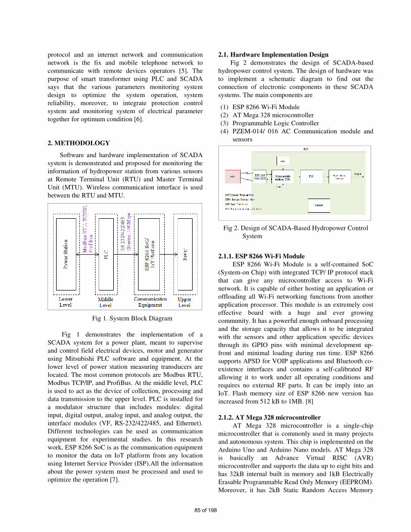
protocol and an internet network and communication

network is the fix and mobile telephone network to

communicate with remote devices operators [5]. The

purpose of smart transformer using PLC and SCADA

says that the various parameters monitoring system

design to optimize the system operation, system

reliability, moreover, to integrate protection control

system and monitoring system of electrical parameter

together for optimum condition [6].

2. METHODOLOGY

Software and hardware implementation of SCADA

system is demonstrated and proposed for monitoring the

information of hydropower station from various sensors

at Remote Terminal Unit (RTU) and Master Terminal

Unit (MTU). Wireless communication interface is used

between the RTU and MTU.

Fig 1. System Block Diagram

Fig 1 demonstrates the implementation of a

SCADA system for a power plant, meant to supervise

and control field electrical devices, motor and generator

using Mitsubishi PLC software and equipment. At the

lower level of power station measuring transducers are

located. The most common protocols are Modbus RTU,

Modbus TCP/IP, and ProfiBus. At the middle level, PLC

is used to act as the device of collection, processing and

data transmission to the upper level. PLC is installed for

a modulator structure that includes modules: digital

input, digital output, analog input, and analog output, the

interface modules (VF, RS-232/422/485, and Ethernet).

Different technologies can be used as communication

equipment for experimental studies. In this research

work, ESP 8266 SoC is as the communication equipment

to monitor the data on IoT platform from any location

using Internet Service Provider (ISP).All the information

about the power system must be processed and used to

optimize the operation [7].

2.1. Hardware Implementation Design

Fig 2 demonstrates the design of SCADA-based

hydropower control system. The design of hardware was

to implement a schematic diagram to find out the

connection of electronic components in these SCADA

systems. The main components are

(1) ESP 8266 Wi-Fi Module

(2) AT Mega 328 microcontroller

(3) Programmable Logic Controller

(4) PZEM-014/ 016 AC Communication module and

sensors

Fig 2. Design of SCADA-Based Hydropower Control

System

2.1.1. ESP 8266 Wi-Fi Module

ESP 8266 Wi-Fi Module is a self-contained SoC

(System-on Chip) with integrated TCP/ IP protocol stack

that can give any microcontroller access to Wi-Fi

network. It is capable of either hosting an application or

offloading all Wi-Fi networking functions from another

application processor. This module is an extremely cost

effective board with a huge and ever growing

community. It has a powerful enough onboard processing

and the storage capacity that allows it to be integrated

with the sensors and other application specific devices

through its GPIO pins with minimal development up-

front and minimal loading during run time. ESP 8266

supports APSD for VOIP applications and Bluetooth co-

existence interfaces and contains a self-calibrated RF

allowing it to work under all operating conditions and

requires no external RF parts. It can be imply into an

IoT. Flash memory size of ESP 8266 new version has

increased from 512 kB to 1MB. [8]

2.1.2. AT Mega 328 microcontroller

AT Mega 328 microcontroller is a single-chip

microcontroller that is commonly used in many projects

and autonomous system. This chip is implemented on the

Arduino Uno and Arduino Nano models. AT Mega 328

is basically an Advance Virtual RISC (AVR)

microcontroller and supports the data up to eight bits and

has 32kB internal built in memory and 1kB Electrically

Erasable Programmable Read Only Memory (EEPROM).

Moreover, it has 2kB Static Random Access Memory

85 of 198

(SRAM) and has several different features that consist of

advanced RISC architecture, good performance, low

power consumption, real timer, counter having separate

oscillator, 6PWM pins, programmable serial USART,

programming lock for software security, throughput up

to 20 MIPS. It is the heart of Arduino Uno and operates

the ranging from 3.3V to 5.5Vhowever; normally

operation is 5V as a standard usage in embedded systems

applications. [9]

2.1.3. Programmable Logic Controller (PLC)

PLC is a special form of microprocessor based

controller that uses programmable memory to store

instructions and specific functions that include On/ Off

control and to implement functions such as logic,

sequencing, timing, counting and arithmetic in order to

control machines and process. Advances of PLC control

systems are flexible, faster time response, less and

simpler wiring, solid-state (no moving parts), modulator

design (easy to repair and expand), handles much more

complicated systems, sophisticated instruction sets

available, allows for diagnostics (easy to troubleshoot)

and less expensive. PLC is used with the input and

output sections that are where the processor receives

information from external devices and communicates

information to external devices to acquire the data and

control the machine. [10]

2.1.4. PZEM-016 AC Communication Module and

Sensors

PZEM is mainly used for measuring AC voltage,

current, active power, frequency, power factor and active

energy. The module is without display function but the

data is read through the RS485 interface. This data is

primary data of hydropower station such as power line,

transformers and generators. [12].

Temperature sensor, PT 100 is used as industrial

temperature sensor to measure high range temperature

(200°C). DHT11 is a basic, ultra-low-cost digital

temperature and humidity sensor that is used to measure

the surrounding air and spits out a digital signal on the

data pin. Temperature is essential information of

transformers, thrust bearing, upper guide bearing, lower

guide bearing, turbine guide bearing and stator coil of

hydropower plant. Moreover, pressure sensor is used for

water inlet (penstock) and outlet (draft tube), water level

sensor is needed for upstream and downstream of

hydropower plant and vibration sensor is mainly used for

rotor (rotating for turbine).

2.2. Software Implementation

The main focus of Industrial Internet of Things (IoT)

is to enable communication across a range of devices and

IoT uses protocols such as MQTT (Message Query

Telemetry Transport) to make it possible to communicate

across different devices throughout the entire system for

acquiring the data from sensors. Two program codes are

developed to program the microcontroller (Arduino

UNO) and ESP 8266 Node MCU Wi-Fi Module. These

microcontrollers are used to receive the data from

sensors by using the C language code. Moreover, Ladder

program is used on Programming Logic Controller

(PLC) to control the ON/OFF state such as the generator

control system of hydropower station. SCADA system

lacks the much needed interoperability, which is a

mandate for developing seamless programmability for

devices and sensors. The IoT can reduce the hardware

devices, while also eliminating the need for software

licensing and upgrading by using the cloud services. [11]

No. Collection Data For Objective Items

1 Active Power (W)

Power Line, Transformers

and Generators

2 Current (A) 3 Voltage (V)

4 Frequency (Hz) 5 Power Factor 6 Temperature (ᵒC) Transformers, Thrust

Bearing, Upper guide

Bearing, Lower guide

Bearing, Turbine Guide

Bearing, Stator Coil

7 Pressure (Pa) Water Inlet (Penstock),

Water Outlet (Draft Tube)

8 Water Level (m) Up Stream and Down

Stream 9 Vibration (m/s

2) Rotor

10 Flow of Water

(m/s2)

Cooling Water System for

all Bearing, Shaft Seal

Table 1. Important data of hydropower station

Table 1 expresses the essential data that is concerned

with the sensors of hydropower station’s components.

In this paper, the information of hydropower station has

already been collected by using the sensors. However,

the information such as active power, current, voltage,

frequency, power factor and temperature on the above

mentioned data will be found out.

3. Experimental Results

SCADA system is used Open Platform

Communications (OPC) for collecting data and IoT

Standards that like it are used to enable real-time device

communication within plant floors that use different

devices and sensors from different manufactures. IoT

Standard is often known as Industry 4.0. [13] In this

section, the operation of data acquisition and control

system for some essential data of hydropower station on

86 of 198

SCADA system is demonstrated. Fig 3 indicates the

hardware implementation of electricity monitoring

system.

Fig 3. Hardware Implementation of SCADA System

Fig 4 points out the collected data from the sensor to

post on IoT cloud. The interface between hardware and

software implementation for SCADA system was based on

the IoT cloud.

Figure 3; Hardware Implementation

Fig 4. Sending the collected data to IoT Cloud

Fig 5 expresses the Monitoring System using IoT

Platform. There have been several conditions for various

kinds of control purposes. The top level control could be

accomplished with the control panel on the monitoring

windows of SCADA system of hydro power station in

real situation.

Fig 5. Energy Data for Monitoring System Using

IoT Platform

Fig 6 shows the Temperature Data for Monitoring

System Using IoT Platform. It is only considered on the

monitoring of temperature values for that station.

Fig 6. Temperature Data for Monitoring System Using

IoT Platform

Fig 7. Master Terminal Control over Remote Terminal

Unit

Normally, the temperature control system could be

maintained the stable condition of the station in real

world. Fig 7 illustrates the Master Terminal Control over

Remote Terminal Unit into the cloud based system. Fig 8

mentions the comparison between experimental results

and calculated results from power equations (P=VI).

Table 2 shows that the tolerance between actual values

PZEM Microcontroller

Wi-Fi Module

PLC

ON/ OFF

Wi-Fi Module

87 of 198

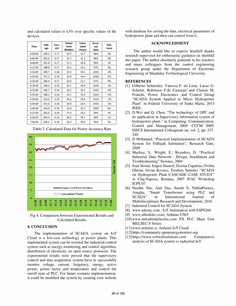
and calculated values is ±3% over specific values of the

devices.

Table 2. Calculated Data for Power Accuracy Rate

Fig 8. Comparison between Experimental Results and

Calculated Results

4. CONCLUSION

The implementation of SCADA system on IoT

Cloud is a low-cost technology at power plants. This

implemented system can be assisted the industrial control

system such as energy monitoring and control algorithm,

distribution of electricity on open source protocols. The

experimental results were proved that the supervisory

control and data acquisition system have to successfully

monitor voltage, current, frequency, energy, active

power, power factor and temperature and control the

on/off state of PLC. For future scenario implementation,

it could be modified the system by creating own website

with database for saving the data, electrical parameters of

hydropower plant and then can control from it.

ACKNOWLEDMENT

The author would like to express heartfelt thanks

research supervisor for enthusiastic guidance on shortfall

this paper. The author absolutely gratitude to his teachers

and many colleagues from the control engineering

research group under the Department of Electronic

Engineering of Mandalay Technological University.

REFERENCES

[1] Gilberto Schneider, Vanessa F. de Lima, Lucas G.

Scherer, Robinson F.de Camargo and Claiton M.

Franchi, Power Electronics and Control Group

“SCADA System Applied to Micro Hydropower

Plant” in Federal University of Santa Maria, 2013

IEEE.

[2] D.Wei and Q. Chen, “The technology of OPC and

its application in Supervisory information system of

hydropower plant,” in Computing, Communication,

Control and Management, 2009. CCCM 2009.

ISECS International Colloquium on, vol. 2, pp. 237-

240

[3] D Mohamed, “Practical Implementation of SCADA

System for Fallujah Substation”, Research Gate,

2009

[4] Mackay, S., Wright, E., Reynders, D. “Practical

Industrial Data Network : Design, Installation and

Troubleshooting” Newnes, 2004

[5] Ioan Stoian, Eugen Stancel, Dorina Capatina, Ovidiu

Ghiran, Istvan Kovacs, Teodora Sanislav “SCADA

on Hydropower Plant CASCADE CASE STUDY”

in Cluj-Napoca, Romina, 2007 IFAC Workshop

ICPS’07

[6] Neethu Nm, Anil Das, Sarath S, NithinPremsy,

Anagha, “Smart Transformer using PLC and

SCADA” in International Journal of

Multidisciplinary Research and Development, 2016

[7] Industrial Control for SCADA System

[8] www.udemy.com : IoT Automation with ESP8266

[9] www.alliedelec.com; Arduino UNO

[10] www.mitsubishielectric.com FX PLC Main Unit

MELSEC-F Series

[11] www.arduino.cc Arduino IoT Cloud

[12] https://community.openenergymonitor.org

[13] https://www.softwebsolutions.com Comparative

analysis of SCADA system vs industrial IoT

Time Volt-

age

Curr-

ent

Power

from

Modbus

Calcu-

lated

Power

Accur-

acy

Rate

Tole-

rance

6:00:00 186.5 0.17 32.5 31.7 98% 2%

6:04:00 183.6 0.17 31.7 31.2 98% 2%

6:08:00 181.8 0.17 31.3 30.9 99% 1%

6:12:00 188.8 0.17 33.1 32.1 97% 3%

6:16:00 189.7 0.18 33.4 34.1 102% -2%

6:20:00 191.2 0.18 33.8 34.4 102% -2%

6:24:00 186.4 0.17 32.6 31.7 97% 3%

6:28:00 188.3 0.18 33.1 33.9 102% -2%

6:32:00 189.7 0.18 33.5 34.1 102% -2%

6:36:00 188.1 0.18 33.1 33.9 102% -2%

6:40:00 193.9 0.18 34.6 34.9 101% -1%

6:44:00 191.6 0.18 34.0 34.5 101% -1%

6:48:00 194.9 0.18 35.0 35.1 100% 0%

6:52:00 202.6 0.18 37.0 36.5 99% 1%

6:56:00 200.3 0.18 36.4 36.1 99% 1%

7:00:00 200.2 0.18 36.4 36.0 99% 1%

88 of 198

Simulation and Analysis on Power Factor Improvement and Harmonic

Reduction of High-voltage, High-frequency Power Supply for Ozone

Generator

Nwe Ni Win1, Yin Yin Pyone2, Mai Kai Suan Tial 3

Department of Electrical Power Engineering, Technological University (Taunggyi)

The Republic of the Union of Myanmar [email protected], [email protected], [email protected]

Abstract- Ozone generating system needs High

Voltage, High Frequency (HV-HF) power supply.

The ozonizer distorts the supply currents and

henceforth affects the supply power factor. This

paper presents the application of active power

filter (APF) for power factor improvement and

harmonic reduction in power supply of ozone

generation system. The conventional inverter has

front end bridge rectifier with smoothing

inductor/capacitor. It draws non-sinusoidal

current from AC mains; as a result input supply

has more harmonics and poor power factor.

Hence, there is a continuous need for power factor

improvement and reduction of line current

harmonics. The proposed system has active power

factor which is used to achieve sinusoidal current

and improve the supply power factor. The active

power factor correction (PFC) converter with

pulse width modulation (PWM) inverter fed ozone

generator generates more ozone output compared

to the conventional inverter. Thus the proposed

system has less current harmonics and better

input power factor compared to the conventional

system. The performance of active power factor

(APF) applications are compared and analyzed

with the help of simulation results using

Matlab/Simulink.

Keywords: Active power filter, Harmonic reduction,

High voltage, High frequency power supply, Ozone

generator, Power factor improvement

I. INTRODUCTION

Ozone (O3) is considered as an excellent

powerful oxidizer and germicide. Its disinfection

potential is significantly higher than chlorine and

other disinfectants. Nowadays, ozone is widely

used for disinfecting and oxidizing in substitution

of chlorine, due to the latter’s by products such as

smell, bad taste and carcinogenic agents resulting

from it. Indeed, ozone produces much less

byproducts and ozone itself is transformed into

oxygen within a few hours. Applications of ozone

technology are various and could be found in

disinfection, water and air purification, medicine and

so on.

The use of high frequency power supplies

increases the power density applied to the ozonizer

electrode surface which in turn enhances the ozone

production for a given surface area, with reduced

peak voltage requirement. By increasing the

operating frequency the ozone production can easily

be controlled. Many compact converter topologies

have been proposed in order to improve efficiency of

the ozonizer. Some power supply derived from AC

main supply. In this case the front end has

uncontrolled rectifier with a large DC link capacitor.

This rectifier is widely used because of its simplicity

and robustness but with the distorted line currents. As

a result, the input power factor is poor. Various

power factor correction (PFC) techniques are

employed in converters to overcome these power

quality problems out of which the basic boost

converter topology has been extensively used in

various power supply conversion applications.

Implementing power factor correction (PFC) into low

frequency to high frequency power supplies will

maximize the power handling capability of the power

supply and current handling capacities of power

distribution networks.

With conventional high voltage high frequency

power supply, the poor power factor and harmonic

distortions are the main problem for Ozone generator.

This type of utility interface draws excessive peak

input currents; it produces a high level of harmonics,

and both the input power factor (PF) and total

harmonic distortion (THD) are poor. The low PF

makes the efficiency of the electrical power grid to be

very low. Regulatory standards with origins in

Europe (EN 61000-3-2) and North America (IEC

1000-3) have been established that aim at protecting

the utility grid from excessive harmonics [1].

Currently, IEEE 519 is used for harmonic

regulations. In order to meet the harmonics limits

imposed by these standards, new active power filters

(APF) are used.

The aim of the present work is the development

of an efficient active power filter (APF) for high

voltage, high frequency (HV-HF) power supply of a

ozone generator, consisting in power stage, filters and

control circuit. The modeling and simulations are

executed using Matlab/Simulink software.

II. OZONE GENERATOR

The configuration of the ozonizer used in this

work is shown in Figure 1. This type of ozonizer is

designed for operation at high frequencies (up to 15

kHz) and ozone is generated by means of a silent

89 of 198

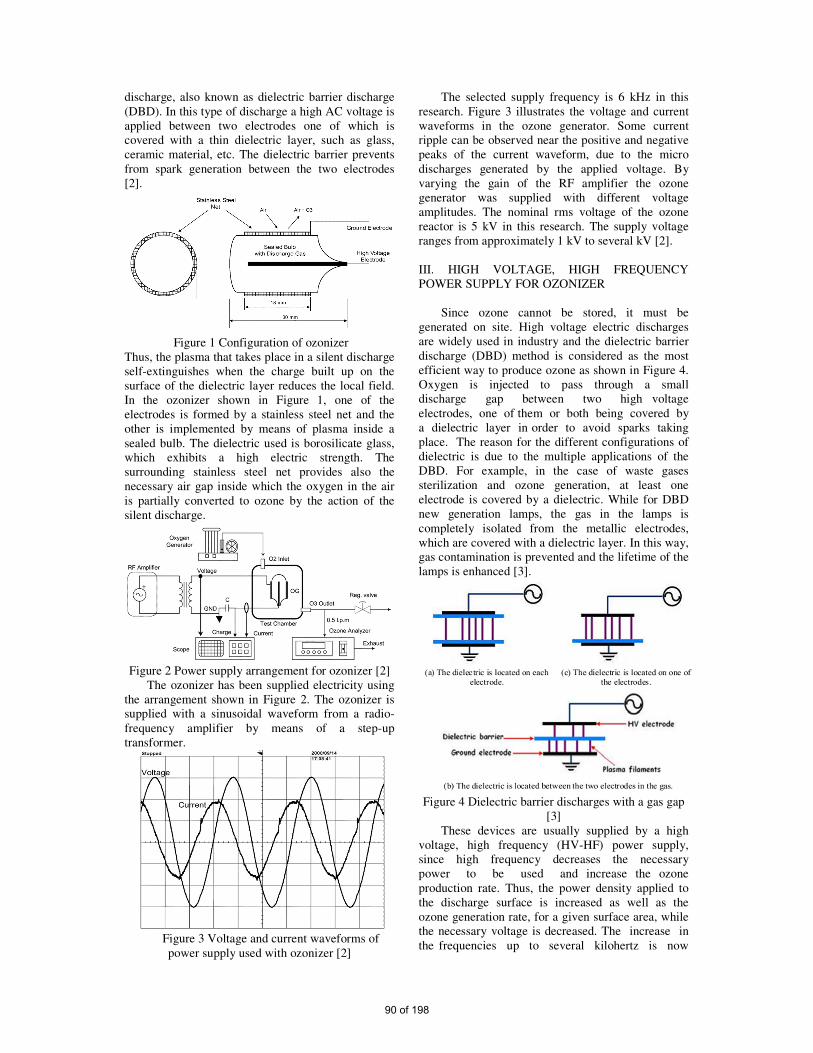
discharge, also known as dielectric barrier discharge

(DBD). In this type of discharge a high AC voltage is

applied between two electrodes one of which is

covered with a thin dielectric layer, such as glass,

ceramic material, etc. The dielectric barrier prevents

from spark generation between the two electrodes

[2].

Figure 1 Configuration of ozonizer

Thus, the plasma that takes place in a silent discharge

self-extinguishes when the charge built up on the

surface of the dielectric layer reduces the local field.

In the ozonizer shown in Figure 1, one of the

electrodes is formed by a stainless steel net and the

other is implemented by means of plasma inside a

sealed bulb. The dielectric used is borosilicate glass,

which exhibits a high electric strength. The

surrounding stainless steel net provides also the

necessary air gap inside which the oxygen in the air

is partially converted to ozone by the action of the

silent discharge.

Figure 2 Power supply arrangement for ozonizer [2]

The ozonizer has been supplied electricity using

the arrangement shown in Figure 2. The ozonizer is

supplied with a sinusoidal waveform from a radio-

frequency amplifier by means of a step-up

transformer.

Figure 3 Voltage and current waveforms of

power supply used with ozonizer [2]

The selected supply frequency is 6 kHz in this

research. Figure 3 illustrates the voltage and current

waveforms in the ozone generator. Some current

ripple can be observed near the positive and negative

peaks of the current waveform, due to the micro

discharges generated by the applied voltage. By

varying the gain of the RF amplifier the ozone

generator was supplied with different voltage

amplitudes. The nominal rms voltage of the ozone

reactor is 5 kV in this research. The supply voltage

ranges from approximately 1 kV to several kV [2].

III. HIGH VOLTAGE, HIGH FREQUENCY

POWER SUPPLY FOR OZONIZER

Since ozone cannot be stored, it must be

generated on site. High voltage electric discharges

are widely used in industry and the dielectric barrier

discharge (DBD) method is considered as the most

efficient way to produce ozone as shown in Figure 4.

Oxygen is injected to pass through a small

discharge gap between two high voltage

electrodes, one of them or both being covered by

a dielectric layer in order to avoid sparks taking

place. The reason for the different configurations of

dielectric is due to the multiple applications of the

DBD. For example, in the case of waste gases

sterilization and ozone generation, at least one

electrode is covered by a dielectric. While for DBD

new generation lamps, the gas in the lamps is

completely isolated from the metallic electrodes,

which are covered with a dielectric layer. In this way,

gas contamination is prevented and the lifetime of the

lamps is enhanced [3].

Figure 4 Dielectric barrier discharges with a gas gap

[3]

These devices are usually supplied by a high

voltage, high frequency (HV-HF) power supply,

since high frequency decreases the necessary

power to be used and increase the ozone

production rate. Thus, the power density applied to

the discharge surface is increased as well as the

ozone generation rate, for a given surface area, while

the necessary voltage is decreased. The increase in

the frequencies up to several kilohertz is now

90 of 198

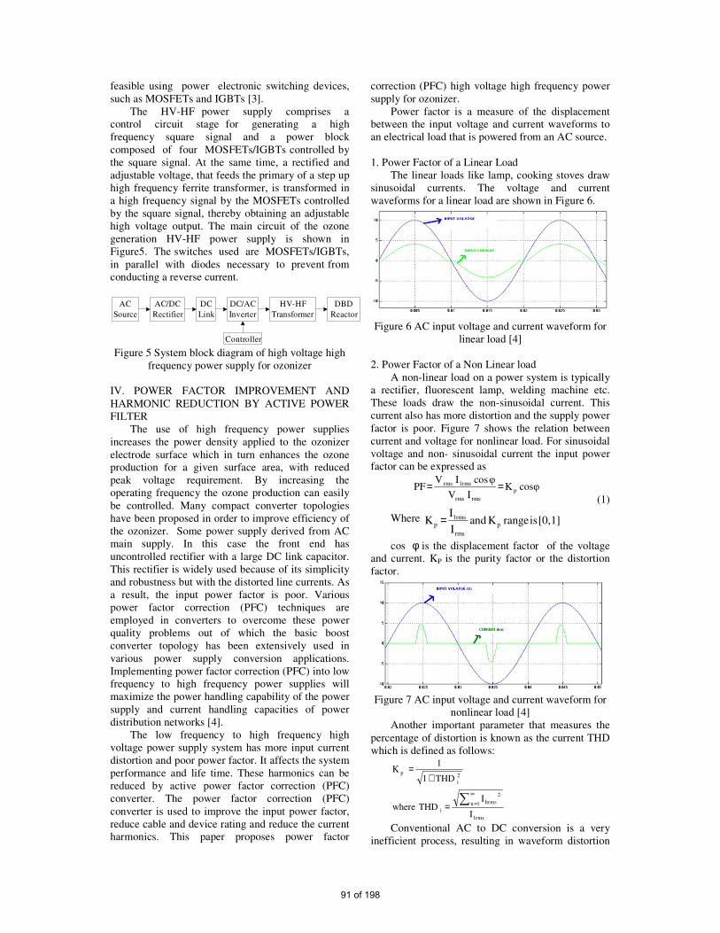
feasible using power electronic switching devices,

such as MOSFETs and IGBTs [3].

The HV-HF power supply comprises a

control circuit stage for generating a high

frequency square signal and a power block

composed of four MOSFETs/IGBTs controlled by

the square signal. At the same time, a rectified and

adjustable voltage, that feeds the primary of a step up

high frequency ferrite transformer, is transformed in

a high frequency signal by the MOSFETs controlled

by the square signal, thereby obtaining an adjustable

high voltage output. The main circuit of the ozone

generation HV-HF power supply is shown in

Figure5. The switches used are MOSFETs/IGBTs,

in parallel with diodes necessary to prevent from

conducting a reverse current.

AC

Source

AC/DC

Rectifier

DC

Link

DC/AC

Inverter

Controller

HV-HF

Transformer

DBD

Reactor

Figure 5 System block diagram of high voltage high

frequency power supply for ozonizer

IV. POWER FACTOR IMPROVEMENT AND

HARMONIC REDUCTION BY ACTIVE POWER

FILTER

The use of high frequency power supplies

increases the power density applied to the ozonizer

electrode surface which in turn enhances the ozone

production for a given surface area, with reduced

peak voltage requirement. By increasing the

operating frequency the ozone production can easily

be controlled. Many compact converter topologies

have been proposed in order to improve efficiency of

the ozonizer. Some power supply derived from AC

main supply. In this case the front end has

uncontrolled rectifier with a large DC link capacitor.

This rectifier is widely used because of its simplicity

and robustness but with the distorted line currents. As

a result, the input power factor is poor. Various

power factor correction (PFC) techniques are

employed in converters to overcome these power

quality problems out of which the basic boost

converter topology has been extensively used in

various power supply conversion applications.

Implementing power factor correction (PFC) into low

frequency to high frequency power supplies will

maximize the power handling capability of the power

supply and current handling capacities of power

distribution networks [4].

The low frequency to high frequency high

voltage power supply system has more input current

distortion and poor power factor. It affects the system

performance and life time. These harmonics can be

reduced by active power factor correction (PFC)

converter. The power factor correction (PFC)

converter is used to improve the input power factor,

reduce cable and device rating and reduce the current

harmonics. This paper proposes power factor

correction (PFC) high voltage high frequency power

supply for ozonizer.

Power factor is a measure of the displacement

between the input voltage and current waveforms to

an electrical load that is powered from an AC source.

1. Power Factor of a Linear Load

The linear loads like lamp, cooking stoves draw

sinusoidal currents. The voltage and current

waveforms for a linear load are shown in Figure 6.

Figure 6 AC input voltage and current waveform for

linear load [4]

2. Power Factor of a Non Linear load

A non-linear load on a power system is typically

a rectifier, fluorescent lamp, welding machine etc.

These loads draw the non-sinusoidal current. This

current also has more distortion and the supply power

factor is poor. Figure 7 shows the relation between

current and voltage for nonlinear load. For sinusoidal

voltage and non- sinusoidal current the input power

factor can be expressed as

cosφKIV

φcosIVPF p

rmsrms

1rmsrms == (1)

Where 1][0,israngeKandI

IK p

rms

1rmsp =

cos φ is the displacement factor of the voltage

and current. KP is the purity factor or the distortion

factor.

Figure 7 AC input voltage and current waveform for

nonlinear load [4]

Another important parameter that measures the

percentage of distortion is known as the current THD

which is defined as follows:

1rms

1n

2

hrms

i

2

i

p

I

ITHDwhere

THD1

1K

∞

==

+=

Conventional AC to DC conversion is a very

inefficient process, resulting in waveform distortion

91 of 198

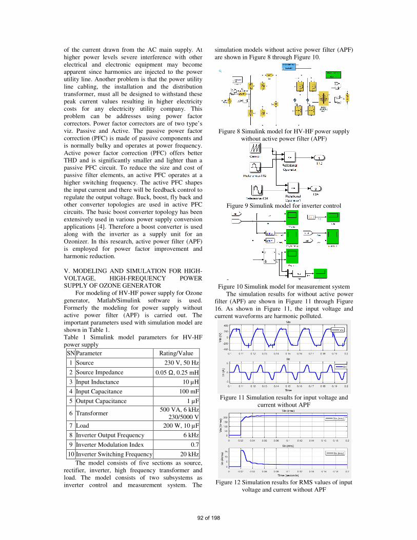
of the current drawn from the AC main supply. At

higher power levels severe interference with other

electrical and electronic equipment may become

apparent since harmonics are injected to the power

utility line. Another problem is that the power utility

line cabling, the installation and the distribution

transformer, must all be designed to withstand these

peak current values resulting in higher electricity

costs for any electricity utility company. This

problem can be addresses using power factor

correctors. Power factor correctors are of two type’s

viz. Passive and Active. The passive power factor

correction (PFC) is made of passive components and

is normally bulky and operates at power frequency.

Active power factor correction (PFC) offers better

THD and is significantly smaller and lighter than a

passive PFC circuit. To reduce the size and cost of

passive filter elements, an active PFC operates at a

higher switching frequency. The active PFC shapes

the input current and there will be feedback control to

regulate the output voltage. Buck, boost, fly back and

other converter topologies are used in active PFC

circuits. The basic boost converter topology has been

extensively used in various power supply conversion

applications [4]. Therefore a boost converter is used

along with the inverter as a supply unit for an

Ozonizer. In this research, active power filter (APF)

is employed for power factor improvement and

harmonic reduction.

V. MODELING AND SIMULATION FOR HIGH-

VOLTAGE, HIGH-FREQUENCY POWER

SUPPLY OF OZONE GENERATOR

For modeling of HV-HF power supply for Ozone

generator, Matlab/Simulink software is used.

Formerly the modeling for power supply without

active power filter (APF) is carried out. The

important parameters used with simulation model are

shown in Table 1.

Table 1 Simulink model parameters for HV-HF

power supply

SN Parameter Rating/Value

1 Source 230 V, 50 Hz

2 Source Impedance 0.05 Ω, 0.25 mH

3 Input Inductance 10 µH

4 Input Capacitance 100 mF

5 Output Capacitance 1 µF

6 Transformer 500 VA, 6 kHz

230/5000 V

7 Load 200 W, 10 µF

8 Inverter Output Frequency 6 kHz

9 Inverter Modulation Index 0.7

10 Inverter Switching Frequency 20 kHz

The model consists of five sections as source,

rectifier, inverter, high frequency transformer and

load. The model consists of two subsystems as

inverter control and measurement system. The

simulation models without active power filter (APF)

are shown in Figure 8 through Figure 10.

Figure 8 Simulink model for HV-HF power supply

without active power filter (APF)

Figure 9 Simulink model for inverter control

-

Figure 10 Simulink model for measurement system

The simulation results for without active power

filter (APF) are shown in Figure 11 through Figure

16. As shown in Figure 11, the input voltage and

current waveforms are harmonic polluted.

Figure 11 Simulation results for input voltage and

current without APF

Figure 12 Simulation results for RMS values of input

voltage and current without APF

92 of 198

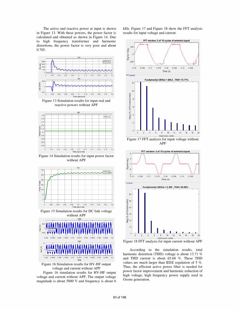
The active and reactive power at input is shown

in Figure 13. With these powers, the power factor is

calculated and obtained as shown in Figure 14. Due

to high frequency transformer and harmonic

distortions, the power factor is very poor and about

0.705.

Figure 13 Simulation results for input real and

reactive powers without APF

Figure 14 Simulation results for input power factor

without APF

Figure 15 Simulation results for DC link voltage

without APF

Figure 16 Simulation results for HV-HF output

voltage and current without APF

Figure 16 simulation results for HV-HF output

voltage and current without APF. The output voltage

magnitude is about 5000 V and frequency is about 6

kHz. Figure 17 and Figure 18 show the FFT analysis

results for input voltage and current.

Figure 17 FFT analysis for input voltage without

APF

Figure 18 FFT analysis for input current without APF

According to the simulation results, total

harmonic distortion (THD) voltage is about 13.71 %

and THD current is about 65.68 %. These THD

values are much larger than IEEE regulation of 5 %.

Thus, the efficient active power filter is needed for

power factor improvement and harmonic reduction of

high voltage, high frequency power supply used in

Ozone generation.

93 of 198

VI. MODELING AND SIMULATION FOR

POWER FACTOR IMPROVEMENT AND

HARMONIC REDUCTION

For power factor improvement and harmonic

reduction, the design calculation for APF is executed

and connected at the common coupling point (PCC)

of HV-HF power supply. The complete simulation

model with APF is shown in Figure 19 and the

control system of APF is shown in Figure 20.

Figure 19 Simulink model for HV-HF power supply

with APF

Figure 20 Simulink model for control of APF

For the control of APF, the proportional-integral

controller is employed. The important parameters for

APF are described in Table 2.

Table 2 Simulink Model Parameters for APF of HV-

HF Power Supply

SN Parameter Rating/Value

1 Reference DC Voltage 650 V

2 Hysteresis Band Current 1.0 A

3 Inductance of APF 5 µH

4 Capacitance of APF 8 mF

5

PI Controller

Proportional Gain

Integral Gain

0.1

0.01

Figure 21 Simulation results for input voltage and

current with APF

The simulation results for HV-HF power supply

with active power filter (APF) are shown in Figure 21

through Figure 24. As shown in Figure 20, the

harmonic distortion at input voltage and current are

negligible. The rms voltage and current as well as

real and reactive power are nearly the same as the

without APF case. The power factor at PCC is

increased and is about 0.98 which is much better

compared to without active power filter (APF) case.

Figure 22 Simulation results for RMS values of input

voltage and current with active power filter (APF)

Figure 23 Simulation results for input real and

reactive powers with (APF)

Figure 24 Simulation results for input power factor

with APF

With the application of active power filter

(APF), the THD of input voltage and current are

significantly reduced. According to the simulation

results, THD voltage is about 3.36 % and THD

current is about 2.86 %. These THD values are within

the IEEE regulation of 5 %. Thus, the active power

filter can reduce the harmonic distortion effectively.

Thus, the application of APF can reduce system cost

and improve system power quality.

94 of 198

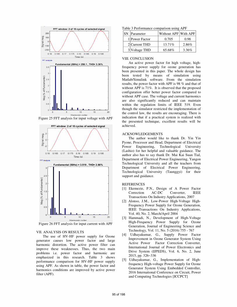
Figure 25 FFT analysis for input voltage with APF

Figure 26 FFT analysis for input current with APF

VII. ANALYSIS ON RESULTS

The use of HV-HF power supply for Ozone

generator causes low power factor and large

harmonic distortion. The active power filter can

improve these weaknesses. Thus, the two main

problems i.e. power factor and harmonic are

emphasized in this research. Table 3 shows

performance comparison for HV-HF power supply

using APF. As shown in table, the power factor and

harmonics conditions are improved by active power

filter (APF).

Table 3 Performance comparison using APF

SN Parameter Without APF With APF

1 Power Factor 0.705 0.98

2 Current THD 13.71% 2.86%

3 Voltage THD 65.68% 3.36%

VIII. CONCLUSION

An active power factor for high voltage, high-

frequency power supply for ozone generation has

been presented in this paper. The whole design has

been tested by means of simulation using

Matlab/Simulink software. From the simulation

results, the power factor with APF is 98 % and that of

without APF is 71%. It is observed that the proposed

configuration offer better power factor compared to

without APF case. The voltage and current harmonics

are also significantly reduced and can maintain

within the regulation limits of IEEE 519. Even

though the simulator restricted the implementation of

the control law, the results are encouraging. There is

indication that if a practical system is realized with

the presented technique, excellent results will be

achieved.

ACKNOWLEDGEMENTS

The author would like to thank Dr. Yin Yin

Pyone, Processor and Head, Department of Electrical

Power Engineering, Technological University

(Lashio) for her helpful and valuable guidance. The

author also has to say thank Dr. Mai Kai Suan Tial,

Department of Electrical Power Engineering, Yangon

Technological University and all the teachers from

Department of Electrical Power Engineering,

Technological University (Taunggyi) for their

support and guidance.

REFERENCES

[1] Ekemezie, P.N., Design of A Power Factor

Correction AC-DC Converter, IEEE

Transactions On Industry Applications, 2007

[2] Alonso, J.M., Low-Power High-Voltage High-

Frequency Power Supply for Ozone Generation,

IEEE Transactions On Industry Applications,

Vol. 40, No. 2, March/April 2004

[3] Hammadi, N., Development of High-Voltage

High-Frequency Power Supply for Ozone

Generation, Journal of Engineering Science and

Technology, Vol. 11, No. 5 (2016) 755 - 767

[4] Udhayakumar, G., Supply Power Factor

Improvement in Ozone Generator System Using

Active Power Factor Correction Converter,

International Journal of Power Electronics and

Drive System (IJPEDS), Vol. 6, No. 2, June

2015, pp. 326~336

[5] Udhayakumar, G., Implementation of High-

frequency High-voltage Power Supply for Ozone

Generator System Using Embedded Controller,

2016 International Conference on Circuit, Power

and Computing Technologies [ICCPCT]

95 of 198

Microtremor Measurement at Some Sites in Mandalay City, Myanmar,

for Earthquake Disaster Mitigation

Yu Nandar Hlaing1, Ichii Koji1

1 Myanmar Earthquake Committee Myanmar Engineering Society,Yangon,Myanmar

2 Faculty of Social Science Kansai University, Osaka, Japan

*[email protected], [email protected]

Abstract — Estimation of earthquake motion is

important for sustainability of a city. It is well known

that the characteristics of earthquake motion relates

to the geological condition of the site (i.e., Idriss and

Seed,1968). Microtremor is quite small vibration can

be measured at anywhere, and the measurement of

microtremor gives some amount of geological

information.

In this study, microtremor measurement was done for

10 points with different geological profile in

Mandalay, Myanmar. The difference of the local site

conditions can be found in the difference of

microtremor measurement results. Then it can be

used for the evaluation of important characteristics of

strong earthquake motions such as frequency

content. Assuming H/V spectra as the natural

frequency of the site, there is a clear tendency of

variation of the natural frequency in the measured

results in Mandalay. The results show that the

microtremor observations are acceptable method for

assessing dynamic characteristics of soil and site

effect in Mandalay City with ease of measurement

and analysis.

Keywords: microtremor, H/V spectra, Mandalay, Earthquake. I. INTRODUCTION

Ground response may be used for prediction of ground

motion and development of design response spectrum in

order to determine the dynamic stress and strains

assessment. The study of distribution of damages caused

by various earthquakes indicates the significant site

effects on earthquake characteristics (Idriss and

Seed,1970)[3] .Local site conditions can influence on all

of the important characteristics such as amplitude,

frequency content and duration of strong ground motion.

As an earthquake prone area such as Mandalay in

Myanmar, several studies on site response analysis were

carried out. Myo Thant et.al [1] proceeded 43

microtremor measurements to analyse seismic hazard

maps by using PSHA, and Pyi Soe Thein et.al [4]

conducted seismic microzonation mapping through 50

soil columns by using multiple reflection analysis and Yu

Nandar Hlaing and Ichii [2] conducted one dimensional

site response analysis at several sites in Mandalay.

However, these studies have mostly focused on seismic

vulnerability and micro-zonation of Mandalay city, the

comparison of characteristics of observed microtremor

and the results from geological profile will be helpful for

the complete study for Mandalay city where earthquake

prone area with dense population..

II. MICROTREMOR MEASUREMENT

Microtremor is a very convenient tool to estimate the

effect of surface geology on seismic motion without

other geological information. The dynamics

characteristics of soil can be stated by microtremor

measurement. Microtremors are ground vibrations with

displacement amplitude about 1-10 micron, and velocity

amplitude is 0.001-0.01cm/s that can be detected by

seismograph with high magnification (Rezaei and

Choobasti 2014) [5]. One of the most popular techniques

for estimation of site effects in the region with low

seismicity is microtremor measurements by Nakamura

method [6] (H/V). Regarding H/V spectral ratio method,

peak frequency and amplification factor were calculated

for all microtremor sites. Geonet 2-2S3D is used for

measurement shown in Fig 1.

Geonet is three component velocity sensor unit; two

in two orthogonal horizontal directions and one in

vertical direction), GPS, laptop and 12V battery are used.

96 of 198

mailto:*[email protected]

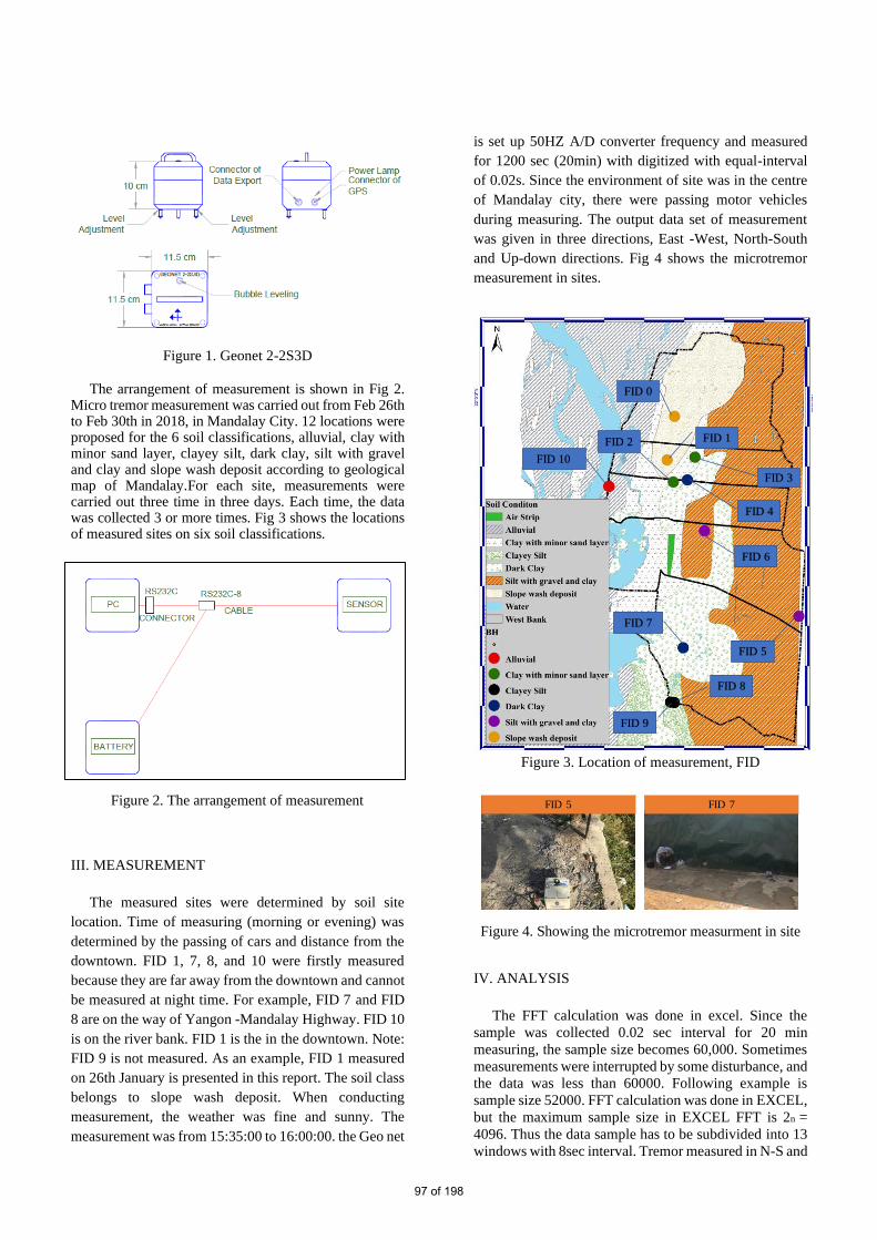
Figure 1. Geonet 2-2S3D

The arrangement of measurement is shown in Fig 2.

Micro tremor measurement was carried out from Feb 26th to Feb 30th in 2018, in Mandalay City. 12 locations were proposed for the 6 soil classifications, alluvial, clay with minor sand layer, clayey silt, dark clay, silt with gravel and clay and slope wash deposit according to geological map of Mandalay.For each site, measurements were carried out three time in three days. Each time, the data was collected 3 or more times. Fig 3 shows the locations of measured sites on six soil classifications.

Figure 2. The arrangement of measurement

III. MEASUREMENT

The measured sites were determined by soil site

location. Time of measuring (morning or evening) was

determined by the passing of cars and distance from the

downtown. FID 1, 7, 8, and 10 were firstly measured

because they are far away from the downtown and cannot

be measured at night time. For example, FID 7 and FID

8 are on the way of Yangon -Mandalay Highway. FID 10

is on the river bank. FID 1 is the in the downtown. Note:

FID 9 is not measured. As an example, FID 1 measured

on 26th January is presented in this report. The soil class

belongs to slope wash deposit. When conducting

measurement, the weather was fine and sunny. The

measurement was from 15:35:00 to 16:00:00. the Geo net

is set up 50HZ A/D converter frequency and measured

for 1200 sec (20min) with digitized with equal-interval

of 0.02s. Since the environment of site was in the centre

of Mandalay city, there were passing motor vehicles

during measuring. The output data set of measurement

was given in three directions, East -West, North-South

and Up-down directions. Fig 4 shows the microtremor

measurement in sites.

Figure 3. Location of measurement, FID

Figure 4. Showing the microtremor measurment in site

IV. ANALYSIS

The FFT calculation was done in excel. Since the

sample was collected 0.02 sec interval for 20 min

measuring, the sample size becomes 60,000. Sometimes

measurements were interrupted by some disturbance, and

the data was less than 60000. Following example is

sample size 52000. FFT calculation was done in EXCEL,

but the maximum sample size in EXCEL FFT is 2n =

4096. Thus the data sample has to be subdivided into 13

windows with 8sec interval. Tremor measured in N-S and

FID 10

FID 8

FID 9

FID 7

FID 1

FID 0

FID 3

FID 4

FID 2

FID 6

FID 5

FID 7FID 5

97 of 198

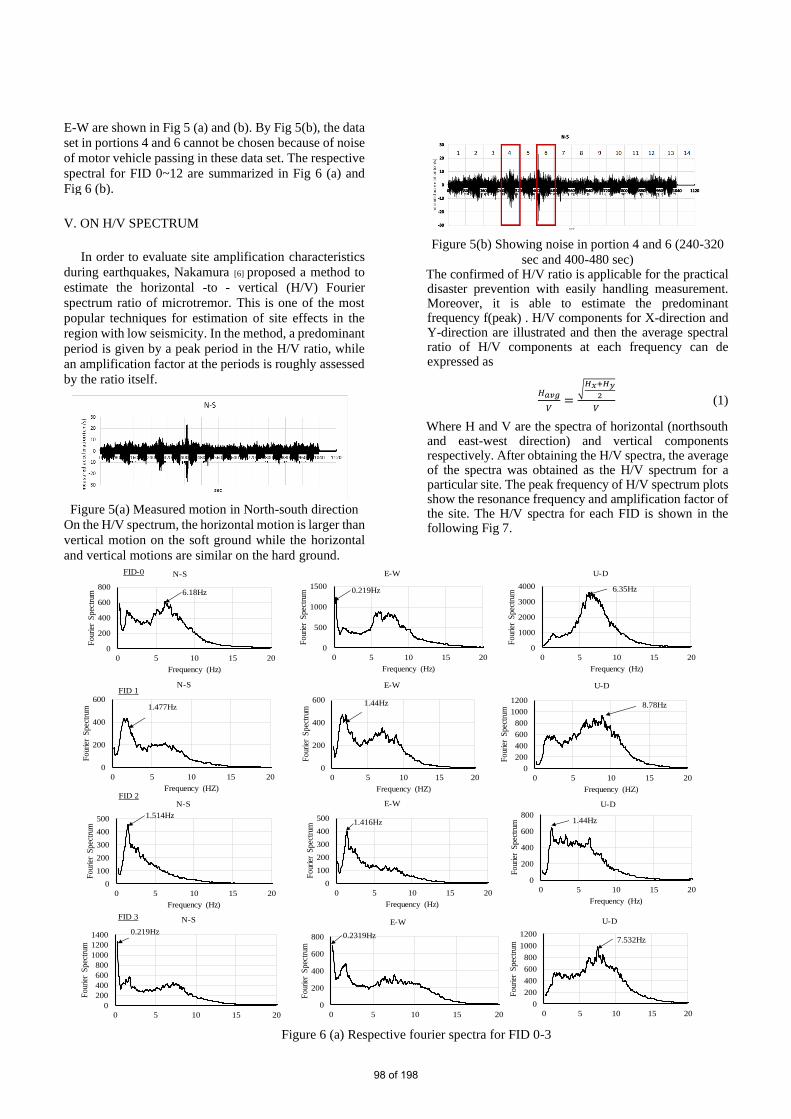
E-W are shown in Fig 5 (a) and (b). By Fig 5(b), the data

set in portions 4 and 6 cannot be chosen because of noise

of motor vehicle passing in these data set. The respective

spectral for FID 0~12 are summarized in Fig 6 (a) and

Fig 6 (b).

V. ON H/V SPECTRUM

In order to evaluate site amplification characteristics

during earthquakes, Nakamura [6] proposed a method to

estimate the horizontal -to - vertical (H/V) Fourier

spectrum ratio of microtremor. This is one of the most

popular techniques for estimation of site effects in the

region with low seismicity. In the method, a predominant

period is given by a peak period in the H/V ratio, while

an amplification factor at the periods is roughly assessed

by the ratio itself.

Figure 5(a) Measured motion in North-south direction

On the H/V spectrum, the horizontal motion is larger than

vertical motion on the soft ground while the horizontal

and vertical motions are similar on the hard ground.

Figure 5(b) Showing noise in portion 4 and 6 (240-320

sec and 400-480 sec) The confirmed of H/V ratio is applicable for the practical disaster prevention with easily handling measurement. Moreover, it is able to estimate the predominant frequency f(peak) . H/V components for X-direction and Y-direction are illustrated and then the average spectral ratio of H/V components at each frequency can de expressed as

𝐻𝑎𝑣𝑔

𝑉=

√𝐻𝑥+𝐻𝑦

2

𝑉 (1)

Where H and V are the spectra of horizontal (northsouth and east-west direction) and vertical components respectively. After obtaining the H/V spectra, the average of the spectra was obtained as the H/V spectrum for a particular site. The peak frequency of H/V spectrum plots show the resonance frequency and amplification factor of the site. The H/V spectra for each FID is shown in the following Fig 7.

0

200

400

600

0 5 10 15 20

Four

ier

Spec

trum

Frequency (HZ)

N-S

1.477Hz

0

200

400

600

0 5 10 15 20

Four

ier

Spec

trum

Frequency (HZ)

E-W

1.44Hz

0

200

400

600

800

1000

1200

0 5 10 15 20

Four

ier

Spec

trum

Frequency (HZ)

U-D

8.78Hz

FID 1

FID-0

0

200

400

600

800

0 5 10 15 20

Four

ier

Spec

trum

Frequency (Hz)

N-S

6.18Hz

0

500

1000

1500

0 5 10 15 20

Four

ier

Spec

trum

Frequency (Hz)

E-W

0.219Hz

0

1000

2000

3000

4000

0 5 10 15 20

Four

ier

Spec

trum

Frequency (Hz)

U-D

6.35Hz

0

100

200

300

400

500

0 5 10 15 20

Four

ier

Spec

trum

Frequency (Hz)

N-S

0

100

200

300

400

500

0 5 10 15 20

Four

ier

Spec

trum

Frequency (Hz)

E-W

1.416Hz

0

200

400

600

800

0 5 10 15 20

Four

ier

Spec

trum

Frequency (Hz)

U-D

1.44Hz1.514Hz

FID 2

0

200

400

600

800

1000

1200

1400

0 5 10 15 20

Four

ier

Spec

trum

Frequency (Hz)

N-S

0.219Hz

0

200

400

600

800

0 5 10 15 20

Four

ier

Spec

trum

Frequency (Hz)

E-W

0.2319Hz

0

200

400

600

800

1000

1200

0 5 10 15 20

Four

ier

Spec

trum

Frequency (Hz)

U-D

7.532Hz

FID 3

Figure 6 (a) Respective fourier spectra for FID 0-3

98 of 198

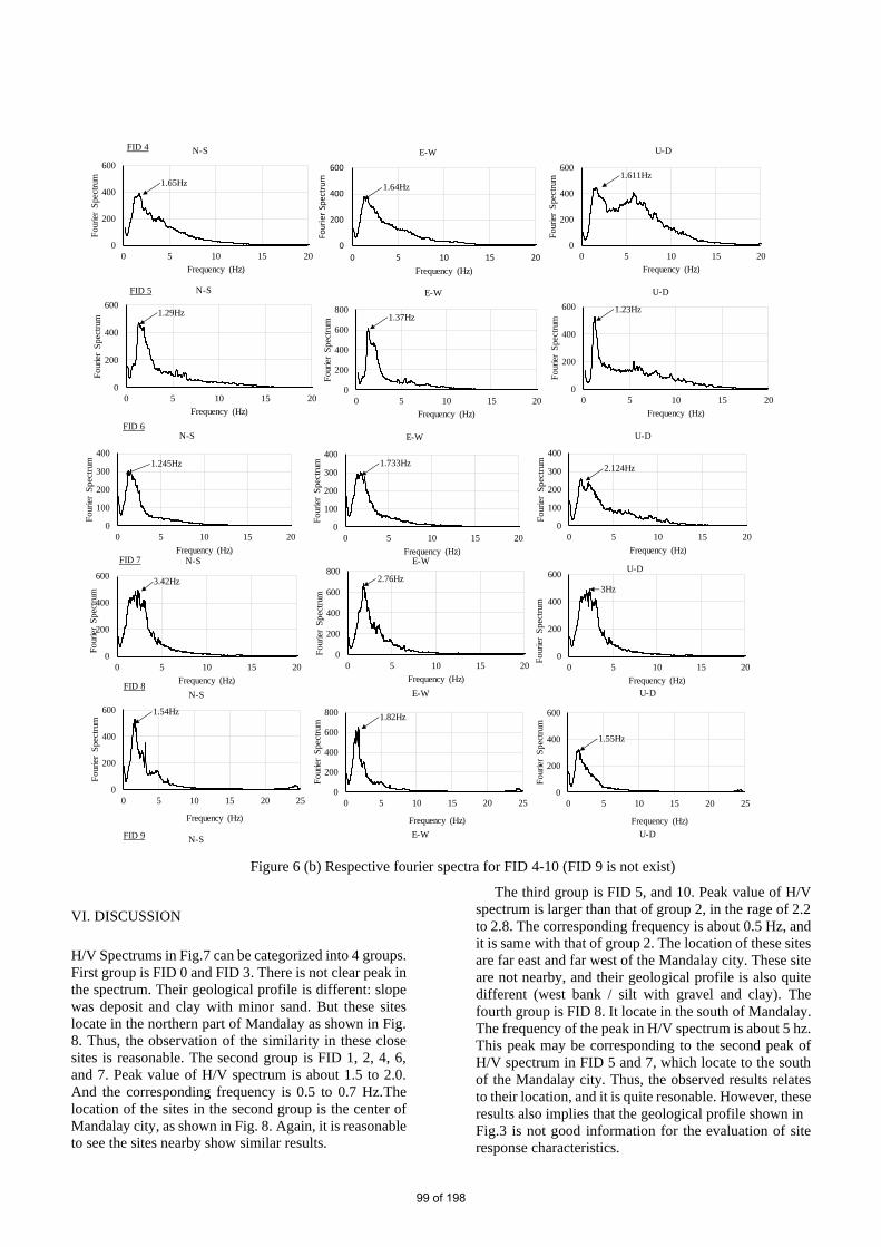
VI. DISCUSSION

H/V Spectrums in Fig.7 can be categorized into 4 groups.

First group is FID 0 and FID 3. There is not clear peak in

the spectrum. Their geological profile is different: slope

was deposit and clay with minor sand. But these sites

locate in the northern part of Mandalay as shown in Fig.

8. Thus, the observation of the similarity in these close

sites is reasonable. The second group is FID 1, 2, 4, 6,

and 7. Peak value of H/V spectrum is about 1.5 to 2.0.

And the corresponding frequency is 0.5 to 0.7 Hz.The

location of the sites in the second group is the center of

Mandalay city, as shown in Fig. 8. Again, it is reasonable

to see the sites nearby show similar results.

The third group is FID 5, and 10. Peak value of H/V

spectrum is larger than that of group 2, in the rage of 2.2

to 2.8. The corresponding frequency is about 0.5 Hz, and

it is same with that of group 2. The location of these sites

are far east and far west of the Mandalay city. These site

are not nearby, and their geological profile is also quite

different (west bank / silt with gravel and clay). The

fourth group is FID 8. It locate in the south of Mandalay.

The frequency of the peak in H/V spectrum is about 5 hz.

This peak may be corresponding to the second peak of

H/V spectrum in FID 5 and 7, which locate to the south

of the Mandalay city. Thus, the observed results relates

to their location, and it is quite resonable. However, these

results also implies that the geological profile shown in

Fig.3 is not good information for the evaluation of site

response characteristics.

Figure 6 (b) Respective fourier spectra for FID 4-10 (FID 9 is not exist)

0

100

200

300

400

0 5 10 15 20

Four

ier

Spec

trum

Frequency (Hz)

N-S

1.245Hz

0

100

200

300

400

0 5 10 15 20

Four

ier

Spec

trum

Frequency (Hz)

E-W

1.733Hz

0

100

200

300

400

0 5 10 15 20F

our

ier

Spec

trum

Frequency (Hz)

U-D

2.124Hz

0

200

400

600

0 5 10 15 20

Four

ier

Spec

trum

Frequency (Hz)

N-S

3.42Hz

0

200

400

600

800

0 5 10 15 20

Four

ier

Spec

trum

Frequency (Hz)

E-W

2.76Hz

0

200

400

600

0 5 10 15 20

Fo

urie

r S

pec

trum

Frequency (Hz)

U-D

3Hz

FID 6

FID 7

0

200

400

600

800

0 5 10 15 20 25

Fo

urie

r S

pec

trum

Frequency (Hz)

E-W

1.82Hz

0

200

400

600

0 5 10 15 20 25

Four

ier

Spec

trum

Frequency (Hz)

N-S

1.54Hz

0

200

400

600

0 5 10 15 20 25

Four

ier

Spec

trum

Frequency (Hz)

U-D

1.55Hz

FID 8

0

200

400

600

800

0 5 10 15 20 25

Four

ier

Spec

trum

Frequency (Hz)

E-W

1.82Hz

0

200

400

600

0 5 10 15 20 25

Fo

urie

r S

pec

trum

Frequency (Hz)

N-S

1.54Hz

0

200

400

600

0 5 10 15 20 25

Four

ier

Spec

trum

Frequency (Hz)

U-D

1.55Hz

FID 9

0

300

600

900

1200

0 5 10 15 20

Four

ier

Spec

trum

Frequency (Hz)

N-S

1.45Hz

0

300

600

900

1200

1500

0 5 10 15 20

Fo

urie

r S

pec

trum

Frequency (Hz)

U-D

6.19Hz

0

300

600

900

1200

0 5 10 15 20

Four

ier

Spec

trum

Frequency (Hz)

E-W

6.85Hz

FID 10

0

300

600

900

1200

0 5 10 15 20

Four

ier

Spec

trum

Frequency (Hz)

N-S

1.45Hz

0

300

600

900

1200

1500

0 5 10 15 20

Fo

urie

r S

pec

trum

Frequency (Hz)

U-D

6.19Hz

0

300

600

900

1200

0 5 10 15 20

Four

ier

Spec

trum

Frequency (Hz)

E-W

6.85Hz

FID 11

0

200

400

600

0 5 10 15 20

Four

ier

Spec

trum

Frequency (Hz)

E-W

1.64Hz

0

200

400

600

0 5 10 15 20

Fo

urie

r S

pec

trum

Frequency (Hz)

N-S

1.65Hz

0

200

400

600

0 5 10 15 20

Fo

urie

r S

pec

trum

Frequency (Hz)

U-D

1.611Hz

FID 4

0

200

400

600

0 5 10 15 20

Fo

urie

r S

pec

trum

Frequency (Hz)

N-S

1.29Hz

0

200

400

600

800

0 5 10 15 20

Fo

urie

r S

pec

trum

Frequency (Hz)

E-W

1.37Hz

0

200

400

600

0 5 10 15 20

Fo

urie

r S

pec

trum

Frequency (Hz)

U-D

1.23Hz

FID 5

99 of 198

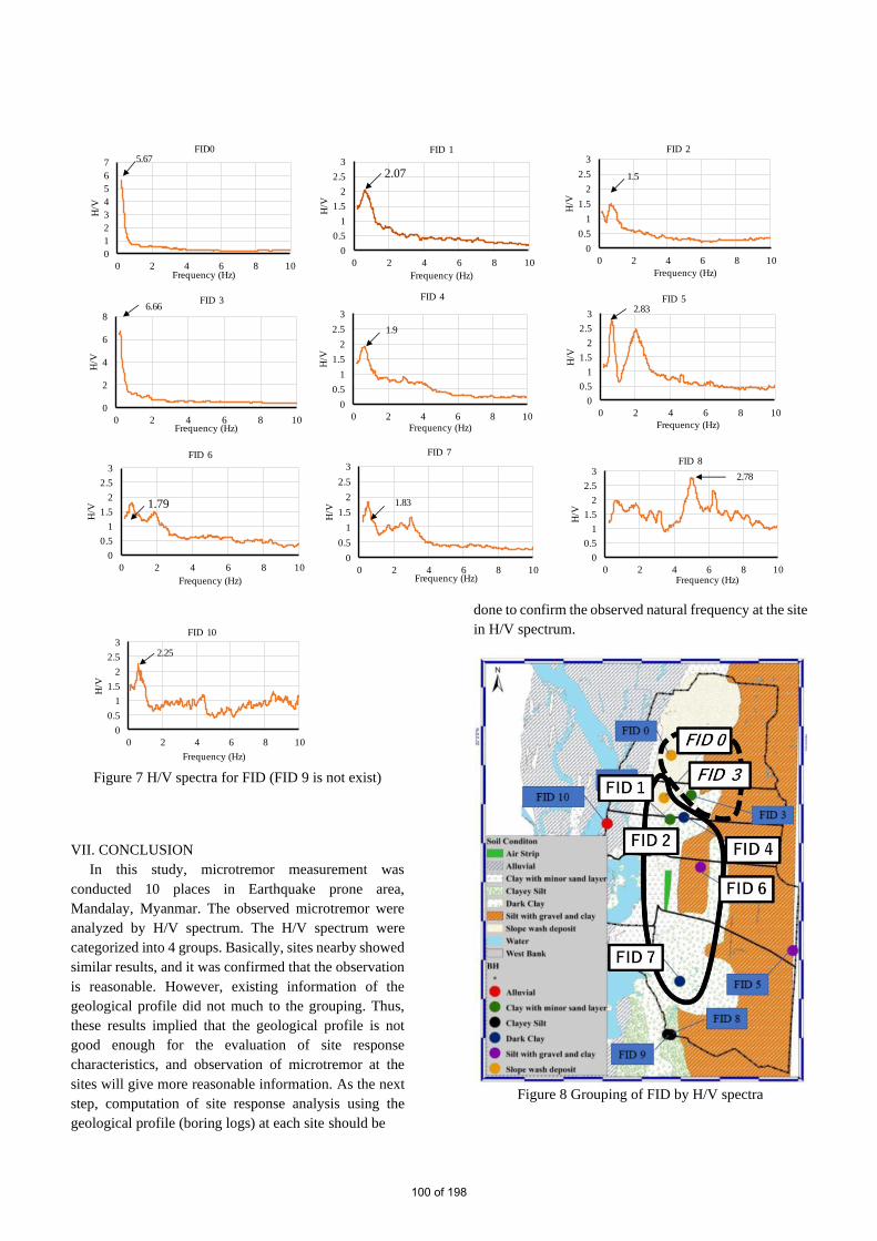
Figure 7 H/V spectra for FID (FID 9 is not exist)

VII. CONCLUSION

In this study, microtremor measurement was

conducted 10 places in Earthquake prone area,

Mandalay, Myanmar. The observed microtremor were

analyzed by H/V spectrum. The H/V spectrum were

categorized into 4 groups. Basically, sites nearby showed

similar results, and it was confirmed that the observation

is reasonable. However, existing information of the

geological profile did not much to the grouping. Thus,

these results implied that the geological profile is not

good enough for the evaluation of site response

characteristics, and observation of microtremor at the

sites will give more reasonable information. As the next

step, computation of site response analysis using the

geological profile (boring logs) at each site should be

done to confirm the observed natural frequency at the site

in H/V spectrum.

Figure 8 Grouping of FID by H/V spectra

0

1

2

3

4

5

6

7

0 2 4 6 8 10

H/V

Frequency (Hz)

FID05.67

0

0.5

1

1.5

2

2.5

3

0 2 4 6 8 10

H/V

Frequency (Hz)

FID 1

2.07

0

0.5

1

1.5

2

2.5

3

0 2 4 6 8 10

H/V

Frequency (Hz)

FID 2

1.5

0

2

4

6

8

0 2 4 6 8 10

H/V

Frequency (Hz)

FID 36.66

0

0.5

1

1.5

2

2.5

3

0 2 4 6 8 10

H/V

Frequency (Hz)

FID 4

1.9

0

0.5

1

1.5

2

2.5

3

0 2 4 6 8 10

H/V

Frequency (Hz)

FID 52.83

0

0.5

1

1.5

2

2.5

3

0 2 4 6 8 10

H/V

Frequency (Hz)

FID 6

1.79

0

0.5

1

1.5

2

2.5

3

0 2 4 6 8 10

H/V

Frequency (Hz)

FID 7

1.83

0

0.5

1

1.5

2

2.5

3

0 2 4 6 8 10

H/V

Frequency (Hz)

FID 8

2.78

0

0.5

1

1.5

2

2.5

3

0 2 4 6 8 10

H/V

Frequency (Hz)

FID 10

2.25

0

0.5

1

1.5

2

2.5

3

0 2 4 6 8 10

H/V

Frequency (Hz)

FID 9

0

0.5

1

1.5

2

2.5

3

0 2 4 6 8 10

H/V

Frequency (Hz)

FID 10

2.252.78

0

1

2

3

4

5

6

7

0 2 4 6 8 10

H/V

Frequency (Hz)

FID05.67

0

0.5

1

1.5

2

2.5

3

0 2 4 6 8 10

H/V

Frequency (Hz)

FID 1

2.07

0

0.5

1

1.5

2

2.5

3

0 2 4 6 8 10

H/V

Frequency (Hz)

FID 2

1.5

0

2

4

6

8

0 2 4 6 8 10

H/V

Frequency (Hz)

FID 36.66

0

0.5

1

1.5

2

2.5

3

0 2 4 6 8 10

H/V

Frequency (Hz)

FID 4

1.9

0

0.5

1

1.5

2

2.5

3

0 2 4 6 8 10

H/V

Frequency (Hz)

FID 52.83

0

0.5

1

1.5

2

2.5

3

0 2 4 6 8 10

H/V

Frequency (Hz)

FID 6

1.79

0

0.5

1

1.5

2

2.5

3

0 2 4 6 8 10

H/V

Frequency (Hz)

FID 7

1.83

0

0.5

1

1.5

2

2.5

3

0 2 4 6 8 10H

/VFrequency (Hz)

FID 8

2.78

0

0.5

1

1.5

2

2.5

3

0 2 4 6 8 10

H/V

Frequency (Hz)

FID 10

2.25

0

0.5

1

1.5

2

2.5

3

0 2 4 6 8 10

H/V

Frequency (Hz)

FID 9

0

0.5

1

1.5

2

2.5

3

0 2 4 6 8 10

H/V

Frequency (Hz)

FID 10

2.252.78

100 of 198

ACKNOWLEDGEMENT

This research was financially supported by JICA (JDA

program) and Japanese people.

REFERENCES

Proceeding Papers

[1] Myo Thant et. Al . Development of seismic hazard

maps for Mandalay, Mandalay Region. International conference on geological engineering, Jakarta, Indonesia. December 11-12, 2013

[2] Y.N. Hlaing, Koji Ichii, [2018] Ground Response Analysis and Site characterization of Mandalay City, Conference on Myanmar Engineering Society, Annual General Meeting, Jan 19-20,2018.

Journal Papers

[3] Seed, H.B & Idriss, I.M 1970. Soil Moduli and Damping Factor for Dynamic Response Analysis. Report No. EERC 75-29, Earthquake Eng. Research

Center, University of California at Berkeley, California.

[4] P.S. Thein, Kiyono J, T.T. Win, T.T. Nu and Aung D.W. Seismic Microzonation of Mandalay City, Myanmar. Journal of Geological Resource and Engineering (2018) 1-13.

[5] Rezaei S, Choobbasti AJ [2014] Liquefaction assessment using microtremor measurement, conventional method and artificial neural network (Case study: Babol, Iran). Front Struct Civ Eng 8(3):292–307

[6] Nakamura Y (1989) A method for dynamic characteristics estimation of subsurface using microtremor on the ground surface. Q Rep RTRI 30:25–33

101 of 198

Secure and Authenticated Data Hiding using Edge Detection

Zin Mar Htun 1, Aye Zarchi Minn

2, Aung Kyaw Oo

3

1 Information Technology, Technological University (Taunggyi)

Taunggyi, Myanmar 2 Information Technology, Technological University (Taunggu)

Taunggu, Myanmar 3Information Technology, Technological University (Taunggyi)

Taunggyi, Myanmar

[email protected], [email protected], [email protected]

ABSTRACT

Data hiding is a great trade-mark in information

security. For information security and intellectual

property, effective methods are required. Steganography

is the art of hiding information which no one can detect

its presence except sender and receiver. The major

characteristics of data hiding are less perception of data

existence and hiding capacity. Formerly, the most

important technique is Least Significant Bit (LSB) and

the users only use it to hide information. However it has

major weak point that information hides serially and so it

causes high perception of data existence. Recently, many

edge detection established steganography approaches

have been developed to provide high imperceptibility of

the stego image. However, the embedding capacity of

these approaches can be limited. This paper presents an

improved method that uses Canny Edge detection and

chooses non-edges as LSB embedding area to give high

embedding capacity and security. Moreover, it produces

position file to authenticate the fact that the stego image

is ensure that it comes from original image by comparing

the position file and edges of stego image. It declares that

it gives high payload, security, less perception and image

checking to authenticate the sender.

Keywords: Data Hiding, LSB, Edge Detection, Sobel or

Canny

1. INTRODUCTION

Steganography comes from the Greek Words:

Steganos-“Covered”, Graphe-“Writing”. The central

objective of steganography is to offer security for most

important data of a user by beating it into an image and it

keeps data existence from attackers. Image

steganography is very popular in these days that can

provide high embedding capacity. Many steganography

applications for digital image, include copyright defence,

feature classification, and secret communication [1,2].

Unfortunately the associates of terrorist groups are using

steganography as a techniques to attack against the western

interests [3, 4].

The traditional image Steganography algorithm is

based upon the LSB bits but it can simply perceive by

enemies because the data is hidden in all pixels. If the

enemy identifies at least one pixels location, easily they

hack the original entire message. Instead of sequentially

beating the data in all pixels some of the algorithms are to

hide the data in selected pixels, but it causes speckles in an

image. Moreover embedding in edges gives less capacity.

So we proposed a novel image steganography

algorithm integrating Canny Edge Detection algorithms for

hiding secret message. The Organization of the paper is as

follows. In section 2 the related work is discussed. Section

3 describes our proposed method. Finally the results are

presented in section 4.

2. RELATED WORKS

The least significant bit (LSB) technology is the

blandest method to be applied in steganography.

Steganography is a method to hide secret data in a

meaningful image. The highest priority is to maintain the

quality of the stego image.

Consequently, steganography is used to embed secret

information in the least significant bit of every pixel.

However, Fridrich [5] asserts that this technique cannot

resist statistical attacks. A few years later, some works of

research [5, 6, 7, 8, 9, 10] proposed that under the

condition which isn't detectable, more information can be

embedded in sharp areas than in smooth areas.

Youssef Bassil proposed an Image Steganography

based on a Parameterized Canny Edge Detection

Algorithm [11]. It was intended to hide top-secret data into

pixels of the image that were chosen the boundaries of

objects detected in the image. More specifically, bits of the

secret data replace the three LSBs of every colour channel

of the pixels detected by the Canny Edge Detection

102 of 198

algorithm as part of the edges in the carrier image. It

gave high imperceptibility but low capacity.

R. Wazirali presented that a new edge detection

method based on gradient, 9x9 mask of LOG and zero

crossing [12]. It combines with clustering to classify the

image to edge and non-edge regions. Different amount of

secret message will be embedded in each cluster after the

finding of the edge regions. It gained the stability

between stego image imperceptibility and high payload

capacity.

3. BACKGROUND THEORY

In this paper, two methods are utilized to hide the

data in images. The main method for hiding is LSB. To

hide the data, firstly we find non-edges in cover image

using canny edge detection algorithms.

3.1 Least significant bit (lSB)

Least Significant Bits substitution is one of the most

public hiding method due to its easiness. The secret

message is considered as bit stream and will be

concealed into cover image by varying the LSBs of the

cover image with the boot stream of the secret file.

With only 1 bit substitution, the change between the

cover and stego image is scarcely obvious by human

visual system. However, when the extent of secret

message is great, the hiding capacity will increase.

Therefore, more bits will be used to cover the large secret

message and consequently, more degradation may

announce to the stego image and hence effects its

imperceptibility.

3.2 Canny Edge Detection

Fundamentally, edge detection is the process of

identifying points in a computer image at which the

image brightness changes abruptly, for instance, pixels

difference from low intensities to high intensities or vice

versa, exhibiting some discontinuities. The goal of edge

detection is to detect and capture important events and

changes in the properties of the image.

The advantage of edge detection is that it decreases

the amount of data to be analysed and processed by

image processing algorithms. It in fact eliminates the less

significant information while maintaining the more

significant structural features of the image. In practice,

many edge detection algorithms have been used,

however, one of the most capable and widely known

algorithm is the Canny edge detection which was

developed by John Canny in 1986 [12]. In essence, it is a

multi-stage algorithm that can extract a wide range of

edges in images regardless of the noise present in them.

The algorithm has the following five stages are grayscale

conversion, Gaussian blur, determine the intensity

gradient,non-maximum suppression and double

threadsholding.

Moreover, it has two basic adjustable parameters, the

size of the Gaussian filter and the threshold.

As Gaussian filter is used in the first stage to smooth

the image and reduce the noise and unwanted details,

declining its size would result in fuzzy image that permits

the finding of smaller details. In contrast, increasing its

size would result in even more blurry images, spreading

the value of a given pixel over a greater area of the image

and permitting the detection of bigger edges.

The Canny algorithm uses two thresholds which agree

more flexibility for edge detection. Often, a threshold set

too high can miss important information; whereas, a

threshold set too low can extract irrelevant information

such as noise.

4. PROPOSED SYSTEM

System design of the proposed system is as shown in

Fig. 1.

In embedding of proposed system shown in Fig. 1(a),

an original image is converted to as grayscale image to

find edges. And then the binary data converted from

message is embedded in non-edges and the system is put

edges data into position file.

The extracting process in Fig. 1(b) is reversed from

embedding. The stego image is transformed to grayscale

image and the system detect edges. The user can get

original message from non-edges and check edge data. If

the position of the edges are the same between the edges

from images and the position file, the original message

verify the real image form the real sender.

4.1 Algorithm for the Proposed System

The algorithm for the proposed system is divided to

two subsection. Embedding algorithm is as follows.

Input cover image and secret message(data).

Transform cover image to grayscale image.

Detect Edges using canny edge detection

techniuques.

Embed message in non-edges of using least

significant bit (LSB).

Output stego image and position file that contains

edges points

Measure MSE, PSNR, embedding capacity of

image.

Extracting algorithm is as follows.

Input stego image and position file

Transform the stego image to grayscale image and

detect edges using canny edge detection

techniques

Check whether the edges points are the same of

the points in position file.

103 of 198

If equal, extract message of using least

significant bit (LSB).

Output original message.

Figure 1. Proposed System Design

4.2 Steps of the System

There are two main steps in proposed system. The

first step is canny edge detection and the second step is

LSB algorithm.

The main steps of canny edge detection are

Step 1 : Grayscale Conversion

Step 2 : Gaussian Blur

Step 3 : Determine the intensity Gradient

Step 4 : Non maximum suppression

Step 5 : Double thresholding

According to Step 1, the system converts the cover

image to grayscale image. The intensity values of the

pixels are 8 bit and range from 0 to 255. After converting

the grayscale image, the user can seen in Fig. 2.

Figure 2. After converting to Grayscale Image

In step 2, the system performs a Gaussian blur on the

image. The blur eliminates some of the noise before further

processing the image. It aims to decrease the level of noise

of in image. The equation of this function is shown in Fig

3.

Figure 3. Guassian Blur Function

In Step 3, the gradients can be determined by using

sobel filter .An edge occurs when the color of an image

changes, hence the intensity of the pixel changes as well.

Gx=

1 0 1

1 0 1

1 0 1

, Gy =

1 2 1

0 0 0

1 2 1

Taking the derivatives will output as Fig. 4.

Figure 4. Gradient Images

Then, it calculates the magnitude and angle of the

directional gradients:

|G|= √(2+2) (1)

∠G= arctan (Gy/Gx) (2)

(or) Angle (ɵ) = tan-1(Gy/Gx)

The magnitude of the image results in the following

output in Fig. 5.

In Step 4, non-maximum suppression methods can

reduce thick edges. Thus, we must perform non maximum

suppression to thin out the edges. Non maximum

suppression works by finding the pixel with the maximum

value in an edge.

104 of 198

In the above image, it occurs when pixel q has an

intensity that is larger than both p and r where pixels p

and r are the pixels in the gradient direction of q.

Figure 5. Gradient Magnitude

If this condition is true, then we keep the pixel,

otherwise we set the pixel to zero (make it a black pixel).

Non maximum suppression can be achieved by

interpolating the pixels for greater accuracy.

r=αb+(1−α)a (3)

The result of this step is as Fig. 6.

Figure 6. NON MAXIMUM SUPPRESSION WITH

INTERPOLATION

The final step is double thresholding. The result

from non-maximum suppression is not perfect, some

edges may not actually be edges and there is some noise

in the image.

Double thresholding takes care of this. It sets two

thresholds, a high and a low threshold. In this algorithm,

I normalized all the values such that they will only range

from 0 to 1.

Pixels with a high value are most likely to be edges.

For example, you might choose the high threshold to be

0.7, this means that all pixels with a value larger than 0.7

will be a strong edge. You might also choose a low

threshold of 0.3, this means that all pixels less than it is

not an edge and you would set it to 0. The values in

between 0.3 and 0.7 would be weak edges, in other

words, we do not know if these are actual edges or not

edges at all.

This threshold is different per image so I had to vary

the values. In my implementation I found it helpful to

choose a threshold ratio instead of a specific value and

multiple that by the max pixel value in the image.

As for the low threshold, I chose a low threshold ratio

and multiplied it by the high threshold value:

4.3 Consideration of Edge Detection

The system considers and confuses whether it can get

the same edge points from stego images as original images.

LSB can produce the same edge points. However the other

methods can cause the error in edge detection.

4.4 Disadvantages of the proposed system

The system considers and confuses whether it can get

the same edge points from stego images as original images.

LSB can produce the same edge points, However the other

methods can cause the error in edge detection.

5. TEST AND RESULT

Performance parameters for this system is embedding

capacity, more security and authenticate the real sender.

Figure 7. ORIGINAL IMAGE AND STEGO IMAGE

According to Fig. 7, there are no more difference

between original image and stego image using both edge

detection and LSB than only LSB.

5.1 Embedding Capacity

The system embeds the data in non-edge pixels and so

it only get less amount to omit edge pixels. It can give high

embedding capacity other data hiding method using edge

detection. It can easily be seen in Fig. 7.

In Fig. 8, tests use five 256×256 images. All image

has more non-edge pixels. Therefore the proposed system

is higher embedding capacity than edges embedding.

The red line shows the less embedding capacity for

data hiding method using edge detection.

105 of 198

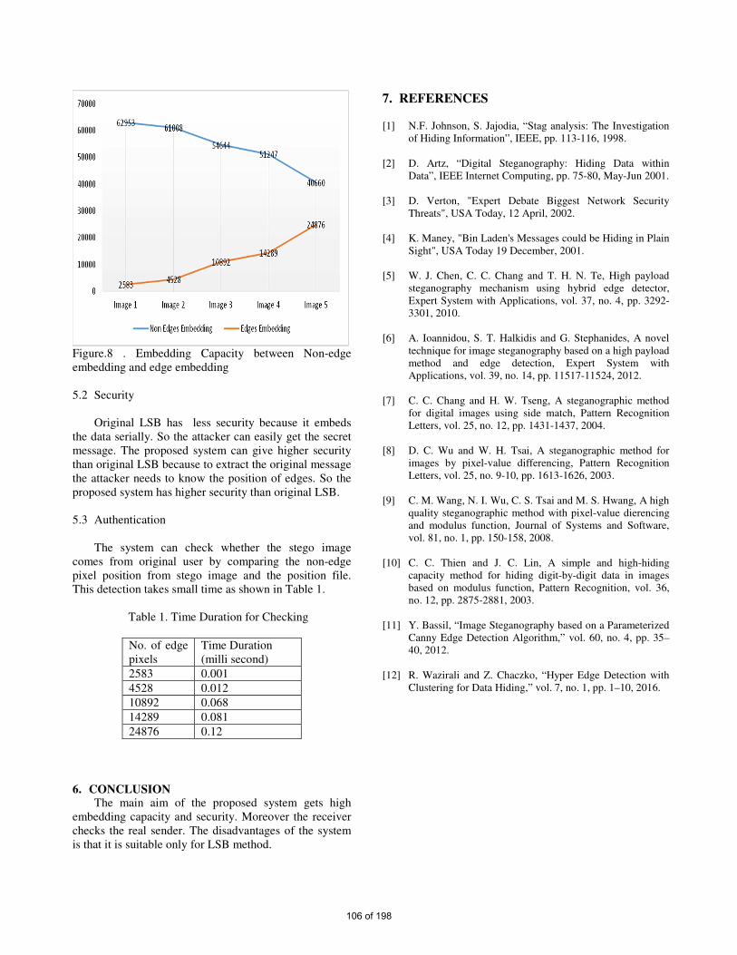
Figure.8 . Embedding Capacity between Non-edge

embedding and edge embedding

5.2 Security

Original LSB has less security because it embeds

the data serially. So the attacker can easily get the secret

message. The proposed system can give higher security

than original LSB because to extract the original message

the attacker needs to know the position of edges. So the

proposed system has higher security than original LSB.

5.3 Authentication

The system can check whether the stego image

comes from original user by comparing the non-edge

pixel position from stego image and the position file.

This detection takes small time as shown in Table 1.

Table 1. Time Duration for Checking

No. of edge

pixels

Time Duration

(milli second)

2583 0.001

4528 0.012

10892 0.068

14289 0.081

24876 0.12

6. CONCLUSION

The main aim of the proposed system gets high

embedding capacity and security. Moreover the receiver

checks the real sender. The disadvantages of the system

is that it is suitable only for LSB method.

7. REFERENCES [1] N.F. Johnson, S. Jajodia, “Stag analysis: The Investigation

of Hiding Information”, IEEE, pp. 113-116, 1998.

[2] D. Artz, “Digital Steganography: Hiding Data within

Data”, IEEE Internet Computing, pp. 75-80, May-Jun 2001.

[3] D. Verton, "Expert Debate Biggest Network Security

Threats", USA Today, 12 April, 2002.

[4] K. Maney, "Bin Laden's Messages could be Hiding in Plain

Sight", USA Today 19 December, 2001.

[5] W. J. Chen, C. C. Chang and T. H. N. Te, High payload

steganography mechanism using hybrid edge detector,

Expert System with Applications, vol. 37, no. 4, pp. 3292-

3301, 2010.

[6] A. Ioannidou, S. T. Halkidis and G. Stephanides, A novel

technique for image steganography based on a high payload

method and edge detection, Expert System with

Applications, vol. 39, no. 14, pp. 11517-11524, 2012.

[7] C. C. Chang and H. W. Tseng, A steganographic method

for digital images using side match, Pattern Recognition

Letters, vol. 25, no. 12, pp. 1431-1437, 2004.

[8] D. C. Wu and W. H. Tsai, A steganographic method for

images by pixel-value differencing, Pattern Recognition

Letters, vol. 25, no. 9-10, pp. 1613-1626, 2003.

[9] C. M. Wang, N. I. Wu, C. S. Tsai and M. S. Hwang, A high

quality steganographic method with pixel-value dierencing

and modulus function, Journal of Systems and Software,

vol. 81, no. 1, pp. 150-158, 2008.

[10] C. C. Thien and J. C. Lin, A simple and high-hiding

capacity method for hiding digit-by-digit data in images

based on modulus function, Pattern Recognition, vol. 36,

no. 12, pp. 2875-2881, 2003.

[11] Y. Bassil, “Image Steganography based on a Parameterized

Canny Edge Detection Algorithm,” vol. 60, no. 4, pp. 35–

40, 2012.

[12] R. Wazirali and Z. Chaczko, “Hyper Edge Detection with

Clustering for Data Hiding,” vol. 7, no. 1, pp. 1–10, 2016.

106 of 198

Mathematical Approach to Stable Hip Trajectory

for Ascending Stairs Biped Robot Aye Aye Thant, Khaing Khaing Aye

1

Faculty of Computing

Myanmar Institute of Information Technology, Mandalay, Myanmar

Department of Engineering Mathematics

Yangon Technological University, Yangon, Myanmar [email protected]

Abstract ---- The key contribution of this paper

is to generate the stable hip trajectory for

ascending stairs of the biped robot from the

mathematical point of view. To approach this

goal, we first construct the mathematical model

for kinematics constraints of step of

ascending stairs and discuss the concept of hip

trajectory relative to stability. From this, the

stable hip trajectory for one cycle of ascending

stairs step is derived by interpolation

polynomial. Finally, the numerical result of the

proposed trajectory is verified with Matlab

figures. The present algorithm is also applicable

for descending stairs of the biped robot.

Keywords: Ascending stairs, Biped Robot, Hip

trajectory, Stable motion, Trajectory planning

I. INTRODUCTION

Biped robots have higher mobility than

conventional wheeled robots, especially when

moving on rough terrain, steep stairs, and in

environments with obstacles [1]. Since a biped

robot tends to tip over easily, it is necessary to take

stability into account when determining a walking

pattern. To walk stably in various environments,

stability is the most important topic in bipedal

robot walking. The zero moment point, (ZMP) is

the point on the ground around which the sum of

all the moments of the active force equals zero, has

been widely used as a criterion to assure stability of

bipedal walking in many studies [1].

The walk of biped robot can be determined by

foot and hip trajectory. Zhang et al [2] have used

the cubic polynomial for motion planning of biped

robot for climbing stairs. However, in these

methods do not ensure continuity of acceleration at

the path points. So, generation of a smooth and

continuous motion has not been guaranteed as

cubic spline interpolation method. To alleviate this

problem, foot and hip trajectory for level ground

are generated by cubic spline interpolation in my

previous research [6]. And then, generation of foot

trajectory for ascending stairs by applying cubic

spline interpolation has been derived [11]. Now,

stable hip trajectory for ascending stairs of biped

robot has been generated. To be able to get stable

hip trajectory, either generates the smooth

trajectory or points the two hip parameters for

stability. From this concept, we formulate the

problem of smooth hip motion with the largest

stability margin using two parameters, and derived

the hip trajectory. Also, both foot trajectories and

the hip trajectory are smooth, and the ZMP

trajectory is always near the center of the stability

region, that is the robot has a large stability margin

[1].

The structure of the paper is as follows: Section

2 describes theoretical element for ascending stairs

cycle of biped robot. . Section 3 represents

kinematic constraints for hip trajectory. Section 4

includes stable hip trajectory planning of biped

robot. Section 5 demonstrates of the resulting hip

trajectory by applying Matlab.

II. THEORETICAL ELEMENT FOR

ASCENDING STAIRS OF BIPED ROBOT

A biped robot is two-legged robot and is

expected to eventually evolve into with a human-

like body. Each leg of an anthropomorphic biped

robot consists of a thigh, a shank, foot and has six

degrees of freedom (DOF); three DOF in the hip

joint, one in the knee joint and two in the ankle

joint [1].

Biped walking is a periodic phenomenon. A

complete climbing upstairs cycle is composed of

two phases. These are single support phase and

double support phase as shown in Figure 1.

Double support phase: During the double

support phase, both feet are in contact with the

stairs.

Single support phase: During the single

support phase, while one foot is stationary with the

stair, the other foot swings from the rear foot to the

font.

107 of 198

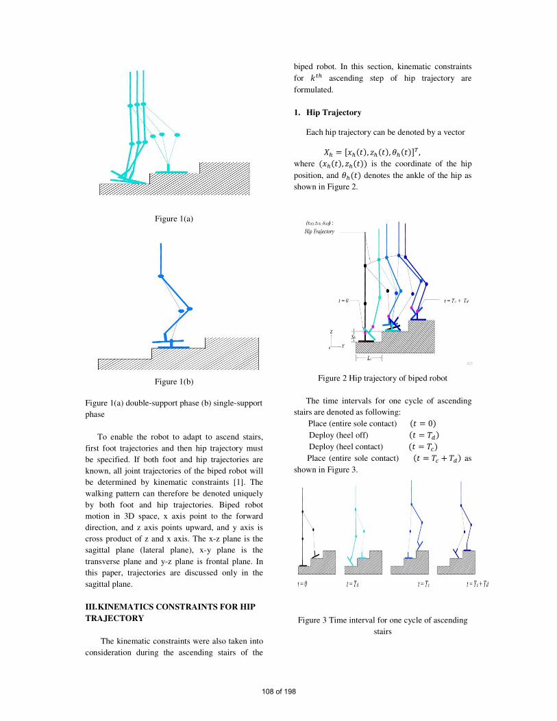
Figure 1(a)

Figure 1(b)

Figure 1(a) double-support phase (b) single-support

phase

To enable the robot to adapt to ascend stairs,

first foot trajectories and then hip trajectory must

be specified. If both foot and hip trajectories are

known, all joint trajectories of the biped robot will

be determined by kinematic constraints [1]. The

walking pattern can therefore be denoted uniquely

by both foot and hip trajectories. Biped robot

motion in 3D space, x axis point to the forward

direction, and z axis points upward, and y axis is

cross product of z and x axis. The x-z plane is the

sagittal plane (lateral plane), x-y plane is the

transverse plane and y-z plane is frontal plane. In

this paper, trajectories are discussed only in the

sagittal plane.

III. KINEMATICS CONSTRAINTS FOR HIP

TRAJECTORY

The kinematic constraints were also taken into

consideration during the ascending stairs of the

biped robot. In this section, kinematic constraints

for ascending step of hip trajectory are

formulated.

1. Hip Trajectory

Each hip trajectory can be denoted by a vector

, , , where , is the coordinate of the hip

position, and denotes the ankle of the hip as

shown in Figure 2.

Figure 2 Hip trajectory of biped robot

The time intervals for one cycle of ascending

stairs are denoted as following:

Place (entire sole contact) 0

Deploy (heel off)

Deploy (heel contact) Place (entire sole contact) as

shown in Figure 3.

Figure 3 Time interval for one cycle of ascending

stairs

108 of 198

The other hip parameters are listed as

following: distances along axis from the hip to

the ankle of the support foot at the start

of the single- support phase distances along axis from the hip to

the ankle of the support foot at the end

of the single- support phase as shown in

Figure 4.

Hhmax the hip highest position at the middle of

single support phase during one

ascending cycle

Hhmin the hip lowest position at the middle of

double support phase during one

ascending cycle

step` length stair length

stair height

ZMP zero moment point

Figure 4(a)

Figure 4(b)

Figure 4 Hip parameters (a) and (b)

For the hip trajectory for one cycle of

ascending stairs, three phases are composed.: a

starting phase in which the ascending speed varies

from zero to a desired constant velocity, a steady

phase with a desired constant velocity and an

ending phase in which the speed varies from a

desired constant velocity to zero.

The time intervals for ascending step are as

follows:

i. Starting position

ii. Steady position

iii. Ending position 1

The hip trajectory on kth

walking step is as

follows:

, 1 , 1 1 (1)

!"#$, 0.5' !"(), 0.5 2' !"#$, 1 0.5 (2)

To be able to get stability motion, the hip

motion parameter is constant.

1.1 The Concept of Ascending Trajectory Relative

to Stability

Hip motion xh(t) hardly affects the position of

the zero moment point. xsd and xed to vary within a

fixed range is specified [1], in particular +0.0 , , 0.50.0 , , 0.5 (3)

To obtain a smooth periodic of the

steady phase, the following constraints must be

specified.

+- - . . (4)

Figure 5 Zero Moment Point

Based on the whole smooth trajectory xh(t) and

(4) and condition for stability ( ZMP) as shown in

Figure 5, a smooth trajectory with the largest

stability margin can be formulated as follows:

109 of 198

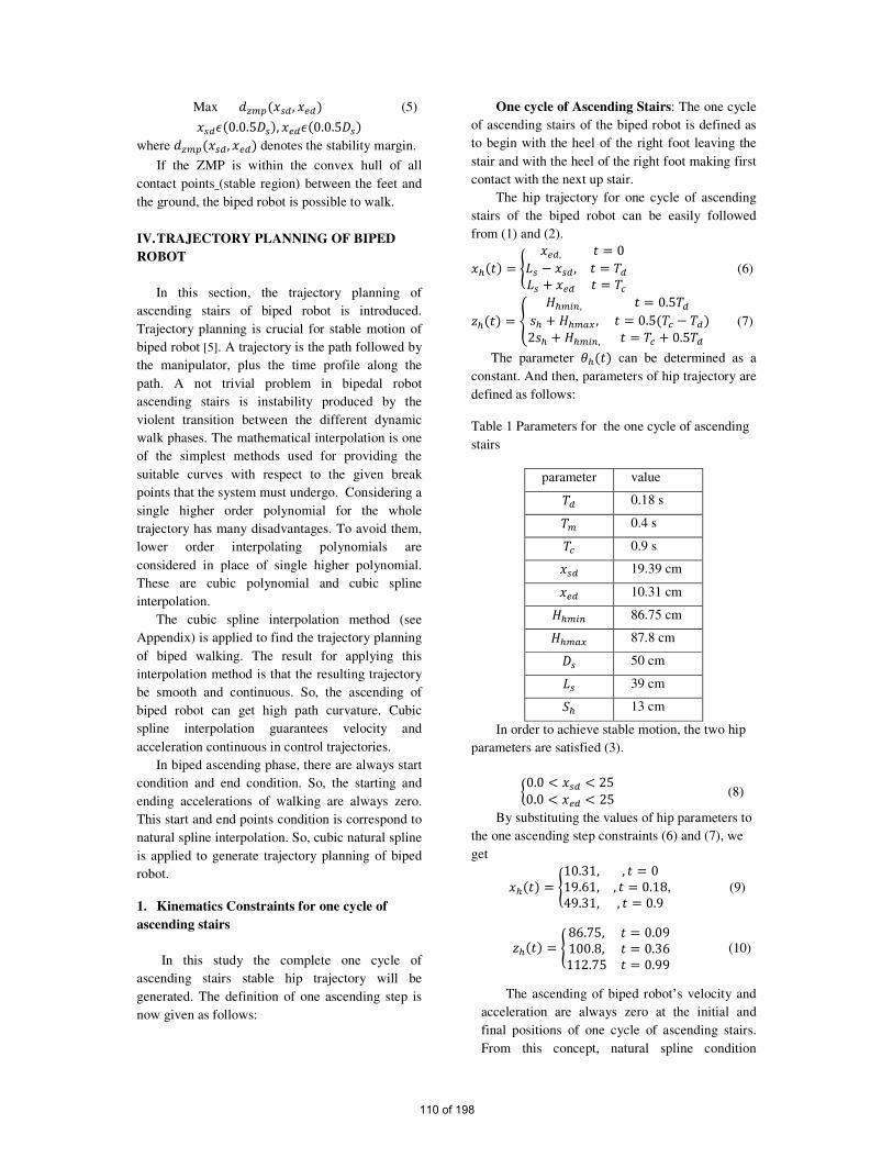
Max /0"1, (5) 20.0.5 , 20.0.5

where /0"1, denotes the stability margin.

If the ZMP is within the convex hull of all

contact points (stable region) between the feet and

the ground, the biped robot is possible to walk.

IV. TRAJECTORY PLANNING OF BIPED

ROBOT

In this section, the trajectory planning of

ascending stairs of biped robot is introduced.

Trajectory planning is crucial for stable motion of

biped robot [5]. A trajectory is the path followed by

the manipulator, plus the time profile along the

path. A not trivial problem in bipedal robot

ascending stairs is instability produced by the

violent transition between the different dynamic

walk phases. The mathematical interpolation is one

of the simplest methods used for providing the

suitable curves with respect to the given break

points that the system must undergo. Considering a

single higher order polynomial for the whole

trajectory has many disadvantages. To avoid them,

lower order interpolating polynomials are

considered in place of single higher polynomial.

These are cubic polynomial and cubic spline

interpolation.

The cubic spline interpolation method (see

Appendix) is applied to find the trajectory planning

of biped walking. The result for applying this

interpolation method is that the resulting trajectory

be smooth and continuous. So, the ascending of

biped robot can get high path curvature. Cubic

spline interpolation guarantees velocity and

acceleration continuous in control trajectories.

In biped ascending phase, there are always start

condition and end condition. So, the starting and

ending accelerations of walking are always zero.

This start and end points condition is correspond to

natural spline interpolation. So, cubic natural spline

is applied to generate trajectory planning of biped

robot.

1. Kinematics Constraints for one cycle of

ascending stairs

In this study the complete one cycle of

ascending stairs stable hip trajectory will be

generated. The definition of one ascending step is

now given as follows:

One cycle of Ascending Stairs: The one cycle

of ascending stairs of the biped robot is defined as

to begin with the heel of the right foot leaving the

stair and with the heel of the right foot making first

contact with the next up stair.

The hip trajectory for one cycle of ascending

stairs of the biped robot can be easily followed

from (1) and (2).

3 , 0 , (6)

!"#$, 0.5' !"() , 0.5 2' !"#$, 0.5 (7)

The parameter can be determined as a

constant. And then, parameters of hip trajectory are

defined as follows:

Table 1 Parameters for the one cycle of ascending

stairs

parameter value 0.18 s " 0.4 s 0.9 s 19.39 cm 10.31 cm !"#$ 86.75 cm !"() 87.8 cm 50 cm 39 cm 13 cm

In order to achieve stable motion, the two hip

parameters are satisfied (3).

+0.0 , , 250.0 , , 25 (8)

By substituting the values of hip parameters to

the one ascending step constraints (6) and (7), we

get

310.31, , 019.61, , 0.1849.31, , 0.9 , (9)

3 86.75, 0.09100.8, 0.36112.75 0.99 (10)

The ascending of biped robot’s velocity and

acceleration are always zero at the initial and

final positions of one cycle of ascending stairs.

From this concept, natural spline condition

110 of 198

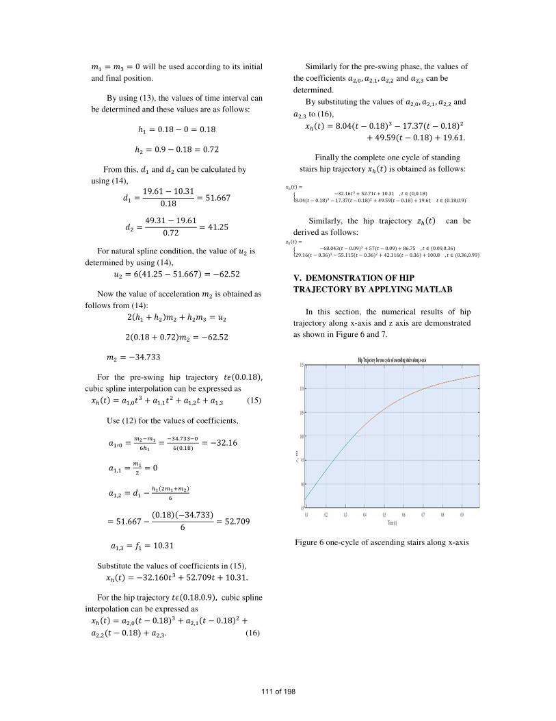
:; :< 0 will be used according to its initial

and final position.

By using (13), the values of time interval can

be determined and these values are as follows:

ℎ; 0.18 0 0.18

ℎ> 0.9 0.18 0.72

From this, /; and /> can be calculated by

using (14), /; 19.61 10.310.18 51.667

/> 49.31 19.610.72 41.25

For natural spline condition, the value of ?> is

determined by using (14), ?> 641.25 51.667 62.52

Now the value of acceleration :> is obtained as

follows from (14): 2ℎ; ℎ> :> ℎ>:< ?>

20.18 0.72 :> 62.52

:> 34.733

For the pre-swing hip trajectory 20.0.18 , cubic spline interpolation can be expressed as @;,A< @;,;> @;,> @;,< (15)

Use (12) for the values of coefficients,

@;BA "CD"EFE D<G.H<<DA FA.;I 32.16

@;,; "E> 0

@;,> /; E>"EJ"C F

51.667 0.18 34.733 6 52.709

@;,< K; 10.31

Substitute the values of coefficients in (15), 32.160< 52.709 10.31. For the hip trajectory 20.18.0.9 , cubic spline

interpolation can be expressed as @>,A 0.18 < @>,; 0.18 > @>,> 0.18 @>,<. (16)

Similarly for the pre-swing phase, the values of

the coefficients @>,A, @>,;, @>,> and @>,< can be

determined.

By substituting the values of @>,A, @>,;, @>,> and @>,< to (16), 8.04 0.18 < 17.37 0.18 > 49.59 0.18 19.61. Finally the complete one cycle of standing

stairs hip trajectory is obtained as follows:

+ 32.16< 52.71 10.31 , ∈ 0,0.18 8.04 0.18 < 17.37 0.18 > 49.59 0.18 19.61 ∈ 0.18,0.9 .

Similarly, the hip trajectory can be

derived as follows: + 68.043 0.09 < 57 0.09 86.75 , ∈ 0.09,0.36 29.16 0.36 < 55.115 0.36 > 42.116 0.36 100.8 , ∈ 0.36,0.99 .

V. DEMONSTRATION OF HIP

TRAJECTORY BY APPLYING MATLAB

In this section, the numerical results of hip

trajectory along x-axis and z axis are demonstrated

as shown in Figure 6 and 7.

Figure 6 one-cycle of ascending stairs along x-axis

111 of 198

Figure 7 one cycle of ascending stairs

along z-axis

VI. CONCLUSION

In this paper, mathematical modeling to stable

hip trajectory for ascending stairs of a biped robot

has been generated. As theoretical background of

ascending stairs hip trajectory has been discussed.

And then, kinematics constraints for ascending

stairs have been described. Finally, the goal of this

research, the one cycle of ascending stairs hip

trajectory has been generated by cubic spline

interpolation. The resulting trajectories for

applying this interpolation method are stable,

smooth and continuous has been verified by Matlab

figures.

APPENDIX

Cubic Spline Interpolation

Suppose that MN , KN ONP;$ are n points, where ; , > , ⋯ , $. The function is called

cubic spline if there exist R 1 cubic polynomials N with coefficients @N,A , @N,; ,@N,> and @N,< that

satisfies the following properties [4]:

I. N @N,A N < @N,; , N > @N,> N @N,< for ∈ SN , NJ;T and U 1,2, ⋯ , R 1

II. VNW KN for U 1,2, ⋯ , R.

III. NVNJ;W NJ;VNJ;W for U 1,2, ⋯ , R 2.

IV. NBVNJ;W NJ;B VNJ;W for U 1,2, ⋯ , R 2.

V. NBBVNJ;W NJ;BB VNJ;W for U 1,2, ⋯ , R 2.

Property I states that consists of piecewise

cubies. Property II states that piecewise cubies

interpolate the given sets of data points. Property

III and IV require that the piecewise cubies

represent a smooth continuous function. Property

IV states that the second derivatives of the resulting

function are also continuous.

A piecewise function is constructed as follows

[4]:

X ; YK ; Z Z >> YK > Z Z <⋮$D; YK $D; Z Z $

where N is a cubic polynomial defined by

N @N,A N < @N,; , N > @N,> N @N,<,U 1,2, ⋯ , R 1. (11)

By using the properties, I, II, III and IV, we can

get the coefficients of cubic spline interpolation as

follow:

@N ,A "\]ED"\F\ ,

@N,; "\> , @NB> @NB< \>"\J"\]E F , (12)

@NB< KN

where:N NBBVNW and ℎN NJ; N. (13)

Construction of natural spline interpolation

There exists a unique cubic spline with the free

boundary conditions :; :$ 0 Mathews&

Fink [3]. The linear system equations for finding :>, :<, … , :$D; connected with natural spline

condition are

2ℎ; ℎ> :> ℎ>:< ?>

ℎND;:ND; 2VℎND; ℎNW:N ℎN:NJ; ?N

for U 3,4, … , _ 2

ℎ$D>:$D> 2ℎ$D> ℎ$D; :$D; ?$D;

where ?N 6V/N /ND;W, U 2,3, … , R 1

and /N `\]ED`\\ . (14)

ACKNOWLEDGEMENT

I am also grateful to my respectable teachers,

Dr.Khaing Khaing Aye and Dr, Ni Ni Win, Heads

of Department of Engineering Mathematics at

YTU, Faculty of computing at MIIT who provided

112 of 198

a support and encouragement. I also wish to

express gratitude to my adorable benefactor parents

for their encouragement and support and my

husband for his AutoCAD drafting for this paper.

REFERENCES

[1] Huang, Qiang, Kazuhito Yokoi, Shuuji Kajita, Kenji

Kaneko, Hirohiko Arai, Noriho Koyachi, Kazuo

Tanie.: Planning walking patterns for a biped robot.

IEEE Trans. Robot. Auto vol.17, no.3 2001 pp.280-

284.

[2] Zhang, R. and Vadakkepet, P. Motion Planning of

Biped Robot Climbing Stairs. Department of

Electrical and Computer Engineering, National

University of Singapore at 4 Engineering Drive 3,

Singapore 117576 pp. 1.

[3] Mathews, J.H. and Fink, K.K. 2004, Numerical

Methods Using Matlab. 4th

ed. U.S.A: Prentice-Hall

pp. 281-284.

[4] Mckinley, S. and Levine, M. Cubic Spline

Interpolation Math45: Linear Algebra. Niku,

S.B,2001 pp. 1-9.

[5] Tang, Z., Zhou, C, and Sun, Z, “Trajectory planning

for smooth transition of a Biped Robot”.

Proceedings of IEEE, International Conference on

Robotics and Automation Taipei, Taiwan, 2003,

pp.1, September.

[6] Thant, A. and Aye, K. Application of Cubic spline

interpolation to walking patterns of biped robot.

Proceedings of World Academy of Science,

Engineering and Technology, 2009, pp. 1.

[7] Bagheri, A., Minpour, B. and Naseradinmousavi, P.

Mathematical Modelling and Simulation of

Combined Trajectory paths of a Seven Link Biped

Robot The University of Guilan, Faculty of

Engineering, Iran, March 2010 pp.2.

[8] Ranjbar, M., and Mayorga, R. A Seven Link Biped

Robot Walking Pattern Generation on Various

Surface Wise& Intelligent Systems& Entities

(WISE) Lab, Faculty of Engineering and Applied

Science, University of Regina, CANADA. Vol 16,

2017 pp.305.

[9] Bachor, Y. Developing Controllers for Biped

Humanoid Locomotion School of Informatics,

University of Edinburgh, 2004 pp.24-26.

[10] Cuevas, E., Zaldivar, D., Perez-Cisneros, M. and

Ramirez-Ortegon, M. Polynomial Trajectory

Algorithm for a Biped Robot International Journal

of Robotics and Automation 25 (4), 2010 pp.7-9.

[11] Thant, A.. and Khaing, M. Foot Trajectory

Generation for Climbing Upstairs of a Biped Robot

10th international Conference on Science and

Engineering 2019 pp.15-18.

113 of 198

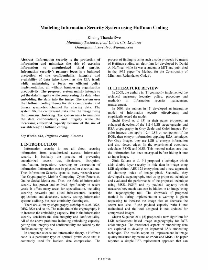
Modeling Information Security System using Huffman Coding

Khaing Thanda Swe

Mandalay Technological University, Lecturer

[email protected]

Abstract- Information security is the protection of

information and minimizes the risk of exposing

information to unauthorized third parties.

Information security’s primary focus is a balanced

protection of the confidentiality, integrity and

availability of data (also known as the CIA triad)

while maintaining a focus on efficient policy

implementation, all without hampering organization

productivity. The proposed system mainly intends to

get the data integrity while compressing the data when

embedding the data into the image. The system uses

the Huffman coding theory for data compression and

binary symmetric channel for sharing data. The

system fits the compressed data into the image using

the K-means clustering. The system aims to maintain

the data confidentiality and integrity while the

increasing embedded capacity because of the use of

variable length Huffman coding.

Key Words- CIA, Huffman coding, K-means

I. INTRODUCTION Information security is not all about securing

information from unauthorized access. Information

security is basically the practice of preventing

unauthorized access, use, disclosure, disruption,

modification, inspection, recording or destruction of

information. Information can be physical or electrical one.

Thus Information Security spans so many research areas

like Cryptography, Mobile Computing, Cyber Forensics,

Online Social Media etc. Thus, the field of information

security has grown and evolved significantly in recent

years. It offers many areas for specialization, including

securing networks and allied infrastructure, securing

applications and databases, security testing, information

systems auditing, business continuity planning etc.

There are so many cryptography techniques such DSA,

DES, RSA and so on. The main aim of the cryptography is

to increase the embedding capacity. But in the information

security considers the data integrity and confidentiality.

All of the above problems including embedding capacity,

getting data integrity and confidentiality are solved by the

Huffman coding theory.

In computer science and information theory, a Huffman

code is a particular type of optimal prefix code that is

commonly used for lossless data compression. The

process of finding is using such a code proceeds by means

of Huffman coding, an algorithm for developed by David

A. Huffman while he was a student at MIT and published

in the 1952 paper “A Method for the Construction of

Minimum-Redundancy Codes”.

II. LITERATURE REVIEW In 2008, the authors in [1] commonly implemented the

technical measures (security policy, procedure and

methods) in Information security management

measurement.

In 2003, the authors in [2] developed an integrative

model of Information security effectiveness and

empirically tested the model.

Suchi Goyal et al [3] in their paper proposed an

enhanced detection of the 1-2-4 LSB steganography and

RSA cryptography in Gray Scale and Color images. For

color images, they apply 1-2-4 LSB on component of the

RGB, then encrypt information applying RSA technique.

For Gray Images, they use LSB to encrypt information

and also detect edges. In the experimental outcomes,

calculates PSNR and MSE. This method makes sure that

the information has been encrypted before hiding it into

an input image.

Zinia Sultana et al. [4] proposed a technique which

adds double layer security to hide data in image using

LSB algorithm, AES-128 encryption and a new approach

of choosing index of image pixel. Secondly, they

developed a steganography tool using proposed technique

and evaluated the performance of the proposed technique

using MSE, PSNR and by payload capacity which

measures how much data can be hidden in an image using

the steganography tool. The drawback of proposed

method is during implementation a warning is given

requesting to increase the image size or decrease the

secret text size, if the payload capacity ratio is not

maintained and the tool designed is not updated for

compressed images.

Sherin Sugathan et al [5] proposed a new algorithm for

LSB replacement based image steganography for RGB

color images. The directional aspects of embedding data

are explored to develop an improved LSB embedding

technique. The results report an improvement in image

quality measured by means of PSNR and MSE. The paper

reported a simple LSB replacement approach that can

114 of 198

improve the quality of a stego image. The results indicate

that the proposed method performs well especially when

embedding secret data at higher LSB bit positions. The

data parallel nature of the problem makes it suitable for

implementation in parallel hardware. The position of the

direction bit can also be shifted and the position can even

act as part of a key for extracting the secret data.

III. METHODOLOGY

This section discusses the background theories used

in the proposed system. These are principles of

information theory C-I-A traid, working flow of Huffman

coding and K-means clustering system.

3.1. Principles of Information Theory C-I-A traid

Information security policy is a well-written and

clearly defined strategy towards protecting information

systems security and maintaining secure practices to the

resources and network of organization (SANS, security

policy, 2007). A general content of information security

policy includes password policy, risk assessment, user

responsibilities, policies of using Internet, policies of

using emails, disaster recovery and incidence detection

(SANS, security policy, 2007) [6].

There are three characteristics that constitute the

principle of information security: confidentiality, identity

and availability; which are commonly called C-I-A traid.

These three characteristics are not necessarily connected

or dependent on each other, however, if there is problem

occurring in any part of this traid, the others are

consequentially affected. Confidentiality guarantees that

only authorized parties or processes with sufficient

privileges could access to the information. Integrity

ensures that information is only created, modified or

deleted by authorized parties. Availability ensures that the

information can be accessed in a timely and reliable way

when people or applications need it. These three

characteristics can also be goals or objectives of

information security since they together represent three

very desirable properties of information system [6].

3.2. Working Flow of Huffman Coding An optimal (shortest expected length) prefix code for

a given distribution can be constructed by a simple

algorithm discovered by Huffman. Their technique works

by creating a binary tree of nodes. Initially, all nodes are

leaf nodes, which contain the symbol itself,

the weight (frequency of appearance) of the symbol and

optionally, a link to a parent node which makes it easy to

read the code (in reverse) starting from a leaf node.

Internal nodes contain a weight, links to two child

nodes and an optional link to a parent node.

The process begins with the leaf nodes containing the

probabilities of the symbol they represent. Then, the

process takes the two nodes with smallest probability, and

creates a new internal node having these two nodes as

children. The weight of the new node is set to the sum of

the weight of the children. We then apply the process

again, on the new internal node and on the remaining

nodes.

The simplest construction algorithm uses a priority

queue where the node with lowest probability is given

highest priority:

1. Start with as many leaves as there are symbols.

2. Enqueue all leaf nodes into the first queue (by

probability in increasing order so that the least

likely item is in the head of the queue).

3. While there is more than one node in the queues:

1. Dequeue the two nodes with the lowest

weight by examining the fronts of both

queues.

2. Create a new internal node, with the two

just-removed nodes as children (either

node can be either child) and the sum

of their weights as the new weight.

3. Enqueue the new node into the rear of

the second queue.

4. The remaining node is the root node; the tree has

now been generated [7].

3.2.1. Modeling of Huffman Coding

The example we’re going to use throughout this paper

is encoding the particular string "happy". Using the

standard ASCII encoding, this 5- character string requires

5*8 = 40 bits total. The table below shows the relevant

subset of the standard ASCII table.

Table1. ASCII character conversion

Char ASCII Bit Pattern (binary)

h 104 01101000

a 97 01100001

p 112 01110000

y 121 01111001

The string "happy" would be encoded in ASCII as

104 97 112 112 121. Although not easily readable by

humans, it would be written as the following stream of bits

(each byte is boxed to show the boundaries):

115 of 198

0110

1000

0110

0001

0111

0000

0111

0000

01111

001

Creating such an encoding is trivial: the systems

creates a list of the unique characters, and then goes

through and assign each a distinct encoded number from 0

to N-1. For example, here is one possible 3-bit encoding

(of the 7! possible permutations):

Table2. 3-bit Pattern Conversion

Char Number Bit pattern

h 0 000

a 1 001

p 2 010

y 3 011

Using this table, "happy" is encoded as 0 1 2 2 3, or

in binary:

000 001 010 010 011

Then the optimal Huffman encoding for variable

length is as follows:

Table3. Variable Length Huffman Coding

Char Bit pattern

h 01

a 000

p 10

y 1111

Each character has a unique bit pattern encoding, but

not all characters use the same number of bits. The string

"happy" encoded using the above variable-length code

table is:

01 000 10 10 1111

One way to visualize any particular encoding is to

diagram it as a binary tree. Each character is stored at a

leaf node. Any particular character encoding is obtained

by tracing the path from the root to its node. Each left-

going edge represents a 0, each right-going edge a 1. For

example, this tree diagrams the compact variable-length

encoding we developed previously:

Figure 1. Binary Tree for Optimal Huffman Coding

The general approach is as follows: 1. Create a

collection of singleton trees, one for each character, with

weight equal to the character frequency. 2. From the

collection, pick out the two trees with the smallest weights

and remove them. Combine them into a new tree whose

root has a weight equal to the sum of the weights of the

two trees and with the two trees as its left and right sub

trees. 3. Add the new combined tree back into the

collection. 4. Repeat steps 2 and 3 until there is only one

tree left. 5. The remaining node is the root of the optimal

encoding tree [8].

3.3. Implementing K-means Clustering

Algorithm K-means clustering is one of the simplest algorithms.

It works well for all distance metrics (where mean is

defined) such as Euclidean distance. It takes the partitions

N observations into K clusters (K<N).

Observation X Y

1 1 1

2 1.5 1.5

3 1 0.5

4 0.8 1.2

5 3.3 3.1

6 2.58 3.68

7 3.5 2.8

8 3 3

Step1: Randomly choose two points as the cluster centers.

Individual Mean x Mean y

Group 1 1 1 1

Group 2 8 3 3

Step2: Compute the distances and group the closest ones

(x2, y2)

Observation Distance 1 Distance 2 Group

1 0 2.8284271 1

2 0.7071068 2.123203 1

3 0.5 3.2015621 1

4 0.2828427 2.8425341 1

5 3.1144823 0.3162278 2

h

a

p

y

0

0

0

0

0

0

1 1

116 of 198

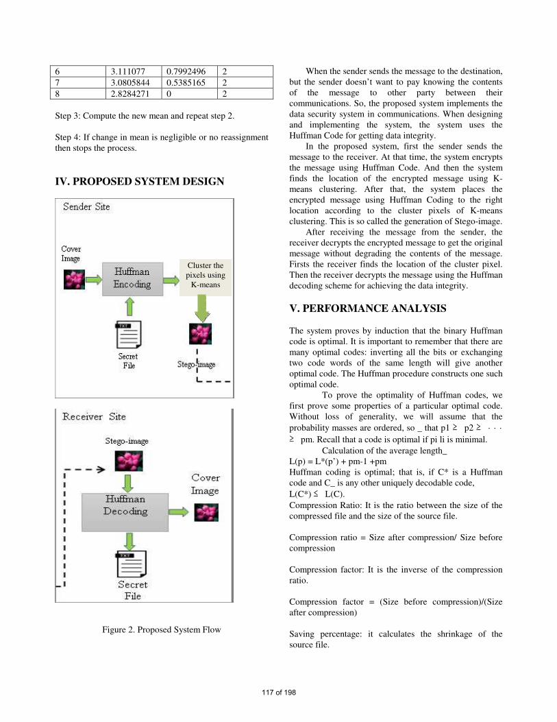
6 3.111077 0.7992496 2

7 3.0805844 0.5385165 2

8 2.8284271 0 2

Step 3: Compute the new mean and repeat step 2.

Step 4: If change in mean is negligible or no reassignment

then stops the process.

IV. PROPOSED SYSTEM DESIGN

Figure 2. Proposed System Flow

When the sender sends the message to the destination,

but the sender doesn’t want to pay knowing the contents

of the message to other party between their

communications. So, the proposed system implements the

data security system in communications. When designing

and implementing the system, the system uses the

Huffman Code for getting data integrity.

In the proposed system, first the sender sends the

message to the receiver. At that time, the system encrypts

the message using Huffman Code. And then the system

finds the location of the encrypted message using K-

means clustering. After that, the system places the

encrypted message using Huffman Coding to the right

location according to the cluster pixels of K-means

clustering. This is so called the generation of Stego-image.

After receiving the message from the sender, the

receiver decrypts the encrypted message to get the original

message without degrading the contents of the message.

Firsts the receiver finds the location of the cluster pixel.

Then the receiver decrypts the message using the Huffman

decoding scheme for achieving the data integrity.

V. PERFORMANCE ANALYSIS

The system proves by induction that the binary Huffman

code is optimal. It is important to remember that there are

many optimal codes: inverting all the bits or exchanging

two code words of the same length will give another

optimal code. The Huffman procedure constructs one such

optimal code.

To prove the optimality of Huffman codes, we

first prove some properties of a particular optimal code.

Without loss of generality, we will assume that the

probability masses are ordered, so _ that p1 ≥ p2 ≥ · · ·

≥ pm. Recall that a code is optimal if pi li is minimal.

Calculation of the average length_

L(p) = L*(p’) + pm-1 +pm

Huffman coding is optimal; that is, if C* is a Huffman

code and C_ is any other uniquely decodable code,

L(C*) ≤ L(C).

Compression Ratio: It is the ratio between the size of the

compressed file and the size of the source file.

Compression ratio = Size after compression/ Size before

compression

Compression factor: It is the inverse of the compression

ratio.

Compression factor = (Size before compression)/(Size

after compression)

Saving percentage: it calculates the shrinkage of the

source file.

Cluster the

pixels using

K-means

117 of 198

Saving percentage = (Size before compression-Size after

compression)/ (Size before compression) [9]

Image Size Arithmetic

Coding Huffman Coding

Compression

ratio Very good Poor

Compression

factor Fixed Variable

Saving

Percentage No

Yes

Embedding

capacity Mega Byte Gega Byte

VI. CONCLUSION The proposed system mainly aims to increase the

embedding capacity and able to get the data integrity and

confidentiality. The system embeds the data into the

image. In this system, jpeg file only uses. First the system

encodes the secret data using Huffman Encoding. Then

the system clusters the pixels of the image using K-means

clustering algorithm. After finishing all, the encoded

secret data are embedded into the image according to the

cluster values. This is the sender site.

And the other site, the receiver site, the receiver

decodes the secrete data using Huffman Decoding

according to the cluster values. In this way, it is more

difficult to attack in Huffman Coding than the arithmetic

Coding because Huffman uses variable-length encoding.

As the further extension, the system can give data

confidentiality and integrity. But there is no evidence for

this statement is true. The other researchers can check the

security privacy using AVISPA and other network

security tools.

VII. REFERENCES

[1] Dave Kaveri Atulbhai and Shilpa Serasiya, “A Survey:

Prediction & Detection of Dengue – Mining Methods &

Techniques, IJAR-IIE–ISSN (O)-2395-4396, Vol-3, Issue-2,

2O17.

[2] Xavier-CarvalhoC, Cezar RDDS, Freire NM, Vasconcelos

CMM, Solorzano VEF, de Toledo-Pinto TG, Fialho LG, do

Carmo RF, Vasconcelos LRS, Cordeiro MT,

[3] Suchi Goyal, Manoj Ramaiya, Deepika Dubey ”Improved

Detection of 1-2-4 LSB Steganography and RSA cryptography

in color and Grayscale Images”, International Conference on

Computational Intelligence and Communication Networks,201

[4] Zinia Sultana , Fatima Jannat , Muhammad Nazrul Islam ”

A New Approach to Hide Data in Color Image Using LSB

Steganography Technique”,3rd International Conference on

Electrical Information and Communication Technology (EICT),

7-9 December 2017, Khulna, Bangladesh

[5] Sherin Sugathan “An Improved LSB Embedding Technique

for Image Steganography”, 2016 IEEE

[6] Yang Yaping, “Literature review on Information Security

Practice Survey Reports”, Service Innovation and Management,

Master’s Thesis, 2018

[7] https://en.wikipedia.org/wiki/Huffman_coding

[8] Julie Zelenski, “ Huffman Encoding and Data Compression”,

Spring , May 23 2012

[9] Hyderabad Jyot Maan, “Analysis Comparison of Algorithms

for Lossless Data Compression”, International Journal of

Information and Computation Technology, ISSN 0974-2239,

Volume 3, pp. 139-146, 2013.

118 of 198

PERFORMANCE EVALUATION FOR CLASSIFICATION ON DENGUE

FEVER

Phyo Thu Zar Tun

Mandalay Technological University

[email protected]

Abstract - Dengue Fever is one of the most dangerous

mosquito-brone viral diseases in the world and it is

also a real problem in Myanmar. According to the

statistics in the previous year, 2018, there have a total

of 3649 dengue cases and 187 deaths. The total dengue

cases were reported in 2018 is about 86%. The

weather in Myanmar has three seasons and the

transmission of the disease takes place during the

rainy season which it from May to October. There

have four types in dengue fever namely DENV-1,

DENV-2, DENV-3 and DENV-4. The Infection may be

asymptomatic in some people but in other people will

develop between 4 to 7 days after bitten by mosquito.

The proposed system is to classify the dengue fever

dataset based on their symptoms using machine

learning algorithms such as Support Vector Machine

(SVM) and K-Nearest Neighbors (KNN). The

symptoms in dataset are based on the dengue and

severe dengue from World Health Organization

(WHO). The total of 70 patients is listed in dengue

fever dataset. In classification tasks, Dengue with no

warning signs, Dengue with warning signs or severe

dengue will give as results.

Key Words- Dengue, classification, fever, symptoms

I. INTRODUCTION

Dengue fever may progress to a fatal complication

known as Dengue Hemorrhagic Fever (DHF). The

symptoms are abdominal pain, diarrhea, vomiting,

convulsions, bruising and continual bleeding and the fever

duration will be from 2 days to 7 days and circulatory

collapse known as Dengue Shock Syndrome. In the

transmission of dengue fever, there are mainly three ways

and they are virus, human and mosquito. The Aedes

aegypti and Aedes albopictus are able to transmit not only

dengue fever but also yellow fever, chikungunya and Zika

fever. The dengue fever can transmit to human by human

when the female Aedes mosquito bites a person infected

with dengue virus. The duration of pick up virus by

mosquito is 4 to 10 days before the transmission virus for

the rest of its life by being to humans. Aedes mosquitoes

can be found in the tropical and subtropical regions which

cover the America, Europe, Africa, Asia and India. The

female Aedes lays about 100 eggs each time and these

eggs are laid in clean water found in both natural and

man-made containers. Then the eggs are able to resist

desiccation for more than six months and will hatch in one

day as soon as they are submerged in water. After

hatching the mosquito larva will develop into pupa in as

little as 5 days. Then spending 2 to 3 days as a pupa, a

flying adult mosquito will emerge after completes in

approximately 8 to 10 days. The female mosquitoes bite

as they need blood for the development of eggs and they

usually bite during the day. The control measures for

mosquitoes can be divided into three types: biological,

physical and chemical. The biological control involves the

use of biological agents such as predators and pathogens

to suppress the population of pests. The physical control

of mosquitoes involves source removal, exclusion and

trapping. Mosquito control is the most conventionally

done using chemical methods that are used to control the

larvae and adults. Mosquitoes are present everywhere so

controlling them can be a challenge. Therefore dengue

fever is a major problem and most dangerous disease by

mosquitoes. In this proposed system, Matlab

programming is used to implement the classification on

dataset using machine learning algorithms. Finally this

system is analyzed which machine learning algorithms

between SVM and KNN can give the better classification.

II. RELATED WORKS

[1] Akash C. Jamgade, Prof. S. D. Zade published the

disease prediction using machine learning in International

Research Journal of Engineering and Technology

(IRJET). In that paper, the dataset were collected based

on symptoms from multisensory devices and other

medical data and then analyzed the dataset using K-mean

clustering machine learning algorithm. The structured data

and text data of patient used to achieve higher accuracy.

[2] C.V. Subbulakshmi and S.N. Deepa published in the

Scientific World Journal with the article of medical

dataset classification. This paper was proposed the hybrid

methodology based on machine learning paradigm and

then experimented on five datasets of UCI Machine

learning Repository for classification. [3] The author

119 of 198

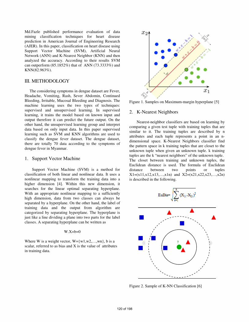
Md.Fazle published performance evaluation of data

mining classification techniques for heart disease

prediction in American Journal of Engineering Research

(AJER). In this paper, classification on heart disease using

Support Vector Machine (SVM), Artificial Neural

Network (ANN) and K-Nearest Neighbor (KNN) and then

analyzed the accuracy. According to their results SVM

can outperform (85.1852%) that of ANN (73.3333%) and

KNN(82.963%).

III. METHODOLOGY

The considering symptoms in dengue dataset are Fever,

Headache, Vomiting, Rash, Sever Abdomin, Continued

Bleeding, Irritable, Mucosal Bleeding and Diagnosis. The

machine learning uses the two types of techniques:

supervised and unsupervised learning. In supervised

learning, it trains the model based on known input and

output therefore it can predict the future output. On the

other hand, the unsupervised learning group and interpret

data based on only input data. In this paper supervised

learning such as SVM and KNN algorithms are used to

classify the dengue fever dataset. The dengue dataset,

there are totally 70 data according to the symptoms of

dengue fever in Myanmar.

1. Support Vector Machine

Support Vector Machine (SVM) is a method for

classification of both linear and nonlinear data. It uses a

nonlinear mapping to transform the training data into a

higher dimension [4]. Within this new dimension, it

searches for the linear optimal separating hyperplane.

With an appropriate nonlinear mapping to a sufficiently

high dimension, data from two classes can always be

separated by a hyperplane. On the other hand, the label of

training data and the output from algorithm are

categorized by separating hyperplane. The hyperplane is

just like a line dividing a plane into two parts for the label

classes. A separating hyperplane can be written as

W.X+b=0

Where W is a weight vector, W=w1,w2,…,wn, b is a

scalar, referred to as bias and X is the value of attributes

in training data.

Figure 1. Samples on Maximum-margin hyperplane [5]

2. K-Nearest Neighbors

Nearest-neighbor classifiers are based on learning by

comparing a given test tuple with training tuples that are

similar to it. The training tuples are described by n

attributes and each tuple represents a point in an n-

dimensional space. K-Nearest Neighbors classifier find

the pattern space in k training tuples that are closet to the

unknown tuple when given an unknown tuple. k training

tuples are the k “nearest neighbors” of the unknown tuple.

The closet between training and unknown tuples, the

Euclidean distance is used. The formula of Euclidean

distance between two points or tuples

X1=(x11,x12,x13,…,x1n) and X2=(x21,x22,x23,…,x2n)

is described in the following.

Figure 2. Sample of K-NN Classification [6]

120 of 198

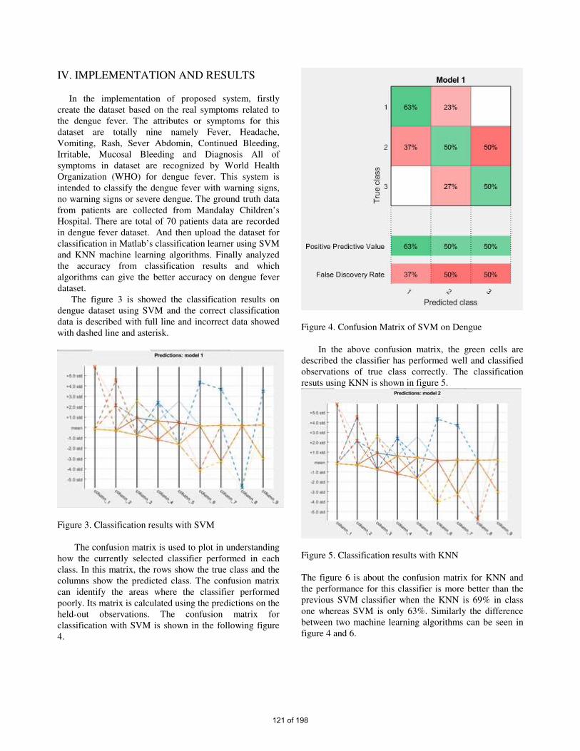
IV. IMPLEMENTATION AND RESULTS

In the implementation of proposed system, firstly

create the dataset based on the real symptoms related to

the dengue fever. The attributes or symptoms for this

dataset are totally nine namely Fever, Headache,

Vomiting, Rash, Sever Abdomin, Continued Bleeding,

Irritable, Mucosal Bleeding and Diagnosis All of

symptoms in dataset are recognized by World Health

Organization (WHO) for dengue fever. This system is

intended to classify the dengue fever with warning signs,

no warning signs or severe dengue. The ground truth data

from patients are collected from Mandalay Children’s

Hospital. There are total of 70 patients data are recorded

in dengue fever dataset. And then upload the dataset for

classification in Matlab’s classification learner using SVM

and KNN machine learning algorithms. Finally analyzed

the accuracy from classification results and which

algorithms can give the better accuracy on dengue fever

dataset.

The figure 3 is showed the classification results on

dengue dataset using SVM and the correct classification

data is described with full line and incorrect data showed

with dashed line and asterisk.

Figure 3. Classification results with SVM

The confusion matrix is used to plot in understanding

how the currently selected classifier performed in each

class. In this matrix, the rows show the true class and the

columns show the predicted class. The confusion matrix

can identify the areas where the classifier performed

poorly. Its matrix is calculated using the predictions on the

held-out observations. The confusion matrix for

classification with SVM is shown in the following figure

4.

Figure 4. Confusion Matrix of SVM on Dengue

In the above confusion matrix, the green cells are

described the classifier has performed well and classified

observations of true class correctly. The classification

resuts using KNN is shown in figure 5.

Figure 5. Classification results with KNN

The figure 6 is about the confusion matrix for KNN and

the performance for this classifier is more better than the

previous SVM classifier when the KNN is 69% in class

one whereas SVM is only 63%. Similarly the difference

between two machine learning algorithms can be seen in

figure 4 and 6.

121 of 198

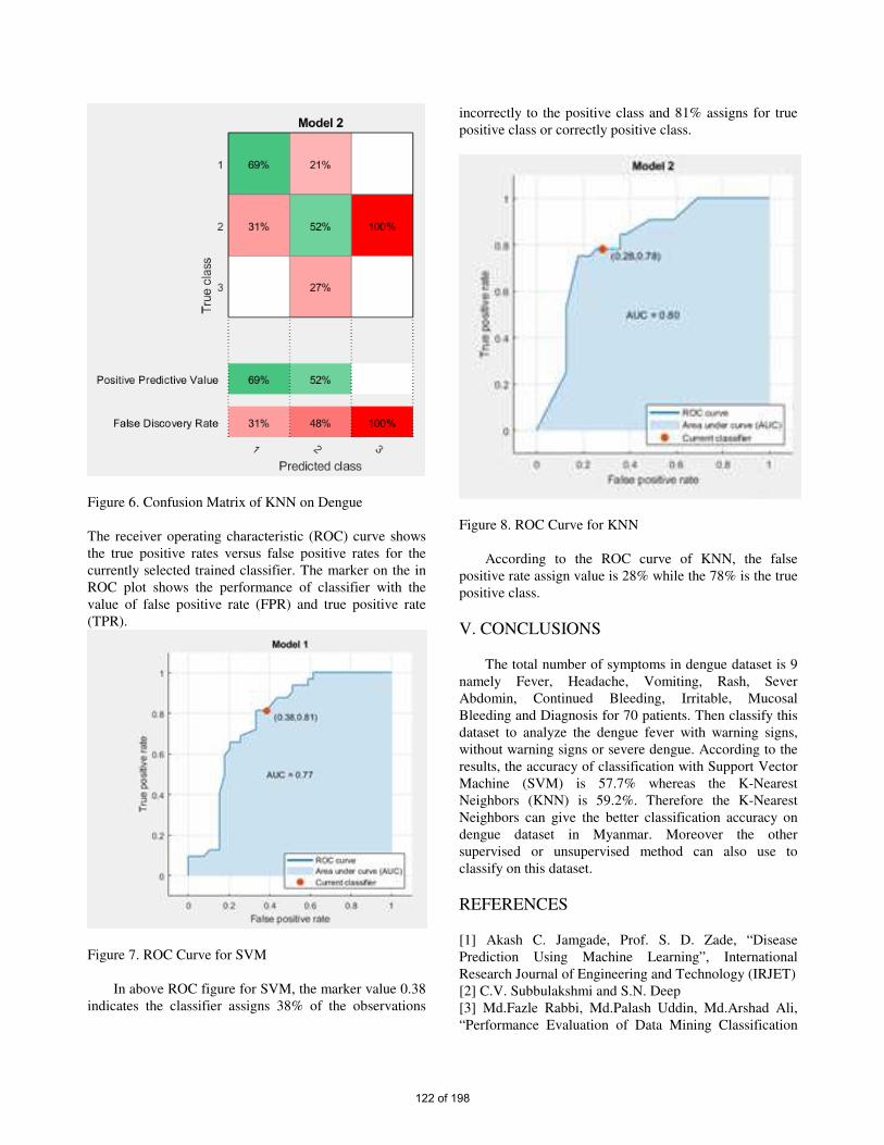
Figure 6. Confusion Matrix of KNN on Dengue

The receiver operating characteristic (ROC) curve shows

the true positive rates versus false positive rates for the

currently selected trained classifier. The marker on the in

ROC plot shows the performance of classifier with the

value of false positive rate (FPR) and true positive rate

(TPR).

Figure 7. ROC Curve for SVM

In above ROC figure for SVM, the marker value 0.38

indicates the classifier assigns 38% of the observations

incorrectly to the positive class and 81% assigns for true

positive class or correctly positive class.

Figure 8. ROC Curve for KNN

According to the ROC curve of KNN, the false

positive rate assign value is 28% while the 78% is the true

positive class.

V. CONCLUSIONS

The total number of symptoms in dengue dataset is 9

namely Fever, Headache, Vomiting, Rash, Sever

Abdomin, Continued Bleeding, Irritable, Mucosal

Bleeding and Diagnosis for 70 patients. Then classify this

dataset to analyze the dengue fever with warning signs,

without warning signs or severe dengue. According to the

results, the accuracy of classification with Support Vector

Machine (SVM) is 57.7% whereas the K-Nearest

Neighbors (KNN) is 59.2%. Therefore the K-Nearest

Neighbors can give the better classification accuracy on

dengue dataset in Myanmar. Moreover the other

supervised or unsupervised method can also use to

classify on this dataset.

REFERENCES

[1] Akash C. Jamgade, Prof. S. D. Zade, “Disease

Prediction Using Machine Learning”, International

Research Journal of Engineering and Technology (IRJET)

[2] C.V. Subbulakshmi and S.N. Deep

[3] Md.Fazle Rabbi, Md.Palash Uddin, Md.Arshad Ali,

“Performance Evaluation of Data Mining Classification

122 of 198

Techniques for Heart Disease Prediction”, American

Journal of Engineering Research (AJER) 2018, Volume-7,

Issue-2, pp-278,283.

[4] Chapter2: SVM (Support Vector Machine)-Theory,

Machine Learning 101, http://medium.com/machine-

learning-101/chapter-2-svm-support-vector-machine-

theory-f0812effc72

[5] https://en.m.wikipedia.org/wiki/Support-vector-

machine

[6] https://en.m.wikipedia.org/wiki/K-nearest_neighbors-

algorithm

123 of 198

Implementation of Sliding Mode Controller for Mobile Robot System

Zin Thuzar Naing#1,

Yangon Region, Republic of the Union of Myanmar 1 [email protected]

Abstract-The development of a Sliding Mode controller

has been done to be compared with the conventional

controller that is being used in a direct current (DC) motor.

Simulation study was used to overcome the appearance of

nonlinearities and uncertainties in the system with the

proposed controller for the armature voltage controlled DC

motors. The results are shown that the outputs changes

have very little impact on each other, and controller is

robust against input disturbances. The proposed model for

control system design is implemented using

MATLAB/SIMULINK.

Keywords: DC Motor Speed Control System, Mobile

Robot, Sliding Mode Controller, SIMULINK, Stability

Analysis.

I. INTRODUCTION

Normally, good dynamics of speed command

tracking and load regulating response is required in a

high performance motor drive system in order to

perform task. The simplicity of DC drives is used

because of its favorable cost, ease of application,

high reliabilities, and flexibilities which is

importantly being used in industrial applications,

robot manipulators and home appliances which speed

and position control of motor are required. Even

though the DC motors have several weaknesses, DC

motors have been used immensely nowadays in

various applications where variable speed was

needed due to DC motors flux and torque can be

controlled separately by means of controlling the

field and armature currents respectively [1].The less

complex DC drives uses a single power conversion

from AC to DC where DC motors tend to have speed

torque characteristics which are better than AC

motors. DC drives are also conventionally cheaper

for most horsepower ratings which it can also give

exceptional speed control in terms of acceleration

and deceleration. Normally, the precise model of a

nonlinear system in a definite DC motor is

problematic to be obtained and parameters acquired

from system identifications are possibly be only

approximated values. When there are disturbances and uncertainties

in a system, an appropriate control should be

designed so that the system stability and desired

system responses are achieved. Sliding mode control

(SMC) is insensitive in the presence of external

disturbances and uncertainties. The robustness

properties of SMC have led this approach to be an

intensive, popular and suitable method for the control

of wide classes of linear and nonlinear systems. PI

controllers are not perfectly able to stabilize the system, particularly, when the nonlinearity is very

high or the bound of uncertainty is large. In many

practical problems, almost perfect disturbance

rejection or control performance is required. Sliding

mode control (SMC) may be applied to the system to

obtain these performances [2].

The objectives of this work are to control the shaft speed and armature current of DC motor and check

the stability analysis with the advanced controller

system.

Reducing the peak overshot and steady-state

error of the DC motor is candidate for controlling the

DC motor in Mobile Robot. Therefore, to control the

shaft speed and armature current as output variables,

armature and field voltages are manipulating

variables of a separately excited DC motor using

sliding mode controller is the main research problem

for the control engineering area.

A SMC could be designed such as to force the system

trajectories to move onto a predefined surface within finite time and approaches to an equilibrium point all

along this surface. The closed-loop dynamics of the

system could be absolutely controlled through the

switching function equations provided the system

trajectories remain on this surface.

At first, the mathematical model of proposed DC

motor has to be derived according to the physical parameters of that motor. And then the theoretical

analysis could be carried out with the help of

MATLAB/SIMULINK. After that the conventional

controller system could be utilized for stability

analysis. And the weakness point of conventional

controller has to be specified by using the software

method like SIMULINK. Finally, the sliding mode control system could be applied to that model for

speed control of DC motor.

The rest of the paper is organized as follows.

Section II presents the mathematical model of the DC

motor which used in mobile robot system. Section III

mentions the implementation of sliding mode

controller design. Section IV discusses on the results

124 of 198

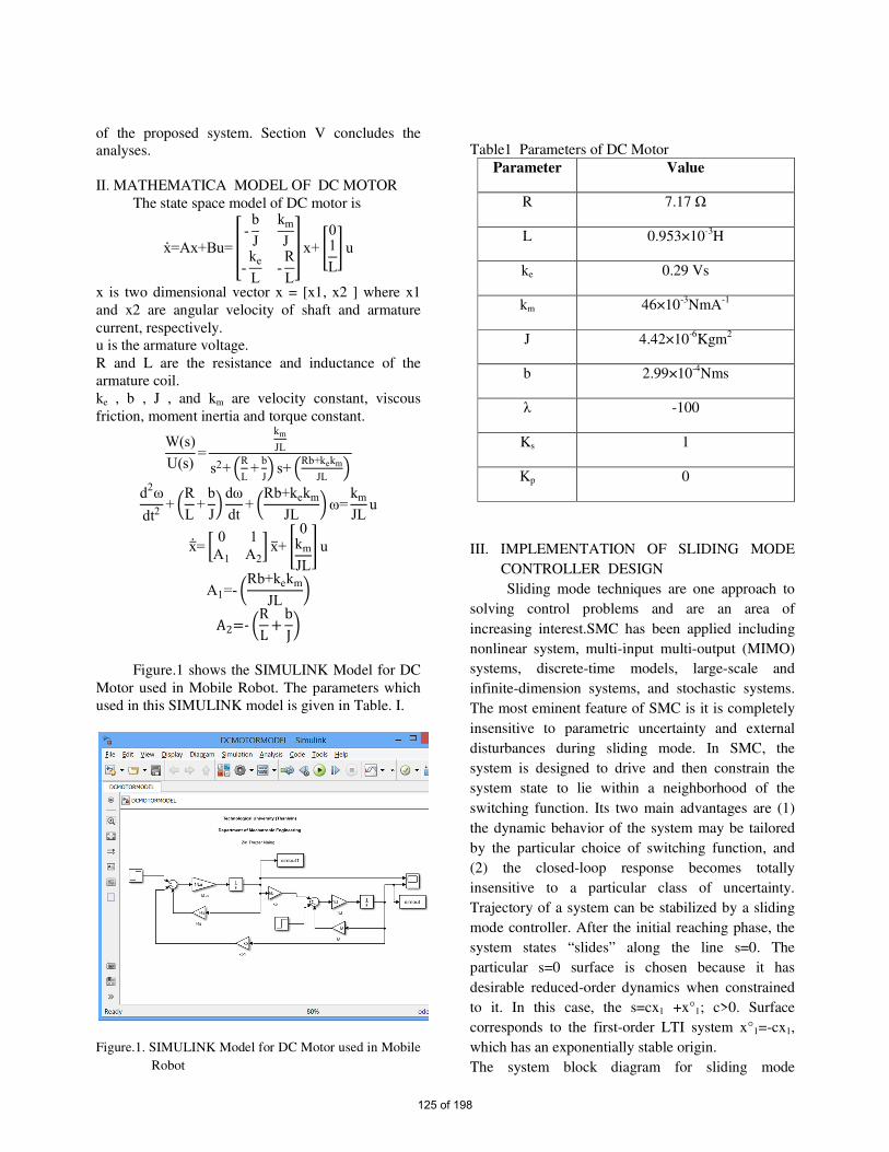
of the proposed system. Section V concludes the

analyses.

II. MATHEMATICA MODEL OF DC MOTOR

The state space model of DC motor is

x=Ax+Bu= - bJ km

J

-ke

L-R

L

x+ 01L

u x is two dimensional vector x = [x1, x2 ] where x1

and x2 are angular velocity of shaft and armature

current, respectively.

u is the armature voltage.

R and L are the resistance and inductance of the

armature coil.

ke , b , J , and km are velocity constant, viscous

friction, moment inertia and torque constant.

W(s)

U(s)=

km

JL

s2+ RL+b

J s+ Rb+kekm

JL

d2ω

dt2+ RL+b

J dωdt+ Rb+kekm

JLω=km

JLu

x= 0 1

A1 A2 x+ 0km

JL

u A1=- Rb+kekm

JL

A2- RLbJ

Figure.1 shows the SIMULINK Model for DC

Motor used in Mobile Robot. The parameters which

used in this SIMULINK model is given in Table. I.

Figure.1. SIMULINK Model for DC Motor used in Mobile

Robot

Table1 Parameters of DC Motor

Parameter Value

R 7.17 Ω

L 0.953×10-3H

ke 0.29 Vs

km 46×10-3

NmA-1

J 4.42×10-6

Kgm2

b 2.99×10-4Nms

λ -100

Ks 1

Kp 0

III. IMPLEMENTATION OF SLIDING MODE

CONTROLLER DESIGN

Sliding mode techniques are one approach to

solving control problems and are an area of

increasing interest.SMC has been applied including

nonlinear system, multi-input multi-output (MIMO)

systems, discrete-time models, large-scale and

infinite-dimension systems, and stochastic systems.

The most eminent feature of SMC is it is completely

insensitive to parametric uncertainty and external

disturbances during sliding mode. In SMC, the

system is designed to drive and then constrain the

system state to lie within a neighborhood of the

switching function. Its two main advantages are (1)

the dynamic behavior of the system may be tailored

by the particular choice of switching function, and

(2) the closed-loop response becomes totally

insensitive to a particular class of uncertainty.

Trajectory of a system can be stabilized by a sliding

mode controller. After the initial reaching phase, the

system states “slides” along the line s=0. The

particular s=0 surface is chosen because it has

desirable reduced-order dynamics when constrained

to it. In this case, the s=cx1 +x°1; c>0. Surface

corresponds to the first-order LTI system x°1=-cx1,

which has an exponentially stable origin.

The system block diagram for sliding mode

125 of 198

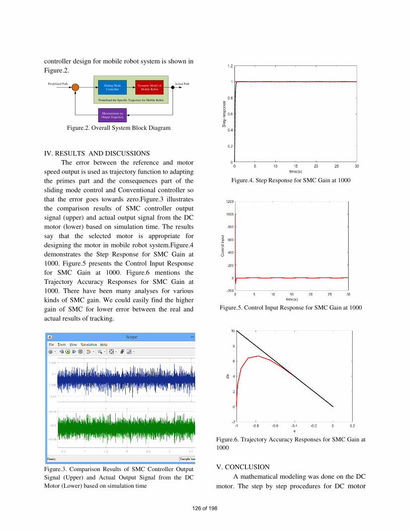
controller design for mobile robot system is shown in

Figure.2.

Dynamic Model of

Mobile Robot

Sliding Mode

Controller

Predefined the Specific Trajectory for Mobile Robot

Measurement on

Output Trajectory

Predefined Path Actual Path

Figure.2. Overall System Block Diagram

IV. RESULTS AND DISCUSSIONS

The error between the reference and motor

speed output is used as trajectory function to adapting

the primes part and the consequences part of the

sliding mode control and Conventional controller so

that the error goes towards zero.Figure.3 illustrates

the comparison results of SMC controller output

signal (upper) and actual output signal from the DC

motor (lower) based on simulation time. The results

say that the selected motor is appropriate for

designing the motor in mobile robot system.Figure.4

demonstrates the Step Response for SMC Gain at

1000. Figure.5 presents the Control Input Response

for SMC Gain at 1000. Figure.6 mentions the

Trajectory Accuracy Responses for SMC Gain at

1000. There have been many analyses for various

kinds of SMC gain. We could easily find the higher

gain of SMC for lower error between the real and

actual results of tracking.

Figure.3. Comparison Results of SMC Controller Output Signal (Upper) and Actual Output Signal from the DC

Motor (Lower) based on simulation time

Figure.4. Step Response for SMC Gain at 1000

Figure.5. Control Input Response for SMC Gain at 1000

Figure.6. Trajectory Accuracy Responses for SMC Gain at

1000

V. CONCLUSION

A mathematical modeling was done on the DC

motor. The step by step procedures for DC motor

126 of 198

analysis according to the various kinds of controller

system are completed by theoretical approaches. The

SMC gain is very important for analyzing the

accuracy of the response for mobile robot. If the

higher SMC gain is used in this system, the higher

accuracy results of mobile robot system will be

obtained. Overall, it is concluded that the sliding

mode controller is found to be superior, more robust,

faster andflexible and is insensitive to the parameter

variation as compared with conventional controller.

The research work is provided the obvious features of

sliding mode controller are robustness in uncertain

and input disturbance.

ACKNOWLEDGMENTS

I greatly appreciate to all teachers from the Yangon

Region of the Union of Myanmar who work in Research.

I would like to give great thanks to the Yangon

Region of the Union of Myanmar who work in Research

for kind permission to study related on-going research

projects.

REFERENCES

[1] J. J. E. Slotine, "sliding controller design for

nonlinear systems", international journal of

control, vol. 40, no.2, (1984), pp. 421-434.

[2] Vadim I. Utkin, "Sliding Mode Control Design

Principles and Applications to Electric Drives",

IEEE Transactions on Industrial Electronics,

February 1993.

[3] K. David Young, Vadim I. Utkin and U mit 0

zguner, "A Control Engineer,s Guide to Sliding

Mode Control", IEEE Transactions on Control

Systems Technology, Vol.7, No.3, May 1999.

[4] S. J. Chapman, "Electric Machinery

Fundamentals," the Mcgraw-hill companies,

1999.

[5] Utkin, V.I., Guldner, J., Shi, J. (1999). "Sliding

mode control in electromechanical Systems" CRC

Press.

[6] K. D. Young, V. Utkin and U. Ozguner, "A

control engineer's guide to sliding mode control",

IEEE conference(2002), pp. 1-14.

[7] Mohammed GodamSarwer, Md. Abdur Rafiq and

B.C.Gosh, "Sliding Mode Speed Controller of a

D.C. Motor Drive", Journal of Electrical

Engineer-ing, The Institution of Engineers,

Bangladesh, Dec 2004.

[8] Uma Maheshwararao, Y.S.KishoreBabu,

K.Arnaresh, "Sliding Mode Speed Control of a

DC Motor", 2011 International Conference on

Communication Systems and Network

Technologies.

[9] Ned Mohan, "Electric Drives: An Integtalive

Approach", MNPERE Minneapolis, 2001.

[10] K.H. Ang, G.c.y. Chong, and Y. Li, "PID Control

System Analysis, Design, and Technology," IEEE

Transactions on Control Systems Technology.,

Vol. 13, No. 4, pp. 559-576, July.2005.

[11] J. K. Liu and F. C. Sun, "Research and

development on theory and algorithms of sliding

mode control", Journal of Control Theory and

Applications, vol. 24, no. 3, 2007.

[12] Transl. J. Magn. Japan, vol. 2, pp. 740-741,

August 1987 [Digests 9th Annual Conf.

Magnetics Japan, p. 301, 1982].

[13] Edward C. and Spurgeon, S. K., "Sliding mode

control: theory and application,", Taylor and

Francis, London,1998.

[14] M. Young, The Technical Writer's Handbook.

Mill Valley, CA: University Science, 1989.

[15] Herlino, A.L.; Jidin, A.; Faizal, C.W.; Zalani,

C.W.M.; Sanusi, S.; Jopri, M.H.; Manap, M.

"Comparative study of current control strategy for

DC motors", Power Engineering and

Optimization Conference (PEOCO), 2013 IEEE

7th International, On page(s): 588 - 593.

127 of 198

THEORETICAL AND NUMERICAL MODAL ANALYSIS OF SIX

SPOKES WHEEL’S RIM USING ANSYS

Dr Htay Htay Win1, May Zon Than Oo2

1Mechanical Engineering Department, Mandalay Technological University, Mandalay, 05072, Myanmar

2Mechanical Engineering Department,

Mandalay Technological University,Mandalay, 05072, Myanmar

*[email protected],[email protected]

Abstract—This paper presents the frequency analysis of 6

spokes wheel’s rim under the value of speed 100km/h.

Modal analysis is to determine the vibration

characteristics (natural frequencies and mode shapes) of a

structure or machine component while it is being designed.

Modal analysis is a way to calculate the working

frequencies of system in structural mechanics. It is to

determine the natural mode shapes and frequencies of an

object or structure during free vibration. The natural

frequencies and mode shapes are important parameters in

the design of a structure for dynamic loading conditions.

The numerical results of natural frequencies for global

mode shapes were compared with working frequency of

car’s wheel’s rim.The model of wheel’s rim is drawn by

using SolidWorks 2014 and analysed by ANSYS 14.5. The

investigation is made on wheel’s rim model of station

wagon, Toyota’s Kluger. The tyre sidewall marking is

P225/65R*17. There are many forces acting on the wheel.

Inflation pressure acts on the wheel’s rim with magnitude

of 241kPa. Principal stress theory, von-Mises stress

theory, total deformation and natural frequency equations

are applied by theoretically and numerically. The results

from theoretical and numerical approaches of frequencies

of wheel’s rim are compared.The materials of wheel’s rim

are aluminum alloy, alloy steel and magnesium alloy.

Among them, alloy steel is the suitable material for

wheel’s rim because it has the minimum values of natural

frequency. Working frequency of wheel’s rim is

41.6Hz.The pitch (angular motion) and the bounce (up and

down linear motion) frequencies are 5 and 6.41rad/s. The

numerical result of frequency for alloy steel are first mode

shape 351Hz, second mode shape 353Hz, third mode

shape431Hz, fourth mode shape 432Hz, fifth mode shape

552Hz, sixth mode shape 578Hz, seventh mode shape

592Hz, eighth mode shape762Hz,ninth mode shape 925Hz

and tenth mode shape 927Hz.Working frequency does not

match with natural frequencies of car’s wheel’s rim at all

mode shapes. This gives clear indication that wheel’s rim

is safe against resonance phenomenon.

Keywords: Car’s Tyre, Deformation, Frequency, Speed,

Von-Mises Stress

I. INTRODUCTION

The wheel is a device that there are forces acting on the

car. Early wheels were simple wooden disks with a hole

for the axle. The spoke wheel was invented more recently,

and allowed the construction of lighter and swifter

vehicles. Alloy Steel wheels are automotive wheels which

are made from an alloy of aluminium or magnesium or

sometimes alloy steel.

Alloy Steel wheels differ from normal steel wheels

because of their lighter weight, which improves the

steering and the speed of the vehicle. Spoked wheels of car

are efficient, highly evolved, structural systems.

To install the wheel, the holes in the center section of

the rim are placed over the studs and lug nuts are threaded

onto the studs. The lug nuts can be tightened in across or

star pattern. The tapered end of each lug nut matches a

tapered area in the wheel mounting hole. The matching

tapers help center the wheel.

Figure1 Alloy Steel Wheel is fastened to the Rear Hub

with Steel Studs and Lug Nuts [16]

Rear Hub

Brake Disc

Flat Screw

Lug Nut

Alloy Steel Wheel

Center Cap

Wheel Stud

128 of 198

Figure 1 illustrates Alloy Steel wheel is fastened to the

rear hub with steel studs and lug nuts.

II. FORCES ACTING ON THE CAR’S TYRE

Braking force, aerodynamic drag force, centrifugal

force, friction force and tangential force act as x direction

of car’s wheel. Bump force, aerodynamic lift force and

radial force act in the vertical direction as y axis of car’s

wheel. Lateral force and axial force act in the direction as z

of car’s wheel.

Figure 2 Forces Acting on the Car [1]

(i) Vertical Weight, WV

The total vertical weight is determined by the sum of

the vehicle weight, passenger weight and extra weight.

Vertical weight=vehicle weight+ passenger weight+ extra

weight

(ii) Lateral Force, FL

Lateral force acts upon the wheel when steering or

when there is a crosswind. They cause the vehicle to

change direction.

FL= [(Cf+Cr)β]+v

1(aCf-bCr)ω-(Cfδ) (1)

(iii) Braking Force, FB

While the car is running with a constant speed, brake

can be used to stop suddenly. Braking force appears at the

time of one second and final speed is zero.

The braking time is the total time required to stop the

vehicle absolutely.

FB =ma=m )t

vv( 0f −

(2)

(iv) Friction Force, FR

When braking force is applied to the wheel, frictional

force is generated between the tire and the road surface.

Coefficient of friction value depends upon the road

condition and the weather conditions.

FR=µFN (3)

(v) Aerodynamic Drag Force, FD

The aerodynamic drag force is the product of the

density of air, the drag coefficient, frontal cross-sectional

area of car and the car’s speed. The value of lift coefficient

(CL) and drag coefficient (CD) depend upon styles of car

such as sedan, coupe, fastback and station wagon. The

value of CL and CD is chosen for station wagon.

FD=2

1ρACDv2 (4)

(vi) Aerodynamic Lift Force, FL

The aerodynamic lift force is the product of the

density of air, the lift coefficient, bottom cross-sectional

area of car and the car’s speed.

FL=2

1 ρACLv2 (5)

(vii) Radial Force, FR

When the car is in motion, the radial load becomes

cyclic in nature with a continuous rotation of the wheel.

Radial load depends upon rim’s radius, the width of the

bead seat, the angle of loading and the inflation pressure in

tire.

FR=8brrimθ0 (6)

(viii) Axial Force, Fa

The air pressure, acting against the sidewall of the

Kluger’s tire, generates a load, which is in the axial

direction.

rim

02rim

2ta

r 4

P)r(rF −= (7)

(ix) Bump Force, Fm

Bump force is the force between the passenger and

passenger’s seat of car.

mgr

mvF

rim

2

m += (8)

(x) Tangential Force, FT

Tangential force is a force that acts on a moving body

in the direction of a tangent to the curved path of the body.

sinθr

mvF

2

T = (9)

(xi) Centrifugal Force, Fc

A centrifugal force is a force , arising from the body’s

inertia, which appears to act on a body moving in a

circular path and is directed away from the centre around

which the body is moving. Table 1 shows the specification

data for the tyre of P225/65R*17. Table 2 showsproperties

of aluminum alloy.

Friction force,

Centrifugal force,

Tangential force

Braking force,

Drag force, Bump force,

Lift force,

Radial force

Lateral force,

Axial force,

Vertical

Vibration Longitudinal

Axis

Vertical

axis

x

y

z

129 of 198

rim

2

cr

mvF =

(10)

Table 1. Specification Data of wheel’s rim

Design Parameter symb

ol

value Unit

Aspect Ratio AR 75 -

Diameter of rim Drim 381 mm

Tyre Diameter Dt 688.5 mm

Overall width w 80 mm

Inflation Pressure Po 241 kPa

The specification data for the tyre of P225/65R*17 is

shown in Table 1. Aspect ratio is 75, diameter of rim is

381mm and tyre diameter is 688.5mm respectively.

Overall width is 80mm and inflation pressure is 241kPa.

Table 2. Properties of Materials [1]

Properties Aluminum

Alloy

Magnesium

Alloy

Alloy

Steel

Density

(kg/m3)

2810 1800 7700

Young

Modulus

(GPa)

72 45 210

Poisson

Ratio

0.33 0.35 0.28

Yield

Stress(MPa)

483 250 552

Properties of materialsare shown in Table 2. The

density of rubber is 1.1Mg/m3, young modulus is 0.05GPa,

Poisson ration is 0.49 and yield stress is 5.5MPa

respectively.

III. THEORETICAL MODAL ANALYSIS OF

WHEEL’S RIM

The x-axis is the intersection of the wheel plane and

the road plane with positive direction forward. The y-axis

perpendicular to the road plane with positive direction

upward. The z-axis in the road plane, its direction being

chosen to make the axis system orthogonal and right hand.

There are vertical component acting in the y direction,

longitudinal component acting in the x direction, and

lateral component acting in the z direction.The force

exerted in the x direction is the sum of friction force,

braking force, aerodynamic drag force and tangential

force. The force exerted in the y direction is the sum of

bump force, lift force and radial force. The force exerted in

the z direction is the sum of lateral force, axial force and

centrifugal force.

Figure 2 shows the forces acting on car direction of x, y

and z.

Stress in x direction,

x

xx

A

Fσ =

(11)

Stress in y direction, y

y

yA

Fσ =

(12)

Stress in z direction, z

zz

A

Fσ =

(13)

By using von-Mises Criterion equation,

[ ]2

12

132

322

21)σ(σ)σ(σ)σ(σ

2

1 −+−+−=σ(14)

E

σl

AE

Plδn,Deformatio == (15)

δ

g

2π

1F(Hz)Frequency, Natural =

(16)

Effective stress, total deformation and natural

frequency can be calculated by using the equation 14, 15

and 16.

IV. MODAL ANALYSIS OF WHEEL’S RIM

The modal of the wheel’s rim was drawn in Solid

work 2014 and added in ANSYS 14.5. This geometry

model was meshed with high smoothing. This meshed

model was imported to static structural analysis. Figure 3

shows design procedure for modal analysis using

ANSYS.In modal analysis of car’s wheel’s rim, only fixed

support is provided at the bolt hole circle location of car’s

wheel as shown in Figure 4. ANSYS 14.5 software is used

to analyze the mode shapes of car’s wheel’s rim.

Figure 3 Design procedure for modal analysis using

ANSYS

130 of 198

Figure 4 Fixed Support of 6 Spokes Wheel’s Rim

Figure 5 Meshing of 6 Spokes Wheel’s Rim

This geometry model was meshed with high

smoothing of 11230 nodes and 15120 elements as shown

in Figure 5.

Figure 6 Natural Frequency of Mode Shape 1 at Total

Deformation

If the wheel is being forced to vibrate at its natural

frequency, resonance and large amplitude vibrations will

occur. When designing objects, the mechanical natural or

resonance frequencies of the component parts do not

match vibration frequencies of oscillating parts. The

numerical results of natural frequencies for global mode

shapes were compared with working frequency of tyre.

In mode shape 1, the working frequency is 41.6 Hz.

Figure 6 shows the natural frequency of mode shape 1 at

total deformation. From obtained results, the natural

frequency of the tyre at mode shape 1 is 351 Hz. As the

operating frequency of wheel’s rim and natural frequency

of wheel’s rim do not match so the wheel’s rim structural

has no tendency of resonance.


Deformation

A mode shape is a specific pattern of vibration

executed by a mechanical system at a specific frequency.

Different mode shapes will be associated with different

frequencies. Figure 7 shows the natural frequency of mode

shape 2 at total deformation. For global mode shape 2, the

natural frequency is 353 Hz while operating frequency is

41.6 Hz. As both the frequencies do not match so the car’s

wheel rim has no tendency of resonance.


Deformation

For global mode shape 3, the natural frequency is 431

Hz while operating frequency is 41.6 Hz. As both the

frequencies do not match so the wheel’s rim has no

tendency of resonance. Figure 8 shows the natural

frequency of mode shape 3 at total deformation.


Deformation

131 of 198







Deformation







Deformation


Hz while tyre operating frequency is 41.6 Hz. As both the





Deformation







Deformation



frequencies do not match so the car’s wheel’s rim has no




Deformation

For global mode shape 9, the natural frequency is

925Hz while working frequency is 41.6 Hz. As both the





Deformation

132 of 198

For global mode shape 10, the natural frequency is

927Hz while operating frequency is 41.6 Hz. As both the




The natural frequencies and mode shapes are

important parameters in the design of a structure. The

numerical results of natural frequencies for global mode

shapes were compared with working frequency of wheel’s

rim. The natural frequencies at mode shapes of wheel’s

rim are shown in Table 3.

Table 3. Natural frequencies of mode shapes of car’

wheel’s rim for different materials

Mode 1 2 3 4 5

Natural

Frequency,

Aluminium

Alloy (Hz)

144

278

344

459

529

Natural

Frequency,

Alloy

Steel(Hz)

351 353 431 432 552

Natural

Frequency,

Magnesium

Alloy (Hz)

347 349 429 480 550

WorkingFrequency (Hz) 41.6

The Pitch(angular motion) frequency,rad/s 5

The Bounce (up and down linear motion)

frequency,rad/s

6.41

Mode 6 7 8 9 10

Natural

Frequency

Aluminium

Alloy (Hz)

570

597

917

928

1117

Natural

Frequency,

Alloy

Steel(Hz)

578 591 762 925 927

Natural

Frequency,

Magnesium

Alloy (Hz)

576 589 755 925 928

Working Frequency (Hz) 41.6

The Pitch(angular motion) frequency,rad/s 5

The Bounce (up and down linear motion)

frequency,rad/s

6.41

Table 4. Result Values of Working Frequency of Rim at

Various Speeds

Velocity,

km/h

Alloy Steel

δ, mm

Working

Frequency, Hz

20 0.00287 294.3

40 0.05752 65.73

60 0.08629 53.66

80 0.11505 46.5

100 0.14381 41.6

120 0.17257 38

140 0.20133 35

160 0.23008 32

180 0.25886 31

Natural frequencies of mode shapes of wheel’s rim are

shown in Table 3. Working frequency of car’s wheel’s rim

is 41.6Hz.The natural frequencies are 351Hz for first mode

shape, 353Hz for second mode shape, 431Hz for third

mode shape, 483Hz for fourth mode shape, 552Hz for fifth

mode shape, 578Hz for sixth mode shape, 594Hz for

seventh mode shape, 762Hz for eighth mode shape, 925Hz

for ninth mode shape and 927Hz for tenth mode shape

respectively.

V. CONCLUSIONS

In this research, forces acting on the wheel’s rim are

calculated in the direction of x, y and z. Then, the von-

Mises stresses, total deformation and working frequency

of the wheel’s rim are calculated for materials alloy steel at

speed 100km/h. And working frequency and natural

frequency are compared. From result, working frequency

of car’s wheel’s rim is 41.6 Hz. Working frequency does

not match with natural frequencies of wheel’s rim with all

mode shapes. Therefore, the car’s wheel’s rim has no

tendency of resonance. The first natural frequency is far

higher than maximum operating frequency. This gives

clear indication that wheel’s rim is safe against resonance

phenomenon. Similarities, in second, third, fourth, fifth,

six, eighth, ninth and tenth mode shape the designed

wheel’s rim working frequency and natural frequencies do

not match. In all global mode shapes, the wheel’s rim have

no tendency of resonance so designed wheel’s rim is safe.

Working frequency changes according to car’s speed. But

the working frequency does not exceed at speed 20 to

180km/h. A real model has an infinite number of natural

frequencies. However, a finite element model has a finite

number of natural frequencies. Only the first few modes

133 of 198

are needed.

ACKNOWLEDGMENT(S)

The first author wishes to acknowledge her deepest

gratitude to her parents, professors, relatives and friends to

carry out this paper.

NOMENCLATURE

v -speed of car

β -slip angle of car

δ -steering angle

µ -coefficient of friction

CD , CL-Drag Coefficient and Lift Coefficient

rrim -the radius of rim

rt -radius of tire

P0 -inflation pressure in tire

σ -von-Mises stress

ε -equivalent elastic strain

δ -deformation

E - Modulus of elasticit

REFERENCES

[1] D. Santhosh Kumar, “Modal Analysis and Design

Optimization of Automotive Wheel Rim”,2017.

[2] ShwetabhSuman. “Impact and modal analysis for

different alloy wheel compositions”,2017.

[3] Prof.Sharad, D.Kachave, “Experimental and Finite

Element Analysis of Automobile Wheel

Disc”,2016.

[4] K. Reif (Ed.), “Basic principles of vehicle

dynamics,” Brakes, Brake Control and Driver

Assistance Systems, 2014.

[5] Sourav Dos, “Design and Weight Optimization of

Aluminum Alloy Wheel”,2014.

[6] S.Ganesh, “Design and Analysis of Spiral Wheel

Rim for Four Wheeler”,2014.

[7] Nicholas Spagnol, “The Influence of the Disc

Manufacturing Process on the Fatigue Life of

Commercial Vehicle Wheels Manufactured By

S55JR Steel”,2014.

[8] Saran theja, Vamsi Krishna Mamidi, “Structural and

Fatigue Analysis of Two Wheeler Lighter Weight

Alloy Wheel”, 2013.

[9] Mr Sunil, “Analyze the Effect of Slip Angle on

Fatigue Life of Wheel Rim of Passenger Car by

Using Radial Fatigue Testing”,2013.

[10] P.Meghashyam, “Design and Analysis of Wheel

Rim using Analysis”,2013.

[11] Ch.P.V.Ravi Kumar, “Topology Optimization Of

Aluminum Alloy Wheel”,2013.

[12] S Vikranth Deepak, “Modelling and Analysis of

Alloy Wheel for Four Wheeler Vehicle”,2012.

[13] J. Stearns, T. S. Srivatsan, X. Gao, and P. C. Lam,

“Understanding the Influence of Pressure and

Radial Loadson Stress andDisplacement Response

of a Rotating Body:The Automobile Wheel”,2005.

[14] N.Kovunovic, M.Trajanovis and M.Stojkovic, “

FEA of tyres subjected to static loading”, 2007.

[15] Keller, T.A., “Model for the Prediction of the

Contact Area and the Distribution of Vertical Stress

below Agricultural Tyres from Readily Available

Tyre Parameters”, Biosystems Engineering, Vol.92,

2005, pp.85-96.

[16] Tonuk,E., “ Prediction of Automobile Tyre

Cornering Forces Characteristics by Finite Element

Modeling and Analysis”, Computer &Struct,

Vol.79,N0.13, 2001,pp.1219-1232.

[17] Willcox, “Driveline and Wheel Components”, 2000.

134 of 198

Synthesis, Characterization and Application of Carbon Nanotubes

for Conductive Ink Application

Htein Win

*, Hsu Pyae Sone Lwin

**

*Faculty of Advanced Materials Engineering, University of Technology (Yatanarpon Cyber City),

Pyin Oo Lwin, 05087, Myanmar **

Faculty of Advanced Materials Engineering, University of Technology (Yatanarpon Cyber City),

Pyin Oo Lwin, 05087, Myanmar

*[email protected],

**[email protected]

ABSTRACT

Chemical synthesis method is a kind of method

in which carbon nanotubes were prepared from

graphite powder by using a new chemical route of

oxidation method in a mixed solution of nitric acid

and sulfuric acid with potassium chlorate. After

heating the solution up to 70°C for 24 hours and

leaving them in the air for 3 days, nearly 0.02 g

carbon nanotube bundles were obtained. Carbon

nanotubes were characterized by X-ray

diffraction (XRD) and Scanning Electron

Microscope (SEM). The resultant carbon

materials can be confirmed as carbon nanotubes

which have hair- like structure and their diameter

is 20~40 nm approximately. Carbon Nanotubes

are remarkable electrical conductivity because of

their structure. Multi-walled carbon nanotubes

obtained by chemical synthesis method for

conductive ink application. Resistance of carbon

nanotubes in conductive ink is ~ 4 Ω and

conductance is 0.25 siemens approximately.

Key Words- Carbon Nanotubes (CNTs),

Conductive Ink, Scanning Electron Microscope

(SEM), X-ray Diffraction (XRD).

I. INTRODUCTION

Carbon nanotubes are graphite sheets rolled up

into cylinders with diameters of the order of a few

nanometers and up to some millimeters in length with

at least one end capped with a hemisphere of the

fullerene structure [1]. Nanotubes are members of the

fullerene structural family. Their name is derived

from their long, hollow structure with the walls

formed by one-atom-thick sheets of carbon, called

grapheme [2]. Carbon nanotubes were discovered by

Sumio Iijima by arc evaporation method in 1991[3].

There are two main types of nanotubes: the single-

walled carbon nanotubes (SWCNTs or SWNTs) and

the multi-walled carbon nanotubes (MWCNTs or

MWNTs), in particular the double walled carbon

nanotubes (DWCNTs or DWNTs) [1].

CNTs have captured the intensive attention of

researchers worldwide due to the combination of their

expected structural perfection, small size, low

density, high stiffness, high strength, and excellent

electronic properties [4]. They feature extraordinary

strength, show efficient conductivity of heat, and

unique electrical properties (metallic conductivity and

semi-conductivity). Many potential applications have

been proposed for carbon nanotubes, including

conductive and high-strength composites; energy

storage and energy conversion devices; sensors; field

emission displays and radiation sources; hydrogen

storage media; and nanometer-sized semiconductor

devices, probes, and interconnect [5].

II. SYNTHESIS OF CARBON NANOTUBES

The three commonly-used methods for production

of CNTs are arc-discharge method, laser ablation

method and chemical vapor deposition method which

require high temperature and high pressure.

Therefore, these methods cannot be performed easily

and inexpensively. Synthesizing CNTs remains costly

and difficult. After studying the literature, it was

discovered that carbon nanotubes can be synthesized

135 of 198

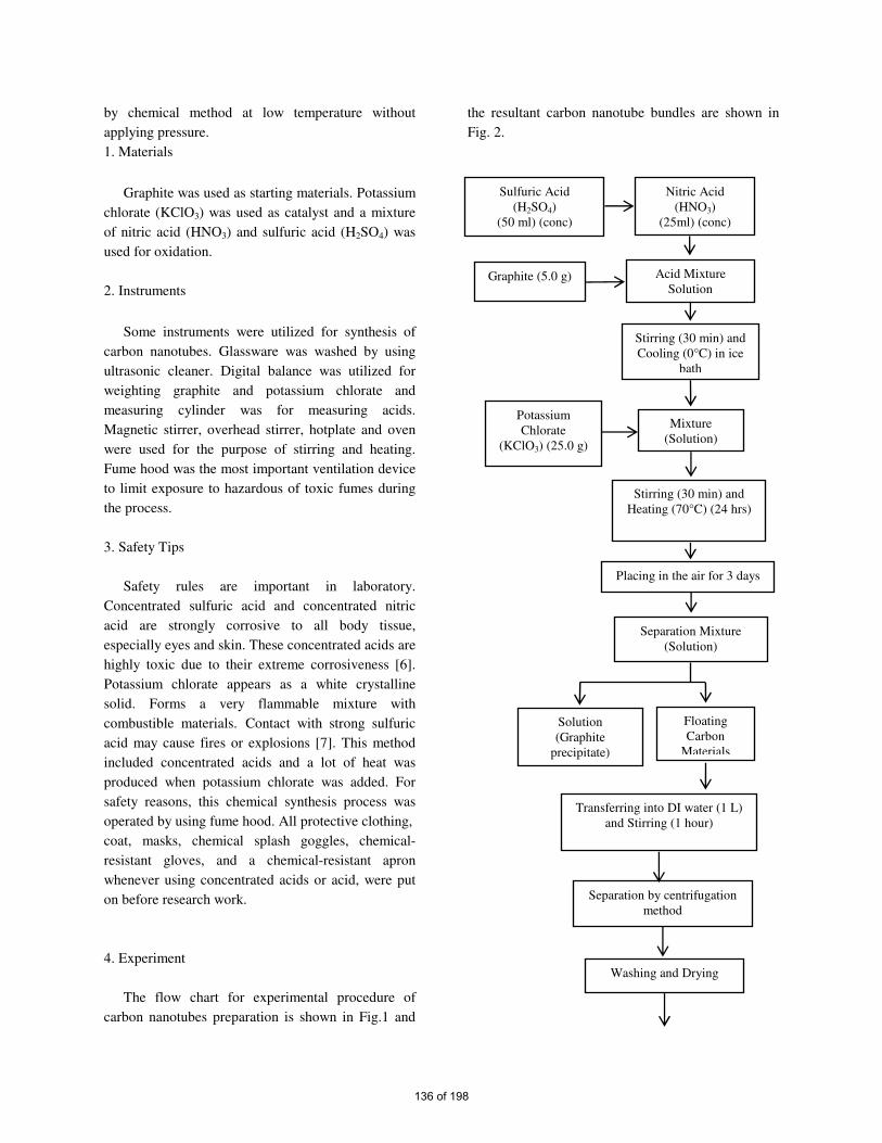
by chemical method at low temperature without

applying pressure.

1. Materials

Graphite was used as starting materials. Potassium

chlorate (KClO3) was used as catalyst and a mixture

of nitric acid (HNO3) and sulfuric acid (H2SO4) was

used for oxidation.

2. Instruments

Some instruments were utilized for synthesis of

carbon nanotubes. Glassware was washed by using

ultrasonic cleaner. Digital balance was utilized for

weighting graphite and potassium chlorate and

measuring cylinder was for measuring acids.

Magnetic stirrer, overhead stirrer, hotplate and oven

were used for the purpose of stirring and heating.

Fume hood was the most important ventilation device

to limit exposure to hazardous of toxic fumes during

the process.

3. Safety Tips

Safety rules are important in laboratory.

Concentrated sulfuric acid and concentrated nitric

acid are strongly corrosive to all body tissue,

especially eyes and skin. These concentrated acids are

highly toxic due to their extreme corrosiveness [6].

Potassium chlorate appears as a white crystalline

solid. Forms a very flammable mixture with

combustible materials. Contact with strong sulfuric

acid may cause fires or explosions [7]. This method

included concentrated acids and a lot of heat was

produced when potassium chlorate was added. For

safety reasons, this chemical synthesis process was

operated by using fume hood. All protective clothing,

coat, masks, chemical splash goggles, chemical-

resistant gloves, and a chemical-resistant apron

whenever using concentrated acids or acid, were put

on before research work.

4. Experiment

The flow chart for experimental procedure of

carbon nanotubes preparation is shown in Fig.1 and

the resultant carbon nanotube bundles are shown in

Fig. 2.

Sulfuric Acid

(H2SO4)

(50 ml) (conc)

Nitric Acid

(HNO3)

(25ml) (conc)

Graphite (5.0 g) Acid Mixture

Solution

Stirring (30 min) and

Cooling (0°C) in ice

bath

Transferring into DI water (1 L)

and Stirring (1 hour)

Floating

Carbon

Materials

Separation by centrifugation

method

Potassium

Chlorate

(KClO3) (25.0 g)

Solution

(Graphite

precipitate)

Washing and Drying

Stirring (30 min) and

Heating (70°C) (24 hrs)

Placing in the air for 3 days

Separation Mixture

(Solution)

Mixture

(Solution)

136 of 198

Figure 1 Flow Sheet for Chemical Synthesis of

Carbon Nanotubes.

In chemical synthesis method, graphite

powder was used as the main raw material to prepare

carbon nanotubes. At first, 5.0 g of graphite was

weighted. Then, 50 ml of concentrated sulfuric acid

was slowly added into 25 ml nitric acid and the

mixture was stirred to mix homogeneously. For

safety, sulfuric acid should slowly be added with

special care.

As the next step, 5.0 g weighted graphite

was added to a mixture of acid solution and that

mixture solution was stirred for 30 minutes with 300

rpm by using magnetic stirrer. After adding graphite,

the mixture was cooled down to 0°C in an ice bath.

While adding potassium chlorate, a lot of heat was

produced. Therefore, the mixture was cooled down

firstly. When the temperature of solution had reached

to 0°C, 25.0 g of potassium chlorate was slowly

added into the solution. Since a lot of heat was

produced, this step was taken with special care.

The mixture was stirred for 30 minutes with

300 rpm. A lot of heat was produced. After stirring,

the solution was heated up to 70°C for 24 hours. Hot

plate was used to heat the solution. Since the

temperature do not affect homogeneously,

thermometer was used to know the actual temperature

of solution. Therefore, the beaker was heated up to

120°C to reach the actual solution temperature up to

70°C. Some reacted carbon materials were floated

during processing.

After heating for 24 hours, the solution was

placed in the air for 3 days. Then, the solution was

separated. Some carbon reacted with potassium

chlorate and floated but most graphite was

precipitated on the bottom. These reacted carbon

materials were transferred into deionized water (1L)

by pipette. It was stirred for 1 hour and the required

carbon nanotube bundles were separated by

centrifugation with 2000 rpm for 2 hours.

After stirring for 1 hour, these carbon

materials were washed three times repeatedly by

using centrifuge and were then dried in oven (~50°C).

Carbon nanotubes obtained by chemical synthesis

method could be seen as shown in Fig.2. Nearly 0.2 g

of carbon nanotube was obtained. Final product,

carbon nanotubes bundles were characterized by X-

Ray Diffraction (XRD) and Scanning Electron

Microscope (SEM) analysis and the results were

studied.

Figure 2 The Resultant Carbon Nanotubes

Bundles.

III. CHARACTERIZATION OF CARBON

NANOTUBES

Resultant carbon nanotubes bundles were analyzed

by X-Ray Diffraction (XRD) to determine whether

they were carbon nanotubes or not and to calculate

the crystalline size of carbon nanotubes. Scanning

Electron Microscope (SEM) analysis was applied to

study the morphology of resultant carbon nanotubes

and to determine the diameter of carbon nanotubes.

1. X-Ray Diffraction Analysis

Carbon Nanotubes obtained by chemical synthesis

method was analyzed by Rigaku, Cu Kα X-ray

Diffractometer.

Carbon Nanotubes

(CNTs)

137 of 198

Figure 3 X-Ray Diffraction (XRD) Pattern of Carbon

Nanotubes.

As shown in Fig.3, the location of the peaks with

the standard characteristics of carbon nanotubes.

There is no (0 0 2) peak can be measured by X-ray

diffraction with well-aligned straight nanotubes on

the substrate surface. In the case of carbon nanotubes

with tube axis perpendicular to the substrate surface,

the X-ray incident beam is scattered inside the sample

and is not collected. Consequently, the intensity of the

(0 0 2) peak decreases monotonically as CNTs are

better aligned. The standard MWCNT line and the

resultant CNT line are same at values of highest

intensity (002), (101), (004), (110) and (006)

Peaks. Therefore, the resultant carbon materials were

confirmed as multi-walled carbon nanotubes.

Debye-Scherrer equation is;

D = kλ / βcosθ

By using Debye-Scherrer equation, the crystallite size

of carbon nanotubes was calculated. The values of

highest intensity (002) peak (2-Theta = 25.8, FWHM

= 1.95) are used and the calculated particle size by

Scherrer equation is 4.18 nm.

2. Scanning Electron Microscope Analysis

To study the morphology of carbon nanotubes,

resultant carbon nanotubes were analyzed by EVO 60

(ZEISS, Germany) Scanning Electron Microscope

operated at 20 kV. SEM images of carbon nanotubes

analyzed with different magnifications can be seen as

shown in Fig. 4 and Fig. 5.

Figure 4 SEM Image of Carbon Nanotubes

(Mag = 12.49 K X).

As shown in above SEM images, carbon

nanotubes can be seen as hair-like structure.

According to SEM images, the average diameter of

carbon nanotubes is 20~40 nm approximately.

SWCNT have a typical diameter of 0.5–1.5 nm, while

those of MWCNT are typically above 100 nm.

MWCNT consist of 2 or more layers of carbon

average diamter 20 nm. Hence the resultant carbon

nanotubes can be confirmed as multi-walled carbon

nanotubes.

Figure 5 SEM Image of Carbon Nanotubes

(Mag = 9.84 K X).

IV. APPLICATION OF CARBON NANOTUBES

IN CONDUCTIVE INK

Electrical properties are the superior properties of

carbon nanotubes because of their structure. Carbon

nanotubes obtained by chemical synthesis method

was applied to prepare conductive ink.

1. Conductive Ink Preparation

138 of 198

An ink composition contains three main elements:

acetone as a solvent, MWCNT as a filler and

cigarette filter as a binder (glue). 0.005 g of cigarette

filter was dissolved in 5 ml of acetone and then 0.1 g

of carbon nanotubes (MWCNTs) were added into this

solution. The solution was stirred to mix

homogeneously and then conductive ink was

obtained. Flow sheet for carbon nanotubes conductive

ink preparation is as shown in Fig. 6.

Figure 6 Flow Sheet for CNT Conductive Ink

Preparation.

Table 1. Conductive ink composition

Experi

ment

MWCNT,

g

Graphite,

g

Acetone,

ml

Cigarette

Filter, g

Sodium

Silicate,

ml

1 0.1 - 5 0.005 -

2 0.01 - 5 0.005 -

3 - 3 g 20 0.1 -

4 - 3 g - - 20

2. Measurement of Resistance

The experiment of carbon nanotubes application

in conductive can be discussed based on the results

determined by using digital multi-meter. The

resistivity of resultant conductive inks was measured

by digital multi-meter. The electrical resistance of an

object is a measure of its opposition to the flow of

electric current. The inverse quantity is electrical

conductance and is the ease with which an electric

current passes. Resistance and conductance are

constants but they also depend on the size and shape

of the object and so when measuring resistance and

conductance, the length of the conductive inks was

kept constant (length = 2 cm). Experimental

measurements are shown in Fig.7. Four types of inks

were prepared and results were studied.

Experiment 1 Experiment 2

Experiment 3 Experiment 4

Figure 7 Experimental Measurement of Resistance

As shown in Fig. 7. the resistances of experiment

1, 2, 3 and 4 are 4 Ω, 14.5 Ω, 76.7 Ω and 124.7 Ω

respectively. Conductance is the inverse quantity of

resistance and its unit is siemens (S). Therefore, the

conductance of experiments 1, 2, 3 and 4 are 0.25 S,

0.069 S, 0.013 S and 0.008 S respectively.

Experiment 1 which is conductive ink made with

0.1 g carbon nanotubes has better conductance.

Sample 2 which is conductive ink made with 0.01 g

of carbon nanotubes has lower conductance than

experiment 1 and so greater amount of carbon

nanotubes, lower surface resistance and greater

conductivity can give. On the other hand, experiment

3 and 4, which are conductive ink made with 3 g

graphite, have lower conductance than experiment 1

and 2. Although greater amount of graphite is

contained in experiment 3 and 4, it has lower

conductivity. As a result, carbon nanotubes are better

than graphite in conductive ink.

The resistance of resultant conductive inks was

measured by digital multi-meter to compare wire and

resistor.

MWCNTs

Acetone +

Cigarette

Filter

Conductive

Ink

139 of 198

(a) Wire (b) Resistor

Figure 8 Measurement of Resistance

The resistance of a wire has nearly 2 Ω in Fig.8

(a) and in Fig. 8 (b) the resistors have nearly 100 Ω in

resistance. As shown in Fig.7, resistance of carbon

nanotubes conductive ink is ~ 4 Ω and conductance is

0.25 siemens approximately. Resistance of

experiment 1 has similar amount of resistance like

wire. The resistance of experiment 2 is slightly

greater than that of wire and experiment 3 and 4 were

more likely to be resistors. Therefore, conductive ink

made with carbon nanotubes can be used like wire in

electronic device as conductor.

3. Measurement of Current Flowing Through

Conductive Ink

Conductive ink made with 0.1 g carbon nanotubes

was tested with LED and 9 V battery and current was

measurement by using multi-meter.

As can be seen in Fig.9, current flowing without

conductive ink was 2 mA. Then, current flowing

through conductive ink was measured and the

resultant current was 2mA. Conductive ink did not

significantly reduce current.

Conductive inks are widely used in solar cells,

digital circuits, sensors and antennas. According to

the results discussed in this experiment, conductive

ink made with carbon nanotubes was suitable for

applying in micro and nano electronics.

(a) (b)

Figure 9 Experimental Measurement of Current

(a) without conductive ink, (b) with conductive ink.

V. CONCLUSION

Nearly 0.2 g carbon nanotubes were obtained by

chemical synthesis method which is a simple

chemical method for producing CNTs in liquid

solution at 70 °C without any pressure treatment.

Moreover, XRD and SEM analysis of carbon

nanotubes prove that the resultant carbon materials

obtained from this chemical synthesis method can be

confirmed as multi-walled carbon nanotube bundles

which have 20~ 40 nm diameter. According to the

results discussed in applications of carbon nanotubes,

multi-walled carbon nanotubes are suitable

conductive materials to prepare conductive ink.

Resistivity of conductive ink depends on length and

wide and amount of conductive materials. Resistance

of carbon nanotubes based conductive ink is ~ 4 Ω

and so conductance is 0.25 siemens approximately.

6. References

[1] Werner M. and Andreas B. Carbon

Nanotubes – A scientometric study, Carbon

Nanotube, Jose Mauricio Marulanda (Ed.),

ISBN: 978-953-054-4, 2010.

[2] Bornmann L. & Werner M. & Hermann S.

Hirsch – Type Index Values for Organic

Chemistry Journals: A Comparison of New

Metrics with the Journal Impact Factor.

European Journal of Organic Chemistry.

1471- 1476, 2009.

[3] Sumio I. Helical microtubules of graphitic

carbon. Nature, 354, 56-58, 1991.

[4] Chang I. L. Structural Instability of Carbon

Nanotube, Synthesis, Characterization,

Applications, ISBN: 978-953-307-497-9,

2011.

[5] Ray H. B. Anvar A. Z. Walt A. D. H.,

Carbon Nanotubes- the Route Toward

Applications. Science. Vol 297, Issue 5582,

787-792, 2002.

[6] https://www.blueridge.edu/sites/default/files/

pdf/ehsi/Acid%20Safety.pdf

140 of 198

[7] https://pubchem.ncbi.nlm.nih.gov/compound/

Potassium-chlorate

[8] T. Belin. F. Epron. Characterization methods

of carbon nanotubes: a review. Materials Sci.

& Engr: B119, 105–118, 2005.

[9] Bansi D. Malhotra. Saurabh Srivastava.

Shine Augustine. Biosensors for food toxin

detection: Carbon Nanotubes and Graphene.

Mater. Res. Soc. Proc. Vol. 1725, 2015.

141 of 198

Effect of Sintering Time on Properties and Shape Memory Behavior of

Cu-Zn-Al Shape Memory Alloy

Saw Mya Ni

1, Htet Soe Aung

2

Faculty of Advanced Materials Engineering, University of Technology

(Yatanarpon Cyber City), Pyin Oo Lwin, Myanmar

[email protected],

[email protected]

Abstract

A shape-memory alloy (SMA) is an alloy

that remembers its original shape and that returns

to its original shape when heated. They are strong,

lightweight alloys (generally, mixtures of two or

more metals). The combination of Cu, Zn and Al by

using powder metallurgy can also produce shape-

memory alloys. The microstructural, physical and

mechanical properties of CuZnAl alloys are studied

by using different sintering times and temperatures.

Porosity, density and hardness tests were measured

to know the physical and mechanical properties of

CuZnAl alloys. The best properties are obtained at

sintering time (2h) and temperature (900ºC).

Key Words- Shape memory alloy, X-ray diffraction

(XRD), X-ray fluorescence (XRF), Microstructure,

Hardness

1. INTRODUCTION

Shape memory alloys (SMAs) are groups of

alloys which can recover their shape when they are

heated above a certain temperature. The shape memory

effect is based on martensitic transformation (MT)

which is a reversible phase transformation. It occurs

between the high-temperature austenite temperature

and the low-temperature martensite phase. It is well

known that many copper alloys such as Cu-Al, Cu-Zn-

Al, Cu-Al-Ni and Cu-Al-Mn exhibit shape memory

properties. Cu-based SMAs have attracted attention

due to their good shape memory capacity, narrow

temperature region of transformation, ease of

fabrication and low production cost. CuZnAl SMAs

have the advantage that they are made from relatively

cheap metals using conventional metallurgical

processes. These reasons make them amongst the

cheapest of the commercial SMAs. [1][2]

Powder metallurgy (PM) is a term covering a

wide range of ways in which materials or components

are made from metal powders. PM processes can

avoid, or greatly reduce, the need to use metal removal

processes, thereby drastically reducing yield losses in

manufacture and often resulting in lower costs. Powder

metallurgy can produce products of materials that are

very difficult to manufacture. Powder metallurgy

products can be designed to provide the targeted

properties. Variations in product size, production rate,

quantity, mechanical properties, and cost can be change

in powder metallurgy [3][6]

The powder metallurgy process is neither

energy nor labor intensive, it conserves material, it is

ecologically clean, and it produces components of high

quality and with homogeneous and reproducible

properties. In more recent years, these attributes have

attracted studies into the application of the technique to

the development of materials for high technology uses.

[9]

2. THEORETICAL BACKGROUND

Only three alloy systems, namely NiTi-based,

Cu-based and Fe-based, are presently more of

commercial importance. NiTi SMAs have high

performance and good biocompability, which is crucial

in biomedical applications. Cu-based SMAs have the

advantages of low material cost and good workability.

Fe-based SMAs are relatively weaker and they are most

likely used only as fastener due to the extremely low

cost. All these SMAs are thermos-responsive, i.e; the

stimulus required to trigger shape memory is heat.

Shape-memory alloys are widely used in aircraft and

spacecraft (wing, propeller, rudder, elevator),

automotive, robotics, civil structures,

telecommunication and medicine (fixation devices for

osteotomies in orthopedic surgery, in dental braces to

exert constant tooth-moving forces on the teeth).

[10][11]

CuZnAl SMAs usually contains 15-30 % Zn

and 3-7% Al, with the balancing copper. The addition

of small quantities (usually less than 1%) of boron,

cobalt, iron, titanium, vanadium and zirconium) are

commonly added to control the grain size. However,

additions should be made carefully as they can upset

142 of 198

mailto:[email protected]


the stability of the structure, thus affecting the shape

memory characteristics. CuZnAl SMAs have the

advantage that they are made from relatively cheap

metals using conventional metallurgical processes.

[8][9]

CuZnAl alloys can be produced using

conventional processes such as vacuum arc melting or

induction melting. Nitrogen or other gases must be

used for shielding purposes over the melt and during

pouring to prevent zinc evaporation. Powder

metallurgy processes can be used to produce fine

grained structures. [5][12]

3. EXPERIMENTAL PROCEDURE

The experimental procedure of CuZnAl shape

memory alloy is shown with the schematic flow

diagram as follows:

Figure 1. Flow diagram of Experimental Procedure

3.1. Raw Materials

Copper powder, zinc powder, aluminium

powder and poly vinyl alcohol from Academy

Chemical Group and Golden Lady (Yangon, Burma).

All glassware are washed with distilled water and dried

in oven before use.

3.2. Production of CuZnAl Shape-Memory Alloy

In this research, powder metallurgy method is

used to get the CuZnAl shape-memory alloy. Copper

powder (75%), zinc powder (20%) and aluminium

powder (5%) are weighed according to their respective

compositions. After weighing, the powders were mixed

by using mixer. The particle sizes of powders were

approximately 200 mesh and the raw powders are

uniformly blended with PVA (2-3%). Then, the

powders are compacted in the hydraulic press machine

with a pressure of 25 tons. The shape of die is cylinder

and size is 1 inch diameter. For one sample billet, 10 g

of powder alloy is used. After compaction, the green

compacts are sintered in the muffle furnace by varying

temperature and time. For this research, the sintering

temperatures used at 800 ºC and 900ºC. The sintering

times are 1h, 1.5h and 2 h. The sintered samples were

characterized by X-ray diffraction analysis, X-ray

fluorescence and microstructure analysis. The physical

properties; the density and porosity were measured by

boiling water method. The mechanical property of

harness was measured. Furthermore, hot rolling and

heat treatment process followed by this technique,

homogeneous CuZnAl alloys exhibit shape memory

behaviour could be produced.

3.3. Hot Rolling of CuZnAl Shape-Memory Alloy

Firstly, the pellets are deformed into rectangular

shape by heating. Then, these are hot rolled in the

roller machine to the required shape by reducing the

diameter step by step. Finally, sintered pellets are

transformed into 0.75mm diameter wire. There is

important to be rolled at sufficient temperature because

it can cause break down during rolling.

3.4. Heat Treatment of CuZnAl Shape-Memory

Alloy

The CuZnAl wires are heated at 800 for

about 1 hour and they are slow-cooled in the furnace.

Then, these wires are heated by 825 for about 1

hour, 850 for about 1 hour , 875 for about 1 hour

and 900 for about 1 hour step by step. After

reaching at 900 , the wires are taken from the furnace

and cooled rapidly by quenching in water or by cooling

with air.

Preparation of Raw Materials

( 10% Al, 20% Zn, 70% Cu )

Mixing Powder (using PVA

2- 3%)

Compaction ( 25 ton, 1min)

Sintering (900)

(1hr, 1.5h and 2 h,)

Evaluation XRD, SEM, XRF & Physical properties

and Mechanical property

Hot Rolling

Heat Treatment Process

(Testing of shape memory effect)

143 of 198

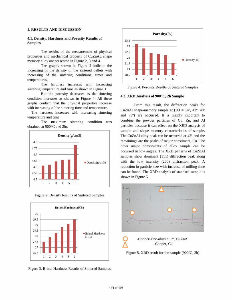
4. RESULTS AND DISCUSSION

4.1. Density, Hardness and Porosity Results of

Samples

The results of the measurement of physical

properties and mechanical property of CuZnAL shape

memory alloy are presented in Figure 2, 3 and 4.

The graphs shown in Figure 2 indicate the

increasing of the density of the sintered pellets with

increasing of the sintering conditions; times and

temperatures.

The hardness increases with increasing

sintering temperature and time as shown in Figure 3.

But the porosity decreases as the sintering

condition increases as shown in Figure 4. All these

graphs confirm that the physical properties increase

with increasing of the sintering time and temperature.

The hardness increases with increasing sintering

temperature and time

The maximum sintering condition was

obtained at 900°C and 2hr.

4.5

4.55

4.6

4.65

4.7

4.75

4.8

1 2 3 4 5 6

Density(g/cm3)

Density(g/cm3)

Figure 2. Density Results of Sintered Samples

Figure 3. Brinel Hardness Results of Sintered Samples

20.5

21

21.5

22

22.5

23

23.5

1 2 3 4 5 6

Porosity(%)

Porosity(%)

Figure 4. Porosity Results of Sintered Samples

4.2. XRD Analysis of 900°C, 2h Sample

From this result, the diffraction peaks for

CuZnAl shape-memory sample at (2ϴ = 14º, 42º, 48º

and 73º) are occurred. It is mainly important to

combine the powder particles of Cu, Zn, and Al

particles because it can effect on the XRD analysis of

sample and shape memory characteristics of sample.

The CuZnAl alloy peak can be occurred at 42º and the

remainings are the peaks of major constituent, Cu. The

other major constituents of alloy sample can be

occurred in low angles. The XRD patterns of CuZnAl

samples show dominant (111) diffraction peak along

with the low intensity (200) diffraction peak. A

reduction in particle size with increase of milling time

can be found. The XRD analysis of standard sample is

shown in Figure 5.

-Copper-zinc-aluminium, CuZnAl

- Copper, Cu

Figure 5. XRD result for the sample (900ºC, 2h)

144 of 198

4.3. XRF Analysis Results

From the X-ray fluorescence analysis, the

sample sintered at 800ºC for 1h contained about

74.54% Cu, 19.45% Zn, 5.03% Al and traces of other

elements. The sample sintered at 800ºC for 2h

contained about 74.12% Cu, 19.13% Zn, 4.96% Al and

traces of other elements. The sample sintered at 900ºC

for 1h contained about 73.84% Cu, 18.87% Zn, 4.87%

Al and traces of other elements. The sample sintered at

900ºC for 2h contained about 73.81% Cu, 19.22% Zn,

4.54% Al and traces of other elements.

Table 1. XRF Analysis of Samples

Type Cu % Zn% Al% Si%

1 74.54 19.45 5.03 0.34

2 74.22 19.32 5.12 0.21

3 74.12 19.13 4.96 0.33

4 73.84 18.87 4.87 0.42

5 73.78 19.13 4.92 0.48

6 73.81 19.22 4.54 0.53

4.4. Microstructure Analysis Result

Figure 6 shows the microstructure analysis

result for CuZnAl alloy sintered at 900ºC for holding

1h. Figure 7 shows the microstructure analysis results

of sample 5 at 900°C, 1.5h and Figure 8 shows the

microstructure analysis result of sample 6 at 900°C, 2h.

Some pores (impurities) are occurred between the

grains and grain boundaries. Most of the pores exhibit

in different structures. The occurrence of pores can

depend on the alloy composition, compaction pressure,

sintering temperature and sintering time.

Figure 9 is the microstructure analysis of

Sample- 3 at 900°C for 2h after heat treatment process.

Figure 5 have shown in the martensitic phase.

Fig. 2 Microstructure analysis results of sample 4 at

900°C, 1h (1000x magnification)

Figure. 7 Microstructure analysis results of sample 5 at

900°C, 1.5h (1000x magnification)

Figure 8. Microstructure analysis result of sample 6 at

900°C, 2h (1000x magnification)

Figure 9. Microstructure Analysis of Sample 6 at

900°C for 2h after heat treatment process (1000x

magnification)

Grains

Grain boundary

Impurities

Grains

Grain boundary

Impurities

Grains

Grain boundary

145 of 198

4.5. Testing of Shape Memory Effect

(a) (b) (c)

Figure 10. Shape Memory Effect Analysis Results (a)

CuZnAl Wire in Original Form, (b) CuZnAl Wire in

Bending Form, (c) CuZnAl Wire after Adding in

Boiling Water Form

Figure 10. can be seen that to get the shape

memory effect, the sintered pellets are deformed into

the hot-rolled machine and transformed into the wire

shape. The wires are heated into the muffle furnace

step by step according to the diameter of wire. In this

research, 0.75mm diameter of wire is used. For this

research, the shape memory effect is firstly occurred at

875°C of sintering temperature and 1 hr of sintering

time. The shape-memory wire is deformed from the

original straight shape. In this deforming the shape, it is

not recommended for twisting. Then, the wire is added

into the boiling water, the wire returned into the

original straight line shape. This is called the shape-

memory effect. For larger diameter shape-memory

wire, more heat is needed to get into the original form.

5. CONCLUSION

The CuZnAl shape memory alloys with different

sintering temperature and time are studied. The

sintering characteristics, mechanical property, physical

properties, X ray diffraction analysis and

microstructure were studied. The density and hardness

of the sintered samples are increased with the

increasing sintering time and temperature. The porosity

was decreased with increasing sintering time and

temperature. The optimum sintering condition was

obtained at 900ºC and 2h. In this research, the shape

memory effect was occurred as shown in Figure 10.

Powder composition, powder size, sintering

temperature, sintering time, hot rolling and heat

treatment process are important to get shape-memory

effect.

146 of 198

RECOVERY OF COBALT METAL FROM SPENT LI-ION BATTERY

BY COMBINATION METHOD OF PRECIPITATION AND

REDUCTION

Dr. MyatMyatSoe1, Dr. Nay Myo Htike2

1 Metallurgical Research Division, Department of Research and Innovation,

Ministry of Education, MYANMAR 2Metallurgical Research Division,Department of Research and Innovation,

Ministry of Education, MYANMAR

* E-mail:[email protected],[email protected]

Abstract—Now a day, recycling of valuable

metals from spent li-ion battery has being

increased. When it may be taken to landfills, the

toxic metals may be leached into the

underground and then contamination of

underground water or contamination of crop. In

this research, recovery of cobalt metal from

spent li-ion battery was extracted by

metallurgical method. There were two steps in

this research; first step, cobalt oxalate was

extracted from li-ion batteries by precipitation

method and second step, cobalt oxalate was

decomposed at high temperature to get cobalt

metal.

Keywords: (Battery, Cobalt, , Gases, Metal,

Metallurgical Method)

I. INTRODUCTION

Cobalt is a chemical element with symbol Co

and atomic number 27 like nickel. Cobalt is found

in the Earth’s crust only in chemically combined

form, save for small deposits found in alloys of

natural meteoric iron. The free element, produced

by reductive smelting, is a hard, lustrous, silver

gray metal.

Lithium-ion batteries are essential to modern

technology, powering smartphones, laptops,

medical devices and even electric vehicles. There

are many different types of li ion batteries; lithium

cobalt oxide battery, Lithium manganese battery,

lithium nickel manganese battery and more.

Lithium cobalt oxide battery is a high specific

energy as compared to the other batteries.

Improper disposal of these batteries becomes

seriousenvironmental problems due to their

hazardous constituents which include heavy metals

and electrolytes. That leads toaffect the human

health and environmental pollution. There are three

ways to prevent environmental damage are

conservation of water, cleaning air and reducing

waste. One way of preventing environmental

damage is recycling or reducing waste. Cobalt is

animportant basic material for industrial

application; however, it is difficult to recover

cobalt from minerals since there is a lack of

independent deposits in nature.

Cobalt is a shiny, brittle metal that is used to

produce strong and heat resistant alloys,permanent

magnet and hard metals. Cobalt is also used

to;make alloys for jet engines and gas turbines,

magnetic steels and some types of stainless steel.

Cobalt 60, a radioactive isotope of cobalt, is an

important source of gamma rays and has been used

to treat some forms of cancer and as a medical

tracer. In addition to the metal itself, cobalt

compounds for instance, cobalt oxalate, cobalt

oxide, cobalt chloride, and cobalt sulfate also have

extensive industrial applications.

II. MATERIALS AND METHOD.

To provide a process to recover cobalt from spent

lithium-ion battery, many methods have been

developed including mechanical process, thermal

process, acid or base leaching, bioleaching, solvent

extraction, chemical precipitation and

electrochemical process. Hydro-metallurgical

method is the main method to recycle valuable

147 of 198

materials from lithium ion batteries. Cobalt from

lithium-ion battery was leached with sulphuric acid

or nitric acid and then precipitated with ammonium

oxalate.

Cobalt oxalate is used in the preparation of

cobalt catalyst, to cobalt metal powder for

metallurgical applications.Cobalt oxalate is an

inorganic compound with a formula of CoC2O4.

Process for extraction of cobalt oxalate from

lithium-ion battery consist sample preparation,

leaching with sulphuric acid, adding with hydrogen

peroxide and precipitation with ammonium oxalate.

Oxalic acid or ammonium oxalate was used for

recovering cobalt from leaching solution of spent

lithium ion battery by precipitation method.

Crushed powders containing LiCoO2 of spent

lithium ion battery were obtained by crushing,

magnetic separation and screening process. These

powders were dissolved in 2 M H2SO4 solution

with H2O2 as a reducing agent. After dissolving Co

and Li components, ammonium oxalate solution

was added. Co (II) in leaching solution could be

removed in the form of insoluble oxalates. The

precipitate formed was crystalline, compact and

easily filtered. When cobalt ion was precipitated

into cobalt oxalate, nickel and copper ions were

also co-precipitated but there were no co-

precipitates of Li, Al and Fe. The amounts of Ni

and Cu in the solutions were below 1%. After

drying of precipitates at 100°C for 1 hour, cobalt

oxalate was obtained. If heating above 200°C

cobalt oxalate hanged into cobalt oxide. [2][3]

The leaching process of LiCoO2 in H2SO4 solution

could be represented as follows;

2LiCoO2(S) + 3 H2SO4 (aq) + H2O2 (aq)

2CoSO4(aq) +Li2SO4(aq)+4H2O(g)+O2(g)(1)

And then cobalt ion was precipitated into

cobalt oxalate by adding ammonium oxalate.

CoSO4 (aq) + (NH4)2C2O4 (aq)

CoC2O4(s) +(NH4)2 SO4 (aq) (2)

Solvent extraction process, reduction process

and precipitation process were used for recovering

cobalt from spent lithium ion battery. More over

cobalt oxalate is also used as a starting compound

for cobalt extraction. At very high temperatures

cobalt oxalate was heated to remove carbon and

oxygen and to get cobalt powder.[2][3]

III. EXPERIMENTAL PROCEDURE

In this study, cobalt oxalate was extracted from

spent lithium cobalt oxide ion batteries. Samples

were collected from spent li cobalt oxide batteries

manually. Next, samples were analyzed to

quantitative determinations of elements, by using

Atomic Absorption Spectroscopy. The figures of

collection of samples from batteries and sample

assay determinations by Atomic Absorption

Spectroscopywere shown in figure 1 and 2.

In each experiment, ten grams of sample was

taken to extract cobalt oxalate from batteries. It

contained 23% of cobalt. Samples were dissolved

into H2SO4-H2O2 solution in beaker. Then samples

were leached at 70˚C for 1 hour. After complete

leaching, solutions were filtered off to remove

residue, and then pH 5 was adjusted by adding

NaOH solution. Then 5 ml of H2O2 was added to

the solution and agitated at the speed of 300 rpm for

1 hour. After 1 hour, the pink color crystalline

precipitate was formed. The precipitate was filtered

anddried, CoC2O4 powder was obtained. Processes

for preparation of CoC2O4 were illustrated in figures

3, 4, 5 and 6.

To obtain the optimum conditions, experiments

were should be madeby the variation of sulphuric

acid concentration, temperature, reaction time and

the amount of hydrogen peroxide. In this research,

the effect of sulphuric acid concentration on the

leaching efficiency and purity of Co% in CoC2O4

precipitate were determined.In these experiments,

leaching temperature and leaching time were kept

constant at 70˚C and 1 hour. Leaching temperature

70˚Cand leachingtime1hourwere chosenaccording

to references. Concentration of H2SO4 varied from

0.5 moles / lit to 2.5 moles / lit with reluctant

amount of 2.0% H2O2.[3]

The precipitate obtained from optimum

conditions were heated with oxyacetylene torch at

3000˚C. The powder was obtained after removing

carbon and oxygen from cobalt oxalate at high

temperature. The powder was preliminary

examined with magnetic pieces. Then it was

analyzed by X-ray Diffraction Spectrometer.

Results showed that the powder was cobalt powder.

Flow sheet for extraction of cobalt from li-ion

batteries is shown in figure 7.

148 of 198

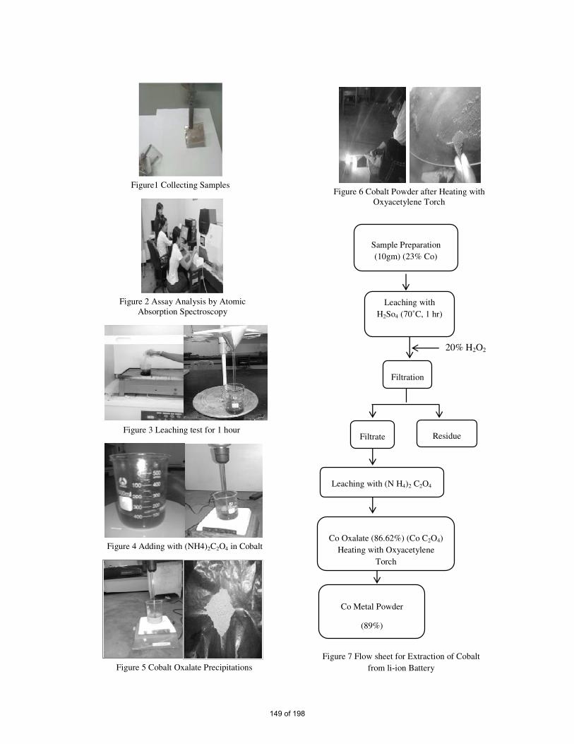
Sample Preparation

(10gm) (23% Co)

Figure 2 Assay Analysis by Atomic

Absorption Spectroscopy

Figure 3 Leaching test for 1 hour

Figure 4 Adding with (NH4)2C2O4 in Cobalt

Figure 5 Cobalt Oxalate Precipitations

Figure 6 Cobalt Powder after Heating with

Oxyacetylene Torch

Figure 7 Flow sheet for Extraction of Cobalt

from li-ion Battery

Figure1 Collecting Samples

Co Metal Powder

(89%)

Leaching with

H2So4 (70˚C, 1 hr)

Filtration

20% H2O2

Filtrate

Residue

Leaching with (N H4)2 C2O4

Co Oxalate (86.62%) (Co C2O4)

Heating with Oxyacetylene

Torch

149 of 198

150 of 198

V. CONCLUSIONS

The leaching efficiency 83.33% and cobalt

purity 86.62%were observed at the H2SO4

concentration of 2 moles /lit. The purity of 89 %

cobalt powder was obtained. In this research, the

variations of H2SO4 solution concentration were

studied for cobalt oxalate extraction. CoC2O4 can

be used as a starting compound to recover cobalt

from spent lithium ion battery.

ACKNOWLEDGMENT(S)

I would like to express my thanks of

gratitude to all staff from Metallurgical Research

Division. I want to express specialthanks to our

Director General and Deputy Director General who

gave me the golden opportunity to do this project.

REFERENCES

[1] MiamariAaliton, Chao Peng, Benjamin P.

Wilson:Leachingof Metals from Spent

Lithium-Ion Battery,

www.mdpi.com/journal/recycling.

[2] L W Ma, X L Xi, Z ZZaung, Z Q HAUNG, J

P Chen: Hydrometallurgical Treatment for

Mixed Waste Battery Materials, 3rd

International conference on Advanced

Materials Science and application

(AMRA2016).

[3] ZHU Shu-guang, HE Wen-zhi: Recovery of

Co and Li from spent lithium ion batteries by

combination method of acid leaching and

chemical precipitation, School of

Environmental Science and Engineering,

Tongji University, Shanghai 200092, China.

[4] ELSEVIER, Separation and Purification

Technology Volume 186, 2 October 2017,

Pages 318-32

151 of 198

Assessment of Surface and Ground Water Quality around the

Kyinsintaung Mine, Myanmar

Myint Aung 1, Dr. Aung Lay Tin2

1Associate Professor, Department of Mining Engineering

Yangon Technological University

Insein Road, Gyogone, Yangon, 11011, Myanmar

2 Professor and Head, Department of Mining Engineering

Yangon Technological University

Insein Road, Gyogone, Yangon, 11011, Myanmar

*Corresponding author: [email protected]

Abstract—This study carried out at the

Kyisintaung copper (Cu) mine, located in

Monywa District, Sagaing Region. The mine is

on the west bank of Chindwin River and on the

east side of Monywa, the capital of Sagaing

Region. Chindwin is the biggest tributary of

Ayeyarwaddy river and the longest navigable

one in Myanmar flowing from north south. Acid

mine drainage of Kyisintaung minecan be a

multi-factor pollutant unless the proper mine

drainage system is conducted. It can affect

surface and underground water quality by a

number of direct and indirect pathways which

lead to destruction of aquatic ecosystems.

Potential impact area includes rivers, lakes,

estuaries and coastal waters especially at the

downstream area of mine. Due to its complexity,

the impact of acid mine drainage is difficult to

quantify and predict, especially in riverine

systems. Pollution effects of acid mine drainage

are complex but can be categorized as (a)

sedimentation processes, (b) acidity, (c) metal

toxicity and (d) salinization. Thus this study

points out the water quality including surface

and ground water in the vicinity of Kyisintaung

Mine to help minimize the water quality impacts

by the mine in near future. The impacts of

surface and ground water quality are discussed

in this study.

Keywords: Environmental Impact, Management

Systems Mine, Water Quality,Surface Water,

Ground Water

I. INTRODUCTION

The Kyisintaung mine is located at the

coordinates of 22° 7' 21.56" N and 95° 1' 58.27" E,

Monywa District, Sagaing Region in Myanmar.

This is an open-pit mine and Copper ore is being

extracted since early 17th century. Many

international companies have been involved in the

development of this mine under several eras of

ownership. In the 1950's the Sebaltaung and

Kyisintaung deposits began to be explored on a

much larger scale and have developed into a mining

enterprise today. Currently, the mining is operated

by Wanbao Mining Limited with the name of

Myanmar Yang Tse Copper Limited (MYTCL) at

an annual production rate of 50,000 tonnes of

copper ore with the average content of 0.31%. The

Yama stream which is the tributary of Chindwin

river is located at the northern part of the mine. The

Chindwin river which is the largest tributary of the

country's chief river of the Ayeyarwady river

located at the eastern part of mine. This river plays

vital role in movement of small and medium vessels

for transportation of goods and materials. It also

serves as portable water resources for the residences

and agricultural farms existed along the river. It has

been said that mining activities cause water

pollution. Thus, this study focused on monitoring of

water quality in the vicinity of Kyisintaung mine.

Location of Kyisintaung mine is shown in Figure 1.

152 of 198

Figure 1 Location of Kyisintaung mine

This paper is organized as the following:

Section II describes the methodology of this study.

Results and discussions are presented in Section III

and Section IV shows the conclusions.

II. METHODOLOGY

Field study was conducted at the mine site to

understand the current mining practice of MYTCL

and help identify the water pollution sources,

sampling locations and parameters to be monitored.

Accordingly, the total of 21 water samples that

comprises 12 surface water samples and 9 ground

water samples around the mining area were

collected in June 2018. Figure 2 shows the surface

water sampling locations along the Yama stream

and ground water sampling locations in Kyisintaug

mine. In-situ measurements were carried out for the

physical parameter-temperature-and some chemical

parameters, pH, conductivity and dissolved oxygen

using HI 98194 Multi-parameter probe. The other

parameters such as TSS, TDS, Cu, Fe, Pb, Mn,

SO4, Ca, Ma and total hardness were taken into

consider for laboratory analysis. To collect the

water samples, sterilized plastic bottles were used.

The bottles were rinsed three times with the water

to be sampled before being filled. Then the samples

chilled and transported to laboratory. The

laboratory analysis was carried out at the certified

laboratories in Myanmar.

Figure 2 Sampling locations of surface water and

ground water

III. RESULTS AND DISCUSSIONS

The results of surface water samples compared

with National Emission Quality Guidelines

(NEQG) are presented in Table 1 whereas ground

water samples’ results are illustrated in Table 2.

For the surface water quality (Figure 3), the

concentrations of TSS of all samples expect SW11

and SW12, significantly exceed the NEQG value at

50 mg/l while the results of remaining parameters

are within the guidelines limits. Regarding with the

results of ground water samples (Figure 4), all the

concentration of monitored parameters are within

the acceptable limit of NEQG values. However, the

TSS values appear to be higher than in GW 07 and

08 at 110 mg/l and 99 mg/l respectively while the

other points are lower than NEQG limit. The

concentrations of total hardness values are also

appeared 2-3 times higher than the guidelines

values. It was found that the concentration of sulfate

in GW08 and GW09 are higher than the guidelines

values and the remaining points are within the

guidelines values.

153 of 198

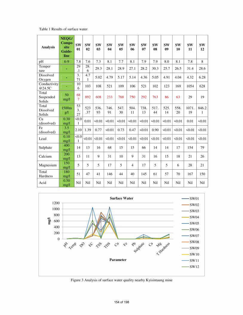
Table 1 Results of surface water

Analysis

NEQG/

Compo

site

Guide-

line

SW

01

SW

02

SW

03

SW

04

SW

05

SW

06

SW

07

SW

08

SW

09

SW

10

SW

11

SW

12

pH 6-9 7.8 7.6 7.3 8.1 7.7 8.1 7.9 7.9 8.0 8.1 7.8 8

Temper

ture -

29

.1

28.

6 29.3 28.1 28.9 27.1 28.2 30.3 25.7 26.5 31.4 28.6

Dissolved

Oxygen -

3.

71

4.7

1 5.02 4.79 5.17 5.14 4.36 5.05 4.91 4.04 4.32 6.28

Conductivity

@24.5C -

10

6 103 108 521 109 106 521 102 123 169 1054 628

Total

Suspended

Solids

50

mg/l

68

7 892 608 233 788 750 292 763 86 63 29 19

Total

Dissolved

Solids

1500m

g/l

53

3.

27

523

.37

536.

93

746.

91

547.

30

504.

11

738.

13

517.

44

525.

14

558.

20

1071.

19

846.2

1

Cu

(dissolved)

0.30

mg/l

<0.0

1 0.01 <0.01 <0.01 <0.01 <0.01 <0.01 <0.01 <0.01 <0.01 0.01 <0.01

Fe

(dissolved)

3.5

mg/l 2.10 1.39 0.77 <0.01 0.73 0.47 <0.01 0.90 <0.01 <0.01 <0.01 <0.01

Lead 0.10

mg/l

<0.0

1 <0.01 <0.01 <0.01 <0.01 <0.01 <0.01 <0.01 <0.01 <0.01 <0.01 <0.01

Sulphate 400

mg/l 14 13 16 68 15 15 66 14 14 17 154 79

Calcium 200

mg/l 13 11 9 31 10 9 31 16 15 18 21 26

Magnesium 150

mg/l 5 5 5 17 5 4 17 5 5 6 28 21

Total

Hardness

180

mg/l 51 47 41 146 44 40 145 61 57 70 167 150

Acid 0.50

mg/l Nil Nil Nil Nil Nil Nil Nil Nil Nil Nil Nil Nil

Figure 3 Analysis of surface water quality nearby Kyisintaung mine

0

200

400

600

800

1000

1200

mg/l

Parameter

Surface Water SW01

SW02

SW03

SW04

SW05

SW06

SW07

SW08

SW09

SW10

SW11

SW12

154 of 198

Table 2 Results of ground water

Analysis

NEQG/

Composite

Guideline

GW

01

GW

02

GW

03

GW

04

GW

05

GW

06

GW

07

GW

08

GW

09

pH 6-9. 7.2 7.6 7.7 7.5 7.6 7.6 7.2 7.2 7.5

Temperature - 30.3 30.5 30.4 31 27.8 30.6 28.3 30.7 28.3

Dissolved

Oxygen - 1.54 2.24 3.06 0.87 2.13 2.23 1.04 1.42 2.77

Total

Suspended

Solids

50 mg/l 52 14 15 92 50 10 110 99 19

Total

Dissolved

Solids

1500mg/l 573 534 645 618 3165 781 1543 3807 2557

Cu

(dissolved) 0.30 mg/l

<0.0

1

<0.0

1 <0.01 <0.01 0.04 0.01 0.01 0.02 0.01

Fe

(dissolved) 3.5 mg/l

<0.0

1

<0.0

1 <0.01 <0.01 0.01 <0.01 0.01 0.01 <0.01

Lead 0.10 mg/l <0.0

1 0.01 <0.01 <0.01 0.03 <0.01 0.01 0.05 0.03

Manganese 0.1mg/l <0.0

1

<0.0

1 <0.01 <0.01 <0.01 <0.01 <0.01 <0.01 0.02

Sulphate 400 mg/l 146 122 196 182 910 194 234 1000 1280

Calcium 200 mg/l 111 96 81 116 7 54 11 67 24

Magnesium 150 mg/l 43 40 38 52 90 54 142 106 116

Total

Hardness 180 mg/l 454 404 359 504 387 356 613 604 538

Acid 0.50 mg/l Nil Nil Nil Nil Nil Nil Nil Nil Nil

Figure 4 Analysis of ground water quality nearby Kyisintaung mine

0500

1000150020002500300035004000

mg

/l

Parameter

Ground Water

GW01

GW02

GW03

GW04

GW05

GW06

GW07

GW08

GW09

155 of 198

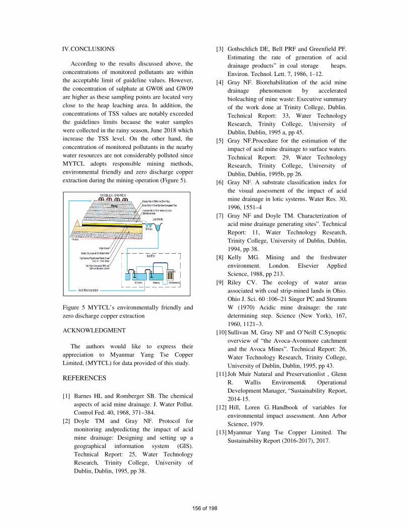
IV. CONCLUSIONS

According to the results discussed above, the

concentrations of monitored pollutants are within

the acceptable limit of guideline values. However,

the concentration of sulphate at GW08 and GW09

are higher as these sampling points are located very

close to the heap leaching area. In addition, the

concentrations of TSS values are notably exceeded

the guidelines limits because the water samples

were collected in the rainy season, June 2018 which

increase the TSS level. On the other hand, the

concentration of monitored pollutants in the nearby

water resources are not considerably polluted since

MYTCL adopts responsible mining methods,

environmental friendly and zero discharge copper

extraction during the mining operation (Figure 5).

Figure 5 MYTCL’s environmentally friendly and

zero discharge copper extraction

ACKNOWLEDGMENT

The authors would like to express their

appreciation to Myanmar Yang Tse Copper

Limited, (MYTCL) for data provided of this study.

REFERENCES

[1] Barnes HL and Romberger SB. The chemical

aspects of acid mine drainage. J. Water Pollut.

Control Fed. 40, 1968, 371–384.

[2] Doyle TM and Gray NF. Protocol for

monitoring andpredicting the impact of acid

mine drainage: Designing and setting up a

geographical information system (GIS).

Technical Report: 25, Water Technology

Research, Trinity College, University of

Dublin, Dublin, 1995, pp 38.

[3] Gothschlich DE, Bell PRF and Greenfield PF.

Estimating the rate of generation of acid

drainage products” in coal storage heaps.

Environ. Technol. Lett. 7, 1986, 1–12.

[4] Gray NF. Biorehabilitation of the acid mine

drainage phenomenon by accelerated

bioleaching of mine waste: Executive summary

of the work done at Trinity College, Dublin.



Dublin, Dublin, 1995 a, pp 45.

[5] Gray NF.Procedure for the estimation of the

impact of acid mine drainage to surface waters.



Dublin, Dublin, 1995b, pp 26.

[6] Gray NF. A substrate classification index for

the visual assessment of the impact of acid

mine drainage in lotic systems. Water Res. 30,

1996, 1551–4

[7] Gray NF and Doyle TM. Characterization of

acid mine drainage generating sites”. Technical

Report: 11, Water Technology Research,

Trinity College, University of Dublin, Dublin,

1994, pp 38.

[8] Kelly MG. Mining and the freshwater

environment. London. Elsevier Applied

Science, 1988, pp 213.

[9] Riley CV. The ecology of water areas

associated with coal strip-mined lands in Ohio.

Ohio J. Sci. 60 :106–21 Singer PC and Strumm

W (1970) Acidic mine drainage: the rate

determining step. Science (New York), 167,

1960, 1121–3.

[10] Sullivan M, Gray NF and O’Neill C.Synoptic

overview of “the Avoca-Avonmore catchment

and the Avoca Mines”. Technical Report: 26,

Water Technology Research, Trinity College,

University of Dublin, Dublin, 1995, pp 43.

[11] Joh Muir Natural and Preservationlist , Glenn

R. Wallis Enviroment& Operational

Development Manager, “Sustainability Report,

2014-15.

[12] Hill, Loren G. Handbook of variables for

environmental impact assessment. Ann Arbor

Science, 1979.

[13] Myanmar Yang Tse Copper Limited. The

Sustainability Report (2016-2017), 2017.

156 of 198

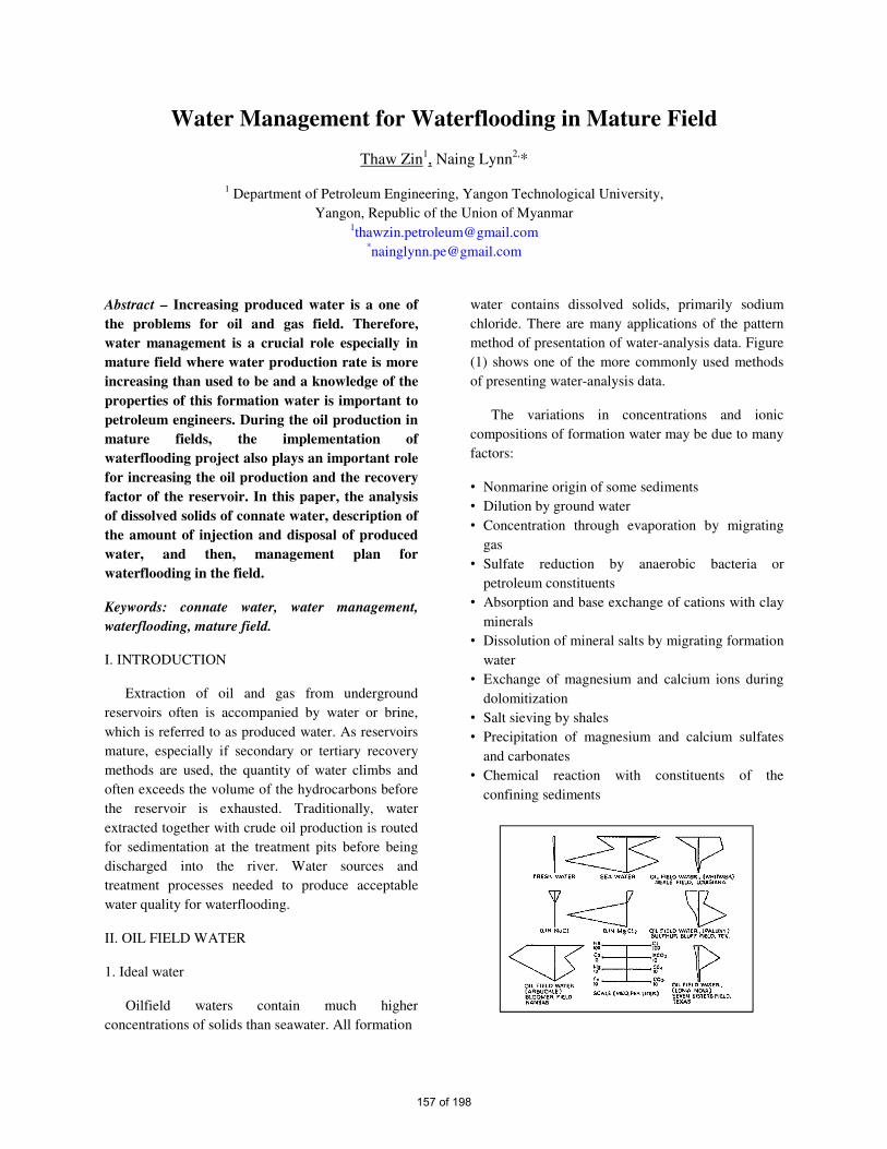
Water Management for Waterflooding in Mature Field

Thaw Zin1, Naing Lynn

2,*

1 Department of Petroleum Engineering, Yangon Technological University,

Yangon, Republic of the Union of Myanmar [email protected]

*[email protected]

Abstract – Increasing produced water is a one of

the problems for oil and gas field. Therefore,

water management is a crucial role especially in

mature field where water production rate is more

increasing than used to be and a knowledge of the

properties of this formation water is important to

petroleum engineers. During the oil production in

mature fields, the implementation of

waterflooding project also plays an important role

for increasing the oil production and the recovery

factor of the reservoir. In this paper, the analysis

of dissolved solids of connate water, description of

the amount of injection and disposal of produced

water, and then, management plan for

waterflooding in the field.

Keywords: connate water, water management,

waterflooding, mature field.

I. INTRODUCTION

Extraction of oil and gas from underground

reservoirs often is accompanied by water or brine,

which is referred to as produced water. As reservoirs

mature, especially if secondary or tertiary recovery

methods are used, the quantity of water climbs and

often exceeds the volume of the hydrocarbons before

the reservoir is exhausted. Traditionally, water

extracted together with crude oil production is routed

for sedimentation at the treatment pits before being

discharged into the river. Water sources and

treatment processes needed to produce acceptable

water quality for waterflooding.

II. OIL FIELD WATER

1. Ideal water

Oilfield waters contain much higher

concentrations of solids than seawater. All formation

water contains dissolved solids, primarily sodium

chloride. There are many applications of the pattern

method of presentation of water-analysis data. Figure

(1) shows one of the more commonly used methods

of presenting water-analysis data.

The variations in concentrations and ionic

compositions of formation water may be due to many

factors:

• Nonmarine origin of some sediments

• Dilution by ground water

• Concentration through evaporation by migrating

gas

• Sulfate reduction by anaerobic bacteria or

petroleum constituents

• Absorption and base exchange of cations with clay

minerals

• Dissolution of mineral salts by migrating formation

water

• Exchange of magnesium and calcium ions during

dolomitization

• Salt sieving by shales

• Precipitation of magnesium and calcium sulfates

and carbonates

• Chemical reaction with constituents of the

confining sediments

157 of 198

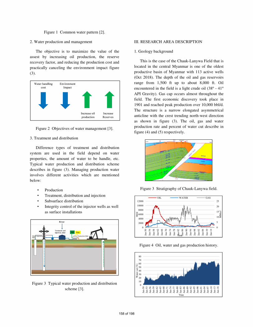
Figure 1 Common water pattern [2].

2. Water production and management

The objective is to maximize the value of the

assest by increasing oil production, the reserve

recovery factor, and reducing the production cost and

practically canceling the environment impact figure

(3).

Figure 2 Objectives of water management [3].

3. Treatment and distribution

Difference types of treatment and distribution

system are used in the field depend on water

properties, the amount of water to be handle, etc.

Typical water production and distribution scheme

describes in figure (3). Managing production water

involves different activities which are mentioned

below:

• Production

• Treatment, distribution and injection

• Subsurface distribution

• Integrity control of the injector wells as well

as surface installations

Figure 3 Typical water production and distribution

scheme [3].

III. RESEARCH AREA DESCRIPTION

1. Geology background

This is the case of the Chauk-Lanywa Field that is

located in the central Myanmar is one of the oldest

productive basin of Myanmar with 113 active wells

(Oct 2018). The depth of the oil and gas reservoirs

range from 1,500 ft up to about 8,000 ft. Oil

encountered in the field is a light crude oil (38° - 41°

API Gravity). Gas cap occurs almost throughout the

field. The first economic discovery took place in

1901 and reached peak production over 10,000 bbl/d.

The structure is a narrow elongated asymmetrical

anticline with the crest trending north-west direction

as shown in figure (3). The oil, gas and water

production rate and percent of water cut describe in

figure (4) and (5) respectively.

Figure 3 Stratigraphy of Chauk-Lanywa field.

Figure 4 Oil, water and gas production history.

0

5

10

15

20

25

0

2000

4000

6000

8000

10000

12000

Jan-5

0

Jan-5

4

Jan-5

8

Jan-6

2

Jan-6

6

Jan-7

0

Jan-7

4

Jan-7

8

Jan-8

2

Jan-8

6

Jan-9

0

Jan-9

4

Jan-9

8

Jan-0

2

Jan-0

6

Jan-1

0

Jan-1

4

MM

scf

bbl/

d

Time

OIL WATER GAS

0

10

20

30

40

50

60

70

80

Jan-5

0

Jan-5

3

Jan-5

6

Jan-5

9

Jan-6

2

Jan-6

5

Jan-6

8

Jan-7

1

Jan-7

4

Jan-7

7

Jan-8

0

Jan-8

3

Jan-8

6

Jan-8

9

Jan-9

2

Jan-9

5

Jan-9

8

Jan-0

1

Jan-0

4

Jan-0

7

Jan-1

0

Jan-1

3

Jan-1

6

Wat

er c

ut

(%)

Time

158 of 198

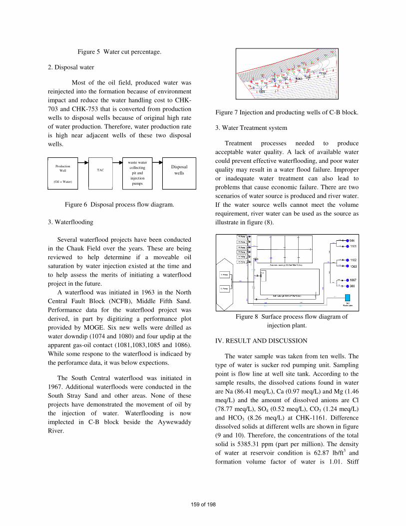
Figure 5 Water cut percentage.

2. Disposal water

Most of the oil field, produced water was

reinjected into the formation because of environment

impact and reduce the water handling cost to CHK-

703 and CHK-753 that is converted from production

wells to disposal wells because of original high rate

of water production. Therefore, water production rate

is high near adjacent wells of these two disposal

wells.

Figure 6 Disposal process flow diagram.

3. Waterflooding

Several waterflood projects have been conducted

in the Chauk Field over the years. These are being

reviewed to help determine if a moveable oil

saturation by water injection existed at the time and

to help assess the merits of initiating a waterflood

project in the future.

A waterflood was initiated in 1963 in the North

Central Fault Block (NCFB), Middle Fifth Sand.

Performance data for the waterflood project was

derived, in part by digitizing a performance plot

provided by MOGE. Six new wells were drilled as

water downdip (1074 and 1080) and four updip at the

apparent gas-oil contact (1081,1083,1085 and 1086).

While some respone to the waterflood is indicaed by

the perforamce data, it was below expections.

The South Central waterflood was initiated in

1967. Additional waterfloods were conducted in the

South Stray Sand and other areas. None of these

projects have demonstrated the movement of oil by

the injection of water. Waterflooding is now

implected in C-B block beside the Aywewaddy

River.

Figure 7 Injection and producting wells of C-B block.

3. Water Treatment system

Treatment processes needed to produce

acceptable water quality. A lack of available water

could prevent effective waterflooding, and poor water

quality may result in a water flood failure. Improper

or inadequate water treatment can also lead to

problems that cause economic failure. There are two

scenarios of water source is produced and river water.

If the water source wells cannot meet the volume

requirement, river water can be used as the source as

illustrate in figure (8).

Figure 8 Surface process flow diagram of

injection plant.

IV. RESULT AND DISCUSSION

The water sample was taken from ten wells. The

type of water is sucker rod pumping unit. Sampling

point is flow line at well site tank. According to the

sample results, the dissolved cations found in water

are Na (86.41 meq/L), Ca (0.97 meq/L) and Mg (1.46

meq/L) and the amount of dissolved anions are Cl

(78.77 meq/L), SO4 (0.52 meq/L), CO3 (1.24 meq/L)

and HCO3 (8.26 meq/L) at CHK-1161. Difference

dissolved solids at different wells are shown in figure

(9 and 10). Therefore, the concentrations of the total

solid is 5385.31 ppm (part per million). The density

of water at reservoir condition is 62.87 lb/ft3 and

formation volume factor of water is 1.01. Stiff

Production

Well

(Oil + Water)

TAC

waste water

collecting

pit and

injection

pumps

Disposal

wells

159 of 198

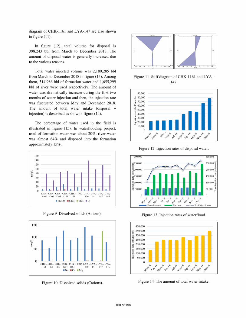
diagram of CHK-1161 and LYA-147 are also shown

in figure (11).

In figure (12), total volume for disposal is

398,243 bbl from March to December 2018. The

amount of disposal water is generally increased due

to the various reasons.

Total water injected volume was 2,180,285 bbl

from March to December 2018 in figure (13). Among

them, 514,986 bbl of formation water and 1,655,299

bbl of river were used respectively. The amount of

water was dramatically increase during the first two

months of water injection and then, the injection rate

was fluctuated between May and December 2018.

The amount of total water intake (disposal +

injection) is described as show in figure (14).

The percentage of water used in the field is

illustrated in figure (15). In waterflooding project,

used of formation water was about 20%, river water

was almost 64% and disposed into the formation

approximately 15%.

Figure 9 Dissolved solids (Anions).

Figure 10 Dissolved solids (Cations).

Figure 11 Stiff diagram of CHK-1161 and LYA -

147.

Figure 12 Injection rates of disposal water.

Figure 13 Injection rates of waterflood.

Figure 14 The amount of total water intake.

0

20

40

60

80

100

120

140

160

CHK -

1161

CHK -

1201

CHK -

1203

CHK -

1204

CHK -

1161

TAC LYA -

136

LYA -

141

LYA -

147

LYA -

146

meq

/L

HCO3 CO3 SO4 Cl

0

50

100

150

CHK -

1161

CHK -

1201

CHK -

1203

CHK -

1204

CHK -

1161

TAC LYA -

136

LYA -

141

LYA -

147

LYA -

146

meq

/L

Na Ca Mg

0

10,000

20,000

30,000

40,000

50,000

60,000

70,000

80,000

90,000

Inje

ctio

n r

ate

(bbl/

mo

nth

)

0

50,000

100,000

150,000

200,000

250,000

300,000

0

50,000

100,000

150,000

200,000

250,000

300,000

To

tal in

ject

ion

rate

(bbl/

mo

nth

)

Inje

ctio

n r

ate

(bb

l/m

onth

)

Formation water River water Total Injected water

0

50,000

100,000

150,000

200,000

250,000

300,000

350,000

400,000

Inje

ctio

n r

ate

(bbl/

mo

nth

)

160 of 198

Figure 15 Percentage of injection rates.

VII CONCLUSION

The variations in concentrations and ionic

composition of formation water may be due to many

factors (precipitation of mangnesium and calcium

sulfates and carbonate, and chemical reaction with

constituents of the confining sediments, etc.).

The injection of water in oil fields to increase oil

production in certain wells. As far as practicable,

produced water will be used for gravity injection

purposes, in order to reduce the discharge of water to

the environment (i.e river, lake, etc). During the

waterflood project, the amount of injected water will

be increased. Therefore, more water will be needed to

supplement from the other source, for example, river

water. Most of the formation water is injected into

the disposal well, therefore, water production rate is

completely increase around of these disposal wells.

All of these formation water should be used as

injection water in C-B waterflooding project to

reduce of river water up to 49%.

In mature fields, sometimes the water control is not

an option, and it’s necessary to produce water for

producing oil.

• A continue surveillance is important for improving

the oil production.

• Improving the water management process can

extend the life of the mature fields.

• Add clay inhibitor and corrosion inhibitor to

protect reservoir and facilities.

• Higher level treatment can be carried out if it is

necessary based on the actual injection data and

performance in future.

• EOR projects implementation could be an option

for improving the recovery factor, but it will

depend on the return on investment.

ACKNOWLEDGEMENT

The author would like to express his special

thanks Dr. Zaw Htet Aung (Professor and Head,

Department of Petroleum Engineering, Yangon

Technological University) for giving permission for

this paper. The author would be glad to express his

thanks to his supervisor Dr. Naing Lynn (Professor,


Technological University) for helping to become this

perfect study by his guidance and suggestions. The

author is grateful to all Professors and Lectures from


Technological University and finally acknowledge to

U Phone Thet Khaing (Executive Geologist, Chauk

Field) the help for supporting the required data for

this study.

REFERENCES

[1] J. F. B. A. R. J. W. STEPHEN C. ROSE, The

design engineering aspects of waterflooding,

Richardson, TX: Society of Petroleum

Enginners, 1989.

[2] J. WILLIAN D. McCAIN, The properties of

petroleum fluids, Tulsa, Oklahoma: PennWell

Publishing Company, 1990.

[3] C. M. H. a. F. D. Bertomeu, Water Mangement

Experience in Mature Field in South Argentian,

Society of Petroleum Engineer, 2017.

[4] Water Flooding Pilot Test Scenarios, 2017.

Formation

water, 20%

River

water, 64%

Dispose,

15%

161 of 198

Promote the Development of Renewable Energy in Myanmar

Khin Thi Aye

Deputy Director

PE (Water Resources) (0402)

Planning and Statistics Branch, Ministerial Office

Ministry of Electricity and Energy, Nay Pyi Taw, Myanmar

[email protected]

Abstract _ Myanmar has an abundance

of renewable energy resources. Moreover,

available energy resources in Myanmar are

Hydropower, Solar Power, Wind Power,

Biomass, Coal, Natural Gas and Crude Oil.

Among them, hydropower, one of renewable

energy resources in Myanmar is large

contribution. Because, country’s rivers, mainly

four rivers, Ayeyawaddy, Chindwin, Sittaung

and Thanlwin and its tributaries, can produce

hydropower above 100,000 MW. And, other

renewable energy resources, solar, wind and

biomass are also available according to the

geography condition of Myanmar. Now,

Myanmar is growing fast and hence energy

demand is significantly expanding. Therefore,

Ministry of Electricity and Energy of Myanmar

(MOEE) has been trying to generate the

electricity from available energy resources to

fulfill the electricity requirement. Moreover,

MOEE has issued six objectives for electric

power sector to meet the electricity demand and

among them; the significant one is to generate

more electricity from renewable energy

resources. Myanmar Government formed the

National Renewable Energy Committee on 6th

February 2019, to promote and improve the

Renewable Energy Sector, to get the

international assistance for implementing the

Renewable Energy Projects and to manage

Renewable Energy Projects systematically when

these are implemented by advanced technology.

Myanmar has always promoted the Renewable

Energy Sector; especially hydropower sector

was promoted rapidly during the last decade of

the 20th

century. Therefore, at present, total

installed capacity of hydropower stations,

including large, medium and small scale is 3262

MW. Among them, 28 number hydropower

stations with the total installed capacity of 3225

MW are connected to National Grid System

and, 33 numbers small scale hydropower

stations with the total installed capacity of 37

MW are off-grid. Moreover, MOEE has been

carrying out studies to generate more electricity

from Solar Power and Wind Power. In this

paper, available energy resources in Myanmar,

renewable energy resources in Myanmar,

Existing Myanmar Electricity Condition

(current generation mix, demand forecast,

electricity consumption, planned and ongoing

projects, strategic ways for power generation),

developments of renewable energy (Hydro,

Solar and Wind) and opportunities to invest in

renewable energy sector are mainly described.

Keywords: renewable energy resources, strategic

ways for power generation, objectives and

policies, developments of renewable energy and

opportunities.

I. INTRODUCTION

Now, Myanmar Government has been trying to

get balanced all round developments of States and

Regions in the country. Therefore, generating

electricity is very important to meet the electricity

requirements of consumers, infrastructures, offices

and all commercial and industrial works. Thus,

renewable energy sector becomes vital role in

Myanmar. Moreover, MOEE has been arranging by

short term and long term plans to get electricity

from available renewable energy resources.

II. AVAILABLE ENERGY RESOURCES IN

MYANMAR

Myanmar has an abundance of renewable

energy resources. Especially, hydropower resources

are very plentiful. It has mainly four rivers,

Ayeyawaddy, Chindwin, Sittaung and Thanlwin,

these rivers and its tributaries are for Hydropower

Resources. Country’s rivers can be produced

above 100,000 MW of hydropower. And, solar

162 of 198

Hydropower Natural Gas Coal Solar

power potential is 51973.8 Trillium Mega Watt

Hour per year and Wind Power Potential is 365.1

Trillium Mega Watt Hour per year. In Myanmar,

52.5% of total land area is covered with forest and

available annual yield of wood fuel is 19.12 million

cubic ton for Biomass Potential. Available Coal

potential has been 711 Million Metric Tons.

Natural Gas for Onshore and Offshore will be

122.5391 Trillion Standard Cubic Feet and Crude

oil for onshore and offshore will be 648.59 Million

Barrels. These available energy resources are

described in Table 1.

Table 1 Available Energy Resources

Particular Potential

Hydropower Above 100,000 MW

Solar Power 51973.8 TWH per year

Wind 365.1 TWH per year

Biomass 52.5 % of total land area covered

with forest

Potential available annual yield of

wood-fuel 19.12 million cubic ton

Coal 711 Million Metric Tons

Natural Gas

(offshore &

Onshore)

(Proven &

Probable )

122.5391 TSCF

Crude Oil

(offshore &

Onshore)

(Proven &

Probable )

648.59 MMBBL

III. RENEWABLE ENERGY RESOURCES

There are many renewable energy resources in

Myanmar. These are Hydropower, Solar Power,

Wind Power, Geothermal Energy, Biomass, Waste

to Energy and Ocean. Among them, hydropower,

solar power and wind power are popular in

Myanmar. MOEE has been trying to generate the

electricity from these renewable energy resources.

IV. EXISTING ELECTRICITY CONDITION

In October 2019, the total installed capacity in

power system is 5668.39 MW and the ratio of

electric power (installed capacity) is 57 %( 3225

MW) from hydro, 40% (2283.39 MW) from gas,

2 %( 120 MW) from coal and 1 %( 40 MW) from

solar power respectively. According to the

National Electricity Master Plan, the electricity

consumption in 2015 was 2527 MW and the

forecasted demand for the 2020, 2025 and 2030 are

4530 MW, 8121 MW and 14542 MW respectively.

Besides, electricity consumption of year by year

was increased from 15% to 19%. In December

2019, as electrified households became about 5.4

million, the electrification ratio became 50%. The

total length of Existing Transmission Lines, 230

kV, 132 kV, 66 kV and 33 kV, up to October 2019

is about 16619 miles and the total length of planned

and ongoing projects 500 kV Transmission line for

Union Grid, Eastern, Western, Southern and

Northern Grid is about 2665 miles. MOEE has also

changed electric meter system from 1 meter system

to 4 meter system to be easing public access and

giving options for meter selection to electricity.

And, Public call centers have been improved for

responding to service with 1616 and 1717 contact

numbers and doing business in Myanmar’s ranking

in Electricity Sector was improved. Moreover,

Myanmar Government formed the National

Renewable Energy Committee on 6th

February

2019 with the Union Minister for Electricity and

Energy as Chairman and having 6 Union Ministers

from related ministries as members to improve

Renewable Energy Sector, to get the international

assistance for implementing the Renewable Energy

Project and to manage Renewable Energy Project

systematically when it is implemented by

developed technology.

57% 40%

2% 1%

Figure 1 Generation Mix in Power System

163 of 198

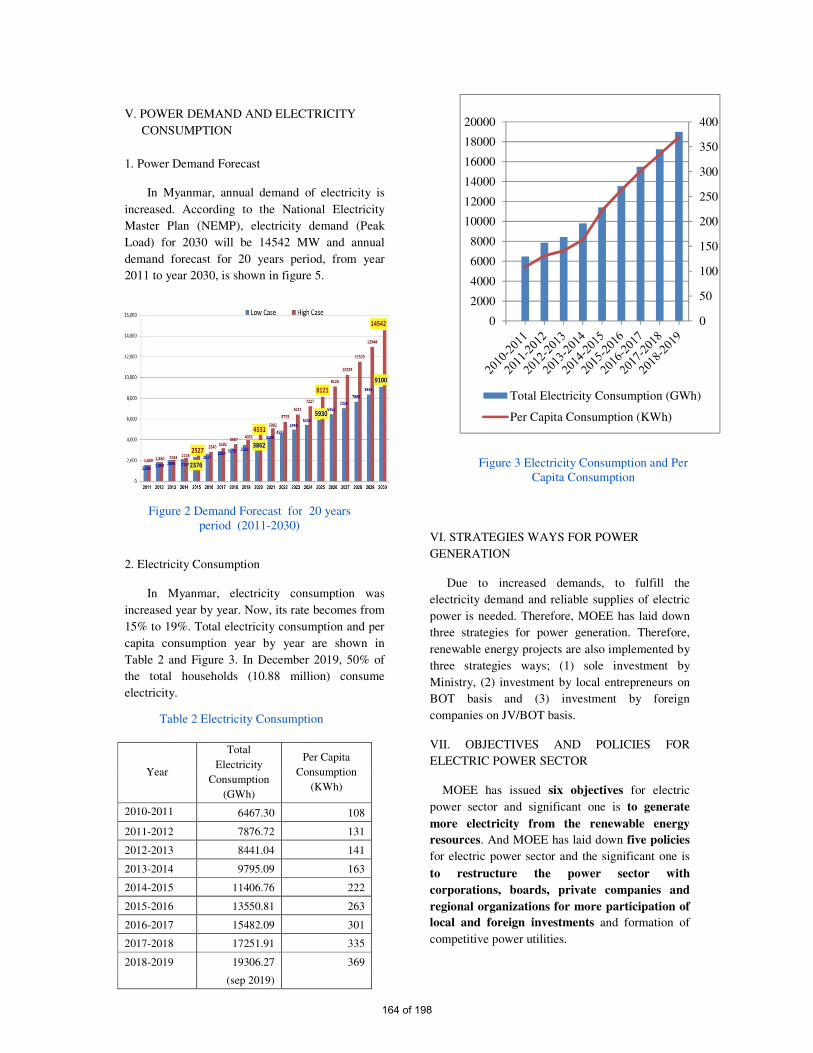
0

50

100

150

200

250

300

350

400

0

2000

4000

6000

8000

10000

12000

14000

16000

18000

20000

Total Electricity Consumption (GWh)

Per Capita Consumption (KWh)

V. POWER DEMAND AND ELECTRICITY

CONSUMPTION

1. Power Demand Forecast

In Myanmar, annual demand of electricity is

increased. According to the National Electricity

Master Plan (NEMP), electricity demand (Peak

Load) for 2030 will be 14542 MW and annual

demand forecast for 20 years period, from year

2011 to year 2030, is shown in figure 5.

2. Electricity Consumption

In Myanmar, electricity consumption was

increased year by year. Now, its rate becomes from

15% to 19%. Total electricity consumption and per

capita consumption year by year are shown in

Table 2 and Figure 3. In December 2019, 50% of

the total households (10.88 million) consume

electricity.

VI. STRATEGIES WAYS FOR POWER

GENERATION

Due to increased demands, to fulfill the

electricity demand and reliable supplies of electric

power is needed. Therefore, MOEE has laid down

three strategies for power generation. Therefore,

renewable energy projects are also implemented by

three strategies ways; (1) sole investment by

Ministry, (2) investment by local entrepreneurs on

BOT basis and (3) investment by foreign

companies on JV/BOT basis.

VII. OBJECTIVES AND POLICIES FOR

ELECTRIC POWER SECTOR

MOEE has issued six objectives for electric

power sector and significant one is to generate

more electricity from the renewable energy

resources. And MOEE has laid down five policies

for electric power sector and the significant one is

to restructure the power sector with

corporations, boards, private companies and

regional organizations for more participation of

local and foreign investments and formation of

competitive power utilities.

Year

Total

Electricity

Consumption

(GWh)

Per Capita

Consumption

(KWh)

2010-2011 6467.30 108

2011-2012 7876.72 131

2012-2013 8441.04 141

2013-2014 9795.09 163

2014-2015 11406.76 222

2015-2016 13550.81 263

2016-2017 15482.09 301

2017-2018 17251.91 335

2018-2019 19306.27 369

(sep 2019)

Figure 2 Demand Forecast for 20 years

period (2011-2030)

Table 2 Electricity Consumption

Figure 3 Electricity Consumption and Per

Capita Consumption

164 of 198

VIII. DEVELOPMENT OF RENEWABLE

ENERGY ( HYDROPOWER)

1. Hydropower Resources

Myanmar has abundant hydropower resources

and the country’s rivers can produce about 100,000

MW of hydroelectric power. Four major river

basins are shown in figure 4. 92 numbers, medium

and large scale hydropower projects, with the total

installed capacity of about 46101 MW in river

basin-wise are shown in Table 3.

Table 3 Hydropower Potential (River Basin-Wise)

2. Present Condition

At present, seven hydropower projects with the

total installed capacity of 1355.4 MW, to connect

the National Grid system are under

implementation. And, three hydropower projects

with the total installed capacity of 2655MW

[ Middle Yeywa-735 MW, Shweli(2)-520 MW

and Upper Thanlwin-1400MW] have been carried

out Feasibility Study. General information of the

projects under implementation is described in

Table 3. Total 28 numbers hydropower stations

with the total installed capacity of 3225 MW have

been connected to national grid and list of these

Hydropower Stations in National Grid System is

shown in Table 4. According to the future plan, 46

numbers hydropower projects with the total

installed capacity of 36943.4 MW are arranged to

be developed by local entrepreneurs and foreign

investors.

Table 4 under implementation projects

Project Name Location

(State/

Region)

Capacity

(MW)

Middle Paunglaung Naypyitaw

(Union Region)

152

Deedoke Mandalay 60

Thahtay Rakhing State 111

Shweli-3 Shan State(N) 671

Upper Yeywa Shan State(N) 280

Upper Kengtawn Shan State(S) 51

Upper

Baluchaung

Shan State(S) 30.4

Total 1355.4

Sr.

No

River Basin Number of

Hydropower

Projects

Installed

Capacity

(MW)

1 Ayeyarwaddy 34 21821

2 Chindwin 8 3015

3 Sittaung 11 1128

4 Thanlwin 21 17,641

5 Mekong 4 720

6 Others 14 1776

Total 92 46101

Figure 4 Four Major Rivers in Myanmar

Chindwin

Thanlwin

Sittaung

Ayeyarwaddy

165 of 198

Table 5 existing hydropower station (connecting to

National Grid)

X. DEVELOPMENT OF RENEWABLE

ENERGY ( SOLAR POWER)

1. Solar Power Condition

Myanmar can use solar power according to the

following situations:

• Myanmar is situated in the south

eastern part of the Asian continent.

• The cooler, dry season lasts from

November to April and the hotter, wet

season from May to October.

• Sunshine is plentiful during the dry

season average 7 to 10 hours a day.

• During the rainy season, the weather

is cloudier and daily sunshine

amounts are average only 3 to 4

hours a day.

2. Existing Solar Power Stations

Existing solar power stations in Myanmar are

shown in table 5.

Table 6 Existing Solar Power Stations

Name Location Installed

Capacity

(MW)

Remark

Minbu Magwe

Region

40 1st Stage of

Minbu 170 MW,

Thaton Mon State 28.6 To be connected

to Grid

Manaung Rakhine

State

3 Isolated

Total 71.6

Note: Off-grid Solar Home Systems excluded.

No Stations Installed

Capacity

(MW)

Annual

Genera

-tion

(Gwh)

Remark

1 Baluchaung(1) 28 200

Sole

Invest-

ment

( 2114

MW )

2 Baluchaung(2) 168 1190

3 Kinda 56 165

4 Sedawgyi 25 134

5 Zawgyi(1) 18 35

6 Zawgyi(2) 12 30

7 Zaungtu 20 76

8 Thaphanseik 30 117.2

9 Mone Chaung 75 330

10 Paunglaung 280 911

11 Yenwe 25 123

12 Kabaung 30 120

13 Keng Taung 54 377.6

14 Yeywa 790 3550

15 Shwekyin 75 262

16 Kun Chaung 60 190

17 Kyee Ohn

Kyee Wa

74 370

18 Nancho 40 152

19 Phyu Chaung 40 120

20 Upper Paung

laung

140 454

21 Myogyi 30 135.7

22 Myittha 40 170

23 Yazagyo 4 96

24 Thaukyegat(2) 120 604 BOT

(172

MW) 25 Baluchaung(3) 52 334

26 Shweli(1) 600 4022 JV

27 Dapein(1) 240 1065 ( 939

MW)

28 Chipwe Nge 99 433

Total

Installed

Capacity

3225

166 of 198

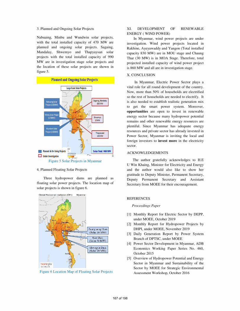
3. Planned and Ongoing Solar Projects

Nabuaing, Minbu and Wundwin solar projects,

with the total installed capacity of 470 MW are

planned and ongoing solar projects. Sagaing,

Mandalay, Shwemyo and Thapyaysan solar

projects with the total installed capacity of 990

MW are in investigation stage solar projects and

the location of these solar projects are shown in

figure 5.

Figure 5 Solar Projects in Myanmar

4. Planned Floating Solar Projects

Three hydropower dams are planned as

floating solar power projects. The location map of

solar projects is shown in figure 6.

XI. DEVELOPMENT OF RENEWABLE

ENERGY ( WIND POWER)

In Myanmar, wind power projects are under

investigation. Wind power projects located in

Rakhine, Ayeyawaddy and Yangon (Total installed

capacity 830 MW) are in MOU stage and Chaung

Thar (30 MW) is in MOA Stage. Therefore, total

projected installed capacity of wind power project

is 860 MW and all are in investigation stage.

X. CONCLUSION

In Myanmar, Electric Power Sector plays a

vital role for all round development of the country.

Now, more than 50% of households are electrified

so the rest of households are needed to electrify. It

is also needed to establish realistic generation mix

to get the smart power system. Moreover,

opportunities are open to invest in renewable

energy sector because many hydropower potential

remains and other renewable energy resources are

plentiful. Since Myanmar has adequate energy

resources and private sector has already invested in

Power Sector, Myanmar is inviting the local and

foreign investors to invest more in the electricity

sector.

ACKNOWLEDGEMENTS

The author gratefully acknowledges to H.E

U Win Khaing, Minister for Electricity and Energy

and the author would also like to show her

gratitude to Deputy Minister, Permanent Secretary,

Deputy Permanent Secretary and Assistant

Secretary from MOEE for their encouragement.

REFERENCES

Proceedings Paper

[1] Monthly Report for Electric Sector by DEPP,

under MOEE, October 2019

[2] Monthly Report for Hydropower Projects by

DHPI, under MOEE, November 2019

[3] Daily Generation Report by Power System

Branch of DPTSC, under MOEE

[4] Power Sector Development in Myanmar, ADB

Economics Working Paper Series No. 460,

October 2015

[5] Overview of Hydropower Potential and Energy

Sector in Myanmar and Sustainability of the

Sector by MOEE for Strategic Environmental

Assessment Workshop, October 2016

Figure 6 Location Map of Floating Solar Projects

167 of 198

Transition of University to Prosumer Consortium Energy Model

Min Set Aung 2, Kaung Si Thu 1, Weerakorn Ongsakul 1, and Nimal Madhu Manjiparambil 1,*

1 Department of Energy, Environment and Climate Change,

School of Environment Resources and Development (SERD)

Asian Institute of Technology, Pathum Thani, 12120, Thailand

2 Department of Information and Communication Technologies,

School of Engineering and Technology (SET)

Asian Institute of Technology, Pathum Thani, 12120, Thailand


Abstract — The conventional electricity grid

system has many critical issues, which could lead

to power instability, blackout, and many other

issues. One main perspective is to consume the

relative amount of distributed renewable energy

in the adaptation system. Prosumer Consortium

Model in a small community can be one of the

solutions to reduce the price of electricity, increase

efficiency and provide a better electronification

for University, moreover, to solve the frequent

blackout of electricity at university level in

developing countries. It can be the learning

opportunity for the researchers as well as the

complementary benefit for the consumers inside

university’s grid.

Keywords: Distributed energy, Energy trading,

Prosumer consortium model, Renewable energy

source, University grid.

I. INTRODUCTION

The increased of greenhouse gas emission and

constantly high demand for energy encourage the

mechanism of electricity generation to increase the

production of green energy and high efficiency.

The factors mainly cause the usage of renewable

energy production with distributed generations

(DG) through the macro/micro power grid. The

current electricity system does not have the ability

to maintain with DG as the main energy source,

thus, only a backup or supplementary source. The

key to play the prosumer consortium market model

in the grid system is the support of distributed

energy resources as in macro or microgrid, which

can bring the energy balance in the grid. This

implementation of prosumer consortium energy

model allows the benefit to the local customers

which allows from arranging dispatchable load at

peak power consumption, reduce the load on

distribution and transmission system.

The model is being conferred in the experimental

studies in which many pilot projects are running in

communities, nonetheless, an instant

implementation can cause the current system to a

revolution of operation, control and storage

technology. The market is established on the

supply and demand of the electricity especially

volatile during peak hours. The comprising features

of a university can be stated as a community grid.

The model grid promotes the incorporation at the

level of consumption of renewable energy sources

(RES) and energy storage systems (ESS) targeting

to increase power quality, reliability and

performance.

II. CHARACTERISTIC OF TRADING MODEL

1. Integration of ICT in the market model

The characteristic of the model has to be changed

from a unidirectional line to a bidirectional power

exchange, as well as ICT infrastructure to transfer

the data between customer nodes. The prosumer

consortium model comprises DERs such as micro-

wind generator, solar generator, biomass, EV

station, different types of ESS and fuel cells. The

168 of 198

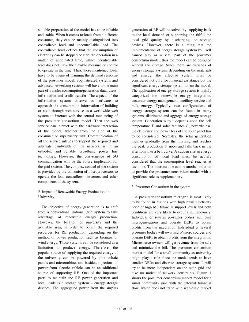
suitable preparation of the model has to be reliable

and stable. When it comes to loads from a different

consumer, they can be mainly distinguished into

controllable load and uncontrollable load. The

controllable load defines that the consumption of

electricity can be stopped or start the operation in a

matter of anticipated time, while incontrollable

load does not have the flexible measure or control

to operate in the time. Thus, these mentioned loads

have to be aware of planning the demand response

of the prosumer model. Sophisticated systems and

advanced networking systems will have to the main

part of transfer consumption/generation data, users’

information and credit transfer. The aspects of the

information system observe as software to

approach the consumption information of building

or node through web service as a worldwide web

system to interact with the central monitoring of

the prosumer consortium model. Then the web

service can interact with the hardware interaction

of the model, whether from the side of the

consumer or supervisory unit. Communication of

all the service intends to support the required and

adequate bandwidth of the network as in an

orthodox and reliable broadband power line

technology. However, the convergence of 5G

communication will be the future implication for

the grid system. The complex control of the system

is provided by the utilization of microprocessors to

operate the load controllers, inverters and other

components of the system.

2. Impact of Renewable Energy Production in

University

The objective of energy generation is to shift

from a conventional national grid system to take

advantage of renewable energy production.

However, the location of university and the

available area, in order to obtain the required

resources for RE production, depending on the

method of power production such as biomass or

wind energy. Those systems can be considered as a

limitation to produce energy. Therefore, the

popular source of supplying the required energy of

the university can be powered by photovoltaic

panels and microturbine, and besides, injections of

power from electric vehicle can be an additional

source of supporting RE. One of the important

parts to maintain the RE power generation and

local loads is a storage system – energy storage

devices. The aggregated power from the surplus

generation of RE will be solved by supplying back

to the local demand or supporting the fulfill the

local grid quality by discharging the storage

devices. However, there is a thing that the

implementation of energy storage system by itself

cannot play as a vital part of the prosumer

consortium model, thus the model can be designed

without the storage. Since there are varieties of

energy storage systems depending on the materials

and energy, the effective system must be

considered not only for financial assistance but the

significant energy storage system to run the model.

The application of energy storage system is mainly

categorized into renewable energy integration,

customer energy management, ancillary service and

bulk energy. Typically, two configurations of

energy storage system can be found in many

systems, distributed and aggregated energy storage

system. Generation output depends upon the cell

temperature and solar radiance , nevertheless,

the efficiency and power loss of the solar panel has

to be considered. Normally, the solar generation

inclines gradually from the morning and reaches

the peak production at noon and falls back in the

afternoon like a bell curve. A sudden rise in energy

consumption of local load must be acutely

considered that the consumption level reaches at

less time. The microturbine can be another solution

to provide the prosumer consortium model with a

significant role as supplementary.

3. Prosumer Consortium in the system

A prosumer consortium microgrid is most likely

to be found in regions with high retail electricity

price or high MS financial support levels and both

conditions are very likely to occur simultaneously.

Individual or several prosumer bodies will own

microgenerations and operate DERs to obtain

profits from the integration. Individual or several

prosumer bodies will own micro/macro sources and

operate DERs to obtain profits from the integration.

Microsource owners will get revenue from the sale

and minimize the bill. The prosumer consortium

market model for a small community as university

might play a role since the model tends to have

smaller DERs and discrete storage system. It will

try to be more independent on the main grid and

take no notice of network constraints. Figure 1

shows the prosumer consortium market model for a

small community grid with the internal financial

flow, which does not trade with wholesale market

169 of 198

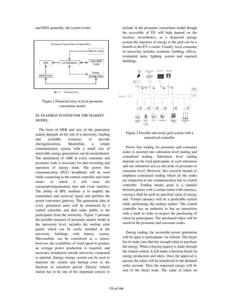
and DSO, generally, the system works.

Figure 1 Financial entry in local prosumer

consortium model.

III. FEASIBLE SYSTEM FOR THE MARKET

MODEL

The form of DER and size of the generation

mainly depends on the size of a university, funding

and available resources to provide

microgenerations. Meanwhile, a simple

communication system with a small size of

renewable energy generations can be premeditated.

The installation of AMI at every consumer and

prosumer node is necessary for data recording and

operation of energy trade. The power line

communication (PLC) broadband will be used

while connecting to the central controller and smart

meter, in which it will store the

consumption/generation data and event statistics.

The ability of BPL modems is to amplify the

transmitted and received signal and perform the

power converters gateway. The generation data of

every generation units will be monitored by a

central controller and thus make public to the

participants from the university. Figure 2 presents

the possible structure of prosumer market model at

the university level, includes the rooftop solar

panels which can be easily installed at the

university buildings with battery system.

Microturbine can be considered as a source,

however, the availability of wind speed to produce

an average power production is required, and

necessary installation outside university compound

is optional. Energy storage system can be used to

maintain the system and backup even in the

blackout or transition period. Electric vehicle

station has to be one of the important sources to

include in the prosumer consortium model though

the accessible of EV will high depend on the

location, nevertheless, as a dispersed storage

system the injection of energy to the grid can be a

benefit to the EV’s owner. Usually, local consumer

of university includes academic building, offices,

residential units, lighting system and outreach

buildings.

Figure 2 Feasible university grid system with a

centralized controller.

Power line trading for prosumer and consumer

nodes is assorted into substation level trading and

centralized trading. Substation level trading

depends on the total participants at each substation

and one substation acts as one node of prosumer or

consumer level. However, this research intends to

emphasis centralized trading which all the nodes

are connected at one communication line to central

controller. Trading means good is a transfer

between parties with a certain return with currency,

currency shall be used on specified value of energy

unit. Virtual currency will be a preferable system

while performing the trading market. The central

controller has an authority to has an interaction

with a bank in order to inspect the purchasing of

token by participants. The purchased token will be

stored in the prosumer and consumer nodes.

During trading, the accessible power generation

will be open to participants via website. The buyer

has to make sure that has enough token to purchase

the energy. When a buying request is made through

the central control, it will make a decision based on

energy production and token. Once the approval is

passed, the token will be transferred to the destined

seller account. Then the requested energy will be

sent to the buyer node. The value of token on

170 of 198

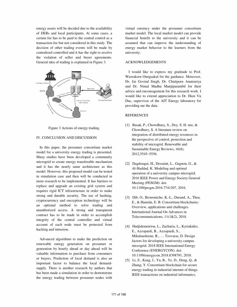
energy assets will be decided due to the availability

of DERs and local participants. At some cases, a

certain fee has to be paid to the central control as a

transaction fee but not considered in this study. The

decision of other trading events will be made by

centralized controlled and it has the right to resolve

the violation of seller and buyer agreements.

General idea of trading is explained in Figure 3.

Figure 3 Actions of energy trading.

IV. CONCLUSION AND DISCUSSION

In this paper, the prosumer consortium market

model for a university energy trading is presented.

Many studies have been developed a community

microgrid to create energy transferable mechanism

and it has the nearly same architecture as this

model. However, this proposed model can be tested

in simulation case and then will be conducted in

more research to be implemented. It has barriers to

replace and upgrade an existing grid system and

requires rigid ICT infrastructure in order to make

strong and durable security. The use of hashing,

cryptocurrency and encryption technology will be

an optional method to solve trading and

unauthorized access. A strong and transparent

contract has to be made in order to accomplish

integrity of the central controller and virtual

account of each node must be protected from

hacking and intrusion.

Advanced algorithms to make the prediction on

renewable energy generation on prosumer or

generation by hourly ahead or day ahead will be

valuable information to purchase from consumers

or buyers. Prediction of local demand is also an

important factor to balance the local demand-

supply. There is another research by authors that

has been made a simulation in order to demonstrate

the energy trading between prosumer nodes with

virtual currency under the prosumer consortium

market model. The local market model can provide

financial benefit to the university and it can be

assumed that can improve the understanding of

energy market behavior to the learners from the

university.

ACKNOWLEDGEMENTS

I would like to express my gratitude to Prof.

Weerakorn Onngsakul for the guidance. Moreover,

Dr. Jai Govind Singh, Dr. Chutiporn Anutrariya

and Dr. Nimal Madhu Manjiparambil for their

advice and encouragement for this research work. I

would like to extend appreciation to Dr. Hien Vu

Duc, supervisor of the AIT Energy laboratory for

providing me the data.

REFERENCES

[1] Basak, P., Chowdhury, S., Dey, S. H. nee, &

Chowdhury, S. A literature review on

integration of distributed energy resources in

the perspective of control, protection and

stability of microgrid. Renewable and

Sustainable Energy Reviews, 16(8),

2012,5545–5556.

[2] Dagdougui, H., Dessaint, L., Gagnon, G., &

Al-Haddad, K. Modeling and optimal

operation of a university campus microgrid.

2016 IEEE Power and Energy Society General

Meeting (PESGM). doi:

10.1109/pesgm.2016.7741207, 2016.

[3] Dib, O., Brousmiche, K.-L., Durand, A., Thea,

E., & Hamida, E. B. Consortium blockchains:

Overview, applications and challenges.

International Journal On Advances in

Telecommunications, 11(1&2), 2018.

[4] Hadjidemetriou, L., Zacharia, L., Kyriakides,

E., Azzopardi, B., Azzopardi, S.,

Mikalauskiene, R., … Tzovaras, D. Design

factors for developing a university campus

microgrid. 2018 IEEE International Energy

Conference (ENERGYCON). doi:

10.1109/energycon.2018.8398791, 2018.

[5] Li, Z., Kang, J., Yu, R., Ye, D., Deng, Q., &

Zhang, Y. Consortium blockchain for secure

energy trading in industrial internet of things.

IEEE transactions on industrial informatics,

171 of 198

14(8), 2017,3690–3700.

[6] Oh, S., Kim, M., Park, Y., Roh, G., & Lee, C.

Implementation of blockchain based energy

trading system. Asia Pacific Journal of

Innovation and Entrepreneurship, 11(3),

2017,322–334.

[7] Soshinskaya, M., Crijns-Graus, W. H.,

Guerrero, J. M., & Vasquez, J. C. Microgrids:

Experiences, barriers and success factors.

Renewable and Sustainable Energy Reviews,

40, 2014,659–672.

[8] Tao, L., Schwaegerl, C., Narayanan, S., &

Zhang, J. H. From laboratory microgrid to real

markets—challenges and opportunities. In 8th

international conference on power electronics-

ecce asia , 2011,pp. 264–271.

[9] Available online at

https://microgridknowledge.com/energy-

storage-microgrid/

172 of 198

THE OPTIMAL COST OF AN OUTPATIENT DEPARTMENT

BY USING SINGLE AND MULTIPLE SERVER SYSTEM

Dr. Win Lei Lei Aung

Associate Professor

Faculty of Computing, University of Information Technology, Hlaing , Yangon

[email protected]

Abstract— Hospital management tradeoffs always

exist between the costs in providing better service

and waiting time of patients in any hospital. The

objective of this study was to investigate whether

increasing the cost for better service decreases the

cost of patients waiting time or not, by using the

technique of single and multiple servers which is

based on the theory of Markovian queuing system.

For this study, four weeks data has been taken from

a public hospital. The results shows that as the

service capacity level of doctors at the hospital

increases from three to four servers then minimum

total costs (include waiting and service costs) and

the waiting time of patients as well as

overutilization of doctors can be reduced. This paper

also suggests that increasing the service units up to

four servers will achieve lower cost as against two

or more service units.

Keywords: Outpatient Department (OPD),

Performance measures, the service cost,

the waiting cost

I. INTRODUCTION

Outpatient department (OPD) is one of the most

important parts of hospital management and is

visited by large section of community. This is the

first point of contact between patient and hospital

staff. The problems faced by the patients in that

department are overcrowding, delay in consultation,

lack of proper guidance etc. which lead to patients

becoming dissatisfied. Every patient in each hospital

is in search of hassle free and quick services in this

fast growing world which is only possible with

optimum utility of the resources through

multitasking in a single server system in the OPD

for better services. As patients flow increases

because of that demands for hospitals and, better

and quick services increases in [1] and [2].

In any hospital, patients come to the Outpatient

Department without prior appointment and patients

have to wait to receive medical service that may be

waiting before, during or after being served.

Generally queues are formed when the demand for a

service exceeds its supply. For many patients or

customers, waiting in lines or queuing is annoying

or negative experience. A few of the factors that are

responsible for long waiting lines or delays in

providing service are: lack of passion and

commitment to work on the part of the hospital

staff, overloading of available doctors, doctors

attending to patients in more than one clinic etc.

A good patient flow means that the patient

queuing is minimized while a poor patient flow

means patients suffer considerable queuing delays

[7]. Considering these points mentioned above, our

present study proposes to evaluate the patients

waiting problems in terms of the performance

measure and also to determine the level of service

that minimizes the total cost of the expected cost of

service and the expected cost of waiting.

II. MATERIALS AND METHODS

The study area is Yangon, which is a fast

developing city in the MYANMAR. In every

hospital, Yangon is actually facing a big issue of

patient waiting time problem at every day. There is

heavy inflow of sick patients in this region from

neighboring rural areas or from smaller towns

because of the availability of advanced health

facilities. For our study we selected one of the

leading public hospitals of the region, North

Oaklapa General Hospital in Yangon where it was

observed that there was a heavy flow of patients

thought the week. Data was collected over a period

of four Weeks from 15.10.2019 to 13.11.2019 as

shown in Table 1. Table 1 shows the data collected

for one week. These data represents the number of

patients at OPD. Data was collected from the

Patients who visited Out- Patient Department during

day shift by using direct observation method.

In this observational study, the traffic intensity

of the out patients at registration counters such as

the arrival rate (λ), service rate (μ) and number of

173 of 198


servers was measured at hourly interval. The

standard simple queuing model assumes that

1. Arrivals have the Poisson distribution

2. Service times have the exponential distribution

3. Arrivals and service times are all independent.

(Independence means, for example, that: arrivals

don't come in groups, and the server does not work

faster when the line is longer.)

Table 1 measured data for one week

Time

(hr)

days

9:00

AM

to

10:0

0AM

10:00

AM

to

11:00

AM

11:0

0AM

to

12:0

0

AM

1:00

PM

to

2:00

PM

2:00

PM

to

3:00

PM

3:00P

M to

4:00P

M

15.10.1

9

60 70 80 65 50 45

16.10..1

9

43 63 70 100 45 55

17.10.1

9

33 56 50 120 55 65

18.10.1

9

23 88 45 80 65 77

19.10.1

9

12 102 35 90 78 78

20.10.1

9.

9 133 25 105 73 82

21.10.1

9

8 117 40 120 88 63

In this M/M/m queuing model, the 1st M

indicates the inter-arrival time distribution arrivals

follows Poisson distribution with parameter λ, and

2nd M indicates service time distribution [5]. Here, it

is exponential distribution with parameter μ and 3rd

m indicates number of servers available those are in

parallel. The system has multiple servers and uses

the FIFO service discipline. The waiting line is of

infinite size. In the case M/M/1 queuing model,

there is only one single server. It means that the

system can process a single request at a time. But in

this M/M/m queuing model, there are m numbers of

servers that are connected in parallel [5]. Queuing

model enable finding an appropriate balance

between the cost of service and the amount of

waiting. The ultimate goal of queuing analysis is to

minimize two costs, which is service capacity cost

and customer waiting cost.

These are analyzed for simultaneous efficiency

in patient satisfaction and cost minimization through

the use of a single server M/M/1(∞: FCFS) and

multi-server queuing models, which are then

compared for a number of queue performances such

as; the average time each patient spends in the queue

and in the system, average number of patients in the

queue and in the system and the probability of the

system being idle. In M/M/1(∞: FCFS) queuing

model, the arrival of patients in a fixed time interval

belongs to Poisson probability distribution at an

average rate of λ patients per unit time. It is also

assumed that the service time was exponentially

distributed, with an average rate of μ patients per

unit of time. The hypothetical structure of Single-

server queuing model is shown in Figure 1.The

hypothetical structure of Multi-server queuing

system is as shown in Figure 2.

Figure 1 Single server queuing system.

The performance measures of single server system

Average server utilization factor in the system

Probability that no patient in the system

Average number of patients in the system

Average time a patient spends in the system

Average number of patients in the queue

Average time a patient spends in the queue

For the multi-server queuing model, the M/M/c

(∞: FCFS) model has been adopted. The basic

hypothetical structure of multi -server queuing

model is shown in Figure 2.

Figure 2 Multi server queuing system.

174 of 198

The performance measures of multi-server system

Average server utilization factor in the system

Probability that no patient in the system

[∑

]

Average number of patients in the queue

Average number of patients in the system

Average time a patient spends in the system

Average time a patient spends in the queue

In this queuing system, the arrival of patients is

assumed to follow a Poisson process, and service

times are assumed to have an exponential

distribution. Let the number of servers be c,

providing service independently of each other. It is

also assumed that the arriving patients form a single

queue and the one at the head of the waiting line

enters into service as soon as a server is free. No

server stays idle as long as there are patients to

serve. If there are n patients in the queuing system,

then two possibilities may arise:

Case.1: k ≤ c. In this case no patient has to wait for

service. However, (c-n) patients will be in

queue and the rate of servicing will be kμ.

Case.2: k >c. In this case, all the doctors will be

busy and the maximum number of patients ρ

will be (k-c) in the queue and the rate of

service will be cμ.

The Variables are analyzed by using the

performance measures of the Queuing Models

[M/M/1(∞: FCFS) and M/M/c (∞: FCFS)] as

presented in equation (1) to (12). There are (5 x 4

weeks) working days in a month used in this study

while the working hours per day are 24 hours for

casualty service and 5 hours for outpatient service.

Queuing models can be used to determine the

operating performance of a waiting-line system.

In the economic analysis of waiting lines, we

seek to use the information provided by the queuing

model to develop a cost model for the waiting line

under study. Then we can use the model to help the

hospital management to make a trade-off between

the increased costs of providing better service and

the decreased waiting time costs of patients derived

from providing that service. To determine the level

of service that minimizes the total cost of the

expected cost of service and the expected cost of

waiting, we utilize the cost analyzing model.

In cost model, we consider the cost of patient

time, both waiting time and servicing time, and the

cost of operating the system.

Let Cw= the waiting cost per unit per patient and

Cs = Cost of providing service per doctors per

unit of time

Therefore, the total cost per minute is

Total cost = CwLs +Cs c, where Ls is the average

number of patients in the system and c is the number

of servers/doctors.

III. RESULTS

Using equation (1) to equation (12), we get the

performance measures of single doctor system and

multi doctor system as shown in following Table 2

and Table 3. Table 2 shows the average server

utilization in the department, the probability of no

patient in the department, the average number of

patient in the outpatient department and the average

waiting time in this department.

Table 2 Summarized data ρ, P0, Ls and Ws for single

server and multi-server system

Docto

rs

Average

patients

Utilizatio

n in the

system

( ρ )

Probability

that there

are no

patient in

the system

(P0)

Average

number

of

patients

in the

system

(Ls)

Average

time a

patient

spends in

the

system

(Ws)

1 60% 0.40000 1.50000 0.50000

2 30% 0.53850 0.65935 0.11978

3 20% 0.54795 0.60616 0.20616

4 15% 0.54873 0.60062 0.20021

5 12% 0.54881 0.60006 0.20002

6 10% 0.54881 0.60001 0.20000

7 8.6% 0.54881 0.60000 0.20000

Figure 3 Utilization rate against the number of

doctor.

175 of 198

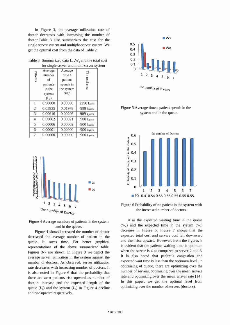
In Figure 3, the average utilization rate of

doctor decreases with increasing the number of

doctor.Table 3 also summarizes the cost for the

single server system and multiple-server system. We

get the optimal cost from the data of Table 2.

Table 3 Summarized data Lq ,Wq and the total cost

for single server and multi-server system

Patien

ts

Average

number

of

patients

in the

system

(Lq)

Average

time a

patient

spends in

the system

(Wq)

The to

tal cost

1 0.90000 0.30000 2250 kyats

2 0.05935 0.01978 989 kyats

3 0.00616 0.00206 909 kyats

4 0.00062 0.00021 900 kyats

5 0.00006 0.00002 900 kyats

6 0.00001 0.00000 900 kyats

7 0.00000 0.00000 900 kyats

Figure 4 Average numbers of patients in the system

and in the queue.

Figure 4 shows increased the number of doctor

decreased the average number of patient in the

queue. It saves time. For better graphical

representations of the above summarized table,

Figures 3-7 are shown. In Figure 3 we depict the

average server utilization in the system against the

number of doctors. As observed, server utilization

rate decreases with increasing number of doctors. It

is also noted in Figure 6 that the probability that

there are zero patients rise upward as number of

doctors increase and the expected length of the

queue (Lq) and the system (Ls) in Figure 4 decline

and rise upward respectively.

Figure 5 Average time a patient spends in the

system and in the queue.

Figure 6 Probability of no patient in the system with

the increased number of doctors.

Also the expected waiting time in the queue

(Wq) and the expected time in the system (Ws)

decrease in Figure 5. Figure 7 shows that the

expected total cost and service cost fall downward

and then rise upward. However, from the figures it

is evident that the patients waiting time is optimum

when the server is 4 as compared to server 2 and 3.

It is also noted that patient’s congestion and

expected wait time is less than the optimum level. In

optimizing of queue, there are optimizing over the

number of servers, optimizing over the mean service

rate and optimizing over the mean arrival rate [14].

In this paper, we get the optimal level from

optimizing over the number of servers (doctors).

00.10.20.30.40.50.60.70.80.9

11.11.21.31.41.5

1 2 3 4 5 6 7

Ls

Lq

1 2 3 4 5 6 7

Ws

Wq

0

0.1

0.2

0.3

0.4

0.5

0.6

1 2 3 4 5 6 7

P0 0.4 0.54 0.55 0.55 0.55 0.55 0.55

Pro

bab

ility

of

no

pat

ien

t in

th

e sy

stem

the number of Doctors

176 of 198

Figure 7 the optimal cost against the number of

the doctors.

IV. DISCUSSION

Table 2 shows that a 4-server system is better

than a single server, 2-server or 3-server system in

terms of the performance criteria used. For instance,

in terms of cost considerations, assume that the

waiting cost is 1500 kyats per patient, for 4-server

system records the lowest cost of 900 kyats

compared to a 2-server and 3-server system that

records 989kyats and 909 kyats respectively.These

costs included the entire cost done by the hospital.

The average time a patient spends in the system and

in the queue are 0.2 minutes and 0.00021 minutes

respectively for a 4-server system.

The probabilities of idleness are 30.0% and

20.0% respectively for 2 and 3 server systems

respectively. The average time a patient spends in

the queue and in the system for a single server

system is 0.3 minutes and 0.5 minutes respectively

while the system has 4.5 and 1.5 patients in the

queue and in the system respectively. The system is

likely to be idle for 0.4 minutes.

In [8], a survey comparing the performance of

a single channel with multi-channel queuing models

in achieving cost reduction and patient satisfaction

using a hospital study, it was concluded that the 3-

server system is better than a single server, 2-server

or 4-server system. The average time a patient

spends in the system and in the queue are 11

minutes and 1.79 minute.

However, another study revealed a positive

correlation between arrival rates of customers and

bank’s service rates where it was concluded that the

potential utilization of the banks service facility was

3.18% efficient and idle 68.2% of the time [9]. A

One week survey revealed that 59.2% of the 390

persons making withdrawals from their accounts

spent between 30 to 60 minutes while 7% spent

between 90 and 120 minutes [10]. Further it was

observed in another survey that although the mean

time spent was 53 minutes by customers, they prefer

to spend a maximum of 20 minutes only [11]. Their

study revealed worse service delays in urban

center’s (average of 64.32 minutes) compared to

(average of 22.2 minutes) in rural areas.

Moreover those customers spend between 55.27

to 64.56 minutes making withdrawal from their

accounts Efforts in this study are directed towards

application of queuing models in capacity planning

to reduce patient waiting time and total operating

costs [12].

V. Conclusion

The results of the analysis showed that that as

the service capacity level of doctors at the hospital

increases from three to four servers then minimum

total costs (include waiting and service costs) and

the waiting time of patients as well as

overutilization of doctors can be reduced. The study

also suggests that, to optimize the processing time

for the patients it is necessary to rationalize the

utilization of the servers for effective utilization of

human resource. Otherwise, the service units may be

increased to four to achieve better results at a lower

cost as against two or three service units. A single

server is not effective as much as compared to

multiple servers. Whereas, five servers eliminates

waiting cost but at a higher cost which is not

optimal too.

ACKNOWLEDMENTS

Firstly, I would like to thank Dr. Pyke Tin who

shares ideas and helpful suggestion. I am also

grateful to Dr. Swe Swe Kyaw , head of Faculty of

Computing , who motivates me to do this. And then,

I appreciate to my mother for her patient,

understanding and encouragement during my work

that has to successful finish. Finally, I am also

thankful for all my teachers and colleagues since my

childhood and I sincerely thank all concerned

persons of North Oaklapa General Hospital for their

help and cooperation during the data collection

177 of 198

process.

REFERENCES

[1] Srinivasan, A. V. (2000). Managing a Modern

Hospital, Response Books. A Division of Sage

Publishers India (P) Ltd., New Delhi, 53-69.

[2] Llewelyn, R. and H. M. C. Davies.(1996).

Macaulay Hospital Planning and Administration,

WHO, Geneva, 105-11.

[3] Hiller, S.F. and Lieberman, J. G., Introduction

to Operations Research, Boston: Mcgraw Hill,

Eight Edition.pp.834-838, 2005.

[4] Singh V., “Use of Queuing Models in Health

Care”, Department of Health Policy and

Management, University of Arkansas for

Medicals Sciences, 2007.

[5] Raj Jian, “The Art Of Computer Systems

Performance Analysis”, John Wily & Sons

Inc, computer press award winner, pp 592-604,

1992.

[6] Trivedi, Kishor S, “Probability and Statistics

with Reliability, Queuing and Computer

Application”, John Wiley & Sons Inc, 2016.

[7] Hall, W. R. (2006). Patient Flow: The New

Queuing Theory for Healthcare, OR/Ms, Today

2006.

[8] Brahma, P. K. An Appraisal of cost of queuing

in healthcare sector a case study of IMS and

SUM hospital, International Journal of

Multidisciplinary Research, Vol. 2(4).

[9] Oladapo. (1998). Relationship between Arrival

Rates of Customers and Bank’s Service Rates,

Seminar Paper Series, Obafemi Awolowo

University, Ile-Ife.

[10] Elegalam. (1978). Customer Retention Versus

Cost Reduction Technique, A Paper presented

at the Bankers forum held at Lagos.

[11] Baale, A. F. (2002). Managerial Applications of

Queuing Models in the Service Industry: A Int.

j. sci. footpr. Dhar et al. (2014) Case Study of

Afribank Nigeria Plc.,Ilorin Main Branch. A

Research Paper submitted to Business

Administration Department, University of

Ilorin, Ilorin.

[12] Juwah. Operational Problems and Customers’

Dissatisfaction, CBN Bullion, 1986.

[13] S Kalavathy, “Operations Research”,Vikas

Publishing House Pvt Ltd,pp411-440, 2000.

[14] Joseph G.Ecker and Michael Kupferschmid,

“Introduction to Operations Research”,John

Wily & Sons, Inc, pp 409-413, 2014.

178 of 198

Abstract— This paper is about the forecasting

techniques of Yathar Cho Industry Limited (YUM

YUM INSTANT NOODLE), Myanmar.

Forecasting is a technique that uses historical data

as inputs to make informed estimates that are

predictive in determining the direction of future

trends. Businesses utilize forecasting to determine

how to allocate their budgets or plan for

anticipated expenses for an upcoming period of

time. The main aim of this paper is to show the

forecasting techniques of Yum Yum noodle. The

forecasting techniques is shown on two ways. The

first way is the calculating of mean absolute

percent Error calculating using the two period

moving average method. The second way is the

calculating of mean absolute percent error using

exponential smoothing method.

Keywords— Yathar Cho Industry Limited, Two-

period moving average, Exponential Smoothing,

Mean Absolute Percentage Error

I. INTRODUCTION

A forecast is a statement about the future value of

a variable such as demand. That is, forecasts are

predictions about the future. The better those

predictions, the more informed decisions can be. Some

forecast are long range, covering several years or

more. It describes the elements of good forecasts, the

necessary steps in preparing a forecast, basic

forecasting techniques and how to monitor a forecast.

Two aspects of forecasts are important. One is the

expected level of demand; the other is the degree of

accuracy that can be assigned to a forecast (i.e., the

potential size of forecast error). The expected level of

demand can be a function of some structural variation,

such as a trend or seasonal variation Forecast accuracy

is a function of the ability of forecasters to correctly

model demand, random variation and sometimes

unforeseen events.

Forecasts are the basic for budgeting, planning

capacity, sales, production and inventory, personnel,

purchasing, and more. Forecasts play an important role

in the planning process because they enable managers

to anticipate the future so they can play accordingly.

II. CASE STUDY

A case study is made at Yathar Cho Industry

Limited (YUM YUM Instant Noodle), located at No

(197,198,199), 10th

Street, Yangon, Myanmar, which

manufactures three different types of products. They

are Original, Xcite and Premium. The machine can

produce approximately 6000 boxes for one small

production line and about 12000 boxes for large

production line. For a day, they can produce around

35000 bags depending upon customer demand. The

information and data are obtained from this factory for

this paper.

III. MANUFACTURING

A. Functionally of raw materials/ ingredients

The main ingredients for instant noodles are wheat

flour, salt or kansui (alkaline salt mixture of sodium

carbonate, potassium carbonate and sodium

phosphate), and water. Other ingredients like starch,

gums, emulsifiers, stabilizers, antioxidants, coloring

and flavoring agents are also added to improve the

texture and eating quality. Nowadays instant noodles

are also fortified with protein, minerals and vitamins to

improve their nutrition value.

Hsu Myat Tin#1 , Kyaw Lin Thet#2

#1Department of Business and Management, Chindwin TU International College, Yangon,11162,

Myanmar.

#2Department of Mechanical Engineering, Yangon Technological University, 11011,

Myanmar


Analysis of Forecasting Techniques of Instant Noodle Manufacturing

Company

179 of 198

B. Role of critical unit operations

Noodle processing typically comprises mixing

raw materials, resting the crumbly dough, sheeting the

dough into two dough sheets, compounding the sheets

into one, gradually the sheet into a specified thickness

and slitting into noodle strands. For instant noodle

preparation, strands are steamed and dehydrated by

drying or frying followed by cooling and packing with

the seasonings.

• Mixing: Ingredients other than flour are pre

dissolved in water, stored at 20-30 ºC while salt water

can be prepared separately. Wheat flour and water

along with other weighted ingredients are mixed first

at high speed and then a low speed, giving a total time

of 15-25 minutes in industries. The mixing time,

however also depends on the type of mixer used.

Mixing is also influenced by the quality of flour,

volume of water added, presence or absence and

amount of certain ingredients (especially salt and

alkaline salt) and temperature and humidity of

processing environment. Mixing is usually followed

by dough resting. Resting improves processing

properties and facilitates gluten formation during

sheeting.

• Sheeting: After mixing, the crumbly dough is

compressto form continuous dough sheet, which is

folded or compounded and passed through subsequent

rolls. The sheeting process is intended to achieve a

smooth dough sheet with desired thickness, and a

continuous and uniform gluten matrix in dough sheet.

Dough sheet are rest to allow gluten structure

relaxation or mellow the gluten and make it more

extensible by slow passage or zigzag conveyor in

automobile plants.

• Cutting / slitting and Waving: The dough

sheet is cut into noodle strands of desired width with a

slitter. The width and shape of noodle strands are

determined by cutting rolls. The speed differential

between noodle feeding and net travelling result in a

unique waving of noodle strands. Noodle strands are

cut into a desirable length by a cutter.

• Steaming and Moulding: The cut and way

noodle strands are conveyed to a steam chamber to

cook them by exposing to a temperature of 100ºC for

one-five minutes. The degree of cooking during

steaming is critical and depends on the original

moisture content of noodle; amount, pressure and

temperature of steam and steaming time. Under

steamed noodles will have a hard core and will be

difficult to cook properly, whereas over steamed

noodles are soft and sticky. Steaming is a key process

in the manufacture of instant noodles. The cut noodles

are placed in moulder of square, round, bowl, or cup

shape, depending on the desired product shape before

moving to the fryer or drier.

• Frying / Drying: After steaming and

molding, noodle blocks are fed into frying baskets,

which are mounted on the traveling chain of a tunnel

fryer. The baskets filled with noodle blocks are

immersed in hot oil for deep frying. Noodles drying

can also be done by hot air to produce instant dried

noodles. Frying is the preferred method of drying as

nonfried instant noodles require a longer cooking

time.

• Packaging: Frying or drying is followed by

cooling the product to room temperature to avoid

rapid oxidation and other changes. The cooled

noodles are packed into a bag along with a soup base

sachet. While for the cup noodles, powdered soup

base is sprinkled over the noodles and sealed with

shrink film. Seasonings and dehydrated vegetables are

included in soup base. Higher fat content makes the

noodles susceptible to oxidative changes and

development of rancid flavour. Thus, proper

packaging plays important role in extending the shelf

life of the product. The packaging material used for

noodles are polypropylene or polyethylene film for

bag noodles and polyester for cup noodles.

Figure 1. New product of YUM YUM instant noodle

180 of 198

Figure 2. Wheat Flour Brands

IV. RESEARCH METHODOLOG Y

Data sheets were gathered for raw materials for the

duration of three months. These data had been taken

by the department of planning and a total of various

wheat flour brands are checked from the production

department. There are many different kinds of

forecasting methods and inventory formulas in

operation planning. For forecasting, the two most

important factors are cost and accuracy. Two-period

moving average and exponential smoothing are used to

make forecast and forecast accuracy. For inventory

management, the goal in ordering is to place an order

when the amount on hand is sufficient to satisfy

demand during the time it takes to receive that order

(i.e., lead time).

A. Forecasting Methods

Demand forecasting is an important component of

yield management, which relates to the percentage of

capacity being used. There are two uses for forecasts.

One is to help managers plan the system and the other

is to help the use of the system. Forecasting techniques

based on time series are made on the assumption that

future values of the series can be estimated from past

values. Three techniques for averaging are

Moving average

= MA =

∑

=

⋯

(1)

Weighted moving average

= …

(2)

Exponential Smoothing

–

(3)

Forecast accuracy is significant factor when

deciding among forecast alternatives. Accuracy is

based on the historical error performance of forecast.

Three commonly used measures for summarizing

historical errors are the mean absolute deviation

(MAD), the mean squared error (MSE), and the mean

absolute percent error (MAPE). Difference between

these measures is that MAD weights all errors evenly,

MSD weights error according to their squared values,

and MAPE weights according to relative error.

Forecast error is the difference between the value that

occurs and the value that was predicted for a given

time period. Hence, Error = Actual-Forecast

MAD ∑| !"#$% –&'()!$*"|

or MAD

∑ |-|

(4)

MSE ∑ !"#$% – &'()!$*"

or MSE

∑ |-|

(5)

MAPE ∑1

|2|

3456789::;

(6)

Where,

= Forecast for time period t

< = n period moving average

= Actual value in period t – 1

n = Number of periods (data points) in moving

average

= = Weight for the period t

== Weight for period t – 1

= Actual value in period t

181 of 198

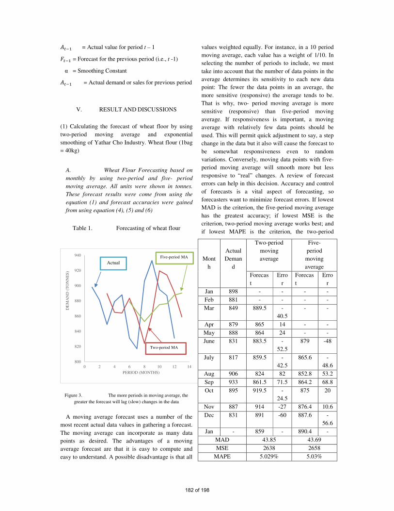
= Actual value for period t – 1

= Forecast for the previous period (i.e., t -1)

α = Smoothing Constant

= Actual demand or sales for previous period

V. RESULT AND DISCUSSIONS

(1) Calculating the forecast of wheat floor by using

two-period moving average and exponential

smoothing of Yathar Cho Industry. Wheat flour (1bag

= 40kg)

A. Wheat Flour Forecasting based on

monthly by using two-period and five- period

moving average. All units were shown in tonnes.

These forecast results were come from using the

equation (1) and forecast accuracies were gained

from using equation (4), (5) and (6)

Table 1. Forecasting of wheat flour

Figure 3. The more periods in moving average, the

greater the forecast will lag (slow) changes in the data

A moving average forecast uses a number of the

most recent actual data values in gathering a forecast.

The moving average can incorporate as many data

points as desired. The advantages of a moving

average forecast are that it is easy to compute and

easy to understand. A possible disadvantage is that all

values weighted equally. For instance, in a 10 period

moving average, each value has a weight of 1/10. In

selecting the number of periods to include, we must

take into account that the number of data points in the

average determines its sensitivity to each new data

point: The fewer the data points in an average, the

more sensitive (responsive) the average tends to be.

That is why, two- period moving average is more

sensitive (responsive) than five-period moving

average. If responsiveness is important, a moving

average with relatively few data points should be

used. This will permit quick adjustment to say, a step

change in the data but it also will cause the forecast to

be somewhat responsiveness even to random

variations. Conversely, moving data points with five-

period moving average will smooth more but less

responsive to “real” changes. A review of forecast

errors can help in this decision. Accuracy and control

of forecasts is a vital aspect of forecasting, so

forecasters want to minimize forecast errors. If lowest

MAD is the criterion, the five-period moving average

has the greatest accuracy; if lowest MSE is the

criterion, two-period moving average works best; and

if lowest MAPE is the criterion, the two-period

800

820

840

860

880

900

920

940

0 2 4 6 8 10 12 14

DE

MA

ND

(T

ON

NE

S)

PERIOD (MONTHS)

Two-period MA

Five-period MA

Mont

h

Actual

Deman

d

Two-period

moving

average

Five-

period

moving

average

Forecas

t

Erro

r

Forecas

t

Erro

r

Jan 898 - - - -

Feb 881 - - - -

Mar 849 889.5 -

40.5

- -

Apr 879 865 14 - -

May 888 864 24 - -

June 831 883.5 -

52.5

879 -48

July 817 859.5 -

42.5

865.6 -

48.6

Aug 906 824 82 852.8 53.2

Sep 933 861.5 71.5 864.2 68.8

Oct 895 919.5 -

24.5

875 20

Nov 887 914 -27 876.4 10.6

Dec 831 891 -60 887.6 -

56.6

Jan - 859 - 890.4 -

MAD 43.85 43.69

MSE 2638 2658

MAPE 5.029% 5.03%

Actual

182 of 198

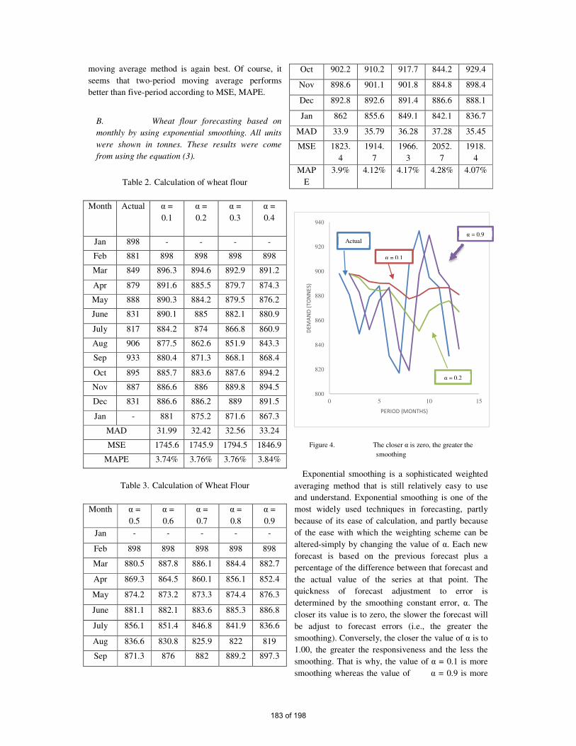
moving average method is again best. Of course, it

seems that two-period moving average performs

better than five-period according to MSE, MAPE.

B. Wheat flour forecasting based on

monthly by using exponential smoothing. All units

were shown in tonnes. These results were come

from using the equation (3).

Table 2. Calculation of wheat flour

Month Actual α =

0.1

α =

0.2

α =

0.3

α =

0.4

Jan 898 - - - -

Feb 881 898 898 898 898

Mar 849 896.3 894.6 892.9 891.2

Apr 879 891.6 885.5 879.7 874.3

May 888 890.3 884.2 879.5 876.2

June 831 890.1 885 882.1 880.9

July 817 884.2 874 866.8 860.9

Aug 906 877.5 862.6 851.9 843.3

Sep 933 880.4 871.3 868.1 868.4

Oct 895 885.7 883.6 887.6 894.2

Nov 887 886.6 886 889.8 894.5

Dec 831 886.6 886.2 889 891.5

Jan - 881 875.2 871.6 867.3

MAD 31.99 32.42 32.56 33.24

MSE 1745.6 1745.9 1794.5 1846.9

MAPE 3.74% 3.76% 3.76% 3.84%

Table 3. Calculation of Wheat Flour

Month α =

0.5

α =

0.6

α =

0.7

α =

0.8

α =

0.9

Jan - - - - -

Feb 898 898 898 898 898

Mar 880.5 887.8 886.1 884.4 882.7

Apr 869.3 864.5 860.1 856.1 852.4

May 874.2 873.2 873.3 874.4 876.3

June 881.1 882.1 883.6 885.3 886.8

July 856.1 851.4 846.8 841.9 836.6

Aug 836.6 830.8 825.9 822 819

Sep 871.3 876 882 889.2 897.3

Oct 902.2 910.2 917.7 844.2 929.4

Nov 898.6 901.1 901.8 884.8 898.4

Dec 892.8 892.6 891.4 886.6 888.1

Jan 862 855.6 849.1 842.1 836.7

MAD 33.9 35.79 36.28 37.28 35.45

MSE 1823.

4

1914.

7

1966.

3

2052.

7

1918.

4

MAP

E

3.9% 4.12% 4.17% 4.28% 4.07%

Figure 4. The closer α is zero, the greater the

smoothing

Exponential smoothing is a sophisticated weighted

averaging method that is still relatively easy to use

and understand. Exponential smoothing is one of the

most widely used techniques in forecasting, partly

because of its ease of calculation, and partly because

of the ease with which the weighting scheme can be

altered-simply by changing the value of α. Each new

forecast is based on the previous forecast plus a

percentage of the difference between that forecast and

the actual value of the series at that point. The

quickness of forecast adjustment to error is

determined by the smoothing constant error, α. The

closer its value is to zero, the slower the forecast will

be adjust to forecast errors (i.e., the greater the

smoothing). Conversely, the closer the value of α is to

1.00, the greater the responsiveness and the less the

smoothing. That is why, the value of α = 0.1 is more

smoothing whereas the value of α = 0.9 is more

800

820

840

860

880

900

920

940

0 5 10 15

DE

MA

ND

(T

ON

NE

S)

PERIOD (MONTHS)

α = 0.2

α = 0.9

α = 0.1

Actual

183 of 198

responsiveness and similar to actual trend. This is

illustrated in figure 4. The goal is to select a

smoothing constant that balances the benefits of

smoothing random variations with the benefits of

responding to real changes if and when they occur.

Commonly used values of α range from .05 to .50.

Low values of α are used when the underlying

average tends to be stable; higher values are used

when the underlying average is susceptible to change.

Selecting a smoothing constant is basically a matter of

judgement or trial and error, using forecast errors to

guide the decision. From all of these data in

exponential smoothing, α = 0.1 is the greatest

accuracy because of the lowest MAD, MSE and

MAPE.

C. Comparison of forecast accuracy of wheat

flour

Table 4. Comparison of forecast accuracy

Methods

Two-

period

moving

average

Exponential Smoothing

α =

0.1

α =

0.2

α =

0.3

Mean

Absolute

Deviation

(MAD)

43.85

31.99

32.42

32.56

Mean Squared

Error

(MSE)

2638

1745.6

1745.9

1794.5

Mean

Absolute

Percent Error

(MAPE)

5.029%

3.74%

3.76%

3.76%

One use for these measures is to compute the

accuracy of alternative forecasting methods. For

instance, we could compare the results to determine to

one which yields the lowest MAD, MSE or MAPE for

a given set of data. MAD is the easiest to compute,

but weights errors linearly. MSE squares errors,

thereby giving more weight to larger errors, which

typically cause more problems. MAPE should be used

when there is a need to put errors in perspective.

Comparison of two-period moving average and

exponential smoothing, the value of α = 0.1 is the best

accuracy.

VI. CONCLUSION

The paper is studied on the operation planning of

Yathar Cho Industry Limited (YUM YUM Instant

Noodle Factory). Planning is the integral part of

manager’s job. If uncertainties cloud the planning

horizon, managers will find it difficult to plan

effectively. Forecasts help managers by reducing

some of the uncertainty, thereby enabling them to

develop more meaningful plans. A forecast is a

statement about the future value of a variable such as

demand. That is, forecasts are predictions about the

future. The better those predictions, the more

informed decisions can be. These are especially

helpful in operation planning and scheduling day-to-

day operations. This paper also describes the elements

of good forecasts; the necessary steps in preparing a

forecast, basic forecasting techniques, and how to

monitor a forecast for wheat flour. Moreover, if

demand was much less than the forecast, an action

such as a price reduction or a promotion may be

needed. If demand was much more than the forecast,

increased output may be advantageous. This may

involve working overtime, outsourcing, or taking

other measures. Inventory management is also a core

operation planning activity. Inadequate control of

inventories can result in both under and overstocking

of items. Understocking results in missed deliveries,

lost sales, dissatisfied customers, and production

bottlenecks; overstocking unnecessarily ties up funds

that might be more productive elsewhere. If these

procedures in operation fulfilled that requirement by

operation planning, the factory will get the material

smoothing and without interruption for operation

process, prevent stock-out.

184 of 198

ACKNOWLEDGEMENT

The author would like thank all her

teachers in Mechanical Engineering Department for

their supporting, for thier encouragement, useful

suggestion, invaluable guidance and help till the

completion.

REFERENCES

[1] Handanhal V.Ravinder, Montaclair State

University, “Forecasting with Exponential

Smoothing- What’s the Right Smoothing

Constant”,USA,Vol17,No 3,2013

[2] The Institute of Cost Account of India.,

“Operation Management and Strategic

Management”

[3] William J.Stevenson., “Operations

Management”,Tenth Edition

[4] Jacobs Chase Aquiland., “Operations

Management”.2nd

edition

[5] N.de P.Barbosa, E.da S.Christo, and

KA.Costa, Department of Production

Engineering “Demand Forecasting for

Production Planning in a Food Company”,

Brazil, Vol 10,No 16,Sep,2015

[6] S.Anil Kumar, N.Suresh,

“Operations Management”, 2009

[7] Nigel Slack, Stuart Chambers,

Robert Johnston, Alan Betts,

185 of 198

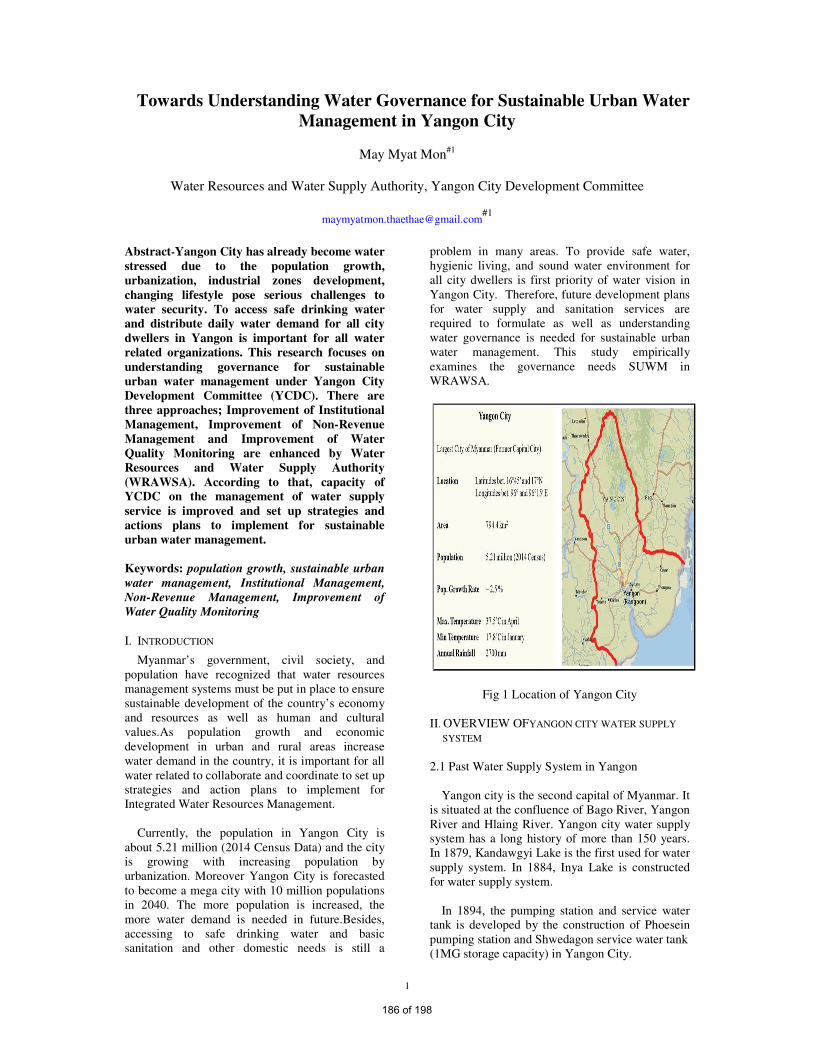
1

Towards Understanding Water Governance for Sustainable Urban Water

Management in Yangon City

May Myat Mon#1

Water Resources and Water Supply Authority, Yangon City Development Committee

[email protected]#1

Abstract-Yangon City has already become water

stressed due to the population growth,

urbanization, industrial zones development,

changing lifestyle pose serious challenges to

water security. To access safe drinking water

and distribute daily water demand for all city

dwellers in Yangon is important for all water

related organizations. This research focuses on

understanding governance for sustainable

urban water management under Yangon City

Development Committee (YCDC). There are

three approaches; Improvement of Institutional

Management, Improvement of Non-Revenue

Management and Improvement of Water

Quality Monitoring are enhanced by Water

Resources and Water Supply Authority

(WRAWSA). According to that, capacity of

YCDC on the management of water supply

service is improved and set up strategies and

actions plans to implement for sustainable

urban water management.

Keywords: population growth, sustainable urban

water management, Institutional Management,

Non-Revenue Management, Improvement of

Water Quality Monitoring

I. INTRODUCTION

Myanmar’s government, civil society, and

population have recognized that water resources

management systems must be put in place to ensure

sustainable development of the country’s economy

and resources as well as human and cultural

values.As population growth and economic

development in urban and rural areas increase

water demand in the country, it is important for all

water related to collaborate and coordinate to set up

strategies and action plans to implement for

Integrated Water Resources Management.

Currently, the population in Yangon City is

about 5.21 million (2014 Census Data) and the city

is growing with increasing population by

urbanization. Moreover Yangon City is forecasted

to become a mega city with 10 million populations

in 2040. The more population is increased, the

more water demand is needed in future.Besides,

accessing to safe drinking water and basic

sanitation and other domestic needs is still a

problem in many areas. To provide safe water,

hygienic living, and sound water environment for

all city dwellers is first priority of water vision in

Yangon City. Therefore, future development plans

for water supply and sanitation services are

required to formulate as well as understanding

water governance is needed for sustainable urban

water management. This study empirically

examines the governance needs SUWM in

WRAWSA.

Fig 1 Location of Yangon City

II. OVERVIEW OFYANGON CITY WATER SUPPLY

SYSTEM

2.1 Past Water Supply System in Yangon

Yangon city is the second capital of Myanmar. It

is situated at the confluence of Bago River, Yangon

River and Hlaing River. Yangon city water supply

system has a long history of more than 150 years.

In 1879, Kandawgyi Lake is the first used for water

supply system. In 1884, Inya Lake is constructed

for water supply system.

In 1894, the pumping station and service water

tank is developed by the construction of Phoesein

pumping station and Shwedagon service water tank

(1MG storage capacity) in Yangon City.

186 of 198

2

The water delivered from Kandawgyi Lake to

Phosein staion was pumped to the Shwedagon

service tank.

In 1904, HlawgaReservoir(14MGD supply

capacity) was constructed and the water from

Hlawga Resevoir was pumped toYegu pumping

station by booster pumping station Hlawga

Reservoir.

In 1906, the construction of Yegu pumping

station was completed. And then the water was

pumped to Shwedagon Reservoir which water was

distributed to the whole city.

In Kokkhine service water tank (20MGD storage

capacity) was constructed and added to the existing

water supply system to expand the served area.

In 1941, Gyobyu Reservoir (27 MGD supply

capacity) and water was supplied through Yegu

pumping station to Kokkhine service water tank.

In 1989, Phugyi Reservoir (54MGD supply

capacity) was constructed and added to the water

supply system by connecting with Hlawga

Reservoir which is distributed to Yangon City.

At that time, the total amount of daily water

supply was 85 MGD, including YCDC owned tube

well (10 MGD). In 2000, Yangon Pauk ground

water treatment project was completed and the

water supply amount is 1MGD.

In 2005, Ngamoeyiek WTP project (Phase1 with

45 MGD supply capacity) was constructed by

Ministry of Agriculture and Irrigation.

In 2009, South Dagon ground water treatment

project (2MGD supply capacity) and Thaephyu

ground water treatment project (11 MGD supply

capacity) is added to the supply water. The second

phase of Ngamoeyiek WTP in early 2014 and it

started to supply daily water capacity 45MGD.

Now Kandawgyi Lake and Inya Lake are not

used for water supply because the water quality is

deterioration by rapid of urbanization. Phoesein

pumping station is stopped, too.

2.2 Existing Current Yangon City Water Supply

System

The current water supply amount is 205MGD.

The source of surface water is about 92% from

reservoir and 8% is the ground water from tube

well for daily water supply.

The major water sources are Gyobyu Reservoir,

Phugyi Reservoir, HlawgaReservoir, Ngamoeyeik

Water Treatment (WTP) 1st and, 2nd phase and

YCDC tube wells.

Fig 2 Existing Yangon City Water Supply System

Table 1 Daily Water Supply Capacity

No Water Source

Million

Gallons per

Day (MGD)

Remark

1

Gyobyu

Reservoir 27 YCDC

2 Phyugyi

Reservoir 54

YCDC

3 Hlawga

Reservoir 14

YCDC

4

Ngamoeyiek

WTP

(1st phase)

45

YCDC

5

Ngamoeyiek

WTP

(2nd

phase)

45

YCDC

6

YCDC Tube

Wells

(425 nos)

20

YCDC

7

Total Water

Supply

Capacity

205

YCDC

2.3 Aged Transmission and Distribution Pipelines

Water Supply system in Yangon has a long

history, the water supply services commenced in

1842. Transmission and distribution pipes have not

been rehabilitated and the old age pipelines did not

have enough flow capacity properly which results

in large quantity of non-revenue water (NRW).

187 of 198

3

Moreover other water facilities have not been

expanded last decades.

Table 2 Aged Transmission pipes

Sta

rt-u

p

yea

r

Pip

e

mat

eria

l

Dia

met

er

(in)

Len

gth

(mil

e)

Age

(yea

r)

Rem

ark

1904 Cast iron

42 14.2 113 YCDC

1914 Cast iron

42 5 103 YCDC

1940

Mild

Steel 56 43 77 YCDC

1989

Pre-

stressed

concrete

60 16 28 YCDC

1992

Pre-

stressed

concrete

66 10.4 25 YCDC

The total length of distribution and transmission

pipelines in whole network is 2655 miles.

2.4 History Water Treatment Plant (WTP)

According to the history of water supply system,

90% of water came from reservoirs, and two thirds

of them is distributed directly without any

treatment.

In the old Gyobyu WTP, water is treated by

sedimentation process without coagulant,

Nyaunghnapin WTP is treated by rapid sand

filtration and groundwater is treated by aeration

method.

III IMPROVEMENT of WATER SUPPLY

MANAGEMENT

3.1 Study Area

Water Resources and Water Supply Authority

(WRAWSA)

3.2 Governance for Sustainable Urban Water

Management (SUWM)

Water is the essential need of mankind for their

life and living especially, the areas where the

drinking water supply is systematically managed

are more rapidly developing. It is not evenly

distributed and well management leading to many

problems and impacts in our environment. Based

on these systemic and inter-related barriers (Brown

and Farrelly, 2009), it can be surmised that there

is a lackof insight intogovernance approaches

required to support SUWM practices.

Governance describes the management of

collectives issues, the stakeholders involved and

process used (Kjаer, 2004; Pierre and Peters,

2000; Stoker, 1998).

Regarding good water governance for SUWM,

WRAWSA is cooperating and collaborating with

Japan International Cooperation Agency (JICA)

Technical Assistance Team as well as implemented

the project for “Improvement of Water Supply

Management of YCDC” from 2016 to 2020.

3.3 Three Approaches

According to that, the three approaches often

identified are Improvement of Institutional

Management, Improvement of Non-Revenue

Management and Improvement of Water Quality

Monitoring.

3.4 Process of Preparation

Moreover, WRAWSA learns neighboring

countries successful urban water supply system.

Based on it, the findings, advantages, and

disadvantages are compared and analyzed with past

water supply situation. According to that,

“Management Improvement Plan” proposal is

designed and proposed to improve the YCDC water

supply industry in more advanced and successful.

Improvement of Institutional Management; this

article assesses the institutional prescriptions of

adaptive (co-)management based on the literature

review of water governance. The public

participation, an experimental approach to water

resources management and bioregional approach is

essential for improvement of institutional

management. The following are the management

improvement area for Institutional Governance.

1. To practice Autonomous System

2. To get approval from respective ministry for

budget allocation

188 of 198

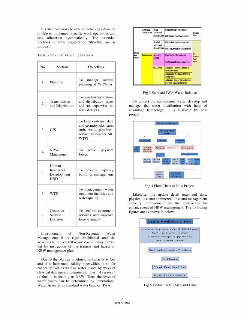
4

It’s also necessary to extend technology division

to able to implement specific work operations and

task allocation systematically. The extended

Sections in New organization Structure are as

follows.

Table 3 Objective of setting Sections

No Section Objectives

1 Planning To manage overall

planning of WRWSA

2 Transmission

and Distribution

To maintain transmission

and distribution pipes

and to supervise its

related works

3 GIS

To keep customer data

and geometry information

(tube wells, pipelines,

service reservoirs SR,

WTP)

4 NRW

Management

To solve physical

losses

5

Human

Resources

Development

HRD

To promote capacity

buildings management

6 WTP

To management water

treatment facilities and

water quality

7

Customer

Service

Division

To perform customers

services and improve

E-government

Improvement of Non-Revenue Water

Management; it is rigid established and the

activities to reduce NRW are continuously carried

out by instruction of the trainers and based on

NRW management plan.

Due to the old age pipelines, its capacity is low

and it is happened leaking pipeswhich is so far

cannot deliver as well as water losses by ways of

physical damage and commercial loss. As a result

of that, it is leading to NRW. Thus, the level of

water losses can be determined by International

Water Association standard water balance (IWA).

Fig 3 Standard IWA Water Balance

To protect the non-revenue water, develop and

manage the water distribution with help of

advantage technology, it is analyzed by new

project.

Fig 4 Flow Chart of New Project

Likewise; the update detail map and data,

physical loss and commercial loss and management

capacity improvement are the approaches for

enhancement of NRW management. The following

figures are as shown in below;

Fig 5 Update Detail Map and Data

189 of 198

5

Fig 6 Physical Loss and Commercial Loss

Fig 7 management capacity improvement

Improvement of Water Quality Management;

acquiring and developing water treatment

technology and capacity of planning, designing and

operation and maintenance are required for

producing safe and clean water.

.

Fig 8 Parameters for Water Quality Monitoring

Fig 9 Sources of Water Quality Monitoring

Fig 10 Sampling Locations

These are the ways to provide safe water,

hygienic living, and sound water environment to all

citizens not only current situation but also in the

future. Besides the perspective in planning,

management and use of water resources about

IWRM principles and participatory approach stand

as a important role for IWRM.

IV. RESULTS AND DISCUSSION

Based on three approaches, it can be formulated

again the problem solution to meet the

improvement of water supply management as well

as it can be developed 5 years plan and annual

activity plan for WRAWSA.

Fig 11 Sufficient Water Supply Services

190 of 198

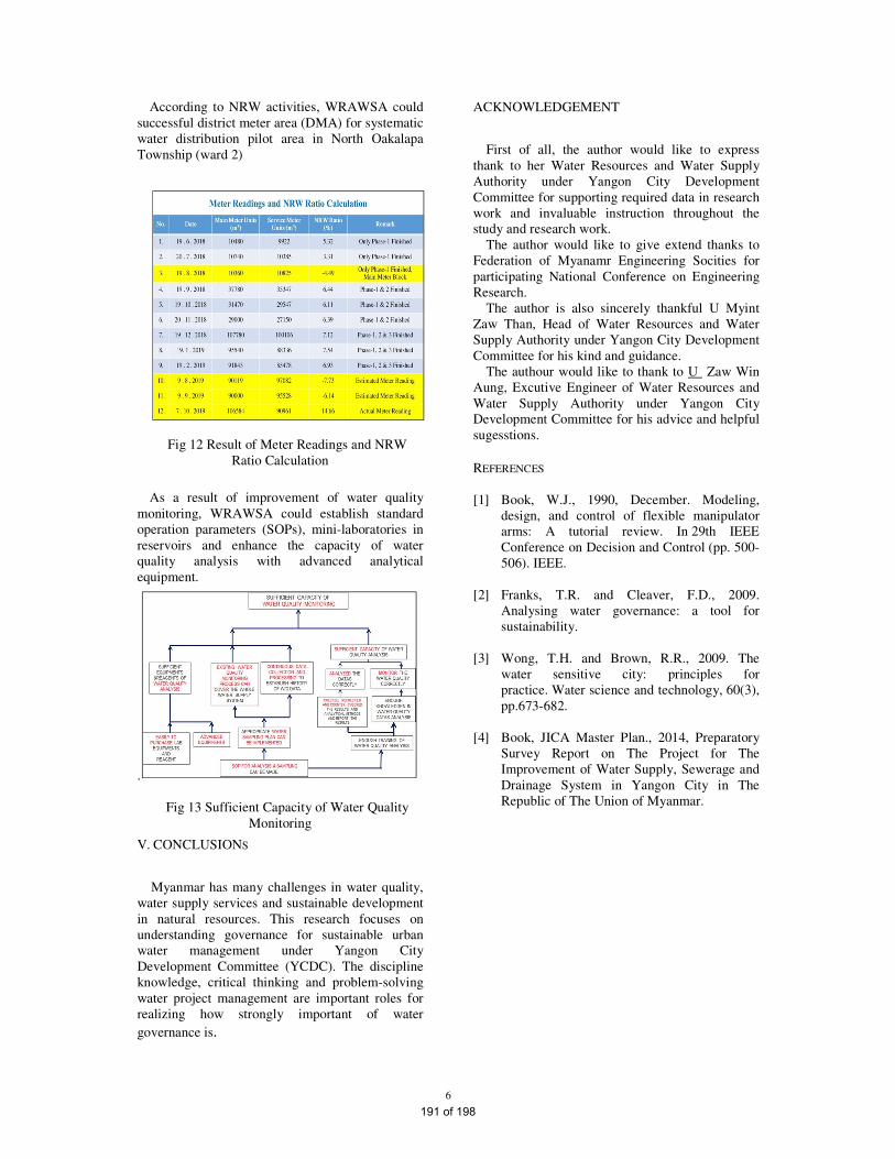
6

According to NRW activities, WRAWSA could

successful district meter area (DMA) for systematic

water distribution pilot area in North Oakalapa

Township (ward 2)

Fig 12 Result of Meter Readings and NRW

Ratio Calculation

As a result of improvement of water quality

monitoring, WRAWSA could establish standard

operation parameters (SOPs), mini-laboratories in

reservoirs and enhance the capacity of water

quality analysis with advanced analytical

equipment.

.

Fig 13 Sufficient Capacity of Water Quality

Monitoring

V. CONCLUSIONS

Myanmar has many challenges in water quality,

water supply services and sustainable development

in natural resources. This research focuses on

understanding governance for sustainable urban

water management under Yangon City

Development Committee (YCDC). The discipline

knowledge, critical thinking and problem-solving

water project management are important roles for

realizing how strongly important of water

governance is.

ACKNOWLEDGEMENT

First of all, the author would like to express

thank to her Water Resources and Water Supply

Authority under Yangon City Development

Committee for supporting required data in research

work and invaluable instruction throughout the

study and research work.

The author would like to give extend thanks to

Federation of Myanamr Engineering Socities for

participating National Conference on Engineering

Research.

The author is also sincerely thankful U Myint

Zaw Than, Head of Water Resources and Water

Supply Authority under Yangon City Development

Committee for his kind and guidance.

The authour would like to thank to U Zaw Win

Aung, Excutive Engineer of Water Resources and

Water Supply Authority under Yangon City

Development Committee for his advice and helpful

sugesstions.

REFERENCES

[1] Book, W.J., 1990, December. Modeling,

design, and control of flexible manipulator

arms: A tutorial review. In 29th IEEE

Conference on Decision and Control (pp. 500-

506). IEEE.

[2] Franks, T.R. and Cleaver, F.D., 2009.

Analysing water governance: a tool for

sustainability.

[3] Wong, T.H. and Brown, R.R., 2009. The

water sensitive city: principles for

practice. Water science and technology, 60(3),

pp.673-682.

[4] Book, JICA Master Plan., 2014, Preparatory

Survey Report on The Project for The

Improvement of Water Supply, Sewerage and

Drainage System in Yangon City in The

Republic of The Union of Myanmar.

191 of 198

Function Hall

Function Hall

Session Time Presenter

9:10 -9:35 H.E Dr.Kyaw Linn PPP Analytical Framework for Infrastructure Asset Allocation

9:35 - 10:00 U Tin Myint

10:00 -10:25 Prof.Dr.Hitoshi Tanaka Impact of Climate Change on River Delta Coastlines

10:25 - 10:40

Function Hall

Session Time Presenter Title Chairperson/ Moderator

10:40 - 11:00 Khaing Chan Myae ThuDevelopment of Flood Inundation Map for Upper Chindwin River Basin By Using HEC-HMS

and HEC-RAS

11:00-11:20 Kyaw Myo HtunProject Management and Construction Method for Different Types of Bridge in Various

Locations of Myanmar. (From Naung Moon to Kawthaung)

11:20-11:40 Shwe Pyi Tan Integrated Water Resources Management Plans for Sittaung River Basin

11:40-12:00 Ei Khaing Zin ThanAssessment of Crop and Irrigation Water Requirements for Some Selected Crops in Chaung

Gauk Irrigation Scheme

12:00- 13:00

Opening Speech by U Aung Myint , President of Federation of Myanmar Engineering Societies

8:00 - 8:45

8:50 - 9:00

9:00 - 9:10

Keynote

Speech

Session (1)

Coffee Break

Lunch

Title

U Hla Baw/

Nan Theint Kham Ko

Ko



16-1-2020



Tentative Agenda

Registration

Opening

Current Status of RE in Myanmar and its Future

192 of 198



16-1-2020



Tentative Agenda

Function Hall


13:00 - 13:20 Aung Aung SoeEffect of Lime Content and Curing Condition on Strength Development of Lime-Stabilized Soil

in Bogalay Township, Ayeyarwaddy Region

13:20 - 13:40 Tin Tin Wai Investigation on Performance Level of 10-storey R.C Building with Pushover Analysis

13:40 - 14:00 Aye Thet Mon Comparative Study on Soft Storey Effect at Different Levels in Reinforced Concrete Buildings

14:00 - 14:20 Aung Myo WaiDesign of Water Distribution System Using Hydraulic Analysis Program (EPANET 2.0) for

Tatkon Town in Myanmar

14:20 - 14:40 May Myat MonTowards Understanding Water Governance for Sustainable Urban Water Management in

Yangon City

14:40 - 15:00

Function Hall


15:00 - 15:20 Chan Myae Kyi Study on the Behavior of Spun Pile Foundation Becoming Due to Seismic Loading

15:20- 15:40 Hla Tun Mathematical Analysis of Reservoir Flood Routing

15:40 - 16:00 Tun Min Thein Key Factors for the Successful Construction of Tunnels and Shafts

16:00 - 16:20 Thi Thi Khaing Transition of Urban Sustainability Approach

16:20 - 16:40 Wai Yar Aung Earthquake Safety Assessment of RC Buildings in Myanmar

Session (3)

Session (2)

Coffee Break

U Khin Maung Htaey/

Kyi Sin Thant

U San Kyu/

Su Latt Twel Tar Bo

193 of 198



16-1-2020



Tentative Agenda

Function Hall

Function Hall



9:35 - 10:00 U Tin Myint


10:25 - 10:40

Conference Room


11:00-11:20 Dr.Htein Win Synthesis, Characterization and Application of Carbon Nanotubes in Conductive Ink

11:20-11:40 Dr. Saw Mya NiEffect of Sintering Time on Properties and Shape Memory Behavior of Cu-Zn-Al Shape Memory

Alloy

11:40-12:00 Dr.Myat Myat SoeRecovery of Cobalt Metal From Spent LI-ION Battery by Combination Method of

Precipitation and Reduction

12:00- 13:00

Session (1)U Kyaw Kyaw/

Yoon Thiri Zaw

Lunch

Coffee Break

8:00 - 8:45 Registration

8:50 - 9:00 Opening

9:00 - 9:10 Opening Speech by U Aung Myint , President of Federation of Myanmar Engineering Societies

Title

Keynote

Speech Current Status of RE in Myanmar and its Future

194 of 198



16-1-2020



Tentative Agenda

Conference Room


13:00 - 13:20 Yu Nanda HlaingMicrotremor Measurement at Some sites in Mandalay City, Myanmar, for Earthquake Disaster

Mitigation

13:20 - 13:40 Myint Aung Assessment of Surface and Ground Water Quality around the Kyinsintaung Mine, Myanmar

13:40 - 14:00 Thaw Zin Water Management for Waterflooding in Mature Field

14:00 - 14:20 Dr.Htay Htay Win Theoretical and Numerical Modal Analysis of Six Spokes wheel’s rim using ANSYS

14:20 - 14:40 Hsu Myat Tin Analysis of Forecasting Techniques of Instant Noodle Manufacturing Company

14:40 - 15:00


15:00 - 15:20 Khin Hnin Thant Maritime Education, Training and Capacity Building in Myanmar Mercantile Marine College

15:40 - 16:00 Thu Thu Aung Capacity Building for Future-Oriented Education in Myanmar

16:00 - 16:20 Zin Thuzar Naing Implementation of Sliding Mode Controller for Mobile Robot System

Session (2)

Session (3)

Coffee Break

Dr.Zaw Htet Aung &

U Khin Maung Than/

Aye Nyein Chan Moe

Dr.Htin Lin/

Soe Moe Htet

195 of 198



16-1-2020



Tentative Agenda

Function Hall

Function Hall



9:35 - 10:00 U Tin Myint


10:25 - 10:40

Seminar Room


10:40 - 11:00 Aung Kyaw Myint Implementation of SCADA System for Hydropower Station

11:00-11:20 Nwe Ni WinSimulation and Analysis on Power Factor Improvement and Harmonic Reduction of High-

voltage, High-frequency Power Supply for Ozone Generator

11:20-11:40 Khin Thi Aye Promote the Development of Renewable Energy in Myanmar

11:40-12:00 Min Set Aung Transition of University to Prosumer Consortium Energy Model

12:00- 13:00

Session (1)

Lunch

8:00 - 8:45

8:50 - 9:00

9:00 - 9:10

Keynote

Speech

Registration

Opening

Opening Speech by U Aung Myint , President of Federation of Myanmar Engineering Societies

Title

Current Status of RE in Myanmar and its Future

Coffee Break

Daw Than Than Win/

Nay Htet Aung

196 of 198



16-1-2020



Tentative Agenda

Seminar Room


13:00 - 13:20 Zin Mar Htun Secure and Authenticated Data Hiding using Edge Detection

13:20 - 13:40 Dr.Aye Aye Thant Mathematical Approach to Stable Hip Trajectory for Ascending Stairs Biped Robot

13:40 - 14:00 Khaing Thanda Swe Modeling Information Security System using Huffman Coding

14:00 - 14:20 Dr. Phyo Thu Zar Tun Performance Evaluation for Classification on Dengue Fever

14:20 - 14:40 Dr.Win Lei Lei Aung The Optimal Cost of an Outpatient Department by Using Single and Multiple Server System

Session (2)Dr.Win Zaw /

Lat yar La Pyae

197 of 198

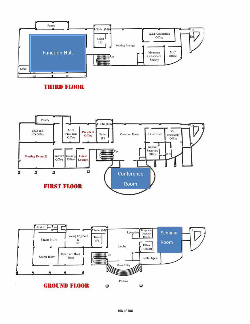
Function Hall

Conference

Room

Seminar

Room

198 of 198

download - Federation of Myanmar Engineering Societies

Documents

Transcript of download - Federation of Myanmar Engineering Societies