DOKTORI (PhD) ÉRTEKEZÉS

KIRÁLY ANDRÁS

Pannon Egyetem

2013.

Pannon EgyetemVegyészmérnöki és Folyamatmérnöki Intézet

Döntéstámogató rendszerekben alkalmazhatószámítási intelligencián és adatbányászaton

alapuló algoritmusok

DOKTORI (PhD) ÉRTEKEZÉS

Király András

KonzulensDr. Abonyi János, egyetemi tanár

Vegyészmérnöki- és Anyagtudományok Doktori Iskola

Pannon Egyetem

2013.

Döntéstámogató rendszerekben alkalmazható

számítási intelligencián és adatbányászaton

alapuló algoritmusok

Értekezés doktori (PhD) fokozat elnyerése érdekében

a Pannon Egyetem Vegyészmérnöki- és Anyagtudományok Doktori Iskola

Doktori Iskolájához tartozóan

Írta:

Király András

Konzulens: Dr. Abonyi János

Elfogadásra javaslom igen / nem ..........................................

(aláírás)

A jelölt a doktori szigorlaton .................. %-ot ért el.

Az értekezést bírálóként elfogadásra javaslom:

Bíráló neve: .......................................... igen / nem ..........................................

(aláírás)

Bíráló neve: .......................................... igen / nem ..........................................

(aláírás)

A jelölt az értekezés nyilvános vitáján .................. %-ot ért el.

Veszprém, ..........................................

a Bíráló Bizottság elnöke

A doktori (PhD) oklevél minősítése ............................

..........................................

az EDT elnöke

University of PannoniaDepartment of Process Engineering

Data mining and soft computing algorithms fordecision support systems

PhD Thesis

András Király

SupervisorJános Abonyi, DSc

Doctoral School in Chemical Engineering and Material Sciences

University of Pannonia

2013.

Köszönetnyilvánítás

Köszönettel tartozom els®sorban témavezet®mnek Dr. Abonyi Jánosnak asokszor már végtelennek t¶n® türelméért valamint folyamatos szakmai út-mutatásaiért és baráti támogatásáért.

Hálás vagyok egész családomnak és barátaimnak hogy bármikor számít-hattam szeret® támogatásukra, megteremtve ezzel azt a biztos lelki hátteretmind egyetemi, mind a doktorandusz évek során, mely elengedhetetlen akreatív munkavégzéshez.

Köszönöm továbbá dr. Gyenesei Attilának hogy lehet®séget teremtettszámomra a turkui kutatómunkára, valamint a Finnish Microarray and Se-quencing Centre valamennyi munkatársának hogy szakmai támogatásukkalsegítették munkámat, melynek eredményeként létrejöhetett a dolgozat 4. fe-jezete.

Ugyancsak köszönöm a Pannon Egyetem Folyamatmérnöki Intézeti Tan-szék valamennyi munkatársának, különösen Dobos Lacinak és Borsos Ákos-nak az éveken át (és azóta is) tartó szakmai és emberi segítséget.

i

Kivonat

Döntéstámogató rendszerekben alkalmazható számítási

intelligencián és adatbányászaton alapuló algoritmusok

A döntéstámogató rendszerek olyan plusz tudást képesek adni a döntéshozókkezébe, melyek naprakész ismereteket szolgáltatnak mind a vállalat folya-matairól mind a küls® környezetr®l, biztos alapot teremtve ezzel a helyesdöntésekhez. A jelen munkában ismertetésre kerül® módszerek és eszközöksegítségével pontosabban modellezhet®k a vállalatban lejátszódó folyamatok;kezelhet®k a rendszerekben fellép® bizonytalanságok; hatékonyabban elemez-het®k a rendelkezésre álló adatok. Az ismertetésre kerül® technikák mind-egyike konkrét ajánlásokat szolgáltat a döntéshozók részére.

A dolgozat komplex rendszerek elemzésével és optimalizálásával foglalko-zik, melyek mindegyike valamilyen gyakorlati probléma megoldását szolgál-tatja. Logisztikai problémák kapcsán olyan útvonalhálózat-tervezési metó-dust ismertet, mely új genetikus algoritmus és reprezentáció alkalmazásávalképes egy 600 mobilszerel®t ellátó hálózat optimális felépítésének ajánlásá-ra. Többszint¶ raktározási problémák robosztus optimálására újszer¶ szi-mulátort vezet be, melynek segítségével többféle optimalizációs eljárás kerültárgyalásra. Továbbá a be- és kimenetek változásai közötti kapcsolatok feltá-rásával újszer¶ döntéstámogató eszközt ismertet. Bioinformatikai eljárásoksorán keletkez® génexpresszió adatokból történ® hasznos információ kinyeré-sére pedig új biclustering algoritmusok és elemzési tevhnikák kerülnek ismer-tetésre.

Az egyes fejezetekben ismertetett metódusok közös vonása a döntéstámo-gató rendszerekbe történ® integrálás lehet®sége, ugyanakkor a köztük lév®kapcsolat inkább marginálisnak mondható. Így a dolgozat a klasszikus felépí-tés helyett három mer®ben eltér® probléma különböz® módszerekkel történ®megoldását ismerteti.

ii

Abstract

Data mining and soft computing algorithms fordecision support systems

Decision support systems are capable to give additional information for deci-sion makers which represent up to date knowledge about the enterprise pro-cesses as well as about the environment, greatly supporting their work anddecreasing the pressure of responsibility. Methods and techniques presentedin this work provides up to date knowledge and tools to model enterpriseprocesses more accurately; to handle uncertainties during these processes;to analyze available data more correctly. The discussed techniques providesconcrete support for decision makers.

The thesis presents the analysis and optimization of complex systems pro-viding a solution for real problems. A route planning method is describedwhich is capable to propose optimal vehicle route system supplying 600 mo-bile mechanics of Hungary's leading energy provider, introducing a novel ge-netic representation based e�ective genetic algorithm. It presents several op-timization techniques for multi-echelon inventory management systems whichis based on a novel robust simulation technique using Monte Carlo method.Furthermore a bene�cial decision support system is demonstrated by theparameter sensitivity analysis of these systems. To retrieve valuable infor-mation form gene expression data new biclustering algorithms and methodsare presented.

Although the possibility of integration into decision support systems arecommon in methods presented in the chapters of the thesis, but the relation-ship between them is rather marginal. Thus, instead of the classical structure,the dissertation proposes three di�erent solutions for three distinct problems.

iii

Auszug

Algorithmen aufgrund der Berechnungsintelligenzund Datenabbau für Decision Support Systeme

Decision Support Systeme stellen den Entscheidungsträgern zusätzliches Wis-sen zur Verfügung, das die Leiter über die Prozesse des Unternehmens, überseine innere Umgebung auf dem Laufenden halten, und legt damit einensicheren Grund für richtige Entscheidungen. Die in der Arbeit dargestell-ten Methoden und Instrumente bieten aktuelles Wissen, mit dessen Hilfe dieProzesse des Unternehmens besser modelliert werden können; die Ungewis-sheit innerhalb der Systeme besser behandelt werden können; die verfügbarenDaten besser analysiert werden können. Alle darzustellenden Instrumente bi-eten konkrete Empfehlungen an Entscheidungsträger.

Die Arbeit beschäftigt sich mit der Analyse und Optimierung der kom-plexen Systeme, die zur Lösung konkreter, realer Probleme dienen. Eine neueRoutenplanung-Methode wird unter logistischen Problemen beschrieben, diemit Anwendung eines neuen genetischen Algorithmus und Repräsentationfähig ist, den optimalen Aufbau eines realen, 600 Mobilinstallateur versor-genden Netzwerkes zu empfehlen. Ein neuer Simulator wird dadurch zurOptimierung der konkreten mehrseitigen Lagerungsprobleme eingeführt, undmit Hilfe des Simulators werden mehrere Optimierungsverfahren erörtert. ImWeiteren werden konkrete Instrumente zur Beschlussfassung klargestellt, mitAufdeckung der Beziehungen zwischen Ein-und Ausgang. Neue Bicluster-ing -Algorithmen werden zum Gewinn der nützlichen Information aufgrundder in bioinformatischen Verfahren entstehenden Gene Expression Datendargestellt. Die zur Methode herausentwickelten Instrumente dienen auf in-tegrierter Weise zur Prozessoptimierung und Beschlussfassung.

Obwohl die einzelnen Kapitel einen gemeinsamen Charakter haben, dieMöglichkeit der Integration in das die Beschlussfassung unterstützende De-cision Support Systeme, kann die Beziehung zwischen Ihnen lieber marginalgenannt werden. So legt die Arbeit die Lösung von drei völlig divergentenProblemen mit verschieden Mitteln dar, statt einen klassischen Aufbau zuhaben.

iv

Contents

1 Introduction 1

2 Optimization of multiple traveling salesman problem by anovel representation based genetic algorithm 62.1 Motivation, literature review, roadmap . . . . . . . . . . . . . 72.2 Theoretical background and algorithm development . . . . . . 10

2.2.1 Problem formulation . . . . . . . . . . . . . . . . . . . 102.2.2 Introduction to traveling salesman speci�c GAs . . . . 132.2.3 A novel way to solve MTSP with GA . . . . . . . . . . 192.2.4 Numerical analysis of the proposed method . . . . . . . 22

2.3 A Google Maps based framework developed to utilize the pro-posed algorithm . . . . . . . . . . . . . . . . . . . . . . . . . . 29

2.4 Application study . . . . . . . . . . . . . . . . . . . . . . . . . 312.5 Conclusions . . . . . . . . . . . . . . . . . . . . . . . . . . . . 35

3 Monte Carlo simulation based optimization and analysis ofinventory management systems 363.1 Introduction . . . . . . . . . . . . . . . . . . . . . . . . . . . . 363.2 Determining optimal safety stock level in multi-echelon supply

chains . . . . . . . . . . . . . . . . . . . . . . . . . . . . . . . 373.2.1 Classic inventory model of a single warehouse . . . . . 393.2.2 The proposed stochastic inventory model . . . . . . . . 413.2.3 A simulation-based multi-echelon warehouse model . . 433.2.4 Particle Swarm Optimization Algorithms . . . . . . . . 483.2.5 The proposed Constrained PSO Algorithm . . . . . . . 513.2.6 Further improvement of PSO algorithm by memory-

based gradient search . . . . . . . . . . . . . . . . . . . 533.2.7 Stochastic optimization of multi-echelon supply chain

models by improved PSO algorithm . . . . . . . . . . . 603.3 Monte Carlo Simulation based Performance Analysis of Supply

Chains . . . . . . . . . . . . . . . . . . . . . . . . . . . . . . . 65

v

3.3.1 The proposed framework for sensitivity analysis of sup-ply chains . . . . . . . . . . . . . . . . . . . . . . . . . 67

3.3.2 Sensitivity analysis of a multi-echelon supply chain prob-lem . . . . . . . . . . . . . . . . . . . . . . . . . . . . . 71

3.4 Conclusions . . . . . . . . . . . . . . . . . . . . . . . . . . . . 75

4 Biclustering algorithms for Data mining in high-dimensionaldata 764.1 Introduction . . . . . . . . . . . . . . . . . . . . . . . . . . . . 76

4.1.1 Literature review . . . . . . . . . . . . . . . . . . . . . 784.2 Problem formulation . . . . . . . . . . . . . . . . . . . . . . . 80

4.2.1 Biclustering . . . . . . . . . . . . . . . . . . . . . . . . 804.2.2 Frequent closed itemset mining . . . . . . . . . . . . . 824.2.3 Connection between biclustering and frequent closed

itemset mining . . . . . . . . . . . . . . . . . . . . . . 824.3 E�cient methods for bicluster mining . . . . . . . . . . . . . . 83

4.3.1 A novel way to mine closed patterns . . . . . . . . . . 844.3.2 Transformation of {−1, 0, 1} data to binary data . . . . 884.3.3 Closed pattern based data visualization . . . . . . . . . 894.3.4 Method for the aggregation of closed patterns . . . . . 904.3.5 Experimental results . . . . . . . . . . . . . . . . . . . 934.3.6 Remark for other methods . . . . . . . . . . . . . . . . 97

4.4 Bit-table representation based biclustering . . . . . . . . . . . 974.4.1 MATLAB implementation of the proposed algorithm . 1024.4.2 Computational results . . . . . . . . . . . . . . . . . . 104

4.5 Biological validation of discovered patterns . . . . . . . . . . . 1044.5.1 Comparison of biclustering methods . . . . . . . . . . . 107

4.6 Conclusions . . . . . . . . . . . . . . . . . . . . . . . . . . . . 109

5 Summary and Theses 1115.1. Tézisek . . . . . . . . . . . . . . . . . . . . . . . . . . . . . . . 1125.2 Theses . . . . . . . . . . . . . . . . . . . . . . . . . . . . . . . 1155.3 Publications related to theses . . . . . . . . . . . . . . . . . . 117

List of Figures and Tables 121

Bibliography 126

vi

Chapter 1

Introduction

In the last decades, optimization was featured in almost all aspects of humancivilization, thus it has truly become an indispensable method. In someaspects, even a local optima can highly improve the e�ciency or reduceexpenses, however, most companies want to keep their operational costs aslow as possible, i.e. on global minimum. Most of the problems come upin industrial environment su�er some kind of risk or uncertainty, and theircomplexity is too high for traditional methods to provide acceptable resultsin applicable time. All three theses presented in the dissertation have acommon property in high complexity which requires new or novel methodsto handle them. A potential solution of these problems can be addressed as itis depicted in Fig. 1.1 which corresponds to the structure of the dissertation.

Because of the high complexity of problems, gradient based optimizationmethods are too expensive computationally thus their running times are toolong, therefore some gradient-free optimization technique has to be used likeGenetic algorithm, (chapter 2) Particle Swarm Optimization (chapter 3) orBiclustering and Frequent Closed Itemset Mining (chapter 4). High complex-ity also necessitates the usage of simulation, as we will see in a minute theapplication of Monte Carlo simulation has serious advantages (chapter 3),and appropriate analysis of initial data (e.g. transformation) can also helphandling complex or high dimensional data (chapter 4).

Although the three thesis has several common properties, they deal withdi�erent problems and provide di�erent approaches for solution. Therefore,the dissertation doesn't follow the traditional way, but presents three di�erentproblems with three di�erent solution procedure and the connection betweenthe chapters is rather fragile.

So the main problems motivated this research can be divided into 3 areas.First one is a logistical problem derived from an industrial problem, whichcame up at E.ON Hungária Zrt., the leading energy provider of Hungary.

1

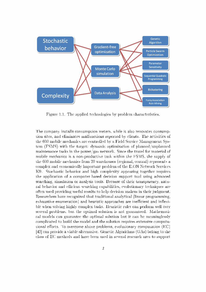
Figure 1.1. The applied technologies by problem characteristics.

The company installs consumption meters, while it also renovates consump-tion sites, and eliminates malfunctions reported by clients. The activities ofthe 600 mobile mechanics are controlled by a Field Service Management Sys-tem (FSMS) with the target: dynamic optimization of planned/unplannedmaintenance tasks in the power/gas network. Since the travel for material ofmobile mechanics is a non-productive task within the FSMS, the supply ofthe 600 mobile mechanics from 20 warehouses (regional, central) represents acomplex and economically important problem of the E.ON Network ServicesKft. Stochastic behavior and high complexity appearing together requiresthe application of a computer-based decision support tool using advancedsearching, simulation or analysis tools. Because of their transparency, natu-ral behavior and e�cient searching capabilities, evolutionary techniques areoften used providing useful results to help decision makers in their judgment.Researchers have recognized that traditional analytical (linear programming,exhaustive enumeration) and heuristic approaches are ine�cient and in�exi-ble when solving highly complex tasks. Heuristic rules can perform well overseveral problems, but the optimal solution is not guaranteed. Mathemati-cal models can guarantee the optimal solution but it can be meaninglesslycomplicated to build the model and the solution requires extensive computa-tional e�orts. To overcome above problems, evolutionary computation (EC)[42] can provide a viable alternative. Genetic Algorithms (GAs) belong to theclass of EC methods and have been used in several research area to support

2

decision making, like for the solution of various synthesis [55] or for support-ing multi-objective economic decisions [33]. Therefore we present a novelgenetic algorithm to solve the supply problem of mobile mechanics. The newdynamic approach presented in chapter 2 aims a signi�cant reduction of ac-tivities regarding material handling for the mobile teams with extending ofserving locations from 20 to 100. The design of the supply system can beconsidered as a complex combinatorial optimization problem, where the goalis to �nd a route plan with minimal route cost, which services all the de-mands from three central warehouses while satisfying the capacity and otherconstraints.

The second problem is also derived from E.ON Hungária Zrt., where theaverage holding cost in warehouses has to be minimized. This inventory man-agement problem includes uncertainty in daily consumption from warehousesand in replenishment lead times which is the time between orders and actualtransportation of goods. Decision makers need to know the e�ects of riskduring business processes and this uncertainty is often described by prob-abilistic models. The Monte Carlo (MC) method is a robust technique tohandle these uncertainties and thus to reduce decision making problems. Adetailed explanation of the usage of Monte Carlo estimators can be found in[142], where authors solve stochastic programming problems by �nite seriesof Monte Carlo samples and applies the results to support decision makingas well.

Another probability to handle the uncertainties is the analysis of the sen-sitivities of the parameters. The goal of sensitivity analysis is to describe howmuch model outputs are a�ected by the inputs of the model [102]. In chap-ter 3, a novel visualization technique for sensitivity analysis will be describedthrough the analysis of a multi-echelon inventory management system.

The presented Monte Carlo method based simulator in chapter 3 is capa-ble to handle these risks providing a robust and modular modeling technique.Using simulation, the average holding cost can be calculated in each ware-houses, and the overall expenses can be optimized while constraints for ser-vice level has to be taken into account. Managers of the previously mentionedcompany necessitates a robust tool to support their decisions. In chapter 3a novel visualization technique will also be presented to provide easily in-terpretable representation of relationship between a multi-echelon warehousesystem's inputs and target variables.

The third research area is the �eld of cell biology, where the task is to �ndco-regulated gene pro�les in microarray Gene Expression Data (GED). Datais presented as a huge matrix with real numbers representing the expressionlevels of genes in given samples. Data are retrieved from DNA microarrays

3

which contains the measurement of mRNA levels in particular cells or tissuesfor many genes at once. These data are generated e.g. in Finnish Microar-ray and Sequencing Centre in Turku. Firstly data has to be cleaned anddiscretized, and some clustering method needs to be used to identify similargenes or samples i.e. subparts of the matrix containing strongly correlatedvalues. Two methods will be presented in chapter 4 for this task which iscalled biclustering.

The main motivation of the work is to develop novel techniques which arerobust, e�cient and transparent enough to solve highly complex problems inreasonable time in an easily interpretable way. A large part of the e�ortswas expended to model a complex industrial problem as realistic as possible.The second chapter realizes these expectations with the usage of real trans-portation data and a novel, more realistic genetic representation, using themduring the optimization process. As it will be presented in the third chapter,a novel simulator was built to provide simulation of inventory managementmuch more close to reality which can handle uncertainty in consumptiondata. The fourth chapter deals with fast algorithm which is extremely easilyinterpretable, using simple matrix operations and working on real biologi-cal data. As another important objective, theses present software solutionsrealizing the novel methods, providing user-friendly implementations to col-lect or generate input data, handle uncertainty, optimize complex tasks oranalyze the results.

According to the motivations and objectives described above, the struc-ture of the thesis is the following. Chapter 2 describes a complete opti-mization framework to solve the modi�ed multiple traveling salesman prob-lem which corresponds to the logistical problem of EON Hungária Kft. Aswe saw during the literature review, using evolutionary computation, theseproblems can be handled e�ectively. Therefore, the chapter proposes a newgenetic representation and a novel genetic algorithm which can handle ad-ditional constraints and an integrated Google Maps based software packagefor the maintenance of the whole optimization process providing a completeDSS.

In chapter 3 the determination of optimal safety stock level in multi-echelon supply chains is presented as well as the sensitivity analysis of thesystem parameters. Handling uncertainty has a wide literature, and most ofthem use Monte Carlo method as a robust simulation technique. Thus, thechapter describes a novel novel component based simulator, SIMWARE tohandle uncertainty in the model using Monte Carlo method and applies twooptimization methods to determine the optimal safety stock and minimizeoverall costs. A novel performance analysis framework is also presented here,

4

where by the help of the new visualization technique an e�ective decisionsupport tool is proposed.

Since our third problem derived from the analysis of high dimensionaldata, novel data mining techniques are presented in Chapter 4. The chapterintroduces novel algorithms for biclustering and for closed frequent patternmining in binary or in {−1, 0, 1} data and o�ers several techniques to com-pose a complete framework in frequent closed itemset mining.

5

Chapter 2

Optimization of multiple traveling

salesman problem by a novel

representation based genetic

algorithm

The aim of logistics is to get the right materials to the right place at theright time, while optimizing a given performance measure (e.g. minimizingtotal operating cost) and satisfying a given set of constraints (e.g. time andcapacity constraints) [53]. Supply chain management includes the planningand management of all activities involved in sourcing, procurement, conver-sion, and logistics management as well as crucial components of coordinationand collaboration. It deals with several problems, like Distribution NetworkCon�guration, Trade-O�s in Logistical Activities, Inventory Management orDistribution Strategy [56]. In most distribution systems goods are trans-ported from various origins to various destinations. For example, many retailchains manage distribution systems in which goods are transported from anumber of suppliers to a number of retail stores. It is often economical toconsolidate the shipments of various origin-destination pairs and transportsuch consolidated shipments in the same truck at the same time. There aremany ways in which such consolidation can be accomplished. Obviously thechallenge is to �nd the optimal i.e. the best consolidation according to someobjective functions [35]. This is a numerical optimization problem, com-monly an NP-hard task. In logistics, several types of problems could comeup; one of the most remarkable is the set of route planning problems.

6

2.1 Motivation, literature review, roadmap

The major motivation of the work presented in this chapter is derived from areal industrial problem, which came up at E.ON Hungária Zrt., the leadingenergy provider of Hungary. E.ON Network Services Kft. provides servicesprimarily to the electricity and gas supply companies of the E.ON HungáriaGroup. This service includes the full range of operations management activi-ties carried out with a view to ensuring uninterrupted energy supply, regularmaintenance of network objects, and the elimination of disruptions associ-ated with malfunctions. In addition, the company installs consumption me-ters, while it also renovates consumption sites, and eliminates malfunctionsreported by clients.

As it will be presented later in sec. 2.4, this industrial problem can bemodeled as an mTSP problem with time windows and additional constraints,therefore, the mTSP related literature will be reviewed here. In the last twodecades the traveling salesman problem (TSP) received a large amount ofinterest, and various approaches have proposed to solve the problem, e.g.branch-and-bound [60], cutting planes [111], neural network [39] or tabusearch [67]. Some of these methods are exact algorithms, while others arenear-optimal or approximate algorithms. The exact algorithms usually useinteger linear programming approaches with additional constraints.

Although TSP has received a great deal of attention, the research ofmTSP is limited. [36] gives a comprehensive review of the known approaches.There are several exact algorithms of the mTSP with relaxation of someconstraints of the problem, like [96], which is the �rst approach to solve themTSP directly, without any transformation of the TSP. In this problem, eachsalesman has a �xed initial cost f , which is activated whenever a salesman isincluded in the solution. The solution in [30] is based on Branch-and-Boundalgorithm, which is applicable for asymmetric, as well as symmetric problems.Another exact solution method is in [73]. The approach of Gromicho et al.is based on a quasi-assignment relaxation obtained by relaxing the subtourelimination constraints (SECs).

Recent research can be found in [59], where mTSP is optimized by amixed method. Feng et al. combined Particle Swarm Optimization withAnt Colony Optimization to �nd the best solution of the problem. Anotherrecent solution is presented in [118] where Nallusamy et al. used K-MeansClustering, Shrink Wrap Algorithm and Meta-Heuristics to solve the mTSP.A multi-objective approach can be found in [62], where the multiple objectiveant colony optimization is used for the bi-criteria TSP. Ant colony optimiza-tion for mTSP is used very recently in [66], where Ghafurian and Javadianprovide a solution for the multi-depot mTSP. In [64] a �xed destination vari-

7

ant of mTSP is solved by the help of simulated annealing.Lately GAs are also used for optimization of mTSP. The previous GA-

based solutions will be discussed later in the article. In the literature thereare several examples that a good problem-speci�c representation can dra-matically improve the e�ciency of genetic algorithms. A problem-speci�cindividual design can reduce the search-space, and in this case, it is neededto implement special operators which can simulate the nature of the prob-lem. These properties can make the problem-speci�c genetic algorithm moree�ective for the given task, and it becomes more easily interpretable.

GAs are direct, random search algorithms, based on the evolutionarymodel [68, 42], related with Darwin's evolutionary theory. The researches ofGAs have begun in the sixties by J.H. Holland [81]. GAs belong to the evo-lutionary computation (EC) methods [32], thus their terminology is closelyrelated to biology. Each solution of the problem, or equivalently, each pointin the search space is represented by an individual who consists of chromo-somes, while chromosomes are composed of genes. Individuals constitute apopulation, which contains all possible solutions. The method is based onthe collective learning process of the population. The individuals are im-proved in the course of iterations by the partway forthcoming operators, likeselection, crossover and mutation.

Recently, GAs are successfully implemented to solve TSP [63]. Potvinpresents a survey of GA approaches for the general TSP [130]. In case ofmTSP, due to its combinatorial complexity, it is necessary to apply someheuristic in the solution, especially in real-sized applications. One of the �rstheuristic approach were published by Russell [140] and another procedureis given by Potvin et al. [131]. The algorithm of Hsu et al. [82] presenteda Neural Network-based solution. Lately GAs are used for the solution ofmTSP too. The �rst result can be bound to Zhag et al. [173]. Most of thework on solving mTSPs using GAs has focused on the Vehicle SchedulingProblem (VSP) [107, 122]. VSP typically includes additional constraints,like the capacity of a vehicle (it also determines the number of cities eachvehicle can visit), or time windows for the duration of loadings. Recentapplication can be found in [157], where GAs were developed for hot rollingscheduling. There are no constraints on the route lengths of the salesmen,and it introduces a lot of dummy nodes and some additional binary variable,thus it can convert the mTSP into a single TSP and apply a modi�ed GAto solve the problem. You et al. [169] use GAs to solve the mTSP in pathplanning. A di�erent approach of chromosome representation, the so-calledtwo-part chromosome technique can be found in [49], which reduces the sizeof the search space by the elimination of redundant solutions.

8

As we mentioned earlier, our work is derived from an industrial problem,where an e�ective, easy-to-use and fast application is needed to o�er a feasi-ble and near-optimal solution for the redesign of supply of mobile mechanics.The main motivation of our research was the lack of an algorithm which is"intelligent" enough to handle constraints on tour length, asymmetric dis-tances, or where the number of salesmen is not prede�ned, and can varyduring the evolution of individual solutions. As we have become familiarwith a real industrial problem, these features are required for an optimiza-tion tool to provide a solution which can be used in practice. To satisfythese conditions, a re�ned mathematical representation is needed, which re-�ects the compound character of the cost function. Furthermore, almost allprevious solutions of mTSP with GA have used a single chromosome to rep-resent the whole solution, i.e. to represent each salesman, although salesmenin mTSP are separated from each other physically. Our main expectationswere to research a novel genetic method, which can support not only theimplementation, but the initialization and heuristic �ne-tuning of the indi-vidual routes easily. To satisfy this expectation, we have developed a novelgenetic algorithm using a di�erent representation to solve mTSP. Based onthis representation, a set of novel genetic operators are de�ned to modify theindividuals accurately enough. To improve the e�ciency of the operators, wehave developed complex operators, which combine multiple simple operators.To prove the necessity and accuracy of the novel representation, a compre-hensive analysis is presented comparing our method with the best publishedapproaches, and supplementary resources are published on our website, de-tailing further tests. Furthermore a novel automated tool was developed toprovide a complete solution for the redesign of the supply of mobile mechan-ics at Hungary's leading energy provider. The implemented tool is capable tooptimize a logistic problem necessitating only a map de�ned on the GoogleMaps web interface. We used the automated tool to support our detailedtests also, wherewith the necessity of the research is proven.

In the next sections, �rstly, the mathematical de�nition of the problemwill be given together with the current problem's cost function. Thereafteran introduction of genetic algorithms will be presented followed by the dis-cussion of previous genetic representations for mTSP. It is manifest from theearlier approaches, that single-chromosome representations could not repre-sent the nature of mTSP su�ciently, thus multi-chromosome representationshould be used. A novel GA-based solution will be presented using thischromosome type, which is realized by an algorithm written in MATLAB.Thereafter, the complexity analysis of the multi-chromosome representation,and detailed statistical analysis of the novel algorithm will be presented in

9

Sec. 2.2.4. Sec. 2.3 discusses the concept of the automated Google Mapsbased framework, while Sec. 2.4 gives a comprehensive view about the mainmotivation of the article, a real optimization problem and application for oneof the biggest Hungarian companies. The application study in this sectionpresents to automated Google Maps based framework in details, which allowsusers to de�ne the input, retrieve the coordinates, run the optimization andvisualize the results in a straightforward, user-friendly way. The last sectioncontains concluding remarks and future plans.

2.2 Theoretical background and algorithm de-velopment

The motivating problem can be modeled as an mTSP problem with timewindows. In this section the problem's mathematical formulation will begiven and the novel genetic operators and algorithm will be presented. Inthis section we will present the e�ciency of multi-chromosomal genetic repre-sentation and how this projection can be further developed by novel complexoperators. Therefore, a short overview of the used genetic representation willbe followed by the description of the novel operators and the e�ciency of theresulted algorithm will be illustrated by simulation results.

2.2.1 Problem formulation

As it was mentioned earlier, the main problem what this work based onis derived from the industry, where the supply of mobile mechanics is veryunpro�table, thus it's needed to redesign the whole supply chain. As far aswe know, there is no standard tool that can solve mTSP related optimizationtasks and can easily handle map based visualization of inputs and outputs.This absence of usable tool makes the mTSP problem presented in this sectionan unanswerable question for most companies.

In case of mTSP, a set of n nodes (locations or cities) are given andm salesmen are located at a single depot node. The remaining nodes orcities that are to be visited are the intermediate nodes. Then, the goalis to �nd tours for all m salesmen, who all start and end at the centraldepot, such that each intermediate city is visited exactly once, and the totaltravelling cost (the cost of visiting all nodes) is minimized. The cost metriccan be de�ned in terms of distance, time, etc. The possible variations ofthe problem can be found in [36] and [74]. In our case, the problem can bede�ned as an asymmetric multiple Traveling Salesman Problem with TimeWindows (mTSPTW) with additional special constraints, where the number

10

of salesmen is an upper bounded variable. The determined constraints arethe following: maximum number of salesmen; maximum travelling time /distance of each salesman; time window at each location.

Usually, mTSP is formulated by di�erent type of integer programmingformulations. Before presenting the model of the modi�ed mTSP mentionedabove, some technical de�nitions will be given. The mTSP is de�ned on agraph G = (V,A), where V is the set of n nodes (vertices) and A is theset of arcs (edges). Let C = (cij) be a cost (distance or duration) matrixassociated with A. The matrix C is symmetric when cij = cji,∀(i, j) ∈ Aand asymmetric otherwise. If cij + cjk ≥ cik,∀i, j, k ∈ V , C is said to satisfythe triangle inequality.

The problem which is analyzed in this article is more complex than thetraditional mTSP problem. It is a so-called mTSPTW [36] with additionalconstraints, which can be formulated as follows. Let us de�ne the followingbinary variable:

xijk =

{1 if arc (i, j) is used on the tour of the kth salesman0 otherwise

Let's de�neM as the maximum number of salesmen, and S as the maximumlength of any tour in the solution. Furthermore, let's de�ne the cost (distanceor duration) matrix associated with A as Ct = (ctij), where c

tij = cij + ctwj ,

and cij is the ordinary cost (e.g. the driver's wage, which is proportional todistance) of the arcij, and ctwj is the cost of the time window. Time windowmeans, that every salesman has to wait in each location, which can be e.g. theduration of loading the goods. Obviously, Ct can't be a symmetric matrix,since in a real life application cij 6= cji,∀(i, j) ∈ A, because of there can existe.g. one-way roads. Thus, the optimization problem can be given as follows.

If we use the newly introduced binary variable, the usual assignment-based objective function is altered into equation (2.1), where the cost ofthe involvement of a salesmen appears too (cm). (2.2) - (2.5) are the usualassignment constraints, using the binary variable xijk, and (2.7) ensures thatthe tour length of each salesmen is under the speci�ed bound, S.

11

minimizen∑i=0

n∑j=0

ctij ·m∑k=1

xijk +m · cm (2.1)

s.t.n∑j=1

m∑k=1

x1jk = m, (2.2)

n∑j=1

m∑k=1

xj1k = m, (2.3)

n∑i=0

m∑k=1

xijk = 1, i = 2, . . . , n, (2.4)

n∑j=0

m∑k=1

xijk = 1, j = 2, . . . , n, (2.5)

+ sub tour elimination constraints, (2.6)

n∑i=0

n∑j=0

ctij · xijk ≤ S, k = 1, . . .m, (2.7)

xijk ∈ {0, 1},∀(i, j) ∈ A, 1 ≤ k ≤ m, 1 ≤ m ≤M (2.8)

In most of real applications the cost of a delivery has to include severalfactors, thus the cost function in (2.1) becomes more complicated. So we canexpress the cost of a transport in the following way: ctij = cij + ctwj , where

cij =∑n

q=1wq ∗ c(q)ij and ctwj =

∑nq=1w

twq ∗ c

tw(q)j , where ws are weights. These

factors can be e.g. the wage of the driver, the consumption of the truck, or thetoll on a highway. Di�erent drivers' wage can be di�erent, and obviously, theconsumption of the truck can be dissimilar, thus we have to use weights forthese costs. This approach can be associated with a multi objective model,as it can be seen in several works in the literature, like in [145] and in [85].However the aggregation of these cost factors is self-evident enough, becauseevery part of the denoted cost function can be expressed in currency, e.g. inUSD or in HUF. Thus, the main task remains a single-objective optimizationproblem, which can be solved by the help a novel approach, which will beproposed by the authors in the next sections.

Furthermore, if we want to add penalty for the salesperson who reachesthe maximal tour length, the above formalism will change slightly. Let

n∑i=0

n∑j=0

ctij · xijk = Ek, k = 1, . . .m, (2.9)

12

Thus, equation (2.1) is changed in the following way:

minimizem∑k=1

(Ek + λ ·max(Ek − S, 0)) +m · cm (2.10)

In (2.10), the penalty is proportional to the tour length of a salesmen abovethe upper bound S, while the degree of the punishment is determined by theconstant λ, which value much depends on the range of cij. Note that anothersort of penalty could be a cuto� of the route of a salesman who reaches theupper bound.

2.2.2 Introduction to traveling salesman speci�c GAs

Since the main novelties of the research are the new genetic operators and thenovel genetic algorithm using these operators, a short introduction of GAsand an overview of the most related approaches to solve TSP and mTSPproblem using GAs are presented here.

GA starts with an initial solution set, which contains individuals createdrandomly. This is called initial population. The initial step can mightilyimprove the e�ciency of the algorithm, thus a good starting strategy canbe momentous. The new population is always generated from the actualpopulation's participants by the genetic operators. The generation of newpopulations is continued until a prede�ned stop criteria is satis�ed.

Figure 2.1 shows the general case of GA's life cycle. Obviously in a spe-ci�c problem, this process can be much more complicated, almost in everystep speci�c realization can be required. The �rst important task is to choosethe encoding of the chromosomes, considering crossover and mutation oper-ators. A very important problem is the determination of parents. Severalopportunities exist, but most often the algorithm selects the participantswith a better attribute with bigger probability (or with better �tness value).The reason of this consideration is that individuals with better �tness couldproduce descendants with better properties.

If the new population was composed from the newly created descendantsonly, the old population's best individual could lost. To eliminate this de�-ciency, a new approach, the so-called elitism was introduced. This methodensures that the previous population's best individual will get into the newpopulation without any modi�cation, thus the best found solution will sur-vive during the whole evolutionary process.

13

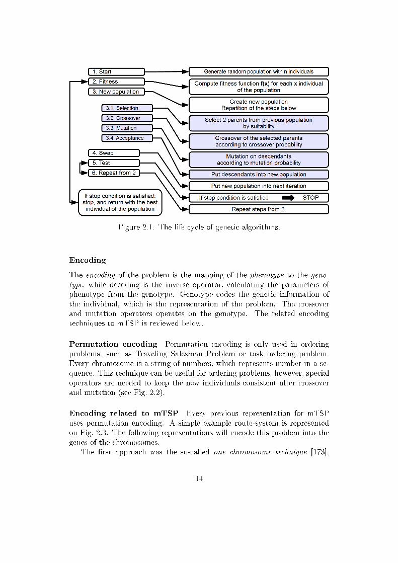
Figure 2.1. The life cycle of genetic algorithms.

Encoding

The encoding of the problem is the mapping of the phenotype to the geno-type, while decoding is the inverse operator, calculating the parameters ofphenotype from the genotype. Genotype codes the genetic information ofthe individual, which is the representation of the problem. The crossoverand mutation operators operates on the genotype. The related encodingtechniques to mTSP is reviewed below.

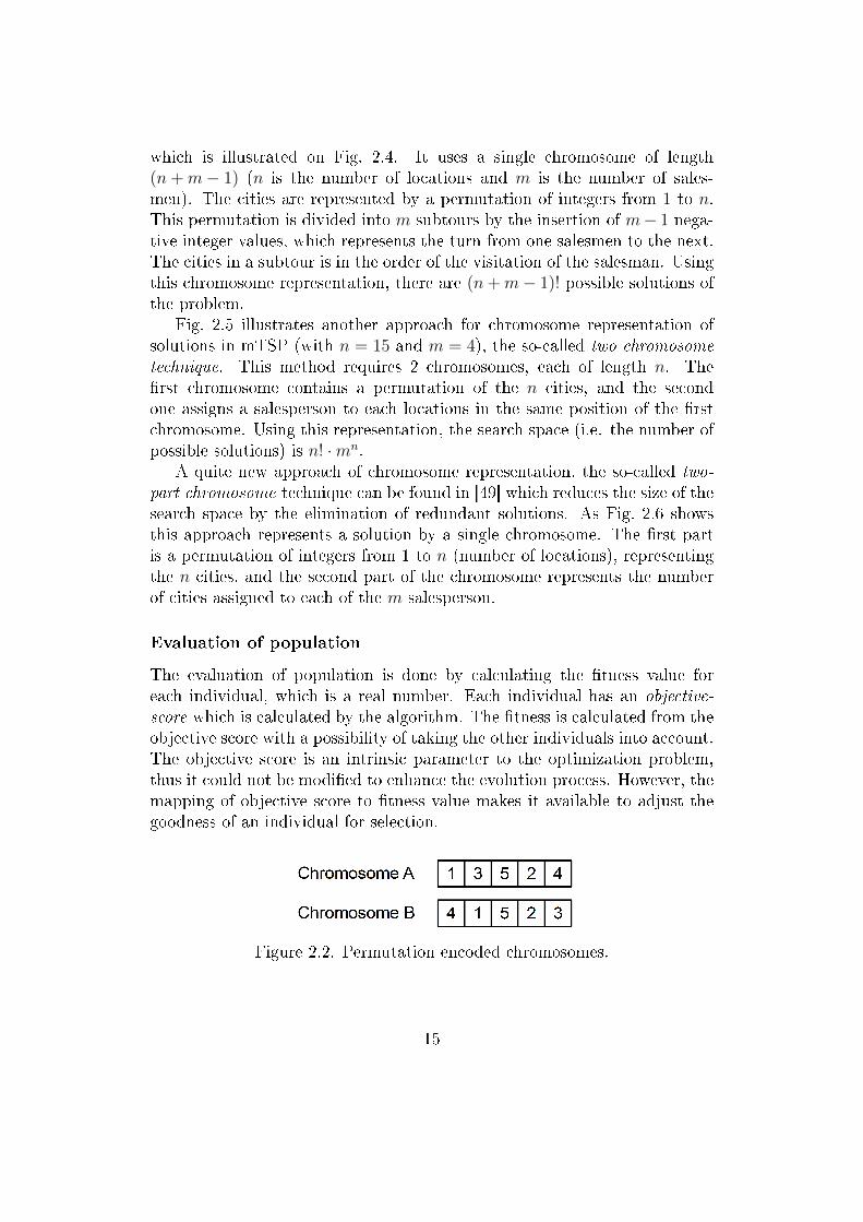
Permutation encoding Permutation encoding is only used in orderingproblems, such as Traveling Salesman Problem or task ordering problem.Every chromosome is a string of numbers, which represents number in a se-quence. This technique can be useful for ordering problems, however, specialoperators are needed to keep the new individuals consistent after crossoverand mutation (see Fig. 2.2).

Encoding related to mTSP Every previous representation for mTSPuses permutation encoding. A simple example route-system is representedon Fig. 2.3. The following representations will encode this problem into thegenes of the chromosomes.

The �rst approach was the so-called one chromosome technique [173],

14

which is illustrated on Fig. 2.4. It uses a single chromosome of length(n+m− 1) (n is the number of locations and m is the number of sales-men). The cities are represented by a permutation of integers from 1 to n.This permutation is divided into m subtours by the insertion of m− 1 nega-tive integer values, which represents the turn from one salesmen to the next.The cities in a subtour is in the order of the visitation of the salesman. Usingthis chromosome representation, there are (n+m− 1)! possible solutions ofthe problem.

Fig. 2.5 illustrates another approach for chromosome representation ofsolutions in mTSP (with n = 15 and m = 4), the so-called two chromosometechnique. This method requires 2 chromosomes, each of length n. The�rst chromosome contains a permutation of the n cities, and the secondone assigns a salesperson to each locations in the same position of the �rstchromosome. Using this representation, the search space (i.e. the number ofpossible solutions) is n! ·mn.

A quite new approach of chromosome representation, the so-called two-part chromosome technique can be found in [49] which reduces the size of thesearch space by the elimination of redundant solutions. As Fig. 2.6 showsthis approach represents a solution by a single chromosome. The �rst partis a permutation of integers from 1 to n (number of locations), representingthe n cities, and the second part of the chromosome represents the numberof cities assigned to each of the m salesperson.

Evaluation of population

The evaluation of population is done by calculating the �tness value foreach individual, which is a real number. Each individual has an objective-score which is calculated by the algorithm. The �tness is calculated from theobjective score with a possibility of taking the other individuals into account.The objective score is an intrinsic parameter to the optimization problem,thus it could not be modi�ed to enhance the evolution process. However, themapping of objective score to �tness value makes it available to adjust thegoodness of an individual for selection.

Figure 2.2. Permutation encoded chromosomes.

15

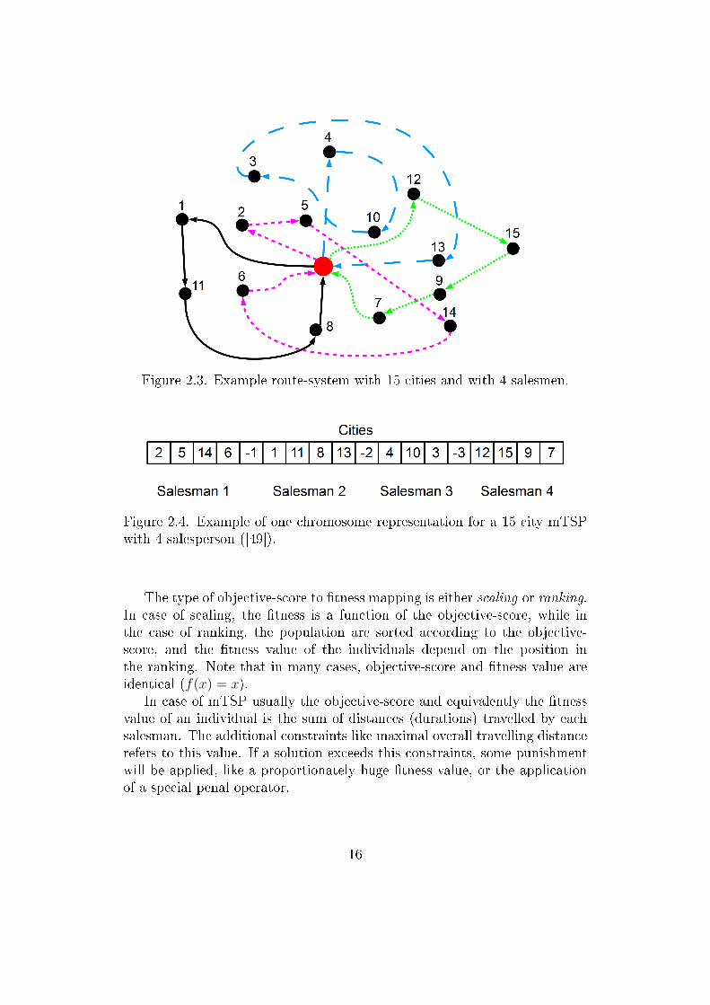
Figure 2.3. Example route-system with 15 cities and with 4 salesmen.

Figure 2.4. Example of one chromosome representation for a 15 city mTSPwith 4 salesperson ([49]).

The type of objective-score to �tness mapping is either scaling or ranking.In case of scaling, the �tness is a function of the objective-score, while inthe case of ranking, the population are sorted according to the objective-score, and the �tness value of the individuals depend on the position inthe ranking. Note that in many cases, objective-score and �tness value areidentical (f(x) = x).

In case of mTSP usually the objective-score and equivalently the �tnessvalue of an individual is the sum of distances (durations) travelled by eachsalesman. The additional constraints like maximal overall travelling distancerefers to this value. If a solution exceeds this constraints, some punishmentwill be applied, like a proportionately huge �tness value, or the applicationof a special penal operator.

16

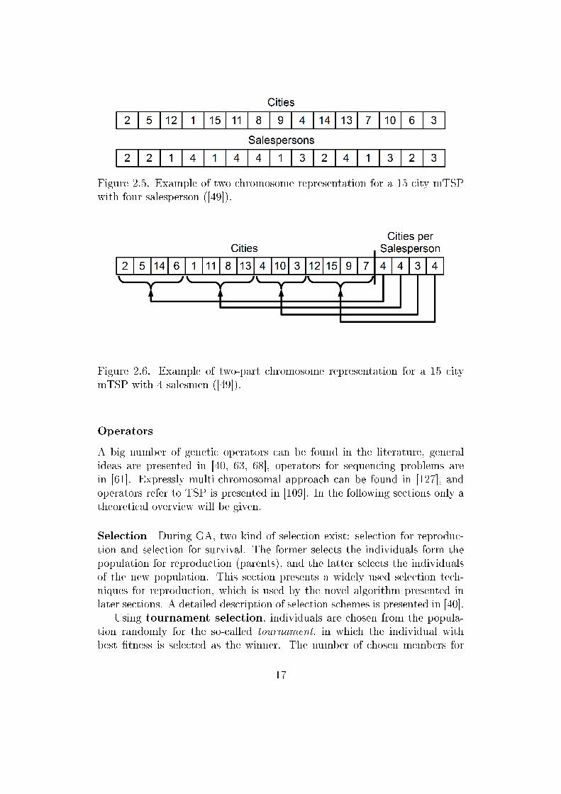
Figure 2.5. Example of two chromosome representation for a 15 city mTSPwith four salesperson ([49]).

Figure 2.6. Example of two-part chromosome representation for a 15 citymTSP with 4 salesmen ([49]).

Operators

A big number of genetic operators can be found in the literature, generalideas are presented in [40, 63, 68], operators for sequencing problems arein [61]. Expressly multi-chromosomal approach can be found in [127], andoperators refer to TSP is presented in [109]. In the following sections only atheoretical overview will be given.

Selection During GA, two kind of selection exist: selection for reproduc-tion and selection for survival. The former selects the individuals form thepopulation for reproduction (parents), and the latter selects the individualsof the new population. This section presents a widely used selection tech-niques for reproduction, which is used by the novel algorithm presented inlater sections. A detailed description of selection schemes is presented in [40].

Using tournament selection, individuals are chosen from the popula-tion randomly for the so-called tournament, in which the individual withbest �tness is selected as the winner. The number of chosen members for

17

Figure 2.7. One-, and two-point crossover of binary encoded individuals.

Figure 2.8. Mutation of binary encoded individuals.

the tournament is determined by the tournament size(t), which is between2 and µ, where µ is the size of the population. The winner can either beremoved from, or kept in the population, if it is allow or disallow to selectan individual multiple times. Tournament selection has a time complexity ofO(N). The selection pressure is adjustable by the size of the tournament.

Crossover Crossover or recombination creates new individuals from thegenes of the parents. The easiest way is the one-point crossover, which isshown on the left hand side of �gure 2.7. One crossover point is randomlyselected (the 3th gene in the example), and the two descendants are createdby interchanging the parents' genes after the crossover point. Similarly, dur-ing two-point crossover (right hand side of �gure 2.7) two crossover point israndomly selected, and the genes of the parents are interchanged before andafter the crossover points.

Mutation After crossover happened, during the mutation randomly chosengenes are selected and the operator changes their value into an other possiblevalue. An example can be seen on �gure 2.8. Mutation can prevent thealgorithm from the convergence to a local extrema. Mutation as same ascrossover largely depends on the encoding of the problem.

18

Genetic algorithms have further parameters, which could e�ects the e�-ciency of the GA. Crossover probability determines how often the crossoveroccurs. If no crossover happens, descendants will be equivalent with theirparents, otherwise the descendant will consist of the copy of the parents' ge-netic parts. If the crossover probability is 100%, every o�spring will createdby crossover, however if it is 0%, the new individuals will be the exact copyof the old population's members (note that it doesn't mean that the twopopulation is equal). It is advisable to transmit the best individuals into thenew population without any modi�cation.

Mutation probability determines how often the mutation is used on theo�springs. If no mutation happens, the o�spring will be the result of thecrossover, or of the copy. If mutation happens, some part of the chromosomewill change, in case of 100%, every descendant will change, otherwise (0%)no modi�cation will occur.

The population size de�nes the number of individuals in the population.If it is too small, the algorithm couldn't cover the whole search space. Whenpopulation size is too big, the GA will slow down.

2.2.3 A novel way to solve MTSP with GA

The proposed algorithm is based on a novel multi-chromosome representationof mTSP problem we presented recently [3]. This representation is similar tothe representation used for vehicle scheduling in [158]. However, the crossoveroperators proposed by Tavares et al. do not produce feasible children, thusadditional improvement steps have to be performed. In contrast, our op-erators always generate proper recombination, i.e. further correction is notnecessary. Therefore, in the following a short description of the used repre-sentation will be presented, and the description of novel crossover operatorswill receive the main focus. The results and analysis of a novel GA-basedalgorithm is also presented in this section. The algorithm was developed inMATLAB, and the cooperation between the web-based framework and theoptimization tool is straightforward and user-friendly.

The main motivation to use multi-chromosome genetic representationswas the recognition, that although salesmen in mTSP are separated fromeach other "physically", almost every previous solutions of mTSP with GAhas used a single chromosome to represent a whole solution, i.e. to representeach salesman like the one chromosome technique [173], the two chromosometechnique [107, 122] or the most a�ective single-chromosome one so far, theso-called two-part chromosome technique [49]. A recent novel grouping GAis used a representation very close to multi-chromosome approach [149] andthe proposed algorithm minimizes redundancy during reproduction. Singh

19

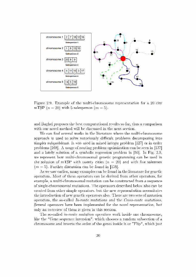
Figure 2.9. Example of the multi-chromosome representation for a 20 citymTSP (n = 20) with 5 salesperson (m = 5).

and Baghel proposes the best computational results so far, thus a comparisonwith our novel method will be discussed in the next section.

We can �nd several works in the literature where the multi-chromosomeapproach is used to solve notoriously di�cult problems decomposing intosimpler subproblems. It was used in mixed integer problem [127] or in orderproblems [168]. A usage of routing problem optimization can be seen in [137]and a lately solution of a symbolic regression problem in [50]. In Fig. 2.9,we represent how multi-chromosomal genetic programming can be used inthe solution of mTSP with twenty cities (n = 20) and with �ve salesmen(m = 5). Further discussion can be found in [158].

As we saw earlier, many examples can be found in the literature for geneticoperators. Most of these operators can be derived from other operators, forexample, a multi-chromosomal mutation can be constructed from a sequenceof single-chromosomal mutations. The operators described below also can becreated from other simple operators, but the new representation necessitatesthe introduction of new genetic operators also. There are two sets of mutationoperators, the so-called In-route mutations and the Cross-route mutations.Several operators have been implemented for the novel representation, butonly an overview of them is given in this section.

The so-called in-route mutation operators work inside one chromosome,like the "Gene sequence inversion", which chooses a random subsection of achromosome and inverts the order of the genes inside it or "Flip", which just

20

Figure 2.10. In-route mutations - "Gene sequence inversion" (upper part)and "Flip" (lower part)

Figure 2.11. Cross-route mutation - gene sequence transposition - "Swap"

swaps 2 randomly chosen genes inside a chromosome (see Fig. 2.10).A cross-route mutation operator modi�es multiple chromosomes at once.

Note that using classical nomenclature and considering chromosomes as indi-viduals, this operator could be very similar to the regular crossover operator.Fig. 2.11 illustrates the operator when randomly chosen sequences of genesfrom two chromosomes are transposed, i.e. the "Swap" operator. If one ofthe gene sequences contains zero genes, the operator is transformed into aninterpolation. "Crossover" operator is also a cross-route mutation, whichdoes a one-point crossover between two salespersons. Authors have applieda so-called "Local Optimization" operator, which is a simple TSP using ge-netic algorithm. This operator operates on each salesmen and optimizes theirroutes separately. The bene�ts of this operator will be discussed in the nextsection.

Combining simple operators like the ones in Fig. 2.11, we can create com-plex operators. Using these, the variability of the newly created individualscan be increased. Fig. 2.12 illustrates the method when two cross-route oper-ators are applied one after the other, composing a complex mutation. Firstly,a slide operator is applied, which moves the last gene from each chromosometo the beginning of another one; thereafter a gene sequence transposition or

21

Figure 2.12. Cross-route mutation - complex operator - Slide + Swap.

Swap is applied producing the new o�set.Using simple mutations to produce complex ones, a hierarchy of the op-

erators can be constructed. Fig. 2.13 shows a tree, which represents theoperators used for testing the novel representation and algorithm. Usingthese and other simple operators, much more complex ones can be gener-ated. An almost complete list of the used genetic operators can be found onour website1.

2.2.4 Numerical analysis of the proposed method

Using the multi-chromosome technique for the mTSP reduces the size of theoverall search space of the problem. Let the length of the �rst chromosomebe k1, let the length of the second be k2 and so on. Of course

∑mi=1 ki = n.

Determining the genes of the �rst chromosome is equal to the problem ofobtaining an ordered subset of k1 element from a set of n elements. There

aren!

(n− k1)!distinct assignment. This number is

(n− k1)!(n− k1 − k2)!

for the

second chromosome, and so on. So the total search space of the problem canbe formulated as equation (2.11).

n!

�����(n− k1)!

∗ �����(n− k1)!

(((((((((n− k1 − k2)!

∗ . . . ∗(((((((

(((((

(n− k1 − . . .− km−1)!(n− k1 − . . .− km)!

=n!

(n− n)!= n!

(2.11)It is necessary to determine the length of each chromosome too. It can be

represented as a positive vector of the lengths (k1, k2, . . . , km) that must sum

to n. There are

(n− 1

m− 1

)distinct positive integer-valued vectors that satisfy

this requirement [138]. Thus, the solution space of the new representation

1http://pr.mk.uni-pannon.hu/Research/eaai-mtsp/

22

Figure 2.13. The hierarchy of mutation operators. Each level indicates thenumber of simple operators used to produce the compound operator. Theacronyms used in the �gure are the following: L.O. - Local Opt. (i.e. LocalOptimization); Cr. - Crossover; Rev. - Reverse; A & B - the combineoperator, i.e. applying operator "B" after "A".

is n!

(n− 1

m− 1

). It is equal with the solution space in [49], but this approach

is more suitable to model an mTSP, so it is more problem-speci�c thereforemore e�ective, as it will be proven in following sections.

To analyze the new representation, a GA using this multi-chromosomaltechnique was developed in MATLAB, and the new method was comparedwith the best known one-chromosome approach (the two-part chromosometechnique). To make a fair comparison, we have developed two di�erent algo-rithm, both of them are based on the implementation available on MATLABCentral2. The complete actual MATLAB code of the algorithms is availableon our website.

The algorithms use two matrices as inputs, the set of coordinates of thelocations (for visualization) and the distance matrix which contains the trav-elling distances between any two cities (in kilometers or in minutes). Ofcourse, genetic parameters have to be speci�ed also, like population size,number of iterations, or the constraints for the novel algorithm. As we men-tioned earlier in Sect. 2.2.4, the depot is not presented because of complexity

2http://www.mathworks.com/matlabcentral/�leexchange/21299

23

Figure 2.14. An example from the test set, with 100 locations.

reduction. First, the initial population is generated which consist of indi-viduals containing randomly permuted genes. The �tness function simplycomputes the sum of overall route length (or duration) of each salesmen in-side an individual. The selection is tournament selection, where tournamentsize (i.e. the number of individuals who compete for survival) is 8. There-fore population size must be divisible by 8. The individual with the smallest�tness value wins the tournament, thus it will be selected for generating newindividuals, and this member will be transferred into the new populationwithout any modi�cation.

To analyze the e�ectiveness of the new representation, it was tested byseveral examples, only one is presented here in details. The example is aquite realistic problem, where the number of input locations is high enough;it contains 1 depot and 100 additional locations. The visualization of theproblem with a possible result can be seen in Fig. 2.14.

The results are presented in Fig. 2.15. The new representation was com-pared with the so-called two-part chromosome approach [49], which is thebest technique to optimize mTSP using a single chromosome so far. It is ev-ident, that two di�erent genetic algorithms can't be compared totally fairly,because the performance of these stochastic methods greatly depends on

24

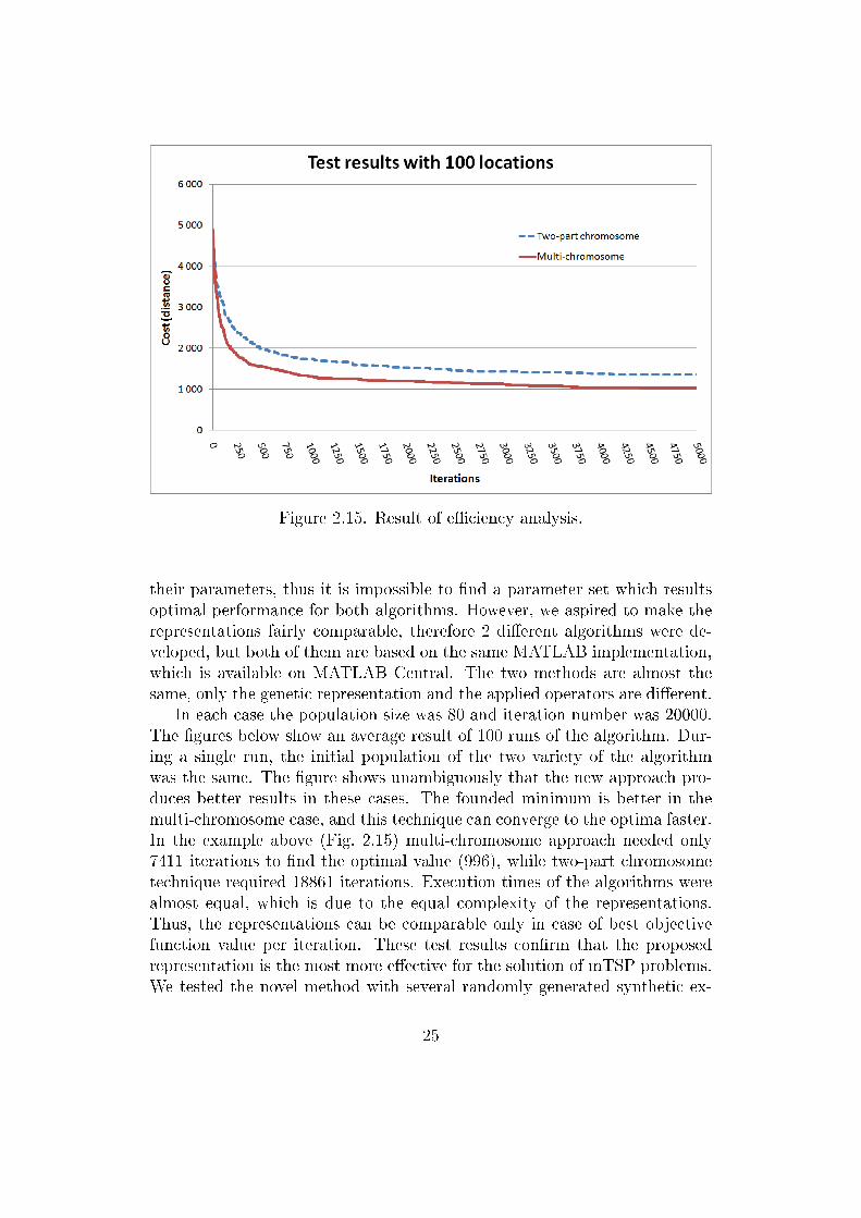
Figure 2.15. Result of e�ciency analysis.

their parameters, thus it is impossible to �nd a parameter set which resultsoptimal performance for both algorithms. However, we aspired to make therepresentations fairly comparable, therefore 2 di�erent algorithms were de-veloped, but both of them are based on the same MATLAB implementation,which is available on MATLAB Central. The two methods are almost thesame, only the genetic representation and the applied operators are di�erent.

In each case the population size was 80 and iteration number was 20000.The �gures below show an average result of 100 runs of the algorithm. Dur-ing a single run, the initial population of the two variety of the algorithmwas the same. The �gure shows unambiguously that the new approach pro-duces better results in these cases. The founded minimum is better in themulti-chromosome case, and this technique can converge to the optima faster.In the example above (Fig. 2.15) multi-chromosome approach needed only7411 iterations to �nd the optimal value (996), while two-part chromosometechnique required 18861 iterations. Execution times of the algorithms werealmost equal, which is due to the equal complexity of the representations.Thus, the representations can be comparable only in case of best objectivefunction value per iteration. These test results con�rm that the proposedrepresentation is the most more e�ective for the solution of mTSP problems.We tested the novel method with several randomly generated synthetic ex-

25

amples, varying the number of input locations, the population size and thenumber of iterations. Some of them are presented in Table 2.1. The resultsin the table present a fair comparison, while the algorithms were very simi-lar, both were implemented in MATLAB and run on the same machine. Anearly complete list of the test cases, and the algorithms are available on ourwebsite.

Table 2.1. Synthetic test results. Average of 100 runs. n: size of the problem,i.e. number of locations; m: number of salesmen; k: minimum tour length;p: population size; Opt.: best found solution (overall distance); It.: iterationnumber when the best solution found; t: running time in seconds.

n m k pTwo part ch. Multi-ch.

Opt. It. t [s] Opt. It. t [s]40 5 5 80 329 5965 29 313 2162 31100 5 5 80 1163 18861 99 996 7411 108200 10 10 480 4342 19806 859 3435 9845 1242500 5 5 240 1133 13868 218 982 5179 226500 40 20 1000 32766 39929 8853 28429 15973 11696

Table 2.1 summarizes the results of our tests using synthetic data sets.All the results presented during the paper were generated on a PC with aCore i5, 2.66 GHz processor with 3 GB of RAM. Table 2.1 shows clearly,that the novel approach can �nd solutions with smaller overall distance, andit can �nd this solution during fewer iterations. The time needed to �ndthe optima were almost identical, thus the novel approach can be consideredmore e�ective in these test cases.

Table 2.2. Test results using complex operators and initialization. Averageof 100 runs. n: size of the problem, i.e. number of locations; m: number ofsalesmen; k: minimum tour length; p: population size; Opt.: best found so-lution (overall distance); It.: iteration number when the best solution found;t: running time in seconds.

n m k pMulti-ch. & initialization Multi-ch. & complex ops.Opt. It. t [s] Opt. It. t [s]

40 5 5 80 314 1819 25 1000 2898 40100 5 5 80 320 423 130 1150 1811 583

Table 2.2 represents the results of our tests using initialization on the ini-

26

tial population, and using complex mutation operators (see Sect. 2.2.3 andFig. 2.12, Fig. 2.13). The initialization was done by a local optimizationprocess, namely a TSP on each salesmen in every individual of the popula-tion. After initialization, the simple operators were used (see the 1st row).Complex operators using Local opt. or L.O. in Fig. 2.13 apply the samemethod. Row 2 indicates the case when the optimization was done withoutthe initialization step, using the complex operators (see the 3rd level of theoperators' hierarchy in Fig. 2.13). Our tests highlight that the usage of initiallocal optimization can improve the process' accuracy and speed, while theapplication of complex operators results much stronger convergence, but itmakes the approach slower, and the accuracy is slightly worse too. Theseresult implies the necessity of initialization by local optimization (e.g. us-ing TSP solver) but indicates that we should be careful with the usage oftoo complex operators. However, because these operators can produce muchhigher variability in the population than simple ones, thus, they can producebetter results in highly complex search spaces. Of course, the selection ofproper operators may di�er from problem to problem.

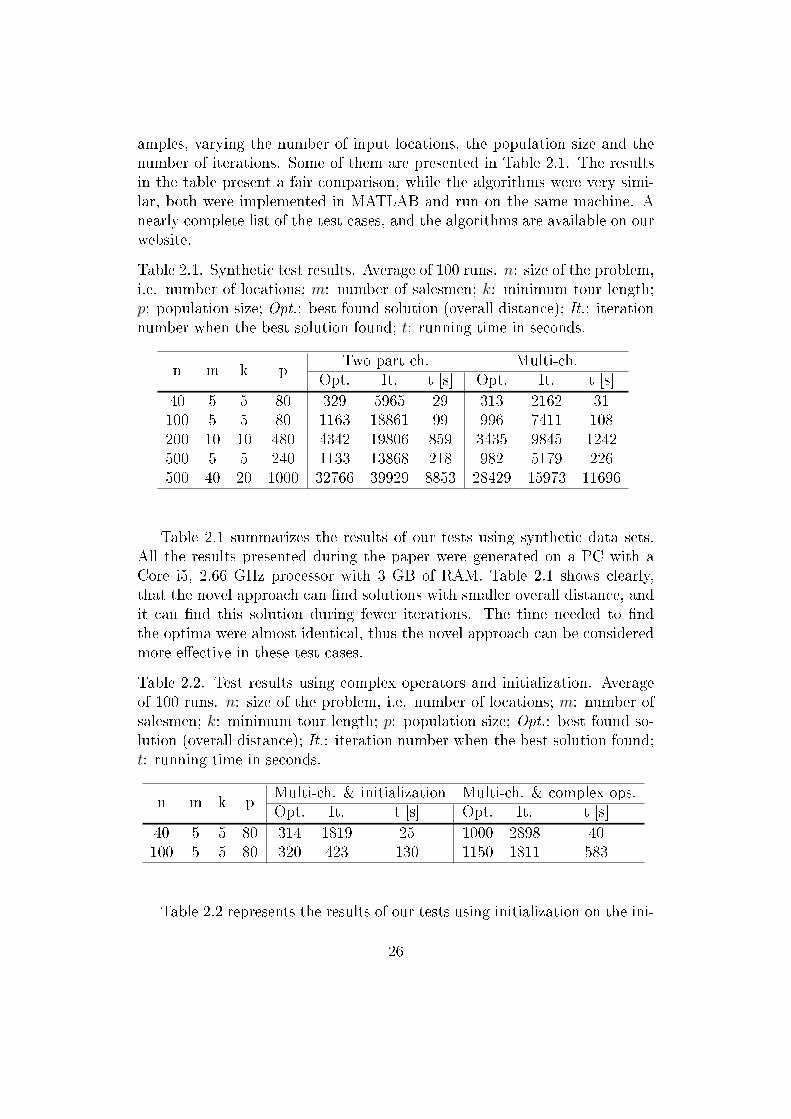
To analyze the performance and scalability of our method, further testswere performed using well-known test problems from TSPLIB [80] and thetest data of Carter and Ragsdale [49] which were used in [44] and [149]. Sincethe programming languages and the running environments di�er greatly, wedisregard the presentation of running times in the following tables.

Table 2.3 represents the tests with �ve instances of TSPLIB with increas-ing size, using 5 salesmen. Our results are compared to the Ant ColonyOptimization algorithm which was proved to perform better than GAs in[88]. Results show unambiguously that our novel method performs betterespecially in huge problems.

Table 2.3. Test results using complex operators and initialization. Averageof 10 runs. n: size of the problem, i.e. number of locations; m: numberof salesmen; l: maximum tour length; Best : best found solution (overalldistance); Avg : Average of 10 runs.

Problem n m lACO Proposed

Best Avg Best Avgpr76 76 5 20 178597 180690 158754 163424pr152 152 5 40 130953 136341 135446 144244pr226 226 5 50 167646 170877 160418 165966pr299 299 5 70 82106 83845 81959 86284pr439 439 5 100 161955 165035 135095 142214

27

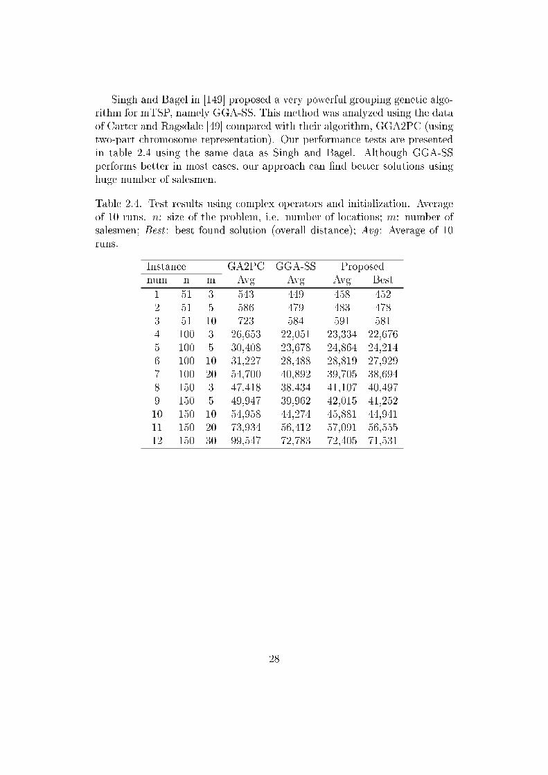
Singh and Bagel in [149] proposed a very powerful grouping genetic algo-rithm for mTSP, namely GGA-SS. This method was analyzed using the dataof Carter and Ragsdale [49] compared with their algorithm, GGA2PC (usingtwo-part chromosome representation). Our performance tests are presentedin table 2.4 using the same data as Singh and Bagel. Although GGA-SSperforms better in most cases, our approach can �nd better solutions usinghuge number of salesmen.

Table 2.4. Test results using complex operators and initialization. Averageof 10 runs. n: size of the problem, i.e. number of locations; m: number ofsalesmen; Best : best found solution (overall distance); Avg : Average of 10runs.

Instance GA2PC GGA-SS Proposednum n m Avg Avg Avg Best1 51 3 543 449 458 4522 51 5 586 479 483 4783 51 10 723 584 591 5814 100 3 26,653 22,051 23,334 22,6765 100 5 30,408 23,678 24,864 24,2146 100 10 31,227 28,488 28,819 27,9297 100 20 54,700 40,892 39,705 38,6948 150 3 47,418 38,434 41,107 40,4979 150 5 49,947 39,962 42,015 41,25210 150 10 54,958 44,274 45,881 44,94111 150 20 73,934 56,412 57,091 56,55512 150 30 99,547 72,783 72,405 71,531

28

2.3 A Google Maps based framework developedto utilize the proposed algorithm

We will present a complete methodology in this section, which demonstratesa novel component-based framework using web technologies and MATLAB.An application study will be presented in the next section which will guide thereader trough an industrial project from the de�nition of the problem to thevisualization of results. The web-based framework presented in this sectionrelies heavily on the Google Maps API, which is unique in the literature sofar.

Based on the novel genetic representation, we have developed a novelalgorithm, which is capable to optimize the traditional mTSP problems, fur-thermore, it can handle the additional constraints and time windows (seeSect. 2.2.1). The algorithm can minimize the number of salesmen includedin the solution also, considering their initial cost. In this section we passesover the presentation of source codes; the whole MATLAB implementationof the algorithm is accessible on our website. Note that the penalizationof routes exceeding constraints is realized as a split using the chromosomepartition operator [3] instead of the assignment of proportionally high �tnessvalue. Since the algorithm minimizes the number of salesmen involved, thispenalty has a remarkable e�ect on the optimization process. Furthermore,the algorithm can handle the constraints for the routes and the time windowsfor the locations too, and we adjudge that the applied representation is moresimilar for the characteristic of the problem than the ones until now, thus itcan be more easily understandable and realizable.

The problem itself which has motivated this research can be addressedas an mTSP problem, which should be solved by an automated system. Aschematic �owchart of such a system is represented in Fig. 2.16. The baselineshould be a map (e.g. de�ned on Google Maps) and the distances betweenthe locations can be calculated by a web based service like Google Maps.Since in the real application, the amount of goods delivered is much lessthan the capacity of vehicles, the volume or mass constraints can be ignored(which de�nes the problem as mTSP instead of VRP). The result of thesystem has to be a route plan which can be de�ned on a web-based mapor on a GPS Device. The calculation of cost, time and material �ows arealso necessary. we decided to use the free and publicly available GoogleMaps API, because it provides a fast and reliable web-service for de�ninguser-friendly maps, computing traveling distances and time, and visualizingroutes. Furthermore, it is the most used mapping service nowadays.

Based on Google's services, we have developed a complete and automated

29

Figure 2.16. The work�ow of the desired application

framework to provide an automated system like in Fig. 2.16. By the helpof this program, users are capable of optimize an mTSP problem de�ned ona Google Maps map in a few minutes, and the result of the computationis visualized in a really easily interpretable way. A complete example willclarify these statements in the next section.

In Fig. 2.17 the component diagram of the proposed solution is illus-trated. First of all, a de�nition of input data (Map) is needed. This �rstobject on the �gure represents the determination of locations on a GoogleMaps map. We have chosen the service of Google Maps, because it is oneof the most common worldwide and it o�ers a reliable API. The secondcomponent (Coordinates Retrieval) provides a handy automatic tool for theretrieval of longitude and latitude values of the locations on the Map. Dis-tance Table component involves the computation of distances and durationbetween each pair of locations and uses the data determined by the previouscomponent. The next step is the determination of optimal routes (RoutePlanning Algorithm) which is presented by the proposed GA discussed ear-lier. This component requires the distance table provided by the previouscomponent and the parameters of the GA. Leaving aside the technical de-tails, it should be mentioned that the computation behind this componentis done by the MATLAB Webserver running in background, which can getthe parameters and send back the result over HTTP protocol. Thus, userscan manage the optimization in their browser window. The last component(Visualiser) is a visualizer, which can show the resulted routes in an easilyinterpretable form on a Google Maps map, and computes the overall costs ofroutes using prede�ned parameters, like per km cost or wage of the driver.

The presented method implements a novel approach in all stages, i.e. thecoordinates retrieval from a Google Maps, the distance table calculation, theoptimization and the visualization are all automated processes, which make

30

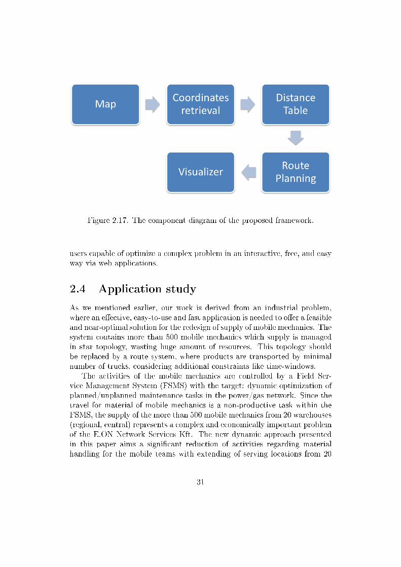
Figure 2.17. The component diagram of the proposed framework.

users capable of optimize a complex problem in an interactive, free, and easyway via web applications.

2.4 Application study

As we mentioned earlier, our work is derived from an industrial problem,where an e�ective, easy-to-use and fast application is needed to o�er a feasibleand near-optimal solution for the redesign of supply of mobile mechanics. Thesystem contains more than 500 mobile mechanics which supply is managedin star topology, wasting huge amount of resources. This topology shouldbe replaced by a route system, where products are transported by minimalnumber of trucks, considering additional constraints like time-windows.

The activities of the mobile mechanics are controlled by a Field Ser-vice Management System (FSMS) with the target: dynamic optimization ofplanned/unplanned maintenance tasks in the power/gas network. Since thetravel for material of mobile mechanics is a non-productive task within theFSMS, the supply of the more than 500 mobile mechanics from 20 warehouses(regional, central) represents a complex and economically important problemof the E.ON Network Services Kft. The new dynamic approach presentedin this paper aims a signi�cant reduction of activities regarding materialhandling for the mobile teams with extending of serving locations from 20

31

to 100. The design of the supply system can be considered as a complexcombinatorial optimization problem, where the goal is to �nd a route planwith minimal route cost, which services all the demands from three centralwarehouses while satisfying other constraints like time windows.

In this section every steps of the methodology will be presented duringa solution of the problem motivated our research. The necessity of the opti-mization is presented in Fig. 2.18. The company has a star topology whichmeans that a truck transports the required materials from the Central De-pot to the Warehouses, while mechanics at the Bases transport the materialsfrom the Warehouse to the bases. This topology produces high operationalcosts, thus the company wanted to replace this supply system with one truckwhich can serve the Warehouse and all the Bases with necessary materials.

Figure 2.18. Schematic view of the current status and the desired solutionof the industrial problem. CD - Central Depot, WH - Warehouse, B - Base

We have developed a complete software package to solve this type of op-timization problems. The input data is given by a Google Maps map, whichcontains the locations (with the depot) and the �nal output is a route systemde�ned by a Google Maps map also. A complete, automated solution is freelyavailable at our website3 as a web-based service. However, it should be men-tioned that for the sake of reducing the load on our server, this applicationprovides only a demo, where the number of input locations is maximized by10. IT development is planned in the near future in our department, whenthis restriction can be removed. Thus, the real project was optimized byan o�ine genetic algorithm written in MATLAB. In the following section,we will demonstrate the optimization of the industrial problem, however,only representative locations are shown (which are really close to the realsituation).

3http://193.6.44.35/gmaps/

32

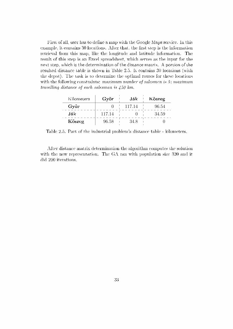
First of all, user has to de�ne a map with the Google Maps service. In thisexample, it contains 30 locations. After that, the �rst step is the informationretrieval from this map, like the longitude and latitude information. Theresult of this step is an Excel spreadsheet, which serves as the input for thenext step, which is the determination of the distance matrix. A portion of theresulted distance table is shown in Table 2.5. It contains 30 locations (withthe depot). The task is to determine the optimal routes for these locationswith the following constraints: maximum number of salesmen is 5 ; maximumtravelling distance of each salesman is 450 km.

Kilometers Gyõr Ják Kõszeg

Gyõr 0 117.14 96.54

Ják 117.14 0 34.59

Kõszeg 96.58 34.8 0

Table 2.5. Part of the industrial problem's distance table - kilometers.

After distance matrix determination the algorithm computes the solutionwith the new representation. The GA ran with population size 320 and itdid 200 iterations.

33

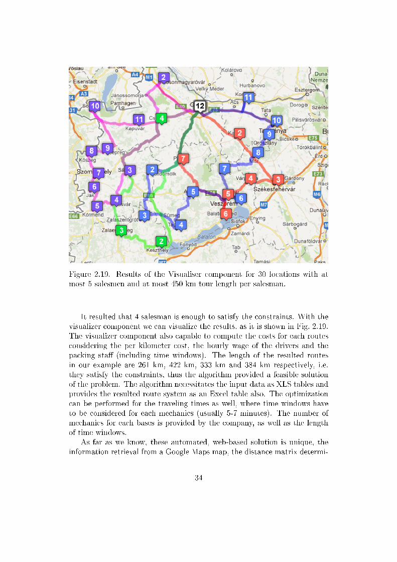
Figure 2.19. Results of the Visualiser component for 30 locations with atmost 5 salesmen and at most 450 km tour length per salesman.

It resulted that 4 salesman is enough to satisfy the constraints. With thevisualizer component we can visualize the results, as it is shown in Fig. 2.19.The visualizer component also capable to compute the costs for each routesconsidering the per kilometer cost, the hourly wage of the drivers and thepacking sta� (including time windows). The length of the resulted routesin our example are 261 km, 422 km, 333 km and 384 km respectively, i.e.they satisfy the constraints, thus the algorithm provided a feasible solutionof the problem. The algorithm necessitates the input data as XLS tables andprovides the resulted route system as an Excel table also. The optimizationcan be performed for the traveling times as well, where time windows haveto be considered for each mechanics (usually 5-7 minutes). The number ofmechanics for each bases is provided by the company, as well as the lengthof time windows.

As far as we know, these automated, web-based solution is unique, theinformation retrieval from a Google Maps map, the distance matrix determi-

34

nation and the automated optimization process are all novel tools, as well asthe applied algorithm behind the scenes or the visualizer components, whichcan draw the resulted routes one after the other.

2.5 Conclusions

Since the travel for material of mobile mechanics is a non-productive task, anovel approach presented in this paper for the optimization of serving loca-tions to reduce the activities related to material handling. A modi�ed mTSPwith additional constraints was introduced and solved by a novel approach.The complexity of the motivating problem implied the introduction of a novelgenetic algorithm using novel crossover operators for multi-chromosome indi-vidual representation, where a separate chromosome is assigned to all sales-men. The approach presented here is innovative in the reproduction of indi-viduals, in the handling of the constraints, and it gives a whole methodologyand a novel complete framework to solve an NP-hard problem, the mTSPTW.Beside the proposed methodology the paper presented the developed tool uti-lizes Google Maps to visualize the supply structure and collect raw data usedfor optimization. The new dynamic approach resulted signi�cant reductionof activities regarding material handling for the mobile teams by extendingof serving locations from 20 to 100.

The application of the novel tool containing the optimization process andthe web-based framework in a real industrial problem's solution justi�ed thenecessity of the research. E.ON Hungária Zrt. already applied the pro-posed tool. Preliminary economic calculations and experiences show thatthe implementation resulted signi�cant savings while the quality of servicealso improved.

35

Chapter 3

Monte Carlo simulation based

optimization and analysis of

inventory management systems

As we saw in the previous chapter, using more realistic representation orreal data for distances, i.e. modeling the real problem closer to reality cangreatly improve the performance and goodness of optimization processes.Following this way, a Monte Carlo simulation based method is presented inthis chapter, where empirical distribution functions are used modeling theconsumption and orders in warehouses. Illustrating the capabilities of thesimulation, a gradient-based optimization method will be presented, followedby a novel and more e�ective Particle Swarm Optimization algorithm. Anovel sensitivity analysis is also presented here providing easily interpretablerepresentation of connections between changes of input and output variables,which proposes an e�ective decision support tool.

3.1 Introduction

Supply chain management (SCM) is a major component of competitive strat-egy to improve organizational competitiveness and pro�tability [52]. The lit-erature on SCM that deals with methodologies and technologies for e�ectivelymanaging a supply chain is vast. In recent years, the performance measure-ment, evaluation and metrics have received much attention from researchersand practitioners [129]. E�ective supply chain management comprises thefollowing main functions: setting objectives, evaluating performance, anddetermining future courses of actions [54]. Setting objectives and creatingpredictive tools to create alternative course of actions play a very important

36

role in the success of an organization and they a�ect the strategic, tacticaland operational planning and control.

In the last decades, optimization was featured in almost all aspects ofhuman civilization, thus it has truly become an indispensable method. Insome aspects, even a local optima can highly improve the e�ciency or reducethe expenses, however, most companies want to keep their operational costsas low as possible, i.e. on global minimum. Problems where solutions mustsatisfy a set of constraints are known as constrained optimization problems.In inventory control theory, one of the most important and most strict con-straints is the service level, i.e. the portion of satis�ed demands from allcustomer needs.

In this chapter a novel framework is presented to promote a better under-standing of how an integrated approach works and how it can improve theoverall e�ectiveness of the supply chain and the organization as a whole. Thestructure of the chapter is the following: �rstly, a literature review and sometheoretical background about inventory management is presented; then thedescription of our stochastic model and the novel simulator is given, whichis followed by the discussion of Monte Carlo method; in the main part ofthe chapter, the multi-echelon inventory model is presented as well as twooptimization methods to solve the problem; the last part deals with keyperformance indicators and provides a novel sensitivity analysis technique.

3.2 Determining optimal safety stock level inmulti-echelon supply chains

The research of inventory management or the investigation of supply chain iswidespread in the scienti�c literature. It is a seriously researched area sincethe �fties; Simpson [86] was the �rst one who formulated the serial-line in-ventory problem. Graves and Willems extended Simpsons work to spanningtrees in [70], while in [71] they give a comprehensive review of the previ-ous approaches for safety stock placement, the same as they propose twogeneral approaches and introduce the supply chain con�guration problem.There exist good overviews in the literature for supply chain and inventorymanagement, like in [112], where authors give an overview of di�erent ap-proaches of supply chain modeling, and outline future opportunities. In [97]Lau et al. give an overview of various average inventory level (AIL) expres-sions and presents two novel expressions which are simpler and more accuratethan previous ones. A comprehensive overview can be found in [116], whereMusalem and Dekkers consider several types of inventory policies and present

37

a simulation model for a real problem with lost sales.The determination of safety stock in an inventory model is one of the

key actions in the management. Miranda and Garrido include both cycleand safety stock in the inventory model in [113], and the resulting modelhas a non-linear objective function. Graves and Willems in [72] gives amodel for positioning safety stock in a supply chain subject to non-stationarydemand, and they show how to extend their former model to �nd the optimalplacement safety stocks under constant time service (CST) policy. Prékopa in[132] gives an improved model for the so called Hungarian inventory controlmodel to �nd the minimal safety stock level that ensures the continuousproduction, without disruption.

The bullwhip e�ect is an important phenomenon in supply chains, Dra-gana et al. in [106] show how a supply chain can be modeled and analyzed bycolored petri nets (CPN). Using CPN tools they evaluate the bullwhip e�ect,the surplus of inventory goods, etc. using the beer game as demonstration.More recent research can be found in [48], which shows that a mature orderpolicy applied to a serial single-product supply chain with four echelons canreduce the bullwhip e�ect and inventory oscillation, or an ine�cient one canamplify them.

Miranda et al. investigate the modeling of a two echelon supply chainsystem and optimization in two steps [114], while a massive multi-echeloninventory model is presented by Seo [147], where an order risk policy forgeneral multi-echelon system is given, which minimizes the system operationcost. A really complex system is examined in [152], where it is necessaryto apply some clustering for similar items, because detailed analysis couldbecome impossible considering each item individually.

Simulation-based approaches were published only in the last decade. Junget al. [87] make a Monte Carlo based sampling from real data, and apply asimulation-optimization framework while looking for managing uncertainty.They use a gradient-based search algorithm, while authors in [93] discusshow to use simulation to describe a �ve-level inventory system, and optimizethis model by genetic algorithm. Schwartz et al. [146] demonstrate the in-ternal model control (IMC) and model predictive control (MPC) algorithmsto manage inventory in uncertain production inventory and multi-echelonsupply/demand networks. The stability of the supply chain is also a seri-ously researched area recently, [117] shows that a linear supply chain can bestabilized by the anticipation of the own future inventory and by taking intoaccount the inventories of other suppliers. Vaughan in [160] presents a linearorder point/lot size model that with its robustness can contribute to businessprocess modeling.

38

A complex instance of inventory model can be found in [79], where orderscross in time considering various distributions for the lead time. Sakaguchi in[141] investigates the dynamic inventory model in which demands are discreteand varying period by period.

Based on the previous review it is clear that most of the multi-echelonsupply chain optimization and analysis are based on analytical approaches.However, Simulation however provides a very good alternative, because it canmodel real life situations accurately. Simulation methods are �exible for in-put parameters, therefore they are easily applicable in decision support. Theresults of simulation can be analyzed with various statistical methods andnumerical optimization algorithms. To analyze complex, especially multi-echelon systems, multi-level simulation models has to be used, where thedetailed models at lower level are fed by the result of the optimized modelsat higher level. We will discuss the main aspects of inventory models in thefollowing subsection.

3.2.1 Classic inventory model of a single warehouse

The modular model of the supply chain is based on the following classic modelof inventory control. This subsection gives a summary of the most importantparameters of this model. In Fig. 3.1, Replenishment Lead time (L) is thetime between the purchase order and the goods receipt, and dL denotes theaverage demand during L. This average demand can be computed as dL =d · L, where d is the daily average demand. Using the same logic dL is thetotal demand over lead time. When service level is 100%, dL will equal toconsumption. We will use dL to denote the consumption during the section.Q is the theoretical demand over cycle time T which is the Order Quantityalso; R is the Reorder point, which is the maximum demand can be satis�edduring the replenishment lead time (L). The Cycle time (T ) is the timebetween two purchase orders. Q = d · T , which is the ordered quantity in apurchase order, and Q is equal to the expected demand and the maximumstock level. Maximum stock level is the stock level necessary to cover theexpected demand in period T ; therefore it has to be the quantity we order.Reorder point is the stock level when the next purchase order has to be issued.It is used for materials where the inventory control is based on actual stocklevels. S is the Safety stock, which is needed if the demand is higher thanthe expected (line d). In an ideal case R equals to sum of safety stock andaverage demand over lead time: R = dL + S, where S is the Safety stockwhich is de�ned to cover the stochastic demand changes. For a given ServiceLevel this is the maximum demand which can be satis�ed over the Lead time.

Assuming constant demand pattern over the cycle time, Average Stock

39

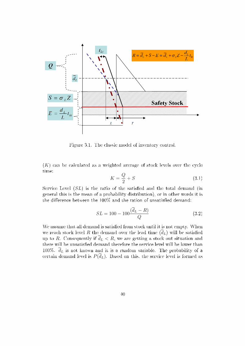
Figure 3.1. The classic model of inventory control.

(K) can be calculated as a weighted average of stock levels over the cycletime:

K =Q

2+ S (3.1)

Service Level (SL) is the ratio of the satis�ed and the total demand (ingeneral this is the mean of a probability distribution), or in other words it isthe di�erence between the 100% and the ration of unsatis�ed demand:

SL = 100− 100(dL −R)

Q(3.2)

We assume that all demand is satis�ed from stock until it is not empty. Whenwe reach stock level R the demand over the lead time (dL) will be satis�edup to R. Consequently if dL < R, we are getting a stock out situation andthere will be unsatis�ed demand therefore the service level will be lower than100%. dL is not known and it is a random variable. The probability of acertain demand level is P (dL). Based on this, the service level is formed as

40

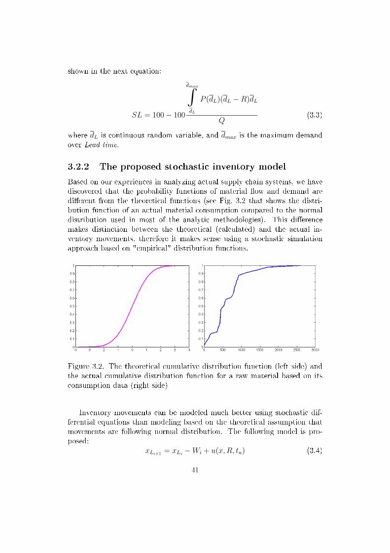
shown in the next equation:

SL = 100− 100

dmax∫dL

P (dL)(dL −R)dL

Q(3.3)

where dL is continuous random variable, and dmax is the maximum demandover Lead time.

3.2.2 The proposed stochastic inventory model

Based on our experiences in analyzing actual supply chain systems, we havediscovered that the probability functions of material �ow and demand aredi�erent from the theoretical functions (see Fig. 3.2 that shows the distri-bution function of an actual material consumption compared to the normaldistribution used in most of the analytic methodologies). This di�erencemakes distinction between the theoretical (calculated) and the actual in-ventory movements, therefore it makes sense using a stochastic simulationapproach based on "empirical" distribution functions.

Figure 3.2. The theoretical cumulative distribution function (left side) andthe actual cumulative distribution function for a raw material based on itsconsumption data (right side)

Inventory movements can be modeled much better using stochastic dif-ferential equations than modeling based on the theoretical assumption thatmovements are following normal distribution. The following model is pro-posed:

xLi+1= xLi

−Wi + u(x,R, tu) (3.4)

41

where xi is stock level on the ith week, Wi is a stochastic process representingconsumption. This stochastic process is based on the empirical cumulativedistribution function we described in the previous section. u is the quantityof material received on week i, based on purchase orders. Purchase ordersare calculated based on the actual inventory level (x), and the replenishmentlead-time (tu).

Handling uncertainty

Monte Carlo Simulation (MCS ) is frequently applied in various areas [139]).This tool has also been proven its e�ciency in risk related optimization ofchemical processes, e.g. it is applied in optimizing maintenance strategies ofoperating processes [41]. There is a common characteristic in these solutions:the stochastic nature of the studied system has to be modeled. In the ap-plied methodology this simulation is related to the modeling of unmeasureddisturbances of the control loops. To handle this random e�ect, Monte-Carlosimulation is applied with the characterized noise.

MCS methods are highly applied in the mathematical modeling problemswhere some kind of stochastic phenomena must be handled. In the proposedmultilayer optimization framework process variance caused by unmeasureddisturbances is considered. The Monte Carlo simulation consists of the fol-lowing steps:

1. De�ne the domain of possible inputs.

2. Generate inputs from this domain randomly using a speci�ed probabil-ity distribution.

3. Execute deterministic computation using the inputs.

4. Aggregate the results of the computations into the �nal result.

In engineering practice normal distribution is considered as an adequateassumption for characterizing uncertainties. At the modeling of the con-sidered process the following steps are followed: at �rst the mathematicalmodel of the process is created. Then noise and unmeasured disturbancesof the control loops are characterized and random signals related to the realprocess variance are added to the corresponding input and output variables.The value of the economic objective function is calculated by aggregating theresults of the individual Monte Carlo runs into a statistical economic per-formance. Since complex production processes are mostly characterized bynon-linear process models the economic assessment and optimization needsan optimization algorithm which is able to handle the non-linear cost func-tions and constraints.

42

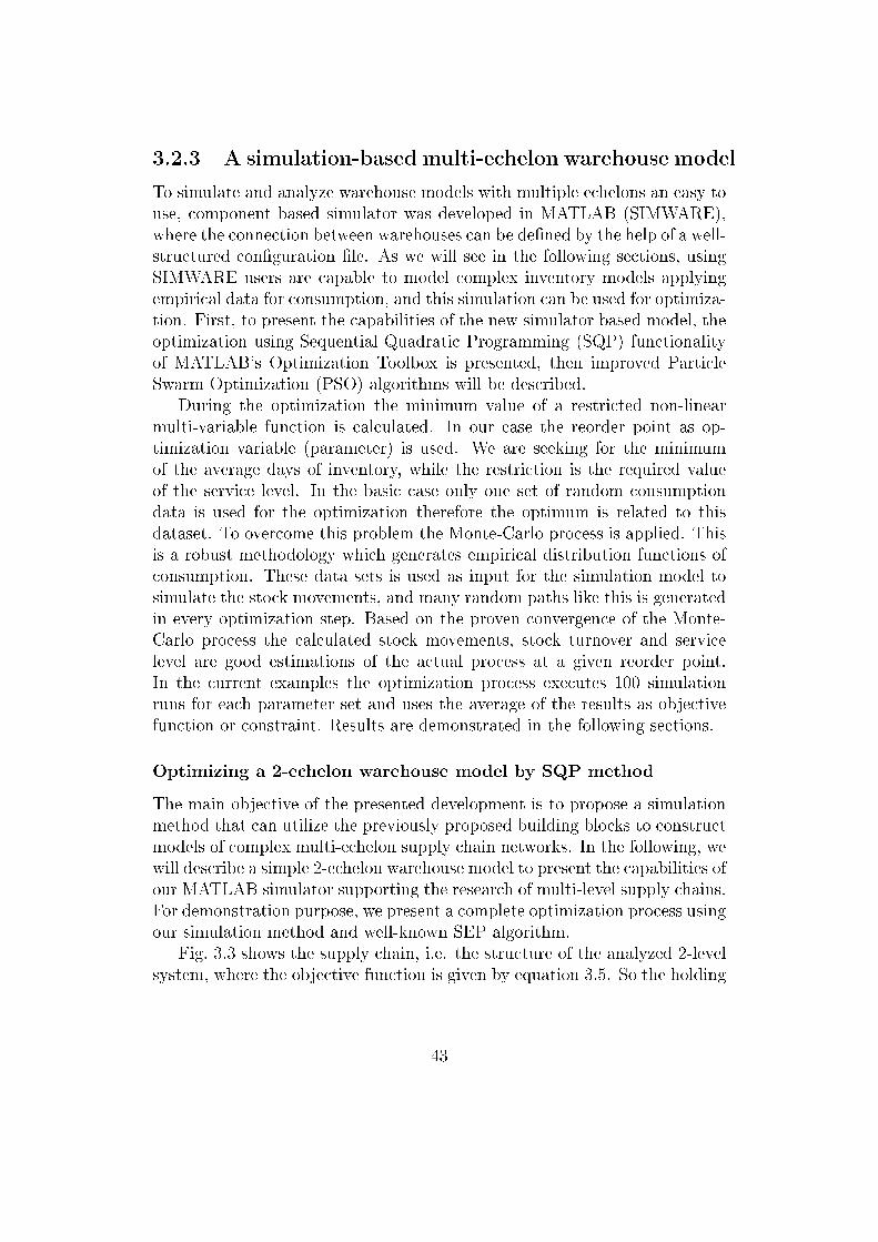
3.2.3 A simulation-based multi-echelon warehouse model

To simulate and analyze warehouse models with multiple echelons an easy touse, component based simulator was developed in MATLAB (SIMWARE),where the connection between warehouses can be de�ned by the help of a well-structured con�guration �le. As we will see in the following sections, usingSIMWARE users are capable to model complex inventory models applyingempirical data for consumption, and this simulation can be used for optimiza-tion. First, to present the capabilities of the new simulator based model, theoptimization using Sequential Quadratic Programming (SQP) functionalityof MATLAB's Optimization Toolbox is presented, then improved ParticleSwarm Optimization (PSO) algorithms will be described.

During the optimization the minimum value of a restricted non-linearmulti-variable function is calculated. In our case the reorder point as op-timization variable (parameter) is used. We are seeking for the minimumof the average days of inventory, while the restriction is the required valueof the service level. In the basic case only one set of random consumptiondata is used for the optimization therefore the optimum is related to thisdataset. To overcome this problem the Monte-Carlo process is applied. Thisis a robust methodology which generates empirical distribution functions ofconsumption. These data sets is used as input for the simulation model tosimulate the stock movements, and many random paths like this is generatedin every optimization step. Based on the proven convergence of the Monte-Carlo process the calculated stock movements, stock turnover and servicelevel are good estimations of the actual process at a given reorder point.In the current examples the optimization process executes 100 simulationruns for each parameter set and uses the average of the results as objectivefunction or constraint. Results are demonstrated in the following sections.

Optimizing a 2-echelon warehouse model by SQP method

The main objective of the presented development is to propose a simulationmethod that can utilize the previously proposed building blocks to constructmodels of complex multi-echelon supply chain networks. In the following, wewill describe a simple 2-echelon warehouse model to present the capabilities ofour MATLAB simulator supporting the research of multi-level supply chains.For demonstration purpose, we present a complete optimization process usingour simulation method and well-known SEP algorithm.

Fig. 3.3 shows the supply chain, i.e. the structure of the analyzed 2-levelsystem, where the objective function is given by equation 3.5. So the holding

43

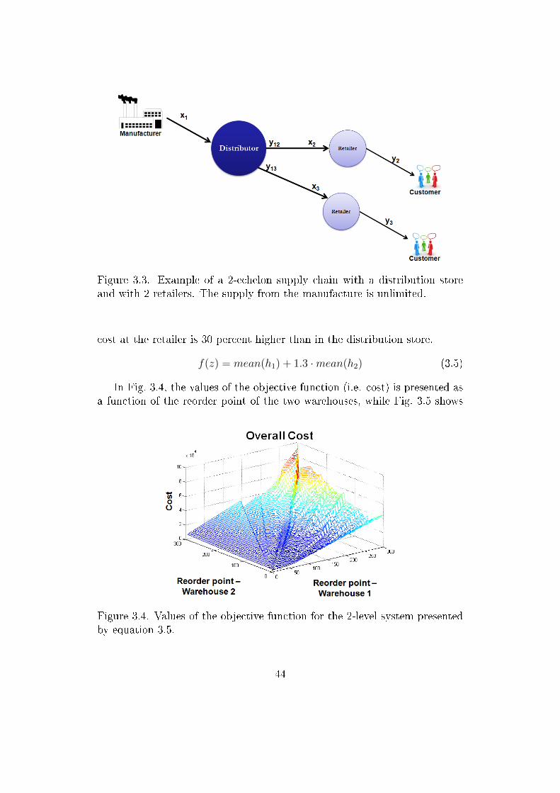
Figure 3.3. Example of a 2-echelon supply chain with a distribution storeand with 2 retailers. The supply from the manufacture is unlimited.

cost at the retailer is 30 percent higher than in the distribution store.

f(z) = mean(h1) + 1.3 ·mean(h2) (3.5)

In Fig. 3.4, the values of the objective function (i.e. cost) is presented asa function of the reorder point of the two warehouses, while Fig. 3.5 shows

Figure 3.4. Values of the objective function for the 2-level system presentedby equation 3.5.

44

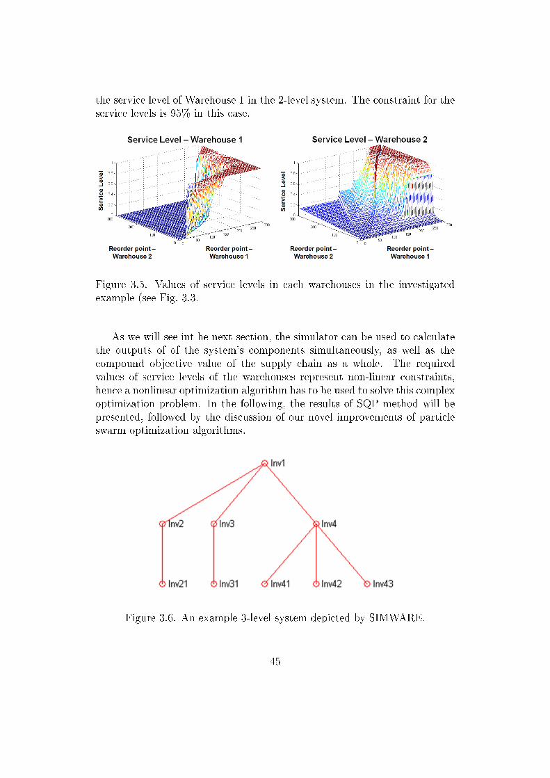
the service level of Warehouse 1 in the 2-level system. The constraint for theservice levels is 95% in this case.

Figure 3.5. Values of service levels in each warehouses in the investigatedexample (see Fig. 3.3.

As we will see int he next section, the simulator can be used to calculatethe outputs of of the system's components simultaneously, as well as thecompound objective value of the supply chain as a whole. The requiredvalues of service levels of the warehouses represent non-linear constraints,hence a nonlinear optimization algorithm has to be used to solve this complexoptimization problem. In the following, the results of SQP method will bepresented, followed by the discussion of our novel improvements of particleswarm optimization algorithms.

Figure 3.6. An example 3-level system depicted by SIMWARE.

45

In the SIMWARE program, users have to de�ne the structure of theproblem, i.e. the connection between the warehouses. The parameters ofeach warehouse has to be de�ned also, e. g. the lead time or the averagedemand for a product as well as the cost values, like the holding cost. Fig. 3.6represents an example for a 3-level system de�ned by the con�guration �leinside the simulator.

Fig. 3.7 represents the results of the simulation for a 3-level inventorymodel, where each inventory level is depicted by lines with di�erent style.

Figure 3.7. Simulated inventory levels of the 3-level multi-echelon systempresented in Fig. 3.6.

Note that we have used separate distribution functions for the centralwarehouse and the other regional warehouses to simulate the consumption.We constructed these distribution functions based on actual data. The cen-tral warehouse consumption �gures are calculated as a total of the down-stream warehouse consumptions. Using di�erent distribution functions in a

46

multi-echelon supply chain, or using di�erent consumption values for eachwarehouse is not a trivial, but necessary task if we want to construct a morerealistic model or simulator. The SIMWARE program o�ers an easy-to-useinterface to build even complex supply chains, and propose a novel componentbased structure. Using this program, users can easily optimize their supplychain by an optimization method (e.q. SQP), but the proposed methodologygives a chance to use more e�ective optimization algorithms also.

Fig. 3.8 shows the result of the optimization using the SQP method. Here,the constraint for service level was 95% in each warehouse. The optimalsolution is highlighted with the green square, which satis�es the constraintsand ensures the minimal holding cost in the warehouses. The result of thesimulation runs is presented in Fig. 3.9. The �uctuations in the averageinventory levels after ten MC simulations are shown, and the investigatedperiod is 50 weeks. The service levels of both warehouses are determined,they are 0.97 and 0.89, respectively. After the optimization, the adjustedparameters make sure that none of the warehouses running out of stockduring the investigated period.

Figure 3.8. Result of the optimization of the 2-echelon system using SQPmethod.

47

Figure 3.9. Inventory levels in the optimized 2-level system.

3.2.4 Particle Swarm Optimization Algorithms

In this section, the concept of Particle Swarm Optimization (PSO) algo-rithms is presented, which is followed by the discussion of the proposed novelmodi�cations of PSO in the next sections, which have bene�cial e�ects onconvergence.

There are two popular swarm inspired methods in computational intel-ligence areas: Ant colony optimization (ACO) and PSO. ACO was inspiredby the behaviors of ants and has many successful applications in discrete op-timization problems. The particle swarm concept originated as a simulationof simpli�ed social system. The original intent was to graphically simulatethe choreography of a bird block or �sh school. However, it was found thatparticle swarm model can be used as an optimizer. Suppose the followingscenario: a group of birds are randomly searching food in an area. There isonly one piece of food in the area being searched. All the birds do not know

48

where the food is. But they know how far the food is in each iteration. Sowhat's the best strategy to �nd the food? The e�ective one is to follow thebird which is nearest to the food.

PSO is based on this scheme. This stochastic optimization technique hasbeen developed by Eberhart and Kennedy in 1995 [91]. In PSO, the potentialsolutions, called particles, �y through the problem space by following thecurrent optimum particles. All of the particles have �tness values which areevaluated by the �tness function to be optimized, and have velocities whichdirect to the �ying of the particles. PSO is initialized with a group of randomparticles (solutions) and then searches for optima by updating generations.In every iteration, each particle is guided by two "best" values. The �rst oneis the best solution (�tness) it has achieved so far. (The �tness value is alsostored.) This value is called pBest. Another "best" value that is trackedby the particle swarm optimizer is the entire swarm's best known positionso far. This value is the current global optima and called gBest. When aparticle takes part of the population as its topological neighbors, the bestvalue is a local best and is called lBest.

vj(k + 1) = w · vj(k) + c1 · rand() · (xpBest − xj(k)) + (3.6)

c2 · rand() · (xgBest − xj(k))

xj(k + 1) = xj(k) + vj(k + 1) · dt (3.7)

where v is the particle velocity, pBest and gBest are de�ned as stated before,rand() is a random number from [0, 1], c1, c2 are learning factors usuallyc1 = c2 = 2. Algorihm 1 shows the pseudo code of the classic PSO algorithm.

The role of the inertia weight w in Equation (3.6), is considered criti-cal for the convergence behavior of PSO. The inertia weight is employed tocontrol the impact of the previous history of velocities on the current one.Accordingly, the parameter regulates the trade-o� between the global andlocal exploration abilities of the swarm. A large inertia weight facilitatesglobal exploration (searching new areas) while a small one tends to facilitatelocal exploration, i.e. �ne-tuning the current search area.

PSO shares many similarities with evolutionary computation techniques,e.g. with genetic algorithms (GAs). Both algorithms are initialized witha group of a randomly generated population, both have �tness values toevaluate the population. Both update the population and search for theoptimum with random techniques. Both systems do not guarantee success.The main di�erence between these algorithms is that PSO does not havegenetic operators like crossover and mutation. Particles update themselveswith the internal velocity. They also have memory, which is important tothe algorithm.

49

Algorithm 1 Pseudo code of the PSO alogorithm

1: Initialize particles2: while not terminate do3: for all particle do4: Calculate �tness value5: if �tness < pBest then6: pBest = �tness7: end if8: end for9: Choose the best particle as the gBest10: for all particle do11: Calculate particle velocity12: Update particle position13: end for14: end while

Compared with genetic algorithms, the information sharing mechanismin PSO is signi�cantly di�erent. In GAs, chromosomes share informationwith each other. So the whole population moves like a one group towards anoptimal area. In PSO, only gBest (or lBest) gives out the information toothers. It is a one-way information sharing mechanism, the evolution onlylooks for the best solution. Compared with GAs, all the particles tend toconverge to the best solution quickly even in the local version in most cases.The advantages of PSO are that PSO is easy to implement and there areonly a few parameters to adjust. Hence, PSO has been successfully appliedin many areas: function optimization, arti�cial neural network training, fuzzysystem control, and other areas where GA can be applied.

The particle swarm optimization algorithm has been successfully appliedto a wide set of complex problems, like data mining [151], software testing[165], nonlinear mapping [57], function minimization [91] or neural networktraining [58] and in the last decade, constrained optimization using PSO gota bigger attention [123, 83, 164].

There exist some well-known conditions under which the basic PSO al-gorithm exhibits poor convergence characteristics [159]. However, only a fewstudies have considered the hybridization of PSO, especially making use ofgradient information directly within PSO. Notable ones are HGPSO [119] andGTPSO [172], which use the gradient descent algorithm, and FR-PSO [43],which applies the Flecher-Reeves method. As it will be demonstrated in thenext section, combining these two methods appropriately can considerablyimprove the e�ciency of PSO in optimization.

50

3.2.5 The proposed Constrained PSO Algorithm

As we saw in the previous section, the basic PSO algorithm exhibits poorconvergence characteristics under some speci�c conditions. We gave a smalloverview also about the previous gradient based methods, and in this sec-tion we will demonstrate a novel way, how the particle swarm optimization(PSO) technique can be improved with the calculation of the gradient of theapplied objective function. There are some well documented algorithms inthe literature to boost the convergence of the basic PSO algorithm. Vic-toire et al. developed a hybrid PSO to solve the economic dispatch program.They combined PSO with Sequential Quadratic Programming to search forthe gradient of the objective function. A very similar algorithm is introducedby Noel, in which quasi Newton-Raphson (QNR) algorithm is applied to cal-culate the gradient [161]. The QNR algorithm optimizes by locally �tting aquadratic surface and �nding the minimum of that surface.

Our aim is to develop a novel PSO algorithm which is able to consider lin-ear and non-linear constraints and it calculates the gradient of the objectivefunction to improve the e�ciency.

Thus, we apply the gradient of the objective function in every generationto control the movements of the particles. Therefore, the equation which isapplied to calculate the velocity of the particles is modi�ed:

vj(k + 1) = w · vj(k) + c1 · rand() · (xpBest − xj(k)) + (3.8)

c2 · rand() · (xgBest − xj(k)) +c3 · grad(f(x))

xj(k + 1) = xj(k) + vj(k + 1) · dt (3.9)

where grad(f(x)) represents the partial derivatives of the objective function,and c3 is the weight for the gradient term. In Noel's work a uniformlydistributed random value is applied as c3 from the interval of [0, 0.5]. Sincethe negative gradient always points in the direction of steepest decrease inthe function, the nearest local minimum will be reached eventually. Since thegradient is zero at a local minimum, smaller steps will automatically be takenwhen a minimum is approached. Furthermore, moving in a direction otherthan the one de�ned by the negative gradient will result smaller decrease inthe cost function's value.

51

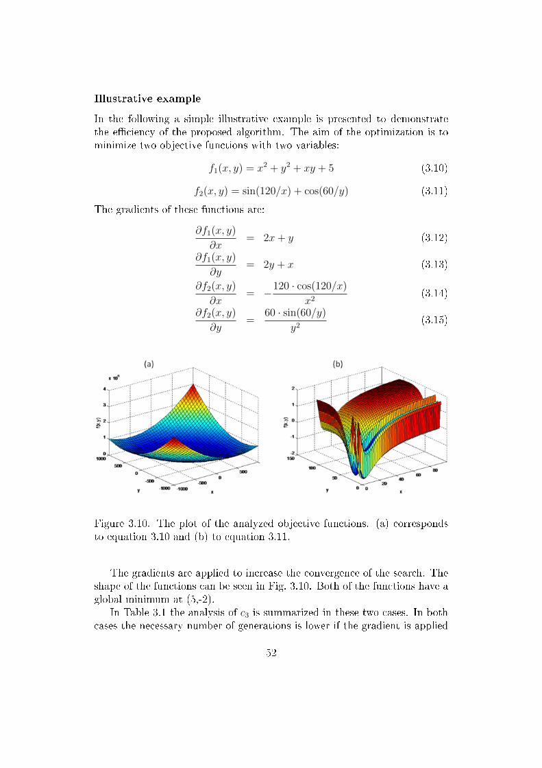
Illustrative example

In the following a simple illustrative example is presented to demonstratethe e�ciency of the proposed algorithm. The aim of the optimization is tominimize two objective functions with two variables:

f1(x, y) = x2 + y2 + xy + 5 (3.10)

f2(x, y) = sin(120/x) + cos(60/y) (3.11)

The gradients of these functions are:

∂f1(x, y)

∂x= 2x+ y (3.12)

∂f1(x, y)

∂y= 2y + x (3.13)

∂f2(x, y)

∂x= −120 · cos(120/x)

x2(3.14)

∂f2(x, y)

∂y=

60 · sin(60/y)y2

(3.15)

Figure 3.10. The plot of the analyzed objective functions. (a) correspondsto equation 3.10 and (b) to equation 3.11.

The gradients are applied to increase the convergence of the search. Theshape of the functions can be seen in Fig. 3.10. Both of the functions have aglobal minimum at (5,-2).

In Table 3.1 the analysis of c3 is summarized in these two cases. In bothcases the necessary number of generations is lower if the gradient is applied

52

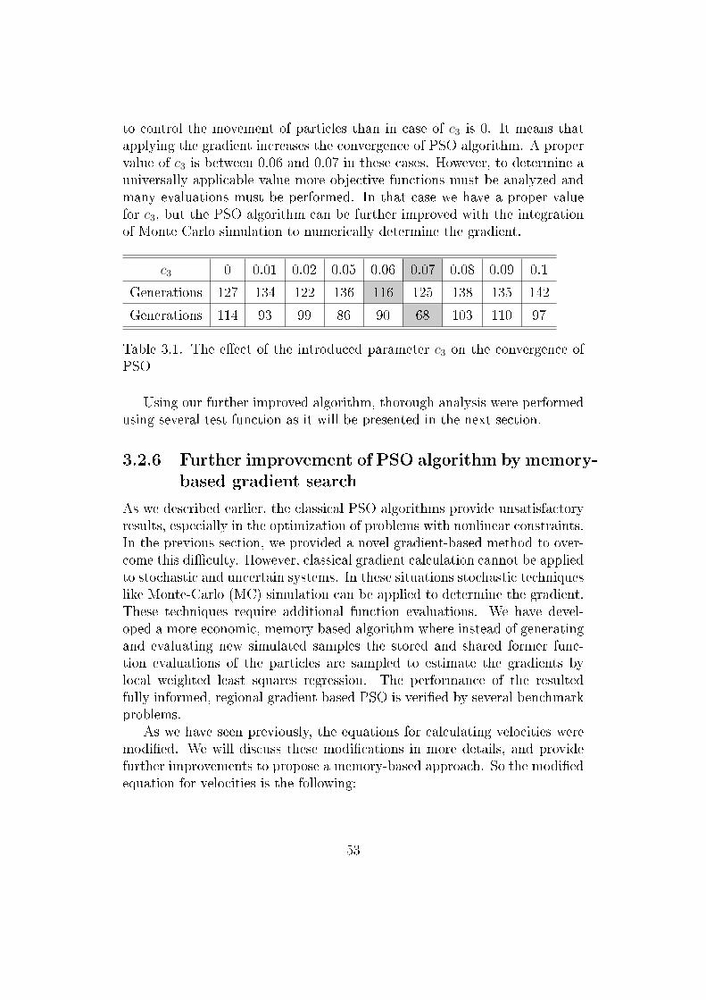
to control the movement of particles than in case of c3 is 0. It means thatapplying the gradient increases the convergence of PSO algorithm. A propervalue of c3 is between 0.06 and 0.07 in these cases. However, to determine auniversally applicable value more objective functions must be analyzed andmany evaluations must be performed. In that case we have a proper valuefor c3, but the PSO algorithm can be further improved with the integrationof Monte Carlo simulation to numerically determine the gradient.

c3 0 0.01 0.02 0.05 0.06 0.07 0.08 0.09 0.1

Generations 127 134 122 136 116 125 138 135 142

Generations 114 93 99 86 90 68 103 110 97

Table 3.1. The e�ect of the introduced parameter c3 on the convergence ofPSO

Using our further improved algorithm, thorough analysis were performedusing several test function as it will be presented in the next section.

3.2.6 Further improvement of PSO algorithm by memory-

based gradient search

As we described earlier, the classical PSO algorithms provide unsatisfactoryresults, especially in the optimization of problems with nonlinear constraints.In the previous section, we provided a novel gradient-based method to over-come this di�culty. However, classical gradient calculation cannot be appliedto stochastic and uncertain systems. In these situations stochastic techniqueslike Monte-Carlo (MC) simulation can be applied to determine the gradient.These techniques require additional function evaluations. We have devel-oped a more economic, memory based algorithm where instead of generatingand evaluating new simulated samples the stored and shared former func-tion evaluations of the particles are sampled to estimate the gradients bylocal weighted least squares regression. The performance of the resultedfully informed, regional gradient based PSO is veri�ed by several benchmarkproblems.

As we have seen previously, the equations for calculating velocities weremodi�ed. We will discuss these modi�cations in more details, and providefurther improvements to propose a memory-based approach. So the modi�edequation for velocities is the following:

53

vj(k + 1) = w · vj(k) + c1 · rand() · (xpBest,j − xj(k)) + (3.16)

c2 · rand() · (xgBest − xj(k)) +

c3 · gj(f(x(k)))

where gj(f(x(k))) =∂f(x(k))∂xj(k)

represents the partial derivatives of the objectivefunction, and is the weight for the gradient term. It should be noted thatthis concept can be interpreted as inserting a gradient-descent update stepinto the iterations of classical PSO, x(k+1) = x(k)− η5 f(x(k)) where thelearning rate is equal to η = c3dt.

The above algorithm can be applied only to continuously di�erentiableobjective functions5f(x(k)). The simples approach to calculate the gradientis HGPSO [119] is the numerical approximation of the gradient.

∂

∂xi(x(k)) =

f(x(k) + Eiε)− f(x(k))ε

(3.17)

The main drawback of this approach is that the step size is di�cult to designand the whole approach is selective to noise and uncertainties. It is interestingto note that PSO itself can also be interpreted as a gradient based searchalgorithm where point di�erences are used as approximation of the regionalgradient. The normalized gradient evaluated as the point di�erence methodis

e =f(xj)− f(xi)

‖(xj − xi)‖(3.18)

This point?di�erence estimate can be considered as regional gradient for thelocal region of xi and xj. Hence, the velocity of PSO can be interpreted asa weighted combination of a point-di�erence estimated global regional gra-dient (xgBest−xj(k))and a point-di�erence estimated �ner regional gradient(xpBest − xj(k)).

Our aim is to further improve the optimization by providing robust yetaccurate estimation of gradients. To obtain a robust estimate a so calledregional gradient should be calculated. When the function is di�erentiablethe gradient for a region S it is calculated as

5 f(x)∗ =1

volume(S)

∫x∈S5f(x)dx (3.19)

where S represents the local region where the gradient is calculated. How-ever, when heuristic optimization algorithm should be applied the objective

54

function is mostly not continuously di�erentiable or not explicitly given dueto limited knowledge. Therefore the gradient is calculated as follows:

5 f(x)∗ =

∫x∈S f(x)dx∫

x∈S dx(3.20)

An interesting example for this approach is how regional gradient is calcu-lated in the Evolutionary-Gradient-Search (EGS) procedure proposed by R.Solomon [143]. In EGS at each iteration λ test candidates are generated byapplying random "mutations" of x(k).

vi = x(k) + zi (3.21)

where zi is a Gaussian distributed variable with zero mean and standarddeviation σ/

√n. For n� 1 these test points will be distributed on a hyper-

sphere with radius σ. By using information given by all candidates theprocedure calculates the gradient and a unit vector e(k) that points into thedirection of the estimated gradient:

gk =λ∑i=1

f(vi)− f(x(k))(vi − x(k)) (3.22)

ek =g(k)

‖g(k)‖(3.23)

These techniques require additional function evaluations. It is important tonote that this concept discards all information related to the evaluation ofvi.

We have developed a more economic, memory based algorithm whereinstead of generating and evaluating new simulated samples the stored andshared former function evaluations of the particles are sampled to estimatethe gradients by local weighted least squares regression. This idea is partlysimilar to the concept of the fully-informed particle swarm (FIPS) algorithmproposed by Mendes et al. [110]. FIPS can be also considered as a hybridmethod for estimating the gradient by a point di�erence of the weightedregional gradient estimate (Pj−x(k)) based on the lBest solutions and addingan additional gradient related term to the velocity adaptation:

νj(k + 1) = · · ·+ c3(νj(k − 1) + ϕ(Pj(k)− x(k))) (3.24)

Pj(k) =

∑k∈S ϕkxlBest,i(k)∑

k∈S ϕk(3.25)

where ϕk is drawn independently from the uniform distribution.

55

FIPS utilizes only the current xlBest,i(k) values so it does not have amemory. The main concept of our work is the e�ective utilization of theprevious function evaluations. So instead of generating new and new samplesand loosing information from previous generations the whole trajectories ofthe particles are utilized.

The weighted regression problem that gives a robust estimates of the gra-dients is formulated by arranging these former function evaluations {x(k), f(x(k))}into indexed data pairs {vi, f(vi)} and calculating the following di�erences:

5 fi(k) = f({vi)− f({x(k)) (3.26)

4xi(k) = vi − x(k) (3.27)

4 f(k) =

4f1(1)4fλ(1)

...4f1(k − 1)4fλ(k − 1)

,4x(k) =

4x1(1)4xλ(1)

...4x1(k − 1)4xλ(k − 1)

(3.28)

where λ represents the number of particles. The weighted least squares esti-mate is calculated as

gj(k) =(4XT (k)Wj(k)4X(k)

)−14XT (k)WTj (k)4 f(k)) (3.29)

where the Wj(K) weighting matrix is a diagonal matrix representing theregion of the jth particle.

Similarly to EGS a Gaussian distributed weighting is used:

βj,i(k) =1

(2π)n/2exp(12(vi − x(k))T

∑−1(vi − x(k))) (3.30)

where vi is the ith row of the matrix 4X, j represents the jth particle,wj,i(k) =

βj,i(k)∑i=1 βj,i(k)

is the normalized probability of the sample,∑

= Iσ isa diagonal matrix where parameter σ represents the size of the region usedto calculate the gradients. By using the information given by all previousstates of the particles it is possible to calculate a unit vector that points intothe direction of the estimated (global) gradient. The resulted algorithm isgiven in Algorithm 2.

56

Algorithm 2 Pseudo code of the improved PSO algorithm

1: Initialize particles2: while not terminate do3: for all particle do4: Calculate �tness value5: if �tness < pBest then6: pBest = �tness7: end if8: end for9: Choose the best particle as the gBest10: for all particle do11: Calculate normalized distance base weights of previous function eval-

uations particles by equation 3.3012: Calculate regional gradients by equation 3.2913: Calculate particle velocity by equation 3.1614: Update particle position15: Store particle position and related cost function in a database,

{vi, f(vi)}16: end for17: end while

Results

We tested the novel algorithm using several functions, including deterministicand stochastic ones as well. Fig. 3.11 presents four of them and Table 3.2contains the mathematical representation of the analyzed functions.

During our tests, the found global best value from the population, themean of the best values of each individual, the iteration number what al-gorithm performed before termination and the iteration number when theglobal best was found were registered. In all tests, we applied Monte Carlomethod to evaluate the performance of our approach e�ectively, thus theweight of the gradient part in the objective value calculation for the indi-viduals was adjusted by 0.1 in the domain of [0,1.25], and for each gradientweight, 500 MC simulations were performed. The result of our tests for thegBest values is presented in Fig. 3.12. It can be deducted from the �gurethat the best global optima was found using 0.7 as the weight of the gra-dient part (since it is a minimization task), while the standard deviation isslightly smaller than in the classic PSO which is presented by the �rst datapoint in Fig. 3.12, where the weight is equal to 0 (w-grad = 0). To prove thee�ectiveness of our method, we present the details of our tests in Table 3.3.

57

Figure 3.11. Surface of the �tness function called "dropwave" (a) the"griewangks" function (b), the stochastic function we used (c), and a stochas-tic version of "griewangks" (noise added) (d).

Including two di�erent deterministic functions (dropwave, griewanks) andtwo stochastic one (griewankgs with noise and another stochastic function),highlighting the best results in each cases.

Using our method, PSO �nds better solution, i.e. the objective value ofthe best individual and the mean of all objective values in the populationis decreased while the number of iterations until the �nal solution found isdecreased also. It yields stronger convergence during the iterations of thealgorithm, thus the novel method increases the e�ciency of PSO. Obviously

58

Function Equation

dropwave f(x, y) = −1+cos(12√x2+y2

12(x2+y2)+2

griewangks f(x) = 14000

∑ni=1 x

2i −

∏ni=1 cos

(xi√i

)+ 1

griewangks with noise f(x) = 14000

∑ni=1 x

2i −

∏ni=1 cos

(xi√i

)+ 1 + rand()

a stochastic function f(x, y) = sin(120/x) + cos(60/y)

Table 3.2. Mathematical equations of the analyzed functions.

the proper setup for the parameters of the PSO and the weight of the gradientis highly problem-dependent, however, during our tests, we found 0.7 as agenerally applicable weight for the gradient, and 10 percent of the domain forσ, which setting in most cases improves the e�ciency of PSO. We propose asimple �ne-tuning technique in the following to setup the parameters of thealgorithm.

1. Set all parameters to zero, i.e. c0 = c1 = c2 = c3.

2. Tune c3 according to the learning method of classic gradient methods,i.e. increase c3 gradually. If oscillation occurs, divide it by 10. Find astable setting.

3. Set the momentum, i.e. c0, which is typically 0.1 or 0.2 in the literature.Increase it gradually, until some improvement is achieved. Find a stablesetting.

4. Tune c1, i.e. increase it gradually until some improvement is achieved.

5. Finally, set c2 = 1.25− c3

These techniques propose a reliable method for tuning the parameters,however, our tests showed clearly that c3 = 0.7 is a generally good choice,and with c1 = 0.5 and c0 = 0.6 the algorithm operates stable.

59

Figure 3.12. Histograms for the "gBest" values using the function called"griewangks" with noise. In the title of the sub�gures, mean representsthe mean value of the histogram, std is the standard deviation and w-gradis the weight of the gradient part in the objective value calculation of theindividuals.

3.2.7 Stochastic optimization of multi-echelon supply

chain models by improved PSO algorithm

As we discussed earlier, most of the multi-echelon supply chain optimizationand analysis are mainly based on analytic approach. Simulation however pro-vides a very good alternative, because it can model real life situations withaccuracy, more �exible in terms of input parameters and therefore it is moreeasy to use in decision support. The simulation results can be analyzed withvarious statistical methods and numerical optimization algorithms. To ana-lyze complex, especially multi-echelon systems, multi-level simulation modelscan be used, where the results of optimized high level model feeds into thelower level more detailed models.

The proposed SIMWARE software provides a framework to analyze thecost structure and optimize inventory control parameters based on cost ob-jectives. With this tool we have minimized the inventory holding cost bychanging the parameters of the reordering strategy while keeping the servicelevel at the required value. The simulation of "actual" inventory control-ling strategies provides the most important KPI-s of these strategies. Onthe other hand we can use the simulator as part of optimization and deter-mine the optimal values of the key inventory control parameters. We have

60

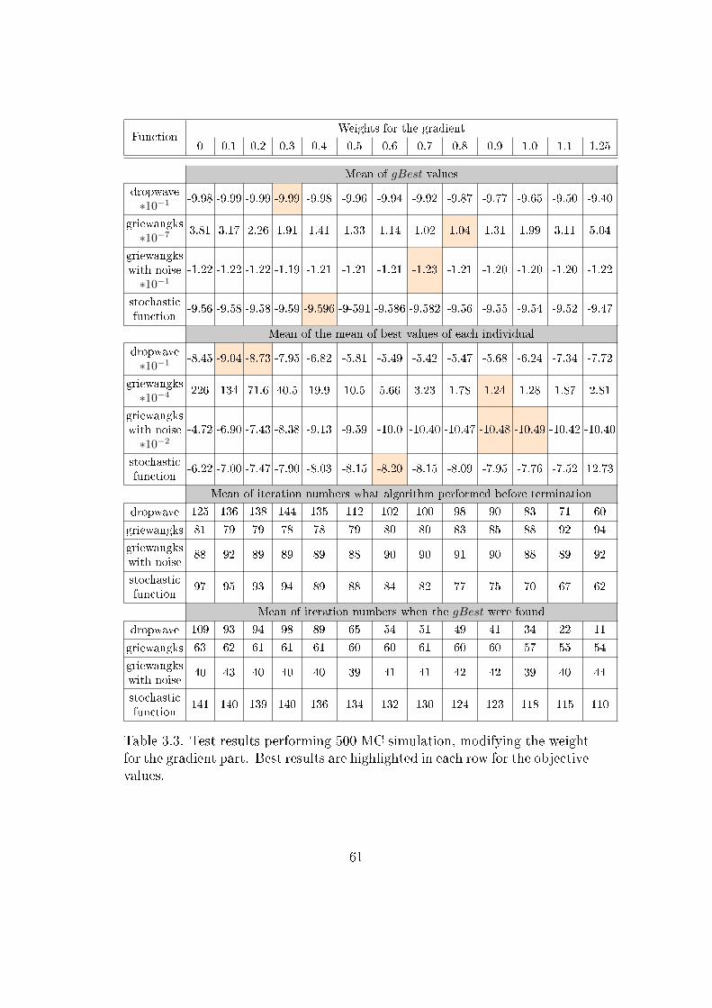
FunctionWeights for the gradient

0 0.1 0.2 0.3 0.4 0.5 0.6 0.7 0.8 0.9 1.0 1.1 1.25

Mean of gBest values

dropwave∗10−1 -9.98 -9.99 -9.99 -9.99 -9.98 -9.96 -9.94 -9.92 -9.87 -9.77 -9.65 -9.50 -9.40

griewangks∗10−7 3.81 3.17 2.26 1.91 1.41 1.33 1.14 1.02 1.04 1.31 1.99 3.11 5.04

griewangkswith noise∗10−1

-1.22 -1.22 -1.22 -1.19 -1.21 -1.21 -1.21 -1.23 -1.21 -1.20 -1.20 -1.20 -1.22

stochasticfunction

-9.56 -9.58 -9.58 -9.59 -9.596 -9-591 -9.586 -9.582 -9.56 -9.55 -9.54 -9.52 -9.47

Mean of the mean of best values of each individual

dropwave∗10−1 -8.45 -9.04 -8.73 -7.95 -6.82 -5.81 -5.49 -5.42 -5.47 -5.68 -6.24 -7.34 -7.72

griewangks∗10−4 226 134 71.6 40.5 19.9 10.5 5.66 3.23 1.78 1.24 1.28 1.87 2.81

griewangkswith noise∗10−2

-4.72 -6.90 -7.43 -8.38 -9.13 -9.59 -10.0 -10.40 -10.47 -10.48 -10.49 -10.42 -10.40

stochasticfunction

-6.22 -7.00 -7.47 -7.90 -8.03 -8.15 -8.20 -8.15 -8.09 -7.95 -7.76 -7.52 12.73

Mean of iteration numbers what algorithm performed before termination

dropwave 125 136 138 144 135 112 102 100 98 90 83 71 60

griewangks 81 79 79 78 78 79 80 80 83 85 88 92 94

griewangkswith noise

88 92 89 89 89 88 90 90 91 90 88 89 92

stochasticfunction

97 95 93 94 89 88 84 82 77 75 70 67 62

Mean of iteration numbers when the gBest were found

dropwave 109 93 94 98 89 65 54 51 49 41 34 22 11

griewangks 63 62 61 61 61 60 60 61 60 60 57 55 54

griewangkswith noise

40 43 40 40 40 39 41 41 42 42 39 40 44

stochasticfunction

141 140 139 140 136 134 132 130 124 123 118 115 110

Table 3.3. Test results performing 500 MC simulation, modifying the weightfor the gradient part. Best results are highlighted in each row for the objectivevalues.

61

minimized the inventory holding cost by changing the parameters of our op-erational space while keeping the service level at the required value.

Fig. 3.13 shows the supply chain, i.e. the structure of the analyzed 2-levelsystem. The investigated case study is a two-level inventory system in whichthere is a central warehouse from only one local warehouse can order (y12).Only one product is stored in these warehouses. The customers can buy fromthe local (y1) and also directly to the central warehouses (y2). To simulate thecustomers purchase behavior two normal distribution functions are applied asy1 and y2. The mean value is 60 and 50 in the applied distribution functions,while the variance is 15 and 10 respectively. The mean value represents that60 units of products are averagely consumed in one week from the centralwarehouse. The variance represents the uncertainty of the mean value, inone week there can be more customers than the mean value, in the other canbe less as in real life.

Figure 3.13. The analyzed 2-level system using one distributor and one re-tailer.

The analyzed time period is 50 weeks (nweek = 50). MC simulations areperformed to simulate the stochastic behavior of the analyzed warehouses.After the simulations the average properties of the warehouses are calculated.The service levels of both warehouses are determined, they are 0.98 and 0.95.The main objective in the chosen case study is to �nd the optimal reorderpoints for both warehouses when the applied objective cost function is at thelowest:

f(reorder point s) =nweek∑i=1

[∑nMC

j=1 (xj,i,1)

nMC

·HC1 +

∑nMC

j=1 (xj,i,2)

nMC

·HC2

](3.31)

where i represents the actual week, j is the actual MC simulation, xj,i,1means the inventory level in the central warehouse at ith week in the jth MC

62

simulation, and HC1 represents the holding cost in the central warehouse.The �uctuations in the average inventory levels after ten MC simulations(nMC = 10) are shown in Fig. 3.14 when the reorder points are 500 and 200respectively. It can be seen that before optimization the average inventoryof the Warehouse 01 is depleted many times and the minimal stock in Ware-house 02 also reaches zero at the 25th week. At the initial reorder points theactual service levels are below the desired values in both of the warehouses(0.60 and 0.89).

Figure 3.14. Average inventory levels before optimization in the 2-echelonsupply chain (see Fig. 3.13). Reorder points are 500 and 200 respectively.

63

Optimization results

The improved PSO algorithm is applied to modify the reorder points dueto the value of the objective function and �nally to �nd the global optima.Since the value of the objective function is very high the chosen weight of thegradient for the search is 10−3. After the optimization process the reorderpoints is changed to 1031 and 100 respectively. Due to this modi�cationthe service levels are much better than at the initial state (0.99 and 0.91)and the value of the objective function is 3.42 · 105. The improved PSO�nishes the search after 127 generations because in the last 50 generationsthere was no signi�cant improvement in the value of the objective function.The average inventory levels after optimization can be seen in Fig. 3.15. Dueto the optimization the inventory in the central warehouse is not empty inthe crucial periods and the minimal stock in the Warehouse 02 is at zerofewer weeks than before the optimization.

Figure 3.15. Average inventory levels after optimization in the 2-echelonsupply chain (see Fig. 3.13). Reorder points are 1031 and 100 respectively.

64

3.3 Monte Carlo Simulation based PerformanceAnalysis of Supply Chains

The section presents the importance and e�ectiveness of supply chain perfor-mance management, which leads to the description of a novel performanceanalysis tool supported by a novel visualization technique.

Our research has been motivated by the energy industry that is veryheavily using e�ective supply chain to ful�ll service level agreements pro-viding continuous service for the customers and �nish projects on time andin budget. E�ectiveness of Supply chains present signi�cant visible impactof distribution, purchasing, and supply management on company assets. Insupply chain systems MRP (Material Requirement Planning) with ERP (en-terprise resource planning) systems are commonly used [29]. The conceptof supply chain management (SCM) represents the current state in the evo-lution of logistics activities. At the operational level the main focus is one�ciency in buying, storing and distributing goods. At the strategic level,SCM brings together a lot of rapidly expanding disciplines which transformsthe way of planning and controlling logistics operations. Our intention wasto create a methodology that provides a strategic decision support tool andconnects strategic planning with operations. SCM systems use ERP soft-ware which creates an opportunity for the application of data mining anddata driven modeling.

Since supply chain performance impacts the �nancial results of servicesand companies, it is important to analyze and optimize supply chain pro-cesses. Our premise is that �rms have to take action by linking their per-formance measurement system to their SCM practices in order to get into abetter position and to become more successful, improving the performance oftheir supply chains and therefore gain more pro�t. Studies show that the bestapproach for controlling SCM systems is based on the Balanced Scorecardmethodology. The intent of using the Balanced Scorecard (BSC) method-ology is to provide a more comprehensive monitoring system for companiesby analyzing the �rm's performance based on a multi dimensional landscapeof Key Performance Indicators. To get a better understanding of the rela-tionships between decision variables and Key Performance Indicators (KPI),performing sensitivity analysis is necessary.

Logistics systems have a certain degree of uncertainty in their behaviorand therefore there is a stochastic connection between the inputs and theoutputs.This stochastic behavior can be analyzed and KPIs can be com-puted according to these results. Our intention is to provide a framework byextending BSC into a dynamic Performance Measurement system and make

65

sure that we use the interrelationship between SCM and Balanced Score-card methodology and show how BSC can be used to assess Supply chainperformance.

KPIs are not simply a list of measures, but they are connected with each-other in the following di�erent ways:

• KPIs are organized into hierarchies based on their respective area.These measure hierarchies contain KPIs that are connected to eachother and calculated from each other. There is another level of inter-connectivity among KPIs.

• KPIs are associated with each other based on cause � e�ect relation-ships.

• KPIs are weighted and there is a relative importance relationship amongthem.

• There is a trade-o� relationship among KPIs.

Individual KPIs and hierarchies of individual KPIs belong to one BSCdimension. Individual KPIs serve the following purposes:

• Provide measurements for e�cient control. They provide the output ofsystem we can use to make decisions.

• Provide a comprehensive reporting solution for management reporting.

• Provide the measurements for the objectives of the BSC system.

• Hierarchies provide strong relationship between KPIs. This relation-ship is based on numerical calculations. These connections are linearand deterministic.

Logistics systems are complex and they interact with other subsystems ina company. They have the following most important attributes which a�ectthe modeling and system analysis approach:

• The processes are non-linear and stochastic.

• System parameters (elements of state transformation matrix) can onlybe determined using system identi�cation and data mining.

• They have large number of components in a complex interaction.

• Systems cannot be analyzed with analytic methods, therefore simula-tion models are necessary for system analysis and optimization.

66

Based on the previous consideration simulation of supply chains is one ofthe key components in our approach. The simulation model can be analyzedfrom the following points of view:

• Estimate the outputs of the model.

• Optimize the process based on this information.

• Calculate the KPIs based on the estimated state variables.

• Determine how KPIs interact and e�ected by the decision variables.

3.3.1 The proposed framework for sensitivity analysis

of supply chains

This section elaborates on the application of Monte Carlo (MC) simulationbased sensitivity analysis to discover the connections between the input andoutput variables in supply chains. The local sensitivity analysis methodcan only be used to determine the local sensitivity near a �xed nominalpoint. However, it does not account for interactions between variables andthe local sensitivity coe�cients. A global sensitivity analysis method can beapplied to determine the e�ect of an input while all the inputs are vary, andthese methods do not depend on the chosen nominal point [126, 150, 144].Fig. 3.16 shows the simpli�ed data �ow diagram of the proposed method.The sensitivity analysis technique is based on our improved method used toextract gradients from MC simulations. It applies the linear least squares�t method to identify the gradients numerically. A hyper plane is �tted tothe output values generated by MC simulation. The parameters of the hyperplane give the partial derivatives of the investigated output functions, andthe extracted gradients (sensitivities) are visualized by a novel technique.

Calculation of sensitivities

In this subsection the method used for the estimation of the sensitivity isdescribed. The utilized method and its description are based on [28].

The expected system performance can be given calculated as the averageof the outputs in every simulation:

L(v) =1

N

N∑i=1

L(x, v) (3.32)

where v contains the parameters of distribution functions of variables inx, L is the output function at a given input and N is the number of MC

67

Figure 3.16. Simpli�ed data �aw diagram of the proposed sensitivity analysis.

simulations performed. A response surface can be constructed from a MonteCarlo analysis with a best �t, using standard criteria, at a near nominalpoint. The �tting of a tangent plane is a known robust procedure calledlinear least squares method. The n-dimensional tangent hyperplane can bede�ned by the following expression:

LL(x) = a0

n∑i=1

aixi (3.33)

where a0 and ai are the coe�cients of the �tted hyperplane, xi is the ith inputand LL is the �tted hyperplane. The ai coe�cients are the partial derivativesof the analyzed output functions respect to xi.

This method applies criteria to select the applicable input and outputvalues to �t the hyperplane from a large number of MC simulations. Theselection is based on the maximum likelihood of each input variable. If allthe values in an input combination are in the following region, that is usedin �tting:

xi,ml ± σi (3.34)

where xi,ml is the maximum likelihood of xi (in normal distribution it equalsto the mean value), σi is the deviation of the ith input.

68

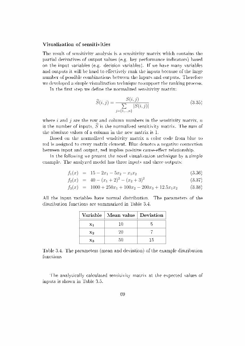
Visualization of sensitivities

The result of sensitivity analysis is a sensitivity matrix which contains thepartial derivatives of output values (e.g. key performance indicators) basedon the input variables (e.g. decision variables). If we have many variablesand outputs it will be hard to e�ectively rank the inputs because of the largenumber of possible combinations between the inputs and outputs. Thereforewe developed a simple visualization technique to support the ranking process.

In the �rst step we de�ne the normalized sensitivity matrix:

S(i, j) =S(i, j)∑

j={1,...,n}|S(i, j)|

(3.35)

where i and j are the row and column numbers in the sensitivity matrix, nis the number of inputs, S is the normalized sensitivity matrix. The sum ofthe absolute values of a column in the new matrix is 1.

Based on the normalized sensitivity matrix a color code from blue tored is assigned to every matrix element. Blue denotes a negative connectionbetween input and output, red implies positive cause-e�ect relationship.

In the following we present the novel visualization technique by a simpleexample. The analyzed model has three inputs and three outputs:

f1(x) = 15− 2x1 − 5x2 − x1x2 (3.36)

f2(x) = 40− (x1 + 2)2 − (x2 + 3)2 (3.37)

f3(x) = 1000 + 250x1 + 100x2 − 200x3 + 12.5x1x2 (3.38)

All the input variables have normal distribution. The parameters of thedistribution functions are summarized in Table 3.4.

Variable Mean value Deviation

x1 10 5

x2 20 7

x3 50 15

Table 3.4. The parameters (mean and deviation) of the example distributionfunctions

The analytically calculated sensitivity matrix at the expected values ofinputs is shown in Table 3.5.

69

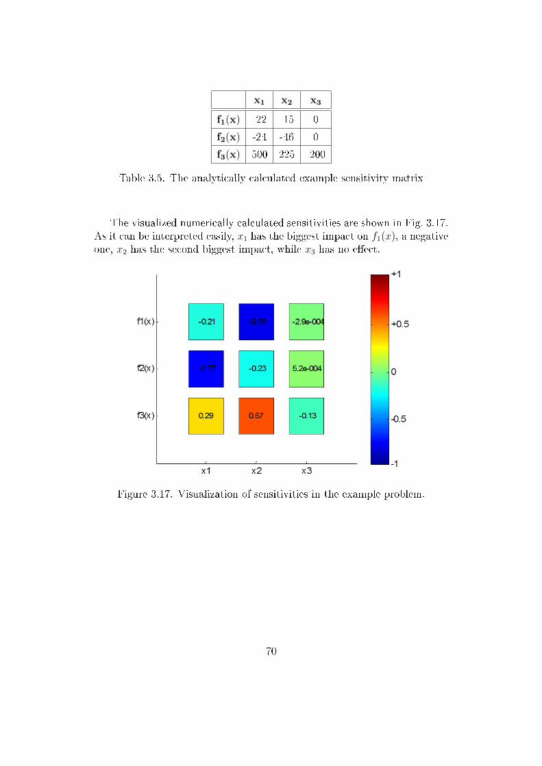
x1 x2 x3

f1(x) -22 -15 0

f2(x) -24 -46 0

f3(x) 500 225 -200

Table 3.5. The analytically calculated example sensitivity matrix

The visualized numerically calculated sensitivities are shown in Fig. 3.17.As it can be interpreted easily, x1 has the biggest impact on f1(x), a negativeone, x2 has the second biggest impact, while x3 has no e�ect.

Figure 3.17. Visualization of sensitivities in the example problem.

70

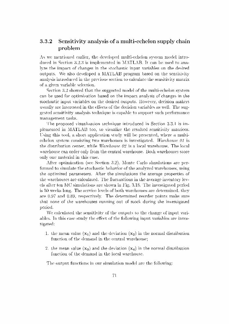
3.3.2 Sensitivity analysis of a multi-echelon supply chain

problem

As we mentioned earlier, the developed multi-echelon system model intro-duced in Section 3.2.3 is implemented in MATLAB. It can be used to ana-lyze the impact of changes in the stochastic input variables on the desiredoutputs. We also developed a MATLAB program based on the sensitivityanalysis introduced in the previous section to calculate the sensitivity matrixof a given variable selection.

Section 3.2 showed that the suggested model of the multi-echelon systemcan be used for optimization based on the impact analysis of changes in thestochastic input variables on the desired outputs. However, decision makersusually are interested in the e�ects of the decision variables as well. The sug-gested sensitivity analysis technique is capable to support such performancemanagement tasks.

The proposed visualization technique introduced in Section 3.3.1 is im-plemented in MATLAB too, to visualize the resulted sensitivity matrices.Using this tool, a short application study will be presented, where a multi-echelon system consisting two warehouses is investigated. Warehouse 01 isthe distribution center, while Warehouse 02 is a local warehouse. The localwarehouse can order only from the central warehouse. Both warehouses storeonly one material in this case.

After optimization (see Section 3.2), Monte Carlo simulations are per-formed to simulate the stochastic behavior of the analyzed warehouses, usingthe optimized parameters. After the simulations the average properties ofthe warehouses are calculated. The �uctuations in the average inventory lev-els after ten MC simulations are shown in Fig. 3.18. The investigated periodis 50 weeks long. The service levels of both warehouses are determined, theyare 0.97 and 0.89, respectively. The determined reorder points make surethat none of the warehouses running out of stock during the investigatedperiod.

We calculated the sensitivity of the outputs to the change of input vari-ables. In this case study the e�ect of the following input variables are inves-tigated:

1. the mean value (x1) and the deviation (x2) in the normal distributionfunction of the demand in the central warehouse;

2. the mean value (x3) and the deviation (x4) in the normal distributionfunction of the demand in the local warehouse.

The output functions in our simulation model are the following:

71

Figure 3.18. Mean value of the actual inventory levels in the investigatedtwo-echelon inventory model.

1. the average holding cost during the investigated period (f1(x));

2. the average inventory level in Warehouse 01 (f2(x));

3. the average service level in Warehouse 01 (f3(x));

4. the average inventory level in Warehouse 02 (f4(x));

5. the average service level in Warehouse 02 (f5(x)).

SIMWARE (see Section 3.2.3) can use di�erent input distributions, likeempirical distributions shown in Fig. 3.2. The e�ect of the uncertainty isalso analyzed, so the results were generated to study the e�ect of parametersof the normal distribution functions (see Table 3.6).

As it was mentioned earlier, MC simulations were performed to analyzethe stochastic behavior and we calculated the average properties of the ware-

72

Variable Mean value Deviation

x1 60 10

x2 15 5

x3 50 15

x3 10 5

Table 3.6. The investigated demand function parameters.

houses based on a large number of simulation runs . We used the followinginput variables:

• Length of simulation is 28 weeks

• The service levels of the warehouses are �xed, they are 97% and 89%respectively

In the output functions, x is a vector like [x1x2x3x4]. 100.000 input combi-nations are generated based on the given distribution functions. The outputfunctions are evaluated next to these combinations. However, only 59 in-put combinations are used to calculate the gradient based on the introducedmethod, because only these combinations are in the given region.

The resulted Sensitivity matrix is summarized in Table 3.7. In this casethe connection between four input variables and �ve output functions aredetermined. The results are presented as a Jacobian matrix in the table.In this case the connection between four input variables and �ve outputsare evaluated. This matrix of the partial derivatives are accurate but notinformative enough for decision makers. It is quite di�cult to rank the inputvariables to show which one has the most impact on the output functionusing a matrix. in order to make the methodology more useful in decisionsupport we developed a visualization technique to show the strengths of theconnections.

As it is shown in Fig. 3.19 the uncertainties in the deviation of the de-mands have the biggest impact on all of the chosen KPIs. The mean valuesof the demands have very small impacts.

In Fig. 3.19 next to the input variables the histograms of that inputs canbe seen. As it was de�ned earlier, values of all these inputs follow normaldistribution. However, the proposed method can be applied any kind of dis-tributions. Below the output functions, the histograms of the outputs can be

73

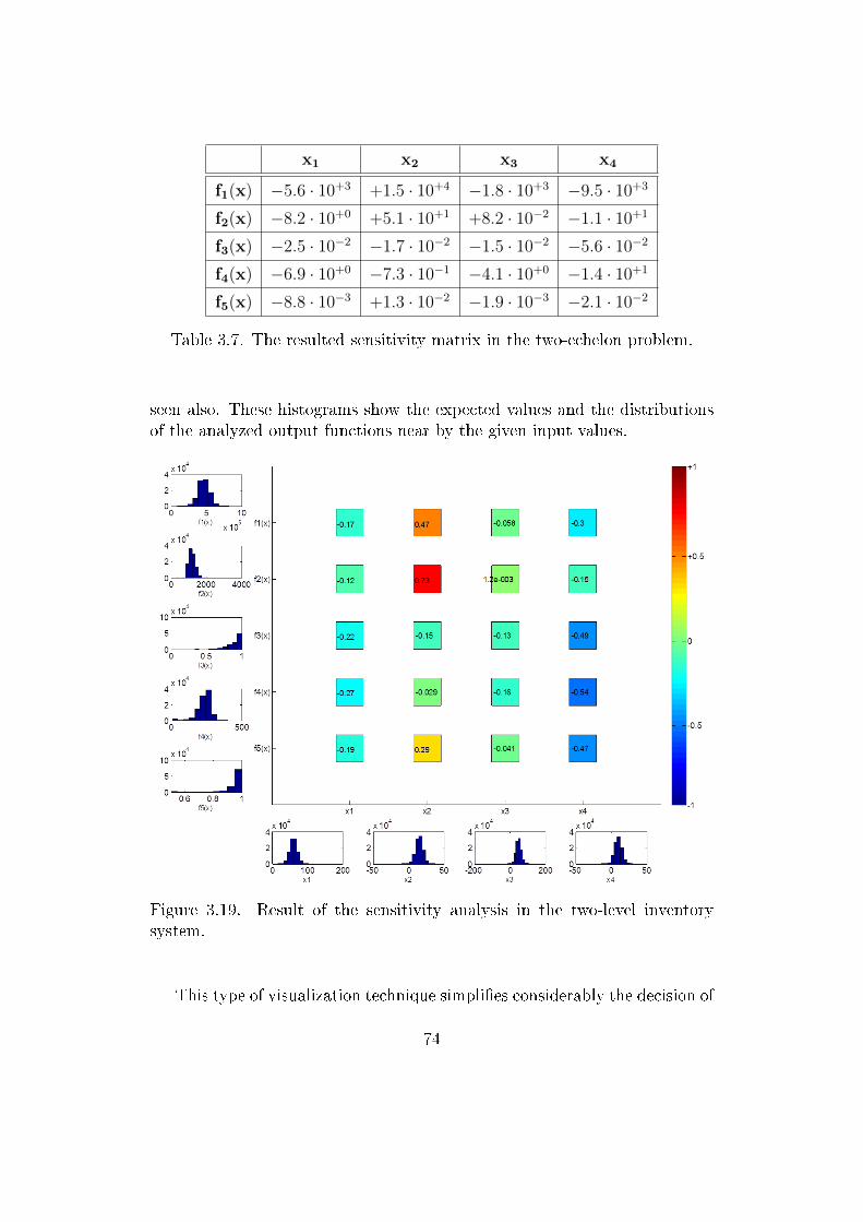
x1 x2 x3 x4

f1(x) −5.6 · 10+3 +1.5 · 10+4 −1.8 · 10+3 −9.5 · 10+3

f2(x) −8.2 · 10+0 +5.1 · 10+1 +8.2 · 10−2 −1.1 · 10+1

f3(x) −2.5 · 10−2 −1.7 · 10−2 −1.5 · 10−2 −5.6 · 10−2

f4(x) −6.9 · 10+0 −7.3 · 10−1 −4.1 · 10+0 −1.4 · 10+1

f5(x) −8.8 · 10−3 +1.3 · 10−2 −1.9 · 10−3 −2.1 · 10−2

Table 3.7. The resulted sensitivity matrix in the two-echelon problem.

seen also. These histograms show the expected values and the distributionsof the analyzed output functions near by the given input values.

Figure 3.19. Result of the sensitivity analysis in the two-level inventorysystem.

This type of visualization technique simpli�es considerably the decision of

74

Key Performance Indicators. The �gure shows unambiguously which inputhas the utmost e�ect to the outputs, e.g. to the cost function, which is themost important objective function for most of the companies.

3.4 Conclusions

Since supply chain performance impacts the �nancial performance compa-nies, it is important to optimize and analyze their e�ciency. For this purposewe presented in Section 3.2 that using an interactive simulator, SIMWARE,we are capable to simulate complex multi-echelon supply chains, providing a�exible simulation method for further investigations. In our project we sim-ulated a central purchasing scenario where the central warehouse suppliesthe other companies in the group. Our methodology can be used to calcu-late stock turnover ratio and safety stock based on the agreed service levelof the warehouses. Our methodology can handle the stochastic behavior ofthe replenishment lead time by the application of Monte-Carlo simulationduring the evaluation of results. Our MATLAB simulation model can beused to determine the optimal parameters for a required service level. Wesuccessfully applied SQP method for optimization, as well as novel ParticleSwarm Optimization algorithms. We developed a novel constrained PSOmethod that utilizes gradients (sensitivities), and we further improved ourprocedure using memory-based gradient search. The performance of the pro-posed methods were evaluated using several test functions from the literatureand we successfully optimized reorder points of multi-echelon supply chainssimulated by our novel simulator.

In Section 3.3, a novel performance analysis technique was introduced.The novel visualization technique was illustrated by a simple example, andthe analysis of a two-echelon inventory system was also performed. We vali-dated our solution by simulating four stochastic input variables. The resultsillustrate that the developed tool is �exible enough to handle complex situa-tions and straightforward and simple enough to be used for decision support.

75

Chapter 4

Biclustering algorithms for Data

mining in high-dimensional data

In previous chapters, we discussed highly complex systems and problems andproposed novel gradient-free optimization algorithms and simulation basedapproaches for solution. Complexity of problems presented in this chapterlies in high-dimensionality of initial data. Inputs are large, mostly biologicaldata, were even the preprocessing step contains serious di�culties. Thissection of the dissertation presents two novel algorithms to solve a highlyresearched data mining problem, the biclustering. As previously, a wholemethodology will be presented here to mine the relevant data and analyzethe results.

4.1 Introduction

One of the most important research �elds in data mining is mining interest-ing patterns (such as sequences, episodes, association rules, correlations orclusters) in large data sets. Frequent itemset mining is one of the earliestsuch concepts originating from economic market basket analysis with the aimof understanding the behaviour of retail customers, or in other words, �ndingfrequent combinations and associations among items purchased together [25].Market basket data can be considered as a matrix with transactions as rowsand items as columns. If an item appears in a transaction it is denoted by 1,otherwise by 0. The general goal of frequent itemset mining is to identify allitemsets that contain at least as many transactions as required, referred to asminimum support threshold. By de�nition, all subsets of a frequent itemsetare frequent. Therefore, it is also important to provide a minimal representa-tion of all frequent itemsets without losing their support information. Such

76

itemsets are called frequent closed itemsets. An itemset is de�ned as closedif none of its immediate supersets has exactly the same support count as theitemset itself. For comprehensive reviews about the e�cient frequent itemsetmining algorithms, see [23, 24].

Independently to frequent itemset mining, biclustering, another impor-tant data mining concept was proposed to complement and expand the ca-pabilities of the standard clustering methods by allowing objects to belong tomultiple or none of the resulting clusters purely based on their similarities.This property makes biclustering a powerful approach especially when it isapplied to data with a large number of objects. During recent years, manybiclustering algorithms have been developed especially for the analysis ofgene expression data [105]. With biclustering, genes with similar expressionpro�les can be identi�ed not only over the whole data set but also across sub-sets of experimental conditions by allowing genes to simultaneously belongto several expression patterns. For comprehensive reviews on biclustering,see [105, 45, 154].

One of the most important properties of biclustering when applied to bi-nary (0,1) data is that it provides the same results as frequent closed itemsetsmining (see Fig. 4.2 later in this chapter). Such biclusters, called inclusion-maximal biclusters (or IMBs), were introduced in [133] together with amining algorithm, BiMAX, to discover all biclusters in a binary matrix thatare not entirely contained by any other cluster. By default an IMB can con-tain any number of genes and samples. Once additional minimum supportthreshold is required for discovering clusters having at least as many genes asthe provided minimum support threshold (i.e. minimum number of genes),BiMAX and all frequent closed itemset mining methods result in the samepatterns.

The mining of closed frequent itemsets can be represented by a processlike in Fig. 4.1. As the �gure depicts, before the application of these datamining techniques, a preprocessing step is mandatory, where the real lifeproblem is coded into a format what the algorithm can handle. After theclosed frequent itemset mining, results are given by a set of biclusters, whichrequires further analysis. The concept itself is simple and easily interpretable,so it supports the compact and e�ective implementation of the algorithm.

77

Figure 4.1. Schematic view of bicluster discovery.

4.1.1 Literature review

Mining frequent itemsets or patterns is a fundamental problem in manydata mining applications, such association rule discovery, correlations, multi-dimensional patterns, sequential rules, episodes, etc. [153]. The basic prob-lem can be expressed as follows: Find frequent patterns in a given largedataset, which are itemsets, subsequences, submatrices or substructures thatappear in the dataset with frequency no less than a user-speci�ed threshold.The problem with this approach is that such mining process often generatesa huge number of substructures satisfying the threshold, because all the sub-patterns of a frequent pattern is also frequent. To overcome this problem,the mining of frequent closed itemsets were proposed by Pasquier et al. in[124], where frequent patterns which have no proper super-pattern with thesame support are searched. The main bene�t of this approach is that the setof closed frequent patterns contains the complete information regarding toits corresponding frequent patterns.

The so-called biclustering is a widely used technique in bioinformat-ics mining in gene expression data, where so-called biclusters are searched[51, 167, 105]. In biological data gene subsets are typically co-expressed onlyunder a subset of samples or sample condition groups. In principle, bicluster-ing provides a solution to this problem as it does not set a priori constrains ofthe organization of the biclusters, meaning that any gene can belong to mul-tiple or none of the resulting clusters. Thus biclustering is potentially able toidentify gene groups that have similar expression patterns over only a subsetof samples or sample condition groups. A bicluster corresponds to a subsetof rows and a subset of genes with a high similarity score, where similarityis not treated as a function of pairs of rows or pairs of columns, instead, it is

78

a measure of coherence of rows and columns in a bicluster. It will be provedin the next section, that frequent closed itemset mining, and biclusteringtechnique can produce the same result, applying appropriate constraints andstrict similarity measure. Because frequent itemset mining is well studiedin numerous articles, we will focus on biclustering in the rest of this sectionusing gene expression data as initial data.

Due to the realization of the underlying potential, several biclusteringalgorithms have been proposed for the identi�cation of gene expression pat-terns during the last decade. The �rst attempt for clustering biclusters withconstant values was introduced by Hartigan [78]. Hartigan introduced apartition-based algorithm, known as Block Clustering, which splits the datamatrix to additional sub-matrices and uses a variance to evaluate the qualityof these sub-matrices. Cheng and Church were the �rst who used the term"biclustering" [51] in gene expression data analysis. In [65], authors werecapable to identify biclusters with constant rows or columns ans in a coupledtwo-way clustering (CTWC) approach. A similar procedure was presentedin [156]. Authors in [47, 166] provided a greedy iterative search algorithm,and FLOC (FLexible Overlapped biClustering) [166, 167] or the algorithmin [92] also addressed the problem of �nding biclusters with coherent val-ues. In the Iterative Signature Algorithm (ISA) [38] and the plaid model[98] was also attempted to discover one bicluster at a time in an iterativeprocess. In [98, 37] authors used statistics, while in [115] an algorithm to�nd xMOTIFs, i.e. biclusters with coherent evolutions on their rows wasintroduced. Tanay et al. in [154] introduced an exhaustive biclustering enu-meration method, which uses probabilistic modeling of the data, and graphtheoretic techniques to �nd the most signi�cant bicluster in the data matrix.Further comprehensive reviews about previous biclustering algorithms canbe found in [155, 105, 45]. A very recent in-press publication [163] deals withbiclustering using hipergraphs in gene expression data.

As we saw in the previous paragraphs some biclustering methods work onreal valued and some on discretized, but most of them in practise, binarizeddata. Methods working on real values are computationally very intensive andusually require signi�cant pre�ltering of data to limit the size of the input.Another common limitation of these methods is the prede�ned number ofbiclusters that the user has to provide before running these tools, e.g. [46].Most discretized methods avoid these problems and even though discretiza-tion decreases information content of the data, sometimes reducing the datacomplexity can be bene�cial. As it will be shown in next sections, even themost powerful techniques from the cited methods are either computationallyexpensive or not accurate enough, i.e. they can't discover all the interesting

79

subsets, or both.The literature of closed frequent itemset mining is at least as wide as

biclustering's. Only the list of most important ones will be presented here.The mining of frequent closed itemsets was proposed by Pasquier et al. in1999 [124] where an apriori-based algorithm was presented. Other algorithmwas presented for closed frequent itemset mining, including CLOSET [125],CHARM [171], FPClose [69], AFOPT [100], CLOSET+ [162]. The mainchallenge in closed pattern mining is to check whether if a candidate itemsetis closed. CHARM uses a hashing technique on its TID (Transaction IDenti-�er) values, while AFOPT, FPCOLSE, CLOSET and CLOSET+ maintainthe found detected patterns in an FP-tree-like pattern-tree. Further reedingabout closed itemset mining can be found in [76]. These algorithms can pro-duce exactly the same results as biclustering techniques, which will be provenmathematically (section 4.2) and by practical examples (section 4.3.5).

In further sections, the mathematical formulation of the problem will begiven (section 4.2), and in the main part of the manuscript in section 4.3, anovel algorithm will be proposed for frequent closed itemset mining, whichuses a recursive procedure and solves the biclustering problem much fasterthan other solutions so far. Furthermore, our novel algorithm is capableto discover patterns in {−1, 0, 1} data, which includes oppositely changedpatterns as well, which have to be discovered. Because of the biologicalimportance, a general technique to handle the {−1, 0, 1} data using previousalgorithms will be proposed, which is a special transformation into binaryvalues. A novel technique to handle errors in clusters and a novel visualizationmethod will be also presented. Section 4.3.5 contain results and comparisonswith previous approaches and conclusion with future opportunities.

4.2 Problem formulation

4.2.1 Biclustering

Biclustering has been introduced to complement and expand the capabilitiesof the standard clustering methods by allowing objects to belong to multipleor none of the resulting clusters purely based on their similarities. This prop-erty makes biclustering a powerful approach especially when it is applied todata with a large number of objects. During recent years, many biclusteringalgorithms have been developed especially for the analysis of gene expressiondata. With biclustering, genes with similar expression pro�les can be identi-�ed not only over the whole data set but also across subsets of experimentalconditions by allowing genes to simultaneously belong to several expression

80

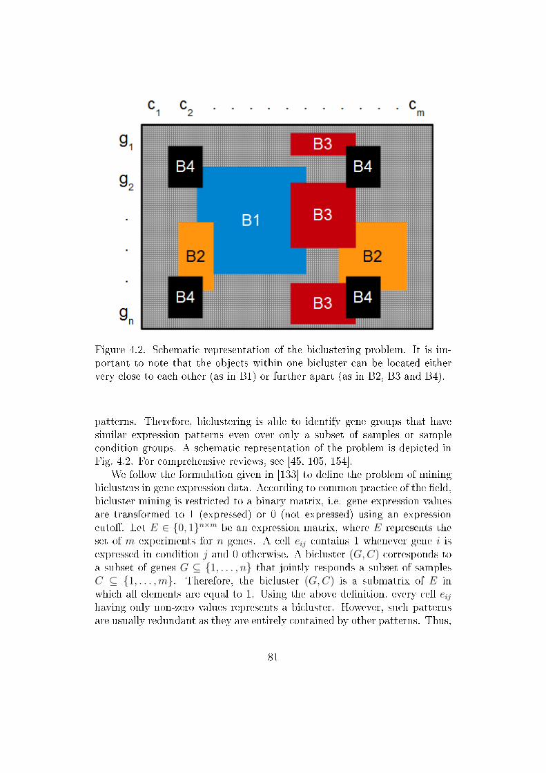
Figure 4.2. Schematic representation of the biclustering problem. It is im-portant to note that the objects within one bicluster can be located eithervery close to each other (as in B1) or further apart (as in B2, B3 and B4).

patterns. Therefore, biclustering is able to identify gene groups that havesimilar expression patterns even over only a subset of samples or samplecondition groups. A schematic representation of the problem is depicted inFig. 4.2. For comprehensive reviews, see [45, 105, 154].

We follow the formulation given in [133] to de�ne the problem of miningbiclusters in gene expression data. According to common practice of the �eld,bicluster mining is restricted to a binary matrix, i.e. gene expression valuesare transformed to 1 (expressed) or 0 (not expressed) using an expressioncuto�. Let E ∈ {0, 1}n×m be an expression matrix, where E represents theset of m experiments for n genes. A cell eij contains 1 whenever gene i isexpressed in condition j and 0 otherwise. A bicluster (G,C) corresponds toa subset of genes G ⊆ {1, . . . , n} that jointly responds a subset of samplesC ⊆ {1, . . . ,m}. Therefore, the bicluster (G,C) is a submatrix of E inwhich all elements are equal to 1. Using the above de�nition, every cell eijhaving only non-zero values represents a bicluster. However, such patternsare usually redundant as they are entirely contained by other patterns. Thus,

81

the de�nition of inclusion-maximal bicluster (IMB) was introduced todiscover all biclusters not entirely contained by any other cluster [133]: thepair (G,C) ∈ 2{1,...,n} × 2{1,...,m} is an IMB, if and only if ∀i ∈ G, j ∈ C :eij = 1 and @(G′, C ′) ∈ 2{1,...,n} × 2{1,...,m} where ∀i′ ∈ G′, j′ ∈ C ′ : ei′j′ = 1and G ⊆ G′ ∧ C ⊆ C ′ ∧ (G′, C ′) 6= (G,C).

By default an IMB can contain any number of genes and samples. Ad-ditionally, the so-called minimum support thresholds can be used to specifythe minimum number of genes and samples required for the biclusters.

4.2.2 Frequent closed itemset mining

One of the earliest and most important concepts in data mining is miningfrequent itemsets in large transactional datasets [104]. Such a dataset canbe considered as a matrix with transactions as rows and items as columns.If an item appears in a transaction it is denoted by 1, otherwise by 0. Thegeneral goal of frequent itemset mining is to identify all itemsets that containat least as many transactions as required, referred to as minimum supportthreshold, min_sup. By de�nition, all subsets of a frequent itemset are fre-quent. Therefore, it is also important to provide a minimal representation ofall frequent itemsets without losing their support information. Such itemsetsare called frequent closed itemsets and can be de�ned as follows. Letσ(x) = |{ti : x ⊆ ti, ti ∈ T }| denote the support count of itemset x. Anitemset x is closed if none of its immediate supersets has exactly the samesupport count as x. Oppositely, the itemset x is not closed if at least one ofits immediate supersets has the same support count as x. Obviously, x, y:σ(x) ≥ σ(y), if x ⊆ y. Finally, an itemset is a frequent closed itemset (FCI)if it is closed and frequent. For comprehensive reviews about the e�cientalgorithms, see [23, 24].

4.2.3 Connection between biclustering and frequent closed

itemset mining

We show here that biclustering and frequent closed itemset mining can infact be reduced to the same problem when working on a binary data matrixof size n ×m. The set of transactions T in frequent itemset mining can beconsidered as the set of genes G in biclustering, and the set of itemsets Ias the set of samples C. The min_sup threshold in frequent itemset miningcorresponds to the min_rows constraint in biclustering . There is no corre-sponding constraint in frequent itemset mining to min_cols in biclusteringbut this can be overcome by setting min_cols to 1 in the biclustering or

82

�ltering the �nal result of frequent itemset mining, i.e. the itemsets with lessthan min_cols items are removed to match the constraints.

Next, the correspondence of the closeness of frequent itemsets and theinclusion-maximality of biclusters needs to be veri�ed. For this, let usassume, that FCI mining with min_sup = k and mining of IMBs withmin_rows = k and min_cols = 1 produce di�erent results. It is only pos-sible if (a) ∃ xc which is a FCI, but not an IMB, or if (b) ∃ (Gb, Cb) whichis IMB but not FCI. We will prove (a) here, while the proof of (b) is almostthe same. Let a FCI xc is an itemset with |xc| = p and σ(x) = q ≥ k.Then @ y, x ⊂ y, where σ(x) ≤ σ(y). Let |y| = p′ and σ(y) = q′. Since abicluster is simply a subset of rows and subset of columns, xc corresponds toa bicluster (G,C)q×p and similarly, y corresponds to a bicluster (G′, C ′)q

′×p′ .By the de�nition of our assumption, @ the bicluster (G′, C ′) with C ′ ⊂ Cand G′ subseteqG, which yields that (G′, C ′) 6= (G,C). Therefore, by thede�nition of IMB, xc is not only a FCI but also an IMB.

From now on, we will use the general terms closed pattern (CP) andfrequent closed pattern (FCP) within the chapter.

4.3 E�cient methods for bicluster mining

As we discussed earlier, biclustering is a widely used technique in bioinfor-matics mining in gene expression data [51, 105, 167]. In biological datagene subsets are typically co-expressed only under a subset of samples orsample condition groups, and the data is in a vertical format, i.e. it con-tains much more rows than columns. Another important property in bi-ological data is the importance of exactly oppositely changing patterns inthe dataset, namely these patterns represent almost identical behaviours inbiological sense. Thus, the so-called vertical mining procedures come intoaccount [148, 170, 171]. Because of these considerations and the fact thatthe existing data mining algorithms (see section 4.1.1) are either not accurateenough, or their running time is not fast enough, authors have developed anovel vertical, recursive mining method. The procedure which will be dis-cussed in the next section, discovers all the frequent itemsets in the initialdata, and its running time is much faster than previous approaches so far(see section 4.3.5).

83

4.3.1 A novel way to mine closed patterns

In this section we propose a new method for mining closed patterns (i.e.frequent closed itemsets and biclusters) for data matrices with up to threevalues: -1, 0, 1. This is an extension of the special binary case and therefore,applicable to both data types. The bene�t of this kind of general approachhas been presented in [75] using gene expression data. The key bene�t ofthe generalized method is the gained ability to make a distinction betweenup- and down-regulated genes and thus, discover previously hidden closedpatterns [75].

The proposed method consists of two procedures and one function todiscover all frequent closed patterns:

• FCPMain is the main procedure (Algorithm 3). First the proceduretakes the three input parameters (input data matrix and minimumsupport thresholds) before encoding the input matrix (A) into a smallerdata structure (B) by taking only non-zero matrix values as follows:

B = (bi),where bi = {j : A(i, j) 6= 0} (4.1)

Note that the transformation in Eq. 4.1 corresponds to the classical rep-resentation of transaction databases in frequent itemset mining prob-lems where bi represents the ith transaction.

The procedure then independently calls the recursive miner procedureFCPMiner for each B row. Note that the parameter vector missin-gRows stores the indices of those rows which are not examined in theactual call (they have been checked before). This is important as close-ness will be checked based on these indices by the IsClosed function.

• FCPMiner procedure is the heart of the method by recursively build-ing up the frequent closed patterns (Algorithm 5). This is done bytaking the consecutive rows one-by-one and recording only those col-umn indices that show the same changing tendency (same or exactlythe opposite). Then the closeness of the candidate pattern is checkedbefore the method is calling itself with the updated parameters. Fi-nally, the newly discovered patterns are added to the output set offrequent closed patterns.

• IsClosed is a simple function to check whether adding a new row indexto the candidate pattern would result in a closed pattern (Algorithm 4).This is done by checking whether there is a row in missingRows thatcontains the same column indices with the same changing tendency as

84

in the pattern under examination. If no such row can be found thenthe pattern is already a closed one.

Algorithm 3 FCPMain: Main procedure for mining closed patterns

Require: A: input discrete matrixminrows: minimum number of rows in a frequent closed patternmincols: minimum number of columns in a frequent closed pattern

Ensure: Y : List of all closed frequent patterns1: global A, Y = {},minrows,mincols, B2: MissingRows = {}3: Transform An×m into data structure B4: for every row Ri ∈ B where i = 1 . . . (n−minrows) do5: if i > 1 then6: MissingRows =MissingRows ∪ {i}7: end if8: if |Ri| ≥ mc then9: if (i == 1) or IsClosed(MissingRows,Ri, i) then10: FCPMiner(MissingRows,Ri, {i})11: end if12: end if13: end for14: return Y

Algorithm 4 isClosed method

Require: missingRows: indices of previously examined rows (omitted)actualCols: current column indices under examinationactualRow: actual row index under examination

Ensure: boolean: is this candidate frequent pattern closed?1: global A2: for every index i in missingRows do3: if Ai,j ∗ Ak,j = 1 ∀j ∈ actualCols,∀k ∈ actualRow or

Ai,j ∗ Ak,j = −1 ∀j ∈ actualCols,∀k ∈ actualRow then4: return true5: end if6: end for7: return false

85

Algorithm 5 FCPMiner procedure

Require: missingRows: indices of previously examined rows (omitted)candidateRows: set of row indices in a candidate closed frequent patternactualCols: actual column indices under examination

1: global A, Y,minrows,mincols, B2: for every rows' index i in {B's rowindices} \ candidateRows do3: actIndices = actualCols ∩Bi

4: change1 = {j}, where Ai,j ∗ AcandidateRows(1),j = 1, j ∈ actIndices5: change−1 = {j}, where Ai,j ∗ AcandidateRows(1),j = −1, j ∈ actIndices6: if (|actualCols| == |change1|) or (|actualCols| == |change−1|) then7: candidateRows = candidateRows ∪ {i}8: else9: if (|change1| ≥ mincols) then10: if IsClosed(missingRows, change1, i) then11: FCPMiner(missingRows, candidateRows ∪ {i}, change1)12: end if13: end if14: if (|change−1| ≥ mincols) then15: if IsClosed(missingRows, change−1, i) then16: FCPMiner(missingRows, candidateRows ∪ {i}, change−1)17: end if18: end if19: missingRows = missingRows ∪ {i}20: end if21: end for22: if |candidateRows| >= minrows then23: Y = Y ∪ {candidateRows, actualCols}24: end if

Fig. 4.3 illustrates how the proposed method discovers all frequent closedpatterns from a simple example data matrix with minimum support thresh-olds min_rows = min_cols = 2. While the process �ow is marked by solidarrows the recursive steps are highlighted by dashed arrows. A bold crosssign indicates that the investigated pattern is not closed, or it does not sat-isfy the minimum support conditions for rows or columns. The discoveredfrequent closed patterns are surrounded by solid rectangles.

86

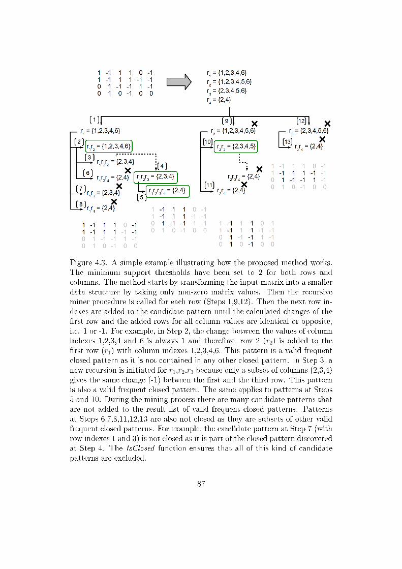
Figure 4.3. A simple example illustrating how the proposed method works.The minimum support thresholds have been set to 2 for both rows andcolumns. The method starts by transforming the input matrix into a smallerdata structure by taking only non-zero matrix values. Then the recursiveminer procedure is called for each row (Steps 1,9,12). Then the next row in-dexes are added to the candidate pattern until the calculated changes of the�rst row and the added rows for all column values are identical or opposite,i.e. 1 or -1. For example, in Step 2, the change between the values of columnindexes 1,2,3,4 and 6 is always 1 and therefore, row 2 (r2) is added to the�rst row (r1) with column indexes 1,2,3,4,6. This pattern is a valid frequentclosed pattern as it is not contained in any other closed pattern. In Step 3, anew recursion is initiated for r1,r2,r3 because only a subset of columns (2,3,4)gives the same change (-1) between the �rst and the third row. This patternis also a valid frequent closed pattern. The same applies to patterns at Steps5 and 10. During the mining process there are many candidate patterns thatare not added to the result list of valid frequent closed patterns. Patternsat Steps 6,7,8,11,12,13 are also not closed as they are subsets of other validfrequent closed patterns. For example, the candidate pattern at Step 7 (withrow indexes 1 and 3) is not closed as it is part of the closed pattern discoveredat Step 4. The IsClosed function ensures that all of this kind of candidatepatterns are excluded.

87

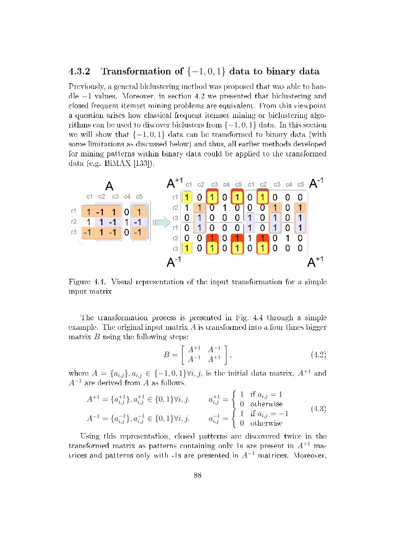
4.3.2 Transformation of {−1, 0, 1} data to binary data

Previously, a general biclustering method was proposed that was able to han-dle −1 values. Moreover, in section 4.2 we presented that biclustering andclosed frequent itemset mining problems are equivalent. From this viewpointa question arises how classical frequent itemset mining or biclustering algo-rithms can be used to discover biclusters from {−1, 0, 1} data. In this sectionwe will show that {−1, 0, 1} data can be transformed to binary data (withsome limitations as discussed below) and thus, all earlier methods developedfor mining patterns within binary data could be applied to the transformeddata (e.g. BiMAX [133]).

Figure 4.4. Visual representation of the input transformation for a simpleinput matrix

The transformation process is presented in Fig. 4.4 through a simpleexample. The original input matrix A is transformed into a four times biggermatrix B using the following steps:

B =

[A+1 A−1

A−1 A+1

], (4.2)

where A = {ai,j}, ai,j ∈ {−1, 0, 1}∀i, j, is the initial data matrix, A+1 andA−1 are derived from A as follows.

A+1 = {a+1i,j }, a+1

i,j ∈ {0, 1}∀i, j. a+1i,j =

{1 if ai,j = 10 otherwise

A−1 = {a−1i,j }, a−1i,j ∈ {0, 1}∀i, j. a−1i,j =

{1 if ai,j = −10 otherwise

(4.3)

Using this representation, closed patterns are discovered twice in thetransformed matrix as patterns containing only 1s are present in A+1 ma-trices and patterns only with -1s are presented in A−1 matrices. Moreover,

88

patterns with oppositely changing values also appear twice in matrix B, in[A+1A−1] and in [A−1A+1], respectively. Therefore, all types of closed pat-terns presented in A also exist in the transformed matrix, but all of themtwice and thus a post-processing step is needed to eliminate the duplicatedpatterns.

Although the presented transformation allows applying previous methodsto {1,0,-1} data, it is more convenient to use our proposed method, FCP-Miner, where the overhead caused by processing duplicated patterns andhaving to perform post �ltering can be avoided.

4.3.3 Closed pattern based data visualization

Although various closed pattern mining methods have been introduced re-cently, none of them provide a visualization technique for the thousands ofscattered subsets of the original data. Here we present an innovative tech-nique for visualizing the original data matrix by reordering the rows andcolumns based on the discovered closed patterns. The visualization can beof use for evaluating the e�ectiveness of the pattern detection and can helpto interpret the pattern structure in a general level. To illustrate the prob-lem we use a tiny synthetic data with size 10 by 10 (Fig. 4.5). Algorithm 6describes the procedure for reordering the matrix data.

The method takes the original data matrix and the closed patterns asinput. At �rst, we generate sparse matrices A′r and A

′c using the following

formula (line 1):

A′r(i, j) = number of rows in Cj where Cj contains columns iA′c(i, j) = number of columns in Cj where Cj contains row i

(4.4)

In steps 2 and 3 the distance tables are generated for both rows and columnsof A respectively. Thus the algorithm computes distances between each pairof rows, DTCr (columns, DTCc) based on the sparse matrices A′r and A′c,respectively. Tanimoto distance is then used to calculate the similarity mea-sure. Therefore, the distance for example between row i and j is calculatedas follows:

DTCr(i, j) = DTCr(j, i) =

∏{A′r(i), A′r(j)}∑{A′c(i), A′c(j)}

(4.5)

Finally, dendrograms for rows (DGr) and columns (DGc) are calculatedbased on the distance tables and the rearranged dataset A′′ is generatedusing the sequence of dendrograms' leaves.

89

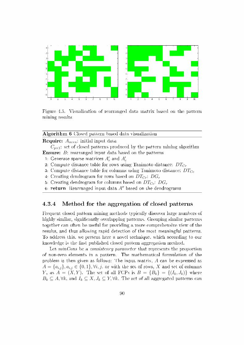
Figure 4.5. Visualization of rearranged data matrix based on the patternmining results

Algorithm 6 Closed pattern based data visualization

Require: Am×n: initial input dataCp×1: set of closed patterns produced by the pattern mining algorithm

Ensure: B: rearranged input data based on the patterns1: Generate sparse matrices A′r and A

′c

2: Compute distance table for rows using Tanimoto distance: DTCr3: Compute distance table for columns using Tanimoto distance: DTCc4: Creating dendrogram for rows based on DTCr: DGr

5: Creating dendrogram for columns based on DTCc: DGr

6: return Rearranged input data A′′ based on the dendrograms

4.3.4 Method for the aggregation of closed patterns

Frequent closed pattern mining methods typically discover large numbers ofhighly similar, signi�cantly overlapping patterns. Grouping similar patternstogether can often be useful for providing a more comprehensive view of theresults, and thus allowing rapid detection of the most meaningful patterns.To address this, we present here a novel technique, which according to ourknowledge is the �rst published closed pattern aggregation method.

Let minCons be a consistency parameter that represents the proportionof non-zero elements in a pattern. The mathematical formulation of theproblem is then given as follows: The input matrix, A can be expressed asA = {ai,j}, ai,j ∈ {0, 1},∀i, j, or with the set of rows, X and set of columnsY , as A = (X, Y ). The set of all FCPs is B = {Bk} = {(Ik, Jk)} whereBk ⊆ A,∀k, and Ik ⊆ X, Jk ⊆ Y, ∀k. The set of all aggregated patterns can

90

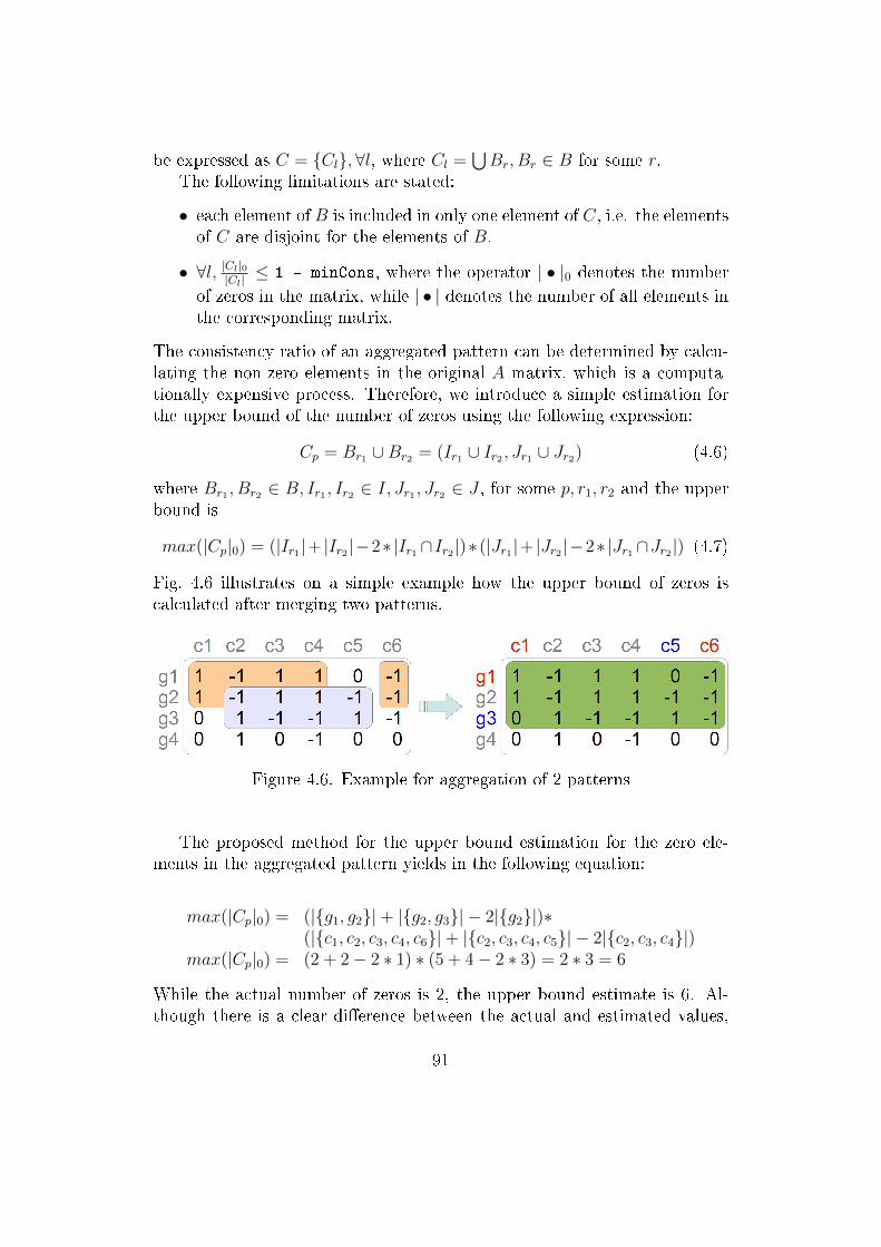
be expressed as C = {Cl},∀l, where Cl =⋃Br, Br ∈ B for some r.

The following limitations are stated:

• each element of B is included in only one element of C, i.e. the elementsof C are disjoint for the elements of B.

• ∀l, |Cl|0|Cl|≤ 1 - minCons, where the operator | • |0 denotes the number

of zeros in the matrix, while | • | denotes the number of all elements inthe corresponding matrix.

The consistency ratio of an aggregated pattern can be determined by calcu-lating the non-zero elements in the original A matrix, which is a computa-tionally expensive process. Therefore, we introduce a simple estimation forthe upper bound of the number of zeros using the following expression:

Cp = Br1 ∪Br2 = (Ir1 ∪ Ir2 , Jr1 ∪ Jr2) (4.6)

where Br1 , Br2 ∈ B, Ir1 , Ir2 ∈ I, Jr1 , Jr2 ∈ J , for some p, r1, r2 and the upperbound is

max(|Cp|0) = (|Ir1|+ |Ir2|−2∗ |Ir1 ∩Ir2|)∗ (|Jr1|+ |Jr2 |−2∗ |Jr1 ∩Jr2|) (4.7)

Fig. 4.6 illustrates on a simple example how the upper bound of zeros iscalculated after merging two patterns.

Figure 4.6. Example for aggregation of 2 patterns

The proposed method for the upper bound estimation for the zero ele-ments in the aggregated pattern yields in the following equation:

max(|Cp|0) = (|{g1, g2}|+ |{g2, g3}| − 2|{g2}|)∗(|{c1, c2, c3, c4, c6}|+ |{c2, c3, c4, c5}| − 2|{c2, c3, c4}|)

max(|Cp|0) = (2 + 2− 2 ∗ 1) ∗ (5 + 4− 2 ∗ 3) = 2 ∗ 3 = 6

While the actual number of zeros is 2, the upper bound estimate is 6. Al-though there is a clear di�erence between the actual and estimated values,

91

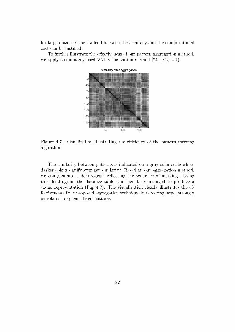
for large data sets the tradeo� between the accuracy and the computationalcost can be justi�ed.

To further illustrate the e�ectiveness of our pattern aggregation method,we apply a commonly used VAT visualization method [84] (Fig. 4.7).

Figure 4.7. Visualization illustrating the e�ciency of the pattern mergingalgorithm

The similarity between patterns is indicated on a gray color scale wheredarker colors signify stronger similarity. Based on our aggregation method,we can generate a dendrogram re�ecting the sequence of merging. Usingthis dendrogram the distance table can then be rearranged to produce avisual representation (Fig. 4.7). The visualization clearly illustrates the ef-fectiveness of the proposed aggregation technique in detecting large, stronglycorrelated frequent closed patterns.

92

4.3.5 Experimental results

In this section we compare our proposed closed pattern mining method (seesection 4.3.1) with a biclustering based (BiMAX [133]) and a frequent closeditemset mining based (DCI_Closed [103]) methods that are able to discoverall frequent closed patterns in binary data. These algorithms previouslyserved as highly recognized reference methods for their application �elds[133]. Note that all methods developed for frequent closed itemset miningproduce the same patterns as DCI_Closed. Using several synthetic and realbiological data sets, we show that 1) all three methods discover the sameclosed patterns in binary data and thus, experimentally prove our claim thatboth biclustering and frequent closed itemset mining methods discover thesame patterns; 2) our pattern discovery method outperforms the other meth-ods and 3) it is the only method that is able to discover previously hiddenand biologically potentially relevant closed patterns by using the extended{−1, 0, 1} data.

Comparison and computational e�ciency of the closed patternmining methods

To compare the three mining methods and demonstrate their computationale�ciency, we applied them to several real and generated synthetic data sets.Real data come from various biological studies previously used as referencedata in biclustering research [75, 99, 15]. For the comparison of the compu-tational e�ciency, all biological data sets were binarized. For both the fold-change data (stem cell data sets) and the absolute expression data (Leukemia,Compendium, Yeast-80) fold-change cut-o� 2 is used. Synthetic data weregenerated by both our own and IBM Quest Synthetic Data generator tool[128]. Results are shown in Table 4.1 (synthetic data) and Table 4.2 (realdata), respectively. All three methods were able to discover all closed pat-terns for all synthetic and real data sets. The tables also show that FCPMineroutperforms the other two methods and provides the best running times inall cases, especially when the number of rows and columns are higher.

Biological relevance of closed pattern mining on {−1, 0, 1} data

Here we illustrate the potential of our closed pattern mining method whenapplied to {−1, 0, 1} data. The real data set used in this section comesfrom the study of the e�ects of Tet1-knockdown on gene expression in mouseembryonic stem cell and trophoblast stem cell conditions. The data havebeen previously analyzed using our standard analysis pipeline and the resultshave been published in [94] (GEO reference:GSE26900). The input data for

93

Table 4.1. Computational results using synthetic data sets.r: number of rowsc: number of columnsd: density (proportion of ones) [%]sc: minimum support count during the search (min_cols in pattern mining)sr: minimum row count during pattern mining (min_rows)cf: number of identi�ed closed patternsc�: number of closed patterns after �lteringb: number of found patterns by the corresponding algorithmt: running time [s]

Data r c d sc srBiMAX DCI_Closed FCPMiner

b t cf c� t b t

S1 50 50 10 2 2 78 ∼1 119 78 0.016 78 0.001

S2 50 50 20 4 2 140 ∼1 189 140 0.024 140 0.016

S3 50 50 50 15 2 238 ∼1 288 238 0.033 238 0.438

S4 100 100 10 3 2 337 ∼2 436 337 0.041 337 0.041

S5 100 100 20 7 2 488 ∼2 588 488 0.028 488 0.015

S6 100 100 50 30 2 694 ∼3 794 694 0.034 694 0.488

S7 300 300 10 8 2 437 ∼5 737 437 0.041 437 0.031

S8 300 300 20 22 2 156 ∼52 456 156 0.085 156 0.047

S9 300 300 50 90 2 1038 >600 1338 1038 0.241 1038 0.318

S10 700 700 10 15 2 1318 ∼195 2018 1318 0.365 1318 0.266

S11 700 700 20 45 2 375 >300 1075 375 0.720 375 0.499

S12 700 700 50 210 2 283 >300 983 283 2.631 283 1.857

S13 1000 1000 10 20 2 1496 >600 2496 1496 0.916 1496 0.671

S14 1000 1000 20 60 2 714 >600 1714 714 2.182 714 1.451

S15 1000 1000 50 290 2 1030 >600 2030 1030 8.110 1030 6.238

IBM1 100 100 9.04 4 4 6 ∼1 452 6 0.070 6 0.004

IBM2 1000 100 9.32 4 6 15 ∼1 19974 15 0.142 15 0.061

IBM3 10000 100 8.94 4 10 NA NA 426508 7 1.517 7 1.099

IBM4 100000 100 8.99 4 12 NA NA 8572510 16 38.909 16 24.147

IBM5 100 100 7.78 6 6 101 ∼0.8 350 101 0.015 101 0.001

IBM6 100 1000 7.14 12 20 216 ∼26 1649889 216 25.648 216 20.668

94

Table 4.2. Comparison to DCI_Closed.r: number of rowsc: number of columnsd: density (portion of ones) [%]sc: minimum support count during the search (min_cols in pattern mining)sr: minimum row count during pattern mining (min_rows)cf: number of identi�ed closed patternsc�: number of closed patterns after �lteringb: number of found patterns by the corresponding algorithmt: running time [s]

Problem r c d sc srDCI_Closed FCPMiner

cf c� t b t

Compendium 6316 300 1.2 50 2 2715 2594 0.157 2594 0.124

StemCell-27 45276 27 5.8 200 2 7999 7972 0.521 7972 0.325

Leukemia 12533 72 19.3 400 2 3715 3643 0.823 3643 0.787

StemCell-9 1840 9 15.5 2 2 186 177 0.032 177 0.001

Yeast-80 6221 80 6.8 80 2 3348 3285 0.094 3285 0.055

closed pattern mining was created based on the di�erentially expressed genesbetween di�erent biological sample groups. Therefore, the expression valueswere discretized as 1's signifying up-regulation, -1's down-regulation and 0'sno change. For more information on preparing the input data for the mining,see [15]. Here it is important to note that methods developed only for binarydata do not take the direction of gene regulation into account and therefore,transform the discretized values to 1's denoting both up- and down-regulationand to 0's denoting no change.

While FCPMiner identi�ed all 115 valid frequent closed patterns, BiMAX,DCI_Closed developed only for binary data, found 128 patterns. Wheninspecting these patterns more closely, we �nd that 70% of them are invalid,i.e. contain erroneous genes with uncorrelated regulation pro�les due to thebinarization. Examples are shown in Fig. 4.8.

A common way to compare di�erent biclustering methods is to run func-tional enrichment analysis for the resulting gene regulation patterns. This ap-proach takes an advantage of databases grouping genes in pathways and func-tional categories according to known biological association. An overrepresen-tation analysis can then be carried out to detect patterns containing moregenes within speci�c functional categories than expected by chance alone andthus giving insight on the underlying biological mechanisms within the stud-

95

Figure 4.8. Examples of patterns discovered by FCPMiner and binary FCPmining methods.

ied experimental setup. Therefore, the di�erent pattern mining methods canbe compared by looking at the patterns detected at certain enrichment sig-ni�cance levels for each method. Here the discovered patterns were analyzedwith respect to the enrichment of functional GO categories [77] and KEGGpathways [90] using overrepresentation analysis applying a hypergeometrictest [135] to calculate an enrichment p-value for each category and pathway.

After examining the results we have identi�ed several closed patterns thatwere discovered only with FCPMiner. For example, the �rst panel on theleft side of Fig. 4.8 shows an FCP reported signi�cant by FCPMiner withina GO category at p-value level 5E-12 but missed at this signi�cance level byother methods due to binarization and the resulting inclusion of erroneousgenes. The remaining panels show patterns for KEGG that were discoveredby FCPMiner and missed by other methods at the p-value signi�cance level5E-6. Patterns with the calculated GO categories and KEGG pathways withthe corresponding p-value are given in the supplementary data.

96

4.3.6 Remark for other methods

We present a short table to explain why we select BiMAX as reference inour comparisons. Table 4.3 show the comparison of our novel algorithm withBiMAX[133], QUBIC [99] and BiBit [136] but did not include Iterative Sig-nature Algorithm [38], Cheng�Church method [51], xMotif [115] and OPSM[37], since they were shown to have rather low performance accuracy in re-covering implanted biclusters as shown by previous studies [101, 133]. As thetable shows, our novel method can �nd all the closed frequent itemsets inall cases much faster than BiMAX. BiBit can't retrieve all the biclusters insmaller data sets while the dimensions of the problem has bigger impact onrunning times than on FCPMiner 's performance. QUBIC has the shortestoperating times, but it can �nd only a subset of all the closed patterns inthis data.

4.4 Bit-table representation based biclustering

In this section we will show how both market basket data and gene expressiondata can be represented as bit-tables before providing a new mining methodin the following. In case of a real gene expression data, it is a common practiceof the �eld of biclustering to transform the original gene expression matrixinto a binary one in such a way that gene expression values are transformedto 1 (expressed) or 0 (not expressed) using an expression cuto� (e.g. two-fold change of the log2 expression values). Then the binarized data canbe used as a classic market basket data and de�ned as follows (Fig. 4.9):Let T = {t1, . . . , tn} be the set of transactions and I = {i1, . . . , im} be theset of items. The Transaction Database can be transformed into a binarymatrix, B0, where each row corresponds to a transaction and each columncorresponds to an item (right side of Fig. 4.9). Therefore, the bit-tablecontains 1 if the item is present in the current transaction, and 0 otherwise[153].

Using the above terminology, a transaction ti is said to support an itemsetJ if it contains all items of J , i.e. J ⊆ ti. The support of an itemset J isthe number of transactions that support this itemset. Using σ for supportcount, the support of itemset J is σ(J) = |{ti|J ⊆ ti, ti ∈ T}| An itemset isfrequent if its support is greater than or equal to a user-speci�ed thresholdsup(J) ≥minsup. An itemset J is called k-itemset if it contains k items fromI, i.e. |J | = k. An itemset J is a frequent closed itemset if it is frequentand there exists no proper superset J ′ ⊃ J such that sup(J ′) = sup(J).

The problem of mining frequent itemsets was introduced by Agrawal et

97

Table 4.3. Comparing FCPMiner with other relevant methods. Highlightedcells indicate di�erences from the reference algorithm, BiMAX.

Data sc srBiMAX BiBit QUBIC FCPMiner

b t b t b t b t

S1 2 2 78 ∼1 77 0.014 59 0.002 78 0.001

S2 4 2 140 ∼1 136 0.018 44 0.001 140 0.016

S3 15 2 238 ∼1 234 0.021 48 0.003 238 0.438

S4 3 2 337 ∼2 335 0.052 129 0.011 337 0.041

S5 7 2 488 ∼2 487 0.057 85 0.010 488 0.015

S6 30 2 694 ∼3 694 0.062 81 0.021 694 0.488

S7 8 2 437 ∼5 437 0.246 173 0.089 437 0.031

S8 22 2 156 ∼52 156 0.252 23 0.017 156 0.047

S9 90 2 1038 >600 1038 0.275 13 0.022 1038 0.318

S10 15 2 1318 ∼195 1318 1.866 382 0.841 1318 0.266

S11 45 2 375 >300 375 2.081 19 0.060 375 0.499

S12 210 2 283 >300 283 2.502 0 0 283 1.857

S13 20 2 1496 >600 1496 5.207 447 1.896 1496 0.671

S14 60 2 714 >600 714 5.740 50 0.308 714 1.451

S15 290 2 1030 >600 1030 7.801 0 0 1030 6.238

Compendium 50 2 2594 ∼19 527 0.902 6 0.108 2594 0.124

StemCell-27 200 2 7972 ∼115 350 1.541 0 0 7972 0.325

Leukemia 400 2 3643 >300 1837 1.477 0 0 3643 0.787

StemCell-9 2 2 177 ∼1 36 0.012 101 0.310 177 0.001

Yeast-80 80 2 3285 ∼17 568 0.388 0 0 3285 0.055

al. in [25] and the �rst e�cient algorithm, called Apriori, was published bythe same group in [27]. The name of the algorithm is based on the factthat the algorithm uses a prior knowledge of the previously determined fre-quent itemsets to identify longer and longer frequent itemsets. Mannila etal. proposed the same technique independently in [108], and both workswere combined in [26]. In many cases, frequent itemset mining approacheshave good performance but they may generate a huge number of substruc-tures satisfying the user-speci�ed threshold. It can be easily realized thatif an itemset is frequent then all its subsets are frequent as well (for moredetails, see "downward closure property" in [27]). Although increasing thethreshold might reduce the resulted itemsets and thus solve this problem, itwould also remove interesting patterns with low frequency. To overcome this,

98

Figure 4.9. Bit-table representation of market basket data.

the problem of mining frequent closed itemsets was introduced by Pasquieret al. in 1999 [124], where frequent itemsets which have no proper super-itemset with the same support value (or frequency) are searched. The mainbene�t of this approach is that the set of closed frequent itemsets containsthe complete information regarding to its corresponding frequent itemsets.During the following few years, various algorithms were presented for miningfrequent closed itemsets, including CLOSET [125], CHARM [171], FPClose[69], AFOPT [100] and CLOSET+ [162]. The main computational task ofclosed itemset mining is to check whether an itemset is a closed itemset.Di�erent approaches have been proposed to address this issue. CHARM,for example, uses a hashing technique on its TID (Transaction IDenti�er)values, while AFOPT, FPCOLSE, CLOSET and CLOSET+ maintain theidenti�ed detected itemsets in an FP-tree-like pattern-tree. Further reedingabout closed itemset mining can be found in [76].

The mining procedure is based on the Apriori principle. Apriori is aniterative algorithm that determines frequent itemsets level-wise in severalsteps (iterations). In any step k, the algorithm calculates all frequent k-itemsets based on the already generated (k − 1)-itemsets. Each step hastwo phases: candidate generation and frequency counting. In the �rst phase,the algorithm generates a set of candidate k-itemsets from the set of frequent(k−1)-itemsets from the previous pass. This is carried out by joining frequent(k− 1)-itemsets together. Two frequent (k− 1)-itemsets are joinable if theirlexicographically ordered �rst k − 2 items are the same, and their last itemsare di�erent. Before the algorithm enters the frequency counting phase,it discards every new candidate itemset having a subset that is infrequent(utilizing the downward closure property). In the frequency counting phase,the algorithm scans through the database and counts the support of the

99

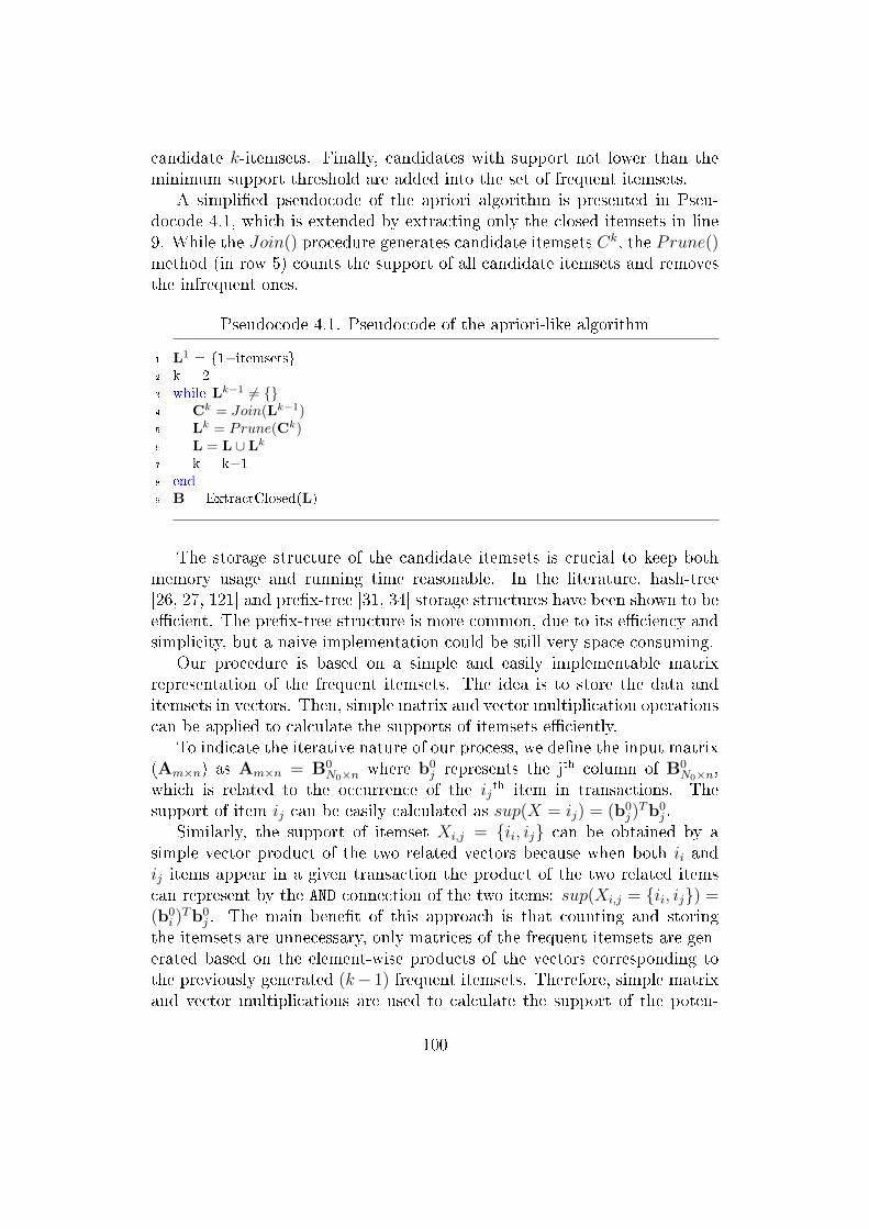
candidate k-itemsets. Finally, candidates with support not lower than theminimum support threshold are added into the set of frequent itemsets.

A simpli�ed pseudocode of the apriori algorithm is presented in Pseu-docode 4.1, which is extended by extracting only the closed itemsets in line9. While the Join() procedure generates candidate itemsets Ck, the Prune()method (in row 5) counts the support of all candidate itemsets and removesthe infrequent ones.

Pseudocode 4.1. Pseudocode of the apriori-like algorithm

1 L1 = {1−itemsets}2 k = 23 while Lk−1 6= {}4 Ck = Join(Lk−1)5 Lk = Prune(Ck)6 L = L ∪ Lk

7 k = k+18 end9 B = ExtractClosed(L)

The storage structure of the candidate itemsets is crucial to keep bothmemory usage and running time reasonable. In the literature, hash-tree[26, 27, 121] and pre�x-tree [31, 34] storage structures have been shown to bee�cient. The pre�x-tree structure is more common, due to its e�ciency andsimplicity, but a naive implementation could be still very space-consuming.

Our procedure is based on a simple and easily implementable matrixrepresentation of the frequent itemsets. The idea is to store the data anditemsets in vectors. Then, simple matrix and vector multiplication operationscan be applied to calculate the supports of itemsets e�ciently.

To indicate the iterative nature of our process, we de�ne the input matrix(Am×n) as Am×n = B0

N0×n where b0j represents the jth column of B0

N0×n,which is related to the occurrence of the ijth item in transactions. Thesupport of item ij can be easily calculated as sup(X = ij) = (b0

j)Tb0

j .Similarly, the support of itemset Xi,j = {ii, ij} can be obtained by a

simple vector product of the two related vectors because when both ii andij items appear in a given transaction the product of the two related itemscan represent by the AND connection of the two items: sup(Xi,j = {ii, ij}) =(b0

i )Tb0

j . The main bene�t of this approach is that counting and storingthe itemsets are unnecessary, only matrices of the frequent itemsets are gen-erated based on the element-wise products of the vectors corresponding tothe previously generated (k− 1) frequent itemsets. Therefore, simple matrixand vector multiplications are used to calculate the support of the poten-

100

tial k + 1 itemsets: Sk = (Bk−1)TBk−1, where the ith and jth element of thematrix Sk represent the support of the Xi,j = {Lk−1i ,Lk−1j } itemset, whereLk−1 represents the set of (k-1)-itemsets. As a consequence, only matri-ces of the frequent itemsets are generated, by forming the columns of theBkNk×nk−1

as the element-wise products of the columns of Bk−1Nk−1×nk−1

, i.e.

BkNk×nk−1

= bk−1i ◦ bk−1j , ∀i 6= j, where A ◦ B means the Hadamard productof matrices A and B.

The concept is simple and easily interpretable and supports compact ande�ective implementation. The proposed algorithm has a similar philosophyto the Apriori TID [120] method to generate candidate itemsets. None ofthese methods have to revisit the original data table, B0

N×n, for computingthe support of larger itemsets. Instead, our method transforms the tableas it goes along with the generation of the k-itemsets, B1

N1×n1. . .Bk

Nk×nk,

Nk < Nk−1 < · · · < N1. B1N1×n1

represents the data related to the 1-frequentitemsets. This table is generated from B0

N×n, by erasing the columns relatedto the non-frequent items, to reduce the size of the matrices and improve theperformance of the generation process.

Rows that are not containing any frequent itemsets (the sum of the row iszero) in Bk

Nk×nkare also deleted. If a column remains, the index of its original

position is written into a matrix that stores only the indices ("pointers") ofthe elements of itemsets L1

N1×1. When Lk−1Nk−1×k−1 matrices related to theindexes of the k − 1-itemsets are ordered, it is easy to follow the heuristicsof the apriori algorithm, as only those Lk−1 itemsets will be joined whose�rst k-1 items are identical (the set of these itemsets form the blocks of theBk−1Nk−1×nk−1

matrix).Fig. 4.10 represents the second step of the algorithm, using minsupp = 3

in the Prune() procedure.

101

Figure 4.10. Mining process example using the bit-table representation.

4.4.1 MATLAB implementation of the proposed algo-

rithm

The proposed algorithm uses matrix operations to identify frequent itemsetsand count their support values. Here we provide a simple but powerful imple-mentation of the algorithm using the user friendly MATLAB environment.The MATLAB code 4.2 and 4.3 present working code snippets of frequentclosed itemset mining, only within 34 lines of code.

The �rst code segment presents the second step of the discovery pipeline(see Fig. 4.1). Preprocessed data is stored in the variable bM in bit-tableformat as discussed above. The �rst and second steps of the iterative pro-cedure are presented in lines 1 and 2, where S2 and B2 are calculated. Theapriori principle is realized in the while loop in lines 4-19. Using the notationin Pseudocode 4.1, Cks are generated in lines 10-11 while Lks are preparedin the loop in lines 12-16.

MATLAB code 4.3 shows the usually most expensive calculation, thegeneration of closed frequent itemsets, which is denoted by Extraction offrequent closed itemsets in Fig. 4.1. Using the set of frequent items as thecandidate frequent closed itemsets, our approach calculates the support asthe sum of columns and eliminates non-closed itemsets from the candidate set(line 11). Again, an itemset J is a frequent closed itemset if it is frequentand there exists no proper superset J ′ ⊃ J such that sup(J ′) = sup(J). Thisis ensured by the for loop in lines 5-9.

102

MATLAB code 4.2. Mining frequent itemsets

1 s{1}=sum(bM); items{1}=�nd(s{1}≥suppn)′; s{1}=s{1}(items{1});2 dum=bM′∗bM; [i1,i2]=�nd(triu(dum,1)≥suppn); items{2}=[i1 i2];3 k=34 while ∼isempty(items{k−1})5 Items{k}=[]; s{k}=[]; ci =[];6 for i=1:size(items{k−1},1)7 vv=prod(bM(:,items{k−1}(i,:)),2);8 if k==3; s{2}(i)=sum(vv); end;9 TID=�nd(vv>0);

10 pf=(unique(items{k−1}(�nd(ismember(items{k−1}(:,1:end−1),items{k−1}(i,1:end−1),′rows′)),end)));

11 �=pf(�nd(pf>items{k−1}(i,end)));12 for jj=�′

13 j=�nd(items{1}==jj);14 v= vv(TID).∗bM(TID,items{1}(j)); sv=sum(v);15 items{k}=[items{k}; [items{k−1}(i,:) items{1}(j) ]]; s{k}=[s{k}; sv];16 end17 end18 k=k+119 end

MATLAB code 4.3. The generation of closed frequent itemsets

1 for k=1:length(items)−12 Citems{k}=[];3 for i=1:size(items{k},1)4 part=0;5 for j=1:size(items{k+1},1)6 IS=intersect(items{k}(i ,:) ,items{k+1}(j,:)) ;7 if and((sum(ismember(items{k}(i,:), IS))==k),s{k}(i)==s{k+1}(j))8 part=part+1; end9 end

10 if part==011 Citems{k}=[Citems{k}; items{k}(i,:)];12 end13 end14 end15 Citems{k+1}=items{end};

103

4.4.2 Computational results

As previously in the chapter, we compare our proposed method to BiMAX[133], which is a highly recognized reference method within the biclusteringresearch community. As BiMAX is regularly applied to binary gene expres-sion data, it serves as a good reference for the comparison. Using severalbiological and various synthetic data sets, we show that while both methodsare able to discover all patterns (frequent closed itemsets/biclusters), ourpattern discovery approach outperforms BiMAX.

To compare the two mining methods and demonstrate the computationale�ciency, we applied them to several real and synthetic data sets. Realdata come from various biological studies previously used as reference datain biclustering research [75, 99]. For the comparison of the computationale�ciency, all biological data sets were binarized. For both the fold-changedata (stem cell data sets) and the absolute expression data (Leukemia, Com-pendium, Yeast-80) fold-change cut-o� 2 is used. Results are shown in Ta-ble 4.4 (synthetic data) and Table 4.5 (real data), respectively. Both methodswere able to discover all closed patterns for all synthetic and real data sets.The results show that our method outperforms BiMAX and provides the bestrunning times in all cases, especially when the number of rows and columnsare higher.

4.5 Biological validation of discovered patterns

The real data set used in this section comes from the study of the e�ects ofTet1-knockdown on gene expression in mouse embryonic stem cell (ES) andtrophoblast stem cell (TS) conditions. We have analyzed the data using ourstandard analysis pipeline and the results have been published in [95]. Thedata set (GEO reference: GSE26900) consists of 27 samples from 8 samplegroups (3-6 replicates per group).

R/Bioconductor tools were used for all data processing except for thebiclustering. The data was normalized using the popular quantile normal-ization method. Various quality measures and visualizations were producedfor both raw and normalized data; boxplots were used for checking the datadistributions, hierarchical clustering, principal component analysis and cor-relation analysis were used for checking the sample relationships. Theseanalyses revealed that the correlation between samples was generally high,especially between the biological replicates. It was also discovered that TSgroup was very di�erent from all other groups, which in turn mainly clusteredaccording to the culture conditions (either TS or ES). Statistical comparisons

104

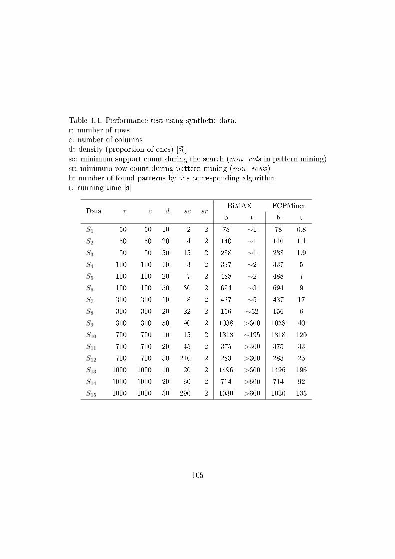
Table 4.4. Performance test using synthetic data.r: number of rowsc: number of columnsd: density (proportion of ones) [%]sc: minimum support count during the search (min_cols in pattern mining)sr: minimum row count during pattern mining (min_rows)b: number of found patterns by the corresponding algorithmt: running time [s]

Data r c d sc srBiMAX FCPMiner

b t b t

S1 50 50 10 2 2 78 ∼1 78 0.8

S2 50 50 20 4 2 140 ∼1 140 1.1

S3 50 50 50 15 2 238 ∼1 238 1.9

S4 100 100 10 3 2 337 ∼2 337 5

S5 100 100 20 7 2 488 ∼2 488 7

S6 100 100 50 30 2 694 ∼3 694 9

S7 300 300 10 8 2 437 ∼5 437 17

S8 300 300 20 22 2 156 ∼52 156 6

S9 300 300 50 90 2 1038 >600 1038 40

S10 700 700 10 15 2 1318 ∼195 1318 120

S11 700 700 20 45 2 375 >300 375 33

S12 700 700 50 210 2 283 >300 283 25

S13 1000 1000 10 20 2 1496 >600 1496 196

S14 1000 1000 20 60 2 714 >600 714 92

S15 1000 1000 50 290 2 1030 >600 1030 135

105

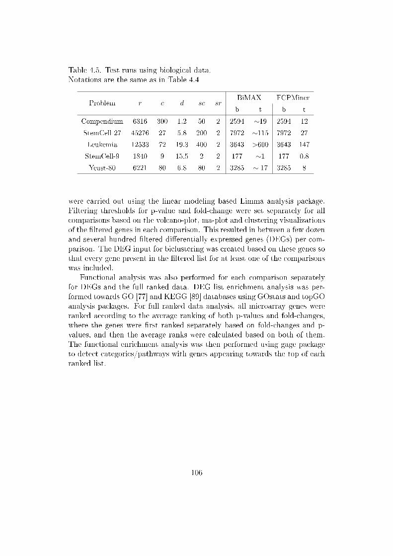
Table 4.5. Test runs using biological data.Notations are the same as in Table 4.4

Problem r c d sc srBiMAX FCPMiner

b t b t

Compendium 6316 300 1.2 50 2 2594 ∼19 2594 12

StemCell-27 45276 27 5.8 200 2 7972 ∼115 7972 27

Leukemia 12533 72 19.3 400 2 3643 >600 3643 147

StemCell-9 1840 9 15.5 2 2 177 ∼1 177 0.8

Yeast-80 6221 80 6.8 80 2 3285 ∼ 17 3285 8

were carried out using the linear modeling based Limma analysis package.Filtering thresholds for p-value and fold-change were set separately for allcomparisons based on the volcano-plot, ma-plot and clustering visualizationsof the �ltered genes in each comparison. This resulted in between a few dozenand several hundred �ltered di�erentially expressed genes (DEGs) per com-parison. The DEG input for biclustering was created based on these genes sothat every gene present in the �ltered list for at least one of the comparisonswas included.

Functional analysis was also performed for each comparison separatelyfor DEGs and the full ranked data. DEG list enrichment analysis was per-formed towards GO [77] and KEGG [89] databases using GOstats and topGOanalysis packages. For full ranked data analysis, all microarray genes wereranked according to the average ranking of both p-values and fold-changes,where the genes were �rst ranked separately based on fold-changes and p-values, and then the average ranks were calculated based on both of them.The functional enrichment analysis was then performed using gage packageto detect categories/pathways with genes appearing towards the top of eachranked list.

106

4.5.1 Comparison of biclustering methods

The processed biological data (StemCell_9) was used to compare our methodand three previously published biclustering methods, namely, BiMAX, QUBICand BiBit. We analyzed both the DEG data and the full sample data (27samples) with all three. For the DEG data, the minimum number of condi-tions was set to 3 for each method. While our method managed to discoverall valid 115 biclusters, BiMAX, BiBit and QUBIC discovered 128, 127 and68, respectively. We found that the 68 biclusters that QUBIC found areentirely included in our 115. Because of the greedy nature of QUBIC, theremaining 47 remained hidden. BiMAX and BiBit found more biclusters dueto their stringent binarization. However, when inspecting these clusters moreclosely, we �nd that 70% of the clusters are invalid, i.e. containing erroneousgenes with uncorrelated regulation pro�les.

Common way to compare di�erent methods is to run functional enrich-ment analysis for the result biclusters and then calculate the percentage ofbiclusters detected with certain signi�cance levels in each method. Here thediscovered biclusters were analyzed with respect to the enrichment of func-tional GO categories and KEGG pathways using overrepresentation analysisapplying a hypergeometric test [134] to calculate enrichment p-value for each

Table 4.6. Number of biclusters showing signi�cant enrichment in GO cate-gories for our method and the three compared biclustering algorithms.

Max.p-value Our method BiMAX QUBIC BiBit

5E-12 2 1 2 1

5E-11 2 2 2 2

5E-10 3 3 3 3

5E-09 5 4 5 4

5E-08 8 5 8 5

5E-07 23 22 17 22

5E-06 56 59 36 59

5E-05 74 86 49 85

5E-04 108 122 66 121

0.005 115 128 68 127

0.05 115 128 68 127

0.5 115 128 68 127

107

Table 4.7. Number of biclusters showing signi�cant enrichment in KEGGpathways for our method and other biclustering algorithms.

Max.p-value Our method BiMAX QUBIC BiBit

5E-06 4 2 4 2

5E-05 7 9 7 9

5E-04 33 35 17 35

0.005 56 68 34 67

0.05 111 124 66 123

0.5 111 124 66 123

category and pathway. In Table4.6 and Table 4.7, the numbers of biclustersare displayed that showed signi�cant enrichment of any GO category andKEGG pathways below certain p-value thresholds.

These data show that all four methods are able to discover the main bi-clusters and capture the major functional categories and pathways relatedto cell di�erentiation processes (e.g. GO:0048863: stem cell di�erentiation,GO:0048864: stem cell development) for the properly preprocessed data eventhough there are slight variation in the p-values. This is somewhat in contrastto �ndings of some previous studies where clear advantages over other meth-ods and even strong disagreements between them have been reported. Likelyexplanations for the earlier reported method disagreement are the improperpreprocessing of data, which may a�ect certain methods stronger than othersand the unsuitability of the metrics used for comparing the performance ofdi�erent methods. The high agreement with respect to enrichment results inour comparison is however not surprising as the majority of the genes in thebiclusters found by di�erent methods remain the same and thus the generalfunctional trends are not strongly a�ected. However, when the focus is on in-dividual genes and gene groups, which is the case when biological researchersare looking at the results related to real experiments, having valid clusterswithout erroneous genes be-comes more important. In addition, despite theoverall consistency of di�erent approaches, methods using binarization com-pletely missed some biclusters at lower signi�cance levels due to erroneousgenes in the clusters.

A representative example is depicted in Fig. 4.11. Analyzing gene ex-pression data like "Yeast-80", we can illustrate the gene expression valuesover di�erent conditions, and biologists can extract the information from thebicluster, like the genes moving the same or exactly opposite way.

108

Figure 4.11. Representative example. Depicts the expression value of thegenes over conditions from "Yeast-80" data, in the identi�ed bicluster no.3282

4.6 Conclusions

The development of closed frequent itemset mining and bicluster mining al-gorithms are separated to each other in the literature. However, as it wasdemonstrated in this chapter, choosing the parameters of existing algorithmsappropriately, these two techniques provide exactly the same result set. Insection 4.2 the equivalence of closed frequent itemset mining and biclusteringunder appropriately chosen parameters was proved, which was con�rmed us-ing small examples from the literature by applying both type of algorithms forthe same dataset. Since most of existing biclustering algorithms are either notaccurate enough or their bad scalability result in long running times, or both,a novel recursive biclustering technique was developed to handle {−1, 0, 1}(see section 4.3.1), while a really easily interpretable bit-table based methodwas discussed in section 4.4. A detailed and comparative computationalanalysis was elaborated for both novel methods in sections 4.3.5 and 4.4.2to illustrate the applicability of the algorithms. The novel methods wereproved to be more powerful than any other solution so far to discover con-stant valued biclusters by the solution of several test problem. Furthermore,our �rst algorithm is capable to �nd oppositely changing patterns also, sinceit has serious importance in �eld of cell biology. Because of the fact thatthe most accurate biclustering algorithm (e.g. BiMAX which can be con-sidered as reference) only capable to deal with binary data, a novel generaldata transformation tool was also presented in subsection 4.3.2 which trans-

109

forms {−1, 0, 1} data into binary format and ensures the consistency with theoriginal data. To provide wider application area of the resulted biclusters,a novel merging technique and visualization method was also presented insection 4.3.4 and 4.3.3, with which bigger but less consistent biclusters canbe constructed and visualized. Since the most important application area ofbiclustering is the �eld of cell biology, section 4.5 presented detailed analysisof the results and fair comparisons with previous methods using biologicaltests.

110

Chapter 5

Summary and Theses

The support of decision making is a complex task consisting of multiplemethods. During the dissertation we investigated three di�erent optimiza-tion problems and provided several techniques for modeling, simulation, op-timization and visualization. All three chapters presented directly applicableresults in decision support, where the presentation of the results are easilyunderstandable, and the optimization methods are fast enough to provideusable tools for decision makers.

In chapter 2 a novel genetic representation based genetic algorithm wasproposed which is capable to optimize complex transportation problems,namely the multiple traveling salesmen problem with time windows, han-dling additional constraints and minimizing the number of salesmen involvedinto the solution also. This technique with the novel genetic operators wasproved to be more e�ective than any other approaches so far. We describedan automated Google Maps based framework also to serve the optimizationtool using Google Maps API to de�ne or generate input data and to visualizethe results in a user-friendly way.

In chapter 3 a complex problem of inventory management was discussed,where warehouses are connected to each other in multiple echelons, and theuncertainty in consumption has to be handled. To satisfy these criteria anovel simulator was developed and used during Monte Carlo simulation pro-viding a robust and user-friendly simulator, SIMWARE. By the help of thesimulator the multi-echelon inventory problem can be modeled in a realisticway, where consumption is generated from empirical distribution functions,and using multiple simulations, uncertainties can be modeled also. Basedon the simulator, a novel gradient-free optimization method, and two mod-i�ed particle swarm optimization algorithms were researched and appliedsuccessfully in the solution. As a concrete result in decision support, a novelsensitivity analysis technique was developed to explore the connection be-

111

tween the changes of input and output variables in a multi-echelon supplychain, and to present the results in an easily interpretable way.

The last chapter discussed problems where the complexity is lied in thehigh number of dimensions of the input data. Two novel dimension-reduction,gradient-free techniques were presented in chapter 4 to mine binary, purebiclusters and to identify correlated gene expressions in biological data. Toreduce the pureness of identi�ed biclusters and provide itemsets in bigger size,a novel aggregation technique as well as a novel visualization method wereproposed. The bit-table representation based algorithm uses simple matrixoperations which supports the easy interpretation and implementation ofthe proposed method. Based on the novel algorithms, an easy to use fuzzyclassi�er rules mining technique was also presented which provides directlyapplicable method in decision making. The proposed techniques were provedto be more e�ective then previous approaches using real biological data, andbiological statistic methods.

5.1. Tézisek

1. Célirányos problémareprezentáció kialakításával korlátokat ésid®ablakokat is kezel® többes utazóügynök probléma megoldá-sában hatékony genetikus algoritmust hoztam létre. Az algo-ritmus segítségével és Google Maps API alapú támogatássalegy felhasználóbarát és hatékony eszközt készítettem és alkal-maztam valós logisztikai probléma megoldásában.(Kapcsolódó publikációk: [2, 3, 4, 11, 16, 17, 18])

(a) Megmutattam, hogy megfelel® genetikus reprezentáció alkalmazá-sával a genetikus algoritmusok hatékonysága nagymértékben javít-ható az irodalomban fellelhet® eddigi megoldásokhoz képest a töb-bes utazóügynök probléma megoldására. A bevezetett ún. multi-chromosome reprezentációra alapozva létrehoztam egy új típusúgenetikus algoritmust, mely a korábbi megoldásokhoz képest rö-videbb futási id®t és hatékonyabb m¶ködést mutat. Az elkészülteszközzel valós logisztikai problémák optimális útvonaltervét ké-szítettem el, minimalizálva a járm¶vek számát, �gyelembe véve azátadási id®t mint id®ablakot, kielégítve az utazási id®re és távol-ságra vonatkozó korlátokat. [2, 3, 4, 16]

112

(b) A kifejlesztett módszer támogatására és valós környezetben törté-n® alkalmazhatóságának biztosítására Google Maps API-n alapulómoduláris szoftvert hoztam létre. Az elkészült programcsomaggalegy, a Google Maps felületén de�niált térképb®l kiindulva felhasz-nálóbarát módon van lehet®ség a jelöl®k koordinátáinak kinyeré-sére, a távolságmátrixok valós útforgalmi viszonyok alapján tör-tén® generálására, illetve az optimalizálás eredményének könnyenértelmezhet®, ugyancsak Google Maps térképen történ® vizualizá-ciójára. [4, 11, 17, 18]

(c) Az elkészült program segítségével komplex logisztikai feladatokkomplett költségoptimalizálását végeztem el, mint az EOn Ser-vices Kft. 600 mobilszerel®b®l álló �ottájának körutas ellátássaltörtén® kielégítése a jelenlegi csillagpontos ellátás helyett. [4]

2. Többszint¶ ellátási hálózatokban készletszintek alakulását mo-dellez® és különböz® rendelési stratégiákat kezel® sztochaszti-kus modellt készítettem. Kimutattam, hogy e modell MonteCarlo szimulációjával ezen rendszerek robosztus és hatékonymódon modellezhet®k és optimalizálhatók.(Kapcsolódó publikációk: [1, 10, 12, 14, 19, 20, 21])

(a) Többszint¶ ellátási hálózatokban feltérképeztem, hogy az elmé-leti modellek alkalmazása helyett historikus adatokból feltárt fo-gyásigények alapján konstruált eloszlásfüggvények használatávaljóval pontosabb modell alkotható, mellyel a valós rendszer ha-tékonyabban modellezhet®. Ennek támogatására kifejlesztettemegy sztochasztikus szimulátort, melyet alkalmazva a Monte Carlomódszertanon alapulva sikeresen optimalizáltam kétszint¶ ellátásihálózatokat mind SQP, mind PSO algoritmusok alkalmazásával.[10, 12, 14, 19, 20]

(b) Az elkészült szimulátor és optimalizációs technika segítségével olyanmódszertant fejlesztettem ki, melynek segítségével meghatározha-tók az ellátási hálózatban megjelen® legfontosabb kulcsmutatók.Az elkészített, Monte Carlo módszertanon alapuló paraméterérzé-kenység-vizsgálat eredményeinek megjelenítésére egy újfajta me-tódust alkottam. Az új típusú vizualizációs technika segítségévelkönnyen értelmezhet® formában jelenítettem meg a érzékenység-analízis eredményeit, mellyel a vállalati döntéshozók számára iskönnyen felderíthet®ek a rendszer bemeneti változói és kimene-tei közötti összefüggések, vagyis meghatározhatók a legfontosabbkulcsmutatók. [1, 21]

113

3. Nagy (biogenetikai) adatmátrixokban rejl® információk feltá-rására újszer¶ biclustering keresési adatbányászati techniká-kat hoztam létre.(Kapcsolódó publikációk: [5, 6, 8, 13, 15, 22])

(a) Feltártam és elméletileg megalapoztam a zárt gyakori elemhal-mazok keresésének és az ún. biclustering technika közötti szorosösszefüggést, nevezetesen hogy a módszerek megfelel® interpretá-lása és paramétereinek helyes megválasztása esetén a két módszerugyanazt az eredményhalmazt szolgáltatja. [6]

(b) Olyan új típusú algoritmust fejlesztettem ki, mely az irodalombanfellelhet® eddigi megoldásokhoz képest gyorsabban képes megta-lálni az összes konstans típusú zárt gyakori elemhalmazt bemenetibináris, vagy {-1, 0, 1} típusú adatban. A létrehozott módszer ro-bosztusabb a bemenet méretére vonatkozóan, mint az eddigi meg-oldások, és pontosan megtalálja a széles körben elfogadott és va-lidált biclustering algoritmus által szolgáltatott elemhalmazokat.[6, 8, 13, 15]

(c) A megtalált elemhalmazok ún. tiszta biclusterek, vagyis nulláktólmentesek. Nullák, vagyis hibás vagy értéktelen adatok megenge-désére a feltárt elemhalmazokban egy olyan új összevonási tech-nikát dolgoztam ki, mely iteratív módon a Tanimoto távolságonalapulva egyesíti az egyes elemhalmazokat, így alakítva ki egyrenagyobb és egyre kevésbé tiszta biclustereket. [6]

(d) Olyan adat-transzformációs technikát dolgoztam ki, mellyel azalapvet®en csak bináris adatokat kezel® algoritmusokat is alkal-massá lehet tenni a {-1, 0, 1} típusú adatok kezelésére, és így azéppen ellentétesen változó adatfolyamok felderítésére is. [6]

(e) Ugyancsak kidolgoztam egy olyan új típusú algoritmust, mely azún. bit-table reprezentációt használva, egyszer¶ mátrix m¶veleteksegítségével képes biclusterek keresésére bináris adathalmazokon.A bevezetett technika egyszer¶ m¶ködéséb®l adódóan különösenkönnyen értelmezhet® és ennek megfelel®en gyors és egyszer¶ imp-lementálhatóságot biztosít. [5]

114

Kapcsolódó eredmények (Kapcsolódó publikációk: [7, 9])

Az irodalomban Mimikri-ként ismert módszer alapján kifejlesztet-tem egy olyan új típusú szoftvert, melynek segítségével a felhasz-náló képes megbecsülni fehérjék és fehérjehalmazok közötti im-munológiai keresztreakció valószín¶ségét. A program segítségévelkönnyen értelmezhet® formában vizualizáltam a kombinatorikaiszámításokon alapuló módszer eredményeit.

5.2 Theses

1. Introducing a novel targeted problem representation, an e�ec-tive genetic algorithm is proposed for the solution of multipletraveling salesmen problem with additional constraints. Us-ing the novel algorithm supported by Google Maps API, ane�ective, user-friendly tool has been implemented and appliedin real logistics problem.(Related publications: [2, 3, 4, 11, 16, 17, 18])

(a) It has been shown that using appropriate and more realistic ge-netic representation, the performance and e�ectiveness of geneticalgorithms can be greatly improve for the solution of multiple trav-eling salesmen problem. Based on the proposed multi-chromosomerepresentation a novel genetic algorithm has been developed pro-viding shorter running times and better solution than previoussolutions in the literature. Using the novel tool, the optimal routeplan of real logistical problems were generated, minimizing thenumber of vehicles, satisfying constraints for traveling time anddistance and taking into consideration time windows. [2, 3, 4, 16]

(b) Supporting the novel algorithm a Google Maps API based mod-ular software package has been developed. This tool providesuser-friendly interfaces to de�ne the initial map, to retrieve thecoordinated from the markers, to generate the distance tables au-tomatically using real tra�c conditions and to visualize the resultson Google Maps' interface. [4, 11, 17, 18]

(c) By the help of the software package and algorithm, complex logis-tical problems were optimized for overall cost, as the redesign ofthe supply of 600 mobile mechanics at EOn Services Kft. [4]

115

2. A novel model has been researched to model the movementof inventory levels in multi-echelon supply chains, which canhandle several ordering strategies. It has shown that usingMonte Carlo simulation, the model is capable to simulatethese multi-level systems e�ectively and robustly.(Related publications: [1, 10, 12, 14, 19, 20, 21])

(a) It was explored during the research that using empirical distribu-tion function from real historical demands instead of theoreticalfunctions in multi-level supply chains, the real system can be mod-eled more accurately and e�ectively. A stochastic simulator wasalso developed to supply the research. By the help of the simu-lator, applying the Monte Carlo method to handle uncertainty inthe model, a two-level inventory management system was success-fully optimized by SQP and two novel modi�ed PSO algorithms.[10, 12, 14, 19, 20]

(b) Using the proposed simulator and optimization technique a novelmethodology has been developed to determine the prime key in-dicators in supply chains. To visualize the results of the MonteCarlo method based parameter sensitivity analysis technique, anew method has been proposed. Using the new visualization tech-nique, results of the sensitivity analysis are presented in an easilyinterpretable way providing an easy method for decision makers toidentify the main relations between the input and output variablesand to determine the key performance indicators. [1, 21]

3. Novel data-mining techniques has been proposed to retrieverelevant information from huge (bioinformatics) data matricesby the identi�cation of biclusters.(Related publications: [5, 6, 8, 13, 15, 22])

(a) It has been theoretically justi�ed that the so-called biclusteringtechnique and closed frequent itemset mining provide the sameresult set using appropriately chosen parameters. [6]

(b) A novel algorithm has been proposed which is capable to �nd allclosed frequent itemsets in binary or in −1, 0, 1 data much fasterthan any previous solution so far. The developed method is morerobust regarding the size of input data than previous solutions inthe literature and as accurate as the widely cited and validatedbiclustering algorithm. [6, 8, 13, 15]

116

(c) The identi�ed itemsets are so-called pure biclusters, i.e. they con-tain no zeros. To allow zeros (fault value) in biclusters, a novelaggregation method has been proposed which iteratively combinesthe itemsets based on their Tanimoto distance, creating biclustersin increasing size and decreasing purity. [6]

(d) A data-transformation technique has been researched and devel-oped which makes binary biclustering methods (methods handleonly binary data) to handle −1, 0, 1 type of data. Using this tech-nique, traditional biclustering methods are capable to identify op-positely changing data streams. [6]

(e) A novel bit-table representation based algorithm has been devel-oped to mine biclusters in binary data using only simple matrixoperations. The applied extremly easily interpretable techniquetechnique supports the rapid and easy implementation of the al-gorithm. [5]

Related results (Related publications: [7, 9])

Based on the method known as Mimikri in the literature, a novelsoftware has been developed to estimate the immunologic correla-tion between proteins ans protein sets. The results of the combi-natorial computation based method is visualized in a user-friendly,easily interpretable way.

5.3 Publications related to theses

Articles in international journals

[1] Gábor Belvárdi, András Király, Zoltán Gyozsán Tamás Varga, andJános Abonyi. Monte carlo simulation based performance analysis ofsupply chains. International Journal of Managing Value and SupplyChains, 3(2):1�15, 2012.

[2] András Király and János Abonyi. A novel approach to solve multi-ple traveling salesmen problem by genetic algorithm. ComputationalIntelligence in Engineering, 313:141�151, 2010.

[3] András Király and János Abonyi. Optimization of multiple travelingsalesmen problem by a novel representation based genetic algorithm. InIntelligent Computational Optimization in Engineering, volume 366 of

117

Studies in Computational Intelligence, pages 241�269. Springer Berlin/ Heidelberg, 2011.

[4] András Király and János Abonyi. Redesign of the supply of mobilemechanics based on a novel genetic optimization algorithm using googlemaps api. Engineering Applications of Arti�cial Intelligence, 2013,under review.

[5] András Király, Attila Gyenesei, and János Abonyi. Bit-table basedbiclustering and frequent closed itemset mining in high-dimensionalbinary data. Lecture Notes in Computer Science, 2013, under review.

[6] András Király, Asta Laiho, János Abonyi, and Attila Gyenesei. Noveltechniques and an e�cient algorithm for closed pattern mining. PatternRecognition Letters, 2013, under review.

[7] Katalin Kristóf, Krisztina Madách, Noémi Sándor, Zsolt Iványi, An-drás Király, Anna Erdei, and Eszter Tulassay. Impact of molecularmimicry on the clinical course and outcome of sepsis syndrome. Molec-ular Immunology, 2011.

[8] Asta Laiho, András Király, and Attila Gyenesei. Genefuncster: A webtool for gene functional enrichment analysis and visualisation. In DavidGilbert and Monika Heiner, editors, Computational Methods in SystemsBiology, Lecture Notes in Computer Science, pages 382�385. SpringerBerlin Heidelberg, 2012.

[9] Krisztina Madách, Katalin Kristóf, Eszter Tulassay, Zsolt Iványi, AnnaErdei, András Király, János Gál, and Zsuzsa Bajtay. Mucosal immunityand the intestinal microbiome in the development of critical illness.ISRN Immunology, 2011, 2011.

[10] Tamás Varga, András Király, and János Abonyi. Improvement of psoalgorithm by memory based gradient search - application in inventorymanagement. In Swarm Intelligence and Bio-Inspired Computation:Theory and Applications. Springer Berlin / Heidelberg, 2013, accepted.

Articles in Hungarian journals

[11] András Király and János Abonyi. A google maps based novel approachto the optimization of multiple traveling salesman problem for limiteddistribution systems. Acta Agraria Kaposváriensis, 14(3):1�14, 2010.

118

[12] András Király, Gábor Belvárdi, and János Abonyi. Determining opti-mal stock level in multi-echelon supply chains. Hungarian Journal ofIndustrial Chemistry, 39(1):107�112, 2011.

Conferences

[13] János Abonyi, András Király, and Attila Gyenesei. Biclustering basedon bittable based frequent itemset mining. In International Workshopon Clustering High-Dimensional Data (CHDD 2012), Naples, Italy,2012.

[14] László Dobos, András Király, and János Abonyi. Economic orientedstochastic optimization of model predictive controlled processes. InVeszprém Optimization Conference: Advanced Algorithms (VOCAL),Veszprém, Hungary, 2010.

[15] Andrá Király, János Abonyi, Asta Laiho, and Attila Gyenesei. Biclus-tering of high-throughput gene expression data with bicluster miner.In Data Mining Workshops (ICDMW), 2012 IEEE 12th InternationalConference, pages 131�138, dec. 2012.

[16] András Király and János Abonyi. Optimization of multiple travelingsalesmen problem by a novel representation based genetic algorithm.In 10th International Symposium of Hungarian Researchers on Com-putational Intelligence and Informatics, Budapest, Hungary, 2009.

[17] András Király and János Abonyi. Google maps alapú programcsomagútvonalhálózat elemzésének és optimalizációjának támogatására. InInformatika Korszer¶ Technikái Konferencia, Dunaújváros, Hungary,2010.

[18] András Király and János Abonyi. A google maps based novel approachto the optimization of limited distribution systems. In VIII. Alkalma-zott Informatika Konferencia, Kaposvár, Hungary, 2010.

[19] András Király and János Abonyi. Optimális szállítási gyakoriságmeghatározása többszint�u elllátási hálózatokban. In Mobilitás ésKörnyezet Konferencia, Veszprém, Hungary, 2011.

[20] András Király, Tamás Varga, and János Abonyi. Constrained particleswarm optimization of supply chains. In International Conference onMathematical, Computational and Statistical Sciences, and Engineer-ing, Zurich, Switzerland, 2012.

119

[21] András Király, Tamás Varga, Gábor Belvárdi, Zoltán Gyozsán, andJános Abonyi. Monte carlo simulation based sensitivity analysis ofmulti-echelon supply chains. In Factory Automation, Veszprém, Hun-gary, 2012.

[22] Asta Laiho, Attila Gyenesei, András Király, János Abonyi, Colin Sem-ple, Chris Haley, and Wenhua Wei. High-throughput detection of epis-tasis in studies of the genetics of complex traits. In 9th annual inter-national conference on Computational Systems Bioinformatics (CSB2010), Stanford, California, 2010.

120

List of Figures

1.1 The applied technologies by problem characteristics. . . . . . . 2

2.1 The life cycle of genetic algorithms. . . . . . . . . . . . . . . . 142.2 Permutation encoded chromosomes. . . . . . . . . . . . . . . . 152.3 Example route-system with 15 cities and with 4 salesmen. . . 162.4 Example of one chromosome representation for a 15 city mTSP

with 4 salesperson ([49]). . . . . . . . . . . . . . . . . . . . . . 162.5 Example of two chromosome representation for a 15 city mTSP

with four salesperson ([49]). . . . . . . . . . . . . . . . . . . . 172.6 Example of two-part chromosome representation for a 15 city

mTSP with 4 salesmen ([49]). . . . . . . . . . . . . . . . . . . 172.7 One-, and two-point crossover of binary encoded individuals. . 182.8 Mutation of binary encoded individuals. . . . . . . . . . . . . 182.9 Example of the multi-chromosome representation for a 20 city

mTSP (n = 20) with 5 salesperson (m = 5). . . . . . . . . . . 202.10 In-route mutations - "Gene sequence inversion" (upper part)

and "Flip" (lower part) . . . . . . . . . . . . . . . . . . . . . . 212.11 Cross-route mutation - gene sequence transposition - "Swap" . 212.12 Cross-route mutation - complex operator - Slide + Swap. . . . 222.13 The hierarchy of mutation operators. . . . . . . . . . . . . . . 232.14 An example from the test set, with 100 locations. . . . . . . . 242.15 Result of e�ciency analysis. . . . . . . . . . . . . . . . . . . . 252.16 The work�ow of the desired application . . . . . . . . . . . . . 302.17 The component diagram of the proposed framework. . . . . . 312.18 Schematic view of the current status and the desired solution

of the industrial problem. CD - Central Depot, WH - Ware-house, B - Base . . . . . . . . . . . . . . . . . . . . . . . . . . 32

2.19 Results of the Visualiser component for 30 locations with atmost 5 salesmen and at most 450 km tour length per salesman. 34

3.1 The classic model of inventory control. . . . . . . . . . . . . . 40

121

3.2 The theoretical cumulative distribution function (left side) andthe actual cumulative distribution function for a raw materialbased on its consumption data (right side) . . . . . . . . . . . 41

3.3 Example of a 2-echelon supply chain with a distribution storeand with 2 retailers. The supply from the manufacture isunlimited. . . . . . . . . . . . . . . . . . . . . . . . . . . . . . 44

3.4 Values of the objective function for the 2-level system pre-sented by equation 3.5. . . . . . . . . . . . . . . . . . . . . . . 44

3.5 Values of service levels in each warehouses in the investigatedexample (see Fig. 3.3. . . . . . . . . . . . . . . . . . . . . . . . 45

3.6 An example 3-level system depicted by SIMWARE. . . . . . . 453.7 Simulated inventory levels of the 3-level multi-echelon system

presented in Fig. 3.6. . . . . . . . . . . . . . . . . . . . . . . . 463.8 Result of the optimization of the 2-echelon system using SQP

method. . . . . . . . . . . . . . . . . . . . . . . . . . . . . . . 473.9 Inventory levels in the optimized 2-level system. . . . . . . . . 483.10 The plot of the analyzed objective functions. (a) corresponds

to equation 3.10 and (b) to equation 3.11. . . . . . . . . . . . 523.11 Surface of the �tness function called "dropwave" (a) the "griewangks"

function (b), the stochastic function we used (c), and a stochas-tic version of "griewangks" (noise added) (d). . . . . . . . . . 58

3.12 Histograms for the "gBest" values using the function called"griewangks" with noise. In the title of the sub�gures, meanrepresents the mean value of the histogram, std is the standarddeviation and w-grad is the weight of the gradient part in theobjective value calculation of the individuals. . . . . . . . . . . 60

3.13 The analyzed 2-level system using one distributor and oneretailer. . . . . . . . . . . . . . . . . . . . . . . . . . . . . . . 62

3.14 Average inventory levels before optimization in the 2-echelonsupply chain (see Fig. 3.13). Reorder points are 500 and 200respectively. . . . . . . . . . . . . . . . . . . . . . . . . . . . . 63

3.15 Average inventory levels after optimization in the 2-echelonsupply chain (see Fig. 3.13). Reorder points are 1031 and 100respectively. . . . . . . . . . . . . . . . . . . . . . . . . . . . . 64

3.16 Simpli�ed data �aw diagram of the proposed sensitivity analysis. 683.17 Visualization of sensitivities in the example problem. . . . . . 703.18 Mean value of the actual inventory levels in the investigated

two-echelon inventory model. . . . . . . . . . . . . . . . . . . . 723.19 Result of the sensitivity analysis in the two-level inventory

system. . . . . . . . . . . . . . . . . . . . . . . . . . . . . . . . 74

122

4.1 Schematic view of bicluster discovery. . . . . . . . . . . . . . . 784.2 Schematic representation of the biclustering problem. It is

important to note that the objects within one bicluster can belocated either very close to each other (as in B1) or furtherapart (as in B2, B3 and B4). . . . . . . . . . . . . . . . . . . . 81

4.3 A simple example illustrating how FCPMiner works. . . . . . 874.4 Visual representation of the input transformation for a simple

input matrix . . . . . . . . . . . . . . . . . . . . . . . . . . . . 884.5 Visualization of rearranged data matrix based on the pattern

mining results . . . . . . . . . . . . . . . . . . . . . . . . . . . 904.6 Example for aggregation of 2 patterns . . . . . . . . . . . . . . 914.7 Visualization illustrating the e�ciency of the pattern merging

algorithm . . . . . . . . . . . . . . . . . . . . . . . . . . . . . 924.8 Examples of patterns discovered by FCPMiner and binary

FCP mining methods. . . . . . . . . . . . . . . . . . . . . . . 964.9 Bit-table representation of market basket data. . . . . . . . . . 994.10 Mining process example using the bit-table representation. . . 1024.11 Representative example. Depicts the expression value of the

genes over conditions from "Yeast-80" data, in the identi�edbicluster no. 3282 . . . . . . . . . . . . . . . . . . . . . . . . . 109

123

List of Tables

2.1 Synthetic test results. Average of 100 runs. n: size of theproblem, i.e. number of locations; m: number of salesmen;k: minimum tour length; p: population size; Opt.: best foundsolution (overall distance); It.: iteration number when the bestsolution found; t: running time in seconds. . . . . . . . . . . . 26

2.2 Test results using complex operators and initialization. Aver-age of 100 runs. n: size of the problem, i.e. number of lo-cations; m: number of salesmen; k: minimum tour length; p:population size; Opt.: best found solution (overall distance);It.: iteration number when the best solution found; t: runningtime in seconds. . . . . . . . . . . . . . . . . . . . . . . . . . . 26

2.3 Test results using complex operators and initialization. Aver-age of 10 runs. n: size of the problem, i.e. number of locations;m: number of salesmen; l: maximum tour length; Best : bestfound solution (overall distance); Avg : Average of 10 runs. . . 27

2.4 Test results using complex operators and initialization. Aver-age of 10 runs. n: size of the problem, i.e. number of locations;m: number of salesmen; Best : best found solution (overall dis-tance); Avg : Average of 10 runs. . . . . . . . . . . . . . . . . . 28

2.5 Part of the industrial problem's distance table - kilometers. . . 33

3.1 The e�ect of the introduced parameter c3 on the convergenceof PSO . . . . . . . . . . . . . . . . . . . . . . . . . . . . . . . 53

3.2 Mathematical equations of the analyzed functions. . . . . . . . 593.3 Test results performing 500 MC simulation, modifying the

weight for the gradient part. Best results are highlighted ineach row for the objective values. . . . . . . . . . . . . . . . . 61

3.4 The parameters (mean and deviation) of the example distri-bution functions . . . . . . . . . . . . . . . . . . . . . . . . . . 69

3.5 The analytically calculated example sensitivity matrix . . . . . 703.6 The investigated demand function parameters. . . . . . . . . . 733.7 The resulted sensitivity matrix in the two-echelon problem. . . 74

124

4.1 Computational results using synthetic data sets. . . . . . . . . 944.2 Comparison to DCI_Closed. . . . . . . . . . . . . . . . . . . . 954.3 Comparing FCPMiner with other relevant methods. . . . . . . 984.4 Performance test using synthetic data. . . . . . . . . . . . . . 1054.5 Test runs using biological data. . . . . . . . . . . . . . . . . . 1064.6 Number of biclusters showing signi�cant enrichment in GO

categories for our method and the three compared biclusteringalgorithms. . . . . . . . . . . . . . . . . . . . . . . . . . . . . 107

4.7 Number of biclusters showing signi�cant enrichment in KEGGpathways for our method and other biclustering algorithms. . 108

125

Bibliography

[23] Fimi'03: Workshop on frequent itemset mining implementations. InBart Göthals and Mohammed J Zaki, editors, IEEE International Con-ference on Data Mining Workshop on Frequent Itemset Mining Imple-mentations, Melbourne, Florida, USA, 2003.

[24] Fimi'04: Workshop on frequent itemset mining implementations. InRoberto Bayardo, Bart Göthals, and Mohammed J Zaki, editors, IEEEInternational Conference on Data Mining Workshop on Frequent Item-set Mining Implementations, Brighton, UK, 2004.

[25] R. Agrawal, T. Imieli«ski, and A. Swami. Mining association rulesbetween sets of items in large databases. In ACM SIGMOD Record,volume 22, pages 207�216. ACM, 1993.

[26] R. Agrawal, H. Mannila, R. Srikant, H. Toivonen, A.I. Verkamo, et al.Fast discovery of association rules. Advances in knowledge discoveryand data mining, 12:307�328, 1996.

[27] Rakesh Agrawal and Ramakrishnan Srikant. Fast algorithms for miningassociation rules. In Proceedings of the 20th International Conferenceon Very Large Data Bases, VLDB, volume 1215, pages 487�499, 1994.

[28] Mukshed Ahammed and Robert E. Melchers. Gradient and parametersensitivity estimation for systems evaluated using monte carlo analysis.Reliability Engineering & System Safety, 91(5):594�601, 2006.

[29] M. Al-Mashari and M. Zairi. Supply-chain re-engineering using en-terprise resource planning (erp) systems: an analysis of a sap r/3 im-plementation case. International Journal of Physical Distribution &Logistics Management, 30(3/4):296�313, 2000.

[30] Agha Iqbal Ali and Je�ery L Kennington. The asymmetric m-travelingsalesmen problem: a duality based branch-and-bound algorithm. Dis-crete Applied Mathematics, 13:259�276, 1986.

126

[31] A. Amir, R. Feldman, and R. Kashi. A new and versatile method forassociation generation. Information Systems, 22(6):333�347, 1997.

[32] T Back, D. B. Fogel, and Z Michalewicz. Handbook of evolutionarycomputation. IOP Publishing Ltd., 1997.

[33] Sándor Balogh. Többszempontú gazdasági döntéseket segít® genetikusalgoritmus kidolgozása és alkalmazásai. PhD thesis, Kaposvár Univer-sity, 2009.

[34] R.J. Bayardo Jr. E�ciently mining long patterns from databases. InACM Sigmod Record, volume 27, pages 85�93. ACM, 1998.

[35] Benita M Beamon. Supply chain design and analysis:: Models andmethods. International Journal of Production Economics, 55(3):281 �294, 1998.

[36] Tolga Bektas. The multiple traveling salesman problem: an overviewof formulations and solution procedures. Omega, 34:209�219, 2006.

[37] Amir Ben-Dor, Benny Chor, Richard Karp, and Zohar Yakhini. Dis-covering local structure in gene expression data: The order-preservingsubmatrix problem. Journal of Computational Biology, 10(3-4):373�384, 2003.

[38] Sven Bergmann, Jan Ihmels, and Naama Barka. Iterative signaturealgorithm for the analysis of large-scale gene expression data. Phys.Rev. E, 67(3):03190201�18, 2003.

[39] S Bhide, N John, and Mansur R Kabuka. A boolean neural networkapproach for the traveling salesman problem. IEEE Transactions onComputers, 42(10):1271, 1993.

[40] Tobias Blickle and Lothar Thiele. A comparison of selection schemesused in evolutionary algorithms. Evolutionary Computation, 4(4):361�394, 1996.

[41] E. Borgonovo, M. Marseguerra, and E. Zio. A monte carlo methodolog-ical approach to plant availability modeling with maintenance, agingand obsolescence. Reliability Engineering and System Safety, 67:61�73, 2000.

[42] István Borgulya. Evolúciós algoritmusok. Dialóg Campus, 2004.

127

[43] B. Borowska and S. Nadolski. Particle swarm optimization: the gradi-ent correction. Journal of Applied Computer Science, 17(2):7�15, 2009.

[44] Evelyn C. Brown, Cli� T. Ragsdale, and Arthur E. Carter. A group-ing genetic algorithm for the multiple traveling salesperson problem.International Journal of Information Technology & Decision Making,6(02):333�347, 2007.

[45] Stanislav Busygin, Oleg Prokopyev, and Panos M. Pardalos. Biclus-tering in data mining. Computers & Operations Research, 35(9):2964�2987, 2008.

[46] J. Caldas and S. Kaski. Bayesian biclustering with the plaid model.In Machine Learning for Signal Processing, 2008. MLSP 2008. IEEEWorkshop on, pages 291�296. IEEE, 2008.

[47] Andrea Califano, Gustavo Stolovitzky, and Yuhai Tu. Analysis of geneexpression microarrays for phenotype classi�cation. In Proc. Int'l Conf.Computational Molecular Biology, volume 8, pages 75�85, 2000.

[48] Giuliano Caloiero, Fernanda Strozzi, and José-Manuel ZaldívarComenges. A supply chain as a series of �lters or ampli�ers ofthe bullwhip e�ect. International Journal of Production Economics,114(2):631�645, 2008.

[49] Arthur E. Carter and Cli� T. Ragsdale. A new approach to solvingthe multiple traveling salesperson problem using genetic algorithms.European Journal of Operational Research, 175:246�257, 2006.

[50] Rachel Cavill, Steve Smith, and Andy Tyrrell. Multi-chromosomalgenetic programming. In Proceedings of the 2005 conference on Geneticand evolutionary computation, pages 1753�1759. ACM New York, NY,USA, 2005.

[51] Yizong Cheng and George M. Church. Biclustering of expression data.In Eighth International Conference on Intelligent Systems for Molecu-lar Biology (ISMB '00), pages 93�103, 2000.

[52] S. Chopra and P. Meindl. Supply chain management. strategy, planning& operation. Das Summa Summarum des Management, pages 265�275,2007.

[53] Martin Christopher. Logistics and supply chain management: creatingvalue-added networks. Pearson education, 2005.

128

[54] M.C. Cooper, D.M. Lambert, and J.D. Pagh. Supply chain manage-ment: more than a new name for logistics. International Journal ofLogistics Management, The, 8(1):1�14, 1997.

[55] B. Csukás and S. Balogh. Combining genetic programming with genericsimulation models in evolutionary synthesis. Computers in Industry,36(3):181�197, 1998.

[56] M. Bixby Cooper Donald J. BowerSox, David J. Closs. Supply ChainLogistics Management. McGraw-Hill, 2002.

[57] AI Edwards, AP Engelbrecht, and N. Franken. Nonlinear mappingusing particle swarm optimisation. In Evolutionary Computation, 2005.The 2005 IEEE Congress on, volume 1, pages 306�313. IEEE, 2005.

[58] A.P. Engelbrecht, A. Engelbrecht, and A. Ismail. Training product unitneural networks. 1999.

[59] H.K. Feng, JS Bao, and Y Jin. Particle swarm optimization combinedwith ant colony optimization for the multiple traveling salesman prob-lem. In Materials science forum, volume 626, pages 717�722. TransTech, 2009.

[60] Gerd Finke. Network �ow based branch and bound method for asym-metric traveling salesman problems. In XI Symposium on OperationsResearch, pages 117�119, Darmstadt, 1986.

[61] B.R. Fox and M.B. McMahon. Genetic operators for sequencing prob-lems. In Gregory J.E. Rawlins, editor, Foundations of genetic algo-rithms, pages 284�300, San Mateo, 1991. Morgan Kaufmann.

[62] Carlos Garcia-Martinez, Oscar Cordón, and Francisco Herrera. A tax-onomy and an empirical analysis of multiple objective ant colony opti-mization algorithms for the bi-criteria tsp. European Journal of Oper-ational Research, 180(1):116�148, 2007.

[63] Mitsuo Gen and Runwei Cheng. Genetic algorithms and engineeringdesign. John Wiley and Sons, Inc., New York, 1997.

[64] Xiutang Geng, Zhihua Chen, Wei Yang, Deqian Shi, and Kai Zhao.Solving the traveling salesman problem based on an adaptive simu-lated annealing algorithm with greedy search. Applied Soft Computing,11(4):3680 � 3689, 2011.

129

[65] Gad Getz, Erel Levine, and Eytan Domany. Coupled two-way clus-tering analysis of gene microarray data. Proceedings of the NationalAcademy of Sciences, 97(22):12079�12084, 2000.

[66] Soheil Ghafurian and Nikbakhsh Javadian. An ant colony algorithmfor solving �xed destination multi-depot multiple traveling salesmenproblems. Applied Soft Computing, 11(1):1256 � 1262, 2011.

[67] Fred Glover. Arti�cial intelligence, heuristic frameworks and tabusearch. Managerial and Decision Economics, 11(5):365�375, 1990.

[68] David E. Goldberg. Genetic algorithms in search, optimization and ma-chine learning. Addison-Wesley Longman Publishing Co., Inc. Boston,MA, USA, 1989.

[69] Gösta Grahne and Jianfei Zhu. E�ciently using pre�x-trees in miningfrequent itemsets. In FIMI'03 Workshop on Frequent Itemset MiningImplementations, pages 123�132, 2003.

[70] Stephen C. Graves and Sean P. Willems. Optimizing strategic safetystock placement in supply chains. Manufacturing & Service OperationsManagement, 2(1):68�83, 2000.

[71] Stephen C. Graves and Sean P. Willems. Supply chain design: safetystock placement and supply chain con�guration. Handbooks in Opera-tions Research and Management Science, 11:95�132, 2003.

[72] Stephen C. Graves and Sean P. Willems. Strategic inventory placementin supply chains: nonstationary demand. Manufacturing & ServiceOperations Management, 10(2):278�287, 2008.

[73] J Gromicho, J Paixão, and I Bronco. Exact solution of multiple travel-ing salesman problems. Combinatorial optimization: new frontiers intheory and practice, pages 291�292, 1992.

[74] Gregory Gutin and Abraham P. Punnen. The Traveling Salesman Prob-lem and Its Variations. Combinatorial Optimization. Kluwer AcademicPublishers, Dordrecht, The Nederlands, 2002.

[75] Attila Gyenesei, Ulrich Wagner, Simon Barkow-Oesterreicher, EtzardStolte, and Ralph Schlapbach. Mining co-regulated gene pro�les forthe detection of functional associations in gene expression data. Bioin-formatics, 23(15):1927�1935, 2007.

130

[76] Jiawei Han, Hong Cheng, Dong Xin, and Xifeng Yan. Frequent pat-tern mining: current status and future directions. Data Mining andKnowledge Discovery, 15:55�86, 2007. 10.1007/s10618-006-0059-1.

[77] MA Harris, J. Clark, A. Ireland, J. Lomax, M. Ashburner, R. Foulger,K. Eilbeck, S. Lewis, B. Marshall, C. Mungall, et al. The gene on-tology (go) database and informatics resource. Nucleic acids research,32(Database issue):D258, 2004.

[78] J. A. Hartigan. Direct clustering of a data matrix. Journal of theAmerican Statistical Association (JASA), 67(337):123�129, 1972.

[79] Jack C. Hayya, Uttarayan Bagchi, Jeon G. Kim, and Daewon Sun. Onstatic stochastic order crossover. International Journal of ProductionEconomics, 114(1):404�413, 2008.

[80] Ruprecht-Karls-Universität Heidelberg. Tsplib, 2013.

[81] John H. Holland. Adaptation in Natural and Arti�cial Systems. TheUniversity of Michigan Press, Cambridge, 1975.

[82] Chau-Yun Hsu, Meng-Hsiang Tsai, and Wei-Mei Chen. A study offeature-mapped approach to the multiple travelling salesmen problem.IEEE International Symposium on Circuits and Systems, 3:1589�1592,1991.

[83] X. Hu and R. Eberhart. Solving constrained nonlinear optimizationproblems with particle swarm optimization. In Proceedings of the sixthworld multiconference on systemics, cybernetics and informatics, vol-ume 5, pages 203�206. Citeseer, 2002.

[84] J.M. Huband, J.C. Bezdek, and R.J. Hathaway. bigvat: visual as-sessment of cluster tendency for large data sets. Pattern Recognition,38(11):1875�1886, 2005.

[85] Nicolas Jozefowiez, Frederic Semet, and El-Ghazali Talbi. Multi-objective vehicle routing problems. European Journal of OperationalResearch, 189(2):293�309, 2008.

[86] Kenneth F. Simpson Jr. In-process inventories. Operations Research,pages 863�873, 1958.

[87] June Young Jung, Gary Blau, Joseph F. Pekny, Gintaras V. Reklaitis,and David Eversdyk. A simulation based optimization approach to

131

supply chain management under demand uncertainty. Computers &chemical engineering, 28(10):2087�2106, 2004.

[88] Pan Junjie and Wang Dingwei. An ant colony optimization algorithmfor multiple travelling salesman problem. In Innovative Computing,Information and Control, 2006. ICICIC'06. First International Con-ference on, volume 1, pages 210�213. IEEE, 2006.

[89] M. Kanehisa, S. Goto, S. Kawashima, Y. Okuno, and M. Hattori.The kegg resource for deciphering the genome. Nucleic acids research,32(suppl 1):D277�D280, 2004.

[90] Minoru Kanehisa, Susumu Goto, Shuichi Kawashima, Yasushi Okuno,and Masahiro Hattori. The kegg resource for deciphering the genome.Nucleic Acids Research, 32(suppl 1):D277�D280, 2004.

[91] J. Kennedy and R. Eberhart. Particle swarm optimization. In Neu-ral Networks, 1995. Proceedings., IEEE International Conference on,volume 4, pages 1942�1948. IEEE, 1995.

[92] Yuval Kluger, Ronen Basri, Joseph T. Chang, , and Mark Gerstein.Spectral biclustering of microarray data: Coclustering genes and con-ditions. Genome Research, 13(4):703�716, 2003.

[93] P. Köchel and U. Nieländer. Simulation-based optimisation of multi-echelon inventory systems. International journal of production eco-nomics, 93:505�513, 2005.

[94] Kian Peng Koh, Akiko Yabuuchi, Sridhar Rao, Yun Huang, Kerri-anne Cunni�, Julie Nardone, Asta Laiho, Mamta Tahiliani, Cesar A.Sommer, Gustavo Mostoslavsky, Riitta Lahesmaa, Stuart H. Orkin,Scott J. Rodig, George Q. Daley, and Anjana Rao. Tet1 and tet2 regu-late 5-hydroxymethylcytosine production and cell lineage speci�cationin mouse embryonic stem cells. Cell stem cell, 8:200�213, 2011.

[95] K.P. Koh, A. Yabuuchi, S. Rao, Y. Huang, K. Cunni�, J. Nardone,A. Laiho, M. Tahiliani, C.A. Sommer, G. Mostoslavsky, et al. Tet1and tet2 regulate 5-hydroxymethylcytosine production and cell lineagespeci�cation in mouse embryonic stem cells. Cell Stem Cell, 8(2):200�213, 2011.

[96] Gilbert Laporte and Yves Nobert. A cutting planes algorithm forthe m-salesmen problem. Journal of the Operational Research Soci-ety, 31:1017�1023, 1980.

132

[97] Amy Hing-Ling Lau and Hon-Shiang Lau. A comparison of di�er-ent methods for estimating the average inventory level in a (q,r) sys-tem with backorders. International Journal of Production Economics,79(3):303�316, 2002.

[98] Laura Lazzeroni and Art Owen. Plaid models for gene expression data.Statistica Sinica, 12(1):61�86, 2002.

[99] Guojun Li, Qin Ma, Haibao Tang, Andrew H. Paterson, and YingXu. Qubic: a qualitative biclustering algorithm for analyses of geneexpression data. Nucleic Acids Research, 37(15):e101, 2009.

[100] Guimei Liu, Hongjun Lu, Wenwu Lou, and Je�rey Xu Yu. On com-puting, storing and querying frequent patterns. In Proceedings of theninth ACM SIGKDD international conference on Knowledge discoveryand data mining, KDD '03, pages 607�612, New York, NY, USA, 2003.ACM.

[101] Xiaowen Liu and Lusheng Wang. Computing the maximum similaritybi-clusters of gene expression data. Bioinformatics, 23(1):50�56, 2007.

[102] D.P. Loucks, E. Van Beek, J.R. Stedinger, J.P.M. Dijkman, and M.T.Villars. Water resources systems planning and management: an intro-duction to methods, models and applications. Paris: UNESCO, 2005.

[103] Claudio Lucchese, Salvatore Orlando, and Ra�aele Perego. Dci_closed:A fast and memory e�cient algorithm to mine frequent closed itemsets.In IEEE ICDM'04 Workshop FIMI'04, 2004.

[104] Claudio Lucchese, Salvatore Orlando, and Ra�aele Perego. Mining top-k patterns from binary datasets in presence of noise. In Proceedingsof the 10th SIAM International Conference on Data Mining (SDM),Columbus, OH, pages 165�176, 2010.

[105] Sara C. Madeira and Arlindo L. Oliveira. Biclustering algorithms forbiological data analysis: A survey. IEEE Transactions on computa-tional Biology and Bioinformatics, pages 24�45, 2004.

[106] Dragana Makaji¢-Nikoli¢, Biljana Pani¢, and Mirko Vujo²evi¢. Bull-whip e�ect and supply chain modelling and analysis using cpn tools.In Fifth Workshop and Tutorial on Practical Use of Colored Petri Netsand the CPN Tools, 2004.

133

[107] Charles J. Malmborg. A genetic algorithm for service level based vehiclescheduling. European Journal of Operational Research, 93(1):121�134,1996.

[108] H. Mannila, H. Toivonen, and A.I. Verkamo. E�cient algorithms fordiscovering association rules. In Proceedings of the 1994 AAAI Work-shop on Knowledge Discovery in Databases, pages 181��192, 1994.

[109] K Mathias and DWhitley. Genetic operators, the �tness landscape andthe traveling salesman problem. Parallel Problem Solving from Nature,2:219�228, 1992.

[110] R. Mendes, J. Kennedy, and J. Neves. The fully informed parti-cle swarm: simpler, maybe better. Evolutionary Computation, IEEETransactions on, 8(3):204 � 210, june 2004.

[111] P. Miliotis. Using cutting planes to solve the symmetric travellingsalesman problem. Mathematical Programming, 15(1):177�188, 1978.

[112] H. Min and G. Zhou. Supply chain modeling: past, present and future.Computers & industrial engineering, 43(1-2):231�249, 2002.

[113] P.A. Miranda and R.A. Garrido. Incorporating inventory control deci-sions into a strategic distribution network design model with stochasticdemand. Transportation Research Part E: Logistics and TransportationReview, 40(3):183�207, 2004.

[114] P.A. Miranda and R.A. Garrido. Inventory service-level optimizationwithin distribution network design problem. International Journal ofProduction Economics, 122(1):276�285, 2009.

[115] T. M. Murali and Simon Kasif. Extracting conserved gene expressionmotifs from gene expression data. In Paci�c Symposium on Biocom-puting, pages 77�88, 2003.

[116] E.P. Musalem and R. Dekker. Controlling inventories in a supply chain:A case study. International Journal of Production Economics, 93:179�188, 2005.

[117] T. Nagatani and D. Helbing. Stability analysis and stabilization strate-gies for linear supply chains. Physica A: Statistical Mechanics and itsApplications, 335(3):644�660, 2004.

134

[118] R Nallusamy, K Duraiswamy, R Dhanalaksmi, and P Parthiban. Op-timization of non-linear multiple traveling salesman problem using k-means clustering, shrink wrap algorithm and meta-heuristics. Interna-tional Journal of Nonlinear Science, 8(4):480�487, 2009.

[119] M.M. Noel and T.C. Jannett. Simulation of a new hybrid particleswarm optimization algorithm. In System Theory, 2004. Proceedingsof the Thirty-Sixth Southeastern Symposium on, pages 150�153. IEEE,2004.

[120] F.P. Pach, A. Gyenesei, and J. Abonyi. Compact fuzzy associationrule-based classi�er. Expert systems with applications, 34(4):2406�2416,2008.

[121] J.S. Park, M.S. Chen, and P.S. Yu. An e�ective hash-based algorithmfor mining association rules, volume 24. ACM, 1995.

[122] Yang-Byung Park. A hybrid genetic algorithm for the vehicle schedul-ing problem with due times and time deadlines. International Journalof Productions Economics, 73(2):175�188, 2001.

[123] K.E. Parsopoulos and M.N. Vrahatis. Particle swarm optimiza-tion method for constrained optimization problems. IntelligentTechnologies�Theory and Application: New Trends in Intelligent Tech-nologies, 76:214�220, 2002.

[124] Nicolas Pasquier, Yves Bastide, Ra�k Taouil, and Lot� Lakhal. Discov-ering frequent closed itemsets for association rules. In Proceedings ofthe 7th International Conference on Database Theory, ICDT '99, pages398�416, London, UK, UK, 1999. Springer-Verlag.

[125] Jian Pei, Jiawei Han, and Runying Mao. Closet: An e�cient algorithmfor mining frequent closed itemsets. In ACM SIGMOD Workshop onResearch Issues in Data Mining and Knowledge Discovery, number 2,pages 21�30, 2000.

[126] D. Petrovic. Simulation of supply chain behaviour and performance inan uncertain environment. International Journal of Production Eco-nomics, 71(1):429�438, 2001.

[127] Hans J. Pierrot and Robert Hinterding. Multi-chromosomal geneticprogramming, volume 1342/1997 of Lecture Notes in Computer Sci-ence, chapter Using multi-chromosomes to solve a simple mixed integerproblem, pages 137�146. Springer Berlin / Heidelberg, 1997.

135

[128] Arthur Pitman. Market-basket synthetic data generator, 2011.

[129] M.E. Poter. Competitive advantage: Creating and sustaining superiorperformance. New York et al, 1985.

[130] Jean-Yves Potvin. Genetic algorithms for the traveling salesman prob-lem. Annals of Operations Research, 63(3):337�370, 1996.

[131] Jean-Yves Potvin Potvin, G Lapalme, and J Rousseau. A generalizedk-opt exchange procedure for the mtsp. INFOR, 27:474�481, 1989.

[132] A. Prékopa. On the hungarian inventory control model. Europeanjournal of operational research, 171(3):894�914, 2006.

[133] Amela Preli¢, Stefan Bleuler, Philip Zimmermann, Anja Wille, PeterBühlmann, Wilhelm Gruissem, Lars Hennig, Lothar Thiele, and EckartZitzler. A systematic comparison and evaluation of biclustering meth-ods for gene expression data. Bioinformatics, 22(9):1122�1129, 2006.

[134] J.A. Rice. Mathematical statistics and data analysis. Thomson Learn-ing, 2006.

[135] John A Rice. Mathematical statistics and data analysis (Third Editioned.). Duxbury press, 2007.

[136] Domingo S. Rodriguez-Baena, Antonio J. Perez-Pulido, and Jesus S.AguilarRuiz. A biclustering algorithm for extracting bit-patterns frombinary datasets. Bioinformatics, 27(19):2738�2745, 2011.

[137] S. Ronald and S. Kirkby. Compound optimization. solving transportand routing problems with a multi-chromosome genetic algorithm. InThe 1998 IEEE International Conference on Evolutionary Computa-tion, ICEC'98, pages 365�370, 1998.

[138] Sheldon M. Ross. Introduction to Probability Models. NY: AcademicPress, Macmillian, New York, 1984.

[139] R.Y. Rubinstein and D.P. Kroese. Simulation and the Monte Carlomethod. Wiley-interscience, 2008.

[140] Robert A. Russell. An e�ective heuristic for the m-tour travelingsalesman problem with some side conditions. Operations Research,25(3):517�524, 1977.

136

[141] M. Sakaguchi. Inventory model for an inventory system with time-varying demand rate. International Journal of Production Economics,122(1):269�275, 2009.

[142] Leonidas L. Sakalauskas. Nonlinear stochastic programming by monte-carlo estimators. European Journal of Operational Research, 137(3):558� 573, 2002.

[143] R. Salomon. Evolutionary algorithms and gradient search: Similaritiesand di�erences, 1998.

[144] A. Saltelli. Sensitivity analysis in practice: a guide to assessing scien-ti�c models. John Wiley & Sons Inc, 2004.

[145] Funda Samanlioglu, William G. Ferrell Jr., and Mary E. Kurz. Amemetic random-key genetic algorithm for a symmetric multi-objectivetraveling salesman problem. Computers & Industrial Engineering,55(2):439�449, 2008.

[146] J.D. Schwartz, W. Wang, and D.E. Rivera. Simulation-based optimiza-tion of process control policies for inventory management in supplychains. Automatica, 42(8):1311�1320, 2006.

[147] Y. Seo. Controlling general multi-echelon distribution supply chainswith improved reorder decision policy utilizing real-time shared stockinformation. Computers & Industrial Engineering, 51(2):229�246,2006.

[148] P. Shenoy, J.R. Haritsa, S. Sudarshan, G. Bhalotia, M. Bawa, andD. Shah. Turbo-charging vertical mining of large databases. In ACMSIGMOD Record, volume 29, pages 22�33. ACM, 2000.

[149] Alok Singh and Anurag Singh Baghel. A new grouping genetic algo-rithm approach to the multiple traveling salesperson problem. SoftComputing-A Fusion of Foundations, Methodologies and Applications,13(1):95�101, 2009.

[150] I.M. Sobol. Global sensitivity indices for nonlinear mathematical mod-els and their monte carlo estimates. Mathematics and computers insimulation, 55(1-3):271�280, 2001.

[151] T. Sousa, A. Silva, and A. Neves. Particle swarm based data miningalgorithms for classi�cation tasks. Parallel Computing, 30(5):767�783,2004.

137

[152] M. Srinivasan and Y.B. Moon. A comprehensive clustering algorithmfor strategic analysis of supply chain networks. Computers & industrialengineering, 36(3):615�633, 1999.

[153] Pang-Ning Tan, Michael Steinbach, and Vipin Kumar. Introduction todata mining. Pearson Addison Wesley Boston, 2006.

[154] Amos Tanay, Roded Sharan, and Ron Shamir. Discovering statisticallysigni�cant biclusters in gene expression data. Bioinformatics, 18(suppl1):S136�S144, 2002.

[155] Amos Tanay, Roded Sharan, and Ron Shamir. Biclustering algorithms:A survey. Handbook of computational molecular biology, 2004.

[156] Chun Tang, Li Zhang, Aidong Zhang, and Murali Ramanathan. Inter-related two-way clustering: An unsupervised approach for gene expres-sion data analysis. In 2nd IEEE International Symposium on Bioin-formatics and Bioengineering (BIBE2001), pages 41�48, 2001.

[157] Lixin Tanga, Jiyin Liu, Aiying Rongc, and Zihou Yanga. A multipletraveling salesman problem model for hot rolling scheduling in shangaibaoshan iron & steel complex. European Journal of Operational Re-search, 124(2):267�282, 2000.

[158] Jorge Tavares, Penousal Machado, Francisco B. Pereira, and ErnestoCosta. On the in�uence of gvr in vehicle routing. In Proceedings of the2003 ACM symposium on Applied computing, pages 753�758. ACM,2003.

[159] F. Van Den Bergh. An analysis of particle swarm optimizers. PhDthesis, University of Pretoria, 2006.

[160] T.S. Vaughan. Lot size e�ects on process lead time, lead time de-mand, and safety stock. International Journal of Production Eco-nomics, 100(1):1�9, 2006.

[161] T. Victoire and A.E. Jeyakumar. Hybrid pso�sqp for economic dispatchwith valve-point e�ect. Electric Power Systems Research, 71(1):51�59,2004.

[162] Jianyong Wang, Jiawei Han, and Jian Pei. Closet+: searching for thebest strategies for mining frequent closed itemsets. In Proceedings of theninth ACM SIGKDD international conference on Knowledge discoveryand data mining, KDD '03, pages 236�245, New York, NY, USA, 2003.ACM.

138

[163] Zhiguan Wang, Chi Wai Yu, Ray C.C. Cheung, and Hong Yan. Hy-pergraph based geometric biclustering algorithm. Pattern RecognitionLetters, (0):�, 2012.

[164] T. Wimalajeewa and S.K. Jayaweera. Optimal power scheduling forcorrelated data fusion in wireless sensor networks via constrainedpso. Wireless Communications, IEEE Transactions on, 7(9):3608�3618, 2008.

[165] A. Windisch, S. Wappler, and J. Wegener. Applying particle swarmoptimization to software testing. In Proceedings of the 9th annual con-ference on Genetic and evolutionary computation, pages 1121�1128.ACM, 2007.

[166] Jiong Yang, Haixun Wang, Wei Wang, and Philip Yu. δ-clusters: Cap-turing subspace correlation in a large data set. In 18th InternationalConference on Data Engineering, pages 517�528. IEEE, 2002.

[167] Jiong Yang, Haixun Wang, Wei Wang, and Philip Yu. Enhanced bi-clustering on expression data. Third IEEE International Symposiumon Bioinformatic and Bioengineering (BIBE'03), pages 321�327, 2003.

[168] Fujimoto Yoshiji, Akita Yuki, and Yasui Tsuyoshi. Applying the geneticalgorithm with multi-chromosomes to order problems. Proceedings ofthe Annual Conference of JSAI, 13:468�471, 2001.

[169] Zhong Yu, Liang Jinhai, Gu Guochang, Zhang Rubo, and Yang Haiyan.An implementation of evolutionary computation for path planning ofcooperative mobile robots. Proceedings of the 4th World Congress onIntelligent Control and Automation, pages 1798�1802, 2002.

[170] M.J. Zaki and K. Gouda. Fast vertical mining using di�sets. In Proceed-ings of the ninth ACM SIGKDD international conference on Knowledgediscovery and data mining, pages 326�335. ACM, 2003.

[171] Mohammed J. Zaki and Ching-Jui Hsiao. Charm: An e�cient algo-rithm for closed association rule mining. In 2nd SIAM InternationalConf. on Data Mining, pages 457�473. Citeseer, 1999.

[172] R. Zhang, W. Zhang, and X. Zhang. A new hybrid gradient-based par-ticle swarm optimization algorithm and its applications to control ofpolarization mode dispersion compensation in optical �ber communica-tion systems. In Computational Sciences and Optimization, 2009. CSO

139

2009. International Joint Conference on, volume 2, pages 1031�1033.IEEE, 2009.

[173] Tiehua Zhang, W.A Gruver, and M.H. Smith. Team scheduling bygenetic search. In Proceedings of the Second International Conferenceon Intelligent Processing and Manufacturing of Materials, volume 2,pages 839�844, 1999.

140