Does Political Affirmative Action Work, and for Whom? Theory ...

Saad Gulzar

Nicholas Haas

Benjamin Pasquale

January, 2020

Working Paper No. 1056

Does Political Affirmative Action Work, and for Whom? Theory and Evidence on India’s

Scheduled Areas

Does Political Affirmative Action Work, andfor Whom? Theory and Evidence on India’s

Scheduled Areas

Saad GulzarStanford University

Nicholas HaasNew York University

Benjamin PasqualeIndependent Researcher∗

January 30, 2020Word count: 11,927

Abstract

Does political affirmative action undermine or promote development, and for whom?We examine Scheduled Areas in India, which reserve political office for the historicallydisadvantaged Scheduled Tribes. We apply a new theoretical framework and datasetof 217,000 villages to evaluate the overall impact of affirmative action on development,as well as its distributional consequences for minorities and non-minorities. Examiningeffects on the world’s largest employment program, the National Rural EmploymentGuarantee Scheme, we find that reservations deliver no worse overall outcomes, thatthere are large gains for targeted minorities, and that these gains come at the cost of therelatively privileged, not other minorities. We also find broader improvements in otherpro-poor policies, including a rural roads program and general public goods. Contraryto the expectations of affirmative action skeptics, our results indicate that affirmativeaction can redistribute both political and economic power without hindering overalldevelopment.

Keywords: Affirmative Action, Electoral Quota, Reservation, Scheduled Areas, ScheduledTribes, Scheduled Castes, NREGS, PMGSY, Employment

∗Gulzar is Assistant Professor, Stanford University ([email protected]). Haas is PhD Candidate, NewYork University ([email protected]). Pasquale is Independent Scholar ([email protected]). The authorswould like to thank Rachel Brule, Miriam Golden, Justin Grimmer, Hakeem Jefferson, Francesca Jensenius,David Laitin, Stephane Lavertu, Vijayendra Rao, Cyrus Samii, David Stasavage, Milan Vaishnav, and sem-inar participants at Gothenburg, Lahore School of Economics, NYU, Wisconsin-Madison, MPSA, OSU, andUppsala for helpful comments.

1 Introduction

Many countries have adopted political affirmative action with the express aim of raising

the voice of marginalized communities in how governments function. This paper asks how

improvements in descriptive representation might impact economic welfare. Studying this

question is of particular import where poor populations rely on large-scale government wel-

fare programs such as in the case of the Benazir Income Support Program in Pakistan that

provides 5.4 million poor women income supplements as a safety net, the Supplemental

Nutrition Assistance Program in the United States that helps 46 million low-income indi-

viduals purchase groceries every month, and the National Rural Employment Guarantee

Scheme (NREGS) in India, the world’s largest employment program that we examine in this

study.

Does descriptive representation achieved through affirmative action deliver improved wel-

fare for marginalized communities, or does restricting representation prove self-defeating in

that it damages the economic prospects of the populations it was designed to politically

empower? We study electoral quotas, an affirmative action policy that directly yields de-

scriptive representation and is implemented in over 100 countries,1 and ask two related, yet

under-explored questions: do electoral quotas improve or hinder development; and how are

the benefits (and costs) of electoral quotas distributed in society?

Prior evidence is mixed and does not offer clear theoretical expectations. Focusing on

minorities explicitly targeted under an electoral quota, some studies, which we review be-

low, show strong positive welfare effects, while others report no improvements. We organize

and extend hypotheses from previous work in a novel theoretical framework that enables an

explicit accounting of how electoral quotas affect the extensive margin of program imple-

mentation (that is, the overall size of the pie) and the intensive margin (the distribution of

the pie) for targeted disadvantaged groups, non-targeted disadvantaged groups, and for the

1See Bird (2014); Long (2019).

1

comparatively privileged groups under the status quo. This exercise allows a fuller under-

standing of the trade-offs involved in the implementation of affirmative action policies. A

solidarity hypothesis predicts that shared interests and experiences between minority groups

should lead to positive program spillovers from quota-targeted to non-targeted minorities.

A crowding-out hypothesis predicts that gains for a quota targeted minority will come at

the cost of other groups, particularly non-targeted minorities. And, a performance hypoth-

esis predicts better outcomes for targeted minorities and unchanged outcomes for others,

or, at the very least, negative outcomes for others that do not outweigh gains for targeted

minorities.

This paper examines a large electoral quota in India that brought increased descriptive

representation to well over 100 million citizens. Shortly after Independence from the British

in 1947, the Indian parliament declared certain regions in the country as Scheduled Areas

(SA), a designation linked to the protection of a historically-disadvantaged category of mi-

nority groups, the Scheduled Tribes (ST). From 2000, under the Panchayat Extension to

Scheduled Areas (PESA) Act, India’s national parliament implemented a dramatic electoral

quota in Scheduled Areas requiring that all chairperson positions in three tiers of local gov-

ernment councils, as well as at least half the seats on each of those councils, be reserved for

individuals from the Scheduled Tribes.

Why does understanding the impact of this electoral quota matter? First, the quota

has received no systematic quantitative analysis despite the fact that it is present in half

of India’s states and covers nearly half of the territory within those states. Second, the

quota targets ST, who are considered to be among the most economically vulnerable and

politically excluded groups in India. Third, the permanence of the Scheduled Areas quota

is qualitatively different from population-based quotas that rotate over time. Scholars have

argued that rotation is an impediment to long-term quota success (Dunning and Nilekani,

2013; Bhavnani, 2009).

Isolating the causal effect of Scheduled Areas is not straightforward. Indeed, comparing

2

SA to non-SA using data from the 2001 Indian Census shows that they differ on a number of

dimensions. By employing a geographic regression discontinuity (RD) design similar to Dell

(2010), we absorb variation that correlates with geographic space, allowing for a comparison

of villages lying just on one or the other side of the border between non-Scheduled and

Scheduled Areas. In other words, control (non-Scheduled) villages appear similar to treated

(Scheduled) villages except that in treated areas candidates for local offices are restricted to

ST individuals, whereas in control areas these restrictions are not in place.

We first examine the impacts of Scheduled Areas using data from NREGS, a flagship

federal program in India with an annual cost of approximately US$6 billion. Each year, the

social protection scheme officially guarantees 100 days of minimum-wage employment for

every rural household in India. We study program delivery to rural populations in 2013, up

to 12 years after the first implementation of PESA. We do this by creating a new dataset

with 217,144 villages that combines official NREGS implementation data with an original

spatial dataset of Scheduled Area status. The scale and depth of these data, which permit us

to evaluate both the extensive and intensive margins of program delivery, are a substantial

advance on existing work on affirmative action and economic development.2

Results show that NREGS delivery improves substantially for the targeted minorities

(ST), who receive 24.1 percent more workdays in Scheduled Areas. Improvement appears

to come primarily at the cost of work for non-minorities, who receive 12.5 percent fewer

workdays. We find no evidence that the quota causes a change in employment for the non-

targeted, historically disadvantaged minorities (SC). Our evidence thus offers support for the

crowding out and performance hypotheses, but not for the solidarity hypothesis. Overall,

the results indicate that the delivery of government programs in Scheduled Areas are no

2While Jensenius (2015), Pande (2003), and Das, Mukhopadhyay and Saroy (2017) con-

duct similar exercises, our detailed data help to disaggregate the non-targeted group into

meaningful categories of SC and non-minorities, allowing us to study the causal effect of

reservations on both efficiency and redistribution.

3

worse than in non-Scheduled Areas.

Are these effects specific to NREGS? We evaluate broader impacts of Scheduled Areas

by examining a second large-scale development scheme as well as outcomes from the 2011

Census. The 2011 Census reveals higher employment for women in Scheduled Areas, par-

ticularly those who are underemployed. Data also show improved provision of public goods

that is likely to benefit disadvantaged communities. We also observe increased rural road

connectivity from the Pradhan Mantri Gram Sadak Yojana (PMGSY) village roads program.

These improvements are consistent with the results from NREGS, insofar as they reflect a

higher responsiveness to the needs of marginalized communities.

To what extent are the results we observe the function of an electoral politics mechanism?

We provide four pieces of evidence. First, qualitative evidence from Indian historical studies,

as well as quantitative evidence from the PMGSY program and the Indian Census, show that

villages on opposite sides of the Scheduled and non-Scheduled border were very similar on a

host of dimensions prior to the implementation of PESA between 2000 and 2010. Second, the

quota is most effective where the targeted group is a relatively small proportion of the local

population – where we would expect a quota to have the largest marginal impact, given the

target group’s lower pre-quota bargaining power. Third, the effects of the quota are reduced

in areas of overlap with quotas for state-level ST legislators. Fourth, the impact of the quota

is largest when it constitutes the greatest shock to political representation: that is, following

the first election.

This paper makes theoretical, empirical, and policy contributions. The theoretical con-

tribution is to explicitly lay out hypotheses on the trade-offs of affirmative action on tar-

geted and historically disadvantaged, non-targeted and disadvantaged, and non-targeted and

non-disadvantaged identity-based groups, and combine them into a unified framework. Em-

pirically, our unique data allow us to test these hypothesis in the context of three critical,

village-level data sources – the largest rural employment scheme in the world, a national

rural roads development program, and public goods and economic measures from the census

4

of the world’s largest democracy, India. From a policy perspective, all too often policy-

makers and analysts treat parallel pro-poor economic and political efforts in isolation. By

considering their interaction, we hope to advance our understanding of how politics can be

made to work for inclusive development.

2 Theory and Hypotheses

In this section, we review conflicting findings and draw hypotheses from existing work on

the effects of political affirmative action on government functioning.

2.1 Extensive Margin (Size of the Pie)

Given the same resources and institutional design, do electoral quotes positively or negatively

affect the overall efficacy of government programs? Implementation of government programs

would suffer if quota politicians are less competent than non-quota politicians (Jensenius,

2017). Jensenius (2015) presents qualitative evidence that SC quota politicians are viewed

as inexperienced and referred to as “weak”, “inefficient”, and “useless” (p.202). Deshpande

and Weisskopf (2014) document how some oppose affirmative action policies due to a belief

that they result in less qualified individuals and worse performance. Bertrand, Hanna and

Mullainathan (2010) find that students admitted under quotas see an increase in income,

but these gains are more than offset by losses in earnings for individuals displaced by the

quota.

Conversely, implementation could improve if quota politicians work harder for their con-

stituents. Chin and Prakash (2011) report that ST quotas, but not SC quotas, result in

lower levels of overall poverty. Deshpande and Weisskopf (2014) find that a greater propor-

tion of high-level SC/ST employees in the Indian Railways is correlated with both increased

productivity and growth. Evidence also suggests that women exert more effort and outper-

form men when positions of political influence are available to them (Beaman et al., 2010;

5

Volden, Wiseman and Wittmer, 2013). Das, Mukhopadhyay and Saroy (2017) argue that

in the presence of asymmetric group sizes, affirmative action can improve the efficiency of

outcomes. Finally, government performance could remain unchanged if quota politicians

perform no better or worse than non-quota politicians, as Bhavnani and Lee (2018) find for

Indian bureaucrats.

2.2 Intensive Margin (Distribution of the Pie)

We now turn to the impact of affirmative action on targeted and non-targeted historically dis-

advantaged communities, and more privileged communities. While theoretical examinations

predict positive results for targeted minorities, existing research from India on electoral

reservations has found mixed effects. Besley, Pande and Rao (2007), Duflo and Chattopad-

hyay (2004), and Beaman et al. (2010) show that reservations for SC/ST and women improve

the welfare of direct beneficiaries. Other work, such as Dunning and Nilekani (2013) and

Jensenius (2015), find no overall effect of electoral quotas on targeted groups. Unlike our

case, one explanation for weak effects in the literature is the rotating nature of quotas in

these contexts, which limits politicians’ incentives to target benefits along ethnic lines.

We expect targeted minorities to benefit under affirmative action. Less clear is what we

should expect for non-targeted groups. We draw three hypotheses from existing literature

for why gains for targeted minorities may alternatively result in positive, negative, or no

spillovers to other groups.

Solidarity Hypothesis: Non-targeted minorities may experience positive spillovers from

quotas targeting other minorities. Studies have found that minority politicians may carry

intrinsic motivations – absent electoral motivations – to help individuals with whom they

identify (Broockman, 2013; Adida, Davenport and McClendon, 2016; Singh, 2015). They

may also share policy preferences with other minorities: Kaufmann (2003) writes that African

Americans and Latinos in the U.S. “share objective circumstances [and] interests” (2003,

6

p.199) and may have a ‘minority group consciousness’. Consistently, Adida, Davenport and

McClendon (2016) show that African Americans respond positively not only to co-ethnic

but also to co-minority (Latino) political cues.

Under this hypothesis, therefore, minority groups not targeted by the quota should also

benefit from improved program implementation. Some evidence from India is consistent

with this prediction: SC reserved councillors increase village expenditures in a manner that

benefits both SC and ST in their village (Palaniswamy and Krishnan, 2012).

These theories are largely silent on the expected effects on non-minorities. While one

can extrapolate that this group will not benefit under this hypothesis because of a lack

of solidarity with targeted minorities, it is unclear if they will be worse off or remain at

the status quo. As a consequence, there are also no clear predictions on what happens to

outcomes on the extensive margin.

Crowding Out Hypothesis: Gains in descriptive representation for one minority group

may come at the expense of benefits for non-targeted minorities, especially where targeted

and non-targeted minorities are in competition. Meier et al. (2004) examine changes in

representation among African-Americans and Latinos and find that improvements in ad-

ministrative and teaching positions for one group are associated with losses for the other.

Expectations of inter-caste competition and negative spillover effects are captured by Khosla

(2011), who argues that as “different castes vie to capture NREGS benefits, they limit the

access of other caste groups” (p.65).

Under this hypothesis, quotas could leave outcomes for non-minorities unchanged es-

pecially if targeted minorities still live under social pressure from non-minorities, or where

non-minorities are not in competition for the same goods. Alternatively, if competition for

resources exists, and if non-minority groups do not retain full control over their distribution,

in a weaker version of the hypothesis, non-minority groups could suffer losses.3 Extant evi-

3Studies also indicate that individuals may be willing to forgo economic gains where they

7

dence is limited: Jenkins and Manor (2017) note that there is no systematic evidence from

India that asks if participation of ‘non-poor’ in NREGS crowds-out the ‘genuinely poor’ (p.

168). Overall, critics of affirmative action cite concern that negative spillovers will outweigh

any benefits to the targeted group.

Performance Hypothesis: Unlike the previous hypotheses that examined the rela-

tionship between various groups on the basis of solidarity or competition, the performance

hypothesis simply states that improvements for a targeted minority may come without nec-

essarily incurring costs on other groups, if, for instance, quota politicians exert more effort

than non-quota politicians. Beaman et al. (2010) consider the effects of a quota for women

on a non-targeted minority group, Muslims, and find that improved outcomes for women

do not appear to crowd out benefits for Muslims. Iyer and Mani (2012) find that quotas

for women increase reporting of crimes against women but do not appear to affect reporting

for crimes against men. Since the spirit of this hypothesis is to make a claim about the net

effects of the quota, a weaker version of the hypothesis would state that potentially positive

effects on the targeted minority are greater than or equal to any negative spillovers to other

groups.

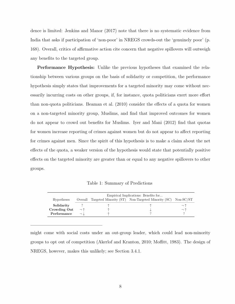
Table 1: Summary of Predictions

Empirical Implications: Benefits for...Hypotheses Overall Targeted Minority (ST) Non-Targeted Minority (SC) Non-SC/ST

Solidarity ? ↑ ↑ ¬ ↑Crowding Out ¬ ↑ ↑ ↓ ¬ ↑Performance ¬ ↓ ↑ ? ?

might come with social costs under an out-group leader, which could lead non-minority

groups to opt out of competition (Akerlof and Kranton, 2010; Moffitt, 1983). The design of

NREGS, however, makes this unlikely; see Section 3.4.1.

8

2.3 Intersecting Identities

We also investigate whether reservations have differential effects, for women and men, for

several reasons. First, NREGS mandates that one-third of workers be women, and that

women and men be paid equal wages. Dutta et al. (2014) find that 48% of NREGS workers

are women, which is approximately twice the share of women in other casual wage work.

If quotas improve program implementation, then positive effects may be particularly strong

for women.

Second, minority politicians elected under quotas may be more or less responsive to

women. Cassan and Vandewalle (2017) report that high caste women are less politically

active than low caste women, and therefore reservations for women result in more lower caste

women elected to office. Flipping this argument in our case may suggest that reservations

will encourage greater participation among women.

Alternatively, men may do better where there are ST reservations. If ST are particularly

in need of NREGS work, and bureaucrats are more likely to provide work for men than

women, then gains in NREGS, in Scheduled Areas, may be concentrated among men. Dutta

et al. (2014) report that this type of rationing is pervasive with NREGS work in poorer

states.

3 Context: Identity, Quotas, & Development in India

The Indian government has instituted numerous forms of political quotas since Indepen-

dence. In the political arena, the constitution provides dramatic guaranteed representation

through quotas for individuals from the Scheduled Tribes (ST), Scheduled Castes (SC), Other

Backward Classes (or Other Backward Castes, OBC), and/or women in the national parlia-

ment, state legislatures, and from 1993 in the country’s three-tier system of local government

9

councils, called Panchayat Raj.4

We focus in this paper on India’s Scheduled Areas, a government institution targeting

tribal populations that has not yet been subject to systematic quantitative analysis. Sched-

uled Areas cover over 100 million citizens across nine Indian states – Andhra Pradesh, Chhat-

tisgarh, Gujarat, Himachal Pradesh, Maharashtra, Madhya Pradesh, Jharkhand, Odisha,

and Rajasthan.

The demarcation of Scheduled Areas has changed little since the initial formulation dur-

ing the pre-Independence period. British authorities first provided a list of ‘Aboriginal

Tribes’ and ‘Semi-Hinduised Aboriginal Tribes’ in the Census of 1872 (Corbridge, 2002, 64)

and implemented special institutions targeting these tribes udner the Scheduled Districts

Act of 1874. Following Independence in 1947, the new Indian state identified Scheduled

Areas in the Fifth Schedule of the Constitution, with minor differences from the British

Scheduled Districts Act. The government justified Scheduled Areas specifically as a means

to improve representation and welfare for Scheduled Tribes (ST) through special programs

and institutions such as the state-level Tribes Advisory Council.5

The Constitution assigns responsibility for adding, subtracting or modifying Scheduled

Areas to the President in consultation with the relevant state’s Governor. In 1962, the

Dhebar Commission proposed that an area should be eligible to become a Scheduled Area

according to four, relatively vague, criteria: i) Preponderance of tribals in the population;

ii) Compact and reasonable size; iii) Under-developed nature of the area; and iv) Marked

disparity in economic standards of the people. In practice there has been no exact formula

4While religion is an additional important identity category, since Independence the Mus-

lim minority group has been excluded from political quotas.

5We focus on the Fifth Schedule that governs the majority of Scheduled Areas in India.

An additional Sixth Schedule of the Constitution details the administration of tribal areas

in four northeastern states. For more information, see Appendix A.3.

10

for updating or adjusting the previous notification or de-notification of Scheduled Areas in

India, and these Areas have remained remarkably stable since their initial formulation (see

Appendix A3).

3.1 Panchayat Extension to Scheduled Areas

Despite government commitments to promote ST interests in Scheduled Areas, villages on

opposing sides of the Scheduled Areas border show few differences on observables or over-time

trends prior to the implementation of the local-level political quotas that we study in this

paper (see Sections 5.2 and 7.1). Indeed, additional legislation instituting political quotas

were designed in large measure to give Scheduled Areas teeth. The Panchayats Extension to

Scheduled Areas Act of 1996 (PESA) mandated that all chairperson positions at the three

levels of local government, and at least 50% of all seats on these councils, be reserved for

ST individuals. Hence, when local elections were next held – as early as 2000 for Rajasthan

and as late as 2010 for Jharkhand – these reforms gave a tremendous positive shock to the

local-level political representation of Scheduled Tribes in India. Unlike other quotas in India

that rotate by constituency and over time, the quotas in Scheduled Areas introduced with

PESA remain fixed.

3.2 Quotas and Political Conflict: A Case Study of Jharkhand

By way of more detail, we provide a case analysis of the state of Jharkhand that has arguably

the most politically charged and turbulent path to local elections with quotas in Scheduled

Areas. Even in this politically fraught case, the actual boundaries of the Scheduled Areas

have remained relatively unchanged. While Jharkhand passed an amendment in 2001 to

allow for PESA-compliant panchayat elections, a legal challenge postponed elections. Only

after a decision by the Indian Supreme Court in 2010, upholding the constitutional status

11

of identity-based quotas in India, were local elections held in Jharkhand in 2010.6

Although the state of Jharkhand was created in part to better represent tribal populations

in the state of Bihar, the actual Scheduled Areas within this region did not change. The

Scheduled Areas assigned as part of the Indian Constitution’s Fifth Schedule remained almost

entirely consistent through the Bihar Scheduled Areas Regulation of 1969 and re-notification

again in 1977 and 2007. The only changes were the addition to the Scheduled Areas of a single

block – Bhandaria of Garhwa district – in 1977; and the Scheduling of two village-clusters,

both within Satbarwa block, in 2007.7

3.3 Comparisons Across Indian Identity Categories

ST are not the only historically disadvantaged minority category in India, nor the only cate-

gory targeted via special legislation. Others include the Scheduled Castes, Other Backward

Classes (OBC), and women. While OBC also receive mandated representation in local gov-

ernment outside of Scheduled Areas in India, on average, and in taking India as a whole, SC

and ST communities in existing literature are considered the most stigmatized, economically

vulnerable and politically excluded communities.

The Indian government has acknowledged the vulnerable position of SC and ST com-

munities and accordingly regularly groups SC and ST together for the purposes of special

legislation.8 Outside of Scheduled Areas that privilege ST, since 1992 all local government

6Union of India And Others v. Rakesh Kumar And Others. Supreme Court of India,

January 12, 2010.

7Appendix A.6 provides further discussion on what constitutes a Scheduled Tribe and

the Scheduled Areas in Jharkhand.

8SC and ST categories first gained some preferential representation in the Government

of India Act of 1935, officially sanctioned in the Constitution via Constitution (Scheduled

Castes) Order, 1950 and The Constitution (Scheduled Tribes) Order, 1950. National Com-

12

councils across the country restrict local council leadership positions for SC and ST, using

identical quotas in proportion to their local population that rotate every election cycle (see

Duflo and Chattopadhyay (2004); Dunning and Nilekani (2013)).

Both popular and academic writing often describe SC and ST in tandem as examples

of minority groups that are the poorest and most vulnerable throughout the country. The

Indian government even studies the development of individuals from both groups together

via the elite, national government appointed, Planning Commission.9 For these reasons, we

consider outcomes for SC a useful comparison to ST outcomes – as both groups are similarly

vulnerable, yet enjoy very different political opportunities in Scheduled Areas. Appendix A

provides more details about political quotas in India and SC and ST identity categories.

3.4 Local Government and Development

Local government panchayat institutions in India are responsible for two key aspects of de-

velopment: welfare schemes and infrastructure, each of which provide local public goods (see

Besley, Pande and Rao (2007)). Existing literature identifies roads, sanitation, electricity,

water, telephones, school and health facilities, irrigation, and communication as important

development sectors for measuring performance of panchayat institutions (Cassan and Van-

dewalle, 2017; Munshi and Rosenzweig, 2015). Our empirical goal is to measure how political

reservations affect the implementation of government programs.

missions for SC and ST were instituted via Articles 338 and 338A respectively. Legislation

was passed to protect individuals from both identity categories from violence in 1989 by

means of The Scheduled Castes and Scheduled Tribe - Prevention of Atrocities Act.

9See for instance http://planningcommission.gov.in/aboutus/taskforce/inter/

inter_sts.pdf.

13

http://planningcommission.gov.in/aboutus/taskforce/inter/inter_sts.pdf

3.4.1 The National Rural Employment Guarantee Scheme (NREGS)

As our key outcome, we chose NREGS, India’s largest development program and the largest

employment program in the world. NREGS and rights-based policies in India build on

prior legislation on decentralization and devolution of power to local government agencies.

(Kapur and Nangia, 2015) classify this welfare scheme as part of the lowest tier of social

protection in India that covers the vast majority of workers in the country (up to 94 percent)

(p. 76-77). Together with other programs like Public Distribution System and the National

Social Assistant Program, NREGS is a risk-coping, instead of risk-mitigating, program that

provides protection to those already at risk.

The scheme officially guarantees 100 days of minimum-wage employment to every rural

household in the country, with no eligibility requirements. Though increases in welfare

spending in general might come at the expense of other spending priorities, NREGS funding

comes primarily from federal and state budgets. Accordingly, local politicians who do not

take full advantage of the NREGS program are effectively “leaving money on the table.”10

Jenkins and Manor (2017) document how NREGS has helped improve the lives of the poorest

in India.

Recent research shows that village-level politics are likely to play an outsized role in the

distribution of NREGS benefits (Marcesse, 2017).11 Local-level council chairpersons – whose

seats are reserved for ST under the Scheduled Areas quota – have both the capacity and

discretion to significantly alter the quality of NREGS implementation and the distribution

of NREGS benefits (Besley, Pande and Rao, 2007; Dasgupta and Kapur, 2017; Dunning and

Nilekani, 2013; Dutta et al., 2014; Sukhtankar, 2017; Marcesse, 2018).

Local-level authorities are responsible for selecting projects through collective deliber-

10We discuss concerns related to leakage in Appendix F.

11See Appendix A.2 for details on the specific responsibilities of local government under

NREGS and how local governments, nevertheless, rely on a network of local agents.

14

ation in village assemblies, selecting program beneficiaries, implementing at least 50% of

all works (in terms of total cost), maintaining and transmitting records to higher author-

ities to process payments, and responding to citizens appeals for work (Sukhtankar, 2017;

Dunning and Nilekani, 2013; Marcesse, 2018; Besley, Pande and Rao, 2007; Munshi and

Rosenzweig, 2015). In turn, NREGS has bolstered the legitimacy and efficacy of local gov-

ernments (Sukhtankar, 2017; Jenkins and Manor, 2017). While NREGS implementation

remains uneven (see Figure 1), the scheme’s implementation carries political rewards - with

research showing good NREGS performance is an ‘election winning device’ in local politics

(Maiorano, 2014, p. 95).

The effects of Scheduled Areas on NREGS outcomes that we identify could be a result of

these supply-side factors, but also changes in demand for services that differ by identity cate-

gory. For example, ST might feel more comfortable in requesting work when an ST politician

is elected. Research has shown that demand and supply for NREGS work are a product of a

large ecosystem that includes informal institutions, bureaucrats, and collective deliberation

(Dutta et al., 2014; Khosla, 2011; Marcesse, 2018). Thus, we interpret changes in NREGS

outcomes as being driven by both demand and supply mechanisms, both of which would

follow changes in representation and which are thus consistent with our conceptualization in

Section 2.

Still, prior research indicates that that the binding constraints on NREGS implementation

are not demand-side but are driven almost entirely by supply-side factors (Khosla, 2011).

Dutta et al. (2014) write that “unmet demand for work is the single most important policy-

relevant factor in accounting for this gap between actual performance and the scheme’s

potential” (p. xxv). Jenkins and Manor (2017) write that while NREGS promises jobs on

demand, “many, if not most, poor rural people have little or no experience of making direct

demands on authority figures (p. 69).” Similarly, Marcesse (2018) argues that demand itself

is affected by incentives of supply agents.

Further, due to the design of NREGS, it is unlikely that electoral quotas will lead individ-

15

uals, including the status-quo privileged groups (as might otherwise be predicted by results

from Akerlof and Kranton (2010); Moffitt (1983)), to reduce their demand for work. This is

because NREGS targets poor households and individuals, in rural areas, with work – such

as digging ditches and building wells – that is “physically taxing, of uncertain duration, and

provides no employment benefits” (Dutta et al., 2014, 14). NREGS was designed for those

most in need of work, and as a last resort. Put differently, “By insisting that participants do

physically demanding manual work at a low wage rate, workfare schemes such as MGNREGS

aim to be self-targeted...nonpoor will not want to do such work, and poor people will readily

turn away from the scheme when better opportunities arise” (Dutta et al., 2014, 5,40). a

3.4.2 Beyond NREGS: Rural Roads and Other Public Goods

In addition to welfare schemes, we take two approaches to evaluate broader impacts on public

goods. First, we examine impacts of Scheduled Areas on PMGSY, the Prime Minister’s

Village Road Program. This program was established in 2000 to connect rural villages to

the all-weather road network by focusing on constructing and upgrading feeder roads that

either did not exist or were unpaved (Asher and Novosad, 2019a). As of 2001 only about

half of the 600,000 villages in India were connected to such roads. Importantly, “100 percent

funding for construction [under this program was provided] by the Central Government”

(ILO, 2015).

As with NREGS, local politicians are critical to PMGSY’s implementation, whereby a

standardized planning process is in place that incorporates representatives from district,

block, and village councils. In fact, the key role of local governments in helping carry out

construction and maintenance of roads at the local level has been inspired by their success

doing the same under NREGS (ILO, 2015).

Finally, we take a more systematic approach to studying effects on public goods outcomes

by using data from the 2011 Indian Census – roughly ten years following the implementation

of PESA.

16

4 Data Construction

To systematically assess how the Scheduled Areas political quota affects development out-

comes, we construct a village level dataset for the nine states that have Scheduled Areas. We

begin by using the Socioeconomic High-resolution Rural-Urban Geographic Dataset for India

(SHRUG) (Asher and Novosad, 2019b). This dataset allows us to track the same villages

over three different Census waves: 1991, 2001, and 2011. SHRUG includes limited Census

data from these waves and data on the PMGSY roads program.

While SHRUG provides information at the village level, NREGS outcomes are measured

at the village-cluster (gram panchayat) level. We use a new dataset as a matching directory

for village and village-cluster data, and then apply fuzzy matching methods to combine

SHRUG and NREGS into a single dataset. We next add information on reservations: both

on whether a village falls within or outside of the Scheduled Areas, and whether a village

falls within an Assembly Constituency that is reserved for ST, for SC, or not reserved. Our

final step is to merge the combined dataset with spatial data, as well as with a more complete

set of Census variables than was available from SHRUG, on villages from the 2001 and 2011

Indian Censuses. These additional Census data were procured from InfoMap India.

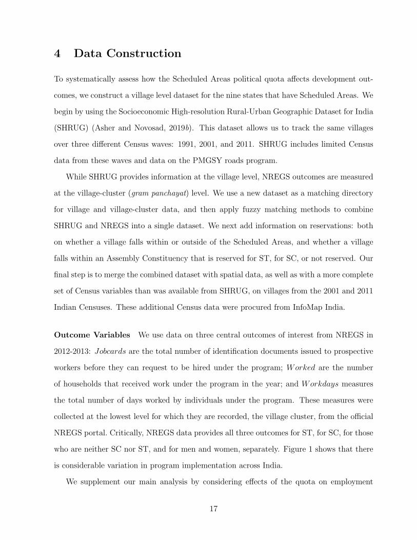
Outcome Variables We use data on three central outcomes of interest from NREGS in

2012-2013: Jobcards are the total number of identification documents issued to prospective

workers before they can request to be hired under the program; Worked are the number

of households that received work under the program in the year; and Workdays measures

the total number of days worked by individuals under the program. These measures were

collected at the lowest level for which they are recorded, the village cluster, from the official

NREGS portal. Critically, NREGS data provides all three outcomes for ST, for SC, for those

who are neither SC nor ST, and for men and women, separately. Figure 1 shows that there

is considerable variation in program implementation across India.

We supplement our main analysis by considering effects of the quota on employment

17

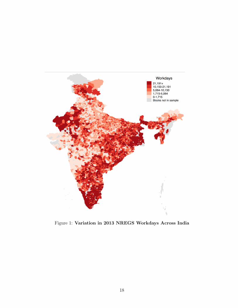
Figure 1: Variation in 2013 NREGS Workdays Across India

18

(sourced from the 2011 Census), road construction under the PMGSY program (from SHRUG),

and on public goods provision (2011 Census, but only available for a subset of villages, called

market villages).

Scheduled Areas Our key independent variable is an indicator for whether a village

is or is not part of the Scheduled Areas. We obtained information on Scheduled Areas

status from the Government of India’s Ministry of Tribal Affairs. See Appendix B.2 for

data sources. States release official documents either listing specific villages as Scheduled

or, where all villages within a block or district are Scheduled, the names of those blocks and

districts. While two states list individual village names (Andhra Pradesh and Rajasthan),

the remaining states list block and district names.

To remain consistent in our coding strategy across states, and to avoid human error that

was more likely to occur had we manually coded each village as Scheduled or not in the two

states that released information at this level, we elected to code an entire block as Scheduled

if any village was designated as Scheduled within the block. Empirically, this approach is

conservative because, while it accurately codes Scheduled Areas when all villages in a district

and block are inside the treatment area, it codes some untreated villages within a block as

treated – that is, the resulting bias will be in the direction of zero. Our coding is illustrated

spatially in Figure 2.12

Control Variables Our control variables, as well as the variables we use to evaluate sorting

and over-time changes, are sourced from the Census (for 1991, from SHRUG, and for 2001,

from the 2001 Census shape files).

12See Figure A4 for validation that our SA identification is done accurately and is more

granular than government maps.

19

Figure 2: Scheduled Areas in India - Unit is the block. Outlined regions refer to districtboundaries.

20

4.1 Summary Statistics

We combine 1991, 2001, and 2011 census data with NREGS data, Scheduled Areas coding,

and data on the PMGSY roads program. The dataset successfully matches approximately

217,000 of the 274,026 villages (79%) in the sample. 19 percent of the villages in our data are

coded as belonging to a Scheduled Area. ST comprise about 28 percent of the population,

while SC are only 13 percent of the population. Non-minorities form the remaining 59

percent. Appendix C.1 presents summary statistics.

5 Empirical Strategy

5.1 Geographic Regression Discontinuity

Consider two proximate villages lying on opposite sides of the Scheduled/non-Scheduled

boundary. If they are sufficiently similar on observable characteristics, we can say that the

only difference between the two villages is that one village lies in a Scheduled Area, while

the other is in a non-Scheduled Area. We approximate this thought experiment with a

geographic regression discontinuity design that restricts attention to villages geographically

proximate to a boundary dividing Scheduled Areas and other areas within a state.13 We use

the following specification:

yvgs = γScheduled Areavgs + as + f(Xvgs, Yvgs) + Z′

vgsφ+ εvgs (1)

∀ v s.t. Xvgs, Yvgs ∈ (−h, h)

where yvgs refers to outcomes for village v in gram panchayat g and state s. The official

NREGS portal only releases data at the gram panchayat level. In NREGS regressions, all

villages in the same gram panchayat are assigned the same outcome value, whereas for Census

13Appendix D.1 also presents simple OLS comparisons for main results.

21

2011 and PMGSY, y varies at the village level. Although treatment is assigned at the village

level, we cluster standard errors at the gram panchayat level throughout the paper. This

has the benefit of correcting for outcome inter-dependence within the gram panchayat in the

NREGS analysis.

Scheduled Areavgs is the treatment variable that equals 1 if a village is coded as being in

a Scheduled Area, and 0 otherwise. Outcomes that are left-skewed are logged such that γ can

be interpreted in percentage terms. State fixed effects as account for any state level shocks,

including the different timing of PESA implementation. f(Xvgs, Yvgs) is a flexible smooth

function in two dimensions, latitudes (X) and longitudes (Y ).14 Adding these geographic

controls helps the regression absorb spatial trends that might be superfluously driving results.

For each village, we calculate distance in kilometers h to a Scheduled Areas border within

the same state so that we may compare villages that provide the closest approximation to

random assignment. Based on bandwidth selection algorithms (see Appendix Table A18)

we take a conservative bandwidth of 10 kilometers as our standard bandwidth (h). 10km

is about one-fifth the size of the median distance (54.4km), and about one-ninth the mean

distance (91.3km), from the border in the data (see Figure A8). Last, we include a vector of

all village-level Census 2001 indices as well as 1991 and 2001 SC and ST population shares,

Z′vgs.

Throughout the analysis, we conduct various robustness tests, including varying band-

widths and functional forms, considering alternate transformations of outcomes, and ac-

counting for spatial spillovers.

14Following Dell (2010), our main specifications use the functional form: x+ y+x2+ y2+

xy + x3 + y3 + x2y + xy2.

22

5.2 Analysis of Balance with Census Data

With pre-treatment census data at the village level from 2001 and population data from 1991,

we analyze balance by evaluating if Scheduled Area predicts census variables. To manage

the vast number of 2001 census variables, we collapse the 140 variables into 14 substantively

meaningful indices by taking the simple mean of their standardized values. We describe this

process in Appendix G.

Overall, we find that the geographic RD model yields good balance between Scheduled

and non-Scheduled Areas. While we are able to tell the two groups apart in some cases

statistically because of the large sample size, the substantive differences across Scheduled and

non-Scheduled Areas are small: they remain below 0.1 standard deviations for all but three

indices (see Appendix Table A10). Only differences for water, urbanization, and banking

indices exceed 0.10 standard deviations, but even in these cases, the differences stay below

0.22. More substantively, the differences we do observe tend toward zero as the bandwidth

of analysis shrinks (see Appendix Figure A6). In addition, for all variables we can trace

across the 1991 and 2001 census waves, there is little reason to believe that the baseline

differences are trending differently over time in Scheduled versus non-Scheduled Areas (see

Appendix Figure A7), indicating that controlling for level differences between Scheduled

and non-Scheduled Areas may be sufficient. Accordingly, in our analysis we control for all

fourteen 2001 indices, both imbalanced and balanced.

6 The Impact of Scheduled Areas

6.1 Effects on NREGS

Table 2 presents the main results on NREGS outcomes. The first column shows treatments

effects at the extensive margin, while the remaining three columns decompose this effect

across ST, SC and Non-SC/ST categories.

23

Our first finding is that NREGS outcomes improve substantially for STs. As shown in

column 2, 20.7% (p < 0.01) more job cards are issued to STs in Scheduled Areas. This result

carries forward to the number of households that receive work during the year through

NREGS – the coefficient reflects a 20.3% (p < 0.01) increase. Overall, the number of

workdays STs receive increases by 24.1% (p < 0.01), a jump of about 1,040 more days of

work. Second, there is strong evidence that non-SC/STs are the main losers, as shown in

column 4. Not only does this group receive 9.8% (p < 0.01) fewer job cards in Scheduled

Areas, they also suffer a reduction in the number of households employed (8.6%, p < 0.05)

as well as the total number of workdays (12.5%, p < 0.01). Third, we find no evidence

that SCs are worse off under Scheduled Areas: the point estimates on all variables are

substantively small and are not statistically distinguishable from zero. Finally, putting these

results together in column 1, there is no evidence that Scheduled Areas affect the extensive

margin of program implementation – the total amount of work remains the same across

Scheduled and non-Scheduled Areas, as the point estimates on outcomes are small, ranging

from 1% on workdays to 0% on jobcards.15

6.2 Intersecting Identities: Decomposing Gender Effects

Do marginalized women comparatively benefit from Scheduled Areas? While “one aim of

[NREGS] was to encourage women from poor households to under take work” (Jenkins and

Manor, 2017, p. 174), checking this for NREGS is difficult as the data do not decompose

15In Appendix D we show that our results are robust to a number of tests, including various

functional forms, bandwidths, transformations of outcomes, and controls for the number of

matched villages. Appendix F shows there is no evidence for two alternative explanations:

that discrepancies in reporting, and that differences in reliance on centralized government

between Scheduled and non-Scheduled Areas account for identified effects.

24

Table 2: The Effect of Scheduled Areas on NREGS (10 km RD)

(1) (2) (3) (4)Total STs SCs Non-SCs/STs

Panel A: Log JobcardsScheduled Areas 0.000 0.207*** -0.038 -0.098***

(0.014) (0.025) (0.031) (0.024)Control Mean (Unlogged) 652.979 259.373 92.768 300.838# GPs 13338 13338 13338 13338# Villages 32641 32641 32641 32641

Panel B: Log Households WorkedScheduled Areas 0.009 0.203*** -0.017 -0.086***


Panel C: Log WorkdaysScheduled Areas -0.010 0.241*** 0.009 -0.125***


Notes: *p < 0.1, **p < 0.05, ***p < 0.01. Standard errors clustered by GP.

outcomes by both identity and gender.16

We make some progress by analyzing the effects of Scheduled Areas on employment

prospects by gender and types of workers in the 2011 Census. These data provide em-

ployment statistics across two categories defined by the Census: “main workers,” who were

employed more than 183 days, or about 6 months, in the 12 months preceding the Census,

and “marginal workers,” who were employed for less than 183 days.

If a large portion of individuals are solely employed through NREGS, we should expect

primary gains among marginal workers due to the 100 NREGS workday maximum per

household. However, individuals might also supplement their NREGS work which would

make it reasonable to expect effects among main workers. Indeed, prior work shows that

16Nevertheless, Appendix Table A20 presents results by gender for workdays under NREGS

(the only outcome for which gender decomposed data are available) and shows that there

are no key differences at least at the extensive margin across gender.

25

NREGS has positive effects on private sector employment by raising the rural reservation

wage (Muralidharan, Niehaus and Sukhtankar, 2017). In addition, 70 percent of NREGS

work occurs during the lean season, additively bringing new labor into the market (Jenkins

and Manor, 2017, p. 170).

We observe three results in Table 3. First, consistent with the extensive margin results

on NREGS, there is no effect on average employment. Second, women experience about 2.5

percent gains in employment, while men are worse off by 1.9 percent. Third, relative to the

other gender, the primarily beneficiaries of Scheduled Areas are ‘marginal’ women workers,

whose employment increases by 3%, while the primary losers are ‘main’ men workers.17

Table 3: Effects on Employment (10 km RD, Census 2011)

(1) (2) (3)Total Women Men

Panel A: Log # Overall WorkersScheduled Areas -0.007 0.025* -0.019**

(0.010) (0.013) (0.010)Control Mean (Unlogged) 552.0 231.9 319.9# GPs 13277 13277 13277# Villages 32522 32522 32522H0: γ(2) - γ(3) = 0 p < 0.000

Panel B: Log # Main Workers (> 183 days)Scheduled Areas -0.018 0.002 -0.021

(0.018) (0.020) (0.017)Control Mean (Unlogged) 377.6 128.0 249.5# GPs 13277 13277 13277# Villages 32522 32522 32522H0: γ(2) - γ(3) = 0 p = 0.104

Panel C: Log # Marginal Workers (< 183 days)Scheduled Areas 0.001 0.030 -0.011

(0.022) (0.022) (0.021)Control Mean (Unlogged) 173.9 103.9 70.0# GPs 13277 13277 13277# Villages 32522 32522 32522H0: γ(2) - γ(3) = 0 p < 0.001

Notes: *p < 0.1, **p < 0.05, ***p < 0.01. Standard errors clustered by GP. Additional controls include

outcome baseline measures from the 2001 Census.

17Appendix E.4 shows several robustness exercises.

26

How do we interpret these results? Control means show that women are more likely to

be employed as marginal workers than are men, suggesting that they work fewer days of the

year on average. The treatments effects indicate that it may be these types of underemployed

workers who benefit the most in Scheduled Areas, suggesting the possibility that ST women

benefit more from the increase in average ST workdays.

6.3 Effects on the Rural Roads Program (PMGSY)

Are there implications of instituting electoral quotas beyond the effects we observe on

NREGS and employment in general? Finding evidence of broader impacts will improve

our confidence that the institution of Scheduled Areas improved the lives of poor commu-

nities. It would also help allay the concern that changes in NREGS come at the cost of

changes in other programs.18

We first consider impacts on the PMGSY roads program. Column 1 of Table 4 shows that

villages in Scheduled Areas are about three percentage points more likely to have completed

roads through the program using our geo RD specification.

An important feature of the PMGSY data is the time variation in road construction,

which, along with state-by-state variation in the implementation of PESA elections, affords

us the opportunity to study the impacts of Scheduled Areas on roads before and after the

introduction of electoral quotas. Using village, year, and year since PESA elections fixed

effects, a difference-in-differences strategy allows us to consider within-village changes in

PMGSY implementation over time. We find that post-PESA elections, Scheduled Areas

villages in our geo RD sample (column 2) are 1 percentage point more likely to have a

PMGSY road, an effect of about 20%. This percentage increases to nearly 5% (an increase of

18For example, quota politicians may prefer NREGS relative to other priorities because

NREGS allows them to perpetuate patronage through handout of state resources (Marcesse,

2017).

27

Table 4: The Effect of Scheduled Areas on Rural Roads (PMGSY)

Outcome: Road=1Model: Geo RD Diff-in-Diff Diff-in-Diff

Sample: 10km 10km Full(1) (2) (3)

Scheduled Areas 0.029***(0.004)

Sch Areas × Post PESA Election 0.010*** 0.048***(0.003) (0.002)

Non-Scheduled Mean 0.127 0.051 0.056# GPs 13338 13338 74120# Villages 32641 32641 217144# Observations 32641 456974 3040016Geo RD Controls Yes - -Village FE No Yes YesYear FE No Yes YesYear of PESA FE No Yes Yes


over 80%) using the full dataset of villages. Figure 3 additionally shows that road sanctioning

increased in Scheduled Areas soon after the introduction of elections but not before. Effects

on the completion of roads followed after a few years.

6.4 Impacts on Public Goods

Guided by the literature on the responsibilities of local governments in India detailed in

Section 3.4, we also evaluate the effect of Scheduled Areas more broadly on public goods

using data from the 2011 Census. We construct six mean indices that take the average of

binary indicators on the presence of particular public goods in a village, such as whether

there is a gravel road. These indices measure the average provision of roads, water, irrigation,

electricity, communication, and education. Similarly, an overall public goods index averages

all individual public goods indicator variables.

Overall, the results presented in Figure 4 show that public goods provision in Scheduled

Areas improved by 2011, particularly in terms of road, water, communication, and education

28

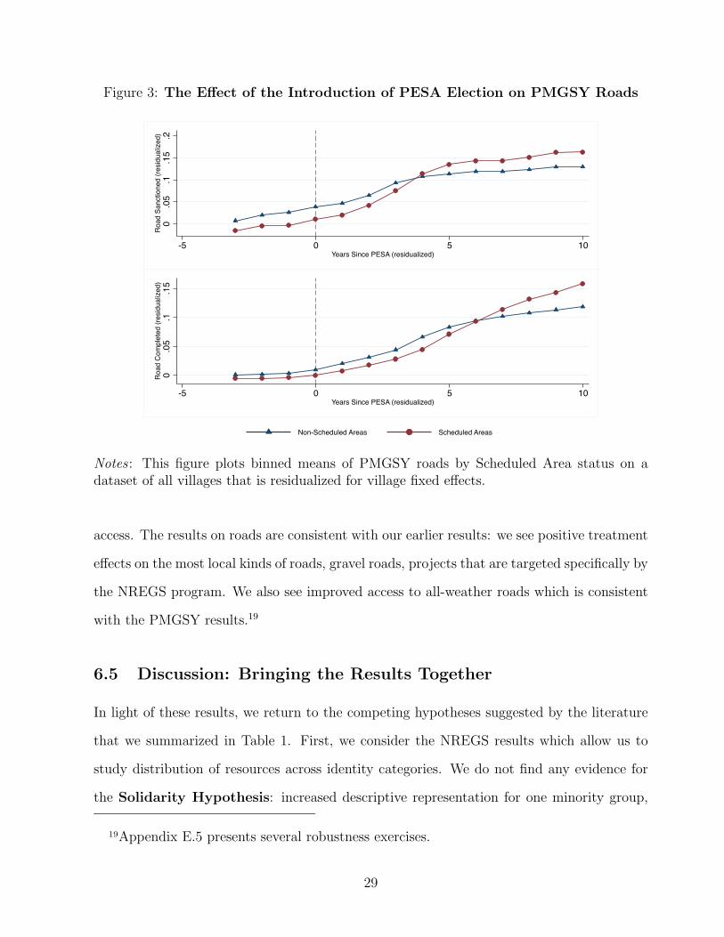
Figure 3: The Effect of the Introduction of PESA Election on PMGSY Roads

0.0

5.1

.15

.2R

oad

Sanc

tione

d (re

sidu

aliz

ed)

-5 0 5 10Years Since PESA (residualized)

0.0

5.1

.15

Roa

d C

ompl

eted

(res

idua

lized

)


Non-Scheduled Areas Scheduled Areas

Notes : This figure plots binned means of PMGSY roads by Scheduled Area status on adataset of all villages that is residualized for village fixed effects.

access. The results on roads are consistent with our earlier results: we see positive treatment

effects on the most local kinds of roads, gravel roads, projects that are targeted specifically by

the NREGS program. We also see improved access to all-weather roads which is consistent

with the PMGSY results.19

6.5 Discussion: Bringing the Results Together

In light of these results, we return to the competing hypotheses suggested by the literature

that we summarized in Table 1. First, we consider the NREGS results which allow us to

study distribution of resources across identity categories. We do not find any evidence for

the Solidarity Hypothesis: increased descriptive representation for one minority group,

19Appendix E.5 presents several robustness exercises.

29

Figure 4: The Effect of Scheduled Areas on Public Goods (Census 2011).

Over

all P

ublic

Goo

ds In

dex

Road

s Ind

ex

Natio

nal H

ighwa

y (Y/

N)

State

High

way (

Y/N)

Major

Dist

rict R

oad (

Y/N)

Othe

r Dist

rict R

oad (

Y/N)

All w

eathe

r roa

d (Y/

N)

Grav

el Ro

ad (Y

/N)

Wate

r Ind

ex

Hand

pump

(Y/N

)

Tap W

ater T

reate

d (Y/

N)

Tank

, Pon

d, La

ke (Y

/N)

Cove

red W

ell (Y

/N)

Unco

vere

d Well

(Y/N

)

Irriga

tion I

ndex

Tube

well/B

oreh

ole (Y

/N)

Rive

r/Can

al (Y

/N)

Elec

tricity

Inde

x

Elec

tricity

for A

gricu

lture

Use

(Y/N

)

Elec

tricity

for D

omes

tic U

se (Y

/N)

Elec

tricity

for C

omme

rcial

Use (

Y/N) Co

mmun

icatio

ns In

dex

Post

Offic

e (Y/

N)

Post

and T

elegr

aph O

ffice (

Y/N)

Telep

hone

(Y/N

)

Mobil

e cov

erag

e (Y/

N)

Educ

ation

Inde

x

Prim

ary S

choo

l (Y/N

)

Midd

le Sc

hool

(Y/N

)

Seco

ndar

y Sch

ool (Y

/N)

Senio

r Sec

onda

ry Sc

hool

(Y/N

)

Colle

ge (Y

/N)

-.1-.0

50

.05.1

Trea

tmen

t Effe

ct

STs, does not appear to improve outcomes for a non-targeted minority group, SCs. We

find support for the Crowding Out Hypothesis to the extent that there is negative

substitution away from the residual non-SC/ST group, which is consistent with the aims

of programs designed to redistribute economic and political power. Importantly, there is no

evidence for outcomes worsening for SCs or at the extensive margin.

The NREGS results are also consistent with the weak version of the Performance

Hypothesis. At the extensive margin, we find that NREGS implementation is no worse

in Scheduled as compared with non-Scheduled Areas. Evidence on overall employment,

PMGSY, and public goods outcomes from the 2011 Census show improvements across the

board, results consistent with the strong version of the performance hypothesis.

How might we square these contrasting results? One interpretation consistent with re-

sults and the literature (for example, Duflo and Chattopadhyay (2004)) is that marginalized

politicians empowered under Scheduled Areas invest more in policies prioritized by their com-

munities. We observe employment gains for the most vulnerable: women marginal workers.

Similarly, Scheduled Areas have positive effects on the PMGSY program that aimed to grant

30

market access to poor rural communities, and on public goods outcomes that are most im-

portant for marginalized groups. In sum, the broader effects we identify may reflect greater

investment in the welfare of marginalized communities. In that sense, the broader results

are consistent with NREGS findings that Scheduled Areas improve the welfare of ST.

Importantly, the results run contrary to the expectations of affirmative action skeptics:

while we do not find that politicians from underrepresented groups outperform other politi-

cians on NREGS, they certainly do not perform worse, and they perform better on a program

(PMGSY) where explicit targeting of benefits to marginalized communities is less possible.

In addition, gains for the targeted group under NREGS do not come at the expense of

similarly marginalized populations.

7 Investigating the Electoral Mechanism

To what extent does an electoral mechanism explain how the Scheduled Areas have improved

development outcomes for ST? We present four pieces of evidence in support of an electoral

mechanism.

7.1 Scheduled Areas Prior to PESA

Prior to the implementation of electoral quotas, Scheduled Areas and non-Scheduled Areas

looked very similar as our geographic RD analysis of the 2001 Census shows in Section

5.2. This analysis mirrors a critical 1995 report by the Indian Parliament-appointed Bhuria

Commission, which found little to no devolution of governance and authority to tribal bodies

in Scheduled Areas, and argued that tribal populations should enjoy greater self-governance

and less governmental administrative interference.

... since planned development has been an article of faith with us, it has to be

ensured that implementation of the policies and programmes drawn up in tribal

interest are implemented in tribal interest. Since, by and large, the politico-

31

bureaucratic apparatus has failed in its endeavour, powers should be devolved on

the people so that they can formulate programmes which suit them and imple-

ment them for their own benefits.

Policies following from these findings were made into law via PESA, passed in 1996 and

going into effect with state panchayat elections from 2000. In this way, PESA gave the

Scheduled Areas teeth that they had theretofore lacked.

7.2 Targeted Minority Electoral Influence

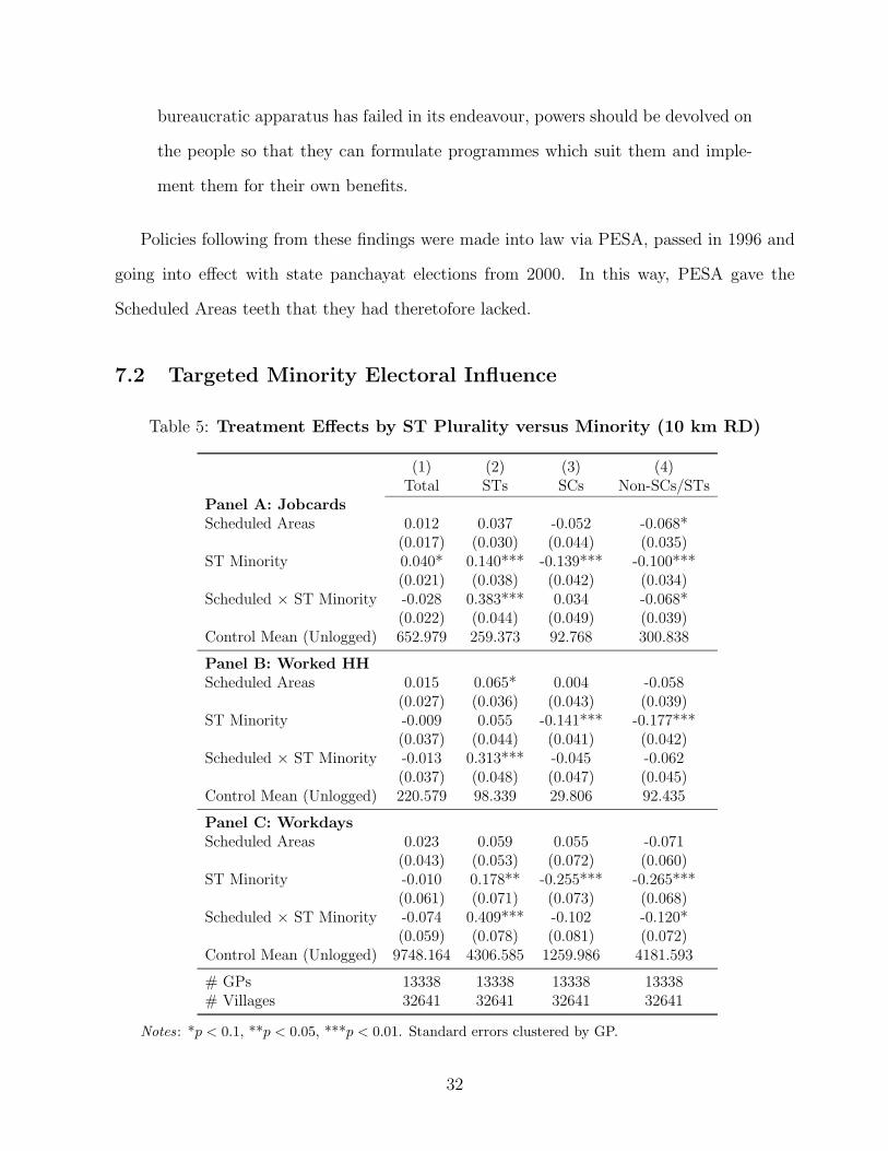
Table 5: Treatment Effects by ST Plurality versus Minority (10 km RD)


Panel A: JobcardsScheduled Areas 0.012 0.037 -0.052 -0.068*

(0.017) (0.030) (0.044) (0.035)ST Minority 0.040* 0.140*** -0.139*** -0.100***

(0.021) (0.038) (0.042) (0.034)Scheduled × ST Minority -0.028 0.383*** 0.034 -0.068*

(0.022) (0.044) (0.049) (0.039)Control Mean (Unlogged) 652.979 259.373 92.768 300.838

Panel B: Worked HHScheduled Areas 0.015 0.065* 0.004 -0.058

(0.027) (0.036) (0.043) (0.039)ST Minority -0.009 0.055 -0.141*** -0.177***

(0.037) (0.044) (0.041) (0.042)Scheduled × ST Minority -0.013 0.313*** -0.045 -0.062


Panel C: WorkdaysScheduled Areas 0.023 0.059 0.055 -0.071

(0.043) (0.053) (0.072) (0.060)ST Minority -0.010 0.178** -0.255*** -0.265***

(0.061) (0.071) (0.073) (0.068)Scheduled × ST Minority -0.074 0.409*** -0.102 -0.120*


# GPs 13338 13338 13338 13338# Villages 32641 32641 32641 32641


32

Prior work suggests that quota effects are largest where the targeted minority group

constitutes a large share of the population (Chin and Prakash, 2011; Jensenius, 2015; Pande,

2003; Das, Mukhopadhyay and Saroy, 2017). For instance, Jensenius (2015) reports that

some SC politicians want to divert funds to SC constituents but do not do so “because

they are scared of being branded as ‘too SC”’ (p.203) by the majority of voters who are

non-SC and on whose votes they depend. Alternatively, while it is true that STs retain

the most power when they have both a high share of population and electoral reservations,

theoretically, the introduction of quotas should have the greatest marginal impact in places

where STs did not possess as much electoral strength initially. To test this, we create an

indicator variable for whether ST are a non-plurality:

ST Minorityv = ¬ST P luralityv = 1 · (ST popv < max(SC popv, non SC/ST popv))

Table 5 presents heterogeneous effects with our standard RD specification. There are

two findings. First, for each of the three main outcomes of interest, we find that Scheduled

Areas have a larger positive effect for ST in places where ST comprised an electoral minority

prior to the implementation of PESA. The result suggests that the electoral quota may

be most effective at improving the lives of groups that see the greatest increase in their

electoral strength due to the quota. Second, as before, the negative spillover on the residual

non-SC/ST category is also more pronounced in these areas.

7.3 Quota Overlap

A certain proportion of State Assembly seats across India are reserved for minorities including

ST and SC based on population (Jensenius, 2012). Although the higher-level quotas are

not randomly assigned, we can use them to investigate quota overlap at different levels

of government. On the one hand, multiple quota politicians should reinforce the effect

of political quotas by improving potential coordination between politicians who share an

33

identity. On the other hand, there could exist some diminishing returns to quota politician

effort because of credit claiming difficulties and free riding problems (Gulzar and Pasquale,

2017).

While our main results are robust to controlling for the incidence of Assembly Con-

stituency level ST reservation (see Appendix Table A31), in Table 6 we interact these higher

level reservations in the latest election before 2013 with the Scheduled Areas treatment

indicator to study if overlapping Assembly Constituency reservations moderate effects on

program implementation. The results show that Scheduled Areas reservations and Assem-

bly Constituency reservations for ST, separately, improve NREGS program implementation

tremendously for ST. However, when the two quotas overlap, the overall implementation of

the program is less than the separate parts, suggesting that there exist some ceiling effects.20

Overall, the results are consistent with program implementation varying with political insti-

tutions.

7.4 Local Elections in Scheduled Areas

Consistent with the historical discussion above, patterns in the data also show that the

introduction of PESA is an important driver in differences between Scheduled Areas and

non-Scheduled Areas. We already presented corroborating evidence of the importance of

PESA’s introduction for the PMGSY program in Figure 3. In contrast, because we only

observe NREGS outcomes at a single point in time, we lack any within-state variation in

PESA introduction when considering these outcomes. With this limitation in mind, in

Appendix Table A28 we interact the Scheduled Areas indicator with the number of elections

between 2000 and 2012 that have taken place in a state under PESA: either one, two,

or three. We find that the main results hold up but the magnitude decreases over time.

20Interestingly, we find that when the Assembly Constituency reservation is for SC, there

are no negative quota overlap effects for ST (see Appendix Table A32).

34

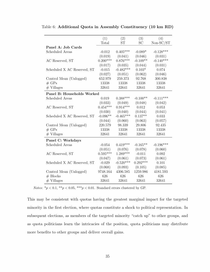
Table 6: Additional Quota in Assembly Constituency (10 km RD)

(1) (2) (3) (4)Total ST SC Non-SC/ST

Panel A: Job CardsScheduled Areas -0.012 0.405*** -0.089* -0.128***

(0.019) (0.041) (0.046) (0.031)AC Reserved, ST 0.200*** 0.876*** -0.109** -0.140***

(0.017) (0.035) (0.044) (0.031)Scheduled X AC Reserved, ST -0.015 -0.482*** 0.103* 0.074


Panel B: Households WorkedScheduled Areas 0.019 0.388*** -0.100** -0.111***

(0.033) (0.049) (0.048) (0.042)AC Reserved, ST 0.454*** 0.914*** 0.012 0.053

(0.030) (0.040) (0.044) (0.041)Scheduled X AC Reserved, ST -0.096** -0.465*** 0.137** 0.033


Panel C: WorkdaysScheduled Areas -0.054 0.419*** -0.165** -0.196***

(0.051) (0.076) (0.078) (0.060)AC Reserved, ST 0.595*** 1.289*** -0.011 0.092

(0.047) (0.061) (0.073) (0.061)Scheduled X AC Reserved, ST -0.029 -0.520*** 0.292*** 0.101

(0.068) (0.093) (0.105) (0.085)Control Mean (Unlogged) 9748.164 4306.585 1259.986 4181.593# Blocks 626 626 626 626# Villages 32641 32641 32641 32641


This may be consistent with quotas having the greatest marginal impact for the targeted

minority in the first election, where quotas constitute a shock to political representation. In

subsequent elections, as members of the targeted minority “catch up” to other groups, and

as quota politicians learn the intricacies of the position, quota politicians may distribute

more benefits to other groups and deliver overall gains.

35

8 Conclusion

Policymakers often treat economic and political efforts in isolation. We show that political

affirmative action and development programs may serve as complementary levers to deliver

better outcomes for marginalized communities, at no cost to other minorities, nor to society

overall.

Our empirical setting is political affirmative action in India, where Scheduled Areas,

as well as similar reservations more generally, are hotly debated and politically divisive.

Protests and riots have broken out for a myriad of related affirmative action issues – out

of fear of reductions in protections for SC and ST throughout India, in anticipation of

the implementation of elections in Scheduled Areas, by groups agitating for inclusion in

identity categories targeted by quotas, and in an effort to extend Scheduled Areas into new

jurisdictions (AlJazeera, 2018; Singh, 2018; ETBureau, 2018; Iyengar, 2015). Despite their

importance, scale, and salience, Scheduled Areas remain understudied in political science and

related disciplines. To our knowledge, this paper provides the first systematic evaluation of

this institution.

We propose a novel theoretical framework comprising solidarity, crowding-out, and perfor-

mance hypotheses to understand the systematic effects of political affirmative action across

groups. To test these, we build a new large-scale dataset combining administrative data on

the largest employment program in the world, a rural roads program, as well as public goods

from the Indian Census. We find that quotas deliver no worse outcomes overall and that

gains for targeted minorities come at the cost of the relatively privileged, rather than other

historically disadvantaged groups. More broadly, improvements in other pro-poor policies,

including a rural roads program and general public goods, further attest to the complemen-

tary impacts of political affirmative action and pro-poor economic development.

Effects appear to operate through an electoral mechanism. They appear strongly (1)

after the introduction of local elections with reservations for minorities, (2) where the quota

is theoretically most likely to have the largest marginal impact – that is – in places where

36

the targeted minority group was previously least powerful), and (3) where there is no overlap

with other quotas targeting the same minority.

What are the implications of our results on debates surrounding affirmative action? Skep-

tics routinely argue that open competition in the political sphere brings the best politicians to

the fore. However, our results show that quota politicians perform no worse than status-quo

politicians. This suggests that status-quo institutions may prevent equally qualified individ-

uals from marginalized communities from running for office and more effectively representing

their communities.

What are the long-term consequences of electoral affirmative action? Our study measures

impacts up to 12 years after implementation of the institution and finds large positive effects

for the targeted minority. One concern for the longer term is that fixed political affirmative

action may develop its own unequal political structures by simply replacing which identity

group is on top. Efforts that helpfully redistribute political power initially could create long-

run political monopolies. We consider this to be an important open question to be explored

in the future.

37

References

Adida, Claire L., Lauren D. Davenport and Gwyneth McClendon. 2016. “Ethnic Cueingacross MinoritiesA Survey Experiment on Candidate Evaluation in the United States.”Public Opinion Quarterly 80(4):815–836.

Akerlof, George A. and Rachel E. Kranton. 2010. Identity Economics: How Our IdentitiesShape Our Work, Wages, and Well-Being. Princeton: Princeton University Press.

AlJazeera. 2018. “Dalits in India hold protests against ‘dilution’ of SC/ST Act.” AlJazeera .URL: https: // www. aljazeera. com/ news/ 2018/ 04/ dalits-india-hold-

protests-dilution-scst-act-180402082213061. html

Asher, Sam and Paul Novosad. 2019a. “Rural roads and local economic development.”American Economic Review .

Asher, Sam and Paul Novosad. 2019b. “Socioeconomic High-resolution Rural-Urban Geo-graphic Dataset for India (SHRUG).”.URL: https://doi.org/10.7910/DVN/DPESAK

Beaman, Lori, Esther Duflo, Rohini Pande, Petia Topalova et al. 2010. Political reservationand substantive representation: Evidence from Indian village councils. In India PolicyForum 2010/11 Volume. Vol. 7 pp. 159–191.

Bertrand, Marianne, Rema Hanna and Sendhil Mullainathan. 2010. “Affirmative actionin education: Evidence from engineering college admissions in India.” Journal of PublicEconomics 94(1-2):16–29.

Besley, Timothy, Rohini Pande and Vijayendra Rao. 2007. “Political Economy of Panchayatsin South India.” Economic and Political Weekly 42(8):661–666.

Beteille, Andre. 1974. Six Essays in Comparative Sociology. New York: Oxford UniversityPress.

Beteille, Andre. 1986. “The concept of tribe with special reference to India.” EuropeanJournal of Sociology 27(2):296–318.

Bhavnani, Rikhil R. 2009. “Do electoral quotas work after they are withdrawn? Evidencefrom a natural experiment in India.” American Political Science Review 103(01):23–35.

Bhavnani, Rikhil R. and Alexander Lee. 2018. “Does Affirmative Action Worsen Bureau-cratic Performance? Evidence from the Indian Administrative Service.”.

Bird, Karen. 2014. “Ethnic quotas and ethnic representation worldwide.” InternationalPolitical Science Review 35(1):12–26.

Broockman, David E. 2013. “Black politicians are more intrinsically motivated to advanceblacks interests: A field experiment manipulating political incentives.” American Journalof Political Science 57(3):521–536.

38

https://www.aljazeera.com/news/2018/04/dalits-india-hold-protests-dilution-scst-act-180402082213061.html

Cassan, Guilhem and Lore Vandewalle. 2017. “Identities and Public Policies: UnintendedEffects of Political Reservations for Women in India.” (18-2017).

Chin, Aimee and Nishith Prakash. 2011. “The redistributive effects of political reservationfor minorities: Evidence from India.” Journal of Development Economics 96(2):265–277.

Corbridge, Stuart. 2002. “The Continuing Struggle for India’s Jharkhand: Democracy,Decentralisation and the Politics of Names and Numbers.” Commonwealth & ComparativePolitics 40(3):55–71.

Corbridge, Stuart, Sarah Jewitt and Sanjay Kumar. 2004. Jharkhand: Environment, Devel-opment, Ethnicity. Oxford University Press.

Das, Sabyasachi, Abhiroop Mukhopadhyay and Rajas Saroy. 2017. “Efficiency Consequencesof Affirmative Action in Politics: Evidence from India.” IZA DP No. 11093 .

Dasgupta, Aditya and Devesh Kapur. 2017. “The Political Economy of Bureaucratic Effec-tiveness: Evidence from Local Rural Development Officials in India.”.

Dell, M. 2010. “The Persistent Effects of Peru’s Mining Mita.” Econometrica 78(6):1863–1903.

Deshpande, Ashwini and Thomas E Weisskopf. 2014. “Does affirmative action reduce pro-ductivity? A case study of the Indian railways.” World Development 64:169–180.

Dhebar, U N. 1962. “Report of the Scheduled Castes and Scheduled Tribes Commission.”Government of India Press .

Duflo, Esther and Raghabendra Chattopadhyay. 2004. “Women as policy makers: Evidencefrom a randomized policy experiment in India.” Econometrica 72(5):1409–1443.

Dunning, Thad and Janhavi Nilekani. 2013. “Ethnic Quotas and Political Mobilization:Caste, Parties, and Distribution in Indian Village Councils.” American Political ScienceReview 107(1):3556.

Dutta, Puja, Rinku Murgai, Martin Ravallion and Dominque van de Walle. 2014. Right toWork: Assessing India’s Emloyment Guarantee Scheme in Bihar.

ETBureau. 2018. “Cabinet nod to expansion of Scheduled Areas in Rajasthan.” TheEconomic Times .URL: https: // economictimes. indiatimes. com/ news/ politics-and-nation/

cabinet-nod-to-expansion-of-scheduled-areas-in-rajasthan/ articleshow/

63918816. cms

Galanter, Marc. 1984. Competing Equalities : Law and the Backward Classes in India.Oxford University Press.

Gulzar, Saad and Benjamin J Pasquale. 2017. “Politicians, bureaucrats, and development:Evidence from India.” American Political Science Review 111(1):162–183.

39

https://economictimes.indiatimes.com/news/politics-and-nation/cabinet-nod-to-expansion-of-scheduled-areas-in-rajasthan/articleshow/63918816.cms

Gupta, Sanjukta Das. 2011a. Adivasis and the Raj: Socio-economic Transition of the Hos,1820-1932. Orient BlackSwan.

Gupta, Sanjukta Das. 2011b. Rethinking Adivasi Identity: The Chota Nagpur TenancyAct (1908) and its aftermath among the Hos of Singbhum. In Adivasis In Colonial India:Survival, Resistance and Negotiation, ed. Biswamoy Pati. Orient BlackSwan.

ILO. 2015. “ILO-PMGSY Rural Road Project Strengthening Capacity of Panchayati RajInstitutions: Managing Maintenance of Rural Roads.”.URL: ”http://pmgsy.nic.in/RSCPR.pdf”

Iyengar, Rishi. 2015. “Riots Break Out in India Over a Dominant Caste’s Attempt to Gain’Backward’ Status.” Time .

Iyer, Lakshmi and Anandi Mani. 2012. “Travelling Agents: Change and BureaucraticTurnover in India.” Review of Economics and Statistics 94(August):723–739.

Jenkins, Rob and James Manor. 2017. Politics and the Right to Work: India’s NationalRural Employment Guarantee Act. Oxford University Press.

Jensenius, Francesca R. 2012. “Political Quotas in India: Perceptions of Constituent PoliticalRepresentation.” Asian Survey 52(2):373–394.

Jensenius, Francesca R. 2015. “Development from representation? A study of quotas for thescheduled castes in India.” American Economic Journal: Applied Economics 7(3):196–220.

Jensenius, Francesca R. 2017. Social justice through inclusion: The consequences of electoralquotas in India. Oxford University Press.

Kapur, Devesh and Prakirti Nangia. 2015. “Social protection in India: A welfare state sanspublic goods?” India Review 14(1):73–90.

Kaufmann, Karen M. 2003. “Cracks in the rainbow: Group commonality as a basis for Latinoand African-American political coalitions.” Political Research Quarterly 56(2):199–210.

Khosla, Rishabh. 2011. “Caste, Politics and Public Good Distribution in India: Evidencefrom NREGS in Andhra Pradesh.” Economic and Political Weekly Vol. 46(Issue No. 12).

Long, Heather. 2019. “80 nations set quotas for female leaders. Should the U.S. be next?”.URL: https://www.washingtonpost.com/business/economy/80-nations-set-quotas-for-female-leaders-should-the-us-be-next/2019/03/29/a27434ba-45c4-11e9-aaf8-4512a6fe3439 story.html

Maiorano, Diego. 2014. “The politics of the Mahatma Gandhi national rural employmentguarantee act in Andhra Pradesh.” World Development 58:95–105.

Marcesse, Thibaud. 2017. “Patronage guaranteed? Public Policy Reform, Patronage andParty–Building in Rural India.” Working Paper .

40

Marcesse, Thibaud. 2018. “Public Policy Reform and Informal Institutions: The PoliticalArticulation of the Demand for Work in Rural India.” World Development 103:284 – 296.

Meier, Kenneth J, Paula D McClain, Jerry L Polinard and Robert D Wrinkle. 2004. “Dividedor together? Conflict and cooperation between African Americans and Latinos.” PoliticalResearch Quarterly 57(3):399–409.

Moffitt, Robert. 1983. “An Economic Model of Welfare Stigma.” American Economic Review73(5):1023–35.

Munshi, Kaivan and Mark Rosenzweig. 2015. Insiders and Outsiders: Local Ethnic Politicsand Public Goods Provision. Working Paper 21720 National Bureau of Economic Research.

Muralidharan, Karthik, Paul Niehaus and Sandip Sukhtankar. 2017. “General EquilibriumEffects of (Improving) Public Employment Programs: Experimental Evidence from India.”(23838).

Palaniswamy, Nethra and Nandini Krishnan. 2012. “Local Politics, Political Institutions, andPublic Resource Allocation.” Economic Development and Cultural Change 60(3):449–473.

Pande, Rohini. 2003. “Can Mandated Political Representation Increase Policy Influence forDisadvantaged Minorities? Theory and Evidence from India.” American Economic Review93(4):1132–1151.

Singh, Prerna. 2015. How Solidarity Works for Welfare: Subnationalism and Social Devel-opment in India. Cambridge University Press.

Singh, S. Harpal. 2018. “Adivasis declare self rule in villages.” The Hindu .URL: https: // www. thehindu. com/ news/ cities/ Hyderabad/ adivasis-declare-self-rule-in-villages/ article24061380. ece

Sukhtankar, Sandip. 2017. “India’s National Rural Employment Guarantee Scheme: WhatDo We Really Know about the World’s Largest Workfare Program?” Brookings-NCAERIndia Policy Forum 13:231–286.

Sundar, Nandini. 2009. Laws Policies and Practices in Jharkhand. In Legal Grounds: NaturalResources, Identity, and the Law in Jharkhand, ed. Nandini Sundar. Oxford UniversityPress.

Volden, Craig, Alan E Wiseman and Dana E Wittmer. 2013. “When are women moreeffective lawmakers than men?” American Journal of Political Science 57(2):326–341.

41

https://www.thehindu.com/news/cities/Hyderabad/adivasis-declare-self-rule-in-villages/article24061380.ece

Online Appendix (Not for Publication)

A Background A3

A.1 Authors’ Summary of Extant Work . . . . . . . . . . . . . . . . . . . . . . . A3

A.2 Role of Local Institutions in NREGS Implementation . . . . . . . . . . . . . A4

A.3 Background on Political Quotas in India . . . . . . . . . . . . . . . . . . . . A6

A.4 Background on Tribes in India . . . . . . . . . . . . . . . . . . . . . . . . . A7

A.5 Scheduled Tribes . . . . . . . . . . . . . . . . . . . . . . . . . . . . . . . . . A8

A.6 Case Study: The State of Jharkhand . . . . . . . . . . . . . . . . . . . . . . A13

A.6.1 Who is an ST? . . . . . . . . . . . . . . . . . . . . . . . . . . . . . . A13

A.6.2 Which Areas are Scheduled? . . . . . . . . . . . . . . . . . . . . . . . A13

B Data Construction A15

B.1 Creating an all-India dataset with NREGS, census, and election data sources A15

B.2 Identifying Scheduled Areas . . . . . . . . . . . . . . . . . . . . . . . . . . A16

B.2.1 Verifying our Identification of Scheduled Areas and our spatial (longi-

tudes and latitudes) data . . . . . . . . . . . . . . . . . . . . . . . . . A19

C Summary Statistics, Balance, and Sorting A21

C.1 Summary Statistics . . . . . . . . . . . . . . . . . . . . . . . . . . . . . . . A21

C.2 Balance . . . . . . . . . . . . . . . . . . . . . . . . . . . . . . . . . . . . . . A27

C.3 Over-time Changes and Sorting . . . . . . . . . . . . . . . . . . . . . . . . . A32

C.4 Density of Distance to Threshold . . . . . . . . . . . . . . . . . . . . . . . . A34

D Additional Results and Robustness of Main Effects A35

D.1 OLS Main Results . . . . . . . . . . . . . . . . . . . . . . . . . . . . . . . . A35

D.2 Functional Form and Bandwidth . . . . . . . . . . . . . . . . . . . . . . . . A36

D.3 Controlling for Number of Matched Villages within a GP . . . . . . . . . . . A37

D.4 Non-Logged Outcomes . . . . . . . . . . . . . . . . . . . . . . . . . . . . . . A38

A1

D.5 Inverse Hyperbolic Sine Transformed Outcomes . . . . . . . . . . . . . . . . A41

D.6 Optimal Bandwidths by Outcome . . . . . . . . . . . . . . . . . . . . . . . . A42

D.7 Gender NREGS Results . . . . . . . . . . . . . . . . . . . . . . . . . . . . . A43

D.8 PMGSY Effects: RD Sample Only . . . . . . . . . . . . . . . . . . . . . . . A45

D.9 State by State Analysis . . . . . . . . . . . . . . . . . . . . . . . . . . . . . . A46

D.10 Conley Standard Errors . . . . . . . . . . . . . . . . . . . . . . . . . . . . . A49

D.11 District-level Muslim Rural Population Controls . . . . . . . . . . . . . . . A50

E Additional Results and Robustness of Electoral Mechanism A53

E.1 PESA Elections . . . . . . . . . . . . . . . . . . . . . . . . . . . . . . . . . . A53

E.2 ST Plurality Information . . . . . . . . . . . . . . . . . . . . . . . . . . . . . A54

E.3 AC-level Reservations . . . . . . . . . . . . . . . . . . . . . . . . . . . . . . . A56

E.4 Robustness of Employment Effects: Census 2011 . . . . . . . . . . . . . . . A58

E.5 Effects on Public Goods: 2011 Census . . . . . . . . . . . . . . . . . . . . . A59

E.5.1 Controlling for Baseline Values . . . . . . . . . . . . . . . . . . . . . A59

E.5.2 Regression Analyses . . . . . . . . . . . . . . . . . . . . . . . . . . . A61

F Alternative Explanations A64

F.1 Data Manipulation and Collusion . . . . . . . . . . . . . . . . . . . . . . . . A64

F.2 Distance from the Center . . . . . . . . . . . . . . . . . . . . . . . . . . . . A66

G Constructing Census Indices A67

A2

A Background

A.1 Authors’ Summary of Extant Work

Table A1: Authors’ Summary of Past Work

Effects onQuota Quota Targeted Spillover Central #

Paper Targets Level Minorities Effects Outcomes Observations

Dunning and Nilekani (2013) SC/ST Village No N/A Reported participation in welfare programs 512 gram panchayats (GPs)Jensenius (2015) SC State No None Literacy, employment, village amenities 896 state constituencesPande (2003) SC/ST State Yes Negative Overall spending, spending on education, welfare 519 state-yearChin and Prakash (2011) SC/ST State Only ST Positive Poverty measures 627 state-yearParthasarathy, Rao and Palaniswamy (2017) Women Village Yes Negative Participation in conversation, state responsiveness 50 villagesBesley, Pande and Rao (2007) SC/ST Village Yes N/A Government transfers to households 201 GPs (527 villages)Duflo and Chattopadhyay (2004) Women, SC/ST Village Yes N/A Constituent policy preferences, gov spending 265 GPsBardhan, Mookherjee and Torrado (2010) SC/ST Village Yes Positive Household benefits: water, employment, etc 57 GPs (89 villages)Palaniswamy and Krishnan (2012) SC Village Yes Positive Spending 80 GPs (225 villages)Bhavnani (2009) Women State Yes N/A Electoral outcomes 118 election wardsBeaman et al. (2010) Women Village Yes None Investment in drinking water 197 villagesBesley, Pande and Rao (2005) SC Village Yes N/A Household beneficiary status 522 villagesChauchard (2014) SC Village Yes N/A Social attitudes, norms, stereotypes 64 GPsDunning (2010) SC/ST Village Yes N/A Political attitudes and preferences 200 GPs

A3

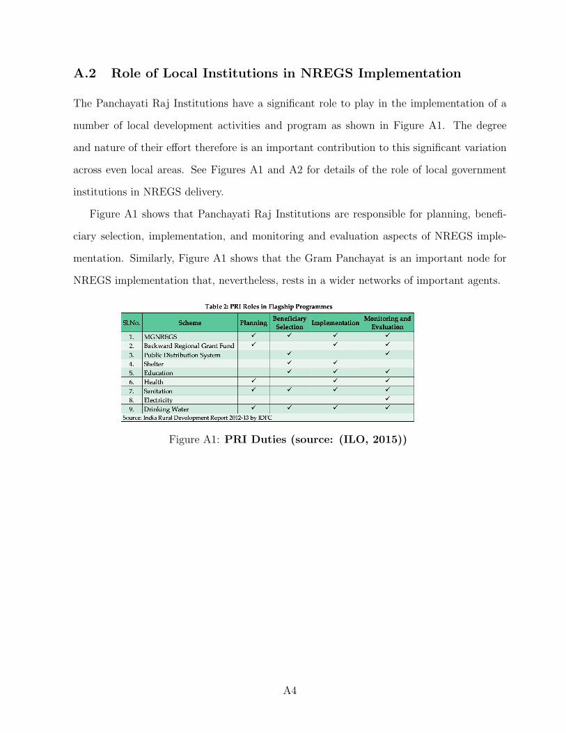
A.2 Role of Local Institutions in NREGS Implementation

The Panchayati Raj Institutions have a significant role to play in the implementation of a

number of local development activities and program as shown in Figure A1. The degree

and nature of their effort therefore is an important contribution to this significant variation

across even local areas. See Figures A1 and A2 for details of the role of local government

institutions in NREGS delivery.

Figure A1 shows that Panchayati Raj Institutions are responsible for planning, benefi-

ciary selection, implementation, and monitoring and evaluation aspects of NREGS imple-

mentation. Similarly, Figure A1 shows that the Gram Panchayat is an important node for

NREGS implementation that, nevertheless, rests in a wider networks of important agents.

Figure A1: PRI Duties (source: (ILO, 2015))

A4

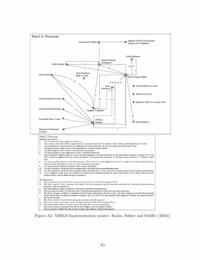
Figure A2: NREGS Implementation (source: Raabe, Sekher and Schiffer (2010))

A5

A.3 Background on Political Quotas in India

Political quotas restrict the representation or leadership of government bodies. The govern-

ment body may be a local or national administrative body, an elected local council, a state

parliament or a national-level parliament.21 While quotas most commonly target citizens

(e.g. for positions as bureaucrats) or leadership positions (in councils or parliaments), quotas

may also target particular geographic areas (e.g. with provisions for local autonomy).

Even prior to Indian Independence, the British government implemented quotas for in-

dividuals from particular ethnic identity categories. The Morley-Minto reforms in 1909 es-

tablished separate electorates for Muslims. In 1919, the Mont-Ford reforms tied this ‘quota’

inversely to the proportion of Muslims in a given province (Rudolph and Rudolph, 2010,

560-561). Beyond political quotas for the national parliament, state parliaments, local gov-

ernment, Fifth Schedule Areas, several other types of political quotas exist in India. Broadly

similar to the Fifth Schedule, the Indian Constitution’s Sixth Schedule allows for the cre-

ation of Autonomous Councils. These councils for Scheduled Tribe communities, typically

at the district or village levels, provide some legislative, administrative and judicial powers

in areas now and formerly contained within the state of Assam (Chaudhury, 2005).22

Another example of a territorial quota is the delimitation of electoral boundaries. In

both the national (Lok Sabha) and state (Vidhan Sabha) parliaments, the shape and number

21While not strictly meeting the definition of a type of government policy, political parties

may also implement quotas. See for instance Mala Htun who analyzes why quotas for

women are more likely to be utilized in parties but ethnic quotas more likely to be designed

for legislatures (Htun, 2004).

22Reforms under the Sixth Schedule, also targeting the welfare of ST, according to our

research, have been less consistent over time and space. Further we have been thus far unable

to gather systematic data on the Autonomous District Councils at the heart of the Sixth

Schedule, though we do believe this an area ripe for systematic research.

A6

of electoral constituencies in a given area are determined by the size of the local population.

Electoral redistricting was completed following every decennial census in 1952, 1963, 1973,

and after a nearly three-decade delay, again in 2002 (Iyer and Reddy, 2013).23 Even the

linguistic reorganization of states, based on the States Reorganisation Act of 1956, can be

considered a quota that generated state boundaries based on the relative linguistic homo-

geneity of a particular area (Tillin, 2013, Chapter 2).

For ordinary individuals, quotas influence individual’s access to state education, govern-

ment employment, and even rights to land. Reservations set aside places for individuals

from the Scheduled Castes, Scheduled Tribes, women, in some states for individuals from

Other Backward Classes, and even some religious groups (Corbridge, 2000; Galanter, 1984).

Even land rights can be considered a type of quota. In Jharkhand for instance, customary

laws such as the Chotanagpur Tenancy Act and the Santhal Parganas Tenancy Act both re-

strict land sales to individuals who are not associated with Scheduled Tribes (Sundar, 2005;

Upadhya, 2009).

A.4 Background on Tribes in India

Early accounts of ‘tribal’ populations listed these groups as savages: animistic, violent, bru-

tal, barbaric, wild. The Fifth Report of the House of Commons in 1812 described the inhab-

itants of Chotanagpur as a ‘savage race, differing extremely in appearance, religion. British

officials constructed Chotanagpur’s ‘tribes’ through the lenses of 18th and 19th C. Victorian

23In 1977 delimitation was halted following complaints that delimitation according to pop-

ulation size incentivized certain population control policies. New legislation froze electoral

boundaries in 1977 until delimitation was once again completed in 2002 Iyer and Reddy

(2013, 5-6).

A7

anthropology of racial types socio-cultural evolution (Damodaran, 2011, 58-59).24 These

administrator’s conceptualizations, built not only on travelers’ reports and racial theory but

also their readings of sacred Hindu texts informed these constructions (Radhakrishna, 2011,

45-46).

British observers also made reference to the relative seclusion of Chotanagpur communi-

ties with references to the jungle, forest, inhospitable forest, wilderness and so-called ‘primi-

tive places.’ S.C Roy wrote that Mundas settled in “primeval forests ... unmolested in their

isolated mountain fastness ... walled off from the outside walls by chains of wooded hills”

(1970: 60-61). As an example, anthropologist Verrier Elwin just after the end of the 19th C.

proposed a system of national parks in order to preserve cultures of the Munda, Ho, Oraon

and so on (Radhakrishna, 2011, 53).25 Perceptions of Chotanagpur’s ‘tribes’ roughly shifted

from at first a wild savage to a ‘noble’ savage, and eventually to indigenous groups that

needed to be protected from Aryan (then Hindu) invaders. In this way the British colonial

government saw itself as “protectors of wild yet innocent tribals against rapacious outsiders”

(Gupta, 2011a, 97). This shift followed the growth of 19th C. humanitarianism in Europe

and the growth of missionaries in Chotanagpur.

24British officials such as Colonel Tickell and Ricketts in the 1840s-1850s, administra-

tors W.W. Hunter and E. Dalton in late 19th C. and anthropologists S.C. Roy and Elwin

Verrier around 1910, had all written of distinct Munda, Ho and Oraon communities. See

(Damodaran, 2011; Gupta, 2011a,b; Galanter, 1984; Guha, 1996; Radhakrishna, 2011) for

more on how British officials documented ‘tribal’ populations.

25Despite these accounts 19th C. reports of British officials and anthropologists make clear

that communities in Singhbhum were not isolated but regularly interacted with groups in

northern Jharkhand (Corbridge, Jewitt and Kumar, 2004).

A8

A.5 Scheduled Tribes

India’s ‘tribal’ identity category was first codified, with corresponding separate adminis-

trative areas specified, during the British Colonial period. Scholars have identified these

‘tribal’ groups (or adivasi) by (a) their descent from particular lineages (Sundar, 2009), (b)

pre-colonial systems of administration, and/or (c) well-defined land arrangements and rights

(Gupta, 2011a,b). Despite regular mention of these factors, scholars agree that there has

been little clear definition or criteria as to what constitutes a ‘tribe’ (Beteille, 1974, 1986;

Dhebar, 1962; Corbridge, Jewitt and Kumar, 2004; Corbridge, 2002; Galanter, 1984).

Both prior to and following Indian Independence, leaders of the country have failed to

systematically define what constitutes a ‘tribe’ (or ‘Scheduled Tribe’). Definitions that have

been given are vague, imprecise, and unclear – suggesting that lists of ‘tribes’ or ST were often

reflected the political convenience of whomever administered the region. Despite numerous

studies by Colonial administrator-anthropologist and close attention paid to the so-called

‘tribes’ of Chotanagpur, relatively little effort was given to writing rules for distinguishing

a tribe or tribal from the rest of the population.26 British authorities first provided a list of

‘Aboriginal Tribes’ and ‘Semi-Hinduised Aboriginal Tribes’ in the Census of 1872 (Corbridge,

2002, 64). Census Commissioner H.H. Risley described a tribe as follows:

A tribe as I find in India is a collection of families or groups of families bearing a

common name which as a rule does not denote any specific occupation; generally

claiming common descent from a mythical or historical ancestor and occasionally

from an animal, but in some parts of the country held together by the obligations

of blood-feud than by the tradition of kinship; usually speaking the same language

26Chotanagpur is a region of Eastern India covering parts of the states of Jharkhand,

Chhattisgarh, Odisha and West Bengal – a region with some of the largest tribal populations

in India and a region geographically proximate to the Colonial capital of Calcutta (today

Kolkata).

A9

and occupying, professing, or claiming to occupy a definite tract of country. A

tribe is not necessarily endogamous. (H.H. (1903, 514), as quoted in Pati (2011,

4).

In 1911, The Imperial Gazetteer of India provided a striking similar definition: “A collection

of families bearing a common name, speaking a common dialect, occupying or professing to

occupy a common territory and is not usually endogamous though originally it might have

been so” (Nazer, 2004, 1). These definitions provide tremendous leeway for colonial officers

to assign groups however they like. When J.H. Hutton, Indian Census Commissioner in

1931, sought to provide a list of ‘tribes’ he aimed to utilize the basis of “soul-substance”

(Corbridge, Jewitt and Kumar, 2004, 30).

Despite the lack of clear criteria identifying so-called Tribals, special institutions were

put in place for their protection with the Scheduled Districts Act of 1874. This territorial

designation led to legislation with the aim of protecting tribals rights to their land, for

instance through the Chotanagpur Tenancy Act of 1908. Upon Indian Independence from

the British, the new constitution continued these policies of special administration in what

were to become renamed “Scheduled Areas.”27

In 1951 the First Report of the Commissioner for Scheduled Castes and Scheduled Tribes

admitted that no precise method for identifying Scheduled Tribes had been created to date

(Report 1951: 11). The report went on to note four characteristics identify a tribal: “tribal

origin, primitive way of life, remote habitation, and general backwardness in all respects”

(Report 1951: 109-111). Subsequent Commissions focused on Scheduled Castes and Sched-

uled Tribes reinforced the idea that little new information, methods of categorization or

27Under the Fifth Schedule of the Indian Constitution (1947), Scheduled Areas were cre-

ated to allow customary practices and autonomy of Scheduled Tribes in these regions. By

order of the President, a list of Scheduled Tribes and a list of Scheduled Areas was produced

in 1950.

A10

codification guided what constituted or defined either Scheduled Tribes or Scheduled Areas.

Sociologist Andre Beteille has written, “lists of Indian tribes were in fact drawn up, with

or without benefit of clear and consistent definitions” (Beteille, 1986, 299), and, “it cannot

be too strongly emphasized that the list reflects the demands more of administrative and

political circumstance than of academic or logical rigour” (Beteille, 1974, 62).

Indian Government officials even admitted the lack of definitions. According to the

Dhebar Commission in 1961, “the term tribe is nowhere defined in the Constitution and in

fact there is no satisfactory definition anywhere” (1962: 1). The Lokur Committee wrote

when revising the list of Scheduled Tribes in 1965: “I have looked for indications of primitive

traits, distinctive culture, geographic isolation, shyness of contact with the community at

large and backwardness” (Galanter, 1984, 152).28

According to the Indian Constitution, Scheduled Areas are to define in those areas with

a large fraction of the population belonging to a Scheduled Tribe. But this mapping of

Scheduled Tribes to Scheduled Areas is equally unclear. Officially, according to the Fifth

Schedule of the Constitution the President has the right to Schedule or De-schedule Areas

and does so in consultation with Governors of Indian states. The Dhebar Commission of 1962

proposed a Scheduled Area be identified according to the following four, relatively vague,

criteria.29

28Galanter notes this rough definition was reused in 1976: “this language is utilized almost

verbatim by the Home Minister more than 10 years later in the debate about revision of the

list” (1984: 152, fn. 143).

29In the mid-1970s the Twenty-Fourth Report of the Commissioner for Scheduled Castes

and Scheduled Tribes proposed a clearer rule that areas with more than fifty-percent Sched-

uled Tribe population should be Scheduled Areas (Commissioner for Scheduled Castes and

Scheduled Tribes, N.d., 117). But as we will show below, no such 50% threshold exists in

terms of defining Scheduled Areas.

A11

1. Preponderance of tribals in the population

2. Compact and reasonable size

3. Under-developed nature of the area

4. Marked disparity in economic standards of the people

While academic research and popular accounts discussing the Scheduled Areas have fo-

cused on political quotas, Scheduled Areas and PESA have several additional features in-

tended to benefit ST. These include the establishment of state-level Tribes Advisory Councils

intended to advocate on behalf of ST, restrictions over the sale of land, in an effort to prevent

alienation of land by ST, as well as, within villages, reinforcing a given village’s gram sabha

(a sub-gram panchayat body), as an important unit of local decision-making.

Appendix Figure A3 below shows while the probability that an area is demarcated as a

Scheduled Area is rising in the share of the ST population, there is no discontinuous jump in

Scheduled Areas status where Scheduled Tribes constitute more than 50% of a village’s total

population. We see a similar continuity in the probability if we conduct an RD on whether

the village has an ST plurality.

A.6 Case Study: The State of Jharkhand

A.6.1 Who is an ST?

After Independence the Government of Bihar made a clear break from historical laws giving

uniform but distinct rights to the whole of Jharkhand. By means of the Scheduled Areas

Order 1950 and the Scheduled Tribes Order 1951, the Government of Bihar effectively halved

the amount of territory defined as Scheduled Areas and substantially shrunk the number of

groups classified as ST. While the British Census of Chotanagpur in 1872 listed 31 aborig-

inal and 31 semi-aboriginal groups, the Scheduled Tribes Order of 1951 listed 30 such ST

communities. According to Corbridge, according to the Census of 1951, “just 31.15% of

A12

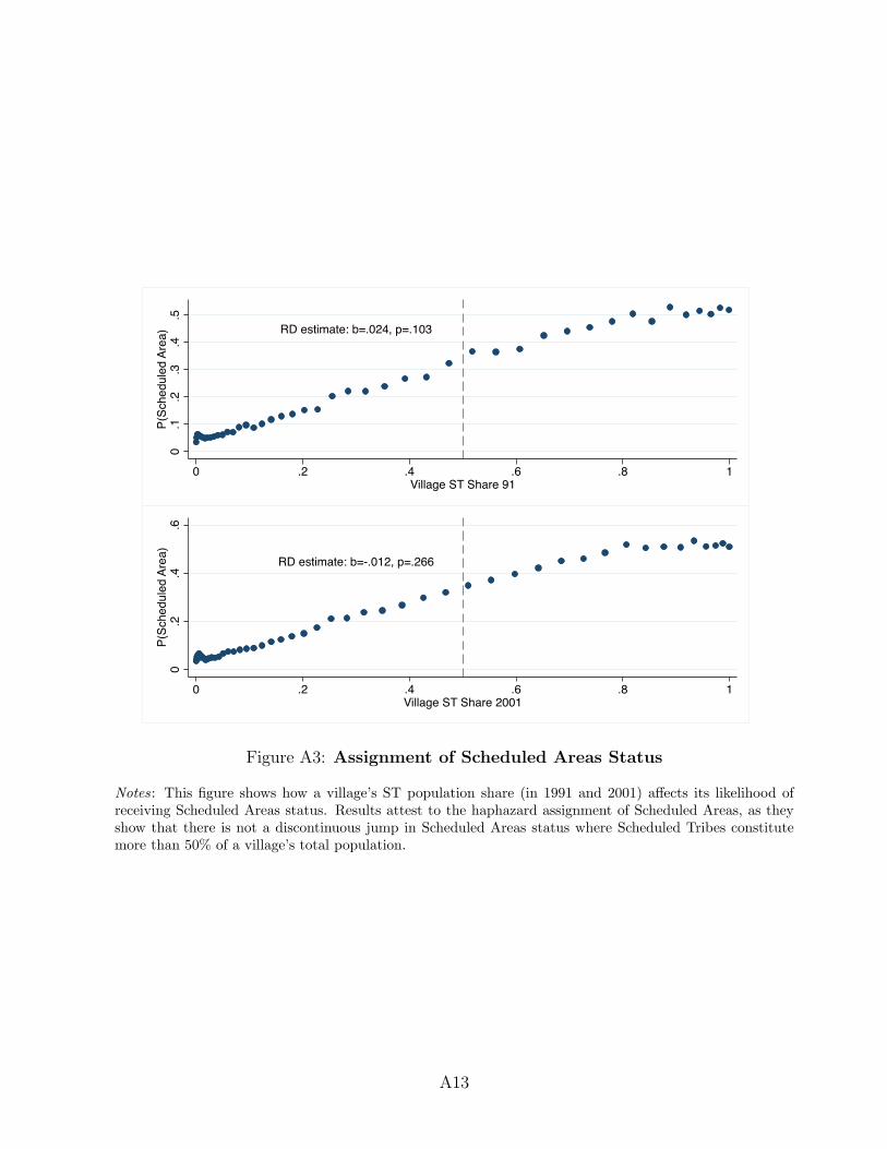
RD estimate: b=.024, p=.103

0.1

.2.3

.4.5

P(Sc

hedu

led

Area

)

0 .2 .4 .6 .8 1Village ST Share 91

RD estimate: b=-.012, p=.266

0.2

.4.6

P(Sc

hedu

led

Area

)

0 .2 .4 .6 .8 1Village ST Share 2001

Figure A3: Assignment of Scheduled Areas Status

Notes: This figure shows how a village’s ST population share (in 1991 and 2001) affects its likelihood ofreceiving Scheduled Areas status. Results attest to the haphazard assignment of Scheduled Areas, as theyshow that there is not a discontinuous jump in Scheduled Areas status where Scheduled Tribes constitutemore than 50% of a village’s total population.

A13

the population of Chota Nagpur, and 44.67% of that of Santal Parganas was made up of

Scheduled Tribals. Had the Census takers adopted the definitions used by the British in

1872, the percentage figures would have been 45.79% and 55.21% respectively” (Corbridge,

Jewitt and Kumar, 2004, 64).30

A.6.2 Which Areas are Scheduled?

In practice, in Jharkhand today, most Scheduled Areas are assigned at the unit of district but

some blocks are assigned as Scheduled Areas within Nonscheduled districts and some village-

clusters are Scheduled within Nonscheduled blocks. With reference to earlier suggested

criteria for which regions should be Scheduled: Jharkhand does not follow the fifty-percent

rule as a criterion for Scheduling Areas. With no modifications in scheduling at the district-

level, the Scheduled Areas assigned for Jharkhand (then Bihar) in 1950 have remained almost

completely unchanged to present.31 The Scheduled Areas of Jharkhand were re-affirmed after

being assigned in 1950 in the Bihar Scheduled Areas Regulation of 1969 and again in 1977

and 2007.

30It is not exactly clear why certain groups were re-classified or if there was a clear method-

ology taken. Corbridge argues that some because some “ ‘aboriginals’ had gained employ-

ment in the mining or industrial sectors was taken as evidence of their ‘detribalisation”’

(Corbridge, Jewitt and Kumar, 2004, 64). Possibly the Government of Bihar thought de-

scheduling some communities and areas would diminish the possibility that the mineral-rich

region of Jharkhand would gain independent statehood.

31The only exceptions are the Scheduling of Bhandaria block of Garhwa district in 1977

and the Scheduling of two village-clusters, both within Satbarwa block in 2007.

A14

B Data Construction

B.1 Creating an all-India dataset with NREGS, census, and elec-

tion data sources

Because we hope this dataset and our procedures will be of use to other researchers we

describe this process in detail:

1. Download the Socioeconomic High-resolution Rural-Urban Geographic Dataset for In-

dia (SHRUG), including available data from 1991-2011 Censuses and keys to match

villages (N ≈ 647, 000) with 2001 and 2011 raw Census shape files (Asher and Novosad,

2019b).32

2. Download and combine village-cluster unit state datasets on NREGS from the MGN-

REGA Public Data Portal.33

3. Build a village/village-cluster directory by downloading and combining individual block-

level directory files from from the Ministry of Drinking Water and Sanitation.34

4. Extract and combine Census shape files using ArcGIS, to form spatially referenced

(longitudes and latitudes) datasets of villages in the 2001 and 2011 Indian Censuses.35

32The SHRUG dataset may be accessed at: https://doi.org/10.7910/DVN/DPESAK.

33The MGNREGA Public Data Portal may be accessed at: mnregaweb4.nic.in/

netnrega/dynamic2/dynamicreport_new4.aspx.

34We access the data from http://indiawater.gov.in/imisreports/nrdwpmain.aspx

at the National Rural Drinking Water Programme, Ministry of Drinking Water and Sanita-

tion (Ministry of Drinking Water and Sanitation, 2014).

35We obtained Census data from New York University and Stanford University libraries,

which licensed the data from InfoMap India (https://www.mlinfomap.com/).

A15

https://doi.org/10.7910/DVN/DPESAK

mnregaweb4.nic.in/netnrega/dynamic2/dynamicreport_new4.aspx

http://indiawater.gov.in/imisreports/nrdwpmain.aspx

https://www.mlinfomap.com/

5. Homogenize district and state names from NREGS dataset to the Water Ministry

directory using a listing of all changes in district names and alternate spellings.36 This

allows matching of the NREGS dataset more efficiently.

6. Fuzzy match SHRID village names to the directory, and then NREGS village-cluster

names to the directory. The directory provides a common reference for the two

datasets.37

7. Add Scheduled Areas reservation status to the village dataset (see Appendix B.2 for

more on Scheduled Areas reservation status construction).

8. Add assembly constituency-candidate level electoral records to the village dataset by

locating each village within an assembly constituency using the village’s latitude and

longitude.38

9. Merge the dataset with Census 2001 and Census 2011 data using match keys from the

SHRID dataset.

B.2 Identifying Scheduled Areas

Data on Scheduled Areas status was obtained from the government of India’s Ministry of

Tribal Affairs. The websites from which we obtained data in 2014 for eight of the nine states

36For this, we rely on a compilation of all name changes between 2001 and 2011 available

from (Statoids, N.d.), at http://www.statoids.com/yin.html.

37We used Stata’s reclink command to carry out the fuzzy match. Other commands

commonly used to fuzzy match string variables such as soundex are not useful in the Indian

context because they rely on phonetic merging.

38Election data was downloaded from Election Commission of India (2014), at http:

//eci.nic.in/eci_main1/ElectionStatistics.aspx. We used the Spatial Join command

in ArcGIS to carry out this procedure.

A16

http://www.statoids.com/yin.html

http://eci.nic.in/eci_main1/ElectionStatistics.aspx

Table A2: Balance Table: Matched Villages Across India

Difference p-value Unmatched MatchedScheduled Areas 0.002 0.181 57457 216569Population Index (Shrug, 1991-2001) 0.036 0.000 42765 213059Minority Index (Shrug, 1991-2001) -0.000 0.937 42765 213059Public Goods Index (Shrug, 1991-2001) 0.116 0.000 42754 213048Vulnerable Index (Shrug, 1991-2001) -0.074 0.000 44197 213404

Notes : This table presents balance on variables that appear in both 1991 and 2001

Census waves between villages we are able to match in our dataset and those that remain

unmatched. The ‘Difference’ column represents the effect of Matched on each outcome in

rows. Importantly, matched villages are not more likely to be Scheduled Areas than are

unmatched villages.

in our sample have since been retired, though they can be accessed today using Internet

archive website The Wayback Machine. Below, we provide original links, as well as links

that can still be used today to access the sites, for each of the eight states.

Andhra Pradesh

• Original link: http://tribal.nic.in/Content/ScheduledAreasinAndhraPradeshSSAreas.

aspx

• Archive link: https://web.archive.org/web/20140818090711/http://tribal.nic.

in:80/Content/ScheduledAreasinAndhraPradeshSSAreas.aspx

Gujarat

• Original link: http://tribal.nic.in/Content/ScheduledAreasinGujarat.aspx


in:80/Content/ScheduledAreasinGujarat.aspx

Jharkhand

• Original link: http://tribal.nic.in/Content/ScheduledAreasinBiharSSAreas.aspx

A17

http://tribal.nic.in/Content/ScheduledAreasinAndhraPradeshSSAreas.aspx

https://web.archive.org/web/20140818090711/http://tribal.nic.in:80/Content/ScheduledAreasinAndhraPradeshSSAreas.aspx

http://tribal.nic.in/Content/ScheduledAreasinGujarat.aspx

https://web.archive.org/web/20140818090722/http://tribal.nic.in:80/Content/ScheduledAreasinGujarat.aspx

http://tribal.nic.in/Content/ScheduledAreasinBiharSSAreas.aspx


in:80/Content/ScheduledAreasinBiharSSAreas.aspx

Himachal Pradesh

• Original link: http://tribal.nic.in/Content/ScheduledAreasinHimachalPradeshSSAreas.

aspx


in:80/Content/ScheduledAreasinHimachalPradeshSSAreas.aspx

Maharashtra

• Original link: http://tribal.nic.in/Content/ScheduledAreasinMaharashtraSSAreas.

aspx


in:80/Content/ScheduledAreasinMaharashtraSSAreas.aspx

Madhya Pradesh

• Original link: http://tribal.nic.in/Content/ScheduledAreasinMadhyaPradeshSSAreas.

aspx


in:80/Content/ScheduledAreasinMadhyaPradeshSSAreas.aspx

Odisha

• Original link: http://tribal.nic.in/Content/ScheduledAreasinOrissaSSAreas.

aspx


in:80/Content/ScheduledAreasinOrissaSSAreas.aspx

A18

https://web.archive.org/web/20140818090717/http://tribal.nic.in:80/Content/ScheduledAreasinBiharSSAreas.aspx

http://tribal.nic.in/Content/ScheduledAreasinHimachalPradeshSSAreas.aspx

https://web.archive.org/web/20140818090727/http://tribal.nic.in:80/Content/ScheduledAreasinHimachalPradeshSSAreas.aspx

http://tribal.nic.in/Content/ScheduledAreasinMaharashtraSSAreas.aspx

https://web.archive.org/web/20140818090843/http://tribal.nic.in:80/Content/ScheduledAreasinMaharashtraSSAreas.aspx

http://tribal.nic.in/Content/ScheduledAreasinMadhyaPradeshSSAreas.aspx

https://web.archive.org/web/20140818090732/http://tribal.nic.in:80/Content/ScheduledAreasinMadhyaPradeshSSAreas.aspx

http://tribal.nic.in/Content/ScheduledAreasinOrissaSSAreas.aspx

https://web.archive.org/web/20140818090738/http://tribal.nic.in:80/Content/ScheduledAreasinOrissaSSAreas.aspx

Rajasthan

• Original link: http://tribal.nic.in/Content/ScheduledAreasinRajasthanSSAreas.

aspx


in/Content/ScheduledAreasinRajasthanSSAreas.aspx

Information on Scheduled Areas in all states, including the ninth in our sample, Chhat-

tisgarh, may also be found in Annexure-II of “Statistical Profile of Scheduled Tribes in India

(2013),” released by the Ministry of Tribal Affairs Statistical Division and accessible here:

https://tribal.nic.in/ST/StatisticalProfileofSTs2013.pdf.

B.2.1 Verifying our Identification of Scheduled Areas and our spatial (longi-

tudes and latitudes) data

.

To verify that we correctly identified Scheduled Areas, and more generally that our spatial

(longitudes and latitudes) data are accurate, we can compare our map of Scheduled Areas

that we generated using our data (Figure 2) to an official government map.39 In Figure A4,

we reproduce our map and compare it to the government map. We can see that our map

closely matches the government map, but that ours provides more fine-grained information,

bolstering our confidence in our data collection methods.

39This map can be accessed at http://pesadarpan.gov.in/en_US/fifth-schedule-

areas/-/asset_publisher

A19

http://tribal.nic.in/Content/ScheduledAreasinRajasthanSSAreas.aspx

https://web.archive.org/web/20140904021414/http://tribal.nic.in/Content/ScheduledAreasinRajasthanSSAreas.aspx

https://tribal.nic.in/ST/StatisticalProfileofSTs2013.pdf

http://pesadarpan.gov.in/en_US/fifth-schedule-areas/-/asset_publisher

Figure A4: Validating Spatial Data and Scheduled Area Identification

(a) Our Map(Coding at Block Level)

(b) Government Map(Coding at District Level)

A20

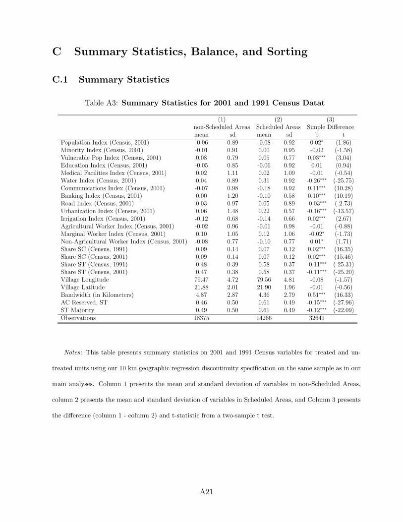
C Summary Statistics, Balance, and Sorting

C.1 Summary Statistics

Table A3: Summary Statistics for 2001 and 1991 Census Datat

(1) (2) (3)non-Scheduled Areas Scheduled Areas Simple Differencemean sd mean sd b t

Population Index (Census, 2001) -0.06 0.89 -0.08 0.92 0.02∗ (1.86)Minority Index (Census, 2001) -0.01 0.91 0.00 0.95 -0.02 (-1.58)Vulnerable Pop Index (Census, 2001) 0.08 0.79 0.05 0.77 0.03∗∗∗ (3.04)Education Index (Census, 2001) -0.05 0.85 -0.06 0.92 0.01 (0.94)Medical Facilities Index (Census, 2001) 0.02 1.11 0.02 1.09 -0.01 (-0.54)Water Index (Census, 2001) 0.04 0.89 0.31 0.92 -0.26∗∗∗ (-25.75)Communications Index (Census, 2001) -0.07 0.98 -0.18 0.92 0.11∗∗∗ (10.28)Banking Index (Census, 2001) 0.00 1.20 -0.10 0.58 0.10∗∗∗ (10.19)Road Index (Census, 2001) 0.03 0.97 0.05 0.89 -0.03∗∗∗ (-2.73)Urbanization Index (Census, 2001) 0.06 1.48 0.22 0.57 -0.16∗∗∗ (-13.57)Irrigation Index (Census, 2001) -0.12 0.68 -0.14 0.66 0.02∗∗∗ (2.67)Agricultural Worker Index (Census, 2001) -0.02 0.96 -0.01 0.98 -0.01 (-0.88)Marginal Worker Index (Census, 2001) 0.10 1.05 0.12 1.06 -0.02∗ (-1.73)Non-Agricultural Worker Index (Census, 2001) -0.08 0.77 -0.10 0.77 0.01∗ (1.71)Share SC (Census, 1991) 0.09 0.14 0.07 0.12 0.02∗∗∗ (16.35)Share SC (Census, 2001) 0.09 0.14 0.07 0.12 0.02∗∗∗ (15.46)Share ST (Census, 1991) 0.48 0.39 0.58 0.37 -0.11∗∗∗ (-25.31)Share ST (Census, 2001) 0.47 0.38 0.58 0.37 -0.11∗∗∗ (-25.20)Village Longitude 79.47 4.72 79.56 4.81 -0.08 (-1.57)Village Latitude 21.88 2.01 21.90 1.96 -0.01 (-0.56)Bandwidth (in Kilometers) 4.87 2.87 4.36 2.79 0.51∗∗∗ (16.33)AC Reserved, ST 0.46 0.50 0.61 0.49 -0.15∗∗∗ (-27.96)ST Majority 0.49 0.50 0.61 0.49 -0.12∗∗∗ (-22.09)Observations 18375 14266 32641

Notes: This table presents summary statistics on 2001 and 1991 Census variables for treated and un-

treated units using our 10 km geographic regression discontinuity specification on the same sample as in our

main analyses. Column 1 presents the mean and standard deviation of variables in non-Scheduled Areas,

column 2 presents the mean and standard deviation of variables in Scheduled Areas, and Column 3 presents

the difference (column 1 - column 2) and t-statistic from a two-sample t test.

A21

Table A4: Summary Statistics: NREGS and Census 2011 Employment Outcomes


Logged (Workdays + 1) 8.06 2.51 8.10 2.66 -0.04 (-1.52)Logged (Workdays ST + 1) 6.34 3.16 6.86 3.15 -0.52∗∗∗ (-14.77)Logged (Workdays SC + 1) 4.84 3.12 4.66 3.15 0.18∗∗∗ (5.14)Logged (Workdays Others + 1) 6.68 2.76 6.42 2.87 0.27∗∗∗ (8.45)Workdays 9748.16 10499.24 11467.71 15104.98 -1719.54∗∗∗ (-11.60)Workdays - ST 4306.59 6367.91 6851.69 12279.96 -2545.10∗∗∗ (-22.52)Workdays - SC 1259.99 2130.40 1139.16 2032.10 120.82∗∗∗ (5.22)Workdays - Others 4181.59 6448.20 3476.85 5384.62 704.74∗∗∗ (10.75)Total Workers 5.85 1.05 5.83 1.06 0.02 (1.33)Total Workers - Men 5.30 1.04 5.25 1.06 0.04∗∗∗ (3.79)Total Workers - Women 4.89 1.22 4.94 1.17 -0.05∗∗∗ (-3.69)Main Workers 5.15 1.51 5.07 1.59 0.07∗∗∗ (4.25)Main Workers - Men 4.78 1.45 4.70 1.53 0.09∗∗∗ (5.24)Main Workers - Women 3.76 1.74 3.75 1.77 0.02 (0.80)Marginal Workers 4.20 1.71 4.24 1.69 -0.04∗∗ (-2.08)Marginal Workers - Men 3.28 1.62 3.30 1.60 -0.02 (-1.24)Marginal Workers - Women 3.64 1.72 3.71 1.69 -0.07∗∗∗ (-3.88)Other Workers 3.01 1.58 2.87 1.64 0.15∗∗∗ (8.07)Other Workers - Men 2.72 1.60 2.56 1.65 0.16∗∗∗ (8.69)Other Workers - Women 1.80 1.25 1.76 1.26 0.04∗∗∗ (2.77)Observations 18375 14266 32641

Notes: This table presents summary statistics on NREGS and 2011 Census employment outcome vari-

ables for treated and untreated units using our 10 km geographic regression discontinuity specification on

the same sample as in our main analyses. Column 1 presents the mean and standard deviation of variables

in non-Scheduled Areas, column 2 presents the mean and standard deviation of variables in Scheduled Areas,

and Column 3 presents the difference (column 1 - column 2) and t-statistic from a two-sample t test.

A22

Table A5: Summary Statistics and Balance for 2011 Public Goods Analysis


Population Index (Census, 2001) 0.77 1.69 1.01 1.96 -0.23∗∗∗ (-3.25)Minority Index (Census, 2001) 0.71 1.58 0.93 1.83 -0.23∗∗∗ (-3.41)Vulnerable Pop Index (Census, 2001) 0.19 0.76 0.11 0.79 0.08∗∗∗ (2.76)Education Index (Census, 2001) 0.64 1.69 0.81 1.96 -0.17∗∗ (-2.36)Medical Facilities Index (Census, 2001) 0.68 2.80 0.91 2.49 -0.23∗∗ (-2.23)Water Index (Census, 2001) 0.30 0.77 0.68 0.84 -0.39∗∗∗ (-12.24)Communications Index (Census, 2001) 0.44 1.40 0.50 1.47 -0.06 (-1.11)Banking Index (Census, 2001) 0.41 1.52 0.46 1.29 -0.05 (-0.98)Road Index (Census, 2001) 0.09 1.09 0.08 0.93 0.01 (0.24)Urbanization Index (Census, 2001) 0.08 1.52 0.32 0.60 -0.23∗∗∗ (-5.64)Irrigation Index (Census, 2001) 0.21 0.96 0.29 1.12 -0.08∗∗ (-2.07)Agricultural Worker Index (Census, 2001) 0.76 1.60 1.01 1.74 -0.25∗∗∗ (-3.86)Marginal Worker Index (Census, 2001) 0.04 1.00 -0.01 0.91 0.06 (1.59)Non-Agricultural Worker Index (Census, 2001) 0.45 1.54 0.55 1.54 -0.10∗ (-1.66)Share SC (Census, 1991) 0.11 0.12 0.09 0.10 0.02∗∗∗ (5.11)Share SC (Census, 2001) 0.11 0.12 0.09 0.10 0.02∗∗∗ (4.47)Share ST (Census, 1991) 0.35 0.34 0.44 0.36 -0.08∗∗∗ (-6.01)Share ST (Census, 2001) 0.36 0.34 0.44 0.35 -0.08∗∗∗ (-6.20)Observations 1632 1117 2749

Notes: This table presents summary statistics on 2001 and 1991 Census variables for treated and un-

treated units using our 10 km geographic regression discontinuity specification on the same sample as in

our analysis on 2011 public goods (Census market villages). Column 1 presents the mean and standard

deviation of variables in non-Scheduled Areas, column 2 presents the mean and standard deviation of vari-

ables in Scheduled Areas, and Column 3 presents the difference (column 1 - column 2) and t-statistic from

a two-sample t test.

A23

Table A6: Summary Statistics for 2011 Census Market Village Outcomes


Overall Public Goods Index 0.51 0.21 0.55 0.19 -0.04∗∗∗ (-5.52)Roads Index 0.49 0.25 0.52 0.23 -0.04∗∗∗ (-3.84)All Weather Road (Y/N) 0.78 0.41 0.83 0.38 -0.04∗∗∗ (-2.93)National Highway (Y/N) 0.08 0.28 0.09 0.29 -0.01 (-0.75)State Highway (Y/N) 0.18 0.38 0.21 0.41 -0.03∗∗ (-2.04)Major District Road (Y/N) 0.39 0.49 0.42 0.49 -0.03 (-1.62)Other District Road (Y/N) 0.62 0.49 0.67 0.47 -0.05∗∗∗ (-2.89)Gravel Road (Y/N) 0.87 0.34 0.91 0.28 -0.04∗∗∗ (-3.69)Water Index 0.53 0.21 0.56 0.19 -0.03∗∗∗ (-4.04)Handpump (Y/N) 0.89 0.31 0.91 0.28 -0.02∗∗ (-2.16)Tap Water Treated (Y/N) 0.30 0.46 0.37 0.48 -0.07∗∗∗ (-3.92)Tank, Pond, Lake (Y/N) 0.49 0.50 0.48 0.50 0.02 (0.86)Covered Well (Y/N) 0.16 0.37 0.21 0.41 -0.05∗∗∗ (-3.26)Uncovered Well (Y/N) 0.79 0.40 0.82 0.38 -0.03∗ (-1.80)Irrigation Index 0.39 0.36 0.41 0.36 -0.02 (-1.43)Tubewell/Borehole (Y/N) 0.42 0.49 0.43 0.50 -0.02 (-0.79)River/Canal (Y/N) 0.37 0.48 0.39 0.49 -0.03 (-1.33)Electricity Index 0.70 0.38 0.72 0.36 -0.02∗ (-1.71)Electricity for Agriculture Use (Y/N) 0.67 0.47 0.71 0.46 -0.03∗ (-1.87)Electricity for Domestic Use (Y/N) 0.85 0.36 0.87 0.33 -0.02∗ (-1.73)Electricity for Commercial Use (Y/N) 0.57 0.49 0.59 0.49 -0.02 (-0.91)Communications Index 0.46 0.34 0.54 0.34 -0.08∗∗∗ (-6.20)Post Office (Y/N) 0.33 0.47 0.43 0.49 -0.10∗∗∗ (-5.37)Post and Telegraph Office (Y/N) 0.24 0.43 0.32 0.47 -0.08∗∗∗ (-4.45)Telephone (Y/N) 0.53 0.50 0.60 0.49 -0.07∗∗∗ (-3.67)Mobile Coverage (Y/N) 0.75 0.43 0.83 0.38 -0.08∗∗∗ (-5.00)Education Index 0.47 0.26 0.53 0.25 -0.05∗∗∗ (-5.36)Primary School (Y/N) 0.90 0.30 0.95 0.22 -0.05∗∗∗ (-4.71)Middle School (Y/N) 0.74 0.44 0.82 0.38 -0.08∗∗∗ (-4.95)Secondary School (Y/N) 0.45 0.50 0.54 0.50 -0.09∗∗∗ (-4.42)Senior Secondary School (Y/N) 0.25 0.43 0.29 0.46 -0.05∗∗∗ (-2.73)College (Y/N) 0.03 0.18 0.04 0.19 -0.01 (-0.83)Observations 1632 1117 2749

Notes: This table presents summary statistics on 2011 public goods Census variables for treated and

untreated units using our 10 km geographic regression discontinuity specification on the same sample as

in our analysis on 2011 public goods (Census market villages). Column 1 presents the mean and standard

deviation of variables in non-Scheduled Areas, column 2 presents the mean and standard deviation of variables

in Scheduled Areas, and Column 3 presents the difference (column 1 - column 2) and t-statistic from a two-

sample t test.

A24

Table A7: Summary Statistics for Assembly Constituency (AC) ST Reservation,Scheduled Areas

(1) (2) (3)non-ST Reserved ST Reserved Simple Differencemean sd mean sd b t

Population Index (Census, 2001) -0.09 1.04 -0.07 0.84 -0.02 (-1.30)Minority Index (Census, 2001) -0.12 0.97 0.08 0.93 -0.21∗∗∗ (-12.58)Vulnerable Pop Index (Census, 2001) 0.17 0.83 -0.02 0.72 0.18∗∗∗ (13.55)Education Index (Census, 2001) -0.11 1.04 -0.03 0.84 -0.08∗∗∗ (-5.06)Medical Facilities Index (Census, 2001) -0.01 1.28 0.05 0.95 -0.05∗∗∗ (-2.75)Water Index (Census, 2001) 0.37 0.81 0.26 0.98 0.11∗∗∗ (7.26)Communications Index (Census, 2001) -0.22 0.97 -0.15 0.89 -0.07∗∗∗ (-4.51)Banking Index (Census, 2001) -0.08 0.62 -0.11 0.56 0.03∗∗∗ (2.75)Road Index (Census, 2001) 0.04 0.99 0.06 0.81 -0.02 (-1.51)Urbanization Index (Census, 2001) 0.06 0.49 0.33 0.60 -0.27∗∗∗ (-29.51)Irrigation Index (Census, 2001) -0.17 0.69 -0.13 0.64 -0.05∗∗∗ (-4.19)Agricultural Worker Index (Census, 2001) -0.12 0.94 0.06 1.00 -0.18∗∗∗ (-10.84)Marginal Worker Index (Census, 2001) 0.18 1.12 0.08 1.01 0.11∗∗∗ (5.76)Non-Agricultural Worker Index (Census, 2001) -0.04 0.89 -0.13 0.68 0.09∗∗∗ (6.70)Population Perc SC (1991) 0.09 0.15 0.05 0.10 0.04∗∗∗ (17.35)Population Perc SC (2001) 0.09 0.15 0.05 0.09 0.04∗∗∗ (19.85)Population Perc ST (1991) 0.42 0.39 0.68 0.33 -0.26∗∗∗ (-41.56)Population Perc ST (2001) 0.42 0.38 0.68 0.32 -0.26∗∗∗ (-42.32)Village Longitude 81.71 5.22 78.20 3.97 3.52∗∗∗ (42.89)Village Latitude 22.04 2.25 21.80 1.75 0.24∗∗∗ (6.78)Bandwidth (in Kilometers) 4.39 2.78 4.34 2.80 0.06 (1.20)Observations 5525 8741 14266

Notes: This table presents summary statistics on 2001 and 1991 Census variables for Scheduled Areas

villages with (ST Reserved) and without (non-ST Reserved) overlapping AC-level ST reservations using our

10 km geographic regression discontinuity specification on the same sample as in our analyses. Column 1

presents the mean and standard deviation of variables in non-ST reserved areas, column 2 presents the mean

and standard deviation of variables in ST reserved areas, and Column 3 presents the difference (column 1 -

column 2) and t-statistic from a two-sample t test.

A25

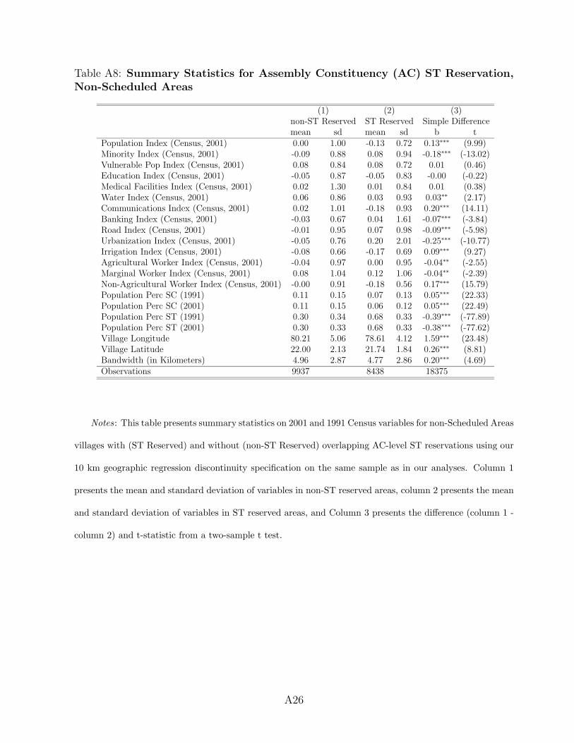
Table A8: Summary Statistics for Assembly Constituency (AC) ST Reservation,Non-Scheduled Areas

(1) (2) (3)non-ST Reserved ST Reserved Simple Differencemean sd mean sd b t

Population Index (Census, 2001) 0.00 1.00 -0.13 0.72 0.13∗∗∗ (9.99)Minority Index (Census, 2001) -0.09 0.88 0.08 0.94 -0.18∗∗∗ (-13.02)Vulnerable Pop Index (Census, 2001) 0.08 0.84 0.08 0.72 0.01 (0.46)Education Index (Census, 2001) -0.05 0.87 -0.05 0.83 -0.00 (-0.22)Medical Facilities Index (Census, 2001) 0.02 1.30 0.01 0.84 0.01 (0.38)Water Index (Census, 2001) 0.06 0.86 0.03 0.93 0.03∗∗ (2.17)Communications Index (Census, 2001) 0.02 1.01 -0.18 0.93 0.20∗∗∗ (14.11)Banking Index (Census, 2001) -0.03 0.67 0.04 1.61 -0.07∗∗∗ (-3.84)Road Index (Census, 2001) -0.01 0.95 0.07 0.98 -0.09∗∗∗ (-5.98)Urbanization Index (Census, 2001) -0.05 0.76 0.20 2.01 -0.25∗∗∗ (-10.77)Irrigation Index (Census, 2001) -0.08 0.66 -0.17 0.69 0.09∗∗∗ (9.27)Agricultural Worker Index (Census, 2001) -0.04 0.97 0.00 0.95 -0.04∗∗ (-2.55)Marginal Worker Index (Census, 2001) 0.08 1.04 0.12 1.06 -0.04∗∗ (-2.39)Non-Agricultural Worker Index (Census, 2001) -0.00 0.91 -0.18 0.56 0.17∗∗∗ (15.79)Population Perc SC (1991) 0.11 0.15 0.07 0.13 0.05∗∗∗ (22.33)Population Perc SC (2001) 0.11 0.15 0.06 0.12 0.05∗∗∗ (22.49)Population Perc ST (1991) 0.30 0.34 0.68 0.33 -0.39∗∗∗ (-77.89)Population Perc ST (2001) 0.30 0.33 0.68 0.33 -0.38∗∗∗ (-77.62)Village Longitude 80.21 5.06 78.61 4.12 1.59∗∗∗ (23.48)Village Latitude 22.00 2.13 21.74 1.84 0.26∗∗∗ (8.81)Bandwidth (in Kilometers) 4.96 2.87 4.77 2.86 0.20∗∗∗ (4.69)Observations 9937 8438 18375

Notes: This table presents summary statistics on 2001 and 1991 Census variables for non-Scheduled Areas

villages with (ST Reserved) and without (non-ST Reserved) overlapping AC-level ST reservations using our

10 km geographic regression discontinuity specification on the same sample as in our analyses. Column 1

presents the mean and standard deviation of variables in non-ST reserved areas, column 2 presents the mean

and standard deviation of variables in ST reserved areas, and Column 3 presents the difference (column 1 -

column 2) and t-statistic from a two-sample t test.

A26

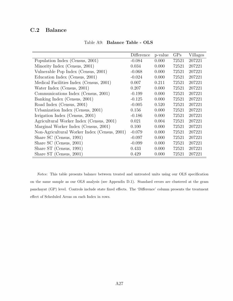
C.2 Balance

Table A9: Balance Table - OLS

Difference p-value GPs VillagesPopulation Index (Census, 2001) -0.084 0.000 72521 207221Minority Index (Census, 2001) 0.034 0.000 72521 207221Vulnerable Pop Index (Census, 2001) -0.068 0.000 72521 207221Education Index (Census, 2001) -0.024 0.000 72521 207221Medical Facilities Index (Census, 2001) 0.007 0.211 72521 207221Water Index (Census, 2001) 0.207 0.000 72521 207221Communications Index (Census, 2001) -0.199 0.000 72521 207221Banking Index (Census, 2001) -0.125 0.000 72521 207221Road Index (Census, 2001) -0.005 0.520 72521 207221Urbanization Index (Census, 2001) 0.156 0.000 72521 207221Irrigation Index (Census, 2001) -0.186 0.000 72521 207221Agricultural Worker Index (Census, 2001) 0.021 0.004 72521 207221Marginal Worker Index (Census, 2001) 0.100 0.000 72521 207221Non-Agricultural Worker Index (Census, 2001) -0.079 0.000 72521 207221Share SC (Census, 1991) -0.097 0.000 72521 207221Share SC (Census, 2001) -0.099 0.000 72521 207221Share ST (Census, 1991) 0.433 0.000 72521 207221Share ST (Census, 2001) 0.429 0.000 72521 207221

Notes: This table presents balance between treated and untreated units using our OLS specification

on the same sample as our OLS analysis (see Appendix D.1). Standard errors are clustered at the gram

panchayat (GP) level. Controls include state fixed effects. The ‘Difference’ column presents the treatment

effect of Scheduled Areas on each Index in rows.

A27

Table A10: Balance Table - 10 km RD

Difference p-value GPs VillagesPopulation Index (Census, 2001) -0.024 0.035 13338 32641Minority Index (Census, 2001) 0.020 0.103 13338 32641Vulnerable Pop Index (Census, 2001) -0.025 0.025 13338 32641Education Index (Census, 2001) 0.003 0.773 13338 32641Medical Facilities Index (Census, 2001) 0.011 0.376 13338 32641Water Index (Census, 2001) 0.214 0.000 13338 32641Communications Index (Census, 2001) -0.092 0.000 13338 32641Banking Index (Census, 2001) -0.116 0.000 13338 32641Road Index (Census, 2001) -0.000 0.997 13338 32641Urbanization Index (Census, 2001) 0.156 0.000 13338 32641Irrigation Index (Census, 2001) -0.016 0.069 13338 32641Agricultural Worker Index (Census, 2001) 0.003 0.795 13338 32641Marginal Worker Index (Census, 2001) 0.023 0.132 13338 32641Non-Agricultural Worker Index (Census, 2001) -0.011 0.253 13338 32641Share SC (Census, 1991) -0.022 0.000 13338 32641Share SC (Census, 2001) -0.021 0.000 13338 32641Share ST (Census, 1991) 0.110 0.000 13338 32641Share ST (Census, 2001) 0.109 0.000 13338 32641

Notes: This table presents balance between treated and untreated units using our 10 km geographic

regression discontinuity specification on the same sample as in our main analyses. Standard errors are

clustered at the gram panchayat (GP) level. Controls include state fixed effects and a geographic control

function. The ‘Difference’ column presents the treatment effect of Scheduled Areas on each Index in rows.

A28

Table A11: Balance Table on 2001 Census for 2011 Market Villages - 10 km RD

Difference p-value GPs VillagesPopulation Index (Census, 2001) 0.002 0.974 2223 2749Minority Index (Census, 2001) 0.060 0.292 2223 2749Vulnerable Pop Index (Census, 2001) -0.044 0.136 2223 2749Education Index (Census, 2001) 0.097 0.128 2223 2749Medical Facilities Index (Census, 2001) 0.061 0.565 2223 2749Water Index (Census, 2001) 0.309 0.000 2223 2749Communications Index (Census, 2001) -0.060 0.162 2223 2749Banking Index (Census, 2001) -0.079 0.125 2223 2749Road Index (Census, 2001) -0.041 0.312 2223 2749Urbanization Index (Census, 2001) 0.193 0.000 2223 2749Irrigation Index (Census, 2001) -0.035 0.317 2223 2749Agricultural Worker Index (Census, 2001) -0.000 0.995 2223 2749Marginal Worker Index (Census, 2001) 0.032 0.365 2223 2749Non-Agricultural Worker Index (Census, 2001) 0.040 0.451 2223 2749Share SC (Census, 1991) -0.018 0.000 2223 2749Share SC (Census, 2001) -0.015 0.000 2223 2749Share ST (Census, 1991) 0.090 0.000 2223 2749Share ST (Census, 2001) 0.090 0.000 2223 2749

Notes: This table presents balance between treated and untreated units using our 10 km geographic

regression discontinuity specification on the same sample as in our analysis on 2011 public goods (Census

market villages). Standard errors are clustered at the gram panchayat (GP) level. Controls include state

fixed effects and a geographic control function. The ‘Difference’ column presents the treatment effect of

Scheduled Areas on each Index in rows.

A29

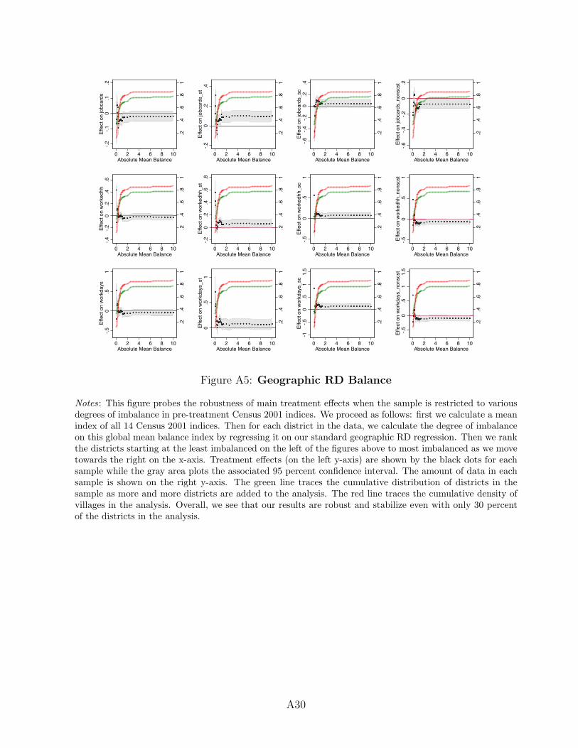
.2.4

.6.8

1

-.2-.1

0.1

.2Ef

fect

on

jobc

ards

0 2 4 6 8 10Absolute Mean Balance

.2.4

.6.8

1

-.20

.2.4

Effe

ct o

n jo

bcar

ds_s

t


.2.4

.6.8

1

-.6-.4

-.20

.2.4

Effe

ct o

n jo

bcar

ds_s

c


.2.4

.6.8

1

-.6-.4

-.20

.2Ef

fect

on

jobc

ards

_non

scst


.2.4

.6.8

1

-.4-.2

0.2

.4.6

Effe

ct o

n w

orke

dhh


.2.4

.6.8

1

-.20

.2.4

.6.8

Effe

ct o

n w

orke

dhh_

st


.2.4

.6.8

1

-.50

.51

Effe

ct o

n w

orke

dhh_

sc


.2.4

.6.8

1

-.50

.51

Effe

ct o

n w

orke

dhh_

nons

cst


.2.4

.6.8

1

-.50

.51

Effe

ct o

n w

orkd

ays


.2.4

.6.8

1

0.5

1Ef

fect

on

wor

kday

s_st


.2.4

.6.8

1

-1-.5

0.5

11.

5Ef

fect

on

wor

kday

s_sc


.2.4

.6.8

1

-.50

.51

1.5

Effe

ct o

n w

orkd

ays_

nons

cst


Figure A5: Geographic RD Balance

Notes: This figure probes the robustness of main treatment effects when the sample is restricted to variousdegrees of imbalance in pre-treatment Census 2001 indices. We proceed as follows: first we calculate a meanindex of all 14 Census 2001 indices. Then for each district in the data, we calculate the degree of imbalanceon this global mean balance index by regressing it on our standard geographic RD regression. Then we rankthe districts starting at the least imbalanced on the left of the figures above to most imbalanced as we movetowards the right on the x-axis. Treatment effects (on the left y-axis) are shown by the black dots for eachsample while the gray area plots the associated 95 percent confidence interval. The amount of data in eachsample is shown on the right y-axis. The green line traces the cumulative distribution of districts in thesample as more and more districts are added to the analysis. The red line traces the cumulative density ofvillages in the analysis. Overall, we see that our results are robust and stabilize even with only 30 percentof the districts in the analysis.

A30

-.2-.10.1.2.3Treatment effects

510

1520

2530

3540

4550

Band

wid

th in

Km

Popu

latio

n In

dex

(Cen

sus,

200

1)


510

1520

2530

3540

4550

Band

wid

th in

Km

Min

ority

Inde

x (C

ensu

s, 2

001)


510

1520

2530

3540

4550

Band

wid

th in

Km

Vuln

erab

le P

op In

dex

(Cen

sus,

200

1)


510

1520

2530

3540

4550

Band

wid

th in

Km

Educ

atio

n In

dex

(Cen

sus,

200

1)


510

1520

2530

3540

4550

Band

wid

th in

Km

Med

ical

Fac

ilitie

s In

dex

(Cen

sus,

200

1)


510

1520

2530

3540

4550

Band

wid

th in

Km

Wat

er In

dex

(Cen

sus,

200

1)


510

1520

2530

3540

4550

Band

wid

th in

Km

Com

mun

icat

ions

Inde

x (C

ensu

s, 2

001)


510

1520

2530

3540

4550

Band

wid

th in

Km

Bank

ing

Inde

x (C

ensu

s, 2

001)


510

1520

2530

3540

4550

Band

wid

th in

Km

Roa

d In

dex

(Cen

sus,

200

1)


510

1520

2530

3540

4550

Band

wid

th in

Km

Urb

aniz

atio

n In

dex

(Cen

sus,

200

1)


510

1520

2530

3540

4550

Band

wid

th in

Km

Irrig

atio

n In

dex

(Cen

sus,

200

1)


510

1520

2530

3540

4550

Band

wid

th in

Km

Agric

ultu

ral W

orke

r Ind

ex (C

ensu

s, 2

001)


510

1520

2530

3540

4550

Band

wid

th in

Km

Mar

gina

l Wor

ker I

ndex

(Cen

sus,

200

1)


510

1520

2530

3540

4550

Band

wid

th in

Km

Non

-Agr

icul

tura

l Wor

ker I

ndex

(Cen

sus,

200

1)


510

1520

2530

3540

4550

Band

wid

th in

Km

Shar

e SC

(Cen

sus,

199

1)


510

1520

2530

3540

4550

Band

wid

th in

Km

Shar

e SC

(Cen

sus,

200

1)


510

1520

2530

3540

4550

Band

wid

th in

Km

Shar

e ST

(Cen

sus,

199

1)


510

1520

2530

3540

4550

Band

wid

th in

Km

Shar

e ST

(Cen

sus,

200

1)

Figure

A6:

Evolution

of1991and

2001Controls

Across

DifferentBandwidth

s

Notes:

Thisfigu

reshow

sthetreatm

enteff

ectofScheduledAreasonall14indices

(aswellas

1991an

d2001populationshares)

atvariousbandwidths.

Wefindthat

thesm

allim

balancesthat

wedoob

servedonotincrease,butin

most

casestendtowardzero,as

thebandwidth

ofan

alysisshrinks.

A31

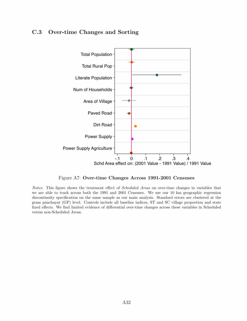
C.3 Over-time Changes and Sorting

Total Population

Total Rural Pop

Literate Population

Num of Households

Area of Village

Paved Road

Dirt Road

Power Supply

Power Supply Agriculture

-.1 0 .1 .2 .3 .4Schd Area effect on: (2001 Value - 1991 Value) / 1991 Value

Figure A7: Over-time Changes Across 1991-2001 Censuses

Notes: This figure shows the treatment effect of Scheduled Areas on over-time changes in variables thatwe are able to track across both the 1991 and 2001 Censuses. We use our 10 km geographic regressiondiscontinuity specification on the same sample as our main analysis. Standard errors are clustered at thegram panchayat (GP) level. Controls include all baseline indices, ST and SC village proportion and statefixed effects. We find limited evidence of differential over-time changes across these variables in Scheduledversus non-Scheduled Areas.

A32

Table A12: Sorting Test

(1) (2) (3) (4) (5)Share ST Share ST Share ST Share ST Share ST

2001 2001 2011 2011 2011Scheduled Areas 0.099*** 0.005*** 0.101*** 0.006*** 0.004***

(0.006) (0.001) (0.006) (0.001) (0.001)ST Share, 1991 0.941*** 0.412***

(0.002) (0.023)ST Share, 2001 0.953*** 0.557***

(0.002) (0.023)Control Mean 0.474 0.474 0.480 0.480 0.480# GPs 13338 13338 13338 13338 13338# Villages 32641 32641 32641 32641 32641

Notes: *p < 0.1, **p < 0.05, ***p < 0.01. This table shows the treatment effect of Scheduled Areas

on the ST share of the population in different Census years and controlling for different preceding

years. We use our 10 km geographic regression discontinuity specification on the same sample as our

main analysis. Standard errors are clustered at the gram panchayat (GP) level. Controls include

state fixed effects, all 14 baseline indices, and a geographic control function. The table shows that

once we account for ST population shares in 1991 and 2001, there remain no substantive differences

in ST population across treated and control areas in 2011. We therefore control for 1991 and 2001

ST population shares in all of our reported analysis in the revised manuscript.

A33

C.4 Density of Distance to Threshold

Figure A8: Cumulative Density of Distance to the Threshold

Notes: This figure plots the density of observations at different kilometer distances to the geographic regres-sion discontinuity threshold. We include indicators for the bandwidth used in the paper (10 kilometers) andthe mean and median distances to the threshold for reference.

A34

D Additional Results and Robustness of Main Effects

D.1 OLS Main Results

A naive ordinary least squares model compares Scheduled and non-Scheduled villages with

state fixed effects and village level controls from the 2001 and 1991 Indian Censuses with

the following specification:

yvgs = as + γScheduled Areavgs + Z′

vgsφ+ εvgs (2)

Table A13: The Effect of Scheduled Areas on NREGS (OLS)


Panel A: JobcardsScheduled Areas 0.020** 0.596*** -0.436*** -0.347***


Panel B: Households WorkedScheduled Areas 0.119*** 0.627*** -0.337*** -0.221***


Panel C: WorkdaysScheduled Areas 0.140*** 0.794*** -0.524*** -0.264***


Notes: *p < 0.1, **p < 0.05, ***p < 0.01. Standard errors are clustered at the gram panchayat (GP)

level. Controls include all baseline indices, ST and SC village proportion and state fixed effects.

A35

D.2 Functional Form and Bandwidth-.1

-.05

0.0

5

0 10 20 30 40 50

Jobcards

.1.2

.3.4

.5

0 10 20 30 40 50

Jobcards, ST

-.3-.2

-.10

.1

0 10 20 30 40 50

Jobcards, SC

-.25-

.2-.1

5-.1

-.05

0

0 10 20 30 40 50

Jobcards, non-SC/ST

-.05

0.0

5.1

0 10 20 30 40 50

Worked HH

.1.2

.3.4

.5

0 10 20 30 40 50

Worked HH, ST

-.2-.1

0.1

.2

0 10 20 30 40 50

Worked HH, SC

-.2-.1

5-.1

-.05

0

0 10 20 30 40 50

Worked HH, non-SC/ST

-.1-.0

50

.05

.1.1

5

0 10 20 30 40 50

Workdays

0.2

.4.6

.8

0 10 20 30 40 50

Workdays, ST-.4

-.20

.2.4

0 10 20 30 40 50

Workdays, SC

-.3-.2

-.10

.1

0 10 20 30 40 50

Workdays, Other

Trea

tmen

t Effe

ct

Bandwidth (in Kilometers)

Linear Quadratic Cubic Quartic

Figure A9: RD Robustness by Bandwidth and Functional Form

Notes: Plots results in Table 2 by control function and bandwidth with 90% confidence intervals.

A36

D.3 Controlling for Number of Matched Villages within a GP

One concern with the approach taken for the NREGS analysis could be that the number

of villages within each gram panchayat differs between Scheduled and non-Scheduled Areas.

Were this the case, then assigning all villages within a gram panchayat the same values could

bias our comparison of Scheduled and non-Scheduled Areas. To account for this possibility,

we show in table A14 that our main results are robust, both substantively and statistically,

when we include fixed effects for the number of gram panchayat villages.

Table A14: Main NREGS Results with Num Matched Villages per GP FE


Panel A: JobcardsScheduled Areas -0.007 0.199*** -0.037 -0.106***


Panel B: Households WorkedScheduled Areas -0.001 0.193*** -0.016 -0.094***


Panel C: WorkdaysScheduled Areas -0.020 0.230*** 0.010 -0.133***



level. Controls include all baseline indices, ST and SC village proportion, state and number of GP

villages fixed effects, and a flexible function in village centroid longitudes (x) and latitudes (y) of the

form: x+ y + x2 + y2 + xy + x3 + y3 + x2y + xy2.

A37

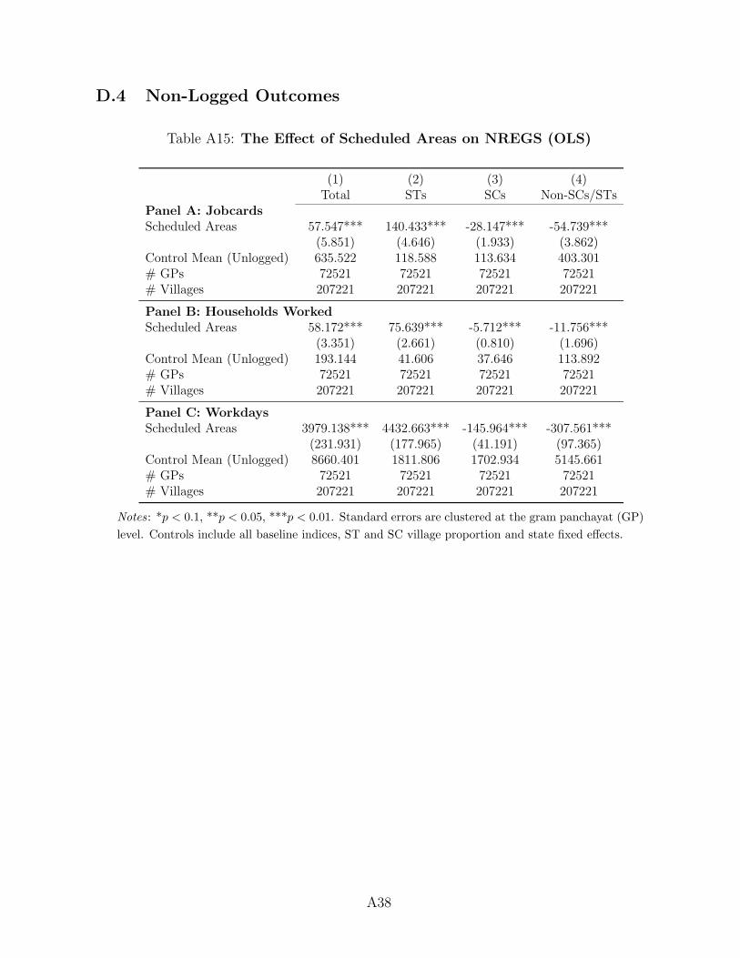
D.4 Non-Logged Outcomes

Table A15: The Effect of Scheduled Areas on NREGS (OLS)


Panel A: JobcardsScheduled Areas 57.547*** 140.433*** -28.147*** -54.739***


Panel B: Households WorkedScheduled Areas 58.172*** 75.639*** -5.712*** -11.756***


Panel C: WorkdaysScheduled Areas 3979.138*** 4432.663*** -145.964*** -307.561***



level. Controls include all baseline indices, ST and SC village proportion and state fixed effects.

A38

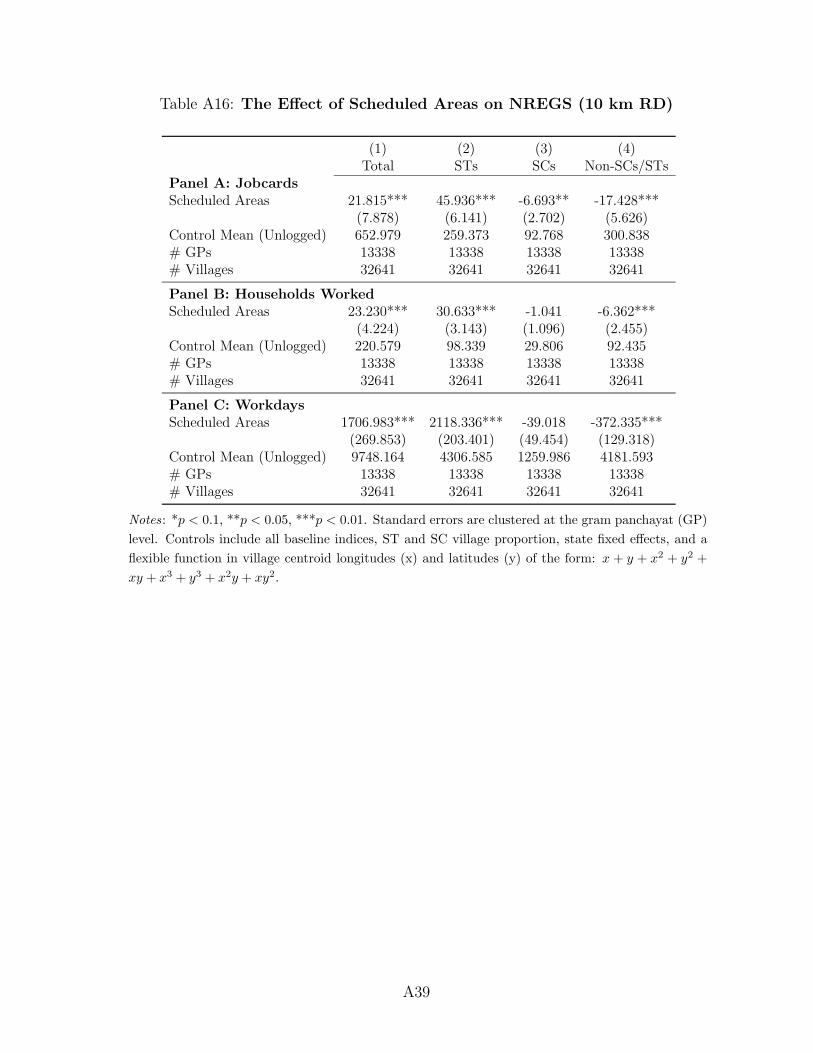
Table A16: The Effect of Scheduled Areas on NREGS (10 km RD)


Panel A: JobcardsScheduled Areas 21.815*** 45.936*** -6.693** -17.428***


Panel B: Households WorkedScheduled Areas 23.230*** 30.633*** -1.041 -6.362***


Panel C: WorkdaysScheduled Areas 1706.983*** 2118.336*** -39.018 -372.335***



level. Controls include all baseline indices, ST and SC village proportion, state fixed effects, and a

flexible function in village centroid longitudes (x) and latitudes (y) of the form: x + y + x2 + y2 +

xy + x3 + y3 + x2y + xy2.

A39

Figure

A10:Levera

gePlots,Logged

and

non-L

ogged

Outcomes

Notes:

This

figu

redisplaysleverage

versussquared

residual

plots

forloggedan

dnon

-logged

outcom

es.Thefigu

reshow

sthatresidualsshrinkunder

logged

outcom

esrelativeto

non

-loggedoutcom

es.Consistentwiththeseresults,

weob

serveim

proved

goodnessoffitandgreaterR

2forou

rmodels

that

use

loggedoutcom

es.

A40

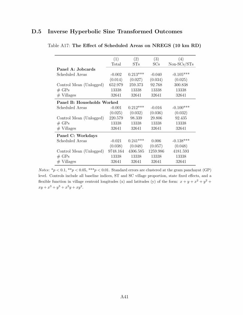
D.5 Inverse Hyperbolic Sine Transformed Outcomes

Table A17: The Effect of Scheduled Areas on NREGS (10 km RD)











xy + x3 + y3 + x2y + xy2.

A41

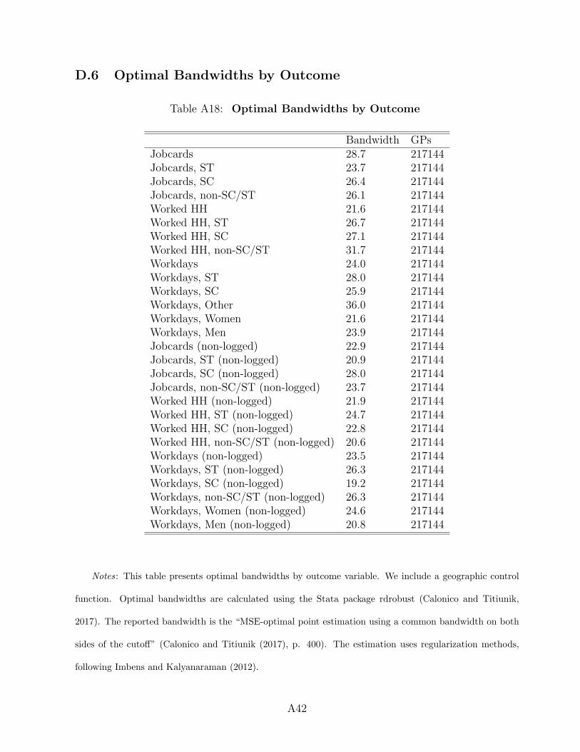
D.6 Optimal Bandwidths by Outcome

Table A18: Optimal Bandwidths by Outcome

Bandwidth GPsJobcards 28.7 217144Jobcards, ST 23.7 217144Jobcards, SC 26.4 217144Jobcards, non-SC/ST 26.1 217144Worked HH 21.6 217144Worked HH, ST 26.7 217144Worked HH, SC 27.1 217144Worked HH, non-SC/ST 31.7 217144Workdays 24.0 217144Workdays, ST 28.0 217144Workdays, SC 25.9 217144Workdays, Other 36.0 217144Workdays, Women 21.6 217144Workdays, Men 23.9 217144Jobcards (non-logged) 22.9 217144Jobcards, ST (non-logged) 20.9 217144Jobcards, SC (non-logged) 28.0 217144Jobcards, non-SC/ST (non-logged) 23.7 217144Worked HH (non-logged) 21.9 217144Worked HH, ST (non-logged) 24.7 217144Worked HH, SC (non-logged) 22.8 217144Worked HH, non-SC/ST (non-logged) 20.6 217144Workdays (non-logged) 23.5 217144Workdays, ST (non-logged) 26.3 217144Workdays, SC (non-logged) 19.2 217144Workdays, non-SC/ST (non-logged) 26.3 217144Workdays, Women (non-logged) 24.6 217144Workdays, Men (non-logged) 20.8 217144

Notes: This table presents optimal bandwidths by outcome variable. We include a geographic control

function. Optimal bandwidths are calculated using the Stata package rdrobust (Calonico and Titiunik,

2017). The reported bandwidth is the “MSE-optimal point estimation using a common bandwidth on both

sides of the cutoff” (Calonico and Titiunik (2017), p. 400). The estimation uses regularization methods,

following Imbens and Kalyanaraman (2012).

A42

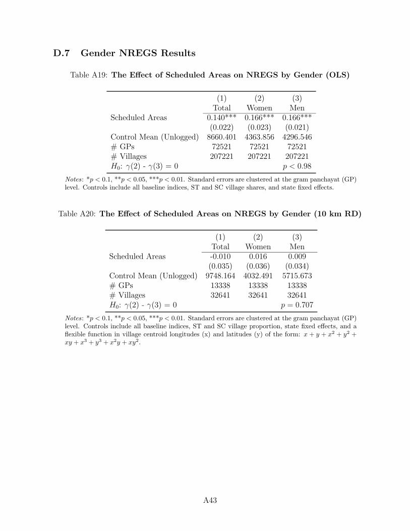
D.7 Gender NREGS Results

Table A19: The Effect of Scheduled Areas on NREGS by Gender (OLS)


Scheduled Areas 0.140*** 0.166*** 0.166***(0.022) (0.023) (0.021)

Control Mean (Unlogged) 8660.401 4363.856 4296.546# GPs 72521 72521 72521# Villages 207221 207221 207221H0: γ(2) - γ(3) = 0 p < 0.98

Notes: *p < 0.1, **p < 0.05, ***p < 0.01. Standard errors are clustered at the gram panchayat (GP)level. Controls include all baseline indices, ST and SC village shares, and state fixed effects.

Table A20: The Effect of Scheduled Areas on NREGS by Gender (10 km RD)


Scheduled Areas -0.010 0.016 0.009(0.035) (0.036) (0.034)

Control Mean (Unlogged) 9748.164 4032.491 5715.673# GPs 13338 13338 13338# Villages 32641 32641 32641H0: γ(2) - γ(3) = 0 p = 0.707

Notes: *p < 0.1, **p < 0.05, ***p < 0.01. Standard errors are clustered at the gram panchayat (GP)level. Controls include all baseline indices, ST and SC village proportion, state fixed effects, and aflexible function in village centroid longitudes (x) and latitudes (y) of the form: x + y + x2 + y2 +xy + x3 + y3 + x2y + xy2.

A43

-.1-.0

50

.05

.1.1

5

0 10 20 30 40 50

Workdays, Women

-.1-.0

50

.05

.1.1

5

0 10 20 30 40 50

Workdays, Men

Trea

tmen

t Effe

ct

Bandwidth (in Kilometers)


Figure A11: RD Results by Bandwidth

Notes: We plot the effect of Scheduled Areas on workdays for women and men at different kilometer band-

widths and with 90% confidence intervals.

A44

D.8 PMGSY Effects: RD Sample Only

Figure A12: The Effect of the introduction of PESA election on PMGSY Roads(RD Sample)

0.0

5.1

.15

Roa

d Sa

nctio

ned

(resi

dual

ized

)


0.0

5.1

.15

Roa

d C

ompl

eted

(res

idua

lized

)


Non-Scheduled Areas Scheduled Areas

Notes : This figure plots binned means of completed PMGSY roads by Scheduled Area statuson a dataset of villages in our RD sample that is residualized for village fixed effects.

A45

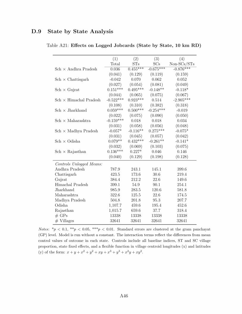
D.9 State by State Analysis

Table A21: Effects on Logged Jobcards (State by State, 10 km RD)


Sch × Andhra Pradesh 0.036 0.455*** -0.675*** -0.876***(0.041) (0.129) (0.119) (0.159)

Sch × Chattisgarh -0.042 0.070 0.062 0.052(0.027) (0.054) (0.081) (0.049)

Sch × Gujrat 0.151*** 0.495*** -0.148** -0.118*(0.044) (0.065) (0.075) (0.067)

Sch × Himachal Pradesh -0.522*** 0.923*** 0.514 -2.905***(0.108) (0.310) (0.382) (0.318)

Sch × Jharkhand 0.059*** 0.500*** -0.254*** -0.019(0.022) (0.075) (0.090) (0.050)

Sch × Maharashtra -0.159*** 0.018 0.018 0.034(0.031) (0.058) (0.056) (0.048)

Sch × Madhya Pradesh -0.057* -0.116** 0.275*** -0.075*(0.031) (0.045) (0.057) (0.042)

Sch × Odisha 0.079** 0.432*** -0.261** -0.141*(0.032) (0.069) (0.103) (0.075)

Sch × Rajasthan 0.136*** 0.227* 0.046 0.146(0.040) (0.129) (0.198) (0.128)

Controls Unlogged Means:Andhra Pradesh 787.9 243.1 145.1 399.6Chattisgarh 423.5 173.6 30.6 219.4Gujrat 384.4 212.2 22.6 149.6Himachal Pradesh 399.1 54.9 90.1 254.1Jharkhand 985.9 283.5 120.6 581.8Maharashtra 322.6 125.5 22.6 174.5Madhya Pradesh 504.8 201.8 95.3 207.7Odisha 1,107.7 459.6 195.4 452.6Rajasthan 1,015.7 659.6 37.7 318.4# GPs 13338 13338 13338 13338# Villages 32641 32641 32641 32641

Notes: *p < 0.1, **p < 0.05, ***p < 0.01. Standard errors are clustered at the gram panchayat

(GP) level. Model is run without a constant. The interaction terms reflect the differences from mean

control values of outcome in each state. Controls include all baseline indices, ST and SC village

proportion, state fixed effects, and a flexible function in village centroid longitudes (x) and latitudes

(y) of the form: x+ y + x2 + y2 + xy + x3 + y3 + x2y + xy2.

A46

Table A22: Effects on Logged Worked HH (State by State, 10 km RD)


Sch × Andhra Pradesh 0.148** 0.473*** -0.560*** -0.731***(0.059) (0.121) (0.139) (0.169)

Sch × Chattisgarh -0.032 0.161** 0.063 0.049(0.049) (0.063) (0.087) (0.071)

Sch × Gujrat 0.013 0.140 -0.139** -0.106(0.096) (0.087) (0.054) (0.082)

Sch × Himachal Pradesh -0.797*** 1.002*** 0.042 -3.115***(0.165) (0.335) (0.436) (0.332)

Sch × Jharkhand -0.035 0.521*** -0.447*** -0.196***(0.051) (0.100) (0.100) (0.069)

Sch × Maharashtra -0.305*** -0.152*** -0.086** -0.092(0.065) (0.058) (0.042) (0.062)

Sch × Madhya Pradesh -0.017 -0.049 0.344*** -0.086**(0.031) (0.047) (0.057) (0.043)

Sch × Odisha 0.289*** 0.595*** -0.115 0.072(0.052) (0.082) (0.108) (0.107)

Sch × Rajasthan 0.679*** 0.789*** 0.712*** 0.888***(0.077) (0.134) (0.187) (0.157)

Controls Unlogged Means:Andhra Pradesh 336.5 117.1 54.4 165.0Chattisgarh 292.4 120.7 19.2 152.5Gujrat 68.9 38.0 4.0 26.9Himachal Pradesh 243.4 29.1 52.5 161.8Jharkhand 345.1 105.2 41.7 198.2Maharashtra 66.6 28.6 4.9 33.1Madhya Pradesh 189.6 90.3 33.9 65.4Odisha 327.1 160.3 52.9 114.0Rajasthan 427.9 334.8 10.5 82.6# GPs 13338 13338 13338 13338# Villages 32641 32641 32641 32641






A47

Table A23: Effects on Logged Workdays (State by State, 10 km RD)


Sch × Andhra Pradesh 0.257*** 0.648*** -1.146*** -1.032***(0.087) (0.200) (0.265) (0.287)

Sch × Chattisgarh 0.037 0.193** 0.328** 0.183*(0.080) (0.094) (0.159) (0.102)

Sch × Gujrat -0.077 0.353** -0.300** -0.322**(0.159) (0.152) (0.130) (0.155)

Sch × Himachal Pradesh -1.057*** 1.352** 0.020 -4.299***(0.233) (0.557) (0.845) (0.705)

Sch × Jharkhand -0.129* 0.506*** -0.580*** -0.243***(0.070) (0.147) (0.165) (0.090)

Sch × Maharashtra -0.419*** -0.227** -0.170* -0.072(0.110) (0.111) (0.093) (0.115)

Sch × Madhya Pradesh -0.044 -0.101 0.537*** -0.166**(0.049) (0.070) (0.090) (0.068)

Sch × Odisha 0.336*** 0.650*** -0.055 0.088(0.070) (0.115) (0.156) (0.134)

Sch × Rajasthan 1.257*** 1.416*** 1.638*** 1.659***(0.099) (0.193) (0.350) (0.194)

Controls Unlogged Means:Andhra Pradesh 18,880.4 6,895.1 2,758.4 9,226.9Chattisgarh 16,805.7 7,561.1 982.5 8,262.1Gujrat 2,787.2 1,516.3 161.7 1,109.2Himachal Pradesh 13,872.1 1,359.6 2,865.9 9,646.7Jharkhand 15,580.7 4,548.1 1,826.7 9,206.0Maharashtra 2,845.9 1,225.5 211.8 1,408.6Madhya Pradesh 7,601.9 3,655.2 1,321.9 2,624.7Odisha 13,749.2 6,829.8 2,156.7 4,762.7Rajasthan 16,459.8 12,972.7 420.1 3,067.0# GPs 13338 13338 13338 13338# Villages 32641 32641 32641 32641






A48

D.10 Conley Standard Errors

Table A24: Replication of Table 2 Main Effects with Conley SEs (10 km RD)


Panel A: JobcardsScheduled Areas 0.000 0.207*** -0.038 -0.098***

(0.017) (0.037) (0.039) (0.031)

Panel B: Households WorkedScheduled Areas 0.009 0.203*** -0.017 -0.086**

(0.034) (0.042) (0.040) (0.039)

Panel C: WorkdaysScheduled Areas -0.010 0.241*** 0.009 -0.125**

(0.054) (0.065) (0.066) (0.062)

Notes: *p < 0.1, **p < 0.05, ***p < 0.01. We report Conley (1999) standard errors in parentheses.

Controls include all baseline indices, ST and SC village proportion, state fixed effects, and a flexible

function in village centroid longitudes (x) and latitudes (y) of the form: x+ y+ x2 + y2 + xy+ x3 +

y3 + x2y + xy2.

A49

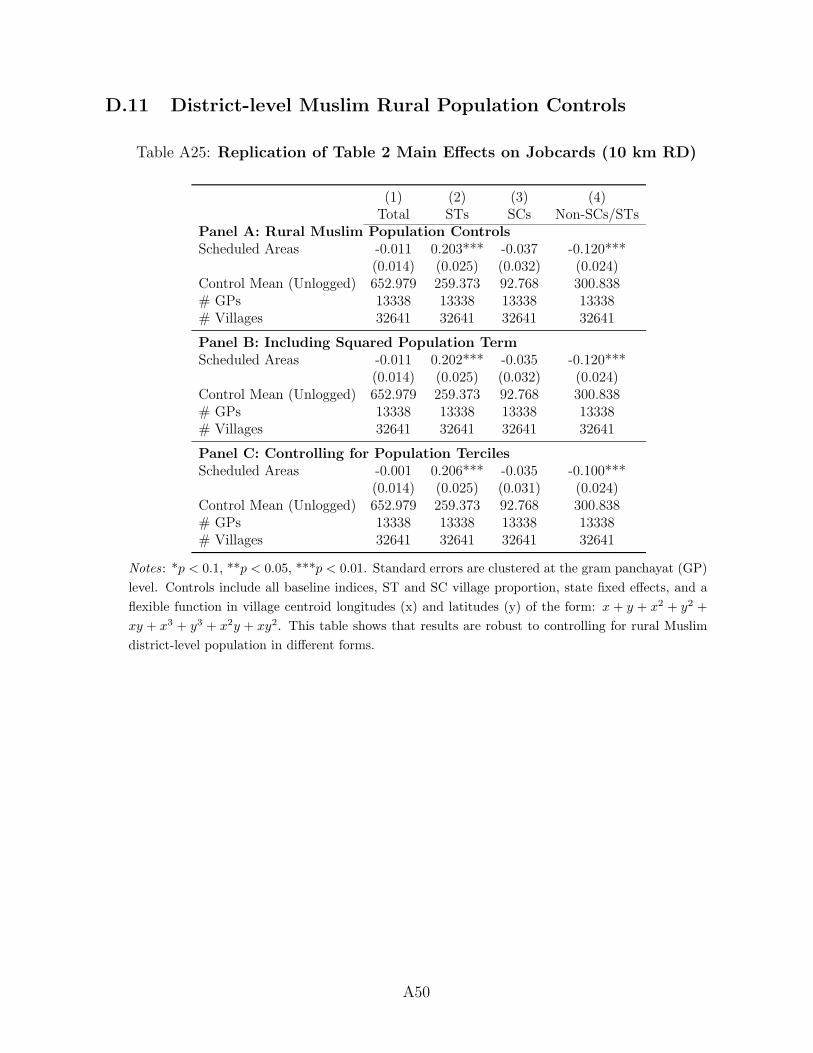
D.11 District-level Muslim Rural Population Controls

Table A25: Replication of Table 2 Main Effects on Jobcards (10 km RD)


Panel A: Rural Muslim Population ControlsScheduled Areas -0.011 0.203*** -0.037 -0.120***


Panel B: Including Squared Population TermScheduled Areas -0.011 0.202*** -0.035 -0.120***


Panel C: Controlling for Population TercilesScheduled Areas -0.001 0.206*** -0.035 -0.100***





xy + x3 + y3 + x2y + xy2. This table shows that results are robust to controlling for rural Muslim

district-level population in different forms.

A50

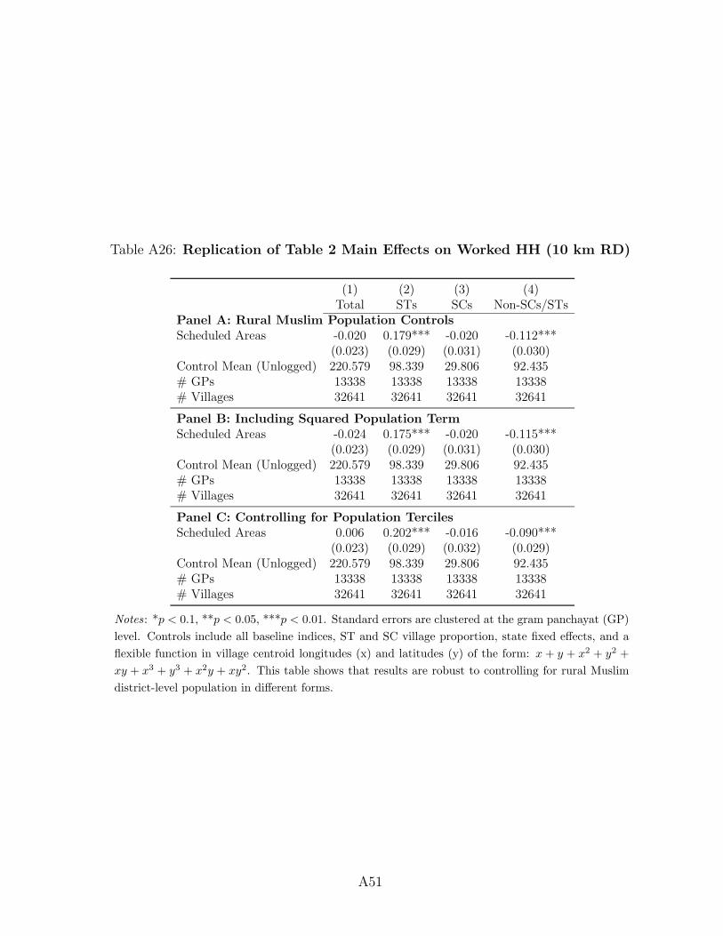
Table A26: Replication of Table 2 Main Effects on Worked HH (10 km RD)




Panel B: Including Squared Population TermScheduled Areas -0.024 0.175*** -0.020 -0.115***


Panel C: Controlling for Population TercilesScheduled Areas 0.006 0.202*** -0.016 -0.090***







A51

Table A27: Replication of Table 2 Main Effects on Workdays (10 km RD)




Panel B: Including Squared Population TermScheduled Areas -0.062* 0.192*** -0.007 -0.172***


Panel C: Controlling for Population TercilesScheduled Areas -0.015 0.237*** 0.010 -0.130***







A52

E Additional Results and Robustness of Electoral Mech-

anism

E.1 PESA Elections

Table A28: The Effect of Scheduled Areas on NREGS by Number of PESA Elec-tions (10 km RD)


Panel A: JobcardsSch Areas × 1 PESA Election 0.062*** 0.505*** -0.260*** -0.015

(0.022) (0.076) (0.090) (0.050)Sch Areas × 2 PESA Elections -0.100*** 0.108** -0.096** -0.123***

(0.021) (0.045) (0.045) (0.044)Sch Areas × 3 PESA Elections 0.028 0.175*** 0.042 -0.109***


Panel B: Worked HHSch Areas × 1 PESA Election -0.030 0.527*** -0.451*** -0.189***

(0.051) (0.100) (0.100) (0.069)Sch Areas × 2 PESA Elections -0.170*** 0.022 -0.141*** -0.176***

(0.043) (0.045) (0.041) (0.052)Sch Areas × 3 PESA Elections 0.095*** 0.201*** 0.144*** -0.022


Panel C: WorkdaysSch Areas × 1 PESA Election -0.122* 0.514*** -0.586*** -0.232***

(0.070) (0.147) (0.165) (0.090)Sch Areas × 2 PESA Elections -0.208*** 0.014 -0.244*** -0.190**

(0.072) (0.081) (0.084) (0.092)Sch Areas × 3 PESA Elections 0.103** 0.269*** 0.264*** -0.071


# GPs 13338 13338 13338 13338# Villages 32641 32641 32641 32641




xy + x3 + y3 + x2y + xy2.

A53

E.2 ST Plurality Information

Table A29 shows the broad coverage of the data in terms of ST plurality status and being

declared a Scheduled Area.

Table A29: Number of Villages (and Gram Panchayats) and ST Share

Panel A: Number of ObservationsScheduled Areas Non-Scheduled Areas

ST Plurality 8,686 (3,786) 8,954 (4,096)ST Non-Plurality 5,580 (3,371) 9,421 (5,358)

Panel B: Average ST ShareScheduled Areas Non-Scheduled Areas

ST Plurality 0.85 0.83ST Non-Plurality 0.16 0.13

A54

Table A30: Treatment Effects by ST Majority (10 km RD)


Panel A: JobcardsScheduled Areas 0.006 0.034 -0.055 -0.074**

(0.018) (0.031) (0.046) (0.036)ST Non-Majority 0.008 0.235*** -0.059 -0.102***

(0.021) (0.039) (0.043) (0.035)Scheduled × ST Non-Majority -0.012 0.373*** 0.037 -0.053


Panel B: Worked HHScheduled Areas 0.007 0.058 0.002 -0.060

(0.028) (0.037) (0.044) (0.040)ST Non-Majority -0.060 0.115** -0.066 -0.172***

(0.037) (0.045) (0.042) (0.043)Scheduled × ST Non-Majority 0.005 0.314*** -0.039 -0.055


Panel C: WorkdaysScheduled Areas 0.011 0.051 0.056 -0.074

(0.044) (0.054) (0.074) (0.061)ST Non-Majority -0.083 0.265*** -0.133* -0.270***

(0.062) (0.073) (0.075) (0.069)Scheduled × ST Non-Majority -0.045 0.408*** -0.101 -0.109


# GPs 13338 13338 13338 13338# Villages 32641 32641 32641 32641




xy+ x3 + y3 + x2y+ xy2. ST Non-Majority defined as less than 50% of the village population share.

A55

E.3 AC-level Reservations

Table A31: Controlling for ST Quota in Assembly Constituency (10 km RD)

(1) (2) (3) (4)Total ST SC Non-SC/ST

Panel A: Job CardsScheduled Areas -0.020 0.136*** -0.031 -0.087***

(0.014) (0.025) (0.032) (0.024)AC Reserved, ST 0.194*** 0.673*** -0.065* -0.109***



(0.023) (0.030) (0.032) (0.030)AC Reserved, ST 0.413*** 0.719*** 0.069** 0.067*


Panel C: WorkdaysScheduled Areas -0.070** 0.129*** -0.002 -0.139***

(0.035) (0.046) (0.054) (0.046)AC Reserved, ST 0.582*** 1.071*** 0.111* 0.135***





xy + x3 + y3 + x2y + xy2.

A56

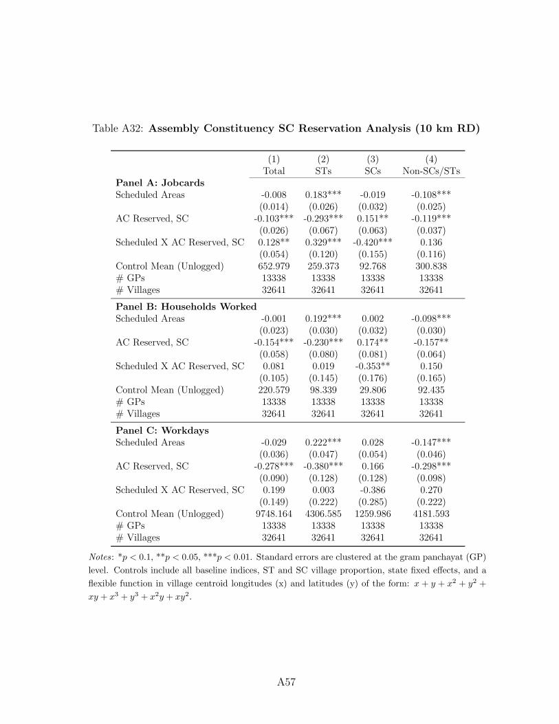
Table A32: Assembly Constituency SC Reservation Analysis (10 km RD)



(0.014) (0.026) (0.032) (0.025)AC Reserved, SC -0.103*** -0.293*** 0.151** -0.119***

(0.026) (0.067) (0.063) (0.037)Scheduled X AC Reserved, SC 0.128** 0.329*** -0.420*** 0.136


Panel B: Households WorkedScheduled Areas -0.001 0.192*** 0.002 -0.098***

(0.023) (0.030) (0.032) (0.030)AC Reserved, SC -0.154*** -0.230*** 0.174** -0.157**

(0.058) (0.080) (0.081) (0.064)Scheduled X AC Reserved, SC 0.081 0.019 -0.353** 0.150



(0.036) (0.047) (0.054) (0.046)AC Reserved, SC -0.278*** -0.380*** 0.166 -0.298***

(0.090) (0.128) (0.128) (0.098)Scheduled X AC Reserved, SC 0.199 0.003 -0.386 0.270





xy + x3 + y3 + x2y + xy2.

A57

E.4 Robustness of Employment Effects: Census 2011-.0

50

.05

.1Tr

eatm

ent E

ffect

0 10 20 30 40 50

Bandwidth (in KMs)

Total Workers

-.05

0.0

5.1

.15

Trea

tmen

t Effe

ct

0 10 20 30 40 50

Bandwidth (in KMs)

Total Workers - Women

-.04-.

020

.02.

04.0

6Tr

eatm

ent E

ffect

0 10 20 30 40 50

Bandwidth (in KMs)

Total Workers - Men

-.05

0.0

5.1

Trea

tmen

t Effe

ct

0 10 20 30 40 50

Bandwidth (in KMs)

Main Workers-.0

50

.05

.1.1

5Tr

eatm

ent E

ffect

0 10 20 30 40 50

Bandwidth (in KMs)

Main Workers - Women

-.05

0.0

5.1

Trea

tmen

t Effe

ct

0 10 20 30 40 50

Bandwidth (in KMs)

Main Workers - Men

-.1-.0

50

.05

.1.1

5Tr

eatm

ent E

ffect

0 10 20 30 40 50

Bandwidth (in KMs)

Marginal Workers

-.10

.1.2

Trea

tmen

t Effe

ct

0 10 20 30 40 50

Bandwidth (in KMs)

Marginal Workers - Women

-.1-.0

50

.05

.1Tr

eatm

ent E

ffect

0 10 20 30 40 50

Bandwidth (in KMs)

Marginal Workers - Men


Figure A13: The Effect of Scheduled Areas on Employment (Census 2011). Thisfigure plots results from a Geographic RD model with various control functions in latitudesand longitudes, as well as bandwidth. Standard errors are clustered at the gram panchayat(GP) level. Controls include all baseline indices, ST and SC village proportion and statefixed effects. Main workers are those employed more than 183 years in the previous year,while Marginal Workers are those employed less than 183 days.

A58

E.5 Effects on Public Goods: 2011 Census

E.5.1 Controlling for Baseline Values

Figure A14: The Effect of Scheduled Areas on Public Goods (Census 2011).

Ove

rall P

ublic

Goo

ds In

dex

Road

s In

dex

Natio

nal H

ighw

ay (Y

/N)

Stat

e Hi

ghwa

y (Y

/N)

Maj

or D

istric

t Roa

d (Y

/N)

Oth

er D

istric

t Roa

d (Y

/N)

All w

eath

er ro

ad (Y

/N)

Gra

vel R

oad

(Y/N

)

Wat

er In

dex

Hand

pum

p (Y

/N)

Tap

Wat

er T

reat

ed (Y

/N)

Tank

, Pon

d, L

ake

(Y/N

)

Cove

red

Wel

l (Y/

N)

Unco

vere

d W

ell (

Y/N)

Irrig

atio

n In

dex

Tube

well/B

oreh

ole

(Y/N

)

Rive

r/Can

al (Y

/N)

Elec

tricit

y In

dex

Elec

tricit

y fo

r Agr

icultu

re U

se (Y

/N)

Elec

tricit

y fo

r Dom

estic

Use

(Y/N

)

Elec

tricit

y fo

r Com

mer

cial U

se (Y

/N) Co

mm

unica

tions

Inde

x

Post

Offi

ce (Y

/N)

Post

and

Tel

egra

ph O

ffice

(Y/N

)

Tele

phon

e (Y

/N)

Mob

ile c

over

age

(Y/N

)

Educ

atio

n In

dex

Prim

ary

Scho

ol (Y

/N)

Mid

dle

Scho

ol (Y

/N)

Seco

ndar

y Sc

hool

(Y/N

)

Seni

or S

econ

dary

Sch

ool (

Y/N)

Colle

ge (Y

/N)

-.1-.0

50

.05

.1Tr

eatm

ent E

ffect

All w

eath

er ro

ad (Y

/N)

Hand

pum

p (Y

/N)

Tap

Wat

er T

reat

ed (Y

/N)

Tank

, Pon

d, L

ake

(Y/N

)

Tube

well/B

oreh

ole

(Y/N

)

Rive

r/Can

al (Y

/N)

Elec

tricit

y fo

r Agr

icultu

re U

se (Y

/N)

Elec

tricit

y fo

r Dom

estic

Use

(Y/N

)

Post

Offi

ce (Y

/N)

Post

and

Tel

egra

ph O

ffice

(Y/N

)

Tele

phon

e (Y

/N)

Prim

ary

Scho

ol (Y

/N)

Mid

dle

Scho

ol (Y

/N)

Seco

ndar

y Sc

hool

(Y/N

)

Seni

or S

econ

dary

Sch

ool (

Y/N)

Colle

ge (Y

/N)

-.4-.3

-.2-.1

0.1

Trea

tmen

t Effe

ct

Notes : Bottom panel replicates top panel results controlling for 2001 baseline values (subjectto data availability).

A59

0.0

1.02

.03.

04.0

5Tr

eatm

ent E

ffect

0 10 20 30 40 50

Bandwidth (in KMs)

Overall Public Goods Index

-.02

0.0

2.0

4.0

6Tr

eatm

ent E

ffect

0 10 20 30 40 50

Bandwidth (in KMs)

Roads Index

-.06-.

04-.0

20

.02.

04Tr

eatm

ent E

ffect

0 10 20 30 40 50

Bandwidth (in KMs)

National Highway (Y/N)

-.05

0.0

5.1

Trea

tmen

t Effe

ct

0 10 20 30 40 50

Bandwidth (in KMs)

State Highway (Y/N)

-.1-.0

50

.05

.1Tr

eatm

ent E

ffect

0 10 20 30 40 50

Bandwidth (in KMs)

Major District Road (Y/N)

-.05

0.0

5.1

Trea

tmen

t Effe

ct

0 10 20 30 40 50

Bandwidth (in KMs)

Other District Road (Y/N)

-.05

0.0

5.1

Trea

tmen

t Effe

ct

0 10 20 30 40 50

Bandwidth (in KMs)

All weather road (Y/N)

0.0

5.1

Trea

tmen

t Effe

ct

0 10 20 30 40 50

Bandwidth (in KMs)

Gravel Road (Y/N)

-.02

0.0

2.0

4Tr

eatm

ent E

ffect

0 10 20 30 40 50

Bandwidth (in KMs)

Water Index

-.05

0.0

5.1

Trea

tmen

t Effe

ct

0 10 20 30 40 50

Bandwidth (in KMs)

Handpump (Y/N)

-.05

0.0

5Tr

eatm

ent E

ffect

0 10 20 30 40 50

Bandwidth (in KMs)

Tap Water Treated (Y/N)

-.1-.0

50

.05

.1Tr

eatm

ent E

ffect

0 10 20 30 40 50

Bandwidth (in KMs)

Tank, Pond, Lake (Y/N)

-.05

0.0

5Tr

eatm

ent E

ffect

0 10 20 30 40 50

Bandwidth (in KMs)

Covered Well (Y/N)

-.05

0.0

5.1

Trea

tmen

t Effe

ct

0 10 20 30 40 50

Bandwidth (in KMs)

Uncovered Well (Y/N)

-.08-.

06-.0

4-.02

0.0

2Tr

eatm

ent E

ffect

0 10 20 30 40 50

Bandwidth (in KMs)

Irrigation Index

-.05

0.0

5.1

Trea

tmen

t Effe

ct

0 10 20 30 40 50

Bandwidth (in KMs)

Tubewell/Borehole (Y/N)

-.15

-.1-.0

50

.05

Trea

tmen

t Effe

ct

0 10 20 30 40 50

Bandwidth (in KMs)

River/Canal (Y/N)

-.06-

.04-

.02

0.0

2Tr

eatm

ent E

ffect

0 10 20 30 40 50

Bandwidth (in KMs)

Electricity Index

-.08-.

06-.0

4-.02

0.0

2Tr

eatm

ent E

ffect

0 10 20 30 40 50

Bandwidth (in KMs)

Electricity for Agriculture Use (Y/N)

-.06-.

04-.0

20.0

2.04

Trea

tmen

t Effe

ct

0 10 20 30 40 50

Bandwidth (in KMs)

Electricity for Domestic Use (Y/N)

-.1-.0

50

.05

Trea

tmen

t Effe

ct

0 10 20 30 40 50

Bandwidth (in KMs)

Electricity for Commercial Use (Y/N)

.02

.04

.06

.08

.1Tr

eatm

ent E

ffect

0 10 20 30 40 50

Bandwidth (in KMs)

Communications Index

-.05

0.0

5.1

Trea

tmen

t Effe

ct

0 10 20 30 40 50

Bandwidth (in KMs)

Post Office (Y/N)

-.04-.

020

.02.

04.0

6Tr

eatm

ent E

ffect

0 10 20 30 40 50

Bandwidth (in KMs)

Post and Telegraph Office (Y/N)

0.0

5.1

.15

Trea

tmen

t Effe

ct

0 10 20 30 40 50

Bandwidth (in KMs)

Telephone (Y/N)

0.0

5.1

.15

.2Tr

eatm

ent E

ffect

0 10 20 30 40 50

Bandwidth (in KMs)

Mobile coverage (Y/N)

.005

.01

.015

.02

Trea

tmen

t Effe

ct

0 10 20 30 40 50

Bandwidth (in KMs)

Education Index

-.01

0.0

1.0

2.0

3Tr

eatm

ent E

ffect

0 10 20 30 40 50

Bandwidth (in KMs)

Primary School (Y/N)

0.0

1.0

2.0

3.0

4Tr

eatm

ent E

ffect

0 10 20 30 40 50

Bandwidth (in KMs)

Middle School (Y/N)

0.0

1.0

2.0

3Tr

eatm

ent E

ffect

0 10 20 30 40 50

Bandwidth (in KMs)

Secondary School (Y/N)

.005

.01.

015.

02.0

25Tr

eatm

ent E

ffect

0 10 20 30 40 50

Bandwidth (in KMs)

Senior Secondary School (Y/N)

-.002

0.0

02.0

04.0

06Tr

eatm

ent E

ffect

0 10 20 30 40 50

Bandwidth (in KMs)

College (Y/N)


Figure A15: The Effect of Scheduled Areas on Public Goods (Census 2011). Thisfigure plots results from a Geographic RD model with a cubic control function in latitudesand longitudes, and a 10 km bandwidth as discussed in the text. Standard errors are clusteredat the gram panchayat (GP) level. Controls include all baseline indices, ST and SC villageproportion and state fixed effects.

A60

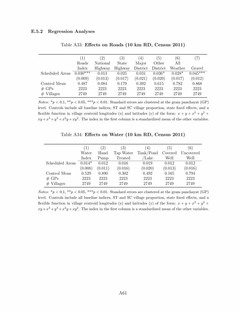
E.5.2 Regression Analyses

Table A33: Effects on Roads (10 km RD, Census 2011)

(1) (2) (3) (4) (5) (6) (7)Roads National State Major Other AllIndex Highway Highway District District Weather Gravel

Scheduled Areas 0.030*** 0.013 0.025 0.031 0.036* 0.028* 0.045***(0.009) (0.013) (0.017) (0.021) (0.020) (0.017) (0.012)

Control Mean 0.487 0.084 0.179 0.392 0.615 0.782 0.868# GPs 2223 2223 2223 2223 2223 2223 2223# Villages 2749 2749 2749 2749 2749 2749 2749




xy+x3+y3+x2y+xy2. The index in the first column is a standardized mean of the other variables.

Table A34: Effects on Water (10 km RD, Census 2011)

(1) (2) (3) (4) (5) (6)Water Hand Tap Water Tank/Pond Covered UncoveredIndex Pump Treated /Lake Well Well

Scheduled Areas 0.014* 0.012 0.016 0.019 0.012 0.012(0.008) (0.011) (0.016) (0.020) (0.013) (0.016)

Control Mean 0.529 0.890 0.302 0.492 0.165 0.794# GPs 2223 2223 2223 2223 2223 2223# Villages 2749 2749 2749 2749 2749 2749





A61

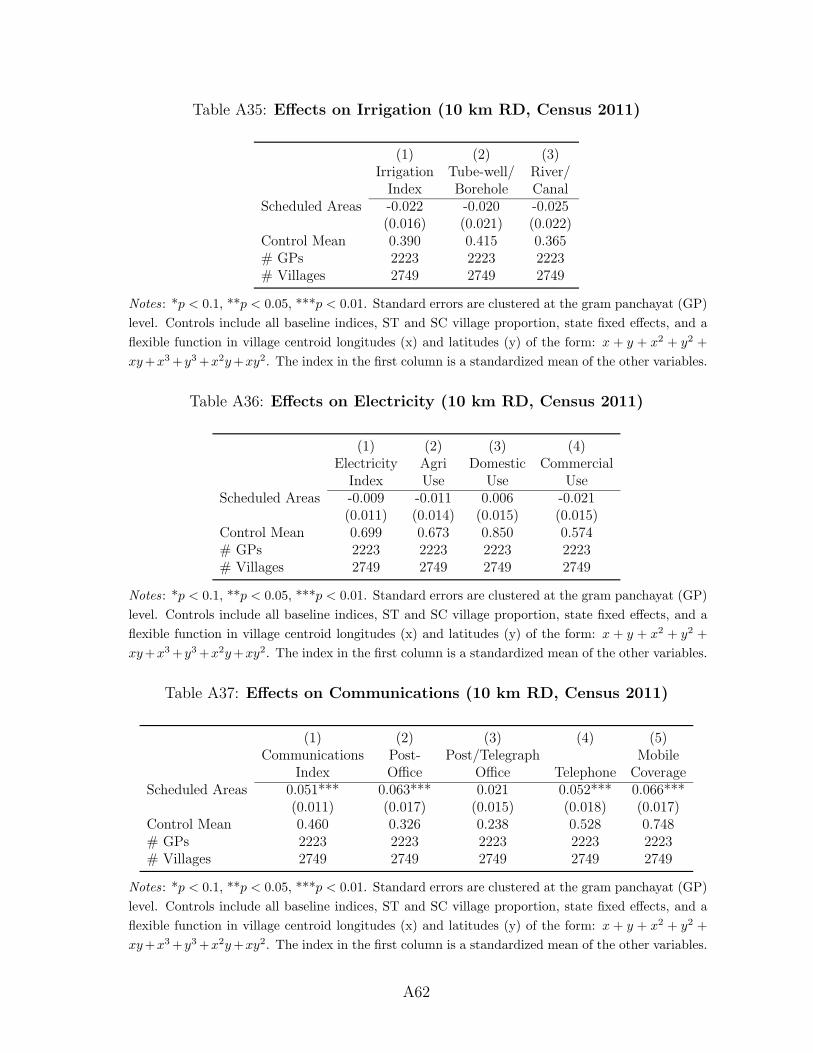
Table A35: Effects on Irrigation (10 km RD, Census 2011)

(1) (2) (3)Irrigation Tube-well/ River/Index Borehole Canal

Scheduled Areas -0.022 -0.020 -0.025(0.016) (0.021) (0.022)

Control Mean 0.390 0.415 0.365# GPs 2223 2223 2223# Villages 2749 2749 2749





Table A36: Effects on Electricity (10 km RD, Census 2011)

(1) (2) (3) (4)Electricity Agri Domestic Commercial

Index Use Use UseScheduled Areas -0.009 -0.011 0.006 -0.021

(0.011) (0.014) (0.015) (0.015)Control Mean 0.699 0.673 0.850 0.574# GPs 2223 2223 2223 2223# Villages 2749 2749 2749 2749





Table A37: Effects on Communications (10 km RD, Census 2011)

(1) (2) (3) (4) (5)Communications Post- Post/Telegraph Mobile

Index Office Office Telephone CoverageScheduled Areas 0.051*** 0.063*** 0.021 0.052*** 0.066***

(0.011) (0.017) (0.015) (0.018) (0.017)Control Mean 0.460 0.326 0.238 0.528 0.748# GPs 2223 2223 2223 2223 2223# Villages 2749 2749 2749 2749 2749





A62

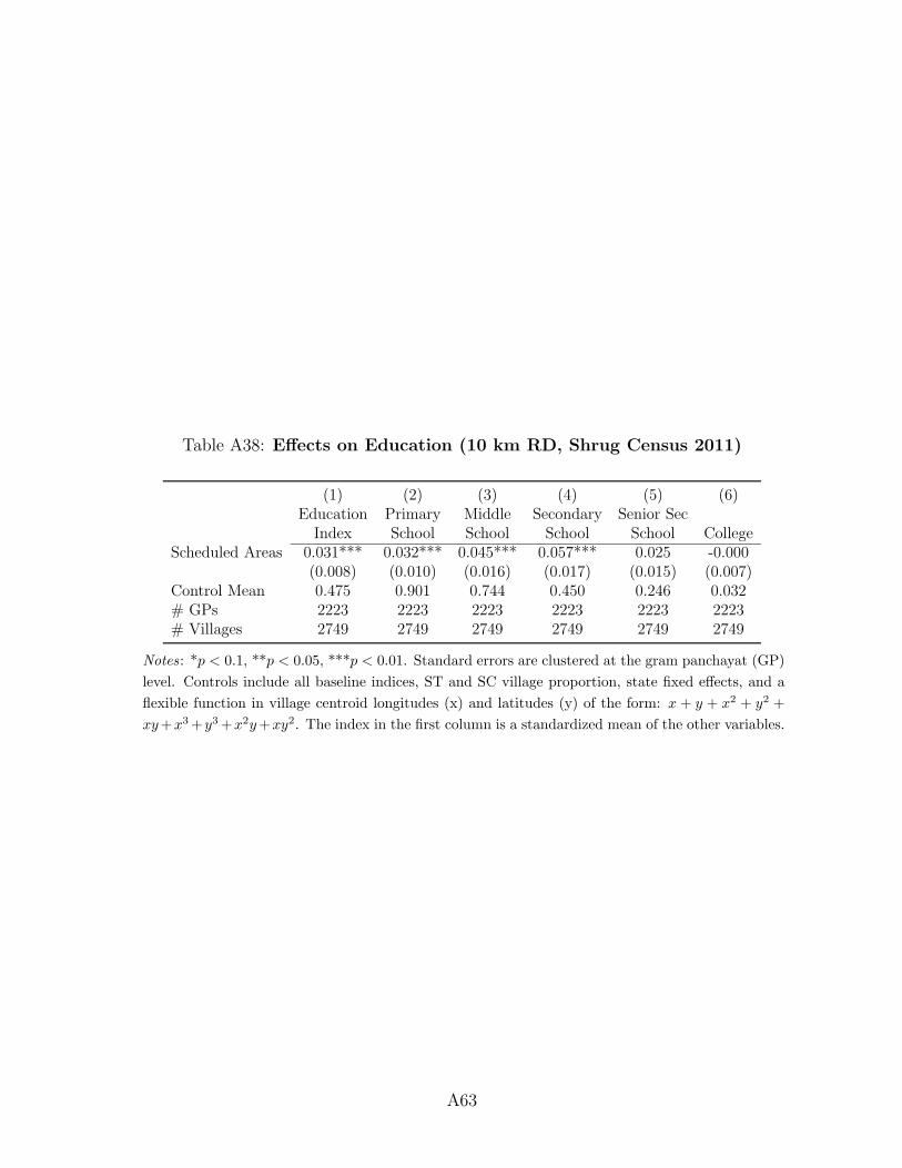
Table A38: Effects on Education (10 km RD, Shrug Census 2011)

(1) (2) (3) (4) (5) (6)Education Primary Middle Secondary Senior SecIndex School School School School College

Scheduled Areas 0.031*** 0.032*** 0.045*** 0.057*** 0.025 -0.000(0.008) (0.010) (0.016) (0.017) (0.015) (0.007)

Control Mean 0.475 0.901 0.744 0.450 0.246 0.032# GPs 2223 2223 2223 2223 2223 2223# Villages 2749 2749 2749 2749 2749 2749





A63

F Alternative Explanations

F.1 Data Manipulation and Collusion

One concern with the results is that that politicians can steal funds earmarked for NREGS

by convincing bureaucrats to report workdays for “ghost workers” who only exist on paper

Bhatia and Dreze (2006). Importantly, the concern for the present paper is that this ten-

dency might exist differentially more for Scheduled Areas. One validated way to measure

manipulation of official data is to consider the distribution of digits in that data. The idea

is that the distribution in naturally-occurring data should follow certain patterns, such as

the well known Benford’s law. These procedures have been adopted to study, for instance,

the presence of fraud and electoral manipulation (Beber and Scacco (2012)).

For our purposes, what matters less is whether there exists fraud in NREGS data – many

accounts say that there is – but, whether fraud is more or less likely to exist in Scheduled

Areas. Thus, we focus not on how far the official data reported is from the “correct”

distribution of numbers, but rather on whether the distribution of digits varies significantly

between Scheduled and non-Scheduled Areas. This approach is particularly desirable because

detecting data manipulation does not demand that we rely on further human-generated audit

data.

To conduct our analysis, we consider if the deposits data in NREGS is more likely to

end with a 0 in Scheduled Areas than in non-Scheduled Areas.40 Deposits end in 0 in

approximately 21% of official data in non-Scheduled Areas, but we do not find that this

percentage differs across non-Scheduled and Scheduled Areas, allaying potential concerns

about differential data manipulation.

As a secondary test, in Appendix Table A40, we evaluate whether the ratio of workdays

to deposits varies by Scheduled Areas (column 1). We find a negligible 2 percentage point

40Previous work has shown that the distribution of manipulated data often bunches at 0

(Best et al. (2015)).

A64

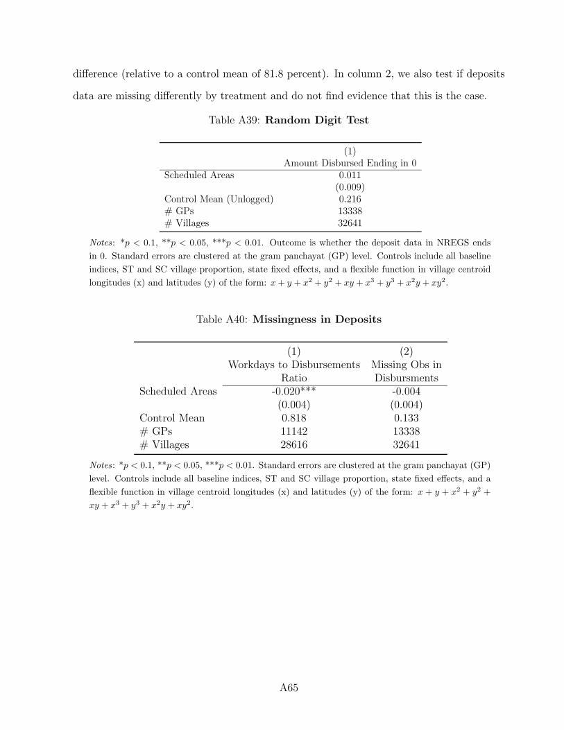
difference (relative to a control mean of 81.8 percent). In column 2, we also test if deposits

data are missing differently by treatment and do not find evidence that this is the case.

Table A39: Random Digit Test

(1)Amount Disbursed Ending in 0

Scheduled Areas 0.011(0.009)

Control Mean (Unlogged) 0.216# GPs 13338# Villages 32641

Notes: *p < 0.1, **p < 0.05, ***p < 0.01. Outcome is whether the deposit data in NREGS ends

in 0. Standard errors are clustered at the gram panchayat (GP) level. Controls include all baseline

indices, ST and SC village proportion, state fixed effects, and a flexible function in village centroid

longitudes (x) and latitudes (y) of the form: x+ y + x2 + y2 + xy + x3 + y3 + x2y + xy2.

Table A40: Missingness in Deposits

(1) (2)Workdays to Disbursements Missing Obs in

Ratio DisbursmentsScheduled Areas -0.020*** -0.004

(0.004) (0.004)Control Mean 0.818 0.133# GPs 11142 13338# Villages 28616 32641




xy + x3 + y3 + x2y + xy2.

A65

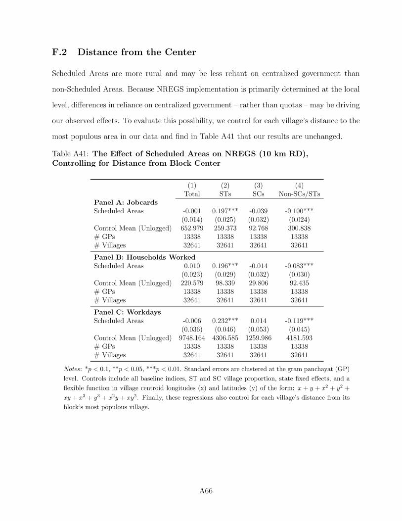
F.2 Distance from the Center

Scheduled Areas are more rural and may be less reliant on centralized government than

non-Scheduled Areas. Because NREGS implementation is primarily determined at the local

level, differences in reliance on centralized government – rather than quotas – may be driving

our observed effects. To evaluate this possibility, we control for each village’s distance to the

most populous area in our data and find in Table A41 that our results are unchanged.

Table A41: The Effect of Scheduled Areas on NREGS (10 km RD),Controlling for Distance from Block Center




Panel B: Households WorkedScheduled Areas 0.010 0.196*** -0.014 -0.083***







xy + x3 + y3 + x2y + xy2. Finally, these regressions also control for each village’s distance from its

block’s most populous village.

A66

G Constructing Census Indices

Due to the large number of variables found in the 2001 Indian census (203 total variables

across the Socio-Demographic module and the Infrastructure module), we decided to combine

the individual census variables into indices. Where possible, we generated these indices

using the Indian Census’ variable groupings - for instance, the Education Index combines

10 variables listed in the census in a group which all refer to different measures of school

and college facilities. However, we note that the titles we assign to indices – for example,

“Banking Index”, should be taken as suggestive. Each index is constructed according to

the following steps and following: first, we standardize and center each constituent variable.

Second, we assign missing variable values the treatment group mean if at least one index

component is non-missing for that observation. Third, we standardize each variable to the

control group mean and standard deviation. Fourth, we take as our index value the average

of all the constituent variable values (Kling, Liebman and Katz, 2007).

We list each census’ variable included in each index below. Note while the vast majority

of census variables are binary or counts, additional variables provide additional qualitative

information when village data was unavailable (known as ‘range codes’) – we omit these

non-numerical variables for simplicity.

We also present analyses using 2011 Census data in Table 3, in Figures 4, A13, and A15,

and in Appendix E.5. The data at our disposal for the 2011 Census did not always match

exactly the data for the 2001 Census. Accordingly, below, we note which variables we had

for which Censuses, as well as the cases when it was necessary to recode variables (typically,

to be binary) so that we could match data across the two Censuses.

Socio-Demographic and Economic Module of 2001 Census, and 2011 Indian

Census

Key:

* = In data for 2001 Census only, ** = In data for 2011 Census only.

A67

• Population Index

TOT NM HH - Total number of households

TOT POP - Total population

M POP - Male population

F POP - Female population

• Vulnerability Index

TOT L6 - Total pop below 6 years

F L6 - Female pop below 6 years

TOT ILLT - Total Illiterates

F ILLT - Female Illiterates

TOT NNW - Total Non-workers

F NNW - Female Non-workers

• Minority Index

TOT SC - Total scheduled caste

M SC - Male scheduled caste

F SC - Female scheduled caste

TOT ST - Total scheduled tribe

M ST - Male scheduled tribe

F ST - Female scheduled tribe

• Agricultural Worker Index

TOT CULT - Total Cultivators

M CULT - Male Cultivators

A68

F CULT - Female Cultivators

TOT AGLB - Total Agricultural Labourers

M AGLB - Male Agricultural Labourers

F AGLB - Female Agricultural Labourers

T MRG CULT - Total Marginal workers as cultivators

M MRG CULT - Male Marginal workers as cultivators

F MRG CULT - Female Marginal workers as cultivators

T MRG AGLB - Total Marginal workers as agricultural labourers

M MRG AGLB - Male Marginal workers as agricultural labourers

F MRG AGLB - Female Marginal workers as agricultural labourers

• Non-Agricultural Worker Index

TOT MFHH - Total Household industry workers

M MFHH - Male Household industry workers

F MFHH - Female Household industry workers

TOT OTH W - Total other workers

M OTH W - Male other workers

F OTH W - Female other workers

T MRG HH - Total Marginal workers household industry workers

M MRG HH - Male Marginal workers household industry workers

F MRG HH - Female Marginal workers household industry workers

T MRG OTH - Total Marginal workers as other workers

M MRG OTH - Male Marginal workers as other workers

F MRG OTH - Female Marginal workers as other workers

A69

• Marginal Worker Index

TOT MRW - Total Marginal workers other workers

M MRW - Male Marginal workers other workers

F MRW - Female Marginal workers other workers

Infrastructure and Amenities Module of 2001 Indian Census, and Market

Villages Data for 2011 Census

• Education Index*

EDU FAC - Educational facilities (binary)*

P SCH - Number of Primary School*

M SCH - Number of Senior Secondary School*

S SCH - Number of Secondary School*

S S SCH - Number of Senior Secondary School*

COLLEGE - Number of Collage*

IND SCH - Number of Industrial School*

TR SCH - Number of Training School*

ADLT LT CT - Number of Adult literacy Class/Centre*

OTH SCH - Number of Other educational facilities*

• Medical Facilities Index*

MEDI FAC - Medical facilities (binary)*

ALL HOSP - Allopathic hospital, Maternity and Child Welfare Centre and Primary

Health Centre*

AYU HOSP - Number of Allopathic Hospital*

A70

UN HOSP - Number of Unani Hospital*

HOM HOSP - Number of Homeopathic Hospital*

ALL DISP - Number of Allopathic Dispensary*

AYU DISP - Number of Ayurvedic Dispensary*

UN DISP - Number of Unani Dispensary*

HOM DISP - Number of Homeopathic Dispensary*

MCW CNTR - Number of Maternity and Child Welfare Centre*

M HOME - Number of Maternity Home*

CWC - Number of Child Welfare Centre Number of Health Centre*

H CNTR - Number of Health Centre*

PH CNTR - Number of Primary Health Centre*

PHS CNT - Number of Primary Health Sub Centre*

FWC CNTR - Number of Family Welfare Centre Number of T.B. Clinic*

TB CLN - Number of T.B. Clinic*

N HOME - Number of Nursing Home*

RMP - Number of Registered Private Medical Practitioners*

SMP - Number of Subsidized Medical Practitioners*

CHW - Number of Community Health workers*

OTH CNTR - Number of Other medical facilities*

• Water Index

HDP ST - Hand Pump (HP)

SPR ST - Spring (S)

TPL ST - Tank/Pond/Lake

A71

TWT ST - Tap Water (Treated)

TUBEWELL - Tubewell Water (TW)

WELL - Well Water (W) (2011 covered/uncovered well variables combined)

DRNK WAT F - Drinking Water facility (binary)*

RIVER - River Water(R)*

OTHER - Other drinking water sources (O)*

TANK - Tank Water (TK)*

TWU ST - Tap Water (Untreated) **

WAT BOM - Water Bounded Macadam**

• Communications Index

BS FAC - Bus services (2011 Census private/public bus services variables com-

bined)

NAV WRC - Navigable water way including River, Canal etc. (2001 recoded to

Y/N)

PO ST - Number of Post Office (2001 recoded to Y/N)

PT OF ST - Number of Post and Telegraph Office (2001 recoded to Y/N)

RS FAC - Railways services

TEL ST - Number of Telephone connections (2001 recoded to Y/N)

COMM FAC - Communication*

P T FAC - Post, Telegraph and Telephone facilities (binary)*

TELE OFF - Number of Telegraph Office*

AUT MODA - Auto/Modified Autos**

INC CSC - Internet Cafes / Common Service Centre (CSC)**

A72

MOB PH CV - Mobile Phone Coverage**

RAIL STAT - Railway Station**

SRF SERV - Sea/River/Ferry Service**

SPO ST - Sub Post Office**

VANS ST - Vans**

• Banking Index

AGRI CRSO - Number of Agricultural Credit Societies (2001 recoded to Y/N)

COOP BANK - Number of Agricultural Credit Societies (2001 recoded to Y/N)

ST AU FAC - Number of Stadium/Auditorium

BANK FAC - Banking facility (binary)*

COMM BANK - Number of Cooperative Commercial Banks*

CRSOC FAC - Credit Societies (Y/N)*

C V HALL - Number of Cinema/Video-hall*

NAC SOC - Number of Non Agricultural Credit Societies*

OTHER SOC - Number of Other Credit Societies*

RC FAC - Recreational and Cultural facilities (binary)*

SP CL FAC - Number of Sports Club*

ATM ST - ATM**

• Road Index

ALL WE RD - Approach - Paved (all weather) Road (2001 recoded to Y/N)

APP FP - Approach - Foot Path*

APP MR - Approach - Mud Road*

A73

APP NAVCAN - Approach - Navigable Canal*

APP NAVRIV - Approach - Navigable River*

APP NW - Approach - Navigable water-way other than river or Canal*

GRA KU RD - Gravel (kuchha) Roads**

NH ST - National Highway**

MDR ST - Major District Road**

OTH DR - Other District Road**

SH ST - State Highway**

• Urbanization Index

POW SAU - Electricity of Agricultural use (2001 recoded to Y/N)

POW SDU - Electricity for Domestic use (2001 recoded to Y/N)

PAP MAG - Newspaper/Magazine (binary)*

POWER ALL - Electricity for all purposes*

POWER OTH - Electricity of other purposes*

POWER SUPL - Power supply (binary)*

A INCEXP - Separate figures available (Y/N). If Yes:*

TOT EXP - Total Expenditure*

TOT INC - Total Income*

POW SCU - Power Supply For Commercial Use**

• Irrigation Index

RIC ST - River/Canal (2001 canal, river variables combined, recoded to Y/N)

TWB ST - Tube well/borehole (2001 tubewell variables combined, recoded to Y/N)

A74

CULT WASTE - Culturable waste (including gauchar and groves)*

LAND FORES - Forest Irrigated (by source)*

LAKE IRR - Lake*

TANK IRR - Tank*

OTH IRR - Others [Water source]*

W FALL - Waterfall*

WELL WO EL - Well (without electricity)*

WELL W EL - Well (with electricity)*

TOT IRR - Total Irrigated Area*

UN IRR - Unirrigated Area*

AREA NA CU - Area not available for cultivation*

A75

Appendix References

Bardhan, Pranab K, Dilip Mookherjee and Monica Parra Torrado. 2010. “Impact of politi-cal reservations in West Bengal local governments on anti-poverty targeting.” Journal ofGlobalization and development 1(1).

Beaman, Lori, Esther Duflo, Rohini Pande, Petia Topalova et al. 2010. Political reservationand substantive representation: Evidence from Indian village councils. In India PolicyForum 2010/11 Volume. Vol. 7 pp. 159–191.

Beber, Bernd and Alexandra Scacco. 2012. “What the numbers say: A digit-based test forelection fraud.” Political analysis 20(2):211–234.

Besley, Timothy, Rohini Pande and Vijayendra Rao. 2005. “Participatory democracy inaction: Survey evidence from South India.” Journal of the European Economic Association3(2-3):648–657.

Besley, Timothy, Rohini Pande and Vijayendra Rao. 2007. “Political Economy of Panchayatsin South India.” Economic and Political Weekly 42(8):661–666.

Best, Michael Carlos, Anne Brockmeyer, Henrik Jacobsen Kleven, Johannes Spinnewijn andMazhar Waseem. 2015. “Production versus revenue efficiency with limited tax capacity:theory and evidence from Pakistan.” Journal of political Economy 123(6):1311–1355.

Beteille, Andre. 1974. Six Essays in Comparative Sociology. New York: Oxford UniversityPress.

Beteille, Andre. 1986. “The concept of tribe with special reference to India.” EuropeanJournal of Sociology 27(2):296–318.

Bhatia, Bela and Jean Dreze. 2006. “Employment Guarantee in Jharkhand: Ground Reali-ties.” Economic and Political Weekly 41(29):3198–3202.

Bhavnani, Rikhil R. 2009. “Do electoral quotas work after they are withdrawn? Evidencefrom a natural experiment in India.” American Political Science Review 103(1):23–35.

Calonico, Sebastian, Cattaneo Mathias D. Farrell Max H. and Rocio Titiunik. 2017. “rdro-bust: Software for Regression Discontinuity Designs.” Stata Journal 17:372–404.

Chauchard, Simon. 2014. “Can descriptive representation change beliefs about a stigmatizedgroup? Evidence from rural India.” American political Science review 108(2):403–422.

Chaudhury, Dipanjan Roy. 2005. “Autonomous District Councils and Panchayati Raj Insti-tutions in North-East India.” Dialogue 7(1).

Chin, Aimee and Nishith Prakash. 2011. “The redistributive effects of political reservationfor minorities: Evidence from India.” Journal of Development Economics 96(2):265–277.

Commissioner for Scheduled Castes and Scheduled Tribes. N.d. Twenty-Fourth Report ofthe Commissioner for SC and ST. New Delhi: Government of India.

A76

Conley, Timothy G. 1999. “GMM estimation with cross sectional dependence.” Journal ofeconometrics 92(1):1–45.

Corbridge, Stuart. 2000. “Competing Inequalities: The Scheduled Tribes and the Reserva-tions System in India’s Jharkhand.” The Journal of Asian Studies 59(1):62–85.

Corbridge, Stuart. 2002. “The Continuing Struggle for India’s Jharkhand: Democracy,Decentralisation and the Politics of Names and Numbers.” Commonwealth & ComparativePolitics 40(3):55–71.

Corbridge, Stuart, Sarah Jewitt and Sanjay Kumar. 2004. Jharkhand: Environment, Devel-opment, Ethnicity. Oxford University Press.

Damodaran, Vinita. 2011. Colonial Constructions of the ‘tribe’ in India: The Case ofChotanagpur. In Adivasis In Colonial India: Survival, Resistance and Negotiation, ed.Biswamoy Pati. Orient BlackSwan.

Duflo, Esther and Raghabendra Chattopadhyay. 2004. “Women as policy makers: Evidencefrom a randomized policy experiment in India.” Econometrica 72(5):1409–1443.

Dunning, Thad. 2010. “Do quotas promote ethnic solidarity? Field and natural experimen-tal evidence from India.” Unpublished manuscript, Yale University .URL: https: // pdfs. semanticscholar. org/ be8e/ 9951c39a6d85b7ac9fec77f96af497d035ec.pdf

Dunning, Thad and Janhavi Nilekani. 2013. “Ethnic Quotas and Political Mobilization:Caste, Parties, and Distribution in Indian Village Councils.” American Political ScienceReview 107(1):3556.

Election Commission of India. 2014. “Election Results - Full Statistical Reports.”.URL: http: // eci. nic. in

Galanter, Marc. 1984. Competing Equalities : Law and the Backward Classes in India.Oxford University Press.

Guha, Ramachandra. 1996. “Savaging the Civilised Verrier Elwin and the Tribal Questionin Late Colonial India.” Economic & Political Weekly 31(35/37).

Gupta, Sanjukta Das. 2011a. Adivasis and the Raj: Socio-economic Transition of the Hos,1820-1932. Orient BlackSwan.

Gupta, Sanjukta Das. 2011b. Rethinking Adivasi Identity: The Chota Nagpur TenancyAct (1908) and its aftermath among the Hos of Singbhum. In Adivasis In Colonial India:Survival, Resistance and Negotiation, ed. Biswamoy Pati. Orient BlackSwan.

H.H., Risley. 1903. General Report by H. H. Risley and. E. A. Gait. Calcutta: Census ofIndia.

Htun, Mala. 2004. “Is Gender like Ethnicity? The Political Representation of IdentityGroups.” Perspectives on Politics 2(3):439–458.

A77

https://pdfs.semanticscholar.org/be8e/9951c39a6d85b7ac9fec77f96af497d035ec.pdf

http://eci.nic.in

ILO. 2015. “ILO-PMGSY Rural Road Project Strengthening Capacity of Panchayati RajInstitutions: Managing Maintenance of Rural Roads.”.URL: ”http://pmgsy.nic.in/RSCPR.pdf”

Imbens, Guido and Karthik Kalyanaraman. 2012. “Optimal bandwidth choice for the re-gression discontinuity estimator.” Review of Economic Studies 79:933–959.

Iyer, Lakshmi and Maya Reddy. 2013. “Redrawing the Lines: Did Political IncumbentsInfluence Electoral Redistricting in the World’s Largest Democracy?” Harvard BusinessSchool Working Paper (14-051).URL: https: // www. hbs. edu/ faculty/ Pages/ item. aspx? num= 46005

Jensenius, Francesca R. 2015. “Development from representation? A study of quotas for thescheduled castes in India.” American Economic Journal: Applied Economics 7(3):196–220.

Kling, Jeffrey R., Jeffrey B. Liebman and Lawrence F. Katz. 2007. “Experimental Analysisof Neighborhood Effects.” Econometrica 75(1):83–119.

Ministry of Drinking Water and Sanitation. 2014. “National Rural Drinking WaterProgramme.”.URL: http: // indiawater. gov. in/ imisreports/ Reports/ BasicInformation/

rpt{ _}RWS{ _}AbstractData{ _}S. aspx? Rep= 0{ &}RP= Y{ &}APP= IMIS

Nazer, M. 2004. A Study of Land Alienation and Indebtedness among Tribals in Tamil Nadu,Kerala and Karnataka. Planning Commission of India.

Palaniswamy, Nethra and Nandini Krishnan. 2012. “Local Politics, Political Institutions, andPublic Resource Allocation.” Economic Development and Cultural Change 60(3):449–473.

Pande, Rohini. 2003. “Can Mandated Political Representation Increase Policy Influence forDisadvantaged Minorities? Theory and Evidence from India.” American Economic Review93(4):1132–1151.

Parthasarathy, Ramya, Vijayendra Rao and Nethra Palaniswamy. 2017. “Deliberativeinequality: a text-as-data study of Tamil Nadu’s village assemblies.” Working Paper .URL: http: // documents. worldbank. org/ curated/ en/ 582551498568606865/

Deliberative-inequality-a-text-as-data-study-of-Tamil-Nadus-village-

assemblies

Pati, Biswamoy. 2011. Adivasis In Colonial India: Survival, Resistance and Negotiation.Orient BlackSwan.

Raabe, Katharina, Madhushree Sekher and Eva Schiffer. 2010. “How to Overcome the Gov-ernance Challenges of Implementing NREGA Insights from Bihar Using Process-InfluenceMapping.” IFPRI Discussion Paper 00963 (April).

Radhakrishna, Meena. 2011. Of Apes and Ancestors: Evolutionary Science and ColonialEthnography. In Adivasis In Colonial India: Survival, Resistance and Negotiation, ed.Biswamoy Pati. Orient BlackSwan.

A78

https://www.hbs.edu/faculty/Pages/item.aspx?num=46005

http://documents.worldbank.org/curated/en/582551498568606865/Deliberative-inequality-a-text-as-data-study-of-Tamil-Nadus-village-assemblies

Rudolph, Lloyd I. and Susanne Hoeber Rudolph. 2010. “Federalism as State Formation inIndia: A Theory of Shared and Negotiated Sovereignty.” International Political ScienceReview 31(5):553–572.

Statoids. N.d. “Districts of India.”.URL: http: // www. statoids. com/ yin. html , year = 2014

Sundar, Nandini. 2005. “Custom and Democracy in Jharkhand.” Economic and PoliticalWeekly 40(41):4430–4434.

Tillin, Louise. 2013. Remapping India: New States and Their Political Origins. New York:Oxford University Press.

Upadhya, Carol. 2009. Law, Custom, and Adivasi Identity: Politics of Land Rights inChotanagpur. In Legal Grounds: Natural Resources, Identity, and the Law in Jharkhand,ed. Nandini Sundar. Oxford University Press.

A79

http://www.statoids.com/yin.html

Does Political Affirmative Action Work, and for Whom? Theory ...

Documents

Transcript of Does Political Affirmative Action Work, and for Whom? Theory ...