Does Microfinance Repayment Flexibility Affect Entrepreneurial Behavior and Loan Default?

Does Microfinance Repayment Flexibility Affect

Entrepreneurial Behavior and Loan Default?

Erica Field, Rohini Pande and John Papp∗

October 30, 2009

Abstract

Recent evidence suggests heterogenous impacts of microfinance loans, with limited av-

erage effects on enterprise growth among the poor. One possibility is that the rigidity

of the classic microcredit contract – widely held to be important for reducing default –

inhibits investment in microenterprises. To explore these trade-offs, we provide exper-

imental estimates of the consequences for client investment behavior of introducing a

grace period before repayment begins. Delaying the onset of repayment by two months

significantly increases both business investment and default. Taken together, the re-

sults are consistent with clients on the delay cycle choosing investments with more

variable returns.

∗The authors are from Harvard University (Field and Pande) and Princeton University (Papp). We thank

Emmerich Davies, Sitaram Mukherjee and Anup Roy for superb field work, the Village Welfare Society and

Center for MicroFinance for hosting this study and Theresa Chen, Annie Duflo, Nachiket Mor and Justin

Oliver for enabling this work. We also thank Natalia Rigol for exceptional research assistance.

1

1 Introduction

Microfinance has been widely hailed as one of the most promising tools for fighting poverty

in the developing world (UN Department of Public Information, 2005). A common claim is

that, by allowing poor households to finance basic self-employment activities and/or weather

shocks to household production, microfinance loans can act as an important catalyst of

economic growth (see, for instance, Nobel Peace Prize 2006 citation). These claims have

been paralleled by a significant expansion of this sector in recent years. In 2007, microfinance

institutions (MFIs) provided 150 million clients across the globe access to small-scale loans

through group lending (Daley-Harris, 2006).

Emerging empirical evidence, however, suggests that access to microcredit may have

limited impact on the average income growth of the poor (Banerjee et al., 2009; Karlan

and Zinman, 2009). One possibility, which we explore in this paper, is that, in a quest to

keep default rates to a bare minimum, MFIs are not offering borrowers the optimal financial

product from an investment perspective. In particular, the immediate repayment obligations

of the classic microcredit contract – widely held to be important for reducing default – may

actually inhibit investment in microenterprises by making relatively illiquid entrepreneurial

investments too risky for small business owners in the short run.

To examine this hypothesis, we test whether client investment behavior, and therefore

the economic impact of microcredit, is sensitive to introducing greater flexibility into loan

contracts. We focus on a central feature of the classic “Grameen Bank” contract: repayment

in small installments starting immediately after loan disbursement. Using a field experiment

we evaluate the effect of relaxing the liquidity demands imposed on households early in the

loan cycle by offering a random set of clients a two-month grace period before repayment

begins. We then compare business investment behavior and repayment rates across these

clients and those required to initiate repayment within two weeks of receiving the loan.

Relaxing short-run liquidity needs should increase the portfolio of investment available

to a household by making illiquid investments more viable. This, in turn, should increase the

average return on available investments and therefore expected business profits for a house-

2

hold. While the predictions for average returns are straightforward, the effects of investment

choices on default and delinquency are ambiguous as they depend on the variability of re-

turns: If relatively illiquid investments also have more variable returns (or, more generally,

increase expected variance of household income by, for instance, reducing short run ability

to deal with shocks), then we may observe higher default even as average returns on business

investments increase. In contrast, by distorting investment towards less risky choices, im-

mediate repayment obligations may simultaneously limit default and income growth.1 We

would also expect this effect to be more pronounced for clients with more growth oppor-

tunities, i.e. those with higher returns to capital today and, therefore, a higher discount

factor.

The contractual form underlying lending to very small businesses in rich countries

provides a good benchmark for comparison. This pool of borrowers is typically perceived

to be risky – however, the typical small business loan contract in developed countries is

significantly more flexible. Using data from the Small Business Administration lending

program in the US, Glennon and Nigro (2005) document default rates between 13-15% for

typical small business loans in the US, which often have a significant grace period between

loan disbursement and the start of repayment.2 These rates are much higher than typical

MFI default rates (2-5%), consistent with the tradeoffs discussed above.

To the best of our knowledge, there is no prior empirical evidence on whether imme-

diate repayment obligations distort investment in microenterprises financed through micro-

credit, largely because MFIs almost universally follow this practice.3 Results from our study

1In theory, early repayment may also discourage risky investments by improving loan officers’ ability to

monitor borrower activities early on in the loan cycle. We exclude this channel from the analysis since loan

officers in our study do not appear to undertake any monitoring activities during loan meetings.2Flexible repayment options are available on SBA loans, and typically negotiated on a loan-by-loan basis.

Payments are typically via monthly installments of principal and interest. There are no balloon payments,

and borrowers may delay their first payment up to three months with prior arrangement. For details, see

for instance https://www.key.com/html/spotlight-quantum-health.html.3Selection issues inhibit causal interpretations of existing non-experimental studies of how greater repay-

ment flexibility affects default, and may explain the mixed findings: Armendariz and Morduch (2005) reports

3

provide rigorous evidence that both client investment and repayment behavior is sensitive to

when repayment obligations start: Microenterprise investment is approximately 8% higher

and the likelihood of starting a new business is twice as high among clients who receive a

two-month grace period. Strikingly, these clients are also roughly 8% more likely to default

on their loan, suggesting that illiquid investments imply greater risk in ability to repay, as

is likely to be the case with new business ventures. We also find indirect evidence of this

interpretation based on survey data on client’s attitudes towards risk and future payoffs: The

effect of the grace period increases significantly with a client’s discount rate, suggesting that

investment choices are most distorted by liquidity demands early on in the loan cycle among

clients with a high opportunity cost of capital, and the effect also appears to increase with

the client’s level of risk aversion, suggesting that risk averse clients are the most deterred by

repayment obligations.

Section 2 describes the MFI setting and client characteristics, the experimental in-

tervention and the basic analytical framework. Section 3 describes the data and empirical

strategy and Section 4 our findings. Section 5 concludes.

2 Background

2.1 Institutional Details

Our partner MFI, ‘Village Welfare Society’ (VWS), started operations in the Indian state of

West Bengal in 1982 and is among the leading MFIs in the state. It only lends to women, and

loan sizes vary from Rs. 4000 to Rs. 12,000 (100-300 US dollars). The typical loan has an

implied annual interest rate of 22%, and clients repay these loans through fixed installments

usually starting two weeks after the loan has been disbursed. Default is low – in 2006, when

we initiated work with VWS, their end-year financial statement reported a repayment rate

of 99%.

that more flexible repayment is associated with higher default in Bangladesh, while McIntosh (2008) finds

that Ugandan MFI clients who choose more flexible repayment schedules are less likely to be delinquent.

4

The average baseline household in our intervention has four members and a monthly

income of Rs. 5300 ($590 PPP). The most common occupations are small business owners,

cooks/domestic servants, and factory workers. Figure 1 shows the distribution of client

businesses at baseline across the entire sample. Seventy-six percent of clients report having

a household business, and the most common businesses are clothing (saris), retail, and

tailoring.

Shocks to business operations are common. Most of these businesses rely significantly

on clients’ labor supply for day-to-day operations. At baseline, 35% of clients report a

household event in which they missed days of work within the last 30 days.4 In addition to

their direct negative effect on household income, such events are likely to adversely affect

the functioning of household businesses by reducing available labor and credit. One way of

smoothing such a shock is via the use of credit and savings. In terms of financial access,

clients enjoy reasonable access to banking services but undertake limited borrowing from

other banks or MFIs. Thirty-one percent of clients have a household savings account, and

28% have some form of formal insurance (26% have life insurance, 5% have health insurance),

which is mainly provided through VWS. All clients report at least one loan taken out within

the year prior to the experiment, the bulk of which were taken out through VWS.

2.2 Experimental Design

Between March and December 2007 we formed 169 five member groups comprising 845

clients. After group formation and prior to loan disbursement, repayment schedules were

randomly assigned in a public lottery. Randomization occurred at the group level after

groups had been approved for loans. Treatment status was assigned to batches of 20 groups

at a time, and we control for this stratification in all regressions. No clients dropped out of

the experiment between randomization and loan disbursement.

Eighty-four groups were assigned the contract with a grace period and 85 groups

were assigned to the standard contract with immediate repayment. Other features of the

4Household events include birth, death, flood, crime, and police case.

5

loan contract were held constant across the two groups, including interest charges. Once

repayment began, both groups of clients were required to repay fortnightly over the course

of 44 weeks. Loan sizes varied from Rs. 4000 to Rs. 10,000, with the modal loan amount being

Rs. 8000. Since clients with a grace period had a total of 55 as opposed to 44 weeks before

their full loan amount was due and faced the same total payment amount, they also faced

a lower effective interest rate on the loan. Hence, the experiment simultaneously introduced

repayment flexibility and increased effective income, although the potential income effect is

arguably minimal given that interest rates are relatively low.

2.3 Predictions

Introducing a grace period and thereby a longer total period over which to repay the same

absolute amount should make it easier for clients to accumulate the income needed to repay

their loan. This is essentially the income effect implied by the lower interest rate in the grace

period credit contract.5 Further, by reducing liquidity needs in the early phase of a client’s

loan cycle, the intervention enhanced client ability to take on less liquid investments. This

works to increase the investment opportunities available to the client. These factors would

suggest that clients assigned to the grace period contract should differ in their business

investments, earn higher average business profits and repay their loans at a higher rate.

However, this presumes that investing in an illiquid project does not affect client risk. In

reality, illiquid investments carry significant risk. For instance, if clients have a sudden need

for money they may be forced to sell their investment at a loss. In this case, the grace period

will both increase investment and worsen repayment outcomes.

Here we formalize the intuition above with a simple model. There are three periods

t = 0, 1, 2. Clients are risk-neutral with utility function u(c0, c1, c2) = c0+c1+c2. Clients have

access to a liquid investment which pays off RL in the following period for each unit invested.

5Differences in implicit interest rates across treatment arms have no direct implication for repayment

timing since clients must pay a fixed interest amount regardless of when they repay. Hence, clients offered

the standard contract have no added incentive to repay early to avoid higher interest charges.

6

They also have access to an illiquid investment which pays off RI after two periods for each

unit invested. In period zero clients receive a loan amount X which they must repay in two

installments, P1 in period one and P2 in period two. Assume that the illiquid investment is

lumpy and requires the entire loan amount X to be invested. There is a probability πS that

in period one the client will face an urgent need for money such as sudden sickness and have

to pay a cost S. The nature of the illiquid investment is such that selling it before period

two yields very low returns.

Here, we take the extreme case in which liquidation net of the liquidity demand (S) is

zero. However, it is possible that the client has enough money on hand or emergency sources

to borrow from that she will not have to liquidate her investment in the face of the liquidity

shock6. We denote the probability that a client will be forced to liquidate her investment

given she must pay S to be πL. πL is a decreasing function of cash on hand in period one and

therefore is increasing in the period one loan payment (π�L(P1) > 0). Figure 2 summarizes

the model setup. Although we have assumed utility is linear in consumption, the fact that

πL(·) is increasing in the first payment amount can be interpreted as concavity of the utility

function. A client would prefer to smooth consumption across periods, but if the required

loan payment combined with a bad shock causes consumption to fall too far in period one,

she may prefer to sell her investment at a loss rather than waiting for it to pay off in the

next period.

Clients will invest in the illiquid asset if and only if:

(1− πS)RIX + πS(1− πL(P1))(RIX −RLS)−RLP1 − P2 ≥

R2LX − πSHRL −RLP1 − P2 (1)

where the left hand side denotes the payoff from investing in the illiquid asset and the right

hand side denotes the payoff from investing in the liquid asset. We specialize to the case

in which πS = 1 as it reduces clutter substantially without affecting the results. We also

assume that, if successful, the illiquid investment pays off more than the liquid investment

6For simplicity, we assume that borrowing to pay S is at rate RL.

7

(RI > R2L) and that the return from liquidation of the illiquid project is less than the return

from successfully completing the illiquid project (RIX > SRL). Equation (1) will be satisfied

as long as:

πL(P1) ≤ min{ (RI −R2L)

RI − (S/X)RL, 1} (2)

Equation (2) shows that, in deciding between the illiquid and the liquid investment, clients

weigh the risk that they will be forced to sell off their investment before it pays off (higher

πL) with the higher return from the illiquid investment (RI). In the present context, grace

period clients will have a lower P1 and therefore a lower πL than clients without a grace

period. The model predicts that grace period clients will be more likely to invest in the

illiquid investment. Although the illiquid investment affords higher returns on average, the

risk of forced liquidation means that grace period clients will also be more likely to enter

period two with no cash on hand, which implies they must default on their loan.

In the example above, the risk of liquidation acts as the disincentive to take on the

illiquid project. However, an alternative possibility is that clients face an uncertain demand

for their product and therefore are reluctant to make large inventory investments. This fear

is especially relevant for clients that have to make early repayments on their loan since a

grace period allows clients to invest in inventory with less concern over not being able to sell

it quickly. In this case, S is zero since clients who invest in the liquid asset do not face any

shocks. For clients with a grace period, we can think of πL as the probability that a client

faces low demand in both period one and period two, in which case she would have to sell at

a loss. Clients without a grace period face a higher πL because they do not have the luxury

of waiting until period two to sell their product.

3 Data and Empirical Strategy

The data used in this paper come from multiple sources which we describe below. The data

appendix covers variable construction in more detail.

8

To gather information on business investments, we collected detailed baseline and

endline survey data from all clients at the time of and approximately one year after loan dis-

bursement. Baseline surveying was conducted between April and August 2007 and endline

surveying between January and November 2008. The baseline survey gathered background

information on household business activities, socio-economic status and demographic char-

acteristics, along with survey measures of risk aversion and discount rates.

Table 1 presents means of a range of variables collected in the survey separately for

clients assigned to the treatment and control group. The majority of clients are literate and

married with two children living at home. Consistent with the type of clients targeted by

VWS, over three quarters of the households in the sample run some kind of microenterprise.

While the group is relatively educated, the rate of shocks experienced by households is high,

as is typical in this setting: 78% of households report experiencing a shock to household

income over the past month. Although there are statistically significant differences across

treatment groups in two of the twelve characteristics (literacy, fraction first time borrowers),

the point estimates of the differences are small and a joint test of significance (chi-squared) of

mean differences across all variables indicates that our randomization produced a balanced

sample. To confirm that small differences in treatment arm balance are not biasing the

experimental results, we estimate all regressions with and without all controls.

The endline survey included a detailed loan use module on business expenditure

amounts and types. Clients were asked how they spent their VWS loan, and answers were

divided into five broad categories (business, health, school, housing, savings, and other).

Figure 3 lists average spending in these broad categories. The most significant expenditure

is business spending: on average, a client spent 80% of her loan on business related activities.

The three most common types of business spending are saris, wood, and sewing materials.

To study delinquency and default, we tracked client repayment behavior using two

sources. First, we used VWS administrative data in which repayment date and amount paid

were recorded by loan officers on a continuous basis in clients’ passbooks and then compiled

into a centralized bank database. We have data on all clients through July 1, 2009, by which

9

date at least 16 weeks had passed since the loan due date for all clients. As a check on the

VWS administrative data, we collected repayment data from loan officers. All loan officers

were required to keep log books on meeting activities for the purpose of our experiment that

recorded date of meeting, number of clients present, and names of clients who repaid at

the meeting. Although the measures differ slightly, this alternative measure gives the same

quantitative results and the same default rate in the full sample as the VWS administrative

data (5.2% compared with 5.4%).

Since VWS does not make explicit the schedule of penalties according to duration

of delinquency (though there is implicit understanding that the degree of delinquency will

influence approval rates and amounts of future loans), some clients repay their loans long

after the due date. For this reason, we present results for different lengths of delinquency.

Our preferred measure is 16 weeks overdue since it is short enough that all clients have

passed it.

Randomization of repayment schedule implies that a comparison of the average out-

comes across clients on the delay versus no-delay interventions has a causal interpretation.

For all outcome variables we estimate regressions of the following form:

yig = βDg + Bg + δXig + �ig (3)

where yig is the outcome of interest for client i in group g. Dg is an indicator variable which

equals one if the group was assigned to the delay intervention. All regressions include batch

dummies for stratification (Bg). Throughout, we report regressions with and without the

controls (Xig) listed in Table 1 and loan officer fixed effects. All standard errors are corrected

for clustering within loan groups. To examine heterogeneity in the treatment effect across

subgroups of clients, we estimate a version of the above regression using a baseline client

variable Zig included on its own and interacted with Dg:

yig = βDg + γZig + θZig ×Dg + Bg + δXig + �ig (4)

Table 2 summarizes the first stage results of our experiment in a regression framework.

The odd columns report regressions without controls, and even columns report regressions

10

with controls. Columns (1) and (2) show that clients assigned to the treatment arm that

included a grace period made their first loan installment an average of 54.4 days after clients

in the control group, or approximately 2 months later. This is reflected in an equivalent

delay in time lapsed between disbursement and final loan due date (columns (3) and (4)). In

general, clients tend to repay earlier than when the loan is actually due; however, columns

(5) and (6) show that the difference in total loan cycle duration persists between clients in

treatment and control arms. Finally, columns (7) and (8) show a weak tendency towards

early repayment among clients on the delay intervention.

4 Repayment Flexibility and Client Behavior

4.1 Loan Use and Investment Behavior

We start by presenting the evidence on loan use. Figure 4 presents a bar graph with the

average expenditures for the main categories divided between clients with and without a

grace period. Business expenditures dominate spending with the average client using eighty

percent of her loan for business expenses. The second largest category is house repairs. The

graph also suggests a significant difference in spending in these two categories across clients

on different loan cycles. In Table 3 we investigate this in a regression framework. We present

results from the estimation of equation (3) using different categories of business expenditure

as outcomes. Columns (1) and (2) show a significant increase in business spending. The

average client on the grace period contract spends roughly 8% (Rs. 421) more on busi-

ness items. They spend less on house repairs (columns (7) and (8)), but this estimate is

statistically insignificant without controls and only weakly significant with controls.

Given the difference in business expenditure and the fact that most loan money

is spent on business expenditures, we further break down business spending into inputs,

equipment and other business spending in Figure 5. The difference in business spending

appears to be driven by differences in spending on inputs – which, in turn, is made up

of inventory purchases and raw materials. Table 4 presents results for the corresponding

11

regressions, and we observe a significant difference in spending on raw materials. These

results are consistent with the prediction that grace period clients increase their spending on

illiquid investments. Raw materials are valuable if clients can find a market for the finished

product, but if demand is uncertain, it may take a while to realize the returns from the

investment. Consistent with the uncertain demand story, small vendors and those involved

in service work are the most likely to purchase raw materials.

Next, we examine client propensity to start new businesses. We asked clients whether

they had started a new business both immediately following loan disbursement and again

twelve months later during the endline. Our measure for whether a client started a new

business is a dummy that equals one if a client reported starting a new business in either

survey. Overall, the rate of new business formation is low - in the control sample only 2%

of clients start new businesses. However, Table 5 shows that the likelihood of starting a

new business is doubled among the treatment group. Figure 8 shows the breakdown of new

business types. All new businesses were either vendors or clothing sellers.

4.2 Loan Repayment Behavior

Having established a link between the more flexible loan contract and business investment,

we next investigate client delinquency and default. Recall that our analytical framework

suggests that increased investment may come at the cost of increased default. If we find

that a grace period is associated with both higher business investment and higher default,

it implies that, in this setting, relatively illiquid investments carry greater risk.

We start by providing a graphical illustration of the impact of providing a grace

period on client repayment behavior. In Figure 6 we show the densities of days from first

meeting in which the client made a payment to when the client finished repaying for clients

who repaid in full as of July 1, 2009. The vertical bars indicate the average loan due date and

16 weeks after the loan was due. The figure indicates that, although a significant fraction

of clients were late, the vast majority of loans were repaid within 16 weeks of being due.

We also observe a significant difference in the repayment patterns of clients who received a

12

grace period versus those who did not. While repayment by clients without a grace period

is heavily concentrated around the loan date, there is significantly more dispersion in time

to repayment among clients who received a grace period. Given that the delay clients, in

effect, had a longer period over which to repay the same size loan, it is not surprising that

many of them were able to repay early relative to the no delay clients.

To see default more clearly, Figure 7 graphs the fraction of clients who have not repaid

in full relative to the date of first installment. As in the previous Figure, the vertical bars

indicate the loan due date and 16 weeks after the loan was due. Truncation is not an issue

since all clients had reached 600 days past their first loan payment by July 1, 2009. Here we

observe a clear difference in the fraction of grace period clients who have repaid in full four

months past the due date.

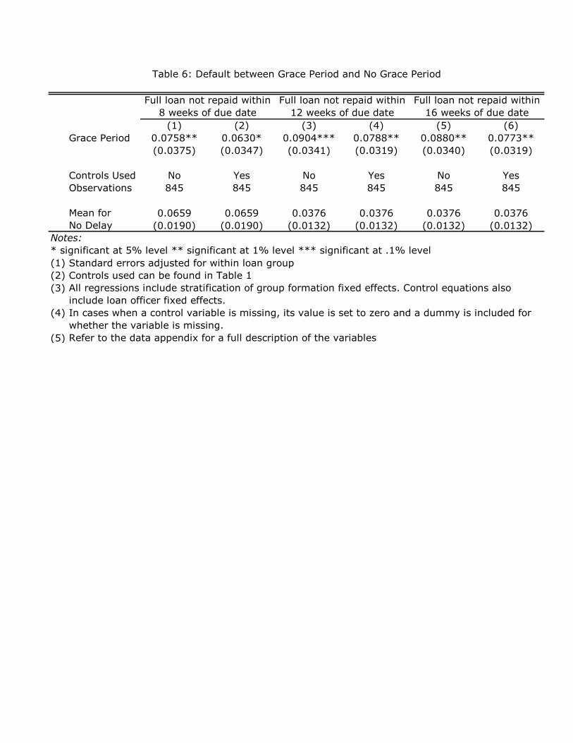
To test for the statistical significance of these patterns, in Table 6 we estimate re-

gressions of experimental assignment on default using three measures of default: whether

the client repaid within 8, 12 and 16 weeks of the loan due date (defined as the date when

the final installment was due). The fraction of defaulting clients falls by three percentage

points between eight weeks after the loan was due and sixteen weeks. However, in all cases

we see a robust difference in default patterns between the delay and no-delay clients. Delay

clients are, on average, between 6 to 8 percentage points more likely to default than non-

delay clients. Sixteen weeks after the loan was due, 3% of the non-delay clients and 11%

of the delay clients have failed to repay. Including controls in the regressions has very little

impact on the point estimates, providing evidence that the results are not contaminated by

treatment imbalance.

4.3 Heterogeneous Treatment Effects

The results outlined in the previous section establish that grace period clients are more likely

to start new businesses and invest in existing businesses. Grace period clients are also more

likely to default. These results suggest that clients who are offered a grace period invest

their loans in riskier though presumably higher expected return business ventures.

13

As a consistency check on this interpretation, in Table 7 we look for evidence of differ-

ences in the influence of the grace period on the business expenditures of various subgroups

of clients.

First, we examine whether the grace period has a larger effect on default for clients

who have a higher discount rate, indicating that they have a higher opportunity cost of

capital. To determine clients’ discount rates, we asked a series of questions about the relative

attractiveness of money today compared with a greater sum of money one week or one month

from now. We increased the second sum of money until clients reported they would prefer

the money at the later date. Using the responses we then computed the net monthly interest

rate that would make clients indifferent between the amount of money today and the amount

of money a month from now. A higher number therefore corresponds to a higher implied

opportunity cost of capital. We report results using the opportunity cost of capital computed

using the one-month time period (we get qualitatively similar results if we compute discount

rates using the one-week method).

In columns (1) and (2) of Table 7 we present results using total business expenditure

as an outcome. The regressor of interest is the measured discount rate interacted with

treatment status. These estimates reveal that the grace period had a larger impact on

clients with higher discount rates. In the context of the model presented in section 2.3, the

discount rate is most naturally associated with a higher return on short-term investments

RL. From equation (2), we can see that an increase in RL will make clients less likely to

invest in the illiquid project, which is consistent with the negative point estimate on the

level effect of the discount rate in columns (1) and (2) of Table 7. However, the model’s

predictions are ambiguous about how the impact of an increase in πL will change as we move

from client’s with low to high RL.

Second, we study the interaction between survey measures of client risk aversion and

the influence of grace period on business investment. Presumably, risk-averse clients are the

least willing to risk missing a loan installment and facing the associated penalties, and are

therefore most constrained by early repayment obligations. In our model, this prediction

14

corresponds to a higher π�L(·) for risk-averse clients. To elicit risk preferences in the baseline

survey, we used the random lottery pairs technique in which subjects were given a sequence

of binary lottery choices and had to choose the preferred lottery, allowing us to deduce risk

aversion based on their switching point from certainty to uncertainty. 7

Regression estimates of the coefficient on the interaction term between risk aversion

and assignment to the grace period group indicate that more risk averse clients increase

business investment by more in response to the grace period contract relative to less risk

averse clients. Though the estimate is only weakly significant, this result is especially striking

given that the level effect of risk aversion is to decrease business investment. While the

coefficient estimates are only weakly significant, this pattern suggests that the standard

loan contract without a grace period deters risk averse clients most from taking on illiquid

investments.

5 Conclusion

Our findings suggest that introducing flexibility to microfinance contracts presents a trade-off

for banks and clients. On the one hand, we find evidence that average levels of default and

delinquency rise when clients are offered a grace period before repayment begins. This basic

finding supports the predominant view among micro-lenders that rigid repayment schedules

are critical to maintaining low rates of default among poor borrowers. On the other hand, our

findings are consistent with a model in which delayed repayment encourages more profitable,

though riskier, investment.

The pattern of long-run default we observe in the data also sheds light on the in-

vestment opportunity set clients face. The fact that a substantial number of grace period

clients still have not repaid more than a year after the loan due date suggests that the avail-

able higher return, less liquid investments also carry higher risk that leads to more variable

7The lotteries were presented as hypotheticals, and clients were not financially incentivized to answer

these questions.

15

business outcomes. In ongoing work we will look for direct evidence of this by examining

differences across experimental groups in long-run business profits.

Assuming for now that the illiquid investments clients undertook were in fact socially

desirable, we perform a back-of-the-envelope calculation to compute the interest rate required

to compensate VWS for the additional default. Given a baseline default rate of 3% for clients

without a grace period and 11% for clients with a grace period, VWS would have to increase

its annualized interest rate from 22% to 33% to cover the additional default. Of course,

a higher interest rate may itself cause a yet higher default rate if moral hazard or adverse

selection are significant, so the new interest rate should be taken as a minimum.

References

Armendariz, B. and J. Morduch (2005). The Economics of Microfinance. Cambridge, MA:

MIT Press.

Banerjee, A., E. Duflo, R. Glennerster, and C. Kinnan (2009). The Miracle of Microfinance?

Evidence from a Randomized Evaluation. mimeo, MIT.

Daley-Harris, S. (2006). State of the MicroCredit Summit Campaign Report.

Glennon, D. and P. Nigro (2005). Measuring the Default Risk of Small Business Loans: A

Survival Analysis Approach. Journal of Money, Credit and Banking 37 (), 923–947.

Karlan, D. and J. Zinman (2009). Expanding Microenterprise Credit Access: Using Ran-

domized Supply Decisions to Estimate the Impacts in Manila. Yale University, mimeo.

McIntosh, C. (2008). Estimating Treatment Effects from Spatial Policy Experiments: An

Application to Ugandan Microfinance. Review of Economics and Statistics 90 (1).

UN Department of Public Information (2005). Microfinance and the Millennium Develop-

ment Goals Fact Sheet.

16

6 Data Appendix

6.1 Baseline Survey

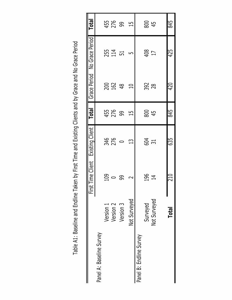
Clients were given three different versions of the baseline survey. The breakdown of number

of new and existing clients by survey is provided in Panel A of Table A1. Existing clients

had already taken out a previous loan with VWS and had taken part in a previous study

conducted by the authors. New clients were both new to VWS and had not taken part in

any previous studies. We were unable to survey 15 clients (1.7%) at the baseline.

Household Shock Defined as whether households had experienced any of the fol-

lowing events in the last 30 days: birth, death, Heavy rain or flood, guest visit, travel.

Household Savings Defined as whether any member in the household has a savings

account.

Employment The borrower is classified as self-employed, wage-employed, or house-

wife. A self-employed woman is defined as one who owns and works on her own business,

a wage-employed woman as one who is either paid a salary or a daily wage by an employer

outside of the home, and a housewife as any woman who does not work.

First Time Borrower Defined as someone who is a new client to our partner MFI

Discount Rate To estimate the discount rate, clients were asked to pick between

receiving a fixed amount of money now or a larger amount a month later. For example, they

were asked if they would prefer receiving 200 rupees now or 250 in a month. In this case,

the implied discount rate for a client that decided to choose 250 rupees now in a month is

between 0 and 25 percent. To generate a more balanced estimate, we took the average of the

implied discount rate at the point at which the client chose to wait (in the previous example

this is 25 percent) and the previous lower discount rate which the client did not choose. So,

if the previous example had been the first question in the game series, we wouldve estimated

the clients discount rate to be 12.5 percent. The higher the discount rate, the more impatient

a client is.

Risk Aversion Index Clients were asked a series of question about whether they

17

would prefer to receive a certain amount of money with certainty or a higher amount with

some degree of uncertainty. Based on these questions, we generated and normalized an index

of how risk averse a person was. The higher a persons score in the index, the more risk loving

they are.

6.2 Endline Survey

Panel B of Table A1 shows the breakdown of clients who were surveyed and who we were

unable to survey at the endline. We were unable to survey 45 clients (5.3%).

Loan Use In order to ascertain how the loan was spent, we asked clients to list

the purposes for which they had used the loan money. We provided a rubric with six

broad categories: Business Expenditures, Health, Schooling, Housing Expenditures, Savings,

and Miscellaneous, which were then further subdivided into more narrow sections. For

example, business expenditures were divided into different types of inputs (saris, fish, etc)

and equipment (sewing machine, rickshaw, etc). Surveyors were instructed to prompt clients

if the total expenditure reported differed from the total loan amount. Still, in 93 cases the

reported amount differed from the total loan amount. In 59 of these cases, the reported

amount matched the amount of a subsequent loan taken by the client and so it is assumed

that the client reported loan use for that loan. For these clients we include a dummy in the

specification. Misreporting is balanced between grace period and no grace period clients.

Since we are unlikely to see differences in loan use between grace period and no grace period

clients in spending of subsequent loans (under which their contract did not differ), this

misreporting will bias our estimates towards zero. In the remaining 34 cases in which the

reported expenditure amount differed from the loan amount, the difference is less than 40%

of the loan in all case.

Inputs This is constructed as the sum of Raw Materials and Inventory from the loan

use section.

18

6.3 Variables from Multiple Surveys or Sources

The following variables were constructed using information from more than one survey in-

strument or data source.

Delinquency and Default The measure of default reported in the paper comes

from the VWS administrative records. Matching between VWS records and study clients

was conducted based on branch name, date of loan disbursement, loan disbursement amount,

group name, and client name. All 845 clients were matched. We present three measures of

default in the paper defined as those clients who have not repaid their loan amount X weeks

after the full loan was due, or 42+X weeks after the first payment where X is 8, 12, and 16.

Due to holidays and issues outlined below 42 weeks after the first meeting may not correspond

to the exact due date. As a check on the VWS administrative records, loan officers were

required to keep a record of payments at each group meeting. Based on consulting with loan

officers, we also computed a separate measure of default. This measure differs slightly but

it is not biased towards more or fewer reported defaults.8 The results presented in Table

6 are quantitatively similar and remain statistically significant when using the alternative

measure.

We are currently using the actual records kept by loan officers as a third check on

the default measure and checking the reason for the few discrepancies between the default

measure reported by loan officers and the default measure in the VWS administrative records.

VWS changed the interest rate that new clients were charged during the study im-

plying that while some clients may repay 8800 Rs on an 8000 Rs loan, others may have

to repay a higher amount. Although the total amount that a client has to repay differs by

interest rate, VWS still requires that each client with a certain size loan repay the same fixed

amount. In other words, regardless of a clients interest rate on the loan, she repays the same

amount at each meeting. This means that, by definition, some clients had more meetings

to repay the same sized loan. Defining the horizon for loan repayment too narrowly would

8The full sample default rate using the administrative records is 5.2% compared with 5.4% for the measure

reported by loan officers.

19

capture clients who simply needed longer to repay their loans due to their interest rate and

not because they were defaulting. The maximum amount of time that any one client was

given to repay their full loan was 45 weeks. The measures reported in the paper all fall after

this cut-off.

Household Business and New Business All 208 new clients to our study were

asked about the businesses that the household owns. They were also asked how long the

business had been operating for. Based on the answers to these questions, we were able to

determine if a household had started a new business with the loan, where new business is

defined as one that was created after the repayment group was formed, or if the household

had an existing business before becoming a participant in our study. The 276 clients who

took version two of the survey were asked about existing and about new household businesses

that were started in the past year. Using the same method as for new clients, we were able

to categorize businesses as either existing at the time of the baseline or newly formed after

disbursement of the new loan. The remaining 346 clients, who took version one and were

existing clients, were only asked about whether they had started a new business in the last

year but not about an existing business. Because they had been in a previous study, we used

their responses from a previous baseline and endline to obtain information about businesses

that existed at the beginning of the second intervention. For all clients, we used the endline

to determine if a new business had been started between the baseline and endline.

20

No Grace Period Grace Period Diff (2) - (1) Full SampleClient-level variable (1) (2) (3) (4)

1 Age 34.228 33.394 -0.8762 33.816(0.408) (0.414) (0.5677) (0.291)

2 Married 0.901 0.875 -0.0269 0.888(0.015) (0.016) (0.0213) (0.011)

3 Literate 0.849 0.792 -0.0561* 0.821(0.017) (0.02) (0.0326) (0.013)

4 Muslim 0.007 0.019 0.0108 0.013(0.004) (0.007) (0.0106) (0.004)

5 Self-Employed 0.501 0.471 -0.0276 0.486(0.024) (0.025) (0.0398) (0.017)

6 Waged Work 0.2 0.204 0.0041 0.202(0.019) (0.02) (0.0336) (0.014)

7 Housewife 0.299 0.325 0.0234 0.312(0.022) (0.023) (0.0336) (0.016)

8 Household Size 3.685 3.797 0.1088 3.74

(0.08) (0.078) (0.1303) (0.056)

9 Household Shock 0.769 0.766 -0.0056 0.767

(0.021) (0.021) (0.0468) (0.015)

10 Household Savings 0.32 0.342 0.0214 0.331

(0.023) (0.023) (0.0405) (0.016)

11 Household Business 0.766 0.766 0.0013 0.766

(0.021) (0.021) (0.0412) (0.015)12 Fraction of First Time Borrowers 0.285 0.212 -0.0691* 0.249

(0.013) (0.012) (0.0398) (0.009)

N 425 420 845 845

(1)(2)

(3)

(4)(5)Rows 1-7 reflect answers about the individual client. Rows 8-12 refer to the household.Refer to the data appendix for a full description of the variables

Table 1: Grace Period vs. No Grace Period Randomization Check

Notes:* significant at 5% level ** significant at 1% level *** significant at .1% level

Standard errors adjusted for within loan group correlation in parenthesis.Column (3) is the coefficient on a dummy for grace period in a regression of the client-level variable on stratification of group formation and loan officer fixed effects. Overall Effect: Chi-Sq. Stat and p value are computed by jointly estimating a system of seemingly unrelated regressions consisting of a dummy for no delay/delay with standard errors adjusted for within loan group correlation.

(1) (2) (3) (4) (5) (6) (5) (6)Grace Period 54.16*** 53.49*** 54.16*** 53.49*** 45.41*** 43.74*** -8.642 -9.810**

(1.521) (1.446) (1.521) (1.446) (5.369) (4.344) (5.261) (4.606)

Controls Used No Yes No Yes No Yes No YesObservations 845 845 845 845 799 799 799 799

Mean for 14.57 14.57 308.6 308.6 326.4 326.4 311.7 311.7No Delay (0.637) (0.637) (0.637) (0.637) (2.594) (2.594) (2.516) (2.516)

Notes:* significant at 5% level ** significant at 1% level *** significant at .1% level(1)(2)(3)(4)

(5) Refer to the data appendix for a full description of the variables

Standard errors adjusted for within loan group correlation in parenthesis.Controls used can be found in Table 1All regressions include stratification of group formation fixed effects. Control equations also include loan officer fixed effects.In cases when a control variable is missing, its value is set to zero and a dummy is included for whether the variable is missing.

Table 2: First Stage between Grace Period and No Grace Period

Disbursement to first meeting

Disbursement to due dateDisbursement to full loan

repaidFirst meeting to full loan

repaid

(3)

(4)

(9)

(10)

(5)

(6)

(11)

(12)

(7)

(8)

(1)

(2)

Grace Period

18.08

12.46

-12.19

5.891

-50.47

-54.34

-28.02

-62.24

-207.5

-268.1*517.6***

421.2**

(67.21)

(64.89)

(44.45)

(45.50)

(47.46)

(50.19)

(109.8)

(113.1)

(134.8)

(145.8)

(197.9)

(201.6)

Controls Used

No

Yes

No

Yes

No

Yes

No

Yes

No

Yes

No

Yes

Observations

845

845

845

845

845

845

845

845

845

845

845

845

107.2

107.2

122.9

122.9

127.7

127.7

402.0

402.0

570.3

570.3

6142.7

6142.7

(52.07)

(52.07)

(32.86)

(32.86)

(53.29)

(53.29)

(88.67)

(88.67)

(115.4)

(115.4)

(162.4)

(162.4)

Notes:

(1)

(2)

(3)

(4)

(5)

(6)

Health

Education

Mean for No

Delay and

Matches

Table 3: Loan Use-All Categories

Savings

Other

All regressions include stratification of group formation fixed effects. Control equations also include loan officer fixed effects.

Controls used can be found in Table 1

Standard errors adjusted for within loan group correlation in parenthesis.

Refer to the data appendix for a full description of the variables

Home Repairs

* significant at 5% level ** significant at 1% level *** significant at .1% level

Clients were asked about the loan they received in this intervention. Some of the clients who went on to the next intervention answered about the

next loan. So all regressions include a dummy for whether the sum of loan use expenditures matched the 3rd intervention loan instead of the 2nd

intervention loan

In cases when a control variable is missing, its value is set to zero and a dummy is included for whether the variable is missing.

Business

(1) (2) (3) (4) (5) (6) (7) (8) (9) (10)Grace Period 126.8 165.2 410.6* 347.4 537.5* 512.6* -47.44 -123.9 27.53 32.46

(294.1) (297.0) (222.0) (227.7) (282.4) (281.9) (240.3) (243.5) (45.90) (46.60)

Controls Used No Yes No Yes No Yes No Yes No YesObservations 845 845 845 845 845 845 845 845 845 845

3241.2 3241.2 1272 1272 4513.2 4513.2 1552.4 1552.4 77.12 77.12

(230.3) (230.3) (144.9) (144.9) (225.4) (225.4) (172.0) (172.0) (34.24) (34.24)Notes:* significant at 5% level ** significant at 1% level *** significant at .1% level(1)(2)(3)(4)

(5)

(6)

Table 4: Loan Use-Business Expenditures Break Down

Clients were asked about the loan they received in this intervention. Some of the clients who went on to the next intervention answered about the next loan. So all regressions include a dummy for whether the sum of loan use expenditures matched the 3rd intervention loan instead of the 2nd intervention loan


Inventory Raw Materials

Standard errors adjusted for within loan group correlation in parenthesis.

All regressions include stratification of group formation fixed effects. Control equations also include loan officer fixed effects.In cases when a control variable is missing, its value is set to zero and a dummy is included for whether the variable is missing.


Inputs EquipmentOther Business Expenditures

Mean for No Delay and Matches

(1) (2)Grace Period 0.0248* 0.0267*

(0.0145) (0.0156)

Controls Used No YesObservations 830 830

0.0254 0.0254

(0.00842) (0.00842)

Notes:

(1)(2)(3)

(4)

(5)

(6)

Mean for No Delay


* significant at 5% level ** significant at 1% level *** significant at .1% levelStandard errors adjusted for within loan group correlation in parenthesis.


New Business New Business

In cases when a control variable is missing, its value is set to zero and a dummy is included for whether the variable is missing.Clients were asked about the loan they received in this intervention. Some of the clients who went on to the next intervention answered about the next loan. So all regressions include a dummy for whether the sum of loan use expenditures matched the 3rd intervention loan instead of the 2nd intervention loan Refer to the data appendix for a full description of the variables

Table 5: New Business Creation

(1) (2) (3) (4) (5) (6)Grace Period 0.0758** 0.0630* 0.0904*** 0.0788** 0.0880** 0.0773**

(0.0375) (0.0347) (0.0341) (0.0319) (0.0340) (0.0319)

Controls Used No Yes No Yes No YesObservations 845 845 845 845 845 845

Mean for 0.0659 0.0659 0.0376 0.0376 0.0376 0.0376No Delay (0.0190) (0.0190) (0.0132) (0.0132) (0.0132) (0.0132)

Notes:* significant at 5% level ** significant at 1% level *** significant at .1% level(1)(2)(3)

(4)

(5) Refer to the data appendix for a full description of the variables

Standard errors adjusted for within loan group Controls used can be found in Table 1

Table 6: Default between Grace Period and No Grace Period


Full loan not repaid within 8 weeks of due date




Discount Rate Discount Rate Risk Index Risk Index

(1) (2) (3) (4)Regressor x Grace Period 27.85* 28.70* -133.0* -91.92

(16.02) (15.85) (75.92) (77.34)

Grace Period 52.61 -112.2 565.8*** 430.1**(365.9) (373.4) (205.7) (210.5)

Regressor -12.36 -12.22 50.39 26.72(10.58) (10.27) (55.44) (55.93)

Controls Used No Yes No YesObservations 845 845 845 845

Mean for No Delay 6282.7 6282.7 6282.7 6282.7(163.0) (163.0) (163.0) (163.0)

Notes:* significant at 5% level ** significant at 1% level *** significant at .1% level(1)(2)(3)(4)

(5)

(6)

Table 7: Heterogenous Effects for Business Expenditures

All regressions include stratification of group formation and loan officer fixed effects.

Standard errors adjusted for within loan group correlation in parenthesis.Controls used can be found in Table 1


Dependent Variable: Business Expenditures

Clients were asked about the loan they received in this intervention. Some of the clients who went on to the next intervention answered about the next loan. So all regressions include a dummy for whether the sum of loan use expenditures matched the 3rd intervention loan instead of the 2nd intervention loan


Figure 1: Distribution of Household Business Types

Figure 2: Model Timing

Large Vendor11% Small Non-‐

Perishables Vendor14%

Convenience Store3%

Small Perishables Vendor9%Clothing Seller

22%Tea Stall2%

Skilled Service Work22%

Piece Rate8%

Unskilled Business Work

9%

Figure 3: Loan Expenditure Categories

Figure 4: Loan Expenditure Categories by Grace Period and No Grace Period Clients

0

1000

2000

3000

4000

5000

6000

7000

Health School House Repairs Savings Other Business Expenditures

0

1000

2000

3000

4000

5000

6000

7000

8000

Health School House Repairs

Savings Other Business Expenditures

No Grace Period

Grace Period

Figure 5: Business Expenditure Categories by Grace Period and No Grace Period Clients

Figure 6: Kernel Density of Days Taken to Repay

0

500

1000

1500

2000

2500

3000

3500

4000

Inventory Raw Materials Equipment Other Business Expenditures

No Grace Period

Grace Period

Figure 7: Fraction of Clients Who Have Not Repaid

Figure 8: Distribution of New Household Business Types

Clothing Seller52%

Large Vendor8%

Small Non-‐Perishables Vendor32%

Small Perishables Vendor8%

First Time ClientExisting Client

Total

Grace PeriodNo Grace Period

Total

Panel A: Baseline Survey

Version 1

109

346

455

200

255

455

Version 2

0276

276

162

114

276

Version 3

990

9948

5199

Not Surveyed

213

1510

515

Panel B: Endline Survey

Surveyed

196

604

800

392

408

800

Not Surveyed

1431

4528

1745

Total

210

635

845

420

425

845

Table A1: Baseline and Endline Taken by First Time and Existing Clients and by Grace and No Grace Period

Does Microfinance Repayment Flexibility Affect Entrepreneurial Behavior and Loan Default?

Documents

Transcript of Does Microfinance Repayment Flexibility Affect Entrepreneurial Behavior and Loan Default?