Does limited access at school result in compensation at home? The effect of soft drink bans in...

Does limited access at school result incompensation at home? The effect of softdrink bans in schools on purchase patternsoutside of schools

Rui Huang† and Kristin Kiesel*,‡,§

†University of Connecticut, USA; ‡California State University-

Sacramento, USA

Received November 2010; final version accepted August 2011

Abstract

This paper investigates the effects of soft drink bans in schools on purchases outsideof schools. Using unique household-level data, we exploit the implementation of astate-mandated ban on soft drinks in Connecticut (USA) in a triple differenceapproach. We compare soft drink purchases of households with school-age childrenbefore and after implementation with purchases of households without school-agechildren in Connecticut, as well as households with and without school-age childrenin other states. Our analysis does not support the notion that school-age children com-pensate for the limited availability at school with increased consumption at home.

Keywords: soft drink bans, purchase data, school environment, quasi-naturalexperiment

JEL classification: D01, D12, D18, C93

1. Introduction

During the past three decades, childhood obesity has more than tripled in theUSA.1 Childhood obesity is associated with health problems at a young age,such as type 2 diabetes, cardiovascular diseases and asthma (American HeartAssociation, 2008). Increases in total caloric intake play a critical role in thegrowth of obesity, with soft drink consumption identified as one of the majorcontributors (Vartanian, Schwartz and Brownell, 2007; Brownell and Frieden,2009). The school environment–its physical, social and educational surroundings–has become a focus in the public policy debate in this context. A number of

*Corresponding author: Department of Economics, California, State University, Sacramento, CA,

USA., E-mail: [email protected]

§ The names of the authors are in alphabetical order, indicating their equal contribution to this

research.

1 The prevalence of obesity among children aged 6–11 years increased from 6.5 per cent in 1980 to

19.6 per cent in 2008, and the prevalence rate among adolescents aged 12–19 years increased

from 5.0 to 18.1 per cent (Centers for Disease Control and Prevention, 2011).

European Review of Agricultural Economics pp. 1–24doi:10.1093/erae/jbs003

# Oxford University Press and Foundation for the European Review of Agricultural Economics 2012; all rightsreserved. For permissions, please email [email protected]

European Review of Agricultural Economics Advance Access published April 6, 2012 at U

niversity of Connecticut on July 1, 2012

http://erae.oxfordjournals.org/D

ownloaded from

http://erae.oxfordjournals.org/

states have considered mandatory policies directly addressing soft drink avail-ability in schools as a nutritional consideration (Center for Science in thePublic Interest, 2007), and national mandatory guidelines are currently dis-cussed in the USA. In addition, the Alliance for a Healthier Generationreached an agreement with the beverage industry, setting voluntary guidelinesto shift to lower calorie, more nutritious beverages (American Beverage As-sociation, 2010). Our study informs the ongoing policy debate by investigat-ing the effects of soft drink bans in schools on out-of-school soft drinkpurchases. This focus addresses shortcomings in the existing literature andprovides a first insight into whether restricted access at school can ultimatelyreduce children’s overall soft drink consumption.

Federally reimbursable school breakfast and lunch programmes must meetstringent nutrition standards under the National School Lunch Program(NSLP) and restrict availability of soft drinks during breakfast and lunchhours. Yet, two-thirds of states have weak or no nutrition standards for com-petitive foods.2 Proponents of regulations beyond the NSLP state that provid-ing healthy snacks and limiting access to foods of minimal nutritional standardwill improve children’s diets because children will consume foods and bev-erages that are most easily available to them. Support for this positioncomes from related research indicating that people eat more when they areprovided with easy access to food (e.g. see Wansink, 2004; Geier, Rozinand Doras 2006; Rolls, Roe and Mengs, 2006). Restricting access shouldtherefore reduce consumption. Opponents fear a loss in revenue and arguethat children will compensate by consuming more soft drinks at home (e.g.see Heatherton, Polivy and Herman 1990; Fischer and Birch, 1999; Francisand Birch, 2005).

To date, there is little direct evidence for either position (Rudd Center forFood Policy and Obesity, 2009). Studies on the effect of improved nutritionalchoices and/or educational campaigns rely mainly on survey responses andsmall sample sizes and primarily focus on elementary schools (e.g. Jameset al., 2004; Blum, Jacobsen and Donnelly, 2005; Fernandes, 2008). Whilethese studies report moderate decreases in soft drink consumption at school,a study addressing high school consumption in Maine finds very limitedeffects on beverage choice of students (Blum et al., 2008). Schwartz,Novak and Fiore (2009) suggest that removing low-nutrition foods decreasedstudents’ consumption at school, and detect no compensation effect at homebased on self-reported purchase behaviour by students. Our study, the firstone to our knowledge that analyses actual out-of-school purchases contributesto this literature by directly addressing whether banning soft drinks at schoolsresults in compensation effects at home.

We use unique household-level purchase data from the AC Nielsen Home-scan. These data allow us to directly link actual purchases to household

2 Competitive foods, often of little or no nutritional value, are those which compete with federally

regulated school meals programmes, and are sold in vending machines, school stores, cafeteria

a la carte lines, and at fund raisers.

of 24 Rui Huang and Kristin Kiesel

at University of C

onnecticut on July 1, 2012http://erae.oxfordjournals.org/

Dow

nloaded from


demographics in a reduced-form econometric approach. We utilise a quasi-natural experiment and build on triple difference (DDD) specifications in atreatment framework commonly used in the policy evaluation literature (seeGruber, 1994; Meyer, 1995; Bertrand, Duflo and Mullainathan, 2004).During our data period, Connecticut implemented a complete ban on allregular and diet soft drink products sold in public schools effective from 1July 2006. We compare soft drink purchases of households with school-age children in Connecticut with purchases of households without school-agechildren in Connecticut, as well as households with and without school-agechildren in other states without state-level regulations. Pre- and post-bantime periods allow us to separate the effect of the soda bans from household-specific, time-invariant unobserved factors that might be correlated with softdrink demand. Furthermore, we are able to test if leading soft drink manufac-turers intensify their advertising efforts to school children in the states thathave implemented bans by controlling for potential differences in children’sadvertising exposure.

Overall, our analysis does not support the notion of compensation effects inout-of-school household purchases.3 As such, our results suggest that banningsoft drinks at schools as one possible restriction of access to unhealthy foodsand beverages might be a viable policy option in an attempt to reduce child-hood obesity.

The next section of this paper briefly reviews soft drink bans and relatedregulations in the school food environment in the USA. Section 3 describesour empirical setting by describing our data, research design and econometricspecifications. We discuss our results and robustness checks in Section 4 andconclude with a discussion of our findings and further research directions inSection 5.

2. Soft drink bans and regulations in the schoolfood environment

Credible estimation of treatment effects in our empirical strategy relies on cor-rectly defining a treatment and control groups in our empirical framework. Wetherefore conducted a comprehensive review of existing policies, using theyearly update and overview provided by the National Conference of StateLegislators (2007), cross-checked available local government and school dis-trict information and searched local and national media to detect potentialrelated interventions at the city, school district and school level.

California was the first state to introduce and pass state-level regulation,banning soft drinks from elementary, middle and junior high schools(except for special events) in 2004. In 2006, California further modified thebeverage restrictions to require soft drink bans at high schools with at least

3 We do not observe restaurant purchases as another possible outlet for out-of-school purchases

of soft drinks, a caveat that will be discussed in more detail in Section 3.2 and in the conclusion of

this paper.

The effect of soft drink bans on out-of-school purchases of 24

at University of C


Dow

nloaded from


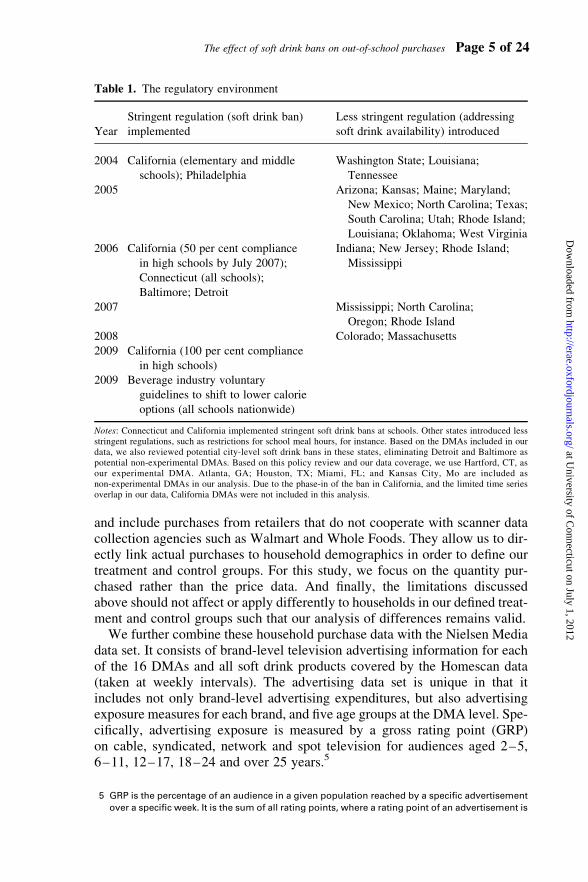
50 per cent compliance by 1 July 2007 and 100 per cent compliance by 1 July2009. In the same year, Connecticut passed a law that banned soft drinks soldto students in all public schools starting 1 July 2006. A number of other stateshave set nutritional guidelines, proposed and passed related measures, buthave not passed state-wide bans. In addition, the Alliance for a Healthier Gen-eration (a partnership of the American Heart Association and the WilliamJ. Clinton Foundation) and beverage industry representatives reached anagreement for voluntary guidelines to shift to lower calorie, more nutritiousbeverages for children’s consumption during the regular and extendedschool day. The industry fully implemented these guidelines on a voluntarybasis by the 2009–2010 school year. And finally, restrictions were also imple-mented at the city and school district level. For instance, Baltimore prohibitedsales of foods and beverages with minimal nutritional standard (includingsoda) starting in September 2006, while carbonated beverages were not soldin school vending machines in Detroit starting on 31 December 2005. ThePhiladelphia school district further approved a soft drink ban, effectivefrom 1 July 2004 for kindergarten to 12th grade levels (K12). Our analysisfocuses on the Connecticut state-wide ban. The regulations used to defineour empirical setting are summarised in Table 1.

3. Empirical setting

3.1. Data

Our data consist of a geographically and demographically representativesample of household panel purchases (Nielsen Homescan) covering threeyears (from January 2006 to December 2008) in 16 geographical markets ordesignated marketing areas (DMAs). The data contain price, quantity andpromotional information on transaction-level household purchases of softdrink products at the universal product code level from all shopping outlets(e.g. grocery stores, drug stores, vending machines and on-line stores).4 Thedata also include annual demographic information for each household, suchas income, race, household size, education, employment, occupation of house-hold heads and, most importantly for our study, age and presence of children.

Due to the increased use of these data in academic research, recent papershave discussed potential caveats of the Nielsen Homescan panel. Einav,Leibtag and Nevo (2010) match the Homescan panel to transactions recordedby a large grocery retailer. They find discrepancies in reported shopping trips,products, prices and quantities, with the largest discrepancies in the price vari-able. Zhen et al. (2009) further suggest potential systematic underreporting offood expenditures, and Lusk and Brooks (2011) discuss potential sample se-lection. However, the advantages of the Nielsen Homescan panel data arethat these data do not rely on consumer recall as they track actual purchases,

4 The Nielsen Homescan instructs its panel members to use in-home scanners to record all pur-

chases from any outlet that are intended for personal consumption by any household members.


at University of C


Dow

nloaded from


and include purchases from retailers that do not cooperate with scanner datacollection agencies such as Walmart and Whole Foods. They allow us to dir-ectly link actual purchases to household demographics in order to define ourtreatment and control groups. For this study, we focus on the quantity pur-chased rather than the price data. And finally, the limitations discussedabove should not affect or apply differently to households in our defined treat-ment and control groups such that our analysis of differences remains valid.

We further combine these household purchase data with the Nielsen Mediadata set. It consists of brand-level television advertising information for eachof the 16 DMAs and all soft drink products covered by the Homescan data(taken at weekly intervals). The advertising data set is unique in that itincludes not only brand-level advertising expenditures, but also advertisingexposure measures for each brand, and five age groups at the DMA level. Spe-cifically, advertising exposure is measured by a gross rating point (GRP)on cable, syndicated, network and spot television for audiences aged 2–5,6–11, 12–17, 18–24 and over 25 years.5

Table 1. The regulatory environment

Year

Stringent regulation (soft drink ban)

implemented

Less stringent regulation (addressing

soft drink availability) introduced

2004 California (elementary and middle

schools); Philadelphia

Washington State; Louisiana;

Tennessee

2005 Arizona; Kansas; Maine; Maryland;

New Mexico; North Carolina; Texas;

South Carolina; Utah; Rhode Island;

Louisiana; Oklahoma; West Virginia

2006 California (50 per cent compliance

in high schools by July 2007);

Connecticut (all schools);

Baltimore; Detroit

Indiana; New Jersey; Rhode Island;

Mississippi

2007 Mississippi; North Carolina;

Oregon; Rhode Island

2008 Colorado; Massachusetts

2009 California (100 per cent compliance

in high schools)

2009 Beverage industry voluntary

guidelines to shift to lower calorie

options (all schools nationwide)

Notes: Connecticut and California implemented stringent soft drink bans at schools. Other states introduced lessstringent regulations, such as restrictions for school meal hours, for instance. Based on the DMAs included in ourdata, we also reviewed potential city-level soft drink bans in these states, eliminating Detroit and Baltimore aspotential non-experimental DMAs. Based on this policy review and our data coverage, we use Hartford, CT, asour experimental DMA. Atlanta, GA; Houston, TX; Miami, FL; and Kansas City, Mo are included asnon-experimental DMAs in our analysis. Due to the phase-in of the ban in California, and the limited time seriesoverlap in our data, California DMAs were not included in this analysis.

5 GRP is the percentage of an audience in a given population reached by a specific advertisement

over a specific week. It is the sum of all rating points, where a rating point of an advertisement is


at University of C


Dow

nloaded from


3.2. Research design

The school environment – its physical, social and educational surroundings –provides an appealing case for policy interventions addressing children’seating habits. Yet, these policies aim to affect children’s consumption offood and beverages beyond school hours and grounds. If we find thatbanning soft drinks in schools leads to no change or even a decrease inout-of-school soft drink purchases by households with school-age children,we can reject the argument that children compensate for reduced soft drinkavailability at schools. We can then argue that it is very likely that overallsoft drink consumption went down as a result of these policies. While wedo not directly observe consumption during the school hours, this conclusionwould rely on results found in previous studies focusing on school purchasesonly (e.g. Schwartz, Novak and Fiore, 2009; American Beverage Association,2010). A potential caveat in this argument is that we do not observe soft drinkpurchases in restaurants, such as fast food outlets. While food expendituresand calorie intake from food away from home (FAFH) has increased forboth adults and children,6 consumption of FAFH may not be a direct causeof weight gain. Instead, higher consumption of FAFH might be a result offamily time constraints, access to various food outlets and preferences forcertain foods (Mancino et al., 2010). Therefore, we would expect to detecta compensation effect in our data sources as well, even though we wouldunderestimate the overall compensation effect due to potential purchases inother outlets.

In order to credibly test for potential compensation effects, we exploit var-iations in soft drink bans over time, across different states, and the fact thatthese bans should only affect households with school-age children. Ourreduced-form econometric approach builds on difference-in-differences(DID) and DDD specifications commonly used in the policy evaluation litera-ture. Estimation of average treatment effects (ATEs) in this framework restson the assumption that average differences in outcomes for treated andcontrol groups are attributable to the treatment, which is satisfied when treat-ment assignment and the potential outcomes are independent (Imbens, 2004).

Our research design makes use of a quasi-natural experiment. Connecticutbanned soft drink in all public schools, effective from 1 July 2006. The Hart-ford DMA in Connecticut therefore serves as the experimental DMA in our

the percentage of households watching a particular programme, relative to the total number of

households with television sets in a DMA. That is, if the advertisement has a rating of 7, then 7

per cent of all households who have television sets in this DMA tune in to this commercial. If an

advertisement is aired twice during a week, and has a rating of 7 and 10, respectively, then its

GRP for that week is 17.

6 In 1977–1978, the average child aged 2–17 obtained 20 per cent of his or her daily calories from

FAFH, while analysis of 2003–2006 data from the National Health and Nutrition Examination Sur-

vey (NHANES) finds that children get roughly 35 per cent of their calories from FAFH (Mancino

et al., 2010). School breakfast and lunch programmes as well as food purchases at school are

included in these measurements, however.


at University of C


Dow

nloaded from


research design. Based on our comprehensive regulatory review, we selectAtlanta, Houston, Miami and Kansas City as the non-experimental DMAs.To our knowledge, these cities have no state, city or school district-levelsoda bans in place.7 Furthermore, we define our potential treatment groupas households with school-age children (aged 6–18). The control group con-sists of households without children, or without children aged 6–18. In orderto address the fact that soft drink purchases are highly seasonal and isolate thetreatment effect from seasonal effects, we choose the same months in the yearsas pre- and post-ban periods when schools are in session. The pre-treatmentperiod is therefore defined as the four-month period between February andMay in 2006, and the post-treatment period is defined as the four-monthperiod between February and May in 2007.

Due to the quasi-natural character of this experiment, we have to consider anumber of potential endogeneity sources in our research design and economet-ric analysis. First, although childhood obesity rates in Connecticut are similarto national averages prior to the ban,8 it is possible that the Connecticut ban isendogenous to soft drink consumption. That is, some unobserved factorsmight be correlated with both household soda demand and the passage ofthe ban in Connecticut. For instance, consumers could be more health con-scious in Connecticut when compared with other states, resulting in bothpassing of the regulation and decreased soft drink consumption.9 FollowingGruber’s (1994) language, our implementation of the DDD model addressesthis issue in three ways. First, we use pre-treatment and post-treatmentperiod fixed effects, as well as month and year fixed effects to capture anytrend in soft drink purchases that are common to all DMAs. Second, we usehousehold fixed effects to control for any time-invariant household-level dif-ferences that could contribute to soft drink consumption. And finally, in orderto control for potential time-varying factors within DMAs potentially corre-lated with the policy implementation and soft drink consumption in the experi-mental DMA, we compare households with school-age children in theexperimental DMAs with households without school-age children in thesame DMA. We measure the change in the treatment household’s relativesoft drink purchases in the experimental DMA, and relative to the non-experimental DMAs. And finally, we also control for potential time-varyingfactors common to all households with school-age children, comparing

7 Due to the partial introduction of the California ban during our data coverage, California DMAs

are not included as experimental DMAs in the analysis. One of our colleagues further suggested

a soft drink ban in Miami during our estimated time period. While we could not verify that infor-

mation at the state level, we excluded Miami as a non-experimental DMA, as an additional ro-

bustness check.

8 Approximately 12.3 per cent of the Connecticut children were overweight or obese relative to a

national average of 14.3% based on the National Survey of Children’s Health 2003 (US Depart-

ment of Health and Human Services, 2005).

9 Another form of endogeneity in this context would arise if households move in or out of the

states because of the bans. Households would therefore self-select in or out of our treatment,

ultimately biasing our results. Using the annual demographics data, we examine whether we

see any abnormal migration patterns after the implementation of the ban, but do not detect any.


at University of C


Dow

nloaded from


households with school-age children living in the experimental DMA withthose living in the non-experimental DMAs.

The resulting identification assumption of the DDD is fairly weak. It onlyrequires that there is no contemporaneous shock on households in the experi-mental DMA in the post-ban period that affects the relative outcomes of thetreatments. In other words, identification of the ATE of soft drink banswould be violated by any systematic shocks to soft drink purchases of house-holds with school-age children in Connecticut that affect soft drink consump-tion over time and might be correlated with but not caused by the ban. Onepossibility relates to the fact that soft drink manufacturers might attempt tocompensate for the loss of sales and visibility at schools by intensifyinglocal advertising campaigns directed at school-age children in Connecticut,and as a result, households with children might increase their purchase ofsoft drink relative to households without children. Our data allow testingthis hypothesis as we are able to combine household purchases withDMA-specific time-varying and age group-specific advertising exposure.

3.2.1. Econometric specification

We obtain our sample from the Nielsen Homescan household-level purchaseand advertising data described in the Data section.10 While some householdsentered or exited during the middle of our data period, our sample onlyincludes households who were in the panel during both the pre- and thepost-ban periods.11 For our analysis, we collapse the monthly time seriesdata into two data points for each of these households, one for the pre-treatment and one for the post-treatment period. This approach closelyfollows Bertrand, Duflo and Mullainathan (2004) and corrects for artificiallylow standard errors in the presence of serially correlated outcomes in paneldata sets. Specifically, for each household, we compute the averagemonthly volume of soft drinks purchased in each of the two data periods.12

We first specify and estimate the following DID equation:

yit = b0 + b1xit + b2tt + b3(CTi × tt) + b4mi + 6it. (1)

10 Although the Nielsen Homescan is a representative sample, our selected regression sample

might not be representative. Households in the Nielsen panel are assigned a ‘projection factor’,

which represents the weight of the household in the national population. In constructing the re-

gression sample, we weigh each of the households equally in our regression. In unreported

regressions, we weigh the households with these ‘projection factors’ as additional robustness

checks. This approach did not alter our results reported here.

11 We do not directly observe whether a household is included in the panel or not at any given time

so we can only indirectly infer this. We have household purchases in four frequently purchased

packaged food categories: soft drinks, breakfast cereal, snacks (such as potato chips, nuts or

popcorn) and candy and confectionary. We keep only households who purchased any product

in these four categories during both periods. Also, demographics are reported for each year a

household is included in the panel. We compare the demographics and locations of households

who were in the panel during both periods with those who entered late or exit early. We find no

statistically significant differences and conclude that sample attrition appears to be random.

12 Not all households purchased soft drink products in both periods such that the volume of pur-

chase of a household in a period could either be zero or positive.


at University of C


Dow

nloaded from


Households are indexed with indexes time period (taking the value of 1 if it isin the post-treatment period, and 0 otherwise). Therefore, yit is defined as theaverage monthly soft drink volume purchase by household i at time t. Theintercept common to all households in all periods is denoted by b0 and tt

denotes the post-ban indicator that takes on the value of 1 if we are in thepost-ban period, and 0 otherwise. The time period fixed effect controls fortrends in monthly volume soda purchase that is common to all householdsin all states (b2). CTi is a Connecticut fixed effect which takes the value of1 if household i lives in Hartford, the Connecticut DMA. We also include anumber of observable control variables such as household demographics,prices and advertising exposure denoted by the vector xit and time-invarianthousehold fixed effect, mi.

13 The interaction between the Connecticut indica-tor and the post-ban dummy (b3) is the DID estimate of the effect of the Con-necticut soft drink ban on out-of-school soda purchases (average monthlyvolume) for Connecticut households. It captures the change in volume pur-chase by Connecticut households (relative to households in other stateswithout soft drink bans) during the post-ban period (relative to pre-banperiod). And finally, 6it denotes an idiosyncratic disturbance term.

The DID identification relies on the common trend assumption. That is, inthe absence of the soft drink ban, the unobservables that are correlated withsoft drink volume purchased by Connecticut households follow similar timetrends as for households living in other states. For instance, the commontrend assumption is not likely to hold if households with school-age childrenfollow a different trend than households without school-age children. We canadditionally exploit the fact that the Connecticut ban should only affect house-holds with school-age children in that state and utilise a DDD frameworkwhich allows relaxing this assumption. Specifically, we estimate the followingDDD equation:

yit =b0 + b1xit + b2tt + b3Treati

+ b4(CTi × tt) + b5(tt × Treati) + b6(CTi × Treati)+ b7(tt × CTi × Treati) + b8mi + 6it.

(2)

Here Treati indicates a household i that has children aged 6–18 in either Con-necticut or the non-experimental DMAs, and zero otherwise and other nota-tions are the same as in equation (1). The treatment group fixed effectcontrols for time-invariant characteristics of households with children aged6–18 (b3). The second-level interactions control for changes in volumepurchase trends over time common to all households in Connecticut (b4),changes in trend over time for treatment group households in all states (b5)and time-invariant characteristics of the treatment group in Connecticut

13 There are no DMA level fixed effects in the specification because only less than 0.1% households

in our data moved from one DMA to the other DMA between the two periods and we exclude

these households from our analysis. Hence, DMA fixed effects are perfectly collinear with house-

hold fixed effects.


at University of C


Dow

nloaded from


(b6). The third-level interaction (b7) is the DDD estimate of the effect of thesoft drink ban on out-of-school soda purchases (average monthly volume) forhouseholds with children aged 6–18 in Connecticut. It captures the change involume purchase by households with school-age children (relative to house-holds without school-age children) in Connecticut (relative to households innon-experimental states) during the post-ban period (relative to pre-banperiod). As in equation (1), we cluster standard errors at the household level.

4. Results and robustness checks

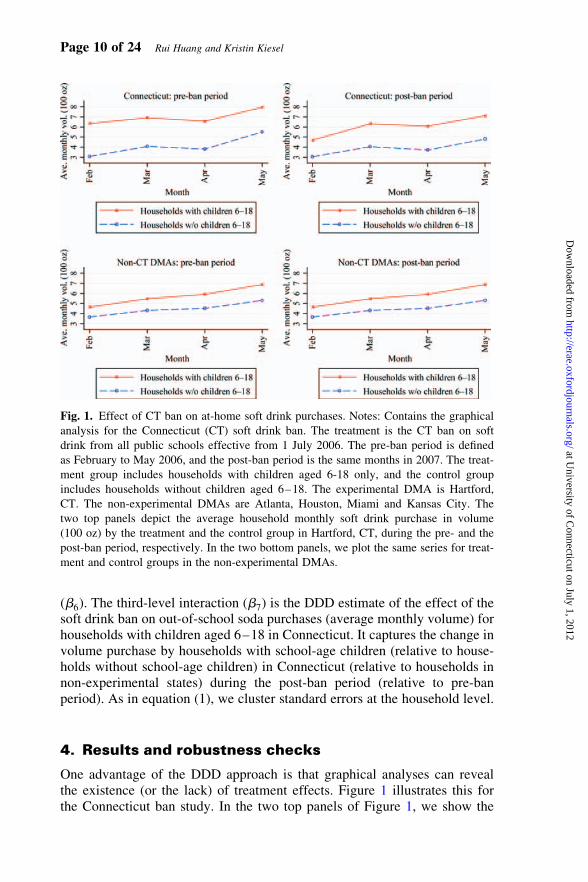
One advantage of the DDD approach is that graphical analyses can revealthe existence (or the lack) of treatment effects. Figure 1 illustrates this forthe Connecticut ban study. In the two top panels of Figure 1, we show the

Fig. 1. Effect of CT ban on at-home soft drink purchases. Notes: Contains the graphical

analysis for the Connecticut (CT) soft drink ban. The treatment is the CT ban on soft

drink from all public schools effective from 1 July 2006. The pre-ban period is defined

as February to May 2006, and the post-ban period is the same months in 2007. The treat-

ment group includes households with children aged 6-18 only, and the control group

includes households without children aged 6–18. The experimental DMA is Hartford,

CT. The non-experimental DMAs are Atlanta, Houston, Miami and Kansas City. The

two top panels depict the average household monthly soft drink purchase in volume

(100 oz) by the treatment and the control group in Hartford, CT, during the pre- and the

post-ban period, respectively. In the two bottom panels, we plot the same series for treat-

ment and control groups in the non-experimental DMAs.


at University of C


Dow

nloaded from


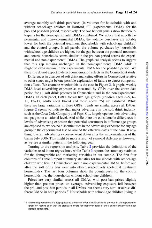
average monthly soft drink purchases (in volume) for households with andwithout school-age children in Hartford, CT (experimental DMA), for thepre- and post-ban period, respectively. The two bottom panels show their coun-terparts for the non-experimental DMAs combined. We notice that in both ex-perimental and non-experimental DMAs, the volume purchases are notablylower for both the potential treatment (households with school-age children)and the control groups. In all panels, the volume purchases by householdswith school-age children are higher, but the gap between the potential treatmentand control households seems similar in the pre-ban period across the experi-mental and non-experimental DMAs. The graphical analysis seems to suggestthat this gap remains unchanged in the non-experimental DMA while itmight be even narrow in the experimental DMA for the post-ban period. Wetherefore do not expect to detect compensation effects in the Connecticut study.

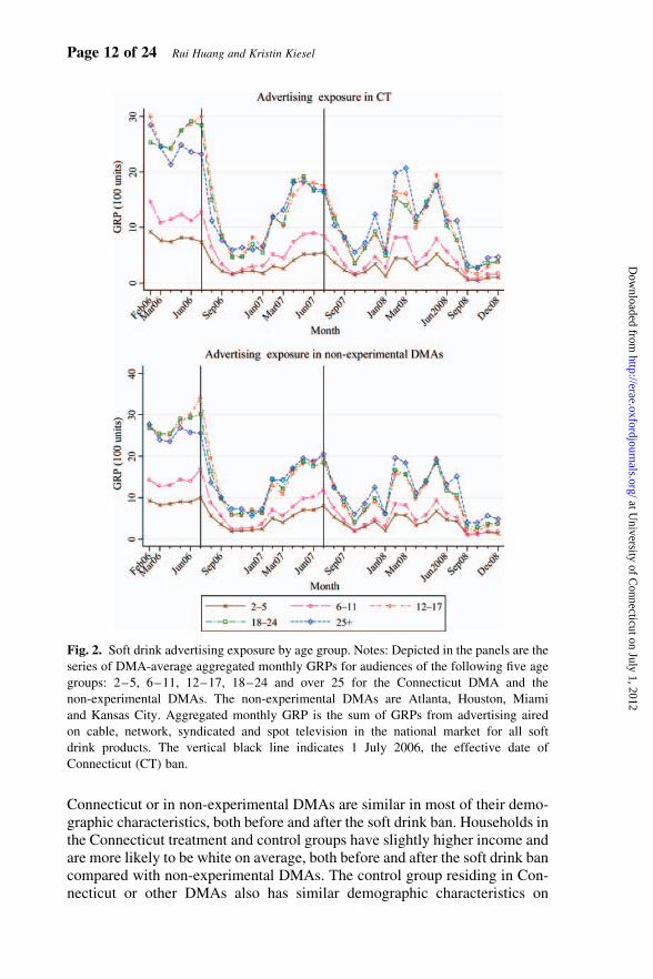
Differences in changes of soft drink marketing efforts in Connecticut relativeto other states might be one possible explanation of failure to detect compensa-tion effects. We examine whether this is the case in Figure 2. It graphs weeklyDMA-level advertising exposure as measured by GRPs over the entire dataperiod for all soft drink products in Connecticut and in the non-experimentalDMAs. In each panel, GRPs for all five age groups (children aged 2–5, 6–11, 12–17, adults aged 18–24 and those above 25) are exhibited. Whilethere are large variations in these GRPs, trends are similar across all DMAs.Figure 2 seems to indicate that major advertisers in the soft drink industry,such as the Coca-Cola Company and Pepsi Co., largely operate their advertisingcampaigns on a national level. And while there are considerable differences inlevels of advertising exposure that potential consumers in different age groupsare exposed to, we see no discontinuities in the advertising exposure for any agegroup in the experimental DMAs around the effective dates of the bans. If any-thing, overall advertising exposure went down after the implementation of theban in July 2006. This might be more a result of seasonal differences, however,as we see a similar pattern in the following year.

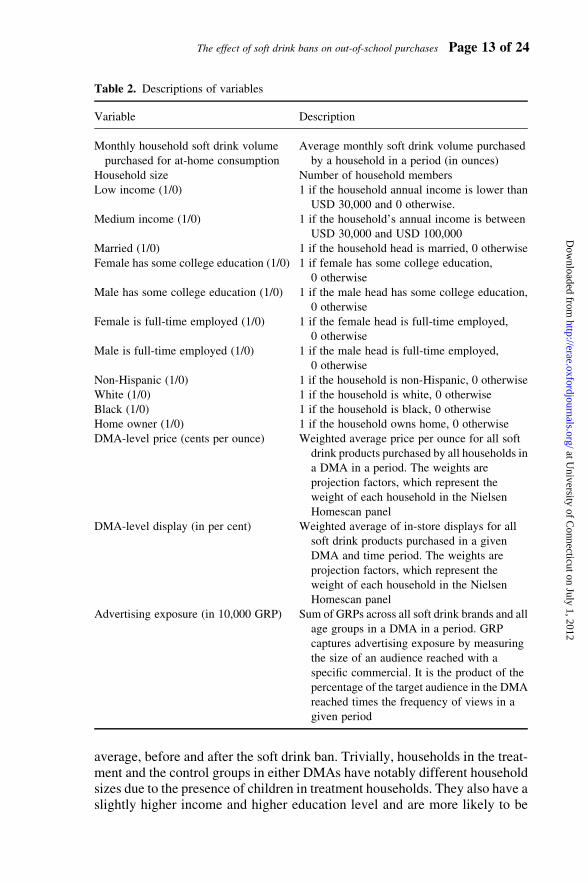
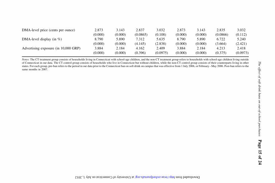
Turning to the regression analysis, Table 2 provides the definitions of thevariables used in our regressions, while Table 3 reports the summary statisticsfor the demographic and marketing variables in our sample. The first fourcolumns of Table 3 report summary statistics for households with school-agechildren who live in Connecticut, and in non-experimental DMAs, before andafter the soft drink ban went into effect, respectively (potential treatmenthouseholds). The last four columns show the counterparts for the controlhouseholds, i.e. the households without school-age children.

Prices are very similar across all DMAs, with post-ban prices slightlyhigher than pre-ban prices on average. Advertising exposure fell betweenthe pre- and post-ban periods in all DMAs, but seems very similar across dif-ferent DMAs in both periods.14 Households with school-age children living in

14 Marketing variables are aggregated to the DMA level and across time periods in the reported re-

gression results such that the standard errors for these variables of the Connecticut DMA in each

period equal zero.


at University of C


Dow

nloaded from


Connecticut or in non-experimental DMAs are similar in most of their demo-graphic characteristics, both before and after the soft drink ban. Households inthe Connecticut treatment and control groups have slightly higher income andare more likely to be white on average, both before and after the soft drink bancompared with non-experimental DMAs. The control group residing in Con-necticut or other DMAs also has similar demographic characteristics on

Fig. 2. Soft drink advertising exposure by age group. Notes: Depicted in the panels are the

series of DMA-average aggregated monthly GRPs for audiences of the following five age

groups: 2–5, 6–11, 12–17, 18–24 and over 25 for the Connecticut DMA and the

non-experimental DMAs. The non-experimental DMAs are Atlanta, Houston, Miami

and Kansas City. Aggregated monthly GRP is the sum of GRPs from advertising aired

on cable, network, syndicated and spot television in the national market for all soft

drink products. The vertical black line indicates 1 July 2006, the effective date of

Connecticut (CT) ban.


at University of C


Dow

nloaded from


average, before and after the soft drink ban. Trivially, households in the treat-ment and the control groups in either DMAs have notably different householdsizes due to the presence of children in treatment households. They also have aslightly higher income and higher education level and are more likely to be

Table 2. Descriptions of variables

Variable Description

Monthly household soft drink volume

purchased for at-home consumption

Average monthly soft drink volume purchased

by a household in a period (in ounces)

Household size Number of household members

Low income (1/0) 1 if the household annual income is lower than

USD 30,000 and 0 otherwise.

Medium income (1/0) 1 if the household’s annual income is between

USD 30,000 and USD 100,000

Married (1/0) 1 if the household head is married, 0 otherwise

Female has some college education (1/0) 1 if female has some college education,

0 otherwise

Male has some college education (1/0) 1 if the male head has some college education,

0 otherwise

Female is full-time employed (1/0) 1 if the female head is full-time employed,

0 otherwise

Male is full-time employed (1/0) 1 if the male head is full-time employed,

0 otherwise

Non-Hispanic (1/0) 1 if the household is non-Hispanic, 0 otherwise

White (1/0) 1 if the household is white, 0 otherwise

Black (1/0) 1 if the household is black, 0 otherwise

Home owner (1/0) 1 if the household owns home, 0 otherwise

DMA-level price (cents per ounce) Weighted average price per ounce for all soft

drink products purchased by all households in

a DMA in a period. The weights are

projection factors, which represent the

weight of each household in the Nielsen

Homescan panel

DMA-level display (in per cent) Weighted average of in-store displays for all

soft drink products purchased in a given

DMA and time period. The weights are

projection factors, which represent the

weight of each household in the Nielsen

Homescan panel

Advertising exposure (in 10,000 GRP) Sum of GRPs across all soft drink brands and all

age groups in a DMA in a period. GRP

captures advertising exposure by measuring

the size of an audience reached with a

specific commercial. It is the product of the

percentage of the target audience in the DMA

reached times the frequency of views in a

given period


at University of C


Dow

nloaded from


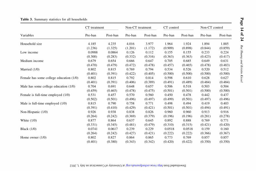
Table 3. Summary statistics for all households

CT treatment Non-CT treatment CT control Non-CT control

Variables Pre-ban Post-ban Pre-ban Post-ban Pre-ban Post-ban Pre-ban Post-ban

Household size 4.185 4.235 4.016 3.977 1.964 1.924 1.894 1.885

(1.236) (1.325) (1.201) (1.172) (0.909) (0.898) (0.844) (0.859)

Low income 0.0988 0.0864 0.126 0.112 0.155 0.155 0.233 0.224

(0.300) (0.283) (0.332) (0.316) (0.363) (0.363) (0.423) (0.417)

Medium income 0.679 0.654 0.666 0.647 0.705 0.685 0.649 0.631

(0.470) (0.479) (0.472) (0.478) (0.457) (0.465) (0.478) (0.483)

Married (1/0) 0.802 0.815 0.769 0.794 0.534 0.526 0.520 0.512

(0.401) (0.391) (0.422) (0.405) (0.500) (0.500) (0.500) (0.500)

Female has some college education (1/0) 0.802 0.815 0.792 0.814 0.598 0.610 0.628 0.627

(0.401) (0.391) (0.406) (0.389) (0.491) (0.489) (0.484) (0.484)

Male has some college education (1/0) 0.704 0.691 0.648 0.657 0.506 0.518 0.503 0.504

(0.459) (0.465) (0.478) (0.475) (0.501) (0.501) (0.500) (0.500)

Female is full-time employed (1/0) 0.531 0.457 0.570 0.560 0.450 0.478 0.442 0.437

(0.502) (0.501) (0.496) (0.497) (0.499) (0.501) (0.497) (0.496)

Male is full-time employed (1/0) 0.815 0.790 0.758 0.771 0.498 0.494 0.419 0.403

(0.391) (0.410) (0.429) (0.421) (0.501) (0.501) (0.494) (0.491)

Non-Hispanic (1/0) 0.926 0.938 0.838 0.826 0.960 0.960 0.913 0.916

(0.264) (0.242) (0.369) (0.379) (0.196) (0.196) (0.281) (0.278)

White (1/0) 0.877 0.864 0.637 0.645 0.892 0.888 0.769 0.771

(0.331) (0.345) (0.481) (0.479) (0.310) (0.315) (0.421) (0.420)

Black (1/0) 0.0741 0.0617 0.239 0.229 0.0518 0.0518 0.159 0.160

(0.264) (0.242) (0.427) (0.421) (0.222) (0.222) (0.366) (0.367)

Home owner (1/0) 0.802 0.827 0.864 0.865 0.773 0.769 0.857 0.857

(0.401) (0.380) (0.343) (0.342) (0.420) (0.422) (0.350) (0.350)

Pa

ge

14

of

24

Rui

Huang

and

Kristin

Kiesel

at University of Connecticut on July 1, 2012 http://erae.oxfordjournals.org/ Downloaded from


DMA-level price (cents per ounce) 2.873 3.143 2.837 3.032 2.873 3.143 2.835 3.032

(0.000) (0.000) (0.0865) (0.108) (0.000) (0.000) (0.0866) (0.112)

DMA-level display (in %) 8.790 5.890 7.312 5.635 8.790 5.890 6.722 5.240

(0.000) (0.000) (4.145) (2.838) (0.000) (0.000) (3.664) (2.421)

Advertising exposure (in 10,000 GRP) 3.884 2.184 4.162 2.409 3.884 2.184 4.213 2.418

(0.000) (0.000) (0.396) (0.0975) (0.000) (0.000) (0.375) (0.0973)

Notes: The CT treatment group consists of households living in Connecticut with school-age children, and the non-CT treatment group refers to households with school-age children living outsideof Connecticut in our data. The CT control group consists of households who live in Connecticut but without children, while the non-CT control group consists of their counterparts living in otherstates. For each group, pre-ban refers to the period in our data prior to the Connecticut ban on soft drink on campus that was effective from 1 July 2006, or February–May 2006. Post-ban refers to thesame months in 2007.

The

effectof

soft

drin

kbans

on

out-o

f-school

purch

ases

Pa

ge

15

of

24



full-time employed than the control group households on average. The DDDspecifications control for these time-invariant and time-varying factorscommon to all households with or without school-age children, to all house-holds with school-age children only and to all households living in Connecti-cut. It further allows us to control for unobserved factors that are common tothese groups of households.

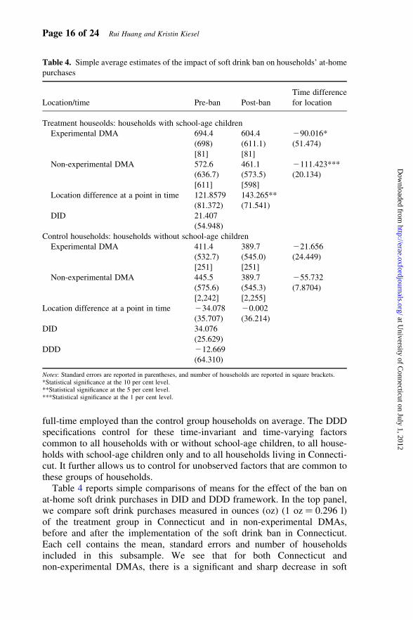
Table 4 reports simple comparisons of means for the effect of the ban onat-home soft drink purchases in DID and DDD framework. In the top panel,we compare soft drink purchases measured in ounces (oz) (1 oz ¼ 0.296 l)of the treatment group in Connecticut and in non-experimental DMAs,before and after the implementation of the soft drink ban in Connecticut.Each cell contains the mean, standard errors and number of householdsincluded in this subsample. We see that for both Connecticut andnon-experimental DMAs, there is a significant and sharp decrease in soft

Table 4. Simple average estimates of the impact of soft drink ban on households’ at-home

purchases

Location/time Pre-ban Post-ban

Time difference

for location

Treatment houseolds: households with school-age children

Experimental DMA 694.4 604.4 290.016*

(698) (611.1) (51.474)

[81] [81]

Non-experimental DMA 572.6 461.1 2111.423***

(636.7) (573.5) (20.134)

[611] [598]

Location difference at a point in time 121.8579 143.265**

(81.372) (71.541)

DID 21.407

(54.948)

Control households: households without school-age children

Experimental DMA 411.4 389.7 221.656

(532.7) (545.0) (24.449)

[251] [251]

Non-experimental DMA 445.5 389.7 255.732

(575.6) (545.3) (7.8704)

[2,242] [2,255]

Location difference at a point in time 234.078 20.002

(35.707) (36.214)

DID 34.076

(25.629)

DDD 212.669

(64.310)

Notes: Standard errors are reported in parentheses, and number of households are reported in square brackets.*Statistical significance at the 10 per cent level.**Statistical significance at the 5 per cent level.***Statistical significance at the 1 per cent level.


at University of C


Dow

nloaded from


drink volume purchased. Specifically, the decrease is as large as 12 per cent inthe Connecticut DMA and 19 per cent in non-experimental DMAs. Also listedare differences over time in the same location. Soft drink purchases do notdiffer significantly prior to the soft drink ban, but the treatment group in Con-necticut purchases 143 oz more on average (4.23 l) than this group in the non-experimental DMAs after the ban. The DID estimate (the difference in thedifferences over time between Connecticut and non-experimental DMAs) isnot statistically significantly different, however. The bottom panel reportsthe same difference for control groups living in Connecticut versus in non-experimental DMAs. Soft drink purchases do not seem to be statistically sig-nificantly different over time or across locations for these households. Finally,the DDD estimate is defined as the difference in the two DID estimates, and isalso not statistically significantly different from zero.

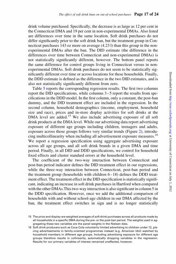
Table 5 reports the corresponding regression results. The first two columnsreport the DID specifications, while columns 3–5 report the results from spe-cifications in the DDD model. In the first column, only a constant, the post-bandummy, and the DID treatment effect are included in the regression. In thesecond column, household demographics (income, employment, householdsize and race), prices and in-store display activities for soft drinks at theDMA level are added.15 We also include advertising exposure of all softdrink products at the DMA level. While our advertising data report advertisingexposure of different age groups including children, teenagers and adults,exposure across those groups follows very similar trends (Figure 2), introdu-cing multicollinearity when including all advertisement exposure measures.16

We report a regression specification using aggregate advertising exposureacross all age groups, and all soft drink brands in a given DMA and timeperiod. Finally, in all DID and DDD specifications, we control for householdfixed effects and cluster standard errors at the household level.

The coefficient of the two-way interaction between Connecticut andpost-ban period indicator defines the DID treatment effect in our regressions,while the three-way interaction between Connecticut, post-ban period andthe treatment group (households with children 6–18) defines the DDD treat-ment effect. The treatment effect in the DID specification is statistically signifi-cant, indicating an increase in soft drink purchases in Hartford when comparedwith the other DMAs.This two-way interaction is also significant in column 5 inthe DDD specification. However, once we add the additional comparison ofhouseholds with and without school-age children in our DMA affected by theban, the treatment effect switches in sign and is no longer statistically

15 The price and display are weighted averages of soft drink purchases across all products made by

all households in a specific DMA during the pre- or the post-ban period. The weights used in ag-

gregating these two variables are the panel weights in the Nielsen data.

16 Soft drink producers such as Coca-Cola voluntarily limited advertising to children under 12, pla-

cing advertisements in family-oriented programmes instead (e.g. American Idol) watched by

household members in different age groups. Including advertising exposure for different age

groups therefore results in collinearity, automatically dropping variables in the regression.

Results for our primary variables of interest remained unaffected, however.


at University of C


Dow

nloaded from


Table 5. Regression results of the impact of soft drink ban on households’ at-home purchases

Dependent variable: monthly household soft drink volume purchased for at-home consumption

(1) (2) (3) (4) (5)

DID DID DDD DDD DDD

Post-ban period (1/0) 267.984*** 22.921 259.885*** 260.158*** 31.318

(6.979) (58.734) (7.450) (7.593) (58.407)

29.650 55.714** 37.837 38.354 63.351**

CT×post-ban period (DID treatment effect) (21.429) (26.186) (24.374) (24.365) (28.666)

Treatment group (1/0) 21.319 22.087 22.536

(35.939) (37.556) (37.679)

CT×treatment group (1/0) 52.861 51.152 51.662

(77.120) (75.747) (75.816)

Post-ban period×treatment group 238.668* 239.751* 242.011**

(20.288) (20.300) (20.287)

CT×post-ban period×treatment group (DDD treatment effect) 228.087 225.315 223.205

(55.612) (55.818) (55.810)

Household size 20.107 1.327 1.688

(11.785) (12.327) (12.283)

Low income (1/0) 235.466 234.032 234.394

(36.395) (36.083) (36.258)

Medium income (1/0) 211.938 210.031 210.853

(30.117) (30.092) (30.081)

Married (1/0) 79.399 81.999 80.530

(51.562) (52.189) (51.635)

Female has some college education (1/0) 229.137 229.652 227.855

(33.972) (33.495) (33.742)

Male has some college education (1/0) 259.080 258.435 261.679

(41.603) (41.428) (41.603)

Female is full-time employed (1/0) 19.827 19.667 20.105

(25.912) (26.058) (25.972)

Male is full-time employed (1/0) 229.885 231.676 229.552

Pa

ge

18

of

24

Rui

Huang

and

Kristin

Kiesel



(31.283) (32.018) (31.666)

Non-Hispanic (1/0) 253.382 256.878 249.139

(51.675) (52.381) (51.974)

White (1/0) 40.437 40.168 40.560

(38.649) (39.549) (39.262)

Black (1/0) 217.154 213.326 213.207

(42.334) (41.969) (42.306)

Home owner (1/0) 10.996 12.651 10.729

(42.363) (42.471) (42.256)

DMA-level price (cents per ounce) 2400.840 2423.548

(293.164) (293.595)

DMA-level display (in per cent) 22.866 23.814

(9.845) (9.881)

Advertising exposure (in 10,000 GRP) 9.716 7.763

(47.223) (47.204)

Constant 473.485*** 1,628.638 472.428*** 505.710*** 1,697.262

(3.299) (1,051.224) (7.795) (82.511) (1,052.336)

Observations 6,370 6,370 6,370 6,370 6,370

R-squared 0.030 0.035 0.032 0.035 0.038

Number of household 3,185 3,185 3,185 3,185 3,185

Note: Robust standard errors clustered at the household level are reported in parentheses.*Statistical significance at the 10 per cent level.**Statistical significance at the 5 per cent level.***Statistical significance at the 1 per cent level.

The

effectof

soft

drin

kbans

on

out-o

f-school

purch

ases

Pa

ge

19

of

24



significant. The significant increase might indicate a difference in consumerpreferences and overall trends for households in Connecticut when comparedwith households in other states, and potentially explains the early adoption ofstate-wide soft drink bans. Only relying on the DID estimates might thereforebe misleading as we cannot account for this potential selection bias due to dif-ferences in trends across DMAs. Alternatively, the significant increase in theDID could also be driven by soft drink purchase increases for householdswithout school-age children only. Interestingly, the interaction between thetreatment group (households with school-age children) and the post-banperiod is negative and statistically significant in all DDD specifications at the10 per cent significance level, suggesting a downward trend in volume pur-chased for all households with school-age children in all DMAs. One possibleexplanation is that regulations addressing soft drink consumption at schools andthe attention these policies have got, as well as potential local-or school-levelinitiatives, did result in an actual overall reduction for this treatment group in-dependent of stringent state-level regulations. While we also find a significantdecrease in soft drink purchases across all households in the post-ban period,this effect switches signs and is no longer statistically significant once weinclude controls for price, in-store display and advertising changes at theDMA level. It is worth pointing out that increases in advertising exposure sig-nificantly increase soft drink consumption in this context when we do notcontrol for price and in-store display differences. In general, the control vari-ables at the household-level are not statistically significant individually.While we have yearly updated information for the household demographics,it suggests that the inclusion of household-level fixed effects already capturestime-invariant taste differences. Including these control variables jointly doesincrease the explanatory power of our regressions slightly, however. Further-more, the results for our primary variables of interest are robust to anynumber of specifications including subsets of our additional controls such as in-cluding market-level controls only.

In addition, we explored a number of alternative specifications notreported here. Rather than using average monthly purchases, we summedpurchases over the school semesters and used monthly purchases with add-itional month fixed effects. We also classified households as light andheavy soda drinkers to test whether these groups were affected differentlyby the ban.17 In addition, we investigated the effect on regular versus dietsoda. And finally, we investigated private label versus branded products, assoft drinks available at school are exclusively provided by theleading national-level brands. However, in all of those specifications, wefail to detect statistically significant treatment effects in the DDD specifi-cations.18 In summary, our results do not support the argument that

17 One might argue that heavy soda drinkers are more likely to compensate than light soda

drinkers.

18 As mentioned in footnote 7, we further excluded Miami as a non-experimental DMA. The results

reported here were robust to this alternative specification as well.


at University of C


Dow

nloaded from


state-mandated soft drink bans in schools result in compensation effects insoft drink consumption at home.

5. Conclusions and future research directions

Soft drink consumption and its role as a major contributor to childhood obesityhas become a highly visible public health and public policy issue. The schoolenvironment can play an important role in successfully reducing and prevent-ing obesity in children. This study investigates the effects of banning softdrinks in schools on purchases outside of schools. It tests whether limitedavailability at schools results in compensation at home.

We combine purchase data with information on state-level regulationsregarding soft drink availability in schools in a quasi-natural experiment ap-proach. We use household panel purchase data and market-level informationon weekly brand-level television advertising exposure directed at different agegroups. Our analysis focuses on Connecticut as one of the states implementingstringent and comprehensive state-level soft drink bans in schools during ourdata period. By further differentiating between households with school-agechildren and households without children, we follow an econometric DDD ap-proach commonly used in the policy evaluation literature.

Overall, our results do not support the argument that restricted availabilityat schools results in compensation at home. In our regression analysis, we areable to control for a number of additional determinants of soft drink consump-tion that could otherwise lead to biased results, such as possible differences inprice promotions and pricing structures, as well as in-store displays. We alsocontrol for potential advertising differences and reject the hypothesis thatleading brands intensify their advertising efforts to school-age children as aresult of soft drink bans to offset their reduced presence in the schoolenvironment.

Our study provides a first insight into this complex topic. While our studyadds an analysis of actual purchase data to the literature, we do acknowledgelimitations that need to be addressed in future research. First, while our com-prehensive policy review allowed us to credibly identify experimental andnon-experimental markets, our study cannot address issues concerning imple-mentation and adherence to these policies at the school level. As mentionedpreviously, we find an overall reduction of soft drink purchases for householdswith school-age children, independent of the actual implementation of softdrink bans at schools. Our failure to detect the same statistically significanteffect for households specifically affected by the ban could be a result of in-complete implementation and lack of adherence to the ban at the school level,or voluntary bans in place prior to implemented state-level regulations. Con-tacting school districts in Connecticut and elsewhere suggested that little isknown about the adherence to either state-level or school district-level regula-tions. Samuels et al. (2009) addressed this shortcoming and collected informa-tion on competitive foods and beverages available in schools for arepresentative sample of 56 public high schools in California in 2006 and


at University of C


Dow

nloaded from


2007. Focusing on the adherence of mandatory nutritional standards, theyreport that California schools are making progress towards full implementa-tion. While beverage standards seemed easier to achieve than standards forfood items, soft drink availability still varied significantly across schools sur-veyed in their sample. A future research extension to this study will analysepurchase response to the ban implemented in California high schools by com-bining this unique data set with store-level purchase data from a major retailerfor all California stores covering an extended time period. Matching stores toneighbouring schools with diverse adherence measures will allow us to direct-ly address this important aspect.

Another limitation of our study is that we do not observe restaurant pur-chases, especially soft drink purchases at fast food restaurants. Studentsmight compensate by increasing their purchases at those outlets, whichwould result in underestimating the compensation effect in our data.However, it seems plausible that students would at least partially compensatethrough purchases in the outlets included in our data set.

Previous research suggests that banning soft drinks decreased calorie con-sumption at schools (e.g. James et al., 2004; Blum, Jacobsen and Donnelly,2005; Fernandes, 2008; Schwartz, Novak and Fiore, 2009; American Bever-age Association, 2010). If these findings capture a general trend, and are ap-plicable to the schools in our sample, our results suggest that banning softdrinks at schools does not result in compensation at home. Our studyfurther supports the notion that soft drink bans at school reduce overallcalorie consumption from soft drinks in children. As such, our resultsinform the policy debate on successful strategies to reduce and prevent child-hood obesity. We suggest that soft drink bans at school present a potentiallyeffective policy option in this regard.

Acknowledgements

This project was supported by Agriculture and Food Research Initiative Competitive Grant

no. 2010-65400-20440 from the USDA National Institute of Food and Agriculture. We would

also like to thank Chantel Crane, two anonymous reviewers, participants of the AAEA meetings

in Denver in July 2010, participants of the Joint EAAE/AAEA Seminar in Freising, Germany, in

September 2010 and participants of the Using Scanner Data to Answer Food Policy Questions

Conference held at the ERS in Washington, DC, in June 2011 for useful comments.

References

American Beverage Association (2010). Alliance School Beverage Guidelines Final

Report. http://www.ameribev.org/. Accessed January 2010.

American Heart Association (2008). Overweight in children. http://www.americanheart.

org/presenter.jhtml?identifier=4670. Accessed April 2008.

Bertrand, M., Duflo, E. and Mullainathan, S. (2004). How much should we trust

differences-in-differences estimates? Quarterly Journal of Economics 119: 249–275.


at University of C


Dow

nloaded from

http://www.ameribev.org/





http://www.americanheart.org/presenter.jhtml?identifier=4670








Blum, J. E. W., Davee, A.-M., Beaudoin, C. M., Jenkins, P. L., Kaley, L. A. and Wigand,

D. A. (2008). Reduced availability of sugar-sweetened beverages and diet soda has a

limited impact on beverage consumption patterns in Maine high school youth. Journal

of Nutrition Education and Behavior 40(6): 341–347.

Blum, J. E. W., Jacobsen, D. J. and Donnelly, J. E. (2005). Beverage consumption patterns

in elementary school aged children across a two-year period. Journal of American

College of Nutrition 24(2): 93–98.

Brownell, K. D. and Frieden, T. R. (2009). Ounces of prevention—the public policy case

for taxes on sugared beverages. New England Journal of Medicine 360: 1805–1808.

Center for Science in the Public Interest (2007). State School Foods Report Card.

http://www.cspinet.org/2007schoolreport.pdf. Accessed January 2010.

Centers for Disease Control and Prevention (2011). Childhood overweight and obesity.

http://www.cdc.gov/obesity/childhood/index.html. Accessed April 2011.

Einav, L., Leibtag, E. and Nevo, A. (2010). Recording discrepancies in Nielsen Homescan

data: are they present and do they matter? Quantitative Marketing and Economics 8(2):

207–239.

Fernandes, M. M. (2008). The effect of soft drink availability in elementary schools on con-

sumption. Journal of American Dietetic Association 108(9): 1445–1452.

Fischer, J. O. and Birch, L. L. (1999). Restricting access to foods and children’s eating.

Appetite 32: 405–419.

Francis, L. A. and Birch, L. L. (2005). Maternal weight status modulates the effect of

restriction on daughter’s eating and weight. International Journal of Obesity 29:

942–949.

Geier, A., Rozin, P. and Doros, G. (2006). Unit bias: a new heuristic that helps explain the

effect of portion size on food intake. Psychological Science 17: 521–525.

Gruber, J. (1994). The incidence of mandated maternity benefits. The American Economic

Review 84(3): 622–641.

Heatherton, T. F., Polivy, J. and Herman, C. (1990). Dietary restraint: some current findings

and speculations. Psychology of Addictive Behavior 4: 100–106.

Imbens, G. W. (2004). Nonparametric estimation of average treatment effects under exo-

geneity: a review. The Review of Economics and Statistics 86: 4–29.

James, J., Thomas, P., Cavan, D. and Kerr, D. (2004). Preventing childhood obesity by re-

ducing consumption of carbonated drinks: cluster randomized controlled trial. British

Medical Journal 328(7450): 1236.

Lusk, L. J. and Brooks, K. (2011). Who participates in household scanning panels? Ameri-

can Journal of Agricultural Economics 93(1): 226–240.

Mancino, L., Todd, J. E., Guthrie, J. and Lin, B.-H. (2010). How food away from home

affects children’s diet quality. Economic Research Report (ERS) No. ERR-104.

Washington, DC: ERS.

Meyer, B. (1995). Natural and quasi-experiments in economics. Journal of Business and

Economic Statistics 33: 151–161.

National Conference of State Legislatures (2007). Childhood Obesity – 2007. http://www.

ncsl.org/default.aspx?tabid=14398. Accessed December 2009.

Rolls, B., Roe, R. and Mengs, J. (2006). Larger portion sizes lead to a sustained increase in

energy intake over 2 days. Journal of American Dietetic Association 106: 543–549.


at University of C


Dow

nloaded from

http://www.cspinet.org/2007schoolreport.pdf






http://www.cdc.gov/obesity/childhood/index.html






http://www.ncsl.org/default.aspx?tabid=14398








Rudd Center for Food Policy and Obesity (2009). School food: opportunities for improve-

ment. http://www.yaleruddcenter.org/resources/upload/docs/what/reports/RuddBrief

SchoolFoodPolicy2009.pdf. Accessed January 2010.

Schwartz, M. B., Novak, S. A. and Fiore, S. S. (2009). The impact of removing snacks of

low nutritional value from middle schools. Health Education Behavior 36: 999–1011.

Samuels, S. E., Lawrence, S., Woodward-Lopez, G., Clarka, S. E., Kao, J., Craypo, L.,

Barry, J. and Crawford, P. B. (2009). To what extent have high schools in California

been able to implement state-mandated nutrition standards? Journal of Adolescent

Health 45(3): 38–44.

US Department of Health and Human Services, Health Resources and Services Adminis-

tration, Maternal and Child Health Bureau (2005). The National Survey of Children’s

Health 2003. http://mchb.hrsa.gov/overweight/state.htm. Accessed December 2009.

Vartanian, L. R., Schwartz, M. B. and Brownell, K. D. (2007). Effects of soft drink con-

sumption on nutrition and health: a systematic review and meta-analysis. American

Journal of Public Health 97(4): 667–675.

Wansink, B. (2004). Environmental factors that increase the food intake and consumption

volume of unknowing consumers. Annual Review of Nutrition 24: 455–479.

Zhen, C., Taylor, J. L., Muth, M. K. and Leibtag, E. (2009). Understanding differences in

self-reported expenditures between household scanner data and diary survey data: a

comparison of Homescan and consumer expenditure survey. Review of Agricultural

Economics 31(3): 470–492.


at University of C


Dow

nloaded from

http://www.yaleruddcenter.org/resources/upload/docs/what/reports/RuddBriefSchoolFoodPolicy2009.pdf







http://mchb.hrsa.gov/overweight/state.htm







Does limited access at school result in compensation at home? The effect of soft drink bans in...

Documents

Transcript of Does limited access at school result in compensation at home? The effect of soft drink bans in...