Does Knowing the Oceanic PDO Phase Help Predict the Atmospheric Anomalies in Subsequent Months?

Does Knowing the Oceanic PDO Phase Help Predict the Atmospheric Anomaliesin Subsequent Months?

ARUN KUMAR

Climate Prediction Center, NOAA/NWS/NCEP, College Park, Maryland

HUI WANG

Climate Prediction Center, NOAA/NWS/NCEP, College Park, Maryland, and Wyle Science, Technology,

and Engineering Group, McLean, Virginia

WANQIU WANG, YAN XUE, AND ZENG-ZHEN HU

Climate Prediction Center, NOAA/NWS/NCEP, College Park, Maryland

(Manuscript received 21 January 2012, in final form 4 October 2012)

ABSTRACT

Based on analysis of a coupled model simulations with and without variability associated with the

El Nino–Southern Oscillation (ENSO), it is demonstrated that knowing the current value of the ocean

surface temperature–based index of the Pacific decadal oscillation (the OPDO index), and the corresponding

atmospheric teleconnection pattern, does not add a predictive value for atmospheric anomalies in sub-

sequent months. This is because although the OPDO index evolves on a slow time scale, it does not constrain

the atmospheric variability in subsequent months, which retains its character of white noise stochastic vari-

ability and remains largely unpredictable. Further, the OPDO adds little to the atmospheric predictability

originating from the tropical Pacific during ENSO years.

1. Introduction

Previous analyses have documented atmospheric and

terrestrial influences of the Pacific decadal oscillation

(PDO; in this paper by PDO we mean the PDO index

based on the ocean surface temperature variability in

North Pacific, and henceforth, will be referred to as the

OPDO index). Examples of analyses include developing

El Nino–Southern Oscillation (ENSO) composites con-

ditional to different phases of the OPDO index and

documenting respective atmospheric and terrestrial

anomalies over different parts of the globe (Gershunov

and Barnett 1998; Pierce 2002; Roy et al. 2003; Goodrich

2007; Hu and Huang 2009).

Given the slow evolution of the OPDO, an analysis

of the associated atmospheric response creates an im-

pression that the relationship between the OPDO and

atmospheric anomalies can also be used in a predictive

mode; for example, knowing the phase of the OPDO

this month might provide a skillful prediction of its

atmospheric and terrestrial counterpart in subsequent

months. This paradigm is analogous to the use of ENSO

sea surface temperature (SST) indices and associated

composites of surface temperature and precipitation

obtained from the analysis of historical data in seasonal

climate prediction efforts. To test whether a similar pre-

dictive relationship between the OPDO and its atmo-

spheric counterpart exists, we examine the following

question based on long coupled model simulations: Does

knowing the OPDO index this month help predict at-

mospheric anomalies in subsequent months?

The scope of the paper is PDO variability on monthly

time scales, rather than decadal ones as its name may

imply. As will be demonstrated later, the autocorrela-

tion of the monthly OPDO index is approximately 0.35

at a 4-month lead time; even though the OPDO has a

higher persistence compared to the monthly mean at-

mospheric variability, the OPDO index can still have

considerable month-to-month variability in line with the

focus of the present analysis on monthly time scales.

Corresponding author address: Dr. Arun Kumar, 5830 Univer-

sity Research Court, NCWCP, College Park, MD 20740.

E-mail: [email protected]

1268 JOURNAL OF CL IMATE VOLUME 26

DOI: 10.1175/JCLI-D-12-00057.1

The design of model simulations is outlined in section 2,

and results are presented in section 3. Conclusions are

summarized in section 4.

2. Model simulation

SST, 200-hPa geopotential heights (H200), surface

temperature over land, and precipitation were ana-

lyzed from a set of 500-yr model simulations with the

National Centers for Environmental Prediction (NCEP)

Climate Forecast System (CFS) coupled model version 1

(Saha et al. 2006). The atmospheric model in the CFS

has a horizontal resolution of T62 and 64 vertical levels.

The ocean model has a horizontal resolution of 18(longitude) by 1/38 (latitude) between 108S and 108N, and

increases to 18 (latitude) poleward of 308S and 308N.

There are 40 layers from 5 m below sea level to 4479 m,

with a 10-m resolution in the upper 240 m. More details

about the CFS can be found in Saha et al. (2006).

Analysis is based on two 500-yr coupled model sim-

ulations. As ENSO has an influence on the OPDO

(Newman et al. 2003; Wang et al. 2012), to keep the

analysis simple, the majority of results shown utilize

data from a coupled simulation in which equatorial Pa-

cific SST variability related to ENSO is suppressed. This

is achieved by relaxing coupled model predicted SST

to a SST climatology on a daily basis, and the relaxation

is equivalent to nudging the model-produced SST to

the daily SST climatology with an e-folding time of

3.3 days in the equatorial tropical Pacific (108S–108N,

1408E–758W) [for more details, seeWang et al. (2012)].

The daily SST climatology was interpolated from long-

term mean monthly SSTs derived from the National

Oceanic and Atmospheric Administration (NOAA) Op-

timum Interpolation SST (OISST) version 2 (Reynolds

et al. 2002) over the 1981–2008 period. The design of

the simulation, therefore, is such that in an equatorial

band in the tropical Pacific the SST is constrained to

follow the seasonal cycle of observed climatology while

elsewhere it is free to evolve based on coupled ocean–

atmosphere interaction. Some results from this simula-

tionwere reported inWang et al. (2012). Results based on

the no-ENSO simulation are complemented by analy-

sis of another 500-yr simulation where SST in all ocean

basins (including the equatorial Pacific) is free to evolve

and the ENSO variability in the tropical eastern Pacific

is included (Zhang et al. 2007).

3. Results

a. Analysis of no-ENSO simulation

For the no-ENSO simulation, we first identify an at-

mospheric circulation pattern that is either responsible

for or is associated with the OPDO-like SST pattern in

the North Pacific. This is done in the following manner:

empirical orthogonal function (EOF) analysis is used to

find the dominant modes of model simulated monthly

mean H200 variability over the North Pacific. Once

these modes are obtained, the SST patterns that covary

with different modes of height variability are found by

regressing model simulated SSTs onto the principal

component (PC) time series associated with the H200

EOFs. The regressed SST pattern that matches the known

SST pattern associated with the ocean-based PDO in-

dex (i.e., the OPDO index) is then used to identify the

atmospheric circulation pattern that is linked with the

OPDO.

The SST pattern that is similar to the SST pattern

associated with the oceanic signature of the PDO

(Mantua et al. 1997) is shown in Fig. 1a. This pattern is

obtained based on regression with the PC time series

of one of the H200 EOFs (discussed below). The spatial

structure of the SST has west-to-east oriented anoma-

lies along 408N, which are surrounded by U-shaped

SST anomalies of opposite sign that start from the coast

of Alaska and stretch along the west coast of North

America down to 308N, where they swing initially

southward and then westward between 208 and 308N.

Indeed, based on the traditional approach of EOF anal-

ysis of the model simulated SST variability, a similar

SST anomaly pattern associated with the OPDO vari-

ability in the North Pacific can also be obtained; this is

shown in Fig. 1b. The spatial anomaly correlation be-

tween the two SST patterns, one based on the regression

with the H200 variability and one based on the EOF of

SST variability itself, is 0.90. We also note that there

are some differences in the amplitude that may occur

because the SST pattern in Fig. 1a is based on re-

gression with the PC of H200 EOF while that in Fig. 1b

is based on direct EOF analysis of the model simulated

SST variability

In Fig. 1c the time series associated with the two SST

patterns for a 100-yr segment is shown. The time series

associated with the SST EOF (Fig. 1b) is merely the

corresponding PC time series, while the time series as-

sociated with the H200-based SST pattern (Fig. 1a) is

obtained by projecting the monthly mean SST onto the

SST pattern in Fig. 1a. The two SST time series (which

are inferred independently) have a very good corre-

spondence with correlation over the 500-yr period of

0.95. Spectral analysis of the PC time series of the SST,

and its comparison with the observed counterpart, was

reported in Wang et al. (2012).

The mode of H200 variability (the PDO index based

on the 200-hPa geopotential heights hereafter referred

to as APDO) associated with the OPDO SST variability

15 FEBRUARY 2013 KUMAR ET AL . 1269

in Fig. 1a is shown in Fig. 2. Wang et al. (2012) dem-

onstrated that surface wind variability associated with

this pattern is the primary forcing for the SST pattern

associated with the OPDO, a conclusion also sup-

ported by the analysis of Davis (1976), Frankignoul and

Hasselmann (1977), Newman et al. (2003), Alexander

(2010), Deser et al. (2010), and Pierce et al. (2001). The

corresponding PC time series for a 100-yr segment shown

in Fig. 2b indicates that this pattern has high month-to-

month variability, and its lack of persistence is later

quantified based on the autocorrelation analysis.

We next discuss the temporal characteristics of the

OPDO and the APDO for the time series in Figs. 1c and

2b. The autocorrelation shown in Fig. 3a indicates that

the APDO has little month-to-month persistence and

the autocorrelation with one (two)-month lag drops to

0.2 (0.05). The time scale associated with OPDO vari-

ability is longer than for the APDO index (e.g., at a lag

of four months the autocorrelation is 0.35).

The characteristic time scales associated with the

APDO and OPDO are in concert with the existing no-

tion of the OPDO variability; that is, the OPDO is a red

noise response to the white noise stochastic atmospheric

forcing (Pierce 2002). Following this notion, the OPDO

time series has been successfully modeled based on two

components: 1) persistence that is due to the thermal

inertia associated with the ocean acting as an integrator

of atmospheric forcing, and 2) atmospheric variability

acting as a stochastic forcing (Liu 2011; Newman et al.

2003). In this paradigm, chance happenstances in the

atmospheric variability [e.g., a preponderance of atmo-

spheric variability (Fig. 2a) to randomly prefer a partic-

ular phase over a period of time] is what leads to the

development of the corresponding phase of the OPDO

in Fig. 1a (Hasselmann 1976). For the subsequent dis-

cussion, and to probe the question of whether knowing

the OPDO index this month helps predict atmospheric

anomalies in subsequent months, differences in the au-

tocorrelation time scale for the APDO and the OPDO

time series will play an important role.

We next analyze the lead–lag correlations for the

APDO and the OPDO index time series (Fig. 3b). The

structure of the lead–lag correlation is such that when

the APDO index leads the OPDO index the correlation

FIG. 1. SST anomalies (unit: K) associated with (a) EOF of H200 heights in Fig. 2b and (b) EOF of North Pacific

SSTs, and (c) the normalized time series (red) based on projecting monthly mean SST anomalies onto the SST

pattern in (a) and the PC time series (blue) associated with the SST EOF. For brevity, time series is only shown from

years 100 to 200. EOFs of SST are computed over 208–608N, 1258E–1008W, and the EOF shown here is the second

leading pattern of the EOF and explains 15%ofmonthlymean SST variability. The spatial patterns of SST anomalies

in (a) and (b) are obtained by regressing monthly mean SST anomalies onto the PC time series of H200 (Fig. 2b) and

the OPDO index based on the EOF of SST, respectively.


is higher than the OPDO index leading the APDO in-

dex. This result motivates the conclusion that although

the white noise atmospheric variability associated with

the APDO is responsible for the OPDO, once the SST

pattern associated with the OPDO is established it does

not constrain the future state of the APDO variability.

The validity of the above conclusion is further illus-

trated from the lead–lag regression patterns for the

North Pacific SST (Fig. 4) and H200 (Fig. 5) with the

OPDO index. Consistent with the longer time scale for

the OPDO, the associated SST pattern maintains the

same spatial structure for various leads and lags, in-

dicating a slow buildup in amplitude of SST to lag 0 and

then a slow decay afterward.

For H200 (Fig. 5), however, it is only whenH200 leads

the OPDO index that the regression coefficients have

significant amplitudes. Furthermore, the spatial struc-

ture of the H200 in Fig. 5 leading to the buildup of the

OPDO is the same as in Fig. 2a.

Based on the analysis of the autocorrelation (Fig. 3a),

the lead–lag correlation between the APDO and the

OPDO time series (Fig. 3b), and the lead–lag regression

of SST and H200 anomalies with the OPDO index

(Figs. 4 and 5), the following conclusions are made: 1)

the SST structure corresponding to the OPDO index

varies on a slow time scale and, given the OPDO index

this month, one can anticipate its value (and the cor-

responding SST structure) during the subsequent months

based on persistence as a forecast; and 2) the simulta-

neous atmospheric regression pattern (Fig. 2a) associ-

ated with the OPDOmay not have any predictive value

for atmospheric anomalies in subsequent months. This

is because the atmospheric variability remains a sto-

chastic noise and is not constrained by the SST forcing

associated with the OPDO; even though the SST pat-

tern is established by the atmospheric variability asso-

ciated with the APDO, the same SST forcing does not

constrain the APDO variability in subsequent months.

This result is consistent with studies that found a weak

influence of extratropical SSTs on atmospheric vari-

ability (Delworth 1996; Lau and Nath 1996; Barsugli

and Battisti 1998; Robinson 2000; Kumar et al. 2008;

Jha and Kumar 2009) and analysis by Pierce (2002) in

the context of PDO variability.

FIG. 2. (a) Spatial pattern of H200 height anomalies (unit: gpm) associated with leading EOF

of H200 monthly mean height computed over the Pacific–North American region (208–908N,

1508E–308W) and (b) corresponding normalized PC time series from years 100 to 200. The

leading EOF explains 17% of monthly mean H200 height variability. The H200 height anom-

alies are obtained by regressing monthly mean height anomalies onto the PC time series.


The lack of predictive utility of atmospheric anom-

alies associated with the OPDO is in contrast to the

predictive nature of atmospheric composites associated

with ENSO variability. It is well established through

analysis of both the historical observational data and

atmospheric general circulation model simulations that

SST variability associated with ENSO forces global at-

mospheric anomalies. Because of the slow evolution of

ENSO-related SST anomalies, these atmospheric tel-

econnection patterns can be used in a predictive sense.

In other words, a combination of knowing the ENSO

SST patterns (and associated index) this month, and the

knowledge of atmospheric teleconnection patterns asso-

ciated with ENSO, does provide predictive capability.

Indeed, such an approach was a catalyst for initiating

seasonal climate prediction efforts (Horel and Wallace

1981; Kumar et al. 1996; Trenberth et al. 1998).

To illustrate that OPDO-related atmospheric anom-

alies indeed have little to no potential predictability,

we create a prediction of H200 anomalies based on

a linear reconstruction with theOPDO index. The linear

reconstruction is based on the simultaneous regression

of the H200 pattern onto the OPDO index, which is

basically the H200 pattern in Fig. 2a. The anomaly cor-

relation map between the linearly reconstructed and

model simulated monthly mean H200 is shown in Fig. 6a.

The spatial pattern of anomaly correlation matches the

regression pattern in Fig. 5. Although there is a good

match in the spatial pattern, the reason that maximum

anomaly correlation is not always proportional to the

FIG. 3. (a) Autocorrelations for the 500-yr-long monthly PC time series of H200 height EOF

(black solid line), the OPDO index based on the SST EOF (gray solid line), and the time series

of SST projection coefficient (black dashed line). (b) Lead–lag correlations between the 500-yr

monthly PC time series of H200 height EOF and theOPDO index (gray solid) and that with the

time series of SST projection coefficients (black dashed line). Negative lags in (b) mean that the

H200 heights are leading the SST. Dotted lines in (a) and (b) indicate the 99% significance

level, estimated by the Monte Carlo test.


amplitude of height anomaly itself is because the anom-

aly correlation depends on the amplitude of regressed

signal relative to the noise (Kumar and Hoerling 2000).

Prediction skill (or alternatively, the potential pre-

dictability as the analysis is done within the context of

model simulations) of H200 anomalies with one-month

lead is negligible [i.e., using this month’s reconstructed

pattern as the prediction for next month’s model, the

simulated H200 has a much smaller anomaly correla-

tion (Fig. 6b)]. Use of reconstructed H200 based on

a pattern where the OPDO index leads the H200 does

not help as the amplitude of this pattern itself is much

smaller (Figs. 5d,e).We also note that although the skill

with one month lead is much smaller, there is a region

with small skill near the western portion of SST in Figs. 1a

and 1b. This region associated with the western boundary

currents has been noted as one of the strongest candi-

dates for possible atmospheric response to SST vari-

ability (Kwon et al. 2010; Frankignoul et al. 2011).

The analysis of the no-ENSO simulation so far

was based on the assumption of linearity (i.e., linear

regression) and also did not differentiate seasonality

in OPDO and APDO. We next demonstrate that the

main conclusion of the analysis (i.e., knowing the OPDO

index does not have predictive value for atmospheric

anomalies in subsequent months) still holds when these

factors are taken into account.

Figure 7 shows the lead–lag H200 response based on

composites (an approach that does not involve any as-

sumption about the linearity). For this analysis, the

months when the absolute value of the OPDO index

exceeds one standard deviation were first identified. Lead

and lag H200 composites were then created with respect

to these months for positive and negative phases of the

OPDO. The general feature of lead–lag H200 com-

posites for both phases of the OPDO is the same as the

regression-based analysis in Fig. 5 and the H200 has

larger amplitude when the OPDO index lags the H200,

but has little amplitude when the OPDO index leads

the H200. An interesting point to note is that for the

opposite phases of the OPDO, the H200 composites

themselves have a fair amount of symmetry.

FIG. 4. Regression patterns of SST anomalies (K) associatedwith one standard deviation departures of the PC time

series of the OPDO index for OPDO lagging SST by (a) 2, (b) 1, and (c) 0 months, and for the OPDO leading SST

by (d) 1 and (e) 2 months.


FIG. 5. Regression patterns of H200 height anomalies (gpm) associated with one standard deviation departures of

the PC time series of theOPDO index for theOPDO laggingH200 height by (a) 2, (b) 1, and (c) 0months, and for the

OPDO leading H200 by (d) 1 and (e) 2 months.


The analysis in Fig. 5 (that was over the annual cycle)

is next repeated just for the months of December–

February (DJF) and June–August (JJA) (Fig. 8). The

analysis procedure is the same as for Fig. 5 except the

lead–lag H200 anomalies are regressed over these months

only (instead of regressed over all months of the year).

Regarding the predictive value of the OPDO index, once

again similar results hold for the analysis over DJF and

JJA in that when the OPDO index leads H200, the am-

plitude of H200 anomalies is much smaller. Between

boreal winter and summer seasons there are differences

in the spatial structure of H200 with the winter pattern

being better defined and having a spatial structure with

longer wavelength, a feature that is typical for winter-

time circulation anomalies (Barnston and Livezey 1987).

Conclusions similar to H200 also hold for surface quan-

tities, and examples of variables of societal relevance—

surface temperature and precipitation—are shown in

Fig. 9, where lead–lag regressions similar to H200 in

Fig. 5 are shown. Consistent with H200, the fingerprint

of the OPDO index on these variables is larger when the

OPDO index lags versus when the OPDO index leads.

This is consistent with the notion that the variability in

H200 is the link that is common between oceanic and

terrestrial anomalies, and the reason atmospheric cir-

culation is often referred to as the ‘‘atmospheric bridge’’

that provides an apparent connection between anoma-

lies over different regions (Alexander et al. 2002). Fol-

lowing this notion, while H200 anomalies (Fig. 2a) are

responsible for forcing the OPDO SST, at the same time

they are also responsible for the surface temperature

and precipitation anomalies over the land. However,

once the OPDO SST is established and no longer con-

strains the H200 variability in the future, the associated

anomalies of surface temperature and precipitation also

diminish.

b. Analysis of the ENSO simulation

The extratropical atmospheric response to the tropi-

cal ENSO SST anomalies also projects onto the pattern

of atmospheric variability that is responsible for the

OPDO (i.e., H200 in Fig. 2a) and ENSO variability has

been documented to influence the OPDO variability

(Newman et al. 2003; Wang et al. 2012). The commin-

gling of the influence of ENSO and the atmospheric

internal variability on the OPDO complicates the analy-

sis of the OPDO variability, and for that reason the

analysis in the previous section was based on the no-

ENSO simulation. To illustrate that the presence of

ENSO variability in the equatorial tropical Pacific does

not alter the fundamental relationship between the

OPDO and the APDO, some selected analysis from

a 500-yr simulation with ENSO is presented next.

For the ENSO simulation two sets of analysis are

done. In the first set the OPDO and the APDO indices

are derived based on the raw model output of monthly

means (similar to that in the previous section) and

therefore their variability contains the combined in-

fluence of atmospheric internal variability (as was the

case for the no-ENSO simulation) and a component

that is forced by ENSO. In the second set of analyses,

we first linearly remove the ENSO-related component

from the monthly means of ocean and atmospheric

anomalies and then compute the OPDO and APDO

FIG. 6. Anomaly correlation between model-simulated and

reconstructed H200 height fields (a) over the entire 500 yr and

(b) when reconstructed H200 height leads model simulated H200

height by onemonth. The reconstructedH200 height anomalies are

obtained based on the OPDO index and its regression against the

model H200 height anomalies. Blue contours indicate the 99%

significance level, estimated by the Monte Carlo test.


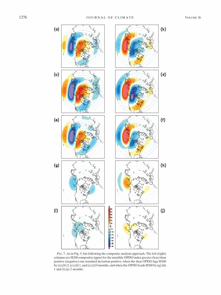
FIG. 7. As in Fig. 5, but following the composite analysis approach. The left (right)

columns areH200 composites (gpm) for themonthlyOPDO index greater (less) than

positive (negative) one standard deviation positive, when the then OPDO lags H200

by (a),(b) 2, (c),(d) 1, and (e),(f) 0months, andwhen theOPDO leadsH200 by (g),(h)

1 and (i),(j) 2 months.


FIG. 8. Regression patterns of H200 anomalies (gpm) associated with one standard

deviation departures of the PC time series of the OPDO index for (left) DJF and

(right) JJA, when the OPDO lags H200 by (a),(b) 2, (c),(d) 1, and (e),(f) 0 months,

and when the OPDO leads H200 by (g),(h) 1 and (i),(j) 2 months.


FIG. 9. As in Fig. 5, but for regression patterns of (left) surface temperature

anomalies (8C) and (right) precipitation (0.1 mm day21) associated with one standard

deviation departures of the PC time series of the OPDO index when the OPDO lags

H200 by (a),(b) 2, (c),(d) 1, and (e),(f) 0 months, and when the OPDO leads H200 by

(g),(h) 1 and (i),(j) 2 months.


indices based on the EOF of residual monthly means.

The removal of the ENSO-related signal follows a sim-

ple procedure where a reconstruction based on the re-

gression between Nino-3.4 SST index and monthly mean

of ocean and atmospheric anomalies is removed from

the original monthly mean data.

In Fig. 10 the autocorrelations (top panel) and lead–

lag correlations (bottom panel) between the OPDO

and the APDO indices for both sets of calculations are

shown. When the influence of ENSO is included, the

autocorrelation for both APDO and OPDO indices has

a somewhat slower decay than for the no-ENSO simu-

lation. This is to be expected since ENSOSST anomalies

in the equatorial tropical Pacific (which have a long time

scale) impart a persistent forcing on the APDO, thereby

tilting its probability to bemore in a particular phase and

resulting in a longer persistence time scale. A longer

persistence in the APDO then also leads to a longer

time scale for the OPDO index compared to that for

the no-ENSO simulation.

For the analysis when the ENSO signal is linearly

removed, the autocorrelations for both the APDO and

theOPDO indices, however, aremuch closer to the ones

for the no-ENSO simulation (Fig. 3, top), indicating that

a linear superposition of the contribution due to the

ENSO response and due to the atmospheric internal

variability on the temporal characteristics of these in-

dices may be a good approximation (Wang et al. 2012).

With the ENSO variability, similar to the analysis for

the autocorrelation, the lead–lag correlation (Fig. 10b) is

somewhat higher between the two indices and further-

more has a slightly higher correlation when the OPDO

index leads the APDO index. This is a consequence of

the OPDO index having a higher chance to be in phase

with the subsequent values of the APDO index that

could now be sustained by the slowly varying ENSO

SST forcing. However, once the ENSO influence from

both the indices is removed, the lead–lag correlation is

smaller and has values similar to that for the no-ENSO

simulation.

For the ENSO simulation we repeat the analysis in

Fig. 5 to assess the lead–lag response in H200, and to

see if conclusions similar to that for the no-ENSO sim-

ulation hold. The result from this analysis is shown in

Fig. 11 (left column). Similar to that for the no-ENSO

simulation, there is substantial decrease in amplitude in

H200 when the OPDO index leads height anomalies.

However, consistent with the higher correlation shown

in Fig. 10, the amplitude of H200 is larger than the

corresponding amplitude for the no-ENSO simulation

(Fig. 5). This discrepancy is accounted for after the

ENSO signal is linearly removed (Fig. 11, right column),

indicating that the larger amplitude for H200 (lagging

the OPDO index) occurs because of the influence of

ENSO, and not because of the OPDO index having

larger influence on the atmospheric circulation in the

presence of ENSO. This analysis indicates that the fun-

damental relationship between the OPDO and APDO is

retained in the presence of ENSO.

Can the information about the OPDO-related SST

help improve seasonal prediction based on ENSO alone?

In the traditional approach for ENSO-based seasonal

prediction, atmospheric composites for different phases

of ENSO (e.g., El Nino or La Nina) are used as specifi-

cations for the future state of the atmosphere once the

future state of ENSO itself is anticipated. Will adding

the information about the current state of the OPDO

improve the prediction based solely on ENSO? In other

words, can ENSO composites conditional to the state

of the OPDO be more useful for seasonal prediction?

Based on the analysis of 500-yr ENSO simulation, we

demonstrate that this is not the case.

We consider the positive phase of theENSO–ElNino

and construct composites conditional to the phase of the

OPDO index. This approach splits all El Ninos (defined

as when the Nino-3.4 SST index exceeds unit standard

FIG. 10. As in Fig. 3; the additional lines are autocorrelation and

lead–lag correlation for the ENSO simulation (red), and ENSO

simulation but after linearly removing the ENSO component

(green; see text for more details). Corresponding analysis for the

no-ENSO simulation is also shown (blue) and is the same as in

Fig. 3. Dotted lines are for the APDO index and solid lines for the

OPDO index. Black dotted lines indicate the 99% significance

level, estimated by the Monte Carlo test.


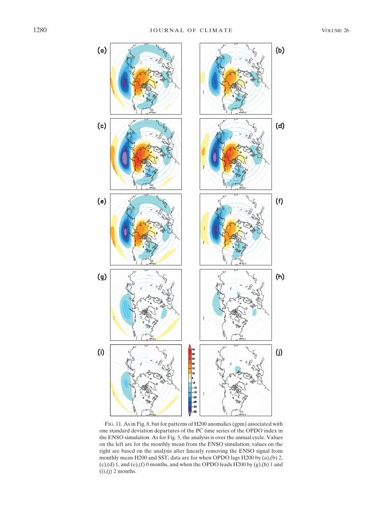
FIG. 11. As in Fig. 8, but for patterns of H200 anomalies (gpm) associatedwith

one standard deviation departures of the PC time series of the OPDO index in

the ENSO simulation. As for Fig. 5, the analysis is over the annual cycle. Values

on the left are for the monthly mean from the ENSO simulation; values on the

right are based on the analysis after linearly removing the ENSO signal from

monthly mean H200 and SST; data are for when OPDO lags H200 by (a),(b) 2,

(c),(d) 1, and (e),(f) 0 months, and when the OPDO leads H200 by (g),(h) 1 and

(i),(j) 2 months.


deviation) in the 500-yr simulation into ones when the

OPDO index is positive and when OPDO index is neg-

ative, and constructs two separate atmospheric compos-

ites for the El Nino conditional to the state of the OPDO.

Lead–lag H200 El Nino composites for the two phases

of the OPDO index are shown in Fig. 12. The left (right)

column is for the positive (negative) OPDO index when

H200 anomalies associated with the respective phase of

the OPDO are in (out of) phase with the extratropical

response to El Nino. The main difference between the

two El Nino H200 conditional composites is when the

OPDO index lags the H200—that is, when atmospheric

circulation anomalies associated with the APDO are re-

sponsible for the establishment of the SST anomalies

associated with the corresponding OPDO index. Be-

yond lag zero, however, when either phase of the OPDO

index does not constrain the APDO index, the condi-

tional H200 El Nino composites are similar, and fur-

thermore are basically the unconditional El Nino H200

composite (not shown). The difference between the two

El Nino composites in Fig. 12 is also consistent with the

linear superposition of the unconditional El Nino H200

composite and H200 composites associated with the two

phases of the OPDO index (analysis not shown).

After the demonstration that concurrent knowledge

of the El Nino and OPDO index does not help improve

seasonal prediction of atmospheric anomalies, the last

issue we discuss is the El Nino composites conditioned

to the low-frequency (LF) phase of the OPDO. This dis-

cussion is in light of results discussed by Gershunov and

Barnett (1998), who reported differences in ENSO tele-

connection in extratropical latitudes during different LF

phases of the OPDO index. The LF OPDO time series

used in this study is obtained by processing the 500-yr

monthly OPDO index through a Lanczos low-pass filter

(Duchon 1979) with a cutoff period of 8 years. The

filtered OPDO time series highlights the LF evolution

of the OPDO and excludes month-to-month and in-

terannual variations.

Although the autocorrelation of the monthly OPDO

index is small (Fig. 3), the OPDO can preferentially stay

in one phase for an extended period of time (see the

OPDO time series in Fig. 1). This can be confirmed

based on the spectral analysis of the monthly OPDO

index having a significant energy in long time scales [see

Wang et al. (2012) for the spectral analysis of the OPDO

index for the simulations used in this paper]. If the sto-

chastic atmospheric variability (i.e., the APDO) is the

primary forcing for the OPDO, then the LF component

of the OPDO is merely a consequence of the APDO

being in a particular phase more often by chance alone.

With this basic premise, the influence of LF variability

of the OPDO on the ENSO composite is discussed. For

a long enough time series (as is the case for the model

simulations) one can construct El Nino composites con-

ditional to the LF phases of the OPDO (Gershunov and

Barnett 1998). By construction, El Nino composites

(which are based on monthly variability of the Nino-3.4

SST index) in the positive (negative) LF phase of the

OPDO will also have a preponderance of the positive

(negative) phase of the corresponding OPDO index,

and consequently will have a larger probability for the

APDO (which forces the OPDO) to be in the phase

consistent with the LF phase of the OPDO index. We

confirmed that atmospheric composites for El Nino

conditional to the positive and negative LF phases of

the OPDO index do indeed differ (not shown), and the

difference is mainly in the amplitude of the unconditional

El Nino composite that is modulated by the mean cir-

culation anomalies corresponding to the LF phase of

the OPDO. This should not come as a surprise since

any subcategorization of El Nino based on an indepen-

dent index will contain the atmospheric signature corre-

sponding to that index. For example, to construct El Nino

composites conditional to the LF phase of the North

Atlantic Oscillation (NAO), the resulting atmospheric

composites will contain the atmospheric fingerprint of

the NAO.

We have already discussed that added information of

the monthly OPDO index does not add to the prediction

based on the El Nino index. The question we now pose is

whether the differences in the El Nino composites for

different LF phases of the OPDO index have a pre-

dictive capability. To assess the potential predictability

(or the skill) of H200 anomalies due to El Nino-based

conditional and unconditional H200 composites, an anom-

aly correlation analysis similar to Fig. 6 was done. The

anomaly correlation computed over El Nino events and

based on various ENSO composites (i.e., conditional and

unconditional) is shown in Fig. 13. The analysis pro-

cedure is as follows: 1) monthly mean H200 anomalies

for December is predicted based on knowing the Nino-

3.4 SST index and the LF phase of the ODPO in the

months of November or October (i.e., using lagged

value for the indices), 2) the corresponding H200 un-

conditional or conditional composite are specified as

the prediction, and 3) a similar procedure for H200

prediction is repeated for the months of January and

February, and then anomaly correlation between the

model simulated and predicted H200 is computed over

the El Nino years. The general procedure for obtaining

H200 El Nino composites conditional to the LF phase

of the OPDO is the same as for the monthly OPDO

index except that the separation of El Ninos into two

categories is now according to the sign of the LF phase

of the OPDO.


FIG. 12. As in Fig. 11, but for H200 (gpm) composites based on the Nino-3.4

SST index greater than one standard deviation (i.e., El Nino events) in the

model simulation. On the left (right) are shown H200 composites when in ad-

dition to a Nino-3.4 SST index greater than one standard deviation, the monthly

OPDO index is also greater (smaller) than positive (negative) one standard

deviation. Data are for when the OPDO lags H200 by (a),(b) 2, (c),(d) 1, and

(e),(f) 0months, andwhen theOPDO leadsH200 by (g),(h) 1 and (i),(j) 2months.


FIG. 13. Spatial map of anomaly correlation between model-simulated H200 and specification of various H200

composites as the prediction, showing prediction of DJF anomalies with (left) zero- and (right) one-month lead.

Shown are (a),(b) anomaly correlation for unconditional El Nino composite as the forecast; (c),(d) the difference

between anomaly correlation for El Nino composite that is conditioned to the low-frequency phase of the OPDO

as the forecast and that in (a) and (b), respectively; and (e),(f) the difference between anomaly correlation for

El Nino composite that is conditioned to the difference phase of the monthly OPDO index and that in (a) and (b),

respectively. Blue contour indicates the 99% significance level, estimated by the Monte Carlo test.


The anomaly correlation for the unconditional El Nino

composite for zero month lead prediction (where H200

for December–February was based on H200 composites

corresponding to the Nino-3.4 SST index for November–

January) and for one-month lead prediction (whereH200

for December–February was predicted based on H200

composites corresponding to Nino-3.4 SST index for

October–December) (Fig. 13, top panels) show a spa-

tial pattern consistent with the El Nino composite with

largest skill in the tropical latitude and over the Pacific–

North American (PNA) region. The difference in skill

for the H200 El Nino composites conditioned on the

LF phase of the OPDO (Fig. 13, middle panels) indi-

cates that the skill is slightly higher, but not significantly

different from that for the unconditional composites.

For the sake of completeness the difference in anomaly

correlation for the H200 El Nino composites, now con-

ditioned to the phase of the monthly (unfiltered) OPDO

index (as in Fig. 12), is shown in the bottom panels

(Fig. 13). Consistent with the discussion related to Fig. 12,

knowledge of the phase of the monthly OPDO index

adds little to the prediction skill.

We note that skill assessment for the ENSO condi-

tional to the LF phase of the OPDO index has a con-

ceptual problem about its interpretation. This issue was

highlighted by Bretherton and Battisti (2000). The time

series of the OPDO is forced by the stochastic variability

associated with the APDO and is a consequence of

a unique realization of the APDO over a time history.

However, to actually predict the LF phase of the OPDO

over a long period of time, and use it to augment pre-

dictions based on the ENSO alone, would require pre-

dicting the monthly sequence of the history of the APDO.

Given the dominant stochastic nature of the APDO

variability, that task may not be feasible.

4. Conclusions

In this analysis we demonstrated that knowing the

PDO index based on the SST variability (i.e., the OPDO

index) does not lead to predictive value for atmospheric

anomalies. Although the understanding of OPDO vari-

ability as a red noise ocean response to white noise at-

mospheric forcing has been discussed in literature, its

implication for predicting the future state of the atmo-

sphere itself has been confusing. Part of this confusion

stems from the fact that since the OPDO index varies

on a slow time scale similar to ENSO, it is assumed that,

like ENSO, the simultaneous atmospheric teleconnec-

tion pattern associated with the OPDO will be of pre-

dictive value in subsequent months. However, as the

results indicate, since the OPDO index does not con-

strain the atmospheric variability (which remains a white

noise), the OPDO index on its own does not have pre-

dictive usefulness for atmospheric variability. Finally,

this conclusion also holds for the simulation in which

ENSO variability was included. The analysis reported

in this paper was based on a single model, and although

is supported by previous results (e.g., Pierce 2002;

Newman et al. 2003) it needs to be further substantiated

based on other model simulations. Additionally, the

CFS has some deficiencies in simulating the variability

of the OPDO. As documented inWang et al. (2012), the

peak of the power spectra for the OPDO in the ENSO

run is weaker than the observations at both the in-

terannual and decadal time scales. However, the model

deficiencies should not alter the cause and effect rela-

tionship between the OPDO and APDO discussed in

this paper, but they need to be verified based on other

model simulations.

Acknowledgments. We thank Michael Halpert,

Dr. Amy Bulter, Dr. Dimitry Smirnov, two anonymous

reviewers, and the editor for constructive comments and

suggestions.

REFERENCES

Alexander, M. A., 2010: Extratropical air–sea interaction, SST

variability, and the Pacific decadal oscillation (PDO). Climate

Dynamics: Why Does Climate Vary?, Geophys. Monogr.,

Vol. 189, Amer. Geophys. Union, 123–148.

——, I. Blade, M. Newman, J. R. Lanzante, N.-C. Lau, and J. D.

Scott, 2002: The atmospheric bridge: The influence of ENSO

teleconnections on air–sea interaction over the global oceans.

J. Climate, 15, 2205–2231.Barnston,A.G., andR. E. Livezey, 1987: Classification, seasonality

and persistence of low-frequency atmospheric circulation pat-

terns. Mon. Wea. Rev., 115, 1083–1126.

Barsugli, J. J., and D. S. Battisti, 1998: The basic effects of

atmosphere–ocean thermal coupling onmidlatitude variability.

J. Atmos. Sci., 55, 477–493.

Bretherton, C. S., and D. S. Battisti, 2000: An interpretation of the

results from atmospheric general circulation models forced by

the time history of the observed sea surface temperature dis-

tribution. Geophys. Res. Lett., 27, 767–770.

Davis, R. E., 1976: Predictability of sea surface temperature and

sea level pressure anomalies over the North Pacific Ocean.

J. Phys. Oceanogr., 6, 249–266.

Delworth, T. L., 1996: North Atlantic interannual variability in

a coupled ocean–atmosphere model. J. Climate, 9, 2356–2375.Deser, C., M. A. Alexander, S.-P. Xie, and A. S. Phillips, 2010: Sea

surface temperature variability: Patterns and mechanisms.

Annu. Rev. Mar. Sci., 2, 115–143.

Duchon, C. E., 1979: Lanczos filtering in one and two dimensions.

J. Appl. Meteor., 18, 1016–1022.

Frankignoul, C., and K. Hasselmann, 1977: Stochastic climate

models, Part II: Application to sea-surface temperature vari-

ability and thermocline variability. Tellus, 29, 289–305.

——, N. Sennechael, Y.-O. Kwon, and M. A. Alexander, 2011:

Influence of the meridional shifts of the Kuroshio and the


Oyashio Extension on the atmospheric circulation. J. Climate,

24, 762–777.

Gershunov, A., and T. P. Barnett, 1998: Interdecadal modulation

of ENSO teleconnections. Bull. Amer. Meteor. Soc., 79, 2715–2725.

Goodrich, G. B., 2007: Influence of the Pacific decadal oscillation

on winter precipitation and drought during years of neutral

ENSO in the western United States. Wea. Forecasting, 22,116–124.

Hasselmann, K., 1976: Stochastic climate models, Part 1: Theory.

Tellus, 28, 473–485.

Horel, J. D., and J. M. Wallace, 1981: Planetary-scale atmospheric

phenomena associated with the Southern Oscillation. Mon.

Wea. Rev., 109, 813–829.

Hu, Z.-Z., and B. Huang, 2009: Interferential impact of ENSO

and PDO on dry and wet conditions in the U.S. Great Plains.

J. Climate, 22, 6047–6065.

Jha, B., and A. Kumar, 2009: A comparison of the atmospheric

response to ENSO in coupled and uncoupled model simula-

tions. Mon. Wea. Rev., 137, 479–487.

Kumar, A., and M. P. Hoerling, 2000: Analysis of a conceptual

model of seasonal climate variability and implications for

seasonal predictions. Bull. Amer. Meteor. Soc., 81, 255–264.——, ——, M. Ji, A. Leetmaa, and P. Sardeshmukh, 1996: As-

sessing a GCM’s suitability for making seasonal predictions.

J. Climate, 9, 115–129.——, Q. Zhang, J.-K. E. Schemm, M. L’ Heureux, and K.-H. Seo,

2008: An assessment of errors in the simulation of atmospheric

interannual variability in uncoupled AGCM simulations.

J. Climate, 21, 2204–2217.Kwon, Y.-O., M. A. Alexander, N. A. Bond, C. Frankignoul,

H. Nakamura, B. Qiu, and L. Thompson, 2010: Role of the

Gulf Stream and Kuroshio–Oyashio systems in large-scale

atmosphere–ocean interaction: A review. J. Climate, 23, 3249–3281.

Lau, N.-C., and M. J. Nath, 1996: The role of the ‘‘atmospheric

bridge’’ in linking tropical Pacific ENSO events to extra-

tropical SST anomalies. J. Climate, 9, 2036–2057.

Liu, Z., 2011: Dynamics of interdecadal climate variability: An

historical perspective. J. Climate, 25, 1963–1995.

Mantua, N. J., S. R. Hare, Y. Zhang, J. M. Wallace, and R. Francis,

1997: A Pacific interdecadal climate oscillation with impacts

on salmon production.Bull. Amer. Meteor. Soc., 78, 1069–1079.

Newman, M., G. P. Compo, and M. A. Alexander, 2003: ENSO-

forced variability of the Pacific decadal oscillation. J. Climate,

16, 3853–3857.Pierce, D. W., 2002: The role of sea surface temperatures in in-

teractions between ENSO and the North Pacific Oscillation.

J. Climate, 15, 1295–1308.

——, T. P. Barnett, N. Schneider, R. Saravanan, D. Dommenget,

and M. Latif, 2001: The role of ocean dynamics in producing

decadal climate variability in the North Pacific. Climate Dyn.,

18, 51–70.Reynolds, R. W., N. A. Rayner, T. M. Smith, D. C. Stokes, and

W.Wang, 2002: An improved in situ and satellite SST analysis

for climate. J. Climate, 15, 1609–1625.

Robinson, W. A., 2000: Review of WETS—The workshop on

extra-tropical SST anomalies. Bull. Amer. Meteor. Soc., 81,

567–577.

Roy, S. S., G. B. Goodrich, and R. C. Balling Jr., 2003: Influence of

El Nino/Southern Oscillation, Pacific decadal oscillation, and

local sea surface temperature anomalies on peak season mon-

soon precipitation in India. Climate Res., 25, 171–178.

Saha, S., and Coauthors, 2006: The NCEP Climate Forecast Sys-

tem. J. Climate, 19, 3483–3517.

Trenberth, K. E., G. W. Branstator, D. J. Karoly, A. Kumar, N. C.

Lau, and C. Ropelewski, 1998: Process during TOGA in un-

derstanding and modeling global teleconnections associated

with tropical sea surface temperatures. J. Geophys. Res., 103

(C7), 14 291–14 324.

Wang, H., A. Kumar, W. Wang, and Y. Xue, 2012: Influence of

ENSO on Pacific decadal variability: An analysis based on the

NCEP Climate Forecast System. J. Climate, 25, 6136–6151.

Zhang, Q., A. Kumar, Y. Xue, W. Wang, and F.-F. Jin, 2007:

Analysis of the ENSO cycle in the NCEP coupled forecast

model. J. Climate, 20, 1265–1284.


Does Knowing the Oceanic PDO Phase Help Predict the Atmospheric Anomalies in Subsequent Months?

Documents

Transcript of Does Knowing the Oceanic PDO Phase Help Predict the Atmospheric Anomalies in Subsequent Months?