NBER WORKING PAPER SERIES

DOES FEMALE EMPOWERMENT PROMOTE ECONOMIC DEVELOPMENT?

Matthias DoepkeMichèle Tertilt

Working Paper 19888http://www.nber.org/papers/w19888

NATIONAL BUREAU OF ECONOMIC RESEARCH1050 Massachusetts Avenue

Cambridge, MA 02138February 2014

We thank Nava Ashraf, Abhijit Banerjee, Lori Beaman, Chris Blattman, Areendam Chanda, StefanDercon, Doug Gollin, Andreas Irmen, Dean Karlan, John Knowles, Per Krusell, Ghazala Mansuri,Sonia Oreffice, Jesefina Posadas, Mark Rosenzweig, Nancy Stokey, Silvana Tenreyro, Duncan Thomas,Dominique van de Walle, Martin Zelder, and seminar participants at Bocconi, Brown, Hannover, Iowa,Marburg, Northwestern, Western Ontario, the NBER/BREAD Conference on Economic Development,IGC Growth Week, SITE, the SED Annual Meeting, the NBER Summer Institute, the CIDE-ThReDConference, the Cologne Macro Workshop, and the ReStud Board Meetings for helpful commentsthat greatly improved the paper. Financial support from the World Bank's Gender Action Plan, theNational Science Foundation (grants SES-0820409 and SES-0748889), and the European ResearchCouncil is gratefully acknowledged. Marit Hinnosaar, Vuong Nguyen, and Veronika Selezneva providedexcellent research assistance. The views expressed herein are those of the authors and do not necessarilyreflect the views of the National Bureau of Economic Research.

NBER working papers are circulated for discussion and comment purposes. They have not been peer-reviewed or been subject to the review by the NBER Board of Directors that accompanies officialNBER publications.

© 2014 by Matthias Doepke and Michèle Tertilt. All rights reserved. Short sections of text, not toexceed two paragraphs, may be quoted without explicit permission provided that full credit, including© notice, is given to the source.

Does Female Empowerment Promote Economic Development?Matthias Doepke and Michèle TertiltNBER Working Paper No. 19888February 2014JEL No. D13,J16,O10

ABSTRACT

Empirical evidence suggests that money in the hands of mothers (as opposed to fathers) increasesexpenditures on children. From this, should we infer that targeting transfers to women is good economicpolicy? In this paper, we develop a non-cooperative model of household decision making to answerthis question. We show that when women have lower wages than men, they may spend more on children,even when they have exactly the same preferences as their husbands. However, this does not necessarilymean that giving money to women is a good development policy. We show that depending on thenature of the production function, targeting transfers to women may be beneficial or harmful to growth.In particular, such transfers are more likely to be beneficial when human capital, rather than physicalcapital or land, is the most important factor of production.

Matthias DoepkeNorthwestern UniversityDepartment of Economics2001 Sheridan RoadEvanston, IL 60208and NBERdoepke@northwestern.edu

Michèle TertiltDepartment of EconomicsUniversity of MannheimL7, 3-568131 MannheimGermanytertilt@uni-mannheim.de

1 Introduction

Across countries and time, there is a strong positive correlation between the rela-tive position of women in society and the level of economic development (Duflo2012; Doepke, Tertilt, and Voena 2012). Based on this correlation, among policymakers the idea has taken hold that there may be a causal link running from fe-male empowerment to development. If this link were to prove real, empoweringwomen would not just be a worthy goal in its own right, but could also serve asa tool to accelerate economic growth.

Indeed, in recent years female empowerment has become a central element ofdevelopment policy. In 2006, the World Bank launched its Gender Action Plan,which was explicitly justified with the effects of female empowerment on eco-nomic development.1 Female empowerment also made its way into the UnitedNations’ Millennium Development Goals, again with reference to the claimedeffects on development: “putting resources into poor women’s hands while pro-moting gender equality in the household and society results in large develop-ment payoffs. Expanding women’s opportunities [. . . ] accelerates economicgrowth.”2

To the extent that female empowerment means reducing discrimination againstwomen in areas such as access to education and labor markets, the existence of apositive feedback from empowerment to development may be uncontroversial.However, a number of empowerment policies go beyond gender equality, andexplicitly favor giving resources to women while excluding men. For example,in 2008 the World Bank committed $100 million in credit lines specifically to fe-male entrepreneurs. Further, the majority of micro credit programs around theworld and many cash transfer programs such as Oportunidades in Mexico are nowavailable exclusively to women.

1At the launch of the Gender Action Plan, World Bank president Paul Wolfowitz said that“women’s economic empowerment is smart economics [. . . ] and a sure path to development”(quoted on World Bank web page, accessed on January 17, 2014). Similarly, in 2008 then-presidentRobert Zoellick claimed that “studies show that the investment in women yields large social andeconomic returns” (speech on April 11, 2008, quoted on the World Bank web page, accessed onJanuary 17, 2014).

2See http://www.worldbank.org/mdgs/gender.html, accessed on January 17, 2014.

1

These are reverse discrimination policies that are not easily justified on equalitygrounds. Rather, they are founded on the belief that they yield returns in terms ofeconomic development. In this paper, we provide the first study to examine thebasis for this belief from the perspective of economic theory. Specifically, we in-corporate a theory of household bargaining in a model of economic growth, andexamine whether targeting transfer payments to women really promotes eco-nomic development.

At first sight, it may appear that existing empirical evidence is sufficient to con-clude that these policies boost economic growth. A number of studies suggestthat when transfer payments are given to women rather than to their husbands,expenditures on children increase.3 To the extent that more spending on childrenpromotes human capital accumulation, this may seem to imply that empower-ing women will result in faster economic growth. Nonetheless, we argue thatthe true effect of targeted transfers depends on the specific mechanism that leadswomen to spend more money on children.

The conventional interpretation of the observed gender expenditure patterns re-lies on women and men having different preferences.4 And indeed, if all womenhighly valued children’s human capital whereas all men just wanted to con-sume, putting women in charge of allocating resources would probably be a goodidea. However, we show that the facts can also be explained without assumingthat women and men have different preferences. We develop a model in whichwomen and men value private and public goods (such as children’s human capi-tal) in the same way, but that nevertheless is consistent with the empirical obser-vation that an increase in female resources leads to more spending on children.Our theory does not lead to clear-cut implications for economic development.

3There is strong evidence against income pooling (e.g., Attanasio and Lechene 2002), andmany studies document that higher female income shares are associated with higher child ex-penditures (Thomas 1993; Lundberg, Pollak, and Wales 1997; Haddad, Hoddinot, and Alderman1997; Duflo 2003; Qian 2008; Bobonis 2009). We discuss this literature in more detail in an earlierversion of this paper, Doepke and Tertilt (2011).

4Studies that feature a preference gap between husband and wife include Lundberg and Pol-lak (1993), Anderson and Baland (2002), Basu (2006), Atkin (2009), Bobonis (2009), Browning,Chiappori, and Lechene (2009), and Attanasio and Lechene (2013), although none of these papersexplicitly considers the growth effects of transfers to women. We examine the effects of transfersin a preference-based model in an earlier version of this paper (Doepke and Tertilt 2011).

2

In particular, we find that empowering women is likely to accelerate growth inadvanced economies that rely mostly on human capital, but may actually hurtgrowth in economies where physical capital accumulation is the main engine ofgrowth.

We begin our analysis by developing a tractable theory of decision making in ahousehold composed of a wife and a husband. The spouses split their time be-tween working in the market and in household production, with the only asym-metry between the spouses being a difference in their market wages. The cou-ple plays a noncooperative equilibrium, i.e., each spouse makes decisions takingthe actions of the other spouse as given. A key feature of the environment isthat a large number (in fact, a continuum) of public goods is produced withinthe household. Public goods are goods from which both spouses derive utility;examples include shelter, furniture, and the many aspects of spending on and in-vesting in children. Household public goods are differentiated by the importanceof goods and time in producing them. In equilibrium, the low-wage spouse (i.e.,typically the wife) specializes in providing relatively time-intensive householdpublic goods.5

We then ask how a mandated wealth transfer from husband to wife affects theequilibrium allocation. Even though preferences are symmetric, mandated trans-fers affect male- and female-provided public goods differently, due to the en-dogenous specialization pattern in household production. In particular, a trans-fer to the wife increases the provision of female-provided, i.e. time-intensive,public goods. Assuming that child-related public goods are relatively intensivein time, the model is consistent with the observed effects that transfers targetedto women have on spending on children. In addition, a mandated transfer alsoincreases the wife’s private consumption and lowers the husband’s private con-sumption. Hence, the model also rationalizes that transfers lead to more spend-ing on female clothing (Phipps and Burton 1998; Lundberg, Pollak, and Wales1997), while lowering spending on male clothing, alcohol, and tobacco (Hod-

5Specialization within the household was first discussed in the literature on the sexual divisionof labor (Becker 1981). However, most of this literature employs unitary models of the household,whereas we embed household production in a noncooperative model.

3

dinott and Haddad 1995; Duflo and Udry 2004).6

Turning to implications for development, we find that our household productionmechanism leads to a fundamentally different tradeoff than does the preference-based mechanism when considering the implications of mandated transfers frommen to women. In a model where women derive more utility from public goods,the higher public-good spending (i.e., spending on children) induced by a trans-fer comes at the expense of male private consumption. In contrast, in the house-hold production model the increase in the provision of female-provided publicgoods comes at least partly at the expense of male-provided public goods.

To spell out what this means for economic growth, we embed our model ofhousehold decision making into an endogenous growth model driven by theaccumulation of human and physical capital. Parents care about their privateconsumption and their children’s future income, which they can raise by invest-ing in children’s human capital (which is time-intensive) and by leaving bequestsof physical capital. In equilibrium, bequests are provided by husbands, whereaswives play a large role in human capital accumulation. We show that a mandatedtransfer from husband to wife leads to an increase in children’s human capital,but a decrease in the physical capital stock. Whether such a policy increases eco-nomic growth depends on the state of technology. In a setting where humancapital is the main driver of growth, mandated transfers to women do promotedevelopment, but they slow down economic growth when the share of physicalcapital in production is large. Given that the human capital share tends to in-crease in the course of development, our results imply that mandated transfersto women may be beneficial in advanced, human capital-intensive countries, butare unlikely to promote growth in less developed economies.

Of course, the implications of female empowerment for economic developmentalso depend on the relative importance of the household production mechanismdeveloped here versus the preference-based mechanism. It is not our intention todeny the possibility that men and women have different preferences,7 but it is not

6Assuming, of course, that men spend a greater share of their private consumption on alcoholand tobacco, and that they are more likely to dress in male versus female clothing.

7In fact, we allow for a preference gap in our own previous work (Doepke and Tertilt 2009)and provide evolutionary justifications for why such a gap may exist.

4

obvious how important such differences are for explaining the data. Experimen-tal evidence shows that women are more risk-averse than men, but in regard tosocial preferences (which would be more relevant here) results are inconclusive(Croson and Gneezy 2009).8 In addition, there is a fair amount of empirical ev-idence supporting the implication of the household production mechanism thatmandated transfers induce a reallocation from male- to female-provided publicgoods, rather than an increase in public goods overall. For example, a number ofstudies suggest that mandated transfers to women raise household expenditureoverall, implying that savings (which is what remains of income after expendi-ture) would benefit more from targeting transfers to men.9 In addition, recentrandomized field experiments have found that transfers to men running smallbusinesses lead to a substantial increase in business profits a few years later,whereas no such effect is found for women (De Mel, McKenzie, and Woodruff2009; Fafchamps et al. 2011). Once again, this finding is consistent with the viewthat men are more likely to use additional funds for investment. Another dis-tinct implication of the household production mechanism is that the size of theeffects of mandated transfers depend on the size of the wage gap. In particular,we show that mandated transfers have a big effect only when the gender wagegap is large. While existing empirical evidence does not speak to this prediction,it could be easily tested in future research.

Our analysis builds on the literature on the noncooperative model of the house-hold, which in turn is closely related to the literature in public economics on thevoluntary provision of public goods.10 Relative to these literatures, a key nov-elty of our paper is that we consider a setting with a continuum of public goodsthat are distinguished by the time-intensity of production; without these features,our theory would not be able to address the facts we are trying to explain. An-

8There is also evidence that women and men have different preferences as policymakers(Chattopadhyay and Duflo 2004; Miller 2008), but it is not obvious whether such differences aredue to “deep” preferences or to the different roles that women and men play in society.

9In particular, studies of micro finance institutions have found that that the provision of creditto women led to a large increase in household expenditures (Pitt and Khandker 1998; Khandker2005) which is consistent with the view that women spend the additional money while men savemore of it.

10See Lundberg and Pollak (1994) and Konrad and Lommerud (1995) for the noncooperativemodel of the household, and Bergstrom, Blume, and Varian (1986) for a related discussion of thevoluntary provision of public goods.

5

other branch of the literature on family decision making relies on cooperativemodels, in which couples achieve efficient outcomes.11 We rely on a noncoopera-tive model here, because in a cooperative model preference differences betweenwomen and men are the only possible explanation for the observed effects ofmandated transfers.12 We are not suggesting that it is truly impossible for cou-ples to cooperate; after all, couples are in a long-term relationship and often careabout each other. Rather, our objective is to describe, in a stark setting, a newmechanism that is present when decision making is not completely frictionless.The empirical literature on the collective model finds some support for efficiency,but at the same time, other empirical papers provide direct evidence of signifi-cant inefficiencies in family decision making in the developing-country context(Udry 1996; Duflo and Udry 2004; Goldstein and Udry 2008). The household pro-duction mechanism is relevant if at least a fraction of households fails to achieveefficiency, which Del Boca and Flinn (2012) argue to be the case even in a rich-country setting.13 Our work also relates to a recent political-economy literatureon the causal link from development to women’s rights (Doepke and Tertilt 2009;Fernandez 2013). In contrast to these papers, here we explore the reverse linkfrom female empowerment to economic development.14

In the following section, we introduce our baseline model and demonstrate thatmandated transfers to women affect the supply of public goods. In Section 3, weshow that depending on the relative importance of female- versus male-providedpublic goods, mandated transfers can either raise or lower the total supply of

11See in particular the collective model introduced by Chiappori (1988, 1992).12The reason is that an efficient bargaining problem is equivalent to a Pareto problem with

joint budget constraints. In such a problem, in the budget constraint all resources are pooled, sothat mandated transfers cannot affect the outcome through the constraint set. Rather, the onlypossibility is that mandated transfers affect bargaining power, and that bargaining power affectsoutcomes because spouses have different preferences.

13Del Boca and Flinn (2012) estimate a model that allows for cooperative and non-cooperativedecision making in the household. Based on PSID data, they find that about one-fourth of Amer-ican couples behave in a non-cooperative way (see also Mazzocco 2007 for a related test of ex-ante efficiency in an environment with limited commitment). Similarly, Ashraf (2009) finds thatspousal observability has large effects on financial choices, which also suggests efficiencies. Inef-ficiencies can also arise from pre-marital investments, see Iyigun and Walsh (2007).

14The role of gender equality for economic growth is also analyzed in Lagerlof (2003) and de laCroix and Vander Donckt (2010), but these papers do not analyze the effects of transfers, andinstead focus on the link between gender equality and demographic change.

6

public goods in the household. In Section 4, we embed our model of householddecision making in a model of endogenous growth, and demonstrate that thegrowth effect of mandated transfers hinges on the importance of physical versushuman capital in production. Section 5 concludes. All proofs are contained in themathematical appendix.

2 Public-Good Provision in a Noncooperative Model

of the Household

2.1 The Household Decision Problem

We consider a model of noncooperative marital decision making in an environ-ment with a continuum of household public goods. Preferences are symmetricbetween women and men. In particular, the husband and wife have utility func-tions:

log(cg) +

∫ 1

0

log (Ci) di. (1)

Here cg is the private-good consumption of the spouse of gender g ∈ {f,m} (fe-male and male), and the {Ci} are a continuum of public goods for the household,indexed from 0 to 1. The public goods represent all final or intermediate goodsthat the spouses jointly care about, such as shelter or goods related to children.In Section 4 below, we provide a concrete example where all public goods areintermediate goods that affect child quality, but the general analysis is equallyapplicable to other kinds of public goods. We use log utility to simplify the anal-ysis; however, the main results carry over to more general settings.15

A key characteristic of the environment is that the public goods Ci are producedwithin the household using household production functions that combine pur-chased inputs and time. The spouses split their time between household produc-tion and participating in the formal labor market. The only asymmetry betweenthe spouses is a difference in their market wages wg.

15Generalizations in terms of preferences and technologies are discussed in Appendix B.

7

Different public goods are distinguished by the relative importance of goods andtime in producing them. Specifically, each public good is produced using a Cobb-Douglas technology where the share of goods and time varies across goods. Pub-lic good i has share parameter α(i) ∈ [0, 1] for the time input and 1 − α(i) forgoods. We assume (without loss of generality) that the function α(i) is such thatthe public goods are ordered from the least to the most time-intensive, i.e., α(i) isnon-decreasing, with α(0) = 0 and α(1) = 1. Each public good can be producedby either spouse; however, each spouse has to combine labor with his or her owngoods contribution. Thus, it is not possible to provide only the goods input fora particular Ci and leave it to the spouse to provide the labor. This assumptioncaptures that time and goods inputs often cannot be separated. For example, thepublic good “getting children fed” requires shopping for groceries first, whichtakes time and knowledge of what the children like to eat. The spouse who typi-cally does not do the feeding may lack such knowledge.16

Each spouse maximizes utility, taking the other spouse’s behavior (in particu-lar, contributions to public goods, Cg,i) as given. In other words, the solutionconcept is a Nash equilibrium, which is the sense in which decision making isnoncooperative. The maximization problem of the spouse of gender g ∈ {f,m}is to maximize (1) subject to the following constraints:

Ci = Cf,i + Cm,i ∀i, (2)

Cg,i = E1−α(i)g,i T

α(i)g,i ∀i, (3)

cg +

∫ 1

0

Eg,i di = wg(1− Tg) + xg, (4)∫ 1

0

Tg,i di = Tg. (5)

Here Eg,i is goods spending on good i by spouse g, Tg,i is the time input for goodi, Tg is the total amount of time spouse g devotes to public goods production,wg is the market wage, and xg is wealth (e.g., an initial endowment or lump-sum

16The requirement for provision of goods and time by the same spouse can also be micro-founded through a monitoring friction, i.e., spouses can provide cash to each other, but theycannot monitor how the cash is being spent. This still leaves open the possibility of general trans-fers between spouses that are not targeted towards specific public goods. Such general transfersare considered in Section 2.3 below.

8

transfer). Equation (2) states that the total provision Ci of public good i is the sumof the wife’s and the husband’s contributions. Equation (3) gives the householdproduction function for good i, where the share parameters depend on i. Equa-tion (4) is the budget constraint of spouse g. Each spouse has a time endowmentof 1, so that 1 − Tg is the time supplied to the labor market. Equation (5) is thetime constraint, which states that all time contributions to public goods add upto Tg.17

Definition 2.1 (Noncooperative Equilibrium). An equilibrium for given wages wg

and wealth levels xg consists of a consumption allocation {cg, Ci} for g ∈ {f,m} and i ∈[0, 1] and household production inputs and outputs {Eg,i, Tg,i, Tg, Cg,i} for g ∈ {f,m}and i ∈ [0, 1] such that for g ∈ {f,m}, the choices cg, Eg,i, Tg,i, Tg, Cg,i, and Ci maximize(1) subject to (2) to (5), taken the spouse’s public good supplies as given.

We now show that the household bargaining game has a generically unique equi-librium. The reason is that as long as male and female wages are different, eachspouse has a comparative advantage in providing either time- or goods-intensivepublic goods. Hence, the low-wage spouse provides a range of time-intensivegoods, whereas the high-wage spouse provides goods-intensive goods. The fol-lowing proposition summarizes the properties of the equilibrium. We focus onthe case of the husband having a higher wage. The case where the wife has ahigher wage is analogous.

Proposition 2.1 (Separate Spheres in Equilibrium). Assume 0 < wf < wm. Thereis a generically unique Nash equilibrium with the following features. There is a cutoffi such that all public goods in the interval i ∈ [0, i] are provided by the husband (i.e.,the husband provides goods-intensive goods), while public goods in the range i ∈ (i, 1]

are provided by the wife (the wife provides time-intensive goods). Private and publicconsumption satisfies

Ci =

(1− α(i))1−α(i)(

α(i)wm

)α(i)cm for i ∈ [0, i],

(1− α(i))1−α(i)(

α(i)wf

)α(i)cf for i ∈ (i, 1].

(6)

17For simplicity, throughout the paper we do not impose a constraint requiring that time spenton market work has to be non-negative. This constraint is never binding if there is only wageincome, and imposing the constraint leaves all results intact, while complicating the notation.

9

If the cutoff i is interior, it is determined such that female and male provision of publicgoods is equalized at the cutoff. Hence, if i ∈ (0, 1), the cutoff and private consumptionsatisfy the condition: (

wm

wf

)α(i)

=cmcf

. (7)

The result that household production is divided into husband and wife tasks isin line with an empirical literature that finds that many couples separate spheresof responsibility. For example, Pahl (1983) reports a sharp division of tasks in astudy of British couples. Husbands are often in charge of moving, finances, andthe car, while women make decisions regarding interior decoration, food, andchildren’s clothing. The phenomenon that husbands and wives are in charge ofdifferent purchasing decisions is studied also in the marketing literature.18 Theidea of separate spheres was first introduced into economics by Lundberg andPollak (1993). However, Lundberg and Pollak assume an exogenous separationof spheres, whereas our model features an endogenous separation. This distinc-tion is important, since the division of spheres may change in response to gov-ernment policy, as we will see in the next section.

2.2 Effect of Mandated Transfers on Public-Good Provision

With the equilibrium characterization at hand, we can now ask how changes inrelative female and male wealth affect outcomes. Consider a mandated wealthtransfer from the husband to the wife, i.e., an increase ϵ > 0 in the wife’s wealthxf and a corresponding decline in the husband’s wealth xm. Given (6), we seethat any two public goods that are provided by the same spouse both beforeand after a change in transfers will still be provided in the same proportion, be-cause public-good provision is proportional to private consumption. However,the wife’s private consumption rises relative to the husband’s private consump-tion after the transfer, which also implies that the transfer increases the provisionof female-provided public goods relative to male-provided public goods.

18For example, Wolgast (1958) finds that women are more likely to be in charge of generalhousehold goods, while husbands are often in charge of car purchase decisions. Green and Cun-ningham (1975) finds that groceries fall in the female sphere, whereas life insurance and car pur-chase decisions are typically in the male sphere. See also Davis (1976) for a survey.

10

Proposition 2.2 (Effect of Mandated Transfers on Public Good Provision). Assume0 < wf < wm. Consider the effects of a transfer ϵ > 0 from the husband to the wife, i.e.,the wife’s wealth increases from xf to xf = xf + ϵ, and the husband’s wealth decreasesfrom xm to xm = xm − ϵ. Let i be the new cutoff between male and female provision,and let cf , cm, and Ci denote the new equilibrium allocation. If the cutoff is interior bothbefore and after the transfer, then the cutoff decreases, i < i. The ratio of female privateconsumption to male private consumption cf/cm increases after the transfer. The ratio ofalways female-provided public goods (i ≥ i) to always male-provided public goods (i ≤ i)increases by the same percentage. Hence, a transfer to the low-wage spouse increases therelative provision of public goods provided by this spouse.

At first sight, the finding that a transfer to a spouse increases the public-goodprovision of this spouse may seem unsurprising. However, it stands in contrastto a well-known result in public economics on the private provision of publicgoods. The result states that when the equilibrium is interior in the sense thatall providers make voluntary contributions (in this case, husband and wife), aredistribution of income between the providers leaves the equilibrium allocationunchanged, so that a (local) version of income pooling prevails.19

In our model, the income pooling result breaks down because of the continuumof public goods. It is well-known that income redistribution does matter in vol-untary contribution games with a finite number of goods if the equilibrium is ata corner.20 Because of our continuum of goods, even though the allocation is in-terior in the sense that both spouses contribute to public goods, each good is pro-vided by only one spouse, so that there is a corner solution for any given publicgood. In this setting, the key determinant of the new level of public-good provi-sion after a transfer is the move in the cutoff between male and female provisionof public goods. The force that increases female provision is that the wife receivesthe transfer; the force that lowers female provision is that in the new equilibrium,the wife provides a wider range of public goods. In the classic public-economicsresult, the increased contributions of one spouse are fully offset by a reductionin contributions of the other spouse. In contrast, in our model the move in the

19See Warr (1983) and Bergstrom, Blume, and Varian (1986).20Browning, Chiappori, and Lechene (2009) make this point in the context of a household bar-

gaining model with a discrete number of public goods.

11

cutoff does not fully offset the direct effect of the transfer. When wealth is trans-ferred to the wife, the provision cutoff moves towards public goods that are moregoods-intensive, and hence public goods where the wife has a smaller compar-ative advantage. This unfavorable shift in comparative advantage slows downthe adjustment of the provision cutoff.

The model implications are consistent with the empirical evidence on the effectsof targeted transfers described in the introduction. Notice that there are no em-pirical studies that have information on all public and private goods producedand consumed within a household. Rather, the nature of the good is usuallyknown only for a few specific spending categories. Studies that point to an in-crease in public-good spending after a mandated transfer to the wife often fo-cus on food and children’s clothing. To the extent that these goods are usuallyfemale-provided, our theory also predicts that spending on these goods shouldrise after a transfer to the wife. Regarding private goods, empirical studies of-ten consider male and female clothing and luxuries such as alcohol. Our theorypredicts that after a mandated transfer, female private consumption should riseand male consumption should fall. Thus, the theory is consistent with the ob-servation that after a transfer, female clothing purchases increase relative to malepurchases, while spending on alcohol declines, as long as (realistically) men havea higher propensity to spend on alcohol than women do.21

We now illustrate these results with a computed example. The household pro-duction functions are parameterized by α(i) = i, i.e., time intensity varies linearlywith the index of the public good. This setting is of special interest, because it im-plies that the overall household production technology is symmetric in terms oftime versus goods intensity. We also set the female wage to half the male wage,wf = 0.5 and wm = 1, and initial wealth is zero, xf = xm = 0.

Figure 1 shows the preferred provision of each public good by the wife and hus-band, holding the marginal utility of wealth constant at its equilibrium level. Thepreferred provision curves of both spouses are U-shaped. This shape is due to the

21Our model only allows for a single homogeneous private consumption good, but it isstraightforward to reinterpret the findings in a setting where male and female private consump-tion correspond to different bundles of goods.

12

0 0.2 0.4 0.6 0.8 10.2

0.3

0.4

0.5

0.6

0.7

0.8

(Goods Intensive) i (Time Intensive)

Pro

vis

ion

Female Provision

Male Provision

Figure 1: Preferred Provision of Each Public Good for wf/wm = 0.5. Dotted line:Preferred Provision by Wife. Dashed Line: Preferred Provision by Husband.

Cobb-Douglas production technology, which induces a U-shape in unit produc-tion costs of the public goods. More importantly, the wife’s preferred provisioncurve has a uniformly larger slope than the husband’s, i.e., the wife’s preferredprovision increases relative to the husband’s as the index i increases. This followsbecause time intensity is increasing in i, and the wife has a comparative advan-tage at providing time-intensive public goods because of her lower market wagewf .

In equilibrium, each public good is provided by the spouse with the higher pre-ferred provision level. Hence, as displayed in Figure 2, the equilibrium provisioncurve is the upper envelope of the female- and male-preferred provision curves.The vertical line in Figure 2 denotes the cutoff i: to the left of this point, goodsare provided by the husband, and to the right they are provided by the wife.

Next, consider how the equilibrium provision of public goods changes if a man-

13

0 0.2 0.4 0.6 0.8 10.2

0.3

0.4

0.5

0.6

0.7

0.8

(Goods Intensive) i (Time Intensive)

Pro

vis

ion

Male ProvidedPublic Goods

Female ProvidedPublic Goods

Female Provision

Male ProvisionEquilibrium Provision

Figure 2: Provision of Each Public Good for wf/wm = 0.5. Dotted line: PreferredProvision by Wife. Dashed Line: Preferred Provision by Husband. Solid Line:Actual Provision.

dated wealth transfer from the husband to the wife is imposed. Figure 3 com-pares the baseline displayed in Figure 2 to the equilibrium outcome when thehusband has to make a transfer of ϵ = 0.3 to the wife (given that initial wealth wasset to zero, this implies that the new wealth levels are xf = 0.3 and xm = −0.3).After the transfer, the equilibrium cutoff between male and female provision ofpublic goods moves to the left, i.e., the wife (who now has higher wealth) pro-vides a wider range of public goods. However, in line with Proposition 2.2, themove in the cutoff does not fully offset the impact of the wealth transfer: equi-librium provision of all public goods that were female-provided before the trans-fer goes up, and equilibrium provision of public goods that are always male-provided goes down. In between the old and the new cutoff, the equilibriumprovider switches from husband to wife, implying that the new equilibrium pro-vision curve is steeper after the transfer compared to the initial equilibrium.

14

0 0.2 0.4 0.6 0.8 10.2

0.3

0.4

0.5

0.6

0.7

0.8

(Goods Intensive) i (Time Intensive)

Pro

vis

ion

Post−Transfer

Cutoff

Pre−Transfer

Cutoff

Pre−Transfer Provision

Post−Transfer Provision

Figure 3: Provision of Each Public Good for wf = 0.5, wm = 1 Before and AfterTransfer of ϵ = 0.3 from Husband to Wife. Dashed Line: Pre-Transfer EquilibriumProvision. Solid Line: Post-Transfer Equilibrium Provision.

Notice that the wife’s comparative advantage in providing time-intensive goods(which follows from the lower female market wage) is the only force in our modelthat slows down the shift in the cutoff between male and female provision after atransfer. Any additional forces that also slow down the shift in the cutoff wouldfurther strengthen our results. For example, consider a setting with learning bydoing, i.e., the spouses become more efficient over time at producing the publicgoods that they provide. In such a setting each spouse would gain an absoluteadvantage at providing a certain range of public goods, which would make thecutoff shift even more slowly and result in even larger effects of mandated trans-fers on public good provision.

15

2.3 Voluntary Transfers between the Spouses

In our baseline model, the only way in which the spouses interact is through theirprovision of public goods. We now explore how results change if we allow forvoluntary transfers between the spouses. Even though the spouses act noncoop-eratively, it may still be in the interest of the richer spouse to make a voluntarytransfer, because this may induce the other spouse to provide more public goods.To model this possibility, we extend our model by adding an initial stage in whichthe spouses can make voluntary transfers, followed by the noncooperative pro-vision game as described above.

To simplify the analysis, we focus on a voluntary transfer from the high-wagespouse (the husband) to the low-wage spouse (the wife). A transfer in this di-rection is more likely to be attractive, because it allows the low-wage spouse tospend more time on home production, which increases overall efficiency andpublic good provision. The transfer takes the form of a lump sum payment (an“allowance”), which the receiving spouse is then able to use in her preferred wayin the second stage. Notice that this rules out transfers that are made for theprovision of a specific public good. The reason for this assumption is that weenvision that time and goods components of a given public good are required atthe same time, and the other spouse is not able to monitor ex post how funds areused. This is a realistic assumption, because it would not be possible to enforce aspecific use of funds without actively spending time on monitoring the activity,at which point it would be more attractive to provide the public good in questiononeself. We start by formally defining an equilibrium with voluntary transfers.

Definition 2.2 (Equilibrium with Voluntary Transfer). Let Vm(wf , wm, xf , xm) de-note the equilibrium utility of the husband corresponding to the equilibrium in Defini-tion 2.1, given wages wf , wm and wealth levels xf , xm (this utility is unique becauseof Proposition 2.1). An equilibrium of the model where voluntary transfers are allowedconsists of an initial transfer X and an equilibrium as defined in Definition 2.1 for wageswf , wm and wealth levels xf +X, xm −X such that the transfer satisfies:

X = argmax0≤X≤wm+xm

{Vm(wf , wm, xf +X, xm −X)} .

16

That is, the husband picks a non-negative transfer to maximize his own ex-post utility.

The possibility of voluntary transfers is important, because if such transfers arepresent, mandated transfers imposed from the outside may no longer be effec-tive. Intuitively, if the husband finds it optimal to transfer money to his wife, hecan reduce his voluntary transfer by the amount of the mandated transfer, result-ing in the same ultimate equilibrium. The following proposition makes this pointprecise.

Proposition 2.3 (Offsetting Voluntary and Mandated Transfers). Consider an equi-librium with transfers as defined in Definition 2.2 where the optimal transfer satisfiesX > 0. If before the voluntary transfer takes place a mandated transfer of ϵ ≤ X to thewife is imposed on the husband, the husband will reduce the voluntary transfer to X − ϵ,and the resulting equilibrium allocation will be unchanged.

Hence, for our theory of the effects of mandated transfers to be viable, we need tocheck that it is not always in the husband’s interest to make a voluntary transfer.The attraction of a voluntary transfer is that it allows the wife to spend more timeon home production, from which the husband benefits. This motive for makingtransfers is especially pronounced if the wage gap between husband and wife islarge. However, there is also a downside to making a transfer, which is that atleast part of the transfer will be diverted for the wife’s private consumption. Wenow establish that even if the wage gap between the spouses is arbitrarily large,the husband does not always want to make a transfer.

Proposition 2.4 (Optimality of Voluntary Transfers). Consider the marginal impactof a voluntary transfer on the husband’s utility. As the relative wealth of the spousesapproaches the level at which i = 0 (all public goods are provided by the wife), thismarginal impact is negative:

limxf→2(wm+xm)−wf

{∂Vm(wf , wm, xf +X, xm −X)

∂X

∣∣∣∣X=0

}< 0.

Hence, the husband does not provide voluntary transfers if relative wealth is close to thislevel.

17

In practice, for realistic wage gaps the husband does not want to provide a vol-untary transfer for most of the range of initial income distributions. Specifically,voluntary transfers do not arise for all numerical examples that we present. In re-ality, of course, there are families where voluntary transfers do take place. Notice,however, that for the household production mechanism to matter empirically itis not necessary that voluntary transfers are absent in all families. Rather, it issufficient that there are at least some families where such transfers do not takeplace, and where transfers mandated from the outside are therefore effective.Our theory should be thought of as modeling the less-cooperative couples whodo not make voluntary transfers and who therefore account for the empiricallyobserved effects of mandated transfers.

2.4 Equilibrium versus Efficient Public Good Provision

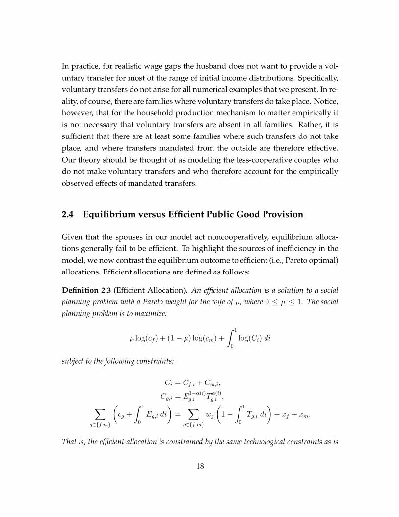
Given that the spouses in our model act noncooperatively, equilibrium alloca-tions generally fail to be efficient. To highlight the sources of inefficiency in themodel, we now contrast the equilibrium outcome to efficient (i.e., Pareto optimal)allocations. Efficient allocations are defined as follows:

Definition 2.3 (Efficient Allocation). An efficient allocation is a solution to a socialplanning problem with a Pareto weight for the wife of µ, where 0 ≤ µ ≤ 1. The socialplanning problem is to maximize:

µ log(cf ) + (1− µ) log(cm) +

∫ 1

0

log(Ci) di

subject to the following constraints:

Ci = Cf,i + Cm,i,

Cg,i = E1−α(i)g,i T

α(i)g,i ,∑

g∈{f,m}

(cg +

∫ 1

0

Eg,i di

)=

∑g∈{f,m}

wg

(1−

∫ 1

0

Tg,i di

)+ xf + xm.

That is, the efficient allocation is constrained by the same technological constraints as is

18

the equilibrium, but there is a joint budget constraint for the household, as opposed toseparate budget constraints for the two spouses.

The presence of a joint budget constraint immediately implies that mandatedtransfers between the spouses do not affect efficient allocations, because only thecouple’s total wealth enters the constraint. The following proposition character-izes efficient allocations in more detail.

Proposition 2.5 (Efficient Specialization). Efficient allocations are characterized by aPareto weight µ, where 0 ≤ µ ≤ 1, such that:

cf =1

2µ (wf + xf + wm + xm) ,

cm =1

2(1− µ) (wf + xf + wm + xm) ,

Ci =1

2(1− α(i))1−α(i)α(i)α(i)w

−α(i)f (wf + xf + wm + xm) .

Hence, the provision of public goods is independent of the Pareto weight µ, which onlymatters for the allocation of private consumption between wife and husband. All homeproduction is carried out by the wife. For given wages and wealth levels, the provisionof public goods Ci that are provided by the wife in equilibrium is always higher in theefficient allocation compared to the equilibrium allocation.

Efficient allocations and equilibrium allocations differ for two reasons. First, ef-ficient allocations feature full specialization, in the sense that only the wife isengaged in home production. This is because the wife has a comparative advan-tage in home production given her lower wage. In contrast, full specialization isnot observed in the equilibrium allocation, unless the wife has at least twice asmuch total income as the husband has. As we will see below, this feature of effi-cient allocations provides one reason for why a mandated transfer from husbandto wife may move the equilibrium closer to efficiency.

There is a second distinction between efficient and equilibrium allocations, re-lated to the weight attached to public goods in the objective function. In the socialplanning problem, the planner takes into account the utility that both spouses de-rive from public goods. In contrast, in the equilibrium allocation the provider of

19

a given public good takes into account only his or her own utility, and not that ofthe spouse. This is the well-known problem of the underprovision of voluntarilyprovided public goods, and explains why in the efficient allocation public goodprovision is usually higher. This source of inefficiency would be less important ifwe allowed for some altruism between the spouses, because then each providerwould take into account at least some of the benefit of public good provision forthe other spouse. Such an extension would be straightforward, as it amountssolely to a higher relative weight for public goods in the utility function, whileleaving the analysis otherwise unchanged. For simplicity, we abstract from altru-ism in our exposition, but it should be kept in mind that none of our results relieson the absence of altruism.

3 Do Mandated Transfers Increase the Total Provi-

sion of Public Goods?

3.1 Decomposing the Effect of Mandated Transfers

Our analysis so far provides a new rationale for why, empirically, mandatedtransfers to women have an impact on the household allocation that is differ-ent from the impact of transfers to men. From the perspective of policy impli-cations, there is a central difference between our household production mech-anism, where the gender wage gap is key, and a mechanism based on genderpreference gaps. In a model where mandated transfers affect allocations becausewomen value public goods more than men do, the increase in public-good spend-ing brought about by a transfer comes exclusively at the expense of men’s pri-vate consumption. In contrast, in the household production model an increase inpublic good spending by women comes at least partially at the expense of male-provided public goods. For this reason, whether mandated transfers to womenare good policy is not obvious.

To assess the desirability of mandated transfers in our model, we now examinethe effect of transfers on the total utility derived from public goods, which is

20

given by:22 ∫ 1

0

log (Ci) di.

While maximizing the utility derived from public goods is not equivalent to max-imizing welfare, public good provision is inefficiently low in our model gener-ally, so that an increase in public good provision moves the economy closer toefficiency.

There are three channels through which a mandated transfer affects the total pro-vision of public goods. The expenditure-share channel implies that a transfer to-wards the spouse who spends a higher share of total income on public goodsraises total public goods spending. This is particularly obvious in a corner solu-tion where one spouse provides all of the public goods (which can happen if thisspouse has much higher wealth). At this corner, the non-providing spouse has amarginal propensity to spend on public goods of zero, implying that transferringfunds from the non-provider to the provider (who has a positive propensity tospend on public goods) will increase total provision.

In an interior solution, there are two additional channels that are related to thechange in the cutoff i between male and female public good provision broughtabout by a mandated transfer. The efficiency channel arises because the spousewith a lower market wage has a comparative advantage in household produc-tion. Hence, if the low-wage spouse substitutes into household production andthe high-wage spouse into market production, the overall efficiency of time use inthe household is improved (it moves closer to the first-best allocation describedin Proposition 2.5). This channel suggests that transferring resources to the low-wage spouse (inducing this spouse to substitute from market work to householdproduction) will increase total provision of public goods. Finally, the change inthe cutoff i also implies that the resources of the provider receiving the trans-fer are spread over more public goods, while the other spouse can focus on asmaller range. This reallocation channel leads to an increase in the provision ofpublic goods if the receiver of the transfer initially provides a small range of pub-lic goods compared to his or her spouse. The following proposition formalizes

22In Section 4, we develop an extension of our model where maximizing utility derived frompublic goods corresponds to maximizing the growth rate of the economy.

21

the decomposition of the total effect of a transfer on public good provision.

Proposition 3.1 (Decomposition of Effect of Mandated Transfers on Total PublicGood Provision). Let ϵ ≥ 0 denote a mandated transfer from husband to wife, at givenwages wf , wm and pre-transfer wealth xf , xm. If there is an interior equilibrium with0 < i < 1, the total provision of public goods is given by:

∫ 1

0

log (Ci) di = B − i log

(1 + i

wm + xm − ϵ

)− (1− i) log

(2− i

wf + xf + ϵ

)−∫ i

0

α(i) di log(wm)−∫ 1

i

α(i) di log(wf ),

where B is a constant and i is the equilibrium cutoff between male and female provisionof public goods. Consequently, the derivative of total public goods provision with respectto ϵ evaluated at ϵ = 0 can be expressed as:

d∫ 1

0log (Ci) di

dϵ=− i

wm + xm

+1− i

wf + xf︸ ︷︷ ︸Expenditure Share Channel

+

[log

((2− i)(wm + xm)

(1 + i)(wf + xf )

)+

1− i

2− i− i

1 + i

]∂i

∂ϵ︸ ︷︷ ︸Reallocation Channel

− α(i) log

(wm

wf

)∂i

∂ϵ︸ ︷︷ ︸Efficiency Channel

. (8)

3.2 Conditions under which Mandated Transfers Increase Pub-

lic Good Provision

Note that ∂i∂ϵ

≤ 0, that is, a transfer to the wife increases the range of publicgoods provided by the wife. Hence, when wm > wf the efficiency channel isalways positive. However, this does not imply that a mandated transfer to thewife always increases the provision of public goods overall, because the signof the other channels is ambiguous. Indeed, we can establish that dependingon the shape of the α(i) function, a transfer from husband to wife may either

22

lower or raise total public good provision. To work towards this result, we firstcharacterize the expenditure share channel in more detail.

Proposition 3.2 (Expenditure Share Channel). Assume 0 < wf < wm. For giveninitial wealth xf and xm, consider the marginal effect of a wealth transfer ϵ from thehusband to the wife, holding constant the equilibrium cutoff i (as if each spouse hadzero productivity in providing public goods provided by the other spouse). Notably, thisimplies that only the expenditure share channel is present. The transfer increases the totalutility derived from public goods if and only if:

1− i

i>

wf + xf

wm + xm

.

That is, holding i constant, transferring resources to the wife increases the total provisionof public goods if and only if the share of public goods provided by the wife exceeds thewife’s share in total resources of the couple.

Depending on the shape of the α(i) function and the overall distribution of re-sources, the expenditure share channel can therefore favor making transfers toeither spouse. In particular, transferring resources to the husband may increasethe overall provision of public goods if a wide range of public goods are goods-intensive, which tends to increase the share of public goods provided by the hus-band.

Of course, for the expenditure channel to dominate, the remaining channels haveto be sufficiently weak. The next proposition demonstrates that depending onthe shape of the α(i) function, the other channels can be arbitrarily weak.

Proposition 3.3 (Expenditure Share Channel Can Dominate). Assume 0 < wf <

wm and that α(i) is continuously differentiable. For given initial wealth xf and xm,consider the marginal effect of a mandated transfer ϵ from the husband to the wife on theequilibrium cutoff i. The derivative ∂i

∂ϵis declining in α′(i) and can thus be arbitrarily

small if α′(i) is arbitrarily large. Given that ∂i∂ϵ

appears in both the reallocation chan-nel and the efficiency channel, this implies that by choosing α(i) these channels can bearbitrarily weakened, so that the expenditure share channel dominates.

23

An even simpler case obtains when α(i) has a discontinuity at i, in which case i

can be constant for a range of ϵ.

Taken together, these results imply that the question of whether mandated trans-fers from husbands to wives increase public good provision has no clear-cut an-swer. Instead, the effect of such transfers depends on the specifics of the tech-nology for producing public goods and on the initial distribution of wealth andrelative wages. This finding is important because of the contrast it provides to amodel that is based on differences between women and men in preferences forpublic goods. In a preference-based model, mandated transfers to the spousewho values public goods more always increases public good provision. In con-trast, our household production model suggests that the effects of such a policyare not uniform, and may depend on the stage of development and on local eco-nomic conditions.

Even though these results show that the effects of mandated transfers on publicgood provision are generally ambiguous, it is also true that the efficiency chan-nel always favors transfers to the low-wage spouse. Thus, one may conjecturethat if the environment is symmetric apart from the wage gap between womenand men, then the efficiency channel should dominate, and mandated transfersto women should increase public good provision. Hence, we now consider thecase when α(i) = i, i.e., time intensity varies linearly with the index of the publicgood. In this setting the overall household production technology is symmetricin terms of time versus goods intensity. It can indeed be shown that in the sym-metric case the efficiency channel always dominates in the interior, so that on themargin total provision of public goods is increased if wealth is transferred to thelow-wage spouse.

Proposition 3.4 (Efficiency Channel Dominates in Symmetric Case). Assume 0 <

wf < wm and α(i) = i. For given initial wealth xf and xm, consider the effects of amandated transfer ϵ from the husband to the wife, so that the new wealth levels are xf + ϵ

and xm − ϵ. If for given xf and xm the equilibrium is interior, i.e., the cutoff i betweenmale and female provision of public goods satisfies 0 < i < 1, a marginal increase in thetransfer from husband to wife increases the total provision of public goods. Formally, we

24

have:∂∫ 1

0log (Ci) di

∂ϵ> 0.

Hence, if public goods are, on average, equally time- versus goods-intensive, theefficiency channel (which favors the wife specializing in time-intensive goods)dominates.

3.3 The Effectiveness of Transfers When the Wage Gap Shrinks

One determinant of the effect of transfers on public good provision is the wagegap between men and women. The wage gap is an essential ingredient in thehousehold production mechanism, because it is what leads the two spouses tospecialize in providing different types of public goods. We now show that whenthe size of the wage gap approaches zero, the effect of mandated transfers (which-ever the sign) also goes to zero. Intuitively, given that the wage gap is the onlydifference between the sexes in our model, when the wage gap disappears sodoes the distinction between women and men. In that case, it no longer mattersmuch who controls resources.

Proposition 3.5 (Role of Wage Gap). Assume 0 < wf ≤ wm. For given initial wealthxf and xm, consider the effects of a wealth transfer ϵ from the husband to the wife onpublic good provision. When the female wage converges to the male wage, the marginaleffect of a transfer ϵ on the total provision of public goods converges to zero:

limwf→wm

∂∫ 1

0log (Ci) di

∂ϵ= 0.

Thus, the model yields the testable prediction that the effects of mandated trans-fers should be large in places where women earn very little, and small in placeswhere equality in the workplace has been nearly achieved.

To illustrate the workings of this mechanism, Figure 4 displays the impact onpublic good provision of a mandated transfer of ϵ = 0.3 from husband to wifewhen the wages are wf = 0.8, wm = 1. Compared to the case of a larger wage gap

25

0 0.2 0.4 0.6 0.8 10.2

0.3

0.4

0.5

0.6

0.7

0.8

(Goods Intensive) i (Time Intensive)

Pro

vis

ion

Post−Transfer

Cutoff

Pre−Transfer

Cutoff

Pre−Transfer Provision

Post−Transfer Provision

Figure 4: Provision of Each Public Good for wf = 0.8, wm = 1 Before and AfterTransfer of ϵ = 0.3 from Husband to Wife. Dashed Line: Pre-Transfer EquilibriumProvision. Solid Line: Post-Transfer Equilibrium Provision.

(wf = 0.5, wm = 1) shown in Figure 3, the quantitative impact on the relative pro-vision of female- and male-provided public goods is much smaller. Indeed, theimpact on equilibrium public good provision is related directly to the differencein the slope between the female and male preferred provision curve, and thisdifference converges to zero as the wage gap disappears. Once the female wageexceeds about 90 percent of the male wage, the impact of a mandated transfer onequilibrium provision is barely discernible.

4 Growth Implications of Mandated Transfers

The results in the analysis above suggest that the effect of gender-targeted trans-fers on development depend on the relative importance of male- versus female-

26

provided public goods in production. In this section, we spell out this link inmore detail using a simple growth model in which we identify male-providedpublic goods with household saving and investment. Buying land, farm animals,or physical capital involves mostly money and little time, and thus falls on thegoods-intensive side of the range of public goods. In contrast, we identify time-intensive inputs in child rearing, which are predominantly female-provided, asbeing associated with the accumulation of human capital. In this framework, weshow that the growth effect of mandated transfers that redistribute wealth frommen to women switches signs as the economy becomes relatively more intensivein human capital.

We consider a model economy that is populated by successive generations ofconstant size. Thus, each couple has two children, one boy and one girl. There ismeasure one of couples in each generation. The preferences of a spouse of genderg are given by the utility function:

log(cg) + log(y′). (9)

Here cg is the private consumption of spouse g, and y′ is the full income23 of thechildren in the next period (i.e., when the children are adults). Thus, we capturealtruism towards children in a warm-glow fashion.

Output is produced using an aggregate production function that employs physi-cal capital K and human capital H :

Y = AK1−θHθ. (10)

Below, we consider how the effects of mandated transfers depend on the shareof human capital θ. We denote the endowment of a specific couple with physicaland human capital by k and h.

Given the production function, parents can raise their children’s future incomein two different ways: by investing in their human capital, or by leaving them

23The full income of a couple consists of market income plus the value of time used for homeproduction; defining preferences in terms of market income would leave the results qualitativelyunchanged.

27

a bequest in the form of physical capital. The children’s physical capital k′ issimply the sum of the bequests bf and bm left by the mother and father:

k′ = bf + bm. (11)

The production of human capital, in contrast, is a more complex process thatinvolves combining many different inputs in a household production function.The log of the children’s human capital h′ is given by:

log(h′) =

∫ 1

0

log(Cj)dj, (12)

where, as in the analysis in the preceding sections, Cj is composed of the con-tributions of both spouses: Cj = Cf,j + Cm,j , and each spouse’s contribution isproduced with a Cobb-Douglas technology using expenditure inputs Eg,j andtime inputs Tg,j , the productivity of which depends on human capital h:

Cg,i = E1−jg,j (Tg,jh)

j . (13)

Hence, the various Cg,j serve as intermediate inputs in the production of chil-dren’s human capital. The interpretation is that the accumulation of human cap-ital requires some relatively goods-intensive inputs such as food, clothing, shel-ter, and health investments, but also more time-intensive inputs such as child-rearing, education, and enrichment activities. The essential point here is thatcompared to physical capital (which consists entirely of goods), human capital ismore intensive in parental time.

We assume that the production technology (10) for the final good (which canbe used for consumption, for intermediate goods in the production of humancapital, or for bequests) is operated by a competitive industry, so that the marketwage w and the return on capital r are given by marginal products. The children’sfull income that enters the parents’ utility function is then given by:

y′ = r′k′ + w′h′, (14)

where r′ and w′ denote the return to capital and the wage in the next period.

28

Capital fully depreciates each generation. There is an exogenous gender gap inthe sense that women’s market productivity relative to men is given by δ < 1,so that the female wage per unit of human capital supplied to the labor marketis wf = δw, whereas the male wage is simply wm = w. We also assume that thetotal endowments of physical and human capital left to the children are dividedequally between the daughter and the son. Clearly, it would be interesting to en-dogenize both the division of endowments between the children and the gendergap. However, since our focus is on mandated transfers, we abstract from theseissues here.24

As in the preceding analysis, husband and wife individually decide on labor sup-ply, household production inputs, and also on bequests. Each spouse thus maxi-mizes (9) subject to (11)–(14) and the following budget constraint:

cg + bg +

∫ 1

0

Eg,j dj =1

2

[wgh

(1−

∫ 1

0

Tg,j dj

)+ rk

]+ τg. (15)

The factor of one-half on the right-hand side appears because each spouse con-trols only one-half of the total physical and human capital endowments providedby his or her respective parents (given two-child families). In addition to capitalincome, a spouse also receives the mandated wealth transfer τg where (to allowfor market clearing) we impose:

τf + τm = 0.

We interpret the transfer as government-mandated redistribution of wealth be-tween husbands and wives, and we will consider how such transfers affect thegrowth rate of the economy.

To close the economy, we specify the market clearing conditions for physical and

24Notice that given our warm-glow utility function, parents do not prefer any specific alloca-tion of endowments between sons and daughters over any other allocation. To model a strategicmotive, a more sophisticated form of altruism would be required.

29

human capital, which (given measure one of identical families) are given by:

K = k,

H =1

2

[1−

∫ 1

0

Tm,j dj + δ

(1−

∫ 1

0

Tf,j dj

)]h.

We start our analysis of the growth model with a closer look at the householddecision problem. First, we provide an alternative representation of the utilityfunction (9).

Lemma 4.1 (Representation of Preferences). The preferences given by the utility func-tion (9) can be represented equivalently by the utility function:

U(cg, k′, h′) = log(cg) + βk log(k

′) + (1− βk) log(h′), (16)

where βk is given by:

βk =(1− θ)ϕ

θ + (1− θ)ϕ, (17)

and ϕ denotes the fraction of human capital employed in market production (which istaken as given by the individual).

Hence, the implicit weight βk on the bequest k′ in utility is decreasing in the shareθ of human capital in goods production (10), whereas the weight on the children’shuman capital h′ is increasing in θ.

Next, we show that the household decision problem in the growth model is aspecial case of the general noncooperative model analyzed in Sections 2 and 3.

Lemma 4.2 (Relation to General Decision Problem). The individual decision problemin the growth model of maximizing (16) subject to (11) to (15) is a special case of thegeneral decision problem in Section 2 of maximizing (1) subject to (2) to (5). Specifically,to map the problem in the growth model into the general decision problem, the functionα(i) is set to:

α(i) =

0 for 0 ≤ i ≤ βk,

i−βk

1−βkfor βk < i ≤ 1,

(18)

30

where βk is given by (17). Let wg and xg denote the wages and wealth levels pertainingto the general decision problem. These are set to:

wg =1

2wgh, (19)

xg =1

2rk + τg. (20)

Let cg, Ci, Cg,i, Eg,i, Tg,i, and Tg denote the equilibrium choices in the general decisionproblem given α(i), wg, and xg as specified in (18) to (20). The equilibrium choices in thedecision problem in the growth model can then be recovered as follows:

cg = cg, (21)

bg =

∫ βk

0

Cg,i di, (22)

Eg,j = (1− βk)Eg,βk+j(1−βk) ∀j ∈ [0, 1], (23)

Tg,j = (1− βk)Tg,βk+j(1−βk) ∀j ∈ [0, 1]. (24)

Intuitively, the bequest in the growth model corresponds to a range of house-hold public goods in the general model for which we have α(i) = 0, i.e., the timecomponent is zero and the goods component is one. The remaining public goodscontribute to the production of human capital. The implicit weight of the bequestin the utility function depends on the weight of physical capital in the produc-tion function. The more important physical capital is for production, the moreimportant the physical bequest becomes in the parent’s utility function, and themore goods-intensive public goods are on average. Conversely, an increase inthe human capital intensity of production also increases the implicit weight onchildren’s human capital in parental preferences, which enhances the importanceof time in producing public goods.

Lemma 4.2 implies that, given state variables k and h, the results from Sections 2and 3 apply. Specifically, this means that in equilibrium only husbands providebequests. Further, assuming the equilibrium is interior, there is a cutoff such thatamong the public goods that are inputs into human capital, the husband will bein charge of the less time-intensive inputs (such as shelter), while the wife spe-

31

cializes in time-intensive activities such as doing homework with the children. Itfollows that a mandated transfer to women will increase human capital, while atransfer to men will increase bequests and hence physical capital. This is consis-tent with the evidence, cited in the introduction, that transfers to women tend toincrease total household spending (which by construction must lower savings).

We now would like to assess the implications of these relationships for the effectof mandated transfers on economic growth. As a first step, the following propo-sition characterizes the equilibrium for the model economy in the case wheremandated wealth transfers are proportional to output. The economy convergesto a balanced growth path with a constant growth rate. Even during the tran-sition to the growth path, the time allocation is constant, and consumption andbequests are constant fractions of income per capita.

Lemma 4.3 (Equilibrium Characterization). If mandated transfers are proportional tooutput, τf = −τm = γY for some γ ≥ 0, equilibrium consumption and bequests are afixed fraction of output also, and the time allocation is constant, i.e. independent of thestate variables k and h.

Next, we establish the key result of this section: The effect of mandated transferson growth rates depends on the share of human capital in production.

Proposition 4.1 (Growth Implications of Mandated Transfers). Let mandated trans-fers be proportional to output, τf = −τm = γY for some fixed scalar γ. Consider anincrease in the transfer in one period. If both spouses contribute to human capital accu-mulation (i.e., the equilibrium is interior) and the share of human capital θ is sufficientlysmall, output Y ′ in the next period is decreasing in today’s transfer γ:

∂Y ′

∂γ< 0.

Conversely, if the share of human capital θ is sufficiently large, future output is increasingin the transfer γ:

∂Y ′

∂γ> 0.

The intuition for the proposition is that the share of human capital θ controls theextent to which male- versus female-provided public goods matter for economic

32

0.45 0.5 0.55 0.6 0.65 0.7−1.5

−1

−0.5

0

0.5

1

1.5

θ (Share of Human Capital)

Perc

en

t C

ha

ng

e i

n O

utp

ut

Transfer

Lowers Growth

Transfer

Increases Growth

Figure 5: Effect of a Mandated Transfer of 10 percent of Income per Capita fromHusband to Wife on Output in the Next Generation as a Function of HumanCapital Share θ

growth. In the limit case θ = 1 (production linear in human capital only), thecouple’s bargaining problem is of the form analyzed in Proposition 3.4, wheretransfers to women on the margin always increase public good provision (or, inthis application, the rate of economic growth). The reason is that at θ = 1 time andmoney inputs are equally important, so that the efficiency channel dominates,which favors transfers to the low-wage spouse. Conversely, as θ tends to zero(production close to linear in physical capital), growth depends mostly on goods-only public goods provided by men, i.e., men provide most of the public goods.In this case the expenditure-share channel dominates, and transfers to womenlower growth (following the intuition of the results in Propositions 3.2 and 3.3).25

Figure 5 illustrates these results with a computed example. The gender gap is setto δ = 0.5; i.e., men are twice as productive as women in the market. The figuredisplays the effect of a mandated transfer from husband to wife, amounting to 10

25The expenditure share channel also dominates in the case of a corner solution where only onespouse is contributing to public goods, i.e., a transfer to the spouse providing the public goodsincreases economic growth.

33

0.45 0.5 0.55 0.6 0.65 0.7−8

−6

−4

−2

0

2

4

6

8

θ (Share of Human Capital)

Perc

en

t C

han

ge

Human Capital

Physical Capital

Figure 6: Effect of a Mandated Transfer of 10 percent of Income per Capita fromHusband to Wife on Phyiscal and Human Capital in the the Next Generation asa Function of Human Capital Share θ

percent of income per capita, on output in the children’s generation as a functionof the human capital share θ. For low values of θ, this transfer lowers futureoutput. In this range men provide the majority of public goods. At a humancapital share of θ = 0.53, the transfer leaves future output unchanged. For evenhigher levels of θ, transfers to women increase future output. At θ = 1, thetransfer increase future output in the children’s generation by almost 2.9 percent.

Notice that even though for low θ a transfer to women lowers growth, it still in-creases the accumulation of human capital. Figure 6 breaks down the effect of themandated transfer on the accumulation of human and physical capital. Physicalcapital (the bequest) is always provided entirely by the husband in this range,whereas the wife provides most of the time-intensive inputs to human capitalproduction. Hence, regardless of θ a transfer from husband to wife results inlower bequests, but more investment in children’s human capital. Nevertheless,for low θ (production intensive in physical capital) the positive effect on humancapital is insufficient to compensate for the lower bequest.

34

If the human capital share θ were to increase slowly in the course of develop-ment, our results imply that targeting transfers to women might be beneficial atan advanced, human capital-intensive production stage, but less so at an earlierstage when human capital plays a small role. Similarly, in a cross section of coun-tries, targeting transfers to women may be counterproductive in less advancedeconomies where physical accumulation is still the main driver of growth. More-over, if female empowerment takes the form of a rise in δ, i.e. a decline in thegender wage gap, then the growth effect of mandated transfers (whether posi-tive or negative) shrinks with empowerment (see Proposition 3.5).

5 Conclusions and Outlook

In this paper we have addressed, from a theoretical perspective, the empiricalobservation that money in the hands of women leads to higher spending on chil-dren. This observation has already fueled a trend in development policy to chan-nel more resources towards women and, more generally, to envision female em-powerment as a conduit to economic development. If we are to fully understandthe effects of such gender-based development policies, however, we must firstpin down the mechanism that generates the observed empirical findings. Theconventional interpretation of the facts is that women and men have differentpreferences, in the sense that women attach more weight to children’s welfare.However, in this paper we show that the facts can be explained also by an alter-native mechanism that relies on the endogenous division of labor in householdproduction.

Under the household production mechanism, it is not obvious whether targetingtransfers to women is good policy. In particular, we show that targeting transfersto women increases the growth rate only if human capital is the key engine ofgrowth. In contrast, in economies that are driven primarily by physical capitalaccumulation, targeting transfers to women can lower economic growth, becauseincreased spending on children crowds out savings and hence physical capital ac-cumulation.26 Moreover, we show that the effects of targeted transfers disappear

26The mutual complementarity between human capital accumulation, female empowerment,

35

when the wage gap between women and men approaches zero. In other words,when women are fully empowered in the labor market, then further empower-ing them through transfers has no effect on the provision of public goods in thehousehold.

The links among the effects of targeted transfers, the share of human capital, andthe degree of labor-market discrimination suggest that there is no fixed relation-ship between female empowerment and economic development, but rather thatthe effectiveness of empowerment policies depends on the stage of development.The theory suggests that mandating wealth transfers from men to women lowerseconomic growth at an early stage of development, when there is little demandfor human capital. At a highly advanced stage of development when human cap-ital is the dominant factor of production and when women and men earn similarwages, transfers would have little effect because in this case women and men be-have similarly. The best case for these kinds of targeted transfers could be madefor countries at an intermediate stage of development, when human capital isalready a key driver of growth, but women’s labor market opportunities still lagbehind men’s.

We have limited our attention here to the implications of a narrow concept of fe-male empowerment, namely the transfer of resources from husbands to wives. Inreality, of course, female empowerment can take other forms. For example, thereare many facets of discrimination against women, not just in labor markets butalso in consumption markets, some of which may lead men and women to act asif they had different preferences.27 That is, if women had access to a more limitedset of private goods than men do, they would endogenously place less weight ontheir private consumption compared to spending on public goods. Such a mech-anism might be relevant in countries like Saudi Arabia where laws explicitly pro-hibit certain behaviors for women, such as driving. Female empowerment thatreduces such consumption discrimination would lead to lower child expenditureshares. Another important dimension of female empowerment concerns access

and economic development in our model resembles features of the political-economy analysisin Doepke and Tertilt (2009), although the mechanism is entirely different, because the model ofDoepke and Tertilt (2009) relies on preference differences.

27In Doepke and Tertilt (2011) we analyze simple examples of this kind, but do not pursue themin the context of a growth model.

36

to education, which could be analyzed in the context of our growth model withhuman capital accumulation. Reducing discrimination against women in termsof education is more likely to promote economic development, but even herethere are potential effects going in the opposite direction (such as repercussionson the time spent educating children). The bottom line is that female empower-ment cannot be regarded as a generic concept that has uniform effects at all stagesof development. Rather, the effects of female empowerment depend both on thespecific form that an empowerment policy takes, and on the nature of the econ-omy where the policy is implemented. While many of these interdependenciesremain to be disentangled in future research, we see our paper as a step towardsa more differentiated view.

References

Anderson, Siwan, and Jean-Marie Baland. 2002. “The Economics of Roscas andIntrahousehold Resource Allocation.” Quarterly Journal of Economics 117 (3):963–995.

Ashraf, Nava. 2009. “Spousal Control and Intra-Household Decision Making:An Experimental Study in the Philippines.” American Economic Review 99 (4):1245–1277.

Atkin, David. 2009. “Working for the Future: Female Factory Work and ChildHealth in Mexico.” Unpublished Manuscript, Yale University.

Attanasio, Orazio, and Valerie Lechene. 2002. “Tests of Income Pooling inHousehold Decisions.” Review of Economic Dynamics 5 (4): 720–748.

. 2013. “Efficient Responses to Targeted Cash Transfers.” UnpublishedManuscript, University College London.

Basu, Kaushik. 2006. “Gender and Say: A Model of Household Behaviour withEndogenously Determined Balance of Power.” Economic Journal 116 (511):558–580.

Becker, Gary S. 1981. A Treatise on the Family. Cambridge: Harvard UniversityPress.

37

Bergstrom, Theodore, Lawrence Blume, and Hal Varian. 1986. “On the PrivateProvision of Public Goods.” Journal of Public Economics 29 (1): 25–49.

Bobonis, Gustavo J. 2009. “Is the Allocation of Resources within the HouseholdEfficient? New Evidence from a Randomized Experiment.” Journal of PoliticalEconomy 117 (3): 453–503.

Browning, Martin, Pierre-Andre Chiappori, and Valerie Lechene. 2009. “Distri-butional Effects in Household Models: Separate Spheres and Income Pool-ing.” Economic Journal 120 (545): 786–799.

Chattopadhyay, Raghabendra, and Esther Duflo. 2004. “Women as Policy Mak-ers: Evidence from a Randomized Policy Experiment in India.” Econometrica72 (5): 1409–1443.

Chiappori, Pierre-Andre. 1988. “Rational Household Labor Supply.” Economet-rica 56 (1): 63–90.

. 1992. “Collective Labor Supply and Welfare.” Journal of Political Economy100 (3): 437–467.

Croson, Rachel, and Uri Gneezy. 2009. “Gender Differences in Preferences.”Journal of Economic Literature 47 (2): 448–474.

Davis, Harry L. 1976. “Decision Making within the Household.” Journal ofConsumer Research 2 (4): 241–260.

de la Croix, David, and Marie Vander Donckt. 2010. “Would EmpoweringWomen Initiate the Demographic Transition in Least Developed Countries?”Journal of Human Capital 4 (2): 85–129.

Del Boca, Daniela, and Chris Flinn. 2012. “Endogenous Household Interaction.”Journal of Econometrics 166 (1): 49–65.

De Mel, Suresh, David McKenzie, and Christopher Woodruff. 2009. “AreWomen More Credit Constrained? Experimental Evidence on Gender andMicroenterprise Returns.” American Economic Journal: Applied Economics 1(3): 1–32.

Doepke, Matthias, and Michele Tertilt. 2009. “Women’s Liberation: What’s in Itfor Men?” Quarterly Journal of Economics 124 (4): 1541–1591.

38

. 2011. “Does Female Empowerment Promote Economic Development?”CEPR Discussion Paper 8441.

Doepke, Matthias, Michele Tertilt, and Alessandra Voena. 2012. “The Economicsand Politics of Women’s Rights.” Annual Review of Economics 4:339–372.

Duflo, Ester. 2012. “Women Empowerment and Economic Development.” Jour-nal of Economic Literature 50 (4): 1051–1079.

Duflo, Esther. 2003. “Grandmothers and Granddaughters: Old-Age Pensionsand Intrahousehold Allocation in South Africa.” World Bank Economic Review17 (1): 1–25.

Duflo, Esther, and Christopher Udry. 2004. “Intrahousehold Resource Alloca-tion in Cote d’Ivoire: Social Norms, Separate Accounts and ConsumptionChoices.” NBER Working Paper 10498.

Fafchamps, Marcel, D. McKenzie, Simon Quinn, and Christopher Woodruff.2011. “When is Capital Enough to Get Female Microenterprises Growing?Evidence from a Randomized Experiment in Ghana.” NBER Working Paper17207.

Fernandez, Raquel. 2013. “Women’s Rights and Development.” Forthcoming,Journal of Economic Growth.

Goldstein, Markus, and Christopher Udry. 2008. “The Profits of Power: LandRights and Agricultural Investment in Ghana.” Journal of Political Economy116 (6): 981–1022.

Green, Robert T., and Isabella C. Cunningham. 1975. “Feminine Role Perceptionand Family Purchasing Decisions.” Journal of Marketing Research 12 (3): 325–332.

Haddad, Lawrence, John Hoddinot, and Harold Alderman, eds. 1997. Intra-Household Resource Allocation in Developing Countries: Models, Methods, andPolicy. Baltimore and London: Johns Hopkins University Press.

Hoddinott, John, and Lawrence Haddad. 1995. “Does Female Income ShareInfluence Household Expenditures? Evidence From Cote D’Ivoire.” OxfordBulletin of Economics and Statistics 57 (1): 77–96.

39

Iyigun, Murat, and Randall P. Walsh. 2007. “Endogenous Gender Power, House-hold Labor Supply, and the Quantity-Quality Tradeoff.” Journal of Develop-ment Economics 82 (1): 138–155.

Khandker, Shahidur R. 2005. “Microfinance and Poverty: Evidence Using PanelData from Bangladesh.” World Bank Economic Review 19 (2): 263–286.

Konrad, Kai A., and Kjell Erik Lommerud. 1995. “Family Policy with Non-cooperative Families.” Scandinavian Journal of Economics 97 (4): 581–601.

Lagerlof, Nils-Petter. 2003. “Gender Equality and Long-Run Growth.” Journalof Economic Growth 8 (4): 403–426.

Lundberg, Shelly, and Robert A. Pollak. 1993. “Separate Spheres Bargainingand the Marriage Market.” Journal of Political Economy 101 (6): 988–1010.

. 1994. “Noncooperative Bargaining Models of Marriage.” AmericanEconomic Review 84 (2): 132–137.

Lundberg, Shelly J., Robert A. Pollak, and Terence J. Wales. 1997. “Do Husbandsand Wives Pool Their Resources? Evidence from the United Kingdom ChildBenefit.” Journal of Human Resources 32 (3): 463–480.

Mazzocco, Maurizio. 2007. “Household Intertemporal Behaviour: A CollectiveCharacterization and a Test of Commitment.” Review of Economic Studies 74(3): 857–895.

Miller, Grant. 2008. “Women’s Suffrage, Political Responsiveness, and ChildSurvival in American History.” Quarterly Journal of Economics 123 (3): 1287–1327.

Pahl, Jan. 1983. “The Allocation of Money and the Structuring of Inequalitywithin Marriage.” Sociological Review 31 (2): 237–263.

Phipps, Shelley A., and Peter S. Burton. 1998. “What’s Mine is Yours? The Influ-ence of Male and Female Incomes on Patterns of Household Expenditure.”Economica 65 (260): 599–613.

Pitt, Mark M., and Shahidur R. Khandker. 1998. “The Impact of Group-BasedCredit Programs on Poor Households in Bangladesh: Does the Gender ofParticipants Matter?” Journal of Political Economy 106 (5): 958–996.

40

Qian, Nancy. 2008. “Missing Women and the Price of Tea in China: The Effect ofSex-Specific Earnings on Sex Imbalance.” The Quarterly Journal of Economics123 (3): 1251–1285.

Thomas, Duncan. 1993. “The Distribution of Income and Expenditure withinthe Household.” Annals of Economics and Statistics 29:109–135.

Udry, Christopher. 1996. “Gender, Agricultural Production, and the Theory ofthe Household.” Journal of Political Economy 104 (5): 1010–46.

Warr, Peter G. 1983. “The Private Provision of a Public Good is Independent ofthe Distribution of Income.” Economics Letters 13 (2–3): 207–211.

Wolgast, Elizabeth H. 1958. “Do Husbands or Wives Make the PurchasingDecisions?” Journal of Marketing 23 (2): 151–158.

41

A Proofs for Propositions and Lemmas

Proof of Proposition 2.1: We start by showing that the equilibrium satisfies the cutoff

rule. The first-order conditions characterizing the wife’s optimization problem are given

by:

cf =1

λf, (25)

Ef,i ≤1− α(i)

λf, (26)

Tf,i ≤α(i)

wfλf, (27)

where (26) and (27) hold with equality for all public goods i that the wife contributes to,

and λf denotes the multiplier on the budget constraint. The corresponding optimality

conditions for the husband are:

cm =1

λm, (28)

Em,i ≤1− α(i)

λm, (29)

Tm,i ≤α(i)

wmλm. (30)

In Nash equilibrium, each spouse contributes only to those public goods for which she or

he has a higher willingness to pay. To show that there is an equilibrium that satisfies the

cutoff rule, we therefore have to show that the wife’s relative willingness to pay increases

with i. Given the first-order conditions, the ratio of female to male preferred public-good

provision for good i (in each case assuming that each spouse would be the sole provider)

is:Cf,i

Cm,i=

E1−α(i)f,i T

α(i)f,i

E1−α(i)m,i T

α(i)m,i

=

(wm

wf

)α(i) λm

λf. (31)

This expression is increasing in i (given the assumption wf < wm), which implies that

there is an equilibrium that satisfies the cutoff rule. Intuitively, women provide public

goods using relatively more time compared to goods because of their low wages, which

induces them to provide relatively more of the time-intensive goods. Given the cutoff

rule, (6) follows from substituting the expressions for Eg,i and Tg,i from the first-order

conditions into the production function for public goods, and (7) follows from equating

42

male and female contributions at the cutoff.

To establish generic uniqueness of the equilibrium, we need to characterize the cutoff i

more sharply by solving for the multipliers on the budget constraint. Plugging the first-

order conditions for the wife back into the budget constraint and using the cutoff rule

gives:1

λf+

∫ 1

i

1− α(i)

λfdi = wf − wf

∫ 1

i

α(i)

wfλfdi+ xf .

Canceling terms we get:1

λf+

∫ 1

i

1

λfdi = wf + xf ,

which gives:

λf =2− i

wf + xf. (32)

Proceeding along the same lines with the male budget constraint gives:

λm =1 + i

wm + xm. (33)

If the cutoff i is interior, it is characterized by the condition that at i female- and male-

preferred provision of the public good is equal. Using (31), this can be written as:

(2− i

1 + i

)(wm + xmwf + xf

)=

(wm

wf

)α(i)

. (34)

Notice that the left-hand side is strictly decreasing in i while the right-hand side is in-

creasing. Hence, there can be at most one solution to the equation. When the equation

does not have a solution the equilibrium is a corner. Specifically, if:

2

(wm + xmwf + xf

)< 1

holds we have i = 0 (the wife is sufficiently rich to provide all public goods). Conversely,

if:1

2

(wm + xmwf + xf

)>

wm

wf

holds, we have i = 1, and the husband provides all public goods.

The equilibrium is only generically unique because we allow for the possibility that α(i)

is constant over some range. If the equilibrium cutoff i falls into such a constant range,

43

there is indeterminacy in terms of which spouse is providing which goods in this range.

However, the private consumption and equilibrium provision of public goods is inde-

pendent of who provides which goods in this range, so that there is no loss in generality

from restricting attention to equilibria that satisfy the cutoff rule. 2

Proof of Proposition 2.2: The equilibrium cutoff conditions (34) before and after the

transfer ϵ read: (2− i

1 + i

)(wm + xmwf + xf

)=

(wm

wf

)α(i)

,(2− i

1 + i

)(wm + xm − ϵ

wf + xf + ϵ

)=

(wm

wf

)α(i)

.

Since ϵ > 0, the second term on the left-hand side is smaller in the second equation,

implying that we must have i < i. It then follows from (7) that the ratio cf/cm has to

increase after the transfer. Moreover, due to (6) the provision of public goods is propor-

tional to the private consumption of the spouse providing the good. For public goods

that have the same provider both before and after the change, the ratio of provision

therefore changes by the same amount as the ratio of private consumption. 2

Proof of Proposition 2.3: From Definition 2.2, X satisfies:

X = argmax0≤X≤wm+xm

{Vm(wf , wm, xf +X,xm −X)} .

Now define X⋆ = X − ϵ. Substituting into the last expression we get:

X⋆ = argmax0≤X⋆+ϵ≤wm+xm

{Vm(wf , wm, xf + ϵ+X⋆, xm − ϵ−X⋆)} .

or:

X⋆ = argmax−ϵ≤X⋆≤wm+xm−ϵ

{Vm(wf , wm, xf + ϵ+X⋆, xm − ϵ−X⋆)} .

Thus, X⋆ is the optimal voluntary transfer if an initial transfer of ϵ is imposed and nega-

tive transfers up to ϵ are allowed. Moreover, because ϵ ≤ X we have X⋆ ≥ 0, so that X⋆

also satisfies:

X⋆ = argmax0≤X⋆≤wm+xm−ϵ

{Vm(wf , wm, xf + ϵ+X⋆, xm − ϵ−X⋆)} ,

implying that X⋆ is indeed the optimal transfer after the initial transfer is imposed, lead-

44

ing to identical post-transfer wealth and hence an identical ex-post equilibrium. 2

Proof of Proposition 2.4: We start by rewriting the husband’s utility derived from the

provision of public goods. In the case of an interior i (which we focus on here) this is

given by: ∫ 1

0log(Ci) di

=

∫ 1

0log(E

1−α(i)i T

α(i)i ) di

=

∫ i

0[(1− α(i)) log(Em,i) + α(i) log(Ti,m)]di

+

∫ 1

i[(1− α(i)) log(Ef,i) + α(i) log(Ti,f )]di

=

∫ i

0

[(1− α(i)) log

(1− α(i)

λm

)+ α(i) log

(α(i)

wmλm

)]di

+

∫ 1

i

[(1− α(i)) log

(1− α(i)

λf

)+ α(i) log

(α(i)

wfλf

)]di.

Denote as B the constant that does not depend on wages or multipliers. Then the expres-

sion can be written as:∫ 1

0log(Ci) di

= B −∫ i

0[log(λm) + α(i) log(wm)] di−

∫ 1

i[log(λf ) + α(i) log(wf )] di

= B − i log(λm)− (1− i) log(λf )

−∫ i

0α(i) di log(wm)−

∫ 1

iα(i) di log(wf ). (35)

Hence, noting that cm = 1/λm from (28), total male utility is given by:

Vm(wf , wm, xf +X,xm −X) =

B − (1 + i) log(λm)− (1− i) log(λf )−∫ i

0α(i) di log(wm)−

∫ 1

iα(i) di log(wf ). (36)

45

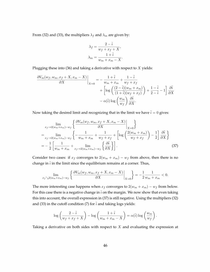
From (32) and (33), the multipliers λf and λm are given by:

λf =2− i

wf + xf +X,

λm =1 + i

wm + xm −X.

Plugging these into (36) and taking a derivative with respect to X yields:

∂Vm(wf , wm, xf +X,xm −X)

∂X

∣∣∣∣X=0

=− 1 + i

wm + xm+

1− i

wf + xf

+

[log

((2− i)(wm + xm)

(1 + i)(wf + xf )

)+

1− i

2− i− 1

]∂i

∂X

− α(i) log

(wm

wf

)∂i

∂X.

Now taking the desired limit and recognizing that in the limit we have i = 0 gives:

limxf→2(wm+xm)−wf

{∂Vm(wf , wm, xf +X,xm −X)

∂X

∣∣∣∣X=0

}= lim

xf→2(wm+xm)−wf

{− 1

wm + xm+

1

wf + xf+

[log

(2(wm + xm)

wf + xf

)− 1

2

]∂i

∂X

}=− 1

2

[1

wm + xm+ lim

xf→2(wm+xm)−wf

{∂i

∂X

}]. (37)

Consider two cases: if xf converges to 2(wm + xm) − wf from above, then there is no

change in i in the limit since the equilibrium remains at a corner. Thus,

limxf↘2(wm+xm)−wf

{∂Vm(wf , wm, xf +X,xm −X)

∂X

∣∣∣∣X=0

}= −1

2

1

wm + xm< 0.

The more interesting case happens when xf converges to 2(wm + xm) − wf from below.

For this case there is a negative change in i on the margin. We now show that even taking

this into account, the overall expression in (37) is still negative. Using the multipliers (32)

and (33) in the cutoff condition (7) for i and taking logs yields:

log

(2− i

wf + xf +X

)− log

(1 + i

wm + xm −X

)= α(i) log

(wm

wf

).

Taking a derivative on both sides with respect to X and evaluating the expression at

46

X = 0 leads to:∂i

∂X= −

1wf+xf

+ 1wm+xm

α′(i) log(wmwf

)+ 1

2−i+ 1

1+i

,

We therefore have:

limxf↗2(wm+xm)−wf

{∂i

∂X

}= −

32

1wm+xm

α′(0) log(wmwf

)+ 3

2

.

Using this in (37) gives the desired result:

limxf↗2(wm+xm)−wf

{∂Vm(wf , wm, xf +X,xm −X)

∂X

∣∣∣∣X=0

}=

− 1

2

1

wm + xm

1− 1

23α

′(0) log(wmwf

)+ 1

< 0.

Intuitively, at i = 0, on the margin a transfer leads the wife to replace the husband as the

provider of a public good that only requires a goods input, so that the wife does not have

a comparative advantage as the provider. 2

Proof of Proposition 2.5: Let λ denote the multiplier on the budget constraint. Given

wm > wf , the cost of female time is strictly lower than the cost of male time, implying

Tm,i = 0 and Tf,i > 0 for all i. Moreover, since in producing a given public good the time

and goods contributions have to come from the same spouse, this also implies Em,i = 0

and Ef,i > 0 for all i. Taking these features into account, the first-order conditions for the

social planning problem are:

cf =µ

λ,

cm =1− µ

λ,

Ef,i =1− α(i)

λ, (38)

Tf,i ≤α(i)

wfλ. (39)

Plugging these expressions into the budget constraint and solving for the multiplier

yields:

λ =2

wf + xf + wm + xm.

47

Using this to solve for the efficient allocation yields:

cf =1

2µ (wf + xf + wm + xm) ,

cm =1

2(1− µ) (wf + xf + wm + xm) ,

Ci =1

2(1− α(i))1−α(i)α(i)α(i)w

−α(i)f (wf + xf + wm + xm) ,

as stated in the proposition.

Regarding the relative provision of public goods in the equilibrium and in the efficient

allocation, notice that the multiplier λ enters (38) and (39) in the same way as the multi-

plier λf enters (26) and (27) in the characterization of the equilibrium allocation. To show

that for an i where the wife is the equilibrium provider, the efficient provision of Ci is

higher than the equilibrium provision, it is therefore sufficient to show that λ < λf , or,

using (32):2

wf + xf + wm + xm<

2− i

wf + xf.

In the case of a corner solution with i = 0 the required inequality is immediate, and if

i = 1 there are no female-provided public goods in equilibrium. For interior solutions,

the cutoff condition (34) yields the following inequality:

wm + xm ≥ 1 + i

2− i(wf + xf ).

Using this inequality, we get:

2

wf + xf + wm + xm≤ 2(

1 + 1+i2−i

)(wf + xf )

=2

3

2− i

wf + xf

<2− i

wf + xf,

as required. 2

Proof of Proposition 3.1: Recall from (35) that the total provision of public goods can be

48

written as:∫ 1

0log(Ci) di = B − i log(λm)− (1− i) log(λf )

−∫ i

0α(i) di log(wm)−

∫ 1

iα(i) di log(wf ), (40)

where B is a constant. From (32) and (33), the multipliers λf and λm are given by:

λf =2− i

wf + xf + ϵ,

λm =1 + i

wm + xm − ϵ.

Plugging these into (40) yields the first expression stated in the proposition. Further,

differentiating with respect to ϵ and evaluating at ϵ = 0 gives equation (8). 2

Proof of Proposition 3.2: The derivative of (35) with respect to ϵ for i held constant is:

∂∫ 10 log(Ci) di

∂ϵ= −i

∂λm∂ϵ

λm− (1− i)

∂λf

∂ϵ

λf. (41)

From (32) and (33), the multipliers λf and λm are given by:

λf =2− i

wf + xf + ϵ, (42)

λm =1 + i

wm + xm − ϵ, (43)

and the derivatives with respect to ϵ evaluated at ϵ = 0 are:

∂λf

∂ϵ= − 2− i

(wf + xf )2,

∂λm

∂ϵ=

1 + i

(wm + xm)2.

Plugging these expressions into (41) gives:

∂∫ 10 log(Ci) di

∂ϵ= − i

wm + xm+

1− i

wf + xf.

49

We therefore have:∂∫ 10 log(Ci) di

∂ϵ> 0

if and only if:1− i

i>

wf + xfwm + xm

.

That is, holding i constant, transferring resources to the wife increases the total provision

of public goods if and only if the share of public goods provided by the wife exceeds the

wife’s share in total resources of the couple. 2

Proof of Proposition 3.3: The cutoff condition (7) characterizing i can be written as:

λf

λm=

(wm

wf

)α(i)

.

Taking logs yields:

log

(λf

λm

)= α(i) log

(wm

wf

).

For varying ϵ, this equation is an identity, with λf , λm, and i all being functions of ϵ.

Differentiating both sides of the identity with respect to ϵ and solving for ∂i∂ϵ yields:

∂i

∂ϵ=

1

α′(i) log(wmwf

) [ 1

λf

∂λf

∂ϵ− 1

λm

∂λm

∂ϵ

].

Thus, the derivative becomes arbitrarily small as α′(i) becomes arbitrarily large. 2

Proof of Proposition 3.4: From (35), the total provision of public goods can be written

as: ∫ 1

0log(Ci) di = B − i log(λm)− (1− i) log(λf )

−∫ i

0α(i) di log(wm)−

∫ 1

iα(i) di log(wf ).

For the case α(i) = i considered here this can be further simplified:∫ 1

0log(Ci) di = B − i log(λm)− (1− i) log(λf )−

1

2

[i2 log

(wm

wf

)+ log(wf )

]. (44)

Next, combining the cutoff condition (7) with the first-order conditions (25) and (28)

50

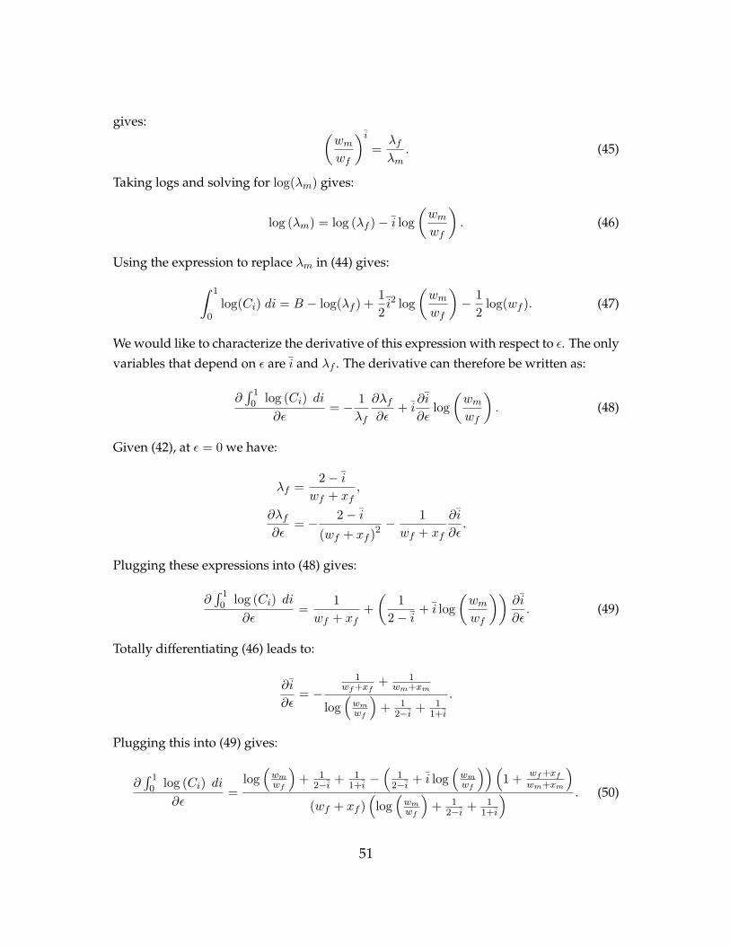
gives: (wm

wf

)i

=λf

λm. (45)

Taking logs and solving for log(λm) gives:

log (λm) = log (λf )− i log

(wm

wf

). (46)

Using the expression to replace λm in (44) gives:∫ 1

0log(Ci) di = B − log(λf ) +

1

2i2 log

(wm

wf

)− 1

2log(wf ). (47)

We would like to characterize the derivative of this expression with respect to ϵ. The only

variables that depend on ϵ are i and λf . The derivative can therefore be written as:

∂∫ 10 log (Ci) di

∂ϵ= − 1

λf

∂λf

∂ϵ+ i

∂i

∂ϵlog

(wm

wf

). (48)

Given (42), at ϵ = 0 we have:

λf =2− i

wf + xf,

∂λf

∂ϵ= − 2− i

(wf + xf )2 − 1

wf + xf

∂i

∂ϵ.

Plugging these expressions into (48) gives:

∂∫ 10 log (Ci) di

∂ϵ=

1

wf + xf+

(1

2− i+ i log

(wm

wf

))∂i

∂ϵ. (49)

Totally differentiating (46) leads to:

∂i

∂ϵ= −

1wf+xf

+ 1wm+xm

log(wmwf

)+ 1

2−i+ 1

1+i

.

Plugging this into (49) gives:

∂∫ 10 log (Ci) di

∂ϵ=

log(wmwf

)+ 1

2−i+ 1

1+i−(

12−i

+ i log(wmwf

))(1 +

wf+xf

wm+xm

)(wf + xf )

(log(wmwf

)+ 1

2−i+ 1

1+i

) . (50)

51

The denominator is positive. To prove the claim, we need to show that the numerator

is positive as well. Using the cutoff condition (45) combined with the multipliers (42)

and (43) to replace the term (wf + xf )/(wm + xm), we need to establish the following

inequality:

log

(wm

wf

)+

1

2− i+

1

1 + i−(

1

2− i+ i log

(wm

wf

))(1 +

2− i

1 + i

(wf

wm

)i)

> 0.

It can be verified numerically that the expression on the left-hand side is decreasing in

i for all wm/wf > 1. It is therefore sufficient to check the inequality at the point i = 1,

i.e., at the point where the husband is providing all public goods and, therefore, the

expenditure-share channel favors transfers to the husband. Plugging in i = 1 yields:

log

(wm

wf

)+

3

2−(1 + log

(wm

wf

))(1 +

wf

2wm

)> 0.

Simplifying the expression yields:

1−(1 + log

(wm

wf

))wf

wm> 0,

or:wm

wf> 1 + log

(wm

wf

),

which is satisfied because we assume wm > wf . 2

Proof of Proposition 3.5: From (8), the derivative of the total provision of public goods

with respect to the transfer ϵ (evaluated at ϵ = 0) is given by:

∂∫ 10 log (Ci) di

∂ϵ=− i

wm + xm+

1− i

wf + xf

+

[log

((2− i)(wm + xm)

(1 + i)(wf + xf )

)+

1− i

2− i− i

1 + i

]∂i

∂ϵ

− α(i) log

(wm

wf

)∂i

∂ϵ.

Using the multipliers (32) and (33) in the cutoff condition (7) for i yields:

(wm

wf

)α(i)

=(2− i)(wm + xm − ϵ)

(1 + i)(wf + xf + ϵ). (51)

52

In the limit as wf → wm, the left hand side converges to 1 and thus we have (evaluated

at ϵ = 0):2− i

wf + xf=

1 + i

wm + xm.

Solving this expression for i, we get:

limwf→wm

i = limwf→wm

2(wm + xm)− (wf + xf )

wf + xf + wm + xm. (52)

The derivative ∂i∂ϵ can be derived from (51) by taking logs, then differentiating both sides

with respect to ϵ, and collecting terms. Evaluated at ϵ = 0 the derivative is:

∂i

∂ϵ= −

1wf+xf

+ 1wm+xm

α′(i) log(wmwf

)+ 1

2−i+ 1

1+i

,

In the limit wf → wm, the first term in the denominator disappears. Then, using (52), the

derivative simplifies to:

limwf→wm

∂i

∂ϵ= −

1wf+xf

+ 1wm+xm

12−i

+ 11+i

= − 3

2wm + xf + xm. (53)

Now plugging the derived limits for i and ∂i∂ϵ into the expression for the total provision

of public goods and simplifying, we get:

limwf→wm

d∫ 10 log (Ci) di

dϵ= lim

wf→wm

{− i

wm + xm+

1− i

wf + xf+

[1− i

2− i− i

1 + i

]∂i

∂ϵ

}=

1

wm + xm− 1

wm + xf− 1

wm + xm+

1

wm + xf

= 0,

which completes the proof. 2

Proof of Lemma 4.1: Substituting (14) into the utility function (9) gives:

U(cg, k′, h′) = log(cg) + log(r′k′ + w′h′). (54)

53

The derivatives of (54) with respect to k′ and h′ are given by:

∂U

∂k′=

r′

r′k′ + w′h′=

(1− θ)(ϕh′

k′

)θ(1− θ)

(ϕh′

k′

)θk′ + θ

(k′

ϕh′

)1−θh′

=(1− θ)ϕ

(1− θ)ϕ+ θ

1

k′,

∂U

∂h′=

w′

r′k′ + w′h′=

θ

(1− θ)ϕ+ θ

1

h′.

Here the prices r′ and w′ were replaced by marginal products given technology (10), and

ϕ denotes the fraction of human capital employed in market production, which is taken

as given by the individual. Since only marginal utilities matter for choices, preferences

(54) can be expressed as:

U(cg, k′, h′) = log(cg) +

∂U

∂k′k′ +

∂U

∂h′h′ = log(cg) + βk log(k

′) + (1− βk) log(h′), (55)

which is (16). 2

Proof of Lemma 4.2: Start with the original formulation of maximizing (1) subject to (2)

to (5), where we denote all variables with a tilde to distinguish them from the ones used

in the growth formulation:

max

{log(cg) +

∫ 1

0log(Ci

)di

}(56)

subject to:

Ci = Cf,i + Cm,i ∀i, (57)

Cg,i = E1−α(i)g,i T

α(i)g,i ∀i, (58)

cg +

∫ 1

0Eg,i di = wg

(1−

∫ 1

0Tg,i di

)+ xg. (59)

Here have already substituted the time constraint into the budget constraint. Substitut-

ing (19) and (20) into the budget constraint (59) gives:

cg +

∫ 1

0Eg,i di =

1

2

[wgh

(1−

∫ 1

0Tg,i di

)+ rk

]+ τk. (60)

For i such that 0 ≤ i ≤ βk, we have α(i) = 0, so that it is optimal to set Tg,i = 0 and

Cg,i = Eg,i to a constant Cg. Noting this fact, we can substitute (21) to (24) into the

54

budget constraint (60) to get:

cg + bg +

∫ 1

βk

Eg,(i−βk)/(1−βk)

1− βkdi =

1

2

[wgh

(1−

∫ 1

βk

Tg,(i−βk)/(1−βk)

1− βkdi

)+ rk

]+ τk. (61)

Notice that in equation 61 the inputs corresponding to human capital are indexed from

βk to 1 (index i), whereas in the growth model the index runs from 0 to 1 (index j).

Applying the change of variables i = βk + j(1− βk) to the two integrals gives:

cg + bg +

∫ 1

0Eg,j dj =

1

2

[wgh

(1−

∫ 1

0Tg,j dj

)+ rk

]+ τk, (62)

which is the budget constraint (15) of the decision problem in the growth model. The

equivalence of the remaining constraints is immediate.

Thus, we have shown that the set of constraints of the decision problem in the growth

model is equivalent to the set of constraints for a special case of the general decision

problem. What remains to be shown is that the objective functions are equivalent as

well. To this end, given (22) and (11) we have:∫ βk

0log(Ci

)di = βk log

(bf + bm

βk

)= βk log

(k′

βk

). (63)

Similarly, using (23), (24), and (12) and applying a change of variables as above gives:

∫ 1

βk

log(Ci

)di =

∫ 1

βk

log

∑g∈{f,m}

E1−α(i)g,i T

α(i)g,i

di

=

∫ 1

βk

log

∑g∈{f,m}

E1−α(i)g,(i−βk)/(1−βk)

Tα(i)g,(i−βk)/(1−βk)

1− βk

di

= (1− βk)

∫ 1

0log

∑g∈{f,m}

E1−jg,j T j

g,j

1− βk

dj

= (1− βk)(log(h′)− log(1− βk)

). (64)

Using (21), (63), and (64), the objective function (56) can be written as:

log(cg) + βk log(k′)+ (1− βk) log

(h′)− βk log (βk)− (1− βk) log (1− βk) . (65)

This is (16) up to an additive constant. The utility function in the special case of the

55

general decision problem therefore induces the same preferences as the utility function

of the decision problem in the growth model, which completes the proof. 2

Proof of Lemma 4.3: Fix the state variables k > 0 and h > 0, and let cg, k′ = bm, Eg,i,

Tg,i, and i denote the equilibrium choices in the current generation given k and h. Now

consider alternative state variables k > 0 and h > 0. Define ξ as the ratio of output under

these and the original state variables:28

ξ =k1−θhθ

k1−θhθ.

We would like to show the following are equilibrium choices given k and h: cg = ξcg,

k′ = ξk′, Eg,i = ξEg,i, Tg,i, and i. We will show this by showing that given these choices,

the decision problem at state variables k and h can be reduced to the decision problem

at state variables k and h. Recall that the decision problem of spouse g is to maximize (9)

subject to constraints (11)–(15).

The budget constraint (15) for spouse g at state variables k and h is given by:

cg + bg +

∫ 1

0Eg,i di =

1

2

[wgh

(1−

∫ 1

0Tg,i di

)+ rk

]+ τg,

where wg and r are factor prices at state variables k and h. Given our conjecture, this can

be written as:

ξcg + ξbg +

∫ 1

0ξEg,i di =

1

2

[wgh

(1−

∫ 1

0Tg,i di

)+ rk

]+ ξτg,

Next, notice that given our conjecture we have wgh = ξwgh and rk = ξrk. Substituting

these expressions and dividing by ξ gives:

cg + bg +

∫ 1

0Eg,i di =

1

2

[wgh

(1−

∫ 1

0Tg,i di

)+ rk

]+ τg,

which is the budget constraint for the state variables k, h. Similarly, we can plug the

conjectured values into the constraints (11)–(14), and in each case reduce the constraint

for k, h to the original constraint for k, h by dividing by ξ or, in the case of constraint (12),

by subtracting log(ξ) on both sides.

28The ratio of output takes this form because the time allocation is the same for the original andthe new state variables, which will be verified below.

56

Hence, we have found so far that the constraint set for ξcg, ξk′ etc. at state variables k,

h is the same as the constraints set for cg, k′ etc. at state variables k, h. To show that the

conjectured choices at k, h are indeed optimal, we still need to show that the preferences

over ξcg, ξk′ and h′ given state variables k, h are equivalent to the preferences over cg, k,

and h given state variables k and h. Here h′ the children’s human capital at current state

variables k, h given the conjectured choices, which is given by:

h′ = exp

(∫ 1

0log

((ξEi)

1−i(Tih)i)

di

).

Here Ei = Em,i and Ti = Tm,i for i < i and Ei = Ef,i and Ti = Tf,i for i ≥ i. To simplify

notation, let ϕ denote the fraction of human capital used for production:

ϕ =1

2

[1−

∫ 1

0Tm,i di+ δ

(1−

∫ 1

0Tf,i di

)]. (66)

Note that under our conjecture, ϕ is a constant that does not depend on current state

variables. We can now write the objective function (16) at state variables k, h as:

log(cg) + βk log(k′) + (1− βk) log(h

′)

= log(ξcg) + βk log(ξk′) + (1− βk)

∫ 1

0log

((ξEi)

1−i(Tih)i)

di

= log(cg) + βk log(k′) + (1− βk)

∫ 1

0log((Ei)

1−i (Tih)i)di

+

(1 + βk +

1− βk2

)log(ξ) +

1− βk2

(log(h)− log (h)

).

This is the objective function at state variables k, h plus a constant that does not depend

on choices. The objective function thus induces the same preferences, which completes

the proof. 2

Proof of Proposition 4.1: It will be useful to first characterize the equilibrium choices.

Define βh = 1−βk. Using Lemma 4.1, the first-order conditions characterizing the wife’s

57

optimization problem are given by:

cf =1

λf, (67)

Ef,i ≤(1− i)βh

λf, (68)

Tf,i ≤iβh

wfh2λf

, (69)

bf ≤ βkλf

, (70)

where (68) and (69) hold with equality for all public goods i that the wife contributes to,

and λf denotes the multiplier on the budget constraint. The corresponding optimality

conditions for the husband are:

cm =1

λm, (71)

Em,i ≤(1− i)βh

λm, (72)

Tm,i ≤iβh

wmh2λm

, (73)

bm ≤ βkλm

. (74)

We can now solve for the multipliers on the budget constraint. Plugging the first-order

conditions for the wife back into the budget constraint and using the cutoff rule gives:

cf +

∫ 1

iEf,i di =

1

2

[wfh

(1−

∫ 1

iTf,i di

)+ rk

]+ τf ,

1

λf+

∫ 1

i

(1− i)βhλf

di =1

2

[wfh

(1−

∫ 1

i

iβh

wfh2λf

di

)+ rk

]+ τf ,

1

λf+

∫ 1

i

(1− i)βhλf

di = wfh

2−∫ 1

i

iβhλf

di+ rk

2+ τf ,

1

λf+

∫ 1

i

βhλf

di =wfh+ rk

2+ τf .

Solving for λf yields:

λf =1 + βh(1− i)wfh+rk

2 + τf. (75)

Proceeding along the same lines with the male budget constraint (but noting that he will

58

provide the bequests in equilibrium) gives:

λm =1 + βk + βhiwmh+rk

2 + τm. (76)

Next, we characterize the cutoff rule for an interior solution. We focus on interior equilib-

ria in which each spouse provides at least part of the human capital input, which implies

that the husband (who has the higher wage) provides all of the bequest. Given the first-

order conditions, the ratio of female to male preferred public-good provision for human

capital good i is:Cf,i

Cm,i=

E1−if,i (Tf,ih)

i

E1−im,i (Tm,ih)i

=

(wm

wf

)i λm

λf. (77)

The condition for the cutoff i is therefore:

λf

λm=

(wm

wf

)i

= δ−i, (78)

where δ < 1 is the gender gap. The cutoff i is characterized by the condition that at i

female- and male-preferred provision of the public good is equal. Using (77) and the

computed multipliers, we can write the cutoff condition as:

(1 + βh(1− i)

1 + βk + βhi

)( wmh+rk2 + τm

wfh+rk2 + τf

)=

(1

δ

)i

. (79)

Now, express the transfers as a fraction of output (or output per capita, population size

is normalized to one):

τf = −τm = γY,

and factor prices as:

wm = δ−1wf =θY

ϕh,

rt =(1− θ)Y

k,

where ϕ is defined in (66) from Lemma 4.3. The cutoff condition can then be written as:

(1 + βh(1− i)

1 + βk + βhi

)( θϕ + 1− θ − 2γ

δθϕ + 1− θ + 2γ

)=

(1

δ

)i

. (80)

59

Notice that the left-hand side is strictly decreasing in i while the right-hand side is strictly

increasing, implying that there is a unique equilibrium. When the equation does not

have a solution, the equilibrium is a corner where either husband or wife provide all of

the public goods that involve time inputs.

We are now ready to address the issue of the effect of a transfer on growth. The log of

output in the next generation is:

log(Y ′) = log(A) + (1− θ) log(k′) + θ log(ϕh′)

= log(A) + (1− θ) log(k′) + θ

∫ 1

0[(1− i) log(Ei,t) + i log(Ti,t)] di

+θ

2log(h) + θ log(ϕ)

= log(A) + (1− θ) log(k′) + θ

∫ i

0[(1− i) log(Em,i) + i log(Tm,i)] di

+ θ

∫ 1

i[(1− i) log(Ef,i) + i log(Tf,i)] di+

θ

2log(h) + θ log(ϕ).

Plugging in the solutions from the first-order conditions this is:

log(Y ′) = log(A) + (1− θ) log

(βkλm

)+ θ

∫ i

0

[(1− i) log

((1− i)βh

λm

)+ i log

(iβh

wmh2λm

)]di

+ θ

∫ 1

i

[(1− i) log

((1− i)βh

λf

)+ i log

(iβh

wfh2λf

)]di

+θ

2log(h) + θ log(ϕ).

Denote by B the constant that does not depend on current prices or multipliers (and thus

not on transfers) to get:

log(Y ′) = B − (1− θ) log (λm)

− θ

[i log(λm) + (1− i) log(λf ) +

1

2

[i2 log(wm) + (1− i2) log(wf )

]].

60

Given that wf = δwm, we can further simplify to:

log(Y ′) = B − (1− θ) log (λm)

− θ

[i log(λm) + (1− i) log(λf ) +

1

2

[log(wm) + (1− i2) log(δ)

]]Now consider the effect of a marginal change in the transfer ϵ from husband to wife on

output in the next period (i.e., on growth). The derivative of Y ′ with respect to ϵ is given

by:

∂ log(Y ′)

∂ϵ= −(1− θ(1− i))

1

λm

∂λm

∂ϵ− θ(1− i)

1

λf

∂λf

∂ϵ− θ

2

1

wm

∂wm

∂ϵ

− θ[log(λm)− log(λf )− i log(δ)]∂i

∂ϵ.

The cutoff condition (78) implies that the term involving ∂i∂ϵ cancels, leaving us with:

∂ log(Y ′)

∂ϵ= −(1− θ(1− i))

1

λm

∂λm

∂ϵ− θ(1− i)

1

λf

∂λf

∂ϵ− θ

2

1

wm

∂wm

∂ϵ. (81)

Now consider the limit cases when the share of human capital goes to either zero or one.

When θ approaches zero, only the first term remains. This term is negative in the limit (an

increase in ϵ lowers male consumption, and hence increases λm). Hence, when physical

capital is the main factor of production, a transfer from husband to wife lowers growth.

Next, consider the limit case θ = 1, i.e., human capital is the only factor of production.

Totally differentiating the cutoff condition (78) yields:

∂i

∂ϵlog(1/δ) =

1

λf

∂λf

∂ϵ− 1

λm

∂λm

∂ϵ.

Using this in (81) together with θ = 1 gives:

∂ log(Y ′)

∂ϵ= − 1

λf

∂λf

∂ϵ+ i

∂i

∂ϵlog(1/δ)− 1

2

1

wm

∂wm

∂ϵ.

This expression is identical to equation (48) in the proof of Proposition 3.4 except for the

last term. In Proposition 3.4 (which applies here because of Lemma 4.2 ), we showed that

the first two terms combine to be positive, and the last term is positive as well. Hence, the

entire derivative is positive: If human capital accounts for all of production, a transfer to

the wife increases growth. 2

61

B The Model with More General Preferences

In the main analysis above, we have relied on log utility and Cobb-Douglas technology

to simplify the analysis. In this section, we discuss the extent to which our results can be

extended to more general functional forms for utility and the home-production technol-

ogy. Let preferences be given by:

u(cf ) +

∫ 1

0U(Ci) di,

u(cm) +

∫ 1

0U(Ci) di,

where u(·) and U(·) are strictly increasing, strictly concave, and continuously differen-

tiable utility functions that satisfy Inada conditions. The maximization problem of the

spouse of gender g ∈ {f,m} is subject to the following constraints:

Ci = Cf,i + Cm,i, (82)

Cg,i = Fi(Eg,i, Tg,i), (83)

cg +

∫ 1

0Eg,i di = wg(1− Tg) + xg, (84)∫ 1

0Tg,i di = Tg. (85)

Here Fi(Eg,i, Tg,i) is a home production function that, for each i, is strictly increasing in

both inputs, displays constant returns to scale to both inputs combined, strictly dimin-

ishing returns to each input individually, and is continuously differentiable.

In equilibrium, each public good i will be provided by only one of the spouses. Denoting

by λg the multiplier on the budget constraint, the first-order conditions for the individual

maximization problem for private consumption cg and the provision of public goods i

that are provided by spouse g are given by:

u′(cg) = λg,

U ′(Fi(Eg,i, Tg,i))Fi,E(Eg,i, Tg,i) = λg,

U ′(Fi(Eg,i, Tg,i))Fi,H(Eg,i, Tg,i) = wgλg.

Notice that these constraints hold as equalities only for those i that are provided by

spouse g. Given this provision, the constraints have to hold as equalities because the

62

utility functions are strictly concave, differentiable, and satisfy Inada conditions.

We can use the first-order conditions to derive the preferred provision of public good i

by spouse g as a function of private consumption cg. Namely, let:

Cg,i(cg) = Fi(Eg,i, Tg,i),

where Eg,i and Tg,i are the solution to the system of equations:

U ′(Fi(Eg,i, Tg,i))Fi,E(Eg,i, Tg,i) = u′(cg), (86)

U ′(Fi(Eg,i, Tg,i))Fi,H(Eg,i, Tg,i) = wgu′(cg). (87)

This system of equations can be defined for all i ∈ [0, 1]. Intuitively, Cg,i(cg) is how much

spouse g would provide of good i if he/she were the sole provider and if the value of the

Lagrange multiplier on the budget constraint were given by u′(cg).

We assume for now that a unique solution to the system (86)–(87) exists for all i and all cg,

so that the preferred provision levels Cg,i(cg) are well defined (later, we will also discuss

specific functional forms that guarantee that this is the case). We can then ask what

properties the preferred provision levels have to satisfy in order to generate a generalized

version of Proposition 2.1 above.

Assumption B.1. The function Cg,i(cg) is strictly increasing and continuous in cg for g ∈{f,m} and the expression:

Cf,i(cf )

Cm,i(cm)(88)

is strictly increasing in i, for all cf , cm > 0 (i.e., relative female willingness to pay is increasingin i).

Proposition B.1. If Assumption B.1 is satisfied, there exists a unique equilibrium characterizedby a cutoff i such that all public goods in the interval i ∈ [0, i] are provided by the husband m

(i.e., the husband provides goods-intensive goods), while public goods in the range i ∈ (i, 1] areprovided by the wife f (the wife provides time-intensive goods). If the cutoff i is interior, it isdetermined such that female and male provision of public goods is equalized at the cutoff. Hence,if i ∈ (0, 1), the cutoff and private consumption satisfy the condition:

Cf,i(cf ) = Cm,i(cm). (89)

Consider now the effects of a transfer from the husband to the wife, i.e., the wife’s wealth increases

63

from xf to xf = xf + ϵ, and the husband’s wealth decreases from xm to xm = xm − ϵ, whereϵ > 0. In the new equilibrium, the cutoff i is lower. Let i be the new cutoff. If wf < wm and ifthe cutoff is interior both before and after the change, i.e., if 0 < i < i < 1 holds, the provisionof public goods that are female-provided both before and after the change (i > i) goes up. In otherwords, a transfer to the low-wage spouse increases the provision of public goods provided by thisspouse.

Proof of Proposition B.1: Equilibrium requires that each public good is provided by

the spouse with the higher willingness to pay. Given that we assume that the ratio of

willingness to pay (88) is strictly increasing in i, for any cf , cm there either has to be a

i(cf , cm) ∈ (0, 1) that satisfies Cf,i(cf ) = Cm,i(cm), or we can set i = 0 with Cf,0(cf ) ≥Cm,0(cm) or i = 1 with Cf,1(cf ) ≤ Cm,1(cm). Moreover, given that willingness to pay

is continuously increasing in cg, i(cf , cm) is a continuous function of cf and cm and at

least weakly decreasing in cf and weakly increasing in cm. To have an equilibrium, in

addition to the public-good provision condition we also need to satisfy individual budget

constraints. We can define total spending by the two spouses as:

Yf (cf , cm) = cf +

∫ 1

i(cf ,cm)

(Ef,i(cf ) + wf Tf,i(cf )

)di,

Ym(cf , cm) = cm +

∫ i(cf ,cm)

0

(Em,i(cm) + wmTm,i(cm)

)di.

Given Assumption B.1, these functions are guaranteed to be continuous, Yf (cf , cm) is

strictly increasing in cf , and Ym(cf , cm) is strictly increasing in cm. An equilibrium is

given by two numbers cf , cm such that the two budget-clearing conditions:

Yf (cf , cm) = wf + xf ,

Ym(cf , cm) = wm + xm

are satisfied. A solution exists, because the functions are continuous, Yf (cf , cm) ap-

proaches zero as cf approaches zero, and exceeds wf + xf as cf approaches wf + xf ,

with parallel conditions holding for cm. The solution is also unique. To see why, assume

to the contrary that there are two different equilibrium values of female consumption, cfand cf < cf . For the female budget constraint to be satisfied, c would have to correspond

to a larger female provision of public goods and thus a lower i. The lower cutoff, in turn,

implies that male consumption must be lower, cm < cm, because male willingness to

pay for public goods has to be lower. But this leads to a contradiction, because then the

64

husband would both have lower private consumption and provide fewer public goods,

implying that the budget constraint cannot be satisfied for cm and cm at the same time.

So far, we have established that for given wf , wm, xf , and xm, there exists a unique

equilibrium characterized by a cutoff i for the provision of public goods. Consider now

the effects of a transfer from the husband to the wife, i.e., the wife’s wealth increases

from xf to xf = xf + ϵ, and the husband’s wealth decreases from xm to xm = xm − ϵ,

where ϵ > 0. Let i be the provision cutoff in the new equilibrium, where we must have

i ≤ i because of the increase in female resources. Consider the case where the cutoff is

interior both before and after the change, i.e., if 0 < i < i < 1 holds. We would like to

show that the provision of public goods that are female-provided both before and after

the change (i > i) goes up. This is equivalent to showing that we must have cf > cf ,

i.e., private female consumption increases. To show this, assume to the contrary that

cf ≤ cf . Then we must have that goods with i such that i ≤ i < i are provided at a lower

level than before, because provision is equal to female preferred provision, which has

not increased and is strictly lower than the original preferred male provision (because of

the restriction on (88) in Assumption B.1), which was the original equilibrium provision.

This also implies that Cm,i(cm) < Cm,i(cm) and hence we must have cm < cm. This, in

turn, implies that all male provided goods are provided at a lower level than previously.

The fact that male private consumption and male contributions to public goods both

fall implies that the amount of the transfer has to be larger than the original full cost of

providing the public goods in the range [i, i]. But this leads to a contradiction, because

then the wife receives a transfer that is more than sufficient (given wf < wm) for the

original provision of public goods in the range [i, i], yet she lowers the provision of these

goods and does not increase the provision of any other goods, implying that the budget

constraint has to be violated. 2

The proposition shows that the key condition for our main result is that relative female

willingness to pay varies across public goods. A wage difference combined with differ-

ences in the time-versus-goods intensity of different public goods is one way of gener-

ating such differences in the willingness to pay, but clearly any mechanism that creates

variation in spouses’ comparative advantage at providing different public goods would

create similar results.

In the model contained in the main text we generate a difference in willingness to pay

that depends only on the time-versus-goods intensity of the production function. While

the log-Cobb-Douglas setup that we use leads to the most straightforward characteriza-

65

tion, this feature carries over to CES production and CRRA utility. To demonstrate this,

assume the following functional forms:

u(cg) =c1−σg

1− σ,

u(Ci) =C1−σi

1− σ,

Fi(Ei, Ti) = ((1− i)Eρi + iT ρ

i )1ρ .

Given these functional forms, the first-order conditions (86)–(87) that pin down the pre-

ferred goods and time contributions Eg,i and Tg,i to public goods can be written as:

(((1− i)Eρ

i + iT ρi

) 1ρ

)−σ

(1− i)Eρ−1i

((1− i)Eρ

i + iT ρi

) 1−ρρ

= (cg)−σ , (90)((

(1− i)Eρi + iT ρ

i

) 1ρ

)−σ

iT ρ−1i

((1− i)Eρ

i + iT ρi

) 1−ρρ

= wg (cg)−σ . (91)

Taking the ratio of (90) and (91), we get:

1− i

i

(Ei

Ti

)ρ−1

=1

wg,

or:Ei

Ti

=

(wg

1− i

i

) 11−ρ

. (92)

Not surprisingly, the spouse with a lower wage provides public goods in a more time-

intensive manner. Notice that the first term in the two-first order conditions contains the

preferred provision level Cg,i(cg). Rewriting (91) yields:

(Cg,i(cg)

)−σi

((1− i)

(Ei

Ti

)ρ

+ i

) 1−ρρ

= wg (cg)−σ .

Plugging in (92) gives:

(Cg,i(cg)

)−σi

((1− i)

(wg

1− i

i

) ρ1−ρ

+ i

) 1−ρρ

= wg (cg)−σ .

66

Simplifying and solving for the preferred provision gives:

(Cg,i(cg)

)−σ ((1− i)

11−ρ (wg)

ρ1−ρ + i

11−ρ

) 1−ρρ

= wg (cg)−σ ,

(Cg,i(cg)

)−σ((1− i)

11−ρ +

(i

wρg

) 11−ρ

) 1−ρρ

= (cg)−σ ,

Cg,i(cg) = cg

((1− i)

11−ρ +

(i

wρg

) 11−ρ

) 1−ρσρ

.

Notice that these preferred provision levels satisfy the continuity and monotonicity re-

strictions in Assumption B.1. Moreover, the ratio of preferred female to preferred male

provision is:

Cf,i(cf )

Cm,i(cm)=

cfcm

(1− i)

11−ρ +

(iwρ

f

) 11−ρ

(1− i)1

1−ρ +(

iwρ

m

) 11−ρ

1−ρσρ

.

Since we have wf < wm, this ratio is indeed strictly increasing in i, which meets the

second part of Assumption B.1.

If we combine the CES production function with still more general preferences (such as

Stone-Geary), additional effects arise, because relative female willingness to pay for dif-

ferent public goods might vary with both relative and absolute female wealth. However,

the presence of a wage gap combined with variation in the time intensity of public goods

always creates a force towards female specialization in time-intensive goods. With more

general utility functions additional forces may be present, but these will not completely

offset the force towards specialization except in knife-edge cases. Even in cases where

Assumption B.1 is not satisfied, income transfers between the spouses will have an effect

on the equilibrium allocation as long as there is some variation in relative willingness to

pay. The direction of the effects could be different, however, if the differences in willing-

ness to pay are mainly due to a factor other than female specialization in time-intensive

production.

67