Dividend Policy, Index Labeling Effect, Investment, and Cash ... - KEEP

Essays in Corporate Policy:

Dividend Policy, Index Labeling Effect, Investment, and Cash Flow Duration

by

Tae Eui Lee

A Dissertation Presented in Partial Fulfillmentof the Requirements for the Degree

Doctor of Philosophy

Approved April 2015 by theGraduate Supervisory Committee:

Rajnish Mehra, Co-ChairYuri Tserlukevich, Co-Chair

Claudia Custodio

ARIZONA STATE UNIVERSITY

May 2015

ABSTRACT

This dissertation consists of two essays on corporate policy. The first chapter analyzes

whether being labeled a “growth” firm or a “value” firm affects the firm’s dividend

policy. I focus on the dividend policy because of its discretionary nature and the link

to investor demand. To address endogeneity concerns, I use regression discontinuity

design around the threshold to assign firms to each category. The results show that

“value” firms have a significantly higher dividend payout - about four percentage

points - than growth firms. This approach establishes a causal link between firm

“growth/value” labels and dividend policy.

The second chapter develops investment policy model which associated with du-

ration of cash flow. Firms are doing their business by operating a portfolio of projects

that have various duration, and the duration of the project portfolio generates dif-

ferent duration of cash flow stream. By assuming the duration of cash flow as a firm

specific characteristic, this paper analyzes how the duration of cash flow affects firms’

investment decision. I develop a model of investment, external finance, and savings to

characterize how firms’ decision is affected by the duration of cash flow. Firms max-

imize total value of cash flow, while they have to maintain their solvency by paying

a fixed cost for the operation. I empirically confirm the positive correlation between

duration of cash flow and investment with theoretical support. Financial constraint

suffocates the firm when they face solvency issue, so that model with financial con-

straint shows that the correlation between duration of cash flow and investment is

stronger than low financial constraint case.

i

DEDICATION

For Boram,

whose love, support, and encouragement made everything possible.

And for my parents,

who set high expectations and provided the foundation to help me achieve my goals.

ii

TABLE OF CONTENTS

Page

LIST OF TABLES . . . . . . . . . . . . . . . . . . . . . . . . . . . . . . . . . . . . . . . . . . . . . . . . . . . . . . . . . v

LIST OF FIGURES . . . . . . . . . . . . . . . . . . . . . . . . . . . . . . . . . . . . . . . . . . . . . . . . . . . . . . . . vi

CHAPTER

1 LABELING EFFECT ON PAYOUT POLICY . . . . . . . . . . . . . . . . . . . . . . . . . 1

1.1 Introduction . . . . . . . . . . . . . . . . . . . . . . . . . . . . . . . . . . . . . . . . . . . . . . . . . . . . 1

1.2 Data . . . . . . . . . . . . . . . . . . . . . . . . . . . . . . . . . . . . . . . . . . . . . . . . . . . . . . . . . . . 5

1.2.1 Summary Statistics . . . . . . . . . . . . . . . . . . . . . . . . . . . . . . . . . . . . . . 7

1.3 Model/Methodology . . . . . . . . . . . . . . . . . . . . . . . . . . . . . . . . . . . . . . . . . . . . 9

1.3.1 Identification . . . . . . . . . . . . . . . . . . . . . . . . . . . . . . . . . . . . . . . . . . . . 9

1.3.2 Regression Discontinuity in Dividend Policy. . . . . . . . . . . . . . . . 10

1.4 Empirical Analysis . . . . . . . . . . . . . . . . . . . . . . . . . . . . . . . . . . . . . . . . . . . . . . 13

1.4.1 Graphical Analysis for Regression Discontinuity . . . . . . . . . . . . 13

1.4.2 Estimation of Regression Discontinuity - Global strategy . . . . 16

1.4.3 Estimation of Regression Continuity - Local Strategy . . . . . . . 20

1.4.4 Changes in the Dividend Policy and Labeling . . . . . . . . . . . . . . 20

1.4.5 Alternative Measure of Dividend Policy - Payment Decision . 23

1.4.6 The Robustness Test Utilizing an additional Time Period . . . 25

1.4.7 Share Repurchases and Other Corporate Policies . . . . . . . . . . . 29

1.5 Conclusion . . . . . . . . . . . . . . . . . . . . . . . . . . . . . . . . . . . . . . . . . . . . . . . . . . . . . 39

2 INVESTMENT AND DURATION OF CASH FLOW . . . . . . . . . . . . . . . . . . 40

2.1 Introduction . . . . . . . . . . . . . . . . . . . . . . . . . . . . . . . . . . . . . . . . . . . . . . . . . . . . 40

2.2 Model . . . . . . . . . . . . . . . . . . . . . . . . . . . . . . . . . . . . . . . . . . . . . . . . . . . . . . . . . 45

2.2.1 Duration of Cash Flow . . . . . . . . . . . . . . . . . . . . . . . . . . . . . . . . . . . 46

2.2.2 Optimal Policy . . . . . . . . . . . . . . . . . . . . . . . . . . . . . . . . . . . . . . . . . . 47

iii

CHAPTER Page

2.2.3 Implication . . . . . . . . . . . . . . . . . . . . . . . . . . . . . . . . . . . . . . . . . . . . . . 53

2.3 Empirical Investigation . . . . . . . . . . . . . . . . . . . . . . . . . . . . . . . . . . . . . . . . . . 55

2.3.1 Empirical Expectation . . . . . . . . . . . . . . . . . . . . . . . . . . . . . . . . . . . 55

2.3.2 Data . . . . . . . . . . . . . . . . . . . . . . . . . . . . . . . . . . . . . . . . . . . . . . . . . . . . 56

2.3.3 External Finance with Duration of Cash Flow . . . . . . . . . . . . . . 59

2.3.4 Optimal Investment with Duration of Cash Flow . . . . . . . . . . . 61

2.3.5 Market Imperfection with Duration of Cash Flow . . . . . . . . . . 65

2.4 Conclusion . . . . . . . . . . . . . . . . . . . . . . . . . . . . . . . . . . . . . . . . . . . . . . . . . . . . . 72

REFERENCES . . . . . . . . . . . . . . . . . . . . . . . . . . . . . . . . . . . . . . . . . . . . . . . . . . . . . . . . . . . . 74

APPENDIX

A INTERNAL VALIDITY TEST FOR CHAPTER 1 . . . . . . . . . . . . . . . . . . . . . 79

B DEFINITION OF MAIN VARIABLES FOR CHAPTER 2 . . . . . . . . . . . . . 81

iv

LIST OF TABLES

Table Page

1 Summary Statistics . . . . . . . . . . . . . . . . . . . . . . . . . . . . . . . . . . . . . . . . . . . . . . . . 8

1.2 Estimation of Sharp Regression Discontinuity - Global Strategy . . . . . . . 18

1.3 Estimation of Sharp Regression Discontinuity - Local Strategy . . . . . . . . 19

1.4 Change of Dividend Payout - Within Firm Effect for Index Switchers . . 21

1.5 Regression Discontinuity - Dividend Payers Only . . . . . . . . . . . . . . . . . . . . . 23

1.6 Logit Result . . . . . . . . . . . . . . . . . . . . . . . . . . . . . . . . . . . . . . . . . . . . . . . . . . . . . . . 24

1.7 Global Strategy after Test Sample Periods . . . . . . . . . . . . . . . . . . . . . . . . . . . 27

1.8 Local Strategy after Test Sample Periods . . . . . . . . . . . . . . . . . . . . . . . . . . . . 29

1.9 Regression Discontinuity Test for Corporate Policies . . . . . . . . . . . . . . . . . . 35

2.1 Summary Statistics . . . . . . . . . . . . . . . . . . . . . . . . . . . . . . . . . . . . . . . . . . . . . . . . 58

2.2 External Finance with Duration of Cash Flow. . . . . . . . . . . . . . . . . . . . . . . . 61

2.3 Investment Decision . . . . . . . . . . . . . . . . . . . . . . . . . . . . . . . . . . . . . . . . . . . . . . . . 63

2.4 Investment Regressions - Robust Test with Alternative Measure . . . . . . 64

2.5 Investment Regressions by Financial Constraint Criteria-Baseline Re-

gression . . . . . . . . . . . . . . . . . . . . . . . . . . . . . . . . . . . . . . . . . . . . . . . . . . . . . . . . . . . 68

2.6 Investment Regressions by Financial Constraint Criteria-Alternative

measure . . . . . . . . . . . . . . . . . . . . . . . . . . . . . . . . . . . . . . . . . . . . . . . . . . . . . . . . . . . 70

2.7 Investment Regressions by Financial Constraint Criteria . . . . . . . . . . . . . . 71

B.1 Definition of Main Variables . . . . . . . . . . . . . . . . . . . . . . . . . . . . . . . . . . . . . . . . 82

v

LIST OF FIGURES

Figure Page

1.1 Dividend Payout Ratio . . . . . . . . . . . . . . . . . . . . . . . . . . . . . . . . . . . . . . . . . . . . . 14

1.2 Dividend Payment Rate . . . . . . . . . . . . . . . . . . . . . . . . . . . . . . . . . . . . . . . . . . . . 16

1.3 Dividend Payout Rate and Payment Rate after Test Sample Periods . . . 28

1.4 Time Trends in Dividend Policy . . . . . . . . . . . . . . . . . . . . . . . . . . . . . . . . . . . . . 31

1.5 Time Trends in Share Repurchases . . . . . . . . . . . . . . . . . . . . . . . . . . . . . . . . . . 32

1.6 Dividend and Repurchase Policy . . . . . . . . . . . . . . . . . . . . . . . . . . . . . . . . . . . . 33

1.7 Corporate Condition and Policies . . . . . . . . . . . . . . . . . . . . . . . . . . . . . . . . . . . 38

2.1 The stylized facts provides relationship between cash flow duration and cash flow volatility.

Volatility measure use four years of quarterly 16 consecutive data of cash flow stream from the

annual COMPUSTAT. . . . . . . . . . . . . . . . . . . . . . . . . . . . . . . . . . . . . . . . . . . . . . . . . . . . 45

2.2 The Timeline of the Model . . . . . . . . . . . . . . . . . . . . . . . . . . . . . . . . . . . . . . . . . 50

2.3 A slope of VOBJ (=FOCOBJ ) is the first part and a slope of VBC (=FOCBC) is the second part

of equation (2.1). If the firm is looking for an optimal level of investment with binding condition,

optimal level of investment, I∗, is located under FOCOBJ > 0 and FOCBC < 0 condition. . . . . 52

A.1 Internal Validity - Density Test . . . . . . . . . . . . . . . . . . . . . . . . . . . . . . . . . . . . . 80

vi

Chapter 1

LABELING EFFECT ON PAYOUT POLICY

1.1 Introduction

Publicly traded firms are often categorized on the basis of identifiable characteris-

tics, such as their size, industry, and past performance. Investors must choose among

thousands of financial assets when allocating capital; financial institutions can ease

this choice by using labeling to convey information to investor and reduce the com-

plexity of asset allocation decisions. With this information in hand, investors can

trade entire asset categories without scrutinizing individual assets. Index labels can

affect investor sentiment and expectations for the asset category, an effect that would

be absent if individual investors already have detailed information for each firm.

In this paper, I examine whether corporate policies, especially payout policy is

affected by whether a firm is labeled a “growth” firm or a “value” firm. How firms

are categorized can change investors’ expectations for firms’ growth opportunities

and their future value. Firms have several choices about how to use their earnings.

For example, a firm may reinvest earnings in production through capital investment

or research & development if such opportunities exist. If not, the firm may choose

to retain its earnings or distribute the earnings to its shareholders. Growth firms

are typically expected to invest more in growth opportunities, while value firms are

expected to pay out more from their earnings. If a firm is labeled “value,” investors

do not expect much growth in the stock price, but they expect more stable value

than they do from a “growth” firm; investors might even leave value firms that do

not provide enough dividends.

1

I investigate dividend policy in particular because it is one of the most direct

channels through which a firm can respond to investor sentiment. Investors maximize

their expected present value by allocating their assets. The expected value of holding

stock is based on the combination of dividend payouts and the future value of the

stock. Growth firms are expected to reinvest their earnings rather than distribute

them to shareholders. Investors do not demand high dividend payouts from growth

firms. Investors can hold stock even without a dividend payout if they expect the

value of the stock itself to compensate for lower dividends. However, if investors do

not observe much growth possibility from a firm, they will demand a high dividend

payout to compensate for the low expected rate of value growth from holding the

stock. These “value” firms have an incentive to pay a higher dividend to investors.

Therefore, a firm’s dividend policy depends not only on the firm’s characteristics, but

also on investors’ demand. This makes the labeling effect on dividend policy feasible

because index labeling delivers information, which affects investor demand through

the change in expected value for the firms.

While the previous literature has focused on the index labeling effect from the

investors’ side, this study contributes by investigating the labeling effect on corporate

policy from the firms’ side. The idea that investors’ behavior is influenced by index

membership is well established. Barberis and Shleifer (2003) use the terminology

“style investing,” which means that investors allocate funds across labels rather than

in individual securities. Boyer (2011) also analyzes whether investors actually use

index labels to determine how to allocate capital.

Baker and Wurgler (2004) propose a new dividend theory, which considers in-

vestors’ demand for dividend payout stocks. Their so-called catering theory hypoth-

esizes that investors categorize stocks as dividend payers and non-payers; categories

that are assumed to represent growth and value firms, and they give more value on

2

payers than on non-payers. By introducing a “dividend premium,” which measures

a valuation difference between dividend payers and non-payers, they report that the

dividend premium is related to aggregate dividend initiations. However, there is

no plausible explanation why investor evaluate differently. Moreover, according to

Hoberg and Prabhala (2009), the dividend premium has little power to explain div-

idend trends. In this paper, I investigate whether economically meaningless labeling

induce payout policy through sentiment of investors who allocate capital across styles

described by labels. This provide empirical evidence for catering theory in the context

of growth versus value index labeling.

The data set I utilize includes firms in the S&P 500, which is a U.S. stock market

index based on the market capitalization of 500 large companies in leading industries.

Barra divided these S&P 500 companies into two groups - “Growth” and “Value” -

based on their book-to-market ratios. These S&P/Barra Growth and Value index

groups are rebalanced every June and December to equate the market cap of both

groups. Although Barra first created the index in May 1992, the index data were

backdated to May 1981, as if the index had existed during this period. I utilize data

from 1981 to 2003, so the 1981-1992 subsample can be used as a “control sample”

that is not expected to have any labeling effect, while the 1992-2003 “test sample” is

expected to have some labeling effect.

It is difficult to estimate the effect of labeling on corporate policy with standard

regressions. The potential problem is that unobservable systematic factors related to

each group might affect the corporate policy. Growth/value labeling only depends

on book-to-market ratio; however, there are firm characteristics other than book-

to-market ratio that clearly differ between the two groups. For example, changes in

corporate policy might be different across the two groups due to systematic disparities,

rather than to labeling itself.

3

I use regression discontinuity design on the dividend policy to overcome the limi-

tation of standard regressions. This empirical strategy compares the dividend policy

changes among firms that are labeled “value” by a small margin and labeled “growth”

by a small margin. S&P/Barra must reset the boundary to rebalance the market cap

of each index group. As a result, a stock’s label can be switched to “value” after

its book-to-market ratios decrease, and vice versa. For firms that are close to the

cut-off value of the index, labeling is considered an exogenous and random event and

therefore uncorrelated with firm characteristics. Since indexation is exogenous from

the point of view of managers, the event should not have any effect on corporate

policy if the corporate policy is based on firms’ fundamentals. However, the labeling

leads to a discrete change in the dividend policy. I examine the labeling effects of

dividend payout empirically for both the control and the test samples. For S&P 500

firms during the test sample years, a positive increase in the dividend payout ratio

is observed when firms are assigned to the “value” index; during the control sample

years, there is no observable increase. The positive effect on dividend supports the

idea that the label has an effect on dividend payout policy even without any changes

in fundamental corporate conditions.

If the label affects individual investors’ sentiment, then it is also expected to have

an effect on institutional holdings. Grinstein and Michaely (2005) and Grullon and

Michaely (2002) show that institutional holdings do not affect firm policy, but earn-

ings distribution policy can attract institutional investors. Conversely, using Russell

1000 and Russell 2000 data, Crane, Michenaud, and Weston (2014) find that institu-

tional holdings increase firms’ dividend payouts. Even though there is no empirical

evidence of discontinuity among institutional holdings with S&P 500 data, I control

for institutional holdings in the analysis of dividend payout policy as a robustness

test.

4

In addition to dividend policy, I also consider share repurchases. Dividend policy

has become more conservative, and firms use repurchases as well as dividends to return

earnings to their investors (Skinner, 2008). I therefore examine whether repurchases

are also affected by index labeling. I also investigate other corporate policies, such

as leverage, investment, R&D, saving, and employment, and no other variables show

significant discontinuity.

The rest of the paper is organized as follows: section 2 describes the data and the

index, while section 3 discusses empirical methods. Section 4 presents the empirical

evidence. Section 5 concludes this paper.

1.2 Data

I use index generated by Barra on book-to-market (BM ) ratio of firms from 1981

though 2003. Even though Barra stopped providing S&P/Barra Value and Growth

index data from their official website, the index data is available from May 1981

through March 2003 from Boyer’s website. 1 While Barra first created the index in

May 1992, the index data were backdated to May 1981, dividing the S&P 500 into

two groups and rebalancing the market cap of each groups every June and December,

exactly as if the index existed over this period. I refer to data before May 1992 as the

“control sample”, because index labeling is not expected to enter into firm’s payout

policy during this period, and data from May 1992 through 2003 is referred as the

“test sample.”

The threshold of BM is reset and the index is rebalanced every June and Decem-

ber. For the purpose of empirical tests, I define a new variable Z to be the distance

of a firm’s BM from the cut-off BM that defines the boundary between categories,

1http://marriottschool.net/emp/boyer/Research/barradata.html

5

BM∗

Zi,t = BMi,t −BM∗t

The empirical sample consists of the S&P 500 firms from quarterly Compustat/CRSP

merged data of the period of 1981-2003. I use BM calculated from Compustat to

match S&P/Barra index data.

For the test of labeling effect on corporate policies, I analyze each corporate poli-

cies of dividend, repurchase, investment, R&D, leverage policy, saving, and employ-

ment. Dividend policy is measured by dividend payout ratio which is a ratio of

dividend per share to earning per share. Other frequently used payout measures in

recent literatures are dividend yield and payment rate, which measure the portion of

payers. These measures are used as substitutes for dividend payout ratio in the ro-

bustness test. Repurchase is defined as total expenditure on the purchase of common

and preferred stocks. Sale of common and preferred stock is subtracted from repur-

chase for the net repurchases. Following Fama and French (2001), net repurchases

are also considered with treasury stock. Not all repurchases are dividend substitutes.

Thus net repurchase is defined as the increment in common treasury stock if a firm

uses the treasury stock method for repurchases. Alternatively, the difference between

stock purchase and stock issuance is applied only if a firm has zero treasury stock

for eight consequent quarters. If either of the amounts is negative, repurchases are

set to zero. Leverage is defined as the ratio of long-term debt to total debt. For

the estimation of dividend policy, profitability, investment opportunities and size are

considered as dividend factors which is consistent with Fama and French (2001) which

provide evidence of the difference between dividend payers and non-payers in term of

these three factors. Return on assets (ROA) measures profitability of firms, and the

coefficient on ROA is expected to be positive. Growth rate is measured by total assets

6

change for investment opportunities, and the coefficient on growth rate is expected

to be negative. To control institutional block holder effect, institutional holdings are

also included in the payout estimation for the robustness test. Institutional holdings

are percentage of institution owned shares to total number of share outstanding which

are from Spectrum 13F filings. Every variable is windsorized top and bottom by 1

percent.

It is a possible hypothesis that employment depends on firms’ earnings distribution

decision, then these value may be affected by index labeling. Since only annual

data is available for these two variables, it may be hard to see the exact effect from

S&P/Barra index which has higher frequency. However, I compare these in graphs

which are shown in the appendix to illustrate how these will be shown with index

labeling. Annual data is matched with fourth quarter of quarterly data.

1.2.1 Summary Statistics

Table 2.1 contains summary statistics for sample quarterly data from Compus-

tat/CRSP. The sample period is 1981 through 2003. The table report dividend pay-

out ratio, dividend yield, dividend payment rate, share repurchases, net repurchases,

normalized BM measure (Z), asset size, growth rate of assets, return on assets as a

proxy for profitability, capital investment, R&D, leverage, cash saving, institutional

holdings, number of employees, number of observation and the number of firms. All

financial values except leverage are scaled by total assets. Each section indicates

overall firms, control sample, test sample. Each column of control and test sample

section presents overall firms, growth index firms and value index firms. Test sample

in Table 2.1 indicates that average percentile size of value firms are about 12 per-

cents higher and average age is also about 3 years higher. While value firms show

lower growth rate by 2 percents and pay 9 percents higher dividend payout ratio than

7

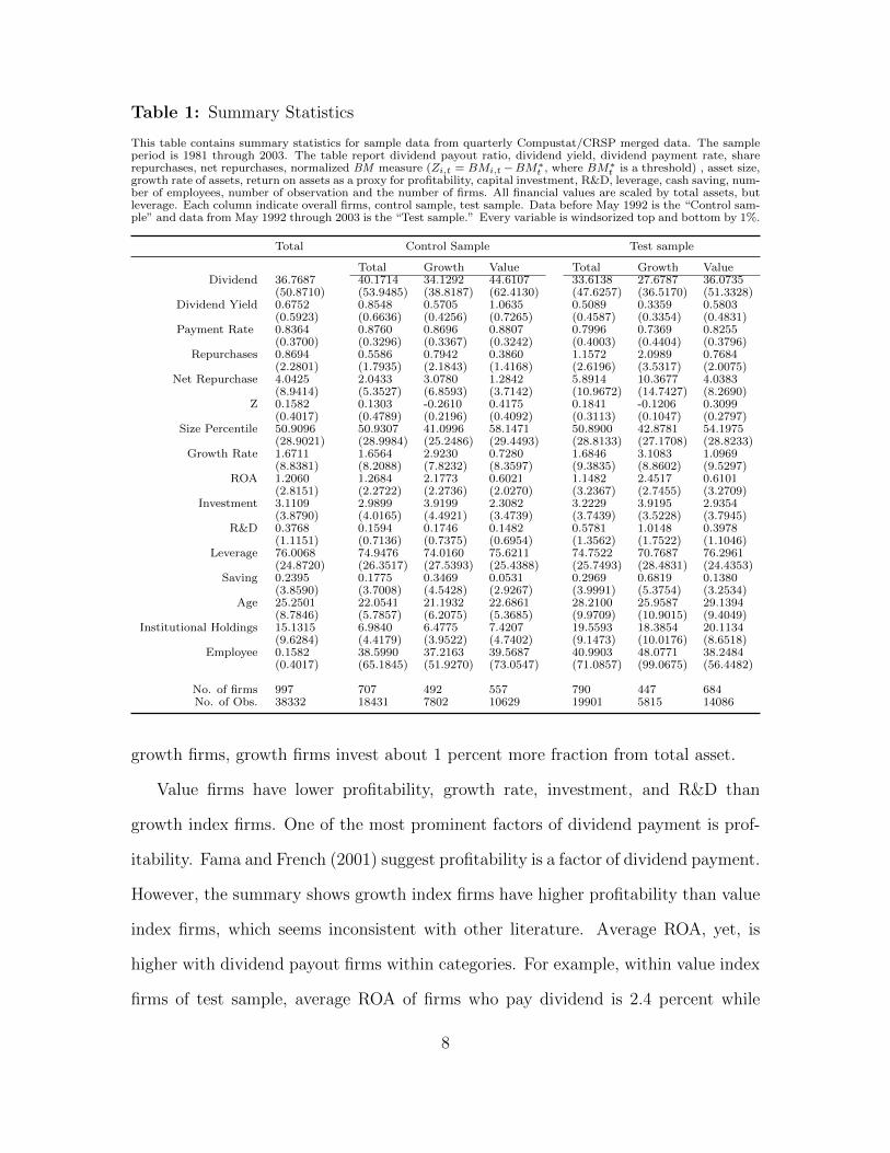
Table 1: Summary Statistics

This table contains summary statistics for sample data from quarterly Compustat/CRSP merged data. The sampleperiod is 1981 through 2003. The table report dividend payout ratio, dividend yield, dividend payment rate, sharerepurchases, net repurchases, normalized BM measure (Zi,t = BMi,t−BM∗

t , where BM∗t is a threshold) , asset size,

growth rate of assets, return on assets as a proxy for profitability, capital investment, R&D, leverage, cash saving, num-ber of employees, number of observation and the number of firms. All financial values are scaled by total assets, butleverage. Each column indicate overall firms, control sample, test sample. Data before May 1992 is the “Control sam-ple” and data from May 1992 through 2003 is the “Test sample.” Every variable is windsorized top and bottom by 1%.

Total Control Sample Test sample

Total Growth Value Total Growth ValueDividend 36.7687 40.1714 34.1292 44.6107 33.6138 27.6787 36.0735

(50.8710) (53.9485) (38.8187) (62.4130) (47.6257) (36.5170) (51.3328)Dividend Yield 0.6752 0.8548 0.5705 1.0635 0.5089 0.3359 0.5803

(0.5923) (0.6636) (0.4256) (0.7265) (0.4587) (0.3354) (0.4831)Payment Rate 0.8364 0.8760 0.8696 0.8807 0.7996 0.7369 0.8255

(0.3700) (0.3296) (0.3367) (0.3242) (0.4003) (0.4404) (0.3796)Repurchases 0.8694 0.5586 0.7942 0.3860 1.1572 2.0989 0.7684

(2.2801) (1.7935) (2.1843) (1.4168) (2.6196) (3.5317) (2.0075)Net Repurchase 4.0425 2.0433 3.0780 1.2842 5.8914 10.3677 4.0383

(8.9414) (5.3527) (6.8593) (3.7142) (10.9672) (14.7427) (8.2690)Z 0.1582 0.1303 -0.2610 0.4175 0.1841 -0.1206 0.3099

(0.4017) (0.4789) (0.2196) (0.4092) (0.3113) (0.1047) (0.2797)Size Percentile 50.9096 50.9307 41.0996 58.1471 50.8900 42.8781 54.1975

(28.9021) (28.9984) (25.2486) (29.4493) (28.8133) (27.1708) (28.8233)Growth Rate 1.6711 1.6564 2.9230 0.7280 1.6846 3.1083 1.0969

(8.8381) (8.2088) (7.8232) (8.3597) (9.3835) (8.8602) (9.5297)ROA 1.2060 1.2684 2.1773 0.6021 1.1482 2.4517 0.6101

(2.8151) (2.2722) (2.2736) (2.0270) (3.2367) (2.7455) (3.2709)Investment 3.1109 2.9899 3.9199 2.3082 3.2229 3.9195 2.9354

(3.8790) (4.0165) (4.4921) (3.4739) (3.7439) (3.5228) (3.7945)R&D 0.3768 0.1594 0.1746 0.1482 0.5781 1.0148 0.3978

(1.1151) (0.7136) (0.7375) (0.6954) (1.3562) (1.7522) (1.1046)Leverage 76.0068 74.9476 74.0160 75.6211 74.7522 70.7687 76.2961

(24.8720) (26.3517) (27.5393) (25.4388) (25.7493) (28.4831) (24.4353)Saving 0.2395 0.1775 0.3469 0.0531 0.2969 0.6819 0.1380

(3.8590) (3.7008) (4.5428) (2.9267) (3.9991) (5.3754) (3.2534)Age 25.2501 22.0541 21.1932 22.6861 28.2100 25.9587 29.1394

(8.7846) (5.7857) (6.2075) (5.3685) (9.9709) (10.9015) (9.4049)Institutional Holdings 15.1315 6.9840 6.4775 7.4207 19.5593 18.3854 20.1134

(9.6284) (4.4179) (3.9522) (4.7402) (9.1473) (10.0176) (8.6518)Employee 0.1582 38.5990 37.2163 39.5687 40.9903 48.0771 38.2484

(0.4017) (65.1845) (51.9270) (73.0547) (71.0857) (99.0675) (56.4482)

No. of firms 997 707 492 557 790 447 684No. of Obs. 38332 18431 7802 10629 19901 5815 14086

growth firms, growth firms invest about 1 percent more fraction from total asset.

Value firms have lower profitability, growth rate, investment, and R&D than

growth index firms. One of the most prominent factors of dividend payment is prof-

itability. Fama and French (2001) suggest profitability is a factor of dividend payment.

However, the summary shows growth index firms have higher profitability than value

index firms, which seems inconsistent with other literature. Average ROA, yet, is

higher with dividend payout firms within categories. For example, within value index

firms of test sample, average ROA of firms who pay dividend is 2.4 percent while

8

non-pay firms have 2.0 percent of ROA. Regression results for dividend policy also

show that ROA has significant positive effect which is consistent with other literature.

Of greater interest, the average value of dividend is higher in value index. Dividend

payout ratio in value index is 44.61 percent with control sample and 36.07 percent

with test sample, which is higher than 34.13 percent and 27.68 percent in growth

index.

1.3 Model/Methodology

This section describes how to adapt the regression discontinuity methodology to

an event study in order to estimate the effect of value and growth index on corporate

dividend policy.

1.3.1 Identification

Regression discontinuity design in this study satisfies required identifying assump-

tions.

1. Index labeling is solely a function of BM ratio. S&P/Barra indices

have simple rules for classify stocks as “growth” and “value” based on

BM ratio. No other variable can contaminate the labeling.

2. Firms do not know what kind of index they would be labeled as,

because the threshold is based on random components. S&P/Barra must

reset the boundary to rebalance the market cap of each index group. As

a result, the label of stocks can be switched to “value” after their BM

ratios actually decrease, or switched to “growth” after their BM ratios

actually increase. Thus labeling contains, at least near the cut-off, random

components. This is the key assumption of the local randomization. Lee

9

(2008) formally shows that as long as there is a random component to the

threshold, the assignment into each group is random around the threshold.

3. For the same reason, firms cannot manipulate their value to get a

specific label they want. Thus index membership does not suffer from

endogeneity issues. If firms can effectively choose the BM ratio for the

labeling, firms who choose above the threshold could be somewhat differ-

ent from those who below the threshold. It will invalidate the regression

discontinuity approach.

1.3.2 Regression Discontinuity in Dividend Policy

Suppose that a firm i have the value of book to market BMi,t at time t: If BMi,t is

larger than the threshold BM∗t , then this firm is labeled as a value firm and the firm

has the indicator Ii,t =1 (BMi,t > BM∗). Let Zi,t = BMi,t − BM∗t , then the cut-off

value Z∗t based on the new measure Zi,t will be always zero. The effect of labeling on

an outcome Di,t can be written as

Di,t = α + Ii,tβ + f(Zi,t) + µi,t

where the coefficient β is the effect of index on the dividend payout Di,t and µi,t

represents all other determinants of the outcome (E(µi,t ) = 0). Ii,t is a dummy

variable indicating whether a firm is labelled “value” or “growth” based on a cut-off

value. Estimating these kind of regressions is problematic, when the labeling is a

highly endogenous outcome, and Ii,t is unlikely to be independent of the error term

(E(Ii,t, µi,t) 6= 0); the estimate of β will be biased. To get a consistent β, labeling

is ideally needed to be a randomly assigned variable. Since whether the value index

or growth index is random in a small interval around the discontinuity (where a cut-

off Z∗=0), the regression discontinuity framework helps me approximate this ideal

10

setup. There is a random component to set the threshold of BM ratio, so that the

assignment into “growth” (Ii,t = 0) and “value” (Ii,t = 1) groups is random around

the threshold. This implies that the estimate of β using the regression discontinuity

design is not affected by omitted variables even if they are correlated with the BM

ratio, as long as their effect is continuous around the threshold. 2 Therefore, by

comparing the dividend of firms that barely have value index to the dividend of firms

that barely have growth index, I get a consistent estimate of the value of the labeling.

Global strategy of regression discontinuity is the methodology which use overall

data set, and it is also called parametric strategy. This methodology assume that I

can approximate the continuous underlying relationship between Di,t and Zi,t with a

continuous function of book to market ratio. This continuous function captures the

underlying relationship between any variable that is continuously affected by book to

market ratio and the dividend payout, and β captures the discontinuity of dividend

payout at the threshold. Allowing for a different function for observations on the

left-hand side of the threshold f(Zi,t) and on the right-hand side of the threshold

g(Zi,t) gives

Di,t = α + Ii,tβ + f(Zi,t) + Ii,t · g(Zi,t) + ηt + λi + µi,t (1.1)

For example, following the standard approach (Lee and Lemiuex, 2010), I can as-

sume the relationship between Di,t and Zi,t as a quadratic polynomial, and the above

equation can be transferred as follows

Di,t = α + Ii,tβ + γ1Zi,t + γ2Ii,tZi,t + γ3Z2i,t + γ4Ii,tZ

2i,t + ηt + λi + µi,t (1.2)

In addition to the polynomial regression model, I control firm specific characteristics

in (1.3). The parameter ηt contains fixed effects for the time periods of years and

2Continuity of other variables are revealed in section 1.4.7

11

quarters, and λi is an industry fixed effect based on two-digit SIC code. Regression

discontinuity design does not require the control of other variables or fixed effect near

the cut-off if regression discontinuity design is valid. Moreover, Lee and Lemieux

(2010) argue that the use of other baseline covariates in an RD design is primarily to

reduce sampling variability. I control firm specific characteristics such as size, prof-

itability and growth rate as suggested by Fama and French (2001) to test robustness

with broad range near the cut-off. The equation extended with firm characteristics is

Di,t = α + Ii,tβ + γ1Zi,t + γ2Ii,tZi,t + γ3Z2i,t + γ4Ii,tZ

2i,t +X ′i,tθ + ηt + λi + µi,t (1.3)

where X contains firm specific characteristics.

Choice of polynomial order is an important consideration to use above polynomial

model, since linear or misspecified polynomial model may capture the curvature of

regression rather than discontinuity. In the empirical test section, various polynomial

orders, from a linear model up to polynomial of order of four on either side of the

threshold, are placed into the model to illustrate the robustness of results.

An alternative methodology is the use of local linear regressions. Local linear

estimation, which is called non-parametric strategy, is more flexible than global poly-

nomial regression, which is called non-parametric strategy, to fit various shapes. The

regression model is as follows

Di,t = α + Ii,tβ + γ1Zi,t + γ2Ii,tZi,t + µi,t, where − h ≤ Z ≤ h

for h > 0. The treatment effect is also captured by β. The choice of bandwidth, h,

is an important consideration, as choice of polynomial order in the global regression.

By using Imbens and Kalyanaraman (2012) procedure as a benchmark for the choice

of bandwidth, I apply various bandwidths around the benchmark bandwidth into the

model for testing the robustness of results. By applying additional fixed effects, the

12

above equation can be rewritten as

Di,t = α + Ii,tβ + γ1Zi,t + γ2Ii,tZi,t + ηt + λi + µi,t, where − h ≤ Z ≤ h (1.4)

The parameter ηt contains fixed effects for the time periods of years and quarters, and

λi is an industry fixed effect based on two-digit SIC code. I also extend regression

model (1.4) by controlling firm specific characteristics X for the robustness test.

Di,t = α+ Ii,tβ + γ1Zi,t + γ2Ii,tZi,t +X ′i,tθ+ ηt + λi + µi,t, where − h ≤ Z ≤ h (1.5)

1.4 Empirical Analysis

1.4.1 Graphical Analysis for Regression Discontinuity

I begin the empirical analysis with a simple plot of the dividend payout ratio as

a function of BM ratio using information of S&P 500 listed firms during the control

(1981-1992) and the test (1992-2003) sample years. Figure 1.1 illustrates a graphi-

cal analysis for dividend payout policy to characterize regression discontinuity. Each

graph in the Figure 1.1 portrays a relationship that might exist between dividend

payout policy and BM ratio, which is normalized to Z value. Each dot shows the

average value of the dividend payout ratio for firms, in each bin with width 0.02,

against the BM ratio. The vertical line in the center of each graph designates a

cut-off point, above which firms are labeled “value” and below which firms are la-

beled “growth”. To show the detailed characteristics, the BM ratio limits within

0.4 near the threshold, which is twice the bandwidth value based on Imbens and

Kalyanaraman (2012) for the regression discontinuity design. The first graph in Fig-

ure 1.1 illustrates the relationship between dividend payout ratio and BM ratio in

the control sample. As can be seen, the relationship is upward sloping to the right,

which indicates that dividend payout ratio increases as BM ratio increases. This

13

relationship passes continuously through the cut-off point, which implies that there

is no difference in dividend payout ratio for value or growth index firms which are

just above and below the cut-off point. The second graph in the Figure 1.1 illustrates

the relationship between dividend payout ratio and BM ratio in the test sample. In

the test sample period (after May 1992), by contrast, there is a sharp upward jump

at the cut-off point in the relationship, which intuitively supports that labeling effect

exist on dividend payout policy.

Figure 1.1: Dividend Payout Ratio

Conservatism in setting dividend may weaken the logic that dividend payout ratio

reflects payout policy. On the contrary, this conservatism shed light on labeling

effect for one side, only for value index. Conservatism in dividend comes from the

classic field survey of managers by Lintner (1956). Lintner reports that managers

are conservative in setting dividend policy. In particular, managers are reluctant to

14

make upward changes in dividends that may have to be reversed in the future. Fifty

years later, Brav, Graham, Harvey, and Michaely (2005) survey a larger number of

384 executives, and they report that managers are reluctant to cut dividends and

take the current level of dividend payments as given. Thus it is possible that firms

can increase dividend payout with value index due to investor’s sentiment, however,

it is hard to decrease payout from current level of dividend payout when the index

is changed to growth. On the other hand, firms may more rely on whether they pay

dividend, rather than how much they pay with reflecting on a notion of conservatism.

In addition to analyzing dividend payout ratio, average payment rate, which measure

how many firms are paying dividend, is taken for another measure of dividend policy

change.

Figure 1.2 illustrates a graphical analysis for average dividend payment rate to

characterize regression discontinuity. Each dot also shows the average dividend pay-

ment rate for firms in BM bin with width 0.02. The vertical line in the center of

each graph designates a cut-off point, and the BM ratio limits within 0.4 near the

threshold. The first graph in Figure 1.2 illustrates the relationship between dividend

payment rate and BM ratio in the control sample. This relationship passes continu-

ously through the cut-off point, which implies that there is no difference in dividend

payment rate for value or growth index firms that are just above and below the cut-

off point. The second graph in the Figure 1.2 illustrates the relationship between

dividend payment rate and BM ratio in the test sample. In this case, there is a

sharp upward jump at the cut-off point in the relationship, which is consistent with

the dividend payout ratio graph. Therefore, this figure support that firms are more

willing to payout dividend with value label.

15

Figure 1.2: Dividend Payment Rate

1.4.2 Estimation of Regression Discontinuity - Global strategy

Significant discontinuity of dividend policy with labeling is observed through the

global strategy. Table 1.2 contains global estimation results of sharp regression dis-

continuity in dividend payout ratio. Panel A presents standard global estimations of

regression discontinuity with various polynomial regressions which are based on equa-

tion (1.1) and equation (1.2). For the test sample, a significant index discontinuity

drive a jump of dividend payout ratio from 4.2 percent to 5 percent with the value

index. This implies that dividend payout ratio increases by about 4.2 to 5 percent

points when a firm has value label, where average payout ratio difference between

growth and value group in the test sample is about 8.4 percents. These coefficients

are significant through the different polynomial models. For the control sample, lin-

16

ear and quadratic models show significant value of discontinuity (7.81, 3.72), however,

higher orders of polynomial models do not show discontinuity. With broad range of

entire sample, as it named global strategy, linear and quadratic models may capture

the curvature of regression rather than discontinuity. Moreover, regressions with dif-

ferent polynomial show inconsistent coefficient, while coefficients in the test sample

are relatively consistent.

Robustness tests are performed in Panel B, and the tests also indicate that the

index has a positive treatment effect on dividend payout ratios during the test sample

period. Panel B controls for firms’ other characteristics such as profitability, growth

rate of assets and size, which are dividend factors suggested by Fama and Frech

(2001). Institutional holdings are also controlled for as another factor influencing

dividend policy. Both Grinstein and Michaely (2005) and Crane, Michenaud, and

Weston (2014) suggest institutional holdings, but they have opposite expectation for

the relationship between institutional holdings and dividend payout. Equation (1.3)

is applied for this test. A robustness test with firm characteristics shows consistent

result (from 4.39 to 5.38), and these values are statistically not different. Other

variables are also significant for dividend payout. More profitable firms and big firms

payout more, and growing firms invest more instead of payout. In regards to the

institutional ownership, there is negative correlation between institutional holdings

and dividend payout. The result is consistent with Grinstein and Michaely (2005),

and contrary to Crane, Michenaud, and Weston (2014).

As Lee and Lemieux (2010) point out, a possible disadvantage of the paramet-

ric/global estimation approach is that it provides a regression over the entire range

of BM ratios, while the regression continuity design depends on local estimates of

the regression function at the cut-off point. The fact that global regression models

use data far away from the cut-off point to predict the value of dividend near the

17

Tab

le1.2

:E

stim

atio

nof

Shar

pR

egre

ssio

nD

isco

nti

nuit

y-

Glo

bal

Str

ateg

y

Th

ista

ble

conta

ins

glo

bal

esti

mati

on

of

sharp

regre

ssio

ndis

conti

nu

ity

resu

ltfo

rd

ivid

end

payou

tra

tio.

Pan

elA

pre

sents

stan

dard

glo

bal

esti

mati

on

of

regre

ssio

nd

isco

nti

nu

ity

an

dvari

ou

sp

oly

nom

ial

regre

ssio

nw

hic

hare

base

don

equ

ati

on

(1.1

)an

deq

uati

on

(1.2

).P

an

elB

ad

dit

ion

ally

contr

ol

firm

s’oth

ersp

ecifi

cssu

chas

boot

tom

ark

et,

pro

fita

bilit

y,gro

wth

rate

of

ass

ets

an

dsi

ze,

bec

au

sed

ivid

end

payou

tca

nb

eaff

ecte

dby

sever

al

firm

chara

cter

isti

cs.

Equ

ati

on

(1.3

)is

ap

pli

edfo

rth

iste

st.

Both

pan

els

ind

icate

that

the

ind

exh

as

posi

tive

trea

tmen

teff

ect

on

div

iden

dp

ayou

tra

tio

for

the

test

sam

ple

.In

contr

ol

pan

el,

lin

ear

an

dp

oly

nom

ial

regre

ssio

nm

od

elsh

ow

sp

osi

tive

ind

exeff

ect,

bu

tit

may

cap

ture

the

curv

atu

reof

regre

ssio

nra

ther

than

dis

conti

nu

ity.

All

data

are

from

the

qu

art

erly

Com

pu

stat/

CR

SP

.T

he

sam

ple

per

iod

is1981

thro

ugh

2003.

Data

bef

ore

May

1992

isth

e“C

ontr

ol

sam

ple

”an

dd

ata

from

May

1992

thro

ugh

2003

isth

e“T

est

sam

ple

.”T

he

esti

mati

on

sin

clu

de

yea

rfi

xed

effec

t,qu

art

erfixed

effec

tan

din

du

stry

fixed

effec

tw

hic

his

base

don

two

dig

itS

IC.

Th

eass

oci

ate

dst

an

dard

erro

rsare

rep

ort

edin

pare

nth

eses

.***,

**

an

d*

ind

icate

stati

stic

al

sign

ifica

nce

at

the

1%

,5%

an

d10%

(tw

o-t

ail)

test

level

s,re

spec

tivel

y.

Cotr

ol

Tes

t

A.

Sta

nd

ard

Tes

t

Lin

ear

Poly

Cu

be

Qu

art

icL

inea

rP

oly

Cu

be

Qu

art

ic

Ind

ex7.8

096***

3.7

228**

0.2

23

0.0

487

4.9

526***

4.6

581***

4.7

779***

4.2

487**

(1.2

293)

(1.4

872)

(1.7

748)

(2.1

147)

(1.1

257)

(1.4

226)

(1.7

402)

(2.1

410)

No.

of

Ob

s.18376

18376

18376

18376

19819

19819

19819

19819

R-S

qu

are

d0.0

80.0

82

0.0

83

0.0

83

0.1

21

0.1

22

0.1

22

0.1

22

B.

Exte

nd

edT

est

-C

ontr

ol

RO

A,

Siz

e,G

row

thR

ate

Lin

ear

Poly

Cu

be

Qu

art

icL

inea

rP

oly

Cu

be

Qu

art

ic

Ind

ex7.3

648***

3.0

474*

-0.9

635

0.3

057

5.2

059***

4.3

865***

5.3

756***

4.9

832**

(1.5

096)

(1.7

985)

(2.1

477)

(2.5

520)

(1.2

867)

(1.5

936)

(1.9

541)

(2.3

917)

RO

A1.2

612***

1.4

326***

1.4

460***

1.4

387***

0.9

149***

0.9

205***

0.9

168***

0.9

121***

(0.2

403)

(0.2

430)

(0.2

438)

(0.2

441)

(0.1

554)

(0.1

569)

(0.1

569)

(0.1

572)

Gro

wth

Rate

-0.1

751***

-0.1

661***

-0.1

694***

-0.1

696***

-0.1

623***

-0.1

621***

-0.1

624***

-0.1

626***

(0.0

536)

(0.0

536)

(0.0

536)

(0.0

536)

(0.0

336)

(0.0

336)

(0.0

336)

(0.0

336)

Siz

e0.1

354***

0.1

294***

0.1

278***

0.1

278***

0.1

132***

0.1

145***

0.1

140***

0.1

141***

(0.0

229)

(0.0

229)

(0.0

229)

(0.0

229)

(0.0

176)

(0.0

176)

(0.0

176)

(0.0

176)

Inst

.H

old

ings

-0.1

796

-0.1

74

-0.2

068*

-0.2

046*

-0.4

036***

-0.4

024***

-0.4

024***

-0.4

027***

(0.1

227)

(0.1

227)

(0.1

228)

(0.1

228)

(0.0

515)

(0.0

515)

(0.0

515)

(0.0

515)

No.

of

Ob

s.11490

11490

11490

11490

14049

14049

14049

14049

R-S

qu

are

d0.0

85

0.0

86

0.0

88

0.0

88

0.1

20.1

21

0.1

22

0.1

22

18

Table 1.3: Estimation of Sharp Regression Discontinuity - Local Strategy

This table contains linear regression result for dividend payout ratio within a range of cut-off value. Panel A presentsstandard local estimation of regression discontinuity with bandwidth 0.2 which are based on bandwidth selectorprocedure by Imbens and Kalyanaraman (2012). On the top of the bandwidth 0.2, ±0.05 of the bandwidth areapplied for the robustness. Equation (1.4) is applied for this test. Panel B additionally control firms’ other specificssuch as profitability, growth rate of assets and size, which are possible factors for dividend payout. Equation (1.5)is applied for this robustness test. The estimations include year fixed effect, quarter fixed effect and industry fixedeffect which is based on two digit SIC. The sample period is 1981 through 2003. Data before May 1992 is the“Control sample” and data from May 1992 through 2003 is the “Test sample.” All data are from the quarterlyCompustat/CRSP. The associated standard errors are reported in parentheses.***, ** and * indicate statistical significance at the 1%, 5% and 10% (two-tail) test levels, respectively.

A. Standard Test

Control Sample Test Sample

Bandwidth +0.05 0 -0.05 +0.05 0 -0.05

Index -0.726 -1.9434 -0.9419 3.6121*** 3.4070** 4.5890***(2.2349) (2.5486) (2.9922) (1.3931) (1.5460) (1.7374)

No. of Obs. 8539 6743 4942 15720 10905 8656R-Squared 0.079 0.072 0.069 0.131 0.134 0.132

B. Extended Test


Bandwidth +0.05 0 -0.05 +0.05 0 -0.05

Index 0.8460 0.4106 1.1883 3.6690** 4.0016** 5.2793***(2.7144) (3.1051) (3.6346) (1.5602) (1.7497) (1.9748)

Z 47.3375*** 59.4743*** 32.9905 25.9536** 28.0553** 26.0176(12.8395) (18.1674) (27.6778) (10.8090) (12.4394) (16.6142)

ROA (0.5987) (0.7135) -1.5532** 0.7467*** 0.5467*** 0.4133*(0.4652) (0.5394) (0.6257) (0.1860) (0.2022) (0.2205)

Growth Rate -0.1255* (0.0374) (0.0801) -0.1469*** -0.1348*** -0.1285***(0.0694) (0.0813) (0.0944) (0.0341) (0.0362) (0.0389)

Size 0.0456 0.0224 (0.0043) 0.1237*** 0.0886*** 0.0966***(0.0308) (0.0354) (0.0410) (0.0185) (0.0202) (0.0221)

Inst. Holdings -0.5483*** -0.5970*** -0.8565*** -0.3807*** -0.4412*** -0.4641***(0.1776) (0.2038) (0.2362) (0.0548) (0.0609) (0.0669)

Const 64.6733*** 64.7418*** 66.2452*** 11.6070 13.7812 15.0307*(7.4964) (8.0917) (9.0102) (9.5881) (8.9944) (8.9706)


cut-off point is not intuitively appealing. That said, trying more flexible specification

by adding polynomials in BM ratio as regressors into the standard linear model is

an important and useful way of assessing the robustness of the RD estimates of the

treatment effect. Moreover, it is recommended to check both global and local model

when implementing a regression discontinuity design.

19

1.4.3 Estimation of Regression Continuity - Local Strategy

In addition to the parametric/global estimation approach, non-parametric/local

estimation approach is also applied near the cut-off value of Z. Consistent to global

estimation, significant discontinuity from dividend policy is captured through overall

local estimations. The local regression results for dividend payout ratio within a range

of cut-off value are presented in Table 1.3. Panel A contains standard local estima-

tion of regression discontinuity with bandwidth 0.2 that derived from the bandwidth

selecting procedure of Imbens and Kalyanaraman (2012). While the entire range of

Z is from -3.18 to 4.88, local bandwidth 0.2 near the cut-off value contains about

46.2 percent of observations (36.7% in control sample and 55% in test sample). On

the top of the bandwidth 0.2, ±0.05 of the bandwidth are applied for the robust-

ness. Equation (1.4) is applied for this test. For the test sample, a significant index

discontinuity drive a jump of dividend payout ratio from 3.4 percent to 4.6 percent

with the value index. These coefficients are significant at least at the 5 percent level

through the different bandwidth. For the control sample, no significant discontinuity

is observed with any bandwidth values.

Both panels indicate that labeling has a positive effect on dividend payout ratio

only for the test sample. These consistent results support that labeling has an effect

on demand of dividend by providing information to the investors. Compared to the

global strategy, local strategy captures less effect of labeling, however, the values are

all within one standard error range, so the difference is statistically insignificant.

1.4.4 Changes in the Dividend Policy and Labeling

In addition to the static dividend policy measurement, I evaluate the effects of

labeling on changes in the dividend policy. Evaluating these real effects are important

20

Table 1.4: Change of Dividend Payout - Within Firm Effect for Index Switchers

This table contains linear regression result for change of dividend payout ratio within a range of cut-off value. PanelA presents standard local estimation of regression discontinuity with bandwidth 0.17 which are based on bandwidthselector procedure by Imbens and Kalyanaraman (2012). On the top of the bandwidth 0.17, ±0.05 of the bandwidthare applied for the robustness. Equation (1.4) is applied for this test. Panel B uses index change dummies. If a firmchange the index from “growth” to “value”, then the firm assigned as G to V, V to G if a firm’s label switches theother way. If a firm does not have previous index data, the firm is dropped. Panel C additionally control firms’other specifics such as profitability, growth rate of assets and size, which are possible factors for dividend payout.The estimations include year fixed effect, quarter fixed effect and industry fixed effect which is based on two digitSIC. The sample period is 1981 through 2003. Data before May 1992 is the “Control sample” and data from May1992 through 2003 is the “Test sample.” All data are from the quarterly Compustat/CRSP. The associated standarderrors are reported in parentheses.***, ** and * indicate statistical significance at the 1%, 5% and 10% (two-tail) test levels, respectively.

A. Standard Test


Bandwidth 0.05 0 -0.05 0.05 0 -0.05

Index -3.1414 -4.0135 -3.9149 1.1388 0.7463 -0.0558(2.7842) (3.1984) (3.7861) (1.7991) (1.9456) (2.1795)


B. Standard Test for Index Change


Bandwidth 0.05 0 -0.05 0.05 0 -0.05

G to V -1.3584 -3.8357 -3.1872 7.0202* 5.9778 6.7021(5.2242) (5.7083) (6.4051) (4.0588) (4.1266) (4.3154)

V to G -8.4367 -9.7248 -8.6575 1.4005 2.3554 1.5327(5.8044) (6.3715) (7.1494) (4.2394) (4.3032) (4.5539)

Const 1.0721 4.1864 -1.1361 3.3019 3.8333 3.0998(9.8981) (10.7004) (12.1349) (11.9043) (11.7352) (11.5227)


C. Extended Test for Index Change


Bandwidth 0.05 0 -0.05 0.05 0 -0.05

G to V -1.3895 -3.8959 -3.1284 7.1334* 6.0982 6.828(5.2249) (5.7098) (6.4070) (4.0573) (4.1254) (4.3168)

V to G -7.4878 -8.6703 -7.1483 1.4811 2.4142 1.5715(5.8289) (6.4019) (7.1912) (4.2374) (4.3014) (4.5543)

Z 0.6746 1.0371 0.6127 2.4694 5.4244 9.878(5.3120) (7.2453) (10.9882) (4.2851) (5.1815) (6.9124)

ROA -0.4942 -0.0365 -0.0647 0.6342*** 0.6844*** 0.6761***(0.5084) (0.5915) (0.6966) (0.2188) (0.2317) (0.2499)

Growth rate -0.0277 -0.0354 -0.111 -0.0022 -0.0008 0.0232(0.0733) (0.0839) (0.1012) (0.0386) (0.0412) (0.0437)

Size -0.0285 -0.0098 -0.0418 0.0225 0.0233 0.0199(0.0329) (0.0377) (0.0446) (0.0208) (0.0218) (0.0236)

Const 3.1777 5.5555 1.8554 2.2221 2.7425 2.0777(9.9590) (10.7715) (12.2354) (11.9077) (11.7407) (11.5363)


21

for determining whether the firms’ payout ratio increases following the switching of

index categories, especially for those switching from “growth” to “value”. The changes

in the dividend policy are applied into regression discontinuity design of equation 1.4.

Thus the changes in the dividend policy is defined as follows

∆Di,t(= Di,t−Di,t−1) = α+Ii,tβ+γ1Zi,t+γ2Ii,tZi,t+ηt+λi+µi,t, where −h ≤ Z ≤ h.

(1.6)

Changes in the dividend payout are presented on the first panel of Table 1.4, but it

is hard to address that the results provide an evidence of labeling effect. This test

does not take into account changes of labeling whether a firm’s label stays in value

or changes to value.

To show changes of dividend policy in actual index switching effect, I divide firms

into three groups, which are “growth to value”, “value to growth”, and “stay in

the same index”. The second panel presents the behavior of actual label switchers.

The total observation of switchers are small, where growth to value switchers are

4.5 percents and value to growth switchers are 3.6 percents of the sample. Yet,

these switchers are clustered in the local bandwidth of 0.2. While the bandwidth

contains 46.2 percent of total observations, 88.7 percent of switchers are located in

the bandwidth. The switching index of “growth to value” does not show significantly

positive dividend payout effects from the labeling for the all bandwidth choices. Even

though various bandwidth show consistent result with relatively small coefficient of

variation, the test with wider bandwidth only shows significant coefficient. The third

panel shows the robust test results by controlling additional firm characteristics.

From panel A, original “value” index does not explain labeling effect with new

index for switchers, instead of index itself, consistent change of dividend payout ratio

is estimated from panel B, and C. It simply says, if a firm were in growth index with

20% of payout ratio, the firm increases the payout ratio to 26% by shifting into the

22

Table 1.5: Regression Discontinuity - Dividend Payers Only

This table contains linear regression result for dividend payout ratio with dividend payers only. Local estimationof regression discontinuity with bandwidth 0.20 which are based on bandwidth selector procedure by Imbens andKalyanaraman (2012). On the top of the bandwidth 0.20, ±0.05 of the bandwidth are applied for the robustness.Equation (1.5) is applied for this test. The estimations include year fixed effect, quarter fixed effect and industryfixed effect which is based on two digit SIC. The sample period is 1981 through 2003. Data before May 1992 isthe “Control sample” and data from May 1992 through 2003 is the “Test sample.” All data are from the quarterlyCompustat/CRSP. The associated standard errors are reported in parentheses.***, ** and * indicate statistical significance at the 1%, 5% and 10% (two-tail) test levels, respectively.

Extended Local Regression Discontinuity with Dividend Payers Only


Bandwidth +0.05 0 -0.05 +0.05 0 -0.05

Index -0.0409 -0.2097 0.4098 4.9916*** 3.8213* 4.9867**(2.8608) (3.2618) (3.7970) (1.9056) (2.0333) (2.2988)

Z 47.0102*** 61.1063*** 42.6881 2.4295 14.2720 10.2880(13.7174) (19.3379) (28.9927) (12.6041) (14.7242) (19.9040)

ROA -2.0840*** -2.2216*** -2.9387*** 0.0129 0.0660 (0.0323)(0.5334) (0.6113) (0.6905) (0.2688) (0.2795) (0.3113)

Growth rate -0.1266* (0.0435) (0.0813) -0.1159*** -0.1324*** -0.1238**(0.0726) (0.0836) (0.0964) (0.0438) (0.0457) (0.0496)

Size (0.0453) -0.0618* -0.0775* (0.0118) (0.0118) 0.0039(0.0328) (0.0374) (0.0430) (0.0227) (0.0236) (0.0260)

Inst. Holdings -0.4058** -0.4519** -0.6953*** -0.2720*** -0.3023*** -0.3329***(0.1959) (0.2225) (0.2551) (0.0730) (0.0768) (0.0849)

Const 73.5291*** 74.5574*** 73.2704*** 10.9611 13.3075 14.2822(7.9863) (8.6139) (9.4188) (9.6434) (9.4610) (9.4818)


value index. Among all the dividend policy factors, only profitability has possible

explanation power for change in dividend payout ratio.

Although the coefficients in panel B and C in Table 1.4 consistently show positive

labeling effect it does not support enough for labeling effect with index switcher sam-

ple. “value to growth” does not show negative effect as expected from conservatism

in setting dividend, even though these coefficients are not significant. I additionally

check local discontinuity design with dividend payers only, and the result is shown in

Table 1.5. For this test, firm quarters that do not show dividend payout, about 15

percent of sample, are dropped from each group.

1.4.5 Alternative Measure of Dividend Policy - Payment Decision

In addition to the regression discontinuity design with dividend payout ratio, Ta-

ble 1.6 reports robustness test using three different setup with payment decision,

23

Table 1.6: Logit Result

This table contains logit regression result for dividend payment. Index increases dividend payment rate only forthe test sample. Regression methods control firm’s other specifications such as BM , profitability, growth rate ofassets and size. Column (A) shows test result of logit with payment decision. For robustness purpose, column (B)replace dividend payout ratio to payment decision in regression discontinuity with the same bandwidth, while column(C) control firms’ other specifications which are included in column (A) results. All data are from the quarterlyCompustat/CRSP. The sample period is 1981 through 2003. Data before May 1992 is the “Control sample” and datafrom May 1992 through 2003 is the “Test sample.” The estimations include year fixed effect, quarter fixed effect andindustry fixed effect which is based on two digit SIC. The associated standard errors are reported in parentheses.Index* is original index from S&P/Barra, while Index refers matched value/growth index.***, ** and * indicate statistical significance at the 1%, 5% and 10% (two-tail) test levels, respectively.


A. Matched Data Set

(A) (B) (C) (A) (B) (C)

Index 0.3291*** 0.1311 0.0712 0.7732*** 0.3590*** 0.2825**(0.0989) (0.2177) (0.2878) (0.0734) (0.1131) (0.1411)

Z 0.0356 -0.0852 0.6324 -0.1984* 1.3144** 2.1576***(0.0948) (0.9143) (1.1943) (0.1108) (0.5364) (0.6850)

ROA 0.1899*** 0.1799*** 0.1077*** 0.0756***(0.0168) (0.0374) (0.0109) (0.0154)

Growth rate 0.001 0.0041 -0.0072*** -0.0087***(0.0036) (0.0071) (0.0021) (0.0026)

Size 0.0299*** 0.0210*** 0.0245*** 0.0248***(0.0017) (0.0033) (0.0012) (0.0017)

Inst. Holdings 0.0051 -0.0562*** -0.0311*** -0.0443***(0.0074) (0.0159) (0.0034) (0.0046)

Const 2.6021*** 3.0830*** 2.5414*** 0.486 3.3498*** 1.3991***(0.4920) (0.6160) (0.6896) (0.4377) (0.4834) (0.5339)

No. of Obs. 10200 6084 3310 13003 10472 7299pseudo R-sq 0.214 0.181 0.241 0.242 0.212 0.276

B. Premitive Data Set

(A) (B) (C) (A) (B) (C)

Index* 0.3466*** 0.0183 0.1611 0.6919*** 0.3348*** 0.3723***(0.0853) (0.1186) (0.1539) (0.0662) (0.0757) (0.0974)

Z 0.0369 0.2249 0.0415 -0.0877 1.3378*** 1.7568***(0.0856) (0.5256) (0.6732) (0.1065) (0.3794) (0.4991)

ROA 0.2061*** 0.2213*** 0.1132*** 0.0847***(0.0165) (0.0342) (0.0108) (0.0148)

Growth rate -0.0003 0.0003 -0.0081*** -0.0094***(0.0034) (0.0061) (0.0020) (0.0025)

Size 0.0277*** 0.0185*** 0.0244*** 0.0243***(0.0016) (0.0029) (0.0011) (0.0015)

Inst. Holdings 0.001 -0.0634*** -0.0343*** -0.0495***(0.0071) (0.0144) (0.0032) (0.0043)

Const 2.4510*** 3.1186*** 2.4627*** 0.486 3.2840*** 1.2158**(0.4268) (0.5226) (0.5719) (0.4359) (0.4784) (0.5157)

No. of Obs. 11550 7512 4145 14097 12120 8365pseudo R-sq 0.222 0.197 0.258 0.244 0.215 0.28

24

whether a firm pay dividend or not, in Panel A. For the binary payment variable,

the robustness test borrows logit model following Fama and French (2001). As they

test payment with three factors; profitability, growth rate, and size, the first robust-

ness test is based on the three factors with index and normalized BM ratio, Z, and

check whether the index has significant effect. The result of this estimation can be

found in column (A). Column (B) shows the result of the logit which based on re-

gression discontinuity model. Thus, payment decision replaces dividend payout ratio

in regression with the same 0.2 bandwidth near the cut-off value of Z, which means

only index and Z are controlled for dividend payment decision. Column (C) shows a

robustness test with the extended regression discontinuity model which additionally

controls three dividend factors and also limits the 0.2 range of Z near the cut-off

value. Column (A) shows significant labeling effect for both of the control and the

test sample, however, index coefficient may capture systematical difference across two

groups, rather than the labeling itself. This is a reason why this paper applies regres-

sion discontinuity design which does not suffer from this problem. Column (B) and

(C) shows significantly positive coefficient from only test sample.

When matching the original data with S&P/Barra index, eight percent of data

was mismatched and dropped for the regression discontinuity test. However, the logit

test does not require the same assumption as regression discontinuity regression. Thus

Panel B uses original data with S&P/Barra index. No matter what kind of data sets

are used and however it models, the results are quite consistent.

1.4.6 The Robustness Test Utilizing an additional Time Period

S&P/Barra index is generated until Barra has merged into MSCI in 2003. If the

discontinuity is coming from systematical difference from book to market ratio, then

discontinuity may exist with S&P/Barra measure even though labeling based on book

25

to market ratio is not exist. Even though control sample periods can test this sys-

tematic difference, this section also consider the possibility that systematic differences

which exist after control sample periods. The sample for the test is S&P firms after

S&P/Barra stop generate growth/value index. I generate the index constituent data

from April 2003 to June 2014, dividing the S&P 500 into two groups and rebalancing

the groups every June and December, exactly as if the indices existed over this period.

Figure 1.3 illustrates a graphical analysis for dividend payout policy and divi-

dend payment rate after test sample years. Each graph in the Figure 1.3 portrays

a relationship that might exist between dividend payout policy and BM ratio. As

it shows in control and test sample, each dot shows the average value of dividend

payout ratio within bin-width 0.02. To show the detailed characteristics, the Z limits

within 0.4 near the threshold, which is twice the bandwidth value based on Imbens

and Kalyanaraman (2012) for the regression discontinuity design. 61.5% of samples

are located within this bandwidth. The relationship between dividend payout ratio

and BM ratio is upward sloping to the right. It is also observable from payment rate

graph. It is hard to address that discontinuity exist at the cut-off. On the contrary,

smooth continuous relationship is shown within this bandwidth.

Table 1.7 contains global estimation results of sharp regression discontinuity in

dividend payout ratio after test sample periods. Left four columns presents stan-

dard global estimations of regression discontinuity with various polynomial regressions

which are based on equation (1.1) and equation (1.2). Right four columns addition-

ally control firms’ other specifics such as boot to market, profitability, growth rate of

assets and size. Equation (1.3) is applied for this test. Cubic and quartic polynomial

models show significant value of discontinuity (-0.83, -1.392) in basic model. Cubic

polynomial model in extended model shows significant discontinuity (1.5038), which

is not consistent with basic model. Moreover, higher orders of polynomial models do

26

Tab

le1.7

:G

lobal

Str

ateg

yaf

ter

Tes

tSam

ple

Per

iods

Th

ista

ble

conta

ins

glo

bal

esti

mati

on

of

sharp

regre

ssio

nd

isco

nti

nu

ity

resu

ltfo

rd

ivid

end

payou

tra

tio

aft

erS

&P

/B

arr

ast

op

gen

erati

ng

style

ind

ex.

Lef

tfo

ur

colu

mn

sp

rese

nt

stan

dard

glo

bal

esti

mati

on

of

regre

ssio

nd

isco

nti

nu

ity

an

dvari

ou

sp

oly

nom

ial

regre

ssio

nw

hic

hare

base

don

equ

ati

on

(1.1

)an

deq

uati

on

(1.2

).R

ight

fou

rco

lum

ns

ad

dit

ion

ally

contr

ol

firm

s’oth

ersp

ecifi

cssu

chas

boot

tom

ark

et,

pro

fita

bilit

y,gro

wth

rate

of

ass

ets

an

dsi

ze,

bec

au

sed

ivid

end

payou

tca

nb

eaff

ecte

dby

sever

al

firm

chara

cter

isti

cs.

Equ

ati

on

(1.3

)is

ap

plied

for

this

test

.A

lld

ata

are

from

the

qu

art

erly

Com

pu

stat/

CR

SP

.T

he

sam

ple

per

iod

is2003

thro

ugh

2014.

Th

ees

tim

ati

on

sin

clu

de

yea

rfi

xed

effec

t,qu

art

erfi

xed

effec

tan

din

du

stry

fixed

effec

tw

hic

his

base

don

two

dig

itS

IC.

Th

eass

oci

ate

dst

an

dard

erro

rsare

rep

ort

edin

pare

nth

eses

.***,

**

an

d*

ind

icate

stati

stic

al

sign

ifica

nce

at

the

1%

,5%

an

d10%

(tw

o-t

ail)

test

level

s,re

spec

tivel

y.

Basi

cE

xte

nd

ed

Cu

bic

Qu

art

icQ

uin

tic

Sex

tic

Cu

bic

Qu

art

icQ

uin

tic

Sex

tic

Ind

ex-0

.8300*

-1.3

920**

-0.0

378

0.8

056

1.5

038**

1.0

457

1.2

845

1.2

267

(0.4

724)

(0.5

668)

(0.6

628)

(0.7

568)

(0.6

702)

(0.7

951)

(0.9

225)

(1.0

484)

RO

A0.1

165***

0.1

154***

0.1

153***

0.1

150***

(0.0

126)

(0.0

126)

(0.0

126)

(0.0

127)

Gro

wth

Rate

-0.0

796***

-0.0

796***

-0.0

795***

-0.0

798***

(0.0

086)

(0.0

086)

(0.0

086)

(0.0

086)

Siz

e0.2

696***

0.2

689***

0.2

688***

0.2

691***

(0.0

076)

(0.0

076)

(0.0

076)

(0.0

076)

Inst

.H

old

ings

-0.1

798***

-0.1

800***

-0.1

800***

-0.1

802***

(0.0

114)

(0.0

114)

(0.0

114)

(0.0

114)

No.

of

Ob

s.311020

311020

311020

311020

158018

158018

158018

158018

R-S

qu

are

d0.1

02

0.1

03

0.1

03

0.1

03

0.1

39

0.1

39

0.1

39

0.1

39

27

Figure 1.3: Dividend Payout Rate and Payment Rate after Test Sample Periods

not show discontinuity.

The local regression results for dividend payout ratio after S&P/Barra stop gen-

erating style index are presented in Table 1.8. Left three columns present standard

local estimation of regression discontinuity with bandwidth 0.2 which are based on

bandwidth selector procedure by Imbens and Kalyanaraman (2012). On the top of

the bandwidth 0.2, ±0.05 of the bandwidth are applied for the robustness. Equa-

tion (1.4) is applied for this test. Right three columns additionally control firms’

other specifics such as profitability, growth rate of assets and size, which are possible

factors for dividend payout. Equation (1.5) is applied for this robustness test. No

significant discontinuity is observed with basic test, and only wide bandwidth choice

shows significant result in extended model.

28

In sum, systematic difference, which may exist based on index labeling, does not

drive consistent discontinuity in dividend payout policy from both of global strategy

and local strategy after S&P/Barra stop generating style index.

1.4.7 Share Repurchases and Other Corporate Policies

Dividend may not be the only policy which is affected by labeling. Other policies,

which may be affected by investor sentiment, are also possible considerations for this

labeling effect study such as repurchases, institutional ownership. Other corporate

policies as investment, leverage, R&D, cash saving, and employment are tested in the

section for the placebo effect. 3 If dividend discontinuity is happened by placebo

3In addition to checking other variables which might related with assignment variable, McCrary(2006) shows the density test is useful to check internal validity for manipulation incentive. Thisdensity is shown in the appendix section as a Figure A.1. However, it is hard to say that thisdensity test provides meaningful result for this paper. That is because McCrary density test requiremonotonic incentive to manipulation, otherwise the test result say nothing about manipulation.

Table 1.8: Local Strategy after Test Sample Periods

This table contains linear regression result for dividend payout ratio within a range of cut-off value after S&P/Barrastop generating style index. Left three columns present standard local estimation of regression discontinuity withbandwidth 0.2 which are based on bandwidth selector procedure by Imbens and Kalyanaraman (2012). On the topof the bandwidth 0.2, ±0.05 of the bandwidth are applied for the robustness. Equation (1.4) is applied for this test.Right three columns additionally control firms’ other specifics such as profitability, growth rate of assets and size,which are possible factors for dividend payout. Equation (1.5) is applied for this robustness test. The estimationsinclude year fixed effect, quarter fixed effect and industry fixed effect which is based on two digit SIC. The sampleperiod is 2003 through 2014. All data are from the quarterly Compustat/CRSP. The associated standard errors arereported in parentheses.***, ** and * indicate statistical significance at the 1%, 5% and 10% (two-tail) test levels, respectively.

Basic Extended

Bandwidth +0.05 0 -0.05 +0.05 0 -0.05

Index 0.0637 -0.2735 -0.0378 1.7917** 0.9682 0.7792(0.5591) (0.6203) (0.7114) (0.7123) (0.7791) (0.8805)

Z -1.6170 4.5793 -0.1008(3.8332) (5.0464) (7.4031)

ROA 0.3026*** 0.3075*** 0.2691***(0.0297) (0.0337) (0.0374)

Growth Rate -0.1306*** -0.1363*** -0.1560***(0.0118) (0.0134) (0.0155)

Size 0.3456*** 0.3582*** 0.3822***(0.0099) (0.0108) (0.0121)

Inst. Holdings -0.2950*** -0.3188*** -0.3558***(0.0149) (0.0161) (0.0181)

Const 2.6577 5.2278 2.1233 -11.4211*** -8.7121* -8.9694*(3.5908) (3.9910) (4.4960) (4.4309) (4.7376) (5.2329)


29

effect from labeling, that other corporate policies, which are not related with investor

sentiment, are also affected by index labeling. Figure 1.6, Figure 1.7, and Table 1.9

show the graphical and empirical analysis for the discontinuity of these variables.

Repurchases

As Skinner (2008) tests substitution of repurchases and dividend policy, share re-

purchases are another method of transferring wealth to investors. However, share

repurchases do not have conservatism as dividend policy does. Firms can choose how

much to repurchases more flexibly than dividend payout. What kind of distribution

methods a firm will take depends on the firm’s own characteristics. Which types of

firms use repurchases more for the earnings distribution can be shown in Figure 1.4

and Figure 1.5.

Figure 1.4 illustrates how dividend policies change in growth and value index firms

through time. It shows that value firms use dividend payout flexibly, and growth

firms do not use dividend flexibly as value firms. The top graph displays the equally

weighted average of dividend payout rate for firms by labeling, while the second graph

displays the same dividend payout ratio with only dividend payers. The vertical line

divides the sample period into the control and test subsamples. In the first graph,

the average growth firms have more stable dividend payout ratio than the average

value firms, and this trend is more transparent in the second graph, which counts

on only dividend payers. On the other side, in the dividend payment case, there is

more significant downward change within growth index firms. On average, value firms

manage more on their dividend payout rather than the payment decision whether they

pay or not, while growth firms have relatively low and conservative dividend payout

ratio and simply do not pay dividend. This can be seen in the bottom graph which

shows how many firms are paying dividend in each year.

30

Figure 1.4: Time Trends in Dividend Policy

31

Figure 1.5: Time Trends in Share Repurchases

In terms of repurchases, growth firms use repurchases more often than average

value firms, which can be shown in Figure 1.5. The first graph illustrates the equally

weighted average of share repurchases for firms through time, and the second graph

displays the equally weighted average of net share repurchase with considering trea-

sury stock issuance for firms through time. Both graphs clearly show the higher rate

of repurchases for growth firms while value firms present a relatively lower rate of

repurchases. The comparison of these two figures provides graphical evidence for the

substitution of dividend and repurchase methods, and which kinds of firms prefer

32

to use share repurchase for their earnings distribution. Growth firms prefer share

repurchases while value firms prefer dividend payout method.

Figure 1.6: Dividend and Repurchase Policy

In Figure 1.6, regression discontinuity design is applied to repurchases based on

distance to the threshold of book to market ratio, Z, and the graphical result is

shown with other corporate policies. The first top left graph is for dividend yield,

and the bottom left graph is for dividend per share as a robustness test of dividend

payout policy. Share repurchases and net share repurchases do not provide visual

discontinuity as clearly as other dividend policies. Repurchases may not depend on

‘Investor sentiment’ but rather on their actual earnings and re-investment level.

33

One of the fundamental value, which categorize firms into the two groups, is BM

ratio. The bottom middle graph indicates that the BM ratio is continuous at the

cut off. Profitability is one factor Fama and French(1997) use for the dividend policy

test. It is hard to convince that the profitability has a discontinuity at the cut off

from the graphical analysis from the bottom right graph in Figure 1.6.

Empirical test results are presented in Table 1.9. A jump in the graph is not

enough to address meaningful discontinuity, but estimation results in Panel B and C

provide some evidence for the possible discontinuity of repurchases. The discontinuity

is not consistently shown as dividend policy and even signs are not consistent in net

repurchases with various bandwidths, especially larger the bandwidth contains the

bigger discontinuity in the local test. However, this may happen even if regression

discontinuity is not valid, because the larger bandwidth may contains some system-

atical differences between growth and value categories. Thus it is hard to conclude

that the repurchase policy shows the labeling effect with discontinuity.

Institutional Share Holdings

Institutional holdings are one of the factors which can affect earnings distribution

policy.

Grinstein and Michaely (2005) and Grullon and Michaely (2002) show that institu-

tional holdings do not affect firms’ policy. While Grinstein and Michaely (2005) show

one-way causality from dividend payout to institutional holdings, Crane, Michenaud,

and Weston (2014) show how institutional holdings affect dividend payout policy.

They use Russell index to show the effect of institutional ownership on payout policy

with Russell 1000 and Russell 2000 indices, which are based on market capitalization.

The largest 1000 firms are the Russell 1000 index while the next 2000 make up the

Russell 2000, thus a total of 3000 firms are considered in the index. It is plausi-

34

Table 1.9: Regression Discontinuity Test for Corporate Policies

This table contains global and local estimation of sharp regression discontinuity result for corporate policies. Leftthree columns of each panel present global estimation of regression discontinuity with various polynomial regressionmethods which are based on equation (1.1) and equation (1.2). Right three columns of each panel present linearregression result for corporate policies within a range of cut-off value. These column presents standard localestimation of regression discontinuity with bandwidth which are based on bandwidth selector procedure by Imbensand Kalyanaraman (2012). Each panel has bandwidth value in the parenthesis with variable name. On the top ofthe bandwidth, ±0.05 of the bandwidth are applied for the robustness. Equation (1.4) is applied for this test. Alldata are from the quarterly Compustat/CRSP. The test sample period is 1992 through 2003. Dividend payout ratioincrease in index dummy which support that value index affect demand of dividend by providing information to theinvestors. The estimations include year fixed effect, quarter fixed effect and industry fixed effect which is based ontwo digit SIC. The associated standard errors are reported in parentheses.***, ** and * indicate statistical significance at the 1%, 5% and 10% (two-tail) test levels, respectively.

Global Test Local Test

Quadratic Cubic Quartic +0.05 0 -0.05

Panel A. Dividend Yield (0.11)Index 0.0409*** 0.0361*** 0.0330* 0.0417*** 0.0509*** 0.0697***

(0.0112) (0.0137) (0.0169) (0.0125) (0.0147) (0.0205)


Panel B. Repurchase (0.18)Index -0.2204*** -0.0381 -0.2469** -0.1954* -0.1767 -0.0761

(0.074) (0.0898) (0.1105) (0.1000) (0.1136) (0.1357)


Panel C. Net repurchase (0.15)Index -0.2467 0.2226 -0.8836* -0.9726** -0.7282 -0.7347

(0.2999) (0.3670) (0.4513) (0.4483) (0.5185) (0.6374)

N 19766 19766 19766 9527 7510 5005R-sq 0.267 0.267 0.268 0.293 0.288 0.282

Panel D. Institutional Holdings (0.14)Index 0.9899*** 0.8830*** 0.6482 0.5685* 0.358 -0.2687

(0.269) (0.3278) (0.4025) (0.3337) (0.3879) (0.4918)


Panel E. Investment (0.20)Index -0.0997 -0.0004 -0.168 0.0079 0.0208 0.0203

(0.0871) (0.1065) (0.131) (0.0964) (0.1058) (0.1193)


Panel F. R&D (0.18)Index -0.0874** -0.0012 -0.0613 -0.0345 -0.0477 -0.1016

(0.0351) (0.0429) (0.0528) (0.0464) (0.0527) (0.0619)


35

Table 1.9: Continued

Global Test Local Test

Quadratic Cubic Quartic +0.05 0 -0.05

Panel G. Leverage (0.17)Index 0.8693 0.4458 3.3769*** 1.3646 2.3673** 1.6622

(0.7309) (0.8925) (1.0987) (0.9317) (1.0520) (1.2622)


Panel H. Saving (0.21)Index -0.2663** -0.2692* -0.2792 -0.1915 -0.2455 -0.2641

(0.1173) (0.1425) (0.1753) (0.1444) (0.1538) (0.1722)


Panel I. Size percentile (0.21)Index -0.6528 0.4131 1.6874 -0.5138 -0.3157 -0.0128

(0.7248) (0.8798) (1.0821) (0.8277) (0.9119) (1.0463)

N 17698 17698 17698 11430 9905 7990R-sq 0.453 0.453 0.453 0.433 0.425 0.415

Panel J. Log(size) (0.15)Index -0.0076 0.0347 0.0914* 0.0275 0.0228 0.0611

(0.0344) (0.0417) (0.0513) (0.0428) (0.0495) (0.0615)

N 17666 17666 17666 9569 7548 5030R-sq 0.52 0.521 0.521 0.511 0.509 0.518

Panel K. Employee (0.19)Index -14.4053*** -9.1344 -10.0502 -7.2189 -4.0819 -2.7331

(4.5486) (5.8777) (7.1046) (5.4873) (6.4106) (7.4849)


Panel L. Employment growth (0.20)Index -3.2736** -2.8156 -2.5116 -1.6572 -1.7942 -2.5186

(1.6467) (2.1259) (2.5689) (1.8639) (2.0860) (2.5556)


ble that institutions pay more attention on leading firms in Russell 2000 than firms

which barely stay in the Russell 1000. Since Russell 1000 covers over 90 percent of

the total market capitalization of all listed U.S. stocks, institutions may look more on

the leading firms from Russell 2000 when they need to invest on Russell 2000 firms.

Moreover, Russell index methodology also shows more weight on higher market cap

firms in each Russell 1000 and Russell 2000 indices. Since index weights more on

large firms in each group, thus institutions, whether they are active or passive in-

vestor, take note of the leading firms of Russell 2000 than the tail of Russell 1000 as

36

long as they care about Russell index. They use regression discontinuity design for

index inclusion into Russell 1000 and Russell 2000 to use the index as an instrument

variable of institutional holdings.

Different level of institutional holding is also expected from labeling within S&P/Barra

index data, because institution is one of the biggest investors. If the labeling affects

individual investors’ sentiments, then it is also expected to have an effect on institu-

tional holdings. However, empirical results does not support the difference with S&P

500 data. Even though institution holding does not show discontinuity, I control for

it in the analysis of dividend payout policy.

Figure 1.6 contains the graphical result of institutional holdings with S&P 500

firms. It does not have visual jump near the cut-off. Moreover, the method on

Russell 1000 and Russell 2000 in Conversely, Crane, Michenaud, and Weston (2014)

include only 10 to 35 firms near the cut-off, which arise the issue of external validity.

Figure 1.6 contains bandwidth of ± 0.2 near the cut-off, which based on Imbens

and Kalyanaraman (2012), and this bandwidth contains about half of total S&P 500

observation. This alleviates the external validity issue. In spite of the significant

effect of institutional holding on divided payout policy seen in Table 1.2 and 1.3, it

is difficult to conceive that the jump of dividend payout policy is due to institutional

holdings from Figure 1.6 and Table 1.9

Corporate Conditions and Policies

Figure 1.7 presents other corporate policies: capital investment, leverage, R&D, cash

saving, and number of employees with a fundamental characteristic, firm size. None

of these policies have clear visible discontinuity based on BM ratio.

Basic assumption of discontinuity design is no changes of firms’ fundamental con-

ditions. One of the basic fundamental characteristics of firm which has significant

37

Figure 1.7: Corporate Condition and Policies

effect on corporate policies is firm size. As expected, firm size does not show disconti-

nuity near the cut-off threshold with two different measures, which are size percentile

and log transform.

Leverage and investment are connected in the sense of external finance. If labeling

affects investors through the channels of external finance, leverage can be affected by

index. In the same breath, external finance can affect the size of investment. This

channel can also affect R&D in the same way. If this external finance give more

financial room for firms with specific labeling, and cash saving could be changed as

dividend policy changed. However, this scenario is strongly kin to the channel of

38

external finance. From Figure 1.6, Figure 1.7, and Table 1.9, it is hard to conclude

that the external finance channel is connected with labeling effect.

1.5 Conclusion

In this paper, by using regression discontinuity design and panel data analysis,

I show that the labeling of firms as value or growth have important implications

for firms’ dividend payout policy. By Investigating the S&P/Barra index, which

divides S&P 500 stocks into “growth” and “value” categories based on their book to

market ratios, the empirical results provide a significant jump from dividend payout

policy with the change of labeling. Indices help investors trade their assets without

scrutinizing individual stocks. On the investor’s side, “style investing” presents that

investors behave with index in the stock market. On the firm’s side, even though the

labeling does not affect corporate condition, labeling can affect firms’ dividend policy

by changing investors demand to dividend. Dividend does not only depend on firms’

corporate condition, but also investor sentiment.

I also provide that the other corporate policies/conditions such as investment,

leverage, R&D, saving, and institutional share holdings. There is no discontinuity in

other corporate conditions, besides the labeling effect itself, to explain the disconti-

nuity of dividend policy.

39

Chapter 2

INVESTMENT AND DURATION OF CASH FLOW

2.1 Introduction

Investment is one of the most important activities that reflects the condition and

characteristics of firms. Firms must choose both how much to invest and how to

finance their investment as long as they are in the market. Firms also consider how

quickly they can make a return on investment because not entire profit is generated

immediately after a factory is built. As a matter of timing discrepancy between

investment and project return, the idea built on investment for the timing argument

is employed in the time-to-build model which is presented by Kydland and Prescott

(1982). The fundamental assumption of time-to-build is that time is required to build

a new project. According to the time-to-build model, omitted variables for empirical

work include lagged investment and growth rate of capital stock (Tsoukalas, 2011).

While the time-to-build model considers the timing issue in terms of investment, this

paper examine the timing issue with regards to cash flow which a firm monitors most

closely throughout the operation.

I provide a novel and intuitive explanation for investment decision by investigat-

ing firms’ heterogeneity in terms of cash flow duration. Duration of cash flow is one

of the most clear characteristics of a firm which is engaged in persistency of cash

flow. Project duration is getting shorter and shorter over time. Thus understanding

the dynamics of the duration is important and interesting to decipher the economics

activities while ignoring these dynamics might lead to misspecification issues in test-

ing the theoretical models, such as investment policy and cash flow sensitivity to

40

investment model, which this paper deals with. Longer duration of cash flow gen-

erates higher cash flow from assets in place in the next period. In the light of this

consideration, it is highly probable that the duration of cash flow has an effect on

investment behavior. Firms with short cash flow duration, which expect relatively

less persistency of cash flow from assets in place, might invest less since they can

face solvency issue in the next period if they invest too much in current period. On

the other hand, asset with short-duration project will bring immediate high return

from investment; while long-duration project will make longer duration of cash flow

even though it produce low return at first. Since firm’s asset is the main source of

cash flow, cash flow duration can be read off by directly looking into the asset. The

strong correlation between cash flow and total asset supports this idea which allow

to assume that the duration of cash flow embeds in a firm’s asset.

I simply assume that firm’s cash flow duration is also given for the new project. A

firm need to decide what kind of project to undertake and how much to invest into the

project. In other words, a firm decides not only how much to invest, but also what kind

of project will be invested. A firm has a strategy for the investment allocation decision

from various projects. Cash flow duration could be determined endogenously with

investment. Here, I assume that the firm already has an investment strategy which is

reflected into project duration, and this strategy is hard to be changed within short

time window. Even though the duration could be changed with exogenous shock, it

affect not only current cash flow but also cash flow of the future, at least the adjacent

period. Therefore, it is a possible scenario that firm does not have different duration

of cash flow between new investment and asset in place in a short period.

To describe duration effect, I investigate all the channel that the duration of cash

flow might affect, which are expected future cash flow from assets in place, timing

discrepancy between investment and project return, and cost of external finance.

41

First channel that duration of cash flow have an effect on is the level of cash

flow that generated from assets in place. The project return decreases at a certain

rate which is high when the duration is short. Cash flow generated from assets in

place with relatively shorter duration is not as persistent as one with longer duration.

As Goswami (2000) describes with asset maturity, a shorter duration of cash flow

generates lower cash flows in the second period. Cash flow from assets in place

plays an important role in investment policy, unless cash flow from new projects is

substantial enough to maintain business.

Second channel that duration of cash flow affects on is cash flow that generated

from new project. I assume that net present value of investment is the same, regardless

of the duration, as long as amount of investment is the same. Thus shorter duration

generate higher cash flow immediately after the investment. According to the time-to-

build model, investment does not have any influence on production before building is

completed. The longer periods of time-to-build necessitate longer periods of waiting

to taste the return from investment. A similar interpretation can be applied to the

duration of cash flow. Firms with shorter duration can achieve a return shortly after

the investment, while firms with longer duration have to wait more to reach the break

even point.

The last channel that duration of cash flow affects is cost of external finance.

External finance is the factor that attracts researchers’ attention for investment and

cash holding policy. When duration of cash flow is short, firms have a shorter payback

period for new project, and therefore they can raise external finance at lower cost. I

assume that marginal cost of external finance is increasing in the amount of external

finance, and investment is decreasing return to scale, while interest rate for saving

is constant. In this model, firms invest in a capital asset, and raise external finance

until the marginal benefit of capital equals the marginal cost of external finance. The

42

firm will raise external funds until the marginal cost of external finance equals the

marginal return on saving, which I assume to be higher than the discount rate in the

model. If no financial friction occurs, reduction of external finance cost increases the

amount of saving and the amount of external finance altogether. The fact that firms

tend to simultaneously raise external finance and accumulate liquid assets is already

empirically discovered. 1 Those three channels offset each other in the aspects of

investment. Shorter duration of cash flow affects cost of external and project returns

during an adjacent period in such a way as to increase investment, while it decreases

cash flow from assets in place.

In this article, I empirically examine these reciprocal effects of cash flow duration

on investment; Decreasing next period cash flow from existing asset versus increasing

return from new investment and easiness of external finance. Using a large sample of

firms between 1976 and 2011, I find a positive correlation between cash flow duration

and investment behavior. Positive effect on investment supports that the cash flow

duration actually has more effect on expected future cash flow from assets in place.

The model also allows me to examine firms’ investment policy with market imper-

fection regarding the aspect of financial friction. Extensive literature examines the

influence of market imperfection on corporate investment by investigating empirical

data. Since the seminal study of Fazzari, Hubbard, and Peterson (1988), investment

response to cash flow has been interpreted as a measure of financial friction. 2 Al-

though several scholars posit that cash flow effect disappears, cash flow is still one

1Eisfeldt and Muir (2013) describe a positive correlation between cash and external financingfrom aggregated level and firm level data, and analyze this fact in a model with increasing marginalcost of external finance.

2Whether investment to cash flow sensitivity works as a measure of financial friction has beendebated by a number of papers; such as measurement error in q, Poterba(1988), non-monotonicityhypothesis, Kaplan and Zingales (1997), Cleary (1999), growth effect, Alti (2003), Bushman et al(2012), inverse relationship of investment-cash flow sensitivity in financial constraints under somemeasures, Kaplan and Zingales (1997), Cleary (1999), and Hadlock and Pierce (2010)

43

financial component which a firm directly faces, and the cash flow effect is still ar-

guable. 3 this paper shows that duration of cash flow has a positive effect on optimal

investment, then one can expect financial friction to amplify the positive effect of

the duration on investment. Quantity financial friction, known as credit rationing, is

imposed in the model to present a market imperfection. Quality constraint embeds

in the cost of external finance along with the duration of cash flow, but not as mar-

ket imperfection in my model. To explore this idea, I analyze duration of cash flow

as a determinant of investment decisions, along with the investment model followed

by Eisfeldt and Muir (2013). I use both theoretical and empirical approaches to in-

vestigate how the heterogeneity of cash flow duration influences investment policy.

Duration of cash flow shows a positive effect on optimal level of investment from an

analysis through the model.

I estimate cash flow duration sensitivity of investment for various financial friction

subsamples, grouped by the likelihood that firms have constrained access to external

finance. For the sub-sampling, I use five alternative approaches suggested by the

literature to partition the sample into unconstrained and constrained subsamples;

payout policy, age, bond ratings, KZ index measure which is derived from results

in Kaplan and Zingales (1997), and asset size. I find that investment to duration

of cash flow for constrained subgroup is significantly different from unconstrained

group which is consistent with theoretical support. However investment to cash flow

sensitivity does not have robust empirical results.

The duration measure might enrich existing literature on cash holding. Han and

Qiu (2007) show cash holding behavior due to precautionary saving motive, and only

a constrained firm has incentive to hold cash for precautionary saving in their analysis

3While Erickson and Whited (2000) show that cash flow adds no significant predictive power tothe investment equation, Gome (2001) provides a significance of cash flow effects as an importantdeterminant of investment.

44

with cash flow volatility. While they use the cash flow volatility to investigate their

analysis, this paper can provide the source of cash flow volatility which can be found

in the firm itself with asset structure with duration of cash flow. Figure 2.1 illustrate

the overall relationship between depreciation rate of cash flow and cash flow volatility.

Figure 2.1: The stylized facts provides relationship between cash flow duration and cash flow volatility. Volatil-

ity measure use four years of quarterly 16 consecutive data of cash flow stream from the annual COMPUSTAT.

The rest of the paper is organized as follows: In section 2, I describe the model and

discuss the solution, while in section 3, results from empirical test for assumption and

model prediction are presented. Lastly, conclusion can be found at the final section.

2.2 Model

I develop a model of investment, external finance, and savings to analyze the

relationship between the duration of cash flow, the financial friction, the amount of

external finance raised, capital investment, and saving. The main purpose is showing

the correlation between duration of cash flow and investment, and how the correlation

45

is affected by financial friction.

2.2.1 Duration of Cash Flow

Duration of cash flow means the length of the cash flow stream generated by

investment. I simply assume cash flow diminishes by δ portion at each period. Tech-

nically, the duration of cash flow with a depreciation rate is infinite, however it is

proper measure to see how persistent their cash flow is from investment. For sim-

plicity, I assume that cash flow duration does not affect the discounted present value

of cash flow from an investment. Thus, discounted values of cash flow are equal per

unit of investment, regardless of cash flow duration. For example, if firm A has a

shorter duration of cash flow than firm B, then the cash flow depreciation rate of firm

A will be higher than that of firm B, δA > δB. Cash flow from new investment at date

one is CF1,A and CF1,B, respectively. I assume that discounted present value of cash

flow, F (I), from new investment with discount rate r is the same, no matter what

the depreciation rate is. By applying the perpetuity formula, the discounted present

value of cash flow can be shown asCF1,A

r+δA= F (I) =

CF1,B

r+δB. Naturally, the higher the δ,

the higher the cash flow at date one, CF1. Thus shorter duration of cash flow brings

higher cash flow during at beginning stages of project.

Duration of cash flow affects a firm’s condition via several channels. The first is

cash flow from assets in place. Since current cash flow is also depreciated by δ portion,

when the duration is short, cash flow from assets in place decreases rapidly as time

goes on due to the high depreciation rate. δ exposes a negative effect on investment

policy through this channel, while next two channels show the opposite.

The second channel represents that shorter duration of cash flow brings higher

cash flow from a new investment at its inception than a longer one brings. I initially

assume that the discounted present value of cash flow from a new investment is the

46

same regardless of the duration. Certainly, cash flow from date one is different. From

the example of discounted present value of cash flow formula above, CF1,A > CF1,B

at date one.

In the third channel, duration affects the cost of external finance. This cost de-

pends on how much external finance is issued and how expensive it is to issue external

finance. It is cheaper to issue external finance if the duration of cash flow is shorter,

because shorter duration can ensure more timely payback. If the external financing

interest rate is higher than the discount rate, re > r, then a firm’s present values

of total cash flow using external finance and internal finance areCF1

re + δand

CF1

r + δ,

respectively. Thus cost of external finance is calculated as the difference between

these two values, which is CF1re − r

(r + δ)(re + δ)= F (I)

re − rre + δ

. Therefore, the cost of

external finance is decreasing in δ.

2.2.2 Optimal Policy

The main goal of this model is to show how the duration of cash flow and financial

friction affect investment and cash saving decisions. The model features a single

levered firm with external finance, investment and saving decisions with considering

duration of cash flow. In this model, a firm chooses how much to invest, I, and save,

S, 4 to maximize the present value of total cash flow.

Cash flow is generated by two sources. The first source is assets in place, which

generates a positive cash flow Xt > 0 in each period t, and the cash flow is depreciated

by δ. Thus Xt = Xt−1(1 − δ) where δ is the depreciation rate of cash flow. The

second source of cash flow is new investment, I, which generates deterministic total

4Eisfeldt and Muir(2013) discuss that cash and cash equivalent as liquid assets produce an interestrate which is greater than the discount rate, by considering that liquid assets may provide a hedgefor investment opportunities at date one. With this setup, it is also possible to explain the positivecorrelation between external finance and cash saving.

47

discounted cash flow F (I), where F (I) is a standard increasing concave function with

F ′(I) > 0 and F ′′(I) < 0. Cash flow from assets in place is available from date

zero, while cash flow from investment is generated from the date one after investment

activity at date zero. If the total amount of investment and saving exceeds the initial

cash flow, then external financing can act as an alternate source.

External finance E = X0 − I − S is defined as a shortage of investment and

saving from internal funds. External financing is available only at date zero for a

new investment decision. When a firm raises external finance, it absorbs the cost of

external finance, η(δ)12E2, where η(δ) is level of external financing cost. η(δ) captures

the first channel that the duration affects. Cost of external finance is decreasing in

δ, so that η(δ) is assumed to be decreasing in δ. In the case of a perfect market, a

firm can raise its external finance as much as desired by paying the external finance

costs. However, an imperfect market can restrict this system.

Market friction, which reflects market imperfection, prevents a firm from accessing

external financing in the model. This constraint can be written as following:

E = X0 − I − S ≥ −qI

A firm is only able to raise external finance up to its capacity for external finance,

qI. This capacity is determined by the level of investment and the degree of capital

market imperfection. The parameter q ∈ (0, 1) is a simple way of measuring the

degree of capital market imperfection in this environment. 5 This external finance,

along with cash flow from assets in place, can be invested into a project or saved as

a liquid asset.

The firm must make a payment for operating costs, O, at date one which is known

at data zero. If the firm can pay the operating costs at date one, then the firm can

5Myers and Rajan (1998), Almeida and Campello(2001) parameterize this q as a function offactors such as the liquidity/tangibility of the firm’s assets and the legal environment that dictatesthe relations between borrowers and creditors.

48

earn all the cash flow generated afterwards. However, failure to pay the operating

costs in full at date one results in default. The firm has three sources for paying the

operating costs; cash flow from new investment, CF1, cash flow from assets in place,

X0(1−δ), and liquid assets, (rl+1)S, which come from saving at date zero where rl is

return on liquidity asset. Thus total inflow at date one is CF1 +X0(1− δ)+(rl+1)S.

Depending on the duration, this could be insufficient to pay the cost even if a new

investment is highly productive. Moreover, external financing is only available at date

zero, hence the operating costs payment must be made out of the firm’s internal funds

at date one. This gives rise to underinvestment, enabling the firm to avoid default.

The timeline of the three periods model is as follows:

At date 0, a firm chooses how much to invest, I, or save, S, with given cash flow

from assets in place, X0. If given cash flow is not enough, then external finance, E,

can be raised with cost η(δ)12E2.

At date 1, the firm faces fixed operating costs, O, and total cash inflow from new

investment, assets in place and saving. The balance must be positive, in order for the

firm to survive and exploit the remaining cash flow, otherwise the firm defaults and

loses future cash flow. The discounted total cash flow until date one is E−η(δ)12E2 +

1r+1{CF1 +X1 + S(rl + 1)−O}, and it can be rewritten as follows:

E − η(δ)1

2E2 +

1

r + 1{F (I)(r + δ) +X0(1− δ) + S(rl + 1)−O} 6

At date 2, the firm expects to take all the remain value of cash flow. Expected

cash flow come from two sources; CF2

r+δfrom new investment and X2

r+δfrom assets in

place. These expected total cash flow sources from date two can be rewritten as

follows:

F (I)(1− δ)r + 1

+X0(1− δ)2

(r + 1)(r + δ)

6Since CF1

r+δ = F (I), CF1 can be replaced by F (I)(r + δ).

49

The firm maximizes the discounted present value of the total cash flow, which

is the sum of the above two amounts of cash flow. For simplicity, discount rate is

normalized to zero. Figure 2.2 illustrates the model’s timeline.

0 1

2

Cash flow X0

External finance with cost Ec

Investment I

Saving S

Cash flow =

X1 (from assets in place)+

CF1 (from investment)

Operation Cost O

Ec +X1 +CF1 + S(rl + 1) ≥ O

Ec +X1 +CF1 + S(rl + 1) < O

Cash flow keep

being generated

CF2

δ+X2

δ

Figure 2.2: The Timeline of the Model

The firm’s objective is to maximize the total cash flow subject to various financial

constraints. This problem can be written as

Max{I,S}

{E − η(δ)

1

2E2 + S(rl + 1)−O + F (I) +X0

1− δδ

}st. E − η(δ)

1

2E2 + F (I)δ +X0(1− δ) + S(rl + 1)−O ≥ 0

E = X0 − I − S ≥ −qI

The first budget constraint ensures firms will not default at date one with operation

cost payment. The second constraint restricts the size of external finance, which is

motivated from a credit rationing approach. 7

7Almeida and Campello(2001) develop a model with quantity constraint on the amount of externalfunds that firms can raise at a given cost.

50

First-Best Solution

The firm’s optimal investment depends on whether or not the borrowing conditions

and budget conditions at date one are binding. If borrowing conditions and budget

conditions are not binding, the first order condition with respect to investment, I, for

interior solution is:

1− η(δ)(X0 − I − S) = F ′(I)

The first order condition with respect to saving, S, is:

1− η(δ)(X0 − I − S) = rl + 1

Intuitively, the first order conditions equate the marginal product of capital, the

return on saving, and the marginal cost of raising external finance. Thus the amount

of investment depends on the marginal product of capital and return on saving, and

it is independent of the cost of external finance, η, and diminution of cash flow, δ.

F ′(IFB) = rl + 1

On the contrary, the amount of external finance is decreasing in η and increasing in

δ.

Second-Best Solution

Even though the financial market has no friction, first-best solution is not achieved

when the budget condition is binding. The first order condition with respect to

investment, I, is:

− 1 + η(δ)(X0 − I − S) + F ′(I) + λ{−1 + η(δ)(X0 − I − S) + δF ′(I)} = 0 (2.1)

The first order condition with respect to saving, S, is:

η(δ)(X0 − I − S) + rl + λ{η(δ)(X0 − I − S) + rl} = 0 (2.2)

51

λ > 0 and −η(δ)(X0−I−S) = rl are derived from equation (2.2). Thus first-best level

of external finance is rendered achievable, while I∗ < IFB. The first part of equation

(2.1) is negative, since investment cannot achieve first-best level. The second part is

positive. If the firm is looking for optimal level of investment with binding condition,

optimal level of investment, I∗, is located under these negative/positive conditions.

These conditions are represented graphically in Figure 2.3.

Figure 2.3: A slope of VOBJ (=FOCOBJ ) is the first part and a slope of VBC (=FOCBC) is the second part

of equation (2.1). If the firm is looking for an optimal level of investment with binding condition, optimal level of

investment, I∗, is located under FOCOBJ > 0 and FOCBC < 0 condition.

Financial Constraint - Credit Rationing

Now consider market imperfection with financial friction. When the borrowing con-

dition is binding due to financial friction, saving is determined by the respective

amounts of investment and external finance, which in turn depend on size of invest-

52

ment, E = X0 − I − S = −qI. firm’s objective can be rewritten as follows:

Max{I}

{−qI − η(δ)

1

2(−qI)2 + {−O + (rl + 1)(X0 + qI − I)}+ F (I) +X0

1− δδ

}st. − qI − η(δ)

1

2(−qI)2 + {−O + (rl + 1)(X0 + qI − I) + F (I)δ +X0(1− δ)} ≥ 0

2.2.3 Implication

Optimal Investment with Cash Flow Duration

Proposition 1 If X0 > −12η′(δ)E2 + F (I), then

The equilibrium investment I∗ is decreasing in depreciation rate of cash flow, δ

There are three major components presented by proposition 1. The external fi-

nance and the cash flow from new investment increase with higher δ, whereas the

cash flow from assets in place shrinks. That is because the reduction of the exter-

nal finance cost with the higher δ allows for the higher amount of external finance.

Furthermore, higher δ increases cash flow from new investment, while cash flow from

assets in place is dropped with δ. Thus, proposition 1 mainly illustrates that when

the depreciated cash flow from assets in place is higher than those increment from

the other sources, the equilibrium level of investment decreases in δ, and vice versa.

The binding budget condition implies the following comparative statistics:

∂I

∂X0

=2− η(δ)E − δ

1− η(δ)E − F ′(I)δ> 0 (2.3)

∂I

∂δ=−1

2η′(δ)E2 + F (I)−X0

1− η(δ)E − F ′(I)δ(2.4)

The binding budget condition with financial constraint implies the following com-

parative statistics:

∂I

∂X0

=2− δ + rl

q + η(δ)q2I − F ′(I)δ + (rl + 1)(1− q)> 0 (2.5)

53

∂I

∂δ=

−12η′(δ)(qI)2 + F (I)−X0

q + η(δ)q2I − F ′(I)δ + (rl + 1)(1− q)(2.6)

Both the equation (2.3) and (2.5) have positive signs, which means that the

amount of investment increases in initial cash flow because δ is not greater than

1. However, the signs of equations (2.4) and (2.6) vary with conditions. The numer-

ator of equation (2.4) and (2.6) shows how δ change affects the balance at date one.

The first part of the numerator is change of external financing cost with δ (positive).

The second part is change of cash flow from new investment at date one (positive),

and the third one is change of cash flow from assets in place (negative). While higher

δ can bring more external finance and higher cash flow from new investment, it can

also bring lower cash flow from assets in place. Empirical test may show which effect

dominate in real world. The empirical result shows negative sign of δ sensitivity for

investment, which indicates the existing cash flow change dominating other factors.

I will show the empirical characteristics later in section 2.3.

Exogenous variation in investment with cash flow duration

Proposition 2 When 2η(δ)qI > rl,

If∂I

∂X0

is decreasing in q,∂I

∂δis increasing in q

Optimal investment is restricted by depreciation rate of cash flow. If effective fi-

nancial friction exists in the market, then negative effect on investment from δ should

be lessen by removing financial friction and be amplified with more restriction. When

the investment to cash flow sensitivity is increasing in financial friction, the invest-

ment to duration of cash flow is decreasing in financial friction. Let the denumerator

of equation (2.5) to be D > 0; then ∂D∂q

= 2η(δ)qI−rl. From equation (2.5), the invest-

ment to cash flow sensitivity for different level of financial friction can be measured

54

by

∂2I

∂X0∂q=−(2− δ + rl)(2η(δ)qI − rl)

D2(2.7)

From equation (2.6), the investment to duration of cash flow sensitivity for different

level of financial friction can be measured by

∂2I

∂δ∂q=−η′(δ)qI2D − (−1

2η′(δ)(qI)2 + F (I)−X0)(2η(δ)qI − rl)

D2(2.8)

The investment to cash flow sensitivity decreases with the capacity of external

finance, ∂2I∂X0∂q

< 0, only if 2η(δ)qI > rl. Thus it can be interpreted as the invest-

ment to cash flow sensitivity increase with high financial friction. The investment

to δ sensitivity increase with the capacity of external finance if 2η(δ)qI > rl. Since

the investment to δ sensitivity is negative, the high financial friction emphasize the

sensitivity. Contrary to ∂2I∂X0∂q

, it is possible that ∂2I∂δ∂q

consistently has a positive sign

with first positive part of numerator, even if 2η(δ)qI > rl condition is not satisfied.

In sum, the investment to duration of cash flow sensitivity has more tolerance.

2.3 Empirical Investigation

2.3.1 Empirical Expectation

The first empirical prediction is that the greater the firm’s depreciation rate of

cash flow, the larger the external finance. This support the characteristics of external

finance cost function η(δ) which is assumed to be decreasing in δ. Following Almeida

and Capello(2010), firms’ cash flow, size, investment opportunities, preexisting stock

of internal funding/wealth and their financial structure are controlled.

Second, the empirical test is required to verify the effect of δ on investment.

According to the proposition 1, δ has negative effect on investment in the case that

the cash flow channel dominate the other channels, and vice versa. The condition of

the proposition 1 is comparison between value of cash flow and the marginal value

55

from both of external financing cost and production. However, on the basis of the

difference between total value and marginal values, one can expects negative effect

from the proposition and from empirical test as well.

Third, the greater negative effect of δ on investment is expected from financially

constrained firms. According to the proposition 2, it is possible that cash flow sen-

sitivity to investment is not affected by financial constraints, but δ sensitivity have

more tolerance to capture financial constraints.

2.3.2 Data

I construct the sample from surviving and non-surviving U.S. firms in the Com-

pustat database at any time over 1976-2011. Firms are classified into industries using

three-digit Standard Industrial Classification (SIC) codes. Similarly to Opler et al.

(1999), utility (SIC codes 4900-4999) and financial institutes (SIC codes 6000-6999)

are not included in the analysis, because investment, external financing and holding

liquid asset decisions of financial firms and utilities can be restricted by other reasons

such as regulations. I eliminate firm-years for which the value of asset or sales are

not reported. As Almeida et al(2004), I eliminate firm-years for which cash holdings

exceeded the value of total assets, those for which market capitalization was less than

$10 million (in 2006 dollars), and those displaying asset or sales growth exceeding

100%. 8 I also require that firms have at least four consecutive years of data in

the sample period in order to address survivorship bias. This is also the minimum

number of years required for firms to be in this analysis given the lag structure to

develop cash flow volatility measure. To minimize the influence of outliers in the

analysis, I winsorize variables at the top and bottom 1% levels.

8Almeida et al(2004) use this screen to eliminates large jumps in business fundamentals, becausethese rises typical indicate mergers, reorganizations, and other major corporate event

56

Measuring Duration of Cash Flow and δ

With strong correlation between cash flow and total asset (0.8224), it is very unlikely

to disagree the claim that asset is the main source of cash flow. Goswami(2000)

describes duration of cash flows on the basis of asset maturity concept which reflects

that a long (short) maturity asset generates high (low) cash flow from assets in place

in the second period. I assume that duration of asset is followed by duration of cash

flow. When cash flow is estimated by asset with year and firm fixed effect, asset can

explain 81.11% of cash flow movement.

Duration of cash flow =PPEGT

DP

PPEGT

AT+

ACT

COGS

ACT

AT

Johnson(2003) defines that the maturity of fixed assets is measured as ratio of prop-

erty, plant and equipment (PPEGT) over depreciation and amortization (DP), while

the maturity of liquid assets is measured as ratio of current assets (ACT) over the

cost of goods sold (COGS). Duration of cash flow is defined as total asset maturity

which is the weighted sum of these measures where the proportion of property, plant

and equipment in total assets (PPEGT/AT) is the weight for fixed assets and the

proportion of current assets in total assets (ACT / AT) is the weight for liquid assets.

Non-linear transformation of this duration measure generates depreciation rate of

cash flow which I use in the model. Since I assume cash flow depreciates by δ rate, I

set δ to match depreciated cash flow at the duration to 10% level of initial cash flow

which means (1−δ)Duration = 0.1. With this transformation, depreciation rate of cash

flow, δ, is generated by the following formula:

δ = 1− 0.1(1/Duration of Cash Flow)

Gopalan et al(2013) use the fraction of long-term assets to test that firms with

more valuable long-term projects and less risky firms offer their executives longer-

57

Table 2.1: Summary Statistics

This table contains summary statistics for sample annual data from Compustat. All data are 2006 CPI adjustedand financial values are scaled by total asset. The table report diminution of cash flow, tangibility, Asset size,R&D, cash, cash flow, saving, cash flow volatility, capital investment, leverage, net external finance, net debtissue, net equity issue, long-term debt(more than three years), working years, number of observation and thenumber of firms. Each column indicate overall firms, manufacturing industry, high-tech industry(three digit SICof 283, 357, 366, 367, 382, 384, 737), and all but high-tech industry. Every variable is winsorized top and bottom by 1%.

Overall Manufacturing High-tech Non High-tech

τ 0.3423 0.3294 0.4044 0.2924(0.2271) (0.194) (0.1949) (0.1825)

PPE 0.321 0.2804 0.2095 0.315(0.2226) (0.1643) (0.1336) (0.1667)

Q 2.424 2.4678 3.1221 2.1446(2.4282) (2.4168) (2.9585) (2.0216)

Size 2026.289 2083.313 1431.411 2401.877(6824.303) (6923.838) (5984.385) (7318.27)

R&D 0.0327 0.045 0.1026 0.0176(0.0694) (0.0769) (0.1051) (0.0337)

Cash 0.1415 0.1437 0.242 0.0968(0.1798) (0.1831) (0.2418) (0.1216)

Saving 0.0039 0.0045 0.0066 0.0035(0.1057) (0.1074) (0.1512) (0.0782)

Cash Flow 0.0735 0.0712 0.0417 0.0853(0.1376) (0.1398) (0.1947) (0.1008)

Volatility 0.0185 0.0186 0.0266 0.0141(0.0406) (0.0409) (0.0437) (0.0385)

CAPX 0.0774 0.0643 0.0639 0.0645(0.084) (0.0616) (0.0675) (0.0586)

Leverage 0.4191 0.4045 0.293 0.4591(0.3072) (0.293) (0.2925) (0.2773)

Net External 0.0323 0.0279 0.0497 0.0179(0.1415) (0.1377) (0.1804) (0.1115)

Net Debt Issue 0.0171 0.0136 0.0141 0.0134(0.0994) (0.0919) (0.0989) (0.0883)

Net Equity Issue 0.0155 0.0146 0.0355 0.0051(0.1013) (0.1036) (0.1503) (0.0712)

Debt 3yr 0.5072 0.5129 0.4084 0.5618(1.6182) (0.5167) (0.6808) (0.4092)

Age 12.8434 14.3657 11.8345 15.6002(11.2164) (11.9323) (10.0113) (12.5814)

No. of Obs. 146146 78950 25916 53034Unique 13564 6519 2512 4007

duration pay contracts. They define the long-term asset as the ratio of book value of

property plant and equity plus goodwill over non-cash total assets. The correlation

of between long-term measure and the duration of cash flow is 0.6659. The robust

tests are performed with this long-term asset measure, and, as expected, The tests

show consistent result with the duration of cash flow.

58

Summary Statistics

Table 2.1 contains summary statistics for sample annual data from Compustat. All

data are 2006 CPI adjusted and financial values are scaled by total asset. The table

report depreciation rate of cash flow, cash flow, and other financial values. Each

column indicate overall firms, manufacturing industry, high-tech industry (three digit

SIC codes 283, 357, 366, 367, 382, 384), and manufacturing but high-tech industry.

Of greater interest, the average value of δ is the highest in high-tech industry which

has fast technology cycle in the market, δ in high-tech industry is 0.4044 which is

higher than 0.2924 in non high-tech industry, so that duration of cash flow in high-

tech industry is much shorter than one in other industry. Net external finance in

high-tech industry is roughly 2.8 times higher than non high tech industry (0.0497

and 0.0179, respectively.) This is consistent with model prediction because shorter

duration of cash flow would decrease cost of external finance.

2.3.3 External Finance with Duration of Cash Flow

Prior to test the model, this section supports the channel of external finance which

is assumed to have positive relationship with the duration of cash flow from the model.

Since δ leads the higher amount of external finance via cost of external finance, the

empirical model for external financing specifies δ. The empirical model for external

finance also consists of firm size, cash flow and investment opportunities based on

Almeida and Campello(2010). The model is as follows:

Issuance of Ext. Financei,t =β0 + β1δi,t + β2Investmenti,t + β3Cash Flowi,t

+β4Qi,t−1 + β5Sizei,t + εi,t

(2.9)

I focus on the effect of δ on the issuance of external financing which is captured

by β1. According to the model, cost of external finance, 12η(δ)(qI)2 depends on δ,

59

investment and level of financial friction. To control economies of scale for external

finance and financial friction, natural log of book value is included in the baseline

specification as Size. Q captures information about the investment opportunities

which denote market to book value. While Almeida and Campello(2010) use net

external finance for the empirical test to provide evidence on the relation between

internal fund and external financing for constrained and unconstrained firms, I inves-

tigate empirical model with issuance of external finance to verify δ effects on cost of

external finance. It is possible to address an idea that this investigation can be biased

due to repurchasing of external finance. However, even if net external finance substi-

tutes the issuance of external finance in the test, the results are consistent. Almeida

and Campello(2010) extend their regression model with cash reserve, inventory and

tangibility to control other investment and liquidity demand. I borrow this extension

for the second regression model. On the top of this model, I consider firm structure

by controlling leverage and the age of the firms.

Table 2.2 presents the result of the estimation from three external finance re-

gression models based on equation (2.9). Left panel of the Table 2.2 shows the test

result when the dependent variable is issuance of external finance and the right hand

side panel shows the identical test with net external finance as a dependent variable.

These two results are consistent. Depreciation rate of cash flow, δ, has positive effect

on both issuance of external finance and net external finance sections for all models

(0.0505 to 0.0766) which means that firm with shorter duration access more external

finance. Positive effect of δ on net external financing support that cost of external

finance η(δ) is decreasing function of δ.

60

Table 2.2: External Finance with Duration of Cash Flow

This table contains linear regression result for issuance of external finance and net external finance which consistsof equity issue and debt issue. δ has positive effect on issuance of external finance and net external finance for allsection. Since external finance can be affected by several firm characteristics, I control firm’s other specifics such astangibility, leverage, working years, cash reserve, and firm size. All data are from the annual COMPUSTAT. Thesample period is 1976 through 2011. Net external financing increase in δ which support that cost of external financeη(δ) is decreasing function of δ. The estimations include year fixed effect and firm fixed effect. The associatedstandard errors are reported as heteroskedasticity-robust standard errors in parentheses.***, ** and * indicate statistical significance at the 1%, 5% and 10% (two-tail) test levels, respectively.

Issuance of External Financing Net External Financing

Ext Ext Ext NetExt NetExt NetExt

δ 0.0505*** 0.0766*** 0.0746*** 0.0542*** 0.0718*** 0.0711***(0.0111) (0.0134) (0.0132) (0.0062) (0.0060) (0.0060)

CAPX 0.8323*** 0.8235*** 0.8007*** 0.7993*** 0.7929*** 0.7850***(0.0150) (0.0171) (0.0174) (0.0102) (0.0109) (0.0110)

Cash Flow -0.2253*** -0.1445*** -0.0691*** -0.2352*** -0.1813*** -0.1554***(0.0137) (0.0140) (0.0154) (0.0114) (0.0112) (0.0121)

Q 0.0063*** 0.0067*** 0.0079*** 0.0058*** 0.0057*** 0.0061***(0.0006) (0.0007) (0.0007) (0.0005) (0.0005) (0.0005)

Size 0.0124*** 0.0125*** 0.0103*** 0.0140*** 0.0163*** 0.0155***(0.0023) (0.0026) (0.0026) (0.0010) (0.0012) (0.0012)

Cash Reserve -0.1699*** -0.1344*** -0.0672*** -0.0555***(0.0097) (0.0097) (0.0061) (0.0063)

Inventory 0.0754*** 0.0794*** 0.0977*** 0.0990***(0.0226) (0.0223) (0.0086) (0.0087)

PPE 0.0782*** 0.0601*** 0.0516*** 0.0455***(0.0154) (0.0153) (0.0076) (0.0077)

Leverage 0.1399*** 0.0466***(0.0080) (0.0038)

Age 0.0034*** 0.0001(0.0003) (0.0001)

Const -0.0674*** -0.1120*** -0.1738*** -0.1109*** -0.1834*** -0.1989***(0.0126) (0.0173) (0.0169) (0.0064) (0.0084) (0.0083)


2.3.4 Optimal Investment with Duration of Cash Flow

I begin my analysis by investigating whether δ can capture the cross-sectional

difference in investment decision. Firm’s investment decision from duration of cash

flow depends on how much the duration affects cost of external finance, cash flow from

new investment at date one, and cash flow from assets in place. Proposition 1 explains

the relationship between the duration and investment decision within endogeneity-

free setup. Table 2.3 contains regression result of the baseline model with fixed effects

which invigorate the argument. The baseline empirical model (2.10) is followed by

investment, external finance and cash saving model which I propose below.

Investmenti,t = β0+β1δi,t+β2Qi,t−1+β3cash flowi,t+β4Net Ext. financei,t+εi,t (2.10)

61

The regression model is extended to manage potential concerns about model spec-

ification. I control firm’s other specifics such as tangibility, leverage, and firm size. δ

is a measure of depreciation rate of cash flow which reflect duration of asset. However

duration of asset may affected by tangibility of asset. Thus δ may indirectly capture

effect of tangibility to external finance. Leverage has the same concern to external

finance. Size is one of the main characteristics of firm which possibly affects all the

existing components from economy of scale. By controlling these factors, I can expect

to capture more accurate effect from existing variables.

Investmenti,t =β0 + β1δi,t + β2Qi,t−1 + β3Cash Flowi,t + β4Net Ext. Financei,t

+ β5Sizei,t + β6Leveragei,t + β7Tangibilityi,t−1 + εi,t

(2.11)

Regressions contain time fixed effect, time and industry fixed effects, and time

and firm fixed effects respectively in each column. These fixed effects can take care

of the potential technological shocks, which imbed into time, industry, or firm itself.

Result of regression model (2.10) and model (2.11) is reported in Table 2.3. The

coefficient of δ in Table 2.3 consistently shows negative sign(-0.1115 to -0.0076) with

1% of significant level , so one can conclude that duration of cash flow have an

effect more on existing cash flow change than on the other factors. This empirical

evidence support the condition of proposition 1. By controlling other effects which

may correlated with existing variables, it shows clear result as baseline model reports

with stronger coefficient values. With year and firm fixed effects, coefficients of δ

has higher values (-0.0911 to -0.0750), while other coefficients have similar coefficient

value.

62

Table 2.3: Investment Decision

This table displays results for OLS estimations of following baseline and extended regression:Investmenti,t = β0 + β1δi,t + β2Qi,t−1 + β3Cash flowi,t + β4Net Ext. financei,t + εi,tInvestmenti,t = β0 + β1δi,t + β2Qi,t−1 + β3Cash Flowi,t + β4Net Ext. Financei,t + β5Sizei,t + β6Leveragei,t +β7Tangibilityi,t−1 + εi,tAll data are from the annual COMPUSTAT. The sample period is 1976 through 2011. The estimations include yearfixed effect and firm fixed effect. The associated standard errors are reported as heteroskedasticity-robust standarderrors in parentheses.***, ** and * indicate statistical significance at the 1%, 5% and 10% (two-tail) test levels, respectively.

Baseline Extended

(Fixed Effect) Year Year/Industry Year/Firm Year Year/Industry Year/Firm

δ -0.1114*** -0.0829*** -0.0750*** -0.0085*** -0.0277*** -0.0911***(0.0018) (0.0039) (0.0027) (0.0020) (0.0048) (0.0033)

Q 0.0036*** 0.0038*** 0.0043*** 0.0045*** 0.0043*** 0.0043***(0.0002) (0.0005) (0.0002) (0.0002) (0.0005) (0.0002)

Cash Flow 0.1856*** 0.1695*** 0.1333*** 0.1675*** 0.1637*** 0.1365***(0.0044) (0.0183) (0.0039) (0.0041) (0.0204) (0.0042)

Net Ext. Finance 0.2357*** 0.2213*** 0.1881*** 0.2119*** 0.2105*** 0.1871***(0.0046) (0.0286) (0.0041) (0.0042) (0.0284) (0.0040)

Size -0.0025*** -0.0017*** 0.0037***(0.0002) (0.0005) (0.0007)

Leverage 0.0017 0.0036 0.0075***(0.0012) (0.0027) (0.0018)

PPE 0.1531*** 0.1075*** -0.0455***(0.0034) (0.0107) (0.0054)

Const 0.0762*** 0.0448*** 0.0764*** 0.0116*** 0.0005 0.0747***(0.0016) (0.0025) (0.0072) (0.0021) (0.0059) (0.0082)


Robust Test with Alternative Measure

The measure of the cash flow duration is derived from asset maturity. Thus the du-

ration of cash flow can be alternatively measured by looking characteristics of asset

itself. For example, long-term asset which is defined by Gopalan et al (2013) can

explain the duration of asset, so I substitutes δ to long term asset for robustness

test. Since δ and long-term asset has opposite direction in the sense of investigating

asset maturity, expected sign from robust test is also opposite. Positive values for

the coefficient of long-term asset are expected, while δ has negative effect on invest-

ment. Regression model for this test is the same as regression model (2.11), but δ is

63

Table 2.4: Investment Regressions - Robust Test with Alternative Measure

This table displays results of δ and cash flow from linear regressions of following model:Investmenti,t = β0 + β1δi,t(or Long term asseti,t) + β2Qi,t−1 + β3Cash flowi,t + β4Net Ext. financei,t + εi,tInvestmenti,t = β0 +β1δi,t(or Long term asseti,t)+β2Qi,t−1 +β3Cash Flowi,t +β4Net Ext. Financei,t +β5Sizei,t +β6Leveragei,t + β7Tangibilityi,t−1 + εi,tAll data are from the annual COMPUSTAT. The sample period is 1988 through 2011. The estimations include yearfixed effect and firm fixed effect. The associated standard errors are reported as heteroskedasticity-robust standarderrors in parentheses.***, ** and * indicate statistical significance at the 1%, 5% and 10% (two-tail) test levels, respectively.

Panel A. δ Basic Extended


δ -0.1023*** -0.0723*** -0.0557*** -0.0046*** -0.0207*** -0.0700***(0.0020) (0.0048) (0.0027) (0.0014) (0.0053) (0.0033)

Q 0.0034*** 0.0046*** 0.0062*** 0.0053*** 0.0054*** 0.0060***(0.0003) (0.0008) (0.0004) (0.0002) (0.0006) (0.0004)

Cash Flow 0.1572*** 0.1381*** 0.0937*** 0.1305*** 0.1259*** 0.0905***(0.0047) (0.0172) (0.0039) (0.0031) (0.0184) (0.0040)

Net Ext. Finance 0.1975*** 0.1813*** 0.1445*** 0.1713*** 0.1704*** 0.1462***(0.0054) (0.0296) (0.0044) (0.0038) (0.0289) (0.0044)

Size -0.0019*** -0.0012** 0.0033***(0.0001) (0.0006) (0.0008)

Leverage -0.0110*** -0.0074** -0.0063***(0.0009) (0.0030) (0.0020)

PPE 0.1552*** 0.1106*** -0.0465***(0.0022) (0.0128) (0.0067)

Const 0.0764*** 0.0421*** 0.0516*** 0.0114*** -0.0044 0.0505***(0.0017) (0.0032) (0.0015) (0.0017) (0.0066) (0.0053)


Panel B. Longterm Basic Extended


Longterm 0.1433*** 0.1173*** 0.0989*** 0.0737*** 0.0711*** 0.1362***(0.0029) (0.0061) (0.0043) (0.0024) (0.0102) (0.0056)

Q 0.0045*** 0.0045*** 0.0068*** 0.0047*** 0.0050*** 0.0064***(0.0003) (0.0007) (0.0004) (0.0002) (0.0006) (0.0004)

Cash Flow 0.1565*** 0.1438*** 0.0992*** 0.1453*** 0.1391*** 0.1015***(0.0048) (0.0171) (0.0042) (0.0034) (0.0194) (0.0044)

Net Ext. Finance 0.1914*** 0.1800*** 0.1470*** 0.1779*** 0.1759*** 0.1516***(0.0054) (0.0300) (0.0048) (0.0041) (0.0300) (0.0048)

Size -0.0025*** -0.0020*** -0.0048***(0.0002) (0.0005) (0.0009)

Leverage -0.0071*** -0.0039 -0.0041*(0.0010) (0.0034) (0.0022)

PPE 0.0981*** 0.0767*** -0.0879***(0.0025) (0.0189) (0.0075)

Const -0.0187*** -0.0432*** -0.0136*** -0.0071*** -0.0337*** 0.0258***(0.0013) (0.0053) (0.0026) (0.0015) (0.0054) (0.0060)


64

substituted to long-term asset. The Regression model is as follows:

Investmenti,t =β0 + β1Long-termi,t + β2Qi,t−1 + β3Cash Flowi,t + β4Net Ext. Financei,t

+ β5Sizei,t + β6Leveragei,t + β7Tangibilityi,t−1 + εi,t

(2.12)

Since variable goodwill which is a component to generate long term asset measure

is available from 1988, Table 2.4 contains results with observation after 1988. As

expected, the coefficients of long-term asset consistently shows positive values in

Table 2.4. One interesting finding is that cash flow after 1988 does not explain

investment as much as before which support disappearance of investment to cash

flow sensitivity literatures. 9

2.3.5 Market Imperfection with Duration of Cash Flow

Financial Constraint Criteria

• Scheme #1: Payout ratio

I rank firms based on their payout ratio in each fiscal year in the data and assign

to the financially constrained (unconstrained) group those firms in the bottom

(top) three deciles of the annual payout distribution. I compute the payout

ratio by scaling dividends plus stock buybacks minus stock issues. As argued

by Fazzari et al. (1988), firms with zero dividend payouts are more likely to

face binding constraints than firms paying high dividends. 10

• Scheme #2: Firm size

9chen et al (2012) address the disappearance of investment-cash flow effect as time goes, thedisappearance exists even in financial crisis which is considered as high financial friction period.Tsoukalas(2011) shows that cash flow effect largely disappears by controlling for time to build

10Moyen (2004) shows that low dividend ratios may come up with high cash flow sensitivitieseven if they are unconstrained by suggesting omitted variable issue with respect to debt financing.Because unconstrained firms can attain more leverage, amount of dividends as a fraction of theirassets would be smaller than that of constrained firms

65

Firm size has been used as a proxy for access to external finance in a number

of studies (Kim et al., 1998). I split firms into large and small size groups

based on average asset size during the sample period. I assign to the financially

constrained (unconstrained) group those firms in the bottom (top) three deciles

of the annual asset size distribution.

• Scheme #3: Age of firm

I assign firms as mature if it has more than 15 working years after the year it

first appear in Compustat with a stock price. Firm age has been used as a proxy

for the presence of financing frictions in a number of recent studies( Brown and

Peterson, 2011). Hadlock and Pierce (2010) argue that the age and size of the

firm are relatively exogenous firm characteristics to identify constrained firms.

• Scheme #4: Bond rating

I split firms based on whether or not a bond rating is reported in Compustat.

Financially unconstrained firms are those whose bonds have been rated during

the sample period.

• Scheme #5: KZ index

I construct an index of firm financial constraints following Lamont, Polk and

Saa-requejo (2001) which is based on results in Kaplan and Zingales (1997).

Firms are separated by following KZ index.

KZ index =− 1.0019(Cash Flow) + 0.2826(Q) + 3.1392(Leverage)

− 39.3678(Dividends)− 1.3148(Cash Holdings)

Firms in the bottom (top) three deciles of the KZ index ranking are considered

financially unconstrained (constrained).

66

Baseline Investment Regressions by Financial Constraint Criteria

I experiment a model with an interaction term that allows the effect of δ to vary with

market friction. The empirical model is as following:

Investmenti,t =β0 + β1δi,t + β2Qi,t−1 + β3Cash flowi,t + β4Net Ext. financei,t

+β5 q+β6(δi,t ×q) + εi,t

(2.13)

where q = 1 if a firm is financially constrained, 0 if unconstrained. Model (2.13)

is a linear measure of the influence of financial friction on investment δ sensitivity,

and its interaction term makes the interpretation of the estimated coefficients more

comprehensible. Since (β1 + β6q) capture the effect of δ on investment, one have to

read off (β1 + β6) to assess the effect of δ for the financially constrained firms, and

β1 only for unconstrained firms. This interaction form has applied to the extended

model (2.11) as following:

Investmenti,t =β0 + β1δi,t + β2Qi,t−1 + β3Cash Flowi,t + β4Net Ext. Financei,t

+β5Sizei,t + β6Leveragei,t + β7Tangibilityi,t−1

+β8 q+β9(δi,t ×q) + εi,t

(2.14)

Results of regression model (2.13) and model (2.14) is reported in Table 2.5 by

financial constraints criteria. Each panel A and panel B reports regression results of

model (2.13) and model (2.14) respectively. Panel A which shows baseline regression

presents negative coefficient value for δ with 1% significant level (-0.0605 to -0.0442).

This result is amplified from the test with extended model in panel B (-0.0925 to

-0.0660) and both panel shows that all financial friction but the size magnify the

negative effect of δ on investment (-0.0084 to -0.0381). These significant effect between

unconstraint and constraint firms is consistent with proposition 2.

67

Table 2.5: Investment Regressions by Financial Constraint Criteria-Baseline Re-gression

This table displays results of δ and cash flow from linear regressions of following models:Panel A : Investmenti,t = β0 + β1δi,t + β2Qi,t−1 + β3Cash flowi,t + β4Net Ext. financei,t + β5 q+β6(δi,t ×q) + εi,tPanel B : Investmenti,t = β0+β1δi,t+β2Qi,t−1+β3Cash Flowi,t+β4Net Ext. Financei,t+β5Sizei,t+β6Leveragei,t+

β7Tangibilityi,t−1 + β8 q+β9(δi,t ×q) + εi,tAll data are from the annual COMPUSTAT. The sample period is 1976 through 2011. The estimations include yearfixed effect and firm fixed effect. The associated standard errors are reported as heteroskedasticity-robust standarderrors in parentheses.***, ** and * indicate statistical significance at the 1%, 5% and 10% (two-tail) test levels, respectively.

Panel A. δ Effect with Baseline Regression

Payout Size Age Bond rate KZ index

δ -0.0605*** -0.0516*** -0.0502*** -0.0543*** -0.0442***(0.0043) (0.0125) (0.0042) (0.0062) (0.0053)

Cash Flow 0.1185*** 0.1251*** 0.1297*** 0.1295*** 0.1307***(0.0041) (0.0048) (0.0037) (0.0037) (0.0049)

Q 0.0032*** 0.0035*** 0.0033*** 0.0033*** 0.0023***(0.0003) (0.0003) (0.0002) (0.0002) (0.0002)

Net Ext. finance 0.1690*** 0.1742*** 0.1815*** 0.1815*** 0.1911***(0.0044) (0.0052) (0.0038) (0.0038) (0.0052)

Constraint 0.0023 -0.0030 0.0099*** 0.0389***(0.0022) (0.0073) (0.0019) (0.0029)

Constraint -0.0084* -0.0185 -0.0316*** -0.0381*** -0.0251***× δ (0.0044) (0.0132) (0.0049) (0.0076) (0.0053)

Const 0.0533*** 0.0652*** 0.0621*** 0.0696*** 0.0455***(0.0023) (0.0050) (0.0025) (0.0022) (0.0033)

No. of Obs. 73748 61460 109869 109869 60792R-Squared 0.236 0.243 0.252 0.252 0.257

Panel B. δ Effect with Extended Regression

Payout Size Age Bond rate KZ index

δ -0.0847*** -0.0925*** -0.0723*** -0.0800*** -0.0660***(0.0045) (0.0061) (0.0037) (0.0037) (0.0041)

Cash Flow 0.1270*** 0.1335*** 0.1394*** 0.1391*** 0.1349***(0.0047) (0.0056) (0.0043) (0.0042) (0.0053)

Q 0.0033*** 0.0037*** 0.0034*** 0.0034*** 0.0019***(0.0003) (0.0003) (0.0003) (0.0003) (0.0003)

Net Ext. finance 0.1751*** 0.1849*** 0.1885*** 0.1885*** 0.2018***(0.0047) (0.0056) (0.0041) (0.0041) (0.0055)

Size 0.0039*** 0.0047*** 0.0032*** 0.0034*** 0.0040***(0.0008) (0.0011) (0.0007) (0.0007) (0.0010)

Leverage 0.0085*** 0.0079*** 0.0065*** 0.0068*** -0.0171***(0.0021) (0.0024) (0.0018) (0.0018) (0.0024)

PPE -0.0616*** -0.0593*** -0.0452*** -0.0462*** -0.0782***(0.0066) (0.0071) (0.0055) (0.0054) (0.0078)

Constraint 0.0025 0.0021 0.0110*** 0.0522***(0.0021) (0.0066) (0.0015) (0.0032)

Constraint -0.0087** 0.0077 -0.0332*** -0.0266*** -0.0324***× δ (0.0039) (0.0079) (0.0034) (0.0059) (0.0054)

Const 0.0902*** 0.0786*** 0.0773*** 0.0840*** 0.0823***(0.0111) (0.0137) (0.0082) (0.0083) (0.0103)

No. of Obs. 67804.000 56639.000 101706.000 101706.000 55703.000R-Squared 0.249 0.259 0.265 0.263 0.275

68

Robust Test for the Model with Financial Friction

I now investigate robustness check with long-term asset measure from Gopalan et al

(2013) for the model in financial friction criteria. Baseline model (2.13) and extended

regression model (2.14) which controls additional size, leverage and tangibility effect

are tested within two financial friction group. Gopalan et al (2013) use goodwill

to generate the long-term measure, which is available from 1988. Thus, the sample

period of this test is limited after 1988. In Table 2.6, I report in two panels for each

regression model. Table 2.6 also displays significant effect of long-term assets which is

consistent with Table 2.5 result. Constraint dummy × Long-term asset presents the

effect of financial friction to the sensitivity of investment to long-term asset. Overall,

the sensitivities are significantly positive and follow model prediction in all financial

friction criteria while it shows not significant coefficient with size criteria.

Subsample Regressions by Financial Constraint Criteria

Investment to cash flow sensitivity is interpreted as financial fiction, since Fazzari,

Hubbard, and Petersen (1988) find out a positive sensitivity of investment to cash flow.

As it is shown in previous Tables, cash flow increase investment activity. Sensitivity

of investment to cash flow and sensitivity of investment to duration of cash flow can

be described from the regression results of equation (2.10). Table 2.7 summaries

the regression result of model (2.10) and model (2.11) in each financial constraint

subsample in panel A and panel B, respectively. A total of 20 estimated equations

is reported in the table (two panels × five constraints criteria × two constraints

categories). Table 2.7 displays significant difference of the investment to duration

of cash flow sensitivity between unconstraint and constraint firm. The sensitivity is

more stable than the sensitivity of investment to cash flow which is expected from

69

Table 2.6: Investment Regressions by Financial Constraint Criteria-Alternative mea-sure

This table displays results of δ and cash flow from linear regressions of following models:Panel A : Investmenti,t = β0 +β1Longtermi,t +β2Qi,t−1 +β3Cash flowi,t +β4Net Ext. Financei,t +β5 q+β6(δi,t×q) + εi,tPanel B : Investmenti,t = β0 + β1Longtermi,t + β2Qi,t−1 + β3Cash Flowi,t + β4Net Ext. Financei,t + β5Sizei,t +

β6Leveragei,t + β7Tangibilityi,t−1 + β8 q+β9(δi,t ×q) + εi,tAll data are from the annual COMPUSTAT. The sample period is 1988 through 2011. The estimations include yearfixed effect and firm fixed effect. The associated standard errors are reported as heteroskedasticity-robust standarderrors in parentheses.***, ** and * indicate statistical significance at the 1%, 5% and 10% (two-tail) test levels, respectively.

Panel A. Longterm Asset Effect with Baseline RegressionPayout Size Age Bond rate KZ index

Longterm 0.0902*** 0.0835*** 0.0816*** 0.0893*** 0.0585***(0.0056) (0.0081) (0.0048) (0.0047) (0.0057)

Cash Flow 0.0944*** 0.0975*** 0.1006*** 0.1002*** 0.0954***(0.0044) (0.0053) (0.0039) (0.0039) (0.0053)

Q 0.0042*** 0.0042*** 0.0043*** 0.0043*** 0.0028***(0.0006) (0.0007) (0.0006) (0.0006) (0.0006)

Net Ext. Finance 0.1312*** 0.1327*** 0.1412*** 0.1412*** 0.1467***(0.0050) (0.0057) (0.0045) (0.0045) (0.0060)

Constraint -0.0073*** -0.0105 -0.0121*** 0.0104***(0.0020) (0.0119) (0.0022) (0.0031)

Constraint 0.0165*** 0.0188 0.0255*** 0.0251*** 0.0387***× Longterm (0.0056) (0.0121) (0.0054) (0.0092) (0.0089)

Const -0.0048 -0.0010 0.0322*** 0.0239*** -0.0067**(0.0032) (0.0065) (0.0032) (0.003) (0.0033)


Panel B. Longterm Asset Effect with Extended RegressionPayout Size Age Bond rate KZ index

Longterm 0.1354*** 0.1489*** 0.1237*** 0.1269*** 0.0886***(0.0071) (0.0095) (0.0061) (0.0061) (0.0076)

Cash Flow 0.1018*** 0.1031*** 0.1062*** 0.1057*** 0.0983***(0.0052) (0.0059) (0.0046) (0.0046) (0.0057)

Q 0.0042*** 0.0047*** 0.0045*** 0.0045*** 0.0028***(0.0007) (0.0007) (0.0007) (0.0007) (0.0007)

Net Ext. Finance 0.1441*** 0.1494*** 0.1538*** 0.1539*** 0.1655***(0.0055) (0.0063) (0.0049) (0.0049) (0.0067)

Size -0.0061*** -0.0049*** -0.0047*** -0.0048*** -0.0041***(0.0011) (0.0015) (0.0009) (0.0010) (0.0013)

Leverage -0.0030 -0.0062** -0.0045** -0.0048** -0.0219***(0.0026) (0.0029) (0.0022) (0.0022) (0.0029)

PPE -0.1060*** -0.1123*** -0.0888*** -0.0900*** -0.1202***(0.0092) (0.0102) (0.0075) (0.0075) (0.0110)

Constraint -0.0081*** -0.0180 -0.0112*** 0.0148***(0.0021) (0.0141) (0.0024) (0.0034)

Constraint 0.0160*** -0.0053 0.0217*** 0.0331*** 0.0620***× Longterm (0.0059) (0.0132) (0.0058) (0.0106) (0.0104)

Const 0.0408*** 0.0791*** 0.0346*** 0.0278*** 0.0370***(0.0072) (0.0122) (0.0063) (0.0061) (0.0081)


70

Tab

le2.7

:In

vest

men

tR

egre

ssio

ns

by

Fin

anci

alC

onst

rain

tC

rite

ria

Th

ista

ble

dis

pla

ys

resu

lts

ofδ

an

dca

shfl

ow

from

lin

ear

regre

ssio

ns

of

follow

ing

mod

els:

Pan

elA

:In

vest

men

t i,t

=β0

+β1δ i

,t+β2Q

i,t−

1+β3C

ash

flo

wi,t

+β4N

etE

xt.

Fin

an

cei,t

+β5q

+β6(δ

i,t×q

)+ε i

,t.

Pan

elB

:In

vest

men

t i,t

=β0

+β1δ i

,t+β2N

etE

xt.

Fin

an

cei,t

+β3C

ash

flo

wi,t

+β4S

ize i

,t+β5Q

i,t−

1+β6L

ever

age

i,t

+β7T

an

gibi

lity

i,t−

1+ε i

,t.

Ato

tal

of

20

esti

mate

deq

uati

on

sis

rep

ort

edin

the

tab

le(t

wo

pan

els×

five

con

stra

ints

crit

eria×

two

con

stra

ints

cate

gori

es).

All

data

are

from

the

an

nu

al

CO

MP

US

TA

T.

Th

esa

mp

lep

erio

dis

1976

thro

ugh

2011.

Th

ees

tim

ati

on

sin

clu

de

yea

rfi

xed

effec

tan

dfi

rmfi

xed

effec

t.T

he

ass

oci

ate

dst

an

dard

erro

rsare

rep

ort

edas

het

erosk

edast

icit

y-r

ob

ust

stan

dard

erro

rsin

pare

nth

eses

.***,

**

an

d*

ind

icate

stati

stic

al

sign

ifica

nce

at

the

1%

,5%

an

d10%

(tw

o-t

ail)

test

level

s,re

spec

tivel

y.

Pan

elA

.B

ase

lin

eR

egre

ssio

n

Payou

tR

ati

oS

ize

Yea

rsB

on

dra

teK

Zin

dex

Un

con

stra

int

Con

stra

int

Un

con

stra

int

Con

stra

int

Un

con

stra

int

Con

stra

int

Un

const

rain

tC

on

stra

int

Un

con

stra

int

Con

stra

int

δ-0

.0733***

-0.0

687***

-0.0

479***

-0.0

685***

-0.0

584***

-0.0

870***

-0.0

543***

-0.0

925***

-0.0

387***

-0.0

915***

(0.0

049)

(0.0

078)

(0.0

126)

(0.0

053)

(0.0

034)

(0.0

111)

(0.0

063)

(0.0

045)

(0.0

032)

(0.0

066)

Cash

Flo

w0.1

421***

0.1

082***

0.2

062***

0.0

903***

0.1

298***

0.1

181***

0.1

167***

0.1

383***

0.0

754***

0.1

754***

(0.0

079)

(0.0

048)

(0.0

099)

(0.0

053)

(0.0

071)

(0.0

040)

(0.0

050)

(0.0

055)

(0.0

047)

(0.0

087)

No.

of

Ob

s.33867.0

00

39881.0

00

36438.0

00

25022.0

00

38822.0

00

71047.0

00

52343.0

00

57526.0

00

29893.0

00

30899.0

00

R-S

qu

are

d0.2

24

0.2

37

0.3

15

0.1

87

0.2

31

0.2

44

0.2

53

0.2

58

0.1

69

0.3

44

Pan

elB

.E

xte

nd

edR

egre

ssio

n

Payou

tR

ati

oS

ize

Yea

rsB

on

dra

teK

Zin

dex

Un

con

stra

int

Con

stra

int

Un

con

stra

int

Con

stra

int

Un

con

stra

int

Con

stra

int

Un

const

rain

tC

on

stra

int

Un

con

stra

int

Con

stra

int

δ-0

.0801***

-0.1

108***

-0.0

662***

-0.1

076***

-0.0

637***

-0.1

444***

-0.0

640***

-0.1

222***

-0.0

439***

-0.1

327***

(0.0

062)

(0.0

053)

(0.0

059)

(0.0

072)

(0.0

043)

(0.0

048)

(0.0

039)

(0.0

056)

(0.0

038)

(0.0

086)

Cash

Flo

w0.1

570***

0.1

125***

0.2

099***

0.0

988***

0.1

318***

0.1

260***

0.1

255***

0.1

503***

0.0

842***

0.1

753***

(0.0

087)

(0.0

056)

(0.0

109)

(0.0

064)

(0.0

076)

(0.0

047)

(0.0

057)

(0.0

065)

(0.0

049)

(0.0

094)

No.

of

Ob

s.32313.0

00

35491.0

00

34597.0

00

22042.0

00

37104.0

00

64602.0

00

48814.0

00

52892.0

00

27689.0

00

28014.0

00

R-S

qu

are

d0.2

28

0.2

62

0.3

19

0.2

31

0.2

39

0.2

76

0.2

63

0.2

78

0.1

73

0.3

71

71

proposition 2. Among five criteria, only two criteria, bond rate and KZ index, displays

investment to cash flow sensitivity increment with friction, while duration of cash flow

sensitivity has emphsized with friction consistently in four criteria except payout ratio.

For example, coefficient of τ is negative and it is emphasized with more financial

friction firm size criteria with baseline model, from -0.0479 to -0.0685. However,

coefficient of cash flow is smaller with financial friction from 0.2062 to 0.0903, which

suppose to be increased if it truly reflects financial friction.

2.4 Conclusion

In this paper, I provide the implication of cash flow duration and investment inter-

action for understanding stylized facts of empirical capital structure, which finding is

that shorter cash flow duration lessen investment activity. From the model depicting

that firm optimally invest in production with firm specific cash flow duration, I ana-

lyze that even in the absence of financing constraints, it is possible to observe positive

investment-cash flow sensitivities. More importantly, firms with a shorter cash flow

duration tend to retrench investment unless new investment has substantially large

return. This result is driven by the firms’ tendencies of operating cost to cash flow

from asset in place rather than external finance or return from new investment.

By analyzing the model with additional financing constraint, I show that the

cash flow duration and investment relationship is amplified with the level of financial

constraint. This also provides an explanation on why the young firms invest more

than the old ones do. Young firmd usually faces financial constraints. When young

firms encounter increment of duration of cash flow with their growth, more investment

will be made, and financial constraints amplify this investment. In addition, I confirm

that it is possible the cash flow sensitivity to investment does not clearly show the

constraint. Therefore, this paper can provide analysis of investment policy model

72

through cash flow duration effect with financial constraint.

73

REFERENCES

“How to Depreciate Property–Section 179 Deduction, MACRS, Listed Property”, IRS(2012).

Acharya, V., S. A. Davydenko and I. A. Strebulaev, “Cash Holdings and Credit Risk”,Review of Financial Studies 25, 12, 3572–3609 (2012).

Almeida, H. and M. Campello, “Financial Constraints and Investment-Cash FlowSensitivities: New Research Directions”, SSRN Electronic Journal (2002).

Almeida, H. and M. Campello, “Financial Constraints, Asset Tangibility, and Cor-porate Investment”, Review of Financial Studies 20, 5, 1429–1460 (2007).

Almeida, H. and M. Campello, “Financing Frictions and the Substitution betweenInternal and External Funds”, Journal of Financial and Quantitative Analysis 45,03, 589–622 (2010).

Almeida, H., M. Campello and M. S. Weisbach, “The cash flow sensitivity of cash”,The Journal of Finance 59, 4, 1777–1804 (2004).

Almeida, H., M. Campello and M. S. Weisbach, “Corporate financial and investmentpolicies when future financing is not frictionless”, Journal of Corporate Finance17, 3, 675–693 (2011).

Baker, M. and J. Wurgler, “A Catering Theory of Dividends”, The Journal of Finance59, 3, 1125–1165 (2004a).

Baker, M. and J. Wurgler, “Appearing and disappearing dividends: The link tocatering incentives”, Journal of Financial Economics 73, 2, 271–288 (2004b).

Barberis, N. and A. Shleifer, “Style investing”, Journal of Financial Economics 68,2, 161–199 (2003).

Berger, P. G., E. Ofek and I. Swary, “Investor valuation of the abandonment option”,Journal of Financial Economics 42, 2, 257–287 (1996).

Bloom, H. S., “Modern regression discontinuity analysis”, Journal of Research onEducational Effectiveness 5, 1, 43–82 (2012).

Bolton, P., H. Chen and N. Wang, “A unified theory of Tobin’s q, corporate invest-ment, financing, and risk management”, The Journal of Finance 66, 5, 1545–1578(2011).

Bond, S. and C. Meghir, “Dynamic investment models and the firm’s financial policy”,The Review of Economic Studies 61, 2, 197–222 (1994).

Boyer, B. H., “Style-Related Comovement: Fundamentals or Labels?”, The Journalof Finance 66, 1, 307–332 (2011).

74

Brav, A., J. R. Graham, C. R. Harvey and R. Michaely, “Payout policy in the 21stcentury”, Journal of Financial Economics 77, 3, 483–527 (2005).

Bushman, R., A. Smith and F. Zhang, “Investment-cash flow sensitivities are reallyinvestment-investment sensitivities”, Working Papar (2011).

Chen, H. J. and S. J. Chen, “Investment-cash flow sensitivity cannot be a good mea-sure of financial constraints: Evidence from the time series”, Journal of FinancialEconomics 103, 2, 393–410 (2012).

Crane, A. D., S. Michenaud and J. P. Weston, “The Effect of Institutional Owner-ship on Payout Policy: Evidence from Index Thresholds”, Working Papar, RiceUnivercity (2014).

Cunat, V., M. Gine and M. Guadalupe, “The Vote Is Cast: The Effect of Corpo-rate Governance on Shareholder Value”, The Journal of Finance 67, 5, 1943–1977(2012).

Custodio, C. and M. A. Ferreira, “Generalists versus specialists: Lifetime work expe-rience and CEO pay”, Available at SSRN 1785943 (2012).

Custodio, C., M. A. Ferreira and L. Laureano, “Why are US firms using more short-term debt?”, Journal of Financial Economics (2012).

Deangelo, H., L. Deangelo and R. M. Stulz, “Dividend policy and theearned/contributed capital mix: a test of the life-cycle theory”, Journal of Fi-nancial Economics (2006).

Eisfeldt, A. and T. Muir, “Aggregate Issuance and Savings Waves”, Available atSSRN 1984063 (2013).

Eisfeldt, A. L. and A. A. Rampini, “Financing shortfalls and the value of aggregate liq-uidity”, Duke University Fuqua School of Business Working Paper. http://faculty.fuqua. duke. edu/areas/finance/SG. papers/WP (2009).

Erickson, T. and T. M. Whited, “Measurement error and the relationship betweeninvestment and q”, Journal of Political Economy 108, 5, 1027–1057 (2000).

Erickson, T. and T. M. Whited, “Treating Measurement Error in Tobin’s q”, Reviewof Financial Studies 25, 4, 1286–1329 (2012).

Fama, E. F. and K. R. French, “Disappearing dividends: changing firm characteristicsor lower propensity to pay?”, Journal of Financial Economics 60, 1, 3–43 (2001).

Fazzari, S. M., R. G. Hubbard and B. C. Petersen, “Financing Constraints and Cor-porate Investment”, (1987).

Franklin, A. and R. Michaely, Payout policy (Handbook of the Economics of Finance,2003).

75

Froot, K. A., D. S. Scharfstein and J. C. Stein, “Risk managements coordinatingcorporate investment and financing policies”, The Journal of Finance 48, 5, 1629–1658 (1993).

Gomes, J. F., “Financing investment”, American Economic Review pp. 1263–1285(2001).

Gomes, J. F., L. Kogan and M. Yogo, “Durability of Output and Expected StockReturns”, Journal of Political Economy 117, 5, 941–986 (2009).

Gopalan, R., T. T. Milbourn, F. Song and A. V. Thakor, “Duration of ExecutiveCompensation”, Journal of Finance (2013).

Goswami, G., “Asset maturity, debt covenants, and debt maturity choice”, FinancialReview 35, 4, 51–68 (2000).

Grinstein, Y. and R. Michaely, “Institutional Holdings and Payout Policy”, The Jour-nal of Finance 60, 3, 1389–1426 (2005).

Grullon, G. and R. Michaely, “Dividends, Share Repurchases, and the SubstitutionHypothesis”, The Journal of Finance 57, 4, 1649–1684 (2002).

Hadlock, C. J. and J. R. Pierce, “New Evidence on Measuring Financial Constraints:Moving Beyond the KZ Index”, Review of Financial Studies 23, 5, 1909–1940(2010).

Han, S. and J. Qiu, “Corporate precautionary cash holdings”, Journal of CorporateFinance 13, 1, 43–57 (2007).

Hayashi, F., “Tobin’s marginal q and average q: A neoclassical interpretation”,Econometrica: Journal of the Econometric Society pp. 213–224 (1982).

Hennessy, C. A. and T. M. Whited, “How costly is external financing? Evidence froma structural estimation”, The Journal of Finance 62, 4, 1705–1745 (2007).

Himmelberg, C. P. and B. C. Petersen, “R & D and internal finance: A panel studyof small firms in high-tech industries”, The Review of Economics and Statistics pp.38–51 (1994).

Hoberg, G. and N. R. Prabhala, “Disappearing Dividends, Catering, and Risk”, TheReview of Financial Studies 22, 1, 79–116 (2009).

Imbens, G. and K. Kalyanaraman, “Optimal Bandwidth Choice for the RegressionDiscontinuity Estimator”, The Review of Economic Studies 79, 3, 933–959 (2012).

Jagannathan, M., C. P. Stephens and M. S. Weisbach, “Financial flexibility and thechoice between dividends and stock repurchases”, Journal of financial Economics57, 3, 355–384 (2000).

Johnson, S. A., “Debt maturity and the effects of growth opportunities and liquidityrisk on leverage”, Review of Financial Studies (2003).

76

Kaplan, S. N. and L. Zingales, “Do investment-cash flow sensitivities provide usefulmeasures of financing constraints?”, The Quarterly Journal of Economics 112, 1,169–215 (1997).

Kim, C.-S., D. C. Mauer and A. E. Sherman, “The determinants of corporate liquidity:Theory and evidence”, Journal of Financial and Quantitative Analysis 33, 3 (1998).

Kydland, F. E. and E. C. Prescott, “Time to build and aggregate fluctuations”,Econometrica: Journal of the Econometric Society pp. 1345–1370 (1982).

Lamont, O., C. Polk and J. Saa-Requejo, “Financial constraints and stock returns”,Review of Financial Studies (2001).

Lee, D. S., “Randomized experiments from non-random selection in U.S. House elec-tions”, Journal of Econometrics 142, 2, 675–697 (2008).

Lee, D. S. and T. Lemieux, “Regression Discontinuity Designs in Economics”, Journalof Economic Literature 48, 2, 281–355 (2010).

Lintner, J., “Distribution of incomes of corporations among dividends, retained earn-ings, and taxes”, The American Economic Review (1956).

Lucas, R. E., Jr and E. C. Prescott, “Investment under uncertainty”, Econometrica:Journal of the Econometric Society pp. 659–681 (1971).

Lyandres, E., “Costly external financing, investment timing, and investment–cashflow sensitivity”, Journal of Corporate Finance 13, 5, 959–980 (2007).

Majd, S. and R. S. Pindyck, “Time to build, option value, and investment decisions”,Journal of Financial Economics 18, 1, 7–27 (1987).

Mao, L. and Y. Tserlukevich, “Repurchasing Debt”, Working paper (2014).

Massa, M. and L. Zhang, “Cosmetic mergers The effect of style investing on the mar-ket for corporate control”, Journal of Financial Economics 93, 3, 400–427 (2009).

Meneghettia, C. and R. Williamsb, “Fortune favors the bold”, eurofidai.org (2013).

Michaely, R. and C. Vincent, “Do Institutional Investors Influence Capital StructureDecisions?”, Available at SSRN 2021364 (2013).

Milne, A. and A. E. Whalley, “‘Time to build, option value and investment decisions’:a comment”, Journal of Financial Economics 56, 2, 325–332 (2000).

Minton, B. A. and C. Schrand, “The impact of cash flow volatility on discretionaryinvestment and the costs of debt and equity financing”, Journal of Financial Eco-nomics 54, 3, 423–460 (1999).

Moore, J. and N. Kiyotaki, “Credit Cycles”, Journal of Political Economy 105, 2(1997).

77

Moyen, N., “Investment–cash flow sensitivities: Constrained versus unconstrainedfirms”, The Journal of Finance 59, 5, 2061–2092 (2004).

Skinner, D. J., “The evolving relation between earnings, dividends, and stock repur-chases”, Journal of Financial Economics 87, 3, 582–609 (2008).

Tsoukalas, J. D., “Time to build captal: Revisiting investment-cash-flow sensitivi-ties”, Journal of Economic Dynamics and Control 35, 7, 1000–1016 (2011).

Whited, T. M., “External finance constraints and the intertemporal pattern of inter-mittent investment”, Journal of Financial Economics 81, 3, 467–502 (2006).

Yoshikawa, H., “On the ‘q’ Theory of Investment”, American Economic Review 70,4, 739–743 (1980).

Zhou, C., “Time-to-build and investment”, Review of Economics and Statistics 82,2, 273–282 (2000).

78

APPENDIX A

INTERNAL VALIDITY TEST FOR CHAPTER 1

79

Figure A.1: Internal Validity - Density Test

80

APPENDIX B

DEFINITION OF MAIN VARIABLES FOR CHAPTER 2

81

Table B.1: Definition of Main Variables

Chapter 1

Dividend Payout Dividend per Share / Earning per Share (excluding extraordinary items),%

Dividend Yield Dividend per Share / Price Close, %

Repurchases Purchase of Common and Preferred Stock / Total Assets, %

Net Repurchases Treasury Stock / Total Assets, %

If Treasury stock is not used for 2 years, then

Max {0, (Purchase - Sale of Common and Preferred Stock)/ Total assets}, %

Growth Rate (Total Assets - Total Assetst−1) / Total Assetst−1, %

ROA Income Before Extraordinary Items / Total Assets, %

Investment Capital Expenditures / Total Assets, %

R&D Research and Development Expense / Total Assets, %

Leverage Long-Term Debt / Total Debt, %

Saving (Cash and Short-Term Investments- Cash and Short-Term Investmentst−1)/ Total Assetst−1, %

Institutional Sum of Institutional Shares Holdings from 13F filingHoldings / Shares Outstanding, %

Employment growth (Employees - Employeest−1) / Employeest−1 , %

Chater 2

Cash Assets Cash and Short-term Investments / Total Assetst−1

Investment Capital Expenditures / Total Assetst−1

Cash Flow Earnings before Extraordinary Items and Depreciation / Total Assetst−1

Q A proxy for investment opportunities computed as(AT + (CSHO × PRCC f) - CEQ- TXDITC) / AT

Net Debt Issue (Long-Term Debt Issuance - Long-Term Debt Reduction) / TotalAssetst−1

Net Equity Issue (Sale of Common and Preferred Stock - Purchase of Common and Pre-ferred Stock) / Total Assetst−1

Net External Finance Net Debt Issue + Net Equity Issue

Long-term Assets (Book Value of Property Plant and Equity + Goodwill) / Non-cash TotalAssets

82

Dividend Policy, Index Labeling Effect, Investment, and Cash ... - KEEP

Documents

Transcript of Dividend Policy, Index Labeling Effect, Investment, and Cash ... - KEEP