Diversidade e estrutura arbórea ao longo de um gradiente ...

UNIVERSIDADE ESTADUAL PAULISTA “JÚLIO DE MESQUITA FILHO”

INSTITUTO DE BIOCIÊNCIAS – RIO CLARO unesp

PROGRAMA DE PÓS-GRADUAÇÃO EM CIÊNCIAS BIOLÓGICAS (BIOLOGIA VEGETAL)

Diversidade e estrutura arbórea ao longo de um gradiente altitudinal na

Floresta Tropical Pluvial Atlântica

VITOR DE ANDRADE KAMIMURA

Novembro - 2020

UNIVERSIDADE ESTADUAL PAULISTA “JÚLIO DE MESQUITA FILHO”

INSTITUTO DE BIOCIÊNCIAS – RIO CLARO unesp

PROGRAMA DE PÓS-GRADUAÇÃO EM CIÊNCIAS BIOLÓGICAS (BIOLOGIA VEGETAL)

Diversidade e estrutura arbórea ao longo de um gradiente altitudinal na

Floresta Tropical Pluvial Atlântica

VITOR DE ANDRADE KAMIMURA

Orientador: Prof. Dr. Marco Antonio de Assis

Coorientadora: Dra. Priscilla de Paula Loiola

Coorientador no exterior: Dr. Francesco de Bello

Tese apresentada ao Instituto de Biociências

do Câmpus de Rio Claro, Universidade

Estadual Paulista, como parte dos requisitos

para obtenção do título de doutor em Ciências

Biológicas (Biologia Vegetal).

Rio Claro - SP Novembro - 2020

K15dKamimura, Vitor de Andrade

Diversidade e estrutura arbórea ao longo de um gradiente altitudinal

na Floresta Tropical Pluvial Atlântica / Vitor de Andrade Kamimura.

-- Rio Claro, 2020

148 p. : tabs., fotos, mapas

Tese (doutorado) - Universidade Estadual Paulista (Unesp),

Instituto de Biociências, Rio Claro

Orientador: Marco Antonio de Assis

Coorientadora: Priscilla de Paula Loiola

1. Ecologia Vegetal. 2. Diversidade. 3. Florestas Tropicais. 4.

Ecologia Funcional. 5. Ecologia Evolutiva. I. Título.

Sistema de geração automática de fichas catalográficas da Unesp. Biblioteca do Instituto deBiociências, Rio Claro. Dados fornecidos pelo autor(a).

Essa ficha não pode ser modificada.

“A função primária da comunicação escrita foi facilitar a servidão.”

Claude Lévi-Strauss

AGRADECIMENTOS

Ao meu orientador, o Prof. Dr. Marco Antonio de Assis, que me acompanha nesta jornada de

crescimento acadêmico e pessoal desde 2008. Agradeço por aceitar a desafiante tarefa de orientar este

aluno inquieto, falante e abstruso. Agradeço a inenarrável chance que me proporcionou de conhecer

a fundo os mistérios da Floresta Atlântica e outras vegetações, além de me oferecer sua amizade e

conselhos ao longo destes anos de trabalho. Sou grato por ter a oportunidade de ser o seu último

orientado nesta grande história que escreveu ao longo de sua vida acadêmica.

À minha (co)orientadora, a Dra. Priscilla de Paula Loiola, que me apresenta continuamente

novas formas de aprender e conhecer o mundo da ecologia e estatística. Agradeço por me

proporcionar uma experiência singular de orientação, e por sua transcendental amizade e

camaradagem desde que nos conhecemos em uma saída de campo, magnífica, na imponente Floresta

Atlântica. Sou muito grato por ter a oportunidade de desfrutar de toda sua sabedoria e sua companhia,

sou grato por compartilhar minha vida com essa pessoa que considero da maior sagacidade e

inteligência que já me deparei neste globo.

À minha família consanguínea, que é a base para que eu consiga seguir me arriscando e

ascendendo nas sagas em que me coloco a viver. Vocês estão sempre criando um alicerce para que

eu possa chegar nos pontos mais altos e melhores lugares da melhor forma possível. Aqui, coloco um

agradecimento especial a minha mãe e irmã, que me possibilitam seguir acreditando nas

transformações e progressos do mundo, que me fazem abrir os olhos para as belezas que a vida possui,

além do cabresto que acabamos por vestir com o passar do tempo. Agradeço de forma especial a meu

pai e meu tio-avô que são fontes inigualáveis de inspiração, ainda que em outra dimensão de suas

existências. Agradeço às minhas avós e aos meus avôs, ao meu tio Gê, e às minhas tias, Ana e Beth,

por sempre me apoiarem e me abastecerem com o conforto de seus braços e abraços. Agradeço ao

Danilo, novo membro da família e meu sobrinho, o qual me gera mais forças para lutar contra o

sistema vigente. Agradeço aos meus entes queridos, Gú, Ana, Tio Lú e Tininha, são mais de 30 anos

me fazendo uma pessoa melhor.

À minha segunda família, que não compartilha laços sanguíneos, mas que é um dos portos-

seguro que carrego desde o dia em que se deu início essa longa e maravilhosa passagem por Rio

Claro. São apenas riscos nos papeis, mas ficam os mais sinceros agradecimentos a vocês: Mudinho,

Tcherbi, Play, Azê, Tabulesco, Porpz, Atum, Couch, Pereirula, Fisga, Pederneiras, Cogu, Padá, Pedo,

Naty e Spock, e aos entes biológicos magníficos que convivi; a mais meiga de todas as cachorras, a

Paçoca, e a minha rainha que está se deleitando em outras esferas, a Palinha. Agradeço também a

todos companheiros da Tijuana e demais pessoas que compartilhei uma parte do espaço-tempo nesta

inigualável experiência de saborear a vida unespiana, os quais me fizeram melhorar e crescer.

À minha terceira família, que também não compartilha laços sanguíneos, mas que é parte

fundamental da minha história. Essa família que se criou no âmbito acadêmico e extrapolou qualquer

previsão de enlaçamentos. Novamente, são apenas riscos nestes papeis digitais, mas ficam os mais

sinceros agradecimentos aos Broncos: Marcusseira, Renovisk, Henriqueta e Mioletra.

Ao Conselho Nacional de Desenvolvimento Científico e Tecnológico – CNPq pela bolsa

doutorado e auxílio financeiro concedido (processo n° 141781/2016-5), essenciais para o

desenvolvimento deste estudo. O presente trabalho foi realizado com apoio da Coordenação de

Aperfeiçoamento de Pessoal de Nível Superior - Brasil (CAPES) - Código de Financiamento 001, no

âmbito de bolsa de doutorado sanduíche (PDSE), a qual foi de suma importância para o meu

crescimento profissional e pessoal. Agradeço o programa de Pós-graduação em Ciências Biológicas

(Biologia Vegetal), aos diretores dos núcleos Cunha, Picinguaba e Santa Virgínia do Parque Estadual

da Serra do Mar, bem como todos os seus funcionários, por todo o suporte concedido para o

desenvolvimento deste projeto.

À todos os colegas e coordenadores dos projetos Temáticos “BIOTA - Gradiente-funcional”

e "ECOFOR: Biodiversidade e funcionamento de ecossistemas em áreas alteradas pelo homem nas

Florestas Amazônica e Atlântica", por me ajudarem em diferentes pontos do meu trabalho, e por me

cederem a oportunidade de trabalhar com um banco de dados extraordinário da Floresta mais

encantadora e mística que já conheci no meu breve caminhar no mundo. Agradeço também aos meus

colegas botânicos e ecólogos pelos grandes ensinamentos: Ana, Rodrigo, Diogo, Bigato, Elton, Pablo,

Biral, Bruna e Gabi, e aos amigos de longa data: Mandoca, Maurer, Giba, Deivas, Carlão, Sota e

Vilas.

Agradezco enormemente al Dr. Francesco de Bello por enseñarme una nueva manera de

disfrutar de los encantos de la ecología. Gracias por acogerme en su grupo de estudio y darme la

oportunidad de probar un poco de su sabiduría y de vivir la genial vida valenciana. Gracias al Dr.

Carlos Carmona por enseñarme algunos de los misterios de la programación y la estadística. Le dejo

un personal agradecimiento al Dr. Patrício Garcia-Fayos por su amistad, orientación y las grandes

conversaciones durante las comidas en el restaurant del CIDE y en su casa. Gracias a los

magnánimos investigadores del CIDE, Dr. Juli Pausas, Dr. Miguel Verdú, Dra. Ester Bochet, Dr.

César Azorín-Molina y Dr. Bruno Moreira por compartir sus conocimientos conmigo. Agradezco la

convivencia y el aprendizaje junto a Dra. Alícia Montesinos, una de las personar más inteligentes y

alegres que he conocido en mi vida. Gracias a todos los amigos que hice en el CIDE, Lola, Guille,

Maya, Lucas, Ricardo, Santi y Thomas, vosotros me fuisteis esenciales para que yo me sintiera

acogido en Valencia. Gracias especialmente a Carmen, por su amistad, charlas maravillosas y por

haber me soportado y por mostrarme las bellezas que hay en la vida en España. Finalmente,

agradezco a mis amigos sudamericanos, Marco, Oscar, Calcita, Andrea, Fabi, Gary, Miguel, Kathia

y Cristian, por toda alegría que me generaron durante el tiempo que estuve en Valencia, y en

específico a Carlitos, un hermano chileno que encontré en los primeros días en Valencia; muchas

gracias por su compañía y amistad, voy a visitarte en tu país, seguramente.

I am very grateful to Prof. Dr. Jan “Suspa” Leps and Dr. Pavel Fibich for receiving me at

the Department of Botany, Faculty of Science, University of South Bohemia, for helping me a lot to

develop my skills with spatial models and present to me different ways to work with different subjects

in functional ecology.

Por fim, agradeço aos desatinos e atinos da longa jornada na vida acadêmica, que para além

do conhecimento científico têm me dado a oportunidade de experimentar um ambiente único. Este

ambiente de vivência que me permite crescer diariamente, em diversas direções, seja no âmbito do

conhecimento científico e pessoal, seja no âmbito filosófico e social. Encerro os agradecimentos da

mesma forma que os principiei no mestrado, mantendo a esperança de poder agradecer de uma forma

mais verdadeira a todos e a “tudo” durante minha jornada nesta pequena vila chamada mundo.

9

SUMÁRIO

APRESENTAÇÃO ........................................................................................................... 10

RESUMO GERAL ............................................................................................................ 13

ABSTRACT ....................................................................................................................... 15

INTRODUÇÃO GERAL .................................................................................................. 17

REFERÊNCIAS ............................................................................................................................. 21

CAPÍTULO I: Splitting and merging: The importance of using different ecological

approaches to understand diversity-elevation relationships ....................................... 27

ABSTRACT ................................................................................................................................... 28

1.INTRODUCTION ...................................................................................................................... 29

2. METHODS ................................................................................................................................ 33

3. RESULTS .................................................................................................................................. 37

4. DISCUSSION ............................................................................................................................ 43

5. CONCLUSIONS ........................................................................................................................ 48

6. REFERENCES ........................................................................................................................... 49

CAPÍTULO II: Phylogenetic structure sheds light on the effect of selective logging

along an elevation gradient in Atlantic Rainforest tree communities ........................ 63

ABSTRACT ................................................................................................................................... 64

1. INTRODUCTION...................................................................................................................... 65

2. MATERIAL AND METHODS ................................................................................................. 67

3.RESULTS ................................................................................................................................... 70

4. DISCUSSION ............................................................................................................................ 75

5. REFERENCES ........................................................................................................................... 78

CAPÍTULO III: Which, where and when traits are functional? Trait interactions

control tropical tree demography depending on environmental context .................. 95

ABSTRACT ................................................................................................................................... 96

1. INTRODUCTION ..................................................................................................................... 97

2. METHODS ................................................................................................................................ 99

3. RESULTS ................................................................................................................................ 106

4. DISCUSSION .......................................................................................................................... 113

5. CONCLUSIONS ...................................................................................................................... 119

6. REFERENCES ......................................................................................................................... 120

CONSIDERAÇÕES FINAIS ......................................................................................... 146

10

APRESENTAÇÃO

Sobre o formato da tese

Esta tese foi estruturada em três capítulos, com uma Introdução Geral que apresenta, de

forma simplificada, os conceitos básicos e o suporte teórico necessário para o entendimento de

todos os capítulos que a compõe. Os capítulos são referentes a estudos realizados com diferentes

abordagens sobre um grande conjunto de dados da comunidade arbórea da Floresta Atlântica,

redigidos em inglês e no formato de manuscritos para apreciação em periódicos científicos.

Ainda, estão inseridas as Considerações Finais, em que coloco pontos de vista, questões e

compreensões pessoais sobre a temática desenvolvida e resultados encontrados.

Para facilitar o entendimento e a fluidez na leitura dos capítulos, as figuras e tabelas

foram inseridas no corpo do texto, e os materiais suplementares de cada manuscrito estão ao

final do capítulo correspondente.

A escolha do tema e a trajetória

A exuberância e encantos da Floresta Atlântica foram fatores determinantes na escolha

de toda a minha carreira acadêmica até este ponto. Desde o Trabalho de Conclusão de Curso,

passando ao Mestrado até culminar no Doutorado, a sua imensurável diversidade continua a me

despertar extrema curiosidade e furor. Apesar de ser uma formação florestal com um número

relativamente grande de estudos e sob diferentes abordagens, ainda nos resta muito a conhecer

e tentar desvendar sobre tudo aquilo que concerne a sua riqueza de espécies e ecologia. As

Florestas Tropicais, no geral, ainda apresentam muitas lacunas de conhecimento e

possibilidades de novos estudos. Assim, qualquer proposta de trabalho envolvendo estes locais

são inerentemente justificáveis e interessantes para o conhecimento científico e público.

Quando fui devidamente apresentado, em 2008, às imensas riquezas e poesia das

diferentes formações florestais da Mata Atlântica, eu me vi tentado e impulsionado a

11

compreender os eventos e processos que são capazes de promover tamanha co-ocorrência de

espécies. Contando com a ajuda do meu ‘contínuo’ orientador, o Professor Marco Antonio

Assis, iniciei minha trajetória no mundo do conhecimento botânico. Hoje, sei que este foi um

primeiro passo fundamental na minha curta aventura acadêmica, culminando em uma

publicação da pesquisa realizada no Trabalho de Conclusão de Curso (Kamimura, et al., 2008;

“Floristic, structure and ecological groups of a tree community in the Atlantic Rainforest at

Serra do Mar, SP, Brazil." - Nativa: Pesquisas Agrárias e Ambientais), e que me permite falar

com um pouco mais de propriedade sobre tudo aquilo que pesquisei até hoje, embora tenha

rumado mais a fundo para a área da Ecologia.

Este anfractuoso caminho teve um despertar na graduação, quando fui apresentado a

Ecologia de Comunidades, por intermédio da Professora Leila Moura. Embora houvesse esse

lado desperto, meu mestrado teve um caráter taxonômico como escopo inicial, no qual

iniciamos com uma revisão das espécies da Família Lauraceae que ocorrem ao longo de um

gradiente de elevação na Floresta Atlântica do sudeste brasileiro. Além disso, propusemos a

produção de uma chave de identificação destas espécies, por meio de seus caracteres

vegetativos. Contudo, na minha dissertação final e defesa, apresentei os padrões de variação da

diversidade e estrutura dessa família ao longo da área estudada, nos quais encontramos uma

novidade para as relações entre riqueza de espécies arbóreas e altitude, verificamos o aumento

de espécies de Lauraceae conforme aumento da elevação. Como produto deste longo e

gratificante trabalho, conseguimos uma publicação no tradicional periódico internacional

“Flora” (Kamimura, et al., 2017; "Tree diversity and elevational gradient: The case of

Lauraceae in the Atlantic Rainforest." - Flora)

Este fato, junto a tudo aquilo descrito anteriormente e a minha descoberta da Ecologia

Funcional e Filogenética, me levaram a buscar compreender os processos e mecanismos que

levam a arrebatadora diversidade arbórea da Floresta Atlântica. Estes quatro anos e meio de

doutorado, além de me abastecerem com um enorme crescimento acadêmico, experiências na

12

docência, saídas de campo inigualáveis, conhecer pessoas e lugares incríveis; me proporcionou

uma das mais transformadoras oportunidades que tive em minha vida. No período de novembro

de 2018 a outubro de 2019, fui contemplado com um bolsa de doutorado sanduíche (PDSE) da

CAPES, por meio de uma aplicação individual. Esta oportunidade me possibilitou trabalhar

junto a um incrível grupo de pesquisa e desenvolver com grande qualidade um dos capítulos

desta tese. Trabalhei no Centro de Investigaciones sobre Desertificación (CIDE), Valência,

Espanha, supervisionado pelo Dr. Francesco de Bello e com colaboração do Dr. Pavel Fibich

do Departamento de Botânica, University of South Bohemia, České Budějovice, República

Checa. A experiência de viver em outro país, beber de uma nova cultura, saborear novas

conversas, e aprender com um dos mais renomados pesquisadores da área de Ecologia

Funcional, e todos pesquisadores do CIDE, entre outros locais, é algo que não seria possível

traduzir em palavras.

Porém, neste final de doutorado, me vejo impulsionado, novamente, a expandir minha

área de trabalho e mantendo toda a gratidão pelo que essa jornada me trouxe de conhecimento,

espero juntá-la a outras áreas de estudo, para poder ressignificar tudo isso, e lograr trazer um

pouco de subjetividade a esta grande área do conhecimento. Por exemplo, inserido a Filosofia

da Alteridade, tal como elucubrada por Emmanuel Lévinas, neste contexto das ciências

biológicas e possibilitar, quiçá, uma maior comunicação entre a ecologia e outras áreas do

conhecimento, bem como com pessoas que não estão dentro da academia.

13

RESUMO GERAL

A ecologia busca elucidar os processos e mecanismos responsáveis pelos padrões de

diversidade, estrutura, montagem e funcionamento das comunidades. Neste trabalho,

investigamos três questões fundamentais na ecologia de comunidades, utilizando um grande

conjunto de dados da composição, demografia e atributos funcionais de comunidades arbóreas

amostrados ao longo de um gradiente de elevação na Floresta Atlântica. No primeiro capítulo,

utilizamos abordagens integrativas por meio de métricas da diversidade de espécies e

filogenética sob diferentes arranjos de espécies (p.e. comunidade vs. famílias) para avaliar os

processos ecológicos que conduzem as relações entre diversidade e elevação em florestas com

mega diversidade. Encontramos um padrão de variação unimodal da diversidade da

comunidade arbórea, emergindo da combinação dos diferentes padrões de diversidade de suas

famílias com maior abundância. A diversidade filogenética local foi negativamente relacionada

com a elevação e a diversidade regional (turnover) de espécies foi maior quanto maior a

distância entre as comunidades. Estes resultados indicam a competição e a filtragem ambiental

como principais processos nos mecanismos de montagem de comunidades ao longo de

gradiente de elevação, e que a união das abordagens ecológica e evolutiva, sob diferentes

arranjos de espécies, é fundamental para entender os processos que conduzem as relações entre

diversidade e os gradientes ambientais. No segundo capítulo, além dos efeitos da variação de

altitude, estudamos os efeitos da extração seletiva de madeira no padrão de diversidade e na

estrutura filogenética de comunidades arbóreas, e avaliamos como a escala espacial pode alterar

os resultados dessas análises. O corte seletivo e o filtro de altitude aumentaram a diversidade

filogenética, apesar de conduzirem ao agrupamento filogenético. Os efeitos da altitude e da

exploração madeireira foram mais fortes em larga escala, e os resultados foram alterados de

acordo com os clados usados na análise. Dessa maneira, o filtro ambiental pode ofuscar o efeito

da extração seletiva de madeira e, quando o filtro de elevação é excluído, os nichos abertos

provavelmente por perturbações da exploração madeireira, levam a maior co-ocorrência de

14

espécies filogeneticamente distantes. No terceiro capítulo, estudamos as relações entre os

atributos funcionais e as taxas demográficas das espécies arbóreas considerando a importância

de incluir interações entre os atributos, assim como o tipo florestal e o intervalo de tempo entre

os censos (incluindo ou não um evento de seca), usando técnicas estatísticas inovadoras para

melhorar o teste de premissas da análise funcional com um grande conjunto de dados.

Aplicando o ‘aprendizado de máquina’ por meio de modelos de árvore de regressão

impulsionados, descobrimos que a inclusão das interações entre atributos aumentou

significativamente o poder dos modelos para prever as relações entre atributos e taxas

demográficas, dependentes do tipo de vegetação e do intervalo de tempo. Assim, para avaliar a

funcionalidade das comunidades vegetais, é importante considerar que pode haver múltiplos

fenótipos com respostas demográficas semelhantes, resultados de interações entre atributos em

diferentes habitats e intervalos de tempo. Concluindo, demonstramos que o uso de diferentes

abordagens na ecologia de comunidades é fundamental para que possamos avaliar os processos

ecológicos e mecanismos que conduzem a mega-diversidade de florestas tropicais e o

funcionamento de suas comunidades.

Palavras-chave: Aprendizado de máquinas, árvores, corte seletivo de madeira, demografia,

diversidade, ecologia de comunidades, ecologia evolutiva, ecologia funcional, diversidade,

floresta atlântica, floresta tropical, gradiente de elevação.

15

ABSTRACT

A central point in ecology is to elucidate the processes and mechanisms responsible for the

patterns of diversity, structure, assembly, and functioning of communities. Here, by using a

large set of data on the composition, demography, and functional attributes of tree communities

sampled along an elevation gradient in the Atlantic Forest, we investigated three fundamental

questions across three chapters in the ecology of communities. In the first chapter, we used an

integrated approach of species diversity and phylogenetic diversity under different species

arrangements (e.g. community vs. families) to assess the ecological processes that drive the

relationships between diversity and elevation in mega-diversity forests. We found a unimodal

pattern of diversity variation for the tree community, emerging from the combination of

different patterns of diversity of its most abundant families. The local phylogenetic diversity

was negatively related to the elevation and the regional diversity (turnover) of species was

greater as greater the elevation difference between communities. These results showed species

competition and environmental filtering as the most important processes in the community's

assembly mechanisms along an elevation gradient and that the union of ecological and

evolutionary approaches, under different species arrangements, are fundamental to evaluate the

processes that drive relationships between diversity and environmental gradients at each scale.

In the second chapter, along with the effects of altitude variation, we studied the effects of

selective logging on the diversity and phylogenetic structure of tree communities and evaluated

how spatial scale change these results. Selective logging tends to increase phylogenetic

diversity but leads to phylogenetic clustering. The effects of elevation and logging were

stronger on large scale, and the results were changed according to the clades used in the

analysis. Therefore, the environmental filter can overshadow the effects of selective logging,

when the elevation-filter was excluded, it revealed open niche-spaces probably created by

disturbance of logging, leading to the co-occurrences of distantly related species. In the third

chapter, we studied the trait-demography rates relationships of tree species taking into account

16

trait-interactions, forest type, time-interval between censuses (including or not a drought event)

under robust statistical techniques to improve testing functional ecology assumptions by means

of large datasets. Using machine learning through boosted regression tree models, we found

that the inclusion of the trait-interactions significantly increased the power of the models to

predict the trait-demography rates relationships and that trait-interactions were dependent on

vegetation type and on time interval. Thus, to assess the functionality of the attributes, it is

necessary to incorporate the concept of multiple phenotypes with similar demographic

responses, resulting from various trait-interactions in different habitats and time intervals. To

sum up, we demonstrate that the use of different approaches over community ecology is crucial

for assessing the ecological processes and mechanisms that lead to a mega-diversity of tropical

forests and the functioning of their communities.

Keywords: Atlantic forest; community ecology; demography; diversity; elevation gradient;

evolutionary ecology, functional ecology, machine learning; selective logging; tree; tropical

forest.

17

INTRODUÇÃO GERAL

Um dos principais e mais antigos objetivos da Ecologia é elucidar os processos

ecológicos e mecanismos responsáveis pelos padrões de distribuição das espécies e

funcionamento das comunidades (Pavoine & Bonsall 2011). Há séculos, os padrões de

distribuição de espécies vegetais e a variação de diversidade são alvos de diversos estudos que

foram baseados, inicialmente, em levantamentos florísticos (e.g. Wright 1878, Preston 1948,

Whittaker 1960, Eiten 1972). Com o avanço e consolidação do conhecimento florístico, muitos

trabalhos passaram a avaliar as mudanças de composição e riqueza de espécies entre diferentes

comunidades (Gentry 1988, Lieberman et al. 2013), e buscaram explicar as causas da variação

da diversidade vegetal ao longo de gradientes ambientais (Körner 2018, Laiolo et al. 2018).

Somado a isto, o aprofundamento sobre abordagens filogenéticas e funcionais permitem outros

entendimentos e possibilidades de análises acerca dos mecanismos e processos que atuam sobre

a montagem e funcionamento das comunidades em diferentes contextos ambientais (Webb et

al. 2002, Swenson et al. 2006, Worthy & Swenson 2019).

Os estudos das implicações da variação altitudinal sobre a riqueza de espécies estão

entre os mais difundidos na literatura (McCain & Grytnes 2010). Porém, não há consenso sobre

um padrão de alteração da distribuição e riqueza de espécies relacionado à variação altitudinal

(McCain & Grytnes 2010, Graham et al. 2014). No geral, dois padrões são relatados para a

variação de diversidade, um linear decrescente e outro unimodal-parabólico ou em forma de

“sino” (e.g. Gentry 1988, Rahbek & Museum 1995, Kluge et al. 2006, McCain & Grytnes 2010,

Khine et al. 2019). Nas Florestas Tropicais, estes dois padrões vêm sendo amplamente descritos

ao longo de gradientes verticais de variação de riqueza de espécies, permanecendo uma falta de

consenso dos principais fatores que poderiam conduzir a estas diferenças encontradas entre os

estudos (Rahbek 2005, McCain & Grytnes 2010, Sanders & Rahbek 2012). Segundo Nogués-

Bravo et al. (2008), a escala de estudo e os impactos por atividade humana seriam dois grandes

fatores gerando diferenças entre padrões de variação de riqueza em gradientes altitudinais, no

18

qual partindo de uma escala regional para escalas menores de estudo, o padrão linear ou

monotônico de variação da diversidade se altera a um padrão unimodal-parabólico. Além da

escala espacial, estas variações nos padrões de diversidade podem estar associadas às

abundâncias relativas das famílias mais ricas em uma comunidade, que podem variar em curtas

distâncias espaciais (e.g. Kamimura et al. 2017, Subedi et al. 2020). Embora estas mudanças

incidam sobre os padrões de diversidade das comunidades como um todo (Peters et al. 2016,

Descombes et al. 2017, Cirimwami et al. 2019), estudos de comunidades que enfoquem

diferentes arranjos de espécies foram pouco explorados (Peters et al. 2016, Kamimura et al.

2017, Subedi et al. 2020). É essencial interpretar como os padrões de diversidade da

comunidade podem emergir da combinação de diferentes padrões de suas famílias com maior

contribuição na riqueza de espécies e abundância de indivíduos.

Contudo, para compreendermos a variação na distribuição e diversidade de espécie ao

longo de gradientes abióticos, não basta usarmos as medidas tradicionais de diversidade,

baseadas em unidades taxonômicas, mas também os índices de diversidade e abordagens

filogenética e funcionais (Webb et al. 2002, Petchey et al. 2004, Hooper et al. 2005). Em linhas

gerais, a diversidade filogenética é uma medida baseada nas idades de especiação (Faith 1992,

Webb et al. 2002), enquanto a diversidade funcional é calculada por meio dos atributos das

espécies relacionados ao funcionamento das comunidades (Petchey & Gaston 2006). Estes

índices de diversidade melhoram a compreensão das possíveis respostas das comunidades às

mudanças ambientais quando somadas as medidas tradicionais (Ricotta 2005, Gerhold et al.

2015).

Nas últimas décadas, foram desenvolvidos diferentes métodos de análises, índices e

medidas de diversidade, que ponderam as diferenças entre as espécies dentro de um contexto

filogenético e funcional (Webb et al. 2002, Petchey & Gaston 2006, Cadotte et al. 2009, 2012).

As análises de diversidade funcional e filogenética, junto a abordagem de riqueza de espécies,

possibilitam frentes de estudos inovadoras sobre as relações das espécies com o funcionamento

19

e manutenção dos ecossistemas, e ajudam a predizer respostas das comunidades às variações

geofísicas em gradientes ambientais (Petchey et al. 2004, Mason et al. 2005). Estas abordagens

assistem a melhor compreensão da ecologia de comunidades e são essenciais para avaliar os

processos ecológico e mecanismos que direcionam as relações de variação da diversidade e o

funcionamento ecossistêmico com a variação altitudinal (Srivastava et al. 2012, Swenson 2013,

Laiolo et al. 2018,).

No geral, os estudos da similaridade taxonômica, filogenética e funcional de espécies

coocorrentes trazem informações-chaves para testar se processos ecológicos são

determinísticos, como partição de nichos e filtragem ambiental, ou processos neutros (Hubbell

2001, Webb et al. 2002, Ackerly 2003, Swenson 2013, Laiolo et al 2018). Porém, os processos

ecológicos podem ser melhor compreendidos ao analisar a diversidade em dois componentes,

a diversidade alpha, em escala local, e a diversidade beta, em escala regional, comparando a

variação da composição de espécies entre comunidades ou ao longo do tempo (Whittaker 1960,

1972, Graham & Fine 2008, Pavoine & Bonsall 2011, Legendre 2019). Estudar cada um dos

componentes da diversidade, sob as diferentes perspectivas ecológicas, e compreender como

estão conectados, é fundamental para testar hipóteses ecológicas sobre a montagem de

comunidades (Pavoine & Bonsall 2011, Elliott & Davies 2019). Estas hipóteses são baseadas,

principalmente, nos mecanismos que atuam na: (i) diferenciação na utilização de recursos em

combinação com as diferentes interações entre espécies; (ii) restrição de distribuição das

espécies relacionadas a condições ambientais mais severas; e (iii) limitação da capacidade

dispersão das espécies ou recrutamento de maneira estocástica (Hubbell 2001, Graham & Fine

2008, Fitzpatrick et al. 2013, Ibanez et al. 2018).

Dentro destas frentes de estudos, os gradientes de elevação podem ser utilizados como

“experimentos naturais” para testar respostas ecológicas e evolutivas das espécies sob a

influência de variáveis ambientais (Graham et al. 2014, Körner 2018). Estes estudos são

especialmente importantes em regiões com elevada diversidade, uma vez que estas regiões

20

apresentam acelerada perda de habitats (Brooks et al. 2002, Mittermeier et al. 2011). Contudo,

poucos estudos exploraram os efeitos do manejo florestal associado aos efeitos da variação

altutidinal em comunidades arbóreas de Florestas Tropicais, sob uma abordagem que inclua a

história evolutiva das espécies pesquisadas (Srivastava et al. 2012, Feng et al. 2014, Monge-

González et al. 2020).

Além da compreensão dos fatores e mecanismo associados aos padrões de variação dos

diferentes componentes da diversidade, novas abordagens e ferramentas estatísticas permitem

avançar nos estudos dentro da ecologia funcional (Wiegand et al. 2017, Körner 2018, Pistón et

al. 2019). Em relação a abordagem funcional, a aplicação de técnicas estatísticas inovadoras,

como a aprendizagem de máquinas (ver Elith et al. 2008, Pistón et al. 2019), permitem revisitar

questões fundamentais sobre a funcionalidade dos atributos (Yang et al. 2018, Worthy &

Swenson 2019). A ecologia funcional é baseada no pressuposto de que os atributos das espécies

determinam seu sucesso (Violle et al. 2007). Contudo, fortes relações entre atributos funcionais

e aptidão (ou fitness) são pouco encontradas na literatura (Griffith et al. 2016, Worthy &

Swenson 2019). Isto ocorre, possivelmente, devido a efeitos ambientais nas interações entre

aptidão e atributos, nos quais fenótipos alternativos podem levar a aptidões semelhantes (Yang

et al. 2014, Pistón et al. 2019). A funcionalidade do atributos das espécies pode ser melhor

analisada por meio do uso do aprendizado de máquinas, como as boosted regression trees, que

permitem a análise de grandes conjuntos de dados com diferentes tipos de distribuição entre as

variáveis analisadas (De’ath 2007, Elith et al. 2008, Pistón et al. 2019). Portanto, a utilização

de novas técnicas e ferramentas analíticas, e a inclusão dos efeitos ambientais na ecologia

funcional se tornou importante para investigar os processos ecológicos que atuam sobre a

coexistência de espécies e dinâmica de Florestas Tropicais (Wiegand et al. 2017, Martins et al.

2018).

A Floresta Atlântica, um hotspot de diversidade (Myers et al. 2000, Rezende et al.

2018), ocorre no leste do Brasil, englobando complexos montanhosos, como a Serra do Mar e

21

a Serra da Mantiqueira, cobrindo uma ampla variação latitudinal, longitudinal e altitudinal

(Fiaschi & Pirani 2009) se apresentando como um sistema ecológico ideal para testar diversas

hipóteses dentro da ecologia de comunidades. Assim, utilizando diferentes abordagens e

métricas de diversidade, análises em diferentes arranjos de espécies e escalas espaciais, e um

novo método de análise sobre a ecologia funcional, este projeto teve três objetivos gerais sobre

a ecologia de comunidades arbóreas de Florestas Tropicais: (1) elucidar o efeito da variação

atitudinal sobre o padrão de diversidade de espécies e diversidade filogenética, em diferentes

arranjos de espécies (e.g. toda a comunidade vs. famílias mais abundantes); (2) analisar como

o filtro ambiental de elevação e corte seletivo de madeira afetam a diversidade taxonômica e a

estrutura filogenética de comunidades arbóreas, e se esses efeitos são mediados pela abordagem

metodológica da escala espacial e taxonômica utilizada nas análises; e (3) associar as interações

entre atributos funcionais, contextos de habitat e intervalo de tempo entre amostragens para

avaliar como esses fatores moldam a demografia das espécies, separadamente e

simultaneamente.

REFERÊNCIAS

Ackerly, D. D. (2003). Community Assembly, Niche Conservatism, and Adaptive Evolution in

Changing Environments. International Journal of Plant Sciences, 164(S3), S165–S184.

doi: 10.1086/368401

Brooks, T. M., Mittermeier, R. A., Mittermeier, C. G., Fonseca, G. A. B. D. A., Rylands, A. B.,

Konstant, W. R., … Hilton-taylor, C. (2002). Habitat Loss and Extinction in the Hotspots

of Biodiversity. 16(4), 909–923.doi: 10.1046/j.1523-1739.2002.00530.x

Cadotte, M. W., Cavender-Bares, J., Tilman, D., & Oakley, T. H. (2009). Using phylogenetic,

functional and trait diversity to understand patterns of plant community productivity. PLoS

ONE, 4(5), 1–9. doi: 10.1371/journal.pone.0005695

Cadotte, M. W., Dinnage, R., & Tilman, D. (2012). Phylogenetic diversity promotes ecosystem

stability. Ecology. doi: 10.1890/11-0426.1

Cirimwami, L., Doumenge, C., Kahindo, J. M., & Amani, C. (2019). The effect of elevation on

species richness in tropical forests depends on the considered lifeform: results from an

22

East African mountain forest. Tropical Ecology. doi: 10.1007/s42965-019-00050-z

De’ath, G. (2007). Boosted trees for ecological modeling and prediction. Ecology. doi:

10.1890/0012-9658(2007)88[243:BTFEMA]2.0.CO;2

Descombes, P., Vittoz, P., Guisan, A., & Pellissier, L. (2017). Uneven rate of plant turnover

along elevation in grasslands. Alpine Botany. doi: 10.1007/s00035-016-0173-7

Eiten, G. (1972). The cerrado vegetation of Brazil. The Botanical Review. doi:

10.1007/BF02859158

Elith, J., Leathwick, J. R., & Hastie, T. (2008). A working guide to boosted regression trees.

Journal of Animal Ecology. doi: 10.1111/j.1365-2656.2008.01390.x

Elliott, T. L., & Davies, T. J. (2019). A comparison of phylogenetic and species beta diversity

measures describing vegetation assemblages along an elevation gradient. Journal of

Vegetation Science. doi: 10.1111/jvs.12700

Faith, D. P. (1992). Conservation evaluation and phylogenetic diversity. Biological

Conservation, 61(1), 1–10. doi: 10.1016/0006-3207(92)91201-3

Feng, G., Svenning, J. C., Mi, X., Jia, Q., Rao, M., Ren, H., … Ma, K. (2014). Anthropogenic

disturbance shapes phylogenetic and functional tree community structure in a subtropical

forest. Forest Ecology and Management. doi: 10.1016/j.foreco.2013.10.047

Fiaschi, P., & Pirani, J. R. (2009). Review of plant biogeographic studies in Brazil. Journal of

Systematics and Evolution, 47(5), 477–496. doi: 10.1111/j.1759-6831.2009.00046.x

Fitzpatrick, M. C., Sanders, N. J., Normand, S., Svenning, J. C., Ferrier, S., Gove, A. D., &

Dunn, R. R. (2013). Environmental and historical imprints on beta diversity: Insights from

variation in rates of species turnover along gradients. Proceedings of the Royal Society B:

Biological Sciences. doi: 10.1098/rspb.2013.1201

Gentry, A. H. (1988). Changes in Plant Community Diversity and Floristic Composition on

Environmental and Geographical Gradients. Annals of the Missouri Botanical Garden,

75(1), 1–34.

Gerhold, P., Cahill, J. F., Winter, M., Bartish, I. V., & Prinzing, A. (2015). Phylogenetic

patterns are not proxies of community assembly mechanisms (they are far better).

Functional Ecology, 29(5), 600–614. doi: 10.1111/1365-2435.12425

Graham, C. H., Carnaval, A. C., Cadena, C. D., Zamudio, K. R., Roberts, T. E., Parra, J. L., …

Sanders, N. J. (2014). The origin and maintenance of montane diversity: Integrating

evolutionary and ecological processes. Ecography. doi: 10.1111/ecog.00578

Graham, C. H., & Fine, P. V. A. (2008). Phylogenetic beta diversity: Linking ecological and

evolutionary processes across space in time. Ecology Letters. doi: 10.1111/j.1461-

23

0248.2008.01256.x

Griffith, A. B., Salguero-Gómez, R., Merow, C., & Mcmahon, S. (2016). Demography beyond

the population. Journal of Ecology. doi: 10.1111/1365-2745.12547

Hooper, D. U., Chapin III, F. S., & Ewel, J. J. (2005). Effects of biodiversity on ecosystem

functioning: a consensus of current knowledge. Ecological Monographs, 75(1), 3–35. doi:

10.1890/04-0922

Hubbell, S. P. (2001). Monographs in Population Biology. The unified neutral theory of

biodiversity and biogeography. In Monographs in Population Biology. The unified neutral

theory of biodiversity and biogeography.

Ibanez, T., Keppel, G., Baider, C., Birkinshaw, C., Culmsee, H., Cordell, S., … Birnbaum, P.

(2018). Regional forcing explains local species diversity and turnover on tropical islands.

Global Ecology and Biogeography. doi: 10.1111/geb.12712

Kamimura, V. de A., Moraes, P. L. R. de, Ribeiro, H. L., Joly, C. A., & Assis, M. A. (2017).

Tree diversity and elevational gradient: The case of Lauraceae in the Atlantic Rainforest.

Flora, 234, 84–91. doi: 10.1016/j.flora.2017.05.013

Khine, P. K., Kluge, J., Kessler, M., Miehe, G., & Karger, D. N. (2019). Latitude-independent,

continent-wide consistency in climate–richness relationships in Asian ferns and

lycophytes. Journal of Biogeography. doi: 10.1111/jbi.13558

Kluge, J., Kessler, M., & Dunn, R. R. (2006). What drives elevational patterns of diversity ? A

test of geometric constraints , climate and species pool effects for pteridophytes on an

elevational gradient in Costa Rica. 358–371. doi: 10.1111/j.1466-822x.2006.00223.x

Körner, C. (2018). Concepts in empirical plant ecology. Plant Ecology and Diversity, 11(4),

405–428. doi: 10.1080/17550874.2018.1540021

Laiolo, P., Pato, J., & Obeso, J. R. (2018). Ecological and evolutionary drivers of the elevational

gradient of diversity. Ecology Letters. doi: 10.1111/ele.12967

Legendre, P. (2019). A temporal beta-diversity index to identify sites that have changed in

exceptional ways in space–time surveys. Ecology and Evolution. doi: 10.1002/ece3.4984

Lieberman, D., Lieberman, M., Peralta, R., & Hartshorn, G. S. (2013). Tropical Forest Structure

and Composition on a Large-Scale Altitudinal Gradient in Costa Rica. 84(2), 137–152.

doi: 10.2307/2261350

Martins, V. F., Seger, G. D. dos S., Wiegand, T., & Santos, F. A. M. dos. (2018). Phylogeny

contributes more than site characteristics and traits to the spatial distribution pattern of

tropical tree populations. Oikos. doi: 10.1111/oik.05142

Mason, N. W. H., Mouillot, D., Lee, W. G., & Wilson, J. B. (2005). Functional richness,

24

functional evenness and functional divergence: The primary components of functional

diversity. Oikos, 111(1), 112–118. doi: 10.1111/j.0030-1299.2005.13886.x

McCain, C. M., & Grytnes, J.-A. (2010). Elevational Gradients in Species Richness.

Encylcopedia of Life Sciences, 1-10. doi: 10.1002/9780470015902.a0022548

Mittermeier, R. A., Turner, W. R., Larsen, F. W., Brooks, T. M., & Gascon, C. (2011). Global

Biodiversity Conservation: The Critical Role of Hotspots. In Biodiversity Hotspots (pp.

3–22). doi: 10.1007/978-3-642-20992-5_1

Monge-González, M. L., Craven, D., Krömer, T., Castillo-Campos, G., Hernández-Sánchez,

A., Guzmán-Jacob, V., … Kreft, H. (2020). Response of tree diversity and community

composition to forest use intensity along a tropical elevational gradient. Applied

Vegetation Science. doi: 10.1111/avsc.12465

Myers, N., Myers, N., Mittermeier, R. a, Mittermeier, R. a, Fonseca, G. a B., Fonseca, G. a B.,

… Kent, J. (2000). Biodiversity hotspots for conservation priorities. Nature, 403(6772),

853–858. doi: 10.1038/35002501

Nogués-Bravo, D., Araújo, M. B., Romdal, T., & Rahbek, C. (2008). Scale effects and human

impact on the elevational species richness gradients. Nature. doi: 10.1038/nature06812

Pavoine, S., & Bonsall, M. B. (2011). Measuring biodiversity to explain community assembly:

A unified approach. Biological Reviews. doi: 10.1111/j.1469-185X.2010.00171.x

Petchey, O. L., & Gaston, K. J. (2006). Functional diversity: Back to basics and looking

forward. Ecology Letters. doi: 10.1111/j.1461-0248.2006.00924.x

Petchey, O. L., Gaston, K. J., Downing, A. L., Mittelbach, G. G., Persson, L., Steiner, C. F., …

Woodward, G. (2004). Species loss and the structure and functioning of multitrophic

aquatic\nsystems. Oikos, 104(September 2003), 467–478. doi: 10.1111/j.0030-

1299.2004.13257.x

Petchey, O. L., Hector, A., & Gaston, K. J. (2004). How do different measures of functional

diversity perform? Ecology. doi: 10.1890/03-0226

Peters, M. K., Hemp, A., Appelhans, T., Behler, C., Classen, A., Detsch, F., … Steffan-

Dewenter, I. (2016). Predictors of elevational biodiversity gradients change from single

taxa to the multi-taxa community level. Nature Communications. doi:

10.1038/ncomms13736

Pistón, N., de Bello, F., Dias, A. T. C., Götzenberger, L., Rosado, B. H. P., de Mattos, E. A.,

… Carmona, C. P. (2019). Multidimensional ecological analyses demonstrate how

interactions between functional traits shape fitness and life history strategies. Journal of

Ecology. doi: 10.1111/1365-2745.13190

25

Preston, F. W. (1948). The Commonness, And Rarity, of Species. Ecology. doi:

10.2307/1930989

Rahbek, C. (2005). The role of spatial scale and the perception of large-scale species-richness

patterns. Ecology Letters. doi: 10.1111/j.1461-0248.2004.00701.x

Rahbek, C., & Museum, Z. (1995). The elevational gradient of species richness: a uniform

pattern? Ecography, 2, 200–205. doi: 10.1111/j.1600-0587.1995.tb00341.x/pdf

Rezende, C. L., Scarano, F. R., Assad, E. D., Joly, C. A., Metzger, J. P., Strassburg, B. B. N.,

… Mittermeier, R. A. (2018). From hotspot to hopespot: An opportunity for the Brazilian

Atlantic Forest. Perspectives in Ecology and Conservation. doi:

10.1016/j.pecon.2018.10.002

Ricotta, C. (2005). A note on functional diversity measures. Basic and Applied Ecology, 6(5),

479–486. doi: 10.1016/j.baae.2005.02.008

Sanders, N. J., & Rahbek, C. (2012). The patterns and causes of elevational diversity gradients.

Ecography. doi: 10.1111/j.1600-0587.2011.07338.x

Srivastava, D. S., Cadotte, M. W., Macdonald, A. A. M., Marushia, R. G., & Mirotchnick, N.

(2012). Phylogenetic diversity and the functioning of ecosystems. Ecology Letters, 15(7),

637–648. doi: 10.1111/j.1461-0248.2012.01795.x

Subedi, S. C., Bhattarai, K. R., Perez, T. M., & Sah, J. P. (2020). Gymnosperm species richness

patterns along the elevational gradient and its comparison with other plant taxonomic

groups in the himalayas. Frontiers of Biogeography. doi: 10.21425/F5FBG44232

Swenson, N. G. (2013a). The assembly of tropical tree communities - the advances and

shortcomings of phylogenetic and functional trait analyses. Ecography, 36(3), 264–276.

doi: 10.1111/j.1600-0587.2012.00121.x

Swenson, N. G. (2013b). The assembly of tropical tree communities – the advances and

shortcomings of phylogenetic and functional trait analyses. (November 2012), 264–276.

doi: 10.1111/j.1600-0587.2012.00121.x

Swenson, N. G., Enquist, B. J., Pither, J., Thompson, J., & Zimmerman, J. K. (2006). The

problem and promise of scale dependency in community phylogenetics. Ecology. doi:

10.1890/0012-9658(2006)87[2418:TPAPOS]2.0.CO;2

Violle, C., Navas, M., Vile, D., Kazakou, E., & Fortunel, C. (2007). Let the concept of trait be

functional ! (January), 882–892. doi: 10.1111/j.2007.0030-1299.15559.x

Webb, C. O., Ackerly, D. D., McPeek, M. a., & Donoghue, M. J. (2002). Phylogenies and

Community Ecology. Annual Review of Ecology and Systematics, 33(1), 475–505. doi:

10.1146/annurev.ecolsys.33.010802.150448

26

Whittaker, R. H. (1960). Vegetation of the Siskiyou Mountains, Oregon and California.

Ecological Monographs. doi: 10.2307/1948435

Whittaker, R. H. (1972). Evolution and measurement of species diversity. taxon. doi:

10.2307/1218190

Wiegand, T., Uriarte, M., Kraft, N. J. B., Shen, G., Wang, X., & He, F. (2017). Spatially Explicit

Metrics of Species Diversity, Functional Diversity, and Phylogenetic Diversity: Insights

into Plant Community Assembly Processes. Annual Review of Ecology, Evolution, and

Systematics. doi: 10.1146/annurev-ecolsys-110316-022936

Worthy, S. J., & Swenson, N. G. (2019). Functional perspectives on tropical tree demography

and forest dynamics. Ecological Processes. doi: 10.1186/s13717-018-0154-4

Wright, E. P. (1878). Tropical Nature and other Essays. Nature. doi: 10.1038/018140a0

Yang, J., Cao, M., & Swenson, N. G. (2018). Why Functional Traits Do Not Predict Tree

Demographic Rates. Trends in Ecology and Evolution. doi: 10.1016/j.tree.2018.03.003

Yang, J., Zhang, G., Ci, X., Swenson, N. G., Cao, M., Sha, L., … Lin, L. (2014). Functional

and phylogenetic assembly in a Chinese tropical tree community across size classes ,

spatial scales and habitats. (Hubbell 2001), 520–529. doi: 10.1111/1365-2435.12176

27

CAPÍTULO I

Splitting and merging: The importance of using different ecological approaches to

understand diversity-elevation relationships

28

ABSTRACT

Aim: Unraveling the ecological processes driving relationships between diversity and the

environment remains a central goal in ecological studies. Here, we investigated the variation

patterns of both alpha and beta diversity under species and phylogenetic approaches, and across

different species arrangements to assess the mechanisms and ecological processes driving the

diversity-elevation relationships in mega-diversity tropical forests.

Location: Atlantic Forest, southeast Brazil.

Methods: We compiled a forest plot dataset encompassing 22,236 trees (DBH ≥ 4.8 cm) from

17 plots (1 ha each) distributed along an elevational gradient (0 – 1,200 m a.s.l). We computed

alpha diversity by means of Hill numbers, for the whole community and for the most abundant

families, and phylogenetic diversity for the whole community under two species arrangements,

including or not the tree ferns. Species and phylogenetic beta diversities were evaluated as

turnover and local contributions to regional beta diversity (LCBD). We used linear mixed-

effects models and Mantel tests to assess diversity-elevation relationships.

Results: Overall, we found unimodal patterns of species diversity for the whole community

and four different variation patterns among the 12 most abundant families. Regarding

phylogenetic diversity, we found a monotonic decrease in relation to elevation for both species

arrangements analyzed. Species and phylogenetic rates of turnover increased with the

elevational differences between communities, and the LCBD was different between both

approaches, in which plots at higher had higher LCBDs regarding phylogenetic analyzes.

Main conclusions: The community´s diversity-elevation relationship emerges from the

combination of diversity variation patterns of its most abundant families, and however species

29

and phylogenetic alpha diversity can differ between them, both approaches for rates of turnover

were similar. Our findings highlight that species competition and environmental filtering, and

not dispersion limit, was the most important ecological processes associated with assembly

mechanisms along elevational gradients. Thus, for evaluating mechanisms and processes

driving diversity-environment relationships we recommend considering both ecological and

evolutionary approaches, different spatial scales, and species arrangements, depending on the

research questions being investigated.

Keywords: Beta diversity; ecological processes; environmental filtering; elevational gradient;

niche conservatism; Tropical forest.

1.INTRODUCTION

Changes in the composition of species assemblages are associated with bounded abiotic

conditions (Soberón 2007, Scheele et al. 2017), in which resource constraints should drive

limitations on species distribution (Huston 1994, Wang et al. 2020). Elevational gradients are

among the most prominent abiotic conditions affecting species diversity and might be

considered a mirror of latitudinal plant distribution patterns (Gaston 2000, Rahbek 2005).

Alongside elevation, other environmental factors change along these gradients, such as

temperature, atmospheric pressure, and UV-B radiation, and other factors may also vary, such

as precipitation, wind speed and seasonality (Körner 2007). Among these abiotic factors,

temperature and humidity are expected to be the most important factors related to plant

distributions (Gentry 1988, McCain & Grytnes 2010, Wang et al. 2020).

Elevational gradients are natural ‘laboratories’, suitable for studying mechanisms that

cause of variation in species distribution, and thus, changes in plant diversity patterns

(Lomolino 2001, Körner 2007). There are broadly four contrasting spatial patterns to describe

species diversity variation along elevational gradients: (i) monotonic decrease in diversity with

30

elevation, (ii) unimodal pattern with a peak at intermediate elevations, (ii), plateaus in diversity

across low elevations then decreasing with increasing elevation, and (iv) no significant changes

in species diversity (Rahbek 2005, McCain & Grytnes 2010). However, variation patterns of

species diversity are not consistent when analyzed among different geographic areas (Hsu et al.

2014, Khine et al. 2019) and species arrangements (Peters et al. 2016). For example, variation

patterns can differ between single-taxa, families, and the whole community (see Yu et al. 2013,

Descombes et al. 2017, Kamimura et al. 2017). Thus, it is also crucial to assess how predictors

of elevational diversity gradients drive diversity patterns among different species arrangements

(Vetaas & Grytnes 2002, Kessler et al. 2005, Kamimura et al. 2017), allowing us to elucidate

ecological drivers conducting species assemblage and diversity-gradient relationships (Kreft &

Jetz 2007, Peters et al. 2016).

The assemblages of co-occurring species are expected as results of their interactions and

environment constraints, which is generally designated by species niches (Hutchinson 1957,

Tokeshi 1990). At the community level, environmental changes among different habitat types

should conduct different species assemblages (Levine & HilleRisLambers 2009, Krishnadas et

al. 2016) and drive the variation patterns of diversity (Valencia et al. 2004, Laiolo et al. 2018).

Although niche conservatism is expected over time, in which related species should present

ecological similarities (Losos 2008), studies of mega-diverse plant communities have not found

consistent niche segregation for hundreds of species as projected by classical niches theory

(Valencia et al. 2004, Tiede et al. 2016). Consequently, the mechanisms and ecological

processes explaining species co-occurrence and distribution remain controversial (Clarke &

Gaston 2006, Mittelbach et al. 2007, Condamine et al. 2019). Overall, at the local scale, the

various forms of observed diversity patterns are postulated to be associated with deterministic

processes, such as environmental filtering, competitive exclusion, interactions between them

(Mayfield & Levine 2010, Graham et al. 2014, Kraft et al. 2015), or neutral processes, such as

dispersal limitation and stochastic recruitments (Hubbell 2001, Ricklefs 2006, Wiegand et al.

31

2017). Regarding elevational gradients, deterministic as well as random processes have been

found to explain the spatial variation of species diversity in relation to elevational increases

(Webb 2000, Rahbek 2005, Swenson 2013, Peters et al. 2016).

To understand multiple ecological processes and mechanisms that shape diversity in

elevational gradients (Graham et al. 2014, Laiolo et al. 2018), it is necessary to assess diversity-

environment relationships across spatial, ecological, and evolutionary complementary

approaches (Pavoine et al. 2011, Graham et al. 2014). In this way, mechanisms conducting

current spatial patterns of species distribution and ecological processes driving the composition

of local communities can be unraveled by using both species and phylogenetic diversities

(Pavoine & Bonsall 2011, Pavoine & Ricotta 2019). Along environmental gradients, the

assessment of variation patterns of species diversity, allows us to evaluate the species diversity-

resource relationships (Gaston 2000) and assess the spatial constraint on species ranges

(Colwell et al. 2004, 2016). Measures of phylogenetic diversity are appropriate to unravel the

mechanisms that build species assemblages (Pavoine & Ricotta 2019). Moreover, disentangling

species and phylogenetic diversity into their alpha and beta components improves the test of

ecological hypotheses, such as niche-based, environmental filtering or dispersal limitation

hypotheses (Fitzpatrick et al. 2013, Ibanez et al. 2018). Thus, integrated approaches are

promising in shedding light on ecological processes and mechanisms driving local diversity and

patterns of species distribution (Baselga 2010, Anderson et al. 2011, Chao et al. 2014, Kubota

et al. 2018).

The patterns of species distribution are usually studied in large elevational ranges (ca.

2500 m, e.g. Vetaas & Grytnes 2002, Lieberman et al. 2013, Yu et al. 2013, Manish et al. 2017,

Monge-González et al. 2020). However, smaller gradients of mega-diversity forests also

present great variation in species diversity patterns (Zhang et al. 2016, Descombes et al. 2017),

including the Atlantic Forest in Brazil (Joly et al. 2012, Sanchez et al. 2013, Caglioni et al.

2018). The Atlantic Forest is a hotspot of biodiversity (Myers et al. 2000), which occurs in

32

eastern Brazil, encompassing important mountain systems, such as the Serra do Mar and Serra

da Mantiqueira, and covers a broad latitudinal, longitudinal and elevational variation (Fiaschi

& Pirani 2009). For this vegetation type, studies have been reporting effects of elevation,

individually or together with other environmental factors, on the vegetation patterns of tree

communities and some of its abundant families (e.g. Sanchez et al. 2013, Duarte et al. 2014,

Eisenlohr & de Oliveira-Filho 2015, Saiter et al. 2015, Kamimura et al. 2017). Moreover, the

Atlantic Forest presents a great phylogenetic differentiation among its forest types (Duarte et

al. 2014). Hence, these forests are suitable systems for studying diversity-elevational

relationships, and mechanisms of ecological processes driving their local diversity.

Here, we used a large plot-dataset of preserved tree communities, distributed along an

elevational gradient in the Atlantic Forest, to investigate the mechanisms and ecological

processes driving the diversity-elevation relationships of a mega-diverse tropical forest, through

an integrated approach of species and phylogenetic diversity metrics at different species

arrangements. Specifically, we addressed three questions: (i) are there differences in species

diversity variation patterns among rare and abundant species, abundant families, and the whole

community? (ii) is the variation of species diversity reflected by the variation in phylogenetic

diversity? (iii) species and phylogenetic variation are similar both locally and regionally? We

hypothesize that the species diversity of the whole community presents a unimodal pattern of

species diversity along the elevational gradient (Rahbek 2005, Eisenlohr et al. 2013), emerging

from a combination of different variation patterns of rare species and abundant families (see

Peters et al. 2016, Kamimura et al. 2017). We expect a close covariation between species and

phylogenetic diversity (Sandel 2018), and the increase of phylogenetic clustering along the

gradient due to stronger environmental filters at a higher elevation (Körner 2007, Zhang et al.

2016, Qian et al. 2020). Finally, we predict similar rates of turnover of species and phylogenetic

beta diversity rather explained by the elevational distance between plots (Condit et al. 2002,

Elliott & Davies 2019).

33

2. METHODS

2.1 Study area

The study is based on sampling plots of the tree community of a tropical montane system called

Serra do Mar State Park (PESM, 23° 22’ S and 45° 05’W), southeastern Brazil. The plots are

located in three of the Park’s Conservation Nuclei (Cunha, Picinguaba and Santa Virgínia).

Overall, the climate is humid subtropical (Cfa type in Koppen system), with no dry season, an

average annual rainfall over 2,200 mm and an average annual temperature of 22 °C (Sentelhas

& Angelocci 2009, Joly et al. 2012). Soils are mainly characterized by high levels of aluminum

and low availability of nutrients (Martins et al. 2015).

The plots were distributed along an elevational gradient (0-1,200 m a.s.l.) in the

Brazilian Atlantic Forest (Table S1). Temperature variation is related to elevational gradient,

showing a decrease of 0.6 to 1.0° C every 100 m (Vieira et al. 2011). In the study area, forest

types are defined by their position in relation to the latitudinal and elevational belts, but the soil

composition and the influence of flooding are also important to characterize other specific forest

types (IBGE 2012). In this manner, our study covers five general forest types as follows: (i)

Seasonally flooded coastal forest (herein, “Restinga”, one plot); (ii) Lowland forest (four plots);

(iii) Submontane forest (four plots); (iv) Montane forest (seven plots); (v) Seasonally flooded

montane forest (one plot).

2.2. Sampling design and data compilation

We conducted a compilation and revision of a forest plot dataset, representing 17 plots of

10,000 m² each, here used as local communities, surveyed in the study area. All tree individuals

with a diameter at breast height (DBH) ≥ 4.8 cm, including palm trees and arborescent ferns,

were sampled. All individuals were measured by their heights and DBH. The forest inventory

dataset was obtained from databases of three projects (BIOTA / Functional Gradient - FAPESP

n ° 03 / 12595-7, ECOFOR - RCUK & FAPESP n ° 12 / 51872-5 and MCTI / CNPq nº 34/2012

34

PELD), and published papers (Assis et al. 2011, Joly et al. 2012, Silva et al. 2016, Kamimura

et al. 2017, De Souza et al. 2018). Fertile materials were incorporated in the herbarium UEC,

IAC and HRCB (acronyms according to Index Herbariorum 2020). The specimen revisions of

the abundant and richest families were done by consulting specialist or are available in Silva et

al. (2016) and Kamimura et al. (2017). The species classification among families followed the

system of the Angiosperm Group of Phylogeny (APG IV; Chase et al. 2016) and Pteridophyte

Phylogeny Group (PPG I; Cole et al. 2016). In the final dataset, we only included individuals

identified to the species level (c.a. 86% of the total abundance), excluding dead individuals and

morphotypes (not revised by specialists).

2.3. Data analysis

We computed the species diversity for two different groups: (i) whole community (all species)

and (ii) most abundant families in the study area (which comprised at least 75% of the total tree

abundance). For each local community, we estimated species diversity in the matter of Hill

numbers (Chao et al. 2014), reporting: (i) effective species richness (q=0), in which is given

equal weight to frequent and infrequent species; (ii) ‘typical’ species (the exponential of

Shannon’s entropy index, q=1), is given emphasize the contributions of frequent species; and

(iii) the effective number of dominant species (the inverse of Simpson’s concentration index;

q=2). For the selected families, we calculated the species diversity in terms of species richness

(Hill numbers, q=0). We also computed the total number of rare species (which comprised at

most 10% of the total tree abundance of each community).

Phylogenetic diversity and structure were analyzed under two scenarios of species

arrangement, including or not the tree ferns (Cyatheaceae), as including basal groups should

influence the phylogenetic analyzes (Feng et al. 2014, Qian et al. 2019). To do so, we built two

phylogenetic trees, considering the whole community and excluding Cyatheaceae species, from

a consensus tree for seed plants, GBOTB (Smith & Brown 2018), using the function

35

phylo.maker (Jin & Qian 2019). Branch lengths were estimated with the BLADJ algorithm

(Webb et al. 2008), and the unresolved genders were placed as basal polytomies within their

families. We then computed the phylogenetic diversity for each community. The phylogenetic

diversity was expected to be correlated to species diversity; thus, we used a phylogenetic

diversity index (PDI), which standardizes the phylogenetic diversity measure of Faith (1992),

according to species richness, to avoid accounting for other sources of variation in phylogenetic

structure (Sandel 2018). Finally, we assessed the phylogenetic structure, by means of the net

relatedness index (NRI) (Webb 2000, Swenson et al. 2012). NRI was calculated using the

standardized effect size (SES) of mean phylogenetic distance (MPD), with 999 probability

times of the SES for MPD giving the NRI (Webb 2000, Kembel & Hubbell 2006). Negative

values of NRI indicate an over-dispersed phylogenetic structure, while positive values of NRI

show clustering (Webb 2000, Kraft & Ackerly 2010). We performed phylogenetic analyses

using PhyloMeasures (Tsirogiannis & Sandel 2016) and picante (Kembel et al. 2010) packages

in R.

To detect the effects of elevation on species and phylogenetic diversity and phylogenetic

structure, we performed linear mixed-effects models (LMM) using the ‘lme4’ package (Bates

et al. 2015). In all models, we used elevation and its quadratic term as fixed effects, whereas

forest types as a random factor to account for the different numbers of plots across forest types.

We then tested the significance of each explanatory variable using the Anova function in the

car package (Firth et al. 2009). Finally, we used the pairwise Kendall rank (Newson 2020) to

assess the correlations between diversity and elevation.

We assessed the influence of elevation on both species and phylogenetic beta diversity

by means of species composition and phylogenetic similarity decay, respectively. Species beta

diversity was calculated using the Jaccard similarity, by means of beta.pair function in the

betapart pacakage (Baselga et al. 2018), and it was partitioned into the turnover and nestedness-

resultant components. Phylogenetic beta diversity was calculated by the mean pairwise distance

36

(MPD), using the comdist function in the picante library (Kembel et al. 2010). We assessed

correlations among elevational divergence and both species and phylogenetic beta diversity

with Mantel tests, using the mantel function in the vegan package (Oksanen et al. 2019). We

then verified the local contributions to regional beta diversity (LCBD), according Legendre &

De Cáceres (2013), to identify plots with unusual unique composition under both ecological

approaches analyzed. To compute the LCDBs, we used the beta.div function implemented in

the adespatial package (Bauman et al. 2018). To compute species LCBD and phylogenetic

LCBD, we employed the distances matrix of compositional Jaccard and phylogenetic (MPD)

dissimilarities matrices, respectively.

All analyses were performed using R 6.2.2 (R Core Team 2019), adopting α ≤ 0.05, and

permutational tests were based on 999 randomized datasets obtained from Monte Carlo

randomizations.

37

3. RESULTS

We evaluated 22,236 tree individuals belonging to 626 species distributed among 75 families.

Myrtaceae presented the highest richness (20.9% of the total number of species), followed by

Lauraceae (11.7%), Rubiaceae (7.82%) and Fabaceae (7.18%). A total of 455 species (72.6%)

presented one or two individuals. Euterpe edulis (Arecaceae) was the most abundant specie /in

the study area (12.4% of the total abundance); only two species occurred in all plots analyzed

(Euterpe edulis and Guapira opposita), while 244 species were present in only one plot.

3.1 Changes in species diversity along the elevation gradient

Overall, we found significant effects of the elevation on the variation patterns of species

diversity. For the whole community, we found unimodal patterns of species diversity (Hill

number, q=0) and ‘typical’ species diversity (Hill number, q=1) variation along the elevational

gradient (Figures 1a and 1b), but no significant variation in dominant species diversity (Hill

number, q=2; Figure 1c). The variation pattern of the number of rare species (Figure 1d)

followed the same pattern found for the species diversity and Shannon diversity (Hill number,

q=1), in which the communities at about 300 m presented the highest number of species.

38

Figure 1. The relationship between species diversity of tree communities and elevational gradient in the Atlantic Forest, southeastern

Brazil. Species diversity was computed by means of Hill numbers (a; 0D), Shannon index (b; 1D), Simpson index (c; 2D) and rare

species (d). A quadratic term was included in the linear mixed models. Shaded areas are the 95% confidence interval and bars are

the standard deviations. Cor = Kendall´s correlation; n.s. – not significant; * P <0.05.

Regarding the most abundant families, four different variation patterns were found

(Figure 2): (i) unimodal variation pattern (comprising 6 families); (ii) monotonic decrease in

species diversity with elevation (comprising 4 families); (iii) monotonic increase in species

diversity with elevation (one family), and (iv) no significant changes in species diversity (one

family).

39

Figure 2. Changes in species richness (Hill numbers, 0D) of the ten most abundant families along an elevational gradient in the

Atlantic Forest, southeastern Brazil. A quadratic term was included in the linear mixed models. Shaded areas are the 95% confidence

intervals, and bars are the standard deviations. Cor = Kendall´s correlation; n.s. – not significant; * P <0.05.

40

3.2 Elevational patterns of phylogenetic diversity and structure

For both scenarios (including or not the tree ferns), we found a monotonic decrease in

phylogenetic diversity with elevation (Figures 3a and 3c). The inclusion of Cyatheaceaes

strongly affected the results of the phylogenetic structure. In the first scenario (all species -

Figure 3b), there was a significant effect of elevation in the phylogenetic structure, driving an

inverted humped-shape along the gradient. The random phylogenetic structure was

predominant among the plots (65% of the total), while four plots above 1.000 m a.s.l presented

a clustered phylogenetic structure. On the other hand, in the second scenario (without

Cyatheaceae - Figure 3d), we found no effect of elevation on the phylogenetic structure,

although the Restinga presented phylogenetic overdispersion.

41

Figure 3. Phylogenetic diversity index (standardized measures of Faith´s diversity; a and c) and standardized effect size of mean

pairwise distances (b and d; NRI- Nearest Relative Index) in relation to elevational for tree communities in the Atlantic forest,

southeastern Brazil. A quadratic term was included in the linear mixed models. Shaded areas are the 95% confidence intervals and

bars are the standard deviations. Cor = Kendall´s correlation; n.s. – not significant; * P <0.05; filled dots – significant values of NRI.

3.3 Elevational patterns of species and phylogenetic beta diversity

In general, the species dissimilarity increased with increased elevational divergence (R² =0,47;

pseudo-F = 112.91; P <0.01). The species beta diversity was mainly generated by species

turnover (βturn mean: 0.71, sd 0.14), while the contribution of nestedness to total dissimilarity

42

was extremely low (βnest mean: 0.04, sd 0.03). For both species and phylogenetic beta

diversity, the dissimilarity between communities was higher with greater elevational divergence

(Figures 4a and 4b), but this pattern was much pronounced for species composition turnover

(Mantel r = 0.67) in comparison to phylogenetic turnover (Mantel r = 0.24).

Figure 4. Species (Jaccard’s index) and phylogenetic (mean pairwise distance) beta diversities in relation to elevational distance (a,

b), and mean local contribution in the beta diversity (LCBD) of each community (c,d), for seventeen tree communities of the Atlantic

forest in southeastern Brazil. Shaded areas are the 95% confidence intervals. Res – Restinga forest; LL – Lowland forest; SM –

Submontane forest; MO – Montane forest; FM – Seasonally flooded montane forest. – Significant LCBD (P <0.05).

43

Regarding the communities’ contributions to the total beta diversity, we found great

differences between the species diversity and phylogenetic diversity approaches (Figures 4c

and 4d). Although higher contributions for both beta diversity approaches were found for

communities located at higher elevations, the mean contributions of each plot to the total

sepcies beta diversity were close but presented great within-plot variation, while those

differences in the community contributions to phylogenetic beta diversity presented the

opposite direction.

4. DISCUSSION

We showed the importance of assessing the diversity-environment relationships at different

species arrangements to understand how tropical tree community patterns emerge from its

different components, and how merging species diversity and phylogenetic diversity

approaches shed lights on the process that conducts the spatial patterns of biodiversity. We

decoupled the species diversity analyzes at three species arrangements and showed that

diversity variation patterns are congruent when comparing the patterns of the whole community

and the rare species. Additionally, within the most abundant families, there are four different

effects of elevation on their diversity patterns. The tree community showed strong differences

between the variation patterns of species and phylogenetic diversity, in which the random

pattern of the phylogenetic structure at low and intermediate elevations became clustered at

higher elevations. Lastly, the species and phylogenetic rates of turnover increase with the

elevational divergence between communities, but the patterns of communities´ contributions to

total beta diversity showed great differences between both approaches.

3.1. Diversity-elevation relationships: the species arrangement matters

In line with our first hypothesis, the species diversity of the whole community presented a

unimodal pattern with a peak at intermediate elevations. Along elevational gradients, unimodal

44

patterns of species diversity variation have been associated with a one or more mechanisms,

such as: (i) spatial constraints on species ranges, leading to an overlap in their distribution at

intermediate elevations (Colwell & Lees 2000, Currie et al. 2004); (ii) unimodal relationships

between spatial distribution and productivity, which have usually been explained by optimal

climatic conditions found at middle elevations (Rahbek 2005, McCain & Grytnes 2010) and;

(iii) unimodal relationships between species diversity and environmental heterogeneity

(Klopfer & MacArthur 1961, Carmelo et al. 2012, Stein et al. 2014). In our case, the various

forms of spatial distributions found among ‘typical’, dominant species and rare species, and

among abundant families indicate an interaction between environmental drivers and constraints

on species distribution conducting the community diversity pattern (Colwell et al. 2016).

Along the elevational gradient in the Atlantic Forest, local heterogeneity of

environmental conditions, mainly topographic and edaphic variations, but not elevation, have

been reported as predictors of tree diversity variation (Eisenlohr et al. 2013, Sanchez et al.

2013). The larger the environmental heterogeneity, the higher co-occurrence of species (Levine

& HilleRisLambers 2009, McCain & Grytnes 2010), while harsher conditions at higher

elevations are expected to decrease species diversity (Zhang et al. 2016, Martínez-Camilo et al.

2018). Here, we argue that an interplay of abiotic factors and constraints on species spatial

distribution lead to the changes in species diversity along the elevational gradient. The species

diversity peak at middle elevations was related to the highest number of ‘frequent’, dominant,

and rare species in the plots at about 300 m a.s.l. (Figures 1b, c, d). This fact can be related to

the intermediate fertility and intrinsic topographic factors at middle elevations (Eisenlohr et al.

2013, Sanchez et al. 2013), together with a species distribution overlap (Colwell & Lees 2000)

of rare species at those elevations. Mutually, the smaller number of ‘frequent’ species at lower

and higher elevations led to a decrease in the total species diversity of plots in that gradient

direction.

45

Historically, the southern Atlantic Forest was considered unstable during the Quaternary

climatic oscillations (Graham et al. 2014), however, recent studies have demonstrated that

optimal forest conditions must have occurred (Aguiar-Melo et al. 2019). This fact implies that,

even in a cold and drier period, rainfall must be enough in this part of the Serra do Mar, allowing

the maintenance of a forest refugium in the lowlands at the windward and, in the highlands,

scattered montane (cloud) forests occurred in protected valleys surrounded by a matrix of

grasslands (Behling & Safford 2010). In this way, this factor helps to explain the high diversity

in the lower to intermediated altitudes, which maintained forested during the climatic

oscillations, and supported the strong differentiation of the high-altitude flora, mainly

exemplified by the presence of typical cold environments taxa (e.g. Cyatheceae, Winteraceae),

and also Lauraceae which exhibits a high diversity in the montane forests of the Atlantic Forest

and Andes (Gentry 1988, Kamimura et al. 2017, Brotto et al. 2019). The main patterns of the

diversity of the families and the whole communities at lower to the intermediary peak of

diversity, also reflect the biogeographic history of these families of tropical wet and hot climate

and can help to explain the actual patterns observed (Chanderbali et al. 2001, Bardon et al.

2013, Berger et al. 2016). In this way, we reveal different elevation effects on the species

diversity of different families and showed that differences in species distributions drive the

general diversity-elevation relationship of the whole community.

3.2 Employing phylogenetic metrics to understand ecological processes driving local tree

assemblages

By using a phylogenetic approach to analyze diversity-elevation relationships, we found a clear

difference between the variation patterns of phylogenetic and species diversities. Although a

trend for tree phylogenetic diversity along elevation gradients has not explicitly been described

(Zhang et al. 2016, Chun & Lee 2018, Ramírez et al. 2019), a monotonic decrease or unimodal

pattern of phylogenetic diversity is frequently found for different plant groups along elevational

46

gradients in different mountain systems (e.g., Bryant et al. 2009, Chun & Lee 2018, Manish &

Pandit 2018, Qian et al. 2019). A close covariation of phylogenetic diversity with species

diversity is usually reported for tree communities in mega-diverse regions (e.g., Gómez-

Hernández et al. 2016, Zhang et al. 2016). Our results did not corroborate these predictions,

since phylogenetic diversity was negatively correlated with elevation, and the higher number

of species at middle elevations did not lead to higher phylogenetic diversity, especially when

tree ferns were excluded from analyzes. These patterns seem to be associated with local

mechanisms, such as elevated temporal turnover of lineages, which may drive high species

diversity and low phylogenetic diversity (Oommen & Shanker 2005). As well, our findings

suggest that mechanisms associated with local factors (e.g. environmental heterogeneity)

promote the unimodal pattern of local diversity, based on the diversity variation of abundant

families, but which are not directly connected with the increase in phylogenetic diversity.

Here, we combined phylogenetic diversity and structure analysis to obtain a better

understanding of assemblage structure (Mazel et al. 2016). In general, we found that random

processes were dominant in driving the community assemblages along the elevational gradient.

However, comparing taxonomic scenarios with and without tree ferns, the results were quite

different for the plots of Restinga and Montane forests. The sensitivity of including basal groups

in phylogenetic structure analyzes has been reported in other studies (e.g. Feng et al. 2014, Qian

et al. 2019). By analyzing the phylogenetic structure of the whole community, we found that

more extreme temperature conditions at higher elevations (Vieira et al. 2011) drove a plot-level

clustered phylogenetic structure. Also, the exclusion of tree ferns from the analyzes modified

this pattern and revealed a prevalence of random phylogenetic structure, except for the

outstanding phylogenetic clustering in the Restinga forest. By analyzing all species, our

findings follow the Tropical Niche Conservatism hypothesis (Hutchinson 1957, Tokeshi 1990),

and the changes in local conditions should have conducted the local assemblages whose resident

species show similar environmental tolerances (Webb et al. 2002, Cardillo 2011). On the other

47

hand, by excluding tree ferns from the analyses, environmental filtering of elevation did not

show effects on conducting any pattern of local tree assemblages. This result can be related to

differences of phylogenetic dispersion sensitivity to harsh environments among families with

different evolutionary history (Qian et al. 2019). Hence, we showed the importance of applying

adequate taxonomic approaches to phylogenetic analyses to understand the variation diversity

patterns using complementary ecological approaches and at different species arrangements,

according to the research questions (Peters et al. 2016, Qian & Chen 2016). This is especially

necessary since the variation patterns of species and phylogenetic diversities can be different

along elevational gradients (e.g., Manish & Pandit 2018, Qian et al. 2019), and the loss of

phylogenetic diversity may have negative effects on ecosystem function and stability (Cadotte

et al. 2012, Gerhold et al. 2015, Knapp et al. 2017).

3.3 The importance of using an integrated approach of species and phylogenetic beta diversity

In our case, the larger the elevational divergence between the plots, the lager the species

turnover and, therefore, beta diversity. The analyses of different metrics of beta diversity

achieve a better understanding of the spatial structure and elucidate the mechanisms conducting

local species assemblages (Anderson et al. 2011, Socolar et al. 2016). It is expected that species

dissimilarity between communities increases with the geographical distance between them

(Whittaker 1972, Soininen et al. 2007, Anderson et al. 2011, König et al. 2017). Jointly, under

the phylogenetic niche conservatism assumption, there is a prospect of indices of phylogenetic

beta diversity that should be rather sensitive in detecting frontiers between those communities

(Graham & Fine 2008). Nevertheless, the relationship between phylogenetic turnover and

community distances was less clear. These differences suggest that dispersal limitation did not

present a great effect, since elevation led to high species turnover rates, but weak phylogenetic

turnover rates, indicating low evolutionary divergences between local communities (Graham &

Fine 2008, González-Caro et al. 2014). These differences between species and phylogenetic

48

diversities responses have been related to species competition and environmental filtering,

being the main ecological processes associated with assembly mechanisms along

environmental gradients (Weiher et al. 1998, Webb et al. 2002).

A clear pattern of LCBD for both species and phylogenetic approaches shows that local

communities presented lower species and phylogenetic diversities and a high contribution to

beta diversity. Both plots of seasonally flooded forests, at the lower and higher elevations,

presented greater LCBD, while the Submontane plots represented the lowest values of LCBD.

This reinforces that temperature, resources and energy limitations along the elevational gradient

and the harsh local conditions in stressful habitats, but not the species capacity of dispersed

diasporas, are the main mechanisms in conducting tree species dissimilarities along elevational

gradients (Qian 2009, Wang et al. 2020). Therefore, harsh local conditions may produce greater

phylogenetic distance among abundant families in relation to less stressful habitats (Pitman et

al. 2001), while an inverted pattern may be found for species diversity, where lower abiotic

constraints and species competition should allow higher species cooccurrence (Levine &

HilleRisLambers 2009, Mayfield & Levine 2010).

5. CONCLUSIONS

By splitting the analyzes of alpha species diversity into different species arrangements, we

showed that diversity-elevation relationships can be different among the abundant families, but

their combination leads to the general pattern of the whole community. We demonstrated that

the possibilities of species and phylogenetic patterns of alpha diversities differ between them

but clarifies the understanding of the processes driving community assemblages. We also

showed that inclusion of basal plant groups had significant effects on phylogenetic analyzes of

diversity. Finally, by analyzing beta diversity under species diversity and phylogenetic diversity

approaches, we were able to demonstrate that elevation and local harsh conditions can lead

different responses in species turnover and local community beta contribution between those

49

approaches. Thus, we recommend the merging of ecological and evolutionary approaches and

splitting the analyzes into different species arrangements to advance the comprehension of

processes and mechanisms leading to diversity-environment relationships.

ACKNOWLEDGEMENTS

We thank the National Council for Scientific and Technological Development (CNPq) for the

scholarship conceded to the first author (process n° 141781/2016-5), and FAPESP for the

research support (processes FAPESP/Biota n°03/12595-7 and n° 10/50811-7, and ECOFOR n°

12/51872-5). We also express thanks for all researchers that collaborated identification of

botanical material, as well as the manager and staff of the PESM.

6. REFERENCES

Aguiar-Melo, C., Zanella, C. M., Goetze, M., Palma-Silva, C., Hirsch, L. D., Neves, B., …

Bered, F. (2019). Ecological niche modeling and a lack of phylogeographic structure in

Vriesea incurvata suggest historically stable areas in the southern Atlantic Forest.

American Journal of Botany. https://doi.org/10.1002/ajb2.1317

Anderson, M. J., Crist, T. O., Chase, J. M., Vellend, M., Inouye, B. D., Freestone, A. L., …

Swenson, N. G. (2011). Navigating the multiple meanings of β diversity: A roadmap for

the practicing ecologist. Ecology Letters, 14(1), 19–28. https://doi.org/10.1111/j.1461-

0248.2010.01552.x

Assis, M. A., Prata, E. M. B., Pedroni, F., Sanchez, M., Eisenlohr, P. V., Martins, F. R., … Joly,

C. A. (2011). Florestas de restinga e de terras baixas na planície costeira do sudeste do

Brasil: vegetação e heterogeneidade ambiental. Biota Neotropica, 11(2), 103–121.

https://doi.org/10.1590/S1676-06032011000200012

Bardon, L., Chamagne, J., Dexter, K. G., Sothers, C. A., Prance, G. T., & Chave, J. (2013).

Origin and evolution of Chrysobalanaceae: Insights into the evolution of plants in the

Neotropics. Botanical Journal of the Linnean Society. https://doi.org/10.1111/j.1095-

8339.2012.01289.x

Baselga, A. (2010). Partitioning the turnover and nestedness components of beta diversity.

Global Ecology and Biogeography. https://doi.org/10.1111/j.1466-8238.2009.00490.x

50

Baselga, A., Orme, D., Villeger, S., De Bortoli, J., Leprieur, F., Logez, M., & Henriques-Silva,

R. (2018). Package ‘betapart. Cran.

Bates D, Maechler M, Bolker B, & Walker S. (2015). lme4. Journal of Statistical Software.

https://doi.org/10.18637/jss.v067.i01

Bauman, D., Drouet, T., Fortin, M. J., & Dray, S. (2018). Optimizing the choice of a spatial

weighting matrix in eigenvector-based methods. Ecology.

https://doi.org/10.1002/ecy.2469

Behling, H., & Safford, H. D. (2010). Late-glacial and Holocene vegetation, climate and fire

dynamics in the Serra dos Órgãos, Rio de Janeiro State, southeastern Brazil. Global

Change Biology. https://doi.org/10.1111/j.1365-2486.2009.02029.x

Berger, B. A., Kriebel, R., Spalink, D., & Sytsma, K. J. (2016). Divergence times, historical

biogeography, and shifts in speciation rates of Myrtales. Molecular Phylogenetics and

Evolution. https://doi.org/10.1016/j.ympev.2015.10.001

Brotto, M. L., Lozano, E. D., Marinero, F. E. C., Uhlmann, A., Blum, C. T., & Roderjan, C. V.

(2019). Lauraceae along an altitudinal gradient in Southern Brazil. Floresta e Ambiente.

https://doi.org/10.1590/2179-8087.063717

Bryant, J. A., Lamanna, C., Morlon, H., Kerkhoff, A. J., Enquist, B. J., & Green, J. L. (2009).

Microbes on mountainsides: Contrasting elevational patterns of bacterial and plant

diversity. In the Light of Evolution, 2, 127–148. https://doi.org/10.17226/12501

Cadotte, M. W., Dinnage, R., & Tilman, D. (2012). Phylogenetic diversity promotes ecosystem

stability. Ecology, 93(8 SPEC. ISSUE), 223–233. https://doi.org/10.1890/11-0426.1

Caglioni, E., Uhlmann, A., Curcio, G. R., Ramos, M. R., Bonnet, A., & Junckes, A. R. (2018).

Altitude e solos determinam variações abruptas da vegetação em gradiente altitudinal de

Mata Atlântica. Rodriguésia. https://doi.org/10.1590/2175-7860201869436

Cardillo, M. (2011). Phylogenetic structure of mammal assemblages at large geographical

scales: Linking phylogenetic community ecology with macroecology. Philosophical

Transactions of the Royal Society B: Biological Sciences.

https://doi.org/10.1098/rstb.2011.0021

Carmelo, M., Gerais, M., Afonso, J., Lopes, S. D. F., Schiavini, I., Santiago, V., … Stein, M.

(2012). da comunidade arbórea de remanescente urbano de Floresta Estacional Os

parques urbanos têm uma importância estratégica para a qualidade de vida dos centros

urbanos , Urban parks have a strategic importance fot the quality of life in urban centers

, contri. 63(3), 489–499.

Chanderbali, A. S., van der Werff, H., & Renner, S. S. (2001). Phylogeny and historical

51

biogeography of Lauraceae: evidence from the chloroplast and nuclear genomes. Annals

of the Missouri Botanical Garden, 88(1), 104–134. https://doi.org/10.2307/2666133

Chao, A., Chiu, C. H., & Jost, L. (2014). Unifying species diversity, phylogenetic diversity,

functional diversity, and related similarity and differentiation measures through hill

numbers. Annual Review of Ecology, Evolution, and Systematics, 45, 297–324.

https://doi.org/10.1146/annurev-ecolsys-120213-091540

Chase, M. W., Christenhusz, M. J. M., Fay, M. F., Byng, J. W., Judd, W. S., Soltis, D. E., …

Weber, A. (2016). An update of the Angiosperm Phylogeny Group classification for the

orders and families of flowering plants: APG IV. Botanical Journal of the Linnean Society,

181(1), 1–20. https://doi.org/10.1111/boj.12385

Chun, J. H., & Lee, C. B. (2018). Diversity patterns and phylogenetic structure of vascular

plants along elevational gradients in a mountain ecosystem, South Korea. Journal of

Mountain Science, 15(2), 280–295. https://doi.org/10.1007/s11629-017-4477-x

Clarke, A., & Gaston, K. J. (2006). Climate, energy and diversity. Proceedings of the Royal

Society B: Biological Sciences, 273(1599), 2257–2266.

https://doi.org/10.1098/rspb.2006.3545

Cole, T., Bachelier, J., & Hilger, H. (2016). Tracheophyte phylogeny poster - Vascular plants:

systematics and characteristics. PeerJ . https://doi.org/10.7287/peerj.preprints.2614

Colwell, R. K., Chang, X. M., & Chang, J. (2004). Interpolating, extrapolating, and comparing

incidence-based species accumulation curves. Ecology. https://doi.org/10.1890/03-0557

Colwell, R. K., Gotelli, N. J., Ashton, L. A., Beck, J., Brehm, G., Fayle, T. M., … Novotny, V.

(2016). Midpoint attractors and species richness: Modelling the interaction between

environmental drivers and geometric constraints. Ecology Letters, 19(9), 1009–1022.

https://doi.org/10.1111/ele.12640

Colwell, R. K., & Lees, D. C. (2000). The mid-domain effect: Geometric constraints on the

geography of species richness. Trends in Ecology and Evolution.

https://doi.org/10.1016/S0169-5347(99)01767-X

Condamine, F. L., Rolland, J., & Morlon, H. (2019). Assessing the causes of diversification

slowdowns: temperature-dependent and diversity-dependent models receive equivalent

support. Ecology Letters, 22(11), 1900–1912. https://doi.org/10.1111/ele.13382

Condit, R., Pitman, N., Leigh Jr., Terborgh, J., Foster, R. B., Nunez, P., … Hubbell, S. P.

(2002). Beta-Diversity in Tropical Forest Trees. Science, 295(2002), 666–669.

https://doi.org/10.1126/science.1066854

Currie, D. J., Mittelbach, G. G., Cornell, H. V., Field, R., Guégan, J. F., Hawkins, B. A., …

52

Turner, J. R. G. (2004). Predictions and tests of climate-based hypotheses of broad-scale

variation in taxonomic richness. Ecology Letters. https://doi.org/10.1111/j.1461-

0248.2004.00671.x

Descombes, P., Vittoz, P., Guisan, A., & Pellissier, L. (2017). Uneven rate of plant turnover

along elevation in grasslands. Alpine Botany. https://doi.org/10.1007/s00035-016-0173-7

Duarte, L. D. S., Bergamin, R. S., Marcilio-Silva, V., Seger, G. D. D. S., & Marques, M. C. M.

(2014). Phylobetadiversity among forest types in the Brazilian Atlantic Forest complex.

PLoS ONE, 9(8). https://doi.org/10.1371/journal.pone.0105043

Eisenlohr, P. V., & de Oliveira-Filho, A. T. (2015). Revisiting Patterns of Tree Species

Composition and their Driving Forces in the Atlantic Forests of Southeastern Brazil.

Biotropica, 47(6), 689–701. https://doi.org/10.1111/btp.12254

Eisenlohr, P. V, Alves, L. F., Bernacci, L. C., Padgurschi, M. C. G., Torres, R. B., Prata, E. M.

B., … Joly, C. A. (2013). Disturbances, elevation, topography and spatial proximity drive

vegetation patterns along an altitudinal gradient of a top biodiversity hotspot. Biodiversity

and Conservation, 22(12), 2767–2783. https://doi.org/10.1007/s10531-013-0553-x

Elliott, T. L., & Davies, T. J. (2019). A comparison of phylogenetic and species beta diversity

measures describing vegetation assemblages along an elevation gradient. Journal of

Vegetation Science. https://doi.org/10.1111/jvs.12700

Faith, D. P. (1992). Conservation evaluation and phylogenetic diversity. Biological

Conservation. https://doi.org/10.1016/0006-3207(92)91201-3

Feng, G., Svenning, J., Mi, X., Jia, Q., Rao, M., Ren, H., … Ma, K. (2014). Forest Ecology and

Management Anthropogenic disturbance shapes phylogenetic and functional tree

community structure in a subtropical forest. Forest Ecology and Management, 313, 188–

198. https://doi.org/10.1016/j.foreco.2013.10.047

Fiaschi, P., & Pirani, J. R. (2009). Review of plant biogeographic studies in Brazil. Journal of

Systematics and Evolution, 47(5), 477–496. https://doi.org/10.1111/j.1759-

6831.2009.00046.x

Firth, D., Gorjanc, G., Graves, S., Heiberger, R., Monette, G., Nilsson, H., … Weisberg, S.

(2009). Package ‘car.’ October.

Fitzpatrick, M. C., Sanders, N. J., Normand, S., Svenning, J. C., Ferrier, S., Gove, A. D., &

Dunn, R. R. (2013). Environmental and historical imprints on beta diversity: Insights from

variation in rates of species turnover along gradients. Proceedings of the Royal Society B:

Biological Sciences. https://doi.org/10.1098/rspb.2013.1201

Gaston, K. J. (2000). Global patterns in biodiversity. Nature, 405(6783), 220–227.

53

https://doi.org/10.1038/35012228

Gentry, A. H. (1988). Changes in Plant Community Diversity and Floristic Composition on

Environmental and Geographical Gradients. Annals of the Missouri Botanical Garden,

75(1), 1–34. doi: 10.2307/2399464

Gerhold, P., Cahill, J. F., Winter, M., Bartish, I. V., & Prinzing, A. (2015). Phylogenetic

patterns are not proxies of community assembly mechanisms (they are far better).

Functional Ecology, 29(5), 600–614. https://doi.org/10.1111/1365-2435.12425

Gómez-Hernández, M., Williams-Linera, G., Lodge, D. J., Guevara, R., Ruiz-Sanchez, E., &

Gándara, E. (2016). Phylogenetic diversity of macromycetes and woody plants along an

elevational gradient in Eastern Mexico. Biotropica, 48(5), 577–585.

https://doi.org/10.1111/btp.12332

González-Caro, S., Umaña, M. N., Álvarez, E., Stevenson, P. R., & Swenson, N. G. (2014).

Phylogenetic alpha and beta diversity in tropical tree assemblages along regional-scale

environmental gradients in northwest South America. Journal of Plant Ecology, 7(2), 145–

153. https://doi.org/10.1093/jpe/rtt076

Graham, C. H., Carnaval, A. C., Cadena, C. D., Zamudio, K. R., Roberts, T. E., Parra, J. L., …

Sanders, N. J. (2014). The origin and maintenance of montane diversity: Integrating

evolutionary and ecological processes. Ecography. https://doi.org/10.1111/ecog.00578

Graham, C. H., & Fine, P. V. A. (2008). Phylogenetic beta diversity: Linking ecological and

evolutionary processes across space in time. Ecology Letters, 11(12), 1265–1277.

https://doi.org/10.1111/j.1461-0248.2008.01256.x

Hsu, R. C. C., Wolf, J. H. D., & Tamis, W. L. M. (2014). Regional and elevational patterns in

vascular epiphyte richness on an East Asian Island. Biotropica.


Hubbell, S. P. (2001). Monographs in Population Biology. The unified neutral theory of

biodiversity and biogeography. In Monographs in Population Biology. The unified neutral

theory of biodiversity and biogeography.

Huston, M. A. (1994). Biological diversity: the coexistence of species on changing landscapes.

Biological Diversity: The Coexistence of Species on Changing Landscapes.

https://doi.org/10.2307/2404662

Hutchinson, G. E. (1957). Population studies: animal ecology and demography: concluding

remarks. Cold Spring Harbor Symposia on Quantitative Biology.

https://doi.org/10.1101/SQB.1957.022.01.039

Ibanez, T., Keppel, G., Baider, C., Birkinshaw, C., Culmsee, H., Cordell, S., … Birnbaum, P.

54

(2018). Regional forcing explains local species diversity and turnover on tropical islands.

Global Ecology and Biogeography. https://doi.org/10.1111/geb.12712

IBGE. (2012). Manual Técnico da Vegetação Brasileira. In Instituto Brasileiro de Geografia e

Estatística - IBGE. https://doi.org/ISSN 0101-4234

Jin, Y., & Qian, H. (2019). V.PhyloMaker: an R package that can generate very large

phylogenies for vascular plants. Ecography. https://doi.org/10.1111/ecog.04434

Joly, C. A., Assis, M. A., Bernacci, L. C., Tamashiro, J. Y., Campos, M. C. R. de, Gomes, J. A.

M. A., … Belinello, R. (2012). Florística e fitossociologia em parcelas permanentes da

Mata Atlântica do sudeste do Brasil ao longo de um gradiente altitudinal. Biota

Neotropica, 12(1), 125–145. https://doi.org/10.1590/S1676-06032012000100012



Flora: Morphology, Distribution, Functional Ecology of Plants, 234, 84–91.

https://doi.org/10.1016/j.flora.2017.05.013

Kembel, S. W., Cowan, P. D., Helmus, M. R., Cornwell, W. K., Morlon, H., Ackerly, D. D., …

Webb, C. O. (2010). Picante: R tools for integrating phylogenies and ecology.

Bioinformatics. https://doi.org/10.1093/bioinformatics/btq166

Kembel, S. W., & Hubbell, S. P. (2006). The phylogenetic structure of a neotropical forest tree

community. Ecology, 87(7 SUPPL.). https://doi.org/10.1890/0012-

9658(2006)87[86:TPSOAN]2.0.CO;2

Kessler, M., Keßler, P. J. a., Gradstein, S. R., Bach, K., Schmull, M., & Pitopang, R. (2005).

Tree diversity in primary forest and different land use systems in Central Sulawesi,

Indonesia. Biodiversity and Conservation, 14(3), 547–560.

https://doi.org/10.1007/s10531-004-3914-7

Khine, P. K., Kluge, J., Kessler, M., Miehe, G., & Karger, D. N. (2019). Latitude-independent,

continent-wide consistency in climate–richness relationships in Asian ferns and

lycophytes. Journal of Biogeography. https://doi.org/10.1111/jbi.13558

Klopfer, P. H., & MacArthur, R. H. (1961). On the Causes of Tropical Species Diversity: Niche

Overlap. The American Naturalist. https://doi.org/10.1086/282179

Knapp, S., Winter, M., & Klotz, S. (2017). Increasing species richness but decreasing

phylogenetic richness and divergence over a 320-year period of urbanization. Journal of

Applied Ecology. https://doi.org/10.1111/1365-2664.12826

König, C., Weigelt, P., & Kreft, H. (2017). Dissecting global turnover in vascular plants. Global

Ecology and Biogeography, 26(2), 228–242. https://doi.org/10.1111/geb.12536

55

Körner, C. (2007). The use of “altitude” in ecological research. Trends in Ecology and

Evolution. https://doi.org/10.1016/j.tree.2007.09.006

Kraft, N. J. B., & Ackerly, D. D. (2010). Functional trait and phylogenetic tests of community

assembly across spatial scales in an Amazonian forest. Ecological Monographs, 80(3),

401–422. https://doi.org/10.1890/09-1672.1

Kraft, N. J. B., Adler, P. B., Godoy, O., James, E. C., Fuller, S., & Levine, J. M. (2015).

Community assembly, coexistence and the environmental filtering metaphor. Functional

Ecology, 29(5), 592–599. https://doi.org/10.1111/1365-2435.12345

Kreft, H., & Jetz, W. (2007). Global patterns and determinants of vascular plant diversity.

Proceedings of the National Academy of Sciences of the United States of America, 104(14),

5925–5930. https://doi.org/10.1073/pnas.0608361104

Krishnadas, M., Kumar, A., & Comita, L. S. (2016). Environmental gradients structure tropical

tree assemblages at the regional scale. Journal of Vegetation Science, 27(6), 1117–1128.

https://doi.org/10.1111/jvs.12438

Kubota, Y., Kusumoto, B., Shiono, T., & Ulrich, W. (2018). Environmental filters shaping

angiosperm tree assembly along climatic and geographic gradients. Journal of Vegetation

Science, 29(4), 607–618. https://doi.org/10.1111/jvs.12648

Laiolo, P., Pato, J., & Obeso, J. R. (2018). Ecological and evolutionary drivers of the elevational

gradient of diversity. Ecology Letters, 21(7), 1022–1032.


Legendre, P., & De Cáceres, M. (2013). Beta diversity as the variance of community data:

Dissimilarity coefficients and partitioning. Ecology Letters.


Levine, J. M., & HilleRisLambers, J. (2009). The importance of niches for the maintenance of

species diversity. Nature, 461(7261), 254–257. https://doi.org/10.1038/nature08251

Lieberman, D., Lieberman, M., Peralta, R., & Hartshorn, G. S. (2013). Tropical Forest Structure

and Composition on a Large-Scale Altitudinal Gradient in Costa Rica. Journal of Ecology.

84(2), 137–152. doi: 10.2307/2261350

Lomolino, M. V. (2001). Elevation gradients of species-density: Historical and prospective

views. Global Ecology and Biogeography. https://doi.org/10.1046/j.1466-

822x.2001.00229.x

Losos, J. B. (2008). Phylogenetic niche conservatism, phylogenetic signal and the relationship

between phylogenetic relatedness and ecological similarity among species. Ecology

Letters, Vol. 11, pp. 995–1003. https://doi.org/10.1111/j.1461-0248.2008.01229.x

56

Manish, K., & Pandit, M. K. (2018). Phylogenetic diversity, structure and diversification

patterns of endemic plants along the elevational gradient in the Eastern Himalaya. Plant

Ecology and Diversity, 11(4), 501–513. https://doi.org/10.1080/17550874.2018.1534147

Manish, K., Pandit, M. K., Telwala, Y., Nautiyal, D. C., Koh, L. P., & Tiwari, S. (2017).

Elevational plant species richness patterns and their drivers across non-endemics,

endemics and growth forms in the Eastern Himalaya. Journal of Plant Research, 130(5),

829–844. https://doi.org/10.1007/s10265-017-0946-0

Martínez-Camilo, R., González-Espinosa, M., Ramírez-Marcial, N., Cayuela, L., & Pérez-

Farrera, M. Á. (2018). Tropical tree species diversity in a mountain system in southern

Mexico: local and regional patterns and determinant factors. Biotropica, 50(3), 499–509.


Martins, S. C., Sousa Neto, E., Piccolo, M. D. C., Almeida, D. Q. A., Camargo, P. B. De, Do

Carmo, J. B., … Martinelli, L. A. (2015). Soil texture and chemical characteristics along

an elevation range in the coastal Atlantic Forest of Southeast Brazil. Geoderma Regional.

https://doi.org/10.1016/j.geodrs.2015.04.005

Mayfield, M. M., & Levine, J. M. (2010). Opposing effects of competitive exclusion on the

phylogenetic structure of communities. Ecology Letters, 13(9), 1085–1093.

https://doi.org/10.1111/j.1461-0248.2010.01509.x

Mazel, F., Davies, T. J., Gallien, L., Renaud, J., Groussin, M., Münkemüller, T., & Thuiller,

W. (2016). Influence of tree shape and evolutionary time-scale on phylogenetic diversity

metrics. Ecography, 39(10), 913–920. https://doi.org/10.1111/ecog.01694

McCain, C. M., & Grytnes, J.-A. (2010). Elevational Gradients in Species Richness.

Encylcopedia of Life Sciences, , 1--10. https://doi.org/10.1002/9780470015902.a0022548

Mittelbach, G. G., Schemske, D. W., Cornell, H. V., Allen, A. P., Brown, J. M., Bush, M. B.,

… Turelli, M. (2007). Evolution and the latitudinal diversity gradient: Speciation,

extinction and biogeography. Ecology Letters, 10(4), 315–331.

https://doi.org/10.1111/j.1461-0248.2007.01020.x

Monge-González, M. L., Craven, D., Krömer, T., Castillo-Campos, G., Hernández-Sánchez,

A., Guzmán-Jacob, V., … Kreft, H. (2020). Response of tree diversity and community

composition to forest use intensity along a tropical elevational gradient. Applied

Vegetation Science, 23(1), 69–79. https://doi.org/10.1111/avsc.12465

Myers, N., Myers, N., Mittermeier, R. a, Mittermeier, R. a, Fonseca, G. a B., Fonseca, G. a B.,

… Kent, J. (2000). Biodiversity hotspots for conservation priorities. Nature, 403(6772),

853–858. https://doi.org/10.1038/35002501

57

Newson, R. (2020). SCSOMERSD: Stata module to compute rank statistics for scenario

comparisons. Statistical Software Components.

Oksanen, J., Blanchet, F. G., Friendly, M., Kindt, R., Legendre, P., McGlinn, D., … Wagner,

H. (2019). vegan: Community Ecology Package. R package version 2.5-2. Cran R.

Oommen, M. A., & Shanker, K. (2005). Elevational species richness patterns emerge from

multiple local mechanisms in Himalayan woody plants. Ecology, 86(11), 3039–3047.

https://doi.org/10.1890/04-1837

Pavoine, S., & Bonsall, M. B. (2011). Measuring biodiversity to explain community assembly:

A unified approach. Biological Reviews. https://doi.org/10.1111/j.1469-

185X.2010.00171.x

Pavoine, Sandrine, & Ricotta, C. (2019). A simple translation from indices of species diversity

to indices of phylogenetic diversity. Ecological Indicators, 101(September 2018), 552–

561. https://doi.org/10.1016/j.ecolind.2019.01.052

Pavoine, Sandrine, Vela, E., Gachet, S., De Bélair, G., & Bonsall, M. B. (2011). Linking

patterns in phylogeny, traits, abiotic variables and space: A novel approach to linking

environmental filtering and plant community assembly. Journal of Ecology, 99(1), 165–

175. https://doi.org/10.1111/j.1365-2745.2010.01743.x

Peters, M. K., Hemp, A., Appelhans, T., Behler, C., Classen, A., Detsch, F., … Steffan-

Dewenter, I. (2016). Predictors of elevational biodiversity gradients change from single

taxa to the multi-taxa community level. Nature Communications.

https://doi.org/10.1038/ncomms13736

Pitman, N. C. A., Terborgh, J. W., Silman, M. R., Núñez, P. V., Neill, D. A., Cerón, C. E., …

Aulestia, M. (2001). Dominance and distribution of tree species in upper Amazonian terra

firme forests. Ecology. https://doi.org/10.1890/0012-

9658(2001)082[2101:DADOTS]2.0.CO;2

Qian, H. (2009). Beta diversity in relation to dispersal ability for vascular plants in North

America. Global Ecology and Biogeography, 18(3), 327–332.

https://doi.org/10.1111/j.1466-8238.2009.00450.x

Qian, H., & Chen, S. (2016). Ecological determinants of mean family age of angiosperm trees

in forest communities in China. Scientific Reports, 6(June), 1–6.

https://doi.org/10.1038/srep28662

Qian, H., Deng, T., Jin, Y., Mao, L., Zhao, D., & Ricklefs, R. E. (2019). Phylogenetic dispersion

and diversity in regional assemblages of seed plants in China. Proceedings of the National

Academy of Sciences of the United States of America, 116(46), 23192–23201.

58

https://doi.org/10.1073/pnas.1822153116

Qian, H., Zhang, J., Sandel, B., & Jin, Y. (2020). Phylogenetic structure of angiosperm trees in

local forest communities along latitudinal and elevational gradients in eastern North

America. Ecography, 43(3), 419–430. https://doi.org/10.1111/ecog.04873

Rahbek, C. (2005). The role of spatial scale and the perception of large-scale species-richness

patterns. Ecology Letters. https://doi.org/10.1111/j.1461-0248.2004.00701.x

Ramírez, S., González-Caro, S., Phillips, J., Cabrera, E., Feeley, K. J., & Duque, Á. (2019).

The influence of historical dispersal on the phylogenetic structure of tree communities in

the tropical Andes. Biotropica, 51(4), 500–508. https://doi.org/10.1111/btp.12661

Ricklefs, R. E. (2006). Evolutionary diversification and the origin of the diversity-environment

relationship. Ecology, 87(7 SUPPL.), 3–13. https://doi.org/10.1890/0012-

9658(2006)87[3:edatoo]2.0.co;2

Saiter, F. Z., Eisenlohr, P. V., França, G. S., Stehmann, J. R., Thomas, W. W., & De Oliveira-

Filho, A. T. (2015). Floristic units and their predictors unveiled in part of the Atlantic

Forest hotspot: Implications for conservation planning. Anais Da Academia Brasileira de

Ciencias, 87(4), 2031–2046. https://doi.org/10.1590/0001-3765201520140132

Sanchez, M., Pedroni, F., Eisenlohr, P. V., & Oliveira-Filho, A. T. (2013). Changes in tree

community composition and structure of Atlantic rain forest on a slope of the Serra do Mar

range, southeastern Brazil, from near sea level to 1000m of altitude. Flora: Morphology,

Distribution, Functional Ecology of Plants, 208(3), 184–196.

https://doi.org/10.1016/j.flora.2013.03.002

Sandel, B. (2018). Richness-dependence of phylogenetic diversity indices. Ecography, 41(5),

837–844. https://doi.org/10.1111/ecog.02967

Scheele, B. C., Foster, C. N., Banks, S. C., & Lindenmayer, D. B. (2017). Niche Contractions

in Declining Species: Mechanisms and Consequences. Trends in Ecology and Evolution,

32(5), 346–355. https://doi.org/10.1016/j.tree.2017.02.013

Sentelhas, P. C., Angelloci, L. R. (2009). Evapotranspiração–definições e conceitos.

ESALQ/USP.

Silva, E. D. da, Tozzi, A. M. G. de A., & Meireles, L. D. (2016). Leguminosae in an altitudinal

gradient in the Atlantic Forest of Serra do Mar State Park, São Paulo, Brazil. Biota

Neotropica. https://doi.org/10.1590/1676-0611-bn-2014-0130

Smith, S. A., & Brown, J. W. (2018). Constructing a broadly inclusive seed plant phylogeny.

American Journal of Botany. https://doi.org/10.1002/ajb2.1019

Soberón, J. (2007). Grinnellian and Eltonian niches and geographic distributions of species.

59

Ecology Letters, 10(12), 1115–1123. https://doi.org/10.1111/j.1461-0248.2007.01107.x

Socolar, J. B., Gilroy, J. J., Kunin, W. E., & Edwards, D. P. (2016). How Should Beta-Diversity

Inform Biodiversity Conservation? Trends in Ecology and Evolution.

https://doi.org/10.1016/j.tree.2015.11.005

Soininen, J., Mcdonald, R., & Hillebrand, H. (2007). The distance decay of similarity in

ecological communities. (September 2006), 3–12. doi: 10.1111/j.2006.0906-7590.04817.x

Souza, A. C. O., Benacci, L., & Joly, C. A. (2018). Floristic and structure of the arboreal

community of an ombrophilous dense forest at 800 m above sea level, in ubatuba/SP,

Brazil. Biota Neotropica. https://doi.org/10.1590/1676-0611-bn-2018-0590

Stein, A., Gerstner, K., & Kreft, H. (2014). Environmental heterogeneity as a universal driver

of species richness across taxa, biomes and spatial scales. Ecology Letters.


Swenson, N. G. (2013). The assembly of tropical tree communities - the advances and

shortcomings of phylogenetic and functional trait analyses. Ecography, 36(3), 264–276.

https://doi.org/10.1111/j.1600-0587.2012.00121.x

Swenson, N. G., Erickson, D. L., Mi, X., Bourg, N. A., Forero-Montana, J., Ge, X., … Kress,

W. J. (2012). Phylogenetic and functional alpha and beta diversity in temperate and

tropical tree communities. Ecology. https://doi.org/10.1890/11-0402.1

Tiede, Y., Homeier, J., Cumbicus, N., Peña, J., Albrecht, J., Ziegenhagen, B., … Farwig, N.

(2016). Phylogenetic niche conservatism does not explain elevational patterns of species

richness, phylodiversity and family age of tree assemblages in andean rainforest.

Erdkunde, 70(1), 83–106. https://doi.org/10.3112/erdkunde.2016.01.06

Tokeshi, M. (1990). Niche Apportionment or Random Assortment: Species Abundance

Patterns Revisited. The Journal of Animal Ecology. https://doi.org/10.2307/5036

Tsirogiannis, C., & Sandel, B. (2016). PhyloMeasures: a package for computing phylogenetic

biodiversity measures and their statistical moments. Ecography. doi: 10.1111/ecog.01814

Valencia, R., Foster, R. B., Villa, G., Condit, R., Svenning, J. C., Hernández, C., … Balslev, H.

(2004). Tree species distributions and local habitat variation in the Amazon: Large forest

plot in eastern Ecuador. Journal of Ecology, 92(2), 214–229.

https://doi.org/10.1111/j.0022-0477.2004.00876.x

Vetaas, O. R., & Grytnes, J. A. (2002). Distribution of vascular plant species richness and

endemic richness along the Himalayan elevation gradient in Nepal. Global Ecology and

Biogeography, 11(4), 291–301. https://doi.org/10.1046/j.1466-822X.2002.00297.x

Vieira, S. A., Alves, L. F., Duarte-neto, P. J., Martins, S. C., Veiga, L. G., Scaranello, M. A.,

60

… Carmo, J. B. (2011). Stocks of carbon and nitrogen and partitioning between above-

and belowground pools in the Brazilian coastal Atlantic Forest elevation range. 421–434.

https://doi.org/10.1002/ece3.41

Wang, J., Legendre, P., Soininen, J., Yeh, C. F., Graham, E., Stegen, J., … Pan, F. (2020).

Temperature drives local contributions to beta diversity in mountain streams: Stochastic

and deterministic processes. Global Ecology and Biogeography, 29(3), 420–432.

https://doi.org/10.1111/geb.13035

Webb, C. (2000). Exploring the Phylogenetic Structure of Ecological Communities: An

Example for Rain Forest Trees. The American Naturalist, 156(2), 145–155.

https://doi.org/10.1086/303378

Webb, C. O., Ackerly, D. D., & Kembel, S. W. (2008). Phylocom: Software for the analysis of

phylogenetic community structure and trait evolution. Bioinformatics, 24(18), 2098–2100.

https://doi.org/10.1093/bioinformatics/btn358

Webb, C. O., Ackerly, D. D., McPeek, M. A., & Donoghue, M. J. (2002). Phylogenies and

Community Ecology. Annual Review of Ecology and Systematics, 33(1), 475–505.

https://doi.org/10.1146/annurev.ecolsys.33.010802.150448

Weiher, E., Clarke, G. D. P., & Keddy, P. A. (1998). Community Assembly Rules,

Morphological Dispersion, and the Coexistence of Plant Species. Oikos, 81(2), 309.

https://doi.org/10.2307/3547051

Whittaker, R. H. (1972). Evolution and measurement of species diversity. TAXON.

https://doi.org/10.2307/1218190

Wiegand, T., Uriarte, M., Kraft, N. J. B., Shen, G., Wang, X., & He, F. (2017). Spatially Explicit

Metrics of Species Diversity, Functional Diversity, and Phylogenetic Diversity: Insights

into Plant Community Assembly Processes. Annual Review of Ecology, Evolution, and

Systematics. https://doi.org/10.1146/annurev-ecolsys-110316-022936

Yu, X. D., Lü, L., Luo, T. H., & Zhou, H. Z. (2013). Elevational Gradient in Species Richness

Pattern of Epigaeic Beetles and Underlying Mechanisms at East Slope of Balang Mountain

in Southwestern China. PLoS ONE, 8(7). https://doi.org/10.1371/journal.pone.0069177

Zhang, W., Huang, D., Wang, R., Liu, J., & Du, N. (2016). Altitudinal patterns of species

diversity and phylogenetic diversity across temperate mountain forests of northern China.

PLoS ONE, 11(7), 1–13. https://doi.org/10.1371/journal.pone.0159995

61

SUPPORTING INFORMATION

Table S1. Environmental and structural characteristics of seventeen 1-ha plots surveyed at the Atlantic forest along an elevation gradient in

southeastern Brazil.

Plot (names) Forest type Number of

individuals

Number of

families Species richness

Elevation

(m .a.s.l)

Annual mean

temperature (oC)

Annual

precipitation

(mm)

A Restinga 1,634 31 83 10 22.6 2,406

B Lowland 1,143 37 147 46 22.6 2,406

C Lowland 1,167 36 122 64 22.6 2,406

D Lowland 1,324 40 158 57 22.6 2,406

E Lowland 1,253 40 139 73 22.3 2,324

G Submontane 1,513 40 149 190 18.3 1,975

H Submontane 1,519 40 159 209 18.3 1,975

I Submontane 2,003 48 203 327 17.5 1,865

J Submontane 1,823 47 208 352 17.5 1,865

P Submontane 1,490 43 154 600 16.8 1,820

Q Submontane 1,490 46 185 800 16.5 1,760

K Montane 1,767 42 177 1,037 16.3 1,724

62

Plot (names) Forest type Number of

individuals

Number of

families Species richness

Elevation

(m .a.s.l)

Annual mean

temperature (oC)

Annual

precipitation

(mm)

L Montane 1,664 37 168 1,020 16.3 1,724

M Montane 1,822 38 171 1,024 16.3 1,724

N Montane 1,397 40 149 1,015 16.3 1,724

S Seasonally

flooded Montane 2,183 44 141 1,100 14,8 1,737

U Montane 2,092 38 134 1,100 14,8 1,737

Dataset was compiled from Alves et al., (2010); Eisenlohr et al., (2013); Joly et al., (2012); Kamimura, Morais, Joly, & Assis, (2018); Leitold, et

al., (2014); Martins, Seger, Wiegand, & Santos, (2018)the databases of ‘Functional Gradient’ and ‘EcoSpace’ Projects.

63

CAPÍTULO II

Phylogenetic structure sheds light on the effect of selective logging along an elevation

gradient in Atlantic Rainforest tree communities

64

ABSTRACT

In Tropical Forests, environmental filtering and human management are considered the most

important factors affecting the assembly rules of tree communities. We studied four plots,

comprising 100 subplots of 10 x 10 m each, in the Atlantic Rainforest of southeastern Brazil,

to test the effects of elevation and selective logging in the phylogenetic diversity and structure

of tree communities. The plots were distributed in two elevation ranges, lowland and montane,

and two management conditions, one submitted to selective logging in 1976 and another

undisturbed. Also, we assessed whether the results were mediated by the spatial scale, fine-

scale, of 100 m², and broad-scale, of 400 m², and the inclusion or exclusion of Cyatheaceae in

the analysis. We sampled 3,101 individuals of 330 species and 58 families. The phylogenetic

diversity was higher for montane areas and in the disturbed communities, but the exclusion of

Cyatheaceae in analysis changed this pattern. Elevation and selective logging tend to increase

phylogenetic diversity and lead to a phylogenetic clustering, but the results were mediated by

the clades used in the analysis. Also, the effects of elevation and logging were stronger at a

broad scale, highlighting the importance of experimental design selection to understand the role

of environmental and disturbances in processes acting on community structuring. The

environmental filter of elevation led to a clustered phylogenetic structure of communities and

overshadowed the selective logging effects. Moreover, when the elevation-filter was excluded,

it revealed open niche-spaces probably created by disturbance of logging, leading to the co-

occurrences of distantly related species.

Keywords: Cyatheaceae; disturbance; environmental filtering, Faith’s diversity; phylogenetic

analysis, spatial scale; Tropical Forest.

65

1. INTRODUCTION

Understanding the processes that that control the assembly of ecological communities is

necessary to maintain biodiversity, especially under the current scenario of anthropogenic

disturbances (Chazdon 2008; Swenson and Enquist 2009). It is essential to understand the

relationship between diversity and assembly rules in the way to predict species responses future

scenarios of filters and disturbances’ frequencies (Petchey et al. 2004; Mason et al. 2005;

Gerhold et al. 2015). To do so, we can perform analysis both on species diversity and on the

phylogenetic structure of communities along environmental filtering gradients and under

different disturbance frequencies, aiming to understand the patterns that determine these

assembly rules (Weiher et al. 1998; Webb et al. 2002). In this context, studies on ecological and

phylogenetic similarity of co-occurring species provide key information to detect the

interconnected processes acting on the communities’ structure (Webb et al. 2002; Ackerly

2003; Swenson 2013).

Changes in species diversity might occur due to changes in environmental filters and to

disturbances, especially anthropogenic impacts, which may lead to limiting similarity among

species (Hooper et al. 2005). In Tropical Forests, environmental filtering is considered an

important factor affecting the assembly rules and ecosystem properties in tree communities

(Hooper et al. 2005; Baraloto et al. 2012). Specifically on the Brazilian Atlantic coast, one of

the most important environmental filters is elevation, which affects temperature, another key

element determining vegetation species (Oliveira-Filho and Fontes 2000; Scudeller et al. 2001;

Alves et al. 2010; Eisenlohr et al. 2013). Elevation and its derived abiotic gradients alter species

diversity in these tropical forest tree communities, but its effect on the phylogenetic structure

has not yet being studied (Sanchez et al. 2013; Eisenlohr et al. 2013, but see de Mattos et al.

2019).

The effect of environmental filtering might be coupled to the presence and intensity of

disturbances, such as the increase of human impacts in structuring the vegetation communities,

66

modifying the species’ distribution and diversity in Tropical Forests (Gibson et al. 2011; Putz

et al. 2012). One major disturbance in Tropical Rainforest is selective logging, which might

lead to a clustered phylogenetic pattern in Tropical tree communities and change its structure

and the recovery capacity in disturbed areas (Hirota et al. 2011; Ding et al. 2012; Whitfeld et

al. 2012; Berenguer et al. 2014). Selective logging is a common management strategy

performed by local human communities and allowed in many sites of the Tropical Forests

(Verissimo et al. 1992; Ribeiro et al. 2009; Matricardi et al. 2010). Therefore, the intricate

dynamic of Tropical forests combining environmental filter and disturbance can hamper the

understanding of ecological process emerging by the phylogenetic structure of their

communities (Kembel and Hubbell 2006; Mayfield and Levine 2010; Baraloto et al. 2012).

Besides the effects of environmental filtering and disturbances, the spatial scale and

clades used in the analysis may change the results on the phylogenetic structure of plant

communities (Swenson et al. 2007; Cadotte et al. 2009; Vamosi et al. 2009; Srivastava et al.

2012; Ndiribe et al. 2013). Abiotic filters are determinant across habitats, considering broad

spatial scales, whilst limiting similarity caused by disturbances shall be dominant within

habitats, in small spatial scales (Götzenberger et al. 2012). Filters shall leave a clustered pattern

in the phylogenetic structure of plant communities due to the grouping of similar strategies of

survival and spread among species. Biotic interactions or disturbances, on the contrary, usually

leave an overdispersed pattern in the phylogenetic structure (Webb et al. 2002, but see Mayfield

and Levine 2010). The effect of environmental filtering on the assembly rules might, in general,

overcome the one caused by limiting similarity, so its effect shall be overshadowed (de Bello

et al. 2012).

The inclusion of different clades when constructing a phylogenetic tree may

significantly contribute to the phylogenetic diversity and structure. When vegetation sampling

is narrowly defined by the researchers (i.e. not including distantly related clades, such as

Cyatheaceae), we might find different outcomes and conclusions of the experiments (Cavender-

67

Bares et al. 2006). For this reason, we incorporated and excluded Cyatheaceae, a distantly

related clade often discarded in vegetation census, in our analysis (Srivastava et al. 2012;

Ndiribe et al. 2013). We tested how the environmental filter of elevation and selective logging

affected the species diversity and the phylogenetic structure in the tree communities of Atlantic

Rainforest in southeast Brazil, and whether these effects were mediated by the methodological

approach of spatial scale used and the taxa inclusion in the phylogenetic analysis.

2. MATERIAL AND METHODS

Study area

The study site is in a continuous area of 1.3 million km2 of Atlantic Rainforest in Southeast

Brazil (Morellato and Haddad 2000), a hotspot for conservation (Myers et al. 2000). However

only 11 to 16% of this biome persist conserved, most of the remaining fragments are located in

the same area of the present study (Ribeiro et al. 2009). The climate of the region is tropical,

with the highest precipitation mean in the summer (Vieira et al. 2011). In general, soils present

low fertility and nutrients, with high levels of aluminum (Sousa Neto et al. 2011).

We analyzed four plots of 1 ha each (Figure 1), divided into 100 sub-plots of 10 x 10

m in the State Park Serra do Mar (23°58' S, 46°38' W). The sub-plots were used to reassemble

the data and calculate the effect of changing the spatial scale of the analysis on the results. The

plots were placed in two ranges along an elevation gradient: two hectares in the so called

lowland, or Floresta Ombrófila Densa das Terras Baixas (IBGE 2012), with elevation around

100 m, and two hectares in the Montane, or Floresta Ombrófila Densa Montana (IBGE 2012),

with elevation around 1,000 m. In each elevation range, we analyzed one undisturbed hectare

and one hectare that suffered selective logging in 1976 (Padgurschi et al. 2011; Ramos et al.

2011). We identified all tree individuals in each of the four hectares, those with perimeter at

breast height equal or higher than 15 cm, including palms and tree ferns (Cyatheaceae) species

68

(Joly et al. 2012). All botanical material was placed in the Herbaria of University of Campinas

(UEC), Agronomic Institute of Campinas (IAC) and São Paulo State University (HRCB).

Figure 1. Distribution map of study plots (100 x 100 m each) in the Atlantic Rainforest, São Paulo,

Brazil. The tree communities (1-hectare plots) were distributed in relation to the disturbance of

69

selective logging (referred with “M”) and to elevation ranges (lowland and montane). Adapted from

(Olson et al. 2001).

Data analysis

We calculated the species diversity using the Shannon-Weaver index (H', Magurran, 2004), the

standardized Phylogenetic Diversity (Faith´s PD, Faith 1992; Webb et al. 2008), the mean

phylogenetic distance (MPD, Swenson 2014), and the nearest relative index (NRI, Webb et al.

2008) of each sub-plot. We used the subplots to account for two different spatial scales: (1) fine

scale, taken out of 50 subplots of 10 x 10 m sampled randomly of each plot; (2) broad scale,

taken out of the random pick of 10 subplots of 20 x 20 m of each plot. For each spatial scale,

we conducted the analysis considering all tree species, and again excluding fern species

(Cyatheaceae).

We built a phylogenetic trees (Appendix 1) based on the hypothetical supertree for all

species sampled, using the software Phylomatic (Webb et al. 2008). The standardized effect

size of phylogenetic diversity was calculated with the independent swap algorithm (Gotelli

2000) maintaining species occurrences and richness of each sub-plot. The supertrees were built

based on given phylogeny (Webb and Donoghue 2005), adding information on family and

genus with good resolution further published (Fabaceae: Doyle et al. 2000; Lauraceae:

Chanderbali et al. 2001; Myrtaceae: Lucas et al. 2007). The phylogenetic trees were built using

randomly samples from the Bayesian pseudo-posterior distribution of trees provided by Kuhn

et al. (2011). After building the trees, the algorithm Bladj was used to date the nodes in each

species pools of the supertrees using data from (Wikström et al. 2001).

We calculated the mean phylogenetic distance (MPD, Swenson 2014) and the nearest

relative index (NRI) by standardized values of MPD, using the independent swap algorithm

(Gotelli, 2000). The NRI was calculated as NRI = −1x 𝑀𝑃𝐷𝑜𝑏𝑠−𝑀𝑃𝐷𝑟𝑛𝑑

𝑠𝑑𝑀𝑃𝐷𝑟𝑛𝑑, with MPDobs being

the mean distance observed in each sub-plot; MPDrnd is the mean value from 999 randomly

70

generated assemblages; and sdMPDrnd is the standard deviations of the mean distance of null

communities. The phylogenetic distances between species were square-rooted, to incorporate

cases in which evolutionary relatedness is not related to ecological distance linearly (Letten and

Cornwell 2015). Finally, we used an analysis of variance followed by t-tests, using Bonferroni

correction, to test for differences between the two elevation ranges and under two different

selective logging conditions. For all analysis, the significance level was set at 0.05. The species

classification followed the Angiosperm Phylogeny Group system (Chase et al. 2016) and

Pteridophytes Phylogeny Group (Schuettpelz et al. 2016).

3. RESULTS

Floristic composition

We sampled 3,101 tree individuals, of 330 species distributed among 58 families (Appendix 2).

Arecaceae presented the highest abundance (18.2 % of the individuals), and Myrtaceae showed

the highest richness (19.7 %, or 65 species). Among the two elevation ranges surveyed, the

undisturbed montane area showed the greater tree abundance (995 individuals) and species

richness (160 species), whereas the managed lowland area presented the lowest abundance

(735) and richness (95 species).

Effects of environmental filter and disturbance on diversity and phylogenetic structure

Species diversity was not different among the treatments; however, we did find an effect of

elevation (P < 0.05) when we excluded tree ferns at broad scale (Table 1). Elevation however

affected phylogenetic diversity in all? analysis, especially in broad scale, both considering all

species and excluding ferns (Figure 2; P < 0.01). All-community analysis showed higher

phylogenetic diversity in montane areas, whereas the exclusion of ferns reverted this pattern

(Figure 2). For the phylogenetic structure, although the effects of elevation were found in all

71

analysis, the mean values of NRI were just consistent and positive for undisturbed montane area

(Table 1).

Figure 2. Phylogenetic diversity (Faith´s PD) in relation to disturbance (Preserved vs. Managed) and

to elevation ranges (lowland and montane), at two spatial scales (fine scale, or 10 x 10 m, and broad

scale, or 20 x 20 m) and including (a and c) or not (b and d) the tree ferns in the analyzes. Different

letters indicate significant differences in the mean values of standardised effect size of PD (S.E.S. PD,

P < 0.05).

72

Species and phylogenetic diversity of communities are different between undisturbed

and disturbed areas, only when elevation was excluded from the analysis (P < 0.01). Although

the lowland undisturbed area presented the greater average species diversity (Shannon-Weaver

index, Magurran 2004), for Faith´s phylogenetic diversity, the higher values were found in

managed lowland area, for both spatial scales. In the montane, where elevation and,

consequently, temperature, plays important roles as environmental filters, disturbance of

logging showed no effect on the phylogenetic diversity of the plots (P > 0.05). When we

excluded ferns of our analysis, the differences between undisturbed and disturbed communities

was less evident, but not reversed (Figure 2). Undisturbed communities showed a lower

phylogenetic diversity than the disturbed ones (Table 1).

Table 1. Shannon-Weaver index (H’), average of the phylogenetic diversity (Faith´s PD) and phylogenetic

structure (NRI; Nearest relatedness Index) of tree communities in relation to the disturbance of selective

logging (referred with “M”) and to elevation ranges (lowland and montane), at two spatial scales. Fine scale

– 10 x 10 m; broad scale – 20 x 20 m; M – Managed. Different letters indicate significant differences in the

mean values of the diversity indices H’ and PD, and NRI (P < 0.05).

Areas Lowland Lowland M Montane Montane M

SW – fine scale 2.09 ± 0.44a 1.87 ± 0.43b 2.03 ± 0.47ab 2.08 ± 0.38ab

Without Ferns 2.08 ± 0.43a 1.79 ± 0.46 b 1.95 ± 0.49 ab 2.01 ± 0.45 ab

SW – broad scale 3.06 ± 0.22 2.85 ± 0.22 2.82 ± 0.44 2.98 ± 0.29

Without Ferns 3.06 ± 0.21a 2.78 ± 0.22ab 2.75 ± 0.47b 2.92 ± 0.32ab

PD – fine scale 0.97 ± 0.72a 2.01 ± 1,16b 1.25 ± 0.87a 1.01 ± 1.01a

Without Ferns 0.02 ± 1.0 0.23 ± 0.83 -0.9 ± 1.09 -0.24 ± 0.98

PD – broad scale -0.04 ± 045a 1.29 ± 0.51b 0.55 ± 0.42b 0.51 ± 1.0b

Without Ferns -0.01 ± 0.36a 0.14 ± 0.83a -0.99 ± 0.71b -0.69 ± 0.96a

NRI – fine scale 0.28 ± 0.55a -0.23 ± 0.64b 0.18 ± 0.57a 0.23 ± 0.7a

Without Ferns -0.17± 0.67a 0.03 ± 0.59ac 0.36 ± 0.63b 0.17 ± 0.59bc

NRI – broad scale 0.64 ± 0.68a -0.33 ± 0.57b 0.25 ± 0.65b -0.18 ± 0.99b

Without Ferns -0.23 ± 0.43a -0.08 ± 0.49ab 0.35 ± 0.54b -0.09 ± 0.47a

73

For the two spatial scale analyzed, selective logging in lowland communities drove

changes in the phylogenetic structure (NRI), and both undisturbed and disturbed areas showed

higher and lowest values for average NRI, respectively (Figure 3). However, the results of

phylogenetic structure analysis including the tree ferns was different from the results of same

analysis excluding this species. For lowlands areas, the effects of selective logging in NRI were

found only we included ferns in analysis, while for montane areas we found the opposite results

of selective logging in phylogenetic structure.

74

Figure 3. Net Relatedness Index (NRI) representing the phylogenetic community structure in relation

to disturbance (Preserved vs. Managed) and to elevation ranges (lowland and montane), at two spatial

scales (fine scale, or 10 x 10 m, and broad scale, or 20 x 20 m), and including (a and c) or not (b and

d) the tree ferns in the analyzes. Different letters indicate significant differences in the mean values of

NRI between disturbance scenarios (P < 0.05).

75

4. DISCUSSION

We identified that selective logging and elevation may interact in their effect on diversity and

phylogenetic structure of tropical tree communities. Along elevational gradients, tree

assemblages were affected by the environmental filter, presenting more phylogenetic clustering

in higher altitudes, as found in other studies (e.g. Culmsee and Leuschner 2013; Qian et al.

2014), but the effect of elevation in species diversity was found only between preserved areas,

while the selective logging altered the species diversity only in lowland communities. The

environmental filter of elevation and, consequently, temperature (Webb et al. 2002; Cavender-

Bares et al. 2009; Norden et al. 2012) might have overshadowed the effect of the disturbance

of selective logging, changing the phylogenetic diversity and structure of communities. When

we excluded the environmental filter of elevation, we revealed that the phylogenetic diversity

increased in areas submitted to selective logging. Additionally, the pattern was stronger when

distantly related clades, such as ferns, were included in the analysis at broad scale (20 x 20 m),

instead of fine scale (10 x 10 m).

Environmental filters are expected to promote clustered communities, since they select

similar species capable of surviving in determined conditions (Webb et al. 2002; Hardy and

Senterre 2007; Mayfield and Levine 2010; Srivastava et al. 2012). We found the elevation-

temperature filter might be selecting more closely related clades, such as Magnoliids, and

ancient’s clades, such as Cyatheaceae, with functional traits that allow their survival in such

conditions (Emerson and Gillespie 2008; Culmsee and Leuschner 2013). In this case, selective

logging had little or no effect in the phylogenetic structure of plant communities.

However, when we excluded the effect of elevation, we revealed that the phylogenetic

diversity increased in areas submitted to selective logging, when compared to undisturbed

areas.The niches made available by the selective logging allow the occupation of distantly

related species and dominant species with functionally important traits (Letcher 2010; Mayfield

and Levine 2010), resulting in higher phylogenetic diversity values. In the lowland, where the

76

filter of elevation is weak, the phylogenetic diversity was associated to the increase in

abundance and richness of ferns species, whereas in montane communities, phylogenetic

diversity was associated with the increase of Asterids, such as Solanaceae species.

Selective logging increases the phylogenetic diversity as it removes particular species

from families with high diversity and abundance in tropical forests (Magnusson et al. 1999;

Villela et al. 2006). The extraction of species that are crucial to forest structure, such as Euterpe

edulis in the Atlantic Rainforest (Genini et al. 2009; Joly et al. 2012), might decrease the

competition among the remaining species of the plant community. This indirect effect would

be the increase of phylogenetic diversity in the resulting communities, as we observed after 40

years of selective logging (Mayfield and Levine 2010; Feng et al. 2014; Jin et al. 2015).

The inclusion of distantly related groups in the analysis change the results observed of

the effect of environmental filter and disturbance on the phylogenetic structure of plant

communities. The assessment of phylogenetic structure and ecological role of traits has better

interpretation through disentangling the patterns of community assembly considering different

species arrangement (Cavender-Bares et al. 2006; Hardy and Senterre 2007; Ndiribe et al.

2013). In tropical and subtropical forest, there were found different effects of filters on the

phylogenetic diversity of Angiosperms communities, mostly tree communities, however they

have generally excluded an important group in their analysis, as ferns species (Duarte et al.

2014; Feng et al. 2014; Qian et al. 2014). Here, we show that practice might have important

impacts in the conclusions of the studies, as they change the outcomes of the analysis. The

selection of clades to analysis should be made carefully, and the consequence of this selection

should be considered in further studies.

The effects of environmental filters and disturbances on the species diversity and on the

phylogenetic structure were affected by the spatial scale considered (Letcher 2010; Feng et al.

2014). Considering two spatial arrangements, the scale used in the analysis of the phylogenetic

structure showed that the values of NRI in fine scales (10 x 10 m) were opposite than the one

77

found for a scale four times larger (20 x 20 m). Although the studies in Tropical forests usually

shows habitat filtering in phylogenetic community structure from small to intermediate scales

(Kraft and Ackerly 2010; Kraft et al. 2015), we have demonstrated that elevation and selective

logging was clearer in broad scale. Niche differentiations seem to be the main process

structuring communities in managed montane areas at a fine scale, whilst at the broad scale,

habitat filtering structures communities.

In conclusion, we show that environmental conditions and methodological decisions

have complex effects in identifying changes on the diversity and on the phylogenetic structure

of communities. When the environmental filter is strong, it shades the effect of disturbance.

The phylogenetic structure of communities is clustered due to elevation, and when the filter

becomes weaker, selective logging develops an important role in the communities, leading to

open niche-spaces to distantly related species and increasing diversity. These effects could only

be observed when we included ferns in the analysis and in broad spatial scale. So, the selection

of the methods of analysis used in studies checking for the effect filter and disturbance on the

phylogenetic structure should be done carefully, to fully understand the processes and not

provide inaccurate conclusions.

ACKNOWLEDGEMENTS

We thank the National Council for Scientific and Technological Development (CNPq) for the

scholarship conceded to the first author (process n° 141781/2016-5), and FAPESP for the

research support (processes FAPESP/Biota n°03/12595-7 and n° 10/50811-7, and ECOFOR n°

12/51872-5). We also express thanks for all researchers that collaborated identification of

botanical material, as well as the manager and staff of the PESM.

78

5. REFERENCES

Ackerly DD (2003) Community Assembly, Niche Conservatism, and Adaptive Evolution in

Changing Environments. Int J Plant Sci 164:S165–S184 . doi: 10.1086/368401

Alves LF, Vieira S a., Scaranello M a., et al (2010) Forest structure and live aboveground

biomass variation along an elevational gradient of tropical Atlantic moist forest (Brazil).

For Ecol Manage 260:679–691 . doi: 10.1016/j.foreco.2010.05.023

Baraloto C, Hardy OJ, Paine CET, et al (2012) Using functional traits and phylogenetic trees

to examine the assembly of tropical tree communities. J Ecol 100:690–701 . doi:

10.1111/j.1365-2745.2012.01966.x

Berenguer E, Ferreira J, Gardner TA, et al (2014) A large-scale field assessment of carbon

stocks in human-modified tropical forests. Glob Chang Biol 20:3713–3726 . doi:

10.1111/gcb.12627

Cadotte MW, Cavender-Bares J, Tilman D, Oakley TH (2009) Using phylogenetic, functional

and trait diversity to understand patterns of plant community productivity. PLoS One 4:1–

9 . doi: 10.1371/journal.pone.0005695

Cavender-Bares J, Keen A, Miles B (2006) Phylogenetic structure of Floridian plant

communities depends on taxonomic and spatial scale. Ecology 87: . doi: 10.1890/0012-

9658(2006)87[109:PSOFPC]2.0.CO;2

Cavender-Bares J, Kozak KH, Fine PVA, Kembel SW (2009) The merging of community

ecology and phylogenetic biology. Ecol Lett 12:693–715 . doi: 10.1111/j.1461-

0248.2009.01314.x

Chanderbali AS, van der Werff H, Renner SS (2001) Phylogeny and historical biogeography

of Lauraceae: evidence from the chloroplast and nuclear genomes. Ann Missouri Bot Gard

88:104–134 . doi: 10.2307/2666133

Chase MW, Christenhusz MJM, Fay MF, et al (2016) An update of the Angiosperm Phylogeny

Group classification for the orders and families of flowering plants: APG IV. Bot J Linn

Soc 181:1–20 . doi: 10.1111/boj.12385

Chazdon RL (2008) Chance and Determinism in Tropical Forest Succession

Culmsee H, Leuschner C (2013) Consistent patterns of elevational change in tree taxonomic

and phylogenetic diversity across Malesian mountain forests. J Biogeogr 40: . doi:

10.1111/jbi.12138

De Bello F, Price JN, Munkemuller T, et al (2012) Functional species pool framework to test

for biotic effects on community assembly. Ecology 93:2263–2273 . doi: 10.1890/11-

1394.1

79

De Mattos, J. S., Morellato, L. P. C., Camargo, M. G. G., & Batalha, M. A. (2019). Plant

phylogenetic diversity of tropical mountaintop rocky grasslands: local and regional

constraints. Plant Ecology, 220 (12), 1119-1129. doi:10.1007/s11258-019-00982-5

Ding Y, Zang R, Letcher SG, et al (2012) Disturbance regime changes the trait distribution,

phylogenetic structure and community assembly of tropical rain forests. Oikos 121:1263–

1270 . doi: 10.1111/j.1600-0706.2011.19992.x

Doyle JJ, Chappill JA, Bailey CD, Kajita T (2000) Towards a comprehensive phylogeny of

legumes: evidence from rbcL sequences and non-molecular data. In: Advances in Legume

Systematics. pp 1–20

Duarte LDS, Bergamin RS, Marcilio-Silva V, et al (2014) Phylobetadiversity among forest

types in the Brazilian Atlantic Forest complex. PLoS One 9: . doi:

10.1371/journal.pone.0105043

Eisenlohr P V, Alves LF, Bernacci LC, et al (2013) Disturbances, elevation, topography and

spatial proximity drive vegetation patterns along an altitudinal gradient of a top

biodiversity hotspot. Biodivers Conserv 22:2767–2783 . doi: 10.1007/s10531-013-0553-x

Emerson BC, Gillespie RG (2008) Phylogenetic analysis of community assembly and structure

over space and time. Trends Ecol Evol 23:619–630 . doi:

http://dx.doi.org/10.1016/j.tree.2008.07.005

Faith DP (1992) Conservation evaluation and phylogenetic diversity. Biol Conserv 61:1–10 .

doi: 10.1016/0006-3207(92)91201-3

Feng G, Svenning J, Mi X, et al (2014) Forest Ecology and Management Anthropogenic

disturbance shapes phylogenetic and functional tree community structure in a subtropical

forest. For Ecol Manage 313:188–198 . doi: 10.1016/j.foreco.2013.10.047

Genini J, Galetti M, Morellato LPC (2009) Fruiting phenology of palms and trees in an Atlantic

rainforest land-bridge island. Flora - Morphol Distrib Funct Ecol Plants 204:131–145 .

doi: 10.1016/j.flora.2008.01.002

Gerhold P, Cahill JF, Winter M, et al (2015) Phylogenetic patterns are not proxies of community

assembly mechanisms (they are far better). Funct Ecol 29:600–614. doi: 10.1111/1365-

2435.12425

Gibson L, Lee TM, Koh LP, et al (2011) Primary forests are irreplaceable for sustaining tropical

biodiversity. Nature 478:378–381. doi: 10.1038/nature10425

Gotelli NJ (2000) Null model analysis of species co-occurrence patterns. Ecology 81:2606–

2621 . doi: 10.1890/0012-9658(2000)081[2606:NMAOSC]2.0.CO;2

Götzenberger L, de Bello F, Bråthen KA, et al (2012) Ecological assembly rules in plant

80

communities-approaches, patterns and prospects. Biol. Rev. 87:111–127

Hardy OJ, Senterre B (2007) Characterizing the phylogenetic structure of communities by an

additive partitioning of phylogenetic diversity. J Ecol 95:493–506 . doi: 10.1111/j.1365-

2745.2007.01222.x

Hirota M, Holmgren M, Van Nes EH, Scheffer M (2011) Global resilience of tropical forest

and savanna to critical transitions. Science 334:232–5 . doi: 10.1126/science.1210657

Hooper DU, Chapin III FS, Ewel JJ (2005) Effects of biodiversity on ecosystem functioning: a

consensus of current knowledge. Ecol Monogr 75:3–35 . doi: 10.1890/04-0922

IBGE (2012) Manual Técnico da Vegetação Brasileira

Jin Y, Qian H, Yu M (2015) Phylogenetic structure of tree species across different life stages

from seedlings to canopy trees in a subtropical evergreen broad-leaved forest. PLoS One

10:e0131162 . doi: 10.1371/journal.pone.0131162

Joly CA, Assis MA, Bernacci LC, et al (2012) Floristic and phytosociology in permanent plots

of the Atlantic Rainforest along an altitudinal gradient in southeastern Brazil. Biota

Neotrop 12:123–145

Kembel SW, Hubbell SP (2006) The phylogenetic structure of a neotropical forest tree

community. Ecology 87: . doi: 10.1890/0012-9658(2006)87[86:TPSOAN]2.0.CO;2

Kraft NJB, Ackerly DD (2010) Functional trait and phylogenetic tests of community assembly

across spatial scales in an Amazonian forest. Ecol Monogr 80:401–422 . doi: 10.1890/09-

1672.1

Kraft NJB, Adler PB, Godoy O, et al (2015) Community assembly, coexistence and the

environmental filtering metaphor. Funct Ecol 29:592–599 . doi: 10.1111/1365-

2435.12345

Kuhn TS, Mooers A, Thomas GH (2011) A simple polytomy resolver for dated phylogenies.

Methods Ecol Evol 2:427–436 . doi: 10.1111/j.2041-210X.2011.00103.x

Letcher SG (2010) Phylogenetic structure of angiosperm communities during tropical forest

succession. Proc Biol Sci 277:97–104 . doi: 10.1098/rspb.2009.0865

Letten AD, Cornwell WK (2015) Trees, branches and (square) roots: Why evolutionary

relatedness is not linearly related to functional distance. Methods Ecol Evol 6:439–444 .

doi: 10.1111/2041-210X.12237

Lucas EJ, Harris SA, Mazine FF, et al (2007) Suprageneric phylogenetics of Myrteae, the

generically richest tribe in Myrtaceae (Myrtales). Taxon 56:1105–1128 . doi:

10.2307/25065906

Magnusson WE, De Lima OP, Quintiliano Reis F, et al (1999) Logging activity and tree

81

regeneration in an Amazonian forest. For Ecol Manage 113:67–74 . doi: 10.1016/S0378-

1127(98)00418-6

Magurran A (2004) Introduction: measurement of (biological) diversity. Meas. Biol. Divers. 1–

17

Mason NWH, Mouillot D, Lee WG, Wilson JB (2005) Functional richness, functional evenness

and functional divergence: The primary components of functional diversity. Oikos

111:112–118 . doi: 10.1111/j.0030-1299.2005.13886.x

Matricardi EAT, Skole DL, Pedlowski MA, et al (2010) Assessment of tropical forest

degradation by selective logging and fire using Landsat imagery. Remote Sens Environ

114:1117–1129 . doi: 10.1016/j.rse.2010.01.001

Mayfield M, Levine J (2010) Opposing effects of competitive exclusion on the phylogenetic

structure of communities. Ecol Lett 13:1085–1093 . doi: 10.1111/j.1461-

0248.2010.01509.x

Morellato LPC, Haddad CFB (2000) Introduction: The Brazilian Atlantic Forest. Biotropica

32:786–792 . doi: 10.1111/j.1744-7429.2000.tb00618.x

Myers N, Myers N, Mittermeier R a, et al (2000) Biodiversity hotspots for conservation

priorities. Nature 403:853–8 . doi: 10.1038/35002501

Ndiribe C, Pellissier L, Antonelli S, et al (2013) Phylogenetic plant community structure along

elevation is lineage specific. Ecol Evol 3:4925–4939 . doi: 10.1002/ece3.868

Norden N, Letcher SG, Boukili V, et al (2012) Demographic drivers of successional changes

in phylogenetic structure across life-history stages in plant communities. Ecology 93: .

doi: 10.1890/10-2179.1

Oliveira-Filho AT, Fontes MAL (2000) Patterns of Floristic Differentiation among Atlantic

Forests in Southeastern Brazil and the Influence of Climate1. Biotropica 32:793–810 . doi:

10.1111/j.1744-7429.2000.tb00619.x

Olson DM, Dinerstein E, Wikramanayake ED, et al (2001) Terrestrial Ecoregions of the World:

A New Map of Life on Earth. Bioscience 51:933 . doi: 10.1641/0006-

3568(2001)051[0933:TEOTWA]2.0.CO;2

Padgurschi MDCG, Pereira LDS, Tamashiro JY, Joly CA (2011) Composição e similaridade

florística entre duas áreas de Floresta Atlântica Montana, São Paulo, Brasil. Biota Neotrop

11:139–152 . doi: 10.1590/S1676-06032011000200014

Petchey OL, Gaston KJ, Downing AL, et al (2004) Species loss and the structure and

functioning of multitrophic aquatic\nsystems. Oikos 104:467–478 . doi: 10.1111/j.0030-

1299.2004.13257.x

82

Putz FE, Zuidema PA, Synnott T, et al (2012) Sustaining conservation values in selectively

logged tropical forests: The attained and the attainable. Conserv Lett 5:296–303 . doi:

10.1111/j.1755-263X.2012.00242.x

Qian H, Hao Z, Zhang J (2014) Phylogenetic structure and phylogenetic diversity of

angiosperm assemblages in forests along an elevational gradient in Changbaishan, China.

J Plant Ecol 7:154–165 . doi: 10.1093/jpe/rtt072

Ramos E, Torres RB, Ferraz R, et al (2011) Estudo do componente arbóreo de dois trechos da

Floresta Ombrófila Densa Submontana em Ubatuba (SP). Biota Neotrop 11:0–23 . doi:

10.1590/S1676-06032011000200031

Ribeiro MC, Metzger JP, Martensen a. C, et al (2009) The Brazilian Atlantic Forest: How

much is left, and how is the remaining\nforest distributed? Implications for conservation.

Biol Conserv 142:1141–1153 . doi: 10.1016/j.biocon.2009.02.021

Sanchez M, Pedroni F, Eisenlohr P V., Oliveira-Filho AT (2013) Changes in tree community

composition and structure of Atlantic rain forest on a slope of the Serra do Mar range,

southeastern Brazil, from near sea level to 1000m of altitude. Flora - Morphol Distrib

Funct Ecol Plants 208:184–196 . doi: 10.1016/j.flora.2013.03.002

Schuettpelz E, Schneider H, Smith AR, et al (2016) A community-derived classification for

extant lycophytes and ferns. J Syst Evol 54:563–603 . doi: 10.1111/jse.12229

Scudeller VV, Martins FR, Shepherd GJ (2001) Distribution and abundance of arboreal species

in the atlantic ombrophilous dense forest in Southeastern Brazil. Plant Ecol 152:185–199

. doi: 10.1023/A:1011494228661

Sousa Neto E, Carmo JB, Keller M, et al (2011) Soil-atmosphere exchange of nitrous oxide,

methane and carbon dioxide in a gradient of elevation in the coastal Brazilian Atlantic

forest. Biogeosciences 8:733–742 . doi: 10.5194/bg-8-733-2011

Srivastava DS, Cadotte MW, Macdonald AAM, et al (2012) Phylogenetic diversity and the

functioning of ecosystems. Ecol Lett 15:637–648 . doi: 10.1111/j.1461-

0248.2012.01795.x

Swenson NG (2013) The assembly of tropical tree communities – the advances and

shortcomings of phylogenetic and functional trait analyses. 264–276 . doi: 10.1111/j.1600-

0587.2012.00121.x

Swenson NG (2014) Functional and Phylogenetic Ecology in R. Funct Phylogenetic Ecol R 9–

26 . doi: 10.1007/978-1-4614-9542-0

Swenson NG, Enquist BJ (2009) Opposing assembly mechanisms in a Neotropical dry forest:

Implications for phylogenetic and functional community ecology. Ecology. doi:

83

10.1890/08-1025.1

Swenson NG, Enquist BJ, Thompson J, Zimmerman JK (2007) The influence of spatial and

size scale on phylogenetic relatedness in tropical forest communities. Ecology 88:1770–

1780 . doi: 10.1890/06-1499.1

Vamosi S, Heard S, Vamosi J, Webb C (2009) Emerging patterns in the comparative analysis

of phylogenetic community structure. Mol Ecol 18:572–592 . doi: 10.1111/j.1365-

294X.2008.04001.x

Verissimo A, Barreto P, Mattos M, et al (1992) Logging impacts and prospects for sustainable

forest management in an old Amazonian frontier: The case of Paragominas. For Ecol

Manage 55:169–199 . doi: 10.1016/0378-1127(92)90099-U

Vieira SA, Alves LF, Duarte-neto PJ, et al (2011) Stocks of carbon and nitrogen and partitioning

between above- and belowground pools in the Brazilian coastal Atlantic Forest elevation

range. 421–434 . doi: 10.1002/ece3.41

Villela DM, Nascimento MT, Aragão LEOC, da Gama DM (2006) Effect of selective logging

on forest structure and nutrient cycling in a seasonally dry Brazilian Atlantic forest. J

Biogeogr 33:506–516 . doi: 10.1111/j.1365-2699.2005.01453.x

Webb CO, Ackerly DD, Kembel SW (2008) Phylocom: Software for the analysis of

phylogenetic community structure and trait evolution. Bioinformatics 24:2098–2100 . doi:

10.1093/bioinformatics/btn358

Webb CO, Ackerly DD, McPeek M a., Donoghue MJ (2002) Phylogenies and Community

Ecology. Annu Rev Ecol Syst 33:475–505 . doi:

10.1146/annurev.ecolsys.33.010802.150448

Webb CO, Donoghue MJ (2005) Phylomatic: Tree assembly for applied phylogenetics. Mol

Ecol Notes 5:181–183 . doi: 10.1111/j.1471-8286.2004.00829.x

Weiher E, Clarke GDP, Keddy PA (1998) Community Assembly Rules, Morphological

Dispersion, and the Coexistence of Plant Species. Oikos 81:309 . doi: 10.2307/3547051

Whitfeld TJS, Kress WJ, Erickson DL, Weiblen GD (2012) Change in community phylogenetic

structure during tropical forest succession: Evidence from New Guinea. Ecography (Cop)

35:821–830 . doi: 10.1111/j.1600-0587.2011.07181.x

Wikström N, Savolainen V, Chase MW (2001) Evolution of the angiosperms: calibrating the

family tree. Proc Biol Sci 268:2211–20 . doi: 10.1098/rspb.2001.1782

84

SUPPLEMENTARY MATERIAL

Appendix 1. Phylogenetic trees of four communities surveyed (1-hectare plots) in Southeast of

the Brazilian Atlantic Rainforest. a) fine scale, taken out of 50 subplots of 10 x 10 m sampled

randomly of each plot; b) broad scale, taken out of the random pick of 10 subplots of 20 x 20

m of each plot; Mono - Moncots; Prot- Proteales.

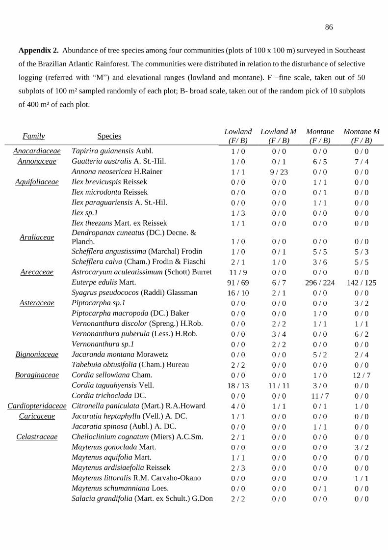
86

Appendix 2. Abundance of tree species among four communities (plots of 100 x 100 m) surveyed in Southeast

of the Brazilian Atlantic Rainforest. The communities were distributed in relation to the disturbance of selective

logging (referred with “M”) and elevational ranges (lowland and montane). F –fine scale, taken out of 50

subplots of 100 m² sampled randomly of each plot; B- broad scale, taken out of the random pick of 10 subplots

of 400 m² of each plot.

Family Species Lowland

(F/ B)

Lowland M

(F / B)

Montane

(F / B)

Montane M

(F / B)

Anacardiaceae Tapirira guianensis Aubl. 1 / 0 0 / 0 0 / 0 0 / 0

Annonaceae Guatteria australis A. St.-Hil. 1 / 0 0 / 1 6 / 5 7 / 4 Annona neosericea H.Rainer 1 / 1 9 / 23 0 / 0 0 / 0

Aquifoliaceae Ilex brevicuspis Reissek 0 / 0 0 / 0 1 / 1 0 / 0 Ilex microdonta Reissek 0 / 0 0 / 0 0 / 1 0 / 0 Ilex paraguariensis A. St.-Hil. 0 / 0 0 / 0 1 / 1 0 / 0 Ilex sp.1 1 / 3 0 / 0 0 / 0 0 / 0 Ilex theezans Mart. ex Reissek 1 / 1 0 / 0 0 / 0 0 / 0

Araliaceae Dendropanax cuneatus (DC.) Decne. &

Planch. 1 / 0 0 / 0 0 / 0 0 / 0 Schefflera angustissima (Marchal) Frodin 1 / 0 0 / 1 5 / 5 5 / 3 Schefflera calva (Cham.) Frodin & Fiaschi 2 / 1 1 / 0 3 / 6 5 / 5

Arecaceae Astrocaryum aculeatissimum (Schott) Burret 11 / 9 0 / 0 0 / 0 0 / 0 Euterpe edulis Mart. 91 / 69 6 / 7 296 / 224 142 / 125 Syagrus pseudococos (Raddi) Glassman 16 / 10 2 / 1 0 / 0 0 / 0

Asteraceae Piptocarpha sp.1 0 / 0 0 / 0 0 / 0 3 / 2 Piptocarpha macropoda (DC.) Baker 0 / 0 0 / 0 1 / 0 0 / 0 Vernonanthura discolor (Spreng.) H.Rob. 0 / 0 2 / 2 1 / 1 1 / 1 Vernonanthura puberula (Less.) H.Rob. 0 / 0 3 / 4 0 / 0 6 / 2 Vernonanthura sp.1 0 / 0 2 / 2 0 / 0 0 / 0

Bignoniaceae Jacaranda montana Morawetz 0 / 0 0 / 0 5 / 2 2 / 4 Tabebuia obtusifolia (Cham.) Bureau 2 / 2 0 / 0 0 / 0 0 / 0

Boraginaceae Cordia sellowiana Cham. 0 / 0 0 / 0 1 / 0 12 / 7 Cordia taguahyensis Vell. 18 / 13 11 / 11 3 / 0 0 / 0 Cordia trichoclada DC. 0 / 0 0 / 0 11 / 7 0 / 0

Cardiopteridaceae Citronella paniculata (Mart.) R.A.Howard 4 / 0 1 / 1 0 / 1 1 / 0

Caricaceae Jacaratia heptaphylla (Vell.) A. DC. 1 / 1 0 / 0 0 / 0 0 / 0 Jacaratia spinosa (Aubl.) A. DC. 0 / 0 0 / 0 1 / 1 0 / 0

Celastraceae Cheiloclinium cognatum (Miers) A.C.Sm. 2 / 1 0 / 0 0 / 0 0 / 0 Maytenus gonoclada Mart. 0 / 0 0 / 0 0 / 0 3 / 2 Maytenus aquifolia Mart. 1 / 1 0 / 0 0 / 0 0 / 0 Maytenus ardisiaefolia Reissek 2 / 3 0 / 0 0 / 0 0 / 0 Maytenus littoralis R.M. Carvaho-Okano 0 / 0 0 / 0 0 / 0 1 / 1 Maytenus schumanniana Loes. 0 / 0 0 / 0 0 / 1 0 / 0 Salacia grandifolia (Mart. ex Schult.) G.Don 2 / 2 0 / 0 0 / 0 0 / 0

87


(F/ B)

Lowland M

(F / B)

Montane

(F / B)

Montane M

(F / B)

Chloranthaceae Hedyosmum brasiliense Mart. ex Miq. 0 / 0 0 / 0 0 / 0 1 / 0

Chrysobalanaceae Couepia venosa Prance 1 / 2 2 / 1 8 / 7 0 / 0 Hirtella hebeclada Moric. ex DC. 1 / 1 0 / 0 9 / 9 3 / 3 Licania hoehnei Pilg. 0 / 0 0 / 0 19 / 19 27 / 17

Clusiaceae Clusia criuva subsp. parviflora Vesque 0 / 0 0 / 0 0 / 1 0 / 0

Garcinia gardneriana (Planch. & Triana)

Zappi 9 / 7 0 / 0 1 / 1 0 / 0

Combretaceae Buchenavia kleinii Exell 0 / 1 0 / 0 0 / 0 0 / 0 Terminalia januarensis DC. 2 / 1 2 / 1 0 / 0 0 / 0 Terminalia sp.1 2 / 3 0 / 0 0 / 0 0 / 0

Cunoniaceae Lamanonia ternata Vell. 0 / 0 0 / 0 1 / 1 0 / 0 Weinmannia paulliniifolia Pohl ex Ser. 0 / 0 0 / 0 1 / 1 0 / 0

Cyatheaceae Alsophila setosa Kaulf. 0 / 0 0 / 0 3 / 1 3 / 5 Alsophila sternbergii (Sternb.) D.S.Conant 16 / 9 71 / 26 9 / 3 8 / 7

Cyathea atrovirens (Langsd. & Fisch.)

Domin 0 / 0 0 / 0 0 / 0 3 / 4 Cyathea delgadii Sternb. 0 / 0 0 / 0 7 / 3 7 / 6 Cyathea dichromatolepis (Fée) Domin 0 / 0 0 / 0 16 / 14 2 / 0 Cyathea hirsuta C.Presl 0 / 0 12 / 8 0 / 0 0 / 0 Cyathea phalerata Mart. 0 / 0 4 / 5 12 / 7 10 / 11

Dichapetalaceae Stephanopodium blanchetianum Baill. 0 / 0 0 / 0 1 / 1 0 / 0 Stephanopodium estrellense Baill. 0 / 0 0 / 0 0 / 3 3 / 0 Stephanopodium sessile Rizzini 0 / 0 0 / 0 3 / 0 0 / 0

Elaeocarpaceae Sloanea guianensis (Aubl.) Benth. 10 / 12 4 / 7 0 / 0 0 / 0 Sloanea hirsuta (Schott) Planch. ex Benth. 0 / 0 0 / 0 4 / 3 2 / 2

Euphorbiaceae Alchornea glandulosa Poepp. & Endl. 0 / 0 9 / 20 6 / 6 12 / 7 Alchornea sidifolia Müll.Arg. 0 / 0 3 / 2 0 / 0 0 / 0 Alchornea triplinervia (Spreng.) Müll.Arg. 6 / 6 18 / 12 0 / 0 9 / 9 Croton macrobothrys Baill. 0 / 0 0 / 0 1 / 1 3 / 3 Mabea piriri Aubl. 8 / 8 0 / 0 0 / 0 0 / 0 Pausandra morisiana (Casar.) Radlk. 3 / 4 0 / 0 0 / 0 0 / 0 Sapium glandulosum (L.) Morong 0 / 1 0 / 1 0 / 0 0 / 0 Tetrorchidium rubrivenium Poepp. 1 / 1 1 / 1 0 / 0 0 / 0

Fabaceae Dahlstedtia pinnata (Benth.) Malme 0 / 1 0 / 0 3 / 0 0 / 0 Inga capitata Desv. 1 / 1 0 / 0 1 / 1 0 / 0 Inga cauliflora Willd. 3 / 2 0 / 0 0 / 0 0 / 0 Inga edulis Mart. 0 / 0 9 / 5 0 / 0 0 / 0 Inga lanceifolia Benth. 0 / 0 0 / 0 0 / 1 14 / 10 Inga marginata Willd. 0 / 0 5 / 2 0 / 0 0 / 0 Inga sessilis (Vell.) Mart. 0 / 0 0 / 0 0 / 0 1 / 2 Inga tenuis (Vell.) Mart. 1 / 1 0 / 0 0 / 0 0 / 0

Lonchocarpus cultratus (Vell.)

A.M.G.Azevedo & H.C.Lima 0 / 0 74 / 39 0 / 0 0 / 0 Machaerium brasiliense Vogel 0 / 0 0 / 0 0 / 0 0 / 1

88


(F/ B)

Lowland M

(F / B)

Montane

(F / B)

Montane M

(F / B) Machaerium nyctitans (Vell.) Benth. 0 / 0 0 / 0 0 / 0 1 / 1 Ormosia minor Vogel 0 / 0 0 / 0 0 / 1 0 / 0 Ormosia sp.1 0 / 0 0 / 0 0 / 1 0 / 0

Pseudopiptadenia leptostachya (Benth.)

Rauschert 0 / 0 2 / 0 0 / 0 0 / 0 Pterocarpus rohrii Vahl 0 / 0 0 / 0 0 / 0 2 / 2

Senna macranthera (DC. ex Collad.)

H.S.Irwin & Barneby 0 / 0 0 / 0 0 / 0 2 / 1 Swartzia oblata R.S.Cowan 1 / 2 3 / 1 0 / 0 0 / 0 Swartzia simplex (Sw.) Spreng. 10 / 5 0 / 0 0 / 0 0 / 0 Swartzia Schreb. 0 / 0 0 / 0 0 / 0 0 / 1 Tachigali denudata (Vogel) Oliveira-Filho 2 / 0 0 / 0 0 / 0 0 / 0

Tachigali friburgensis (Harms) L.G.Silva &

H.C.Lima 0 / 0 0 / 0 1 / 0 0 / 0 Tachigali multijuga Benth. 1 / 2 0 / 0 0 / 0 0 / 0 Tachigali Aubl. 0 / 0 0 / 0 1 / 2 0 / 0 Zollernia ilicifolia (Brongn.) Vogel 2 / 3 0 / 0 0 / 0 0 / 0

Humiriaceae Vantanea compacta (Schnizl.) Cuatrec. 0 / 0 0 / 0 0 / 0 2 / 0

Lamiaceae Aegiphila integrifolia (Jacq.) Moldenke 0 / 0 1 / 0 0 / 0 0 / 0

Lauraceae Aiouea acarodomatifera Kosterm. 0 / 0 0 / 0 4 / 2 0 / 0 Aniba viridis Mez 0 / 0 0 / 0 1 / 2 1 / 0 Cinnamomum montanum (Sw.) J.Presl 0 / 0 0 / 0 4 / 0 1 / 1 Cryptocarya mandioccana Meisn. 1 / 0 0 / 0 1 / 3 10 / 10 Cryptocarya saligna Mez 4 / 3 0 / 1 9 / 2 4 / 5 Endlicheria paniculata (Spreng.) J.F.Macbr. 1 / 1 1 / 2 0 / 0 0 / 0 Licaria armeniaca (Nees) Kosterm. 0 / 0 1 / 1 0 / 0 10 / 6 Nectandra membranacea (Sw.) Griseb. 0 / 0 0 / 6 1 / 0 0 / 0 Ocotea aciphylla (Nees & Mart.) Mez 0 / 0 0 / 0 2 / 2 0 / 0 Ocotea bicolor Vattimo-Gil 0 / 0 0 / 0 0 / 1 0 / 0 Ocotea brachybotrya (Meisn.) Mez 1 / 0 3 / 4 0 / 0 0 / 0 Ocotea catharinensis Mez 0 / 0 0 / 0 19 / 11 21 / 21 Ocotea daphnifolia (Meisn.) Mez 0 / 0 0 / 0 2 / 3 1 / 2 Ocotea dispersa (Nees & Mart.) Mez 1 / 4 9 / 9 10 / 8 12 / 11 Ocotea divaricata (Nees) Mez 0 / 0 0 / 0 1 / 0 0 / 0 Ocotea floribunda (Sw.) Mez 0 / 0 0 / 0 1 / 1 0 / 0 Ocotea glaziovii Mez 0 / 0 0 / 0 0 / 0 1 / 2 Ocotea lancifolia (Schott) Mez 0 / 0 0 / 0 2 / 1 0 / 0 Ocotea laxa (Nees) Mez 0 / 0 0 / 0 1 / 0 0 / 0 Ocotea leucoxylon (Sw.) Laness. 0 / 0 0 / 0 1 / 1 0 / 0 Ocotea paranapiacabensis Coe-Teixeira 0 / 0 5 / 4 0 / 0 0 / 0 Ocotea puberula (Rich.) Nees 0 / 0 0 / 0 1 / 2 1 / 0 Ocotea silvestris Vattimo-Gil 0 / 0 0 / 0 1 / 0 1 / 0 Ocotea sp.1 0 / 0 0 / 0 1 / 0 0 / 0 Ocotea sp.2 0 / 0 0 / 0 0 / 0 1 / 0

89


(F/ B)

Lowland M

(F / B)

Montane

(F / B)

Montane M

(F / B) Ocotea teleiandra (Meisn.) Mez 0 / 0 0 / 0 2 / 2 0 / 0

Lecythidaceae Cariniana estrellensis (Raddi) Kuntze 1 / 0 1 / 0 0 / 0 0 / 0

Malpighiaceae Byrsonima salzmanniana A.Juss. 0 / 0 0 / 0 1 / 1 0 / 0

Malvaceae Eriotheca pentaphylla (Vell. & K.Schum.)

A.Robyns 4 / 5 0 / 0 0 / 0 0 / 0 Quararibea turbinata (Sw.) Poir. 4 / 1 0 / 0 0 / 0 0 / 0

Melastomataceae Henriettea glabra (Vell.) Penneys, F.A.

Michelangeli, Judd et 0 / 0 0 / 0 3 / 3 0 / 0 Leandra variabilis Raddi 0 / 0 2 / 0 0 / 0 0 / 0 Melastomataceae A. Juss. 0 / 0 0 / 0 0 / 0 1 / 1 Meriania calyptrata (Naudin) Triana 0 / 0 2 / 3 0 / 0 0 / 0 Miconia brasiliensis (Spreng.) Triana 0 / 0 0 / 0 7 / 2 0 / 0 Miconia cabucu Hoehne 0 / 0 0 / 0 3 / 3 1 / 1 Miconia cinnamomifolia (DC.) Naudin 0 / 0 0 / 1 0 / 0 0 / 0 Miconia cubatanensis Hoehne 0 / 0 0 / 0 0 / 1 0 / 0 Miconia dodecandra Cogn. 0 / 0 1 / 0 0 / 0 0 / 0 Miconia sp.1 0 / 0 4 / 3 0 / 0 0 / 0 Miconia sp.2 0 / 0 0 / 0 0 / 0 14 / 13 Miconia tristis Spring 0 / 0 0 / 1 0 / 0 0 / 0 Mouriri chamissoana Cogn. 0 / 0 0 / 0 0 / 0 2 / 0 Tibouchina pulchra Cogn. 0 / 0 0 / 0 1 / 2 4 / 5 Tibouchina sp.1 0 / 0 0 / 0 0 / 0 0 / 1

Meliaceae Cabralea canjerana (Vell.) Mart. 0 / 0 6 / 4 2 / 1 6 / 5 Cedrela odorata L. 0 / 0 0 / 0 0 / 0 1 / 1 Guarea kunthiana A.Juss. 0 / 0 0 / 0 0 / 0 3 / 3 Guarea macrophylla Vahl 1 / 2 1 / 3 6 / 4 11 / 4 Trichilia lepidota Mart. 1 / 1 0 / 0 0 / 0 0 / 0 Trichilia silvatica C. DC. 2 / 0 0 / 0 0 / 0 1 / 1

Monimiaceae Mollinedia acutissima Perkins 0 / 0 0 / 0 1 / 1 0 / 0 Mollinedia argyrogyna Perkins 0 / 0 0 / 0 13 / 18 16 / 21 Mollinedia blumenaviana Perkins 0 / 0 0 / 0 3 / 5 0 / 0 Mollinedia boracensis Peixoto 0 / 0 0 / 0 1 / 3 0 / 0 Mollinedia elegans Tul. 2 / 1 0 / 0 0 / 0 6 / 6 Mollinedia engleriana Perkins 1 / 1 0 / 0 2 / 2 12 / 11 Mollinedia gilgiana Perkins 0 / 0 0 / 0 4 / 1 0 / 0 Mollinedia glabra (Spreng.) Perkins 0 / 0 0 / 0 0 / 1 11 / 7 Mollinedia lamprophylla Perkins 2 / 3 0 / 0 0 / 0 0 / 0 Mollinedia ovata Ruiz & Pav. 0 / 0 0 / 0 0 / 0 2 / 2 Mollinedia salicifolia Perkins 0 / 0 0 / 0 17 / 9 0 / 0 Mollinedia schottiana (Spreng.) Perkins 39 / 26 25 / 24 4 / 9 13 / 10 Mollinedia sp.1 0 / 0 0 / 0 1 / 1 0 / 1 Mollinedia uleana Perkins 6 / 3 0 / 0 0 / 0 0 / 0

Moraceae Brosimum guianense (Aubl.) Huber 2 / 2 0 / 0 0 / 0 0 / 0 Brosimum Sw. 1 / 1 0 / 0 0 / 0 0 / 0

90


(F/ B)

Lowland M

(F / B)

Montane

(F / B)

Montane M

(F / B) Ficus gomelleira Kunth 1 / 0 0 / 0 0 / 0 0 / 0 Ficus insipida Willd. 1 / 1 2 / 1 0 / 0 0 / 0 Ficus luschnathiana (Miq.) Miq. 0 / 1 0 / 0 0 / 0 0 / 0 Ficus obtusiuscula (Miq.) Miq. 0 / 0 1 / 1 0 / 0 0 / 0 Ficus pulchella Schott 0 / 0 1 / 0 0 / 0 0 / 0 Ficus sp.1 0 / 0 0 / 0 0 / 0 1 / 0 Sorocea bonplandii (Baill.) W.C.Burger et al. 2 / 2 0 / 0 0 / 0 0 / 0 Sorocea hilarii Gaudich. 4 / 4 0 / 0 0 / 0 0 / 0

Myristicaceae Virola bicuhyba (Schott ex Spreng.) Warb. 12 / 5 2 / 5 0 / 0 0 / 0

Myrtaceae Blepharocalyx salicifolius (Kunth) O.Berg 0 / 0 0 / 0 1 / 1 0 / 0 Calyptranthes grandifolia O.Berg 0 / 0 0 / 1 15 / 12 0 / 0 Calyptranthes lucida Mart. ex DC. 1 / 2 2 / 0 19 / 19 20 / 18 Calyptranthes rufa O.Berg 0 / 0 0 / 0 2 / 0 3 / 0 Calyptranthes Sw. 0 / 0 0 / 0 4 / 3 4 / 4 Calyptranthes strigipes O.Berg 6 / 6 0 / 0 3 / 3 11 / 5 Campomanesia guaviroba (DC.) Kiaersk. 1 / 1 5 / 5 0 / 0 4 / 7 Eugenia batingabranca Sobral 1 / 0 0 / 0 0 / 0 4 / 2 Eugenia brevistyla D.Legrand 1 / 1 1 / 3 0 / 0 0 / 0 Eugenia burkartiana (D.Legrand) D.Legrand 0 / 0 0 / 0 1 / 1 0 / 1 Eugenia cerasiflora Miq. 2 / 1 0 / 0 0 / 0 1 / 0 Eugenia cereja D.Legrand 5 / 5 0 / 0 0 / 0 0 / 0 Eugenia copacabanensis Kiaersk. 0 / 0 0 / 0 0 / 1 0 / 0 Eugenia excelsa O.Berg 1 / 0 0 / 0 0 / 0 0 / 0 Eugenia expansa Spring ex Mart. 0 / 0 0 / 0 0 / 0 2 / 1 Eugenia fusca O.Berg 13 / 14 0 / 0 0 / 0 0 / 0

Eugenia magnibracteolata Mattos &

D.Legrand 1 / 0 0 / 0 0 / 0 0 / 0 Eugenia melanogyna (D.Legrand) Sobral 3 / 3 0 / 0 0 / 0 0 / 0 Eugenia monosperma Vell. 11 / 7 0 / 0 0 / 0 0 / 0 Eugenia mosenii (Kausel) Sobral 2 / 2 0 / 0 0 / 0 0 / 0 Eugenia multicostata D.Legrand 0 / 0 0 / 0 0 / 1 0 / 0 Eugenia brevistyla D.Legrand 1 / 0 0 / 0 0 / 0 0 / 0 Eugenia oblongata O.Berg 7 / 6 1 / 0 4 / 1 3 / 0 Eugenia plicata Nied. 1 / 0 0 / 0 0 / 0 0 / 0 Eugenia prasina O.Berg 8 / 2 1 / 2 11 / 11 5 / 3 Eugenia pisiformis Cambess. 0 / 0 0 / 1 0 / 0 3 / 1 Eugenia sp.1 0 / 0 19 / 24 0 / 0 0 / 0 Eugenia sp.2 0 / 0 0 / 0 5 / 3 8 / 13 Eugenia sp.3 0 / 0 0 / 0 0 / 0 2 / 1 Eugenia sp.4 0 / 0 0 / 0 2 / 1 0 / 0 Eugenia sp.5 0 / 0 0 / 0 1 / 2 0 / 0 Eugenia sp.6 0 / 0 0 / 0 0 / 0 1 / 1 Eugenia subavenia O.Berg 3 / 2 0 / 0 0 / 0 0 / 0

91


(F/ B)

Lowland M

(F / B)

Montane

(F / B)

Montane M

(F / B) Marlierea excoriata Mart. 0 / 0 0 / 0 13 / 15 0 / 0 Marlierea obscura O.Berg 5 / 6 0 / 0 0 / 0 0 / 0 Marlierea racemosa (Vell.) Kiaersk. 0 / 1 0 / 0 0 / 0 0 / 0 Marlierea silvatica (O.Berg) Kiaersk. 2 / 1 2 / 1 1 / 1 4 / 3 Marlierea Cambess. 0 / 1 0 / 0 0 / 0 0 / 0

Myrceugenia campestris (DC.) D.Legrand &

Kausel 0 / 0 0 / 0 2 / 0 0 / 0

Myrceugenia miersiana (Gardner) D.Legrand

& Kausel 0 / 0 0 / 0 4 / 2 0 / 0 Myrceugenia sp.1 0 / 0 14 / 21 0 / 0 0 / 0 Myrceugenia sp.2 0 / 0 0 / 0 0 / 0 6 / 4 Myrcia amazonica DC. 0 / 0 0 / 0 2 / 0 0 / 0 Myrcia guianensis (Aubl.) DC. 0 / 0 0 / 0 0 / 1 0 / 1 Myrcia insigniflora M.F.Santos 3 / 3 1 / 0 0 / 0 0 / 0 Myrcia neoblanchetiana E.Lucas & Sobral 2 / 1 0 / 0 0 / 0 0 / 0 Myrcia sp.1 0 / 0 1 / 0 0 / 2 0 / 0 Myrcia sp.2 0 / 0 0 / 0 3 / 0 0 / 0 Myrcia sp.3 0 / 0 0 / 0 0 / 0 26 / 15 Myrcia spectabilis DC. 7 / 2 8 / 7 37 / 18 1 / 0 Myrcia strigipes Mart. 6 / 5 1 / 1 0 / 1 15 / 5 Myrcia tijucensis Kiaersk. 0 / 1 0 / 0 4 / 4 0 / 0

Myrciaria floribunda (H.West ex Willd.)

O.Berg 4 / 6 3 / 4 8 / 6 7 / 5 Myrtaceae sp.1 0 / 0 0 / 1 0 / 0 1 / 0 Myrtaceae sp.2 0 / 0 0 / 0 2 / 0 4 / 1 Myrtaceae sp.3 0 / 0 0 / 0 1 / 1 0 / 4 Myrtaceae sp.4 0 / 1 0 / 0 1 / 0 0 / 0 Myrtaceae sp.5 0 / 0 0 / 0 0 / 1 0 / 0 Myrtaceae sp.6 0 / 0 0 / 0 0 / 1 0 / 0 Myrtaceae sp.7 0 / 0 0 / 0 0 / 1 0 / 0 Myrtaceae sp.8 0 / 0 0 / 0 0 / 2 0 / 0

Neomitranthes glomerata (D.Legrand)

D.Legrand 1 / 1 0 / 0 4 / 4 0 / 0

Pimenta pseudocaryophyllus (Gomes)

Landrum 0 / 0 0 / 0 1 / 0 1 / 0 Syzygium jambos (L.) Alston 0 / 0 0 / 0 1 / 0 0 / 0

Nyctaginaceae Guapira areolata (Heimerl) Lundell 0 / 0 0 / 0 0 / 0 6 / 9

Guapira nitida (Mart. ex J.A.Schmidt)

Lundell 0 / 0 0 / 0 0 / 0 6 / 5 Guapira opposita (Vell.) Reitz 28 / 24 37 / 27 35 / 33 1 / 1

Ochnaceae Ouratea parviflora (A.DC.) Baill. 1 / 0 0 / 0 0 / 0 0 / 0

Olacaceae Chionanthus crassifolius (Mart.) P.S.Green 0 / 0 0 / 0 5 / 0 0 / 0 Heisteria silvianii Schwacke 0 / 0 0 / 0 0 / 0 2 / 1 Tetrastylidium grandifolium (Baill.) Sleumer 0 / 1 0 / 0 0 / 0 0 / 0 Chionanthus crassifolius (Mart.) P.S.Green 0 / 0 0 / 0 0 / 2 0 / 0

92


(F/ B)

Lowland M

(F / B)

Montane

(F / B)

Montane M

(F / B)

Peraceae Pera glabrata (Schott) Poepp. ex Baill. 1 / 1 0 / 0 0 / 0 0 / 0 Pera sp.1 0 / 0 0 / 0 1 / 1 0 / 0

Phyllanthaceae Hyeronima alchorneoides Allemão 1 / 1 29 / 31 1 / 0 6 / 3

Phytolaccaceae Phytolacca dioica L. 0 / 0 6 / 5 0 / 0 0 / 0 Phytolaccaceae sp.1 0 / 0 0 / 0 1 / 0 0 / 0

Picramniaceae Picramnia ciliata Mart. 2 / 0 0 / 0 0 / 0 0 / 0

Piperaceae Piper cernuum Vell. 0 / 0 0 / 0 0 / 0 1 / 2 Piper gaudichaudianum Kunth 0 / 0 5 / 5 0 / 0 0 / 0 Piper rivinoides Kunth 0 / 0 1 / 1 0 / 0 0 / 0

Polygonaceae Ruprechtia laxiflora Meisn. 2 / 2 0 / 0 0 / 0 0 / 0

Primulaceae Myrsine coriacea (Sw.) R.Br. ex Roem. &

Schult. 0 / 0 1 / 0 0 / 0 0 / 0 Myrsine gardneriana A. DC. 0 / 0 0 / 0 2 / 1 4 / 2 Myrsine guianensis (Aubl.) Kuntze 0 / 0 0 / 0 4 / 2 0 / 0

Myrsine hermogenesii (Jung-Mend. &

Bernacci) M.F.Freitas & Kin.-Gouv. 0 / 0 0 / 0 4 / 3 5 / 6 Myrsine leuconeura Mart. 0 / 0 0 / 0 1 / 0 0 / 0 Stylogyne lhotzkyana (A.DC.) Mez 1 / 0 4 / 0 0 / 0 0 / 0

Proteaceae Euplassa hoehnei Sleumer 0 / 0 0 / 0 0 / 0 1 / 1 Roupala montana Aubl. 0 / 3 0 / 0 4 / 0 0 / 0

Roupala montana var. brasiliensis (Klotzsch)

K.S.Edwards 2 / 0 0 / 0 0 / 4 0 / 0 Roupala paulensis Sleumer 0 / 0 0 / 0 1 / 0 0 / 0

Quiinaceae Quiina glaziovii Engl. 0 / 1 1 / 0 0 / 0 0 / 0

Rosaceae Prunus myrtifolia (L.) Urb. 0 / 0 0 / 0 1 / 1 0 / 0

Rubiaceae Alseis floribunda Schott 2 / 1 4 / 2 0 / 0 0 / 0

Amaioua intermedia Mart. ex Schult. &

Schult.f. 0 / 0 0 / 0 7 / 7 0 / 0 Bathysa australis (A.St.-Hil.) K. Schum. 2 / 1 108 / 105 33 / 28 9 / 6 Bathysa mendoncaei K. Schum. 18 / 22 0 / 0 0 / 0 0 / 0 Chomelia pedunculosa Benth. 0 / 0 0 / 0 0 / 0 0 / 1 Coussarea accedens Müll.Arg. 20 / 25 3 / 3 0 / 0 0 / 0 Coussarea meridionalis (Vell.) Müll.Arg. 24 / 20 4 / 3 1 / 1 0 / 0 Faramea pachyantha Müll.Arg. 1 / 0 0 / 0 0 / 0 0 / 0

Margaritopsis cymuligera (Müll.Arg.)

C.M.Taylor 0 / 0 0 / 1 0 / 0 0 / 0 Posoqueria latifolia (Rudge) Schult. 0 / 0 0 / 0 3 / 3 1 / 2 Psychotria mapourioides DC. 1 / 1 0 / 0 0 / 0 0 / 0 Psychotria nuda (Cham. & Schltdl.) Wawra 0 / 0 15 / 12 0 / 0 0 / 0 Psychotria sp.1 0 / 0 0 / 0 0 / 1 0 / 0 Psychotria vellosiana Benth. 0 / 0 0 / 0 3 / 4 2 / 3 Randia armata (Sw.) DC. 0 / 0 0 / 0 1 / 1 0 / 0 Rubiaceae sp.1 0 / 0 0 / 0 0 / 0 1 / 1 Rubiaceae sp.2 1 / 0 0 / 0 0 / 0 0 / 0

93


(F/ B)

Lowland M

(F / B)

Montane

(F / B)

Montane M

(F / B) Rubiaceae sp.3 1 / 0 0 / 0 0 / 0 0 / 0 Rudgea jasminoides (Cham.) Müll.Arg. 0 / 0 2 / 0 0 / 0 0 / 0 Rudgea vellerea Müll.Arg. 2 / 2 0 / 0 2 / 1 0 / 0 Rustia formosa (Cham. & Schltdl.) Klotzsch 36 / 20 0 / 0 0 / 0 0 / 0 Simira sampaioana (Standl.) Steyerm. 1 / 1 0 / 0 0 / 0 0 / 0

Rutaceae Conchocarpus fontanesianus (A. St.-Hil.)

Kallunki & Pirani 0 / 0 0 / 0 1 / 0 0 / 0 Rutaceae sp.1 0 / 0 0 / 0 2 / 3 0 / 0 Rutaceae sp.2 0 / 0 0 / 0 0 / 0 1 / 1 Zanthoxylum fagara (L.) Sarg. 0 / 0 1 / 1 0 / 0 0 / 0

Sabiaceae Meliosma sellowii Urb. 0 / 0 0 / 0 0 / 0 1 / 1 Casearia decandra Jacq. 0 / 0 0 / 0 0 / 1 0 / 0 Casearia obliqua Spreng. 0 / 0 0 / 0 1 / 1 0 / 0 Casearia paranaensis Sleumer 0 / 0 0 / 0 0 / 0 5 / 3 Casearia sylvestris Sw. 0 / 0 0 / 1 0 / 1 0 / 0

Sapindaceae Allophylus petiolulatus Radlk. 0 / 0 0 / 1 1 / 3 0 / 0 Cupania furfuracea Radlk. 0 / 0 0 / 0 1 / 1 1 / 0 Cupania oblongifolia Mart. 1 / 1 2 / 2 2 / 0 1 / 2 Cupania vernalis Cambess. 0 / 0 0 / 0 3 / 2 2 / 0 Cupania zanthoxyloides Radlk. 0 / 0 0 / 0 1 / 0 0 / 0 Matayba guianensis Aubl. 0 / 0 0 / 0 8 / 11 9 / 10 Matayba intermedia Radlk. 0 / 0 0 / 0 3 / 1 0 / 0

Sapotaceae Chrysophyllum flexuosum Mart. 20 / 25 0 / 0 1 / 1 0 / 0 Chrysophyllum inornatum Mart. 0 / 0 0 / 0 1 / 2 0 / 2 Chrysophyllum viride Mart. & Eichler 1 / 1 0 / 0 24 / 26 8 / 9 Ecclinusa ramiflora Mart. 7 / 1 0 / 0 0 / 0 1 / 1

Micropholis crassipedicellata (Mart. &

Eichler) Pierre 2 / 0 0 / 0 0 / 0 0 / 0 Micropholis gardneriana (A.DC.) Pierre 0 / 0 0 / 0 0 / 0 2 / 5 Pouteria sp.1 1 / 0 0 / 0 0 / 0 14 / 8 Pouteria bullata (S.Moore) Baehni 1 / 1 0 / 0 0 / 0 0 / 0 Pouteria caimito (Ruiz & Pav.) Radlk. 0 / 0 0 / 0 23 / 14 0 / 0 Pouteria psammophila (Mart.) Radlk. 1 / 1 5 / 10 0 / 0 0 / 0 Pouteria venosa (Mart.) Baehni 9 / 8 0 / 0 0 / 0 0 / 0

Siparunaceae Siparuna brasiliensis (Spreng.) A. DC. 0 / 0 5 / 7 0 / 0 0 / 0

Solanaceae Aureliana fasciculata (Vell.) Sendtn. 0 / 0 0 / 0 0 / 0 1 / 0 Solanum pseudoquina A.St.-Hil. 0 / 0 0 / 0 0 / 1 1 / 0 Solanum rufescens Sendtn. 0 / 0 0 / 0 0 / 0 1 / 1 Solanum sp.1 0 / 0 3 / 0 0 / 0 0 / 1 Solanum sp.2 0 / 0 1 / 0 0 / 0 0 / 0 Solanum sp.3 0 / 0 0 / 0 0 / 0 3 / 0 Solanum swartzianum Roem. & Schult. 0 / 0 1 / 1 0 / 0 3 / 0 Solanum vellozianum Dunal 0 / 0 0 / 0 0 / 0 1 / 0

Symplocaceae Symplocos laxiflora Benth. 0 / 0 0 / 0 1 / 1 0 / 0

94


(F/ B)

Lowland M

(F / B)

Montane

(F / B)

Montane M

(F / B) Symplocos estrellensis Casar. 0 / 0 0 / 0 0 / 2 0 / 0

Thymelaeaceae Daphnopsis schwackeana Taub. 0 / 0 0 / 0 3 / 1 2 / 1

Urticaceae Cecropia glaziovii Snethl. 8 / 3 22 / 23 2 / 2 0 / 1 Cecropia pachystachya Trécul 0 / 0 1 / 1 0 / 0 0 / 0 Coussapoa microcarpa (Schott) Rizzini 0 / 0 1 / 0 3 / 2 2 / 0 Coussapoa Aubl. 0 / 0 0 / 0 0 / 0 1 / 2 Pourouma guianensis Aubl. 1 / 2 5 / 1 0 / 0 0 / 0 Urera baccifera (L.) Gaudich. ex Wedd. 0 / 0 1 / 0 0 / 0 0 / 0

Verbenaceae Citharexylum myrianthum Cham. 0 / 0 1 / 0 0 / 0 0 / 0

Winteraceae Drimys brasiliensis Miers 0 / 0 0 / 0 3 / 4 0 / 0

95

CAPÍTULO III

Which, where and when traits are functional? Trait interactions control tropical tree

demography depending on environmental context

96

ABSTRACT

1. Although functional traits are defined based on their impact on species fitness and their

demographic components, the reported trait-demography relationships are frequently weak.

These weak relationships might be due to traits affecting demography in combination with other

traits and that environmental conditions also influence the trait-demography relationship.

2. Here, we considered trait-interactions and environmental contexts (habitat and time interval

between censuses) to assess how these factors shape species demography, separately and

simultaneously. Specifically, we applied boosted regression tree (BRT) models to investigate

changes in the trait-demographic rates relationships of tropical tree species along an elevational

gradient and among time intervals between censuses (including and excluding one strong

drought event). Based on a large-dataset of 18,000 tree individuals from 133 common species,

distributed among four forest types (habitats) in the Atlantic forest, we assessed how trait-

interactions and the environmental context control the demographic rates (growth, mortality,

and recruitment).

3. The BRT models showed excellent trait ability to predict demography after the inclusion of

interactions among functional traits and forest types. Such interactions and the relative

influence of traits were different among time intervals and for different demographic

components. For example, changes in growth rates were best related to specific leaf area, while

changes in mortality and recruitment rates were best related to seed mass and wood density,

respectively. Moreover, habitat affected growth particularly by interacting with wood density,

and mortality and recruitment through interaction with height.

4. Trait-based studies should consider both the environmental context (space and time) and

traits interactions to understand the changes in the demography of tropical tree communities.

To assess which, where and when traits are functional, it is necessary to fully incorporate the

concept of multiple trait-fitness optima, resulting from traits interactions in different habitats

and censuses time intervals.

97

Keywords: Boosted regression trees, demography, functional ecology, habitat context, time

interval, trait-demography relationships, trait-interactions, tropical forest.

1. INTRODUCTION

Trait-based ecology is largely founded on the primary assumption that functional traits

determine the individual fitness and population demography (Adler et al., 2014; Lavorel &

Garnier, 2002; Mcgill, Enquist, Weiher, & Westoby, 2006; Salguero-Gómez, Violle, Gimenez,

& Childs, 2018). Specifically, to be called ‘functional’, a trait needs to impact ‘fitness indirectly

via its effects on growth, reproduction and survival’ (Violle, Navas, Vile, Kazakou, & Fortunel,

2007). Along this line, economic trait spectra (e.g., leaf, seed and wood economic spectra) are

expected to represent central trade-off axes that predict life-history strategies (Díaz et al., 2016)

and species demography (Salguero-Gómez et al., 2016). The functional economics spectra

should help to understand individual fitness (Reich, 2014) and species-demography

relationships (Adler et al., 2014). For example, a high specific leaf area is related to faster-

growing species (Wright et al., 2004), while high wood density and heavy seeds are negatively

correlated with growth and mortality rates (Chave et al., 2009; Wright et al., 2010).

However, evidences of strong trait-demography relationships have been limited in the

literature. Among the possible reasons for this, are the overriding environmental effects on

demography (Worthy & Swenson, 2019; Yang, Cao, & Swenson, 2018) and the fact that a given

trait does not affect fitness independently from other traits. As a matter of fact, trait interactions

can cause alternative trait combinations to have similar fitness or demographic effects in a given

context (Laughlin & Messier, 2015; Pistón et al., 2019). Despite the expectations of both trait

interactions and environmental conditions on species demography (Ackerly et al., 2006; Dwyer

& Laughlin, 2017; Laughlin & Messier, 2015), trait-based studies traditionally focus on single

98

trait-demography relationships and do not consider environment constraints on demographic

rates (Poorter et al., 2008; Visser et al., 2016; Wright et al., 2010).

Different phenotypes can have similar fitness since multiple functional strategies might

result in comparable performances (i.e. alternative designs) (Laughlin & Messier, 2015; Pistón

et al., 2019; Worthy & Swenson, 2019). It is thus crucial to consider trait combinations in order

to understand trait-demography relationships and species dynamics (Pistón et al., 2019; Yang

et al., 2018). Moreover, environmental factors can shape functional traits and their

combinations, also affecting species demography (Bruelheide et al., 2018; Ordoñez et al.,

2009). Environment may shift the relationship between traits and species’ performance along

environmental gradients, wherein different habitats lead to different effects of traits on

demography in response to stress or competition (Dwyer & Laughlin, 2017; Yang et al., 2018).

Hence, the trait-demography relationship can vary across environmental gradients, in terms of

the strength of trait influences and the interactions among functional traits (Salguero-Gómez et

al., 2018; Worthy & Swenson, 2019).

In addition to changes across the spatial environmental gradient, trait- demography

relationships can also change across time. For instance, population dynamics might be affected

by stochastic temporal variations (Griffith, Salguero-Gómez, Merow, & Mcmahon, 2016;

Körner, 2018) and the variation of species vital rates could be related to the specific habitat

conditions at different points in time (Worthy & Swenson, 2019), here also considered as

‘environmental context’. Thus, it is unlikely to expect unvarying tree population dynamics and

those functional strategies predict species demography similarly across time (Aleixo et al.,

2019; Dwyer & Laughlin, 2017; Worthy & Swenson, 2019; Yang et al., 2018). Although trait-

demography relationships can be affected by the time interval in which they are taken,

unraveling how the temporal changes of habitat conditions modify the plant functional

responses and the relationships between traits and vegetation dynamics remains an open

question (Ehrlén, Morris, von Euler, & Dahlgren, 2016; Worthy & Swenson, 2019).

99

To date, there is still a great shortage of studies that have assessed how multiple

functional traits affect plant demographic rates, especially under different environmental

contexts, including the effects of temporal variations (Salguero-Gómez et al., 2018; Worthy &

Swenson, 2019; Yang et al., 2018). Further, most studies have used analytical approaches

considering linear and additive responses of demography to single traits, which seems

inadequate to deal with interactions and non-linear responses (De’ath, 2007; Elith, Leathwick,

& Hastie, 2008). To manage with these tasks, alternative statistical techniques have been

indicated, such as regression trees (De’ath, 2007; Elith et al., 2008), which allows us to asses

trait interactions and represent a promising tool for functional ecology studies (de Bello et al.,

2005; Piston et al. 2018).

Here, we applied Boosted Regression Trees (BRT) models to investigate changes in the

trait-demography relationships of tropical tree species along an elevational gradient and at

different moments in time. We used demographic data extracted from a forest plot database in

combination with a dataset of sampled functional traits from tree communities of the Brazilian

Atlantic forest to answer four questions: (i) to which extent did interactions between functional

traits modulate tree demography? (ii) Are trait predictions consistent across different forest

types (habitats)? (iii) Did trait-demography relationships change across time? (iv) Are these

relationships affected by habitat and environmental temporal variations?

2. METHODS

2.1 Site description

Our study is focused on Atlantic forest tree communities distributed along an elevational

gradient (0-1,100m a.s.l.) of tropical moist forest in southeastern Brazil. The study area is

located in a tropical montane system called Serra do Mar (23° 22’ S and 45° 05’W). The

elevational gradient covers four broadly defined forest types (IBGE, 2012), here treated as

habitats, distributed as follows: (i) Seasonally flooded coastal forest (herein, “Restinga”, one

100

plot); (ii) Lowland forest (four plots); (iii) Submontane forest (four plots); (iv) Montane forest

(three plots). In general, these forest types are defined by their position on altitudinal and

latitudinal belts, except for the Restinga, which is characterized by its sandy and seasonally

flooded soil at the lowest altitude (Assis et al., 2011). Temperature decreases along the

elevational gradient, presenting a range elevational lapse rate of 0.6 to 1.0°C every 100m

increase in elevation (Vieira et al., 2011).

Soils are generally low in nutrients and have a high level of aluminum (Martins et al.,

2015). The climate is humid subtropical (Cfa type in Köppen system), with ca. 2500 mm of

rainfall annually, and monthly average temperature range from 19.1 to 25.5°C (Sentelhas et al.,

1999). Droughts are rare in southeastern Brazil, but one drought event occurred in this region

between 2013 and 2015, resulting in the warmest and driest summers in 50 years (Coelho,

Cardoso, & Firpo, 2016). In comparison with long-term data collected by the Brazilian Center

for Weather Forecast and Climate Studies of the National Institute for Space Research

(CPTEC/INPE) for 1961-2015, the mean precipitation records were 60% and 25% below

average in the wet seasons of 2013-2014 and 2014-2015, respectively, and temperatures were

2.5 °C above typical temperatures (Nobre, Marengo, Seluchi, Cuartas, & Alves, 2016). Local

climatological records, from the “Centro Integrado de Informações Agrometeorológicas”

(CIIAGRO), indicates the lowest total precipitation between 2013 and 2015, with dryer

summers and more humid winters than the average for the last 25-year period (Figure S1).

2.2. Sampling design

We used data extracted from a forest inventory dataset representing twelve 1-ha plots (100 x

100 m) at undisturbed areas, distributed along an elevational gradient, ranging from sea level

to 1,100 m (Alves et al., 2010; Joly et al., 2012; details in Table S1). All woody stems (trees,

palms and tree ferns) with the diameter at breast height (DBH) equal to or larger than 4.8 cm

101

were tagged and measured for diameter and re-censused four times along 10 years. The

demographic database represents 22,770 stems from 21,509 tree individuals.

To make a consistent assessment of functional diversity and to increase the accuracy of

our models (Májeková et al., 2016), we first selected, from the demographic database, species

that presented a minimum of 15 individuals sampled in at least one of 12 plots, and at least five

individuals per plot where they had their second-highest abundance (Table S2). The final

dataset included 133 species from 37 families, comprising 82% and 84% of the total stem and

individual abundances, respectively. These species cover a wide range of ecological strategies,

from shade-tolerant species with light seeds (e.g., Bathysa australis, Rubiaceae) to light-

demanding species with heavy seeds (e.g., Andira fraxinifolia, Fabaceae); three of 133 species

included are locally abundant palm species. The sampling protocol and further information on

species composition, including the species dominance and revisions of the richest families, are

available in Alves et al. (2010), Joly et al. (2012), Silva et al. (2016) and Kamimura et al. (2017).

2.3. Demographic rates

We calculated relative growth rate (RGR), mortality (MR) and recruitment (RCT) for each of

the 133 selected species (see above) in all forest types where they were sampled. In other words,

we computed the different demographic parameters for each species population in each forest

type. These parameters then were computed for different time intervals (details in Table S1):

(i) between first and fourth census, i.e. whole time interval (ten-years, from 2005 to 2016); (ii)

between first and second census, i.e. first time interval (three years); (iii) between second and

third census, i.e. second time interval (three years); and (iv) between third and fourth census,

i.e. third time interval (four years, which includes the drought event, see above). The

demographic rates were taken by means of both growth and vital rates parameters, as described

by Kohyama et al. (2018), Sheil, Burslem and Alder (1995).

102

We computed the relative growth rate (RGR) of each stem, as their performance,

employing the formula: RGR = ln(DBHf/DBHi)/Δt, where DBHf and DBHi are the final and

initial DBH of each individual, respectively, and Δt is the number of years between two

censuses. For each species at each forest type, we considered the potential growth rates as the

95th quantile of the distribution of the RGR of each species at forest type (Wright et al.,

2010).The annual vital rates (VR) for each population were estimated as mortality (MR) and

recruitment rates (RcR). Both vital rates were calculated using the formula VR= ln(ΔN) /Δt, in

which ΔN is the relative difference in the number of individuals of each species at each forest

type, between two censuses (Kohyama et al., 2018; Sheil et al., 1995).

2.4. Traits

For each selected species, we collected data on six functional traits representing the leaf, seed

and wood economics spectra, which are expected to respond to environmental context and to

be related to species demography (Bruelheide et al., 2018, Table S3). We measured leaf area

(LA, cm²), leaf dry matter content (LDMC, mg g-1), and specific leaf area (SLA, cm² g-1) from

ten leaves of ten individuals per species in each forest type. Leaf traits were measured in the

summer of 2016, following standard protocols (Cornelissen et al., 2003; Pérez-Harguindeguy

et al., 2013). As a measure of maximum height (Hmax) under site conditions, we calculated the

95th percentile of the distribution of height values for each species. Individual stem height was

calculated using forest type-derived allometric Weibull models based on stem diameter (DBH)

(see Alves et al., 2010; Scaranello et al., 2010; Martins, Seger, Wiegand, & Santos, 2018)

Wood density (WD, cm³ g-1) and seed mass (SM, mg) were obtained from three global

repositories, Dryad (Zanne et al., 2009), BIEN (Maitner et al., 2018) and TRY (Kattge et al.,

2011), and from the literature (Bello et al., 2017; Bufalo, Galetti, & Culot, 2016; Chave et al.,

2009; Gressler, Pizo, & Morellato, 2006; Lorenzi, 1992; Wanderley, Shepherd, Melhem,

Giulietti, & Martins, 2016). When the same species was present in two or more dataset, we

103

computed the average for its trait values. Missing trait-values included four traits (LDMC, SLA,

WD and SM) and represented 5% of the total trait dataset. The SLA, LA, and SM values were

log-transformed before conducting the analysis, as they showed right-skewed distributions.

2.5. Data analysis

We used linear mixed-effects models (LMM) in order to detect the effects of habitat and time

and their interaction on performance and vital rates. Species were treated as a random factor to

account for different populations of each species across forest types, whereas forest types and

time-intervals and their interactions were treated as fixed effects. Linear mixed-effects models

were fitted using the ‘lme4’ package (Bates, Mächler, Bolker, & Walker, 2015). The

significance of each explanatory variable was tested using the ‘Anova’ function in the ‘car’

package (Firth et al., 2009). We then performed multiple comparisons, based on LMM, to

compare the demographic rates across habitats and across time using the ‘emmeans’ package

(Lenth, Singmann, Love, Buerkner, & Herve, 2019).

We performed a principal component analysis (PCA) on the species’ trait matrix, using

the ade4 package (Dray & Dufour, 2007), to visually assess how the functional traits were

correlated among them, and to describe the main axes of trait variation among the tree species

selected.

We used boosted regression trees (BRT) to investigate the relationships between traits

and demographic rates. The association between traits and demography can be ideally explored

using the boosted regression tree models (Elith et al., 2008; Pistón et al., 2019), which does not

assume linearity and additive effects of predictors. BRTs, based on combining large numbers

of regression trees, are a novel and flexible statistical method capable of handling different

types of predictors without the need to specify a priori shape to the demography-trait

relationship, which makes them particularly powerful for exploring the fitness-trait relationship

(Elith et al., 2008; Pistón et al., 2019). Further, BRTs are adequate to evaluate interactions

104

between predictors (De’ath, 2007; Elith et al., 2008). Compared to traditional linear models,

BRT’s can accommodate missing information of the predictor variables, which is common in

trait-based studies, thus having higher predictive performance (Pistón et al., 2019).

The BRT models were built following the methods described by Pistón et al. (2019).

We considered as environmental contexts both forest type and different sampling time intervals

(including or excluding the drought event). To assess the effects of traits on the components of

demography and to check if the trait-demography relationships are consistent across habitats

and time, we used z-scores (mean of 0 and a unit standard deviation) for each demographic rate

parameter (of each species in each forest type and in each time interval, see above). We did this

to focus on the effects of traits on the components of demography beyond the main absolute

differences between forest types. We then tested if trait predictions were consistent across forest

types by assessing the importance of the interactions between traits and forest type, within each

time interval. We thus included forest types (habitats) as a predictor in the BRT models to test

if traits were consistent predictors across different forest types, accounting for its relative

influence in interaction with functional traits.

We adjusted the BRT parameters for each demographic rate component analysis

separately, according to Elith et al. (2008) and Pistón et al. (2019). Based on a minimum of

1,000 trees, we fixed the BRT parameters for each model, which mainly comprised the bag

fraction, learning rate, step size, and tree complexity (TC) (Elith et al., 2008; Pistón et al., 2019).

We examined the effect of TC in the predictive ability of models by quantifying the R² of

models with increasing values of TC, ranging from 1 to 20. We then selected the lowest TC

value that did not show significant differences compared to the largest TC value, indicating that

model performance had reached a plateau (Pistón et al., 2019). Finally, to show the interactions

between predictors detected and modeled, and to evaluate the possible changes in predictors

interactions among the periods studied, we reported both pairwise interactions ranked with

higher relative strengths in each model (Elith et al., 2008). Beyond that, we compared the traits

105

and habitat relative influences in each model, to verify the consistency of the results among

different sampling intervals and the response of the trait-demographic rates relationships to the

drought time interval. In a nutshell, we used the BRT model for two sets of sampling time

intervals, i.e. considering the whole interval and for each of the three sample-interval separately.

The statistical analyses were conducted by means of dismo package (Hijmans, Phillips,

Leathwick, & Maintainer, 2017), and MuMIn package (Bartón, 2014).

In addition to the models described above, we inspected the influence of the

phylogenetic relatedness influences on our results. We used a dated megaphylogeny for seed

plants, GBOTB (Smith & Brown, 2018) to generate the phylogenetic tree, using the function

phylo.maker (Jin & Qian, 2019). For this, we performed a Principal Coordinates Analysis

(PCoA) based on the species pairwise phylogenetic cophenetic distance matrix (Pistón et al.,

2019). Then, for each BRT analyzing each demographic parameter rate in each time interval,

we included phylogenetic information as the residuals from the regression models between the

demographic rate values (response) and the two first axes of the PCoA. Since results were

generally consistent when using, or not, species phylogeny into the models, we report in the

main paper the results without phylogeny and include part of the results using phylogeny in the

supporting information (Figure S2). All statistical analyses were performed in R v 6.3.1 (R Core

Development Team, 2019).

106

3. RESULTS

3.1 Demographic rates

We found significant differences in the demographic rates across forest types and across time

intervals (Figure 1). The effect of sampling interval was similar across forest types for relative

growth rate and mortality (interaction between time-interval and forest type p>0.05) but it

changed for recruitment (interaction between time-interval and forest type p<0.01). Relative

growth rates decreased with the elevation, while mortality rates only differed between Restinga

and Montane forests. Growth and mortality rates presented differences among the time-

intervals, except between the second and the whole time intervals. Recruitment was higher in

the Restinga and Lowland forests when compared to the Submontane and Montane forests, and

among time intervals, recruitment rates at the third interval were different from the other

intervals (Figure 1).

107

Figure 1. Effects of habitat and time and their interactions in the demography of tree species analyzed

along an elevation gradient in the Brazilian Atlantic forest. The results of those effects are indicated on

the bottom right of each panel. The results of multiple comparisons of demographic variation across

habitats are indicated below the square brackets, and the results of variations across time are presented

above the time-intervals legends. For the recruitment rate, multiple comparisons across habitats were

performed within each time interval (letter above boxplots), once we found an interaction between habitat

and time. Different letters indicate differences at p < 0.05. n.s.: not significant; *: p <0.05; **: p <0.01.

3.2 Tree functional patterns

The two first axes of the PCA explained respectively 31% and 20% of the total variation in tree

functional traits. The first axis was mostly associated with seed mass and leaf area, whilst leaf

dry matter content, specific leaf area, height, and wood density variation greatly determined the

108

second axis (Figure S3). In general, wood density and specific leaf area were positively

correlated with each other (Pearson’s r = 0.24; p <0.01) and negatively correlated with leaf area

(Pearson’s r = -0.11 and -0.28, respectively; p <0.01). Leaf dry matter content was positively

correlated with seed mass and height (Pearson’s r = -0.13 and -0.27, respectively; p <0.01),

whereas seed mass was negatively correlated with leaf area (Pearson’s r = - 0.52; p<0.01).

3.3. Influence of traits and trait-interactions on tree demographic rates

For the whole time interval, tree demography was strongly related to functional traits and by

the interactions among them (Figure 2). The BRT models explained at least 29% of the variance

of demographic rates, in which the predictive abilities were significantly improved by the

inclusion of interactions among the predictors (Figure S2). The BRT models presented an

improvement of at least 15% in R² when interactions were included (TC > 1). The inclusion of

phylogenetic information on the BRT models presented different effects in the proportion of

explained variances, depending on the demographic parameter and time intervals analyzed.

Nevertheless, we found that in general, the R² values were only slightly different between BRT

models including and not including the phylogeny (Figure S2).

The importance of each trait and trait-interactions varied between different demographic

parameters (Figure 2). Specific leaf area was the primary trait related to the relative growth rate

(24.4% of the total relative influence), while seed mass to mortality (39.6% of the total relative

influence) and wood density to recruitment rates (22.3% of the total relative influence). For the

whole-time interval studied, trait-interactions strongly impacted all demographic rates (“int” in

Figure 2), but these interactions were distinct for each component. For relative growth rates,

the interaction between specific leaf area and height was the central trait-interaction, while for

mortality the main trait-interaction was found between seed mass and height, and for

recruitment, it was the interaction between wood density and leaf dry matter content.

110

Figure 2. Trait-demography relationships in tree species from Brazilian Atlantic forest were

explained by multidimensional ecological approach and habitat context. The interactions

between predictors and their influence in tree demographics rates were analyzed by boosted

regression trees models. The colors represent leaf, seed and wood economics spectra (green,

orange and brown, respectively), and habitat context (white; forest types). HT: height; LA: leaf

area; LDMC: leaf dry matter content; SM: seed mass; SLA: specific leaf area; Hab: habitat;

WD: wood density; Int: interaction. Numbers in parentheses are the interaction values extracted

from boosted regression trees models.

3.4. Environment context effects on trait-fitness outcomes

We observed that environmental context, considering both forest type and the sampling time

intervals, affected the relationships between functional traits and demographic parameters

(Figure 2). The relative influence of habitat varied among demographic parameters and across

time, presenting the lowest relative influence in mortality at first time interval (4.4%) and the

highest relative influence in growth at third time interval (15.7%). The relative growth rate was

further influenced by wood density-habitat interactions, while mortality and recruitment by

interactions between height and habitat.

Trait relative influences changed among the time intervals within all demographic

parameters. For both vital rates, the models presented a critical variation of R² (Figure2).

Relative growth rate was best related to specific leaf area and seed mass, and the variations

across time were mostly related to leaf dry matter content and habitat. Predictor interactions

related to growth changed at the third time interval, but not in other intervals. Regarding the

vital rates, functional traits and habitat were good predictors (R² > 0.25) at the whole and third

time intervals.

We represented the variations of relationships between relative growth rates and

functional traits across time (Figure 3) once their models presented remarkable R2 for all time

intervals. Overall, taller species with lower wood densities showed higher relative growth rates.

However, the relationships between relative growth rates and wood density were different

111

among the forest types: in the Restinga and Montane forests, there was the topmost difference

between the prediction values of growth rates, in contrast to the lowest differences found in

Submontane and Lowland forests populations (Figure 3). Besides that, we found fluctuations

in the relationships of traits and growth across time. The growth rates related to height and the

interactions between wood density and habitat predicting the species’ performance were distinct

across the time intervals analyzed.

In relation to the vital rates, the environmental context also had effects on trait-

demography relationships (Figures S4 and S5). For mortality rates, the prediction patterns by

height were different among forest types, in which higher mortality rates by smaller species

were more pronounced in the Restinga and Submontane forests in comparison to the species in

the Lowland and Montane forests. Also, the effect of habitat on height-mortality relationships

changed between the time intervals. At the whole time interval, mortality rates by taller species

were similar among all forest types, but this pattern was different at the third time interval, in

which mortality of taller species was negatively related to elevation. Regarding the recruitment

rates, habitat affected height-recruitment relationships mainly due to higher rates found in the

Restinga forest in contrast to the other forest types. Finally, the variation patterns of the

recruitment predictions by functional traits at the whole time interval were very similar to

patterns found at the third time interval analyzed (Figure S5).

113

Figure 3. Effects of forest type (habitat) and time interval on outcomes of trait-growth

relationships of tree species from Brazilian Atlantic forest. The habitat alters the influence of

functional traits on relative growth rate (RGR), and the environmental condition related to time

changed the trait-growth relationships. RGR is presented as predicted values from boosted

regression trees analysis. Res: Restinga forest; LL: Lowland forest; Sub: Submontane forest;

Mon: Montane forest.

4. DISCUSSION

By employing multidimensional ecological analyses, we demonstrated that trait-interactions

and environmental context are crucial factors to be considered when assessing trait-

demography, and therefore, trait-fitness relationships. Our trait-demography approach

highlighted the importance of (i) different functional economy spectra (e.g. wood density, seed

mass, and specific leaf area) in tropical tree demography; (ii) considering trait interactions to

understand functional strategies producing comparable demography, and (iii) trade-offs among

trait combinations for the different demographic parameters. Further, our results showed the

importance of accounting for (iv) habitat in the context of demography and functional traits

relationships (Yang et al., 2018), and (v) the changes on tree demographic rates across time

(Worthy & Swenson, 2019) modulating trait-demography relationships. We discuss these

subjects in the following sections.

4.1 Traits are functional: which?

Specific leaf area, seed mass, tree height and wood density were the most important predictors

of tree performance and vital rates. This pattern is consistent across different tropical plant

communities (Poorter et al., 2008; Visser et al., 2016; Wright et al., 2010), However, in contrast

to the frequently low percentage of explained variation found in trait-demography relationships

(Pistón et al., 2019; Salguero-Gómez et al., 2018), especially for tree communities (Worthy &

Swenson, 2019), our models explained a good proportion of the variation in the demographic

114

parameters analyzed, particularly the effect of functional traits (Figure 2). Thus, based on a

large dataset of tropical tree species, our results endorse the central point of trait-based studies

and confirm the role of key plant traits and their interactions in predicting species demography

(Laughlin & Messier, 2015; Violle et al., 2007).

The functionality of traits can be limited for each fitness-component (Salguero-Gómez

et al., 2018), and single-trait approaches cannot cover the fundamental idea that species

demography is determined by their integrated phenotype (Laughlin & Messier, 2015;

Májekova, de Bello, Doležal, & Lepš, 2014). Both these facts are reflected in the considerable

variation found due to different effects on the demographic parameters (Adler et al., 2014; Paine

et al., 2015; Visser et al., 2016; Wright et al., 2010). In our case, there was a great variation of

the relative influence of each trait among the demographic parameters analyzed. For the whole

time interval analyzed, wood density was the key-trait related to tree recruitment, and the fourth

trait related to growth and mortality, while seed mass presented the highest and lowest relative

influence on mortality and recruitment, respectively (Figure 2). The relationships between

single traits and demographic rates is widely described and discussed in traits-based studies

(Salguero-Gómez et al., 2018; Yang et al., 2018), but the ‘functionality’ of trait interactions,

shaping species demography, are rarely considered (Pistón et al., 2019; Worthy & Swenson,

2019).

Traits interactions modulate alternative designs associated with similar demographic

rates. Considering the multidimensionality of trait ecology (Laughlin & Messier, 2015) is

fundamental to evaluate how alternative designs shape similar demographic rates (Dias,

Rosado, de Bello, Pistón, & de Mattos, 2019; Pistón et al., 2019). The inclusion of predictor

interactions was fundamental to assess the relationships between traits and demography.

Beyond that, different trait-interactions are modulating comparable demographic rates. For

example, the interaction between height and specific leaf area was crucial in regulating

equivalent relative growth rates. For mortality, the interaction between seed mass and

115

conducted comparable rates, and similar recruitment was modulated by interactions between

wood density and height. Thus, incorporating multidimensional ecological analyses (Pistón et

al., 2019) and assessing the effects of trait-interactions are fundamental to clarify the

relationship between integrated phenotypes and demographic rates (Bruelheide et al., 2018;

Paine et al., 2015).

Last, the tree species analyzed present a large number of traits that are conserved

(Martins et al., 2018), but the inclusion of phylogenetic information, in our BRT models, did

not affect the predictive abilities of demographic rates by multi-traits and habitat. Therefore,

we used the results of BRT models without phylogenetic information, once the traits remained

related to environmental context and explaining changes on demographic rates, even after

accounting for phylogenetic relationships between species, and because we used an approach

independent of the result interpretations at different evolutionary scales (de Bello et al., 2015).

4.2 Habitat context matters: where?

Our analyses revealed trait-habitat interactions regulating changes on trait-demography

relationships along all the time intervals analyzed. Both species demography and trait-

demography relationships are dependent on habitat context (Laughlin & Messier, 2015;

Salguero-Gómez et al., 2018). In this sense, by using the z-score of the demographic rates, we

were able to focus on the effects of trait-habitat interactions on species demography. For

example, wood density was an important trait related to different species’ performance by

interacting with the habitats, in which taller species with low wood density were related to

higher relative growth rates, but those trait-growth relationships were dissimilar among the

forest types (Figure 3). Analyzed in general, we see a weak influence of wood density on tree

performance, which is probably caused by differences in the wood density response across

habitats. Wood density-growth relationships were more pronounced in the Restinga and in the

Montane forest, whilst the other forest types did not show this relationship. Because the tree

116

species analyzed present variations on their ecological strategies, those differences can be

related to the variation in species abundance and distribution within forest types (Joly et al.,

2012; Kamimura et al., 2017), and effects of elevation on tree height and wood density variation

(Alves et al., 2010; Scaranello et al., 2010).

We found trait-demography relationships depending on the habitat context, in which not

all traits are correspondingly functional for all habitats (Violle et al., 2007) and habitat context

limits the demographic responses related to each phenotype (Dwyer & Laughlin, 2017; Yang

et al., 2018). In this way, we found a negative relationship between growth and wood density,

but this pattern was different among forest types. The growth differences between species with

low and high wood densities were remarkable in the Restinga Forest, while in the Submontane

and Montane Forests, tree performances almost did not change in relation to this trait. On the

other hand, height was a great predictor of recruitment in most habitats but not in the Restinga

Forest (Figure S5).

Although trait-demography relationships are often expected to be controlled by

correlations between habitat and functional traits (Salguero-Gómez et al., 2018; Shipley et al.,

2016), those relationships remain unclear and inconsistent (Adler et al., 2014; Laughlin,

Strahan, Adler, & Moore, 2018; Moles, 2018). To cope with this issue, trait-based studies are

expected to unravel the effect of environmental context affecting both functional traits and

population dynamics (Paine et al., 2015; Worthy & Swenson, 2019). Here, we presented the

importance of assessing the differences in relative influence of habitat context on different tree

demographic rates, and how the environment affects trait-demography relationships. In this

way, understanding how phenotypes depend on habitat context is essential to assess the traits

functionality and the variation of relationships between demographic rates and traits along

environmental gradients (Worthy & Swenson, 2019; Yang et al., 2018).

117

4.3 Trait-demography relationships change across time: When?

We found outstanding predictions of tree demography by functional traits and habitat context

(Figure 2). However, the variance explained was dependent on the demographic parameter and

on the time interval of the censuses. Besides including habitat context in trait-based analyses,

we have shed light on how integrated phenotypes respond to environmental changes across time

(Salguero-Gómez et al., 2018; Worthy & Swenson, 2019).

Regarding the species’ performance and its vital rates, we found significant differences

in tree demography in relation to both environmental contexts analyzed (habitat and time-

interval). Tree growth and mortality were significantly different across habitats, mainly due to

their low values for these demographic parameters in the Montane forest. We found interaction

between habitat and time affecting recruitment rates, in which the differences found across

forest types were stronger at the third time interval, which includes the drought event. The

results of the effect of both habitat and sampling interval, with and without interaction, highlight

the importance of the context in assessing absolute demographic differences between species,

which need to be accounted for when assessing the specific role of traits.

Assessing the impacts of environmental context on tree performance and vital rates have

been widely explored in trait-based studies (e. g. Laughlin et al., 2018; Visser et al., 2016;

Wright et al., 2010). Though, proper predictions in changes of species demography also require

assessing how the environmental changes across time affect trait-demography relationships

(Salguero-Gómez et al., 2018; Worthy & Swenson, 2019). There were changes in relative

influences of traits, trait-interactions and trait-habitat interactions among time intervals

analyzed. Since changes in habitats conditions of tropical forests are related to their dynamics

(Clark, Clark, & Rich, 1993; Schnitzer & Carson, 2001), changes in trait-demography

relationships across time can be related to differences of trade‐offs in growth and survival

within and across the different habitat contexts of tropical forest (Inman-Narahari et al., 2014;

Paine et al., 2015).

118

In order to assess the drivers and mechanisms of the ecological process, it is fundamental

to tie the processes under investigation with time and timing resolution of the dataset (Schimel,

2013). Alongside the approach of integrated phenotype and habitat context we assessed the

variation on patterns of trait-demography relationships across time by analyzing these

relationships for each time interval. Our models were powerful on explaining tree performance

for all time intervals, but trait-growth relationships were different for each interval analyzed.

Those changes in trait-demography relationships could be related to the variation of

environmental context across time (Korner, 2018, Worthy & Swenson, 2019), once the habitat

context affects the trait-performance relationships (Salguero-Gómez et al., 2018). Moreover,

considering the whole time interval, the relationship between functional traits and growth was

expressed as a sum of patterns found in shorter time intervals.

Regarding the vital rates, the main variations in trait-demography relationships across

time were found to the explained variation by BRT models. We found greater R2-values for the

models at whole and for the third time intervals. Traits and habitat did not explain mortality or

recruitment rates along time intervals which not included the drought event. Although relative

contribution of main drivers and mechanisms on vital rates remain unidentified (McDowell et

al., 2018; Paine et al., 2015), among-site variations, such as rising temperature, wind events,

and lightning are reported as key cause of tree mortality (McDowell et al., 2018). Along non-

drought time intervals, tree mortality and recruitment rates appear to be related to a stochastic

temporal variation of populations (Doak, Morris, Pfister, Kendall, & Bruna, 2005; Griffith et

al., 2016). However, the higher explanation of vital rates by traits and trait-interactions in time

intervals which included the drought event, suggests the traits were more important in defining

different ecological strategies of species along harsh periods (Salguero-Gómez et al., 2016).

Thus, considering the analyzes at different time intervals is crucial to assessing the

consequences of environmental changes related to time in trait-demography relationships.

119

5. CONCLUSIONS

Altogether, our findings indicate that trait interactions and environmental context, i. e. habitat

and time interval of the censuses, control tree demographic changes in tropical forests. By using

boosted regression trees, we demonstrate the importance of considering trait-trait and

environmental-trait interactions to understand the mechanisms modulating tree demographic

rates, and the advantages of using appropriate statistical analyses to handle with complex

ecology approaches and large datasets. An essential next step is to incorporate spatial patterns

and individual-level analyses in trait ecology studies, once the local neighbors characteristics,

such as individuals’ crowding and neighborhood trait composition, should affect the

relationships of functional traits determining individual fitness and demographic rates (Yang et

al., 2018; Zambrano, Marchand, & Swenson, 2017).

ACKNOWLEDGMENTS

We thank the Brazilian National Research Council (CNPq) and the Coordination for the

Improvement of Higher Education Personnel (CAPES) for the scholarships conceded to the

first author (process n° 141781/2016-5 and n° 88881.189491/2018-01, respectively). This study

was financed by research funding of the projects: “Gradiente Funcional” (Biota/FAPESP

03/12595-7), “PELD/BIOTA” and “ECOFOR” (Processes 2012/51509-8 and 2012/51872-5,

within the BIOTA/FAPESP Program), “EcoSpace” (Edital Universal CNPq 459941/2014-3),

“Sustainable Landscapes Brazil” project (US Forest Service, USAID, US Department of State

and EMBRAPA), “Sustainable Landscapes” (NASA-Goddard). This study was also supported

by CNPq (PELD Process 403710/2012-0), British Natural Environment Research

Council/NERC (NE/K016431/1) and FAPESP as part of the doctoral fellowship (process n°

11/11604-0). CPC was financed by the Estonian Research Council (PSG293). Finally, we are

grateful to all researchers that collaborated in the botanical material identification, as well as

120

the staff of the PESM and Centro de Investigaciones sobre Desertificación (CIDE) for assisting

this research.

6. REFERENCES

Ackerly, D. D., Dudley, S. A., Sultan, S. E., Schmitt, J., Coleman, J. S., Linder, C. R., …

Lechowicz, M. J. (2006). The Evolution of Plant Ecophysiological Traits: Recent

Advances and Future Directions. BioScience. doi: 10.1641/0006-

3568(2000)050[0979:teopet]2.0.co;2

Adler, P. B., Salguero-Gomez, R., Compagnoni, A., Hsu, J. S., Ray-Mukherjee, J., Mbeau-

Ache, C., & Franco, M. (2014). Functional traits explain variation in plant life history

strategies. Proceedings of the National Academy of Sciences. doi:

10.1073/pnas.1315179111

Aleixo, I., Norris, D., Hemerik, L., Barbosa, A., Prata, E., Costa, F., & Poorter, L. (2019).

Amazonian rainforest tree mortality driven by climate and functional traits. Nature

Climate Change, 9(5), 384–388. doi: 10.1038/s41558-019-0458-0

Alves, L. F., Vieira, S. a., Scaranello, M. a., Camargo, P. B., Santos, F. a. M., Joly, C. a., &

Martinelli, L. a. (2010). Forest structure and live aboveground biomass variation along an

elevational gradient of tropical Atlantic moist forest (Brazil). Forest Ecology and

Management, 260(5), 679–691. doi: 10.1016/j.foreco.2010.05.023

Assis, M. A., Prata, E. M. B., Pedroni, F., Sanchez, M., Eisenlohr, P. V., Martins, F. R., … Joly,

C. A. (2011). Florestas de restinga e de terras baixas na planície costeira do sudeste do

Brasil: vegetação e heterogeneidade ambiental. Biota Neotropica, 11(2), 103–121. doi:

10.1590/S1676-06032011000200012

Bartón, K. (2014). MuMIn: Multi-model inference. R Package Version 1.10.0.

Bates, D., Mächler, M., Bolker, B. M., & Walker, S. C. (2015). Fitting linear mixed-effects

models using lme4. Journal of Statistical Software. doi: 10.18637/jss.v067.i01

Bello, C., Galetti, M., Montan, D., Pizo, M. A., Mariguela, T. C., Culot, L., … Jordano, P.

(2017). Atlantic frugivory: a plant–frugivore interaction data set for the Atlantic Forest.

Ecology. doi: 10.1002/ecy.1818

Bruelheide, H., Dengler, J., Purschke, O., Lenoir, J., Jiménez-Alfaro, B., Hennekens, S. M., …

Jandt, U. (2018). Global trait–environment relationships of plant communities. Nature

Ecology and Evolution. doi: 10.1038/s41559-018-0699-8

Bufalo, F. S., Galetti, M., & Culot, L. (2016). Seed Dispersal by Primates and Implications for

121

the Conservation of a Biodiversity Hotspot, the Atlantic Forest of South America.

International Journal of Primatology. doi: 10.1007/s10764-016-9903-3

Chave, J., Coomes, D., Jansen, S., Lewis, S. L., Swenson, N. G., & Zanne, A. E. (2009).

Towards a worldwide wood economics spectrum. Ecology Letters. doi: 10.1111/j.1461-

0248.2009.01285.x

Clark, D. B., Clark, D. A., & Rich, P. M. (1993). Comparative analysis of microhabitat

utilization by saplings of nine tree species in neotropical rain forest. Biotropica. doi:

10.2307/2388863

Coelho, C. A. S., Cardoso, D. H. F., & Firpo, M. A. F. (2016). Precipitation diagnostics of an

exceptionally dry event in São Paulo, Brazil. Theoretical and Applied Climatology. doi:

10.1007/s00704-015-1540-9

Cornelissen, J. H. C., Lavorel, S., Garnier, E., Diaz, S., Buchmann, N., Gurvich, D. E., …

Pooter, H. (2003). Handbook of protocols for standardised and easy measurement of plant

functional traits worldwide . Aust J Bot A handbook of protocols for standardised and easy

measurement of plant functional traits worldwide. Australian Journal of Botany, 51(4),

335–380. doi: 10.1071/BT02124

De’ath, G. (2007). Boosted trees for ecological modeling and prediction. Ecology. doi:

10.1890/0012-9658(2007)88[243:BTFEMA]2.0.CO;2

de Bello, F., Berg, M. P., Dias, A. T. C., Diniz-Filho, J. A. F., Götzenberger, L., Hortal, J., …

Lepš, J. (2015). On the need for phylogenetic ‘corrections’ in functional trait-based

approaches. Folia Geobotanica. doi: 10.1007/s12224-015-9228-6

Dias, A. T. C., Rosado, B. H. P., de Bello, F., Pistón, N., & de Mattos, E. A. (2019). Alternative

plant designs: consequences for community assembly and ecosystem functioning. Annals

of Botany. doi: 10.1093/aob/mcz180

Díaz, S., Kattge, J., Cornelissen, J. H. C., Wright, I. J., Lavorel, S., Dray, S., … Gorné, L. D.

(2016). The global spectrum of plant form and function. Nature. doi: 10.1038/nature16489

Doak, D. F., Morris, W. F., Pfister, C., Kendall, B. E., & Bruna, E. M. (2005). Correctly

estimating how environmental stochasticity influences fitness and population growth. The

American Naturalist. doi: 10.1086/430642

Dray, S., & Dufour, A. B. (2007). The ade4 package: Implementing the duality diagram for

ecologists. Journal of Statistical Software. doi: 10.18637/jss.v022.i04

Dwyer, J. M., & Laughlin, D. C. (2017). Constraints on trait combinations explain climatic

drivers of biodiversity: the importance of trait covariance in community assembly.

Ecology Letters. doi: 10.1111/ele.12781

122

Ehrlén, J., Morris, W. F., von Euler, T., & Dahlgren, J. P. (2016). Advancing environmentally

explicit structured population models of plants. Journal of Ecology. doi: 10.1111/1365-

2745.12523

Elith, J., Leathwick, J. R., & Hastie, T. (2008). A working guide to boosted regression trees.

Journal of Animal Ecology. doi: 10.1111/j.1365-2656.2008.01390.x

Firth, D., Gorjanc, G., Graves, S., Heiberger, R., Monette, G., Nilsson, H., … Weisberg, S.

(2009). Package ‘car.’ October.

Gressler, E., Pizo, M. A., & Morellato, L. P. C. (2006). Polinização e dispersão de sementes em

Myrtaceae do Brasil. Revista Brasileira de Botânica. doi: 10.1590/s0100-

84042006000400002

Griffith, A. B., Salguero-Gómez, R., Merow, C., & Mcmahon, S. (2016). Demography beyond

the population. Journal of Ecology. doi: 10.1111/1365-2745.12547

Hijmans, R. J., Phillips, S., Leathwick, J., & Maintainer, J. E. (2017). Package “dismo” Species

Distribution Modeling. R Package. doi: 10.1002/abio.370020112

IBGE. (2012). Manual Técnico da Vegetação Brasileira. In Instituto Brasileiro de Geografia e

Estatística - IBGE. doi: ISSN 0101-4234

Inman‐Narahari, F., Ostertag, R., Asner, G. P., Cordell, S., Hubbell, S. P., & Sack, L. (2014).

Trade‐offs in seedling growth and survival within and across tropical forest microhabitats.

Ecology and Evolution, doi: 10.1002/ece3.1196

Jin, Y., & Qian, H. (2019). V.PhyloMaker: an R package that can generate very large

phylogenies for vascular plants. Ecography. doi: 10.1111/ecog.04434

Joly, C. A., Assis, M. A., Bernacci, L. C., Tamashiro, J. Y., Campos, M. C. R. de, Gomes, J. A.

M. A., … Belinello, R. (2012). Florística e fitossociologia em parcelas permanentes da

Mata Atlântica do sudeste do Brasil ao longo de um gradiente altitudinal. Biota

Neotropica, doi: 10.1590/S1676-06032012000100012



Flora: Morphology, Distribution, Functional Ecology of Plants, 234, 84–91. doi:

10.1016/j.flora.2017.05.013

Kattge, J., Díaz, S., Lavorel, S., Prentice, I. C., Leadley, P., Bönisch, G., … Wirth, C. (2011).

TRY - a global database of plant traits. Global Change Biology. doi: 10.1111/j.1365-

2486.2011.02451.x

Kohyama, T. S., Kohyama, T. I., & Sheil, D. (2018). Definition and estimation of vital rates

from repeated censuses: Choices, comparisons and bias corrections focusing on trees.

123

Methods in Ecology and Evolution, 9(4), 809–821. doi: 10.1111/2041-210X.12929

Körner, C. (2018). Concepts in empirical plant ecology. Plant Ecology and Diversity, 11(4),

405–428. doi: 10.1080/17550874.2018.1540021

Laughlin, D. C., & Messier, J. (2015). Fitness of multidimensional phenotypes in dynamic

adaptive landscapes. Trends in Ecology and Evolution. doi: 10.1016/j.tree.2015.06.003

Laughlin, D. C., Strahan, R. T., Adler, P. B., & Moore, M. M. (2018). Survival rates indicate

that correlations between community-weighted mean traits and environments can be

unreliable estimates of the adaptive value of traits. Ecology Letters, 21(3), 411–421. doi:

10.1111/ele.12914

Lavorel, S., & Garnier, E. (2002). Predicting changes in community composition and ecosystem

functioning from plant traits : 545–556. doi:10.1046/j.1365-2435.2002.00664.x

Lenth, R., Singmann, H., Love, J., Buerkner, P., & Herve, M. (2019). Package “emmeans.”

CRAN. doi: 10.1080/00031305.1980.10483031

Lorenzi, H. (1992). Árvores brasileiras: manual de identificação e cultivo de plantas arbóreas

nativas do Brasil. Ed. Plantarum, Nova Odessa, Brazil.

Maitner, B. S., Boyle, B., Casler, N., Condit, R., Donoghue, J., Durán, S. M., … Enquist, B. J.

(2018). The bien r package: A tool to access the Botanical Information and Ecology

Network (BIEN) database. Methods in Ecology and Evolution. doi: 10.1111/2041-

210X.12861

Májekova, M., De Bello, F., Doležal, J., & Lepš, J. (2014). Plant functional traits as

determinants of population stability. Ecology. doi: 10.1890/13-1880.1

Májeková, M., Paal, T., Plowman, N. S., Bryndová, M., Kasari, L., Norberg, A., … De Bello,

F. (2016). Evaluating Functional diversity: Missing trait data and the importance of species

abundance structure and data transformation. PLoS ONE, 11(2), 1–17. doi:

10.1371/journal.pone.0149270

Martins, S. C., Sousa Neto, E., Piccolo, M. D. C., Almeida, D. Q. A., Camargo, P. B. De, Do

Carmo, J. B., … Martinelli, L. A. (2015). Soil texture and chemical characteristics along

an elevation range in the coastal Atlantic Forest of Southeast Brazil. Geoderma Regional.

doi: 10.1016/j.geodrs.2015.04.005

Martins, V. F., Seger, G. D. dos S., Wiegand, T., & Santos, F. A. M. dos. (2018). Phylogeny

contributes more than site characteristics and traits to the spatial distribution pattern of

tropical tree populations. Oikos. doi: 10.1111/oik.05142

McDowell, N., Allen, C. D., Anderson‐Teixeira, K., Brando, P., Brienen, R., Chambers, J., ...

& Espirito‐Santo, F. (2018). Drivers and mechanisms of tree mortality in moist tropical

124

forests. New Phytologist. doi: 10.1111/nph.15027

Mcgill, B. J., Enquist, B. J., Weiher, E., & Westoby, M. (2006). Rebuilding community ecology

from functional traits. 21(4). doi: 10.1016/j.tree.2006.02.002

Moles, A. T. (2018). Being John Harper: Using evolutionary ideas to improve understanding

of global patterns in plant traits. Journal of Ecology. doi: 10.1111/1365-2745.12887

Nobre, C. A., Marengo, J. A., Seluchi, M. E., Cuartas, L. A., & Alves, L. M. (2016). Some

Characteristics and Impacts of the Drought and Water Crisis in Southeastern Brazil during

2014 and 2015. Journal of Water Resource and Protection. doi:

10.4236/jwarp.2016.82022

Ordoñez, J. C., Van Bodegom, P. M., Witte, J. P. M., Wright, I. J., Reich, P. B., & Aerts, R.

(2009). A global study of relationships between leaf traits, climate and soil measures of

nutrient fertility. Global Ecology and Biogeography. doi: 10.1111/j.1466-

8238.2008.00441.x

Paine, C. E. T., Amissah, L., Auge, H., Baraloto, C., Baruffol, M., Bourland, N., … Hector, A.

(2015). Globally, functional traits are weak predictors of juvenile tree growth, and we do

not know why. Journal of Ecology. doi: 10.1111/1365-2745.12401

Pérez-Harguindeguy, N., Diaz, S., Garnier, E., Lavorel, S., Poorter, H., Jaureguiberry, P., …

Cornelissen, J. H. C. (2013). New Handbook for standardized measurment of plant

functional traits worldwide. Australian Journal of Botany, 61(34), 167–234. doi:

http://dx.doi.org/10.1071/BT12225

Pistón, N., de Bello, F., Dias, A. T. C., Götzenberger, L., Rosado, B. H. P., de Mattos, E. A.,

… Carmona, C. P. (2019). Multidimensional ecological analyses demonstrate how

interactions between functional traits shape fitness and life history strategies. Journal of

Ecology. doi: 10.1111/1365-2745.13190

Poorter, L., Wright, S. J., Paz, H., Ackerly, D. D., Condit, R., Ibarra-Manriquez, G., … Wright,

I. J. (2008). Are functional traits good precictors of demographic rates? Evidence from

five neotropical forests. Ecology, 89(7), 1908–1920. doi: 10.1890/07-0207.1

R Core Development Team. (2019). R: A language and environment for statistical computing.

Vienna, Austria.

Reich, P. B. (2014). The world-wide “fast-slow” plant economics spectrum: A traits manifesto.

Journal of Ecology. doi: 10.1111/1365-2745.12211

Salguero-Gómez, R., Jones, O. R., Jongejans, E., Blomberg, S. P., Hodgson, D. J., Mbeau-

Ache, C., … Buckley, Y. M. (2016). Fast-slow continuum and reproductive strategies

structure plant life-history variation worldwide. Proceedings of the National Academy of

125

Sciences of the United States of America. doi: 10.1073/pnas.1506215112

Salguero-Gómez, R., Violle, C., Gimenez, O., & Childs, D. (2018). Delivering the promises of

trait-based approaches to the needs of demographic approaches, and vice versa. Functional

Ecology. doi: 10.1111/1365-2435.13148

Scaranello, M. A., Alves, L. F., Vieira, S. A., de Camargo, P. B., Joly, C. A., & Martinelli, L.

A. (2012). Height-diameter relationships of tropical Atlantic moist forest trees in

southeastern Brazil. Scientia Agricola. doi: 10.1590/S0103-90162012000100005

Schimel DS. (2013). Climate and Ecosystems. Princeton: Princeton University Press.

Sentelhas, P.C., Pereira, A.R., Marin, F.R., Angelocci, L.R., Alfonsi, R.R., Caramori,P.H.,

Swart, S., 1999. Balanc ̧os Hídricos Climatológicos do Brasil-500balanc ̧os hídricos

de localidades brasileiras. ESALQ, Piracicaba. Available

at:http://www.bdclima.cnpm.embrapa.br/index.php.

Sheil, D., Burslem, D. F. R. P., & Alder, D. (1995). The Interpretation and Misinterpretation of

Mortality Rate Measures. The Journal of Ecology. doi: 10.2307/2261571

Shipley, B., De Bello, F., Cornelissen, J. H. C., Laliberté, E., Laughlin, D. C., & Reich, P. B.

(2016). Reinforcing loose foundation stones in trait-based plant ecology. Oecologia. doi:

10.1007/s00442-016-3549-x

Silva, E. D. da, Tozzi, A. M. G. de A., & Meireles, L. D. (2016). Leguminosae in an altitudinal

gradient in the Atlantic Forest of Serra do Mar State Park, São Paulo, Brazil. Biota

Neotropica. doi: 10.1590/1676-0611-bn-2014-0130

Smith, S. A., & Brown, J. W. (2018). Constructing a broadly inclusive seed plant phylogeny.

American Journal of Botany. doi: 10.1002/ajb2.1019

Vieira, S. A., Alves, L. F., Duarte-neto, P. J., Martins, S. C., Veiga, L. G., Scaranello, M. A.,

… Carmo, J. B. (2011). Stocks of carbon and nitrogen and partitioning between above-

and belowground pools in the Brazilian coastal Atlantic Forest elevation range. 421–434.

doi: 10.1002/ece3.41

Violle, C., Navas, M., Vile, D., Kazakou, E., & Fortunel, C. (2007). Let the concept of trait be

functional ! (January), 882–892. doi: 10.1111/j.2007.0030-1299.15559.x

Visser, M. D., Bruijning, M., Wright, S. J., Muller-Landau, H. C., Jongejans, E., Comita, L. S.,

& de Kroon, H. (2016). Functional traits as predictors of vital rates across the life cycle of

tropical trees. Functional Ecology, 30(2), 168–180. doi: 10.1111/1365-2435.12621

Wanderley, M. das G. L., Shepherd, G. J., Melhem, T. S., Giulietti, A. M., & Martins, S. E.

(2016). Flora Fanerogâmica do Estado de São Paulo. In Fapesp – Fundação De Amparo

À Pesquisa Do Estado De São Paulo. doi: 0803973233

126

Worthy, S. J., & Swenson, N. G. (2019). Functional perspectives on tropical tree demography

and forest dynamics. Ecological Processes. doi: 10.1186/s13717-018-0154-4

Wright, I. J., Reich, P. B., Westoby, M., Ackerly, D. D., Baruch, Z., Bongers, F., ... Flexas, J.

(2004). The worldwide leaf economics spectrum. Nature, 428(6985), 821-827. doi:

10.1111/j.1469-8137.2005.01349.x

Wright, S. J., Kitajima, K., Kraft, N. J. B., Reich, P. B., Wright, I. J., Bunker, D. E., … Zanne,

A. E. (2010). Functional traits and the growth-mortality trade-off in tropical trees. Ecology,

91(12), 3664–3674. doi: 10.1890/09-2335.1

Yang, J., Cao, M., & Swenson, N. G. (2018). Why Functional Traits Do Not Predict Tree

Demographic Rates. Trends in Ecology and Evolution. doi: 10.1016/j.tree.2018.03.003

Zambrano, J., Marchand, P., & Swenson, N. G. (2017). Local neighbourhood and regional

climatic contexts interact to explain tree performance. Proceedings of the Royal Society

B: Biological Sciences, 284(1855). doi: 10.1098/rspb.2017.0523

Zanne, A. E., Lopez-Gonzalez, G., Coomes, D. A., Ilic, J., Jansen, S., Lewis, S. L., … Chave,

J. (2009). Data from: Global wood density database. doi: 10.5061/dryad.234

127

SUPPORTING INFORMATION

Table S1. Environmental and structural characteristics and sampling dates of twelve 1-ha plots surveyed at the Atlantic forest along an

elevation gradient in southeastern Brazil.

Plot

(names) Forest

type

Number of

individuals

Number of

families

Species

richness

Gaps area

(m²)

Elevation

(m.a.s.l)

Elevational

range (m.a.s.l)

Annual mean

temperature

(oC)

Annual

precipitation

(mm)

1st census 2nd census 3rd census 4th census

A Restinga 1634 31 83 2052.9 10 1 22.6 2406 Dec-2005 Jan-2008 Dec-2011 Apr-2015

B Lowland 1143 37 147 2598.9 46 23 22.6 2406 Dec-2005 Feb-2008 Jan-2012 May-2015

C Lowland 1167 36 122 2588.1 64 12 22.6 2406 Mar-2006 Feb-2008 Mar-2012 Jul-2015

D Lowland 1324 40 158 1870.9 57 26 22.6 2406 Mar-2006 Mar-2008 Apr-2012 Jul-2015

E Lowland 1253 40 139 1908.1 73 25 22.3 2324 Apr-2006 Apr-2008 Jun-2012 Jul-2015

G Submontane 1513 40 149 1280.4 190 19 18.3 1975 Jul-2006 Aug-2008 Sep-2012 Sep-2016

H Submontane 1519 40 159 1196.2 209 16 18.3 1975 Aug-2006 Aug-2008 Oct-2012 Sep-2016

I Submontane 2003 48 203 939,0 327 48 17.5 1865 Feb-2007 Feb-2009 Oct-2012 Oct-2016

J Submontane 1823 47 208 1232.2 352 46 17.5 1865 Oct-2006 Nov-2008 Oct-2012 Oct-2016

K Montane 1767 42 177 1531,0 1037 47 16.3 1724 Sep-2007 Dec-2009 Dec-2012 Feb-2016

L Montane 1664 37 168 1599,0 1020 50 16.3 1724 Oct-2007 Dec-2009 Dec-2012 Feb-2016

M Montane 1822 38 171 1317.8 1024 49 16.3 1724 May-2008 Dec-2009 Nov-2012 Nov-2015

Dataset was compiled from Alves et al., (2010); Eisenlohr et al., (2013); Joly et al., (2012); Kamimura, Morais, Joly, & Assis, (2018); Leitold,

et al., (2014); Martins, Seger, Wiegand, & Santos, (2018), and updated from the databases of ‘Functional Gradient’ and ‘EcoSpace’ Projects.

128

Table S2. Summary of forest types distribution, functional trait values, and demographic rate values (z-scores, for further details see the methods), for each time-

interval analyzed, of 133 tree species in the Atlantic forest, southeastern, Brazil. Ll – Lowland forest; Sub- Submontante forest; Mon – Montane forest; Res –

Restinga forest; LA: leaf area; LDMC: leaf dry matter content; SM: seed mass; SLA: specific leaf area; WD: wood density; Max. H.: Maximum height; RGR:

relative growth rates; MR – mortality rates; RCT: recruitment rates; NA: not available.

Specie Family Forest

Type

Max. height

(m)

WD (cm³ g-

1)

LA

(cm²)

LDMC (mg g-

1)

SLA (cm² g-

1)

SM

(mg)

RGR whole

interval

RGR interval

1

RGR interval

2

RGR interval

3

MR whole

interval

MR interval

1

MR interval

2

MR interval

3

RCT whole

interval

RCT interval

1

RCT interval

2

RCT interval

3

Alchornea glandulosa Euphorbiaceae Ll 21.75 0.68 85.16 330.3 102.5 80 1.21 0.28 0.51 0.24 -0.56 -0.86 0.77 -1.41 -0.65 -0.79 -0.18 -0.98

Alchornea glandulosa Euphorbiaceae Mon 21.75 0.68 85.16 330.3 102.5 80 -0.48 0.08 -0.82 -0.37 0.04 -0.87 -0.13 0.46 -0.17 1.39 -0.15 -0.81

Alchornea triplinervia Euphorbiaceae Ll 21.55 0.94 60.46 400.81 122.64 100 0.92 0.13 0.37 0.08 0.32 -0.86 -0.48 1.71 -0.74 -0.79 -0.37 -0.98

Alchornea triplinervia Euphorbiaceae Mon 21.55 0.95 60.46 400.81 122.64 100 -1.45 -1.17 -1.53 -1.88 -0.45 -0.87 1.37 -1.22 0.42 -0.97 -0.66 1.55

Alchornea triplinervia Euphorbiaceae Res 21.55 0.95 60.46 400.81 122.64 100 -0.85 -0.70 0.17 -0.76 -0.41 -0.26 -0.24 -0.55 -0.58 -0.10 -0.61 -0.53

Alchornea triplinervia Euphorbiaceae Sub 21.55 0.95 60.46 400.81 122.64 100 -0.99 -0.26 -0.81 -0.92 -0.09 -0.71 0.17 -0.15 -0.83 -0.78 -0.79 -0.70

Amaioua guianensis Rubiaceae Mon 17.49 0.59 67.94 421.19 120.1 8 -1.25 -0.13 -1.96 -1.53 -0.59 -0.87 -1.20 -0.07 -1.00 -0.97 -0.66 -0.81

Amaioua intermedia Rubiaceae Mon 16.71 0.58 67.94 421.19 120.1 7 -0.89 -0.84 -0.77 -1.04 -1.25 -0.87 -1.20 -1.22 -1.00 -0.97 -0.66 -0.81

Amaioua intermedia Rubiaceae Res 16.71 0.58 67.94 421.19 120.1 7 0.19 -0.13 1.60 1.92 -0.58 -0.94 0.07 -0.88 0.19 1.59 0.59 -0.65

Amaioua intermedia Rubiaceae Sub 16.71 0.58 67.94 421.19 120.1 7 -1.01 -0.73 -0.76 -1.06 0.06 -0.71 1.61 -1.38 -0.83 -0.78 -0.79 -0.70

Andira fraxinifolia Fabaceae Res 15.06 0.79 10.72 403.77 151.61 14285 -0.61 -0.48 -0.89 -0.24 -0.30 -0.20 -0.04 -0.51 -0.99 -0.73 -1.08 -0.65

Annona dolabripetala Annonaceae Mon 13.71 0.46 24.25 375 130.25 80 -0.84 -1.16 -1.31 -0.52 -0.76 1.55 -1.20 -1.22 -1.00 -0.97 -0.66 -0.81

Annona neosericea Annonaceae Ll 18.09 0.61 24.94 375.65 128.4 53 -1.54 -1.01 -1.21 -1.18 -1.47 -0.86 -1.21 -1.41 -1.06 -0.79 -1.02 -0.98

Annona neosericea Annonaceae Sub 18.09 0.61 24.94 375.65 128.4 53 -0.58 -0.71 -0.58 -0.73 0.71 -0.71 2.62 -1.38 -0.83 -0.78 -0.79 -0.70

Ardisia martiana Primulaceae Ll 9.53 0.74 41.45 NA 146.2 98 -1.32 -0.41 -1.00 -1.05 -1.47 -0.86 -1.21 -1.41 -1.06 -0.79 -1.02 -0.98

Ardisia martiana Primulaceae Sub 9.53 0.74 41.45 NA 146.2 98 -0.24 -0.19 -0.30 -0.46 -0.06 0.08 -0.17 0.04 -0.15 -0.44 0.02 -0.12

Astrocaryum

aculeatissimum Arecaceae Ll 12.78 0.96 27.92 364 122.7 11430 -1.10 -0.58 -0.77 -0.76 -0.55 -0.27 0.00 -1.00 -0.64 -0.79 -0.67 -0.37

Astrocaryum

aculeatissimum Arecaceae Res 12.78 0.96 27.92 364 122.7 11430 -1.66 -1.53 -2.64 3.06 -0.95 -0.94 -0.89 -0.88 1.21 -0.73 5.40 -0.65

Astrocaryum aculeatissimum Arecaceae Sub 12.78 0.96 27.92 364 122.7 11430

-1.35 -0.58 -0.87 -0.94 -0.34 -0.34 -0.21 -0.37 -0.76 -0.78 -0.60 -0.70

Bathysa australis Rubiaceae Ll 17.15 NA 843.14 200.07 34.57 0.1 0.86 0.51 -0.29 0.05 -0.01 0.68 -0.14 -0.31 -0.05 0.22 0.22 -0.52

Bathysa australis Rubiaceae Mon 17.15 NA 843.14 200.07 34.57 0.1 -0.42 -0.74 -0.23 -0.33 -0.53 -0.87 -0.92 -0.16 -0.53 -0.54 -0.24 -0.51

Bathysa australis Rubiaceae Sub 17.15 NA 843.14 200.07 34.57 0.1 1.07 0.17 0.62 0.54 -0.37 -0.13 -0.42 -0.25 -0.32 -0.78 0.12 -0.35

Bathysa mendoncaei Rubiaceae Ll 13.85 0.67 31.96 277.36 108.71 0.1 -0.17 -0.28 -0.25 -0.47 -0.90 -0.72 -0.64 -0.84 -0.45 -0.59 -0.64 -0.02

129

Specie Family Forest Type

Max.

height

(m)

WD

(cm³ g-

1)

LA (cm²)

LDMC

(mg g-

1)

SLA

(cm² g-

1)

SM (mg)

RGR

whole

interval

RGR

interval

1

RGR

interval

2

RGR

interval

3

MR

whole

interval

MR

interval

1

MR

interval

2

MR

interval

3

RCT

whole

interval

RCT

interval

1

RCT

interval

2

RCT

interval

3

Bathysa mendoncaei Rubiaceae Sub 13.85 0.67 31.96 277.36 108.71 0.1 -0.52 -0.55 -0.42 -0.55 -0.79 -0.53 -0.48 -0.91 -0.59 -0.70 -0.56 -0.45

Brosimum guianense Moraceae Ll 16.58 0.47 19.89 539.2 52.2 291 -0.15 -0.64 -0.51 -0.25 -0.71 -0.86 -1.21 0.21 -1.06 -0.79 -1.02 -0.98

Brosimum guianense Moraceae Sub 16.58 0.47 19.89 539.2 52.2 291 -1.28 -0.86 -0.87 -0.89 -1.00 -0.71 -0.42 -1.38 -0.61 -0.78 -0.16 -0.70

Cabralea canjerana Meliaceae Ll 22.44 0.62 42.11 335 163.4 700 -0.42 -0.79 -0.45 -0.38 1.26 -0.86 4.77 -1.41 -1.06 -0.79 -1.02 -0.98

Cabralea canjerana Meliaceae Mon 22.44 0.62 42.11 335 163.4 700 -1.06 -0.93 -1.16 -0.93 -0.56 -0.87 -1.20 -0.02 0.24 1.42 -0.66 0.20

Cabralea canjerana Meliaceae Sub 22.44 0.62 42.11 335 163.4 700 -0.08 -0.47 -0.15 -0.24 -1.20 -0.71 -0.78 -1.38 -0.83 -0.78 -0.79 -0.70

Calyptranthes

grandifolia Myrtaceae Mon 17.65 0.62 56.15 299.51 92.35 95 -1.07 -1.12 -0.85 -1.11 -1.25 -0.87 -1.20 -1.22 -1.00 -0.97 -0.66 -0.81

Calyptranthes grandifolia Myrtaceae Sub 17.65 0.62 56.15 299.51 92.35 95

-0.58 -0.88 -0.74 -0.55 -1.20 -0.71 -0.78 -1.38 -0.44 -0.78 0.33 -0.70

Calyptranthes lucida Myrtaceae Ll 20.54 0.58 39.35 280.72 114.06 380 -0.54 -0.59 -0.58 -0.75 -0.39 -0.86 0.33 -0.61 -0.43 0.71 -1.02 -0.23

Calyptranthes lucida Myrtaceae Mon 20.54 0.58 39.35 280.72 114.06 380 -0.57 -1.13 -0.55 -0.95 -0.64 -0.87 -0.91 -0.33 -0.81 -0.97 -0.22 -0.81

Calyptranthes lucida Myrtaceae Res 20.54 0.58 39.35 280.72 114.06 380 2.16 0.41 2.77 0.04 -0.95 -0.94 -0.89 -0.88 1.21 -0.73 -1.08 2.64

Calyptranthes lucida Myrtaceae Sub 20.54 0.58 39.35 280.72 114.06 380 -0.47 -0.55 -0.34 -0.38 -0.57 -0.71 -0.78 -0.01 -0.09 -0.78 -0.41 0.39

Calyptranthes

maritima Myrtaceae Ll 17.7 0.83 42.45 312 109.02 285 -1.37 -0.85 -1.20 -0.64 -1.47 -0.86 -1.21 -1.41 -0.20 -0.79 0.75 -0.98

Calyptranthes

maritima Myrtaceae Mon 17.7 0.83 42.45 312 109.02 285 -0.97 -1.21 -0.66 -1.24 -0.11 -0.87 2.03 -1.22 -1.00 -0.97 -0.66 -0.81

Calyptranthes maritima Myrtaceae Sub 17.7 0.83 42.45 312 109.02 285

-0.29 0.19 -0.29 -0.61 -1.06 -0.71 -0.78 -1.08 -0.67 -0.78 -0.79 -0.44

Calyptranthes

strigipes Myrtaceae Ll 22.21 0.94 31.85 355.8 120.64 380 -0.19 -0.56 -0.63 -0.20 -0.62 -0.86 0.01 -0.78 -0.20 -0.79 -0.22 0.19

Calyptranthes

strigipes Myrtaceae Mon 22.21 0.95 31.85 355.8 120.64 380 -0.56 -0.39 -0.11 -1.05 -0.96 -0.87 -1.20 -0.72 -0.45 -0.97 -0.66 0.08

Calyptranthes strigipes Myrtaceae Sub 22.21 0.95 31.85 355.8 120.64 380

0.09 -0.36 -0.38 -0.41 -0.92 -0.71 -0.53 -1.07 -0.68 -0.05 -0.79 -0.70

Cecropia glaziovii Urticaceae Ll 16.42 0.38 898 165.96 26.81 0.5 5.02 5.23 5.06 6.21 4.75 4.18 3.89 3.67 4.84 2.20 4.17 5.85

Cecropia glaziovii Urticaceae Mon 16.42 0.38 898 165.96 26.81 0.5 5.05 7.61 6.15 0.11 0.14 -0.87 -1.20 1.18 -1.00 -0.97 -0.66 -0.81

Cecropia glaziovii Urticaceae Res 16.42 0.38 898 165.96 26.81 0.5 2.74 1.39 2.98 -1.20 3.69 -0.94 -0.89 8.99 -0.99 -0.73 -1.08 -0.65

Cecropia glaziovii Urticaceae Sub 16.42 0.38 898 165.96 26.81 0.5 2.51 0.15 3.90 4.80 6.41 5.07 8.06 2.18 5.60 2.25 2.48 7.56

Chionanthus

filiformis Oleaceae Mon 13.77 0.65 36.49 421.21 90.87 NA -0.29 -0.30 0.02 -0.17 -0.72 -0.87 -1.20 -0.31 -1.00 -0.97 -0.66 -0.81

Chrysophyllum

flexuosum Sapotaceae Ll 15.62 0.55 61.24 304.63 119.38 1999 -0.76 -0.54 -0.85 -0.49 -0.88 -0.54 -0.79 -0.77 -0.90 -0.79 -0.87 -0.75

Chrysophyllum flexuosum Sapotaceae Sub 15.62 0.55 61.24 304.63 119.38 1999

-0.42 -0.41 -0.43 -0.46 -0.68 -0.33 -0.43 -0.81 -0.56 -0.45 -0.40 -0.59

Chrysophyllum viride Sapotaceae Ll 24.76 0.45 21.77 366.23 154.4 2000 -1.18 -0.93 -0.93 -0.83 -1.47 -0.86 -1.21 -1.41 -1.06 -0.79 -1.02 -0.98

Chrysophyllum viride Sapotaceae Mon 24.76 0.45 21.77 366.23 154.4 2000 -0.56 -0.47 -0.81 -0.46 -0.95 -0.87 -0.86 -0.91 -0.77 -0.97 -0.66 -0.44

Citronella paniculata Cardiopteridaceae Ll 16.76 0.57 88.13 278.68 113.72 310 -0.46 -0.59 -0.90 -0.70 0.53 -0.86 0.33 1.37 -0.63 -0.79 -0.79 -0.19

130


Max.

height

(m)

WD

(cm³ g-

1)

LA (cm²)

LDMC

(mg g-

1)

SLA

(cm² g-

1)

SM (mg)

RGR

whole

interval

RGR

interval

1

RGR

interval

2

RGR

interval

3

MR

whole

interval

MR

interval

1

MR

interval

2

MR

interval

3

RCT

whole

interval

RCT

interval

1

RCT

interval

2

RCT

interval

3

Citronella paniculata Cardiopteridaceae Mon 16.76 0.57 88.13 278.68 113.72 310 -0.38 -0.70 -0.12 -1.25 -1.25 -0.87 -1.20 -1.22 2.32 -0.97 7.77 -0.81

Citronella paniculata Cardiopteridaceae Sub 16.76 0.57 88.13 278.68 113.72 310 -0.44 -0.03 -0.53 -0.87 0.54 -0.71 -0.16 1.59 -0.83 -0.78 -0.79 -0.70

Cordia sellowiana Boraginaceae Mon 15.54 0.46 31.29 405.43 136.6 313 1.56 3.02 -1.22 3.19 -1.25 -0.87 -1.20 -1.22 2.32 -0.97 7.77 -0.81

Cordia taguahyensis Boraginaceae Ll 14.64 0.89 30.92 207.63 210.34 136 0.14 -0.58 -0.17 0.05 0.89 0.78 1.99 -0.55 -0.25 -0.79 -0.23 0.07

Cordia taguahyensis Boraginaceae Mon 14.64 0.9 30.92 207.63 210.34 136 -1.60 -0.95 -0.87 -2.12 -1.25 -0.87 -1.20 -1.22 -1.00 -0.97 -0.66 -0.81

Cordia taguahyensis Boraginaceae Sub 14.64 0.9 30.92 207.63 210.34 136 -0.14 -0.23 -0.44 -0.14 -0.14 -0.26 -0.36 0.22 -0.51 -0.78 -0.08 -0.57

Cordia trichoclada Boraginaceae Mon 15.26 0.8 31.1 306.52 173.47 136 -1.51 -1.80 -0.78 -1.38 -0.59 -0.87 -0.29 -0.64 -0.40 -0.97 -0.66 0.17

Couepia venosa Chrysobalanaceae Ll 18.08 0.41 68.45 445.1 75.39 210 -0.91 -0.51 -1.05 -0.73 -0.98 -0.86 -0.14 -1.41 -0.83 0.27 -1.02 -0.98

Couepia venosa Chrysobalanaceae Mon 18.08 0.41 68.45 445.1 75.39 210 -1.36 -0.59 -1.29 -1.18 -0.56 -0.50 0.03 -0.81 -0.86 -0.97 -0.30 -0.81

Couepia venosa Chrysobalanaceae Sub 18.08 0.41 68.45 445.1 75.39 210 -0.27 -0.61 -0.19 -0.76 -0.93 -0.71 -0.78 -0.80 -0.83 -0.78 -0.79 -0.70

Coussapoa

microcarpa Urticaceae Ll 20.98 0.61 25 272.58 261.51 140 1.35 0.22 0.46 0.50 0.26 -0.86 -1.21 2.28 0.29 -0.79 -1.02 2.39

Coussapoa microcarpa Urticaceae Mon 20.98 0.61 25 272.58 261.51 140

1.50 1.29 3.01 1.58 -0.41 1.16 -1.20 -0.47 7.65 -0.97 8.17 7.81

Coussapoa

microcarpa Urticaceae Res 20.98 0.61 25 272.58 261.51 140 2.75 1.59 0.66 1.58 -0.95 -0.94 -0.89 -0.88 0.19 -0.73 -1.08 1.11

Coussapoa

microcarpa Urticaceae Sub 20.98 0.61 25 272.58 261.51 140 0.22 0.06 0.71 -0.38 3.41 -0.71 1.68 5.49 1.12 -0.78 1.70 1.24

Coussarea accedens Rubiaceae Ll 12.58 0.46 54.58 189.05 143.63 293 -0.14 -0.20 -0.19 0.12 -0.14 -0.36 -0.19 0.12 -0.23 -0.34 -0.03 -0.35

Coussarea accedens Rubiaceae Sub 12.58 0.46 54.58 189.05 143.63 293 -0.16 -0.43 -0.15 0.06 0.92 0.22 0.84 0.87 0.26 0.29 0.15 0.26

Coussarea meridionalis Rubiaceae Ll 12.34 0.44 144.09 209.79 116.3 293

-0.20 -0.28 -0.08 -0.20 -0.10 -0.47 0.11 -0.03 0.10 -0.26 0.28 0.07

Coussarea

meridionalis Rubiaceae Sub 12.34 0.45 144.09 209.79 116.3 293 0.18 -0.04 0.11 0.16 0.23 -0.39 0.23 0.36 0.32 0.06 0.66 0.15

Cryptocarya

mandioccana Lauraceae Ll 23.54 0.68 42.48 323.78 101.62 1826 0.25 -0.58 0.13 0.14 -0.77 -0.86 -1.21 0.09 -0.73 -0.79 -1.02 -0.17

Cryptocarya mandioccana Lauraceae Mon 23.54 0.68 42.48 323.78 101.62 1826

-0.66 -0.42 -1.08 -1.13 -1.01 -0.87 -1.20 -0.82 -0.55 1.07 -0.66 -0.81

Cryptocarya

mandioccana Lauraceae Sub 23.54 0.68 42.48 323.78 101.62 1826 -0.32 -0.30 -0.19 -0.41 -0.64 -0.71 -0.22 -0.85 -0.83 -0.78 -0.79 -0.70

Cryptocarya saligna Lauraceae Ll 19.45 0.77 17.97 396.83 119.8 1340 -0.02 -0.58 -0.09 -0.52 -0.11 1.31 -0.45 -0.64 -0.90 -0.79 -1.02 -0.60

Cryptocarya saligna Lauraceae Mon 19.45 0.77 17.97 396.83 119.8 1340 -0.90 -0.65 -1.01 -0.92 -0.89 -0.87 -1.20 -0.61 -0.34 0.57 -0.66 -0.28

Cryptocarya saligna Lauraceae Sub 19.45 0.77 17.97 396.83 119.8 1340 0.03 -0.31 -0.45 0.01 -0.64 -0.71 -0.78 -0.15 -0.54 -0.78 -0.79 -0.19

Cupania furfuracea Sapindaceae Mon 19.25 0.65 27.61 380.46 129.6 263 -0.67 -0.66 -0.97 -0.98 -1.25 -0.87 -1.20 -1.22 -1.00 -0.97 -0.66 -0.81

Cupania furfuracea Sapindaceae Sub 19.25 0.65 27.61 380.46 129.6 263 -0.49 -1.11 -0.73 -0.39 -0.65 -0.71 -0.30 -0.78 -0.83 -0.78 -0.79 -0.70

Cupania oblongifolia Sapindaceae Ll 22.12 0.51 27.61 380.46 129.6 1110 0.02 0.02 -0.19 -0.24 -0.74 -0.86 -1.21 0.15 -1.06 -0.79 -1.02 -0.98

Cupania oblongifolia Sapindaceae Mon 22.12 0.51 27.61 380.46 129.6 1110 -0.48 0.07 -0.40 -0.41 -0.73 -0.87 -0.45 -0.77 0.39 1.23 1.44 -0.81

131


Max.

height

(m)

WD

(cm³ g-

1)

LA (cm²)

LDMC

(mg g-

1)

SLA

(cm² g-

1)

SM (mg)

RGR

whole

interval

RGR

interval

1

RGR

interval

2

RGR

interval

3

MR

whole

interval

MR

interval

1

MR

interval

2

MR

interval

3

RCT

whole

interval

RCT

interval

1

RCT

interval

2

RCT

interval

3

Cupania oblongifolia Sapindaceae Res 22.12 0.51 27.61 380.46 129.6 1110 1.44 0.94 0.97 -0.58 -0.95 -0.94 -0.89 -0.88 -0.99 -0.73 -1.08 -0.65

Cupania oblongifolia Sapindaceae Sub 22.12 0.51 27.61 380.46 129.6 1110 -0.65 -1.15 0.15 -0.65 -0.07 -0.71 1.28 -1.38 0.22 1.90 -0.79 0.20

Dahlstedtia pinnata Fabaceae Ll 10.4 0.4 44.49 NA NA NA -1.55 -0.92 -1.36 -1.07 2.37 4.87 3.43 -1.41 -0.33 -0.79 -1.02 0.82

Dahlstedtia pinnata Fabaceae Mon 10.4 0.4 44.49 NA NA NA -0.89 -0.51 -0.50 -1.40 -1.25 -0.87 -1.20 -1.22 0.45 -0.97 2.57 -0.81

Dahlstedtia pinnata Fabaceae Sub 10.4 0.4 44.49 NA NA NA -1.57 -1.20 -1.01 -1.18 -0.42 -0.71 -0.10 -0.52 -0.83 -0.78 -0.79 -0.70

Daphnopsis

schwackeana Thymelaeaceae Mon 11.82 0.49 13.73 325.16 82.12 100 0.16 0.57 -0.03 -0.37 -1.25 -0.87 -1.20 -1.22 1.89 -0.97 1.95 2.28

Daphnopsis

schwackeana Thymelaeaceae Sub 11.82 0.49 13.73 325.16 82.12 100 0.83 0.18 0.04 0.17 1.38 -0.71 0.10 3.06 1.36 -0.78 -0.79 3.14

Ecclinusa ramiflora Sapotaceae Ll 22 0.78 152.84 466.53 67.48 575 -0.84 -0.90 -1.03 -0.43 -1.47 -0.86 -1.21 -1.41 -1.06 -0.79 -1.02 -0.98

Ecclinusa ramiflora Sapotaceae Sub 22 0.78 152.84 466.53 67.48 575 -0.33 -0.73 -0.42 -0.45 -1.06 -0.71 -0.65 -1.23 -0.46 -0.05 -0.58 -0.45

Endlicheria

paniculata Lauraceae Ll 16.83 0.8 103.18 284.55 147.4 1298 -0.40 -0.48 -0.34 0.02 0.57 1.24 -0.48 0.89 -0.35 0.57 -0.18 -0.98

Endlicheria

paniculata Lauraceae Res 16.83 0.8 103.18 284.55 147.4 1298 -2.83 -1.05 -2.60 -2.04 4.91 -0.94 6.76 5.35 -0.99 -0.73 -1.08 -0.65

Endlicheria paniculata Lauraceae Sub 16.83 0.8 103.18 284.55 147.4 1298

-0.77 -0.01 -1.02 -0.90 0.28 -0.71 1.80 -1.38 0.48 -0.78 2.98 -0.70

Eriotheca pentaphylla Malvaceae Ll 23.45 0.49 46.41 276.7 81.42 176 0.94 0.07 0.02 0.34 -1.14 -0.86 -1.21 -0.71 -0.46 -0.79 -0.54 -0.07

Eriotheca pentaphylla Malvaceae Sub 23.45 0.49 46.41 276.7 81.42 176 0.20 -0.25 -0.21 -0.28 -0.84 -0.71 -0.59 -0.83 -0.46 -0.40 -0.23 -0.51

Eugenia cereja Myrtaceae Ll 18.84 0.51 32.46 244.42 156.06 1415 -0.89 -0.57 -0.82 -0.15 -0.35 0.33 -0.39 -0.58 -0.41 -0.79 0.00 -0.60

Eugenia

copacabanensis Myrtaceae Mon 19.64 0.42 17.42 476.66 44.9 1415 -1.05 -1.01 -1.37 -1.23 -0.77 -0.87 -0.53 -0.80 -1.00 -0.97 -0.66 -0.81

Eugenia

copacabanensis Myrtaceae Sub 19.64 0.42 17.42 476.66 44.9 1415 -1.60 -1.53 -1.03 -1.28 -1.20 -0.71 -0.78 -1.38 -0.83 -0.78 -0.79 -0.70

Eugenia fusca Myrtaceae Ll 15.94 0.84 56.22 273.65 65.22 1415 -0.98 -0.74 -0.88 -0.68 -0.47 -0.22 0.10 -0.96 -0.87 -0.79 -0.83 -0.75

Eugenia fusca Myrtaceae Res 15.94 0.84 56.22 273.65 65.22 1415 1.11 1.87 0.87 0.12 -0.95 -0.94 -0.89 -0.88 0.72 5.72 -1.08 -0.65

Eugenia fusca Myrtaceae Sub 15.94 0.84 56.22 273.65 65.22 1415 -0.59 -0.22 -0.53 -0.96 -0.74 -0.71 0.04 -1.38 -0.83 -0.78 -0.79 -0.70

Eugenia monosperma Myrtaceae Ll 14.27 0.61 19.94 296.02 127.82 1415 -0.49 -0.58 -0.38 -0.26 -0.40 -0.18 -0.29 -0.47 -0.23 0.12 -0.63 0.11

Eugenia monosperma Myrtaceae Sub 14.27 0.61 19.94 296.02 127.82 1415 -0.06 -0.30 -0.34 -0.55 1.21 1.04 0.96 1.05 -0.23 -0.78 -0.79 0.35

Eugenia mosenii Myrtaceae Ll 17.68 0.68 24.29 334.44 99.23 4000 -0.64 -0.70 -0.69 -0.47 -1.01 -0.86 -0.71 -0.91 -0.63 -0.28 -0.80 -0.46

Eugenia mosenii Myrtaceae Sub 17.68 0.68 24.29 334.44 99.23 4000 -0.89 -0.56 -0.81 -0.77 0.81 1.04 -0.23 1.61 -0.52 -0.78 -0.79 -0.17

Eugenia oblongata Myrtaceae Ll 17.42 0.59 43.05 385.45 81.23 1000 -0.78 -0.75 -0.70 -0.75 0.09 -0.38 -0.23 0.65 -0.65 -0.79 -0.59 -0.48

Eugenia oblongata Myrtaceae Mon 17.42 0.59 43.05 385.45 81.23 1000 -0.72 0.54 -1.10 -1.29 -1.25 -0.87 -1.20 -1.22 -1.00 -0.97 -0.66 -0.81

Eugenia oblongata Myrtaceae Sub 17.42 0.59 43.05 385.45 81.23 1000 0.15 -0.02 -0.25 -0.20 -0.44 0.17 -0.78 -0.03 -0.52 -0.01 -0.34 -0.70

Eugenia pisiformis Myrtaceae Ll 14.39 0.68 24.29 334.44 99.23 1415 0.27 -0.54 -0.15 0.04 -0.33 -0.26 0.45 -0.98 -0.40 -0.79 -0.48 0.02

Eugenia pisiformis Myrtaceae Mon 14.39 0.68 24.29 334.44 99.23 1415 -0.70 -1.20 0.06 -0.74 -1.25 -0.87 -1.20 -1.22 -1.00 -0.97 -0.66 -0.81

132


Max.

height

(m)

WD

(cm³ g-

1)

LA (cm²)

LDMC

(mg g-

1)

SLA

(cm² g-

1)

SM (mg)

RGR

whole

interval

RGR

interval

1

RGR

interval

2

RGR

interval

3

MR

whole

interval

MR

interval

1

MR

interval

2

MR

interval

3

RCT

whole

interval

RCT

interval

1

RCT

interval

2

RCT

interval

3

Eugenia prasina Myrtaceae Ll 11.6 0.67 22.42 387.1 93.42 1415 -1.10 -0.63 -0.78 -0.36 -0.85 -0.35 -1.21 -0.40 0.62 0.87 1.14 -0.31

Eugenia prasina Myrtaceae Mon 11.6 0.67 22.42 387.1 93.42 1415 -1.09 -0.96 -1.01 -0.84 -0.39 -0.87 -0.16 -0.38 0.01 -0.17 -0.66 0.55

Eugenia prasina Myrtaceae Sub 11.6 0.67 22.42 387.1 93.42 1415 -0.08 -0.13 -0.36 0.04 0.07 -0.48 -0.12 0.44 0.10 -0.16 -0.06 0.26

Eugenia subavenia Myrtaceae Ll 13.58 0.61 6.3 277.78 126 1415 -1.07 1.66 -0.84 -0.59 0.43 2.14 -1.21 0.72 -1.06 -0.79 -1.02 -0.98

Eugenia subavenia Myrtaceae Mon 13.58 0.61 6.3 277.78 126 1415 -1.14 -1.03 -1.39 -0.43 -1.07 -0.87 -1.20 -0.91 -0.65 0.61 -0.66 -0.81

Eugenia subavenia Myrtaceae Sub 13.58 0.61 6.3 277.78 126 1415 -0.23 -0.21 -0.29 0.13 0.43 2.87 0.40 -0.62 -0.83 -0.78 -0.79 -0.70

Eugenia verticillata Myrtaceae Res 11.95 0.68 30.53 334.44 99.23 1415 -1.68 -1.06 -1.49 -1.32 -0.39 -0.94 -0.32 -0.14 1.30 -0.01 0.51 1.69

Eugenia verticillata Myrtaceae Sub 11.95 0.68 30.53 334.44 99.23 1415 -1.27 -0.34 -1.02 -1.02 0.14 -0.71 1.72 -1.38 -0.83 -0.78 -0.79 -0.70

Euplassa cantareirae Proteaceae Res 17.84 0.56 19.44 NA NA 4000 -1.39 -1.33 -1.03 -1.43 0.11 -0.18 0.47 -0.06 -0.99 -0.73 -1.08 -0.65

Euplassa cantareirae Proteaceae Sub 17.84 0.56 19.44 NA NA 4000 -1.22 -1.58 -1.21 -0.60 -1.20 -0.71 -0.78 -1.38 -0.83 -0.78 -0.79 -0.70

Euterpe edulis Arecaceae Ll 13.66 0.51 40.89 332.42 65.6 1300 1.18 1.29 1.35 0.92 0.57 0.95 0.18 0.42 1.23 1.54 1.34 0.62

Euterpe edulis Arecaceae Mon 13.66 0.51 40.89 332.42 65.6 1300 1.17 1.18 1.11 1.15 1.28 1.04 1.12 1.29 0.53 0.29 0.40 0.49

Euterpe edulis Arecaceae Res 13.66 0.51 40.89 332.42 65.6 1300 1.50 2.14 1.84 2.09 2.14 2.13 2.16 1.85 1.73 0.65 2.09 1.26

Euterpe edulis Arecaceae Sub 13.66 0.51 40.89 332.42 65.6 1300 2.24 2.48 2.30 2.17 1.10 1.72 0.73 0.83 1.87 2.16 2.18 1.21

Faramea pachyantha Rubiaceae Ll 18.47 0.5 56.52 351.45 165.7 527 -1.13 -0.98 -1.07 -0.77 -1.47 -0.86 -1.21 -1.41 -1.06 -0.79 -1.02 -0.98

Faramea pachyantha Rubiaceae Res 18.47 0.5 56.52 351.45 165.7 527 1.70 -0.27 0.89 1.44 -0.95 -0.94 -0.89 -0.88 -0.46 -0.73 -1.08 0.14

Faramea pachyantha Rubiaceae Sub 18.47 0.5 56.52 351.45 165.7 527 -0.49 -0.49 -0.23 -0.61 -0.64 -0.07 -0.58 -0.65 -0.71 -0.50 -0.62 -0.70

Garcinia gardneriana Clusiaceae Ll 14.71 0.48 22.96 449.65 81.3 2900 -0.43 -0.70 -0.48 -0.35 -1.13 -0.86 -0.72 -1.16 -0.40 -0.54 -0.80 0.27

Garcinia gardneriana Clusiaceae Mon 14.71 0.48 22.96 449.65 81.3 2900 -1.32 -1.33 -1.43 -1.23 0.32 -0.87 0.89 0.21 -1.00 -0.97 -0.66 -0.81

Garcinia gardneriana Clusiaceae Res 14.71 0.48 22.96 449.65 81.3 2900 1.22 0.46 0.85 0.51 -0.82 -0.94 -0.89 -0.60 -0.12 0.14 -0.43 -0.01

Garcinia gardneriana Clusiaceae Sub 14.71 0.48 22.96 449.65 81.3 2900 -0.35 -0.46 -0.48 -0.23 -0.44 -0.38 -0.37 -0.36 -0.14 -0.49 -0.27 0.08

Guapira hirsuta Nyctaginaceae Mon 17.24 0.46 36.35 154.98 134.88 123 -0.90 -1.51 -1.24 -0.95 -1.25 -0.87 -1.20 -1.22 -1.00 -0.97 -0.66 -0.81

Guapira hirsuta Nyctaginaceae Sub 17.24 0.46 36.35 154.98 134.88 123 -0.43 -0.42 -0.14 -0.62 -0.97 -0.71 -0.78 -0.89 -0.58 -0.78 -0.79 -0.28

Guapira nitida Nyctaginaceae Ll 18.24 0.46 36.72 154.98 130.54 123 -0.71 -0.53 -0.80 -0.69 -0.01 -0.86 1.99 -1.41 -1.06 -0.79 -1.02 -0.98

Guapira nitida Nyctaginaceae Sub 18.24 0.46 36.72 154.98 130.54 123 -0.84 -0.26 -0.47 -0.43 -0.12 -0.71 -0.17 0.19 -0.48 -0.78 -0.79 -0.09

Guapira opposita Nyctaginaceae Ll 19.03 0.67 35.98 154.98 171.33 300 -0.46 -0.44 -0.54 -0.31 0.63 -0.53 0.63 1.08 -0.46 -0.34 -0.44 -0.43

Guapira opposita Nyctaginaceae Mon 19.03 0.67 35.98 154.98 171.33 300 -0.57 -0.75 -0.57 -0.33 0.05 0.07 0.73 -0.32 -0.07 0.67 -0.48 -0.11

Guapira opposita Nyctaginaceae Res 19.03 0.67 35.98 154.98 171.33 300 -0.44 -0.61 -0.46 0.11 -0.15 -0.23 0.81 -0.88 0.00 -0.73 0.42 0.07

Guapira opposita Nyctaginaceae Sub 19.03 0.67 35.98 154.98 171.33 300 -0.41 -0.54 -0.40 -0.55 -0.12 -0.71 0.00 0.00 -0.55 -0.23 -0.63 -0.51

Guarea macrophylla Meliaceae Ll 14.57 0.65 119.12 399.22 77.91 203 -0.05 0.00 -0.27 -0.69 -1.47 -0.86 -1.21 -1.41 -0.56 -0.79 0.00 -0.98

133


Max.

height

(m)

WD

(cm³ g-

1)

LA (cm²)

LDMC

(mg g-

1)

SLA

(cm² g-

1)

SM (mg)

RGR

whole

interval

RGR

interval

1

RGR

interval

2

RGR

interval

3

MR

whole

interval

MR

interval

1

MR

interval

2

MR

interval

3

RCT

whole

interval

RCT

interval

1

RCT

interval

2

RCT

interval

3

Guarea macrophylla Meliaceae Mon 14.57 0.65 119.12 399.22 77.91 203 -0.65 -0.93 -1.04 -1.23 -0.96 -0.87 -0.65 -1.06 -0.12 -0.97 0.98 -0.53

Guarea macrophylla Meliaceae Res 14.57 0.65 119.12 399.22 77.91 203 0.52 1.22 0.18 -0.09 -0.15 -0.30 -0.34 0.08 1.44 3.47 -0.19 0.88

Guarea macrophylla Meliaceae Sub 14.57 0.65 119.12 399.22 77.91 203 -0.54 -0.82 -0.19 -0.11 0.01 -0.71 1.38 -1.38 -0.25 2.01 -0.79 -0.70

Guatteria australis Annonaceae Ll 16.24 0.71 32.61 402.44 148.2 100 1.21 -0.52 0.81 0.49 -1.47 -0.86 -1.21 -1.41 -0.65 -0.79 -0.24 -0.98

Guatteria australis Annonaceae Mon 16.24 0.71 32.61 402.44 148.2 100 -0.39 0.11 0.21 0.30 -0.63 0.13 -1.20 -0.49 0.49 -0.97 -0.66 1.66

Guatteria australis Annonaceae Res 16.24 0.71 32.61 402.44 148.2 100 -1.69 -1.19 -1.46 -1.68 -0.95 -0.94 -0.89 -0.88 4.31 -0.73 -1.08 7.27

Guatteria australis Annonaceae Sub 16.24 0.71 32.61 402.44 148.2 100 0.34 0.10 -0.28 -0.38 -0.74 -0.71 -0.78 -0.41 -0.36 1.47 -0.79 -0.70

Guatteria sp. 4 Annonaceae Ll 14.29 0.71 32.61 402.44 148.2 86 -0.56 -0.76 -0.41 0.19 -1.47 -0.86 -1.21 -1.41 0.84 -0.79 2.91 -0.98

Guatteria sp. 4 Annonaceae Res 14.29 0.71 32.61 402.44 148.2 86 0.65 -0.31 0.54 -0.24 1.23 0.99 0.81 1.51 -0.79 -0.35 -0.80 -0.65

Hieronyma

alchorneoides Phyllanthaceae Ll 26.53 0.94 90.53 215.66 122.67 20 -0.11 -0.40 -0.37 -0.34 -1.47 -0.86 -1.21 -1.41 -0.91 -0.79 -0.71 -0.98

Hieronyma alchorneoides Phyllanthaceae Mon 26.53 0.95 90.53 215.66 122.67 20

-0.10 -0.76 -0.05 -0.33 -1.25 -0.87 -1.20 -1.22 -1.00 -0.97 -0.66 -0.81

Hieronyma

alchorneoides Phyllanthaceae Res 26.53 0.95 90.53 215.66 122.67 20 0.92 -0.54 0.03 0.61 -0.95 -0.94 -0.89 -0.88 0.72 -0.73 -1.08 1.90

Hieronyma

alchorneoides Phyllanthaceae Sub 26.53 0.95 90.53 215.66 122.67 20 0.81 1.04 0.02 -0.52 -0.50 -0.71 -0.30 -0.47 -0.68 -0.09 -0.79 -0.70

Hirtella hebeclada Chrysobalanaceae Ll 17.69 0.72 50.57 419.06 90.5 512 -0.50 -0.95 -0.53 -0.40 -0.81 -0.86 -1.21 -0.01 -0.47 -0.79 -0.39 -0.27

Hirtella hebeclada Chrysobalanaceae Mon 17.69 0.72 50.57 419.06 90.5 512 -1.22 -1.28 -1.27 -1.38 -0.19 0.80 -1.20 0.04 -1.00 -0.97 -0.66 -0.81

Hirtella hebeclada Chrysobalanaceae Sub 17.69 0.72 50.57 419.06 90.5 512 -1.06 -0.76 -0.63 -0.98 -0.73 -0.71 -0.23 -1.04 -0.66 -0.78 -0.79 -0.42

Inga edulis Fabaceae Ll 19.67 0.8 70.83 423 146.66 493 1.73 0.80 0.74 0.13 4.10 2.84 8.56 -1.41 -0.12 -0.79 -1.02 1.37

Inga edulis Fabaceae Res 19.67 0.8 70.83 423 146.66 493 -2.41 -1.61 -1.84 -2.02 -0.95 -0.94 -0.89 -0.88 2.11 -0.73 -1.08 3.98

Inga edulis Fabaceae Sub 19.67 0.8 70.83 423 146.66 493 1.11 1.01 0.67 -0.45 -1.20 -0.71 -0.78 -1.38 2.83 -0.78 5.31 2.11

Inga lanceifolia Fabaceae Mon 13.58 0.78 58.87 290.9 73.59 493 0.32 -0.18 0.19 0.44 -0.75 -0.38 -0.47 -0.93 -0.69 -0.26 -0.31 -0.81

Inga subnuda Fabaceae Res 16.92 0.63 65.85 382.62 37 493 0.42 -0.16 0.57 -0.73 -0.75 -0.94 -0.37 -0.88 -0.99 -0.73 -1.08 -0.65

Jacaranda montana Bignoniaceae Mon 18.49 0.61 4.9 357.25 251.85 6 -0.94 0.28 -1.09 -0.48 -0.48 -0.87 -0.51 -0.33 -0.54 1.15 -0.66 -0.81

Jacaranda puberula Bignoniaceae Res 15.92 0.59 5.9 444.08 171.3 7 -0.65 -0.68 -0.50 -0.59 -0.23 -0.52 -0.28 -0.03 -0.60 -0.43 -0.40 -0.53

Jacaranda puberula Bignoniaceae Sub 15.92 0.59 5.9 444.08 171.3 7 -0.92 -1.45 -0.64 -0.82 -1.20 -0.71 -0.78 -1.38 -0.83 -0.78 -0.79 -0.70

Kielmeyera petiolaris Calophyllaceae Res 14.84 0.67 34.16 141 293.78 131 -0.72 -0.08 -0.45 -0.80 -0.79 -0.18 -0.89 -0.88 -0.99 -0.73 -1.08 -0.65

Licania hoehnei Chrysobalanaceae Mon 21.77 0.62 43.5 479.85 87 4700 -0.79 -0.76 -0.90 -0.79 -1.14 -0.87 -1.20 -1.04 -0.59 0.28 -0.36 -0.81

Licania hoehnei Chrysobalanaceae Sub 21.77 0.62 43.5 479.85 87 4700 -0.65 0.61 -0.32 -0.89 -0.89 -0.71 -0.78 -0.72 -0.66 -0.78 -0.32 -0.70

Licaria armeniaca Lauraceae Ll 14.06 0.58 18.5 233.12 115.6 1805 -0.07 -0.69 0.11 -0.18 -1.47 -0.86 -1.21 -1.41 1.34 1.78 0.62 1.63

Licaria armeniaca Lauraceae Mon 14.06 0.58 18.5 233.12 115.6 1805 -0.80 -0.84 -0.02 -1.03 -0.36 1.27 -1.20 -0.42 -0.20 2.06 -0.66 -0.81

Licaria armeniaca Lauraceae Sub 14.06 0.58 18.5 233.12 115.6 1805 0.17 0.30 -0.28 0.27 1.49 -0.71 2.62 0.29 -0.83 -0.78 -0.79 -0.70

134


Max.

height

(m)

WD

(cm³ g-

1)

LA (cm²)

LDMC

(mg g-

1)

SLA

(cm² g-

1)

SM (mg)

RGR

whole

interval

RGR

interval

1

RGR

interval

2

RGR

interval

3

MR

whole

interval

MR

interval

1

MR

interval

2

MR

interval

3

RCT

whole

interval

RCT

interval

1

RCT

interval

2

RCT

interval

3 Lonchocarpus

cultratus Fabaceae Ll 20.38 0.47 12.84 428.95 27.65 1639 -0.88 -0.69 -0.90 -0.80 5.09 -0.86 -1.21 12.61 0.84 7.99 -1.02 -0.98

Lonchocarpus cultratus Fabaceae Sub 20.38 0.47 12.84 428.95 27.65 1639

-0.13 -0.67 -0.36 -0.47 -1.20 -0.71 -0.78 -1.38 -0.83 -0.78 -0.79 -0.70

Mabea piriri Euphorbiaceae Ll 22.05 0.5 30.87 363.81 165.08 500 1.79 1.83 0.60 0.42 -0.69 -0.86 -0.09 -0.84 -0.70 -0.79 -0.28 -0.98

Mabea piriri Euphorbiaceae Sub 22.05 0.5 30.87 363.81 165.08 500 0.41 0.06 -0.38 0.12 -1.20 -0.71 -0.78 -1.38 -0.20 -0.78 -0.79 0.39

Malouetia cestroides Apocynaceae Ll 20.08 0.77 62.03 382.33 170.69 NA -1.31 -0.37 -1.12 1.65 5.09 8.18 -1.21 6.79 0.84 -0.79 2.91 -0.98

Malouetia cestroides Apocynaceae Sub 20.08 0.77 62.03 382.33 170.69 NA -0.03 0.45 0.02 -0.13 -0.31 -0.71 -0.16 -0.19 -0.31 0.10 -0.27 -0.40

Marlierea excoriata Myrtaceae Mon 16.89 0.59 15.77 432.94 85.71 525 -1.03 -0.98 -1.13 -0.97 -0.42 -0.87 0.54 -0.85 0.10 -0.97 -0.66 0.99

Marlierea obscura Myrtaceae Ll 16.47 0.42 55.94 306.44 141.62 200 -0.67 -0.58 -0.54 -0.61 -0.19 -0.49 0.04 -0.12 -0.79 -0.79 -0.80 -0.59

Marlierea obscura Myrtaceae Mon 16.47 0.42 55.94 306.44 141.62 200 -1.21 -0.55 -1.38 -1.24 -1.02 -0.87 -0.45 -1.22 -0.13 -0.97 -0.66 0.64

Marlierea obscura Myrtaceae Res 16.47 0.42 55.94 306.44 141.62 200 -0.04 -1.15 0.36 1.10 -0.95 -0.94 -0.89 -0.88 2.92 -0.73 5.40 1.90

Marlierea racemosa Myrtaceae Ll 21.92 0.65 16.01 351 109.9 525 -0.59 -0.86 -0.72 -0.45 -0.81 -0.86 -1.21 -0.01 -1.06 -0.79 -1.02 -0.98

Marlierea racemosa Myrtaceae Mon 21.92 0.65 16.01 351 109.9 525 -0.85 -0.63 -1.10 -0.93 -1.25 -0.87 -1.20 -1.22 -1.00 -0.97 -0.66 -0.81

Marlierea racemosa Myrtaceae Sub 21.92 0.65 16.01 351 109.9 525 -0.01 -0.56 -0.39 -0.16 -0.54 -0.71 -0.78 0.03 -0.83 -0.78 -0.79 -0.70

Marlierea suaveolens Myrtaceae Mon 18.25 0.54 45.09 351 109.9 600 -1.65 -1.84 -1.21 -1.90 -0.11 -0.87 -1.20 0.74 -1.00 -0.97 -0.66 -0.81

Marlierea suaveolens Myrtaceae Sub 18.25 0.54 45.09 351 109.9 600 -0.79 -0.09 -0.73 -0.88 -0.14 2.54 -0.31 -0.78 -0.83 -0.78 -0.79 -0.70

Marlierea tomentosa Myrtaceae Ll 17.44 0.54 89.17 351 109.9 300 -0.72 -0.68 -0.73 -0.62 -1.03 -0.86 -0.57 -1.09 -0.78 -0.46 -1.02 -0.47

Marlierea tomentosa Myrtaceae Mon 17.44 0.54 89.17 351 109.9 300 -1.05 0.20 -1.76 -1.69 -1.25 -0.87 -1.20 -1.22 -1.00 -0.97 -0.66 -0.81

Marlierea tomentosa Myrtaceae Res 17.44 0.54 89.17 351 109.9 300 0.27 0.62 -0.92 0.41 -0.75 -0.46 -0.62 -0.88 -0.31 -0.73 0.44 -0.40

Marlierea tomentosa Myrtaceae Sub 17.44 0.54 89.17 351 109.9 300 -0.73 -0.61 -0.27 -0.54 -0.56 -0.71 -0.14 -0.78 -0.19 -0.32 0.02 -0.24

Matayba guianensis Sapindaceae Ll 12.33 NA 379.34 198.82 94.13 253 -1.96 -1.18 -1.05 -1.14 -1.47 -0.86 -1.21 -1.41 5.44 16.08 2.72 2.39

Matayba guianensis Sapindaceae Mon 12.33 NA 379.34 198.82 94.13 253 -0.83 -0.66 -1.11 -0.65 -0.56 -0.87 0.77 -1.22 -1.00 -0.97 -0.66 -0.81

Matayba guianensis Sapindaceae Sub 12.33 NA 379.34 198.82 94.13 253 -0.50 -0.86 -0.26 -0.85 1.19 3.96 -0.78 2.18 -0.83 -0.78 -0.79 -0.70

Maytenus gonoclada Celastraceae Mon 13.59 0.68 11.02 NA 105.6 210 -0.77 1.14 -1.10 -1.09 1.29 1.91 2.88 0.04 -1.00 -0.97 -0.66 -0.81

Maytenus littoralis Celastraceae Res 13.13 0.44 13.31 NA 105.6 210 0.83 -0.15 0.12 0.37 -0.73 -0.59 -0.69 -0.72 -0.73 -0.23 -0.71 -0.65

Meriania calyptrata Melastomataceae Sub 10.96 0.45 16.25 NA NA NA 0.02 -0.38 -0.48 -0.68 4.08 0.58 4.63 2.94 0.04 -0.78 -0.79 0.82

Miconia atlantica Melastomataceae Mon 11.53 0.74 108.55 298.8 144.7 2.3 -1.28 -0.81 -1.05 -1.85 3.07 -0.87 4.07 3.14 -1.00 -0.97 -0.66 -0.81

Miconia atlantica Melastomataceae Sub 11.53 0.74 108.55 298.8 144.7 2.3 0.83 0.51 1.17 0.08 0.86 -0.71 -0.78 3.01 -0.83 -0.78 -0.79 -0.70

Miconia cabussu Melastomataceae Mon 20.36 0.71 268.14 201.17 97.86 3 1.78 1.47 0.96 1.47 -0.81 -0.87 -1.20 -0.44 -0.58 -0.97 -0.66 -0.12

Miconia cabussu Melastomataceae Sub 20.36 0.71 268.14 201.17 97.86 3 -0.48 -0.09 0.20 -0.53 3.41 -0.71 -0.78 8.43 -0.83 -0.78 -0.79 -0.70

Miconia petropolitana Melastomataceae Sub 10.49 0.95 188.34 249.98 121.28 2.3 1.02 0.10 -0.29 0.82 1.14 1.98 0.88 0.80 -0.02 -0.78 -0.79 0.70

135


Max.

height

(m)

WD

(cm³ g-

1)

LA (cm²)

LDMC

(mg g-

1)

SLA

(cm² g-

1)

SM (mg)

RGR

whole

interval

RGR

interval

1

RGR

interval

2

RGR

interval

3

MR

whole

interval

MR

interval

1

MR

interval

2

MR

interval

3

RCT

whole

interval

RCT

interval

1

RCT

interval

2

RCT

interval

3 Micropholis

crassipedicellata Sapotaceae Ll 24.05 0.67 8.7 437.99 52.39 465 -1.28 -0.74 -1.07 -0.91 -1.47 -0.86 -1.21 -1.41 -1.06 -0.79 -1.02 -0.98

Micropholis crassipedicellata Sapotaceae Mon 24.05 0.67 8.7 437.99 52.39 465

-0.95 -0.81 -0.86 -1.16 -0.97 -0.87 -0.75 -0.98 -1.00 -0.97 -0.66 -0.81

Micropholis

crassipedicellata Sapotaceae Sub 24.05 0.67 8.7 437.99 52.39 465 0.03 -0.21 -0.17 -0.19 -0.78 -0.71 -0.78 -0.47 -0.83 -0.78 -0.79 -0.70

Mollinedia

argyrogyna Monimiaceae Mon 19 0.71 32.17 348.33 153.9 470 -0.90 -0.64 -1.09 -1.16 -1.17 -0.87 -1.20 -1.08 -1.00 -0.97 -0.66 -0.81

Mollinedia argyrogyna Monimiaceae Sub 19 0.71 32.17 348.33 153.9 470

-0.94 -0.80 -0.80 -1.07 -1.20 -0.71 -0.78 -1.38 -0.21 0.36 0.44 -0.70

Mollinedia elegans Monimiaceae Mon 12.8 0.8 26.27 317.49 83.9 470 -1.35 -1.56 -0.81 -1.51 -1.25 -0.87 -1.20 -1.22 -1.00 -0.97 -0.66 -0.81

Mollinedia engleriana Monimiaceae Ll 13.43 0.78 40.09 161.66 190.9 470 -1.20 -1.09 -0.57 -0.88 0.65 -0.86 3.43 -1.41 -1.06 -0.79 -1.02 -0.98

Mollinedia engleriana Monimiaceae Mon 13.43 0.78 40.09 161.66 190.9 470 -1.45 -1.30 -1.06 -1.51 -0.71 -0.87 0.34 -1.22 -1.00 -0.97 -0.66 -0.81

Mollinedia engleriana Monimiaceae Sub 13.43 0.78 40.09 161.66 190.9 470 -1.03 -0.28 -0.59 -0.93 -0.71 -0.71 -0.78 -0.33 -0.83 -0.78 -0.79 -0.70

Mollinedia gilgiana Monimiaceae Ll 14.08 0.82 63.65 316.12 124.63 470 -0.47 -0.52 -0.43 -0.88 -1.47 -0.86 -1.21 -1.41 0.29 -0.79 -1.02 2.39

Mollinedia gilgiana Monimiaceae Mon 14.08 0.82 63.65 316.12 124.63 470 -0.61 -0.66 -0.50 -1.18 0.76 3.22 0.27 0.21 0.21 2.77 0.24 -0.81

Mollinedia gilgiana Monimiaceae Sub 14.08 0.82 63.65 316.12 124.63 470 -0.57 -0.64 -0.66 -0.54 1.06 2.01 1.38 -0.11 -0.83 -0.78 -0.79 -0.70

Mollinedia puberula Monimiaceae Ll 15.88 0.74 7.49 316.12 124.63 470 -1.15 -0.73 -0.70 -0.81 -0.56 0.79 -0.25 -1.41 -1.06 -0.79 -1.02 -0.98

Mollinedia puberula Monimiaceae Sub 15.88 0.74 7.49 316.12 124.63 470 -0.90 -1.09 -0.58 -0.98 -1.20 -0.71 -0.78 -1.38 0.13 -0.78 1.97 -0.70

Mollinedia salicifolia Monimiaceae Mon 13.37 0.61 37.53 247.88 106.92 470 -0.49 -0.23 -0.50 -1.32 -0.90 -0.87 -0.71 -0.92 -1.00 -0.97 -0.66 -0.81

Mollinedia schottiana Monimiaceae Ll 11.64 0.5 34.43 448.28 162.48 381 -0.45 -0.41 -0.39 -0.41 0.23 -0.06 0.25 0.29 -0.24 -0.25 -0.25 -0.17

Mollinedia schottiana Monimiaceae Mon 11.64 0.5 34.43 448.28 162.48 381 -1.07 -0.59 -0.74 -1.23 -0.92 -0.87 -0.90 -0.85 -0.79 -0.03 -0.66 -0.81

Mollinedia schottiana Monimiaceae Sub 11.64 0.5 34.43 448.28 162.48 381 -0.36 -0.24 -0.47 -0.08 0.29 0.08 -0.03 0.69 0.19 0.75 -0.10 0.14

Mollinedia sp. 3 Monimiaceae Mon 13.68 0.74 44.11 316.12 124.63 470 -1.14 -0.80 -1.76 -1.28 -0.19 -0.87 1.02 -0.58 -1.00 -0.97 -0.66 -0.81

Mollinedia triflora Monimiaceae Mon 12.69 0.53 24.07 295.65 205.3 381 -1.40 -1.74 -1.42 -1.01 -1.25 -0.87 -1.20 -1.22 -1.00 -0.97 -0.66 -0.81

Mollinedia triflora Monimiaceae Sub 12.69 0.53 24.07 295.65 205.3 381 -0.87 -0.44 -0.53 -0.53 -0.23 -0.71 0.25 -0.50 -0.54 0.18 -0.79 -0.53

Myrceugenia

glaucescens Myrtaceae Mon 14.67 0.58 13.32 462.96 106.56 180 -1.14 -0.66 -1.19 -0.99 -0.27 -0.87 0.33 -0.34 -1.00 -0.97 -0.66 -0.81

Myrceugenia

myrcioides Myrtaceae Mon 12.11 0.7 18.79 320.49 102.68 180 -1.42 -0.04 -1.25 -0.90 0.19 -0.87 0.49 0.26 0.04 -0.97 0.16 0.30

Myrceugenia myrcioides Myrtaceae Sub 12.11 0.7 18.79 320.49 102.68 180

-1.06 -0.75 -0.89 -0.47 -0.82 -0.71 -0.78 -0.57 -0.07 -0.78 -0.79 0.62

Myrcia brasiliensis Myrtaceae Mon 17.38 NA 85.32 327.04 93.47 1090 -0.99 -1.12 -1.07 -1.13 -0.45 -0.87 1.37 -1.22 -1.00 -0.97 -0.66 -0.81

Myrcia brasiliensis Myrtaceae Res 17.38 NA 85.32 327.04 93.47 1090 -0.16 -0.68 -0.08 -0.80 -0.18 0.22 -0.33 -0.21 -0.99 -0.73 -1.08 -0.65

Myrcia congestiflora Myrtaceae Ll 8.67 0.96 163.49 327.04 95.01 647 -1.16 -0.31 -0.75 -0.84 -1.47 -0.86 -1.21 -1.41 0.56 0.45 0.00 1.15

Myrcia congestiflora Myrtaceae Sub 8.67 0.96 163.49 327.04 95.01 647 -0.50 -1.13 -0.40 -0.51 0.28 -0.71 1.28 -0.69 -0.01 -0.78 0.04 0.23

Myrcia insigniflora Myrtaceae Sub 12.48 0.7 33.81 379.09 81.08 647 -0.78 -1.01 -0.73 -0.38 -0.57 -0.71 0.32 -1.38 -0.83 -0.78 -0.79 -0.70

136


Max.

height

(m)

WD

(cm³ g-

1)

LA (cm²)

LDMC

(mg g-

1)

SLA

(cm² g-

1)

SM (mg)

RGR

whole

interval

RGR

interval

1

RGR

interval

2

RGR

interval

3

MR

whole

interval

MR

interval

1

MR

interval

2

MR

interval

3

RCT

whole

interval

RCT

interval

1

RCT

interval

2

RCT

interval

3

Myrcia multiflora Myrtaceae Res 13.42 0.63 85.32 327.04 95.01 116 -1.55 -0.94 -1.54 -1.22 0.60 1.05 0.68 0.26 -0.59 -0.73 0.09 -0.65

Myrcia racemosa Myrtaceae Res 11.92 0.43 85.32 327.04 95.01 720 0.20 -0.07 -0.21 0.24 -0.57 -0.71 -0.50 -0.49 0.07 0.41 0.01 -0.06

Myrcia spectabilis Myrtaceae Ll 14.99 0.78 162.68 311.87 74.62 647 -0.59 -0.29 -0.30 0.08 1.22 2.08 -0.29 1.56 0.47 0.26 0.42 0.53

Myrcia spectabilis Myrtaceae Mon 14.99 0.78 162.68 311.87 74.62 647 0.59 -0.31 0.74 0.73 -0.68 -0.32 -0.53 -0.80 0.28 0.25 -0.08 0.41

Myrcia spectabilis Myrtaceae Res 14.99 0.78 162.68 311.87 74.62 647 1.69 0.57 0.92 0.16 -0.95 -0.94 -0.89 -0.88 -0.99 -0.73 -1.08 2.64

Myrcia spectabilis Myrtaceae Sub 14.99 0.78 162.68 311.87 74.62 647 0.99 -0.40 0.43 0.42 -0.67 -0.71 -0.78 -0.25 -0.83 -0.78 -0.79 -0.70

Myrciaria floribunda Myrtaceae Ll 18.31 0.92 4.51 275 205 425 -0.84 -0.74 -0.74 -0.63 -0.16 0.17 -0.51 0.04 -0.76 -0.10 -0.72 -0.98

Myrciaria floribunda Myrtaceae Mon 18.31 0.92 4.51 275 205 425 -1.18 -1.50 -0.75 -0.90 -1.08 -0.87 -1.20 -0.93 0.82 1.42 0.12 0.66

Myrciaria floribunda Myrtaceae Sub 18.31 0.92 4.51 275 205 425 -0.25 0.02 -0.30 -0.33 -0.70 -0.71 -0.78 -0.29 0.58 1.10 -0.43 0.92

Myrsine venosa Primulaceae Res 13.27 NA 52.5 333 35.1 63 -1.39 -1.04 -0.97 -1.08 0.45 1.06 0.32 0.22 -0.53 0.16 -0.41 -0.65

Nectandra

oppositifolia Lauraceae Res 17.17 0.92 58.8 509.73 43.4 2500 -1.08 -0.91 -0.82 -0.65 -0.32 -0.23 -0.49 -0.19 -0.48 -0.73 -0.32 -0.27

Ocotea aciphylla Lauraceae Mon 18.63 0.46 14.45 305.5 131.36 380 0.22 -0.11 -0.30 -0.05 -0.01 1.47 0.43 -0.76 1.48 3.91 1.38 -0.17

Ocotea catharinensis Lauraceae Mon 21.6 0.49 15.14 487.71 124.7 833 -0.88 -1.24 -0.48 -0.88 -0.83 -0.25 -0.91 -0.86 -0.61 -0.07 -0.44 -0.65

Ocotea dispersa Lauraceae Ll 18.02 NA 34.1 435.41 93.68 300 0.17 -0.46 0.07 0.01 -0.16 -0.86 0.18 0.04 -0.10 -0.79 0.70 -0.67

Ocotea dispersa Lauraceae Mon 18.02 NA 34.1 435.41 93.68 300 -0.62 -0.70 -0.42 -0.21 -0.49 -0.87 -0.67 -0.23 0.17 -0.17 -0.27 0.53

Ocotea dispersa Lauraceae Sub 18.02 NA 34.1 435.41 93.68 300 0.67 0.14 0.13 0.04 0.47 1.21 -0.17 0.76 -0.38 0.31 -0.47 -0.51

Ocotea elegans Lauraceae Mon 15.66 0.8 19.8 404.32 148.02 1078 -0.45 -1.22 -0.28 0.43 -1.01 -0.87 -0.51 -1.22 -1.00 -0.97 -0.66 -0.81

Ocotea sp. Lauraceae Mon 15.37 0.38 19.61 359.02 115.45 1078 -0.66 -0.10 -0.33 0.45 -1.25 -0.87 -1.20 -1.22 5.05 -0.97 4.07 5.72

Ocotea teleiandra Lauraceae Mon 16.44 0.68 15.74 385.2 104.24 1900 -0.94 -0.89 -0.73 -1.17 -0.97 -0.87 -1.20 -0.75 -1.00 -0.97 -0.66 -0.81

Ocotea teleiandra Lauraceae Sub 16.44 0.68 15.74 385.2 104.24 1900 -0.68 -0.33 -0.55 -0.75 -0.67 -0.71 -0.78 -0.25 -0.83 -0.78 -0.79 -0.70

Ouratea parviflora Ochnaceae Ll 7.62 0.84 7.91 450.52 78.04 108 -0.94 -0.76 -0.79 -0.82 -0.20 -0.86 1.57 -1.41 0.84 -0.79 1.14 1.15

Ouratea parviflora Ochnaceae Sub 7.62 0.84 7.91 450.52 78.04 108 -1.03 -0.73 -0.96 -0.59 0.11 -0.71 -0.35 0.89 1.36 2.76 -0.12 1.46

Pausandra morisiana Euphorbiaceae Ll 13.9 0.49 159.86 361.86 108.01 380 -0.41 -0.46 -0.51 -0.50 -0.64 -0.86 -0.62 -0.22 -0.33 -0.79 -0.24 -0.11

Pausandra morisiana Euphorbiaceae Sub 13.9 0.49 159.86 361.86 108.01 380 -0.41 -0.32 -0.47 -0.59 -0.42 -0.71 -0.34 -0.25 -0.83 -0.78 -0.79 -0.70

Pera glabrata Peraceae Ll 15.4 0.46 10.29 321.5 142.7 12 -1.30 -0.93 -0.86 -1.08 -1.47 -0.86 -1.21 -1.41 -1.06 -0.79 -1.02 -0.98

Pera glabrata Peraceae Res 15.4 0.46 10.29 321.5 142.7 12 -0.57 -0.46 -0.60 -0.26 -0.76 -0.72 -0.72 -0.71 -0.44 -0.62 -0.11 -0.37

Pera glabrata Peraceae Sub 15.4 0.46 10.29 321.5 142.7 12 -0.62 -0.53 -0.54 -0.53 -0.65 -0.71 0.27 -1.38 -0.83 -0.78 -0.79 -0.70

Pouteria caimito Sapotaceae Ll 18.35 0.62 89.24 386.97 88.36 3128 -1.43 -0.99 -1.07 -1.19 1.26 -0.86 -1.21 4.41 -1.06 -0.79 -1.02 -0.98

Pouteria caimito Sapotaceae Mon 18.35 0.62 89.24 386.97 88.36 3128 -0.38 -0.73 -0.17 -0.46 -0.97 -0.87 -1.20 -0.73 -0.60 0.05 -0.66 -0.59

Pouteria caimito Sapotaceae Sub 18.35 0.62 89.24 386.97 88.36 3128 -0.66 -0.41 -0.40 -0.79 -0.94 0.83 -0.78 -1.38 -0.29 -0.78 -0.79 0.23

137


Max.

height

(m)

WD

(cm³ g-

1)

LA (cm²)

LDMC

(mg g-

1)

SLA

(cm² g-

1)

SM (mg)

RGR

whole

interval

RGR

interval

1

RGR

interval

2

RGR

interval

3

MR

whole

interval

MR

interval

1

MR

interval

2

MR

interval

3

RCT

whole

interval

RCT

interval

1

RCT

interval

2

RCT

interval

3 Pouteria

psammophila Sapotaceae Ll 20.35 0.68 64.23 328.25 101.02 3128 -0.92 -0.75 -0.83 -0.91 0.65 -0.86 -1.21 3.11 -1.06 -0.79 -1.02 -0.98

Pouteria psammophila Sapotaceae Sub 20.35 0.68 64.23 328.25 101.02 3128

-0.38 -0.47 -0.09 -0.17 -0.71 -0.10 -0.78 -0.54 -0.83 -0.78 -0.79 -0.70

Pouteria venosa Sapotaceae Ll 20.28 0.59 39.22 269.53 113.68 3128 -0.75 -0.63 -0.97 -0.47 0.18 -0.22 0.10 0.43 -0.96 -0.79 -0.83 -0.98

Pouteria venosa Sapotaceae Sub 20.28 0.59 39.22 269.53 113.68 3128 -1.15 -1.11 -0.73 -0.28 -1.20 -0.71 -0.78 -1.38 -0.20 -0.78 1.05 -0.70

Psychotria nuda Rubiaceae Ll 7.81 0.57 36.07 201.08 228.2 380 -1.44 -0.96 -1.28 -0.97 -1.47 -0.86 -1.21 -1.41 6.49 -0.79 5.37 9.74

Psychotria nuda Rubiaceae Sub 7.81 0.57 36.07 201.08 228.2 380 0.36 0.17 -0.18 0.29 0.91 0.50 -0.02 1.78 2.00 -0.78 2.20 2.50

Roupala montana Proteaceae Ll 21.66 0.8 129.8 496.3 148.63 25.5 -1.54 -1.04 -1.24 -1.01 -1.47 -0.86 -1.21 -1.41 -1.06 -0.79 -1.02 -0.98

Roupala montana Proteaceae Mon 21.66 0.8 129.8 496.3 148.63 25.5 -1.64 -0.35 -1.18 -1.90 -0.59 -0.87 0.67 -1.22 -1.00 -0.97 -0.66 -0.81

Roupala montana Proteaceae Res 21.66 0.8 129.8 496.3 148.63 25.5 -0.97 -0.19 -1.07 -0.29 -0.95 -0.94 -0.89 -0.88 -0.99 -0.73 -1.08 -0.65

Roupala montana Proteaceae Sub 21.66 0.8 129.8 496.3 148.63 25.5 -1.51 -1.35 -0.84 -1.17 -0.90 -0.71 -0.20 -1.38 -0.51 -0.78 0.21 -0.70

Rudgea jasminoides Rubiaceae Mon 10.65 0.75 49.35 310.93 159.3 200 -1.67 -1.77 -1.59 -1.48 -1.25 -0.87 -1.20 -1.22 3.98 11.56 2.04 0.93

Rudgea jasminoides Rubiaceae Sub 10.65 0.75 49.35 310.93 159.3 200 -0.68 -0.34 -0.68 -0.28 0.18 -0.53 -0.11 0.69 -0.33 -0.30 -0.46 -0.21

Rudgea vellerea Rubiaceae Ll 12.82 0.52 154.01 180.58 94.66 200 -0.27 -0.44 -0.52 -0.17 -1.01 -0.86 -0.20 -1.41 -0.43 -0.79 -1.02 0.58

Rudgea vellerea Rubiaceae Mon 12.82 0.52 154.01 180.58 94.66 200 -1.24 -0.95 -1.34 -1.62 -1.25 -0.87 -1.20 -1.22 -1.00 -0.97 -0.66 -0.81

Rudgea vellerea Rubiaceae Sub 12.82 0.52 154.01 180.58 94.66 200 0.24 -0.14 -0.39 -0.02 -0.90 0.17 -0.78 -1.06 -0.51 -0.78 0.13 -0.70

Rustia formosa Rubiaceae Ll 17.92 0.65 452.12 176.55 117.31 NA -0.63 -0.46 -0.50 -0.57 -0.59 -0.41 -0.81 -0.20 -0.58 -0.09 -0.55 -0.73

Rustia formosa Rubiaceae Sub 17.92 0.65 452.12 176.55 117.31 NA -0.78 -0.51 -0.61 -0.70 -0.91 -0.71 -0.40 -1.23 -0.60 -0.38 -0.79 -0.44

Schefflera

angustissima Araliaceae Ll 20.85 0.64 60.76 307.47 62.35 15 -0.25 -0.53 -0.72 0.09 0.43 -0.86 0.67 0.72 -1.06 -0.79 -1.02 -0.98

Schefflera

angustissima Araliaceae Mon 20.85 0.64 60.76 307.47 62.35 15 0.38 -0.61 0.03 0.54 -0.76 -0.87 -0.43 -0.79 -1.00 -0.97 -0.66 -0.81

Schefflera angustissima Araliaceae Res 20.85 0.64 60.76 307.47 62.35 15

1.56 0.69 1.74 -0.29 0.31 0.88 -0.54 0.70 -0.16 0.88 0.10 -0.65

Schefflera

angustissima Araliaceae Sub 20.85 0.64 60.76 307.47 62.35 15 0.22 -0.51 0.05 -0.50 0.54 -0.71 1.15 -0.03 -0.29 -0.78 0.74 -0.70

Sloanea guianensis Elaeocarpaceae Ll 23.97 0.72 48.83 424.26 112 200 -0.14 -0.34 -0.35 -0.22 -0.79 0.25 -0.71 -1.16 -0.55 -0.29 -0.70 -0.36

Sloanea guianensis Elaeocarpaceae Mon 23.97 0.72 48.83 424.26 112 200 -1.78 -1.08 -1.84 -2.01 1.81 14.32 -1.20 -1.22 -1.00 -0.97 -0.66 -0.81

Sloanea guianensis Elaeocarpaceae Res 23.97 0.72 48.83 424.26 112 200 1.16 -0.09 1.44 0.24 -0.39 -0.94 -0.89 0.32 -0.09 -0.73 -1.08 0.70

Sloanea guianensis Elaeocarpaceae Sub 23.97 0.72 48.83 424.26 112 200 -0.08 -0.50 -0.37 0.04 -0.86 0.08 -0.66 -1.09 -0.34 -0.43 -0.38 -0.22

Sorocea bonplandii Moraceae Ll 20.38 NA 41.38 353.18 94.26 321 -0.27 -0.12 -0.31 -0.11 2.91 -0.86 5.03 1.88 -0.89 -0.79 -1.02 -0.56

Sorocea hilarii Moraceae Ll 14.02 0.69 41.38 353.18 94.26 325 -0.99 -0.48 -0.90 -0.95 1.07 1.05 1.57 0.09 -0.79 -0.79 -1.02 -0.31

Sorocea hilarii Moraceae Sub 14.02 0.69 41.38 353.18 94.26 325 -0.57 -0.06 -0.36 -0.60 -1.01 -0.71 -0.78 -0.95 0.06 0.25 0.40 -0.20

Swartzia simplex Fabaceae Ll 16.8 0.69 45.18 333.06 109.93 1732 -0.55 -0.28 -0.52 -0.75 -1.08 -0.86 -0.79 -0.99 -0.28 -0.79 -0.27 0.06

138


Max.

height

(m)

WD

(cm³ g-

1)

LA (cm²)

LDMC

(mg g-

1)

SLA

(cm² g-

1)

SM (mg)

RGR

whole

interval

RGR

interval

1

RGR

interval

2

RGR

interval

3

MR

whole

interval

MR

interval

1

MR

interval

2

MR

interval

3

RCT

whole

interval

RCT

interval

1

RCT

interval

2

RCT

interval

3

Swartzia simplex Fabaceae Res 16.8 0.69 45.18 333.06 109.93 1732 -0.59 -0.71 -1.24 -0.53 0.27 -0.94 -0.89 1.71 -0.99 -0.73 -1.08 -0.65

Syagrus pseudococos Arecaceae Ll 22.61 0.59 34.53 477.07 79.28 19090 0.23 0.04 -0.16 -0.35 0.82 -0.56 1.29 0.87 -0.56 -0.58 -0.84 -0.06

Syagrus pseudococos Arecaceae Sub 22.61 0.59 34.53 477.07 79.28 19090 -0.82 -0.76 -0.66 -0.61 0.38 0.85 -0.18 0.78 -0.74 -0.78 -0.70 -0.60

Tetrastylidium

grandifolium Olacaceae Ll 19.33 0.81 43.52 151.97 291.84 380 -0.46 -0.67 -0.44 -0.25 -1.03 -0.86 -1.21 -0.47 0.55 -0.79 0.97 0.64

Tetrastylidium grandifolium Olacaceae Sub 19.33 0.81 43.52 151.97 291.84 380

-0.69 -0.81 -0.43 -0.80 -0.46 -0.71 0.54 -1.38 -0.83 -0.78 -0.79 -0.70

Trichilia silvatica Meliaceae Ll 21.69 0.51 6.2 317.93 52.95 93 -0.90 -0.66 -0.61 -0.76 0.37 1.05 1.57 -1.41 -1.06 -0.79 -1.02 -0.98

Trichilia silvatica Meliaceae Sub 21.69 0.51 6.2 317.93 52.95 93 -0.51 -0.53 -0.34 -0.64 -0.86 -0.71 -0.78 -0.66 -0.83 -0.78 -0.79 -0.70

Vantanea sp. Humiriaceae Mon 18.85 0.64 14.34 403.92 64.58 2683 -1.93 -1.48 -1.10 -2.07 -1.25 -0.87 -1.20 -1.22 -1.00 -0.97 -0.66 -0.81

Vantanea sp. Humiriaceae Sub 18.85 0.64 14.34 403.92 64.58 2683 -0.92 -0.47 -0.64 -0.89 -0.91 -0.71 -0.22 -1.38 -0.52 0.82 -0.79 -0.70

Vernonanthura

puberula Asteraceae Sub 19.66 0.59 13.56 395.11 37.7 6 0.56 0.06 -0.35 -0.07 3.41 -0.71 -0.78 8.43 2.08 -0.78 -0.79 4.40

Virola bicuhyba Myristicaceae Ll 24.73 0.53 41.94 249.69 65.39 2300 -0.01 -0.49 0.33 -0.40 -0.79 -0.86 0.29 -1.41 -0.45 -0.19 -0.89 0.06

Virola bicuhyba Myristicaceae Res 24.73 0.53 41.94 249.69 65.39 2300 -0.84 -0.87 -0.37 -1.52 -0.95 -0.94 -0.89 -0.88 7.41 -0.73 -1.08 11.90

Virola bicuhyba Myristicaceae Sub 24.73 0.53 41.94 249.69 65.39 2300 0.66 0.20 0.68 -0.12 -0.52 -0.71 0.12 -1.01 -0.65 -0.78 -0.28 -0.70

Virola gardneri Myristicaceae Sub 24.46 0.68 41.94 259.5 97.42 5600 -0.51 -1.14 -0.64 -0.60 -0.87 -0.71 -0.78 -0.67 -0.65 0.06 -0.79 -0.70

139

Table S3. Overview of the functional traits used in this study and their relation to demography components and function in the community,

followed by key references.

Functional Trait Description Expected relation to tree

demographic components

Function References

Leaf area (LA) One-side projected surface

area of a single or an average

leaf or leaf lamina

LA has important

consequences for the leaf

energy and water balance and

can be linked to allometric

factor

Productivity and competitive

ability

Bruelheide et al., (2018);

Cornelissen et al., (2003)

Leaf dry matter

content (LDMC)

Oven-dry mass of a leaf

divided by its water-saturated

fresh mass

LDMC has been shown to

correlate negatively with

potential relative growth and

positively with survival


ability



Specific leaf area

(SLA)

One-side area of a fresh leaf

divided by its oven-dry mass

SLA of a specie is in many

cases a positive correlate of its

potential relative growth rate


ability



Seed mass (SM) Oven-dry mass of an average

seed of a specie

Seeds with high storage

facilitate establishment and

increase survival

Nutrient supply Bruelheide et al., (2018);


Maximum height 95th quantile of individual

height of adult plant

Tree size is expected to be

positively correlated with

relative growth rates

Competitive ability Bruelheide et al., (2018);

Cornelissen et al., (2003);

Iida et al., (2014)

Wood density

(WD)

Oven-dry mass of a section of

a plant´s main stem divided by

the volume of the same section

when still fresh

Fast growth species are

expected to present low values

of WD

Productivity and drought

tolerance


Cornelissen et al., (2003).

Pérez-Harguindeguy et al.,

(2013)

References:

Alves, L. F., Vieira, S. A., Scaranello, M. A., Camargo, P. B., Santos, F. A. M., Joly, C. A., & Martinelli, L. A. (2010). Forest structure and

live aboveground biomass variation along an elevational gradient of tropical Atlantic moist forest (Brazil). Forest Ecology and

140

Management. doi: 10.1016/j.foreco.2010.05.023

Bruelheide, H., Dengler, J., Purschke, O., Lenoir, J., Jiménez-Alfaro, B., Hennekens, S. M., … Jandt, U. (2018). Global trait–environment

relationships of plant communities. Nature Ecology and Evolution. doi: 10.1038/s41559-018-0699-8

Cornelissen, J. H. C., Lavorel, S., Garnier, E., Diaz, S., Buchmann, N., Gurvich, D. E., … Pooter, H. (2003). Handbook of protocols for

standardised and easy measurement of plant functional traits worldwide . Aust J Bot A handbook of protocols for standardised and

easy measurement of plant functional traits worldwide. Australian Journal of Botany, 51(4), 335–380. doi: 10.1071/BT02124

Eisenlohr, P. V, Alves, L. F., Bernacci, L. C., Padgurschi, M. C. G., Torres, R. B., Prata, E. M. B., … Joly, C. A. (2013). Disturbances,

elevation, topography and spatial proximity drive vegetation patterns along an altitudinal gradient of a top biodiversity hotspot.

Biodiversity and Conservation, 22(12), 2767–2783. doi: 10.1007/s10531-013-0553-x

Iida, Y., Poorter, L., Sterck, F., Kassim, A. R., Potts, M. D., Kubo, T., & Kohyama, T. S. (2014). Linking size-dependent growth and

mortality with architectural traits across 145 co-occurring tropical tree species. Ecology, 95(2), 353–363. doi: 10.1890/11-2173.1

Joly, C. A., Assis, M. A., Bernacci, L. C., Tamashiro, J. Y., Campos, M. C. R. de, Gomes, J. A. M. A., … Belinello, R. (2012). Florística e

fitossociologia em parcelas permanentes da Mata Atlântica do sudeste do Brasil ao longo de um gradiente altitudinal. Biota

Neotropica, 12(1), 125–145. doi: 10.1590/S1676-06032012000100012

Kamimura, V. D. A., Morais, R. F., Joly, C. A., & Assis, M. A. (2018). Floristic, structure and ecological groups of a tree community in the

Atlantic Rainforest at Serra do Mar, SP, Brazil. Nativa. doi: 10.31413/nativa.v6i0.6351

Leitold, V., Michael Keller, Douglas C Morton, Bruce D Cook, & Yosio E Shimabukuro. (2014). Airborne lidar-based estimates of tropical

forest structure in complex terrain: Opportunities and trade-offs for REDD+. Carbon Balance and Management. doi: 10.1186/s13021-

015-0013-x

Martins, V. F., Seger, G. D. dos S., Wiegand, T., & Santos, F. A. M. dos. (2018). Phylogeny contributes more than site characteristics and

traits to the spatial distribution pattern of tropical tree populations. Oikos. doi: 10.1111/oik.05142

Pérez-Harguindeguy, N., Diaz, S., Garnier, E., Lavorel, S., Poorter, H., Jaureguiberry, P., … Cornelissen, J. H. C. (2013). New Handbook

for standardized measurment of plant functional traits worldwide. Australian Journal of Botany, 61(34), 167–234. doi:

http://dx.doi.org/10.1071/BT12225

141

FIGURES

Figure S1. Climate anomalies displayed as percentage deviations in mean annual precipitation (black

points) and temperature (white points) from the historical mean of 25 years (1993 - 2017). The climate

data was extracted from a database of the municipality of Ubatuba city, São Paulo state, southeastern

Brazil. The climate data are collected and made available by the “Centro Integrado de Informações

Agrometeorológicas” (CIIAGRO in www.ciiagro.sp.gov.br). pp: precipitation; temp: temperature.

142

Figure S2. Results of explained variation (R²) in relation to systematic increasing of tree complexity in the boosted regression tree models (for further information,

see the methods). phylo: boosted regression tree models including phylogenetic information; t-i: time-interval.

143

Figure S3. Results of the Principal Component Analyses applied to functional traits of

133 tree species from Atlantic forest, southeastern Brazil. Traits measured: HT: height;

LA: leaf area; LDMC: leaf dry matter content; SM: seed mass; SLA: specific leaf area;

WD: wood density; Res: Restinga forest; LL: Lowland forest; Sub: Submontane forest;


144

Figure S4. Trait-mortality relationships outcomes of tree species from Brazilian Atlantic forest.

Mortality rates (MR) are presented as predicted values from boosted regression trees analysis (see the

methods). SLA: specific leaf area. Res: Restinga forest; LL: Lowland forest; Sub: Submontane forest;


145

Figure S5. Trait-recruitment relationships outcomes of tree species from Brazilian Atlantic forest.

Recruitment rates (RCT) are presented as predicted values from boosted regression trees analysis (see

the methods). LDMC: leaf dry matter content; SLA: specific leaf area. Res: Restinga forest; LL:

Lowland forest; Sub: Submontane forest; Mon: Montane forest.

146

CONSIDERAÇÕES FINAIS

Neste trabalho, realizamos três estudos sobre temas centrais na ecologia de

comunidades, usando um grande conjunto de dados de indivíduos arbóreos em um sistema

montanhoso da Floresta Atlântica. Apesar de independentes, os estudos seguem uma ampliação

de complexidade em suas abordagens, que refletem um breve alvorecer do meu conhecimento

ecológico e as mudanças no meu pensamento científico.

Nossos resultados revelam a importância de que estudos em ecologia de comunidades

usem uma abordagem taxonômica, evolutiva e funcional integrada para compreender, não

apenas as relações de variação da diversidade ao longo de gradiente ambientais, mas também

os processos e mecanismos ecológicos que conduzem ao padrão e funcionamento

ecossistêmico. Salientamos haver melhor compreensão dos padrões de diversidade das

comunidades vegetais ao longo de gradientes ambientais que foi observada por meio de análises

em diferentes arranjos de espécies, ou seja, confrontando o padrão da comunidade com os

padrões apresentados por suas famílias com maior abundância e das espécies raras.

Integramos análises de diversidade local (alpha) e regional (beta) sob ambas as

abordagens, diversidade de espécies e filogenética, e apuramos os múltiplos processos

ecológicos que conduzem os mecanismos de montagem de comunidades. Ao longo do gradiente

de elevação na Floresta Atlântica, verificamos um padrão de variação monotônica e um

decréscimo da diversidade de espécies e filogenética, respectivamente. A diferença nos

resultados nos levou a compreender o papel da elevação na diversidade local, promovendo

maior número de espécies em áreas de média elevação, apesar de conter maior diversidade de

espécies da mesma família. Os resultados da diversidade regional abriram caminho para

compreender que a limitação de dispersão não é um processo determinante na distribuição de

espécies nesse ambiente, mas condições abióticas locais mais restritivas, como o solo

sazonalmente alagadiço e temperaturas baixas em maiores elevações, são filtros ambientais que

147

levam a uma composição distinta. A partição de nicho parece ser um processo fundamental para

manutenção da mega-diversidade de áreas intermediárias.

Diferentemente do que esperávamos, o corte seletivo de madeira e o filtro ambiental de

elevação promoveram um aumento na diversidade filogenética. Além disso, esse padrão foi

modificado? pelos clados usados na análise. A inclusão ou exclusão de um clado basal, as

samambaias arbóreas (Cyatheaceae), nas análises filogenéticas, alterou os resultados

encontrados. Com isso, pudemos compreender os efeitos de perda de diversidade em locais

antropizados e como este distúrbio pode gerar diferentes consequências em comunidades sob

diferentes condições climáticas. O filtro ambiental de elevação levou a uma estrutura

filogenética agrupada de comunidades e ofuscou os efeitos da extração seletiva de madeira.

Porém, quando o filtro de elevação foi excluído, encontramos que a abertura de nichos criados

por perturbações na exploração madeireira, levando a maior co-ocorrência de espécies

distantemente aparentadas, porém com menor diversidade de espécies. Além disso, os efeitos

da elevação e da exploração madeireira foram melhor elucidados em larga escala nestas

comunidades arbóreas tropicais. Assim, destacamos a relevância do desenho experimental para

compreender o papel dos filtros ambientais e distúrbios nos processos que atuam na

estruturação de comunidades.

Após explorar os padrões de diversidade sob uma perspectiva taxonômica e evolutiva,

integramos a ecologia funcional com novas técnicas de análise de dados para compreender

como os atributos das espécies moldam as suas taxas demográficas. Por meio da utilização do

aprendizado de máquinas, muito aplicado em estudos com conjuntos de dados gigantescos e

manipulações eleitorais, como a ocorrida em 2016 nos Estados Unidos da América e 2018 no

Brasil, conseguimos melhorar os modelos de predição das relações entre atributos e taxas

demográficas, utilizando o conceito de fenótipos multifuncionais com respostas demográficas

semelhantes e os efeitos do contexto ambiental. As possibilidades de distintos fenótipos

multifuncionais apresentarem taxas demográficas próximas foram considerados a partir das

148

interações entre os atributos das espécies, ou seja, verificamos a possibilidade de duas espécies

diferentes em suas características, apresentarem taxas demográficas semelhantes por

combinarem de forma diferente estes atributos. Essa premissa foi testada considerando,

também, diferentes contextos ambientais, em que consideramos os tipos florestais e o período

de amostragem dos dados (incluindo ou não um evento de seca) como fatores de influência na

relação atributo-demografia. Concluímos que os estudos baseados em características devem

considerar o contexto ambiental (espaço e tempo) e as interações de características para

entender as mudanças na demografia das comunidades de árvores tropicais. Para avaliar quais,

onde e quando os traços são funcionais, é necessário incorporar o conceito de fenótipos

multifuncionais, resultante das interações dos atributos em diferentes habitats e período de

avaliação.

No meu entendimento, esta tese demonstra a importância de considerar os estudos em

ecologia de comunidade com uma grande visão integrada, principalmente, em sistemas

ecológicos complexos e mega-diversos, como a Floresta Atlântica, para trazer novas formas de

análises e auxiliar na compreensão questões ainda sem respostas, como os processos ecológicos

e mecanismos que atuam na manutenção da co-ocorrência de um enorme número de espécies e

indivíduos em floresta tropicais e o funcionamento de suas comunidades. Além disso,

mostramos como técnicas de análises utilizadas em outras áreas, como o ‘aprendizado de

máquina’ nos subcampos da Engenharia e da Ciência da Computação, podem ser uma grande

contribuição para as nossas pesquisas em ecologia.

Diversidade e estrutura arbórea ao longo de um gradiente ...

Documents

Transcript of Diversidade e estrutura arbórea ao longo de um gradiente ...