Distributed AdaBoost Extensions for ... - Institutional Repository
120
Distributed AdaBoost Extensions for Cost-sensitive Classification Problems Ankit Bharatkumar Desai A Dissertation Submitted to the Faculty of Ahmedabad University in Partial Fulfillment of the Requirements for the Degree of Doctor of Philosophy January 2020
-
Upload
khangminh22 -
Category
Documents
-
view
1 -
download
0
Transcript of Distributed AdaBoost Extensions for ... - Institutional Repository

Distributed AdaBoost Extensions forCost-sensitive Classification Problems
Ankit Bharatkumar Desai
A Dissertation Submitted to the Faculty of Ahmedabad University in Partial
Fulfillment of the Requirements for the Degree of
Doctor of Philosophy
January 2020

Copyright©Ankit Bharatkumar Desai; Year 2020
All Rights Reserved
ii

Declaration
This is to certify that
1. The dissertation titled, “Distributed AdaBoost Extensions for Cost-sensitive
Classification Problems” comprises my original work towards the degree of
Doctor of Philosophy at Ahmedabad University and it has not been submitted
elsewhere for a degree.
2. Due acknowledgment has been made in the text to all other material used.
Ankit Bharatkumar Desai (135001)
iii
Certificate
This is to certify that the dissertation work titled “Distributed AdaBoost Exten-
sions for Cost-sensitive Classification Problems” in Information and Communica-
tion Technology has been completed by Ankit Bharatkumar Desai (135001) for the
degree of Doctor of Philosophy at the School of Engineering and Applied Science
of Ahmedabad University under my supervision.
Signature of Dissertation Supervisor(s):
Name of Dissertation Supervisor(s):
Sanjay R. Chaudhary,
Interim Dean and Professor,
School of Engineering and Applied Science,
Ahmedabad University
iv
Dedication
To my family
Shri. Bharat DesaiSmt. Rita DesaiSmt. Kruti DesaiSu. Ruhi Desai
v

Abstract
In statistics and machine learning, the problem of identifying the categories to which
a new sample belongs to, based on training data, is known as classification. It has
always drawn the attention of researchers and more so after the rapid increase in
the amount of data. Cost-sensitive classification is a subset of classification where
the focus has always remained on solving the class imbalance problem. Boosting
learning is one of the main methods of learning from such data. Over the past two
decades, it has been applied to a variety of domains. Moreover, for applications in
the real world, accuracy alone is not enough; there are costs involved - those when
classification errors occur. Furthermore, the rapid increase in the amount of data
has generated the data explosion problem. When data explosion, as well as class
imbalance problems, occurs together, the existing cost-sensitive algorithms fail in
terms of balancing between accuracy and cost measures. This dissertation attempts
to address this very problem, using Cost-Sensitive Distributed Boosting (CsDb).
CsDb is a meta-classifier designed to solve the class imbalance problem for
big data. CsDb is an extension of distributed decision tree v.2 (DDTv2) and CSEx-
tensions. CsDb is based on the concept of MapReduce. The focus of the research
is to solve the class imbalance problem for the size of data which is beyond the ca-
pacity of standalone commodity hardware to handle. CsDb solves the classification
problem by a learning model in a distributed environment. The empirical evaluation
carried over datasets from different application domains show reduced cost while
preserving accuracy.
This dissertation develops a new framework and an algorithm concentrating on
the view that cost-sensitive boosting learning involves a trade-off between costs and
accuracy. Decisions arising from these two viewpoints can often be incompatible,
resulting in the reduction of the accuracy rates.
A comprehensive survey of cost-sensitive decision tree learning has identified
over thirty algorithms, developing a taxonomy in order to classify the algorithms
by the way in which cost has been incorporated, and a recent comparison shows
that many cost-sensitive algorithms can process balanced, two-class datasets well,
vi
but produce lower accuracy rates in order to achieve lower costs when the dataset is
imbalanced or has multiple classes.
The new algorithm has been evaluated on eleven datasets and has been com-
pared with six algorithms CSE1-5 and DDTv2. The results obtained show that the
new CsDb algorithm can produce more cost-effective trees without compromising
on accuracy. The dissertation also includes a critical appraisal of the limitations of
the algorithm developed and proposes avenues for further research.
vii

Acknowledgements
The majority of my thanks go to my supervisor Professor Sanjay Chaudhary for his
continuing help and support whilst undertaking this research. He has given me the
confidence to believe in myself when otherwise I would not. I would like to express
my gratitude for his valuable and patient guidance. He has been a great mentor
and guide who helped me to learn ‘how to learn’. I would also like to express my
thanks to him for providing liberty to me to take decisions. At the same time, he
provided continuous guidance on choice of the decisions. He always push me to
walk an extra mile by adding words of encouragement. He provided a healthy and
flexible environment during this doctoral research endeavor. Thank you for guiding
me professionally and personally with patience, faith, and understanding.
I would like to express my thanks to my Thesis Advisory Committee (TAC)
members Dr. Mehul Raval and Dr. Devesh Jinwala. They helped me greatly at each
stage of my research by sharing their knowledge, skills, and experience.
I would like to acknowledge School of Engineering and Applied Science for
providing resources for the experiments. I thank all faculties, staff members, and
PhD students of the school to make my research journey more comfortable and
pleasant.
I really appreciate the great support and love which I have got from my daugh-
ter Ruhi. She helped me a lot at her level during this journey. I owe my special
thanks to my wife Dr. Kruti Desai for her love, care, and understanding. She has
been a great companion who gave me all freedom and comfort to explore myself
personally and professionally. I would also like to express my deepest thanks to
my family members, especially my mother and father who has taken care of my
daughter during this long journey.
viii

Contents
List of Figures x
List of Tables xii
1 Introduction 1
1.1 Classification in data mining . . . . . . . . . . . . . . . . . . . . . 1
1.1.1 Cost-sensitive classification . . . . . . . . . . . . . . . . . 2
1.2 Approaches for handling class imbalance problem . . . . . . . . . . 4
1.3 The motivation for the research in this dissertation . . . . . . . . . . 5
1.4 Research hypothesis, aims and objectives . . . . . . . . . . . . . . 7
1.5 Outline of the dissertation report . . . . . . . . . . . . . . . . . . . 8
2 Background 10
2.1 Decision Tree . . . . . . . . . . . . . . . . . . . . . . . . . . . . . 10
2.1.1 Advantages and disadvantages of decision tree . . . . . . . 12
2.2 AdaBoost . . . . . . . . . . . . . . . . . . . . . . . . . . . . . . . 13
2.2.1 Advantages and disadvantages of AdaBoost . . . . . . . . . 14
2.3 MapReduce Programming model . . . . . . . . . . . . . . . . . . . 15
2.3.1 Apache Hadoop MapReduce and Apache Spark . . . . . . . 16
2.4 Important Definitions - Keywords . . . . . . . . . . . . . . . . . . 17
2.5 Summary . . . . . . . . . . . . . . . . . . . . . . . . . . . . . . . 18
3 Literature Review of Cost-sensitive Boosting Algorithms 19
3.1 CS Boosters . . . . . . . . . . . . . . . . . . . . . . . . . . . . . . 19
3.2 Cost-sensitive boosting . . . . . . . . . . . . . . . . . . . . . . . . 20
3.2.1 Related Work . . . . . . . . . . . . . . . . . . . . . . . . . 27
3.3 Summary . . . . . . . . . . . . . . . . . . . . . . . . . . . . . . . 33

4 The development of a new MapReduce based cost-sensitive boosting 34
4.1 Understanding the need to build a new cost-sensitive boosting algo-
rithm . . . . . . . . . . . . . . . . . . . . . . . . . . . . . . . . . . 34
4.2 A new algorithm for cost-sensitive boosting learning using MapRe-
duce . . . . . . . . . . . . . . . . . . . . . . . . . . . . . . . . . . 36
4.2.1 Distributed Decision Tree . . . . . . . . . . . . . . . . . . 36
4.2.2 Distributed Decision Tree v2 . . . . . . . . . . . . . . . . . 42
4.2.3 Cost-sensitive Distributed Boosting (CsDb) . . . . . . . . . 45
4.3 Summary of the development of the CsDb algorithm . . . . . . . . 45
5 An empirical comparison of the CsDb algorithm 46
5.1 Experimental setups . . . . . . . . . . . . . . . . . . . . . . . . . . 46
5.2 Empirical comparison results and discussion . . . . . . . . . . . . . 50
5.2.1 Misclassification cost and number of high cost errors . . . . 50
5.2.2 Accuracy, precision, recall, and F-measure . . . . . . . . . 51
5.2.3 Model building time . . . . . . . . . . . . . . . . . . . . . 54
5.3 Summary of the findings of the evaluation . . . . . . . . . . . . . . 55
6 Conclusions and Future Research 56
6.1 Conclusions . . . . . . . . . . . . . . . . . . . . . . . . . . . . . . 56
6.2 Future Research . . . . . . . . . . . . . . . . . . . . . . . . . . . . 58
Bibliography 60
Appendices 67
A List of Abbreviations 67
B Details of the datasets used in the evaluation 69
C Detailed results of the evaluation (graphs) 79
D Detailed results of the evaluation (tables) 87
x

List of Figures
1.1 Model construction in classification . . . . . . . . . . . . . . . . . 2
1.2 Model usage in classification . . . . . . . . . . . . . . . . . . . . . 3
1.3 Approaches for handling skewed distribution of the class . . . . . . 5
2.1 Example of Decision Tree . . . . . . . . . . . . . . . . . . . . . . 11
3.1 Taxonomy of cost-sensitive learning . . . . . . . . . . . . . . . . . 20
3.2 Timeline of CS Boosters . . . . . . . . . . . . . . . . . . . . . . . 21
4.1 MapReduce of DDT . . . . . . . . . . . . . . . . . . . . . . . . . 37
4.2 phase 1 model construction . . . . . . . . . . . . . . . . . . . . . . 38
4.3 phase 2 model evaluation . . . . . . . . . . . . . . . . . . . . . . . 38
4.4 Working of DDT . . . . . . . . . . . . . . . . . . . . . . . . . . . 40
4.5 Map phase of DDTv2 . . . . . . . . . . . . . . . . . . . . . . . . . 42
5.1 Group wise average mc for csex, csdbx and ddtv2 . . . . . . . . . . 50
5.2 Group wise average number of hce for csex, csdbx and ddtv2 . . . . 52
6.1 parameter-wise comparison of csex, csdbx, and ddtv2 . . . . . . . . 57
C.1 Misclassification Cost (MC) . . . . . . . . . . . . . . . . . . . . . 80
C.2 # High Cost Errors (HCE) . . . . . . . . . . . . . . . . . . . . . . 81
C.3 Accuracy . . . . . . . . . . . . . . . . . . . . . . . . . . . . . . . 82
C.4 Precision . . . . . . . . . . . . . . . . . . . . . . . . . . . . . . . 83
C.5 Recall . . . . . . . . . . . . . . . . . . . . . . . . . . . . . . . . . 84
C.6 F-Measure . . . . . . . . . . . . . . . . . . . . . . . . . . . . . . . 85
C.7 Model Building Time . . . . . . . . . . . . . . . . . . . . . . . . . 86
List of Tables
3.1 Comparison between cost-sensitive boosting algorithms . . . . . . . 28
4.1 % Reduction of sot and nol in DDT, ST and DDTv2 with respect to
BT and DT . . . . . . . . . . . . . . . . . . . . . . . . . . . . . . 44
5.1 Characteristics of selected datasets . . . . . . . . . . . . . . . . . . 47
5.2 A confusion matrix structure for a binary classifier . . . . . . . . . 49
5.3 Misclassification cost of CSE1-5, CsDb1-5, DDTv2 . . . . . . . . . 51
5.4 Number of High cost errors of CSE1-5, CsDb1-5, DDTv2 . . . . . 52
5.5 Accuracy of CSE1-5, CsDb1-5, DDTv2 . . . . . . . . . . . . . . . 52
5.6 Precision of CSE1-5, CsDb1-5, DDTv2 . . . . . . . . . . . . . . . 53
5.7 Recall of CSE1-5, CsDb1-5, DDTv2 . . . . . . . . . . . . . . . . . 53
5.8 F-measure of CSE1-5, CsDb1-5, DDTv2 . . . . . . . . . . . . . . . 54
5.9 Model Building Time of CSE1-5, CsDb1-5, DDTv2 . . . . . . . . . 55
6.1 percentage variation in different parameters with respect to CSE . . 58
D.1 Cost matrix wise misclassification cost of CSE1-5, CsDb1-5, DDTv2 87
D.2 Cost matrix wise number of high cost errors of CSE1-5, CsDb1-5,
DDTv2 . . . . . . . . . . . . . . . . . . . . . . . . . . . . . . . . 89
D.3 Cost matrix wise accuracy of CSE1-5, CsDb1-5, DDTv2 . . . . . . 91
D.4 Cost matrix wise precision of CSE1-5, CsDb1-5, DDTv2 . . . . . . 94
D.5 Cost matrix wise recall of CSE1-5, CsDb1-5, DDTv2 . . . . . . . . 96
D.6 Cost matrix wise F-measure of CSE1-5, CsDb1-5, DDTv2 . . . . . 98
D.7 Cost matrix wise model building time of CSE1-5, CsDb1-5, DDTv2 100
D.8 Cost matrix wise confusion matrix of CSE1-5, CsDb1-5, DDTv2 . . 103

Chapter 1
Introduction
Classification is a data mining technique used to predict group membership for data
instances. Several classification models have been proposed over the years. For ex-
ample, neural networks, statistical models like linear/quadratic discriminates, near-
est neighbours, bayesian methods, decision trees and meta learners. Cost-sensitive
classifiers are meta learners which make its base classifier cost-sensitive. Moreover,
many classifiers are studied under the error based framework, which concentrates
on improving the accuracy of the classifier. On the other hand, the cost of mis-
classification is also an important parameter to consider in many applications of
classification, such as, credit card fraud detection, medical diagnosis, etc. All the
error-based classifier methods consider the classification errors as equally likely,
which is not the case in all the real world applications. For example, cost of classi-
fying a credit card transaction as non-fraudulent in case it is actually a fraudulent is
much higher than the cost of classifying a non-fraudulent transaction as fraudulent.
It is recommended that these misclassification costs have to be incorporated into a
classifier model while dealing with such cost-sensitive applications.
1.1 Classification in data mining
In a nutshell, the classification process involves two steps. The first step is model
construction. Each sample/tuple/instance is assumed to belong to a predefined class
as determined by the class label attribute. The set of samples used for model con-
struction is called a training set. The algorithm takes the training set as input and
generates the output as a classifier model. The model is represented as classification

1.1. Classification in data mining
TrainingData
ClassificationAlgorithm
Classifier(Model)
IFDESIGNATION='Professor'
ORYEAR>4THENTENURED='yes'
NAME DESIGNATION YEAR TENURED
AakashSaxena AssistantProfessor 1 No
RaxitMalhar AssociateProfessor 4 Yes
AnnaMalik Professor 4 Yes
AmitDube AssociateProfessor 5 No
Figure 1.1: Model construction in classification
rules or mathematical formulae. The second step is model use. The model produced
in step one is used for classifying future or unknown samples. The known label of a
test sample is compared with the classification result from the model. The accuracy
of the model is estimated based on this. Accuracy rate is the percentage of test set
samples that are correctly classified by the model. It is important to note that, the
training set used to build a model should not be used to assess the accuracy. An
independent set should be used instead. The independent set is also known as test
set.
For example, a classification model can be built to categorize the names of
faculty members according to their designation and experience. Figure 1.1 and
Figure 1.2 shows the two step process of model construction and model use.
1.1.1 Cost-sensitive classification
Data mining classification algorithms can be classified into two categories, namely,
error based model (EBM) and cost based model (CBM). EBM does not incorporate
the cost of misclassification in the model building phase while CBM does. EBM
treats all errors as equally likely but this is not the case with all real world appli-
cations - credit card fraud detection systems, loan approval systems, medical diag-
nosis, etc., are some examples where the cost of misclassifying one class is usually
much higher than the cost of misclassifying the other class.
Cost-sensitive learning is a descendant of classification in machine learning
2

1.1. Classification in data mining
TestingData
Classifier(Model)
(Amrita,Professor,4)
NAME DESIGNATION YEAR TENURED
NinadKota AssistantProfessor 1 No
KrishnaKant AssociateProfessor 4 No
A.N.Avasthi Professor 10 Yes
Sahastrabudhhe AssociateProfessor 5 Yes
UnseenData
Yes
TENURED?
Figure 1.2: Model usage in classification
techniques. It is one of the methods to overcome the class imbalance problem.
Classifier algorithms such as decision tree and logistic regression have a bias to-
wards classes which have a higher number of instances. They tend to predict only
the majority class data. The features of the minority class are treated as noise and
are often ignored. Thus, there is a higher probability of misclassification of the mi-
nority class than misclassifying the majority class. The problem of class imbalance
and the approaches to solve it are discussed in section 1.2.
1.1.1.1 Cost-sensitive boosting
Boosting and bagging approaches reduce variance and provide higher stability to a
model. Boosting, however, tries to reduce bias (overcomes under fitting) whereas
bagging tries to solve the high variance (over fitting) problem. Datasets with skewed
class distributions are prone to high bias. Therefore, it is natural to choose boosting
over bagging to solve the class imbalance problem [1].
The intuition behind cost (function) based approaches is that, in the case of a
false negative being costlier than a false positive, one false negative is over counted
as, say, n false negatives, where n > 1. For example, if a false negative is costlier
than a false positive, the machine learning algorithm tries to make fewer false neg-
atives compared to false positives (since it is cheaper). Penalized classification im-
poses an additional cost on the model for making classification mistakes on the neg-
3

1.2. Approaches for handling class imbalance problem
ative class during training. These penalties can bias the model to pay more attention
to the negative class.
Boosting involves creating a number of hypotheses ht and combining them to
form a more accurate, composite hypothesis of the form
f (x) =T
∑t=1
αtht(x) (1.1)
where αt indicates the extent of the weight that should be given to ht(x). In Ad-
aBoost for instance, initial weights are 1m for each sample. It is important to note
that these weights are increased using a weight update equation if a sample is mis-
classified. Weights are decreased if a sample is classified correctly. At the end,
hypothesis ht is available which can be combined to perform classification. In sum-
mary, AdaBoost can be considered to be a three-step process, that is, initialization,
weight update equations, and a final weighted combination of the hypotheses. All
Cost-sensitive (CS) Boosters (Figure 3.2) are adaptations of the three step process
of AdaBoost to design cost-sensitive algorithms.
1.2 Approaches for handling class imbalance problem
Class imbalance problem is also known as the skewed distribution of classes prob-
lem. This happens, typically, when the number of instances of one class (For exam-
ple, positive) is far less than the number of instances of another class (For example,
negative). This problem is extremely common in practice and can be observed in
various disciplines including fraud detection, anomaly detection, medical diagnosis,
facial recognition, clickstream analytics, etc.
Due to the prevalence of this problem, there are many approaches to deal with
it. In general, these approaches can be classified into two major categories - 1) Data
level approach - resampling techniques, and 2) Algorithmic ensemble techniques
as shown in Figure 1.3. Resampling techniques can be broken into three major
categories: a) Oversampling, b) Undersampling, and c) Synthetic Minority Over-
sampling Technique (SMOT). The algorithmic techniques can be divided into two
major categories: a) Bagging, and b) Boosting.
4

1.3. The motivation for the research in this dissertation
ApproachforhandlingImbalancedDatasets
ResamplingTechniques
EnsembleTechniques
SMOTE
OR
Oversampling Undersampling Bagging Boosting
HybridCluster-BasedMSMOTE AdaBoost DecisionTreeBoosting XGBoost
CostFunction-based
Approaches
AND
Figure 1.3: Approaches for handling skewed distribution of the class
1.3 The motivation for the research in this dissertation
Boosting, Bagging and Stacking are ensemble methods of classification. They are
meta classifiers which are built on top of base learner (weak learner). Weak learner
can be any classifier which performs only slightly correlated with true classification.
Here, the weak learner can be decision tree, k-nearest neighbour (k-nn), or Naive
Bayes etc. Classification accuracy of weak learners can be improved naturally by
using an ensemble of classifiers [2]. The availability of bagging and boosting al-
gorithms further embellishes this method. Learning ensemble model from data,
however, is more complex especially using boosting. AdaBoost is a boosting al-
gorithm developed by Freund and Schapire [2]. Most of the boosting methods are
based on their algorithm. The algorithm is as follows. Take a dataset as an input,
in which each sample has a set of attributes along with the class label. Next, the
ensemble of classifiers are induced where each classifier will contribute to the final
classification. The final classification is considered by voting from all the classifiers.
Cost-UBoost and Cost-Boosting [3] are immediate descendants of AdaBoost which
incorporate the misclassification cost into the model building phase to improve cost
of misclassification.
In practice, several authors have recognized (for example, Ting [3]; Elkan [4])
5
1.3. The motivation for the research in this dissertation
that there are costs involved in classification. For example, it costs time and money
for medical tests to be carried out. In addition, they may incur varying costs of mis-
classification depending on whether they are false positives (classifying a negative
sample as positive: Type I error) or false negatives (classifying a positive samples
negative: Type II error). Thus, many algorithms that aim to induce cost-sensitive
classifiers have come up.
Some past comparisons have evaluated algorithms which have incorporated
this cost into the model building phase using boosting techniques [5]. Experiments
carried out over a range of cost matrices showed that using costs in the model build-
ing was a better method than incorporating the cost in pre or post processing stage of
the algorithm. Factors which contribute to the variation in performances are number
of classes, numbers of attributes, numbers of attribute values and class distribution.
Accuracy is sacrificed due to the trade-off with high misclassification cost. The na-
ture of the dataset (for example, noisy dataset) may also account for some of the
discrepancies. These factors influence the algorithm to classify the samples.
In recent years, due to data (information) explosion 1 there exist data mining
challenges which never existed earlier. For example, processing and storage, deriv-
ing insights, visualization of big data. Big data is the term used to refer to datasets
that are beyond the capacity of commodity hardware to handle. Such big datasets
are a major challenge for mining, because they cannot be accommodated in the
primary memory of commodity hardware. Therefore, classical data mining algo-
rithms fail to process such data. On the other hand, there have been advancements
in distributed data mining, in recent years. Distributed data mining algorithms work
on the notion of Hadoop MapReduce. Apache Mahout and Spark contain a list of
such algorithms which can operate in a distributed environment. They are example
libraries of scalable machine learning on Hadoop and Spark.
Cost-sensitive variants of AdaBoost use costs within the learning process. This
has introduced many interesting problems involving the trade-off required between
1Information explosion is the rapid increase in the amount of information or data and the effectsof this abundance.
6

1.4. Research hypothesis, aims and objectives
accuracy and costs. It is clear that, there are existing cost-sensitive AdaBoost algo-
rithms which can solve two-class balanced problems well while other types of prob-
lems cause difficulties. Moreover, existing algorithms do not scale for big datasets.
In particular, several authors have recognized that there can be a reduction in per-
formance [6] or a trade-off between accuracy and minimizing cost [1]. Along with
cost-sensitive learning MapReduce can be used to achieve parallelism so that mul-
tiple commodity hardware can be used to process big datasets. In boosting based
cost-sensitive learning the goal is to reduce costs. Therefore, methods such as voting
with minimum expected cost criteria from the ensemble of classifiers and incorpo-
rating misclassification cost in the model building phase using weight update rule
of all models of the ensemble of classifiers can be used to reduce the cost.
Hence, this research aims to use MapReduce as a basis for developing a cost-
sensitive boosting algorithm and aims to address the trade-off between cost and
accuracy, that has been observed in previous studies.
1.4 Research hypothesis, aims and objectives
The hypothesis proposed in this research work is that cost-sensitive boosting in-
volves a trade-off between decisions based on costs and decisions based on accuracy
and an algorithm can be developed, that uses MapReduce, to improve the scalability
of existing algorithms. By using cost-sensitive boosting with MapReduce, it may
be possible to scale the algorithms for big data in such a way as to decide that scal-
ability and reduced cost of misclassification can indeed be achieved. In order to
function correctly, this trade-off needs to be achieved by any algorithm which aims
to be cost-sensitive. The aim of this PhD research work is therefore, to design a
distributed cost-sensitive boosting algorithm that can use the trade-off effectively to
achieve adequate accuracy as well as reduced cost of misclassification. In order to
test this hypothesis the research objectives are:
1. To survey and review existing cost-sensitive boosting algorithms for investi-
gating different ways in which the cost of misclassification has been intro-
duced into the boosting process and at which stages.
7

1.5. Outline of the dissertation report
2. To evaluate existing cost-sensitive boosting algorithms for the purpose of dis-
covering whether they are successful over class imbalanced datasets and mul-
ticlass problems.
3. To design a new distributed cost-sensitive boosting algorithm which is based
on MapReduce.
4. To investigate and evaluate the performance of the new algorithm and com-
pare it with existing algorithms in terms of cost of misclassification, number
of high cost errors, model building time, accuracy. Moreover, to evaluate
performance on measures important for class imbalanced dataset, namely,
precision, recall and F-measure, in order to test the research hypothesis.
1.5 Outline of the dissertation report
This chapter discusses classification in data mining, cost-sensitive classification,
cost-sensitive boosting, class imbalance problem and motivation for the research
related to cost-sensitive distributed boosting (CsDb). The chapter also describes
the major research contributions of the dissertation. The rest of the dissertation is
structured as follows.
Chapter 2 presents the background to the class algorithms, tools and technolo-
gies used for implementing CsDb.
Chapter 3 presents a literature survey which identifies existing cost-sensitive
boosting algorithms and categorizes them into classes by how cost of misclassifi-
cation has been introduced and stage at which it has been introduced in each of
them.
Chapter 4 presents an analysis of previous cost-sensitive boosting algorithms,
highlights their weaknesses, and presents the design of the new cost-sensitive dis-
tributed boosting algorithm.
Chapter 5 presents the experimental setup. The results of the empirical com-
parison and evaluation against existing cost-sensitive boosting algorithms, in order
to determine whether the aim of the algorithm is met, is also depicted.
8

1.5. Outline of the dissertation report
Chapter 6 summarizes the aims and objectives of the research on which this
dissertation is based. The chapter also describes the present implementation status
of CsDb algorithm with future directions.
9
Chapter 2
Background
Information explosion has posed new challenges and offered new opportunities re-
lated to computation and data mining. Many researchers are doing extensive re-
search in developing data mining algorithms which are scalable for datasets beyond
the capacity of a stand alone commodity hardware to handle. There are tools and
techniques already available for processing such big data. It requires algorithms
which can run on distributed data processing frameworks to derive insights from
such data sets.
Big data mining algorithms and technologies are developed to process dis-
tributed, batch, or real-time data with a high degree of resource utilization. In con-
trast to conventional systems, big data mining algorithms and technologies have
gained popularity and success for massive scale data mining as they are high-speed,
scalable, and fault tolerant.
2.1 Decision Tree
A decision tree is a hierarchical tree structure with two types of nodes. The first
type of nodes is internal nodes or decision nodes, which split the data (represented
as circles in the figure 2.1). The second type of nodes is leaf nodes or prediction
nodes, which make a prediction (represented as hexagons in the figure 2.1). An
example of a decision tree is shown in figure 2.1. In figure 2.1 the example tree
shows binary splits on each node. A decision tree can be deeper or wider depending
upon the characteristics of data or the amount of data or both. Decision nodes are
used to examine the value of a given attribute.

2.1. Decision Tree
Figure 2.1: Example of Decision Tree
The decision tree is a classification algorithm and hence, as explained in sec-
tion 1.1, follows two steps.
Model Construction. Building a decision tree follows top-down and divide
and conquer approaches. The tree is built recursively as follows. Select an attribute
to split on at the root node, and then create a branch for each possible attribute
value, and that splits the instances into subsets, one for each branch that extends
from the root node. Repeat the procedure recursively for each branch. This process
is repeated until prediction nodes are created in all left sub-trees or right sub-trees
depending upon the number of samples available at that node.
Model usage. Prediction using a decision tree is simple. Suppose, xi is an
input. Take xi down the tree until it hits a leaf node. Predict the value stored in the
leaf that xi hits.
In the tree building process, imagine G is the current node and let DG be the
data that reaches G. A decision is required on whether to continue building the tree.
If the decision is a yes, which variable and value to be used for a split (continue
building the tree recursively)? If the decision is a no, how to make a prediction
(build a predictor node)? Algorithm 1 summarizes the BuildSubtree routine of the
decision tree algorithm [7, 8, 9].
Split process in decision tree. Pick an attribute and a value that optimizes
some criteria. Here, Information Gain is used to select on attribute. Information
Gain measures how much a given attribute X tells us about the class Y. Attribute X,
11

2.1. Decision Tree
Algorithm 1 BuildSubTree algorithm1: procedure BUILDSUBTREE
2: Require : Node n,Data D⊂ D∗
3: (n⇒ split,DL,DR) = FindBestSplit(D)4: if StoppingCriteria(DL) then5: n⇒ le f t Prediction = FindPrediction(DL)6: else7: BuildSubTree(n⇒ le f t,DL)8: end if9: if StoppingCriteria(DR) then
10: n⇒ right Prediction = FindPrediction(DR)11: else12: BuildSubTree(n⇒ right,DR)13: end if14: end procedure
having higher Information Gain is a good split [10].
IG(Y |X) = H(Y )−H(Y |X) (2.1)
where,
H =−∑ p(x) log p(x) (2.2)
Where, IG stands for Information Gain and H represents entropy.
2.1.1 Advantages and disadvantages of decision tree
Decision trees are simple to understand and interpret. People are able to understand
decision tree models after a brief explanation. As decision trees are interpretable
models (structure) they are considered as a white box model. On the other hand,
they are unstable, meaning that a small change in the data can lead to a large change
in the structure of the model. Stand alone decision tree models are often relatively
inaccurate. This limitation, however, can be overcome by replacing a single deci-
sion tree with an ensemble of decision trees, but an ensemble model loses the model
interpretability and becomes a black box model.
12

2.2. AdaBoost
2.2 AdaBoost
In real life, when we have important decisions to make, we often choose to make
them using a committee. Having different experts sitting down together, with differ-
ent perspectives on the problem, and letting them vote, is often a very effective and
robust way of making good decisions. The same is true in machine learning. We
can often improve predictive performance by having a bunch of different machine
learning methods, all producing classifiers for the same problem, and then letting
them vote when it comes to classifying an unknown test instance. Four methods
exist to combine multiple classifiers. That is, bagging, randomization, boosting,
and stacking. This is very suitable for learning schemes that are called unstable.
Unstable learning schemes are those in which a small change in the training data
makes a big change in the model. Decision trees are a good example of this. You
can take a decision tree and make a very small change in the training data and get
a completely different kind of decision tree. Whereas with NaiveBayes, because of
how NaiveBayes works, little changes in the training set do not make a big differ-
ence to the result of NaiveBayes. Therefore, it is a stable machine learning method
[11].
Boosting is one of the ensemble techniques to improve the classification ac-
curacy of a weak learner (for example decision tree, Ibk, knn, etc). It is a meta
classifier which can take any other classifier as a base learner and create the ensem-
ble of base learners. It is an iterative process in which new models are influenced
by the performance of models built earlier. The idea is that you create a model and
then look at the instances that are misclassified by that model. These are hard in-
stances to classify - the ones the model gets wrong. The next iteration puts extra
weight on those instances to make a training set for producing the next model in
the iteration. This encourages the new model to become an expert for instances that
were misclassified by all the earlier models.
In this dissertation generalized analysis of AdaBoost by Schapire and Singer
has been followed. The step by step procedure to construct classifier using Ad-
aBoost is shown in Algorithm 2. It maintains a distribution Wt over the training
13
2.2. AdaBoost
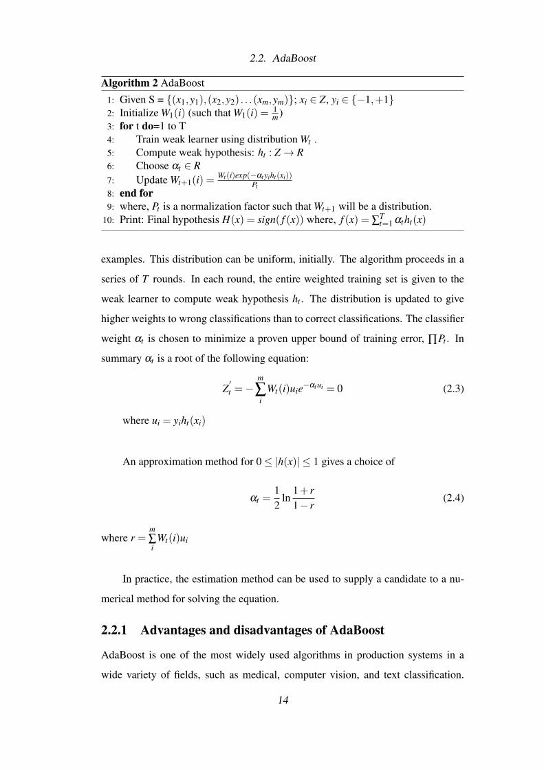
Algorithm 2 AdaBoost
1: Given S = {(x1,y1),(x2,y2) . . .(xm,ym)}; xi ∈ Z, yi ∈ {−1,+1}2: Initialize W1(i) (such that W1(i) = 1
m )3: for t do=1 to T4: Train weak learner using distribution Wt .5: Compute weak hypothesis: ht : Z→ R6: Choose αt ∈ R7: Update Wt+1(i) =
Wt(i)exp(−αtyiht(xi))Pt
8: end for9: where, Pt is a normalization factor such that Wt+1 will be a distribution.
10: Print: Final hypothesis H(x) = sign( f (x)) where, f (x) = ∑Tt=1 αtht(x)
examples. This distribution can be uniform, initially. The algorithm proceeds in a
series of T rounds. In each round, the entire weighted training set is given to the
weak learner to compute weak hypothesis ht . The distribution is updated to give
higher weights to wrong classifications than to correct classifications. The classifier
weight αt is chosen to minimize a proven upper bound of training error, ∏Pt . In
summary αt is a root of the following equation:
Z′t =−
m
∑i
Wt(i)uie−αtui = 0 (2.3)
where ui = yiht(xi)
An approximation method for 0≤ |h(x)| ≤ 1 gives a choice of
αt =12
ln1+ r1− r
(2.4)
where r =m∑i
Wt(i)ui
In practice, the estimation method can be used to supply a candidate to a nu-
merical method for solving the equation.
2.2.1 Advantages and disadvantages of AdaBoost
AdaBoost is one of the most widely used algorithms in production systems in a
wide variety of fields, such as medical, computer vision, and text classification.
14
2.3. MapReduce Programming model
Compared to other classifiers like support vector machines (SVM), AdaBoost re-
quires much less tweaking of parameters to achieve similar results. The required
hyper parameters are: (1) the weak learner (classifier); (2) the number of boosting
rounds. On the other hand, AdaBoost is sensitive to outliers and noisy data. It is less
susceptible, however, to the problem of overfitting than most learning algorithms.
2.3 MapReduce Programming model
MapReduce is a programming model used to process data stored in a distributed
file system (DFS) [12] [13]. To make it work, a programmer provides two methods,
namely mapper and reducer, of the following template:
Map(k,v)→< k′,v′ >∗
• Takes a key-value pair and outputs a transformed set of key-value pairs.
• There is one Map call for every (k,v) pair.
Reduce(k′,< v′ > ′)→< k′,v′′ >∗
• All values v′ with same key k′ are reduced together. Every key is reduced by
applying various transformations, filters and/or aggregations.
• There is one reduce function per unique key k′
• Reduce operations are first applied locally to each partition in the distributed
environment to maintain data locality with distributed environment. Hence,
it reduces data shuffling across the distributed nodes. Then, locally re-
duced/transformed results are brought to the master node to apply the final
reduce operation.
< k′,v′ >∗ is a intermediate key value pair. This consists of a key and a set
of values associated with the key. < k′,v′ >∗ is supplied as an input to the reducer.
The reducer processes < k′,v′ >∗ and generates a final output as < k′,v′′ >∗
15
2.3. MapReduce Programming model
MapReduce can be used to solve many problems, such as, crawling the web,
finding the size of a host from the meta-data files of a web-server, building a lan-
guage model, image processing, data mining (clustering or classification), data an-
alytics, etc. Apache Hadoop MapReduce and Apache Spark are two open-source
data processing frameworks which work on the concept of MapReduce.
2.3.1 Apache Hadoop MapReduce and Apache Spark
Apache Hadoop MapReduce and Spark are distributed data processing frameworks.
Both frameworks work on the principal of MapReduce. The following paragraph
compares them.
Hadoop MapReduce persists the data back to the disk after a map or reduce
action while Spark processes data in-memory. Because of this feature, Spark out-
performs Hadoop MapReduce in terms of data processing speed. Some think this
could be the end of Hadoop MapReduce as Spark promises data processing speeds
up to 100 times faster than Hadoop MapReduce. Hadoop MapReduce and Spark
both have good fault tolerance, but Hadoop MapReduce is slightly more tolerant
because it persists data on disk. Hadoop MapReduce integrates with Hadoop secu-
rity projects, such as Knox Gateway and Sentry. Moreover, to persist the data Spark
can still use Hadoop Distributed File System (HDFS). Moreover, Hive, Pig, HBase,
etc., are some of the Hadoop ecosystem tools which can be leveraged by Spark
for completeness. This means, for a full big data package Hadoop MapReduce
is still running alongside Spark. In a nutshell, Spark serves multi purpose (batch
and stream) data processing; Hadoop MapReduce works better for batch process-
ing. Spark can run as a standalone framework or on top of Hadoop’s Yet Another
Resource Negotiator (YARN), where it can read data directly from HDFS. In gen-
eral, Spark is still improving in its security where as Hadoop MapReduce is more
secure and it has many projects in its ecosystem. Spark has APIs for Java, Scala
and Python whereas Hadoop MapReduce can be implemented using Java. Overall,
Hadoop MapReduce is designed for processing data that does not fit in the primary
memory of a stand alone commodity hardware. It runs well alongside other ser-
vices. Spark is designed to process data sets where the data fits in the memory,
16
2.4. Important Definitions - Keywords
especially on dedicated clusters. Lastly, Apache Mahout uses Hadoop MapReduce
for distributed machine learning whereas Spark has SparkMLib for machine learn-
ing support.
2.4 Important Definitions - Keywords
• Error based models: There are classifiers which work towards the goal of re-
ducing the overall error. That is analogous to saying, classifiers of this group
try to reduce classification errors. For example, decision tree. Therefore, the
algorithms for such classifiers are also designed to reduce classification er-
rors. There are many real world applications where error based classifiers are
most likely to be applied. One such application is weather condition classifi-
cation in which, classification errors are treated equally likely.
• Cost based models: There are classifiers intended to reduce the overall cost
of misclassification. Classifiers of this group try to reduce misclassification
cost and number of high cost errors. An application of such classifiers is in
learning from highly imbalanced datasets, for example, loan approval system.
In such applications, the cost of classifying a defaulter as non-defaulter is
higher than classifying a non-defaulter as a defaulter. CBMs incorporate the
cost parameter in the model building phase and thereby achieve low cost of
classification.
• Cost-sensitive classifier: The classifier which incorporates the cost of mis-
classification in its model building phase or in the model aggregation phase is
considered a cost-sensitive classifier. For example, AdaCost, CSE1, etc.
• Cost matrix: This is a special input necessary while constructing a cost-
sensitive classifier. In this matrix each element represents the misclassifi-
cation cost of classifying a sample to a class X, when it actually belongs to
class Y. An example cost matrix for a two class classification problem (For
example, breast cancer detection) can be, [0 5;1 0]. This indicates the fol-
lowing. A patient is in fact having a cancer and is advised not to undergo
treatment (false negative) is five times costlier than if a patient is not having
17

2.5. Summary
a cancer and is advised to undergo treatment (false positive). There is no cost
involved for true positive and true negative classification.
• Misclassification cost: This is one of the performance measures for a cost-
sensitive classifiers. The cost of misclassification is defined here as, the sum
of, the product of the number of false positive and associated cost of misclas-
sification from cost matrix and the product of the number of false negatives
and the corresponding cost from the cost matrix. To calculate the misclassi-
fication cost (MC), assume a cost matrix to be [0 1; 5 0] and the confusion
matrix to be [10 5; 3 20]. Then, MC = (1*5) + (5*3) = 20, wherein 5 and 3
are false positive and false negative respectively and 1 and 5 are their corre-
sponding cost values.
• Number of High Cost Errors: This is one of the measures for a cost-sensitive
classifier. To calculate the number of high cost errors, consider the CM to be
[0 10; 1 0] and the confusion matrix as [10 4; 2 15]. Therefore, the number
of high cost errors is 4. Here, 4 (in the confusion matrix) is the total number
of false positive examples which associates with high cost in the cost matrix.
2.5 Summary
This chapter described the algorithms, tools and technologies and the terminology
which are used in the implementation of cost-sensitive distributed boosting (CsDb).
It explained the tools with their key components, key features, and working of al-
gorithms. This chapter also covered the strengths and limitations of the tools and
algorithms described .
18
Chapter 3
Literature Review of Cost-sensitive Boosting
Algorithms
Cost-sensitive (CS) learning has attracted researchers since the last decade. Learn-
ing with cost-sensitive classification algorithms is an essential method because it
takes cost of misclassification into account, apart from considering error in classifi-
cation. This survey identifies boosting based cost-sensitive classifiers in literature.
The other categories of cost-sensitive classifiers are genetic algorithms, use of cost
at pre or post tree construction stage, bagging, multiple structure, and stochastic ap-
proach. A useful taxonomy and further scope of research in cost-sensitive boosting
is brought together in this chapter.
3.1 CS Boosters
Cost-sensitive classification adjusts a classifier output to optimize a given cost ma-
trix. That is, cost-sensitive classification adjusts an output of the classifier by re-
calculating the probability threshold. The cost-sensitive learning, on the other hand,
learns a new classifier to optimize with respect to a given cost matrix, effectively by
duplicating or internally re-weighting the instances in accordance with the cost ma-
trix. This survey identifies cost-sensitive learning methods (as they are used for the
classification process only to avoid much confusion the word CS classifier is used).
However, it is important to note that the cost-sensitive boosters (CS Boosters) are a
subset of the cost-sensitive classifiers as boosting is one of the classification tech-
niques.

3.2. Cost-sensitive boosting
Figure 3.1: Taxonomy of cost-sensitive learning
The algorithms identified in this survey with respect to the taxonomy shown
in Figure 3.1 falls under the category boosting. Figure 3.2 shows the significant
volume of work done in this field in cost-sensitive learning using boosting. The
algorithms shown on this timeline incorporate the cost of misclassification while
tree induction, boosting or both.
The timeline of the development of these algorithms is interesting. ID3 is one
of the initial decision tree algorithms developed by Quinlan [9]. It was the first
time when Pazzani et al. identified that, in place of using information gain of an
attribute for deciding split, the cost measures can also be used to reduce cost of
misclassification in classification using decision tree [14]. More novel algorithms
have been developed over the years, including intense research in boosting based
approach in this area.
A significant amount of research has been done on EBM, and instead of de-
veloping new cost-sensitive classifiers, an alternative strategy is to develop wrapper
algorithms over EBM based algorithms.
3.2 Cost-sensitive boosting
Boosting involves creating a number of hypotheses ht and combining them to form
a more accurate composite hypothesis of the form [2]
f (x) =T
∑t=1
αtht(x) (3.1)
20

3.2. Cost-sensitive boosting
2000 2005 2010 2015
UBoost,
Cost-U
Boost,
Boosti
ng, C
ost-B
oosti
ng
AdaCos
t
Found
ation
ofco
st-sen
sitive
Learni
ng
CSB0,CSB1,C
SB2,Ada
Cost(β
1), A
daCos
t(β2)
AsymBoo
st
SSTBoost
GBSE,GBSE-T
,Ada
Boost
withThre
shold
Mod
ificatio
n
AdaC1,A
daC2,A
daC3,J
OUS-Boo
st
LP-CSB, L
P-CSB-PA
and LP-C
SB-A
CS-Ada
, CS-L
og, C
S-Rea
l
Cost-G
enera
lized
AdaBoo
st
AdaBoo
stDB
CBE1,CBE2,
CBE3,Ada
-calib
rated
Figure 3.2: Timeline of CS Boosters
where, αt indicates the portion of weight that should be given to ht(x). The Ad-
aBoost (Adaptive Boosting) algorithm is discussed in section 2.2. Where, in step.
2 it can be seen that initial weights are 1m for each sample. It is important note that
these weights are increased during steps 3 to 8 (by an equation in step 7) if a sample
is misclassified. Weights are decreased if a sample is classified correctly. At the
end, hypothesis ht are available and can be combined to perform classification. In
summary, AdaBoost can be viewed as a three step process, that is, initialization,
weight update, and creating a final weighted combination of hypotheses. All CS
boosters discussed in this report are adaptations of the three steps of AdaBoost to
develop CS boosters. Figure 3.2 shows the list of CS boosters proposed over time.
Boosting was used for the first time by Ting et al. for cost-sensitive learn-
ing [3]. Ting et al. used misclassification cost in the model building phase im-
proves the performance of the algorithm. They proposed two cost-sensitive variants
of AdaBoost, namely, UBoost (boosting with unequal initial weights) and Cost-
UBoost. Cost-UBoost is a cost-sensitive extension of UBoost. Boosting trees has
been proven an effective method of reducing the number of high cost errors as well
as the total misclassification cost. Both variants perform significantly better than
their predecessor method of boosting, that is, C4.5C. The important thing to note is
that both algorithms incorporate the cost of misclassification in post-processing or
decision tree induction stage. Minimum expected cost criteria (MECC) was used in
21

3.2. Cost-sensitive boosting
voting. Later, Ting et al. proposed another two variants with minor modifications
that is starting the training of AdaBoost with all the samples assigned equal initial
weights [15].
The empirical evaluation conducted by Ting et al. suggest that Cost-UBoost
outperforms UBoost in terms of minimizing the misclassification cost for binary
class problems. However, for multi-class problems the cost is not reduced. The
reduction in cost is not achieved because the different costs of misclassification are
mapped into a single misclassification cost by weight update equation.
Later, Ting et al. followed up and proposed further extensions [6]. In this paper
CSB0, CSB1 and CSB2 are empirically evaluated with another set of AdaBoost ex-
tensions namely AdaCost [16] and its variants AdaCost(β1) and AdaCost(β2). The
parameters for performance comparison are kept the same, that is, misclassification
cost and the number of high cost errors. Weight update equation is modified and
kept simple in CSB0. CSB1 and CSB2 introduce parameter α and cost in weight
update equation. This helps increase the confidence in the prediction. Variants
of AdaCost are proposed by incorporating β (cost adjustment function) in rk and
weight update rule.
Ting et al. [6] empirically evaluated CSB family of algorithms. They conclude
that there is no significant cost reduction by the introduction of the αt in CSB2.
Moreover, the introduction of an additional parameter in weight update equation of
AdaCost does not help significantly in reducing misclassification cost or number of
high cost errors.
However, CSB1 outperforms AdaCost variations, namely, AdaCost(β1),
AdaCost(β2), in terms of cost-effectiveness. In contradiction to its nature, Ad-
aBoost (which is an EBM based algorithm) is proven to be more cost-effective
as compared to AdaCost(β1) and AdaCost(β2) which are CBM based algorithms.
About this, Ting [6] et al. comment that this is due to the reason that β parameter
which is introduced in weight update equation assigns comparatively low penalty
(reward) when high cost samples are incorrectly (correctly) classified. It is impor-
tant to note that Ting et al. [6] used C4.5 as a weak learner. Whereas, originally,
22

3.2. Cost-sensitive boosting
when Fan et al. [16] empirically evaluated the AdaCost they had used Ripper as
a weak learner. Moreover, Fan et al. [16] have concluded that AdaCost is more
cost-effective than AdaBoost. In AdaCost, the objective of the cost-adjustment
function β is to reduce overall misclassification cost. The function is designed to
increase more weight when example is misclassified, but decreases its weight less
in the other case.
With a goal of minimizing the loss, Viola et al. developed AsymBoost [17].
It is a simple modification of the confidence-rated boosting approach of Singer [2].
It incorporates the loss (cost) in classifier training phase. It works on a cascade of
classifiers approach for feature selection in the face detection problem. In this algo-
rithm Viola et al. used support vector machines (SVM) as a cascade of classifiers.
The results show faster face detection and reduction in the number of false positive
samples. In a follow up study, Viola et al. proposed a seminal work in the same
domain dealing with a markedly asymmetric problem and an enormous number of
weak classifiers (of the order of hundred of thousands). It uses a validation set to
modify the threshold of the original (cost-insensitive) AdaBoost classifier with a
goal to balance between false positive and detection rate [18].
The intuition behind the development of the sensitivity specificity tuning boost-
ing (SSTBoost) by Merler is interesting [19]. If the costs are not defined it is possi-
ble to approximate the cost of false negatives and false positives in classifier train-
ing. SSTBoost is an AdaBoost variant. It is proposed based on the following two
principals. First, weighting the model error function with separate costs for false
negative and false positive errors. Second, updating the weights differently for neg-
ative and positive for each boosting step. In first part, the algorithm tries to achieve
the sensitivity by maximizing the number of true positives and at the same time clas-
sifier maintains the specificity within acceptable bounds. As the dataset was from
the medical domain, in the second part, a team of medical experts would examine
the positive samples carefully. This leads to reduction in the cost of misclassifica-
tion. SSTBoost introduces the cost parameter x into weight update equation as well
as into estimated error function. This allowed the moving of the decision boundary
23

3.2. Cost-sensitive boosting
of one class marginally with respect to the other.
All the algorithms discussed above work on binary class problems. For multi-
class problems determining the weight for cost adjustment becomes complex as
a given sample can be misclassified into more than one class. To overcome this
limitation, an intuitive approach can be employed, that is, to sum or average the cost
into other classes. However, Ting comments that by applying these methods leads
to the reduction in overall cost of misclassification [3] [6]. Hence, an alternative
approach of utilizing boosting for multi-class classification is developed by Abe et
al. [20] in gradient boosting with stochastic ensembles (GBSE). Gradient boosting
with stochastic ensembles approach is well motivated theoretically and a method
based on iterative schemes for sample weighting. The key ideas for deriving their
method are: 1. iterative weighting, 2. expanding dataspace, 3. gradient boosting
with stochastic ensembles. The first two are combined in a unifying framework
given by the third. An important property of any extension of a boosting algorithm
is that it should converge. For GSEB, however, this has not been shown by Abe
et al. [20]. Nevertheless, GSEB-T (where T stands for theoretical variant) which
follows GSEB proves the conversions of cost equation.
Later Abe, Lozano et al. followed up and built an even stronger foundation
for multi-class cost-sensitive learning [21] in cost-sensitive boosting with p-norm
loss LP−CSB. LP−CSB is a family of methods which includes LP−CSB, LP−
CSB−PA and LP−CSB−A. They work on p-norm cost functions and the gradient
boosting framework [20]. In this study, Lozano et al. proved the conversions of
weight update equation. LP−CSB family of methods tries to minimize the cost
approximation using p-norm. The weight update equations in LP−CSB are different
than GSEB.
Elkan showed in his study that it is possible to change the class distribution
of the data samples to reflect the cost ratio. Basically, either over-sampling or the
under-sampling is applied over the data in preprocessing stage. It is possible to
apply sampling with or without replacement. In general, over-sampling leads to
increasing the data set size due to the introduction of the duplicate data samples
24
3.2. Cost-sensitive boosting
whereas under-sampling leads to reduction in the number of samples in the dataset.
Further, by applying boosting over this new distribution can help achieve reduced
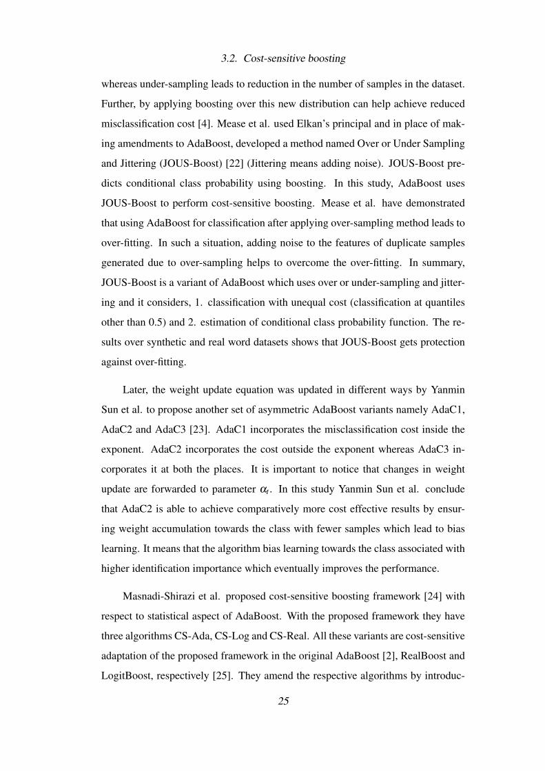
misclassification cost [4]. Mease et al. used Elkan’s principal and in place of mak-
ing amendments to AdaBoost, developed a method named Over or Under Sampling
and Jittering (JOUS-Boost) [22] (Jittering means adding noise). JOUS-Boost pre-
dicts conditional class probability using boosting. In this study, AdaBoost uses
JOUS-Boost to perform cost-sensitive boosting. Mease et al. have demonstrated
that using AdaBoost for classification after applying over-sampling method leads to
over-fitting. In such a situation, adding noise to the features of duplicate samples
generated due to over-sampling helps to overcome the over-fitting. In summary,
JOUS-Boost is a variant of AdaBoost which uses over or under-sampling and jitter-
ing and it considers, 1. classification with unequal cost (classification at quantiles
other than 0.5) and 2. estimation of conditional class probability function. The re-
sults over synthetic and real word datasets shows that JOUS-Boost gets protection
against over-fitting.
Later, the weight update equation was updated in different ways by Yanmin
Sun et al. to propose another set of asymmetric AdaBoost variants namely AdaC1,
AdaC2 and AdaC3 [23]. AdaC1 incorporates the misclassification cost inside the
exponent. AdaC2 incorporates the cost outside the exponent whereas AdaC3 in-
corporates it at both the places. It is important to notice that changes in weight
update are forwarded to parameter αt . In this study Yanmin Sun et al. conclude
that AdaC2 is able to achieve comparatively more cost effective results by ensur-
ing weight accumulation towards the class with fewer samples which lead to bias
learning. It means that the algorithm bias learning towards the class associated with
higher identification importance which eventually improves the performance.
Masnadi-Shirazi et al. proposed cost-sensitive boosting framework [24] with
respect to statistical aspect of AdaBoost. With the proposed framework they have
three algorithms CS-Ada, CS-Log and CS-Real. All these variants are cost-sensitive
adaptation of the proposed framework in the original AdaBoost [2], RealBoost and
LogitBoost, respectively [25]. They amend the respective algorithms by introduc-
25
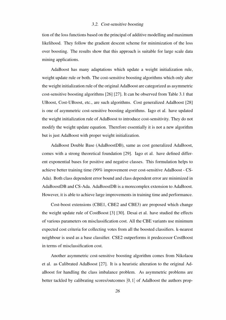
3.2. Cost-sensitive boosting
tion of the loss functions based on the principal of additive modelling and maximum
likelihood. They follow the gradient descent scheme for minimization of the loss
over boosting. The results show that this approach is suitable for large scale data
mining applications.
AdaBoost has many adaptations which update a weight initialization rule,
weight update rule or both. The cost-sensitive boosting algorithms which only alter
the weight initialization rule of the original AdaBoost are categorized as asymmetric
cost-sensitive boosting algorithms [26] [27]. It can be observed from Table 3.1 that
UBoost, Cost-UBoost, etc., are such algorithms. Cost generalized AdaBoost [28]
is one of asymmetric cost-sensitive boosting algorithms. Iago et al. have updated
the weight initialization rule of AdaBoost to introduce cost-sensitivity. They do not
modify the weight update equation. Therefore essentially it is not a new algorithm
but is just AdaBoost with proper weight initialization.
AdaBoost Double Base (AdaBoostDB), same as cost generalized AdaBoost,
comes with a strong theoretical foundation [29]. Iago et al. have defined differ-
ent exponential bases for positive and negative classes. This formulation helps to
achieve better training time (99% improvement over cost-sensitive AdaBoost - CS-
Ada). Both class dependent error bound and class dependent error are minimized in
AdaBoostDB and CS-Ada. AdaBoostDB is a morecomplex extension to AdaBoost.
However, it is able to achieve large improvements in training time and performance.
Cost-boost extensions (CBE1, CBE2 and CBE3) are proposed which change
the weight update rule of CostBoost [3] [30]. Desai et al. have studied the effects
of various parameters on misclassification cost. All the CBE variants use minimum
expected cost criteria for collecting votes from all the boosted classifiers. k-nearest
neighbour is used as a base classifier. CSE2 outperforms it predecessor CostBoost
in terms of misclassification cost.
Another asymmetric cost-sensitive boosting algorithm comes from Nikolaou
et al. as Calibrated AdaBoost [27]. It is a heuristic alteration to the original Ad-
aBoost for handling the class imbalance problem. As asymmetric problems are
better tackled by calibrating scores/outcomes [0,1] of AdaBoost the authors prop-
26

3.2. Cost-sensitive boosting
erly calibrate the outcome of the AdaBoost to correspond to probability estimates.
A new approach to map score to probability estimation is proposed in this algo-
rithm. The results show that Calibrated AdaBoost preserves theoretical guarantees
of AdaBoost while taking misclassification cost into account.
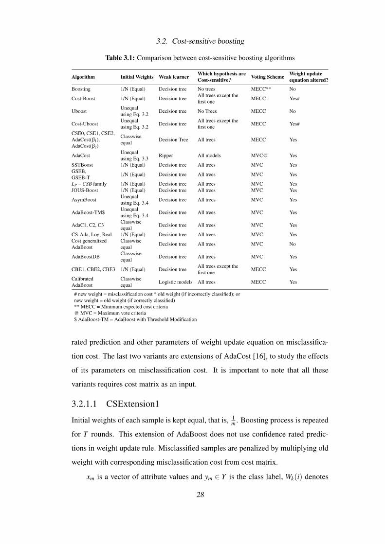
Finally, Table 3.1 shows a comparative analysis between a set of AdaBoost
extensions for cost-sensitive classification.
Equation used to initialise the weights of each sample in Ting’s algorithms (see
Table 3.1.)
wi = ci(N
∑c jN j) (3.2)
Where, wi is the initial weight of the class i instance, and Ci is the cost of
misclassifying a class i instance, and N j is the number of class j instances.
Equation used to initialise the weights in AdaCost (see Table 3.1.)
wi = (ci
∑c j) (3.3)
AsymBoost assigns different weights to positive and negative class samples
see Table 3.1.
wi =1
2p,
12n
(3.4)
for yi = 0 and 1, respectively. where, p and n are number of positives and negative
samples, respectively.
3.2.1 Related Work
AdaBoost is a meta classifier. Total cost of misclassification can be incorporated
into the model building phase to extend AdaBoost with cost-sensitivity. Misclassi-
fication cost can be incorporated during the weight update, weight initialization or
both phases of AdaBoost. Moreover, confidence rated predictions of AdaBoost can
be useful in improving the accuracy of the classifier.
Initially, Desai et al. proposed extensions to AdaBoost for cost-sensitive clas-
sification [5]. The first three variants are extensions of discrete AdaBoost [2]. Ad-
aBoost with modified weight update equation to study the effects of confidence
27
3.2. Cost-sensitive boosting
Table 3.1: Comparison between cost-sensitive boosting algorithms
Algorithm Initial Weights Weak learner Which hypothesis areCost-sensitive? Voting Scheme Weight update
equation altered?
Boosting 1/N (Equal) Decision tree No trees MECC** No
Cost-Boost 1/N (Equal) Decision treeAll trees except thefirst one MECC Yes#
UboostUnequalusing Eq. 3.2 Decision tree No Trees MECC No
Cost-UboostUnequalusing Eq. 3.2 Decision tree
All trees except thefirst one MECC Yes#
CSE0, CSE1, CSE2,AdaCost(β1),AdaCost(β2)
Classwiseequal Decision Tree All trees MECC Yes
AdaCostUnequalusing Eq. 3.3 Ripper All models MVC@ Yes
SSTBoost 1/N (Equal) Decision tree All trees MVC YesGSEB,GSEB-T 1/N (Equal) Decision tree All trees MVC Yes
LP−CSB family 1/N (Equal) Decision tree All trees MVC YesJOUS-Boost 1/N (Equal) Decision tree All trees MVC Yes
AsymBoostUnequalusing Eq. 3.4 Decision tree All trees MVC Yes
AdaBoost-TM$Unequalusing Eq. 3.4 Decision tree All trees MVC Yes
AdaC1, C2, C3Classwiseequal Decision tree All trees MVC Yes
CS-Ada, Log, Real 1/N (Equal) Decision tree All trees MVC YesCost generalizedAdaBoost
Classwiseequal Decision tree All trees MVC No
AdaBoostDBClasswiseequal Decision tree All trees MVC Yes
CBE1, CBE2, CBE3 1/N (Equal) Decision treeAll trees except thefirst one MECC Yes
CalibratedAdaBoost
Classwiseequal Logistic models All trees MECC Yes
# new weight = misclassification cost * old weight (if incorrectly classified); ornew weight = old weight (if correctly classified)** MECC = Minimum expected cost criteria@ MVC = Maximum vote criteria$ AdaBoost-TM = AdaBoost with Threshold Modification
rated prediction and other parameters of weight update equation on misclassifica-
tion cost. The last two variants are extensions of AdaCost [16], to study the effects
of its parameters on misclassification cost. It is important to note that all these
variants requires cost matrix as an input.
3.2.1.1 CSExtension1
Initial weights of each sample is kept equal, that is, 1m . Boosting process is repeated
for T rounds. This extension of AdaBoost does not use confidence rated predic-
tions in weight update rule. Misclassified samples are penalized by multiplying old
weight with corresponding misclassification cost from cost matrix.
xm is a vector of attribute values and ym ∈ Y is the class label, Wk(i) denotes
28

3.2. Cost-sensitive boosting
the weight of the ith example at kth trial. In other words, each instance (or example
or sample) xm belongs to a feature domain Z and has an associated label, also called
class. For binary problems each instance is labelled as +1 or −1. Every exam-
ple also has an associated weight, which will indicate, intuitively, the difficulty of
achieving its correct classification. Initially, all the examples have the same weight.
In each iteration a base (also named weak) classifier is constructed, according to
the distribution of weights. Afterwards, the weight of each example is readjusted,
based on the correctness of the class assigned to the example by the base classifier.
With this, the method can be focused upon the examples which are harder to clas-
sify properly. The final result is obtained by maximum votes of the base classifiers.
Algorithm 3 shows CSExtension1 in detail.
Algorithm 3 CSExtension1
1: Given S = {(x1,y1),(x2,y2) . . .(xm,ym)}; xi ∈ Z, yi ∈ {−1,+1}2: Initialize W1(i) (such that W1(i) = 1)3: for t do=1 to T4: Train weak learner using distribution Wt .5: Compute weak hypothesis: ht : Z→ R
rt =1n ∑
nδwt(i)ht(xi) where, δ =
{+1 if, ht(xi) = yi
−1 otherwise
αt =12
ln(1+ rt
1− rt)
6: Update Wt+1(i) =CδWt(i) where, Cδ = misclassification cost7: end for8: collect vote from T models:
H ∗(x) = argmaxx ∑αtht(xi)
3.2.1.2 CSExtension2
This is also an extension of AdaBoost. In step 6, the weight update rule is modified
as given below. It uses the exponential loss in weight update equation. It does not,
however, use confidence of prediction αt into the weight update equation. The step
by step depiction of CSExtension2 is carried out in Algorithm 4.
29
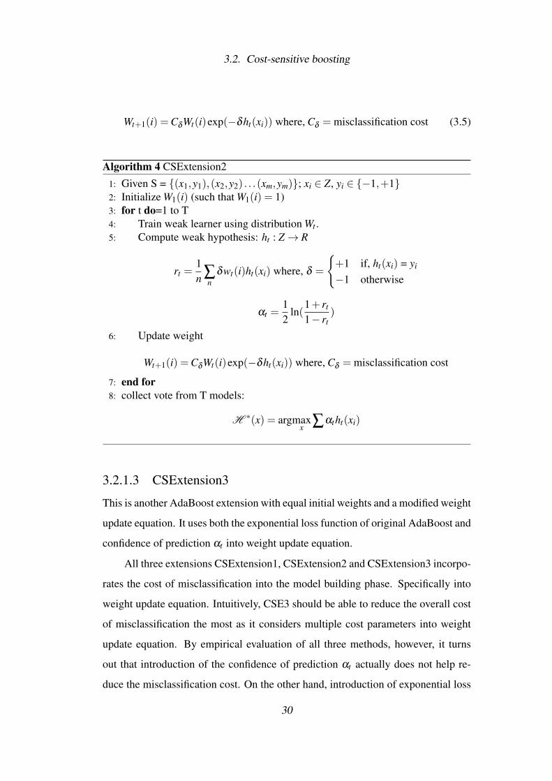
3.2. Cost-sensitive boosting
Wt+1(i) =CδWt(i)exp(−δht(xi)) where, Cδ = misclassification cost (3.5)
Algorithm 4 CSExtension2
1: Given S = {(x1,y1),(x2,y2) . . .(xm,ym)}; xi ∈ Z, yi ∈ {−1,+1}2: Initialize W1(i) (such that W1(i) = 1)3: for t do=1 to T4: Train weak learner using distribution Wt .5: Compute weak hypothesis: ht : Z→ R
rt =1n ∑
nδwt(i)ht(xi) where, δ =
{+1 if, ht(xi) = yi
−1 otherwise
αt =12
ln(1+ rt
1− rt)
6: Update weight
Wt+1(i) =CδWt(i)exp(−δht(xi)) where, Cδ = misclassification cost
7: end for8: collect vote from T models:
H ∗(x) = argmaxx ∑αtht(xi)
3.2.1.3 CSExtension3
This is another AdaBoost extension with equal initial weights and a modified weight
update equation. It uses both the exponential loss function of original AdaBoost and
confidence of prediction αt into weight update equation.
All three extensions CSExtension1, CSExtension2 and CSExtension3 incorpo-
rates the cost of misclassification into the model building phase. Specifically into
weight update equation. Intuitively, CSE3 should be able to reduce the overall cost
of misclassification the most as it considers multiple cost parameters into weight
update equation. By empirical evaluation of all three methods, however, it turns
out that introduction of the confidence of prediction αt actually does not help re-
duce the misclassification cost. On the other hand, introduction of exponential loss
30

3.2. Cost-sensitive boosting
helps achieve reduced cost of misclassification. The empirical evaluation conducted
over selected datasets from UCI machine learning repository shows that with CSEx-
tension2 average misclassification cost is minimum. CSExtension3 is depicted in
Algorithm 5.
Algorithm 5 CSExtension3
1: Given S = {(x1,y1),(x2,y2) . . .(xm,ym)}; xi ∈ Z, yi ∈ {−1,+1}2: Initialize W1(i) (such that W1(i) = 1)3: for t do=1 to T4: Train weak learner using distribution Wt .5: Compute weak hypothesis: ht : Z→ R
rt =1n ∑
nδwt(i)ht(xi) where, δ =
{+1 if, ht(xi) = yi
−1 otherwise
αt =12
ln(1+ rt
1− rt)
6: Update weight
Wt+1(i) =CδWt(i)exp(−δht(xi)αt) where, Cδ = misclassification cost
7: end for8: collect vote from T models:
H ∗(x) = argmaxx ∑αtht(xi)
3.2.1.4 CSExtension4
CSE4 is an extension of AdaCost. As discussed in section 3.2 AdaCost introduces
another parameter βδ along with αt and confidence of prediction into its weight up-
date equation and achieves improvement in misclassification cost. Individual effects
of βδ and its variants over misclassification cost, however, was neither discussed
nor evaluated. To evaluate the impact of this parameter, Desai et al. proposed two
variants of AdaCost where CSE4 uses equal value of parameter β for both positive
and negative class samples whereas, CSE5 assigns different values to positive sam-
ples and negative samples for parameter β . Both these algorithms are depicted in
Algorithm 6 and 7 respectively.
31
3.2. Cost-sensitive boosting
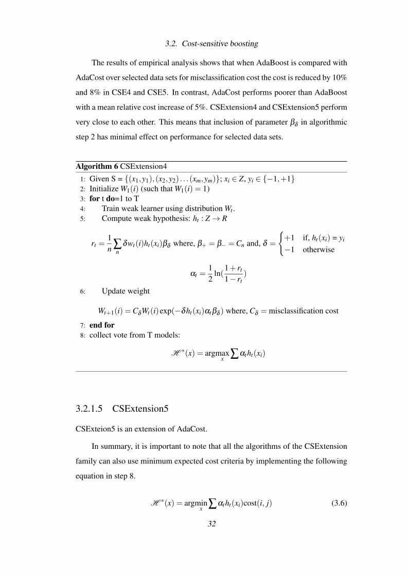
The results of empirical analysis shows that when AdaBoost is compared with
AdaCost over selected data sets for misclassification cost the cost is reduced by 10%
and 8% in CSE4 and CSE5. In contrast, AdaCost performs poorer than AdaBoost
with a mean relative cost increase of 5%. CSExtension4 and CSExtension5 perform
very close to each other. This means that inclusion of parameter βδ in algorithmic
step 2 has minimal effect on performance for selected data sets.
Algorithm 6 CSExtension4
1: Given S = {(x1,y1),(x2,y2) . . .(xm,ym)}; xi ∈ Z, yi ∈ {−1,+1}2: Initialize W1(i) (such that W1(i) = 1)3: for t do=1 to T4: Train weak learner using distribution Wt .5: Compute weak hypothesis: ht : Z→ R
rt =1n ∑
nδwt(i)ht(xi)βδ where, β+ = β− =Cn and, δ =
{+1 if, ht(xi) = yi
−1 otherwise
αt =12
ln(1+ rt
1− rt)
6: Update weight
Wt+1(i) =CδWt(i)exp(−δht(xi)αtβδ ) where, Cδ = misclassification cost
7: end for8: collect vote from T models:
H ∗(x) = argmaxx ∑αtht(xi)
3.2.1.5 CSExtension5
CSExteion5 is an extension of AdaCost.
In summary, it is important to note that all the algorithms of the CSExtension
family can also use minimum expected cost criteria by implementing the following
equation in step 8.
H ∗(x) = argminx ∑αtht(xi)cost(i, j) (3.6)
32

3.3. Summary
Since all proposed algorithms are meta classifiers, they can use any weak
learner as a base classifier, for example, Ibk, Naive Bayes, k-nn, etc. This dis-
sertation proposes distributed extensions of stated algorithms in this section which
use Weka’s J48 as a base classifier for experimental evaluation.
Algorithm 7 CSExtension5
1: Given S = {(x1,y1),(x2,y2) . . .(xm,ym)}; xi ∈ Z, yi ∈ {−1,+1}2: Initialize W1(i) (such that W1(i) = 1)3: for t do=1 to T4: Train weak learner using distribution Wt .5: Compute weak hypothesis: ht : Z→ R
rt =1n ∑n δwt(i)ht(xi)βδ where, β+ =−1
2Cn +12
and, β− =12
Cn +12
and, δ =
{+1 if, ht(xi) = yi
−1 otherwise
αt =12
ln(1+ rt
1− rt)
6: Update weight
Wt+1(i) =CδWt(i)exp(−δht(xi)αtβδ ) where, Cδ = misclassification cost
7: end for8: collect vote from T models:
H ∗(x) = argmaxx ∑αtht(xi)
3.3 Summary
This chapter reviewed a challenging research area of cost-sensitive boosting. The
taxonomy of the algorithm is also derived. The chapter ends with details of the
algorithms used for empirical evaluation of CsDb.
33

Chapter 4
The development of a new MapReduce based
cost-sensitive boosting
This chapter depicts the development of a framework for cost-sensitive distributed
boosting induction which works on the principles of MapReduce. Section 4.1
presents the limitations of the existing cost-sensitive classifiers which motivates this
work. Section 4.2 shows the core process of the development of the algorithm and
Section 4.3 summarizes the chapter.
4.1 Understanding the need to build a new cost-sensitive boost-
ing algorithm
There are attributes that define big data. These are called the four V’s: volume, va-
riety, velocity, and veracity. Research on distributed data mining (DDM) has been
motivated primarily by the desire to mine data beyond gigabytes. This is aimed at
the first V of big data - volume. Using stand alone commodity hardware having
limited gigabytes of primary memory and only tens of cores, mining gigabytes of
data is not possible using machine learning and statistics since it can take hours,
even days, to generate a model using classical data mining algorithms (explained
later in this section). This implies a need for a scalable data mining algorithm.
Moreover, mining a sample of the data as opposed to mining datasets of gigabytes
or beyond fuels an interesting debate - to which DDM researchers should pay atten-
tion. Nevertheless, faster data mining is necessary. Easy decomposability of data
mining algorithms makes them ideal candidates for parallel processing. This can be

4.1. Understanding the need to build a new cost-sensitive boosting algorithm
achieved using a distributed data mining system.
Class imbalance problem can be handled by approaches discussed in section
1.2. The algorithmic ensemble techniques are suitable candidates for scaling to
datasets of volumes beyond gigabytes. Some real world problems, however, come
with data sizes in gigabytes or terabytes for training with biased class distribution.
For example, click stream data [31]. Therefore, there is a need to design an algo-
rithm of machine learning which can learn from these datasets. In this case, DDM
can provide an effective solution. In earlier work [5, 30] cost-based approach was
used to address the class imbalance problem, using data mining as explained in the
next paragraph. Most of the solutions as discussed in Section 1.2 for solving the
class imbalance problem do not scale to the volume of data beyond the capacity of
commodity hardware to handle. Therefore, there exists a need to modify CSE1-5 [5]
so that it can address the said challenge. Moreover, it is important to preserve accu-
racy, precision, recall, F-measure, number of high cost errors, and misclassification
cost of a DDM based implementation of an algorithm with respect to its stand alone
implementation. For fast iterations of data mining modelling, the model building
time should be reduced. The choice of these performance measures is explained in
section 5.1.
In a distributed system, many commodity machines are connected together to
do a single task in an efficient way. In distributed data mining processes, many
commodity hardware work together to extract the knowledge from the data stored
across all the nodes. The data analytics approaches can be divided into three cate-
gories depending upon the volume of the data they consider. The first approach is
based on machine learning 1 and statistics. Here, if data can be read from a disk
into the main memory, the algorithm runs and reads the data available in the main
memory. This leads to a situation where repetitive disk access is needed. Such an
architecture is a single node architecture. The second approach is as follows. If the
data does not fit into the main memory then as a fallback mechanism, the classical
1It is a subfield of computer science that evolved from the study of pattern recognition and computational learning theoryin artificial intelligence.
35

4.2. A new algorithm for cost-sensitive boosting learning using MapReduce
data mining 2 algorithm searches for the data into the disk (secondary memory).
This mechanism is followed in data mining algorithms [32, 33]. Only a portion of
the data is brought into memory at a time. The algorithm processes the data in parts
and writes back partial results to the disk. Sometimes even this is not sufficient as
in the case of Google crawling web pages. This requires the third approach, that is,
distributed environment [34, 35, 36, 37, 38, 39, 40, 41].
As discussed in this section there is a need for a fast, distributed, scalable, and
cost-sensitive data mining algorithm.
4.2 A new algorithm for cost-sensitive boosting learning using
MapReduce
The development of the algorithm is accomplished in three phases. First, the dis-
tributed version of the decision tree algorithm is proposed. Then, an extension to
enhance the performance of the Distributed Decision Trees (DDT), DDTv2 is intro-
duced, which works on the notion of ‘hold the model’ (explained in section 4.2.2).
Finally, cost-sensitive distributed boosting (CsDb) is introduced in section 4.2.3.
4.2.1 Distributed Decision Tree
It can take hours or days to generate a model for a stand alone commodity hardware
with a limited number of cores, a primary memory of a limited gigabytes, running
machine learning and statistics based classical data mining algorithms (section 4.1).
To overcome this limitation, an algorithm is needed which could be used when a
dataset can not be accommodated in the primary memory. Therefore, using the
third approach DDT and Spark Trees (ST) are implemented. It means, DDT or ST
could be used when a dataset is too large to be loaded into the primary memory or
when processing would take too long on a single machine. Given a large dataset
with hundreds of attributes the task is to build a decision tree. The goal is to have
a tree which is small enough to be kept in the memory (data can be big but the
tree itself can be small). This is useful for handling datasets which can not be
2It is the computational process of discovering patterns in large data sets involving methods at the intersection of artificialintelligence, machine learning, statistics, and database systems.
36

4.2. A new algorithm for cost-sensitive boosting learning using MapReduce
processed on a single machine. MapReduce and Spark can be used to achieve this.
The algorithm will be useful for many applications such as analysing the functional
MRI Neuroimaging data, infrared data from soil samples, large corpus of web-
log data, and so on. DDT and ST are suitable for the large, offline batch based
processing. The algorithm works on the idea of divide (the data) and conquer - over
multiple processing machines. Here, it is important to note that the DDT and ST
are two different implementations of the same algorithm using Hadoop MapReduce
and Spark, respectively.
Figure 4.1: MapReduce of DDT
The approach of DDT and ST is as follows. As defined in Figure 4.1, before the
MapReduce phase, the dataset is divided into a number of splits defined by the user.
In the next step, that is, Map, it creates decision trees using chunks of data available
on each data node. In the reduce step, it collects all the models created in the map
tasks. Basically, in the case when decision tree is considered as a base classifier, an
ensemble of trees is generated. In general, in the case of non-aggregatable classifiers
(for example, decision tree), the final model produced from the reducer is a voted
ensemble of the models learned by the mappers. Model construction and model
evaluation phases with three-fold cross validation are explained in figure 4.2 and
4.3 respectively [42].
37

4.2. A new algorithm for cost-sensitive boosting learning using MapReduce
Figure 4.2: phase 1 model construction
Figure 4.3: phase 2 model evaluation
Let us now consider cross validation of DDT and ST. It involves two separate
phases or passes over the data. First is model construction, and second, model
evaluation (Figure 4.2 and 4.3). Consider a simple three-fold cross validation. As
noted earlier, the dataset is split into three distinct chunks during this process, and
models are created by training on two out of the three chunks. This leads to a
situation where three models are created at the end, each of them trained on two-
thirds of the data, and then they are tested on the chunk not used during the training
38
4.2. A new algorithm for cost-sensitive boosting learning using MapReduce
process. The second phase of cross validation is straightforward. It takes the models
learned from the first phase and applies them to the holdout folds of cross validation
in each of the logical partitions of the dataset. It uses them to evaluate each of those
holdout folds. The reducer then takes all the partial evaluation results coming out
of the map tasks and aggregates them to one final full evaluation result, then written
out to the file system.
In this example, the dataset is made up of two logical partitions. Each of these
partitions can be thought of as containing part of each cross validation fold. In this
case, they would hold exactly half of each cross validation fold, because there are
two partitions. Each partition, is processed by a worker, or a map task. In the model
building phase, workers build partial models, and there will be a model inside the
worker that is created for one of the training splits of this cross validation. So, it is a
partial model. For example, the first model is created on folds two and three, or parts
of folds two and three. Similarly, model two is created on fold one and three and
model three on fold one and two. In each of these workers, these models are partial
models, because they have only seen part of the data from those particular folds.
In the present example, the map tasks output a total of six partial models, two for
each training split of the cross validation. This allows for parallelism in the reduce
phase. As many reduce tasks can be run as there are models to be aggregated. Each
reducer has the goal of aggregating one of the models. So, in the present example,
the six partial models are aggregated to the three final models that you would expect
from a three-fold cross validation.
Overall, as depicted in figure 4.4, our algorithm first determines metadata
(Mean, standard deviation, sum, min, max, etc.) for individual data chunks which
are used for the purpose of the further data processing. Next, in a single pass over
the data, partial matrix of covariance sum is created by Map tasks and aggregation
of individual rows is performed by Reducer. In the third step, Mapper will create a
tree from a given data chunk. In this step Reducer aggregates the individual model.
The decision tree is a non-aggregatable classifier and hence voted ensemble is used.
The classifier is built by passing over the data just once. Next, the algorithm cross
39
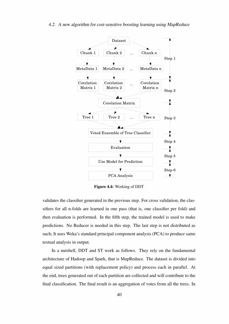
4.2. A new algorithm for cost-sensitive boosting learning using MapReduce
Figure 4.4: Working of DDT
validates the classifier generated in the previous step. For cross validation, the clas-
sifiers for all n-folds are learned in one pass (that is, one classifier per fold) and
then evaluation is performed. In the fifth step, the trained model is used to make
predictions. No Reducer is needed in this step. The last step is not distributed as
such; It uses Weka’s standard principal component analysis (PCA) to produce same
textual analysis in output.
In a nutshell, DDT and ST work as follows. They rely on the fundamental
architecture of Hadoop and Spark, that is MapReduce. The dataset is divided into
equal sized partitions (with replacement policy) and process each in parallel. At
the end, trees generated out of each partition are collected and will contribute to the
final classification. The final result is an aggregation of votes from all the trees. In
40
4.2. A new algorithm for cost-sensitive boosting learning using MapReduce
case of regression, an average output is considered.
This whole mechanism leads to the following problems.
1. Model Experience Problem: The number of trees generated is equal to the
number of partitions. If the user supplies hundred partitions as an input, there
will be an ensemble of hundred trees after training. In this case, the amount
of time required to generate a model will be low but the accuracy will also
be low. This case is analogous to consulting a hundred doctors with bachelor
of medicine degrees and taking their opinions for a probable diagnosis and
concluding that the diagnosis is the one with the maximum votes.
2. Trade-off Problem: The trade-off is between the size of each partition and
accuracy. Consider a case where the size of each partition is considerably
small. Either because the dataset is small or the number of partitions are large
or both. In such cases, trees generated out of each partition would have learnt
from a small number of samples. Therefore, its predictive accuracy will be
low. If the converse is considered, that is, if the size of each partition is very
large (either because of a large dataset or a small number of partitions or both)
the partitions will not fit into the primary memory (or the primary memory
needs to be increased). Of course, if the dataset can fit into the memory and
if training is possible, the accuracy of prediction will be high, as the learning
would take place from a large number of samples.
The DDT and ST was empirically evaluated over ten selected datasets from
UCI machine learning repository and one click-stream dataset from Yahoo! (further
details about the dataset is mentioned in section 5.1). The decision tree, ensemble of
trees using boosting (BT), DDT and ST are compared over three parameters namely,
accuracy, size of tree and number of leaves of tree(s). DDT and ST outperformed
DT and BT in terms of size of tree (sot) and number of leaves (nol) with acceptable
accuracy of classification. Table 4.1 shows percentage reduction obtained in size
of tree and number of leaves in DDT and ST with respect to BT and DT. Average
accuracy of DT, BT, DDT and ST over all ten selected datasets are 92.79, 99.70,
41

4.2. A new algorithm for cost-sensitive boosting learning using MapReduce
83.76 and 86.93 respectively. For Yahoo! dataset, BT takes a very long time to build
the model with accuracy improvement of just 1% over DT. ST takes advantage of
using Spark, it builds the model in just a few seconds even with such a large dataset,
its accuracy is comparable to DT and BT and comparatively less then DDT. At the
same time, the size of a tree and number of leaves are comparatively lower in ST.
4.2.2 Distributed Decision Tree v2
Figure 4.5: Map phase of DDTv2
The way DDTv2 and DDT work is similar except in dataset split step, that is,
hold the model approach is considered in DDTv2. In “Hold the model” approach
the model prepared by split 1 of the dataset is held aside until it is also trained
from split 2 (Figure 4.5). Therefore, the number of decision trees generated out of
DDTv2 is equal to half of the number of splits.
number of models = bn/2c,where, n is number of partitions (4.1)
This strategy of holding the model work solves two major problems associated
with DDT. First, the Model Experience Problem. Now, the number of trees will not
be equal to the number of partitions. Moreover, it is possible to apply the “hold
the model” strategy up to the last partition but in that case, parallelism will not be
42
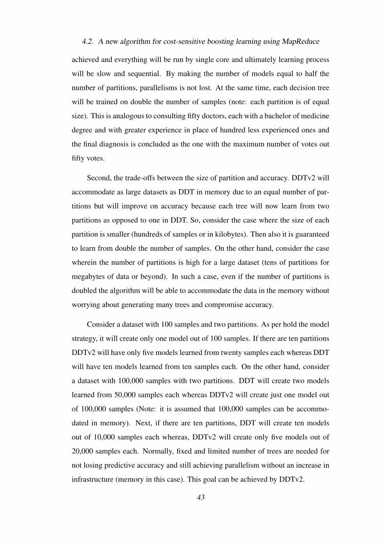
4.2. A new algorithm for cost-sensitive boosting learning using MapReduce
achieved and everything will be run by single core and ultimately learning process
will be slow and sequential. By making the number of models equal to half the
number of partitions, parallelisms is not lost. At the same time, each decision tree
will be trained on double the number of samples (note: each partition is of equal
size). This is analogous to consulting fifty doctors, each with a bachelor of medicine
degree and with greater experience in place of hundred less experienced ones and
the final diagnosis is concluded as the one with the maximum number of votes out
fifty votes.
Second, the trade-offs between the size of partition and accuracy. DDTv2 will
accommodate as large datasets as DDT in memory due to an equal number of par-
titions but will improve on accuracy because each tree will now learn from two
partitions as opposed to one in DDT. So, consider the case where the size of each
partition is smaller (hundreds of samples or in kilobytes). Then also it is guaranteed
to learn from double the number of samples. On the other hand, consider the case
wherein the number of partitions is high for a large dataset (tens of partitions for
megabytes of data or beyond). In such a case, even if the number of partitions is
doubled the algorithm will be able to accommodate the data in the memory without
worrying about generating many trees and compromise accuracy.
Consider a dataset with 100 samples and two partitions. As per hold the model
strategy, it will create only one model out of 100 samples. If there are ten partitions
DDTv2 will have only five models learned from twenty samples each whereas DDT
will have ten models learned from ten samples each. On the other hand, consider
a dataset with 100,000 samples with two partitions. DDT will create two models
learned from 50,000 samples each whereas DDTv2 will create just one model out
of 100,000 samples (Note: it is assumed that 100,000 samples can be accommo-
dated in memory). Next, if there are ten partitions, DDT will create ten models
out of 10,000 samples each whereas, DDTv2 will create only five models out of
20,000 samples each. Normally, fixed and limited number of trees are needed for
not losing predictive accuracy and still achieving parallelism without an increase in
infrastructure (memory in this case). This goal can be achieved by DDTv2.
43

4.2. A new algorithm for cost-sensitive boosting learning using MapReduce
Table 4.1: % Reduction of sot and nol in DDT, ST and DDTv2 with respect to BT and DT
DDT ST DDTv2BT DT BT DT BT DT
sot 82% 71% 67% 48% 64% 44%nol 81% 70% 65% 45% 61% 38%
Algorithm 8 CsDb
1: Given: S = {(x1,y1),(x2,y2) . . .(xm,ym)}; xi ∈ Z, yi ∈ {−1,+1}, P ∈ N+
2: Initialize: T = bP2 c
3: Initialize: W1(i)4: for t do=1 to T5: for u do = 1 to U6: s = USETRAININGSETS(S(t−1)∗(m/T )+1, St∗(m/T ))7: w = USEWEIGHTS(W(t−1)∗(m/T )+1, Wt∗(m/T ))8: tru = BUILDDECISIONTREE(s, w)9: ht = COMPUTEWEAKHYPOTHESIS(tru)
10: Compute rt and αt11: WT−t+1(i) = UPDATEWEIGHTS(Wt+1(i))12: end for13: end for14: collect vote from T models:
H ∗(x) = argmaxx ∑αtht(xi)
Again, DDT, ST and DDTv2 are empirically evaluated upon the same param-
eters and the same datasets to prove scalability over large datasets. However, one
more large clickstream dataset, namely IQM, was added for evaluation. Average
accuracy of DT, BT, DDT, ST and DDTv2 over all ten selected datasets are 92.79,
99.70, 83.76, 86.93, 97.16, respectively. It is important to note that the results of
DDTv2 are comparable with BT. Even with large dataset DDTv2 is proved to pro-
duce accurate results with an acceptable learning time. Distributed implementations
of decision tree (DDT, ST and DDTv2) outperformed DT and BT in terms of size
of tree and number of leaves with acceptable accuracy of classification.Table 4.1
shows percentage reduction obtained in size of tree and number of leaves in DDT,
ST and DDTv2 with respect to BT and DT.
44

4.3. Summary of the development of the CsDb algorithm
4.2.3 Cost-sensitive Distributed Boosting (CsDb)
The distributed nature of DDTv2 [31] and cost sensitivity of CSE1-5 [5] are derived
into CsDb. CsDb is designed as a meta classifier so that, it can use a weak learner
(for decision tree, ibk, etc) as a base classifier. A wrapper (meta) algorithm that
works in replacement for CSExtensions is depicted in algorithm 8.
CsDb first divides the training set S into P partitions and initializes T with half
the number of partitions. Each partition t follows the same process as defined in al-
gorithm 8 steps 6-11. It is important to note that the inner loop runs asynchronously.
It means all iterations of the outer loops are independent. Therefore, each of them
spawns a mapper. Moreover, each mapper runs U times as defined by the user.
During the map phase, it trains a weak learner (decision tree is used as a weak
learner) using weights W(t−1)∗(m/T )+1 to Wt∗(m/T ) and training set S(t−1)∗(m/T )+1 to
St∗(m/T ). This is analogous to equi frequency binning. Next, it computes weak hy-
pothesis ht : Z → R. Thereafter, by computing rt and αt it also updates weights
W(t−1)∗(m/T )+1(i) to Wt∗(m/T )(i) as per rules defined in CSEx. Finally, in the re-
ducer, it collects the vote from T models using equation 4.2
H ∗(x) = argmaxx ∑αtht(xi) (4.2)
4.3 Summary of the development of the CsDb algorithm
This chapter depicts the limitations of existing cost-sensitive classifiers which leads
to requirement for developing a new algorithm. The phase wise development pro-
cess of the CsDb is explained which includes details about DDT. Moreover, how
DDT falls short and how DDTv2 is designed to overcome the limitations of the
DDT is also presented in this chapter. The CsDb combines advantages of CSE1-5
and DDTv2 to build distributed cost-sensitive boosting algorithm is also explained.
45

Chapter 5
An empirical comparison of the CsDb algorithm
The CsDb algorithm derives the distributed nature of DDT and the cost-sensitivity
of CSE family of algorithms. It should be able to solve the class imbalance prob-
lem which is an inherent property of CSE algorithms. It should also be able to
reduce the model building time while being scalable. While it is essential to have
the feature of scalability for CsDb, it should not compromise cost-sensitivity over
small or medium datasets. To test all these capabilities this chapter evaluates CsDb
empirically.
5.1 Experimental setups
Weka is a collection of open source machine learning algorithms. DDTv2 was
implemented as an extension of Weka. The CsDb is implemented as an extension
of DDTv2 [31] and CSE1-5 [5]. To test the performance of CsDb, nine datasets,
namely, breast cancer Wisconsin (bcw), liver disorder (bupa), credit screening
(crx), echocardiogram (echo), house-voting 84 (hv-84), hypothyroid (hypo), king-
rook versus king-pawn (krkp), pima indian diabetes (pima), and sonar (sonar) from
UCI machine learning repository were selected. These datasets belong to various
domains (more details can be found in Appendix B). In addition, an algorithm is
evaluated using Yahoo! webscope dataset 1 and IQM bid log dataset. Here, IQM
bid log dataset is the proprietary dataset of IQM Co. It is not available in the public
domain. The skewness of the data which is explained in the next paragraph is the
reason for selecting these datasets. The datasets are preprocessed to meet the need
1http://labs.yahoo.com/Academic Relations
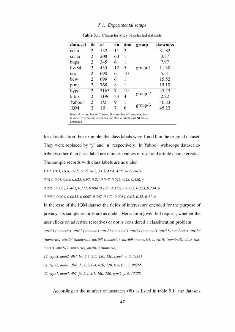
5.1. Experimental setups
Table 5.1: Characteristics of selected datasets
data-set #c #i #n #no group skewnessecho 2 132 11 2
group-1
31.82sonar 2 208 60 1 3.37bupa 2 345 6 1 7.97hv-84 2 435 12 5 11.38crx 2 690 6 10 5.51bcw 2 699 6 1 15.52pima 2 768 8 1 15.10hypo 2 3163 7 19
group-245.23
krkp 2 3196 33 4 2.22Yahoo! 2 1M 9 1
group-346.83
IQM 2 1B 7 6 45.22Note: #c = number of Classes, #i = number of Instances, #n =number of Numeric attributes and #no = number of NOminalattributes
for classification. For example, the class labels were 1 and 0 in the original dataset.
They were replaced by ‘y’ and ‘n’ respectively. In Yahoo! webscope dataset at-
tributes other than class label are numeric values of user and article characteristics.
The sample records with class labels are as under.
UF2, UF3, UF4, UF5, UF6, AF2, AF3, AF4, AF5, AF6, class
0.013, 0.01, 0.04, 0.023, 0.97, 0.21, 0.067, 0.045, 0.23, 0.456, y
0.096, 0.0032, 0.481, 0.112, 0.004, 0.127, 0.0002, 0.0325, 0.123, 0.234, n
0.0036, 0.004, 0.0035, 0.0067, 0.567, 0.342, 0.0034, 0.02, 0.52, 0.41, y
In the case of the IQM dataset the fields of interest are encoded for the purpose of
privacy. Its sample records are as under. Here, for a given bid request, whether the
user clicks on advertise (creative) or not is considered a classification problem.
attrib1 (numeric), attrb2 (nominal), attrib3 (nominal), attrib4 (nominal), attrib5 (numberic), attrib6
(numeric), attrib7 (numeric), attrib8 (numeric), attrib9 (numeric), attrib10 (nominal), class (nu-
meric), attrib12 (numeric), attrib13 (numeric)
12, type3, man2, db3, ba, 2.3, 2.5, 430, 120, type3, n, 0, 54321
31, type2, man1, db4, dc, 0.7, 0.4, 620, 120, type1, y, 1, 98765
42, type1, man3, db2, fe, 5.9, 3.7, 160, 720, type2, y, 0, 13578
According to the number of instances (#i) as listed in table 5.1. the datasets
47

5.1. Experimental setups
are grouped into three categories for the purpose of result analysis. The first group
contains echo, sonar, bupa, hv-84, crx, bcw, and pima datasets. They have a few
hundred instances (#i ∈ [100,999]). The second group contains hypo and krkp. The
second group can contain datasets with the number of instances [1000, 99999]. The
last group contains Yahoo! and IQM datasets with a million and a billion instances
respectively. The third group can contain datasets with more than 99,999 instances.
An instance in any group can have a size of [1, 10] kilobytes. That means, group-1
contains datasets with size [1, 10] megabytes and [10, 1000] and [1000, ∞] sizes are
covered by group-2 and group-3 respectively. The skewness in table 5.1 represents
the distribution of the number of instances of minority class over majority class.
Here, the skewness index can take any value between 0 and 50 where 0 means
no skewness and 50 means the highest possible skewness. Average skewness of
datasets in group-1, 2 and 3 is 12.95%, 23.72%, and 46.02% respectively. The
important characteristics of datasets are summarized in table 5.1.
The key measure to evaluate the performance of the algorithms for cost-
sensitive classification is the total cost of misclassification made by a classifier (That
is, ∑m = cost(actual(m), predicted(m))) [30]. In addition, the number of high cost
errors is also used. It is the number of misclassifications associated with max(false
positive, false negative) in cost matrix to that of in confusion matrix. The param-
eters misclassification cost and number of high cost errors are defined in section
2.4. The third measure is the model building time. It is the amount of time taken
to build a model. Other than these, accuracy, precision, recall, and F-measure, are
used to evaluate the performance of the algorithm. These measures are usual candi-
dates for model evaluation when it comes to cost-sensitive classification. To define
these measures TP (true positive), TN (true negative), FP (false positive) and FN
(false negative) terms are used. These terms are derived from the confusion matrix.
The structure of confusion matrix for binary class problem is shown in Table 5.2.
In Table 5.2 C1 and C2 are defined as class-1 and class-2 respectively. Now, the
accuracy is defined as accuracy = (T P+T N)(T P+T N+FP+FN) , and hence the accuracy can be
considered as a statistical measure of how well a binary classification test correctly
48

5.1. Experimental setups
Table 5.2: A confusion matrix structure for a binary classifier
Actual Class
C1 C2
Predicted ClassC1 TP FP
C2 FN TN
identifies a condition. Precision is defined as precision = T P(T P+FP) . Precision is
also referred to as positive predictive value (ppv) and hence it can be interpreted as
a ratio of all events the classifier predicted correctly to all the events the classifier
predicted, correctly or incorrectly. Recall, which is also known as sensitivity, is
defined as recall = T P(T P+FN) . Therefore, recall is the ratio of the number of events a
classifier can correctly recall to the number of all correct events. F-measure, which
is also known as F1-score, is the harmonic mean of precision and recall. Therefore,
F−measure = 2∗ precision∗recallprecision+recall .
The CsDb algorithm was tested on the selected eleven datasets. For each
dataset, six variations (i.e. [0 1; 2 0], [0 2; 1 0], [0 1; 5 0], [0 5; 1 0], [0 10; 1
0], and [0 1; 10 0]) of cost matrix (hyperparameter) were used. The cost matrix
is defined in section 2.4. An average result over all six cost matrices is reported.
The detailed results can be found in Appendix D. There are eleven algorithms in
comparison. Thus, in total 726 (11∗11∗6) runs were performed.
The CsDb is a meta-classifier and for this experimental setup, Weka’s imple-
mentation of decision tree with default parameter settings is used as a weak learner.
The experiments of the CsDb and DDTv2 were performed using Elastic
MapReduce (EMR) cluster of Amazon. The EMR for these experiments was con-
figured with one master (c4.4xlarge) and three slaves (c4.4xlarge) nodes. A single
instance of c4.4xlarge comes with 16 vCPUs and 30 GiB of memory. To run CSE
an r4.8xlarge instance of Amazon Elastic Compute Cloud (Amazon EC2) was used.
An r4 series instance r4.8xlarge features 32 vCPUs, 244 GiB of memory.
49

5.2. Empirical comparison results and discussion
43.64
22.36
62.34
42.97
23.33
61.4554.45
32.25
71.83
dataset groups
mis
clas
sific
atio
n co
st
0.00
20.00
40.00
60.00
80.00
group-1 group-2 group-3
csex csdbx ddtv2
group wise average mc for csex, csdbx and ddtv2
Figure 5.1: Group wise average mc for csex, csdbx and ddtv2
5.2 Empirical comparison results and discussion
The algorithm is analysed empirically in this section. Parameter wise, the compari-
son is broken down into sub-sections. As the misclassification cost and the number
of high cost errors are cost-based parameters they are discussed together in sec-
tion 5.2.1. Secondly, the accuracy, precision, recall, and F-measure are discussed
together as they are similar in nature (section 5.2.2). Lastly, in section 5.2.3 the
algorithms are compared for the time they take to build the model. For each param-
eter, the dataset group wise analysis was performed. The dataset groups are defined
in table 5.1 and discussed in section 5.1.
5.2.1 Misclassification cost and number of high cost errors
CsDb when compared with CSE over group 1, 2, and 3 datasets the misclassifica-
tion cost varies, on an average, by 2.44% (for group-1, 2 and 3 it is 1.54%, -4.35%
and 1.43% respectively) and the number of high cost errors by 14.30% (for group-1,
2 and 3 it is 5.52%, -31.59% and -5.79% respectively). CsDb produces 21.06% (for
group-1, 2 and 3 it is 21.08%, 27.65% and 14.45% respectively) fewer misclassifi-
cation errors and 30.15% (for group-1, 2 and 3 it is 31.39%, 27.11% and 31.94%
respectively) less number of high cost errors when compared with DDTv2.
50
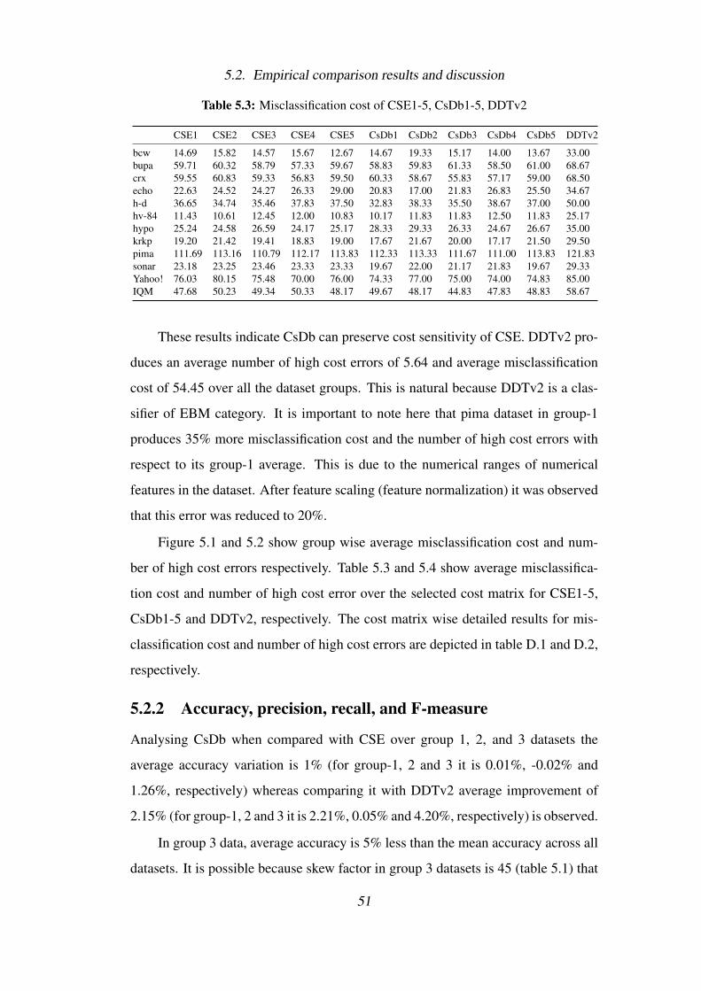
5.2. Empirical comparison results and discussion
Table 5.3: Misclassification cost of CSE1-5, CsDb1-5, DDTv2
CSE1 CSE2 CSE3 CSE4 CSE5 CsDb1 CsDb2 CsDb3 CsDb4 CsDb5 DDTv2
bcw 14.69 15.82 14.57 15.67 12.67 14.67 19.33 15.17 14.00 13.67 33.00bupa 59.71 60.32 58.79 57.33 59.67 58.83 59.83 61.33 58.50 61.00 68.67crx 59.55 60.83 59.33 56.83 59.50 60.33 58.67 55.83 57.17 59.00 68.50echo 22.63 24.52 24.27 26.33 29.00 20.83 17.00 21.83 26.83 25.50 34.67h-d 36.65 34.74 35.46 37.83 37.50 32.83 38.33 35.50 38.67 37.00 50.00hv-84 11.43 10.61 12.45 12.00 10.83 10.17 11.83 11.83 12.50 11.83 25.17hypo 25.24 24.58 26.59 24.17 25.17 28.33 29.33 26.33 24.67 26.67 35.00krkp 19.20 21.42 19.41 18.83 19.00 17.67 21.67 20.00 17.17 21.50 29.50pima 111.69 113.16 110.79 112.17 113.83 112.33 113.33 111.67 111.00 113.83 121.83sonar 23.18 23.25 23.46 23.33 23.33 19.67 22.00 21.17 21.83 19.67 29.33Yahoo! 76.03 80.15 75.48 70.00 76.00 74.33 77.00 75.00 74.00 74.83 85.00IQM 47.68 50.23 49.34 50.33 48.17 49.67 48.17 44.83 47.83 48.83 58.67
These results indicate CsDb can preserve cost sensitivity of CSE. DDTv2 pro-
duces an average number of high cost errors of 5.64 and average misclassification
cost of 54.45 over all the dataset groups. This is natural because DDTv2 is a clas-
sifier of EBM category. It is important to note here that pima dataset in group-1
produces 35% more misclassification cost and the number of high cost errors with
respect to its group-1 average. This is due to the numerical ranges of numerical
features in the dataset. After feature scaling (feature normalization) it was observed
that this error was reduced to 20%.
Figure 5.1 and 5.2 show group wise average misclassification cost and num-
ber of high cost errors respectively. Table 5.3 and 5.4 show average misclassifica-
tion cost and number of high cost error over the selected cost matrix for CSE1-5,
CsDb1-5 and DDTv2, respectively. The cost matrix wise detailed results for mis-
classification cost and number of high cost errors are depicted in table D.1 and D.2,
respectively.
5.2.2 Accuracy, precision, recall, and F-measure
Analysing CsDb when compared with CSE over group 1, 2, and 3 datasets the
average accuracy variation is 1% (for group-1, 2 and 3 it is 0.01%, -0.02% and
1.26%, respectively) whereas comparing it with DDTv2 average improvement of
2.15% (for group-1, 2 and 3 it is 2.21%, 0.05% and 4.20%, respectively) is observed.
In group 3 data, average accuracy is 5% less than the mean accuracy across all
datasets. It is possible because skew factor in group 3 datasets is 45 (table 5.1) that
51

5.2. Empirical comparison results and discussion
4.10
2.08
3.863.87
2.73
4.08
5.64
3.75
6.00
dataset groups
# H
CE
0.00
2.00
4.00
6.00
group-1 group-2 group-3
csex csdbx ddtv2
group wise average # hce for csex, csdbx and ddtv2
Figure 5.2: Group wise average number of hce for csex, csdbx and ddtv2
Table 5.4: Number of High cost errors of CSE1-5, CsDb1-5, DDTv2
CSE1 CSE2 CSE3 CSE4 CSE5 CsDb1 CsDb2 CsDb3 CsDb4 CsDb5 DDTv2
bcw 1.00 1.00 1.00 1.50 1.33 1.67 2.50 1.50 1.50 2.17 4.33bupa 5.74 5.47 5.61 4.17 6.00 4.17 4.50 3.67 3.50 3.33 4.50crx 7.04 5.31 5.30 5.50 5.50 5.50 4.33 5.83 5.83 5.00 7.00echo 2.31 2.51 2.13 3.50 3.17 2.33 2.33 1.67 2.67 2.17 3.83h-d 4.20 3.06 3.61 5.17 3.67 3.33 3.83 5.83 4.17 4.67 6.17hv-84 0.95 0.69 0.81 1.33 1.17 0.83 0.83 1.33 1.33 1.50 3.33hypo 2.50 2.52 2.57 2.67 1.67 4.17 2.83 3.33 2.67 4.50 4.50krkp 1.55 1.27 1.36 2.17 2.50 1.50 2.50 2.33 1.50 2.00 3.00pima 10.39 10.81 10.38 12.50 11.50 12.33 11.83 10.67 11.67 10.33 12.83sonar 1.93 1.10 1.60 1.83 1.33 1.00 1.00 0.83 1.83 2.00 3.67Yahoo! 2.76 1.63 1.61 3.17 2.17 2.50 2.50 2.83 1.50 3.33 5.67IQM 5.28 5.52 4.97 6.33 5.17 6.00 5.33 5.00 5.33 6.50 6.33average 3.80 3.41 3.41 4.15 3.76 3.78 3.69 3.74 3.63 3.96 5.43
Table 5.5: Accuracy of CSE1-5, CsDb1-5, DDTv2
CSE1 CSE2 CSE3 CSE4 CSE5 CsDb1 CsDb2 CsDb3 CsDb4 CsDb5 DDTv2
bcw 0.9855 0.9840 0.9862 0.9857 0.9921 0.9862 0.9886 0.9845 0.9866 0.9907 0.9826bupa 0.8891 0.9068 0.9005 0.8908 0.9029 0.8860 0.8754 0.8817 0.8875 0.8720 0.8556crx 0.9552 0.9454 0.9471 0.9454 0.9517 0.9474 0.9415 0.9536 0.9384 0.9451 0.9440echo 0.7950 0.7928 0.8018 0.7928 0.7635 0.8176 0.8716 0.8379 0.7928 0.7590 0.7095hv-84 0.9812 0.9851 0.9816 0.9851 0.9843 0.9828 0.9789 0.9843 0.9828 0.9854 0.9724hypo 0.9952 0.9954 0.9953 0.9953 0.9946 0.9953 0.9948 0.9950 0.9952 0.9961 0.9948krkp 0.9961 0.9948 0.9958 0.9961 0.9966 0.9963 0.9955 0.9965 0.9964 0.9962 0.9957pima 0.9171 0.9191 0.9128 0.9254 0.9197 0.9087 0.9128 0.9047 0.9262 0.9043 0.9141sonar 0.9303 0.9103 0.9207 0.9343 0.9199 0.9231 0.9102 0.9223 0.9327 0.9351 0.9271Yahoo! 0.8540 0.8948 0.8321 0.8640 0.9103 0.8543 0.8162 0.8694 0.8541 0.9204 0.8649IQM 0.8389 0.8697 0.8608 0.9323 0.8748 0.8675 0.8785 0.8409 0.8582 0.8783 0.8610
52
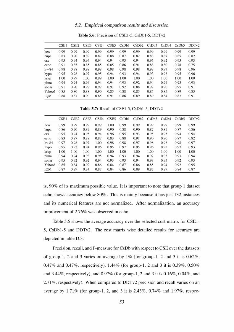
5.2. Empirical comparison results and discussion
Table 5.6: Precision of CSE1-5, CsDb1-5, DDTv2
CSE1 CSE2 CSE3 CSE4 CSE5 CsDb1 CsDb2 CsDb3 CsDb4 CsDb5 DDTv2
bcw 0.99 0.99 0.99 0.99 0.99 0.99 0.99 0.99 0.99 0.99 0.99bupa 0.83 0.90 0.89 0.87 0.88 0.87 0.82 0.88 0.87 0.85 0.82crx 0.95 0.94 0.94 0.94 0.94 0.93 0.94 0.95 0.92 0.95 0.93echo 0.91 0.85 0.85 0.85 0.85 0.86 0.91 0.88 0.80 0.78 0.75hv-84 0.98 0.98 0.98 0.98 0.98 0.98 0.98 0.98 0.97 0.98 0.96hypo 0.95 0.98 0.97 0.95 0.94 0.93 0.94 0.93 0.98 0.95 0.96krkp 1.00 0.99 1.00 0.99 1.00 1.00 1.00 1.00 1.00 1.00 1.00pima 0.94 0.94 0.94 0.94 0.94 0.93 0.92 0.94 0.94 0.93 0.93sonar 0.91 0.90 0.92 0.92 0.91 0.92 0.88 0.92 0.90 0.95 0.91Yahoo! 0.85 0.80 0.88 0.90 0.85 0.88 0.85 0.85 0.85 0.89 0.85IQM 0.88 0.87 0.90 0.85 0.91 0.86 0.89 0.89 0.84 0.87 0.91
Table 5.7: Recall of CSE1-5, CsDb1-5, DDTv2
CSE1 CSE2 CSE3 CSE4 CSE5 CsDb1 CsDb2 CsDb3 CsDb4 CsDb5 DDTv2
bcw 0.99 0.99 0.99 0.99 1.00 0.99 0.99 0.99 0.99 0.99 0.99bupa 0.86 0.90 0.89 0.89 0.90 0.88 0.90 0.87 0.89 0.87 0.86crx 0.95 0.94 0.95 0.94 0.96 0.95 0.93 0.95 0.95 0.94 0.94echo 0.83 0.87 0.88 0.87 0.83 0.88 0.91 0.90 0.90 0.87 0.82hv-84 0.97 0.98 0.97 1.00 0.98 0.98 0.97 0.98 0.98 0.98 0.97hypo 0.95 0.93 0.94 0.96 0.95 0.97 0.95 0.96 0.93 0.97 0.93krkp 1.00 1.00 1.00 1.00 1.00 1.00 1.00 1.00 1.00 1.00 1.00pima 0.94 0.94 0.93 0.95 0.94 0.93 0.94 0.92 0.95 0.93 0.94sonar 0.95 0.92 0.92 0.94 0.93 0.93 0.94 0.93 0.95 0.92 0.93Yahoo! 0.85 0.84 0.92 0.86 0.84 0.87 0.86 0.85 0.94 0.92 0.95IQM 0.87 0.89 0.84 0.87 0.84 0.86 0.89 0.87 0.89 0.84 0.87
is, 90% of its maximum possible value. It is important to note that group 1 dataset
echo shows accuracy below 80% . This is mainly because it has just 132 instances
and its numerical features are not normalized. After normalization, an accuracy
improvement of 2.76% was observed in echo.
Table 5.5 shows the average accuracy over the selected cost matrix for CSE1-
5, CsDb1-5 and DDTv2. The cost matrix wise detailed results for accuracy are
depicted in table D.3.
Precision, recall, and F-measure for CsDb with respect to CSE over the datasets
of group 1, 2 and 3 varies on average by 1% (for group-1, 2 and 3 it is 0.62%,
0.47% and 0.47%, respectively), 1.44% (for group-1, 2 and 3 it is 0.39%, 0.50%
and 3.44%, respectively), and 0.97% (for group-1, 2 and 3 it is 0.16%, 0.04%, and
2.71%, respectively). When compared to DDTv2 precision and recall varies on an
average by 1.71% (for group-1, 2, and 3 it is 2.43%, 0.74% and 1.97%, respec-
53

5.2. Empirical comparison results and discussion
Table 5.8: F-measure of CSE1-5, CsDb1-5, DDTv2
CSE1 CSE2 CSE3 CSE4 CSE5 CsDb1 CsDb2 CsDb3 CsDb4 CsDb5 DDTv2
bcw 0.99 0.99 0.99 0.99 0.99 0.99 0.99 0.99 0.99 0.99 0.99bupa 0.84 0.89 0.88 0.87 0.88 0.86 0.84 0.86 0.86 0.84 0.82crx 0.95 0.94 0.94 0.94 0.95 0.94 0.93 0.95 0.93 0.94 0.94echo 0.86 0.85 0.84 0.85 0.83 0.86 0.91 0.88 0.83 0.80 0.76hv-84 0.98 0.98 0.98 0.98 0.98 0.98 0.97 0.98 0.98 0.98 0.96hypo 0.95 0.95 0.95 0.95 0.94 0.95 0.94 0.95 0.95 0.96 0.95krkp 1.00 1.00 1.00 1.00 1.00 1.00 1.00 1.00 1.00 1.00 1.00pima 0.94 0.93 0.93 0.94 0.94 0.93 0.93 0.93 0.94 0.93 0.93sonar 0.92 0.90 0.92 0.93 0.91 0.92 0.90 0.92 0.92 0.93 0.92Yahoo! 0.81 0.90 0.92 0.84 0.84 0.85 0.86 0.87 0.90 0.90 0.85IQM 0.87 0.84 0.87 0.83 0.88 0.85 0.85 0.86 0.91 0.89 0.87
tively), 1.89% (for group-1, 2 and 3 it is 1.53%, 1.14% and 3.01%, respectively),
and 2.77% (for group 1, 2 and 3 it is 2.19%, 0.21% and 5.92%, respectively).
This is because CsDb is CBM and boosting technique and hence it can main-
tain bias variance trade-off and hence able to balance precision and recall. Hence,
F-measure is also balanced within 1.5%. Moreover, DDTv2 is EBM based and
hence fails to balance between precision and recall. Hence, F-measure is also in-
creased by 8.73%.
Table 5.6, 5.7 and 5.8 show average precision, recall and F-measure over the
selected cost matrix for CSE1-5, CsDb1-5 and DDTv2, respectively. The cost ma-
trix wise detailed results for precision, recall and F-measure are depicted in table
D.4, D.5 and D.6, respectively.
5.2.3 Model building time
Model building time over group 3 datasets for CSE takes 13.75 hours, on average,
and it is reduced to 1.3 hours for CsDb. This reduction of 90.14% is especially
useful because, as noted in section 5.2.1 and 5.2.2, CsDb preserves cost sensitivity
and other efficiency measures. However, over group 1 and group 2 datasets, the
difference between model building time of CSE and CsDb is 2% on average.
Table 5.9 shows average model building times over the selected cost matrix
for CSE1-5, CsDb1-5 and DDTv2. The cost matrix wise detailed results for model
building time are depicted in table D.7.
54

5.3. Summary of the findings of the evaluation
Table 5.9: Model Building Time of CSE1-5, CsDb1-5, DDTv2
CSE1 CSE2 CSE3 CSE4 CSE5 CsDb1 CsDb2 CsDb3 CsDb4 CsDb5 DDTv2
bcw 31.63 32.83 39.00 31.50 32.00 31.67 22.33 31.67 32.00 35.17 32.50bupa 9.39 10.00 6.67 8.33 8.50 9.83 8.50 6.67 8.83 9.33 8.67crx 27.17 25.00 26.50 38.33 29.17 27.00 32.33 28.00 28.67 30.83 26.17echo 7.70 6.33 6.83 6.33 8.00 7.00 6.67 6.67 8.33 5.83 6.33h-d 1.98 2.33 1.83 1.67 2.00 1.83 1.33 2.17 1.83 2.17 1.50hv-84 8.73 6.83 7.50 8.33 8.50 5.50 7.83 7.00 7.00 9.00 7.33hypo 118.74 124.67 125.67 160.17 114.00 142.00 153.17 105.17 132.83 145.33 122.67krkp 11.32 13.50 12.83 12.17 8.50 12.00 14.00 14.67 13.17 13.83 12.50pima 5.48 3.50 5.00 3.17 5.17 4.33 3.83 5.50 5.00 4.00 5.17sonar 4.82 6.50 7.17 6.83 5.33 5.83 4.83 6.17 6.67 5.50 7.33Yahoo! 5990.01 8342.67 6708.17 7527.00 7340.67 484.83 859.33 629.33 623.33 665.17 686.17
Moreover, table D.8 shows the detailed confusion matrix generated for all
datasets, cost matrix and algorithms during the experiments.
5.3 Summary of the findings of the evaluation
An empirical evaluation of the proposed algorithm CsDb was carried out. This
chapter shows the experimental setup in section 5.1 by demonstrating the character-
istics of the dataset used and the test setup used. The empirical results and follow
up discussion are divided into three different verticals with respect to relevance of
the parameters used for evaluation. Moreover, the datasets used are divided into
three groups for ease of analysis. However, the detailed results of each experiment
carried out is listed in Appendix D. Further, the details about the datasets and their
references are listed in Appendix B and charts of the tables presented in this chapter
are available in Appendix C for comparative analysis.
55

Chapter 6
Conclusions and Future Research
The overall research focus was to develop a fast, distributed, cost-sensitive, and scal-
able classification algorithm for big data, especially for datasets which are skewed
in nature. The CsDb algorithm is developed to address the big data challenge: Vol-
ume. The algorithm has four major features; distributed, cost-sensitive, scalable
and fast. The algorithm development was in three stages. First, the distributed ver-
sion of the decision tree algorithm is proposed. Then, an extension to enhance the
performance of the Distributed Decision Trees (DDT), DDTv2 is introduced, which
works on the notion of ‘hold the model’. Finally, cost-sensitive distributed boost-
ing (CsDb) is introduced. The results show that the DDT and DDTv2 are able to
preserve the accuracy of classical BT and DT even after reduction in size of tree
and number of leaves. This is helpful when production systems require faster clas-
sification where the size of the tree plays a vital role. CsDb is able to preserve the
accuracy along with cost-sensitivity from its predecessor CSE1-5. Moreover, using
CsDb, the model building time is reduced.
The algorithms (DDT, DDTv2 and CsDb) are realised for various domains.
The datasets from AdTech, medical and social domain are used for empirical eval-
uation. A novel approach of grouping the datasets according to their characteristics
is designed to compare the performance of the algorithm.
6.1 Conclusions
The central goal of this research work was to study and improve CBM for the vol-
ume of data which cannot be handled by stand-alone commodity hardware. The
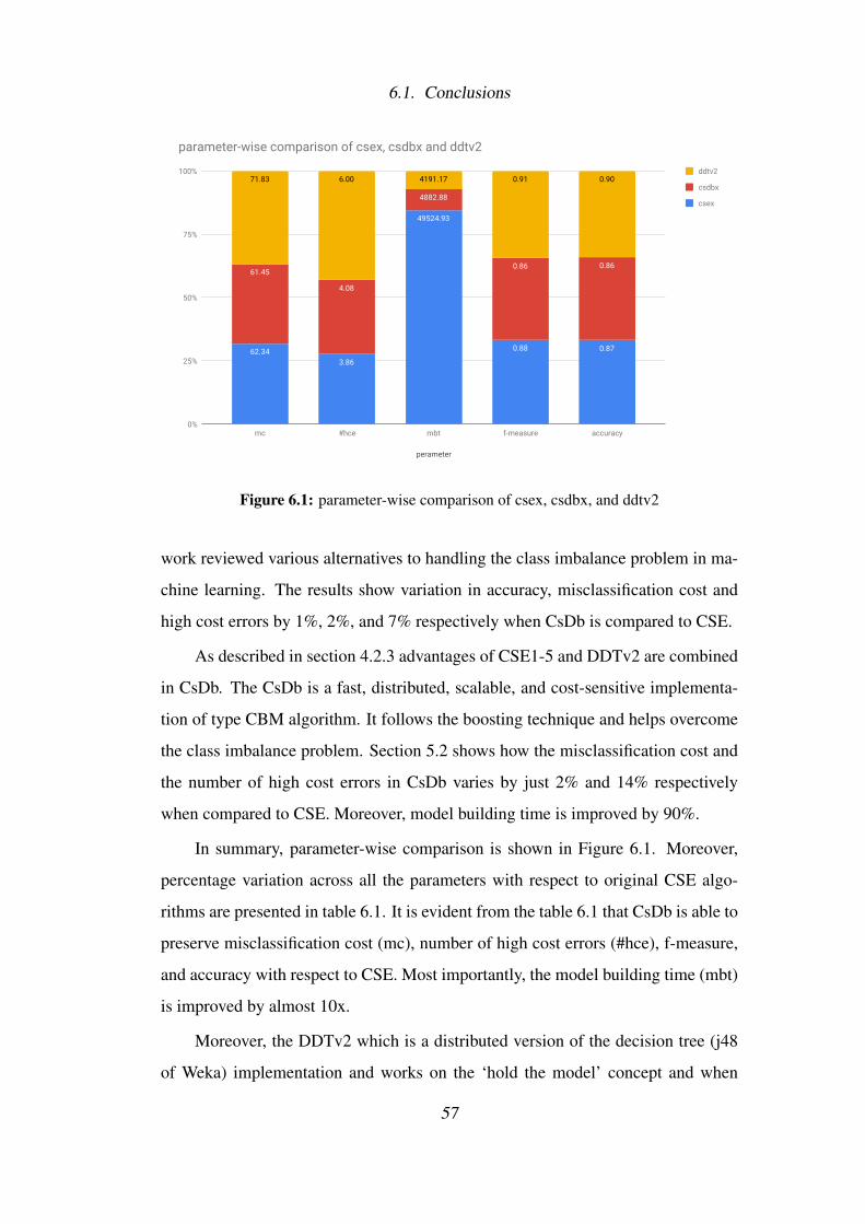
6.1. Conclusions
62.343.86
49524.93
0.88 0.87
61.45
4.08
4882.88
0.86 0.86
71.83 6.00 4191.17 0.91 0.90
perameter
0%
25%
50%
75%
100%
mc #hce mbt f-measure accuracy
ddtv2
csdbx
csex
parameter-wise comparison of csex, csdbx and ddtv2
Figure 6.1: parameter-wise comparison of csex, csdbx, and ddtv2
work reviewed various alternatives to handling the class imbalance problem in ma-
chine learning. The results show variation in accuracy, misclassification cost and
high cost errors by 1%, 2%, and 7% respectively when CsDb is compared to CSE.
As described in section 4.2.3 advantages of CSE1-5 and DDTv2 are combined
in CsDb. The CsDb is a fast, distributed, scalable, and cost-sensitive implementa-
tion of type CBM algorithm. It follows the boosting technique and helps overcome
the class imbalance problem. Section 5.2 shows how the misclassification cost and
the number of high cost errors in CsDb varies by just 2% and 14% respectively
when compared to CSE. Moreover, model building time is improved by 90%.
In summary, parameter-wise comparison is shown in Figure 6.1. Moreover,
percentage variation across all the parameters with respect to original CSE algo-
rithms are presented in table 6.1. It is evident from the table 6.1 that CsDb is able to
preserve misclassification cost (mc), number of high cost errors (#hce), f-measure,
and accuracy with respect to CSE. Most importantly, the model building time (mbt)
is improved by almost 10x.
Moreover, the DDTv2 which is a distributed version of the decision tree (j48
of Weka) implementation and works on the ‘hold the model’ concept and when
57

6.2. Future Research
Table 6.1: percentage variation in different parameters with respect to CSE
CsDb DDTv2
mc 1.43% -15.23%#hce -5.79% -55.45%mbt 90.14% 91.54%
f-measure 2.71% -3.05%accuracy 1.26% -2.89%
compared with BT and DT (section 4.2.2), outperforms them in terms of accuracy,
size of tree, and number of leaves. Using DDTv2, the size of the tree is reduced
by 64% and 44% compared with BT and DT, respectively. Whereas, the number
of leaves is reduced by 61% and 38%, respectively. All this is achieved without
compromising on classification accuracy. Moreover, the DDTv2 is able to reduce
model building time by 15% as it builds the tree in a distributed way. DDTv2 works
to solve two major problems, namely, model experience and trade-off between size
of partition and performance (in terms of accuracy) associated with DDT (refer to
section 4.2.1).
This dissertation brings three major research contributions. The fast, dis-
tributed, and scalable extensions to the decision tree algorithm namely DDT and
DDTv2. Moreover, CsDb, which is a fast, distributed, scalable, and cost-sensitive
implementation of the type CBM algorithm.
6.2 Future Research
In this section, the following four verticals have been identified in which this re-
search can be extended.
The performance of CsDb is dependent upon the choice of weak learner. One
can use different weak learners (For example, k-nn, Decision Stump, etc.) to com-
pare the results with respect to decision tree. Coming up with a strategic way of
choosing a weak learner to improve performance of CsDb is an important future
extension.
Recently, there has been significant amount of research work in automated
hyperparameters tuning of a classification algorithm. CsDb has sensitive hyperpa-
58

6.2. Future Research
rameters such as cost matrix. Automatic tuning of the hyperparameters of CsDb
using neural networks is an important research extension.
As shown in Figure 1.3 there exist multiple methods for handling skewed dis-
tribution of the class. An empirical comparison between CsDb and other approaches
for handling skewed distribution of class can provide concrete conclusions on a ver-
tical of scalability of the methods.
There exist application domains such as computer vision, bio-genetics, etc.
where the use of machine learning algorithms is becoming popular. The common
characteristics of the datasets from these domains are high-dimensionality, high-
volume, and high-skewness. The existing algorithms of cost-sensitive domain do
not perform well on such data. To propose an algorithm that can learn from such
datasets while preserving the cost-sensitivity of the application can be an important
research extension.
59
6.2. Future Research
Publications by Author
1. Ankit Desai and Sanjay Chaudhary, “Distributed decision tree v.2.0,” 2017
IEEE International Conference on Big Data (Big Data), Boston, MA, 2017,
pp. 929-934. doi: 10.1109/BigData.2017.8258011
2. Ankit Desai and Sanjay Chaudhary. 2016. Distributed Decision Tree. In Pro-
ceedings of the 9th Annual ACM India Conference (COMPUTE ’16). ACM,
New York, NY, USA, 43-50. DOI: https://doi.org/10.1145/2998476.2998478
3. Ankit Desai, Kaushik Jadav, and Sanjay Chaudhary. 2015. An Empirical
evaluation of CostBoost Extensions for Cost-sensitive Classification. In Pro-
ceedings of the 8th Annual ACM India Conference (Compute ’15). ACM,
New York, NY, USA, 73-77. DOI: https://doi.org/10.1145/2835043.2835048
4. Ankit Desai and Sanjay Chaudhary. Distributed AdaBoost Extensions for
Cost-sensitive Classification Problems. International Journal of Computer
Applications 177(12):1-8, October 2019. https://doi.org/10.5120/ijca2019919531
5. Ankit Desai and Sanjay Chaudhary. Application of distributed back propaga-
tion neural network for dynamic real-time bidding [work in progress]
60

Bibliography
[1] Susan Lomax and Sunil Vadera. A survey of cost-sensitive decision tree in-
duction algorithms. ACM Computing Surveys (CSUR), 45(2):16, 2013.
[2] Yoav Freund and Robert E Schapire. A decision-theoretic generalization of
on-line learning and an application to boosting. Journal of computer and sys-
tem sciences, 55(1):119–139, 1997.
[3] Kai Ming Ting and Zijian Zheng. Boosting cost-sensitive trees. In Interna-
tional Conference on Discovery Science, pages 244–255. Springer, 1998.
[4] Charles Elkan. The foundations of cost-sensitive learning. In Interna-
tional joint conference on artificial intelligence, volume 17, pages 973–978.
Lawrence Erlbaum Associates Ltd, 2001.
[5] Ankit Desai and PM Jadav. An empirical evaluation of ad boost extensions for
cost-sensitive classification. International Journal of Computer Applications,
44(13):34–41, 2012.
[6] Kai Ming Ting. A comparative study of cost-sensitive boosting algorithms.
In In Proceedings of the 17th International Conference on Machine Learning.
Citeseer, 2000.
[7] J. R. Quinlan. Decision trees and decision-making. IEEE Transactions on
Systems, Man, and Cybernetics, 20(2):339–346, March 1990.
[8] J Ross Quinlan. Improved use of continuous attributes in c4. 5. Journal of
artificial intelligence research, 4:77–90, 1996.
Bibliography
[9] J. Ross Quinlan. Induction of decision trees. Machine learning, 1(1):81–106,
1986.
[10] Mark Hall, Eibe Frank, Geoffrey Holmes, Bernhard Pfahringer, Peter Reute-
mann, and Ian H. Witten. The weka data mining software: An update.
SIGKDD Explor. Newsl., 11(1):10–18, November 2009.
[11] New Zealand Department of Computer Science at the University of
Waikato. Data Mining with Weka, More classifiers, Ensemble
learning. https://www.cs.waikato.ac.nz/ml/weka/mooc/
dataminingwithweka/, 2015. [Online; accessed 19-July-2018].
[12] Jeffrey Dean and Sanjay Ghemawat. Mapreduce: Simplified data processing
on large clusters. Commun. ACM, 51(1):107–113, January 2008.
[13] Sanjay Ghemawat, Howard Gobioff, and Shun-Tak Leung. The google file
system. In Proceedings of the Nineteenth ACM Symposium on Operating Sys-
tems Principles, SOSP ’03, pages 29–43, New York, NY, USA, 2003. ACM.
[14] Michael Pazzani, Christopher Merz, Patrick Murphy, Kamal Ali, Timothy
Hume, and Clifford Brunk. Reducing misclassification costs. In Machine
Learning Proceedings 1994, pages 217–225. Elsevier, 1994.
[15] Kai Ming Ting and Zijian Zheng. Machine Learning: ECML-98: 10th Eu-
ropean Conference on Machine Learning Chemnitz, Germany, April 21–23,
1998 Proceedings, chapter Boosting trees for cost-sensitive classifications,
pages 190–195. Springer Berlin Heidelberg, Berlin, Heidelberg, 1998.
[16] Wei Fan, Salvatore J Stolfo, Junxin Zhang, and Philip K Chan. Adacost:
misclassification cost-sensitive boosting. In Icml, volume 99, pages 97–105,
1999.
[17] Paul Viola and Michael Jones. Fast and robust classification using asymmetric
adaboost and a detector cascade. In Advances in Neural Information Process-
ing System 14, pages 1311–1318. MIT Press, 2001.
62
Bibliography
[18] Paul Viola and Michael J. Jones. Robust real-time face detection. International
Journal of Computer Vision, 57(2):137–154, 2004.
[19] Stefano Merler, Cesare Furlanello, Barbara Larcher, and Andrea Sboner. Au-
tomatic model selection in cost-sensitive boosting. Information Fusion, 4(1):3
– 10, 2003.
[20] Naoki Abe, Bianca Zadrozny, and John Langford. An iterative method for
multi-class cost-sensitive learning. In Proceedings of the Tenth ACM SIGKDD
International Conference on Knowledge Discovery and Data Mining, KDD
’04, pages 3–11, New York, NY, USA, 2004. ACM.
[21] Aurelie C. Lozano and Naoki Abe. Multi-class cost-sensitive boosting with p-
norm loss functions. In Proceedings of the 14th ACM SIGKDD International
Conference on Knowledge Discovery and Data Mining, KDD ’08, pages 506–
514, New York, NY, USA, 2008. ACM.
[22] David Mease, Abraham J. Wyner, and Andreas Buja. Boosted classification
trees and class probability/quantile estimation. J. Mach. Learn. Res., 8:409–
439, May 2007.
[23] Yanmin Sun, Mohamed S. Kamel, Andrew K.C. Wong, and Yang Wang. Cost-
sensitive boosting for classification of imbalanced data. Pattern Recognition,
40(12):3358 – 3378, 2007.
[24] H. Masnadi-Shirazi and N. Vasconcelos. Cost-sensitive boosting. IEEE Trans-
actions on Pattern Analysis and Machine Intelligence, 33(2):294–309, Feb
2011.
[25] Jerome Friedman, Trevor Hastie, Robert Tibshirani, et al. Additive logistic
regression: a statistical view of boosting (with discussion and a rejoinder by
the authors). The annals of statistics, 28(2):337–407, 2000.
63

Bibliography
[26] Iago Landesa-Vazquez and Jose Luis Alba-Castro. Revisiting adaboost
for cost-sensitive classification. part I: theoretical perspective. CoRR,
abs/1507.04125, 2015.
[27] Nikolaos Nikolaou and Gavin Browwn. Multiple Classifier Systems: 12th
International Workshop, MCS 2015, Gunzburg, Germany, June 29 - July 1,
2015, Proceedings, chapter Calibrating AdaBoost for Asymmetric Learning,
pages 112–124. Springer International Publishing, Cham, 2015.
[28] Iago Landesa-Vazquez and Jose Luis Alba-Castro. Shedding light on the
asymmetric learning capability of adaboost. Pattern Recognition Letters,
33(3):247 – 255, 2012.
[29] Iago Landesa-Vazquez and Jose Luis Alba-Castro. Double-base asymmetric
adaboost. Neurocomputing, 118:101 – 114, 2013.
[30] Ankit Desai, Kaushik Jadav, and Sanjay Chaudhary. An empirical evaluation
of costboost extensions for cost-sensitive classification. In Proceedings of the
8th Annual ACM India Conference, Compute ’15, pages 73–77, New York,
NY, USA, 2015. ACM.
[31] A. Desai and S. Chaudhary. Distributed decision tree v.2.0. In 2017 IEEE
International Conference on Big Data (Big Data), pages 929–934, Dec 2017.
[32] Jiawei Han, Micheline Kamber, and Jian Pei. 1 - introduction. In Jiawei
Han, Micheline Kamber, and Jian Pei, editors, Data Mining (Third Edition),
The Morgan Kaufmann Series in Data Management Systems, pages 1 – 38.
Morgan Kaufmann, Boston, third edition edition, 2012.
[33] Ian H. Witten, Eibe Frank, and Mark A. Hall. Data Mining: Practical Ma-
chine Learning Tools and Techniques. Morgan Kaufmann Publishers Inc., San
Francisco, CA, USA, 3rd edition, 2011.
[34] Anand Rajaraman and Jeffrey David Ullman. Mining of Massive Datasets.
Cambridge University Press, New York, NY, USA, 2011.
64

Bibliography
[35] J. Cooper and L. Reyzin. Improved algorithms for distributed boosting. In
2017 55th Annual Allerton Conference on Communication, Control, and Com-
puting (Allerton), pages 806–813, Oct 2017.
[36] Aleksandar Lazarevic and Zoran Obradovic. Boosting algorithms for parallel
and distributed learning. Distributed and Parallel Databases, 11(2):203–229,
Mar 2002.
[37] Munther Abualkibash, Ahmed ElSayed, and Ausif Mahmood. Highly scal-
able, parallel and distributed adaboost algorithm using light weight threads
and web services on a network of multi-core machines. CoRR, abs/1306.1467,
2013.
[38] I. Palit and C. K. Reddy. Scalable and parallel boosting with mapreduce.
IEEE Transactions on Knowledge and Data Engineering, 24(10):1904–1916,
Oct 2012.
[39] Jerry Ye, Jyh-Herng Chow, Jiang Chen, and Zhaohui Zheng. Stochastic gra-
dient boosted distributed decision trees. In Proceedings of the 18th ACM
Conference on Information and Knowledge Management, CIKM ’09, pages
2061–2064, New York, NY, USA, 2009. ACM.
[40] K. W. Bowyer, L. O. Hall, T. Moore, N. Chawla, and W. P. Kegelmeyer. A par-
allel decision tree builder for mining very large visualization datasets. In Smc
2000 conference proceedings. 2000 ieee international conference on systems,
man and cybernetics. ‘cybernetics evolving to systems, humans, organizations,
and their complex interactions’ (cat. no.0, volume 3, pages 1888–1893 vol.3,
Oct 2000.
[41] John C. Shafer, Rakesh Agrawal, and Manish Mehta. Sprint: A scalable par-
allel classifier for data mining. In Proceedings of the 22th International Con-
ference on Very Large Data Bases, VLDB ’96, pages 544–555, San Francisco,
CA, USA, 1996. Morgan Kaufmann Publishers Inc.
65

Bibliography
[42] Ankit Desai and Sanjay Chaudhary. Distributed decision tree. In Proceedings
of the 9th Annual ACM India Conference, COMPUTE ’16, pages 43–50, New
York, NY, USA, 2016. ACM.
66

Appendix A
List of Abbreviations
• #HCE: Number of High Cost Errors
• Amazon: EC2 Amazon Elastic Compute Cloud
• API: Application Programming Interface
• BT: Boosted Trees
• CBE: Cost Boost Extension
• CBM: Cost Based Model
• CM: Cost Matrix
• CS: Cost-sensitive
• CSB: Cost-sensitive Boosting
• CsDb: Cost-sensitive Distributed Boosting
• CSE: Cost-sensitive Extension
• DDM: Distributed Data Mining
• DDT: Distributed Decision Tree
• DDTv2: Distributed Decision Treev2
• DFS: Distributed File System

• DT: Decision Tree
• EBM: Error Based Model
• EMR: Elastic MapReduce
• FN: False Negative
• FP: False Positive
• HDFS: Hadoop Distributed File System
• k-nn: K Nearest Neighbour
• MC: Misclassification Cost
• nol: Number of Leaves
• SMOT: Synthetic Minority Over- sampling Technique
• sot: Size of Tree
• ST: Spark Trees
• TN: True Negative
• TP: True Positive
• YARN: Yet Another Resource Negotiator
68

Appendix B
Details of the datasets used in the evaluation
• Breast Cancer Wisconsin (diagnostic) data Set (bcw) The dataset is of the
life sciences domain. Attribute information is as follows.
1. Sample code number: id number
2. Clump Thickness: 1 - 10
3. Uniformity of Cell Size: 1 - 10
4. Uniformity of Cell Shape: 1 - 10
5. Marginal Adhesion: 1 - 10
6. Single Epithelial Cell Size: 1 - 10
7. Bare Nuclei: 1 - 10
8. Bland Chromatin: 1 - 10
9. Normal Nucleoli: 1 - 10
10. Mitoses: 1 - 10
11. Class: (2 for benign, 4 for malignant)
Samples arrive periodically as Dr. Wolberg reports his clinical cases. The
database, therefore, reflects this chronological grouping of the data. This
grouping information appears immediately below, having been removed from
the data itself:
Group 1: 367 instances (January 1989)
Group 2: 70 instances (October 1989)

Group 3: 31 instances (February 1990)
Group 4: 17 instances (April 1990)
Group 5: 48 instances (August 1990)
Group 6: 49 instances (Updated January 1991)
Group 7: 31 instances (June 1991)
Group 8: 86 instances (November 1991)
Total: 699 points (as of the donated database on 15 July 1992)
Note that the results summarized above in Past Usage refer to a dataset of size
369, while Group 1 has only 367 instances. This is because it originally con-
tained 369 instances; 2 were removed. The following statements summarize
changes to the original Group 1’s set of data:
Group 1 : 367 points: 200B 167M (January 1989)
Revised Jan 10, 1991: Replaced zero bare nuclei in 1080185 & 1187805
Revised Nov 22,1991: Removed 765878,4,5,9,7,10,10,10,3,8,1 no record Re-
moved 484201,2,7,8,8,4,3,10,3,4,1 zero epithelial Changed 0 to 1 in field
6 of sample 1219406 Changed 0 to 1 in field 8 of the following samples:
1182404,2,3,1,1,1,2,0,1,1,1
source: http://archive.ics.uci.edu/ml/datasets/Breast+Cancer+Wisconsin+(Original)
• Liver Disorders data Set (bupa) The data set is of the life sciences domain.
Attribute information is as follows.
1. mcv mean corpuscular volume
2. alkphos alkaline phosphotase
3. sgpt alanine aminotransferase
4. sgot aspartate aminotransferase
5. gammagt gamma-glutamyl transpeptidase
6. drinks number of half-pint equivalents of alcoholic beverages drunk per
day
70

7. selector field created by the BUPA researchers to split the data into
train/test sets
The first five variables are all from blood tests which are thought to be sen-
sitive to liver disorders that might arise from excessive alcohol consumption.
Each line in the dataset constitutes the record of a single male individual.
Important note: The 7th field (selector) has been widely misinterpreted in the
past as a dependent variable representing presence or absence of a liver disor-
der. This is incorrect [1]. The 7th field was created by BUPA researchers as a
train/test selector. It is not suitable as a dependent variable for classification.
The dataset does not contain any variable representing presence or absence
of liver disorder. Researchers who wish to use this dataset as a classifica-
tion benchmark should follow the method used in experiments by the donor
(Forsyth & Rada, 1986, Machine learning: applications in expert systems
and information retrieval) and others (e.g., Turney, 1995, Cost-sensitive clas-
sification: Empirical evaluation of a hybrid genetic decision tree induction
algorithm), who used the 6th field (drinks), after dichotomising, as a depen-
dent variable for classification. Because of widespread misinterpretation in
the past, researchers should take care to state their method clearly.
source: http://archive.ics.uci.edu/ml/datasets/liver+disorders
• Credit Approval data set (crx) The data set is of the financial domain. At-
tribute information is as follows.
1. A1: b, a.
2. A2: continuous.
3. A3: continuous.
4. A4: u, y, l, t.
5. A5: g, p, gg.
6. A6: c, d, cc, i, j, k, m, r, q, w, x, e, aa, ff.
7. A7: v, h, bb, j, n, z, dd, ff, o.
71

8. A8: continuous.
9. A9: t, f.
10. A10: t, f.
11. A11: continuous.
12. A12: t, f.
13. A13: g, p, s.
14. A14: continuous.
15. A15: continuous.
16. A16: +,- (class attribute)
This file concerns credit card applications. All attribute names and values
have been changed to meaningless symbols to protect the confidentiality of
the data.
This dataset is interesting because there is a good mix of attributes – continu-
ous, nominal with small numbers of values, and nominal with larger numbers
of values. There are also a few missing values.
source: http://archive.ics.uci.edu/ml/datasets/credit+approval
• Echocardiogram data set (echo) The dataset is of the life sciences domain.
Attribute information is as follows.
1. survival – the number of months patient survived (has survived, if pa-
tient is still alive). Because all the patients had heart attacks at different
times, it is possible that some patients have survived less than one year
but they are still alive. Check the second variable to confirm this. Such
patients cannot be used for the prediction task mentioned above.
2. still-alive – a binary variable. 0=dead at the end of survival period, 1
means still alive
3. age-at-heart-attack – age in years when heart attack occurred
72

4. pericardial-effusion – binary. Pericardial effusion is fluid around the
heart. 0=no fluid, 1=fluid
5. fractional-shortening – a measure of contractility around the heart, lower
numbers are increasingly abnormal
6. epss – E-point septal separation, another measure of contractility. Larger
numbers are increasingly abnormal.
7. lvdd – left ventricular end-diastolic dimension. This is a measure of the
size of the heart at end-diastole. Large hearts tend to be sick hearts.
8. wall-motion-score – a measure of how the segments of the left ventricle
are moving
9. wall-motion-index – equals wall-motion-score divided by number of
segments seen. Usually 12 to 13 segments are seen in an echocardio-
gram. Use this variable INSTEAD of the wall motion score.
10. mult – a derivate var which can be ignored
11. name – the name of the patient (I have replaced them with “name”)
12. group – meaningless, ignore it
13. alive-at-1 – Boolean-valued. Derived from the first two attributes. 0
means patient was either dead after one year or had been followed up
for less than one year. 1 means patient was alive at one year.
All the patients suffered heart attacks at some point in the past. Some are
still alive and some are not. The survival and still-alive variables, when taken
together, indicate whether a patient survived for at least one year following
the heart attack.
The problem addressed by past researchers was to predict from the other vari-
ables whether or not the patient will survive at least one year. The most dif-
ficult part of this problem is predicting correctly that the patient will NOT
survive. (Part of the difficulty seems to be the size of the data set.)
source: https://archive.ics.uci.edu/ml/datasets/echocardiogram
73

• Congressional Voting Records data set (hv84) The data set is of the social
sciences domain. Attribute information is as follows.
1. Class Name: 2 (democrat, republican)
2. handicapped-infants: 2 (y,n)
3. water-project-cost-sharing: 2 (y,n)
4. adoption-of-the-budget-resolution: 2 (y,n)
5. physician-fee-freeze: 2 (y,n)
6. el-salvador-aid: 2 (y,n)
7. religious-groups-in-schools: 2 (y,n)
8. anti-satellite-test-ban: 2 (y,n)
9. aid-to-nicaraguan-contras: 2 (y,n)
10. mx-missile: 2 (y,n)
11. immigration: 2 (y,n)
12. synfuels-corporation-cutback: 2 (y,n)
13. education-spending: 2 (y,n)
14. superfund-right-to-sue: 2 (y,n)
15. crime: 2 (y,n)
16. duty-free-exports: 2 (y,n)
17. export-administration-act-south-africa: 2 (y,n)
This data set includes votes for each of the US House of Representatives Con-
gressmen on the 16 key votes identified by the CQA. The CQA lists nine dif-
ferent types of votes: voted for, paired, and announced for (these three simpli-
fied to yea), voted against, paired against, and announced against (these three
simplified to nay), voted present, voted present to avoid conflict of interest,
and did not vote or otherwise make a position known (these three simplified
to an unknown disposition).
source: http://archive.ics.uci.edu/ml/datasets/congressional+voting+records
74
• Hypothyroid data set(hypo) The data set is of the life domain. Attribute
information is as follows.
1. age: numeric
2. sex: (M,F)
3. on thyroxine: (f,t)
4. query on thyroxine: (f,t)
5. on antithyroid medication: (f,t)
6. thyroid surgery: (f,t)
7. query hypothyroid: (f,t)
8. query hyperthyroid: (f,t)
9. pregnant: (f,t)
10. sick: (f,t)
11. tumor: (f,t)
12. lithium: (f,t)
13. goitre: (f,t)
14. TSH measured: (y,n)
15. TSH: numeric
16. T3 measured: (y,n)
17. T3: numeric
18. TT4 measured: (y,n)
19. TT4: numeric
20. T4U measured: (y,n)
21. T4U: numeric
22. FTI measured: (y,n)
23. FTI: numeric
75
24. TBG measured: (n,y)
25. TBG: numeric
26. hypothyroid: (hypothyroid,negative)
source: https://www.kaggle.com/kumar012/hypothyroid
• Chess (King-Rook vs. King-Pawn) data set (krkp) The data set is from the
domain of games. Number of Instances: 3196 total Number of Attributes:
36 Attribute Summaries: Classes (2): – White-can-win (“won”) and White-
cannot-win (“nowin”). I believe that White is deemed to be unable to win
if the Black pawn can safely advance. Class Distribution: In 1669 of the
positions (52%), White can win. In 1527 of the positions (48%), White cannot
win.
The format for instances in this database is a sequence of 37 attribute values.
Each instance is a board-descriptions for this chess endgame. The first 36
attributes describe the board. The last (37th) attribute is the classification:
“win” or “nowin”. There are no missing values. A typical board-description
is
f,f,f,f,f,f,f,f,f,f,f,f,l,f,n,f,f,t,f,f,f,f,f,f,f,t,f,f,f,f,f,f,f,t,t,n,won
The names of the features do not appear in the board-descriptions. Instead,
each feature corresponds to a particular position in the feature-value list. For
example, the head of this list is the value for the feature “bkblk”. The fol-
lowing is a list of features, in the order in which their values appear in the
feature-value list:
[bkblk,bknwy,bkon8,bkona,bkspr,bkxbq,bkxcr,bkxwp,blxwp,bxqsq,cntxt,dsopp,dwipd,
hdchk,katri,mulch,qxmsq,r2ar8,reskd,reskr,rimmx,rkxwp,rxmsq,simpl,skach,skewr,
skrxp,spcop,stlmt,thrsk,wkcti,wkna8,wknck,wkovl,wkpos,wtoeg]
In the file, there is one instance (board position) per line.
source: https://archive.ics.uci.edu/ml/datasets/Chess+(King-Rook+vs.+King-
Pawn)
76
• Pima Indians Diabetes data set (pima) The data set is from the life sciences
domain. This dataset is originally from the National Institute of Diabetes and
Digestive and Kidney Diseases. The objective of the dataset is to diagnosti-
cally predict whether or not a patient has diabetes, based on certain diagnostic
measurements included in the dataset. Several constraints were placed on the
selection of these instances from a larger database. In particular, all patients
here are females at least 21 years old of Pima Indian heritage. Attribute in-
formation is as follows.
1. Pregnancies: Number of times pregnant
2. Glucose: Plasma glucose concentration a 2 hours in an oral glucose
tolerance test
3. Blood: PressureDiastolic blood pressure (mm Hg)
4. Skin: ThicknessTriceps skin fold thickness (mm)
5. Insulin: 2-Hour serum insulin (mu U/ml)
6. BMI: Body mass index (weight in kg/(height in m)2)
7. Diabetes: PedigreeFunctionDiabetes pedigree function
8. Age: Age (years)
9. Outcome: Class variable (0 or 1) 268 of 768 are 1, the others are 0
source: https://www.kaggle.com/uciml/pima-indians-diabetes-database
• Connectionist Bench (Sonar, Mines vs. Rocks) data set (sonar) The data
set is from the physical sciences domain. The task is to train a model to
discriminate between sonar signals bounced off a metal cylinder and those
bounced off a roughly cylindrical rock.
The file “sonar.mines” contains 111 patterns obtained by bouncing sonar sig-
nals off a metal cylinder at various angles and under various conditions. The
file “sonar.rocks” contains 97 patterns obtained from rocks under similar con-
ditions. The transmitted sonar signal is a frequency-modulated chirp, rising
77

in frequency. The dataset contains signals obtained from a variety of different
aspect angles, spanning 90 degrees for the cylinder and 180 degrees for the
rock.
Each pattern is a set of 60 numbers in the range 0.0 to 1.0. Each number
represents the energy within a particular frequency band, integrated over a
certain period of time. The integration aperture for higher frequencies occur
later in time, since these frequencies are transmitted later during the chirp.
The label associated with each record contains the letter “R” if the object is a
rock and “M” if it is a mine (metal cylinder). The numbers in the labels are
in increasing order of aspect angle, but they do not encode the angle directly.
Sample record is as follows.
0.02, 0.0371, 0.0428, 0.0207, 0.0954, 0.0986, 0.1539, 0.1601, 0.3109,
0.2111, 0.1609, 0.1582, 0.2238, 0.0645, 0.066, 0.2273, 0.31, 0.2999, 0.5078,
0.4797, 0.5783, 0.5071, 0.4328, 0.555, 0.6711, 0.6415, 0.7104, 0.808,
0.6791, 0.3857, 0.1307, 0.2604, 0.5121, 0.7547, 0.8537, 0.8507, 0.6692,
0.6097, 0.4943, 0.2744, 0.051, 0.2834, 0.2825, 0.4256, 0.2641, 0.1386,
0.1051, 0.1343, 0.0383, 0.0324, 0.0232, 0.0027, 0.0065, 0.0159, 0.0072,
0.0167, 0.018, 0.0084, 0.009, 0.0032, R
source: http://archive.ics.uci.edu/ml/datasets/connectionist+bench+
(sonar,+mines+vs.+rocks)
• Yahoo!
As described in section 5.1.
• IQM
As described in section 5.1.
78

Appendix C
Detailed results of the evaluation (graphs)

data
sets
misclassification cost
0.00
25.0
0
50.0
0
75.0
0
100.
00
125.
00
bcw
bupa
crx
echo
hv-8
4hy
pokr
kppi
ma
sona
rYa
hoo!
IQM
CSE1
CSE2
CSE3
CSE4
CSE5
CsDb
1Cs
Db2
CsDb
3Cs
Db4
CsDb
5DD
Tv2
Mis
clas
sific
atio
n Co
st
Figu
reC
.1:M
iscl
assi
ficat
ion
Cos
t(M
C)
80
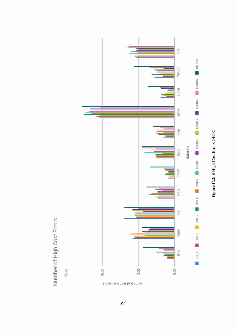
data
sets
number of high cost errors
0.00
5.00
10.0
0
15.0
0
bcw
bupa
crx
echo
hv-8
4hy
pokr
kppi
ma
sona
rYa
hoo!
IQM
CSE1
CSE2
CSE3
CSE4
CSE5
CsDb
1Cs
Db2
CsDb
3Cs
Db4
CsDb
5DD
Tv2
Num
ber o
f Hig
h Co
st E
rror
s
Figu
reC
.2:#
Hig
hC
ostE
rror
s(H
CE
)
81

datase
ts
accuracy
0.00
0.25
0.50
0.75
1.00
bcw
bupa
crx
echo
hv-84
hypo
krkp
pima
sona
rYa
hoo!
IQM
CSE1
CSE2
CSE3
CSE4
CSE5
CsDb
1Cs
Db2
CsDb
3Cs
Db4
CsDb
5DD
Tv2
Accu
racy
Figu
reC
.3:A
ccur
acy
82
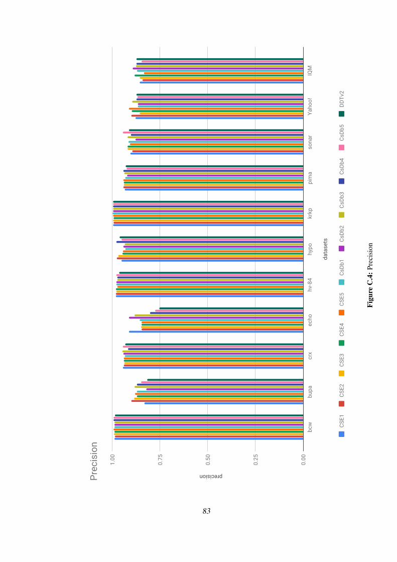
datase
ts
precision
0.00
0.25
0.50
0.75
1.00
bcw
bupa
crx
echo
hv-84
hypo
krkp
pima
sona
rYa
hoo!
IQM
CSE1
CSE2
CSE3
CSE4
CSE5
CsDb
1Cs
Db2
CsDb
3Cs
Db4
CsDb
5DD
Tv2
Prec
ision
Figu
reC
.4:P
reci
sion
83

datase
ts
recall
0.00
0.25
0.50
0.75
1.00
bcw
bupa
crx
echo
hv-84
hypo
krkp
pima
sona
rYa
hoo!
IQM
CSE1
CSE2
CSE3
CSE4
CSE5
CsDb
1Cs
Db2
CsDb
3Cs
Db4
CsDb
5DD
Tv2
Reca
ll
Figu
reC
.5:R
ecal
l
84

datase
ts
F-measure
0.00
0.25
0.50
0.75
1.00
bcw
bupa
crx
echo
hv-84
hypo
krkp
pima
sona
rYa
hoo!
IQM
CSE1
CSE2
CSE3
CSE4
CSE5
CsDb
1Cs
Db2
CsDb
3Cs
Db4
CsDb
5DD
Tv2
F-Mea
sure
Figu
reC
.6:F
-Mea
sure
85
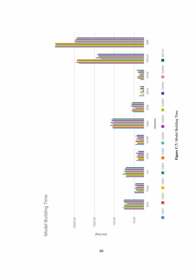
data
sets
time (log)
10.0
0
100.
00
1000
.00
1000
0.00
bcw
bupa
crx
echo
hv-8
4hy
pokr
kppi
ma
sona
rYa
hoo!
IQM
CSE1
CSE2
CSE3
CSE4
CSE5
CsDb
1Cs
Db2
CsDb
3Cs
Db4
CsDb
5DD
Tv2
Mod
el B
uild
ing
Tim
e
Figu
reC
.7:M
odel
Bui
ldin
gTi
me
86
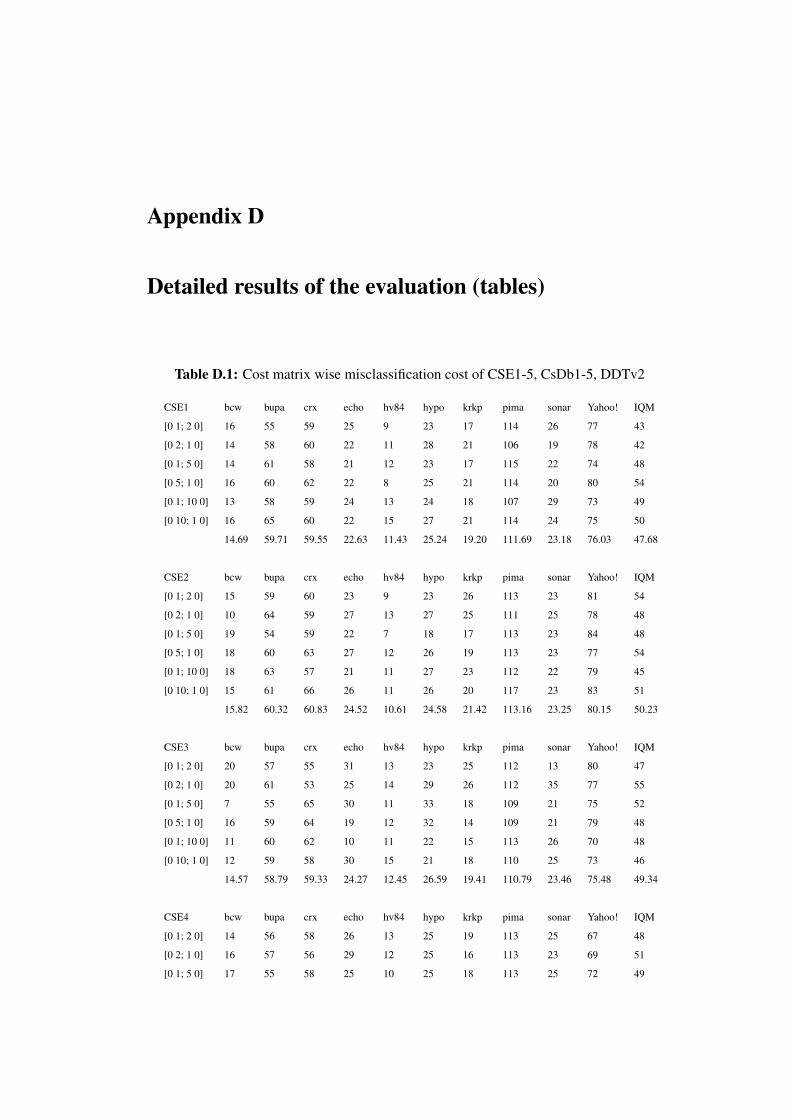
Appendix D
Detailed results of the evaluation (tables)
Table D.1: Cost matrix wise misclassification cost of CSE1-5, CsDb1-5, DDTv2
CSE1 bcw bupa crx echo hv84 hypo krkp pima sonar Yahoo! IQM
[0 1; 2 0] 16 55 59 25 9 23 17 114 26 77 43
[0 2; 1 0] 14 58 60 22 11 28 21 106 19 78 42
[0 1; 5 0] 14 61 58 21 12 23 17 115 22 74 48
[0 5; 1 0] 16 60 62 22 8 25 21 114 20 80 54
[0 1; 10 0] 13 58 59 24 13 24 18 107 29 73 49
[0 10; 1 0] 16 65 60 22 15 27 21 114 24 75 50
14.69 59.71 59.55 22.63 11.43 25.24 19.20 111.69 23.18 76.03 47.68
CSE2 bcw bupa crx echo hv84 hypo krkp pima sonar Yahoo! IQM
[0 1; 2 0] 15 59 60 23 9 23 26 113 23 81 54
[0 2; 1 0] 10 64 59 27 13 27 25 111 25 78 48
[0 1; 5 0] 19 54 59 22 7 18 17 113 23 84 48
[0 5; 1 0] 18 60 63 27 12 26 19 113 23 77 54
[0 1; 10 0] 18 63 57 21 11 27 23 112 22 79 45
[0 10; 1 0] 15 61 66 26 11 26 20 117 23 83 51
15.82 60.32 60.83 24.52 10.61 24.58 21.42 113.16 23.25 80.15 50.23
CSE3 bcw bupa crx echo hv84 hypo krkp pima sonar Yahoo! IQM
[0 1; 2 0] 20 57 55 31 13 23 25 112 13 80 47
[0 2; 1 0] 20 61 53 25 14 29 26 112 35 77 55
[0 1; 5 0] 7 55 65 30 11 33 18 109 21 75 52
[0 5; 1 0] 16 59 64 19 12 32 14 109 21 79 48
[0 1; 10 0] 11 60 62 10 11 22 15 113 26 70 48
[0 10; 1 0] 12 59 58 30 15 21 18 110 25 73 46
14.57 58.79 59.33 24.27 12.45 26.59 19.41 110.79 23.46 75.48 49.34
CSE4 bcw bupa crx echo hv84 hypo krkp pima sonar Yahoo! IQM
[0 1; 2 0] 14 56 58 26 13 25 19 113 25 67 48
[0 2; 1 0] 16 57 56 29 12 25 16 113 23 69 51
[0 1; 5 0] 17 55 58 25 10 25 18 113 25 72 49
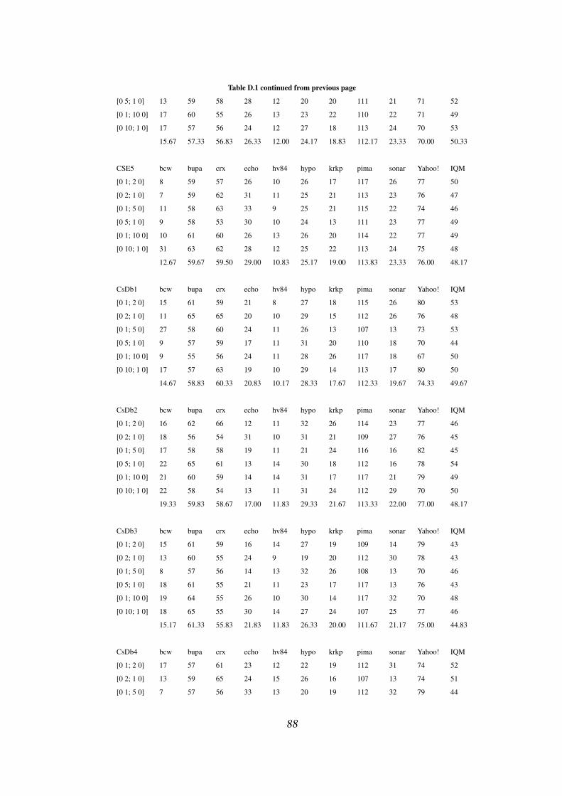
Table D.1 continued from previous page
[0 5; 1 0] 13 59 58 28 12 20 20 111 21 71 52
[0 1; 10 0] 17 60 55 26 13 23 22 110 22 71 49
[0 10; 1 0] 17 57 56 24 12 27 18 113 24 70 53
15.67 57.33 56.83 26.33 12.00 24.17 18.83 112.17 23.33 70.00 50.33
CSE5 bcw bupa crx echo hv84 hypo krkp pima sonar Yahoo! IQM
[0 1; 2 0] 8 59 57 26 10 26 17 117 26 77 50
[0 2; 1 0] 7 59 62 31 11 25 21 113 23 76 47
[0 1; 5 0] 11 58 63 33 9 25 21 115 22 74 46
[0 5; 1 0] 9 58 53 30 10 24 13 111 23 77 49
[0 1; 10 0] 10 61 60 26 13 26 20 114 22 77 49
[0 10; 1 0] 31 63 62 28 12 25 22 113 24 75 48
12.67 59.67 59.50 29.00 10.83 25.17 19.00 113.83 23.33 76.00 48.17
CsDb1 bcw bupa crx echo hv84 hypo krkp pima sonar Yahoo! IQM
[0 1; 2 0] 15 61 59 21 8 27 18 115 26 80 53
[0 2; 1 0] 11 65 65 20 10 29 15 112 26 76 48
[0 1; 5 0] 27 58 60 24 11 26 13 107 13 73 53
[0 5; 1 0] 9 57 59 17 11 31 20 110 18 70 44
[0 1; 10 0] 9 55 56 24 11 28 26 117 18 67 50
[0 10; 1 0] 17 57 63 19 10 29 14 113 17 80 50
14.67 58.83 60.33 20.83 10.17 28.33 17.67 112.33 19.67 74.33 49.67
CsDb2 bcw bupa crx echo hv84 hypo krkp pima sonar Yahoo! IQM
[0 1; 2 0] 16 62 66 12 11 32 26 114 23 77 46
[0 2; 1 0] 18 56 54 31 10 31 21 109 27 76 45
[0 1; 5 0] 17 58 58 19 11 21 24 116 16 82 45
[0 5; 1 0] 22 65 61 13 14 30 18 112 16 78 54
[0 1; 10 0] 21 60 59 14 14 31 17 117 21 79 49
[0 10; 1 0] 22 58 54 13 11 31 24 112 29 70 50
19.33 59.83 58.67 17.00 11.83 29.33 21.67 113.33 22.00 77.00 48.17
CsDb3 bcw bupa crx echo hv84 hypo krkp pima sonar Yahoo! IQM
[0 1; 2 0] 15 61 59 16 14 27 19 109 14 79 43
[0 2; 1 0] 13 60 55 24 9 19 20 112 30 78 43
[0 1; 5 0] 8 57 56 14 13 32 26 108 13 70 46
[0 5; 1 0] 18 61 55 21 11 23 17 117 13 76 43
[0 1; 10 0] 19 64 55 26 10 30 14 117 32 70 48
[0 10; 1 0] 18 65 55 30 14 27 24 107 25 77 46
15.17 61.33 55.83 21.83 11.83 26.33 20.00 111.67 21.17 75.00 44.83
CsDb4 bcw bupa crx echo hv84 hypo krkp pima sonar Yahoo! IQM
[0 1; 2 0] 17 57 61 23 12 22 19 112 31 74 52
[0 2; 1 0] 13 59 65 24 15 26 16 107 13 74 51
[0 1; 5 0] 7 57 56 33 13 20 19 112 32 79 44
88

Table D.1 continued from previous page
[0 5; 1 0] 8 60 53 27 13 27 14 115 16 78 46
[0 1; 10 0] 21 61 53 30 11 24 18 112 23 67 51
[0 10; 1 0] 18 57 55 24 11 29 17 108 16 72 43
14.00 58.50 57.17 26.83 12.50 24.67 17.17 111.00 21.83 74.00 47.83
CsDb5 bcw bupa crx echo hv84 hypo krkp pima sonar Yahoo! IQM
[0 1; 2 0] 15 59 65 32 11 31 25 114 16 79 45
[0 2; 1 0] 8 63 56 18 11 30 22 117 14 79 53
[0 1; 5 0] 12 64 63 30 13 30 17 112 22 81 48
[0 5; 1 0] 15 63 54 23 11 26 17 114 18 70 48
[0 1; 10 0] 11 58 55 24 14 22 26 110 23 71 46
[0 10; 1 0] 21 59 61 26 11 21 22 116 25 69 53
13.67 61.00 59.00 25.50 11.83 26.67 21.50 113.83 19.67 74.83 48.83
DDTv2 bcw bupa crx echo hv84 hypo krkp pima sonar Yahoo! IQM
[0 1; 2 0] 23 72 65 42 25 30 30 123 24 86 57
[0 2; 1 0] 27 67 66 28 22 34 31 127 26 77 55
[0 1; 5 0] 25 67 74 43 24 42 23 117 30 80 55
[0 5; 1 0] 28 67 74 47 27 37 24 127 25 86 65
[0 1; 10 0] 52 65 68 27 26 34 28 119 39 93 56
[0 10; 1 0] 43 74 64 21 27 33 41 118 32 88 64
33.00 68.67 68.50 34.67 25.17 35.00 29.50 121.83 29.33 85.00 58.67
Table D.2: Cost matrix wise number of high cost errors of CSE1-5, CsDb1-5, DDTv2
CSE1 bcw bupa crx echo hv84 hypo krkp pima sonar Yahoo! IQM
[0 1; 2 0] 1 4 8 4 1 2 1 10 2 2 8
[0 2; 1 0] 1 5 8 3 1 4 1 13 3 4 7
[0 1; 5 0] 1 8 8 4 1 2 2 11 1 3 5
[0 5; 1 0] 1 6 7 1 1 2 3 8 2 2 5
[0 1; 10 0] 1 5 5 2 2 2 1 10 2 4 3
[0 10; 1 0] 1 5 6 0 0 2 1 11 2 2 4
1.00 5.74 7.04 2.31 0.95 2.50 1.55 10.39 1.93 2.76 5.28
CSE2 bcw bupa crx echo hv84 hypo krkp pima sonar Yahoo! IQM
[0 1; 2 0] 1 5 6 4 1 7 2 11 1 2 6
[0 2; 1 0] 1 6 6 3 1 0 2 9 1 2 7
[0 1; 5 0] 1 7 4 2 0 3 1 12 2 1 6
[0 5; 1 0] 1 5 5 3 1 1 1 10 2 2 7
[0 1; 10 0] 1 6 5 1 1 2 0 11 0 2 4
[0 10; 1 0] 1 5 5 2 1 2 2 11 1 1 3
1.00 5.47 5.31 2.51 0.69 2.52 1.27 10.81 1.10 1.63 5.52
CSE3 bcw bupa crx echo hv84 hypo krkp pima sonar Yahoo! IQM
[0 1; 2 0] 1 6 6 1 1 2 1 14 2 2 4
89

Table D.2 continued from previous page
[0 2; 1 0] 1 9 4 1 1 0 1 10 1 1 4
[0 1; 5 0] 1 4 6 4 1 6 2 10 2 1 7
[0 5; 1 0] 1 6 8 3 1 2 2 11 2 2 8
[0 1; 10 0] 1 6 4 1 1 2 1 10 1 1 4
[0 10; 1 0] 1 4 4 2 1 2 1 7 1 2 4
1.00 5.61 5.30 2.13 0.81 2.57 1.36 10.38 1.60 1.61 4.97
CSE4 bcw bupa crx echo hv84 hypo krkp pima sonar Yahoo! IQM
[0 1; 2 0] 3 4 6 5 3 2 2 11 1 3 7
[0 2; 1 0] 1 5 8 3 3 4 4 16 1 4 9
[0 1; 5 0] 1 1 5 5 0 4 2 13 2 3 4
[0 5; 1 0] 2 6 5 4 0 4 4 13 3 5 9
[0 1; 10 0] 1 6 4 2 1 1 0 11 2 1 4
[0 10; 1 0] 1 3 5 2 1 1 1 11 2 3 5
1.50 4.17 5.50 3.50 1.33 2.67 2.17 12.50 1.83 3.17 6.33
CSE5 bcw bupa crx echo hv84 hypo krkp pima sonar Yahoo! IQM
[0 1; 2 0] 2 6 3 4 2 3 5 12 1 0 5
[0 2; 1 0] 1 7 7 5 1 1 4 11 3 2 5
[0 1; 5 0] 0 6 6 4 1 1 1 14 0 2 8
[0 5; 1 0] 1 7 6 2 2 1 2 11 0 3 5
[0 1; 10 0] 1 5 5 2 0 2 2 11 2 3 4
[0 10; 1 0] 3 5 6 2 1 2 1 10 2 3 4
1.33 6.00 5.50 3.17 1.17 1.67 2.50 11.50 1.33 2.17 5.17
CsDb1 bcw bupa crx echo hv84 hypo krkp pima sonar Yahoo! IQM
[0 1; 2 0] 4 3 6 4 1 6 5 16 1 4 6
[0 2; 1 0] 0 3 5 5 0 7 0 15 3 4 8
[0 1; 5 0] 0 4 6 1 2 2 1 14 0 1 8
[0 5; 1 0] 5 8 7 1 2 6 0 11 0 2 4
[0 1; 10 0] 0 5 3 2 0 2 2 7 1 4 5
[0 10; 1 0] 1 2 6 1 0 2 1 11 1 0 5
1.67 4.17 5.50 2.33 0.83 4.17 1.50 12.33 1.00 2.50 6.00
CsDb2 bcw bupa crx echo hv84 hypo krkp pima sonar Yahoo! IQM
[0 1; 2 0] 0 6 6 2 3 1 2 16 0 1 8
[0 2; 1 0] 4 8 5 5 0 6 5 16 3 2 4
[0 1; 5 0] 3 2 4 3 0 2 4 7 0 3 6
[0 5; 1 0] 4 4 3 2 1 2 3 14 2 5 5
[0 1; 10 0] 2 2 5 1 0 3 1 9 0 2 4
[0 10; 1 0] 2 5 3 1 1 3 0 9 1 2 5
2.50 4.50 4.33 2.33 0.83 2.83 2.50 11.83 1.00 2.50 5.33
CsDb3 bcw bupa crx echo hv84 hypo krkp pima sonar Yahoo! IQM
90
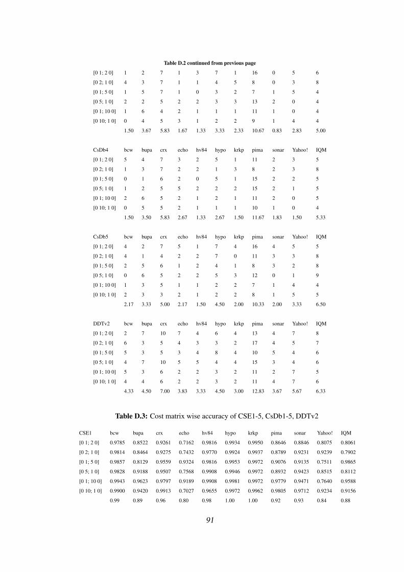
Table D.2 continued from previous page
[0 1; 2 0] 1 2 7 1 3 7 1 16 0 5 6
[0 2; 1 0] 4 3 7 1 1 4 5 8 0 3 8
[0 1; 5 0] 1 5 7 1 0 3 2 7 1 5 4
[0 5; 1 0] 2 2 5 2 2 3 3 13 2 0 4
[0 1; 10 0] 1 6 4 2 1 1 1 11 1 0 4
[0 10; 1 0] 0 4 5 3 1 2 2 9 1 4 4
1.50 3.67 5.83 1.67 1.33 3.33 2.33 10.67 0.83 2.83 5.00
CsDb4 bcw bupa crx echo hv84 hypo krkp pima sonar Yahoo! IQM
[0 1; 2 0] 5 4 7 3 2 5 1 11 2 3 5
[0 2; 1 0] 1 3 7 2 2 1 3 8 2 3 8
[0 1; 5 0] 0 1 6 2 0 5 1 15 2 2 5
[0 5; 1 0] 1 2 5 5 2 2 2 15 2 1 5
[0 1; 10 0] 2 6 5 2 1 2 1 11 2 0 5
[0 10; 1 0] 0 5 5 2 1 1 1 10 1 0 4
1.50 3.50 5.83 2.67 1.33 2.67 1.50 11.67 1.83 1.50 5.33
CsDb5 bcw bupa crx echo hv84 hypo krkp pima sonar Yahoo! IQM
[0 1; 2 0] 4 2 7 5 1 7 4 16 4 5 5
[0 2; 1 0] 4 1 4 2 2 7 0 11 3 3 8
[0 1; 5 0] 2 5 6 1 2 4 1 8 3 2 8
[0 5; 1 0] 0 6 5 2 2 5 3 12 0 1 9
[0 1; 10 0] 1 3 5 1 1 2 2 7 1 4 4
[0 10; 1 0] 2 3 3 2 1 2 2 8 1 5 5
2.17 3.33 5.00 2.17 1.50 4.50 2.00 10.33 2.00 3.33 6.50
DDTv2 bcw bupa crx echo hv84 hypo krkp pima sonar Yahoo! IQM
[0 1; 2 0] 2 7 10 7 4 6 4 13 4 7 8
[0 2; 1 0] 6 3 5 4 3 3 2 17 4 5 7
[0 1; 5 0] 5 3 5 3 4 8 4 10 5 4 6
[0 5; 1 0] 4 7 10 5 5 4 4 15 3 4 6
[0 1; 10 0] 5 3 6 2 2 3 2 11 2 7 5
[0 10; 1 0] 4 4 6 2 2 3 2 11 4 7 6
4.33 4.50 7.00 3.83 3.33 4.50 3.00 12.83 3.67 5.67 6.33
Table D.3: Cost matrix wise accuracy of CSE1-5, CsDb1-5, DDTv2
CSE1 bcw bupa crx echo hv84 hypo krkp pima sonar Yahoo! IQM
[0 1; 2 0] 0.9785 0.8522 0.9261 0.7162 0.9816 0.9934 0.9950 0.8646 0.8846 0.8075 0.8061
[0 2; 1 0] 0.9814 0.8464 0.9275 0.7432 0.9770 0.9924 0.9937 0.8789 0.9231 0.9239 0.7902
[0 1; 5 0] 0.9857 0.8129 0.9559 0.9324 0.9816 0.9953 0.9972 0.9076 0.9135 0.7511 0.9865
[0 5; 1 0] 0.9828 0.9188 0.9507 0.7568 0.9908 0.9946 0.9972 0.8932 0.9423 0.8515 0.8112
[0 1; 10 0] 0.9943 0.9623 0.9797 0.9189 0.9908 0.9981 0.9972 0.9779 0.9471 0.7640 0.9588
[0 10; 1 0] 0.9900 0.9420 0.9913 0.7027 0.9655 0.9972 0.9962 0.9805 0.9712 0.9234 0.9156
0.99 0.89 0.96 0.80 0.98 1.00 1.00 0.92 0.93 0.84 0.88
91

Table D.3 continued from previous page
CSE2 bcw bupa crx echo hv84 hypo krkp pima sonar Yahoo! IQM
[0 1; 2 0] 0.9800 0.8435 0.9217 0.7432 0.9816 0.9949 0.9925 0.8672 0.8942 0.8464 0.9069
[0 2; 1 0] 0.9871 0.8319 0.9232 0.6757 0.9724 0.9915 0.9928 0.8672 0.8846 0.9115 0.7998
[0 1; 5 0] 0.9785 0.9246 0.9377 0.8108 0.9839 0.9981 0.9959 0.9154 0.9279 0.9116 0.9449
[0 5; 1 0] 0.9800 0.8841 0.9377 0.7973 0.9816 0.9930 0.9953 0.9049 0.9279 0.8783 0.8881
[0 1; 10 0] 0.9871 0.9739 0.9826 0.8378 0.9954 0.9972 0.9928 0.9831 0.8942 0.8533 0.9348
[0 10; 1 0] 0.9914 0.9826 0.9696 0.8919 0.9954 0.9975 0.9994 0.9766 0.9327 0.8718 0.8195
0.98 0.91 0.95 0.79 0.99 1.00 0.99 0.92 0.91 0.88 0.88
CSE3 bcw bupa crx echo hv84 hypo krkp pima sonar Yahoo! IQM
[0 1; 2 0] 0.9728 0.8522 0.9290 0.5946 0.9724 0.9934 0.9925 0.8750 0.9471 0.9632 0.8660
[0 2; 1 0] 0.9728 0.8493 0.9290 0.6757 0.9701 0.9908 0.9922 0.8672 0.8365 0.8505 0.8896
[0 1; 5 0] 0.9957 0.8870 0.9406 0.8108 0.9839 0.9972 0.9969 0.9102 0.9183 0.7654 0.7602
[0 5; 1 0] 0.9828 0.8986 0.9536 0.9054 0.9816 0.9924 0.9981 0.9154 0.9375 0.8453 0.9847
[0 1; 10 0] 0.9971 0.9826 0.9623 0.9865 0.9954 0.9987 0.9981 0.9701 0.9183 0.9661 0.9515
[0 10; 1 0] 0.9957 0.9333 0.9681 0.8378 0.9862 0.9991 0.9972 0.9388 0.9663 0.8078 0.7848
0.99 0.90 0.95 0.80 0.98 1.00 1.00 0.91 0.92 0.87 0.87
CSE4 bcw bupa crx echo hv84 hypo krkp pima sonar Yahoo! IQM
[0 1; 2 0] 0.9843 0.8493 0.9217 0.7432 0.9816 0.9927 0.9947 0.8672 0.8846 0.9602 0.8075
[0 2; 1 0] 0.9785 0.8493 0.9232 0.6757 0.9724 0.9934 0.9962 0.8737 0.8942 0.8946 0.8228
[0 1; 5 0] 0.9814 0.8522 0.9377 0.8108 0.9839 0.9972 0.9969 0.9206 0.9183 0.9454 0.9028
[0 5; 1 0] 0.9928 0.8986 0.9377 0.7973 0.9816 0.9987 0.9987 0.9232 0.9567 0.8348 0.7645
[0 1; 10 0] 0.9886 0.9826 0.9826 0.8378 0.9954 0.9956 0.9931 0.9857 0.9808 0.7695 0.8038
[0 10; 1 0] 0.9886 0.913 0.9696 0.8919 0.9954 0.9943 0.9972 0.9818 0.9712 0.8643 0.7777
0.99 0.89 0.95 0.79 0.99 1.00 1.00 0.93 0.93 0.88 0.81
CSE5 bcw bupa crx echo hv84 hypo krkp pima sonar Yahoo! IQM
[0 1; 2 0] 0.9914 0.8464 0.9217 0.7027 0.9816 0.9927 0.9962 0.8633 0.8798 0.7823 0.9447
[0 2; 1 0] 0.9914 0.8493 0.9203 0.6486 0.977 0.9924 0.9947 0.8672 0.9038 0.9004 0.9720
[0 1; 5 0] 0.9843 0.9014 0.9435 0.7703 0.9885 0.9934 0.9947 0.9232 0.8942 0.8532 0.8795
[0 5; 1 0] 0.9928 0.9188 0.958 0.7027 0.9954 0.9937 0.9984 0.9128 0.8894 0.7648 0.7692
[0 1; 10 0] 0.9986 0.9536 0.9783 0.8919 0.9701 0.9975 0.9994 0.9818 0.9808 0.7566 0.8484
[0 10; 1 0] 0.9943 0.9478 0.9884 0.8649 0.9931 0.9978 0.9959 0.9701 0.9712 0.9857 0.9529
0.99 0.90 0.95 0.76 0.98 0.99 1.00 0.92 0.92 0.84 0.89
CsDb1 bcw bupa crx echo hv84 hypo krkp pima sonar Yahoo! IQM
[0 1; 2 0] 0.9843 0.8319 0.9232 0.7703 0.9839 0.9934 0.9959 0.8711 0.8798 0.9523 0.7768
[0 2; 1 0] 0.9843 0.8203 0.913 0.7973 0.977 0.993 0.9953 0.8737 0.8894 0.8602 0.7586
[0 1; 5 0] 0.9828 0.8783 0.9478 0.7297 0.9908 0.9943 0.9972 0.9336 0.9375 0.8413 0.9349
[0 5; 1 0] 0.99 0.9275 0.9551 0.8243 0.9931 0.9978 0.9937 0.862 0.9135 0.7556 0.7895
[0 1; 10 0] 0.9871 0.971 0.958 0.9189 0.9747 0.9968 0.9975 0.9297 0.9567 0.9820 0.9621
[0 10; 1 0] 0.9886 0.887 0.987 0.8649 0.977 0.9965 0.9984 0.9818 0.9615 0.9141 0.8920
0.99 0.89 0.95 0.82 0.98 1.00 1.00 0.91 0.92 0.88 0.85
92
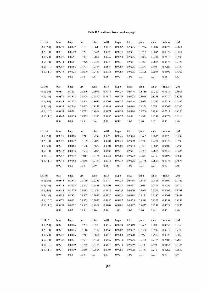
Table D.3 continued from previous page
CsDb2 bcw bupa crx echo hv84 hypo krkp pima sonar Yahoo! IQM
[0 1; 2 0] 0.9771 0.8377 0.913 0.8649 0.9816 0.9902 0.9925 0.8724 0.8894 0.9773 0.9611
[0 2; 1 0] 0.98 0.8609 0.929 0.6486 0.977 0.9921 0.995 0.8789 0.8846 0.8973 0.8011
[0 1; 5 0] 0.9928 0.8551 0.9391 0.9054 0.9747 0.9959 0.9975 0.8854 0.9231 0.7612 0.8598
[0 5; 1 0] 0.9914 0.858 0.9275 0.9324 0.977 0.993 0.9981 0.9271 0.9615 0.9872 0.7728
[0 1; 10 0] 0.9957 0.8783 0.9797 0.9324 0.9678 0.9987 0.9975 0.9531 0.899 0.7782 0.7783
[0 10; 1 0] 0.9943 0.9623 0.9609 0.9459 0.9954 0.9987 0.9925 0.9596 0.9038 0.8697 0.8302
0.99 0.88 0.94 0.87 0.98 0.99 1.00 0.91 0.91 0.88 0.83
CsDb3 bcw bupa crx echo hv84 hypo krkp pima sonar Yahoo! IQM
[0 1; 2 0] 0.98 0.829 0.9246 0.7973 0.9747 0.9937 0.9944 0.8789 0.9327 0.9384 0.7603
[0 2; 1 0] 0.9871 0.8348 0.9304 0.6892 0.9816 0.9953 0.9953 0.8646 0.8558 0.9589 0.8321
[0 1; 5 0] 0.9943 0.8928 0.9594 0.8649 0.9701 0.9937 0.9944 0.8958 0.9567 0.7718 0.9462
[0 5; 1 0] 0.9857 0.8464 0.9493 0.8243 0.9931 0.9965 0.9984 0.9154 0.976 0.8265 0.9165
[0 1; 10 0] 0.9857 0.971 0.9725 0.8919 0.9977 0.9934 0.9984 0.9766 0.8894 0.7713 0.8220
[0 10; 1 0] 0.9742 0.9159 0.9855 0.9595 0.9885 0.9972 0.9981 0.8971 0.9231 0.8079 0.9110
0.98 0.88 0.95 0.84 0.98 0.99 1.00 0.90 0.92 0.85 0.86
CsDb4 bcw bupa crx echo hv84 hypo krkp pima sonar Yahoo! IQM
[0 1; 2 0] 0.9828 0.8464 0.9217 0.7297 0.977 0.9946 0.9944 0.8659 0.8606 0.8676 0.8298
[0 2; 1 0] 0.9828 0.8377 0.9159 0.7027 0.9701 0.9921 0.9959 0.8711 0.9471 0.8970 0.8990
[0 1; 5 0] 0.99 0.8464 0.9536 0.6622 0.9701 0.9987 0.9953 0.9323 0.8846 0.9600 0.9595
[0 5; 1 0] 0.9943 0.8493 0.9522 0.9054 0.9885 0.994 0.9981 0.9284 0.9615 0.8640 0.8236
[0 1; 10 0] 0.9957 0.9797 0.9014 0.8378 0.9954 0.9981 0.9972 0.9831 0.976 0.9192 0.8843
[0 10; 1 0] 0.9742 0.9652 0.9855 0.9189 0.9954 0.9937 0.9975 0.9766 0.9663 0.9073 0.8676
0.99 0.89 0.94 0.79 0.98 1.00 1.00 0.93 0.93 0.90 0.88
CsDb5 bcw bupa crx echo hv84 hypo krkp pima sonar Yahoo! IQM
[0 1; 2 0] 0.9843 0.8348 0.9159 0.6351 0.977 0.9924 0.9934 0.8724 0.9423 0.8300 0.9167
[0 2; 1 0] 0.9943 0.8203 0.9245 0.7838 0.9793 0.9927 0.9931 0.862 0.9471 0.8252 0.7716
[0 1; 5 0] 0.9943 0.8725 0.9435 0.6486 0.9885 0.9956 0.9959 0.8958 0.9519 0.8692 0.7748
[0 5; 1 0] 0.9785 0.887 0.9507 0.7973 0.9885 0.9981 0.9984 0.9141 0.9135 0.8068 0.8448
[0 1; 10 0] 0.9971 0.9101 0.9855 0.7973 0.9885 0.9987 0.9975 0.9388 0.9327 0.8258 0.8398
[0 10; 1 0] 0.9957 0.9072 0.9507 0.8919 0.9908 0.9991 0.9987 0.9427 0.9231 0.9529 0.9835
0.99 0.87 0.95 0.76 0.99 1.00 1.00 0.90 0.94 0.85 0.86
DDTv2 bcw bupa crx echo hv84 hypo krkp pima sonar Yahoo! IQM
[0 1; 2 0] 0.97 0.8116 0.9203 0.527 0.9517 0.9924 0.9919 0.8659 0.9038 0.9052 0.8760
[0 2; 1 0] 0.97 0.8145 0.9116 0.6757 0.9563 0.9902 0.9972 0.8568 0.8942 0.9210 0.7783
[0 1; 5 0] 0.9928 0.8406 0.9217 0.5811 0.9816 0.9968 0.9978 0.8997 0.9519 0.9322 0.8053
[0 5; 1 0] 0.9828 0.887 0.9507 0.6351 0.9839 0.9934 0.9975 0.9128 0.9375 0.7600 0.9663
[0 1; 10 0] 0.99 0.8899 0.9739 0.8784 0.9816 0.9978 0.9969 0.974 0.899 0.9155 0.8385
[0 10; 1 0] 0.99 0.8899 0.9855 0.9595 0.9793 0.9981 0.9928 0.9753 0.976 0.9769 0.7862
0.98 0.86 0.94 0.71 0.97 0.99 1.00 0.91 0.93 0.90 0.84
93

Table D.4: Cost matrix wise precision of CSE1-5, CsDb1-5, DDTv2
CSE1 bcw bupa crx echo hv84 hypo krkp pima sonar Yahoo! IQM
[0 1; 2 0] 0.9694 0.6759 0.8599 0.6600 0.9583 0.8742 0.9910 0.8120 0.7732 0.9384 0.9756
[0 2; 1 0] 0.9978 0.9655 0.9739 0.9400 0.9940 0.9735 0.9994 0.9740 0.9691 0.9350 0.9549
[0 1; 5 0] 0.9803 0.5000 0.9130 0.9800 0.9583 0.9139 0.9958 0.8800 0.8247 0.8512 0.9048
[0 5; 1 0] 0.9978 0.9448 0.9772 0.9800 0.9940 0.9868 0.9982 0.9840 0.9794 0.9165 0.8466
[0 1; 10 0] 0.9934 0.9448 0.9707 0.9200 0.9821 0.9735 0.9952 0.9860 0.9072 0.8992 0.7754
[0 10; 1 0] 0.9958 0.9655 0.9805 1.0000 1.0000 0.9868 0.9994 0.9780 0.9794 0.7723 0.7543
0.99 0.83 0.95 0.91 0.98 0.95 1.00 0.94 0.91 0.89 0.87
CSE2 bcw bupa crx echo hv84 hypo krkp pima sonar Yahoo! IQM
[0 1; 2 0] 0.9716 0.6621 0.8436 0.7000 0.9583 0.9404 0.9868 0.8180 0.7835 0.8048 0.9839
[0 2; 1 0] 0.9978 0.9586 0.9805 0.9400 0.9940 1.0000 0.9988 0.9820 0.9897 0.7579 0.8834
[0 1; 5 0] 0.9694 0.8690 0.8730 0.7600 0.9583 0.9801 0.9928 0.8940 0.8660 0.8996 0.8115
[0 5; 1 0] 0.9978 0.9655 0.9837 0.9400 0.9940 0.9934 0.9994 0.9800 0.9794 0.7910 0.9039
[0 1; 10 0] 0.9825 0.9793 0.9772 0.7800 0.9940 0.9536 0.9862 0.9960 0.7732 0.7551 0.8654
[0 10; 1 0] 0.9978 0.9655 0.9837 0.9600 0.9940 0.9868 0.9988 0.9780 0.9897 0.8721 0.8057
0.99 0.90 0.94 0.85 0.98 0.98 0.99 0.94 0.90 0.81 0.88
CSE3 bcw bupa crx echo hv84 hypo krkp pima sonar Yahoo! IQM
[0 1; 2 0] 0.9607 0.6897 0.8599 0.4200 0.9345 0.8742 0.9862 0.8360 0.9072 0.8346 0.9736
[0 2; 1 0] 0.9978 0.9379 0.9870 0.9800 0.9940 1.0000 0.9994 0.9800 0.9897 0.8124 0.9370
[0 1; 5 0] 0.9956 0.7586 0.8860 0.8000 0.9643 0.9801 0.9952 0.8820 0.8351 0.8185 0.9851
[0 5; 1 0] 0.9978 0.9586 0.9739 0.9400 0.9940 0.9868 0.9988 0.9780 0.9794 0.8592 0.9784
[0 1; 10 0] 0.9978 1.0000 0.9283 1.0000 0.9940 0.9868 0.9970 0.9740 0.8351 0.8215 0.9708
[0 10; 1 0] 0.9978 0.9724 0.9870 0.9600 0.9940 0.9868 0.9994 0.9860 0.9794 0.9414 0.8404
0.99 0.89 0.94 0.85 0.98 0.97 1.00 0.94 0.92 0.85 0.95
CSE4 bcw bupa crx echo hv84 hypo krkp pima sonar Yahoo! IQM
[0 1; 2 0] 0.9825 0.669 0.8436 0.7 0.9583 0.8609 0.991 0.818 0.7629 0.8336 0.8882
[0 2; 1 0] 0.9978 0.9655 0.9805 0.94 0.994 0.9735 0.9976 0.968 0.9897 0.9741 0.8358
[0 1; 5 0] 0.9738 0.6552 0.873 0.76 0.9583 0.9669 0.9952 0.904 0.8454 0.8974 0.8288
[0 5; 1 0] 0.9956 0.9586 0.9837 0.94 0.994 0.9735 0.9976 0.974 0.9691 0.9272 0.7644
[0 1; 10 0] 0.9847 1 0.9772 0.78 0.994 0.9139 0.9868 1 0.9794 0.9871 0.7906
[0 10; 1 0] 0.9978 0.9793 0.9837 0.96 0.994 0.9934 0.9994 0.978 0.9794 0.8555 0.8093
0.99 0.87 0.94 0.85 0.98 0.95 0.99 0.94 0.92 0.91 0.82
CSE5 bcw bupa crx echo hv84 hypo krkp pima sonar Yahoo! IQM
[0 1; 2 0] 0.9913 0.6759 0.8339 0.64 0.9643 0.8675 0.9958 0.814 0.7526 0.8646 0.9481
[0 2; 1 0] 0.9978 0.9517 0.9772 0.9 0.994 0.9934 0.9976 0.978 0.9691 0.8471 0.8034
[0 1; 5 0] 0.976 0.8069 0.8925 0.74 0.9762 0.8675 0.9904 0.91 0.7732 0.8594 0.7528
[0 5; 1 0] 0.9978 0.9655 0.9805 0.96 1 0.9934 0.9988 0.978 1 0.7972 0.8228
[0 1; 10 0] 1 0.9241 0.9674 0.88 0.9226 0.9603 1 0.994 0.9794 0.9238 0.8398
[0 10; 1 0] 0.9943 0.9655 0.9805 0.96 0.994 0.9868 0.9994 0.98 0.9794 0.7658 0.9366
0.99 0.88 0.94 0.85 0.98 0.94 1.00 0.94 0.91 0.84 0.85
94

Table D.4 continued from previous page
CsDb1 bcw bupa crx echo hv84 hypo krkp pima sonar Yahoo! IQM
[0 1; 2 0] 0.9847 0.6207 0.8469 0.74 0.9643 0.9007 0.9952 0.834 0.7526 0.9191 0.9322
[0 2; 1 0] 1 0.9793 0.9837 0.9 1 0.9536 1 0.97 0.9691 0.8444 0.7568
[0 1; 5 0] 0.9738 0.7379 0.9023 0.62 0.9881 0.894 0.9952 0.926 0.866 0.9122 0.7548
[0 5; 1 0] 0.9891 0.9448 0.9772 0.98 0.994 0.9603 1 0.978 1 0.9245 0.8004
[0 1; 10 0] 0.9803 0.9655 0.9153 0.92 0.9345 0.947 0.9964 0.906 0.9175 0.9551 0.9174
[0 10; 1 0] 0.9978 0.9862 0.9805 0.98 1 0.9404 0.9994 0.978 0.9897 0.9789 0.9020
0.99 0.87 0.93 0.86 0.98 0.93 1.00 0.93 0.92 0.92 0.84
CsDb2 bcw bupa crx echo hv84 hypo krkp pima sonar Yahoo! IQM
[0 1; 2 0] 0.9651 0.6552 0.8241 0.84 0.9702 0.8013 0.9868 0.836 0.7629 0.8261 0.8819
[0 2; 1 0] 0.9913 0.9448 0.9837 0.9 1 0.9603 0.997 0.968 0.9691 0.9531 0.9435
[0 1; 5 0] 0.9956 0.669 0.8762 0.92 1 0.9272 0.9976 0.838 0.8351 0.7935 0.7743
[0 5; 1 0] 0.9913 0.9724 0.9902 0.96 0.994 0.9868 0.9982 0.972 0.9381 0.9160 0.9634
[0 1; 10 0] 0.9978 0.7241 0.9837 0.92 0.9167 0.9934 0.9958 0.946 0.7835 0.8054 0.7709
[0 10; 1 0] 0.9956 0.9655 0.9902 0.94 0.994 0.9801 1 0.982 0.9897 0.9782 0.7955
0.99 0.82 0.94 0.91 0.98 0.94 1.00 0.92 0.88 0.88 0.85
CsDb3 bcw bupa crx echo hv84 hypo krkp pima sonar Yahoo! IQM
[0 1; 2 0] 0.9716 0.6069 0.8534 0.72 0.9524 0.9139 0.9898 0.846 0.8557 0.7895 0.9660
[0 2; 1 0] 0.9913 0.9793 0.9772 0.98 0.994 0.9735 0.997 0.984 1 0.9774 0.7960
[0 1; 5 0] 0.9934 0.7793 0.9316 0.82 0.9226 0.8874 0.9904 0.854 0.9175 0.9791 0.9773
[0 5; 1 0] 0.9956 0.9862 0.9837 0.96 0.9881 0.9801 0.9982 0.974 0.9794 0.8411 0.8798
[0 1; 10 0] 0.9803 0.9724 0.9511 0.88 1 0.8675 0.9976 0.986 0.7732 0.8415 0.7751
[0 10; 1 0] 1 0.9724 0.9837 0.94 0.994 0.9868 0.9988 0.982 0.9897 0.7631 0.8327
0.99 0.88 0.95 0.88 0.98 0.93 1.00 0.94 0.92 0.87 0.87
CsDb4 bcw bupa crx echo hv84 hypo krkp pima sonar Yahoo! IQM
[0 1; 2 0] 0.9847 0.6621 0.8469 0.66 0.9524 0.9205 0.9898 0.816 0.7216 0.9099 0.8238
[0 2; 1 0] 0.9978 0.9793 0.9772 0.96 0.9881 0.9934 0.9982 0.984 0.9794 0.8992 0.7817
[0 1; 5 0] 0.9847 0.6414 0.9153 0.54 0.9226 1 0.9916 0.926 0.7732 0.8156 0.9137
[0 5; 1 0] 0.9978 0.9862 0.9837 0.9 0.9881 0.9868 0.9988 0.97 0.9794 0.8051 0.9458
[0 1; 10 0] 0.9978 0.9931 0.7948 0.8 0.994 0.9735 0.9952 0.978 0.9691 0.8367 0.8743
[0 10; 1 0] 1 0.9655 0.9837 0.96 0.994 0.9934 0.9994 0.98 0.9897 0.9843 0.7632
0.99 0.87 0.92 0.80 0.97 0.98 1.00 0.94 0.90 0.88 0.85
CsDb5 bcw bupa crx echo hv84 hypo krkp pima sonar Yahoo! IQM
[0 1; 2 0] 0.9847 0.6207 0.8339 0.56 0.9464 0.8874 0.9898 0.836 0.9175 0.7704 0.9461
[0 2; 1 0] 0.9913 0.9931 0.9869 0.96 0.9881 0.9536 1 0.978 0.9691 0.9282 0.8624
[0 1; 5 0] 0.9956 0.731 0.8925 0.5 0.9821 0.9338 0.9928 0.856 0.9278 0.9726 0.7773
[0 5; 1 0] 1 0.9586 0.9837 0.96 0.9881 0.9669 0.9982 0.976 1 0.8698 0.8150
[0 1; 10 0] 0.9978 0.8069 0.9837 0.72 0.9762 0.9868 0.9964 0.92 0.866 0.8690 0.9311
[0 10; 1 0] 0.9956 0.9793 0.9902 0.96 0.994 0.9868 0.9988 0.984 0.9897 0.8586 0.7554
0.99 0.85 0.95 0.78 0.98 0.95 1.00 0.93 0.95 0.88 0.85
95

Table D.4 continued from previous page
DDTv2 bcw bupa crx echo hv84 hypo krkp pima sonar Yahoo! IQM
[0 1; 2 0] 0.9585 0.6 0.8534 0.44 0.8988 0.8808 0.9868 0.82 0.8351 0.9389 0.9540
[0 2; 1 0] 0.9869 0.9793 0.9837 0.92 0.9821 0.9801 0.9988 0.966 0.9588 0.8631 0.8362
[0 1; 5 0] 1 0.6414 0.8404 0.44 0.9762 0.9868 0.9982 0.866 0.9485 0.9273 0.9102
[0 5; 1 0] 0.9913 0.9517 0.9674 0.9 0.9702 0.9735 0.9976 0.97 0.9691 0.7664 0.9306
[0 1; 10 0] 0.9956 0.7586 0.9739 0.86 0.9643 0.9735 0.9952 0.982 0.8041 0.9898 0.8272
[0 10; 1 0] 0.9913 0.9724 0.9805 0.96 0.9881 0.9801 0.9988 0.978 0.9691 0.9535 0.8936
0.99 0.82 0.93 0.75 0.96 0.96 1.00 0.93 0.91 0.91 0.89
Table D.5: Cost matrix wise recall of CSE1-5, CsDb1-5, DDTv2
CSE1 bcw bupa crx echo hv84 hypo krkp pima sonar Yahoo! IQM
[0 1; 2 0] 0.9978 0.9608 0.9706 0.8919 0.9938 0.9851 0.9994 0.9760 0.9740 0.8014 0.7989
[0 2; 1 0] 0.9744 0.7447 0.8768 0.7460 0.9489 0.8802 0.9887 0.8589 0.8785 0.7901 0.9416
[0 1; 5 0] 0.9978 0.7241 0.9594 0.9245 0.9938 0.9857 0.9988 0.9756 0.9877 0.7899 0.9899
[0 5; 1 0] 0.9765 0.8726 0.9174 0.7424 0.9824 0.9085 0.9964 0.8693 0.9048 0.7547 0.9103
[0 1; 10 0] 0.9978 0.9648 0.9835 0.9583 0.9940 0.9866 0.9994 0.9801 0.9778 0.7831 0.8983
[0 10; 1 0] 0.9870 0.9032 1.0000 0.6944 0.9180 0.9551 0.9934 0.9919 0.9596 0.8179 0.8176
0.99 0.86 0.95 0.83 0.97 0.95 1.00 0.94 0.95 0.79 0.89
CSE2 bcw bupa crx echo hv84 hypo krkp pima sonar Yahoo! IQM
[0 1; 2 0] 0.9978 0.9505 0.9774 0.8974 0.9938 0.9530 0.9988 0.9738 0.9870 0.8569 0.7622
[0 2; 1 0] 0.9828 0.7277 0.8649 0.6912 0.9382 0.8483 0.9876 0.8408 0.8067 0.8633 0.9865
[0 1; 5 0] 0.9978 0.9474 0.9853 0.9500 1.0000 0.9801 0.9994 0.9739 0.9767 0.8492 0.9205
[0 5; 1 0] 0.9723 0.8000 0.8882 0.7966 0.9598 0.8772 0.9917 0.8861 0.8796 0.7743 0.8323
[0 1; 10 0] 0.9978 0.9595 0.9836 0.9750 0.9940 0.9863 1.0000 0.9784 1.0000 0.9154 0.9396
[0 10; 1 0] 0.9892 0.9929 0.9497 0.8889 0.9940 0.9613 1.0000 0.9859 0.8807 0.8649 0.7574
0.99 0.90 0.94 0.87 0.98 0.93 1.00 0.94 0.92 0.85 0.87
CSE3 bcw bupa crx echo hv84 hypo krkp pima sonar Yahoo! IQM
[0 1; 2 0] 0.9977 0.9434 0.9778 0.9545 0.9937 0.9851 0.9994 0.9676 0.9778 0.8291 0.8472
[0 2; 1 0] 0.9621 0.7598 0.8707 0.6806 0.9330 0.8389 0.9858 0.8419 0.7442 0.7670 0.7712
[0 1; 5 0] 0.9978 0.9649 0.9784 0.9091 0.9939 0.9610 0.9988 0.9778 0.9878 0.7768 0.9772
[0 5; 1 0] 0.9765 0.8274 0.9257 0.9216 0.9598 0.8713 0.9976 0.9006 0.8962 0.9136 0.9321
[0 1; 10 0] 0.9978 0.9603 0.9862 0.9804 0.9940 0.9868 0.9994 0.9799 0.9878 0.9587 0.8062
[0 10; 1 0] 0.9956 0.8813 0.9439 0.8276 0.9709 0.9933 0.9952 0.9250 0.9500 0.9210 0.8832
0.99 0.89 0.95 0.88 0.97 0.94 1.00 0.93 0.92 0.86 0.87
CSE4 bcw bupa crx echo hv84 hypo krkp pima sonar Yahoo! IQM
[0 1; 2 0] 0.9934 0.9604 0.9774 0.8974 0.9938 0.9848 0.9988 0.9738 0.9867 0.8869 0.9868
[0 2; 1 0] 0.9703 0.7487 0.8649 0.6912 0.9382 0.8963 0.9952 0.8566 0.8205 0.9381 0.9679
[0 1; 5 0] 0.9978 0.9896 0.9853 0.95 1 0.9733 0.9988 0.972 0.9762 0.8140 0.9582
[0 5; 1 0] 0.9935 0.8274 0.8882 0.7966 0.9598 1 1 0.9137 0.94 0.7735 0.9248
[0 1; 10 0] 0.9978 0.9603 0.9836 0.975 0.994 0.9928 1 0.9785 0.9794 0.7571 0.9501
96
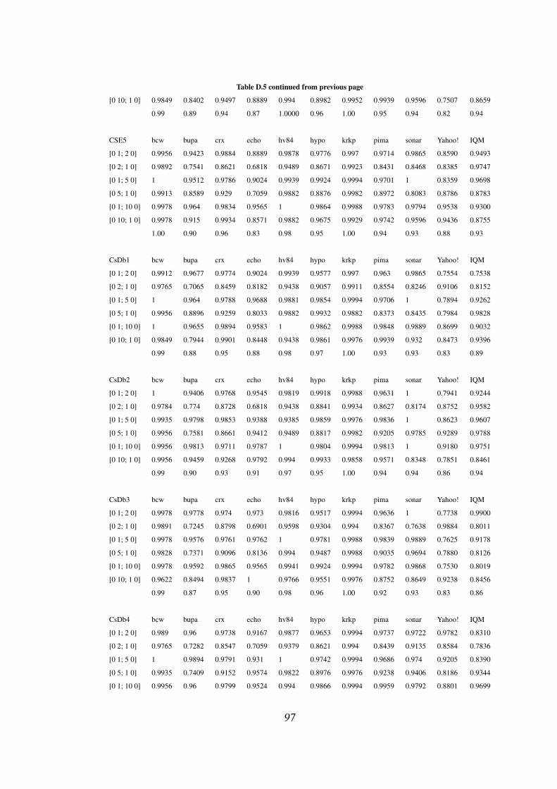
Table D.5 continued from previous page
[0 10; 1 0] 0.9849 0.8402 0.9497 0.8889 0.994 0.8982 0.9952 0.9939 0.9596 0.7507 0.8659
0.99 0.89 0.94 0.87 1.0000 0.96 1.00 0.95 0.94 0.82 0.94
CSE5 bcw bupa crx echo hv84 hypo krkp pima sonar Yahoo! IQM
[0 1; 2 0] 0.9956 0.9423 0.9884 0.8889 0.9878 0.9776 0.997 0.9714 0.9865 0.8590 0.9493
[0 2; 1 0] 0.9892 0.7541 0.8621 0.6818 0.9489 0.8671 0.9923 0.8431 0.8468 0.8385 0.9747
[0 1; 5 0] 1 0.9512 0.9786 0.9024 0.9939 0.9924 0.9994 0.9701 1 0.8359 0.9698
[0 5; 1 0] 0.9913 0.8589 0.929 0.7059 0.9882 0.8876 0.9982 0.8972 0.8083 0.8786 0.8783
[0 1; 10 0] 0.9978 0.964 0.9834 0.9565 1 0.9864 0.9988 0.9783 0.9794 0.9538 0.9300
[0 10; 1 0] 0.9978 0.915 0.9934 0.8571 0.9882 0.9675 0.9929 0.9742 0.9596 0.9436 0.8755
1.00 0.90 0.96 0.83 0.98 0.95 1.00 0.94 0.93 0.88 0.93
CsDb1 bcw bupa crx echo hv84 hypo krkp pima sonar Yahoo! IQM
[0 1; 2 0] 0.9912 0.9677 0.9774 0.9024 0.9939 0.9577 0.997 0.963 0.9865 0.7554 0.7538
[0 2; 1 0] 0.9765 0.7065 0.8459 0.8182 0.9438 0.9057 0.9911 0.8554 0.8246 0.9106 0.8152
[0 1; 5 0] 1 0.964 0.9788 0.9688 0.9881 0.9854 0.9994 0.9706 1 0.7894 0.9262
[0 5; 1 0] 0.9956 0.8896 0.9259 0.8033 0.9882 0.9932 0.9882 0.8373 0.8435 0.7984 0.9828
[0 1; 10 0] 1 0.9655 0.9894 0.9583 1 0.9862 0.9988 0.9848 0.9889 0.8699 0.9032
[0 10; 1 0] 0.9849 0.7944 0.9901 0.8448 0.9438 0.9861 0.9976 0.9939 0.932 0.8473 0.9396
0.99 0.88 0.95 0.88 0.98 0.97 1.00 0.93 0.93 0.83 0.89
CsDb2 bcw bupa crx echo hv84 hypo krkp pima sonar Yahoo! IQM
[0 1; 2 0] 1 0.9406 0.9768 0.9545 0.9819 0.9918 0.9988 0.9631 1 0.7941 0.9244
[0 2; 1 0] 0.9784 0.774 0.8728 0.6818 0.9438 0.8841 0.9934 0.8627 0.8174 0.8752 0.9582
[0 1; 5 0] 0.9935 0.9798 0.9853 0.9388 0.9385 0.9859 0.9976 0.9836 1 0.8623 0.9607
[0 5; 1 0] 0.9956 0.7581 0.8661 0.9412 0.9489 0.8817 0.9982 0.9205 0.9785 0.9289 0.9788
[0 1; 10 0] 0.9956 0.9813 0.9711 0.9787 1 0.9804 0.9994 0.9813 1 0.9180 0.9751
[0 10; 1 0] 0.9956 0.9459 0.9268 0.9792 0.994 0.9933 0.9858 0.9571 0.8348 0.7851 0.8461
0.99 0.90 0.93 0.91 0.97 0.95 1.00 0.94 0.94 0.86 0.94
CsDb3 bcw bupa crx echo hv84 hypo krkp pima sonar Yahoo! IQM
[0 1; 2 0] 0.9978 0.9778 0.974 0.973 0.9816 0.9517 0.9994 0.9636 1 0.7738 0.9900
[0 2; 1 0] 0.9891 0.7245 0.8798 0.6901 0.9598 0.9304 0.994 0.8367 0.7638 0.9884 0.8011
[0 1; 5 0] 0.9978 0.9576 0.9761 0.9762 1 0.9781 0.9988 0.9839 0.9889 0.7625 0.9178
[0 5; 1 0] 0.9828 0.7371 0.9096 0.8136 0.994 0.9487 0.9988 0.9035 0.9694 0.7880 0.8126
[0 1; 10 0] 0.9978 0.9592 0.9865 0.9565 0.9941 0.9924 0.9994 0.9782 0.9868 0.7530 0.8019
[0 10; 1 0] 0.9622 0.8494 0.9837 1 0.9766 0.9551 0.9976 0.8752 0.8649 0.9238 0.8456
0.99 0.87 0.95 0.90 0.98 0.96 1.00 0.92 0.93 0.83 0.86
CsDb4 bcw bupa crx echo hv84 hypo krkp pima sonar Yahoo! IQM
[0 1; 2 0] 0.989 0.96 0.9738 0.9167 0.9877 0.9653 0.9994 0.9737 0.9722 0.9782 0.8310
[0 2; 1 0] 0.9765 0.7282 0.8547 0.7059 0.9379 0.8621 0.994 0.8439 0.9135 0.8584 0.7836
[0 1; 5 0] 1 0.9894 0.9791 0.931 1 0.9742 0.9994 0.9686 0.974 0.9205 0.8390
[0 5; 1 0] 0.9935 0.7409 0.9152 0.9574 0.9822 0.8976 0.9976 0.9238 0.9406 0.8186 0.9344
[0 1; 10 0] 0.9956 0.96 0.9799 0.9524 0.994 0.9866 0.9994 0.9959 0.9792 0.8801 0.9699
97
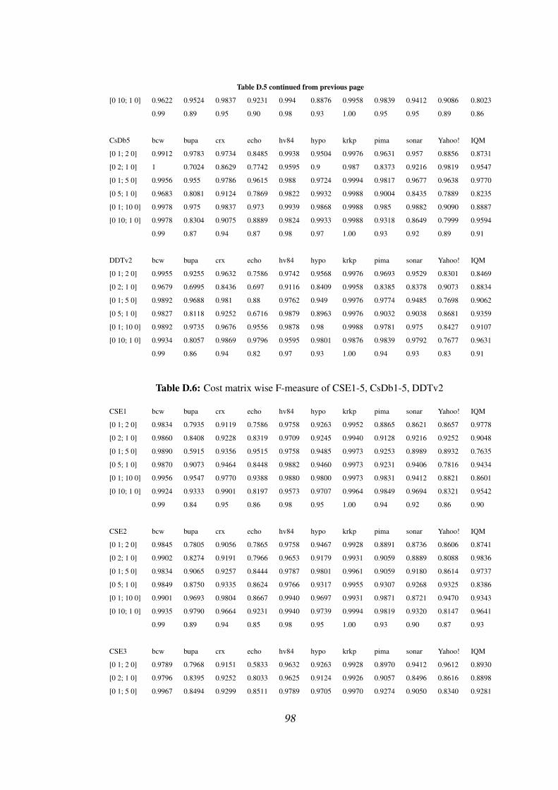
Table D.5 continued from previous page
[0 10; 1 0] 0.9622 0.9524 0.9837 0.9231 0.994 0.8876 0.9958 0.9839 0.9412 0.9086 0.8023
0.99 0.89 0.95 0.90 0.98 0.93 1.00 0.95 0.95 0.89 0.86
CsDb5 bcw bupa crx echo hv84 hypo krkp pima sonar Yahoo! IQM
[0 1; 2 0] 0.9912 0.9783 0.9734 0.8485 0.9938 0.9504 0.9976 0.9631 0.957 0.8856 0.8731
[0 2; 1 0] 1 0.7024 0.8629 0.7742 0.9595 0.9 0.987 0.8373 0.9216 0.9819 0.9547
[0 1; 5 0] 0.9956 0.955 0.9786 0.9615 0.988 0.9724 0.9994 0.9817 0.9677 0.9638 0.9770
[0 5; 1 0] 0.9683 0.8081 0.9124 0.7869 0.9822 0.9932 0.9988 0.9004 0.8435 0.7889 0.8235
[0 1; 10 0] 0.9978 0.975 0.9837 0.973 0.9939 0.9868 0.9988 0.985 0.9882 0.9090 0.8887
[0 10; 1 0] 0.9978 0.8304 0.9075 0.8889 0.9824 0.9933 0.9988 0.9318 0.8649 0.7999 0.9594
0.99 0.87 0.94 0.87 0.98 0.97 1.00 0.93 0.92 0.89 0.91
DDTv2 bcw bupa crx echo hv84 hypo krkp pima sonar Yahoo! IQM
[0 1; 2 0] 0.9955 0.9255 0.9632 0.7586 0.9742 0.9568 0.9976 0.9693 0.9529 0.8301 0.8469
[0 2; 1 0] 0.9679 0.6995 0.8436 0.697 0.9116 0.8409 0.9958 0.8385 0.8378 0.9073 0.8834
[0 1; 5 0] 0.9892 0.9688 0.981 0.88 0.9762 0.949 0.9976 0.9774 0.9485 0.7698 0.9062
[0 5; 1 0] 0.9827 0.8118 0.9252 0.6716 0.9879 0.8963 0.9976 0.9032 0.9038 0.8681 0.9359
[0 1; 10 0] 0.9892 0.9735 0.9676 0.9556 0.9878 0.98 0.9988 0.9781 0.975 0.8427 0.9107
[0 10; 1 0] 0.9934 0.8057 0.9869 0.9796 0.9595 0.9801 0.9876 0.9839 0.9792 0.7677 0.9631
0.99 0.86 0.94 0.82 0.97 0.93 1.00 0.94 0.93 0.83 0.91
Table D.6: Cost matrix wise F-measure of CSE1-5, CsDb1-5, DDTv2
CSE1 bcw bupa crx echo hv84 hypo krkp pima sonar Yahoo! IQM
[0 1; 2 0] 0.9834 0.7935 0.9119 0.7586 0.9758 0.9263 0.9952 0.8865 0.8621 0.8657 0.9778
[0 2; 1 0] 0.9860 0.8408 0.9228 0.8319 0.9709 0.9245 0.9940 0.9128 0.9216 0.9252 0.9048
[0 1; 5 0] 0.9890 0.5915 0.9356 0.9515 0.9758 0.9485 0.9973 0.9253 0.8989 0.8932 0.7635
[0 5; 1 0] 0.9870 0.9073 0.9464 0.8448 0.9882 0.9460 0.9973 0.9231 0.9406 0.7816 0.9434
[0 1; 10 0] 0.9956 0.9547 0.9770 0.9388 0.9880 0.9800 0.9973 0.9831 0.9412 0.8821 0.8601
[0 10; 1 0] 0.9924 0.9333 0.9901 0.8197 0.9573 0.9707 0.9964 0.9849 0.9694 0.8321 0.9542
0.99 0.84 0.95 0.86 0.98 0.95 1.00 0.94 0.92 0.86 0.90
CSE2 bcw bupa crx echo hv84 hypo krkp pima sonar Yahoo! IQM
[0 1; 2 0] 0.9845 0.7805 0.9056 0.7865 0.9758 0.9467 0.9928 0.8891 0.8736 0.8606 0.8741
[0 2; 1 0] 0.9902 0.8274 0.9191 0.7966 0.9653 0.9179 0.9931 0.9059 0.8889 0.8088 0.9836
[0 1; 5 0] 0.9834 0.9065 0.9257 0.8444 0.9787 0.9801 0.9961 0.9059 0.9180 0.8614 0.9737
[0 5; 1 0] 0.9849 0.8750 0.9335 0.8624 0.9766 0.9317 0.9955 0.9307 0.9268 0.9325 0.8386
[0 1; 10 0] 0.9901 0.9693 0.9804 0.8667 0.9940 0.9697 0.9931 0.9871 0.8721 0.9470 0.9343
[0 10; 1 0] 0.9935 0.9790 0.9664 0.9231 0.9940 0.9739 0.9994 0.9819 0.9320 0.8147 0.9641
0.99 0.89 0.94 0.85 0.98 0.95 1.00 0.93 0.90 0.87 0.93
CSE3 bcw bupa crx echo hv84 hypo krkp pima sonar Yahoo! IQM
[0 1; 2 0] 0.9789 0.7968 0.9151 0.5833 0.9632 0.9263 0.9928 0.8970 0.9412 0.9612 0.8930
[0 2; 1 0] 0.9796 0.8395 0.9252 0.8033 0.9625 0.9124 0.9926 0.9057 0.8496 0.8616 0.8898
[0 1; 5 0] 0.9967 0.8494 0.9299 0.8511 0.9789 0.9705 0.9970 0.9274 0.9050 0.8340 0.9281
98
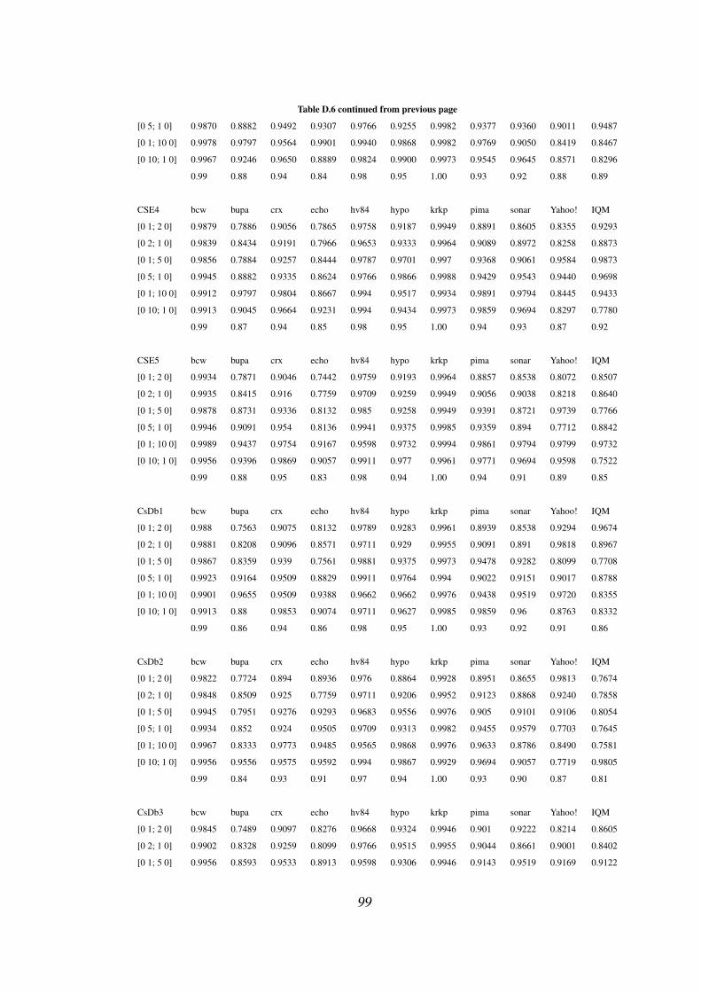
Table D.6 continued from previous page
[0 5; 1 0] 0.9870 0.8882 0.9492 0.9307 0.9766 0.9255 0.9982 0.9377 0.9360 0.9011 0.9487
[0 1; 10 0] 0.9978 0.9797 0.9564 0.9901 0.9940 0.9868 0.9982 0.9769 0.9050 0.8419 0.8467
[0 10; 1 0] 0.9967 0.9246 0.9650 0.8889 0.9824 0.9900 0.9973 0.9545 0.9645 0.8571 0.8296
0.99 0.88 0.94 0.84 0.98 0.95 1.00 0.93 0.92 0.88 0.89
CSE4 bcw bupa crx echo hv84 hypo krkp pima sonar Yahoo! IQM
[0 1; 2 0] 0.9879 0.7886 0.9056 0.7865 0.9758 0.9187 0.9949 0.8891 0.8605 0.8355 0.9293
[0 2; 1 0] 0.9839 0.8434 0.9191 0.7966 0.9653 0.9333 0.9964 0.9089 0.8972 0.8258 0.8873
[0 1; 5 0] 0.9856 0.7884 0.9257 0.8444 0.9787 0.9701 0.997 0.9368 0.9061 0.9584 0.9873
[0 5; 1 0] 0.9945 0.8882 0.9335 0.8624 0.9766 0.9866 0.9988 0.9429 0.9543 0.9440 0.9698
[0 1; 10 0] 0.9912 0.9797 0.9804 0.8667 0.994 0.9517 0.9934 0.9891 0.9794 0.8445 0.9433
[0 10; 1 0] 0.9913 0.9045 0.9664 0.9231 0.994 0.9434 0.9973 0.9859 0.9694 0.8297 0.7780
0.99 0.87 0.94 0.85 0.98 0.95 1.00 0.94 0.93 0.87 0.92
CSE5 bcw bupa crx echo hv84 hypo krkp pima sonar Yahoo! IQM
[0 1; 2 0] 0.9934 0.7871 0.9046 0.7442 0.9759 0.9193 0.9964 0.8857 0.8538 0.8072 0.8507
[0 2; 1 0] 0.9935 0.8415 0.916 0.7759 0.9709 0.9259 0.9949 0.9056 0.9038 0.8218 0.8640
[0 1; 5 0] 0.9878 0.8731 0.9336 0.8132 0.985 0.9258 0.9949 0.9391 0.8721 0.9739 0.7766
[0 5; 1 0] 0.9946 0.9091 0.954 0.8136 0.9941 0.9375 0.9985 0.9359 0.894 0.7712 0.8842
[0 1; 10 0] 0.9989 0.9437 0.9754 0.9167 0.9598 0.9732 0.9994 0.9861 0.9794 0.9799 0.9732
[0 10; 1 0] 0.9956 0.9396 0.9869 0.9057 0.9911 0.977 0.9961 0.9771 0.9694 0.9598 0.7522
0.99 0.88 0.95 0.83 0.98 0.94 1.00 0.94 0.91 0.89 0.85
CsDb1 bcw bupa crx echo hv84 hypo krkp pima sonar Yahoo! IQM
[0 1; 2 0] 0.988 0.7563 0.9075 0.8132 0.9789 0.9283 0.9961 0.8939 0.8538 0.9294 0.9674
[0 2; 1 0] 0.9881 0.8208 0.9096 0.8571 0.9711 0.929 0.9955 0.9091 0.891 0.9818 0.8967
[0 1; 5 0] 0.9867 0.8359 0.939 0.7561 0.9881 0.9375 0.9973 0.9478 0.9282 0.8099 0.7708
[0 5; 1 0] 0.9923 0.9164 0.9509 0.8829 0.9911 0.9764 0.994 0.9022 0.9151 0.9017 0.8788
[0 1; 10 0] 0.9901 0.9655 0.9509 0.9388 0.9662 0.9662 0.9976 0.9438 0.9519 0.9720 0.8355
[0 10; 1 0] 0.9913 0.88 0.9853 0.9074 0.9711 0.9627 0.9985 0.9859 0.96 0.8763 0.8332
0.99 0.86 0.94 0.86 0.98 0.95 1.00 0.93 0.92 0.91 0.86
CsDb2 bcw bupa crx echo hv84 hypo krkp pima sonar Yahoo! IQM
[0 1; 2 0] 0.9822 0.7724 0.894 0.8936 0.976 0.8864 0.9928 0.8951 0.8655 0.9813 0.7674
[0 2; 1 0] 0.9848 0.8509 0.925 0.7759 0.9711 0.9206 0.9952 0.9123 0.8868 0.9240 0.7858
[0 1; 5 0] 0.9945 0.7951 0.9276 0.9293 0.9683 0.9556 0.9976 0.905 0.9101 0.9106 0.8054
[0 5; 1 0] 0.9934 0.852 0.924 0.9505 0.9709 0.9313 0.9982 0.9455 0.9579 0.7703 0.7645
[0 1; 10 0] 0.9967 0.8333 0.9773 0.9485 0.9565 0.9868 0.9976 0.9633 0.8786 0.8490 0.7581
[0 10; 1 0] 0.9956 0.9556 0.9575 0.9592 0.994 0.9867 0.9929 0.9694 0.9057 0.7719 0.9805
0.99 0.84 0.93 0.91 0.97 0.94 1.00 0.93 0.90 0.87 0.81
CsDb3 bcw bupa crx echo hv84 hypo krkp pima sonar Yahoo! IQM
[0 1; 2 0] 0.9845 0.7489 0.9097 0.8276 0.9668 0.9324 0.9946 0.901 0.9222 0.8214 0.8605
[0 2; 1 0] 0.9902 0.8328 0.9259 0.8099 0.9766 0.9515 0.9955 0.9044 0.8661 0.9001 0.8402
[0 1; 5 0] 0.9956 0.8593 0.9533 0.8913 0.9598 0.9306 0.9946 0.9143 0.9519 0.9169 0.9122
99

Table D.6 continued from previous page
[0 5; 1 0] 0.9892 0.8437 0.9452 0.8807 0.991 0.9642 0.9985 0.9374 0.9744 0.7756 0.8008
[0 1; 10 0] 0.989 0.9658 0.9685 0.9167 0.997 0.9258 0.9985 0.9821 0.8671 0.7728 0.9624
[0 10; 1 0] 0.9807 0.9068 0.9837 0.9691 0.9853 0.9707 0.9982 0.9255 0.9231 0.8164 0.9828
0.99 0.86 0.95 0.88 0.98 0.95 1.00 0.93 0.92 0.83 0.89
CsDb4 bcw bupa crx echo hv84 hypo krkp pima sonar Yahoo! IQM
[0 1; 2 0] 0.9869 0.7837 0.9059 0.7674 0.9697 0.9424 0.9946 0.8879 0.8284 0.8246 0.8836
[0 2; 1 0] 0.987 0.8353 0.9119 0.8136 0.9623 0.9231 0.9961 0.9086 0.9453 0.8704 0.7570
[0 1; 5 0] 0.9923 0.7782 0.9461 0.6835 0.9598 0.9869 0.9955 0.9468 0.8621 0.9749 0.9332
[0 5; 1 0] 0.9956 0.8462 0.9482 0.9278 0.9852 0.9401 0.9982 0.9463 0.9596 0.9466 0.8830
[0 1; 10 0] 0.9967 0.9763 0.8777 0.8696 0.994 0.98 0.9973 0.9869 0.9741 0.7696 0.9334
[0 10; 1 0] 0.9807 0.9589 0.9837 0.9412 0.994 0.9375 0.9976 0.982 0.9648 0.7845 0.8924
0.99 0.86 0.93 0.83 0.98 0.95 1.00 0.94 0.92 0.86 0.88
CsDb5 bcw bupa crx echo hv84 hypo krkp pima sonar Yahoo! IQM
[0 1; 2 0] 0.988 0.7595 0.8982 0.6747 0.9695 0.9178 0.9937 0.8951 0.9368 0.9522 0.9548
[0 2; 1 0] 0.9956 0.8229 0.9207 0.8571 0.9736 0.926 0.9935 0.9022 0.9447 0.9790 0.9857
[0 1; 5 0] 0.9956 0.8281 0.9336 0.6579 0.9851 0.9527 0.9961 0.9145 0.9474 0.9138 0.9705
[0 5; 1 0] 0.9839 0.877 0.9467 0.8649 0.9852 0.9799 0.9985 0.9367 0.9151 0.8776 0.9230
[0 1; 10 0] 0.9978 0.883 0.9837 0.8276 0.985 0.9868 0.9976 0.9514 0.9231 0.9558 0.7828
[0 10; 1 0] 0.9967 0.8987 0.947 0.9231 0.9882 0.99 0.9988 0.9572 0.9231 0.8215 0.8987
0.99 0.84 0.94 0.80 0.98 0.96 1.00 0.93 0.93 0.92 0.92
DDTv2 bcw bupa crx echo hv84 hypo krkp pima sonar Yahoo! IQM
[0 1; 2 0] 0.9766 0.728 0.905 0.557 0.935 0.9172 0.9922 0.8884 0.8901 0.8227 0.9173
[0 2; 1 0] 0.9773 0.8161 0.9083 0.7931 0.9456 0.9052 0.9973 0.8978 0.8942 0.7736 0.7777
[0 1; 5 0] 0.9946 0.7718 0.9053 0.5867 0.9762 0.9675 0.9979 0.9183 0.9485 0.9772 0.8701
[0 5; 1 0] 0.987 0.8762 0.9459 0.7692 0.979 0.9333 0.9976 0.9354 0.9353 0.8294 0.8343
[0 1; 10 0] 0.9924 0.8527 0.9708 0.9053 0.9759 0.9767 0.997 0.98 0.8814 0.8068 0.8248
[0 10; 1 0] 0.9923 0.8813 0.9837 0.9697 0.9736 0.9801 0.9931 0.9809 0.9741 0.9114 0.9390
0.99 0.82 0.94 0.76 0.96 0.95 1.00 0.93 0.92 0.85 0.86
Table D.7: Cost matrix wise model building time of CSE1-5, CsDb1-5, DDTv2
CSE1 bcw bupa crx echo hv84 hypo krkp pima sonar Yahoo! IQM
[0 1; 2 0] 32.80 8.35 26.00 6.23 8.38 129.41 12.90 4.87 5.93 673.06 8950.57
[0 2; 1 0] 38.00 7.00 16.00 8.00 14.00 80.00 11.00 5.00 7.00 657.00 6856.00
[0 1; 5 0] 21.00 11.00 47.00 8.00 6.00 152.00 6.00 7.00 2.00 241.00 9981.00
[0 5; 1 0] 54.00 7.00 15.00 6.00 8.00 137.00 12.00 6.00 6.00 534.00 12342.00
[0 1; 10 0] 25.00 14.00 27.00 10.00 13.00 175.00 20.00 6.00 4.00 710.00 12363.00
[0 10; 1 0] 19.00 9.00 32.00 8.00 3.00 39.00 6.00 4.00 4.00 779.00 8049.00
31.63 9.39 27.17 7.70 8.73 118.74 11.32 5.48 4.82 599.01 9756.93
CSE2 bcw bupa crx echo hv84 hypo krkp pima sonar Yahoo! IQM
[0 1; 2 0] 25.00 8.00 22.00 10.00 7.00 119.00 10.00 2.00 7.00 612.00 9547.00
100

Table D.7 continued from previous page
[0 2; 1 0] 31.00 9.00 11.00 7.00 7.00 149.00 8.00 1.00 8.00 1101.00 15348.00
[0 1; 5 0] 42.00 10.00 25.00 7.00 6.00 112.00 21.00 3.00 6.00 581.00 4282.00
[0 5; 1 0] 33.00 8.00 26.00 6.00 8.00 116.00 16.00 8.00 3.00 820.00 10786.00
[0 1; 10 0] 35.00 13.00 41.00 2.00 9.00 144.00 17.00 4.00 6.00 892.00 6473.00
[0 10; 1 0] 31.00 12.00 25.00 6.00 4.00 108.00 9.00 3.00 9.00 1002.00 9373.00
32.83 10.00 25.00 6.33 6.83 124.67 13.50 3.50 6.50 834.67 9301.50
CSE3 bcw bupa crx echo hv84 hypo krkp pima sonar Yahoo! IQM
[0 1; 2 0] 35.00 8.00 30.00 6.00 9.00 118.00 9.00 7.00 10.00 451.00 3666.00
[0 2; 1 0] 25.00 7.00 34.00 8.00 9.00 134.00 15.00 6.00 9.00 779.00 8327.00
[0 1; 5 0] 26.00 7.00 22.00 6.00 8.00 48.00 16.00 4.00 6.00 207.00 16031.00
[0 5; 1 0] 38.00 2.00 35.00 6.00 6.00 164.00 12.00 3.00 5.00 659.00 12986.00
[0 1; 10 0] 52.00 8.00 16.00 9.00 5.00 129.00 13.00 6.00 10.00 1262.00 4202.00
[0 10; 1 0] 58.00 8.00 22.00 6.00 8.00 161.00 12.00 4.00 3.00 663.00 3837.00
39.00 6.67 26.50 6.83 7.50 125.67 12.83 5.00 7.17 670.17 8174.83
CSE4 bcw bupa crx echo hv84 hypo krkp pima sonar Yahoo! IQM
[0 1; 2 0] 23 7 46 9 9 231 17 2 6 375 8167
[0 2; 1 0] 30 9 28 5 6 191 11 5 9 1139 3852
[0 1; 5 0] 29 13 34 7 14 159 10 1 6 628 10415
[0 5; 1 0] 31 2 42 4 8 146 11 5 8 643 12093
[0 1; 10 0] 47 11 35 7 5 129 18 4 5 1043 9457
[0 10; 1 0] 29 8 45 6 8 105 6 2 7 684 11251
31.50 8.33 38.33 6.33 8.33 160.17 12.17 3.17 6.83 752.00 9205.83
CSE5 bcw bupa crx echo hv84 hypo krkp pima sonar Yahoo! IQM
[0 1; 2 0] 37 7 19 7 6 167 3 5 5 773 9738
[0 2; 1 0] 36 11 27 10 1 141 13 8 6 907 6512
[0 1; 5 0] 36 9 38 6 12 138 14 5 5 517 12521
[0 5; 1 0] 45 9 33 9 8 90 10 2 1 796 14620
[0 1; 10 0] 30 11 26 6 10 88 9 6 7 939 5522
[0 10; 1 0] 8 4 32 10 14 60 2 5 8 476 8067
32.00 8.50 29.17 8.00 8.50 114.00 8.50 5.17 5.33 734.67 9496.67
CsDb1 bcw bupa crx echo hv84 hypo krkp pima sonar Yahoo! IQM
[0 1; 2 0] 47 9 30 8 3 75 10 3 5 334 8769
[0 2; 1 0] 22 12 31 7 3 122 16 5 4 513 8918
[0 1; 5 0] 24 6 17 10 8 154 12 8 9 415 8484
[0 5; 1 0] 34 7 46 5 6 175 10 1 3 814 8914
[0 1; 10 0] 26 11 33 6 9 231 13 7 8 667 13036
[0 10; 1 0] 37 14 5 6 4 95 11 2 6 166 7366
31.67 9.83 27.00 7.00 5.50 142.00 12.00 4.33 5.83 484.83 9247.83
CsDb2 bcw bupa crx echo hv84 hypo krkp pima sonar Yahoo! IQM
101

Table D.7 continued from previous page
[0 1; 2 0] 36 9 39 9 13 159 20 2 2 699 8946
[0 2; 1 0] 9 7 26 6 4 115 11 3 8 1005 9012
[0 1; 5 0] 23 9 23 7 3 214 21 6 6 697 8572
[0 5; 1 0] 23 10 35 8 13 135 13 3 5 1247 9506
[0 1; 10 0] 24 6 39 4 9 116 9 3 3 603 5334
[0 10; 1 0] 19 10 32 6 5 180 10 6 5 905 13971
22.33 8.50 32.33 6.67 7.83 153.17 14.00 3.83 4.83 859.33 9223.50
CsDb3 bcw bupa crx echo hv84 hypo krkp pima sonar Yahoo! IQM
[0 1; 2 0] 40 7 31 6 3 46 15 5 7 140 8945
[0 2; 1 0] 49 8 39 6 8 155 17 5 6 406 12534
[0 1; 5 0] 37 8 15 9 5 180 9 9 8 1285 7048
[0 5; 1 0] 18 9 18 5 6 115 8 5 2 288 14014
[0 1; 10 0] 16 3 38 7 10 117 24 5 8 477 9176
[0 10; 1 0] 30 5 27 7 10 18 15 4 6 1180 10128
31.67 6.67 28.00 6.67 7.00 105.17 14.67 5.50 6.17 629.33 10307.50
CsDb4 bcw bupa crx echo hv84 hypo krkp pima sonar Yahoo! IQM
[0 1; 2 0] 44 5 42 11 11 95 8 6 7 835 13185
[0 2; 1 0] 16 8 39 6 8 253 18 4 6 176 7599
[0 1; 5 0] 34 8 29 7 3 65 14 5 8 574 8010
[0 5; 1 0] 13 10 24 12 9 178 14 5 6 681 3617
[0 1; 10 0] 29 8 22 6 10 110 12 5 8 730 11611
[0 10; 1 0] 56 14 16 8 1 96 13 5 5 744 9315
32.00 8.83 28.67 8.33 7.00 132.83 13.17 5.00 6.67 623.33 8889.50
CsDb5 bcw bupa crx echo hv84 hypo krkp pima sonar Yahoo! IQM
[0 1; 2 0] 35 11 31 5 8 111 11 5 5 695 8640
[0 2; 1 0] 53 8 30 4 8 131 10 6 9 947 7243
[0 1; 5 0] 41 9 15 9 7 124 14 1 3 61 9743
[0 5; 1 0] 42 7 30 3 11 145 14 3 6 846 4296
[0 1; 10 0] 16 16 38 9 13 190 20 4 6 789 12505
[0 10; 1 0] 24 5 41 5 7 171 14 5 4 653 4964
35.17 9.33 30.83 5.83 9.00 145.33 13.83 4.00 5.50 665.17 7898.50
DDTv2 bcw bupa crx echo hv84 hypo krkp pima sonar Yahoo! IQM
[0 1; 2 0] 41 8 25 9 4 46 7 6 6 319 9311
[0 2; 1 0] 25 11 28 5 12 153 17 2 10 985 9308
[0 1; 5 0] 53 8 26 4 3 107 17 7 3 736 2370
[0 5; 1 0] 17 13 9 7 11 96 9 4 5 720 10287
[0 1; 10 0] 23 8 26 6 9 187 10 9 10 1192 10208
[0 10; 1 0] 36 4 43 7 5 147 15 3 10 165 4693
32.50 8.67 26.17 6.33 7.33 122.67 12.50 5.17 7.33 686.17 7696.17
102
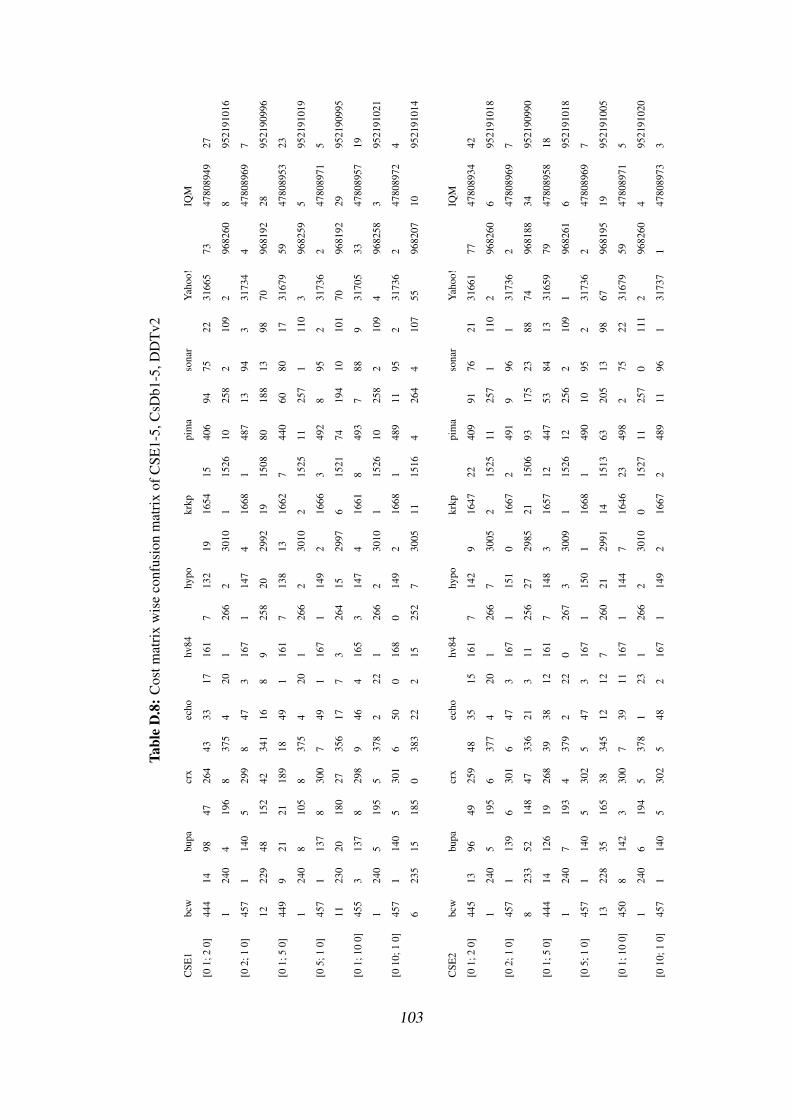
Tabl
eD
.8:C
ostm
atri
xw
ise
conf
usio
nm
atri
xof
CSE
1-5,
CsD
b1-5
,DD
Tv2
CSE
1bc
wbu
pacr
xec
hohv
84hy
pokr
kppi
ma
sona
rY
ahoo
!IQ
M
[01;
20]
444
1498
4726
443
3317
161
713
219
1654
1540
694
7522
3166
573
4780
8949
27
124
04
196
837
54
201
266
230
101
1526
1025
82
109
296
8260
895
2191
016
[02;
10]
457
114
05
299
847
316
71
147
416
681
487
1394
331
734
447
8089
697
1222
948
152
4234
116
89
258
2029
9219
1508
8018
813
9870
9681
9228
9521
9099
6
[01;
50]
449
921
2118
918
491
161
713
813
1662
744
060
8017
3167
959
4780
8953
23
124
08
105
837
54
201
266
230
102
1525
1125
71
110
396
8259
595
2191
019
[05;
10]
457
113
78
300
749
116
71
149
216
663
492
895
231
736
247
8089
715
1123
020
180
2735
617
73
264
1529
976
1521
7419
410
101
7096
8192
2995
2190
995
[01;
100]
455
313
78
298
946
416
53
147
416
618
493
788
931
705
3347
8089
5719
124
05
195
537
82
221
266
230
101
1526
1025
82
109
496
8258
395
2191
021
[010
;10]
457
114
05
301
650
016
80
149
216
681
489
1195
231
736
247
8089
724
623
515
185
038
322
215
252
730
0511
1516
426
44
107
5596
8207
1095
2191
014
CSE
2bc
wbu
pacr
xec
hohv
84hy
pokr
kppi
ma
sona
rY
ahoo
!IQ
M
[01;
20]
445
1396
4925
948
3515
161
714
29
1647
2240
991
7621
3166
177
4780
8934
42
124
05
195
637
74
201
266
730
052
1525
1125
71
110
296
8260
695
2191
018
[02;
10]
457
113
96
301
647
316
71
151
016
672
491
996
131
736
247
8089
697
823
352
148
4733
621
311
256
2729
8521
1506
9317
523
8874
9681
8834
9521
9099
0
[01;
50]
444
1412
619
268
3938
1216
17
148
316
5712
447
5384
1331
659
7947
8089
5818
124
07
193
437
92
220
267
330
091
1526
1225
62
109
196
8261
695
2191
018
[05;
10]
457
114
05
302
547
316
71
150
116
681
490
1095
231
736
247
8089
697
1322
835
165
3834
512
127
260
2129
9114
1513
6320
513
9867
9681
9519
9521
9100
5
[01;
100]
450
814
23
300
739
1116
71
144
716
4623
498
275
2231
679
5947
8089
715
124
06
194
537
81
231
266
230
100
1527
1125
70
111
296
8260
495
2191
020
[010
;10]
457
114
05
302
548
216
71
149
216
672
489
1196
131
737
147
8089
733
103
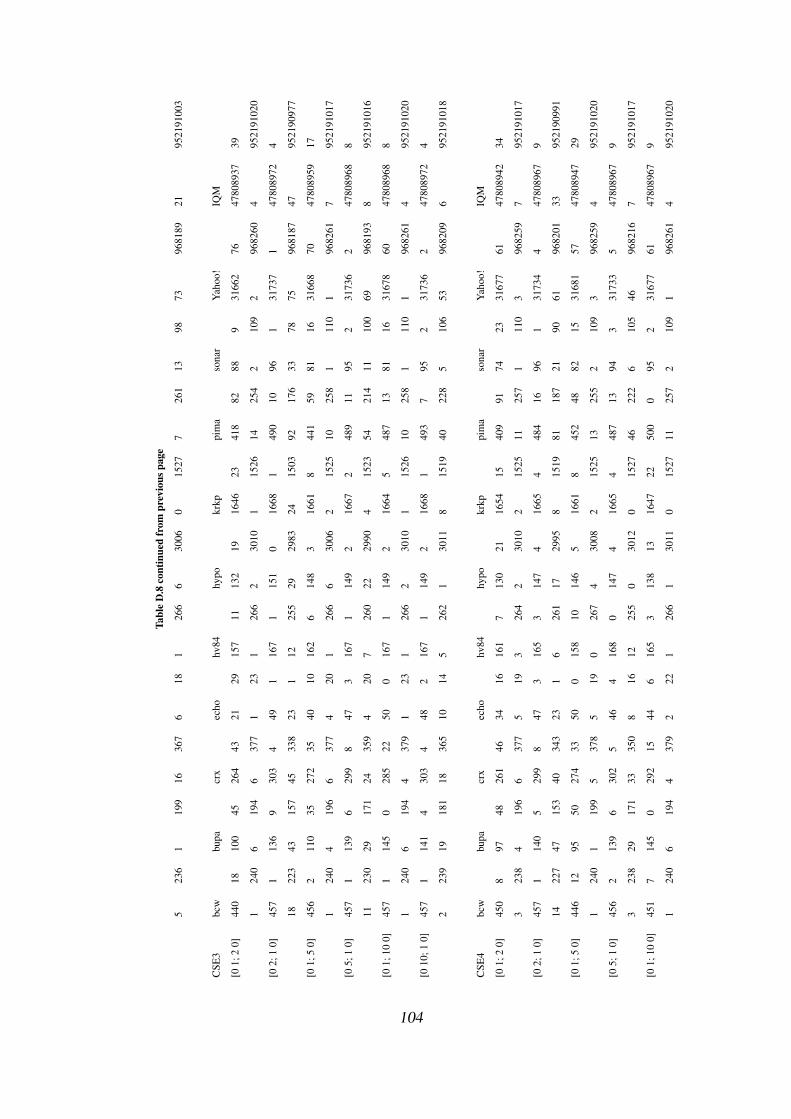
Tabl
eD
.8co
ntin
ued
from
prev
ious
page
523
61
199
1636
76
181
266
630
060
1527
726
113
9873
9681
8921
9521
9100
3
CSE
3bc
wbu
pacr
xec
hohv
84hy
pokr
kppi
ma
sona
rY
ahoo
!IQ
M
[01;
20]
440
1810
045
264
4321
2915
711
132
1916
4623
418
8288
931
662
7647
8089
3739
124
06
194
637
71
231
266
230
101
1526
1425
42
109
296
8260
495
2191
020
[02;
10]
457
113
69
303
449
116
71
151
016
681
490
1096
131
737
147
8089
724
1822
343
157
4533
823
112
255
2929
8324
1503
9217
633
7875
9681
8747
9521
9097
7
[01;
50]
456
211
035
272
3540
1016
26
148
316
618
441
5981
1631
668
7047
8089
5917
124
04
196
637
74
201
266
630
062
1525
1025
81
110
196
8261
795
2191
017
[05;
10]
457
113
96
299
847
316
71
149
216
672
489
1195
231
736
247
8089
688
1123
029
171
2435
94
207
260
2229
904
1523
5421
411
100
6996
8193
895
2191
016
[01;
100]
457
114
50
285
2250
016
71
149
216
645
487
1381
1631
678
6047
8089
688
124
06
194
437
91
231
266
230
101
1526
1025
81
110
196
8261
495
2191
020
[010
;10]
457
114
14
303
448
216
71
149
216
681
493
795
231
736
247
8089
724
223
919
181
1836
510
145
262
130
118
1519
4022
85
106
5396
8209
695
2191
018
CSE
4bc
wbu
pacr
xec
hohv
84hy
pokr
kppi
ma
sona
rY
ahoo
!IQ
M
[01;
20]
450
897
4826
146
3416
161
713
021
1654
1540
991
7423
3167
761
4780
8942
34
323
84
196
637
75
193
264
230
102
1525
1125
71
110
396
8259
795
2191
017
[02;
10]
457
114
05
299
847
316
53
147
416
654
484
1696
131
734
447
8089
679
1422
747
153
4034
323
16
261
1729
958
1519
8118
721
9061
9682
0133
9521
9099
1
[01;
50]
446
1295
5027
433
500
158
1014
65
1661
845
248
8215
3168
157
4780
8947
29
124
01
199
537
85
190
267
430
082
1525
1325
52
109
396
8259
495
2191
020
[05;
10]
456
213
96
302
546
416
80
147
416
654
487
1394
331
733
547
8089
679
323
829
171
3335
08
1612
255
030
120
1527
4622
26
105
4696
8216
795
2191
017
[01;
100]
451
714
50
292
1544
616
53
138
1316
4722
500
095
231
677
6147
8089
679
124
06
194
437
92
221
266
130
110
1527
1125
72
109
196
8261
495
2191
020
104
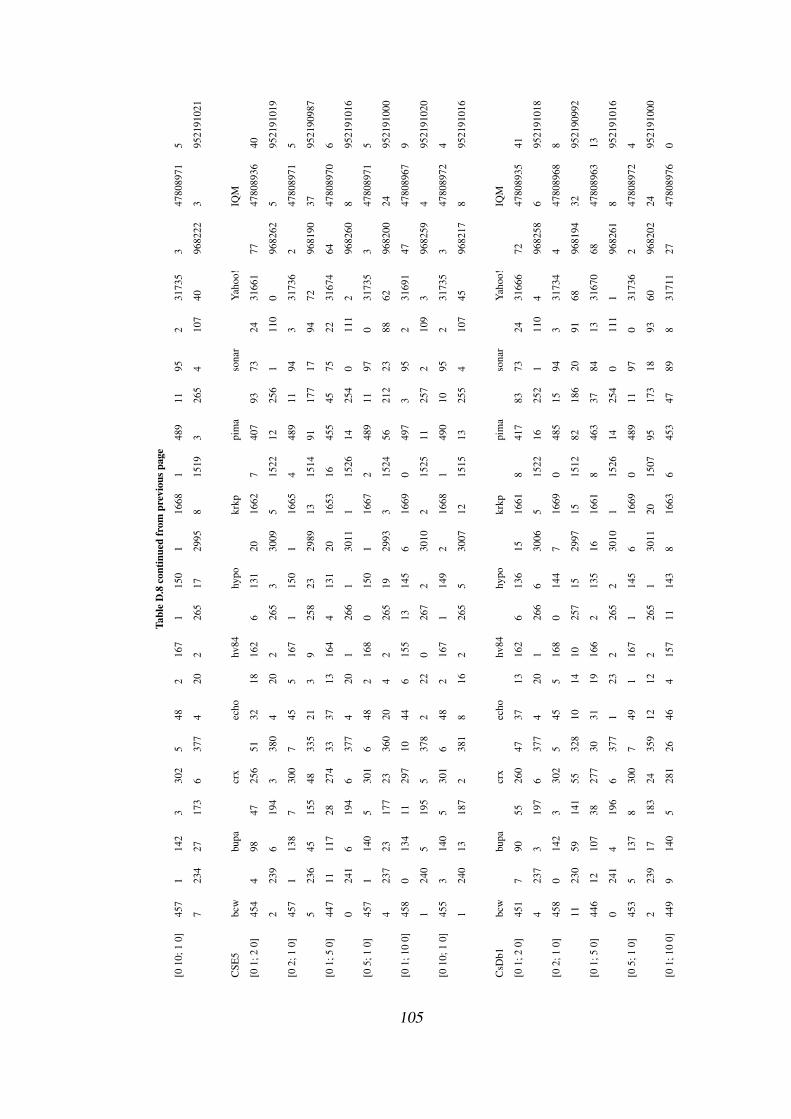
Tabl
eD
.8co
ntin
ued
from
prev
ious
page
[010
;10]
457
114
23
302
548
216
71
150
116
681
489
1195
231
735
347
8089
715
723
427
173
637
74
202
265
1729
958
1519
326
54
107
4096
8222
395
2191
021
CSE
5bc
wbu
pacr
xec
hohv
84hy
pokr
kppi
ma
sona
rY
ahoo
!IQ
M
[01;
20]
454
498
4725
651
3218
162
613
120
1662
740
793
7324
3166
177
4780
8936
40
223
96
194
338
04
202
265
330
095
1522
1225
61
110
096
8262
595
2191
019
[02;
10]
457
113
87
300
745
516
71
150
116
654
489
1194
331
736
247
8089
715
523
645
155
4833
521
39
258
2329
8913
1514
9117
717
9472
9681
9037
9521
9098
7
[01;
50]
447
1111
728
274
3337
1316
44
131
2016
5316
455
4575
2231
674
6447
8089
706
024
16
194
637
74
201
266
130
111
1526
1425
40
111
296
8260
895
2191
016
[05;
10]
457
114
05
301
648
216
80
150
116
672
489
1197
031
735
347
8089
715
423
723
177
2336
020
42
265
1929
933
1524
5621
223
8862
9682
0024
9521
9100
0
[01;
100]
458
013
411
297
1044
615
513
145
616
690
497
395
231
691
4747
8089
679
124
05
195
537
82
220
267
230
102
1525
1125
72
109
396
8259
495
2191
020
[010
;10]
455
314
05
301
648
216
71
149
216
681
490
1095
231
735
347
8089
724
124
013
187
238
18
162
265
530
0712
1515
1325
54
107
4596
8217
895
2191
016
CsD
b1bc
wbu
pacr
xec
hohv
84hy
pokr
kppi
ma
sona
rY
ahoo
!IQ
M
[01;
20]
451
790
5526
047
3713
162
613
615
1661
841
783
7324
3166
672
4780
8935
41
423
73
197
637
74
201
266
630
065
1522
1625
21
110
496
8258
695
2191
018
[02;
10]
458
014
23
302
545
516
80
144
716
690
485
1594
331
734
447
8089
688
1123
059
141
5532
810
1410
257
1529
9715
1512
8218
620
9168
9681
9432
9521
9099
2
[01;
50]
446
1210
738
277
3031
1916
62
135
1616
618
463
3784
1331
670
6847
8089
6313
024
14
196
637
71
232
265
230
101
1526
1425
40
111
196
8261
895
2191
016
[05;
10]
453
513
78
300
749
116
71
145
616
690
489
1197
031
736
247
8089
724
223
917
183
2435
912
122
265
130
1120
1507
9517
318
9360
9682
0224
9521
9100
0
[01;
100]
449
914
05
281
2646
415
711
143
816
636
453
4789
831
711
2747
8089
760
105

Tabl
eD
.8co
ntin
ued
from
prev
ious
page
024
15
195
338
02
220
267
230
102
1525
726
11
110
496
8258
595
2191
019
[010
;10]
457
114
32
301
649
116
80
142
916
681
489
1196
131
738
047
8089
715
723
437
163
338
09
1510
257
230
104
1523
326
57
104
8096
8182
095
2191
024
CsD
b2bc
wbu
pacr
xec
hohv
84hy
pokr
kppi
ma
sona
rY
ahoo
!IQ
M
[01;
20]
442
1695
5025
354
428
163
512
130
1647
2241
882
7423
3166
375
4780
8946
30
024
16
194
637
72
223
264
130
112
1525
1625
20
111
196
8261
895
2191
016
[02;
10]
454
413
78
302
545
516
80
145
616
645
484
1694
331
736
247
8089
724
1023
140
160
4433
921
310
257
1929
9311
1516
7719
121
9072
9681
9037
9521
9098
7
[01;
50]
456
297
4826
938
464
168
014
011
1665
441
981
8116
3167
167
4780
8961
15
323
82
198
437
93
2111
256
230
104
1523
726
10
111
396
8259
695
2191
018
[05;
10]
454
414
14
304
348
216
71
149
216
663
486
1491
631
733
547
8089
715
223
945
155
4733
63
219
258
2029
923
1524
4222
62
109
5396
8209
2995
2190
995
[01;
100]
457
110
540
302
546
415
414
150
116
627
473
2776
2131
679
5947
8089
679
223
92
198
937
41
230
267
330
091
1526
925
90
111
296
8260
495
2191
020
[010
;10]
456
214
05
304
347
316
71
148
316
690
491
996
131
736
247
8089
715
223
98
192
2435
91
231
266
130
1124
1503
2224
619
9250
9682
120
9521
9102
4
CsD
b3bc
wbu
pacr
xec
hohv
84hy
pokr
kppi
ma
sona
rY
ahoo
!IQ
M
[01;
20]
445
1388
5726
245
3614
160
813
813
1652
1742
377
8314
3166
969
4780
8945
31
124
02
198
737
61
233
264
730
051
1526
1625
20
111
596
8257
695
2191
018
[02;
10]
454
414
23
300
749
116
71
147
416
645
492
897
031
735
347
8089
688
523
654
146
4134
222
27
260
1130
0110
1517
9617
230
8172
9681
9027
9521
9099
7
[01;
50]
455
311
332
286
2141
915
513
134
1716
5316
427
7389
831
693
4547
8089
5026
124
05
195
737
61
230
267
330
092
1525
726
11
110
596
8257
495
2191
020
[05;
10]
456
214
32
302
548
216
62
148
316
663
487
1395
231
738
047
8089
724
823
351
149
3035
311
131
266
830
042
1525
5221
63
108
7696
8186
2395
2191
001
106
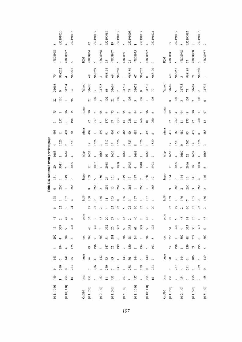
Tabl
eD
.8co
ntin
ued
from
prev
ious
page
[01;
100]
449
914
14
292
1544
616
80
131
2016
654
493
775
2231
668
7047
8089
688
124
06
194
437
92
221
266
130
111
1526
1125
71
110
096
8262
495
2191
020
[010
;10]
458
014
14
302
547
316
71
149
216
672
491
996
131
734
447
8089
724
1822
325
175
537
80
244
263
730
054
1523
7019
815
9637
9682
256
9521
9101
8
CsD
b4bc
wbu
pacr
xec
hohv
84hy
pokr
kppi
ma
sona
rY
ahoo
!IQ
M
[01;
20]
451
796
4926
047
3317
160
813
912
1652
1740
892
7027
3167
068
4780
8934
42
523
64
196
737
63
212
265
530
071
1526
1125
72
109
396
8259
595
2191
019
[02;
10]
457
114
23
300
748
216
62
150
116
663
492
895
231
735
347
8089
688
1123
053
147
5133
220
411
256
2429
8810
1517
9117
79
102
6896
8194
3595
2190
989
[01;
50]
451
793
5228
126
2723
155
1315
10
1655
1446
337
7522
3166
969
4780
8957
19
024
11
199
637
72
220
267
430
081
1526
1525
32
109
296
8260
595
2191
019
[05;
10]
457
114
32
302
545
516
62
149
216
672
485
1595
231
737
147
8089
715
323
850
150
2835
52
223
264
1729
954
1523
4022
86
105
7396
8189
2195
2191
003
[01;
100]
457
114
41
244
6340
1016
71
147
416
618
489
1194
331
671
6747
8089
751
223
96
194
537
82
221
266
230
101
1526
226
62
109
096
8262
595
2191
019
[010
;10]
458
014
05
302
548
216
71
150
116
681
490
1096
131
738
047
8089
724
1822
37
193
537
84
201
266
1929
937
1520
826
06
105
7296
8190
395
2191
021
CsD
b5bc
wbu
pacr
xec
hohv
84hy
pokr
kppi
ma
sona
rY
ahoo
!IQ
M
[01;
20]
451
790
5525
651
2822
159
913
417
1652
1741
882
898
3166
969
4780
8941
35
423
72
198
737
65
191
266
730
054
1523
1625
24
107
596
8257
595
2191
019
[02;
10]
454
414
41
302
448
216
62
144
716
690
489
1194
331
735
347
8089
688
024
161
139
4833
514
107
260
1629
9622
1505
9517
38
103
7396
8189
3795
2190
987
[01;
50]
456
210
639
274
3325
2516
53
141
1016
5712
428
7290
731
667
7147
8089
688
223
95
195
637
71
232
265
430
081
1526
826
03
108
296
8260
895
2191
016
[05;
10]
458
013
96
302
548
216
62
146
516
663
488
1297
031
737
147
8089
679
107
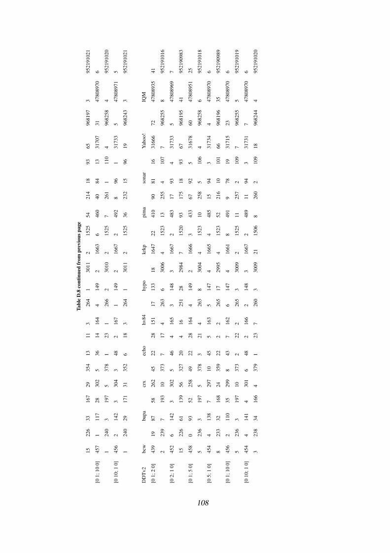
Tabl
eD
.8co
ntin
ued
from
prev
ious
page
1522
633
167
2935
413
113
264
130
112
1525
5421
418
9365
9681
973
9521
9102
1
[01;
100]
457
111
728
302
536
1416
44
149
216
636
460
4084
1331
707
3147
8089
706
124
03
197
537
81
231
266
230
102
1525
726
11
110
496
8258
495
2191
020
[010
;10]
456
214
23
304
348
216
71
149
216
672
492
896
131
733
547
8089
715
124
029
171
3135
26
183
264
130
112
1525
3623
215
9619
9682
433
9521
9102
1
DD
Tv2
bcw
bupa
crx
echo
hv84
hypo
krkp
pim
aso
nar
Yah
oo!
IQM
[01;
20]
439
1987
5826
245
2228
151
1713
318
1647
2241
090
8116
3166
672
4780
8935
41
223
97
193
1037
37
174
263
630
064
1523
1325
54
107
796
8255
895
2191
016
[02;
10]
452
614
23
302
546
416
53
148
316
672
483
1793
431
733
547
8089
697
1522
661
139
5632
720
416
251
2829
847
1520
9317
518
9367
9681
9541
9521
9098
3
[01;
50]
458
093
5225
849
2228
164
414
92
1666
343
367
925
3167
860
4780
8951
25
523
63
197
537
83
214
263
830
044
1523
1025
85
106
496
8258
695
2191
018
[05;
10]
454
413
87
297
1045
516
35
147
416
654
485
1594
331
734
447
8089
706
823
332
168
2435
922
22
265
1729
954
1523
5221
610
101
6696
8196
3595
2190
989
[01;
100]
456
211
035
299
843
716
26
147
416
618
491
978
1931
715
2347
8089
706
523
63
197
1037
32
222
265
330
092
1525
1125
72
109
796
8255
595
2191
019
[010
;10]
454
414
14
301
648
216
62
148
316
672
489
1194
331
731
747
8089
706
323
834
166
437
91
237
260
330
0921
1506
826
02
109
1896
8244
495
2191
020
108