539

Recibido: Septiembre, 2006. Aprobado: Mayo, 2007.Publicado como ENSAYO en Agrociencia 41: 539-554. 2007.

RESUMEN

Hay muchos índices de vegetación (IV) basados en relaciones del

espacio espectral del rojo e infrarrojo cercano. En este trabajo

se hace una revisión de la estructura de los IV más utilizados,

usando una formulación para caracterizar curvas de igual índice

de área foliar. Con el fin de resolver las inconsistencias encon-

tradas en los IV, se propone uno nuevo (NDVIcp), basado en la

estructura correcta del problema, bajo consideraciones empíri-

cas. El NDVIcp se valida usando datos de experimentos en cam-

po con maíz (Zea mays, L.) y algodón (Gossipyum spp).

Palabras clave: Espacio R-IRC, índices de vegetación, NDVIcp.

INTRODUCCIÓN

La tecnología de los sensores remotos ha creadouna gran expectativa en la caracterizaciónbiofísica de la vegetación. Los trabajos en esta

área muestran relaciones empíricas entre la informa-ción captada por los sensores (radianzas) a bordo desatélites comerciales, y diversas variables biofísicas[biomasa, índice de área foliar (IAF), cobertura, etcé-tera]. Debido a las propiedades ópticas de las hojasverdes, la absorción en la banda espectral del rojo delespectro electromagnético es muy alta, mientras quereflejan o dispersan la mayor parte en la banda delinfrarrojo cercano. Los índices de vegetación (IV)(Tucker, 1979; Huete, 1988), aprovechan este con-traste utilizando relaciones entre dos bandas de muestreodel espectro electromagnético, la roja (R) y la infrarrojacercana (IRC). Así, las relaciones empíricas calculadasentre las variables biofísicas de los cultivos y los IVreflejan patrones generales o tendencias entre las pro-piedades ópticas de los cultivos y su arquitectura (dis-tribución espacial y angular de los fitoelementos delfollaje), para una geometría sensor–iluminación dada.Aunque se ha intentado optimizar los IV (Liu y Huete,1995), los resultados dependen de las hipótesis consi-deradas en relación con la estructura del problema.

DISEÑO DE UN ÍNDICE ESPECTRAL DE LA VEGETACIÓN: NDVIcp

DESIGN OF A VEGETATION SPECTRAL INDEX: NDVIcp

Fernando Paz-Pellat1, Enrique Palacios-Vélez1, Martín Bolaños-González1, Luis A. Palacios-Sánchez1,

Mario Martínez-Menes1, Enrique Mejía-Saenz1 y Alfredo Huete2

1Hidrociencias. Campus Montecillo. Colegio de Postgraduados. 56230. Montecillo, Estado de México.(pellat@colpos.mx). 2University of Arizona Dept. of Soil, Water and Environ. Sciences 1200 E.South Campus Dr., Rm. 429 Shantz Bldg. #38 Tucson, AZ 85721-0038.

ABSTRACT

There are many vegetation indices (VI) based on relationships ofthe spectral space of the red and near infrared. In this study, thestructure of the most widely used VI is examined, using a

formulation to characterize curves of equal leaf area index. Inorder to solve the inconsistencies found in the VI, a new one(NDVIcp) is proposed, based on the correct structure of theproblem, under empirical considerations. The NDVIcp is validatedusing data from field experiments with maize (Zea mays L.) andcotton (Gossipyum spp.).

Key words: Space R-IRC, vegetation indices, NDVIcp.

INTRODUCTION

The technology of remote sensors has created agreat expectation in the biophysicalcharacterization of plants. The works in this

area show empirical relationships between theinformation captured by the sensors (radiances) oncommercial satellites, and diverse biophysical variables(biomass, leaf area index (LAI), canopy cover, etc.).Due to the optical properties of the green leaves, theabsorption in the spectral band of the red of theelectromagnetic spectrum is very high, whereas theyreflect or disperse the greatest part in the band of thenear infrared. The vegetation indices (VI) (Tucker,1979; Huete, 1988), take advantage of this contrastby utilizing relationships between two bands of theelectromagnetic spectrum, the red (R) and the nearinfrared (IRC). Thus, the empirical relationshipscalculated between the biophysical variables of the cropsand the VI reflect general patterns or tendencies amongthe optical properties of the crops and their architecture(spatial and angular distribution of the phytoelementsof the foliage), for a given sensor-illumination geometry.Although several attempts have been made to optimizethe VI (Liu and Huete, 1995), the results depend onthe hypotheses considered in relation to the structureof the problem.

Although numerous works have been written relatedto vegetation indices, the problem remains as to which

AGROCIENCIA, 1 de julio - 15 de agosto, 2007

540 VOLUMEN 41, NÚMERO 5

Aunque se han escrito numerosos trabajos relacio-nados con los índices de vegetación, permanece el pro-blema sobre cuál es el más apropiado. Así, el objetivoprimario de este trabajo es esclarecer la estructura delproblema en el diseño de IV y plantear un esquemaapropiado de solución.

En este trabajo se revisan diferentes IV y se mues-tran sus alcances y limitaciones, utilizando un plantea-miento general del problema de estimación de IV. Par-tiendo de la estructura del problema, se propone uníndice que considera la dinámica de la mezcla suelo-vegetación en forma correcta. Se ejemplifica el índicepropuesto con mediciones en campo.

Espacio espectral R-IRC de la mezclasuelo-vegetación

En la Figura 1 se muestra el espacio espectral R-IRC del patrón temporal de crecimiento de un cultivo,representado por curvas de igual índice de área foliaro IAF (iso-IAF); el nombre común de esta gráfica essombrero de tres picos. La Figura 1 se generó usandoseis tipos de suelos (S2, S5, S7, S9, S11 y S12; delmás oscuro al más claro). Paz et al. (2005) detallan lassimulaciones radiativas mostradas en la Figura 1.

El análisis de la Figura 1 define varios patronesmuy importantes para entender el comportamiento dela reflectividad durante el desarrollo de los cultivos:

a) Si se unen los valores de igual IAF (iso-IAF) decada curva de igual suelo (iso-Suelo), se obtiene unpatrón cuasi-lineal. Este patrón ha sido verificadoexperimentalmente (Huete et al., 1985; Price, 1992-con datos de Huete y Jackson 1987-, Baush, 1993;Xia, 1994; Gilabert et al., 2002; Meza Díaz yBlackburn, 2003) y por modelos de transferenciaradiativa (Richardson y Wiegand, 1991; Baret yGuyot, 1991; Qi et al., 1994; Yoshioka et al., 2000).En realidad, la curva de iso-IAF corresponde a uncomportamiento de tipo parabólico (considerandointeracciones de segundo orden), que si no se consi-deran suelos muy claros, resulta en una línea recta(interacciones de primer orden). Así, el estado decrecimiento de un cultivo (IAF) se refleja en unalínea recta, independientemente del tipo de suelo defondo en el cultivo.

b) La pendiente e intersección de las líneas rectas deiso-IAF varían con el valor del IAF, como se obser-va en la Figura 1. La inclinación (pendiente) de lasrectas de iso-IAF parte desde una pendiente igual ala de la línea del suelo (IAF=0) y aumenta hastaalcanzar un ángulo de 90° en sentido contrario a lasmanecillas del reloj. Esta última condición corres-ponde al caso de saturación de la reflectividad de la

Figura 1. Espacio espectral IRC-R para las simulaciones en elcultivo maíz.

Figure 1. Spectral space IRC-R for the simulations in the maizecrop.

70

60

50

40

30

IRC (

%)

20

10

00 5

R (%)

10 15

S12

IAF=0.0IAF=1.0IAF=3.0IAF=12IAF=0.5IAF=2.0IAF=5.0

S11S9

S7S5

S2

20

is the most appropriate. Therefore, the primary objectiveof the present study is to clarify the structure of theproblem in the design of VI and to offer an appropriatescheme of solution.

The present work examines different VI and theirpotential and limits are shown, using a general statementof the problem of estimation of VI. From the structureof the problem, an index is proposed that considers thedynamic of the soil-vegetation mixture in the correctform. The proposed index is exemplified with fieldmeasurements.

Spectral space R-IRC of thesoil-vegetation mixture

Figure 1 shows the spectral space R-IRC of thetemporal growth pattern of a crop, represented by curvesof equal leaf area index or LAI (iso-LAI); the commonname of this graph is tassled cap. Figure 1 was generatedusing six types of soil (S2, S5, S7, S9, S11 and S12;from the darkest to the lightest). Paz et al. (2005)detail the radiative simulations shown in Figure 1.

The analysis of Figure 1 defines various patternsthat are very important for understanding the behaviourof the reflectance during crop development:

a) If the values of equal LAI (iso-LAI) are joined fromeach curve of equal soil (iso-Soil), a quasi-linearpattern is obtained. This pattern has been verifiedexperimentally (Huete et al., 1985; Price, 1992 –with data of Huete and Jackson 1987-, Baush, 1993;Xia, 1994; Gilabert et al., 2002; Meza Díaz andBlackburn, 2003) and by models of radiative transfer(Richardson and Wiegand, 1991; Baret and Guyot,

541PAZ-PELLAT et al.

DISEÑO DE UN ÍNDICE ESPECTRAL DE LA VEGETACIÓN: NDVIcp

banda del R, representada en la Figura 1 como losvalores de reflectividad arriba del ápice del sombre-ro de tres picos (IAF>5 en la Figura 1). Los patro-nes de los espacios espectrales IRC-Visible (azul,verde y rojo) son similares para todas las bandas delespectro visible, dado que hay una relación linealentre estas bandas.

c) Todas las curvas de iso-Suelos convergen al mismopunto de saturación de las bandas visibles. En reali-dad el sombrero de tres picos tiene una línea rectacomo ápice, ya que cuando una banda visible sesatura, el IRC no lo hace y sigue creciendo hasta supropio punto de saturación. Esta propiedad es muyimportante para el diseño de algoritmos de índicesde la señal del suelo y de la vegetación, y refleja lacondición física en que el suelo no se ve (relativo acada banda espectral) y sólo se observa la vegeta-ción. El punto de saturación, llamado también dereflectividad infinita o de medio ópticamente denso,es función del espectro de las hojas y de su distribu-ción angular.

Las curvas iso-IAF mostradas en la Figura 1 sepueden describir como:

IRCIAF = a0,IAF + b0,IAF RIAF (1)

donde el subíndice IAF se refiere a un valor específicodel IAF de la mezcla suelo-vegetación. Los parámetrosde la recta definida por la ecuación (1), a0,IAF (en %para nuestro caso) y b0,IAF (adimensional), dependendel valor de IAF. En lo que sigue se omitirá el subíndiceIAF en R e IRC.

Índices de vegetación y sus limitaciones

Los índices de vegetación basados en el espacioespectral R-IRC tratan de calcular el estado de creci-miento de un cultivo (IAF u otra variable relacionada).Índices de vegetación ampliamente usados en las apli-caciones de la técnica de sensores remotos son:

- IV de razones (Ratio Vegetation Index: Pearson yMiller, 1972):

RVIIRCR

= (2)

- IV de diferencias normalizadas (Normalized DifferenceVegetation Index: Rouse et al., 1974):

NDVIIRC RIRC R

RVIRVI

=−

+=

−

+

11

(3)

1991; Qi et al., 1994; Yoshioka et al., 2000).Actually, the curve of iso-LAI corresponds to aparabolic type behaviour (considering second orderinteractions), which if very light soils are notconsidered, result in a straight line (first orderinteractions). Thus, the stage of growth of a crop(LAI) is mapped in a straight line, regardless of thetype of background soil in the crop.

b) The slope and intersection of the straight lines ofiso-LAI vary with the value of the LAI, as isobserved in Figure 1. The slope of the straight linesof iso-LAI goes from a slope equal to that of thesoil line (LAI=0) and increases until reaching a90° angle counter clock-wise. This last conditioncorresponds to the case of saturation of thereflectance of the band of the R, represented inFigure 1 as the values of reflectance above the apexof the tassled cap (LAI>5 in Figure 1). The patternsof the spectral spaces IRC-Visible (blue, green andred) are similar for all of the bands of the visiblespectrum, given that there is a linear relationshipamong these bands.

c) All of the curves of iso-Soils converge at the samepoint of saturation of the visible bands. In realitythe tassled cap has a straight line as apex, giventhat when a visible band becomes saturated, theIRC does not, and keeps growing up to its ownsaturation point. This property is very importantfor the design of algorithms of indices of the signalfrom the soil and of the vegetation, and shows thephysical condition in which the soil is not visible(relative to each spectral band) and only thevegetation is observed. The saturation point, alsoreferred to as infinite reflectance or optically densemedium, is a function of the spectrum of the leavesand of their angular distribution.

The iso-LAI curves shown in Figure 1 can be describedas follows:

IRCLAI = a0,LAI + b0,LAI RLAI (1)

where the sub-index LAI refers to a specific value ofthe LAI of the soil-vegetation mixture. The parametersof the straight line defined by equation (1), a0,LAI (in %for this case) and b0,LAI (adimensional), depend on thevalue of LAI. In what follows the sub-index LAI willbe omitted in R and IRC.

Vegetation indices and their limitations

The vegetation indices based on the spectral spaceR-IRC attempt to calculate the growth stage of a crop(LAI or another related variable). Vegetation indices

AGROCIENCIA, 1 de julio - 15 de agosto, 2007

542 VOLUMEN 41, NÚMERO 5

- IV perpendicular (Perpendicular Vegetation Index:Richardson y Wiegand, 1977):

(4)

- IV de diferencias (Difference Vegetation Index: Jordan,1969):

DVI=IRC−R (5)

- IV de diferencias ponderadas (Weighted DifferenceVegetation Index: Clevers, 1989):

WDVI=IRC−bSR (6)

- IV ajustado por suelo (Soil Adjusted Vegetation Index:Huete, 1988):

SAVIIRC R

IRC R LL=

−( )

+ +( )+( )1 (7)

- IV ajustado por suelo transformado (Transformed SoilAdjusted Vegetation Index: Baret et al., 1989):

TSAVIb IRC b R a

R b IRC a b X b

S S S

S S S S

=− −

+ − + +

a fc h1 2 (8)

- IV ajustado por suelo optimizado (Optimized SoilAdjusted Vegetation Index: Rondeaux et al., 1996):

OSAVIIRC R

IRC R Y=

−

+ +(9)

- IV ajustado por suelo generalizado (Generalized SoilAdjusted Vegetation Index: Gilabert et al., 2002):

(10)

- IV de proporciones pareadas (Paz et al., 2003):

(11)

donde L, X, Y y Z son valores que se dejan constantes(L=0.5, X=0.08, Y=0.16 y Z=0.35, para valores dereflectividad en proporciones) y la línea del suelo(IAF=0) está definida por los parámetros aS y bS.

widely used in the applications of remote sensortechnique are:

-VI of ratios (Ratio Vegetation Index: Pearson andMiller, 1972):

RVIIRCR

= (2)

-VI of normalized differences (Normalized DifferenceVegetation Index: Rouse et al., 1974):

NDVIIRC RIRC R

RVIRVI

=−

+=

−

+

11

(3)

-VI perpendicular (Perpendicular Vegetation Index:Richardson and Wiegand, 1977):

(4)

-VI of differences (Difference Vegetation Index: Jordan,1969):

DVI=IRC−R (5)

-VI of weighted differences (Weighted DifferenceVegetation Index: Clevers, 1989):

WDVI=IRC−bSR (6)

-VI soil adjusted (Soil Adjusted Vegetation Index: Huete,1988):

SAVIIRC R

IRC R LL=

−( )

+ +( )+( )1 (7)

-VI transformed soil adjusted (Transformed Soil AdjustedVegetation Index: Baret et al., 1989):

TSAVIb IRC b R a

R b IRC a b X b

S S S

S S S S

=− −

+ − + +

a fc h1 2 (8)

-VI optimized soil adjusted (Optimized Soil AdjustedVegetation Index: Rondeaux et al., 1996):

OSAVIIRC R

IRC R Y=

−

+ +(9)

GESAVIIRC b R a

IRC ZS S=

− −

+

PVIIRC b R a

b

S S

S

=− −

+1 2

PVIIRC b R a

b

S S

S

=− −

+1 2

IVPPIRC b R a

IRCS S=

− −

543PAZ-PELLAT et al.

DISEÑO DE UN ÍNDICE ESPECTRAL DE LA VEGETACIÓN: NDVIcp

Para entender las limitaciones de los IV es necesa-rio definir el contexto de lo que se caracterizará. UnIV trata de aproximar una línea recta usando sólo unpar de valores (R, IRC) que representan una cantidaddesconocida de vegetación mezclada con un suelo dereflectividad también desconocida.

Las hipótesis para caracterizar un conjunto de lí-neas rectas (iso-IAF) representando la dinámica de cre-cimiento de un cultivo se pueden plantear como:

a) suponer la intersección de las líneas en el origen (0,0) y dejar que la pendiente varíe (casos del RVI yNDVI):

IRCNDVINDVI

R RVIxR=+

−FHG

IKJ =

11 (12)

b) suponer una pendiente de las líneas y dejar que laintersección con el eje IRC varíe (casos del DVI yWDVI):

IRC = DVI + R (13)

IRC = WDVI + bSR (14)

El PVI es similar al WDVI, pero lo que varía es laintersección con el eje IRC, ya que está en función dela distancia perpendicular a la línea del suelo y seincrementa a partir de la intersección aS de la línea delsuelo con el eje IRC.

c) dejar que el origen, generalmente en el tercer cua-drante de los ejes R e IRC, con coordenadas (−l1 y−l2) y la pendiente varíen (resto de los índices). Porejemplo, el SAVI fue diseñado en función del NDVIagregándole valores constantes (para una línea iso-IAF dada) al R e IRC:

SAVIIRC l R l

IRC l R l=

+ − +

+ + +2 1

2 1

a f a fa f a f (15)

Puesto que la línea del suelo tiene una pendientecercana a 1.0, los factores de ajuste l1 y l2 (origen)serán aproximadamente iguales. Así, el SAVI suponeque L=l1+l2, donde el factor (L) en la ecuación (7) seintroduce para mantener los mismos límites que elNDVI. De esta forma, la ecuación que representa elSAVI está definida por:

IRCSAVIxLL SAVI

L SAVI

L SAVIR=

+( )−

FHG

IKJ+

+( )+

+( )−

FHG

IKJ1

1

1 (16)

-VI generalized soil adjusted (Generalized Soil AdjustedVegetation Index: Gilabert et al., 2002):

GESAVIIRC b R a

IRC ZS S=

− −

+(10)

-VI of paired proportions (Paz et al., 2003):

IVPPIRC b R a

IRCS S=

− −

(11)

where L, X, Y and Z are values that are left constant(L=0.5, X=0.08, Y=0.16 and Z=0.35, for values ofreflectance in proportions) and the soil line (LAI=0) isdefined by the parameters aS and bS.

To understand the limitations of the VI, it isnecessary to define the context of what is to becharacterized. A VI attempts to approximate a straightline using only one pair of values (R, IRC) that representan unknown amount of vegetation mixed with a soil ofalso unknown reflectance.

The hypotheses for characterizing a group of straightlines (iso-LAI) representing the growth dynamic of acrop can be stated as follows:

a) assume the intersection of the lines at the origin (0,0) and let the slope vary (cases of the RVI andNDVI):

IRCNDVINDVI

R RVIxR=+

−FHG

IKJ =

11 (12)

b) assume a slope of the lines and let the intersectionwith the axis IRC vary (cases of DVI and WDVI):

IRC = DVI + R (13)

IRC = WDVI + bSR (14)

The PVI is similar to the WDVI, but what varies isthe intersection with the axis IRC, given that it is afunction of the distance perpendicular to the soil lineand increases from the intersection aS of the soil linewith the axis IRC.

c) let the origin, generally in the third quadrant of theaxis R and IRC, with coordinates (−1 and −12),and the slope vary (rest of the indices). For example,the SAVI was designed as a function of the NDVIadding constant values (for a given line iso-LAI) tothe R and IRC:

IVPPIRC b R a

IRCS S=

− −IVPP

IRC b R aIRC

S S=− −

El PVI es similar al WDVI, pero lo que varía es laintersección con el eje IRC, ya que está en función dela distancia perpendicular a la línea del suelo y seincrementa a partir de la intersección aS de la línea delsuelo con el eje IRC.

AGROCIENCIA, 1 de julio - 15 de agosto, 2007

544 VOLUMEN 41, NÚMERO 5

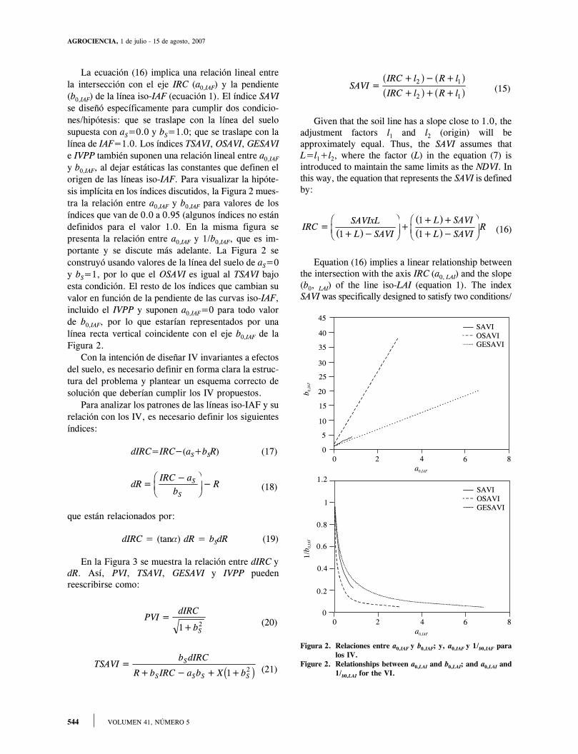
La ecuación (16) implica una relación lineal entrela intersección con el eje IRC (a0,IAF) y la pendiente(b0,IAF) de la línea iso-IAF (ecuación 1). El índice SAVIse diseñó específicamente para cumplir dos condicio-nes/hipótesis: que se traslape con la línea del suelosupuesta con aS=0.0 y bS=1.0; que se traslape con lalínea de IAF=1.0. Los índices TSAVI, OSAVI, GESAVIe IVPP también suponen una relación lineal entre a0,IAF

y b0,IAF, al dejar estáticas las constantes que definen elorigen de las líneas iso-IAF. Para visualizar la hipóte-sis implícita en los índices discutidos, la Figura 2 mues-tra la relación entre a0,IAF y b0,IAF para valores de losíndices que van de 0.0 a 0.95 (algunos índices no estándefinidos para el valor 1.0. En la misma figura sepresenta la relación entre a0,IAF y 1/b0,IAF, que es im-portante y se discute más adelante. La Figura 2 seconstruyó usando valores de la línea del suelo de aS=0y bS=1, por lo que el OSAVI es igual al TSAVI bajoesta condición. El resto de los índices que cambian suvalor en función de la pendiente de las curvas iso-IAF,incluido el IVPP y suponen a0,IAF=0 para todo valorde b0,IAF, por lo que estarían representados por unalínea recta vertical coincidente con el eje b0,IAF de laFigura 2.

Con la intención de diseñar IV invariantes a efectosdel suelo, es necesario definir en forma clara la estruc-tura del problema y plantear un esquema correcto desolución que deberían cumplir los IV propuestos.

Para analizar los patrones de las líneas iso-IAF y surelación con los IV, es necesario definir los siguientesíndices:

dIRC=IRC−(aS+bSR) (17)

dRIRC a

bRS

S=

−FHG

IKJ− (18)

que están relacionados por:

dIRC = (tanα) dR = bSdR (19)

En la Figura 3 se muestra la relación entre dIRC ydR. Así, PVI, TSAVI, GESAVI y IVPP puedenreescribirse como:

PVIdIRC

bS

=+1 2 (20)

TSAVIb dIRC

R b IRC a b X bS

S S S S

=+ − + +1 2c h (21)

Figura 2. Relaciones entre a0,IAF y b0,IAF; y, a0,IAF y 1/b0,IAF paralos IV.

Figure 2. Relationships between a0,LAI and b0,LAI; and a0,LAI and1/b0,LAI for the VI.

45

1.2

40

1

35

0.8

SAVIOSAVIGESAVI

SAVIOSAVIGESAVI

30

0.6

25

0.4

b 0,I

AF

1/b 0

,IAF

20

0.2

15

10

5

0

0

0

0

2

2

a0,IAF

a0,IAF

4

4

6

6

8

8

SAVIIRC l R l

IRC l R l=

+ − +

+ + +2 1

2 1

a f a fa f a f (15)

Given that the soil line has a slope close to 1.0, theadjustment factors l1 and l2 (origin) will beapproximately equal. Thus, the SAVI assumes thatL=l1+l2, where the factor (L) in the equation (7) isintroduced to maintain the same limits as the NDVI. Inthis way, the equation that represents the SAVI is definedby:

IRCSAVIxLL SAVI

L SAVI

L SAVIR=

+( )−

FHG

IKJ+

+( )+

+( )−

FHG

IKJ1

1

1 (16)

Equation (16) implies a linear relationship betweenthe intersection with the axis IRC (a0, LAI) and the slope(b0, LAI) of the line iso-LAI (equation 1). The indexSAVI was specifically designed to satisfy two conditions/

545PAZ-PELLAT et al.

DISEÑO DE UN ÍNDICE ESPECTRAL DE LA VEGETACIÓN: NDVIcp

GESAVIdIRC

IRC Z=

+(22)

IVPPdIRCIRC

=

(23)

En la Figura 4 se muestra la geometría general dela posición de una línea iso-IAF en relación con lalínea del suelo. El punto de cruce entre ambas líneas(Figura 4) ésta dado por:

Figura 3. Relación entre los índices dIRC y dR.Figure 3. Relationship between the indices dIRC and dR.

Figura 4. Relaciones geométricas entre las curvas iso-IAF y lalínea del suelo.

Figure 4. Geometric relationships between the curves iso-LAI andthe soil line.

35

30

25

20

15

dR

PVI

αdIRC

IRC

(%

)

10

5

00 5

Curva iso-IAFLínea del suelo

10 15 20 25 30 35R (%)

35

30

25

20

15θ1

θ2

IRC

(%

)

10

5

−5−5

−10

−10

−15

00 5

(Rc, IRCc)

Curva iso-IAFLínea del suelo

10 15 20 25 30 35

R (%)

hypotheses: that it overlaps with the assumed soil linewith aS=0.0 and bS=1.0; that it overlaps with the lineof LAI=1.0. The indices TSAVI, OSAVI, GESAVI andIVPP also assume a linear relationship between a0,LAI

and b0,LAI, as they leave static the constants that definethe origin of the lines iso-LAI. To visualize thehypothesis implicit in the previously mentioned indices,Figure 2 shows the relationship between a0,LAI andb0,LAI for values of the indices that go from 0.0 to 0.95(some indices are not defined for the value 1.0). In thesame figure, the relationship is presented between a0,LAI

and 1/b0,LAI, which is important and is discussed below.Figure 2 was constructed using values of the soil lineof aS=0 and bS=1, therefore the OSAVI is equal to theTSAVI under this condition. The rest of the indices thatchange their value as a function of the slope of thecurves iso-LAI, including the IVPP assume a0,LAI=0for all values of b0,LAI, thus would be represented by avertical straight line coinciding with the axis b0, LAI ofFigure 2.

With the intention of designing VI invariant to effectsof the soil, it is necessary to clearly define the structureof the problem and to establish a correct scheme ofsolution that should be satisfied by the proposed VI.

To analyze the patterns of the lines iso-LAI andtheir relationship with the VI, it is necessary to definethe following indices:

dIRC=IRC−(aS+bSR) (17)

dRIRC a

bRS

S=

−FHG

IKJ− (18)

which are related by:

dIRC = (tanα) dR = bSdR (19)

Figure 3 shows the relationship between dIRC anddR. Thus, PVI, TSAVI, GESAVI and IVPP can berewritten as:

PVIdIRC

bS

=+1 2 (20)

TSAVIb dIRC

R b IRC a b X bS

S S S S

=+ − + +1 2c h (21)

GESAVIdIRC

IRC Z=

+(22)

IVPPdIRCIRC

=

IVPPdIRCIRC

=

AGROCIENCIA, 1 de julio - 15 de agosto, 2007

546 VOLUMEN 41, NÚMERO 5

Rca a

b bS IAF

IAF S=

−

−0

0

,

,(24)

IRCa b a b

b bcIAF S S IAF

S IAF=

−

−0 0

0

, ,

,(25)

De las propiedades invariantes entre dos líneas rec-tas que se cruzan (Gilabert et al., 2002), se puedenestablecer las siguientes relaciones (Figura 3 y 4):

tan θ1 = −=

−

dIRCR Rc

b dRR R

S

C(26)

tan θ2 = −=

−

dRIRC IRC

dIRCb IRC IRCC S Ca f (27)

IVPPdR

R RdIRC

b R RCRC S

=−

=−( ) (28)

IVPPdIRC

IRC IRCb dR

IRC IRCIRCC

S

C=

−=

− (29)

Los índices definidos por las relaciones (26) a (29),para curvas iso-IAF individuales, son IV perfectos parala eliminación del efecto del suelo.

De las ecuaciones 26 a 29, la relación entre ellasestá dada por:

tan θ1 = bS IVPPR (30)

tan θ2 =IVPP

bIRC

S(31)

De los IV revisados, sólo GESAVI e IVPP tienenuna estructura correcta, de acuerdo con las propieda-des invariantes mostradas en las ecuaciones 26 a 29.Para determinar estas propiedades o índices invariantes(sin efecto del suelo) es necesario conocer los parámetrosde las curvas iso-IAF. Puesto que ésto no es posible,ya que sólo se cuenta con un punto (R, IRC) de lalínea, es necesario suponer uno de los valores (Rc,IRCc; IRCc=aS+bSRc) o uno de los parámetros de lalínea iso-IAF (a0,IAF, b0,IAF).

El problema de las relaciones (26) a (29), IVinvariantes, es que se requiere conocer en forma di-námica los cruces de las líneas iso-IAF con la línea

IVPPdIRCIRC

= (23)

Figure 4 shows the general geometry of the positionof a line iso-LAI with respect to the soil line. Thecross point between both lines (Figure 4) is given by:

Rca a

b bS LAI

LAI S=

−

−0

0

,

,(24)

IRCa b a b

b bcLAI S S LAI

S LAI=

−

−0 0

0

, ,

,(25)

From the invariant properties between two straightlines that cross (Gilabert et al., 2002), the followingrelationships can be established (Figures 3 and 4):

tan θ1 = −=

−

dIRCR Rc

b dRR R

S

C(26)

tan θ2 = −=

−

dRIRC IRC

dIRCb IRC IRCC S Ca f (27)

IVPPdR

R RdIRC

b R RCRC S

=−

=−( ) (28)

IVPPdIRC

IRC IRCb dR

IRC IRCIRCC

S

C=

−=

− (29)

The indices defined by the relationships (26) to (29),for individual curves iso-LAI, are VI perfect for theelimination of the effect of the soil.

Of equations 26 to 29, the relationship among themis given by:

tan θ1 = bS IVPPR (30)

tan θ2 =IVPP

bIRC

S(31)

Of the VI that were analyzed, only GESAVI andIVPP have a correct structure, according to the invariantproperties shown in equations 26 to 29. To determinethese properties or invariant indices (without soil effect),it is necessary to know the parameters of the curvesiso-LAI. Since this is not possible, because we have

547PAZ-PELLAT et al.

DISEÑO DE UN ÍNDICE ESPECTRAL DE LA VEGETACIÓN: NDVIcp

del suelo. Para establecer una primera aproximaciónen relación al patrón temporal (crecimiento del IAF)de la vegetación, es necesario conocer la relación entrelos parámetros a0,IAF−b0,IAF para definir una relaciónfuncional entre ellos. Los IV con una estructura simi-lar al SAVI suponen una relación lineal entre estosparámetros.

Índice espectral de la vegetación NDVIcp

Suponiendo un intervalo de valores del NDVI de 0a 1 para la mezcla suelo-vegetación, el valor NDVI=0.0representa una línea del suelo (suelo desnudo, sin ve-getación) con parámetros as=0.0 y bS=1.0. La condi-ción NDVI=1.0 representa el caso donde el suelo estátotalmente cubierto por la vegetación (con la banda delR saturada; sin cambiar de valor).

En la Figura 1 se muestra que las intersecciones delas curvas iso-IAF son diferentes para cada valor delIAF, aunque las pendientes de éstas siguen un patrónsimilar al mostrado por el NDVI. El NDVI supone quetodas las líneas iso-IAF tienen un origen común en elespacio del R-IRC (0,0), y los cambios en la vegeta-ción sólo se manifiestan por un cambio en la pendien-te. De la Figura 1 resulta claro que la hipótesis implí-cita en el NDVI es incorrecta, por lo que se requiereajustar las reflectividades del R y del IRC para que lashipótesis del NDVI reflejen la realidad.

De la definición de las líneas iso-IAF dada por laecuación (1), para que las curvas iso-IAF tengan unorigen en (0,0) es necesario que la reflectividad delIRC sea transformada como:

IRCcs=(IRC−a0,IAF)=b0,IAFR (32)

La reflectividad IRCcs está corregida por el efectodel suelo y cumple con que el patrón para las curvasde igual NDVI sea igual al de iso-IAF. El problema deeste esquema de corrección del efecto del suelo en elNDVI es que es necesario conocer el valor del parámetroa0,IAF el cual varía con el IAF de la vegetación. Paraconocer el valor de a0,IAF es necesario establecer larelación entre a0,IAF−b0,IAF de las curvas iso-IAF.

En la Figura 5 se muestra la relación entre losparámetros a0,IAF y b0,IAF de la Figura 1, para el ciclode crecimiento del cultivo desde el suelo desnudo has-ta su cubrimiento completo por la vegetación. En ellase observa que en la etapa inicial hay un patrón decomportamiento tipo exponencial, hasta el punto don-de la banda R se satura (no cambia de valor). Despuésdel punto de saturación de la banda R, el patrón es deltipo lineal. El punto inicial de la curva a0,IAF−b0,IAF (Fi-gura 4) representa el caso de suelo desnudo (a0,IAF=0 =aS y b0,IAF=0 =bS). El punto donde a0,IAF alcanza su

only one point (R, IRC) of the line, it is necessary toassume one of the values (Rc, IRCc; IRCc=aS+bSRc)or one of the parameters of the line iso-LAI (a0,LAI,

b0,LAI). The problem of the relationships (26) to (29) VI,invariant is that it requires dynamic knowledge of thecrosses of the lines iso-LAI with the soil line. To establishan initial approximation with respect to the temporalpattern (growth of the LAI) of the vegetation, it isnecessary to know the relationship between theparameters a0,LAI−b0,LAI to define a functionalrelationship between them. The VI with a structuresimilar to the SAVI assume a linear relationship betweenthese parameters.

Vegetation spectral index NDVIcp

Assuming an interval of values of the NDVI from 0to 1 for the soil-vegetation mixture, the value NDVI=0.0represents a soil line (bare soil, without vegetation)with parameters as=0.0 and bS=1.0. The conditionNDVI=1.0 represents the case in which the soil is totallycovered by the vegetation (with the R band saturated;without change of value).

Figure 1 shows that the intersections of the curvesiso-LAI are different for each value of the LAI, althoughtheir slopes follow a pattern similar to that shown bythe NDVI. The NDVI assumes that all the lines iso-LAIhave a common origin in the space of the R-IRC (0,0),and the changes in the vegetation are only manifestedby a change in slope. From Figure 1 it is clear that thehypothesis implicit in the NDVI is incorrect, thus it isnecessary to adjust the reflectances of the R and of theIRC so that the hypotheses of the NDVI reflect reality.

From the definition of the lines iso-LAI given byequation (1), for the curves iso-LAI to have an originin (0,0), it is necessary that the reflectance of the IRCbe transformed as follows:

IRCcs=(IRC−a0,LAI)=b0,LAI R (32)

The reflectance IRCcs is corrected by the effect ofsoil and complies with the requirement that the patternfor the curves of equal NDVI be equal to that of iso-LAI. The problem of this scheme of correction of thesoil effect in the NDVI is that it is necessary to knowthe value of the parameter a0,IAF , which varies withthe LAI of the vegetation. To know the value of a0,LAI,it is necessary to know the relationship between a0,LAI−

b0,LAI of the curves iso-LAI.Figure 5 shows the relationship between the

parameters a0,LAI and b0,LAI of Figure 1, for the growthcycle of the crop from bare soil to its complete coverageby the vegetation. It can be observed that in the initial

AGROCIENCIA, 1 de julio - 15 de agosto, 2007

548 VOLUMEN 41, NÚMERO 5

stage there is an exponential type behaviour pattern,up to the point in which the R band becomes saturated(no more change of value). After the saturation pointof the R band, the pattern is of the linear type. Theinitial point of the curve a0,LAI−b0,LAI (Figure 4)represents the case of bare soil (a0,LAI=0=aS and b0,LAI=0=bS). The point where a0,LAI reaches its maximum value(transition point of the exponential to the linear pattern),represents the end of the exponential growth phase andthe start of the linear one. The final point of the linearpattern of the curve a0,LAI−b0,LAI represents the situationwhere the band of the IRC becomes saturated, whichoccurs when the LAI reaches its maximum value.

Figure 5 also shows a transformation (b0,LAI → 1/b0,LAI) which turns the expo-linear functionapproximately linear. This transformation was chosento adequately model the transition between theexponential and linear phases. Comparing thehypotheses of the VI (Figure 2), with those defined bythe radiative simulations (Figure 5), the differencesbetween the assumed and the theoretical (andexperimental, as will be seen below) are clear.

To validate the proposal of the relationship betweena0,LAI and b0,LAI, an analysis is made of two fieldexperiments with contrasting crops: maize (Zea maysL.) (Bausch, 1993) and cotton (Gossipium spp) (Hueteet al., 1985). In both experiments, sliding trays wereused with different soils under the crops. In thereferences mentioned these experiments are describedin detail.

Figure 6 shows the curves iso-LAI of theexperiment of maize and cotton, in the spectral spaceR-IRC. The pattern between the parameters a0,LAI ofthe curves iso-LAI OF Figure 6 is similar to thatshown in Figure 1.

A good approximation to the exponential behaviourshown in Figure 5, including its transition, is obtainedwith the equation:

1

00b

c daLAI

LAI,

,= + (33)

Figure 7 shows a good fit of the equation (33) tothe data of maize and cotton. The data of R and IRCare normalized by multiplying the reflectances by thecosine of the solar zenithal angle to reduce the effectof the sol-sensor geometry (Bolaños et al., 2007). Figure7 also shows the fit of the same model to the data ofthe linear phase; although the value of slope d, ofequation (33), shows that 1/b0,LAI is practically constant.

To simplify the model of Figure 7, a value of c=1.0(aS=0.0 and bS=1.0) was assumed, considering thatthe values of the soil line are unknown. As a firstsemi-empirical approximation of the relationship a0,LAI

Figura 5. Patrón entre los valores a0,IAF y b0,IAF de las curvas iso-IAF.

Figure 5. Pattern among the values a0,LAI and b0,LAI of the curvesiso-LAI.

40

0.7

35

0.6

IAF=5

IAF=5

IAF=0.5

IAF=4

IAF=4

IAF=0

IAF=0

IAF=3

IAF=3

IAF=2

IAF=2

IAF=1

IAF=1

30

0.5

25

0.4

20

15

0.3

10

0.2

Parámetro a0,IAF

Parámetro a0,IAF

Par

ámet

ro b

0,IA

FPa

rám

etro

b0,

IAF

−50

−50

−30

−30

−10

−10

10

10

30

30

5

0.1

0

0

valor máximo (punto de transición del patrón exponencialal lineal), representa el término de la fase de crecimien-to exponencial e inicio de la lineal. El punto final delpatrón lineal de la curva a0,IAF−b0,IAF representa la situa-ción donde la banda del IRC se satura, lo cual ocurrecuando el IAF alcanza su valor máximo.

En la misma Figura 5 se muestra una transforma-ción (b0,IAF→1/b0,IAF) que vuelve aproximadamentelineal la función expo-lineal. Esta transformación fueelegida para modelar en forma adecuada la transiciónentre las fases exponencial y lineal. Comparando lashipótesis de los IV (Figura 2), con las definidas por lassimulaciones radiativas (Figura 5), resultan claras lasdiferencias entre lo supuesto y lo teórico (y experi-mental, como se verá más adelante).

Para validar la propuesta de la relación entre a0,IAF

y b0,IAF enseguida se analizan dos experimentos de cam-po con cultivos contrastantes: maíz (Zea mays L.)(Bausch, 1993) y algodón (Gossypium spp) (Hueteet al., 1985). En ambos experimentos se utilizaron

549PAZ-PELLAT et al.

DISEÑO DE UN ÍNDICE ESPECTRAL DE LA VEGETACIÓN: NDVIcp

charolas deslizantes con diferentes suelos debajo delos cultivos. En las referencias mencionadas se deta-llan esos experimentos.

En la Figura 6 se muestran las curvas iso-IAF delexperimento de maíz y algodón, en el espacio espectralR-IRC. El patrón entre los parámetros a0,IAF y b0,IAF delas curvas iso-IAF de la Figura 6 es similar al mostradoen la Figura 1.

Una buena aproximación al comportamiento expo-lineal mostrado en la Figura 5, incluyendo su transi-ción, se obtiene con la ecuación:

1

00b

c daIAF

IAF,

,= + (33)

En la Figura 7 se muestra un buen ajuste de laecuación (33) a los datos de maíz y algodón. Los datosde R e IRC se normalizaron multiplicando las

−b0,LAI for crops, the values c=1.0 and d=−0.022 canbe used. Paz and Bolaños (2004)3 discuss this situation,analyze other crops, and show that the use of the valuesof Figure 7 results in adequate fits for other crops,including grasses.

The design of a generalized vegetation index shouldbe based on the slope of the curves iso-LAI (Paz andBolaños, 2004)3. Thus, solving equation (33) for a0,LAI,and substituting it in equation (1), then b0,LAI can beobtained from:

bB B AC

AA R

Bcd

IRC

Cd

LAI0

2 42

1

, =− + −

=

=− +FHG

IKJ

=

(34)Figura 6. Curvas iso-IAF del experimento de maíz (Bausch, 1993)y algodón (Huete et al., 1985).

Figure 6. Curves iso-LAI of the maize experiment (Bausch, 1993)and cotton experiment (Huete et al., 1985).

IRC

(%

)IR

C (%

)

60

70

50

60

40

50

30

40

30

Maíz

Algodón

30

30

35

40

20

20

20

20

25

10

10

10

10

150

0

0

0

5R(%)

R(%)

SueloIAF=0.1IAF=0.31

SueloIAF=0.7IAF=1.0

IAF=0.58IAF=1.16IAF=1.43IAF=2.58

IAF=1.5IAF=2.8IAF=3.5IAF=3.6

Figura 7. Modelo ajustado entre a0 y b0 para los experimentosde maíz y algodón.

Figure 7. Fitted model between a0 and b0 for the experiments ofmaize and cotton.

1.2

1.2

y= 0.0224x+1R =0.983

−2

y= 0.0222x+1R =0.989

−2

y= 0.0091x 0.0585R =0.939

−2

y= 0.0091x+0.0248R =0.9982

1

1

0.8

0.8

0.6

0.6

Algodón

Maíz

30

30

40

40

0.4

0.4

20

20

0.2

0.2

Fase ExponencialFase Lineal

Fase ExponencialFase Lineal

10

10

0

0

0

0

1/b 0

,IAF

1/b 0

,IAF

a0,IAF

a0,IAF

AGROCIENCIA, 1 de julio - 15 de agosto, 2007

550 VOLUMEN 41, NÚMERO 5

reflectividades por el coseno del ángulo cenital solar,para reducir el efecto de la geometría sol-sensor(Bolaños et al., 2007). En la Figura 7 también se mues-tra el ajuste del mismo modelo a los datos de la faselineal; aunque el valor de la pendiente d, de la ecua-ción (33), muestra que 1/b0,IAF es prácticamente cons-tante.

Para simplificar el modelo de la Figura 7 se supusoun valor de c=1.0 (aS=0.0 y bS=1.0), considerandoque se desconocen las constantes de la línea del suelo.Como una primera aproximación semi-empírica de larelación a0,IAF−b0,IAF para cultivos, se pueden utilizarlos valores c=1.0 y d=−0.022. Paz y Bolaños (2004)3

discuten esta situación, analizan otros cultivos, y mues-tran que el uso de las constantes de la Figura 7 resultaen ajustes adecuados para otros cultivos, incluidos lospastos.

El diseño de un índice de vegetación generalizadodebe basarse en la pendiente de las curvas iso-IAF (Pazy Bolaños, 2004)3. Así, resolviendo la ecuación (33)para a0,IAF, y sustituyéndola en la ecuación (1), se tieneque b0,IAF puede obtenerse de:

bB B AC

AA R

Bcd

IRC

Cd

IAF0

2 42

1

, =− + −

=

=− +FHG

IKJ

=

(34)

Para estimar el valor de b0,IAF, sólo es necesariousar los valores de R e IRC, ya que los valores de c yd son supuestos. Así, dado un punto de una línea iso-IAF, (R,IRC), su pendiente se calcula a partir de laecuación (34). Con el valor de b0,IAF calculado, se pue-de calcular a0,IAF usando la ecuación (33), resolviéndo-la para a0,IAF. De la ecuación del NDVI, corregida porel efecto del suelo, se puede construir un índice sineste efecto (NDVIcp, del Colegio de Postgraduados, elcual varía de 0 a 1):

NDVIIRC a R

IRC a R

b

bcpIAF

IAF

IAF

IAF=

− −

− +=

−

+0

0

0

0

1

1,

,

,

,

b gb g (35)

En la Figura 8 se muestran los resultados de usar laecuación (35) en el cultivo de algodón y el de maíz,

To estimate the value of b0,LAI, it is only necessaryto use the values of R and IRC, given that the values ofc and d are assumed. Thus, given a point of a line iso-LAI, (R,IRC), its slope is calculated from equation (34).With the value of b0,LAI calculated, a0,LAI can becalculated using equation (33), solving it for a0,LAI.From the equation of the NDVI, corrected by the effectof soil, an index without this effect can be developed(NDVIcp, of the Colegio de Postgraduados, which variesfrom 0 to 1):

NDVIIRC a R

IRC a R

b

bcpLAI

LAI

LAI

LAI=

− −

− +=

−

+0

0

0

0

1

1,

,

,

,

b gb g (35)

Figure 8 shows the results of using equation (35) inthe cotton and maize crops, including the data of thesenescence phase of an experiment with maize inMontecillo, México, with two conditions of soilmoisture. It is observed that the effect of soil wasstrongly reduced when the approximated model wasused for estimating a0,LAI and b0,LAI (same values for allof the growth stages). An approximately linearrelationship was also observed between the NCVIcpand the LAI in the exponential phase, and that in thelinear phase the values of the NDVIcp became saturated(their value changes very little).

In the case of the cotton experiment, the linearphase of the vegetative stage is confused with thestart of the reproduction stage, therefore a saturationof the NDVIcp does not appear, product of change inthe optical properties of the phytoelements(reproductive organs, additional to the leaves).Something similar happens in the maize experiment,but in a less pronounced way.

In comparison, Figure 9 shows the relationshipbetween the original NDVI and the LAI, and a greatdispersion is observed in the exponential growth phaseof the maize and the cotton.

Although it can be argued that, given that theNDVIcp was formulated using the non-linear structurebetween a0,LAI and b0,LAI (verified theoretically andexperimentally), contrary to the rest of the indices thatassume it to be linear and use the hypothesis of a fixedslope or intersection, then the errors of estimation ofthe LAI using the NDVIcp will be lower. One exceptionwill be the VI that approximate, linearly, segments ofthe curve a0,LAI –b0,LAI.

To verify the argument that, because of its design,the NDVI is better than the rest of the indices analyzed,

3 Paz, F. y M. Bolaños. 2004. Bases para el diseño de un índice de vegetación generalizado, Reporte Octubre-Noviembre para AGROASEMEX,Grupo de Gestión de Recursos Naturales Asistida por Sensores Remotos, Colegio de Postgraduados, Montecillo, México.155 p.

551PAZ-PELLAT et al.

DISEÑO DE UN ÍNDICE ESPECTRAL DE LA VEGETACIÓN: NDVIcp

incluyendo datos de la fase de senescencia de un expe-rimento con maíz en Montecillo, México, con dos con-diciones de humedad del suelo. Se observa que el efec-to del suelo se redujo fuertemente al usar el modeloaproximado para estimar a0,IAF y b0,IAF (mismos valorespara todas las fases del crecimiento). También se ob-serva una relación aproximadamente lineal entre elNDVIcp y el IAF en la fase exponencial, y que en lafase lineal los valores del NDVIcp se saturan (su valorcambia muy poco).

En el caso del experimento de algodón, la fase li-neal de la etapa vegetativa se confunde con el inicio dela etapa de reproducción, por lo que no se presentauna saturación del NDVIcp, producto de cambio en laspropiedades ópticas de los fitoelementos (órganosreproductivos, adicionales a las hojas). Algo similarsucede en el experimento del maíz, pero en forma me-nos pronunciada.

En comparación, en la Figura 9 se muestra la rela-ción entre el NDVI original y el IAF, y se observa una

an efficiency parameter (inverse) defined by Gilabertet al. (2002) was used:

T LAI xIVLAI( ) =σ

σ100 (36)

where σLAI is the standard deviation for the values ofthe VI corresponding to a value of the LAI and σ isthe standard deviation of the values of the VI for allthe interval of variation of the LAI. TVI(LAI) measuresthe efficiency (%) of the VI to reduce the effect ofthe soil on the estimations of the LAI, where thesmaller the TVI(LAI), the more efficient the VI willbe.

Given that the main interest was to reduce the effectof soil on the VI, only the experimental data shown inFigure 6 were analyzed for the exponential phase. Asthe vegetation covers the soil, the VI tend to becomestabilized and have small errors.

Figura 9. Relación entre el NDVI y el IAF para experimentos demaíz y algodón.

Figure 9. Relationship between the NDVI and the LAI forexperiments of maize and cotton.

ND

VIc

pN

DV

I or

igin

al

1

1

0.9

0.9

0.8

0.8

0.7

0.7

0.6

0.6

Maíz

Algodón

4

4

5

0.5

0.5

3

3

0.4

0.4

0.3

0.3

0.2

0.2

0.1

0.1

1

1

Fase exponencialFase lineal

Fase exponencialFase linealFase de senescencia

2

2

0

0

0

0

IAF

IAF

Figura 8. Relación entre el NDVIcp y el IAF para los experimen-tos con maíz y algodón.

Figure 8. Relationship between the NDVIcp and the LAI for theexperiments with maize and cotton.

ND

VIc

pN

DV

I or

igin

al0.9

0.9

0.8

0.8

0.7

0.7

0.6

0.6

0.5

0.5

0.4

0.4

Maíz

Algodón

4

4

5

0.3

0.3

3

3

0.2

0.2

0.1

0.1

1

1

Fase exponencialFase lineal

Fase exponencialFase linealFase de senescencia

2

2

0

0

0

0

IAF

IAF

AGROCIENCIA, 1 de julio - 15 de agosto, 2007

552 VOLUMEN 41, NÚMERO 5

gran dispersión en la fase exponencial del crecimientodel maíz y el algodón.

Aunque puede argumentarse que dado que elNDVIcp fue formulado usando la estructura no-linealentre a0,IAF y b0,IAF (verificada teórica y experimental-mente), a diferencia del resto de los índices que lasuponen lineal y usan la hipótesis de una intersección opendiente fija, entonces los errores de estimación delIAF usando el NDVIcp serán menores. Una excepciónserán los IV que aproximen, linealmente, segmentosde la curva a0,IAF−b0,IAF.

Para verificar el argumento de que, por diseño, elNDVIcp es mejor que el resto de los índices revisados,se utilizó un parámetro de eficiencia (inversa) definidopor Gilabert et al., 2002:

(36)

donde σIAF es la desviación estándar para los valoresdel IV correspondientes a un valor del IAF y σ es ladesviación estándar de los valores del IV para todo elintervalo de variación del IAF. TIV(IAF) mide la efi-ciencia (%) de los IV para reducir el efecto del sueloen las estimaciones del IAF, donde entre más pequeñosea TIV(IAF), más eficiente será el IV.

Puesto que el mayor interés es reducir el efecto delsuelo en los IV, sólo se analizaron los datos experimen-tales mostrados en la Figura 6 para la fase exponencial.A medida que la vegetación cubre al suelo, los IV tien-den a estabilizarse y tienen errores pequeños.

En el Cuadro 1 se muestran las eficiencias de losIV analizados para el experimento del maíz y en elCuadro 2 para el de algodón. Tal como se comentóanteriormente, validando los argumentos, el NDVIcpfue superior, en promedio y en casi todos los valoresparticulares del IAF, a todos los IV analizados. Uníndice que se comportó muy bien fue el GESAVI, con-cordando con su hipótesis intrínseca de suponer uncruce fijo óptimo entre las líneas iso-IAF con la líneadel suelo. También el SAVI y TSAVI se comportaronbien y reflejan la condición de optimización para valo-res del IAF alrededor de 1, como es el caso mostradoen los Cuadros 1 y 2.

CONCLUSIONES

En este trabajo se analizó la estructura correcta paradesarrollar un índice de vegetación que aproxime ladinámica de la mezcla suelo-vegetación. Los índicescomunes en sensores remotos se caracterizan por aproxi-maciones empíricas con hipótesis implícitas incongruen-tes con la evidencia experimental o teórica.

In Table 1 are shown the efficiencies of the IVanalyzed for the maize experiment, and in Table 2, forthat of cotton. As mentioned previously, validating thearguments, the NDVIcp was superior, on the averageand in almost all of the particular values of the LAI, toall of the VI analyzed. One index that behaved verywell was the GESAVI, concurring with its intrinsichypothesis of assuming an optimum fixed cross betweenthe lines iso-LAI with the soil line. Also SAVI andTSAVI behaved well and reflect the condition ofoptimization for values of the LAI close to 1, as is thecase shown in Tables 1 and 2.

CONCLUSIONS

In the present study an analysis was made of thecorrect structure for developing a vegetation index thatapproximates the dynamic of the soil-vegetation mixture.The indices common in remote sensors are characterizedby empirical approximations with implicit hypothesesthat are incongruent with the experimental or theoreticalevidence.

Using the notion of invariant indices for the curvesiso-LAI and the structure of their dynamic pattern, aVI was designed similar to the NDVI, but with thecorrect structure. This index was validated usinginformation from field experiments for maize and cotton,proving itself to be superior to the classic NDVI (andthe rest of the VI presented).

—End of the English version—

�������

Usando el planteamiento de índices invariantes paralas curvas iso-IAF y la estructura del patrón dinámicode ellas, se diseñó un IV similar al NDVI, pero con laestructura correcta. Este índice se validó usando infor-mación de experimentos en campo para maíz y algo-dón, mostrándose que es superior al NDVI clásico (ylos demás IV presentados).

AGRADECIMIENTOS

Este trabajo se realizó con apoyo del CONACYT, convenio

CONACYT-2002-C01-41792, del proyecto Agricultura Asistida por

Sensores Remotos, y el de AGROASEMEX, S.A., contrato “Desarrollo

de un Seguro Ganadero con Base en Sensores Remotos”, 2004-2005.

LITERATURA CITADA

Baret, F., and G. Guyot. 1991. Potentials and limits of vegetationindices for LAI and APAR assessment. Remote Sensing ofEnvironnment. 35:161-173.

T IAF xIVIAF( ) =σ

σ100

553PAZ-PELLAT et al.

DISEÑO DE UN ÍNDICE ESPECTRAL DE LA VEGETACIÓN: NDVIcp

Baret, F., G. Guyot, and D. J. Major. 1989. TSAVI: a vegetationindex which minimizes soil brightness effects on LAI and APARestimation, In: Proceedings of IGARSS‘89. 12th CanadianSymposium on Remote Sensing, Vancouver, Canada. Vol. 3,pp: 1355-1358.

Bausch, W. C. 1993. Soil background effects on reflectance-basedcrop coefficients for corn. Remote Sensing of Environnment.46: 213-222.

Bolaños, M., F. Paz, E. Palacios, E. Mejía, y A. Huete 2007.Modelación de los efectos de la geometría sol-sensor en lareflectancia de la vegetación, Agrociencia, 41: 527-537.

Clevers, J. G. P. W. 1989. The application of a weighted infrared-red vegetation index for estimating leaf area by correcting forsoil moisture. Remote Sensing of Environment. 29: 25-37.

Gilabert, M. A., J. González-Piqueras, F. J. Garcia-Haro, and J.Meliá. 2002. A generalized soil-adjusted vegetation index.Remote Sensing of Environment. 82: 303-310.

Huete, A. R., 1988. A soil-adjusted vegetation index (SAVI). RemoteSensing of Environment. 25: 295-309.

Huete, A. R., y R. D. Jackson, 1987. Suitability of spectral indicesfor evaluating vegetation characteristics on rangelands. RemoteSensing of Environment, 23: 213-232.

Huete, A. R., R. D. Jackson, and D. F. Post. 1985. Spectral responseof a plant canopy with different soil backgrounds. Remote Sensingof Environment. 17: 35-53.

Jordan, C. F. 1969. Derivation of leaf area index from quality oflight on the forest floor. Ecology. 50: 663-666.

Liu, H. Q., and A. Huete. 1995. A feedback based modification ofthe NDVI to minimize canopy background and atmospheric noise.IEEE Transactions on Geoscience and Remote Sensing. 33: 457-465.

Meza Díaz, B., y G.A. Blackburn. 2003. Remote sensing of mangrovebiophysical properties: evidence from a laboratory simulationof the possible effects of background variation on spectral indices.International Journal of Remote Sensing. 24:53-75.

Paz, F., L. A. Palacios, E. Palacios, M. Martínez, y E. Mejía.2003. Un índice de vegetación sin efecto atmosférico: IVPP. In:A. de Alba, L. Reyes y M. Tiscareño (eds), Memoria del Sim-posio Binacional de Modelaje y Sensores Remotos en Agricultu-ra México-USA. INIFAP-SAGARPA, Aguascalientes, México.pp: 46-51.

Paz, F., E. Palacios, E. Mejía, M. Martínez, y L.A. Palacios.2005. Análisis de los espacios espectrales de la reflectividad delfollaje de los cultivos. Agrociencia, 39:293-301.

Cuadro 1. Eficiencias de los IV para el experimento del maíz.Table 1. Efficiencies of the VI for the maize experiment.

Índice deIAF

DesviaciónPromedioVegetación 0.004 0.02 0.1 0.31 0.58 1.16 1.43 Estándar

NDVIcp 4.31 3.08 2.37 2.83 1.03 4.23 2.62 2.72 1.19NDVI 19.48 21.79 29.31 35.08 39.26 24.17 18.96 28.98 8.44RVI 5.29 6.14 10.27 16.65 30.69 58.78 66.43 13.81 10.45WDVI 3.13 3.66 3.76 8.42 10.15 18.50 18.54 5.82 3.23PVI 3.13 3.66 3.76 8.42 24.94 18.50 18.54 8.78 9.28DVI 13.72 11.36 14.24 17.46 17.19 22.48 21.81 14.80 2.55WDVI 3.13 3.66 3.76 8.42 10.15 18.50 18.54 5.82 3.23SAVI 4.57 3.97 3.32 3.20 4.58 3.10 3.07 3.93 0.66TSAVI 5.09 4.98 8.69 11.99 17.02 10.29 7.18 9.55 5.08OSAVI 7.18 9.82 13.73 16.15 19.97 11.68 8.25 13.37 5.06GESAVI 4.74 5.15 3.85 3.00 2.64 3.82 4.16 3.88 1.08IVPP 9.14 7.90 16.37 21.30 24.10 11.87 8.63 15.76 7.18

Nota: Los valores en negritas indican los mejores (más eficientes).

Cuadro 2. Eficiencias de los IV para el experimento del algodón.Table 2. Efficiencies of the VI for the cotton experiment.

Índice deIAF

DesviaciónPromedioVegetación 0 0.5 0.7 1 1.5 Estándar

NDVIcp 6.78 5.85 5.11 6.44 4.42 5.72 0.96NDVI 25.83 65.24 47.10 42.21 27.26 41.53 16.15RVI 9.10 56.49 39.49 75.07 78.58 51.75 28.53WDVI 8.30 16.36 15.83 20.80 25.96 17.45 6.54PVI 8.30 16.36 15.83 20.80 40.28 20.31 12.03DVI 10.07 21.35 20.06 23.57 27.91 20.59 6.59WDVI 8.30 16.36 15.83 20.80 25.96 17.45 6.54SAVI 10.00 9.75 8.79 26.28 1.08 11.18 9.21TSAVI 14.02 23.52 21.41 19.21 12.27 18.08 4.80OSAVI 12.22 30.74 26.31 22.40 14.14 21.16 7.89GESAVI 12.13 6.55 4.08 4.00 4.29 6.21 3.47IVPP 32.83 36.05 27.80 21.23 12.18 26.02 9.55

Nota: Los valores en negritas indican los mejores (más eficientes)

AGROCIENCIA, 1 de julio - 15 de agosto, 2007

554 VOLUMEN 41, NÚMERO 5

Pearson, R. L., and L. D. Miller. 1972. Remote mapping of stan-ding crop biomass for estimation of the productivity of the short-grass prairie, Pawnee National Grasslands, Colorado. In:Proceedings of the 8th International Symposium on RemoteSensing of Environment, ERIM International, Ann Arbor, MI.pp: 1357-1381

Price, J. C. 1992. Estimating vegetation amount from visible andnear infrared reflectances. Remote Sensing of Environment. 41:29-34.

Qi, J., A. Chehbouni, A.R. Huete, Y.H. Kerr, and S. Sorooshian.1994. A modified soil adjusted vegetation index. Remote Sensingof Environment. 48:119-126.

Richardson, A. J., and C. L. Wiegand. 1977. Distinguishingvegetation from soil background information. PhotogrammetricEng. Remote Sensing. 43: 1541-1552.

Richardson, A. J., and C. L. Wiegand, 1991. Comparison of twomodels for simulating the soil vegetation composite reflectance

of a developing cotton canopy. International Journal of RemoteSensing. 11:447-459.

Rondeaux, G., M. Steven, and F. Baret. 1996. Optimization of soil-adjusted vegetation indices. Remote Sensing of Environment.55:97-107.

Rouse, J. W., R. H. Haas, J. A. Schell, D. W. Deering, and J. C.Harlan. 1974. Monitoring the vernal advancement ofretrogradation of natural vegetation, MASA/GSFC, Type III,Final Report, Greenbelt, MD. pp: 1-371.

Tucker, C. J. 1979. Red and photographics infrared linear combinationfor monitoring vegetation. Remote Sensing of Environment. 8:127-150.

Xia, L. 1994. A two-axis adjusted vegetation index (TWVI).International Journal of Remote Sensing. 15:1447-1458

Yoshioka, H., T. Miura, A. R. Huete, and B. D. Ganapol, 2000.Analysis of vegetation isolines in red-nir reflectance space.Remote Sensing of Environment. 74: 313-326.