Mon. Not. R. Astron. Soc. 000, 000–000 (0000) Printed 8 July 2008 (MN LATEX style file v2.2)

Diffuse radio emission from clustersin the MareNostrum Universe simulation

M. Hoeft1, M. Bruggen2, G. Yepes3, S. Gottlober1, and A. Schwope11Astrophysikalisches Institut Potsdam, An der Sternwarte 16, 14482 Potsdam, Germany2Jacobs University Bremen, Campus Ring 1, 28759 Bremen, Germany3Grupo de Astrofısica, Universidad Autonoma de Madrid, Cantoblanco, 28039 Madrid, Spain

ABSTRACT

Large-scale diffuse radio emission is observed in some clusters of galaxies. There isample of evidence that the emission has its origin in synchrotron losses of relativisticelectrons, accelerated in the course of clusters mergers. In a cosmological simulation welocate the structure formation shocks and estimate their radio emission. We proceedas follows: Introducing a novel approach to identify strong shock fronts in an SPHsimulation, we determine the Mach number as well as the downstream density andtemperature in the MareNostrum Universe simulation which has 2×10243 particles ina 500h−1 Mpc box and was carried out with non-radiative physics. Then, we estimatethe radio emission using the formalism derived in Hoeft & Bruggen (2007) and produceartificial radio maps of massive clusters. Several of our clusters show radio objects withsimilar morphology to large-scale radio relics found in the sky, whereas about half ofthe clusters show only very little radio emission. In agreement with observationalfindings, the maximum diffuse radio emission of our clusters depends strongly on theirX-ray temperature. We find that the so-called accretion shocks cause only very littleradio emission. We conclude that a moderate efficiency of shock acceleration, namelyξe . 0.005, and moderate magnetic fields in the region of the relics, namely 0.07 to0.8µG are sufficient to reproduce the number density and luminosity of radio relics.

Key words: cosmology: large-scale structure of the Universe – cosmology: diffuseradiation – galaxies: clusters: general – radiation mechanisms: non-thermal – radiocontinuum: general – shock waves – methods: numerical

1 INTRODUCTION

The large-scale structure of the Universe, composed ofclusters, superclusters, filaments, and sheets of galaxies, isstill in the process of formation. Overdense regions such asclusters and filaments keep accreting matter. Gas streamsout of cosmic voids onto the sheets and filaments. When thenewly accreted gas collides with the denser gas within thesestructures, shock fronts arise, dissipating the kinetic energy.In sheets and filaments, the gas follows the gravitationalpotential towards the clusters of galaxies. Eventually, thegas collides with the intra-cluster medium (ICM) with afew 1000 km s−1 an gets heated to temperatures of 107 to108 K.

The flow of gas is not as steady as the above picturesuggests. A significant fraction of the gas accretion ontoclusters is in the form of groups and clusters. The mergersof rich clusters are – to our knowledge – the most energeticevents after the Big Bang. Kinetic energies of the order of

1064 erg are dissipated in giant shock waves. Only in recentyears, X-ray telescopes have reached the necessary spatialand spectral resolution to detect the signatures of suchshock waves in a few massive clusters.

A number of diffuse, steep-spectrum radio sourceswithout optical identification have been observed in galaxyclusters. These sources have complex morphologies andshow diffuse and irregular emission (Kempner & Sarazin2001; Slee et al. 2001; Bacchi et al. 2003; Feretti 2005; Gio-vannini et al. 2006). They are usually subdivided into twoclasses, denoted as ‘radio halos’ and ‘radio relics’. Clusterradio halos are unpolarised and have diffuse morphologiesthat are similar to those of the thermal X-ray emissionof the cluster gas (Giovannini et al. 2006). Examples forclusters with radio halos are the Coma cluster (Kim et al.1989; Deiss et al. 1997), the galaxy cluster 1E 0657-56(Liang et al. 2000), the X-ray luminous cluster A2163, anddistant clusters such as CL 0016+16. The cluster A520shows a halo with a low surface brightness with a clumpy

c© 0000 RAS

arX

iv:0

807.

1266

v1 [

astr

o-ph

] 8

Jul

200

8

2 Hoeft et al.

structure (Govoni et al. 2001). Other examples can befound in Giovannini et al. (1999). In general, radio halosare found in clusters with significant substructure and richclusters with high X-ray luminosities and temperatures. Theradio power correlates strongly with the cluster luminosity(Feretti 2005).

Unlike halos, radio relics are typically located near theperiphery of the cluster. They often exhibit sharp emissionedges and many of them show strong radio polarisation(Giovannini & Feretti 2004). The sizes of relics and thedistance to the cluster centre vary significantly. Examplesfor radio relic with sizes of one Mpc or even larger havebeen observed in Coma and A2256, which contain both arelic and a halo (as do A225, A1300, A2744 and A754).The cluster A3667 (Rottgering et al. 1997) contains twovery luminous, almost symmetric relics with a separationof more than five Mpc. The cluster A3376 shows analmost ring-like radio emission (Bagchi et al. 2006). Theclusters A115 and A1664 show relics only at one side of theelongated X-ray distribution (Govoni et al. 2001). The relicsource 0917+75 is particularly puzzling as it is located at5 to 8 Mpc from the most nearby clusters. Other clustersshow rather small relics as for example A85 (Slee et al. 2001).

The spectra of the diffuse radio sources indicate thattheir origin lies in synchrotron losses of relativistic electrons.The cooling time of the electrons which cause observableemission is of the order of one hundred Myr (see e. g. themodels in Slee et al. 2001). The origin of the relativisticelectron population which causes the emission is still notclear. There are essentially two classes of models thatexplain the presence of relativistic electrons. Either they areinjected into the ICM via AGN activity or stellar feedbackor they obtain their energy from particle acceleration atlarge-scale shock fronts in galaxy clusters. As discussedabove, structure formation in the universe causes a varietyof shock fronts in the intergalactic medium and the ICM(Miniati et al. 2000; Ryu et al. 2003; Ryu & Kang 2008).These shock fronts are expected to be collisionless andcapable of accelerating protons and electrons to relativisticenergies. The correlation between the presence of diffuseradio emission in galaxy clusters and signs for a recentmerger supports the scenario in which merger shocksgenerate the necessary relativistic electrons (Feretti 2006).A3367 may serve as another piece of evidence: The radiorelic is located where the merger induced bow shock isexpected (Roettiger et al. 1999). Three mechanisms havebeen proposed for the action of the shock wave: (i) in-situdiffusive shock acceleration of electrons by the Fermi I pro-cess (primary electrons, Enßlin et al. 1998; Roettiger et al.1999; Miniati et al. 2001), (ii) re-acceleration of electronsby compression of existing cocoons of radio plasma (Enßlin& Gopal-Krishna 2001; Enßlin & Bruggen 2002; Hoeftet al. 2004), or (iii) in-situ acceleration of protons andthe production of relativistic electrons and positrons byineleastic p-p collisions (secondary electrons). In the firsttwo cases, the diffuse radio emission is roughly confinedto the region of the shock fronts. In contrast, in the latterscenario the relativistic protons have long life times and cantravel a large distance from their source before they releasetheir energy. Hence, secondary electrons may be lead to

radio halos.

In principle, observations of non-thermal cluster phe-nomena could provide an independent and complementaryway of studying the growth of structure in our Universeand could shed light on the existence and the properties ofthe warm-hot intergalactic medium (WHIM), provided theunderlying processes are understood. Sheets and filamentsare predicted to host this WHIM with temperatures in therange 105 to 107 K whose evolution is primarily driven byshock heating from gravitational perturbations breaking onmildly non-linear, non-equilibrium structures (Cen & Os-triker 1999). Low-frequency aperture arrays such as Lofarare ideally suited to detect many diffuse steep-spectrumsources. In the next two years, the first Lofar surveyis expected to chart a million galaxies and may discoverhundreds of cluster radio halos (Rottgering et al. 2006).It is thus timely to study the distribution of diffuse radiosources in a cosmological context.

There have been efforts to simulate the non-thermalemission from galaxy clusters by modelling discretisedcosmic ray (CR) energy spectra on top of Eulerian grid-based cosmological simulations (Miniati 2001, 2004, 2007).Recently, a series of papers explored the dynamical impactof CR protons on hydrodynamics in a cosmological SPHsimulation (Jubelgas et al. 2008; Pfrommer et al. 2006;Enßlin et al. 2007). Skillman et al. (2008) presented anew method for identifying shock fronts in adaptive meshrefinement simulations and they computed the productionof CRs in a cosmological volume adopting a nonlineardiffusive shock acceleration model. They found that CRsare dynamically important in galaxy clusters. Pfrommeret al. (2008) used Gadget simulations of a sample of galaxyclusters and implemented a formalism for CR physics ontop of radiative hydrodynamics. They modelled relativisticelectrons that are (i) accelerated at cosmological structureformation shocks and (ii) produced in hadronic interactionsof CRs with protons of the ICM. Pfrommer et al. (2008)approximated both the CR spectrum and that of relativisticelectrons locally by single power-laws with free parametersfor the slope, the normalisation, and the low energy cut-off.Energy and momentum conservation, including source andsink terms, result in evolution equations for the spectra.They found that the radio emission in galaxy clusters isdominated by secondary electrons. Only at the location ofstrong shocks the contribution of primary electrons maydominate. In the cluster centres they found a radio emis-sion of about 102 h3 mJy arcmin−2, while in the peripherythe azimuthal average the emission is 10−3 h3mJy arcmin−2.

Little is still known about the structure of shockfronts in the ICM. With high resolution imaging one canconstrain the width of the transition and a deconvolutionof the images gives an estimate for the density and pressurejump. Since the mean free path of protons in the clusterenvironment is of the order of Mpc, shock fronts in theICM are collisionless. As studies of the best investigatedcollisionless shock front, namely the Earth bow shock,have revealed, the dissipation of the upstream kineticenergy is a complex process and depends on several shockproperties (see e. g. Burgess (2007) for an introduction).

c© 0000 RAS, MNRAS 000, 000–000

Diffuse radio emission in cosmological simulations 3

For instance, the angle between the upstream magneticfield and the shock normal determines if an ion can gyratebetween the upstream and downstream region, and theMach number determines if instabilities in the shock regionoperate efficiently. However, shock fronts in the intra-clustermedium may differ significantly from the bow shock of theEarth as, for instance, the upstream plasma in the ICM ismuch less magnetised. Unfortunately, it is beyond the scopeof current computer resources to study collisionless shockfrom the first principles, since scales from the electrongyro radius up to the large-scale structure of the shocksare involved. In hybrid simulations an effective small-scaleresponse of electrons and protons is assumed. Using sucha method, Kang & Jones (2007) found that upstream CRsexcite Alfven waves and thereby amplify the magnetic field.

In this paper we combine a large cosmological simula-tion with a simple model for the radio emission of shockaccelerated electrons. Our aim is to apply the emissionmodel to the whole range of shock fronts generated dur-ing cosmic structure formation. A representative shockfront sample is obtained from the MareNostrum Universesimulation which has been carried out with TreeSPHcode Gadget-2. We have developed a novel approachfor locating the shock fronts and to estimate their Machnumber. For computing the radio emission we follow Hoeft& Bruggen (2007, HB07). They assumed that electronsare accelerated by diffusive shock acceleration and coolsubsequently by synchrotron and inverse Compton losses.As a result the radio emission can be expressed as afunction of downstream plasma properties, Mach number,and surface area of the shock front. Applying this radioemission model to the MareNostrum Universe simulationleads to radio-loud shock fronts with complex morphologies.We visualize these shock fronts to show where the radioemission is generated and compute artificial radio maps. Asthe MareNostrum Universe simulation provides a cosmolog-ically representative cluster sample, we also investigate therelation between radio luminosity and X-ray temperature.

This paper is organised as follows: In Sec. 2 we brieflysummarise the main characteristics of the MareNostrumUniverse simulation. In Sec. 3 we describe our approach forlocating strong shock fronts in a SPH simulation and forestimating the Mach number. The radio emission model asworked out in HB07 is outlined and adopted for the SPHsimulation in Sec. 4. Finally, in Sec. 5 we show our resultsfor the shock fronts in the MareNostrum Universe simu-lation and for the radio properties of structure formationshocks.

2 THE SIMULATION

To study the large-scale distribution of dark matter and gasin the universe, we have carried out a large cosmologicalgasdynamical simulations dubbed MareNostrum Universe(Gottlober & Yepes 2007). In this simulation, we assumedthe spatially flat concordance cosmological model. In aseries of lower resolution simulations we have studied theeffect of different normalisation of the power spectrum

(Yepes et al. 2007).

This paper is based on the original simulation withthe cosmological parameters Ωm = 0.3, Ωbar = 0.045,ΩΛ = 0.7, the normalization σ8 = 0.9 and the slope n = 1of the power spectrum. The simulation has been carriedout with the Gadget-2 code (Springel 2005). Within a boxof 500 h−1 Mpc size the linear power spectrum at redshiftz = 40 has been represented by 10243 dark matter particlesof mass mDM = 8.3× 109 h−1 M and the same number ofgas particles with mass mgas = 1.5 × 109 h−1 M. WithinGadget-2 the equations of gas dynamics are solved bymeans of the smoothed particle hydrodynamics (SPH)method in its entropy conservation scheme. Radiativeprocesses or star formation are not included in this simula-tion. The spatial force resolution was set to an equivalentPlummer gravitational softening of 15 h−1 kpc (comoving)and the SPH smoothing length was set to the distance tothe 40th nearest neighbor of each SPH particle.

We have identified objects in this simulation using aparallel version of the hierarchical friends-of-friends (FOF)algorithm described in Klypin et al. (1999). The FOF algo-rithm is based on the minimal spanning tree (MST) of theparticle distribution. The highest density peaks of the ob-jects are calculated using a shorter linking length (1/8 of thevirial linking length corresponding to 512 times the virialoverdensity). The virial radius (overdensity 330) has beencalculated around these centres. The most massive clustercontains about 250 000 dark matter particles and 230 000gas particles within the virial radius. The mass of this clus-ter is 2.5× 1015 h−1 M. For the analysis presented in thispaper, we selected the three hundred most massive clusters.The least massive cluster taken into account has a mass of4×1014 h−1 M, corresponding to roughly 50 000 dark mat-ter and gas particles.

3 FINDING AND CHARACTERISING SHOCKFRONTS IN SPH SIMULATIONS

The temperature of the intra-cluster medium (ICM), asderived from the X-ray emission, rises with the mass of acluster. Roughly, the temperature is proportional to thevelocity dispersion of the cluster galaxies, indicating thatthe gravitational energy gained during infall is mainlydissipated in the ICM. Since the latter is collisionless,meaning that Coulomb collisions are rare compared tothe dynamical time scales, viscous dissipation is inefficientbut shocks have to turn the energy gained by infall intoheat. Therefore, shock heating has to be captured by anynumerical scheme for simulating the formation of galaxyclusters.

In smoothed-particle hydrodynamics (SPH) artificialviscosity is used to dissipate energy in shocks. Shock frontsare detected by evaluating the velocity field within the SPHkernel. Negative velocity divergence indicates a region of ashock. The form of the artificial viscosity is tuned to obeythe jump conditions of discontinuities and to avoid spuriousdissipation at shear flows. Simulations of the Sod shock tubeproblem (Landau & Lifshitz 1959) and comparison with the

c© 0000 RAS, MNRAS 000, 000–000

4 Hoeft et al.

analytic solution show that artificial viscosity reliably de-termines the dissipation at a shock front, see e. g. Springel(2005). However, this formalism does not rely on macro-scopic properties of shock fronts, such as the density or tem-perature jump. Since we will need the Mach number of theshock to compute the radio emission, we have to locate theshock fronts in the simulation and to determine their Machnumber.

3.1 Hydrodynamical shocks

In cosmic gas flows the bulk velocity often exceeds the lo-cal sound speed. As a result shock fronts develop and dis-sipate the kinetic energy. The front separates the pre-shock(upstream) and the post-shock (downstream) regime. At theshock front the coherent motion of the upstream gas is partlyrandomised, meaning that part of the kinetic energy is con-verted into heat. Dissipation may procced via an intricatesequence of processes, however, mass, momentum, and totalenergy fluxes are conserved, except for radiative losses. Fornon-radiative, unmagnetised shocks, upstream and down-stream density, ρ, velocity, v, pressure, P , and specific in-ternal energy, u, are related by

ρuvu = ρdvd

Pu + ρuv2u = Pd + ρdv

2d (1)

1

2v2

u + uu +Pu

ρu=

1

2v2

d + ud +Pd

ρd,

where the velocities have to be measured in the rest-frameof the shock surface. For a more detailed description of jumpconditions, see, e. g. Landau & Lifshitz (1959). The entropy,in contrast, increases at the shock discontinuity due to thedissipative processes. As a measure for entropy we will usefor simplicity the entropic index

S = u ρ1−γ , (2)

where γ denotes the adiabatic exponent. For given upstreamplasma conditions, a shock front is entirely characterised bythe upstream Mach number

M =vu

cu, (3)

where cu denotes the upstream sound speed, c2u = γ(γ−1)uu.Alternatively, the shock front can also be characterised bythe compression ratio,

r =ρd

ρu, (4)

or the entropy ratio,

q =Sd

Su. (5)

In order to identify shock fronts in the MareNostrum Uni-verse simulation and to determine the related radio emission,it will be useful to express the Mach number and the com-pression ratio as a function of the entropy ratio. Therefore,we relate these three properties by the help of the definitionof the Mach number, Eq. (3), and the conservation equa-tions, Eqs. (1). For the Mach number we find

M2 =1

c2u

ρd

ρu

Pd − Pu

ρd − ρu.

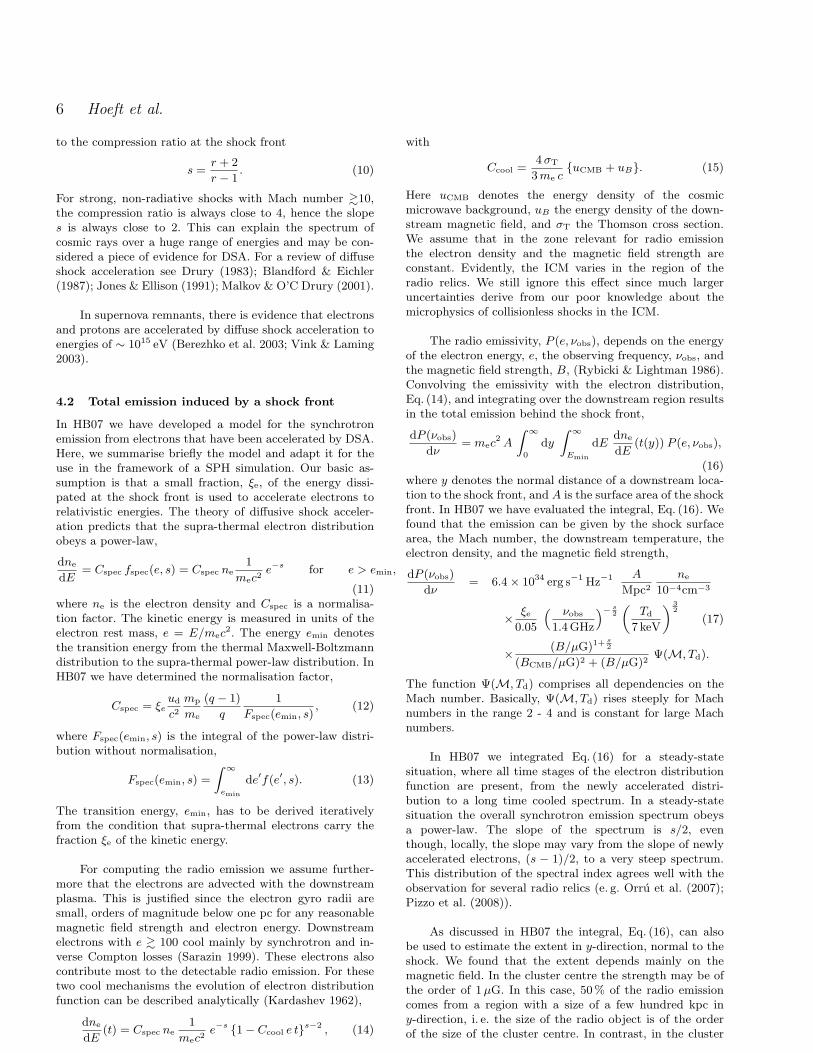
upstream region downstream regionSPH broadenedshock transition

! 2hi

Ai

Figure 1. The shock structure in SPH simulations.

Furthermore, assuming that the plasma obeys the polytropicrelation, i. e. P = (γ − 1)ρu, we obtain

M2 =r

γ

qrγ − 1

r − 1. (6)

For a polytropic plasma the compression ratio and entropyratio are related by the implicit equation

r =(γ + 1) q rγ + (γ − 1)

(γ − 1) q rγ + (γ + 1). (7)

Eqs. (6) and (7) provide a one-to-one mapping between theMach number, compression ratio, and entropy ratio. Finally,the difference between downstream and upstream velocity isrelated to the Mach number via

vd − vu =M r − 1

ruu. (8)

Our Mach number estimator computes the entropy ratio, q,and (vd − vu)/uu for each SPH particle in the simulation.Beforehand, we tabulate the relations between q, r, Mand M(r − 1)/r. This allows us to simply read the Machnumber from the table. The implementation of the Machnumber estimator is explained in Sec. 3.2.

Most likely, the structure of cosmological shock fronts ismore complex than that of simple hydrodynamical shocks.It is beyond the scope of this paper to include a more de-tailed structure of collisionless shocks. Instead, we combinethe shock fronts detected in the simulation with a paramet-ric model for the radio emission. Any aspect of the shockstructure has to be captured by the parameters used for theradio emission since cosmological simulations are not ableto resolve any relevant scale for plasma processes.

3.2 A novel approach for estimating the Machnumber

Our aim is to identify shock fronts in the MareNostrumUniverse simulation and to derive the Mach number of theshocks. In order to estimate the radio emission produced bythe shock, we will need the Mach number, downstream tem-perature and electron density. In SPH, energy is dissipatedat shocks using an artificial viscosity. Most implementations

c© 0000 RAS, MNRAS 000, 000–000

Diffuse radio emission in cosmological simulations 5

of artificial viscosity follow the suggestions by Monaghan(1992) and Balsara (1995). In addition, viscosity-limitersare used to reduce spurious angular momentum transportin shear flows (Balsara 1995; Steinmetz 1996). In contrastto actually solving a Riemann problem, the SPH formalismdoes not identify any discontinuity. For our purpose it issufficient to identify the shock fronts by post-processingsnapshots of the simulation.

One possible approach is to extract the ratio of theupstream and downstream entropy. In SPH the dissipationrate is computed but the upstream and downstream entropyare never computed. The ratio of these two quantities wouldimmediately give the strength of the shock. Pfrommer et al.(2006) determine the entropy gain in the shock by comput-ing the product of the dissipation rate and the estimatedcrossing time of particles through the smoothed shock front.However, for particles in the SPH broadened shock frontthe analysis of local properties underestimates the strengthof a shock. Pfrommer et al. (2006) cure this difficulty byusing the maximum Mach number from within a certaintime interval. As we wish to determine the Mach numberfrom a single snapshot, we have developed the followingscheme:

In the first step, for each SPH particle, we compute theentropy gradient,∇S. In a shock front this gradient gives thedirection of the shock normal pointing into the downstreamdirection. We define an associated upstream position,

xui = xi + fh hi n1i , (9)

where xi is the position of the SPH particle i, hi thesmoothing length of the particle i, and n1

i denotes the shocknormal, n1

i = −∇S/|∇S|. Moreover, we have introduced afactor fh, chosen to be 1.3, which ensures that xui is indeedin the upstream region and not in the transition betweenupstream and downstream properties. In a similar manner,we introduce an associated downstream position, xdi, inthe opposite direction.

Using the usual SPH scheme, we compute the densityand internal energy at the upstream and downstreamposition. Moreover, we compute the velocity at thesetwo positions and project it onto the shock normal.This results in the upstream and downstream velocity,vui + vsh = v(xui) · n1

i and vdi + vsh = v(xdi) · n1i , where

vsh is the velocity of the shock front in the rest-frame of thesimulation. Since vsh is not known, it is advantageous toassess only the differences (vdi − vui). Beside a componentparallel to the shock normal, the velocity field may alsoshow perpendicular components. We compute these compo-nents in a similar manner to the upstream and downstreamvelocities, vk±i = v(xi ± fhhin

ki ) · nki , where the three

vectors n1, n2, and n3 form an orthonormal base.

For those particles, that belong clearly to a shockfront, we demand that the velocity has to be divergentin the direction of the shock normal, i. e. (vd − vu) > 0.Moreover, the velocity differences in the directions perpen-dicular to the shock normal have to be smaller than thatparallel to the shock, |v+

k − v−k | < (vd − vu)/2. Therefore,

the difference (vd−vu) gives roughly the velocity divergence.

There are two possibilities to compute the Machnumber: First, we can evaluate the entropy ratio q =S(xd)/S(xu). Secondly, we can use the ratio (vd−vu)/cu. Asdiscussed in Sec. 3.1, for both properties there exists a one-to-one mapping with the Mach number of the shock. Weuse a look-up table to obtain for both the entropy ratio andthe velocity difference the corresponding Mach number. Inorder to have a conservative estimate for the Mach numberwe use the smaller of the two.

4 THE RADIO EMISSION MODEL IN ANUTSHELL

At collisionless shock fronts a small fraction of particles maybe accelerated to energies far beyond the thermal energy dis-tribution. This has been directly observed in particle spec-tra of the Earth’s bow shock where the resulting momen-tum distribution depends strongly on the Mach number andthe angle between shock normal and the direction of theupstream magnetic field. Also, the radio emission of solarbursts is generally attributed to shock-drift acceleration andsubsequent excitation of plasma wave. Larger electron ener-gies may be achieved by diffusive shock acceleration (DSA).The details of particle acceleration at collisionless shocks arecomplex and not fully understood yet. It is expected thatDSA can operate in the ICM only with a starting energyabove a few MeV, since at lower energies Coulomb lossesare too efficient. Some electrons may attain this injectionenergy by shock-drift acceleration. It is beyond the scope ofthis paper to include a very detailed model for the processesat collisionless shock fronts. For simplicity, we assume thatDSA operates already at thermal energies where Coulomblosses have to be compensated by acceleration mechanismsdifferent from DSA. Following our model Hoeft & Bruggen(2007, HB07) we assume that supra-thermal electrons showa power-law spectrum, with a slope as predicted by DSA. Wealso suppose that a fixed fraction of the energy dissipatedat the shock front is used to accelerate electrons. Finally,we assume that the supra-thermal electrons advect with thedownstream plasma. In this section, we briefly introduce dif-fusive shock acceleration and review the model discussed inHB07. Moreover, we discuss our assumptions about the mag-netic field. Finally, we present shock tube simulations thattest our shock finder and allows us to calibrate the emissionmodel.

4.1 Diffusive shock acceleration

In DSA, particles are accelerated by multiple shock cross-ings, in a first-order Fermi process. If the shock thicknessis much smaller than the diffusion scale which, in turn, hasto be much smaller than the curvature of the shock front, aone-dimensional diffusion-convection equation can be solved(Axford et al. 1978; Bell 1978a,b; Blandford & Ostriker1978). The result is that the energy spectrum of suprather-mal electrons is a power-law distribution, nE ∝ E−s. Thespectral index, s, of the accelerated particles is only related

c© 0000 RAS, MNRAS 000, 000–000

6 Hoeft et al.

to the compression ratio at the shock front

s =r + 2

r − 1. (10)

For strong, non-radiative shocks with Mach number &10,the compression ratio is always close to 4, hence the slopes is always close to 2. This can explain the spectrum ofcosmic rays over a huge range of energies and may be con-sidered a piece of evidence for DSA. For a review of diffuseshock acceleration see Drury (1983); Blandford & Eichler(1987); Jones & Ellison (1991); Malkov & O’C Drury (2001).

In supernova remnants, there is evidence that electronsand protons are accelerated by diffuse shock acceleration toenergies of ∼ 1015 eV (Berezhko et al. 2003; Vink & Laming2003).

4.2 Total emission induced by a shock front

In HB07 we have developed a model for the synchrotronemission from electrons that have been accelerated by DSA.Here, we summarise briefly the model and adapt it for theuse in the framework of a SPH simulation. Our basic as-sumption is that a small fraction, ξe, of the energy dissi-pated at the shock front is used to accelerate electrons torelativistic energies. The theory of diffusive shock acceler-ation predicts that the supra-thermal electron distributionobeys a power-law,

dne

dE= Cspec fspec(e, s) = Cspec ne

1

mec2e−s for e > emin,

(11)where ne is the electron density and Cspec is a normalisa-tion factor. The kinetic energy is measured in units of theelectron rest mass, e = E/mec

2. The energy emin denotesthe transition energy from the thermal Maxwell-Boltzmanndistribution to the supra-thermal power-law distribution. InHB07 we have determined the normalisation factor,

Cspec = ξeud

c2mp

me

(q − 1)

q

1

Fspec(emin, s), (12)

where Fspec(emin, s) is the integral of the power-law distri-bution without normalisation,

Fspec(emin, s) =

Z ∞emin

de′f(e′, s). (13)

The transition energy, emin, has to be derived iterativelyfrom the condition that supra-thermal electrons carry thefraction ξe of the kinetic energy.

For computing the radio emission we assume further-more that the electrons are advected with the downstreamplasma. This is justified since the electron gyro radii aresmall, orders of magnitude below one pc for any reasonablemagnetic field strength and electron energy. Downstreamelectrons with e & 100 cool mainly by synchrotron and in-verse Compton losses (Sarazin 1999). These electrons alsocontribute most to the detectable radio emission. For thesetwo cool mechanisms the evolution of electron distributionfunction can be described analytically (Kardashev 1962),

dne

dE(t) = Cspec ne

1

mec2e−s 1− Ccool e ts−2 , (14)

with

Ccool =4σT

3me cuCMB + uB. (15)

Here uCMB denotes the energy density of the cosmicmicrowave background, uB the energy density of the down-stream magnetic field, and σT the Thomson cross section.We assume that in the zone relevant for radio emissionthe electron density and the magnetic field strength areconstant. Evidently, the ICM varies in the region of theradio relics. We still ignore this effect since much largeruncertainties derive from our poor knowledge about themicrophysics of collisionless shocks in the ICM.

The radio emissivity, P (e, νobs), depends on the energyof the electron energy, e, the observing frequency, νobs, andthe magnetic field strength, B, (Rybicki & Lightman 1986).Convolving the emissivity with the electron distribution,Eq. (14), and integrating over the downstream region resultsin the total emission behind the shock front,

dP (νobs)

dν= mec

2 A

Z ∞0

dy

Z ∞Emin

dEdne

dE(t(y)) P (e, νobs),

(16)where y denotes the normal distance of a downstream loca-tion to the shock front, and A is the surface area of the shockfront. In HB07 we have evaluated the integral, Eq. (16). Wefound that the emission can be given by the shock surfacearea, the Mach number, the downstream temperature, theelectron density, and the magnetic field strength,

dP (νobs)

dν= 6.4× 1034 erg s−1 Hz−1 A

Mpc2

ne

10−4cm−3

× ξe0.05

“ νobs

1.4 GHz

”− s2„

Td

7 keV

« 32

(17)

× (B/µG)1+ s2

(BCMB/µG)2 + (B/µG)2Ψ(M, Td).

The function Ψ(M, Td) comprises all dependencies on theMach number. Basically, Ψ(M, Td) rises steeply for Machnumbers in the range 2 - 4 and is constant for large Machnumbers.

In HB07 we integrated Eq. (16) for a steady-statesituation, where all time stages of the electron distributionfunction are present, from the newly accelerated distri-bution to a long time cooled spectrum. In a steady-statesituation the overall synchrotron emission spectrum obeysa power-law. The slope of the spectrum is s/2, eventhough, locally, the slope may vary from the slope of newlyaccelerated electrons, (s − 1)/2, to a very steep spectrum.This distribution of the spectral index agrees well with theobservation for several radio relics (e. g. Orru et al. (2007);Pizzo et al. (2008)).

As discussed in HB07 the integral, Eq. (16), can alsobe used to estimate the extent in y-direction, normal to theshock. We found that the extent depends mainly on themagnetic field. In the cluster centre the strength may be ofthe order of 1µG. In this case, 50 % of the radio emissioncomes from a region with a size of a few hundred kpc iny-direction, i. e. the size of the radio object is of the orderof the size of the cluster centre. In contrast, in the cluster

c© 0000 RAS, MNRAS 000, 000–000

Diffuse radio emission in cosmological simulations 7

periphery the magnetic field strength may be of the orderof 0.1µG. In this case, the extent of the emission regionis about 100 kpc, which is significantly smaller than thescale of spatial variations in the cluster periphery. In thefollowing, we assign the radio emission solely to the shockfront and ignore the extent of the radio emission region iny-direction. This approach is perfectly suited for studyingthe radio emission in the cluster periphery, since there thedownstream extend of the emission region is smaller thanthe numerical resolution. In the cluster centre our approachmay lead to too compact radio objects.

The shock finder described in Sec. 3.2 allows us to lo-cate shock discontinuities in a SPH simulation snapshot.The shock finder also provides estimates for the Mach num-ber and for the shock normal. Using the normal vector, wecan find a position which is sufficiently downstream to de-termine the downstream temperature, Td, and the electrondensity, ne, which are needed to compute the radio emissionvia Eq. (17). To compute the radio power, dP/dν, we alsoneed the area, A, of the shock front. Since in SPH a shockfront is comprised of particles, each particle represents anarea of the shock. More precisely, the shock discontinuity issmoothed by the size of the SPH kernel, hSPH, see Fig. 1.The kernel may contain NSPH particles, the correspondingvolume is of the order of h3

SPH. Hence, one particle belongingto the shock front represents a shock area of

A = fAh2

SPH

NSPH, (18)

where fA is a normalisation constant, which will be deter-mined by the help of Sod shock tube simulations, see Sec. 4.4.Finally, we have to determine the downstream magnetic fieldstrength. In the next paragraph, Sec. 4.3 we detail how weestimate Bd.

4.3 Magnetic field model

The downstream magnetic field is crucial for the synchrotronemission. For a power-law electron energy distribution theemission is given by

P (ν) ∝ ne (B sin θ)1+α ν−α, (19)

where θ is the pitch angle between the electron velocity andthe magnetic field. The exponent α is related to the slopeof the electron spectrum by α = (s − 1)/2. Unfortunately,in Eq. (19) the electron density and the field strength aredegenerated. Therefore, evaluating only the synchrotronemission of diffuse radio objects in the ICM is not sufficientto derive the magnetic field strength. For some clusters ithas been possible to measure the electron density by thehard X-ray excess in the cluster spectrum (see Rephaeliet al. (2008) for a review). As a result, the average clustermagnetic field strength has been estimated to be of theorder of 0.1 to 1µG (Fusco-Femiano et al. 2001; Rephaeli& Gruber 2003; Rephaeli et al. 2006). Alternatively, oneassumes that the energy density of the ICM is minimal(Govoni & Feretti 2004). This method also results in mag-netic field strengths of the order of 0.1 to 1µG. Contrarily,Faraday rotation measurement studies (see e. g. Govoniet al. (2006)) typically yield field strengths that are larger

by about an order of magnitude.

The strength, structure and origin of magnetic fields inthe ICM is still debated. Intergalactic magnetic fields may bea remainder of primordial processes, may be generated by adynamo in first stars and subsequently expelled, may be gen-erated by the Biermann battery effect during cosmic reioni-sation, may be caused by microinstabilities in the turbulentICM, or may be generated at collisionless shock fronts. It isbeyond the scope of this paper to include a detailed modelfor the generation and evolution of magnetic fields. Eventhe passive evolution of magnetic fields during cosmic struc-ture formation is complex (Dolag et al. 2002; Bruggen et al.2005). However, we assume here that the magnetic strengthin the downstream region of the shock front, Bd, on averagesimply obeys flux conservation to follow

Bd

Bref=“ nd

10−4 cm−3

”2/3

. (20)

4.4 Normalisation of the radio emission

In our model it is necessary to determine the effectivearea of the shock front represented by one SPH particle,Ai, which may also depend on the actual Mach number.Therefore, we simulated the Sod shock tube problem anddetermine the Mach number by our method described inSec. 3.2. As shown in Fig. 2, the original Mach number usedto set up the initial conditions is well reproduced by theMach number estimator. We have simulated shock tubeswith Mach numbers from 1.5 to 100. This covers well therange of relevant Mach numbers for the radio emissionof merger-induced and accretion shocks. In all cases, thetheoretically expected Mach number is found in the centreof the transition region between the upstream and thedownstream region. In the periphery the Mach number isunderestimated, i. e. the particles in the shock region showa Mach number distribution, as shown in the third row ofFig. 2.

The theoretical value of the radio emission is easily com-puted via Eq. (17). The Mach number is known from settingup the initial conditions of a shock tube, and the proper-ties of the downstream plasma are known from the analyticsolution. In the simulation a large number of SPH particlescontributes to the emission. To show the total emission weplot the cumulative radio emission, i. e. the emission, P (xi),of all particles on the left-hand side of a given x-position issummed,

P (< x) =X

iP (xi) with xi < x. (21)

As noted above the Mach number estimator results in a dis-tribution of Mach numbers for the particles in the SPH-broadened shock discontinuity. For small Mach numbers,M . 5, the radio emission depends strongly on M, whilefor large Mach numbers it does not. Hence, a constant areanormalisation factor, fA (introduced in Sec. 4.2), would sys-tematically underestimate the radio emission of shocks withM . 5. One could correct for this effect by introducing afunction fA(M). However, we choose a somewhat simplersolution and increase the Mach number slightly when com-

c© 0000 RAS, MNRAS 000, 000–000

8 Hoeft et al.Radio relic luminosity function 15

Figure 6. Shock tube simulations.

that flux density evolves according to simple compression, i. e. no additional amplification

by dynamo processes is present,

B = Brefn

10!4 cm!3. (19)

To be consistent with the findings in the periphery of galaxy clusters we chose a field strength

of Bref = 0.1µGauss.

4.4 Shock tube validation

Due to the complexity of the radio emission model it is necessary to determine free parame-

ters by simulating configurations with known analytic solutions. More precisely, the e!ective

area of the shock front represented by one SPH particle, Ai, may depend on the actual Mach

number. Therefore, we carry out a few simulations of the Sod shock tube problem and sub-

sequently determine the Mach number by the method described in Sec. 3.2. As shown by

Fig. 6 the original Mach number used to set up the initial conditions is well reproduced by

the Mach number estimator. We have simulated shock tubes with Mach numbers from 1.5

to 100. This covers well the range of relevant Mach numbers for radio emission. In all case

the theoretical Mach number is restored in the centre region of the transition from the up-

stream to the downstream region, while in the periphery the Mach number is underestimated.

The theoretical value of the radio emission is easily computed by the help of Eq. (16).

The Mach number is known from setting up the initial conditions of a shock tube, and the

c" 0000 RAS, MNRAS 000, 000–000

Figure 2. Simulations of the Sod shock tube problem with Mach numbers 1.5, 3, 10, 100. The upper panel shows the electron density

assuming a fully ionised ICM, the second row the temperature, the third row the Mach number as determined by the Mach number

estimator described in Sec. 3.2 and the lower panel the cumulative radio emission as described in Sec. 4.4 assuming an observationfrequency of 1.4 GHz. Note that the irregularites in ne and T are caused by the small number of particles in the SPH kernel, namely

NSPH = 40. We choose this number in order to conform with the parameters used in the MareNostrum Universe simulation. For the

shock finding we smoothed the fields to some extend by using Nkernel = 80 in the finder, see Tab. 1.

puting the radio emission for a particle,

Ψ(M)→ Ψ(M× 1.045). (22)

As a result we are able to reproduce the expected radioemission of the different shock tubes with deviations smallerthan a factor of three. Regarding the simplicity of our model(power-law electron spectrum, uniform energy fraction insupra-thermal electrons, flux conservation of magnetic field)this accuracy is sufficient.

5 THE RADIO EMISSION IN THESIMULATION

We now wish to apply the tools prepared in the previoussections to estimate the radio emission of strong shockswhich occur during cosmic structure formation. The mostluminous diffuse radio emission is observed in massiveclusters or their periphery. We therefore analyse massiveclusters from a cosmological simulation. Our aim is to applythe radio emission model to the whole range of structureformation shocks, caused by mergers and gas accretion. Inthis paper we estimate only the radio emission which isoriginated by primary electrons.

We apply the Mach number estimator described inSec. 3.2 and the radio emission model described in Sec. 4.2 tothe MareNostrum Universe simulation described in Sec. 2.More precisely, we analyse the 300 most massive clusterswith masses in the range 0.4 to 2.5 × 1015h−1M. We donot include less massive clusters since the resolution getstoo poor. First we show the results of our Mach numberestimator for a selection of clusters. Then, we present ar-tificial observations and compare them to observed radio

relics. Finally, we discuss how the radio emission correlateswith X-ray temperature of the clusters.

5.1 The ICM in slices

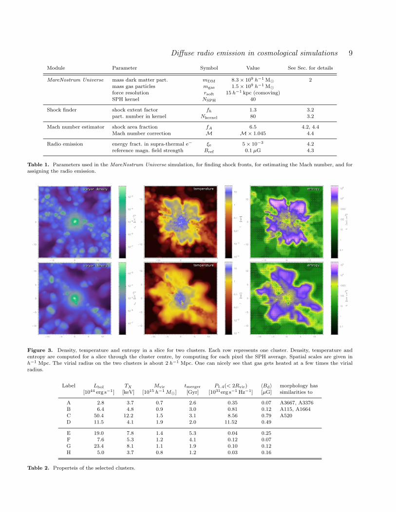
It is instructive to consider the physical properties of theICM in slices through the cluster, see Fig. 3. One can clearlysee how the temperature rises sharply in the periphery of acluster, far beyond the virial radius. At this location, aboutfour times the viral radius, the ICM gets heated to clustertempertaures, i. e. about 1 keV, by accretion shocks. Withinclusters, the temperature and entropy maps are complex,since rather cold intergalactic medium flows in filaments tothe cluster centre and ongoing or past mergers lead to in-tricate gas flows. However, the velocity divergence revealsalso the location of the inner merger shocks, see Fig. 4. Notethat we compute the divergence according to the proceduredescribed in Sec. 3, i. e. we determine first the shock nor-mal and subsequently compute the difference (vd − vu). Asalso described in Sec. 3 the ratio of the velocity divergenceand the upstream sound speed allows us to infer the Machnumber of the shock. Additionally, the ratio of downstreamand upstream entropy allows to determine the Mach num-ber. We use the minimum of both for further analysis, i. e.for computing radio emission.

5.2 Visualising the shock fronts

As seen in the slices through the clusters, the geometryof the strong shocks may be very complex. To visualisethe shocks, we represent each of these particles by a smallsquare to which the shock normal is perpendicular. Each ofthese square may be considered as a small part of the shock

c© 0000 RAS, MNRAS 000, 000–000

Diffuse radio emission in cosmological simulations 9

Module Parameter Symbol Value See Sec. for details

MareNostrum Universe mass dark matter part. mDM 8.3× 109 h−1 M 2

mass gas particles mgas 1.5× 109 h−1 Mforce resolution rsoft 15 h−1 kpc (comoving)SPH kernel NSPH 40

Shock finder shock extent factor fh 1.3 3.2part. number in kernel Nkernel 80 3.2

Mach number estimator shock area fraction fA 6.5 4.2, 4.4Mach number correction M M× 1.045 4.4

Radio emission energy fract. in supra-thermal e− ξe 5× 10−3 4.2reference magn. field strength Bref 0.1 µG 4.3

Table 1. Parameters used in the MareNostrum Universe simulation, for finding shock fronts, for estimating the Mach number, and for

assigning the radio emission.

Figure 3. Density, temperature and entropy in a slice for two clusters. Each row represents one cluster. Density, temperature andentropy are computed for a slice through the cluster centre, by computing for each pixel the SPH average. Spatial scales are given inh−1 Mpc. The virial radius on the two clusters is about 2 h−1 Mpc. One can nicely see that gas gets heated at a few times the virialradius.

Label Lbol TX Mvir tmerger P1.4(< 2Rvir) 〈Bd〉 morphology has[1044 erg s−1] [keV] [1015 h−1M] [Gyr] [1031erg s−1 Hz−1] [µG] similarities to

A 2.8 3.7 0.7 2.6 0.35 0.07 A3667, A3376B 6.4 4.8 0.9 3.0 0.81 0.12 A115, A1664

C 50.4 12.2 1.5 3.1 8.56 0.79 A520

D 11.5 4.1 1.9 2.0 11.52 0.49

E 19.0 7.8 1.4 5.3 0.04 0.25F 7.6 5.3 1.2 4.1 0.12 0.07G 23.4 8.1 1.1 1.9 0.10 0.12H 5.0 3.7 0.8 1.2 0.03 0.16

Table 2. Properteis of the selected clusters.

c© 0000 RAS, MNRAS 000, 000–000

10 Hoeft et al.

Figure 4. Velocity divergence in a slice through the cluster center for six different clusters of our sample. The velocity divergence refershere to the difference (vd − vu), see Sec. 3. One can clearly distinguish the outer ‘accretion’ shocks and the inner ‘merger’ shocks. Note

that the width of the shocks is caused by the the numerical resolution, which is much poorer in the region of the accretion shocks thanin inner region of the clusters.

Figure 5. A textbook example of a double relic found in the MareNostrum Universe simulation.

c© 0000 RAS, MNRAS 000, 000–000

Diffuse radio emission in cosmological simulations 11

Figure 6. Radio emission and particle distribution for four typical galaxy clusters. The particles of the simulation are represented by

dots with temperature colour-coded. Each SPH particles which belongs to a shock front a small square is drawn. The size of the square

is proportional to the smoothing length of the particle. The colour gives the radio emission associated with the particle. Moreover weencode if a square is seen from upstream or the downstream direction. The latter are shaded grey. The circles indicate the viral radius

of the galaxy cluster. See Tab. 2 for the properties of these exemplaric clusters. Each row represents one cluster, rotated by azimuthal

angles of 60 and 120. See Fig. 7 for the projected radio emission.

surface. The edge length of a square is proportional to thesmoothing length of the corresponding SPH particle.

We color-code the squares by the radio emission com-puted for the corresponding SPH particle. Fig. 5 shows atext-book example of a double relic found in the MareNos-trum Universe simulation. This cluster has developed twolarge shock fronts in the cluster periphery, similar to theradio objects found in A3667 (Rottgering et al. 1997) and

A3376 (Bagchi et al. 2006). In addition to the emission ofeach SPH particle in the shock front, we color-code theorientation of the shock normal. We shade squares grey forwhich the normal points away from the observer, wherethe level of shading depends on the angle, α, betweenshock normal and the direction to the observer. As aresult, shock fronts which propagate towards the observerappear blueish while fronts which move away appear greyish.

c© 0000 RAS, MNRAS 000, 000–000

12 Hoeft et al.

To show the location of the cluster, we represent theSPH particles by dots with the temperature colour-coded.Infalling substructures can often be identified in tem-perature maps since they are usually much colder thanthe surrounding ICM. The clusters in the MareNostrumUniverse simulation show radio objects with very differentmorphologies. In Fig. 6 four examples are displayed, eachof which viewed from three different angles. As discussedabove, cluster A contains a textbook example for a doublerelic. Cluster B shows only one relic which is composed ofseveral smaller fragments. In cluster C, several stronglyemitting sources in the centre of the cluster are found. Fi-nally, cluster D shows the emission of an early state mergersystem. The temperature of this cluster is only about 4 keV(see Tab. 2), but still a strong radio relic has been developed.

The structure of the shock fronts can be seen best inan animation. We therefore encourage the reader to viewthe movies of the rotations of the four exemplary clustersavailable from our web site 1.

5.3 Radio maps

Having assigned a radio luminosity to each SPH particle,we are able to compute artificial radio maps. To this end weproject the emission of each particle along the line-of-sightand smooth it according to the SPH kernel size. We computethe radio emission for an observing frequency of 1.4 GHzand a hypothetical beam size of 10′′ × 10′′. For comparison,we also compute contours of the bolometric X-ray flux. Wefollow Navarro et al. (1995) and assign each particle theluminosity

LX = 1.2× 1024 erg s−1 mgas

µmp

ne

cm−3

„T

keV

«1/2

. (23)

Fig. 7 shows the artificial radio maps and the X-ray contoursfor the same clusters already presented in Fig. 6. The doublerelic structure of cluster A becomes even more prominent.The X-ray contours reveal for some viewing angles clearlythe merger state of the clusters.

The examples in Fig. 7 and Fig. 6 are selected toillustrate the variety of diffuse radio objects obtained byour simple emission model. Example A shows the large-scale merger shocks that are also found in idealised mergersimulations (e.g. Roettiger et al. 1999). In contrast, exampleC shows a large number of smaller shock fronts. Some ofthem are related to substructures moving through theICM, while others are obviously unrelated to any substruc-ture (this can be best seen in the animations mentionedabove). The morphology of the radio emission resemblesthat found in A2255, where several rather small pieces ofdiffuse radio emission have been detected (Pizzo et al. 2008).

Another property of our model for diffuse radio emis-sion is the fact that many of the massive clusters show noor only little radio emission. Therefore, we show four exam-ples with almost radio-quiet clusters, see Fig. 8. Example Eis the stereotype of a relaxed massive clusters. There is no

1 www.faculty.iu-bremen.de/mhoeft/RadioRelicAnimation/

1030 1031 1032 1033 10341

10

100

1000

101

102

103

104

radio luminosity P1.4 [erg s-1 Hz-1]

N(>

P 1.4

)

[ (

h-1

500

Mpc

)-3 ]

[h3

Gpc-3

]

Radio object LF Cluster LF radio halo LF

(Enßlin & Röttgering 02)

Figure 9. The cumulative number density of radio objects. Theleft axis give the number of objects found in the simulation box.

The solid line indicates the number of radio objects as identified

by splitting the objects in well separated groups (see Sec. 5.4).The long-dashed line gives the radio luminosity function for the

clusters in MareNostrum Universe simulation. The radio power

of a cluster includes all emission within the virial radius. For com-parison we depict the radio halo luminosity function as computed

by Enßlin & Rottgering (2002). We adopt their best fitting of the

radio halo–X-ray correlation with aν = 3.37 and bν = 1.69.

large-scale shock present which can cause significant radioemission, only a very few small regions with a radio-loudshock are found. This is consistent with the time of the lastmajor merger (the mass of the accreted substructure has tobe at least 25 % of the main cluster), which has take placemore than 5Gyr in the past. Examples D and F show a dis-torted X-ray morphology indicating recent merger activity.However, the resulting merger shocks are very faint in theradio. Finally, example G shows a merger in an early statewith no radio emission. Hence, even with our simple radioemission model merger activity does not lead in all cases tostrong radio emission. This is expected from modelling elec-tron acceleration at the shock front, since a Mach numberabove 2.5 is needed for a significant amount of radio emis-sion. Many of the merger shocks have lower Mach numbers.

5.4 The luminosity function of radio objects

As can be seen by the examples A to D, one can oftendivide the emitting structures into individual objects, suchas the emission in front of a supersonically moving galaxyand that of a merger shock front travelling outwards in theICM. In order to identify individual radio objects in oursimulation, we select all particles whose radio emission liesabove a very low threshold. For these particles we determinetheir nearest neighbours, and obtain as a result a spanningtree for radio-loud particles. We now cut all links that arelarger than the minimum of the smoothing lengths of thetwo connected particles. As a result, the spanning treeseparates into sub-trees, each of which can be consideredan individual radio object. By this method we can forinstance disentangle the radio emission of an infallingsubstructure from that of large merger shock. Finally, we

c© 0000 RAS, MNRAS 000, 000–000

Diffuse radio emission in cosmological simulations 13

Figure 7. Mimic observations of the X-ray and the radio emission. We have projected the radio emission and bolometric X-ray emissionof the clusters shown in Fig. 6. The radio flux at 1.4 GHz is computed for a hypothetical beam size of 10′′ × 10′′. No redshift effects aretaken into account.

compute the cumulative number of radio objects above agiven luminosity, see Fig. 9, i. e. the luminosity function ofdiffuse radio objects. Most of the very luminous objects(P1.4 & 1032 erg s−1 Hz−1) are rather small structures,similar to that seen in example C. The textbook merger

shocks, as in example A, have only luminosities of theorder of 1031 erg s−1 Hz−1 and below. Therefore, the veryluminous relics in A3667 seem to be very exceptional. Ourtextbook merger shocks are similar to the less luminous

c© 0000 RAS, MNRAS 000, 000–000

14 Hoeft et al.

Figure 8. Mimic observations of the X-ray and the radio emission for four galaxy clusters with a low radio emission.

c© 0000 RAS, MNRAS 000, 000–000

Diffuse radio emission in cosmological simulations 15

relics found in A3376 (Bagchi et al. 2006).

We choose the parameters of our model in a way thatthe resulting radio objects agree with observations in therespect that the most luminous ones have a radio power,P1.4, of ∼ 1033 erg s−1 Hz−1. Towards small luminositiesthe cumulative number of radio objects increases witha slope close to −2/3. For comparison we compute theradio luminosity within the virial radius of the clusters inthe MareNostrum Universe simulation and find an evenshallower curve. The rather shallow slope of the faintend of the radio luminosity function reflects that theradio luminosity depends strongly on the cluster mass ortemperature. We will discuss this further in the next section.

For comparison we have shown in Fig. 9 the radio haloluminosity derived by Enßlin & Rottgering (2002). Theyconcluded that the upcoming radio telescope Lofar coulddiscover about 1000 radio halos by a survey in a yearstimescale. With the parameters used in our model we find amuch larger abundance of radio objects. However, we mayoverestimate the efficiency of diffusive shock acceleration orthe strength of magnetic fields. It is worth noticing that theslope of the radio luminosity function at the low-luminosityend is similar to that of Enßlin & Rottgering (2002), hence,one may expect the discovery of a large number of radioobjects with Lofar. The radio luminosity function of clus-ters is significantly flatter, indicating that one cluster maycontain several radio objects with moderate luminosity. As aresult we expect that the number of cluster for which Lofarwill find new radio features is significantly lower than 1000.However, for a more quantitative analysis model parametershave to be normalised and the redshift evolution has to beincluded properly. This will be discussed in a forthcomingpaper.

5.5 Radio versus X-ray

We also estimate the radio–X-ray correlation of the galaxyclusters in our simulation by computing the bolometricX-ray luminosity and the emission-weighted temperature.Fig. 10 shows that only a fraction of the clusters is very lu-minous in radio, meaning that they show a radio luminosityabove 1031 erg s−1 Hz−1. This is also true for a significantnumber of the massive, i. e. hot, clusters. However, the max-imum radio luminosity scales strongly with the cluster tem-perature. This is indeed expected for radio relics the mostmassive clusters (see e.g. Feretti et al. 2004). We plot forcomparison the radio luminosity of several radio relics andhalos. The MareNostrum Universe simulation clusters showa trend similar to the observed ones, however, the radio lu-minosity of our clusters is in average higher than that of theobserved clusters. This difference may be caused by our as-sumptions for the parameters in the radio emission model,i. e. the shock acceleration is too efficient in our model, orthe magnetic fields are too strong. Alternatively, the X-raytemperature of the simulated clusters might be too low. Ina forthcoming work we will use the comparison to observedradio halos and relics to constrain our model parameters.Here we wish to point out that our simple emission modeltaking only primary electrons into account nicely restoresin combination with a cosmological simulation the fact that

2 5 10

1030

1031

1032

1033

cluster X-ray temperature [keV]

radi

o lu

min

osity

P1.

4 [

erg

s-1 H

z-1]

Mare Nostrum clusters! Observations

Figure 10. Bolometric X-ray temperature versus radio lumi-nosity. For comparison observational data are shown. The data

include radio relics and halos (Govoni et al. (2001), Govoni & Fer-

etti (2004), Feretti et al. (1997), Liang et al. (2000), Giovanniniet al. (1999) ).

only a small fraction of clusters show luminous diffuse radiostructures and in addition the trend in the radio luminosity–X-ray relation.

5.6 Radio emission of accretion shocks

Our method also allows to study the radio emission ofaccretion shocks. Here we show artificial radio maps for twoof the most massive clusters in the simulation using a largerfield-of-view, see Fig. 11. We find only very little emissionin the region of the accretion shocks, which are roughlylocated at four times the virial radius, i. e. ∼ 10h−1 Mpcfor the two most massive clusters. The reason is that thetemperature, density and magnetic field are simultaneouslylow in the cluster periphery. As a result the two clustersshown in Fig. 11 have a radio emission even below 10−4 mJy(for a 10′′× 10′′ beam). Hence, it may be difficult even withthe sensitivity of upcoming radio telescopes to detect theaccretion shock by their radio emission.

5.7 Magnetic field strength in radio relics

Magnetic fields in the region of radio relics are difficult todetermine observationally since the field strength and thenumber density of relativistic electrons are degenerated inthe expression for the radio luminosity. Estimates for ICMmagnetic fields range from 0.1 to 10µG. We compute theradio luminosity-averaged magnetic field within two timesthe virial radius for the sample of clusters presented here indetail, see Tab. 2. More precisely, we compute

〈Bd〉 =1

P1.4(< 2rvir)

Xri<2rvir

P1.4(ri)Bd(ri).

We find that that for the clusters presented here the aver-age magnetic field strength is in the range of 0.07 to 0.8µG.

c© 0000 RAS, MNRAS 000, 000–000

16 Hoeft et al.

Figure 11. Mimic observations of the X-ray and the radio emission of the periphery of the two most massive clusters in the MareNostrum

Universe simulation.

Despite general over-luminosity of of the radio objects gener-ated in our simulation the magnetic fields in the downstreamregion has been modelled with moderate field strength only.This implies that the abundance of radio relics in generalcan be explained with rather weak magnetic fields in theperiphery of galaxy clusters.

6 DISCUSSION AND SUMMARY

We have presented a novel method for estimating the radioemission of strong shocks that occur during the process ofstructure formation in the universe. Our approach is basedon an estimate for the shock surface area and we computethe radio emission per surface element using the Machnumber of the shock and the downstream plasma properties.The advantage of our method is that we can accuratelydetermine the emission of the downstream regime withoutusing an approximate, discretised electron spectrum. Thedisadvantage is clearly that we do not include any evolutionof the shock front and the downstream medium. However,our main goal here is to compute the radio emissionfrom all shock fronts generated during cosmic structureformation. Our main assumption is that radio emissionis caused by primary electrons accelerated at the shockfront. To obtain a model suitable for the application in theframework of a cosmological simulation we have to neglectthe complexity of collisonless shocks, details of the electronacceleration mechanisms, the amplification of magneticfields by upstream cosmic rays, and so forth. The modelreflects rather an expectation for the average radio emissionentailed by structure formation shocks.

Our results show that in a cosmological simulation oneindeed finds textbook examples for large-scale, ring-likeradio relics as observed in A3667 and A3376. Our exampleA shows two large half-shell shaped shock fronts and noradio emission in the centre of the merging cluster. However,

cluster A is not very massive, hence the radio luminosity ofthe two half-shells is low compared to A3667. Another niceexample is cluster B which shows a radio relic only one sideof the cluster, similar to A115. Beside those spectacularrelics in the periphery of galaxy clusters, we find that a lotof clusters show complex, radio-loud shock structures closeto the cluster centre. This suggests that part of the centraldiffuse radio emission in galaxy clusters, i. e.the radio halophenomena, can be attributed to synchrotron emission ofprimary electrons.

We have modelled the radio emission with conservativeassumptions for the efficiency of shock acceleration, namelyξe = 0.005, and for the strength of magnetic fields in thedownstream region, namely of the order of 0.07 to 0.8µG.Still, we find that the radio luminosity in the clusterregion is on average significantly above observed values,see Fig. 9. Even lower values for the acceleration efficiencyor the magnetic field strength would suffice to explain theabundance of diffuse radio objects on the sky. In conclusion,our findings support the scenario in which radio relics aregenerated by primary electrons.

In summary, we have analysed one of the largest hydro-dynamical simulations of cosmic structure formation withrespect to shock fronts in clusters of galaxies. We have de-veloped a method to identify the shock fronts, to estimatetheir Mach numbers and their orientation. We have appliedthe method described in Hoeft & Bruggen (2007) to deter-mine the radio emission as a function of the shock surfacearea and the downstream plasma properties. Our analysisled to the following results:

• By evaluating the entropy and the velocity field we areable to identify strong shocks in the simulation and to de-termine their properties.• Using conservative values for the efficiency of strong

shocks to accelerate electrons and for strengths of magnetic

c© 0000 RAS, MNRAS 000, 000–000

Diffuse radio emission in cosmological simulations 17

fields, we are able to reproduce the number density and theluminosity of large-scale radio relics. Only a very few of themost massive clusters show such luminous, extended sources.• Our model reproduces various spectacular sources of

diffuse radio emission at the periphery of galaxy clusters.Other clusters show emission with complex morphologyclose to the cluster centre. These sources may be classifiedas part of a central radio halo, following the observationaldistinction between relics and halos.• Our results reproduce the strong correlation between

radio luminosity and cluster temperature. The highest radioluminosities occur in dense and hot environments such asmassive clusters. In addition we find that a large number ofgalaxy clusters show only little diffuse radio emission.• We find that the abundance of radio relics can be ex-

plained with efficiency of diffusive shock acceleration forelectrons lower than ξe = 0.005 and a strength of magneticfields in the relic region lower than 0.07 to 0.8µG.• All of the luminous radio relics belong to internal shock

fronts. The accretion shocks are located at larger distancesfrom the cluster centre. Since density and temperature arelow at this location, their luminosity is too small to reach asimilar flux as internal shock fronts.

AcknowledgmentMH acknowledges DLR funding under the grant 50 OX

0201. MB acknowledges the support by the DFG grant BR2026/3. The MareNostrum Universe simulations have beendone at the Barcelona Supercomputing Center (Spain) andanalysed at NIC Julich (Germany). GY thanks MEC (Spain)for financial support under project numbers FPA2006-01105and AYA2006-15492-C03. Our collaboration has been sup-ported by the European Science Foundation (ESF) for theactivity entitled ‘Computational Astrophysics and Cosmol-ogy’ (AstroSim).

REFERENCES

Axford, W. I., Leer, E., & Skadron, G. 1978, in Interna-tional Cosmic Ray Conference, 132–137

Bacchi, M., Feretti, L., Giovannini, G., & Govoni, F. 2003,A&A, 400, 465

Bagchi, J., Durret, F., Neto, G. B. L., & Paul, S. 2006,Science, 314, 791

Balsara, D. S. 1995, Journal of Computational Physics, 121,357

Bell, A. R. 1978a, MNRAS, 182, 147—. 1978b, MNRAS, 182, 443Berezhko, E. G., Ksenofontov, L. T., & Volk, H. J. 2003,A&A, 412, L11

Blandford, R., & Eichler, D. 1987, PhysRep, 154, 1Blandford, R. D., & Ostriker, J. P. 1978, ApJL, 221, L29Bruggen, M., Ruszkowski, M., Simionescu, A., Hoeft, M.,& Dalla Vecchia, C. 2005, ApJL, 631, L21

Burgess, D. 2007, in Lecture Notes in Physics, BerlinSpringer Verlag, Vol. 725, Lecture Notes in Physics, BerlinSpringer Verlag, ed. K.-L. Klein & A. L. MacKinnon, 161–+

Cen, R., & Ostriker, J. P. 1999, ApJ, 514, 1Deiss, B. M., Reich, W., Lesch, H., & Wielebinski, R. 1997,A&A, 321, 55

Dolag, K., Bartelmann, M., & Lesch, H. 2002, A&A, 387,383

Drury, L. O. 1983, Reports of Progress in Physics, 46, 973Enßlin, T. A., Biermann, P. L., Klein, U., & Kohle, S. 1998,A&A, 332, 395

Enßlin, T. A., & Bruggen, M. 2002, MNRAS, 331, 1011Enßlin, T. A., & Gopal-Krishna. 2001, A&A, 366, 26Enßlin, T. A., Pfrommer, C., Springel, V., & Jubelgas, M.2007, A&A, 473, 41

Enßlin, T. A., & Rottgering, H. 2002, A&A, 396, 83Feretti, L. 2005, Advances in Space Research, 36, 729—. 2006, ArXiv Astrophysics e-printsFeretti, L., Burigana, C., & Enßlin, T. A. 2004, New As-tronomy Review, 48, 1137

Feretti, L., Giovannini, G., & Bohringer, H. 1997, New As-tronomy, 2, 501

Fusco-Femiano, R., Dal Fiume, D., Orlandini, M., Brunetti,G., Feretti, L., & Giovannini, G. 2001, ApJL, 552, L97

Giovannini, G., & Feretti, L. 2004, Journal of Korean As-tronomical Society, 37, 323

Giovannini, G., Feretti, L., Govoni, F., Murgia, M., &Pizzo, R. 2006, Astronomische Nachrichten, 327, 563

Giovannini, G., Tordi, M., & Feretti, L. 1999, New Astron-omy, 4, 141

Gottlober, S., & Yepes, G. 2007, ApJ, 664, 117Govoni, F., & Feretti, L. 2004, International Journal ofModern Physics D, 13, 1549

Govoni, F., Feretti, L., Giovannini, G., Bohringer, H.,Reiprich, T. H., & Murgia, M. 2001, A&A, 376, 803

Govoni, F., Murgia, M., Feretti, L., Giovannini, G., Dolag,K., & Taylor, G. B. 2006, A&A, 460, 425

Hoeft, M., & Bruggen, M. 2007, MNRAS, 375, 77Hoeft, M., Bruggen, M., & Yepes, G. 2004, MNRAS, 347,389

Jones, F. C., & Ellison, D. C. 1991, Space Science Reviews,58, 259

Jubelgas, M., Springel, V., Enßlin, T., & Pfrommer, C.2008, A&A, 481, 33

Kang, H., & Jones, T. W. 2007, Astroparticle Physics, 28,232

Kardashev, N. S. 1962, Soviet Astronomy, 6, 317Kempner, J. C., & Sarazin, C. L. 2001, ApJ, 548, 639Kim, K.-T., Kronberg, P. P., Giovannini, G., & Venturi, T.1989, Nature, 341, 720

Klypin, A., Gottlober, S., Kravtsov, A. V., & Khokhlov,A. M. 1999, ApJ, 516, 530

Landau, L. D., & Lifshitz, E. M. 1959, Fluid mechanics(Course of theoretical physics, Oxford: Pergamon Press,1959)

Liang, H., Hunstead, R. W., Birkinshaw, M., & Andreani,P. 2000, ApJ, 544, 686

Malkov, M. A., & O’C Drury, L. 2001, Reports of Progressin Physics, 64, 429

Miniati, F. 2001, Computer Physics Communications, 141,17

—. 2004, Journal of Korean Astronomical Society, 37, 465—. 2007, Journal of Computational Physics, 227, 776Miniati, F., Jones, T. W., Kang, H., & Ryu, D. 2001, ApJ,562, 233

Miniati, F., Ryu, D., Kang, H., Jones, T. W., Cen, R., &Ostriker, J. P. 2000, ApJ, 542, 608

Monaghan, J. J. 1992, ARA&A, 30, 543

c© 0000 RAS, MNRAS 000, 000–000

18 Hoeft et al.

Navarro, J. F., Frenk, C. S., & White, S. D. M. 1995, MN-RAS, 275, 720

Orru, E., Murgia, M., Feretti, L., Govoni, F., Brunetti, G.,Giovannini, G., Girardi, M., & Setti, G. 2007, A&A, 467,943

Pfrommer, C., Enßlin, T. A., & Springel, V. 2008, MNRAS,385, 1211

Pfrommer, C., Springel, V., Enßlin, T. A., & Jubelgas, M.2006, MNRAS, 367, 113

Pizzo, R. F., de Bruyn, A. G., Feretti, L., & Govoni, F.2008, A&A, 481, L91

Rephaeli, Y., & Gruber, D. 2003, ApJ, 595, 137Rephaeli, Y., Gruber, D., & Arieli, Y. 2006, ApJ, 649, 673Rephaeli, Y., Nevalainen, J., Ohashi, T., & Bykov, A. M.2008, Space Science Reviews, 16

Roettiger, K., Burns, J. O., & Stone, J. M. 1999, ApJ, 518,603

Rottgering, H. J. A., Braun, R., Barthel, P. D., vanHaarlem, M. P., Miley, G. K., Morganti, R., Snellen, I.,Falcke, H., de Bruyn, A. G., Stappers, R. B., Boland,W. H. W. M., Butcher, H. R., de Geus, E. J., Koopmans,L., Fender, R., Kuijpers, J., Schilizzi, R. T., Vogt, C.,Wijers, R. A. M. J., Wise, M., Brouw, W. N., Hamaker,J. P., Noordam, J. E., Oosterloo, T., Bahren, L., Brent-jens, M. A., Wijnholds, S. J., Bregman, J. D., van Cap-pellen, W. A., Gunst, A. W., Kant, G. W., Reitsma, J.,van der Schaaf, K., & de Vos, C. M. 2006, ArXiv Astro-physics e-prints

Rottgering, H. J. A., Wieringa, M. H., Hunstead, R. W.,& Ekers, R. D. 1997, MNRAS, 290, 577

Rybicki, G. B., & Lightman, A. P. 1986, RadiativeProcesses in Astrophysics (Radiative Processes in As-trophysics, by George B. Rybicki, Alan P. Lightman,pp. 400. ISBN 0-471-82759-2. Wiley-VCH , June 1986.)

Ryu, D., & Kang, H. 2008, ArXiv e-prints, 806Ryu, D., Kang, H., Hallman, E., & Jones, T. W. 2003, ApJ,593, 599

Sarazin, C. L. 1999, ApJ, 520, 529Skillman, S. W., O’Shea, B. W., Hallman, E. J., Burns,J. O., & Norman, M. L. 2008, ArXiv e-prints, 806

Slee, O. B., Roy, A. L., Murgia, M., Andernach, H., & Ehle,M. 2001, AJ, 122, 1172

Springel, V. 2005, MNRAS, 364, 1105Steinmetz, M. 1996, MNRAS, 278, 1005Vink, J., & Laming, J. M. 2003, ApJ, 584, 758Yepes, G., Sevilla, R., Gottlober, S., & Silk, J. 2007, ApJL,666, L61

c© 0000 RAS, MNRAS 000, 000–000