DG REGIO - European Commission
79
DG REGIO Study on the Economic Impacts of Convergence Interventions (2007-2013) Final Report Prepared for: European Commission Directorate-General for Regional Policy, Unit Evaluation and Additionality Office CSM2 – 9/126 B-1049 Brussels EU Tender No: 2006.CE16.0.AT.022 Project Title: Study on the Economic Impacts of Convergence Interventions (2007-2013) Report Submitted by: Prof. Ali BAYAR, President, ECOMOD Released: 15 June 2007 Status: Final
-
Upload
khangminh22 -
Category
Documents
-
view
1 -
download
0
Transcript of DG REGIO - European Commission

DG REGIO
Study on the Economic Impacts of Convergence Interventions (2007-2013) Final Report Prepared for: European Commission Directorate-General for Regional Policy, Unit Evaluation and Additionality Office CSM2 – 9/126 B-1049 Brussels EU Tender No: 2006.CE16.0.AT.022 Project Title: Study on the Economic Impacts of Convergence Interventions (2007-2013) Report Submitted by: Prof. Ali BAYAR, President, ECOMOD Released: 15 June 2007 Status: Final

AB/EC/DG REGIO/dg regio cohesion funds final report v_15
Administrative information
Contact person for this project: Name Prof. Ali BAYAR
President, ECOMOD Address Université Libre de Bruxelles
Avenue F. Roosevelt, 50 C.P. 140 B-1050 Brussels -- Belgium
Telephone +32 2 650 4115 Fax +32 2 706 7020 and +32 2 650 4137 e-mail [email protected]

AB/EC/DG REGIO/dg regio cohesion funds final report v_15
Table of contents
Administrative information 2
1 Introduction 5
2 Modelling framework 6
3 Scenario setup 10 3.1 Past profile scenario 10 3.2 Worst case scenario 15 3.3 Programming prices scenario 17 3.4 Lisbon scenario 17 3.5 Co-financing scenario 21 3.6 Simulations with different elasticities 21 3.7 Simulation with a different closure and different elasticities 22
4 Overview of the simulation results 22 4.1 Modelling the EU funds 22 4.2 Overview of the simulation results 26
5 Appendix: Technical overview of the EcoMod model 43 5.1 Firms 43 5.2 Household 46 5.3 Government 48 5.4 The Fund 51 5.5 Foreign trade 54 5.6 Investment demand 57 5.7 Price equations 58 5.8 Labour market 59 5.9 Market clearing equations 60 5.10 Other macroeconomic indicators 61 5.11 Incorporation of dynamics 61 5.12 Closure rules 65 5.13 Model equations 66
5.13.1 Household 66 5.13.2 Firms 66 5.13.3 Government 67 5.13.4 Domestic supply to domestic and foreign markets 68 5.13.5 Foreign sector 68 5.13.6 The Fund 68 5.13.7 Investment 69 5.13.8 Labour market 69 5.13.9 Trade and transport margins 70 5.13.10 Market clearing 70 5.13.11 Price definitions 70 5.13.12 Gross domestic product at current and constant market
prices 71

AB/EC/DG REGIO/dg regio cohesion funds final report v_15
5.13.13 Components of GDP at constant prices 71 5.13.14 Equivalent variation in income 71 5.13.15 Capital accumulation 71
5.14 Endogenous variables 72 5.15 Exogenous variables 75 5.16 Other parameters 76 5.17 List of indices used in the model 78

AB/EC/DG REGIO/dg regio cohesion funds final report v_15
1 Introduction The main objective of this study is to quantify the economic impacts of the convergence interventions in a number of selected countries for the period 2007-2013.
A sound evaluation of these impacts can only be done within a consistent quantitative modelling framework capable of taking into account the multisectoral issues, the linkages between the economic agents. In this project we use EcoMod’s dynamic multi-sector general equilibrium model.
The main tasks of the project are:
1. to update the database of the model using the latest harmonised input-output tables for the 15 current and future Member States (Spain, Greece, Portugal, Poland, Hungary, Czech Republic, Slovakia, Slovenia, Estonia, Latvia, Lithuania, Italy, Germany, Bulgaria, and Romania);
2. to run country-level simulations/projections for different scenarios;
3. to provide the Commission potential impact estimates for a number of economic variables.
After updating the database of the EcoMod model using the latest input-output, supply and use tables, and other economic data, we have run the following five scenarios:
1. Past profile scenario 2. Worst case scenario 3. Programming prices scenario 4. Lisbon scenario 5. Co-financing scenario
The “past profile scenario” assumes that structural and cohesion funds are spent following the average profile of six countries1 that received funds during 2000-2006 (see Tables 2 and 3).
The “worst case scenario” (n+3/n+2) is based on the programming prices expenditures but assumes that the structural and cohesion funds are spent with a delay during 2010-2015. Therefore, the annual expenditures profile is more ‘bunched’ than in the past profile of six countries scenario, reaching a peak in 2013.
The “programming prices scenario” assumes that the structural and cohesion funds are spent as planned, during 2007-2013.
The “Lisbon scenario” assumes that the annual use of the funds follow the same pattern as the past profile scenario. However, the allocation of the structural funds between fields of intervention is different (see Table 6). A part of the expenditures on infrastructure is shifted to the productive environment and human resources. 1 We only consider the payments to Spain, Ireland, Portugal, Eastern Germany, Italy, and Greece.
AB/EC/DG REGIO/dg regio cohesion funds final report v_15
The “co-financing scenario” assumes the same annual expenditure profile as the past profile scenario. The co-financing rate is assumed to be 25 per cent. The co-financing of structural and cohesion funds is financed through an increase in the personal income taxes. The budget deficit to the GDP ratio is kept at the same level as in the past profile scenario. The allocation between the fields of intervention is the same as in the past profile scenario.
These five scenarios have been simulated under the assumption of an identical elasticity of TFP growth to investment of 0.1 for all the countries. However, as we have shown in the interim reports, the results are sensitive to this assumption. The interim reports provide the simulation results under different elasticity assumptions for different countries for the “past profile” and “worst case” scenarios.
In addition to the differentiated TFP elasticities, as an illustration of the sensitivity of the results not only to the TFP elasticity but also to the model closure assumption, we have run the same five scenarios described above for Poland under a non-classical closure and a smaller elasticity (0.03 instead of 0.1) of TFP and labour productivity growth to investment.
2 Modelling framework
This study uses the general equilibrium framework for impact assessment.
General equilibrium models are powerful tools for the analysis of structural issues and are flexible enough to incorporate micro and macro elements and highly disaggregated features of the economy at the regional, country, sectoral, household, and government levels. These models take into account the complex and dynamic social, economic, and financial framework in which factor and product markets, as well as domestic and foreign markets interact, and how governments intervene.
General equilibrium models are based on microeconomic theories. They are designed to measure the direct, indirect and induced economic and environmental impacts of policy changes on an economy in the short, medium and long run. The input-output core enables the model to trace the extent and the channels of changes in policy and international environment. The resulting price changes affect the demand for the sectoral outputs and alter the resource allocation of factors. The simulations explore the effects of external shocks (such as changes in the international prices, the fluctuations in the real exchange rate, foreign demand, etc) and domestic policy changes. Model simulations provide results regarding the impacts on the:
GDP
sectoral production,
sectoral value added
sectoral trade flows,
employment,

AB/EC/DG REGIO/dg regio cohesion funds final report v_15
investment,
prices,
wages
income,
public finance outcomes,
energy use,
etc.
While CGE models comprise a large number1 of simultaneous non-linear equations, their structure is relatively straightforward. They have a strong micro-economic theoretical background. The main premise of the CGE models is that "structure" matters and they explicitly consider the workings of a multi-sectoral, multi-market, general equilibrium system undergoing structural adjustment, i.e. CGE models simulate the transactions in a market economy. They capture the interaction of various actors in the economy including: households, (as consumers, workers and savers); firms, (as producers, consumers of intermediate goods, and investors); government, (as consumer and transfer agent); and the rest of the world, (as consumers of exports, producers of imports and providers or recipients of international capital flows). Consistent with microeconomic theory, all agents are assumed to optimize within budget constraints as well as the constraints imposed by regulatory frameworks. CGEs are unique in their ability to present the trade-offs of a given policy decision, especially when the policy has economy-wide repercussions as in the case of corporate, sales and individual income taxes. Even the sign of an affected variable may change when an analysis is extended from partial to general equilibrium.
One of the most desirable properties of CGE models is their ability to trace economy-wide implications of several policy changes simultaneously, taking into account both the interactions between these policy changes as well as the policy changes and existing distortions. Hence, they are well suited to simulate the effects of various tax regimes. In particular, CGE models capture the interactions between indirect taxes, income taxes, payroll taxes, subsidies and import duties, as well as the trade and transportation margins.
The use of detailed inter-industry flow information allows the modelling of the interaction between industries that can result from the change in relative prices of specific commodities or the level of demand.
For the purposes of this project, the EcoMod modelling platform has been customized for each one of the fifteen countries under consideration: Bulgaria, Czech Republic, Estonia, Germany, Greece, Hungary, Italy, Latvia, Lithuania, Poland, Portugal, Romania, Slovakia, Slovenia, and Spain. The customised models differ depending on the data availability and the specific features of each economy. The technical details 1 The number of equations can go from several hundred to several hundred of thousands of equations depending on the disaggregation level.

AB/EC/DG REGIO/dg regio cohesion funds final report v_15
of the model are provided in appendix 1. The database of the model has been updated using the latest data available at the Eurostat and national statistical offices. The social accounting matrices used by the models incorporate the latest input-output tables which are currently available (see Table 1) for the fifteen countries.
The full database of the EcoMod model covers 60 activities. However, for the purpose of this study, they are aggregated in the following six branches of activity:
1. Agriculture 2. Manufacturing 3. High-tech manufacturing 4. Services 5. Construction 6. Public administration

AB/EC/DG REGIO/dg regio cohesion funds final report v_15
Table 1: Most recent available input-output data
Czech Rep. Estonia Germany Greece Hungary Italy Latvia Lithuania Poland Portugal Slovakia Slovenia Spain Romania BulgariaSupply table at basic prices, including a transformation into purchasers' prices
2003 1997 2002 1999 2001 2001 1998 2002 2000 1999 2000 2004 2000 2003 2004
Use table at purchasers' prices 2003 1997 2002 1999 2001 2001 1998 2002 - 1999 2000 2004 2000 2003 2004
Input-output table at basic prices 2003 1997 2003 1998 2000 2000 1998 2000 2000 1999 - 2001 1995 2003 2004
Input-output table for domestic output at basic prices
- 1997 2003 - 2000 2000 1998 2000 2000 1999 - 2001 1995 2003 2004
Input-output table for imports at basic prices - 1997 2003 - 2000 2000 1998 2000 2000 1999 - 2001 1995 2003 2004
SourceNational
Statistical Office
EurostatEurostat & National
Statistical OfficeEurostat Eurostat Eurostat
National Statistical
OfficeEurostat Eurostat Eurostat Eurostat
Eurostat & National
Statistical OfficeEurostat
National Institute of Statistics
National Institute of Statistics
Currency Mill.NAC Mill.NAC Mill.EUR Mill.EUR Mill.NAC Mill.EUR Thsd.NAC Mill.NAC Mill.NAC Mill.EUR Mill.NAC Mill.NAC Mill.EUR Mill.ROL Mill.BGN
N° of sectors 60 60 60 60 60 60 60 60 60 60 60 60 60 34 60
Ava
ilabl
e ta
bles

10
3 Scenario setup
The following main five scenarios have been simulated:
1. Past profile scenario 2. Worst case scenario 3. Programming prices scenario 4. Lisbon scenario 5. Co-financing scenario
All these scenarios have been simulated under the assumption of a uniform elasticity of 0.1 of TFP growth with respect to investment for all the member states.
Given the uncertainty regarding the TFP elasticity, the “past profile” and the “worst case” scenarios have also been simulated under the assumption of different elasticities for different member states for the interim report. We reproduce here the results to show their sensitivity of the assumption of uniform elasticity of 0.1.
Given that general equilibrium models focus on long term, potential allocative impacts, the current account balance is kept constant (in real terms or as a share of GDP) in the simulations. As a variant, we also ran an additional simulation with a different model closure where the current adjusts to the policy measures. This simulation was run as an illustration for Poland only.
3.1 Past profile scenario
The “past profile scenario” assumes that structural and cohesion funds are spent following the average payment profile of six countries3 that received funds during 2000-2006 (see Tables 2 and 3).
Table 2: Payments profile of the six countries that received structural and cohesion funds (2000-2008) Country 2000 2001 2002 2003 2004 2005 2006 2007 2008 TotalSpain 0.29% 8.84% 13.77% 13.75% 13.70% 12.40% 8.36% 14.44% 14.44% 100.0%Ireland 5.50% 12.76% 16.98% 15.19% 13.92% 10.77% 9.92% 7.48% 7.48% 100.0%Portugal 5.52% 7.40% 11.90% 13.02% 13.02% 11.23% 9.81% 14.05% 14.05% 100.0%Eastern Germany 2.87% 10.75% 11.51% 10.69% 12.84% 14.14% 13.08% 12.06% 12.06% 100.0%Italy 5.35% 1.05% 5.63% 11.46% 10.75% 12.17% 13.79% 19.90% 19.90% 100.0%Greece 0.00% 8.48% 5.93% 5.37% 9.81% 9.13% 13.19% 24.04% 24.04% 100.0%Average 3.26% 8.21% 10.95% 11.58% 12.34% 11.64% 11.36% 15.33% 15.33% 100.0%
3 We only consider the payments to Spain, Ireland, Portugal, Eastern Germany, Italy, and Greece.

11
Table 3: Payments profile in the past profile scenario Payments profile 2007-2015
2007 2008 2009 2010 2011 2012 2013 2014 2015 Total
Payments profile at current prices 3.26% 8.21% 10.95% 11.58% 12.34% 11.64% 11.36% 15.33% 15.33% 100.0%Payments profile at constant prices 2004 3.57% 8.83% 11.54% 11.96% 12.50% 11.56% 11.06% 14.63% 14.35% 100.0%
The assumptions regarding the fields of intervention corresponding to the structural funds are provided in Table 4. The allocation of the structural funds between different fields of intervention is assumed to be the same each year.
The positive effects of the funds on the TFP and labour productivity are assumed to take place with a delay of one year.

12
Table 4: Assumptions regarding the fields of intervention for the structural funds Fields of intervention
Share in % Volume Share in % Volume Share in % Volume Share in % Volume Share in % Volume Share in % VolumeProductive environment 12.9 5,178 24.0 3,808 25.2 514 12.3 1,836 18.7 5,289 33.2 6,397Business support 10.7 4,295 15.0 2,380 10.5 214 7.2 1,075 10.1 2,857 20.0 3,854Tourism 1.2 482 7.6 1,206 7.5 153 2.9 433 1.4 396 8.0 1,541RTDI 1.0 401 1.4 222 7.2 147 2.2 328 7.2 2,037 5.2 1,002Human resources 28.3 11,359 29.9 4,745 26.6 542 23.1 3,449 30.3 8,571 20.5 3,950Labour market 7.4 2,970 6.8 1,079 6.9 141 4.7 702 13.1 3,705 6.0 1,156Social inclusion 2.5 1,003 5.3 841 2.3 47 4.2 627 2.6 735 1.1 212Education 11.3 4,535 12.0 1,904 11.4 232 7.6 1,135 3.6 1,018 7.9 1,522Entrepreneurship 6.1 2,448 4.8 762 5.6 114 4.3 642 9.7 2,744 3.9 751Actions for women 1.0 401 1.0 159 0.4 8 2.3 343 1.3 368 1.6 308Infrastructure 52.5 21,072 41.7 6,617 43.7 891 59.7 8,913 50.2 14,200 39.3 7,572Transport 30.9 12,402 18.8 2,983 13.4 273 33.4 4,986 25.4 7,185 16.7 3,218Telecom 7.5 3,010 2.9 460 2.3 47 7.1 1,060 2.3 651 5.5 1,060Energy 1.5 602 1.6 254 2.9 59 1.0 149 0.6 170 1.4 270Environment 5.6 2,248 6.9 1,095 1.3 27 4.7 702 10.9 3,083 8.3 1,599Urban rehabilitation 3.9 1,565 8.4 1,333 5.2 106 7.2 1,075 6.2 1,754 6.0 1,156Social infrastructure and health 3.1 1,244 3.1 492 18.6 379 6.3 941 4.8 1,358 1.4 270Subtotal 93.7 37,608 95.6 15,170 95.5 1,947 95.1 14,197 99.2 28,060 93.0 17,919Rest 6.3 2,529 4.4 698 4.5 92 4.9 732 0.8 226 7.0 1,349Total SF 2007-2013 100.0 40,137 100.0 15,868 100.0 2,039 100.0 14,929 100.0 28,286 100.0 19,268
Poland Czech R Estonia Greece Spain Italy

13
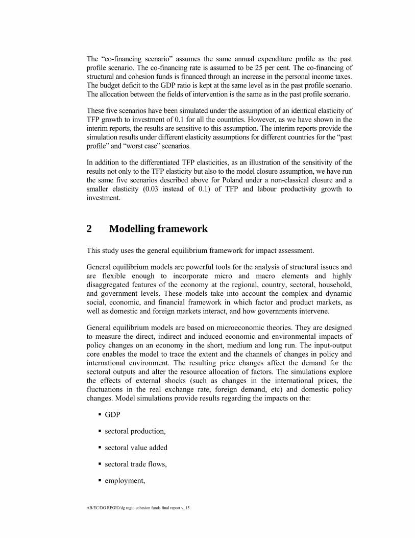
Table 4: Assumptions regarding the fields of intervention for the structural funds (continued) Fields of intervention
Share in % Volume Share in % Volume Share in % Volume Share in % Volume Share in % Volume Share in % VolumeProductive environment 32.1 876 27.8 1,130 23.3 3,463 22.2 3,646 41.3 1,033 8.4 574Business support 26.6 726 11.0 447 12.8 1,902 12.8 2,102 19.0 475 3.0 205Tourism 1.9 52 10.5 427 4.7 699 4.3 706 15.0 375 4.2 287RTDI 3.6 98 6.3 256 5.8 862 5.1 838 7.3 183 1.2 82Human resources 27.1 739 18.6 756 25.7 3,820 28.6 4,698 29.2 730 34.7 2,371Labour market 10.7 292 4.5 183 7.3 1,085 2.6 427 11.0 275 16.2 1,107Social inclusion 2.3 63 1.7 69 5.0 743 4.4 723 4.1 103 2.1 143Education 9.7 265 6.0 244 8.9 1,323 15.1 2,480 10.3 258 14.3 977Entrepreneurship 3.9 106 6.0 244 4.0 594 6.1 1,002 3.4 85 1.2 82Actions for women 0.5 14 0.4 16 0.5 74 0.4 66 0.4 10 0.9 61Infrastructure 34.9 952 47.9 1,946 45.5 6,762 46.5 7,638 23.6 590 44.0 3,006Transport 18.2 496 18.4 748 16.1 2,393 18.7 3,071 3.7 93 25.1 1,715Telecom 3.9 106 6.7 272 5.5 817 3.4 558 8.7 218 1.1 75Energy 3.9 106 7.8 317 0.9 134 0.0 0 3.7 93 0.5 34Environment 5.8 158 0.9 37 3.7 550 4.5 739 3.7 93 9.5 649Urban rehabilitation 0.0 0 1.6 65 6.3 936 9.8 1,610 3.8 95 1.8 123Social infrastructure and health 3.1 85 12.5 508 13.0 1,932 10.1 1,659 0.0 0 6.0 410Subtotal 94.1 2,567 94.3 3,831 94.5 14,045 97.3 15,982 94.1 2,353 87.1 5,951Rest 5.9 161 5.7 232 5.5 817 2.7 443 5.9 148 12.9 881Total SF 2007-2013 100.0 2,728 100.0 4,063 100.0 14,862 100.0 16,425 100.0 2,500 100.0 6,832
Latvia Lithuania Hungary Portugal Slovenia Slovakia
14
Table 4: Assumptions regarding the fields of intervention for the structural funds (continued) Fields of intervention
Share in % Volume Share in % Volume Share in % VolumeProductive environment 31.3 4,807 20.1 809 20.1 2,317Business support 19.6 3,010 12.8 518 12.8 1,482Tourism 1.7 261 4.5 181 4.5 520RTDI 10.0 1,536 2.7 110 2.7 316Human resources 32.2 4,945 28.0 1,128 28.0 3,229Labour market 12.7 1,950 7.2 289 7.2 828Social inclusion 6.6 1,014 4.3 172 4.3 493Education 3.5 538 10.7 433 10.7 1,239Entrepreneurship 5.7 875 5.0 200 5.0 574Actions for women 3.7 568 0.8 34 0.8 96Infrastructure 36.3 5,575 46.6 1,878 46.6 5,377Transport 18.7 2,872 21.9 885 21.9 2,533Telecom 0.9 138 5.3 214 5.3 612Energy 0.1 15 1.3 54 1.3 154Environment 7.8 1,198 5.4 218 5.4 624Urban rehabilitation 5.7 875 6.2 250 6.2 716Social infrastructure and health 3.1 476 6.4 258 6.4 739Subtotal 99.8 15,327 94.6 3,815 94.6 10,923Rest 0.2 31 5.4 218 5.4 624Total SF 2007-2013 100.0 15,358 100.0 4,033 100.0 11,547
Eastern Germany Bulgaria Romania

15
3.2 Worst case scenario
The “worst case scenario” (n+3/n+2) is based on the programming prices expenditures but assumes that the structural and cohesion funds are spent with a delay, during 2010-2015. Therefore, the annual expenditures profile is more ‘bunched’ than in the past profile of six countries scenario, reaching a peak in 2013. An example for Poland is provided in Tables 5 and 6.
In fact, in this scenario the annual expenditures for 2010-2012 are assumed to be the same as the planned expenditures for 2007-2009. In 2013, the planned expenditures for 2010-2011 are regrouped, while during 2014-2015 the expenditures follow the planned ones for 2012-2013.
The allocation between the fields of intervention is the same as in the past profile of 6 countries scenario (see Table 4).

16
Table 5: Payments profile, worst case payment scenario (n+3/n+2) – Poland (EUR mil., current prices) Poland (mil. euro, current prices) 2007 2008 2009 2010 2011 2012 2013 2014 2015 TotalStructural and cohesion funds 0 0 0 8,150 8,686 9,237 19,514 10,631 11,235 67,454Structural funds 0 0 0 6,147 6,290 6,433 12,861 6,664 6,827 45,221
Productive environment 0 0 0 793 811 830 1,659 860 881 5,834Manufacturing 0 0 0 491 503 514 1,028 532 545 3,613Services 0 0 0 302 309 316 631 327 335 2,220
Human resources 0 0 0 1,739 1,780 1,821 3,640 1,886 1,932 12,798Infrastructure 0 0 0 3,227 3,302 3,378 6,752 3,499 3,584 23,741Rest (services) 0 0 0 387 396 405 810 420 430 2,849
Cohesion funds 0 0 0 2,004 2,397 2,803 6,653 3,967 4,409 22,232
Table 6: Payments profile, programming prices scenario – Poland (EUR mil., current prices) Poland (mil. euro, current prices) 2007 2008 2009 2010 2011 2012 2013 2014 2015 TotalStructural and cohesion funds 8,150 8,686 9,237 9,465 10,049 10,631 11,235 0 0 67,454Structural funds 6,147 6,290 6,433 6,354 6,507 6,664 6,827 0 0 45,221
Productive environment 793 811 830 820 839 860 881 0 0 5,834Manufacturing 491 503 514 508 520 532 545 0 0 3,613Services 302 309 316 312 320 327 335 0 0 2,220
Human resources 1,739 1,780 1,821 1,798 1,842 1,886 1,932 0 0 12,798Infrastructure 3,227 3,302 3,378 3,336 3,416 3,499 3,584 0 0 23,741Rest (services) 387 396 405 400 410 420 430 0 0 2,849
Cohesion funds 2,004 2,397 2,803 3,112 3,541 3,967 4,409 0 0 22,232

17
3.3 Programming prices scenario
The “programming prices scenario” assumes that structural and cohesion funds are spent as planned, during 2007-2013.
The allocation between the fields of intervention is the same as in the past profile scenario (see Table 4).
3.4 Lisbon scenario
The “Lisbon scenario” assumes that the annual allocation of the structural and cohesion funds follows the past profile scenario.
However, the allocation of the structural funds between the fields of intervention is different (see Table 7). A part of the expenditures in infrastructure is shifted to the productive environment and human resources.
In the Lisbon scenario, the share of the infrastructure expenditures in the total structural funds is 5 percentage points lower than in the past profile scenario, while the expenditures related to the productive environment and the human resources are each 2.5 percentage points higher than in the past profile scenario.

18
Table 7: Assumptions regarding the fields of intervention for the structural funds – Lisbon scenario Fields of intervention
share in % Volume share in % Volume share in % Volume share in % Volume share in % Volume share in % VolumeProductive environment 15.4 6,181 26.5 4,205 27.7 565 14.8 2,209 21.2 5,997 35.7 6,879Business support 12.8 5,127 16.6 2,628 11.5 235 8.7 1,293 11.5 3,239 21.5 4,144Tourism 1.4 575 8.4 1,332 8.2 168 3.5 521 1.6 449 8.6 1,658RTDI 1.2 479 1.5 245 7.9 161 2.6 395 8.2 2,309 5.6 1,077Human resources 30.8 12,362 32.4 5,141 29.1 593 25.6 3,822 32.8 9,278 23.0 4,432Labour market 8.1 3,233 7.4 1,169 7.5 154 5.2 778 14.2 4,011 6.7 1,297Social inclusion 2.7 1,092 5.7 911 2.5 51 4.7 695 2.8 796 1.2 238Education 12.3 4,936 13.0 2,063 12.5 254 8.4 1,257 3.9 1,102 8.9 1,708Entrepreneurship 6.6 2,665 5.2 825 6.1 125 4.8 711 10.5 2,970 4.4 843Actions for women 1.1 437 1.1 172 0.4 9 2.5 381 1.4 398 1.8 346Infrastructure 47.5 19,065 36.7 5,824 38.7 789 54.7 8,166 45.2 12,785 34.3 6,609Transport 28.0 11,221 16.5 2,625 11.9 242 30.6 4,569 22.9 6,469 14.6 2,808Telecom 6.8 2,724 2.6 405 2.0 42 6.5 971 2.1 586 4.8 925Energy 1.4 545 1.4 223 2.6 52 0.9 137 0.5 153 1.2 235Environment 5.1 2,034 6.1 964 1.2 23 4.3 643 9.8 2,776 7.2 1,396Urban rehabilitation 3.5 1,416 7.4 1,173 4.6 94 6.6 985 5.6 1,579 5.2 1,009Social infrastructure and health 2.8 1,126 2.7 433 16.5 336 5.8 862 4.3 1,222 1.2 235Subtotal 93.7 37,608 95.6 15,170 95.5 1,947 95.1 14,197 99.2 28,060 93.0 17,919Rest 6.3 2,529 4.4 698 4.5 92 4.9 732 0.8 226 7.0 1,349Total SF 2007-2013 100.0 40,137 100.0 15,868 100.0 2,039 100.0 14,929 100.0 28,286 100.0 19,268
Poland Czech R Estonia Greece Spain Italy

19
Table 7: Assumptions regarding the fields of intervention for the structural funds – Lisbon scenario (continued) Fields of intervention
share in % Volume share in % Volume share in % Volume share in % Volume share in % Volume share in % VolumeProductive environment 34.6 944 30.3 1,231 25.8 3,834 24.7 4,057 43.8 1,095 10.9 745Business support 28.7 782 12.0 487 14.2 2,106 14.2 2,339 20.2 504 3.9 266Tourism 2.0 56 11.4 465 5.2 773 4.8 786 15.9 398 5.5 372RTDI 3.9 106 6.9 279 6.4 954 5.7 932 7.7 194 1.6 106Human resources 29.6 807 21.1 857 28.2 4,191 31.1 5,108 31.7 793 37.2 2,542Labour market 11.7 319 5.1 207 8.0 1,190 2.8 464 11.9 299 17.4 1,187Social inclusion 2.5 69 1.9 78 5.5 815 4.8 786 4.5 111 2.3 154Education 10.6 289 6.8 277 9.8 1,451 16.4 2,697 11.2 280 15.3 1,047Entrepreneurship 4.3 116 6.8 277 4.4 652 6.6 1,090 3.7 92 1.3 88Actions for women 0.5 15 0.5 18 0.5 82 0.4 71 0.4 11 1.0 66Infrastructure 29.9 816 42.9 1,743 40.5 6,019 41.5 6,816 18.6 465 39.0 2,664Transport 15.6 425 16.5 670 14.3 2,130 16.7 2,741 2.9 73 22.2 1,520Telecom 3.3 91 6.0 244 4.9 728 3.0 498 6.9 171 1.0 67Energy 3.3 91 7.0 284 0.8 119 0.0 0 2.9 73 0.4 30Environment 5.0 136 0.8 33 3.3 489 4.0 660 2.9 73 8.4 575Urban rehabilitation 0.0 0 1.4 58 5.6 833 8.7 1,437 3.0 75 1.6 109Social infrastructure and health 2.7 72 11.2 455 11.6 1,720 9.0 1,481 0.0 0 5.3 363Subtotal 94.1 2,567 94.3 3,831 94.5 14,045 97.3 15,982 94.1 2,353 87.1 5,951Rest 5.9 161 5.7 232 5.5 817 2.7 443 5.9 148 12.9 881Total SF 2007-2013 100.0 2,728 100.0 4,063 100.0 14,862 100.0 16,425 100.0 2,500 100.0 6,832
Latvia Lithuania Hungary Portugal Slovenia Slovakia

20
Table 7: Assumptions regarding the fields of intervention for the structural funds – Lisbon scenario (continued) Fields of intervention
share in % Volume share in % Volume share in % VolumeProductive environment 33.8 5,191 22.6 910 22.6 2,606Business support 21.2 3,251 14.4 582 14.4 1,666Tourism 1.8 282 5.1 204 5.1 584RTDI 10.8 1,658 3.1 124 3.1 355Human resources 34.7 5,329 30.5 1,229 30.5 3,518Labour market 13.7 2,102 7.8 315 7.8 902Social inclusion 7.1 1,092 4.6 187 4.6 537Education 3.8 579 11.7 472 11.7 1,350Entrepreneurship 6.1 943 5.4 218 5.4 625Actions for women 4.0 612 0.9 37 0.9 105Infrastructure 31.3 4,807 41.6 1,676 41.6 4,800Transport 16.1 2,476 19.6 790 19.6 2,261Telecom 0.8 119 4.7 191 4.7 546Energy 0.1 13 1.2 48 1.2 137Environment 6.7 1,033 4.8 194 4.8 557Urban rehabilitation 4.9 755 5.5 223 5.5 639Social infrastructure and health 2.7 411 5.7 230 5.7 660Subtotal 99.8 15,327 94.6 3,815 94.6 10,923Rest 0.2 31 5.4 218 5.4 624Total SF 2007-2013 100.0 15,358 100.0 4,033 100.0 11,547
Eastern Germny Bulgaria Romania

Tender no: 2006.CE16.0.AT022 – Study on the Economic Impact of Convergence Interventions (2007-2013)
AB/EC/DG REGIOdg regio cohesion funds final report v_15 21
3.5 Co-financing scenario
The “co-financing scenario” assumes the same annual expenditures profile as the past profile scenario. The co-financing rate is assumed to be 25 per cent.
The co-financing of structural and cohesion funds is financed through an increase in the personal income taxes.
The budget deficit to the GDP ratio is kept at the same level as in the past profile scenario.
The allocation between the fields of intervention is the same as in the past profile scenario (see Table 4).
3.6 Simulations with different elasticities
The five scenarios explained above have been simulated under the assumption of an identical elasticity of 0.1 for the TFP and labour productivity growth with respect to investment for all the countries.
However, as we have shown in the interim reports, the results are sensitive to this uniform elasticity assumption. Given the uncertainty regarding the TFP elasticity, the “past profile” and the “worst case” scenarios have also been simulated under the assumption of different elasticities for different member states for the interim report. We reproduce here the results to show their sensitivity of the assumption of uniform elasticity of 0.1.
Table 8: Elasticity of TFP growth Country Different UniformBulgaria 0.02 0.1 Czech Republic 0.07 0.1 Estonia 0.13 0.1 Germany 0.02 0.1Greece 0.10 0.1 Hungary 0.02 0.1 Italy 0.06 0.1 Latvia 0.12 0.1 Lithuania 0.03 0.1 Poland 0.04 0.1 Portugal 0.11 0.1 Romania 0.02 0.1 Slovakia 0.09 0.1 Slovenia 0.04 0.1 Spain 0.11 0.1

Tender no: 2006.CE16.0.AT022 – Study on the Economic Impact of Convergence Interventions (2007-2013)
AB/EC/DG REGIOdg regio cohesion funds final report v_15 22
3.7 Simulation with a different closure and different elasticities
Given that general equilibrium models focus on long term, potential allocative impacts, the current account balance is kept constant (in real terms or as a share of GDP) in the simulations. This is also the classical closure
1 which has been used in the simulations
explained above. However, as a variant, we also ran additional simulations for each of the five scenarios described earlier with a different model closure where the current account a balance adjusts to the policy measures. These simulations were run as an illustration for Poland only and with an elasticity of 0.03 (instead of 0.1) for the TFP growth with respect to investments.
4 Overview of the simulation results
In this section we summarise the main findings of the simulation results.
The simulations take into account the different impact channels of the different components of the structural and cohesions funds. In this respect, we use DG REGIO’s classification of the structural and cohesion funds into the three following fields of intervention:
• Productive environment
• Human resources
• Infrastructure
4.1 Modelling the EU funds
In the model, an institution called ‘The Fund’ receives the EU structural and cohesion funds and the domestic public co-financing funds and allocates them according to the stated uses.
The effects of the EU funds are captured in the model in several ways:
First, the structural and cohesion funds are distributed by the Fund to different branches of activity as investments, which add to the capital stock and lead to an increase in the productive capacity of the sector;
Secondly, the investments by the Fund lead to an increase in the total factor productivity (TFP) or labour productivity depending on the field of intervention
Three types of investments are distinguished in the model:
1 For details, please see the model closure section in the annexed technical overview of the model.

Tender no: 2006.CE16.0.AT022 – Study on the Economic Impact of Convergence Interventions (2007-2013)
AB/EC/DG REGIOdg regio cohesion funds final report v_15 23
Investments to improve the productive environment s(INVSF ) , which are provided to the manufacturing and services sectors and originate from the structural funds.
Investments in human resources s(INVSFH ) , which also originate from the structural funds and are destined to the services sector.
Investments in infrastructure s(INVCF ) , which are meant for the services sector and rely on both structural and cohesion funds.
The EU funds are expressed in national currency by multiplying them with the exchange rate ( ER ) . Furthermore, they are translated into real terms using the price index corresponding to investments ( PI ) :
s sINVSFR = INVSF ER/PI⋅
s sINVSFHR = INVSFH ER/PI⋅
s sINVCFR = INVCF ER/PI⋅
where sINVSFR stands for the investments to improve the productive environment in branch s, expressed in real terms and in the domestic currency, sINVSFHR represents the investments in human resources expressed in real terms and domestic currency and sINVCFR gives the investments in infrastructure in real terms and domestic currency.
The domestic public co-financing corresponding to each type of investment is derived by applying the co-financing rate ( tcof ) :
s sINVSFRCOF = tcof/(100-tcof) INVSF ER/PI⋅ ⋅
s sINVSFHRCOF = tcof/(100-tcof) INVSFH ER/PI⋅ ⋅
s sINVCFRCOF = tcof/(100-tcof) INVCF ER/PI⋅ ⋅
where sINVSFRCOF is the domestic public co-financing for the investments to improve the productive environment, sINVSFHRCOF represents the domestic public co-financing for the investments in human resources and sINVCFRCOF stands for the domestic public co-financing for the investments in infrastructure.
Total domestic public co-financing for the EU funds, expressed in nominal terms (COFIN) , is thus given by:
s s ss
COFIN = PI ( INVSFRCOF +INVSFHRCOF +INVCFRCOF )⋅∑
and adds to the government expenditures.

Tender no: 2006.CE16.0.AT022 – Study on the Economic Impact of Convergence Interventions (2007-2013)
AB/EC/DG REGIOdg regio cohesion funds final report v_15 24
Total investments (including domestic public co-financing) to productive environment s(INVSFRTOT ) , total investments in human resources s(INVSFHRTOT ) and total
investments in infrastructure s(INVCFRTOT ) , expressed in real terms, can be expressed as:
s s sINVSFRTOT = INVSFR +INVSFRCOF
s s sINVSFHRTOT = INVSFHR +INVSFHRCOF
s s sINVCFRTOT = INVCFR +INVCFRCOF
The Fund’s total resources ( SFUND ) , in nominal terms, should be equal to the total investments by the Fund:
s s ss
SFUND = PI (INVSFRTOT +INVSFHRTOT +INVCFRTOT )⋅∑
whereas the investments by the Fund excluding domestic public co-financing should be equal to the total transfers from the EU (TREUF) , expressed in domestic currency:
s s ss
PI (INVSFR +INVSFHR +INVCFR ) = TREUF ER⋅ ⋅∑
In addition to increasing the productive capacity, the investments for improving the productive environment are assumed to increase the TFP in the manufacturing and services sectors:
elasTFPSFs,t+1 s,t s,t s,t s,tTFPSF = TFPSF [(KSKBA +INVSFRTOT )/KSKBA ]⋅
where s,t+1TFPSF represents the TFP improvement in branch s in year t+1 thanks to investments in productive environment, s,tTFPSF stands for the TFP improvement in branch s in year t, s,tKSKBA provides the capital stock of sector s in year t in the non-cohesion policy baseline scenario and elasTFPSF is the TFP elasticity of investments provided to the productive environment. The effects of the EU funds on the TFP arise with one year lag.
Investments in human resources are assumed to lead to an improvement in the labour productivity in all the activities. In order to derive the increase in the labour productivity, we first calculate the number of trainees that could be supported by the structural funds (Bradley, Morgenroth, Gács and Untiedt, 2004):
ctm,t t ctm,t t t tctm ctm
t t
INVSFHRTOT PI OVERHD INVSFHRTOT PI TRAIN PLMA
(TRAIN / TRATIO ) PLSV
⋅ = ⋅ ⋅ + ⋅ +
⋅
∑ ∑
by assuming that a part of the total funds for human resources in year t ctm,t t
ctm( INVSFHRTOT PI )⋅∑ , expressed in nominal terms, represent the current operation
costs related to the buildings, materials, etc. ctm,t tctm
( OVERHD INVSFHRTOT PI )⋅ ⋅∑ , a part

Tender no: 2006.CE16.0.AT022 – Study on the Economic Impact of Convergence Interventions (2007-2013)
AB/EC/DG REGIOdg regio cohesion funds final report v_15 25
of the funds reflects payments to the trainees t t(TRAIN PLMA )⋅ and the rest are expenditures related to the compensation of instructors t t[(TRAIN / TRATIO ) PLSV ]⋅ . Current operation costs are derived as a share ( OVERHD ) of the total structural funds for human resources, where OVERHD , given the lack of detailed information, is assumed to be equal to the average share of other current expenditures in the total current expenditures in tertiary education (OECD, 2006). The payments to the trainees are calculated by assuming that each trainee receives a share of the average wage in the manufacturing sectors, services and construction t( PLMA ) , where tTRAIN is the number of policy-funded trainees (expressed in trainee-years). Finally, the compensation of the instructors is derived by applying the average wage in the services sector t( PLSV ) to the number of instructors t(TRAIN / TRATIO ) , where TRATIO is the trainee-instructor ratio assumed to be equal to the student-teacher ratio in the tertiary education for each country under study (OECD, 2006).
Thus, the number of trainees (expressed in trainee-years) that could be supported through the structural funds is given by:
t ctm,t t t tctm
TRAIN = INVSFHRTOT PI (1 OVERHD)/[PLMA +PLSV /TRATIO]⋅ ⋅ −∑
while the stock of trainees (expressed in trainee-years) is provided by:
t+1 t tKSKTRAIN = (1 dhc) KSKTRAIN +TRAIN− ⋅
where t+1KSKTRAIN is the stock of trainee in year t+1, tKSKTRAIN represents the stock of trainees in year t and dhc is the depreciation rate equal to 5 per cent (Bradley, Morgenroth, Gács and Untiedt, 2004).
The labour productivity improvements due to the structural funds on human resources are derived as:
elasTFPSFHs,t+1 s,t t t tTFPSFH = TFPSFH [(KSKTRAIN +KSKHBA )/KSKHBA ]⋅
where s,t+1TFPSFH represents the labour productivity improvement in branch s in year t+1, s,tTFPSFH provides the labour productivity improvement in branch s in year t,
tKSKHBA is the stock of human capital in the non-cohesion policy baseline scenario in year t and elasTFPSFH is the labour productivity elasticity of investments in human resources.
The spillover effects related to the investments in infrastructure are captured through a TFP increase in all the branches of activity:
elasTFPCFs,t+1 s,t t ctm,t t
ctmTFPCF = TFPCF [(KSKPbBA + INVCFRTOT )/KSKPbBA ]⋅ ∑
where s,t+1TFPCF is the TFP increase in branch s in year t+1 due to investments in infrastructure, s,tTFPCF is the TFP increase in branch s in year t, ctm,t
ctm
INVCFRTOT∑
stand for the total investments in infrastructure, tKSKPbBA gives the stock of

Tender no: 2006.CE16.0.AT022 – Study on the Economic Impact of Convergence Interventions (2007-2013)
AB/EC/DG REGIOdg regio cohesion funds final report v_15 26
infrastructure in the non-cohesion policy baseline scenario in year t and elasTFPCF represents the TFP elasticity of investments in infrastructure.
Both improvements in the labour productivity due to the investments in human resources and TFP increases related to investments in infrastructure occur with a lag of one year after the investments take place.
Value-added is a CES aggregation of capital ( )sKSK and labour ( )sLSK :
1( ) [ ( ) ]F F Fs s ss s s s s s s s sKL aF TFPSF TFPCF FK KSK FL TFPSFH LSKρ ρ ργ γ− − −= ⋅ ⋅ ⋅ ⋅ + ⋅ ⋅ (1)
where sTFPSF reflects the total factor productivity (TFP) increase due to the structural funds provided as direct aid to the productive environment, sTFPCF gives the TFP increase due to the structural and cohesion funds on infrastructure and sTFPSFH provides the labour productivity increase due to the structural funds targeted to human resources.
Minimizing the costs function:
s s s s s s s s s sCost ( KSK ,LSK ) [PK (1+tk )+d PI] KSK [PL (1+premLSK ) (1+tl )] LSK= ⋅ ⋅ ⋅ + ⋅ ⋅ ⋅ (2)
subject to (9) yields the demand equations for capital and labour:
s s sF F ( F 1)s s s s s s s s s sKSK = KL {PKL /[PK (1+tk )+d PI]} FK (aF TFPSF TFPCF )σ σ σγ −⋅ ⋅ ⋅ ⋅ ⋅ ⋅ ⋅ (3)
s s s
s
F F ( F 1)s s s s s s s
( F 1)s s s
LSK = KL { PKL /[PL (1+premLSK ) (1+tl )]} FL TFPSFH
(aF TFPSF TFPCF )
σ σ σ
σ
γ −
−
⋅ ⋅ ⋅ ⋅ ⋅ ⋅
⋅ ⋅ (4)
and the associated zero profit condition:
s s s s s s s s sPKL KL = PK (1+tk ) KSK +PL (1+premLSK ) (1+tl ) LSK +DEP PI⋅ ⋅ ⋅ ⋅ ⋅ ⋅ ⋅ (5)
where PL is the national average wage and spremLSK is the wage differential of branch s with respect to the average wage PL , stl is the social security contributions rate for industry s , sPK is the return to capital in branch s, stk is the corporate income tax rate for branch s, and sd is the depreciation rate in industry s. The depreciation s( DEP ) related to the private and public capital stock is valued at the investment price index ( PI ) . The elasticity of substitution between capital and labour is given by sFσ , where
1 (1 )s sF Fσ ρ= + , and sFKγ and sFLγ represent the distribution parameters corresponding to capital and labour.
4.2 Overview of the simulation results
The detailed year-by-year macro and sectoral results of the policy simulations are provided in the annexed country documents for each one of the simulations. Below we provide only the summary tables which present the macroeconomic impacts and the effects on the labour market for 2015 and 2020.

Tender no: 2006.CE16.0.AT022 – Study on the Economic Impact of Convergence Interventions (2007-2013)
AB/EC/DG REGIOdg regio cohesion funds final report v_15 27
Before we summarise the most salient outcomes of the simulations, it is important to underline that the simulation results should not be interpreted as economic forecasts or projections. Using the general equilibrium framework, in this study, we try to isolate and capture the impacts the EU funds. In order to isolate the impacts du to the EU funds, we need to make an abstraction of any other probable changes which may influence the development of the economies in the coming years. This is done through the model closure.
The most widely used macro closure rule for CGE models is based on the investment and savings balance. In the model, the investment is assumed to adjust to the available domestic and foreign savings. This reflects an economy in which savings form a binding constraint. An alternative closure is possible where the investments determine the total level of savings. In this case the foreign savings adjusts to meet the total savings requirement.
Additional assumptions are needed with regard to the government behaviour in the EcoMod model. First, the total current consumption by the government is fixed as a share of GDP, while the allocation between the consumption of different goods and services is provided by a Cobb-Douglas function. Secondly, the government net transfers to the foreign sector are assumed to be fixed in real terms, while the government net transfers to the household (except the unemployment benefits) are fixed as a share of GDP. Thus, the government savings are endogenously determined in the current version of EcoMod model. Alternative assumptions are possible, where total government expenditures can be fixed in real terms or as a share of GDP, while the total current consumption adjusts.
In the co-financing scenario an alternative closure is used for the government balance, where, besides the current consumption, the government savings are fixed as a share of GDP. The personal income tax rate adjusts to meet this constraint. In order to allow the comparability between the past profile of 6 countries scenario and the co-financing scenario, government savings to GDP ratio in the co-financing scenario has been fixed to its levels in the past profile of 6 countries scenario.
With respect to the external balance, the current account balance to GDP ratio is kept unchanged in the simulations, while the real exchange rate adjusts. In an illustrative scenario for Poland, we let current account (and thus the capital account) adjust which leads to capital flows other than the EU funds. This means that the results from this simulation do not only represent the potential impacts of the EU funds, but also other stem from other changes such as additional capital inflows or capital outflows. If there are any additional capital inflows for example, then the impacts shown by the model simulations are not only those of the EU funds but also of other foreign resources (increased or decreased).
The setup of the closure rules is important in determining the mechanisms governing the model. Therefore, the closure rules should be established also taking into account the policy scenario in question.
Below is an overview of the main findings from the simulation results:
• Structural and cohesion funds will have positive impacts in all the recipient countries.

Tender no: 2006.CE16.0.AT022 – Study on the Economic Impact of Convergence Interventions (2007-2013)
AB/EC/DG REGIOdg regio cohesion funds final report v_15 28
• The positive impacts in all the new member states are substantial and long-lasting.
• The impacts, though positive and substantial, in the “worst case” scenario are smaller than those of all the other scenarios given the delays in the use of the funds in the MS.
• The changes go in the same direction in all the scenarios. However, the magnitude of the annual impacts is different given that the pattern of the flows of funds is naturally different in each one of the scenarios. However, the mechanisms are the same, only the magnitudes change.
• Given that in most cases the impact channels are the same in all the scenarios, the differences in the magnitude and in the year-by-year pattern of the changes are simply due to the differences in the annual pattern of the funds available to the member states in the different scenarios.
• Even if, in all the scenarios the macroeconomic impacts and the effects on the labour market are highly positive, the magnitude of the changes is sensitive to the assumption on the elasticity of the productivity growth with respect to investment. The variants with different and usually lower elasticities we ran for the “past profile” and “worst case” scenarios show that the effects would be smaller though still positive and strong. In the case of Bulgaria, for example, real GDP would increase by 8.8% (instead of 12.3% under the assumption of 0.1 for the productivity elasticity) in 2015 and by 10.6% (instead of 16.2%) in the “past profile” scenario. In the case of Poland, real GDP would increase by 6.1% (instead of 8.6% under the assumption of 0.1 for the productivity elasticity) in 2015 and by 7.2% (instead of 10.7%). The positive impacts in the labour market would also be smaller (see Tables 9 and 10, and the details in Tables 17-20 for the “past profile” scenario, and Tables 25-28 for the “worst case” scenario).
• As explained above (and in the technical appendix), the simulation results are sensitive not only to the assumption of the elasticity of productivity to the model closure. In order to investment, but also to the model closure. In order to isolate and capture the impacts of the EU funds, we need to make a set of theoretical abstractions and hypothesis on the government expenditures, deficit, current and capital account balances. If we change these closure rules, the results would of course change as they would not only capture the impacts of the EU funds, but of other elements as well. For example, in the illustrative simulation for Poland with a modified foreign account closure (flexible current and capital account balances), the potential impact on real GDP and employment effects become smaller: real GDP would increase by 5.07% in 2007 instead of 7.15%, and total employment would increase by 2.96% in 2020 instead of 4.08% in the “past profile” scenario (for details see the appendix on this specific simulation for Poland)..
• In some countries, such as Slovakia, Lithuania, Latvia, and Bulgaria the real GDP would be more than 15% higher than the business-as-usual level by the year 2020 (in the uniform elasticity simulations).

Tender no: 2006.CE16.0.AT022 – Study on the Economic Impact of Convergence Interventions (2007-2013)
AB/EC/DG REGIOdg regio cohesion funds final report v_15 29
• The positive impacts of the structural and cohesion funds would continue even after the end of the financial period 2007-2013, thanks to increased TFP growth, higher labour productivity, and higher human, capital, and better infrastructure.
• The main engine of growth would be investment, both public and private.
• Private consumption would also be major component in the growth dynamics thanks to increasing real income and decreasing unemployment.
• The positive impacts on Germany, Italy, Spain, and to some extend on Greece and Slovenia are smaller (at the national level, though they may be important at the regional level in these countries) given that the amount of funds they receive are much smaller compared to their baseline GDP.
• The highest impacts are observed in the co-financing scenario (Tables 37-40). This is understandable given that in this scenario we assume that the total amount of funds available for the structural and cohesion policies will increase thanks to national co-financing. However, since we assume a constant deficit-to-GDP ratio, co-financing needs to be funded by an increase in taxes. We assume that the increase in the government expenditures is compensated by an increase in personal income taxes. The simulation results show that this compensation is not large enough to dampen the positive impacts of the additional investments carried out thanks to the national co-financing sources. In the long-run, the government would even be able to reduce the tax rates thanks to the additional revenue generated by higher economic growth in this scenario (see Table 41). The decline in the personal income tax rates strengthens the positive demand effect through an increase in private consumption and savings given the increase in the disposable real income.
• Following the co-financing scenario, the second best one would be the “programming prices” scenario (Tables 33-36) which, optimistically, assumes that the fund will be spent as planned.
• All the industries and services benefit from growth, however, construction and high-tech industries are the two branches which benefit the most. This is understandable given the considerable increase in investment and productivity.
• Improvement in the labour markets is substantial: employment increases in all the member states and the number of unemployed decreases tremendously (by more than 30% in some countries by 2020).
• As a result of considerably improved labour market conditions and high growth, the unemployment rate decreases by more than 5 percentage points in some countries.
• The increase in the labour productivity generated by the new investments does not lead to a decline in the total employment. On the contrary, the strong economic growth generated by the structural and cohesion funds leads to a long-lasting increase in employment. Given the sustainable long-term impact of the cohesion

Tender no: 2006.CE16.0.AT022 – Study on the Economic Impact of Convergence Interventions (2007-2013)
AB/EC/DG REGIOdg regio cohesion funds final report v_15 30
policy on the potential economic capacity of the member countries, the increase in employment endures even after the end of the funds.
• Imports increase considerably in the first years given the required import content by the high growth rates, and exports may even decline given rapidly growing domestic demand. During the 2007-2013 programming period, the increase in the imports is especially strong in the sectors providing goods and services to investment. However, after a couple of years, exports catch up and increase to a large extent thanks to increased capacity and the changes in the terms of trade. In the long run, both imports and exports are much higher with respect to the baseline for all industries. Even if higher exports are an important element in the higher growth path (going well beyond the programming period), growth is not export drive. The main engines of growth beyond the programming period are domestic: much improved capital and labour productivity, better human resources, higher physical capital stock in the industries and services, improved infrastructure, and higher productive capacity.
• The version of the model used in this study does not distinguish bilateral trade flows, however, given the importance of the bilateral trade among all the member states, we can confidently assume that the initial surge in import demand in the new member states will benefit to the other member states.
• In all the scenarios, thanks to the flow of funds, there is a build-up of the productive capacity and increased productivity (even if the timings are different in the scenarios) with cumulative and long-term positive effects on the potential output and employment.
• In all the scenarios, the supply side effects dominate the demand side effects. This explains why even after the end of the flow of EU funds there is no sharp decline in output or employment. However, beyond the programming period, the annual growth rates slow down, but the effect of the EU funds on the increased potential output is long-lasting in the sense that the real GDP growth path is higher than the baseline. This may of course be partially due to the general equilibrium modelling framework which focuses on the long-run impacts of policy changes on the potential GDP and productive capacity of the economy. The short-run Keynesian effects are not properly captured by this modelling framework.
The impacts of the cohesion funds come through both demand and supply sides of the economy. The question of demand-side effects is a trivial one. These are well understood in the literature and usually well captured in the macroeconometric models. The direct and indirect demand side effects play a major role in the short run. However, the most important rationale of the cohesion policy is related to the long term effects of the flow of funds to the recipient countries. If there were no positive long-term structural and sustainable impacts remaining after the end of the flow of funds, the cohesion policy would only produce a temporary relief to the recipient countries and the termination of the EU funds would have a negative effect on output and employment. The EcoMod model and many other studies show that the supply-side effects would fortunately play a major role in the positive long run impacts of the cohesion funds.

Tender no: 2006.CE16.0.AT022 – Study on the Economic Impact of Convergence Interventions (2007-2013)
AB/EC/DG REGIOdg regio cohesion funds final report v_15 31
The EcoMod model captures well these long-term supply side effects on investment, infrastructure, physical capital, human capital, labour supply, productivity growth, and the decline in the production costs.
The dynamic supply effects of the cohesion funds are captured through several channels in the model:
First, the structural and cohesion funds are distributed by the Fund to different branches of activity as investments, which add to the capital stock and lead to an increase in the productive capacity of the sector. Three types of investments are distinguished in the model:
Investments to improve the productive environment, which are provided to the manufacturing and services sectors and originate from the structural funds.
Investments in human resources, which also originate from the structural funds and are destined to the services sector.
Investments in infrastructure, which are meant for the services sector and rely on both structural and cohesion funds.
Secondly, the investments by the Fund lead to an increase in the total factor productivity (TFP) or labour productivity depending on the field of intervention.
During the funding period, the flow of structural and cohesion funds increase the stock of productive capital in the economy, generates higher TFP growth, and develop skills and productivity in human resources. All these mechanisms not only increase the productive capacity of the economy over the years, but they also have a favourable impact on the unit cost of production, an increase in household income and total savings in the economy. These virtuous circle effects help the expansion of the production, employment, investment, and capital stock over the years. Even when the funds end, the increased productive capacity, improved productivity, better human resources remain as long term development engines within the country and continue to sustain a higher growth path of the economy with respect to the baseline. Beyond the funding period, even if the annual growth rates decline due to the end of the flow of EU funds, the growth path of the economy remains much above the baseline thanks to increased and improved productive domestic capacity of the economies.

Tender no: 2006.CE16.0.AT022 – Study on the Economic Impact of Convergence Interventions (2007-2013)
AB/EC/DG REGIOdg regio cohesion funds final report v_15 32
Table 9: Growth effects (% change in real GDP with respect to the BAU) - 2015 BG CZ EE DE EL HU IT LV LT PL PT RO SK SI ES Past profile 12.27 8.39 7.15 0.31 2.85 4.94 0.43 12.71 16.05 8.55 3.35 6.23 14.80 3.07 1.05
Worst case 10.19 7.72 6.41 0.28 2.63 4.47 0.39 11.30 13.17 7.45 3.10 5.27 12.29 2.86 1.00
Programming prices 14.76 9.75 8.07 0.38 3.08 5.53 0.51 14.57 18.81 10.10 3.73 7.02 18.00 3.37 1.18
Lisbon 12.14 8.27 7.00 0.30 2.78 4.83 0.41 12.52 15.89 8.42 3.27 6.13 14.67 3.01 1.02
Co-financing 15.65 10.49 8.90 0.38 3.62 5.97 0.53 15.81 19.92 10.65 4.14 7.96 18.22 3.75 1.31
Past profile different elasticities 8.80 7.34 8.39 0.22 2.85 2.51 0.36 13.99 11.99 6.14 3.49 3.95 14.41 2.22 1.09
Worst case different elasticities 7.58 6.79 7.44 0.21 2.63 2.34 0.33 12.35 10.06 5.47 3.22 3.49 11.98 2.12 1.04
Table 10: Growth effects (% change in real GDP with respect to the BAU) - 2020 BG CZ EE DE EL HU IT LV LT PL PT RO SK SI ES Past profile 16.20 9.57 8.22 0.41 3.11 5.53 0.53 14.90 22.54 10.70 3.73 6.95 20.58 3.22 1.17
Worst case 14.12 8.95 7.48 0.38 2.92 5.09 0.49 13.56 19.24 9.59 3.46 6.10 18.05 3.04 1.11
Programming prices 17.70 10.11 8.84 0.45 3.41 5.90 0.59 16.04 25.05 11.90 4.05 7.44 22.64 3.40 1.30
Lisbon 16.00 9.41 8.01 0.40 3.03 5.38 0.52 14.64 22.26 10.51 3.61 6.81 20.36 3.14 1.13
Co-financing 20.42 12.27 10.69 0.50 4.06 7.08 0.67 18.96 27.82 13.46 4.86 9.08 24.52 4.15 1.49
Past profile different elasticities 10.58 8.10 9.90 0.27 3.11 2.40 0.44 16.76 15.60 7.15 3.91 3.89 19.93 2.09 1.23
Worst case different elasticities 9.50 7.62 8.97 0.25 2.92 2.24 0.41 15.18 13.40 6.49 3.63 3.51 17.51 2.01 1.17

Tender no: 2006.CE16.0.AT022 – Study on the Economic Impact of Convergence Interventions (2007-2013)
AB/EC/DG REGIOdg regio cohesion funds final report v_15 33
Table 11: Employment effects (% change to the BAU) - 2015 BG CZ EE DE EL HU IT LV LT PL PT RO SK SI ES Past profile 6.57 3.27 2.92 0.15 1.56 1.95 0.22 5.91 7.11 4.79 1.39 2.38 6.18 1.21 0.61Worst case 5.48 3.07 2.76 0.14 1.36 1.87 0.20 5.46 6.11 4.29 1.29 2.06 5.36 1.14 0.56Programming prices 7.54 3.01 2.70 0.17 1.26 1.41 0.23 6.08 7.19 5.50 1.23 2.40 6.59 1.10 0.56Lisbon 6.51 3.24 2.87 0.14 1.53 1.92 0.22 5.84 7.06 4.73 1.37 2.35 6.13 1.19 0.59Co-financing 8.14 3.75 3.33 0.18 1.90 2.12 0.27 6.90 8.29 5.77 1.61 2.79 7.20 1.36 0.73Past profile different elasticities 5.02 3.00 3.28 0.11 1.56 1.34 0.19 6.34 5.78 3.62 1.43 1.67 6.05 0.96 0.63Worst case different elasticities 4.31 2.83 3.07 0.11 1.36 1.33 0.18 5.82 5.06 3.31 1.33 1.51 5.25 0.93 0.58
Table 12: Employment effects (% change to the BAU) - 2020 BG CZ EE DE EL HU IT LV LT PL PT RO SK SI ES Past profile 8.89 3.41 3.11 0.19 1.43 1.62 0.25 6.71 9.45 5.82 1.29 2.65 8.66 1.13 0.58Worst case 7.83 3.18 2.84 0.17 1.32 1.48 0.23 6.18 8.26 5.27 1.20 2.32 7.71 1.07 0.55Programming prices 9.65 3.65 3.35 0.21 1.61 1.74 0.27 7.18 10.33 6.40 1.41 2.85 9.41 1.20 0.65Lisbon 8.79 3.36 3.04 0.18 1.39 1.58 0.24 6.61 9.36 5.73 1.26 2.60 8.57 1.11 0.56Co-financing 10.88 4.23 3.96 0.23 1.85 2.06 0.31 8.31 11.14 7.21 1.66 3.38 10.14 1.45 0.73Past profile different elasticities 6.20 2.96 3.68 0.13 1.43 0.71 0.20 7.40 7.07 4.08 1.35 1.61 8.42 0.77 0.61Worst case different elasticities 5.59 2.77 3.34 0.12 1.32 0.64 0.19 6.79 6.15 3.73 1.25 1.43 7.50 0.74 0.58

Tender no: 2006.CE16.0.AT022 – Study on the Economic Impact of Convergence Interventions (2007-2013)
AB/EC/DG REGIOdg regio cohesion funds final report v_15 34
Past profile scenario (TFP elasticity of 0.1 for all countries) Table 13: Macroeconomic effects in real terms (% change to the BAU) - 2015 BG CZ EE DE EL HU IT LV LT PL PT RO SK SI ESGDP 12.27 8.39 7.15 0.31 2.85 4.94 0.43 12.71 16.05 8.55 3.35 6.23 14.80 3.07 1.05
Private consumption 7.33 5.39 4.07 0.19 2.90 4.23 0.33 6.98 7.09 6.05 2.85 5.18 6.19 2.22 0.83
Government consumption 10.64 7.87 6.51 0.28 3.19 4.84 0.40 11.13 15.09 8.44 3.22 6.04 16.61 2.89 1.04
Gross fixed investment 29.36 20.05 18.42 1.06 8.43 16.92 1.43 30.88 42.40 21.88 10.02 15.55 31.94 8.88 3.33
Exports 10.42 4.74 4.68 0.15 0.10 1.72 0.08 10.78 11.84 4.99 0.49 3.84 11.73 1.60 0.14
Imports 10.44 6.95 7.18 0.32 5.43 5.73 0.69 12.78 12.15 10.39 4.83 7.35 10.01 3.38 1.60
Table 14: Macroeconomic effects in real terms (% change to the BAU) - 2020 BG CZ EE DE EL HU IT LV LT PL PT RO SK SI ESGDP 16.20 9.57 8.22 0.41 3.11 5.53 0.53 14.90 22.54 10.70 3.73 6.95 20.58 3.22 1.17
Private consumption 10.05 5.88 4.23 0.25 2.55 3.83 0.37 7.79 9.36 7.15 2.58 5.43 8.96 2.07 0.82
Government consumption 13.62 7.79 7.14 0.37 2.98 4.82 0.50 12.65 19.61 10.04 3.39 6.35 20.41 2.89 1.09
Gross fixed investment 23.33 11.29 9.39 0.82 3.37 5.86 0.88 19.28 41.56 15.18 5.12 6.71 30.49 3.36 1.61
Exports 15.73 8.38 7.75 0.35 3.09 4.80 0.46 16.62 22.49 10.42 3.43 7.06 19.82 3.19 1.05
Imports 10.22 5.89 5.15 0.25 1.78 3.33 0.33 9.97 14.33 6.68 2.28 4.27 12.26 2.02 0.73
Table 15: Labour market effects - 2015 BG CZ EE DE EL HU IT LV LT PL PT RO SK SI ESNational employment 6.57 3.27 2.92 0.15 1.56 1.95 0.22 5.91 7.11 4.79 1.39 2.38 6.18 1.21 0.61Number of unemployed -23.45 -26.32 -19.74 -1.24 -9.26 -20.87 -1.82 -28.98 -39.40 -21.04 -16.71 -21.31 -23.11 -12.38 -3.90Active population 0.72 0.82 0.59 0.03 0.26 0.63 0.05 0.92 1.35 0.63 0.49 0.64 0.70 0.35 0.11Unemployment rate (in %) 14.82 6.07 8.22 8.10 10.86 4.56 8.24 10.06 7.41 12.63 4.14 5.75 14.28 5.50 10.66Unemployment rate (% points difference with BAU) -4.68 -2.23 -2.08 -0.10 -1.14 -1.24 -0.16 -4.24 -4.99 -3.47 -0.86 -1.60 -4.42 -0.80 -0.44
Table 16: Labour market effects - 2020 BG CZ EE DE EL HU IT LV LT PL PT RO SK SI ES National employment 8.89 3.41 3.11 0.19 1.43 1.62 0.25 6.71 9.45 5.82 1.29 2.65 8.66 1.13 0.58Number of unemployed -31.48 -27.33 -20.98 -1.56 -8.52 -17.45 -2.03 -32.79 -51.18 -25.45 -15.55 -23.58 -32.08 -11.63 -3.72Active population 1.01 0.86 0.63 0.04 0.24 0.51 0.05 1.07 1.93 0.79 0.45 0.72 1.04 0.33 0.10Unemployment rate (in %) 13.23 5.98 8.09 8.07 10.95 4.76 8.23 9.51 5.94 11.91 4.20 5.58 12.57 5.55 10.68Unemployment rate (% points difference with BAU) -6.27 -2.32 -2.21 -0.13 -1.05 -1.04 -0.17 -4.79 -6.46 -4.19 -0.80 -1.77 -6.13 -0.75 -0.42

Tender no: 2006.CE16.0.AT022 – Study on the Economic Impact of Convergence Interventions (2007-2013)
AB/EC/DG REGIOdg regio cohesion funds final report v_15 35
Past profile scenario (different TFP elasticities for different countries) Table 17: Macroeconomic effects in real terms (% change to the BAU) - 2015 BG CZ EE DE EL HU IT LV LT PL PT RO SK SI ES GDP 8.80 7.34 8.39 0.22 2.85 2.51 0.36 13.99 11.99 6.14 3.49 3.95 14.41 2.22 1.09
Private consumption 5.38 4.68 4.62 0.15 2.90 2.79 0.29 7.65 5.58 4.36 2.95 3.51 5.97 1.69 0.86
Government consumption 7.50 6.96 7.59 0.20 3.19 2.65 0.34 12.21 11.31 6.07 3.36 3.90 16.23 2.13 1.08
Gross fixed investment 24.76 19.23 19.64 0.90 8.43 14.50 1.34 32.20 35.81 18.97 10.17 13.41 31.55 8.15 3.38
Exports 7.12 3.81 5.85 0.08 0.10 -0.45 0.03 12.18 7.71 2.82 0.61 1.58 11.36 0.74 0.18
Imports 8.63 6.41 7.83 0.27 5.43 4.46 0.66 13.48 9.95 9.17 4.90 6.18 9.82 2.91 1.62
Table 18: Macroeconomic effects in real terms (% change to the BAU) - 2020 BG CZ EE DE EL HU IT LV LT PL PT RO SK SI ES GDP 10.58 8.10 9.90 0.27 3.11 2.40 0.44 16.76 15.60 7.15 3.91 3.89 19.93 2.09 1.23
Private consumption 6.61 4.83 5.12 0.17 2.55 1.75 0.30 8.87 6.30 4.60 2.72 3.04 8.60 1.31 0.87
Government consumption 8.60 6.51 8.66 0.24 2.98 1.94 0.41 14.26 13.31 6.61 3.57 3.49 19.77 1.85 1.15
Gross fixed investment 15.51 9.94 11.22 0.54 3.37 2.55 0.73 21.37 29.81 10.65 5.34 3.79 29.75 2.31 1.68
Exports 10.26 7.09 9.36 0.22 3.09 1.99 0.38 18.68 15.50 7.05 3.59 4.00 19.21 2.05 1.10
Imports 6.71 4.98 6.21 0.16 1.78 1.37 0.27 11.19 9.97 4.50 2.39 2.40 11.89 1.29 0.77
Table 19: Labour market effects - 2015 BG CZ EE DE EL HU IT LV LT PL PT RO SK SI ES National employment 5.02 3.00 3.28 0.11 1.56 1.34 0.19 6.34 5.78 3.62 1.43 1.67 6.05 0.96 0.63Number of unemployed -17.99 -24.20 -22.10 -0.96 -9.26 -14.50 -1.60 -31.04 -32.34 -15.99 -17.17 -15.09 -22.62 -9.90 -4.03Active population 0.53 0.74 0.67 0.03 0.26 0.42 0.04 1.00 1.05 0.47 0.50 0.44 0.69 0.28 0.11Unemployment rate (in %) 15.91 6.25 7.97 8.12 10.86 4.94 8.26 9.76 8.30 13.46 4.12 6.21 14.37 5.66 10.64Unemployment rate (% points difference with BAU) -3.59 -2.05 -2.33 -0.08 -1.14 -0.86 -0.14 -4.54 -4.10 -2.64 -0.88 -1.14 -4.33 -0.64 -0.46
Table 20: Labour market effects - 2020 BG CZ EE DE EL HU IT LV LT PL PT RO SK SI ES National employment 6.20 2.96 3.68 0.13 1.43 0.71 0.20 7.40 7.07 4.08 1.35 1.61 8.42 0.77 0.61Number of unemployed -22.15 -23.88 -24.66 -1.06 -8.52 -7.74 -1.68 -35.99 -39.19 -17.96 -16.23 -14.53 -31.23 -7.95 -3.90Active population 0.67 0.73 0.76 0.03 0.24 0.22 0.05 1.20 1.34 0.53 0.47 0.42 1.00 0.22 0.11Unemployment rate (in %) 15.08 6.27 7.70 8.11 10.95 5.34 8.25 9.05 7.44 13.14 4.17 6.26 12.73 5.79 10.66Unemployment rate (% points difference with BAU) -4.42 -2.03 -2.60 -0.09 -1.05 -0.46 -0.15 -5.25 -4.96 -2.96 -0.83 -1.09 -5.97 -0.51 -0.44

Tender no: 2006.CE16.0.AT022 – Study on the Economic Impact of Convergence Interventions (2007-2013)
AB/EC/DG REGIOdg regio cohesion funds final report v_15 36
Worst case scenario (TFP elasticity of 0.1 for all countries) Table 21: Macroeconomic effects in real terms (% change to the BAU) - 2015 BG CZ EE DE EL HU IT LV LT PL PT RO SK SI ESGDP 10.19 7.72 6.41 0.28 2.63 4.47 0.39 11.30 13.17 7.45 3.10 5.27 12.29 2.86 1.00
Private consumption 6.14 5.04 3.91 0.18 2.58 3.99 0.30 6.51 6.32 5.36 2.64 4.59 5.48 2.10 0.77
Government consumption 9.16 7.41 5.99 0.25 2.88 4.47 0.36 10.16 13.19 7.51 2.99 5.35 14.92 2.72 0.98
Gross fixed investment 29.00 19.95 19.67 0.99 7.86 17.55 1.36 31.65 39.17 21.21 9.48 17.32 29.64 8.72 2.90
Exports 8.28 3.98 3.61 0.14 0.22 1.12 0.06 8.68 8.22 3.74 0.38 2.26 8.85 1.38 0.24
Imports 10.19 6.72 7.44 0.30 4.88 5.77 0.66 12.94 11.10 10.34 4.58 8.00 9.01 3.27 1.38
Table 22: Macroeconomic effects in real terms (% change to the BAU) - 2020 BG CZ EE DE EL HU IT LV LT PL PT RO SK SI ESGDP 14.12 8.95 7.48 0.38 2.92 5.09 0.49 13.56 19.24 9.59 3.46 6.10 18.05 3.04 1.11
Private consumption 8.74 5.46 3.83 0.23 2.36 3.49 0.34 7.06 7.92 6.39 2.38 4.72 7.93 1.95 0.78
Government consumption 11.92 7.45 6.49 0.34 2.78 4.42 0.46 11.50 16.92 9.03 3.14 5.59 18.03 2.73 1.03
Gross fixed investment 20.40 10.53 8.58 0.75 3.24 5.47 0.81 17.63 35.63 13.59 4.75 5.96 26.73 3.17 1.53
Exports 13.74 7.80 7.05 0.32 2.92 4.42 0.43 15.13 19.23 9.34 3.19 6.26 17.33 3.00 1.00
Imports 8.94 5.48 4.69 0.23 1.67 3.06 0.30 9.08 12.31 5.98 2.11 3.76 10.76 1.90 0.69
Table 23: Labour market effects - 2015 BG CZ EE DE EL HU IT LV LT PL PT RO SK SI ESNational employment 5.48 3.07 2.76 0.14 1.36 1.87 0.20 5.46 6.11 4.29 1.29 2.06 5.36 1.14 0.56Number of unemployed -19.61 -24.71 -18.69 -1.14 -8.12 -20.00 -1.66 -26.87 -34.11 -18.86 -15.54 -18.54 -20.08 -11.69 -3.61Active population 0.58 0.76 0.55 0.03 0.23 0.60 0.04 0.84 1.12 0.56 0.45 0.55 0.60 0.33 0.10Unemployment rate (in %) 15.58 6.20 8.33 8.10 11.00 4.61 8.26 10.37 8.08 12.99 4.20 5.95 14.86 5.54 10.69Unemployment rate (% points difference with BAU) -3.92 -2.10 -1.97 -0.10 -1.00 -1.19 -0.14 -3.93 -4.32 -3.11 -0.80 -1.39 -3.84 -0.76 -0.41
Table 24: Labour market effects - 2020 BG CZ EE DE EL HU IT LV LT PL PT RO SK SI ES National employment 7.83 3.18 2.84 0.17 1.32 1.48 0.23 6.18 8.26 5.27 1.20 2.32 7.71 1.07 0.55Number of unemployed -27.84 -25.61 -19.17 -1.45 -7.88 -15.96 -1.87 -30.25 -45.27 -23.08 -14.45 -20.79 -28.68 -10.98 -3.54Active population 0.87 0.79 0.57 0.04 0.22 0.47 0.05 0.97 1.62 0.70 0.42 0.62 0.91 0.31 0.10Unemployment rate (in %) 13.95 6.13 8.28 8.08 11.03 4.85 8.24 9.88 6.68 12.30 4.26 5.79 13.22 5.59 10.70Unemployment rate (% points difference with BAU) -5.55 -2.17 -2.02 -0.12 -0.97 -0.95 -0.16 -4.42 -5.72 -3.80 -0.74 -1.56 -5.48 -0.71 -0.40

Tender no: 2006.CE16.0.AT022 – Study on the Economic Impact of Convergence Interventions (2007-2013)
AB/EC/DG REGIOdg regio cohesion funds final report v_15 37
Worst case scenario (different TFP elasticities for different countries) Table 25: Macroeconomic effects in real terms (% change to the BAU) - 2015 BG CZ EE DE EL HU IT LV LT PL PT RO SK SI ES GDP 7.58 6.79 7.44 0.21 2.63 2.34 0.33 12.35 10.06 5.47 3.22 3.49 11.98 2.12 1.04
Private consumption 4.69 4.42 4.36 0.14 2.58 2.75 0.26 7.06 5.16 3.95 2.73 3.30 5.30 1.63 0.80
Government consumption 6.77 6.62 6.90 0.19 2.88 2.56 0.31 11.05 10.22 5.54 3.11 3.66 14.62 2.05 1.02
Gross fixed investment 25.54 19.25 20.71 0.85 7.86 15.41 1.28 32.73 34.15 18.85 9.62 15.61 29.36 8.10 2.95
Exports 5.81 3.17 4.60 0.07 0.22 -0.79 0.02 9.83 5.04 1.95 0.49 0.49 8.57 0.63 0.28
Imports 8.83 6.24 7.99 0.26 4.88 4.65 0.64 13.52 9.38 9.33 4.65 7.08 8.87 2.87 1.40
Table 26: Macroeconomic effects in real terms (% change to the BAU) - 2020 BG CZ EE DE EL HU IT LV LT PL PT RO SK SI ES GDP 9.50 7.62 8.97 0.25 2.92 2.24 0.41 15.18 13.40 6.49 3.63 3.51 17.51 2.01 1.17
Private consumption 5.92 4.50 4.62 0.16 2.36 1.61 0.28 8.00 5.35 4.16 2.51 2.70 7.61 1.25 0.82
Government consumption 7.74 6.27 7.85 0.23 2.78 1.79 0.38 12.91 11.54 6.02 3.31 3.16 17.49 1.79 1.09
Gross fixed investment 13.93 9.32 10.20 0.51 3.24 2.44 0.68 19.46 25.67 9.66 4.96 3.48 26.12 2.22 1.60
Exports 9.22 6.63 8.48 0.21 2.92 1.85 0.35 16.94 13.34 6.41 3.35 3.66 16.81 1.95 1.05
Imports 6.04 4.66 5.63 0.15 1.67 1.26 0.25 10.16 8.60 4.08 2.22 2.17 10.45 1.24 0.73
Table 27: Labour market effects - 2015 BG CZ EE DE EL HU IT LV LT PL PT RO SK SI ES National employment 4.31 2.83 3.07 0.11 1.36 1.33 0.18 5.82 5.06 3.31 1.33 1.51 5.25 0.93 0.58Number of unemployed -15.49 -22.87 -20.68 -0.90 -8.12 -14.43 -1.46 -28.58 -28.49 -14.64 -15.95 -13.66 -19.69 -9.55 -3.73Active population 0.45 0.70 0.62 0.02 0.23 0.42 0.04 0.90 0.90 0.42 0.47 0.39 0.59 0.27 0.10Unemployment rate (in %) 16.41 6.36 8.12 8.12 11.00 4.94 8.27 10.12 8.79 13.69 4.18 6.32 14.93 5.68 10.67Unemployment rate (% points difference with BAU) -3.09 -1.94 -2.18 -0.08 -1.00 -0.86 -0.13 -4.18 -3.61 -2.41 -0.82 -1.03 -3.77 -0.62 -0.43
Table 28: Labour market effects - 2020 BG CZ EE DE EL HU IT LV LT PL PT RO SK SI ES National employment 5.59 2.77 3.34 0.12 1.32 0.64 0.19 6.79 6.15 3.73 1.25 1.43 7.50 0.74 0.58Number of unemployed -20.00 -22.44 -22.49 -1.00 -7.88 -7.03 -1.56 -33.14 -34.33 -16.45 -15.08 -12.99 -27.93 -7.63 -3.71Active population 0.60 0.68 0.68 0.03 0.22 0.19 0.04 1.08 1.13 0.48 0.44 0.37 0.88 0.21 0.10Unemployment rate (in %) 15.51 6.39 7.93 8.12 11.03 5.38 8.27 9.46 8.05 13.39 4.23 6.37 13.36 5.81 10.68Unemployment rate (% points difference with BAU) -3.99 -1.91 -2.37 -0.08 -0.97 -0.42 -0.13 -4.84 -4.35 -2.71 -0.77 -0.98 -5.34 -0.49 -0.42

Tender no: 2006.CE16.0.AT022 – Study on the Economic Impact of Convergence Interventions (2007-2013)
AB/EC/DG REGIOdg regio cohesion funds final report v_15 38
Programming prices scenario (TFP elasticity of 0.1 for all countries) Table 29: Macroeconomic effects in real terms (% change to the BAU) - 2015 BG CZ EE DE EL HU IT LV LT PL PT RO SK SI ESGDP 14.76 9.75 8.07 0.38 3.08 5.53 0.51 14.57 18.81 10.10 3.73 7.02 18.00 3.37 1.18
Private consumption 8.41 5.06 3.48 0.22 2.32 3.42 0.34 6.51 6.07 6.34 2.40 4.91 6.02 1.97 0.80
Government consumption 12.10 8.37 6.74 0.33 2.88 4.62 0.46 11.82 16.23 9.59 3.39 6.44 18.83 2.98 1.09
Gross fixed investment 20.13 10.50 8.46 0.74 3.63 5.48 0.84 17.82 33.82 13.90 5.02 6.80 27.10 3.28 1.57
Exports 14.19 8.26 7.59 0.32 3.07 4.76 0.42 16.45 19.21 9.63 3.42 7.33 16.85 3.28 1.03
Imports 7.78 4.81 4.18 0.19 1.46 2.73 0.26 8.08 10.08 5.15 1.89 3.60 8.68 1.75 0.61
Table 30: Macroeconomic effects in real terms (% change to the BAU) - 2020 BG CZ EE DE EL HU IT LV LT PL PT RO SK SI ESGDP 17.70 10.11 8.84 0.45 3.41 5.90 0.59 16.04 25.05 11.90 4.05 7.44 22.64 3.40 1.30
Private consumption 11.01 6.32 4.58 0.28 2.83 4.11 0.41 8.44 10.50 7.96 2.82 5.87 9.80 2.19 0.91
Government consumption 14.80 7.81 7.66 0.41 3.27 5.15 0.56 13.62 21.65 11.10 3.67 6.79 22.27 3.04 1.21
Gross fixed investment 25.42 12.05 10.08 0.91 3.58 6.21 0.97 20.65 45.94 16.90 5.57 7.11 33.53 3.55 1.80
Exports 17.16 8.94 8.33 0.39 3.34 5.14 0.51 17.86 24.94 11.56 3.70 7.51 21.87 3.38 1.16
Imports 11.12 6.29 5.55 0.27 1.95 3.56 0.36 10.71 15.85 7.43 2.48 4.55 13.49 2.14 0.81
Table 31: Labour market effects - 2015 BG CZ EE DE EL HU IT LV LT PL PT RO SK SI ESNational employment 7.54 3.01 2.70 0.17 1.26 1.41 0.23 6.08 7.19 5.50 1.23 2.40 6.59 1.10 0.56Number of unemployed -26.84 -24.27 -18.30 -1.41 -7.51 -15.26 -1.86 -29.80 -39.77 -24.06 -14.75 -21.49 -24.61 -11.25 -3.62Active population 0.84 0.74 0.54 0.04 0.21 0.44 0.05 0.95 1.36 0.74 0.43 0.65 0.76 0.32 0.10Unemployment rate (in %) 14.15 6.24 8.37 8.08 11.08 4.89 8.24 9.94 7.37 12.14 4.24 5.73 13.99 5.57 10.69Unemployment rate (% points difference with BAU) -5.35 -2.06 -1.93 -0.12 -0.92 -0.91 -0.16 -4.36 -5.03 -3.96 -0.76 -1.62 -4.71 -0.73 -0.41
Table 32: Labour market effects - 2020 BG CZ EE DE EL HU IT LV LT PL PT RO SK SI ES National employment 9.65 3.65 3.35 0.21 1.61 1.74 0.27 7.18 10.33 6.40 1.41 2.85 9.41 1.20 0.65Number of unemployed -34.11 -29.15 -22.55 -1.75 -9.59 -18.69 -2.26 -34.94 -55.40 -27.92 -16.94 -25.31 -34.78 -12.29 -4.16Active population 1.12 0.92 0.68 0.05 0.27 0.55 0.06 1.15 2.18 0.88 0.50 0.78 1.15 0.35 0.11Unemployment rate (in %) 12.71 5.83 7.92 8.05 10.82 4.69 8.21 9.20 5.41 11.50 4.13 5.45 12.06 5.51 10.63Unemployment rate (% points difference with BAU) -6.79 -2.47 -2.38 -0.15 -1.18 -1.11 -0.19 -5.10 -6.99 -4.60 -0.87 -1.90 -6.64 -0.79 -0.47

Tender no: 2006.CE16.0.AT022 – Study on the Economic Impact of Convergence Interventions (2007-2013)
AB/EC/DG REGIOdg regio cohesion funds final report v_15 39
Lisbon scenario (TFP elasticity of 0.1 for all countries) Table 33: Macroeconomic effects in real terms (% change to the BAU) - 2015 BG CZ EE DE EL HU IT LV LT PL PT RO SK SI ESGDP 12.14 8.27 7.00 0.30 2.78 4.83 0.41 12.52 15.89 8.42 3.27 6.13 14.67 3.01 1.02
Private consumption 7.25 5.30 4.00 0.19 2.84 4.16 0.32 6.88 7.03 5.97 2.79 5.10 6.12 2.19 0.80
Government consumption 10.51 7.75 6.36 0.27 3.12 4.72 0.39 10.93 14.91 8.29 3.13 5.93 16.46 2.83 1.00
Gross fixed investment 29.22 19.96 18.27 1.05 8.36 16.81 1.42 30.72 42.13 21.74 9.92 15.47 31.79 8.83 3.29
Exports 10.31 4.65 4.55 0.15 0.03 1.63 0.08 10.60 11.69 4.88 0.42 3.74 11.63 1.55 0.11
Imports 10.38 6.90 7.11 0.32 5.40 5.68 0.69 12.70 12.08 10.34 4.79 7.31 9.96 3.35 1.58
Table 34: Macroeconomic effects in real terms (% change to the BAU) - 2020 BG CZ EE DE EL HU IT LV LT PL PT RO SK SI ESGDP 16.00 9.41 8.01 0.40 3.03 5.38 0.52 14.64 22.26 10.51 3.61 6.81 20.36 3.14 1.13
Private consumption 9.93 5.77 4.12 0.24 2.47 3.73 0.36 7.64 9.24 7.02 2.49 5.32 8.84 2.02 0.79
Government consumption 13.44 7.64 6.95 0.36 2.90 4.68 0.48 12.38 19.35 9.85 3.27 6.21 20.19 2.81 1.05
Gross fixed investment 23.07 11.14 9.18 0.80 3.29 5.71 0.85 19.01 41.09 14.96 4.98 6.58 30.22 3.29 1.56
Exports 15.55 8.26 7.57 0.34 3.00 4.68 0.45 16.36 22.22 10.24 3.33 6.93 19.62 3.12 1.01
Imports 10.10 5.80 5.03 0.24 1.73 3.24 0.32 9.82 14.16 6.57 2.21 4.18 12.14 1.97 0.70
Table 35: Labour market effects - 2015 BG CZ EE DE EL HU IT LV LT PL PT RO SK SI ESNational employment 6.51 3.24 2.87 0.14 1.53 1.92 0.22 5.84 7.06 4.73 1.37 2.35 6.13 1.19 0.59Number of unemployed -23.24 -26.07 -19.42 -1.22 -9.07 -20.57 -1.78 -28.67 -39.14 -20.79 -16.40 -21.03 -22.94 -12.20 -3.81Active population 0.71 0.81 0.58 0.03 0.25 0.62 0.05 0.91 1.33 0.62 0.48 0.63 0.70 0.35 0.10Unemployment rate (in %) 14.86 6.09 8.25 8.10 10.88 4.58 8.25 10.11 7.45 12.67 4.16 5.77 14.31 5.51 10.67Unemployment rate (% points difference with BAU) -4.64 -2.21 -2.05 -0.10 -1.12 -1.22 -0.15 -4.19 -4.95 -3.43 -0.84 -1.58 -4.39 -0.79 -0.43
Table 36: Labour market effects - 2020 BG CZ EE DE EL HU IT LV LT PL PT RO SK SI ES National employment 8.79 3.36 3.04 0.18 1.39 1.58 0.24 6.61 9.36 5.73 1.26 2.60 8.57 1.11 0.56Number of unemployed -31.15 -26.95 -20.51 -1.53 -8.27 -17.01 -1.97 -32.30 -50.74 -25.08 -15.11 -23.18 -31.78 -11.38 -3.59Active population 1.00 0.84 0.61 0.04 0.23 0.50 0.05 1.05 1.91 0.77 0.44 0.71 1.03 0.32 0.10Unemployment rate (in %) 13.29 6.01 8.14 8.07 10.98 4.79 8.23 9.58 5.99 11.97 4.23 5.61 12.63 5.57 10.69Unemployment rate (% points difference with BAU) -6.21 -2.29 -2.16 -0.13 -1.02 -1.01 -0.17 -4.72 -6.41 -4.13 -0.77 -1.74 -6.07 -0.73 -0.41

Tender no: 2006.CE16.0.AT022 – Study on the Economic Impact of Convergence Interventions (2007-2013)
AB/EC/DG REGIOdg regio cohesion funds final report v_15 40
Co-financing scenario (TFP elasticity of 0.1 fro all countries) Table 37: Macroeconomic effects in real terms (% change to the BAU) - 2015 BG CZ EE DE EL HU IT LV LT PL PT RO SK SI ESGDP 15.65 10.49 8.90 0.38 3.62 5.97 0.53 15.81 19.92 10.65 4.14 7.96 18.22 3.75 1.31
Private consumption 8.18 4.84 2.86 0.21 3.05 3.82 0.34 6.42 7.25 6.52 2.81 5.36 6.74 1.89 0.83
Government consumption 13.45 9.76 8.01 0.34 4.01 5.79 0.49 13.71 18.61 10.49 3.95 7.66 20.66 3.49 1.28
Gross fixed investment 37.03 25.09 23.30 1.28 10.70 19.97 1.77 38.56 52.34 26.82 12.45 20.14 38.32 11.00 4.04
Exports 13.93 6.64 6.59 0.22 0.90 2.74 0.18 14.84 15.75 7.21 1.21 5.90 15.07 2.40 0.38
Imports 12.29 8.04 8.19 0.36 5.82 6.31 0.75 14.67 14.19 11.54 5.24 8.35 11.68 3.80 1.74
Table 38: Macroeconomic effects in real terms (% change to the BAU) - 2015 BG CZ EE DE EL HU IT LV LT PL PT RO SK SI ESGDP 20.42 12.27 10.69 0.50 4.06 7.08 0.67 18.96 27.82 13.46 4.86 9.08 24.52 4.15 1.49
Private consumption 13.25 7.83 5.63 0.32 3.37 5.01 0.48 10.55 12.05 9.41 3.48 7.14 11.52 2.76 1.12
Government consumption 17.14 10.27 9.26 0.45 3.90 6.18 0.63 16.05 24.07 12.62 4.43 8.28 24.31 3.70 1.39
Gross fixed investment 27.44 13.69 11.96 0.95 4.22 7.22 1.07 23.06 49.51 18.05 6.36 8.64 34.06 4.12 1.88
Exports 19.68 10.71 10.09 0.43 4.01 6.16 0.58 21.01 27.86 12.98 4.47 9.24 23.44 4.11 1.33
Imports 12.72 7.49 6.69 0.30 2.31 4.26 0.41 12.56 17.61 8.33 2.97 5.57 14.44 2.60 0.93
Table 39: Labour market effects - 2015 BG CZ EE DE EL HU IT LV LT PL PT RO SK SI ESNational employment 8.14 3.75 3.33 0.18 1.90 2.12 0.27 6.90 8.29 5.77 1.61 2.79 7.20 1.36 0.73Number of unemployed -29.88 -32.66 -25.40 -1.54 -12.02 -25.45 -2.31 -35.79 -46.96 -26.15 -20.72 -26.96 -27.31 -15.52 -4.93Active population 0.73 0.73 0.37 0.04 0.23 0.53 0.05 0.79 1.44 0.64 0.50 0.60 0.75 0.30 0.10Unemployment rate (in %) 13.58 5.55 7.66 8.07 10.53 4.30 8.20 9.11 6.48 11.82 3.94 5.34 13.49 5.31 10.54Unemployment rate (% points difference with BAU) -5.92 -2.75 -2.64 -0.13 -1.47 -1.50 -0.20 -5.19 -5.92 -4.28 -1.06 -2.01 -5.21 -0.99 -0.56
Table 40: Labour market effects - 2020 BG CZ EE DE EL HU IT LV LT PL PT RO SK SI ES National employment 10.88 4.23 3.96 0.23 1.85 2.06 0.31 8.31 11.14 7.21 1.66 3.38 10.14 1.45 0.73Number of unemployed -37.83 -33.12 -26.31 -1.89 -10.93 -21.67 -2.53 -39.62 -58.76 -30.96 -19.51 -29.64 -36.86 -14.56 -4.62Active population 1.38 1.13 0.84 0.05 0.32 0.68 0.07 1.46 2.47 1.06 0.60 0.95 1.35 0.44 0.14Unemployment rate (in %) 11.96 5.49 7.53 8.04 10.65 4.51 8.18 8.51 4.99 11.00 4.00 5.12 11.65 5.36 10.57Unemployment rate (% points difference with BAU) -7.54 -2.81 -2.77 -0.16 -1.35 -1.29 -0.22 -5.79 -7.41 -5.10 -1.00 -2.23 -7.05 -0.94 -0.53

Tender no: 2006.CE16.0.AT022 – Study on the Economic Impact of Convergence Interventions (2007-2013)
AB/EC/DG REGIOdg regio cohesion funds final report v_15 41
Table 41: Percentage change in the personal income tax rates in the co-financing scenario 2007 2008 2009 2010 2011 2012 2013 2014 2015 2016 2017 2018 2019 2020
BG 8.55 19.81 24.10 22.95 21.81 17.84 14.90 18.90 16.26 -7.28 -7.63 -7.81 -7.89 -7.91 CZ 5.71 13.50 16.97 16.92 16.94 14.89 13.48 17.35 16.11 -2.43 -2.49 -2.50 -2.54 -2.57 EE 5.80 13.66 17.13 17.10 17.15 15.21 13.90 17.63 16.50 -0.81 -0.85 -0.89 -0.92 -0.95 DE 0.07 0.17 0.21 0.20 0.20 0.17 0.14 0.19 0.17 -0.08 -0.09 -0.09 -0.09 -0.09 EL 1.98 4.72 5.96 5.97 6.04 5.38 4.97 6.45 6.11 -0.56 -0.56 -0.56 -0.56 -0.55 HU 3.81 9.00 11.34 11.38 11.48 10.22 9.37 11.97 11.23 -1.05 -1.10 -1.16 -1.21 -1.25 IT 0.14 0.33 0.42 0.42 0.42 0.37 0.34 0.44 0.41 -0.07 -0.07 -0.07 -0.08 -0.08 LV 7.10 16.41 20.21 19.73 19.30 16.48 14.46 18.38 16.56 -4.08 -4.17 -4.23 -4.28 -4.31 LT 5.01 11.56 14.30 14.02 13.74 11.71 10.22 13.06 11.77 -3.49 -3.49 -3.45 -3.40 -3.34 PL 5.51 12.71 15.51 14.94 14.46 12.15 10.49 13.51 12.00 -4.36 -4.43 -4.49 -4.53 -4.57 PT 2.36 5.61 7.05 7.03 7.05 6.22 5.66 7.33 6.85 -1.01 -1.09 -1.11 -1.13 -1.14 RO 4.31 9.94 12.23 11.99 11.82 10.30 9.26 11.54 10.63 -0.47 -0.47 -0.46 -0.46 -0.45 SK 7.79 17.63 20.76 18.86 17.15 12.79 9.62 13.50 10.53 -13.61 -12.75 -12.08 -11.52 -11.02 SI 2.55 6.08 7.67 7.66 7.71 6.83 6.24 8.04 7.53 -0.74 -0.76 -0.77 -0.79 -0.80 ES 0.57 1.36 1.71 1.68 1.67 1.43 1.26 1.66 1.51 -0.52 -0.54 -0.55 -0.56 -0.57

Tender no: 2006.CE16.0.AT022 – Study on the Economic Impact of Convergence Interventions (2007-2013)
AB/EC/DG REGIOdg regio cohesion funds final report v_15 42

Tender no: 2006.CE16.0.AT022 – Study on the Economic Impact of Convergence Interventions (2007-2013)
AB/EC/DG REGIOdg regio cohesion funds final report v_15 43
5 Appendix: Technical overview of the EcoMod model
This section provides a technical overview of the EcoMod model. For the purposes of this study, the model has been customized for each one of the 15 countries: Bulgaria, Czech Republic, Estonia, Germany, Greece, Hungary, Italy, Latvia, Lithuania, Poland, Portugal, Romania, Slovakia, Slovenia, and Spain. The customised models differ depending on the data availability and the specific features of each economy. However, only the common, general framework is presented in this section.
EcoMod model incorporates the economic behaviour of five economic agents: firms, household, government, the Fund and the external sector. The behaviour of each agent in the model is described in detail below.
The model has been solved by using the general algebraic modelling system GAMS (Rosenthal, 2006).
The following conventions are adopted for the presentation of the model. Variable names are given in capital letters, small letters denote parameters calibrated from the database (SAM) and elasticity parameters. The subscript s stands for one of the production activities (6 branches of activity). The subscript c stands for one of the commodities (6 types of commodities). The subscript ctm stands for services, while nctm stands for all the other commodities except services (5 types of commodities). Finally, subscript sm stands for the manufacturing sectors, services and construction (4 branches of activity).
5.1 Firms
CGE models do not take into account the behaviour of individual firms, but of groups of similar ones aggregated into branches. The full database of the EcoMod model covers 60 activities. However, for the purpose of this study, they are aggregated in 6 branches of activity, summarized in Table A1.
Table A1: Activity and commodity aggregation in EcoMod
1 Agriculture 2 Manufacturing 3 High-tech manufacturing 4 Services 5 Construction 6 Public administration
The usual assumption for such a model is that producers operate in perfectly competitive markets and maximize profits (or minimize costs for each level of output) to determine the optimal levels of inputs and output. Furthermore, production prices equal average and marginal costs, a condition that implied by profit maximization for a constant returns to scale technology.

Tender no: 2006.CE16.0.AT022 – Study on the Economic Impact of Convergence Interventions (2007-2013)
AB/EC/DG REGIOdg regio cohesion funds final report v_15 44
The level of production for each branch of activity is determined from a nested production structure (see Figure A1). In the first stage, producers are assumed to choose between intermediate inputs and value-added according to a Leontief production function. In the second stage, the optimal mix between capital and labour is given by another optimization process, where substitution possibilities between capital and labour are represented by a constant elasticity of substitution (CES) function. Firms’ costs related to corporate income tax and social security contributions are also taken into account in the optimization process.
Figure A1. The nested Leontief and CES production technology for the domestic production by branch of activity
Value-added ( )sKL is related to domestic production by branch s ( )sXD through a Leontief production function, which assumes an optimal allocation of inputs:
s s sKL aKL XD= ⋅ (6)
where saKL is the well-known fixed coefficient relating value-added to domestic production. Similarly, total intermediate inputs used by industry s ( )sIO are derived as:
,s c s sc
IO io XD= ⋅∑ (7)
where ,c sio are the technical coefficients. Thus, domestic production valued at basic prices net of taxes s( tp ) but including direct subsidies s( tsp ) on production, (1 )s s sPD tp tsp⋅ − +⎡ ⎤⎣ ⎦ , is given by the sum of value-added ( )sKL for branch s valued at basic prices s(PKL ) and intermediate commodities used by sector s valued at the price of the commodities ( )cP , less subsidies on intermediate consumption c(tsic ) but including the trade and transport margins ctm,c ctm
ctm( tcictm P )⋅∑ and other taxes ( )ctic on intermediate consumption:
s s s s c,s s c c ctm,c ctm cc ctm
s s
PD (1 tp +tsp ) XD = {io XD [(1 tsic ) P + tcictm P ] (1+tic )}+
PKL KL
⋅ − ⋅ ⋅ ⋅ − ⋅ ⋅ ⋅
⋅
∑ ∑ (8)
The trade and transport margins are valued at the price ctm(P ) of the corresponding service (trade services or transport services), while ctm,ctcictm represents the trade and transport services ctm per unit of intermediate consumption of commodity c.
Value-added is a CES aggregation of capital ( )sKSK and labour ( )sLSK :
Domestic production by branch
Value-added Intermediates
Capital Labour

Tender no: 2006.CE16.0.AT022 – Study on the Economic Impact of Convergence Interventions (2007-2013)
AB/EC/DG REGIOdg regio cohesion funds final report v_15 45
1( ) [ ( ) ]F F Fs s ss s s s s s s s sKL aF TFPSF TFPCF FK KSK FL TFPSFH LSKρ ρ ργ γ− − −= ⋅ ⋅ ⋅ ⋅ + ⋅ ⋅ (9)
where sTFPSF reflects the total factor productivity (TFP) increase due to the structural funds provided as direct aid to the productive environment, sTFPCF gives the TFP increase due to the structural and cohesion funds on infrastructure and sTFPSFH provides the labour productivity increase due to the structural funds targeted to human resources.
Minimizing the costs function:
s s s s s s s s s sCost ( KSK ,LSK ) [PK (1+tk )+d PI] KSK [PL (1+premLSK ) (1+tl )] LSK= ⋅ ⋅ ⋅ + ⋅ ⋅ ⋅ (10)
subject to (9) yields the demand equations for capital and labour:
s s sF F ( F 1)s s s s s s s s s sKSK = KL {PKL /[PK (1+tk )+d PI]} FK (aF TFPSF TFPCF )σ σ σγ −⋅ ⋅ ⋅ ⋅ ⋅ ⋅ ⋅ (11)
s s s
s
F F ( F 1)s s s s s s s
( F 1)s s s
LSK = KL { PKL /[PL (1+premLSK ) (1+tl )]} FL TFPSFH
(aF TFPSF TFPCF )
σ σ σ
σ
γ −
−
⋅ ⋅ ⋅ ⋅ ⋅ ⋅
⋅ ⋅ (12)
and the associated zero profit condition:
s s s s s s s s sPKL KL = PK (1+tk ) KSK +PL (1+premLSK ) (1+tl ) LSK +DEP PI⋅ ⋅ ⋅ ⋅ ⋅ ⋅ ⋅ (13)
where PL is the national average wage and spremLSK is the wage differential of branch s with respect to the average wage PL , stl is the social security contributions rate for industry s , sPK is the return to capital in branch s, stk is the corporate income tax rate for branch s, and sd is the depreciation rate in industry s. The depreciation s( DEP ) related to the private and public capital stock is valued at the investment price index ( PI ) . The elasticity of substitution between capital and labour is given by sFσ , where
1 (1 )s sF Fσ ρ= + , and sFKγ and sFLγ represent the distribution parameters corresponding to capital and labour.
Capital is industry specific, introducing rigidities in the capital market. The inter-sectoral wage differential is a parameter derived as the ratio between the wage by branch and the national average wage (Dervis, De Melo and Robinson, 1982). Holding the inter-sectoral wage differentials constant in counterfactual policy simulations introduce rigidities in the labour market.
Each branch of activity in the EcoMod model produces several types of goods and services. The optimal allocation of domestic production between the different types of commodities is given by a Leontief function:
c s,c ss
XDDE = ioC XD⋅∑ (14)
where cXDDE represents the domestic production of commodity c by different branches, supplied on the home and foreign markets, sXD is the domestic production of branch s, and s ,cioC is a fixed coefficient expressing the volume of production of commodity c by the industry s per unit of production of industry s.

Tender no: 2006.CE16.0.AT022 – Study on the Economic Impact of Convergence Interventions (2007-2013)
AB/EC/DG REGIOdg regio cohesion funds final report v_15 46
The corresponding zero profit condition is given by:
s s,c cc
PD = ioC PDDE⋅∑ (15)
where cPDDE is the domestic price of commodity c supplied on the home and foreign markets and sPD is the price index corresponding to domestic production by branch s.
Treated at an aggregate level, firms’ savings are given by a share of the net operating surplus less net transfers by the firms to the household, to the government and to the external sector.
5.2 Household
The representative household receives a part of the capital income (net operating surplus), all labour income and net transfers from the government, from the firms and from the external sector. Government transfers comprise the unemployment benefits and other transfers such as pensions. The household pays income taxes and saves a share of the net income. Household savings ( SH ) are given by:
SH = MPS (1 ty MUty) YH⋅ − ⋅ ⋅ (16)
where YH is the household income, ty is the personal income tax rate, MUty represents the change in the personal income tax rate1 and MPS the household propensity to save. Household propensity to save reacts to changes in the after-tax average return to capital, according to:
elasSMPS = MPSZ {[(1 ty MUty) PKavr]/[(1 tyz) PKavrZ]}⋅ − ⋅ ⋅ − ⋅ (17)
where MPSZ is the benchmark level of the propensity to save, PKavr is the real average return to capital received by the household, PKavrZ is the benchmark level of PKavr , tyz is the benchmark level of the personal income tax rate and elasS is the elasticity of savings with respect to after-tax rate of return. Subsequently, household budget disposable for consumption ( CBUD ) is derived as:
CBUD = (1 ty MUty) YH SH− ⋅ ⋅ − (18)
The disposable budget for consumption is allocated between different goods and services according to a Stone-Geary utility function. Maximizing the utility function:
cHc c c
c
U( C ) ( C H )αμ= −∏ (19)
subject to the budget constraint:
c c ctm,c ctm c cc ctm
CBUD = {[(1 tsc ) P + tchtm P ] (1+tc ) C }− ⋅ ⋅ ⋅ ⋅∑ ∑ (20)
1 MUty is used to derive the change in the personal income tax rate in the co-financing scenario.

Tender no: 2006.CE16.0.AT022 – Study on the Economic Impact of Convergence Interventions (2007-2013)
AB/EC/DG REGIOdg regio cohesion funds final report v_15 47
with: cc
H 1α =∑ , yields the demand equations for commodities:
c c ctm,c ctm c c c c ctm,c ctm cctm ctm
c c cc cc ctm,cc ctm cc cccc ctm
[(1 tsc ) P + tchtm P ] (1+tc ) C = [(1 tsc ) P + tchtm P ] (1+tc )
H H {CBUD [(1 tsc ) P + tchtm P ] (1+tc ) H }μ α μ
− ⋅ ⋅ ⋅ ⋅ − ⋅ ⋅ ⋅ ⋅
+ ⋅ − − ⋅ ⋅ ⋅ ⋅
∑ ∑
∑ ∑ (21)
Consumption of commodity c c( C ) is valued at purchaser’s prices, which include trade and transport margins ctm,c ctm
ctm( tchtm P )⋅∑ and other taxes on consumption c( tc ) less
subsidies c( tsc ) , where cP is the price of commodity c net of taxes but including subsidies. The trade and transport margins on private consumption are valued at the prices corresponding to the trade and transport services ctm( P ) , where ctm,ctchtm represents the quantity of trade and transport services ctm per unit of commodity c.
In the allocation process, the consumer first decides on the minimum (subsistence) level of consumption of commodity c c( H )μ . Then, the marginal income is allocated between different types of commodities according to the marginal budget shares c( H )α . A schematic representation of the household decisions is given in Figure A2.
Household welfare gains/losses are valued using the equivalent variation in income ( EV ) , which is based on the concept of a money metric indirect utility function (Varian, 1992).
cHc c ctm,c ctm c c
ctmc
EV = (VU VUI) {{[(1 tscz ) PZ + tchtmz PZ ] (1+tcz )}/ H }αα− ⋅ − ⋅ ⋅ ⋅∑∏ (22)
The indirect utility function (VU ) corresponding to the Linear Expenditures System (LES) in the counter-factual (policy scenario) equilibrium is defined as:
c
c c ctm,c ctm c cc ctm
Hc c c ctm,c ctm c
ctmc
VU = {CBUD [(1 tsc ) P + tchtm P ] (1+tc ) H }
{ H /{[(1 tsc ) P + tchtm P ] (1+tc )}}α
μ
α
− − ⋅ ⋅ ⋅ ⋅ ⋅
− ⋅ ⋅ ⋅
∑ ∑
∑∏ (23)
and the indirect utility function (VUI ) in the benchmark equilibrium is given by:
c
c c ctm,c ctm c cc ctm
Hc c c ctm,c ctm c
ctmc
VUI = {CBUDZ [(1 tscz ) PZ + tchtmz PZ ] (1+tcz ) H }
{ H /{[(1 tscz ) PZ + tchtmz PZ ] (1+tcz )}}α
μ
α
− − ⋅ ⋅ ⋅ ⋅ ⋅
− ⋅ ⋅ ⋅
∑ ∑
∑∏ (24)
where CBUDZ is the benchmark level of the disposable budget for consumption, cPZ is the benchmark level of the price of commodity c net of taxes but including subsidies,
ctm,ctchtmz is the benchmark level of the trade and transport margin rate, and ctscz and
ctcz are the benchmark rates corresponding to subsidies and taxes on consumption, respectively.

Tender no: 2006.CE16.0.AT022 – Study on the Economic Impact of Convergence Interventions (2007-2013)
AB/EC/DG REGIOdg regio cohesion funds final report v_15 48
Capital supply Labour supply
Unemployment Labour demand
Unemploymentbenefits Labour incomeCapital income
Total income
Savings Personalincome taxes
Consumptionbudget
O ther governmenttransfers
Net transfers fromthe external sector
Net transfersfrom the firms
Commodities(6 types)
Figure A2. Decision structure of the household
Equivalent variation measures the income needed to make the household as well off as she is in the new counter-factual equilibrium (policy scenario) evaluated at benchmark prices. Thus, the equivalent variation is positive for welfare gains from the policy scenario and negative for losses.
5.3 Government
Government collects all the taxes, such as: taxes on income and wealth (TRPROP) , taxes on products and on production (TRPROD) , social security contributions (TRSOC) and receives transfers from the firms and the external sector (TRANSR) (see Figure A3):
GREV = TRPROP+TRPROD+TRSOC+TRANSR (25)
where GREV stands for the total government revenues.
The taxes on income and wealth are given by:
s s ss
TRPROP = ty MUty YH + tk KSK PK⋅ ⋅ ⋅ ⋅∑ (26)
In the derivation of each category of tax revenue the tax rate is applied to the corresponding tax base.

Tender no: 2006.CE16.0.AT022 – Study on the Economic Impact of Convergence Interventions (2007-2013)
AB/EC/DG REGIOdg regio cohesion funds final report v_15 49
Figure A3. Structure of the government budget
Taxes on products are differentiated in the model according to the category of consumption on which they apply: intermediate consumption, private consumption, and gross capital formation. Taxes on products and on production are provided by:
s s s c c ctm,c ctm c cs c ctm
c c ctm,c ctm c cc ctm
c c ctm,c ctm c c,s s c c cc ,s ctm c
TRPROD = tp XD PD [(1 tsc ) P + tchtm P ] tc C
[(1 tsi ) P + tcitm P ] ti I
[(1 tsic ) P + tcictm P ] tic io XD tm PWM M ER
⋅ ⋅ + − ⋅ ⋅ ⋅ ⋅ +
− ⋅ ⋅ ⋅ ⋅ +
− ⋅ ⋅ ⋅ ⋅ ⋅ + ⋅ ⋅ ⋅
∑ ∑ ∑
∑ ∑
∑ ∑ ∑ (27)
where cI represents the investment demand for commodity c, ctm,ctcitm gives the trade and transport margin rate on investment good c, ctsi is the subsidy rate on investment good c,
cti gives the tax rate on investment good c, ctm represents the tariff rate on commodity c, cM give the imports of commodity c, cPWM stands for the world import price of
commodity c and ER is the exchange rate.
Social security contributions are derived by applying the social security contribution rate s(tl ) to the tax base:
s s ss
TRSOC = tl LSK PL (1+premLSK )⋅ ⋅ ⋅∑ (28)
The total transfers received by the government (TRANSR) are given by transfers from the firms (TRGF ) and transfers from the external sector (TRGW ) :
TRANSR = TRGW ER+TRGF GDPDEF ⋅ ⋅ (29)
where the transfers from the firms are expressed in nominal terms using the GDP deflator ( GDPDEF ) .
Government revenues
Currentconsumption Subsidies Transfers
Government expenditures
Governmentsavings
Goods andservices (6 types)
Taxes on incomeand wealth
Taxes on productsand on production
Social securitycontributions Transfers

Tender no: 2006.CE16.0.AT022 – Study on the Economic Impact of Convergence Interventions (2007-2013)
AB/EC/DG REGIOdg regio cohesion funds final report v_15 50
Government expenditures ( GEXP ) comprise the public current consumption ( CGBUD ) , total transfers by the government (TRANS ) and subsidies on products and on production ( SUBSID ) :
GEXP = CGBUD+TRANS+SUBSID (30)
The optimal allocation of the public current consumption between different types of goods and services is given by the maximization of a Cobb-Douglas function:
cCGc c
c
U( CG ) CGα=∏ (31)
subject to the budget constraint:
c cc
CGBUD P CG= ⋅∑ (32)
with: cc
CG 1α =∑ . The maximization U(CGc) of yields the demand equations for public
current consumption by type of commodity:
c c cP CG = CG CGBUDα⋅ ⋅ (33)
where cCG represents the public demand for commodity c, cP is the price of commodity c and cCGα gives the Cobb-Douglas preference parameter corresponding to commodity c.
Total transfers by the government include the transfers to the household (TRHG ) , the transfers to the external sector (TRWG ) and the domestic public co-financing for the EU funds ( COFIN ) :
TRANS = TRHG+TRWG ER+COFIN⋅ (34)
Government net transfers to the household:
TRHG = PL trep UNEMP shUNEMPB+TRHGOTH PCINDEX ⋅ ⋅ ⋅ ⋅ (35)
consist of the unemployment benefits, determined by the combination of the replacement rate ( trep ) , the national average wage ( PL ) , the number of unemployed (UNEMP ) and the share of unemployed subject to unemployment benefits (shUNEMPB) , and the other transfers (TRHGOTH ) such as pensions, translated into nominal terms by using the Laspeyres consumer price index ( PCINDEX ) .
The total subsidies on products and on production are further derived as:
c c c c c c c c c,s s s s sc c ,s s
SUBSID = (tsc C P +tsi I P ) tsic P io XD tsp XD PD⋅ ⋅ ⋅ ⋅ + ⋅ ⋅ ⋅ + ⋅ ⋅∑ ∑ ∑ (36)
The difference between the government revenues and the government expenditures yields the government savings ( SG ) .

Tender no: 2006.CE16.0.AT022 – Study on the Economic Impact of Convergence Interventions (2007-2013)
AB/EC/DG REGIOdg regio cohesion funds final report v_15 51
SG = GREV GEXP− (37)
5.4 The Fund
In the model, an institution called ‘The Fund’ receives the EU structural and cohesion funds and the domestic public co-financing funds and allocates them according to the stated uses.
Structural funds, following the DG REGIO classification, are regrouped into three fields of intervention:
Productive environment;
Human resources;
Infrastructure.
The effects of the EU funds are captured in the model in several ways:
First, the structural and cohesion funds are distributed by the Fund to different branches of activity as investments, which add to the capital stock and lead to an increase in the productive capacity of the sector;
Secondly, the investments by the Fund lead to an increase in the total factor productivity (TFP) or labour productivity depending on the field of intervention
Three types of investments are distinguished in the model:
Investments to improve the productive environment s(INVSF ) , which are provided to the manufacturing and services sectors and originate from the structural funds.
Investments in human resources s(INVSFH ) , which also originate from the structural funds and are destined to the services sector.
Investments in infrastructure s(INVCF ) , which are meant for the services sector and rely on both structural and cohesion funds.
The EU funds are expressed in national currency by multiplying them with the exchange rate ( ER ) . Furthermore, they are translated into real terms using the price index corresponding to investments ( PI ) :
s sINVSFR = INVSF ER/PI⋅ (38)
s sINVSFHR = INVSFH ER/PI⋅ (39)
s sINVCFR = INVCF ER/PI⋅ (40)

Tender no: 2006.CE16.0.AT022 – Study on the Economic Impact of Convergence Interventions (2007-2013)
AB/EC/DG REGIOdg regio cohesion funds final report v_15 52
where sINVSFR stands for the investments to improve the productive environment in branch s, expressed in real terms and in the domestic currency, sINVSFHR represents the investments in human resources expressed in real terms and domestic currency and sINVCFR gives the investments in infrastructure in real terms and domestic currency.
The domestic public co-financing corresponding to each type of investment is derived by applying the co-financing rate ( tcof ) :
s sINVSFRCOF = tcof/(100-tcof) INVSF ER/PI⋅ ⋅ (41)
s sINVSFHRCOF = tcof/(100-tcof) INVSFH ER/PI⋅ ⋅ (42)
s sINVCFRCOF = tcof/(100-tcof) INVCF ER/PI⋅ ⋅ (43)
where sINVSFRCOF is the domestic public co-financing for the investments to improve the productive environment, sINVSFHRCOF represents the domestic public co-financing for the investments in human resources and sINVCFRCOF stands for the domestic public co-financing for the investments in infrastructure.
Total domestic public co-financing for the EU funds, expressed in nominal terms (COFIN) , is thus given by:
s s ss
COFIN = PI ( INVSFRCOF +INVSFHRCOF +INVCFRCOF )⋅∑ (44)
and adds to the government expenditures.
Total investments (including domestic public co-financing) to productive environment s(INVSFRTOT ) , total investments in human resources s(INVSFHRTOT ) and total
investments in infrastructure s(INVCFRTOT ) , expressed in real terms, can be expressed as:
s s sINVSFRTOT = INVSFR +INVSFRCOF (45)
s s sINVSFHRTOT = INVSFHR +INVSFHRCOF (46)
s s sINVCFRTOT = INVCFR +INVCFRCOF (47)
The Fund’s total resources ( SFUND ) , in nominal terms, should be equal to the total investments by the Fund:
s s ss
SFUND = PI (INVSFRTOT +INVSFHRTOT +INVCFRTOT )⋅∑ (48)
whereas the investments by the Fund excluding domestic public co-financing should be equal to the total transfers from the EU (TREUF) , expressed in domestic currency:

Tender no: 2006.CE16.0.AT022 – Study on the Economic Impact of Convergence Interventions (2007-2013)
AB/EC/DG REGIOdg regio cohesion funds final report v_15 53
s s ss
PI (INVSFR +INVSFHR +INVCFR ) = TREUF ER⋅ ⋅∑ (49)
In addition to increasing the productive capacity, the investments for improving the productive environment are assumed to increase the TFP in the manufacturing and services sectors:
elasTFPSFs,t+1 s,t s,t s,t s,tTFPSF = TFPSF [(KSKBA +INVSFRTOT )/KSKBA ]⋅ (50)
where s,t+1TFPSF represents the TFP improvement in branch s in year t+1 thanks to investments in productive environment, s,tTFPSF stands for the TFP improvement in branch s in year t, s,tKSKBA provides the capital stock of sector s in year t in the non-cohesion policy baseline scenario and elasTFPSF is the TFP elasticity of investments provided to the productive environment. The effects of the EU funds on the TFP arise with one year lag.
Investments in human resources are assumed to lead to an improvement in the labour productivity in all the activities. In order to derive the increase in the labour productivity, we first calculate the number of trainees that could be supported by the structural funds (Bradley, Morgenroth, Gács and Untiedt, 2004):
ctm,t t ctm,t t t tctm ctm
t t
INVSFHRTOT PI OVERHD INVSFHRTOT PI TRAIN PLMA
(TRAIN / TRATIO ) PLSV
⋅ = ⋅ ⋅ + ⋅ +
⋅
∑ ∑ (51)
by assuming that a part of the total funds for human resources in year t ctm,t t
ctm( INVSFHRTOT PI )⋅∑ , expressed in nominal terms, represent the current operation
costs related to the buildings, materials, etc. ctm,t tctm
( OVERHD INVSFHRTOT PI )⋅ ⋅∑ , a part
of the funds reflects payments to the trainees t t(TRAIN PLMA )⋅ and the rest are expenditures related to the compensation of instructors t t[(TRAIN / TRATIO ) PLSV ]⋅ . Current operation costs are derived as a share ( OVERHD ) of the total structural funds for human resources, where OVERHD , given the lack of detailed information, is assumed to be equal to the average share of other current expenditures in the total current expenditures in tertiary education (OECD, 2006). The payments to the trainees are calculated by assuming that each trainee receives a share of the average wage in the manufacturing sectors, services and construction t( PLMA ) , where tTRAIN is the number of policy-funded trainees (expressed in trainee-years). Finally, the compensation of the instructors is derived by applying the average wage in the services sector t( PLSV ) to the number of instructors t(TRAIN / TRATIO ) , where TRATIO is the trainee-instructor ratio assumed to be equal to the student-teacher ratio in the tertiary education for each country under study (OECD, 2006).
Thus, the number of trainees (expressed in trainee-years) that could be supported through the structural funds is given by:
t ctm,t t t tctm
TRAIN = INVSFHRTOT PI (1 OVERHD)/[PLMA +PLSV /TRATIO]⋅ ⋅ −∑ (52)

Tender no: 2006.CE16.0.AT022 – Study on the Economic Impact of Convergence Interventions (2007-2013)
AB/EC/DG REGIOdg regio cohesion funds final report v_15 54
while the stock of trainees (expressed in trainee-years) is provided by:
t+1 t tKSKTRAIN = (1 dhc) KSKTRAIN +TRAIN− ⋅ (53)
where t+1KSKTRAIN is the stock of trainee in year t+1, tKSKTRAIN represents the stock of trainees in year t and dhc is the depreciation rate equal to 5 per cent (Bradley, Morgenroth, Gács and Untiedt, 2004).
The labour productivity improvements due to the structural funds on human resources are derived as:
elasTFPSFHs,t+1 s,t t t tTFPSFH = TFPSFH [(KSKTRAIN +KSKHBA )/KSKHBA ]⋅ (54)
where s,t+1TFPSFH represents the labour productivity improvement in branch s in year t+1, s,tTFPSFH provides the labour productivity improvement in branch s in year t,
tKSKHBA is the stock of human capital in the non-cohesion policy baseline scenario in year t and elasTFPSFH is the labour productivity elasticity of investments in human resources.
The spillover effects related to the investments in infrastructure are captured through a TFP increase in all the branches of activity:
elasTFPCFs,t+1 s,t t ctm,t t
ctmTFPCF = TFPCF [(KSKPbBA + INVCFRTOT )/KSKPbBA ]⋅ ∑
(55)
where s,t+1TFPCF is the TFP increase in branch s in year t+1 due to investments in infrastructure, s,tTFPCF is the TFP increase in branch s in year t, ctm,t
ctmINVCFRTOT∑
stand for the total investments in infrastructure, tKSKPbBA gives the stock of infrastructure in the non-cohesion policy baseline scenario in year t and elasTFPCF represents the TFP elasticity of investments in infrastructure.
Both improvements in the labour productivity due to the investments in human resources and TFP increases related to investments in infrastructure occur with a lag of one year after the investments take place.
5.5 Foreign trade
The specification of the foreign trade is based on the small-country assumption, which means that the country is a price taker in both its import and its export markets.
On the import side, imperfect substitution is assumed between domestically produced and imported goods, according to the Armington function (see Figure A4). Thus, domestic consumers use composite goods c( X ) of imported and domestically produced goods, according to a CES function:
c c cA A 1 / Ac c c c c cX aA ( A1 XDD A2 M )ρ ρ ργ γ− − −= ⋅ ⋅ + ⋅ (56)

Tender no: 2006.CE16.0.AT022 – Study on the Economic Impact of Convergence Interventions (2007-2013)
AB/EC/DG REGIOdg regio cohesion funds final report v_15 55
Minimizing the cost function:
c c c c c c cCost ( XDD ,M ) PDD XDD PM M= ⋅ + ⋅ (57)
subject to (56) provides the demand for imports c( M ) and demand for domestically produced goods c( XDD ) :
c c cA A ( A 1)c c c c c cM = X (P /PM ) A2 aAσ σ σγ −⋅ ⋅ ⋅ (58)
c c cA A ( A 1)c c c c c cXDD = X (P /PDD ) A1 aAσ σ σγ −⋅ ⋅ ⋅ (59)
and the corresponding zero profit condition:
c c c c c cP X = PM M + PDD XDD⋅ ⋅ ⋅ (60)
where cP is the price index of the composite good c incorporating the imported and domestically produced goods supplied on the domestic market, cPM represents the domestic price of imports (including tariffs) and cPDD is the price of good c from the domestic producers. caA represents the efficiency parameter while cA1γ and cA2γ are the distribution parameters corresponding to domestic demand for the domestically produced goods and the demand for imports, respectively. The elasticity of substitution between imports and domestically produced goods c( A )σ is given by c1 /(1 A )ρ+ .
In a similar fashion, the differentiation between the exported goods by the domestic producers c( E ) and the domestic goods supplied on the domestic market c( XDD ) is captured through a constant elasticity of transformation (CET) function:
c c cT T 1 / Tc c c c c cXDDE aT ( T1 XDD T 2 E )ρ ρ ργ γ− − −= ⋅ ⋅ + ⋅ (61)
where cXDDE is the domestic production of commodity c by different branches, supplied on the home and foreign markets, caT is the efficiency parameter, cT1γ and cT 2γ are the distribution parameters corresponding to cXDD and cE , respectively, and the elasticity of transformation c( T )σ between domestically produced goods supplied on the domestic market and the exports by the domestic producers is given by c1 /(1 T )ρ+ .
By maximizing the revenue:
c c c c c c cRevenue ( XDD ,E ) PDD XDD PE E= ⋅ + ⋅ (62)
subject to (61) we derive the supply of exports by the domestic producers and the supply by the domestic producers to the domestic market:
c c cT T ( T 1)c c c c c cE = XDDE (PDDE /PE ) T2 aTσ σ σγ −⋅ ⋅ ⋅ (63)
c c cT T ( T 1)c c c c c cXDD = XDDE (PDDE /PDD ) T1 aTσ σ σγ −⋅ ⋅ ⋅ (64)

Tender no: 2006.CE16.0.AT022 – Study on the Economic Impact of Convergence Interventions (2007-2013)
AB/EC/DG REGIOdg regio cohesion funds final report v_15 56
and the corresponding zero profit condition:
c c c c c cPDDE XDDE = PDD XDD +PE E⋅ ⋅ ⋅ (65)
where cPDDE is the price index corresponding to cXDDE , and cPE represents the domestic price of exports received by the domestic producers.
Figure A4. Foreign trade specification
In addition, an export demand function is introduced in the model (see Figure A4):
celasEc c c cED = EDI (PWE ER/PEFOB )⋅ ⋅ (66)
such that the export demand for domestically produced goods by the foreign sector c( ED ) , depends on the benchmark level of the export demand by the foreign sector c( EDI ) , the relative price change and the price elasticity of export demand c( elasE ) . cPWE represents the world price of exports of commodity c, ER is the exchange rate, and cPEFOB gives the domestic price of exports of commodity c f.o.b. The market clearing equation for exports:
c cE = ED (67)
determines the domestic price of exports f.o.b.
The balance of payments takes into account all the trade and capital flows:
c c c cc c
M PWM +TRWH+TRWF+TRWG = (E PEFOB /ER) TRHW+TRGW+
PLLSW LSW+TREUF +SW
⋅ ⋅ +
⋅
∑ ∑
(68)
where cPWM is the world price of imports of commodity c, TRWH gives the household transfers to the foreign sector, TRWF represents the firms transfers to the external sector and TRWG stands for the government transfers to the foreign sector, TRHW are the transfers received by the household from the external sector, TRGW gives the transfers
Domestic supplyto foreign and
domestic marketsby type ofproduct
Domestic sales
Imports
Domestic demandfrom domestic market
Export supply
Value-added Intermediates Intermediates
Domestic supplyto domestic market
Finaldemand
Domesticproduction by
branch
Export demand External sector
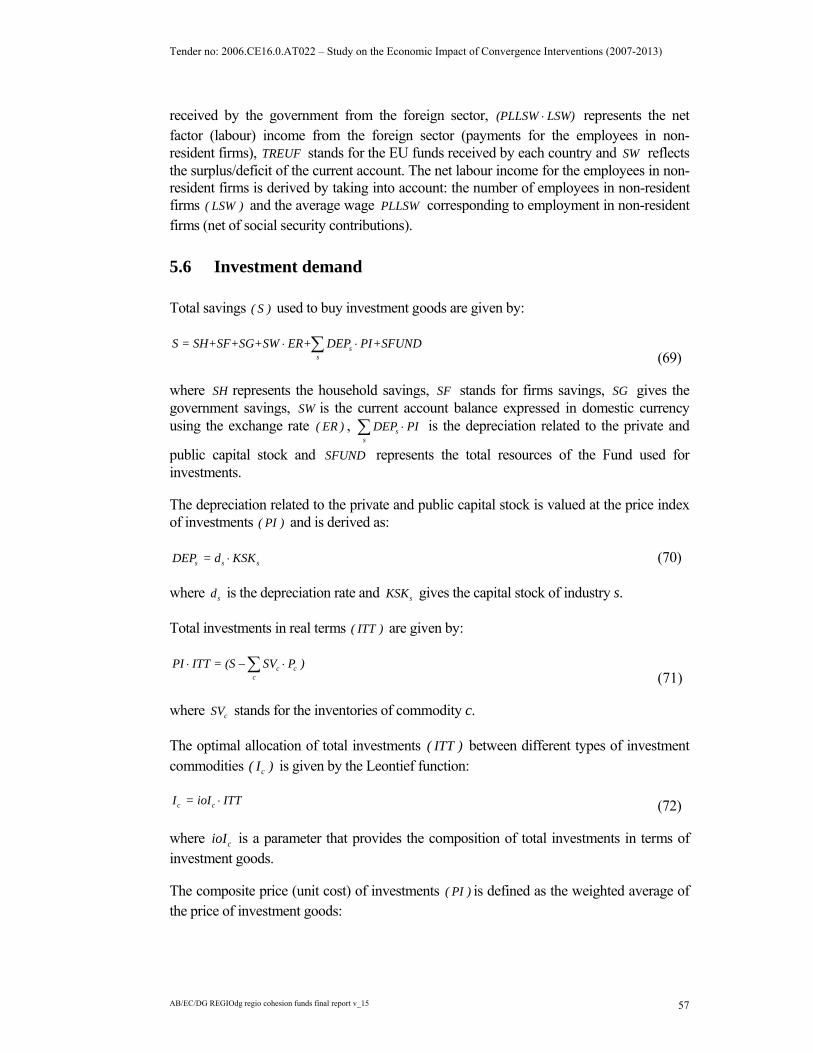
Tender no: 2006.CE16.0.AT022 – Study on the Economic Impact of Convergence Interventions (2007-2013)
AB/EC/DG REGIOdg regio cohesion funds final report v_15 57
received by the government from the foreign sector, (PLLSW LSW)⋅ represents the net factor (labour) income from the foreign sector (payments for the employees in non-resident firms), TREUF stands for the EU funds received by each country and SW reflects the surplus/deficit of the current account. The net labour income for the employees in non-resident firms is derived by taking into account: the number of employees in non-resident firms ( LSW ) and the average wage PLLSW corresponding to employment in non-resident firms (net of social security contributions).
5.6 Investment demand
Total savings ( S ) used to buy investment goods are given by:
ss
S = SH+SF+SG+SW ER+ DEP PI+SFUND⋅ ⋅∑ (69)
where SH represents the household savings, SF stands for firms savings, SG gives the government savings, SW is the current account balance expressed in domestic currency using the exchange rate ( ER ) , s
sDEP PI⋅∑ is the depreciation related to the private and
public capital stock and SFUND represents the total resources of the Fund used for investments.
The depreciation related to the private and public capital stock is valued at the price index of investments ( PI ) and is derived as:
s s sDEP = d KSK⋅ (70)
where sd is the depreciation rate and sKSK gives the capital stock of industry s.
Total investments in real terms ( ITT ) are given by:
c cc
PI ITT = (S SV P )⋅ − ⋅∑ (71)
where cSV stands for the inventories of commodity c.
The optimal allocation of total investments ( ITT ) between different types of investment commodities c( I ) is given by the Leontief function:
c cI = ioI ITT⋅ (72)
where cioI is a parameter that provides the composition of total investments in terms of investment goods.
The composite price (unit cost) of investments ( PI ) is defined as the weighted average of the price of investment goods:

Tender no: 2006.CE16.0.AT022 – Study on the Economic Impact of Convergence Interventions (2007-2013)
AB/EC/DG REGIOdg regio cohesion funds final report v_15 58
c c c ctm,c ctm cc ctm
PI = {(1+ti ) [(1 tsi ) P + tcitm P ] ioI }⋅ − ⋅ ⋅ ⋅∑ ∑ (73)
where cP stands for the price of (investment) commodity c, ctsi is the subsidy rate on investment good c, cti is the tax rate on investment goods c and ctm,ctcitm is the trade and transport margin rate on investment good c.
5.7 Price equations
A common assumption for CGE models, which has also been adopted here, is that the economy is initially in equilibrium with the quantities normalized in such a way that prices of commodities equal unity. Due to the homogeneity of degree zero in prices, the model only determines the relative prices. Therefore, a particular price is selected to provide the numeraire against which all relative prices in the model will be measured. We choose the GDP deflator ( GDPDEF ) as the numeraire.
Different prices are defined for all the branches, exports and imports. The domestic price of exports c( PE ) reflects the price received by the domestic producers for selling their production on the foreign market. The relationship between the domestic price of exports received by the domestic producers and the domestic price of exports free on board is provided by:
c c ctm,c ctmctm
PE = PEFOB tcetm P− ⋅∑ (74)
The cost of trade and transport services reduces the domestic price received by the producers, where ctm,ctcetm is the quantity of trade and transport services ctm per unit of commodity c exported, and ctmP represents the price of the trade and transport services ctm.
As already explained, trade and transport margins are paid on all categories of demand in the EcoMod model except the government consumption (on intermediate consumption, on private consumption and on investment goods).
The domestic price of imports c( PM ) is determined by the world price of imports, the exchange rate and the tariff rate c(tm ) , according to:
c c cPM = PWM ER (1 + tm )⋅ ⋅ (75)
The consumer price index ( PCINDEX ) used in the model is defined as:
c c ctm,c ctm c cc ctm
c c ctm,c ctm c cc ctm
PCINDEX = { [(1 tsc ) P + tchtm P ] (1+tc ) CZ } /
{ [(1 tscz ) PZ + tchtmz PZ ] (1+tcz ) CZ }
− ⋅ ⋅ ⋅ ⋅
− ⋅ ⋅ ⋅ ⋅
∑ ∑
∑ ∑ (76)
where ctsc is the subsidy rate on commodity c and ctscz its benchmark level, cP is the price index of commodity c net of taxes but including subsidies and cPZ gives its benchmark level, ctm,ctchtm represents the trade and transport margin rate on private consumption and

Tender no: 2006.CE16.0.AT022 – Study on the Economic Impact of Convergence Interventions (2007-2013)
AB/EC/DG REGIOdg regio cohesion funds final report v_15 59
ctm,ctchtmz is its benchmark level, and ctc gives the tax rate on private consumption, while
ctcz is its benchmark level. Finally, cCZ accounts for the benchmark level of private consumption of commodity c.
Consumer prices c( PCT ) are further defined as:
c c c ctm,c ctm cctm
PCT = [(1 tsc ) P + tchtm P ] (1+tc )− ⋅ ⋅ ⋅∑ (77)
The average wage paid to the trainees ( PLMA ) , supported by the structural funds on human resources, is given by a share (shPLMA) of the average wage in the manufacturing sectors, services and construction:
sm sm smsm sm
PLMA = shPLMA { [(1+premLSK ) PL LSK ] / LSK }⋅ ⋅ ⋅∑ ∑ (78)
whereas the average wage in the services sector ( PLSV ) is given by:
ctm ctm ctmctm ctm
PLSV [ PL (1 premLSK ) LSK ] / LSK= ⋅ + ⋅∑ ∑ (79)
5.8 Labour market
The following identity defines the relation between the labour supply, the labour demand, and unemployment:
ss
LSK = LSR UNEMP−∑ (80)
where sLSK stands for the number of employees in industry s, UNEMP represents the number of unemployed and LSR reflects the active population.
The responsiveness of real wage to the labour market conditions is surprised by a wage curve (Blanchflower, 2001; Sanz-de-Galdeano & Turunen, 2006):
log(PL/PCINDEX) = elasU log(UNRATE)+ err ⋅ (81)
where PL is the nominal wage corresponding to national employment (net of social security contributions), PCINDEX is the consumer price index, UNRATE provides the unemployment rate, err is the error term and elasU is the unemployment elasticity.
The labour supply is provided by the following equation:
elasLSLSR = LSRI { [PL (1 ty MUty) PCINDEXZ]/[PLZ (1 tyz) PCINDEX]}⋅ ⋅ − ⋅ ⋅ ⋅ − ⋅ (82)
where LSRI is the benchmark level corresponding to the active population, ty is the personal income tax rate and tyz its benchmark level, and PLZ and PCINDEXZ are the benchmark levels corresponding to the nominal wage and CPI, respectively. elasLS further provides the elasticity of labour supply.

Tender no: 2006.CE16.0.AT022 – Study on the Economic Impact of Convergence Interventions (2007-2013)
AB/EC/DG REGIOdg regio cohesion funds final report v_15 60
The national employment ( EMPN ) is defined as:
EMPN = LSR UNEMP− (83)
5.9 Market clearing equations
The equilibrium in the product, capital and labour markets requires that demand equals supply at prevailing prices (taking into account unemployment for the labour market). Labour market clearing equation has already been presented above. Capital stock is sector specific, such that the equality between capital demand and supply determines the return to capital by branch of activity.
Separate market clearing equations are distinguished in the model for each commodity c. For the trade and transport services ctm, the sum of demand for intermediate consumption of commodity ctm ctm,s s
s( io XD )⋅∑ , the private demand for commodity ctm ctm(C ) , the
public demand for commodity ctm ctm( CG ) , the demand for inventories ctm( SV ) and the demand for trade and transport services ctm(MARGTT ) which are invoiced separately (trade and transport margins) should be equal with the total supply of commodity ctm ctm( X ) from imports and domestic production:
ctm ctm ctm ctm ctm,s s ctm ctms
C +CG +I +SV + io XD MARGTT X⋅ + =∑ (84)
The demand for trade and transport services ctm ctm(MARGTT ) invoiced separately (Löfgren, Harris and Robinson, 2002), is further derived as the sum of demand for trade and transport services on private consumption ctm,c c
c( tchtm C )⋅∑ , of demand for trade and
transport services on investment goods ctm,c cc
( tcitm I )⋅∑ , of demand for trade and transport
services on exports ctm,c cc
( tcetm E )⋅∑ , and of demand for trade and transport services on
intermediate consumption ctm,c c,s ss ,c
( tcictm io XD )⋅ ⋅∑ :
ctm ctm,c c ctm,c c ctm,c c ctm,c c,s sc s,c
MARGTT = (tchtm C +tcitm I +tcetm E )+ tcictm io XD⋅ ⋅ ⋅ ⋅ ⋅∑ ∑ (85)
The market clearing equations corresponding to all commodities nctm, except the trade and transport services are given by:
nctm nctm nctm nctm nctm,s s nctms
C +CG +I +SV + io XD X⋅ =∑ (86)
The demand for inventories for each commodity c is defined as a fixed share of domestic sales:
c c cSV = svr X⋅ (87)

Tender no: 2006.CE16.0.AT022 – Study on the Economic Impact of Convergence Interventions (2007-2013)
AB/EC/DG REGIOdg regio cohesion funds final report v_15 61
5.10 Other macroeconomic indicators
Gross domestic product is provided at both constant prices ( GDP ) and at current market prices ( GDPC ) :
c c c ctm,c ctm c c cc ctm c
c c c c ctm,c ctm c c c cc ctm c c
c cc
GDP = {C [(1 tscz ) PZ + tchtmz PZ ] (1+tcz )} CG PZ
{I (1+tiz ) [(1 tsiz ) PZ + tcitmz PZ ]}+ SV PZ E PEFOBZ
M PWMZ ERZ
⋅ − ⋅ ⋅ ⋅ + ⋅ +
⋅ ⋅ − ⋅ ⋅ ⋅ + ⋅ −
⋅ ⋅
∑ ∑ ∑
∑ ∑ ∑ ∑
∑ (88)
c c c ctm,c ctm c c cc ctm c
c c c c ctm,c ctm c c c cc ctm c c
c cc
GDPC = {C [(1 tsc ) P + tchtm P ] (1+tc )} CG P
{I (1+ti ) [(1 tsi ) P + tcitm P ]}+ SV P E PEFOB
M PWM ER
⋅ − ⋅ ⋅ ⋅ + ⋅ +
⋅ ⋅ − ⋅ ⋅ ⋅ + ⋅ −
⋅ ⋅
∑ ∑ ∑
∑ ∑ ∑ ∑
∑ (89)
where cPWMZ , cPEFOBZ and ERZ represent the benchmark levels corresponding to the world price of imports, domestic price of exports f.o.b. and the exchange rate, respectively.
Derivation of some other macroeconomic indicators like the components of GDP at constant prices is provided in section 1.13 of this technical overview.
5.11 Incorporation of dynamics
EcoMod model has a recursive dynamic structure composed of a sequence of several temporary equilibria. The first equilibrium in the sequence is given by the benchmark year. In each time period, the model is solved for an equilibrium given the exogenous conditions assumed for that particular period. The equilibria are connected to each other through capital accumulation. Thus, the endogenous determination of investment behaviour is essential for the dynamic part of the model. Investment and capital accumulation in year t depend on expected rates of return for year t+1, which are determined by actual returns on capital in year t.
The normal rate of return to capital in branch s s( ROR ) is specified as an inverse logistic function (see Figure A5) of the proportionate growth in sector’s s capital stock (Dixon and Rimmer, 2002):
s ,t s s s ,t s s s ,t
s s s s
ROR RORH (1 / B ) [ln( KSKg KSKg min ) ln( KSKg max KSKg )ln( KSKtrend KSKg min ) ln( KSKg max KSKtrend )]
= + ⋅ − − − −
− + − (90)
where sRORH is the historically normal rate of return in branch s, s ,tKSKg is the capital growth rate in industry s in year t, sKSKg min and sKSKg max are the minimum and the maximum possible growth rates of capital stock in branch s, sKSKtrend is the industry’s historically normal growth rate and sB is a positive parameter. The minimum possible growth rate is set at the negative of the rate of depreciation in branch s. This condition implies that investments in each branch of activity have positive values, such that once

Tender no: 2006.CE16.0.AT022 – Study on the Economic Impact of Convergence Interventions (2007-2013)
AB/EC/DG REGIOdg regio cohesion funds final report v_15 62
installed, capital cannot be shifted from one sector to another except for the gradual process of depreciation. The maximum possible growth rate of capital stock in industry s is set at sKSKtrend plus slim INV in order to avoid unrealistically large simulated growth rates (Dixon and Rimmer, 2002). In the current version slim INV is taken equal to 6 per cent for all the branches. For example, if the historically normal growth rate in an industry is 4 per cent, the upper limit in any year t would not exceed 10 per cent.
Parameter s( B ) reflects the sensitivity of capital growth in branch s to variations in its expected rate of return. It is derived by differentiating equation (90) with respect to
s ,tKSKg :
s ss
s s s s
KSKgmax KSKgminB SEA
( KSKgmax KSKtrend ) ( KSKtrend KSKgmin )⎡ ⎤−
= ⋅⎢ ⎥− ⋅ −⎣ ⎦ (91)
where:
s ,t
s ,t
1RORSEA
KSKg
−⎛ ⎞∂= ⎜ ⎟⎜ ⎟∂⎝ ⎠
(92)
Evaluating (92) in the neighbourhood of s ,t sKSKg KSKtrend= provides:
s ,t
s ,t ss ,t
1RORSEA KSKg KSKtrendKSKg
−⎛ ⎞∂= ⎜ ⎟⎜ ⎟=∂⎝ ⎠
(93)
where SEA is the reciprocal of the slope of the RR’ in Figure A5, which is considered to be the same for all industries due to the lack of detailed estimates by branch.
The present value s ,t( PVK ) of investing a unit of capital in industry s in year t is defined as:
s ,t t s ,t 1 t 1 s t 1 s tPVK PI [ PK PI d PI (1 d )] /[1 NINT ]+ + += − + + ⋅ + ⋅ − + (94)
where tPI is the cost of buying a unit of capital (the price of composite investment good) in year t, s ,t t 1 sPK PI d++ ⋅ is the rental rate on industry’s s capital stock, sd is the depreciation rate in branch s and tNINT is the nominal interest rate in year t (Dixon and Rimmer, 2002). The purchase of one unit of capital in year t by industry s involves an immediate expenditure t( PI ) , followed by two benefits in year t+1 which are discounted by t( 1 NINT )+ : the rental value of an extra unit of capital in year t+1 s,t 1 t 1 s( PK PI d )+ ++ ⋅ , including the depreciation, and the value at which the depreciated unit of capital can be sold in year t+1 t 1 s[ PI (1 d )]+ ⋅ − .

Tender no: 2006.CE16.0.AT022 – Study on the Economic Impact of Convergence Interventions (2007-2013)
AB/EC/DG REGIOdg regio cohesion funds final report v_15 63
RORs
RORHs
0.06
KSKtrends
KSKgs
KSKgmaxsKSKgmins
R
R'
Figure A5. The expected rate of return for industry s
The expected rate of return on investment in industry s in year t is given by dividing both sides of (94) by tPI :
s ,t s ,t 1 t t 1 t tROR 1 [ PK / PI PI / PI ] /[1 NINT ]+ += − + + + (95)
Under static expectations, investors are assumed to anticipate that the asset prices (the cost of buying a unit of capital) and the net rental rates will increase by the current rate of inflation t( RINF ) . Thus, the expected rate of return s ,t( ROR ) under static expectations is given by:
s ,t s ,t t t t t t tROR 1 [ PK (1 RINF ) / PI PI (1 RINF ) / PI ] /[1 NINT ]= − + ⋅ + + ⋅ + + (96)
Simplifying further, we get:
s ,t s ,t t tROR 1 [ PK / PI 1] /(1 RINT )= − + + + (97)
where the real interest rate t( RINT ) is defined as:
t t t1 RINT (1 NINT ) /( 1 RINF )+ = + + (98)

Tender no: 2006.CE16.0.AT022 – Study on the Economic Impact of Convergence Interventions (2007-2013)
AB/EC/DG REGIOdg regio cohesion funds final report v_15 64
The weighted average real return to capital has been taken as a proxy for the real interest rate in EcoMod model. The return to capital is expressed in real terms using the production price index:
t s ,t s ,t s ,t s ,ts s
RINT [(PK / PD ) KSK ]/ KSK= ⋅∑ ∑ (99)
The capital stock in industry s in the next period (year t+1) is given by:
s,t+1 s s,t s,t s,t s,t s,tKSK = (1 d ) KSK +INV +INVSFRTOT +INVSFHRTOT +INVCFRTOT− ⋅ (100)
where s ,tKSK is the current capital stock (in year t), s ,tINV stand for the investments by the branch s in year t (before the investments supported by the EU funds), sINVSFRTOT represents the investments to productive environment supported by the structural funds (including co-financing), sINVSFHRTOT represents the investments in human resources supported by structural funds (including co-financing) and sINVCFRTOT stands for the investments in infrastructure supported by structural and cohesion funds (including co-financing).
The capital growth rate in terms of capital stock in year t+1 and the capital stock in year t is given by:
s ,t s ,t 1 s ,tKSKg KSK / KSK 1+= − (101)
whereas the actual growth rate of capital in industry s can be derived from equation. (90) as:
]]
s ,t s ,t s s s
s s s s ,t s
s s s
KSKg ROR KSKg max ( KSKtrend KSKg min )
KSKg min ( KSKg max KSKtrend ) / ROR ( KSKtrend
KSKg min ) ( KSKg max KSKtrend )
α
α
= ⋅ ⋅ − +⎡⎣⋅ − ⋅ −⎡⎣+ −
(102)
The parameter s ,tRORα is given by:
s ,t s s s s s s s{[(ROR RORH ) (KSKgmax KSKgmin )]/[(KSKgmax KSKtrend ) (KSKtrend KSKgmin )]}s ,tROR = eα − ⋅ − − ⋅ − (103)
A first estimate of investments in the branch s in year t s,t(INVS ) excluding investments supported by the structural and cohesion funds is derived from equations (100)-(102) as:
s,t s,t s,t s s s s
s s s,t s s
s s s s,t
INVS = KSK [ ROR KSKgmax (KSKtrend KSKgmin )+ KSKgmin(KSKgmax KSKtrend )]/[ ROR (KSKtrend KSKgmin )+(KSKgmax KSKtrend )]+d KSK
αα
⋅ ⋅ ⋅ − ⋅
− ⋅ −
− ⋅
(104)
while the actual level of investments in branch s in year t, excluding investments supported by the structural and cohesion funds, is provided by:
s,t s,t ss,t t c,t c,t t tss c
INV = INVS / INVS (S SV P SFUND )/PI⋅ − ⋅ −∑ ∑ (105)

Tender no: 2006.CE16.0.AT022 – Study on the Economic Impact of Convergence Interventions (2007-2013)
AB/EC/DG REGIOdg regio cohesion funds final report v_15 65
which also insures the consistency between total investments and savings.
The model is solved dynamically with annual steps. The simulation horizon of the model has been set at 20 years but it can easily be extended.
5.12 Closure rules
The closure rules refer to the manner in which demand and supply of commodities, the macroeconomic identities and the factor markets are equilibrated ex-post. Due to the complexity of the model, a combination of closure rules is needed. The particular set of closure rules should also be consistent, to the largest extent possible, with the institutional structure of the economy and with the purpose of the model.
In mathematical terms, the model should consist of an equal number of independent equations and endogenous variables. The closure rules reflect the choice of the model builder of which variables are exogenous and which variables are endogenous, so as to achieve ex-post equality.
Three macro balances are usually identified in CGE models that can be a potential source of ex-ante disequilibria and must be reconciled ex-post (Adelman and Robinson, 1989):
The savings-investment balance;
The government balance;
The external balance.
The most widely used macro closure rule for CGE models is based on the investment and savings balance. In the model, the investment is assumed to adjust to the available domestic and foreign savings. This reflects an economy in which savings form a binding constraint. An alternative closure is possible where the investments determine the total level of savings. In this case the foreign savings adjusts to meet the total savings requirement.
Additional assumptions are needed with regard to government behaviour in the EcoMod model. First, the total current consumption by the government is fixed as a share of GDP, while the allocation between the consumption of different goods and services is provided by a Cobb-Douglas function. Secondly, the government net transfers to the foreign sector are assumed to be fixed in real terms, while the government net transfers to the household (except the unemployment benefits) are fixed as a share of GDP. Thus, the government savings are endogenously determined in the current version of EcoMod model. Alternative assumptions are possible, where total government expenditures can be fixed in real terms or as a share of GDP, while the total current consumption adjusts.
In the co-financing scenario an alternative closure is used for the government balance, where, besides the current consumption, the government savings are fixed as a share of GDP. The personal income tax rate adjusts to meet this constraint. In order to allow the comparability between the past profile of 6 countries scenario and the co-financing scenario, government savings to GDP ratio in the co-financing scenario has been fixed to its levels in the past profile of 6 countries scenario.

Tender no: 2006.CE16.0.AT022 – Study on the Economic Impact of Convergence Interventions (2007-2013)
AB/EC/DG REGIOdg regio cohesion funds final report v_15 66
With respect to the external balance, the current account balance to GDP ratio is kept unchanged in the simulations, while the real exchange rate adjusts. In an alternative scenario, we let current account adjust.
The setup of the closure rules is important in determining the mechanisms governing the model. Therefore, the closure rules should be established also taking into account the policy scenario in question.
According to the Walras law if (n-1) markets are cleared the nth one is cleared as well. Therefore, in order to avoid over-determination of the model, the current account balance has been dropped (see equation (68), section 1.5 of this technical overview). However, the system of equations guarantees, through the Walras law, that the total imports plus transfers by different agents to the external sector equals total exports plus transfers received by different agents from the external sector plus the current account balance.
5.13 Model equations
5.13.1 Household
c c ctm,c ctm c c c c ctm,c ctm cctm ctm
c c cc cc ctm,cc ctm cc cccc ctm
[(1 tsc ) P + tchtm P ] (1+tc ) C = [(1 tsc ) P + tchtm P ] (1+tc )
H H {CBUD [(1 tsc ) P + tchtm P ] (1+tc ) H }μ α μ
− ⋅ ⋅ ⋅ ⋅ − ⋅ ⋅ ⋅ ⋅
+ ⋅ − − ⋅ ⋅ ⋅ ⋅
∑ ∑
∑ ∑ (A.1)
s s s ss s
YH = shYKH PK KSK + PL LSK (1+premLSK ) PLLSW LSW ER+
TRHF GDPDEF+TRHG+TRHW ER TRWH ER
⋅ ⋅ ⋅ ⋅ + ⋅ ⋅
⋅ ⋅ − ⋅
∑ ∑ (A.2)
CBUD = (1 ty MUty) YH SH− ⋅ ⋅ − (A.3)
SH = MPS (1 ty MUty) YH⋅ − ⋅ ⋅ (A.4)
elasSMPS = MPSZ {[(1 ty MUty) PKavr]/[(1 tyz) PKavrZ]} ⋅ − ⋅ ⋅ − ⋅ (A.5)
5.13.2 Firms
s ss
SF = shYKF PK KSK TRHF GDPDEF TRGF GDPDEF TRWF ER⋅ ⋅ − ⋅ − ⋅ − ⋅∑ (A.6)
s s sKL = aKL XD⋅ (A.7)
s s sF F ( F 1)s s s s s s s s s sKSK = KL {PKL /[PK (1+tk )+d PI]} FK (aF TFPSF TFPCF )σ σ σγ −⋅ ⋅ ⋅ ⋅ ⋅ ⋅ ⋅ (A.8)
s s s
s
F F ( F 1)s s s s s s s
( F 1)s s s
LSK = KL { PKL /[PL (1+premLSK ) (1+tl )]} FL TFPSFH
(aF TFPSF TFPCF )
σ σ σ
σ
γ −
−
⋅ ⋅ ⋅ ⋅ ⋅ ⋅
⋅ ⋅ (A.9)

Tender no: 2006.CE16.0.AT022 – Study on the Economic Impact of Convergence Interventions (2007-2013)
AB/EC/DG REGIOdg regio cohesion funds final report v_15 67
s s s s s s s s sPKL KL = PK (1+tk ) KSK +PL (1+premLSK ) (1+tl ) LSK +DEP PI⋅ ⋅ ⋅ ⋅ ⋅ ⋅ ⋅ (A.10)
s s s s c,s s c c ctm,c ctm cc ctm
s s
PD (1 tp +tsp ) XD = {io XD [(1 tsic ) P + tcictm P ] (1+tic )}+
PKL KL
⋅ − ⋅ ⋅ ⋅ − ⋅ ⋅ ⋅
⋅
∑ ∑
(A.11)
5.13.3 Government
GREV = TRPROP+TRPROD+TRSOC+TRANSR (A.12)
s s ss
TRPROP = ty MUty YH + tk KSK PK⋅ ⋅ ⋅ ⋅∑ (A.13)
s s s c c ctm,c ctm c cs c ctm
c c ctm,c ctm c cc ctm
c c ctm,c ctm c c,s s c c cc ,s ctm c
TRPROD = tp XD PD [(1 tsc ) P + tchtm P ] tc C
[(1 tsi ) P + tcitm P ] ti I
[(1 tsic ) P + tcictm P ] tic io XD tm PWM M ER
⋅ ⋅ + − ⋅ ⋅ ⋅ ⋅ +
− ⋅ ⋅ ⋅ ⋅ +
− ⋅ ⋅ ⋅ ⋅ ⋅ + ⋅ ⋅ ⋅
∑ ∑ ∑
∑ ∑
∑ ∑ ∑ (A.14)
s s ss
TRSOC = tl LSK PL (1+premLSK )⋅ ⋅ ⋅∑ (A.15)
TRANSR = TRGW ER+TRGF GDPDEF ⋅ ⋅ (A.16)
GEXP = CGBUD+TRANS+SUBSID (A.17)
c c cP CG = CG CGBUD α⋅ ⋅ (A.18)
TRANS = TRHG+TRWG ER+COFIN⋅ (A.19)
TRHG = PL trep UNEMP shUNEMPB+TRHGOTH PCINDEX ⋅ ⋅ ⋅ ⋅ (A.20)
c c c c c c c c c,s s s s sc c ,s s
SUBSID = (tsc C P +tsi I P ) tsic P io XD tsp XD PD⋅ ⋅ ⋅ ⋅ + ⋅ ⋅ ⋅ + ⋅ ⋅∑ ∑ ∑ (A.21)
SG = GREV GEXP− (A.22)
rTRPROPGDP = TRPROP/GDPC 100⋅ (A.23)
rTRPRODGDP = TRPROD/GDPC 100⋅ (A.24)
rTRSOCGDP = TRSOC/GDPC 100⋅ (A.25)
rTRANSRGDP = TRANSR/GDPC 100⋅ (A.26)
rCGBUDGDP = CGBUD/GDPC 100⋅ (A.27)
rTRANSGDP = TRANS/GDPC 100⋅ (A.28)

Tender no: 2006.CE16.0.AT022 – Study on the Economic Impact of Convergence Interventions (2007-2013)
AB/EC/DG REGIOdg regio cohesion funds final report v_15 68
rTRHGOTHGDP = (TRHGOTH PCINDEX)/GDPC 100⋅ ⋅ (A.29)
rSUBSIDGDP = SUBSID/GDPC 100⋅ (A.30)
rSGGDP = SG/GDPC 100⋅ (A.31)
5.13.4 Domestic supply to domestic and foreign markets
c s,c ss
XDDE = ioC XD⋅∑ (A.32)
s s,c cc
PD = ioC PDDE⋅∑ (A.33)
5.13.5 Foreign sector
c c cT T ( T 1)c c c c c cE = XDDE (PDDE /PE ) T2 aTσ σ σγ −⋅ ⋅ ⋅ (A.34)
celasEc c c cED = EDI (PWE ER/PEFOB )⋅ ⋅ (A.35)
c c cT T ( T 1)c c c c c cXDD = XDDE (PDDE /PDD ) T1 aTσ σ σγ −⋅ ⋅ ⋅ (A.36)
c c c c c cPDDE XDDE = PDD XDD +PE E⋅ ⋅ ⋅ (A.37)
c c cA A ( A 1)c c c c c cM = X (P /PM ) A2 aAσ σ σγ −⋅ ⋅ ⋅ (A.38)
c c cA A ( A 1)c c c c c cXDD = X (P /PDD ) A1 aAσ σ σγ −⋅ ⋅ ⋅ (A.39)
c c c c c cP X = PM M + PDD XDD⋅ ⋅ ⋅ (A.40)
c c c cc c
M PWM +TRWH+TRWF+TRWG = (E PEFOB /ER) TRHW+TRGW+
PLLSW LSW+TREUF +SW
⋅ ⋅ +
⋅
∑ ∑
(A.41)
rSWGDP = (SW ER)/GDPC 100⋅ ⋅ (A.42)
5.13.6 The Fund
s sINVSFR = INVSF ER/PI⋅ (A.43)
s sINVSFHR = INVSFH ER/PI⋅ (A.44)
s sINVCFR = INVCF ER/PI⋅ (A.45)
s s INVSFRCOF = tcof/(100-tcof) INVSF ER/PI⋅ ⋅ (A.46)

Tender no: 2006.CE16.0.AT022 – Study on the Economic Impact of Convergence Interventions (2007-2013)
AB/EC/DG REGIOdg regio cohesion funds final report v_15 69
s sINVSFHRCOF = tcof/(100-tcof) INVSFH ER/PI⋅ ⋅ (A.47)
s s INVCFRCOF = tcof/(100-tcof) INVCF ER/PI⋅ ⋅ (A.48)
s s sINVSFRTOT = INVSFR +INVSFRCOF (A.49)
s s sINVSFHRTOT = INVSFHR +INVSFHRCOF (A.50)
s s sINVCFRTOT = INVCFR +INVCFRCOF (A.51)
s s ss
COFIN = PI ( INVSFRCOF +INVSFHRCOF +INVCFRCOF )⋅∑ (A.52)
s s ss
SFUND = PI (INVSFRTOT +INVSFHRTOT +INVCFRTOT )⋅∑ (A.53)
s s ss
PI (INVSFR +INVSFHR +INVCFR ) = TREUF ER⋅ ⋅∑ (A.54)
rTREUFGDP = TREUF ER/GDPC 100⋅ ⋅ (A.55)
ctmctm
TRAIN = INVSFHRTOT PI (1 OVERHD)/[PLMA+PLSV/TRATIO]⋅ ⋅ −∑ (A.56)
5.13.7 Investment
ss
S = SH+SF+SG+SW ER+ DEP PI+SFUND⋅ ⋅∑ (A.57)
c cI = ioI ITT⋅ (A.58)
c c c ctm,c ctm cc ctm
PI = {(1+ti ) [(1 tsi ) P + tcitm P ] ioI }⋅ − ⋅ ⋅ ⋅∑ ∑ (A.59)
c cc
PI ITT = (S SV P )⋅ − ⋅∑ (A.60)
c c cSV = svr X⋅ (A.61)
s s sDEP = d KSK⋅ (A.62)
5.13.8 Labour market
elasLSLSR = LSRI { [PL (1 ty MUty) PCINDEXZ]/[PLZ (1 tyz) PCINDEX]}⋅ ⋅ − ⋅ ⋅ ⋅ − ⋅ (A.63)
log(PL/PCINDEX) = elasU log(UNRATE)+err⋅ (A.64)
EMPN = LSR UNEMP− (A.65)

Tender no: 2006.CE16.0.AT022 – Study on the Economic Impact of Convergence Interventions (2007-2013)
AB/EC/DG REGIOdg regio cohesion funds final report v_15 70
UNRATE = UNEMP/LSR (A.66)
5.13.9 Trade and transport margins
ctm ctm,c c ctm,c c ctm,c c ctm,c c,s sc s,c
MARGTT = (tchtm C +tcitm I +tcetm E )+ tcictm io XD⋅ ⋅ ⋅ ⋅ ⋅∑ ∑ (A.67)
5.13.10 Market clearing
ss
LSK = LSR UNEMP−∑ (A.68)
nctm nctm nctm nctm nctm,s s nctms
C +CG +I +SV + io XD X⋅ =∑ (A.69)
ctm ctm ctm ctm ctm,s s ctm ctms
C +CG +I +SV + io XD MARGTT X⋅ + =∑ (A.70)
c cE = ED (A.71)
5.13.11 Price definitions
c c ctm,c ctm c cc ctm
c c ctm,c ctm c cctm
PCINDEX = {[(1-tsc ) P + tchtm P ] (1+tc ) CZ } /
{[(1-tscz ) PZ + tchtmz PZ ] (1+tcz ) CZ }
⋅ ⋅ ⋅ ⋅
⋅ ⋅ ⋅ ⋅
∑ ∑
∑ (A.72)
c c ctm,c ctmctm
PE = PEFOB tcetm P− ⋅∑ (A.73)
c c cPM = PWM ER (1+tm )⋅ ⋅ (A.74)
s s s ss s
RINT = [(PK /PD ) KSK ]/ KSK⋅∑ ∑ (A.75)
s s ss s
PKavr = [(PK /PCINDEX) KSK ]/ KSK⋅∑ ∑ (A.76)
c c c ctm,c ctm cctm
PCT = [(1-tsc ) P + tchtm P ] (1+tc )⋅ ⋅ ⋅∑ (A.77)
s s ss
PLAVRT (LSR UNEMP) = [ PL (1+tl ) (1+premLSK ) LSK ]⋅ − ⋅ ⋅ ⋅∑ (A.78)
sm sm smsm sm
PLMA = shPLMA { [(1+premLSK ) PL LSK ] / LSK }⋅ ⋅ ⋅∑ ∑ (A.79)
ctm ctm ctmctm ctm
PLSV [ PL (1 premLSK ) LSK ] / LSK= ⋅ + ⋅∑ ∑ (A.80)

Tender no: 2006.CE16.0.AT022 – Study on the Economic Impact of Convergence Interventions (2007-2013)
AB/EC/DG REGIOdg regio cohesion funds final report v_15 71
5.13.12 Gross domestic product at current and constant market prices
c c c ctm,c ctm c c cc ctm c
c c c c ctm,c ctm c c c cc ctm c c
c cc
GDPC = {C [(1 tsc ) P + tchtm P ] (1+tc )} CG P
{I (1+ti ) [(1 tsi ) P + tcitm P ]}+ SV P E PEFOB
M PWM ER
⋅ − ⋅ ⋅ ⋅ + ⋅ +
⋅ ⋅ − ⋅ ⋅ ⋅ + ⋅ −
⋅ ⋅
∑ ∑ ∑
∑ ∑ ∑ ∑
∑ (A.81)
c c c ctm,c ctm c c cc ctm c
c c c c ctm,c ctm c c c cc ctm c c
c cc
GDP = {C [(1 tscz ) PZ + tchtmz PZ ] (1+tcz )} CG PZ
{I (1+tiz ) [(1 tsiz ) PZ + tcitmz PZ ]}+ SV PZ E PEFOBZ
M PWMZ ERZ
⋅ − ⋅ ⋅ ⋅ + ⋅ +
⋅ ⋅ − ⋅ ⋅ ⋅ + ⋅ −
⋅ ⋅
∑ ∑ ∑
∑ ∑ ∑ ∑
∑ (A.82)
GDPDEF = GDPC/GDP (A.83)
5.13.13 Components of GDP at constant prices
c c c ctm,c ctm cc ctm
CT {C [(1 tscz ) PZ + tchtmz PZ ] (1+tcz )}= ⋅ − ⋅ ⋅ ⋅∑ ∑ (A.84)
c cc
CGT CG PZ= ⋅∑ (A.85)
c c c c ctm,c ctm c cc ctm c
IT {I (1+tiz ) [(1 tsiz ) PZ + tcitmz PZ ]} SV PZ= ⋅ ⋅ − ⋅ ⋅ + ⋅∑ ∑ ∑ (A.86)
c cc
ET E PEFOBZ= ⋅∑ (A.87)
c cc
MT M PWMZ ERZ= ⋅ ⋅∑ (A.88)
5.13.14 Equivalent variation in income
c
c c ctm,c ctm c cc ctm
Hc c c ctm,c ctm c
ctmc
VU = {CBUD [(1 tsc ) P + tchtm P ] (1+tc ) H }
{ H /{[(1-tsc ) P + tchtm P ] (1+tc )}}α
μ
α
− − ⋅ ⋅ ⋅ ⋅ ⋅
⋅ ⋅ ⋅
∑ ∑
∑∏ (A.89)
cHc c ctm,c ctm c c
ctmc
EV = (VU VUI) {{[(1 tscz ) PZ + tchtmz PZ ] (1+tcz )}/ H }αα− ⋅ − ⋅ ⋅ ⋅∑∏ (A.90)
5.13.15 Capital accumulation
s,t s,t t tROR = 1+(PK /PI +1)/(1+RINT )− (A.91)
s,t s s s s s s s{[(ROR RORH ) (KSKgmax KSKgmin )]/[(KSKgmax KSKtrend ) (KSKtrend KSKgmin )]}s,tROR = eα − ⋅ − − ⋅ −
(A.92)

Tender no: 2006.CE16.0.AT022 – Study on the Economic Impact of Convergence Interventions (2007-2013)
AB/EC/DG REGIOdg regio cohesion funds final report v_15 72
s,t s,t s,t s s s s
s s s,t s s
s s s s,t
INVS = KSK [ ROR KSKgmax (KSKtrend KSKgmin )+ KSKgmin(KSKgmax KSKtrend )]/[ ROR (KSKtrend KSKgmin )+(KSKgmax KSKtrend )]+d KSK
αα
⋅ ⋅ ⋅ − ⋅
− ⋅ −
− ⋅
(A.93)
s,t s,t ss,t t c,t c,t t tss c
INV = INVS / INVS (S SV P SFUND )/PI⋅ − ⋅ −∑ ∑ (A.94)
s,t+1 s s,t s,t s,t s,t s,tKSK = (1 d ) KSK +INV +INVSFRTOT +INVSFHRTOT +INVCFRTOT− ⋅ (A.95)
t+1 t tKSKTRAIN = (1 dhc) KSKTRAIN +TRAIN− ⋅ (A.96)
elasTFPSFHs,t+1 s,t t t tTFPSFH = TFPSFH [(KSKTRAIN +KSKHBA )/KSKHBA ]⋅ (A.97)
elasTFPSFs,t+1 s,t s,t s,t s,tTFPSF = TFPSF [(KSKBA +INVSFRTOT )/KSKBA ]⋅ (A.98)
elasTFPCFs,t+1 s,t t ctm,t t
ctmTFPCF = TFPCF [(KSKPbBA + INVCFRTOT )/KSKPbBA ]⋅ ∑
(A.99)
5.14 Endogenous variables
αRORs,t parameter in the supply of capital function CBUD household budget disposable for consumption Cc consumer demand for commodity c CGBUD government current expenditures CGc public current consumption of commodity c CGT total public consumption at constant prices COFIN total domestic public co-financing for structural and cohesion
funds CT total private consumption at constant prices DEPs depreciation related to public and private capital stock Ec export supply of commodity c by the domestic producers EDc export demand of commodity c from the external sector EMPN national employment ER exchange rate ET total exports at constant prices EV equivalent variation in income GDP gross domestic product at constant prices GDPC gross domestic product at current market prices GEXP total government expenditures GREV total government revenues Ic demand for investment good c INVs investments carried out in branch s excluding investments
supported by the structural and cohesion funds (actual level) INVSs investments carried out in branch s excluding investments
supported by the structural and cohesion funds (first estimate) INVCFRs investments in infrastructure carried out in branch s, supported by
the structural and cohesion funds, excluding domestic public co-financing (expressed in real terms, in domestic currency)

Tender no: 2006.CE16.0.AT022 – Study on the Economic Impact of Convergence Interventions (2007-2013)
AB/EC/DG REGIOdg regio cohesion funds final report v_15 73
INVCFRCOFs domestic public co-financing for investments in infrastructure carried out in branch s, supported by the structural and cohesion funds (expressed in real terms, in domestic currency)
INVCFRTOTs total investments in infrastructure carried out in branch s, supported by the structural and cohesion funds, including domestic public co-financing (expressed in real terms, in domestic currency)
INVSFRs investments to productive environment carried out in branch s, supported by the structural funds, excluding domestic public co-financing (expressed in real terms, in domestic currency)
INVSFRCOFs domestic public co-financing for investments to productive environment carried out in branch s, supported by the structural funds (expressed in real terms, in domestic currency)
INVSFRTOTs total investments to productive environment carried out in branch s, supported by the structural funds, including domestic public co-financing (expressed in real terms, in domestic currency)
INVSFHRs investments in human resources carried out in branch s, supported by the structural funds, excluding domestic public co-financing (expressed in real terms, in domestic currency)
INVSFHRCOFs domestic public co-financing for investments in human resources carried out in branch s, supported by the structural funds (expressed in real terms, in domestic currency)
INVSFHRTOTs total investments in human resources carried out in branch s, supported by the structural funds, including domestic public co-financing (expressed in real terms, in domestic currency)
IT total gross capital formation at constant prices (including inventories)
ITT total investments in real terms KLs value-added by branch KSKTRAINt stock of trainees funded by structural funds on human resources KSKBAs,t capital stock of branch s and year t in the non-cohesion policy
baseline scenario KSKHBAt human capital in the non-cohesion policy baseline scenario KSKPbBAt stock of infrastructure in the non-cohesion policy baseline
scenario LSKs number of employees in branch s LSR active population MARGTTc trade and transport margins Mc imports of commodity c MPS household propensity to save MT total imports at constant prices MUty change in the personal income tax rate (co-financing scenario) Pc price level of domestic sales (composite commodities coming
from imports and domestic production) PCINDEX consumer price index PCTc consumer prices (including taxes) PDs price index of domestic production by branch of activity PDDc price index of domestic production delivered to home market by
type of good c

Tender no: 2006.CE16.0.AT022 – Study on the Economic Impact of Convergence Interventions (2007-2013)
AB/EC/DG REGIOdg regio cohesion funds final report v_15 74
PDDEc price index of domestic production delivered to home and foreign markets by type of good c
PEc domestic price of exports received by the domestic producers PEFOBc domestic price of exports free on board PI price index corresponding to composite investment good PKavr real average return to capital received by the household PKLs price index corresponding to value-added by branch of activity PKs return to capital by branch of activity PL national average wage (excluding social security contributions) PLAVRT national average wage (including social security contributions) PLMA average wage in the manufacturing sectors, services and
construction (net of social security contributions) PLSV average wage in the services sector (net of social security
contributions) PMc domestic price of imports (including tariffs) RINT average return to capital corresponding to firms RORs,t normal rate of return to capital rSGGDP government savings to the GDP ratio rSUBSIDGDP total subsidies by the government to the GDP ratio rTRANSGDP total transfers by the government to the GDP ratio rTRANSRGDP total transfers received by the government to the GDP ratio rTREUFGDP total EU funds, expressed in domestic currency, to the GDP ratio rTRPRODGDP government revenues from taxes on products and on production
to the GDP ratio rTRPROPGDP government revenues from taxes on income and wealth to the
GDP ratio rTRSOCGDP government revenues from social security contributions to the
GDP ratio S total savings SF firms’ savings SFUND total resources available for investments by the Fund (Fund
savings) SG government savings SH household savings SUBSID total subsidies by the government SVc inventories SW balance of the current account TFPCFs,t TFP improvements due to investments in infrastructure,
supported by structural and cohesion funds TFPSFs,t TFP improvements due to investments to productive environment
supported by the structural funds TFPSFHs,t labour productivity improvements due to investments in human
resources supported by the structural funds TRAIN trainees that can be funded by structural funds on human
resources (expressed in number of trainee-years) TRANS total transfers by the government TRANSR total transfers received by the government TREUF total EU funds expressed in euros TRHG total transfers by the government to the household

Tender no: 2006.CE16.0.AT022 – Study on the Economic Impact of Convergence Interventions (2007-2013)
AB/EC/DG REGIOdg regio cohesion funds final report v_15 75
TRHGOTH transfers by the government to the household (excluding unemployment benefits)
TRPROD government revenues from taxes on products and on production TRPROP government revenues from taxes on income and wealth TRSOC government revenues from social security contributions UNEMP number of unemployed UNRATE unemployment rate VU level of indirect utility corresponding to the household Xc domestic sales of composite commodities coming from imports
and domestic production XDs domestic production by branch of activity XDDc domestic production delivered to home market XDDEc domestic production delivered to home and foreign markets (by
type of commodity) YH household income
5.15 Exogenous variables
CZc consumer demand for commodity c (benchmark value) EDIc export demand from the external sector (benchmark value) ERZ exchange rate (benchmark value) GDPDEF GDP deflator INVCFs investments in infrastructure carried out in branch s, supported by
the structural and cohesion funds, excluding domestic public co-financing (expressed in nominal terms, in euros)
INVSFs investments to productive environment carried out in branch s, supported by the structural funds, excluding domestic public co-financing (expressed in nominal terms, in euros)
INVSFHs investments in human resources carried out in branch s, supported by the structural funds, excluding domestic public co-financing (expressed in nominal terms, in euros)
KSKs capital demand by branch (capital stock) LSRI active population (benchmark value) LSW number of employed in non-resident firms MPSZ household propensity to save (benchmark value) PCINDEXZ consumer price index (benchmark value) PEFOBZc domestic price of exports free on board (benchmark value) PLLSW average wage in the non-resident firms (excluding social security
contributions) PLZ national average wage (excluding social security contributions) –
benchmark value PKavrZ real average return to capital received by the household
(benchmark value) PWEc world price of exports PWMc world price of imports PWMZc world price of imports (benchmark value) PZc price level of domestic sales (composite commodities coming
from imports and domestic production) – benchmark value RORHs historically normal rate of return to capital
Tender no: 2006.CE16.0.AT022 – Study on the Economic Impact of Convergence Interventions (2007-2013)
AB/EC/DG REGIOdg regio cohesion funds final report v_15 76
rCGBUDGDP government current expenditures to the GDP ratio rTRHGOTHGDP transfers by the government to the household (excluding
unemployment benefits) rSWGDP current account balance to GDP ratio TRGF transfers received by the government from the firms TRGW transfers received by the government from the external sector TRHF transfers received by the household from the firms TRHW transfers received by the household from the external sector TRWF transfers by the firms to the external sector TRWG transfers by the government to the external sector TRWH transfers by the household to the external sector VUI level of indirect utility corresponding to the household
(benchmark level)
5.16 Other parameters
aAc efficiency parameter in the Armington function for imports aFs efficiency parameter in the CES production function of the firm aKLs Leontief parameter - share of value added in domestic production aTc efficiency parameter in the CET function for exports dhc depreciation rate corresponding to the stock of trainees funded by
the structural funds on human resources ds depreciation rate by branch of activity elasEc price elasticity of export demand elasS elasticity of private savings with respect to after-tax rate of return elasLS elasticity of labour supply elasU unemployment elasticity elasTFPSFH labour productivity elasticity of investments in human resources
(structural funds) elasTFPCF TFP elasticity of investments in infrastructure (structural and
cohesion funds) elasTFPSF TFP elasticity of investments provided to productive environment
(structural funds) err error term in the wage curve equation ioc,s technical coefficients corresponding to intermediate consumption ioCs,c shares of domestic production delivered to home and foreign
markets by branch of activity and commodity ioIc Leontief parameter for the investment demand by type of
investment good KSKgmaxs maximum possible growth rate of capital stock in branch s KSKgmins minimum possible growth rate of capital stock in branch s (equal
to the negative of the rate of depreciation in branch s) KSKtrends industry’s historically normal growth rate OVERHD share of current operation costs in total expenditures on human
resources supported by the structural funds premLSKs wage premium by branch shUNEMPB share of unemployed subject to unemployment benefits shPLMA share of average wage in the manufacturing sectors, services and
construction paid to the trainees funded through structural funds

Tender no: 2006.CE16.0.AT022 – Study on the Economic Impact of Convergence Interventions (2007-2013)
AB/EC/DG REGIOdg regio cohesion funds final report v_15 77
shYKH share of the net operating surplus received by the household shYKF share of the net operating surplus retained by the firms svrc share of inventories in domestic sales tcc tax rate on private consumption of commodity c tcetmctm,c quantity of commodity ctm as trade and transport services per
unit of exports tchtmctm,c quantity of commodity ctm as trade and transport services per
unit of private consumption tchtmzctm,c quantity of commodity ctm as trade and transport services per
unit of private consumption (benchmark value) tcictmctm,c quantity of commodity ctm as trade and transport services per
unit of intermediate consumption tcitmctm,c quantity of commodity ctm as trade and transport services per
unit of investment goods tcitmzctm,c quantity of commodity ctm as trade and transport services per
unit of investment goods (benchmark value) tczc tax rate on private consumption (benchmark level) tcof co-financing rate for the structural and cohesion funds (in per
cent) tic tax rate on investment good c ticc tax rate on intermediate consumption of commodity c tizc tax rate on investment goods (benchmark level) tks corporate tax rate in branch s tls social security contributions rate in branch s tmc tariff rate applied on commodity c tps tax rate on production in branch s trep replacement rate out of national average wage (net of social
security contributions) TRATIO trainee-instructor ratio tscc subsidy rate on private consumption tsic subsidy rate on investment good c tsizc subsidy rate on investment good c (benchmark level) tsicc subsidy rate on intermediate consumption tsczc subsidy rate on private consumption (benchmark level) tsps subsidy rate on production in branch s ty personal income tax rate tyz personal income tax rate (benchmark level) αCGc Cobb-Douglas preference parameter in government utility
function αHc marginal budget shares in the Stone-Geary utility function γA1c CES distribution parameter for the domestic demand from the
domestic producers in the Armington function γA2c CES distribution parameter for imports in the Armington
function γFKs CES distribution parameter for capital in the production function
of the firm γFLs CES distribution parameter for labour in the production function
of the firm

Tender no: 2006.CE16.0.AT022 – Study on the Economic Impact of Convergence Interventions (2007-2013)
AB/EC/DG REGIOdg regio cohesion funds final report v_15 78
γT1c CET distribution parameter for domestic production delivered to home markets
γT2c CET distribution parameter for exports μHc subsistence level out of consumer demand for commodities σAc substitution elasticities for the Armington function σFs CES capital-labour substitution elasticities by branch σTc elasticities of transformation in the CET function
5.17 List of indices used in the model
c a subscript for one of the commodities (6 types of commodities) cc the same as c (used for exposition purposes) ctm a subscript for services nctm a subscript for all the other commodities except services (5 types of
commodities) s a subscript for one of the production activities (6 branches of
activity) sm a subscript for the manufacturing sectors, services and construction
(4 branches of activity) ss the same as s (used for exposition purposes) t a subscript for year t References Adelman, I., & Robinson, S. (1989). Income distribution and development. In H. Chenery & T. N. Srinivasan (Eds.), Handbook of development economics, vol. 2 (pp. 949-1003). Amsterdam: North-Holland.
Blanchflower, D. (2001). Unemployment, well-being, and wage curves in Eastern and Central Europe. Journal of Japanese and International Economies, 15, 364-402.
Bradley, J., Morgenroth, E., Gács, J., & Untiedt, G. (2004). A study of the macro-economic impact of the reform of EU cohesion policy. Retrieved from: http://ec.europa.eu/regional_policy/sources/docgener/studies/pdf/3cr/
Dervis, K., De Melo, J., & Robinson, S. (1982). General equilibrium models for development policy. Cambridge, UK: Cambridge University Press.
Dixon, P.B., & Rimmer, M.T. (2002). Dynamic general equilibrium modeling for forecasting and policy: A practical guide and documentation of MONASH. In R. Blundell, R. Caballero, J.-J. Laffont & T. Persson (Eds.), Contributions to economic analysis, vol. 256. Amsterdam: North-Holland.
Harrison, G.W., & Kriström, B. (1997). General equilibrium effects of increasing carbon taxes in Sweden. Retrieved from: http://dmsweb.badm.sc.edu/Glenn/papers/
Löfgren, H., Harris, R. L., & Robinson, S. (2002). A standard computable general equilibrium (CGE) in GAMS. IFPRI, Microcomputers in Policy Research, 5. Retrieved from: http://www.ifpri.org/pubs/microcom/micro5.htm.

Tender no: 2006.CE16.0.AT022 – Study on the Economic Impact of Convergence Interventions (2007-2013)
AB/EC/DG REGIOdg regio cohesion funds final report v_15 79
Rosenthal, R.E. (2006). GAMS – A user’s guide. Washington: GAMS Development Corporation.
Sanz-de-Galdeano, A., & Turunen, J. (2006). The euro area wage curve. Economics Letters, 92, 93-98.
Varian, H.R. (1992). Microeconomic analysis. New York: W. W. Norton and Company.