econstorMake Your Publications Visible.

A Service of

zbwLeibniz-InformationszentrumWirtschaftLeibniz Information Centrefor Economics

de Dios, Emmanuel S.; Williamson, Jeffrey G.

Working Paper

Deviant behavior: A century of Philippineindustrialization

UPSE Discussion Paper, No. 2013-03

Provided in Cooperation with:University of the Philippines School of Economics (UPSE)

Suggested Citation: de Dios, Emmanuel S.; Williamson, Jeffrey G. (2013) : Deviant behavior: Acentury of Philippine industrialization, UPSE Discussion Paper, No. 2013-03, University of thePhilippines, School of Economics (UPSE), Quezon City

This Version is available at:http://hdl.handle.net/10419/93539

Standard-Nutzungsbedingungen:

Die Dokumente auf EconStor dürfen zu eigenen wissenschaftlichenZwecken und zum Privatgebrauch gespeichert und kopiert werden.

Sie dürfen die Dokumente nicht für öffentliche oder kommerzielleZwecke vervielfältigen, öffentlich ausstellen, öffentlich zugänglichmachen, vertreiben oder anderweitig nutzen.

Sofern die Verfasser die Dokumente unter Open-Content-Lizenzen(insbesondere CC-Lizenzen) zur Verfügung gestellt haben sollten,gelten abweichend von diesen Nutzungsbedingungen die in der dortgenannten Lizenz gewährten Nutzungsrechte.

Terms of use:

Documents in EconStor may be saved and copied for yourpersonal and scholarly purposes.

You are not to copy documents for public or commercialpurposes, to exhibit the documents publicly, to make thempublicly available on the internet, or to distribute or otherwiseuse the documents in public.

If the documents have been made available under an OpenContent Licence (especially Creative Commons Licences), youmay exercise further usage rights as specified in the indicatedlicence.

www.econstor.eu

UP School of Economics Discussion Papers

UPSE Discussion Papers are preliminary versions circulated privately to elicit critical comments. They are protected by Republic Act No. 8293

and are not for quotation or reprinting without prior approval.

1Professor, University of the Philippines School of Economics

2Professor Emeritus, Harvard University and University of Wisconsin

Discussion Paper No. 2013-03 April 2013

Deviant Behavior: A Century of Philippine Industrialization

by

Emmanuel S. de Dios1 and Jeffrey G. Williamson2

  

 

Deviant Behavior:  A Century of Philippine Industrialization 

  

Emmanuel S. de Dios and Jeffrey G. Williamson1   

Abstract  

Recent work has documented industrial output growth around the poor periphery from 1870 to the present, finding unconditional convergence on the leaders long before the modern BRICS and even before the Asian Tigers. The Philippines was very much part of that catching up. In the decade or so up to 1913, Philippine industrial output grew at 6.3 percent per annum, way above that achieved by the industrial leaders. Indeed, the Philippines was the third Asian country to enter the 5% industrial growth club: Japan 1899, China 1900, the Philippines 1913, Taiwan 1914, Korea 1921, and India 1929. The Philippines continued its industrial catch up during the interwar years 1920-1938, as it did during the ISI years 1950-1972. While the Philippines conformed to the world-wide unconditional industrial convergence pattern for seven decades, it began to deviate from the pack in the 1980s, leaving the industrial catching up club in 1982, never to re-enter. What were the causes of this regime switch? Was it political instability at a critical time in the 1980s? Was it a subsequent failure to exploit the move of Japanese manufacturing FDI into the region? Was it an institutional weakness benign in the pre-1982 past but made more powerful since? Was it some liberal policy package that penalized manufacturing when it was already on the ropes? Was it a labor emigration surge in the 1980s that stripped the work force of industrial skills? Was it some massive Dutch Disease created by subsequent huge emigrant remittances? Given the initial political shock, all of these negative forces had their influence in the form of a ‘perfect de-industrializing storm’.

 JEL No. F1, N7, O2 Key words: industrial development, growth, Philippines 

      

                                                        1 Respectively, Professor (University of the Philippines) and Professor Emeritus, (Harvard University and University of Wisconsin). De Dios acknowledges support from a Fulbright Advanced Research Grant to conduct research at the Department of Agricultural and Resource Economics, University of California (Berkeley). Katrina Dinglasan provided able research assistance. 

  1 

Deviant Behavior: A Century of Philippine Industrialization2 

 Emmanuel S. de Dios (University of the Philippines) Jeffrey G. Williamson (Harvard and Wisconsin) 

  Introduction 

Recent research has now documented industrial output growth around the poor periphery since 1870, finding unconditional convergence on the leaders by countries including those in East, Southeast, and South Asia (Bénétrix, O’Rourke, and Williamson 2012). Industrial growth accelerated over the century between the 1870s and the 1970s, especially during the interwar 1920‐1938 and import‐substitution‐industrialization (ISI) 1950‐1972 years when the precocious poor periphery leaders underwent a surge (intensive growth) and more poor countries joined the modern industrial growth club (extensive growth). Furthermore, by the 1920s and 1930s the majority were even catching up with the three core industrial leaders ‐‐ Germany, the US and the UK, a process that accelerated during 1950‐1972. In short, there was unconditional industrial convergence long before the modern BRICS and even before the Asian Tigers. The Philippines was very much part of that industrial catching up. After decades of 19th century de‐industrialization in the face of American and European competition (Legarda 1999; Williamson 2011: chp. 5), Philippine industrial growth quickened in the early 20th century. Like every other emerging industrial nation, it was led by small‐scale, labor‐intensive manufacturing—without much inanimate power—that first specialized in commodity processing. Still, in the decade or so up to 1913, Philippine industrial output grew at 6.3 percent per annum, way above that achieved by the three leaders, thus catching up. Indeed, the Philippines was a regional leader, since it was the third Asian country to enter the 5% industrial growth club. The Asian leaders were: Japan 1899, China 1900, the Philippines 1913, Taiwan 1914, Korea 1921, and India 1929.3 The Philippines continued its industrial catch up during the interwar years 1920‐1938. This impressive industrial performance also obtained during the ISI years 1950‐1972, when Philippine industry grew at 7 percent per annum, 1.8 percent faster than the three leaders even though the latter were undergoing a postwar growth miracle.4  

                                                        2 Draft of an essay for a volume entitled Risk, Resources, Governance and Development: Foundations of Public Policy.  3 No other Asian nation joined the industrial growth club until after the ISI period. 4 These figures are reported in Bénétrix, O’Rourke, and Williamson (2012), and they are based on the following sources: 1902‐1951: gross value added in manufacturing in 1985 pesos (Hooley 2005: Table A.1, pp. 480‐1); 1951‐1960: industrial production (Mitchell 2007: Table D1, p. 368); and 1960‐2007: manufacturing in constant pesos (World Bank 2011). 

  2 

While the Philippines conformed to the industrial convergence pattern, it began to deviate sharply from the pack in the 1980s. Indeed, it left the industrial catching up club in 1982 following the country’s worst post‐World War II economic and political crisis. While per‐capita incomes eventually recovered in the mid‐1990s, the Philippines never re‐entered the industrial growth club. Instead, services have served as the platform of growth for more than a quarter‐century.  This premature transition from manufacturing to services is a significant  puzzle. Several factors will be examined to help explain this deviant behavior after almost a century of impressive industrial growth. Was it some institutional weakness absent (or at least benign) in the pre‐1982 past but made more powerful since that explains the regime switch? Was it the liberal policy package introduced at a time which penalized manufacturing when it was least able to defend itself? Was it the labor emigration surge starting in the 1980s – and stimulated by slow manufacturing job growth ‐‐ that stripped the work force of industrial skills? Was it some massive and subsequent Dutch Disease created by huge emigrant remittances? We think the answers only emerge when the Philippine deviant performance is placed in a comparative context, and when the successful 1900‐1972 experience is compared with the past four decades or so of failure.  The Philippines and the Competition: Catching Up since 18705  An Overview    World economic history since 1800 has largely been one of how the international economic system adjusted to the dramatic asymmetric shock that was the Industrial Revolution. The transition to modern economic growth created a system that was lop‐sided in the extreme. The new energy‐intensive manufacturing technologies originated in Britain, and spread with a short lag to western continental Europe and North America.  The result was what economic historians call the Great Divergence ‐‐ per capita income gaps between the West and the rest surged. The Industrial Revolution also gave rise to what could be called a Great Specialization (Lewis 1978). The new technologies gave Britain, Germany, the United States (US) and other industrial leaders a powerful comparative advantage in manufacturing relative to the economies of the periphery, like Asia.  This comparative advantage was increasingly realized across the 19th century, as ocean freight rates declined, the Suez Canal opened, as railroads linked port to interior, as world peace prevailed (pax Britannica), and as trade‐fostering gold standard regimes flourished. The result was an exchange of manufactures from what we will call the industrial core for commodities from what we will call the poor periphery. This exchange posed both challenges and opportunities for the periphery. It allowed the periphery to expand its commodity exports greatly, and to enjoy a steeply‐rising terms of trade. But the same forces led to de‐industrialization. If modern industry provided the route to modern growth as endogenous growth theory suggests (Krugman 1981, 1991; 

                                                        5 This section draws heavily on Bénétrix et al. (2012).  

  3 

Romer 1986, 1990; Lucas 1988; Helpman 2004), then the static benefits of trade were potentially offset, or even outweighed, by the dynamic consequences of de‐industrialization. This potential became a fact (Williamson 2011).    Although most poor countries became a little richer from their commodity export trade, the key question was how to join the faster‐growing industrial club. Falling transport costs cut both ways. On the one hand, domestic industries were increasingly exposed to European competition. On the other hand, transport costs eventually fell to the point where having thick coal seams, large iron ore deposits, extensive oil fields, and land suitable for producing fibres was losing its importance: increasingly, poorly‐endowed industrial laggards (like the Philippines) could purchase these inputs on world markets at competitive prices, and well‐endowed leaders lost their edge (Wright 1990).  In the years following 1870, poor industrial followers interacted with a world economic system that went through several radically different phases: the globalization of the late 19th century; its disintegration during the world wars and the interwar between; the reintegration of the Atlantic economy following World War 2, which coincided in Asia with decolonization and state‐led import substitution (ISI) policies; and the second wave of globalization which embraced more and more of the world from the 1970s onwards.  Was there 20th century industrial catch up in the Third World after the 19th century Great Divergence? If so, when, and was the Philippines part of it?      The Industrial Output Data  We focus on six periods. The years before World War I are divided in two periods, before and after 1890. There is then the interwar period from 1920 to 1938; the post‐war reconstruction years from 1950 to 1972; the period following the oil crises from 1973 to 1989; and the years of rapid globalization between 1990 and 2007. There are 175 countries in the 1990‐2007 sample. Naturally, the farther back into the past we go, the fewer are the countries whose manufacturing growth we can document, and the smaller are the samples.  Thus, our sample falls to 141 countries in 1973‐1989, and to 93 in 1950‐1972. We have information for 55 countries in the interwar period, 41 in 1890‐1913 (the Philippines entering the sample in 1902), and 31 in 1870‐1889.   These countries are divided into nine groups in the tables and figures that follow. First, there are the three traditional industrial leaders: the United Kingdom (UK), Germany and the US. Next, there are other rich industrial countries in the European core: Belgium, France, Luxembourg, the Netherlands and Switzerland. A third, intermediate group lying between the European core and periphery contains the three Scandinavian countries, while the fourth, the European periphery, includes all other European countries in the south and east. The settler economies of Australia, Canada and New Zealand form a fifth group. The remaining four groups are the Middle East and North Africa (MENA), Asia, sub‐Saharan Africa, and Latin America and the Caribbean (hereafter simply Latin America). We often refer to these last four regions, plus the European periphery, 

  4 

as “the periphery”, or as “followers”, contrasting the experience of these five regions with those of the other four, referred to as “the core”, or as “leaders”. Regional Growth Rates: When and Where did Industrial Growth Begin? 

 When did individual countries and entire regions start recording rapid manufacturing output growth? When did peripheral regions begin to experience higher growth than the rich industrial nations, thus catching up? Tables 1 and 2 provide some answers. The growth rates reported there are computed by regressing the log of real manufacturing output during the period in question on a time trend.  Table 1 reports average annual growth rates of industrial output in our nine regions and six time periods between 1870 and 2007. In each case, the regional growth rate is a simple unweighted average of individual country growth rates. Table 2 presents the growth rates in each region relative to the growth rate in the three industrial leaders, where the core growth is a GDP‐weighted average of the three.  Since the country samples change over time, use of Tables 1 and 2 should be limited to growth rate comparisons between regions in any given period. Of course, we can only compute growth rates where output data are available, and one can surmise that where output data are missing for the earlier periods, there was probably not much modern manufacturing to measure. For example, according to Table 1, there was an unweighted average manufacturing growth rate of 4.2 per cent per annum in Asia between 1890 and 1913. This figure represents an average of Japan, China, British India, Indonesia, Korea, Burma, the Philippines, Taiwan and Thailand.  These nine account for a very large share of the late 19th century Asian economy, but it might be reasonable to assume that the average Asian industrial growth rate was in fact a bit lower than 4.2 per cent during this period, reflecting lower rates in those (much smaller) countries for which we do not have data (like Malaya, Indo‐China, and Nepal).     

  5 

 Table 1. Industrial growth rates 

Panel A: Leaders always US, Germany and UK  

Groups  1870‐1889 

1890‐1913 

1920‐1938 

1950‐1972 

1973‐1989 

1990‐2007 

Leaders  3.0  3.4  1.9  5.2  1.0  2.1 European Core  2.5  2.8  2.9  4.0  1.4  2.0 Scandinavia  2.8  4.8  3.9  4.9  1.1  3.1 European Periphery  4.7  5.0  4.7  8.6  3.5  2.8 Newly Settled  4.9  4.6  2.3  5.2  2.0  2.3 Asia  1.5  4.2  4.2  8.1  5.5  4.2 Latin America  6.3  4.4  2.8  5.2  2.9  2.2 MENA  1.2  1.2  4.9  7.6  6.4  4.5 Sub‐Saharan Africa        4.6  5.0  3.5  3.8 Countries  31  41  54  93  141  175 

Panel B: Leaders are US and Germany, plus UK before 1939, Japan after 

Groups  1870‐1889 

1890‐1913 

1920‐1938 

1950‐1972 

1973‐1989 

1990‐2007 

Leaders  3.0  3.4  1.9  7.9  2.3  2.2 European Core  2.5  2.8  2.9  4.0  1.1  1.8 Scandinavia  2.8  4.8  3.9  4.9  1.1  3.1 European Periphery  4.7  5.0  4.7  8.6  3.5  2.8 Newly Settled  4.9  4.6  2.3  5.2  2.0  2.3 Asia  1.5  4.2  4.2  7.8  5.5  4.3 Latin America  6.3  4.4  2.8  5.2  2.9  2.2 MENA  1.2  1.2  4.9  7.6  6.4  4.5 Sub‐Saharan Africa        4.6  5.0  3.5  3.8 

 31  41  54  93  141  175 

Note: The table reports unweighted average industrial growth rates by region. Individual country growth rates are computed as the β coefficient of the following regression: Y = α+βt where Y is the natural logarithm of industrial production and t is a linear time trend. Regressions are performed only where at least four observations are present. Source:  Bénétrix et al. (2012), Table 1.    

  6 

Table 2. Catching Up: Industrial growth rates relative to the leaders 

Panel A: Leaders are always US, Germany and UK 

Groups  1870‐1889 

1890‐1913 

1920‐1938 

1950‐1972 

1973‐1989 

1990‐2007 

European Core  ‐0.4  ‐0.6  1.1  ‐1.0  0.0  ‐1.1 Scandinavia  ‐0.1  1.3  2.1  0.0  ‐0.2  0.0 European Periphery  1.8  1.5  3.0  3.6  2.1  ‐0.3 Newly Settled  2.0  1.1  0.6  0.2  0.7  ‐0.8 Asia  ‐1.4  0.8  2.5  3.1  4.1  1.1 Latin America  3.4  0.9  1.1  0.2  1.5  ‐0.9 MENA  ‐1.7  ‐2.3  3.1  2.7  5.0  1.3 Sub‐Saharan Africa        2.8  0.0  2.1  0.7 

Panel B: Leaders are US and Germany, plus UK before 1939, Japan after  

Groups  1870‐1889 

1890‐1913 

1920‐1938 

1950‐1972 

1973‐1989 

1990‐2007 

European Core  ‐0.4  ‐0.6  1.1  ‐2.4  ‐1.1  ‐1.0 Scandinavia  ‐0.1  1.3  2.1  ‐1.5  ‐1.1  0.3 European Periphery  1.8  1.5  3.0  2.1  1.2  0.0 Newly Settled  2.0  1.1  0.6  ‐1.3  ‐0.2  ‐0.5 Asia  ‐1.4  0.8  2.5  1.3  3.3  1.5 Latin America  3.4  0.9  1.1  ‐1.3  0.7  ‐0.6 MENA  ‐1.7  ‐2.3  3.1  1.2  4.1  1.6 Sub‐Saharan Africa        2.8  ‐1.5  1.2  1.0 Note: Average industrial growth rates by region relative to the leaders are computed in two steps. First, we compute the average growth rates for each region as in Table 1. Second, we subtract the GDP‐weighted average of the three leaders’ growth rates. Note that the leader averages in Table 1 are unweighted. Source: Bénétrix et al. (2012), Table 2.     

  7 

 Table 3. Industrial growth of early members in the modern growth club   

Group  Country  In 1870‐1889 

1890‐1913 

1920‐1938 

1950‐1972 

1973‐1989 

1990‐2007 

European Periphery  Finland  1880  3.7  5.0  6.7  5.9  3.5  6.4 

 Russia  1880  5.3  4.6  15.3  8.3  4.2  ‐0.5 

 Austria  1883  4.9  3.3  2.3  5.8  2.5  2.8 

 Hungary  1883  4.9  3.3  4.0  7.3  2.3  5.9 

   Spain  1884  3.4  1.3  ‐0.5  8.8  1.2  2.9 Asia  Japan  1899  3.0  5.3  6.7  12.4  3.9  1.0 

 China  1900 

 7.8  5.3  9.2  8.4  9.8 

 Philippines  1913 

 6.3  3.4  7.0  1.7  3.3 

 Taiwan  1914     5.1  4.4  11.5  9.0  4.9 

   Korea  1921  

8.0  7.1  13.2  11.8  7.4 Latin America and Caribbean  Chile  1881  7.5  3.9  2.6  5.2  2.0  3.5 

 Brazil  1884  7.2  0.0  3.2  7.8  2.9  2.1 

 Argentina  1886  6.4  8.8  4.2  4.9  ‐0.9  1.7 

 Uruguay  1886  4.2  3.9  3.2  1.4  1.5  0.1 

   Mexico  1902     6.0  3.7  7.1  3.1  3.2 MENA  Turkey  1931  1.2  1.2  8.1  7.6  5.0  4.1 

 Morocco  1949 

     4.8  4.2  2.9 

 Tunisia  1950 

     3.5  7.7  4.6 

 Algeria  1959 

     9.7  7.9  0.1 

   Egypt  1962        1.6  6.9  7.9  5.6 Sub‐Saharan Africa  South Africa  1924 

   6.7  6.9  2.8  2.6 

 

Congo, Dem. Rep. of  1940 

   2.4  ‐4.2  ‐0.4  ‐3.9 

 Zimbabwe  1951 

     ‐0.3  2.7  ‐3.7 

 Kenya  1964 

     8.5  5.4  1.7 

   Zambia  1966           8.3  2.1  2.8  Note: “In” indicates the first year that a country experienced a 10‐year average backward looking growth rate greater than 5 per cent. Source: Bénétrix et al. (2012), Table 4.     

  8 

Tables 1 and 2 tell us that growth among the leaders was fairly steady between 1870 and 1913, averaging 3‐3.4 per cent per annum, followed by a decline to 1.9 per cent during the troubled interwar years. If we keep the same three leaders, their growth rates reached 5.2 per cent per annum during the post‐WW2 growth miracle era (Panel A); if instead the UK is replaced by Japan, leader growth rates reached 7.9 per cent per annum (Panel B). These were, of course, the years of the German Wirtschaftswunder and the Japanese growth miracle. Thus, this post‐war recovery set the bar very high for any other region to surpass, although Asia did (Table 2, Panel B). While the Philippines could not match Japan’s miraculous 12.4 percent per annum, it’s 7 percent per annum beat out the other leading three ‐‐ 5.2 percent per annum between 1950 and 1972 (Table 3) – by quite a margin. Since 1973, growth in the three post‐war leaders has only averaged slightly more than 2 per cent per annum. This leader slow down must have been due in part to the fact that war reconstruction forces were exhausted and to the poor macroeconomic conditions following the oil crises. But long‐term de‐industrialization forces were probably playing the bigger role, as suggested by the continued slow leader growth between 1990 and 2007 (Table 1). But one of the biggest – and premature – slowdowns was in the Philippines, its manufacturing growth falling from 7 percent per annum in the ISI period, to 2.5 percent in the quarter century thereafter.   When did rapid industrial growth become widespread? 

 The average regional growth rates presented above have their limitations: they are masking differing country performances within each region, and they are also based on country samples which increase in size over time.  We are interested not only in when modern industrial growth began in each region, but when it began to be widespread. Figure 1 addresses this issue. It exploits information on the first year each country joined the modern industrial growth club, where membership is defined as recording 5% percent per annum or more over the previous decade. The share of the countries in each region which had joined the “modern industrial growth club” is calculated for each year and then plotted in Figure 1. The shares are monotonically increasing, since we are not concerned with the industrially‐mature as they permanently exit from the club late in the post‐war period. After all, every successful economy eventually starts to de‐industrialize as it moves on to high‐tech services: most of the European core and the leaders leave the club in the 1960s and 1970s.   

[Place Figure 1 about here.]  Figure 1 shows the successive waves of diffusion of rapid manufacturing growth in various regions of the periphery: first in Scandinavia, then the European periphery, then Latin America, then Asia, then MENA, and finally sub‐Saharan Africa. By 1913, 31 per cent of the European periphery had joined the club, 18 per cent of Latin America had, and 10 per cent of Asia had. Since club membership is based on a retrospective criterion, this implies that these countries had been growing rapidly since well before World War 1. By 1938, club membership had been attained by half of the European periphery, 24 per 

  9 

cent of Latin America, and 15 per cent of Asia. By 1973 and the end of the ISI period, the threshold had been attained by 31 per cent of Asia. 

 The percentages plotted in Figure 1 are conservative for two reasons. The first is that where we cannot document industrial performance, we are forced to exclude the country in question from the club. The second is that these percentages are based on a denominator which includes a large number of modern‐day countries, several of which are very small, some of which did not exist in previous periods, and for many of which we do not have data for these earlier periods.  Figure 2 provides an alternative perspective which deals at least to some extent with the second of these problems, since it weights the different country experiences by their populations in 2007. More precisely, it asks: what proportion of a region’s 2007 population was living in countries which had attained the 5 per cent growth threshold by any given year?   

[Place Figure 2 about here.]  By giving more weight to Russia than Finland, Brazil than Saint Lucia, or China than Bhutan, we increase dramatically the measured diffusion rates in the periphery.  By World War 1, the modern growth threshold had been attained in countries accounting for 42 per cent of Asia’s 2007 population, already a very large number. By 1938, it had been achieved by three‐quarters of the Asian 2007 population. By 1973, the club had been attained in countries accounting for 94 per cent of the Asian population. Asia, Latin America and the European periphery saw their greatest diffusion in the 1890‐1938 years, and the Philippines was in the van.  

 Unconditional Industrial Convergence  Unconditional Convergence   There is a vast empirical literature that asks whether poorer countries grow more rapidly than richer ones (Abramovitz 1986, Barro 1997, Bourguignon and Morrisson 2002), and, when measured by aggregates like GDP per capita, it finds that they do not.6 More recently, however, Rodrik (2013) has found evidence of unconditional convergence in labor productivity for individual manufacturing sectors. Since we do not have comparable data on manufacturing employment, we cannot engage with that issue. Here we ask a related question: did less industrialized economies experience more rapid industrial growth than more industrialized ones? More precisely, did countries with lower manufacturing output per capita experience more rapid growth in manufacturing output than countries with more manufacturing output per capita? In order to answer this question, we need to be able to compare levels of manufacturing output across countries. Comparable manufacturing output levels are much more difficult to measure over long time periods than are rates of growth. Here we use two approximations. First, the World Bank’s World Development Indicators report 

                                                        6 Economists have only found evidence of conditional convergence (Durlauf, Johnson and Temple 2005). 

  10 

comparable manufacturing output levels for 2001, expressed in US dollars. We extrapolate these 2001 output levels back in time using our output indices, and then divide these by population taken from the World Development Indicators (2011) and Maddison (2010). This procedure yields estimates of manufacturing output per capita back to 1870, for 179 countries during the most recent 1990‐2007 period, 145 for 1973‐1989, 101 for 1950‐1972, 54 for 1920‐1938, 42 for 1890‐1913, and 29 for 1870‐1889.  There are dangers in extrapolating relative output levels backwards over such long periods, involving as they do compositional shifts, relative price changes, and the like. Furthermore, Maddison’s data assume constant boundaries, whereas our growth rates are typically for period‐specific boundaries. Therefore, we also adopted a second approach, which was to take Bairoch’s (1982) data on cross‐country industrial output per capita for two benchmark years (1913, 1928), and then use our annual output indices (and population data) to generate comparable absolute levels of per capita output for each year within the periods 1870‐1913 and 1920‐1938. Similarly, we used UN data for 1967 to generate comparable absolute levels of per capita output for 1950‐72, and World Bank data to generate comparable absolute levels for 1973‐89 and 1990‐2007.   Table 4 provides the slope coefficients from regressions of manufacturing output growth rates against initial levels of per capita output. The first column presents our preferred estimates, using the data on output per capita generated from period‐specific benchmarks (i.e. the Bairoch data for 1913 and 1928, and the UN data for 1967). One problem with these results is that the number of observations is not constant across time periods, making the coefficients difficult to compare.7 Subsequent columns address this issue, using the data on levels constructed by extrapolating backward from the 2001 World Bank data. In this manner, the coefficients in any given column are comparable with each other, based as they are on the same country samples.   Table 4 tells a consistent story. While there is evidence of unconditional convergence between 1870 and 1913, it only became statistically significant at conventional levels after World War 1. Clearly, the highpoint of unconditional industrial convergence in the periphery was the ISI period between 1950 and 1972: while strong unconditional convergence persisted after the first oil shock, it was less pronounced than before (compare the coefficients obtained using the 1950‐72 country sample). Unconditional convergence in per capita manufacturing output fizzled out after 1990.  

    

                                                        7 For our six periods, the coefficients are estimated using data for 20, 23, 29, 40, 70 and 134 countries respectively. For the final two periods, this column uses benchmark data from the World Development Indicators. 

  11 

 Table 4. Unconditional industrial convergence 

Period  

Using period‐specific benchmarks 

Country sample             

1870‐1889 

1890‐1913 

1920‐1938 

1950‐1972 

1973‐1989 

1990‐2007 

1870‐1889  ‐0.384  ‐0.106            

   (0.493)  (0.275)            1890‐1913  ‐0.589  ‐0.049  ‐0.271          

   (0.388)  (0.118)  (0.225)          1920‐1938  ‐0.766**  ‐0.464*  ‐0.380*  ‐0.646***        

   (0.329)  (0.256)  (0.189)  (0.207)        1950‐1972  ‐3.095***  ‐1.066*  ‐1.067**  ‐1.091***  ‐1.004***      

   (0.387)  (0.516)  (0.395)  (0.287)  (0.222)      1973‐1989  ‐0.523***  ‐0.584**  ‐1.178***  ‐0.937**  ‐0.804***  ‐0.540***    

   (0.168)  (0.233)  (0.397)  (0.386)  (0.282)  (0.169)    1990‐2007  ‐0.175  ‐0.363  ‐0.908**  ‐0.471  ‐0.115  ‐0.106  ‐0.175 

   (0.166)  (0.346)  (0.382)  (0.293)  (0.262)  (0.227)  (0.166) No. of 

countries     23  28  44  56  87  134 Note: Coefficients are obtained by regressing average growth rates per annum on the log level at the beginning of the period. The first column reports coefficients using period specific benchmarks; subsequent columns use backward extrapolation from a 2001 benchmark. Statistical significance at the 10%, 5% and 1% levels is indicated by *, **, ***, respectively. Source: Bénétrix et al. (2012), Table 5.   Was There Persistence?  Finally, how persistent were high growth rates over time? More precisely, were high‐growth countries in one period also the high growth countries in the following period? For each region and time period, Table 5 provides a list of the top ten performers, ranked by their average growth performance over the period as a whole.8 Certain countries appear consistently in the table: Russia, China, Japan, India and Brazil being perhaps the most prominent: it looks like the BRICs’ rapid industrialization is a phenomenon with deep historical roots. It is also obvious from the table that there has been a good deal of churning over time, with many countries entering, exiting, and re‐entering the top‐ten leader board over time (like Burma, Indonesia, and Thailand). What is surprising about the Philippines, is that it didn’t churn: rather, it dropped off the Asia leader board entirely.  

    

   

                                                        8 Table 3, in contrast, ranked countries according to how early they joined the modern growth club, which was defined in terms of growth performance over just ten years. 

  12 

Table 5. The top ten performers by region and period 

  

!"#$%&'()*&#+%,&#-./012.//3 ./312.3.4 .3512.34/ .3612.305 .3042.3/3 .33125110!"#$%& !"#$%& '(##%& )*+&$%& ,-./(# 0/1*&$2'(##%& '"3&$%& 4&56%& !(*7&/%& 8&*5& 4%59(&$%&)(#5/%& :1/+%& '"3&$%& '"3&$%& 0/1*&$2 :*"6&;<'1.(+*%=>($7&/- ?%$*&$2 ?%$*&$2 @(7"#*&6%& !(*7&/%& A"*&$2?%$*&$2 '(##%& !(*7&/%& A"*&$2 A"/5(7&* ?%$*&$2:.&%$ !(*7&/%& 0/1*&$2 ,-./(# '(##%& >($7&/-!(*7&/%& 05&*- B#5"$%& :.&%$ @(7"#*&6%& !"#$%&05&*- )(#5/%& >($7&/- 05&*- 4&56%& ,C1=9<'1.DA"/5(7&* >($7&/- E/11=1 '(##%& 05&*- !1*&/(#

A"/5(7&* A"*&$2 E/11=1 ?%$*&$2 B#5"$%&78+'./012.//3 ./312.3.4 .3512.34/ .3612.305 .3042.3/3 .33125110F&.&$ G"/1& G"/1& :%$7&."/1 0$2"$1#%& ,&3+"2%&0$2"$1#%& ,9%$& F&.&$ G"/1& G"/1& !(/3&H9&%*&$2 A9%*%..%$1# ,9%$& F&.&$ !9(5&$ )I79&$%#5&$0$2%& F&.&$ H&%J&$ 8&*&-#%& H"$7& K%15$&3

H&%J&$ A9%*%..%$1# H&%J&$ H&%J&$ ,9%$&0$2%& 0$2%& A&;%#5&$ >"$7<G"$7 G&C&;9#5&$H9&%*&$2 0$2"$1#%& 8"$7"*%& ,9%$& !9(5&$0$2"$1#%& !(/3& ,9%$& 8&*2%61# G"/1&!(/3& H9&%*&$2 K%15$&3 8&*&-#%& 8&*&-#%&

0$2%& H9&%*&$2 4&"#9':+()7;&#+<')'(=)>'#+??&'(./012.//3 ./312.3.4 .3512.34/ .3612.305 .3042.3/3 .33125110,9%*1 )/71$5%$& ,"*"3+%& A&$&3& :5D<4(=%& H/%$%2&2<L<H"+&7"!/&C%* A1/( A1/( A(1/5"<'%=" E/1$&2& ,"#5&<'%=&)/71$5%$& 81M%=" )/71$5%$& N%=&/&7(& O"3%$%=& O"3%$%=&$<'1.DP/(7(&- ,9%*1 ,"#5&<'%=& ,"#5&<'%=& A&/&7(&- >"$2(/&#

P/(7(&- 81M%=" !/&C%* :5D<K%$=1$5<L<<E/1$&2%$1# !1*%C1

,"*"3+%& E(&513&*& K1$1C(1*& )$5%7(&<L<!&/+(2& N%=&/&7(&!/&C%* !/&C%* 81M%=" !1*%C1 B*<:&*6&2"/

P/(7(&- B*<:&*6&2"/ A(1/5"<'%=" :5D<G%55#<L<N16%#,9%*1 >"$2(/&# ,(+& A1/(,(+& A1/( B=(&2"/ :(/%$&31

@+==A&)!'8:)'(=)B$#:,)7C#+<'./012.//3 ./312.3.4 .3512.34/ .3612.305 .3042.3/3 .33125110H(/;1- H(/;1- H(/;1- 0/&$ P)B P)B

B7-.5 0#/&1* )*71/%& Q3&$:&(2%<)/&+%& B7-.5 F"/2&$)*71/%& H($%#%& 0/&$H(/;1- :&(2%<)/&+%& :-/%&B7-.5 :-/%& @131$8"/"==" :(2&$ B7-.5H($%#%& H(/;1- :&(2%<)/&+%&:-/%& F"/2&$ :(2&$

8"/"==" H($%#%&D"?2D','#'()7C#+<'./012.//3 ./312.3.4 .3512.34/ .3612.305 .3042.3/3 .33125110

:"(59<)I/%=& 8"C&3+%R(1 ,&31/""$ BR(&5"/%&*<E(%$1&,"$7"S<O13D<'1.D ,1$5/&*<)I/%=&$<'1.D ,&.1<K1/21 8"C&3+%R(1

G1$-& :J&C%*&$2 N&3%+%&T&3+%& 41#"59" P7&$2&,&31/""$ !"5#J&$& 41#"59":"(59<)I/%=& 8&(/%5%(# :%1//&<41"$1!"5#J&$& 8&*% )$7"*&E9&$& ,1$5/&*<)I/%=&$<'1.D :U"<H"3V<L<:1$17&* E&3+%& !(/;%$&<?&#"E&3+%& ,"$7"S<'1.D !1$%$

  13 

Understanding the Philippines’ Deviant Behavior  The Philippines’ early inclusion in and then sudden disappearance from league tables of leading industrial performers in otherwise economically backward countries warrants explanation. Since manufacturing output per employed person is simply the product of manufacturing productivity and the share of manufacturing in total employment9, our search will focus on changing manufacturing employment shares and manufacturing productivity growth. Figure 3 makes evident the absence of dynamism in the Philippine industrial sector, and manufacturing in particular. This is true whether one views employment shares or absolute employment numbers.  In terms of output, the share of industry remained constant at around 25 percent between 1970 and 1990, then fell to 20 percent in the next decade. The manufacturing employment share has stagnated at some 10 percent for more than five decades, and broader industry fared no better, staying essentially at around 15 percent. Thus, the structural shift since the 1950s has not been the classic one from agriculture to industry, but rather from agriculture to services. This relatively slow transformation has meant too many poor farmers for too long, and thus too much inequality and poverty for too long: the agricultural employment share only fell below 50 percent in the early 1980s. 

[Place Figure 3 about here.] 

A closer link can be drawn between the growth of overall labor productivity and the growth of manufacturing productivity if, following MacMillan and Rodrik (2011), we divide the growth in aggregate labor productivity into two components: the growth of labor productivity within each sector and the growth that reflects structural change, as labor is pulled towards sectors where productivity growth is fastest. (See Appendix 1 for details). When these components are computed for 1956‐2009, we find that within‐sector manufacturing productivity has more or less grown steadily, except for the two periods, 1980‐1985 and 1990‐1995 (Figure 4). The first of these coincides with the largest post‐war recession the economy experienced, a combined financial and political crisis, while the second relates to a less prolonged but severe power‐sector crisis (1991‐1992). The growth of within‐sector productivity in manufacturing is consistent with Rodrik’s (2013) earlier‐cited observation that suggests an unconditional global convergence in manufacturing productivity. 

[Place Figure 4 here.] On the other hand, manufacturing’s productivity contribution due to structural shift is mixed at best (Figure 5). For most sub‐periods, productivity gains due to structural shift were mostly negative, reflecting losses in the share of manufacturing employment throughout the period. Taken with the more consistent growth of within‐sector productivity, this fact explains how continuing convergence in manufacturing productivity by sub‐sector can coexist with divergence in manufacturing productivity, economy‐wide productivity and 

                                                        9 This is a close measure of manufacturing output per capita, which was used in the first half of this essay. Labor‐force participation and dependency rates for the population at large will account for the difference. 

  14 

industrial output per capita. Briefly put: although manufacturing productivity within sectors has more or less kept abreast of global trends, aggregate manufacturing productivity has not, and thus the importance of manufacturing has steadily diminished in the Philippines since the early 1970s.  

[Place Figure 5 here.] 

There are brief and significant episodes, however, in which manufacturing did contribute positively to productivity via structural shift. These occurred during incipient recoveries from preceding crises. The 1965‐1970 years, for example, coincide with a revival of manufacturing following the dismantling of the system of quantitative restrictions (decontrol) in 1962. This was not sustained, however, and gave way to structural productivity losses between 1970 and 1985. The same pattern is evident after the most acute post‐war crisis 1980‐1985, when a positive structural shift into manufacturing was subsequently wiped out.  

Why weren’t promising recoveries sustained? What caused the 1970‐1984 and post‐1995 periods to be net negatives for industrialization even as within‐sector productivity appeared to grow? Four important narratives have been advanced to explain parts or all of the Philippine deviant industrial behavior. We denote these as: the institutional story; the liberalization story; the real exchange rate story; and the overseas migration story. We take up each in what follows.  

Institutions: Political Instability and Threatened Property Rights? 

The recent literature has trained attention on the developmental role of political regimes and the distribution of economic power (North 1990; Acemoglu, Johnson and Robinson 2002; Acemoglu and Robinson 2012; Engerman and Sokoloff 2012). Moreover, the development discussion in the Philippines has stressed the legitimacy of political institutions and the control of corruption (NEDA 2011). The main institutional hypothesis is that perennial political instability and legitimacy crises have been a major hindrance to investment and growth (see, e.g., de Dios 2011). This hypothesis finds its strongest support in the turbulent years of 1983‐1986, when the debt‐repayments crisis combined with political instability to produce the worst post‐independence recession. The 1983‐1986 crisis began as a debt‐repayments problem as the over‐leveraged Philippine economy—like some Latin American countries but unlike most of East Asia—became caught in the pincers forged in America’s Volcker recession: rising interest rates on the country’s foreign loans and slumping exports (as major markets slipped into recession). Serious difficulties in servicing floating‐rate debt necessitated a unilateral debt‐moratorium by early 1984.  The debt‐payments moratorium cut off the supply of imports, while the implementation of IMF conditionalities (mostly through a radical monetary contraction) depressed domestic demand. Both factors precipitated huge declines in total output and total employment, but the hardest hit was industry, the most import‐dependent part of the economy. This can be seen in the large productivity declines in manufacturing during the 1980‐1985 period, both for within‐sector and structural terms. Real GDP fell 6.2 percent between 1980 and 1985. Industrial output, however, fell by an even larger 19 percent over the same 

  15 

period, while investment fell by 48 percent. The automotive, electronics, garments, and textile industries were affected especially severely as trade credits dried up, and both home‐demand and exports collapsed.  

Feeding into the financial crisis was the political instability that culminated in a popular revolt leading ultimately to the overthrow of the authoritarian Marcos regime. Political uncertainty did not immediately subside even with the restoration of democratic rule, however, with major putsch attempts (i.e., 1987, 1989, 1990) and farmer and worker strikes preoccupying the new government. Aside from these severe political threats, the post‐Marcos government was also confronted with the problem of sorting out (and sometimes squabbling with Marcos cronies over) the ownership and operations of several dominant firms, notably food‐processing conglomerates, iron and steel, drugs and chemicals, power distribution and generation, and telecommunications. Throughout the period, therefore, not only was political stability was in doubt, but so too were property rights. Further political instability occurred in 2000‐2001, following the corruption scandal and aborted impeachment process involving the Estrada administration. This led to a second popular revolt that installed the Arroyo administration. The latter, however, became embroiled in scandals involving corruption and electoral anomalies that undermined its legitimacy and gave rise to mass demonstrations and attempted putsches (2003, 2006, and 2007). On the whole, therefore, the country fared poorly on political stability and property rights assurances throughout the entire period 1984‐2010. Some measures provided by investor‐services cited the Philippines as a “high political risk” for the entire period 1984‐1991.10 Econometric evidence suggests that the Philippine investment‐ratio has been suppressed by political instability and corruption. In a previous work, one of us has shown that the lending rate is raised by political instability, corruption, and internal conflict. In addition, perceptions of corruption tends to diminish investment demand directly (de Dios 2011). 

The timing of political crises and institutional failure matters, especially in the Philippine case. The period of deepest political crisis 1984‐1991—i.e., spanning the downfall of the Marcos dictatorship and the continuing political challenges to the Aquino government that replaced it—was also a period of large‐scale relocation to Southeast Asia of Japanese manufacturing industries in response to the yen revaluation following the Plaza‐Louvre Accords. This wave of foreign direct investments benefited Malaysia, Thailand, and Indonesia and led to the build‐up of a significant export‐oriented manufacturing in those countries. Owing to its political instability, Japanese (as well as Taiwanese and Hong Kong) FDI largely bypassed the Philippines. The volume of FDI from Japan, Taiwan, and Hong Kong11 entering Thailand during the 1987‐1991 period has been estimated at $24 billion, as compared with $1.6 billion entering the Philippines (Yoshihara 1994: 49). A measure of the Philippines’ political stability relative to neighboring Southeast Asian countries also explains half of the differential in per‐capita 

                                                        10 The ICRG measure of “political risk” is consistently below 50 (described as “very high risk”) for this entire period. 11 The inclusion of Taiwan and Hong Kong recognizes the pattern of Japanese investment that relies on ancillary industries. 

  16 

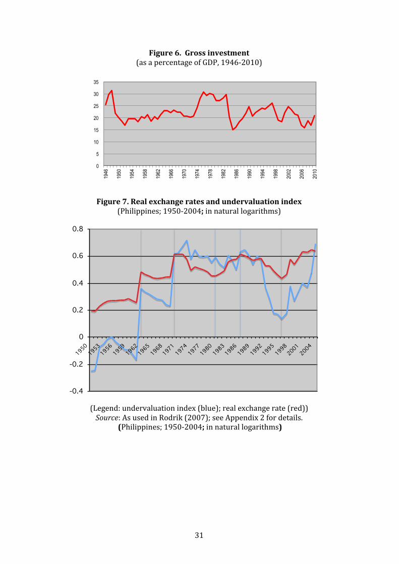
direct foreign investment for the period 1985‐1992 (de Dios 2011: 89, Table 5).  It is likely that this phenomenon explains much of Coxhead’s (2013) finding of powerful regional spillovers from the growth of Japan and China. The Philippines’ failure to benefit from such spillovers, which effectively jump‐started the industrialization of Malaysia, Thailand, and Indonesia, may in turn ultimately be attributed to the political instability that plagued the country at just that historical juncture. The relatively low investment rates over the greater postwar period are evident from Figure 6. Investment exceeded 25 percent of GDP only during 1975‐1983, the most stable years of the Marcos regime. This coincided with the global recycling of petrodollars from the Mideast oil bonanza, at which time the Philippines obtained access to large amounts of foreign loans. The well‐known backlash occurred in the shape of the financial and political crisis of 1983‐1985 described earlier. Since then, however, the investment ratio has never exceeded 25 percent. Aside from the understandable drop following the Asian crisis, a further decline took place after 2004, when investment ultimately dropped and remained at 20 percent of GDP or even less. 

[Figure 6 about here] To summarize: to the extent that political uncertainty and a dysfunctional government affected investment negatively; that import‐dependent manufacturing was hit especially hard by these crises; and that political instability and disputed property rights caused the country to miss out on the massive relocation of Japanese, Taiwanese, and Hong Kong manufacturing—then institutional factors must be considered one indispensable explanation for the failure of industrialization to continue after the ISI period.  What the institutions narrative is unable to explain, however, is why the structural contribution to productivity growth was already negative even before the crisis, the missed FDI opportunities, and unexploited regional spillovers. It also cannot explain why fast industrial growth did not resume after political stability returned.  In any event, the ability of Southeast Asian latecomers like Vietnam, Cambodia, and Laos to adapt and increase industrial output per capita undermines the sufficiency of the explanation. Although political instability and governance issues may explain the poor industrial performance from the 1970s to the 1990s, they cannot account for the poor industrial performance after the 1990s. 

 

Trade Liberalization? 

The notion that trade liberalization—the elimination of foreign exchange and quantitative import restrictions, the reduction of tariffs, or all of these—may have caused the failure of Philippine industrialization is a long and widely held view among the Left in Philippine politics (e.g., Bello et al. 2004).  The argument is that the reduction of protection undercut markets for domestic manufacturing when it needed it most. This hypothesis might be relevant in the late 1980s and especially in the 1990s. But before that time, the country had largely maintained a protectionist stance towards industry. This began with import‐ and exchange‐restrictions during 1949‐1961 and the replacement of import‐restrictions by 

  17 

high tariffs by 1962 (Power and Sicat 1971; Bautista, Power, et al. 1979; Medalla, Tecson, et al. 1995). The cascading tariff structure was largely maintained throughout the extended Marcos regime, modified only by modest concessions to new exports in the form of tax incentives and the creation of a few export‐processing enclaves. A tariff reform program that the Marcos regime finally undertook in 1981 initially cut nominal tariffs to the 10‐50 percent range (from as high as 100 percent) and eased quantitative restrictions. But this reform was quickly undone by the debt crisis when strict quantitative restrictions were reimposed to ration foreign exchange as all trade financing dried up.  After import controls were removed, the effective rate of protection for manufacturing was still a high 64.7 percent (Bautista 2005: 19). 

The decisive liberalization move was taken in 1991, when, in its last year in office and after the restoration of macroeconomic stability, the Aquino administration reduced tariffs to a 3‐30 percent range. The Ramos administration continued the liberalization trend by replacing import restrictions in agriculture with tariffs in 1992; acceding to the World Trade Organization in 1994; and making further tariff reductions in 1998 with a trajectory of reaching a uniform 5 percent by 2004.12 These 1981‐2003 trends are documented in Table 6.  

Table 6. Average tariffs for various economic sectors (in percent) 

Sector  1981  1985  1990  1991  1995  1998  2000   2001  2003 

Agriculture  43.23  34.61  34.77  35.95  27.99  18.91  14.40  14.21  11.04 Mining  16.46  15.34  13.97  11.46   6.31   3.58   3.27   3.25   2.84 Manufacturing  33.74  27.09  27.49  24.61  13.96   9.36   6.91   6.68   5.43 OVERALL  34.60  27.60  27.84  25.94  15.87  10.69   7.95   7.70   6.19 

Source: (Philippine) Tariff Commission  Even conceding a role for liberalization in the failure of industrialization, any such effect would have occurred only after the early to mid‐1990s. Thus, the liberalization thesis fails to provide an explanation for the dismal industrial performance after the early 1970s, by which time the country had already dropped out from the league of high growth performers.   

Real Currency Overvaluation? 

Another prominent explanation for Philippine deviant industrial development has been currency real overvaluation. Policy and academic debates have periodically13 focused on the possible role of the exchange rate as a developmental tool rather than simply a lever for attaining macroeconomic stability.  But the debate has been further stoked by difficulties currently faced by the authorities in stemming the nominal appreciation of the peso, as well as by a recent academic literature (e.g., Rodrik 2007) which highlights the salutary 

                                                        12 This measure was also an attempt avoid possible trade diversion with the advent of the low tariffs on intra‐ASEAN trade under the ASEAN Free Trade Area.  13 These policy debates have occurred at least in the late 1970s, the early 1990s, and more recently the present decade. (On these, see: Bautista, Power et al. 1979; de Dios et al. 1995; and Fabella 2011). 

  18 

growth effects of systematic real currency undervaluation in emerging economies. Until 1970, currency overvaluation under fixed exchange rates was generally associated with the import‐substitution strategy in place at the time, with the fixed exchange rate being partly supported by explicit foreign‐exchange controls, import‐quotas, and tariffs (Bautista, Power, et al. 1979). A second source of overvaluation treated in the literature has been the accumulation of debt, first involving heavy public borrowing during the authoritarian Marcos episode 1974‐1981 (Fabella 1996), then the debt accumulation by the private sector and portfolio capital inflows in the period preceding the Asian financial crisis 1992‐1997 (de Dios et al. 1998). Finally, overseas workers’ remittances have recently emerged as a major influence on the current account and the exchange rate. Together with monetary expansion in the US and other countries, overseas remittances have been associated with a historically unprecedented secular appreciation of the peso in nominal terms (by some 33 percent relative to the dollar between 2004 and 2012).  

To what extent does currency overvaluation contribute to an explanation of Philippine industrial failure after the early 1970s? Mustering evidence can be thorny, beginning with the definition of “real overvaluation” itself, a notion that depends heavily on the selection of a reference point. Although Rodrik’s (2007) evidence lends support to undervaluation as a successful industrialization policy tool, its applicability to the Philippines is somewhat awkward, since his own data suggest that the Philippines—together with other countries in Southeast Asia—had consistently undervalued its currency for most of the postwar period.  Figure 7 uses data from Rodrik (2011) and shows only a single episode (1950‐1961) of overvaluation for the Philippines (blue line), that which preceded the 1962 devaluation.  This is partly because Rodrik applies the Balassa‐Samuelson adjustment, an adjustment that shifts the observed real exchange rate by an amount depending on a country’s rate of growth. (The red line in Figure 7 also displays the trend in the real exchange rate without that adjustment.) Rodrik’s adjusted series seems inconsistent with the fact that the Philippines has run current account deficits throughout most of the entire post‐war period14 until continuous surpluses began to appear after 2003.  It may be more constructive, therefore, to speak only of the trends of real appreciation and depreciation rather than levels.  

[Place Figure 7 about here.]  

Whether one uses the undervaluation index or the (natural logarithm of the) real exchange rate, some general trends are common: large real depreciations resulting from the 1962 devaluation and the adoption of a floating rate in 1970; a real appreciation in 1973‐1979; significant real appreciation beginning in about 1991 until the Asian financial crisis; and significant real depreciation thereafter. No longer seen in the above series but evident in others, such as the central bank’s series, is the real appreciation of the peso from around  

 

                                                        14 The exceptions are the years 1962‐1966, 1986, and 1998 .  

  19 

 Table 7. Indices of Real Effective Exchange Rates of the Peso  

(1980‐2010)   1980  1985  1990  1995  2000  2003*  2005  2010 Major  99.44  89.28  66.20  79.19  71.92  59.94  61.98  84.08 Broad  101.44  100.51  86.90  100.78  109.12  99.91  101.51  137.65 Narrow  99.52  101.98  124.41  146.35  169.40  142.67  149.52  173.16 

Source: Bangko Sentral ng Pilipinas Notes: Index is based on the dollar price of a peso; a higher value of the index 

signifies peso appreciation.  Major index weights: U.S., Japan, Eurozone;  Broad index weights: Singapore, South Korea, Taiwan, Malaysia, Thailand, 

Indonesia, Hong Kong Narrow index weights: Indonesia, Malaysia, Thailand 

 2003 onward (Table 7). Focusing on Rodrik’s undervaluation index—and for the moment neglecting obvious annual fluctuations—the most favorable conditions for industrial development from this aspect should have been the years bracketed by the 1970 peso‐float and the debt crisis from 1983.  Yet we have already seen that in terms of structural contributions to productivity growth, the period 1970‐1985 was a net negative and failed to reinforce the effects of the 1962 devaluation. A fact relevant to any explanation for Philippine deviant industrialization behavior is that the period in question was also characterized by persistent current account deficits that were financed by heavy government borrowings from private sources. Part of these loans were in turn used to finance government budgets and industrial projects of Marcos cronies. The capital‐intensity and inefficiency of many of these projects are a likely explanation for their weak impact on manufacturing employment. This is also partly reflected in the behavior of total‐factor productivity for the period. Hooley (1985) finds that total factor productivity in manufacturing throughout most of the 1970s was declining, a fact he attributes to the inefficiency of the industries set up at the time (and thus a conflict between small overall manufacturing total factor productivity growth and bigger within‐manufacturing total factor productivity growth). 

The real appreciation prior to the Asian financial crisis (1990‐1995) is also well understood as the result of the renewed access to foreign credit and heavy borrowing by the private sector, fueling a real estate boom as it did in other countries. That this was also a period of positive structural contributions from manufacturing is probably due to the recovery of industrial employment after the brief but crippling power‐related recession of 1990‐1992. In contrast, between 2003 and 2010 the peso appreciated in real terms in relation to the currencies of its trading partners and competitors (Table 7) by as much as 38 percent15.  This phase coincides with the emergence of regular current account surpluses owing to overseas workers’ remittances, rapid decline in manufacturing competitiveness, and a further loss in manufacturing jobs. 

                                                        15   That is, 137.65 from 99.91 in the second row of Table 7. The real appreciation is 38 (respectively 21) percent if the values of the Major (respectively Narrow) indices are used for the same years. 

  20 

 

Overseas Labor Migration? 

As a candidate for explaining the failure of Philippine industrialization, Dutch Disease caused by overseas migrant remittances are only relevant beginning with the early 1990s. Data on remittances are deficient before the mid‐1980s, but overseas deployment, with a lag, can serve as a proxy for remittance trends. Prior to the early 1980s, overseas migration was a minor phenomenon. In relation to the domestic labor force, overseas migration became significant only from 1983, when registered annual deployment shot up to more than two percent of the labor force. A further acceleration occurred in 1998, when registered deployment rose 56 percent and exceeded three percent of the labor force (Table 8, line 1). These growth‐spurts in overseas deployment coincided with or occurred shortly after major economic crises at home, when domestic urban employment opportunities were shrinking significantly16, and overseas markets were relatively open.  Increasing foreign deployment is mirrored, with a lag, by rising inward remittances by workers based overseas. The leap in the importance of remittances occurred in the late1990s (Table 8, line 2), when they came to represent 14 percent of all current account receipts (from only 5 percent in the late 1970s). This figure rose further to 20 percent by the late 2000s, but the country had already begun to run current‐account surpluses on a regular basis as early as 2003. The upshot is that overseas remittances had only modest impact on the current account and exchange rates until the early 1990s. If they have generated a significant industrial Dutch Disease, they can only have done so from that time onward. 

 Table 8. Deployment of Overseas Workers and Remittances (1975‐2004) (as percentage of domestic labor force; annual averages for selected periods) 

 1975‐1979 

 1980‐1984 

 1985‐1989 

 1990‐1994 

 1995‐1999 

 2000‐2004 

 2005‐2009 

Deployment*  0.48  1.70  2.02  2.65  2.75  2.96  3.44 

Remittances**  5.26***  7.86  7.75  10.48  13.56  13.95  19.78 

Sources: Philippine Overseas Employment Authority; National Statistical Coordination Board *Annual overseas deployment relative to domestic labor force. **Remittances (current transfers) as a percentage of total current‐account receipts.  *** Labor force figure for 1979 is a between‐year interpolation.  

Real Exchange Rate and Trade Regime Interactions? 

Any cross‐country real exchange rate assessment should also take in to account the trade regime. While real exchange rates deal with the prices of tradables relative to nontradables, they do not deal with the relative prices between exportables and importables. Thus, it is critical to sort out the net incentive 

                                                        16 The slight slowdown in overseas deployment immediately after the 1986 revolution is also evident and may indicate the goodwill and optimism early in the post‐Marcos period. This soon faded, however, and the gradual rise in deployment resumed and shot up in 1998. 

  21 

effect of real over‐ or undervaluation of the peso in conjunction with the trade regime. 

Table 9. Trade Liberalization and Real Depreciation   

Liberalized imports

Restricted imports and export penalties

Real depreciation

I. Demand‐ and supply‐  constraints relaxed 

II. Supply‐side constraints  binding 

Real appreciation

III. Demand‐side  constraints binding 

IV. Demand‐ and supply‐  constraints binding 

Source: Schematisation of Bautista (2003) 

Policy debates in the 1960s over the trade regime were superseded since the 1990s by controversies over the exchange rate, but an explicit consideration of the two together is rarely made. Bautista (2003) is the rare exception. Its most relevant point, schematized in Table 9 above, is that a failure to coordinate exchange‐rate management and trade policy could lead to paradoxical or even perverse results. 

In line with the usual efficiency arguments for free trade, episodes of currency undervaluation or real depreciation are best accompanied or preceded by a liberalization of imports (Quadrant I). A well known other extreme (Quadrant IV) is a restrictive import regime combined with an overvalued currency. This latter case may roughly characterize the entire import‐substitution period 1949‐1961 before the 1962 devaluation, which many others have discussed.  This was a period when manufacturing growth ran up against limited market size, which consisted almost exclusively of the protected domestic market. Indeed, an expansion of manufacturing exports was stifled by the implied penalty of currency overvaluation. The 1990s, before the Asian financial crisis hit the Philippines in 1998, were years commonly characterized by import liberalization, when tariffs were lowered and import‐licensing requirements (introduced in the crisis years 1980‐1988) were removed17. However, this was also a period of real currency appreciation if not outright overvaluation. Private access to foreign borrowing resumed, fueling a real‐estate and equity market boom, and overseas workers’ remittances began to contribute a significant share (more than 10 percent) of current‐account receipts. This regime falls in Quadrant III of Table 9. Import liberalization eased the input‐supply constraints to manufacturing, but at the same time real appreciation undercut its competitiveness in both domestic and foreign markets. From this perspective, the observed fall‐off in the structural contribution of manufacturing growth is hardly surprising. The most enigmatic part of the historical record, however, is the 1971‐1981 decade. These years marked the first stage of the secular collapse of Philippine manufacturing growth. As already noted, it was also a period of relative political stability (if through repression), and it included years when investment was at an unequaled high. Dutch Disease from overseas migration could not have played a role during the decade, since that phenomenon attained a significant 

                                                        17 Aldaba (2005) provides a brief chronology. 

  22 

magnitude only in the 1990s. Also, most data indicate that the adoption of a managed float in 1970 resulted in a real depreciation that should have stimulated manufacturing and its exports. In short, many conditions were favorable for industrialization. So, why the poor industrial performance? Bautista [2003] argues, however, that this period’s potential was seriously diluted by the continuing protection of importables, which raised the cost of  

Table 10. Effective exchange rates for various categories of goods (1949‐1980; period averages; pesos per dollar) 

 

Nominal  NEC  SEC  EC  NEP  SEP  EP  TX  NX  Ratio: EP/NX 

1949  2.00  2.05  2.05  2.00  2.05  2.00  2.00  2.00  2.24  0.89 

1950‐1959  2.00  3.65  2.46  2.06  2.43  2.44  2.44  2.00  2.29  1.065 

1960‐1969  3.90  10.56  5.27  3.91  6.91  4.22  4.61  3.46  3.70  1.245 

1970‐1975  6.86  21.19  9.16  7.56  12.46  8.08  8.24  6.17  7.66  1.076 

1976‐1980  7.42  25.49  10.17  8.82  13.46  9.34  9.40  7.12  8.44  1.114 

Categories refer to: nonessential consumer goods (NEC); semi‐essential consumer goods (SEC); essential consumer goods (EC); nonessential producer goods (NEP); semi‐essential producer 

goods (SEP); essential producer goods (EP); traditional exports (TX);  and nontraditional exports (NX). 

Source: Senga [1983] for 1972‐1980 and Baldwin [1975] for 1949‐1971.  

imported inputs. His thesis finds support when one considers the effective exchange rates confronted by various tradables during the period. Reading off the entries for 1970‐1975 and 1976‐1980 in Table 10, it is evident that export industries were still constrained on the supply side, given the exchange‐rate penalty on producer goods. Over that decade, a nontraditional exporting firm would have confronted a 7.6 to 11.4 percent penalty on foreign exchange as between its final product and its essential production input. The penalty is even larger if one considers the import of “semi‐essential” and “non‐essential” producer goods. To be sure, a few export processing zones (Bataan, Cavite, and Mactan) and some export incentives relieved these constraints somewhat, but these efforts were limited. The export boom in 1970‐71 was short‐lived, the drive by the Marcos regime to establish “major industrial projects”, including a number of heavy (capital‐intensive) industries, was aborted, and the supply‐constrained effort failed to generate a manufactured export take off. The resulting current‐account deficits were covered by massive government foreign borrowings, which in turn laid the foundation for the debt crisis beginning in 1983 when global conditions became adverse. The failure of the new export industries to expand and the capital‐intensity of the regime’s favored projects explain the weak structural impact (especially on employment) of manufacturing during the decade, in spite of the higher investment ratios. 

 Deviant Behavior and Path Dependence 

We conclude our assessment of the sources of the Philippine industrialization collapse by stressing the role of path‐dependence. The 1983‐1986 political crisis and recession shunted the economy off on a debt‐driven trajectory. By the 1990s, helped along by a popular restoration of democracy, the protectionist 

  23 

regime, which had been the principal obstacle to industrial growth in the 1970s, was eliminated.  If the global crisis had not occurred and political instability had been averted, would the regime’s debt‐financed industrial effort—crony‐led and corrupt as it was—have ultimately transitioned into a more typical  East Asian growth pattern?  Or alternatively, if the post‐Marcos Aquino government had not been beleaguered by successive putsch attempts, would the Southeast Asian flood of Japanese FDI in the 1990s have given the Philippines a second chance at an industrial future?  

In the event, the widespread joblessness occasioned by poor manufacturing growth in the 1970s and 1980s gave birth to a new phenomenon that would further stifle growth in the future: large‐scale overseas workers’ migration. The size and growth of this migration, and its resulting foreign remittances, would by the early 2000s resolve the foreign‐exchange constraint that had been Philippine industry’s other perennial nemesis. Indeed it did more: increasing remittance inflows would be responsible for a Dutch Disease phenomenon by the late 2000s, causing a sustained real appreciation and imposing a penalty on tradable manufacturing. If the outmigration had not occurred or had been much more modest (like the rest of Southeast Asia), would Philippine manufacturing have fared better had liberalization combined with a currency that was competitively depreciated after the Asian Crisis?  The path followed has led to a new stable equilibrium where a largely liberalized trade in goods coexists with a recurrent current account surplus built on remittances and strong (skill‐intensive) service‐sector exports. The peso is under steady pressure to rise in real terms, which leaves little room for (lower‐skill) manufacturing to compete and expand.  A considerable rise in the investment rate—still low by East Asian standards—would relieve the current‐account pressure for real appreciation and create more jobs. But the low investment rate may be part of an equilibrium where capital requirements are low simply because a significant share of the urban labor force is already abroad. 

It appears that the deviant behavior of Philippine manufacturing since the 1960s was produced by a “perfect storm” of protectionist policy, political instability, a missed FDI opportunity, foreign capital dependency, and two financial crises. The new equilibrium that has emerged since the 1990s suggests that the well‐trodden route to industrialization has been missed forever. If at all, a different path must be found. 

  

 

END 

 

  

  

  24 

References  Abramovitz, M. (1986), “Catching Up, Forging Ahead, and Falling Behind,” 

Journal of Economic History 46 (2): 385-406. Acemoglu, D. and J. Robinson (2012), Why Nations Fail. New York: Crown 

Business. Acemoglu, D., S. Johnson, and J. Robinson (2002), “Reversal of Fortune: 

Geography and Institutions in the Making of the Modern World Income Distribution,” Quarterly Journal of Economics 117 (November): 231‐94. 

Aldaba, R. (2005) “The Impact of Market Reforms on Competition, Structure, and Performance of the Philippine Economy”. Discussion Paper Series, No. 2005‐24. Makati: Philippine Institute for Development Studies 

Bairoch, P. (1982), “International Industrialization Levels from 1750 to 1980,” Journal of European Economic History, 11 (Fall): 269‐333. 

Baldwin, R. (1975) Foreign Trade Regimes and Economic Development: the Philippines. (New York: National Bureau of Economic Research). 

Barro, R. J. (1997) Determinants of Economic Growth: A Cross‐Country Empirical Study (Cambridge, Mass.: MIT Press). 

Bautista, R. (2003) Exchange Rate Policy in Philippine Development. Research Paper Series, 2003‐01. (Makati: Philippine Institute for Development Studies). 

Bautista, R., J. Power, et al. (1979) Industrial Promotion Policies in the Philippines. (Makati: Philippine Institute for Development Studies). 

Bello, W., H. Docena, M. de Guzman, and M.L. Mulig (2004) The Anti‐development State: the Political Economy of Permanent Crisis in the Philippines. (Quezon City: University of the Philippines Department of Sociology and Focus on the Global South). 

Bénétrix, A., K. H. O'Rourke, and J. G. Williamson (2012) “The Spread of Manufacturing to the Periphery 1870‐2007: Eight Stylized Facts,” NBER Working Paper 18221, National Bureau of Economic Research, Cambridge, Mass. (July). 

Bourguignon, F. and C. Morrisson (2002), “Inequality among World Citizens: 1820‐1992,” American Economic Review, 92, 4 (September): 727‐44. 

Coxhead, Ian [2013], “Southeast Asian Economics and Development: An Overview,” Handbook of Southeast Asian Economics (forthcoming, Routledge). 

de Dios, E. [2011] “Institutional Constraints on Philippine Growth”, Philippine Review of Economics and Business. 49(1). June 2011: 71‐124. 

de Dios, E., R. Fabella, F. Medalla, and S. Monsod (1998) “Exchange Rate Policy: Past Failures and Future Tasks”, Public Policy [Philippines], 1(1) October. 

Durlauf, S., P. Johnson, and J. Temple (2005), “Growth Econometrics.” In P. Aghion and S. Durlauf (eds.), Handbook of Economic Growth (Amsterdam: North‐Holland). 

  25 

Engerman, Stanley L. and Kenneth L. Sokoloff. 2012. Economic Development in  the Americas since 1500: Endowments and Institutions. (New York: Cambridge University Press). 

Fabella, R. (1996) “The Debt‐Adjusted Real Effective Exchange Rate”, Journal of International Money and Finance 15(3): 475‐484.  

Helpman, E. (2004), The Mystery of Economic Growth. Cambridge, (Mass.: Harvard University Press). 

Hooley, R. (1985) Productivity Growth in Philippine Manufacturing: Retrospect and Future Prospects. PIDS Monograph Series No. 9. Makati: Philippine Institute for Development Studies. 

Hooley, Richard (2005), “American Economic Policy in the Philippines, 1902‐1940: Exploring a Statistical Dark age in Colonial Statistics,” Journal of Asian Studies 16. 

Krugman, P. (1981), “Trade, Accumulation, and Uneven Development,” Journal of Development Economics, 8: 149‐61. 

Krugman, P. (1991), “Increasing Returns and Economic Geography,” Journal of Political Economy, 99: 483‐99. 

Legarda, B. J. (1999), After the Galleons: Foreign Trade, Economic Change and Entrepreneurship in the Nineteenth‐Century Philippines. Madison, Wis.: University of Wisconsin Press. 

Lewis, W. A. (1978), The Evolution of the International Economic Order. (Princeton, N. J.: Princeton University Press). 

Lucas, R. E. (1988), “On the Mechanics of Economic Development,” Journal of Monetary Economics 22(1): 3‐42. 

Maddison, A. (2010), Statistics on World Population, GDP and Per Capita GDP, 1‐2008 AD, http://www.ggdc.net/MADDISON/oriindex.htm 

Medalla, E., G. Tecson, R. Bautista,  J. Power, and Associates (1995) Philippine Trade and Industrial Policies: Catching Up with Asia’s Tigers, Vol. I. (Makati: Philippine Institute for Development Studies). 

Mitchell, B. R. (2007), International Historical Statistics: Africa, Asia & Oceania 1750‐2005, 6th ed. Palgrave Macmillan.  

National Economic and Development Authority [NEDA] (2011), Philippine Development Plan 2011‐2016. Pasig City. 

North, D. [1990] Institutions, Institutional Change, and Economic Performance. Cambridge University Press. 

Power, J. and G. Sicat (1971) The Philippines: Industrialization and Trade Policies. (London: Oxford University Press). 

Rodrik, D. (2007) "The Real Exchange Rate and Economic Growth: Theory and Evidence." Working Paper 2008‐0141, Weatherhead Center for International Affairs, Harvard University. 

Rodrik, D. (2013), “Unconditional Convergence,” Quarterly Journal of Economics 128 (February): 165‐204. 

  26 

Romer, P. M. (1986), “Increasing Returns and Long‐Run Growth,” Journal of Political Economy 94: 1002‐37. 

Romer, P. M. (1990), “Endogenous Technological Change,” Journal of Political Economy 98: S71‐S102. 

Senga, K [1983] “A Note on Industrial Policies and Incentive Structures in the Philippines 1949‐1980”, Philippine Review of Economics and Business 20(3‐4): 299‐305. 

Williamson, J. G. (2011), Trade and Poverty: When the Third World Fell Behind. (Cambridge, Mass.: MIT Press). 

World Bank (2011), World Development Indicators. Washington, D.C.  Wright, G. (1990), "The Origins of American Industrial Success, 1879‐1940," 

American Economic Review, 80 (September): 651‐68. Yoshihara, K (1994) The Nation and Economic Growth. Oxford University Press. 

  27 

Appendix 1. 

Let yt  denote labor productivity in the whole economy at time t and Δyt  its change relative to a previous period k. Then: 

 

Here, yi,t  is labor productivity in the entire economy and in sector i at time t, and θi,t is the employment share of sector i at time t, with ∑i θi,t = 1 for all t. Dividing both sides by yt (and properly annualizing) gives the annual rate of growth of productivity for the period as the sum of two terms:  𝑤!"!

!!!  is the change in productivity “within” the sector, while the second  𝑠!"!

!!!  is a measure of structural change, reflecting the extent to which labor is pulled towards sectors where productivity is growing rapidly.  

  

 

Appendix 2. Rodrik (2007: 6) explains his undervaluation index as  

ln UNDERVALt = ln RERt – ln RER*t ,   where ln RERt = ln(XRATt /PPPt ), while ln RER*it is the predicted values from the equation: ln RER*t  = a + b ln RGDPCHt+ ft + uit,  which is estimated across countries with ft being a time fixed‐effect and a value of b = –0.24 is obtained to represent the “Balassa‐Samuelson” effect of lower prices of nontraded goods in developing countries (so that currencies strengthen as their economies prosper). In the case of overvaluation, RERt /RER*t < 1, or ln UNDERVALt < 0. On the other hand, ln UNDERVALt > 0 implies undervaluation.    

!yt= !

i ,t"kyi ,t" y

i ,t"k( )i=1

n

# + yi ,t!i ,t"!

i ,t"k( )i=1

n

#

!yt

yt

= wit+

i=1

n

# sit

i=1

n

# = wit+ s

it( )i=1

n

#

  28 

Figure 1. Regional diffusion curves: reaching the 5 per cent threshold 

 Note: The figure shows the proportion of countries for which the 10‐year backward looking average industrial growth rate exceeded a 5 per cent threshold. Countries for which data are missing are assumed not to have exceeded this threshold.   

  29 

Figure 2. Regional population‐weighted diffusion curves:  reaching the 5 per cent threshold 

 Note: The figure shows the proportion of the region’s population in 2007 living in countries for which the 10‐year backward looking average industrial growth rate exceeded a 5 per cent threshold. Countries for which data are missing are assumed not to have exceeded this threshold.    

Figure 3.  Employment shares by sector (1956‐2009, in percent) 

    

0.0 

10.0 

20.0 

30.0 

40.0 

50.0 

60.0 

70.0 

1956  1960  1965  1970  1975  1980  1985  1990  1995  2000  2005  2009 

Agriculture 

Industry 

Manufacturing 

Services 

  30 

Figure 4. Within‐sector productivity growth by sector (annual rates, in percent); 1956‐2009 

 Source of basic data: National Statistical Coordination Board (output measured in constant 1984 prices). 

 Figure 5. Productivity growth from structural shift by sector 

(annual rates, in percent); 1956‐2009 

 Source of basic data: National Statistical Coordination Board (output measured in constant 1984 prices). 

  

 

 

‐4 

‐3 

‐2 

‐1 

0 

1 

2 

Manufacturing 

Rest of economy 

‐1.5 

‐1 

‐0.5 

0 

0.5 

1 

1.5 

Manufacturing 

Rest of economy 

  31 

Figure 6.  Gross investment (as a percentage of GDP, 1946‐2010) 

  

Figure 7. Real exchange rates and undervaluation index  (Philippines; 1950‐2004; in natural logarithms) 

 (Legend: undervaluation index (blue); real exchange rate (red)) Source: As used in Rodrik (2007); see Appendix 2 for details. 

 (Philippines; 1950‐2004; in natural logarithms)   

 

0

5

10

15

20

25

30

35

1946

1950

1954

1958

1962

1966

1970

1974

1978

1982

1986

1990

1994

1998

2002

2006

2010

-0.4

-0.2

0

0.2

0.4

0.6

0.8

1950

1953

1956

1959

1962

1965

1968

1971

1974

1977

1980

1983

1986

1989

1992

1995

1998

2001

2004