
Developing robust Iot to monitor smart spaces at scale - Cnam
150
HAL Id: tel-03175539 https://hal-cnam.archives-ouvertes.fr/tel-03175539 Submitted on 20 Mar 2021 HAL is a multi-disciplinary open access archive for the deposit and dissemination of sci- entific research documents, whether they are pub- lished or not. The documents may come from teaching and research institutions in France or abroad, or from public or private research centers. L’archive ouverte pluridisciplinaire HAL, est destinée au dépôt et à la diffusion de documents scientifiques de niveau recherche, publiés ou non, émanant des établissements d’enseignement et de recherche français ou étrangers, des laboratoires publics ou privés. Public Domain Developing robust Iot to monitor smart spaces at scale Francoise Sailhan To cite this version: Francoise Sailhan. Developing robust Iot to monitor smart spaces at scale. Computer Science [cs]. Saclay, CNAM, 2021. tel-03175539
-
Upload
khangminh22 -
Category
Documents
-
view
1 -
download
0
Transcript of Developing robust Iot to monitor smart spaces at scale - Cnam

HAL Id: tel-03175539https://hal-cnam.archives-ouvertes.fr/tel-03175539
Submitted on 20 Mar 2021
HAL is a multi-disciplinary open accessarchive for the deposit and dissemination of sci-entific research documents, whether they are pub-lished or not. The documents may come fromteaching and research institutions in France orabroad, or from public or private research centers.
L’archive ouverte pluridisciplinaire HAL, estdestinée au dépôt et à la diffusion de documentsscientifiques de niveau recherche, publiés ou non,émanant des établissements d’enseignement et derecherche français ou étrangers, des laboratoirespublics ou privés.
Public Domain
Developing robust Iot to monitor smart spaces at scaleFrancoise Sailhan
To cite this version:Francoise Sailhan. Developing robust Iot to monitor smart spaces at scale. Computer Science [cs].Saclay, CNAM, 2021. tel-03175539
Mémoire présentée en vue de l’obtention del’habilitation à diriger des recherches
Université Paris-Saclay
§
Discipline : Informatique
Developing Robust IoT toMonitor Smart Spaces at
ScaleHabilitation à diriger la recherche
Par : Françoise Sailhan
Sous la direction de ,
Membres du jury:Rapporteur: Julien Bourgeois, Prof. des Universités, Univ. de Franche Comté,
Rapporteure: Siobhán Clarke, Prof. des Universités, Trinity College,
Rapporteure: Nathalie Mitton, Directrice de Recherche, Inria-Lille,
Marraine: Valérie Issarny, Directrice de Recherche, Inria-Paris,
Examinatrice: Nalini Venkatasubramanian, University of California,
Présidente: Karine Zeitouni, Prof. des Universités, Université Paris-Saclay,
Date de soutenance : 14 janvier 2021


Contents
1 Introduction 11.1 Context and Related Opportunities . . . . . . . . . . . . . . . . . . . . . . . . . 11.2 Challenges of designing and deploying an IoT system . . . . . . . . . . . . . . . 21.3 Outline . . . . . . . . . . . . . . . . . . . . . . . . . . . . . . . . . . . . . . . . . 3
2 Into the Wild - Intrusion Detection 72.1 Introduction . . . . . . . . . . . . . . . . . . . . . . . . . . . . . . . . . . . . . . 72.2 Signature-based Intrusion Detection in MANETs . . . . . . . . . . . . . . . . . . 9
2.2.1 Attacks Threatening the OLSR Protocol . . . . . . . . . . . . . . . . . . 92.2.2 Attack Detection . . . . . . . . . . . . . . . . . . . . . . . . . . . . . . . 132.2.3 Trustworthiness Evaluation . . . . . . . . . . . . . . . . . . . . . . . . . 152.2.4 Reducing the Cost of Investigations . . . . . . . . . . . . . . . . . . . . . 18
2.3 Anomaly Detection . . . . . . . . . . . . . . . . . . . . . . . . . . . . . . . . . . 192.3.1 RFID System supporting access control . . . . . . . . . . . . . . . . . . . 202.3.2 Anomaly Detector . . . . . . . . . . . . . . . . . . . . . . . . . . . . . . 21
2.4 Performance Evaluation . . . . . . . . . . . . . . . . . . . . . . . . . . . . . . . 242.4.1 Signature-based Intrusion Detection . . . . . . . . . . . . . . . . . . . . 242.4.2 Trustworthiness and Confidence . . . . . . . . . . . . . . . . . . . . . . . 27
2.5 Conclusion . . . . . . . . . . . . . . . . . . . . . . . . . . . . . . . . . . . . . . . 28
3 Enhancing the Observation Quality through Calibration 313.1 Introduction . . . . . . . . . . . . . . . . . . . . . . . . . . . . . . . . . . . . . . 313.2 Planned Calibration of an IoT Infrastructure . . . . . . . . . . . . . . . . . . . . 33
3.2.1 Multi-Sensor Calibration Planning . . . . . . . . . . . . . . . . . . . . . 343.2.2 Multi-Sensor Calibration Optimisation Problem . . . . . . . . . . . . . . 363.2.3 Solutions and Derived Algorithms . . . . . . . . . . . . . . . . . . . . . . 37
3.3 Robust Multi-Party calibration . . . . . . . . . . . . . . . . . . . . . . . . . . . 403.3.1 Multivariate Linear Regression . . . . . . . . . . . . . . . . . . . . . . . . 413.3.2 Multi-hop, Multi-party Calibration . . . . . . . . . . . . . . . . . . . . . 44
3.4 Evaluation . . . . . . . . . . . . . . . . . . . . . . . . . . . . . . . . . . . . . . . 483.4.1 Planning the Calibration . . . . . . . . . . . . . . . . . . . . . . . . . . . 483.4.2 Multi-Hop Multi-Party calibration . . . . . . . . . . . . . . . . . . . . . . 51
3.5 Conclusion . . . . . . . . . . . . . . . . . . . . . . . . . . . . . . . . . . . . . . . 57
4 Leveraging Crowdensors to support Context-aware and Cost-effective Crowd-sensing 634.1 Introduction . . . . . . . . . . . . . . . . . . . . . . . . . . . . . . . . . . . . . . 634.2 Context-Awareness sustaining a Collaborative Crowdsensing . . . . . . . . . . . 65
4.2.1 Context Characterisation . . . . . . . . . . . . . . . . . . . . . . . . . . . 664.2.2 Feature Selection . . . . . . . . . . . . . . . . . . . . . . . . . . . . . . . 674.2.3 Classifier Initialisation . . . . . . . . . . . . . . . . . . . . . . . . . . . . 684.2.4 Online Personalising . . . . . . . . . . . . . . . . . . . . . . . . . . . . . 69
4.3 Assessing the Crowdsensor Utilities . . . . . . . . . . . . . . . . . . . . . . . . . 70
i
CONTENTS
4.4 Opportunistic Aggregation and Interpolation . . . . . . . . . . . . . . . . . . . 734.4.1 Spatio-temporal Interpolation . . . . . . . . . . . . . . . . . . . . . . . . 734.4.2 Opportunistic Aggregation . . . . . . . . . . . . . . . . . . . . . . . . . . 75
4.5 Performance Evaluation . . . . . . . . . . . . . . . . . . . . . . . . . . . . . . . 764.5.1 User-centric Context Inference . . . . . . . . . . . . . . . . . . . . . . . . 764.5.2 Group-based Collaborative Crowdsensing . . . . . . . . . . . . . . . . . . 824.5.3 Interpolation and Aggregation . . . . . . . . . . . . . . . . . . . . . . . 85
4.6 Conclusion . . . . . . . . . . . . . . . . . . . . . . . . . . . . . . . . . . . . . . . 90
5 Information centric Networking 935.1 Context and Motivation . . . . . . . . . . . . . . . . . . . . . . . . . . . . . . . 935.2 Group-based Publish-Subscribe System . . . . . . . . . . . . . . . . . . . . . . 95
5.2.1 Underlying Group Communication . . . . . . . . . . . . . . . . . . . . . 955.2.2 Cluster-based Routing . . . . . . . . . . . . . . . . . . . . . . . . . . . . 96
5.3 Notification and Subscription Representation . . . . . . . . . . . . . . . . . . . . 975.3.1 Notification and Subscription Formats . . . . . . . . . . . . . . . . . . . 975.3.2 Subscription Organisation - State of the Art . . . . . . . . . . . . . . . . 99
5.4 Enhanced Forwarding . . . . . . . . . . . . . . . . . . . . . . . . . . . . . . . . . 1005.4.1 Preventing Intermediate Routers From Performing Duplicate Searches . . 1035.4.2 Prefiltering with an Index-based Subscription Repository . . . . . . . . . 1055.4.3 Synthesis . . . . . . . . . . . . . . . . . . . . . . . . . . . . . . . . . . . 107
5.5 Folding Bloom Filters . . . . . . . . . . . . . . . . . . . . . . . . . . . . . . . . . 1085.5.1 Finding y-Smooth Numbers . . . . . . . . . . . . . . . . . . . . . . . . . 1095.5.2 On-Line Folding Strategy . . . . . . . . . . . . . . . . . . . . . . . . . . 1135.5.3 Folding . . . . . . . . . . . . . . . . . . . . . . . . . . . . . . . . . . . . . 114
5.6 Performance Evaluation . . . . . . . . . . . . . . . . . . . . . . . . . . . . . . . 1165.6.1 Event Notification System . . . . . . . . . . . . . . . . . . . . . . . . . . 1165.6.2 Evaluation of the folding . . . . . . . . . . . . . . . . . . . . . . . . . . 119
5.7 Conclusion . . . . . . . . . . . . . . . . . . . . . . . . . . . . . . . . . . . . . . . 123
6 Conclusion 1256.1 Summary of Contributions . . . . . . . . . . . . . . . . . . . . . . . . . . . . . . 1256.2 Perspectives . . . . . . . . . . . . . . . . . . . . . . . . . . . . . . . . . . . . . 127
Bibliographie 131
ii

Chapter 1
Introduction
1.1 Context and Related Opportunities
The Internet of Things (IoT) has emerged as a distributed, self-healing and large-scale ar-chitecture composed of a variety of objects that monitor and affect their environment.Thiscombination of sensing and actuation capabilities holds great promise as the enabler of a widespectrum of applications, e.g., smart space (e.g., building surveillance and ecology-friendly con-trol), emergency response and environmental monitoring. Instrumented with sensors, RFIDsand actuators, smart spaces (including the residents, employees) provide valuable informa-tion that serve supporting e.g., access control [66, 26], inform rescuers in case of emergency[137, 12, 56], provide assisted/enhanced living [179], ect.. In the area of environmental monitor-ing for example, large cities have made progress, in recent years, in monitoring and assessingthe biological and ecological impacts of pollution to respond appropriately, from the politicalto the individual level. Cities have traditionally relied on sensing stations that gather observa-tions (e.g., atmospheric conditions, noise levels, temperatures). Recently cities have also beguntaking advantage of crowdsensing movement, wherein users (citizens, groups, communities) relyon the small and low-cost sensors embedded in –or connected to– their smartphones so as tohelp identify environmental problems. IoT-based applications build on a communication andcomputing infrastructure spanning different scales, from smartphones embedding or connectingto sensors (a.k.a. detectors) and actuators (e.g., electromechanical and/or software-based de-vices), enabling them to capture, measure, react and communicate with their environment, allthe way to large-scale networks, capable of disseminating critical information from event sourcesto multiple recipients. At the network edge, some wireless networks (e.g., Device-to-Device andwireless sensor networks ) with no specific underlying infrastructure in place, connect diverseThings hosting sensors and actuators (e.g., mobile phones, vehicles, smart clothing, motes).Interestingly, these networks mirror ad hoc networks — some of the nodes are battery poweredand communicate via wireless connections, possibly involving intermediate/proxy-nodes andusing multi-hop routing.
So far many specific, distributed, energy-/memory-/computationally-aware protocols, sys-tems and applications have been proposed to enhance the collection and processing of theincreasingly massive amount of available information in the IoT. However as the range of ap-plications extends to the fields of industrial and mission-critical systems, additional assurancerequirements related to accuracy, reliability and security must be considered. Accomplishingthe challenging task of Developing Robust IoT therefore necessitates: (i) supporting accurateand resource-efficient sensing and actuation capabilities and (ii) providing efficient and reliablecommunication among Things/users across heterogeneous and volatile networks from the edgeup to the cloud.
1
Chapter 1 – Introduction
1.2 Challenges of designing and deploying an IoT systemWhile expectations are high for the wide applicability of IoT systems, the need to monitorphenomena at unprecedented scale is far from being a trivial concern especially consideringthat IoT applications must remain dependable under any circumstance (e.g., despite disrup-tions, harsh conditions or even attacks). IoT system applications are subject to a variety offaults/threats, spanning hardware, software and networking layers. Given that the IoT ecosys-tem is information-centric (i.e., Things generate a torrent of information delivered to manyrecipients that in turn must filter, customise, and process it on the fly), we are mostly con-cerned with the two following classes of impairments:
• Communication faults - Any intentional or accidental attempt to disrupt the flow of in-formation seriously jeopardises IoT systems. IoT systems are actually very difficult toinsulate against communication faults due to the openness of the wireless communicationmedium, coupled with the cooperative nature of the network, which render protocols andrelated applications easy to compromise. In this regards, detecting any misuse or anomaly(i.e., deviations from the normal behaviour) that threatens the networking structure –from edge to core networks – is of critical importance. In this regard we began (i) inves-tigating the detection of misuses and anomalies. Our attention was specifically directedat detecting attempts to disorganise the routing or disturb the data flow relaying. Inaddition we aimed at detecting anomalies corresponding to certain types of misbehaviour(e.g., unusual and potentially unauthorised access to some data, unexpected presence ina smart building).
• Information-related faults - The collection of data of sufficient quality is a major chal-lenge facing the IoT. Many sensors in use are low cost, mass produced and are made ofoff-the-shelf components and their relatively low accuracy challenges the relevance andaccuracy of the collected sensory data. In addition, the exposure of the sensors to naturalperturbations leads to questioning the accuracy of the observations. Correcting inade-quate observations in order to derive proper conclusions is therefore of prime importance.Meanwhile, knowledge of the sensors’ context is vitally important in order to discoverwhether the sensing devices are in a position that enables sensing, instead of interferingwith it. In response to this challenge we propose to: (i) calibrate the inexpensive (andoften inaccurate) sensors and (ii) fuse the information provided by multiple sensors soas to supply more accurate/reliable observations (as opposed to trying to improve thereliability of the individual devices involved).
While IoT enables environmental monitoring at an unprecedented scale ( leveraging cali-brated sensors and information fusion), it also involves significant communication, computation,and, therefore, financial costs due to the reliance on cloud infrastructures for processing thespatio-temporal data. The situation is actually worsen due to the fact that IoT systems require(i) a low-level control loop to support timely and situational-aware sensing and actuation and(ii) a higher-level control loop to infer a physical phenomenon as a whole, i.e., at macro scaleand across time. As an illustration, knowledge of the level of ambient pollution (e.g., noiselevel, air quality) within a particular area helps citizens measure their own exposure to pollu-tion. An extended control loop is also needed so that citizens, authorities and decision-makerscan design adequate policies. As an alternative to the centralised gathering and analysis ofcrowdsensing observations through such a high-level control loop, we introduce a crowdsensingsystem that functions on a collaborative model, operating primarily at the very edge, i.e., em-powering smartphones so as to enhance the quality of the data transferred to the cloud while
2

1.3. Outline
reducing the related communication cost and resource consumption. We adopt an information-centric paradigm in which the information drives decision-making. To achieve this we buildupon a publish/subscribe system that supports a loosely-coupled communication towards/fromThings/users across heterogeneous and volatile networks in which data flows are governed byboth user interests and data content.
1.3 OutlineThis document brings together a large portion of the research I have been conducting over aperiod that spans 2005-2020. After completing my PhD in July 2005 at Inria on the subject ofservice discovery in mobile ad hoc networks, my work has covered several topics at the heartof what is today the (mobile) IoT, with an emphasis on the effective gathering of accuratesensor data. However, I do not detail all of my work thus far; in particular, my industrialresearch on network management [145, 15, 14, 48, 139, 142, 59, 80] and my work on sentimentanalysis [104, 103, 89] are deliberately omitted. This manuscript is instead specifically focusedon my research contributions to the design of robust distributed IoT systems supporting theaccurate monitoring of urban-scale phenomena, leveraging sensors and actuators embeddedin or connected to devices (e.g., smartphones or motes). The focus of this research is thesupport of robust routing, observation gathering and processing and overcoming misbehaviouror anomalies, while involving end-users as little as possible.
The core of the manuscript is structured around the following chapters, each covering aspecific theme of the aforementioned research.
Chapter 2 – Into the Wild: Resource-Efficient Intrusion Detection for Secure IoT
• Publications: [99, 6, 8, 7, 141, 146, 66, 22, 138, 126].
• Supervision: Mouhannad Alattar (PhD), Khaled Gari (Master student), ChristophePitrey (Master student).
• Project on the topic: FP7 Securinet.
The starting point of my research concerns the detection of intrusions that threaten anIoT system. This usually consists of diverse networks, ranging from ad hoc networks dealingwith mobile devices, highly constrained RFID (Radio Frequency Identification) systems andalso the core networks. In order to protect the networks against malicious activities, we ex-plore two complementary approaches that relate to the detection of misuses and anomalies.We introduce a misuse detection system [7, 146, 127], which is intended to detect an attackbased on a predefined attack signature (i.e., a series of operations threatening security). Ouranomaly-based detection [66, 22] consists in establishing the “normal”1 behaviour of the systemto be protected and identifies an anomaly as a deviation between a given observation(s) and thepre-established normal behaviour. With our misuse detector, our primary objective is to modelthe general form of attacks and identify the related attack signatures. Our signature-based in-trusion detector distinguishes itself with respect to the state of the art because it uses logs anddoes not inspect the network traffic. Relevant logs are categorised and exchanged according totheir degree of importance. An additional issue is the cost associated with the acquisition andprocessing of the logs. Our approach [99] to reducing related resource consumption is based onprobabilistically questioning neighbours and controlling the flow of logs gathered through the
1. Alternatively, the “abnormal” behaviour of the system can be expressed.
3

Chapter 1 – Introduction
use of statistical parameters. We further establish the trustworthiness [6] of the interrogatednode(s) and filter incorrect logs supplied by misbehaving ones. We then design an anomalydetection system [66] that provides early warnings about anything out of the ordinary (e.g.,zero-day attacks). Leveraging advanced machine learning techniques, our detector automati-cally categorises (normal) activities without supervision.
Chapter 3 – Enhancing the Observation Quality through Calibration
• Publications: [148, 179].
• Supervision on the topic: O. Tavares-Nascimento (Master student).
• Project: MINES project in collaboration with UC Irvine.
Environmental monitoring represents a class of applications with an unprecedented benefitfor the scientific community and society as well. Outfitting our physical space and people withlow cost sensors can enable long-term data collection at scale, but poses the fundamental chal-lenge of gathering high quality data from low-cost sensing devices. It is well-known that sensorsare prone to faults, bias and sometimes drifts, which is unfortunate, given that the ability toreport accurate and reliable data motivates the use of sensors. A typical approach to enhancethe quality of the data and hence fully exploit the potential of sensors, is to calibrate sensors.Traditional calibration processes are carried in an environmentally controlled environment, i.e.,typically using a stimuli and in a control chamber. But, calibration in the field is essential toensure a proper operation of the sensing device, as aging, external conditions (such as solarradiation) and other factors (e.g., activity of the end user) affect sensor’s measurements overtime. To this end, we propose to carefully plan the sensors calibration and to send mobile units(e.g., trained personnel) equipped with high-quality (more expensive) and freshly-calibratedreference sensors to carry out calibration in the field. The proposed calibration solution is par-ticularly well suited for the calibration of IoT infrastructures as it significantly reduces thecost associated to the upkeep of the sensors in place. Going one step further, we introduce anapproach supporting the calibration of mobile crowdsensors without requiring the user involve-ment because they unlikely have the necessary expertise to do so in an accurate way. We thusintroduce a collaborative and automatic calibration among nearby sensing smartphones whilecapitalising on the calibrated IoT infrastructure, whose sensors provide a bootstrapping cali-bration to the mobile crowdsensors that are passing by. This leads to the introduction of a novelmacro-calibration problem where numerous devices calibrate without involving the end-users.
Chapter 4 – On the Move Again: Leveraging Crowdsensors to Support Robust andContext-Aware Sensing
• Publications: [52, 53, 51, 54].
• Supervision on the topic: Yifan Du (PhD).
The recent proliferation of human-carried mobile devices has given rise to a new class of IoTapplications, called mobile crowdsensing, which aims at outsourcing the collection of sensorydata to participating users. However the accuracy of the sensory data depends highly on theexpertise of the participants and their behaviour, which should not interfere with the sensingof physical phenomena. At the same time, the involvement of many (possibly incentivised)participants is financially challenging and demanding from the cloud perspective, while it doesnot necessarily lead to a proportional increase of accuracy and spatio-temporal coverage. A
4
1.3. Outline
crowdsensing platform has to therefore correct, properly filter, and interpolate the contributedinformation as much as possible, so as to deal with missing values and cancel out any possibleerrors and omissions arising from faulty devices or inexperienced participants. In order toaddress these issues, we introduce a context-aware [52, 53] and collaborative crowdsensingapproach that operates at the edge, where co-located crowd-sensors, operating in the samecontext, group together [53] to share the workload in a cost- and quality-effective manner. Inparticular, the most adequate crowdsensors are assigned the crowdsensing tasks, according tothe nodes’ abilities (for instance a smartphone located in a pocket cannot adequately sense thesurrounding sound level). We then jointly distribute the processing of contributed data over thecrowdsensors: the collected data is aggregated and the partially observed physical phenomenonis interpolated collaboratively, so as to offload the cloud and overcome any spatio-temporalsparsity.
Chapter 5 – Information-Centric Networking within the IoT
• Publications: [82, 140, 147, 82]
• Supervision on the topic: Zaid Anwer, Donnacha Nylan (Master students).
• Project: European Madeira project, Ericsson Omega project.
Current IoT applications typically sense physical phenomena locally, and usually outsourcetheir authority over information to the cloud. The cloud infrastructure further distributes sen-sory and control data to end-users and external services. Nonetheless, highly-constrained IoTdevices usually work more efficiently in a loosely-coupled environment without maintainingend-to-end connectivity. We therefore adopt an information-centric networking approach [82]and introduce a purposely-built content-based publish-subscribe system. This supports a highdemand by decoupling (in time and space) content consumers from data producers. As a result,data producers, e.g., (crowd)sensors, may leverage this loose coupling to reduce their duty-cycleand increase their battery life. Subscribers identify interesting content topics by stipulating theattribute(s) of the content relevant to them. Such a content-based publish/subscribe systemimproves the expressiveness of subscriptions, hence reducing the dissemination of irrelevantnotifications.On the downside, the subscription process comes with a sophisticated and henceresource-consuming filtering and hop-wise forwarding. We improve scalability and expressive-ness, although they are two conflicting goals, by supporting a lightweight filtering [147] anddistributed notification [143]. In particular, we propose a compact approximation of the sub-scriptions [140] that speeds up the subscription lookup. We then introduce a self-organising,cluster-based hierarchical structure, which ensures a strict control on the underlying structureand enables the aggregation and correlation of notifications.
5

Chapter 2
Into the Wild - Intrusion Detection
2.1 Introduction
The practical realisation of IoT involves the design and development of various subsystems(e.g., platforms, protocols and technologies) that identify, sense, actuate, communicate andprocess at different levels of sophistication. That said, IoT subsystems development is mainlyprofit-driven and constrained by a short time-to-market, which has historically led – and stillleads – manufacturers to overlook security considerations. As a matter of fact, poorly designedIoT devices open the door to adversaries, who often exploit Things with little or no effort.Moreover, Things are easily accessible as they usually remain outside of properly protectedand compartmentalised networks. The seriousness of the situation is well illustrated by anattack launched by IoT-specific malware called Mirai [2]. Dyn, a leading DNS provider inthe United States, has been the target of one of the largest Denial of Service attacks everlaunched on a myriad of vulnerable Things. The attack hampered name resolution and causedconsiderable collateral damage as users were unable to access websites. Given the Internet-widedeployment of IoT, any malicious manipulation may have a profound effect on the resilience ofthe entire Internet. It therefore becomes vitally important to track events occurring in today’sIoT networks and to analyse them for potential signs of security breaches. Once an attack isdetected, proper counter-measure mechanisms must be considered to prevent the attacker fromcausing widespread damage. One straightforward approach to securing the myriad Things is toredesign them, incorporating security agents within their structure. Such an approach wouldbe neither affordable nor would it scale up to the massive amount of Things. This brings usto introduce an Intrusion Detection System (IDS) capable of detecting security threats withinIoT environments without any design alterations.
In the course of this chapter we focus on Intrusion Detection, with the aim of discoveringwhether or not the IoT ecosystem is functioning normally. Our scope covers the search for: (i)misuses, which correspond to some specific attacks that are already known and (ii) anomalies,which occur when an intruder’s behaviour does not conform to the expected or legitimatebehaviour. We introduce a misuse detector that exploits current knowledge about existingattacks in order to look for evidence/symptoms that signal an attack development. An anomalydetector further builds a reference model describing the usual behaviour of a given system andsubsequently searches for any noticeable deviation from this model. Whilst essential to avertand control the risks associated with attacks, the general detection of misuses and anomaliesthat threaten the IoT at large is undeniably an ambitious project. Indeed, the wide range ofattacks [163, 38] target different levels, covering hardware, networks, systems, and applications.It is moreover necessary to consider and handle: (i) The heterogeneity of Things, from highlyresource-constrained Things (e.g., RFID tags and readers) to personal laptops and (ii) thevarious underlying organisations, from fully cooperative systems to individual Things.
To this end we cover two case studies, ranging from intrusion detection in Mobile Ad hocNETwork (MANET) to anomaly detection in RFID-based access control systems. In bothcases we consider the nature of the monitored system (network/computer/object and supplied
7
Chapter 2 – Into the Wild - Intrusion Detection
service) to determine intrinsic vulnerabilities and their corresponding attacks.We begin with the problem of intrusion detection for the routing protocol in MANETs
(§2.2). Our choice is motivated by the fact that a routing protocol supplies a critical networkservice and is therefore a prime target. Unlike existing systems that monitor packets passingthrough host [5, 168], our signature-based intrusion detector analyses logs to identify patternsof misuse. Thus, this approach does not necessitate modifying the implementation of the rout-ing protocol, nor does it require inspection of the traffic. Our detector relies on the attacksignatures that we pre-established. To this end, we have surveyed and modeled the attacks ina way that reflects the dependencies between their constituting tasks. In particular, we focusedour attention on the intrusions threatening the Olsr routing protocol [39]. Based on the attacksignatures, our detector discovers the attacks threatening the Olsr protocol. Whilst essential,intrusion detection faces two problems. First is the minimisation of computation overload andbandwidth usage associated with the investigation and intrusion detection processes. Second,the intrusion detection process involves open and spontaneous cooperation with other devices,which are generally unknown or barely known. It is very likely that malicious nodes intend totake advantage of this lack of mutual knowledge in order to disrupt the detection process. It istherefore indispensable to develop a cooperative intrusion detection system that: (i) regulatesthe amount of remote logs/evidences that are collected and (ii) assesses the trustworthiness ofthe devices involved in intrusion detection and weighs the contributed logs/evidences accord-ingly. Our strategy to reduce resource consumption Things on the development of a lightweightand distributed intrusion detection system that analyses logs as close as possible to the devicethat generated them. The intrusion detection system selects a subset of nearby nodes that arerandomly and uniformly questioned. By leveraging the statistical approach (and in particularthe confidence interval and confidence level), we reduce the resource consumption and regulatethe gathering of evidence without compromising detection reliability. We then incorporate amechanism for assessing trust and supporting informed decision making. Before consideringevidences from another device, a node assesses the device’s trustworthiness, which reflects thenode’s evaluation of its past activities and future intentions. Establishing a relationship of trustis a challenge, not only because it must be insusceptible to deception, but it must also be ableto bypass attackers who adapt their behaviour, i.e., behave well and then misbehave in orderto abuse the system. To this end we introduce an entropy-based trust system, which aims toobjectively express an opinion on a device based on its actions and its recommendations fromother nodes. This system capitalises on the notion of entropy, which allows it to establish thesimilarity between a personal opinion and the received recommendations while determining theextent to which a node’s behaviour is legitimate.
Next, we explore a complementary approach that detects anomalies (§ 2.3), considering acase study in which individuals are monitored using RFID tags. Our objective is to depict thenormal behaviour of the system and classify any deviation as an attack. We address the problemof detecting anomalies in an RFID system, using unsupervised algorithm. Rather than relyingon a simple statistical method to detect any deviation from the normal activity, we select theKohonen’s self-organising maps [92] as an advanced neural network architecture that permitsthe user’s profile to be built as an ordered representation of spatial proximity among vectorsof an unlabelled data set. The data provided by the RFID system is used to train a Kohonenmap which allows the definition of a region representing the normal behaviour of the observedsubjects. Based on the trained Kohonen map, any activity that does not match the definednormal behaviour is identified as an anomaly; the main advantage is that there is no needto pre-define the pattern of an intrusion. Kohonen’s maps are also recognised for their abilityto automatically classify activities without supervision. Thus, our anomaly detection system
8
2.2. Signature-based Intrusion Detection in MANETs
detects any spoofing attack wherein an adversary mimics an authentic tag or uses a robed tagsince such an intrusion will presumably deviate from normal usage.
2.2 Signature-based Intrusion Detection in MANETsSecuring ad hoc networks presents a challenge since these networks rely on an open mediumof communication, are cooperative by nature and hence lack centralised security enforcementpoints (e.g., routers) from which preventive strategies are launched. While a wide variety ofattacks [118] are aimed at disrupting ad hoc networks, routing protocols constitute a keytarget because: (i) devices operate as routers, which facilitates the manipulation of messagesand more generally the compromising of the routing, and (ii) no security countermeasure isspecified as a part of the published RFCs. In the following, we introduce an Intrusion DetectionSystem (IDS) that monitors the attacks against routing protocols. We exemplify our IDS,focusing our attention on the attacks that threaten the Optimized Link State Routing protocol[39] (abbreviated as Olsr). We begin by detailing each attack (§ 2.2.1), relying on a modelthat captures the complexity and temporal dependencies between each of the constitutingsub-tasks. We attempt to describe the general form of this attack so as to deal with slightlyvarying attacks. Based on these modelled attacks, we can further define the correspondingattack signatures (2.2.2).
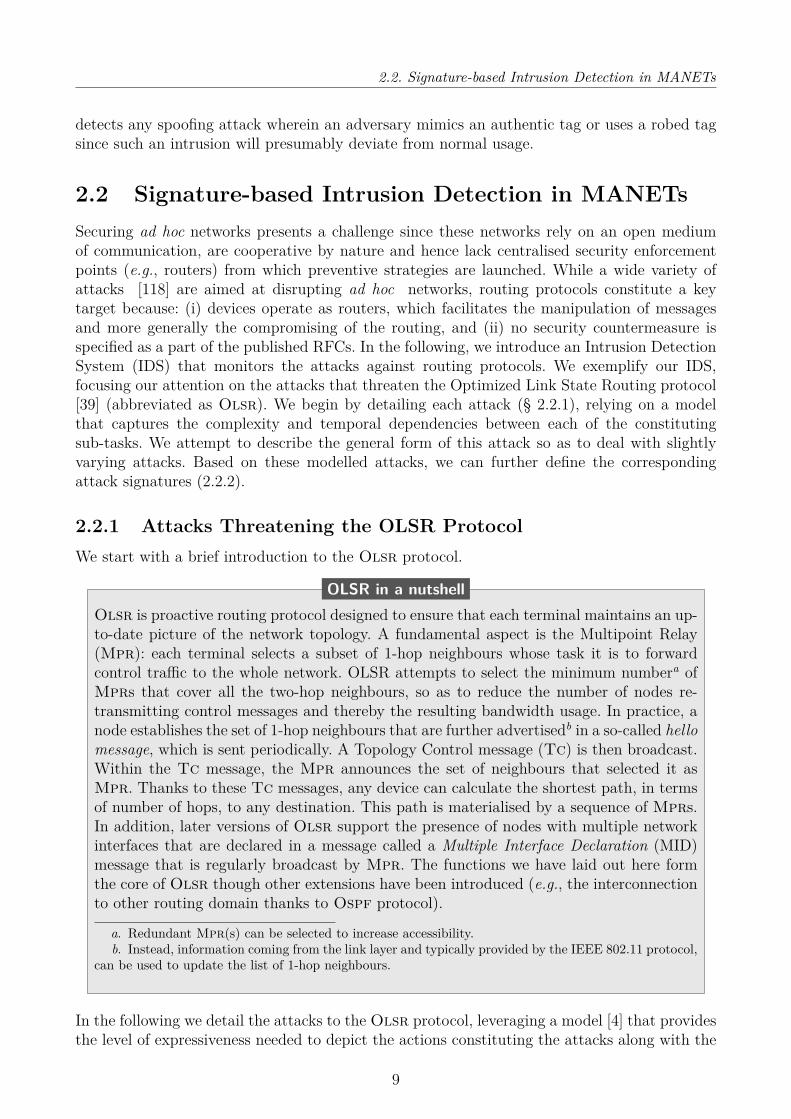
2.2.1 Attacks Threatening the OLSR ProtocolWe start with a brief introduction to the Olsr protocol.
Olsr is proactive routing protocol designed to ensure that each terminal maintains an up-to-date picture of the network topology. A fundamental aspect is the Multipoint Relay(Mpr): each terminal selects a subset of 1-hop neighbours whose task it is to forwardcontrol traffic to the whole network. OLSR attempts to select the minimum numbera ofMprs that cover all the two-hop neighbours, so as to reduce the number of nodes re-transmitting control messages and thereby the resulting bandwidth usage. In practice, anode establishes the set of 1-hop neighbours that are further advertisedb in a so-called hellomessage, which is sent periodically. A Topology Control message (Tc) is then broadcast.Within the Tc message, the Mpr announces the set of neighbours that selected it asMpr. Thanks to these Tc messages, any device can calculate the shortest path, in termsof number of hops, to any destination. This path is materialised by a sequence of Mprs.In addition, later versions of Olsr support the presence of nodes with multiple networkinterfaces that are declared in a message called a Multiple Interface Declaration (MID)message that is regularly broadcast by Mpr. The functions we have laid out here formthe core of Olsr though other extensions have been introduced (e.g., the interconnectionto other routing domain thanks to Ospf protocol).
a. Redundant Mpr(s) can be selected to increase accessibility.b. Instead, information coming from the link layer and typically provided by the IEEE 802.11 protocol,
can be used to update the list of 1-hop neighbours.
OLSR in a nutshell
In the following we detail the attacks to the Olsr protocol, leveraging a model [4] that providesthe level of expressiveness needed to depict the actions constituting the attacks along with the
9

Chapter 2 – Into the Wild - Intrusion Detection
related consequences. We further enrich the model with temporal annotations (as visible inTable 2.1). Then we categorise attacks threatening the OLSR protocol according to actionsundertaken against the following routing messages [121]:
• Drop attack: consists in dropping routing message(s).
• Active forge attack: proactively generates deceptive routing message(s).
• Modify and forward attack: modifies received routing message(s) before forwarding it.
CommunicationX
Mt←− Y At time t, Y sends a Mt←− Y At time t, Y send a message Mmessage M received by X
X 6 Mt←− X does not receive a messageM at time t
Parameters4t Time period NSX 1-hop neighbour of Xsq Sequence number hc Hop numberMPRX MPRs of X SelMPRX MPR selector for X
MessagesHello Hello message TC TC messageFM Forwarded message CM Control message
Table 2.1 – Notations
Drop attack
A Drop attack consists in suppressing a control message that should be normally1 relayed. ADrop attack is carried out by the MPRs, which forward control messages (i.e.,Tc, Mid or Hnamessages). Let us exemplify a drop attack: at time t, host H sends a control message, whichis intended to be forwarded. The message is received by an Mpr I that does not forward itduring a time period that is greater than the maximum allowed period: 4t:
IFMt←−− H, 6 FMt′←−−− I, |t′ − t| > 4t
⇓I ∈ I
(2.1)
There are few variants of drop attacks: a malicious Mpr may either delete all the incomingcontrol messages (black hole) or a portion of them (grey hole) depending on e.g., the source,the destination or the message type. Attack is detectable by comparing the rate of packetsreceived with that re-transmitted, considering each message type individually. Rather thandeleting messages, an alternative behaviour consists in modifying the routing messages prior toforwarding it.
1. Deletion shall exclude the withdraw of some packets, which are empty, expired, duplicated or badlyformatted.
10

2.2. Signature-based Intrusion Detection in MANETs
Active forge attack
An active forge attack proactively generates misleading routing messages. The best-knownexample of this kind of attack is probably the Denial Of Service attack (DOS), where a massiveamount of control messages are forged to saturate the communication medium (see Expression(2.2)). The attack is usually conducted in a distributed manner with the participation of severaldevices. The scope of a DOS is either local (i.e., targeting 1-hop neighbours) or global in whichcase messages are broadcast over multiple hops. While a local attack cannot be prevented, it isrecommended to delay and limit the forward of control messages to circumvent a global attack.
CMt←−− I,CM ′t←−− I, |t′ − t| < 5t
⇓I ∈ I
(2.2)
A DOS attack is highly visible and is hence typically conducted along with a masquerade inwhich the attacks switch their identity. The insertion of falsified messages also falls under thecategory of active forge attacks. Typically the falsification concerns the list of adjacent linksthat are advertised in hello messages. Similarly, the information about network interfaces inthe Mid and Hna messages may be modified. In the first case (Expression (2.3)), I forges ahello message, which declares a list of 1-hop and symmetric2 neighbors NS ′I that differs fromthe real set NSI .
Shello(NS′I)t←−−−−−− I,NS ′I 6= NSI
⇓I ∈ I
(2.3)
In particular, the basis of an attack aiming at falsifying the state of the links lies in:• Publishing the presence of a symmetric 1-hop node that does not actually exist (Ex-
pression (2.4)). This allows the intruder to be selected as Mpr. Indeed, if I advertisesa non-existing node N (N /∈ N , with N defining the set of nodes composing the Olsrnetwork3), I ensures that no other (well-behaving) Mpr claims being a 1-hop symmetricneighbour of N . I is hence selected as an Mpr. In addition, the connectivity of I is alsoartificially increased (Card(NS ′I\(NS ′I ∩N )) > 0).
hello(NSS)t←−−−−−−− S, Shello(NS′I)t′←−−−−−−− I, |t′ − t| < 4t,
∃N ∈ NS ′I 3: N /∈ N ∩NSI⇓
I ∈ I,∃I ′ ∈ I ∩NSS 3: I ′ ∈MPRS,
Card(NS ′I\(NS ′I ∩N )) > 0.
(2.4)
• Publishing an existing node s is a 1-hop neighbour, when it is not the case. This claimdisrupts the routing and artificially increases the connectivity of I i.e., Card((NS ′I\NSI)∩
2. A symmetric 1-hop neighbor, hereafter simply referenced as neighbor, corresponds to an adjacent nodewith which communication is bidirectional.
3. According to the Olsr RFC [39], messages can be flooded into the entire network (with a maximumnetwork diameter defined by the message Time To Live field, or flooding can be limited to nodes within adiameter (defined in terms of number of hops) from the originator of the message. For the sake of clarity, let beN represent the network in both case.
11

Chapter 2 – Into the Wild - Intrusion Detection
N ) > 0.hello(NSS)t←−−−−−−− S, S
hello(NS′I)t′←−−−−−−− I, |t′ − t| < 4t,∃X ∈ NS ′I ∩N 3: X /∈ NSI
⇓I ∈ I,
Card((NS ′I\NSI) ∩N ) > 0,@A ∈ N\I 3: A ∈ NSS ∧X ∈ NSA
⇓∃I ′ ∈ I 3: I ′ ∈MPRS.
(2.5)
If no other (well-behaving) Mpr covers S (@A ∈ N\I 3: A ∈ NSS ∧ X ∈ NSA), thenat least one misbehaving node is selected as a Mpr of S (∃I ′ ∈ I 3: I ′ ∈ MPRS). Suchinsertion typically characterises an attempt to create a blackhole: I introduces a novelpath toward M that whenever selected provisions the blackhole.
• omitting a symmetric 1-hop neighbour P as a means of isolating the latter. As a matterof fact, omitting to advertise the presence of P (∃P ∈ NSI 3: P /∈ NS ′I) artificiallydecreases the connectivity of both P and I (NSI * NS ′I).
hello(NSS)t←−−−−−−− S, Shello(NS′I)t′←−−−−−−− I, |t′ − t| < 4t,
∃P ∈ NSI 3: P /∈ NS ′I⇓
I ∈ I,∃I ′ ∈ I ∩NSS, NSI * NS ′I .
(2.6)
The falsification of the adjacency links may pervert the overall local topology, which is per-ceived by a node and may influence Mpr selection. The attack is potentially coupled witha modification of the willingness field [3]. I may prevent (resp. ensure) its selection as Mprby setting willingness field to the value will_never (resp. will_always). The Mpr selectionis altered either by falsifying the topological information or the willingness attribute. Overall,the aforementioned forge attack may contaminate the Olsr network ; interconnected routingdomains are impacted4 if a compromised gateway forge falsified routing messages. In such acase the gateway publishes some nodes or some networks that do not exist or exist but are un-reachable. In addition, the gateway may also omit to advertise some existing nodes or networks.This attack is quite similar to a link spoofing attack, which is why we will not detail it here.Another way of carrying an attack lies in altering the control messages that are disseminated.
Modify and forward attack
This attack consists in capturing a victim’s control message, modifying and then relaying it.Any packet field may be modified, including e.g., the Mpr set in TC message, the interfaceconfiguration in MID message and routing information injected in HNA message. The attackalso involves replaying the packet several times or forwarding it later (possibly to a differentlocation) so that routing tables are updated based on outdated information. Interestingly,
4. Symmetrically, false routes can be imported into the OLSR domain.
12
2.2. Signature-based Intrusion Detection in MANETs
attacks may be carried out by multiple nodes. Let us illustrate this case by considering apair of intruders (Expression 2.7).
I1CM(S)t←−−−− S, I2
CM(S)←−−−−enc
I1,CM(S)t′←−−−−− I2,
5t ≤ |t′ − t| < 4t⇓
X ∈ NSY
(2.7)
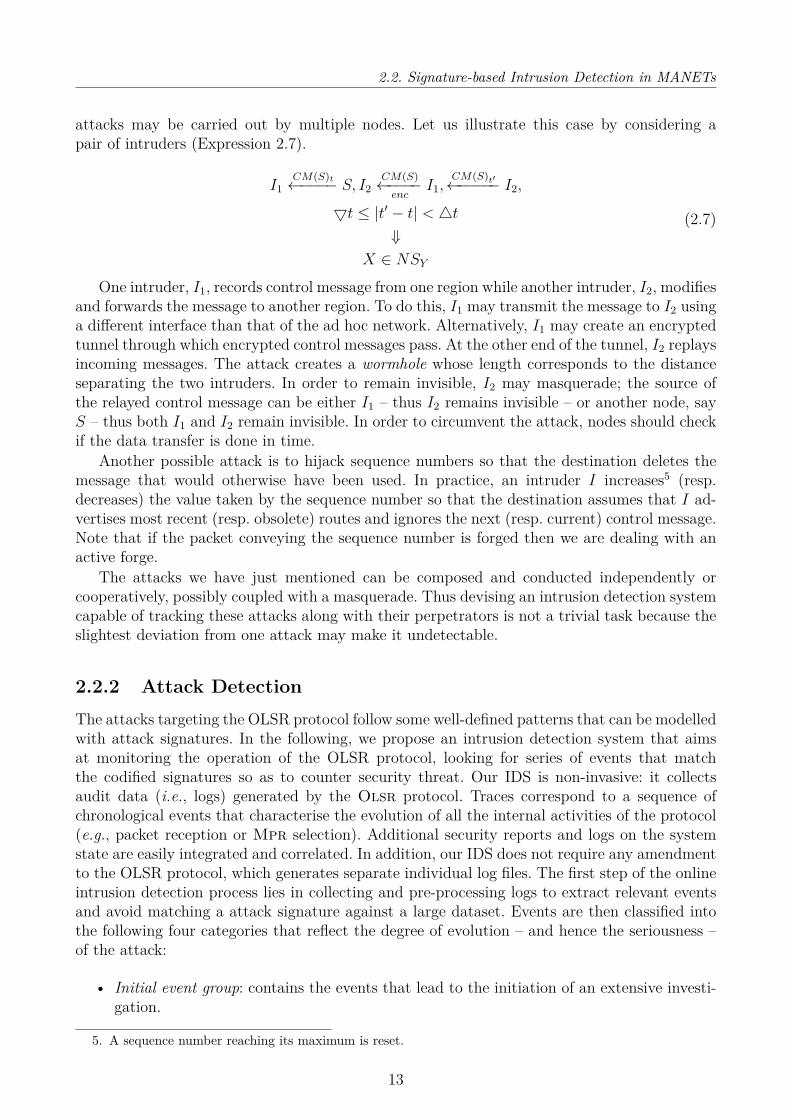
One intruder, I1, records control message from one region while another intruder, I2, modifiesand forwards the message to another region. To do this, I1 may transmit the message to I2 usinga different interface than that of the ad hoc network. Alternatively, I1 may create an encryptedtunnel through which encrypted control messages pass. At the other end of the tunnel, I2 replaysincoming messages. The attack creates a wormhole whose length corresponds to the distanceseparating the two intruders. In order to remain invisible, I2 may masquerade; the source ofthe relayed control message can be either I1 – thus I2 remains invisible – or another node, sayS – thus both I1 and I2 remain invisible. In order to circumvent the attack, nodes should checkif the data transfer is done in time.
Another possible attack is to hijack sequence numbers so that the destination deletes themessage that would otherwise have been used. In practice, an intruder I increases5 (resp.decreases) the value taken by the sequence number so that the destination assumes that I ad-vertises most recent (resp. obsolete) routes and ignores the next (resp. current) control message.Note that if the packet conveying the sequence number is forged then we are dealing with anactive forge.
The attacks we have just mentioned can be composed and conducted independently orcooperatively, possibly coupled with a masquerade. Thus devising an intrusion detection systemcapable of tracking these attacks along with their perpetrators is not a trivial task because theslightest deviation from one attack may make it undetectable.
2.2.2 Attack DetectionThe attacks targeting the OLSR protocol follow some well-defined patterns that can be modelledwith attack signatures. In the following, we propose an intrusion detection system that aimsat monitoring the operation of the OLSR protocol, looking for series of events that matchthe codified signatures so as to counter security threat. Our IDS is non-invasive: it collectsaudit data (i.e., logs) generated by the Olsr protocol. Traces correspond to a sequence ofchronological events that characterise the evolution of all the internal activities of the protocol(e.g., packet reception or Mpr selection). Additional security reports and logs on the systemstate are easily integrated and correlated. In addition, our IDS does not require any amendmentto the OLSR protocol, which generates separate individual log files. The first step of the onlineintrusion detection process lies in collecting and pre-processing logs to extract relevant eventsand avoid matching a attack signature against a large dataset. Events are then classified intothe following four categories that reflect the degree of evolution – and hence the seriousness –of the attack:
• Initial event group: contains the events that lead to the initiation of an extensive investi-gation.
5. A sequence number reaching its maximum is reset.
13
Chapter 2 – Into the Wild - Intrusion Detection
• Suspicious-evidence-group: encompasses the events leading to the qualification of a nodeas possibly malicious.
• Confirmed-evidence-group: comprises the event confirming the attack occurrence.
• Cancel-evidence-group: includes events that eliminate all suspicion.
Based on a compact set of categorised events, our signature-based IDS supports a fast patternmatching that ensures that incidents are promptly addressed. Additionally, the evolution of along term attack can be easily tracked. Once filtered and analysed, logs are matched againstpredefined intrusion signatures. A signature can be viewed as an ordered sequence of eventsthat characterises a suspicious activity. The procedure can be expensive in terms of memoryand bandwidth usage as it may require the collection of evidence from other nodes in order tocorrelate them. Thus, an investigation needs to be initiated if a sufficient degree of suspicionexists. Before delving into the operation of the above evidence groups, let us first exemplify theproposed intrusion detection system with the link spoofing attack we purposely developed.
Signature of a Link Spoofing Attack
Central to the notion of misuse detection is the definition of the attack signature. We are inter-ested in establishing the signature of an attack that tampers adjacent links. A first step towardsthat goal lies in describing the specific6 attack relying on the model introduced in [4], which weenrich with temporal annotations so as to support the expressiveness necessary to establish therelationship between actions constituting the attack and the resulting consequences. In orderto perform a link spoofing attack, an intruder, denoted I, forges a hello message, which declaresthe list of 1-hop neighbours whose link is bidirectional, denoted NS ′I and which differs fromthe correct one, denoted NSI .
Shello(NS′I)t←−−−−−− I,NS ′I 6= NSI
⇓I ∈ I
(2.8)
In order to ascertain the occurrence of such an attack, one should determine whether NS ′Idiffers from NSI . There are three variants of falsification (see §2.2.1):
1. Declaring a non-existent node as a symmetric 1-hop neighbour of I (or of another node)so that I (or another node) is selected as Mpr.
2. Claiming that an existing node as a 1-hop symmetric neighbour even though the node isdistant or is an asymmetric 1-hop neighbour.
3. Omitting a 1-hop symmetric neighbour artificially decreases the connectivity of the omit-ted node.
The detection of the link spoofing attack described above necessarily requires a continuousinvestigation that aims at confronting each node’s vision (which includes the set of 1-hop and2-hops neighbours). Unfortunately this involves a continuous confrontation and hence is notviable. We therefore take a different approach, noting that inflecting the Mpr selection is one
6. Interested reader may refer to [8] for a detailed modelling of all the attacks threatening Olsr and adescription of the related signatures.
14

2.2. Signature-based Intrusion Detection in MANETs
attack goal and thereby an attack indicator. Our approach thus consists of looking for changes(or an absence of changes) in the Mpr selection and in the Mpr coverage. As a complement, aMpr behaving inappropriately (e.g., suppressing, falsifying, failing to adequately relay controlmessages or defining itself as a Mpr without having been selected as such) is also an interestingaspect. Events (extracted from the logs) that reveal such (possibly inappropriate) behaviourare tagged as evidence announcing an attack occurrence and are categorised as an "initial eventgroup" (as defined in §2.2.2). In such a case, an in-depth investigation is triggered to collectinformation concerning the 1-hop and 2-hops neighbourhood.
Collaborative Investigation An in depth investigation consists in verifying that the Mprcoverage is adequately advertised. For this purpose, 2-hops neighbours are questioned withthe aim of determining if the suspicious Mpr is indeed a symmetric 1-hop neighbour and issusceptible of being a Mpr. The corresponding request is sent out, avoiding the suspect asmuch as possible. Based on the returned answers, the attack diagnosis takes place using thesignature described above. If all the interrogated nodes provide information that conforms tothat of the suspected Mpr, the behaviour of the Mpr is defined as appropriate. If instead oneor more nodes provide information that differs from the Mpr information, this may indicatethat an attack is taking place. Two special cases in particular may pose problems:
• Some or all of the responses are missing due to e.g., some packet collisions or somedisconnections of the queried nodes. In such a situation, the diagnosis is biased as it isonly based on a portion of the evidence.
• Answers are contradictory. For instance, a malicious node may non-legibly accuse a well-behaving Mpr or may certify the good behaviour of a malicious Mpr. A legitimate nodemay also have a different vision due to e.g., the node mobility or to slightly inconsistentrouting table.
In order to prevent misbehaving nodes from foiling the intrusion detection, we propose to evalu-ate the trustworthiness of the node(s) that provide second-hand observations (see § 2.2.3). Theobjective is to favour the observations provided by trustworthy nodes while being detrimentalto misbehaving nodes. In addition we leverage a statistical parameter, namely the confidenceinterval, to control the evidence-gathering and determine to what extent additional evidence isneeded to make an informed judgement (§ 2.2.4).
2.2.3 Trustworthiness EvaluationIn the presence of malicious nodes, supporting a reliable intrusion detection strategy is chal-lenging because attackers will try to conceal the attack by providing false observations. Whileessential, trust establishment in a distributed and resource-constraint MANET is much moredifficult than in traditional wired networks as there is no certification authorities nor trustedthird parties; as opposed to traditional centralised approaches, trust management in MANETsshould handle uncertainty and incompleteness of trust evidences.
In the years 2010, a great majority of existing work on distributed intrusion detection as-sumes that any participating node is trustworthy and faithfully reports intrusion attempts [63].Alternatively, Duma et al. [55] introduce a trust-aware engine that correlates intrusion alerts.Nonetheless, the proposed trust model does address highly distributed intrusion detection.Meanwhile, much research has been conducted on modelling and quantifying trust [87]. Trustand reputation are usually utilised to prevent packets from being routed through misbehaving
15
Chapter 2 – Into the Wild - Intrusion Detection
nodes [151, 175]. In this work, we develop a robust trust management model that specificallycopes with distributed intrusion detection. Our trust system evaluates node trustworthinessbased on personal experience and on the recommendations formulated by others. We propose adistributed and entropy-based trust system in which trust relationships are primarily built withneighbours, based on local observations and on mutually exchanged evidence. Trust is evaluateddepending on the similarities between received evidence and local evidence. Each time a nodeprovides a similar (resp. dissimilar) evidence of intrusion, its trustworthiness increases (resp.decreases). Recommendations from neighbours are also necessary to derive indirect trust values.A fundamental challenge is then to define a suitable means by which to represent trust andsynthesise the set of opinions that are provided by others into a unique aggregated value. Tothis end, we first define the notion of trust and introduce some axioms that describe the basicrules for establishing trust. Then, based on these axioms, we develop techniques to calculatetrust values.
Trust Definition
A trust relationship established between node A concerning node I, represents the extent towhich A thinks that I behaves adequately. Trust is established before a misbehaving actiontakes place and as such can be viewed as a belief, i.e., level of likelihood with which a node isexpected to perform a particular action. Trust is characterised by the following properties:
• Trust is subjective. For instance, the trust that two nodes grant to a third node maydiffer.
• Trust has a dynamic nature and usually varies over time. The trust value is a discretereal number.
• Trust is an action – and context– dependent function: an entity may be trustworthy forperforming one task (e.g., forwarding packets) but not for another one (e.g., detectingattacks).
• Trust is asymmetric and not transitive. Trust is not necessarily mutual and the fact thatA trusts B and B trusts C does not imply that A trusts C,
Building trust requires a quantitative analysis of the nodes behaviours based on the history oftheir previous activities and interactions. Thus, trust can be assessed by a measure of uncer-tainty, and as such trust values can be estimated based on entropy. In the following we introducethe rules (axioms) to follow for calculating trust values based on observations and also througha third party (concatenation propagation) and through recommendations from multiple nodes(multipath propagation).
Trust Establishment
The following five axioms are used to establish trust relationships accordingly, leverage previousinteractions and consider recommendations:
• Axiom 1 - Measuring trust based on entropy: An activity that is beneficial to others(e.g., packet relaying) increases the confidence in the node that performs it. Conversely,a malicious activity decreases this confidence. A piece of evidence that concerns a node Iand is established by a node A, is denoted eA,Ij . Such evidence contains all the observationsnecessary to evaluate the trust and calculate a value that reflects the confidence associated
16

2.2. Signature-based Intrusion Detection in MANETs
with the evidence. The confidence associated with the evidence is not absolute but theopinion of the specific node instead. In order to increase the readability of the manuscript,the trust value is referred as an evidence value. The evidence (a.k.a confidence value)takes a positive value (resp. a negative value) if the related behaviour is beneficial (resp.malicious). The trust is a real number in [-1,1]. When the trust value is -1 the node is nottrusted and if trust value is +1 the node is trusted. We define the entropy-based trustvalue as follows:
TA,I(eA,Ij ) = −eA,Ij log2(eA,Ij )− (1− eA,Ij ) log2(1− eA,Ij ) (2.9)
• Axiom 2 - Danger: the degree of danger should be taken into account when assigninga trust value. To do so, a factor αj weights the evidence eA,Ij .
• Axiom 3 - Freshness: Newer activities should be prioritised over older ones. In practice,an omission factor β privileges fresh evidences rather than older ones. A node A calculatesthe trust of a node I based on n evidence denoted eA,I1 , · · · , eA,Ii , · · · , eA,In , which concernsI and that have been collected during ∆t:
TA,I∆t =n∑j=0
αj eA,Ij + β TA,I∆t−1 (2.10)
Note that in absence of evidence, the trust value is periodically updated as follows toensure node redemption: TA,I∆t = β TA,I∆t−1
• Axiom 4: Recommendation of a third party: First-hand evidence that is obtainedby the node itself is preferred to second-hand evidences, which are comparatively morecontroversial. Nonetheless, when the observations obtained by A are not sufficient, addi-tional (less reliable) evidence provided by other nodes is gleaned (see § 2.2.4). In this caseA considers the recommendations of the third parties but the uncertainty increases. NodeA establishes the trust value associated with a node I based on the recommendation of athird party S as follows:
TsA,I∆t = RA,S∆t T
S,I∆t (2.11)
Thus node A relies on the evidence T S,I∆t provided by S. Given that node S may lie, Alowers the resulting trust value using RA,S
∆t .Note that the computation of the trust value (Eq. 2.11) reflects the probability that I willperform an attack. Let pS denote the probability that S makes a correct recommendationand pI/B=0 the probability that I will perform an attack if B lies. This probability canbe expressed as :
pASI = pS pI/S=1 + (1− pS) pI/S=1 (2.12)
Unfortunately A ignores the value of pS and pI/S=1. Leveraging our distributed trustmodel, A evaluates the probability p(AS) that A observes the behaviour of S and Amakes a recommendation on S. In addition, A estimates p(SI) the probability that Sobserves the behaviour of I and that S makes a correct recommendation on S. Finally,A computes the value of pASI :
pASI = p(AS) p(SI) + (1− p(AS)) (1− p(SI)) (2.13)
• Axiom 5- Concatenating multiple recommendations: The recommendations of
17

Chapter 2 – Into the Wild - Intrusion Detection
several nodes may be considered together in order to establish a trust value. Recommen-dations are concatenated into a trust value that should not be artificially amplified. Thus,when several nodes, denoted S1, S2, · · · , Sm, generate recommendations, A computes anaggregated trustworthiness about I as follows:
TmA,I∆t =
m∑i=1
wiRA,Si∆t T
Si,I∆t (2.14)
with wi = 1∑m
j=0 R∆tA,Sj
serving as an averaging factor. Once established, trust is then usedto prevent malicious nodes from interfering with intrusion detection.
Trust Establishment in the presence of a link spoofing attack
In the following, we detail the computation of the trust value considering a link spoofing attack:In order for Node A to establish whether I is carrying a link spoofing attack A interrogates theneighbours of the suspected node I. The interrogated neighbours either do or do not corroboratethe information provided by the suspect, in which case the answer includes the fields rSi,I thateither takes the value 1, if the link established by I is correct, or the value −1 otherwise. Theanswers from each interrogated neighbour Si (with i ∈ [1,m]) are weighted with the trustlevel TA,Si that the investigator A places in the neighbour Si as well as taking into account aweighting factor wi:
DetectA,I∆t =m∑i=1
wiTA,SiRSi,Ii (2.15)
with wi = 1∑m
j=0 TA,Sj. Ultimately, a fake link attack is detected if DetectA,I∆t is close to 1.
2.2.4 Reducing the Cost of InvestigationsIntrusion detection is a resource-consuming process that needs to last because an attack againsta routing protocol is typically persistent and continuous (i.e., attack repeats itself over time).Thus intrusion detection leads to the collection of a massive amount of logs and evidence.In a dense network, the number of collected evidence becomes colossal. In order to reducethe corresponding bandwidth usage and thereby lighten the intrusion detection process, wepropose to randomly and uniformly request the nearby nodes into collaborative investigation(i.e., the 2 hop neighbours of the Mpr). As a result, fewer nodes are less frequently contactedcompared to the deterministic approach introduced above. We employ confidence interval andconfidence level as means for regulating (either reducing or increasing) the evidence-gatheringwhile ensuring a satisfactory level of detection reliability.
Confidence interval and confidence level
The confidence interval represents a statistical uncertainty associated with the estimation of apopulation parameter (e.g., proportion, mean, median) [156]. The confidence interval is associ-ated with confidence level, which corresponds to the likelihood that the true parameter belongsto the interval.
In our case, based on a partial set of evidence, denoted e1, · · · , en, we establish an interval inwhich the mean, computed using the entire set of evidence, has a high probability of belongingto. In practice, based on a confidence level fixed by the investigator, the true mean m hasa certain probability of being contained in the confidence interval [me − ε, me + ε] with ε
18

2.3. Anomaly Detection
reflecting the allowed margin of error that is defined by the end user. The sampling error εdecreases as the sample size increases. According to the central limit theorem introduced byPierre Simon Laplace [135], the sampling distribution of the mean follows a t-distribution [157]when the sample size is small and a normal distribution when the sample size becomes large[11], regardless of the population form. With a normal distribution, the margin of error ε isexpressed as a function of the standard deviation σ and the standard density z:
ε = zσ√n
(2.16)
With a t-distribution, the margin of error ε is expressed as a function of the standard deviationσ and the standard density z:
ε = zσ√df
(2.17)
with df corresponding to the degree of freedom. Note that there are many potential t distribu-tions, whose forms are determined by their degrees of freedom. Nonetheless, when estimatingthe mean, df = n− 1. The standard deviation is then calculated as follows:
σ =
√√√√∑ni=0(m− eA,Sii )2
n− 1 (2.18)
The overall estimation of the confidence interval of a population mean proceeds as follows:
• Gather a few pieces evidence (a.k.a samples).
• Compute the sample mean and standard deviations.
• If the sample size is large (resp. small), select the zα/2 (resp. tα/2) from the normaldistribution (resp. the t-distribution),
• Compute the sampling error ε and the confidence interval as [me − ε, me + ε].
The computation of the confidence level and interval during the diagnostic permits our Ids to:(i) regulate the number of gathered and processed evidences while maintaining the requireddetection accuracy and (ii) measure to what extent the diagnosis is reliable, especially in thepresence of inconsistent evidences.
At best, the confidence level is high and the confidence interval is narrow. If an attack7
is taking place, evidence will be collected with less but sufficient regularity. In practice, theIDS follows a stepwise process that reduces the volume of evidences to collect. Instead, if theconfidence level is low and the confidence interval is wide, additional evidence should be col-lected to establish a representative diagnostic. Note that collecting more evidences convenientlyincreases the confidence level but not necessarily narrow the confidence interval: a controversyis established but cannot be prevented.
2.3 Anomaly DetectionWe propose an anomaly detection, whose aim is to find any behaviour that does not conform tothe expected behaviour. We begin by modelling the normal behaviour of the target and definean anomaly as any observed behaviour that does not conform the the normal/baseline model. A
7. In absence of detected attack, investigation ends.
19
Chapter 2 – Into the Wild - Intrusion Detection
key challenge to searching for an anomaly lies in identifying which data are dissimilar to the restof the data set, since an individual piece of data can be considered as anomalous with respectto the the larger whole. As an illustration, an anomaly may refer to credit card transactioncharacterised by a very high amount of expense compared to the usual range of expenditure. Acontextual anomaly corresponds to a data instance that is anomalous only in a specific context.A collective anomaly comprises a collection of instances; the individual instances are not bythemselves defined as anomalies but their concomitant occurrences, as a collection, is abnormal.A Denial Of Service illustrates such an anomaly: individual events are not anomalies when theyoccur sporadically over a large time frame.
In order to detect individual, context-dependant and collective anomalies, we investigatethe feasibility of applying machine learning techniques and in particular unsupervised learning,considering an application that controls the access of users [138, 126]. To this ends, users areprovided active RFID tags which are used to monitor the user’s location. Given this specificuse case, anomalies are primarily detected based on spatial-temporal features rather than oper-ational ones. Rather than relying on a simple statistical method, we select an advanced neuralnetwork architecture permitting the construction of the user’s profile automatically i.e., with-out involving users or experts. Note that such automatic training permits the easy additionof (operational) features without modifying the core implementation. Based on an advancedKohonen’s map, our detection system detects any spoofing/cloning attack wherein an adversarymimics an authentic tag and any usage of a robed tag since these intrusions, by assumption,will deviate from normal user’s normal activity.
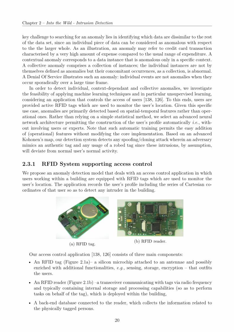
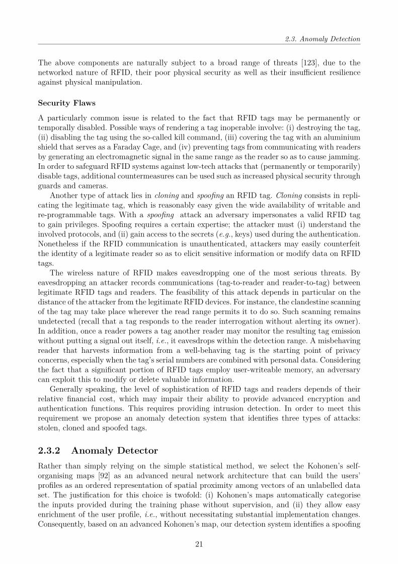
2.3.1 RFID System supporting access controlWe propose an anomaly detection model that deals with an access control application in whichusers working within a building are equipped with RFID tags which are used to monitor theuser’s location. The application records the user’s profile including the series of Cartesian co-ordinates of that user so as to detect any intruder in the building.
(a) RFID tag. (b) RFID reader.
Our access control application [138, 126] consists of three main components:• An RFID tag (Figure 2.1a)– a silicon microchip attached to an antennae and possibly
enriched with additional functionalities, e.g., sensing, storage, encryption – that outfitsthe users.
• An RFID reader (Figure 2.1b) –a transceiver communicating with tags via radio frequencyand typically containing internal storage and processing capabilities (so as to performtasks on behalf of the tag), which is deployed within the building,
• A back-end database connected to the reader, which collects the information related tothe physically tagged persons.
20
2.3. Anomaly Detection
The above components are naturally subject to a broad range of threats [123], due to thenetworked nature of RFID, their poor physical security as well as their insufficient resilienceagainst physical manipulation.
Security Flaws
A particularly common issue is related to the fact that RFID tags may be permanently ortemporally disabled. Possible ways of rendering a tag inoperable involve: (i) destroying the tag,(ii) disabling the tag using the so-called kill command, (iii) covering the tag with an aluminiumshield that serves as a Faraday Cage, and (iv) preventing tags from communicating with readersby generating an electromagnetic signal in the same range as the reader so as to cause jamming.In order to safeguard RFID systems against low-tech attacks that (permanently or temporarily)disable tags, additional countermeasures can be used such as increased physical security throughguards and cameras.
Another type of attack lies in cloning and spoofing an RFID tag. Cloning consists in repli-cating the legitimate tag, which is reasonably easy given the wide availability of writable andre-programmable tags. With a spoofing attack an adversary impersonates a valid RFID tagto gain privileges. Spoofing requires a certain expertise; the attacker must (i) understand theinvolved protocols, and (ii) gain access to the secrets (e.g., keys) used during the authentication.Nonetheless if the RFID communication is unauthenticated, attackers may easily counterfeitthe identity of a legitimate reader so as to elicit sensitive information or modify data on RFIDtags.
The wireless nature of RFID makes eavesdropping one of the most serious threats. Byeavesdropping an attacker records communications (tag-to-reader and reader-to-tag) betweenlegitimate RFID tags and readers. The feasibility of this attack depends in particular on thedistance of the attacker from the legitimate RFID devices. For instance, the clandestine scanningof the tag may take place wherever the read range permits it to do so. Such scanning remainsundetected (recall that a tag responds to the reader interrogation without alerting its owner).In addition, once a reader powers a tag another reader may monitor the resulting tag emissionwithout putting a signal out itself, i.e., it eavesdrops within the detection range. A misbehavingreader that harvests information from a well-behaving tag is the starting point of privacyconcerns, especially when the tag’s serial numbers are combined with personal data. Consideringthe fact that a significant portion of RFID tags employ user-writeable memory, an adversarycan exploit this to modify or delete valuable information.
Generally speaking, the level of sophistication of RFID tags and readers depends of theirrelative financial cost, which may impair their ability to provide advanced encryption andauthentication functions. This requires providing intrusion detection. In order to meet thisrequirement we propose an anomaly detection system that identifies three types of attacks:stolen, cloned and spoofed tags.
2.3.2 Anomaly DetectorRather than simply relying on the simple statistical method, we select the Kohonen’s self-organising maps [92] as an advanced neural network architecture that can build the users’profiles as an ordered representation of spatial proximity among vectors of an unlabelled dataset. The justification for this choice is twofold: (i) Kohonen’s maps automatically categorisethe inputs provided during the training phase without supervision, and (ii) they allow easyenrichment of the user profile, i.e., without necessitating substantial implementation changes.Consequently, based on an advanced Kohonen’s map, our detection system identifies a spoofing
21
Chapter 2 – Into the Wild - Intrusion Detection
attack wherein an adversary mimics an authentic tag and any usage of a robed tag becausethese intrusions, by assumption, deviate from the normal usage of the users.
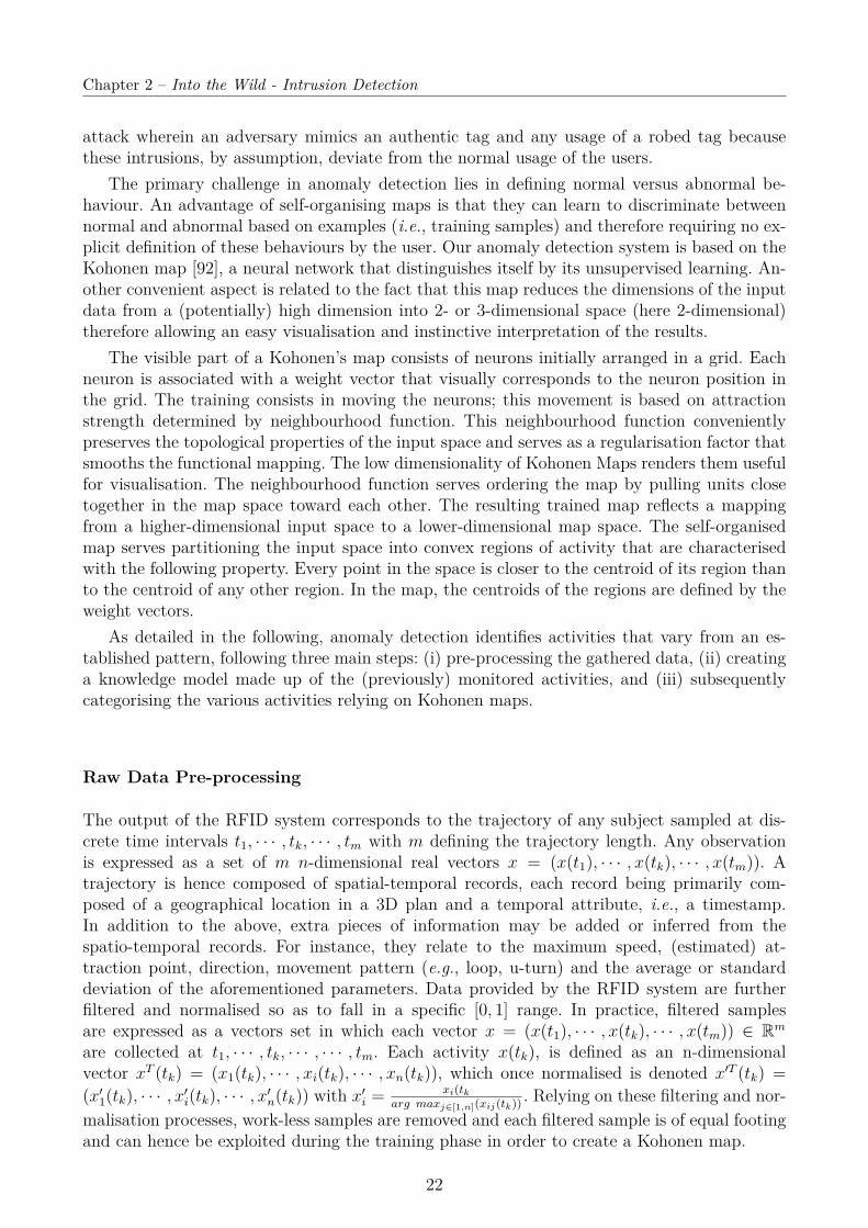
The primary challenge in anomaly detection lies in defining normal versus abnormal be-haviour. An advantage of self-organising maps is that they can learn to discriminate betweennormal and abnormal based on examples (i.e., training samples) and therefore requiring no ex-plicit definition of these behaviours by the user. Our anomaly detection system is based on theKohonen map [92], a neural network that distinguishes itself by its unsupervised learning. An-other convenient aspect is related to the fact that this map reduces the dimensions of the inputdata from a (potentially) high dimension into 2- or 3-dimensional space (here 2-dimensional)therefore allowing an easy visualisation and instinctive interpretation of the results.
The visible part of a Kohonen’s map consists of neurons initially arranged in a grid. Eachneuron is associated with a weight vector that visually corresponds to the neuron position inthe grid. The training consists in moving the neurons; this movement is based on attractionstrength determined by neighbourhood function. This neighbourhood function convenientlypreserves the topological properties of the input space and serves as a regularisation factor thatsmooths the functional mapping. The low dimensionality of Kohonen Maps renders them usefulfor visualisation. The neighbourhood function serves ordering the map by pulling units closetogether in the map space toward each other. The resulting trained map reflects a mappingfrom a higher-dimensional input space to a lower-dimensional map space. The self-organisedmap serves partitioning the input space into convex regions of activity that are characterisedwith the following property. Every point in the space is closer to the centroid of its region thanto the centroid of any other region. In the map, the centroids of the regions are defined by theweight vectors.
As detailed in the following, anomaly detection identifies activities that vary from an es-tablished pattern, following three main steps: (i) pre-processing the gathered data, (ii) creatinga knowledge model made up of the (previously) monitored activities, and (iii) subsequentlycategorising the various activities relying on Kohonen maps.
Raw Data Pre-processing
The output of the RFID system corresponds to the trajectory of any subject sampled at dis-crete time intervals t1, · · · , tk, · · · , tm with m defining the trajectory length. Any observationis expressed as a set of m n-dimensional real vectors x = (x(t1), · · · , x(tk), · · · , x(tm)). Atrajectory is hence composed of spatial-temporal records, each record being primarily com-posed of a geographical location in a 3D plan and a temporal attribute, i.e., a timestamp.In addition to the above, extra pieces of information may be added or inferred from thespatio-temporal records. For instance, they relate to the maximum speed, (estimated) at-traction point, direction, movement pattern (e.g., loop, u-turn) and the average or standarddeviation of the aforementioned parameters. Data provided by the RFID system are furtherfiltered and normalised so as to fall in a specific [0, 1] range. In practice, filtered samplesare expressed as a vectors set in which each vector x = (x(t1), · · · , x(tk), · · · , x(tm)) ∈ Rm
are collected at t1, · · · , tk, · · · , · · · , tm. Each activity x(tk), is defined as an n-dimensionalvector xT (tk) = (x1(tk), · · · , xi(tk), · · · , xn(tk)), which once normalised is denoted x′T (tk) =(x′1(tk), · · · , x′i(tk), · · · , x′n(tk)) with x′i = xi(tk
arg maxj∈[1,n](xij(tk)) . Relying on these filtering and nor-malisation processes, work-less samples are removed and each filtered sample is of equal footingand can hence be exploited during the training phase in order to create a Kohonen map.
22
2.3. Anomaly Detection
Training phase
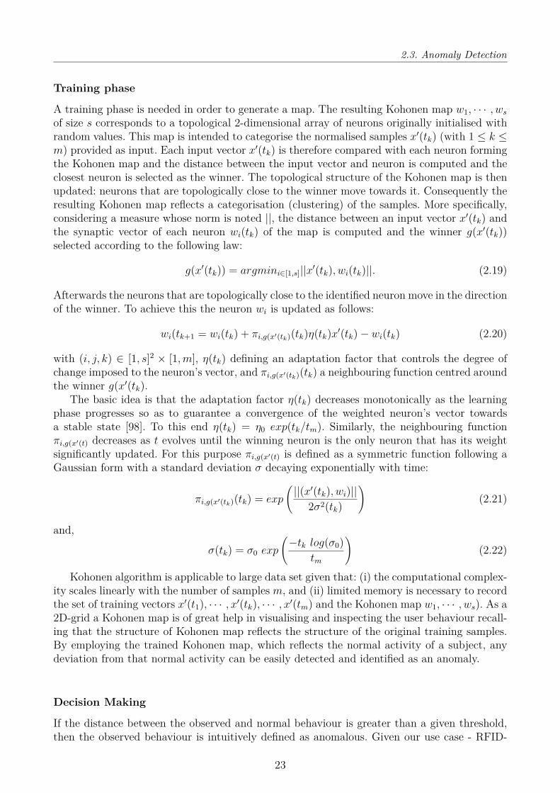
A training phase is needed in order to generate a map. The resulting Kohonen map w1, · · · , wsof size s corresponds to a topological 2-dimensional array of neurons originally initialised withrandom values. This map is intended to categorise the normalised samples x′(tk) (with 1 ≤ k ≤m) provided as input. Each input vector x′(tk) is therefore compared with each neuron formingthe Kohonen map and the distance between the input vector and neuron is computed and theclosest neuron is selected as the winner. The topological structure of the Kohonen map is thenupdated: neurons that are topologically close to the winner move towards it. Consequently theresulting Kohonen map reflects a categorisation (clustering) of the samples. More specifically,considering a measure whose norm is noted ||, the distance between an input vector x′(tk) andthe synaptic vector of each neuron wi(tk) of the map is computed and the winner g(x′(tk))selected according to the following law:
g(x′(tk)) = argmini∈[1,s]||x′(tk), wi(tk)||. (2.19)
Afterwards the neurons that are topologically close to the identified neuron move in the directionof the winner. To achieve this the neuron wi is updated as follows:
wi(tk+1 = wi(tk) + πi,g(x′(tk)(tk)η(tk)x′(tk)− wi(tk) (2.20)
with (i, j, k) ∈ [1, s]2 × [1,m], η(tk) defining an adaptation factor that controls the degree ofchange imposed to the neuron’s vector, and πi,g(x′(tk)(tk) a neighbouring function centred aroundthe winner g(x′(tk).
The basic idea is that the adaptation factor η(tk) decreases monotonically as the learningphase progresses so as to guarantee a convergence of the weighted neuron’s vector towardsa stable state [98]. To this end η(tk) = η0 exp(tk/tm). Similarly, the neighbouring functionπi,g(x′(t) decreases as t evolves until the winning neuron is the only neuron that has its weightsignificantly updated. For this purpose πi,g(x′(t) is defined as a symmetric function following aGaussian form with a standard deviation σ decaying exponentially with time:
πi,g(x′(tk)(tk) = exp
(||(x′(tk), wi)||
2σ2(tk)
)(2.21)
and,
σ(tk) = σ0 exp
(−tk log(σ0)
tm
)(2.22)
Kohonen algorithm is applicable to large data set given that: (i) the computational complex-ity scales linearly with the number of samples m, and (ii) limited memory is necessary to recordthe set of training vectors x′(t1), · · · , x′(tk), · · · , x′(tm) and the Kohonen map w1, · · · , ws). As a2D-grid a Kohonen map is of great help in visualising and inspecting the user behaviour recall-ing that the structure of Kohonen map reflects the structure of the original training samples.By employing the trained Kohonen map, which reflects the normal activity of a subject, anydeviation from that normal activity can be easily detected and identified as an anomaly.
Decision Making
If the distance between the observed and normal behaviour is greater than a given threshold,then the observed behaviour is intuitively defined as anomalous. Given our use case - RFID-
23
Chapter 2 – Into the Wild - Intrusion Detection
enabled control access system attempting to analyse the user location - we distinguish twosources of potential anomalies: the user’s position and its trajectory. A position is said to beanomalous if it does not belong to any of the classification defined during the training, i.e., ifit does not pertain to any of the clusters centred on the wining neurons defined as part of thetraining phase. By extension we define a trajectory as anomalous if a large percentage of theuser’s positions are anomalous, i.e., if the pre-processed observations do not pertain to any ofthe clusters centred around the winning neurons g(x′(tk)) and delimited by the radius definedas the maximum distance separating the winning node g(x′(tk)) from its neighbouring neurons(i.e., the neurons that belong to Dg(x′(tk))). By extension, a trajectory o′(t), · · · , o′(t + p) isanomalous if the ratio of anomalous positions exceeds a given threshold defined by β(r).
The computational complexity related to detecting a position and then its trajectory scaleslinearly to the number of winning vectors g(x′(tk)) (bounded by m). In addition to the memoryallocated to the training phase, little additional memory (essentially just the index i of thewinning neurons and their established radii) is used during the anomaly detection.
Identifying trajectories that exhibit irregular or even suspicious traits is crucial in manyapplications including access control and intrusion detection. In such scenarios, unsupervisedlearning is the most advantageous model when learning from many regular data instances,as the algorithm thoroughly approximates the underlying distribution and produces a concisemodel of normality. As a consequence, unsupervised learning method are often used to detectanomalies.
2.4 Performance EvaluationIn the following section we evaluate performances associated with the intrusion detection system(§ 2.4.1) and the trust system (§ 2.4.2).
2.4.1 Signature-based Intrusion DetectionIn order to evaluate the performance of our intrusion detection system (§2.2) we simulate amobile ad hoc network using the Ns3 network simulator8 [133] and we virtualise each deviceusing Lxc9 [23]. The MANET area is defined by a squared area of S = 310 × 310 m2 andis comprised of N = 30 devices split into 25 well-behaving devices and 5 intruders, the latterof whom repeatedly launch the implemented link spoofing attack10. Devices move randomly,following a randomly chosen direction, at a given speed that is the same for all the devices.When a device hits the network boundaries it rebounds following a reflexive angle. Nodes usethe Olsr protocol, communicating via Ieee 802.11a with transmissions that have a range of90m. Data traffic is further simulated using the V4PingHelper application of NS3; the nodesexchanges 56 bytes Icmp echo requests to one another and wait for 1s before sending it again.
During our experiments we evaluate the performance of our IDS in terms of:
• The number of intrusions that are successfully detected.
• The number of false positives that occur when a legitimate node is wrongly designatedas an intruder.
8. http://www.nsnam.org9. http://lxc.sourceforge.net
10. In our experiments, the number of successful intrusions varies between 15 and 33, according the specificityof the simulated network.
24

2.4. Performance Evaluation
0
20
40
60
80
100
6 8 10 12 14 16
Pe
rce
nta
ge
of
De
tecte
d I
ntr
usio
ns (
%)
Density (average number of neighbors)
Percentage of DetectionAverage of Detection
(a) Detection accuracy.
0
10
20
30
40
50
6 8 10 12 14 16
Pe
rce
nta
ge
of
Fa
lse
Po
sitiv
e (
%)
Density (average number of neighbors)
Percentage of False PositiveAverage of False Positive
(b) False positive rate.
0
10
20
30
40
50
6 8 10 12 14 16
Ave
rag
e in
cre
me
nt
in m
em
ory
usa
ge
(M
B)
Density (average number of neighbors)
(c) Memory usage.
0.25
0.5
1
5
20
50
100
6 8 10 12 14 16
Pe
rce
nta
ge
of
IDA
R T
raff
ic t
o O
LS
R T
raff
ic(%
)
Density (average number of neighbors)
(d) Bandwidth usage.
Figure 2.2 – Performances of our intrusion detection system depending on the Network Density.
• Detection overhead, referring to the memory usage and network traffic that are generatedby our IDS.
Using these performance criteria, we consider the impacts of the network density (Figure 2.2)and the device mobility (Figure 2.3). The network density corresponds to the average numberof neighbours, which is defined in [75] as N×π×T 2
x
S.
Impact of the density
At first glance, the rate of intrusions that are detected is conveniently high (Figure 2.2-a)and the false positive rate remains low (Figure 2.2-b). Specifically, the detection rate increasesslightly from 93.5% to a maximum of 96.3% when the density varies from 6 to 8 neighboursbecause the attack is seen by a larger number of neighbours. Then a slow decrease is observedwhen density is above 8. The decline is caused by a higher number of collisions that partiallyprevent the collection of evidence and slows down intrusion detection. Still the detection ratealways remains greater than 80%. As visible in Figure 2.2-b, the percentage of false positivesis on average always under 5.9%. Further analysis reveal that many false positives occur dueto the lack of synchronisation among nodes: some links are valid (i.e., existing) for some nodesand expired (i.e., absent) for others. To address this problem, the period during which linksare considered valid should be slightly lengthened, as in [164]. While memory usage (Figure2.2-c) gently fluctuates between 17.6MB and 22.2MB, the traffic generated by our intrusion
25

Chapter 2 – Into the Wild - Intrusion Detection
detection system (Figure 2.2-d) is almost negligible. Overall, there is clearly a good trade-offbetween detection accuracy and resource consumption (i.e., computing and bandwidth usage)associated with the distributed detection. When the density is high, our intrusion detectionsystem is confronted with a typical limitation of a constrained network: the traffic volume –most of which stems from the routing protocol and the application – is too high and cannotbe supported by the network. In this situation, MANET can no longer fulfil its mission andintrusions are hardly discerned.
0
20
40
60
80
100
0 2 4 6 8
Pe
rce
nta
ge
of
De
tecte
d I
ntr
usio
ns (
%)
Velocity (m/s)
Percentage of DetectionAverage of Detection
(a) Detection accuracy.
0
10
20
30
40
50
0 2 4 6 8
Pe
rce
nta
ge
of
Fa
lse
PO
sitiv
e (
%)
Velocity (m/s)
Percentage of False PositiveAverage of False Positive
(b) False positive rate.
0
10
20
30
40
50
0 2 4 6 8
Ave
rag
e in
cre
me
nt
in m
em
ory
usa
ge
(M
B)
Velocity (m/s)
(c) Memory usage.
0.25
0.5
1
5
20
50
100
0 2 4 6 8
Pe
rce
nta
ge
of
IDA
R T
raff
ic t
o O
LS
R T
raff
ic(%
)
Velocity (m/s)
(d) Overload.
Figure 2.3 – Performance associated with our intrusion detection System, considering a varyingMobility given a network density of 8 neighbours.
Impact of mobility
From the standpoint of intrusion detection, mobility is the biggest challenge. When node mo-bility increases, the intrusion detection rate decreases (Figure 2.3-a) and false positive rate(Figure (2.3-b) falls due to the constantly changing topology. However a high detection rateremains (e.g., about 70.7% with a moving speed of 8m/s, i.e., around 28.7 kilometers/hourequivalent to 17.89 miles/hour). The memory usage (Figure 2.3-c) rises steadily from 17.6MBto 26.5MB, which is a reasonable figure even for resource-limited devices. Traffic remains verylow compared to the Olsr. Overall, our evaluation shows that the intrusion detection systemis characterised by a high detection rate and a low false positive rate even under harsh con-ditions. While the traffic overhead is negligible compared to OLSR, the fairly small memoryusage means that the intrusion detection can be undertaken by resource-limited devices.
26
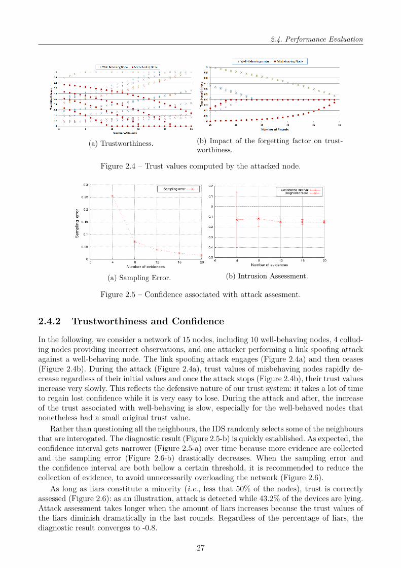
2.4. Performance Evaluation
(a) Trustworthiness. (b) Impact of the forgetting factor on trust-worthiness.
Figure 2.4 – Trust values computed by the attacked node.
(a) Sampling Error. (b) Intrusion Assessment.
Figure 2.5 – Confidence associated with attack assesment.
2.4.2 Trustworthiness and Confidence
In the following, we consider a network of 15 nodes, including 10 well-behaving nodes, 4 collud-ing nodes providing incorrect observations, and one attacker performing a link spoofing attackagainst a well-behaving node. The link spoofing attack engages (Figure 2.4a) and then ceases(Figure 2.4b). During the attack (Figure 2.4a), trust values of misbehaving nodes rapidly de-crease regardless of their initial values and once the attack stops (Figure 2.4b), their trust valuesincrease very slowly. This reflects the defensive nature of our trust system: it takes a lot of timeto regain lost confidence while it is very easy to lose. During the attack and after, the increaseof the trust associated with well-behaving is slow, especially for the well-behaved nodes thatnonetheless had a small original trust value.
Rather than questioning all the neighbours, the IDS randomly selects some of the neighboursthat are interogated. The diagnostic result (Figure 2.5-b) is quickly established. As expected, theconfidence interval gets narrower (Figure 2.5-a) over time because more evidence are collectedand the sampling error (Figure 2.6-b) drastically decreases. When the sampling error andthe confidence interval are both bellow a certain threshold, it is recommended to reduce thecollection of evidence, to avoid unnecessarily overloading the network (Figure 2.6).
As long as liars constitute a minority (i.e., less that 50% of the nodes), trust is correctlyassessed (Figure 2.6): as an illustration, attack is detected while 43.2% of the devices are lying.Attack assessment takes longer when the amount of liars increases because the trust values ofthe liars diminish dramatically in the last rounds. Regardless of the percentage of liars, thediagnostic result converges to -0.8.
27
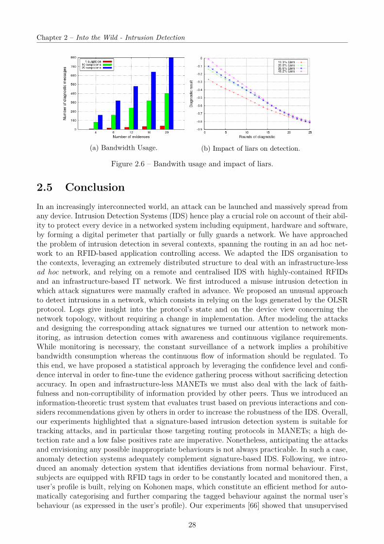
Chapter 2 – Into the Wild - Intrusion Detection
(a) Bandwidth Usage. (b) Impact of liars on detection.
Figure 2.6 – Bandwith usage and impact of liars.
2.5 ConclusionIn an increasingly interconnected world, an attack can be launched and massively spread fromany device. Intrusion Detection Systems (IDS) hence play a crucial role on account of their abil-ity to protect every device in a networked system including equipment, hardware and software,by forming a digital perimeter that partially or fully guards a network. We have approachedthe problem of intrusion detection in several contexts, spanning the routing in an ad hoc net-work to an RFID-based application controlling access. We adapted the IDS organisation tothe contexts, leveraging an extremely distributed structure to deal with an infrastructure-lessad hoc network, and relying on a remote and centralised IDS with highly-contained RFIDsand an infrastructure-based IT network. We first introduced a misuse intrusion detection inwhich attack signatures were manually crafted in advance. We proposed an unusual approachto detect intrusions in a network, which consists in relying on the logs generated by the OLSRprotocol. Logs give insight into the protocol’s state and on the device view concerning thenetwork topology, without requiring a change in implementation. After modeling the attacksand designing the corresponding attack signatures we turned our attention to network mon-itoring, as intrusion detection comes with awareness and continuous vigilance requirements.While monitoring is necessary, the constant surveillance of a network implies a prohibitivebandwidth consumption whereas the continuous flow of information should be regulated. Tothis end, we have proposed a statistical approach by leveraging the confidence level and confi-dence interval in order to fine-tune the evidence gathering process without sacrificing detectionaccuracy. In open and infrastructure-less MANETs we must also deal with the lack of faith-fulness and non-corruptibility of information provided by other peers. Thus we introduced aninformation-theoretic trust system that evaluates trust based on previous interactions and con-siders recommendations given by others in order to increase the robustness of the IDS. Overall,our experiments highlighted that a signature-based intrusion detection system is suitable fortracking attacks, and in particular those targeting routing protocols in MANETs; a high de-tection rate and a low false positives rate are imperative. Nonetheless, anticipating the attacksand envisioning any possible inappropriate behaviours is not always practicable. In such a case,anomaly detection systems adequately complement signature-based IDS. Following, we intro-duced an anomaly detection system that identifies deviations from normal behaviour. First,subjects are equipped with RFID tags in order to be constantly located and monitored then, auser’s profile is built, relying on Kohonen maps, which constitute an efficient method for auto-matically categorising and further comparing the tagged behaviour against the normal user’sbehaviour (as expressed in the user’s profile). Our experiments [66] showed that unsupervised
28

2.5. Conclusion
machine learning used in combination with the functionality of an IDS forms a robust defenceagainst possible attacks by predicting them based on past events. Even a simple Kohonen map,trained based on normal data, detects anomalous features that the system is exposed to. Inthe course of our research we observed that Kohonen maps may deal with multiple users. Morefeatures could easily be integrated leveraging vectorisation techniques. As long as the intrusioncontaminates only a fraction of the training set and generates sufficiently distinct vectors, amap remains dominated by normal activity.
29


Chapter 3
Enhancing the Observation Qualitythrough Calibration
3.1 Introduction
In the light of the ever expanding importance of IoT, a noticeable trend is to promote theadoption of IoT technologies, to support the sustainable development of urban spaces, thusrealising the so-called vision of smart spaces and smart cities. In particular, IoT technologiescontribute to the improvement of the services the city delivers and thereby respond to a numberof environmental challenges generated by the city itself (e.g., pollution) or caused by naturalphenomena (e.g., global warming). With this in prospect, various research projects, includingthose in which I was involved in [1, 64, 144], primarily rely on IoT infrastructures to manageand optimise some services, the oversight of public spaces (e.g., campus, building, parking),environmental and pollution monitoring, surveillance for disaster preparedness and efficientfirst responses,as well as the preservation of cultural heritage. The delivering of problem-solvingservices requires the joint effort and engagement of a wide range of persons, communities,organisations and stakeholders. This also demands a(n) (r)evolution of the relationship betweenthe participants. These needs led to the development of the crowdsensing movement whereinusers (citizens, groups, communities) engage in some collaborative data collection, analysis anddecision making. In practice, citizens rely on the small and low-cost sensors embedded in –orconnected to– their smartphones so as to e.g., help identifying environmental problems, alertabout an imminent danger, collaboratively monitor road traffic, or trace the evolution of anepidemic.
Together, IoT-based sensing and mobile crowdsensing gather some observations at a finegrain, based on the fixed things of the urban infrastructure and on the mobile devices thatpeople carry. On the one hand, stationary sensors (e.g., weather stations, cameras) relay their(a priori) high-quality measurements to data sinks that redirect the resulting traffic towards thecloud (e.g., a back-end server typically owned by some public organisations) – this is the typicalsetting involving a secured wireless sensor network connected to a wired infrastructure. On theother hand, mobile smartphones opportunistically publish their data to a (crowdsensing) serveraccording to the connectivity allowed by their data plan. Leveraging both (mobile) individually-owned and (primarily fixed) organisation-owned sensors, smart cities may henceforth overseea physical phenomenon at a large-scale. The resulting breed of multi-purpose applications(w.r.t apps), has shifted and keeps shifting the urban areas towards environmental, social andsustainable paths.
Nonetheless, such a vision comes with a fair share of challenges. The financial cost associatedto the maintenance of the IoT infrastructure is high; limited budgets lead to a partial instru-mentation of the public space. The spatio-temporal coverage problem is typically addressed byleveraging mobile crowdsensors that conveniently fill the gap thanks to the mobility of the par-ticipants. Morever, leveraging crowdsensing is a double-edged sword as crowdsensing is highly
31

Chapter 3 – Enhancing the Observation Quality through Calibration
constrained by the choice of the sensing hardware: off-the-shelf sensors/actuators outfit or areconnected to the smartphones. In respect to this, the prevalence of low-cost and multi-purposecrowdsensing platforms conducts to discrepancy in the quality of observations.
To overcome this issue, a classical approach consists in calibrating sensors. Yet, we shallnot solely count on the manufacturers to do so for several reasons: (i) manufacturers calibratesensors within laboratories, under a specific range of conditions, using a controlled stimuliserving as ground-truth data; (ii) in many cases, sensors are delivered uncalibrated and areshipped along with a data-sheet that briefly sketches some generic calibration values; (iii)multi-purpose sensing devices (e.g., smartphones) are not accompanied with a data-sheet noreven a mention to the manufacturer, version or brand of the sensors/actuators.
Obviously, any non calibrated sensors, whether mobile or static, need to be calibrated. Inaddition, calibration in the field is essential to ensure a proper operation of the sensing device,as aging, external conditions (such as solar radiation) and other factors (e.g., activity of theend user) affect sensoring the measurements over time.
In situ calibration is essential to preserve data quality, yet challenging, for several reasons.Firstly, sensors are usually scattered over large areas and operate across long periods of time.Thus, they shall be checked and calibrated on a regular basis to preserve the measurements’quality. Secondly, massive amounts of sensors need to calibrate. The required calibration entailsa significant upkeep of the sensors. A team of dedicated technicians needs to conduct thenecessary parameterisations and the related manipulations in the field. This modus operandiis particularly well suited for the calibration of the IoT infrastructure. The situation is moreproblematic with mobile crowdsensing because participants do not hold the required expertise.
While essential, yet challenging, the calibration of (crow)sensors in the field has received lit-tle attention. All the proposed solutions [173, 171, 160, 114, 76, 31, 152, 107] perform a pairwisecalibration: the measurements of the calibrated device then serve calibrating the non-calibrateddevice. This calibration applies with static and mobile sensors. Within a dense but very small-scale Wireless Sensor Network (WSN), the inaccurate readings of an uncalibrated sensor can becompensated using the measurements provided by a nearby (calibrated) sensor [173, 171, 160].Such calibration eliminates the need for calibrating each sensor individually through the iter-ative and automatic calibration of sensor pairs. However, the calibration approach requires adense deployment and is unpractical with large-scale deployments. With mobile sensing, a cali-bration process happens when a mobile sensing device meets another sensing device, either in aplanned manner [114] or opportunistically [76, 31, 152, 107], depending on whether the mobileuser is intentionally guided. In [114], a single mobile user, which is guided, is featured witha high-fidelity sensor, so that user calibrates static sensors. The problem then lies in findingthe shortest path that the mobile user follows. With mobile calibration, it is assumed that twosensors that move freely, may opportunistically meet. In such an occurrence, the two devicessense the same phenomenon if their relative distance is inferior to a given threshold [76, 31, 152]or if they belong to the same spatial area [107], which is defined by, e.g., a cell. The sequenceof meetings/calibrations constitutes a so-called calibration path. The best calibration path isfurther assessed using the model of pairwise rendezvous introduced in [31], which representsthe meetings as a matrix where a non-zero edge represents a pairwise calibration. Based on thismatrix, the shortest calibration path starting at a high fidelity sensor, is selected.
In contrast to the above efforts, we take a more holistic approach to cost-effective calibrationin smart spaces at scale. Our objective is to enable the effective calibration of the connectednodes, from the fixed Things that make up the IoT infrastructure to the mobile Things thatpeople carry. To overcome such an issue, our approach is two-fold:
• We propose (§3.2) to send mobile units (e.g., trained personnel) equipped with high-
32
3.2. Planned Calibration of an IoT Infrastructure
quality (more expensive) and freshly-calibrated reference sensors so as to carry out cal-ibration in the field. One can thus generate “sufficiently accurate” knowledge over timethrough the frequent calibration of the sensors in the field; however, this might resultin increased maintenance costs! Careful planning of the calibration process is thereforeessential for the cost-effective monitoring of the smart spaces – this is increasingly im-portant as the number and size of smart spaces grow. We address cost-accuracy issuesthat arise in the deployment of affordable IoT systems, with the aim of developing a planfor the calibration of a large number of often inaccurate sensors in a smart space usinghigh-integrity reference sensors that are mobile, such that (a) the deployment and oper-ational costs for calibration are minimised, while (b) maintaining a sufficient observationaccuracy from the sensor measurements. We take into consideration the presence of het-erogeneous sensor types with varying calibration characteristics. We then program thecalibration with respect to an observed phenomenon so as to maintain an adequate sens-ing accuracy while minimising the required effort from the mobile calibrators. We exploitthe locality of IoT infrastructure in place – we leverage the fact that a static sensor maycalibrate another nearby static sensor and thereby foster the automatic calibration of asmall-scale wireless sensor network. Our proposed approach is application-aware and isable to take into account diverse sensing needs (sensor type, sensing accuracy) presentedby the context at hand.Going one step further, we capitalise on the IoT-based infrastructure whose sensors mayopportunistically serve as reference to provide a bootstrapping calibration to the mobilecrowdsensors that are passing by.
• Afterwards, we propose a distributed opportunistic calibration system (§3.3) that com-pensates the crowdsensor errors while alleviating the need for visiting each crowsensorto manually (re-)calibrate. Precisely, the distributed calibration system opportunisticallyleverages the presence of the nearby crowdsensors that monitor the same phenomenon. Allthe (macro-)calibration approaches introduced so far, operate either in an opportunisticor planned manner, and perform a pairwise calibration when two sensors are closeby, ormeet. Instead, our solution leverages all the calibrated crowdsensors in the relevant sens-ing range in order to implement a multi-party calibration, which –we show– improves theperformance of the calibration in terms of the resulting sensing accuracy. Our calibrationsystem hence generalises the automated calibration to the multi-party case. Following theopportunistic calibration of crowdsensors as they meet, we introduce a multi-hop, multi-party calibration algorithm that is such that the history of the calibrated crowdsensors isused to assess the best calibration hyperpath, which is the one that minimises the accu-mulated calibration error. Such an opportunist calibration approach is particularly wellsuited to mobile crowdsensing scenarios wherein the crowd senses and meets in publicplace. Last but not the least,
Once calibrated, the sensors, - static and mobile – are operational and the collection of theobservations accross time and space can begin.
3.2 Planned Calibration of an IoT InfrastructureNote: This work results from a collaboration with the Distributed Systems Middleware (DSM)Group, under Professor Nalini Venkatasubramanian of the Department of Information & Com-puter Science at the University of California Irvine.
33

Chapter 3 – Enhancing the Observation Quality through Calibration
Figure 3.1 – Calibration planning over a long maintenance period.
Cost-effectively planning the on-site calibration of IoT devices helps in the sustainable longterm operation of deployments. Our aim is to develop a plan (Figure 3.1) for the calibrationof a large number of inexpensive sensors in a smart space using high-integrity reference sensorsthat are mobile, such that (a) the deployment and operational costs for calibration are min-imised while (b) maintaining a sufficient observation accuracy from the sensor measurementsover a given – possibly long – maintenance period T . More realistically, given the knowledge ofa sensor’s degradation characteristics, we program its calibration with respect to an observedphenomenon so as to maintain an adequate sensing accuracy while minimising the requiredeffort from the mobile calibrators.
With that goal in mind, (i) we firstly partition the space to form calibration spots byexploiting the locality of in-situ sensors; a sensor can calibrate other sensors of the same typeat the same spot. (ii) Subsequently, we carry out multiple iterations of calibration during thegiven maintenance period T . Our challenge lies in determining the number of iterations and thetime at which each iteration should be executed. Furthermore, at each iteration we determine:the sensors to be calibrated, the number of mobile calibrators needed, and the paths taken byeach mobile calibrator. The sensor calibration is then carried out accordingly over the leastnumber of Ω iterations so that the overall cost over T is kept to a minimum and ensures thatall the sensors always comply with the data accuracy requirements.
We formalise the above (Section 3.2.1) as a long-term multi-sensor calibration planningproblem, which we solve using a two-phase iterative solution (Section 3.2.2) and a family ofheuristic methods to enable the cost-effective planning of multi-sensor calibration in large smartspaces and over longer time periods (Section 3.2.3).
3.2.1 Multi-Sensor Calibration PlanningA mobile calibrator (or simply a calibrator) mi is a person who carries some sensors andvisits the field to calibrate the deployed low-cost sensors. Sensor calibration takes place whena calibrator mi visits a node nj and stays at the spot for long enough to calibrate a sensor nj,k.
A node nj, j=1, 2, . . . , N , corresponds to a IoT device that embeds one or several typesof low-cost sensors. A sensor type sk, k=1, 2, . . . , K, refers to the capability of detecting acertain type of phenomenon (e.g., temperature, gas concentration), which usually requires aspecific kind (or combination) of low-cost sensor(s). Afterwards, we denote an individual sensor
34

3.2. Planned Calibration of an IoT Infrastructure
by nj,k, and we introduce the binary sensor presence matrix QN×K to characterise the set ofavailable sensors so that Qj,k=1 (resp. 0) if sensor type sk is present (resp. absent) on node nj.
Calibration-Related Terms
Each sensor type sk is associated with a calibration time τk that ranges from a few secondsto several minutes, depending on the phenomenon detected by the type of sensor and the cal-ibration complexity. We associate each sensor type sk with a calibration period Tk, whichcharacterises the maximum duration, during which the sensors remain valid (i.e., the measure-ments have sufficient accuracy) once calibrated. The period depends on the usage scenario andmay be learned from empirical studies.
During the operation, each individual sensor nj,k is associated with a time to next calibra-tion (TTNC) Fj,k, which indicates how soon the sensor needs to be (re-)calibrated. The TTNCmatrix FN×K then represents the TTNCs of all the sensors. F is a function of time, where eachFj,k decreases between iterations and is reset to Tk when nj,k is calibrated. We further denoteF[ω−] (resp. F[ω+]), the matrix TTNC immediately before (resp. after) the iteration ω. Notethat F is non-negative, i.e., Fj,k[ω±]>0, ∀(j, k), ω∈N+. If node nj does not hold a sensor oftype sk, the corresponding TTNC is infinite.
A sensor selection is a collection of sensors (selected for calibration) represented by abinary matrix ΓN×K [ω], where Γj,k6Qj,k. If sensor nj,k is selected for calibration at iteration ω(i.e., Γj,k[ω]=1), then, at the end of this iteration, its TTNC is reset to its calibration periodTk, i.e., Fj,k[ω+]=Tk; otherwise, its TTNC stays unchanged (during iteration ω):
F[ω+] = Γ[ω] TN + (1− Γ[ω]) F[ω−] (3.1)
Where TN is the nodal calibration period matrix that consists ofN identical rows of [T1, T2, · · · , TK ];“” is the element-wise multiplication of matrices. Also, special needs and unexpected changescould be easily addressed by altering the TTNC matrix. Hence, the time to next iteration(TTNI) after ω is the minimum TTNC of all the sensors, i.e., tω+1−tω= min F[ω+]; thus, theTTNC matrix immediately before the next iteration is F[(ω+1)−]=F[ω+]−min F[ω+].
Smart-Space-Related Terms
Given the node locations D, we can derive the spot selection vector hL from the sensorselection Γ. A spot is selected for iteration ω if any sensor on any node deployed at that spotis selected in Γ[ω] i.e.,
hl[ω] =N∨j=1
K∨k=1
Γj,k[ω]·Dj,l (3.2)
In each iteration, the path of a calibrator is an ordered sequence that starts from the depotand visits a set of non-repeating selected spots. It can be represented as a binary matrix WL×L,where Wl1,l2=1 if the calibrator visits spot νl2 immediately after visiting νl1 ; or 0 otherwise.The path of calibrator mi in iteration ω is denoted Wi[ω]. Each selected spot is visited exactlyonce by one calibrator:
M∑i=1
L∑l=1
Wl,l0,i[ω] = hl0 , l0 = 2, 3, . . . , L (3.3)
35

Chapter 3 – Enhancing the Observation Quality through Calibration
3.2.2 Multi-Sensor Calibration Optimisation Problem
We now introduce the multi-sensor calibration planning problem to minimise the averagecost of operation over the maintenance period T . The operation cost of any iteration ω, denotedC[ω] incurs three following types of costs:
• The iteration overhead Cit is the cost related to the preparation, equipment, and thetransport to the deployment.
• The calibration cost Cc reflects the time and effort required to conduct sensor calibrationwhile staying at the spots. Cc[ω]=∑
iCc,i[ω].
• The movement cost Cw is associated with the travel time of the calibrators while movingbetween spots. Cw[ω]=∑
iCw,i[ω].
The total operation cost is the weighted sum of:
C[ω] = µ0·Cit + µc·Cc[ω] + µw·Cw[ω] (3.4)
The calibration cost Cc reflects the time and effort it takes to conduct sensor calibration whilestaying at the spots. The cost Cc,i[ω] of a specific calibrator mi in iteration ω is computed basedon a given selection of sensors Γ[ω]. We further assume that the calibration that happens at thesame spot is done in parallel. Thus, the calibration time that mi spends at spot νl equals themaximum τk of all selected sensors at that spot (i.e., Γj,k=1 and Dj,l=1). Then Cc,i[ω] equalsthe sum of the calibration times at all the spots assigned to mi:
Cc,i[ω] =L∑l=1
(maxj,k
(Dj,l·Γj,k[ω]·τk
)·L∑l′=1
Wl,l′,i[ω])
(3.5)
The movement time Cw,i[ω] of a single calibrator mi in iteration ω can be computed from themap G and the calibrator’s path Wi[ω]. It equals the sum of the weights on the edges betweenall the consecutive pairs of spots visited by the calibrator:
Cw,i[ω] =L∑
l1=1
L∑l2=1
(Wl1,l2,i[ω]·Gl1,l2
)(3.6)
Problem formulation of the multi-sensor calibration planning
Our multi-sensor calibration planning problem, which aims at minimising the averagecost of operation over the maintenance period, is formulated as follows: Given the time spanT , the map G, the location matrix D and the sensor presence matrix Q of all the nodes, thecalibration time τk and the calibration period Tk of all the sensor types, and the initial TTNCmatrix F[1−]; find the total number of iterations Ω, and for each iteration ω=1, 2, ...,Ω, find thetime tω it takes place, the sensor selection Γ[ω], and the number and the paths of calibrations
36

3.2. Planned Calibration of an IoT Infrastructure
W[ω]; such that the average cost of all iterations over the time span T is minimised:
min 1T·
Ω∑ω=1
C(Γ[ω], W[ω]) (3.7)
s.t. t1 = 0Γj,k[ω] ∈ 0, 1, ∀ω,∀j,∀kWl1,l2,i[ω] ∈ 0, 1, ∀ω,∀i,∀(l1, l2)Fj,k[ω−] > 0, ∀ω,∀j,∀kFj,k[ω+] > 0, ∀ω,∀j,∀kΓj,k[ω] 6 Qj,k, ∀ω,∀j,∀kF[ω+] = Γ[ω] TN + (1− Γ[ω]) F[ω−], ∀ωF[(ω+1)−] = F[ω+]−min F[ω+], ∀ωtω+1 = tω + min F[ω+], ∀ωtΩ + min F[Ω+] > T (3.8)
hl[ω] =N∨j=1
K∨k=1
Γj,k[ω] ·Dj,l, ∀ω,∀l (3.9)
M∑i=1
L∑l=1
Wl,l0,i[ω] = hl0 , l0=2, 3, . . . , L, ∀ω (3.10)
Ci(Γ[ω],Wi[ω]) 6 c, ∀ω,∀i (3.11)W[ω] are valid path(s): constraints in 3.2.3 apply.
where C[ω] is representative of the total cost of iteration ω given by Equation (3.4), which de-pends on the sensor selection Γ and the calibrators’ paths W[ω], i.e., C[ω]= C(Γ[ω], W[ω]);obviously, it also depends on problem inputs (i.e., G, D, Q, etc.) which are hidden for cleanerexpressions. The unnumbered constraints relate to the definition of sensor selection and TTNC.Constraint (3.8) says the iterations need to cover the entire time span of T ; (3.9) and (3.10)make sure all the spots with selected sensors in Γ are visited in W; (3.11) says no calibratorshould work for longer than c in any iteration. Additional constraints ensure that W arevalid path(s).
The sensor calibration planning problem is NP-hard. It tries to minimise the total cost ofall iterations while the choices of early iterations can affect and limit the choices of latter ones.Moreover, the cost of each iteration C[ω] involves a movement time Cw[ω], which also needsto be minimised, and thus requires an optimisation on the paths of the calibrators, which is avariant of the Multiple Travelling Salesman Problem (mTSP) that is known to be NP-hard.
3.2.3 Solutions and Derived AlgorithmsOur formulation suggests we find Γ[ω] (sensor selection) and a path plan W[ω] (path plan)simultaneously for all iterations. However, if we know which spots the calibrators need to visit,we can optimise the paths to visit them accordingly. Hence, we attempt a two-phase localoptimisation on the single-iteration average cost, C[ω]/(tω+1−tω), where we decouple theoptimisation of Γ[ω] and W[ω]. Accordingly, for each iteration we have a sensor selectionplanning phase and a multi-path planning phase. In the selection planning phase, giventhe initial TTNC matrix F[ω−], we optimise the sensor selection Γ, from which we derive theset of selected spots H, which is then used in the path planning phase to decide the number of
37

Chapter 3 – Enhancing the Observation Quality through Calibration
calibrators and the optimal path(s) to visit the selected spots.
Sensor Selection Planning Algorithms
Leveraging the discrete nature of TTNC and the definition of TTNI (time to next iteration), wepropose the TTNI-driven local optimisation algorithm. The intuition behind this algorithm isto exhaust the possible values of TTNI (i.e., tω+1−tω) and find the “cheapest” one to fulfil. Theprocedure of the TTNI-driven local optimisation involves the following steps: (1) Determineall the possible values of TTNI that could result from any possible sensor selection in thisiteration. The minimum TTNI candidate is minFj,k[ω−] | Qj,k=1∧Fj,k[ω−]>0, selecting onlythe sensors that need immediate calibration. The maximum TTNI candidate is minTk, selectingall sensors. All values in F[ω−] between them become TTNI candidates. In the worst case, thenumber of TTNI candidates is O(N ·K) (2) For each TTNI candidate Tcand, tentatively assumeit to be the desired TTNI and create the minimum selection of sensors to meet the TTNI, i.e.,let Γj,k=1 if Qj,k=1 and Fj,k[ω−]<Tcand; then add all the sensors that are co-located with theselected sensors and that do not induce extra time for calibration, because their calibrationis done in parallel, if it takes a shorter time). Generating Γ from Tcand takes O(N ·K+N ·L)time. Compute the single-iteration average cost from Γ. (3) Select the TTNI candidate thatgives the minimum average cost, and its corresponding Γ is the output of the algorithm. Theworst-case running time excluding the time used to compute or estimate the movement time,is O(N2·K2+N2·K·L).If during step (2) we are able to compute the optimal paths of calibrators, we will compute thebest cost evaluation for each selection and find the local optima.
Multiple-Path Planning Algorithms
The objective of the multi-path planning problem is to generate a set of paths W[ω] ofminimum cost (i.e., movement time Cw[ω]) for the selected spots yielded by the sensor selectionΓ[ω]. It is a variant of the classic mTSP or VRP: we determine the number of calibrators basedon the demand instead of having the numberm of travellers given, as in mTSP. Also, evaluatingthe calibrator workload constraint involves the movement time of individual calibrators, whichadds to the complexity of solutions. Hence, we derive the following mixed-integer-programming(MIP) formulation of the multi-path planning problem based on a flow-based three-index MIPformulation of mTSP [19], adding appropriate modifications to match our assumptions andconstraints: Given a map G, the location of the nodes D, the sensor selection Γ, and thecalibration time τk, ∀k; find WL×L×M and helper variables UL×M to
minL∑
l1=1
L∑l2=1
(Gl1,l2 ·
M∑i=1
Wl1,l2,i
)(3.12)
s.t. Wl1,l2,i ∈ 0, 1, ∀i, ∀(l1, l2)Wl,l,i = 0, ∀l=2, 3, . . . , L, ∀i∑L
l2=1W1,l2,i = 1, ∀i∑Ll1=1Wl1,l,i −
∑Ll2=1Wl,l2,i = 0, ∀i, ∀l∑L
l1=1∑Li=1Wl1,l2,i = hl, ∀l2 (3.13)
ul,i > 2, ∀i, ∀l(3.14)
38
3.2. Planned Calibration of an IoT Infrastructure
ul1,i − ul1,i + 1− (L− 1)·(1−Wl1,l2,i) 6 0,∀i,∀(l1, l2)∑Ll1=1
∑Ll2=1Wl1,l2,i·
(Gl1,l2 + Υl2
)6 c, ∀i (3.15)
Where Wl1,l2,i=1 if calibrator mi visits spot νl2 immediately after spot νl1 ; or 0 otherwise. M isthe maximum number of calibrators; assuming we always have enough calibrators, L would bean effective upper bound of M to be used in solvers. The unnumbered constraints are relatedto the construction of multiple paths. Constraint (3.13) makes sure all selected spots are visitedby exactly one calibrator; (3.15) enforces the maximum workload of calibrators, where Υl is thetotal calibration time spent at spot νl, i.e., Υl[ω] = maxj,k(Dj,l·Γj,k[ω]·τk).
However, the problem is NP-hard; the number of independent variables and the number ofconstraints in this MIP formulation are both in the order of O(L3), resulting in a huge solutionspace. It is hard for any MIP solver to optimally solve the problem in a reasonable amountof time [19]. In practice, we tried two widely used solvers: GLPK (GNU Linear ProgrammingKit, open-source – https://www.gnu.org/software/glpk/) and Gurobi (commercial software –http://www.gurobi.com/). None of the two solved the problem in less than 48 hours for L>15.To solve the problem at a larger scale, we propose two heuristics: a greedy algorithm derivedfrom the nearest neighbour heuristic of traditional TSP, and an improved genetic algorithm(GA) based on the one proposed by Sedighpour, et al. [154] for mTSP. For a clean designof the algorithms, after the completion of the sensor selection planning phase, the planningframework computes the set of selected spots H and the calibration time β at these spotsfrom the sensor selection matrix Γ.
Nearest-Neighbor-Based Greedy Heuristic
The nearest neighbor algorithm for TSP starts with a tour containing only one spot. At eachstep, it determines the next spot to visit as the one that is closest to the last visited spot, andloops until all the spots are visited. Inspired by this straightforward TSP algorithm, we derivethat our greedy algorithm (see Algorithm 1) for the multi-path planning problem, works asfollows: (1) Start with a set of empty paths (i.e., all the calibrators stay at the depot) and theset of all selected spots H. (2) At each step, for each unvisited spot, pick the spot-calibratorpair that induces the least additional movement time. (3) Loop until all the spots are visited.Note: Our actual implementation of this algorithm caches the movement and calibration timeassociated with each calibrator to reduce redundant computation, so the worst-case runningtime of this algorithm is O(L3).
Improved Genetic Algorithm (GA)
We design our genetic algorithm (GA) based on the mTSP GA solution of [154]. Featuresare added to address the peculiarities of our MPP formulation, i.e., the variable number ofcalibrators, the workload constraint, and the map (i.e., a directed-graph).
A chromosome is an integer vector that is made of two parts: a permutation of all theselected spots (1st half) and an assignment mapping the spots to mobile calibrators (2nd half).If the number of selected spots is |H|=L′, a chromosome’s length will be of 2L′. The assignment(2nd half) is represented by the number of spots visited by each calibrator, so these integersshould all be in range [0, L′] and sum up to L′. For example, chromosome [2, 4, 5, 6, 3, 2, 3, 0, 0, 0]means L′=5 and that m1 will visit spots ν2, ν4, and m2 will visit ν5, ν6, ν3. The fitness is thenegative of the total movement time of all the mobile calibrators, and the selection is done bya standard scaled-fitness proportional selection.
39
Chapter 3 – Enhancing the Observation Quality through Calibration
The initial population is composed of randomly generated individuals. The permutationis performed by a uniformly random permutation generator, and the assignment is done byuniformly and randomly picking an integer and subtracting it from the total number of selectedspots until none is left. The crossover is done by applying a standard “order crossover” on thefirst half of the chromosome.
Because of the variable number of mobile calibrators, we design three helper functionsthat apply to chromosomes: (a) compress: shift all zeros in the assignment section to theend and non-zeros values to the beginning; (b) split: check if any assignment (>2 spots)leads to an overloaded calibrator, randomly split it into two calibrators, and loop until noneis found; (c) merge: check if there exists a pair of assignments that can be merged into onewithout overloading the calibrator; then merge the first pair found. Among the three, compressand split are applied to every newly-generated chromosome during population initialisation,mutation, and crossover, while merge is applied as one type of mutation.
Apart from “merge”, there are three other types of mutation: (a) two-point swap, (b)segment reversal, and (c) 3-opt local optimisation. Every time a mutation is triggered, werandomly pick one of the four types of mutation functions. (a) and (b) are straightforward. 2-opt is a commonly used local optimisation for TSP on undirected graphs, but an odd numberedopt is required for digraphs to avoid reversing any segment, which makes it faster to computethe new movement time.
Finally, the tunable parameters such as the population size, elite-keeping size, and thetermination conditions are assigned by the framework according to the problem size (i.e., L′).
Overall, we have presented a collaborative and distributed calibration solution that en-hances the quality of the gathered observations. We frame multi-sensor calibration planning asan optimisation problem where we propose a two-phase iterative local optimisation approachto determine (a) how many calibration iterations are necessary, (b) which sensors should becalibrated at each of these iterations, and (c) the number of mobile calibrators that are required(as well as their respective calibration paths). Such an effective deployment and maintenance ofthe IoT infrastructure within a metropolitan area fosters the long term gathering of meaningfulobservations. In addition, calibrated IoT infrastructure can in turn serve as a high-quality ref-erence to opportunistically calibrate some mobile sensors that monitor the same phenomenonand that are engaged to sense at a larger scale.
3.3 Robust Multi-Party calibrationThe distributed collaborative calibration requires rendezvous, although infrequent, with refer-ence sensor(s) belonging to the IoT infrastructure, for the calibration of the mobile crowdsen-sors. An overriding requirement is to minimise the involvement of end-users, who usually donot hold the required expertise. The calibration system shall require no specific knowledge ormanual configuration – end-users do not need to place themselves under ideal conditions. End-users engaged in the crowdsensing, are simply required to install a mobile app – implementingthe calibration and the crowdsensing together– on the smartphones at their disposal.
Our solution leverages robust regression so as to discard the measurements that are of toolow quality for being meaningful. We further introduce a multi-party calibration system, whichexploits the spatial dimension of the problem which –we show– improves the performance ofthe calibration in terms of the resulting sensing accuracy. Several sensors that are separatedin space, may track better the physical phenomenon and should therefore be involved intoa multi-party calibration of higher-quality. In particular, we say that there is a multi-partycalibration rendezvous between a non-calibrated smartphone i and m calibrated smartphones
40

3.3. Robust Multi-Party calibration
(1 ≤ m ≤ n− 1) in the case of both spatial and temporal proximity over a time period. Thatis, if the following conditions are met:
• The m reference – or previously calibrated– sensors are in communication range with iduring the overall calibration period t1, ..., tp.
• The m reference sensors are in a shared sensing range with i, i.e.,, the distance betweeni and any reference sensor j ∈ 1, · · · ,m is less than the maximum calibration distancedmax, which is defined based on the measured physical phenomenon and environmentbeing considered.
During the multi-party rendezvous, the uncalibrated sensor i attempts to calibrate using thecalibrated measurements provided by the m nearby sensors. The objective lies in determining acalibration function, which describes the relationship between the non-calibrated measurementsand the calibrated one(s) and thereby enables correcting the measurements of the non-calibratedsensor(s). As presented in literature, for many sensors, there is close to linear dependencebetween the measurements produced by the sensor and the sensed phenomenon (e.g., see [105,30]). Accordingly, it is assumed that a sensor i can be provided with the relevant calibrationcoefficients/parameters for the linear function, which returns the calibrated measurements yigiven the sensor measurements yi at time t. In the same way, the measurements of a non-calibrated sensor have a linear dependence with those of some calibrated sensors, as illustratedin Figure 3.3 with the specific example of noise sensing using the smartphones’ microphones.In this case, any reading yi(t) of the uncalibrated sensors (at time t) can be expressed as thefollowing function: yi(t) = β0 + β1x1(t) + β2x2(t) with x1(t) and x2(t) corresponding to thereading of two calibrated sensors. Once calibrated, the sensor i can in turn, be used to calibrateothers. Such a dynamic calibration, which is also known as blind calibration, allows calibratingsensors under their deployment conditions and without involving the end-user.
To the best of our knowledge, this is the first calibration system that generalises the au-tomated calibration to the multi-party case. Following the opportunistic calibration of sensorsas they meet, we introduce a multi-hop, multi-party calibration algorithm that is such thatthe history of the calibrated sensors is used to assess the best calibration hyperpath, which isthe one that minimises the accumulated calibration error. Figure 3.2a depicts the pairwise andmulti-hop case supported in literature [76, 31, 152], which is based on a sequence of pairwise cal-ibration rendezvous with the initial calibration starting with the Reference sensor. Figure 3.2bthen introduces the general case of multi-hop, multiparty calibration, in which a succession ofpairwise or multi-party calibrations may take place. In practice, our sensor calibration aims atassessing the sensor’s bias compared to the measurements of reference (or previously calibrated)sensor(s) that happen to be in the relevant communication and sensing range. Overall, the cal-ibration system is unobtrusive in that it requires no configuration or handling once started.Furthermore, the system does not require a parsimonious and dense deployment, making itpractically relevant to various urban scenarios.
3.3.1 Multivariate Linear RegressionGiven the multi-party calibration rendezvous of the sensor i with m smartphones, the multi-variate linear regression computes the calibration coefficients/parameters for i based on thecalibrated measurements provided by the m mobile sensors. In particular, the uncalibrated(raw) measurement of the sensor i is defined as the following linear function:
Yi = XB + Ei (3.16)
41
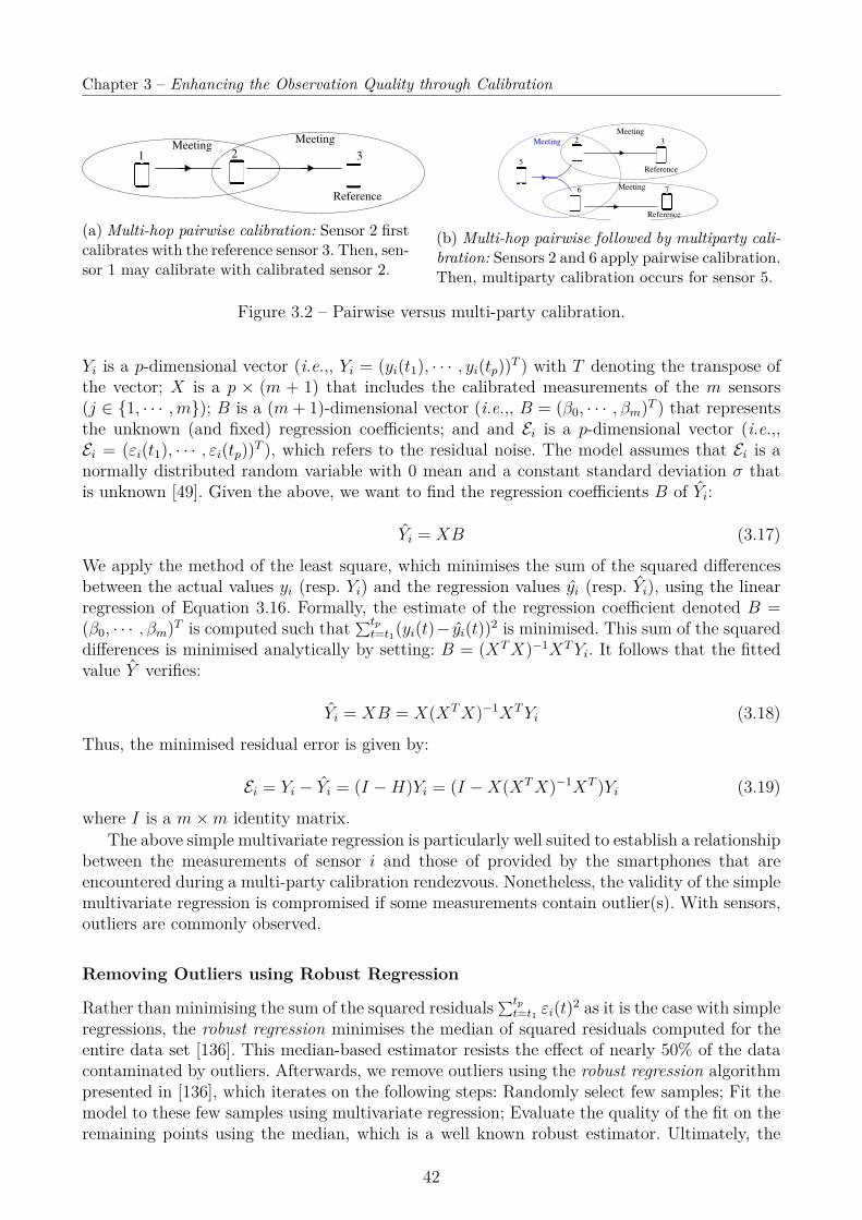
Chapter 3 – Enhancing the Observation Quality through Calibration
Reference
1 2 3Meeting
Meeting
(a) Multi-hop pairwise calibration: Sensor 2 firstcalibrates with the reference sensor 3. Then, sen-sor 1 may calibrate with calibrated sensor 2.
Reference
Reference
2 3
6
Meeting
7Meeting
5
Meeting
(b) Multi-hop pairwise followed by multiparty cali-bration: Sensors 2 and 6 apply pairwise calibration.Then, multiparty calibration occurs for sensor 5.
Figure 3.2 – Pairwise versus multi-party calibration.
Yi is a p-dimensional vector (i.e.,, Yi = (yi(t1), · · · , yi(tp))T ) with T denoting the transpose ofthe vector; X is a p × (m + 1) that includes the calibrated measurements of the m sensors(j ∈ 1, · · · ,m); B is a (m+ 1)-dimensional vector (i.e.,, B = (β0, · · · , βm)T ) that representsthe unknown (and fixed) regression coefficients; and and Ei is a p-dimensional vector (i.e.,,Ei = (εi(t1), · · · , εi(tp))T ), which refers to the residual noise. The model assumes that Ei is anormally distributed random variable with 0 mean and a constant standard deviation σ thatis unknown [49]. Given the above, we want to find the regression coefficients B of Yi:
Yi = XB (3.17)
We apply the method of the least square, which minimises the sum of the squared differencesbetween the actual values yi (resp. Yi) and the regression values yi (resp. Yi), using the linearregression of Equation 3.16. Formally, the estimate of the regression coefficient denoted B =(β0, · · · , βm)T is computed such that ∑tp
t=t1(yi(t)− yi(t))2 is minimised. This sum of the squareddifferences is minimised analytically by setting: B = (XTX)−1XTYi. It follows that the fittedvalue Y verifies:
Yi = XB = X(XTX)−1XTYi (3.18)
Thus, the minimised residual error is given by:
Ei = Yi − Yi = (I −H)Yi = (I −X(XTX)−1XT )Yi (3.19)
where I is a m×m identity matrix.The above simple multivariate regression is particularly well suited to establish a relationship
between the measurements of sensor i and those of provided by the smartphones that areencountered during a multi-party calibration rendezvous. Nonetheless, the validity of the simplemultivariate regression is compromised if some measurements contain outlier(s). With sensors,outliers are commonly observed.
Removing Outliers using Robust Regression
Rather than minimising the sum of the squared residuals∑tpt=t1 εi(t)2 as it is the case with simple
regressions, the robust regression minimises the median of squared residuals computed for theentire data set [136]. This median-based estimator resists the effect of nearly 50% of the datacontaminated by outliers. Afterwards, we remove outliers using the robust regression algorithmpresented in [136], which iterates on the following steps: Randomly select few samples; Fit themodel to these few samples using multivariate regression; Evaluate the quality of the fit on theremaining points using the median, which is a well known robust estimator. Ultimately, the
42
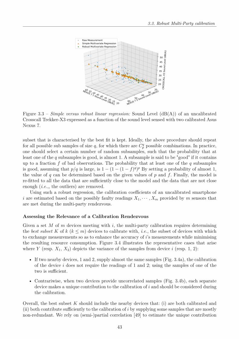
3.3. Robust Multi-Party calibration
NEXUS 7 1 Sound Level (dB(A)) 202530354045505560
NEXUS 7 2
Sound Le
vel (dB(A
))20
3040
5060
CROS
SCAL
L X3
Sou
nd Level (d
B(A))
20253035404550
Raw MeasurementSimple Multivariate RegressionRobust Multivariate Regression
Figure 3.3 – Simple versus robust linear regression: Sound Level (dB(A)) of an uncalibratedCrosscall Trekker-X3 expressed as a function of the sound level sensed with two calibrated AsusNexus 7.
subset that is characterised by the best fit is kept. Ideally, the above procedure should repeatfor all possible sub samples of size q, for which there are Cq
p possible combinations. In practice,one should select a certain number of random subsamples, such that the probability that atleast one of the q subsamples is good, is almost 1. A subsample is said to be "good" if it containsup to a fraction f of bad observations. The probability that at least one of the q subsamplesis good, assuming that p/q is large, is 1− (1− (1− f)q)p By setting a probability of almost 1,the value of q can be determined based on the given values of p and f . Finally, the model isre-fitted to all the data that are sufficiently close to the model and the data that are not closeenough (i.e.,, the outliers) are removed.
Using such a robust regression, the calibration coefficients of an uncalibrated smartphonei are estimated based on the possibly faulty readings X1, · · · , Xm provided by m sensors thatare met during the multi-party rendezvous.
Assessing the Relevance of a Calibration Rendezvous
Given a set M of m devices meeting with i, the multi-party calibration requires determiningthe best subset K of k (k ≤ m) devices to calibrate with, i.e., the subset of devices with whichto exchange measurements so as to enhance the accuracy of i’s measurements while minimisingthe resulting resource consumption. Figure 3.4 illustrates the representative cases that arisewhere Y (resp. X1, X2) depicts the variance of the samples from device i (resp. 1, 2):
• If two nearby devices, 1 and 2, supply almost the same samples (Fig. 3.4a), the calibrationof the device i does not require the readings of 1 and 2; using the samples of one of thetwo is sufficient.
• Contrariwise, when two devices provide uncorrelated samples (Fig. 3.4b), each separatedevice makes a unique contribution to the calibration of i and should be considered duringthe calibration.
Overall, the best subset K should include the nearby devices that: (i) are both calibrated and(ii) both contribute sufficiently to the calibration of i by supplying some samples that are mostlynon-redundant. We rely on (semi-)partial correlation [49] to estimate the unique contribution
43

Chapter 3 – Enhancing the Observation Quality through Calibration
X1 X2
Y
(a) X1 and X2 are highly cor-related.
X1X2
Y
(b) X1 and X2 are uncorre-lated.
X1 X2
Ya
b c d
e
(c) X1 and X2 are correlated.
Figure 3.4 – Device i meets two calibrated devices 1 and 2. Device i collects samples locally,whose variance is Y and determines if it can calibrate using the samples of 1 and 2 (withvariance denoted X1 and X2). The figure depicts the relationship between the 3 variables Y ,X1 and X2. In 3.4c: a is the variance specific to the samples of i; b (resp. d) is the part of Yvariance uniquely influenced by X1 (resp. X2); e is the part of X1 variance uniquely influencedby X2; c is the part of Y variance influenced by both X1 and X2.
of each device to the calibration of i. Consider the case depicted in Figure 3.4c, the area arepresents the variance specific to Y , while the area b + c + d (i.e., the area of Y intersectingwith X1 and X2) represents the overlap of Y with X1 and X2. We may further decomposethe variance Y with respect to X1 and X2. The area b (resp. d) is the part of the Y varianceuniquely influenced by X1 (resp. X2); it is represented by the squared semi-partial correlationcoefficient, denoted rX1 (resp. rX2), which reflects the correlation between Y and X1 while X2has been partialed out (i.e., the effect of X2 has been removed from X1 but not from Y ). Thesemi-partial correlation of X1 with Y , which can be simply denoted srX1 , corresponds to thecorrelation rX1\X2Y between X1 and Y , removing the effect of X2 from X1, but not from Y :
srX1 = rX1\X2Y = rX1 Y − rX1 X2rX2 Y√1− r2
X1 X2
(3.20)
Following, we use the semi-partial correlation to characterise the specific effect that eachcalibrated device of M may have on the calibration of i so as to exclude any device j thatcontributes measurements that are not sufficient/unique (i.e., with srXj ≤ ε). We apply astepwise process, wherein the devices having the lowest semi-partial regression are removedfirst. Semi-partial correlations are further used in a stepwise regression procedure, where thedevice (rather than the end-user) determines which variables (i.e., device) should be consideredin the final regression. We note that, in a forward stepwise regression, the calibrated devicethat would add the largest semi-partial correlation is added next (provided it is statisticallysignificant).
3.3.2 Multi-hop, Multi-party CalibrationWe now consider the history of the sensors’ calibrations to assess the relevance of a given multi-party rendezvous. Indeed, we must compare the quality of the calibration parameters computedin the current rendezvous to the quality of the previous calibrations, if any.
Formalising the History of Multi-party Calibrations using Hypergraphs
Formally, we represent the history of multi-party calibrations using a weighted, directed hy-pergraph (Figure 3.5a). A directed hypergraph is a pair H = (V,E), where V denotes the finite
44
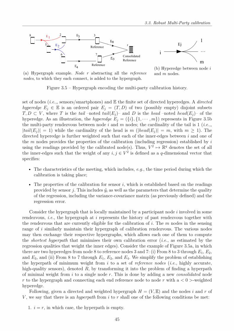
3.3. Robust Multi-Party calibration
Reference
Reference
r
Consolidated
Reference
E1
E2
0
(a) Hypergraph example. Node r abstracting all the referencenodes, to which they each connect, is added to the hypergraph.
Ej
i. . .
1
m
(b) Hyperedge between node iand m nodes.
Figure 3.5 – Hypergraph encoding the multi-party calibration history.
set of nodes (i.e.,, sensors/smartphones) and E the finite set of directed hyperedges. A directedhyperedge Ej ∈ E is an ordered pair Ej = (T,D) of two (possibly empty) disjoint subsetsT,D ⊂ V , where T is the tail –noted tail(Ej)– and D is the head –noted head(Ej)– of thehyperedge. As an illustration, the hyperedge Ej = (i, 1, · · · ,m) represents in Figure 3.5bthe multi-party rendezvous between node i and m nodes; the cardinality of the tail is 1 (i.e.,,|tail(Ej)| = 1) while the cardinality of the head is m (|head(Ej)| = m, with m ≥ 1). Thedirected hyperedge is further weighted such that each of the inner-edges between i and one ofthe m nodes provides the properties of the calibration (including regression) established by iusing the readings provided by the calibrated node(s). Thus, V 2 7→ Rq denotes the set of allthe inner-edges such that the weight of any i, j ∈ V 2 is defined as a q-dimensional vector thatspecifies:
• The characteristics of the meeting, which includes, e.g., the time period during which thecalibration is taking place;
• The properties of the calibration for sensor i, which is established based on the readingsprovided by sensor j. This includes yi as well as the parameters that determine the qualityof the regression, including the variance-covariance matrix (as previously defined) and theregression error.
Consider the hypergraph that is locally maintained by a participant node i involved in somerendezvous, i.e., the hypergraph at i represents the history of past rendezvous together withthe rendezvous that are currently eligible for the calibration of i. The m nodes in the sensingrange of i similarly maintain their hypergraph of calibration rendezvous. The various nodesmay then exchange their respective hypergraphs, which allows each one of them to computethe shortest hyperpath that minimises their own calibration error (i.e., as estimated by theregression qualities that weight the inner edges). Consider the example of Figure 3.5a, in whichthere are two hyperedges from node 8 to reference nodes 3 and 7: (i) From 8 to 3 through E1, E2,and E3, and (ii) From 8 to 7 through E1, E2, and E4. We simplify the problem of establishingthe hyperpath of minimum weight from i to a set of reference nodes (i.e., highly accurate,high-quality sensors), denoted R, by transforming it into the problem of finding a hyperpathof minimal weight from i to a single node r. This is done by adding a new consolidated noder to the hypergraph and connecting each end reference node to node r with a < 0 >-weightedhyperedge.
Following, given a directed and weighted hypergraph H = (V,E) and the nodes i and r ofV , we say that there is an hyperpath from i to r shall one of the following conditions be met:
1. i = r, in which case, the hyperpath is empty.
45

Chapter 3 – Enhancing the Observation Quality through Calibration
2. There is a hyperedge (i, K) ∈ E such that ∀k ∈ K ⊂ V , there is a hyperpath from kto r.
Condition 2 signifies that a node i can calibrate using the surrounding sensors inK if and only ifthe sensors in K are also calibrated (i.e., there is a hyperpath from each of them to r). Overall,considering the set of eligible hyperpaths, Hi,r = (Vi,r,Ei,r), from i, according to the set of nodesin the sensing and communication ranges of i, the goal of node i, which attempts to calibrate,is to find the calibration hyperpath (from i to r) –and thus the associated hypergraph– thatminimises the accumulated weight, which is:
PPP : minEi,r⊆E
∑Ej∈Ei,r
w(Ej)h(Ej) (3.21)
where w(Ej) specifies the sum of the weights of the inner edges of an hyperedge Ej, andh(Ej) = 1 if the hyperpath goes through the edge Ej and h(Ej) = 0 otherwise.
Finding the Shortest Hyperpath
Using the local hypergraph, any sensor i may independently compute the shortest hyperpath(in terms of the edge weights) towards the "consolidated end reference" sensor r, for which weintroduce Algorithm 2:
1. The initialisation (lines 2-4) is as follows: the hyperpath from i to any node is set toempty; the distance to the source is set to 0 and to all the other nodes to infinite; andthe set of nodes that need to be visited, denoted Q, is set to V .
2. Then, all the nodes are visited (line 5), starting with i as the current node (i.e., u = i). Inthe consecutive rounds, the current node refers to the closest node, i.e., the closest nodethat is reachable by an outgoing hyperedge (line 6).
3. The set of nodes that can be reached from the current node through any outgoing hyper-edge Ej is determined (line 7):
• First, we treat the pairwise rendezvous (lines 8-14), which is characterised by ahyperedge Ej having a head of cardinality 1. If a shorter path passing through Ejis found, the distance from i to the newly connected node v is updated consideringthe minimal distance, and the hyperpath to v is updated accordingly.
• Then, we treat the multi-party rendezvous (lines 15-25) with a hyperedge Ej with|head(Ej)| > 1, which has not been visited so far (i.e., Ej /∈ E). We establishthe shortest hyperpath from each node v participating to the rendezvous (for eachv ∈ head(Ej). We check if each node v is already calibrated, i.e., if there exists ahyperpath for each node v to r (i.e., Hv,r 6= ∅) or if node r is reached. In such a case,if the hyperpath going through each v is the shortest one (so far), this hyperpath isestablished as the shortest one.
4. After having visited any node of the hypergraph, the shortest hyperpath established sofar (if any) is returned.
The algorithm runs in O(log V Eu+V
(V−Ep)(V−Ep) ) time, assuming that there are V nodes in thehypergraph (including the consolidated node r that has been added) and that there are Ehyperedges with: Eu hyperedges reflecting each a single party meeting, and Ep hyperedges
46

3.3. Robust Multi-Party calibration
designating multi-party meetings (i.e., E = Eu + Ep). More precisely, the main loop of thealgorithm extracts one node that has not been visited. All these –unvisited yet– nodes arestored in a min heap of size V which contains the node identification along with the distanceto i. So, the extraction of the closest node v not yet visited (as performed in line 6) takesO(log V ). The next step consists in checking all the outgoing (single-party and then multi-party) hyperedges of v. First, we consider any single-party hyperedge and we store the shortestdistance to the node v accessible through this hyperedge. If that node is not yet visited, we addit to the list of unvisited node Q; given that at most V nodes are not yet visited, we have a totalcost of at most O(V logV ). On the other hand, if the node v is already in Q, its priority maybe increased considering the shortest distance to i, leading to a cost of O(Eulog V ). Therefore,so far, the total run time is O(V log V + Eulog V ), which is O(EulogV ) because V is O(Eu)assuming a connected hypergraph. In addition, we consider the analyses of Ep multi-partyrendezvous. For each of them, there are at most V hyperpaths established using a hypergraphcontaining at most V − 1 nodes and Ep − 1 + Eu, leading to the overall time complexity:
Eulog V +Ep∑i=1
V ilog(V − i) ∼ Eulog V + logEp∏i=1
(V − i)V i = Eulog V + VV−Ep∑i=V
log i! =
Eulog V + VV−Ep∑i=1
log i!− VV−1∑i=1
log i! < Eulog V + V log V − (V − Ep)log(V − Ep) =
log V Eu+V
(V−Ep)(V−Ep)
The multi-hop, multi-party calibration in practice
Summarising the multi-hop, multi-party calibration, any mobile i participating in the collabo-rative calibration periodically runs the following process:
1. Sensor i detects the presence of the nearby sensing device(s), i.e., the devices in the sharedsensing range.
2. Sensor i and the surrounding devices exchange their respective hypergraphs and any nodeupdates its hypergraph (see Algorithm 2).
3. In the presence of any eligible rendezvous, i exchanges its sensing measurements (i.e.,time series) in a synchronised manner so as to establish the linear relationship betweenthe measurements of the nearby sensors and the raw measurements obtained locally.
4. The best calibration path is determined, the calibration function is set and the hypergraphis updated accordingly.
The calibration function is a linear function from the actually measured values to the calibratedvalues. Let the expected calibrated measurements of sensor i be Yi. In order to calibrate theactual measurements Yi = (yi(t1), · · · , yi(tp))T , it is required to apply the reversion of thelinear relationship for: Yi 7→ Yi simply by replacing the reference values with Yi and replacingthe regressed values Yi with Yi, in Equation (3.17), where Yi eliminates the residual noise errorwhile maintaining the linear relationship from reference to actual measurements. Thus, thecalibration function is:
yi(t) = yi(t)− β0∑kj=1 βj
(3.22)
where the index j indicates a vertex from the k reference vertices. The multi-hop allows arecursive loop for the calibration process from the reference vertices to all uncalibrated vertices.
47
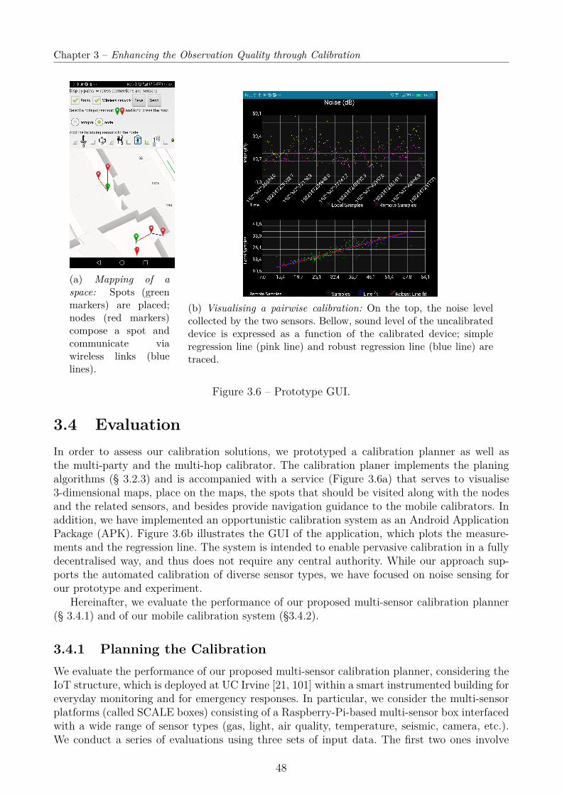
Chapter 3 – Enhancing the Observation Quality through Calibration
(a) Mapping of aspace: Spots (greenmarkers) are placed;nodes (red markers)compose a spot andcommunicate viawireless links (bluelines).
(b) Visualising a pairwise calibration: On the top, the noise levelcollected by the two sensors. Bellow, sound level of the uncalibrateddevice is expressed as a function of the calibrated device; simpleregression line (pink line) and robust regression line (blue line) aretraced.
Figure 3.6 – Prototype GUI.
3.4 EvaluationIn order to assess our calibration solutions, we prototyped a calibration planner as well asthe multi-party and the multi-hop calibrator. The calibration planer implements the planingalgorithms (§ 3.2.3) and is accompanied with a service (Figure 3.6a) that serves to visualise3-dimensional maps, place on the maps, the spots that should be visited along with the nodesand the related sensors, and besides provide navigation guidance to the mobile calibrators. Inaddition, we have implemented an opportunistic calibration system as an Android ApplicationPackage (APK). Figure 3.6b illustrates the GUI of the application, which plots the measure-ments and the regression line. The system is intended to enable pervasive calibration in a fullydecentralised way, and thus does not require any central authority. While our approach sup-ports the automated calibration of diverse sensor types, we have focused on noise sensing forour prototype and experiment.
Hereinafter, we evaluate the performance of our proposed multi-sensor calibration planner(§ 3.4.1) and of our mobile calibration system (§3.4.2).
3.4.1 Planning the CalibrationWe evaluate the performance of our proposed multi-sensor calibration planner, considering theIoT structure, which is deployed at UC Irvine [21, 101] within a smart instrumented building foreveryday monitoring and for emergency responses. In particular, we consider the multi-sensorplatforms (called SCALE boxes) consisting of a Raspberry-Pi-based multi-sensor box interfacedwith a wide range of sensor types (gas, light, air quality, temperature, seismic, camera, etc.).We conduct a series of evaluations using three sets of input data. The first two ones involve
48
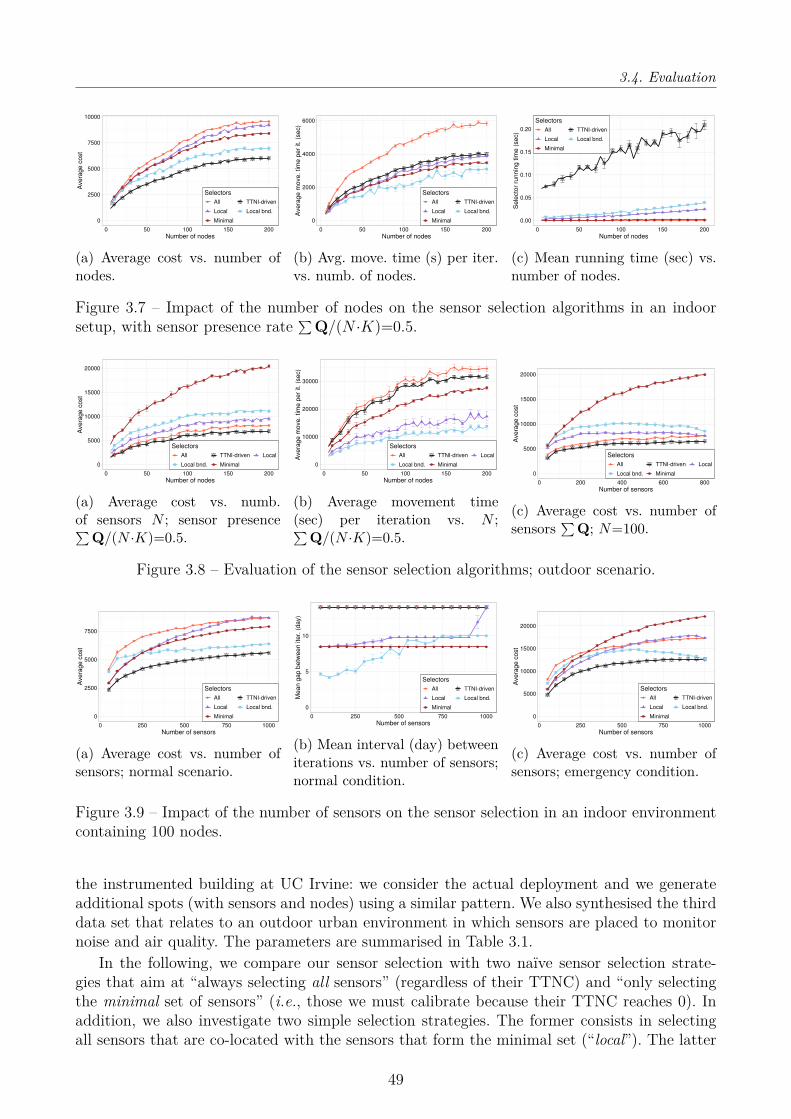
3.4. Evaluation
0
2500
5000
7500
10000
0 50 100 150 200Number of nodes
Ave
rage
cos
t
SelectorsAll TTNI-driven
Local Local bnd.
Minimal
(a) Average cost vs. number ofnodes.
0
2000
4000
6000
0 50 100 150 200Number of nodes
Ave
rage
mov
e. ti
me
per i
t. (s
ec)
SelectorsAll TTNI-driven
Local Local bnd.
Minimal
(b) Avg. move. time (s) per iter.vs. numb. of nodes.
0.00
0.05
0.10
0.15
0.20
0 50 100 150 200Number of nodes
Sel
ecto
r run
ning
tim
e (s
ec)
SelectorsAll TTNI-driven
Local Local bnd.
Minimal
(c) Mean running time (sec) vs.number of nodes.
Figure 3.7 – Impact of the number of nodes on the sensor selection algorithms in an indoorsetup, with sensor presence rate ∑Q/(N ·K)=0.5.
0
5000
10000
15000
20000
0 50 100 150 200Number of nodes
Ave
rage
cos
t
SelectorsAll TTNI-driven Local
Local bnd. Minimal
(a) Average cost vs. numb.of sensors N ; sensor presence∑
Q/(N ·K)=0.5.
0
10000
20000
30000
0 50 100 150 200Number of nodes
Ave
rage
mov
e. ti
me
per i
t. (s
ec)
SelectorsAll TTNI-driven Local
Local bnd. Minimal
(b) Average movement time(sec) per iteration vs. N ;∑
Q/(N ·K)=0.5.
0
5000
10000
15000
20000
0 200 400 600 800Number of sensors
Ave
rage
cos
t
SelectorsAll TTNI-driven Local
Local bnd. Minimal
(c) Average cost vs. number ofsensors
∑Q; N=100.
Figure 3.8 – Evaluation of the sensor selection algorithms; outdoor scenario.
0
2500
5000
7500
0 250 500 750 1000Number of sensors
Ave
rage
cos
t
SelectorsAll TTNI-driven
Local Local bnd.
Minimal
(a) Average cost vs. number ofsensors; normal scenario.
0
5
10
0 250 500 750 1000Number of sensors
Mea
n ga
p be
twee
n ite
r. (d
ay)
SelectorsAll TTNI-driven
Local Local bnd.
Minimal
(b) Mean interval (day) betweeniterations vs. number of sensors;normal condition.
0
5000
10000
15000
20000
0 250 500 750 1000Number of sensors
Ave
rage
cos
t
SelectorsAll TTNI-driven
Local Local bnd.
Minimal
(c) Average cost vs. number ofsensors; emergency condition.
Figure 3.9 – Impact of the number of sensors on the sensor selection in an indoor environmentcontaining 100 nodes.
the instrumented building at UC Irvine: we consider the actual deployment and we generateadditional spots (with sensors and nodes) using a similar pattern. We also synthesised the thirddata set that relates to an outdoor urban environment in which sensors are placed to monitornoise and air quality. The parameters are summarised in Table 3.1.
In the following, we compare our sensor selection with two naïve sensor selection strate-gies that aim at “always selecting all sensors” (regardless of their TTNC) and “only selectingthe minimal set of sensors” (i.e., those we must calibrate because their TTNC reaches 0). Inaddition, we also investigate two simple selection strategies. The former consists in selectingall sensors that are co-located with the sensors that form the minimal set (“local”). The latter
49
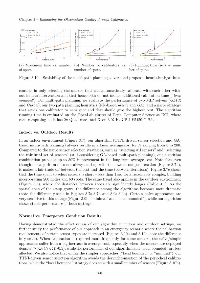
Chapter 3 – Enhancing the Observation Quality through Calibration
0
2000
4000
6000
8000
4 6 8 10 12Number of spots
Tota
l mov
emen
t tim
e (s
ec)
Path plannersEach GA
Greedy GLPK
Gurobi
(a) Movement time vs. numberof spots.
0
20
40
4 6 8 10 12Number of spots
Pat
h pl
anne
r run
ning
tim
e (s
ec)
Path plannersEach GA
Greedy GLPK
Gurobi
(b) Number of calibrators vs.number of spots.
0
20
40
4 6 8 10 12Number of spots
Pat
h pl
anne
r run
ning
tim
e (s
ec)
Path plannersEach GA
Greedy GLPK
Gurobi
(c) Running time (sec) vs. num-ber of spots.
Figure 3.10 – Scalability of the multi-path planning solvers and proposed heuristic algorithms.
consists in only selecting the sensors that can automatically calibrate with each other with-out human intervention and that henceforth do not induce additional calibration time (“localbounded"). For multi-path planning, we evaluate the performance of two MIP solvers (GLPKand Gurobi), our two path planning heuristics (NN-based greedy and GA), and a naïve strategythat sends one calibrator to each spot and that should give the highest cost. The algorithmrunning time is evaluated on the OpenLab cluster of Dept. Computer Science at UCI, whereeach computing node has 2x Quad-core Intel Xeon 3.0GHz CPU E5450 CPUs.
Indoor vs. Outdoor Results:
In an indoor environment (Figure 3.7), our algorithm (TTNI-driven sensor selection and GA-based multi-path planning) always results in a lower average cost for N ranging from 5 to 200.Compared to the naïve sensor selection strategies, such as “selecting all sensors” and “selectingthe minimal set of sensors” (still considering GA-based multi-path planning), our algorithmcombination provides up-to 30% improvement in the long-term average cost. Note that eventhough our algorithm does not always end up with the lowest cost per iteration (Figure 3.7b),it makes a fair trade-off between the cost and the time (between iterations). Figure 3.7c showsthat the time spent to select sensors is short – less than 1 sec for a reasonably complex buildingincorporating 200 nodes and 60 spots. The same trend also applies in the outdoor environment(Figure 3.8), where the distances between spots are significantly longer (Table 3.1). As thespatial span of the setup grows, the difference among the algorithms becomes more dramatic(note the different y-scale in Figures 3.7a,3.7b and 3.9a,3.9b). Certain naïve approaches arevery sensitive to this change (Figure 3.9b, “minimal” and “local bounded”), while our algorithmshows stable performance in both settings.
Normal vs. Emergency Condition Results:
Having demonstrated the effectiveness of our algorithm in indoor and outdoor settings, wefurther study the performance of our approach in an emergency scenario where the calibrationrequirements of certain sensor types are increased (Figures 3.10a and 3.10c, note the differencein y-scale). When calibration is required more frequently for some sensors, the naïve/simpleapproaches suffer from a big increase in average cost, especially when the sensors are deployeddensely (∑Q/(N ·K)>0.5), while the performance of our algorithm and “local bounded” are lessaffected. We also notice that unlike the simpler approaches (“local bounded” or “minimal”), ourTTNI-driven sensor selection algorithm avoids the desynchronisation of the periodical calibra-tions, while the “local bounded” strategy does so with a small number of sensors (Figure 3.10b).
50
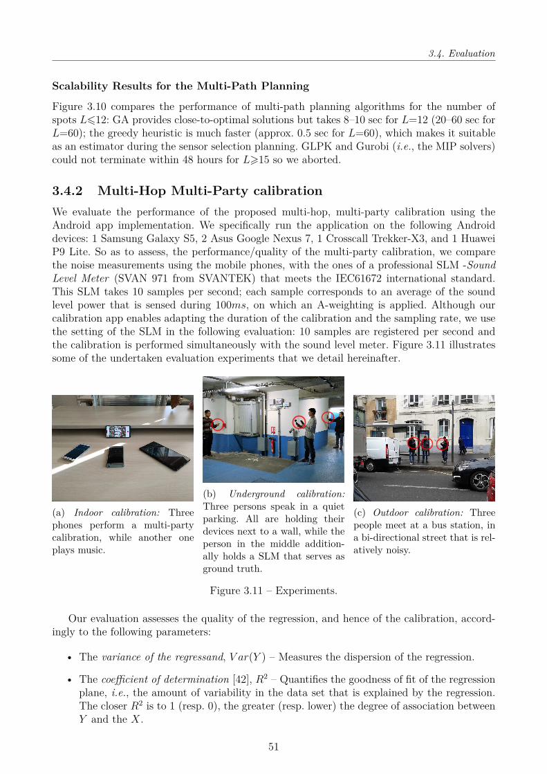
3.4. Evaluation
Scalability Results for the Multi-Path Planning
Figure 3.10 compares the performance of multi-path planning algorithms for the number ofspots L612: GA provides close-to-optimal solutions but takes 8–10 sec for L=12 (20–60 sec forL=60); the greedy heuristic is much faster (approx. 0.5 sec for L=60), which makes it suitableas an estimator during the sensor selection planning. GLPK and Gurobi (i.e., the MIP solvers)could not terminate within 48 hours for L>15 so we aborted.
3.4.2 Multi-Hop Multi-Party calibrationWe evaluate the performance of the proposed multi-hop, multi-party calibration using theAndroid app implementation. We specifically run the application on the following Androiddevices: 1 Samsung Galaxy S5, 2 Asus Google Nexus 7, 1 Crosscall Trekker-X3, and 1 HuaweiP9 Lite. So as to assess, the performance/quality of the multi-party calibration, we comparethe noise measurements using the mobile phones, with the ones of a professional SLM -SoundLevel Meter (SVAN 971 from SVANTEK) that meets the IEC61672 international standard.This SLM takes 10 samples per second; each sample corresponds to an average of the soundlevel power that is sensed during 100ms, on which an A-weighting is applied. Although ourcalibration app enables adapting the duration of the calibration and the sampling rate, we usethe setting of the SLM in the following evaluation: 10 samples are registered per second andthe calibration is performed simultaneously with the sound level meter. Figure 3.11 illustratessome of the undertaken evaluation experiments that we detail hereinafter.
(a) Indoor calibration: Threephones perform a multi-partycalibration, while another oneplays music.
(b) Underground calibration:Three persons speak in a quietparking. All are holding theirdevices next to a wall, while theperson in the middle addition-ally holds a SLM that serves asground truth.
(c) Outdoor calibration: Threepeople meet at a bus station, ina bi-directional street that is rel-atively noisy.
Figure 3.11 – Experiments.
Our evaluation assesses the quality of the regression, and hence of the calibration, accord-ingly to the following parameters:
• The variance of the regressand, V ar(Y ) – Measures the dispersion of the regression.
• The coefficient of determination [42], R2 – Quantifies the goodness of fit of the regressionplane, i.e., the amount of variability in the data set that is explained by the regression.The closer R2 is to 1 (resp. 0), the greater (resp. lower) the degree of association betweenY and the X.
51

Chapter 3 – Enhancing the Observation Quality through Calibration
• The adjusted R2 – Evaluates the goodness of fit and penalises the use of additionalvariables. The adjusted R2 increases only if new variables improve the regression morethan it would be expected by chance. It remains less or equal to R2 but it can also benegative.
• The standard deviation of the residual noise, εi.
• The difference/bias between the measurements provided by a calibrated device and theones of the SLM.
We use box plots to depict the above parameters when reporting the evaluation results (e.g.,see Figure 3.12): the triangle denotes the mean, the line inside the box indicates the median,the lines on edge reflect the range of values, and the rectangle corresponds to the InterquartileRange (IQR).
In order to evaluate the multi-hop, multi-party calibration, we consider the following sce-narios:
1. Comparison between the simple and robust regression (§ 3.4.2).
2. Comparison between univariate (pairwise) and multivariate (multi-party) regression (§ 3.4.2).
3. Comparison of multi-hop, pairwise with multi-hop, multi-party calibration (§ 3.4.2).
4. Evaluating the impact of the environment (in-door vs out-door) on multi-party calibration(§ 3.4.2).
The first three scenarios involve in-door calibration within a room (see Figure 3.11a), while thefourth also considers the underground and out-door cases (see Figures 3.11b and 3.11c). In mostof the experiments, the devices were less than 1 meter away from each other, except when weconsider the impact of the following sensing conditions: distance, obstacle and in-/out-pocket.
Simple versus Robust Regression
We compare the simple vs robust regression using an uncalibrated device (the Crosscall Trekker-X3) and two devices (the 2 Asus Google Nexus 7) that were previously calibrated with the SLM,and that exchange the noise level they collected during 10s. The experiments were run in-door,100 times.
Figure 3.12a (resp. 3.12b) compares the robust regression with the simple regression consid-ering the variance of the regressand (resp. the standard deviation of the regression residuals). Asshown, the robust regression provides a lower regressand variance in terms of mean and median.In particular, the average value of the variance corresponds to 11.984 with the simple regressionand 5.529 with the robust regression. In fact, the robust regression reduces the influence of out-liers, which leads to a lower regressand variance and thereby to a more accurate regression. Also,the regression residuals (Figure 3.12b) produced by a robust regression is characterised by aweaker standard deviation: the average value of this standard deviation is equal to 1.531 dB(A)for the simple regression and 0.915 dB(A) for the robust regression. Meanwhile, the IQR of thestandard deviation exhibited by the robust regression, i.e., [0.402dB(A), 1.336dB(A)], is muchlower, compared to the one provided by the simple regression, i.e., [1.019dB(A), 2.017dB(A)].
In order to evaluate the computational overhead and accuracy of the robust regression, weuse the same three devices and we run series of calibrations characterised by various samplingdurations; we execute 20 times each of these series.
52
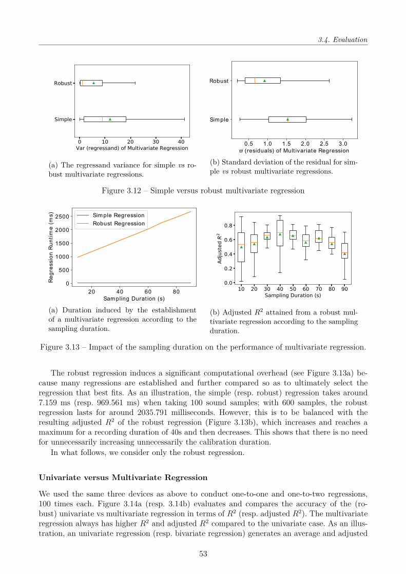
3.4. Evaluation
0 10 20 30 40Var (regressand) of Multivariate Regression
Simple
Robust
(a) The regressand variance for simple vs ro-bust multivariate regressions.
0.5 1.0 1.5 2.0 2.5 3.0
(residuals) of Mult ivariate Regression
Sim ple
Robust
(b) Standard deviation of the residual for sim-ple vs robust multivariate regressions.
Figure 3.12 – Simple versus robust multivariate regression
20 40 60 80
Sam pling Durat ion (s)
0
500
1000
1500
2000
2500
Re
gre
ssio
n R
un
tim
e (
ms)
Sim ple Regression
Robust Regression
(a) Duration induced by the establishmentof a multivariate regression according to thesampling duration.
10 20 30 40 50 60 70 80 90Sampling Duration (s)
0.0
0.2
0.4
0.6
0.8Ad
justed
R2
(b) Adjusted R2 attained from a robust mul-tivariate regression according to the samplingduration.
Figure 3.13 – Impact of the sampling duration on the performance of multivariate regression.
The robust regression induces a significant computational overhead (see Figure 3.13a) be-cause many regressions are established and further compared so as to ultimately select theregression that best fits. As an illustration, the simple (resp. robust) regression takes around7.159 ms (resp. 969.561 ms) when taking 100 sound samples; with 600 samples, the robustregression lasts for around 2035.791 milliseconds. However, this is to be balanced with theresulting adjusted R2 of the robust regression (Figure 3.13b), which increases and reaches amaximum for a recording duration of 40s and then decreases. This shows that there is no needfor unnecessarily increasing unnecessarily the calibration duration.
In what follows, we consider only the robust regression.
Univariate versus Multivariate Regression
We used the same three devices as above to conduct one-to-one and one-to-two regressions,100 times each. Figure 3.14a (resp. 3.14b) evaluates and compares the accuracy of the (ro-bust) univariate vs multivariate regression in terms of R2 (resp. adjusted R2). The multivariateregression always has higher R2 and adjusted R2 compared to the univariate case. As an illus-tration, an univariate regression (resp. bivariate regression) generates an average and adjusted
53
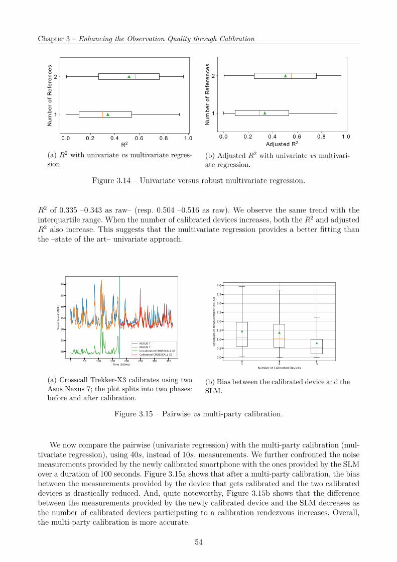
Chapter 3 – Enhancing the Observation Quality through Calibration
0.0 0.2 0.4 0.6 0.8 1.0
R2
1
2
Nu
mb
er o
f R
efe
re
nce
s
(a) R2 with univariate vs multivariate regres-sion.
0.0 0.2 0.4 0.6 0.8 1.0
Adjusted R2
1
2
Nu
mb
er
of
Re
fere
nce
s
(b) Adjusted R2 with univariate vs multivari-ate regression.
Figure 3.14 – Univariate versus robust multivariate regression.
R2 of 0.335 –0.343 as raw– (resp. 0.504 –0.516 as raw). We observe the same trend with theinterquartile range. When the number of calibrated devices increases, both the R2 and adjustedR2 also increase. This suggests that the multivariate regression provides a better fitting thanthe –state of the art– univariate approach.
0 50 100 150 200 250 300 350Time (100ms)
20
25
30
35
40
45
50
Soun
d Le
vel (
dB(A
))
NEXUS 7NEXUS 7Uncalibrated CROSSCALL X3Calibrated CROSSCALL X3
(a) Crosscall Trekker-X3 calibrates using twoAsus Nexus 7; the plot splits into two phases:before and after calibration.
1 2 3Number of Calibrated Devices
0.0
0.5
1.0
1.5
2.0
2.5
3.0
3.5
4.0
Resid
uals in Mea
suremen
t (dB
(A))
(b) Bias between the calibrated device and theSLM.
Figure 3.15 – Pairwise vs multi-party calibration.
We now compare the pairwise (univariate regression) with the multi-party calibration (mul-tivariate regression), using 40s, instead of 10s, measurements. We further confronted the noisemeasurements provided by the newly calibrated smartphone with the ones provided by the SLMover a duration of 100 seconds. Figure 3.15a shows that after a multi-party calibration, the biasbetween the measurements provided by the device that gets calibrated and the two calibrateddevices is drastically reduced. And, quite noteworthy, Figure 3.15b shows that the differencebetween the measurements provided by the newly calibrated device and the SLM decreases asthe number of calibrated devices participating to a calibration rendezvous increases. Overall,the multi-party calibration is more accurate.
54
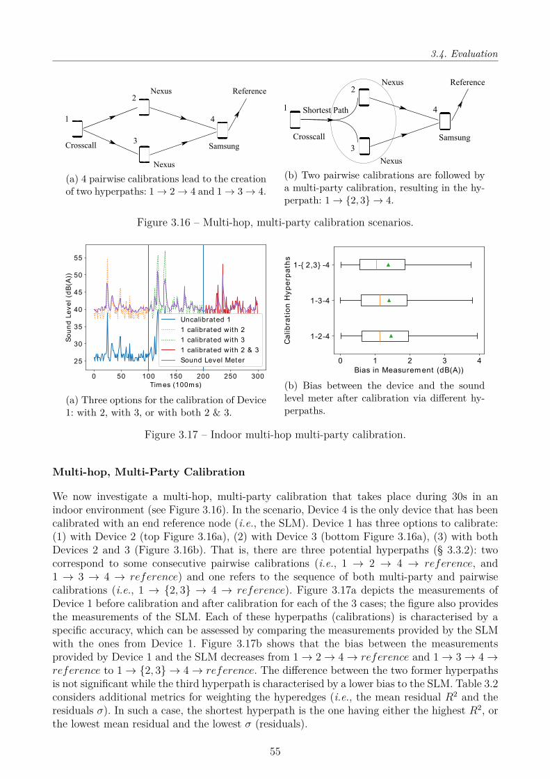
3.4. Evaluation
1
2
3
4
Reference
Crosscall
Nexus
Samsung
Nexus
(a) 4 pairwise calibrations lead to the creationof two hyperpaths: 1→ 2→ 4 and 1→ 3→ 4.
Reference
1
2
3
4Shortest Path
Crosscall
Nexus
Nexus
Samsung
(b) Two pairwise calibrations are followed bya multi-party calibration, resulting in the hy-perpath: 1→ 2, 3 → 4.
Figure 3.16 – Multi-hop, multi-party calibration scenarios.
0 50 100 150 200 250 300
Tim es (100m s)
25
30
35
40
45
50
55
So
un
d L
ev
el
(dB
(A))
Uncalibrated 1
1 calibrated with 2
1 calibrated with 3
1 calibrated with 2 & 3
Sound Level Meter
(a) Three options for the calibration of Device1: with 2, with 3, or with both 2 & 3.
0 1 2 3 4
Bias in Measurem ent (dB(A))
1-2-4
1-3-4
1- 2,3 -4
Ca
lib
rati
on
Hy
pe
rpa
ths
(b) Bias between the device and the soundlevel meter after calibration via different hy-perpaths.
Figure 3.17 – Indoor multi-hop multi-party calibration.
Multi-hop, Multi-Party Calibration
We now investigate a multi-hop, multi-party calibration that takes place during 30s in anindoor environment (see Figure 3.16). In the scenario, Device 4 is the only device that has beencalibrated with an end reference node (i.e., the SLM). Device 1 has three options to calibrate:(1) with Device 2 (top Figure 3.16a), (2) with Device 3 (bottom Figure 3.16a), (3) with bothDevices 2 and 3 (Figure 3.16b). That is, there are three potential hyperpaths (§ 3.3.2): twocorrespond to some consecutive pairwise calibrations (i.e., 1 → 2 → 4 → reference, and1 → 3 → 4 → reference) and one refers to the sequence of both multi-party and pairwisecalibrations (i.e., 1 → 2, 3 → 4 → reference). Figure 3.17a depicts the measurements ofDevice 1 before calibration and after calibration for each of the 3 cases; the figure also providesthe measurements of the SLM. Each of these hyperpaths (calibrations) is characterised by aspecific accuracy, which can be assessed by comparing the measurements provided by the SLMwith the ones from Device 1. Figure 3.17b shows that the bias between the measurementsprovided by Device 1 and the SLM decreases from 1→ 2→ 4→ reference and 1→ 3→ 4→reference to 1→ 2, 3 → 4→ reference. The difference between the two former hyperpathsis not significant while the third hyperpath is characterised by a lower bias to the SLM. Table 3.2considers additional metrics for weighting the hyperedges (i.e., the mean residual R2 and theresiduals σ). In such a case, the shortest hyperpath is the one having either the highest R2, orthe lowest mean residual and the lowest σ (residuals).
55
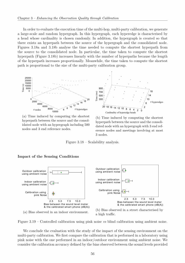
Chapter 3 – Enhancing the Observation Quality through Calibration
In order to evaluate the execution time of the multi-hop, multi-party calibration, we generatea large-scale and random hypergraph. In this hypergraph, each hyperedge is characterised bya head whose cardinality is chosen randomly. In addition, the hypergraph is created so thatthere exists an hyperpath between the source of the hypergraph and the consolidated node.Figures 3.18a and 3.18b analyse the time needed to compute the shortest hyperpath fromthe source to the consolidated node. In particular, the time taken to compute the shortesthyperpath (Figure 3.18b) increases linearly with the number of hyperpaths because the lengthof the hyperpath increases proportionally. Meanwhile, the time taken to compute the shortestpath is proportional to the size of the multi-party calibration group.
0
2000
4000
6000
8000
100006
810
1214
1618
20
0
5000
10000
15000
20000
25000
Tim
e (s
)
# nodes # hyperedges
(a) Time induced by computing the shortesthyperpath between the source and the consol-idated node with an hypergraph including 500nodes and 3 end reference nodes.
2
6
10
14
18
02468101214161820
300
500
700
900
Tim
e (m
s)
# hyperedges
Cardinality of hyperedge heads
(b) Time induced by computing the shortesthyperpath between the source and the consoli-dated node with an hypergraph with 3 end ref-erence nodes and meetings involving at most3 nodes.
Figure 3.18 – Scalability analysis.
Impact of the Sensing Conditions
2.5 5.0 7.5 10.0
Bias between the sound level m eter & the calibrated sm art phone (dB(A))
Calibrat ion using pink Noise
Indoor calibrat ion using am bient noise
Outdoor calibrat ion using am bient noise
(a) Bias observed in an indoor environment.
2.5 5.0 7.5 10.0
Bias between the sound level m eter & the calibrated sm art phone (dB(A))
Calibrat ion using pink Noise
Indoor calibrat ion using am bient noise
Outdoor calibrat ion using am bient noise
(b) Bias observed in a street characterised bya high traffic.
Figure 3.19 – Controlled calibration using pink noise vs blind calibration using ambient noise.
We conclude the evaluation with the study of the impact of the sensing environment on themulti-party calibration. We first compare the calibration that is performed in a laboratory usingpink noise with the one performed in an indoor/outdoor environment using ambient noise. Weconsider the calibration accuracy defined by the bias observed between the sound levels provided
56
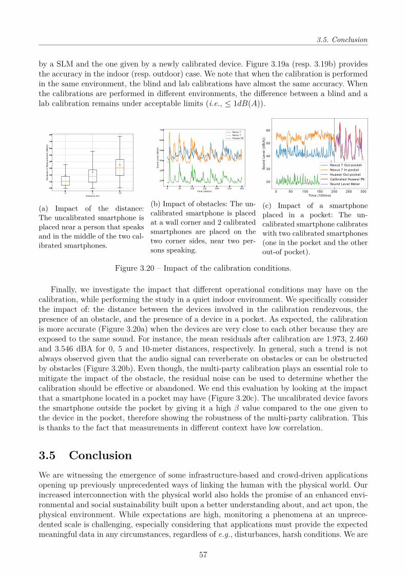
3.5. Conclusion
by a SLM and the one given by a newly calibrated device. Figure 3.19a (resp. 3.19b) providesthe accuracy in the indoor (resp. outdoor) case. We note that when the calibration is performedin the same environment, the blind and lab calibrations have almost the same accuracy. Whenthe calibrations are performed in different environments, the difference between a blind and alab calibration remains under acceptable limits (i.e., ≤ 1dB(A)).
0 5 10Distance (m)
0
1
2
3
4
5
6
7
8
Resid
uals in M
easuremen
t (dB
(A))
(a) Impact of the distance:The uncalibrated smartphone isplaced near a person that speaksand in the middle of the two cal-ibrated smartphones.
0 50 100 150 200 250 300Time (100ms)
20
30
40
50
60
70
Soun
d Leve
l (dB
(A))
Nexus 7Nexus 7Huawei P6
(b) Impact of obstacles: The un-calibrated smartphone is placedat a wall corner and 2 calibratedsmartphones are placed on thetwo corner sides, near two per-sons speaking.
0 50 100 150 200 250 300
Tim e (100m s)
20
30
40
50
60
So
un
d L
ev
el
(dB
(A))
Nexus 7 Out -pocket
Nexus 7 In-pocket
Huawei Out -pocket
Calibrated Huawei P6
Sound Level Meter
(c) Impact of a smartphoneplaced in a pocket: The un-calibrated smartphone calibrateswith two calibrated smartphones(one in the pocket and the otherout-of pocket).
Figure 3.20 – Impact of the calibration conditions.
Finally, we investigate the impact that different operational conditions may have on thecalibration, while performing the study in a quiet indoor environment. We specifically considerthe impact of: the distance between the devices involved in the calibration rendezvous, thepresence of an obstacle, and the presence of a device in a pocket. As expected, the calibrationis more accurate (Figure 3.20a) when the devices are very close to each other because they areexposed to the same sound. For instance, the mean residuals after calibration are 1.973, 2.460and 3.546 dBA for 0, 5 and 10-meter distances, respectively. In general, such a trend is notalways observed given that the audio signal can reverberate on obstacles or can be obstructedby obstacles (Figure 3.20b). Even though, the multi-party calibration plays an essential role tomitigate the impact of the obstacle, the residual noise can be used to determine whether thecalibration should be effective or abandoned. We end this evaluation by looking at the impactthat a smartphone located in a pocket may have (Figure 3.20c). The uncalibrated device favorsthe smartphone outside the pocket by giving it a high β value compared to the one given tothe device in the pocket, therefore showing the robustness of the multi-party calibration. Thisis thanks to the fact that measurements in different context have low correlation.
3.5 ConclusionWe are witnessing the emergence of some infrastructure-based and crowd-driven applicationsopening up previously unprecedented ways of linking the human with the physical world. Ourincreased interconnection with the physical world also holds the promise of an enhanced envi-ronmental and social sustainability built upon a better understanding about, and act upon, thephysical environment. While expectations are high, monitoring a phenomena at an unprece-dented scale is challenging, especially considering that applications must provide the expectedmeaningful data in any circumstances, regardless of e.g., disturbances, harsh conditions. We are
57
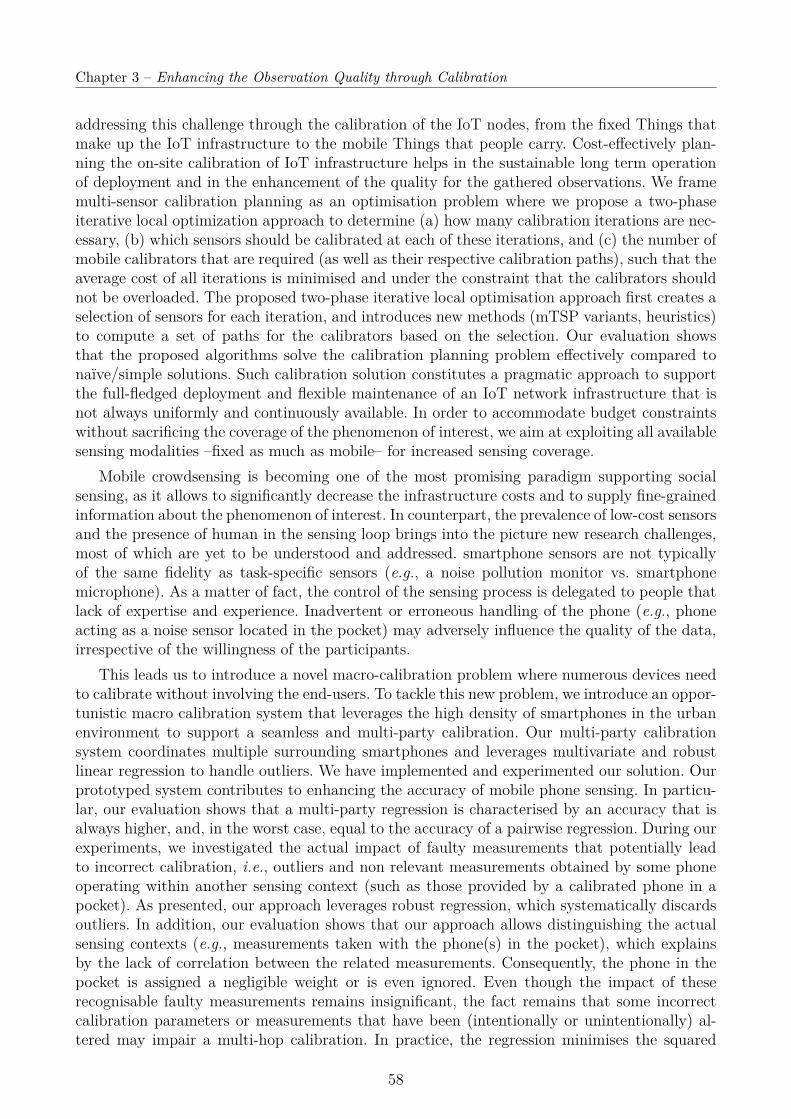
Chapter 3 – Enhancing the Observation Quality through Calibration
addressing this challenge through the calibration of the IoT nodes, from the fixed Things thatmake up the IoT infrastructure to the mobile Things that people carry. Cost-effectively plan-ning the on-site calibration of IoT infrastructure helps in the sustainable long term operationof deployment and in the enhancement of the quality for the gathered observations. We framemulti-sensor calibration planning as an optimisation problem where we propose a two-phaseiterative local optimization approach to determine (a) how many calibration iterations are nec-essary, (b) which sensors should be calibrated at each of these iterations, and (c) the number ofmobile calibrators that are required (as well as their respective calibration paths), such that theaverage cost of all iterations is minimised and under the constraint that the calibrators shouldnot be overloaded. The proposed two-phase iterative local optimisation approach first creates aselection of sensors for each iteration, and introduces new methods (mTSP variants, heuristics)to compute a set of paths for the calibrators based on the selection. Our evaluation showsthat the proposed algorithms solve the calibration planning problem effectively compared tonaïve/simple solutions. Such calibration solution constitutes a pragmatic approach to supportthe full-fledged deployment and flexible maintenance of an IoT network infrastructure that isnot always uniformly and continuously available. In order to accommodate budget constraintswithout sacrificing the coverage of the phenomenon of interest, we aim at exploiting all availablesensing modalities –fixed as much as mobile– for increased sensing coverage.
Mobile crowdsensing is becoming one of the most promising paradigm supporting socialsensing, as it allows to significantly decrease the infrastructure costs and to supply fine-grainedinformation about the phenomenon of interest. In counterpart, the prevalence of low-cost sensorsand the presence of human in the sensing loop brings into the picture new research challenges,most of which are yet to be understood and addressed. smartphone sensors are not typicallyof the same fidelity as task-specific sensors (e.g., a noise pollution monitor vs. smartphonemicrophone). As a matter of fact, the control of the sensing process is delegated to people thatlack of expertise and experience. Inadvertent or erroneous handling of the phone (e.g., phoneacting as a noise sensor located in the pocket) may adversely influence the quality of the data,irrespective of the willingness of the participants.
This leads us to introduce a novel macro-calibration problem where numerous devices needto calibrate without involving the end-users. To tackle this new problem, we introduce an oppor-tunistic macro calibration system that leverages the high density of smartphones in the urbanenvironment to support a seamless and multi-party calibration. Our multi-party calibrationsystem coordinates multiple surrounding smartphones and leverages multivariate and robustlinear regression to handle outliers. We have implemented and experimented our solution. Ourprototyped system contributes to enhancing the accuracy of mobile phone sensing. In particu-lar, our evaluation shows that a multi-party regression is characterised by an accuracy that isalways higher, and, in the worst case, equal to the accuracy of a pairwise regression. During ourexperiments, we investigated the actual impact of faulty measurements that potentially leadto incorrect calibration, i.e., outliers and non relevant measurements obtained by some phoneoperating within another sensing context (such as those provided by a calibrated phone in apocket). As presented, our approach leverages robust regression, which systematically discardsoutliers. In addition, our evaluation shows that our approach allows distinguishing the actualsensing contexts (e.g., measurements taken with the phone(s) in the pocket), which explainsby the lack of correlation between the related measurements. Consequently, the phone in thepocket is assigned a negligible weight or is even ignored. Even though the impact of theserecognisable faulty measurements remains insignificant, the fact remains that some incorrectcalibration parameters or measurements that have been (intentionally or unintentionally) al-tered may impair a multi-hop calibration. In practice, the regression minimises the squared
58

3.5. Conclusion
distance between the measurements of the uncalibrated and calibrated nodes, which compen-sates for small discrepancies among the (miscalibrated and well-calibrated) measurements. Ingeneral, we argue that the multi-party calibration allows for a more precise characterization ofthe relationship between crowdsensors than would a pairwise calibration.
Once calibrated – static as much as mobile – sensors provide some observations that areexpressed with regards to a common reference system. Their interpretation of the observationdepends on the conditions under which they are made. For example, if we are interested ina temperature sensor, knowing whether the sun is hitting is crucial. Same applies with noiseobservation, previous analysis [83, 165] of the noise observations collected from the opportunis-tic crowdsensing application Ambiciti (formerly SoundCity) showed that less than 5% of thecollected data were of sufficient quality to be considered for use in the mapping of urban noisepollution.
59
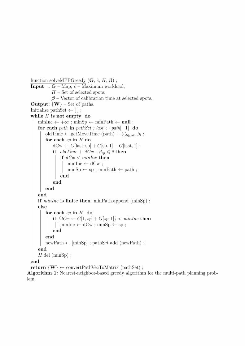
function solveMPPGreedy (G, c, H, β) ;Input : G – Map; c – Maximum workload;
H – Set of selected spots;β – Vector of calibration time at selected spots.
Output: W – Set of paths.Initialise pathSet ← [ ] ;while H is not empty do
minInc ← +∞ ; minSp ← minPath ← null ;for each path in pathSet ; last ← path[−1] do
oldTime ← getMoveTime (path) + ∑l∈path βl ;
for each sp in H dodCw ← G[last, sp] +G[sp, 1]−G[last, 1] ;if oldTime + dCw +βsp 6 c then
if dCw < minInc thenminInc ← dCw ;minSp ← sp ; minPath ← path ;
endend
endendif minInc is finite then minPath.append (minSp) ;else
for each sp in H doif (dCw ← G[1, sp] +G[sp, 1]) < minInc then
minInc ← dCw ; minSp ← sp ;end
endnewPath ← [minSp] ; pathSet.add (newPath) ;
endH.del (minSp) ;
endreturn W ← convertPathVecToMatrix (pathSet) ;
Algorithm 1: Nearest-neighbor-based greedy algorithm for the multi-path planning prob-lem.
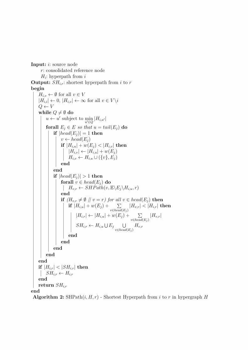
Input: i: source noder: consolidated reference nodeHi: hyperpath from i
Output: SHi,r: shortest hyperpath from i to rbegin
Hi,v ← ∅ for all v ∈ V|Hi,i| ← 0, |Hi,v| ← ∞ for all v ∈ V \iQ← Vwhile Q 6= ∅ do
u← u′ subject to minu′∈Q|Hi,u′ |
forall Ej ∈ E so that u = tail(Ej) doif |head(Ej)| = 1 then
v ← head(Ej)if |Hi,u|+ w(Ej) < |Hi,v| then|Hi,v| ← |Hi,u|+ w(Ej)Hi,v ← Hi,u ∪ (v, Ej)
endendif |head(Ej)| > 1 then
forall v ∈ head(Ej) doHv,r ← SHPath(v,E\Ej\Hi,u, r)
endif (Hv,r 6= ∅ || v = r) for all v ∈ head(Ej) then
if |Hi,u|+ w(Ej) + ∑v∈head(Ej)
|Hv,r| < |Hi,r| then
|Hi,r| ← |Hi,u|+ w(Ej) + ∑v∈head(Ej)
|Hv,r|
SHi,r ← Hi,u⋃Ej
⋃v∈head(Ej)
Hv,r
endend
endend
endif |Hi,r| < |SHi,r| then
SHi,r ← Hi,r
endreturn SHi,r
endAlgorithm 2: SHPath(i,H, r) - Shortest Hyperpath from i to r in hypergraph H
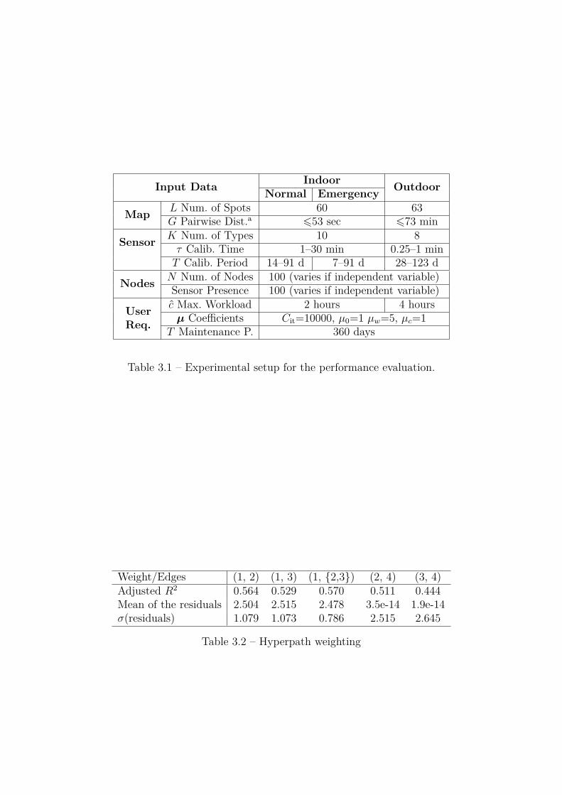
Input Data Indoor OutdoorNormal Emergency
Map L Num. of Spots 60 63G Pairwise Dist.a 653 sec 673 min
Sensor K Num. of Types 10 8τ Calib. Time 1–30 min 0.25–1 minT Calib. Period 14–91 d 7–91 d 28–123 d
Nodes N Num. of Nodes 100 (varies if independent variable)Sensor Presence 100 (varies if independent variable)
UserReq.
c Max. Workload 2 hours 4 hoursµ Coefficients Cit=10000, µ0=1 µw=5, µc=1
T Maintenance P. 360 days
Table 3.1 – Experimental setup for the performance evaluation.
Weight/Edges (1, 2) (1, 3) (1, 2,3) (2, 4) (3, 4)Adjusted R2 0.564 0.529 0.570 0.511 0.444Mean of the residuals 2.504 2.515 2.478 3.5e-14 1.9e-14σ(residuals) 1.079 1.073 0.786 2.515 2.645
Table 3.2 – Hyperpath weighting

Chapter 4
Leveraging Crowdensors to supportContext-aware and cost-effective
Crowdsensing
4.1 Introduction
Crowdsensing is becoming one of the most promising paradigms supporting the vision ofsocial sensing: citizens may contribute valuable spatio-temporal observations using the low-cost,yet powerful, sensors embedded in their smartphones/tablets, with the GPS for positioning andthe Internet access for uploading. As opposed to mere physical equipment that only senses theenvironment and transfers data, crowdsensor should be treated as "social sensor".
There is a wide range of users’ engagements to sensing tasks [94, 65], which depend on howthe smartphones’ owners contribute observations [94, 65], which may be either: (i) pro-actively,aka participatory crowdsensing [74, 90]; or (ii) passively in the background, aka opportunis-tic crowdsensing [37, 102]. Participatory crowdsensing allows covering a specific area whilemaximising the number of tasks that each participant may achieve [91] through careful pathplanning. On the other hand, opportunistic crowdsensing makes it easy to collect a massiveamount of observations across time and space. Indeed, there is no burden put on the end-users.The human presence in the sensing loop brings into the picture new research challenges, mostof which are yet to be understood and addressed. With participatory sensing, the massive col-lection of data often necessitates the participants’ long term commitments, which are very hardto achieve in practice, mainly due to the practical problem of "hiring" motivated volunteers.Participants lack the technical skills required to set-up and maintain sensors. Participatorysensing is critiqued as a top-down approach allowing non-experts to participate in scientificprogress. In other words, participatory sensing is perceived as being closer to a participatorypush [62] as opposed to a “form of science developed and enacted by citizens themselves”. Onthe other hand, the opportunistically-collected observations often cover the urban space andtime unevenly, due to the mobility of citizens throughout the city. In addition, previous analysis[83, 165] on the noise observations collected from the opportunistic crowdsensing applicationAmbiciti (formerly SoundCity), showed that less than 5% of the collected data were of sufficientquality to be considered for use in the mapping of urban noise pollution.
Our approach to support the democratisation of environmental crowdsensing, lies in sup-porting an opportunistic and collaborative crowdsensing. State-of-the-art opportunistic crowd-sensing systems address the aforementioned shortcoming – namely the uneven coverage of theurban space and the low-quality of the collected observation – through the centralised analysis –spanning filtering, aggregation and interpolation– of the contributed observations on cloud/edgeinfrastructure servers [93, 108, 69, 68, 166]. The implemented centralisation then severely limitsthe adoption of crowdsensing for environmental monitoring due the resulting resource cost andthreat to privacy. Instead, our approach is to allow a fully distributed, collaborative approach
63

Chapter 4 – Leveraging Crowdensors to support Context-aware and Cost-effective Crowdsensing
to crowdsensing: Crowdsensors interpolate data, and aggregate their respective contributionsto the observations of the phenomenon in a collaborative way, so as to overcome the spatio-temporal sparsity and to limit –or even avoid– the use of a centralised infrastructure server. Wesupport a distributed solution to the problem of collection, interpolation and aggregation on theMove, which builds upon the two following trends to support crowdsensing-based environmentalmonitoring at scale:
(i) We view crowdsensors as "social sensors" that often encounter each other during crowd-sensing campaigns or as part of their owners’ daily routine. When the crowdsensing isopportunistic, participants follow their daily routine without being directly involved in thesensing task [37]. Thus, at the micro level, behavioural signatures (i.e., routines) as wellas recurrent meeting patterns reflect the underlying relational dynamics of organisationsor communities to which the user is affiliated [97]. Participatory crowdsensing campaignsbring groups of people together to meet, exchange information and share their findings[10], with the aim of improving the quality of the data collected for better impact on theground [18]. Compared to the opportunistic crowdsensing, participants in participatorycampaigns meet more often and contribute finer scale measurements but cover smaller ar-eas [169]. In both cases, the end-users are more likely to share their information, especiallyin short meetings, as the risk of losing their anonymity is lower [88].
(ii) The control of the sensing process is delegated to people, who may choose to deliver (ornot) relevant information depending on their context as well as their personal constraints,such as financial budget, time, smartphone battery, available network bandwidth. Otherfactors may also influence the quality of submitted sensing measurements. In particular,smartphone sensors are not typically of the same fidelity as task-specific sensors (e.g.,a noise pollution monitor vs. smartphone microphone). Besides, inadvertent erroneoushandling of the phone (e.g., phone acting as a noise sensor located in the pocket) coupledwith the lack of experience in performing the sensing task (e.g. blurry photo captured bymistake) may adversely influence the quality of the data, irrespective of the willingnessof the participants.
(iii) The collaborative and ubiquitous processing of crowdsensor observations improves theoverall efficiency of the system in terms of resource consumption [176], regarding boththe infrastructure and contributing devices. It also allows end users to collaborate andshare knowledge effortlessly and with little or no cost. In particular, D2D collaborationenhances mobile edge computing by enabling the sharing of heterogeneous computing andcommunication resources between powerful mobile end-devices [36].
The design rationale of our crowdsensing solution directly derives from the social nature andin particular from the location-, context- and time-dependence of the crowdsensors: co-locatedcrowdsensors contribute related observations [96], and may thus collaborate toward improvingthe provided contributions and avoiding unnecessary duplication of work. More precisely, thecrowdsensing tasks that need to be performed at the edge encompass: environment sensing,location provisioning, data processing, and uploading to the cloud. Then, while the replica-tion of physical sensing within a group potentially allows for the gathering of more accurateknowledge, any of the other tasks only need to be performed by the most cost-effective groupmember(s). The fact that people tend to group [43, 150] as part of their daily activity, followa daily/weekly routine [61, 47], and are most of the time still [83] further supports such aedge-based collaborative strategy to opportunistic crowdsensing.
64
4.2. Context-Awareness sustaining a Collaborative Crowdsensing
Beyond the user’s mobility which is relevant to initiate the collaboration with the nearbycrowdsensors, to know whether the smartphone is in-/out-pocket, in-/out-door and under-/on-ground is particularly important because the smartphone/sensing device needs to be ina position that enables – yet does not interfere with – sensing the physical characteristics ofthe surrounding. The sensing context must distinguish between in-pocket and out-pocket ob-servations because the former lead to a quite significant deviation from the ground truth andare thus not readily usable [130]. The same applies to in-door versus out-door – as much asunder-ground and on-ground – measurements since aggregating them together to analyse en-vironmental phenomena obviously leads to unreliable results [106]. The context informationallows keeping more observations -and even correcting them- for aggregating environmentalknowledge, rather than filtering out drastically the crowdsensed data. We qualify as "context"the combination of these criteria. Our aim is to create dynamic context-aware collaborativegroups of crowdsensors, which are such that the peers within any given group: (i) Stay togetherfor a long-enough time period so as to prevent constant changes and unnecessary grouping re-configuration; (ii) Operate within the same physical environment (e.g., in-door vs out-door) andhence sense related physical phenomena; and (iii) Perform the same activity so that they behavealike –e.g., it is preferable that all the crowdsensors that collaborate either move together or arestill. Then, upon the creation of a group, the middleware distributes the crowdsensing tasks tothe most adequate group members according to the nodes’ abilities –e.g., a smartphone locatedin the pocket cannot adequately sense the surrounding sound level. Overall, our approach fos-ters opportunistic collection of the observations that puts minimum burden on the end-users,while increasing the accuracy and resource-efficiency of the crowdsensing system.
Still, a major issue is to cope with the absence of observations due to the uneven distributionof the crowdsensors and the resulting spatio-temporal sparsity of crowdsensors in some specificareas. Concretely, our solution also allows a fully distributed, collaborative approach to supportthe interpolation of data and aggregation of the respective contributions to the observationsof the phenomenon, so as to overcome the spatio-temporal sparsity and to limit –or evenavoid– the use of a centralised infrastructure server. There are many interpolation methods forinferring spatio-temporal phenomena, and the smartphone is becoming increasingly powerful toperform such advanced tasks. At the same time, P2P wireless ad hoc network technology (e.g.,WiFi Direct) enables the discovery of nearby mobile devices and the exchange of data betweenpeers, making the collaboration possible [54]. Some crowdsensing systems already exploit theP2P collaboration of crowdsensors as they meet [170, 46, 177]. However, the collaborationprimarily deals with handling the relay of data, while deployed static edge servers are in chargeof the distributed data aggregation. Our approach leverages the advantage of the former andovercomes the disadvantage of the latter: it implements an opportunistic data relay and analysis– spanning the interpolation and aggregation – on the move, across the crowdsensors.
4.2 Context-Awareness sustaining a Collaborative Crowd-sensing
A major challenge is to cope with the dynamics and heterogeneity of the crowdsensors: the useractivity, the resources available on the device, and the position of the sensors/smartphones areall criteria that characterise the crowdsensor’s contribution to the upper layer application. Wequalify as context the combination of these criteria.
The accurate monitoring of the physical environment through crowdsensing requires thecontextualisation of the contributed observations because the context impacts the quality of
65

Chapter 4 – Leveraging Crowdensors to support Context-aware and Cost-effective Crowdsensing
the quantitative observations that mobile crowdsensing gathers.Characterising the contextof crowdsensed observations has been extensively studied regarding the recognition of theuser activity and more specifically the mobility condition (whether moving and with whichmean) [122, 134]. On the other hand, inferring the sensing context with respect to the physicalenvironment under scrutiny has received less attention, while related solutions focus on a singlecontext element and do not account for the diversity of the contributing devices. Yet, it isessential to infer together the context elements that impact the crowdsensing, as they are allequally important. While considering a variety of eligible features, one should account for thevariation in the availability of features across the contributing devices. Our approach addressesthese requirement by being self-adaptive to the diversity of users (and devices). As a first step,we start from the characterisation of the crowdsensor context, spanning from the physical en-vironment, user’s activity and device capabilities. In particular, we provide a ranking over allthe candidate features so as to compose the most significant feature set for each classification.Then, the user-centric classification on the user’s device may be performed on any subset of theabove set so as to account for the diversity of devices and related embedded sensors. The setmay further be customised and freely recomposed, trading off energy efficiency and accuracy,to offer adaptiveness.
The sensing context must distinguish between in-pocket and out-pocket observations be-cause the former leads to a quite significant deviation from the ground truth and are thusnot readily usable [43]. The same applies to both in-door versus out-door measurements aswell as under-ground versus upper-ground readings since aggregating them together to analyseenvironmental phenomena obviously leads to unreliable results [83].
Overall, the major outcome of the group-based collaboration is:
• A context inference module for crowdsensor to provide explicit context information in-cluding both device attributes and user behaviours (§ 4.2.1).
• A context-based grouping to share position/internet and optimise the crowdsensing tasks,so as to decrease power consumption during registration and task assignments (§ 4.3).
• A context-based data aggregation/pre-processing module for crowdsensing groups in orderto decrease the Internet traffic toward the cloud (§ 4.4.1).
4.2.1 Context CharacterisationThe context of a crowdsensor serves assessing the relevance of its peering with nodes in theD2D communication range for the sake of enhanced efficiency, that is, the ability to improvethe gathered knowledge prior to transferring it to the cloud in a way that reduces resource-consumption. In addition, determining how long the current context is going to last is criticalto ensure that the benefit of the collaborative crowdsensing at the edge outperforms the over-head due to the group management/configuration. The context characterises the crowdsensor’scollaboration profile, which subdivides into:
• PE (Physical Environment) defines the position of the embedded sensors, which influencesthe given observations of physical phenomena. It detects if the crowdsensor is: in/out-pocket, in/out-door and under/above-ground.
• UA (User Activity) refers to the mobility (walking, cycling, driving) or non-mobility(still) of the end-user. In order to support the activity recognition, we rely on the activityrecognition module [57] implemented by the operating system.
66
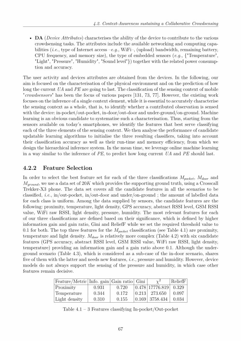
4.2. Context-Awareness sustaining a Collaborative Crowdsensing
• DA (Device Attributes) characterises the ability of the device to contribute to the variouscrowdsensing tasks. The attributes include the available networking and computing capa-bilities (i.e., type of Internet access –e.g., WiFi–, (upload) bandwidth, remaining battery,CPU frequency, and memory size), the type of embedded sensors (e.g., "Temperature","Light", "Pressure", "Humidity", "Sound level") together with the related power consump-tion and accuracy.
The user activity and devices attributes are obtained from the devices. In the following, ouraim is focused on the characterisation of the physical environment and on the prediction of howlong the current UA and PE are going to last. The classification of the sensing context of mobile"crowdsensors" has been the focus of various papers [131, 73, 77]. However, the existing workfocuses on the inference of a single context element, while it is essential to accurately characterisethe sensing context as a whole, that is, to identify whether a contributed observation is sensedwith the device: in-pocket/out-pocket, in-door/out-door and under-ground/on-ground. Machinelearning is an obvious candidate to systematise such a characterisation. Thus, starting from thesensors available on today’s smartphones, we identify the features that best serve classifyingeach of the three elements of the sensing context. We then analyse the performance of candidateupdatable learning algorithms to initialise the three resulting classifiers, taking into accounttheir classification accuracy as well as their run-time and memory efficiency, from which wedesign the hierarchical inference system. In the mean time, we leverage online machine learningin a way similar to the inference of PE, to predict how long current UA and PE should last.
4.2.2 Feature SelectionIn order to select the best feature set for each of the three classifications Mpocket, Mdoor andMground, we use a data set of 20K which provides the supporting ground truth, using a CrosscallTrekker-X3 phone. The data set covers all the candidate features in all the scenarios to beclassified, i.e., in/out-pocket, in/out-door and under/on-ground ; the amount of labelled datafor each class is uniform. Among the data supplied by sensors, the candidate features are thefollowing: proximity, temperature, light density, GPS accuracy, abstract RSSI level, GSM RSSIvalue, WiFi raw RSSI, light density, pressure, humidity. The most relevant features for eachof our three classifications are defined based on their significance, which is defined by higherinformation gain and gain ratio, Gini and ReliefF while we set the required threshold value to0.1 for both. The top three features for the Mpocket classification (see Table 4.1) are proximity,temperature and light density. Mdoor is relatively more complex (Table 4.2) with six candidatefeatures (GPS accuracy, abstract RSSI level, GSM RSSI value, WiFi raw RSSI, light density,temperature) providing an information gain and a gain ratio above 0.1. Although the under-ground scenario (Table 4.3), which is considered as a sub-case of the in-door scenario, sharesfive of them with the latter and needs new features, i.e., pressure and humidity. However, devicemodels do not always support the sensing of the pressure and humidity, in which case otherfeatures remain decisive.
Feature/Metric Info. gain Gain ratio Gini χ2 ReliefFProximity 0.931 0.720 0.478 17776.819 0.329Temperature 0.344 0.172 0.213 273.650 0.097Light density 0.310 0.155 0.169 3758.434 0.034
Table 4.1 – 3 Features classifying In-pocket/Out-pocket
67
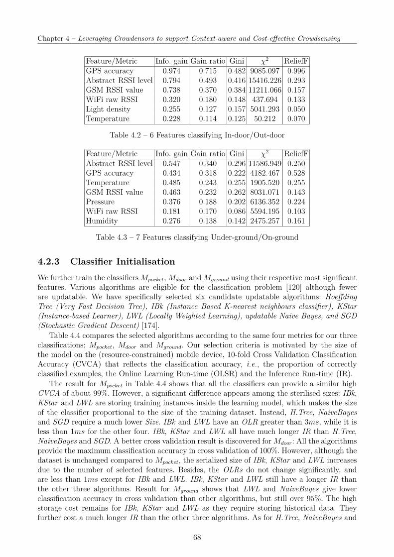
Chapter 4 – Leveraging Crowdensors to support Context-aware and Cost-effective Crowdsensing
Feature/Metric Info. gain Gain ratio Gini χ2 ReliefFGPS accuracy 0.974 0.715 0.482 9085.097 0.996Abstract RSSI level 0.794 0.493 0.416 15416.226 0.293GSM RSSI value 0.738 0.370 0.384 11211.066 0.157WiFi raw RSSI 0.320 0.180 0.148 437.694 0.133Light density 0.255 0.127 0.157 5041.293 0.050Temperature 0.228 0.114 0.125 50.212 0.070
Table 4.2 – 6 Features classifying In-door/Out-door
Feature/Metric Info. gain Gain ratio Gini χ2 ReliefFAbstract RSSI level 0.547 0.340 0.296 11586.949 0.250GPS accuracy 0.434 0.318 0.222 4182.467 0.528Temperature 0.485 0.243 0.255 1905.520 0.255GSM RSSI value 0.463 0.232 0.262 8031.071 0.143Pressure 0.376 0.188 0.202 6136.352 0.224WiFi raw RSSI 0.181 0.170 0.086 5594.195 0.103Humidity 0.276 0.138 0.142 2475.257 0.161
Table 4.3 – 7 Features classifying Under-ground/On-ground
4.2.3 Classifier InitialisationWe further train the classifiersMpocket,Mdoor andMground using their respective most significantfeatures. Various algorithms are eligible for the classification problem [120] although fewerare updatable. We have specifically selected six candidate updatable algorithms: HoeffdingTree (Very Fast Decision Tree), IBk (Instance Based K-nearest neighbours classifier), KStar(Instance-based Learner), LWL (Locally Weighted Learning), updatable Naive Bayes, and SGD(Stochastic Gradient Descent) [174].
Table 4.4 compares the selected algorithms according to the same four metrics for our threeclassifications: Mpocket, Mdoor and Mground. Our selection criteria is motivated by the size ofthe model on the (resource-constrained) mobile device, 10-fold Cross Validation ClassificationAccuracy (CVCA) that reflects the classification accuracy, i.e., the proportion of correctlyclassified examples, the Online Learning Run-time (OLSR) and the Inference Run-time (IR).
The result for Mpocket in Table 4.4 shows that all the classifiers can provide a similar highCVCA of about 99%. However, a significant difference appears among the sterilised sizes: IBk,KStar and LWL are storing training instances inside the learning model, which makes the sizeof the classifier proportional to the size of the training dataset. Instead, H.Tree, NaiveBayesand SGD require a much lower Size. IBk and LWL have an OLR greater than 3ms, while it isless than 1ms for the other four. IBk, KStar and LWL all have much longer IR than H.Tree,NaiveBayes and SGD. A better cross validation result is discovered forMdoor: All the algorithmsprovide the maximum classification accuracy in cross validation of 100%. However, although thedataset is unchanged compared to Mpocket, the serialized size of IBk, KStar and LWL increasesdue to the number of selected features. Besides, the OLRs do not change significantly, andare less than 1ms except for IBk and LWL. IBk, KStar and LWL still have a longer IR thanthe other three algorithms. Result for Mground shows that LWL and NaiveBayes give lowerclassification accuracy in cross validation than other algorithms, but still over 95%. The highstorage cost remains for IBk, KStar and LWL as they require storing historical data. Theyfurther cost a much longer IR than the other three algorithms. As for H.Tree, NaiveBayes and
68
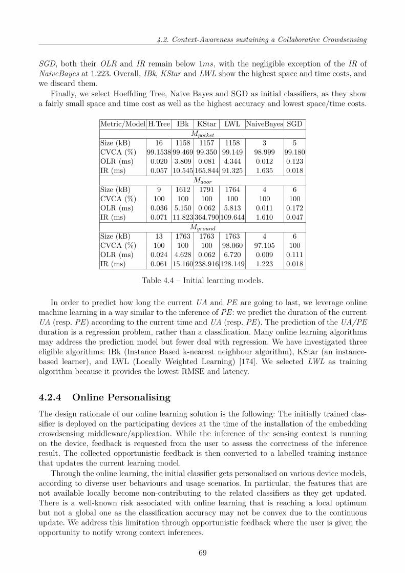
4.2. Context-Awareness sustaining a Collaborative Crowdsensing
SGD, both their OLR and IR remain below 1ms, with the negligible exception of the IR ofNaiveBayes at 1.223. Overall, IBk, KStar and LWL show the highest space and time costs, andwe discard them.
Finally, we select Hoeffding Tree, Naive Bayes and SGD as initial classifiers, as they showa fairly small space and time cost as well as the highest accuracy and lowest space/time costs.
Metric/Model H.Tree IBk KStar LWL NaiveBayes SGDMpocket
Size (kB) 16 1158 1157 1158 3 5CVCA (%) 99.1538 99.469 99.350 99.149 98.999 99.180OLR (ms) 0.020 3.809 0.081 4.344 0.012 0.123IR (ms) 0.057 10.545 165.844 91.325 1.635 0.018
Mdoor
Size (kB) 9 1612 1791 1764 4 6CVCA (%) 100 100 100 100 100 100OLR (ms) 0.036 5.150 0.062 5.813 0.011 0.172IR (ms) 0.071 11.823 364.790 109.644 1.610 0.047
Mground
Size (kB) 13 1763 1763 1763 4 6CVCA (%) 100 100 100 98.060 97.105 100OLR (ms) 0.024 4.628 0.062 6.720 0.009 0.111IR (ms) 0.061 15.160 238.916 128.149 1.223 0.018
Table 4.4 – Initial learning models.
In order to predict how long the current UA and PE are going to last, we leverage onlinemachine learning in a way similar to the inference of PE : we predict the duration of the currentUA (resp. PE) according to the current time and UA (resp. PE). The prediction of the UA/PEduration is a regression problem, rather than a classification. Many online learning algorithmsmay address the prediction model but fewer deal with regression. We have investigated threeeligible algorithms: IBk (Instance Based k-nearest neighbour algorithm), KStar (an instance-based learner), and LWL (Locally Weighted Learning) [174]. We selected LWL as trainingalgorithm because it provides the lowest RMSE and latency.
4.2.4 Online PersonalisingThe design rationale of our online learning solution is the following: The initially trained clas-sifier is deployed on the participating devices at the time of the installation of the embeddingcrowdsensing middleware/application. While the inference of the sensing context is runningon the device, feedback is requested from the user to assess the correctness of the inferenceresult. The collected opportunistic feedback is then converted to a labelled training instancethat updates the current learning model.
Through the online learning, the initial classifier gets personalised on various device models,according to diverse user behaviours and usage scenarios. In particular, the features that arenot available locally become non-contributing to the related classifiers as they get updated.There is a well-known risk associated with online learning that is reaching a local optimumbut not a global one as the classification accuracy may not be convex due to the continuousupdate. We address this limitation through opportunistic feedback where the user is given theopportunity to notify wrong context inferences.
69

Chapter 4 – Leveraging Crowdensors to support Context-aware and Cost-effective Crowdsensing
Gathering feedback should be limited as much as possible to minimise the burden on theuser, while still enhancing the accuracy of our three classifiers Mpocket, Mdoor and Mground overtime. We achieve the above by applying a hierarchical inference and update of the classifiers.While more detail about the hierarchical inference (along with the related Algorithm) can befound in [51], the design rational of the hierarchical follows from the predominant role of thein-pocket classifier over the two others and of the in-door classifier over the under-ground onewhen sensing the physical environment. Specifically, a crowdsensed measurement is relevant ifout-pocket. Thus, the in-door/out-door detection is meaningful only when the device is out-pocket and ready for sensing. Further, the under-ground/on-ground case is a sub-scenario ofthe in-door situation. Similarly, requesting the user’s feedback is sensible only if the user is inthe position to easily do so. Typically, requesting feedback when the device is in the pocket istoo cumbersome for the user.
4.3 Assessing the Crowdsensor UtilitiesWe introduce a set of utility functions to evaluate the extent to which crowdsensors are eli-gible to carry out the various crowdsensing tasks. The following crowdsensing tasks must beimplemented within any collaborative group: Coordinator (implementing the D2D network ac-cess point for the group and assigning the crowdsensing tasks to the connected crowdsensors,i.e.,neighbours), Location provider (supplying geographical coordinates), Internet proxy (pro-viding Internet access and thus transferring data to the cloud), Data aggregator (analysingtogether the collected data locally before sending to the cloud to, e.g., calibrate the sensors[149], analyse the data [165]), and, of course, Sensors. In practice, we rely on the followingclassical squashing function f for the normalisation of the values used in the computation andcomparison of the utilities:
f(x, k, x0) = 11 + ek(x0−x)
where: the range of f lays into (0, 1), k is the logistic growth rate or steepness of the curve,and x0 is the x-value of the midpoint of sigmoid, while x is the variable to be normalised. Thevalues of k and x0 are set according to the domain of the specific x. In the following, we denotekf and xf the values of k and x0 for a given function f , while the actual values of the variousparameters have been set during the prototype evaluation. Next, we further define the utilityfunctions for each crowdsensing tasks, relying on the squashing function that normalises thevalues (as defined in Table 4.5)
Coordinator
- The selection of the coordinator is based on the following criteria:
• The number of neighbours Ni has a significant impact on the overall performance becauseincreasing the number of collaborators enables analysing more data locally and reducingthe transfer of data to the cloud. In contrast, there is no benefit in creating groups withtoo few crowdsensors for which the minimum value δ depends on the application.
• The occurrences of collaboration hi between a crowdsensor i and its neighbours is anotherrelevant parameter as it reveals the relationship between crowdsensors materialised bythe sharing of daily routines, habits, activities.
• The UA and PE (except pocket) di of the crowdsensor should last sufficiently long.
70

4.3. Assessing the Crowdsensor Utilities
Parameter Function Parameter(s)Sufficient number ∆i = f(max0, |Ni| − δ, k∆, x∆) Ni : neighbours
of neighbours δ: minimum value
Collaboration hi = f(∑
j∈Nitcollab(i,j)|Ni| , kh, xh) tcollab(i, j): number of times
occurences i collaborated with j
Context (i.e., UA, PE) di = f(mindur(UA), dur(PE), dur(UA), resp. dur(PE)durability kd, xd) predicted duration of the
current UA, resp. PERemaining battery bi = f(bati, kb, xb) bati: remaining
capacity batteryAccuracy li = f(accl, kl, xl)− f(powl, kl, xl) accl: accuracy
versus power pow: powerUpstream ni = f(bwup, kn, xn)− f(pownet, bwup: Bandwidthbandwidth knp, xnp) pownet: power consumedversus power for transmission
Accuracy vs power d′i = f(dur(PEout), kd, xd) dur(PEout): duration of thecrowdsensor being out of the pocket
Table 4.5 – Set of parameters used to measure the utility associated with a task
• The remaining battery capacity bi of the crowdsensor should obviously be taken intoaccount.
Next, provided the weights w∆, wh, wd, wb, all ∈ [0, 1], set for the above criteria, we definethe utility uc(i) of the crowdsensor i associated with acting as coordinator as the weighted sumof the above functions:
uc(i) = w∆.∆i + wh.hi + wd.di + wb.bi
Location provider
On a smartphone, the location is either GPS- or network-based. While the GPS location bringshigher accuracy out-door, it also comes with higher energy consumption and latency, comparedto the network-based location. The utility function for crowdsensor i of being a location provideris thus defined as ul(i), which accounts for the location service source1, location accuracy andremaining battery capacity:
ul(i) = li + wd.di + wb.bi
Internet proxy
The Internet proxy transfers the (analysed) data provided by the group of crowdsensors to thecloud server. The service may be provided using either long range cellular or short range WiFitransmission, while we assume that a node supporting both networks will offer the WiFi basedtransmission by default. The utility function up(i)) for crowdsensor i acting as Internet proxythen accounts for the Internet connection interface, up-link network bandwidth, and remainingbattery capacity:
up(i) = ni + wd.di + wb.bi
1. Note that when the location service not operational, li = −∞.
71

Chapter 4 – Leveraging Crowdensors to support Context-aware and Cost-effective Crowdsensing
Data aggregator
The data aggregator provides in charge the analysis of the sensing data collected locally. Whilelightweight data processing can be performed by the coordinator or by the proxy, complex dataanalysis may be delegated to a dedicated device that holds the necessary processing capabilities(spanning available memory, CPU frequency and remaining battery capacity). This results inthe following definition for the supporting utility function ua(i):
ua(i) = wc.[f(cpui, kc, xc) − f(powc, kcp, xcp)] + wr.f(memi, kr, xr) + wd.di + wb.bi
where: cpui is the CPU frequency, powc is the power consumption of the CPU, memi is theavailable memory, and coefficients wc, wr are the weights set for the metrics.
Sensors
The utility of a crowdsensor to carry out the sensing task depends on the accuracy of thecontributed observations and their power consumption. In particular, a crowdsensor within apocket/bag is ignored, which we filter out using the duration of the crowdsensor being out ofthe pocket (as defined by the PEout value of PE):which leads to the following utility function, us(i) ∈ (−1, 1 + wd):
us(i) = d′i.[f(accsi , ka, xa)− f(powsi , ksp, xsp) + wd.di]
where: accsi (resp. powsi ) is the accuracy (resp. power consumption) of the sensor of type s oncrowdsensor i.
Utility-based Grouping
Provided the utility functions, the grouping algorithm leverages the communication and discov-ery protocols implemented at the link layer by state of the art D2D communication technologies.Without loss of generality, our grouping algorithm builds upon the WiFi Direct technology [9].In a nutshell, WiFi Direct establishes a D2D opportunistic network through the discovery ofpeer nodes followed by the election of the node acting as the network’s access point accordingto the criteria provided by the upper layer (i.e., in our case, the coordinator utility value pro-vided by the middleware). Furthermore, the grouping algorithm runs on every node i, eitheron-demand or on a periodic basis according to the network’s dynamics. Once a group is created,the arrival/departure of nodes is detected at the link layer by the underlying D2D protocol.This enables two approaches to the reconfiguration of the group: (i) on a periodic basis, or (ii)on-demand upon the detection of the departure/arrival of a group member. The latter per-forms very well and induces almost no cost when very few topology changes occur and whenthe context evolves slowly. On the other hand, it may lead to a unnecessarily high traffic andconstant reassignment in a highly dynamic environment. Keeping in mind that, in practice,users are still most of the time (and hence evolving in the same context), by default we adoptan on-demand approach (based on context change). Nevertheless, the middleware switches toperiodic re-assignment when the context gets highly dynamic. Subsequently, our work focuseson a distributed interpolation and aggregation approach running on the crowdsensors to achieveboth higher sensing quality and efficiency.
72
4.4. Opportunistic Aggregation and Interpolation
4.4 Opportunistic Aggregation and InterpolationA mobile crowdsensing application dealing with urban pollution monitoring (e.g., noise, airquality, water quality, etc.) needs to sense, pre-process, interpolate, then aggregate and relaymeasurements in a P2P way so as to favour computation at the edge and thereby limit theresource and financial costs associated with the use of the cloud infrastructure. Concretely, weattempt to support a fully distributed, collaborative approach to crowdsensing, in which crowd-sensors further interpolate data, and aggregate their respective contributions to the observationsof the phenomenon in a collaborative way. The intent is to overcome the spatio-temporal spar-sity and to limit –or even avoid– the use of a centralised infrastructure server. There are manyinterpolation methods for inferring spatio-temporal phenomena ; the smartphone is becomingincreasingly powerful to perform such advanced tasks. However, the collaboration [170, 46, 177]primarily deals with handling the relay of data, while deployed static edge servers are in chargeof the distributed data aggregation. Our approach leverages the advantage of the former andovercomes the disadvantage of the latter: it implements an opportunistic data relay and analysison the move, across the crowdsensors.
In particular, our solution supports the repeated monitoring of a physical phenomena over (apossibly large) area over a given time period D using the contributions of the m crowdsensors.The data that each crowdsensor collects is represented as a concise 3-dimensional tensor wherethe first two dimensions refer to the spatial space and the third one to the temporal domain.In particular, we discretise the target region into a I × J area, which contains equally spacedgrid points. We also discretise D into K time slots of equal duration.
We denote Ys ∈ RI×J×K the tensor that crowdsensor s (1 ≤ s ≤ m) maintains and that issuch that entry y(x) ∈ R at position x := (i, j, k) ∈ R3 is the average of the measurements col-lected by s over the area indexed by (i, j) during the time interval indexed by k. In other words,any crowdsensor s contributes a tensor Ys that provides a sparse/incomplete observation of thephysical phenomenon according to s behaviour. The middleware then allows the opportunisticcombination of the various tensors Ys (1 ≤ s ≤ m) using interpolation and aggregation so asto compute an overall Y .
The periodic process runs on every participating crowdsensor to compute Y . The processiterates over time windows of duration D. Within a given time window T+D, the process runsin parallel: (i) the collection of the measurements provided by the embedded sensors to updatethe tensor Ys(T+D) of the current time window, and (ii) the opportunistic aggregation of thelocal tensor of the previous time window T with the ones of peers as they meet (see detail in§ 4.4.2). At the end of the time window, GPR-based spatio-temporal interpolation is appliedon the associated local tensor to recover missing values (see detail in § 4.4.1). We highlight thatthe interpolation is run locally, only once and prior to the aggregation process run over thenext time window because: (i) the number of occurrences must be minimised due to the highcost of the interpolation computation, and (ii) the local interpolated tensor allows assessing thequality of the local measurements against the ones of the peers that the node meets, which theaggregation process leverages. Finally, at the end of the current time window T+D, the nodeultimately sends its local tensor to the cloud, unless it got aggregated and relayed by anotherpeer.
4.4.1 Spatio-temporal InterpolationGiven a sparse tensor Ys resulting from the averaging of the local measurements collectedat s over time duration D, interpolation allows completing the tensor by estimating missing
73

Chapter 4 – Leveraging Crowdensors to support Context-aware and Cost-effective Crowdsensing
observations. The dense tensor Ys denotes the resulting (denser) tensor. The quality of theestimation can be established based on the approximation error (i.e., residual) at point x, thatis: e(x) := |y(x)− y(x)| where we recall that the function y : R3 7→ R maps an arbitrary pointx := (i, j, k) to its observation value y(x). The overall residual is then given by E = ‖Y − Y‖.
Let Ω be the set of observation points collected by a given crowdsensor. The boolean masktensorM ∈ BI×J×K is defined such that m(x) = 1 if there is a corresponding value within Ω,and m(x) = 0 otherwise. Thus,M∗ Y provides the actual observations (i.e., ground truth assensed). When estimating Y based on a sparse tensor Y with mask M, we seek to minimisethe following loss function, which is associated with the approximation Y :
J(Y , Y) := 12∑x∈Ω
e(x)2 = 12‖M ∗ (Y − Y)‖2
where: ‖ · ‖ denotes the Euclidean norm of a tensor, and ∗ represents the element-wise multi-plication.
We leverage Gaussian Process Regression (GPR) [132] to compute Y out of Y . That is, weassume that y follows a Gaussian Process (Gaussian distribution over functions), i.e.,:
y(x) ∼ GP(µ(x), k(x, x′))
where: µ(x) = E[y(x)] refers to the mean function, and k(x, x′) is the covariance matrix, i.e.,the kernel of the GPR, which verifies k(x, x′) = E[(y(x)− µ(x))(y(x′)− µ(x′))].
The covariance function is a crucial ingredient of GPR as it encodes the notion of similaritybetween two nearby data points x and x′ on the basis that observations that are close toeach other (in both time and space) are likely to have higher correlation. Various familiesof covariance functions exist (see [132] for an overview), including, e.g., squared exponential,polynomial, and Matérn class. In our case, the Matérn class [110] induced the lowest error andruntime compared to alternative functions.
We assume that the observation y is noisy, which is more realistic. We therefore consider aregression that aims at establishing y = y(x) + ε where: the function y(x) follows a GaussianProcess, i.e., y(x) ∼ GP(µ, k), and the noise is additive, independent, and corresponds to anidentically distributed Gaussian noise: ε ∼ N (0, σ2
e). Furthermore, given n observed valuesY = [y1, · · · , yn]> obtained at the location points X = [x1, · · · , xn]>, the joint distribution of[y(x1), · · · , y(xn)]> follows a Gaussian distribution:
[y(x1), · · · , y(xn)]> ∼ N (µ,K)
where: µ = [µ(x1), · · · , µ(xn)]> refers to the mean vector, and K is a n× n covariance matrixwith Kij = k(xi, xj).
Our interpolation aims at inferring Y ∗ = y(X∗), which includes m unobserved points storedin the tensor X∗ = [x∗1, · · · , x∗m]>.The inferred tensor Y ∗ follows a Gaussian distribution:
p(Y ∗|X∗, X, Y ) = N (µ, σ2 + σ2eI)
With a mean and variance of Y ∗ respectively estimated as:
µ = K(X,X∗)>[K(X,X) + σ2eI]−1Y
σ2 = K(X∗, X∗)−K(X,X∗)>[K(X,X) + σ2eI]−1K(X,X∗)
74

4.4. Opportunistic Aggregation and Interpolation
Once the GPR model is trained, the mean value µ and variance σ of any given point x areinferred. In addition, the complete approximation tensor Y is provided along with the variancetensor Σ2 ∈ RI×J×K , in which each element σ2 provides the variance of the corresponding µ,namely y(x). Note that GPR is computationally demanding as the training scales in O(n3) withn being the number of observations. Thus, applying such a regression over the overall dataset atthe cloud incurs significant computation and financial costs. As an alternative, the middlewaredistributes the training and inference load over the crowdsensors in an opportunistic way.
4.4.2 Opportunistic AggregationThe design of the middleware is such that it favours the occurrences of aggregation among thecrowdsensors over the ones of the cloud for the sake of lowering the overall computation andcommunication costs at the cloud, while maintaining the same data quality. To achieve this,our middleware implements an opportunistic aggregation approach. Upon a meeting (involvinga shared D2D communication range) of two crowdsensors s and s′, the middleware selects oneof the two to aggregate their respective tensors Ys and Ys′ . Assuming the selected node is s,then Ys is updated as the aggregation of Ys and Ys′ , and Ys′ is set to the null tensor. Then, srelays Ys till it meets another crowdsensor or till the current time window T+D expires in whichcase s sends the tensor to the cloud.
The crowdsensor that is the best suited to act as the relay node is the one that will meetthe highest number of nodes in the future and thus minimises the occurrences of Ac. Weconsider that the respective inference quality of the tensors somehow hints on the probabilityof encountering other crowdsensors in the future. Evaluation further shows that it is a relevantcriterion. Precisely, we use the inference quality as defined by the following loss function:
D(Ys, Ys′) := ‖(Ms′ ∗ ¬Ms) ∗ (Ys′ − Ys)‖2
2‖Ms′ ∗ ¬Ms‖2
where ¬ corresponds to the NOT Boolean operation andMs andMs′ correspond to the masktensors of s and s′.The crowdsensor with the lowest loss function performs the actual aggregation. In the following,we describe the aggregation function that crowdsensor s runs provided the tensor Ys′ from s′,to compute the new tensor Yss′ . The aggregation function (see Eq. 4.2) sums the following :
• the sensor measurements that are only provided by s omitting the interpolated measure-ments of s′: Ys ∗ (Ms ∗ ¬Ms′),
• the sensor measurements provided by s′ omitting the ones of s′ that are interpolated:Ys′ ∗ (Ms′ ∗ ¬Ms),
• the actual sensor measurements provided by both s and s′, which are averaged together:nsYs+ns′Ys′ns+ns′
∗ (Ms ∗Ms′) with m (resp. n) measurements denoting the amount of measure-ments collected by crowdsensor s (resp. s′). Note that the above merged average is builtupon a simple algebraic expression of addition that works well to fuse the measurementsprovided by, e.g., temperature sensor. Such a merged average should be tailored to dealwith observations that do not follow an algebraic expression. This is, e.g., the case whenmerging the average sound level provided by mobile crowdsensors, which is the focus ofthe experiments.
• The two values resulting from interpolation, which are aggregated using the GeneralisedProduct-of-Expert of GPR, as detailed below.
75
Chapter 4 – Leveraging Crowdensors to support Context-aware and Cost-effective Crowdsensing
Overall, the aggregation function performed by crowdsensor s, provided the tensor Ys′ from s′,to compute the new tensor Yss′ , is the following:
Yss′ =Ys ∗ (Ms ∗ ¬Ms′) + Ys′ ∗ (Ms′ ∗ ¬Ms) + nsYs + ns′Ys′ns + ns′
∗ (Ms ∗Ms′) (4.1)
+ (βsYs/Σ2s + βs′Ys′/Σ2
s′)/(βsΣ−2s + βs′Σ−2
s′ ) ∗ (¬Ms ∗ ¬Ms′) (4.2)
Generalised Product-of-Expert is a method that allows combining predicted results thathave been inferred by several experts (e.g., sensor measurements and interpolation). In particu-lar, it enables weighting the respective importance of the experts according to the reliability oftheir prediction. The aggregation of multiple GPR inferences is a generalised product-of-expert,which accounts for multiple inference distributions ps of an arbitrary point x∗. According to[33], it combines many Gaussian distributions with mean µs(x∗) and variance σ2
s(x∗) from anycrowdsensor s, and it is defined based on:
µ(x∗) = σ2(x∗)m∑s=1
βs(x∗)σ−2s (x∗)µs(x∗)
σ2(x∗) = [m∑s=1
βs(x∗)σ−2s (x∗)]−1
with a weighting parameter βs that allows tuning the relative importance of a crowdsensor saccording to the reliability of its prediction. Regarding the value of β, we distinguish whetherthe aggregation is performed at the cloud or at a crowdsensor. In the former case, the cloudconsiders all the incoming data as equivalent; thereby, βs = βs′ = 1. On the other hand, theopportunistic aggregation on the move is asymmetric, as captured by the loss function D. Ourevaluation shows that assigning a greater β to the crowdsensor acting as the merge base (i.e.,resulting in the least loss) leads to a higher aggregation accuracy.
4.5 Performance Evaluation
4.5.1 User-centric Context Inference
Our primary aim is to evaluate the accuracy of the proposed classifications and the amountof feedback required for personalization. In order to select the most efficient machine learningalgorithm for the classifications, we assess candidate algorithms using both negative and posi-tive feedback. The final solution relies on the Hoeffding Tree and uses only negative feedbackhierarchically so as to keep the amount of feedback to a minimum and limit the burden puton the end user. The initial classifier is trained once on a computer and then deployed on thesmartphones where it evolves.
We evaluate our updatable approach relying on the training dataset DATASET1 (see Sec-tion 4.2.2), and a new testing dataset DATASET2.
76
4.5. Performance Evaluation
DATASET2: Similarly to DATASET1, DATASET2 contains 20k instances, eachembedding three labels representing the ground truth, and covers all the relevant sce-narios (i.e., in/out-pocket, in/out-door and under/on-ground) uniformly. Differentlyto DATASET1, the environment sensors, including temperature, humidity, pressureare not available on the contributing device Xiaomi Redmi Note 4, and the availablesensors are from a distinct manufacturer. In addition, the user can switch off theWiFi module. Furthermore, the data gathered for DATASET1 and DATASET2 cor-respond to two different physical environments as they were collected in two differentcity areas and at different time period (i.e., different months).
The simulation-based experiments reported in the two next sections are run multiple timesand break down into the following three steps:
1. The initial classifier, which is generated from batch training using DATASET1 is im-ported and assessed against the entire DATASET2 to provide an initial classificationaccuracy for Mpocket, Mdoor and Mground respectively.
2. The opportunism is simulated by randomly selecting 30 instances from DATASET2. The30 instances are classified sequentially using their corresponding feature vector. Then,the feedback is simulated: the inference result is compared to the ground truth label inthe instance. If the classification is correct, the instance represents a positive feedback.Otherwise, it represents a negative feedback.
3. The simulated feedback is used to update the classifier. Once a classifier is updated, it isevaluated on the entire DATASET2 again to provide a new classification accuracy. Thus,every feedback iteration has a corresponding classification accuracy.
DATASET2 is shuffled in each run. Therefore the opportunistic feedback are randomised. Thebaseline is the initial classification accuracy performed by the initial classifier on DATASET2before any update.
Assessing the online learning algorithms and the type of feedback
Since our objective is to update the classifier for a particular user, it is important to (i) inves-tigate the amount of feedback required to achieve a high inference accuracy and (ii) identifythe algorithm providing the highest accuracy with the least feedback. For Mpocket, Mdoor andMground, we evaluate the three algorithms Hoeffding Tree, Naive Bayes and SGD, as selected inSection 4.2.3. For each learning algorithm in each classifier M , the λ parameter is configuredconstantly as 10 to boost the online learning process.
We have run the experiment 100 times and in each run, the volume of feedback reachingthe highest accuracy along with the classification accuracy itself are recorded. Note that in thisexperiment, the inference and update are not hierarchical, which means that the update foreach M is independent of each other.
Figure 4.1 shows the classification accuracy for the three algorithms over the three classi-fications, when both positive and negative feedback are requested from the user. We observethat the algorithms have different performance across the classifications. For Mpocket, the accu-racy of Naive Bayes does not increase at all with the volume of feedback, while both HoeffdingTree and SGD can increase their accuracy after few feedback, and Hoeffding Tree requires lessfeedback to reach the highest accuracy. For Mdoor, Naive Bayes shows both lower initial clas-sification accuracy and updated classification accuracy than the other two. Hoeffding Tree is
77
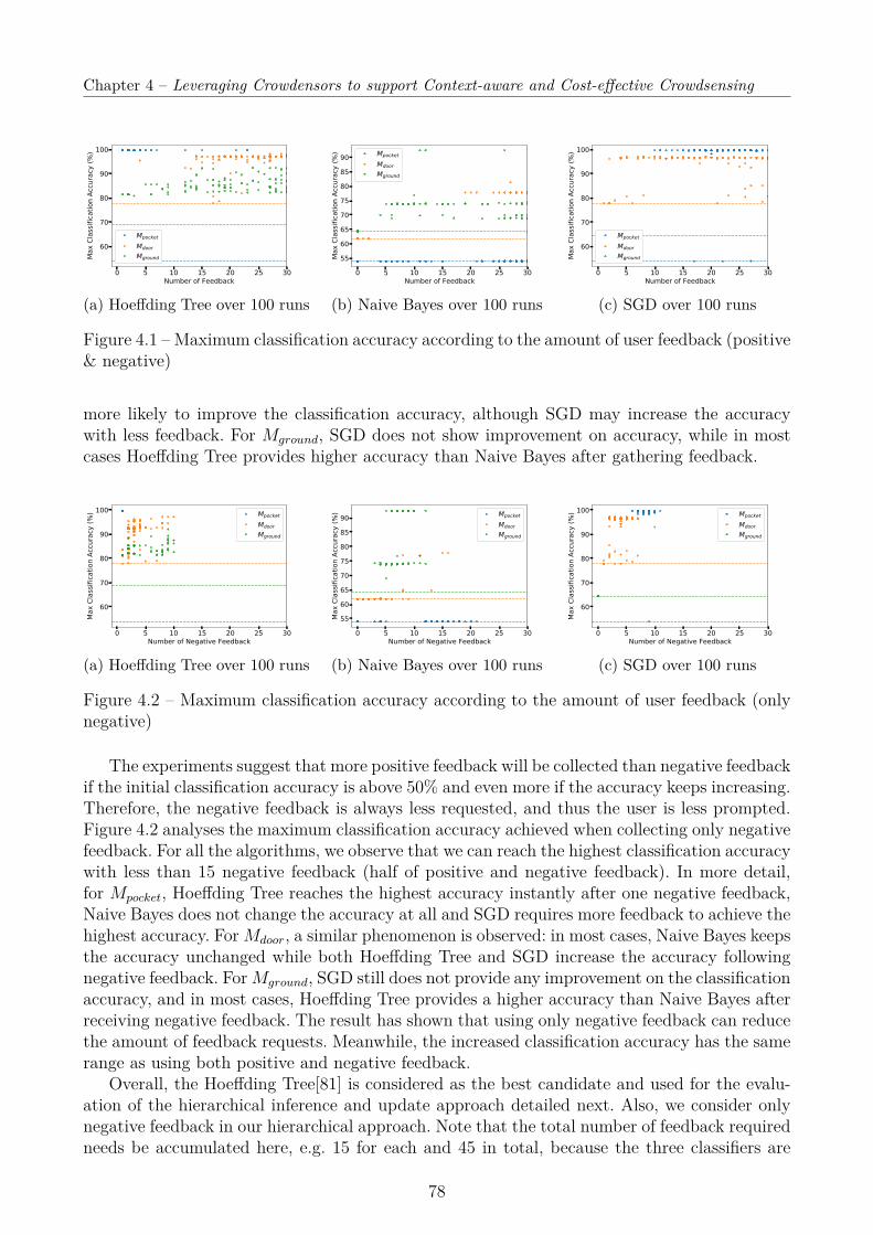
Chapter 4 – Leveraging Crowdensors to support Context-aware and Cost-effective Crowdsensing
0 5 10 15 20 25 30Number of Feedback
60
70
80
90
100
Max
Cla
ssifi
catio
n Ac
cura
cy (%
)
Mpocket
Mdoor
Mground
(a) Hoeffding Tree over 100 runs
0 5 10 15 20 25 30Number of Feedback
55
60
65
70
75
80
85
90
Max
Cla
ssifi
catio
n Ac
cura
cy (%
) Mpocket
Mdoor
Mground
(b) Naive Bayes over 100 runs
0 5 10 15 20 25 30Number of Feedback
60
70
80
90
100
Max
Cla
ssifi
catio
n Ac
cura
cy (%
)
Mpocket
Mdoor
Mground
(c) SGD over 100 runs
Figure 4.1 – Maximum classification accuracy according to the amount of user feedback (positive& negative)
more likely to improve the classification accuracy, although SGD may increase the accuracywith less feedback. For Mground, SGD does not show improvement on accuracy, while in mostcases Hoeffding Tree provides higher accuracy than Naive Bayes after gathering feedback.
0 5 10 15 20 25 30Number of Negative Feedback
60
70
80
90
100
Max
Class
ifica
tion Ac
curacy
(%) Mpocket
Mdoor
Mground
(a) Hoeffding Tree over 100 runs
0 5 10 15 20 25 30Number of Negative Feedback
55
60
65
70
75
80
85
90
Max
Class
ifica
tion Ac
curacy
(%) Mpocket
Mdoor
Mground
(b) Naive Bayes over 100 runs
0 5 10 15 20 25 30Number of Negative Feedback
60
70
80
90
100
Max
Class
ifica
tion Ac
curacy
(%) Mpocket
Mdoor
Mground
(c) SGD over 100 runs
Figure 4.2 – Maximum classification accuracy according to the amount of user feedback (onlynegative)
The experiments suggest that more positive feedback will be collected than negative feedbackif the initial classification accuracy is above 50% and even more if the accuracy keeps increasing.Therefore, the negative feedback is always less requested, and thus the user is less prompted.Figure 4.2 analyses the maximum classification accuracy achieved when collecting only negativefeedback. For all the algorithms, we observe that we can reach the highest classification accuracywith less than 15 negative feedback (half of positive and negative feedback). In more detail,for Mpocket, Hoeffding Tree reaches the highest accuracy instantly after one negative feedback,Naive Bayes does not change the accuracy at all and SGD requires more feedback to achieve thehighest accuracy. ForMdoor, a similar phenomenon is observed: in most cases, Naive Bayes keepsthe accuracy unchanged while both Hoeffding Tree and SGD increase the accuracy followingnegative feedback. ForMground, SGD still does not provide any improvement on the classificationaccuracy, and in most cases, Hoeffding Tree provides a higher accuracy than Naive Bayes afterreceiving negative feedback. The result has shown that using only negative feedback can reducethe amount of feedback requests. Meanwhile, the increased classification accuracy has the samerange as using both positive and negative feedback.
Overall, the Hoeffding Tree[81] is considered as the best candidate and used for the evalu-ation of the hierarchical inference and update approach detailed next. Also, we consider onlynegative feedback in our hierarchical approach. Note that the total number of feedback requiredneeds be accumulated here, e.g. 15 for each and 45 in total, because the three classifiers are
78
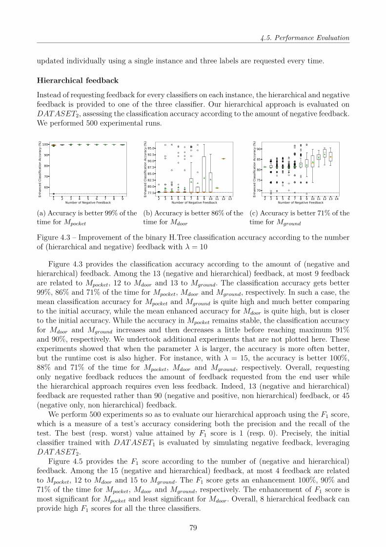
4.5. Performance Evaluation
updated individually using a single instance and three labels are requested every time.
Hierarchical feedback
Instead of requesting feedback for every classifiers on each instance, the hierarchical and negativefeedback is provided to one of the three classifier. Our hierarchical approach is evaluated onDATASET2, assessing the classification accuracy according to the amount of negative feedback.We performed 500 experimental runs.
1 2 3 4 5 6 7 8 9Number of Negative Feedback
60
70
80
90
100
Enha
nced
Classificatio
n Ac
curacy (%
)
(a) Accuracy is better 99% of thetime for Mpocket
2 3 4 5 6 7 8 9 10 11 12 13Number of Negative Feedback
77.5
80.0
82.5
85.0
87.5
90.0
92.5
95.0Enhanced Classificatio
n Accuracy (%
)
(b) Accuracy is better 86% of thetime for Mdoor
2 3 4 5 6 7 8 9 10 11 12 13 14Number of Negative Feedback
70
75
80
85
90
Enha
nced
Classificatio
n Ac
curacy (%
)
(c) Accuracy is better 71% of thetime for Mground
Figure 4.3 – Improvement of the binary H.Tree classification accuracy according to the numberof (hierarchical and negative) feedback with λ = 10
Figure 4.3 provides the classification accuracy according to the amount of (negative andhierarchical) feedback. Among the 13 (negative and hierarchical) feedback, at most 9 feedbackare related to Mpocket, 12 to Mdoor and 13 to Mground. The classification accuracy gets better99%, 86% and 71% of the time for Mpocket, Mdoor and Mground, respectively. In such a case, themean classification accuracy for Mpocket and Mground is quite high and much better comparingto the initial accuracy, while the mean enhanced accuracy for Mdoor is quite high, but is closerto the initial accuracy. While the accuracy in Mpocket remains stable, the classification accuracyfor Mdoor and Mground increases and then decreases a little before reaching maximum 91%and 90%, respectively. We undertook additional experiments that are not plotted here. Theseexperiments showed that when the parameter λ is larger, the accuracy is more often better,but the runtime cost is also higher. For instance, with λ = 15, the accuracy is better 100%,88% and 71% of the time for Mpocket, Mdoor and Mground, respectively. Overall, requestingonly negative feedback reduces the amount of feedback requested from the end user whilethe hierarchical approach requires even less feedback. Indeed, 13 (negative and hierarchical)feedback are requested rather than 90 (negative and positive, non hierarchical) feedback, or 45(negative only, non hierarchical) feedback.
We perform 500 experiments so as to evaluate our hierarchical approach using the F1 score,which is a measure of a test’s accuracy considering both the precision and the recall of thetest. The best (resp. worst) value attained by F1 score is 1 (resp. 0). Precisely, the initialclassifier trained with DATASET1 is evaluated by simulating negative feedback, leveragingDATASET2.
Figure 4.5 provides the F1 score according to the number of (negative and hierarchical)feedback. Among the 15 (negative and hierarchical) feedback, at most 4 feedback are relatedto Mpocket, 12 to Mdoor and 15 to Mground. The F1 score gets an enhancement 100%, 90% and71% of the time for Mpocket, Mdoor and Mground, respectively. The enhancement of F1 score ismost significant for Mpocket and least significant for Mdoor. Overall, 8 hierarchical feedback canprovide high F1 scores for all the three classifiers.
79
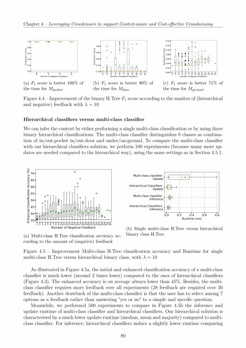
Chapter 4 – Leveraging Crowdensors to support Context-aware and Cost-effective Crowdsensing
8 1 2 4Number of Negative Feedback
0.0
0.2
0.4
0.6
0.8
1.0
Enha
nced
F1 S
core
(a) F1 score is better 100% ofthe time for Mpocket
2 3 4 5 6 7 8 9 10 11 12Number of Negative Feedback
0.70
0.75
0.80
0.85
0.90
Enha
nced
F1 S
core
(b) F1 score is better 90% ofthe time for Mdoor
2 3 4 5 6 7 8 9 10 11 12 13 14 15Number of Negative Feedback
0.80
0.82
0.84
0.86
0.88
0.90
0.92
0.94
Enha
nced
F1 S
core
(c) F1 score is better 71% ofthe time for Mground
Figure 4.4 – Improvement of the binary H.Tree F1 score according to the number of (hierarchicaland negative) feedback with λ = 10
Hierarchical classifiers versus multi-class classifier
We can infer the context by either performing a single multi-class classification or by using threebinary hierarchical classifications. The multi-class classifier distinguishes 8 classes as combina-tion of in/out-pocket in/out-door and under/on-ground. To compare the multi-class classifierwith our hierarchical classifiers solution, we perform 100 experiments (because many more up-dates are needed compared to the hierarchical way), using the same settings as in Section 4.5.1.
1 2 3 4 5 6 7 8 9 10111213141516171819202122232425262728Number of Negative Feedback
35
40
45
50
55
60
65
70
Enha
nced
Classificatio
n Ac
curacy (%
)
(a) Multi-class H.Tree classification accuracy ac-cording to the amount of (negative) feedback
0.0 0.2 0.4 0.6 0.8Runtime (ms)
Hierarchical Classifiers Inference
Multi-class classifier Inference
Hierarchical Classifiers Update
Multi-class classifier Update
(b) Single multi-class H.Tree versus hierarchicalbinary class H.Tree
Figure 4.5 – Improvement Multi-class H.Tree classification accuracy and Runtime for singlemulti-class H.Tree versus hierarchical binary class, with λ = 10
As illustrated in Figure 4.5a, the initial and enhanced classification accuracy of a multi-classclassifier is much lower (around 2 times lower) compared to the ones of hierarchical classifiers(Figure 4.3). The enhanced accuracy is on average always lower than 45%. Besides, the multi-class classifier requires more feedback over all experiments (28 feedback are required over 30feedback). Another drawback of the multi-class classifier is that the user has to select among 7options as a feedback rather than answering "yes or no" to a simple and specific question.
Meanwhile, we performed 500 experiments to compare in Figure 4.5b the inference andupdate runtime of multi-class classifier and hierarchical classifiers. Our hierarchical solution ischaracterised by a much lower update runtime (median, mean and majority) compared to multi-class classifier. For inference, hierarchical classifiers induce a slightly lower runtime comparing
80
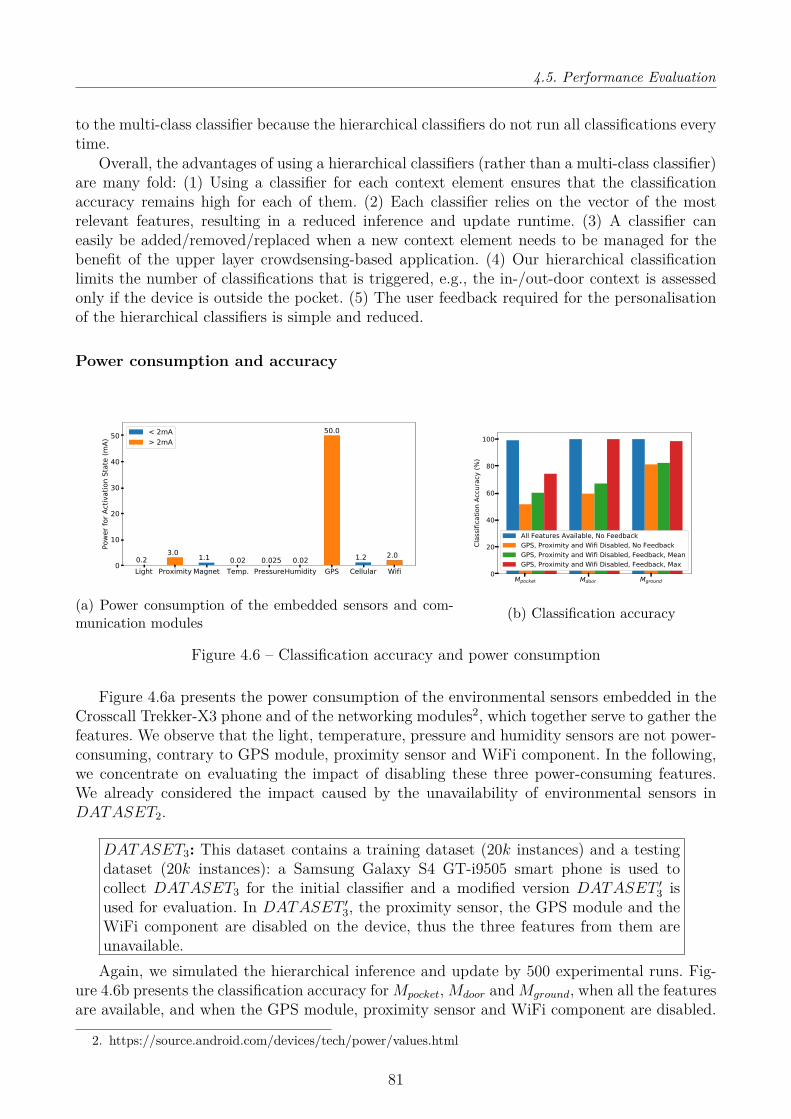
4.5. Performance Evaluation
to the multi-class classifier because the hierarchical classifiers do not run all classifications everytime.
Overall, the advantages of using a hierarchical classifiers (rather than a multi-class classifier)are many fold: (1) Using a classifier for each context element ensures that the classificationaccuracy remains high for each of them. (2) Each classifier relies on the vector of the mostrelevant features, resulting in a reduced inference and update runtime. (3) A classifier caneasily be added/removed/replaced when a new context element needs to be managed for thebenefit of the upper layer crowdsensing-based application. (4) Our hierarchical classificationlimits the number of classifications that is triggered, e.g., the in-/out-door context is assessedonly if the device is outside the pocket. (5) The user feedback required for the personalisationof the hierarchical classifiers is simple and reduced.
Power consumption and accuracy
Light Proximity Magnet Temp. PressureHumidity GPS Cellular Wifi0
10
20
30
40
50
Powe
r for Activation State (m
A)
0.23.0 1.1 0.02 0.025 0.02
50.0
1.2 2.0
< 2mA> 2mA
(a) Power consumption of the embedded sensors and com-munication modules
Mpocket Mdoor Mground0
20
40
60
80
100
Classifica
tion Ac
curacy (%
)
All Features Available, No FeedbackGPS, Proximity and Wifi Disabled, No FeedbackGPS, Proximity and Wifi Disabled, Feedback, MeanGPS, Proximity and Wifi Disabled, Feedback, Max
(b) Classification accuracy
Figure 4.6 – Classification accuracy and power consumption
Figure 4.6a presents the power consumption of the environmental sensors embedded in theCrosscall Trekker-X3 phone and of the networking modules2, which together serve to gather thefeatures. We observe that the light, temperature, pressure and humidity sensors are not power-consuming, contrary to GPS module, proximity sensor and WiFi component. In the following,we concentrate on evaluating the impact of disabling these three power-consuming features.We already considered the impact caused by the unavailability of environmental sensors inDATASET2.
DATASET3: This dataset contains a training dataset (20k instances) and a testingdataset (20k instances): a Samsung Galaxy S4 GT-i9505 smart phone is used tocollect DATASET3 for the initial classifier and a modified version DATASET ′3 isused for evaluation. In DATASET ′3, the proximity sensor, the GPS module and theWiFi component are disabled on the device, thus the three features from them areunavailable.Again, we simulated the hierarchical inference and update by 500 experimental runs. Fig-
ure 4.6b presents the classification accuracy forMpocket,Mdoor andMground, when all the featuresare available, and when the GPS module, proximity sensor and WiFi component are disabled.
2. https://source.android.com/devices/tech/power/values.html
81

Chapter 4 – Leveraging Crowdensors to support Context-aware and Cost-effective Crowdsensing
When the GPS module, proximity sensor and WiFi component are disabled, the classificationaccuracy diminishes to respectively 50%, 40% and 20%. After getting feedback, the mean clas-sification accuracy increases by 10%, 8% and 1% respectively, while the maximum classificationaccuracy after feedback reaches 74%, 99% and 98% respectively. Overall, our approach person-alises the classifiers and deals with the disabled power-consuming features according to userpreference.
Our implementation requires 100MB of memory on a Nokia X6 Android 9 smartphone(Qualcomm Snapdragon 636) and leads to an increase of 5% of the CPU. The inference andupdate of contexts necessitates around 3MB of memory and an increase of 5% of the CPU.We evaluate the computation runtime of the entire inference and update phases. The inferenceruntime is on average 0.2ms, 0.1ms and 0.1ms for Mpocket, Mdoor and Mground, respectively,while the runtime necessary to update the model is 7.3ms, 7.5ms and 10.0ms on average (withλ = 10).
4.5.2 Group-based Collaborative CrowdsensingWe evaluate the performance of our approach, assessing: (i) the impact on the power consump-tion of the device running the BeTogether middleware in the background, and (ii) the potentialbenefit of the collaborative crowdsensing at the edge from the standpoint of data quality andcommunication cost based on a one-year dataset obtained from the Ambiciti application forurban pollution monitoring. We note that due to privacy and commercial concerns, the Ambic-iti company shared the data with us within the framework of a collaboration agreement whiledata cannot be released openly.
Power consumption
Table 4.6 – Active power of components for Nexus 5X
WiFi TX WiFi Scan Cellular TX Light Sensor GPS RX173 mA 2 mA 186 mA 0.2 mA 60 mA
We estimate theoretically the power consumption on a single crowdsensor; Table 4.6 showsthe power of the main components used in our crowdsensing middleware. The reference valuesare for the Google Nexus 5X smartphone, as provided by the Android OS (https://source.android.com/devices/tech/power/values) according to the power profile provided by themanufacturer. Herein, we select the light sensor, which involves a power consumption compa-rable to that of most sensors [52, 96]. Note that the power consumption associated with thetransmission depends on the transmission duration, which increases linearly with the packetsize. We assume that cellular and WiFi Direct communications have the same transmissionspeed.
Figure 4.7 shows the power consumption of a crowdsensor working individually at varioussensing and upload frequencies. The upload is the most energy-demanding and the energyconsumption can be reduced by lowering the upload frequency. As a comparison, Figure 4.8provides the power consumption of the various nodes contributing to collaborative crowdsensingwith regards to a high sensing frequency (every 1 minute) and upload frequency (every 10minutes) for the individual case. Results show that the proxy always consumes the most energydue to the cellular transmission that takes place with the cloud, followed by the coordinatorthat communicates with the nearby devices to distribute the tasks. Other group participants
82
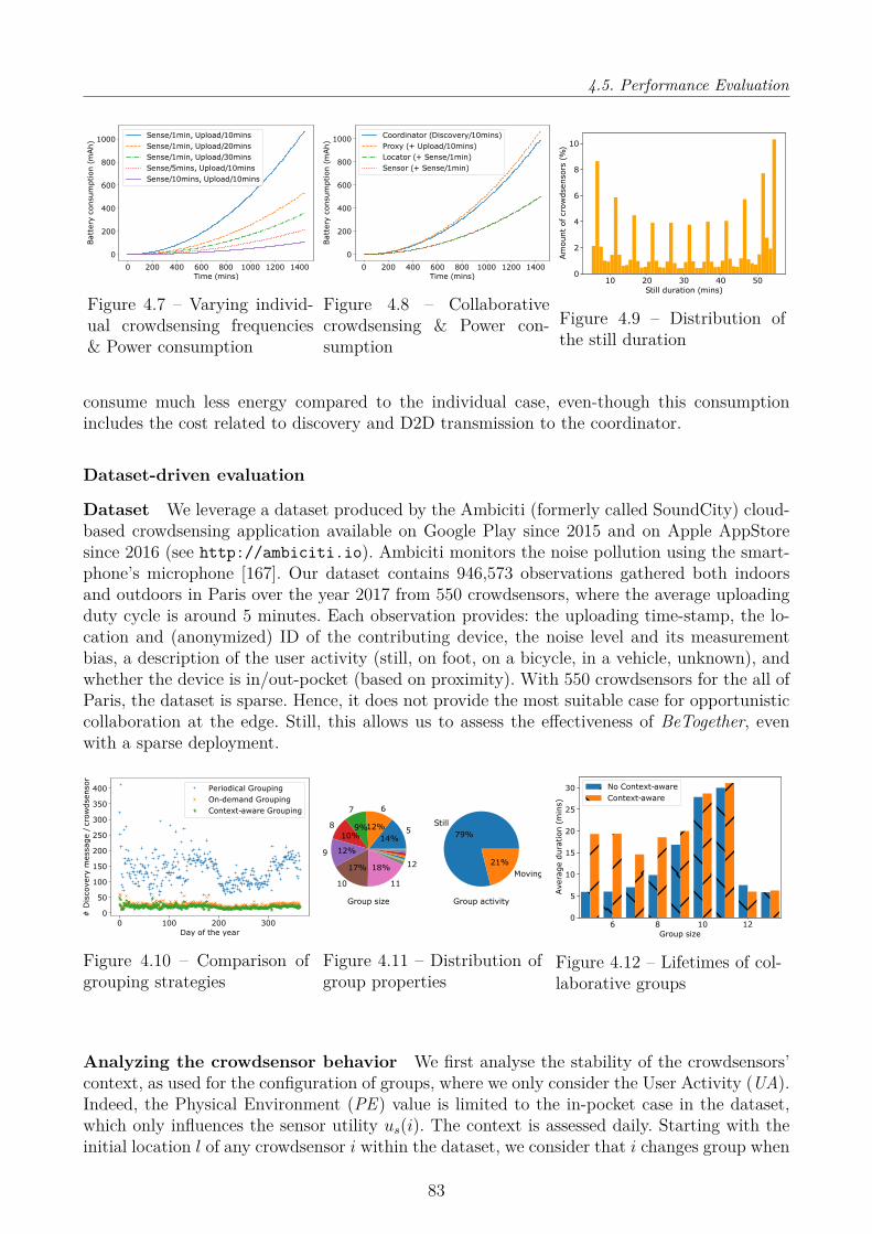
4.5. Performance Evaluation
0 200 400 600 800 1000 1200 1400Time (mins)
0
200
400
600
800
1000
Batt
ery
consu
mption (
mAh)
Sense/1min, Upload/10minsSense/1min, Upload/20minsSense/1min, Upload/30minsSense/5mins, Upload/10minsSense/10mins, Upload/10mins
Figure 4.7 – Varying individ-ual crowdsensing frequencies& Power consumption
0 200 400 600 800 1000 1200 1400Time (mins)
0
200
400
600
800
1000
Batt
ery
consu
mption (
mAh)
Coordinator (Discovery/10mins)Proxy (+ Upload/10mins)Locator (+ Sense/1min)Sensor (+ Sense/1min)
Figure 4.8 – Collaborativecrowdsensing & Power con-sumption
10 20 30 40 50Still duration (mins)
0
2
4
6
8
10
Am
ount
of cr
ow
dse
nso
rs (
%)
Figure 4.9 – Distribution ofthe still duration
consume much less energy compared to the individual case, even-though this consumptionincludes the cost related to discovery and D2D transmission to the coordinator.
Dataset-driven evaluation
Dataset We leverage a dataset produced by the Ambiciti (formerly called SoundCity) cloud-based crowdsensing application available on Google Play since 2015 and on Apple AppStoresince 2016 (see http://ambiciti.io). Ambiciti monitors the noise pollution using the smart-phone’s microphone [167]. Our dataset contains 946,573 observations gathered both indoorsand outdoors in Paris over the year 2017 from 550 crowdsensors, where the average uploadingduty cycle is around 5 minutes. Each observation provides: the uploading time-stamp, the lo-cation and (anonymized) ID of the contributing device, the noise level and its measurementbias, a description of the user activity (still, on foot, on a bicycle, in a vehicle, unknown), andwhether the device is in/out-pocket (based on proximity). With 550 crowdsensors for the all ofParis, the dataset is sparse. Hence, it does not provide the most suitable case for opportunisticcollaboration at the edge. Still, this allows us to assess the effectiveness of BeTogether, evenwith a sparse deployment.
0 100 200 300Day of the year
0
50
100
150
200
250
300
350
400
# D
isco
very
mess
age / c
row
dse
nso
r
Periodical GroupingOn-demand GroupingContext-aware Grouping
Figure 4.10 – Comparison ofgrouping strategies
Group size
514%
6
12%
7
9%810%
9 12%
10
17%
11
18% 12
Group activity
Still79%
Moving21%
Figure 4.11 – Distribution ofgroup properties
6 8 10 12Group size
0
5
10
15
20
25
30
Ave
rage d
ura
tion (
min
s)
No Context-awareContext-aware
Figure 4.12 – Lifetimes of col-laborative groups
Analyzing the crowdsensor behavior We first analyse the stability of the crowdsensors’context, as used for the configuration of groups, where we only consider the User Activity (UA).Indeed, the Physical Environment (PE) value is limited to the in-pocket case in the dataset,which only influences the sensor utility us(i). The context is assessed daily. Starting with theinitial location l of any crowdsensor i within the dataset, we consider that i changes group when
83
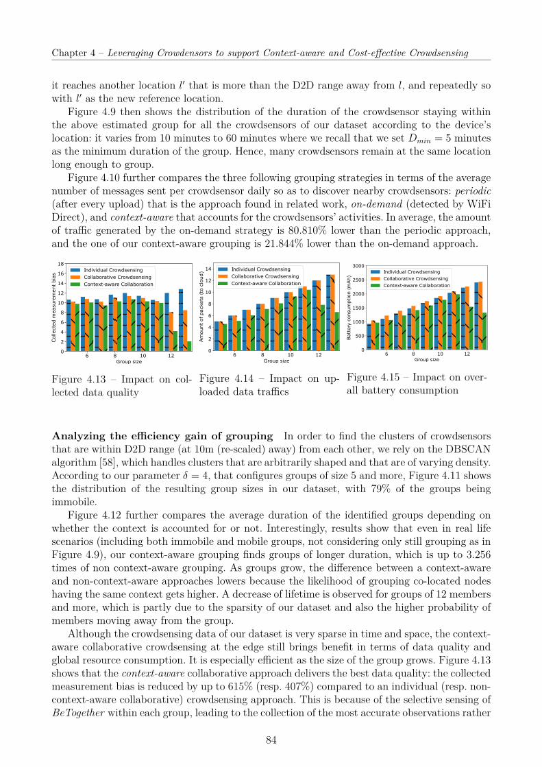
Chapter 4 – Leveraging Crowdensors to support Context-aware and Cost-effective Crowdsensing
it reaches another location l′ that is more than the D2D range away from l, and repeatedly sowith l′ as the new reference location.
Figure 4.9 then shows the distribution of the duration of the crowdsensor staying withinthe above estimated group for all the crowdsensors of our dataset according to the device’slocation: it varies from 10 minutes to 60 minutes where we recall that we set Dmin = 5 minutesas the minimum duration of the group. Hence, many crowdsensors remain at the same locationlong enough to group.
Figure 4.10 further compares the three following grouping strategies in terms of the averagenumber of messages sent per crowdsensor daily so as to discover nearby crowdsensors: periodic(after every upload) that is the approach found in related work, on-demand (detected by WiFiDirect), and context-aware that accounts for the crowdsensors’ activities. In average, the amountof traffic generated by the on-demand strategy is 80.810% lower than the periodic approach,and the one of our context-aware grouping is 21.844% lower than the on-demand approach.
6 8 10 12Group size
0
2
4
6
8
10
12
14
16
18
Colle
cted m
easu
rem
ent
bia
s
Individual CrowdsensingCollaborative CrowdsensingContext-aware Collaboration
Figure 4.13 – Impact on col-lected data quality
6 8 10 12Group size
0
2
4
6
8
10
12
14
Am
ount
of pack
ets
(to
clo
ud) Individual Crowdsensing
Collaborative CrowdsensingContext-aware Collaboration
Figure 4.14 – Impact on up-loaded data traffics
6 8 10 12Group size
0
500
1000
1500
2000
2500
3000
Batt
ery
consu
mption (
mAh)
Individual CrowdsensingCollaborative CrowdsensingContext-aware Collaboration
Figure 4.15 – Impact on over-all battery consumption
Analyzing the efficiency gain of grouping In order to find the clusters of crowdsensorsthat are within D2D range (at 10m (re-scaled) away) from each other, we rely on the DBSCANalgorithm [58], which handles clusters that are arbitrarily shaped and that are of varying density.According to our parameter δ = 4, that configures groups of size 5 and more, Figure 4.11 showsthe distribution of the resulting group sizes in our dataset, with 79% of the groups beingimmobile.
Figure 4.12 further compares the average duration of the identified groups depending onwhether the context is accounted for or not. Interestingly, results show that even in real lifescenarios (including both immobile and mobile groups, not considering only still grouping as inFigure 4.9), our context-aware grouping finds groups of longer duration, which is up to 3.256times of non context-aware grouping. As groups grow, the difference between a context-awareand non-context-aware approaches lowers because the likelihood of grouping co-located nodeshaving the same context gets higher. A decrease of lifetime is observed for groups of 12 membersand more, which is partly due to the sparsity of our dataset and also the higher probability ofmembers moving away from the group.
Although the crowdsensing data of our dataset is very sparse in time and space, the context-aware collaborative crowdsensing at the edge still brings benefit in terms of data quality andglobal resource consumption. It is especially efficient as the size of the group grows. Figure 4.13shows that the context-aware collaborative approach delivers the best data quality: the collectedmeasurement bias is reduced by up to 615% (resp. 407%) compared to an individual (resp. non-context-aware collaborative) crowdsensing approach. This is because of the selective sensing ofBeTogether within each group, leading to the collection of the most accurate observations rather
84
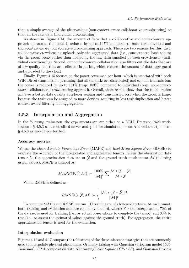
4.5. Performance Evaluation
than a simple average of the observations (non-context-aware collaborative crowdsensing) orthan all the raw data (individual crowdsensing).
As shown in Figure 4.14, the amount of data that a collaborative and context-aware ap-proach uploads to the cloud is reduced by up to 197% compared to both the individual and(non-context-aware) collaborative crowdsensing approach. There are two reasons for this: first,collaborative crowdsensing uploads only the aggregated data (i.e., concatenated hash tables)via the group proxy rather than uploading the raw data supplied by each crowdsensor (indi-vidual crowdsensing). Second, our context-aware collaboration also filters out the data that areof low-quality and that are collected in-pocket, which reduces the amount of data aggregatedand uploaded to the cloud.
Finally, Figure 4.15 focuses on the power consumed per hour, which is associated with bothWiFi Direct transmission (assuming that all the tasks are distributed) and cellular transmission:the power is reduced by up to 181% (resp. 183%) compared to individual (resp. non-context-aware collaborative) crowdsensing approach. Overall, these results show that the collaborationachieves a better data quality at a lower sensing and transmission cost when the group is largerbecause the tasks can be assigned to more devices, resulting in less task duplication and bettercontext-aware filtering and aggregation.
4.5.3 Interpolation and AggregationIn the following evaluation, the experiments are run either on a DELL Precision 7520 work-station - § 4.5.3 as a centralised server and § 4.4 for simulation, or on Android smartphones -§ 4.5.3 as end-device testbed.
Accuracy metrics
We use the Mean Absolute Percentage Error (MAPE) and Root Mean Square Error (RMSE) toevaluate the accuracy of the interpolated and aggregated tensors. Given the observation datatensor Y , the approximation data tensor Y and the ground truth mask tensor M (indexinguseful values), MAPE is defined as:
MAPE(Y , Y ,M) := 100%‖M‖2
∑M∗ |Y − Y|M ∗ Y
While RMSE is defined as:
RMSE(Y , Y ,M) :=
√√√√‖M ∗ (Y − Y)‖2
‖M‖2
To compute MAPE and RMSE, we run 100 training rounds followed by tests. At each round,both training and evaluation sets are randomly shuffled, where: For the interpolation, 70% ofthe dataset is used for training (i.e., as actual observations to complete the tensor) and 30% totest (i.e., to assess the estimated values against the ground truth). For aggregation, the entireapproximation tensor is used for the evaluation.
Interpolation evaluation
Figures 4.16 and 4.17 compare the robustness of the three inference strategies that are commonlyused to interpolate physical phenomena: Ordinary kriging with Gaussian variogram model (OK-Gaussian), CP decomposition with Alternating Least Square (CP-ALS), and Gaussian Process
85
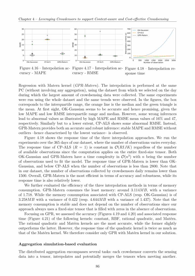
Chapter 4 – Leveraging Crowdensors to support Context-aware and Cost-effective Crowdsensing
OK-Gaussian CP-ALS GPR-Matern0
5
10
15
20
25
30
MAPE
Figure 4.16 – Interpolation ac-curacy - MAPE
OK-Gaussian CP-ALS GPR-Matern0
10
20
30
40
50
60
RMSE
Figure 4.17 – Interpolation ac-curacy - RMSE
0 500 1000 1500 2000 2500 3000Number of observation
0
100
200
300
400
500
600
700
Inte
rpol
atio
n ru
ntim
e (s
)
OK-GaussianCP-ALSGPR-Matern
Figure 4.18 – Interpolation re-sponse time
Regression with Matern kernel (GPR-Matern). The interpolation is performed at the samePC (without involving any aggregation), using the dataset from which we selected on the dayduring which the largest amount of crowdsensing data were collected. The same experimentswere run using the whole dataset and the same trends were observed. In the figures, the boxcorresponds to the interquartile range, the orange line is the median and the green triangle isthe mean. At first sight, OK-Gaussian seems to be accurate and hence promising, given thelow MAPE and low RMSE interquartile range and median. However, some wrong inferenceslead to abnormal values as illustrated by high MAPE and RMSE mean values of 16% and 47,respectively. Similarly but to a lower extent, CP-ALS shows some abnormal RMSE. Instead,GPR-Matern provides both an accurate and robust inference: stable MAPE and RMSE withoutoutliers –hence characterised by the lowest variance– is observed.
Figure 4.18 shows the response time of the three interpolation approaches. We run theexperiments over the 365 days of our dataset, where the number of observations varies everyday.The response time of CP-ALS (R = 1) is constant in O(RIJK) regardless of the numberof available observations since the computation applies on the entire fixed-size tensor. BothOK-Gaussian and GPR-Matern have a time complexity in O(n3) with n being the numberof observations used to fit the model. The response time of GPR-Matern is lower than OK-Gaussian, and below CP-ALS when the number of observations is less than 2800. Note thatin our dataset, the number of observations collected by crowdsensors daily remains lower than1500. Overall, GPR-Matern is the most efficient in terms of accuracy and robustness, while itsresponse time is also relatively lower.
We further evaluated the efficiency of the three interpolation methods in terms of memoryconsumption. GPR-Matern consumes the least memory: around 3.114MB, with a varianceof 1.718. While the memory consumption associated with CP-ALS (resp. OK-Gaussian) is of3.258MB with a variance of 0.422 (resp. 4.644MB with a variance of 1.437). Note that thememory consumption is stable and does not depend on the number of observations since ourapproach always uses a fixed-size tensor that is filled with zeros in the absence of observations.
Focusing on GPR, we assessed the accuracy (Figures 4.19 and 4.20) and associated responsetime (Figure 4.21) of the following kernels: constant, RBF, rational quadratic, and Matérn.The rational quadratic and Matérn kernels are the most accurate, while the former slightlyoutperforms the latter. However, the response time of the quadratic kernel is twice as much asthat of the Matérn kernel. We therefore consider only GPR with Matérn kernel in our solution.
Aggregation simulation-based evaluation
The distributed aggregation encompasses several tasks: each crowdsensor converts the sensingdata into a tensor, interpolates and potentially merges the tensors when meeting another.
86
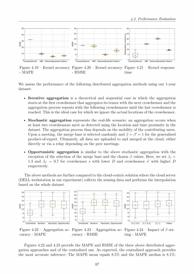
4.5. Performance Evaluation
ConstantKernel RBF RationalQuadratic Matern0
10
20
30
40
50
MAPE
Figure 4.19 – Kernel accuracy- MAPE
ConstantKernel RBF RationalQuadratic Matern0
5
10
15
20
25
30
RMSE
Figure 4.20 – Kernel accuracy- RMSE
ConstantKernel RBF RationalQuadratic Matern0
5
10
15
20
25
30
Inte
rpol
atio
n ru
ntim
e (s
)
Figure 4.21 – Kernel responsetime
We assess the performance of the following distributed aggregation methods using our 1-yeardataset:
• Iterative aggregation is a theoretical and sequential case in which the aggregationstarts at the first crowdsensor that aggregates its tensor with the next crowdsensor and theaggregation process repeats with the following crowdsensors until the last crowdsensor isreached. This is the ideal case for which we ignore the actual locations of the crowdsensor.
• Stochastic aggregation represents the real-life scenario: an aggregation occurs whenat least two crowdsensors meet as detected using the location and time proximity in thedataset. The aggregation process thus depends on the mobility of the contributing users.Upon a meeting, the merge base is selected randomly and β = β′ = 1 for the generalisedproduct-of-expert. Ultimately, all data are uploaded to and merged at the cloud, eitherdirectly or via a relay depending on the peer meetings.
• Opportunistic aggregation is similar to the above stochastic aggregation with theexception of the selection of the merge base and the chosen β values. Here, we set βs =1.3 and βs′ = 0.7 for crowdsensor s with lower D and crowdsensor s′ with higher Drespectively.
The above methods are further compared to the cloud-centric solution where the cloud server(DELL workstation in our experiment) collects the sensing data and performs the interpolationbased on the whole dataset.
Centralized Iterative Stochastic Opportunistic4
6
8
10
12
14
16
18
MAPE
Figure 4.22 – Aggregation ac-curacy - MAPE
Centralized Iterative Stochastic Opportunistic
6
8
10
12
14
16
18
20
22
RMSE
Figure 4.23 – Aggregation ac-curacy - RMSE
(1.5, 0.5) (1.7, 0.3) (1, 1) #Meet
4
6
8
10
12
14
16
18
MAPE
Figure 4.24 – Impact of β set-ting - MAPE
Figures 4.22 and 4.23 provide the MAPE and RMSE of the three above distributed aggre-gation approaches and of the centralized one. As expected, the centralized approach providesthe most accurate inference: The MAPE mean equals 8.5% and the MAPE median is 8.1%;
87

Chapter 4 – Leveraging Crowdensors to support Context-aware and Cost-effective Crowdsensing
the RMSE mean equals 10.8 and the RMSE median is 10.6. The accuracy of the distributedaggregations are quite similar, with a MAPE of around 12.5% with a median of 12.5% anda RMSE mean of 15.6 with a median of 15.8. In particular, our opportunistic aggregation iscomparable to the centralised approach (e.g., the MAPE accuracy difference is 4% lower thanthe centralised approach). It has mean and median MAPE of 12.0%; a RMSE mean of 15.0 anda RMSE median of 15.2. Overall, our approach is characterised by very slight decrease of theaccuracy compared to centralised aggregation.
(1.5, 0.5) (1.7, 0.3) (1, 1) #Meet5.0
7.5
10.0
12.5
15.0
17.5
20.0
22.5
RM
SE
Figure 4.25 – Impact of β set-ting - RMSE
0 250 500 750 1000 1250 1500Number of observation
0
5
10
15
20
25
30
35Acc
um
ula
ted r
untim
e (
s)
CentralizedIterativeStochasticOpportunistic
Figure 4.26 – Simulation re-sponse time
0 100 200 300 400 500Number of crowdsensors
0
20
40
60
80
100
120
140
Clo
ud r
untim
e (
s)
CentralizedStochasticOpportunistic
Figure 4.27 – Cloud server re-sponse time
Figures 4.24 and 4.25 compare different weighting configurations (βs, βs′) for crowdsensor sand s′. For three of the pairs, we manually set their values depending on the loss function D,i.e. the lower loss has a higher weight. For the fourth one, we set βs = 2 ns
ns+ns′using the ratio
depending on the history number of aggregations n. The results show that assigning a higherweight to the crowdsensor with the lower loss function slightly increases the overall accuracyaggregated at the cloud.
Figure 4.26 shows the response time associated with the entire procedure including datapre-processing, interpolation and aggregation, with the simulation being run on the server. Weobserve that the centralised aggregation response time is lower than the accumulated responsetime of the distributed aggregation schemes. However, in the distributed approach, the clouddoes not perform any interpolation, thus the centralised interpolation requiring a high responsetime is eliminated. As illustrated in Figure 4.27, the response time associated with the aggre-gation at the cloud server significantly increases when the number of crowdsensors gets high.Instead, when the interpolation and aggregation are mainly performed by crowdsensors, thecloud response time is almost negligible regardless of the number of crowdsensors. In addition,the storage requirement is minimised on cloud because the data tensor size is always unchangedwhen aggregating new incoming data.
0 100 200 300 400 500Number of crowdsensors
0
100
200
300
400
500
Num
ber
of m
ess
ages
Stochastic, to cloudOpportunistic, to cloud
Centralized, to cloud
Figure 4.28 – Directly up-loaded messages
0 100 200 300 400 500Number of crowdsensors
0
100
200
300
400
500
Num
ber
of m
ess
ages
Iterative, to peerStochastic, to peerOpportunistic, to peer
Figure 4.29 – P2P forwardedmessages
0 100 200 300 400 5000
200
400
Run
tim
e (s
)
0 100 200 300 400 500Number of observation (up) / aggregation (down)
50
100
Run
tim
e (s
)
Figure 4.30 – On-device re-sponse time
88
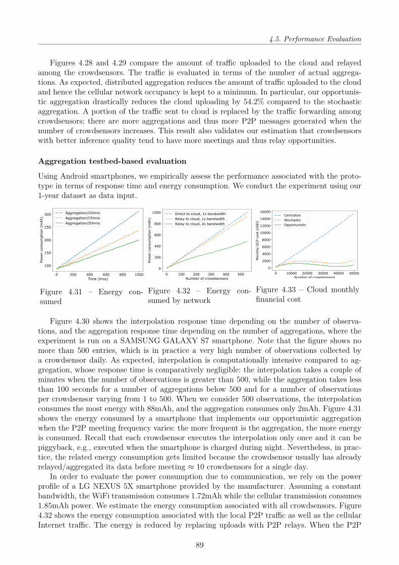
4.5. Performance Evaluation
Figures 4.28 and 4.29 compare the amount of traffic uploaded to the cloud and relayedamong the crowdsensors. The traffic is evaluated in terms of the number of actual aggrega-tions. As expected, distributed aggregation reduces the amount of traffic uploaded to the cloudand hence the cellular network occupancy is kept to a minimum. In particular, our opportunis-tic aggregation drastically reduces the cloud uploading by 54.2% compared to the stochasticaggregation. A portion of the traffic sent to cloud is replaced by the traffic forwarding amongcrowdsensors; there are more aggregations and thus more P2P messages generated when thenumber of crowdsensors increases. This result also validates our estimation that crowdsensorswith better inference quality tend to have more meetings and thus relay opportunities.
Aggregation testbed-based evaluation
Using Android smartphones, we empirically assess the performance associated with the proto-type in terms of response time and energy consumption. We conduct the experiment using our1-year dataset as data input.
0 200 400 600 800 1000Time (mns)
100
150
200
250
300
Pow
er c
onsu
mpt
ion
(mAh)
Aggregation/10mnsAggregation/15mnsAggregation/20mns
Figure 4.31 – Energy con-sumed
0 100 200 300 400 500Number of crowdsensors
0
200
400
600
800
1000
Pow
er c
onsu
mpt
ion
(mAh)
Direct to cloud, 1x bandwidthRelay to cloud, 1x bandwidthRelay to cloud, 2x bandwidth
Figure 4.32 – Energy con-sumed by network
0 10000 20000 30000 40000 50000Number of crowdsensors
0
2000
4000
6000
8000
10000
12000
14000
16000
Month
ly G
CP
cost
(U
SD
)
CentralizeStochasticOpportunistic
Figure 4.33 – Cloud monthlyfinancial cost
Figure 4.30 shows the interpolation response time depending on the number of observa-tions, and the aggregation response time depending on the number of aggregations, where theexperiment is run on a SAMSUNG GALAXY S7 smartphone. Note that the figure shows nomore than 500 entries, which is in practice a very high number of observations collected bya crowdsensor daily. As expected, interpolation is computationally intensive compared to ag-gregation, whose response time is comparatively negligible: the interpolation takes a couple ofminutes when the number of observations is greater than 500, while the aggregation takes lessthan 100 seconds for a number of aggregations below 500 and for a number of observationsper crowdsensor varying from 1 to 500. When we consider 500 observations, the interpolationconsumes the most energy with 88mAh, and the aggregation consumes only 2mAh. Figure 4.31shows the energy consumed by a smartphone that implements our opportunistic aggregationwhen the P2P meeting frequency varies: the more frequent is the aggregation, the more energyis consumed. Recall that each crowdsensor executes the interpolation only once and it can bepiggyback, e.g., executed when the smartphone is charged during night. Nevertheless, in prac-tice, the related energy consumption gets limited because the crowdsensor usually has alreadyrelayed/aggregated its data before meeting ≈ 10 crowdsensors for a single day.
In order to evaluate the power consumption due to communication, we rely on the powerprofile of a LG NEXUS 5X smartphone provided by the manufacturer. Assuming a constantbandwidth, the WiFi transmission consumes 1.72mAh while the cellular transmission consumes1.85mAh power. We estimate the energy consumption associated with all crowdsensors. Figure4.32 shows the energy consumption associated with the local P2P traffic as well as the cellularInternet traffic. The energy is reduced by replacing uploads with P2P relays. When the P2P
89

Chapter 4 – Leveraging Crowdensors to support Context-aware and Cost-effective Crowdsensing
bandwidth is higher than the cellular bandwidth (e.g., two times in figure), the advantage ismore significant. Furthermore, the local P2P traffic is not only less costly in terms of energyaspect but also in terms of budget.
Impact on the financial cost
We estimate the financial cost associated with our crowdsensing system, using the GoogleCloud Platform (GCP, https://cloud.google.com/products/) as an example of cloud plat-form. GCP provides the following key services: Cloud IoT Core is responsible for connecting thecloud to the IoT devices and establishing a two-ways communication. Upon the reception of apacket, the Cloud Pub/Sub service creates and delivers an event notification to Cloud Functionsthat implements basic operations (e.g., average, maximum, minimum) needed to pre-processthe data. BigQuery is used to temporarily store the pre-processed data during the aggregationand interpolation. Compute Engine runs a virtual machine that performs the advanced com-putation (e.g., interpolation and aggregation). Cloud Bigtable is a NoSQL database that storesthe resulting aggregated and interpolated sensing data.
The use of each of the above services is priced: for a detailed description, one may refer tohttps://cloud.google.com/pricing/list. In a nutshell, the price depends on the amountof network traffic received/sent, the amount of storage needed, and the load associated withthe computation (e.g., number of pre-processing functions invoked and response time associatedwith the interpolation and aggregation). Figure 4.33 shows the monthly financial cost associatedwith running different crowdsensing in GCP, assuming that each crowdsensor sends a 2MBpacket everyday. The cost associated with the centralised approach increases linearly becausethe number of uploads and the computation involved to interpolate the phenomena are bothhigh. Instead, the costs of the stochastic and opportunistic approaches remain low becausecommunication toward the cloud is reduced and only lightweight aggregation is performedat the cloud. Our opportunistic aggregation outperforms the stochastic approach because wefurther reduce the computing load on the cloud.
4.6 ConclusionOne of the major benefits of crowdsensing is the possibility to monitor environmental phenom-ena at an urban scale, simply leveraging the abundance and capacity of people’s smartphones.However, as the number of contributors grows, the increasing number of observations that thecrowdsensing systems must process gets challenging: the high network and financial cost associ-ated to a cloud-centric system hinders the widespread deployment of crowdsensing, and the highcomputational cost due to the large amount of data makes the modelling of the environmentalphenomenon intractable.
We tackle the above issues by exploiting the increasing computing capacity of today’s smart-phones, that is, we enforce a collaboration strategy at the edge so as to enhance the quality ofthe data transferred to the cloud while reducing the related communication cost and resourceconsumption. For this purpose, we introduce a set of utility functions that assess to whichextent a device should carry out a given crowdsensing task, while achieving a trade-off betweenthe benefit for all (for the whole group) and the related cost for the device.
Furthermore, we distribute the interpolation and aggregation associated with the sensingdata at the powerful end devices. To do so, we introduce a middleware that runs on the smart-phone to capture complex and potentially non-linear relationships among the collected obser-vations across both space and time by relying on Gaussian Process Regression and 3D tensors.
90

4.6. Conclusion
Then, the resulting tensors are opportunistically combined together following a stochastic pro-cess based on the physical encounters of people. Rather than applying a naive combination(e.g., averaging) of the tensors that would actually degrade the quality of the sensing data, oursolution performs a Product-of-Expert on the inference. The benefit our approach is threefold:(i) a selected crowdsensor (i.e., expert) may independently establish a very precise interpolationof the regions covered by a crowdsensor group; (ii) the aggregation resulting from the Product-of-Experts is sharper than any of the individual tensor and renders much more tractable theestablishment of the overall tensor; and (iii) the computation achieved on the device is energy-efficient. Indeed, the evaluation using simulation and prototype implementation, together witha real-world dataset shows that our approach significantly reduces the transmission to, and thecomputing resource consumed on, the infrastructure server, without compromising the overalldata accuracy.
91

Chapter 5
Information centric Networking
5.1 Context and Motivation
IoT is an ever growing ecosystem in which the Things (e.g., smartphones, sensors, actuators,RFIDs, just to name a few) continuously exchange some data streams with other interestedThings, applications and users spread across the Internet. IoT is an event driven ecosystem inthe sense that reactions (e.g., actuations, decisions) are triggered after an event or a series ofevents is captured by the event producer (e.g., a sensor). Events correspond to some changes inthe state (e.g., a temperature increase, an excessive sound level) or simply an update. Relying onevent notification permits to minimise the need of integration among Things and applications.As a result, Things are easily deployed and operate independently, as needed.
The IoT presents a number of challenges, especially in regard to routing and aggregation of acontinuous flow of information that is exchanged among things. Thus, our attempt is to supportan efficient communication between Things/users across heterogeneous networks by adoptingan information-centric philosophy that heralds a new communication style, in which the dataflow is governed by both the Things/users interests and the data content. More specifically,we build upon the publish/subscribe paradigm in which event producers send notifications tosubscribers who have previously expressed their interests. The degree of expressiveness, whichpermits the users to describe their interest, is of critical importance and greatly differs fromone publish/subscribe system to another. This leads to the categorisation of these systems intothe two following classes: Topic- versus content-based publish/subscribe systems.
With topic-based pub/sub systems [180, 158, 159, 119, 67, 178, 35], a subscriber identifies atopic of interest (i.e., a keyword) and is thereby endowed with a low level of expressiveness. Eachindividual topic can be viewed, and thereby abstracted, as a separate channel /pipe, which isfurther mapped to a interested group of subscribers towards whom a notification is forwarded.Partitioning the topic space - and thereby the event space - into sub-topics leads to the creationof separate groups in which subscribing is equivalent to becoming a group member, with onegroup defined per (sub)topic. Due to the simplicity and ease of use of topic-strings, topic-based pub/sub systems became widely employed as part of enterprise and message-orientedmiddlewares [158, 159, 109, 40] and are now the cornerstone of modern stream analytic pipelines[71, 153]. Still, despite their effectiveness topic-base pub/sub systems suffer from a lack ofexpressiveness, meaning that that many irrelevant notifications are disseminated.
Content-based publish/subscribe systems overcome the limitations of topic-based publish/subscribe system by improving the expressiveness of subscriptions. A subscription is composedof a set of filters (e.g., "String function = temperature sensing", "String unit = Celsius", "Integerpriority > 1") that are further used to match event notifications. Thus a subscriber can easilycombine several filters applying to notification attributes [34, 155, 13, 84, 124]. However thisexpressive subscription process comes with a more sophisticated and fine-grained filtering, whichincreases the broker workload. Indeed, the proposed filtering algorithms (§5.2) scale poorly (i.e.,sublinearly) with an increase of the event notification size (i.e., number of attributes) and the
93

Chapter 5 – Information centric Networking
Figure 5.1 – Overview of the routing structure over which routers propagate the subscriptionsand event notifications
subscription size (i.e., number of filters), not to mention the volume of event notifications.Thus many of the approaches to scale the Publish/Subscribe system share the overheads ofsubscription management (matching, update) and event filtering among distributed routers.Whilst a variety of distributed notification systems have been proposed, a significant portion[34, 16] assume a pre-established organisation, which is not a realistic model for large-scale andgeographically distributed networks.
Within this work we focus our attention on content-based publish/subscribe systems. Ouraim is to render our content-based publish/subscribe system accessible by/from any Thingsover a wide-area network while overcoming some of the limitations of distributed content-basedpublish/subscribe systems, including: (i) the lack of robustness and flexibility [70], and (ii) thecomputing-gluttony associated with the fine-grained filtering. Our primary concern is hence todefine – from design to the implementation – an effective strategy for dynamically organisingthe delivery of event notifications so that it scales and tolerates failures. Another key goal isto lighten the filtering process that takes place during the event notification delivery, withoutcompromising the expressiveness of the subscriptions and the fine-grained nature of the filtering.
The publish subscribe system we propose is non-centralised so as to avoid using a centralaccess point that may become a bottleneck. The system self-organises in a cluster-based hier-archical structure that self-adjusts upon link/device failures and device arrival and departurewhile ensuring strict control over the underlying structure. Conceptually, cluster heads serveas routers (Figure 5.1) and forward event notifications (as well as (un)subscriptions) to thenext routers, towards their final destination(s). The advantage of a hierarchical structure isthreefold. First, the cluster-based structure enables a short and situation-aware control loop,in which cluster members (a.k.a Things) can individually adapt and react in real-time to localevents. Second, the hierarchical structure supports the aggregation [115], subsumption [85] andcorrelation of event notifications and hence alleviates the traffic load. Higher-level decisions canalso be made on the basis of a macro-view/ state through an extended and hierarchical controlloop.
The key activity of a router is to convey the event notifications and the related (un)subscriptions.In order to filter event notifications and (un)subscriptions (§ 5.3) the router maintains a reposi-tory containing the received subscriptions. It is noteworthy that most routers get unnecessarilyoverloaded because they perform the same filtering task i.e., each router goes through therepository looking for the same subscription(s) (a.k.a. filter(s) to apply) as its neighbours. Inorder to alleviate the filtering process we introduce (§ 5.4) a new, compact way of representingfilters that must be applied and that form a subscription. We rely on the Bloom filter [25],which corresponds to a compact approximation supporting probabilistic membership queries.Bloom filters intuitively introduce small space overheads when stored and conveyed due totheir compact nature. In addition, Bloom filters save a substantial amount of time performing
94
5.2. Group-based Publish-Subscribe System
the membership test that takes place during the notification/(un)subscription forwarding. Theprobabilistic nature of the Bloom filter means that false positives may eventually occur whilethere are no false negatives.
This constitutes a classical trade-off between space (i.e., storage and communication), time(i.e.,, computation) and accuracy (false positives): increasing the performance of one of thethree factors is done at the expense of the others. We formalise the problem of approximatingand summarising the subscription filters into Bloom filters as an optimisation problem (§ 5.5).In particular we determine the degree of approximation desired and thereby a suitable size ofBloom filter so that the probabilities of false positive/negative always remains negligible. Wefurther introduce a lossy compression algorithm that conveniently compresses the Bloom filterwhen needed. As a complement, we aim at improving the search algorithm that is used by arouter looking for the applicable subscription(s)/filter(s) to filter the incoming notification. Asshown during our evaluation (§ 5.6), the space cost associated with the indexing, is compen-sated by the gain in terms of responsiveness achieved when forwarding event notifications and(un)subscriptions. Scalability and expressiveness are two conflicting goals that a content-basedpublish/subscribe faces: the more expressive the subscription, the more overloaded the routeris by the forwarding process.
5.2 Group-based Publish-Subscribe SystemWe adopt an event communication model that derives from the well-known asynchronous pub-lish/subscribe paradigm in which consumers express their demands to producers during a sub-scription process and producers transfer to subscribers the description of any event that hasbeen triggered locally. From a communication standpoint, our distributed event notification sys-tem exchanges notifications and control messages (i.e., (un)subscriptions) between producersand subscribers through a collection of intermediate routers that host our notification service.The key objective pursued by any router lies in forwarding a notification to a router only ifthere exists a consumer interested in receiving it. For the purpose of selectively forwardingnotifications, each router holds a repository that includes the received subscription along witha list of the routers, which forwarded it. Indeed, a neighbouring router constitutes the potentialcandidate towards which the corresponding notifications are forwarded. Intermediate routersare organised into a cluster-based structure (also called an overlay) in which each cluster leader(a.k.a, router) keeps the information concerning: (i) the cluster members under its responsibil-ity and (ii) its connections with other cluster leaders. Such a cluster-based structure facilitatesthe aggregation and the correlation of notifications and as a result of this significantly reducesbandwidth usage.
5.2.1 Underlying Group CommunicationIn order to dynamically manage the delivery structure to react upon any network failure, werely on the Nice protocol [17], which is an application-level protocol originally developed tosupport video streaming over the Internet. The Nice protocol creates a self-organised, cluster-based hierarchy of nl layers (nl=log(nn), with nn designating the number of nodes that areexpected to join the group, in which each layer is composed of a set of bounded-size clusterscontrolled by a cluster head. The reason for setting bounds on the number of layers and on thecluster size is twofold. First, it ensures a control overhead of about log(nn) at each node. Second,it bounds the length of the path used for delivering notifications, and thereby the related delay(o log(nn)). In practice, to warrant a loop-free structure, each node belongs to the lowest layer
95
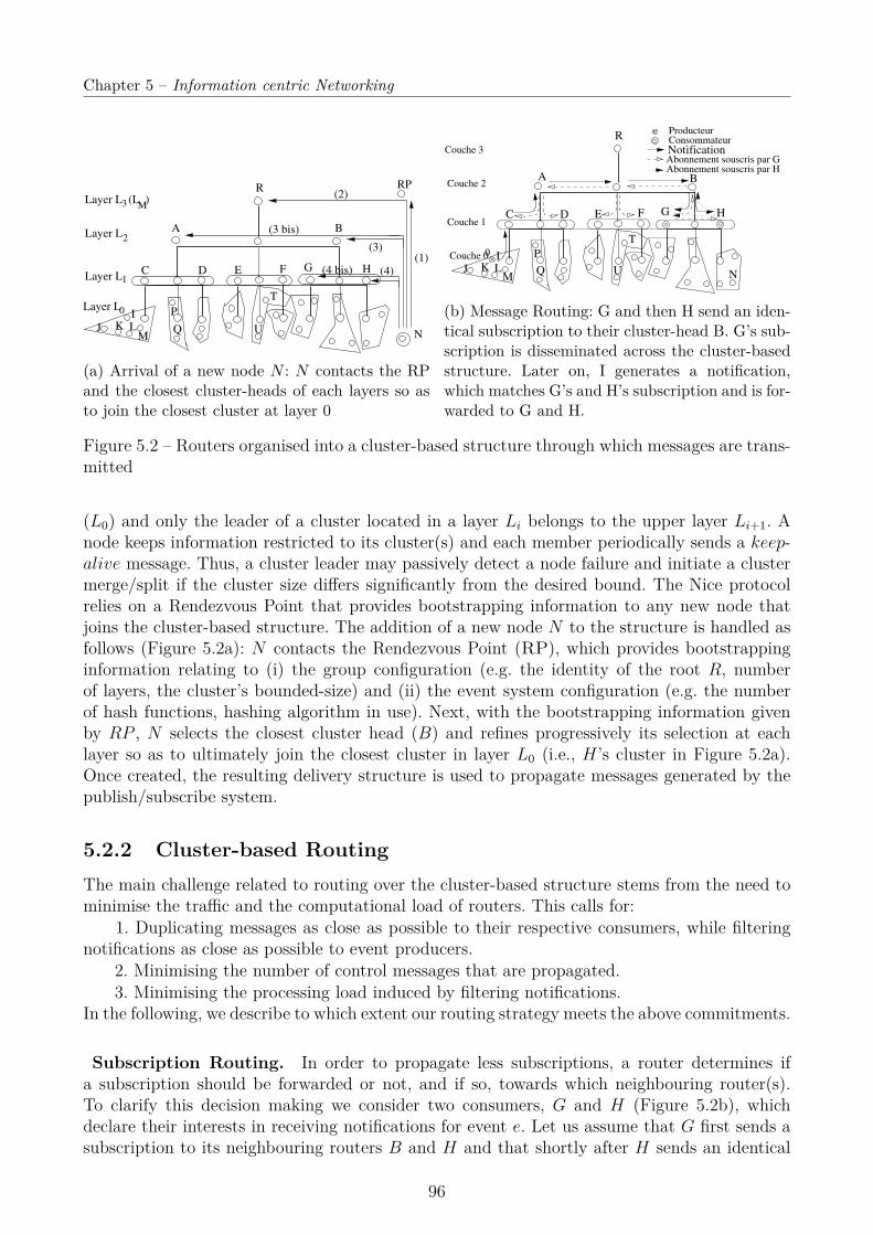
Chapter 5 – Information centric Networking
Layer L
Layer L
3
2
1
Layer L (L )
Layer L0
R
J K LM
I P
Q
T
U
M
EDC F HG
RP
N
BA
(1)
(2)
(3)
(4)
(3 bis)
(4 bis)
(a) Arrival of a new node N : N contacts the RPand the closest cluster-heads of each layers so asto join the closest cluster at layer 0
R
A
J K LM
I P
Q
T
U N
EDC F HG
0
BCouche 2
Couche 3
Couche 0
Couche 1
Notification
Producteur Consommateur
Abonnement souscris par GAbonnement souscris par H
(b) Message Routing: G and then H send an iden-tical subscription to their cluster-head B. G’s sub-scription is disseminated across the cluster-basedstructure. Later on, I generates a notification,which matches G’s and H’s subscription and is for-warded to G and H.
Figure 5.2 – Routers organised into a cluster-based structure through which messages are trans-mitted
(L0) and only the leader of a cluster located in a layer Li belongs to the upper layer Li+1. Anode keeps information restricted to its cluster(s) and each member periodically sends a keep-alive message. Thus, a cluster leader may passively detect a node failure and initiate a clustermerge/split if the cluster size differs significantly from the desired bound. The Nice protocolrelies on a Rendezvous Point that provides bootstrapping information to any new node thatjoins the cluster-based structure. The addition of a new node N to the structure is handled asfollows (Figure 5.2a): N contacts the Rendezvous Point (RP), which provides bootstrappinginformation relating to (i) the group configuration (e.g. the identity of the root R, numberof layers, the cluster’s bounded-size) and (ii) the event system configuration (e.g. the numberof hash functions, hashing algorithm in use). Next, with the bootstrapping information givenby RP , N selects the closest cluster head (B) and refines progressively its selection at eachlayer so as to ultimately join the closest cluster in layer L0 (i.e., H’s cluster in Figure 5.2a).Once created, the resulting delivery structure is used to propagate messages generated by thepublish/subscribe system.
5.2.2 Cluster-based RoutingThe main challenge related to routing over the cluster-based structure stems from the need tominimise the traffic and the computational load of routers. This calls for:
1. Duplicating messages as close as possible to their respective consumers, while filteringnotifications as close as possible to event producers.
2. Minimising the number of control messages that are propagated.3. Minimising the processing load induced by filtering notifications.
In the following, we describe to which extent our routing strategy meets the above commitments.
Subscription Routing. In order to propagate less subscriptions, a router determines ifa subscription should be forwarded or not, and if so, towards which neighbouring router(s).To clarify this decision making we consider two consumers, G and H (Figure 5.2b), whichdeclare their interests in receiving notifications for event e. Let us assume that G first sends asubscription to its neighbouring routers B and H and that shortly after H sends an identical
96

5.3. Notification and Subscription Representation
subscription to its neighbouring routers B and G. Upon receiving G’s subscription, B forwardsit to its upper-layer router R and its sibling A. Following, G’s subscription is forwarded to allthe remaining routers: R sends G’s subscription to E and F while A forwards G’s subscriptionto C and D.
Later, upon receiving H’s subscription, B does not propagate it to R and G, because thereis no need for B to propagate a subscription for a notification that it has already previouslyreceived. Herein H’s subscription is not propagated because an identical subscription ( G’ssubscription) was already propagated. The same propagation process would apply if H’s sub-scription were covered by G’s subscription since this would mean that the events that match G’ssubscription(s) also match H’s subscription. Subscription is routed as follows: if the subscrip-tion is ascendant1, then that subscription is forwarded2 to the upper-level router. Conversely, ifthe incoming subscription corresponds to a descendant message or has been issued by a cluster-mate, then that subscription is forwarded to all lower-level routers. The unsubscription routingis similar to the subscription routing: a router forwards an unsubscription only if the relatedsubscription was previously forwarded to that router.
Event Notification Routing
Figure 5.2b illustrates our presentation on notification routing: an event producer I generates anotification e in which two consumers are interested (G and H). I then sends a notification e toits cluster head C, which propagates it to A since a subscription that matches e was previouslyissued by A. Following, A propagates the event notification to B, which in turn propagates itto G and H. Overall, the event notification is not propagated to all the routers: any router thatreceives the notification selects the router(s) towards which the notification should be propa-gated. The selection process consists in first matching the notification against the subscriptionsummary and then in extracting the list of neighbouring routers that should forward the match-ing subscriptions. The propagation of the notification over the delivery structure formed by therouter is the same to the one carried to disseminate (un-)subscriptions.
5.3 Notification and Subscription RepresentationThe effectiveness of the routing depends on the structure used to represent notifications,(un)subscriptions (§5.3.1 and §5.3.2) and on the structure used to organise all subscriptions(§5.4).
5.3.1 Notification and Subscription Formats
An event notification (or simply a notification) is composed of a set of ne attributes that aretyped and that describe the event (Figure 5.3a); each attribute αi (with 1 ≤ i ≤ ne) consists ofa type as well as a name-value pair: αi = (typeαi , nameαi , valueαi). An attribute type belongsto a predefined set of primitive types( e.g., string, integer or date). Figure 5.3a illustrates anotification issued by a network-monitoring application that informs about a directory servicebeing stopped.
1. An ascendant subscription is conveyed to an upper-level router.2. If we consider an edge router belonging to layer L0 (resp. LM ), the subscription is not forwarded to a
lower (resp. upper) layer.
97
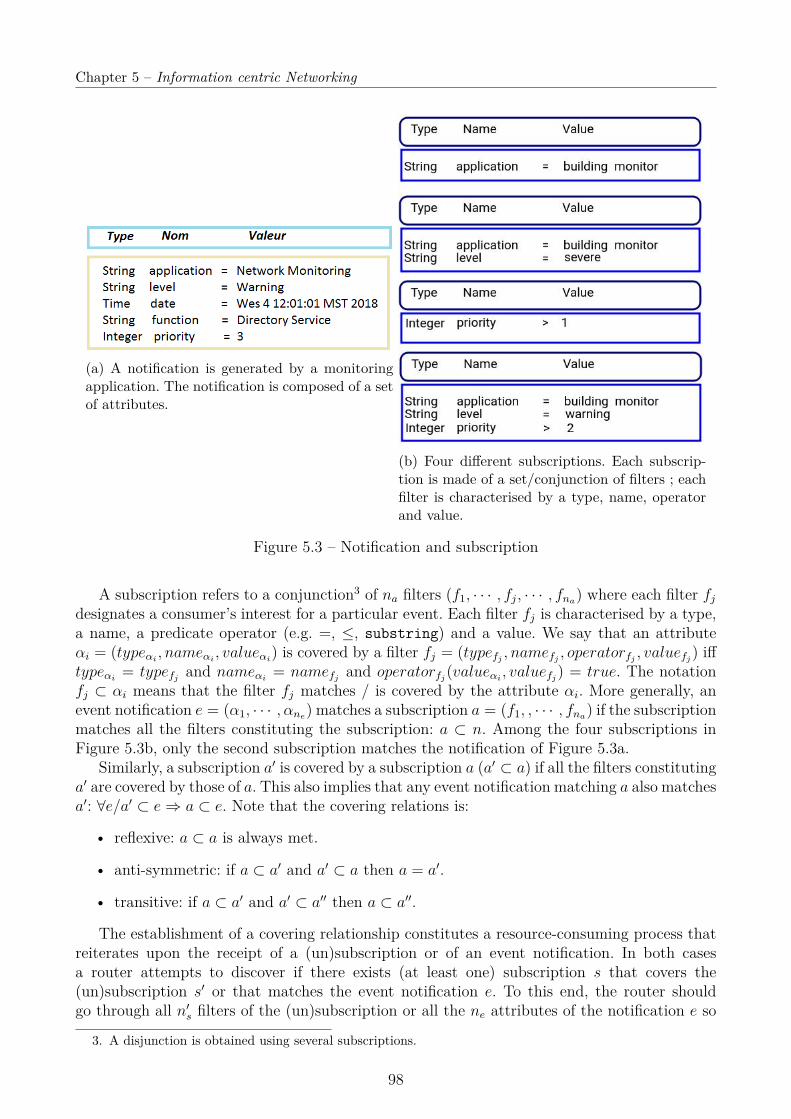
Chapter 5 – Information centric Networking
(a) A notification is generated by a monitoringapplication. The notification is composed of a setof attributes.
(b) Four different subscriptions. Each subscrip-tion is made of a set/conjunction of filters ; eachfilter is characterised by a type, name, operatorand value.
Figure 5.3 – Notification and subscription
A subscription refers to a conjunction3 of na filters (f1, · · · , fj, · · · , fna) where each filter fjdesignates a consumer’s interest for a particular event. Each filter fj is characterised by a type,a name, a predicate operator (e.g. =, ≤, substring) and a value. We say that an attributeαi = (typeαi , nameαi , valueαi) is covered by a filter fj = (typefj , namefj , operatorfj , valuefj) ifftypeαi = typefj and nameαi = namefj and operatorfj(valueαi , valuefj) = true. The notationfj ⊂ αi means that the filter fj matches / is covered by the attribute αi. More generally, anevent notification e = (α1, · · · , αne) matches a subscription a = (f1, , · · · , fna) if the subscriptionmatches all the filters constituting the subscription: a ⊂ n. Among the four subscriptions inFigure 5.3b, only the second subscription matches the notification of Figure 5.3a.
Similarly, a subscription a′ is covered by a subscription a (a′ ⊂ a) if all the filters constitutinga′ are covered by those of a. This also implies that any event notification matching a also matchesa′: ∀e/a′ ⊂ e⇒ a ⊂ e. Note that the covering relations is:
• reflexive: a ⊂ a is always met.
• anti-symmetric: if a ⊂ a′ and a′ ⊂ a then a = a′.
• transitive: if a ⊂ a′ and a′ ⊂ a′′ then a ⊂ a′′.
The establishment of a covering relationship constitutes a resource-consuming process thatreiterates upon the receipt of a (un)subscription or of an event notification. In both casesa router attempts to discover if there exists (at least one) subscription s that covers the(un)subscription s′ or that matches the event notification e. To this end, the router shouldgo through all n′s filters of the (un)subscription or all the ne attributes of the notification e so
3. A disjunction is obtained using several subscriptions.
98
5.3. Notification and Subscription Representation
as to assess if the attributes are covered by or match the filters constituting the subscription s.This results in O(ns.ns′) or O(ne.na) comparisons if the attributes and filters are not ordered,and in O(min(ne, ns)) (resp. O(min(ns, ns′)) comparisons if they are ordered. Overall, the han-dling of a new (un)subscription or event notification is laborious with content-based pub/subsystems while topic-based publish/subscribe systems filter events and handle (un)subscriptionsin O(1) when the subscriptions are stored in hash tables.
5.3.2 Subscription Organisation - State of the ArtFew solutions [112, 125, 34, 24, 85, 32] thus far address reorganisation of subscriptions so as toimprove the notification filtering and the (un)subscription process. All propose to organise thesubscriptions into a single data structure, which corresponds to a list, a partially ordered set (orposet), a R-tree, a B+-tree or a binary decision diagram. As detailed in the following, perfor-mance associated with notification filtering or with the establishment of a new (un)subscriptioncovering varies depending on the data structure:
• List [112, 125] - In a list containing n subscriptions, the establishment of the coveringrelationship with an (un)subscription s′ is costly: the covering is established in O(n.ns.ns′)if subscriptions are not ordered and in O(log(n).min(ns, ns′) if ordered. The filtering ofan incoming event notification e takes O(n.ne.ns) when subscriptions are not orderedand O(log(n).min(ne, ns)) if subscriptions are ordered. With a list, the subscriptions arestored one by one. The alternative structures described below, combine the filters thatform the subscription into a single data structure, which is organised in different ways.
• Poset [34] (see Figure 5.5 on page 103) exploits the covering relations of a set of filtersby applying a partial order on the set of subscriptions. Thus, any subscription at theupper level covers its descendant (Figure 5.6a). In practice, a poset corresponds to adirect acyclic graph whose size has an information-theoric lower bound of n2
p/4 + O(np)[113] and a (worst case) space complexity of O(n2
p) [34] with np defining the numberof elements stored in the poset. Adding/removing a subscription or filtering an eventnotification necessitates the lookup of subscription(s), which is done [34] by traversing theposet following a breadth-first order and starting from the root. This lookup has a worstcase complexity of np, though in practice it may be lower. This results in a subscriptionprocess done in O(np2), an unsubscription process of O(n3
p), and a notification matchingof O(np). The two following data structure (R-tree and B+-tree) also exploit the coveringrelationship.
• R-tree [24] has been traditionally used to support spatial queries. An R-tree is a tree inwhich each internal node has between m and M children. A node refers to the smallestpoly-space rectangle (a.k.a set of filters) that encloses all the rectangles of its subtree(a.k.a covers all its descendants). A range query is answered thought a top-down traversal,starting at the root and recursively following the subtree of each matching child. Theheight of an R-tree containing nr nodes is dlogM(nr)e − 1 with nr corresponding to thenumber of nodes. However, there is no acceptable guarantee, given that more than onesub tree under a node may need to be visited. In the worst case, the lookup with anR-tree is as expensive as a naive sequential scan.
• B+-tree is an ordered tree wherein all the intervals (all the filters) are stored and sortedat leaf level for fast traversing. A B+-tree is designed to have a fairly high number ofchildren for each internal node so that the height of the tree remains relatively small.
99
Chapter 5 – Information centric Networking
After insertion and deletion, a B+-tree may thus require balancing. In a tree of size n,performing a range query with k elements occurring within the range requires O(logbn+k)operations.
• Binary Diagram [32] structure represents a generic data structure used to represent theBoolean functions constituting a filter. A binary decision diagram may be represented as aDAG with a unique root, in which the internal nodes correspond to the Boolean functions.Thus, there are exactly two outgoing edges, labelled 0 or 1, for each inner node. With thebinary decision diagram, an arbitrarily complex Boolean expression of n variables can bestraightforwardly evaluated, by simply descending the DAG in n steps according to thevalues of the n Boolean functions. In counterpart, the size of the tree may exponentiallygrow with the number of functions.
Overall, the list, poset, R-tree, B+-tree and the binary decision diagram all place a high loadon routers and lead to a lower throughput and higher end-to-end latency.
Overload Reduction
The cost incurred by a lookup may be reduced by keeping the number of nodes in the datastructure to a minimum , thereby ensuring a faster traversal. This can be achieved in threeways: (i) reordering the data structure, (ii) merging the overlapping filters [111, 41, 24] or(iii) exploiting the fact [162] that there is no need to store the (new) subscription(s) that arealready covered by other subscription(s). A (re)ordering of the nodes may lead to a smallerdata structure and hence may reduce the (worst) time complexity. Still, an optimal re-orderingleading to a canonical form is known as an NP-hard problem. While a poset reordering wassuggested in [111], complicated heuristics have been devised in the literature on the subject toeither avoid the exponential growth of binary diagrams or of balanced R-trees. In particular,the binary tree can be organised in regards to the frequency of attributes and the variabledependencies (the analysis being an O(n2) process). In such a case, frequent attributes arepositioned near the root. The R-tree can be balanced by splitting an overflowing node duringthe joining process. Both a linear and an enhanced quadratic method inM and in the number ofdimensions have been proposed. Going one step further, the filters that overlap can be mergedtogether [111, 41] so as to reduce the depth and width of the data structure.
5.4 Enhanced ForwardingForwarding a notification or a (un)subscription is a common and resource-consuming processfor a router as it entails the two following tasks:
• Searching for the subscriptions that (i) match the incoming notification, or (ii) cover theincoming (un)subscription. As seen in Section 5.3.2 the matching of the notification andthe establishment of the coverage both imply going through the router’s subscriptions andare organised in several ways (list [112, 125], R- or B+-tree [24] or binary decision tree[32] and poset [34]). With a list, the search consists of reviewing the subscriptions oneby one ; with the remaining structures, the router traverses the structure, following thechildren that match/cover. The sequential reviewing and the traversal of the structureboth involve an elementary operation that consists in either matching the notificationattribute against a subscription filter or establishing the covering relationship betweentwo filters.
100

5.4. Enhanced Forwarding
• The two elementary operations are relatively complex. As an illustration, matching theattribute “String priority = 3" against the filter “Integer priority > 2" requires veri-fying that both have (i) the same type (String), (ii) the same name (priority) and (iii)that the value taken by the attribute (3) is indeed > 2. These elementary operations (i.e.,matching and establishment of a covering relationship) are repeated until any subscriptionthat matches/covers is discovered.
It is worth stressing that each router traversed by a notification/(un)subscription often unnec-essarily looks for the same subscription(s) and thereby performs a duplicate search. In order toavoid any unnecessary duplication of the search while making it easier to search when necessaryour approach is threefold:
• We include in the notifications (resp. (un)subscriptions to be conveyed) the subscrip-tion filters that need to be applied to filter the notification (resp. cover the incoming(un)subscriptions). Based on these embedded filters, any intermediate router gains fast ac-cess to the subscription(s) that match(es)/cover(s) the incoming subscriptions/notificationswithout searching for it/them.
• We summarise/approximate the subscription filters using a Bloom filter, which is use-ful for several purposes (§ 5.4). First, handling a summary (i.e., a Bloom filter) – inlieu of a full subscription filter – speeds up the filtering of event notifications and theestablishment of a covering relationship between subscriptions. Second, rather than in-cluding in the notification/(un)subscription all the subscription filters that match/coverthe notification/(un)subscription, a router adds a compact set made of the related Bloomfilters. Third, Bloom filters can be easily aggregated. This means that a set of Bloomfilters that are added to the notification/(un)subscription can be easily aggregated into asingle and comparatively smaller Bloom filter. Based on the set of Bloom filters (or theaggregated Bloom filter) a router forwards the notification/(un)subscription to the nextrouter without searching for the subscription(s) that match(es)/cover(s) the incomingnotification/(un)subscription (§ 5.4.1).
• We index subscriptions (§ 5.4.2) so as to enhance the search for a matching/coveringsubscription; the index is similar to a book index that allows anyone to quickly find thechapter of interest, without sequentially going through the book. In our case, the indexcorresponds to a hash table, which allows us to easily find the subscriptions covering theincoming notifications/(un)subscriptions.
Subscription and notification summarising
In order to accelerate matching notifications against subscription filters, we propose to representeach filter (and also each subscription) in a compact form by using Bloom filters. A shortintroduction on Bloom filters is provided in the following section.
101

Chapter 5 – Information centric Networking
Bloom filters are commonly used first to represent a set in a compact manner and subse-quently to test the membership of an element. A Bloom filter [25] is a bit vector of sizem, denoted B = b(1), · · · , b(m), which is initialised to 0 (i.e., ∀i ∈ [1,m], b(i) = 0).Updating a Bloom filter - To add an element e to the Bloom filter, k hash functionsh1, · · · , hk are used. Each hash function is applied to the element and the k bits at thepositions designated by h1(e) mod(m), · · · , hk(e) mod(m) are set to 1. Assuming that thehash time is O(1) then the time spent adding an element is O(k).Testing the membership of an element - Testing whether an e element belongs tothe set encoded in a Bloom filter is very similar to adding an element. The e is hashed,which gives the values h1(e) mod(m), · · · , hk(e) mod(m). In a Bloom filter, if a bit at saidpositions is 0 then the element is not stored in the Bloom filter. Otherwise (if none of thebits are at 0), the element is considered to be contained in the Bloom filter, knowing thata false positive may occur but no false negative can occur. The time required to test themembership of an element is O(k).Delete an element - An element cannot be removed from a Bloom filter simply byresetting the k bits to 0. To solve this problem, counting Boom filters have been intro-duced [60]. The idea is to replace the bit vector forming the Bloom filter with a u bitcounter vector. A counting Bloom filter corresponds to a vector of m counters. Each timean element is added, the counters at h1(e) mod(m), · · · , hk(e)mod(m)mod(m) are incre-mented. Thus, an e element can be deleted by decreasing the k counters located at thepositions h1(e) mod(m), · · · , hk(e) mod(m). A counting Bloom filter supports deletion ofdata in O(k). However, the use of counters implies an increased use of storage space andthe possibility of false negatives.
The Bloom Filter in a nutshell
Encoding of subscription filters as Bloom filter
A subscription is composed of a set of p filters. Each subscription filter, denoted fj (with1 ≤ j ≤ p), composing the subscription is hashed4 using k hash functions and stored in aBloom filter.
In order to limit their space footprint, there are two options for representing the Bloom filterdepending on the number of elements (i.e., filters) to be stored: as a bit vector (as is the casewith traditional Bloom filters) if the number of elements is low or as a list of hashes. Since aset of Bloom filters can be easily aggregated, a subscription can therefore be summarised into asingle Bloom filter (Figure 5.6b). In order to summarise a set of filters, denoted f1, · · · , fj, · · · fp,into a Bloom filter bf , we apply a bitwise OR on the corresponding Bloom filters: bf = bf1 OR· · · OR bfj OR · · · OR fp. If the Bloom filter is encoded as a list of hashes, the resulting Bloomfilter is encoded as: bf = bf1 , · · · , bfp .
Bloom-filter based repository
Each router keeps the received subscriptions in a dedicated repository, which may be organisedas:
• A list of subscriptions in which each subscription is stored along with the correspondingBloom filter that summarises the subscription. Assuming that nf filters compose a sub-
4. Each field composing the filter can be hashed independently or more simply the entire filter can be hashed.
102
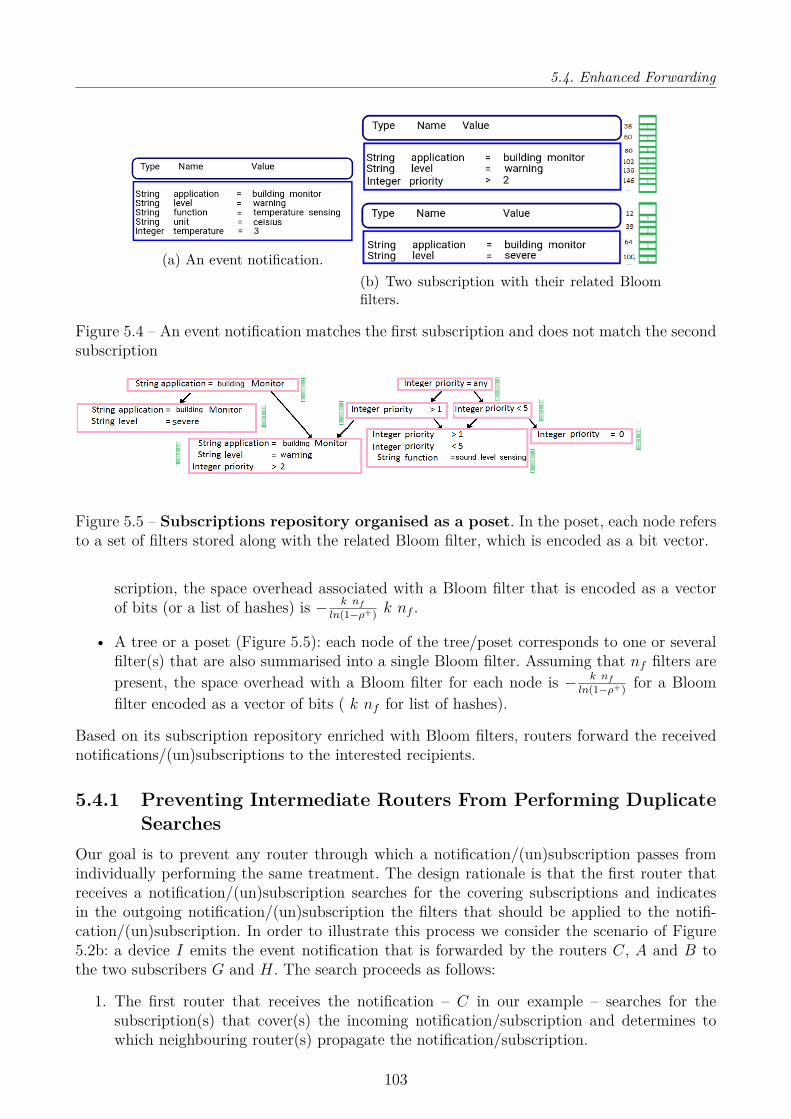
5.4. Enhanced Forwarding
(a) An event notification.(b) Two subscription with their related Bloomfilters.
Figure 5.4 – An event notification matches the first subscription and does not match the secondsubscription
Figure 5.5 – Subscriptions repository organised as a poset. In the poset, each node refersto a set of filters stored along with the related Bloom filter, which is encoded as a bit vector.
scription, the space overhead associated with a Bloom filter that is encoded as a vectorof bits (or a list of hashes) is − k nf
ln(1−ρ+) k nf .
• A tree or a poset (Figure 5.5): each node of the tree/poset corresponds to one or severalfilter(s) that are also summarised into a single Bloom filter. Assuming that nf filters arepresent, the space overhead with a Bloom filter for each node is − k nf
ln(1−ρ+) for a Bloomfilter encoded as a vector of bits ( k nf for list of hashes).
Based on its subscription repository enriched with Bloom filters, routers forward the receivednotifications/(un)subscriptions to the interested recipients.
5.4.1 Preventing Intermediate Routers From Performing DuplicateSearches
Our goal is to prevent any router through which a notification/(un)subscription passes fromindividually performing the same treatment. The design rationale is that the first router thatreceives a notification/(un)subscription searches for the covering subscriptions and indicatesin the outgoing notification/(un)subscription the filters that should be applied to the notifi-cation/(un)subscription. In order to illustrate this process we consider the scenario of Figure5.2b: a device I emits the event notification that is forwarded by the routers C, A and B tothe two subscribers G and H. The search proceeds as follows:
1. The first router that receives the notification – C in our example – searches for thesubscription(s) that cover(s) the incoming notification/subscription and determines towhich neighbouring router(s) propagate the notification/subscription.
103

Chapter 5 – Information centric Networking
2. Then the first router adds to the outgoing notification any indications about the locationof the subscription (i.e., how to access the subscription), which allows the next routersto quickly find the subscription(s) without searching for the subscription(s). The type ofindication varies depending on the underlying structure adopted to store the subscriptions.With a list of subscriptions the indication consists of the ordered list of subscriptionsthat match (or resp. cover) the incoming notification (resp. subscription). Note that thisordered list of filters is expressed as a compact set of Bloom filters. In the case of a binary-decision-/R-tree or poset, the path(s) to follow to get the matching subscription(s) mustbe added. This path materialises by an ordered list of filters that are aggregated into aBloom filter.
3. The subsequent routers (i.e., A and B) rely on the provided indications (i.e., the listof ordered subscriptions/filters) to extract the related subscription(s) and to forwardnotification/(un)subscription to the appropriate router(s).
Overall, the above outlined approach eases (and even prevents) the search for subscriptionsby intermediary routers. An intermediate router that receives a (un)subscription/ notificationcontaining Bloom filters proceeds by extracting each Bloom filter. If the repository is organisedas a list of subscriptions, the router checks if the filter equals a Bloom filter of the repository,which requires O(k × nf ) comparisons per Bloom filter. If the repository is organised as a treeor poset the router goes through the structure following the path expressed in the providedBloom filter, which requires O(k × np) comparisons with a path going through np filters.
Overall, the representation of subscriptions as Bloom filters speeds up the matching of anotification against a subscription. Nonetheless false positives may occur. In such a case, arouter assumes that an incoming subscription/notification is covered/matches (while this is notthe case) and unnecessarily forwards the notification/(un)subscription. The probability of afalse positive differs depending on the representation of the Bloom filter.
• Probability of false positives with a Bloom filter corresponding to a list of hashes - Knowingthat the probable occurrence of a false positive when an filter is compared to a filter isequal to (1 − 1
N)k, we can therefore infer that the probability of a false positive p(E)
occurring when nf filters are compared to ne attributes is:
p(E) = Cnfnf
(1− 1N
)k (5.1)
• Probability of false positive with a Bloom filter expressed as a vector of bits - We will usea balls-and-urns construct to model the handling of a Bloom filter. A Bloom filter (i.e.,a vector of bit) is modelled as m urns. We distinguish the repository subscriptions andincoming subscription using different colours: an incoming subscription is modelled as aset of bright balls and a subscription of the repository as set of back balls. The addition ofnf filters in a Bloom filter is equivalent to throwing k×nf bright balls into m urns (withm corresponding to the size of the Bloom filter). We define an urn as shiny if it contains atleast one shiny ball. Adding nf filters to a Bloom filter corresponds to randomly throwingnf × k black balls into m urns. A false positive occurs if a subscription of the repositorydoes not correspond to an incoming subscription even thought the nf × k black ballshave been thrown into bright urns. Using conditional probabilities and applying the lawof total probability we infer that the p(E) probability of a false positive occurring is:
p(E) =m∑r=1
[ m∑i=1
p(E/Ei/Er)p(Ei)]p(Er) (5.2)
104

5.4. Enhanced Forwarding
with p(E/Ei/Ej) denoting the probability that r black balls are thrown in i bright urns,p(Ei) corresponding to the probability that i urns are bright, and p(Er) the probabilitythat r urns are black. For a given i and given r, we observe that p(E/Ei/Er) is:
p(E/Ei/Er) =(i
m
)r(5.3)
In addition, the probability p(Ei) that i urns are bright corresponds to the quotientbetween:
– The number of surjections from a set containing k × nf elements to a set of i ele-ments [79]. This number is equal to i!.St(k × nf , i), with St symbolising Stirling’snumber.
– The number of functions of k× nf elements in a set of size m, which corresponds tomk×nf .
So:p(Ei) = 1
mk×nf
i∑j=0
(−1)j Cji j
k×nf (5.4)
Likewise, p(Er) = 1mk×nf
∑rs=0(−1)sCs
rsk×nf . We conclude that:
p(E) = 1mk2×nf×nf
m∑r=1
r∑s=0
(−1)sCsrsk×nf
m∑i=1
ir
mr
i∑j=0
(−1)j Cji j
k×nf (5.5)
Based on Formulas 5.2 and 5.5, the number of hash functions is set according to the numberof filters contained in the subscription/path, so that the probability of a false positive remainsbellow a given threshold.
5.4.2 Prefiltering with an Index-based Subscription RepositoryThe efficiency associated with the event/subscription forwarding depends of various aspects.With a repository containing a list of subscriptions, key factor is the number of subscriptionsstored in the repository. With tree or poset, the depth and the width of the tree/poset aretwo key factors. Ususally, the root tends to have many children. Visiting all the children ofthe root – wich we call horizontal crossing – is laborious and very frequent. Note: if there isno subscription filter that matches, all the children of the root are visited. In order to: (i)speed up the subscription search (especially the horizontal crossing) and (ii) avoid starting asubscription search when no subscription filter match, we propose to: (i) rely on hash tablesthat speedup the horizontal crossing (ii) introduce a prefiltering process that avoid searchingfor some covering subscriptions while no subscription covers.
Index-based Structure
We propose to index the subscriptions, leveraging hash table. With a list of subscriptions, wepropose to replace the list by a hash table. Thus, subscriptions are located with a key (asdetailed in the following paragraph), without searching for the subscription. In the case of aposet or tree, the first level of nodes are also organised in a hash table. Similarly, subsequentlevel may also be accessed using a hash table, i.e.,, the children of a given node are easily
105
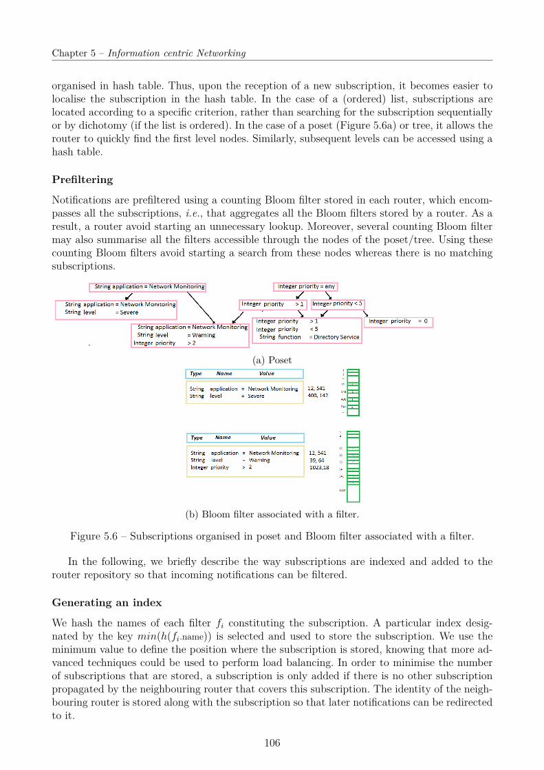
Chapter 5 – Information centric Networking
organised in hash table. Thus, upon the reception of a new subscription, it becomes easier tolocalise the subscription in the hash table. In the case of a (ordered) list, subscriptions arelocated according to a specific criterion, rather than searching for the subscription sequentiallyor by dichotomy (if the list is ordered). In the case of a poset (Figure 5.6a) or tree, it allows therouter to quickly find the first level nodes. Similarly, subsequent levels can be accessed using ahash table.
Prefiltering
Notifications are prefiltered using a counting Bloom filter stored in each router, which encom-passes all the subscriptions, i.e., that aggregates all the Bloom filters stored by a router. As aresult, a router avoid starting an unnecessary lookup. Moreover, several counting Bloom filtermay also summarise all the filters accessible through the nodes of the poset/tree. Using thesecounting Bloom filters avoid starting a search from these nodes whereas there is no matchingsubscriptions.
(a) Poset
(b) Bloom filter associated with a filter.
Figure 5.6 – Subscriptions organised in poset and Bloom filter associated with a filter.
In the following, we briefly describe the way subscriptions are indexed and added to therouter repository so that incoming notifications can be filtered.
Generating an index
We hash the names of each filter fi constituting the subscription. A particular index desig-nated by the key min(h(fi.name)) is selected and used to store the subscription. We use theminimum value to define the position where the subscription is stored, knowing that more ad-vanced techniques could be used to perform load balancing. In order to minimise the numberof subscriptions that are stored, a subscription is only added if there is no other subscriptionpropagated by the neighbouring router that covers this subscription. The identity of the neigh-bouring router is stored along with the subscription so that later notifications can be redirectedto it.
106
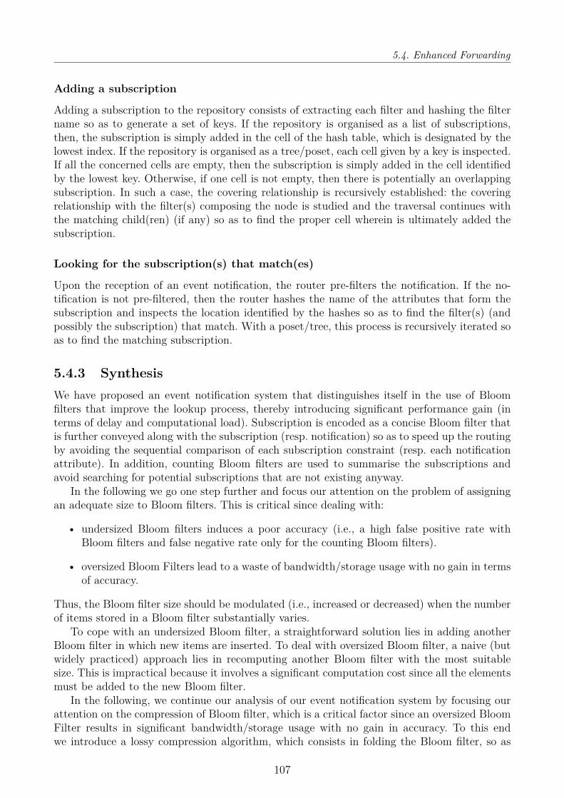
5.4. Enhanced Forwarding
Adding a subscription
Adding a subscription to the repository consists of extracting each filter and hashing the filtername so as to generate a set of keys. If the repository is organised as a list of subscriptions,then, the subscription is simply added in the cell of the hash table, which is designated by thelowest index. If the repository is organised as a tree/poset, each cell given by a key is inspected.If all the concerned cells are empty, then the subscription is simply added in the cell identifiedby the lowest key. Otherwise, if one cell is not empty, then there is potentially an overlappingsubscription. In such a case, the covering relationship is recursively established: the coveringrelationship with the filter(s) composing the node is studied and the traversal continues withthe matching child(ren) (if any) so as to find the proper cell wherein is ultimately added thesubscription.
Looking for the subscription(s) that match(es)
Upon the reception of an event notification, the router pre-filters the notification. If the no-tification is not pre-filtered, then the router hashes the name of the attributes that form thesubscription and inspects the location identified by the hashes so as to find the filter(s) (andpossibly the subscription) that match. With a poset/tree, this process is recursively iterated soas to find the matching subscription.
5.4.3 SynthesisWe have proposed an event notification system that distinguishes itself in the use of Bloomfilters that improve the lookup process, thereby introducing significant performance gain (interms of delay and computational load). Subscription is encoded as a concise Bloom filter thatis further conveyed along with the subscription (resp. notification) so as to speed up the routingby avoiding the sequential comparison of each subscription constraint (resp. each notificationattribute). In addition, counting Bloom filters are used to summarise the subscriptions andavoid searching for potential subscriptions that are not existing anyway.
In the following we go one step further and focus our attention on the problem of assigningan adequate size to Bloom filters. This is critical since dealing with:
• undersized Bloom filters induces a poor accuracy (i.e., a high false positive rate withBloom filters and false negative rate only for the counting Bloom filters).
• oversized Bloom Filters lead to a waste of bandwidth/storage usage with no gain in termsof accuracy.
Thus, the Bloom filter size should be modulated (i.e., increased or decreased) when the numberof items stored in a Bloom filter substantially varies.
To cope with an undersized Bloom filter, a straightforward solution lies in adding anotherBloom filter in which new items are inserted. To deal with oversized Bloom filter, a naive (butwidely practiced) approach lies in recomputing another Bloom filter with the most suitablesize. This is impractical because it involves a significant computation cost since all the elementsmust be added to the new Bloom filter.
In the following, we continue our analysis of our event notification system by focusing ourattention on the compression of Bloom filter, which is a critical factor since an oversized BloomFilter results in significant bandwidth/storage usage with no gain in accuracy. To this endwe introduce a lossy compression algorithm, which consists in folding the Bloom filter, so as
107

Chapter 5 – Information centric Networking
to require less space for storage or transmission. Note that this approach can be applied tocounting Bloom filter. The proposed compression takes advantage of the fact that Bloom filterscontain more information than necessary.
5.5 Folding Bloom FiltersFolding a Bloom filter is beneficial in the two following circumstances:
1. the Bloom filter stored in memory should be folded because it was initially over-sized.This situation frequently occurs because it is difficult to find a suitable size for a Bloomfilter since one must estimate in advance the amount of data that will be stored. Thus, aconservative approach based on over-sizing Bloom filters, which is often adopted.
2. A large Bloom filter needs to be transmitted and must first be folded so as to keepbandwidth usage and communication delay to a minimum.
In order to deal with both cases, we introduce a lossy compression algorithm, which performsthe folding of the Bloom filter and hence optimises the bandwidth/storage usage by reducingthe Bloom filter’s size.
In the following, we exemplify the folding of a Bloom filter with the following Bloom filterof 20 bits: 10010 11111 11101 11000. The halving of the Bloom filter consists of applying a ORon the two portions of the Bloom filter: 10010 11111 OR 11101 11000. The resulting Bloomfilter of size 10 is 10000 11000. With a counting Bloom filter, the folding is done by addingthe corresponding counters, using the maximum in case of overflow. It is worst-emphasisingthat with a Bloom filter of size 20, there exists several possible folding. Instead, a Bloom filtercontaining 5 bits/counters cannot be folded5. Let us understand the reason why by consideringa Bloom filter of size 20. A Bloom filter of size 20 can be folded in 7 ways because there are7 ways of factorising the original size of the Bloom filter: 20 = 2.10 = 2.2.5 = 2.5.2 = 4.5 =5.4 = 5.2.2 = 10.2. Remark that 5 and 2 are primes while 20, 10 and 4 are some compositenumbers, i.e., they can be expressed as a product of primes. Their composite nature impliesthat a Bloom filter with a size of 20, 10 or 4 can be folded while a Bloom filter with a size equalto 5, cannot be folded because 5 is a prime. Overall, selecting a proper size for the Bloom filteris critical so as to guarantee that many different folding may be applied later. Then, among thepossible choice(s), our goal is then to determine which is the best folding to apply at run time.In the following, we explore to which extend the folding may be achieved and we break thetwo related optimization problems into the off-line sizing of the Bloom filters and their on-linefolding:
• Off-line sizing of the Bloom filters (§ 5.5.1) - The sizing of a Bloom filter depends on thenumber of elements that are expected to be added and the required false positive rate. Wewill show that the ability to fold a Bloom filter is related to the size of the Bloom filter.We will investigate this relationship by introducing the mathematical background onnumber theory as well as providing a mathematical and practical formulation for findingthe optimal Bloom filter size. Although we will show that this size should be ideally ahighly composite number (i.e., a positive number that has a larger number of divisorsthan any number smaller than itself), practical considerations will lead us to formulatethe problem of finding a Bloom filter size as equivalent to finding a y-smooth-number, i.e.,a positive number whose prime factors are little primes (i.e., ≤ y). Once the size is set,the filter is created and may be compressed whenever needed by folding it.
5. We purposely exclude a bloom filter of size 1 that only reflects that the encoded set is empty or not empty
108

5.5. Folding Bloom Filters
• On-line folding can be modulated (§ 5.5.2) based on the amount of data actually storedin the Bloom filter and the admissible false positive rate. The folding (§ 5.5.3) can beviewed as a simple form of lossy compression that reduces the size of the Bloom filter andhence requires less space for storage or transmission. The lossy nature of the compressionimplies that the original Bloom filter cannot be reconstructed from the folded Bloomfilter.
5.5.1 Finding y-Smooth NumbersNumber theory comes into play here because the determining the precise sizing of Bloom filtersis critical to our approach. So before moving on with the planning of the Bloom filter size, letus first introduce some basic notions and background on number theory and more specificallyon smooth numbers.
Any number m ∈ N∗ can be expressed in an unique way as a product of primes:
m =∞∏j=1
(pj)γj =a∏j=1
(pj)γj (5.6)
with pj ∈ N, (i, γj) ∈ N2, a = maxi ∈ N | γi > 0 and ∀i < j, pi < pj. Contrary to a primenumber, a composite number has divisor(s) apart from itself and one. Keeping in mindthat we aim at finding numbers that have a high number of divisors, we naturally excludeprimes and focus our attention on highly composite numbers. A highly composite number(resp. a largely composite number) [129] is a number that has a larger number of divisors(resp. a larger or equal number of divisors) than any number less than itself and is hereinthe best (resp. good) candidate. Unfortunately, even though largely composite numbersare more crowded than highly composite numbers, both remain rare. To illustrate: 34highly composite numbers and 87 largely composite numbers are ≤ 332640; examplevalues are provided in Table 5.1. More formally [116], the number of highly compositeand largely composite numbers less than x, denoted Ψ(x), is subject to Ψ(x) << ln(x)bwith b being constant and respectively to exp(logc(x)) ≤ Ψ(x) ≤ exp(logd(x)) with cand d constant, for any large x. Studying the decomposition of the largely and highlycomposite numbers given in Table 5.2, we can hypothesise that a number suitable for ourpurposes would be composed of little primes, because this reflects the ability to fold aBloom filter and thus to smoothly reduce the Bloom filter size. This suggests consideringusing a smooth number, which is a number with only small prime factors [100]. Technically,a positive integer is said to be y-smooth if it holds no prime factor exceeding y (i.e., anyconstituting prime factors 6 y).These numbers are fairly numerous. Theorem 5.5.1, whosedetailed proof can be found in [78], gives a sense of the density of the smooth numbersthat belong to an interval [1, x] by showing that the proportion of y-smooth numbers upto x that have only small primes (i.e., y ≤ x
1u ) tends to a non-zero limit which is denoted
ρ(u).Theorem 5.5.1 Let S(x, y) be the set of y-smooth up to x and Ψ(x, y) denote its cardi-nality. Given y = x
1u (∀u ≥ 1), this number tends to a non-zero limit as x → ∞. This
limit is denoted ρ(u) and the cardinality satisfies [45]:
Ψ(x, y) v x ρ(u) as x→∞ (5.7)
Digression on Number Theory
109

Chapter 5 – Information centric Networking
with ρ defined as:• ρ(u) = 1
u
∫ uu=−1 ρ(t) dt, ∀u > 1, and,
• ρ(u) = 1 for the initial condition 0 ≤ u ≤ 1.A closed form of ρ to express Ψ(x, y) has been established in [72]:
Ψ(x, y) = 1π(y)
∏p≤y
(log x
log p
)(1 +O
(y2
log x log y
))(5.8)
Although this theorem gives the global distribution of y-smooth numbers over a range[0, x) - the values of the function ρ used in Expression 5.7 are provided in [72] (page 288)- the density of the smooth numbers is represented by the average gap in the sequence oftwo smooth numbers, denoted ni and ni+1 with ni < ni+1, is about:
≈ ni(log ni)π(y) with c2(y) ≤ π(y) ≤ c1(y) (5.9)
Based on Equations 5.8-5.9, we observe that y-smooth numbers are quite numerous. Thisimplies that they constitute a good solution for our folding problem.
∗1 ∗2 ∗3 ∗4 ∗6 8 10 ∗12 1820 ∗24 30 ∗36 ∗48 ∗60 72 84 9096 108 ∗120 168 ∗180 ∗240 336 ∗360 420480 504 540 600 630 660 672 ∗720 ∗8401080 ∗1260 1440 ∗1680 2160 2520 3360 3780 39604200 4320 4620 4680 ∗5040 ∗7560 9240 ∗10080 12600
Table 5.1 – Largely Composite Numbers (extracted from the annotations provided as partas [129] from the table handwritten by S. Ramanujan). Highly composite numbers are identifiedby *
∗2 3 ∗4 = 22 6 = 2 ∗ 3 8 = 23 10∗12 = 22.3 18 = 2.32 20 = 22.5 24 = 23.3 30 = 2.3.5 36 = 22.348 = 24.3 ∗60 = 22.3.5 72 = 23.32 84 = 22.3.7 90 = 2.32.5 96 = 25.3108 = 22.33 ∗120 = 23.3.5 168 = 23.7 180 = 22.3.7 240 = 24.3.5 336 = 24.3.7
Table 5.2 – Decomposition of Highly and Largely Composite Numbers
Based on a Bloom filter size, denoted x, which is provided as input by the applicationdepending on its need, the objective is to find a y-smooth, denoted m, that is near the givensize x and that offers a large number of possible folding. In practice, we isolate a short interval[x, x + z] near x and find a smooth number in this interval. Note that z should be selectedbased on Expression 5.9 so that the interval [x, x + z] contains at least one smooth number.Then, all the numbers x, x + 1, ...x + z should be enumerated and the divisibility with smallprimes (i.e., with all the primes ≤ y) tested for each. Assuming that x is fairly large, yrelatively very small and z sufficient to find at least one smooth number, excessive calculation
110
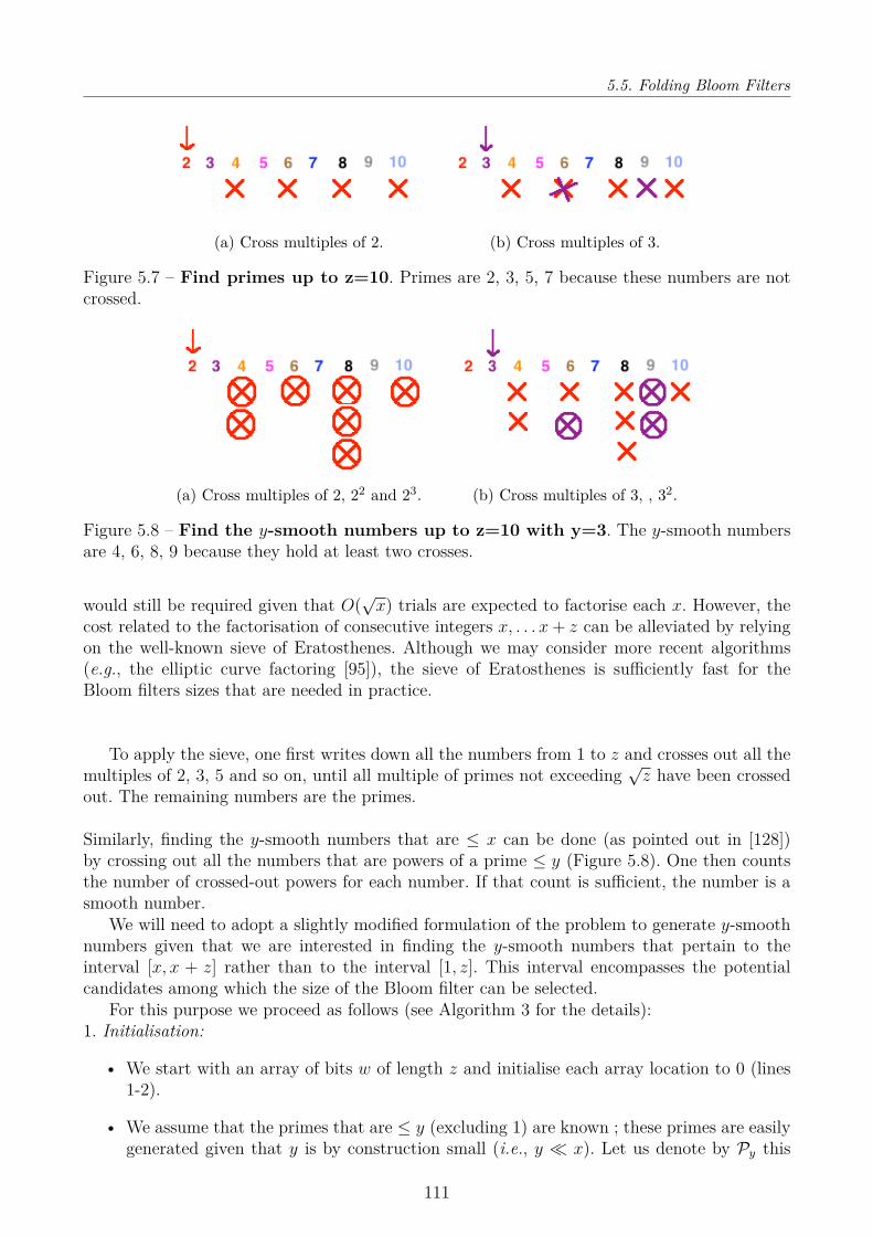
5.5. Folding Bloom Filters
(a) Cross multiples of 2. (b) Cross multiples of 3.
Figure 5.7 – Find primes up to z=10. Primes are 2, 3, 5, 7 because these numbers are notcrossed.
(a) Cross multiples of 2, 22 and 23. (b) Cross multiples of 3, , 32.
Figure 5.8 – Find the y-smooth numbers up to z=10 with y=3. The y-smooth numbersare 4, 6, 8, 9 because they hold at least two crosses.
would still be required given that O(√x) trials are expected to factorise each x. However, the
cost related to the factorisation of consecutive integers x, . . . x+ z can be alleviated by relyingon the well-known sieve of Eratosthenes. Although we may consider more recent algorithms(e.g., the elliptic curve factoring [95]), the sieve of Eratosthenes is sufficiently fast for theBloom filters sizes that are needed in practice.
To apply the sieve, one first writes down all the numbers from 1 to z and crosses out all themultiples of 2, 3, 5 and so on, until all multiple of primes not exceeding
√z have been crossed
out. The remaining numbers are the primes.
Similarly, finding the y-smooth numbers that are ≤ x can be done (as pointed out in [128])by crossing out all the numbers that are powers of a prime ≤ y (Figure 5.8). One then countsthe number of crossed-out powers for each number. If that count is sufficient, the number is asmooth number.
We will need to adopt a slightly modified formulation of the problem to generate y-smoothnumbers given that we are interested in finding the y-smooth numbers that pertain to theinterval [x, x + z] rather than to the interval [1, z]. This interval encompasses the potentialcandidates among which the size of the Bloom filter can be selected.
For this purpose we proceed as follows (see Algorithm 3 for the details):1. Initialisation:
• We start with an array of bits w of length z and initialise each array location to 0 (lines1-2).
• We assume that the primes that are ≤ y (excluding 1) are known ; these primes are easilygenerated given that y is by construction small (i.e., y x). Let us denote by Py this
111

Chapter 5 – Information centric Networking
predetermined set and by π(y) the number of primes in this set.
2. Consider successively all the primes pi ≤ y, and for each perform the following actions:
• Find the starting point, i.e., the smallest number in the interval, which can be dividedby pi and cross-out all the multiple of pi until all are crossed (line 12), i.e., cross x + s,x + s + pi, x + s + 2 pi, x + s + 3 pj ..., until all multiples of pi within [x, x + z] arecrossed. Note that such a crossing-out has to be performed not only for pi = p1
i but also(whenever possible) for p2
i (double crossing-out), p3i (triple crossing-out) etc, which leads
to the following step:
• Perform the same action (whenever possible) for p2i , p
3i , p
4i ... until all the crossing-out
ends. More precisely, this requires shifting the starting point to x + s + pji and crossingout x+ s+ pji , x+ s+ 2 pji , x+ s+ 3 pji , x+ s+ 4 pji ..., until all multiples of pji withinx, x+ z are crossed out (line 12).
3. Finally, we attempt to enumerate the y-smooth numbers, i.e., all the numbers m of [x, x+z]that hold a sufficient number of crosses.
Require: x ∈ N∗, y ∈ N∗, z ∈ N∗, z > x,Py1: for i = 0 to z do2: w[i] = 0 initialise the array w used to record the sum of the primes powers3: end for4: for pi ∈ Py do5: j ← 16: startpji
←(pi −
(x−pi
2
)mod pi
)mod pifind the starting point so that pji |x+ i
7: while startpji ≤ z do
8: for k ← 0 to bz−start
pji
pjic do
9: w[i+ k · pji ]← log(pi) cross the multiple k.pji10: end for11: startpji
← startpji.pi
12: j ← j + 113: end while14: end for15: if w[i] ≥ log(x) then16: SmoothNumbers = SmoothNumbers ∩ x+ i x+ i is a y-smooth number17: end if
Algorithm 3: Looking for Smooth Numbers
Complexity analysis - Let us investigate the time and space complexity of the algorithm.
• Initialisation: the initialisation of an array whose length is z, requires ∼ z steps and,according to the Prime Number Theorem, the space allocated to store the primes isO(π(y)) ≈ y
ln(y) .
• Crossing: the time devoted to multiple crossings-out splits into the research of the startingpoint startpji and then the crossing operation starting from startpji
. For all pi the time forfinding the starting point startjpi is ≈ π(y) ≈ y
log(y) . In the following, we first consider the
112

5.5. Folding Bloom Filters
time devoted to the first crossing (step 2.a) and then generalise our analysis to the jthcrossing (step 2.b), with j ≥ 1. The first crossing lies in enumerating all the multiples of pi,with pi ≤ y. This operation is the one achieved by the sieve of Eratosthenes implementedin the usual way [117], the execution time being Θ(z log log y). More precisely, z
picrossing
operations are performed for a given pi. Assuming that y ≤ z, we henceforth obtain thatfor all pi there are ∑
1≤pi≤yzpi≈ z log log y crosses.
The general case consists of crossing all multiples of pji , with j ≥ 1. For a given prime pisubject to pji ≤ z, the jth operation consists of crossing the multiples of pji , leading to z
pji
crosses. All pi subject to pji ≤ z hence involve ∑1≤pi≤y
z
pjicrossing with j ≥ 2. Overall, the
time φ(x, z, y) needed for all crossing operations satisfies:
φ(x, z, y) =y∑
pi=1
logpi (z)∑j=1
z
pji
Let us find the upper-bound of φ:
φ(x, z, y) =min(y,z)∑pi=1
zpi
+min(y,z1/2)∑
pi=1zp2i
+min(y,z1/3)∑
pi=1zp3i
+ . . . ≤pi=y≤z∑pi=1
zpi
+min(y,z1/2)∑
pi=1zp2i(1 + 1
p+
1p2 + · · ·+ 1
plog2(x+z)−2 ) =min(y,z)∑pi=1
zpi
+ zmin(y,z1/2)∑
pi=1
1−plog(x+z)−1i
pi(pi−1) ≤ z (log log y +O(1))
• Enumerating y-smooth Number - Finding all the smooth number in [x,x+z] requires anO(z) time execution.
Overall, the space required is z + π(y) and the computation time is π(y) + z (log logy +O(1)).Note that a logarithm formulation of the problem is used in the provided algorithm so as tolimit the space requirement involved in storing the crosses for any of the investigated z and forrepresenting the π(y) primes. It also privileges addition over multiplication by representing a
composite number in its logarithmic formulation as the following sum: log m =a∑j=1
γj log(pj)
rather than as the product m =a∏j=1
pγjj .
Among the resulting candidates, one y-smooth number, denoted m, is selected ; the smoothnumber should be selected to ensure that the Bloom filter is highly foldable, which yields tothe following canonical factorisation of m:
m =a∏j=1
(pj)γj with pi ≤ y. (5.10)
Thus the operational Bloom filter can be subsequently folded when necessary.
5.5.2 On-Line Folding StrategyThe goal is to determine the optimal folding to apply at run time, keeping in mind that thegoal remains to meet the required false positives rate ρ+ (and the required false negatives rateρ− for the counting Bloom filter).
We express this on-line folding strategy as the following optimisation problem. Given thatmt is the actual size of the Bloom filter, nt the number of elements stored and k the number ofhash functions, our goal is to find the minimal size of the resulting folded filter mt+1 that stillmeets the required false positive rate ρ+ and false negative rate ρ−, subject to mt+1 dividing
113

Chapter 5 – Information centric Networking
mt (which is denoted mt+1|mt). We assume that the number of hash functions is set once,preferably to its optimal value, minimising the false positives rate and is given by k = m0
n0ln(2),
with m0 referring to the initial size of the Bloom filter which is about −n0 ln(ρ+)(ln(2))2 and n0 denoting
the number of items that is expected to be added to the filter. We find that the mt+1 that stillmeets the false positives rate satisfies:
mt+1 ≥−n0 mt ln(1− (ρ+)1/k)
nt+1 f0...ft ln(2) (5.11)
Given that our goal is also to find mt+1 that divides mt, the above expressed goal can be refinedas finding all the combinations of pγii which produce mt+1 and selecting one combination. Forinstance, as suggested in the following algorithm, the minimal mt+1 that matches Equation 5.11can be used.
Recall that with mt =∏j∈St
pγjj the exhaustive enumeration of any folding is characterised by
a worst case computing time that is exponential in ∑j∈St
γj because the maximum number6 of
distinct products mt obtainable is 2∑j∈St
γj
. The storage required is ∑j∈St
γj in the worst case. But
if some combinations of folding are equivalent (i.e., have the same product) and are henceforth
not computed and not stored, the number of possible folding becomes in the order ofqt−1∑j=0
(qtj
)with qt = ∑
j∈Stγj. Then if the overall set of folding which is computed for m0 is ordered (the
duplicates being pruned), the computational cost related to finding mt+1 can be reduced to theorder of (log(
qt−1∑j=0
Cjq )) with a worst case of O( ∑
j∈S0γj). Once the size of the Bloom filter is fixed,
the Bloom filter can be folded.
5.5.3 FoldingThe folding of a Bloom filter consists in first dividing the Bloom filter into segments of size m′,which are denoted s1, · · · , sm/m′ . Next, these segments are combined to create a folded Bloomfilter which is expressed as s1⊕· · ·⊕sm/m′ , with the folding operator ⊕ defined as a combinationcorresponding to an or logic for a Bloom filter and an addition for a counting Bloom filter with.Precisely, with a Bloom filter (resp. counting Bloom Filter) the folding corresponds to applyinga bitwise or on (resp. summing7) the segments.
The Bloom filter is expressed as follows:
B′ =
⊕pl−1l=0 b(1 + l m′)
· · ·⊕pl−1l=0 b(i+ l m′)· · ·
⊕pl−1l=0 b(mt+1 + l m′)
with B =
b(1)· · ·b(i)· · ·b(m)
This folding corresponds to a lossy compression that leads to the establishment of a Bloom
filter whose size is less than or equal to that of the filter before folding. Given that a Bloom filteris a vector of sizem whose constituent elements are counters whose values go from 0 · · · 2u−1,
6. This number is in fact achieved for some mt.7. if a sum exceeds the maximum value 2u − 1, the counter is set to 2u − 1
114

5.5. Folding Bloom Filters
we have proved that the folding function ϕ: 0 · · · 2u − 1m −→ 0 · · · 2u − 1m′ satisfies thefollowing properties:
1. Compression with loss - ϕ maps a set of cardinality m to a set of cardinality m′ suchthat m′ divides m for any m′,m ∈ N∗.Note: a Bloom filter Bm is indexed by its size m and a folding ϕpl by the folding ratiopl ∈ N∗ ; this ratio can be expressed as the following quotient: pl = m/m.
2. Invariance - The folding always provides the same result and the operations correspond-ing to the addition of elements, the membership test and the deletion of an element in thecase of a Bloom filter, are all performed on a folded Bloom filter the same as they wouldbe on an unfolded filter. The membership test, which is denoted ω, is performed on a foldedfilter ϕpl(Bm) as it would be on a filter of size m′ = m/pl with ωk(ϕpl(Bm)) = ωk((B′m)).
3. Commutativity - A sequential folding, denoted o, corresponding to two folds ϕpl and ϕpris commutative: ϕpl o ϕpr = ϕpr o ϕpl
4. Associativity - sequential folding is associative: ϕplo (ϕpr : o ϕpv) = (ϕpr o ϕpl) o ϕpv
5. Efficiency - Any ϕ folding of a Bloom filter Bm ∈ 0 · · · 2u − 1m, ϕ(B) can be done ina polynomial time.
Verifying that the folding satisfies Condition 1 is straightforward. Condition 2 mainly relatesto the capacity to query the membership of an element and to add or delete this element ina folded Bloom filter. In the following we concentrate on proving that Condition 2 applies tothe membership test. The proof for the addition and deletion, which can be deduced from thisequation, will be left to the reader. Recall that the membership query proceeds as follows: theelement e is hashed with the k hash functions and if all the k investigated bits are set to 1, eis said to be stored. Thus Condition 2 holds if, for all k, b(hk(e) mod m) ≤ b′(hk(e) mod m′).Given that b′(hk(e) mod m′) = ⊕pl−1
l=0 b(hk(e) mod m′ + l m′) ≥ b(hk(e) mod m) it followsthat Condition 2 is satisfied and that the resulting probability of false positives ρ+’ on thefolded (counting) Bloom filter B containing n elements, using k hash functions satisfies: ρ+’= (1− (1− 1
m′)kn)k ≈ (1− e knm′ ). For Conditions 3 and 4, we consider a folding method that is
sequentially performed.Lemma - The sequential folding ϕpl and ϕpr satisfies:
ϕplo ϕpr = ϕpr pl (5.12)
Proof: Given a Bloom filter B, we can prove that:
ϕpl o ϕpr(B) = ϕpl pr(B)
The successive folding of B leading to B′ and the subsequent folding of B′ resulting in B′′ canbe expressed as:
∀i ∈ [1,m′′], b′′(i) =ϕpl o ϕpr(b(i)
)= ϕpl
(b′(i)
)with: ∀i ∈ [1,m′], b′(i) = ⊕pr−1
r=0 b(i+ r ·m′).
115
Chapter 5 – Information centric Networking
Thus, ∀i ∈ [1,m′′], b′′(i) can be expressed as:b′′(i) =⊕pl−1
l=0 ⊕pr−1r=0 b(i+ l ·m′′ + r ·m′)
=⊕pl−1l=0 ⊕
pr−1r=0 b(i+ l · m
pl pr+ r · m
pr)
A one-time-composite folding of B that leads to B′′ is performed as follows:
∀i ∈ [1,m′′], b′′(i) = φpr pl(b(i))= ⊕pr pl−1
j=0 b(i+ j ·m′′)
= ⊕pr pl−1j=0 b(i+ j · m
pr pl)
Thus, ϕpl o ϕpr(b) = ϕpr pl(b) given l ∈ [0, pl], r ∈ [0, pr], and, j = l + rpl .The above lemma means that the Bloom filters resulting of a sequential folding φproφpl isidentical to a single folding (φpr pl). Based on this lemma, the proof of conditions 3 and 4 canbe established as:ϕpr o ϕpl(Bt) = ϕpl pr(Bt) = ϕpr pl(Bt) = ϕpl o ϕpr(Bt). Thus, ϕpl o ϕpr = ϕpr o ϕpl In addition, ϕplo (ϕpr o ϕpv) = ϕpr pl pv = (ϕpr o ϕpl) o ϕpvThus, φplo (ϕpr o ϕpv) = ϕplo (ϕpr o ϕpv)
The commutative and associative properties of the folding imply that the order of thefolding does not matter. More generally, given the folded Bloom filter B, it is impossible toguess whether the Bloom filter went through a one-time or sequential folding; the foldingpathway cannot be inspected given the resulting Bloom filter. Although the sequential foldingφpr oφpl and a one-time folding φpr pl provide the same result, the cost in terms of time resultingfrom a sequential folding is greater than the cost of a one-time folding. Indeed (as defined inCondition 5), the computation cost associated with the folding is O(m): it depends on the sizeof B even if this cost can be reduced if the folding is parallelised. But, the cost of a sequentialfolding is O
(m (1 + 1
pl))with pl defining the second folding ratio.
5.6 Performance EvaluationOur next step is to assess the performance of our event notification system 5.6.1 via the foldingof Bloom filters 5.6.2.
5.6.1 Event Notification SystemIn order to reveal the scaling properties of our event notification system, we distinguish thecorresponding control traffic induced by the management of the cluster-based structure (Figures5.9a and 5.9b) and by the dissemination of the event notifications and (un)subscriptions. For thispurpose we use a constant load of 3 events/s per publisher. The distribution of subscriptions andnotifications follow a zipf law8 ; the probability of occurrence of the ith subscription/notificationis given by 1
iα. We will then aggregate the results obtained from several runs over a period of
20 minutes. As illustrated in Figures 5.9a and 5.9b, the group size has a low impact on theamount of control traffic ; the bandwidth usage being indifferent to the group size, highlightingthe benefits of maintaining membership information restricted to a cluster. When we considerthe traffic associated with the event notification and (un)susbcription routing (Figure 5.9c), we
8. Zipf distribution has been observed by stock quote providers [172].
116

5.6. Performance Evaluation
(a) Traffic associated with thewhole group management.
(b) Traffic related to groupmanagement per group mem-ber.
(c) Overall susbcription andnotification traffic for a groupof 70 members.
Figure 5.9 – Bandwidth usage associated with our notification system.
can see that the volume of subscriptions and notifications decreases as their similarities (i.e.,popularity ranking given by alpha) increases. This reveals the combined effect of (i) leveragingthe subscription covering and (ii) the aggregation and filtering capabilities made possible thanksto our cluster-based routing.
25 50 75 100 125 150 175 200 2 4 6 8 10 12 14 16 18 20
0 100 200 300 400 500
Time (ms)
Summary Size (#Subscriptions)
Subscription Size (#Constraints)
Time (ms)
(a) Bloom-filter based reposi-tory, with k=3 and m=6000.
25 50 75 100 125 150 175 200 2 4 6 8 10 12 14 16 18 20
0 100 200 300 400 500 600 700 800
Time (ms)
Summary Size (#Subscriptions)
Subscription Size (#Constraints)
Time (ms)
(b) Sienna repository.
100
150
200
250
300
350
400
450
500
2 4 6 8 10 12 14 16 18 20
Tim
e (
ms)
Subscription Size (#Constraints)
Our approach, m=1000Our approach, m=5000
Our approach, m=10000Sienna
(c) Router repository.
Figure 5.10 – Adding a subscription organised in poset and tree.
Following this we will measure the respective performances of, in term of latency, the mainstages constituting the subscription and notification processes, i.e., the addition of a subscrip-tion into a router repository and the filtering of an event notification. These results are thencompared with the poset-based repository promoted by Siena [34], using the delay as an ac-curate indicator of the processing overhead incurred within each of the above stages. In orderto test the impact of a complex subscriptions and notifications scanning, we further vary thesubscription size (number of constraints) and notifications (number of attributes).
Subscription Insertion
We measure the latency associated with adding a subscription into a repository by consideringboth our approach (Figure 5.10a) and the Siena approach (Figure 5.10b), with regards to avarying number of (i) subscriptions in the repository ([1, 200]) and of (ii) subscription filters([1,20]). Results show that Siena performs better than our approach for a number of subscriptionconstraints inferior to 5. To illustrate: if we consider 5 constraints per subscription filter, weobserve in our approach an average time ratio per subscription of 0.35 and an upper limitof 283ms and a corresponding ratio of 0.44 and maximum of 369ms with Siena. This reflectsthe computing cost of indexing and summarising the new subscription. However our approach
117

Chapter 5 – Information centric Networking
outperforms Siena when the number of constraints per subscription is greater than 5 because theindexing and summarising costs are compensated by the significant gain induced by the researchcovering the new subscription. Indeed, if we consider 10 and 20 constraints per subscriptionfilter respectively, we measure a lower latency (425ms and 499ms compared to 430ms and761ms obtained with Siena) and slower ascending rate (0.495 and 0.5925 with our approachcompared to the 0.525 and 0.87 experienced with Siena). Note that this difference, in termsof ascending rate and maximum latency, increases when we consider an increased repositorysize (i.e., number of subscriptions summarised), demonstrating that our event filtering systemperforms better in large-scale networks.
A similar trend is observed in Figure 5.11a. The delay incurred by our approach and Siennaincreases in a linear way, our system performing better when the number of subscriptionsreaches a certain threshold (from 5 up to 7 filters per subscription) whose value depends ofthe value of m. As expected, the latency induced by the insertion of a subscription into therepository depends of the repository size. However such impact remains limited and is easilyminimised by adequately configuring our event notification system and in particular the Bloomfilters’ sizes (§ 5.6.2).
100
150
200
250
300
350
400
450
500
2 4 6 8 10 12 14 16 18 20
Tim
e (
ms)
Subscription Size (#Constraints)
Our approach, m=1000Our approach, m=5000
Our approach, m=10000Sienna
(a) Adding a subscription into a router reposi-tory.
Notification Filtering
Next we compare the performances of the event notification filtering process in our solution(Figure 5.12) and Siena (Figure 5.13), considering varying repository sizes (Figures 5.12a and5.13a), varying subscription sizes (Figures 5.12b and 5.13b) and varying notification sizes (Fig-ures 5.12c and 5.13c). In all of the above cases we observe that the minima, maxima andascending slope obtained by our approach are always inferior to those of Siena. If we look atFigures 5.12a and 5.13a, the difference is mostly due to the combined effect of using a summaryand an index-based structure that allows the acceleration of the retrieval of the subscription(s)matching an incoming notification. The linear increase of the delay in Figures 5.12b and 5.13bis attributed to the sequential comparison of each subscription filter against each notificationattribute; the lower rate of increase exhibited by our solution is due to the compact digest usedto summarise the subscription.
Finally, in Figures 5.12c and 5.13c, we measure delay as a function of repository size ([1,200])and subscription similarity (given by the ratio of covered attributes shared by the subscriptionswhich are stored in the router repositories). The delay decrease experienced by both our ap-proach and Siena when considering an ascending similarity, is due to a reduced number of
118
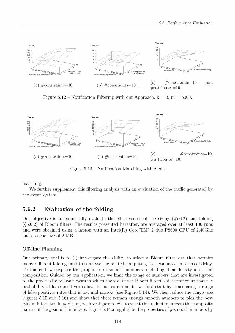
5.6. Performance Evaluation
20 40 60 80 100 120 140 160 180 200
5
10
15
20
0
100
200
300
400
500
Time (ms)
Summary Size (#Subscriptions)
Notification Size (#Attributes)
Time (ms)
(a) #constraints=10.
2 4 6 8 10 12 14 16 18 20
5
10
15
20
0
5
10
15
20
Time (ms)
Notification Size (#Attributes)
Subscription Size (#Constraints)
Time (ms)
(b) #constraints=10 .
10 20 30 40 50 60 70 80 90 100 0 0.2
0.4 0.6
0.8 1
0
5
10
15
20
25
Time (ms)
#NotificationsSubscription Similarity
Time (ms)
(c) #constraints=10 and#attributes=10.
Figure 5.12 – Notification Filtering with our Approach, k = 3, m = 6000.
20 40 60 80 100 120 140 160 180 200
5
10
15
20
0 100 200 300 400 500 600
Time (ms)
Summary Size (#Subscriptions)
Notification Size (#Attributes)
Time (ms)
(a) #constraints=10.
2 4 6 8 10 12 14 16 18 20 2
4 6
8 10
12 14
16 18
20
0 5
10 15 20 25 30 35 40
Time (ms)
Notification Size (#Attributes)
Subscription Size (#Constraints)
Time (ms)
(b) #constraints=10.
10 20 30 40 50 60 70 80 90 100 0 0.2
0.4 0.6
0.8 1
0
10
20
30
40
50
Time (ms)
#NotificationsSubscription Similarity
Time (ms)
(c) #constraints=10,#attributes=10.
Figure 5.13 – Notification Matching with Siena.
matching.We further supplement this filtering analysis with an evaluation of the traffic generated by
the event system.
5.6.2 Evaluation of the foldingOur objective is to empirically evaluate the effectiveness of the sizing (§5.6.2) and folding(§5.6.2) of Bloom filters. The results presented hereafter, are averaged over at least 100 runsand were obtained using a laptop with an Intel(R) Core(TM) 2 duo P8600 CPU of 2,40Ghzand a cache size of 2 MB.
Off-line Planning
Our primary goal is to (i) investigate the ability to select a Bloom filter size that permitsmany different foldings and (ii) analyse the related computing cost evaluated in terms of delay.To this end, we explore the properties of smooth numbers, including their density and theircomposition. Guided by our application, we limit the range of numbers that are investigatedto the practically relevant cases in which the size of the Bloom filters is determined so that theprobability of false positives is low. In our experiments, we first start by considering a rangeof false positives rates that is low and narrow (see Figure 5.14). We then reduce the range (seeFigures 5.15 and 5.16) and show that there remain enough smooth numbers to pick the bestBloom filter size. In addition, we investigate to what extent this reduction affects the compositenature of the y-smooth numbers. Figure 5.14.a highlights the properties of y-smooth numbers by
119

Chapter 5 – Information centric Networking
2 3 5 7 11 13
17 19 23 1
2 3
4 5
6 7
8 9
10
6200 6400 6600 6800 7000 7200 7400
y-S
mo
oth
Nu
mb
ers
Primes not exceeding y
Prime Power
(a) y-Smooth Numbers with an op-timal k = 4, y = 23.
1
2
3
4
5
6
7
8
9
10
2 3 5 7 11 13 17 19 23
Prim
e P
ow
er
Primes not exceeding y
(b) Power of the primes constitut-ing the y-smooth numbers, y = 23.
0
100
200
300
400
500
600
700
800
900
0 100 200 300 400 500 600 700 800 900 1000
# y
-Sm
ooth
Num
ber
s
y
(c) Amount of y-smooth num-bers.
Figure 5.14 – Effectiveness of the Planning , considering n =1000, 3.10−2 ≤ ρ+ ≤ 5.10−2.
2 3 5 7 11 13
17 19 23 1
2 3
4 5
6 7
8 9
10
25400 25600 25800 26000 26200 26400 26600
y-S
mooth
Num
bers
Primes not exceeding y
Prime Power
(a) y-Smooth Numbers with anoptimal k = 17, y = 23.
2 3 5 7 11 13
17 19 23 0
2 4
6 8
10 12
14
84000 86000 88000 90000 92000 94000
y-S
mooth
Num
bers
Primes not exceeding y
Prime Power
(b) y-Smooth Numbers with k =4, y = 23. (c) Delay with k = 4.
Figure 5.15 – Scalability of the Planing, setting n =1000, 3 10−6 ≤ ρ+ ≤ 5 10−6
2 3 5 7 11 13
17 19 23 1
2 3
4 5
6 7
8 9
10
35000 35200 35400 35600 35800 36000 36200
y-S
mooth
Num
bers
Primes not exceeding y
Prime Power
(a) y-Smooth Numbers with anoptimal k = 24, n = 1000.
2 3 5 7 11 13
17 19 23 0
2 4
6 8
10 12
14
300000 305000 310000 315000 320000 325000 330000 335000 340000
y-S
mooth
Num
bers
Primes not exceeding y
Prime Power
(b) y-Smooth Numbers with k =4, n = 1000.
(c) Amount of y-smoothnumbers.
Figure 5.16 – Scalability of the Planning, considering 3.10−8 ≤ ρ+ ≤ 5.10−8, y = 23
120
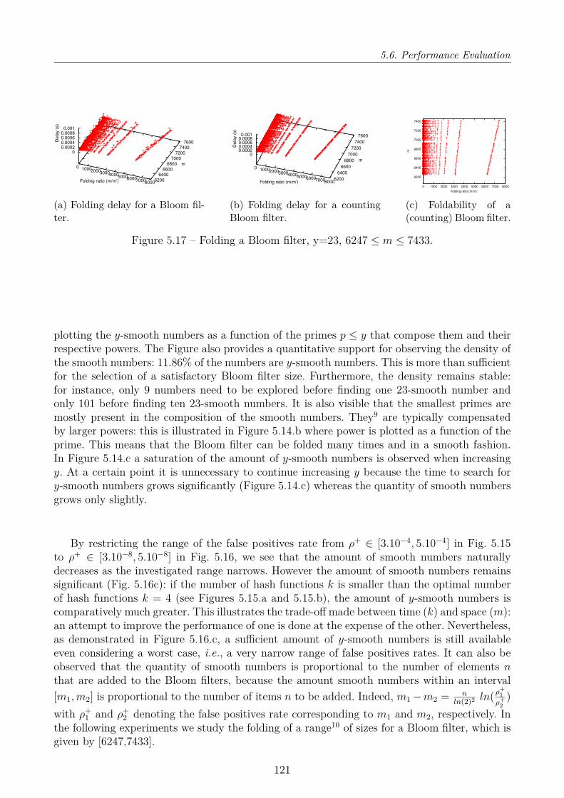
5.6. Performance Evaluation
0 1000 2000 3000 4000 5000 6000 7000 8000 6200
6400
6600
6800
7000
7200
7400
7600
0 0.0002 0.0004 0.0006 0.0008 0.001
Dela
y (
s)
Folding ratio (m/m’)
m
(a) Folding delay for a Bloom fil-ter.
0 1000 2000 3000 4000 5000 6000 7000 8000 6200
6400
6600
6800
7000
7200
7400
7600
0 0.0002 0.0004 0.0006 0.0008 0.001
Dela
y (
s)
Folding ratio (m/m’)
m
(b) Folding delay for a countingBloom filter.
6200
6400
6600
6800
7000
7200
7400
0 1000 2000 3000 4000 5000 6000 7000 8000
m
Folding ratio (m/m’)
(c) Foldability of a(counting) Bloom filter.
Figure 5.17 – Folding a Bloom filter, y=23, 6247 ≤ m ≤ 7433.
plotting the y-smooth numbers as a function of the primes p ≤ y that compose them and theirrespective powers. The Figure also provides a quantitative support for observing the density ofthe smooth numbers: 11.86% of the numbers are y-smooth numbers. This is more than sufficientfor the selection of a satisfactory Bloom filter size. Furthermore, the density remains stable:for instance, only 9 numbers need to be explored before finding one 23-smooth number andonly 101 before finding ten 23-smooth numbers. It is also visible that the smallest primes aremostly present in the composition of the smooth numbers. They9 are typically compensatedby larger powers: this is illustrated in Figure 5.14.b where power is plotted as a function of theprime. This means that the Bloom filter can be folded many times and in a smooth fashion.In Figure 5.14.c a saturation of the amount of y-smooth numbers is observed when increasingy. At a certain point it is unnecessary to continue increasing y because the time to search fory-smooth numbers grows significantly (Figure 5.14.c) whereas the quantity of smooth numbersgrows only slightly.
By restricting the range of the false positives rate from ρ+ ∈ [3.10−4, 5.10−4] in Fig. 5.15to ρ+ ∈ [3.10−8, 5.10−8] in Fig. 5.16, we see that the amount of smooth numbers naturallydecreases as the investigated range narrows. However the amount of smooth numbers remainssignificant (Fig. 5.16c): if the number of hash functions k is smaller than the optimal numberof hash functions k = 4 (see Figures 5.15.a and 5.15.b), the amount of y-smooth numbers iscomparatively much greater. This illustrates the trade-off made between time (k) and space (m):an attempt to improve the performance of one is done at the expense of the other. Nevertheless,as demonstrated in Figure 5.16.c, a sufficient amount of y-smooth numbers is still availableeven considering a worst case, i.e., a very narrow range of false positives rates. It can also beobserved that the quantity of smooth numbers is proportional to the number of elements nthat are added to the Bloom filters, because the amount smooth numbers within an interval[m1,m2] is proportional to the number of items n to be added. Indeed, m1−m2 = n
ln(2)2 ln(ρ+1ρ+
2)
with ρ+1 and ρ+
2 denoting the false positives rate corresponding to m1 and m2, respectively. Inthe following experiments we study the folding of a range10 of sizes for a Bloom filter, which isgiven by [6247,7433].
121
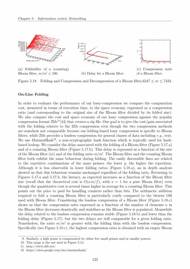
Chapter 5 – Information centric Networking
10 20 30 40 50 60 70 80 90 100 6200 6400
6600 6800
7000 7200
7400 7600
7.5e-05 8e-05
8.5e-05 9e-05
9.5e-05 0.0001
0.000105
Dela
y (
s)
Folding ratio (m/m’)
m
(a) Foldability of a (counting)Bloom filter, m/m′ ≤ 100.
0 200
400 600
800 1000 0
50 100
150 200
250 300
0
0.005
0.01
0.015
0.02
Dela
y (
s)
n
m/m’
(b) Delay for a Bloom filter.
0
50
100
150
200
250
300
0 200 400 600 800 1000
m/m
’
n
(c) Compression ratioof a Bloom filter.
Figure 5.18 – Folding and Compression and Decompression of a Bloom filter,6247 ≤ m ≤ 7433.
On-Line Folding
In order to evaluate the performance of our lossy-compression we compare the computationcost, measured in terms of execution time, to the space economy, expressed as a compressionratio (and corresponding to the original size of the Bloom filter divided by its folded size).We also compare the cost and space economy of our lossy compression against the popularcompression format Zlib11[44] that creates a zip file. Our goal is to give the cost/gain associatedwith the folding relative to the Zlib compression even though the two compression methodsare somehow not comparable because our folding-based lossy compression is specific to Bloomfilters, while Zlib provides a lossless compression for general classes of data including e.g., text.We use MurmurHash12, a non-cryptographic hash function which is typically used for hash-based lookup. We consider the delay associated with the folding of a Bloom filter (Figure 5.17.a)and of a counting Bloom filter (Figure 5.17.b). This delay is expressed as a function of the sizeof the Bloom filter (m) and of the folding ratio m/m′. The Bloom filter and the counting Bloomfilter both exhibit the same behaviour during folding. The easily discernible lines are relatedto the repetitive combinations of the same primes: the lower y, the higher the repetition.Although it is less observable in lower folding ratios (Figure 5.18.a), an in depth analysisshowed us that this behaviour remains unchanged regardless of the folding ratio. Returning toFigures 5.17.a and 5.17.b, the latency, as expected increases as a function of the Bloom filtersize (recall that the theoretical cost is O(um/f), with u = 1 for a pure Bloom filter) eventhough the quantitative cost is several times higher in average for a counting Bloom filter. Thispoints out the price to paid for handling counters rather than bits. The arithmetic additionrequired to fold a counting Bloom filter is particularly costly compared to the bitwise ORused with Bloom filter. Considering the lossless compression of a Bloom filter (Figure 5.18.c)shows us that the compression ratio expressed as a function of the number of elements n inthe Bloom filter decreases drastically and stabilises as the Bloom filter is populated. Meanwhilethe delay related to the lossless compression remains stable (Figure 5.18.b) and lower than thefolding delay (Figure 5.17), but the two delays are still comparable for a given folding ratio.Nonetheless, the ratio m/m′ is greater with the folding than with the lossless compression.Specifically (see Figure 5.18.c), the highest compression ratio is obtained with an empty Bloom
9. Similarly, a high prime is compensated by either few small primes and/or smaller powers.10. This range is the one used in Figure 5.14.11. http://www.zlib.net/12. https://sites.google.com/site/murmurhash/
122

5.7. Conclusion
filter (i.e., a vector of entirely set to 0) whereas the lowest ratio stands for the highest13 value ofn (here, 1000). The monotonic decrease and the small compression ratio reflects the difficultyof compressing random data (i.e., a Bloom filter wherein some bits are randomly set to 1) andthe practical advantage of a folding-based lossy-compression.
5.7 ConclusionThe IoT is characterised by a large number of Things scattered around the world that need toexchange messages over the Internet. The provision of a reliable and timely means of commu-nication over a wide area network is still a critical and problematic issue. We have addressedthis issue through the introduction of an event notification system that supports a lightweightcontent-based filtering and that relies on a self-configuring grouping service that dynamicallyorganises the event delivery structure. Our content-based event notification system supportsa scalable group communication and novel lightweight event filtering scheme that keeps theload on routers to a minimum. Our event notification system is automatically deployed withoutrequiring human intervention and is fault-tolerant as it adapts dynamically to any permanentor transient network failure.
It is worth stressing that the routers traversed by a notification/(un)subscription dedi-cate significant time and effort to search the matching subscriptions while the search is oftenthe same for all the routers. If one router – ideally, the first router receiving the notifica-tion/(un)subscription – can indicate how to access the subscriptions, then subsequent routersdo not have to repeat the same time-consuming subscription search. In order to support suchan approach without congesting the network and routers, we represent the subscription ashighly compact Bloom filters. In this way it is possible to effectively filter event notifications.In addition, we propose a hash-based indexing structure that allows subscriptions to be quicklyretrieved, possibly based on the provided indications.
Still, finding the correct Bloom filter size is challenging, because the quantity of data mustbe estimated in advance to ensure that the required false positive rate is always respected. Ingeneral practice this leads to a situation in which the Bloom filter is oversized. In order toovercome this issue we propose – and further evaluate the performance of – a lossy compressionsystem that consists of folding the Bloom filter. We show that the foldability depends on thethe exact size of the Bloom filter, thereby establishing an interesting link between numbertheory and Bloom filters. More precisely, we propose to select a y-smooth number due to theirhigh density and ease of production, which derives from their simple multiplicative structure.We show that selecting y-smooth numbers is advantageous since they allow a large number ofpossible folding combinations. We then present an algorithm based on a sieve of Eratosthenes,which is efficient with regards to the envisaged sizes of Bloom filters. Once properly sized, theBloom filter can be folded very efficiently so that the false positive/negative rate is always met.We further analyse the ease of selecting a size for Bloom filters that allows a large numberof folds and evaluate the associated costs. This led us to empirically explore the properties ofy-smooth numbers, their density and composition.
Overall, Bloom filter folding is advantageous in two application scenarios. The first assumesa Bloom filter stored in memory, which needs to be folded; this is advantageous, for example, ifthe Bloom filter was initially over-sized. The second scenario, and the main motivation for ourwork, deals with the transmission of a Bloom filter, which should be folded prior to transmission
13. Although a highly populated Bloom filter would exhibit a high compression ratio, it would be subject toa unacceptable false positives rate.
123

Chapter 5 – Information centric Networking
in order to minimise bandwidth usage and communication delay. After appropriate sizing , theremaining problem in both scenarios is the determination of the applied folding rate in order toachieve the required false positive/negative rate. Ultimately this folding and filtering problemis a classic compromise between time (computation) and space (storage and communication):increasing the performance of one is inevitably to the detriment of the other.
124
Chapter 6
Conclusion
The forward-thinking academic John Culkin remarked that “we become what we behold. Weshape our tools and then our tools shape us.” The truth behind this observation written in1967, has perhaps never been more obvious than it is today. We are witnessing a unique stagein mankind’s technological history and just as technology evolves – and continues to evolve –so do we too change with it. From this perspective, the IoT has greatly increased our intercon-nectedness and thereby our understanding of the physical world around us. The shift towardswidespread use mobile, consumer-centric smartphones is making our immersion with comput-ing into a permanent, and somehow dependant, state by permeating practically all aspects ofour daily lives. The real and the virtual have remained relatively dissociated since the dawn ofinformation technology, but are nowadays becoming increasingly intertwined.
Shaped by the Internet of Things, my own research journey is anchored in these last decades,anticipated by Mark Weiser (1988), which has predicted a world in which "technology recedesinto the background of our lives." Since then, the IoT ecosystem has been successfully appliedto enhance our interconnection with physical spaces. Due to its ubiquity, the IoT might wellaspire to become the lingua franca of a newly emerging generation of people long immersed in anIoT-landscape. However the path leading towards ubiquitous computing raises some challengesand significant research efforts remain to be invested as tribute to the discrepancy in the qualityof data and services contributed by the Things.
6.1 Summary of ContributionsIn an increasingly interconnected IoT where Things freely exchange data and offer servicesthat are accessible through open and poorly secured interfaces, the IoT raises some concernsrelated to reliability, faithfulness and accuracy. In the last mile, IoT networks are predominatelydriven by – and built upon – wireless networks (Near Field Communication or slightly longerWiFi or Bluetooth-enabled technologies) that: (i) allow greater access to outsiders that exploitvulnerabilities and may cause significant damage, and (ii) make it easier for insiders to avoididentification. Monitoring the behaviour of things and the network is necessary in order to spotintrusions, coming from either inside or outside the network. Intrusions manifest in the formsof: (i) attack behaviour which differs to that of a normal user, or as (ii) a sequence of actionsundertaken by the attacker that characterises the attack pattern. We have covered both formsof attacks and explored signature-based and anomaly detection, focusing on the communicationand computing infrastructures that span different scales from the MANETs composed of per-sonal laptops equipping mobile users to RFIDs tags that are highly miniaturised. Unlike mobilelaptops that may undertake advanced analytics, RFID tags are passive and unintelligent; thesefeatures imply their inability to monitor and understand their environment. In each case, wehave considered the nature of the monitored system (network/computer/object and suppliedservice) and tailored the detection system accordingly. To secure MANETs, we have introduceda distributed signature-based Intrusion Detection System (IDS) intended to monitor the attacksagainst the OLSR routing protocol. We noted that the device has a limited observability and
125

Chapter 6 – Conclusion
that the partial network view, which is gained thanks to other peers, is questionable in termsof reliability. To address this issue we have devised an entropy-based trust system that dealswith uncertainties and incompleteness involved in trust relationships, leveraging a statisticalgathering approach that gracefully and incrementally gathers observations without sacrificingdetection accuracy. As a complement we have explored anomaly detection to identify any devi-ations from normal behaviour. Relying on Kohonen maps, which constitute an efficient way forautomatically categorising, our IDS further compares the tagged behaviour against the normaluser’s behaviour as expressed in the user’s profile.
A lack of security is not the only flaw in the IoT. The loss of data quality is a highly debatedissue within the academic and practitioner communities who often deal with the unintentionalcorruption of sensed data. A conflict between end-users’ expectations over the data and thereliability of data gleaned from low-cost or DIY sensing devices is often present. Sensor cali-bration in the field is essential to overcoming this issue as it: (i) ensures a proper operationof the sensing devices, and (ii) deals with varying external conditions (e.g., solar radiation,freezing) and other factors (e.g., activity of the end user) that affect the measurements overtime. Sensor calibration has received surprisingly little attention from researchers. We have thusproposed a holistic approach to reduce the cost associated with calibration in smart spaces atscale, from the fixed Things that make up the IoT infrastructure to the mobile Things thatpeople carry. We have developed a plan for the calibration of a large number of often inac-curate sensors in a smart space using high-integrity reference sensors that are mobile, so asto maintain an adequate sensing accuracy while minimising the required effort from the mo-bile calibrators. We have in turn generalised the automated calibration to the multi-party caseto sustain a macro-calibration. In particular we have conceived a distributed, opportunisticmacro-calibration system that leverages the presence of the nearby crowdsensors that monitorthe same physical phenomenon, which we have shown improves the accuracy of the perfor-mance sensing application. Such an approach to calibration is particularly well suited to mobilecrowdsensing scenarios in which the crowd senses and meets in public places.
Opportunistic crowdsensing shows a great potential to monitor the physical environment ina cost-effective and dynamic way by empowering people to contribute as part of their daily life.As such, crowdsensing is gradually becoming a cost-effective complement to fixed wireless sensornetworks. The major emerging challenge currently facing mobile crowdsensing is related to thegathering and processing of an ever-increasing amount of data collected across time and space,with the intention of making the best sense of it so as to provide citizens and communities withrelevant value-added information. In practice, people’s mobility makes the crowdsensing contri-bution unevenly distributed over space and time, thus requiring the post-processing of sensingdata on the cloud. As the number of contributors grows, the increasing number of observationsthat the crowdsensing platform must process becomes challenging: the high network and finan-cial cost associated with a cloud-centric system hinders the widespread use of crowdsensing andthe high computational cost required makes the modelling of the environmental phenomenonintractable. Given the growing volume of data involved to cover urban-scale areas, restrainingthe increasing operational cost of the cloud-assisted infrastructure and keeping to a minimumthe resource consumed by the hand-held devices are a prerequisite. We have addressed thisissue by exploiting the ever-increasing computing capacity of smartphones by evenly distributethe collection, interpolation and aggregation associated with the sensing data to powerful enddevices. To this end we have introduced a crowdsensing middleware, which supports a novelin-network collaboration strategy that enhances the quality of the data before their transferto the cloud, while reducing the related communication cost and resource consumption. Themiddleware tailors a set of utility functions that assess to what extent a device should carry out
126
6.2. Perspectives
a given crowdsensing task while achieving a trade-off between the benefit for all (aka for thegroup) and the related cost for the device. Rather than applying a naive combination (e.g., aver-aging) of the data collected by the crowdsensors that would actually degrade the quality of thesensing data, our middleware performs an advanced inference. A Crowdsensor may establish avery precise interpolation of the regions it covers. Individual interpolations are then aggregatedon the cloud, which renders the overall interpolation on the cloud much more tractable.
We observe a paradigm shift towards "edgeness" and information-centric networking thatsupports an early edge decision-making. In this perspective we have proposed a content-basedpublish/subscribe system that supports flexible and scalable messaging among Things (e.g.,sensors and actuators) and applications, delivering information across the wide range networkto interested consumers as the amount of IoT devices increases and spreads geographically. Wehave built a cluster-based and hierarchical delivery structure that scales and tolerates failureswhile achieving both low latency and efficient use of resources. In the delivery structure, routers(a.k.a cluster heads) dedicate significant effort to filter and forward the messages (i.e., eventnotifications and (un)subscriptions). To reduce the routers loads we have proposed to helprouters by including in the message the filters that need to be applied. In order to supportsuch an approach without congesting the network, we have compacted filters. As a result, theflow of event notifications produced by any Thing can be filtered and distributed to providesituation-awareness and trigger actions accordingly.
In this manuscript I have presented a snapshot of my research as it stands today, keep-ing in mind that the development of a robust and resilient IoT remains a daunting task andmany improvements are needed. From hardware to middleware, data collection to analysis anddecision-making, actual practice to guiding theory, much works lies ahead in the creation of anefficient, resilient and ultimately life-enhancing IoT.
6.2 PerspectivesConveying and processing the massive amount of data that is produced by the IoT – and inparticular by crowdsensing applications – has become a major issue in terms of the managementand operation of the underlying applications and networks. Conventional cloud computingsystems and current communication architectures must be adapted and optimised to efficientlyprocess the very large volumes of data generated by the IoT, which will continue to grow intime and space.
Further solutions and related optimisations need to be designed – acknowledging that someservices can be moved close to smartphones and that much of the data can be stored or evenanalysed and filtered at an early stage to limit the amount of data transferred. Data, services andunderlying infrastructure must also be secured in a complementary fashion. I intend to addressthese issues by exploring several research directions, ranging from the design of collaborativeand distributed systems capable of supporting crowdsensing applications that operate on alarge scale to the development of a secure environment for these applications.
Towards Virtual(ised) CrowdsensingThe data supplied by sensing applications, including mobile crowdsensing apps, contain insightsabout the physical and social environment and concerns user’s activities and situation. Our pastwork has shown us that contributed data are often unusable unless first compared, fused, con-textualised, enriched, classified ect.. Somehow, sensors are not intended to operate individually;they should not be considered as an autonomous pieces of hardwares and softwares capable of
127

Chapter 6 – Conclusion
monitoring a physical or social phenomenon on their own. Sensors are heterogeneous and oper-ate at different scales spanning the nano, personal, and urban. Yet they are domain-specific andtask-oriented: the mass of information they produce is specific to a sensor model, dedicated toa particular use(r), and mostly tailored to a given application with little or no possibility of usewith other applications. To overcome this limitation we must abstract the set of physical sen-sors along with the operations performed on them to increase the data usability. The aim is todefine and support virtual sensors that supply measurements that are not directly available bycombining the measurements provided by a group of heterogeneous sensors. This also involvesbroadening the types of context we may thus characterise and integrating other sources of infor-mation of a social (social networks) or environmental (such as open street maps) nature. Fromthis perspective it is crucial to define new methods of cooperation between physical and virtualsensors capable of performing complex and virtual tasks sustaining the enrichment, analysis,fusion, interpretation and transformation of data provided by both virtual and physical sen-sors, including other sources of relevant information. During the synthesis and comparison ofthe sensed information, the context/situation dependence and multi-dimensional nature of thesensed data cause a non-stationarity, which is not adequately addressed by conventional leastsquare regression and derived interpolation methods. Rather than breaking down the data,using for instance multiple regressions to deal with the multi-dimensionality of the context, wepropose an exploration of weighted regression [29] and moving weighted windows over the data,thereby estimating groups of coefficient values that fit the samples. This method first selectsa bandwidth for an isotropic spatial weights kernel, typically a Gaussian kernel with a fixedbandwidth chosen by leave-one-out cross-validation. The choice of the bandwidth [28] is verydemanding and requires investigation, as regressions must be fitted at each step.
Mobile and edge computing
Delivering seamless connectivity and communication to mobile users and ensuring sufficientquality of service despite the mobility of users/things remains a vast area of research, of whichonly certain challenges have been solved thus far. Our approach to improving communicationreliability relies on exploiting multiple access networks that should be further adapted to dealwith the dynamic aspects induced by mobility. As far as the mobile IoT is concerned, intelligentand opportunistic clustering helps to structure the network architecture; "intelligent gatewayplacement" techniques are prerequisites to enabling a smooth connection. Still there is a needto establish the most suitable path based on dynamic network properties (such as link quality)so as to convey packets to (mobile) gateways, taking into account the Braess paradox thatoften occurs as certain gateways act as vortexes. Supporting algorithms lead to an overuse ofcertain paths and therefore severe congestion, e.g., with video [27]. Rather than merely selectingthe optimal path our approach will aim at distributing/splitting the information using gametheory. Although theory and algorithms for game have been extensively studied, a majority ofthe approaches [86] assumes that players are aware of the overall game state and previous movesbefore playing. This not realistic with IoT: Things (a.k.a players) have a limited observabilityand do share a consistent knowledge on their previous or ongoing actions. Incomplete knowledgeintroduces uncertainty that needs to be modelled [161], a critical issue that we address byfinding an equilibrium without necessarily needing information regarding the presence of otherdata streams, the strategies implemented, or the paths taken by others. In addition, contentfragmentation, network coding, joint and adaptive routing are all needed to effectively exploitthe diversity of access paths while taking into account factors such as content specifics, userpriorities and reliability.
128
6.2. Perspectives
On securing virtualised infrastructuresNetworks are made up of virtualised infrastructures – ranging from cloud computing to NFVsystems – that are constantly evolving and, as a result, highly complex and thus subject tovulnerabilities. Their dependability/security is contingent on our skill at detecting these vul-nerabilities and in turn updating virtualised systems as soon as new threats are discovered.To this end it is necessary to understand how the attacker compromises the system, what vul-nerabilities they exploit, what actions they undertake, and where vulnerabilities are located atthe system level. Detecting and combating attacks in real time for virtualised infrastructuresis tricky due to their modular structure, elasticity, rapid evolution (materialised by frequentupgrades), and containerization as isolated components comparable to black boxes.
While classification techniques are becoming popular to resolve problems related to anomalydetection [50], assuming the availability of a sufficiently large, diverse and labelled data set fora virtualised infrastructures is unrealistic. With this regards, unsupervised learning has to beprivileged and new statistical profiling techniques using dynamic/multiple regressions need tobe devised. Importantly, the model need to be pre-trained to properly reconstruct multivariatetime series, using e.g., stacked denoising auto-encoders [20]. This causes significant challengesdue to the anomalies’ variability and the need for designing adapted or dedicated models. Severalsources of information should be collected and correlated in order to derive features, keepingin mind that the relationships between them are highly complex while taking into accountreal-time requirements. Rules must define the abnormal or normal character of a behaviour bycomparing predicted and real behaviours. The simplest approach to setting a threshold basedon (Euclidean) distance is likely to lead to many false positives, especially with noisy data.It is therefore crucial to design new methods based on statistical and probabilistic profilingapproaches while also defining concrete policies to be applied to containers in order to create aline of defence that can be applied on a large scale and on the fly.
129


Bibliographie
131

132

Bibliography
[1] Mine project, http://cedric.cnam.fr/ sailhanf/murphy/.
[2] Mirai botnet, Dec. 2016.
[3] C. Adjih, D. Raffo, and P. Mühlethaler. Attacks against OLSR: distributed key manage-ment for security. In OLSR interoperability workshop, 2005.
[4] A. Adnane, C. Bidan, and R.T.S. Junior. Trust-based countermeasures for securing OLSRprotocol. In IEEE International Conference on Computational Science and Engineering(CSE), 2009.
[5] A. Adnane, R.T. Sousa, C. Bidan, and al. Autonomic trust reasoning enables misbehaviordetection in OLSR. In ACM ACM symposium on Applied computing, 2008.
[6] A. Alattar, F. Sailhan, and J. Bourgeois. Reliable trust estimation in ad hoc networksusing confidence interval. In proc. of Conference on Security of Internet of Things (Se-curIT), 2012.
[7] M. Alattar, F. Sailhan, and J. Bourgeois. Modeling and detecting intrusions in ad hocnetwork routing protocols. In 3SL Workshop, RENPAR, SYMPA, CFSE conferences,2011.
[8] M. Alattar, F. Sailhan, and J. Bourgeois. Log-based intrusion detection for manet. In 8thIEEE Wireless Communications and Mobile Computing Conference (IWCMC), 2012.
[9] Wi-Fi Alliance. Wi-fi peer-to-peer services (p2ps) technical specification (for wi-fi directservices certification). Wi-Fi Alliance Document, 2014.
[10] Dimitrios Amaxilatis, Evangelos Lagoudianakis, Georgios Mylonas, et al. Managingsmartphone crowdsensing campaigns through the organicity smart city platform. In ACMInternational Joint Conference on Pervasive and Ubiquitous Computing, 2016.
[11] M.O. Asadoorian and D. Kantarelis. Essentials of inferential statistics. University PressofAmer, 2005.
[12] I. Astic, C. Aunis, J. Dupire, V. Gal, E. Gressier-Soudan, C. Pitrey, M. Roy, F. Sailhan,M. Stimatic, A. Topol, and E. Zaza. Entre jeux pervasifs et applications critiques. InInformatique et intelligence ambiante - des capteurs aux applications, chapter 12. Hermes- Lavoisier, 2012.
[13] M. Astley, J. Auerbach, S. Bhola, and al. Achieving scalability and throughput in apublish/subscribe system. In Research Report RC23103, IBM, 2004.
[14] J. Baliosian, H. Oliver, A. Devitt, F. Sailhan, B. Danev, E. Salamanca, and G. Parr. Self-configuration for radio access networks. In In proc. of the IEEE Workshop on Policiesfor Distributed Systems and Networks (POLICY), 2006.
133

[15] J. Baliosian, F. Sailhan, A. Devitt, and A.M. Bosneag. The omega architecture: to-wards adaptable self-managed networks. In In proc. of IEEE Workshop on DistributedAutonomous Network Management (DANMS), 2006.
[16] G. Banavar, T. Chandra, B. Mukherjee, and al. An efficient multicast protocol for content-based publish-subscribe systems. In IEEE International Conference on Distributed Com-puting Systems (ICDCS), 1999.
[17] S. Banerjee, B. Bhattacharje, and C. Kommareddy. Scalable application layer multicast.ACM conference on Applications, technologies, architectures, and protocols for computercommunications (SIGCOMM), 2002.
[18] Avinoam Baruch, Andrew May, and Dapeng Yu. The motivations, enablers and barriersfor voluntary participation in an online crowdsourcing platform. Computers in HumanBehavior, 64, 2016.
[19] Tolga Bektas. The multiple traveling salesman problem: an overview of formulations andsolution procedures. Elsevier Omega, 34(06), 2006.
[20] Y. Bengio, L. Yao, G. Alain, and P. Vincent. Generalized denoising auto-encoders asgenerative models. Advances in Neural Information Processing Systems 26 (NIPS’13,2013.
[21] K. Benson, C. Fracchia, Guoxi Wang, Qiuxi Zhu, and al. SCALE: Safe community aware-nessand alerting leveraging the internet of things. IEEE Communications Magazine,53(12), 2015.
[22] W. Berriche, F. Sailhan, and S. Secci. Prise en main du machine learning avec splunk.Magasine de la cybersécurité offensive et défensive, 2020.
[23] S. Bhattiprolu, E.W. Biederman, S. Hallyn, and al. Virtual servers and checkpoint/restartin mainstream linux. ACM SIGOPS Operating Systems Review, 42(5), 2008.
[24] S. Bianchi, P. Felber, and M. Gradinariu. Content-based publish/subscribe using dis-tributed r-trees. In European Conference on Parallel Processing (Euro-Par), 2007.
[25] H.B. Bloom. Space/time trade-offs in hash coding with allowable errors. Communicationwith ACM, 13(7), 1970.
[26] I. Bouacheria, Z. Bidai, B., and F. Sailhan. Leveraging multi-instance rpl routing protocolto enhance the video traffic delivery in IoMT. Springer Wireless Personal Communica-tions, 2020.
[27] I. Bouacheria, Z. Bidai, B. Kechar, and F. Sailhan. Leveraging multi-instance rpl routingprotocol to enhance the video traffic delivery in iomt. Wireless Personal Communications,2020.
[28] A.W. Bowman and A. Azzalini. Applied smoothing techniques for data analysis. OxfordUniversity Press, 1997.
[29] C. Brunsdon, A.S. Fotheringham, and M.E. Charlton. Geographically weighted regression:A method for exploring spatial nonstationarity. Geographical Analysis, Wiley Press, 1996.
134

[30] S. Burke. Regression and calibration. In Statistics and data analysis, LC.GC Europeanonline supplement, 2011.
[31] Vladimir Bychkovskiy, Seapahn Megerian, Deborah Estrin, and Miodrag Potkonjak. Acollaborative approach to in-place sensor calibration. In Information Processing in SensorNetworks, pages 301–316. Springer, 2003.
[32] A. Campailla, D.S. Rosenblum, E. Clarkes, and al. Efficient filtering in publish-subscribesystems using binary decision diagrams. ACM International Conference on SoftwareEngineering (ICSE), 2001.
[33] Yanshuai Cao and David J Fleet. Generalized product of experts for automatic and prin-cipled fusion of gaussian process predictions. In Modern Nonparametrics 3: Automatingthe Learning Pipeline workshop at NIPS, 2014.
[34] A. Carzaniga, D.S. Rosenblum, and A.L. Wolf. Design and evaluation of a wide areaevent notification service. IEEE Transactions on Software Engineering, 19(1-6), 2001.
[35] M. Castro, P. Drushel, A. Kermarrec, and al. Scribe: a large-scale and decentralizedapplication-level multicast infrastructure. IEEE Journal on Selected Areas in Communi-cations, 2002.
[36] Xu Chen, Lingjun Pu, Lin Gao, et al. Exploiting massive d2d collaboration for energy-efficient mobile edge computing. Wireless Communications, 24(4), 2017.
[37] Yohan Chon, Nicholas D Lane, Fan Li, et al. Automatically characterizing places withopportunistic crowdsensing using smartphones. In ACM International Conference onUbiquitous Computing, 2012.
[38] M.U. Chowdhury, R. Doss, B. Ray, and al. Iot insider attack - survey. In InternationalConference on Smart Grid and Internet of Things, June 2020.
[39] T. Clausen and P. Jacquet. Optimized link state routing protocol. IETF RFC 3626,www.ietf.org, October 2003.
[40] Object management group. corba services – event service specification. technical report.https://www.omg.org/spec/evnt/1.1/pdf, 2001.
[41] A. Crespo, O.Buyukkokten, and H. Garcia-Molina. Efficient query subscription processingin a multicast environment. In IEEE International Conference on Data Engineering(ICDE), 2000.
[42] Richard B Darlington and Andrew F Hayes. Regression analysis and linear models:Concepts, applications, and implementation. Guilford Publications, 2016.
[43] Pedro OS Vaz de Melo, Aline Carneiro Viana, Marco Fiore, et al. Recast: Telling apartsocial and random relationships in dynamic networks. Performance Evaluation, 87, 2015.
[44] P. Deutsch and J-L. Gailly. Zlib compressed data format specification version 3.3. IETFRFC 1950, 1996.
[45] K. Dickman. On the frequency of numbers containing prime factors of a certain relativemagnitude. Arkiv f. mat. Ast. Fys, 44, 1930.
135
[46] Ngoc Do, Ye Zhao, Cheng-Hsin Hsu, et al. Crowdsourced mobile data transfer with delaybound. ACM Transactions on Internet Technology, 16(4), 2016.
[47] Trinh Minh Do and Daniel Gatica-Perez. Human interaction discovery in smartphoneproximity networks. Personal and Ubiquitous Computing, 17(3), 2013.
[48] S.G. Doudane, F. Sailhan, and S. Collins. A clustering mechanism optimized for managingand wireless mesh networks. patent application number PCT/EP2007/052277, 2007.
[49] Norman R Draper and Harry Smith. Applied regression analysis, volume 326. John Wiley& Sons, 2014.
[50] A. Drewek-Ossowicka, M. Pietrolaj, and J. Ruminski. A survey of neural networks usagefor intrusion detection systems. Journal of Ambient Intelligence and Humanized Com-puting, Springer, 2020.
[51] Y. Du, V. Issarny, and F. Sailhan. User-centric context inference for mobile crowdsensing.In Proc. ACM/IEEE IoTDI, 2019.
[52] Yifan Du, Valérie Issarny, and Françoise Sailhan. User-centric context inference for mobilecrowdsensing. In ACM/IEEE International Conference on Internet of Things Design andImplementation, 2019.
[53] Yifan Du, Valérie Issarny, and Françoise Sailhan. When the power of the crowd meets theintelligence of the middleware: The mobile phone sensing case. ACM SIGOPS OperatingSystems Review, 53(1), 2019.
[54] Yifan Du, Francoise Sailhan, and Valerie Issarny. Let opportunistic crowdsensors worktogether for resource-efficient, quality-aware observations. In IEEE International Con-ference on Pervasive Computing and Communications, 2020.
[55] C. Duma, M. Karresand, N. Shahmehri, and al. A trust-aware, p2p-basedoverlay forintrusion detection. In InDEXA Workshops, 2006.
[56] M. Dunaway, R.R. Murphy, N. Venkatasubramanian, L. Palen, and D. Lopresti. Researchagenda in intelligent infrastructure to enhance disaster management, community resilienceand public safety. CoRR abs, 2017.
[57] Mostafa Elhoushi, Jacques Georgy, Aboelmagd Noureldin, and Michael J. Korenberg. ASurvey on Approaches of Motion Mode Recognition Using Sensors. IEEE Transactionson Intelligent Transportation Systems, 18(7):1662–1686, July 2017.
[58] Martin Ester, Hans-Peter Kriegel, Jörg Sander, et al. A density-based algorithm for dis-covering clusters in large spatial databases with noise. In ACM Conference on KnowledgeDiscovery and Data Mining, 1996.
[59] L. Fallon, D. Parker, and F. Sailhan. Self-forming network management topologies. patentapplication number PCT/SE2006/070125, 2006.
[60] L. Fan, P. Cao, J. Ameida, and A.Z. Broder. Summary cache: a scalable wide-area Webcache sharing protocol. IEEE/ACM Transaction on Networking, 8(3), 2000.
136
[61] Katayoun Farrahi and Daniel Gatica-Perez. Discovering routines from large-scale hu-man locations using probabilistic topic models. Transactions on Intelligent Systems andTechnology, 2(1), 2011.
[62] S. Frickel, Sahra Gibbon, Jeff Howard, and al. Undone science: Charting social movementand civil society challenges to research agenda setting. Science, Technology and HumanValues, 35(4), 2010.
[63] C.J. Fung, O.Baysal, J. Zhang, and al. Trust management for host-based collaborativeintrusion detection. In International Workshop on Distributed Systems: Operations andManagement, 2008.
[64] V. Gal, F. Sailhan, E. Gressier-Soudan, A. Topol, and J. Dupire. Entre jeux pervasifset applications critiques. In Informatique et Intelligence ambiante : Des capteurs auxapplications ; Traité IC2, série Informatique et Systèmes d’Information. Hermès Science,2012.
[65] Raghu K Ganti, Fan Ye, and Hui Lei. Mobile crowdsensing: Current state and futurechallenges. Communications Magazine, 49(11), 2011.
[66] K. Garri, Sailhan, S. Bouzzefrane, and M. Uy. Anomaly detection in RFID systems.International Journal on Radio Frequency Identification Technology and Applications,special issue on RFID-enhanced Technology Intelligence and Management, 2010.
[67] H. Geng and R.van Renesse. Reliable broadcast for geographically dispersed datacenters.In 14th ACM/IFIP/USENIX International Middleware Conference, 2013.
[68] Michele Girolami, Stefano Chessa, Gaia Adami, et al. Sensing interpolation strategiesfor a mobile crowdsensing platform. In IEEE International Conference on Mobile CloudComputing, Services, and Engineering, 2017.
[69] Michele Girolami, Stefano Chessa, Mauro Dragone, et al. Using spatial interpolation inthe design of a coverage metric for mobile crowdsensing systems. In IEEE InternationalSymposium on Computers and Communication, 2016.
[70] J. Goldszmidth and Y. Yemini. Distributed management by delegation. IEEE Interna-tional Conference on Distributed Computing Systems (ICDCS), 2002.
[71] Google(INC). Cloud pub/sub. https://cloud.google.com/pubsub/docs/overview.
[72] A. Granville. Smooth numbers: computational number theory and beyond. Algorithmicnumber theory, 44, 2008.
[73] Robert E Guinness. Beyond where to how: A machine learning approach for sensingmobility contexts using smartphone sensors. Sensors, 15(5), 2015.
[74] Bin Guo, Zhiwen Yu, Xingshe Zhou, et al. From participatory sensing to mobile crowdsensing. In IEEE International Conference on Pervasive Computing and CommunicationWorkshops, 2014.
[75] J. Haerri, F. Filali, and C. Bonnet. Performance comparison of AODV and OLSR in vanetsurban environments under realistic mobility patterns. In IFIP Med-Hoc-Net workshop,2006.
137

[76] David Hasenfratz, Olga Saukh, and Lothar Thiele. On-the-fly calibration of low-cost gassensors. In European Conference on Wireless Sensor Networks, pages 228–244. Springer,2012.
[77] Takamasa Higuchi, Hirozumi Yamaguchi, and Teruo Higashino. Context-supported lo-cal crowd mapping via collaborative sensing with mobile phones. Pervasive and MobileComputing, 13, 2014.
[78] A. Hildebrand. Integers free of large prime factors and the Riemann hypothesis. Mathe-matika, 31(2), 1984.
[79] P. Hilton, J. Pedersen, and J. Stigter. On partitions, surjections, and stirling numbers.Bulletin of the Belgian mathematical society, 1994.
[80] Y. Huang, D. Parkerand F. Sailhan, S. Collins, L. Fallon, and S.G. Doudane. Extensibleoptimized link state routing protocol. patent application number PCT/EP2006/21958,2006.
[81] Geoff Hulten, Laurie Spencer, and Pedro Domingos. Mining time-changing data streams.In ACM SIGKDD Intl. Conf. on Knowledge Discovery and Data Mining, pages 97–106.ACM Press, 2001.
[82] V. Issarny, G. Bouloukakis, N. Georgantas, F. Sailhan, and G. Texier. When serviceoriented computing meets the iot: A use case in the context of urban mobile crowdsensing.In 7th European Conference on Service oriented and Cloud Computing (ESOCC), 2018.
[83] Valerie Issarny, Vivien Mallet, Kinh Nguyen, Pierre-Guillaume Raverdy, Fadwa Rebhi,and Raphael Ventura. Dos and Don’ts in Mobile Phone Sensing Middleware: Learningfrom a Large-Scale Experiment. In Proceedings of the 17th International MiddlewareConference on - Middleware ’16, pages 1–13, Trento, Italy, 2016. ACM Press.
[84] H-A Jacobsen, A. Cheung, G. Lia, and al. The padres publish/subscribe system. InPrinciples and Applications of Distributed Event-Based Systems. Hershey: IGI Global,2010.
[85] Hojjat Jafarpour, Sharad Mehrotra, Nalini Venkatasubramanian, and Mirko Montanari.Mics: an efficient content space representation model for publish/subscribe systems. InACM International Conference on Distributed Event-Based Systems (DEBS), 2009.
[86] A. Jonnalagadda and L. Kuppusamy. A survey on game theoretic models for communitydetection in social networks. Social Network Analysis and Mining, 6, 2016.
[87] A. Josanga, R. Ismail, and C. Boyd. A survey of trust and reputation systems for onlineservice provision. Decision Support Systems, 43(2), 2007.
[88] Oskar Juhlin and Mattias Östergren. Time to meet face-to-face and device-to-device.In ACM Conference on Human-Computer Interaction with Mobile Devices and Services,2006.
[89] F.Z. Kaghat, F. Sailhan, and P. Cubaud. Application de la réalité augmentée sonore pourles visites de musées par les malvoyants. In Handicap, congres sur les aides techniquespour les personnes handicapées, 2012.
138
[90] Salil S Kanhere. Participatory sensing: Crowdsourcing data from mobile smartphonesin urban spaces. In International Conference on Distributed Computing and InternetTechnology. Springer, 2013.
[91] Merkouris Karaliopoulos, Orestis Telelis, and Iordanis Koutsopoulos. User recruitmentfor mobile crowdsensing over opportunistic networks. In IEEE International Conferenceon Computer Communications, 2015.
[92] T. Kohonen. Self-organised formation of topologically correct feature maps. BiologicalCybernetics, 43(1), 1982.
[93] Linghe Kong, Mingyuan Xia, Xiao-Yang Liu, et al. Data loss and reconstruction in sensornetworks. In IEEE International Conference on Computer Communications, 2013.
[94] Nicholas D Lane, Shane B Eisenman, Mirco Musolesi, et al. Urban sensing systems:opportunistic or participatory? In ACM International Workshop on Mobile ComputingSystems and Applications, 2008.
[95] H.W. Lenstra. Factoring integers with elliptic curves. Annals of Mathematics, 126(3),1993.
[96] Chenguang Liu, Jie Hua, and Christine Julien. Scents: Collaborative sensing in proximityiot networks. In IEEE International Conference on Pervasive Computing and Commu-nications Workshops. IEEE, 2019.
[97] Tony Liu, Jennifer Nicholas, Max M Theilig, et al. Machine learning for phone-based rela-tionship estimation: The need to consider population heterogeneity. ACM on Interactive,Mobile, Wearable and Ubiquitous Technologies, 3(4), 2019.
[98] Z.-P. Lo and B. Bavarian. On the rate of convergence in topology preserving neuralnetworks. Biomedical Cybernetic, 65, 1991.
[99] M. Alattar M. and F. Sailhan J. Bourgeois. On lightweight intrusion detection: modellingand detecting intrusions dedicated to OLSR protocol. International Journal of DistributedSensor Networks, June 2013.
[100] J. M. Reyneri M. E. Hellman. Fast computation of discrete logarithms in GF(q). InAdvances in Cryptology: Proceedings of CRYPTO ’82, pages 3–13, 1983.
[101] A. Nelson Kyle Benson M. Y. S. Uddin, Guoxi Wang, Qiuxi Zhu, Qing Han, NailahAlhassoun, Prakash Chakravarthi, Julien Stamatakis, Daniel Hoffman, Luke Darcy, andNalini Venkatasubramanian. The scale2 multi-network architecturefor iot-based resilientcommunities. In IEEE International Conference on Smart Computing (SMARTCOMP),2016.
[102] Huadong Ma, Dong Zhao, and Peiyan Yuan. Opportunities in mobile crowd sensing.Communications Magazine, 52(8), 2014.
[103] Y. Madani, M. Erritali, J. Bengorram, and Sailhan. Social collaborative filtering ap-proach for recommending courses in an e-learning platform. In International conferenceon Ambient Systems, Networks and Technologies (ANT), 2019.
139
[104] Y. Madani, M. Erritali, J. Bengourram, and F. Sailhan F. A hybrid multilingual fuzzy-based approach to the sentiment analysis problem using sentiwordnet. InternationalJournal of Uncertainty, Fuzziness and Knowledge-Based Systems, 2019.
[105] J. Majewski and O. Boyko. Application of regression methods to humidity sensors cali-bration. Proceedings of electrotechnical institute, 252, 2011.
[106] Mahesh K. Marina, Valentin Radu, and Konstantinos Balampekos. Impact of Indoor-Outdoor Context on Crowdsourcing based Mobile Coverage Analysis. In Proceedingsof the 5th Workshop on All Things Cellular: Operations, Applications and Challenges -AllThingsCellular ’15, pages 45–50, London, United Kingdom, 2015. ACM Press.
[107] Jan-Frederic Markert, Matthias Budde, Gregor Schindler, Markus Klug, and MichaelBeigl. Private rendezvous-based calibration of low-cost sensors for participatory environ-mental sensing. In Proceedings of the Second International Conference on IoT in UrbanSpace, pages 82–85. ACM, 2016.
[108] Diego Mendez, Miguel Labrador, and Kandethody Ramachandran. Data interpolationfor participatory sensing systems. Pervasive and Mobile Computing, 9(1), 2013.
[109] Sun Microsystems. Inc. jini(tm) jini distributed events specification v1.0. technical report,2000.
[110] Budiman Minasny and Alex B McBratney. The matérn function as a general model forsoil variograms. Geoderma, 128(3-4), 2005.
[111] G. Muhl. Large-scale content-based publish/subscribe systems. Ph.D. thesis, DarmstadtUniversity of Technology, 2002.
[112] G. Muhl, A. Ulbrich, K. Herrmann, and al. Disseminating information to mobile clientsusing publish/subscribe. IEEE Internet Computing, 8, 2004.
[113] J.I. Munro and P.K. Nicholson. Succinct posets. Algorthmica, 2(76), 2012.
[114] Sudarsanan Nesamony, Madhan Karky Vairamuthu, and Maria E. Orlowska. On opti-mal route of a calibrating mobile sink in a wireless sensor network. In IEEE FourthInternational Conference on Networked Sensing Systems, 2007.
[115] H. Nguyen, M.Y.S. Uddin, and Nalini Venkatasubramanian. Multistage adaptive loadbalancing for big active data publish subscribe systems. In ACM International Conferenceon Distributed Event-Based Systems (DEBS), 2019.
[116] J.-L. Nicholas. On highly composite numbers. In Ramanujan revisited: proceedings of thecentenary conference, University of Illinois at Urbana-Champaign, Ed. G. E. Andrews,B. C. Berndt, and R. A. Rankin). Boston, MA: Academic Press, pages 215–244, 1998.
[117] M.E. O’Neill. The genuine sieve of eratosthenes. Journal of Functional Programming,2008.
[118] P.Albers, O.Camp, J.Percher, and al. Security in ad hoc networks: a general intrusiondetection architecture enhancing trust based approaches. In WIS Workshop, 2002.
140

[119] J.A. Patel, E. Rivière, I. Gupta, and A-M Kermarrec. Rappel:exploiting interest andnetwork locality to improve fairness in publish-subscribe systems. Computer Networks,53(13), 2009.
[120] Fabian Pedregosa, Gaël Varoquaux, Alexandre Gramfort, Vincent Michel, BertrandThirion, Olivier Grisel, Mathieu Blondel, Peter Prettenhofer, Ron Weiss, VincentDubourg, Jake Vanderplas, Alexandre Passos, David Cournapeau, Matthieu Brucher,Matthieu Perrot, and Édouard Duchesnay. Scikit-learn: Machine Learning in Python. J.Mach. Learn. Res., 12:2825–2830, November 2011.
[121] N. Peng and S. Kun. How to misuse AODV: a case study of insider attacks against mobilead-hoc routing protocols. Ad Hoc Network, 3(6), 2005.
[122] C. Perera, D.S. Talagala, C.H. Liu, and J.C. Estrella. Energy-Efficient Location andActivity-Aware On-Demand Mobile Distributed Sensing Platform for Sensing as a Ser-vice in IoT Clouds. IEEE Transactions on Computational Social Systems, 2(4):171–181,December 2015.
[123] P. Peris-Lopez, J.C. Hernandez-CastroJuan, J.M. Estevez-Tapiador, and A. Ribagorda.Rfid systems: A survey on security threats and proposed solutions. In IFIP InternationalConference on Personal Wireless Communications, 2006.
[124] P. Pietzuch and J.Bacon. Hermes: a distributed event based middleware architecture.ACM International Conference on Distributed and Event-based Systems (DEBS), 2002.
[125] P.R. Pietzuch. Hermes, a scalable event-based middleware. Ph.D. thesis, University ofCambridge, 2004.
[126] C. Pitrey and F. Sailhan. On developping dependable positionning. In 3SL Workshop,CFSE conferences, 2011.
[127] C. Pitrey and F. Sailhan. On developping dependable positionning. In 3SL Workshop,RENPAR, SYMPA, CFSE conferences, 2011.
[128] C. Pomerance. The role of smooth numbers in number-theoretic algorithms. In Interna-tional Congress of Mathematicians, pages 411–422, 1994.
[129] S. Ramanujan. Highly composite numbers. In The Ramanujan Journal annoted by J.L.Nicolas and G. Robin, Kluwer Academic publishers, pages 119–153, 1997.
[130] R. Rana, C.T. Chou, N. Bulusu, and al. Ear-Phone: A context-aware noise mapping usingsmart phones. Pervasive and Mobile Computing, 17:1–22, February 2015.
[131] Rajib Rana, Chun Tung Chou, Nirupama Bulusu, Salil Kanhere, and Wen Hu. Ear-phone:A context-aware noise mapping using smart phones. Pervasive and Mobile Computing,17:1–22, 2015.
[132] C.E. Rasmussen and C.K.I. Williams. Gaussian Processes for Machine Learning.journalthe MIT Press, 2006.
[133] G.F. Riley and T.R. Henderson. The ns-3 network simulator. In Modeling and Tools forNetwork Simulation. Springer Berlin Heidelberg, 2010.
141

[134] J.P.J Rodrigues, J.P. Pereira, and A. Aguiar. Impact of crowdsourced data quality ontravel pattern estimation. In ACM Workshop on Mobile Crowdsensing Systems and Ap-plications (CrowdSenSys), pages 38–43. ACM Press, 2017.
[135] M. Rosenblatt. A central limit theorem and a strong mixing condition. Proceedings oftheNational Academy of Sciences of the United States of America, 42(1), 1956.
[136] Peter J Rousseeuw. Least median of squares regression. Journal of the American statisticalassociation, 79(388):871–880, 1984.
[137] F. Sailhan, I. Astic, F. Michel, C. Pitrey, M. Uy, E. Gressier-Soudan, P. Gerbaud, andH. Forgeot. Conception d’une solution de localisation et de surveillance, à base de rfidsactifs, défis et perspectives. In INFORSID GEDSIP Workshop, 2009.
[138] F. Sailhan, I. Astic, C. Pitrey, M.Uy, E. Gressier-Soudan, P. Gerbaud, and H. Forgeot.Sauvegarde du patrimoine en cas de sinistre : conception d’une solution de localisation etde surveillance a base de rfids actifs, défis et perspectives. In GEDSIP Workshop, 2009.
[139] F. Sailhan and J. Baliosian. An event prefiltering method for publish subscribe eventsystem. patent application number PCT/EPT2007/056607, 2007.
[140] F. Sailhan and J. Baliosian. Scalable event notification for ubiquitous networks, ericssoninternal report number lmi-07:000222 uen, 2007.
[141] F. Sailhan and J. Bourgeois. Log-based distributed intrusion detection for hybrid net-works. In Proc. of ACM Cyber Security and Information Intelligence Research Workshop(CSIIR), 2008.
[142] F. Sailhan, S. Collins, L. Fallon, D. Parker, S.G. Doudane, and Y. Huang. A pol-icy driven grouping service for network management. patent application numberPCT/EP2006/068448, 2006.
[143] F. Sailhan, E. Cuadrado-Salamanca, and J. Bourgeois. Group-based event notification inhybrid networks, research report rr2008-02, university of franche comté, 2008.
[144] F. Sailhan, T. Delot, A. Pathak, A. Puech, and M. Roy. Dependable sensor networks. InINFORSID GEDSIP Workshop, 2010.
[145] F. Sailhan, L. Fallon, K. Quinn, P. Farrell, S. Collins, D. Parker, S. Ghamri-Doudane,and Y.G. Huang. Wireless mesh network monitoring: Design, implementation and exper-iments. In In proc. of IEEE Workshop on Distributed Autonomous Network Management(DANMS), 2007.
[146] F. Sailhan, Bourgeois J., and Issarny V. Security supervision in hybrid networks. Studiesin Computation Intelligence (SCI), Kacprzyk, Janusz ed., Springer, 2008.
[147] F. Sailhan and M.O. Stehr. Folding and unfolding bloom filters - towards off-line planningand on-line optimization. In proc. of the IEEE International Conference on Internet ofThings (ITHINGS), 2012.
[148] Francoise Sailhan, Valérie Issarny, and Otto Tavares-Nascimiento. Opportunistic multi-party calibration for robust participatory sensing. In Mobile Ad Hoc and Sensor Systems(MASS), 2017 IEEE 14th International Conference on, pages 435–443. IEEE, 2017.
142
[149] Francoise Sailhan, Valérie Issarny, and Otto Tavares-Nascimiento. Opportunistic multi-party calibration for robust participatory sensing. In IEEE International Conference onMobile Ad Hoc and Sensor Systems, 2017.
[150] Matteo Saloni, Christine Julien, Amy L Murphy, et al. Lasso: A device-to-device groupmonitoring service for smart cities. In IEEE International Smart Cities Conference. IEEE,2017.
[151] M. Sardar and K. Majumder. A new trust based secure routing scheme in manet. InInternational Conference on Frontiers of Intelligent Computing: Theory and Applications,2013.
[152] Olga Saukh, David Hasenfratz, and Lothar Thiele. Reducing multi-hop calibration errorsin large-scale mobile sensor networks. In Proceedings of the 14th International Conferenceon Information Processing in Sensor Networks, pages 274–285. ACM, 2015.
[153] Luca Scalzotto, Kyle Benson, Georgios Bouloukakis, Paolo Bellavista, Valérie Issarny,Sharad Mehrotra, and Nalini Venkatasubramanian. An implementation experience withsdn-enabled iot data exchange middleware. In ACM/IFIP/USENIX Middleware confer-ence, 2018.
[154] M. Sedighpour, M. Yousefikhoshbakht, and al. An effective genetic algorithm for solvingthe multiple traveling salesman problem. Journal of Optimization in Industrial Engineer-ing, 34(08), 2012.
[155] B. Segall, D. Arnold, J. Boot, and al. Content based routing with elvin. In AustralianUNIX Users Group (AUUG), 2000.
[156] M. Smithson. Confidence intervales. Sage University Papers Series on Quantitative Ap-plications in Social Sciences, 2003.
[157] M.J. Smithson. Statistics with confidence: an introduction for psychologists. Sage Publi-cations Limited, 2000.
[158] Oasis standard. Mqtt version 5.0, march 2019.
[159] A. Standford-Clark and H.L. Truong. Mqtt for sensor networks (mqtt-sn), november2013.
[160] M. S. Stankovic, S. S. Stankovic, and al. Asynchronous distributed blind calibration ofsensor networks under noisy measurements. IEEE Transactions on Control of NetworkSystems, 5(1), 2016.
[161] M.O. Stehr, Minyoung Kim, and Tim McCarthy. A distributed computing model fordataflow, controlflow, and workflow in fractionated cyber-physical systems. LNCS Com-puting with New Resources, 2014.
[162] S. Tarkoma and J. Kangasharju. Optimizing content-based routers: posets and forests.Distributed Computing, 19(1), 2006.
[163] J. Tournier, F. Lesueur, F. Le Mouël, and al. A survey of iot protocols and their securityissues through the lens of a generic iot stack. Internet ofThings, Elsevier, July 2020.
143
[164] C.H. Tseng, S. Tao, P. Balasubramanyam, and al. A specification-based intrusion de-tection model for OLSR. In International Workshop on Recent Advances in IntrusionDetection, 2008.
[165] Raphaël Ventura, Vivien Mallet, and Valérie Issarny. Assimilation of mobile phone mea-surements for noise mapping of a neighborhood. Journal of the Acoustical Society ofAmerica, 144(3), 2018.
[166] Raphaël Ventura, Vivien Mallet, and Valérie Issarny. Assimilation of mobile phone mea-surements for noise mapping of a neighborhood. The journal of the acoustical society ofAmerica, 144(3), 2018.
[167] Raphaël Ventura, Vivien Mallet, Valérie Issarny, et al. Evaluation and calibration ofmobile phones for noise monitoring application. Journal of the Acoustical Society ofAmerica, 142(5), 2017.
[168] G. Vigna, S. Gwalani, K. Srinivasan, and al. An intrusion detection tool for AODV-based ad hoc wireless networks. In Annual Computer Security Applications Conference(ACSAC), 2004.
[169] Leye Wang, Daqing Zhang, Yasha Wang, et al. Sparse mobile crowdsensing: challengesand opportunities. Communications Magazine, 54(7), 2016.
[170] Leye Wang, Daqing Zhang, Haoyi Xiong, et al. ecosense: Minimize participants’ total 3gdata cost in mobile crowdsensing using opportunistic relays. Transactions on Systems,Man, and Cybernetics: Systems, 47(6), 2016.
[171] Y. Wang, A. Yanget, and al. A deep learning approach for blind drift calibration of sensornetworks. IEEE Sensors Journal, 17(13), 2017.
[172] Y.M. Wang, L. Qiu, D. Achlioptas, and al. Subscription partionning and routing incontent-based publish/subscribe networks. International Symposium on DIStributedComputing (DISC), 2002.
[173] K. Whitehouse and D. Culler. Macro-calibration in sensor/actuator networks. MobileNetworks and Applications, 142(8):463–472, 2003.
[174] Ian H Witten, Eibe Frank, Mark A Hall, et al. Data Mining: Practical Machine LearningTools and Techniques. Morgan Kaufmann, 2016.
[175] H. Xia, Z. Jia, X. li, and al. Trust prediction and trust-based source routing in mobilead hoc networks. Ad Hoc Networks, 11(7), 2013.
[176] Yu Xiao, Pieter Simoens, Padmanabhan Pillai, et al. Lowering the barriers to large-scalemobile crowdsensing. In ACM International Workshop on Mobile Computing Systemsand Applications, 2013.
[177] Sijia Yang, Jiang Bian, Licheng Wang, et al. Edgesense: Edge-mediated spatial-temporalcrowdsensing. IEEE Access, 7, 2018.
[178] Zeromq distributed messaging, http://zeromq.org, 2015.
144

[179] Q. Zhu, F. Sailhan, Y.S.M. Uddin, V. Issarny, and N. Venkatasubramanian. Multi-sensorcalibration planning in iot-enabled smart spaces. In 39th IEEE International Conferenceon Distributed Computing Systems (ICDCS), 2019.
[180] S.Q. Zhuang and al. Bayeux: an architecture for scalable and fault-tolerant wide-areadata dissemination. ACM Network and Operating System Support for Digital Audio andVideo (NOSSDAV), 2001.
145