Towards a Shared Curriculum in Translator and Interpreter Education
Upload
khangminh22Category
view
3download
0
Detection of Translator Stylometry using Pair-wiseComparative Classification and Network Motif Mining
Author:El-Fiqi, Heba
Publication Date:2013
DOI:https://doi.org/10.26190/unsworks/16460
License:https://creativecommons.org/licenses/by-nc-nd/3.0/au/Link to license to see what you are allowed to do with this resource.
Downloaded from http://hdl.handle.net/1959.4/53020 in https://unsworks.unsw.edu.au on 2022-06-02

Detection of Translator Stylometry using Pair-wise
Comparative Classification and Network Motif
Mining
Heba Zaki Mohamed Abdallah El-Fiqi
M.Sc. (Computer Sci.) Cairo University, Egypt
B.Sc. (Computer Sci.) Zagazig University, Egypt
MANU E T MENTE
SCIENTIA
A thesis submitted in partial fulfillment of the requirements
for the degree of Doctor of Philosophy at the
School of Engineering and Information Technology
University of New South Wales
Australian Defence Force Academy
© Copyright 2013 by Heba El-Fiqi

[This page is intentionally left blank]
i

Abstract
Stylometry is the study of the unique linguistic styles and writing behaviours of
individuals. The identification of translator stylometry has many contributions
in fields such as intellectual-property, education, and forensic linguistics. Despite
the research proliferation on the wider research field of authorship attribution
using computational linguistics techniques, the translator stylometry problem is
more challenging and there is no sufficient machine learning literature on the
topic. Some authors even claimed that detecting who translated a piece of text
is a problem with no solution; a claim we will challenge in this thesis.
In this thesis, we evaluated the use of existing lexical measures for the transla-
tor stylometry problem. It was found that vocabulary richness could not identify
translator stylometry. This encouraged us to look for non-traditional represen-
tations to discover new features to unfold translator stylometry. Network motifs
are small sub-graphs that aim at capturing the local structure of a real network.
We designed an approach that transforms the text into a network then identifies
the distinctive patterns of a translator by employing network motif mining.
During our investigations, we redefined the problem of translator stylometry
identification as a new type of classification problems that we call Comparative
Classification Problem (CCP). In the pair-wise CCP (PWCCP), data are col-
lected on two subjects. The classification problem is to decide given a piece of
evidence, which of the two subjects is responsible for it. The key difference be-
tween PWCCP and traditional binary problems is that hidden patterns can only
be unmasked by comparing the instances as pairs. A modified C4.5 decision tree
classifier, we call PWC4.5, is then proposed for PWCCP.
ii
A comparison between the two cases of detecting the translator using tradi-
tional classification and PWCCP demonstrated a remarkable ability for PWCCP
to discriminate between translators.
The contributions of the thesis are: (1) providing an empirical study to eval-
uate the use of stylistic based features for the problem of translator stylometry
identification; (2) introducing network motif mining as an effective approach to
detect translator stylometry; (3) proposing a modified C4.5 methodology for pair-
wise comparative classification.
iii

keywords
Stylometry Analysis; Translator Stylometry Identification; Parallel Translations;
Computational Linguistics; Social Network Analysis; Network Motifs; Machine
learning; Pattern Recognition; Classification Algorithms; Paired Classification;
C4.5; Decision Trees.
iv

[This page is intentionally left blank]
v
Acknowledgements
All praises are due to ALLAH the almighty God, the Most Beneficent and the
Most Merciful. I thank Him for bestowing His Blessings upon me to accomplish
this task.
Afterwards, I wish to thank, first and foremost, my supervisor, Professor/Hussein
Abbass. His wisdom, knowledge, endless ideas, and commitment to the highest
standards inspired and motivated me through out my candidature. I cannot find
words to express my gratitude to him. Thank you for your continued encourage-
ment, guidance, and support. Thank you for believing in me. I consider it an
honour to work with you.
It gives me great pleasure in acknowledging the support and help of my co-
supervisor Professor/ Eleni Petraki. She is one of the kindest people I have ever
met. She always supported me and praised every single step that I was making
toward thesis’ completion. Her useful discussions, suggestions, ideas were a vital
component of this research.
Immeasurable thanks go to Ahmed, my wonderful husband, who always be-
lieved in me when I doubted. Without his love, constant patience, and sacrifices,
I wouldn’t have the mindset to go through this challenging journey. Specially,
with my little angel Nada. Ahmed always looked after her during the critical pe-
riods of my research. He was the father for both of us during these times. That
reminds me to thank Nada for being part of my life. Her smiles were the treasure
bank of happiness that kept me going.
I would especially like to thank my parents, Zaki and Fatma, for their un-
vi

conditional love, prayers and support. I would like to extend my thanks to my
brothers, sisters, and in-laws: Mohamed, Ehab, Shaimaa, Asmaa, Alaa, Nashwa,
Abeer, Sahar, and Dina for their continued support and encouragement even
though they were physically thousands of miles away.
I would like to express my gratitude to my colleagues in the Computational In-
telligence Group: Amr Ghoneim, Shir Li Wang, Murad Hossain, Ayman Ghoneim,
George Leu, Shen Ren, Bing Wang, Kun Wang, and Bin Zhang.
My sincere thanks to Eman Samir, Mai Shouman, Noha Hamza, Hafsa Is-
mail, Sara Khalifa, Mayada Tharwat, Mona Ezzeldeen, Sondoss El-Sawah, Yas-
min Abdelraouf, Wafaa Shalaby, Arwa Hadeed, Amira Hadeed, Irman Hermadi,
Ibrahim Radwan, AbdelMonaem Fouad, Saber Elsayed, and Mohamed Abdallah
for their moral support and encouragement, which made my stay in Australia
highly enjoyable.
Last but not least, I am also thankful to UNSW Canberra for providing the
university postgraduate research scholarship support during my PhD candidature.
I am also grateful for the assistance provided to me by the school’s administration,
the research office, and IT staff.
vii
Originality Statement
‘I hereby declare that this submission is my own work and that, to the best of
my knowledge and belief, it contains no material previously published or written
by another person, nor material which to a substantial extent has been accepted
for the award of any other degree or diploma at UNSW or any other educational
institution, except where due acknowledgement is made in the thesis. Any contri-
bution made to the research by colleagues, with whom I have worked at UNSW
or elsewhere, during my candidature, is fully acknowledged.
I also declare that the intellectual content of this thesis is the product of my
own work, except to the extent that assistance from others in the project’s design
and conception or in style, presentation and linguistic expression is acknowledged.’
Heba El-Fiqi
viii

[This page is intentionally left blank]
ix
Copyright Statement
‘I hereby grant the University of New South Wales or its agents the right to
archive and to make available my thesis or dissertation in whole or part in the
University libraries in all forms of media, now or here after known, subject to
the provisions of the Copyright Act 1968. I retain all proprietary rights, such as
patent rights. I also retain the right to use in future works (such as articles or
books) all or part of this thesis or dissertation.
I also authorise University Microfilms to use the 350 word abstract of my
thesis in Dissertation Abstract International. I have either used no substantial
portions of copyright material in my thesis or I have obtained permission to use
copyright material; where permission has not been granted I have applied/will
apply for a partial restriction of the digital copy of my thesis or dissertation.’
Heba El-Fiqi
x

[This page is intentionally left blank]
xi

Authenticity Statement
‘I certify that the Library deposit digital copy is a direct equivalent of the final
officially approved version of my thesis. No emendation of content has occurred
and if there are any minor variations in formatting, they are the result of the
conversion to digital format.’
Heba El-Fiqi
xii

[This page is intentionally left blank]
xiii
Contents
Abstract ii
Keywords iv
Acknowledgements vi
Declaration viii
Table of Contents xiv
List of Figures xx
List of Tables xxiv
List of Acronyms xxviii
List of Publications xxx
1 Introduction 2
1.1 Overview . . . . . . . . . . . . . . . . . . . . . . . . . . . . . . . 2
1.2 Research Motivation . . . . . . . . . . . . . . . . . . . . . . . . . 4
1.2.1 Author, Translator, and the Intellectual property . . . . . 4
xiv
1.2.2 The Linguistic Challenge: Fidelity and transparency (from
theory to practise) . . . . . . . . . . . . . . . . . . . . . . 5
1.2.3 The Computational Linguistic Challenge . . . . . . . . . . 6
1.3 Research Question and hypothesis . . . . . . . . . . . . . . . . . 8
1.4 Original contributions . . . . . . . . . . . . . . . . . . . . . . . . 11
1.5 Organization of the thesis . . . . . . . . . . . . . . . . . . . . . . 12
2 Background 14
2.1 Introduction . . . . . . . . . . . . . . . . . . . . . . . . . . . . . . 14
2.2 Stylometry Analysis . . . . . . . . . . . . . . . . . . . . . . . . . 15
2.2.1 Authors Stylometric Analysis (Problem Definitions) . . . . 31
2.2.2 Translators Stylometric Analysis (Problem Definitions) . . 40
2.2.3 Methods of Stylometric Analysis . . . . . . . . . . . . . . . 46
2.3 Translator Identification: A Data Mining Perspective . . . . . . . 53
2.3.1 Classification for Translator Identification . . . . . . . . . 53
2.3.2 Stylometric Features for Translator Stylometry Identification 54
2.3.3 Social Network Analysis . . . . . . . . . . . . . . . . . . . 57
2.3.4 Analysing Local and Global Features of Networks . . . . . 60
2.4 Chapter Summary . . . . . . . . . . . . . . . . . . . . . . . . . . 62
3 Data and Evaluation of Existing Methods 64
3.1 Overview . . . . . . . . . . . . . . . . . . . . . . . . . . . . . . . . 64
3.2 Why Arabic to English translations? . . . . . . . . . . . . . . . . 65
xv
3.3 Why the “Holy Qur’an”? Is the proposed approach restricted to
Holy Qur’an? . . . . . . . . . . . . . . . . . . . . . . . . . . . . . 66
3.4 How the dataset is structured? . . . . . . . . . . . . . . . . . . . . 70
3.5 Evaluating Existing Methods . . . . . . . . . . . . . . . . . . . . 72
3.5.1 Is there such a thing as a translator’s style . . . . . . . . . 72
3.5.2 Vocabulary Richness Measures as Translator Stylometry
Features . . . . . . . . . . . . . . . . . . . . . . . . . . . . 84
3.6 Chapter Summary . . . . . . . . . . . . . . . . . . . . . . . . . . 87
4 Identifying Translator Stylometry Using Network Motifs 88
4.1 Overview . . . . . . . . . . . . . . . . . . . . . . . . . . . . . . . . 88
4.2 Methodology . . . . . . . . . . . . . . . . . . . . . . . . . . . . . 89
4.2.1 Data Pre-processing . . . . . . . . . . . . . . . . . . . . . 90
4.2.2 Network Formation . . . . . . . . . . . . . . . . . . . . . . 90
4.2.3 Features identification . . . . . . . . . . . . . . . . . . . . 90
4.2.4 Motif extraction . . . . . . . . . . . . . . . . . . . . . . . . 91
4.2.5 Randomization . . . . . . . . . . . . . . . . . . . . . . . . 94
4.2.6 Significance test . . . . . . . . . . . . . . . . . . . . . . . . 95
4.2.7 Global Network Features . . . . . . . . . . . . . . . . . . . 95
4.3 Classifiers . . . . . . . . . . . . . . . . . . . . . . . . . . . . . . . 95
4.4 Experiment I . . . . . . . . . . . . . . . . . . . . . . . . . . . . . 97
4.4.1 Results and analysis of Experiment I . . . . . . . . . . . . 99
4.5 Experiment II . . . . . . . . . . . . . . . . . . . . . . . . . . . . . 103
xvi
4.5.1 Results and Discussion of Experiment II . . . . . . . . . . 103
4.6 Different Representations of Network Motifs for Detecting Trans-
lator Stylometry . . . . . . . . . . . . . . . . . . . . . . . . . . . . 108
4.6.1 Method III . . . . . . . . . . . . . . . . . . . . . . . . . . 108
4.6.2 Experiment III . . . . . . . . . . . . . . . . . . . . . . . . 108
4.6.3 Results and Discussion of Experiment III . . . . . . . . . . 109
4.7 Chapter Summary . . . . . . . . . . . . . . . . . . . . . . . . . . 110
5 Translator Identification as a Pair-Wise Comparative Classifica-
tion Problem 114
5.1 Overview . . . . . . . . . . . . . . . . . . . . . . . . . . . . . . . . 114
5.2 From Classification to Comparative Classification . . . . . . . . . 115
5.2.1 Inner vs Outer Classification . . . . . . . . . . . . . . . . . 119
5.2.2 Univariate Vs. Multivariate Decision Trees . . . . . . . . . 120
5.2.3 C4.5 . . . . . . . . . . . . . . . . . . . . . . . . . . . . . . 121
5.2.4 Relational Learning . . . . . . . . . . . . . . . . . . . . . . 124
5.2.5 Classification vs Comparative Classification . . . . . . . . 125
5.3 PWC4.5 Decision Tree Algorithm . . . . . . . . . . . . . . . . . . 128
5.4 Experiment . . . . . . . . . . . . . . . . . . . . . . . . . . . . . . 132
5.4.1 Artificial Data . . . . . . . . . . . . . . . . . . . . . . . . . 132
5.4.2 Translator Stylometry Identification Problem . . . . . . . . 149
5.5 Chapter summary . . . . . . . . . . . . . . . . . . . . . . . . . . . 156
xvii
6 Conclusions and Future Research 160
6.1 Summary of Results . . . . . . . . . . . . . . . . . . . . . . . . . 160
6.2 Future Research . . . . . . . . . . . . . . . . . . . . . . . . . . . . 164
Appendix A Dataset Description 166
Appendix B Most Frequent Words 172
Appendix C 5D Decision Trees Analysis 176
Bibliography 192
xviii

[This page is intentionally left blank]
xix

List of Figures
1.1 The Thesis Scope . . . . . . . . . . . . . . . . . . . . . . . . . . . 9
2.1 Road-Map to Research on Stylometry Analysis. Numerical Tags
Correspond to Entries in Table 2.1 . . . . . . . . . . . . . . . . . 16
3.1 In the Holy Qur’an 78(6-7)- Color Coding Represents Variations
of Lexical Uses . . . . . . . . . . . . . . . . . . . . . . . . . . . . 67
3.2 In the Holy Qur’an 23(14) - Color Coding Represents Variations
of Lexical Uses . . . . . . . . . . . . . . . . . . . . . . . . . . . . 68
3.3 Calculating Thresholds for F-Index . . . . . . . . . . . . . . . . . 74
3.4 Vocabulary Richness Measures . . . . . . . . . . . . . . . . . . . . 78
3.5 Comparison between Most Frequent Words Index for Translators
Asad and Pickthall . . . . . . . . . . . . . . . . . . . . . . . . . . 82
3.6 Comparison between Favorite Words Index for Translators Asad
and Pickthall . . . . . . . . . . . . . . . . . . . . . . . . . . . . . 83
4.1 Network Example . . . . . . . . . . . . . . . . . . . . . . . . . . . 92
4.2 All Possible 3-Nodes Connected Subgraph . . . . . . . . . . . . . 93
4.3 Network of Chapter 80 by “Yousif Ali” . . . . . . . . . . . . . . . 94
xx
4.4 Comparison between the Average of the 13 Motifs for the Arabic,
First English Translation, Second Translation . . . . . . . . . . . 99
5.1 Outer Classification . . . . . . . . . . . . . . . . . . . . . . . . . . 119
5.2 Inner Classification . . . . . . . . . . . . . . . . . . . . . . . . . . 120
5.3 Traditional Decision Tree . . . . . . . . . . . . . . . . . . . . . . . 122
5.4 ILP Classifier . . . . . . . . . . . . . . . . . . . . . . . . . . . . . 125
5.5 PWC4.5 . . . . . . . . . . . . . . . . . . . . . . . . . . . . . . . . 129
5.6 Example 1: Pair-Wise Relationship Based on Variable V1 . . . . . 130
5.7 C4.5 Decision Tree of Example 1 . . . . . . . . . . . . . . . . . . 130
5.8 PWC4.5 Decision Tree of Example 1 . . . . . . . . . . . . . . . . 130
5.9 Example 2: Pair-Wise Relationship Based on Variables V1 and V2 131
5.10 C4.5 Decision Tree of Example 2 . . . . . . . . . . . . . . . . . . 131
5.11 PWC4.5 Decision Tree of Example 2 . . . . . . . . . . . . . . . . 131
5.12 Average Accuracy for C4.5 and PWC4.5 for 2D Dataset . . . . . . 138
5.13 Average Accuracy for C4.5 and PWC4.5 for 5D Dataset . . . . . . 138
5.14 Pair-Wise Relationship of Noise Free 2D(Exp1) . . . . . . . . . . 139
5.15 Decision Tree for Noise Free 2D(Exp1) . . . . . . . . . . . . . . . 139
5.16 Pair-Wise Relationship of 2D(EXP1) with Noise Level of 1% . . . 140
5.17 Decision Tree for 2D(EXP1) with Noise Level of 1% . . . . . . . 140
5.18 Pair-Wise Relationship of 2D(EXP1) with Noise Level of 2.5% . . 141
5.19 Decision Tree for 2D(EXP1) with Noise Level of 2.5% . . . . . . 141
xxi
5.20 Pair-Wise Relationship of 2D(EXP1) with Noise Level of 5% . . . 142
5.21 Decision Tree for 2D(EXP1) with Noise Level of 5% . . . . . . . 142
5.22 Pair-Wise Relationship of 2D(EXP1) with Noise Level of 10% . . 143
5.23 Decision Tree for 2D(EXP1) with Noise Level of 10% . . . . . . 143
5.24 Pair-Wise Relationship of 2D(EXP1) with Noise Level of 15% . . 144
5.25 Decision Tree for 2D(EXP1) with Noise Level of 15% . . . . . . 144
5.26 Pair-Wise Relationship of 2D(EXP1) with Noise Level of 20% . . 145
5.27 Decision Tree for 2D(EXP1) with Noise Level of 20% . . . . . . 145
5.28 Pair-Wise Relationship of 2D(EXP1) with Noise Level of 25% . . 146
5.29 Decision Tree for 2D(EXP1) with Noise Level of 25% . . . . . . 146
5.30 PWC4.5 Decision Tree for 1strun(Exp1) Asad-Daryabadi . . . . . 156
5.31 PWC4.5 Decision Tree for 1strun(Exp1) Asad-Maududi . . . . . 157
5.32 PWC4.5 Decision Tree for 1strun(Exp1) Asad-Pickthall . . . . . 157
5.33 PWC4.5 Decision Tree for 1strun(Exp1) Asad-Raza . . . . . . . . 157
5.34 PWC4.5 Decision Tree for 1strun(Exp1) Asad-Sarwar . . . . . . 158
5.35 PWC4.5 Decision Tree for 1strun(Exp1) Asad-YousifAli . . . . . . 158
5.36 PWC4.5 Decision Tree for 1strun(Exp1) Daryabadi-Maududi . . . 158
5.37 PWC4.5 Decision Tree for 1strun(Exp1) Raza-Daryabadi . . . . . 159
5.38 PWC4.5 Decision Tree for 1strun(Exp1) Daryabadi-Sarwar . . . . 159
C.1 C4.5 Decision Tree for Noise Free 5D(EXP1) . . . . . . . . . . . 176
C.2 PWC4.5 Decision Tree for Noise Free 5D(EXP1) . . . . . . . . . 177
xxii

C.3 C4.5 Decision Tree for 5D(EXP1) with Noise Level of 1% . . . . 178
C.4 PWC4.5 Decision Tree for 5D(EXP1) with Noise Level of 1% . . 179
C.5 C4.5 Decision Tree for 5D(EXP1) with Noise Level of 2.5% . . . 180
C.6 PWC4.5 Decision Tree for 5D(EXP1) with Noise Level of 2.5% . 181
C.7 C4.5 Decision Tree for 5D(EXP1) with Noise Level of 5% . . . . 182
C.8 PWC4.5 Decision Tree for 5D(EXP1) with Noise Level of 5% . . 183
C.9 C4.5 Decision Tree for 5D(EXP1) with Noise Level of 10% . . . . 184
C.10 PWC4.5 Decision Tree for 5D(EXP1) with Noise Level of 10% . 185
C.11 C4.5 Decision Tree for 5D(EXP1) with Noise Level of 15% . . . . 186
C.12 PWC4.5 Decision Tree for 5D(EXP1) with Noise Level of 15% . 187
C.13 C4.5 Decision Tree for 5D(EXP1) with Noise Level of 20% . . . . 188
C.14 PWC4.5 Decision Tree for 5D(EXP1) with Noise Level of 20% . 189
C.15 C4.5 Decision Tree for 5D(EXP1) with Noise Level of 25% . . . . 190
C.16 PWC4.5 Decision Tree for 5D(EXP1) with Noise Level of 25% . 190
xxiii

List of Tables
3.1 Translators’ Demography . . . . . . . . . . . . . . . . . . . . . . . 71
3.2 Number of Words in the Dataset for Each Translator . . . . . . . 71
3.3 Optional caption for list of figures . . . . . . . . . . . . . . . . . . 75
3.4 Most Frequent Words Index - for the Same Translator . . . . . . . 77
3.5 Vocabulary Richness Measures . . . . . . . . . . . . . . . . . . . 79
3.6 Most Frequent Words Index - for the Same Part . . . . . . . . . 79
3.7 Favorite Words Index - for the Same Translator . . . . . . . . . . 80
3.8 Favorite Words Index - for the Same Part . . . . . . . . . . . . . 81
3.9 Classification Results for Vocabulary Richness Measures as Trans-
lator Stylometry Features . . . . . . . . . . . . . . . . . . . . . . 86
4.1 Experiment I Parameters . . . . . . . . . . . . . . . . . . . . . . . 98
4.2 Paired T-Test between Frequencies of Motifs for the Two Translators100
4.3 Correlation between Frequencies of Motifs . . . . . . . . . . . . . 100
4.4 Accuracy of the Different Classifiers for Experiment I(a) . . . . . 101
4.5 Accuracy of the Different Classifiers for Experiment I(b) . . . . . 101
4.6 Accuracy of the Different Classifiers for Experiment I(c) . . . . . 102
xxiv
4.7 Classification Results for Network Global Features as Translator
Stylometry Features . . . . . . . . . . . . . . . . . . . . . . . . . 105
4.8 Classification Results for Network Motifs of Size Three as Trans-
lator Stylometry Features . . . . . . . . . . . . . . . . . . . . . . 106
4.9 Classification Results for Network Motifs of Size Four as Translator
Stylometry Features . . . . . . . . . . . . . . . . . . . . . . . . . 107
4.10 Classification Results for Using Motifs Size Three and Motifs Size
Four with Ranking as Translator Stylometry Features . . . . . . 112
5.1 Summary of the Results of One-Tail Paired T-Tests between the
Accuracy of C4.5 and the Accuracy of PWC4.5 on 2D Artificial
Data Where (Alpha=0.05) and (Degree of Freedom=9) . . . . . . 136
5.2 Summary of the Results of One-Tail Paired T-Tests between the
Accuracy of C4.5 and the Accuracy of PWC4.5 on 5D Artificial
Data Where (Alpha=0.05) and (Degree of Freedom=9) . . . . . . 137
5.3 Accuracy by Class of Exp1(2D) for All Noises Levels . . . . . . . 147
5.4 Accuracy by Class of Exp1(5D) for All Noises Levels . . . . . . . 148
5.5 Classification Accuracy of C4.5 and PWC4.5 for Translators Asad-
Daryabadi . . . . . . . . . . . . . . . . . . . . . . . . . . . . . . . 151
5.6 Classification Accuracy of C4.5 and PWC4.5 for Translators Asad-
Raza . . . . . . . . . . . . . . . . . . . . . . . . . . . . . . . . . . 152
5.7 T-Test: Paired Two Sample for Means of C4.5 and PWC4.5 for
Classification Problem of Identifying Translators Asad-Daryabadi 153
5.8 T-Test: Paired Two Sample for Means of C4.5 and PWC4.5 for
Classification Problem of Identifying Translators Asad-Raza . . . 153
xxv

5.9 Summary of the Results of One-Tail Paired T-Tests between the
Accuracy of C4.5 and the Accuracy of PWC4.5 Where (Alpha=0.05)
and (Degree of Freedom=9) . . . . . . . . . . . . . . . . . . . . . 155
xxvi

[This page is intentionally left blank]
xxvii
List of Acronyms
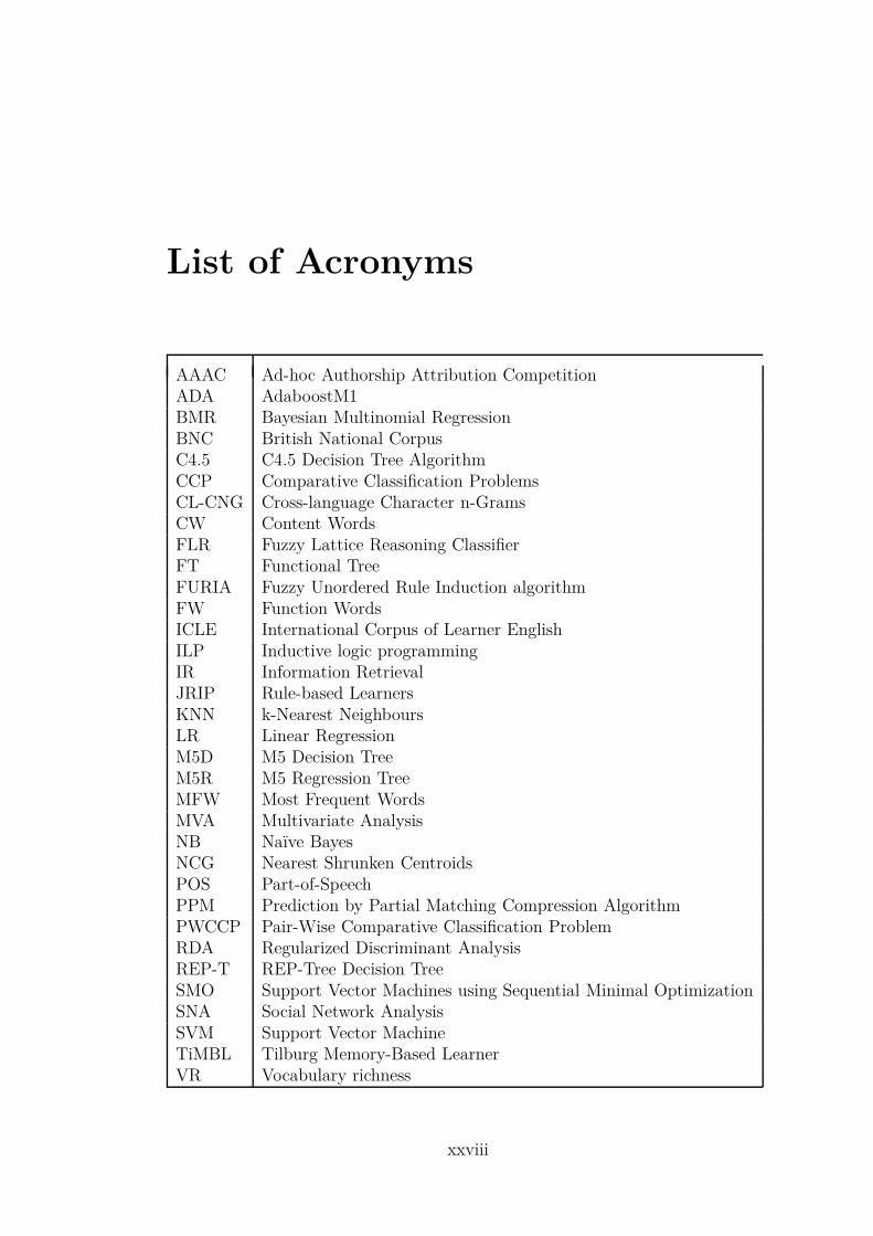
AAAC Ad-hoc Authorship Attribution CompetitionADA AdaboostM1BMR Bayesian Multinomial RegressionBNC British National CorpusC4.5 C4.5 Decision Tree AlgorithmCCP Comparative Classification ProblemsCL-CNG Cross-language Character n-GramsCW Content WordsFLR Fuzzy Lattice Reasoning ClassifierFT Functional TreeFURIA Fuzzy Unordered Rule Induction algorithmFW Function WordsICLE International Corpus of Learner EnglishILP Inductive logic programmingIR Information RetrievalJRIP Rule-based LearnersKNN k-Nearest NeighboursLR Linear RegressionM5D M5 Decision TreeM5R M5 Regression TreeMFW Most Frequent WordsMVA Multivariate AnalysisNB Naïve BayesNCG Nearest Shrunken CentroidsPOS Part-of-SpeechPPM Prediction by Partial Matching Compression AlgorithmPWCCP Pair-Wise Comparative Classification ProblemRDA Regularized Discriminant AnalysisREP-T REP-Tree Decision TreeSMO Support Vector Machines using Sequential Minimal OptimizationSNA Social Network AnalysisSVM Support Vector MachineTiMBL Tilburg Memory-Based LearnerVR Vocabulary richness
xxviii

[This page is intentionally left blank]
xxix
List of Publications
Journal Publications
• Heba El-Fiqi, Eleni Petraki, and Hussein Abbass
“Network Motifs for Translator Stylometry Identification"
A manuscript submitted to a peer-reviewed journal.
• Heba El-Fiqi, Eleni Petraki, and Hussein Abbass
“Pairwise Comparative Classification Problems for Computational Linguis-
tics"
A manuscript submitted to a peer-reviewed journal.
Conference Publications
• Heba El-Fiqi, Eleni Petraki, and Hussein Abbass, 2011
“A Computational Linguistic Approach for the Identification of Translator
Stylometry Using Arabic-English Text"
IEEE International Conference on Fuzzy Systems (FUZZ-IEEE) , pp. 2039
- 2045 , Taipei (Taiwan), 27-30 June 2011.
xxx

[This page is intentionally left blank]

Chapter 1
Introduction
1.1 Overview
Translation is a challenging task, as it involves understanding of the meaning and
function of language of the original author. Successful translation necessitates
that the translator communicates the same mental picture as the original author
of the text.
The art of translation is a complex process. Good translation does not
stop at the level of mapping words; rather, it extends to mapping meaning,
mental pictures, imagination, and feelings. During the translation process, the
translator is trying to maintain the spirit of the original work. Nevertheless, the
translator also has to make many personal decisions including the choice of words,
discourse markers, modal verb selection, length of sentences, frames, and his/her
own understanding of the original text. Such decisions constitute the translator’s
own distinctive style. Using these distinctive markers to identify the translator
is the aim of this translator stylometry study. This is defined as the “loyalty”
dilemma, and there is extensive literature on the importance of maintaining the
spirit of the original work.
In 1995, Venuti discussed translator invisibility [185]. He echoes the aim of
a good translation that was originally introduced by Shapiro “A good translation
is like a pane of glass. You only notice that it’s there when there are little
CHAPTER 1. INTRODUCTION 3
imperfections - scratches, bubbles. Ideally, there shouldn’t be any. It should never
call attention to itself.” [185]. This concept ignores the effect of the translator’s
own identity on the translation process. Publishers and readers are satisfied
with translator’s invisibility, which makes the translation considered as derivative
rather than innovative process. Baker described the implication of that view to
translator stylometry as “... the translator cannot have, indeed should not have, a
style of his or her own, the translator’s task being simply to reproduce as closely
as possible the style of the original."[19]
Translator invisibility is a tricky concept that has been criticized in the lin-
guistics literature [61, 143]. Baker and Xiumei independently point out the trans-
lators’ difficulty of excluding their personal views and attitudes when translating
a text [19, 197]. Baker suggested the existence of translator fingerprints, and
she pioneered the research in this area and tried to identify a possible signatures
for translators in their translations [19]. Although Baker’s study demonstrated
the existence of translator stylometry, her study was limited in terms of com-
putational linguistics analysis. Baker used in her study translations of different
languages and for different text. The first translator translated from Portuguese
and Spanish to English, while the second translator translated from Arabic to En-
glish. Furthermore, these translations are not for the same original texts. Such
analysis left many open questions in terms of the translators’ differences. These
would be assigned to translating from different original languages, or maybe be-
cause they came from different original texts.
Translator stylometry is an under-researched area in the field of computa-
tional linguistics. It refers to the identification of stylistic differences that distin-
guish the writing style of different translators. In fact, it was treated as a noise
affecting the original text [62]; Hedegaard and Simonsen originally considered
the translator effect in the text as a noise that challenged identifying the au-
thor of the text rather than considering the translator’s intellectual contribution
to the work. Based on our knowledge, very limited research was found in this
field. Mikhailov and Villikka’s study is one of the few studies that suggested that
translator stylometry cannot be detected using computational linguistics [121].
Heba El-Fiqi November 6, 2013
CHAPTER 1. INTRODUCTION 4
Again, this claim is supported by Rybicki [154], when he questioned the translator
stylometry identification using clustering analysis.
1.2 Research Motivation
Detecting the translator of a text is an important problem and can serve a range
of functions. In the legal domain, it can be used in resolving intellectual property
cases [44]. In education, it can be used for detecting plagiarism in translation
classes, or addressing differences between experts and learners [33].
1.2.1 Author, Translator, and the Intellectual property
In the beginning of the 90s, Lenita Esteves, a Brazilian translator was invited by
a Brazilian publishing house to translate “The Lord of the Rings”, the famous
fantasy novel. That agreement was before the release of the first film in 2001,
when the book turned to be a bestseller. Esteves sued the publishing house
claiming for her share in the profit of book sales. Then, she discovered that
all the subtitles in the Brazilian version of the film had been taken from her
translation, including the names and some lines of poems. So, she sued the
distributor of the film as well; but the distributor of the film offered her out
of court agreement, and she accepted that offer and got paid by them. On the
other hand, the publishing house rejected that claim because according to market
practices the translators are not paid for copyright but for the task of translation;
which means that they are paid once for whatever the book have been sold. The
first judgment ended with the claim being accepted, and the publisher had to
pay 5% of the price of each book sold to the translator, but the publishing house
appealed that decision. We couldn’t gain any information about the final judge
decision. But the publishing house took a protective step by announcing about
future translations for this book to stop the translators from gaining any further
profit in case of wining the claim. The translator wrote an article about her story
[44], in which she is arguing about her intellectual property rights; she also argued
Heba El-Fiqi November 6, 2013
CHAPTER 1. INTRODUCTION 5
about the translated names that she used to introduce the novel characters to
the Brazilian readers. If the new translation used them, she claims that this is
plagiarism, if they changed them, then readers need to be reeducated about the
new characters’ names!!!
What is important in this story is how market practice ignored the intellec-
tual property of the translator. In fact, this suggests that translators want their
own voice and identity in the field. This offers a strong justification and support
for pursuing the topic of translator stylometry. This poses the question: Can we
prove that the translator has a signature in the translated text? if so, how can
we define the stylometric characteristics that can be used for such claim?
1.2.2 The Linguistic Challenge: Fidelity and transparency
(from theory to practise)
Venuti described the practice of the translators in society and in their transla-
tions themselves with the term invisibility. He claimed that this is what readers
and publishers expect from the translator. Shapiro asked translators to confine
themselves to transparency [185]. Although Venuti called the translators to be
more visible in terms of claiming intellectual property, he still argued that high
quality translations are associated with fidelity, with loyalty to the original text,
and again with being invisible in the text. Both terms of fidelity and trans-
parency affected translation theories in the last decades, but both of them are
too ideal to be attained in practice. Moving from theory to practice, we see how
the translators are highly affected by their beliefs, backgrounds, understanding,
and cultural boundaries. Their identities affect their translations [60].
The literature in many fields discussed the existence of translator styles. For
example, in 2000, Baker discussed the existence of translator style in saying: “it
is as impossible to produce a stretch of language in a totally impersonal way as it
is to handle an object without leaving one’s fingerprints on it” [19]. She suggested
to study translator styles using forensic stylistics (unconscious linguistic habits)
rather than literary stylistics (conscious linguistic choices).
Heba El-Fiqi November 6, 2013
CHAPTER 1. INTRODUCTION 6
Xiumei used relevance theory to explain the translator’s style [197]. The
findings from Xiumei research demonstrated that, while the translator tries to
balance between the original author’s communicative intentions and the target
reader’s cognitive environment, s/he is still influenced by his/her own preferences
and abilities; the outcome of all of that introduces his/her style.
In 2010, Winters discussed how a translator’s attitude influences his/her
translation [194]. Winters, who used two German translations of the original
novel “The Beautiful and Damned” (1922) written by F. Scott Fitzgerald, showed
that different translators’ views affect the macro level of the novel. Furthermore,
he discussed how this from his point of view extended to influence the readers’
attitude.
Scholars used different linguistics approaches to detect translator styles.
While Winters used loan words, code switches [191] and speech-act report verbs
[192], Kamenická explored how explicitations contributed to translators’ style
[84]. Wang and Li looked for translator’s fingerprints in two parallel Chinese
translations of Ulysses using keywords lists. They identified different preferences
in choosing keywords by different translators. They also found differences on
the syntactic level by analysing the decision on clause positions in the sentences
[187]. This research confirmed the existence of stylistic features identifying dif-
ferent translators.
In translation studies in the field of linguistics, the researcher would rely on
a very small sample of translators and text, mostly in the order of two translators
and a few pieces of text. This manual process, while constrained in the sample
size, relies on the researchers’ solid linguistic expertise.
This poses the question whether this manual subjective process can be re-
placed with a computational and objective way.
1.2.3 The Computational Linguistic Challenge
The sample of papers reviewed above and others [194, 197, 9] showed that linguis-
tics offers evidence for the existence of stylometric differences between translators
Heba El-Fiqi November 6, 2013
CHAPTER 1. INTRODUCTION 7
in a way that affect the translated texts. However, the area of automatic identi-
fication and feature extraction of translator stylometric features has not seen an
equivalent breed of research.
We found very limited attempts which employ computational linguistics in
translator identification. The first one was by Baker as discussed earlier [19].
Later on, in 2001, another study by Mikhailov and Villikka [121]. They tried
to find “stylistic fingerprints” for a translator by extracting three lexical features
: “Vocabulary richness”, “Most frequent words” and “Favourite words”. Their
experiment was done on Russian fiction texts in addition to their Finnish trans-
lations. The lexical features that they used in the research failed to find stylistic
fingerprints for different translators. Their conclusion was summed up in their
title; that it is not possible to differentiate between translators. While this conclu-
sion is inconsistent with traditional linguistic studies, another research by Burrow
in 2002 using delta analysis on most frequent words supported these findings by
concluding unclear results in translators’ identification [29]. It seems that it was
sufficient to turn away researchers from this line of research for almost 10 years.
Recently, in 2011, Rybicki revisited the question of translators invisibility us-
ing cluster analysis, principal component analysis and bootstrap consensus tree
graphs based on Burrows’ Delta in three related studies [153, 63, 154]. Rybicki
aimed to cluster translations into groups based on this method. He expected
that the clustering will be according to their translators [154]. Unfortunately, his
approach clustered the translators into their original authors rather than trans-
lators. He emphasises the shadowy existence of translators, and supported the
vision of Venuti that of translators receiving minimal recognition for their work.
Not only in fame, fortune and law, but in stylistically based statistics [154].
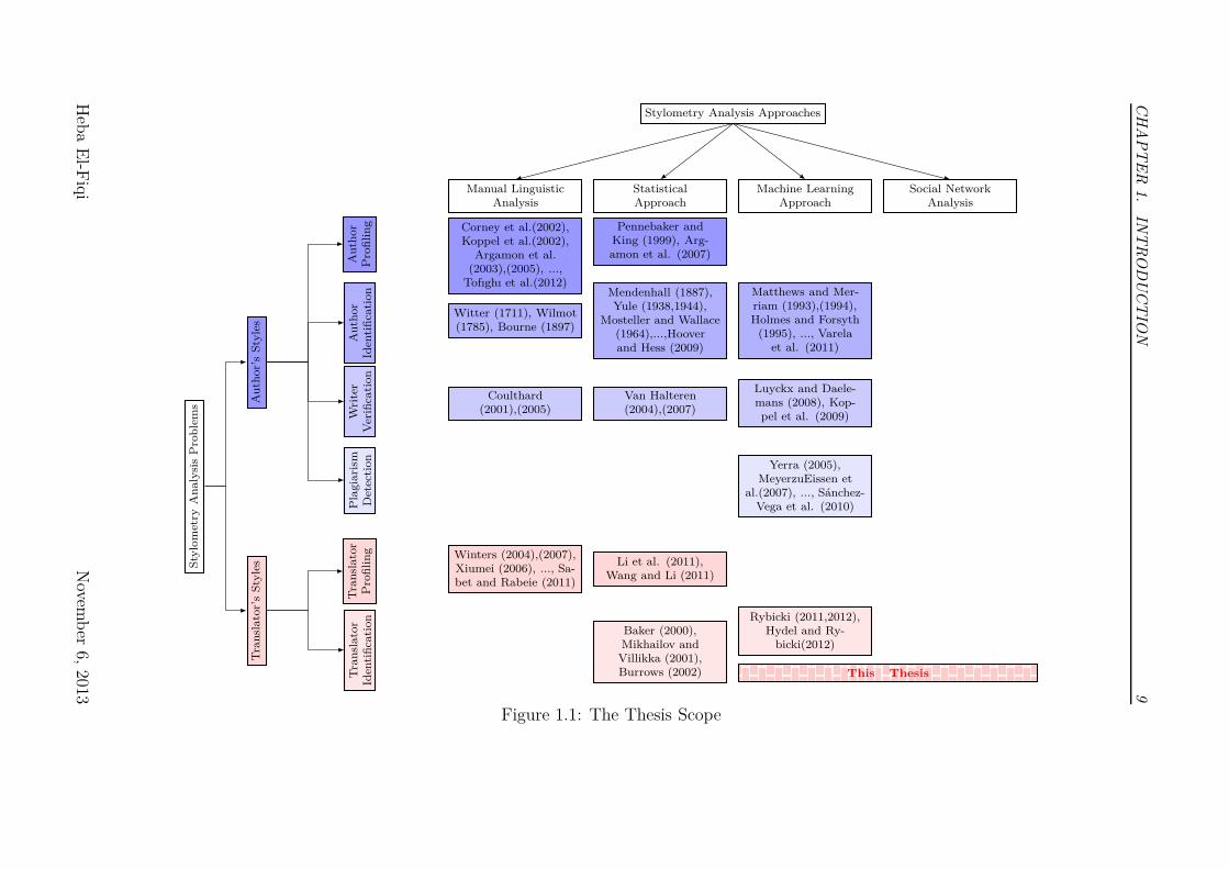
The limited number of research studies that we found and the findings from
these elevated the need for further studies in employing computational linguistics
for translator stylometry identification. Figure 1.1 illustrates how the research in-
terest is distributed in the area of Stylometry Analysis. The listed research studies
are only samples of the existing literature in the stylometry analysis subproblems.
More details will be discussed later in the background chapter (Chapter 2). As
Heba El-Fiqi November 6, 2013
CHAPTER 1. INTRODUCTION 8
we can see, authorship attribution gained most interest amongst researchers. The
sub-area of translator identification gain the least interest. Furthermore, social
network analysis has not been investigated for the purpose of stylometry analysis.
While linguistic studies highlighted the existence of translator differences,
computational research has not explored this issue in depth. In this thesis we are
readdressing this question of the existence of translator stylometry considering
the development of authorship techniques in the last few years. We also examine
the features that can be used to distinguish different translators.
1.3 Research Question and hypothesis
If we compare author attributions to translator attributions, we find that the
former is expected to have more signatures or discriminatory factors representing
the choices made by the authors. Authors have many more degrees of freedom,
where they can build their own identity as authors. Translators have less. Their
objective is to transparently transmit the mental picture contained in the original
text to the target language. Addressing the transparency factor limits transla-
tors’ linguistic choices compared to an author who has more linguistic choices
to draw his/her own mental picture from. Being constrained with the original
text is a non-trivial limitation. This feature alone makes translator attributions
a more difficult problem than author attributions. Nevertheless, we conjecture
that translators attempt to have their own touch, signatures that can be used to
detect who translated what.
The scope of this thesis is the study of translator stylometry identification
using a computational linguistic approach. The study in this thesis aims at
answering the following research question:
Heba El-Fiqi November 6, 2013
CH
AP
TE
R1.
INT
RO
DU
CT
ION
9
Sty
lom
etry
An
alys
isP
rob
lem
s
Tra
nsl
ator
’sS
tyle
s
Tra
nsl
ator
Iden
tifi
cati
onT
ran
slat
orP
rofi
lin
g
Au
thor
’sS
tyle
s
Pla
giar
ism
Det
ecti
onW
rite
rV
erifi
cati
onA
uth
orId
enti
fica
tion
Au
thor
Pro
fili
ng
Stylometry Analysis Approaches
Manual LinguisticAnalysis
StatisticalApproach
Machine LearningApproach
Social NetworkAnalysis
Corney et al.(2002),Koppel et al.(2002),
Argamon et al.(2003),(2005), ...,
Tofıghı et al.(2012)
Witter (1711), Wilmot(1785), Bourne (1897)
Coulthard(2001),(2005)
Winters (2004),(2007),Xiumei (2006), ..., Sa-bet and Rabeie (2011)
Pennebaker andKing (1999), Arg-amon et al. (2007)
Mendenhall (1887),Yule (1938,1944),
Mosteller and Wallace(1964),...,Hooverand Hess (2009)
Van Halteren(2004),(2007)
Li et al. (2011),Wang and Li (2011)
Baker (2000),Mikhailov and
Villikka (2001),Burrows (2002)
Matthews and Mer-riam (1993),(1994),Holmes and Forsyth
(1995), ..., Varelaet al. (2011)
Luyckx and Daele-mans (2008), Kop-pel et al. (2009)
Yerra (2005),MeyerzuEissen et
al.(2007), ..., Sánchez-Vega et al. (2010)
Rybicki (2011,2012),Hydel and Ry-
bicki(2012)
This Thesis
Figure 1.1: The Thesis Scope
Heb
aE
l-Fiq
iN
ovemb
er6,
2013
CHAPTER 1. INTRODUCTION 10
Main Research Question“ Can a computational linguistics framework meet the challenges
of translators’ stylometry identification problem?”
This research question can be broken down into several sub-questions to
investigate and identify possible features and method as follows:
• The first sub-question we attempt to answer is: “Which of the stylistic
features to use to unfold a translator’s stylometry?”.
In order to investigate an appropriate feature set for translator stylometry
identification, we need to investigate the employment of network motifs,
which is a novel feature in the area of stylometric analysis. It has not been
used for the purpose of stylometry identification previously.
• The promising results that we found when we researched the first ques-
tion encouraged us to evaluate the use of network motifs in comparing
other features for the problem of translator stylometry identification. This
raised the second sub-question “What is the performance of network
motifs approach compared to other approaches?”. To answer this
sub-question, we needed to evaluate the different features using the same
dataset. We first investigated the performance of existing methods. Then,
we evaluated the use of global network features as stylometry identifica-
tion features. Furthermore, we explored the performance of both motif size
three and size four using the same dataset. The accuracy obtained when we
researched the performance of network motifs went lower than the accuracy
we found while answering the first sub-question. We investigated the cause
of that drop in accuracy. The details of that investigation are discussed in
Chapter 4. That problem raised another issue: the effect of using different
representations of the frequencies of network motifs in handling the change
in text size.
• Researching the last element in the second sub-question revealed the exis-
tence of a hidden pattern that can only be uncovered by comparing paired
Heba El-Fiqi November 6, 2013
CHAPTER 1. INTRODUCTION 11
instances that represent the parallel translations that we examine. This
investigation led us to define a new type of classification problems that we
call Comparative Classification Problems (CCP)- where a data record is a
block of instances. In CCP, given a single data record with n instances
for n classes, the problem is to map each instance to a unique class. The
interdependency in the data poses challenges for techniques relying on the
independent and identically distributed assumption. In the Pair-Wise CCP
(PWCCP), two different measurements - each belonging to one of the two
classes - are grouped together. The key difference between PWCCP and
traditional binary problems is that hidden patterns can only be unmasked
by comparing the instances as pairs. That raised the third sub-question of
this thesis, which is “What is an appropriate classification algorithm
that can handle Pair-Wise Comparative Classification Problem
(PWCPP) ?".
1.4 Original contributions
The main contribution of this thesis is the support of our claim that a compu-
tational linguistics framework can meet the challenges of translators’ stylometry
identification problem. In general, the contributions of the thesis can be sum-
marised as follows:
1. Providing an empirical study to support the use of computational linguistics
and specifically stylistic features to support the identification of translator
stylometry. This contradicts previous studies which were unable to provide
evidence of translator stylometry.
2. The effectiveness of network motifs in detecting translator stylometry.
3. It introduces a new model that can handle Pair-Wise Comparative Classifi-
cation Problem which assists the identification of translator stylometry by
comparing their parallel translations.
Heba El-Fiqi November 6, 2013
CHAPTER 1. INTRODUCTION 12
1.5 Organization of the thesis
The remainder of the thesis is organized in six chapters as follows:
• Chapter 2 - Background :
This chapter provides literature review on the different aspect of stylom-
etry analysis problem, and how the sub-problem of translator stylometry
identification is addressed in the literature . Furthermore, how we can see
the problem of translator stylometry identification from a data mining per-
spective.
• Chapter 3 - Data and Evaluation of Existing Methods:
The choice and design of the dataset used in this study is discussed in this
chapter. Then, we evaluate the performance of existing computational lin-
guistics methods for the problem of translator stylometry using the defined
dataset.
• Chapter 4 - Identifying Translator Stylometry Using Network Motifs:
This chapter aims at answering both first and second sub-questions of the
thesis through two main experiments. In the first experiment, it investigates
the possibility of using a computational based features for the problem of
translator stylometry identification. That includes exploring the effect of:
data normalization, sample size, and class imbalance on this problem. The
aim of the second experiment is to answer the second sub-question of the
thesis. Furthermore, it investigates the possibility of introducing different
representation of the data as a response to variation in text size issue.
• Chapter 5 - Translator Identification Problem Redefined as Pair-Wise Com-
parative Classification Problem:
The aim of this chapter is to address the third sub-question of the thesis.
In this chapter, the Translator identification problem is redefined as a Pair-
Wise Comparative Classification Problem. Then, a new model is proposed
based on C4.5 decision tree algorithm to address this specific problem of
classification.
Heba El-Fiqi November 6, 2013

CHAPTER 1. INTRODUCTION 13
• Chapter 6 - Conclusion and Future Work:
This chapter summarises the contributions of the research, and discusses
the future directions that stem from this work.
Heba El-Fiqi November 6, 2013
Chapter 2
Background
2.1 Introduction
Translator Stylometry is a small but growing area of research in computational
linguistics. Despite the research proliferation on the wider research field of sty-
lometry analysis for authors, the translator stylometry identification problem is
a challenging one and there is no sufficient literature on the topic. Stylome-
try, which is the study of literary style, focus on the way of writing rather than
the contents of the writings. Over the last decades, authorship attribution and
profiling gained most of the attention in the area of stylometry analysis. The
importance of and applications of stylometry analysis will be explored in detail
in the next section.
These problems benefited from the development of computational linguistics
and machine learning techniques, as translator stylometry analysis was limited to
literary style analysis. In order to identify an appropriate approach for translator
stylometry identification, we need not only understand the literary style analysis
that has been used for identifying differences in translator’s writing styles, but
to extend our knowledge to the wider area of stylometry analysis, which involves
both authors and translators. We should note that stylometry analysis for both
authors and translators are related. In both cases we are analysing writing styles
by identifying measurable features in the writing. However, it is important to

CHAPTER 2. BACKGROUND 15
note there is additional difficulties for the translator identification problem due
to the limited choices that the translator makes while translating in comparison
to the freedom that an author has while he is writing.
In this chapter, we are going to explore the literature of the stylometry
analysis area. We will start with the analysis of author styles before translator
styles for two reasons. The first reason is that a significant proportion of the work
in the stylometry analysis area started from author identification analysis. The
second reason is to be able to see what type of features and approaches employed
in the authorship analysis literature that can be applied to translator stylometry
analysis. For both authors and translators stylometry analysis, we are going to
identify the different types of problems, and discuss the methods and approaches
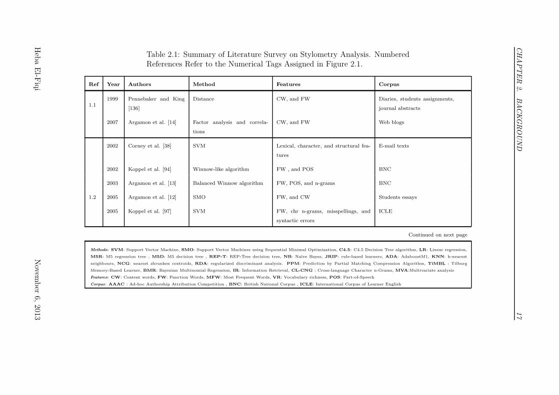
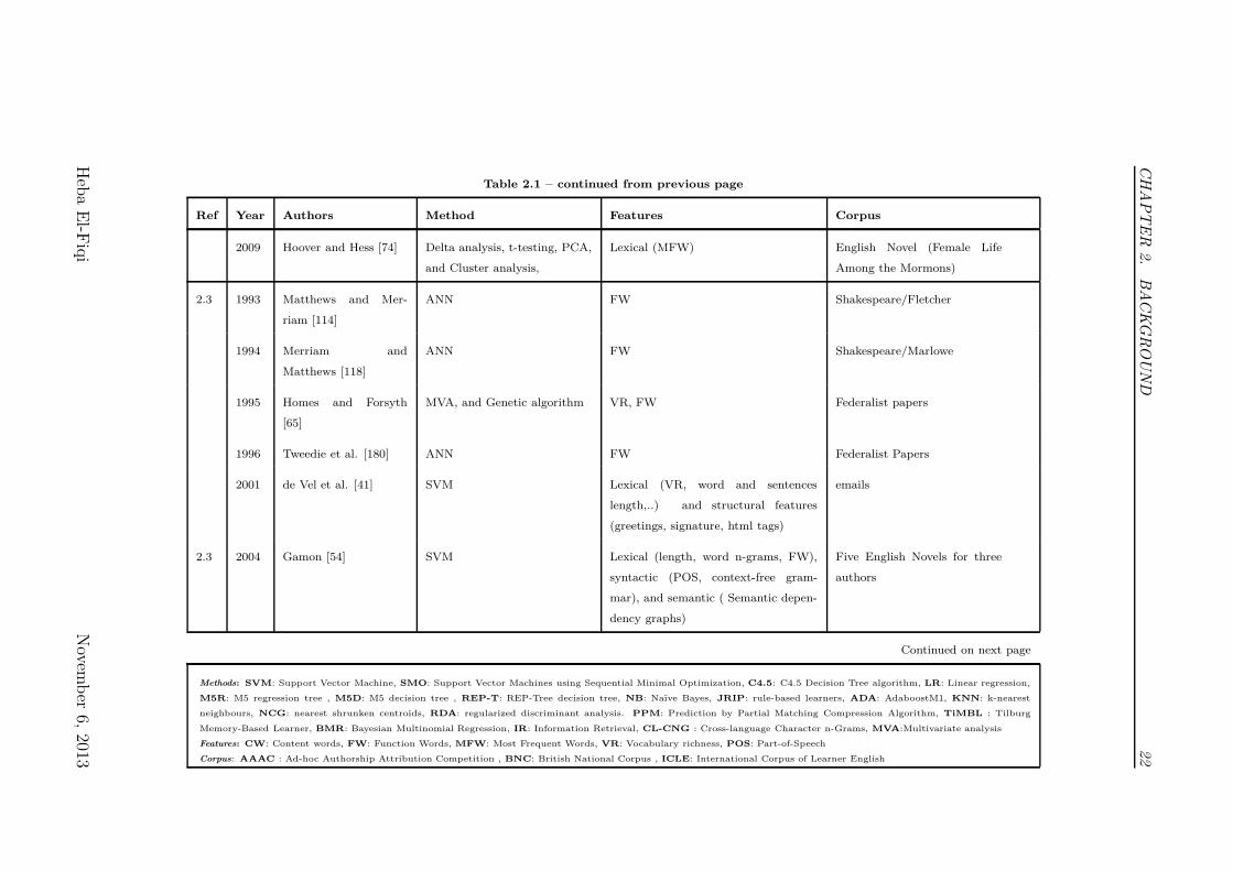
that have been used for that purpose. Figure 2.1 in conjunction with Table 2.1
provides a road map to the literature surveyed in this chapter.
2.2 Stylometry Analysis
Stylometry is the study of the unique linguistic styles and writing behaviours of
individuals. Kestemont defined it as the quantitative study of (literary) style,
nowadays often by means of computation [91]. Stylometry can be thought as a
measure of the style. So, what is a style?
“Style is the variable element of human behaviour” [115]. Typical human
activities may look like being similar. How people get dressed, eat, or drive are
generally invariant, but also they slightly vary from one person to another. The
procedure along with the outcomes of these kind of activities are usually pretty
much the same for everybody, yet the way an individual goes about this course
of action in order to get the outcome will vary noticeably from one person to
another.
Style in written language is generated by the repeated choices that the writer
tends to make. These repeated choices are hypothesised to reflect his unconscious
behaviour or preference of some writing pattern than others to represent the same
Heba El-Fiqi November 6, 2013

CH
AP
TE
R2.
BA
CK
GR
OU
ND
16
StylometryAnalysis
Translator’sStyles
TranslatorIdentification
MachineLearningApproach
6.2
StatisticalApproach
6.1
TranslatorProfiling
StatisticalApproach
5.2
ManualLinguisticAnalysis
5.1
Author’sStyles
PlagiarismDetection
MachineLearningApproach
4.1
WriterVerification
MachineLearningApproach
3.3
StatisticalApproach
3.2
ManualLinguisticAnalysis
3.1
AuthorIdentification
MachineLearningApproach
2.3
StatisticalApproach
2.2
ManualLinguisticAnalysis
2.1
AuthorProfiling
MachineLearningApproach
1.2
StatisticalApproach
1.1
Figure 2.1: Road-Map to Research on Stylometry Analysis. Numerical Tags Correspond to Entries in Table 2.1
Heb
aE
l-Fiq
iN
ovemb
er6,
2013
CH
AP
TE
R2.
BA
CK
GR
OU
ND
17
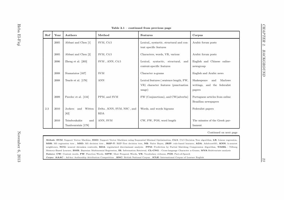
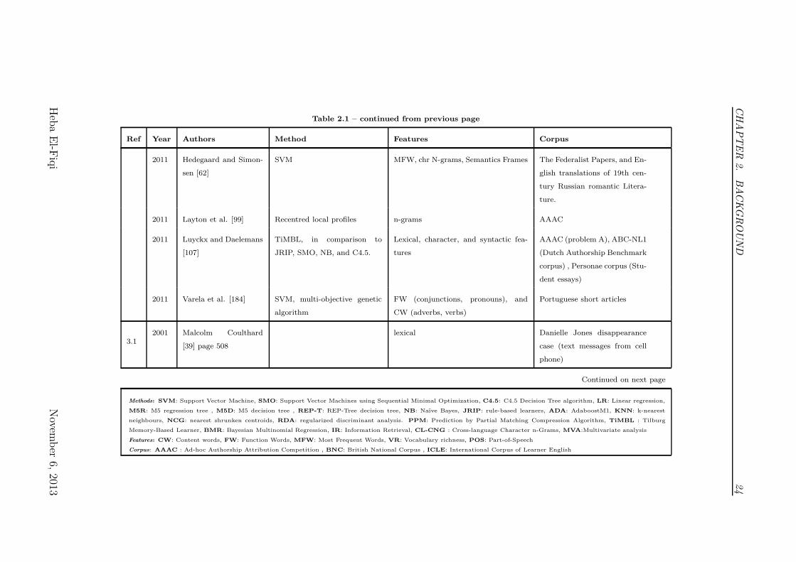
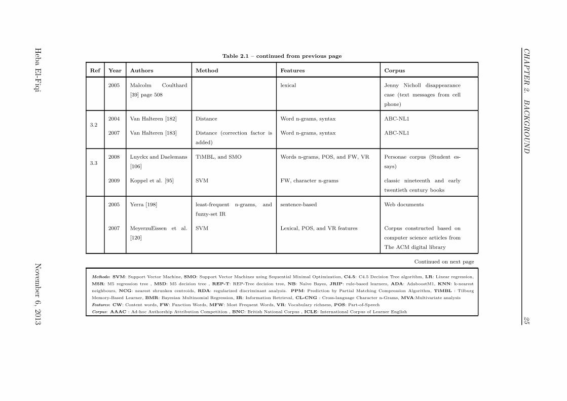
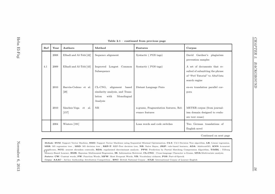
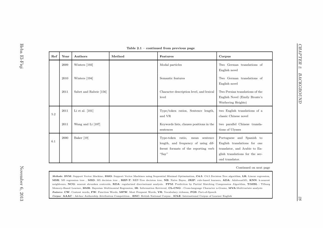
Table 2.1: Summary of Literature Survey on Stylometry Analysis. NumberedReferences Refer to the Numerical Tags Assigned in Figure 2.1.
Ref Year Authors Method Features Corpus
1.11999 Pennebaker and King
[136]
Distance CW, and FW Diaries, students assignments,
journal abstracts
2007 Argamon et al. [14] Factor analysis and correla-
tions
CW, and FW Web blogs
2002 Corney et al. [38] SVM Lexical, character, and structural fea-
tures
E-mail texts
2002 Koppel et al. [94] Winnow-like algorithm FW , and POS BNC
2003 Argamon et al. [13] Balanced Winnow algorithm FW, POS, and n-grams BNC
1.2 2005 Argamon et al. [12] SMO FW, and CW Students essays
2005 Koppel et al. [97] SVM FW, chr n-grams, misspellings, and
syntactic errors
ICLE
Continued on next page
Methods: SVM: Support Vector Machine, SMO: Support Vector Machines using Sequential Minimal Optimization, C4.5: C4.5 Decision Tree algorithm, LR: Linear regression,
M5R: M5 regression tree , M5D: M5 decision tree , REP-T: REP-Tree decision tree, NB: Naïve Bayes, JRIP: rule-based learners, ADA: AdaboostM1, KNN: k-nearest
neighbours, NCG: nearest shrunken centroids, RDA: regularized discriminant analysis. PPM: Prediction by Partial Matching Compression Algorithm, TiMBL : Tilburg
Memory-Based Learner, BMR: Bayesian Multinomial Regression, IR: Information Retrieval, CL-CNG : Cross-language Character n-Grams, MVA:Multivariate analysis
Features: CW: Content words, FW: Function Words, MFW: Most Frequent Words, VR: Vocabulary richness, POS: Part-of-Speech
Corpus: AAAC : Ad-hoc Authorship Attribution Competition , BNC: British National Corpus , ICLE: International Corpus of Learner English
Heb
aE
l-Fiq
iN
ovemb
er6,
2013

CH
AP
TE
R2.
BA
CK
GR
OU
ND
18
Table 2.1 – continued from previous page
Ref Year Authors Method Features Corpus
2006 Mairesse and Walker
[110]
LR, M5R, M5d, REP-T, C4.5,
KNN, NB, JRIP, ADA, and
SMO
CW Students essays, conversation
transcripts
2006 Oberlander and Now-
son [131]
SVM, NB word n-grams Web blogs
2006 Schler et al. [158] Multi-Class Real Winnow FW Web blogs
2007 Estival [45] C4.5, Random Forest, Lazy
learner, JRIP, SMO SVM ,
Bagging, and ADA
Character, lexical, and structural fea-
tures
English email messages
1.2 2007 Tsur and Rappoport
[179]
SVM Character n-grams, and FW ICLE
2008 Estival [46] C4.5, Random Forest, Lazy
learner, JRIP, SMO SVM ,
Bagging, and ADA
Character, lexical, and structural fea-
tures
English and Arabic email mes-
sages
2009 Argamon et al. [15] BMR FW, POS and CW English blog posts and stu-
dents essays
Continued on next page
Methods: SVM: Support Vector Machine, SMO: Support Vector Machines using Sequential Minimal Optimization, C4.5: C4.5 Decision Tree algorithm, LR: Linear regression,
M5R: M5 regression tree , M5D: M5 decision tree , REP-T: REP-Tree decision tree, NB: Naïve Bayes, JRIP: rule-based learners, ADA: AdaboostM1, KNN: k-nearest
neighbours, NCG: nearest shrunken centroids, RDA: regularized discriminant analysis. PPM: Prediction by Partial Matching Compression Algorithm, TiMBL : Tilburg
Memory-Based Learner, BMR: Bayesian Multinomial Regression, IR: Information Retrieval, CL-CNG : Cross-language Character n-Grams, MVA:Multivariate analysis
Features: CW: Content words, FW: Function Words, MFW: Most Frequent Words, VR: Vocabulary richness, POS: Part-of-Speech
Corpus: AAAC : Ad-hoc Authorship Attribution Competition , BNC: British National Corpus , ICLE: International Corpus of Learner English
Heb
aE
l-Fiq
iN
ovemb
er6,
2013
CH
AP
TE
R2.
BA
CK
GR
OU
ND
19
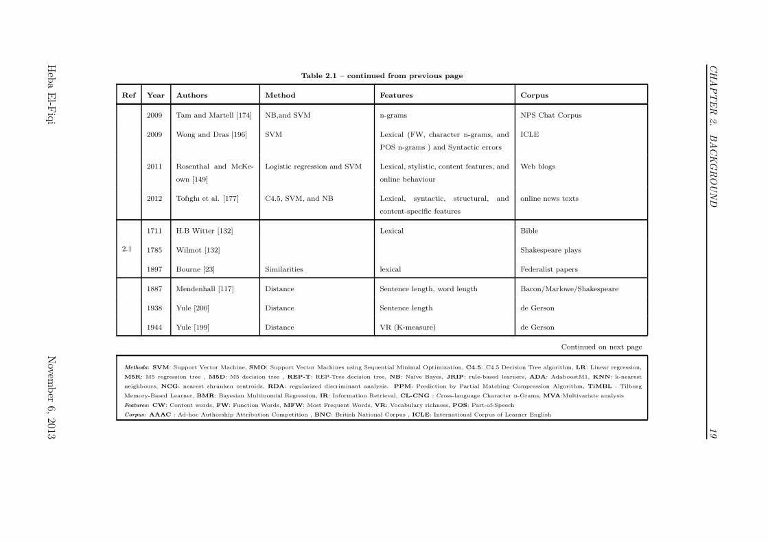
Table 2.1 – continued from previous page
Ref Year Authors Method Features Corpus
2009 Tam and Martell [174] NB,and SVM n-grams NPS Chat Corpus
2009 Wong and Dras [196] SVM Lexical (FW, character n-grams, and
POS n-grams ) and Syntactic errors
ICLE
2011 Rosenthal and McKe-
own [149]
Logistic regression and SVM Lexical, stylistic, content features, and
online behaviour
Web blogs
2012 Tofıghı et al. [177] C4.5, SVM, and NB Lexical, syntactic, structural, and
content-specific features
online news texts
2.1
1711 H.B Witter [132] Lexical Bible
1785 Wilmot [132] Shakespeare plays
1897 Bourne [23] Similarities lexical Federalist papers
1887 Mendenhall [117] Distance Sentence length, word length Bacon/Marlowe/Shakespeare
1938 Yule [200] Distance Sentence length de Gerson
1944 Yule [199] Distance VR (K-measure) de Gerson
Continued on next page
Methods: SVM: Support Vector Machine, SMO: Support Vector Machines using Sequential Minimal Optimization, C4.5: C4.5 Decision Tree algorithm, LR: Linear regression,
M5R: M5 regression tree , M5D: M5 decision tree , REP-T: REP-Tree decision tree, NB: Naïve Bayes, JRIP: rule-based learners, ADA: AdaboostM1, KNN: k-nearest
neighbours, NCG: nearest shrunken centroids, RDA: regularized discriminant analysis. PPM: Prediction by Partial Matching Compression Algorithm, TiMBL : Tilburg
Memory-Based Learner, BMR: Bayesian Multinomial Regression, IR: Information Retrieval, CL-CNG : Cross-language Character n-Grams, MVA:Multivariate analysis
Features: CW: Content words, FW: Function Words, MFW: Most Frequent Words, VR: Vocabulary richness, POS: Part-of-Speech
Corpus: AAAC : Ad-hoc Authorship Attribution Competition , BNC: British National Corpus , ICLE: International Corpus of Learner English
Heb
aE
l-Fiq
iN
ovemb
er6,
2013
CH
AP
TE
R2.
BA
CK
GR
OU
ND
20
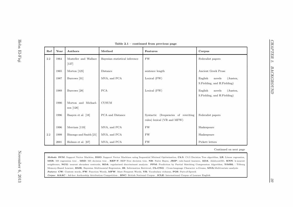
Table 2.1 – continued from previous page
Ref Year Authors Method Features Corpus
2.2 1964 Mosteller and Wallace
[127]
Bayesian statistical inference FW Federalist papers
1965 Morton [125] Distance sentence length Ancient Greek Prose
1987 Burrows [31] MVA, and PCA Lexical (FW) English novels (Austen,
S.Fielding, and H.Fielding)
1989 Burrows [28] PCA Lexical (FW) English novels (Austen,
S.Fielding, and H.Fielding)
1990 Morton and Michael-
son [126]
CUSUM
1996 Baayen et al. [18] PCA and Distance Syntactic (frequencies of rewriting
rules) lexical (VR and MFW)
Federalist papers
1996 Merriam [119] MVA, and PCA FW Shakespeare
2.2 1999 Binongo and Smith [21] MVA, and PCA FW Shakespeare
2001 Holmes et al. [67] MVA, and PCA FW Pickett letters
Continued on next page
Methods: SVM: Support Vector Machine, SMO: Support Vector Machines using Sequential Minimal Optimization, C4.5: C4.5 Decision Tree algorithm, LR: Linear regression,
M5R: M5 regression tree , M5D: M5 decision tree , REP-T: REP-Tree decision tree, NB: Naïve Bayes, JRIP: rule-based learners, ADA: AdaboostM1, KNN: k-nearest
neighbours, NCG: nearest shrunken centroids, RDA: regularized discriminant analysis. PPM: Prediction by Partial Matching Compression Algorithm, TiMBL : Tilburg
Memory-Based Learner, BMR: Bayesian Multinomial Regression, IR: Information Retrieval, CL-CNG : Cross-language Character n-Grams, MVA:Multivariate analysis
Features: CW: Content words, FW: Function Words, MFW: Most Frequent Words, VR: Vocabulary richness, POS: Part-of-Speech
Corpus: AAAC : Ad-hoc Authorship Attribution Competition , BNC: British National Corpus , ICLE: International Corpus of Learner English
Heb
aE
l-Fiq
iN
ovemb
er6,
2013
CH
AP
TE
R2.
BA
CK
GR
OU
ND
21
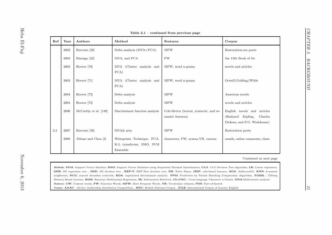
Table 2.1 – continued from previous page
Ref Year Authors Method Features Corpus
2002 Burrows [29] Delta analsyis (MVA+PCA) MFW Restoration-era poets
2003 Binongo [22] MVA, and PCA FW the 15th Book of Oz
2003 Hoover [70] MVA (Cluster analysis and
PCA)
MFW, word n-grams novels and articles
2003 Hoover [71] MVA (Cluster analysis and
PCA)
MFW, word n-grams Orwell/Golding/Wilde
2004 Hoover [73] Delta analysis MFW American novels
2004 Hoover [72] Delta analysis MFW novels and articles
2006 McCarthy et al. [138] Discriminant function analysis Coh-Metrix (lexical, syntactic, and se-
mantic features)
English novels and articles
(Rudyard Kipling, Charles
Dickens, and P.G. Wodehouse)
2.2 2007 Burrows [30] MVA& zeta MFW Restoration poets
2008 Abbasi and Chen [3] Writeprints Technique, PCA,
K-L transforms, SMO, SVM
Ensemble
characters, FW, syntax,VR, various emails, online comments, chats
Continued on next page
Methods: SVM: Support Vector Machine, SMO: Support Vector Machines using Sequential Minimal Optimization, C4.5: C4.5 Decision Tree algorithm, LR: Linear regression,
M5R: M5 regression tree , M5D: M5 decision tree , REP-T: REP-Tree decision tree, NB: Naïve Bayes, JRIP: rule-based learners, ADA: AdaboostM1, KNN: k-nearest
neighbours, NCG: nearest shrunken centroids, RDA: regularized discriminant analysis. PPM: Prediction by Partial Matching Compression Algorithm, TiMBL : Tilburg
Memory-Based Learner, BMR: Bayesian Multinomial Regression, IR: Information Retrieval, CL-CNG : Cross-language Character n-Grams, MVA:Multivariate analysis
Features: CW: Content words, FW: Function Words, MFW: Most Frequent Words, VR: Vocabulary richness, POS: Part-of-Speech
Corpus: AAAC : Ad-hoc Authorship Attribution Competition , BNC: British National Corpus , ICLE: International Corpus of Learner English
Heb
aE
l-Fiq
iN
ovemb
er6,
2013
CH
AP
TE
R2.
BA
CK
GR
OU
ND
22
Table 2.1 – continued from previous page
Ref Year Authors Method Features Corpus
2009 Hoover and Hess [74] Delta analysis, t-testing, PCA,
and Cluster analysis,
Lexical (MFW) English Novel (Female Life
Among the Mormons)
2.3 1993 Matthews and Mer-
riam [114]
ANN FW Shakespeare/Fletcher
1994 Merriam and
Matthews [118]
ANN FW Shakespeare/Marlowe
1995 Homes and Forsyth
[65]
MVA, and Genetic algorithm VR, FW Federalist papers
1996 Tweedie et al. [180] ANN FW Federalist Papers
2001 de Vel et al. [41] SVM Lexical (VR, word and sentences
length,..) and structural features
(greetings, signature, html tags)
emails
2.3 2004 Gamon [54] SVM Lexical (length, word n-grams, FW),
syntactic (POS, context-free gram-
mar), and semantic ( Semantic depen-
dency graphs)
Five English Novels for three
authors
Continued on next page
Methods: SVM: Support Vector Machine, SMO: Support Vector Machines using Sequential Minimal Optimization, C4.5: C4.5 Decision Tree algorithm, LR: Linear regression,
M5R: M5 regression tree , M5D: M5 decision tree , REP-T: REP-Tree decision tree, NB: Naïve Bayes, JRIP: rule-based learners, ADA: AdaboostM1, KNN: k-nearest
neighbours, NCG: nearest shrunken centroids, RDA: regularized discriminant analysis. PPM: Prediction by Partial Matching Compression Algorithm, TiMBL : Tilburg
Memory-Based Learner, BMR: Bayesian Multinomial Regression, IR: Information Retrieval, CL-CNG : Cross-language Character n-Grams, MVA:Multivariate analysis
Features: CW: Content words, FW: Function Words, MFW: Most Frequent Words, VR: Vocabulary richness, POS: Part-of-Speech
Corpus: AAAC : Ad-hoc Authorship Attribution Competition , BNC: British National Corpus , ICLE: International Corpus of Learner English
Heb
aE
l-Fiq
iN
ovemb
er6,
2013
CH
AP
TE
R2.
BA
CK
GR
OU
ND
23
Table 2.1 – continued from previous page
Ref Year Authors Method Features Corpus
2005 Abbasi and Chen [1] SVM, C4.5 Lexical„ syntactic, structural and con-
tent specific features
Arabic forum posts
2005 Abbasi and Chen [2] SVM, C4.5 Characters, words, VR, various Arabic forum posts
2006 Zheng et al. [203] SVM , ANN, C4.5 Lexical, syntactic, structural, and
content-specific features
English and Chinese online-
newsgroup
2008 Stamatatos [167] SVM Character n-grams English and Arabic news
2008 Tearle et al. [176] ANN Lexical features ( sentence length, FW,
VR) character features (punctuation
usage)
Shakespeare and Marlowe
writings, and the federalist
papers
2009 Pavelec et al. [134] PPM, and SVM FW (Conjunctions), and CW(adverbs) Portuguese articles from online
Brazilian newspapers
2.3 2010 Jockers and Witten
[82]
Delta , KNN, SVM, NSC , and
RDA
Words, and words bigrams Federalist papers
2010 Tsimboukakis and
Tambouratzis [178]
ANN, SVM CW, FW, POS, word length The minutes of the Greek par-
liament
Continued on next page
Methods: SVM: Support Vector Machine, SMO: Support Vector Machines using Sequential Minimal Optimization, C4.5: C4.5 Decision Tree algorithm, LR: Linear regression,
M5R: M5 regression tree , M5D: M5 decision tree , REP-T: REP-Tree decision tree, NB: Naïve Bayes, JRIP: rule-based learners, ADA: AdaboostM1, KNN: k-nearest
neighbours, NCG: nearest shrunken centroids, RDA: regularized discriminant analysis. PPM: Prediction by Partial Matching Compression Algorithm, TiMBL : Tilburg
Memory-Based Learner, BMR: Bayesian Multinomial Regression, IR: Information Retrieval, CL-CNG : Cross-language Character n-Grams, MVA:Multivariate analysis
Features: CW: Content words, FW: Function Words, MFW: Most Frequent Words, VR: Vocabulary richness, POS: Part-of-Speech
Corpus: AAAC : Ad-hoc Authorship Attribution Competition , BNC: British National Corpus , ICLE: International Corpus of Learner English
Heb
aE
l-Fiq
iN
ovemb
er6,
2013
CH
AP
TE
R2.
BA
CK
GR
OU
ND
24
Table 2.1 – continued from previous page
Ref Year Authors Method Features Corpus
2011 Hedegaard and Simon-
sen [62]
SVM MFW, chr N-grams, Semantics Frames The Federalist Papers, and En-
glish translations of 19th cen-
tury Russian romantic Litera-
ture.
2011 Layton et al. [99] Recentred local profiles n-grams AAAC
2011 Luyckx and Daelemans
[107]
TiMBL, in comparison to
JRIP, SMO, NB, and C4.5.
Lexical, character, and syntactic fea-
tures
AAAC (problem A), ABC-NL1
(Dutch Authorship Benchmark
corpus) , Personae corpus (Stu-
dent essays)
2011 Varela et al. [184] SVM, multi-objective genetic
algorithm
FW (conjunctions, pronouns), and
CW (adverbs, verbs)
Portuguese short articles
3.12001 Malcolm Coulthard
[39] page 508
lexical Danielle Jones disappearance
case (text messages from cell
phone)
Continued on next page
Methods: SVM: Support Vector Machine, SMO: Support Vector Machines using Sequential Minimal Optimization, C4.5: C4.5 Decision Tree algorithm, LR: Linear regression,
M5R: M5 regression tree , M5D: M5 decision tree , REP-T: REP-Tree decision tree, NB: Naïve Bayes, JRIP: rule-based learners, ADA: AdaboostM1, KNN: k-nearest
neighbours, NCG: nearest shrunken centroids, RDA: regularized discriminant analysis. PPM: Prediction by Partial Matching Compression Algorithm, TiMBL : Tilburg
Memory-Based Learner, BMR: Bayesian Multinomial Regression, IR: Information Retrieval, CL-CNG : Cross-language Character n-Grams, MVA:Multivariate analysis
Features: CW: Content words, FW: Function Words, MFW: Most Frequent Words, VR: Vocabulary richness, POS: Part-of-Speech
Corpus: AAAC : Ad-hoc Authorship Attribution Competition , BNC: British National Corpus , ICLE: International Corpus of Learner English
Heb
aE
l-Fiq
iN
ovemb
er6,
2013
CH
AP
TE
R2.
BA
CK
GR
OU
ND
25
Table 2.1 – continued from previous page
Ref Year Authors Method Features Corpus
2005 Malcolm Coulthard
[39] page 508
lexical Jenny Nicholl disappearance
case (text messages from cell
phone)
3.22004 Van Halteren [182] Distance Word n-grams, syntax ABC-NL1
2007 Van Halteren [183] Distance (correction factor is
added)
Word n-grams, syntax ABC-NL1
3.32008 Luyckx and Daelemans
[106]
TiMBL, and SMO Words n-grams, POS, and FW, VR Personae corpus (Student es-
says)
2009 Koppel et al. [95] SVM FW, character n-grams classic nineteenth and early
twentieth century books
2005 Yerra [198] least-frequent n-grams, and
fuzzy-set IR
sentence-based Web documents
2007 MeyerzuEissen et al.
[120]
SVM Lexical, POS, and VR features Corpus constructed based on
computer science articles from
The ACM digital library
Continued on next page
Methods: SVM: Support Vector Machine, SMO: Support Vector Machines using Sequential Minimal Optimization, C4.5: C4.5 Decision Tree algorithm, LR: Linear regression,
M5R: M5 regression tree , M5D: M5 decision tree , REP-T: REP-Tree decision tree, NB: Naïve Bayes, JRIP: rule-based learners, ADA: AdaboostM1, KNN: k-nearest
neighbours, NCG: nearest shrunken centroids, RDA: regularized discriminant analysis. PPM: Prediction by Partial Matching Compression Algorithm, TiMBL : Tilburg
Memory-Based Learner, BMR: Bayesian Multinomial Regression, IR: Information Retrieval, CL-CNG : Cross-language Character n-Grams, MVA:Multivariate analysis
Features: CW: Content words, FW: Function Words, MFW: Most Frequent Words, VR: Vocabulary richness, POS: Part-of-Speech
Corpus: AAAC : Ad-hoc Authorship Attribution Competition , BNC: British National Corpus , ICLE: International Corpus of Learner English
Heb
aE
l-Fiq
iN
ovemb
er6,
2013
CH
AP
TE
R2.
BA
CK
GR
OU
ND
26
Table 2.1 – continued from previous page
Ref Year Authors Method Features Corpus
2008 Elhadi and Al-Tobi [42] Sequence alignment Syntactic ( POS tags) David Gardner’s plagiarism
prevention samples
4.1 2009 Elhadi and Al-Tobi [43] Improved Longest Common
Subsequence
Syntactic ( POS tags) A set of documents that re-
sulted of submitting the phrase
of “Perl Tutorial” to AltaVista
search engine
2010 Barrón-Cedeno et al.
[20]
CL-CNG, alignment based
similarity analysis, and Trans-
lation with Monolingual
Analysis
Distant Language Pairs en-eu translation parallel cor-
pora
2010 Sánchez-Vega et al.
[157]
NB n-grams, Fragmentation features, Rel-
evance features
METER corpus (from journal-
ism domain designed to evalu-
ate text reuse)
5.1
2004 Winters [191] Loan words and code switches Two German translations of
English novel
Continued on next page
Methods: SVM: Support Vector Machine, SMO: Support Vector Machines using Sequential Minimal Optimization, C4.5: C4.5 Decision Tree algorithm, LR: Linear regression,
M5R: M5 regression tree , M5D: M5 decision tree , REP-T: REP-Tree decision tree, NB: Naïve Bayes, JRIP: rule-based learners, ADA: AdaboostM1, KNN: k-nearest
neighbours, NCG: nearest shrunken centroids, RDA: regularized discriminant analysis. PPM: Prediction by Partial Matching Compression Algorithm, TiMBL : Tilburg
Memory-Based Learner, BMR: Bayesian Multinomial Regression, IR: Information Retrieval, CL-CNG : Cross-language Character n-Grams, MVA:Multivariate analysis
Features: CW: Content words, FW: Function Words, MFW: Most Frequent Words, VR: Vocabulary richness, POS: Part-of-Speech
Corpus: AAAC : Ad-hoc Authorship Attribution Competition , BNC: British National Corpus , ICLE: International Corpus of Learner English
Heb
aE
l-Fiq
iN
ovemb
er6,
2013

CH
AP
TE
R2.
BA
CK
GR
OU
ND
27
Table 2.1 – continued from previous page
Ref Year Authors Method Features Corpus
2006 Xiumei [197] Relevance-theoretic approach Semantic level Different samples of Chinese to
English translations
2006 Rybicki [152] Delta analysis MFW Henryk Sienkiewicz’s Trilogy
and two English translations of
them
2007 Leonardi [100] Textual, Lexical , grammatical and
syntactic level, pragmatic and seman-
tic level
Italian into English translation
2007 Winters [192] speech-act report verbs Two German translations of
English novel
2008 KAMENICKÁ [84] Explicitation profile Lexical and Semantic level (explication
and implication)
Czech translations of two En-
glish novels
2009 Castagnoli [33] Conjunctions, explications, and con-
junctive explicitation
English to Italian and French
to Italian student translations
Corpus
Continued on next page
Methods: SVM: Support Vector Machine, SMO: Support Vector Machines using Sequential Minimal Optimization, C4.5: C4.5 Decision Tree algorithm, LR: Linear regression,
M5R: M5 regression tree , M5D: M5 decision tree , REP-T: REP-Tree decision tree, NB: Naïve Bayes, JRIP: rule-based learners, ADA: AdaboostM1, KNN: k-nearest
neighbours, NCG: nearest shrunken centroids, RDA: regularized discriminant analysis. PPM: Prediction by Partial Matching Compression Algorithm, TiMBL : Tilburg
Memory-Based Learner, BMR: Bayesian Multinomial Regression, IR: Information Retrieval, CL-CNG : Cross-language Character n-Grams, MVA:Multivariate analysis
Features: CW: Content words, FW: Function Words, MFW: Most Frequent Words, VR: Vocabulary richness, POS: Part-of-Speech
Corpus: AAAC : Ad-hoc Authorship Attribution Competition , BNC: British National Corpus , ICLE: International Corpus of Learner English
Heb
aE
l-Fiq
iN
ovemb
er6,
2013
CH
AP
TE
R2.
BA
CK
GR
OU
ND
28
Table 2.1 – continued from previous page
Ref Year Authors Method Features Corpus
2009 Winters [193] Modal particles Two German translations of
English novel
2010 Winters [194] Semantic features Two German translations of
English novel
2011 Sabet and Rabeie [156] Character description level, and lexical
level
Two Persian translations of the
English Novel (Emily Bronte’s
Wuthering Heights)
5.22011 Li et al. [101] Type/token ratios, Sentence length,
and VR
two English translations of a
classic Chinese novel
2011 Wang and Li [187] Keywords lists, clauses positions in the
sentences
two parallel Chinese transla-
tions of Ulysses
6.12000 Baker [19] Type-token ratio, mean sentence
length, and frequency of using dif-
ferent formats of the reporting verb
“Say”
Portuguese and Spanish to
English translations for one
translator, and Arabic to En-
glish translations for the sec-
ond translator.
Continued on next page
Methods: SVM: Support Vector Machine, SMO: Support Vector Machines using Sequential Minimal Optimization, C4.5: C4.5 Decision Tree algorithm, LR: Linear regression,
M5R: M5 regression tree , M5D: M5 decision tree , REP-T: REP-Tree decision tree, NB: Naïve Bayes, JRIP: rule-based learners, ADA: AdaboostM1, KNN: k-nearest
neighbours, NCG: nearest shrunken centroids, RDA: regularized discriminant analysis. PPM: Prediction by Partial Matching Compression Algorithm, TiMBL : Tilburg
Memory-Based Learner, BMR: Bayesian Multinomial Regression, IR: Information Retrieval, CL-CNG : Cross-language Character n-Grams, MVA:Multivariate analysis
Features: CW: Content words, FW: Function Words, MFW: Most Frequent Words, VR: Vocabulary richness, POS: Part-of-Speech
Corpus: AAAC : Ad-hoc Authorship Attribution Competition , BNC: British National Corpus , ICLE: International Corpus of Learner English
Heb
aE
l-Fiq
iN
ovemb
er6,
2013
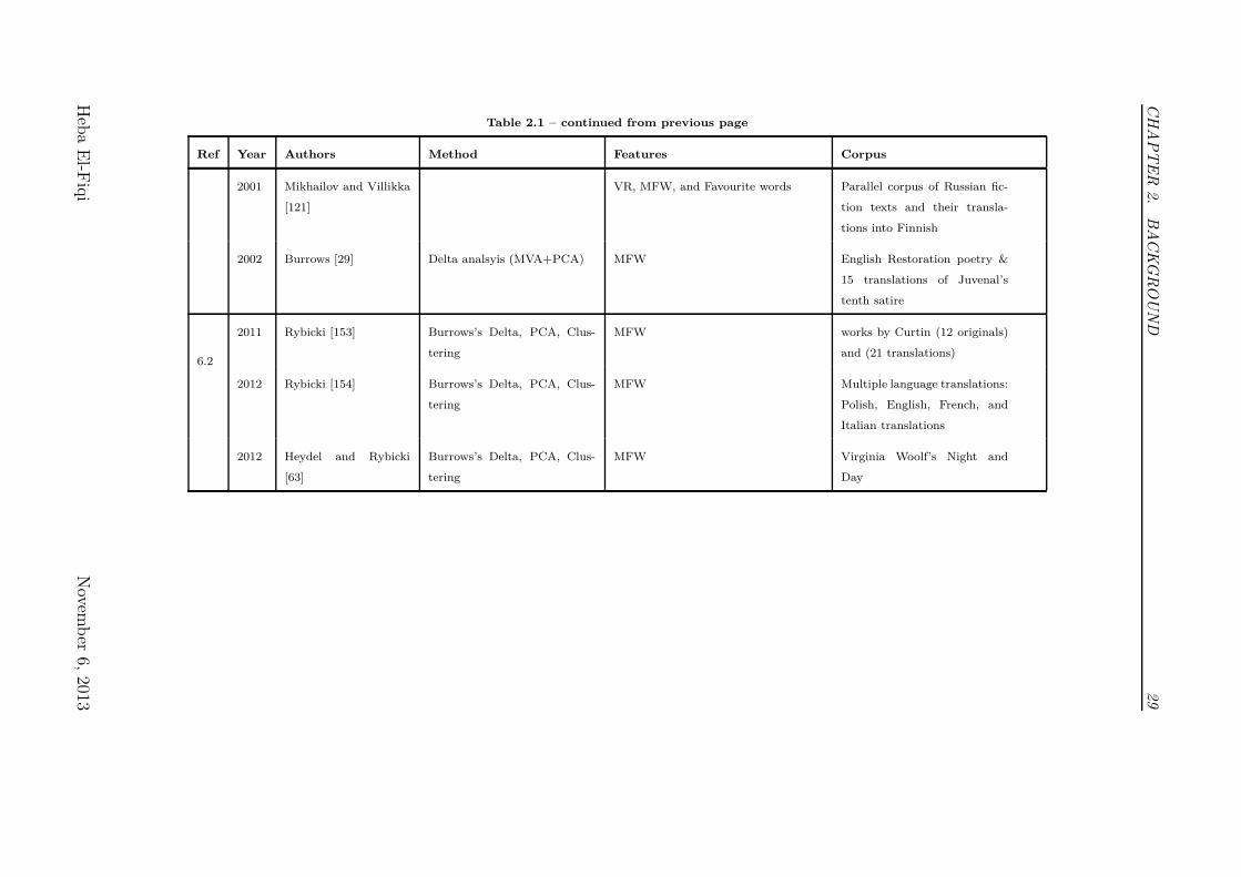
CH
AP
TE
R2.
BA
CK
GR
OU
ND
29
Table 2.1 – continued from previous page
Ref Year Authors Method Features Corpus
2001 Mikhailov and Villikka
[121]
VR, MFW, and Favourite words Parallel corpus of Russian fic-
tion texts and their transla-
tions into Finnish
2002 Burrows [29] Delta analsyis (MVA+PCA) MFW English Restoration poetry &
15 translations of Juvenal’s
tenth satire
6.2
2011 Rybicki [153] Burrows’s Delta, PCA, Clus-
tering
MFW works by Curtin (12 originals)
and (21 translations)
2012 Rybicki [154] Burrows’s Delta, PCA, Clus-
tering
MFW Multiple language translations:
Polish, English, French, and
Italian translations
2012 Heydel and Rybicki
[63]
Burrows’s Delta, PCA, Clus-
tering
MFW Virginia Woolf’s Night and
Day
Heb
aE
l-Fiq
iN
ovemb
er6,
2013
CHAPTER 2. BACKGROUND 30
thing. Group and individual variation in written language can be manifested in
examination of the style. Linguistic group variation can be observed for example
using sociolinguistics and discourse studies, which examine the use of language in
various context or the effect of social factors such as age or gender on the use of
language [69, 188]. For example, a sociolinguistic study by Argamon et.al showed
that males tend to use determiners (a, the, that, these) and quantifiers (one, two,
more, some) more than females. On the other hand, females use pronouns (I, you,
she, her, their, myself, yourself, herself) more frequently than males [13]. Addi-
tional Examples of sociolinguistics include the examination of linguistics charac-
teristics between teenagers and elderly people, and the observation of the use of
the English language by Chinese Australians and Italian Australians. Linguistic
variation is affected by different factors such as age, culture, race, geography,
social class, gender, education level, and specialisation. Despite the existence of
similarities in speaking or writing of specific groups of language users, there can
be individual characteristics which can contribute to individual distinctive styles.
With respect to writing, individual variation is created by the writer’s decision to
pick up one particular form out of the assortment of all different possible forms.
These variations can be within the norm, which are different correct ways of ex-
pressing the same thing, or deviation from a norm which may be mistakes, or
Idiosyncrasy behaviour of the writer. An example by McMenamin [115] to de-
scribe grammatically correct variations within the norm is: if the norm is “I am
going now", while variation within the norm can be “I’m going now", deviation
from the norm “I be goin’ now". Another example which describes socially an
appropriate variation to the norm “I’m afraid you’re too late" is “Sorry, the shop
is closed". In this case, a deviation may be “Get the hell out of here!". As the
style constitutes distinctiveness, identifying the writer’s distinctive markers is the
key to identifying their style. Analysis of the variation is the first step towards
identification of style-markers.
In the following section, we are going to discuss the different problems ad-
dressed using Stylometric analysis: how stylometry analysis is used to profile
an author or translator, identification of authors and translators based on their
Heba El-Fiqi November 6, 2013

CHAPTER 2. BACKGROUND 31
writing style, verification of an author of text as used in forensic linguistics, and
finally the use of stylometry analysis for plagiarism detection.
2.2.1 Authors Stylometric Analysis (Problem Definitions)
The development of computational tools, and the growing interest in forensic
analysis, humanities scholarship, and electronic commerce led to the growing
interest in the authorship attribution problem. This general problem was subdi-
vided into more specific sub-problems: The first one is Author Profiling, which
involves making inferences about the gender, age group, or origin of the author on
the basis of their writing style [168, 97]. Another form of the problem is Author
Identification, which includes identifying who wrote a piece of text from a set of
candidate authors by analysing their writing styles. Attributing authorship of
an anonymous text comprises the identification of stylistic similarities relating to
previously known texts belonging to the candidate authors. Author Verification
is another sub-problem, where the objective is to answer if this text is written by
the claimed author. The fourth sub-problem is Plagiarism detection which at-
tempts to identify the plagiarism by analysing the similarity between two pieces
of texts.
2.2.1.1 Author profiling
Writer profiling is a stylometry analysis sub problem which is concerned with
extracting as much information as possible about an unknown author by analysing
his/her writing. This information may include his gender, personality, cultural
background, etc... .
Researchers addressed author profiling and translator profiling in different
ways. For author profiling, the focus is on observing sociolinguistic behaviour.
Researchers analyse how a particular group of people use the language differently
than other groups. These observations can be collected by grouping people based
on gender [13], age [158], native language [97], or personality [137]. Then, these
Heba El-Fiqi November 6, 2013
CHAPTER 2. BACKGROUND 32
observations can be used in similar unknown text to extract information about
this text author.
The importance of the author profiling problem is growing with the recent
development in forensic linguistics, security applications, and commercial mar-
keting. An example of such importance in the area of forensic linguistics is giving
the police the chance to identify the characteristics of the person behind the crime
under investigation.
An example in the area of marketing includes analysing weblogs and product
reviews websites. Author profiling can help in identifying the characteristics of
groups of customers who do not like particular products. Then, the proposed
company undergoing the renew can use these identified characteristics to help in
the development of a marketing strategy to match the needs of the unsatisfied
customers.
Gender based stylistics
Extracting the gender of the author of a text has been studied using different
corpora in the literature. Corney et al. addressed the problem of author gender
profiling of e-mail text documents based on the gender-preferential language used
by the email writer [38]. Koppel et al. found out that male authors use determin-
ers much more than female authors, while female authors tend to use pronouns
and negation more than male authors [94]. This research was followed by another
experiment by Argamon et.al to further investigate the employment of pronouns
and certain types of noun modifiers that vary significantly when comparing doc-
uments belonging to male authors and female authors to determine the author
gender [13].
In 2007, Argamon et al. analysed web blog data to explore what types of
features can be used to determine the gender and the age of the authors [14].
Heba El-Fiqi November 6, 2013
CHAPTER 2. BACKGROUND 33
They found that the Articles and Prepositions are used significantly more by
male bloggers, while Personal Pronouns, Conjunctions, and Auxiliary Verbs are
used significantly more by female bloggers [14].
Age stylistic features
Age specific characteristics was also studied by Argamon et al. in 2007
in the same research mentioned earlier [14]. Argamon et al. found that the
usage of words associated with Family, Religion, Politics, Business, and Internet
increases with age, while usage of words associated with Conversation, AtHome,
Fun, Romance, Music, School, and Swearing decreases significantly with age.
Another observation of that experiment is that the use of Personal Pronouns,
Conjunctions, and Auxiliary Verbs decreases significantly with age, while the
usage of the Articles and Prepositions increases significantly with age. More
studies that have found age linked differences include research conducted by Schler
et al. [158], and also Argamon et al. in 2009 [15].
Another research attempt is introduced by Tam and Martell to determine if
the text writer belongs to teenagers or other ages using NPS Chat Corpus. This
research demonstrates n-grams are useful with regard to sensing the age in ad-
dition to demonstrating the challenge of distinction between consecutive groups
such as teens and 20s [174]. In 2011, Rosenthal et al. used lexical stylistic features,
content and online behaviour to predict the age of bloggers of virtual community
Live Journal using logistic regression and support vector machine [149].
Native language
To identify the native language of an author, researchers have used inter-
national Corpus of Learner English (ICLE) which contains essays written by
intermediate to advanced learners of English. Koppel et al. used a set of function
words and character n-grams as features, in addition to 185 error types, including
Heba El-Fiqi November 6, 2013
CHAPTER 2. BACKGROUND 34
misspellings and syntactic errors such as repeated letter, letter substitution, let-
ter inversion, and conflated words [97]. These features were used to identify five
native languages for the writers: Bulgarian, Czech, Russian, French and Span-
ish. After that, Tsur and Rappoport formed the hypothesis that the choice of
words people make when writing in a foreign language is strongly influenced by
the phonology of their native language [179]. Thus, they only used character n-
grams to identify the native language of the text author. The accuracy of 65.6%
that achieved by their approach was enough to validate their hypothesis where
the baseline was 20%, but it was less than the 80.2% accuracy that was achieved
by Koppel et al. using a different combination of features on the same dataset
[97].
Another research that supports the use of syntactic errors as a clue for au-
thor’s native language identification is produced by Wong and Dras in 2009 [196].
They structured their approach based on the contrastive analysis hypothesis,
where the common errors that a learner of a language makes can be explained
by observing differences between that learner’s native language and the learned
language.
In 2012, Tofıghı et al. used online news texts as a corpus to identify the au-
thor’s native language for four languages: English, Persian, Turkish and German
[177]. They used a combination of lexical, syntactic, structural, and content-
specific features for that purpose and demonstrated that this combination was
able to identify the author’s native language with an accuracy ranged from 70%
to 80% using SVM.
Personality
Human personality is usually described in terms of the well known Big
Five personality dimensions: Openness to experience (Imagination, Creativity
vs. Conventionality), Conscientiousness (Need for achievement, organization vs.
Impulsiveness), Extraversion (Sociability, Assertiveness vs. Quietness), Agree-
Heba El-Fiqi November 6, 2013
CHAPTER 2. BACKGROUND 35
ableness (Kindness vs. Unfriendliness), and Neuroticism (Calmness and Emotions
Stability vs. Self-conscious and Anxious)[113].
Pennebaker and King identified modest nevertheless dependable effects as-
sociated with individuality on word choices by analysing numerous text samples
of students [136]. The correlations ranged between 0.10 and 0.16. Neuroticism
was positively correlated with using negative feeling text as well as negatively
with positive feeling text. Examples of positive feeling texts include happy, love,
beautiful, nice, exciting, win, ...etc. On the other hand, negative feelings texts
include : ugly, hurt, anxiety, fear, anger, sadness, depression,...etc. Extraversion
correlated positively with positive feeling text as well as text associated with so-
cial processes. Agreeableness seemed to be positively linked to positive feeling
as well as negatively to negative feeling text. Furthermore, Neuroticism seemed
to be seen as an even more regular by using first person singular. After that, a
further study by Pennebaker et al. was conducted to identify the Neuroticism
level of text writers in 2003 [137]. They used Particles (pronouns, articles, prepo-
sitions, conjunctives, and auxiliary words) and function words for that purpose.
They found that more frequent use of first person pronouns is associated with
high degree of self involvement.
Argamon et al. used four lexical feature sets to identify Neuroticism and
Extraversion in 2005 [12]. These features are a standard function word list,
conjunctive phrases, modality indicators, and appraisal adjectives and modifiers
[12]. They found that appraisal lexical (text choise that reflect appreciation,
affect, or judgment) is effective in identifying Neuroticism level, and function
words are more appropriate for identifying Extraversion.
In 2006, Mairesse and Walker used machine learning algorithms in order
to model the five big personality aspects [110]. Their research findings showed
that Extraversion, Neuroticism and Conscientiousness are easier to model than
Openness and Agreeableness. Also, analysing the text using the constructed
recognition models outperformed the results of self-reports based models [110].
Another research on analysing languages to predict personality traits is con-
Heba El-Fiqi November 6, 2013
CHAPTER 2. BACKGROUND 36
ducted in the same year by Oberlander and Nowson. They used word bi and
trigrams as features to analyse web blogs in order to predict four psychometric
aspects: Neuroticism, Agreeableness, Extraversion and Conscientiousness [131].
After that, Estival et al extracted character, lexical, and structural features
from Email messages in English [45] and Arabic [46] in order to profile five au-
thors demographic characteristics: gender, age, geographic origin, level of educa-
tion and native language, and the big five personality aspects as well. In 2009,
Argamon et al. used content-based features and style-based features to profile
gender, age, language, and neuroticism in English blog posts and students essays
[15].
All of these discussed research studies demonstrate how the use of language
varies significantly according to these different factors. Also, these research find-
ings underline the use of computational linguistics in identifying stylistic features
of texts.
2.2.1.2 Author Identification
The authorship attribution problem is not a recent research area. There are some
Biblical authorship disputes traced back to 1711 by H.B Witter [132]. In 1785,
the authorship of Shakespeare plays have been disputed. Wilmot raised the claim
that Bacon is the real author of the Shakespeare plays [132]. Another study on
the plays of Shakespeare was conducted by Mendenhall in 1887 using word length
distribution. This was criticised later due to the expected differences between
poetry and prose rather than being related to the author style [162]. Later on,
Multiple researchers targeted authorship attribution dispute of Shakespeare plays:
Matthews and Merriam in 1993 [114] and 1994 [118], Merriam in 1996 [119],
Binongo and Smith in 1999 [21] ,and recently, Zhao and Zobel in 2007 [202].
Another famous authorship dispute is the Federalist papers, which is one
of the most studied problems in this research area [23] [127] [151] [82]. These
articles appeared New York newspapers under the pseudonym “Publius”. Twelve
out of the 85 essays were claimed by both Hamilton and Madison. These twelve
Heba El-Fiqi November 6, 2013
CHAPTER 2. BACKGROUND 37
disputed papers attracted many authorship attribution research studies in the
last decades. The first research to my knowledge was introduced in 1897 [23].
Then it was followed by many research studies but the most popular was the
one conducted by Frederick Mosteller and David Wallace in 1964 [127], which is
described by Rudman [151] as the “most statistically sophisticated non-traditional
study ever carried out”. That research was cited hundreds of times by researchers
who were interested in their statistical techniques, authorship attribution, and
the federalist political beliefs themselves. Since that time, the Federalist papers
were used by researchers who want to test their new method or hypothesis in
authorship attribution. Example of some recent research includes Hedegaard
and Simonsen in 2011 [62], who used the federalist to prove the validity of their
authorship methods. Additionally in 2010, Jockers and Witten used the federalist
papers as the corpus for their comparative analysis of five authorship attribution
method [82].
In 2004, Patrick Juola invited authorship attribution scholars to participate
in an authorship attribution competition as a part of the 2004 Joint Interna-
tional Conference of the Association for Literary and Linguistic Computing and
the Association for Computers and the Humanities (ALLC/ACH 2004). The pur-
pose of this competition was to conduct a benchmark study of the new methods
that the researchers introduced recently. This competition attracted 12 teams to
participate in it [83]. This dataset attracted some of the researchers after the
competition as well, who were interested to test their methods in comparison to
others. An example of recent research that used the same dataset is Layton and
others in 2011 [99] for the purpose of authorship attribution. In their research,
they generated authors’ profiles, and then classified text into authors based on the
best match author profile. Another example of using this dataset in authorship
attribution is Luyckx [107] who used part of this data in 2011 aiming to identify
the effect of data set size on the attribution problem.
More examples of authorship attribution problem will be discussed later in
this chapter through the discussion of the stylometric features and methods.
Heba El-Fiqi November 6, 2013

CHAPTER 2. BACKGROUND 38
2.2.1.3 Writer Verification
McMenamin highlights the existence of individual writer variation: “No two indi-
viduals use and perceive language in exactly the same way, so there will always be
at least small differences in the grammar each person has internalized to speak,
write, and respond to other speakers and writers” [115].
Given examples of the writing of a single author, the authorship verification
task aims to determine if given texts were or were not written by this author [182].
It can be seen as a categorization problem or one class classification problem from
the point of view of machine learning. Some of the research studies in this area
who used authorship attribution techniques are Halteren [182] [183], Koppel et
al. [95], and Luyckx and Daelemans [106]. Most of the research related to writer
verification is conducted from forensic linguistics prospective.
Although the authorship attribution is not a new research area, the forensic
linguistics research area is considered new. The first appearance of the phrase
“Forensic Linguistics” was at 1968 by Jan Svartvik in an analysis of statements
by Timothy John Evans [132]. After that, the growth of the Forensic linguistics
was slow until the beginning of the 1990s, when a new wave in the development
of Forensic Linguistics field came with 1989’s murder trial at the Old Bailey. The
first expert linguistic evidence was used in the court [132]. The International
Association of Forensic Linguists was then founded in 1992; then the International
Journal of Speech, Language and the Law, was founded in 1994.
Forensic linguistics is defined as the scientific study of language as applied
to forensic purposes and contexts [115]. Forensic linguistics doesn’t focus on
hand writing recognition or the source of the suicide note paper or how old is
it. Forensic Linguistic is concerned with author identification and stylometric
analysis [41, 167, 135, 95, 134], Author Profiling [182, 94], Discourse Analysis [78],
Forensic phonetics [81, 32], and significantly contributes to crime investigations.
One of the most prominent examples of the importance of forensic linguistics
is seen in the case of “Jenny Nicholl", a nineteen year old girl who went missing in
30th of July 2005. After her disappearance, some text messages were sent from
Heba El-Fiqi November 6, 2013
CHAPTER 2. BACKGROUND 39
her mobile to her family and friends. These messages were suspected of being not
sent by her. That is why these messages were been analysed linguistically to find
if she is the author of these messages or not. Some linguistics differences were
identified in her writing like using ME/MESELF rather than MY/MYSELF; that
is how she used to write them. Examples for other couples of words that was
encountered in the analysis (IM / I AM), (OFF / OF), (CU /CYA), (FONE /
PHONE), and (SHIT / SHITE). David Hodgson; her ex-lover was convicted for
Nicholl’s murder in Feb 2008 with the aid of these linguistic evidences [39].
2.2.1.4 Plagiarism Detection
Another related area to the field of translator stylometry is plagiarism detection.
There are many types of plagiarism. It can start from the level of copying an
idea, and it may extend to the text operation levels such as exact copy, or through
translation from one language to another. It may also go to the level of the
sentence, such as merging, splitting or paraphrasing of the text. Plagiarism on
the word level may include addition, deletion, or substitution.
Plagiarism detection is divided into two main types: extrinsic analysis and
intrinsic analysis. In the extrinsic case, we need to diagnose plagiarism by dis-
covering near-matches of some text message in a database of texts. The ex-
trinsic detection problem is addressed by different researchers in the last years
[198, 20, 42, 157, 43]. In intrinsic detection, we analyse the possible suspicious
document in isolation to show that various areas of a single author document
could not have been authored by that identical writer. Intrinsic plagiarism anal-
ysis can be detected through stylistic inconsistencies within the explored text.
Notably, that is similar to the problem of authorship verification, except that
in the authorship verification problem; the tested corpus is not only a single
document. Therefore, Intrinsic plagiarism can be seen as a generalization of the
authorship verification problem [8]. Research targeted intrinsic detection includes
[169, 171, 172, 120]. For further information, we refer the readers to plagiarism
Heba El-Fiqi November 6, 2013
CHAPTER 2. BACKGROUND 40
detection surveys by Stamatatos and Koppel [169], Osman et al. [133], and Ali
et al.[6].
2.2.2 Translators Stylometric Analysis (Problem Defini-
tions)
2.2.2.1 Translator profiling
The translator profiling problem was dealt with differently to the author profiling.
The focus of the conducted research in the literature is how the gender [100, 156],
proficiency level [33], social [101], and cultural backgrounds [101] affected their
translations. Most of the research in this area analysed two different parallel
translations of the same original text by different translators to address how
their identities might have affected the choices that they made throughout the
process of the text translation.
Translator background has been shown to affect the translators’ style. Most
of the translation analysis studies in the literature targeted this area of research.
Researchers were interested in analysing how two translations of the same text
by two translators (which we will refer to it as parallel translations) differed
in delivering different meaning and mental pictures based on their translators’
identities. This includes their cultural background, social, and political views.
Scholars used different linguistic approaches to detect translator styles. Xi-
umei used relevance theory to explain the translator’s style [197]. The findings
from Xiumei’s research demonstrated that: while the translator tries to balance
between the original author’s communicative intentions and the target reader’s
cognitive environment, s/he is still influenced by his/her own preferences and
abilities; the outcome of all of that introduces her style [197].
Rybicki used Burrow’s Delta to investigate character Idiolects in two English
translations of Henryk Sienkiewicz’s Trilogy in terms of major characters, old
friends, nationality, characters in love, and idiolects of female characters. That
study found that character’s idiolects were preserved in translations. Burrow’s
Heba El-Fiqi November 6, 2013
CHAPTER 2. BACKGROUND 41
Delta was able to capture similar distances between characters in both the original
text and the translations [152].
Kamenická explored how Explicitations contributes to translators’ style in
two parallel English to Czech translations of “Small World” by David Lodge
and “Falconer” by John Cheever in 2008 [84]. Explicitation happens when the
translator transfers a message that was hidden (but can be understood from the
context) in the original text to the reader explicitly using the target language.
Implicitation, on the other hand, occurs when the translator use the target lan-
guage to conceal some details that were mentioned explicitly using the source
language. Kamenická findings conclude that the two translators use experiential
and interpersonal explicitation and implicitation in textual segments differently.
In terms of identifying the gender of a translator as in author profiling, there
are some research studies that addressed this problem. In 2007, Leonardi con-
ducted Contrastive Analysis of Italian to English translation corpus to address
the question of how gender and ideology affect translation [100]. The same ques-
tion was addressed again in 2011 by Sabet and Rabeie [156]. They studied the
effect of gender ideology of the translators on their translation using two Persian
translations of the English Novel “Wuthering Heights” by Emily Brontë, one of
them by a male translator and the other by a female translator.
In 2009, Castagnoli investigated the possibility of a relationship between
the occurrence of specific phenomena and translator competence [33]. For that
investigation, she used a corpus consisting of student translations (from English
to Italian) and (from French to Italian). That corpus provides the availability of
multiple parallel translations of the same original text and availability of different
levels of translation competency.
Winters conducted multiple studies on how a translator’s attitude influences
his/her translation [191, 192, 193, 194]. In all of these studies, Winters used two
German translations of the original novel “The Beautiful and Damned” (1922)
written by F. Scott Fitzgerald. In 2004, Winters used loan words and code
switches to differentiate between translators’ styles [191]. The analysis showed
Heba El-Fiqi November 6, 2013
CHAPTER 2. BACKGROUND 42
that one of the translators tends to transfer English words from the source text
into the translation where possible, while the other translator tends to Germanize
the words to transfer the source text culture towards the target language reader.
Later on in 2007, Winters used speech-act report verbs [192] to investigate their
usefulness as potential elements of translator’s individual style. Although the
original text used repetition of some words, one of the translator transferred that
repetition to the translation, but the other translator avoided that, and used
different words to reflect different situations. In a 2009 study, Winters conducted
a quantitative analysis to analyse the use of modal particles by the translators.
That research showed that despite the overall similarities in using modal particles,
there was a significant difference in the translation’ choice and use of individual
modal particles [193]. In 2010, Winters’ study showed that different translators’
views affect the macro level of the novel, in which, the main message delivered
by the translations of the novel is different. The focus of one translator was to
provide a character study while the other focused on societal issues. Furthermore,
Winters discussed how that may extend to influence the readers’ attitude as well
[194].
Li et.al [101] tried to capture differences in the translation styles of two
English translations of a classic Chinese novel “Hongloumeng”. They calculated
Type/token ratios, sentence length, and vocabulary. The analysis in that study
aimed at differentiating between the styles regards translators’ social, political,
and ideological context of the translations. They also explored the effect of the
translator’s native language on their translation style as one of the translator was
a Chinese native speaker, and the other was a British scholar. They found that
the two translators used two different strategies in translation. They contributed
that variations to be affected by their social, political, ideological preferences, as
well as their primary purpose of the translations.
Wang and Li looked for translators’ fingerprints in two parallel Chinese trans-
lations of Ulysses using keywords lists. They identified different preferences in
choosing keywords by different translators. They also found differences on the
syntactic level by analysing the decision of clauses positions in the sentences [187].
Heba El-Fiqi November 6, 2013
CHAPTER 2. BACKGROUND 43
Additionally, their findings affirmed a hypothesis that they made in their study
that a writer’s preferences of linguistic expression is demonstrated in free writing.
All the above studies can be used as an evidence for the existence of trans-
lators’ fingerprints in their translations. It also provides substantial background
for this research. Although the variations in the linguistics approaches that these
research studies introduced, none of these research studies employed data mining
and machine learning, even the quantitative studies.
2.2.2.2 Translator Identification
Previously, in translator profiling section, we discussed the literature related to
the analysis of variation in translations by different translators. These mentioned
studies revealed how the translators as individuals use linguistic features differ-
ently to deliver the same original text. Their identities are reflected in the choices
that they make while translating. Analysing their translations demonstrates the
variation in their choices, which constitute their own translation styles.
In 2000, Baker discussed the existence of translator style: “it is as impossible
to produce a stretch of language in a totally impersonal way as it is to handle
an object without leaving one’s fingerprints on it” [19]; Baker suggested study-
ing translator styles using forensic stylistics rather than literary stylistics [19].
According to Baker description, literary stylistics are generated by the choices
that translators make consciously. On the other hand, Forensic stylistics reflects
unconscious linguistic habits, in which translators do not realise such linguistic
preferences.
The identification of the translator of a piece of text didn’t attract the re-
searchers because some research produced conflicting results. Furthermore, there
was a research study in 2011 which considered attributing the translated text to
their original author rather than the translator, where they looked at the transla-
tor’s contribution to the text as a noise [62]. Their study investigated the use of
semantic features to investigate authorship attribution of translated texts. They
based their study on the expectation that the most significant effect of the trans-
Heba El-Fiqi November 6, 2013

CHAPTER 2. BACKGROUND 44
lator is seen on the lexical and syntactic level, while the strongest influence of the
author is on the semantic level. In other words, there was as expectation that
translations and originals share the same semantic content.
In 2001, Mikhailov and Villikka questioned the existence of translators’ stylis-
tic fingerprints [121]. That research is based on a parallel corpus of Russian fiction
texts and their translations into Finnish. They used vocabulary richness, word
frequencies, and favourite words. Their analysis shows that the language of dif-
ferent translations of the same text performed by different people is closer than
that of the different translation by the same translator. Their finding concludes
that despite the existence of some translators’ preference patterns, authorship
existing techniques (which they evaluated) failed to identify translator’s styles.
Using their words, “it appeared as if translators did not have a language of their
own” [121]. Their conclusion was summed up in their title; “Is there such a thing
as a translator’s style?”.
In 2002, Burrows proposed Delta analysis for authorship attribution. In his
first trial, he worked on translations as well. In that study, Burrows examined
fifteen translations of Juvenal’s tenth satire with a number of English restoration
poetry. With Delta distance, the output is a table containing authors ranked from
the most possible author to the least possible author. Interestingly, Dryden’s rank
on his translation was 9th out of 25. While Johnson style was correctly identified
by Delta, Vaughan and Shadwell appeared significantly down the rank of their
own translations.
Recently, in a number of studies by Rybicki and others in 2011 and 2012
[153, 154, 63], they investigated the problem of translator stylometry attribution
by employing a well known technique for authorship attribution called Burrows’s
Delta [29], which is based on the z-score of the word frequencies. Burrows’s Delta
used successfully for authorship attribution in multiple studies [72, 73, 55, 11,
163]. A brief discussion about Burrows’s Delta is discussed in section 2.2.3.2.
They submit the calculated z-score to Cluster Analysis to produce tree diagrams
for a given set of parameters, such as number of MFWs studied, pronoun deletion,
and culling rate. Based on that culling rate, a decision is made to include a
Heba El-Fiqi November 6, 2013

CHAPTER 2. BACKGROUND 45
specific word in the analysis. Then, these results that produced a great variety
of parameter combinations are used as input for a bootstrap procedure. Based
on the generated tree, they analysed how these translations were grouped in the
same branches.
In the first study, Rybicki employed this method for the investigation of the
translator Jeremiah Curtin and his wife Alma Cardell contribution to his trans-
lations. Rybicki discussed the literature that shows that Memoirs of Jeremiah
Curtin (1940) is proven to be the work of his wife. In Rybicki’s investigation, that
memoirs was clustered in a different branch with some other suspected literary
works. The second study was by Heydel and Rybicki, they employed the same
method to investigate if it can differentiate the collaborations between transla-
tors on a single literary work. The case that they investigated was for Virginia
Woolf’s Night and Day, which consists of 36 chapters. The first translator, Anna
Kołyszko, died after translating the first 26 chapters, then another translator,
Heydel, translated the remaining chapters. Their proposed method succeeded
in clustering the translations according to their translators. Hydel and Rybicki
highlighted that despite the success of these investigations, the detected transla-
tor signature may be lost if investigated in context of various corpus. In 2012, in
another trial for translator stylometry attribution, Rybicki conducted a research
study under the title of “The Great Mystery of the (Almost) Invisible Translator:
Stylometry in Translation” [154]. The title reveals the challenge of identifying
the translator of a piece of text. Rybicki’s approach failed to attribute texts to
their translators using machine learning techniques and the use of most frequent
words. He concluded that except for some few highly adaptative translations, the
investigated method failed to identify the translator of the text, but it identified
the author instead. Rybicki found that in most of the cases, the translations were
grouped based on the original author rather than the translators. For that study,
he used a corpus of multiple language translations: Polish, English, French, and
Italian translations. He tested each corpus translations group separately. Rybicki
emphasises that his study supports Venuti’s observation on translator’s invisibil-
ity, and concluded that multivariate analysis of most-frequent-word condemns
Heba El-Fiqi November 6, 2013
CHAPTER 2. BACKGROUND 46
translators to Stylometric invisibility in the case of a large corpus of transla-
tions [154].
2.2.3 Methods of Stylometric Analysis
The most important function of language is communication and understanding
the message produced during this communication. It has become the subject of
different fields. Linguistics is the scientific study of language and explores the
language system at different levels: Phonetics, Phonology, Morphology, Lexicon,
Syntax, and Semantics. Observing the variation through these different levels
shows the linguistic variations that may occur between different groups as well
as between individuals. These variations may appear in the pronunciation as a
variation in the accent, word choice as a variation in (lexicon, word spelling, or
morphology), punctuation choices, or grammar rules’ preferences. McMenamin
[115] gave an interesting example about written variation and included 23 different
forms of the same word “strawberry" on different signs in the road in one state.
The analysis of variation is the first step of the identification of style-markers as
the style is about the distinctiveness.
Linguistic variation is observed between groups and between individuals. For
example, sociolinguistics studies the language of social groups such as teenagers,
or cultural groups. Group variation is affected by factors such as age, culture,
race, geography, social class, education level, and specialisation. Despite the
existence of similarities in writing produced by specific groups of language users,
there are still some individual decisions made by the writer which can contribute
to the study of individual distinctive markers. These distinctive markers can be
used to identify stylometry. In the next subsection, we are going to discuss which
type of features have been used for stylometry analysis. In the later subsection,
the different approaches and methods are discussed in details.
Heba El-Fiqi November 6, 2013

CHAPTER 2. BACKGROUND 47
2.2.3.1 Features
Researchers used many stylistic features for attributing authorship. These fea-
tures can be categorized into five main groups: Lexical, Character, Syntactic,
Semantic, and Application-specific features.
Lexical features include all the features that are associated with analysing the
sentence as a sequence of tokens or words, such as: word length [117], sentence
length [125], word frequencies, word n-grams, vocabulary richness, and typo-
errors.
Character features constitute a stylistic variation when the text is being
analysed as a sequence of characters. For example: counting character types as
letters, digits, or punctuation. Another example is counting character n-grams
either fixed or variable length. Using compression methods for authorship attri-
butions analyse the text as a sequence of characters as well.
Syntactic Features are being used when the analysis is done on the syntacti-
cal level where a similar syntactic pattern can be captured. This group includes
frequencies of Part-of-speech (POS) and chunks, sentence and phrase structure,
frequencies of rewriting rules [18], and function words. These features are ex-
tracted using Natural Language Processing (NLP) tools such as: Tokenizers,
Sentence splitters, POS taggers, Text chunkers, Partial and full parsers [168].
Semantic Features need deeper analysis to capture. Semantic dependency
graphs were used by Gamon [54] for author identification. McCarthy et al. [138]
used the synonyms and hypernyms of words to extract semantic measures. Defin-
ing a set of functional features that associate certain words or phrases with se-
mantic information was another approach introduced by Argamon [16].
Application-specific Features is important if the attribution is related to a
specific application. This includes: attributing the author of an e-mail message
or the writer in online-forums. In such cases, features associated with the text
organization and layout are important like font colour count, font size count, the
use of indentation, and paragraph length [1, 2] . Furthermore, some structural
Heba El-Fiqi November 6, 2013
CHAPTER 2. BACKGROUND 48
features are important such as greetings and farewells in messages, the types of
signatures that are being used.
2.2.3.2 Approaches
1. Manual linguistic analysis
Early authorship disputes cases like biblical authorship disputes and plays
of Shakespeare were first analysed by Human linguistic experts. All of that
changed since 1964, when Mosteller and Wallace employed Bayesian statis-
tical analysis for the problem of authorship attribution of “The Federalist
Papers”. Although the shift in direction of authorship attribution studies
from human to computational models for the analysis, the forensic linguis-
tics area still prefer the human expert based methods [132]. Olsson aruges
this is an appropriate method because: First, most of the exiting compu-
tational methods are based on availability of a large amount of data, while
the forensic linguists face the challenge of very limited samples of data in
real cases scenarios. So, the linguist expert needs to identify the possible
stylometry marker according to the available text, and the type of this text.
Secondly: forensic linguists do not see the goal of automating authorship
attribution as an important forensic aim. On the other hand, they may find
it a dangerous practice that may mislead them. Thirdly, in court, linguists
need to deliver and explain their opinion for the court. Their judgement
as experts is part of the process [132]. Different forensic interesting cases
where linguists analysed writers style either for authorship attribution, veri-
fication, and profiling are presented in a number of forensic linguistics books
[132, 77, 39] .
As for translator stylometry analysis, a number of studies were conducted
by linguists. Translator’s attitude toward the novel characters and how
this extends to affect the readers are studies by Winters [194]. Another
example is a study by Xiumei which examined translator’s style in terms
of Relevance theory [197]. Another linguistic study is introduced by Sabet
Heba El-Fiqi November 6, 2013
CHAPTER 2. BACKGROUND 49
and Rabeie to explore the effect of gender ideology on translation style [156].
2. Statistical approach
Univariate analysis approach is the simplest one; where the analysis is done
based on one feature or attribute, such as average word length, vocabulary
size, occurrences of vowel-initial words, or 2-3 letter words. One of the well-
known techniques in forensic linguistics is the CUSUM (abbreviation for
cumulative sum) technique, which is introduced by Morton and Michaelson
in 1990 [126]. In this method, the cumulative sum of the deviations of the
measured variable is calculated and plotted in a graph to compare different
author’s styles. Although this method was used by forensic experts and was
accepted by the court, Holmes [68] criticized this method as being unreliable
in regard to its stability when evaluated with multiple topics.
Dealing with one feature at a time is a limitation of the univariate methods
that cannot be ignored; that has led to the need of multivariate analysis.
Principal component analysis (PCA) is a good example for multivariate
analysis approach. PCA first usage in this research area was by Burrows
in 1987 with a set of 50 highest frequency words for the analysis of “The
Federalist Papers” [31, 28]. It showed high level of accuracy in the author-
ship attribution field over the years [67, 29, 22, 3, 74]. Burrows’ Delta was
interpreted by Argamon [11] as being an equivalent to an approximate prob-
abilistic ranking based on a multidimensional Laplacian distribution over
frequently appearing words. In 2004, Hoover suggested some modifications
in the way of calculating Delta and also introduced alternatives of the way of
transforming Delta that improved the performance of the method. Hoover
variation was introduced under the name of Delta Prime [72].
In a work by Rybicki and Eder [155] to investigate the performance of Bur-
row’s Delta in authorship attribution in different languages, they examined
a number of corpora in English, Polish, Frensh, Latin, Hungarian, German,
and Italian. Among these languages, English and Germen were the easier
Heba El-Fiqi November 6, 2013

CHAPTER 2. BACKGROUND 50
languages for attribution by Delta method. On the other hand, Polish or
Latin showed poor results. Rybicki and Eder suggested that degree of in-
flection as a possible factor that may affect authorship attribution in these
languages. In linguistics, inflection is referring to the alteration of word
forms to show its grammatical role in the sentence [147]. For example, in
English, the use of suffix –s to represent singular and plural forms of the
same lexemes is an example of inflection. Another example is the –o ending
of Latin ‘amo’ ‘I love’ represents: first person singular, present test, active,
and indicative [40]. In the topological classification of languages, languages
are inflecting, synthetic, or fusional languages if they have some degree of
inflection. Latin, Greek, and Arabic are highly inflected languages, while
English is weakly inflected language.
The explanation that Rybicki and Eder provided for the reason of the ef-
fect of the degree of inflection on the authorship attribution method that
they investigated in their research was: “The relatively poorer results for
Latin and Polish—both highly inflected in comparison with English and
German—suggests the degree of inflection as a possible factor. This would
make sense in that the top strata of word frequency lists for languages with
low inflection contain more uniform words, especially function words; as a
result, the most frequent words in languages such as English are relatively
more frequent than the most frequent words in agglutinative languages such
as Latin” [155].
3. Machine learning approach
The third group includes the approaches that used machine learning meth-
ods to construct classifiers. These include: Support Vector Machine (SVM)
[167, 3, 184, 41, 203], neural network [180, 203, 170, 176, 134, 178], and de-
cision trees [203]. The benefit of their scalability allows for handling more
features smoothly in addition to the fact that they are less susceptible to
noisy data [96, 166, 109].
The interest in machine learning algorithms for this research area led to
Heba El-Fiqi November 6, 2013
CHAPTER 2. BACKGROUND 51
multiple comparative studies between these methods. One of these studies
was introduced by Zheng in 2006 [203] between decision trees, back prop-
agation neural network, and support vector machines using four groups
of stylistic features that include lexical, syntactic, structural, and content-
specific features. Support vector machine introduced the higher accuracy
than both decision tree and neural network in Zheng’s study. Pavelec, et
al. conducted a comparison between compression algorithm called PPM
and Support Vector Machine classifier [134]. Results using the same testing
protocol show that both strategies produce very similar results, but with
different confusion matrices.
In 2010, Tsimboukakis and Tambouratzis [178] conducted a comparative
study between both neural network and support vector machines. Their
study resulted in introducing higher accuracy by the proposed neural net-
work approach (multilayer perceptron MLP-based) in addition to that it
need a smaller set of parameters. Another example is the comparative
study conducted by Jockers and Witten in 2010 [82]. They evaluated five
classification methods: Delta [11, 29], k-nearest neighbours, support vector
machine, nearest shrunken centroids, and regularized discriminate analysis.
This study suggested that both nearest shrunken centroids and regularized
discriminate analysis outperformed the other classification methods.
Cluster analysis was examined by Hoover on different data sets with differ-
ent features [70, 71, 72, 73], and [74].
Hoover compared the raw frequencies of the n most frequent words simul-
taneously using cluster analysis to determine the similarity of two pieces of
text to each other. The process continues with the next most similar pair
or group. This process had been repeated until all the texts are grouped
into a single cluster. Hoover found that the best clustering was achieved
over a range of (the 500 to 800 most frequent words) when the novels were
divided into section of size of 5000 words [71]. Hoover also found that using
clustering analysis to compare the texts based on the frequencies of frequent
sequences of words (Frequent Collocations) outperformed the frequencies of
Heba El-Fiqi November 6, 2013
CHAPTER 2. BACKGROUND 52
the most frequent words for authorship stylistic analysis [70]. In another
study by Hoover to investigate the use of clustering analysis with Burrows’
Delta, he found that the best accuracy was achieved at a choice of the most
frequent words to be over 500 words [73]. If 70% of the occurrence of per-
sonal pronouns and words falls within the same piece of text, the analysis
eliminates these pronouns and words. This resulted in a significant increase
in accuracy [73]. An investigation of other variations of Burrow’s Delta
using Cluster Analysis had been introduced in another study by Hoover
but no significant improvement over the original Delta method had been
achieved [72]. In 2009, Hoover examined a case study of a real life author-
ship problem for a novel called “Female Life Among the Mormons” using
cluster analysis, Delta analysis, t-testing, and PCA, and he recommended
that Mrs Ferris is not the real author of this novel based on his investigation
[74].
4. Social Network Analysis
Since everything is connected: individuals, information, activities, as well
as locations, a sensible strategy for generating perception of such mass of
connections is to analyse them as networks. Social network analysis (SNA)
is the mapping and measuring of relationships and flows between the studied
entities.
To the best of our knowledge, Social network analysis was not employed by
researchers for the purpose of stylometry analysis. However, it was com-
bined with authorship identification for a number of forensic email investi-
gations studies to explore suspected collaborators and suspicious activities,
and behavioural profiles [173, 58, 108]. None of these researchers analysed
the actual contents of the email using social network analysis for the pur-
pose of stylometry analysis. This thesis proposes that the development of
this method may offer an additional approach to the field.
Heba El-Fiqi November 6, 2013

CHAPTER 2. BACKGROUND 53
2.3 Translator Identification: A Data Mining
Perspective
The Data mining term is used interchangeably with Knowledge discovery. Fraw-
ley et al. defined Data mining as “the nontrivial extraction of implicit, previ-
ously unknown, and potentially useful information from data” [50].
The key reason for the captivated interest in data mining is the huge amount
of available data that is caused by information explosion that necessitate the
need to convert this data into useful information and knowledge. The data min-
ing importance can be explained under the perception of “we are data rich but
information poor”. [59]
Fayyad et al. defined the high level goals of data mining to be predictive,
descriptive, or a combination of predictive and descriptive [48]. The particular
objectives associated with prediction and description are targeted by different
data mining tasks. Among the different tasks, the major principal data mining
tasks are: Classification, Regression, Clustering, Summarization, Dependency
modelling, and Link analysis.
2.3.1 Classification for Translator Identification
Translator identification using stylometry analysis can be seen as a data mining
task, which investigates (an) interesting pattern(s) that can be used to distinguish
between two Translators’ styles.
Among the different data mining tasks, Classification and Clustering are
considered as the most important tasks that can help in the task of identifying
the translator stylometry as in both cases, the problem can be seen as grouping
the documents into appropriate classes, which are the translators. Clustering
has been used in 2012 for the purpose of attributing translator’s style [154].
Though, classification is more appropriate for stylometry identification or at-
tributing problem. Clustering is an unsupervised learning approach in which the
Heba El-Fiqi November 6, 2013
CHAPTER 2. BACKGROUND 54
groups are unlabelled. Stylistic markers are used by the clustering technique to
group the documents based on the similarities. With Clustering, there is no pre-
defined classes. The Clustering technique may group these translations based on
an interesting pattern or similarity different than translator’s styles. Rybicki’s
research is a good example for that [154]. The objective of Rybicki’s research was
translator stylometry attribution. Rybicki used clustering techniques for that
purpose. Documents were grouped based on their original authors rather that
their translators.
Translator identification problem, which may be referred to as “Translator
Attributing Problem” as well, is the task of identifying the translator of a given
text[175]. Generally, it can be considered as a typical classification problem, in
which a set of documents with a known translator are used for training and the
aim is to automatically determine the corresponding translator of an anonymous
text. Classification techniques have been used to support the decision making
processes in different applications areas [35].
The first challenge in this classification problem is in identifying the appro-
priate features to be used in translator identification. This question is raised due
to the variation of features used by different research studies. Consequently, the
main concern of computer-assisted translator identification problem is to define
the appropriate features that are able to capture the writing style of a transla-
tor. For that purpose, we need to explore what type of features are suitable for
translator identification problem from a data mining perspective.
2.3.2 Stylometric Features for Translator Stylometry Iden-
tification
Stylometric features are grouped into five categories as mentioned earlier in this
chapter: Lexical, Character, Syntactic, Semantic, and Application-specific Fea-
tures. Among these different categories, there is a need to identify what type of
features may be suitable for translator stylometry identification.
A study by Hedegaard and Simonsen examining authorship attribution of
Heba El-Fiqi November 6, 2013
CHAPTER 2. BACKGROUND 55
a translated text, Hedegaard and Simonsen used the semantic level for authors
attribution [62]. They hypothesise their research on the perception that the
author’s fingerprint on the lexical level and syntactic levels are defaced by the
translation process, and that the traditional lexical markers are highly affected by
the translator fingerprints. They found that semantic features outperformed the
baseline of random chance accuracy. Despite their findings that function words-,
which is a lexical measure, -based classifier was influenced by translator rather
than author, they found that combining semantic features with the traditional
lexical approach introduced better results than semantic features alone.
This perception of the translator fingerprint being the highest on the lexi-
cal level, followed by the influence on the syntactic level are also demonstrated
through the choices made by the translator stylometry analysis conducted previ-
ously.
Baker conducted a comparative study in 2000 looking for “translator’s fin-
gerprints” [19]. Baker analysed the text on the lexical level using three features:
type-token ratio, mean sentence length, and frequency of using different formats
of the reporting verb “Say”. The comparative study for the two translators Peter
Clark and Peter Bush showed differences in the evaluated features [19]. However,
we need to highlight here that these translations were not of the same source text
neither for the same source language. This is a limitation in such a compara-
tive study. It is not clear if the reported differences are caused by variation in
translation styles, or by variation in the source texts or variation between source
languages.
As discussed in previously in section 2.2.2.2, Mikhailov and Villikka evalu-
ated three lexical features to examine the existence of translator’s styles . These
three lexical features are: vocabulary richness, word frequency, and favourite
words [121]. In this study, they used Russian to Finnish translations of different
texts performed by the same translator and, in one case, translations of the same
text performed by different translators. In that study, they found that comparing
translations to originals by the same translators may give some similar ratios for
number of words in original / number of words in translation, number of sentences
Heba El-Fiqi November 6, 2013

CHAPTER 2. BACKGROUND 56
in original / number of sentences in translation ratio, and number of paragraphs
in original / number of paragraphs in translation. However, they attributed those
similarities to the translator’s attitude to the structure of the original rather than
translator’s individual writing styles. Mikhailov and Villikka concluded that the
language of different translations of the same text performed by different people
is closer than that of the different translations by the same translator [121].
Wang and Li in 2011 focused on investigating the translator’s fingerprints
based on English to Chinese translations of Ulysses, they explored both lexical
and syntactic features [187]. On the lexical level, verbal keywords and emotional
particles keyword are compared for the two translations. On the syntactic level,
frequency and percentage of post-positioned adverbial clauses in the translated
texts are also compared. Wang and Li discussed the variations that they found
between the two translations[187]. This study was only conducted on one pair
of translations that included two translators Xiao Qian and Jin. They found
differences on the syntactic level in frequency and percentage of post-positioned
adverbial clauses between the two translations. That study also included some
original writings of Xiao in Chinese language to investigate if there are similarities
between the way of composing text while writing or translating. That investi-
gation on the lexical level showed that Xiao has some lexical idiosyncrasy that
exists in both his own writing as well as his translations.
Wang and Li did not mention in this study that the Ulysses translation by
Qian was translated by both Xiao Qian and his wife Wen Jieruo [201, 186]. This
information of shared contribution to the translation by two translators may have
significantly affected the results of this translator stylometry study.
Rybicki’s study on translator’s stylometry relied on the lexical level [154].
Rybicki used Burrows’s Delta to measure the similarities/distances between two
pieces of text. For that study, Polish, English, French, and Italian translations
are evaluated for different translators. Using clustering, the translations in most
of the cases were grouped based on their original author rather than their trans-
lators.
Heba El-Fiqi November 6, 2013

CHAPTER 2. BACKGROUND 57
As highlighted in the literature, there is limited number of research studies
in using computational linguistics for translator stylometry identification, which
revealed contradictory findings. Some of these studies had limitations in terms
of the chosen corpus like Baker’s study and Wang and Li study as highlighted
earlier. Although the recent development in machine learning and data mining
techniques helped in similar stylometry identification problems like authorship
attribution, except from Rybicki’s study [154], neither of these translator sty-
lometry analyses employed data mining techniques to evaluate the features that
they studied. Despite the high expectation of employing the lexical features for
translator identification, existing lexical features failed to identify translator sty-
lometry as shown in Mikhailov and Villikka and Rybicki studies. Thus, there
is a need to explore other methods that can be used for translator stylometry
identification problem. The support of translator stylometry signature that has
been demonstrated in our previous discussion of the literary analysis of translator
styles encouraged us to explore another possible approach to identify translator
stylometry. This new approach will be based on employing the use of social
network analysis and data mining techniques.
2.3.3 Social Network Analysis
Newman [129] defined a Network as “a collection of points joined together in pairs
by lines”; these points are referred to as vertices or nodes and the lines are referred
to as edges. Networks are everywhere; almost any system can be represented
as a network. The traditional definition of a system is that it is a group of
components interacting together for a purpose; this is a definition whereby a
network representation is paramount (components are nodes and interactions are
through links). Many tools exist in the literature for analysing networks [189].
These tools vary from mathematical, computational, to statistical tools.
Social network analysis has gained researchers’ interest because of its ability
to represent relationships among social entities in a way that enable further anal-
ysis of the relationship patterns and their implication. There were many research
Heba El-Fiqi November 6, 2013
CHAPTER 2. BACKGROUND 58
studies that have benefited from using social network analysis, such as, studies in
occupational mobility, community, group problem solving, social support, world
political and economic system, markets, etc · · · [189].
Social network analysis is the mapping and measuring of relationships and
flows between people, groups, organizations, computers or other information/knowledge
processing entities. Social network analysis measures and represents the regular-
ities in the patterns of relations among entities.
From social network analysis perspective, the network has two types of com-
ponents: Actors, and Relations. Actors, which are also known as: Nodes, Points,
and Vertices, represent the entities. These entities may be individuals, organiza-
tions, or events. Relations, which are also known as (lines, arcs, edges, and ties),
represent the connections between pairs of actors. Social relations vary along
three dimensions: direction, strength, content. The directions are either directed
(asymmetric) or undirected (symmetric). Strength represents the intensity or
frequency of interaction. Strength in its simplest way is binary and represents
the existence or absence of the relation. In other cases, discrete or continuous
numerical values are used to represent the weight of these relations. The third
factor, content, is used to represent a specific substantive connection among ac-
tors. Relations are multiplex when actors are connected by more than one type
of tie (e.g., friendship and business).
Important observations in regards to social network analysis definitions that
can be linked to stylometry analysis to translator identification problems are:
• “. . . Social network analysis is based on an assumption of the importance
of relationships among interacting units” [189].
• “. . . The unit of analysis in network analysis is not the individual, but
an entity consisting of a collection of individuals and the linkages among
them” [189]
• The main goal of social network analysis is detecting and interpreting pat-
terns of relations among actors [130].
Heba El-Fiqi November 6, 2013
CHAPTER 2. BACKGROUND 59
• ”Actors and their actions are viewed as interdependent rather than inde-
pendent, autonomous units”. [189].
The question that arises here is: The question that arises here is: “Why
has social network analysis be chosen for investigation rather than a non-network
explanation?” The answer to this question relies on the understanding of the
following idea: While the main focus in a non-network explanations targets one
or all of the followings features of the individual entities, the associations of these
features, and the convenience of using one or more feature to predict another
feature [189], the social network analysis refers to the set of entities and the
relations among them. In social network analysis, relations come first, and then
the features of the entities come later.
Traditional Stylometric features discussed in the literature are represented
by the non-network explanation that we discussed here, and we know that it
failed in identifying translator stylometry. That raises another question; which
is, Can we benefit from the social network analysis in stylometry analysis field?
As mentioned earlier in this section, networks can represent most of the complex
structure in our life. What about texts?
Network Text Analysis is one method for encoding the relationships between
words in a text and constructing a network of the linked words by Popping in 2000
[140]. The technique is based on the assumption that language and knowledge can
be modelled as networks of words and the relations between them as introduced by
Sowa in 1984 [164]. Text was also modelled as a network for Centring resonance
analysis by Corman et al. [37] and Willis and Miertschin [190] . Foster et al.
analysed word-adjacency networks in a study that investigate the effect of edge
direction on the networks structure. In Foster’s study, the edges point from each
word to any word that immediately follows it in a selected text [49]. Another
example of word adjacency network is a study by Grabska-Gradzinska et al. of
literary and scientific texts written in English and Polish [57].
Analysing texts as networks goes way beyond traditional text analysis tools.
We are not interested in the usage of part-of-speeches tags, or finding the most
Heba El-Fiqi November 6, 2013
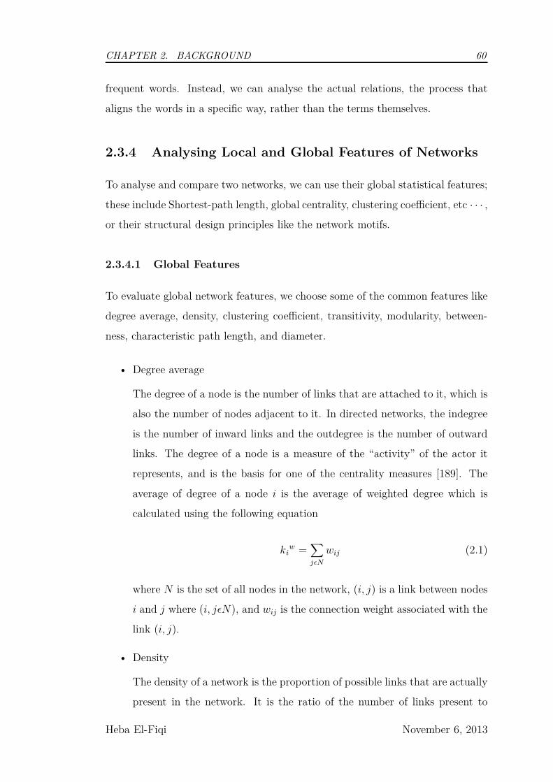
CHAPTER 2. BACKGROUND 60
frequent words. Instead, we can analyse the actual relations, the process that
aligns the words in a specific way, rather than the terms themselves.
2.3.4 Analysing Local and Global Features of Networks
To analyse and compare two networks, we can use their global statistical features;
these include Shortest-path length, global centrality, clustering coefficient, etc · · · ,
or their structural design principles like the network motifs.
2.3.4.1 Global Features
To evaluate global network features, we choose some of the common features like
degree average, density, clustering coefficient, transitivity, modularity, between-
ness, characteristic path length, and diameter.
• Degree average
The degree of a node is the number of links that are attached to it, which is
also the number of nodes adjacent to it. In directed networks, the indegree
is the number of inward links and the outdegree is the number of outward
links. The degree of a node is a measure of the “activity” of the actor it
represents, and is the basis for one of the centrality measures [189]. The
average of degree of a node i is the average of weighted degree which is
calculated using the following equation
kiw =
∑
jǫN
wij (2.1)
where N is the set of all nodes in the network, (i, j) is a link between nodes
i and j where (i, jǫN), and wij is the connection weight associated with the
link (i, j).
• Density
The density of a network is the proportion of possible links that are actually
present in the network. It is the ratio of the number of links present to
Heba El-Fiqi November 6, 2013
CHAPTER 2. BACKGROUND 61
the maximum possible links in this network [189]. Connection weights are
ignored in calculations. This measure is used to evaluate the cohesiveness
of subgroups.
• Diameter
The diameter of a connected graph is the length of the largest geodesic
between any pair of nodes [189]. The diameter represents the maximum
eccentricity. The diameter of a graph is important because it quantifies
how far apart the farthest two nodes in the graph are.
• Assortativity
The assortativity coefficient is a correlation coefficient between the degrees
of all nodes on two opposite ends of a link. A positive assortativity coef-
ficient indicates that nodes tend to link to other nodes with the same or
similar degree.
• Clustering coefficient
The clustering coefficient is the fraction of triangles around a node. It is
equivalent to the fraction of node’s neighbours that are neighbours of each
other. Clustering coefficient is a measure of the degree to which nodes in a
graph tend to cluster together.
• Transitivity
The transitivity is the ratio of “triangles to triplets" in the network (an
alternative version of the clustering coefficient).
• Modularity
The modularity is a statistic measure that is used to quantify how the net-
work can be divided into optimal community structure, which is the subdi-
vision of the network into non- overlapping groups of nodes in a way that
maximizes the number of within-group edges, and minimizes the number of
between-group edges.
Heba El-Fiqi November 6, 2013
CHAPTER 2. BACKGROUND 62
• Betweenness
Node betweenness centrality is the fraction of all shortest paths in the net-
work that contain a given node. Nodes with high values of betweenness
centrality participate in a large number of shortest paths.
• Characteristic path length
The characteristic path length is the average shortest path length in the
network.
2.3.4.2 Local Features
Local measures attempt to capture the global features of the network using the
local constructs. A widely used local measure is network motifs. Network motifs
which are initially introduced by Milo et al. [122] are patterns (represented by
small sub graphs) that are repeated in a real network more often than randomly
generated networks. They are used to uncover network structural design princi-
ples [7]. The motifs usually consist of three, four or five nodes. Network motifs
have been successfully used by different researchers in biology [165, 142], game
theory [56], evolutionary algorithms [103], electronic circuits [79], and software
[181].
2.4 Chapter Summary
This chapter has provided a brief summary of the stylometry analysis problem. It
discussed the extensive literature of writer stylometric analysis and its subtopics:
writer profiling, writer attribution, writer verification, and plagiarism detection.
It also discussed the varied methodology employed in this topic. The different
nominated features and approaches used to solve this problem are also presented.
The challenge of identifying translator stylometry is discussed in both literary
studies and computational linguistic studies. Failure of attributing translation to
their translators led to the need of identifying Stylometric features that are able
Heba El-Fiqi November 6, 2013
CHAPTER 2. BACKGROUND 63
to capture the translators’ individual styles. For that purpose, we explored how
we can redefine the problem of translator stylometry identification as a classifica-
tion problem, and how we can employ social network analysis to identify hidden
Stylometric features.
There is limited research in stylometry analysis with identified problems.
This study addressed the gap in the literature by combining a mixed methodol-
ogy that employ features extracted from social network analysis as attributes for
machine learning classification. The aim of this study is to introduce a compu-
tational framework that is able to identify translator stylometry.
Heba El-Fiqi November 6, 2013

Chapter 3
Data and Evaluation of Existing
Methods
3.1 Overview
In this study, we follow Baker’s definition of “Translator styles”: “ a study of
a translator’s style must focus on the manner of expression that is typical of a
translator, rather than simply instances of open intervention. It must attempt
to capture the translator’s characteristic use of language, his or her individual
profile of linguistic habits, compared to other translators” [19]. Her definition of
the style as a matter of patterning of linguistic behaviour is what we targeted in
this research. That guided us through the design and choice of our data corpus.
Based on Baker’s definition, we find that the best way to identify transla-
tor stylometry is to compare translations of the same original text by different
translators from the same source language to the same target language. That
will minimize the variations that may be caused by factors other than transla-
tors individual style, such as: variations of the source text types or contents, or
variations caused by different languages characteristics.
For that purpose, we are going to use for this study parallel Arabic to English
translations of the “Holy Qura’an". In this chapter, we are going to clarify the
CHAPTER 3. DATA AND EVALUATION OF EXISTING METHODS 65
reason for our choices of the source and target languages of translation, the nature
of the source text, and the structure of our dataset. After that, we are going to
evaluate some of the existing methods that have been used in the literature for
translator stylometry identification problem on our data corpus.
3.2 Why Arabic to English translations?
This study is focusing on translations from Arabic to English. Arabic Language
is the third most official language in the world after English and French; where
it is the official language for 26 countries 1 with approximately 280 million native
speakers in the world [141].
Second language learners face difficulties when they learn a language that
is derived from a different language family. For example, learning German lan-
guage for a native English speaker is not as difficult as learning Arabic Language.
German and English languages belong to the same branch and subgroup of the
language families’ taxonomy. Both of them belong to Western branch from Ger-
manic subgroup from Indeo-Eurpoean family [88], while Arabic belongs to Semitic
subgroup from Afro-Asiatic family [88]. Translating may pose similar difficulties
between languages that belong to different language families; spaces of choices
while mapping increase in this case.
The importance of the Arabic language can be understood because of its
socio-political role, but it extends to its religious role. Approximately 1.57 billion
Muslims of all ages live in the world today [148] who read Qur’an on a daily basis
as a part of their religious activities, which explains the reason for having millions
of Muslims seeking to learn Arabic, the language of “The Holy Qur’an” which is
the main religious text of Islam.
1As in World Atlas website http://www.worldatlas.com/ on 28th of January 2011
Heba El-Fiqi November 6, 2013
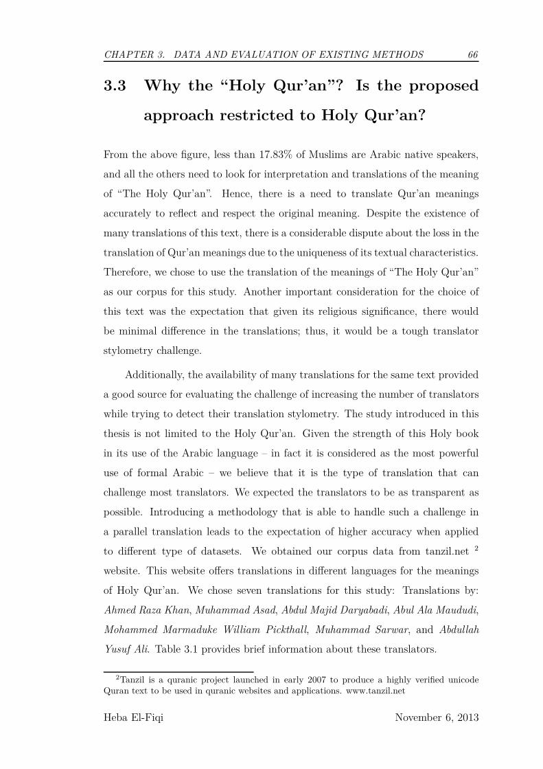
CHAPTER 3. DATA AND EVALUATION OF EXISTING METHODS 66
3.3 Why the “Holy Qur’an”? Is the proposed
approach restricted to Holy Qur’an?
From the above figure, less than 17.83% of Muslims are Arabic native speakers,
and all the others need to look for interpretation and translations of the meaning
of “The Holy Qur’an”. Hence, there is a need to translate Qur’an meanings
accurately to reflect and respect the original meaning. Despite the existence of
many translations of this text, there is a considerable dispute about the loss in the
translation of Qur’an meanings due to the uniqueness of its textual characteristics.
Therefore, we chose to use the translation of the meanings of “The Holy Qur’an”
as our corpus for this study. Another important consideration for the choice of
this text was the expectation that given its religious significance, there would
be minimal difference in the translations; thus, it would be a tough translator
stylometry challenge.
Additionally, the availability of many translations for the same text provided
a good source for evaluating the challenge of increasing the number of translators
while trying to detect their translation stylometry. The study introduced in this
thesis is not limited to the Holy Qur’an. Given the strength of this Holy book
in its use of the Arabic language – in fact it is considered as the most powerful
use of formal Arabic – we believe that it is the type of translation that can
challenge most translators. We expected the translators to be as transparent as
possible. Introducing a methodology that is able to handle such a challenge in
a parallel translation leads to the expectation of higher accuracy when applied
to different type of datasets. We obtained our corpus data from tanzil.net 2
website. This website offers translations in different languages for the meanings
of Holy Qur’an. We chose seven translations for this study: Translations by:
Ahmed Raza Khan, Muhammad Asad, Abdul Majid Daryabadi, Abul Ala Maududi,
Mohammed Marmaduke William Pickthall, Muhammad Sarwar, and Abdullah
Yusuf Ali. Table 3.1 provides brief information about these translators.
2Tanzil is a quranic project launched in early 2007 to produce a highly verified unicodeQuran text to be used in quranic websites and applications. www.tanzil.net
Heba El-Fiqi November 6, 2013
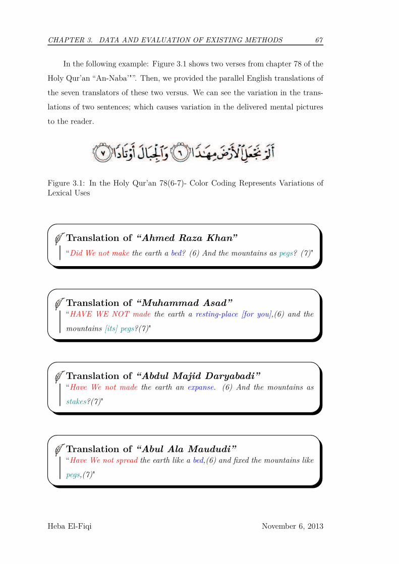
CHAPTER 3. DATA AND EVALUATION OF EXISTING METHODS 67
In the following example: Figure 3.1 shows two verses from chapter 78 of the
Holy Qur’an “An-Naba’"”. Then, we provided the parallel English translations of
the seven translators of these two versus. We can see the variation in the trans-
lations of two sentences; which causes variation in the delivered mental pictures
to the reader.
Figure 3.1: In the Holy Qur’an 78(6-7)- Color Coding Represents Variations ofLexical Uses
Translation of “Ahmed Raza Khan”
“Did We not make the earth a bed? (6) And the mountains as pegs? (7)"
Translation of “Muhammad Asad”“HAVE WE NOT made the earth a resting-place [for you],(6) and the
mountains [its] pegs?(7)"
Translation of “Abdul Majid Daryabadi”“Have We not made the earth an expanse. (6) And the mountains as
stakes?(7)"
Translation of “Abul Ala Maududi”“Have We not spread the earth like a bed,(6) and fixed the mountains like
pegs,(7)"
Heba El-Fiqi November 6, 2013
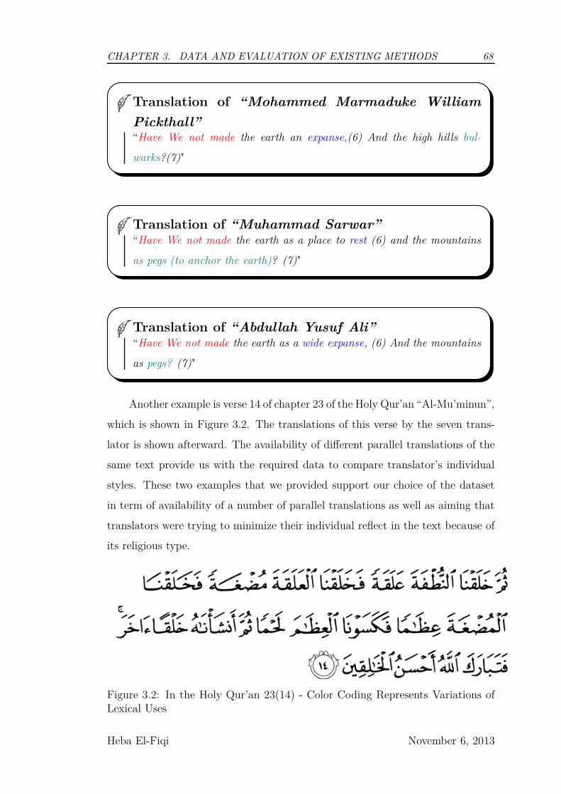
CHAPTER 3. DATA AND EVALUATION OF EXISTING METHODS 68
Translation of “Mohammed Marmaduke William
Pickthall”“Have We not made the earth an expanse,(6) And the high hills bul-
warks?(7)"
Translation of “Muhammad Sarwar”“Have We not made the earth as a place to rest (6) and the mountains
as pegs (to anchor the earth)? (7)"
Translation of “Abdullah Yusuf Ali”“Have We not made the earth as a wide expanse, (6) And the mountains
as pegs? (7)"
Another example is verse 14 of chapter 23 of the Holy Qur’an “Al-Mu’minun”,
which is shown in Figure 3.2. The translations of this verse by the seven trans-
lator is shown afterward. The availability of different parallel translations of the
same text provide us with the required data to compare translator’s individual
styles. These two examples that we provided support our choice of the dataset
in term of availability of a number of parallel translations as well as aiming that
translators were trying to minimize their individual reflect in the text because of
its religious type.
Figure 3.2: In the Holy Qur’an 23(14) - Color Coding Represents Variations ofLexical Uses
Heba El-Fiqi November 6, 2013
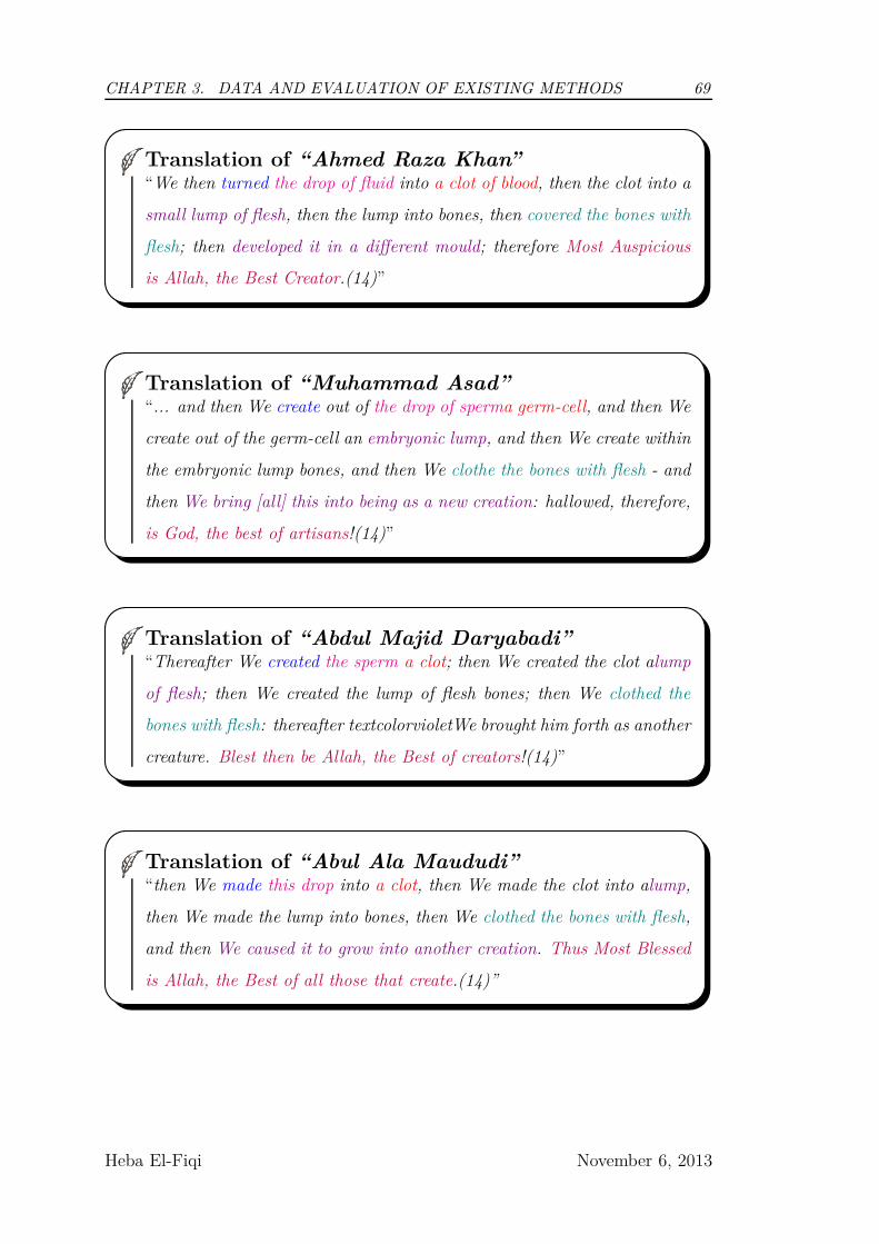
CHAPTER 3. DATA AND EVALUATION OF EXISTING METHODS 69
Translation of “Ahmed Raza Khan”“We then turned the drop of fluid into a clot of blood, then the clot into a
small lump of flesh, then the lump into bones, then covered the bones with
flesh; then developed it in a different mould; therefore Most Auspicious
is Allah, the Best Creator.(14)”
Translation of “Muhammad Asad”“... and then We create out of the drop of sperma germ-cell, and then We
create out of the germ-cell an embryonic lump, and then We create within
the embryonic lump bones, and then We clothe the bones with flesh - and
then We bring [all] this into being as a new creation: hallowed, therefore,
is God, the best of artisans!(14)”
Translation of “Abdul Majid Daryabadi”“Thereafter We created the sperm a clot; then We created the clot alump
of flesh; then We created the lump of flesh bones; then We clothed the
bones with flesh: thereafter textcolorvioletWe brought him forth as another
creature. Blest then be Allah, the Best of creators!(14)”
Translation of “Abul Ala Maududi”“then We made this drop into a clot, then We made the clot into alump,
then We made the lump into bones, then We clothed the bones with flesh,
and then We caused it to grow into another creation. Thus Most Blessed
is Allah, the Best of all those that create.(14)”
Heba El-Fiqi November 6, 2013
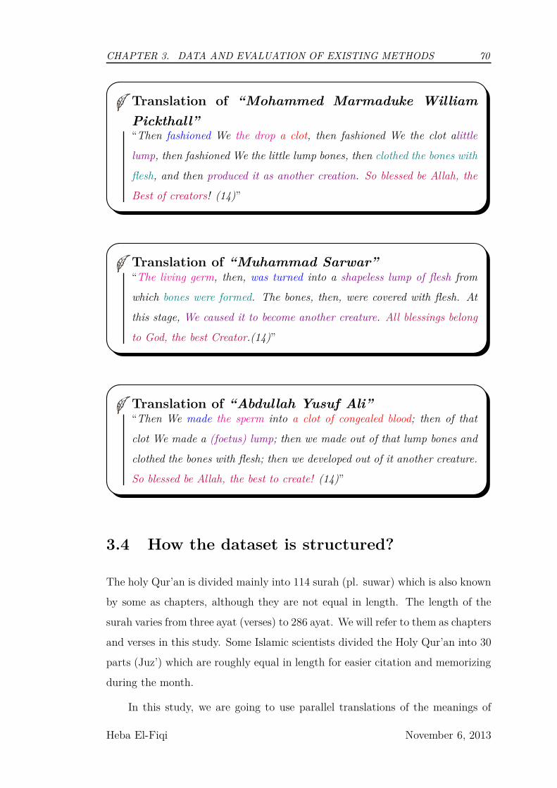
CHAPTER 3. DATA AND EVALUATION OF EXISTING METHODS 70
Translation of “Mohammed Marmaduke William
Pickthall”“Then fashioned We the drop a clot, then fashioned We the clot alittle
lump, then fashioned We the little lump bones, then clothed the bones with
flesh, and then produced it as another creation. So blessed be Allah, the
Best of creators! (14)”
Translation of “Muhammad Sarwar”“The living germ, then, was turned into a shapeless lump of flesh from
which bones were formed. The bones, then, were covered with flesh. At
this stage, We caused it to become another creature. All blessings belong
to God, the best Creator.(14)”
Translation of “Abdullah Yusuf Ali”“Then We made the sperm into a clot of congealed blood; then of that
clot We made a (foetus) lump; then we made out of that lump bones and
clothed the bones with flesh; then we developed out of it another creature.
So blessed be Allah, the best to create! (14)”
3.4 How the dataset is structured?
The holy Qur’an is divided mainly into 114 surah (pl. suwar) which is also known
by some as chapters, although they are not equal in length. The length of the
surah varies from three ayat (verses) to 286 ayat. We will refer to them as chapters
and verses in this study. Some Islamic scientists divided the Holy Qur’an into 30
parts (Juz’) which are roughly equal in length for easier citation and memorizing
during the month.
In this study, we are going to use parallel translations of the meanings of
Heba El-Fiqi November 6, 2013
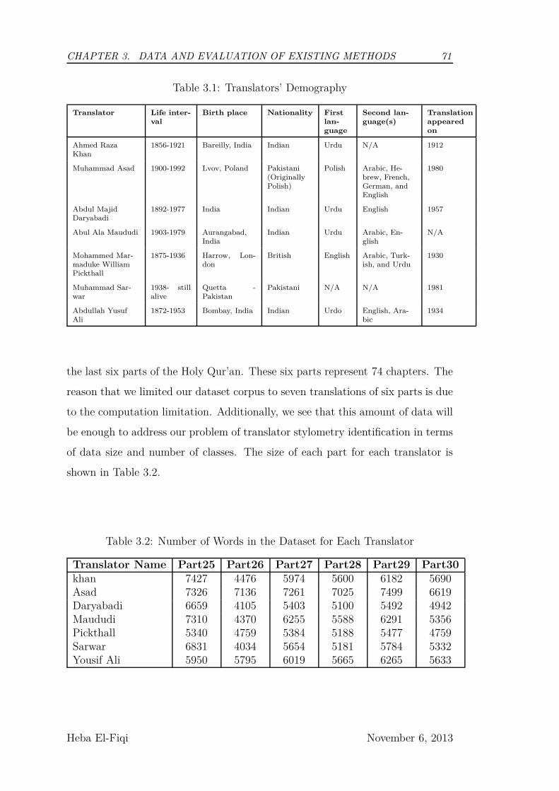
CHAPTER 3. DATA AND EVALUATION OF EXISTING METHODS 71
Table 3.1: Translators’ Demography
Translator Life inter-val
Birth place Nationality Firstlan-guage
Second lan-guage(s)
Translationappearedon
Ahmed RazaKhan
1856-1921 Bareilly, India Indian Urdu N/A 1912
Muhammad Asad 1900-1992 Lvov, Poland Pakistani(OriginallyPolish)
Polish Arabic, He-brew, French,German, andEnglish
1980
Abdul MajidDaryabadi
1892-1977 India Indian Urdu English 1957
Abul Ala Maududi 1903-1979 Aurangabad,India
Indian Urdu Arabic, En-glish
N/A
Mohammed Mar-maduke WilliamPickthall
1875-1936 Harrow, Lon-don
British English Arabic, Turk-ish, and Urdu
1930
Muhammad Sar-war
1938- stillalive
Quetta -Pakistan
Pakistani N/A N/A 1981
Abdullah YusufAli
1872-1953 Bombay, India Indian Urdo English, Ara-bic
1934
the last six parts of the Holy Qur’an. These six parts represent 74 chapters. The
reason that we limited our dataset corpus to seven translations of six parts is due
to the computation limitation. Additionally, we see that this amount of data will
be enough to address our problem of translator stylometry identification in terms
of data size and number of classes. The size of each part for each translator is
shown in Table 3.2.
Table 3.2: Number of Words in the Dataset for Each Translator
Translator Name Part25 Part26 Part27 Part28 Part29 Part30khan 7427 4476 5974 5600 6182 5690Asad 7326 7136 7261 7025 7499 6619Daryabadi 6659 4105 5403 5100 5492 4942Maududi 7310 4370 6255 5588 6291 5356Pickthall 5340 4759 5384 5188 5477 4759Sarwar 6831 4034 5654 5181 5784 5332Yousif Ali 5950 5795 6019 5665 6265 5633
Heba El-Fiqi November 6, 2013
CHAPTER 3. DATA AND EVALUATION OF EXISTING METHODS 72
3.5 Evaluating Existing Methods
3.5.1 Is there such a thing as a translator’s style
In 2001 a paper published by Mikhailov and Villikka [121] claimed that translators
didn’t have a language and a style of their own. In their research, they used
vocabulary richness, most frequent words and favourite words as they are typical
authorship attribution features to prove their claim. In response to this paper,
and as a first step, we reapplied the same method and features that they used for
their claim on our dataset.
3.5.1.1 Method I
1. Vocabulary Richness
Vocabulary richness can be evaluated using different methods. Mikhailov
and Villikka [121] used three different measures of Vocabulary richness from
a multivariate approach to measure vocabulary richness that were originally
introduced by Holmes in 1991 [66] then modified by Holmes and Forsyth in
1995 [65] for analyzing the federalist papers. These three measures are:
(a) R-index is a measure suggested by Honore (1979). This measure tar-
gets (hapax legomena) which means words that used only once in the
text. The higher number of words used only once in the text, the
higher the R value.
R =100LogN
1− V 1V
(3.1)
where N is the text length of N words, and V is the number of different
words;
(b) K-index is a measure that was proposed by Yule (1944). The mea-
sure monotonically increases as the high-frequency words in the text
increases.
Heba El-Fiqi November 6, 2013
CHAPTER 3. DATA AND EVALUATION OF EXISTING METHODS 73
K =104(
∑∞i=1 i2Vi −N)
N2(3.2)
where Vi(i=1,2,. . . ) is the number of words used exactly i times in
the text.
(c) W-index is originally proposed by Brunet (1978), who claimed that
this measure is not affected by text length, and it is author specific.
W-index increases as number of different words increases.
W = NV −a (3.3)
where a is a constant ranges from 0.165 to 0.172. As we couldn’t find
the methodology of choosing the value of ( a), we used the value of
0.172 which was used by Mikhailov and Villikka [121] in their research.
2. Most Frequent Words
F-Index is used to measure the closeness of most frequent words as it re-
flects a correlation between two pieces of texts. The two targeted texts are
compared by selecting the 40 most frequent words from their word lists.
Then, the F-Index is calculated by adding three points for each word with
close relative frequency, two points for each word with different relative fre-
quency, and one point for each word with quite different relative frequency.
One point is deduced for each word absent in the other list. We applied
this method on lemmatized word lists for each text in our dataset.
To calculate the F-Index, we needed to define threshold for close relative
frequency, different relative frequency, and quite different relative frequency,
which were not defined in Mikhailov and Villikka research [121]. To do that,
we divided the distance between the minimum frequency and maximum
frequency to three equal parts, the first section represent low difference area,
the middle two sections represent medium difference, and the last section
represent high difference area. If the difference between the frequency of
the same words in the two text occur in the low difference area, that means
Heba El-Fiqi November 6, 2013
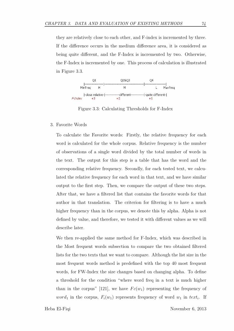
CHAPTER 3. DATA AND EVALUATION OF EXISTING METHODS 74
they are relatively close to each other, and F-index is incremented by three.
If the difference occurs in the medium difference area, it is considered as
being quite different, and the F-Index is incremented by two. Otherwise,
the F-Index is incremented by one. This process of calculation is illustrated
in Figure 3.3.
Figure 3.3: Calculating Thresholds for F-Index
3. Favorite Words
To calculate the Favorite words: Firstly, the relative frequency for each
word is calculated for the whole corpus. Relative frequency is the number
of observations of a single word divided by the total number of words in
the text. The output for this step is a table that has the word and the
corresponding relative frequency. Secondly, for each tested text, we calcu-
lated the relative frequency for each word in that text, and we have similar
output to the first step. Then, we compare the output of these two steps.
After that, we have a filtered list that contains the favorite words for that
author in that translation. The criterion for filtering is to have a much
higher frequency than in the corpus, we denote this by alpha. Alpha is not
defined by value, and therefore, we tested it with different values as we will
describe later.
We then re-applied the same method for F-Index, which was described in
the Most frequent words subsection to compare the two obtained filtered
lists for the two texts that we want to compare. Although the list size in the
most frequent words method is predefined with the top 40 most frequent
words, for FW-Index the size changes based on changing alpha. To define
a threshold for the condition “where word freq in a text is much higher
than in the corpus” [121], we have Fc(w1) representing the frequency of
word1 in the corpus, Fi(w1) represents frequency of word w1 in texti. If
Heba El-Fiqi November 6, 2013
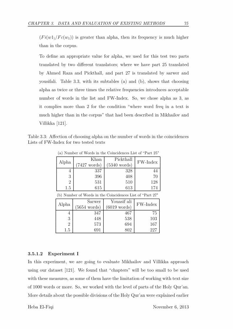
CHAPTER 3. DATA AND EVALUATION OF EXISTING METHODS 75
(Fi(w1)/Fc(w1)) is greater than alpha, then its frequency is much higher
than in the corpus.
To define an appropriate value for alpha, we used for this test two parts
translated by two different translators; where we have part 25 translated
by Ahmed Raza and Pickthall, and part 27 is translated by sarwer and
yousifali. Table 3.3, with its subtables (a) and (b), shows that choosing
alpha as twice or three times the relative frequencies introduces acceptable
number of words in the list and FW-Index. So, we chose alpha as 3, as
it complies more than 2 for the condition “where word freq in a text is
much higher than in the corpus” that had been described in Mikhailov and
Villikka [121].
Table 3.3: Affection of choosing alpha on the number of words in the coincidencesLists of FW-Index for two tested texts
(a) Number of Words in the Coincidences List of “Part 25"
AlphaKhan Pickthall
FW-Index(7427 words) (5340 words)
4 337 328 443 396 408 702 531 510 128
1.5 615 613 174
(b) Number of Words in the Coincidences List of “Part 27"
AlphaSarwer Youasif ali
FW-Index(5654 words) (6019 words)
4 347 467 753 448 538 1032 573 694 167
1.5 691 802 227
3.5.1.2 Experiment I
In this experiment, we are going to evaluate Mikhailov and Villikka approach
using our dataset [121]. We found that “chapters” will be too small to be used
with these measures, as some of them have the limitation of working with text size
of 1000 words or more. So, we worked with the level of parts of the Holy Qur’an.
More details about the possible divisions of the Holy Qur’an were explained earlier
Heba El-Fiqi November 6, 2013

CHAPTER 3. DATA AND EVALUATION OF EXISTING METHODS 76
in the data section. Therefore, we used seven translations for six parts of the Holy
Qur’an in this experiment.
For vocabulary richness: R-Index, K-Index, and W-Index were calculated
for each text. Then the results for these calculations were used to compare
and analyze the similarities and differences between translations by the same
translator with translations for the same text. The objective of this experiment
is to identify if vocabulary richness for the same translator is the same for different
translations, or it is only affected by the original text.
For the most frequent and most favourite words, we cannot evaluate a single
text each time; as the proposed measures are used to measure similarities between
two texts. Therefore, for the most frequent words, we calculated these measures
for all possible combinations for the existing dataset. First, we calculated all the
pairs of translations by the same translator. For example, for translator Asad, we
calculated the most frequent words measure, F-Index, for (part25-part26), then
for (part25-part27), then for (part 25-part 28),...etc. After measuring these for all
translators, we evaluated the F-Index for different translators for the same origi-
nal text. For example, for Part25, we calculated F-Index for (Asad-Daraybadi),
(Asad,Maududi), (Asad-Pickthall),...etc. Then, all of these results were used to
analyze if the most frequent words measure is more affected by the translator
style or the original text. The same procedure is used for evaluating the favorite
words measure.
3.5.1.3 Results and Discussion of Experiment I
For Vocabulary Richness, the three used measures are highly affected by the
original text as seen in Figures 3.4(a), 3.4(b), and 3.4(c). The R-Index didn’t
reflect an individual translator’s style; It is affected by the original text. Despite
that all orginial text to come from the same language, both of K-Index and W-
Index also didn’t reflect individual translator styles. However, Asad had lower
K-index for all translations, and Khan had the highest W-index values for all
translations. This implies that both of K-Index and W-Index can show individual
Heba El-Fiqi November 6, 2013
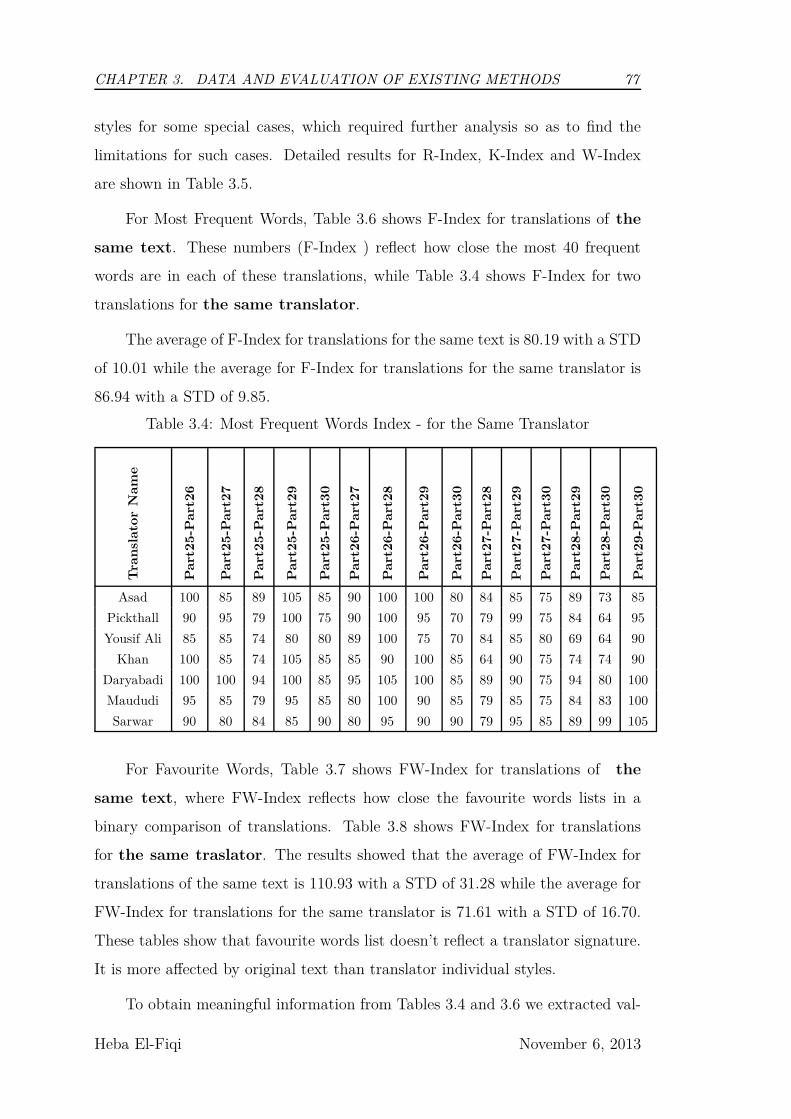
CHAPTER 3. DATA AND EVALUATION OF EXISTING METHODS 77
styles for some special cases, which required further analysis so as to find the
limitations for such cases. Detailed results for R-Index, K-Index and W-Index
are shown in Table 3.5.
For Most Frequent Words, Table 3.6 shows F-Index for translations of the
same text. These numbers (F-Index ) reflect how close the most 40 frequent
words are in each of these translations, while Table 3.4 shows F-Index for two
translations for the same translator.
The average of F-Index for translations for the same text is 80.19 with a STD
of 10.01 while the average for F-Index for translations for the same translator is
86.94 with a STD of 9.85.
Table 3.4: Most Frequent Words Index - for the Same Translator
Tra
nsl
ato
rN
am
e
Part
25
-Part
26
Part
25
-Part
27
Part
25
-Part
28
Part
25
-Part
29
Part
25
-Part
30
Part
26
-Part
27
Part
26
-Part
28
Part
26
-Part
29
Part
26
-Part
30
Part
27
-Part
28
Part
27
-Part
29
Part
27
-Part
30
Part
28
-Part
29
Part
28
-Part
30
Part
29
-Part
30
Asad 100 85 89 105 85 90 100 100 80 84 85 75 89 73 85
Pickthall 90 95 79 100 75 90 100 95 70 79 99 75 84 64 95
Yousif Ali 85 85 74 80 80 89 100 75 70 84 85 80 69 64 90
Khan 100 85 74 105 85 85 90 100 85 64 90 75 74 74 90
Daryabadi 100 100 94 100 85 95 105 100 85 89 90 75 94 80 100
Maududi 95 85 79 95 85 80 100 90 85 79 85 75 84 83 100
Sarwar 90 80 84 85 90 80 95 90 90 79 95 85 89 99 105
For Favourite Words, Table 3.7 shows FW-Index for translations of the
same text, where FW-Index reflects how close the favourite words lists in a
binary comparison of translations. Table 3.8 shows FW-Index for translations
for the same traslator. The results showed that the average of FW-Index for
translations of the same text is 110.93 with a STD of 31.28 while the average for
FW-Index for translations for the same translator is 71.61 with a STD of 16.70.
These tables show that favourite words list doesn’t reflect a translator signature.
It is more affected by original text than translator individual styles.
To obtain meaningful information from Tables 3.4 and 3.6 we extracted val-
Heba El-Fiqi November 6, 2013
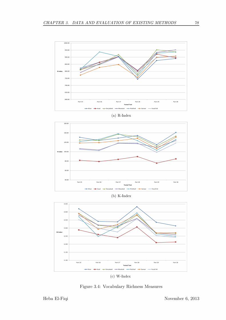
CHAPTER 3. DATA AND EVALUATION OF EXISTING METHODS 78
750.00
800.00
850.00
900.00
950.00
1000.00
R Index
600.00
650.00
700.00
Part 25 Part 26 Part 27 Part 28 Part 29 Part 30
Tested!Text
Khan Asad Daryabadi Maududi Pickthall Sarwar Yousif Ali
(a) R-Index
100.00
120.00
140.00
160.00
K Index
40.00
60.00
80.00
Part 25 Part 26 Part 27 Part 28 Part 29 Part 30
Tested!Text
Khan Asad Daryabadi Maududi Pickthall Sarwar Yousif Ali
(b) K-Index
12.50
13.00
13.50
14.00
14.50
W Index
11.00
11.50
12.00
Part 25 Part 26 Part 27 Part 28 Part 29 Part 30
Tested!Text
Khan Asad Daryabadi Maududi Pickthall Sarwar Yousif Ali
(c) W-Index
Figure 3.4: Vocabulary Richness Measures
Heba El-Fiqi November 6, 2013
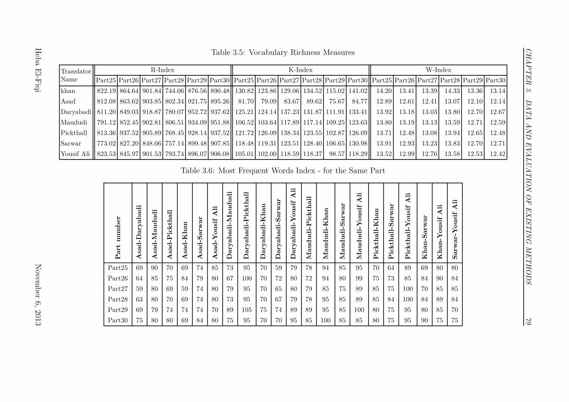
CH
AP
TE
R3.
DA
TA
AN
DE
VA
LU
AT
ION
OF
EX
IST
ING
ME
TH
OD
S79
Table 3.5: Vocabulary Richness Measures
TranslatorName
R-Index K-Index W-Index
Part25 Part26 Part27 Part28 Part29 Part30 Part25 Part26 Part27 Part28 Part29 Part30 Part25 Part26 Part27 Part28 Part29 Part30
khan 822.19 864.64 901.84 744.06 876.56 890.48 130.82 123.86 129.06 134.52 115.02 141.02 14.20 13.41 13.39 14.33 13.36 13.14
Asad 812.08 863.62 903.85 802.34 921.75 895.26 81.70 79.09 83.67 89.62 75.67 84.77 12.89 12.61 12.41 13.07 12.10 12.14
Daryabadi 811.20 849.03 918.87 780.07 952.72 937.62 125.21 124.14 137.23 131.87 111.91 133.41 13.92 13.18 13.03 13.80 12.70 12.67
Maududi 791.12 852.45 902.81 806.51 934.09 951.88 106.52 103.64 117.89 117.14 109.25 123.63 13.80 13.19 13.13 13.59 12.71 12.59
Pickthall 813.36 937.52 905.89 768.45 928.14 937.52 121.72 126.09 138.34 123.55 102.87 126.09 13.71 12.48 13.08 13.94 12.65 12.48
Sarwar 773.02 827.20 848.06 757.14 899.48 907.85 118.48 119.31 123.51 128.40 106.65 130.98 13.91 12.93 13.23 13.83 12.70 12.71
Yousif Ali 823.53 845.97 901.53 793.74 896.07 906.08 105.01 102.00 118.59 118.37 98.57 118.29 13.52 12.99 12.76 13.58 12.53 12.42
Table 3.6: Most Frequent Words Index - for the Same Part
Part
nu
mb
er
Asa
d-D
ary
ab
ad
i
Asa
d-M
au
du
di
Asa
d-P
ick
thall
Asa
d-K
han
Asa
d-S
arw
ar
Asa
d-Y
ou
sif
Ali
Dary
ab
ad
i-M
au
du
di
Dary
ab
ad
i-P
ick
thall
Dary
ab
ad
i-K
han
Dary
ab
ad
i-S
arw
ar
Dary
ab
ad
i-Y
ou
sif
Ali
Mau
du
di-
Pic
kth
all
Mau
du
di-
Kh
an
Mau
du
di-
Sarw
ar
Mau
du
di-
Yo
usi
fA
li
Pic
kth
all
-Kh
an
Pic
kth
all
-Sarw
ar
Pic
kth
all
-Yo
usi
fA
li
Kh
an
-Sarw
ar
Kh
an
-Yo
usi
fA
li
Sarw
ar-
Yo
usi
fA
li
Part25 69 90 70 69 74 85 73 95 70 59 79 78 94 85 95 70 64 89 69 80 80
Part26 64 85 75 84 79 80 67 100 70 72 80 72 94 80 99 75 73 85 84 90 84
Part27 59 80 69 59 74 80 79 95 70 65 80 79 85 75 89 85 75 100 70 85 85
Part28 63 80 70 69 74 80 73 95 70 67 79 78 95 85 89 85 84 100 84 89 84
Part29 69 79 74 74 74 70 89 105 75 74 89 89 95 85 100 80 75 95 80 85 70
Part30 75 80 80 69 84 80 75 95 70 70 95 85 100 85 85 80 75 95 90 75 75
Heb
aE
l-Fiq
iN
ovemb
er6,
2013
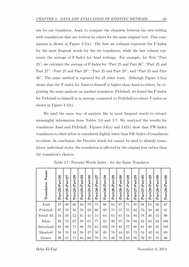
CHAPTER 3. DATA AND EVALUATION OF EXISTING METHODS 80
ues for one translator, Asad, to compare the closeness between his own writing
with translations that are written by others for the same original text. This com-
parison is shown in Figure 3.5(a). The first six columns represent the F-Index
for the most frequent words for the six translators, while the last column rep-
resent the average of F-Index for Asad writings. For example, for Text “Part
25”, we calculate the average of F-Index for “Part 25 and Part 26”, “Part 25 and
Part 27”, “Part 25 and Part 28”, “Part 25 and Part 29”, and “Part 25 and Part
30”. The same method is repeated for all other texts. Although Figure 3.5(a)
shows that the F-index for Asad-to-himself is higher than Asad-to-others, by re-
peating the same analysis on another translator, Pickthall, we found the F-Index
for Pickthall-to-himself is in average compared to Pickthall-to-others F-index as
shown in Figure 3.5(b).
We used the same way of analysis like in most frequent words to extract
meaningful information from Tables 3.8 and 3.7; We analyzed the results for
translators Asad and Pickthall. Figures 3.6(a) and 3.6(b) show that FW-Index
translators-to-their selves is considered slightly lower than FW-Index of translators-
to-others. In conclusion, the Favorite words list cannot be used to identify trans-
lators’ individual styles; the translation is affected by the original text rather than
the translator’s choices.
Table 3.7: Favorite Words Index - for the Same Translator
Tra
nsl
ato
rN
am
e
Pa
rt2
5-P
art
26
Pa
rt2
5-P
art
27
Pa
rt2
5-P
art
28
Pa
rt2
5-P
art
29
Pa
rt2
5-P
art
30
Pa
rt2
6-P
art
27
Pa
rt2
6-P
art
28
Pa
rt2
6-P
art
29
Pa
rt2
6-P
art
30
Pa
rt2
7-P
art
28
Pa
rt2
7-P
art
29
Pa
rt2
7-P
art
30
Pa
rt2
8-P
art
29
Pa
rt2
8-P
art
30
Pa
rt2
9-P
art
30
Asad 97 80 86 94 79 75 88 64 67 71 91 98 65 66 67
Pickthall 87 76 56 70 58 66 80 71 57 55 82 73 58 60 81
Yousif Ali 54 50 52 61 41 51 64 61 61 54 94 78 46 53 96
Khan 93 74 67 83 61 77 82 92 87 76 94 82 63 62 106
Daryabadi 94 89 71 86 73 84 103 78 83 77 98 91 68 65 100
Maududi 50 55 43 58 37 50 49 55 44 35 73 53 42 43 69
Sarwar 99 81 75 84 69 78 76 80 76 63 95 76 67 55 96
Heba El-Fiqi November 6, 2013
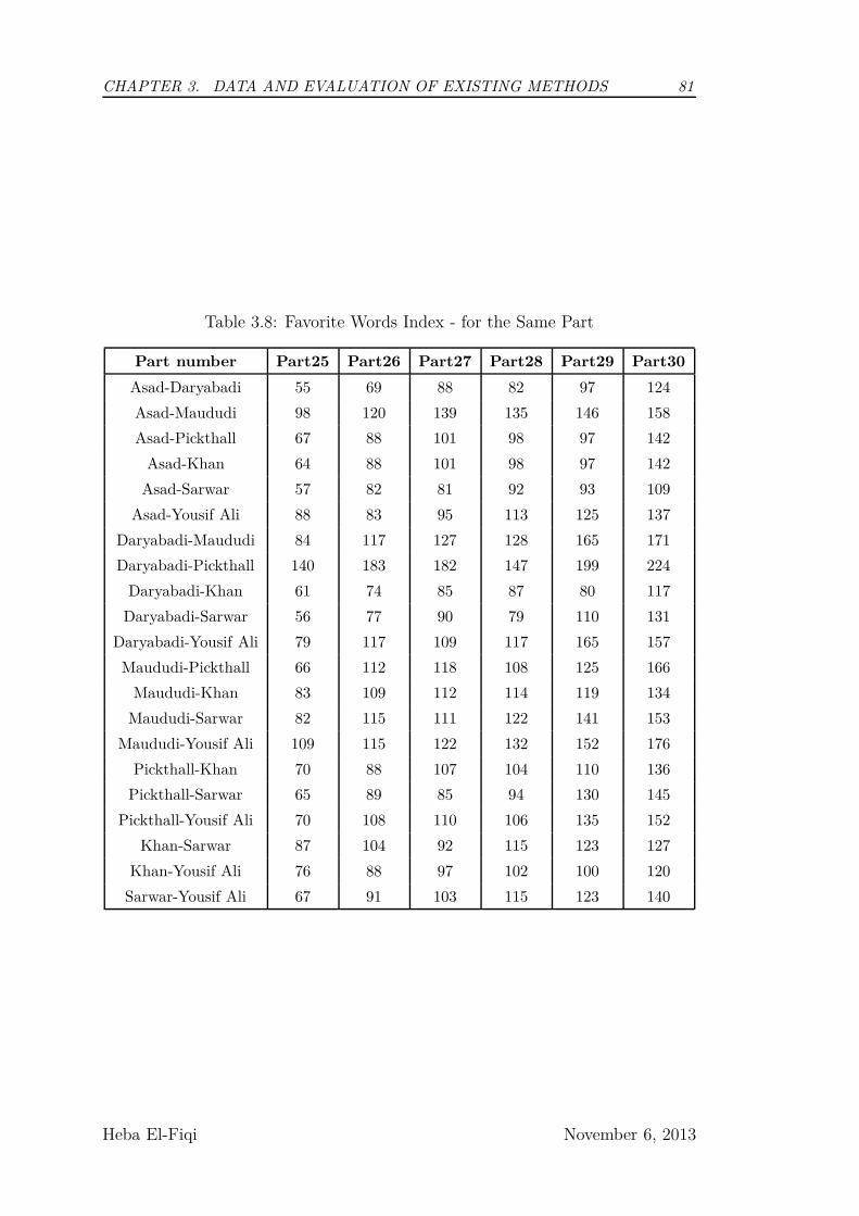
CHAPTER 3. DATA AND EVALUATION OF EXISTING METHODS 81
Table 3.8: Favorite Words Index - for the Same Part
Part number Part25 Part26 Part27 Part28 Part29 Part30
Asad-Daryabadi 55 69 88 82 97 124
Asad-Maududi 98 120 139 135 146 158
Asad-Pickthall 67 88 101 98 97 142
Asad-Khan 64 88 101 98 97 142
Asad-Sarwar 57 82 81 92 93 109
Asad-Yousif Ali 88 83 95 113 125 137
Daryabadi-Maududi 84 117 127 128 165 171
Daryabadi-Pickthall 140 183 182 147 199 224
Daryabadi-Khan 61 74 85 87 80 117
Daryabadi-Sarwar 56 77 90 79 110 131
Daryabadi-Yousif Ali 79 117 109 117 165 157
Maududi-Pickthall 66 112 118 108 125 166
Maududi-Khan 83 109 112 114 119 134
Maududi-Sarwar 82 115 111 122 141 153
Maududi-Yousif Ali 109 115 122 132 152 176
Pickthall-Khan 70 88 107 104 110 136
Pickthall-Sarwar 65 89 85 94 130 145
Pickthall-Yousif Ali 70 108 110 106 135 152
Khan-Sarwar 87 104 92 115 123 127
Khan-Yousif Ali 76 88 97 102 100 120
Sarwar-Yousif Ali 67 91 103 115 123 140
Heba El-Fiqi November 6, 2013
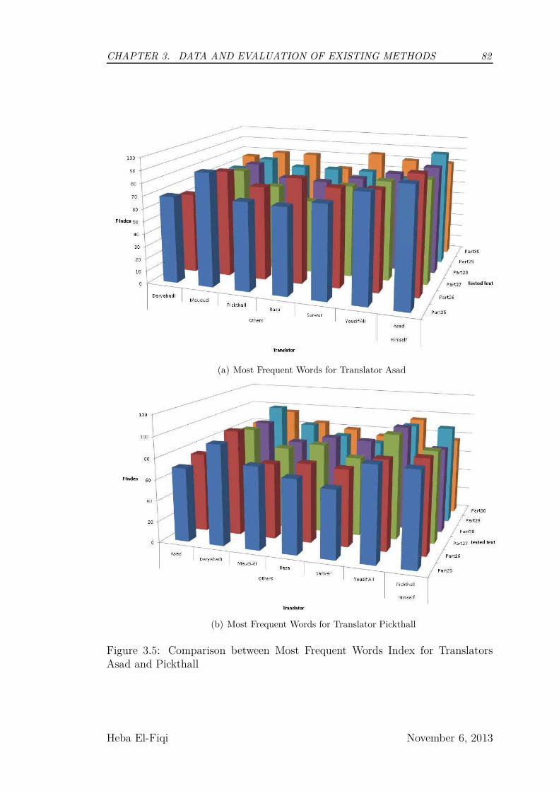
CHAPTER 3. DATA AND EVALUATION OF EXISTING METHODS 82
(a) Most Frequent Words for Translator Asad
(b) Most Frequent Words for Translator Pickthall
Figure 3.5: Comparison between Most Frequent Words Index for TranslatorsAsad and Pickthall
Heba El-Fiqi November 6, 2013

CHAPTER 3. DATA AND EVALUATION OF EXISTING METHODS 83
(a) Favorite Words Index for Translator Asad
(b) Favorite Words Index for Translator Pickthall
Figure 3.6: Comparison between Favorite Words Index for Translators Asad andPickthall
Heba El-Fiqi November 6, 2013
CHAPTER 3. DATA AND EVALUATION OF EXISTING METHODS 84
In conclusion, changes in vocabulary richness measures were mostly affected
by the original text rather than being affected by the differences of the transla-
tors. Except for Asad, who has a distinct style, most frequent words and favourite
words measures used in this section were not able to discriminate different trans-
lators.
3.5.2 Vocabulary Richness Measures as Translator Sty-
lometry Features
The main objective of this experiment is to investigate the ability of vocabulary
richness measures to discriminate between translators. To evaluate the effective-
ness of vocabulary richness as translator stylometry features, we used the idea of
classifying texts (as instances) into their translators (as classes) based on vocab-
ulary richness (as attributes). Working on the level of parts for the Holy Qur’an
as the instances give us only 6 instances (parts)/ per class (translator). For that
reason, we chose to work on chapters’ level as that gives us 74 instances/class.
3.5.2.1 Method II
For this experiment, we used five vocabulary richness measures as attributes:
which are N, V, R-Index, K-index, and W-Index. Their description is discussed
in section 3.5.1.1.
3.5.2.2 Experiment II
We use two of the most studied classification algorithms in the literature: these
are the decision tree C4.5 and support vector machine (SVM). We used their im-
plementation in WEKA “data mining software”. For C4.5, which is a decision tree
based classification algorithm developed by Quinlan in 1993 [144], we used pruned
weka.classifiers.trees.J48. For SVM, we used weka.classifiers.functions.SMO; which
is based on the Sequential Minimal Optimization algorithm for support vector
machine [139] [89].
Heba El-Fiqi November 6, 2013
CHAPTER 3. DATA AND EVALUATION OF EXISTING METHODS 85
As we have seven translators, we worked with them in pairs using binary
classifiers. We used ten- fold cross-validation to evaluate the classifiers. Ten-
fold cross-validation is a common statistical method of measuring the predictive
performance of a model, in which, data is partitioned into ten non-overlapping
sets. Then, each of these partitions is being held once for testing while the other
nine partitions are used for training the model. The average accuracy of the
ten iterations is calculated to estimate the average accuracy of the model. The
advantages of this cross-validation technique include the non-overlapping nature
of the training and testing data and the provision of a chance for each instance
in the data to appear in the testing dataset once. Additionally cross-validation
is recommended when the available data for training and testing is limited [195].
3.5.2.3 Results and Discussion of Experiment II
In this thesis, we are evaluating binary classification for each pair of transla-
tors where training and testing data are balanced (i.e. equal class distribution)
between the two translators. For such case, a baseline for the classifier is the
random case of 50% chance of labelling the correct class. Anything above 50%
is better than the random chance. Therefore, we choose 2/3, which is 66.67% as
a threshold to achieve significantly better than the random baseline accuracy of
50%.
Considering a classifier is being acceptable if it is able to correctly classify
2/3 of tested instances, among the 21 studied cases, only 6/21 was acceptable
using each of C4.5 and SVM as shown in Table 3.9 using vocabulary richness. All
these 6 cases are easy to classify because they have Asad in common. As shown
in Figure 3.4(b), Asad has very distinct translation style compared to all others.
Vocabulary richness measures did not introduce acceptable results neither
using C4.5 nor SVM. The overall average accuracy was 55.12% using C4.5 and
54.31% using SVM.
Heba El-Fiqi November 6, 2013
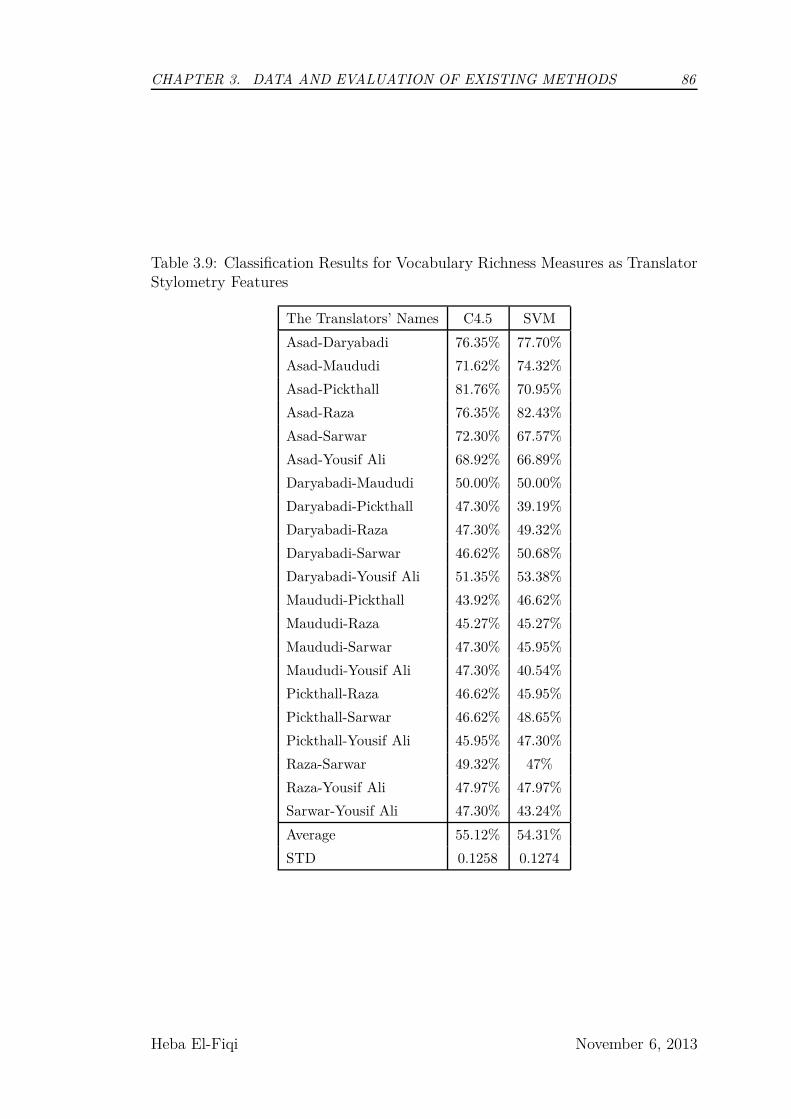
CHAPTER 3. DATA AND EVALUATION OF EXISTING METHODS 86
Table 3.9: Classification Results for Vocabulary Richness Measures as TranslatorStylometry Features
The Translators’ Names C4.5 SVM
Asad-Daryabadi 76.35% 77.70%
Asad-Maududi 71.62% 74.32%
Asad-Pickthall 81.76% 70.95%
Asad-Raza 76.35% 82.43%
Asad-Sarwar 72.30% 67.57%
Asad-Yousif Ali 68.92% 66.89%
Daryabadi-Maududi 50.00% 50.00%
Daryabadi-Pickthall 47.30% 39.19%
Daryabadi-Raza 47.30% 49.32%
Daryabadi-Sarwar 46.62% 50.68%
Daryabadi-Yousif Ali 51.35% 53.38%
Maududi-Pickthall 43.92% 46.62%
Maududi-Raza 45.27% 45.27%
Maududi-Sarwar 47.30% 45.95%
Maududi-Yousif Ali 47.30% 40.54%
Pickthall-Raza 46.62% 45.95%
Pickthall-Sarwar 46.62% 48.65%
Pickthall-Yousif Ali 45.95% 47.30%
Raza-Sarwar 49.32% 47%
Raza-Yousif Ali 47.97% 47.97%
Sarwar-Yousif Ali 47.30% 43.24%
Average 55.12% 54.31%
STD 0.1258 0.1274
Heba El-Fiqi November 6, 2013

CHAPTER 3. DATA AND EVALUATION OF EXISTING METHODS 87
3.6 Chapter Summary
In this chapter, we described the choice and design of our dataset. We justified our
choice for that corpus. Then we examined our dataset using the same approach
evaluated by Mikhailov and Villikka, which included vocabulary richness, most
frequent words and favorite words. Then, we evaluated the use of vocabulary
richness measures as attribution features for translator identification, as they
are commonly used in authorship attribution area which is the closest area in
computational linguistics to our problem. Vocabulary richness did not introduce
acceptable results. Hence, there is a need to find an appropriate approach to
identify translators’ stylometry.
Heba El-Fiqi November 6, 2013
Chapter 4
Identifying Translator Stylometry
Using Network Motifs
4.1 Overview
We started our journey to identify appropriate features to detect translators by
our first experiment that we discussed in chapter 3, in which we evaluated Vo-
cabulary Richness measures as translator stylometry features. The findings from
that experiment encouraged us to evaluate the use of network motifs search for
the purpose of translator stylometry identification. Therefore, the objective of
this chapter is to introduce the methodology of using network motifs search for
translator stylometry identification. The second objective of this chapter is to
evaluate the performance of network motifs approach in comparison with other
approaches.
In this chapter, we are going to describe two experiments that we conducted
to evaluate the feasibility and performance of network motifs search as translator
stylometry features. The first experiment is a preliminary experiment, in which
we applied the network motifs search to a subset of the dataset which contains
30 samples for two translators. The promising results of the first experiment
encouraged us to evaluate the proposed features on the entire dataset for the
seven translators. Furthermore, we expanded the social network analysis with a
CHAPTER 4. IDENTIFYING TRANSLATOR STYLOMETRY USING
NETWORK MOTIFS 89
group of features that include global network features and two groups of local
network features, where one group included all possible motifs of size three and
the second group included all motifs of size four.
The accuracy levels obtained by these experiments were much lower than
expected. We carefully investigated the problem and identified that the proposi-
tional nature of the classifier we used was the cause of the problem. This problem
is overcome with a transformation that we performed on the data to still use the
propositional classifier. We changed the data representation that was used to feed
the classifier by replacing the discrete values of motifs frequency by their rank-
ing. This transformation improved the results dramatically where we obtained
an average accuracy of 79.02%.
The details of the study are explained in the rest of this chapter. The fol-
lowing section describes the expansion of the dataset used for this analysis. The
next section explains the methodology that we used to apply social network anal-
ysis techniques for the problem of translator stylometry.Section 4.3 provides brief
information in regards to the classifiers used in the experiments conducted in
this chapter. Section 4.4 discusses the design and the findings of the first ex-
periments. The second experiment design and results are described in Section
4.5. After that, section 4.6 describes the data transformation that we performed
in order to introduce different representation of the data. Finally the last sec-
tion concludes the chapter with a reflection on the initial problem of translator
stylometry and the use of network analysis for identifying translator stylometry
followed by suggestions for future research in the field.
4.2 Methodology
In this section, we are going to describe how social network analysis can be applied
to the problem of translator stylometry identification. That includes how text
can be transformed into network, how network motifs can be extracted, how to
compute other network analysis measures like global network features.
Heba El-Fiqi November 6, 2013
CHAPTER 4. IDENTIFYING TRANSLATOR STYLOMETRY USING
NETWORK MOTIFS 90
4.2.1 Data Pre-processing
For the data pre-processing step, Natural Language Tool Kit NLTK of Python
programming language had been used. First the text had been cleaned from
anything rather than alphanumeric and any decimal digits. Then, each sentence
had been tokenized into words. After that, these words had been lemmatized
to their lemmas. “Lemmatization is the process of reducing a word into its base
form” [10]. Then, each lemma of these words has been lowercased. By completing
this data pre-processing stage, all of the occurrences of the same word (including
their inflections) can be identified and grouped together during the formation of
the word adjacency network.
4.2.2 Network Formation
To establish the word-adjacency network from the dataset, we worked on Ayah
(verse) level. Each word is represented by a node, and each ordered word ad-
jacency is represented by an edge (a link that connects two nodes) going from
the first occurring word to the following word. The frequency of two word adja-
cencies is counted and represented by edge labels. The edges here represent an
“occurring- before” binary relationship.
4.2.3 Features identification
By looking in the linguistics literature on translator stylometry, we found that we
should primarily target the lexical level as this is the level that can be affected
most by translators if compared to the syntactical and even to much lesser extent
the semantic levels (considering translator invisibility assumption) .
Working on the lexical level, there are different features that can be extracted
like word n-gram, vocabulary richness, word frequencies, and token-based [2]. We
are trying to find the linkage between the words and how frequently they are used
by different translators. We also attempt to extract the frequency of occurrence
of patterns of ordered words –known in linguistics as ‘lexical chunks’- in the text.
Heba El-Fiqi November 6, 2013

CHAPTER 4. IDENTIFYING TRANSLATOR STYLOMETRY USING
NETWORK MOTIFS 91
4.2.4 Motif extraction
To analyze and compare two networks, we can use their global statistical features;
these include Shortest-path length, global centrality, clustering coefficient, etc..,
or their structural design principles like the network motifs. Network motifs
which are initially introduced by Ron Milo et al. [122] are patterns (represented
by small subgraphs) that are repeated in a real network more often than randomly
generated networks.
The motifs are small subgraphs, usually 3, 4 or 5 nodes. For a subgraph
with three connected nodes, we have only 13 distinguished possible subgraphs as
shown in Figure 4.2. For four connected nodes, we have 199 distinguished possible
subgraphs, and 9364 possible subgraphs for five nodes. This study stopped at
investigating motifs of size four because increasing the size of the motif results in
an exponential increase in the number of features.
To illustrate how we can extract these 13 motifs, we give an example of a
network generated using a sample translation by “Yousif Ali” for chapter 112 in
the Holy Qura’n. The sample text is “Say: He is Allah, the One and Only; (1)
Allah, the Eternal, Absolute; (2) He begetteth not, nor is He begotten; (3) And
there is none like unto Him. (4)”.
The network formed to represent this sample text is shown in Figure 4.1,
and examples of the extracted motifs are shown in Figure 4.2
For example, motif 7 (M7) represent the relationship between three nodes;
two way relationship between the left and upper nodes, and one way relationship
between the right and upper nodes. The first relationship is represented by the
ordered appearance of words “is” and “He” in Aya (3), and the other direction
where “He” before “is” in Aya (1). The second relationship is represented by the
ordered appearance of words “nor” and “He” in Aya (3).
In motif 8 (M8), the first relationship that appeared in motif 7 is the same,
while we have another two way relationship between the upper and right nodes,
represented in Aya (3) where the word “He” appeared once before “not” and the
second time after it.
Heba El-Fiqi November 6, 2013

CHAPTER 4. IDENTIFYING TRANSLATOR STYLOMETRY USING
NETWORK MOTIFS 92
Figure 4.1: Network Example
We scanned the network for all of these possible subgraphs and counted each
of them. As we illustrated earlier, we are going to conduct two different experi-
ments in this chapter. For the first experiment, we used a tool of network motifs
detection called MAVisto [160]. The first experiment contained only a subset
of our dataset corpus. MAVisto tool scans the network for all possible network
motifs subgraphs and count them, even if they are overlapping. It uses Frequent
Pattern Finder (FPF) algorithm, which searches the network for the occur-
rence of target size patterns under a given frequency concept [159]. After that,
in our second experiment which included the entire dataset, MAVisto showed
very slow performance for counting network motifs for two reasons. First, in the
second experiment, we were looking for both motifs of size three and size four,
while in the first experiment we were looking for motifs of size three only. The
second reason is related to the sample size. As for the second experiment, which
contains the entire dataset, the text size of some chapters is significantly larger
than the chapters that were included in the first experiment. Details regarding
the sample size of the text are available in the appendix. To overcome the slow
Heba El-Fiqi November 6, 2013
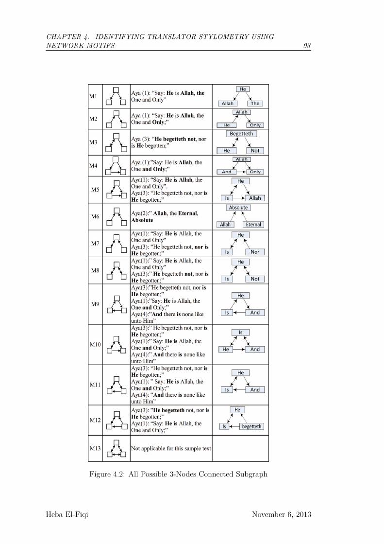
CHAPTER 4. IDENTIFYING TRANSLATOR STYLOMETRY USING
NETWORK MOTIFS 93
Figure 4.2: All Possible 3-Nodes Connected Subgraph
Heba El-Fiqi November 6, 2013
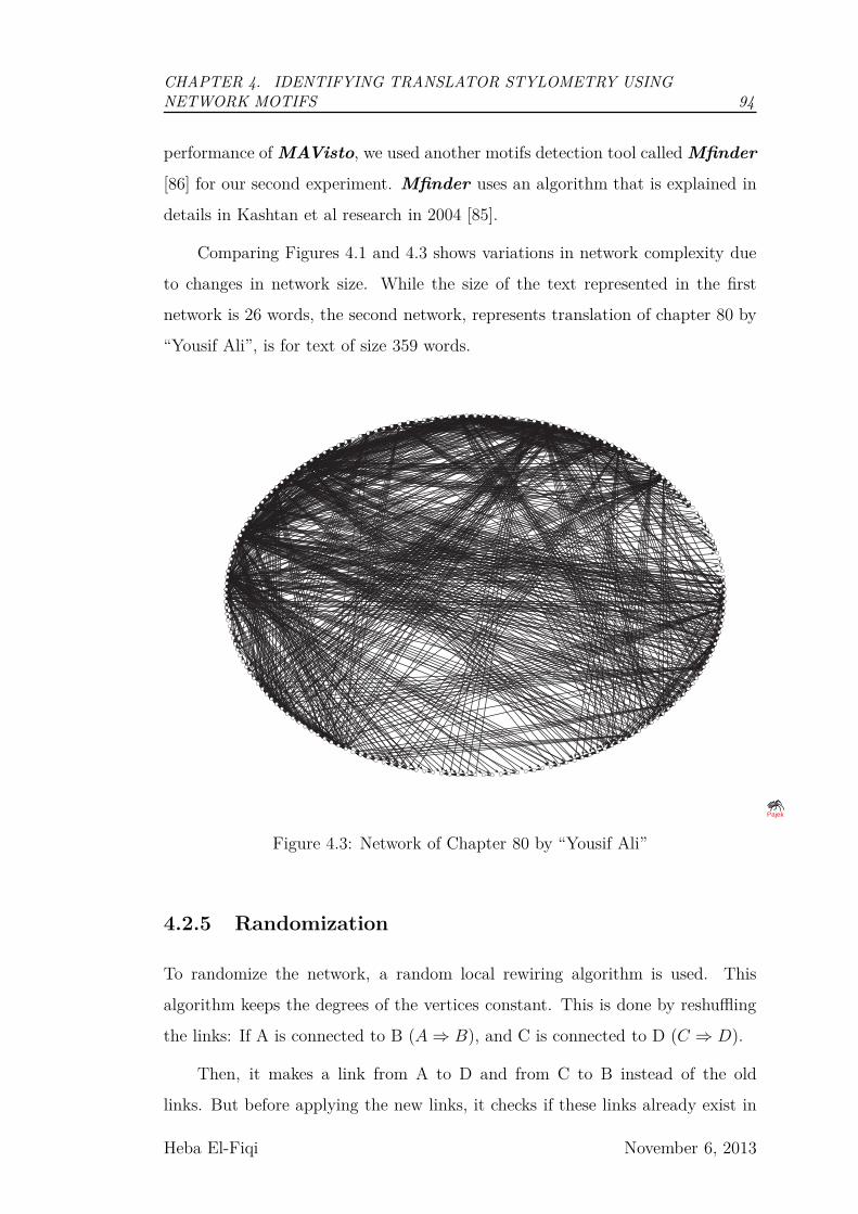
CHAPTER 4. IDENTIFYING TRANSLATOR STYLOMETRY USING
NETWORK MOTIFS 94
performance of MAVisto, we used another motifs detection tool called Mfinder
[86] for our second experiment. Mfinder uses an algorithm that is explained in
details in Kashtan et al research in 2004 [85].
Comparing Figures 4.1 and 4.3 shows variations in network complexity due
to changes in network size. While the size of the text represented in the first
network is 26 words, the second network, represents translation of chapter 80 by
“Yousif Ali”, is for text of size 359 words.
Pajek
Figure 4.3: Network of Chapter 80 by “Yousif Ali”
4.2.5 Randomization
To randomize the network, a random local rewiring algorithm is used. This
algorithm keeps the degrees of the vertices constant. This is done by reshuffling
the links: If A is connected to B (A⇒ B), and C is connected to D (C ⇒ D).
Then, it makes a link from A to D and from C to B instead of the old
links. But before applying the new links, it checks if these links already exist in
Heba El-Fiqi November 6, 2013

CHAPTER 4. IDENTIFYING TRANSLATOR STYLOMETRY USING
NETWORK MOTIFS 95
the network. If so, this process is skipped and the algorithm attempts to find
other links. This check is necessary to prevent having multiple links connecting
the same vertices [111]. This process is repeated several times in excess of the
total number of edges in the system to generate a randomized network [112].
We considered 500 randomized networks for each sample when conducting our
experiments.
4.2.6 Significance test
To calculate Z-score, we need to calculate the average and standard deviation of
occurrences of a motif in all randomized networks. The z-score is calculated as
the difference between the frequency of this motif in the target network and the
mean frequency of the generated randomized networks divided by the standard
deviation of the frequency values for these randomized networks.
Since we are testing for confidence level %95, the z normal range is from
-1.96 to +1.96. If the z-score is outside this range, it is significant.
4.2.7 Global Network Features
Among the different global network features, we choose the nine most common
ones to be the classification attributes: Average of degree, density, clustering
coefficient, transitivity, modularity, betweenness, characteristic path length, and
diameter. All of these measures were evaluated using brain connectivity toolbox
[150]. Their definitions are described in section 2.3.4.1 in the background chapter.
4.3 Classifiers
In order to evaluate frequency of network motifs as stylometry features using
existing classification algorithms, we are going to apply a number of well known
classifiers. The reason of starting with this number of classifiers is to overcome
Heba El-Fiqi November 6, 2013

CHAPTER 4. IDENTIFYING TRANSLATOR STYLOMETRY USING
NETWORK MOTIFS 96
possible limitations of individual classifiers that may mislead our investigations.
These classifiers are:
1. FT: Functional Tree (FT) is a classifier that was introduced by João in 2004
[53]. This classifier uses decision tests based on a combination of attributes.
FT is used with its default parameters using WEKA where the minimum
number of instances at which a node is considered for splitting is set to 15,
and the number of fixed LogitBoost iterations is set to 15 with no weight
trimming.
2. NBTree: This decision tree uses Naive Bayes classifiers at the leaves. This
hyperid classifier is firstly presented by Kohavi in 1996 [93].
3. Random Forest: This classifier generates a random number of decision
trees that represent a forest to be used for classification [24]. We used this
classifier with no constraints on the maximum depth of the trees and the
number of attributes to be used, while the number of trees in limited to 10.
4. Random Tree: While constructing decision trees, a random number of
attributes is chosen at each node to introduce a Random Tree classifier. We
used the defaults parameters for this classifier which includes no backfitting
or pruning.
5. FURIA: Fuzzy Unordered Rule Induction algorithm (FURIA) is an ex-
tension to the well-known RIPPER algorithm [36] but using fuzzy rather
than conventional rules. This algorithm is introduced in 2009 by Hühn
and demonstrated promising results in some types of classification prob-
lems [64, 76]. The parameters for applying this algorithm includes setting
the minimum total weight of the instances in a rule to two, with two runs
of an optimization procedure, and to use check for error rate that ≥ 0.5 for
the stopping criterion.
6. FLR: Fuzzy Lattice Reasoning Classifier (FLR) is initially introduced by
Athanasiadis in 2003 [17]. This classifier uses the Fuzzy Lattices to create
Heba El-Fiqi November 6, 2013
CHAPTER 4. IDENTIFYING TRANSLATOR STYLOMETRY USING
NETWORK MOTIFS 97
a Reasoning Environment. The rules are induced in a mathematical lattice
data domain. FLR has the advantage that it can be incremental. It is also
able to deal with missing data [80]. The vigilance parameter value is set to
0.5 while running our experiments.
7. Logistic Classifier: This classifier uses a multinomial logistic regression
model with a ridge estimator. This classifier is based on le Cessie and
Houwelingen model [34].
4.4 Experiment I
The purpose of this preliminary experiment is to explore the feasibility of using
network motifs as a stylometric feature. For that reason, we choose to start with
the last 30 chapters from the 74 chapters that we have in our dataset. Another
reason for choosing these chapters is that they are also the smallest chapters;
thus, the pilot study can identify efficiency of the methods on a limited corpus.
We also limited the number of classes into two classes. Therefore, we choose
two parallel translations in addition to their original texts: the first one is by
Muhammad Marmaduke Pickthall and the second one is by Abdullah Yusuf Ali.
These two translations are among the few translations that have been assessed by
Khaleel Mohammed in 2005 [124] as being among the most accurate translations.
First: to address the normalization problem, we conduct 5 different tests
considering the parameters as in Table 4.1: In the first test, we consider abso-
lute values: The attributes of motifs represent f(xi) and f(yi). So, we have 13
attributes representing the 13 motifs and one attribute representing class label
for 40 samples for training and 20 samples for testing considering class balance.
The second test, using the same configuration of the first test but we tried to
minimise the translator bias to her own writing; thus, we used the attributes of
motifs to represent f(xi)/∑
(f(xi)) for the first translator, and f(yi)/∑
(f(yi))
for the second translator. In the third test: The attributes of motifs represent
f(xi)/f(zi) and f(yi)/f(zi). The conjecture behind this is to minimise the bias
Heba El-Fiqi November 6, 2013

CHAPTER 4. IDENTIFYING TRANSLATOR STYLOMETRY USING
NETWORK MOTIFS 98
regarding the original text. While in the fourth test; we used the attributes of
motifs to represent f(x)/(∑
((f(xi) ∗ f(zi)) as a conjecture for minimising both
the original text bias and translator bias. For tests 3 and 4, we need to divide
by the frequency of Arabic motifs, which is sometimes zero, so we increment the
number of motifs for Arabic text by 1. In the fifth test, we used 16 attributes
which are the 13 motifs in addition to the number of nodes and edges and one
attribute for class label. These five test are collected into one experiment, which
we will denoted by Experiment I(a).
Table 4.1: Experiment I Parameters
f(xi) is the frequency of each motif in a sample i for the first translator.∑
f(xi) is the summation of all frequencies of motifs in a sample i for the firsttranslator.
f(yi) is the frequency of each motif in a sample i for the second translator.∑
f(yi) is the summation of all frequencies of motifs in a sample i for the secondtranslator.
f(zi) is the frequency of each motif in a sample i for the original Arabic text.
Second: to address the sample size problem, we repeated the previous exper-
iments with 10 sample chapters for each translator for training and 10 samples for
testing, and compared these results to their corresponding results from the Ex-
periment I(a). The comparison is between an experiment with 10 samples as the
training size and the other with 20 samples for the training size. In both cases,
we maintained the test sample constant to have a fair comparison. The test size
is 10 sample chapters, forming a total of 20 chapters covering both translators.
We will denote this second experiment as Experiment I(b).
The third question was about class balance. To address such question we
conducted Experiment I(c), in which we repeated the first experiment but con-
sidered randomizing the choice of the classes for training and testing purposes,
and compared the results to the balanced experiment. Since we have 30 samples
which introduce 60 (30x2) instances, and we are considering an imbalance prob-
lem, we choose randomly 40 out of the 60 instances for training and the rest are
used for testing.
Heba El-Fiqi November 6, 2013
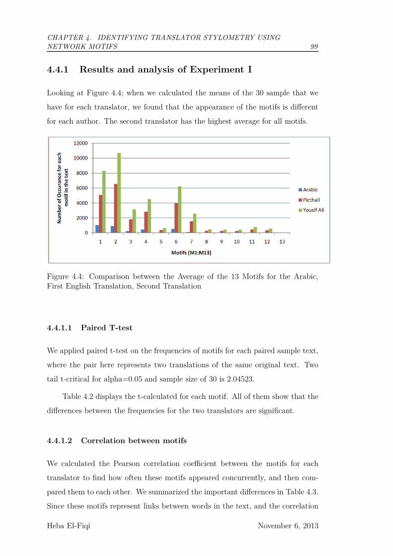
CHAPTER 4. IDENTIFYING TRANSLATOR STYLOMETRY USING
NETWORK MOTIFS 99
4.4.1 Results and analysis of Experiment I
Looking at Figure 4.4; when we calculated the means of the 30 sample that we
have for each translator, we found that the appearance of the motifs is different
for each author. The second translator has the highest average for all motifs.
Figure 4.4: Comparison between the Average of the 13 Motifs for the Arabic,First English Translation, Second Translation
4.4.1.1 Paired T-test
We applied paired t-test on the frequencies of motifs for each paired sample text,
where the pair here represents two translations of the same original text. Two
tail t-critical for alpha=0.05 and sample size of 30 is 2.04523.
Table 4.2 displays the t-calculated for each motif. All of them show that the
differences between the frequencies for the two translators are significant.
4.4.1.2 Correlation between motifs
We calculated the Pearson correlation coefficient between the motifs for each
translator to find how often these motifs appeared concurrently, and then com-
pared them to each other. We summarized the important differences in Table 4.3.
Since these motifs represent links between words in the text, and the correlation
Heba El-Fiqi November 6, 2013
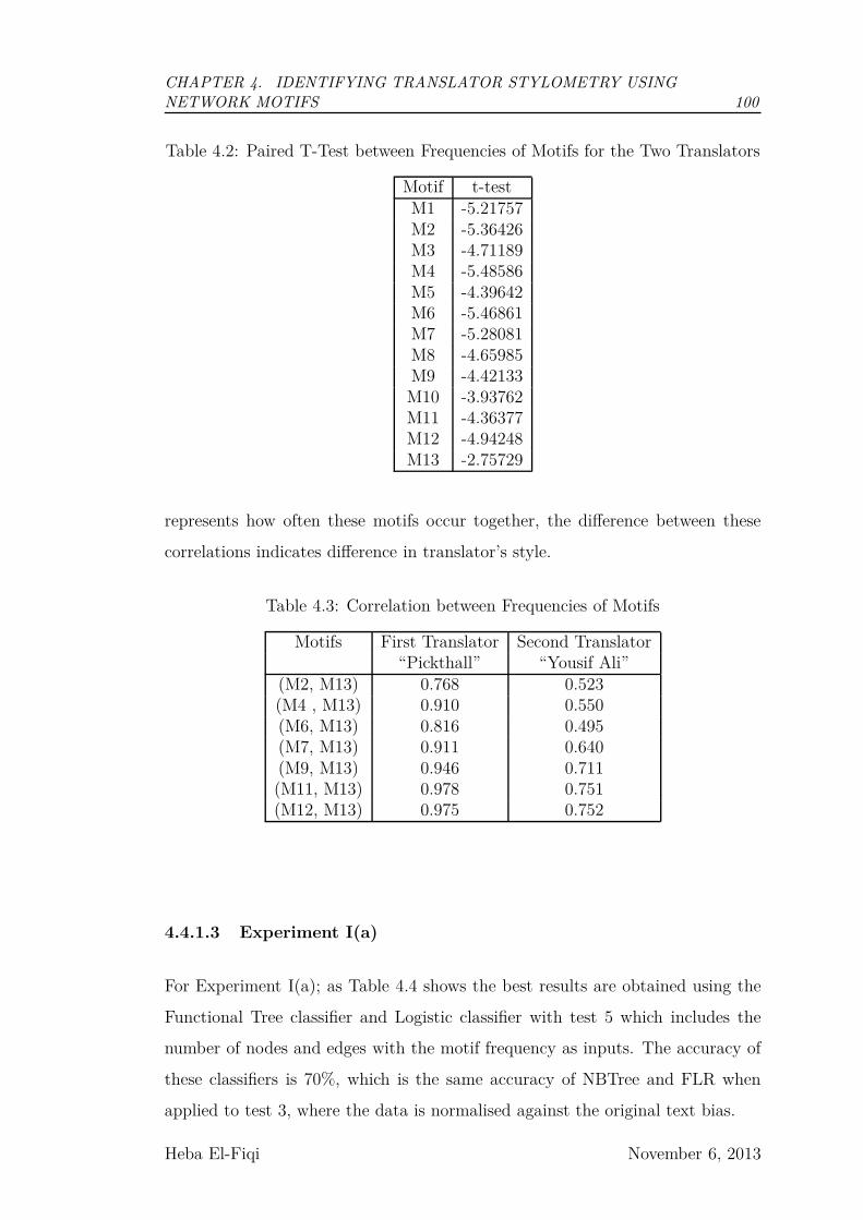
CHAPTER 4. IDENTIFYING TRANSLATOR STYLOMETRY USING
NETWORK MOTIFS 100
Table 4.2: Paired T-Test between Frequencies of Motifs for the Two Translators
Motif t-testM1 -5.21757M2 -5.36426M3 -4.71189M4 -5.48586M5 -4.39642M6 -5.46861M7 -5.28081M8 -4.65985M9 -4.42133M10 -3.93762M11 -4.36377M12 -4.94248M13 -2.75729
represents how often these motifs occur together, the difference between these
correlations indicates difference in translator’s style.
Table 4.3: Correlation between Frequencies of Motifs
Motifs First Translator Second Translator“Pickthall” “Yousif Ali”
(M2, M13) 0.768 0.523(M4 , M13) 0.910 0.550(M6, M13) 0.816 0.495(M7, M13) 0.911 0.640(M9, M13) 0.946 0.711(M11, M13) 0.978 0.751(M12, M13) 0.975 0.752
4.4.1.3 Experiment I(a)
For Experiment I(a); as Table 4.4 shows the best results are obtained using the
Functional Tree classifier and Logistic classifier with test 5 which includes the
number of nodes and edges with the motif frequency as inputs. The accuracy of
these classifiers is 70%, which is the same accuracy of NBTree and FLR when
applied to test 3, where the data is normalised against the original text bias.
Heba El-Fiqi November 6, 2013
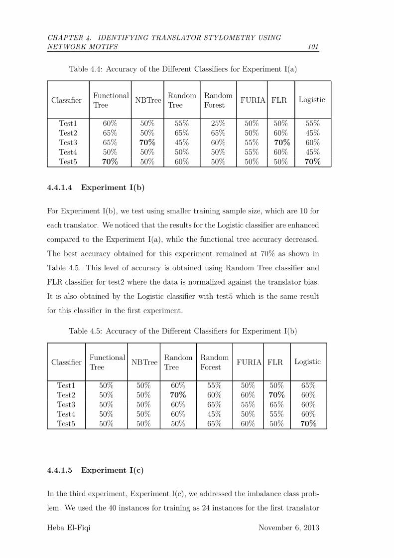
CHAPTER 4. IDENTIFYING TRANSLATOR STYLOMETRY USING
NETWORK MOTIFS 101
Table 4.4: Accuracy of the Different Classifiers for Experiment I(a)
ClassifierFunctionalTree
NBTreeRandomTree
RandomForest
FURIA FLR Logistic
Test1 60% 50% 55% 25% 50% 50% 55%Test2 65% 50% 65% 65% 50% 60% 45%Test3 65% 70% 45% 60% 55% 70% 60%Test4 50% 50% 50% 50% 55% 60% 45%Test5 70% 50% 60% 50% 50% 50% 70%
4.4.1.4 Experiment I(b)
For Experiment I(b), we test using smaller training sample size, which are 10 for
each translator. We noticed that the results for the Logistic classifier are enhanced
compared to the Experiment I(a), while the functional tree accuracy decreased.
The best accuracy obtained for this experiment remained at 70% as shown in
Table 4.5. This level of accuracy is obtained using Random Tree classifier and
FLR classifier for test2 where the data is normalized against the translator bias.
It is also obtained by the Logistic classifier with test5 which is the same result
for this classifier in the first experiment.
Table 4.5: Accuracy of the Different Classifiers for Experiment I(b)
ClassifierFunctionalTree
NBTreeRandomTree
RandomForest
FURIA FLR Logistic
Test1 50% 50% 60% 55% 50% 50% 65%Test2 50% 50% 70% 60% 60% 70% 60%Test3 50% 50% 60% 65% 55% 65% 60%Test4 50% 50% 60% 45% 50% 55% 60%Test5 50% 50% 50% 65% 60% 50% 70%
4.4.1.5 Experiment I(c)
In the third experiment, Experiment I(c), we addressed the imbalance class prob-
lem. We used the 40 instances for training as 24 instances for the first translator
Heba El-Fiqi November 6, 2013
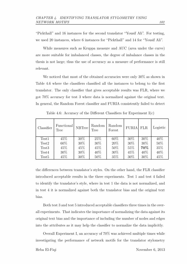
CHAPTER 4. IDENTIFYING TRANSLATOR STYLOMETRY USING
NETWORK MOTIFS 102
“Pickthall” and 16 instances for the second translator “Yousif Ali”. For testing,
we used 20 instances, where 6 instances for “Pickthall” and 14 for “Yousif Ali”.
While measures such as Kruppa measure and AUC (area under the curve)
are more suitable for imbalanced classes, the degree of imbalance classes in the
thesis is not large; thus the use of accuracy as a measure of performance is still
relevant.
We noticed that most of the obtained accuracies were only 30% as shown in
Table 4.6 where the classifiers classified all the instances to belong to the first
translator. The only classifier that gives acceptable results was FLR, where we
got 70% accuracy for test 3 where data is normalized against the original text.
In general, the Random Forest classifier and FURIA consistently failed to detect
Table 4.6: Accuracy of the Different Classifiers for Experiment I(c)
ClassifierFunctionalTree
NBTreeRandomTree
RandomForest
FURIA FLR Logistic
Test1 45% 30% 25% 60% 30% 30% 40%Test2 60% 30% 30% 20% 30% 30% 50%Test3 45% 45% 45% 50% 55% 70% 35%Test4 30% 30% 40% 30% 45% 40% 40%Test5 45% 30% 50% 35% 30% 30% 45%
the differences between translator’s styles. On the other hand, the FLR classifier
introduced acceptable results in the three experiments. Test 1 and test 4 failed
to identify the translator’s style, where in test 1 the data is not normalized, and
in test 4 it is normalized against both the translator bias and the original text
bias.
Both test 3 and test 5 introduced acceptable classifiers three times in the over-
all experiments. That indicates the importance of normalizing the data against its
original text bias and the importance of including the number of nodes and edges
into the attributes as it may help the classifier to normalize the data implicitly.
Overall Experiment I, an accuracy of 70% was achieved multiple times while
investigating the performance of network motifs for the translator stylometry
Heba El-Fiqi November 6, 2013
CHAPTER 4. IDENTIFYING TRANSLATOR STYLOMETRY USING
NETWORK MOTIFS 103
identification problem. Among the seven classifiers that have been used, Fuzzy
Lattice Reasoning Classifier (FLR) had the best performance. Additionally, nor-
malizing the translated text against its original source outperformed the other
normalization methods that were investigated in this experiment.
4.5 Experiment II
In this experiment, we are going to use the entire dataset to expand our inves-
tigation. We are going also to evaluate the global network features in addition
to the local network features which are represented by the motifs. Furthermore,
for the motifs search, we are going to consider motifs of size four in addition to
motifs of size three that we considered in the previous experiment.
In this experiment, we have three groups of features: the first one is 13
attributes which are all possible network motifs of size three, the second group is
199 attributes which are all the possible network motifs of size four, and the third
group is nine attributes, which are the selected global network features that we
used. All of these three groups of features were used as attributes for the same
classifiers that we used in Experiment I in addition to C4.5 and SVM, which
we discussed earlier in Chapter 3. We feed these classifiers with 74 instances,
chapters, for each of the seven translators. We used ten folds cross-validation for
evaluation.
4.5.1 Results and Discussion of Experiment II
When we ran the experiment, we expected network motifs to introduce good
results. This expectation was based on the findings of Experiment I, where we
attempted to classify two translators using network motifs of size three. However,
here we are attempting to use seven translators. The results were beyond our
expectation. Both Network motifs and network global features failed to identify
translator stylometry as shown in Tables 4.7, 4.8, and 4.9. For global features,
Table 4.7 shows that the best average accuracy obtained was by FT classifier.
Heba El-Fiqi November 6, 2013

CHAPTER 4. IDENTIFYING TRANSLATOR STYLOMETRY USING
NETWORK MOTIFS 104
That was 52.57%, which means that global features can not be used to identify
translators stylometry. Although network motifs of size three showed promising
results in the previous experiment, it failed in this experiment to identify trans-
lator stylometry. The best average accuracy we obtained was also 52.06% using
Logistic classifier as shown in Table 4.8. Furthermore, Motifs of size four pro-
duced similar results, with maximum average accuracy of 52.43% obtained using
Logistic classifier. The detailed results of using motifs of size four as stylometry
features are displayed in Table 4.9.
We tried to identify repeated patterns, that is lexical chunks which are re-
peated by one translator more often than others. Network motifs are also used to
detect subgraphs that happen more frequently in a network than in random net-
works. Therefore theoretically, network motifs should work to identify different
translators.
We found that as the size of the network varied in a wide range between
instances and between each other, and the number of the subgraphs may vary
widely as well. In our dataset, the network sizes varied from 19 nodes (as in
Pickthall:Chapter109, Sarwar:Chapter112, Yousif Ali:Chapter112) to 597 (as in
Asad: Chapter42), and the number of edges varied from 64 ( as in Sarwar: Chap-
ter112) to 29851 (as in Asad:Chapter42). As the number of subgraphs is highly
affected by the network size, using the values of motifs count directly mislead the
classifiers. The classifiers failed to detect a relation such as M3(A1) >M3(A7);
which means translator A1 uses the pattern of motif id3 more than translator
A7 does. On the other hand, a decision tree classifier can identify the relation
of M3(A1)>100. Since we were interested in the first type of relation, where we
can identify a translator preferred pattern, we needed to find a way to solve this
problem.
Heba El-Fiqi November 6, 2013
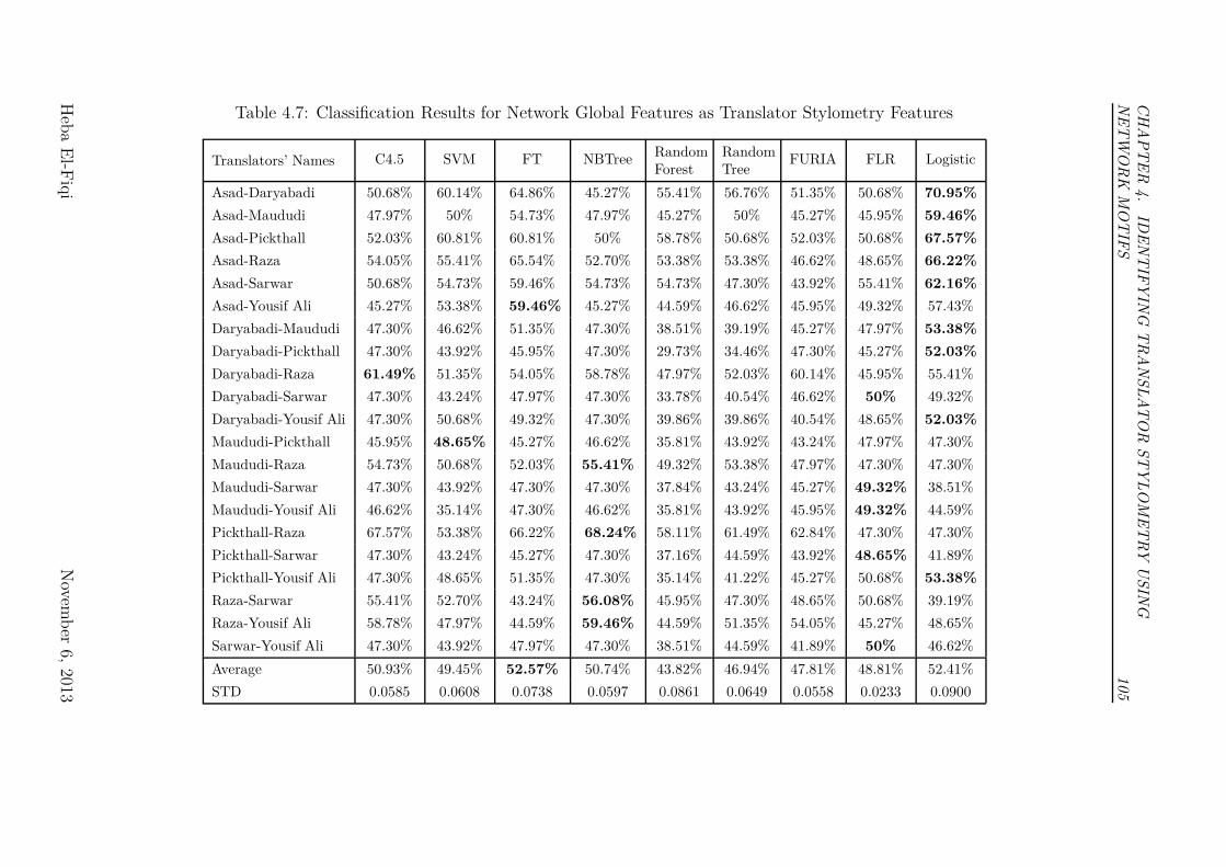
CH
AP
TE
R4.
IDE
NT
IFY
ING
TR
AN
SL
AT
OR
ST
YL
OM
ET
RY
US
ING
NE
TW
OR
KM
OT
IFS
105
Table 4.7: Classification Results for Network Global Features as Translator Stylometry Features
Translators’ Names C4.5 SVM FT NBTreeRandomForest
RandomTree
FURIA FLR Logistic
Asad-Daryabadi 50.68% 60.14% 64.86% 45.27% 55.41% 56.76% 51.35% 50.68% 70.95%
Asad-Maududi 47.97% 50% 54.73% 47.97% 45.27% 50% 45.27% 45.95% 59.46%
Asad-Pickthall 52.03% 60.81% 60.81% 50% 58.78% 50.68% 52.03% 50.68% 67.57%
Asad-Raza 54.05% 55.41% 65.54% 52.70% 53.38% 53.38% 46.62% 48.65% 66.22%
Asad-Sarwar 50.68% 54.73% 59.46% 54.73% 54.73% 47.30% 43.92% 55.41% 62.16%
Asad-Yousif Ali 45.27% 53.38% 59.46% 45.27% 44.59% 46.62% 45.95% 49.32% 57.43%
Daryabadi-Maududi 47.30% 46.62% 51.35% 47.30% 38.51% 39.19% 45.27% 47.97% 53.38%
Daryabadi-Pickthall 47.30% 43.92% 45.95% 47.30% 29.73% 34.46% 47.30% 45.27% 52.03%
Daryabadi-Raza 61.49% 51.35% 54.05% 58.78% 47.97% 52.03% 60.14% 45.95% 55.41%
Daryabadi-Sarwar 47.30% 43.24% 47.97% 47.30% 33.78% 40.54% 46.62% 50% 49.32%
Daryabadi-Yousif Ali 47.30% 50.68% 49.32% 47.30% 39.86% 39.86% 40.54% 48.65% 52.03%
Maududi-Pickthall 45.95% 48.65% 45.27% 46.62% 35.81% 43.92% 43.24% 47.97% 47.30%
Maududi-Raza 54.73% 50.68% 52.03% 55.41% 49.32% 53.38% 47.97% 47.30% 47.30%
Maududi-Sarwar 47.30% 43.92% 47.30% 47.30% 37.84% 43.24% 45.27% 49.32% 38.51%
Maududi-Yousif Ali 46.62% 35.14% 47.30% 46.62% 35.81% 43.92% 45.95% 49.32% 44.59%
Pickthall-Raza 67.57% 53.38% 66.22% 68.24% 58.11% 61.49% 62.84% 47.30% 47.30%
Pickthall-Sarwar 47.30% 43.24% 45.27% 47.30% 37.16% 44.59% 43.92% 48.65% 41.89%
Pickthall-Yousif Ali 47.30% 48.65% 51.35% 47.30% 35.14% 41.22% 45.27% 50.68% 53.38%
Raza-Sarwar 55.41% 52.70% 43.24% 56.08% 45.95% 47.30% 48.65% 50.68% 39.19%
Raza-Yousif Ali 58.78% 47.97% 44.59% 59.46% 44.59% 51.35% 54.05% 45.27% 48.65%
Sarwar-Yousif Ali 47.30% 43.92% 47.97% 47.30% 38.51% 44.59% 41.89% 50% 46.62%
Average 50.93% 49.45% 52.57% 50.74% 43.82% 46.94% 47.81% 48.81% 52.41%
STD 0.0585 0.0608 0.0738 0.0597 0.0861 0.0649 0.0558 0.0233 0.0900
Heb
aE
l-Fiq
iN
ovemb
er6,
2013
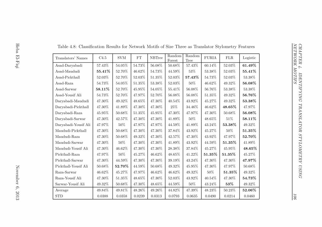
CH
AP
TE
R4.
IDE
NT
IFY
ING
TR
AN
SL
AT
OR
ST
YL
OM
ET
RY
US
ING
NE
TW
OR
KM
OT
IFS
106
Table 4.8: Classification Results for Network Motifs of Size Three as Translator Stylometry Features
Translators’ Names C4.5 SVM FT NBTreeRandomForest
RandomTree
FURIA FLR Logistic
Asad-Daryabadi 57.43% 54.05% 54.73% 56.08% 50.68% 57.43% 60.14% 52.03% 61.49%
Asad-Maududi 55.41% 52.70% 46.62% 54.73% 44.59% 53% 53.38% 52.03% 55.41%
Asad-Pickthall 52.03% 52.70% 52.03% 51.35% 52.03% 57.43% 54.73% 52.03% 53.38%
Asad-Raza 54.73% 54.05% 51.35% 53.38% 52.03% 50% 46.62% 49.32% 56.08%
Asad-Sarwar 58.11% 52.70% 45.95% 54.05% 55.41% 56.08% 56.76% 53.38% 53.38%
Asad-Yousif Ali 54.73% 52.70% 47.97% 52.70% 56.08% 56.08% 51.35% 49.32% 56.76%
Daryabadi-Maududi 47.30% 49.32% 48.65% 47.30% 40.54% 43.92% 45.27% 49.32% 53.38%
Daryabadi-Pickthall 47.30% 41.89% 47.30% 47.30% 25% 34.46% 46.62% 48.65% 47.97%
Daryabadi-Raza 45.95% 50.68% 51.35% 45.95% 47.30% 47.97% 47.30% 50.68% 56.08%
Daryabadi-Sarwar 47.30% 42.57% 47.30% 47.30% 41.89% 50% 48.65% 51% 58.11%
Daryabadi-Yousif Ali 47.97% 50% 47.97% 47.97% 44.59% 41.89% 43.24% 53.38% 49.32%
Maududi-Pickthall 47.30% 50.68% 47.30% 47.30% 37.84% 43.92% 45.27% 50% 51.35%
Maududi-Raza 47.30% 50.68% 49.32% 47.30% 42.57% 47.30% 43.92% 47.97% 52.70%
Maududi-Sarwar 47.30% 50% 47.30% 47.30% 41.89% 43.92% 44.59% 51.35% 41.89%
Maududi-Yousif Ali 47.30% 46.62% 47.30% 47.30% 28.38% 37.84% 45.27% 45.95% 48.65%
Pickthall-Raza 47.97% 50% 45.27% 46.62% 48.65% 41.22% 51.35% 51.35% 45.27%
Pickthall-Sarwar 47.30% 44.59% 47.30% 47.30% 39.19% 43.24% 47.30% 47.30% 47.97%
Pickthall-Yousif Ali 50.68% 52.70% 44.59% 50.68% 49.32% 45.95% 47.30% 47.97% 50.68%
Raza-Sarwar 46.62% 45.27% 47.97% 46.62% 46.62% 49.32% 50% 51.35% 49.32%
Raza-Yousif Ali 47.30% 51.35% 48.65% 47.30% 52.03% 43.92% 40.54% 47.30% 54.73%
Sarwar-Yousif Ali 49.32% 50.68% 47.30% 48.65% 44.59% 50% 43.24% 53% 49.32%
Average 49.84% 49.81% 48.26% 49.26% 44.82% 47.39% 48.23% 50.23% 52.06%
STD 0.0388 0.0358 0.0239 0.0313 0.0793 0.0635 0.0490 0.0214 0.0460
Heb
aE
l-Fiq
iN
ovemb
er6,
2013
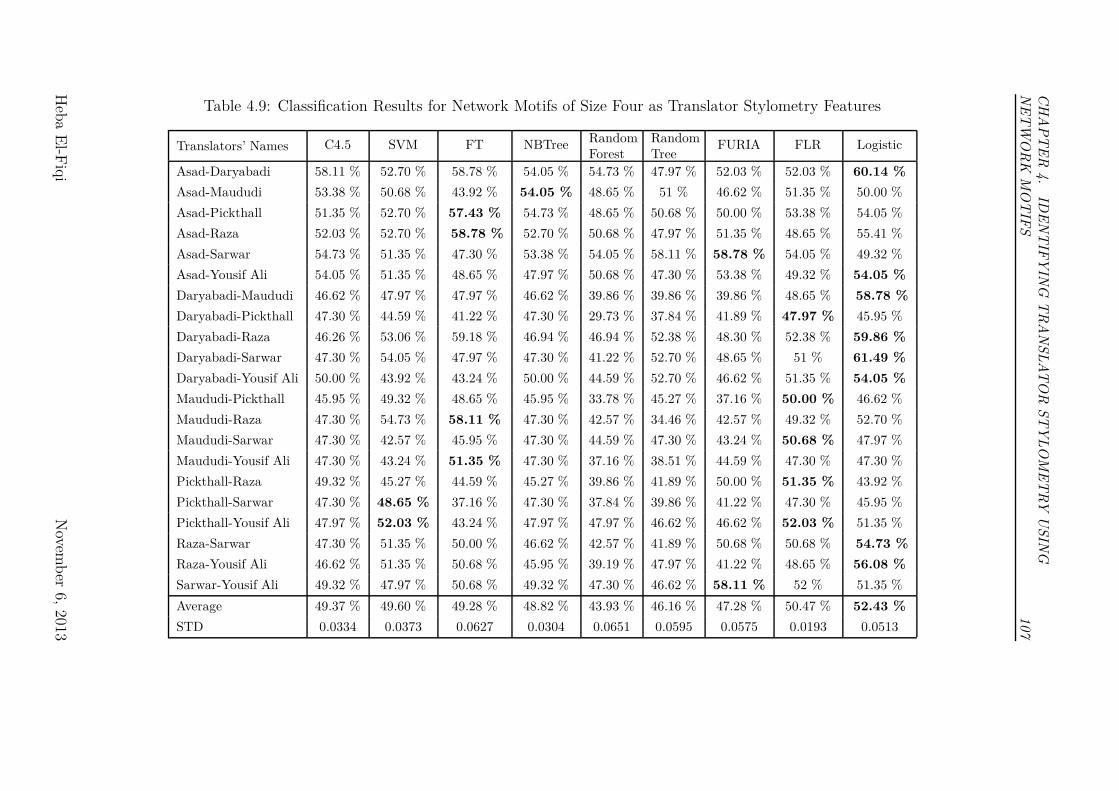
CH
AP
TE
R4.
IDE
NT
IFY
ING
TR
AN
SL
AT
OR
ST
YL
OM
ET
RY
US
ING
NE
TW
OR
KM
OT
IFS
107
Table 4.9: Classification Results for Network Motifs of Size Four as Translator Stylometry Features
Translators’ Names C4.5 SVM FT NBTreeRandomForest
RandomTree
FURIA FLR Logistic
Asad-Daryabadi 58.11 % 52.70 % 58.78 % 54.05 % 54.73 % 47.97 % 52.03 % 52.03 % 60.14 %
Asad-Maududi 53.38 % 50.68 % 43.92 % 54.05 % 48.65 % 51 % 46.62 % 51.35 % 50.00 %
Asad-Pickthall 51.35 % 52.70 % 57.43 % 54.73 % 48.65 % 50.68 % 50.00 % 53.38 % 54.05 %
Asad-Raza 52.03 % 52.70 % 58.78 % 52.70 % 50.68 % 47.97 % 51.35 % 48.65 % 55.41 %
Asad-Sarwar 54.73 % 51.35 % 47.30 % 53.38 % 54.05 % 58.11 % 58.78 % 54.05 % 49.32 %
Asad-Yousif Ali 54.05 % 51.35 % 48.65 % 47.97 % 50.68 % 47.30 % 53.38 % 49.32 % 54.05 %
Daryabadi-Maududi 46.62 % 47.97 % 47.97 % 46.62 % 39.86 % 39.86 % 39.86 % 48.65 % 58.78 %
Daryabadi-Pickthall 47.30 % 44.59 % 41.22 % 47.30 % 29.73 % 37.84 % 41.89 % 47.97 % 45.95 %
Daryabadi-Raza 46.26 % 53.06 % 59.18 % 46.94 % 46.94 % 52.38 % 48.30 % 52.38 % 59.86 %
Daryabadi-Sarwar 47.30 % 54.05 % 47.97 % 47.30 % 41.22 % 52.70 % 48.65 % 51 % 61.49 %
Daryabadi-Yousif Ali 50.00 % 43.92 % 43.24 % 50.00 % 44.59 % 52.70 % 46.62 % 51.35 % 54.05 %
Maududi-Pickthall 45.95 % 49.32 % 48.65 % 45.95 % 33.78 % 45.27 % 37.16 % 50.00 % 46.62 %
Maududi-Raza 47.30 % 54.73 % 58.11 % 47.30 % 42.57 % 34.46 % 42.57 % 49.32 % 52.70 %
Maududi-Sarwar 47.30 % 42.57 % 45.95 % 47.30 % 44.59 % 47.30 % 43.24 % 50.68 % 47.97 %
Maududi-Yousif Ali 47.30 % 43.24 % 51.35 % 47.30 % 37.16 % 38.51 % 44.59 % 47.30 % 47.30 %
Pickthall-Raza 49.32 % 45.27 % 44.59 % 45.27 % 39.86 % 41.89 % 50.00 % 51.35 % 43.92 %
Pickthall-Sarwar 47.30 % 48.65 % 37.16 % 47.30 % 37.84 % 39.86 % 41.22 % 47.30 % 45.95 %
Pickthall-Yousif Ali 47.97 % 52.03 % 43.24 % 47.97 % 47.97 % 46.62 % 46.62 % 52.03 % 51.35 %
Raza-Sarwar 47.30 % 51.35 % 50.00 % 46.62 % 42.57 % 41.89 % 50.68 % 50.68 % 54.73 %
Raza-Yousif Ali 46.62 % 51.35 % 50.68 % 45.95 % 39.19 % 47.97 % 41.22 % 48.65 % 56.08 %
Sarwar-Yousif Ali 49.32 % 47.97 % 50.68 % 49.32 % 47.30 % 46.62 % 58.11 % 52 % 51.35 %
Average 49.37 % 49.60 % 49.28 % 48.82 % 43.93 % 46.16 % 47.28 % 50.47 % 52.43 %
STD 0.0334 0.0373 0.0627 0.0304 0.0651 0.0595 0.0575 0.0193 0.0513
Heb
aE
l-Fiq
iN
ovemb
er6,
2013

CHAPTER 4. IDENTIFYING TRANSLATOR STYLOMETRY USING
NETWORK MOTIFS 108
4.6 Different Representations of Network Mo-
tifs for Detecting Translator Stylometry
The finding from the previous experiment triggered the need for another way of
representing the data before using classification. The previous representation was
considered as univariate approach where the decision was based on single variable
as seen in the example M3(A1)>100, but we needed a multivariate approach that
can identify two variables as in M3(A1) >M3(A7), which can be expressed as
M3(A1) - M3(A7)>0. This is not a traditional multivariate classifier since the
comparison is not between different attributes, but the same attribute for different
translators.
In this section, we are introducing another representation of the data in a
way that simplified this multivariate approach to single values, which can be used
by the classifiers.
4.6.1 Method III
To express the discussed relationship, we grouped the translated text based on
their original sources; the seven translations of chapter 41 are grouped in the first
group, the seven translations of chapter 42 are grouped in the second group, and
so on. Then, within each group, we compared motif id “1” for all translators, and
replaced the frequency with rank of the translator. For example, if for a piece
of text M3 if 10 for Author A1, 20 for Author A2, 30 for Author A3, we replace
these frequencies with “3” for Author A1, “2” for Author A2 and “1” for Author
A3. Here “1” for Author A3 means that Author A3 ranks on M3 for this piece of
text is the highest.
4.6.2 Experiment III
We applied the proposed method for both motifs size three and motifs size four.
We also used the same classification algorithms and dataset as in the previous
Heba El-Fiqi November 6, 2013
CHAPTER 4. IDENTIFYING TRANSLATOR STYLOMETRY USING
NETWORK MOTIFS 109
experiment. We evaluated the attributes in five groups. The first group contains
13 attributes (all the possible 13 motifs of size three). The second group contains
15 attributes, which are the same as the first group in addition to the number of
nodes and edges for each instance. The third group contains 199 attributes (all the
possible 199 motifs of size four). The fourth group contains 201 attributes which
are the 199 attributes of the third group in addition to the number of nodes and
edges. The fifth group contains 214 attributes which are all the possible motifs
of size three and size four in addition to the number of nodes and edges.
4.6.3 Results and Discussion of Experiment III
The average of the classifiers that was built using the five group of attributes in-
troduced acceptable results as shown in 4.10. They ranged from 75% to 79.02%.
Moreover, some of the individual classifiers performed very well up to 97.97%
accuracy as in the case of translators (Asad-Daryabadi) and (Asad-Pickthall).
On the other hand, some pairs of translators couldn’t be distinguished from one
another. The five groups of attributes failed to differentiate between them. This
case happened with three pairs of translators ( Daryabadi-Pickthall), (Maududi-
Yousif Ali), and (Maududi-Sarwar). Generally, SVM classification algorithm out-
performed C4.5 decision tree. Comparing the five groups of attributes to each
other, we found that the best accuracy was achieved by the fifth group (all the
motifs of size three and four and the number of nodes and edges) using SVM clas-
sifier. However, this accuracy was not much higher than in all the other features
groups in the case of SVM. In the best cases, 16 out of the 21 translator pairs
introduced acceptable classifiers using the same group of features.
Such accuracy of 79% is enough to say that translators do have styles on
their own. These styles, which are the results of individual behaviour, can be
used to identify them. In this way, we were able to answer our first question on
the existence of translators’ styles. Our results provided evidence that translators
can be identified through individual styles. This research also discussed possible
features that can be used to distinguish translator stylometry. The use of network
motifs in this research can be seen as capturing patterns on the lexical level while
Heba El-Fiqi November 6, 2013
CHAPTER 4. IDENTIFYING TRANSLATOR STYLOMETRY USING
NETWORK MOTIFS 110
been affected slightly by syntactic level. That may direct the research in trans-
lator stylometry to investigate more features on the lexical and syntactic level.
Finally, this accuracy suggests that network motifs can be used for identifying
translator stylometry.
4.7 Chapter Summary
Studying “Translator Stylometry” is a non-trivial task. While there has been
research in linguistics and social sciences discussing the characteristics of each
translator, this line of research is limited in computational linguistics. Contrary
to previous findings that this problem does not have an automatic solution, this
chapter presented a first attempt to counteract this belief. We demonstrated that
translators cannot disappear under the skin of the original authors; they have
their own identities. Different translators represent the same idea in different
ways. Although some existing authorship attributions could not capture these
differences [121, 154], this work shows that we can use social network analysis
to differentiate between translators’ styles. Detecting network motifs shows that
each author is using certain patterns while writing.
In the first experiment, the proposed method introduced a classifier that
can classify translated texts into their translators with accuracy of 70%. Fuzzy
Lattice Reasoning Classifier (FLR) introduces the best results among seven tested
classifiers. Normalising the data against its original text and the network size
offers promising results. Further analysis is needed to explore this research area.
Although using network motifs as stylometry features failed to identify trans-
lators in the second Experiment, representing the data using ranking to express
the relationship between different usages of the same pattern in comparison to
different translators introduced promising results in the third Experiment. Some
of the generated classifiers achieved accuracy of 97.97%, while the overall average
of accuracy reached 79.02%.
The first contribution of this chapter is in providing further evidence for
Heba El-Fiqi November 6, 2013
CHAPTER 4. IDENTIFYING TRANSLATOR STYLOMETRY USING
NETWORK MOTIFS 111
the existence of translator stylometry using computational linguistics and data
mining. The second contribution is the effectiveness of network motifs in detecting
translator stylometry. Both of these contributions encourage further studies in
translator stylometry identifications. Future research could continue on the use of
network motifs with other linguistic features such as searching for some syntactic
structures in word adjacency networks, or looking for network motifs in networks
formed on the syntactic level.
Heba El-Fiqi November 6, 2013
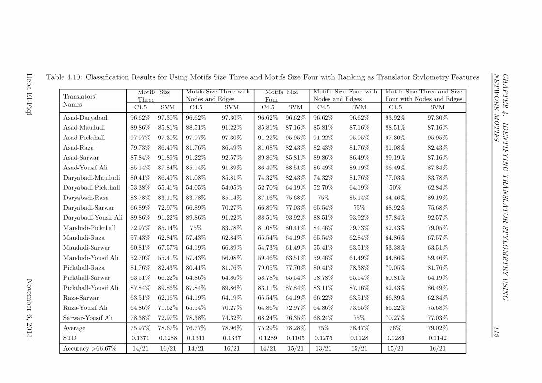
CH
AP
TE
R4.
IDE
NT
IFY
ING
TR
AN
SL
AT
OR
ST
YL
OM
ET
RY
US
ING
NE
TW
OR
KM
OT
IFS
112
Table 4.10: Classification Results for Using Motifs Size Three and Motifs Size Four with Ranking as Translator Stylometry Features
Translators’Names
Motifs SizeThree
Motifs Size Three withNodes and Edges
Motifs SizeFour
Motifs Size Four withNodes and Edges
Motifs Size Three and SizeFour with Nodes and Edges
C4.5 SVM C4.5 SVM C4.5 SVM C4.5 SVM C4.5 SVM
Asad-Daryabadi 96.62% 97.30% 96.62% 97.30% 96.62% 96.62% 96.62% 96.62% 93.92% 97.30%
Asad-Maududi 89.86% 85.81% 88.51% 91.22% 85.81% 87.16% 85.81% 87.16% 88.51% 87.16%
Asad-Pickthall 97.97% 97.30% 97.97% 97.30% 91.22% 95.95% 91.22% 95.95% 97.30% 95.95%
Asad-Raza 79.73% 86.49% 81.76% 86.49% 81.08% 82.43% 82.43% 81.76% 81.08% 82.43%
Asad-Sarwar 87.84% 91.89% 91.22% 92.57% 89.86% 85.81% 89.86% 86.49% 89.19% 87.16%
Asad-Yousif Ali 85.14% 87.84% 85.14% 91.89% 86.49% 88.51% 86.49% 89.19% 86.49% 87.84%
Daryabadi-Maududi 80.41% 86.49% 81.08% 85.81% 74.32% 82.43% 74.32% 81.76% 77.03% 83.78%
Daryabadi-Pickthall 53.38% 55.41% 54.05% 54.05% 52.70% 64.19% 52.70% 64.19% 50% 62.84%
Daryabadi-Raza 83.78% 83.11% 83.78% 85.14% 87.16% 75.68% 75% 85.14% 84.46% 89.19%
Daryabadi-Sarwar 66.89% 72.97% 66.89% 70.27% 66.89% 77.03% 65.54% 75% 68.92% 75.68%
Daryabadi-Yousif Ali 89.86% 91.22% 89.86% 91.22% 88.51% 93.92% 88.51% 93.92% 87.84% 92.57%
Maududi-Pickthall 72.97% 85.14% 75% 83.78% 81.08% 80.41% 84.46% 79.73% 82.43% 79.05%
Maududi-Raza 57.43% 62.84% 57.43% 62.84% 65.54% 64.19% 65.54% 62.84% 64.86% 67.57%
Maududi-Sarwar 60.81% 67.57% 64.19% 66.89% 54.73% 61.49% 55.41% 63.51% 53.38% 63.51%
Maududi-Yousif Ali 52.70% 55.41% 57.43% 56.08% 59.46% 63.51% 59.46% 61.49% 64.86% 59.46%
Pickthall-Raza 81.76% 82.43% 80.41% 81.76% 79.05% 77.70% 80.41% 78.38% 79.05% 81.76%
Pickthall-Sarwar 63.51% 66.22% 64.86% 64.86% 58.78% 65.54% 58.78% 65.54% 60.81% 64.19%
Pickthall-Yousif Ali 87.84% 89.86% 87.84% 89.86% 83.11% 87.84% 83.11% 87.16% 82.43% 86.49%
Raza-Sarwar 63.51% 62.16% 64.19% 64.19% 65.54% 64.19% 66.22% 63.51% 66.89% 62.84%
Raza-Yousif Ali 64.86% 71.62% 65.54% 70.27% 64.86% 72.97% 64.86% 73.65% 66.22% 75.68%
Sarwar-Yousif Ali 78.38% 72.97% 78.38% 74.32% 68.24% 76.35% 68.24% 75% 70.27% 77.03%
Average 75.97% 78.67% 76.77% 78.96% 75.29% 78.28% 75% 78.47% 76% 79.02%
STD 0.1371 0.1288 0.1311 0.1337 0.1289 0.1105 0.1275 0.1128 0.1286 0.1142
Accuracy >66.67% 14/21 16/21 14/21 16/21 14/21 15/21 13/21 15/21 15/21 16/21
Heb
aE
l-Fiq
iN
ovemb
er6,
2013

[This page is intentionally left blank]
Chapter 5
Translator Identification as a
Pair-Wise Comparative
Classification Problem
5.1 Overview
In this chapter, we present a new type of classification problems - we call it
Comparative Classification Problems (CCP), where we use the term data record
to refer to a block of instances. However, we acknowledge that in the wider
literature, there might be a distinction between the two terms “records" and
“instances". Given a single data record with n instances for n classes, the CCP
problem is to map each instance to a unique class. This problem occurs in a wide
range of applications where the independent and identically distribute assumption
is broken down. The interdependency in the data poses challenges if the problem
is handled as a traditional classification problem.
In the Pair-Wise CCP (PWCCP), two different measurements - each belong-
ing to one of the two classes - are grouped together. The classification problem
is to decide given these two measurements, which measurement belongs to which
class. The key difference between PWCCP and traditional binary problems is
that hidden patterns can only be unmasked by comparing the instances as pairs.
CHAPTER 5. TRANSLATOR IDENTIFICATION AS A PAIR-WISE
COMPARATIVE CLASSIFICATION PROBLEM 115
Paired data sets contain repeated measurements of the same attribute. The
changes in the values of the paired instances hold pertinent information to the
data mining process.
In this chapter, We introduce a new algorithm PWC4.5, which is based on
the traditional C4.5 decision tree classifier, to manage PWCCP by dynamically
inducing relationships between paired instances. We evaluated PWC4.5 using
synthetic datasets to understand the performance of the algorithm.
In the next section, we discuss existing classification algorithms, and how
these algorithms take into account the relationship between the attributes while
ignoring the relationship between instances. We use examples to demonstrate
these differences. In section 5.3, PWC4.5 is discussed in details. Experimental
design and results are discussed in section 5.4.
5.2 From Classification to Comparative Classi-
fication
Repeated measurements are observations taken from the same subjects or differ-
ent subjects on the same phenomenon over time or in different circumstances.
Examples of repeated measurements for the same subject in the medical domain
would be weight loss or reaction to a drug over time. Another example may
include some blood test results for the same patient in a progressive disease.
Limited research exists on classification problems for paired data. Brenning
and Lausen [26] and Adler et al. [4] [5] focused on the medical domain. Their
research emphasized the need to use repeated measurements for a subject when
the data is limited. They used different resampling-based methods. Brenning
and Lausen [26] used an ensemble of k decision tree classifiers, while Adler et al.
[4] [5] used k fold cross validation to resample the k number of observations that
are taken from the same subject.
The above literature still treats instances independently despite that the
Heba El-Fiqi November 6, 2013
CHAPTER 5. TRANSLATOR IDENTIFICATION AS A PAIR-WISE
COMPARATIVE CLASSIFICATION PROBLEM 116
underlying measurements may come from the same subject; therefore a level
of dependency is expected. In some applications, as in forensic sciences, the
dependency in the data may be leveraged to improve detection rate. In this study,
we focus on computational linguistics, whereby we may have some linguistics
measurements for a parallel translation of the same text. Such type of “Paired
Data” breaks away from the independent and identically distributed assumption
that lies underneath many classifiers.
Let us now define our problem using this example. We will later on provide
a general formal definition of the problem. Assume chapters o1 . . . om, with m
represents the number of chapters, represent the original text in the Arabic lan-
guage. Let ~v1 . . . ~vm be the corresponding translations, with the cardinality of the
vector ~v, |~v| = n, representing the number of translators for each chapter. Let us
also assume that we know the translators and as such, the order of elements in ~v
follows the orders of translators c1 . . . cn.
Given V m+1 . . . V m+u additional translations, where V is now a set ( i.e. the
elements are unordered), the problem is how to map every element in V to the
corresponding translator ci. This can be seen as ordering V into ~V or simply
having a bijection from V onto the set of translators c1 . . . cn. We will call this
class of problems as CCP and when n = 2, we will call it PWCCP.
In CCP, the data is clearly not independent. While in the above example
each translator independently translated the text, they all translated the same
piece of text. Traditional classification trees and relational learning techniques
are not designed to solve this problem.
Data mining searches for the existence of hidden patterns in the examined
dataset using supervised, unsupervised, or semi-supervised machine learning tech-
niques. Supervised machine learning methods can be used to generate a model
that represents relationship between input attributes (independent variables) and
target attribute (dependent variable). Supervised machine learning methods in-
clude: Classification models in case of a nominal or a categorical target attribute,
and regression models in case of a continuous numeric target attribute. Classi-
Heba El-Fiqi November 6, 2013
CHAPTER 5. TRANSLATOR IDENTIFICATION AS A PAIR-WISE
COMPARATIVE CLASSIFICATION PROBLEM 117
fication has been widely used to assist the decision making processes in various
applications. Among the many classification techniques that exist in the litera-
ture, decision tree algorithms are considered to be the most widely used learning
algorithms in practice [123].
Decision trees are inductive inference algorithms that approximate discrete
valued functions as trees. An algorithm in this class is based on the assumption
that a concept is a disjunction of the conjunctions of attribute-values. It uses
the observed examples to generate rules that can be generalized to unobserved
examples. Decision tree learning normally relies on a heuristic, one-step, non-
backtracking search through the space. The general idea behind the construction
of Decision Trees is to use a divide and conquer strategy that divides a training
dataset into homogeneous subgroups according to attribute based logical tests in
a greedy top-down approach.
Decision trees consist of nodes and branches. Nodes in decision trees are of
two types: either a leaf node which holds class/label value or a decision node that
holds selected attribute for splitting the data into subgroups. The decision value
of this attribute based logical test is represented on the branches that comes from
this decision node. Decision trees are considered as deterministic algorithms as
they use sharp boundaries with no consideration of degree of membership like
other learning algorithms. As the divide and conquer algorithm partitions the
data until every leaf contains cases of a single class, or until further partitioning is
impossible, if there are no conflicting cases, the decision tree will correctly classify
all training cases. This so-called overfitting is generally thought to lead to a loss
of predictive accuracy in most applications [145].
Overfitting can be avoided by a stopping criterion that prevents some sets of
training cases from being subdivided, or by removing some of the structure of the
decision tree after it has been produced; a process known as pruning. Different
pruning strategies are used by decision tree algorithms to overcome overfitting
the training data; adding robustness to the algorithms. This robustness in ad-
dition to the intuitive representation and ease of interpretation of decision trees
attracted many data mining researchers as well as non technical experts to use
Heba El-Fiqi November 6, 2013

CHAPTER 5. TRANSLATOR IDENTIFICATION AS A PAIR-WISE
COMPARATIVE CLASSIFICATION PROBLEM 118
them in a wide areas of applications. Not all of decision tree algorithms have the
ability to handle continuous values. Thus, a discretization process of the contin-
uous attribute is used before applying such algorithm on a classification problem
with continues attribute(s), in which the continuous attribute values is trans-
formed into intervals. Examples of discretization algorithms includes ChiMerge
[90], Entropy-MDLC [47], and Heter-Disc [104].
There are many decision tree algorithms that are well known in the area of
data mining. These include the three algorithms introduced by Quinlan : ID3
(Iterative Dichotomiser 3 ) in 1986 [145], and its successor C4.5 in 1993 [144],
which was improved to produce a better memory efficient commercial system
C5.0. Other decision tree algorithms includes (Chisquare Automatic Interaction
Detection) algorithm known as CHAID developed by Kass in 1980 [87], CART
(Classification And Regression Tree) developed by Breiman et al. in 1984 [25],
LMDT by Brodley and Utgoff in 1995 [27], SPRINT by Shafer et al. in 1996 [161]
, SLIQ by Mehta et al. in 1996 [116], and QUEST (Quick, Unbiased, Efficient,
Statistical Tree) algorithm by Loh and Shih in 1997 [105].
Different splitting selection criteria have been used in decision tree algo-
rithms. Splitting criterion can be characterized either according to their origin
of measure such as information theory, dependence, and distance, or according
to their measure structure such as impurity based criteria, normalized impu-
rity criteria and binary criteria. ID3 algorithm uses an impurity-based crite-
rion called Information gain which is based on the concept of entropy. Another
impurity-based criterion is Gini index, which measures the divergences between
the probability distributions of the target attribute‘s values. The CART algo-
rithm uses Gini index as splitting criterion. An impurity based criterion is biased
towards input attributes with many outcomes. Although this attribute would get
the highest information gain, it may result in poor accuracy when generalized.
Thus, a normalized impurity measure criteria called Gain ratio was introduced
by Quinlan in C4.5 algorithm. Rank Mutual Information (RMI) is a recent split-
Heba El-Fiqi November 6, 2013

CHAPTER 5. TRANSLATOR IDENTIFICATION AS A PAIR-WISE
COMPARATIVE CLASSIFICATION PROBLEM 119
ting criterion that was developed in 2012 by Hu et al. [75]. RMI based decision
trees are designed for special type of classification problems known as Monotonic
classification through merging the robustness of Shannon’s entropy with rough
sets.
5.2.1 Inner vs Outer Classification
Classification algorithms can be categorized into two categories: outer algorithms
and inner algorithms [92]. The first category (outer algorithms) contains algo-
rithms that use a certain function or approach to approximate the boundaries
of each class. Examples of this group of algorithms include neural networks,
decision trees, and classification rules. The second category (inner algorithms)
contains algorithms that have the objective of clustering data into classes groups.
The boundary of each group is defined by a certain measure like a mean or me-
dian. Then, a new instance is classified into the class of the nearest group [92].
K-Nearest Neighbours algorithm is an example of inner classification algorithms.
Figures 5.1 and 5.2 show the differences between outer and inner classification
approaches.
0 20 40 60 80 100
0
20
40
60
80
100
120
V1
V2
c1c2
Figure 5.1: Outer Classification
Heba El-Fiqi November 6, 2013
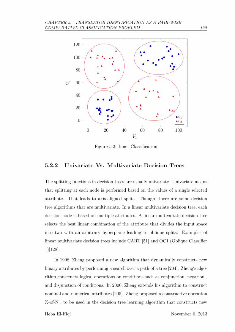
CHAPTER 5. TRANSLATOR IDENTIFICATION AS A PAIR-WISE
COMPARATIVE CLASSIFICATION PROBLEM 120
0 20 40 60 80 100
0
20
40
60
80
100
120
V1
V2
c1c2
Figure 5.2: Inner Classification
5.2.2 Univariate Vs. Multivariate Decision Trees
The splitting functions in decision trees are usually univariate. Univariate means
that splitting at each node is performed based on the values of a single selected
attribute. That leads to axis-aligned splits. Though, there are some decision
tree algorithms that are multivariate. In a linear multivariate decision tree, each
decision node is based on multiple attributes. A linear multivariate decision tree
selects the best linear combination of the attribute that divides the input space
into two with an arbitrary hyperplane leading to oblique splits. Examples of
linear multivariate decision trees include CART [51] and OC1 (Oblique Classifier
1)[128].
In 1998, Zheng proposed a new algorithm that dynamically constructs new
binary attributes by performing a search over a path of a tree [204]. Zheng‘s algo-
rithm constructs logical operations on conditions such as conjunction, negation ,
and disjunction of conditions. In 2000, Zheng extends his algorithm to construct
nominal and numerical attributes [205]. Zheng proposed a constructive operation
X-of-N , to be used in the decision tree learning algorithm that constructs new
Heba El-Fiqi November 6, 2013

CHAPTER 5. TRANSLATOR IDENTIFICATION AS A PAIR-WISE
COMPARATIVE CLASSIFICATION PROBLEM 121
attributes in the form of X-of-N representations. For a given instance, the value
of at-least M-of-N representation is true if at least M of its conditions is true of
the instance, otherwise it is false. Another constructive induction multivariate
decision tree called linear tree was proposed by Gama and Brazdil [52] in 1999.
Linear tree combines decision tree algorithms with linear discrimination to de-
fine decision surfaces in both orthogonal and oblique to the axes defined by the
attributes of the input space. Gama, then, introduced the “Functional trees" al-
gorithm which is a multivariate tree learning algorithm that combines univariate
decision trees with a discriminant function by means of constructive induction
[51].
A conceptual diagram demonstrating how a decision tree algorithm works by
comparing a split on a variable and its impact on the class is presented in Figure
5.3(a) with an example of a traditional decision tree output in Figure 5.3(b).
5.2.3 C4.5
C4.5 is an extension of the basic ID3 algorithm to overcome its limitations. C4.5
avoids overfitting the data by determining how deeply to grow a decision tree. Its
advantages include its ability to handle missing values and numeric attributes. In
a study that compared decision trees and other learning algorithms by Tjen-Sien
et al. [102], C4.5 was found to have a very good combination of error rate and
speed.
The selection criterion in C4.5 is based on either Information Gain or Gain
Ratio. Both of these measures are based on another basic measure in information
theory called Entropy. The Entropy measure is used to characterize the impurity
of a collection of examples.
Entropy(S) =c∑
i=1
−pi log2 pi (5.1)
Given S is any set of samples that belongs to k number of classes C : Ci,
Heba El-Fiqi November 6, 2013

CHAPTER 5. TRANSLATOR IDENTIFICATION AS A PAIR-WISE
COMPARATIVE CLASSIFICATION PROBLEM 122
(a) Framework
a1
C1
≤ x
C2
> x
(b) Output
Figure 5.3: Traditional Decision Tree
Heba El-Fiqi November 6, 2013
CHAPTER 5. TRANSLATOR IDENTIFICATION AS A PAIR-WISE
COMPARATIVE CLASSIFICATION PROBLEM 123
where Freq(Ci, S) = the number of instances in S belongs to Ci and |S|= total
number of instances in S. Entropy can be calculated as:
Info(S) = −k∑
i=1
freq(Ci, S)
|S|log2
(
freq(Ci, S))
|S|
)
(5.2)
For T training set, that can be divided into subsets {T1, T2, · · · , Tn} based
on test x : The total information content after T is partitioned is:
Infox(T ) =n∑
i=1
|Ti|
|T |Info(Ti) (5.3)
The quantity
Gain(x) = Info(T )− Infox(T ) (5.4)
measures the information that is gained by partitioning T according to test x.
The selection criterion is to select test x to maximize Gain(x).
The information gain criterion has deficiency: it has a strong bias in favor of
tests with a lot of outcomes. To solve this problem, Split-Info(x) is calculated as
Split− Info(x) = −n∑
i=1
|Ti|
|T |log2
(
|Ti|
|T |
)
(5.5)
This represents the potential information generated by dividing set T into n
subsets Ti. Gain Ratio measure expresses the proportion of information generated
by splitting of samples using test x. Gain-Ratio is robust, it gives consistently
better choice of a test than Information Gain. Algorithm 1 list the Pseudocode
of C4.5 decision tree.
Gain− Ratio(x) =Gain(x)
Split− Info(x)(5.6)
Heba El-Fiqi November 6, 2013
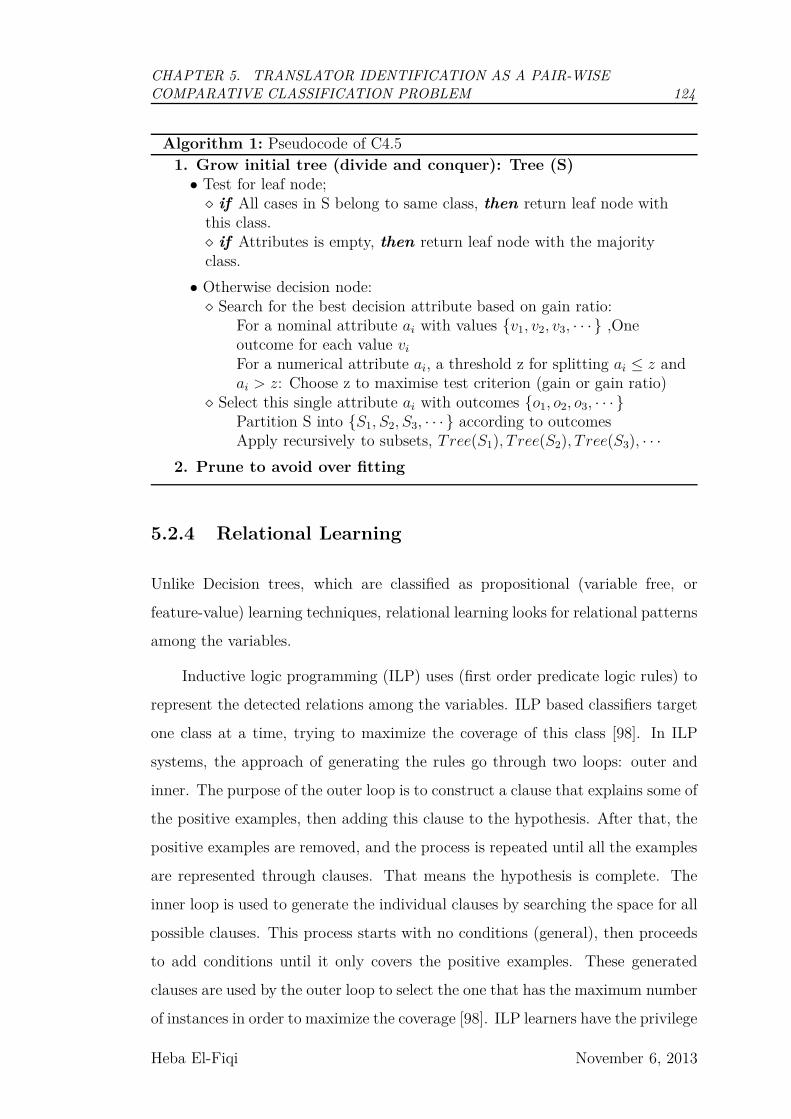
CHAPTER 5. TRANSLATOR IDENTIFICATION AS A PAIR-WISE
COMPARATIVE CLASSIFICATION PROBLEM 124
Algorithm 1: Pseudocode of C4.5
1. Grow initial tree (divide and conquer): Tree (S)• Test for leaf node;⋄ if All cases in S belong to same class, then return leaf node withthis class.⋄ if Attributes is empty, then return leaf node with the majorityclass.
• Otherwise decision node:⋄ Search for the best decision attribute based on gain ratio:
For a nominal attribute ai with values {v1, v2, v3, · · · } ,Oneoutcome for each value vi
For a numerical attribute ai, a threshold z for splitting ai ≤ z andai > z: Choose z to maximise test criterion (gain or gain ratio)
⋄ Select this single attribute ai with outcomes {o1, o2, o3, · · · }Partition S into {S1, S2, S3, · · · } according to outcomesApply recursively to subsets, Tree(S1), T ree(S2), T ree(S3), · · ·
2. Prune to avoid over fitting
5.2.4 Relational Learning
Unlike Decision trees, which are classified as propositional (variable free, or
feature-value) learning techniques, relational learning looks for relational patterns
among the variables.
Inductive logic programming (ILP) uses (first order predicate logic rules) to
represent the detected relations among the variables. ILP based classifiers target
one class at a time, trying to maximize the coverage of this class [98]. In ILP
systems, the approach of generating the rules go through two loops: outer and
inner. The purpose of the outer loop is to construct a clause that explains some of
the positive examples, then adding this clause to the hypothesis. After that, the
positive examples are removed, and the process is repeated until all the examples
are represented through clauses. That means the hypothesis is complete. The
inner loop is used to generate the individual clauses by searching the space for all
possible clauses. This process starts with no conditions (general), then proceeds
to add conditions until it only covers the positive examples. These generated
clauses are used by the outer loop to select the one that has the maximum number
of instances in order to maximize the coverage [98]. ILP learners have the privilege
Heba El-Fiqi November 6, 2013
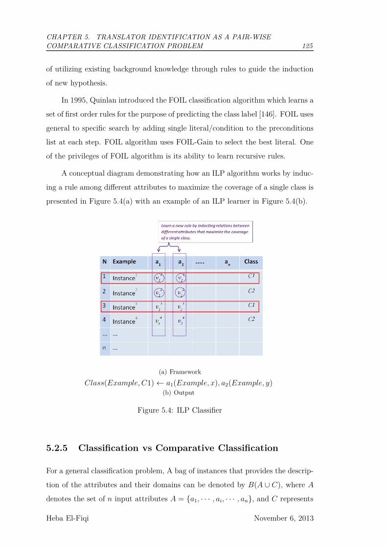
CHAPTER 5. TRANSLATOR IDENTIFICATION AS A PAIR-WISE
COMPARATIVE CLASSIFICATION PROBLEM 125
of utilizing existing background knowledge through rules to guide the induction
of new hypothesis.
In 1995, Quinlan introduced the FOIL classification algorithm which learns a
set of first order rules for the purpose of predicting the class label [146]. FOIL uses
general to specific search by adding single literal/condition to the preconditions
list at each step. FOIL algorithm uses FOIL-Gain to select the best literal. One
of the privileges of FOIL algorithm is its ability to learn recursive rules.
A conceptual diagram demonstrating how an ILP algorithm works by induc-
ing a rule among different attributes to maximize the coverage of a single class is
presented in Figure 5.4(a) with an example of an ILP learner in Figure 5.4(b).
(a) Framework
Class(Example, C1)← a1(Example, x), a2(Example, y)(b) Output
Figure 5.4: ILP Classifier
5.2.5 Classification vs Comparative Classification
For a general classification problem, A bag of instances that provides the descrip-
tion of the attributes and their domains can be denoted by B(A ∪ C), where A
denotes the set of n input attributes A = {a1, · · · , ai, · · · , an}, and C represents
Heba El-Fiqi November 6, 2013
CHAPTER 5. TRANSLATOR IDENTIFICATION AS A PAIR-WISE
COMPARATIVE CLASSIFICATION PROBLEM 126
the set of k classes variable (target attribute) C = {c1, · · · , ci, · · · , ck}.
A training set is defined as a collection of instances (also known as records,
rows or tuples) that may contain duplicates. Each instance is an individual, inde-
pendent example of the concept to be learned. These instances are characterized
by a vector of predetermined attribute values as:
v11, · · · , v1
n
......
...
vm1 , · · · , vm
n
(5.7)
where, vji is the value of attribute j in instance i, n is the number of attributes
and m is the number of instances.
A traditional classification problem can be defined as: Given a training set S
with input attributes set A = {a1, · · · , ai, · · · , an} and a nominal target attribute
C, the goal is to find a model/classifier that can map previously unseen instances
to the appropriate class that belongs to the target attribute c ∈ C as accurate as
possible.
PWCCP is a special type of binary classification problems. The goal of
PWCCP is to find a model that maps unseen instances to the appropriate pre-
defined classes in one-to-one correspondence for each pair of instances. Instances
are paired in both training and testing data set, where each pair consists exclu-
sively of classes instances; one instance per class. Thus, if one instance in this
pair is misclassified, the other instance will be misclassified as well. Values of
the same attribute for the paired instances are collected into a single vector as−→vj
i = [vji (c1), · · · , vj
i (ck)], where i represents the instance id, j represents the at-
tribute id, and |vij| = k
Heba El-Fiqi November 6, 2013
CHAPTER 5. TRANSLATOR IDENTIFICATION AS A PAIR-WISE
COMPARATIVE CLASSIFICATION PROBLEM 127
Instances in PWCCP can be represented as :
−→v1
1 , · · · ,−→v1
n
......
...−→vm
1 , · · · ,−→vm
n
(5.8)
Based on this description, the definition of PWCCP becomes: Given a train-
ing set S with input attributes set A = {a1, · · · , ai, · · · , an} and a nominal target
attribute C, and a test set of instances V = {V m+1, . . . , Vm+u}, u is the size of
the test set, the goal is to find a bijection mapping from every element in each
V i to the corresponding class or target attribute c ∈ C as accurate as possible.
To avoid the confusion from switching between a vector representation for the
training set and a set representation for the test set, we will adopt the notation
Vi(pj) to represent the value of attribute i. We use pj as an index for the order of
the measurement. For example, in a PWCCP, j = 2, and V1(p1) denotes the value
of the first attribute for the first instance of the pairs. We will use the notation
p1 → c1, p2 → c2 to denote that the first instance in the pairs are classified as class
c1, while the second instance is classified as class c2. In a paired classification,
the only other alternative would be p1 → c2, p2 → c1.
We will also use the following functions and notations to establish a relation-
ship between the two instances in a pair.
1. (R(V1(p1), {V1(p1), V2(p2)}) = min) to signify that the value of V1 in the
first instance of the pairs is the minimum value among the two values of V1
in that pair.
2. (R(V1(p1), {V1(p1), V2(p2)}) = max) to signify that the value of V1 in the
first instance of the pairs is the maximum value among the two values of
V1 in that pair.
Heba El-Fiqi November 6, 2013
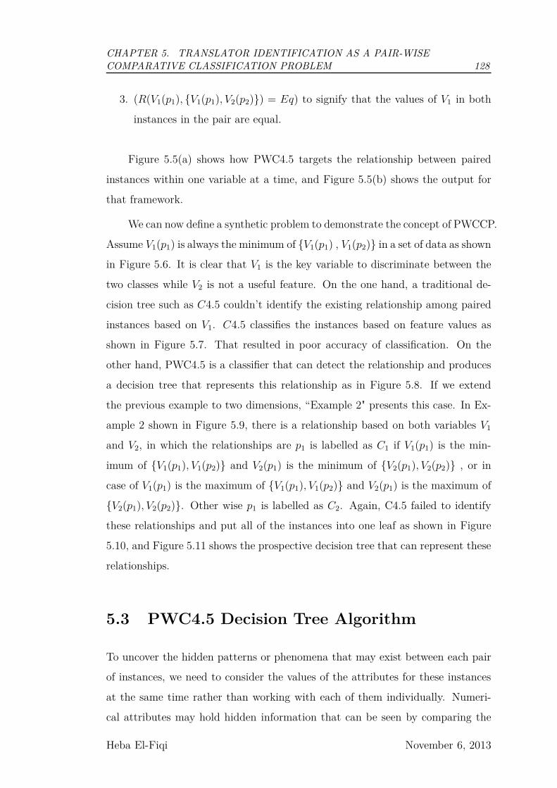
CHAPTER 5. TRANSLATOR IDENTIFICATION AS A PAIR-WISE
COMPARATIVE CLASSIFICATION PROBLEM 128
3. (R(V1(p1), {V1(p1), V2(p2)}) = Eq) to signify that the values of V1 in both
instances in the pair are equal.
Figure 5.5(a) shows how PWC4.5 targets the relationship between paired
instances within one variable at a time, and Figure 5.5(b) shows the output for
that framework.
We can now define a synthetic problem to demonstrate the concept of PWCCP.
Assume V1(p1) is always the minimum of {V1(p1) , V1(p2)} in a set of data as shown
in Figure 5.6. It is clear that V1 is the key variable to discriminate between the
two classes while V2 is not a useful feature. On the one hand, a traditional de-
cision tree such as C4.5 couldn’t identify the existing relationship among paired
instances based on V1. C4.5 classifies the instances based on feature values as
shown in Figure 5.7. That resulted in poor accuracy of classification. On the
other hand, PWC4.5 is a classifier that can detect the relationship and produces
a decision tree that represents this relationship as in Figure 5.8. If we extend
the previous example to two dimensions, “Example 2" presents this case. In Ex-
ample 2 shown in Figure 5.9, there is a relationship based on both variables V1
and V2, in which the relationships are p1 is labelled as C1 if V1(p1) is the min-
imum of {V1(p1), V1(p2)} and V2(p1) is the minimum of {V2(p1), V2(p2)} , or in
case of V1(p1) is the maximum of {V1(p1), V1(p2)} and V2(p1) is the maximum of
{V2(p1), V2(p2)}. Other wise p1 is labelled as C2. Again, C4.5 failed to identify
these relationships and put all of the instances into one leaf as shown in Figure
5.10, and Figure 5.11 shows the prospective decision tree that can represent these
relationships.
5.3 PWC4.5 Decision Tree Algorithm
To uncover the hidden patterns or phenomena that may exist between each pair
of instances, we need to consider the values of the attributes for these instances
at the same time rather than working with each of them individually. Numeri-
cal attributes may hold hidden information that can be seen by comparing the
Heba El-Fiqi November 6, 2013
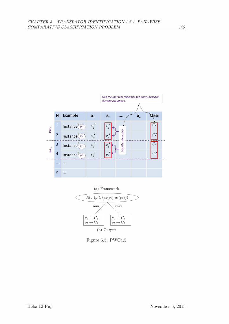
CHAPTER 5. TRANSLATOR IDENTIFICATION AS A PAIR-WISE
COMPARATIVE CLASSIFICATION PROBLEM 129
(a) Framework
R(a1(p1), {a1(p1), a1(p2)})
p1 → C2
p2 → C1
min
p1 → C1
p2 → C2
max
(b) Output
Figure 5.5: PWC4.5
Heba El-Fiqi November 6, 2013
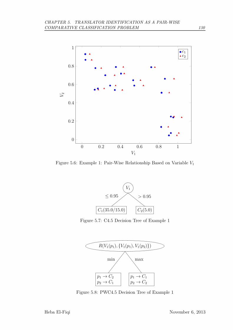
CHAPTER 5. TRANSLATOR IDENTIFICATION AS A PAIR-WISE
COMPARATIVE CLASSIFICATION PROBLEM 130
0 0.2 0.4 0.6 0.8 1
0
0.2
0.4
0.6
0.8
1
V1
V2
c1c2
Figure 5.6: Example 1: Pair-Wise Relationship Based on Variable V1
V1
C1(35.0/15.0)
≤ 0.95
C2(5.0)
> 0.95
Figure 5.7: C4.5 Decision Tree of Example 1
R(V1(p1), {V1(p1), V1(p2)})
p1 → C2
p2 → C1
min
p1 → C1
p2 → C2
max
Figure 5.8: PWC4.5 Decision Tree of Example 1
Heba El-Fiqi November 6, 2013
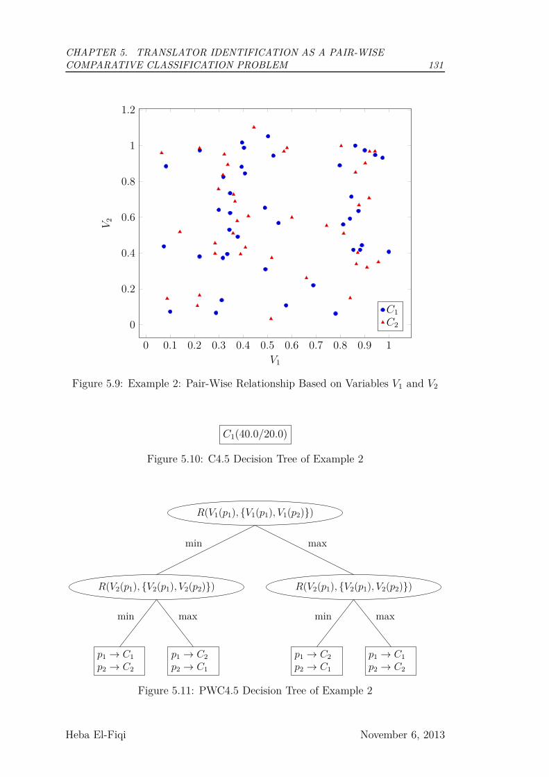
CHAPTER 5. TRANSLATOR IDENTIFICATION AS A PAIR-WISE
COMPARATIVE CLASSIFICATION PROBLEM 131
0 0.1 0.2 0.3 0.4 0.5 0.6 0.7 0.8 0.9 1
0
0.2
0.4
0.6
0.8
1
1.2
V1
V2
C1
C2
Figure 5.9: Example 2: Pair-Wise Relationship Based on Variables V1 and V2
C1(40.0/20.0)
Figure 5.10: C4.5 Decision Tree of Example 2
R(V1(p1), {V1(p1), V1(p2)})
R(V2(p1), {V2(p1), V2(p2)})
p1 → C1
p2 → C2
min
p1 → C2
p2 → C1
max
min
R(V2(p1), {V2(p1), V2(p2)})
p1 → C2
p2 → C1
min
p1 → C1
p2 → C2
max
max
Figure 5.11: PWC4.5 Decision Tree of Example 2
Heba El-Fiqi November 6, 2013
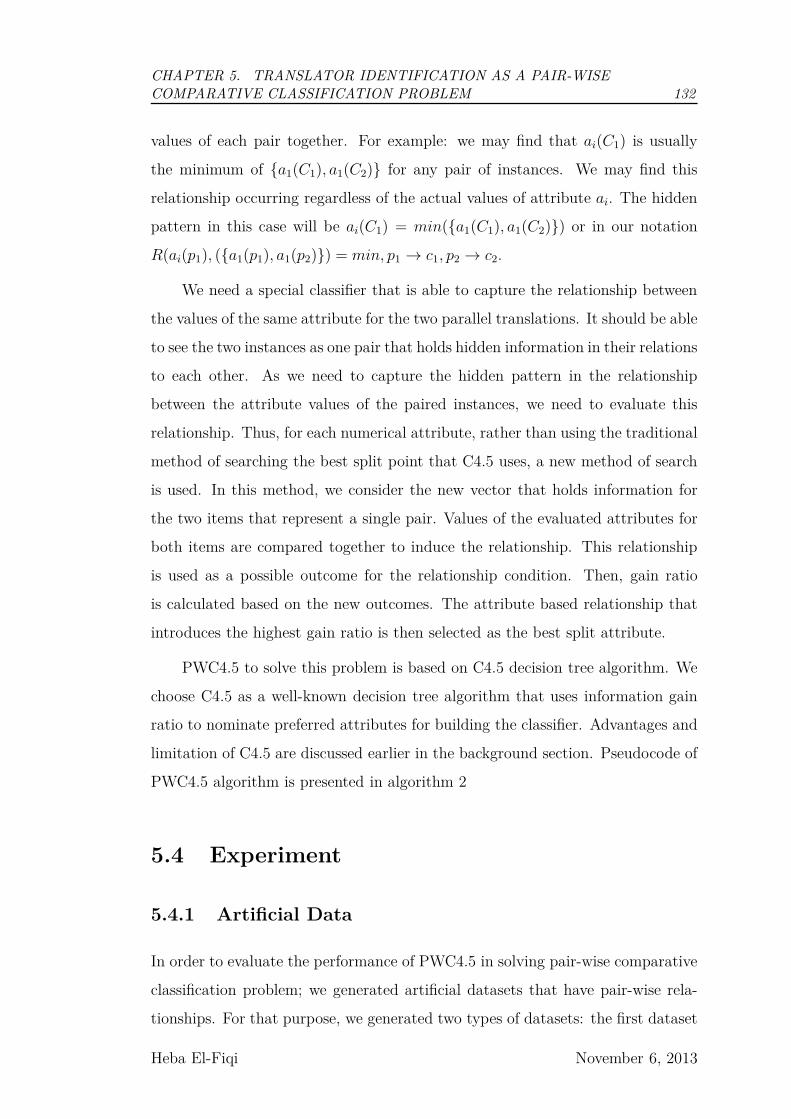
CHAPTER 5. TRANSLATOR IDENTIFICATION AS A PAIR-WISE
COMPARATIVE CLASSIFICATION PROBLEM 132
values of each pair together. For example: we may find that ai(C1) is usually
the minimum of {a1(C1), a1(C2)} for any pair of instances. We may find this
relationship occurring regardless of the actual values of attribute ai. The hidden
pattern in this case will be ai(C1) = min({a1(C1), a1(C2)}) or in our notation
R(ai(p1), ({a1(p1), a1(p2)}) = min, p1 → c1, p2 → c2.
We need a special classifier that is able to capture the relationship between
the values of the same attribute for the two parallel translations. It should be able
to see the two instances as one pair that holds hidden information in their relations
to each other. As we need to capture the hidden pattern in the relationship
between the attribute values of the paired instances, we need to evaluate this
relationship. Thus, for each numerical attribute, rather than using the traditional
method of searching the best split point that C4.5 uses, a new method of search
is used. In this method, we consider the new vector that holds information for
the two items that represent a single pair. Values of the evaluated attributes for
both items are compared together to induce the relationship. This relationship
is used as a possible outcome for the relationship condition. Then, gain ratio
is calculated based on the new outcomes. The attribute based relationship that
introduces the highest gain ratio is then selected as the best split attribute.
PWC4.5 to solve this problem is based on C4.5 decision tree algorithm. We
choose C4.5 as a well-known decision tree algorithm that uses information gain
ratio to nominate preferred attributes for building the classifier. Advantages and
limitation of C4.5 are discussed earlier in the background section. Pseudocode of
PWC4.5 algorithm is presented in algorithm 2
5.4 Experiment
5.4.1 Artificial Data
In order to evaluate the performance of PWC4.5 in solving pair-wise comparative
classification problem; we generated artificial datasets that have pair-wise rela-
tionships. For that purpose, we generated two types of datasets: the first dataset
Heba El-Fiqi November 6, 2013
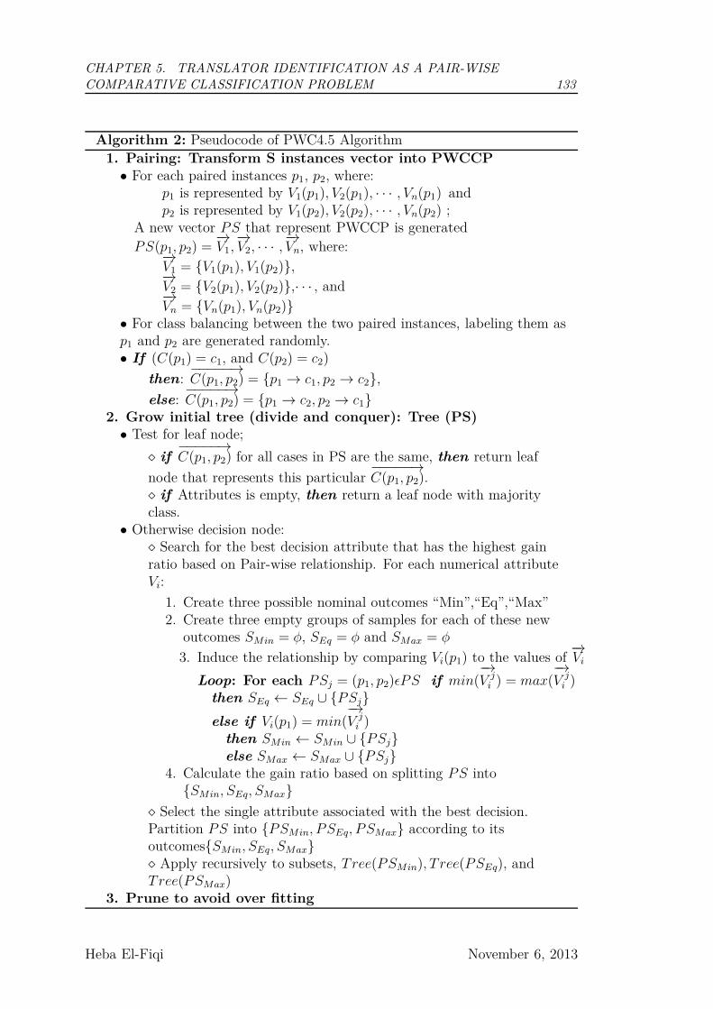
CHAPTER 5. TRANSLATOR IDENTIFICATION AS A PAIR-WISE
COMPARATIVE CLASSIFICATION PROBLEM 133
Algorithm 2: Pseudocode of PWC4.5 Algorithm
1. Pairing: Transform S instances vector into PWCCP• For each paired instances p1, p2, where:
p1 is represented by V1(p1), V2(p1), · · · , Vn(p1) andp2 is represented by V1(p2), V2(p2), · · · , Vn(p2) ;
A new vector P S that represent PWCCP is generated
P S(p1, p2) =−→V1,−→V2, · · · ,
−→Vn, where:
−→V1 = {V1(p1), V1(p2)},−→V2 = {V2(p1), V2(p2)},· · · , and−→Vn = {Vn(p1), Vn(p2)}
• For class balancing between the two paired instances, labeling them asp1 and p2 are generated randomly.• If (C(p1) = c1, and C(p2) = c2)
then:−−−−−→C(p1, p2) = {p1 → c1, p2 → c2},
else:−−−−−→C(p1, p2) = {p1 → c2, p2 → c1}
2. Grow initial tree (divide and conquer): Tree (PS)• Test for leaf node;
⋄ if−−−−−→C(p1, p2) for all cases in PS are the same, then return leaf
node that represents this particular−−−−−→C(p1, p2).
⋄ if Attributes is empty, then return a leaf node with majorityclass.
• Otherwise decision node:⋄ Search for the best decision attribute that has the highest gainratio based on Pair-wise relationship. For each numerical attributeVi:
1. Create three possible nominal outcomes “Min”,“Eq”,“Max”2. Create three empty groups of samples for each of these new
outcomes SMin = φ, SEq = φ and SMax = φ
3. Induce the relationship by comparing Vi(p1) to the values of−→Vi
Loop: For each P Sj = (p1, p2)ǫP S if min(−→V j
i ) = max(−→V j
i )then SEq ← SEq ∪ {P Sj}
else if Vi(p1) = min(−→V j
i )then SMin ← SMin ∪ {P Sj}else SMax ← SMax ∪ {P Sj}
4. Calculate the gain ratio based on splitting P S into{SMin, SEq, SMax}
⋄ Select the single attribute associated with the best decision.Partition P S into {P SMin, P SEq, P SMax} according to itsoutcomes{SMin, SEq, SMax}⋄ Apply recursively to subsets, Tree(P SMin), T ree(P SEq), andTree(P SMax)
3. Prune to avoid over fitting
Heba El-Fiqi November 6, 2013
CHAPTER 5. TRANSLATOR IDENTIFICATION AS A PAIR-WISE
COMPARATIVE CLASSIFICATION PROBLEM 134
contains two attributes (2D), and the second dataset contains five attributes
(5D). In each case, we first generated 10 noise free datasets for each problem,
then generated from these noise free datasets other datasets with different levels
of noise.
5.4.1.1 Artificial Data Generation
The data were generated using an XOR function over the predicate that Vj(p1)
is the minimum between Vj(p1) and Vj(p2) as follows
if⊗
j(R(Vj(p1), {Vj(p1), Vj(p2)}) = min)then p1 → +, p2 → −
We can see that in these rules, p1 is labeled by + if the number of minimum
relations is even, otherwise it is negative. For the case of 2D, 200 pairs were
generated for training and 100 for testing. For the case of 5D, we increased the
number of the pairs to 500 pairs for training, and 200 for testing to cover the
larger space.
We experimented with 7 levels of noise in addition to the noise free baseline
case. The test sets were always noise free. To explore the performance of PWC4.5
in case of noise, we added the following level of noise. Each of the eight cases (7
datasets with noise and one without) in each of the two problems (2D and 5D), 10
datasets were independently sampled using the above XOR relationship. These
results were then collected to perform t-test analysis for the performance of C4.5
and PWC4.5 in each level of noise. A one tail paired T-Test with confidence level
of 95% (alpha=0.05) was carried out. The proposed hypothesis is ”The average
accuracy of PWC4.5 is better than traditional C4.5 ”. This can be expressed
using:
H0 : µ(P WC4.5) ≤ µ(C4.5)
H1 : µ(P WC4.5) > µ(C4.5)
Heba El-Fiqi November 6, 2013
CHAPTER 5. TRANSLATOR IDENTIFICATION AS A PAIR-WISE
COMPARATIVE CLASSIFICATION PROBLEM 135
5.4.1.2 Results
For 2D Experiment, PWC4.5 achieved average accuracy of 100% using noise free
data. This accuracy was not affected by exposing the training data to noise of
levels 1%, 2.5%, 5%, 10%, and 15%. At noise level of 20% the average accuracy
dropped to 98.20%. The minimum average accuracy achieved was at the level of
25% noise, which was 82.90%. Meanwhile, C4.5 average accuracy ranged from
50.55% to 55.60% for the same samples. Details of the results are summarised
in Table 5.1. For each level of noise, t-Test analysis was conducted to compare
C4.5 accuracy to PWC4.5 as discussed in the experimental design. For the eight
different levels of noise, H0 is always rejected, and the alternative hypothesis is
accepted, which concludes that µ(P WC4.5) > µ(C4.5).
Similarly, the same experiment is applied to 5D dataset. The findings of
this experiment is similar to 2D results. PWC4.5 always outperformed C4.5.
The average accuracy for PWC4.5 was 100% for noise free data, and with noise
levels of 1%, 2.5%, and 5%. For level of noise of 10%, 15%, 20%, the average
accuracy achieved was 99.20%, 94.25%, and 82.80% respectively. The lowest
average accuracy achieved was 63.65% at the noise level of 25%. As for C4.5, the
average accuracy ranged from 48.53% to 51.35%. Additionally, the null hypothesis
was rejected for all levels of noise.
Figure 5.12 shows a comparison between the accuracy obtained by PWC4.5
and C4.5 when exposed to different levels of noise. PWC4.5 demonstrated stabil-
ity with different levels of noise up to 20%. Meanwhile, C4.5 was always around
50%. On the 5D dataset, Accuracy of PWC4.5 was more sensitive to the noise
starting from noise level of 15% as shown in Figure 5.13.
In order to visualize the pairwise relationship in the 2D artificial dataset, we
used first sample (Exp1) of each 10 samples at each level of noise. Then we show
the two decision trees obtained by C4.5 and PWC4.5. These visualizations are
collected in Figures 5.14 to 5.29. Additionally, we summarized the true positive,
true negative, false positive, and false negative rates for each of these samples in
Tables 5.3 and 5.4.
Heba El-Fiqi November 6, 2013
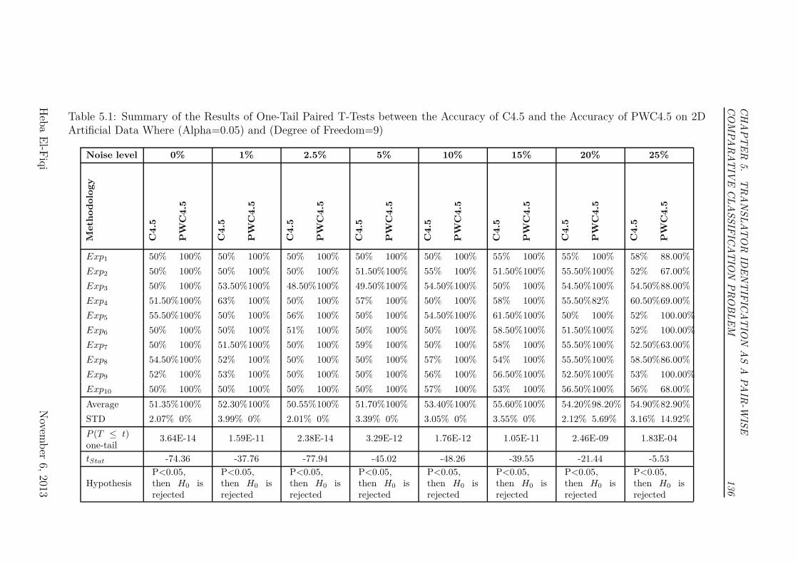
CH
AP
TE
R5.
TR
AN
SL
AT
OR
IDE
NT
IFIC
AT
ION
AS
AP
AIR
-WIS
E
CO
MP
AR
AT
IVE
CL
AS
SIF
ICA
TIO
NP
RO
BL
EM
136
Table 5.1: Summary of the Results of One-Tail Paired T-Tests between the Accuracy of C4.5 and the Accuracy of PWC4.5 on 2DArtificial Data Where (Alpha=0.05) and (Degree of Freedom=9)
Noise level 0% 1% 2.5% 5% 10% 15% 20% 25%
Meth
od
olo
gy
C4
.5
PW
C4
.5
C4
.5
PW
C4
.5
C4
.5
PW
C4
.5
C4
.5
PW
C4
.5
C4
.5
PW
C4
.5
C4
.5
PW
C4
.5
C4
.5
PW
C4
.5
C4
.5
PW
C4
.5
Exp1 50% 100% 50% 100% 50% 100% 50% 100% 50% 100% 55% 100% 55% 100% 58% 88.00%
Exp2 50% 100% 50% 100% 50% 100% 51.50%100% 55% 100% 51.50%100% 55.50%100% 52% 67.00%
Exp3 50% 100% 53.50%100% 48.50%100% 49.50%100% 54.50%100% 50% 100% 54.50%100% 54.50%88.00%
Exp4 51.50%100% 63% 100% 50% 100% 57% 100% 50% 100% 58% 100% 55.50%82% 60.50%69.00%
Exp5 55.50%100% 50% 100% 56% 100% 50% 100% 54.50%100% 61.50%100% 50% 100% 52% 100.00%
Exp6 50% 100% 50% 100% 51% 100% 50% 100% 50% 100% 58.50%100% 51.50%100% 52% 100.00%
Exp7 50% 100% 51.50%100% 50% 100% 59% 100% 50% 100% 58% 100% 55.50%100% 52.50%63.00%
Exp8 54.50%100% 52% 100% 50% 100% 50% 100% 57% 100% 54% 100% 55.50%100% 58.50%86.00%
Exp9 52% 100% 53% 100% 50% 100% 50% 100% 56% 100% 56.50%100% 52.50%100% 53% 100.00%
Exp10 50% 100% 50% 100% 50% 100% 50% 100% 57% 100% 53% 100% 56.50%100% 56% 68.00%
Average 51.35%100% 52.30%100% 50.55%100% 51.70%100% 53.40%100% 55.60%100% 54.20%98.20% 54.90%82.90%
STD 2.07% 0% 3.99% 0% 2.01% 0% 3.39% 0% 3.05% 0% 3.55% 0% 2.12% 5.69% 3.16% 14.92%
P (T ≤ t)one-tail
3.64E-14 1.59E-11 2.38E-14 3.29E-12 1.76E-12 1.05E-11 2.46E-09 1.83E-04
tStat -74.36 -37.76 -77.94 -45.02 -48.26 -39.55 -21.44 -5.53
HypothesisP<0.05,then H0 isrejected
P<0.05,then H0 isrejected
P<0.05,then H0 isrejected
P<0.05,then H0 isrejected
P<0.05,then H0 isrejected
P<0.05,then H0 isrejected
P<0.05,then H0 isrejected
P<0.05,then H0 isrejected
Heb
aE
l-Fiq
iN
ovemb
er6,
2013
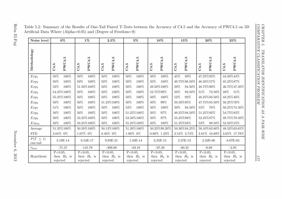
CH
AP
TE
R5.
TR
AN
SL
AT
OR
IDE
NT
IFIC
AT
ION
AS
AP
AIR
-WIS
E
CO
MP
AR
AT
IVE
CL
AS
SIF
ICA
TIO
NP
RO
BL
EM
137
Table 5.2: Summary of the Results of One-Tail Paired T-Tests between the Accuracy of C4.5 and the Accuracy of PWC4.5 on 5DArtificial Data Where (Alpha=0.05) and (Degree of Freedom=9)
Noise level 0% 1% 2.5% 5% 10% 15% 20% 25%
Meth
od
olo
gy
C4
.5
PW
C4
.5
C4
.5
PW
C4
.5
C4
.5
PW
C4
.5
C4
.5
PW
C4
.5
C4
.5
PW
C4
.5
C4
.5
PW
C4
.5
C4
.5
PW
C4
.5
C4
.5
PW
C4
.5
Exp1 50% 100% 50% 100% 50% 100% 50% 100% 50% 100% 45% 89% 47.25%92% 44.50%44%
Exp2 50% 100% 50% 100% 50% 100% 50% 100% 50% 100% 49.75%98.50% 46.50%57% 45.25%87%
Exp3 53% 100% 51.50%100% 50% 100% 50% 100% 49.50%100% 50% 94.50% 48.75%90% 46.75%47.50%
Exp4 54.25%100% 50% 100% 50% 100% 50% 100% 52.75%99% 50% 93.50% 51% 73.50% 48% 51%
Exp5 55.25%100% 50% 100% 50% 100% 50% 100% 50% 100% 52% 92% 48.25%83.50% 43.25%40%
Exp6 50% 100% 50% 100% 51.25%100% 50% 100% 50% 99% 50.50%95% 47.75%85.50% 50.25%76%
Exp7 51% 100% 50% 100% 50% 100% 52% 100% 50% 100% 50% 94.50% 55% 78% 50.25%74.50%
Exp8 50% 100% 50% 100% 50% 100% 51.25%100% 50% 97% 49.25%94.50% 51.25%92% 54.75%82%
Exp9 50% 100% 53.25%100% 50% 100% 53.50%100% 50% 97% 55.25%98% 52.25%87% 49.75%79.50%
Exp10 50% 100% 50.25%100% 50% 100% 55.25%100% 50% 100% 51.25%93% 53% 89.50% 52.50%55%
Average 51.35%100% 50.50%100% 50.13%100% 51.20%100% 50.23%99.20% 50.30%94.25% 50.10%82.80% 48.53%63.65%
STD 2.04% 0% 1.07% 0% 0.40% 0% 1.86% 0% 0.90% 1.23% 2.54% 2.74% 2.81% 10.89% 3.65% 17.78%
P (T ≤ t)one-tail
3.19E-14 8.54E-17 9.93E-21 1.33E-14 3.25E-15 2.37E-13 2.32E-06 8.07E-03
tStat -75.47 -145.79 -399.00 -83.18 -97.29 -60.35 -9.69 -2.95
HypothesisP<0.05,then H0 isrejected
P<0.05,then H0 isrejected
P<0.05,then H0 isrejected
P<0.05,then H0 isrejected
P<0.05,then H0 isrejected
P<0.05,then H0 isrejected
P<0.05,then H0 isrejected
P<0.05,then H0 isrejected
Heb
aE
l-Fiq
iN
ovemb
er6,
2013
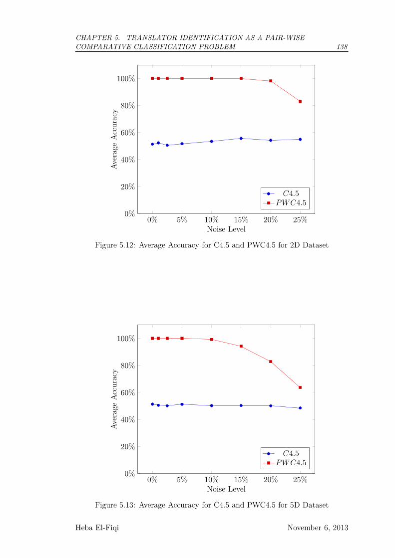
CHAPTER 5. TRANSLATOR IDENTIFICATION AS A PAIR-WISE
COMPARATIVE CLASSIFICATION PROBLEM 138
0% 5% 10% 15% 20% 25%0%
20%
40%
60%
80%
100%
Noise Level
Ave
rage
Acc
ura
cy
C4.5P WC4.5
Figure 5.12: Average Accuracy for C4.5 and PWC4.5 for 2D Dataset
0% 5% 10% 15% 20% 25%0%
20%
40%
60%
80%
100%
Noise Level
Ave
rage
Acc
ura
cy
C4.5P WC4.5
Figure 5.13: Average Accuracy for C4.5 and PWC4.5 for 5D Dataset
Heba El-Fiqi November 6, 2013

CHAPTER 5. TRANSLATOR IDENTIFICATION AS A PAIR-WISE
COMPARATIVE CLASSIFICATION PROBLEM 139
0 1 2 3 4 5 6 7 8 9 10
0
2
4
6
8
10
V1
V2
−+
Figure 5.14: Pair-Wise Relationship of Noise Free 2D(Exp1)
R(V1(p1), {V1(p1), V1(p2)})
R(V2(p1), {V2(p1), V2(p2)})
63
p1 → +,
p2 → −
min
37
p1 → −,
p2 → +
max
min
R(V2(p1), {V2(p1), V2(p2)})
39
p1 → −,
p2 → +
min
61
p1 → +,
p2 → −
max
max
(a) PWC4.5 Decision Tree
-(400.0/200.0)
(b) C4.5 Decision Tree
Figure 5.15: Decision Tree for Noise Free 2D(Exp1)
Heba El-Fiqi November 6, 2013
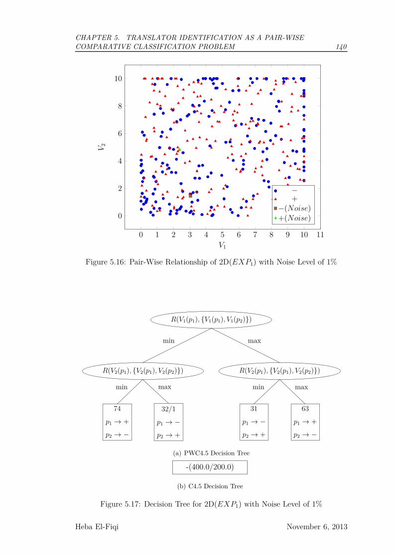
CHAPTER 5. TRANSLATOR IDENTIFICATION AS A PAIR-WISE
COMPARATIVE CLASSIFICATION PROBLEM 140
0 1 2 3 4 5 6 7 8 9 10 11
0
2
4
6
8
10
V1
V2
−+
−(Noise)+(Noise)
Figure 5.16: Pair-Wise Relationship of 2D(EXP1) with Noise Level of 1%
R(V1(p1), {V1(p1), V1(p2)})
R(V2(p1), {V2(p1), V2(p2)})
74
p1 → +
p2 → −
min
32/1
p1 → −
p2 → +
max
min
R(V2(p1), {V2(p1), V2(p2)})
31
p1 → −
p2 → +
min
63
p1 → +
p2 → −
max
max
(a) PWC4.5 Decision Tree
-(400.0/200.0)
(b) C4.5 Decision Tree
Figure 5.17: Decision Tree for 2D(EXP1) with Noise Level of 1%
Heba El-Fiqi November 6, 2013
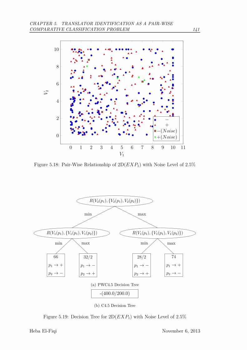
CHAPTER 5. TRANSLATOR IDENTIFICATION AS A PAIR-WISE
COMPARATIVE CLASSIFICATION PROBLEM 141
0 1 2 3 4 5 6 7 8 9 10 11
0
2
4
6
8
10
V1
V2
−+
−(Noise)+(Noise)
Figure 5.18: Pair-Wise Relationship of 2D(EXP1) with Noise Level of 2.5%
R(V2(p1), {V2(p1), V2(p2)})
R(V1(p1), {V1(p1), V1(p2)})
66
p1 → +
p2 → −
min
32/2
p1 → −
p2 → +
max
min
R(V1(p1), {V1(p1), V1(p2)})
28/2
p1 → −
p2 → +
min
74
p1 → +
p2 → −
max
max
(a) PWC4.5 Decision Tree
-(400.0/200.0)
(b) C4.5 Decision Tree
Figure 5.19: Decision Tree for 2D(EXP1) with Noise Level of 2.5%
Heba El-Fiqi November 6, 2013
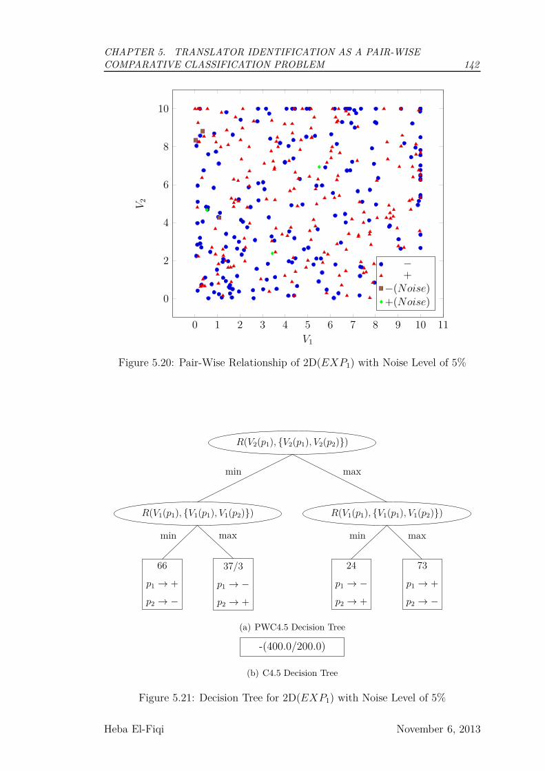
CHAPTER 5. TRANSLATOR IDENTIFICATION AS A PAIR-WISE
COMPARATIVE CLASSIFICATION PROBLEM 142
0 1 2 3 4 5 6 7 8 9 10 11
0
2
4
6
8
10
V1
V2
−+
−(Noise)+(Noise)
Figure 5.20: Pair-Wise Relationship of 2D(EXP1) with Noise Level of 5%
R(V2(p1), {V2(p1), V2(p2)})
R(V1(p1), {V1(p1), V1(p2)})
66
p1 → +
p2 → −
min
37/3
p1 → −
p2 → +
max
min
R(V1(p1), {V1(p1), V1(p2)})
24
p1 → −
p2 → +
min
73
p1 → +
p2 → −
max
max
(a) PWC4.5 Decision Tree
-(400.0/200.0)
(b) C4.5 Decision Tree
Figure 5.21: Decision Tree for 2D(EXP1) with Noise Level of 5%
Heba El-Fiqi November 6, 2013
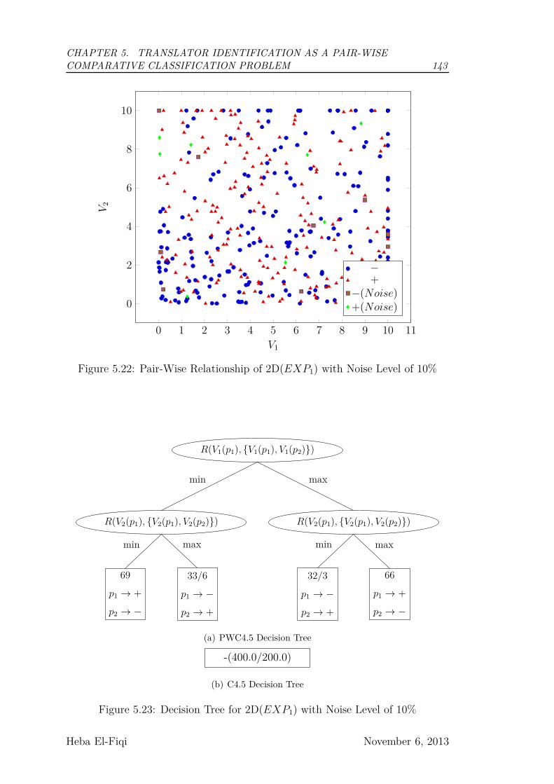
CHAPTER 5. TRANSLATOR IDENTIFICATION AS A PAIR-WISE
COMPARATIVE CLASSIFICATION PROBLEM 143
0 1 2 3 4 5 6 7 8 9 10 11
0
2
4
6
8
10
V1
V2
−+
−(Noise)+(Noise)
Figure 5.22: Pair-Wise Relationship of 2D(EXP1) with Noise Level of 10%
R(V1(p1), {V1(p1), V1(p2)})
R(V2(p1), {V2(p1), V2(p2)})
69
p1 → +
p2 → −
min
33/6
p1 → −
p2 → +
max
min
R(V2(p1), {V2(p1), V2(p2)})
32/3
p1 → −
p2 → +
min
66
p1 → +
p2 → −
max
max
(a) PWC4.5 Decision Tree
-(400.0/200.0)
(b) C4.5 Decision Tree
Figure 5.23: Decision Tree for 2D(EXP1) with Noise Level of 10%
Heba El-Fiqi November 6, 2013

CHAPTER 5. TRANSLATOR IDENTIFICATION AS A PAIR-WISE
COMPARATIVE CLASSIFICATION PROBLEM 144
0 1 2 3 4 5 6 7 8 9 10 11
0
2
4
6
8
10
V1
V2
−+
−(Noise)+(Noise)
Figure 5.24: Pair-Wise Relationship of 2D(EXP1) with Noise Level of 15%
R(V2(p1), {V2(p1), V2(p2)})
R(V1(p1), {V1(p1), V1(p2)})
74
p1 → +
p2 → −
min
32/9
p1 → −
p2 → +
max
min
R(V1(p1), {V1(p1), V1(p2)})
32/8
p1 → −
p2 → +
min
62
p1 → +
p2 → −
max
max
(a) PWC4.5 Decision Tree
V2
+(368/174)
≤ 9.91
-(32/6)
> 9.91
(b) C4.5 Decision Tree
Figure 5.25: Decision Tree for 2D(EXP1) with Noise Level of 15%
Heba El-Fiqi November 6, 2013

CHAPTER 5. TRANSLATOR IDENTIFICATION AS A PAIR-WISE
COMPARATIVE CLASSIFICATION PROBLEM 145
0 1 2 3 4 5 6 7 8 9 10 11
0
2
4
6
8
10
V1
V2
−+
−(Noise)+(Noise)
Figure 5.26: Pair-Wise Relationship of 2D(EXP1) with Noise Level of 20%
R(V2(p1), {V2(p1), V2(p2)})
R(V1(p1), {V1(p1), V1(p2)})
72
p1 → +
p2 → −
min
27/9
p1 → −
p2 → +
max
min
R(V1(p1), {V1(p1), V1(p2)})
44/18
p1 → −
p2 → +
min
57
p1 → +
p2 → −
max
max
(a) PWC4.5 Decision Tree
V2
+(369/174)
≤ 9.96
-(31/5)
> 9.96
(b) C4.5 Decision Tree
Figure 5.27: Decision Tree for 2D(EXP1) with Noise Level of 20%
Heba El-Fiqi November 6, 2013
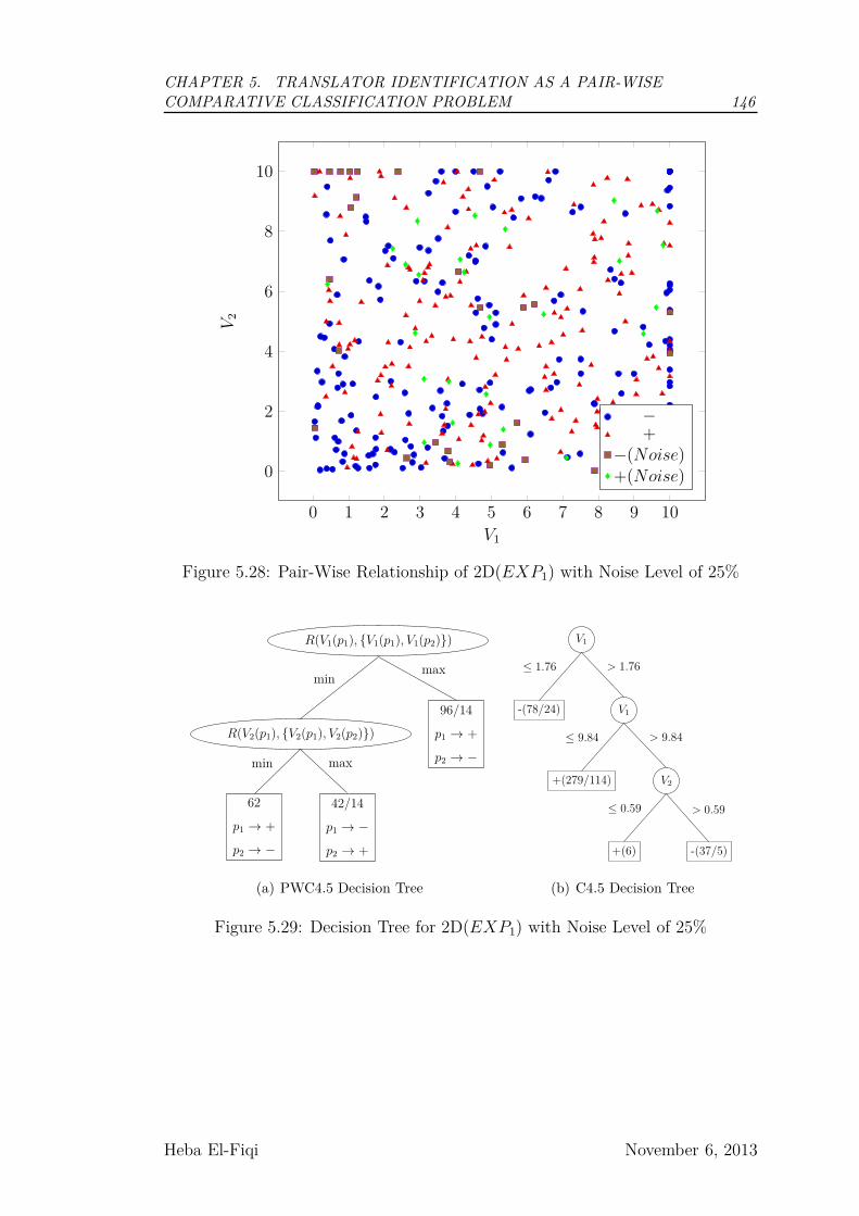
CHAPTER 5. TRANSLATOR IDENTIFICATION AS A PAIR-WISE
COMPARATIVE CLASSIFICATION PROBLEM 146
0 1 2 3 4 5 6 7 8 9 10
0
2
4
6
8
10
V1
V2
−+
−(Noise)+(Noise)
Figure 5.28: Pair-Wise Relationship of 2D(EXP1) with Noise Level of 25%
R(V1(p1), {V1(p1), V1(p2)})
R(V2(p1), {V2(p1), V2(p2)})
62
p1 → +
p2 → −
min
42/14
p1 → −
p2 → +
max
min
96/14
p1 → +
p2 → −
max
(a) PWC4.5 Decision Tree
V1
-(78/24)
≤ 1.76
V1
+(279/114)
≤ 9.84
V2
+(6)
≤ 0.59
-(37/5)
> 0.59
> 9.84
> 1.76
(b) C4.5 Decision Tree
Figure 5.29: Decision Tree for 2D(EXP1) with Noise Level of 25%
Heba El-Fiqi November 6, 2013
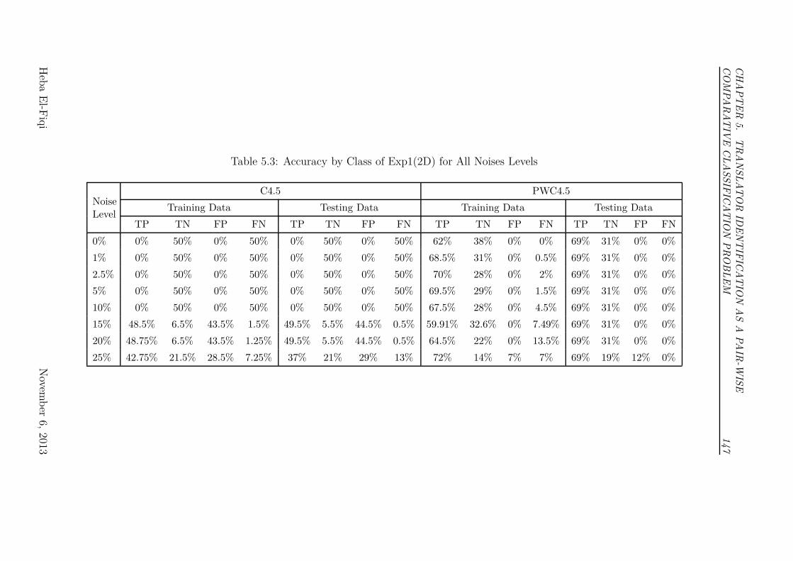
CH
AP
TE
R5.
TR
AN
SL
AT
OR
IDE
NT
IFIC
AT
ION
AS
AP
AIR
-WIS
E
CO
MP
AR
AT
IVE
CL
AS
SIF
ICA
TIO
NP
RO
BL
EM
147
Table 5.3: Accuracy by Class of Exp1(2D) for All Noises Levels
NoiseLevel
C4.5 PWC4.5
Training Data Testing Data Training Data Testing Data
TP TN FP FN TP TN FP FN TP TN FP FN TP TN FP FN
0% 0% 50% 0% 50% 0% 50% 0% 50% 62% 38% 0% 0% 69% 31% 0% 0%
1% 0% 50% 0% 50% 0% 50% 0% 50% 68.5% 31% 0% 0.5% 69% 31% 0% 0%
2.5% 0% 50% 0% 50% 0% 50% 0% 50% 70% 28% 0% 2% 69% 31% 0% 0%
5% 0% 50% 0% 50% 0% 50% 0% 50% 69.5% 29% 0% 1.5% 69% 31% 0% 0%
10% 0% 50% 0% 50% 0% 50% 0% 50% 67.5% 28% 0% 4.5% 69% 31% 0% 0%
15% 48.5% 6.5% 43.5% 1.5% 49.5% 5.5% 44.5% 0.5% 59.91% 32.6% 0% 7.49% 69% 31% 0% 0%
20% 48.75% 6.5% 43.5% 1.25% 49.5% 5.5% 44.5% 0.5% 64.5% 22% 0% 13.5% 69% 31% 0% 0%
25% 42.75% 21.5% 28.5% 7.25% 37% 21% 29% 13% 72% 14% 7% 7% 69% 19% 12% 0%
Heb
aE
l-Fiq
iN
ovemb
er6,
2013
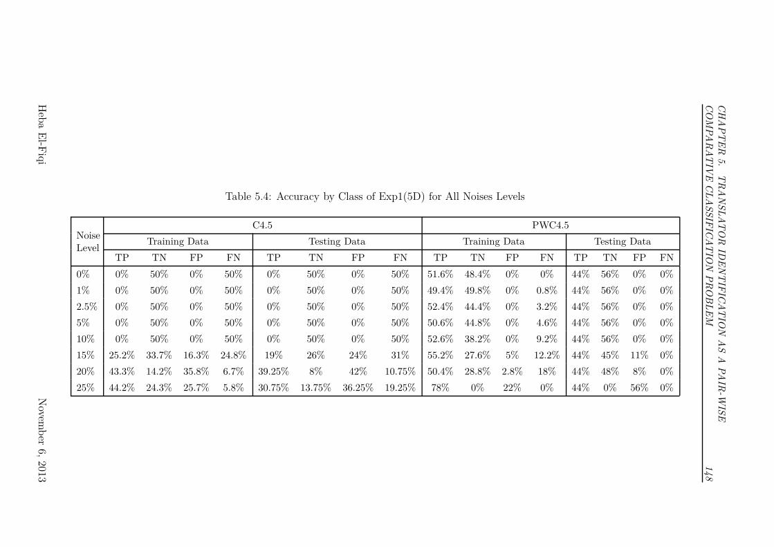
CH
AP
TE
R5.
TR
AN
SL
AT
OR
IDE
NT
IFIC
AT
ION
AS
AP
AIR
-WIS
E
CO
MP
AR
AT
IVE
CL
AS
SIF
ICA
TIO
NP
RO
BL
EM
148
Table 5.4: Accuracy by Class of Exp1(5D) for All Noises Levels
NoiseLevel
C4.5 PWC4.5
Training Data Testing Data Training Data Testing Data
TP TN FP FN TP TN FP FN TP TN FP FN TP TN FP FN
0% 0% 50% 0% 50% 0% 50% 0% 50% 51.6% 48.4% 0% 0% 44% 56% 0% 0%
1% 0% 50% 0% 50% 0% 50% 0% 50% 49.4% 49.8% 0% 0.8% 44% 56% 0% 0%
2.5% 0% 50% 0% 50% 0% 50% 0% 50% 52.4% 44.4% 0% 3.2% 44% 56% 0% 0%
5% 0% 50% 0% 50% 0% 50% 0% 50% 50.6% 44.8% 0% 4.6% 44% 56% 0% 0%
10% 0% 50% 0% 50% 0% 50% 0% 50% 52.6% 38.2% 0% 9.2% 44% 56% 0% 0%
15% 25.2% 33.7% 16.3% 24.8% 19% 26% 24% 31% 55.2% 27.6% 5% 12.2% 44% 45% 11% 0%
20% 43.3% 14.2% 35.8% 6.7% 39.25% 8% 42% 10.75% 50.4% 28.8% 2.8% 18% 44% 48% 8% 0%
25% 44.2% 24.3% 25.7% 5.8% 30.75% 13.75% 36.25% 19.25% 78% 0% 22% 0% 44% 0% 56% 0%
Heb
aE
l-Fiq
iN
ovemb
er6,
2013

CHAPTER 5. TRANSLATOR IDENTIFICATION AS A PAIR-WISE
COMPARATIVE CLASSIFICATION PROBLEM 149
5.4.2 Translator Stylometry Identification Problem
5.4.2.1 Using T Test to compare PWC4.5 to C4.5
For this experiment, 213 attributes are used (13 attributes as all possible mo-
tifs of size 3 in addition to 199 attributes as all possible motifs of size 4. The
data set contains 74 parallel translations for seven translators. There are 21 pos-
sible combinations of these seven translators. We used all of these 21 possible
combinations. For each pair of translator, we have (74x2) instances: 74 parallel
translations. To evaluate the effectiveness of the algorithm without being affected
by how these 74 pairs will be split, we decided to generate 10 different sets using
these 74 sample pairs. The planned ratio of splitting for the data is (2/3) training
and (1/3) testing. To generate these 10 different splits; we loop on the nominated
pair of translator 10 times:
• For each pair of parallel translation, a random number is generated between
0 to 1.
• If this number belongs to the interval [0,0.667], then this pair go to the
training dataset, otherwise, it is considered for testing dataset.
These 10 generated dataset are evaluated by C4.5 and then by PWC4.5 to
compare the accuracy in each case. A one tail paired T-Test with confidence
level of 95% (alpha=0.05) was carried out to evaluate if the accuracy of PWC4.5
is significantly better than the accuracy of C4.5. The question that we address
in this experiment is “Can classification accuracy for paired data be enhanced
by extracting information that represents paired instances relationship?”. Thus,
the proposed hypothesis will be “The average accuracy of PWC4.5 is better than
traditional C4.5 ”. This can be expressed using:
H0 : µ(PWC4.5 ) ≤ µ(C4.5)
H1 : µ(PWC4.5 ) > µ(C4.5)
As described in PWC4.5 Pseudocode, labeling the two paired instances as p1
and p2 are generated randomly for equal opportunity between the two instances.
Heba El-Fiqi November 6, 2013

CHAPTER 5. TRANSLATOR IDENTIFICATION AS A PAIR-WISE
COMPARATIVE CLASSIFICATION PROBLEM 150
Therefore, this randomness may cause some variation in the generated decision
tree. For the validation purpose of this experiment, we are going to run each
experiment ten times, and take the mean of the accuracy to represent this single
experiment’s accuracy.
5.4.2.2 Results and analysis
Table 5.5 shows that the accuracy obtained by evaluating the 10 generated data
sets using C4.5 and PWC4.5 for translators “Asad-Daryabadi”. While the aver-
age accuracy of C4.5 is 56.24% ± 0.15%, PWC4.5 produced an average accuracy
of 98.31% ±0.08%. After that, paired one-tail t-test is conducted for the average
accuracy of the two algorithms using the 10 generated datasets. Results of this
t-test are shown in Table 5.7. For this t-test, tCritical(9) = 1.833, and alpha=0.05.
Since P (T ≤ t) = 7.59E − 11, P <0.05, then the test revealed that there was a
statistical significance difference between PWC4.5 and C4.5
Although the variations between the ten runs of the experiment is not shown
for the case of “Asad-Daryabadi”, another example, for translators “Asad-Raza”,
shows these variations in Table 5.6. For example, accuracy of Exp1 for ’“Asad-
Raza” varied from 70.37% to 92.598% with average of 82.96%±6.58%. Therefore,
we used the average to represent the accuracy of PWC4.5. Then, we applied t-
test to compare between C4.5 and PWC4.5. P (T ≤ t) = 2.90E − 7, P <0.05
as illustrated in Table 5.8. Therefore, the null hypothesis was rejected, and the
alternative hypothesis H1 : µ(PWC4.5 ) > µ(C4.5) is accepted.
We followed the same steps for each pair of translators. For all of the 21 pairs
of translators, the null hypothesis was rejected, and the alternative hypothesis of
µ(PWC4.5) >µ(C4.5) was always accepted. Results of T-tests are summarized in
Table 5.9. These results demonstrates that PWC4.5 always outperformed C4.5
in this experiment.
The overall average of the accuracy of PWC4.5 is 78.81% in comparison to
Heba El-Fiqi November 6, 2013

CH
AP
TE
R5.
TR
AN
SL
AT
OR
IDE
NT
IFIC
AT
ION
AS
AP
AIR
-WIS
E
CO
MP
AR
AT
IVE
CL
AS
SIF
ICA
TIO
NP
RO
BL
EM
151
Table 5.5: Classification Accuracy of C4.5 and PWC4.5 for Translators Asad-Daryabadi
Expn
PWC4.5C4.5
1st run 2nd run 3rd run 4th run 5thrun 6th run 7th run 8th run 9th run 10thrun Mean STD
Exp1 54.17% 95.83% 95.83% 95.83% 95.83% 95.83% 95.83% 95.83% 95.83% 95.83% 95.83% 95.83% 0.00%
Exp2 60.00% 100.00% 100.00% 100.00% 100.00% 100.00% 100.00% 100.00% 100.00% 100.00% 100.00% 100.00% 0.00%
Exp3 51.92% 100.00% 100.00% 100.00% 100.00% 100.00% 100.00% 100.00% 100.00% 100.00% 100.00% 100.00% 0.00%
Exp4 62.50% 100.00% 100.00% 100.00% 100.00% 100.00% 100.00% 100.00% 100.00% 100.00% 100.00% 100.00% 0.00%
Exp5 58.93% 100.00% 100.00% 100.00% 100.00% 100.00% 100.00% 100.00% 100.00% 100.00% 100.00% 100.00% 0.00%
Exp6 55.36% 100.00% 100.00% 100.00% 100.00% 100.00% 100.00% 100.00% 100.00% 100.00% 100.00% 100.00% 0.00%
Exp7 51.92% 92.31% 92.31% 92.31% 92.31% 92.31% 92.31% 92.31% 92.31% 92.31% 92.31% 92.31% 0.00%
Exp8 52.63% 100.00% 100.00% 100.00% 100.00% 100.00% 100.00% 100.00% 100.00% 100.00% 100.00% 100.00% 0.00%
Exp9 55.00% 100.00% 100.00% 100.00% 100.00% 100.00% 100.00% 100.00% 100.00% 100.00% 100.00% 100.00% 0.00%
Exp10 60.00% 95.00% 95.00% 95.00% 95.00% 95.00% 95.00% 95.00% 95.00% 95.00% 95.00% 95.00% 0.00%
Average 56.24% ± 0.15% 98.31% ±0.08%
Heb
aE
l-Fiq
iN
ovemb
er6,
2013
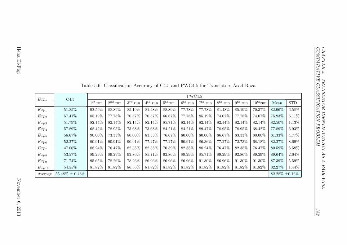
CH
AP
TE
R5.
TR
AN
SL
AT
OR
IDE
NT
IFIC
AT
ION
AS
AP
AIR
-WIS
E
CO
MP
AR
AT
IVE
CL
AS
SIF
ICA
TIO
NP
RO
BL
EM
152
Table 5.6: Classification Accuracy of C4.5 and PWC4.5 for Translators Asad-Raza
Expn
PWC4.5C4.5
1st run 2nd run 3rd run 4th run 5thrun 6th run 7th run 8th run 9th run 10thrun Mean STD
Exp1 51.85% 92.59% 88.89% 85.19% 81.48% 88.89% 77.78% 77.78% 81.48% 85.19% 70.37% 82.96% 6.58%
Exp2 57.41% 85.19% 77.78% 70.37% 70.37% 66.67% 77.78% 85.19% 74.07% 77.78% 74.07% 75.93% 6.11%
Exp3 51.79% 82.14% 82.14% 82.14% 82.14% 85.71% 82.14% 82.14% 82.14% 82.14% 82.14% 82.50% 1.13%
Exp4 57.89% 68.42% 78.95% 73.68% 73.68% 84.21% 84.21% 89.47% 78.95% 78.95% 68.42% 77.89% 6.93%
Exp5 56.67% 90.00% 73.33% 80.00% 83.33% 76.67% 80.00% 80.00% 86.67% 83.33% 80.00% 81.33% 4.77%
Exp6 52.27% 90.91% 90.91% 90.91% 77.27% 77.27% 90.91% 86.36% 77.27% 72.73% 68.18% 82.27% 8.69%
Exp7 47.06% 88.24% 76.47% 82.35% 82.35% 70.59% 82.35% 88.24% 76.47% 82.35% 76.47% 80.59% 5.58%
Exp8 53.57% 89.29% 89.29% 92.86% 85.71% 92.86% 89.29% 85.71% 89.29% 92.86% 89.29% 89.64% 2.64%
Exp9 71.74% 95.65% 78.26% 78.26% 86.96% 86.96% 86.96% 91.30% 86.96% 91.30% 91.30% 87.39% 5.59%
Exp10 54.55% 81.82% 81.82% 86.36% 81.82% 81.82% 81.82% 81.82% 81.82% 81.82% 81.82% 82.27% 1.44%
Average 55.48% ± 0.43% 82.28% ±0.16%
Heb
aE
l-Fiq
iN
ovemb
er6,
2013
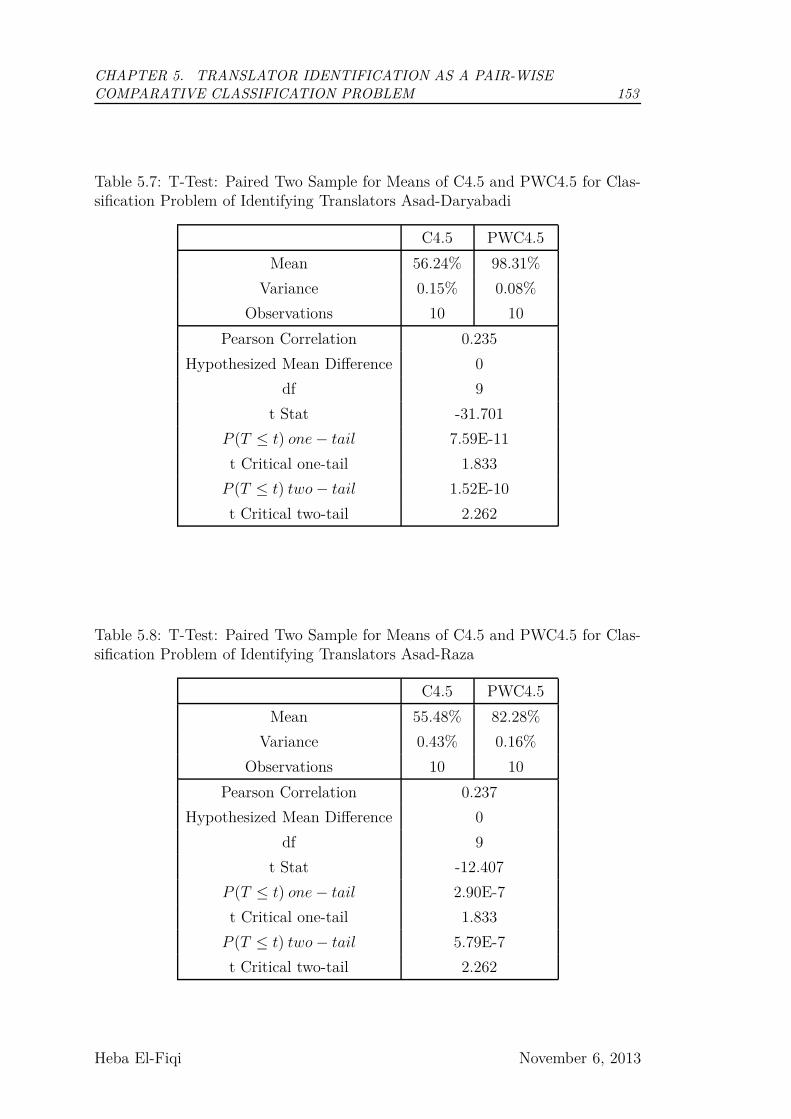
CHAPTER 5. TRANSLATOR IDENTIFICATION AS A PAIR-WISE
COMPARATIVE CLASSIFICATION PROBLEM 153
Table 5.7: T-Test: Paired Two Sample for Means of C4.5 and PWC4.5 for Clas-sification Problem of Identifying Translators Asad-Daryabadi
C4.5 PWC4.5
Mean 56.24% 98.31%
Variance 0.15% 0.08%
Observations 10 10
Pearson Correlation 0.235
Hypothesized Mean Difference 0
df 9
t Stat -31.701
P (T ≤ t) one− tail 7.59E-11
t Critical one-tail 1.833
P (T ≤ t) two− tail 1.52E-10
t Critical two-tail 2.262
Table 5.8: T-Test: Paired Two Sample for Means of C4.5 and PWC4.5 for Clas-sification Problem of Identifying Translators Asad-Raza
C4.5 PWC4.5
Mean 55.48% 82.28%
Variance 0.43% 0.16%
Observations 10 10
Pearson Correlation 0.237
Hypothesized Mean Difference 0
df 9
t Stat -12.407
P (T ≤ t) one− tail 2.90E-7
t Critical one-tail 1.833
P (T ≤ t) two− tail 5.79E-7
t Critical two-tail 2.262
Heba El-Fiqi November 6, 2013
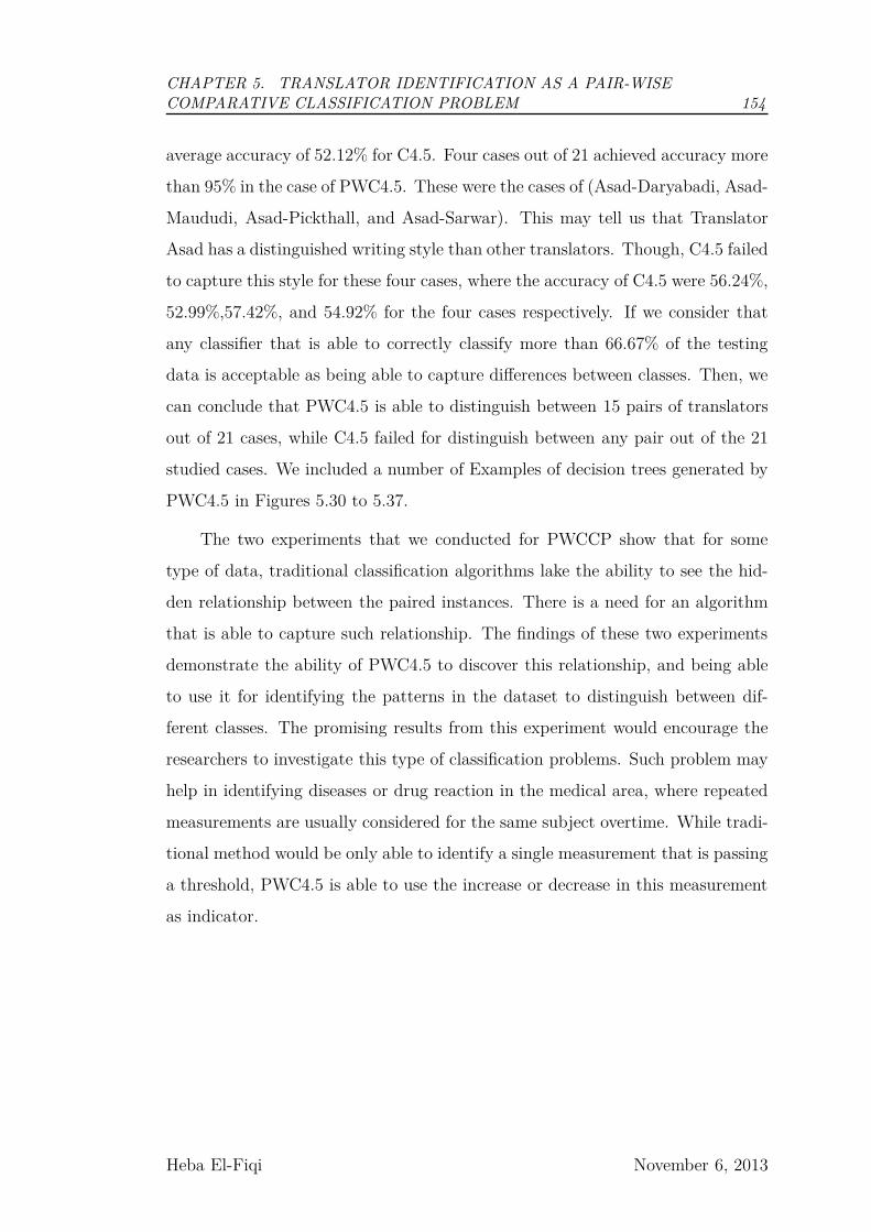
CHAPTER 5. TRANSLATOR IDENTIFICATION AS A PAIR-WISE
COMPARATIVE CLASSIFICATION PROBLEM 154
average accuracy of 52.12% for C4.5. Four cases out of 21 achieved accuracy more
than 95% in the case of PWC4.5. These were the cases of (Asad-Daryabadi, Asad-
Maududi, Asad-Pickthall, and Asad-Sarwar). This may tell us that Translator
Asad has a distinguished writing style than other translators. Though, C4.5 failed
to capture this style for these four cases, where the accuracy of C4.5 were 56.24%,
52.99%,57.42%, and 54.92% for the four cases respectively. If we consider that
any classifier that is able to correctly classify more than 66.67% of the testing
data is acceptable as being able to capture differences between classes. Then, we
can conclude that PWC4.5 is able to distinguish between 15 pairs of translators
out of 21 cases, while C4.5 failed for distinguish between any pair out of the 21
studied cases. We included a number of Examples of decision trees generated by
PWC4.5 in Figures 5.30 to 5.37.
The two experiments that we conducted for PWCCP show that for some
type of data, traditional classification algorithms lake the ability to see the hid-
den relationship between the paired instances. There is a need for an algorithm
that is able to capture such relationship. The findings of these two experiments
demonstrate the ability of PWC4.5 to discover this relationship, and being able
to use it for identifying the patterns in the dataset to distinguish between dif-
ferent classes. The promising results from this experiment would encourage the
researchers to investigate this type of classification problems. Such problem may
help in identifying diseases or drug reaction in the medical area, where repeated
measurements are usually considered for the same subject overtime. While tradi-
tional method would be only able to identify a single measurement that is passing
a threshold, PWC4.5 is able to use the increase or decrease in this measurement
as indicator.
Heba El-Fiqi November 6, 2013
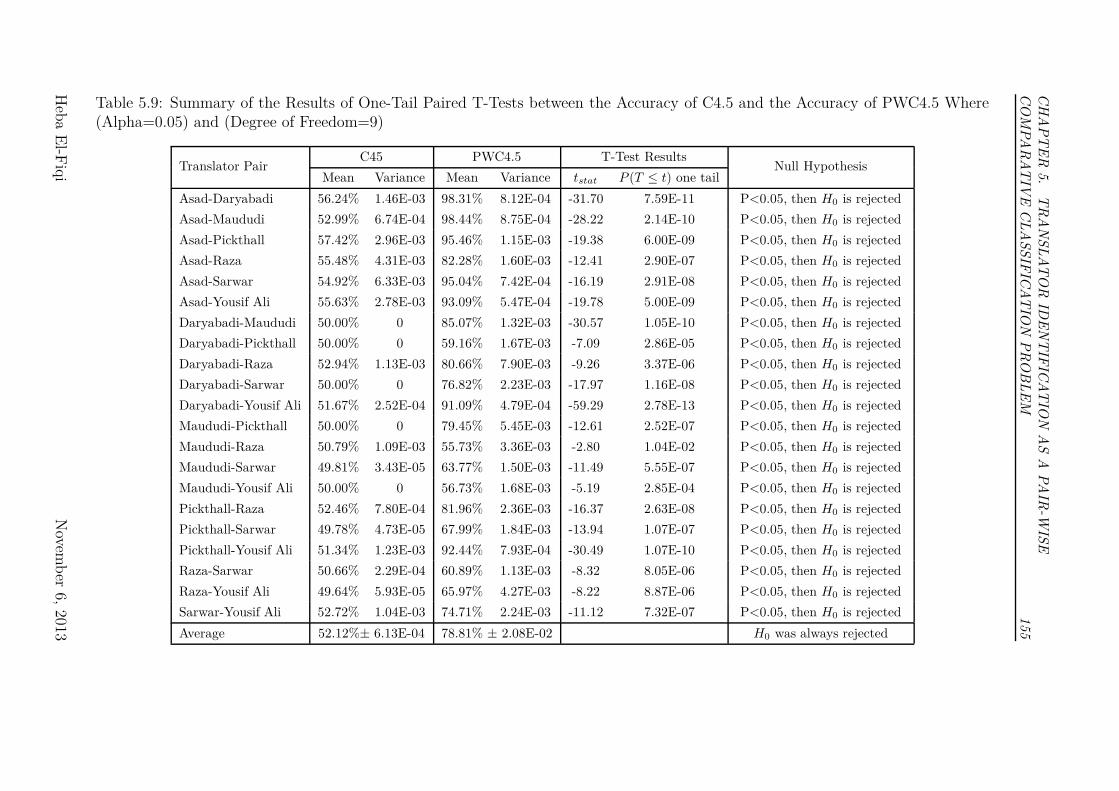
CH
AP
TE
R5.
TR
AN
SL
AT
OR
IDE
NT
IFIC
AT
ION
AS
AP
AIR
-WIS
E
CO
MP
AR
AT
IVE
CL
AS
SIF
ICA
TIO
NP
RO
BL
EM
155
Table 5.9: Summary of the Results of One-Tail Paired T-Tests between the Accuracy of C4.5 and the Accuracy of PWC4.5 Where(Alpha=0.05) and (Degree of Freedom=9)
Translator PairC45 PWC4.5 T-Test Results
Null HypothesisMean Variance Mean Variance tstat P (T ≤ t) one tail
Asad-Daryabadi 56.24% 1.46E-03 98.31% 8.12E-04 -31.70 7.59E-11 P<0.05, then H0 is rejected
Asad-Maududi 52.99% 6.74E-04 98.44% 8.75E-04 -28.22 2.14E-10 P<0.05, then H0 is rejected
Asad-Pickthall 57.42% 2.96E-03 95.46% 1.15E-03 -19.38 6.00E-09 P<0.05, then H0 is rejected
Asad-Raza 55.48% 4.31E-03 82.28% 1.60E-03 -12.41 2.90E-07 P<0.05, then H0 is rejected
Asad-Sarwar 54.92% 6.33E-03 95.04% 7.42E-04 -16.19 2.91E-08 P<0.05, then H0 is rejected
Asad-Yousif Ali 55.63% 2.78E-03 93.09% 5.47E-04 -19.78 5.00E-09 P<0.05, then H0 is rejected
Daryabadi-Maududi 50.00% 0 85.07% 1.32E-03 -30.57 1.05E-10 P<0.05, then H0 is rejected
Daryabadi-Pickthall 50.00% 0 59.16% 1.67E-03 -7.09 2.86E-05 P<0.05, then H0 is rejected
Daryabadi-Raza 52.94% 1.13E-03 80.66% 7.90E-03 -9.26 3.37E-06 P<0.05, then H0 is rejected
Daryabadi-Sarwar 50.00% 0 76.82% 2.23E-03 -17.97 1.16E-08 P<0.05, then H0 is rejected
Daryabadi-Yousif Ali 51.67% 2.52E-04 91.09% 4.79E-04 -59.29 2.78E-13 P<0.05, then H0 is rejected
Maududi-Pickthall 50.00% 0 79.45% 5.45E-03 -12.61 2.52E-07 P<0.05, then H0 is rejected
Maududi-Raza 50.79% 1.09E-03 55.73% 3.36E-03 -2.80 1.04E-02 P<0.05, then H0 is rejected
Maududi-Sarwar 49.81% 3.43E-05 63.77% 1.50E-03 -11.49 5.55E-07 P<0.05, then H0 is rejected
Maududi-Yousif Ali 50.00% 0 56.73% 1.68E-03 -5.19 2.85E-04 P<0.05, then H0 is rejected
Pickthall-Raza 52.46% 7.80E-04 81.96% 2.36E-03 -16.37 2.63E-08 P<0.05, then H0 is rejected
Pickthall-Sarwar 49.78% 4.73E-05 67.99% 1.84E-03 -13.94 1.07E-07 P<0.05, then H0 is rejected
Pickthall-Yousif Ali 51.34% 1.23E-03 92.44% 7.93E-04 -30.49 1.07E-10 P<0.05, then H0 is rejected
Raza-Sarwar 50.66% 2.29E-04 60.89% 1.13E-03 -8.32 8.05E-06 P<0.05, then H0 is rejected
Raza-Yousif Ali 49.64% 5.93E-05 65.97% 4.27E-03 -8.22 8.87E-06 P<0.05, then H0 is rejected
Sarwar-Yousif Ali 52.72% 1.04E-03 74.71% 2.24E-03 -11.12 7.32E-07 P<0.05, then H0 is rejected
Average 52.12%± 6.13E-04 78.81% ± 2.08E-02 H0 was always rejected
Heb
aE
l-Fiq
iN
ovemb
er6,
2013
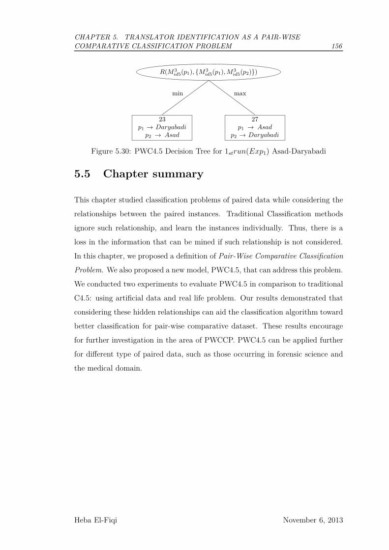
CHAPTER 5. TRANSLATOR IDENTIFICATION AS A PAIR-WISE
COMPARATIVE CLASSIFICATION PROBLEM 156
R(M3
id5(p1), {M3
id5(p1), M3
id5(p2)})
23p1 → Daryabadi
p2 → Asad
min
27p1 → Asad
p2 → Daryabadi
max
Figure 5.30: PWC4.5 Decision Tree for 1strun(Exp1) Asad-Daryabadi
5.5 Chapter summary
This chapter studied classification problems of paired data while considering the
relationships between the paired instances. Traditional Classification methods
ignore such relationship, and learn the instances individually. Thus, there is a
loss in the information that can be mined if such relationship is not considered.
In this chapter, we proposed a definition of Pair-Wise Comparative Classification
Problem. We also proposed a new model, PWC4.5, that can address this problem.
We conducted two experiments to evaluate PWC4.5 in comparison to traditional
C4.5: using artificial data and real life problem. Our results demonstrated that
considering these hidden relationships can aid the classification algorithm toward
better classification for pair-wise comparative dataset. These results encourage
for further investigation in the area of PWCCP. PWC4.5 can be applied further
for different type of paired data, such as those occurring in forensic science and
the medical domain.
Heba El-Fiqi November 6, 2013
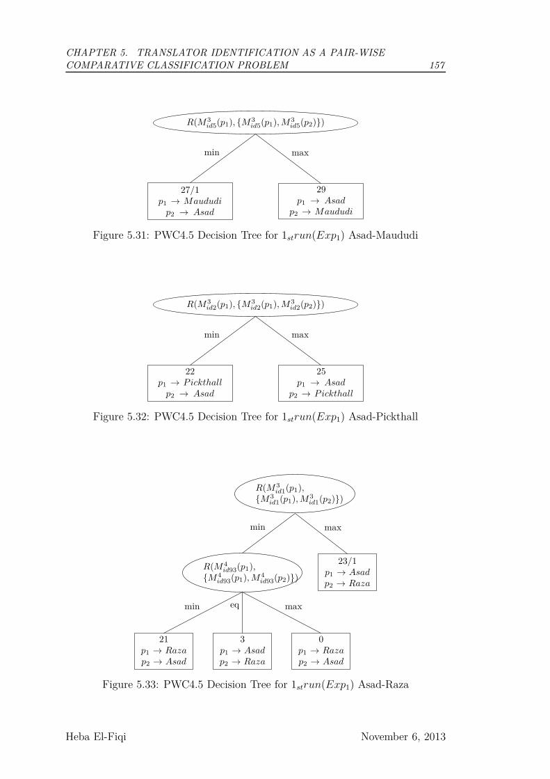
CHAPTER 5. TRANSLATOR IDENTIFICATION AS A PAIR-WISE
COMPARATIVE CLASSIFICATION PROBLEM 157
R(M3
id5(p1), {M3
id5(p1), M3
id5(p2)})
27/1p1 → Maududi
p2 → Asad
min
29p1 → Asad
p2 → Maududi
max
Figure 5.31: PWC4.5 Decision Tree for 1strun(Exp1) Asad-Maududi
R(M3
id2(p1), {M3
id2(p1), M3
id2(p2)})
22p1 → P ickthall
p2 → Asad
min
25p1 → Asad
p2 → P ickthall
max
Figure 5.32: PWC4.5 Decision Tree for 1strun(Exp1) Asad-Pickthall
R(M3
id1(p1),
{M3
id1(p1), M3
id1(p2)})
R(M4
id93(p1),
{M4
id93(p1), M4
id93(p2)})
21p1 → Raza
p2 → Asad
min
3p1 → Asad
p2 → Raza
eq
0p1 → Raza
p2 → Asad
max
min
23/1p1 → Asad
p2 → Raza
max
Figure 5.33: PWC4.5 Decision Tree for 1strun(Exp1) Asad-Raza
Heba El-Fiqi November 6, 2013
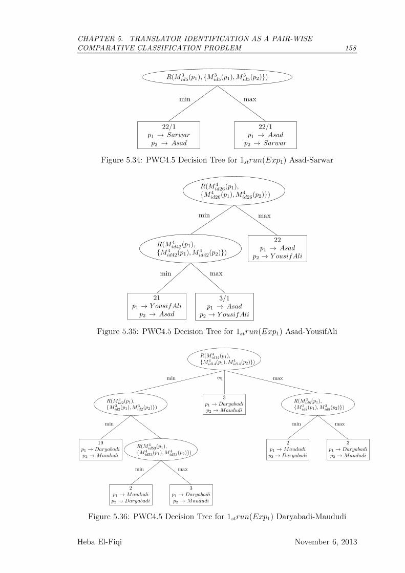
CHAPTER 5. TRANSLATOR IDENTIFICATION AS A PAIR-WISE
COMPARATIVE CLASSIFICATION PROBLEM 158
R(M3
id5(p1), {M3
id5(p1), M3
id5(p2)})
22/1p1 → Sarwar
p2 → Asad
min
22/1p1 → Asad
p2 → Sarwar
max
Figure 5.34: PWC4.5 Decision Tree for 1strun(Exp1) Asad-Sarwar
R(M4
id26(p1),
{M4
id26(p1), M4
id26(p2)})
R(M4
id42(p1),
{M4
id42(p1), M4
id42(p2)})
21p1 → Y ousifAli
p2 → Asad
min
3/1p1 → Asad
p2 → Y ousifAli
max
min
22p1 → Asad
p2 → Y ousifAli
max
Figure 5.35: PWC4.5 Decision Tree for 1strun(Exp1) Asad-YousifAli
R(M4
id14(p1),
{M4
id14(p1), M4
id14(p2)})
R(M3
id2(p1),
{M3
id2(p1), M3
id2(p2)})
19p1 → Daryabadi
p2 → Maududi
min
R(M4
id53(p1),
{M4
id53(p1), M4
id53(p2)})
2p1 → Maududi
p2 → Daryabadi
min
3p1 → Daryabadi
p2 → Maududi
max
min
3p1 → Daryabadi
p2 → Maududi
eq
R(M3
id8(p1),
{M3
id8(p1), M3
id8(p2)})
2p1 → Maududi
p2 → Daryabadi
min
3p1 → Daryabadi
p2 → Maududi
max
max
Figure 5.36: PWC4.5 Decision Tree for 1strun(Exp1) Daryabadi-Maududi
Heba El-Fiqi November 6, 2013
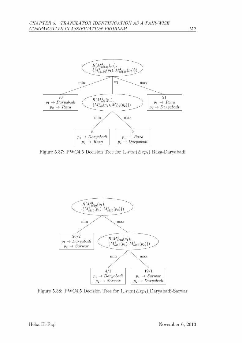
CHAPTER 5. TRANSLATOR IDENTIFICATION AS A PAIR-WISE
COMPARATIVE CLASSIFICATION PROBLEM 159
R(M4
id136(p1),
{M4
id136(p1), M4
id136(p2)})
20p1 → Daryabadi
p2 → Raza
min
R(M4
id8(p1),
{M4
id8(p1), M4
id8(p2)})
8p1 → Daryabadi
p2 → Raza
min
2p1 → Raza
p2 → Daryabadi
max
eq
21p1 → Raza
p2 → Daryabadi
max
Figure 5.37: PWC4.5 Decision Tree for 1strun(Exp1) Raza-Daryabadi
R(M3
id10(p1),
{M3
id10(p1), M3
id10(p2)})
20/2p1 → Daryabadi
p2 → Sarwar
min
R(M4
id16(p1),
{M4
id16(p1), M4
id16(p2)})
4/1p1 → Daryabadi
p2 → Sarwar
min
19/1p1 → Sarwar
p2 → Daryabadi
max
max
Figure 5.38: PWC4.5 Decision Tree for 1strun(Exp1) Daryabadi-Sarwar
Heba El-Fiqi November 6, 2013

Chapter 6
Conclusions and Future Research
6.1 Summary of Results
This thesis presented a study of the problem of translator stylometry identification
using a computational linguistic framework. The problem of translator stylometry
identification is understudied in the machine learning literature in comparison
with other types of stylometry analysis problems such as authorship attribution,
writer verification, and plagiarism detection. Research in linguistics has identified
features of translator stylometry but in the computational linguistics field research
is non-existent.
In this study, we first evaluated the performance of existing stylometry iden-
tification methods to identify translators based on their translations. These meth-
ods could not differentiate between different translators. Therefore, there was a
need to identify another stylometric feature that may have potential usefulness
for this specific problem. By studying and analysing the problem of transla-
tor’s stylometry analysis, we found a similarity between the process of identifying
writers interesting patterns and network motifs in social network analyses. We
studied the possibility of using network motifs search for the problem of translator
stylometry identification.
Another interesting pattern that we discovered while analysing our dataset is
CHAPTER 6. CONCLUSIONS AND FUTURE RESEARCH 161
the existence of relationship that can only be seen if we compared paired parallel
translations rather than examining each translation individually.
This interesting pattern cannot be detected using traditional classifiers. There-
fore, we studied this type of relationship carefully, and proposed a new classifier
-PWC4.5- based on C4.5 decision tree algorithm. After that, we evaluated this
new classifier using different dataset.
In section 1.3 of the thesis, we specified the main research question that this
thesis aims to answer, which is “Can a computational linguistics framework meet
the challenges of translators’ stylometry identification problem?”. Furthermore,
we divided this question into sub-questions that we identified in order to address
the main question of the thesis.
The first sub-question was “Which of the stylistic features to use to unfold
a translator’s stylometry?”. To answer this question, we evaluated the existing
methods for the problem of translator stylometry identification in Chapter 3
of this thesis and we found that they failed to discriminate translators based
on their stylometry. Then, we evaluated network motifs for the same problem
as stylometric features in Chapter 4, and they introduced promising results for
a subset of the studied dataset of accuracy up to 70% by different classifiers.
Network formation, extracting features such as network motifs and global network
features had been detailed in Chapter 4 as well.
The second sub-question that had been investigated in this thesis was “What
is the performance of network motifs approach compared to other approaches?”.
This question has been addressed in Chapter 4 by conducting a comparison be-
tween network motifs and other features on the complete dataset. The task
was to evaluate the performance of each feature set in discriminating 21 pairs
of translators using 74 parallel translations for each pair of translators. All the
evaluated features did not introduce acceptable results including network motifs.
We investigated the reason for that dropping in accuracy of the performance of
network motifs, and we found that the variation in text size of the originals and
translations affected the network size and network motifs frequencies. Therefore,
Heba El-Fiqi November 6, 2013
CHAPTER 6. CONCLUSIONS AND FUTURE RESEARCH 162
we replaced the network motifs frequencies by their rank in order to overcome the
variation of text size problem. That method enhanced the accuracy significantly
for network motifs as translator stylometric features.
The third sub-question was a result of the relation that we identified while
addressing the last question, when we found a hidden pattern that can be uncov-
ered by comparing the frequencies of network motifs for each pair of translators.
We identified that this relation is happening regardless the change in the text
size. Therefore, we defined a new problem that we call as Pair-Wise Comparative
Classification Problem (PWCPP). In Chapter 5, we defined PWCPP problem and
answer the sub-question of “What is an appropriate classification algorithm that
can handle Pair-Wise Comparative Classification Problem (PWCPP) ?”. The
design of a new algorithm that we call PWC4.5 had been detailed in Chapter 5 in
addition to two experiments to evaluate its performance in addressing PWCPP
in comparison to traditional classifiers. We found that PWC4.5 outperformed
other traditional classifiers for the two samples of PWCPP that we investigated
in Chapter 5 which were artificial dataset problem and Translator stylometric
identification problem.
The contributions of this thesis can be recapped as follows:
1. Evaluating existing methods such as vocabulary richness, most frequent
words, and favourite words as stylometric features for the problem of trans-
lator stylometry identification showed that these features do not have the
discriminative power for identifying translators’ signature. Changes in the
values of the different measures were affected by changes in the original text
rather than by different translator’s styles.
2. Contrary to previous findings that this problem does not have an automatic
solution, Experiment I in Chapter 4 presented a first attempt to counteract
this belief. We demonstrated that translators cannot disappear under the
skin of the original authors; they have their own identities. Different trans-
lators represent the same idea in different ways. Although some existing
Heba El-Fiqi November 6, 2013
CHAPTER 6. CONCLUSIONS AND FUTURE RESEARCH 163
authorship attributions could not capture these differences [121] and [154],
this study shows that we can use a computational linguistics approach to
differentiate between translator’s styles.
3. Network motifs frequencies showed promising usefulness as stylometric meth-
ods for the problem of translator stylometry identification using a subset of
the corpus. Classifying translations into their translators based on network
motifs frequencies achieved 70% accuracy in multiple tests in Experiment I.
4. In Experiment II, in which the entire corpus was used to evaluate the perfor-
mance of network motifs in comparison with other features, network motifs
did not achieve acceptable accuracy. An investigation that we conducted for
the cause of that change in the results showed that frequencies of network
motifs were affected by variations of the original text size. Short text was
represented in small size network. Thus, a count of an interesting network
motif that is associated with a specific translator in this network is differ-
ent than a count of the same network motif in a network that represents
large size text. The relationship that was identified by that investigation
was that frequencies of Mx(translator A) was frequently the minimum of
frequencies of Mx(translator A),Mx(translator B) regardless of the original
text size. To address this relationship, we replaced frequencies of network
motifs by their ranking, and then we fed this new representation to the
same classifiers. That new representation achieved significant change in the
results and the overall average accuracy achieved was 79.02%.
5. Another contribution of Experiment II is that it demonstrated that global
network features are not useful as translator Stylometric features. Evalu-
ating the accuracy of classifiers based on global network features showed
an average accuracy that ranged from 43.82% to 52.57% using different
classifiers.
6. The interesting phenomena that was identified throughout the analysis of
Experiment II guided us to a new definition of the problem of translator sty-
lometry identification as a comparative classification problem, where each
Heba El-Fiqi November 6, 2013
CHAPTER 6. CONCLUSIONS AND FUTURE RESEARCH 164
parallel translations are considered as paired instances. Traditional classi-
fiers could not handle this type of problems, as the interesting pattern can
only be seen if we examined the relationship between paired instances. In
Chapter 5, we proposed a new classifier that can handle this type of prob-
lem. The proposed classifier is based on C4.5 decision tree algorithm. The
difference between C4.5 algorithm and PWC4.5 algorithm is in handling
numerical attributes. While C4.5 tried to find the split that maximizes the
purity of examples splitting, the proposed algorithm identified the poten-
tial propositional relationship between instances, and split them based on
this identified relationship. The proposed classifier achieved high accuracy
in comparison to C4.5, which failed to differentiate between the paired in-
stances with an average accuracy of C4.5 of 52.12%. In that experiment,
which included 21 pairs of translators, the proposed classifier achieved av-
erage accuracy of 78.81%. A t-test was conducted to compare the accuracy
for the two classifiers for each of these 21 pairs. The findings from this
experiment, was that the proposed classifier achieved significantly higher
accuracy for each of these 21 pairs tests.
In conclusion, this thesis identified new stylometric features that can be used
successfully for the problem of translator stylometry identification. It also pro-
posed a new classifier that is able to handle comparative classification problems.
6.2 Future Research
This section introduces some research directions in which this work may be ex-
tended in future investigations in the field of translator stylometry.
One future direction for this study is in regards to features identification.
That includes investigating the smallest text size that network motifs search
can be applied to, investigating the performance of network motifs search when
applied to multiple translators, and the efficiency of network motifs search for
other type of stylometric analysis.
Heba El-Fiqi November 6, 2013

CHAPTER 6. CONCLUSIONS AND FUTURE RESEARCH 165
Another future direction is related to the proposed methodology. In this
study, we are considering the relationship between instances. Splitting data based
on a given nominal attribute is not considered yet, as it requires maintaining long
distance relationship between paired instances if split. Modifying the algorithm
to consider such issue is expected to enhance the classification accuracy.
Additionally, the promising results that we achieved using the proposed clas-
sifier could be used to investigate other types of real life comparative classification
problems that can be handled in similar contexts, such as repeated diagnostic
measures in the medical domain.
Heba El-Fiqi November 6, 2013
Appendix A
Dataset Description

AP
PE
ND
IXA
.D
AT
AS
ET
DE
SC
RIP
TIO
N167
Table A.1: Summary of Dataset Description
ChapterOriginal Text (Arabic)
DescriptionNumber of Words in English Translations of ..
Chapter
Number
Chapter
Title
Number of
Verses (Ayat)
Number
of WordsAsad Daryabadi Maududi Pickthall Sarwar Raza
Yousif
Ali
Chapter 41 (Fussilat) 54 796 2196 1660 1706 1606 1543 1706 1781
Chapter 42 (Ash-Shura) 53 860 2217 1672 1778 1635 1659 1824 1830
Chapter 43 (Az-Zukhruf) 89 837 2421 1736 1909 1749 1862 1934 1953
Chapter 44 (Ad-Dukhan) 59 346 971 685 773 702 754 764 775
Chapter 45 (Al-Jathiya) 37 488 1288 984 1070 986 970 1059 1068
Chapter 46 (Al-Ahqaf) 35 646 1702 1288 1419 1288 1308 1392 1397
Chapter 47 (Muhammad) 38 542 1543 1149 1217 1126 1094 1194 1224
Chapter 48 (Al-Fath) 29 560 1497 1196 1229 1157 1109 1248 1206
Chapter 49 (Al-Hujurat) 18 353 851 650 687 656 663 777 716
Chapter 50 (Qaf) 45 373 1033 785 849 794 798 808 860
Chapter 51 (Adh-Dhariyat) 60 360 1049 743 832 782 796 804 857
Chapter 52 (At-Tur) 49 312 991 638 782 692 664 693 752
Chapter 53 (An-Najm) 62 359 964 724 797 713 730 841 762
Chapter 54 (Al-Qamar) 55 342 1067 788 871 764 846 789 877
Chapter 55 (Ar-Rahman) 78 352 924 861 1026 823 938 956 905
Continued on next page
Heb
aE
l-Fiq
iN
ovemb
er6,
2013

AP
PE
ND
IXA
.D
AT
AS
ET
DE
SC
RIP
TIO
N168
Table A.1 – continued from previous page
ChapterOriginal Text (Arabic)
DescriptionNumber of Words in English Translations of ..
Chapter
Number
Chapter
Title
Number of
Verses (Ayat)
Number
of WordsAsad Daryabadi Maududi Pickthall Sarwar Raza
Yousif
Ali
Chapter 56 (Al-Waqi’a) 96 379 1159 802 959 795 894 902 991
Chapter 57 (Al-Hadid) 29 575 1518 1172 1252 1162 1156 1252 1314
Chapter 58 (Al-Mujadila) 22 475 1230 915 937 909 964 959 998
Chapter 59 (Al-Hashr) 24 447 1215 883 946 915 894 954 971
Chapter 60 (Al-Mumtahina) 13 352 946 691 764 705 673 733 795
Chapter 61 (As-Saff) 14 226 604 409 446 413 416 444 449
Chapter 62 (Al-Jumu’a) 11 177 449 336 358 336 313 348 384
Chapter 63 (Al-Munafiqun) 11 180 483 350 389 354 361 380 398
Chapter 64 (At-Taghabun) 18 242 688 501 568 512 514 550 561
Chapter 65 (At-Talaq) 12 279 751 541 602 560 544 605 606
Chapter 66 (At-Tahrim) 12 254 699 474 542 492 502 544 533
Chapter 67 (Al-Mulk) 30 337 920 659 707 667 656 693 755
Chapter 68 (Al-Qalam) 52 301 916 637 771 642 725 728 742
Chapter 69 (Al-Haqqa) 52 261 767 580 646 558 584 600 648
Chapter 70 (Al-Ma’arij) 44 217 617 457 499 442 464 479 503
Chapter 71 (Nuh) 28 227 575 441 470 445 422 486 489
Continued on next page
Heb
aE
l-Fiq
iN
ovemb
er6,
2013
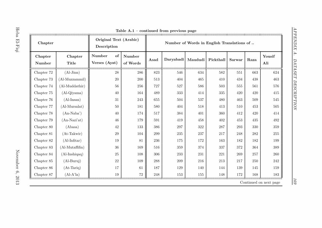
AP
PE
ND
IXA
.D
AT
AS
ET
DE
SC
RIP
TIO
N169
Table A.1 – continued from previous page
ChapterOriginal Text (Arabic)
DescriptionNumber of Words in English Translations of ..
Chapter
Number
Chapter
Title
Number of
Verses (Ayat)
Number
of WordsAsad Daryabadi Maududi Pickthall Sarwar Raza
Yousif
Ali
Chapter 72 (Al-Jinn) 28 286 823 546 634 582 551 663 624
Chapter 73 (Al-Muzzammil) 20 200 513 404 465 410 434 438 463
Chapter 74 (Al-Muddathir) 56 256 727 527 586 503 555 561 576
Chapter 75 (Al-Qiyama) 40 164 489 333 414 335 420 420 415
Chapter 76 (Al-Insan) 31 243 655 504 537 480 463 509 545
Chapter 77 (Al-Mursalat) 50 181 580 404 518 413 510 453 505
Chapter 78 (An-Naba’) 40 174 517 384 401 360 412 420 414
Chapter 79 (An-Nazi’at) 46 179 591 419 458 402 453 435 492
Chapter 80 (Abasa) 42 133 386 297 322 287 293 330 359
Chapter 81 (At-Takwir) 29 104 299 235 237 217 248 282 255
Chapter 82 (Al-Infitar) 19 81 236 175 172 163 182 182 199
Chapter 83 (Al-Mutaffifin) 36 169 516 359 374 337 372 364 389
Chapter 84 (Al-Inshiqaq) 25 108 306 233 231 221 269 257 260
Chapter 85 (Al-Buruj) 22 109 288 209 216 213 217 250 242
Chapter 86 (At-Tariq) 17 61 187 129 140 144 139 145 159
Chapter 87 (Al-A’la) 19 72 248 153 155 148 172 168 183
Continued on next page
Heb
aE
l-Fiq
iN
ovemb
er6,
2013
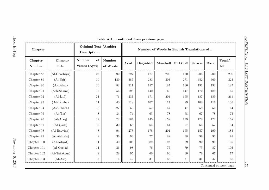
AP
PE
ND
IXA
.D
AT
AS
ET
DE
SC
RIP
TIO
N170
Table A.1 – continued from previous page
ChapterOriginal Text (Arabic)
DescriptionNumber of Words in English Translations of ..
Chapter
Number
Chapter
Title
Number of
Verses (Ayat)
Number
of WordsAsad Daryabadi Maududi Pickthall Sarwar Raza
Yousif
Ali
Chapter 88 (Al-Ghashiya) 26 92 227 177 200 160 205 200 200
Chapter 89 (Al-Fajr) 30 139 385 283 303 271 352 309 323
Chapter 90 (Al-Balad) 20 82 211 157 187 166 191 192 187
Chapter 91 (Ash-Shams) 15 54 195 140 160 147 172 189 165
Chapter 92 (Al-Lail) 21 71 237 171 201 165 187 189 211
Chapter 93 (Ad-Dhuha) 11 40 118 107 117 99 108 116 105
Chapter 94 (Ash-Sharh) 8 27 59 57 57 47 59 50 64
Chapter 95 (At-Tin) 8 34 74 63 78 68 67 78 73
Chapter 96 (Al-Alaq) 19 72 184 145 158 139 178 172 168
Chapter 97 (Al-Qadr) 5 30 66 64 61 57 65 57 54
Chapter 98 (Al-Bayyina) 8 94 273 178 204 165 157 190 183
Chapter 99 (Az-Zalzala) 8 36 93 77 88 68 99 93 91
Chapter 100 (Al-Adiyat) 11 40 105 89 93 89 92 99 105
Chapter 101 (Al-Qari’a) 11 36 98 76 75 79 75 87 103
Chapter 102 (At-Takathur) 8 28 95 60 96 60 79 67 77
Chapter 103 (Al-Asr) 3 14 42 31 36 31 31 47 36
Continued on next page
Heb
aE
l-Fiq
iN
ovemb
er6,
2013
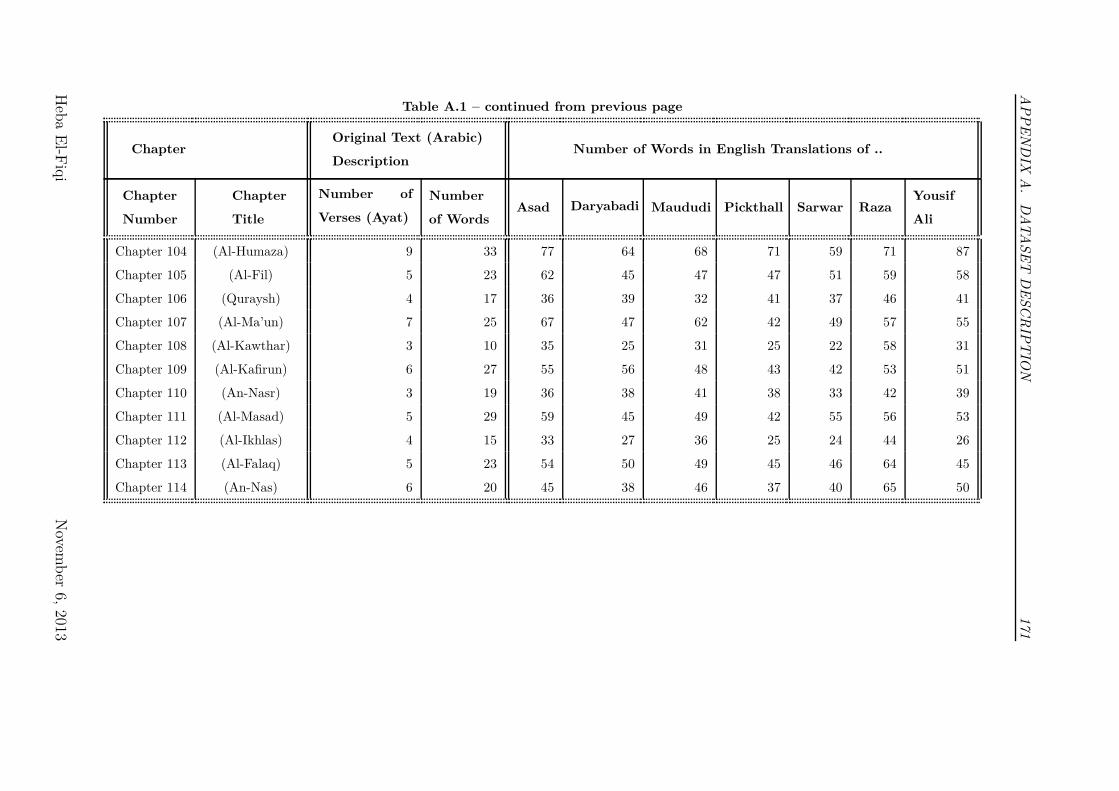
AP
PE
ND
IXA
.D
AT
AS
ET
DE
SC
RIP
TIO
N171
Table A.1 – continued from previous page
ChapterOriginal Text (Arabic)
DescriptionNumber of Words in English Translations of ..
Chapter
Number
Chapter
Title
Number of
Verses (Ayat)
Number
of WordsAsad Daryabadi Maududi Pickthall Sarwar Raza
Yousif
Ali
Chapter 104 (Al-Humaza) 9 33 77 64 68 71 59 71 87
Chapter 105 (Al-Fil) 5 23 62 45 47 47 51 59 58
Chapter 106 (Quraysh) 4 17 36 39 32 41 37 46 41
Chapter 107 (Al-Ma’un) 7 25 67 47 62 42 49 57 55
Chapter 108 (Al-Kawthar) 3 10 35 25 31 25 22 58 31
Chapter 109 (Al-Kafirun) 6 27 55 56 48 43 42 53 51
Chapter 110 (An-Nasr) 3 19 36 38 41 38 33 42 39
Chapter 111 (Al-Masad) 5 29 59 45 49 42 55 56 53
Chapter 112 (Al-Ikhlas) 4 15 33 27 36 25 24 44 26
Chapter 113 (Al-Falaq) 5 23 54 50 49 45 46 64 45
Chapter 114 (An-Nas) 6 20 45 38 46 37 40 65 50
Heb
aE
l-Fiq
iN
ovemb
er6,
2013
Appendix B
Most Frequent Words

AP
PE
ND
IXB
.M
OS
TF
RE
QU
EN
TW
OR
DS
173
Table B.1: Relative Frequency for the 40th Most Frequent Words for Each Trans-lator for the Entire Corpus
Asad Daryabadi Maududi Pickthall Sarwar Raza Yousif Ali
Ra
nk
Wo
rd
Rela
tiv
eF
req
uen
cy
Wo
rd
Rela
tiv
eF
req
uen
cy
Wo
rd
Rela
tiv
eF
req
uen
cy
Wo
rd
Rela
tiv
eF
req
uen
cy
Wo
rd
Rela
tiv
eF
req
uen
cy
Wo
rd
Rela
tiv
eF
req
uen
cy
Wo
rd
Rela
tiv
eF
req
uen
cy
1st and 0.0427 the 0.0573 the 0.0541 the 0.0547 the 0.0646 the 0.0622 the 0.0520
2nd the 0.0399 and 0.0571 and 0.0426 and 0.0535 and 0.0342 and 0.0551 and 0.0451
3rd of 0.0313 of 0.0283 to 0.0280 of 0.0309 of 0.0321 of 0.0263 of 0.0326
4th to 0.0281 is 0.0215 of 0.0273 is 0.0240 to 0.0262 is 0.0243 to 0.0257
5th a 0.0209 a 0.0197 you 0.0245 a 0.0185 you 0.0245 you 0.0233 a 0.0196
6th in 0.0181 they 0.0178 a 0.0193 that 0.0173 will 0.0225 to 0.0184 in 0.0182
7th that 0.0166 that 0.0169 is 0.0183 they 0.0166 god 0.0176 will 0.0153 is 0.0182
8th is 0.0165 he 0.0166 that 0.0164 allah 0.0156 is 0.0167 in 0.0152 will 0.0167
9th you 0.0162 allah 0.0140 they 0.0158 he 0.0155 a 0.0165 allah 0.0151 that 0.0155
10th who 0.0147 them 0.0135 allah 0.0147 them 0.0143 they 0.0156 they 0.0151 they 0.0155
11th they 0.0146 in 0.0125 in 0.0144 in 0.0136 have 0.0136 a 0.0148 allah 0.0155
12th it 0.0133 who 0.0125 will 0.0138 who 0.0131 in 0.0133 it 0.0135 he 0.0137
13th god 0.0131 shall 0.0123 he 0.0135 will 0.0129 them 0.0122 them 0.0132 for 0.0133
14th will 0.0126 be 0.0123 them 0.0132 it 0.0126 who 0.0118 he 0.0116 ye 0.0129
15th for 0.0120 unto 0.0122 it 0.0127 ye 0.0123 be 0.0114 for 0.0116 them 0.0127
16th he 0.0115 we 0.0120 who 0.0116 to 0.0120 he 0.0114 who 0.0115 it 0.0113
Continued on next page
Heb
aE
l-Fiq
iN
ovemb
er6,
2013
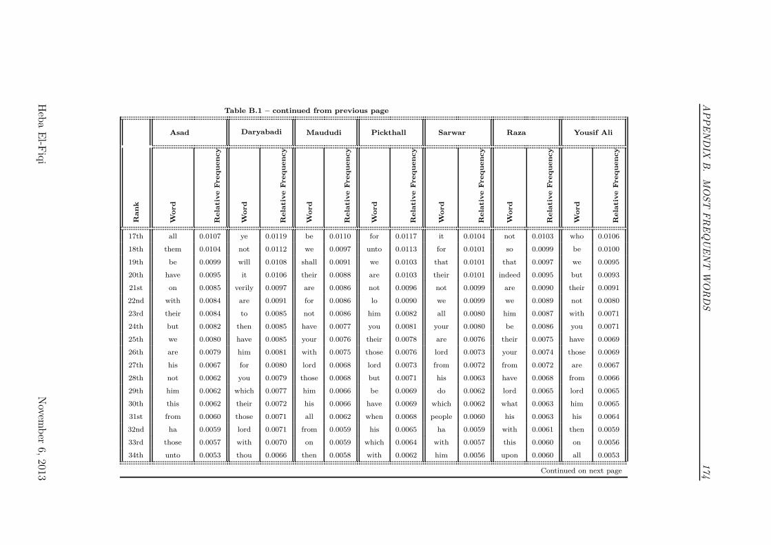
AP
PE
ND
IXB
.M
OS
TF
RE
QU
EN
TW
OR
DS
174
Table B.1 – continued from previous page
Asad Daryabadi Maududi Pickthall Sarwar Raza Yousif AliR
an
k
Wo
rd
Rela
tiv
eF
req
uen
cy
Wo
rd
Rela
tiv
eF
req
uen
cy
Wo
rd
Rela
tiv
eF
req
uen
cy
Wo
rd
Rela
tiv
eF
req
uen
cy
Wo
rd
Rela
tiv
eF
req
uen
cy
Wo
rd
Rela
tiv
eF
req
uen
cy
Wo
rd
Rela
tiv
eF
req
uen
cy
17th all 0.0107 ye 0.0119 be 0.0110 for 0.0117 it 0.0104 not 0.0103 who 0.0106
18th them 0.0104 not 0.0112 we 0.0097 unto 0.0113 for 0.0101 so 0.0099 be 0.0100
19th be 0.0099 will 0.0108 shall 0.0091 we 0.0103 that 0.0101 that 0.0097 we 0.0095
20th have 0.0095 it 0.0106 their 0.0088 are 0.0103 their 0.0101 indeed 0.0095 but 0.0093
21st on 0.0085 verily 0.0097 are 0.0086 not 0.0096 not 0.0099 are 0.0090 their 0.0091
22nd with 0.0084 are 0.0091 for 0.0086 lo 0.0090 we 0.0099 we 0.0089 not 0.0080
23rd their 0.0084 to 0.0085 not 0.0086 him 0.0082 all 0.0080 him 0.0087 with 0.0071
24th but 0.0082 then 0.0085 have 0.0077 you 0.0081 your 0.0080 be 0.0086 you 0.0071
25th we 0.0080 have 0.0085 your 0.0076 their 0.0078 are 0.0076 their 0.0075 have 0.0069
26th are 0.0079 him 0.0081 with 0.0075 those 0.0076 lord 0.0073 your 0.0074 those 0.0069
27th his 0.0067 for 0.0080 lord 0.0068 lord 0.0073 from 0.0072 from 0.0072 are 0.0067
28th not 0.0062 you 0.0079 those 0.0068 but 0.0071 his 0.0063 have 0.0068 from 0.0066
29th him 0.0062 which 0.0077 him 0.0066 be 0.0069 do 0.0062 lord 0.0065 lord 0.0065
30th this 0.0062 their 0.0072 his 0.0066 have 0.0069 which 0.0062 what 0.0063 him 0.0065
31st from 0.0060 those 0.0071 all 0.0062 when 0.0068 people 0.0060 his 0.0063 his 0.0064
32nd ha 0.0059 lord 0.0071 from 0.0059 his 0.0065 ha 0.0059 with 0.0061 then 0.0059
33rd those 0.0057 with 0.0070 on 0.0059 which 0.0064 with 0.0057 this 0.0060 on 0.0056
34th unto 0.0053 thou 0.0066 then 0.0058 with 0.0062 him 0.0056 upon 0.0060 all 0.0053
Continued on next page
Heb
aE
l-Fiq
iN
ovemb
er6,
2013
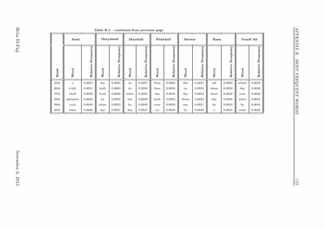
AP
PE
ND
IXB
.M
OS
TF
RE
QU
EN
TW
OR
DS
175
Table B.1 – continued from previous page
Asad Daryabadi Maududi Pickthall Sarwar Raza Yousif Ali
Ra
nk
Wo
rd
Rela
tiv
eF
req
uen
cy
Wo
rd
Rela
tiv
eF
req
uen
cy
Wo
rd
Rela
tiv
eF
req
uen
cy
Wo
rd
Rela
tiv
eF
req
uen
cy
Wo
rd
Rela
tiv
eF
req
uen
cy
Wo
rd
Rela
tiv
eF
req
uen
cy
Wo
rd
Rela
tiv
eF
req
uen
cy
35th s 0.0053 his 0.0065 so 0.0057 from 0.0062 this 0.0055 all 0.0060 which 0.0049
36th truth 0.0051 hath 0.0063 do 0.0056 then 0.0054 on 0.0054 when 0.0059 day 0.0048
37th shall 0.0050 from 0.0058 when 0.0054 day 0.0054 day 0.0054 those 0.0058 your 0.0046
38th sustainer 0.0049 on 0.0052 but 0.0050 hath 0.0054 those 0.0053 day 0.0056 when 0.0045
39th your 0.0048 when 0.0052 ha 0.0048 your 0.0050 one 0.0051 do 0.0054 by 0.0044
40th what 0.0046 day 0.0051 day 0.0047 on 0.0048 by 0.0049 o 0.0045 what 0.0043
Heb
aE
l-Fiq
iN
ovemb
er6,
2013

Appendix C
5D Decision Trees Analysis
-(1000.0/5000.0)
Figure C.1: C4.5 Decision Tree for Noise Free 5D(EXP1)
R(V2(p1), {V2(p1), V2(p2)} = min :
| R(V5(p1), {V5(p1), V5(p2)} = min :
| | R(V1(p1), {V1(p1), V1(p2)} = min :
| | | R(V3(p1), {V3(p1), V3(p2)} = min :
| | | | R(V4(p1), {V4(p1), V4(p2)} = min : p1 → −, p2 → + (73.0)
| | | | R(V4(p1), {V4(p1), V4(p2)} = max : p1 → +, p2 → − (15.0)
| | | R(V3(p1), {V3(p1), V3(p2)} = max :
| | | | R(V4(p1), {V4(p1), V4(p2)} = min : p1 → +, p2 → − (16.0)
| | | | R(V4(p1), {V4(p1), V4(p2)} = max : p1 → −, p2 → + (11.0)
| | R(V1(p1), {V1(p1), V1(p2)} = max :
| | | R(V4(p1), {V4(p1), V4(p2)} = min :
| | | | R(V3(p1), {V3(p1), V3(p2)} = min : p1 → +, p2 → − (17.0)
| | | | R(V3(p1), {V3(p1), V3(p2)} = max : p1 → −, p2 → + (5.0)
| | | R(V4(p1), {V4(p1), V4(p2)} = max :
| | | | R(V3(p1), {V3(p1), V3(p2)} = min : p1 → −, p2 → + (8.0)
| | | | R(V3(p1), {V3(p1), V3(p2)} = max : p1 → +, p2 → − (10.0)
| R(V5(p1), {V5(p1), V5(p2)} = max :
| | R(V1(p1), {V1(p1), V1(p2)} = min :
| | | R(V4(p1), {V4(p1), V4(p2)} = min :
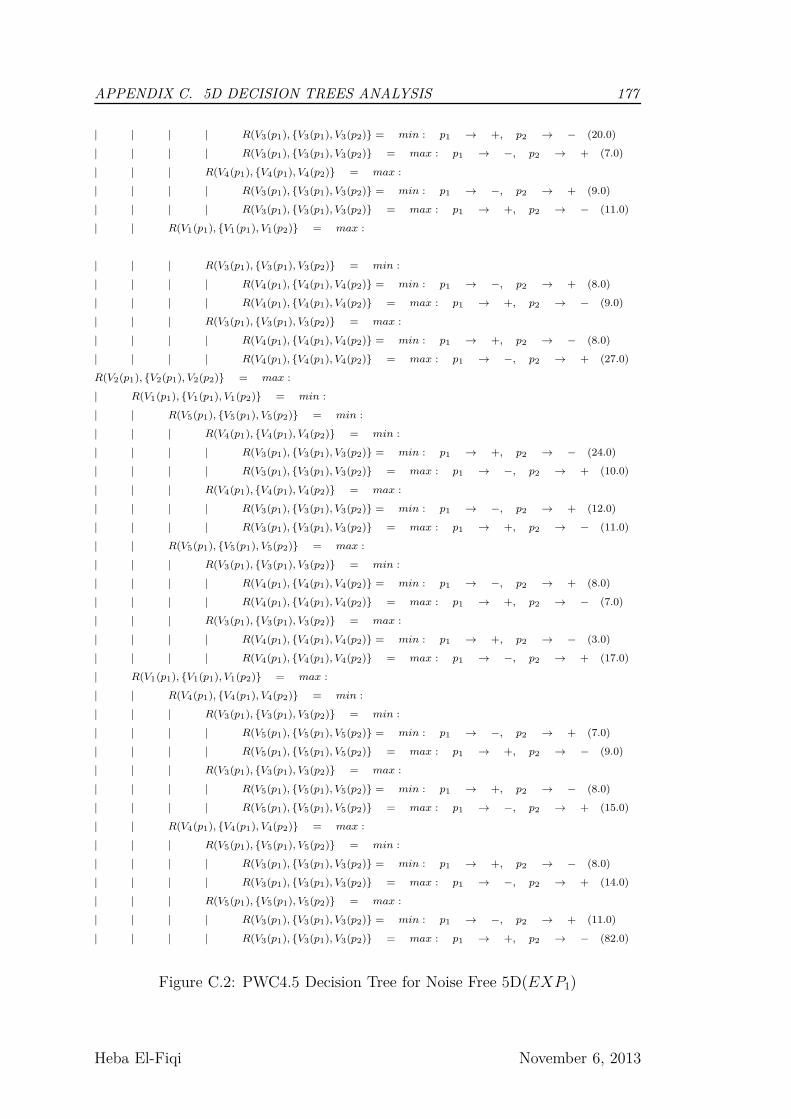
APPENDIX C. 5D DECISION TREES ANALYSIS 177
| | | | R(V3(p1), {V3(p1), V3(p2)} = min : p1 → +, p2 → − (20.0)
| | | | R(V3(p1), {V3(p1), V3(p2)} = max : p1 → −, p2 → + (7.0)
| | | R(V4(p1), {V4(p1), V4(p2)} = max :
| | | | R(V3(p1), {V3(p1), V3(p2)} = min : p1 → −, p2 → + (9.0)
| | | | R(V3(p1), {V3(p1), V3(p2)} = max : p1 → +, p2 → − (11.0)
| | R(V1(p1), {V1(p1), V1(p2)} = max :
| | | R(V3(p1), {V3(p1), V3(p2)} = min :
| | | | R(V4(p1), {V4(p1), V4(p2)} = min : p1 → −, p2 → + (8.0)
| | | | R(V4(p1), {V4(p1), V4(p2)} = max : p1 → +, p2 → − (9.0)
| | | R(V3(p1), {V3(p1), V3(p2)} = max :
| | | | R(V4(p1), {V4(p1), V4(p2)} = min : p1 → +, p2 → − (8.0)
| | | | R(V4(p1), {V4(p1), V4(p2)} = max : p1 → −, p2 → + (27.0)
R(V2(p1), {V2(p1), V2(p2)} = max :
| R(V1(p1), {V1(p1), V1(p2)} = min :
| | R(V5(p1), {V5(p1), V5(p2)} = min :
| | | R(V4(p1), {V4(p1), V4(p2)} = min :
| | | | R(V3(p1), {V3(p1), V3(p2)} = min : p1 → +, p2 → − (24.0)
| | | | R(V3(p1), {V3(p1), V3(p2)} = max : p1 → −, p2 → + (10.0)
| | | R(V4(p1), {V4(p1), V4(p2)} = max :
| | | | R(V3(p1), {V3(p1), V3(p2)} = min : p1 → −, p2 → + (12.0)
| | | | R(V3(p1), {V3(p1), V3(p2)} = max : p1 → +, p2 → − (11.0)
| | R(V5(p1), {V5(p1), V5(p2)} = max :
| | | R(V3(p1), {V3(p1), V3(p2)} = min :
| | | | R(V4(p1), {V4(p1), V4(p2)} = min : p1 → −, p2 → + (8.0)
| | | | R(V4(p1), {V4(p1), V4(p2)} = max : p1 → +, p2 → − (7.0)
| | | R(V3(p1), {V3(p1), V3(p2)} = max :
| | | | R(V4(p1), {V4(p1), V4(p2)} = min : p1 → +, p2 → − (3.0)
| | | | R(V4(p1), {V4(p1), V4(p2)} = max : p1 → −, p2 → + (17.0)
| R(V1(p1), {V1(p1), V1(p2)} = max :
| | R(V4(p1), {V4(p1), V4(p2)} = min :
| | | R(V3(p1), {V3(p1), V3(p2)} = min :
| | | | R(V5(p1), {V5(p1), V5(p2)} = min : p1 → −, p2 → + (7.0)
| | | | R(V5(p1), {V5(p1), V5(p2)} = max : p1 → +, p2 → − (9.0)
| | | R(V3(p1), {V3(p1), V3(p2)} = max :
| | | | R(V5(p1), {V5(p1), V5(p2)} = min : p1 → +, p2 → − (8.0)
| | | | R(V5(p1), {V5(p1), V5(p2)} = max : p1 → −, p2 → + (15.0)
| | R(V4(p1), {V4(p1), V4(p2)} = max :
| | | R(V5(p1), {V5(p1), V5(p2)} = min :
| | | | R(V3(p1), {V3(p1), V3(p2)} = min : p1 → +, p2 → − (8.0)
| | | | R(V3(p1), {V3(p1), V3(p2)} = max : p1 → −, p2 → + (14.0)
| | | R(V5(p1), {V5(p1), V5(p2)} = max :
| | | | R(V3(p1), {V3(p1), V3(p2)} = min : p1 → −, p2 → + (11.0)
| | | | R(V3(p1), {V3(p1), V3(p2)} = max : p1 → +, p2 → − (82.0)
Figure C.2: PWC4.5 Decision Tree for Noise Free 5D(EXP1)
Heba El-Fiqi November 6, 2013
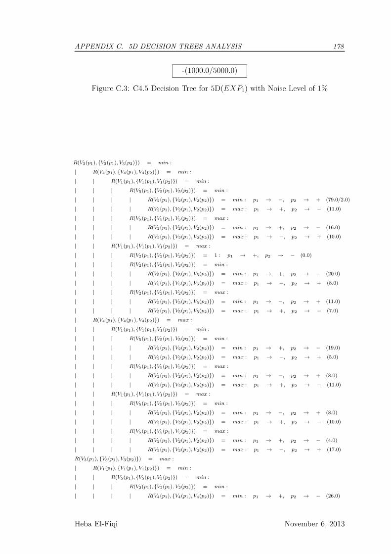
APPENDIX C. 5D DECISION TREES ANALYSIS 178
-(1000.0/5000.0)
Figure C.3: C4.5 Decision Tree for 5D(EXP1) with Noise Level of 1%
R(V3(p1), {V3(p1), V3(p2)}) = min :
| R(V4(p1), {V4(p1), V4(p2)}) = min :
| | R(V1(p1), {V1(p1), V1(p2)}) = min :
| | | R(V5(p1), {V5(p1), V5(p2)}) = min :
| | | | R(V2(p1), {V2(p1), V2(p2)}) = min : p1 → −, p2 → + (79.0/2.0)
| | | | R(V2(p1), {V2(p1), V2(p2)}) = max : p1 → +, p2 → − (11.0)
| | | R(V5(p1), {V5(p1), V5(p2)}) = max :
| | | | R(V2(p1), {V2(p1), V2(p2)}) = min : p1 → +, p2 → − (16.0)
| | | | R(V2(p1), {V2(p1), V2(p2)}) = max : p1 → −, p2 → + (10.0)
| | R(V1(p1), {V1(p1), V1(p2)}) = max :
| | | R(V2(p1), {V2(p1), V2(p2)}) = 1 : p1 → +, p2 → − (0.0)
| | | R(V2(p1), {V2(p1), V2(p2)}) = min :
| | | | R(V5(p1), {V5(p1), V5(p2)}) = min : p1 → +, p2 → − (20.0)
| | | | R(V5(p1), {V5(p1), V5(p2)}) = max : p1 → −, p2 → + (8.0)
| | | R(V2(p1), {V2(p1), V2(p2)}) = max :
| | | | R(V5(p1), {V5(p1), V5(p2)}) = min : p1 → −, p2 → + (11.0)
| | | | R(V5(p1), {V5(p1), V5(p2)}) = max : p1 → +, p2 → − (7.0)
| R(V4(p1), {V4(p1), V4(p2)}) = max :
| | R(V1(p1), {V1(p1), V1(p2)}) = min :
| | | R(V5(p1), {V5(p1), V5(p2)}) = min :
| | | | R(V2(p1), {V2(p1), V2(p2)}) = min : p1 → +, p2 → − (19.0)
| | | | R(V2(p1), {V2(p1), V2(p2)}) = max : p1 → −, p2 → + (5.0)
| | | R(V5(p1), {V5(p1), V5(p2)}) = max :
| | | | R(V2(p1), {V2(p1), V2(p2)}) = min : p1 → −, p2 → + (8.0)
| | | | R(V2(p1), {V2(p1), V2(p2)}) = max : p1 → +, p2 → − (11.0)
| | R(V1(p1), {V1(p1), V1(p2)}) = max :
| | | R(V5(p1), {V5(p1), V5(p2)}) = min :
| | | | R(V2(p1), {V2(p1), V2(p2)}) = min : p1 → −, p2 → + (8.0)
| | | | R(V2(p1), {V2(p1), V2(p2)}) = max : p1 → +, p2 → − (10.0)
| | | R(V5(p1), {V5(p1), V5(p2)}) = max :
| | | | R(V2(p1), {V2(p1), V2(p2)}) = min : p1 → +, p2 → − (4.0)
| | | | R(V2(p1), {V2(p1), V2(p2)}) = max : p1 → −, p2 → + (17.0)
R(V3(p1), {V3(p1), V3(p2)}) = max :
| R(V1(p1), {V1(p1), V1(p2)}) = min :
| | R(V5(p1), {V5(p1), V5(p2)}) = min :
| | | R(V2(p1), {V2(p1), V2(p2)}) = min :
| | | | R(V4(p1), {V4(p1), V4(p2)}) = min : p1 → +, p2 → − (26.0)
Heba El-Fiqi November 6, 2013
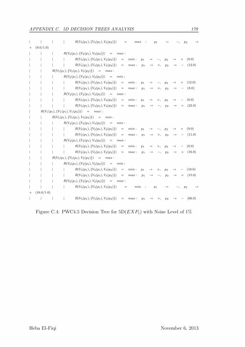
APPENDIX C. 5D DECISION TREES ANALYSIS 179
| | | | R(V4(p1), {V4(p1), V4(p2)}) = max : p1 → −, p2 →
+ (9.0/1.0)
| | | R(V2(p1), {V2(p1), V2(p2)}) = max :
| | | | R(V4(p1), {V4(p1), V4(p2)}) = min : p1 → −, p2 → + (8.0)
| | | | R(V4(p1), {V4(p1), V4(p2)}) = max : p1 → +, p2 → − (12.0)
| | R(V5(p1), {V5(p1), V5(p2)}) = max :
| | | R(V2(p1), {V2(p1), V2(p2)}) = min :
| | | | R(V4(p1), {V4(p1), V4(p2)}) = min : p1 → −, p2 → + (12.0)
| | | | R(V4(p1), {V4(p1), V4(p2)}) = max : p1 → +, p2 → − (8.0)
| | | R(V2(p1), {V2(p1), V2(p2)}) = max :
| | | | R(V4(p1), {V4(p1), V4(p2)}) = min : p1 → +, p2 → − (8.0)
| | | | R(V4(p1), {V4(p1), V4(p2)}) = max : p1 → −, p2 → + (22.0)
| R(V1(p1), {V1(p1), V1(p2)}) = max :
| | R(V5(p1), {V5(p1), V5(p2)}) = min :
| | | R(V4(p1), {V4(p1), V4(p2)}) = min :
| | | | R(V2(p1), {V2(p1), V2(p2)}) = min : p1 → −, p2 → + (9.0)
| | | | R(V2(p1), {V2(p1), V2(p2)}) = max : p1 → +, p2 → − (11.0)
| | | R(V4(p1), {V4(p1), V4(p2)}) = max :
| | | | R(V2(p1), {V2(p1), V2(p2)}) = min : p1 → +, p2 → − (8.0)
| | | | R(V2(p1), {V2(p1), V2(p2)}) = max : p1 → −, p2 → + (16.0)
| | R(V5(p1), {V5(p1), V5(p2)}) = max :
| | | R(V2(p1), {V2(p1), V2(p2)}) = min :
| | | | R(V4(p1), {V4(p1), V4(p2)}) = min : p1 → +, p2 → − (10.0)
| | | | R(V4(p1), {V4(p1), V4(p2)}) = max : p1 → −, p2 → + (15.0)
| | | R(V2(p1), {V2(p1), V2(p2)}) = max :
| | | | R(V4(p1), {V4(p1), V4(p2)}) = min : p1 → −, p2 →
+ (16.0/1.0)
| | | | R(V4(p1), {V4(p1), V4(p2)}) = max : p1 → +, p2 → − (66.0)
Figure C.4: PWC4.5 Decision Tree for 5D(EXP1) with Noise Level of 1%
Heba El-Fiqi November 6, 2013

APPENDIX C. 5D DECISION TREES ANALYSIS 180
-(1000.0/5000.0)
Figure C.5: C4.5 Decision Tree for 5D(EXP1) with Noise Level of 2.5%
R(V5(p1), {V5(p1), V5(p2)} = min :
| V 1 = min :
| | R(V2(p1), {V2(p1), V2(p2)} = min :
| | | R(V4(p1), {V4(p1), V4(p2)} = min :
| | | | R(V3(p1), {V3(p1), V3(p2)} = min : p1 → −, p2 → + (75.0/2.0)
| | | | R(V3(p1), {V3(p1), V3(p2)} = max : p1 → +, p2 → − (12.0)
| | | R(V4(p1), {V4(p1), V4(p2)} = max :
| | | | R(V3(p1), {V3(p1), V3(p2)} = min : p1 → +, p2 → − (14.0)
| | | | R(V3(p1), {V3(p1), V3(p2)} = max : p1 → −, p2 → + (8.0/1.0)
| | R(V2(p1), {V2(p1), V2(p2)} = max :
| | | R(V3(p1), {V3(p1), V3(p2)} = min :
| | | | R(V4(p1), {V4(p1), V4(p2)} = min : p1 → +, p2 → − (19.0)
| | | | R(V4(p1), {V4(p1), V4(p2)} = max : p1 → −, p2 → + (7.0/1.0)
| | | R(V3(p1), {V3(p1), V3(p2)} = max :
| | | | R(V4(p1), {V4(p1), V4(p2)} = min : p1 → −, p2 → + (15.0/2.0)
| | | | R(V4(p1), {V4(p1), V4(p2)} = max : p1 → +, p2 → − (6.0)
| V 1 = max :
| | R(V3(p1), {V3(p1), V3(p2)} = min :
| | | R(V2(p1), {V2(p1), V2(p2)} = min :
| | | | R(V4(p1), {V4(p1), V4(p2)} = min : p1 → +, p2 → − (31.0)
| | | | R(V4(p1), {V4(p1), V4(p2)} = max : p1 → −, p2 → + (7.0/1.0)
| | | R(V2(p1), {V2(p1), V2(p2)} = max :
| | | | R(V4(p1), {V4(p1), V4(p2)} = min : p1 → −, p2 → + (7.0)
| | | | R(V4(p1), {V4(p1), V4(p2)} = max : p1 → +, p2 → − (9.0)
| | R(V3(p1), {V3(p1), V3(p2)} = max :
| | | R(V2(p1), {V2(p1), V2(p2)} = min :
| | | | R(V4(p1), {V4(p1), V4(p2)} = min : p1 → −, p2 → + (8.0)
| | | | R(V4(p1), {V4(p1), V4(p2)} = max : p1 → +, p2 → − (8.0)
| | | R(V2(p1), {V2(p1), V2(p2)} = max :
| | | | R(V4(p1), {V4(p1), V4(p2)} = min : p1 → +, p2 → − (7.0)
| | | | R(V4(p1), {V4(p1), V4(p2)} = max : p1 → −, p2 → + (19.0)
R(V5(p1), {V5(p1), V5(p2)} = max :
| R(V2(p1), {V2(p1), V2(p2)} = min :
| | R(V4(p1), {V4(p1), V4(p2)} = min :
| | | V 1 = min :
| | | | R(V3(p1), {V3(p1), V3(p2)} = min : p1 → +, p2 → − (11.0)
| | | | R(V3(p1), {V3(p1), V3(p2)} = max : p1 → −, p2 → + (4.0)
| | | V 1 = max :
Heba El-Fiqi November 6, 2013
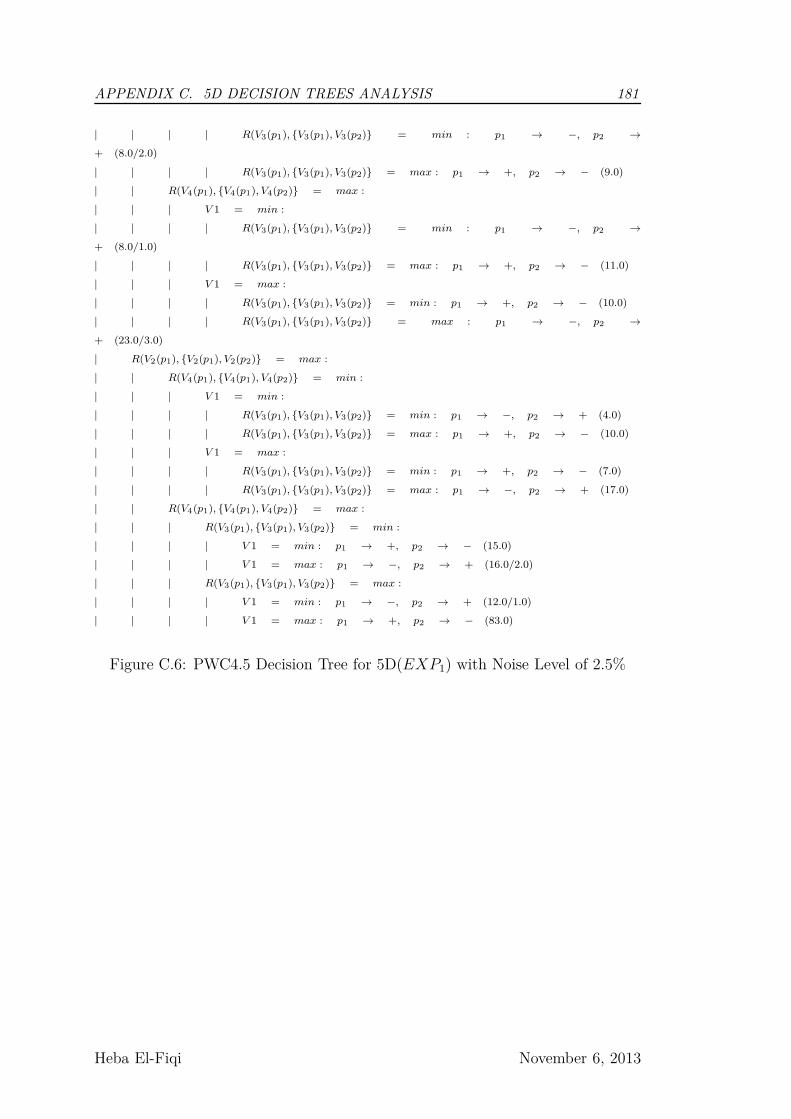
APPENDIX C. 5D DECISION TREES ANALYSIS 181
| | | | R(V3(p1), {V3(p1), V3(p2)} = min : p1 → −, p2 →
+ (8.0/2.0)
| | | | R(V3(p1), {V3(p1), V3(p2)} = max : p1 → +, p2 → − (9.0)
| | R(V4(p1), {V4(p1), V4(p2)} = max :
| | | V 1 = min :
| | | | R(V3(p1), {V3(p1), V3(p2)} = min : p1 → −, p2 →
+ (8.0/1.0)
| | | | R(V3(p1), {V3(p1), V3(p2)} = max : p1 → +, p2 → − (11.0)
| | | V 1 = max :
| | | | R(V3(p1), {V3(p1), V3(p2)} = min : p1 → +, p2 → − (10.0)
| | | | R(V3(p1), {V3(p1), V3(p2)} = max : p1 → −, p2 →
+ (23.0/3.0)
| R(V2(p1), {V2(p1), V2(p2)} = max :
| | R(V4(p1), {V4(p1), V4(p2)} = min :
| | | V 1 = min :
| | | | R(V3(p1), {V3(p1), V3(p2)} = min : p1 → −, p2 → + (4.0)
| | | | R(V3(p1), {V3(p1), V3(p2)} = max : p1 → +, p2 → − (10.0)
| | | V 1 = max :
| | | | R(V3(p1), {V3(p1), V3(p2)} = min : p1 → +, p2 → − (7.0)
| | | | R(V3(p1), {V3(p1), V3(p2)} = max : p1 → −, p2 → + (17.0)
| | R(V4(p1), {V4(p1), V4(p2)} = max :
| | | R(V3(p1), {V3(p1), V3(p2)} = min :
| | | | V 1 = min : p1 → +, p2 → − (15.0)
| | | | V 1 = max : p1 → −, p2 → + (16.0/2.0)
| | | R(V3(p1), {V3(p1), V3(p2)} = max :
| | | | V 1 = min : p1 → −, p2 → + (12.0/1.0)
| | | | V 1 = max : p1 → +, p2 → − (83.0)
Figure C.6: PWC4.5 Decision Tree for 5D(EXP1) with Noise Level of 2.5%
Heba El-Fiqi November 6, 2013

APPENDIX C. 5D DECISION TREES ANALYSIS 182
-(1000.0/5000.0)
Figure C.7: C4.5 Decision Tree for 5D(EXP1) with Noise Level of 5%
R(V2(p1), {V2(p1), V2(p2)} = min :
| R(V4(p1), {V4(p1), V4(p2)} = min :
| | R(V3(p1), {V3(p1), V3(p2)} = min :
| | | R(V1(p1), {V1(p1), V1(p2)} = min :
| | | | R(V5(p1), {V5(p1), V5(p2)} = min : p1 → −, p2 → + (85.0/11.0)
| | | | R(V5(p1), {V5(p1), V5(p2)} = max : p1 → +, p2 → − (14.0)
| | | R(V1(p1), {V1(p1), V1(p2)} = max :
| | | | R(V5(p1), {V5(p1), V5(p2)} = min : p1 → +, p2 → − (21.0)
| | | | R(V5(p1), {V5(p1), V5(p2)} = max : p1 → −, p2 → + (13.0/1.0)
| | R(V3(p1), {V3(p1), V3(p2)} = max :
| | | R(V1(p1), {V1(p1), V1(p2)} = min :
| | | | R(V5(p1), {V5(p1), V5(p2)} = min : p1 → +, p2 → − (19.0)
| | | | R(V5(p1), {V5(p1), V5(p2)} = max : p1 → −, p2 → + (6.0/1.0)
| | | R(V1(p1), {V1(p1), V1(p2)} = max :
| | | | R(V5(p1), {V5(p1), V5(p2)} = min : p1 → −, p2 → + (12.0)
| | | | R(V5(p1), {V5(p1), V5(p2)} = max : p1 → +, p2 → − (7.0)
| R(V4(p1), {V4(p1), V4(p2)} = max :
| | R(V3(p1), {V3(p1), V3(p2)} = min :
| | | R(V5(p1), {V5(p1), V5(p2)} = min :
| | | | R(V1(p1), {V1(p1), V1(p2)} = min : p1 → +, p2 → − (29.0)
| | | | R(V1(p1), {V1(p1), V1(p2)} = max : p1 → −, p2 → + (7.0/1.0)
| | | R(V5(p1), {V5(p1), V5(p2)} = max :
| | | | R(V1(p1), {V1(p1), V1(p2)} = min : p1 → −, p2 → + (9.0/1.0)
| | | | R(V1(p1), {V1(p1), V1(p2)} = max : p1 → +, p2 → − (9.0)
| | R(V3(p1), {V3(p1), V3(p2)} = max :
| | | R(V1(p1), {V1(p1), V1(p2)} = min :
| | | | R(V5(p1), {V5(p1), V5(p2)} = min : p1 → −, p2 → + (7.0)
| | | | R(V5(p1), {V5(p1), V5(p2)} = max : p1 → +, p2 → − (9.0)
| | | R(V1(p1), {V1(p1), V1(p2)} = max :
| | | | R(V5(p1), {V5(p1), V5(p2)} = min : p1 → +, p2 → − (8.0)
| | | | R(V5(p1), {V5(p1), V5(p2)} = max : p1 → −, p2 → + (20.0/2.0)
R(V2(p1), {V2(p1), V2(p2)} = max :
| R(V5(p1), {V5(p1), V5(p2)} = min :
| | R(V4(p1), {V4(p1), V4(p2)} = min :
| | | R(V1(p1), {V1(p1), V1(p2)} = min :
| | | | R(V3(p1), {V3(p1), V3(p2)} = min : p1 → +, p2 → − (19.0)
| | | | R(V3(p1), {V3(p1), V3(p2)} = max : p1 → −, p2 → + (4.0)
Heba El-Fiqi November 6, 2013

APPENDIX C. 5D DECISION TREES ANALYSIS 183
| | | R(V1(p1), {V1(p1), V1(p2)} = max :
| | | | R(V3(p1), {V3(p1), V3(p2)} = min : p1 → −, p2 →
+ (7.0/1.0)
| | | | R(V3(p1), {V3(p1), V3(p2)} = max : p1 → +, p2 → − (9.0)
| | R(V4(p1), {V4(p1), V4(p2)} = max :
| | | R(V1(p1), {V1(p1), V1(p2)} = min :
| | | | R(V3(p1), {V3(p1), V3(p2)} = min : p1 → −, p2 → + (7.0)
| | | | R(V3(p1), {V3(p1), V3(p2)} = max : p1 → +, p2 → − (8.0)
| | | R(V1(p1), {V1(p1), V1(p2)} = max :
| | | | R(V3(p1), {V3(p1), V3(p2)} = min : p1 → +, p2 → − (5.0)
| | | | R(V3(p1), {V3(p1), V3(p2)} = max : p1 → −, p2 → + (19.0)
| R(V5(p1), {V5(p1), V5(p2)} = max :
| | R(V3(p1), {V3(p1), V3(p2)} = min :
| | | R(V4(p1), {V4(p1), V4(p2)} = min :
| | | | R(V1(p1), {V1(p1), V1(p2)} = min : p1 → −, p2 →
+ (9.0/3.0)
| | | | R(V1(p1), {V1(p1), V1(p2)} = max : p1 → +, p2 → − (9.0)
| | | R(V4(p1), {V4(p1), V4(p2)} = max :
| | | | R(V1(p1), {V1(p1), V1(p2)} = min : p1 → +, p2 → − (5.0)
| | | | R(V1(p1), {V1(p1), V1(p2)} = max : p1 → −, p2 →
+ (17.0/1.0)
| | R(V3(p1), {V3(p1), V3(p2)} = max :
| | | R(V4(p1), {V4(p1), V4(p2)} = 1 : p1 → +, p2 → − (0.0)
| | | R(V4(p1), {V4(p1), V4(p2)} = min :
| | | | R(V1(p1), {V1(p1), V1(p2)} = min : p1 → +, p2 → − (8.0)
| | | | R(V1(p1), {V1(p1), V1(p2)} = max : p1 → −, p2 → + (12.0)
| | | R(V4(p1), {V4(p1), V4(p2)} = max :
| | | | R(V1(p1), {V1(p1), V1(p2)} = min : p1 → −, p2 →
+ (13.0/1.0)
| | | | R(V1(p1), {V1(p1), V1(p2)} = max : p1 → +, p2 → − (74.0)
Figure C.8: PWC4.5 Decision Tree for 5D(EXP1) with Noise Level of 5%
Heba El-Fiqi November 6, 2013
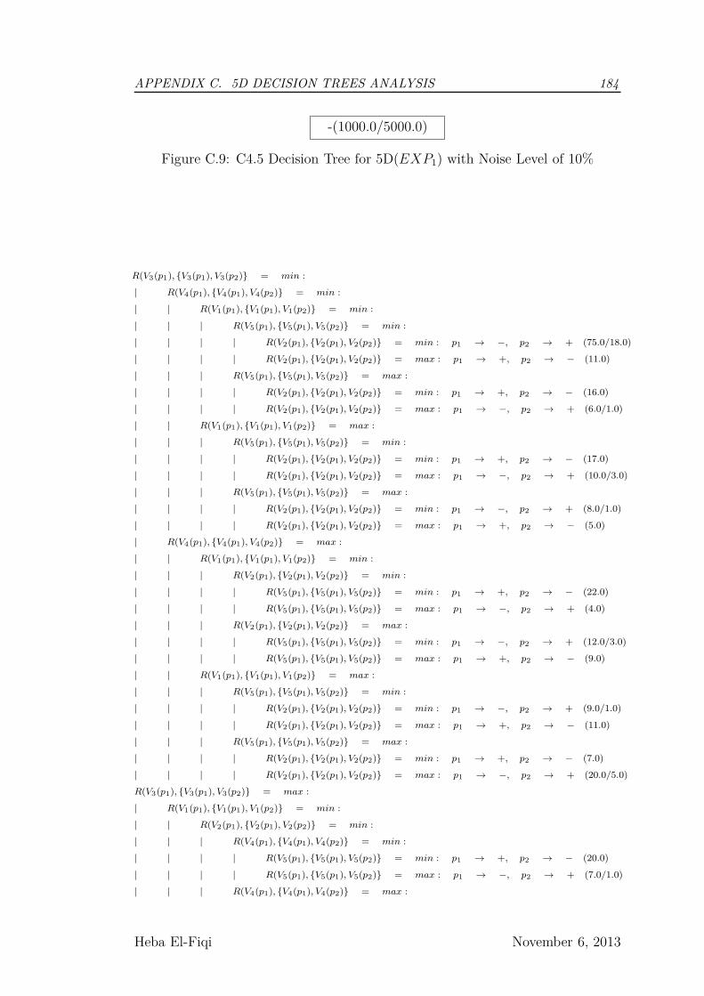
APPENDIX C. 5D DECISION TREES ANALYSIS 184
-(1000.0/5000.0)
Figure C.9: C4.5 Decision Tree for 5D(EXP1) with Noise Level of 10%
R(V3(p1), {V3(p1), V3(p2)} = min :
| R(V4(p1), {V4(p1), V4(p2)} = min :
| | R(V1(p1), {V1(p1), V1(p2)} = min :
| | | R(V5(p1), {V5(p1), V5(p2)} = min :
| | | | R(V2(p1), {V2(p1), V2(p2)} = min : p1 → −, p2 → + (75.0/18.0)
| | | | R(V2(p1), {V2(p1), V2(p2)} = max : p1 → +, p2 → − (11.0)
| | | R(V5(p1), {V5(p1), V5(p2)} = max :
| | | | R(V2(p1), {V2(p1), V2(p2)} = min : p1 → +, p2 → − (16.0)
| | | | R(V2(p1), {V2(p1), V2(p2)} = max : p1 → −, p2 → + (6.0/1.0)
| | R(V1(p1), {V1(p1), V1(p2)} = max :
| | | R(V5(p1), {V5(p1), V5(p2)} = min :
| | | | R(V2(p1), {V2(p1), V2(p2)} = min : p1 → +, p2 → − (17.0)
| | | | R(V2(p1), {V2(p1), V2(p2)} = max : p1 → −, p2 → + (10.0/3.0)
| | | R(V5(p1), {V5(p1), V5(p2)} = max :
| | | | R(V2(p1), {V2(p1), V2(p2)} = min : p1 → −, p2 → + (8.0/1.0)
| | | | R(V2(p1), {V2(p1), V2(p2)} = max : p1 → +, p2 → − (5.0)
| R(V4(p1), {V4(p1), V4(p2)} = max :
| | R(V1(p1), {V1(p1), V1(p2)} = min :
| | | R(V2(p1), {V2(p1), V2(p2)} = min :
| | | | R(V5(p1), {V5(p1), V5(p2)} = min : p1 → +, p2 → − (22.0)
| | | | R(V5(p1), {V5(p1), V5(p2)} = max : p1 → −, p2 → + (4.0)
| | | R(V2(p1), {V2(p1), V2(p2)} = max :
| | | | R(V5(p1), {V5(p1), V5(p2)} = min : p1 → −, p2 → + (12.0/3.0)
| | | | R(V5(p1), {V5(p1), V5(p2)} = max : p1 → +, p2 → − (9.0)
| | R(V1(p1), {V1(p1), V1(p2)} = max :
| | | R(V5(p1), {V5(p1), V5(p2)} = min :
| | | | R(V2(p1), {V2(p1), V2(p2)} = min : p1 → −, p2 → + (9.0/1.0)
| | | | R(V2(p1), {V2(p1), V2(p2)} = max : p1 → +, p2 → − (11.0)
| | | R(V5(p1), {V5(p1), V5(p2)} = max :
| | | | R(V2(p1), {V2(p1), V2(p2)} = min : p1 → +, p2 → − (7.0)
| | | | R(V2(p1), {V2(p1), V2(p2)} = max : p1 → −, p2 → + (20.0/5.0)
R(V3(p1), {V3(p1), V3(p2)} = max :
| R(V1(p1), {V1(p1), V1(p2)} = min :
| | R(V2(p1), {V2(p1), V2(p2)} = min :
| | | R(V4(p1), {V4(p1), V4(p2)} = min :
| | | | R(V5(p1), {V5(p1), V5(p2)} = min : p1 → +, p2 → − (20.0)
| | | | R(V5(p1), {V5(p1), V5(p2)} = max : p1 → −, p2 → + (7.0/1.0)
| | | R(V4(p1), {V4(p1), V4(p2)} = max :
Heba El-Fiqi November 6, 2013
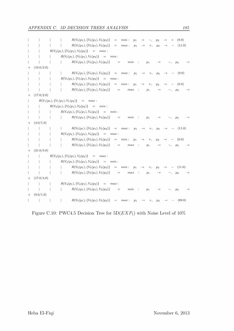
APPENDIX C. 5D DECISION TREES ANALYSIS 185
| | | | R(V5(p1), {V5(p1), V5(p2)} = min : p1 → −, p2 → + (8.0)
| | | | R(V5(p1), {V5(p1), V5(p2)} = max : p1 → +, p2 → − (11.0)
| | R(V2(p1), {V2(p1), V2(p2)} = max :
| | | R(V5(p1), {V5(p1), V5(p2)} = min :
| | | | R(V4(p1), {V4(p1), V4(p2)} = min : p1 → −, p2 →
+ (10.0/2.0)
| | | | R(V4(p1), {V4(p1), V4(p2)} = max : p1 → +, p2 → − (9.0)
| | | R(V5(p1), {V5(p1), V5(p2)} = max :
| | | | R(V4(p1), {V4(p1), V4(p2)} = min : p1 → +, p2 → − (8.0)
| | | | R(V4(p1), {V4(p1), V4(p2)} = max : p1 → −, p2 →
+ (17.0/2.0)
| R(V1(p1), {V1(p1), V1(p2)} = max :
| | R(V2(p1), {V2(p1), V2(p2)} = min :
| | | R(V4(p1), {V4(p1), V4(p2)} = min :
| | | | R(V5(p1), {V5(p1), V5(p2)} = min : p1 → −, p2 →
+ (4.0/1.0)
| | | | R(V5(p1), {V5(p1), V5(p2)} = max : p1 → +, p2 → − (11.0)
| | | R(V4(p1), {V4(p1), V4(p2)} = max :
| | | | R(V5(p1), {V5(p1), V5(p2)} = min : p1 → +, p2 → − (6.0)
| | | | R(V5(p1), {V5(p1), V5(p2)} = max : p1 → −, p2 →
+ (21.0/3.0)
| | R(V2(p1), {V2(p1), V2(p2)} = max :
| | | R(V4(p1), {V4(p1), V4(p2)} = min :
| | | | R(V5(p1), {V5(p1), V5(p2)} = min : p1 → +, p2 → − (11.0)
| | | | R(V5(p1), {V5(p1), V5(p2)} = max : p1 → −, p2 →
+ (17.0/4.0)
| | | R(V4(p1), {V4(p1), V4(p2)} = max :
| | | | R(V5(p1), {V5(p1), V5(p2)} = min : p1 → −, p2 →
+ (9.0/1.0)
| | | | R(V5(p1), {V5(p1), V5(p2)} = max : p1 → +, p2 → − (89.0)
Figure C.10: PWC4.5 Decision Tree for 5D(EXP1) with Noise Level of 10%
Heba El-Fiqi November 6, 2013

APPENDIX C. 5D DECISION TREES ANALYSIS 186
V 4 <= 4.07981 : − (443.0/189.0)
V 4 > 4.07981 :
| V 4 <= 8.99737 : + (415.0/163.0)
| V 4 > 8.99737 : − (142.0/59.0)
Figure C.11: C4.5 Decision Tree for 5D(EXP1) with Noise Level of 15%
R(V4(p1), {V4(p1), V4(p2)} = min :
| R(V1(p1), {V1(p1), V1(p2)} = min :
| | R(V3(p1), {V3(p1), V3(p2)} = min :
| | | R(V2(p1), {V2(p1), V2(p2)} = min :
| | | | R(V5(p1), {V5(p1), V5(p2)} = min : p1 → −, p2 → + (93.0/30.6)
| | | | R(V5(p1), {V5(p1), V5(p2)} = max : p1 → +, p2 → − (11.0/1.3)
| | | R(V2(p1), {V2(p1), V2(p2)} = max :
| | | | R(V5(p1), {V5(p1), V5(p2)} = min : p1 → +, p2 → − (20.0/1.3)
| | | | R(V5(p1), {V5(p1), V5(p2)} = max : p1 → −, p2 → + (8.0/2.4)
| | R(V3(p1), {V3(p1), V3(p2)} = max :
| | | R(V2(p1), {V2(p1), V2(p2)} = min : p1 → +, p2 → − (25.0/4.9)
| | | R(V2(p1), {V2(p1), V2(p2)} = max :
| | | | R(V5(p1), {V5(p1), V5(p2)} = min : p1 → −, p2 → + (5.0/2.3)
| | | | R(V5(p1), {V5(p1), V5(p2)} = max : p1 → +, p2 → − (9.0/1.3)
| R(V1(p1), {V1(p1), V1(p2)} = max :
| | R(V3(p1), {V3(p1), V3(p2)} = min : p1 → +, p2 → − (47.0/12.6)
| | R(V3(p1), {V3(p1), V3(p2)} = max :
| | | R(V2(p1), {V2(p1), V2(p2)} = min :
| | | | R(V5(p1), {V5(p1), V5(p2)} = min : p1 → −, p2 → + (7.0/3.4)
| | | | R(V5(p1), {V5(p1), V5(p2)} = max : p1 → +, p2 → − (10.0/1.3)
| | | R(V2(p1), {V2(p1), V2(p2)} = max :
| | | | R(V5(p1), {V5(p1), V5(p2)} = min : p1 → +, p2 → − (9.0/1.3)
| | | | R(V5(p1), {V5(p1), V5(p2)} = max : p1 → −, p2 → + (19.0/5.9)
R(V4(p1), {V4(p1), V4(p2)} = max :
| R(V2(p1), {V2(p1), V2(p2)} = min :
| | R(V3(p1), {V3(p1), V3(p2)} = min : p1 → +, p2 → − (51.0/12.6)
| | R(V3(p1), {V3(p1), V3(p2)} = max :
| | | R(V1(p1), {V1(p1), V1(p2)} = min :
| | | | R(V5(p1), {V5(p1), V5(p2)} = min : p1 → −, p2 → + (11.0/5.6)
| | | | R(V5(p1), {V5(p1), V5(p2)} = max : p1 → +, p2 → − (11.0/1.3)
| | | R(V1(p1), {V1(p1), V1(p2)} = max :
| | | | R(V5(p1), {V5(p1), V5(p2)} = min : p1 → +, p2 → − (4.0/1.2)
| | | | R(V5(p1), {V5(p1), V5(p2)} = max : p1 → −, p2 → + (16.0/7.9)
| R(V2(p1), {V2(p1), V2(p2)} = max :
Heba El-Fiqi November 6, 2013
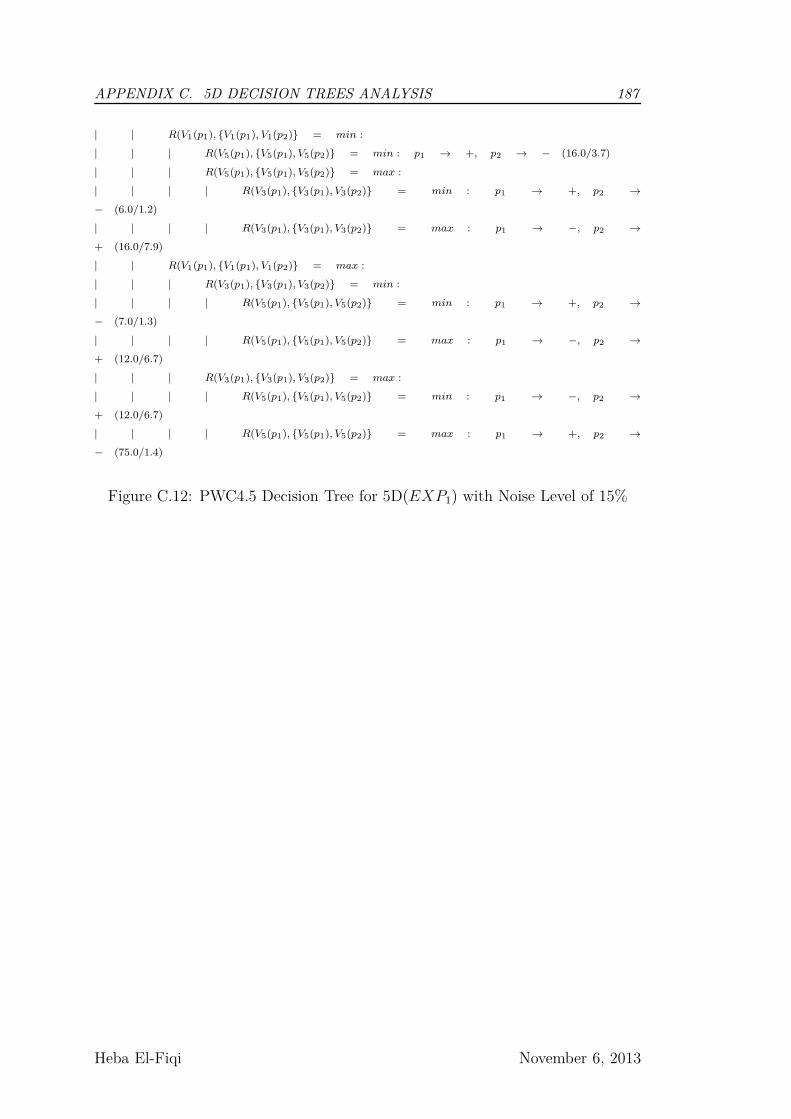
APPENDIX C. 5D DECISION TREES ANALYSIS 187
| | R(V1(p1), {V1(p1), V1(p2)} = min :
| | | R(V5(p1), {V5(p1), V5(p2)} = min : p1 → +, p2 → − (16.0/3.7)
| | | R(V5(p1), {V5(p1), V5(p2)} = max :
| | | | R(V3(p1), {V3(p1), V3(p2)} = min : p1 → +, p2 →
− (6.0/1.2)
| | | | R(V3(p1), {V3(p1), V3(p2)} = max : p1 → −, p2 →
+ (16.0/7.9)
| | R(V1(p1), {V1(p1), V1(p2)} = max :
| | | R(V3(p1), {V3(p1), V3(p2)} = min :
| | | | R(V5(p1), {V5(p1), V5(p2)} = min : p1 → +, p2 →
− (7.0/1.3)
| | | | R(V5(p1), {V5(p1), V5(p2)} = max : p1 → −, p2 →
+ (12.0/6.7)
| | | R(V3(p1), {V3(p1), V3(p2)} = max :
| | | | R(V5(p1), {V5(p1), V5(p2)} = min : p1 → −, p2 →
+ (12.0/6.7)
| | | | R(V5(p1), {V5(p1), V5(p2)} = max : p1 → +, p2 →
− (75.0/1.4)
Figure C.12: PWC4.5 Decision Tree for 5D(EXP1) with Noise Level of 15%
Heba El-Fiqi November 6, 2013
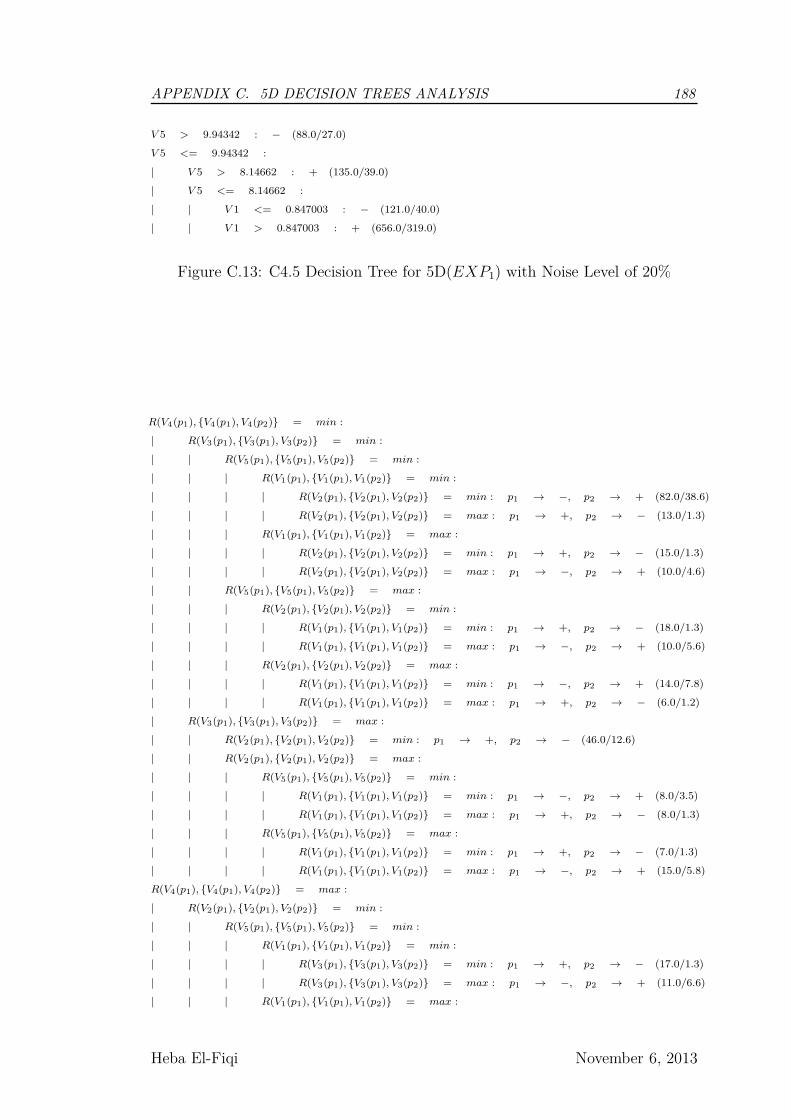
APPENDIX C. 5D DECISION TREES ANALYSIS 188
V 5 > 9.94342 : − (88.0/27.0)
V 5 <= 9.94342 :
| V 5 > 8.14662 : + (135.0/39.0)
| V 5 <= 8.14662 :
| | V 1 <= 0.847003 : − (121.0/40.0)
| | V 1 > 0.847003 : + (656.0/319.0)
Figure C.13: C4.5 Decision Tree for 5D(EXP1) with Noise Level of 20%
R(V4(p1), {V4(p1), V4(p2)} = min :
| R(V3(p1), {V3(p1), V3(p2)} = min :
| | R(V5(p1), {V5(p1), V5(p2)} = min :
| | | R(V1(p1), {V1(p1), V1(p2)} = min :
| | | | R(V2(p1), {V2(p1), V2(p2)} = min : p1 → −, p2 → + (82.0/38.6)
| | | | R(V2(p1), {V2(p1), V2(p2)} = max : p1 → +, p2 → − (13.0/1.3)
| | | R(V1(p1), {V1(p1), V1(p2)} = max :
| | | | R(V2(p1), {V2(p1), V2(p2)} = min : p1 → +, p2 → − (15.0/1.3)
| | | | R(V2(p1), {V2(p1), V2(p2)} = max : p1 → −, p2 → + (10.0/4.6)
| | R(V5(p1), {V5(p1), V5(p2)} = max :
| | | R(V2(p1), {V2(p1), V2(p2)} = min :
| | | | R(V1(p1), {V1(p1), V1(p2)} = min : p1 → +, p2 → − (18.0/1.3)
| | | | R(V1(p1), {V1(p1), V1(p2)} = max : p1 → −, p2 → + (10.0/5.6)
| | | R(V2(p1), {V2(p1), V2(p2)} = max :
| | | | R(V1(p1), {V1(p1), V1(p2)} = min : p1 → −, p2 → + (14.0/7.8)
| | | | R(V1(p1), {V1(p1), V1(p2)} = max : p1 → +, p2 → − (6.0/1.2)
| R(V3(p1), {V3(p1), V3(p2)} = max :
| | R(V2(p1), {V2(p1), V2(p2)} = min : p1 → +, p2 → − (46.0/12.6)
| | R(V2(p1), {V2(p1), V2(p2)} = max :
| | | R(V5(p1), {V5(p1), V5(p2)} = min :
| | | | R(V1(p1), {V1(p1), V1(p2)} = min : p1 → −, p2 → + (8.0/3.5)
| | | | R(V1(p1), {V1(p1), V1(p2)} = max : p1 → +, p2 → − (8.0/1.3)
| | | R(V5(p1), {V5(p1), V5(p2)} = max :
| | | | R(V1(p1), {V1(p1), V1(p2)} = min : p1 → +, p2 → − (7.0/1.3)
| | | | R(V1(p1), {V1(p1), V1(p2)} = max : p1 → −, p2 → + (15.0/5.8)
R(V4(p1), {V4(p1), V4(p2)} = max :
| R(V2(p1), {V2(p1), V2(p2)} = min :
| | R(V5(p1), {V5(p1), V5(p2)} = min :
| | | R(V1(p1), {V1(p1), V1(p2)} = min :
| | | | R(V3(p1), {V3(p1), V3(p2)} = min : p1 → +, p2 → − (17.0/1.3)
| | | | R(V3(p1), {V3(p1), V3(p2)} = max : p1 → −, p2 → + (11.0/6.6)
| | | R(V1(p1), {V1(p1), V1(p2)} = max :
Heba El-Fiqi November 6, 2013

APPENDIX C. 5D DECISION TREES ANALYSIS 189
| | | | R(V3(p1), {V3(p1), V3(p2)} = min : p1 → −, p2 →
+ (6.0/1.2)
| | | | R(V3(p1), {V3(p1), V3(p2)} = max : p1 → +, p2 →
− (9.0/1.3)
| | R(V5(p1), {V5(p1), V5(p2)} = max :
| | | R(V1(p1), {V1(p1), V1(p2)} = min :
| | | | R(V3(p1), {V3(p1), V3(p2)} = min : p1 → −, p2 →
+ (11.0/5.6)
| | | | R(V3(p1), {V3(p1), V3(p2)} = max : p1 → +, p2 →
− (6.0/1.2)
| | | R(V1(p1), {V1(p1), V1(p2)} = max :
| | | | R(V3(p1), {V3(p1), V3(p2)} = min : p1 → +, p2 →
− (6.0/1.2)
| | | | R(V3(p1), {V3(p1), V3(p2)} = max : p1 → −, p2 →
+ (17.0/8.9)
| R(V2(p1), {V2(p1), V2(p2)} = max :
| | R(V1(p1), {V1(p1), V1(p2)} = min :
| | | R(V5(p1), {V5(p1), V5(p2)} = min : p1 → +, p2 → − (17.0/5.9)
| | | R(V5(p1), {V5(p1), V5(p2)} = max :
| | | | R(V3(p1), {V3(p1), V3(p2)} = min : p1 → +, p2 →
− (6.0/1.2)
| | | | R(V3(p1), {V3(p1), V3(p2)} = max : p1 → −, p2 →
+ (19.0/9.0)
| | R(V1(p1), {V1(p1), V1(p2)} = max :
| | | R(V5(p1), {V5(p1), V5(p2)} = min :
| | | | R(V3(p1), {V3(p1), V3(p2)} = min : p1 → +, p2 →
− (15.0/1.3)
| | | | R(V3(p1), {V3(p1), V3(p2)} = max : p1 → −, p2 →
+ (15.0/7.8)
| | | R(V5(p1), {V5(p1), V5(p2)} = max :
| | | | R(V3(p1), {V3(p1), V3(p2)} = min : p1 → −, p2 →
+ (16.0/8.9)
| | | | R(V3(p1), {V3(p1), V3(p2)} = max : p1 → +, p2 →
− (77.0/1.4)
Figure C.14: PWC4.5 Decision Tree for 5D(EXP1) with Noise Level of 20%
Heba El-Fiqi November 6, 2013
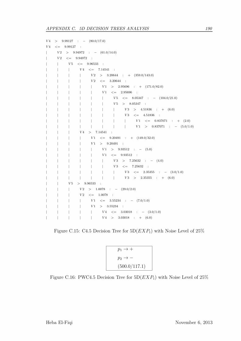
APPENDIX C. 5D DECISION TREES ANALYSIS 190
V 4 > 9.99127 : − (80.0/17.0)
V 4 <= 9.99127 :
| V 2 > 9.94972 : − (61.0/14.0)
| V 2 <= 9.94972 :
| | V 5 <= 9.96533 :
| | | V 4 <= 7.14541 :
| | | | V 2 > 3.20644 : + (359.0/143.0)
| | | | V 2 <= 3.20644 :
| | | | | V 1 > 2.95696 : + (171.0/82.0)
| | | | | V 1 <= 2.95696 :
| | | | | | V 5 <= 8.05347 : − (104.0/21.0)
| | | | | | V 5 > 8.05347 :
| | | | | | | V 3 > 4.51836 : + (6.0)
| | | | | | | V 3 <= 4.51836 :
| | | | | | | | V 1 <= 0.837071 : + (2.0)
| | | | | | | | V 1 > 0.837071 : − (5.0/1.0)
| | | V 4 > 7.14541 :
| | | | V 1 <= 9.20491 : + (149.0/32.0)
| | | | V 1 > 9.20491 :
| | | | | V 1 > 9.93512 : − (5.0)
| | | | | V 1 <= 9.93512 :
| | | | | | V 3 > 7.25632 : − (4.0)
| | | | | | V 3 <= 7.25632 :
| | | | | | | V 3 <= 2.35355 : − (3.0/1.0)
| | | | | | | V 3 > 2.35355 : + (6.0)
| | V 5 > 9.96533 :
| | | V 2 > 1.0078 : − (29.0/2.0)
| | | V 2 <= 1.0078 :
| | | | V 1 <= 3.55234 : − (7.0/1.0)
| | | | V 1 > 3.55234 :
| | | | | V 4 <= 3.03018 : − (3.0/1.0)
| | | | | V 4 > 3.03018 : + (6.0)
Figure C.15: C4.5 Decision Tree for 5D(EXP1) with Noise Level of 25%
p1 → +
p2 → −
(500.0/117.1)
Figure C.16: PWC4.5 Decision Tree for 5D(EXP1) with Noise Level of 25%
Heba El-Fiqi November 6, 2013

[This page is intentionally left blank]

Bibliography
[1] Ahmed Abbasi and Hsinchun Chen. Applying authorship analysis to ara-
bic web content. In Intelligence and Security Informatics, volume 3495
of Lecture Notes in Computer Science, pages 183–197. Springer Berlin /
Heidelberg, 2005.
[2] Ahmed Abbasi and Hsinchun Chen. Applying authorship analysis to
extremist-group web forum messages. IEEE Intelligent Systems, 20:67–75,
September 2005.
[3] Ahmed Abbasi and Hsinchun Chen. Writeprints: A stylometric approach
to identity-level identification and similarity detection in cyberspace. ACM
Transactions on Information Systems, 26(2):1–29, 2008.
[4] Werner Adler, Alexander Brenning, Sergej Potapov, Matthias Schmid, and
Berthold Lausen. Ensemble classification of paired data. Computational
Statistics & Data Analysis, 55(5):1933 – 1941, 2011.
[5] Werner Adler, Sergej Potapov, and Berthold Lausen. Classification of re-
peated measurements data using tree-based ensemble methods. Computa-
tional Statistics, 26:355–369, 2011.
[6] Asim M. El Tahir Ali, Hussam M. Dahwa Abdulla, and Vaclav Snasel.
Survey of plagiarism detection methods. In Modelling Symposium (AMS),
2011 Fifth Asia, pages 39–42, May.
[7] Uri Alon. Network motifs: theory and experimental approaches. Nat Rev
Genet, 8(6):450–461, 2007.
BIBLIOGRAPHY 193
[8] S.M. Alzahrani, N. Salim, and A. Abraham. Understanding plagiarism
linguistic patterns, textual features, and detection methods. Systems, Man,
and Cybernetics, Part C: Applications and Reviews, IEEE Transactions on,
42(2):133 –149, march 2012.
[9] Philipp Sebastian Angermeyer. Translation style and participant roles in
court interpreting. Journal of Sociolinguistics, 13(1):3–28, 2009.
[10] L. Antiqueira, M.G.V. Nunes, O.N. Oliveira Jr., and L. da F. Costa. Strong
correlations between text quality and complex networks features. Physica
A: Statistical Mechanics and its Applications, 373(0):811 – 820, 2007.
[11] Shlomo Argamon. Interpreting burrows’s delta: Geometric and probabilis-
tic foundations. Literary and Linguistic Computing, 23(2):131–147, 2008.
[12] Shlomo Argamon, Sushant Dhawle, Moshe Koppel, and James W. Pen-
nebaker. Lexical predictors of personality type. In Proceedings of the 2005
Joint Annual Meeting of the Interface and the Classification Society ofNorth
America. St. Louis, 2005.
[13] Shlomo Argamon, Moshe Koppel, Jonathan Fine, and Anat R. Shimoni.
Gender, genre, and writing style in formal written texts. Interdisciplinary
Journal for the Study of Discourse, 23(3):321–346, 2003.
[14] Shlomo Argamon, Moshe Koppel, James W. Pennebaker, and Jonathan
Schler. Mining the blogosphere: Age, gender and the varieties of self-
expression. First Monday, 12(9), 2007.
[15] Shlomo Argamon, Moshe Koppel, James W. Pennebaker, and Jonathan
Schler. Automatically profiling the author of an anonymous text. Commun.
ACM, 52(2):119–123, February 2009.
[16] Shlomo Argamon, Casey Whitelaw, Paul Chase, Sobhan Raj Hota,
Navendu Garg, and Shlomo Levitan. Stylistic text classification using func-
tional lexical features. Journal of the American Society for Information
Science and Technology, 58(6):802–822, 2007.
Heba El-Fiqi November 6, 2013

BIBLIOGRAPHY 194
[17] Ioannis N. Athanasiadis, Vassilis G. Kaburlasos, Pericles A. Mitkas, and
Vassilios Petridis. Applying machine learning techniques on air quality
data for real-time decision support. In In: First International NAISO
Symposium on Information Technologies in Environmental Engineering
(ITEE’2003, pages 24–27. ICSC-NAISO Publishers, 2003.
[18] H Baayen, H van Halteren, and F Tweedie. Outside the cave of shadows:
using syntactic annotation to enhance authorship attribution. Literary and
Linguistic Computing, 11(3):121–132, 1996.
[19] Mona Baker. Towards a methodology for investigating the style of a
literary translator. Target, International Journal of Translation Studies,
12(2):241–266, 2000.
[20] Alberto Barrón-Cedeño, Paolo Rosso, Eneko Agirre, and Gorka Labaka.
Plagiarism detection across distant language pairs. In Proceedings of the
23rd International Conference on Computational Linguistics, COLING ’10,
pages 37–45, Stroudsburg, PA, USA, 2010. Association for Computational
Linguistics.
[21] J.N.G. Binongo and M.W.A. Smith. The application of principal component
analysis to stylometry,. Literary and Linguistic Computing, 14(4):445–466,
1999.
[22] José Nilo G Binongo. Who wrote the 15th book of oz? an application of
multivariate analysis to authorship attribution. Chance, 16(2):9–17, 2003.
[23] Edward Gaylord Bourne. The authorship of the federalist. The American
Historical Review, 2(3):443–460, 1897.
[24] Leo Breiman. Random forests. Machine Learning, 45(1):5–32, October
2001.
[25] Leo Breiman, Jerome Friedman, Charles J. Stone, and R. A. Olshen. Classi-
fication and Regression Trees. Chapman and Hall/CRC, 1 edition, January
1984.
Heba El-Fiqi November 6, 2013

BIBLIOGRAPHY 195
[26] A. Brenning and B. Lausen. Estimating error rates in the classification of
paired organs. Statistics in Medicine, 27(22):4515–4531, 2008. cited By
(since 1996) 10.
[27] Carla E. Brodley and Paul E. Utgoff. Multivariate decision trees. Machine
Learning, 19(1):45–77, April 1995.
[28] J. F. Burrows. ’an ocean where each kind...’: Statistical analysis and
some major determinants of literary style. Computers and the Humani-
ties, 23(4/5):pp. 309–321, 1989.
[29] John Burrows. “Delta”: a measure of stylistic difference and a guide to
likely authorship. Literary and Linguistic Computing, 17(3):267–287, 2002.
[30] John Burrows. All the way through: Testing for authorship in different
frequency strata. Literary and Linguistic Computing, 22(1):27–47, 2007.
[31] John F Burrows. Word patterns and story shapes: The statistical analysis
of narrative style. Journal of the Association for Literary and Linguistic
Computing, 2(4):61–70, 1987.
[32] J.P. Campbell, W. Shen, W.M. Campbell, R. Schwartz, J.-F. Bonastre,
and D. Matrouf. Forensic speaker recognition. Signal Processing Magazine,
IEEE, 26(2):95 –103, march 2009.
[33] Sara Castagnoli. Regularities and variations in learner translations : a
corpus-based study of conjunctive explicitation. PhD thesis, University of
Bologna, ITALY, 2009.
[34] Le S. Cessie and J. C. van Houwelingen. Ridge estimators in logistic re-
gression. Applied Statistics, 41(1):191–201, 1992.
[35] Yin-ling Cheung. Techniques in data mining: Decision trees classification
and constraint-based itemsets mining. Master’s thesis, The Chinese Uni-
versity of Hong Kong, 2001.
Heba El-Fiqi November 6, 2013
BIBLIOGRAPHY 196
[36] William W. Cohen. Fast effective rule induction. In In Proceedings of
the Twelfth International Conference on Machine Learning, pages 115–123.
Morgan Kaufmann, 1995.
[37] Steven R. Corman, Timothy Kuhn, Robert D. Mcphee, and Kevin J. Doo-
ley. Studying complex discursive systems. Human Communication Re-
search, 28(2):157–206, 2002.
[38] Malcolm Corney, Olivier de Vel, Alison Anderson, and George Mohay.
Gender-preferential text mining of e-mail discourse. In Proceedings of
the 18th Annual Computer Security Applications Conference, ACSAC ’02,
pages 282–, Washington, DC, USA, 2002. IEEE Computer Society.
[39] Malcolm Coulthard and Alison Johnson. The Routledge Handbook of Foren-
sic Linguistics. Routledge Handbooks in Applied Linguistics. Routledge,
2010.
[40] David Crystal. The Cambridge Encyclopedia of Language. Cambridge Uni-
versity Press, 2 edition, 1997.
[41] O. de Vel, A. Anderson, M. Corney, and G. Mohay. Mining e-mail content
for author identification forensics. Sigmod Record, 30(4):55–64, 2001.
[42] M. Elhadi and A. Al-Tobi. Use of text syntactical structures in detection of
document duplicates. In Digital Information Management, 2008. ICDIM
2008. Third International Conference on, pages 520–525, 2008.
[43] M. Elhadi and A. Al-Tobi. Duplicate detection in documents and webpages
using improved longest common subsequence and documents syntactical
structures. In Computer Sciences and Convergence Information Technology,
2009. ICCIT ’09. Fourth International Conference on, pages 679–684, 2009.
[44] Lenita M. R. Esteves. Intellectual property and copyright: The case of
translators. Translation Journal: A Publication for Translators by Trans-
lators about Translators and Translation, 9(3), 2005.
Heba El-Fiqi November 6, 2013
BIBLIOGRAPHY 197
[45] Dominique Estival, Tanja Gaustad, Son B. Pham, Will Radford, and Ben
Hutchinson. Author profiling for english emails. In 10th Conference of the
Pacific Association for Computational Linguistics (PACLING 2007), pages
262–272, 2007.
[46] Dominique Estival, Tanja Gaustad, Son Bao Pham, Will Radford, and Ben
Hutchinson. Tat: an author profiling tool with application to arabic emails.
In Proceedings of the Australasian Language Technology Workshop (ALTW
2007), pages 21–30, 2007.
[47] Fayyad and Irani. Multi-interval discretization of continuous-valued at-
tributes for classification learning. pages 1022–1027, 1993.
[48] Usama Fayyad, Gregory Piatetsky-Shapiro, and Padhraic Smyth. The kdd
process for extracting useful knowledge from volumes of data. Commun.
ACM, 39(11):27–34, November 1996.
[49] Jacob G. Foster, David V. Foster, Peter Grassberger, and Maya Paczuski.
Edge direction and the structure of networks. Proceedings of the National
Academy of Sciences, 107(24):10815–10820, June 2010.
[50] William J. Frawley, Gregory Piatetsky-Shapiro, and Christopher J.
Matheus. Knowledge discovery in databases: an overview. AI Mag.,
13(3):57–70, September 1992.
[51] J. Gama. Functional trees for classification. In Data Mining, 2001. ICDM
2001, Proceedings IEEE International Conference on, pages 147 –154, 2001.
[52] João Gama and Pavel Brazdil. Linear tree. Intelligent Data Analysis, 3(1):1
– 22, 1999.
[53] João Gama. Functional trees. Machine Learning, 55(3):219–250, June 2004.
[54] Michael Gamon. Linguistic correlates of style: authorship classification with
deep linguistic analysis features. In Proceedings of the 20th international
conference on Computational Linguistics, COLING ’04, Stroudsburg, PA,
USA, 2004. Association for Computational Linguistics.
Heba El-Fiqi November 6, 2013
BIBLIOGRAPHY 198
[55] Antonio Miranda García and Javier Calle Martín. Function words in au-
thorship attribution studies. Literary Linguist Computing, 22(1):49–66,
2007.
[56] A. Ghoneim, H. Abbass, and M. Barlow. Characterizing game dynamics
in two-player strategy games using network motifs. Systems, Man, and
Cybernetics, Part B: Cybernetics, IEEE Transactions on, 38(3):682–690,
2008.
[57] Iwona Grabska-Gradzińska, Andrzej Kulig, Jarosław Kwapień, and
Stanisław Drożdż. Complex network analysis of literary and scientific texts.
International Journal of Modern Physics C, 23(7):1250051(1:15), 2012.
[58] Rachid Hadjidj, Mourad Debbabi, Hakim Lounis, Farkhund Iqbal, Adam
Szporer, and Djamel Benredjem. Towards an integrated e-mail forensic
analysis framework. Digital Investigation, 5(3):124 – 137, 2009.
[59] Jiawei Han, Micheline Kamber, and Jian Pei. Data Mining: Concepts and
Techniques, Second Edition (The Morgan Kaufmann Series in Data Man-
agement Systems). Morgan Kaufmann, 2 edition, January 2006.
[60] S Hanna. Translation and questions of identity (re-
view article in arabic). Diwan Al Arab Journal
http://www.diwanalarab.com/spip.php?article5903, 2006.
[61] S Hanna. Translation studies: Beginnings, trajectories and questions of the
future (in arabic). Fusul: A Journal of Literary Criticism, 74:36–48, 2008.
[62] Steffen Hedegaard and Jakob Grue Simonsen. Lost in translation: author-
ship attribution using frame semantics. In Proceedings of the 49th Annual
Meeting of the Association for Computational Linguistics: Human Lan-
guage Technologies: short papers, volume 2, pages 65–70, Stroudsburg, PA,
USA, 2011. Association for Computational Linguistics.
[63] Magda Heydel and Jan Rybicki. The stylometry of collaborative translation.
In Digital Humanities, 2012.
Heba El-Fiqi November 6, 2013

BIBLIOGRAPHY 199
[64] Jens Hühn and Eyke Hüllermeier. Furia: an algorithm for unordered fuzzy
rule induction. Data Mining and Knowledge Discovery, 19(3):293–319, 2009.
10.1007/s10618-009-0131-8.
[65] D. I. Holmes and R. S. Forsyth. The federalist revisited: New directions in
authorship attribution. Literary and Linguistic Computing, 10(2):111–127,
1995.
[66] David I. Holmes. Vocabulary richness and the prophetic voice. Literary
and Linguistic Computing, 6(4):259–268, 1991.
[67] David I. Holmes, Lesley J. Gordon, and Christine Wilson. A widow and
her soldier: Stylometry and the american civil war. Literary and Linguistic
Computing, 16(4):403–420, 2001.
[68] D.I Holmes and F.J. Tweedie. Forensic stylometry: A review of the cusum
controversy. Revue Informatique et Statistique dansles Sciences Humaines,
pages 19–47, 1995. Liege, Belgium: University of Liege.
[69] Janet Holmes. An Introduction to Sociolinguistics (Learning About Lan-
guage). Longman, 2008.
[70] David L. Hoover. Frequent collocations and authorial style. Literary and
Linguistic Computing, 18(3):261–286, 2003.
[71] David L. Hoover. Multivariate analysis and the study of style variation.
Literary and Linguistic Computing, 18(4):341–360, 2003.
[72] David L. Hoover. Delta prime? Literary and Linguistic Computing,
19(4):477–495, 2004.
[73] David L. Hoover. Testing burrows’s delta. Literary and Linguistic Com-
puting, 19(4):453–475, 2004.
[74] David L. Hoover and Shervin Hess. An exercise in non-ideal authorship
attribution: the mysterious maria ward. Literary and Linguistic Computing,
24(4):467–489, 2009.
Heba El-Fiqi November 6, 2013
BIBLIOGRAPHY 200
[75] Qinghua Hu, Xunjian Che, Lei Zhang, D. Zhang, Maozu Guo, and D. Yu.
Rank entropy-based decision trees for monotonic classification. Knowledge
and Data Engineering, IEEE Transactions on, 24(11):2052–2064, 2012.
[76] Jens Christian Hühn and Eyke Hüllermeier. Advances in machine learning
i: Dedicated to the memory of professor ryszard s. michalski. In Jacek Ko-
ronacki, Zbigniew W. Ras, Slawomir T. Wierzchon, and Janusz Kacprzyk,
editors, Advances in Machine Learning I, volume 262 of Studies in Compu-
tational Intelligence. Springer, 2010.
[77] Christopher Hutton. Authority and expertise in forensic linguistics. Lan-
guage & Communication, 25(2):183–188, 2005. A Book review.
[78] Ken Hyland and Brian Paltridge. Continuum Companion to Discourse
Analysis. Continuum Companions. Continuum, 2011.
[79] S. Itzkovitz, R. Levitt, N. Kashtan, R. Milo, M. Itzkovitz, and U. Alon.
Coarse-graining and self-dissimilarity of complex networks. Physical Re-
view E - Statistical, Nonlinear and Soft Matter Physics, 71(1 Pt 2):016127,
January 2005.
[80] Ilyes Jenhani, Nahla Ben Amor, and Zied Elouedi. Decision trees as possi-
bilistic classifiers. Int. J. Approx. Reasoning, 48(3):784–807, August 2008.
[81] Michael Jessen. Forensic phonetics. Language and Linguistics Compass,
2(4):671–711, 2008.
[82] Matthew L. Jockers and Daniela M. Witten. A comparative study of ma-
chine learning methods for authorship attribution. Literary and Linguistic
Computing, 25(2):215–223, 2010.
[83] Patrick Juola. Authorship attribution. Foundations and Trends in Infor-
mation Retrieval, 1(3):233–334, 2006.
[84] Renata Kamenická. Translation research projects 1, chapter Explicitation
profile and translator style, pages 117–130. Intercultural Studies Group,
Universitat Rovira i Virgili, 2008.
Heba El-Fiqi November 6, 2013
BIBLIOGRAPHY 201
[85] N. Kashtan, S. Itzkovitz, R. Milo, and U. Alon. Efficient sampling algo-
rithm for estimating subgraph concentrations and detecting network motifs.
Bioinformatics, 20(11):1746–1758, 2004.
[86] N. Kashtan, S. Itzkovitz, R. Milo, and U. Alon. Network motif detection
tool mfinder tool guide. Technical report, Departments of Molecular Cell
Biology and Computer Science and Applied Mathematics, Weizmann Insti-
tute of Science, Rehovot, Israel., 2004.
[87] G. V. Kass. An exploratory technique for investigating large quantities of
categorical data. Journal of the Royal Statistical Society. Series C (Applied
Statistics), 29(2):119–127, 1980.
[88] Kenneth Katzner. The Languages of the World. Routledge, 2002.
[89] S. S. Keerthi, S. K. Shevade, C. Bhattacharyya, and K. R. K. Murthy.
Improvements to platt’s smo algorithm for SVM classifier design. Neural
Comput., 13:637–649, March 2001.
[90] Randy Kerber. Chimerge: discretization of numeric attributes. In Proceed-
ings of the tenth national conference on Artificial intelligence, AAAI’92,
pages 123–128. AAAI Press, 1992.
[91] Mike Kestemont. What can stylometry learn from its application to middle
dutch literature? Journal of Dutch Literature, 2(2):46–65, 2012.
[92] Michael Kirley, HusseinA. Abbass, and Robert(Bob)I. McKay. Diversity
mechanisms in pitt-style evolutionary classifier systems. In Evangelos Tri-
antaphyllou and Giovanni Felici, editors, Data Mining and Knowledge Dis-
covery Approaches Based on Rule Induction Techniques, volume 6 of Mas-
sive Computing, pages 433–457. Springer US, 2006.
[93] Ron Kohavi. Scaling up the accuracy of naive-bayes classifiers: a decision-
tree hybrid. In Proceedings of the Second International Conference on
Knowledge Discovery and Data Mining, pages 202–207. AAAI Press, 1996.
Heba El-Fiqi November 6, 2013
BIBLIOGRAPHY 202
[94] Moshe Koppel, Shlomo Argamon, and Anat Rachel Shimoni. Automati-
cally categorizing written texts by author gender. Literary and Linguistic
Computing, 17(4):401–412, 2002.
[95] Moshe Koppel, Jonathan Schler, and Shlomo Argamon. Computational
methods in authorship attribution. Journal of the American Society for
Information Science and Technology, 60(1):9–26, 2009.
[96] Moshe Koppel, Jonathan Schler, and Elisheva Bonchek-Dokow. Measuring
differentiability: Unmasking pseudonymous authors. J. Mach. Learn. Res.,
8:1261–1276, December 2007.
[97] Moshe Koppel, Jonathan Schler, and Kfir Zigdon. Determining an author’s
native language by mining a text for errors. In Proceedings of the eleventh
ACM SIGKDD international conference on Knowledge discovery in data
mining, KDD ’05, pages 624–628, New York, NY, USA, 2005. ACM.
[98] S. B. Kotsiantis, I. D. Zaharakis, and P. E. Pintelas. Machine learning:
a review of classification and combining techniques. Artif. Intell. Rev.,
26(3):159–190, November 2006.
[99] Robert Layton, Paul Watters, and Richard Dazeley. Recentred local profiles
for authorship attribution. Jouranl of Natural Language Engineering, pages
1–20, 2011.
[100] Vanessa Leonardi. Gender and Ideology in Translation: Do Women and
Men Translate Differently? a Contrastive Analysis Form Italian into En-
glish. European University Studies. Peter Lang, 2007.
[101] Defeng Li, Chunling Zhang, and Kanglong Liu. Translation style and ideol-
ogy: a corpus-assisted analysis of two english translations of hongloumeng.
Literary and Linguistic Computing, 26(2):153–166, 2011.
[102] Tjen-Sien Lim, Wei-Yin Loh, and Yu-Shan Shih. A comparison of predic-
tion accuracy, complexity, and training time of thirty-three old and new
classification algorithms. Mach. Learn., 40(3):203–228, September 2000.
Heba El-Fiqi November 6, 2013
BIBLIOGRAPHY 203
[103] Jing Liu, Hussein A. Abbass, David G. Green, and Weicai Zhong. Motif
difficulty (md): A predictive measure of problem difficulty for evolutionary
algorithms using network motifs. Evol. Comput., 20(3):321–347, September
2012.
[104] Xiaoyan Liu and Huaiqing Wang. A discretization algorithm based on a het-
erogeneity criterion. Knowledge and Data Engineering, IEEE Transactions
on, 17(9):1166–1173, 2005.
[105] W. Y. Loh and Y. S. Shih. Split selection methods for classification trees.
Statistica Sinica, 1997.
[106] Kim Luyckx and Walter Daelemans. Authorship attribution and verifica-
tion with many authors and limited data. In Proceedings of the 22nd In-
ternational Conference on Computational Linguistics - Volume 1, COLING
’08, pages 513–520, Stroudsburg, PA, USA, 2008. Association for Compu-
tational Linguistics.
[107] Kim Luyckx and Walter Daelemans. The effect of author set size and
data size in authorship attribution. Literary and Linguistic Computing,
26(1):35–55, 2011.
[108] Jianbin Ma, Guifa Teng, Shuhui Chang, Xiaoru Zhang, and Ke Xiao. Social
network analysis based on authorship identification for cybercrime investi-
gation. In Michael Chau, G.Alan Wang, Xiaolong Zheng, Hsinchun Chen,
Daniel Zeng, and Wenji Mao, editors, Intelligence and Security Informatics,
volume 6749 of Lecture Notes in Computer Science, pages 27–35. Springer
Berlin Heidelberg, 2011.
[109] David Madigan, Alexander Genkin, David D. Lewis, Shlomo Argamon,
Dmitriy Fradkin, and Li Ye. Author identification on the large scale. In In
Proc. of the Meeting of the Classification Society of North America, 2005.
[110] François Mairesse and Marilyn Walker. Words mark the nerds: Computa-
tional models of personality recognition through language. In Proceedings
Heba El-Fiqi November 6, 2013
BIBLIOGRAPHY 204
of 28th Annual Conference of th e Cognitive Science Society, pages 543–548,
2006.
[111] Sergei Maslov and Kim Sneppen. Specificity and stability in topology of
protein networks. Science, 296(5569):910–913, 2002.
[112] Sergei Maslov, Kim Sneppen, and Uri Alon. Correlation profiles and mo-
tifs in complex networks. Handbook of Graphs and Networks. Wiley-VCH
Verlag GmbH & Co. KGaA, 2005.
[113] Gerald Matthews, Ian J. Deary, and Martha C. Whiteman. Personality
Traits. Cambridge University Press, 2nd edition, 2003.
[114] R. Matthews and T. Merriam. Neural computation in stylometry : An
application to the works of shakespeare and fletcher. Literary and Linguistic
Computing, 8(4):203–209, 1993.
[115] Gerald R. McMenamin. Forensic Linguistics: Advances in Forensic Stylis-
tics. CRC Press, 2002.
[116] Manish Mehta, Rakesh Agrawal, and Jorma Rissanen. SLIQ: A fast scal-
able classifier for data mining. In Peter Apers, Mokrane Bouzeghoub, and
Georges Gardarin, editors, Advances in Database Technology - EDBT ’96,
volume 1057 of Lecture Notes in Computer Science, pages 18–32. Springer
Berlin Heidelberg, 1996.
[117] T. C. Mendenhall. The characteristic curves of composition. Science, ns-
9(214S):237–246, 1887.
[118] T. Merriam and R Matthews. Neural compuation in stylometry ii: An ap-
plication to the works of shakespeare and marlowe. Literary and Linguistic
Computing, 9:1–6, 1994.
[119] THOMAS Merriam. Marlowe’s hand in edward iii revisited. Literary and
Linguistic Computing, 11(1):19–22, 1996.
Heba El-Fiqi November 6, 2013
BIBLIOGRAPHY 205
[120] Sven Meyer zu Eissen, Benno Stein, and Marion Kulig. Plagiarism detection
without reference collections. In Reinhold Decker and Hans-J. Lenz, editors,
Advances in Data Analysis, Studies in Classification, Data Analysis, and
Knowledge Organization, pages 359–366. Springer Berlin Heidelberg, 2007.
[121] Mikhail Mikhailov and Miia Villikka. Is there such a thing as a trans-
lator’s style? In Paul Rayson, Andrew Wilson, Tony McEnery, Andrew
Hardie, and Shereen Khoja, editors, Proceedings of the Corpus Linguistics
2001 conference, pages 378–386, Lancaster, 29 March - 2 April 2001 2001.
Lancaster University (UK).
[122] R. Milo, S. Shen-Orr, S. Itzkovitz, N. Kashtan, D. Chklovskii, and U. Alon.
Network motifs: Simple building blocks of complex networks. Science,
298(5594):824–827, 2002.
[123] Tom M. Mitchell. Machine Learning. McGraw Hill, 1997.
[124] Khaleel Mohammed. Assessing english translations of the qur’an. The
Middle East Quarterly, XII(2):58–71, SPRING 2005.
[125] A. Q. Morton. The authorship of greek prose. Journal of the Royal Statis-
tical Society. Series A (General), 128(2):169–233, 1965.
[126] A. Q. Morton and S. Michaelson. The qsum plot. Internal Report CSR-3-90,
Department of Computer Science, University of Edinburgh, 1990.
[127] F. Mosteller and D. Wallace. Inference and Disputed Authorship: The
Federalist. Series in Behavioral Science: Quantitative Methods Edition.
Addison-Wesley, 1964.
[128] Sreerama K. Murthy, Simon Kasif, and Steven Salzberg. A system for
induction of oblique decision trees. J. Artif. Int. Res., 2(1):1–32, August
1994.
[129] Mark Newman. Networks: An Introduction. Oxford University Press, New
York, 2010.
Heba El-Fiqi November 6, 2013
BIBLIOGRAPHY 206
[130] Wouter de Nooy, Andrej Mrvar, and Vladimir Batagelj. Exploratory social
network analysis with Pajek, volume 27 of Structural analysis in the social
sciences. Cambridge University Press, New York, USA, 2005.
[131] Jon Oberlander and Scott Nowson. Whose thumb is it anyway?: classi-
fying author personality from weblog text. In Proceedings of the COL-
ING/ACL on Main conference poster sessions, COLING-ACL ’06, pages
627–634, Stroudsburg, PA, USA, 2006. Association for Computational Lin-
guistics.
[132] John Olsson. Forensic Linguistics. Continuum International Publishing
Group, 2nd edition, 2008.
[133] Ahmed Hamza Osman, Naomie Salim, and Albaraa Abuobieda. Survey of
text plagiarism detection. Computer Engineering and Applications, 1(1):37–
45, 2012.
[134] D. Pavelec, L. S. Oliveira, E. Justino, F. D. Nobre Neto, and L. V. Batista.
Compression and stylometry for author identification. In Proceedings of the
2009 international joint conference on Neural Networks, IJCNN’09, pages
669–674, Piscataway, NJ, USA, 2009. IEEE Press.
[135] Daniel Pavelec, Edson Justino, Leonardo V. Batista, and Luiz S. Oliveira.
Author identification using writer-dependent and writer-independent
strategies. In Proceedings of the 2008 ACM symposium on Applied com-
puting, SAC ’08, pages 414–418, New York, NY, USA, 2008. ACM.
[136] James W Pennebaker and Laura A. King. Linguistic styles: language use
as an individual difference. Journal of Personality and Social Psychology,
77(6):1296–1312, 1999.
[137] James W Pennebaker, Matthias R Mehl, and Kate G Niederhoffer. Psy-
chological aspects of natural language. use: our words, our selves. Annual
Review of Psychology, 54(1):547–77, 2003.
Heba El-Fiqi November 6, 2013
BIBLIOGRAPHY 207
[138] David F. Dufty Philip M. McCarthy, Gwyneth A. Lewis and Danielle S.
McNamar. Analyzing writing styles with coh-metrix. In In Proceedings
of the Florida Artificial Intelligence Research Society International Confer-
ence, page 764–769, 2006.
[139] John C. Platt. Fast training of support vector machines using sequential
minimal optimization, pages 185–208. MIT Press, Cambridge, MA, USA,
1999.
[140] Roel Popping. Computer-Assisted Text Analysis. SAGE Publications, 2000.
[141] Stephan Procházka. Arabic. In Keith Brown, editor, Encyclopedia of Lan-
guage and Linguistics (Second Edition), pages 423 – 431. Elsevier, Oxford,
2nd edition, 2006.
[142] Nuria Puig, Iosifina Pournara, and Lorenz Wernisch. Statistical model
comparison applied to common network motifs. BMC Systems Biology,
4(1):18, 2010.
[143] Anthony Pym. Venuti’s visibility. Target, 8:165–178, 1996.
[144] J R Quinlan. C4.5: Programs for Machine Learning. Morgan Kaufmann,
1993.
[145] J Ross Quinlan. Induction of decision trees. Mach. Learn., 1(1):81–106,
March 1986.
[146] J.R. Quinlan and R.M. Cameron-Jones. Induction of logic programs: Foil
and related systems. New Generation Computing, 13(3-4):287–312, 1995.
[147] Andrew Radford, Martin Atkinson, David Britain, Harald Clahsen, and An-
drew Spencer. Linguistics: An Introduction. Cambridge University Press,
2009.
[148] Alan Cooperman Brian J. Grim Mehtab S. Karim Sahar Chaudhry Becky
Hsu Jacqueline E. Wenger Kimberly McKnight Megan Pavlischek Hilary
Ramp. Mapping the global muslim population: A report on the size and
Heba El-Fiqi November 6, 2013
BIBLIOGRAPHY 208
distribution of the world’s muslim population. Technical report, The Pew
Research Center, 2009.
[149] Sara Rosenthal and Kathleen McKeown. Age prediction in blogs: a study
of style, content, and online behavior in pre- and post-social media gen-
erations. In Proceedings of the 49th Annual Meeting of the Association
for Computational Linguistics: Human Language Technologies - Volume
1, HLT ’11, pages 763–772, Stroudsburg, PA, USA, 2011. Association for
Computational Linguistics.
[150] Mikail Rubinov and Olaf Sporns. Complex network measures of brain con-
nectivity: Uses and interpretations. NeuroImage, 52(3):1059 – 1069, 2010.
[151] Joseph Rudman. The non-traditional case for the authorship of the twelve
disputed "federalist" papers: A monument built on sand? In Proceedings
of ACH/ALLC 2005, Victoria, BC, Canada, 2005.
[152] Jan Rybicki. Burrowing into translation: Character idiolects in henryk
sienkiewicz’s trilogy and its two english translations. Literary and Linguistic
Computing, 21(1):91–103, 2006.
[153] Jan Rybicki. Alma cardell curtin and jeremiah curtin: the translator’s
wife’s stylistic fingerprint. In Digital Humanities, 2011.
[154] Jan Rybicki. The great mystery of the (almost) invisible translator : Sty-
lometry in translation. In Michael P. Oakes and Meng Ji, editors, Quantita-
tive Methods in Corpus-Based Translation Studies: A practical guide to de-
scriptive translation research, Studies in Corpus Linguistics, page 231–248.
John Benjamins Publishing, 2012.
[155] Jan Rybicki and Maciej Eder. Deeper delta across genres and languages:
do we really need the most frequent words? Literary and Linguistic Com-
puting, 26(3):315–321, 2011.
Heba El-Fiqi November 6, 2013
BIBLIOGRAPHY 209
[156] S. G Shafiee Sabet and A Rabeie. The effect of the translator’s gender
ideology on translating emily bronte’s wuthering heights. The Journal of
Teaching Language Skills (JTLS), 3(3):143–158, 2011.
[157] Fernando Sánchez-Vega, Luis Villaseñor Pineda, Manuel Montes-Y-Gómez,
and Paolo Rosso. Towards document plagiarism detection based on the rel-
evance and fragmentation of the reused text. In Proceedings of the 9th Mex-
ican international conference on Advances in artificial intelligence: Part I,
MICAI’10, pages 24–31, Berlin, Heidelberg, 2010. Springer-Verlag.
[158] J. Schler, M. Koppel, S. Argamon, and J. Pennebaker. Effects of age and
gender on blogging. In Proc. of AAAI Spring Symposium on Computational
Approaches for Analyzing Weblogs, pages 199–205, March 2006.
[159] Falk Schreiber and Henning Schwöbbermeyer. Towards motif detection in
networks: Frequency concepts and flexible search. In in Proceedings of
the International Workshop on Network Tools and Applications in Biology
(NETTAB04), pages 91–102, 2004.
[160] Falk Schreiber and Henning Schwöbbermeyer. Mavisto: a tool for the ex-
ploration of network motifs. Bioinformatics, 21(17):3572–3574, 2005.
[161] John C. Shafer, Rakesh Agrawal, and Manish Mehta. Sprint: A scalable
parallel classifier for data mining. In Proceedings of the 22th International
Conference on Very Large Data Bases, VLDB ’96, pages 544–555, San Fran-
cisco, CA, USA, 1996. Morgan Kaufmann Publishers Inc.
[162] K. Shaker and D. Corne. Authorship attribution in arabic using a hybrid
of evolutionary search and linear discriminant analysis. In Computational
Intelligence (UKCI), 2010 UK Workshop on, pages 1 –6, sept. 2010.
[163] Peter W. H. Smith and W. Aldridge. Improving authorship attribution:
Optimizing burrows’ delta method*. Journal of Quantitative Linguistics,
18(1):63–88, 2011.
Heba El-Fiqi November 6, 2013
BIBLIOGRAPHY 210
[164] J. F. Sowa. Conceptual structures: information processing in mind and
machine. Addison-Wesley Longman Publishing Co., Inc., Boston, MA,
USA, 1984.
[165] Olaf Sporns and Rolf Kötter. Motifs in brain networks. PLoS Biol,
2(11):1910–1918, 2004.
[166] E Stamatatos. Authorship attribution based on feature set subspacing en-
sembles. International Journal on Artificial Intelligence Tools, 15(5):823–
838, 2006.
[167] Efstathios Stamatatos. Author identification: Using text sampling to han-
dle the class imbalance problem. Information Processing & Management,
44(2):790–799, 2008.
[168] Efstathios Stamatatos. A survey of modern authorship attribution methods.
Journal of the American Society for Information Science and Technology,
60(3):538–556, 2009.
[169] Efstathios Stamatatos and Moshe Koppel. Plagiarism and authorship anal-
ysis: introduction to the special issue. Lang. Resour. Eval., 45(1):1–4,
March 2011.
[170] Urszula Stanczyk and Krzysztof A. Cyran. Application of artificial neu-
ral networks to stylometric analysis. In Proceedings of the 8th conference
on Systems theory and scientific computation, pages 25–30, Stevens Point,
Wisconsin, USA, 2008. World Scientific and Engineering Academy and So-
ciety (WSEAS).
[171] Benno Stein, Moshe Koppel, and Efstathios Stamatatos. Plagiarism analy-
sis, authorship identification, and near-duplicate detection. SIGIR Forum,
41(2):68–71, December 2007.
[172] Benno Stein, Nedim Lipka, and Peter Prettenhofer. Intrinsic plagiarism
analysis. Language Resources and Evaluation, 45:63–82, 2011.
Heba El-Fiqi November 6, 2013
BIBLIOGRAPHY 211
[173] Salvatore J. Stolfo, Germán Creamer, and Shlomo Hershkop. A tempo-
ral based forensic analysis of electronic communication. In Proceedings of
the 2006 international conference on Digital government research, dg.o ’06,
pages 23–24. Digital Government Society of North America, 2006.
[174] Jenny Tam and Craig H. Martell. Age detection in chat. In Proceedings
of the 2009 IEEE International Conference on Semantic Computing, ICSC
’09, pages 33–39, Washington, DC, USA, 2009. IEEE Computer Society.
[175] Kuo-Ming Tang, Chien-Kang Huang, Chia-Ming Lee, and Kuang-Hua
Chen. Iterative feature selection of translation texts for translator identifi-
cation. In Hsin-Hsi Chen and Gobinda Chowdhury, editors, The Outreach
of Digital Libraries: A Globalized Resource Network, volume 7634 of Lec-
ture Notes in Computer Science, pages 365–367. Springer Berlin Heidelberg,
2012.
[176] Matt Tearle, Kye Taylor, and Howard Demuth. An algorithm for automated
authorship attribution using neural networks. Literary and Linguistic Com-
puting, 23(4):425–442, 2008.
[177] Parham Tofıghı, Cemal Köse, and Leila Rouka. Author’s native language
identification from web-based texts. International Journal of Computer and
Communication Engineering, 1(1):47–50, 2012.
[178] Nikos Tsimboukakis and George Tambouratzis. A comparative study on
authorship attribution classification tasks using both neural network and
statistical methods. Neural Computing and Applications, 19:573–582, 2010.
10.1007/s00521-009-0314-7.
[179] Oren Tsur and Ari Rappoport. Using classifier features for studying the
effect of native language on the choice of written second language words. In
Proceedings of the Workshop on Cognitive Aspects of Computational Lan-
guage Acquisition, CACLA ’07, pages 9–16, Stroudsburg, PA, USA, 2007.
Association for Computational Linguistics.
Heba El-Fiqi November 6, 2013
BIBLIOGRAPHY 212
[180] F. J. Tweedie, S. Singh, and D. I. Holmes. Neural network applications
in stylometry: The "federalist papers". Computers and the Humanities,
30(1):pp. 1–10, 1996.
[181] Sergi Valverde and Ricard V Solé. Network motifs in computational graphs:
a case study in software architecture. Physical Review E - Statistical, Non-
linear and Soft Matter Physics Journal, 72(2 Pt 2):026107, 2005.
[182] Hans Van Halteren. Linguistic profiling for author recognition and ver-
ification. In Proceedings of the 42nd Annual Meeting on Association for
Computational Linguistics, ACL ’04, Stroudsburg, PA, USA, 2004. Associ-
ation for Computational Linguistics.
[183] Hans Van Halteren. Author verification by linguistic profiling: An explo-
ration of the parameter space. ACM Transactions on Speech and Language
Processing (TSLP), 4(1):1–17, 2007.
[184] P. Varela, E. Justino, and L.S. Oliveira. Selecting syntactic attributes for
authorship attribution. In Neural Networks (IJCNN), The 2011 Interna-
tional Joint Conference on, pages 167 –172, 31 2011-aug. 5 2011.
[185] Lawrence Venuti. The translator’s invisibility: a history of translation,
volume 2nd. Routledge, 1995.
[186] Qing Wang. Ulysses: The novel, the author and the translators. Theory
and Practice in Language Studies, 1:21–27, 2011.
[187] Qing Wang and Defeng Li. Looking for translator’s fingerprints: a corpus-
based study on chinese translations of ulysses. Literary and Linguistic
Computing, 2011.
[188] Ronald Wardhaugh. An Introduction to Sociolinguistics. Wiley-Blackwell,
6th edition, 2009.
[189] Stanley Wasserman and Katherine Faust. Social Network Analysis: Meth-
ods and Applications. Cambridge University Press, 1994.
Heba El-Fiqi November 6, 2013

BIBLIOGRAPHY 213
[190] Cheryl L. Willis and Susan L. Miertschin. Centering resonance analysis: a
potential tool for it program assessment. In Proceedings of the 2010 ACM
conference on Information technology education, SIGITE ’10, pages 135–
142, New York, NY, USA, 2010. ACM.
[191] Marion Winters. F. scott fitzgerald’s die schönen und verdammten: A
corpus-based study of loan words and code switches as features of transla-
tors’ style. Language Matters, 35(1):248–258, 2004.
[192] Marion Winters. F. scott fitzgerald’s die schönen und verdammten: A
corpus-based study of speech-act report verbs as a feature of translators’
style. Meta, 52(3):412–425, 2007.
[193] Marion Winters. Modal particles explained: How modal particles creep into
translations and reveal translators’ styles. Target: International Journal of
Translation Studies, 21:74–97, 2009.
[194] Marion Winters. From modal particles to point of view a theoretical frame-
work for the analysis of translator attitude. Translation and Interpreting
Studies, 5:163–185, 2010.
[195] Ian H. Witten and Eibe Frank. Data Mining: Practical Machine Learning
Tools and Techniques. Morgan Kaufmann Series in Data Management Sys-
tems. Morgan Kaufmann Publishers Inc., San Francisco, CA, USA, second
edition edition, 2005.
[196] Sze-Meng Jojo Wong and Mark Dras. Contrastive analysis and native lan-
guage identification. In Proceedings of the Australasian Language Technol-
ogy Association Workshop, pages 53–61. Sydney : Australasian Language
Technology Association, 2009.
[197] Xu Xiumei. Style is the relationship a relevance-theoretic approach to the
translator’s style. Babel, 52(4):334–348, 2006.
[198] Rajiv Yerra and Yiu-Kai Ng. A sentence-based copy detection approach for
web documents. In Proceedings of the Second international conference on
Heba El-Fiqi November 6, 2013
BIBLIOGRAPHY 214
Fuzzy Systems and Knowledge Discovery - Volume Part I, FSKD’05, pages
557–570, Berlin, Heidelberg, 2005. Springer-Verlag.
[199] G. Udnv Yule. The Statistical Study of Literary Vocabulary. Cambridge
University Press, 1944.
[200] G. Udny Yule. On sentence-length as a statistical characteristic of style in
prose: With application to two cases of disputed authorship. Biometrika,
30(3/4):pp. 363–390, 1939.
[201] Aiping Zhang. Faithfulness through alterations: The chinese translation
of molly’s soliloquy in james joyce’s "ulysses". James Joyce Quarterly,
36(3):pp. 571–586, 1999.
[202] Ying Zhao and Justin Zobel. Searching with style: authorship attribution
in classic literature. In Proceedings of the thirtieth Australasian conference
on Computer science - Volume 62, ACSC ’07, pages 59–68, Darlinghurst,
Australia, Australia, 2007. Australian Computer Society, Inc.
[203] Rong Zheng, Jiexun Li, Hsinchun Chen, and Zan Huang. A framework
for authorship identification of online messages: Writing-style features and
classification techniques. Journal of the American Society for Information
Science and Technology, 57(3):378–393, 2006.
[204] Zijian Zheng. Constructing conjunctions using systematic search on decision
trees. Knowledge-Based Systems, 10(7):421 – 430, 1998. KDD: Techniques
and Applications.
[205] Zijian Zheng. Constructing x-of-n attributes for decision tree learning.
Mach. Learn., 40(1):35–75, July 2000.
Heba El-Fiqi November 6, 2013
Copyright © 2022 FDOKUMEN