Detecting Differential Expressions in GeneChipMicroarray Studies: A Quantile Approach

Huixia Wang and Xuming He∗

Abstract

In this paper, we consider testing for differentially expressed genes in GeneChip

studies by modeling and analyzing the quantiles of gene expression through

probe level measurements. By developing a robust rank score test for linear

quantile models with a random effect, we propose a reliable test for detect-

ing differences in certain quantiles of the intensity distributions. By using a

genome-wide adjustment to the test statistic to account for within-array cor-

relation, we demonstrate that the proposed rank score test is highly effective

even when the number of arrays is small. Our empirical studies with real ex-

perimental data show that detecting differences in the quartiles for the probe

level data is a valuable complement to the usual mixed model analysis based on

Gaussian likelihood. The methodology proposed in this paper is a first attempt

in developing inferential tools for quantile regression in mixed models.

Key Words: Gene expression; Quantile regression; Microarray data; Randomeffect; Rank score test.

∗Huixia Wang is Assistant Professor, Department of Statistics, North Carolina State Univer-sity, Raleigh, NC 27695 (email: wang@stat.ncsu.edu); and Xuming He is Professor, Departmentof Statistics, University of Illinois, Champaign, IL 61820 (email: x-he@uiuc.edu). The research ispartially supported by the NSF Awards DMS-0102411 and DMS-0604229, and the NIH-NIDCDGrant R01-DC3378. The authors thank Professors Roger Koenker and Stephen Portnoy, and anAssociate Editor for stimulating discussions and helpful suggestions, and the Bioinformatics Unitat the University of Illinois for making available several microarray data sets, including those notdisclosed in this paper.

1

1 Introduction

Recent advances in high-throughput technologies such as microarrays are playing

a major role in our understanding of the molecular mechanisms underlying normal

and dysfunctional biological processes. Gene expression profiling on microarrays has

enabled the measurement of thousands of genes in a single RNA sample. Gene ex-

pression data, however, are noisy, and require careful statistical analysis. One of

the basic questions that interest the biologists is to identify differentially expressed

genes across experimental conditions. In this paper, we focus on the GeneChip data

from Affymetrix, a popular commercial oligonucleotide technology for studying gene

expression. A GeneChip is a glass wafer synthesized with oligonucleotides, where

each gene is represented by a probe set composed of 11–20 probe pairs, each of which

consists of a perfect match (PM) probe, and a mismatch (MM) probe. Each array

contains a varying number of probe sets, usually in thousands, depending on the

experiments. The labeled mRNA samples are added to the arrays and hybridize to

the probes. After hybridization, arrays are scanned, and the scanned images are an-

alyzed to obtain intensity measurements for each probe. These intensities measure

how much hybridization has occurred in the corresponding probes.

A common approach to analyze GeneChip data is to summarize the probe in-

tensities for each probe set, then use the summarized values for statistical inference.

Among the most popular summarization methods are the Affymetrix Microarray Suite

5 (MAS5) of Affymetrix (2001), the Model-Based Expression Index (MBEI) of Li and

Wong (2001), and the Robust Multi-array Analysis (RMA) of Irizarry et al. (2003).

While the summarization methods are certainly useful, the probe level intensities

contain more information and may give more power for statistical inference. Based

on the probe level data, Chu, Weir and Wolfinger (2002) compared the intensity mea-

surements between different biological samples for each gene, using a mixed model

2

treating the array effect as a random effect:

yijk = µ + Ti + Pk + aij + eijk, (1)

where yijk indicates the log base 2 transformed intensity measurement after some

appropriate normalization, µ stands for the overall level, Ti is the ith treatment

effect, Pk is the kth probe effect, aij is the effect of the jth array nested within

the ith treatment, and eijk is the random error. Both the aij’s and eijk’s in their

work are assumed to be i.i.d. normal random variables with mean 0, and variances

σ2a and σ2

e , respectively, and the eijk’s are independent of the aij’s. By treating the

array effect as a random effect, the model accounts for within-array correlation that

is often seen in GeneChip data. Inference on Ti in Model (1) can be made with the

standard likelihood-based methods in linear mixed models; see for example, Khuri,

Mathew and Sinha (1998) and Littell, Milliken, Stroup, and Wolfinger (1996). In

essence, one compares the means of the log intensity distributions under different

treatments. However, it is clear from microarray data that the normality assumptions

are often severely violated for interesting genes. Unusual probes and outlying probe-

level measurements also occur frequently to upset normality. There are biological as

well as technical reasons for those problems, as we shall discuss later in the paper.

To avoid the distributional assumptions, we shall propose a robust inferential method

for Model (1) by the means of quantile regression.

Instead of focusing on the changes in the mean, the quantile regression of Koenker

and Bassett (1978) models the conditional quantiles, allowing us to test whether there

is a change in the τth quantile of y for any given τ ∈ (0, 1). When the conditional

distributions of y are non-Gaussian, the mean may not be the most appropriate

summary, and a change in distributions may not be effectively detected through the

means. We shall show that the quantile approach is a highly valuable complement

to the mean approach for detecting differential gene expressions, especially in the

3

presence of unusual probes or arrays in the microarray data.

Inference for linear quantile regression models has become a subject of intense

study in recent years, and statistics and econometrics software (e.g., R, SAS and

Stata) has started to include inferential methods in their packages for quantile re-

gression. However, existing inferential methods such as those discussed in Koenker

(2005) and Kocherginsky, He and Mu (2005) are developed for independent data.

The primary objective of the present paper is to develop a rank score test for quantile

regression models with a random effect as in Model (1). We recognize that most other

inferential methods require a modestly large sample size, but microarray experiments

are often carried out with a small number of arrays. Therefore we propose to use a

genome-wide estimate of within-array correlation to preserve a valid significance level

and the desired false positive rates at small sample sizes. The details of the proposed

rank score test are given in Section 2, and Monte Carlo assessments of the test are

provided in Section 3. By applying the rank score test to two GeneChip studies, we

demonstrate in Section 4 how and why our proposed quantile approach adds value to

GeneChip studies. Some concluding remarks are made in Section 5. Some technical

details are given in the Appendix.

Although the present paper focuses on Affymetrix GeneChip data, its primary goal

is to develop inferential tools based on quantiles. In microarray studies, there are other

important issues that are of interest or concern to statisticians. For example, Hu and

He (2005) and Fan, Huang, and Peng (2005) proposed new methods of normalization,

and Fan, Chen, Chan, Tam, and Ren (2005) used a semilinear in-slide model for

Affymetrix arrays, all of which can help detection of significant genes. For the sake

of focus, we will not elaborate on those issues in this paper.

4

2 Quantile Regression and Proposed Test

In this section, we consider a more general form

yijk = xTijkα + zT

ijkβ + uijk, i = 1, · · · , I, j = 1, · · · , Ji, k = 1, · · · , Kij, (2)

where yijk are defined in the same way as before, xijk and zijk are the p× 1 and q× 1

design vectors, α and β are the p- and q-dimensional parameters, which in Model (1)

represent the probe and treatment effects, respectively, and uijk = aij + eijk are the

composite error terms. In addition to the treatment and probe effects, other covariates

(e.g., log mismatch intensity or some phenotype measurements) are possible in Model

(2). Obviously, the model arises in other applications too where an additive random

effect represents subjects or clusters. Throughout the paper, we assume that the first

element of xijk is 1, corresponding to the intercept in α.

For any given τ , we consider the τth quantile of y given (x, z). For identifiability,

we assume that the τth quantile of u is zero. Other than that, no distributional

assumptions are made on u. We consider testing the null hypothesis H0 : β = 0

versus the alternative hypothesis H1 : β 6= 0.

Following Koenker and Bassett (1978), the quantile regression estimate of (α, β) is

obtained by minimizing∑

ijk ρτ (yijk−xTijkα−zT

ijkβ), where ρτ (u) = u(τ−I{u<0}) is the

quantile loss function. Under mild conditions, the estimate is asymptotically normal,

so the Wald-type tests can be carried out under the justification of large sample

theory; see He, Zhu and Fung (2002). Related work appears in Koenker (2004),

where a shrinkage approach is used to predict aij in addition to the estimation of the

fixed effects. In either approach, the large sample variance of the quantile estimate

involves the unknown density of u, and the large-sample inference based on the Wald-

type test is generally unstable at small sample sizes. To avoid direct estimation of the

nuisance parameter (i.e., density), we turn to the idea of rank score test for quantile

5

regression as considered by Gutenbrunner, Jureckova, Koenker, and Portnoy (1993),

hereafter GJKP.

2.1 Quantile Rank Score

We shall focus on the quantile rank score, which was proposed in GJKP for i.i.d.

error models and is now extended to Model (2). When τ = 0.5, it is a generalization

of the sign test in the univariate sample. First, we fix the notation.

Let n =∑I

i

∑Ji

j=1 Kij, and L =∑I

i

∑Ji

j=1 Kij(Kij − 1). Upon rewriting Model (2)

in the matrix form as Yn = Xnα + Znβ + Un, we have Yn and Un as n-dimensional

vectors, Xn and Zn as n × p and n × q matrices, respectively. Furthermore, we let

H = Xn(XTn Xn)−1XT

n , and Z∗n = (z∗ijk)n×q = (I −H)Zn.

The piecewise derivative of ρτ (u) is called the score function ψτ (u) = τ − I{u<0}.

In what follows, we write Xn = (Xn, Zn), and use F1 to denote the common marginal

distribution function of uijk, for any i, j, k.

The quantile rank score test is based on

Sn = n−1/2∑

ijk

z∗ijkψτ (uijk(τ)),

where z∗ijk are elements of Z∗n, and uijk(τ) = yijk − xT

ijkα(τ) are the residuals of the

quantile estimate obtained under the null hypothesis. Letting

Qn(δ) = n−1∑

ijk

z∗ijkz∗Tijkτ(1− τ) + n−1

∑ij

∑

k1 6=k2

z∗ijk1z∗Tijk2

(−τ 2 + δ), (3)

with

δ = P (u111 < 0, u112 < 0), (4)

we define the quantile rank score test statistic as

Tn(τ) = STn {Qn(δ)}−1Sn, (5)

6

where

δ = (L− p)−1∑ij

∑

k1 6=k2

I{uijk1(τ)<0, uijk2

(τ)<0}. (6)

The second term on the right hand side of (3) accounts for the dependence within

arrays. If the uijk’s are i.i.d., then this reduces to the quantile rank score test of

GJKP (with δ = τ 2). If the number of arrays Ji tends to infinity, then, without

surprise, we have the following asymptotic limiting distribution.

Theorem 1 Under Assumptions A1–A4 spelled out in the Appendix, the null distri-

bution of Tn(τ) converges to χ2q as mini{Ji} → ∞.

The proof of Theorem 1 is outlined in the Appendix. In Section 3, we shall see

through simulation that this δ-adjustment to Qn is critical for valid inference when

the errors uijk are correlated.

2.2 Variations in Estimating δ

When the chi-square distribution is used as the reference distribution, the small-

sample performance of the test Tn(τ) depends on how δ is estimated in Qn. Our

Monte Carlo simulation study shows that the particular estimate (6) based on the

signs of the residuals obtained under H0 does well in preserving the significance level

of the test even for Ji as small as 3. This quantile rank score test will be referred to

as QRS0. Using an alternative estimate of δ based on the residuals obtained under

the alternative hypothesis leads to an asymptotically equivalent test, later referred to

as QRS1. Monte Carlo comparisons (not reported in this paper) indicate that QRS1

has higher power at the cost of slightly inflated level. After calibrating for type I

errors, these two variants of the test have about the same performance.

When the number of arrays Ji is small (in the range of 3 to 10), we propose to

take advantage of the large number of genes available on those arrays to obtain a

7

more stable estimate of δ. If we average the δ’s used in QRS0 across genes to obtain

a combined estimate δ, we then conduct the quantile rank score test by rejecting

H0 if Tc(τ) = STn {Qn(δ)}−1Sn > χ2

q(α), the upper αth quantile of the chi-square

distribution with q degrees of freedom. The resulting test will be denoted as QRSc.

It is not unreasonable to assume that the sign correlations of the error terms in

the probe intensity measures are about the same across the genes; those correlations

are all due to the probe sets living on the same arrays. The common δ approach

is a simplistic form of shrinkage. As demonstrated in Section 3, our proposed test

QRSc tends to outperform QRS0 and QRS1 when the Ji’s are small, even when the

true δ values are not exactly shared across the genes. However, more sophisticated

shrinkage methods towards information-sharing tests across genes may be developed

in future work using empirical Bayes ideas such as those behind the refined t-test

given in Lonnstedt and Speed (2002).

2.3 Heteroscedastic Errors

The assumption of homoscedastic errors in uijk simplifies the derivation of Qn in the

quantile rank score test, but in reality, the quantile rank score test for the hypothesis

on treatment effects is highly robust against heteroscedastic errors. Consider the case

where the uijk’s are not exchangeable but δij,k1,k2 = P (uij,k1 < 0, uijk2 < 0) = δi,k1,k2

are common across j for given i, k. Theorem 1 remains valid if Qn is replaced by

Qn,2 = n−1∑

ijk

z∗ijkz∗Tijkτ(1− τ) + n−1

∑ij

∑

k1 6=k2

z∗ijk1z∗Tijk2

(−τ 2 + δi,k1,k2).

For testing the treatment effect with zijk = zij (=1 or -1), this reduces to (3) with

δ as the average of δi,k1,k2 over i and k, which can be consistently estimated by (6).

Therefore, the quantile rank score test given in Section 2.1 remains valid in this rather

realistic heteroscedastic error models for GeneChip studies, where the replicate arrays

are taken to be exchangeable. For more general forms of heteroscedasticity, we refer

8

to Wang (2006), the doctoral dissertation of the first author.

2.4 Combined Tests on Multiple Quantiles

A change in the gene expression measures might be most distinguishable in the upper

or lower quantiles, depending on the distribution of the probe level measurements.

It might be useful to be able to formulate joint hypotheses about the relevance of

certain groups of covariates at several quantiles. Here, we restrict to the partitioned

mixed model (2), and propose a combined rank score test.

The null hypothesis to be tested is

H0 : β(τ1) = β(τ2) = · · · = β(τl) = 0,

where β(τa) is the coefficient vector of the quantile regression model at the quantile

level τa, for a set of 0 < τ1 < τ2 < · · · < τl < 1.

Let D1n = n−1∑

ijk z∗ijkz∗Tijk, and D2n = n−1

∑ij

∑k1 6=k2

z∗ijk1z∗Tijk2

, and define

Wn =(S(1)

n , S(2)n , · · · , S(l)

n

),

where S(a)n = n−1/2

∑ijk z∗ijkψτa(uijk(τa)) is the quantile regression score at the quan-

tile level τa, a = 1, · · · , l. The asymptotic covariance matrix of Wn, V ∗n =

(v

(ab)∗n

), 1 ≤

a, b ≤ l, is given by

v(ab)∗n = (τa − τaτb)D1n + (−τaτb + δ(τa, τb))D2n,

where δ(τa, τb) = P (u111(τa) < 0, u112(τb) < 0), u111(τa) = u111 − F−11 (τa), and

u112(τb) = u112 − F−11 (τb).

For the sake of clearer presentation, we denote uijk(τa) as the estimated residuals

from the quantile regression model at the quantile level τa. Then we can estimate the

δ’s by

δ(τa, τb) = (L− 2p)−1∑ij

∑

k1 6=k2

I{uijk1(τa)<0, uijk2

(τb)<0},

9

and (L − 2p)−1 above should be replaced by (L − p)−1 when τa = τb, in consistency

with (6). Furthermore, as with QRSc in the preceding section, we may carry out

the combined test by assuming common δ’s across genes, and we refer to this test as

CRSc. By replacing the nuisance parameters with the corresponding estimates, we

obtain a consistent estimator of V ∗n and denote it as Vn.

Theorem 2 Under Assumptions A1–A4 listed in the Appendix, we have, under H0,

Tn = W Tn V −1

n WnD−→ χ2

lq, as mini{Ji} → ∞. (7)

For GeneChip data, we propose testing the hypotheses at the 3 quartiles. An

alternative to the combined test is to use the Bonferroni adjustment to the p-values

of these three individual tests. The relative performances of these two approaches

depend on the correlations among the individual scores.

3 Monte Carlo Simulations

This section summarizes our findings on the performance of the quantile rank score

tests through Monte Carlo simulations. We generate data from models that mimic

those we encountered in GeneChip experiments.

3.1 Model Descriptions

The simulation study is based on Model (1). We assume that the number of treat-

ments I = 2, the number of probes K = 16, and each treatment has J replicate

arrays. The parameter µ is chosen to be 8, and the probe effects Pi’s are generated

from N(0, 4). The parameter β = T1−T2 = T1 (with T2 = 0) measures the treatment

effect. The following four different cases are considered in this study.

• Case 1 Fixed-effect linear model. The aij’s are set to be 0, and the eijk’s are

generated randomly from the distribution N(0, 0.42).

10

• Case 2 The aij’s are generated randomly from the distribution N(0, 0.22),

and the eijk’s are generated from N(0, 0.42).

• Case 3 The aij’s are generated from N(0, 0.22), and the eijk’s are set as 0.4z,

where z follows the mixture distribution 0.9N(0, 1) + 0.1t1.

• Case 4 The aij’s and eijk’s are generated from N(0, σ2a) and N(0, σ2

e), re-

spectively, where σa is chosen to be 0.2 and kept unchanged, σ2e is set to be

σ2a(1−γ)/γ varying from gene to gene, and γ = σ2

a(σ2a +σ2

e)−1 is the intra-array

correlation coefficient. The γ’s are generated by converting the Fisher’s z, which

are randomly chosen from N(0.2, 0.12), back to the correlation scale. For the

particular z generated in our study, δ ranges between 0.25 and 0.32.

In each case, we generate 100 data sets, each consisting of 120 genes, of which 100

genes are non-differentially expressed (β = 0) and 20 genes are differentially expressed

(β 6= 0). This is a simplistic case where those 20 genes can be viewed as a cluster.

The fixed effect parameter values are held constant across all simulations. We also

vary the treatment effect β under H1 from 0.1 to 1 (in increments of 0.1) in the study.

For the rank score tests, we concentrate on the median regression here.

3.2 Simulation Results

For each simulated data set, we test the null hypothesis on 120 genes simultaneously,

with the FDR adjustment following Benjamini and Hochberg (1995). The genes with

FDR adjusted p-values smaller than 0.05 are identified as significant. The Benjamini

and Hochberg adjustment is chosen for convenience, but other FDR adjustments can

be expected to yield similar comparisons.

Table 1 summarizes the results in terms of true positives and false positives, where

TP is the number of identified genes which are truly differentially expressed (with an

ideal value of 20), and FDR is the empirical FDR, averaged over the 100 data sets.

11

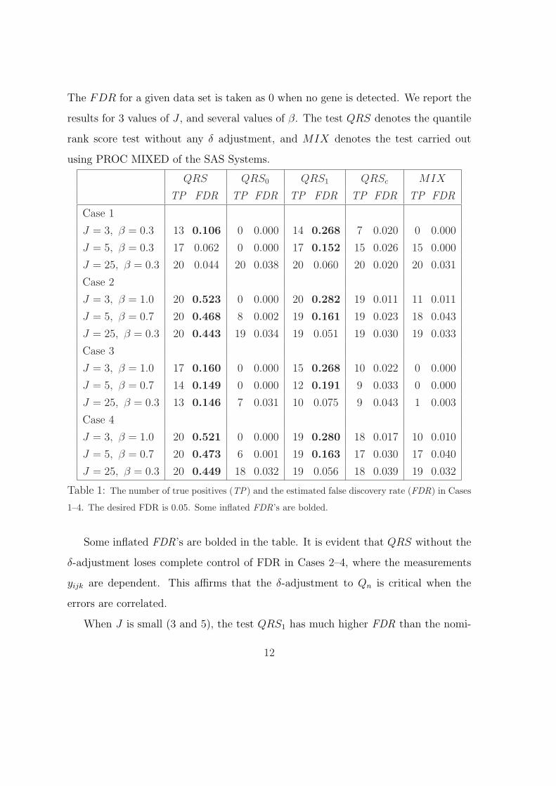
The FDR for a given data set is taken as 0 when no gene is detected. We report the

results for 3 values of J , and several values of β. The test QRS denotes the quantile

rank score test without any δ adjustment, and MIX denotes the test carried out

using PROC MIXED of the SAS Systems.

QRS QRS0 QRS1 QRSc MIX

TP FDR TP FDR TP FDR TP FDR TP FDR

Case 1

J = 3, β = 0.3 13 0.106 0 0.000 14 0.268 7 0.020 0 0.000

J = 5, β = 0.3 17 0.062 0 0.000 17 0.152 15 0.026 15 0.000

J = 25, β = 0.3 20 0.044 20 0.038 20 0.060 20 0.020 20 0.031

Case 2

J = 3, β = 1.0 20 0.523 0 0.000 20 0.282 19 0.011 11 0.011

J = 5, β = 0.7 20 0.468 8 0.002 19 0.161 19 0.023 18 0.043

J = 25, β = 0.3 20 0.443 19 0.034 19 0.051 19 0.030 19 0.033

Case 3

J = 3, β = 1.0 17 0.160 0 0.000 15 0.268 10 0.022 0 0.000

J = 5, β = 0.7 14 0.149 0 0.000 12 0.191 9 0.033 0 0.000

J = 25, β = 0.3 13 0.146 7 0.031 10 0.075 9 0.043 1 0.003

Case 4

J = 3, β = 1.0 20 0.521 0 0.000 19 0.280 18 0.017 10 0.010

J = 5, β = 0.7 20 0.473 6 0.001 19 0.163 17 0.030 17 0.040

J = 25, β = 0.3 20 0.449 18 0.032 19 0.056 18 0.039 19 0.032

Table 1: The number of true positives (TP) and the estimated false discovery rate (FDR) in Cases

1–4. The desired FDR is 0.05. Some inflated FDR’s are bolded.

Some inflated FDR’s are bolded in the table. It is evident that QRS without the

δ-adjustment loses complete control of FDR in Cases 2–4, where the measurements

yijk are dependent. This affirms that the δ-adjustment to Qn is critical when the

errors are correlated.

When J is small (3 and 5), the test QRS1 has much higher FDR than the nomi-

12

nal level, which indicates that the χ2 approximation for QRS1 deteriorates at small

samples. This problem is mostly rectified by QRSc, which controls FDR reasonably

well without losing much power, when the true δ are constant (Cases 1–3), as well as

when they differ slightly from gene to gene (Case 4), supporting our preference for

a genome-wide adjustment of δ. For J = 25, the three variations QRS0, QRS1 and

QRSc perform very similarly.

Generally speaking, the proposed QRSc is very competitive to MIX even in the

Gaussian cases, where the latter loses some power due to the FDR adjustment being

too conservative. In Case 3, where eijk follows a mixture distribution of the standard

normal and t1, QRSc is clearly more powerful than MIX. It is interesting to note

that the efficiency of median regression for Gaussian data is clearly higher than 64%,

the well-known asymptotic efficiency of the univariate sample median relative to the

mean. In fact, the relative efficiency of the median increases for correlated data,

which can be verified both mathematically and empirically.

3.3 Chi-square Approximation Versus Resampling

When J is small, we naturally ask whether we can do better in approximating the

p-values than the (limiting) chi-square distribution for the quantile rank score statis-

tic. We considered permutation, array-wise bootstrap, and blocked wild bootstrap

to generate reference distributions for the quantile rank scores, and compared their

performances with that of QRS0. The details of our Monte Carlo study are skipped,

but the results show that use of the chi-square distribution for the quantile rank score

test is hard to beat by those methods even for small J .

4 Empirical Data Analysis

In this section, we will apply the proposed rank score tests to identify differentially

expressed genes across two experimental conditions to two GeneChip studies. These

13

examples demonstrate the value of the quantile approach in the analysis of GeneChip

data.

4.1 Spiked-In Study

The Spiked-In data set from GeneLogic (http://qolotus02.genelogic.com/datasets.nsf/)

consists of 32 human GeneChip arrays (HG-U95A), and all the arrays have a common

background cRNA derived from an acute myeloid leukemia (AML) tumor cell line. In

the experiment, 11 different cRNA fragments were hybridized at different picomolar

concentrations to each array (apart from replicates). In this example, we choose six

arrays from a pair of triplicates (T1 and T2 ), and the spiked-in concentrations for

each of the 11 control cRNAs are shown in Table 3. Irizarry et al. (2003) provided

some detail on the experimental design.

The total number of probe sets in this study is 12,626. The data are normalized

with the quantile normalization method from Bioconductor’s affy package, using the

default setting as of March, 2006. We consider the log base 2 transformed perfect

match (PM) intensity as dependent variable y. In this study, we expect only those

11 spiked-in probe sets to be differentially expressed.

Considering the small number of replicates in the study, we choose to use the

quantile rank score test QRSc at three quartiles denoted as Q1, Q2 and Q3, respec-

tively. The method MIX on the means is also included for comparison. To study

the genes having a difference between two concentration groups in one of the three

quartiles, we also perform the combined rank score test CRSc, and the Bonferroni

correction (Bonf ) to the p-values of the four individual tests (Q1, Q2, Q3 and MIX)

for each gene. A cutoff 0.05 is used thereafter for the FDR adjusted p-values to iden-

tify differentially expressed genes. Table 2 summarizes the total number of significant

probe sets (Total Positive), the number of correctly identified spiked-in probe sets

(True Positive), and the number of misidentified probe sets (False Positive) for each

14

method used. The Q2 and Bonf perform similarly, both detecting 10 probe sets, 8 of

which are the spiked-ins. The combined rank score test detects all the 11 spiked-in

probe sets successfully without a false positive.

Tests Total Positive True Positive False Positive

Q1 7 7 0

Q2 10 8 2

Q3 0 0 0

MIX 0 0 0

CRSc 11 11 0

Bonf 10 8 2

Table 2: Summary statistics for the Spiked-In study.

Probe Concentration Expected Observed Rank

Set T1 T2 Rank RMA Q1 Q2 Q3 MIX CRSc

BioB-5 at 100.0 0.5 1 1 1 1 1 2 1

BioB-3 at 0.5 25.0 2 2 1 1 1 3 1

BioC-5 at 2.0 75.0 3 3 8 7 1 73 7

BioB-M at 1.0 37.5 3 5 1 1 1 1 1

BioDn-3 at 1.5 50.0 5 4 1 1 1 5 1

DapX-3 at 37.5 3.0 6 7 1 1 1 6 1

CreX-3 at 50.0 5.0 7 9 7 7 1 7 8

CreX-5 at 12.5 2.0 8 8 10 118 1858 2179 10

BioC-3 at 25.0 10.0 9 6431 1096 114 9 12319 11

DapX-5 at 5.0 1.5 10 10 9 118 1266 3433 9

DapX-M at 3.0 1.0 11 6 1 1 1 4 1

Table 3: Expected and observed ranks of the spiked-in probe sets.

Using the same data set, Irizarry et al. (2003) calculated the observed ratios

or “fold changes” between the two averages over the triplicate RMA summarized

measures, and obtained the ranks of the ratios. Here, we provide ranks based on

15

the test statistics proposed in the present paper, as compared to the ranks obtained

under RMA. For the probe sets representing spiked-in cRNAs, the observed ranks

of either fold changes or the test statistics should, ideally, coincide with those of the

true fold changes of the spiked-in concentrations. Table 3 summarizes the spiked-in

concentrations for each of the 11 control cRNAs on the two sets of triplicates (T1 and

T2 ), the expected ranks of the true fold changes, the observed ranks of RMA, QRSc

at three quartiles (Q1, Q2 and Q3), MIX, and the combined rank score test (CRSc).

The quantile score test statistics often have ties, and that is why, for example, the

rank 1 is given to 8 probe-sets under Q3, and in this case, the next rank is 9.

From Table 3, we notice that 8 out of the 11 spiked-in genes are easy to detect, but

3 of them, namely CreX-5 at, BioC-3 at and DapX-5 at show up in the top only by

some measures. The combined test statistic CRSc is a lucky winner, as it separates

all the 11 spiked-in probe sets from the rest. Due to the small number of replicates,

significance tests such as the 2-sample t-test applied to the RMA summarized expres-

sion indices fail to detect any spiked-in genes after the FDR adjustment, even though

the ranks based on the RMA summarized values reflect the expected ranks quite well

(except for one probe set). The use of the probe level data results in a more powerful

statistical inference here.

To explain some of the discrepancies among various tests used, we focus on DapX-

5 at, which is singled out by the quantile rank score test statistic at Q1, but not by

any test statistic (say, MIX) on the mean. Figure 1 gives the expression profile of

this probe set, where the x-axis is the probe number, and the y-axis is the normalized

log2(PM) centered by the median of 6 arrays within each probe. It is clear from

the plot that Array 4 shows the opposite direction of regulation from Arrays 5 and

6. Earlier studies of this data set did not identify this phenomenon, and the reason

for this outlying array is unknown. Possible reasons are image scratches and dust,

16

but if one analyzes the probe level data with no awareness of outliers of this nature,

inference based on averages may take its toll. In this case, Array 4 leads to a large

variance estimate under the Gaussian model, but the 1st quartiles are still clearly

distinguishable for the two groups. If Array 4 is removed, all the tests give consistent

results.

5 10 15 20

−2−1

01

DapX−5_at

Probe

log2P

M

11

1

1 1

11 1

11

1

11 1

1

1

11

11

2 2 22 2

22 2

2 2

22 2 2

2

22

22 2

3 3 3 33

3 3 3 3 3 33 3 3

33 3

3 3 3

44

4

4

4

4

44

44

4

4

4

4

4

44

4

4

4

5

5

5

5

5

5

5

5

5

5

5

5

5

5

5

5

5

5

5

5

6

6

6 6 6

6

6

6

6

6

6

66

6

6

6

6

6

6

6

Figure 1: Expression profiles of gene DapX-5 at in Spiked-In study. The y-axis is the normalized

log2(PM) centered by the median of 6 arrays within each probe. The symbols 1–3 represent the 3

replicate arrays from T1, and the symbols 4–6 represent the 3 arrays from T2.

4.2 Smoking Study

The Smoking study was conducted by the Boston University School of Medicine. The

raw data set was downloaded from the National Center for Biotechnology Information

(accession no. GSE994). The experiment was designed to study the effects of cigarette

smoking on the human airway epithelial cell transcriptome. The data set consists of

75 Affymetrix U133A human gene expression arrays, including 34 arrays with RNA

samples of current smokers, 23 arrays of healthy nonsmokers, and 18 arrays from

former smokers. More information of the data set can be found in Spira et al. (2004).

17

The number of genes analyzed is 22,204, and the number of probes is 11 for most of

the genes. The data are preprocessed with the background correction and quantile

normalization methods from Bioconductor’s package affy. In this analysis, we focus

on the genes that are found to be differentially expressed by one test, but not the

other.

There are 217 genes detected by MIX but not by Q2, and 378 genes vice versa.

For those “controversial” genes, we examine their expression profiles, and verify the

probe sequences using the BLAST program from NCBI. We find that many of these

cases have outlying probes or observations. Four such genes (210384 at, 201147 s at,

208725 at and 200654 at) are shown here for illustration. Figure 2 shows the boxplots

of expression intensities with regard to different probes. The x-axis represents the

probes. The y-axis is the log2PM after quantile normalization. The grey boxes are

of current smokers, and the white boxes are of nonsmokers. The genes 210384 at and

201147 s at are detected to be significant in the mean but not in the median, while

genes 208725 at and 200654 at are found to be significant in the median but not in

the mean. Table 4 summarizes the raw p-values from MIX and Q2 for these 4 genes

before and after excluding the outlying probes or observations. The p-values from

the 2-sample t-test based on the RMA summarized values are included for reference.

Note that RMA is not robust against outlying arrays, but rather robust against a

small number of outlying probes, so it is quite clear from the table that the results

from RMA are more in line with those from Q2, but the test is less powerful.

For gene 210384 at, the BLAST results show that the probes 3, 6, 8 and 10

have no match to human genome, while the rest of the probes match sequences on

chromosome 21. From Figure 2, we notice the low intensities of these 4 probes. In

addition, the probes 3, 8, and 10 show smaller median in the nonsmoker group, which

is the opposite to the comparisons from the other probes. This leads the test on

18

the median to show no significance. After excluding these four suspectable probes,

both mean and median tests show that this gene has significantly higher intensities

in nonsmokers than in smokers (see Table 4).

1 1 2 2 3 3 4 4 5 5 6 6 7 7 8 8 9 9 10 11

34

56

78

210384_at

log

2P

M

1 1 2 2 3 3 4 4 5 5 6 6 7 7 8 8 9 9 10 11

46

81

0

201147_s_at

1 1 2 2 3 3 4 4 5 5 6 6 7 7 8 8 9 9 10 11

34

56

78

9

208725_at

Probe

log

2P

M

1 1 2 2 3 3 4 4 5 5 6 6 7 7 8 8 9 9 10 11

46

81

0

200654_at

Probe

Figure 2: Expression profiles of four example genes in Smoking study. The x-axis represents the

probes. The y-axis is the log2PM after quantile normalization. The grey boxes are of current

smokers, and the white boxes are of nonsmokers.

19

GeneID Probes excludedBefore After

Q2 MIX RMA Q2 MIX

210384 at 3, 6, 8 and 10 0.033 0.001 0.050 0.000 0.000

201147 s at outlying observations 0.676 0.005 0.425 0.873 0.200

208725 at 1 and 6 0.001 0.088 0.010 0.000 0.005

200654 at 8–11 0.002 0.249 0.051 0.003 0.084

Table 4: P -values before and after excluding the outlying cases for 4 genes in the Smoking study.

For gene 201147 s at, the test MIX gives a p-value 0.005 while the median test

Q2 gives a large p-value 0.676. Figure 2 suggests that the significance in the mean is

mostly due to quite a few outlying observations, which drives up the mean intensities

of current smokers. After excluding the outlying observations (marked as circles in

the box plots), neither mean nor median tests show significance. In this case it is

unclear whether any conclusion could be made without further study.

For gene 208725 at, the BLAST results show that the probes 1 and 6 have no

match to any sequence on human genome, while the other probes match sequences on

chromosome 20. The two suspectable probes, especially probe 6, inflate the variances

to make it harder to detect changes in the mean. With these two probes removed,

the p-value from MIX falls from 0.088 to 0.005.

For gene 200654 at, we see an interesting phenomenon. The probes 8–11 have

much lower intensities than the other probes. Furthermore, the first 7 probes show

higher median intensities for the smokers, leading to a significance in the quantile

rank score test at Q2. The differences in the means are found to be insignificant

due to high between-probe variability. For this gene, alternative splicing might have

occurred (see, e.g., Wu et al., 2005), but further studies are needed to definitively

explain the different gene expression profiles in probes 8–11.

The upshot of this example is that examining the differences in the quantiles in

20

addition to the mean can help identify individual genes that cannot be summarized

rightly by the means. As we know, different probes have different sensitivity and

specificity, and more importantly, problems in probe selection, cross-hybridization,

probe-to-gene mapping, and alternative splicing all point to one thing, that is, it

would be naive to trust the results from any test on the mean. Because of the large

number of genes in microarray studies, human inspection of every single gene might

be practically prohibitive. The quantile approach considered in this paper may be

used to cross check the results we normally obtain on the mean intensities. We have

found that significant differences in the quartiles can often be detected more reliably

than differences in the means. Discrepancies in the test results may flag anomaly

in the probe sets used, suggesting focused validation studies on a smaller number of

genes.

Some empirical studies of the current and earlier GeneChip data suggest that up to

20% of the probe level data might be compromised for certain genes, which support

our preference on hypothesis testing on the 3 quartiles. In one study, Mecham et

al. (2004) pointed out that for mammalian Affymetrix microarrays the proportion of

inaccurate probes is in the 20% range. Quality improvement is being made constantly

in microarray technology, but the quantile approach can be valuable even if the probe

level measurements are free of technical problems. The genes of interest are often

those with non-Gaussian distributions in their intensities (on log scale), and the

quantiles give more comprehensive summaries than the mean in those cases.

5 Conclusions

The quantile rank score tests are very useful in the analysis of probe level genomic

data. The array effect, which is a random effect in linear models, requires an ad-

justment of the rank score test statistic as discussed in the present paper. General

inferential tools for linear quantile regression with correlated measurements are lit-

21

tle discussed in the literature yet. In this paper, we propose a simple genome-wide

δ-adjustment to the quantile rank score test under the working assumption of an ad-

ditive homogenous random effect to the error. The resulting quantile rank score test

is easy to implement and robust in performance. Our empirical studies of GeneChip

data show that inference on the quartiles of the gene expression distribution often

lead to more reliable results than inference on the mean. We also demonstrate that

discrepancies in the significance results on the quartiles and on the mean often flag

anomaly in the probe sets being considered. It is our hope that by taking the proposed

quantile approach in the analysis of probe level microarray data can one improve re-

liability of and confidence in the results.

In the Genechip studies given in this paper, we take the position that any apparent

probe-treatment interaction in the data is a nuisance, against which our comparisons

of treatment should be robust. In other studies however, the interaction terms may

be of interest. For example, the quantile approach will also be useful for analyzing

the more recent release of the exon tiling arrays where inference needs to be made on

the exon sites by treatment interaction. The proposed rank score test applies readily

to those applications, but no empirical work has been done so far.

6 Appendix

Following Section 2.1, we start with technical assumptions.

A1: F1 has a Lebesgue density f1 > 0 with a bounded first-order derivative. The

joint distribution function F1,2 of uijk1 and uijk2 for any i, j and k1 6= k2 is

Lipschitz in a neighborhood of (0, 0).

A2: maxijk ‖xijk‖ = O(n1/4/√

logn), and n−1∑

ijk ‖xijk‖3 = O(1) as n →∞, where

‖xijk‖ denotes the Euclidean norm of xijk.

A3: The minimum eigenvalues of D1n = n−1Z∗Tn Z∗

n, D2n = n−1∑

ij

∑k1 6=k2

z∗Tijk1z∗ijk2

22

and D3n = n−1XTn Xn are bounded away from 0 as n →∞.

A4: {Kij, i = 1, · · · , I, j = 1, · · · , Ji} is an uniformly bounded sequence of positive

integers.

Note that Assumption A2 implies that the maximum eigenvalues of D1n, D2n and

D3n are bounded away from infinity.

The proof of Theorem 1 relies on the following three lemmas. Lemma 1 follows

easily from Theorem 1 of He, Zhu and Fung (2002), so the proof is skipped.

Lemma 1 Let α(τ) = argmina∈Rp

∑ijk ρτ (yijk − xT

ijka) be a quantile estimate of

α(τ). Then, under Assumptions A2–A4 and H0, we have α(τ)− α(τ) = Op(n−1/2).

Lemma 2 Let S∗n = n−1/2∑

ijk z∗ijkψτ (yijk − xTijkα(τ)), then under Assumptions A1–

A4 and under H0, we have Sn = S∗n + op(1).

Proof of Lemma 2: Consider any t such that ||t|| ≤ C(logn)1/2 for some constant

C. Let uijk(τ) = uijk − F−11 (τ),

Rij(t) =

Kij∑

k=1

z∗ijk[ψ(uijk(τ)− n−1/2(xT

ijkt))− ψ(uijk(τ))]. (8)

and rn(t) =∑

ij Rij(t). For each (i, j), we have

V ar(Rij(t)) ≤ Kij

Kij∑

k=1

||z∗ijk||2 ·∣∣P (uijk(τ) < n−1/2(xT

ijkt))− P (uijk(τ) < 0)∣∣

= Kij

Kij∑

k=1

||z∗ijk||2f1(F−11 (τ)) · n−1/2|xT

ijkt|, (9)

where F−11 (τ) is between F−1

1 (τ) and F−11 (τ) + n−1/2(xT

ijkt), and the first part of

Assumption A1 is used in the last step.

23

Therefore, by Assumptions A2 and A4, we know that

∑ij

V ar(Rij(t)) ≤ c1(nlogn)1/2, (10)

and

maxijk

Rij(t) ≤ c2 maxijk

||z∗ijk|| ≤ c3(nlogn)1/4/√

logn, (11)

where c1, c2 and c3 are positive constants.

Thus, applying the well-known Hoeffding inequality, there is c0 such that for λ > 0

and n large enough,

P{|rn(t)− E(rn(t))| ≥ c0λn1/4(logn)3/4

} ≤ 2n−λ. (12)

Following the similar chaining argument used in the proof of Lemma A.2 in

Koenker and Portnoy (1987), we can extend (12) uniformly in {t : ||t|| ≤ C(logn)1/2},and get,

sup||t||≤C(logn)1/2

||rn(t)− E(rn(t))|| = Op(n1/4(logn)3/4). (13)

From (8), we know that

sup||t||≤C(logn)1/2

||E(rn(t))||

= sup||t||≤C(logn)1/2

||∑

ijk

z∗ijk[F1(F

−11 (τ))− F1(F

−11 (τ) + n−1/2(xT

ijkt))] ||

= sup||t||≤C(logn)1/2

||∑

ijk

z∗ijk[f1(F

−11 (τ))n−1/2(xT

ijkt) + f′1(F

−11 (τ))n−1(xT

ijkt)2]||

= O(logn), (14)

where the fact that Z∗Tn X = 0, and Assumptions A1, A2 and A4 are used in the last

step.

24

Combining (13) and (14), we have

sup‖t‖≤C(logn)1/2

n−1/2

∣∣∣∣∣∑

ijk

z∗ijk[ψτ

(uijk(τ)− n−1/2(xT

ijkt))− ψτ (uijk(τ))

]∣∣∣∣∣ = op(1), (15)

which together with Lemma 1 complete the proof.

Lemma 3 Under H0 and Assumptions A1–A4, we have δP−→ δ, as n →∞.

Recall that δ = P (u111(τ) < 0, u112(τ) < 0). Lemma 3 can be verified using

Lemma 4.1 of He and Shao (1996), which provides an uniform approximation of the

sum in δ. We skip the details that are purely technical.

Proof of Theorems 1 and 2:

Let

Rij =

Kij∑

k=1

z∗ijkψτ (yijk − xTijkα(τ)) =

Kij∑

k=1

z∗ijk(τ − I{uijk(τ)<0}

),

where uijk(τ) = uijk − F−11 (τ). Direct calculations show that

Cov(Rij) =

Kij∑

k=1

z∗ijkz∗Tijkτ(1− τ) +

Kij∑

k1 6=k2

z∗ijk1z∗Tijk2

[−τ 2 + δ].

Note that S∗n = n−1/2∑I

i=1

∑Ji

j=1 Rij, and that Rij are independent entries. It follows

from the Lindberg-Feller central limit theorem (CLT) that

(Q∗n)−1/2 S∗n

D−→ N(0q, Iq), (16)

as n →∞, where Q∗n = n−1

∑ijk z∗ijkz

∗Tijkτ(1− τ)+n−1

∑ij

∑Kij

k1 6=k2z∗ijk1

z∗Tijk2(−τ 2 + δ).

The proof for Theorem 1 is therefore complete by combining (16), Lemmas 2 and 3.

The proof of Theorem 2 is a direct extension of that of Theorem 1, where we

approximate each S(a)n in Wn by S

(a)∗n = n−1/2

∑ijk z∗ijkψτa(uijk(τa)) for 1 ≤ a ≤ l.

For details, we refer to the doctoral thesis Wang (2006).

25

References

[1] Affymetrix (2001), Statistical algorithm reference guide, Affymetrix, Santa Clara,

CA, version 5.

[2] Benjamini, Y. and Hochberg, Y. (1995), “Controlling the false discovery rate: a

practical and powerful approach to multiple testing,” Journal of the Royal Statis-

tical Society Series B, 57, 289-300.

[3] Chu, T., Weir, B. and Wolfinger, R. (2002), “A systematic statistical linear mod-

eling approach to oligonucleotide array experiments,” Mathematical Biosciences,

176, 35-51.

[4] Fan, J. Chen, Y., Chan, H. M., Tam, P. K. H. and Ren, Y. (2005), “Removing

intensity effects and identifying significant genes for Affymetrix arrays in MIF-

suppressed neuroblastoma cells,” Proc. Natl. Acad. Sci., 102, 17751-17756.

[5] Fan, J., Huang, T. and Peng, H. (2005), “Semilinear high-dimensional model for

normalization of microarray data: a theoretical analysis and partial consistency,”

(with discussion) Journal of American Statistical Association, 100, 781–813.

[6] Gutenbrunner, C., Jureckova, J., Koenker, R. and Portnoy, S. (1993), “Tests

of linear hypotheses based on regression rank scores,” Journal of Nonparametric

Statistics, 2, 307-333.

[7] He, X. and Shao, Q. M. (1996), “A general Bahadur representation of M-

estimators and its application to linear regression with nonstochatic designs,”

Annals of Statistics, 24, 2608-2630.

26

[8] He, X., Zhu, Z. Y. and Fung, W. K. (2002), “Estimation in a semiparametric

model for longitudinal data with unspecified dependence Structure,” Biometrika,

89, 579-590.

[9] Hu, J. and He, X. (2005), “Enhanced quantile normalization of microarray data to

reduce loss of information in the gene expression profile,” To appear in Biometrics.

[10] Irizarry, R. A., Hobbs, F. C. B., Beaxer-Barclay, Y., Antonellis, K., Scherf, U.

and Speed, T. P. (2003), “Exploration, normalization, and summaries of high

density oligonucleotide array probe level data,” Biostatistics, 4, 249-264.

[11] Khuri, A. I., Mathew, T., and Sinha, B. K. (1998), Statistical tests for mixed

linear models, Wiley, Inc., New York, NY.

[12] Kocherginsky, M., He, X. and Mu, Y. (2005), “Practical Confidence Intervals for

Regression Quantiles,” Journal of Computational and Graphical Statistics, 14,

41-55.

[13] Koenker, R. (2004), “Quantile regression for longitudinal Data,” Journal of Mul-

tivariate Analysis, 91, 74-89.

[14] Koenker, R. (2005), Quantile regression, Cambridge University Press.

[15] Koenker, R. and Bassett, G. J. (1978), “Regression quantiles,” Econometrica,

46, 33-50.

[16] Koenker, R. and Portnoy, S. (1987), “L-estimation for linear models,” Journal

of the American Statistical Association, 82, 851-857.

[17] Li, C. and Wong, W. H. (2001), “Model-based analysis of oligonucleotide arrays:

expression index computation and outlier detection,” Proceedings of the National

Academy of Science U S A, 98, 31-36.

27

[18] Littell, R. C., Milliken, G. A., Stroup, W. W., Wolfinger R. D. (1996), SAS

system for mixed models, SAS Institute.

[19] Lonnstedt, I. and Speed, T. P. (2002), “Replicated microarray data,” Statistica

Sinica, 12, 31-46.

[20] Mecham, B. H., Wetmore, D. Z., Szallasi, Z., Sadovsky. Y., Kohane, I. and

Mariani, T. J. (2004), “Increased measurement accuracy for sequence-verified mi-

croarray probes,” Physiol Genomics, 18, 308-15.

[21] Spira, A., Beane, J., Shah, V., Liu, G., Schembri, F., Yang, X., Palma, J. and

Brody, J. S. (2004), “Effects of cigarette smoke on the human airway epithelial

cell transcriptome,” Proceedings of the National Academy of Sciences, 101, 10143-

10148.

[22] Wang, H. (2006), Inference on quantile regression for mixed models with appli-

cations to GeneChip data, Ph.D. Dissertation, University of Illinois at Urbana-

Champaign, IL.

[23] Wu, C., Morris, J.S., Baggerly, K. A., Coombes, K. R., Girard. L., Minna, J. D.,

and Zhang, L. (2005), “A probe-to-transcripts mapping method for microarray

data preprocessing to reflect transcriptome complexity,” Preprint.

28