DESIGNERS' GUIDE TO EUROCODE 7: GEOTECHNICAL ...
213
DESIGNERS’ GUIDES TO THE EUROCODES DESIGNERS’ GUIDE TO EUROCODE 7: GEOTECHNICAL DESIGN DESIGNERS’ GUIDE TO EN 1997-1 EUROCODE 7: GEOTECHNICAL DESIGN – GENERAL RULES R. FRANK, C. BAUDUIN, R. DRISCOLL, M. KAVVADAS, N. KREBS OVESEN, T. ORR and B. SCHUPPENER Series editor H. Gulvanessian
-
Upload
khangminh22 -
Category
Documents
-
view
0 -
download
0
Transcript of DESIGNERS' GUIDE TO EUROCODE 7: GEOTECHNICAL ...

DESIGNERS’ GUIDES TO THE EUROCODES
DESIGNERS’ GUIDE TO EUROCODE 7:GEOTECHNICAL DESIGN
DESIGNERS’ GUIDE TO EN 1997-1EUROCODE 7: GEOTECHNICAL DESIGN – GENERAL RULES
R. FRANK, C. BAUDUIN, R. DRISCOLL, M. KAVVADAS,N. KREBS OVESEN, T. ORR and B. SCHUPPENER
Series editorH. Gulvanessian
Published by ICE Publishing, One Great George Street, Westminster, London SW1P 3AA.
Full details of ICE Publishing sales representatives and distributors can be found at: www.icevirtuallibrary.com/info/printbooksales
First published 2005Reprinted 2009, 2013
A catalogue record for this book is available from the British Library
ISBN: 978-0-7277-3154-8
© The authors and Thomas Telford Limited 2005
All rights, including translation, reserved. Except as permitted by the Copyright, Designs and PatentsAct 1988, no part of this publication may be reproduced, stored in a retrieval system or transmitted inany form or by any means, electronic, mechanical, photocopying or otherwise, without the prior
This book is published on the understanding that the authors are solely responsible for the statementsmade and opinions expressed in it and that its publication does not necessarily imply that suchstatements and/or opinions are or reflect the views or opinions of the publishers. While every efforthas been made to ensure that the statements made and the opinions expressed in this publicationprovide a safe and accurate guide, no liability or responsibility can be accepted in this respect by theauthors or publishers.
Typeset by Helius, Brighton and RochesterPrinted and bound in Great Britain by CPI Group (UK) Ltd, Croydon CR0 4YY
Eurocodes Expert
Structural Eurocodes offer the opportunity of harmonized design standards for the European construction market and the rest of the world. To achieve this, the construction industry needs to become acquainted with the Eurocodes so that the maximum advantage can be taken of these opportunities
Eurocodes Expert is a new ICE and Thomas Telford initiative set up to assist in creating a greater awareness of the impact and implementation of the Eurocodes within the UK construction industry
Eurocodes Expert provides a range of products and services to aid and support the transition to Eurocodes. For comprehensive and useful information on the adoption of the Eurocodes and their implementation process please visit our website or email [email protected]
written permission of the Publisher, ICE Publishing, One Great George Street, Westminster, London SW1P 3AA.

Preface
EN 1997-1, Eurocode 7: Geotechnical Design, Part 1: General Rules, is the document in theEurocode suite concerned with the general geotechnical aspects of the design of structures.It applies the principles of EN 1990, Eurocode: Basis of Structural Design, by setting therules for determining the geotechnical actions and for checking the acceptability of thegeotechnical resistances.
Aims and objectives of this guideThe principal aim of this guide is to provide guidance on the use and interpretation ofEN 1997-1.
Eurocode 7 assumes that the user has an adequate knowledge and understanding of soilmechanics and geotechnical engineering. The reader of this guide is also expected to be ageotechnical engineer or to be familiar with conventional geotechnical design.
Throughout this guide emphasis is placed on everyday practice, avoiding complicatedgeotechnical design cases, in order to ease the understanding of the new concepts and rulesfor geotechnical design appearing in EN 1997-1. Comment is made only on material inEN 1997-1 that is felt to differ from traditional practice.
For many aspects, this guide aims to be a self-sufficient document but, as the clauses ofEN 1997-1 are repeated only when strictly necessary, the reader should read the guide inconjunction with the code itself.
Layout of this guideEN 1997-1 has a Foreword and 12 sections together with nine annexes; this guide has thesame structure, with the chapters corresponding to the sections in the code. Annex A ofEN 1997-1 gives the partial factors and their recommended values for checking ultimatelimit states in persistent and transient situations. All the other annexes of EN 1997-1 relateto a specific section, and are thus dealt with in the corresponding chapters of this guide.
Each chapter of the guide follows the order of its corresponding section of EN 1997-1unless this is found to be unhelpful for providing guidance on the use and interpretation ofEN 1997-1 (this is particularly the case for Section 6 and, to some extent, for Section 8).Consequently, the section numbering in this guide does not necessarily match that inEN 1997-1: the correspondence between the numbering is indicated in the contents listbeginning each chapter in this guide.
Worked examples are given for the determination of characteristic values (Chapter 2), forspread foundations (Chapter 6), for pile foundations (Chapter 7), for anchorages (Chapter

8), for retaining structures (Chapter 9) and for overall stability (Chapter 11). These examplesare intended to highlight issues relevant to the application of EN 1997-1.
All cross-references in this guide to sections, clauses, subclauses, paragraphs, annexes,figures, tables and expressions of EN 1997-1-1 are in italic type, which is also used where textfrom EN 1997-1-1 has been directly reproduced (conversely, quotations from other sources,including other Eurocodes, and cross-references to sections, etc., of this guide, are in romantype). Expressions repeated from EN 1997-1-1 retain their numbering; other expressionshave numbers prefixed by D (for Designers’ Guide), e.g. equation (D2.1) in Chapter 2. Boldtype is used for textual emphasis.
AcknowledgementsThis book would not have been possible without the successful completion of Eurocode 7 –Part 1. Those involved in this process included:
• the project team for converting ENV 1997-1 into EN 1997-1• the working group for converting ENV 1997-1 into EN 1997-1• the project team for ENV 1997-1 (1994)• the chairman and members of the ad hoc group of the European Commission, who in
1978 drafted the first model code for Eurocode 7.
The important contributions of the following in the development of Eurocode 7 – Part 1are also acknowledged:
• the national geotechnical societies of the EC countries (who are members of theInternational Society for Soil Mechanics and Geotechnical Engineering, ISSMGE) fortheir support, especially in the early years of the development of Eurocode 7
• national delegations to CEN/TC 250/SC7, and their national technical contacts, for theirvaluable and constructive comments
• members of the project team for EN 1990, Eurocode: Basis of Structural Design, for theircontributions to the clauses in EN 1997-1 relating to soil–structure interaction.
This guide is dedicated by its authors to their colleagues mentioned above. The authorsalso wish to thank:
• Their wives, Vassilia Frank, Bénédicte Bauduin, Liz Driscoll, Kitty Kavvadas, HanneKrebs Ovesen, Diane Orr and Jutta Schuppener, for their support and patience.
• Their employers, CERMES (ENPC-LCPC), Paris; BESIX, Brussels; BRE, Garston;NTUA, Athens; GEO-Danish Geotechnical Institute, Lyngby; Trinity College, Dublin;and BAW, Karlsruhe.
R. FrankC. BauduinR. DriscollM. KavvadasN. Krebs OvesenT. OrrB. Schuppener
vi
DESIGNERS’ GUIDE TO EN 1997-1

Contents
Preface vAims and objectives of this guide vLayout of this guide vAcknowledgements vi
Foreword 1The Eurocode programme 1The development of Eurocode 7 2The content of Eurocode 7 3The three Design Approaches 3National implementation of Eurocode 7 5Application of informative annexes 7The schedule 8Packages of EN Eurocode parts 8National tasks for implementation 9
Chapter 1. General 111.1. Scope 11
1.1.1. Scope of Eurocode 7 – Part 1 111.1.2. Designs not fully covered by Eurocode 7 – Part 1 121.1.3. Contents and organization of Eurocode 7 – Part 1 121.1.4. Eurocode 7 – Part 2 13
1.2. References 131.3. Assumptions 141.4. Distinction between Principles and Application Rules 161.5. Definitions 16
1.5.1. Definitions common to all Eurocodes 161.5.2. Definitions specific to Eurocode 7 16
1.6. Symbols 17
Chapter 2. Basis of geotechnical design 192.1. Design requirements 192.2. Design situations 202.3. Durability 212.4. Geotechnical design by calculation 23
2.4.1. General 232.4.2. Actions 24

2.4.3. Ground properties 242.4.4. Characteristic values of geotechnical parameters 242.4.5. Ultimate limit states 302.4.6. Serviceability limit state design 37
2.5. Design by prescriptive measures 392.6. Observational method 392.7. Geotechnical Design Report 39Example 2.1: selection of a characteristic value using statisticalmethods 41Appendix: an example of the use of statistical methods to assesscharacteristic values 44
Chapter 3. Geotechnical data 533.1. Introduction 533.2. Geotechnical investigations 533.3. Evaluation of geotechnical parameters 54
3.3.1. General 543.3.2. Characterization of soil and rock type 553.3.3. Procedure for evaluating geotechnical parameters 553.3.4. Characteristic values 58
3.4. Ground Investigation Report 58
Chapter 4. Supervision of construction, monitoring and maintenance 614.1. Introduction 614.2. Supervision 624.3. Checking ground conditions 634.4. Checking construction 634.5. Monitoring 64
Chapter 5. Fill, dewatering, ground improvement and reinforcement 655.1. General 655.2. Fundamental requirements 655.3. Fill construction 665.4. Dewatering 665.5. Ground improvement and reinforcement 66
Chapter 6. Spread foundations 696.1. Design methods 706.2. Overall stability 706.3. Direct method: ULS design 72
6.3.1. Bearing resistance 726.3.2. Sliding resistance 786.3.3. Loads with large eccentricities 806.3.4. Structural failure due to foundation movement 81
6.4. Direct method: SLS design by settlement calculations 826.5. Indirect method: simplified SLS method 84
6.5.1. General 846.5.2. Indirect method based on limiting the mobilization
of bearing resistance 846.6. Prescriptive method 856.7. Structural design 85Example 6.1: square pad foundation on soft clay 86
DESIGNERS’ GUIDE TO EN 1997-1
viii

Example 6.2: ULS design of spread foundation for a tower 93Example 6.3: design based on the indirect method usingpressuremeter test results 99
Chapter 7. Pile foundations 1017.1. General 1017.2. Limit states 1027.3. Actions and design situations 1027.4. Design methods and design considerations 1037.5. Pile load tests 1047.6. Axially loaded piles 105
7.6.1. General 1057.6.2. Compressive ground resistance (ULS) 1067.6.3. Ground tensile resistance 1127.6.4. Vertical displacements of pile foundations 114
7.7. Transversely loaded piles 1147.8. Structural design of piles 1147.9. Supervision of construction 115Example 7.1: design of a pile in compression from static loadtest results 115Example 7.2: design of a pile in compression from in situ testresults 118Example 7.3: design of a pile in compression from laboratorytest results 121Example 7.4: design of a pile subject to downdrag 125Example 7.5: uplift of piled structures 128
Chapter 8. Anchorages 1338.1. General 1338.2. Ultimate limit state design 134
8.2.1. Design of the anchorage 1348.2.2. Design value of the anchorage load 1348.2.3. Design value of the anchorage resistance 138
8.3. Structural design of anchorages 1398.4. Load testing of ground anchorages 140
8.4.1. Acceptance tests 1408.4.2. Suitability tests 1408.4.3. Investigation tests 1418.4.4. Proof load as an action to the structure 141
Example 8.1: assessment of proof load for suitability andacceptance tests 141
Chapter 9. Retaining structures 1459.1. General 1469.2. Limit states 1469.3. Actions, geometrical data and design situations 147
9.3.1. Actions 1479.3.2. Geometrical data 148
9.4. Design and construction considerations 1489.5. Determination of earth pressures 1499.6. Water pressures 1519.7. Ultimate limit state design 1519.8. Serviceability limit state design 160
CONTENTS
ix

9.8.1. General 1609.8.2. Displacements 161
Example 9.1: ULS design of a stem (gravity) wall 161Example 9.2: ULS and SLS design of an embedded sheet pile wall 173
Chapter 10. Hydraulic failure 18510.1. General 18510.2. Failure by uplift (UPL) 186
10.2.1. General 18610.2.2. Submerged structures 18710.2.3. Design against uplift of an impermeable layer 18810.2.4. Worked example of a design against uplift 188
10.3. Failure by heave (HYD) 18910.3.1. General 18910.3.2. Design using total stresses 18910.3.3. Design using submerged weight 19010.3.4. Determination of the relevant pore water pressure 19010.3.5. Worked example of a design against failure by heave 19110.3.6. Discussion on failure by uplift and failure by heave 191
10.4. Internal erosion 19110.4.1. Filter criteria and hydraulic criteria 19110.4.2. Effects of material transport 192
10.5. Failure by piping 19210.5.1. General 19210.5.2. Design against failure by piping 192
Chapter 11. Overall stability 19511.1. General 19511.2. Limit states 19511.3. Actions and design situations 19611.4. Design and construction considerations 19611.5. Ultimate limit state design 19611.6. Serviceability limit state design 20111.7. Monitoring 202Example 11.1: overall stability of a cutting in stiff clay 202
Chapter 12. Embankments 20712.1. General 20712.2. Limit states 20712.3. Actions and design situations 20812.4. Design and construction considerations 20812.5. Ultimate limit state design 20812.6. Serviceability limit state design 20812.7. Supervision and monitoring 208
References 211
Index 213
DESIGNERS’ GUIDE TO EN 1997-1
x

CHAPTER 1
General
This chapter is concerned with the general aspects of EN 1997-1. The structure of thechapter follows that of Section 1:
1.1. Scope Clause 1.11.2. References Clause 1.21.3. Assumptions Clause 1.31.4. Distinction between Principles and Application Rules Clause 1.41.5. Definitions Clause 1.51.6. Symbols Clause 1.6
1.1. Scope1.1.1. Scope of Eurocode 7 – Part 1
Clause 1.1.1(2)Clause 1.1.2(1)Clause 1.1.1(1)
EN 1997-1 gives the general principles and requirements, as well as the general applicationrules, relevant to the geotechnical aspects of the design of buildings and civil engineeringworks. It has to be used in conjunction with EN 1990, Eurocode: Basis of Structural Design,which is the head document in the Eurocode suite and thus establishes, for all the structuralEurocodes, the principles and requirements for safety, serviceability and durability ofstructures; it further describes the basis of design and verification and provides guidelines forrelated aspects of structural reliability.
Clause 1.1.1(4)EN 1990 gives, in particular, the rules for calculating the combinations of the actions on
buildings and civil engineering works. The numerical values of the structural actions aregiven in EN 1991, Eurocode 1: Actions on Structures, and in the corresponding NationalAnnex for a particular country.
The provisions for the design of a structure in a particular material (e.g. concrete orsteel), specifically its strength and resistance, are the subject of the ‘material’ Eurocodes(Eurocodes 2 to 6 and 9). Eurocode 7 (on geotechnical design) and Eurocode 8 (onearthquake resistance) are relevant to all types of structures, whatever the constructionmaterial.
Clause 1.1.1(3)Clause 1.1.1(4)
EN 1997-1 describes the requirements for geotechnical design, in order to ensure safety(strength and stability), serviceability and durability of supported structures, i.e. of buildingsand civil engineering works, founded on soil and rock. In particular, it deals with thecalculation of geotechnical actions, of their effects on structures and of geotechnicalresistances.
Clause 1.1.1(7)For geotechnical design under seismic conditions, the design rules of EN 1997-1 should becomplemented by the rules of EN 1998-5, Eurocode 8 – Part 5: Design of Structures forEarthquake Resistance. Foundations, Retaining Structures and Geotechnical Aspects.

1.1.2. Designs not fully covered by Eurocode 7 – Part 1
Clause 2.1(21)
As already noted in the Foreword to this guide, Eurocode 7 can also serve as a referencedocument for the geotechnical aspects of dams and tunnels, of slope stabilization, and offoundations for special construction works (e.g. nuclear power plants); additional provisionsto those provided by EN 1997-1 will probably be necessary (see clause 1.1(2) in EN 1990 andclause 2.1(21) in EN 1997-1).
1.1.3. Contents and organization of Eurocode 7 – Part 1Clause 1.1.2(2) The subjects covered in the different sections of EN 1997-1 are as follows:
• Section 1: general• Section 2: basis of geotechnical design• Section 3: geotechnical data• Section 4: supervision of construction, monitoring and maintenance• Section 5: fill, dewatering, ground improvement and reinforcement• Section 6: spread foundations• Section 7: pile foundations• Section 8: anchorages• Section 9: retaining structures• Section 10: hydraulic failure• Section 11: site stability• Section 12: embankments.
The sections of EN 1997-1 can be described as follows:
• Section 1 gives the general assumptions and definitions, the symbols, etc.• Sections 2, 3, 4, 10 and 11 are applicable to all types of geotechnical structures.• Sections 6, 7 and 9 are specific to particular categories of geotechnical works (shallow or
spread foundations, deep or pile foundations and retaining structures, respectively).• Section 8 on anchorages is intended to be used for the design of temporary and
permanent anchorages used to support retaining structures, to stabilize slopes, cuts ortunnels, and to resist uplift forces on structures.
• Sections 5 and 12 cover geotechnical works of a more general nature.
The chapters in this guide and their contents correspond to the sections of Eurocode 7.Clause 1.1.2(3) The following annexes are included in EN 1997-1:
• Annex A (normative): partial and correlation factors for ultimate limit states andrecommended values
• Annex B (informative): background information on partial factors for Design Approaches1, 2 and 3
• Annex C (informative): sample procedures to determine limit values of earth pressureson vertical walls
• Annex D (informative): a sample analytical method for bearing resistance calculation• Annex E (informative): a sample semi-empirical method for bearing resistance estimation• Annex F (informative): sample methods for settlement evaluation• Annex G (informative): a sample method for deriving presumed bearing resistance for
spread foundations on rock• Annex H (informative): limiting values of structural deformation and foundation movement• Annex J (informative): checklist for construction supervision and performance monitoring.
Annex A is to be used with Sections 6 to 12, as it gives the relevant partial and correlationfactors for ultimate limit state design. Annex A is normative, which means that it is an integralpart of the standard and must be applied. However, the values of the partial and correlationfactors, given in informative notes, are recommended values and therefore may be modifiedin the National Annex for each country.
12
DESIGNERS’ GUIDE TO EN 1997-1

Annex B gives some background information on partial factors for applying the threepossible Design Approaches permitted by EN 1990 and by EN 1997-1 (for ultimate limitstates in persistent and transient situations).
Annexes C to J are informative, which means that in a given country, a choice can be madein the National Annex whether or not to apply them in that country.
Annexes C to G are examples of internationally recognized calculation methods relevantto the design of foundations or retaining structures.
Annex H deals with limiting movements of foundations, and Annex J is a proposedchecklist for construction supervision and performance monitoring.
The contents of each annex are discussed in this guide in the chapter that corresponds tothe appropriate section of EN 1997-1.
1.1.4. Eurocode 7 – Part 2Clause 1.1.3(1)EN 1997-1 will be supplemented by a second part: EN 1997-2, Eurocode 7: Geotechnical
Design, Part 2: Ground Investigation and Testing. Part 2 will give the general requirementsand rules for the performance and evaluation of laboratory and field testing for use ingeotechnical design. Note that Part 2 is the result of the merger of the two pre-standardsENV 1997-2 and ENV 1997-3.
1.2. ReferencesClause 1.2(1)There are references in clause 1.2(1) to the other Eurocodes and to other standards that are
relevant for geotechnical designs to EN 1997-1. The list of the 10 Eurocodes is given in theForeword to this guide. Figure 1.1 illustrates the scope of these Eurocodes and the linksbetween them.
Clause 1.1.1(6)Clause 1.1.1(5)
Clause 1.2(1)
The execution (or construction) of geotechnical works is covered by Eurocode 7 only tothe extent necessary to comply with the assumptions in the design rules. A series ofEuropean standards on the execution of special geotechnical works is presently (July 2004)being developed under the auspices of CEN Technical Committee 288 (CEN/TC 288); a listof these standards is provided in Eurocode 7 and is reproduced in Table 1.1. Reference tocorresponding CEN/TC 288 standards is given in the various sections of EN 1997-1, whererelevant.
13
CHAPTER 1. GENERAL
Links between Eurocodes
Structural safety,serviceability anddurability
Actions on structures
Design and detailing
Geotechnical andseismic design
EN 1990
EN 1991
EN 1993
EN 1996
EN 1994
EN 1999
EN 1998EN 1997
EN 1992
EN 1995
Fig. 1.1. Scope of the 10 Eurocodes and the links between them

European standards for the execution of many geotechnical tests are being drafted underthe auspices of CEN/TC 341 on geotechnical investigation and testing. The present list ofexpected test standards and technical specifications is given in Table 1.2.
1.3. AssumptionsClause 1.3(2) The assumptions on which the provisions of EN 1997-1 are based, and with which the users of
the code must strive to comply, are that:
(1) data required for design are collected, recorded and interpreted by appropriatelyqualified personnel
(2) structures are designed by appropriately qualified and experienced personnel(3) adequate continuity and communication exist between the personnel involved in data-
collection, design and construction(4) adequate supervision and quality control are provided in factories, in plants, and on site(5) execution is carried out according to the relevant standards and specifications by
personnel having the appropriate skill and experience(6) construction materials and products are used as specified in EN 1997-1 or in the relevant
material or product specifications(7) the structure will be adequately maintained to ensure its safety and serviceability for the
designed service life(8) the structure will be used for the purpose defined for the design.
Clause 1.3(3) These assumptions need to be considered both by the designer and the client. To preventuncertainty, compliance with them should be documented, e.g. in the geotechnical designreport.
The seventh and eighth assumptions relate to the responsibilities of the client (owner/user), who needs to be aware of his/her responsibilities regarding a maintenance regime forthe structure and needs to ensure that neither overloading nor change in the local orsurrounding geotechnical conditions takes place. The designer of the structure shouldrecommend a maintenance regime, and should clearly state to the owner the limits ofintended use in terms of loads, as well as the ground conditions assumed in the design (i.e.water levels and other relevant conditions).
14
DESIGNERS’ GUIDE TO EN 1997-1
Table 1.1. Work programme of CEN/TC 288 on the execution of special geotechnical works
Document Title Status at July 2004 Future progress
EN 1536: 1999 Bored PilesEN 1537: 1999 Ground AnchorsEN 1538: 2000 Diaphragm WallsEN 12063: 1999 Sheet PilingEN 12699: 2000 Displacement PilesEN 12715: 2000 GroutingEN 12716:2001 Jet GroutingprEN 14199 Micro Piling prEN dated April 1998 Conversion to EN in progressprEN 14475 Reinforcement of FillsprEN 14490 Soil NailingprEN 288011 Deep Mixing CEN enquiry stage
Deep VibrationDeep Drainage
EN published:see year in title
NA
prEN dated March 2002 CEN enquiry stage
Drafting Working groups in progress
¸ÔÔÔ˝ÔÔÔ
¸˝˛
¸˝˛

15
CHAPTER 1. GENERAL
Table 1.2. Work programme of CEN/TC 341 on geotechnical investigation and testing
Title Status at July 2004
TC 341 Testing Standards
Drilling and Sampling Methods, and GroundwaterMeasurements:
Part 1: Sampling – PrinciplesPart 2: Sampling – Qualification CriteriaPart 3: Sampling – Conformity Assessment
Part 1 nearing completion ready for publicenquiry in 2004; Parts 2 and 3 to follow inspring 2004
Cone and Piezocone Penetration Tests:Part 1: Electrical Cone and PiezoconePart 2: Mechanical Cone
Part 1: to enquiry in mid-2004; Part 2 toenquiry late 2004
Dynamic Probing and Standard Penetration Test Public enquiry completed; publication in 2004of the two standards
Vane Testing Drafting underway; target date for enquiry is2005
Borehole Expansion Tests:Ménard PressuremeterFlexible DilatometerSelf-boring PressuremeterBorehole JackFull Displacement PressuremeterBorehole Shear Test
Drafts on the Ménard pressuremeter, theflexible dilatometer and the borehole jack testsare well advanced
Plate Load Test Drafting yet to commence
Pumping Tests Drafting yet to commence
Testing of Geotechnical Structures:Pile Load Test – Static Axially Loaded
Compression TestPile Load Test – Static Axially Loaded
Tension TestPile Load Test – Static Transversally
Loaded Tension TestPile Load Test – Dynamic AxiallyLoaded Compression TestTesting of AnchoragesTesting of NailingTesting of Reinforced Fill
Drafting of pile load test documents nowunderway, as is the document on testing ofanchorages
TC 341 Technical Specifications
Water ContentDensity of Fine Grained SoilsDensity of Solid ParticlesParticle Size DistributionOedometer TestFall Cone TestCompression TestUnconsolidated Triaxial TestConsolidated Triaxial TestDirect Shear TestPermeability TestLaboratory Tests on Rock
All out for editorial comment

1.4. Distinction between Principles and Application RulesClause 1.4(1) In Eurocode 7, as in all other Eurocodes, a distinction is made between Principles and
Application Rules, depending on the character of the individual clauses. Eurocode 7 statesthat:
Clause 1.4(2) • The Principles comprise:– general statements and definitions for which there is no alternative– requirements and analytical models for which no alternative is permitted unless
specifically stated.Clause 1.4(3) • The Principle clauses are preceded by the letter P following the paragraph number.
• Application Rule clauses are identified by the paragraph number only.Clause 1.4(4) • The Application Rules are examples of generally recognized rules which follow the
Principles and satisfy their requirements.Clause 1.4(5) • It is permissible to use alternatives to the Application Rules provided it is shown that the
alternative rules accord with the relevant Principles.
Clause 1.4(5) With regard to alternatives to the Application Rules, clause 1.4(5) and the note tothe clause (both reproduced from EN 1990) add that the alternatives should at leastdemonstrate equivalent levels of structural safety, serviceability and durability to thoseexpected when using the Eurocode. Furthermore, if an alternative rule is substituted for anApplication Rule, the resulting design cannot be claimed to be wholly in accordance withEN 1997-1 although the design may remain in accordance with the Principles of EN 1997-1.
It has already mentioned in the Foreword to this guide that, in implementing Eurocode 7through its National Annex, a member state has special dispensation to refer to‘supplementary rules/standards’; these are meant to provide application rules that confirmto the Principles of the code but which are not provided in it. Therefore, as mentioned above,these ‘supplementary rules/standards’ are not ‘alternatives’ to any application rules that areprovided in the code.
1.5. Definitions1.5.1. Definitions common to all Eurocodes
Clause 1.5.1(1) Much of the limit state design terminology is defined in EN 1990 (see also the companiontitle to this guide, the Designer’s Guide to EN 1990, Eurocode: Basis of Structural Design) andis not repeated in Eurocode 7. In fact, repetition of any kind is avoided as far as possible.Therefore, users of Eurocode 7 are advised to have EN 1990 available.
It is important to note that in all the Eurocodes an ‘action’ is defined as a load or animposed deformation, e.g. a temperature effect or settlement (clause 1.5.3.1 of EN 1990).Examples of actions in geotechnical design are given in clause 2.4.2, and comments ongeotechnical actions are given in Chapter 2 of this guide.
1.5.2. Definitions specific to Eurocode 7Terms which are specific to Eurocode 7, or are repeated (and adapted) from EN 1990, aredefined as follows:
Clause 1.5.2.1 • Geotechnical action: action transmitted to the structure by the ground, fill, standingwater or groundwater (definition adapted from clause 1.5.3.7 of EN 1990). Examples ofgeotechnical actions are earth pressures on retaining walls and downdrag on piles.
Clause 1.5.2.2 • Comparable experience: documented or other clearly established information related tothe ground being considered in design, involving the same types of soil and rock and for
16
DESIGNERS’ GUIDE TO EN 1997-1
The word ‘shall’ is always used in Principle clauses. The word ‘should’ is normally used for Application Rule clauses; the word ‘may’ is also used, for example in an alternative Application Rule. The words ‘is’ and ‘can’ are used for a definitive statement or as an ‘assumption’.
which similar geotechnical behaviour is expected, and involving similar structures.Information gained locally is considered to be particularly relevant.
Clause 1.5.2.3• Ground: soil, rock and fill in place prior to the execution of the construction works.Clause 1.5.2.4• Structure: an organized combination of connected parts, including fill placed during
execution of the construction works, designed to carry loads and provide adequaterigidity (definition adapted from EN 1990).
Clause 1.5.2.5• Derived value: value of a geotechnical parameter obtained by theory, correlation orempiricism from test results.
Clause 1.5.2.6• Stiffness: material resistance against deformation.Clause 1.5.2.7• Resistance: capacity of a component, or cross-section of a component, of a structure to
withstand actions without mechanical failure, e.g. resistance of the ground, bendingresistance, buckling resistance and tensile resistance (definition adapted from EN 1990).
The verbs ‘consider’, ‘assess’, ‘account’ and ‘evaluate’ are used frequently throughoutEurocode 7, for example in Clause 3.3, but are not defined in Eurocode 7. The followingdefinitions for these verbs, based on Orr and Farrell (1999) and Simpson and Driscoll (1998),are offered:
• To consider is to think carefully and rationally about all relevant factors affecting thedesign and to decide, on the basis of the available information, what effects they arelikely to have. If it is decided that one (or more) of them affects the design, then it mustbe included in the design, while if it is decided that the factor is not significant for thedesign, then it may be ignored. The verb ‘consider’ often does not imply the need toinclude the factors in a calculation, although this may be appropriate in some cases. It isrecommended that, in a geotechnical design, checklists are prepared of the items to beconsidered and that the designer should put a mark against the items on the checklistonce they have been considered.
• To assess is to use a process involving some combination of calculation, measurementand comparable experience, including consideration of all relevant factors, to obtain thenumerical value of a parameter or check if certain criteria are satisfied.
• To take into account is to include the influence of an aspect of the design process. InEurocode 7 this phrase generally has a stronger meaning than ‘to consider’, and impliesthat the influence of the aspect is included in the design calculation.
• To evaluate is to determine the numerical value of a parameter, taking account of allrelevant factors affecting its value.
1.6. SymbolsMany symbols used in limit state design are defined in EN 1990 and are not repeated inEurocode 7.
Clause 1.6(1)All the symbols unique to Eurocode 7 are listed in clause 1.6(1). They are in accordancewith ISO 3898, as well as with the recommendations of the International Society for SoilMechanics and Geotechnical Engineering (ISSMGE, 1981).
Characteristic values of parameters are identified by the subscript ‘k’, while design valuesare identified by the subscript ‘d’. The subscript ‘dst’ indicates a destabilizing action while thesubscript ‘stb’ indicates a stabilizing one.
In this guide the same symbols and subscripts are used as in EN 1997-1.The ‘Système International’ (SI) units should be used in geotechnical designs to Eurocode 7.
These units are defined in ISO 1000.
Clause 1.6(2)The units most commonly used in geotechnical calculations are presented in Eurocode 7
in clause 1.6(2).
17
CHAPTER 1. GENERAL

CHAPTER 2
Basis of geotechnical design
In this chapter the basic philosophy and concepts of EN 1997-1 are presented. The chapterdescribes the material covered by Section 2 of EN 1997-1, together with Annex A, for partialfactors, and Annex B for background information on Design Approaches 1, 2 and 3.
The structure of the chapter follows that of Section 2:
2.1. Design requirements Clause 2.12.2. Design situations Clause 2.22.3. Durability Clause 2.32.4. Geotechnical design by calculation Clause 2.42.5. Design by prescriptive methods Clause 2.52.6. Observational method Clause 2.72.7. Geotechnical Design Report Clause 2.8
An appendix presents information on the use of statistical methods for the quantitativeassessment of characteristic values.
2.1. Design requirementsClause 2.1(1)PEN 1990 defines limit states as ‘states beyond which the structure no longer fulfils the
relevant design criteria’. The aim of limit state design is to check that no limit state is exceededwhen the relevant design values of actions, of material or product resistance properties andof geometrical properties are used in appropriate calculation models. In order to simplify thedesign procedures, two fundamentally different types of limit state are generally recognized,each of them having its own relevant design criteria (see the Designers’ Guide to EN 1990,pp. 36–40, for further discussion on limit states (Gulvanessian et al., 2002)):
• ultimate limit states (ULS) defined in EN 1990 as ‘states associated with collapse orwith other similar forms of structural failure’ (e.g. failure of the foundation due toinsufficient bearing resistance);
• serviceability limit states (SLS) defined in EN 1990 as ‘states that correspond toconditions beyond which specified service requirements for a structure or structuralmember are no longer met’ (e.g. excessive settlement related to the intended use of thestructure).
Clause 2.1(3)
Clause 2.4.7.1(1)P
Ultimate limit states corresponding to full ‘collapse’ of geotechnical structures areextremely rare; instead, ultimate states usually develop from such large displacements thatthe safety requirements of the supported structure are no longer fulfilled. Therefore, thecode requires a check to be made that ultimate limit states cannot occur through failure ofthe ground, or through failure of the supported structure itself; the avoidance of an ultimate

limit state in the supported structure due to very large (excessive) deformations in theground should be also checked.
Clause 2.1(4) The avoidance of limit states should be checked by one or a combination of following:
• use of calculations (described in clause 2.4)• the adoption of prescriptive measures (described in clause 2.5), in which a well
established and proven design is adopted without calculation under well defined groundand loading conditions
• tests on models or full scale tests (described in clause 2.6), which are particularly usefulin the design of piles and anchors
• the observational method (described in clause 2.7).
Clauses 2.1(8)to 2.1(28)
To establish geotechnical design requirements EN 1997-1 recommends the classificationof structures into Geotechnical Categories 1, 2 or 3 according to the complexity of thestructure, of the ground conditions and of the loading, and the level of risk that is acceptablefor the purposes of the structure; however, this categorization is not mandatory. GeotechnicalCategories are used in the code to establish the extent of site investigation required and theamount of effort to be expended in the checking of the design. In Fig. 2.1 a flow diagramillustrates the stages of geotechnical design according to the principles and rules of EN 1997-1.It is important to note that the Geotechnical Category should be checked at each stage of thedesign and construction processes.
Clauses 2.1(14)to 2.1(21)
Simple structures with negligible risk and where the requirements can be satisfied on thebasis of local experience will fall into Category 1. Most structures will be in Category 2, whilstcomplex problems fall into Category 3.
Clause 2.1(19) EN 1997-1 concentrates on structures in Geotechnical Category 2, and lists examples oftypical design problems.
Figure 2.2 is a flow chart to assist in the assignment of a problem to an appropriategeotechnical category.
2.2. Design situationsThe geotechnical design must be checked for the relevant ‘design situations’. These shouldbe selected so as to encompass all conditions which are reasonably foreseeable as likely tooccur during the construction and use of the structure. The different design situationsfor ultimate and serviceability limit states are defined in EN 1990, and discussed in theDesigners’ Guide to EN 1990 (pp. 35–36). EN 1997-1 deals with ultimate limit states inpersistent and transient situations and in accidental situations, and with serviceability limitstates.
Clause 2.2(1) Where the mass permeability of saturated ground is relatively low (i.e. the time requiredfor the dissipation of excess positive or negative pore water pressures generated byconstruction activities is large compared with the time of construction), both drained andundrained situations have to be considered in the checking of the ultimate limit state; that is,the undrained condition with excess pore water pressures and the drained condition whenthe pore water pressures have dissipated. Undrained conditions are likely to be critical whenfine-grained soils are loaded and where pore water pressure dissipation with time causes anincrease in the soil strength. Typically, such conditions exist during the loading of soft clays(e.g. in soft clays beneath dams). Drained conditions are likely to be critical in fine-grainedsoils where negative pore water pressure dissipation with time causes a decrease in the soilstrength. Typically, such conditions exist during the unloading of stiff clays, e.g. afterexcavating a cutting.
Clause 2.2(2) A list is presented in clause 2.2(2) for consideration of items which can be important whenspecifying the design situations.
The probability of occurrence and the consequences of the various design situationsmay be different. The safety requirements may thus also be different. For example, for
20
DESIGNERS’ GUIDE TO EN 1997-1

an accidental situation a structure may be required merely not to collapse, with theserviceability condition being irrelevant (for further details see p. 30).
Seismic design situations are not treated in EN 1997-1; the reader is referred to EN 1998-5,Eurocode 8: Design of Structures for Earthquake Resistance – Part 5: Foundations, RetainingStructures and Geotechnical Aspects.
2.3. DurabilityClause 2.3(1)PDurability is the ability of the structure to remain fit for use during its design life, given
appropriate maintenance. For geotechnical structures, maintenance is often difficult orimpossible. In this case, the design should take into account the degradation of materialsover time due to any aggressiveness of the environment (ground, groundwater chemistry) byproviding adequately resistant materials or protection for them.
21
CHAPTER 2. BASIS OF GEOTECHNICAL DESIGN
Establish preliminary Geotechnical Categoryof the structure (2.1(10))
Preliminary ground investigations (3.2.2) andcheck of Geotechnical Category
Design investigations (3.2.3)
Ground investigation report (3.4) and checkof Geotechnical Category
Sufficient information?
Design by calculations (2.4), prescriptivemeasures (2.5), load or model tests (2.6)or observational method (2.7)
Yes
No
Geotechnical design report (2.8) andreassessment of Geotechnical Category
Supervision of the execution of the work (4)and reassessment of Geotechnical Category
Fig. 2.1. The design process of EN 1997-1 (the numbers in parentheses refer to the relevantsection and clause in EN 1997-1). (After Simpson and Driscoll, 1998)

22 DESIG
NERS’G
UID
ET
OEN
1997-1
Is the structure small and relatively simple?
Are ground conditions known from comparablelocal experience to be sufficiently straightforwardthat routine methods may be used for foundationdesign and construction?
If excavation below the water table is involved,does comparable local experience indicate thatit will be straightforward?
Is there negligible risk in terms of overall stabilityor ground movements?
Category 1
Is the structure very large or unusual?
Does it involve abnormal risks?
Is there unusual or exceptionally difficult ground?
Are there unusual or exceptional loading conditions?
Is the structure in a highly seismic area?
Is the structure in an area of probable siteinstability or persistent ground movements?
Category 2
For example, spread foundations, raft foundations, pile foundations, walls and other structures retaining or supporting soil or water, excavations, bridge piers and abutments, embankments andearthworks, ground anchorages and other tieback systems, tunnels in hard, non-fracturedrock not subjected to special water tightness orother requirements
Category 3
Structures or parts of structures which donot fall within the limits of GeotechnicalCategories 1 and 2
Yes
Yes
Yes
Yes
No
No
No
No
No
No
No
No
No
No
Yes
Yes
Yes
Yes
Yes
Yes
Fig. 2.2. Flow chart for geotechnical categorization. (After Simpson and Driscoll, 1998)

2.4. Geotechnical design by calculation2.4.1. General
Clause 2.4.1(1)PEN 1990 defines the actions that have to be considered in the calculations. The values ofstructural actions must be taken from EN 1991, whereas EN 1997-1 deals with
• geotechnical actions• geotechnical resistance.
Design by calculation is the most commonly applied procedure for checking the avoidanceof limit states. It is therefore the main subject of EN 1997-1.
The limit state design procedure involves:
• establishing actions, which may be either imposed loads or imposed displacements• establishing ground properties and properties of the structural materials• defining limiting values of deformation, crack width, vibrations, etc.• setting up calculation models for the relevant ultimate and serviceability limit states
which predict the effect of actions, the resistance and/or the deformations of the groundand in which the various design situations are considered
• showing that the limit states will not be exceeded in the design situations by usingappropriate calculation models.
Clause 2.4.1(2)Although design by calculation is the most commonly used method of geotechnical design,the designer should always be aware
that knowledge of the ground conditions depends on the extent and quality of the geotechnicalinvestigations. Such knowledge and the control of workmanship are usually more significant tofulfilling the fundamental requirements than is precision in the calculation models and partialfactors.
Clauses 2.4.1(3)Pto 2.4.1(5)
The calculation model may consist of an analytical model, a semi-empirical rule or anumerical model. EN 1997-1 does not prescribe calculation models for the limit states, butsome sample models are given in informative annexes. Several examples of analytical modelsand semi-empirical calculation rules are illustrated in the examples of this guide. Note thatnot only analytical and semi-empirical models are recognized by EN 1997-1, but alsonumerical models (the finite element method, finite differences, etc.), although they are notdiscussed further in the code.
Clause 2.4.1(4)When no reliable calculation model is available for a specific limit state, EN 1997-1permits the analysis of another limit state, using factors to ensure that the specific limit stateis sufficiently improbable. This approach is commonly used in geotechnical design forchecking serviceability limit states in a simplified way, when no values of deformations arerequired to be known, by using ultimate limit state models (e.g. bearing capacity models)with rather large ‘safety factors’ on loads (see also Section 2.4.6 in this guide). This method isapplied for example in Section 6 by the ‘indirect method’ for checking the design of spreadfoundations.
Clauses 2.4.1(6)to 2.4.1(9)
Calculation models often include simplifications, the results of which should err onthe side of safety. It may happen that the calculation model includes a systematic erroror that it presents a range of uncertainty. The results of calculations based on suchmodels may be modified, if needed, by a model factor to ensure that the results are eitheraccurate or err on the safe side. Model factors may be applied to the effects of actions orto resistances. The practical use of model factors is illustrated in several chapters of thisguide.
23
CHAPTER 2. BASIS OF GEOTECHNICAL DESIGN
The design values of actions and material resistances, as well as the load (action) combinations, are different for the persistent and transient design situations, for the accidental design situations and for the serviceability limit states.

2.4.2. ActionsClause 2.4.2(1)P The characteristic values of actions must be derived using the principles of EN 1990. The
values of the actions from the structure must be taken from EN 1991. EN 1997-1 is devotedto geotechnical actions on structures and to geotechnical resistances.
Actions may be loads (forces) applied to the structure or to the soil and displacements oraccelerations that are imposed by the soil on the structure, or by the structure on the soil.Loads may be permanent (e.g. self-weight of structures or soil), variable (e.g. imposed loadson building floors) or accidental (e.g. impact loads).
It is necessary to distinguish between actions imposed by the structure on the ground andgeotechnical actions imposed by the ground because, in some Design Approaches, partialfactors are applied to each of them differently (see the section on Design Approaches onp. 31 of this guide).
Clause 2.4.2(9)P An important principle when dealing with actions is the ‘single-source principle’ (see note
arising from the same physical source act simultaneously both favourably and unfavourably,a single factor may be applied to the sum of these actions or to the effect of them. A typicalexample is water pressure acting on both sides of a retaining wall when the water is from thesame hydrogeological formation; the effect of the water pressure on the active and passivesides of the retaining structure is therefore calculated using the same partial factor for bothsides (see Example 9.2).
2.4.3. Ground propertiesClause 2.4.3(1)P EN 1997-1 stresses that ground properties must be obtained from results of tests or from
other relevant data. Such data might be, for example, back-calculations of settlementmeasurements or of failures of foundations or slopes.
Clause 2.4.3(3)PClause 2.4.3(4)
When assessing geotechnical parameters from test results, account must be taken of thepossible difference between the properties obtained from the tests and those governing thebehaviour of the ground mass and/or the geotechnical structure. A checklist is given of thosefactors that might cause these differences. One of the most important features to be checkedis whether the ground shows marked strain-softening behaviour or brittleness. When thepeak strength is exceeded locally, there is a dramatic loss of resistance, and redistributionof stresses might lead to further exceeding of the resistance of the ground, which mayeventually lead to progressive failure.
Section 2.4.4 of this guide provides further explanation.
2.4.4. Characteristic values of geotechnical parametersGeneral
Clause 2.4.5.2(1)P The process of selecting, from laboratory and/or field measurements, characteristic valuesfor the geotechnical parameters relevant for design can usually be divided into two mainsteps (Fig. 2.3):
• Step 1: establish the values of the appropriate ground propertiesClause 2.4.5.2(2)P • Step 2: from these, select the characteristic value as a cautious estimate of the value
affecting the occurrence of the limit state, including all relevant, complementaryinformation.
All aspects concerned with step 1 are discussed in Section 3.3.3 of this guide. This chapterdeals with step 2.
Clause 2.4.5.2(2)P EN 1997-1 defines the characteristic value as being ‘selected as a cautious estimate of thevalue affecting the occurrence of the limit state’. Each word and phrase in this clause isimportant:
• selected – emphasizes the importance of engineering judgement• cautious estimate – some conservatism is required• limit state – the selected value must relate to the limit state (this is discussed further in
Chapter 3).
24
DESIGNERS’ GUIDE TO EN 1997-1
3 in Table A.1.2(B) of Annex A.1 in EN 1990). This principle states that, if permanent actions

25
CHAPTER 2. BASIS OF GEOTECHNICAL DESIGN
Measured valuesStep 1
Covered by:EN 1997-1, clauses 2.4.3, 3.3and EN 1997-2
Step 2
Covered by:EN 1997-1, clause 2.4.5.2
Test resultsResults of field tests at particular points in the ground or locations on a site or laboratory tests on particular specimens
Geotechnical parameter valuesQuantified for design calculations
Test related correction, independent of any further analysis
Characteristic parameter value
Cautious estimate of geotechnical parameter value taking account of:• number of test results• variability of the ground• the scatter of the test results, e.g. application of x factors to pile test results• particular limit state and volume of ground involved• nature of the structure, its stiffness and ability to redistribute loads
Selection of relevant test results, e.g. peak or constant volume strengths
Theory, empirical relationships or correlations to obtainDerived values• Choice of a very cautious correlation when using standard tables relating parameters to test results
Assessment of influence of test and design conditions on parameter value. Calibration and correction factors applied to relate the parameter to actual design situation and to account for correlations used to obtainderived values from test results, e.g.• factor to convert from axisymmetric to plane strain conditions• Correction factor to derive appropriate cu values obtained from cfv measured values in a field vane test
Relevant published data and local and general experience
Fig. 2.3. General procedure for determining characteristic values from measured values

Clause2.4.5.2(4)P There are two major aspects to consider when selecting the characteristic value:
(1) the amount of, and degree of confidence in, knowledge of the parameter values(2) the soil volume involved in the limit state considered and the ability of the structure to
transfer loads from weak to strong zones in the ground.
Amount and degree of confidence in the informationThe cautiousness with which a characteristic value will be selected depends on, among otherthings, the confidence the geotechnical engineer has in his or her knowledge of the ground.This is determined by:
(1) the amount of information (local test results and other relevant information)(2) the scatter (variability) of the results.
Clearly, the larger the number of tests performed at the site and the greater the amount ofother relevant information, the better the determination can be expected to be of thecharacteristic value governing the occurrence of a limit state in the ground. Any otherrelevant background information may include tests in the neighbourhood and regional orgeological database information. This is especially important for simple projects, wherenormally only a small number of test results are available. A cautious margin between theselected characteristic value and, for example, the mean value of the test results will be largerif only a small number of test results is available.
Clearly also, the larger the scatter of the results, the greater the uncertainty about thevalue governing the limit state in the ground. The cautious margin between the selectedcharacteristic value and, for example, the mean value of the test results will be larger if thetest results show a large scatter.
It should be noted that a cautious estimate of the mean property value in a soil layer maysometimes be misleading as it does not reveal, say, weak zones which may govern theoccurrence of the limit state. Examples of such weak zones which should be detected in theground investigations are:
• previously developed failure surfaces• a kinematically admissible slip surface through a ‘chain’ of weak points.
Soil volume involved and ability of the structure to transfer loadsClause 2.4.5.2(7) The values of test results of ground parameters fluctuate at random (stochastically) around a
mean value or a mean trend. In situ or laboratory tests involve small volumes of soil. Thevolume of the soil involved in a limit state in the ground is much larger than the volume of atest sample. Therefore, the test results have to be averaged over the volume of soil involvedin the limit state considered. Consequently, a value very close to the mean value of the soilparameter governs the limit state when:
• a ‘large’ soil volume within the homogeneous layers is involved, allowing for compensationof weaker areas by stronger areas or
Clause 2.4.5.2(9) • the structure is sufficiently stiff and strong to transfer forces from ‘weaker’ foundationpoints to ‘stronger’ foundation points.
It should be noted that piled foundations are an example where advantage may be taken ofthe ability of the structure to redistribute loads between the piles (see Chapter 7, ξ values). Inthis case, the stiffness of the structure must be sufficient to allow transfer of load from ‘softer’to ‘harder’ piles.
Clause 2.4.5.2(8) On the other hand, a value close to the (randomly occurring) lowest values of the soilparameter may govern the limit state when:
• a ‘small’ volume of ground is involved and the failure surface may develop mainly withinthe volume of weak soil and/or
• the structure fails before transfer of forces from the ‘weak’ to the ‘strong’ areas occurs,because it is not sufficiently strong and stiff.
26
DESIGNERS’ GUIDE TO EN 1997-1

In such cases the selected characteristic value should be close to the lowest test result, or themean value of the test results in the relevant (small) volume of soil.
Figure 2.4 illustrates the items above and shows the test results for undrained shearstrength cu as a function of depth. The pile shaft resistance, which averages the strengths overthe length of the shaft, should be calculated from a characteristic value which is a cautiousestimate of the mean of the test results of undrained shear strength along the shaft betweenthe depth z1 and z2. The base resistance, which is determined by a small volume of groundaround the pile base, should be calculated using a characteristic value close to the lowest testresult between depth z1 and z4 if there are no test results in the small volume which is relevantfor the behaviour of the base. If there are such test results, as is the case in Fig. 2.4, a cautiousestimate of the mean of the test results between depths z3 and z4 should be taken. Thecharacteristic value shown in Fig. 2.4 is a very cautious estimate of the mean, with greateremphasis placed on the lowest value as very few test results are available between depths z3
and z4.Clause 2.4.5.2(5)Characteristic values are usually values lower than the most probable value (when lower
values of ground parameters yield more conservative results, e.g. for bearing capacityproblems). In some situations, when higher values of ground parameters yield more conservativeresults, e.g. downdrag, the characteristic values should be greater than the most probablevalue.
Clause 2.4.5.2(6)PSome limit states may be governed more by the difference between the highest and lowestvalues, rather than by the mean values themselves. This is especially relevant for serviceabilitylimit states, where differential settlements may be more detrimental than overall settlements.Differential settlements are governed by the difference between ‘lower’ and ‘higher’ meanvalues of soil compressibility parameters. In this case, the determination of characteristicvalues should focus on the differences between weaker and stronger zones and on theextent of these zones, in relation to the stiffness of the supported structure. Where theparameters are independent, the most adverse combination of upper and lower valuesshould be used.
27
CHAPTER 2. BASIS OF GEOTECHNICAL DESIGN
z depth
z1
z3
z2
z4
Test result: cu
Undrained shear strength cu
Mean value of the test results of the undrainedshear strength cu over the length of the shaft
More cautious characteristic value of undrainedshear strength cu around the pile base
Characteristic value of undrained shear strength cu over the length of the shaft
Fig. 2.4. Characteristic values of undrained shear strength cu for the determination of shaft andbase resistance of a pile

Use of statistical methodsClause 2.4.5.2(10) Statistical methods may be used when selecting characteristic values of geotechnical parameters,
but they are not mandatory. The statistical techniques aim to calculate the ‘characteristic’parameter value from the sample parameters (mean value, standard deviation) and a prioriknowledge. The characteristic value is selected such that there is only a small probabilitythat the value governing the limit state in the ground will be less favourable than thecharacteristic value.
Clause 2.4.5.2(11) The use of statistical methods implies that there is a sufficiently large number of testresults (these test results may include data from previous experience).
When statistical methods are used, the code recommends that the calculated probabilityof a worse value governing the occurrence of the limit state considered should not be greaterthan 5%. The note of clause 2.4.5.2(11) raises the difference between a situation where acautious estimate of the ‘mean value of the limited set of geotechnical parameter values’becomes relevant and a situation ‘where local failure is concerned’.
When the mean value of a soil parameter governs a limit state (e.g. when the limit state isgoverned by a large soil volume and when redistribution can occur), the characteristic valueXc, mean should be selected as a cautious estimate of the (unknown) mean value. The statisticalmethods need to deliver an estimate of Xc, mean, the unknown mean value of the parametergoverning the limit state in the ground, with a given confidence level (e.g. 95%) that thisvalue will be more favourable than the characteristic value Xc, mean (see Fig. 2.5).
When a cautious estimate of the local low value is sought (e.g. if a small soil volume isinvolved in the limit state and there are no test results in the small soil volume), thecharacteristic value Xlow should be selected such that there is only a 5% chance thatsomewhere in the ground a value is less favourable than the characteristic value. In suchcases the characteristic value Xlow should be selected as a 5% fractile (see Fig. 2.5).
In many cases the 5% fractile will give a very low characteristic value Xlow, which mayresult in a very conservative design. In such cases it is advisable to intensify the groundinvestigation and determine the local mean parameter values at those locations where theyare relevant for design (see Fig. 2.4).
Clause 2.4.5.2(10) The statistical formulae to determine the 95% reliable mean value or the 5% fractiledepend on the type of population, the type of samples and the amount and reliability of apriori knowledge. Populations without trend and populations showing significant trendshould be distinguished. In a homogeneous population without trend, the fluctuations of thevalues of the parameter are purely random around the mean value. There is no relationshipbetween the value of the parameter and location. In a population with trend, the parametervalues are randomly distributed around a clearly distinguishable variation as a function ofanother parameter. The sample data, and any other relevant information (e.g. geologicalinformation), can be used to decide whether the population has a significant trend or ishomogeneous. Examples of trends are undrained shear strength increasing with depth, anddrained shear strength increasing with normal stress. The statistical formulae are differentfor populations with and without trend.
Parameter values are gathered in statistical populations of ‘samples’. Different types ofstatistical population are distinguished depending on the way the populations are built up. Ina local population, the sample test results or the derived values are obtained from tests at thesite of or very close to the geotechnical structure being designed. In the case of regionalpopulations, the sample test results are obtained from tests on the same ground formationextending over a large area and collected, for example in a data bank. If a sufficiently largelocal population is available, it will be used primarily to select the characteristic value of theparameter considered; however, if no or only little local information is available, theselection of the characteristic value may be mainly based on results of regional sampling orother relevant experience. For structures of Geotechnical Categories 2 and 3, regionalsampling should only be used for preliminary design. The assumed characteristic valueshould in a later stage be confirmed by local sampling. When a limited number of local
28
DESIGNERS’ GUIDE TO EN 1997-1

test results are available, but an important regional population exists, both sources ofinformation can be combined when selecting the characteristic value.
When selecting a characteristic value, any complementary information and a priori knowledgeshould be introduced. This can be done through Bayesian techniques. Discussion of Bayesiantechniques is, however, outside the scope of this guide, and they are not practical for routineproblems.
Another way to introduce a priori knowledge is by assuming the coefficient of variation VX
of the property is known. The concept of the case called ‘VX known’ is introduced in EN 1990(see EN 1990, clause D7.1(5)). Within a soil layer, the coefficient of variation does not varymuch. Knowledge of the coefficient of variation can thus often be assumed when selectingthe characteristic value. The statistical formula to be used will give a characteristic valuewhich will be closer to the sample mean value, compared with the one to be used when thecoefficient of variation of the property is not known from a priori knowledge (a case called‘VX unknown’) and has to be established from the sample data alone.
A simple approach to select the characteristic value Xk is to apply the equation (D2.1),given in the appendix to this chapter:
Xk = Xmean(1 – knVX)
where Xmean is the arithmetical mean value of the parameter values; VX is the coefficient ofvariation; and kn is a statistical coefficient which depends on the number n of test results, onthe ‘type’ of characteristic value (‘mean’ or ‘fractile’) and a priori knowledge about thecoefficient of variation (case ‘VX unknown’ or ‘VX known’). For further information on theapplication see the appendix to this chapter and Example 2.1.
Figure 2.5 illustrates the determination of characteristic values in the simple case of asample consisting of n parameter values Xi in a homogeneous soil layer without trend. It is
29
CHAPTER 2. BASIS OF GEOTECHNICAL DESIGN
Xlow = 5% fractile
Xmeankn, fractileVx
Num
ber
of te
st r
esul
ts, n
*
**
*
**
*
*
*
*
*
*
Value of parameter
Possible distribution best guessthrough n tests results
Mean of test results, Xmean
Xc, mean X mean
sX sX
Xmeankn, meanVx
Fig. 2.5. Cautious estimate of the mean value Xc, mean and cautious estimate of the local low valueXlow by the 5% fractile from the sample parameters Xmean and sX in the case ‘VX unknown’

assumed that the parameter has a normal distribution and there is no complementaryinformation available (case ‘VX unknown’). The sample parameters are its mean value Xmean
and standard deviation sX. The characteristic value Xc, mean is determined using equation(D2.1) so that there is a probability of 95% that the mean value governing the occurrence ofa limit state in the ground is larger than the characteristic value. From Table 2.5 in theappendix to this chapter the coefficient kn is then taken as the value of kn, mean for ‘VX
unknown’.This simple case illustrates that:
• the characteristic value Xc, mean becomes closer to the sample mean Xmean as the number nof test results increases
• as the standard deviation sX increases, the ‘distance’ between the sample mean Xmean andthe characteristic value Xc, mean increases.
Figure 2.5 also indicates the 5% fractile of the low value Xlow, for comparison. Xlow can becalculated using equation (D2.1) in which the value of kn is taken as kn, fractile from Table 2.7 inthe appendix. It should be noted that Table 2.7 distinguishes between the cases ‘VX unknown’and ‘VX known’ for which the values of kn, fractile are different. kn, fractile is considerably greaterthan kn, mean for a 95% reliable mean value. Therefore, the value Xlow of the fractile isconsiderably lower than the 95% reliable estimate Xc, mean of the mean value.
Example 2.1 on the statistical evaluation of test results illustrates the difference betweenlocal low and mean values and shows the effect of the knowledge of the coefficient ofvariation, case ‘VX known’.
Further discussion and details on statistical methods and the formulae to be applied todetermine characteristic values are given in the appendix to this chapter and in Appendix Cof the Designers’ Guide to EN 1990.
2.4.5. Ultimate limit statesGeneralAlthough EN 1997-1 deals with the design of different types of foundation, retainingstructure and other geotechnical structures, the code does not specify which soil mechanicstheories or soil behaviour models to use to determine, for example, the earth pressure actingon a retaining structure or the stability of a slope. But EN 1997-1 does state which designcriteria are to be used in the calculations, and it makes mandatory the format of checkingusing partial factors. The values of the partial factors in Annex A are recommendations, andcan be altered in the National Annex. (The general concepts of the method of checking bypartial factors, the definition of the different partial factors and the uncertainties they coverare described in EN 1990 (see Section 6 and Annex C9).)
Clause 2.4.7.1(1)P EN 1997-1 distinguishes between five different types of ultimate limit state, and usesabbreviations for them that are defined in EN 1990:
• ‘loss of equilibrium of the structure or the ground, considered as a rigid body, in which thestrengths of structural materials and the ground are insignificant in providing resistance(EQU)’, e.g. tilting of a retaining structure on rock
• ‘internal failure or excessive deformation of the structure or structural elements, includingfootings, piles, basement walls, etc, in which the strength of structural materials is significantin providing resistance (STR)’
• ‘failure or excessive deformation of the ground, in which the strength of soil or rock issignificant in providing resistance (GEO)’, e.g. overall stability, bearing resistance ofspread foundations or pile foundations
• ‘loss of equilibrium of the structure or the ground due to uplift by water pressure (buoyancy)or other vertical actions (UPL)’
• ‘hydraulic heave, internal erosion and piping in the ground caused by hydraulic gradients(HYD)’.
Formulae for checking these limit states are given in clauses 2.4.7.2 to 2.4.7.5.
30
DESIGNERS’ GUIDE TO EN 1997-1

Clause 2.4.7.1(2)PThe avoidance of ultimate limit states as dealt with in EN 1997-1 mainly applies topersistent and transient situations, and the partial factors proposed in Annex A are only validfor these situations.
Clause 2.4.7.1(3)In accidental situations, all values of partial factors should normally be taken as equal to1.0. Requirements and recommendations for seismic design are given in EN 1998-5.
Clause 2.4.7.1(4)In cases of abnormal risk or exceptionally difficult ground conditions, more severe valuesfor the partial factors than those given in Annex A should be used.
Clause 2.4.7.1(5)Less severe values may be used for temporary structures or transient design situationswhere the likely conditions justify it.
In design situations where the ground strength acts in an unfavourable manner (e.g.downdrag or heave on piles), the design value of the unfavourable action may be obtained byeither of the following methods:
(1) Applying the inverse of the M2 set of partial material factors as partial action factors tothe characteristic unfavourable action (see Example 7.4).
(2) Applying the inverse of the M2 set of partial material factors to the characteristicmaterial strengths to obtain the design strengths, and hence the design unfavourableaction. When adopting this approach, if the soil strength parameters are used tocalculate another component of the unfavourable action (e.g. the lateral earth pressureon piles), it is important to ensure that the application of this inverse partial factor to thecharacteristic soil strength to determine this component of the action does not, becauseof compensating effects, lead to reduced (unconservative) unfavourable actions, andhence reduced safety. A similar situation of possible compensating effects can arisewhen the ground strength acts in a favourable manner (as in the case of uplift; seeSection 10.2.2, equation (D10.4)).
Clause 2.4.7.1(6)Clause 2.4.7.1(6) mentions cases where a model factor is applied to the effect of theactions instead of applying it at source to the characteristic value of the action.
Checking for static equilibriumClause 2.4.7.2(1)PChecking for static equilibrium (EQU) presumes that the strength of the ground and the
structure are insignificant in providing stability. Static equilibrium is mainly relevant instructural design. In geotechnical design, checking the avoidance of the EQU limit stateapplies only in rare cases such as a foundation, bearing on rock, which can tilt about an edge.The inequality for static equilibrium (inequality (2.4)) requires that the design value of thedestabilizing action (e.g. the overturning moment from earth or water pressures) is notgreater than the sum of the design value of the stabilizing action (e.g. restoring moment dueto the weight of the structure) and the design value of any minor shearing resistance (e.g. onthe side of the structure). Partial factors to apply for EQU checking in persistent andtransient design situations are given in EN 1997-1, in Tables A.1 and A.2 of Annex A.
Table A.2 is meant to apply to any minor shearing resistance. (This resistance should notbe treated as a stabilizing action and therefore should not be factored using the partial factorvalues given in Table A.1.)
Checking against failure in the ground (GEO) and in the structure (STR)Clause
2.4.7.3.1(1)PWhen checking for limit states of failure or excessive deformation in the ground and in thestructure, the following inequality must be satisfied:
Ed £ Rd (2.5)
where Ed is the design value of the effects of all the actions, and Rd is the design value of thecorresponding resistance of the ground and/or structure.
In contrast to the checking of structural designs, geotechnical actions from and resistancesof the ground cannot be separated: geotechnical actions sometimes depend on the groundresistance, e.g. active earth pressure, and ground resistance sometimes depends on actions,
31
CHAPTER 2. BASIS OF GEOTECHNICAL DESIGN

e.g. the bearing resistance of a shallow foundation depends on the actions on the foundation.There are different and equivalent ways to account for this coupling between the geotechnicalactions and resistances. Therefore, EN 1997-1 proposes three Design Approaches forchecking the avoidance of failure in the ground (GEO) and in the structure (STR).
Design effects of actionsClause2.4.7.3.2(1)P
Effects of actions are functions of the action itself, of ground properties and of geometricaldata. Expressions (2.6a) and (2.6b) express the calculation of the design values of the effectsof actions in different mathematical forms, depending on the manner in which the partialfactors are applied.
Partial factors for actions can be applied:
• either to the representative values Frep of the action,
Ed = E{γFFrep, Xk/γM, ad} (2.6a)
• or to their effect (E),
Ed = γEE{Frep, Xk/γM, ad} (2.6b)
where γF is the partial factor for an action, γM is the partial factor for a material property, γE isthe partial factor for the effect of actions and ad is the design value of the geometrical data.
EN 1990 (clause 6.3.1) and Annex B of EN 1997-1 give some explanation of when to useeither expressions (2.6a) or (2.6b). The term Xk/γM introduces into the calculation the effectsof geotechnical actions such as earth pressures.
The following methods can be used for calculating the design value of the effect of ageotechnical action (see Annex B.2 of EN 1997-1):
• by using design values of the strength parameters and by applying a partial factor γM
larger than 1.0 to the source of the action• by using design values that are equal to the characteristic values of the strength parameters,
i.e. by applying a partial factor γM equal to 1.0.
Then, expressions (2.6a) and (2.6b) become
Ed = E{γFFrep, Xk, ad} (expression (B.3.2) in Annex B.2)
Ed = γEE{Frep, Xk, ad} (expression (B.3.1) in Annex B.2)
Clause2.4.7.3.2(3)P
Recommended values of partial factors for use in persistent and transient situations aregiven in Tables A.3 and A.4. Alternative values may be given in the National Annex. Rules forthe combining of actions and values of the combination factor y are given in EN 1990.
Design resistancesClause 2.4.7.3.3 The resistance in the ground is a function of the ground strength, Xk, sometimes of the
actions, Frep (when the value of the resistance is affected by the action, e.g. spread foundationssubjected to inclined loads), and of the geometrical data. To obtain the design value of theresistance, Rd, partial factors can be applied either to ground properties (X) or to resistance(R), or to both, as follows:
Rd = R{γFFrep, Xk/γM, ad} (2.7a)
Rd = R{γFFrep, Xk, ad}/γR (2.7b)
Rd = R{γFFrep, Xk/γM, ad}/γR (2.7c)
where γR is the partial factor for the resistance of the ground.In expression (2.7a) the design value of the resistance is obtained by applying the partial
factor γM > 1.0 to the characteristic values of the ground strength parameters ck¢and tan ϕk¢ or cu, k, etc. If actions play a role in the resistance, design values of actions
32
DESIGNERS’ GUIDE TO EN 1997-1

(γF × Frep) are introduced in the calculation of Rd (see Design Approaches 1 and 3 and Figs2.6 and 2.8).
In expression (2.7b) the design value of the resistance is obtained by applying the partialfactor γR > 1.0 to the resistance obtained using design values equal to characteristic values ofthe ground strength parameters. If actions play a role in the resistance, design values ofactions (γFFrep) are introduced in the calculation of Rd (see Design Approach 2 and Fig. 2.7).If the effects of actions are factored (see Annex B.3(6) of EN 1997-1), γF = 1.0, andexpression (2.7b) becomes
Rd = R{Frep, Xk, ad}/γR (expression (B.6.2.2) in Annex B.3)
Expression (2.7c) is similar to expression (2.7a), but a complementary resistance factorγR > 1.0 can be applied to obtain the design value of the resistance. This factor then actsmerely as a model factor.
The values of partial factors to be used in the expressions above should be selected fromAnnex A; alternative values may be set in the National Annex.
Design ApproachesClause
2.4.7.3.4.1(1)PExpressions (2.6) and (2.7) differ in the way that they distribute the partial factors betweenactions, ground properties and resistances. Different combinations of expressions (2.6) and(2.7), and thus different ways to introduce the partial factors in the terms E and R ofthe fundamental inequality (2.5), have led to the three Design Approaches permitted inEN 1997-1. The choice of the Design Approach is for national determination, and should bestated in the National Annex. Different design problems may be treated by different DesignApproaches. The values of the partial factors to apply with a chosen Design Approach arealso left to national determination, as indicated in the National Annex.
The ways of combining sets of partial factors to obtain the design values of the effects ofactions and of the resistance in inequality (2.5) are indicated in a symbolic way, e.g.
A1 ‘+’ M1 ‘+’ R1
The meaning of the above expression is as follows:
(1) the partial factors for the actions (γF) or the effects of actions (γE) are represented by thesymbol A and are taken from set A1 in Table A.3 of Annex A of EN 1997-1; the symbol ‘+’signifies that they are used in combination with
(2) the partial factors (γM) for strength (material) parameters of the ground (symbol M),which are taken from set M1 in Table A.4, and
(3) the partial factors for the resistance (γR) (symbol R), which are taken from set R1 inTables A.5 to A.6.
The procedure for combining partial factors described in a symbolic way above impliesthat a geotechnical action, or the effect of an action including a geotechnical action,will involve two sets of partial factors: An ‘+’ Mn. Likewise, a geotechnical resistance willalways involve two sets of partial factors: Mn ‘+’ Rn. However, in a number of cases, the factorvalues in these sets will be equal to unity; this applies, for example, to sets M1, R1 and R3.
Making use of the partial factor values of set M1 implies that the design values of the soilparameters are equal to their characteristic values. As a consequence, design geotechnicalactions, design values of the effects of actions and design resistances, calculated using theM1 set of partial factors, may sometimes, for simplicity, be stated as calculated ‘fromcharacteristic values’, when the true meaning is that they are calculated ‘from design soilparameters with partial factors equal to unity’. Examples of such simplifications may befound in this guide, especially in the examples.
Design Approach 1Clause
2.4.7.3.4.2(1)PThe design should be separately checked for failure in the soil and in the structure using twocombinations of sets of partial factors.
33
CHAPTER 2. BASIS OF GEOTECHNICAL DESIGN

The partial factors are applied at the source, i.e. to the representative values of the actionsand to the characteristic values of the ground strength parameters (such as c¢ and tan ϕ¢ orcu) using expression (2.7a). However, an exception to this is made for the design of pile andanchorage resistances, which are obtained by applying partial resistance factors to measuredor calculated resistances using expression (2.7b).
Clause2.4.7.3.2(2)
The partial factors are usually applied directly to the representative values of the actions(expression (2.6a)), except when doing so leads to physically impossible situations (e.g. in thecase of factoring the known depth of a free water surface. In such cases, partial factors areapplied to the effects of the action; thus, expression (2.6b) is used (clause 2.4.7.3.2(2)).
Combination 1. The combination of partial factors used is A1 ‘+’ M1 ‘+’ R1. For mostreaders familiar with ENV 1997-1, Combination 1 is the old ‘Case B’ used in that ‘trial’version of the code. It aims to provide safe design against unfavourable deviations of theactions, or their effects, from their characteristic values, while the design values of groundproperties are equal to their characteristic values. So, for unfavourable actions (or theireffects) the calculations for Combination 1 are performed using set A1 of Table A.3 ofAnnex A (Fig. 2.6a: recommended values γG = 1.35 and γQ = 1.5); for favourable actions,recommended values are γG = 1.0 and γQ = 0.0. For ground resistances, the calculations areperformed using set M1 of Table A.4, and R1 of Tables A.5 to A.8 and A.12 to A.14 (Fig. 2.6a:γϕ¢ = γc¢ = γcu = 1.0 and γR, v = 1.0).
Combination 2. The combination of partial factors used is A2 ‘+’ M2 ‘+’ R1. Combination2 was called ‘Case C’ in ENV 1997-1. It aims to provide safe design against unfavourabledeviations of the ground strength properties from their characteristic value and againstuncertainties in the calculation model, while it is assumed that the permanent actions arevery close to their expected representative values and the variable actions from the structuremay deviate slightly in an unfavourable way. So, for actions (or their effects) the calculationsfor Combination 2 are performed using set A2 of Table A.3 of Annex A (Fig. 2.6b:
34
DESIGNERS’ GUIDE TO EN 1997-1
Qd = gQQk = 1.5Qk
qd = gQqk = 1.5qk
j¢d = j¢k, c¢d = c¢k
tan j¢d = tan j¢k /gj¢ = tan j¢k /1.25c¢d = c¢k/gc = c¢k /1.25
gj¢ = gc = 1.0
Gd = gGGk = 1.35Gk
qd = gQqk = 1.3qk
Gd = gGGk = 1.0Gk
EQ, d = EQ(j¢d, c¢d, qd)
Rv, d = Rv(V d, H d, j¢d, c ¢d)/gRv
Vd = ÂVG, d + ÂV Q, d
Qd = gQQk = 1.3Qk
= Rv(V d, H d, j¢k, c¢k)/1.0
EG, d = gGEG(j¢d, c ¢d)
= 1.35EG(j¢k, c¢k)
EQ, d = EQ(j¢d, c¢d, qd)
EG, d = gGEG(j¢d, c ¢d) = 1.0EG(j¢d, c¢d)
Rv, d = Rv(V d, H d, j¢d, c ¢d)/gRv
Vd = ÂVG, d + ÂV Q, d
= Rv(V d, H d, j¢d, c ¢d)/1.0
(a) (b)
Fig. 2.6. Design Approach 1: introduction of partial factors (recommended values) in the checkingof ground bearing capacity using (a) Combination 1 and (b) Combination 2. For simplicity, onlyvertical equilibrium is considered and only unfavourable actions are shown

recommended values γG = 1.0, for both favourable and unfavourable actions, and γQ = 1.3(unfavourable) and γQ = 0.0 (favourable)). For ground resistances, the calculations areperformed using set M2 of Table A.4 and set R1 of Tables A.5 to A.8 and A.12 to A.14 (Fig.2.6b: recommended values γϕ¢ = γc¢ = 1.25, γcu = 1.4; γR, v = 1.0).
Clause2.4.7.3.4.2(2)P
For the design of piles and anchorages, the design value of their resistance is calculatedusing set M1 of Table A.4 (γϕ = γc = γcu = 1.0) and a partial factor (γR > 1.0) from set R4 ofTables A.6 to A.8 or A.12. The design values of the unfavourable actions on the piles oranchorages are calculated using the partial factors of sets A2 and M2 (see also Chapters 7and 8).
Where it is obvious that one combination of sets of partial factors governs the design,it is not necessary to perform full calculations for the other combination. Usually, thegeotechnical ‘sizing’ is governed by Combination 2, and the structural design is governed byCombination 1. So, it is often obvious in a first step to determine the size of the geotechnicalelement using Combination 2 and then simply to check in a second step that this size ofelement is acceptable using Combination 1; similarly, it is often obvious to determine thestructural strength of the resulting element using Combination 2 and, when relevant, tocheck it for Combination 1.
For further details of Design Approach 1, see Simpson (2000).
Design Approach 2Clause 2.4.7.3.4.3In Design Approach 2 a single combination of the sets of partial factors is applied to the
calculations for the checking of each relevant ultimate limit state in the ground and in thestructure. The combination of partial factors A1 ’+’ M1’ +’ R2 is used. The same values ofthe partial factors are applied to geotechnical actions and to actions on/from the structure.Partial factors are applied to the ground resistance and either to the actions (referred to as‘DA-2’) or to the effects of actions (referred to as ‘DA-2*’) (Fig. 2.7).
35
CHAPTER 2. BASIS OF GEOTECHNICAL DESIGN
Qd = gQQk = 1.5Qk
qd = gQqk = 1.5qk
j¢d = j¢k, c ¢d = c¢k j¢d = j¢k, c ¢d = c¢k
gj = gc = 1.0 gj¢ = gc = 1.0
Gd = gGGk = 1.35Gk
qk
Gk
EQ, d = EQ(j¢d, c ¢d, qd)
Rv, d = Rv(V d, H d, j¢d, c ¢d)/gRv
Vd = ÂVG, d + ÂV Q, d
Qk
= Rv(V d, H d, j¢k, c¢k)/1.4
EG, d = gGEG(j¢d, c ¢d) = 1.35EG(j¢k, c¢k)
EQ, k = EQ(j¢k, c¢k, qk)
EG, k = EG(j¢k, c ¢k)
Rv, d = Rv(V k, H k, j¢k, c¢k)/gRv
Vd = gG ÂVG, k + gQ ÂV Q, k
= 1.35 ÂVG, k + 1.5 ÂV Q, k
= Rv(V k, H k, j¢k, c ¢k)/1.4
(a) (b)
Fig. 2.7. Introduction of partial factors (recommended values) in the checking of ground bearingcapacity using Design Approach 2. (a) Factoring actions at the source, Design Approach DA-2. (b)Factoring effects of actions, Design Approach DA-2*. For simplicity, only vertical equilibrium isconsidered and only unfavourable actions are shown

The practical application of and the results for the two ways of applying the partial factorsare different.
For the procedure where the actions are factored at their source (DA-2), the factors of setA1 of Table A.3, set M1 of Table A.4 and set R2 of Tables A.5 to A.8 and A.12 to A.14 are used(Fig 2.7a: recommended values γG = 1.35 and γQ = 1.5; set M1, γϕ¢ = γc¢ = γcu = 1.0; set R2,γR, v =1.4 applied to the bearing resistance).
resistance calculated using the characteristic values of the ground properties (Fig. 2.7b:Rv, d = Rv(ϕk¢, ck¢)/1.4). In this procedure, expressions (B.3.1) and (B.6.2.2) of Annex B inEN 1997-1 are used, so that a direct relationship with the traditional overall factor of safetyη = Rk/Ek can be established thus:
Ed £ Rd
is written as
γEE{Frep, Xk, ad} £ R{Frep, Xk, ad}/γR
so that
η = γEγR
It should be noted that γE is a compound factor, where the value depends on theproportions of the permanent and variable parts of the action. The product γEγR is dependenton this proportion, whereas the overall factor of safety η is usually independent of it.
For further details of Design Approach 2 see Schuppener et al. (1998).
Design Approach 3Clause 2.4.7.3.4.4 In Design Approach 3, a single combination of the sets of partial factors is applied to the
calculations for the checking of each relevant ultimate limit state in the ground and in thestructure. The combination of partial factors (A1 or A2) ‘+’ M2 ‘+’ R3 is used. Thecharacteristic values of actions coming from the structure (structural actions) are multipliedby the factors of set A1 in Table A.3 (Fig. 2.8: recommended values γG = 1.35 and γQ = 1.5)to produce their design values. Design values of actions arising from the ground ortransferred through it (geotechnical actions) are assessed using the partial factors on groundstrength of set M2 and the partial action factors of set A2 (Fig. 2.8: recommended valuesγG = 1.0 and γQ = 1.3). Design values of soil strength parameters are obtained by applyingthe factors of set M2 in Table A.4 (Fig. 2.8: recommended values γϕ¢ = γc¢ = 1.25; γcu = 1.4).Design values of the soil resistance are obtained by applying the partial factors from set M2in Table A.4 to the ground strength parameters and the partial resistance factors of set R3 inTables A.5 to A.8 and A.12 to A.14 of Annex A (Fig. 2.8: set M2, recommended valuesγϕ¢ = γc¢ = 1.25, γcu = 1.4 and γR, v =1.0).
In all Design Approaches the design values of structural material strength properties aretaken from the relevant material code.
Checking procedure and partial factors for the avoidance of upliftClause 2.4.7.4(1)P The inequality for the checking of resistance to failure by uplift (UPL) requires that the
design value of the destabilizing permanent and variable vertical actions, Vdst, d, is less than orequal to the sum of the design value of the stabilizing permanent vertical actions, Gstb, d, andof any additional resistance to uplift, Rd (see inequality (2.8)). The recommended values forpartial factors to be applied in the avoidance of UPL in persistent and transient designsituations are given in Tables A.15 and A.16 of Annex A.
36
DESIGNERS’ GUIDE TO EN 1997-1
For the procedure where the partial factors are applied to the effect of actions (DA-2*), the same factors are used but the calculations of E and R are performed with characteristic values of actions and characteristic values of ground strength parameters. The partial factors (sets A1 and R2) are applied, at the end, to the resulting effects of permanentand variable characteristic actions (Fig 2.7b: and to theVd = 1.35 × ÂVG, k + 1.5 × ÂVQ, k)

Table A.15 is applied to the stabilizing and destabilizing actions. Stabilizing permanentactions are, for example, the weight of the structure and/or of the ground. Water pressuresunder the structure and any other upward or pull-out forces are destabilizing actions.
Table A.16 is applied to any additional resistance, Rd, to uplift provided by shearingresistance (where this resistance is calculated using shear strength parameters), pile tensileresistance or anchorage resistance.
Clause 2.4.7.4(2)Alternatively, this resistance may be treated as a stabilizing permanent vertical actionGstb, d, and Table A.15 is applied to it (note that, in this case, model factors are also generallyintroduced).
Some details of UPL avoidance and measures to resist failure by uplift forces aredescribed in Chapter 10 of this guide (on hydraulic failure) and in Example 7.5, whichcomprises the UPL checking of a pile foundation for a structure subjected to uplift waterpressures.
Checking resistance to failure by heave due to seepage of water in the groundClause 2.4.7.5(1)PChecking the resistance to failure by heave due to seepage of water in the ground (HYD) is
performed using either stresses or forces as the variables. Considering a column of soil in theground, through which water percolates vertically upwards, inequalities (2.9a) and (2.9b)require that the design value of the destabilizing total pore pressure at the bottom of thecolumn or the seepage force in the column should not be greater than the stabilizing totalvertical stress at the bottom of the column or the buoyant weight of the column, respectively.
The recommended values for the partial factors to be applied in HYD checking inpersistent and transient design situations are given in Table A.17 of Annex A.
Details of HYD checking and measures to resist failure by heave due to seepage of waterare described in Chapter 10 of this guide and in Example 9.2.
2.4.6. Serviceability limit state designLimit state design requires that the occurrence of serviceability limit states is sufficientlyimprobable. Serviceability limit states may be checked in two ways:
37
CHAPTER 2. BASIS OF GEOTECHNICAL DESIGN
c ¢d = c¢k /gc = c¢k /1.25
tan j¢d = tan j¢k /gj¢ = tan j¢k /1.25
qd = gQqk = 1.3qk
Gd = gGGk = 1.35Gk
Qd = gQQk = 1.5Qk
EQ, d = EQ(j¢d, c¢d, qd)
EG, d = gGEG(j¢d, c¢d) = 1.0EG(j¢d, c¢d)
R v, d = Rv(V d, H d, j¢d, c¢d)/gRv
Vd = ÂVG, d + ÂV Q, d
= Rv(V d, H d, j¢d, c¢d)/1.0
Fig. 2.8. Introduction of partial factors (recommended values) in the checking of ground bearingcapacity using Design Approach 3. For simplicity, only vertical equilibrium is considered and onlyunfavourable actions are shown

Clause 2.4.8(1)P • by calculating the design values of the effects of the actions Ed (deformations,differential settlements, vibrations, etc.) and comparing them with limiting values, Cd,
using inequality (2.10)Clause 2.4.8(4) • by a simplified method, based on comparable experience.
Clause 2.4.8(2) Design values of actions and of material properties for checking the avoidance ofserviceability limit states will normally be equal to their characteristic values. In cases wheredifferential settlements are calculated, a combination of upper and lower characteristicvalues of deformation moduli should be considered, to account for any local variations in theground properties.
Clause 2.4.9(1)PClause 2.4.9(3)P
Ideally, the limiting values of deformations should be specified as design requirements foreach supported structure, and the code lists a series of items to take into account whenestablishing limiting values of movements. It is important that limiting values are establishedas realistically as possible and in close cooperation with the designer of the structure.Unnecessarily severe values usually lead to uneconomic design. Annex H gives some indicationsof limiting values of differential settlements which can be used as guidelines in the absence ofspecified limiting values of structural deformations.
Clause 2.4.8(4) As an alternative to serviceability checks by calculation, it may be shown in a simplifiedmethod that a sufficiently low fraction of the ground strength is mobilized to keepdeformations within the required serviceability limit (see also clause 2.4.1(4)). Thissimplified method requires the existence of comparable experience with similar soil andstructure. These requirements clearly restrict the circumstances in which the simplifiedmethod may be applied to conventional structures and foundations in familiar groundconditions.
Clause 6.4(5)Clause 7.6.4.2(1)Clauses 9.8.2(2)Pto 9.8.2(4)P
The simplified method is applied in EN 1997-1 to spread foundations through the indirectmethod, to pile foundations and to retaining structures. EN 1997-1 gives no indication ofwhat is a ‘sufficiently low fraction of ground strength’. Considerable experience exists ofapplying to the characteristic resistance global safety factors that are sufficiently high todeal implicitly with the avoidance of serviceability limit states. It is probable that similarexperience with partial factors will increasingly develop in the future.
EN 1990 (clause 6.5.3) defines three combinations of actions for checking serviceabilitylimit states, and gives a note on their use (Table 2.1).
The combinations differ by the value of the y factors (see EN 1990, Annex A (normative),Table A1.1: ‘Recommended values of y factors for buildings’).
EN 1990 refers to the relevant parts of EN 1991 to EN 1997 for more information on rulesof application (see the note to clause 6.5.3(4)). Unfortunately, EN 1997-1 does not give thisinformation. It is intended for EN 1990 and EN 1997-1 to apply the combinations for SLSchecking as follows:
• When serviceability limit states are checked by applying inequality (2.10) of clause2.4.8(1), the frequent or quasi-permanent combinations are appropriate.
• When serviceability limit states are checked by applying the alternative method givenin clause 2.4.8(4), the characteristic combination is appropriate, as the comparable
38
DESIGNERS’ GUIDE TO EN 1997-1
Table 2.1. Combinations of actions for checking serviceability limit states
Combination Use according to EN 1990
Characteristic Irreversible limit statesFrequent Reversible limit statesQuasi-permanent Long-term effect and appearance

experience required for the use of clause 2.4.8(4) has been built up with combinations ofactions close to the characteristic combination.
2.5. Design by prescriptive measuresClause 2.5
Clause 1.5.2.2Prescriptive measures should be applied in the context defined in EN 1997-1; an example isgiven in Annex G. The partial factors of Annex A are not intended to be applied when usingprescriptive measures. It should be noted that charts and tables established from comparableexperience implicitly contain their own safety factor. A definition of comparable experienceis given in EN 1997-1. Very often, the concept of ‘allowable stress on the soil’ is used insuch charts or tables. Here, the comparable experience is related to serviceability limitstates, and ultimate limit states are considered to be implicitly covered by the serviceabilitylimit states.
Prescriptive measures can be applied in cases where calculation models are not availableor not appropriate. Examples of such prescriptive measures are often related to durability(e.g. excess thickness to prevent the effects of corrosion loss) or in rules of good practice (e.g.depth of footings below the frost penetration depth).
2.6. Observational methodClause 2.7
Clauses 2.7(2)Pto 2.7(4)P
EN 1997-1 introduces design by the ‘observational method’, in which the design is reviewed ina planned manner during the course of the construction and in response to the monitoredperformance of the structure. The essence of the method is a precise plan of monitoring andof the actions to be taken as a result of the observations. The minimum requirements to bemet before and during construction are indicated. The advantage of this method is that itfacilitates design where a precise prediction of the geotechnical behaviour is difficult, e.g.where the ground conditions are complex or not sufficiently well known. The observationalmethod allows ‘optimistic’ or ‘pessimistic’ assumptions to be checked by monitoring theactual behaviour.
EN 1997-1 leaves open the manner in which safety is introduced in the supportingcalculations. This might be done through reduced values of partial factors or through a lesscautious selection of the characteristic values of the soil properties. The way to introducesafety into design when using the observational method is best evaluated for each individualproject, depending on the perceived reasons for using factors of safety (uncertainty ordisplacement control) and on the consequences of ‘failure’.
2.7. Geotechnical Design ReportClause 2.8(1)PClause 2.8(2)
Clauses 2.8(3)Clause 2.8(4)P
The design assumptions, data, methods of calculation and results of the checking of safetyand serviceability should be recorded in a Geotechnical Design Report (GDR) for allgeotechnical designs, including small and relatively simple structures in straightforwardground conditions. The level of detail may vary greatly. For simple designs, a single-sheetreport may be sufficient (Fig. 2.9). A checklist of items which should normally be includedin the GDR is given in EN 1997-1. The two most important parts of the GDR are:
• the Ground Investigation Report (see Chapter 3 of this guide)• a plan for appropriate supervision and monitoring (see Chapter 4 of this guide).
Clause 2.8(5)A checklist is given of the items to be covered in the plan for supervision and monitoring.
39
CHAPTER 2. BASIS OF GEOTECHNICAL DESIGN
The observational method cannot be applied where a sudden collapse could occur without warning, such as when ground and the interaction between ground and structure are not sufficiently ductile (brittle behaviour).

40
DESIGNERS’ GUIDE TO EN 1997-1
Fig. 2.9. Single-sheet GDR. (After Simpson and Driscoll, 1998)

Example 2.1: selection of a characteristic value using statistical methodsDescription of the problem
This example illustrates how the characteristic value of the drained shear strengthparametersϕk¢ and ck¢ can be selected from the sets of values obtained from triaxial tests.
The ultimate limit state of an embedded retaining wall is considered. This ultimate limitstate involves a large volume of soil. The characteristic value of the shear strengthparameters is then a cautious estimate of their mean value. In this example, it is assumedthat the variations of the shear strength are random, without significant local weakerzones and without significant trend with depth.
The calculations are performed using the statistical formulae given in the appendix tothis chapter; different cases are treated with the corresponding statistical method andtheir results are compared:
(1) There is no information available other than the results obtained from the triaxial testresults on four local samples from boreholes located on the site (local sampling).Complementary to the results, it is assumed that there is reliable knowledge of thevariability of c¢ and tan ϕ¢ through their coefficients of variation.
(2) Instead of analysing c¢ and tan ϕ¢ separately, an analysis is performed on the shearresistance using t as a linear function of s¢: the characteristic mean value at the 95%confidence level for a linear trend between t and s¢ is determined, from which thevalues of ck¢ and tan ϕk¢ can be obtained.
Note:
s¢ = (σv¢ + σh¢)/2 t = (σv¢ – σh¢)/2 sin ϕk¢ = ∆t/∆s¢ c¢ = t(0)/cos ϕ¢
Evaluation using results of ϕ and c from tests with local samples only (case ‘VX
unknown’)
As only the information obtained from the results of the triaxial test is used in this firstcalculation, the method outlined in the appendix to this chapter is applied forhomogeneous soil without significant trend and the case ‘VX unknown’. Table 2.2 gives themean value and the standard deviation of the values of c¢ and tan ϕ¢ estimated from thefour triaxial test results.
From Table 2.2 the characteristic value of tan ϕ¢ is calculated using equation (D2.1).For a characteristic value having a reliability of 95%, Table 2.5 in the appendix (on thebasis of four tests, n = 4, and ‘VX unknown’) gives kn, mean = 1.18:
tan ϕk¢ = (tan ϕ¢)mean(1 – kn, meanVtan ϕ)tan ϕk¢ = 0.603 × (1 – 1.18 × 0.118) = 0.519
tan ϕk¢ = 27.5°
41
CHAPTER 2. BASIS OF GEOTECHNICAL DESIGN
Table 2.2. Mean values of c¢ and tan ϕ¢, their standard deviation and coefficient of variationobtained from four triaxial test results
c¢ (kPa) ϕ¢ (°) tan ϕ¢ (–)
Borehole/test106.01331/1HB775.00342/1HB007.05311/2HB235.08272/2HB
Statistical resultsMean value cmean nat(57.3= ϕ¢)mean = 0.603Standard deviation σc = 2.50 σϕ= 0.071Coefficient of variation Vc = 0.667 Vtan ϕ = 0.118

The calculation for the characteristic value of ck¢ gives
ck¢ = cmean(1 – kn, meanVc)ck¢ = 3.75 × (1 – 1.18 × 0.667)
ck¢ = 0.8 kPa
In Fig. 2.10 the corresponding Mohr’s envelope is presented together with the results ofthe triaxial tests (values of t and s¢ at failure).
Evaluation using results of ϕ and c assuming ‘VX known’
It should be noted that the use of ‘VX known’ is new and has not yet gained generalacceptance in the geotechnical engineering profession. The method is presented herebecause it may be of some help to the engineer; but it should be used with caution.
Schneider (1999), using results from Rethati (1998) and Lumb (1974), presents typicalvalues for the coefficient of variation VX for soil properties, which are generally valid andof which the magnitudes have been confirmed by many researchers world-wide. Typicalvalues of VX for the tangent of the angle of shearing resistance and for the cohesion rangefrom 0.05 to 0.15 and 0.3 to 0.5, respectively. Schneider (1999) recommends averagevalues of VX = 0.1 for the angle of internal friction and VX = 0.4 for cohesion. Thesevalues are used to select the characteristic mean values with a reliability of 95% for tan ϕ¢and c¢ from the four tests results, applying the case ‘VX known’.
When four tests results are available (n = 4) Table 2.6 in the appendix gives:kn, mean = 0.82 for ‘VX known’. Using equation (D2.1) the characteristic value tan ϕk¢ is
tan ϕk¢ = (tan ϕ¢)mean(1 – kn, meanVtan ϕ)tan ϕk¢ = 0.603 × (1 – 0.82 × 0.10) = 0.554
tan ϕk¢ = 29°
Similarly, the characteristic value ck¢ can be calculated using equation (D2.1):
ck¢ = cmean(1 – kn, meanVc)ck¢ = 3.75 × (1 – 0.82 × 0.4)ck¢ = 2.5 kPa
42
DESIGNERS’ GUIDE TO EN 1997-1
0
50
100
150
200
250
300
350
0 200 400
s ¢–t test resultss ¢–t characteristicj¢k and c ¢k 'Vx known'j¢k and c ¢k 'Vx unknown'
s ¢ = (s ¢v + s ¢h)/2
t =
(s
¢ v –
s
¢ h)/
2
600 800
Fig. 2.10. Results of triaxial tests and their statistical evaluations with respect to Mohr´senvelopes for the characteristic shear parameters

In Fig. 2.10 the corresponding Mohr’s envelope is presented together with the results ofthe triaxial tests (values of t and s¢ at failure).
Evaluation using the values of s and t at failure
In the analysis above, c¢ and tan ϕ¢ have been analysed separately. However, one observesthat they are negatively correlated, i.e. the larger c¢ values correspond to the smaller ϕ¢,and vice versa. Analysing c¢ and tan ϕ¢ separately is conservative. Starting from theassumption of a linear relation between effective normal stress s¢ and shear strength t, onecan, alternatively, plot all s¢– t points obtained from the triaxial tests (see Fig. 2.10) anddetermine the characteristic value of the angle of shearing resistance, ϕk¢, by using themethod for local sampling, with a linear trend of the shear strength t with s¢.
Equation (D2.3) permits the determination of the characteristic value tk as a function ofs¢, and this is applied in Table 2.3, where the parameter z stands for s¢ and parameter Xk
stands for tk. The factor t n( ).
– 20 95 is determined using Table 2.6 of the appendix, which,
for n = 12 test results and r = n – 2 = 10, gives t n( ). .– =2
0 95 1 812. Table 2.3 indicates theparameter values for linear regression through the measured s¢ and t values (zerointercept and slope of the linear regression of t* for s¢), the value of the term s1 (applyingequation (D2.2)) and the characteristic value tk as a function of s¢. It should be noted thatthe relationship between s¢ and tk is slightly hyperbolic due to the non-linear term s1. Thedistance between the linear regression and the characteristic value is smallest in themiddle of the stress interval and increases slightly towards its beginning and end.
The characteristic values of ck¢ and tan ϕk¢ may be deduced by linearizing the relations¢–tk in the stress interval relevant for the problem. As sin ϕ¢ = ∆t/∆s¢ andc¢ = t(s¢ = 0)/cos ϕ¢, for the stress interval s¢ between 200 and 500 kPa (see Fig. 2.10):
tan ϕk¢ = 0.5
tan ϕk¢ = 30°
tan ck¢ = 1 kPa
43
CHAPTER 2. BASIS OF GEOTECHNICAL DESIGN
Table 2.3. Statistical analysis of the values of t as a function of s¢ according to equations (D2.2)and (D2.3) in the appendix to this chapter
Test results Statistical analysis
s¢ (kPa) t (kPa)t*(s¢) from linearregression (kPa)
s1
(kPa)t sn( )
.– 2
0 951
(kPa)t t t snk –= –* ( )
.2
0 951
(kPa)
70.0 40.0 40.8 4.5 8.2 32.690.0 52.0 51.0 4.2 7.7 43.3
100.0 55.0 56.1 4.1 7.5 48.6120.0 64.0 66.3 3.9 7.0 59.3200.0 105.0 107.0 3.1 5.6 101.4225.0 130.0 119.8 3.0 5.4 114.4240.0 121.0 127.4 2.9 5.3 122.1250.0 134.0 132.5 2.9 5.3 127.2400.0 231.0 208.9 3.8 6.9 202.0420.0 201.0 219.1 4.0 7.3 211.8450.0 229.0 234.3 4.4 8.0 226.3600.0 312.0 310.7 6.7 12.1 298.6
Coefficients of linear regression:Intercept: c¢= 5.2 kPaSlope: sin ϕ¢= 0.51, ϕ¢= 30.5°

In the present example, the characteristic value is close to the linear regression linethrough all the s¢–t values. This is due to the fact that the results show quite smallvariability.
Discussion
A summary of the statistical evaluations of the characteristic values of the shear strengthparameters ϕk¢ and ck¢ is presented in Fig 2.10 and Table 2.4. The characteristic valuesbased on local test results for ϕ¢ and c¢, without any further knowledge (case ‘VX
unknown’), are in this example close to the smallest values of the test results (see Table2.2). This is due to the small number of samples and the rather large variability of the testsresults, especially for c¢.
The introduction of knowledge of the coefficient of variation VX (case ‘VX known’)has significant influence on the calculated characteristic value. The introduction ofcomplementary information is especially relevant when few test results are available orwhen the variability is rather large.
Schneider (1999) proposed the following simplified equation, based on the assumptionthat there is always certain knowledge of the coefficient of variation of the soilparameters:
Xk = Xmean – 0.5s
where Xmean and the standard deviation s are deduced from values for the local samples.Application of Schneider’s equation to the values of Table 2.2 yields results that are inclose agreement with the values obtained for the case ‘VX known’.
The analysis of c¢ and tan ϕ¢ as independent variables is generally over-conservative forevaluating the characteristic shear resistance of the soil. When c¢ and tan ϕ¢ are notcorrelated, advantage can be taken from an analysis where all results are treated togetherin an s¢–t linear relation.
Appendix: an example of the use of statistical methods toassess characteristic valuesGeneralThe statistical determination of a material property is introduced in Annex D (informative)of EN 1990, ‘Basis of structural design’. Statistical terms and techniques are explained inAppendix C of the Designers’ Guide to EN 1990, and are not repeated here. Appendix C alsogives detailed information on the way characteristic values can be estimated as a fractile,according to the recommendations of EN 1990.
The main difference between a characteristic value of a property of a structural materialand of the ground is that, in the former, the characteristic value is often defined as a (5%)fractile while in the latter the characteristic value is usually an estimate of the mean value
44
DESIGNERS’ GUIDE TO EN 1997-1
Table 2.4. Summary of statistical evaluations of the results of the triaxial tests
Basis and method of statistical evaluation
Characteristic values of shear parameters
ϕk¢ (°) ck¢ (kPa)
ϕ¢ and c¢ of four tests for the case ‘VX unknown’ 27.5 0.8ϕ¢ and c¢ of four tests for the case ‘VX known’ 29.0 2.5Schneider (1999) 29.5 2.5Evaluation of values of s¢ and t of 12 tests 30.0 1.0

with a probability of 95% that the mean value governing the occurrence of a limit state in theground is more favourable than the characteristic value. This appendix can be considered asan extension of Annex D (informative) of EN 1990 for the selection of characteristic groundproperty values for geotechnical design; this appendix also complements Chapter 10 of thisguide and Appendix C of the Designers’ Guide to EN 1990.
Statistical methods to assess characteristic values of ground parameters should take intoaccount:
• the type (local and regional) and extent (number of results) of the sample populationand the related statistical uncertainty
• the variability of the sample test results, the rate of value fluctuation in relation to theground volume sampled and the ability of the structure to redistribute loads
• significant trends in the sample test results• the prior, statistically quantified parameter knowledge, if available• the required level of confidence in the characteristic value.
The flow chart in Fig. 2.11 brings together all the major items affecting the selection of thecharacteristic value of a ground parameter, starting from a local sampling programme (i.e.the test results are obtained from tests at the site considered) in homogeneous soil,supplemented by complementary information, if any. The path leads to appropriatestatistical formulations for the assessment of characteristic values relevant for current dailypractice. Statistical formulae for some simple cases, corresponding to some of the bottom
45
CHAPTER 2. BASIS OF GEOTECHNICAL DESIGN
Geotechnicalparameters orderived values
Usefulexperience(regional)
Usefulexperience(regional)
Mean value at95% confidencelevel, V unknown
Mean value at 95% confidencelevel,V unknown
Mean value at 95% confidencelevel, linearvariation
5% fractile,V unknown
5% fractile,V known
5% fractile,linearvariation
Bayesiananalysis
Bayesiananalysis
No
No
Yes
Yes
No
Yes
Yes
No
No
Yes
NoYes
• Soil volume• Structural stiffness
Cautious mean value Low local values
Significanttrend
Significanttrend
Full knowledgeof variationcoefficient
Full knowledgeof variationcoefficient
Mean valueLocal low value
Fig. 2.11. Flow chart to formulae for the assessment of characteristic value of a ground property,starting from a local sampling programme.

blocks of the flow chart, will be given in the following sections. Bayesian analysis is nottreated further.
The statistical formulae are valid for ‘homogeneous’ soil. The formulae assume a normaldistribution of the value of the geotechnical parameter. They can also be applied tolog-normally distributed parameters by applying the formulae after transforming theparameter value X to its logarithm in Y = ln X. For processes governed by extreme values ofsoil properties, analysis of a sample consisting of only the extreme values is much moreappropriate than an analysis based on all the values of test results.
Homogeneous soil with local sampling and without a significant trend in theground parameterA normal distribution of the value of the geotechnical parameter can be assumed, althoughthis assumption is not always valid; in some cases, a log-normal distribution is preferred,especially when the coefficient of variation is large.
For soil layers where the geotechnical parameter does not show a significant, systematictrend in either the horizontal direction or with depth, the characteristic value Xk of theparameter can be assessed from a set of individual parameter values according to
Xk = Xmean(1 – knVX) (D2.1)
where
Xmean is the arithmetical mean value of the individual sample parameter values
XA
VX is the coefficient of variation of the parameter Xkn is a statistical coefficient taking account of the following:
– the number of test results (n) of the sample;– the volume of ground involved in the limit state in question, related to length
of the fluctuations (often denoted ‘auto-correlation length’) of the materialproperty;
– the type of sample population: local sample only or local sample together withrelevant experience in the soil layer considered;
– the statistical level of confidence required for the assessed characteristicvalue.
Two extreme situations may be considered for the coefficient of variation VX:
(1) VX is not known a priori but must be estimated from the n test results of the local sampleonly. This case is denoted as ‘VX unknown’. The value of VX to be introduced in equation(D2.1) is estimated as:
VX = sX/Xmean
where sX is the standard deviation of the n sample test results:
(2) The coefficient of variation VX is known a priori. This case is denoted as ‘VX known’. Apriori knowledge can be found from the evaluation of previous tests, from databases orfrom published tables of coefficients of variations of ground properties in comparablesituations; a ‘comparable situation’ is determined by engineering judgement (see alsoclause 1.5.2.2). In this case, the value of VX in equation (D2.1) is the a priori known value,and does not relate to the sample. Xmean is the sample mean value.
In practice, there is often some prior knowledge of the coefficient of variation; it isrecommended (see also EN 1990) to use ‘VX known’ together with a conservative upperestimate of VX rather than applying the rules given for ‘VX unknown’. As the number of
46
DESIGNERS’ GUIDE TO EN 1997-1
/iX n= Â
2 2X mean
1( )
1 is X Xn
= -- Â

test results is usually small in geotechnical design, advantage should be taken of a prioriinformation whenever possible.
When the soil volume involved in the limit state considered is very large compared withthe length of the fluctuations (auto-correlation length) of the soil property, and when it maytherefore be assumed that the behaviour is governed by the mean value of the groundparameter, the characteristic value should be a cautious estimate of the mean value. In thiscase the characteristic value Xc, mean represents an estimated value corresponding to a 95%confidence level that the (unknown) mean value of the population governing the occurrenceof a limit state in the ground is more favourable than the calculated characteristic value Xk
derived from the sample and previous knowledge.The basic equations for the cases ‘VX unknown’ and ‘VX known’ are equation (D21) and
equation (D20), respectively, in Appendix C of the Designers’ Guide to EN 1990. Thecorresponding values of kn, mean to be used in equation (D2.1) are given in Table 2.5 for thecase ‘VX unknown’ (second column) and for the case ‘VX known’ (third column). The last rowin Table 2.5 gives the full equation for kn.
The factor tn – 10 95. is the t factor of Student’s distribution with n – 1 degrees of freedom and
confidence of 95%, tabulated in Table 2.6. The values tn – 1 and tn – 2 can be read from Table
47
CHAPTER 2. BASIS OF GEOTECHNICAL DESIGN
Table 2.5. Values of the coefficient kn, mean for the assessment of acharacteristic value as a 95% reliable mean value
n VX unknown VX known
3 1.69 0.954 1.18 0.825 0.95 0.746 0.82 0.678 0.67 0.58
10 0.58 0.5220 0.39 0.3730 0.31 0.30• 0 0
kn
Table 2.6. Values of the t factor of Student’s distribution
r
tn – 1 and tn – 2
p = 95% p = 90%
2 2.920 1.8863 2.353 1.6384 2.132 1.5335 2.015 1.4766 1.943 1.4407 1.895 1.4158 1.860 1.3979 1.833 1.383
10 1.812 1.37212 1.782 1.35615 1.753 1.34120 1.725 1.32525 1.708 1.31630 1.686 1.310• 1.645 1.282
-= 0.95, mean 1
1n nk t
n=, mean
11.64nk
n

2.6, putting r = n – 1 and r = n – 2, respectively. The values are given for p = 95% (for 95%reliable mean value and 5% fractile) and for p = 90% (for 90% reliable mean value and 10%fractile).
When the soil volume involved in the limit state considered is very small compared withthe length of the fluctuations of the soil property, or when it may be assumed that thebehaviour is governed by the local low value, the characteristic value Xlow should be selectedas a 5% fractile. In this case, there will be only 5% probability that somewhere in the layerconsidered there is an element of soil having property values lower than the characteristicvalue. The values of kn, low to be used in equation (D2.1) are given in Table 2.7 for the casewhere the coefficient of variation is unknown (second column) and for the case wherethe coefficient of variation is known (third column). (Tables from EN 1990, Annex D(informative), Table D1; see also Designers’ Guide to EN 1990, Appendix C, equations (D37)and (D38) and Tables 2 and 3).
Table 2.8 summarizes the different cases and indicates which value of the coefficient kn toapply.
‘Large’ and ‘small’ soil volumes are related to the auto-correlation length of the parameter;this is the length over which the value of the parameter does not vary significantly (the rate offluctuation). When the auto-correlation length is small compared with the dimensions of thesoil volume, low and high local values compensate. When the auto-correlation length is largecompared with the dimension of the soil volume involved in the limit state, a large part of thesoil is possibly located in the weaker part; hence a ‘mean’ value might be too optimistic. Acharacteristic value somewhere between the 5% fractile and the 95% reliable mean valuemay be selected.
48
DESIGNERS’ GUIDE TO EN 1997-1
Table 2.7. Values of the coefficient kn, low for the assessment of acharacteristic value as a 5% fractile
n VX unknown VX known
3 3.37 1.894 2.63 1.835 2.33 1.806 2.18 1.778 2.00 1.74
10 1.92 1.7220 1.76 1.6830 1.73 1.67• 1.64 1.64
kn
Table 2.8. Overview of cases and the values of the coefficient kn to apply
Characteristic valuelooked for Statistical formulation
Coefficient of variation
Estimated from resultsof the sample only:case ‘VX unknown’
Known frompublished data:case ‘VX known’
Cautious estimate ofthe mean value
95% reliable estimateof the mean value
kn, mean kn, mean
Cautious estimate ofthe low local value inthe ground
5% fractile kn, low kn, low
-= +0.95, low 1
11n nk t
n= +, low
11.64 1nk
n

When ground shows marked strain softening behaviour or brittle failure, statistics shouldbe used cautiously when selecting the characteristic value of the strength: when the strengthis exceeded locally there is a local loss of any resistance. Due to the absence of ductility,‘averaging’ of weak and strong spots is limited or even does not occur, and the characteristicvalue is usually determined to be close to the lowest values of the test results.
Comment on introducing ‘previous knowledge’ by applying the formulae for ‘VX known’The formulae for the case ‘VX known’ assume that there is no prior knowledge about thevalue of the mean and that there is full knowledge of the coefficient of variation. Theseassumptions are usually valid for geotechnical parameters because:
• the mean value of a soil property may fluctuate significantly from one site to another• the value of the coefficient of variation of a soil property has been found by many
researchers world-wide to lie within narrow ranges (e.g. see Schneider, 1999) – whichmeans that the coefficient of variation can be estimated from published tables,databases, etc., and can be applied to the parameter values found at the site.
Thus, it is assumed that, even if the mean value and the standard deviations are unknown,the coefficient of variation may be known. This implies that:
• the characteristic mean value (or fractile) at a given site is merely governed by theestimate of the mean value on that site through the sample mean, and not by someoverall ‘known mean value’ from, for example, a database
• the (estimate of) the standard deviation sX of the sample at a given site is not introducedin the calculation of the characteristic value, but is assumed to be related to the estimateof the mean value on that site through the ‘overall’ coefficient of variation, of which thevalue is known from previous knowledge.
When analysing the local geotechnical data, care should be taken if there is strong andclear evidence that the standard deviation sX of the parameter X on the site differssignificantly from the standard deviation (VX, knownXmean) obtained with the a priori known‘overall’ coefficient of variation VX, known and the mean value Xmean.
Comment on characteristic values of ground parameters when a high value is unfavourableIn some design situations, high values of the ground parameters may be unfavourable. Insuch cases, the characteristic values can be assessed by using equation (D2.1) in which theterm (1 – knVX) is replaced by the term (1 + knVX):
Xk = Xmean(1 + knVX)
Comment on log-normal distributionsThe very common normal distribution may often be used to approximate many symmetricalbell-shaped distributions. Adopting a log-normal distribution (if a parameter X is log-normally distributed then Y = ln X becomes normally distributed) has the advantage that nonegative value can occur, which is physically correct. If a log-normal distribution is adopted,the formulae above may be used, with Y = ln X being introduced instead of X. More detailscan be found in EN 1990, Annex D (clause D7.2(3), note 2), and in the Designers’ Guide toEN 1990, Chapter 4 (Appendix 2) and Appendix C. The kn values are those of Table 2.5 orTable 2.7.
Homogeneous soil, with local sampling and a linear trend in the groundparametersThe characteristic mean value Xk at the 95% confidence level for a linear trend can bederived from the best estimate (x) of the ground parameter at a depth (z) following Student’st distribution with (n – 2) degrees of freedom, a mean value equal to the true mean of theground parameter at this depth, and a standard deviation from
49
CHAPTER 2. BASIS OF GEOTECHNICAL DESIGN

(D2.2)
Thus, the characteristic of the mean value of (X) at depth (z) is
(D2.3)
where
The calculated characteristic values are no longer linear functions of depth but hyperbolicfunctions, due to the term . For tn – 2 values, see Table 2.6.
The distance between the linear regression and the characteristic value is smallest at thecentre of gravity of the measurements and increases towards the beginning and the end ofthe interval of the measurements. This indicates the advantage of performing tests in therelevant problem interval and slightly outside it.
As many calculation methods and computer programs use linear relationships, one has tolinearize the hyperbolic relation for Xk in the relevant problem stress interval. Errorsinvolved with that linearization are usually small.
For the local low value, the 5% fractile can be derived from the difference between thelocal value of the ground parameter and its best estimate at a depth (z), following Student’st distribution with (n – 2) degrees of freedom, mean value equal to zero and standarddeviation:
(D2.4)
Thus, the characteristic of the local value of (X) at depth (z) is
In some situations, one can apply statistical formulae directly to the parameters of theregression line (zero intercept or slope, or both). Thus, instead of applying equations (D2.2)or (D2.4) and (D2.3) above, the linear regression line can be treated statistically as a whole.These methods allow the imposition of some conditions to the linear regression line; suchconditions can, for example, result from previous experience (e.g. condition on the slope,or condition on the zero intercept). Formulations can be found in Van Aalboom andMengé (1999).
The example on p. 41 of this guide illustrates the application of equations (D2.3) and(D2.2) to the results of triaxial tests.
50
DESIGNERS’ GUIDE TO EN 1997-1
22
12 1
1
( )1 1[( ) ( )]
2( )
n
i ini
ii
z zs x x b z z
n nz z =
=
Ê ˆÁ ˜-Á ˜= + - - -
- Á ˜-Á ˜Ë ¯
ÂÂ
0.95k 2 1[ ( )] nX x b z z t s-= + - -
* ( ): linear regressionx x b z z= + -
1 21
( )nx x x xn
= + + º +
1 21
( )nz z z zn
= + + º +
1
2
1
( )( )
( )
n
i ii
n
ii
x x z z
bz z
=
=
- -=
-
Â
Â
22
22 1
1
( )1 11 [( ) ( )]
2( )
n
i ini
ii
z zs x x b z z
n nz z =
=
Ê ˆÁ ˜-Á ˜= + + - - -
- Á ˜-Á ˜Ë ¯
ÂÂ
0.95k 2 2[ ( )] nX x b z z t s-= + - -
0.952 1nt s-
x

Regional samplingCharacteristic values can also be deduced from regional samples. This is beyond the scope ofthis guide, but an introduction can be found in Bauduin (2002a).
51
CHAPTER 2. BASIS OF GEOTECHNICAL DESIGN

CHAPTER 3
Geotechnical data
This chapter is concerned with the acquisition, evaluation, assessment and reporting ofgeotechnical data. The structure of the chapter follows that of Section 3 of EN 1997-1:
3.1. Introduction Clause 3.13.2. Geotechnical investigations Clause 3.23.3. Evaluation of geotechnical parameters Clause 3.33.4. Ground Investigation Report Clause 3.4
3.1. Introduction
Clause 3.1(1)P
Clause 3.1(4)
The reliability of every geotechnical design depends on the quality of the geotechnicalinvestigations and the correct interpretation of the data obtained. Hence, Section 3of EN 1997-1, which provides the general requirements for planning geotechnicalinvestigations and assessing geotechnical parameter values, emphasizes that the carefulcollection, recording and interpretation of geotechnical information must always beundertaken. The specific requirements for field and laboratory tests and for thedetermination of derived geotechnical parameter values from these are provided inEN 1997-2. The concept of derived geotechnical parameter values, which is introduced inPart 2 of the code, is explained in this chapter.
Clause 3.1(3)P
As EN 1997-1 is a standard for geotechnical design, it does not provide standards for fieldor laboratory tests. Standards for the most common geotechnical field and laboratory tests,for the identification and classification of soils and for the identification and descriptionof rock, are being prepared by CEN Technical Committee 341 and ISO TechnicalCommittee 182, as noted in Section 1.2 of this guide. Designs to EN 1997-1 should be basedon geotechnical data obtained from tests carried out and reported generally in accordancewith internationally recognized standards and recommendations.
3.2. Geotechnical investigationsEN 1997-2 defines the following hierarchy of investigations:
• geotechnical investigations, which are ground investigations and other informationabout the site
• ground investigations, which are field investigations, laboratory testing and desk studiesof geotechnical and geological information
• field investigations, which are direct investigations (drilling, sampling and trial pits) andindirect investigations (in situ tests, such as the cone penetrometer test (CPT)).

Clause 3.2.1(1)P
Clause 3.2.1(4)
As stated in clause 3.2.1(1)P, geotechnical investigations must provide sufficient dataconcerning the ground and groundwater conditions at, and around, the site to enable aproper description of the essential ground properties and a reliable assessment of thecharacteristic values of the geotechnical parameters to be used in design calculations.Hence, Eurocode 7 – Part 2 states that the objectives of ground investigations are to providea full description of all ground conditions relevant to the proposed works and to establish therelevant geotechnical parameters. The character and extent of a geotechnical investigationdepend on the complexity of the ground conditions. When geotechnical categories are beingused, the ground conditions should be determined as early as possible as these are relatedto, and may affect, the choice of geotechnical category. Three phases of geotechnicalinvestigation are considered in EN 1997-1:
• preliminary investigations• design investigations• control investigations.
Preliminary investigationsClause 3.2.2(1)P Preliminary investigations are investigations carried out during the planning or feasibility
stage of a project with the objective to assess the general suitability of a site, comparealternative sites, if relevant, plan the design and control investigations, and identify borrowareas, if relevant. Preliminary investigations normally include:
• desk studies of geotechnical and geological information about the ground conditions,including reports of previous investigations in the vicinity
• field reconnaissance (walk-over surveys)Clause 3.2.3(1)P • consideration of construction experience in the vicinity.
Design investigations
Clause 3.2.3(6)P
Design investigations are the main geotechnical investigations carried out to obtain thegeotechnical data required for an adequate design of both the temporary and permanentworks. Design investigations are also carried out to provide the information required forconstruction and to identify any difficulties that may arise during construction. Designinvestigations normally include in situ testing and sampling of the ground for laboratorytests. Design investigations should be carried out at least through all the formations whichare considered likely to be relevant to the particular design. Some guidance on the spacingand depth of investigations is provided in EN 1997-2.
Control investigations
Clause 4.2.2(1)P
Clause 4.2.3(1)P
Control investigations are inspections carried out during the construction phase of a projectto check and compare the actual ground conditions encountered with those assumed inthe design. The clauses in Section 3 are only concerned with preliminary and designinvestigations; there are no clauses in this section concerned with control investigations. Thegeneral requirements for inspections during construction are presented in Section 4, andinclude the need to inspect the ground on a continuous basis and the need to record theresults of the inspections. In control investigations, additional tests may need to be carriedout to test that the ground conditions encountered, the quality of delivered constructionmaterials and the construction work correspond to those assumed in the design. The designmust then be assessed on the basis of the results of the inspections and the tests.
3.3. Evaluation of geotechnical parameters3.3.1. General
Clause 2.4.3(1)P According to clause 2.4.3(1)P, the properties of soil and rock masses for use in designcalculations are quantified by geotechnical parameters, which are obtained from test results,
54
DESIGNERS’ GUIDE TO EN 1997-1

Clause 3.3.1(1)Peither directly or through correlation, theory or empiricism, and from other relevant data.Clause 3.3 presents the general requirements for assessing geotechnical parameters from themost commonly used laboratory and field tests. Further requirements for evaluatinggeotechnical parameters from particular tests are given in EN 1997-2. No specific standardsfor carrying out the different tests are mentioned in EN 1997. Testing standards for the mostcommon soil tests are being prepared by CEN. Other tests may be used, provided that theirsuitability has been demonstrated through comparable experience.
3.3.2. Characterization of soil and rock type
Clause 3.3.2(1)PClause 3.3.2(2)PClause 3.3.2(3)
Prior to setting up a test programme to obtain the geotechnical parameters required for aparticular design, the stratigraphy of the site should be established. The character and basicconstituents of the soil or rock relevant for the design must be identified before the results ofother tests are interpreted. The material must be examined, identified and describedin accordance with a recognized nomenclature. Soils should be classified and describedaccording to an acknowledged geotechnical classification and description system. Noparticular geotechnical classification and description system is mentioned in Eurocode 7,but a new international standard, ISO 144688, Identification and Classification of Soil,covers this.
3.3.3. Procedure for evaluating geotechnical parameters
Clause 2.4.3Clause 3.3
Clause 2.4.3Clause 2.4.5.2Clause 2.4.6.2
Measured values and test resultsA measured value is defined in EN 1997-2 as a value measured in a test. Often, correctionsneed to be applied to the measured values in order to obtain the test results used todetermine the required geotechnical parameter values. These corrections are test related,and are unrelated to the design situation for which the test results will be used. Examples oftest-related corrections are provided in EN 1997-2. One example of a test-related correctionis the correction to the stresses measured in triaxial tests to account for the effects of themembrane. Another example is the correction factor applied to the measured blow count, N,in a standard penetration test in sand to account for the energy delivered to the drive rodsand for the effect of the overburden pressure.
55
CHAPTER 3. GEOTECHNICAL DATA
The procedure for evaluating the design values of geotechnical parameters from the results of field and laboratory tests is a three-step procedure, and normally involves proceeding from the measured values obtained from field and laboratory tests to the design values used in calculations, via test results, geotechnical parameter values and characteristic values. The first two steps, including the various aspects that need to be considered and the various factors, such as calibration and correction factors, that need to be applied during these steps in order to obtain the appropriate characteristic value from measured values are shown in Fig. 2.3 in Chapter 2 of this guide, and are discussed below.
Step 1, going from measured values to geotechnical parameter values, is concerned with evaluating and assessing the properties of soil and rock masses at the particular locations of the field tests or laboratory samples, and does not involve taking account of the variability of the soil properties or the design situation. The requirements of Step 1 are covered by clauses2.4.3 and 3.3 of EN 1997-1 and by the clauses of EN 1997-2, and are the main concern of this chapter. Steps 2 and 3, going from the geotechnical parameter values to the characteristic value, and from the characteristic value to the design value, involve consideration of the design situation, and are covered by clauses 2.4.3, 2.4.5.2 and 2.4.6.2 of EN 1997-1, and are discussed in Chapter 2.
EN 1997-2 gives the requirements for the use of routine classification tests, whichinclude soil class, water content, density, Atterberg limits, grain size distribution, undrained shear strength and sensitivity. Guidance is offered on the suitability of these routine classification tests for samples of different types of soil and for various degrees of sample disturbance.

Examples of test results include:
• the blow count, N, recorded in an standard penetration test• the limit pressure, pLT, measured in a Ménard pressuremeter test• the cone penetration resistance, qc, measured in a CPT• the stresses, e.g.σ1¢ andσ3¢, s¢ and t, or p¢ and q, and deformations measured in a triaxial test• the deformations measured in a triaxial test• the pile bearing resistance, R, measured in a pile load test• the Atterberg limits obtained from index tests.
Clause 2.4.3(2)P
Before evaluating the geotechnical parameter values from test results, and in order tointerpret them appropriately for the actual limit state being considered, it is necessary toselect the test results which are relevant for the design. Depending on the limit state, thesemay be the peak or constant-volume strength parameters.
Directly obtained and derived valuesClause 2.4.3(1)P As noted in Section 3.3.1 above, clause 2.4.3(1)P states that the values of geotechnical
parameters are obtained from test results, either directly or through correlation, theory orempiricism, and from other relevant data. An example of a geotechnical parameter valueobtained directly from a test result without the use of correlation, theory or empiricism is thepile bearing resistance obtained from a pile load test. In this situation, the geotechnicalparameter value is the measured pile resistance. Another example of a geotechnicalparameter used in design calculations that is obtained directly from test results, without theuse of correlation, theory or empiricism, is the weight density.
Clause 1.5.2.5Clause 2.4.5.2(1)P
In most design situations, however, geotechnical parameters are obtained from testresults using correlation, theory or empiricism. These values are defined in EN 1997-1 asderived values, and form the basis for the selection of the characteristic values of geotechnicalparameters. The term ‘derived value’ is hardly used in EN 1997-1, but it has been founduseful in EN 1997-2 to describe the geotechnical parameter values obtained from the resultsof the most common field and laboratory tests using the different correlations, theories, andempirical relationships presented in EN 1997-2.
The use of different types of test can result in different derived values of the sameparameter being obtained at the same location. The example is given in EN 1997-2 ofdifferent cu values being obtained by the following three different test methods:
• from CPT test results through correlations with qc
• from Ménard pressuremeter test results through correlations with pLM
• from laboratory triaxial test results evaluated using Mohr–Coulomb theory.
It should be noted that a derived value is the value of a geotechnical parameter, such as thesoil strength, resistance or stiffness, determined from the results of field or laboratory testson soil or rock at or from one particular point in the ground or from field test measurementsat one particular location on a site. It does not take account of the variability of the ground,the scatter of the test results, the number of test results or the design situation, including thevolume of ground involved. Examples of derived parameters include:
• c¢ and ϕ¢ values obtained from triaxial test results using Mohr–Coulomb theory• Em values obtained from measured triaxial stress-strain curves• cu values derived from field vane test values (cfv) using an emperical correction factor• cu values derived from index properties using empirical relationships• ϕ¢ and Em values obtained from standard penetration test blow-counts using correlations• ϕ¢ values obtained from CPT qc values using correlations• R (bearing resistance) values obtained from measured pLM values and empirical
relationships.
When reporting derived geotechnical values, it is important to clarify how the derivedvalues have been obtained and to state the assumptions made. Also, when using correlations
56
DESIGNERS’ GUIDE TO EN 1997-1

to determine derived geotechnical parameter values from test results, it is important todetermine if the correlation is based on the mean value or on a conservative estimate of thetest values. Correlations should preferably relate to mean test results. When conservativecorrelations are used, an unknown safety margin is introduced. A very cautious correlationshould be chosen when using standard tables relating geotechnical parameters to test results.
Assessment of geotechnical parameter valuesClause 2.4.3(3)P
Clause 2.4.3(4)Clause 3.3
Clause 3.3.6(1)
Clause 2.4.3(3)P states that account should be taken of possible differences betweenthe ground properties and geotechnical parameters obtained from test results and thosegoverning the behaviour of the geotechnical structure. These differences can be due to anumber of factors, such as stress level, time effects and construction activities, which arelisted in clause 2.4.3(4). The subclauses of clause 3.3 list the various factors and featuresthat should either be considered or taken into account when assessing the values of thegeotechnical parameters obtained from particular field and laboratory tests. The factors tobe considered when assessing the other geotechnical information, such as the classificationand description of soil and rock, and the quality of rock and rock masses, are also provided.
Examples of the factors that need to be considered when assessing the shear strength ofsoil include the following:
• the stress level imposed on the soil• anisotropy of strength• strain rate effects• sample disturbance• the level of confidence in the theory used to obtain the derived value.
Clause 3.3Generally, the features that need to be considered or taken into account when assessing
the derived values of geotechnical parameter values are simply listed in clause 3.3 ofEN 1997-1, without explicit guidance being given there as to how these features are to beconsidered or taken into account.
Calibration and correction factorsClause 2.4.3(6)PAccording to clause 2.4.3(6)P, calibration factors must be applied where necessary to convert
the parameter values obtained from test results into values representing the behaviour of thesoil or rock in the ground, for the actual limit state and to take account of correlations used toobtain derived values from test results.
Clause3.3.10.3(3)P
An example of a calibration factor is the correction factor which must be applied to the cfv
values measured in field vane tests in order to derive the appropriate undrained shearstrength values of cu corresponding to those obtained from comparable experience and fromthe back-analyses of slope failures. This factor depends on the liquid limit, plasticity indexand vertical effective stress, and examples of correction factors are given in EN 1997-2 fornormally consolidated and over-consolidated clays.
Another example of a correction factor is the factor of 1.1 applied to the ϕ¢ valuesobtained from triaxial tests to convert them from axi-symmetric to plane strain conditions.
Other relevant dataClause 2.4.3(1)
Clause 2.4.3(5)
It is noted in clause 2.4.3(1) that geotechnical parameter values must be obtained from testresults, either directly or through correlation, theory and empiricism, and from otherrelevant data. The phrase ‘other relevant data’ is very important when establishing the valuesof geotechnical parameters, and relates to the items listed in clause 2.4.3(5), which are theother information and factors that should be considered, and include:
• published material for the test in appropriate ground conditions in order to interpret thetest results
• comparison of each derived parameter value with published data, local experience andlarge-scale field trials, if available
57
CHAPTER 3. GEOTECHNICAL DATA

• correlations between the results of more than one type of field test, whenever available,the results of any large-scale field trials and measurements from neighbouringconstructions.
3.3.4. Characteristic values
Clause2.4.5.2(2)P
Having obtained a set of geotechnical parameter values from test results in Step 1, byapplying the appropriate calibration and correction factors and taking account of the otherrelevant data, the characteristic value for a particular design situation is then assessed inStep 2. The characteristic value of a geotechnical parameter is defined in clause 2.4.5.2(2)Pas a cautious estimate of the value affecting the occurrence of the limit state.
Clause2.4.5.2(4)P
As indicated in Fig. 2.3, assessing the characteristic value of a geotechnical parameterinvolves taking account of the following factors:
• the variability of the ground• the number of tests results• the scatter of the test results• the type of limit state• the volume of the ground involved• the nature of the structure.
The assessment of characteristic values is described in detail in Chapter 2.
3.4. Ground Investigation Report
Clause 3.4.1(1)P
Clause 1.3(2)
All geotechnical designs, including small and relatively simple structures on straightforwardground conditions, should be based on the results of geotechnical investigations. Clause3.4.1(1)P states that the information obtained from geotechnical investigations must becompiled in a Ground Investigation Report, which forms part of the Geotechnical DesignReport. The person who prepares the Ground Investigation Report is often not the personwho prepares the Geotechnical Design Report. It is assumed that there will be adequatecontinuity and communication between those involved in data collection, design andconstruction. It is important, therefore, that the person who is responsible for the geotechnicaldesign, if not also involved in the ground investigation, has good communication with thosewho carried out the investigation and obtained the geotechnical data for the design.
Clause 3.4.1(3) The information in a Ground Investigation Report normally consists of the following twoparts:
(1) a presentation of all the available geotechnical data and other information(2) a geotechnical evaluation of the information, including the assumptions made in
interpreting the test results and the derived parameter values.
Clause 3.4.2(1)PThe first part of the Ground Investigation Report is the presentation of the geotechnical
information from the ground investigation and corresponds to what is commonly referred toas a ‘factual report’. This part must include:
• a factual account of all the field and laboratory investigations• information about the methods used to carry out the field investigations and laboratory
testing.
Clause 3.4.2(2) A list of additional information that should also be included in this part of the GroundInvestigation Report, if relevant, is provided in clause 3.4.2(2). This list includes items such as:
• the names of all consultants and contractors• the history of the site• the geology of the site, including faulting• local experience in the area.
58
DESIGNERS’ GUIDE TO EN 1997-1

Clause 3.4.3(1)P
The second part of the Ground Investigation Report is the evaluation of the geotechnicalinformation, and corresponds to what is commonly referred to as an ‘interpretative report’.According to clause 3.4.3(1)P, this part must include the following items:
• a review of the field and laboratory work, particularly any factors that need to beconsidered when interpreting the results, for example limitations in the data, sampling,sample transportation and storage procedures and any particularly adverse test results
• a review of the derived values of geotechnical parameters• proposals for necessary further field and laboratory work and the purposes of such work.
Clause 3.4.3(2)A list is also provided in clause 3.4.3(2) of some additional items that should also beincluded, if relevant, in this part of the Ground Investigation Report. This list includes itemssuch as:
• depth of the groundwater table and its seasonal fluctuations• subsurface profile(s) showing the differentiation of the various formations• detailed descriptions of all formations including their physical properties and their
deformation and strength characteristics.
In the case of simple design situations, for example Geotechnical Category 1 designsinvolving small structures on ground that is known from comparable experience to bestraightforward, the two parts of the Ground Investigation Report together with theGeotechnical Design Report may be presented on one page, as shown in Fig. 2.9.
59
CHAPTER 3. GEOTECHNICAL DATA

CHAPTER 4
Supervision of construction,monitoring and maintenance
This chapter is concerned with the supervision of construction, monitoring and maintenanceof those geotechnical structures covered by Eurocode 7. The structure of the chaptergenerally follows that of Section 4 in EN 1997-1.
4.1. Introduction Clause 4.14.2. Supervision Clause 4.24.3. Checking ground conditions Clause 4.34.4. Checking construction Clause 4.44.5. Monitoring Clause 4.5
4.1. IntroductionClause 4.1(1)PIt is a Principle of EN 1997-1 that all geotechnical construction processes, including the
workmanship applied, shall be supervised, that the performance of the structure shallbe monitored, both during and after construction, and that the finished structure shall beadequately maintained.
Section 4 of EN 1997-1 has three main themes:
Clause 4.1(8)P(1) Ensuring safety and quality through supervision, monitoring and maintenance. Animportant requirement is that the nature and quality of the supervision and monitoringprescribed for the project shall be commensurate with the degree of precision assumedin the design and in the selection of the engineering parameters and partial factors in thedesign calculations. In other words, it may be necessary to prescribe an enhanced regimeof construction supervision and monitoring, where greater uncertainty surrounds thereliability of the design parameters and the degree of accuracy of design calculations.
Clause 2.8(1)P(2) Specifying what shall be done, and communicating this formally in contract documentsand records such as the Geotechnical Design Report (GDR).
(3) Supervising, monitoring and maintaining in an orderly, planned manner, with thekeeping of records.
The section is primarily concerned with the designer’s responsibility for specifying therequirements for construction supervision, monitoring and maintenance. The section isconcerned principally with the decisions of the designer and with information that othersshould make available to him or her. Clearly, it cannot be the designer’s responsibility toensure that post-construction monitoring and maintenance are carried out on the structure;however, it is the designer’s responsibility to prepare and communicate specifications for

any such monitoring and maintenance, so that assumptions made in the design can beconfirmed during and subsequent to construction.
Section 4 gives no details of the requirements for workmanship, for which referenceshould be made to the various ‘execution’ standards for special geotechnical structures; seethe list in Chapter 1 of this guide.
In many instances, it is left to the designer to specify what is ‘appropriate’, and, in mostrespects, the whole section is simply a checklist reminding the designer of many of the itemswhich might be required or desirable in various circumstances. The amount of supervision,monitoring and maintenance will depend on the nature of the project and the ground conditions.
As in other parts of Eurocode 7, this section does not specify contractual arrangements. Itdoes, however, specify what tasks must be undertaken and that an appropriate flow ofinformation must be maintained.
The section does not deal specifically with site safety matters, for which reference shouldbe made to national legislation.
Who is to do the supervision, monitoring and maintenance?
Clause 2.8(6)P
This is not stated, but it is assumed that adequate continuity and communication existbetween the designer and the constructor, and that adequate maintenance of the structurewill occur during its life. The GDR is intended to establish the requisite communication byincluding a plan for the supervision and monitoring of listed items during construction,and items to be checked for maintenance in service. Extracts from the GDR concerningany monitoring and maintenance requirements post-construction shall be provided to theowner/client.
Annex J of EN 1997-1 provides a list of the more important items to be considered forsupervision during construction; a summary is given in Box 4.1.
The last item, safety of workers, is not specifically covered by the Eurocodes, being amatter for national health and safety regulation. However, there is a requirement for theperson checking geotechnical construction activities to ensure the safety of workers against,for example, the collapse of an excavation in which they are working.
4.2. SupervisionClause 4.2 Supervision in EN 1997-1 means checking both the design and the construction. A plan is
required, to be included in the GDR, that will depend on the scale and complexity of the
62
DESIGNERS’ GUIDE TO EN 1997-1
Box 4.1. Summary of items to be checked during construction
• Location and general layout of structure• Ground conditions, by direct checking:
• during excavation, i.e.– slopes and bottom of the excavation pit– ground material when boring for piles and anchorages
• By indirect checks, i.e. during– piling driving– driving of sheet piles
• Groundwater conditions:– flow and pore-water pressure regime– effectiveness of groundwater control measures
• Structural settlements and movements, and stability of excavations• Temporary support systems• Effects of construction on nearby buildings and utilities• Soil pressure on retaining structures• Safety of workers

project, as represented by Geotechnical Categories (GCs). In the case of GC1, supervisionmay be reduced to a visual inspection of the ground, superficial quality controls, and aqualitative assessment of the performance of the structure during and immediately afterconstruction may be all that is required. Further monitoring and maintenance will probablynot be required at all. For GC2, measurements of the properties of the ground or themovement of the structure may be necessary. Tests to check the movement under load andthe quality of piles, or tests of the density of fill behind a retaining wall, are examples of themonitoring that might be required for GC2 projects.
Clause 4.2.1(1) states that ‘The construction shall be inspected on a continuous basis’.‘Continuous’ means that inspection should not be so infrequent that important features ofthe ground or of the installation of foundations, for example, may be missed.
Clause 4.2.2(5)PThat inspection records should systematically be kept and made available to the designeris an important requirement of EN 1997-1. The following features shall be recorded, asappropriate:
• significant ground and groundwater features• the sequence of works• the quality of materials• deviation from design• as-built drawings• results of measurements and their interpretation• observations of the environmental conditions• unforeseen events.
Clause 4.34.3. Checking ground conditions‘Control investigations’ concern checks of the ground and groundwater conditions. Theyinvolve checking the design assumptions made and, if necessary, carrying out furtherinvestigation of:
• the ground (soil or rock type and properties)Clause 4.3.2• the groundwater, including the level, pore-water pressures and chemistry, and the
effects on the groundwater regime of such operations as dewatering, grouting andtunnelling.
Clause 4.3.1(5)
In the case of simple, GC1, designs, checking of ground and groundwater may be limitedto visual inspection and reliance on documented or other indirect evidence of site conditions.For GC2 designs, additional sampling and laboratory testing or in situ testing and measuringmay be required as part of the control investigation. Indirect evidence of ground propertiesfrom pile-driving records, for example, should be recorded and used in interpretation ofground conditions.
Clause 4.4(1)P4.4. Checking construction
Clause 4.4(4)
Construction operations shall be checked to ensure that they comply with the methodsassumed in the design and documented in the GDR. This Eurocode 7 requirementmay result in designers having to consider more carefully the likely construction methods,and to state their design assumptions in the GDR (an example is the checking of fillplacement and compaction). However, this is not normally necessary for GC1 designs,where construction sequences are frequently simple and straightforward and decided by thecontractor.
Clause 4.4(1)PDeviations from design assumptions about ground and groundwater conditions andconstruction methods shall be reported without delay to the person responsible for thedesign.
63
CHAPTER 4. SUPERVISION OF CONSTRUCTION, MONITORING AND MAINTENANCE

4.5. MonitoringClause 4.5(4) The measurements that may be required from a monitoring scheme include the following
features and their variation with time:
• deformations of the ground affected by the structure• values of actions• values of contact pressures between ground and structure• pore-water pressures• forces and displacements in structural elements.
Clause 4.5(8)Clause 4.5(10)
Clause 4.5(1)PClause 4.5(4)
For GC1 designs, a simple visual inspection may be sufficient, while for GC2 structuresmonitoring may include measurements at selected points on the structure. For GC3projects, EN 1997-1 recommends that analysis of the construction operations beadded to measurements at selected points. The requirements for monitoring, with the
activities (as described for GC1 and GC2). In the case of a simple foundation, they need onlybe minimal, as shown in the sample Geotechnical Design Report for a strip footing in Fig. 2.9.
64
DESIGNERS’ GUIDE TO EN 1997-1
recommendation of formal keeping of records, need not be onerous for ‘routine’ geotechnical

CHAPTER 5
Fill, dewatering, groundimprovement and reinforcement
This chapter is concerned with design requirements related to fill, dewatering, groundimprovement and reinforcement. The chapter describes what could be termed ‘engineeredground’ or ‘made ground’. The material is covered in Section 5 of EN 1997-1. The structureof the chapter follows that of Section 5:
5.1. General Clause 5.15.2. Fundamental requirements Clause 5.25.3. Fill construction Clause 5.35.4. Dewatering Clause 5.45.5. Ground improvement and reinforcement Clause 5.5
5.1. General
Clause 5.1(1)P
The requirements for the design of fill, dewatering, ground improvement and (ground)reinforcement according to EN 1997-1 are combined in one section, Section 5. This is due tothe fact that each of these processes is concerned with improving the properties of theground, while an earlier section of EN 1997-1, Section 3, is concerned with determining theproperties of existing ground. Section 5 provides the general requirements for the designof fill, dewatering, ground improvement and ground reinforcement giving few specificrequirements except for some aspects of fill. The section is effectively a checklist of itemswhich must be considered in the design.
Clause 1.5.2.4
The design procedures for geotechnical structures involving the use of fill, groundimprovement or reinforcement processes are covered in the sections of EN 1997-1 dealingwith the design of spread foundations, piles, anchorages, retaining structures, hydraulicfailure, overall stability and embankments. It should be noted that, in the contextof EN 1997-1, fill placed during execution is by definition part of the structure in thatEN 1997-1 defines a structure as an organized combination of connected parts, including fillplaced during execution of the construction works, designed to carry loads and provideadequate rigidity.
5.2. Fundamental requirements
Clause 5.2(1)PFill, dewatered, improved or reinforced ground all have to satisfy the same fundamentalrequirements as existing ground, which are that they must be capable of sustaining theactions arising from their function and from their environment.

5.3. Fill construction
Clause 5.3The design and construction of fill beneath foundations and floor slabs, as well as backfill toexcavations and retaining structures, is covered by the provisions in clause 5.3. The designand construction of fill for general landfill, including hydraulic fill, landscape mounds,spoil heaps and fill for embankments for dams (dykes) and transportation networks, arealso covered. This clause covers the selection, placement, compaction and checking offills. It provides a checklist of items, which should all be covered in specifications forearthworks.
Clause 2.4.5.2
In the same way as for natural ground, design calculations involving fill materials requireassessment of the characteristic values of the material properties. At the time of design, thefill to be used may not have been identified, though its properties will have been specified.The assessment of the characteristic values of fill properties should follow the principles ofclause 2.4.5.2, requiring an assessment of a cautious estimate of the value affecting theoccurrence of the limit state.
5.4. Dewatering
Clause 5.4
Dewatering covers the abstraction of water both to improve the properties of ground and tofacilitate construction. In some situations, groundwater recharge may also be required aspart of a dewatering scheme to prevent drawdown causing unacceptable settlements ofneighbouring structures. The conditions to be satisfied and the aspects to be checked whendesigning a dewatering scheme to EN 1997-1 are set out in Clause 5.4, which provides achecklist of conditions to be considered by designers.
Clause 5.4(4) In the checklist of conditions to be considered, there is one condition that is particularlyimportant in the design of a dewatering scheme: it should be checked that the settlementsinduced by the groundwater lowering do not lead to settlements of neighbouring structures,which may cause damage or impair their serviceability. Especially dangerous are situationswhere a permeable stratum overlying a compressible stratum is dewatered. Moreover, itshould be checked that the groundwater lowering does not have adverse effects on otherwater extractions in the neighbourhood.
It should be noted that the extent to which the groundwater can be lowered in a specificsituation is highly dependent on the permeability of the ground and its variation over thestrata involved.
Clause 2.7 The design of dewatering schemes may very often benefit from the use of the observationalmethod.
Clause 2.4.2(9)P
Clause 10.5(1)P
The importance of considering the effects of groundwater is mentioned in many sectionsand clauses of EN 1997-1; for example, clause 2.4.2(9)P emphasizes the importance ofidentifying for special consideration actions in which groundwater and free water forcespredominate, while clause 10.5(1)P highlights the need for measures to control or block thegroundwater flow to prevent piping endangering the stability or serviceability of a structure.
5.5. Ground improvement and reinforcementClause 5.5 The design of ground improvement and reinforcement schemes is only covered in general
terms in EN 1997-1. In many cases such schemes would be classified as GeotechnicalCategory 3 structures. As such, they would not be fully covered by the code requirements inEN 1997-1, and their design should be carried out by a geotechnical specialist. It appears thatthe basis for this is that ground improvement and reinforcement are not considered tobe conventional types of structures and foundations, which could be classified underGeotechnical Category 2.
66
DESIGNERS’ GUIDE TO EN 1997-1

Clause 5.5(2)P
Clause 5.5(3)
Clause 5.5(1)P
Some of the aspects which must be considered when designing a ground improvement orground reinforcement scheme are listed. This list includes, for example, the thickness of thein situ strata or fill material, the nature, size and position of the structure to be supported bythe ground, the importance of preventing damage to adjacent structures, etc. EN 1997-1requires that the effectiveness of ground improvement be checked against the acceptancecriteria by determining the changes in the appropriate ground properties or groundconditions resulting from use of the improvement method. In order to do this, EN 1997-1requires that a geotechnical investigation to determine the initial conditions be carried outbefore any ground improvement is chosen or used.
67
CHAPTER 5. FILL, DEWATERING, GROUND IMPROVEMENT AND REINFORCEMENT

CHAPTER 6
Spread foundations
This chapter is concerned with checking the design of spread foundations. The material iscovered in Section 6 of EN 1997-1 and in the informative Annexes D (‘Sample analyticalmethod for bearing resistance calculation’), E (‘Sample semi-empirical method for bearingresistance estimation’), F (‘Sample methods for settlement evaluation’), G (‘A sample methodfor deriving presumed bearing resistance for spread foundations on rock’) and H (‘Limitingvalues of structural deformation and foundation movement’).
Several sections and annexes of EN 1997-2 give additional information regardingsemi-empirical calculation models for bearing resistance and settlement evaluation using insitu test results.
The structure of the chapter differs slightly from that of Section 6 of EN 1997-1, andcorresponds as follows:
6.1. Design methods Clause 6.46.2. Overall stability Clause 6.5.16.3. Direct method: ULS design Clause 6.5.26.4. Direct method: SLS design by settlement calculations Clause 6.66.5. Indirect method: simplified SLS method Clauses 6.4 and 2.46.6. Prescriptive method Clause 6.5.4.26.7. Structural design Clause 6.8
In common with other sections of EN 1997-1, Section 6 gives only the basic requirementsfor the design of spread foundations. To assist the designer, this chapter describes typicalcalculation methods for ultimate limit state (ULS) and serviceability limit state (SLS) designchecks, and includes the following examples:
• Example 6.1: a vertically loaded, square foundation pad on soft clay in drained andundrained conditions. The ‘direct’ method is illustrated using the analytical calculationmodel for bearing resistance of Appendix D of EN 1997-1.
• Example 6.2: the design of a square pad foundation, on sand and gravel, for a towersubjected to a small, vertical, permanent action and a large, variable, horizontal action.The ‘direct’ method, applying the analytical calculation model in Appendix D ofEN 1997-1, is used for a ULS design.
• Example 6.3: the design of a spread foundation using pressuremeter test results inwhich both the ‘direct’ and ‘indirect’ methods are demonstrated for a semi-empiricalcalculation model.
Clause 9.7.3(1)PMany of the provisions of Section 6 also apply to gravity retaining structures; Example 9.1in this guide, consisting of the ULS check against bearing capacity and sliding of the design ofthe foundation of a gravity (stem) wall, illustrates the application.

Section 6 may also be applicable to pile groups in compression (e.g. checking againstfailure of a pile group by equivalent raft methods).
6.1. Design methodsClause 6.2(1)P Some limit states are listed for consideration. The first four are clearly ULSs where an
‘infinite’ movement of the foundation occurs; the fifth on the list implies such large butcontained (differential) movements of the foundation that the supported structure reachesa ULS, i.e. no longer fulfils the basic ULS requirements of its members or memberconnections; the last three items concern SLSs.
Clause 6.4(1)PClause 2.5
The attention of the designer is also drawn to several aspects which may play a role in thechoice of the depth of a spread foundation. Some of the listed items may be treated byprescriptive measures. The checklist requires that future excavations should be considered.This does not demand that the spread foundation be designed to withstand all conceivableexcavations; it merely requires that the designer considers possible future situations andadopts a reasonable course of action. The same holds for other items in the checklist.
Clause 6.4(5)P One of three design methods has to be used to check the foundation design (see also Table6.1 for a general overview), as follows:
(1) A direct method which involves two separate checks:– firstly using a calculation model as close as possible to the ULS failure mechanism– secondly using a settlement calculation to satisfy the SLS.
Clause 6.5.2.2Clause 6.5.3Clause 6.5.2.3
No restriction is placed on the calculation models that can be used for each of the twosteps. The ULS check can be performed using analytical calculation models for bearingor sliding resistance, or using semi-empirical calculation models where the bearingresistance is assessed directly as a derived value from in situ test results. The SLS checkmust be performed by using settlement calculations (either an analytical calculation –see Annex F, for example – or semi-empirical models for settlement calculation – seeEN 1997-2, Annex B2, C2 or D4, for example).
(2) An indirect method which is based on comparable experience (an essential prerequisite),and which uses the results of field or laboratory measurements or other observationsand SLS loads. The comparable experience is related to SLSs, so that the use of thismethod is intended automatically to satisfies the SLS requirement. The indirect methodalso implicitly covers the ULS, at least for common structures with no exceptionalloading, provided the comparable experience is relevant. The indirect method is thusa one-step method for checking both the SLS and the ULS. Calculations may beperformed using analytical or semi-empirical models. The choice of a Design Approach(see Chapter 2) does not apply as the check is based on SLS conditions.
(3) A prescriptive method, which is usually based on comparable experience of theobservation of serviceability states.
Table 6.1 gives an overview of these three design methods as well as examples ofcalculation models for spread foundations, with reference to relevant clauses and to samplemethods in informative annexes of EN 1997-1 and EN 1997-2.
It should be noted that simple structures, with no exceptional loading conditions, may bedesigned using the indirect method or the prescriptive method, but that large or complexstructures, on difficult or compressible soil, should be designed using the two-stepdirectmethod. Furthermore, for structures subjected to significant horizontal loads, carefulattention should be paid to the eccentricity and inclination of the design loads.
6.2. Overall stabilityClause 6.5.1(1)P EN 1997-1 requires the design to be checked for the overall stability of the ground mass
according to the principles described in Section 11. The potentially unstable ground may
70
DESIGNERS’ GUIDE TO EN 1997-1

contain the foundation (Fig. 6.1, failure surface A–B) or the failure surface may pass close toit (Fig. 6.1, failure surface C–D). Since failure along surface C–D may substantially affect thebearing resistance of the foundation itself, the slope failure along C–D should also besufficiently improbable.
Clause 6.5.1(2)PThe qualification ‘sufficiently improbable’ is vague, and should be taken to mean that lossof overall stability should be as improbable as the loss of vertical bearing resistance of the
71
CHAPTER 6. SPREAD FOUNDATIONS
Table 6.1. Overview of the design methods permitted by EN 1997-1 and correspondingcalculation models
Method and limitstates Calculation model
EN 1997-1clause Sample method
Direct method(a) ULS 6.5.2, 6.5.3
Analytical calculation model– Bearing resistance– Sliding resistanceSemi-empirical calculationmodel– Pressuremeter
6.5.2.26.5.3
6.5.2.3
EN 1997-1, Annex D
EN 1997-1, Annex EEN 1997-2, Annex C1
(b) SLS 6.6Analytical settlement calculation– Settlement calculationSemi-empirical settlementcalculation– Cone penetrometer,
pressuremeter, standardpenetration test
6.6.2EN 1997-1, Annex F
EN 1997-2, AnnexesB2, C2, D4
Indirect method 2.4.1(4), 2.4.8(4)ULS and SLScombined
Analytical calculation model– Applying high ‘global’ factors
to ‘characteristic’ bearingresistance
Semi-empirical calculation model– Applying high ‘global’ factors
to ‘characteristic’ bearingresistance
EN 1997-1, Annex D
EN 1997-2, Annex C1
Prescriptive method 6.5.2.4, 6.7ULS and SLScombined
Charts or tables for values ofpresumed bearing resistance
EN 1997-1, Annex G
A C
BD
Fig. 6.1. Overall stability has to be checked for failure surfaces A–B and C–D. The failure surfaceC–D passes outside of the foundation but, if slope movement occurs, the vertical bearing resistanceof the foundation is substantially reduced

foundation. When Design Approaches 1 (DA-1) and 3 (DA-3) are used, this will usually beensured by using the same partial factors for the slope stability calculations and for thecalculation of the bearing resistance. When Design Approach 2 (DA-2) is used, the partialresistance factors for overall stability and for bearing resistance are different (see TablesA.14 and A.5, respectively).
6.3. Direct method: ULS design6.3.1. Bearing resistance
Clause 6.5.2.1(1)P The fundamental ULS requirement is represented by the inequality
Vd £ Rd (6.1)
where Vd is the ULS design load normal to the foundation and Rd is the design bearingresistance of the foundation against loads normal to it (Fig. 6.2). Rd may be calculated usinganalytical or semi-empirical models. Vd includes the weight of the foundation and of anybackfill material (to be considered as a ‘structural action’) placed on top of it. Earthpressures on structural elements above the foundation level are geotechnical actions and arealso included in Vd where relevant.
The basic inequality Vd £ Rd has to be checked for the recommended partial factors forpersistent and transient situations in Annex A (Table A.1 for partial factors on actions or theeffects of actions; Tables A.2 and A.5 for partial factors on soil parameters and resistances).For accidental situations, the partial factors are usually put equal to 1.0. It should be notedthat the recommended values for the partial factors given in Annex A are established foranalytical methods in all three Design Approaches and for the semi-empirical method inDA-2; thus semi-empirical methods in DA-1 and DA-3 may need the application of modelfactors according to clause 2.4.7.1(6).
EN 1997-1 recommends that water pressures not caused by the foundation loads areincluded explicitly in calculations. For drained conditions, it suggests that water pressuresare included as actions. A typical situation is illustrated in Fig. 6.3. It is consistent with the
72
DESIGNERS’ GUIDE TO EN 1997-1
FV, FHM
W2
W1
AHAV
Vd
Rd
P
Fig. 6.2. Example of actions on the footing. Vd is the component, normal to the foundation, of thedesign values of the following actions (the subscript d is omitted for clarity):
H, M and V, which are structural actionsA and P, which are earth pressuresW1 and W2,, which are weights of backfillweight of the footing

Clause 2.4.2(9)P
definition of actions to treat all water pressures in drained conditions as actions, since theyare known at the start of the calculation. This implies that the resistance is calculated interms of effective stress. The question may arise: how to apply the partial factors to theweight of a submerged or partially submerged structure? The force due to water pressureacting on the underside of the foundation acts so as to reduce the value of Vd, and may thenbe considered as ‘favourable’, while the (total) weight of the foundation is unfavourable.Physically, however, it is the submerged weight (total weight minus upward force of water)which has to be sustained by the soil, for which the resistance is then expressed in terms ofeffective forces; the same single partial factor may be applied to the sum of these actions.This is illustrated in Fig. 6.3. The design values of the actions due to the weight of thesubmerged footing and to the backfill become the design values of their effective weights.Action factors of 1.0 (DA-1 Combination 2) and 1.35 (DA-1 Combination 1, and DA-2 andDA-3) are applied to the effective weight of the submerged footing and backfill if they areunfavourable. This is illustrated in Example 6.1. Action factors of 1.0 apply for all DesignApproaches if the effective weight of the foundation is favourable.
The calculations for undrained conditions are shown in Fig. 6.4 and in Example 6.1.A method similar to that outlined in Fig. 6.4 applies in the semi-empirical calculation
model given in Annex E, which is expressed in terms of a total stress (independent of whetherthe soil is in a drained or an undrained condition). Example 6.3 illustrates this.
For the design of structural members, water pressures may be unfavourable (e.g. for raftsor closed caissons forming boxes), and the action factor for unfavourable structural actionsshould be applied to the water pressures (see Section 6.7).
73
CHAPTER 6. SPREAD FOUNDATIONS
d1 g1
g2
d2
d3
Rd
U2U2
F ¢1 U1 F ¢1 U1
W
S
Fig. 6.3. Actions on a footing with hydrostatic water pressure. (After Simpson and Driscoll, 1998.)
Ab = area of footing baseAc = area of column cross-sectionγ1 = total weight density of soil above the water tableγ2 = total weight density of soil below the water tableS = action from the superstructureW = weight of footingU1, U2 = forces due to water pressureF1 = effect of the action of backfill on the foundation
= (γ1d1 + γ2d2)(Ab – Ac)= F1¢+ U1
= (γ1d1 + (γ2 – γw)d2 + γwd2)(Ab – Ac)whereF1¢ = effective effect of the action of the backfill on the foundationU2 = γw(d2 + d3)Ab
Vd must be matched by design resistance Rd, which in this case is an effective force

Analytical calculationClause 6.5.2.2(1) The sample calculation model given in Annex D is widely recognized. Annex D gives an idea
of the degree of accuracy and conservatism that is appropriate. The recommended values forthe partial factors of Annex A (Tables A.1, A.2 and A.5) have been calibrated to the method inAnnex D.
Annex D is marked as ‘informative’. The designer may, therefore, use other methods thatmay be specified in the National Annex.
Clauses 6.5.2.2(4)to 6.5.2.2(6)
The calculation model of Annex D applies to a single soil layer. Caution is advised forlayered soils or ground containing discontinuities. Paragraph (5) may be over-conservative orinappropriate in several situations. More refined calculation models may be employed, e.g.for punching failure, for squeezing, or for undrained shear resistance increasing with depth.The partial factors to be used depend on which Design Approach is adopted.
Basic input parameters for the analytical calculations are characteristic values of soil shearstrength (ck¢, ϕk¢ in drained conditions; cu, k in undrained conditions) and weight density (γk
and γk¢). Their characteristic value should be selected to account for the variability of theground relative to the size of the foundation and the stiffness of the structure:
• For a large, spread foundation, the characteristic value of the shear resistance parameterswill usually be a cautious estimate of the mean value under the foundation. When abuilding is supported on several footings, the characteristic value should account for thespatial variability of the shear strength parameters over the footprint of the building andfor the stiffness of the supported structure.
74
DESIGNERS’ GUIDE TO EN 1997-1
Rd
U1F ¢U1
W
S 1F ¢1
Fig. 6.4. Footing with hydrostatic water pressure in granular soil over undrained clay. (AfterSimpson and Driscoll, 1998.)
Arrows show hydrostatic water pressures (vertical components only). Those acting on the footingare included in Vd whilst those alongside the footing augment Rd. In this (undrained) case, Rd is a totalforce, acting on the base, which includes both the hydrostatic pore pressures and excess porepressures due to undrained shearing.
The action on the ground, Vd, which is to be supported by the undrained resistance Rd, is given by
Vd = S + W + F1 = S + W + (F1¢ + U1)
F1¢ is defined in Fig. 6.3.A possible alternative approach is to include the hydrostatic water pressures in the clay as part of
Vd, as for the drained case; these act upwards on the base of the footing, reducing the value of Vd asin Fig. 6.3. The excess pore pressures generated at the base of the footing due to shearing remainpart of Rd, however. This is consistent with the definition of actions in clause 2.4.2(2)P, since thehydrostatic component is known, but the excess pore pressure is unknown at the start (and end) ofthe calculation

• Local weak spots, leading to significantly lower bearing resistance, should be identifiedwhen selecting the characteristic values. If no such weak spots exist, the characteristicshear strength may be a cautious estimate of the mean values over the footprint of thestructure. If weak spots exist and the supported structure is not stiff enough to transferloads from footings at weak spots to footings at stronger spots, the characteristic value ofthe shear strength parameters may be a cautious estimate of the mean or lower valuesunder each footing separately.
When selecting the characteristic value of ground shear strength parameters for thedesign of a small footing, attention should be paid to failure surfaces which may developpreferentially along points of weakness in the ground. Should this possibility be likely, thenthe selection of the characteristic value should be governed by the lower values of the groundstrength parameters.
The characteristic value of the unit weight of the soil should be a cautious estimate of itsmean value.
The effective overburden pressure at the level of the foundation, q¢, is a cautious estimateof its mean value in the vicinity of the footing. It should account for unfavourable water levelsand the adverse effect on bearing resistance of a reduction in overburden through anyremoval of soil.
Clause 2.4.7.3.4.2Some features to note when applying an analytical calculation model using DA-1For persistent and transient situations, the design has to be checked for both Combinations 1and 2:
Combination 1: A1 ‘+’ M1 ‘+’ R1
Combination 2: A2 ‘+’ M2 ‘+’ R1
The partial factors are applied at the source, i.e. on the actions (for recommended values,see Table A.1) and on the material shear strength parameters c¢ and tan ϕ¢ or cu (forrecommended values, see Table A.2). For spread foundations, the factors on the resistanceare equal to 1.0 (see Table A.5).
Combination 2 usually determines the dimensions of the foundation, except in situationswhere a horizontal variable load, the value of which is large compared with the permanentvertical load, leads to a large overturning moment on the foundation. Such a load combinationmay lead to a very eccentric design value of the resulting action. It is advisable, in a first step,to calculate the size of the foundation for the partial factors of Combination 2, and then tocheck, in a second step, that the resulting size fulfils the ULS requirements for the partialfactors of Combination 1.
Step 1 – sizing of foundation using Combination 2: A2 ‘+’ M2 ‘+’ R1. The design values ofthe structural actions on the foundation are obtained by applying the factors in set A2of Table A.3 (recommended values are γF = 1.0 on unfavourable, permanent loads andγQ = 1.3 on unfavourable, variable loads; but these may be changed in the National Annex).Design values of geotechnical actions (e.g. active pressure) are obtained by applying thefactors of set M2 of Table A.4 to the shear strength parameters, and the action factors of setA2 of Table A.3 to unfavourable, permanent geotechnical actions (recommended value isγF = 1.0) and to the unfavourable, variable geotechnical actions (recommended value:γQ = 1.3).
The design values of the soil shear strength parameters are obtained by applying factorslarger than 1.0 to the characteristic values, as in set M2 of Table A.4 (recommended valuesare γϕ = 1.25, γc¢ = 1.25 and γcu = 1.4; but these may be changed in the National Annex). Thepartial factor on the resistance γRv is 1.0 according to set R1 of Table A.5.
A partial material factor of 1.0 is applied to the characteristic (effective) weight density ofthe ground when calculating the overburden pressure as part of the bearing resistance.
75
CHAPTER 6. SPREAD FOUNDATIONS

The design values of the actions and of the shear strength parameters permit thecalculation of:
• The design values of the components of the resulting actions normal (Vd) and parallel(Hd) to the foundation.
• The eccentricities eB, d and eL, d of the resulting actions and hence the effectivedimensions B¢ and L¢ of the foundation.
• The bearing resistance factors Nq(ϕd), Nγ(ϕd) and Nc(ϕd).• The inclination factors iq, iγ and ic as functions of the design values of the shear strength
parameters and of Hd and of Vd.• The shape factors sq, sγ and sc and the base inclination factors bq, bγ and bc.• The design value of the bearing resistance, from Rd/A¢.
Usually, several iterations will be needed to obtain the optimal foundation size to fulfil theULS requirement.
Step 2 – checking the size of the foundation found in step 1 for the sets of partial factors ofCombination 1: A1 ‘+’ M1 ‘+’ R1. The design values of the actions on the foundation areobtained by applying the factors according to Table A.3, set A1 (recommended values are:γF = 1.35 on unfavourable, permanent, loads and γQ = 1.5 on unfavourable, variable loads;but they may be changed in the National Annex). Design values of geotechnical actions (e.g.active pressure) are obtained by applying these action factors to the characteristic values ofthe geotechnical actions. The design values of the soil shear strength parameters are equal totheir characteristic values (with partial factors equal to 1.0, Table A.4, set M1). The partialfactor on the resistance γRv is 1.0 according to Table A.5.
It should be noted that a partial action factor equal to 1.0 is applied to the permanentwater pressures, and a partial material factor equal to 1.0 is applied to the characteristic(effective) weight density of the ground, when calculating the (effective) overburden pressure.
Since the size of the foundation is usually determined by Combination 2, the calculationfor Combination 1 is reduced to a simple check that the size of the footing fulfils therequirement of Combination 1.
Notes.
(1) For vertical or nearly vertical loads, it is often obvious that Combination 1 is not relevantfor determining the foundation dimensions. Calculations for step 2 are not thennecessary.
(2) Permanent actions may be favourable when, for example, they are acting in combinationwith large variable actions. In such cases, it is necessary to perform two calculationsfor Combination 1: one in which the permanent, vertical action is considered to befavourable, and hence acquires an action factor of 1.0, and another one in which thepermanent vertical action is considered to be unfavourable, and hence acquires anaction factor of 1.35. The first case is denoted by ‘Vfavourable’ and the second by ‘Vunfavourable’in the examples.
In Combination 1, the design value of the resistance is equal to its characteristic valuewhen the load is vertical and is somewhat lower when the load is inclined.
Clause 2.4.7.3.4.3 Some features when applying an analytical calculation model using DA-2The design has to be checked for one set of partial factors using the combination
A1 ‘+’ M1 ‘+’ R2
There are two ways to introduce the partial factors in DA-2, either by applying them to theactions (at the source) or by applying them to the effect of the actions. Both are discussedbelow.
76
DESIGNERS’ GUIDE TO EN 1997-1

When applying the partial factors to the actions, at the source, the design values of thestructural actions on the foundation are obtained by applying the action factors in Table A.3,set A1 (recommended values are γF = 1.35 on unfavourable, permanent actions andγQ = 1.5 on unfavourable, variable actions). Design values of geotechnical actions (e.g.active pressure) are obtained by applying γF and γQ to the values of the geotechnical actionscalculated by applying a γM of 1.0 to the shear strength parameters (see Table A.4, set M1).
A partial material factor equal to 1.0 is applied to the characteristic (effective) weightdensity of the ground when calculating the (effective) overburden pressure.
The design value of the bearing resistance is obtained by applying a partial resistancefactor γR larger than 1.0 (see Table A.5, set R2, where γR, v = 1.4) to the bearing resistancecalculated using design values of the soil shear strength parameters equal to theircharacteristic values (i.e. bearing resistance calculated with γM = 1.0, see Table A.4, set M1).
The design value of the actions and the design value of the shear strength parameterspermit the calculation of:
• The design values of the components of the resulting action normal (Vd) and parallel(Hd) to the foundation.
• The eccentricity eB, d and eL, d of the resulting action, and hence the effective dimensionsB¢ and L¢ of the foundation.
• The bearing resistance factors Nq(ϕd) = Nq(ϕk), Nγ(ϕd) = Nγ(ϕk) and Nc(ϕd) = Nc(ϕk).• The inclination factors iq, iγ and ic as functions of the design values of the shear strength
parameters equal to their characteristic values and of Hd and Vd.• The shape factors sq, sγ and sc and the base inclination factors bq, bγ and bc.• The value of the bearing resistance R/A¢ is calculated using the above-mentioned factors
in a bearing resistance formula (e.g. see Annex D). The design value of the bearingresistance Rd/A¢ is calculated by applying a partial resistance factor γR, v which is greaterthan 1.0. (See Table A.4, set R2: recommended value γRv = 1.4.)
Clause 2.4.7.3.3(1)For the procedure in DA-2 where the partial factors are applied to the effect of all actions(procedure denoted as DA-2*), the characteristic bearing resistance Rk/A¢ is calculated usingcharacteristic values of the actions and characteristic values of the shear strength parameters.The inclined actions and the eccentricities eB, k and eL, k (and thus the effective width andlength B¢ and L¢) are also calculated using characteristic values of the actions and shearstrength parameters. As a result, the eccentricity will be smaller than if design values ofactions were used, with γF ≥ 1.0 applied at the source. As a consequence of this, when usingthe procedure in DA-2 where the partial factors are applied to the effect of actions and theresistance factor is applied to the bearing resistance calculated with characteristic values ofactions, special care must be taken regarding overturning of the foundation. When applyingthis method, the eccentricities eB, k and eL, k are often limited to B/3, although this is not arequirement of EN 1997-1.
For both of the above procedures, it must be remembered that permanent actions may befavourable when, for example, they are acting in combination with large variable actions. Insuch cases, it is necessary to perform two calculations: one in which the permanent verticalaction is considered to be favourable, and hence acquires a partial factor γF of 1.0, andanother one in which the permanent vertical action is considered to be unfavourable, andhence acquires γF = 1.35.
Clause 2.4.7.3.4.4Some features when applying an analytical calculation model using DA-3The design has to be checked using the following sets of partial factors in combination:
(A1 or A2) ‘+’ M2 ‘+’ R3
The design values of the actions on the foundation are obtained as follows:
• Structural actions: by applying the factors of set A1 of Table A.3 (recommended valuesare: γF = 1.35 on unfavourable, permanent actions and γQ = 1.5 on unfavourable,variable actions).
77
CHAPTER 6. SPREAD FOUNDATIONS
• Geotechnical actions (e.g. active pressure): by applying the partial material factors of setM2 of Table A.4 to the characteristic values of the shear strength parameters, and thepartial factors of set A2 of Table A.3 to the actions (recommended values are γF = 1.0 onpermanent geotechnical actions and γQ = 1.3 on unfavourable, variable geotechnicalactions).
The design values of the soil shear strength parameters are obtained by applying factorslarger than 1.0 to the characteristic values, as in set M2 of Table A.4 (recommended valuesare γϕ = 1.25, γc¢ = 1.25 and γcu = 1.4; these values may be changed in the National Annex).
The partial factor on the resistance, γR, v, is 1.0, according to set R3 of Table A.5.The design values of the actions and of the shear strength parameters as determined above
permit the calculation of:
• The design values of the components of the resulting action normal (Vd) and parallel(Hd) to the foundation.
• The eccentricity eB, d and eL, d of the resulting action, and hence the effective dimensionsB¢ and L¢ of the foundation.
• The bearing resistance factors Nq(ϕd), Nγ(ϕd) and Nc(ϕd).• The inclination factors iq, iγ and ic as functions of the design values of the shear strength
parameters and of Hd and Vd.• The shape factors sq, sγ and sc and the base inclination factors bq, bγ and bc.• The design value of the bearing resistance from Rd/A¢.
Usually, several iterations will be needed to obtain the optimal foundation size to fulfil therequirement.
It should be noted that permanent structural actions may be favourable when, forexample, they are acting in combination with large variable actions. In such cases, it isnecessary to perform two calculations: one in which the permanent vertical action isconsidered to be favourable, and hence acquires an action factor γF of 1.0, and another onein which the permanent vertical action is considered to be unfavourable, and hence acquiresγF = 1.35.
Clause 6.5.2.3 Semi-empirical calculationSemi-empirical models can be used to assess the bearing resistance of a spread foundationfrom ground parameters (usually from the results of in situ tests). A sample method usingpressuremeter test results is given in Annex E. This annex gives no further details on how toassess ple* and no values for the bearing factor k; the reader is referred to EN 1997-2, AnnexC1, or to the literature.
When using semi-empirical models for ULS design, the actions and the resistancesmust be factored using the partial factors for which recommended values are given inAnnex A. The application of partial factors to resistance is most appropriate when usingsemi-empirical models for ULS design. DA-2 can thus be applied straightforwardlywith semi-empirical models. In DA-1 and DA-3, values greater than 1.0 for the factor γR, v ofset R1 (DA-1) and set R3 (DA-3) (Table A.5) and values of γM equal to 1.0 could be applied forsemi-empirical models; the factor γR, v then acts merely as a model factor (see Example 6.3).
Clause 6.5.3 6.3.2. Sliding resistanceThe fundamental ULS requirement is represented by the inequality (Fig. 6.5):
Hd £ Rd + Rp, d (6.2)
Clause 6.5.3(5) A limit state for the foundation may be reached even if the ground has not reached thelimits of its strength, that is, without the formation of a failure mechanism in the ground. It isthus necessary to consider the displacement appropriate to the limit state considered. Forthis reason, Rp, d may not necessarily be the limiting passive resistance of the ground. Itshould be considered also that the maximum available sliding resistance, Rd, is likely to
78
DESIGNERS’ GUIDE TO EN 1997-1

be mobilized with relatively little movement, though it could possibly reduce as largemovements take place. Hence it may not be possible to mobilize the maximum valuesof Rd and Rp, d simultaneously. The selection of the characteristic values of the shearstrength parameters to assess Rd and Rp, d should take account of any incompatibility in themovements in the limit state of sliding.
Clause 6.5.3(6)PClause 6.5.3(7)P
Consideration should be given to the effects of local excavation, erosion, shrinkage of clay,etc., acting to reduce or eliminate the passive resistance on relatively shallow foundations ofretaining walls.
Clause 6.5.3(8)PThe application of equation (6.2) in the three Design Approaches is similar to the
procedure outlined in the section on bearing resistance. Rd can be written as follows:
• Drained conditions:
Rd = Vd¢ tan δd when the ground properties are factored (equation (6.3a))
Rd = Vd¢ tan δk/γR, h when the ground resistances are factored and the actionsare factored at their source (equation (6.3b))
Rd = Vk¢ tan δk/γR, h when the ground resistances are factored and the effectsof actions are factored (equation (6.3a), see the note).
Clause 6.5.4(11)P• Undrained conditions:
Rd = Accu, d when the ground properties are factored (equation (6.4a))
Rd = Accu, k/γR, h when the ground resistances are factored (equation (6.4b)).
Clause 6.5.3(10)It should normally be assumed that the soil at the interface with a concrete structure will
be disturbed. Hence, critical state (constant volume) angles of shearing resistance areusually relevant at the interface, even if higher values of the angle of shearing resistance areused in the main body of the soil. Thus, the design value of the structure–ground interfacefriction angle, δd, should be deduced from a cautious estimate of the critical state angle ofshearing resistance: δd =ϕ ¢cv, d for cast-in-situ concrete and δd = 2
3 ϕ ¢cv, d for smooth, precastconcrete foundations; any effective cohesion, c¢, should be neglected. This illustrates that,for the same soil, two different characteristic values may be relevant for two different ULSs
79
CHAPTER 6. SPREAD FOUNDATIONS
Vd
W2
Fv
W1AH
AV
Rp, d
Rd
Hd
FH
Fig. 6.5. H is the resultant of the horizontal components of earth pressure A and the structuralaction F (FH). V is the resulting force normal to the foundation. The resistance against sliding is thesum of the frictional resistance under the footing, R, and the mobilized passive earth resistance, Rp

of the same structure: vertical bearing resistance failure may be governed by peak values ofthe angle of shearing resistance, while sliding at the soil–structure interface may be governedby the critical state angle of shearing resistance.
Clause 6.5.3(11)P Equation (6.4) is mainly relevant for the sliding of bases on clay or weak rock, for whichundrained shear strength could be relevant, especially with rapid loading conditions. Thecontact area, Ac, is restricted to the compressed area under design loads.
Clause 6.5.3(13)
Because, in some circumstances, the vertical load may be insufficient to produce fullcontact between the soil and the foundation, inequality (6.5) limits the design resistance to0.4Vd in undrained conditions. Consider, for example, a light, precast base subjected to alarge horizontal force, as shown in Fig. 6.6a. In order to calculate the available horizontalresistance, the contact area must be derived as a function of the vertical force and the verticalbearing resistance, with allowance for load inclination. Mortensen (1983) has shown thatcalculations of this type give a result which can be summarized as inequality (6.5). In somecases of rapid loading, for footings which fit intimately onto the ground surface, suction mayensure that no gap can form between the ground and the footing (Fig. 6.6b). In these cases,inequality (6.5) can be disregarded.
6.3.3. Loads with large eccentricitiesClause 6.5.4(1)P EN 1997-1 does not place a specific limit on the degree of eccentricity of the load on the
foundation; however, special precautions are required when the resultant force lies outsidethe middle two-thirds of the foundation. Although it is not stated, it may be assumed that theresultant force considered is the ULS force. The commonly used ‘middle third model’ (onthe basis of SLS forces and material properties) is useful as it helps the designer to assess ifpart of the foundation will lose contact with the ground during loading; it is, however, not arequirement as EN 1997-1 puts no limits on the eccentricity of the load (see also Example 6.2).
When an eccentric load lies outside the middle-third of the foundation, it is likely thatelastic calculations of rocking will underestimate the movements, if these are required tocheck if structural failure or second-order effects in the supported structure could occur, orif serviceability limits are exceeded.
The precautions to be taken when large eccentricities could occur include:
80
DESIGNERS’ GUIDE TO EN 1997-1
Light vertical load
Large horizontal load
(a)
Light vertical load
Large horizontal load
(b)
Fig. 6.6. (a) Light precast footing subjected to horizontal load. (b) Cast-in-situ footing fittingintimately to the ground

• careful review of the design value of the actions, as small deviations may have detrimentaleffects on safety when the load is very eccentric
• taking account of the magnitude of the construction tolerances, as constructing afoundation slightly too small may have detrimental effects on the safety when the load isvery eccentric.
Clause 6.5.56.3.4. Structural failure due to foundation movementA ULS may be reached in a supported structure by displacements of the ground, even if nounlimited plastic mechanism has occurred in the ground. Examples of ground movementsthat may cause a ULS in the structure, or severe damage, are:
• large settlements or horizontal displacements, e.g. in soft clays loaded beyond thepre-consolidation pressure
• severe settlements caused by (artificial) groundwater lowering, desiccation due to treeroots, etc.
• swelling of clays due to variations in water content (volume expansion of partly saturatedsoil)
• collapsing soils• settlements of loose fills due to vibrations, inundation, etc.
It is difficult to establish general rules for allowable foundation displacements, andEN 1997-1 gives no advice on suitable values, except for some information in Annex Hindicating that a relative rotation of about 1/150 or more is likely to cause a ULS in thesupported structure.
For conventional problems (i.e. conventional structures and loadings in ground conditionsfor which experience exists), the ULS partial factors given in Annex A may be regarded asproviding sufficiently low mobilization of ground strength to avoid ULSs in the structure dueto ground movements, at least for drained soil with angles of shearing resistance not less thanabout 25–27°, and of reasonable stiffness and density.
For clays which are loaded rapidly enough to remain in an undrained condition, the partialfactor on cu in DA-1, for instance, is small, and is usually insufficient to prevent largesettlements due to approaching plastic failure. For soils with low angles of shearing resistance,such as soft clays and organic soils, settlement analyses are required to check against ULSs inthe supported structure.
Presumed bearing pressures based on comparable experience should be low enough toavoid settlement problems leading to failure in the supported structure.
When ULSs in the supported structure subjected to (differential) settlements are checked,design values of (differential) settlements are to be imposed.
Figure 6.7 illustrates the situation for a continuous beam on three supports for which it isrequired to check the bending moment and shear force at the middle support induced by theimposed settlement of the end support.
Design values of the settlement under the relevant design value of the load may, ideally, beassessed from a ‘characteristic’ load–settlement curve of the foundation; a ‘characteristic’load–settlement curve is a cautious estimate of the load–settlement curve. This can beobtained by test (but this is not common) or by calculation. A load–settlement curve up tofailure usually has the shape of curve 1 in Fig. 6.8a. Above a certain value of the load, thecurve becomes significantly non-linear, and the effect of the action (i.e. the settlement)increases more than the action (i.e. the load). This downward curvature is due to localyielding of the soil beneath the foundation. For such a shape, according to EN 1990, clause6.3.2(4), ‘design’ values of settlements are read from the characteristic load–settlementcurve at Vd, the design value of the ULS load to be checked.
The characteristic load–settlement curve may be assessed using Terzaghi’s logarithmicsettlement formula (Fig. 6.8b) using characteristic values of deformation parameters. Thisformula assumes that no significant yield occurs below the foundation. Using this method,the calculated settlement increases less than the load. For such a shape, according
81
CHAPTER 6. SPREAD FOUNDATIONS

to EN 1990 (clause 6.3.2(4)), ULS ‘design’ values of settlements are deduced from thecharacteristic load–settlement curve by applying the ULS action factor to the ‘characteristic’settlement obtained for Vk, the characteristic value of the action.
The characteristic load–settlement curve may be assessed using adjusted elasticity formulae(Fig. 6.8c) and characteristic values of deformation parameters. Adjusted elasticity formulaeassume that no significant yield occurs below the foundation. Using such formulae, thecalculated settlement increases linearly with the load. For a linear relationship, the ‘design’value of settlement, sd, obtained at Vd, the ULS design value of the load, and sd obtained bymultiplying the settlement sk at Vk, the ULS characteristic value of the load, by the actionfactor, are the same.
It should be emphasized that Terzaghi’s settlement formula and adjusted elasticity methodsare only reliable when the value of the load is small compared with the failure load. Theresulting settlements cannot be extrapolated to a complete load–settlement curve. Their useto check for ULSs in the structure should be restricted to situations where plastic behaviourin the soil does not affect the load–settlement curve significantly, or where a correction maybe made for plastic behaviour.
When such ULS design values of settlements are entered into the structural calculation,the resulting internal moments and shear forces are ULS design values (i.e. Md, Sd) to whichthe requirements of the relevant structural Eurocode apply.
6.4. Direct method: SLS design by settlement calculationsClause 6.4(5)PClause 2.4.9
When the direct method is used, settlement calculations have to be performed and theirresults compared with limiting values. Limiting values should be established for the foundationmovements, depending on several factors, of which a list is given. In the absence of specifiedlimiting values of deformations of the supported structure, the values of structural deformationsand foundation movements given in Annex H (informative) may be used. Annex H is based onthe state-of-the-art report by Burland et al. (1977).
Not only should deformations due to the load on the foundation be considered, but alsoany other source of settlement such as self-weight compaction, crushing of sand, effects ofvibrations, flooding, water table lowering or rise, and collapse of soil structure.
Clause 6.6.1Clause 6.6.2
General requirements and recommendations are given for the assessment of SLSs andlimiting values of foundation displacements. Annex F gives sample (analytical) methods forthe evaluation of settlements. Although not quoted in EN 1997-1, EN 1997-2 gives four
82
DESIGNERS’ GUIDE TO EN 1997-1
Bending moment induced bysettlement of end support
Md
Design value ofsettlement support
Fig.6.7. Example of check against structural failure in a continuous beam on three supports byexceeding the design value of the bending resistance at the middle support due to large settlementof end support

83
CHAPTER 6. SPREAD FOUNDATIONS
VdVk
Simplified linear springfor ULS design
Simplified linear springfor SLS designS
ettle
men
t
Sk: settlement forcharacteristic value of action
Sd: settlement for designvalue of action, to be usedfor ULS check of the structure
Loads
Curve 1
Fig. 6.8. (a) Evaluation of the design value of the imposed settlement sd when the effect of the load(the settlements) increases more than the load: the design value of the settlement is read from thecharacteristic load settlement curve for the design value of the action Vd
Simplified linear springfor ULS design
Load–settlement curve obtained fromTerzaghi's logarithmic settlement formula
Sk: settlement forcharacteristic value of action
Sd: settlement for designvalue of action, to be usedfor ULS check of the structure
Vk
Set
tlem
ent
Loads
Fig. 6.8. (b) Evaluation of the design value of the imposed settlement sd when the effect of the load(the settlement) increases less than the load: the design value of the settlement is obtained bymultiplying the settlement for characteristic load, read from the characteristic load–settlementcurve, by the action factor
VdVk
Set
tlem
ent
Sk: settlement forcharacteristic value of action
Sd: settlement for designvalue of action to be usedfor ULS check of the structure
Loads
Load–settlement curve obtainedusing adjusted elasticity methods
Fig. 6.8. (c) Evaluation of the design value of the imposed settlement sd when the effect of the load(the settlements) increases linearly with the load

sample methods for calculating settlements from in situ measurements using semi-empiricalcalculation models (EN 1997-2, Annexes B2, C2 and D4).
Clause 2.4.8(2)
Clauses 6.6.2(1)to 6.6.2(15)
Usually, the partial factors for checking SLSs by settlement calculations are equal to 1.0,and are applied to the representative values of the actions in the SLS (see also EN 1990 forload combinations), as well as to the characteristic values of the deformation parameters ofthe ground. The characteristic values of the deformation parameters should be selectedaccording to the principles of clause 2.4.5, and thus are cautious estimates. Items suchas stress and strain level, variability, and stiffness of the structure should be carefullyconsidered. EN 1997-1 offers some generally accepted rules of good practice for settlementcalculation. The designer should concentrate on variability and the range of values for thesoil volume affected rather than on the ‘mean’ values.
Clause 6.6.1(8)P When calculating the settlement of a footing, interaction with neighbouring footings hasto be considered.
6.5. Indirect method: simplified SLS method6.5.1. General
Clause 6.4(5)P Indirect methods use comparable experience and the results of field or laboratorymeasurements or observations, chosen in relation to SLS loads, to satisfy the requirement ofall relevant limit states. The indirect method, therefore, satisfies the SLS and, implicitly, alsothe ULS, at least for common structures for which comparable experience exists and forwhich no exceptional loading or ground conditions apply. The indirect method differs fromthe direct method in that only one analysis is performed to check both ULSs and SLSs. Theindirect method is well-suited to routine Geotechnical Category 2 problems. As a minimum,Geotechnical Category 3 problems should be treated using the direct method.
Clause 2.4.1(4)PBesides the requirement of comparable experience and the relation to SLS loads,
EN 1997-1 gives no clear guidance on how to apply the indirect method. Based on the statedgeneral principle, it can be understood that the indirect method may consist of:
• either performing an SLS settlement calculation or• limiting the mobilization of the ground resistance calculated using the models (analytical
or semi-empirical) for the bearing resistance, to avoid exceeding the SLS.
As there is rather limited experience with the first-mentioned procedure, this will not betreated further in this guide.
6.5.2. Indirect method based on limiting the mobilization of bearingresistanceAt least for simple ground and loading conditions, experience of classical design indicatesthat foundations behave satisfactorily for serviceability, and therefore automatically forpersistent and transient ULS requirements, when the foundation dimensions have beendetermined with a sufficiently high value of the overall safety factor on bearing resistance(e.g. safety factor greater than 2.5–3). This experience has been gained with analytical as wellas with semi-empirical calculation models.
Clause 2.4.8(4) For the indirect method, EN 1997-1 states that ‘it may be verified that a sufficientlylow fraction of the ground strength is mobilised to keep deformations within the requiredserviceability limits’. This is a statement of traditional practice. Limiting the mobilization ofground resistance can be achieved by:
• Comparing the serviceability loads to the bearing resistance divided by a sufficientlylarge ‘global’ mobilization factor. Values of this ‘global’ factor may be taken fromtraditional practice.
• Comparing the serviceability loads to the bearing resistance calculated by applying asufficiently large ‘mobilization factor’ directly to the shear strength parameters. There is
84
DESIGNERS’ GUIDE TO EN 1997-1

less experience with values of these ‘partial mobilization’ factors, but it may be expectedthat such experience will quickly grow in the future.
Both methods can be applied when analytical formulae (e.g. in Annex D) are used; whensemi-empirical rules (e.g. in Annex E) are used, only a ‘global’ mobilization factor can beapplied.
EN 1997 gives no indication on which combination of actions for SLSs as definedin EN 1990 (clause 6.5.3) is to be considered when applying the indirect method. Asirreversible limit states are considered in the indirect method, the characteristic combinationis appropriate.
In this indirect method, the SLS settlements are expected not to be exceeded. This‘simplified method’ for checking SLS is thus a way to apply the indirect method in whichSLSs and ULSs are checked together.
Some indications are given of what could be considered to be ‘a sufficiently low mobilizedresistance’ in (medium-to-stiff) clays when using the simplified method. Similar figures areoften applied to medium-dense and dense sand, but are, strangely, not given in EN 1997-1.
Clause 2.4.8(4)The use of the simplified method for SLS checking is subject to the following conditions:
(1) Well-established and documented successful experience must exist.(2) There is no explicit settlement limit specified for checking SLSs and ULSs in the
supported structure due to foundation movements.(3) Exceptional loading conditions do not prevail, such as for highly inclined or eccentric
loads, highly variable or cyclic loads or climatic loads (such as snow and wind). Wheresuch exceptional loading conditions prevail, extreme care is required, and the authors donot recommend the use of semi-empirical methods for lightweight structures.
Clause 6.6.1(3)P(4) The method is not applicable for soft clays and for highly organic soils, for whichsettlement calculations are always required.
The indirect method consists of a very simple procedure that corresponds to traditionalpractice, with no calculation of settlements being required. In many design situations, thestrength parameters of the ground (tan ϕ¢ and c¢ or cu) are known with much greaterconfidence than the ground deformation parameters, and consequently the simplifiedmethod may be more appropriate than settlement calculations.
6.6. Prescriptive methodClause 6.5.2.4Prescriptive methods should be applied in the context defined in clause 2.5. A sample
method for deriving the presumed bearing resistance for spread foundations on rock is givenin Annex G.
Clause 6.8(1)P6.7. Structural designThe structural design of the foundation involves checks against ULSs occurring in thefoundation element. A check against SLSs (e.g. crack width) may also be relevant.
The values of the internal bending moments and shear forces in the foundation element,for ULSs and SLSs, are obtained by integrating the bearing pressures under the foundation,the size of which has been determined to resist geotechnical failure (or the requirements ofserviceability should these lead to a larger foundation size).
For ULS structural design, the bearing pressures under the foundation are deduced fromthe ULS design values of the actions, i.e. values including the partial action factors γG and γQ
and the partial material factors γM. It is important to treat all known values of waterpressures as actions as their effect is often unfavourable for the bending moments andinternal forces (e.g. upward water pressure under a raft); the water pressures are thenmultiplied by the corresponding action factor (recommended values for the three DesignApproaches are given in Table A.3).
85
CHAPTER 6. SPREAD FOUNDATIONS

It should be noted that DA-1 Combination 2 is not relevant for the structural design whenthe ground strength plays no role in the assessment of the bearing pressure under thefoundation (this is always the case for conventional methods for the assessment of thebearing pressures). In DA-1, the structural design of spread foundations is then performedwith the set of action factors of Combination 1, although usually the size of the foundationhas been determined using Combination 2.
Clauses 6.8(2)to 6.8(6)
Clause 2.4.1(13)Clause 6.8(6)
EN 1997-1 differentiates between stiff and flexible foundations, without giving any guidanceon how to do this. Similarly, no guidance is given on the domains of applicability or therelative merits and limitations of subgrade reaction (spring) and continuum models. Thechoice is left to the designer’s judgement and experience and to guidance in the literature.Compatibility of strains at a limit state should be considered. Detailed interaction analysismay be needed.
The distribution of bearing pressures to be used for the SLS check of the foundation (e.g.crack width) is deduced from the relevant SLS combinations of actions according to EN 1990and by accounting for the deformations of the ground and the foundation.
Example 6.1: square pad foundation on soft clayIntroduction
This is an example of the ULS design of a footing, using the direct method with the sampleanalytical procedure of Annex D. Undrained and drained conditions are considered. ULScalculations, for persistent and transient situations, are performed for the three DesignApproaches. ULS accidental situations should also be checked, where relevant, but, forsimplicity, the calculations are not presented in this example. When using the directmethod, the SLS should be checked using settlement calculations, which are also notpresented in this example.
Description of the problem
A 0.5 m thick, square pad foundation, bearing on soft clay 1 m below ground level,carries a vertical, centric, permanent load of 270 kN and a variable load of 70 kN. Thecharacteristic values of soil properties and other relevant data are shown in Fig. 6.9. Thewater table is at the ground surface. For simplicity, the cross-section of the column on thefoundation is neglected.
As the load is applied at the centre of the pad and no moment acts on it, the effectivewidth and the effective length of the foundation are equal to their nominal values, i.e.B ¢ = B and L¢ = L; thus A¢ = A.
86
DESIGNERS’ GUIDE TO EN 1997-1
Pk = 270 kN
B × B
Ground properties: gk = 18 kN/m3
gwater = 10 kN/m3
gk¢ = 8 kN/m3
jk¢ = 20˚ck¢ = 5 kPacu, k = 30 kPa
gk = 25 kN/m3 g k¢ = 15 kN/m3
Qk = 70 kN
h2 = 0.5 m
h1 = 0.5 m
Fig. 6.9. Problem geometry, characteristic values of actions and ground properties

ULS design using analytical calculations
The minimum footing size is assessed for each Design Approach.
(a) Undrained conditionsThe analysis is performed in total stresses.
Design Approach 1 Combination 2The requirement Vd £ Rd is checked for a 1.7 m × 1.7 m pad.
The design value of the actions (including the weight of the foundation and the backfillon it (Gpad, k = 1.72 × (0.5 × 18 + 0.5 × 25) = 62 kN) is obtained using the action factorsof set A2 in Table A.3:
Vd = γG(Pk + Gpad, k) + γQQk
Vd = 1.0 × (270 + 62) + 1.3 × 70 = 423 kN
The design value of the vertical bearing resistance is calculated using equation (D.1) ofAnnex D, and applying the partial factors to undrained strength of set M2 in Table A.4; thepartial resistance factor γR, v is equal to 1.0 according to set R1 in Table A.5.
Rd /A¢ = (π + 2)cu, d bc sc ic + qd
Thus
cu, d = cu, k/γcu = 30/1.4 = 21.4 kPa
sc = 1.2 (square shape: B¢/L¢ = 1)
bc = 1 (horizontal base and soil surface); ic = 1 (vertical loads)
qd = (γ/γγ)(h1 + h2) = (18/1.0) × (0.5 + 0.5) = 18 kPa
and
Rd /A¢ = (3.14 + 2) × 21.4 × 1 × 1.2 × 1 + 18 × 1.0 = 150 kPa
The design value of the vertical bearing resistance of the foundation (1.70 m × 1.70 m)is then
Rd = 150 × 1.7 × 1.7 = 433 kN
The requirement Vd £ Rd is fulfilled as 423 kN < 433 kN.
Design Approach 1 Combination 1The requirement Vd £ Rd is checked for the 1.7 m × 1.7 m pad sized in Combination 2.
The design value of the actions (including the weight of the foundation and the backfillon it) is obtained using the action factors of set A1 in Table A.3:
Vd = 1.35 × (270 + 62) + 1.5 × 70 = 553 kN
The design value of the vertical bearing resistance is calculated using equation (D.1) ofAnnex D, and applying the partial factors on undrained strength of set M1 of Table A.4; thepartial resistance factor γR, v is equal to 1.0 according to set R1 in Table A.5. Thus
cu, d = 30/1.0 = 30 kPa
sc = 1.2 (square shape: B¢/L¢ = 1)
bc = 1 (horizontal base and soil surface); ic = 1 (vertical loads)
qd = (γ/γγ)(h1 + h2) = (18/1.0) × (0.5 + 0.5) = 18 kPa
and
87
CHAPTER 6. SPREAD FOUNDATIONS

Rd /A¢ = (3.14 + 2) × 30 × 1.2 × 1 × 1 + 18 × 1.0 = 203 kPa
The design value of the vertical bearing resistance of the foundation (1.70 m × 1.70 m)is then
Rd = 203 × 1.7 × 1.7 = 586 kN
The requirement Vd £ Rd is fulfilled as 553 kN < 586 kN
The GEO ULS design requirements are fulfilled for both Combinations 1 and 2. Thedesign for DA-1 is governed by Combination 2 as the ratio Rd /Vd is smaller forCombination 2 than for Combination 1.
The equivalent deterministic overall factor of safety is
OFS = Rk /(Pk + Qk + Gpad) = 586/(270 + 70 + 62) = 586/402 = 1.46
This value is very low compared with the values used in traditional design.
Design Approach 2The requirement Vd £ Rd is checked for a 2.0 m × 2.0 m pad.
The design value of the actions (including the weight of the foundation and the backfillon it) is obtained using the action factors of set A1 in Table A.3:
Vd = 1.35 × (270 + 86) + 1.5 × 70 = 585 kN
The design value of the vertical bearing resistance is calculated using equation (D.1) ofAnnex D, in which characteristic values of soil properties are introduced (the materialfactor γc, u is equal to 1.0 in Table A.4), and applying the partial factor γR, v of set R2 to thecalculated (characteristic) undrained resistance (γR, v = 1.4 in Table A.5). Thus
cu, k = 30 kPa
sc = 1.2 (square shape: B¢/L¢ = 1)
bc = 1 (horizontal base and soil surface); ic = 1 (vertical loads)
qk = 1.0 × 18 = 18 kPa
and
Rk /A¢ = (3.14 + 2) × 30 × 1.2 × 1 × 1 + 18 × 1.0 = 203 kPa
As Rd = Rk /γR, v = Rk/1.4, the design resistance of the foundation (A¢ = 2.0 m × 2.0 m)becomes
Rd = 203 × 2 × 2/1.4 = 580 kN
The GEO requirement Vd £ Rd may be considered as being fulfilled as585 kN @ 580 kN.
The equivalent deterministic overal lfactor of safety is OFS = 812/426 = 1.91.
Design Approach 3The requirement Vd £ Rd is checked for a 2.0 m × 2.0 m pad.
The actions are ‘structural actions’. Their design values (including the weight of thefoundation and the backfill on it) are obtained using the action factors of set A1 in TableA.3, because all actions are structural actions:
Vd = 1.35 × (270 + 86) + 1.5 × 70 = 585 kN
The design value of the vertical bearing resistance is calculated using equation (D.1) ofAnnex D, and applying the partial factors to undrained strength of set M2 of Table A.4; thepartial resistance factor γR, v is equal to 1.0 according to set R3 in Table A.5. Thus
88
DESIGNERS’ GUIDE TO EN 1997-1

cu, d = cu, k/γcu = 30/1.4 = 21.4 kPa
sc = 1.2 (square shape: B¢/L¢ = 1)
bc = 1 (horizontal base and soil surface); ic = 1 (vertical loads)
qd = (γ/γγ)(h1 + h2) = (18/1.0) × (0.5 + 0.5) = 18 kPa
and
Rd /A¢ = (3.14 + 2) × 21.4 × 1.2 × 1 × 1 + 1.0 × 18 = 150 kPa
The design value of the vertical bearing resistance of the foundation (2.0 m × 2.0 m) isthen
Rd = 150 × 2.0 × 2.0 = 600 kN
The requirement Vd £ Rd is fulfilled as 586 kN < 600 kN.The equivalent deterministic overall factor of safety is OFS = 812/426 = 1.91
Comparison of results for undrained conditionsTable 6.2 summarizes the calculation results for the three Design Approaches in undrainedconditions.
Clause 2.4.8(4)Clause 6.6.2(16)
The equivalent overall factor of safety found in DA-1 may seem small compared withvalues commonly found in traditional practice. But the final size of the footing dependsalso on the SLS check, and it can be argued that, in traditional practice, the SLSrequirement usually governs the size of the footing. Thus, the result can be compared withtraditional practice only when the SLS has been checked. The SLS can be checked bycalculating the settlement or by the simplified method.
(b) Drained conditionsThe ULS requirement is written in terms of effective stress. As all the water pressures arefrom the same single source, the same factor is applied to them, and they cancel out.The actions due to the weight of the submerged footing and to the backfill are theireffective weights. Thus, the action factor applies to the effective (buoyant) weight of thesubmerged soil and of the footing. The design value of the action on the ground is thengiven by
Vd = γG, unfavVk + γQ, unfavQk + (γG, unfav h2γk¢ + γG, unfavγ ¢concrete h A1)
The values of the partial factors γG, unfav and γQ, unfav depend on the Design Approachadopted. The cross-section of the column has been neglected in this equation.
It should be noted that, using this equation, the action factor for unfavourable actions isapplied to the effective weight of the footing and of the backfill; thus, the action factor forunfavourable actions is also applied to the favourable water pressure. This is questionablein some special cases where the water pressure plays an important role in the equilibriumand a separate factoring of the (total) weight and water forces should be considered.
89
CHAPTER 6. SPREAD FOUNDATIONS
Table 6.2. Results for undrained conditions
DA-1 DA-2 DA-3
Size (m × m) 1.70 × 1.70 2.00 × 2.00 2.00 × 2.00Equivalent overall factor of safety 1.46 1.91 1.91

Design Approach 1 Combination 2The requirement Vd £ Rd is checked for a 1.85 m × 1.85 m pad.
Again, we start with Combination 2 as, for vertical (and slightly inclined loads), italways governs the sizing of the foundation.
The design value of the actions (including the effective weight of the foundation and ofthe backfill on it) is obtained using the action factors of set A2 in Table A.3:
Vd = γG, unfav(Pk + G¢pad, k ) + γQQk
Vd = 1.0 × (270+39) + 1.3 × 70 = 400 kN
where
G¢pad, k = 1.852 × [(25–10) × 0.5 + (18–10) × 0.5] = 39 kN
The design value of the vertical bearing resistance is calculated using equation (D.2) ofAnnex D and applying the partial factors of set M2 in Table A.4 to drained strengthparameters c¢ and tan ϕ¢; the partial resistance factor γR, v is equal to 1.0 according to setR1 in Table A.5.
Rd /A¢ = q¢Nq, d bq iqsq, d + 0.5γ ¢B¢Nγ, d bγ iγ sγ + c¢Nc, d bc ic sc, d
in which
ϕd¢ = 16.23° (tan ϕd¢ = tan ϕk¢ /1.25)
cd¢ = 5/1.25 = 4 kPa
The design values of bearing capacity factors and shape factors are (see the equations inAnnex D, inserting ϕ = ϕd¢)
Nq, d = 4.43 sq, d = 1.28 iq = 1.0 bq = 1.0
Nγ, d = 2.00 sγ = 0.7 iγ= 1.0 bγ= 1.0
Nc, d = 11.79 sc, d = 1.36 ic = 1.0 bc = 1.0
The effective overburden pressure is q¢ = γ ¢D = 8 × 1.0 = 8 kPa.
Rd /A¢ = 8 × 4.43 × 1.28 + 0.5 × 1.85 × 2.0 × 8 × 0.7 + 4 × 11.79 × 1.36 = 120 kPa
The design value of the vertical bearing resistance of the foundation (1.85 m × 1.85 m)is then
Rd = 120 × 1.85 × 1.85 = 410 kN
The requirement Vd £ Rd is fulfilled as 400 kN < 410 kN.
Design Approach 1 Combination 1The design values of the actions (including the effective weight of the foundation pad andof the backfill on it) is obtained using the action factors of set A1 in Table A.3:
Vd = 1.35 × (270 + 39) + 1.5 × 70 = 522 kN
The design value of the vertical bearing resistance is calculated using equation (D.2) ofAnnex D, and applying the partial factors of set M1 (equal to 1.0) in Table A.4 to drainedstrength parameters c¢ and tan ϕ¢; the partial resistance factor is equal to 1.0, according toset R1 in Table A.5.
The design values of bearing capacity factors and shape factors are obtained usingϕ = ϕd¢ = ϕ k¢; c¢ = cd¢ = ck¢ and the inclination factors i and b are equal to 1.0:
Nq, d = 6.40 sq, d = 1.34 iq = 1.0 bq = 1.0
Nγ, d = 3.93 sγ = 0.7 iγ= 1.0 bγ= 1.0
Nc, d = 14.83 sc, d = 1.40 ic = 1.0 bc = 1.0
90
DESIGNERS’ GUIDE TO EN 1997-1

The effective overburden pressure is qd = (γ/γγ)(h1 + h2) = (8/1.0) × (0.5 + 0.5) = 8 kPa.
Rd /A¢ = 8 × 6.40 × 1.34 + 0.5 × 1.85 × 3.93 × 8 × 0.7 + 5 × 14.83 × 1.40 = 193 kPa
The design value of the vertical bearing resistance of the foundation (1.85 m × 1.85 m)is then
Rd = 193 × 1.85 × 1.85 = 660 kN
The requirement Vd £ Rd is fulfilled as 522 kN < 660 kN.
The GEO ULS design requirements are fulfilled for both Combinations 1 and 2. Thedesign for DA-1 is governed by Combination 2.
Note that the design value of the bearing resistance for Combination 1 is equal to thecharacteristic value of the bearing resistance.
The equivalent deterministic overall factor of safety is
OFS = Rk/(Pk + Qk – Wk + Gpad) = 193 × 1.852/(270 + 39 + 70) = 660/379 = 1.74
Design Approach 2The requirement Vd £ Rd is checked for a 1.95 m × 1.95 m pad.
The design value of the actions (including the effective weight of the foundation and ofthe backfill on it) is obtained using the action factors of set A1 in Table A.3:
Vd = 1.35 × (270 + 44) + 1.5 × 70 = 530 kN
The design value of the vertical bearing resistance is calculated using equation (D.2) ofAnnex D, in which the partial factors of set M1 in Table A.4 are applied to characteristicvalues of soil shear strength parameters c¢ and tan ϕ¢ and the partial resistance factor ofset R2 of Table A.5 (γR, v = 1.4) is applied to the calculated (characteristic) resistance. Thedesign value of the bearing capacity factors, shape and inclination factors are equal totheir ‘characteristic values’:
Nq, k = 6.40 sq, k = 1.34 iq = 1.0 bq = 1.0
Nγ, k = 3.93 sγ = 0.70 iγ= 1.0 bγ= 1.0
Nc, k = 14.83 sc, k = 1.40 ic = 1.0 bc = 1.0
Rk/A¢ = 8 × 6.40 × 1.34 + 0.5 × 1.95 × 3.93 × 8 × 0.70 + 5 × 14.83 × 1.40 = 194 kPa
Applying the partial resistance factor γRv = 1.4 to the characteristic resistance yields
Rd /A¢ = 194/1.4 = 139 kPa
Rd = 139 × 1.95 × 1.95 = 529 kN
The GEO requirement Vd £ Rd is fulfilled as 530 kN < 529 kN.The equivalent deterministic overall factor of safety is
OFS = Rk/Vk = Rk/(Pk + Qk – Wk + Gpad) = 738/(270 + 44 + 70) = 738/384 = 1.92
Design Approach 3The requirement Vd £ Rd is checked for a 2.15 m × 2.15 m pad.
The actions are ‘structural actions’. Their design value (including the effective weightof the foundation pad and of the backfill on it) is obtained using the action factors of setA1 in Table A.3:
Vd = 1.35 × (270 + 53) + 1.5 × 70 = 541 kN
The design value of the vertical bearing resistance is calculated using equation (D.2) ofAnnex D, and applying the partial factors of set M2 in Table A.4 to drained strength
91
CHAPTER 6. SPREAD FOUNDATIONS

parameters c¢ and tan ϕ¢; the partial resistance factor γRv is equal to 1.0, according to setR3 in Table A.5:
Nq, d = 4.43 sq, d = 1.28 iq = 1.0 bq = 1.0
Nγ, d = 2.00 sγ = 0.7 iγ = 1.0 bγ = 1.0
Nc, d = 11.79 sc, d = 1.36 ic = 1.0 bc = 1.0
The effective overburden pressure is q¢ = γ¢D = 8 × 1.0 = 8 kPa.
Rd /A¢ = 8 × 4.43 × 1.28 + 0.5 × 2.15 × 2.0 × 8 × 0.7 + 4 × 11.79 × 1.36
Rd /A¢ = 121.5 kPa
Rd = 2.15 × 2.15 × 121.5 = 562 kN
The GEO requirement Vd £ Rd is fulfilled as 541 kN < 562 kN.The equivalent overall factor of safety is
OFS = Rk/Vk = Rk/(Pk + Qk – Wk + Gpad) = 906/(270 + 70 + 53) = 906/393 = 2.30
Comparison of the results for drained conditionsTable 6.3 presents a comparison of the results.
Design for SLS
Clause 6.6.2(16) As the direct method is used, settlement calculations are required to check the SLS.Furthermore, as the ratio of the bearing capacity of the ground at its initial undrainedstrength to the applied serviceability load is less than 2.5–3 (in all the Design Approaches),EN 1997-1 requires that assessments of settlements should be undertaken. The settlementcalculations should be performed using SLS combinations of the actions, with actionfactors equal to 1.0 (see EN 1990) and characteristic values of deformation parameters,for the undrained as well as for the drained loading conditions.
The calculated settlements should be compared with the limiting values established forthe structure being considered. The settlement calculations are necessary before the sizeof the footing can be finalized, but they are not presented here.
ULS structural design
Clause 6.8(2)The structural design is performed for the foundation, the dimensions of which fulfil theGEO ULS requirements and the SLS requirements. As the foundation is very stiffcompared with the ground, a uniform linear distribution of the bearing pressures can beassumed.
The design value of the bending moments is
Md = [σd × (B/2)2]/2Md = [(Vd /B2)(B/2)2]/2Md =Vd /8
where σd is the ULS design value of the bearing pressure due to column load.Table 6.4 summarizes the calculation results for the three Design Approaches.The required reinforcement is determined using EN 1992.
92
DESIGNERS’ GUIDE TO EN 1997-1
Table 6.3. Results for drained conditions
DA-1 DA-2 DA-3
Size (m × m) 1.85 × 1.85 1.95 × 1.95 2.15 × 2.15Equivalent overall factor of safety 1.74 1.92 2.30

Example 6.2: ULS design of spread foundation for a towerIntroduction
This is an example of footing design by the direct method and using the sample ULSanalysis given in Annex D. The ULS bearing capacity calculations are performedfor persistent and transient design situations using the three Design Approaches. Thechecking of the serviceability limit state should be done by calculating the settlement andthe rocking of the footing; these calculations are, however, not presented in this example.
Description of the problem
The footing shown in Fig. 6.10 carries a tall, lightweight structure which is subjected tosignificant variable, horizontal loading, for example a windmill or chimney. A momentresults from the horizontal load which is applied to the structure at a point 10 m above thetop of the square pad footing. The footing is 2 m deep, and rests on a dry, medium-densesand and gravel layer, the strength parameters of which are ϕk¢ = 35° and ck¢ = 0 kPa. Thecritical state (constant volume) value of the angle of shearing resistance is ¢ϕcv, k = 30°.The characteristic values of the permanent and variable actions and the points where theyact on the structure are shown in the figure. A low characteristic value for the concreteweight density is selected, as the permanent weight would appear to be favourable.
93
CHAPTER 6. SPREAD FOUNDATIONS
Qhk = 300 kN
Gvk = 600 kN
h = 10 m
gconcrete = 24.5 kN/m32 m
Ground properties: g ¢ = 20 kN/m3
j k¢ = 35˚ck¢ = 0 kPaj ¢cv, k = 30˚
Fig. 6.10. Geometry, actions and ground properties for the example of a tall, lightweightstructure
Table 6.4. ULS structural design results for the three Design Approaches
Design Approach Vd (kN)Pad dimension,B (m)
Md
(kN m/m)
DA-1Combination 1 470 1.85 59Combination 2 361 1.85 Not relevant
DA-2 470 1.95 59DA-3 470 2.15 59

The partial factors and design values of the actions are indicated in Table 6.5 for DA-1,DA-2 and DA-3. As it is not known in advance if the vertical action Gv, k and the weight ofthe footing are favourable or unfavourable to the bearing resistance, two values for γG inset A1 will be considered in DA-1 Combination 1, DA-2 and DA-3. The design situationwhere γG = 1.35 is applied to the permanent vertical actions will be denoted ‘Vunfavourable’.
ULS design
Design Approach 1Vertical bearing resistanceA footing having a size of B × L = 5.6 m × 5.6 m (the characteristic value of its weightGpad, k is 1537 kN) is checked for both Combinations 1 and 2. The design values of actions,ground parameters, bearing capacity factors, shape factors and inclination factors aresummarized in the Table 6.6. As the foundation base and soil surface are horizontal, theinclination factors b are all equal to 1.0. For Combination 1, it is necessary to considerthe permanent vertical actions as both ‘favourable’ and ‘unfavourable’. This is notnecessary for Combination 2 as the permanent actions are multiplied by a partial factorγG = 1.0.
The recommended values of the partial factors are taken from Table A.4 (Combination2 – set M2, γϕ = 1.25; Combination 1 – set M1, γϕ = 1.0) and Table A.5 (set R1, γRv = 1.0).For all cases analysed in this example the basic requirement Vd £ Rd is fulfilled.Combination 1, with the permanent vertical actions taken as ‘favourable’, is found to bethe critical case, with a required footing dimensions of 5.6 m × 5.6 m. The requiredminimum dimension for Combination 2 is 5.4 m × 5.4 m. Hence, Combination 1 ismarginally critical for sizing of the pad footing (i.e. critical for geotechnical stability).
Sliding resistanceClause 6.5.3(10) The angle of shearing resistance at constant volume, ϕ¢cv , k, is used when checking sliding
resistance. The passive resistance in front of the foundation is neglected in this example.The 5.6 m square footing is checked against sliding resistance for both Combinations 2and 1.
DA-1 Combination 2. The recommended value γϕ = 1.25 indicated in set M2 of Table A.4is applied to ϕ¢cv, k. For the 5.6 m square footing, the design value of the sliding resistanceis given by
94
DESIGNERS’ GUIDE TO EN 1997-1
Table 6.5. Characteristic and design values of actions for the different Design Approaches(weight of the footing not included). The recommended values of partial factors in Table A.3 areused
Action
Characteristicvalue of action(kN) Symbol
DA-1 Combination 1, DA-2, DA-3:set A1
DA-1Combination 2:set A2
Vunfavourable Vfavourable Vunfavourable
Partialfactor
Designload
Partialfactor
Designload
Partialfactor
Designload
PermanentVertical Gv, k = 600 γG 1.35 810 1.0 600 1.0 600
VariableVertical Qv, k = 0 γQ 1.5 0 0 0 1.3 0Horizontal Qh, k = 300 γQ 1.5 450 1.5 450 1.3 390

RH, d = [γGVk tan(ϕcv, k)/γϕ]/γR, h = (1.0 × 2137 × tan 30°/1.25)/1.0 = 996 kN
Hd = 1.3 × 300 = 390 kN
The design is satisfactory since Hd < Rd, H.
DA-1 Combination 1. The case ‘Vfavourable’ clearly governs the design. The recommendedvalue γϕ= 1.0 indicated in set M1 in Table A.4 is applied to ϕcv, k. For the 5.6 m squarefooting, the design value of the sliding resistance is given by
RH, d = (Vd tan ϕcvd)/γR, h = (2137 × tan 30°)/1.0 = 1136 kN
Hd = 1.5 × 300 = 450 kN
The design is satisfactory since Hd < Rd, H.
The GEO requirement for sliding is fulfilled for both Combinations 1 and 2.
Design Approach 2Bearing resistanceCalculations using DA-2 can be performed in two ways:
95
CHAPTER 6. SPREAD FOUNDATIONS
Table 6.6. Calculations for DA-1 Combination 2 and Combination 1, ‘ Vfavourable’ and ‘Vunfavourable’
Design value of DA-1 Combination 2
DA-1 Combination 1
Vfavourable Vunfavourable
Footing size B × L (m2) 5.6 × 5.6 5.6 × 5.6 5.6 × 5.6Gpad, d (kN) 1537 1537 2075Gd (kN) 600 600 810Vd (kN) 2137 2137 2885Hd (kN) 390 450 450Md = Hd × 12m (kN m) 4680 5400 5400i = Hd/Vd 0.182 0.210 0.156ed = Md/Vd (m) 2.19 2.53 1.87B¢ = 2 × (B/2 – ed) (m) 1.22 0.54 1.85A¢ = B¢L (m2) 6.83 3.02 10.36B¢/L 0.22 0.10 0.33ϕd (°) 29.3 35 35cd¢ (kPa) 0 0 0γ ¢ (kN/m3) 20 20 20q¢ (kPa) 40 40 40Nq, d 17.00 33.30 33.30Nγ, d 17.96 45.23 45.23Nc, d Not relevant Not relevant Not relevantsq, d 1.108 1.057 1.189sγ, d 0.93 0.97 0.90sc, d Not relevant Not relevant Not relevantmB 1.82 1.91 1.75iq, d 0.69 0.52 0.74iγ, d 0.57 0.50 0.63ic, d Not relevant Not relevant Not relevantRd /A¢ (kPa) 520 + 117 = 637 725 + 122 = 847 1176 + 472 = 1648Rd (kN) 4330 2557 1790Rd/Vd 2.03 1.19 5.92Vd /A¢ (kPa) 313 707 278
(1) DA-2 – by factoring the actions at their source and calculating the bearing resistanceusing factored values of actions; thus, design values of eccentricity and loadinclination depend on design values of the actions.
(2) DA-2* – by factoring the effects of actions and calculating the bearing resistanceusing characteristic values of actions; thus, design values of eccentricity and loadinclination depend on the unfactored (characteristic) values of the actions.
In the first calculation, it is necessary to consider two cases: one with the permanentvertical actions as ‘favourable’ and the other with the actions as ‘unfavourable’. In thesecond calculation, only the case where the vertical actions are unfavourable has to beconsidered, as the other case is not relevant.
Square footings having dimensions of 5.65 m × 5.65 m (characteristic value of itsweight Gpad, k = 1564 kN) and 4.8 m × 4.8 m (1129 kN) are checked in calculations 1 and2, respectively. The design value of the bearing resistance is obtained for both calculationsby applying the partial factor γRv to R/A¢. The recommended resistance factor value of 1.4is used, as indicated in set R2 of Table A.5. Values used in the calculations are shown inTable 6.7.
Clause 6.5.4(1)P
Discussion. When performing the second calculation (i.e. by calculating the eccentricityof the actions, the inclination factors, and hence Rk, using characteristic values ofactions), the resulting force lies outside the middle two-thirds of the foundation(e = 2.08 m > B/3 = 1.6). The foundation will lose contact with the ground over morethan half its width under the service loads. It is common practice (although not requiredby EN 1997-1) to put some limit on the eccentricity under characteristic values of actions.For instance, should it be required that less than half the foundation loses contact with thesoil, the foundation should be at least 6.24 m wide.
Sliding resistanceThe angle of shearing resistance at constant volume, ϕ¢cv, is used when checking slidingresistance. The passive resistance in front of the foundation is neglected in this example.
In the first calculation, where the actions are factored at their source, the case ‘Vfavourable’clearly governs the design. The recommended value is used for the partial resistancefactor γR, h in set R2 of Table A.5. The design value of the sliding resistance is given by
RH, d = (Vd tan ϕcv, k)/γR, h = (1.0 × (1564 + 600) × tan 30°/1.1 = 1136 kN
Hd = 1.5 × 300 = 450 kN
The design is satisfactory since Hd < RH, d.In the second calculation, where the effects of actions are factored,
RH, d = (Vk tan ϕcv, k)/γR, h = (1129 + 600) × tan 30°/1.1 = 907 kN
Hd = γQHk = 1.5 × 300 = 450 kN
Again, the design is satisfactory since Hd < RH, d.
Design Approach 3Vertical bearing resistanceA square footing of dimensions 5.7 m × 5.7 m (characteristic value of its weightGpad, k = 1592 kN) is checked for DA-3. The design values of the actions, the groundparameters, the bearing capacity factors, the shape factors and inclination factors aresummarized in Table 6.8. It is necessary to consider the permanent vertical actions both as‘Vfavourable’ and as ‘Vunfavourable’.
The recommended values of the partial factors for material properties and resistancesare taken from Tables A.4 (set M2, γϕ = 1.25) and A.5 (set R3, γRv = 1.0).
96
DESIGNERS’ GUIDE TO EN 1997-1

Sliding resistanceThe angle of shearing resistance at constant volume, ϕ¢cv, is used when checking slidingresistance. The recommended strength factor value γϕ= 1.25 in set M2 in Table A.4is applied to ϕ¢cv, k. The passive resistance in front of the foundation is neglected inthis example. The case ‘Vfavourable’ clearly governs the design. For the square footing ofdimensions 5.7 m × 5.7 m, the design value of the sliding resistance is given by
RH, d = (γG, favVk tan ϕcv, k/γϕ)/γR,h = (1.0 × 2192 × tan 30°/1.25)/1.0 = 1022 kN
Hd = γQHk = 1.5 × 300 = 450 kN
The design is satisfactory since Hd < RH, d.
97
CHAPTER 6. SPREAD FOUNDATIONS
Table 6.7. Calculations for DA-2, Rd being calculated using design values of actions (columns 1and 2) and Rd being calculated using characteristic values of actions (column 3)
Design value of
Calculation 1 (factoring actions at theirsource: R calculated using design values ofactions)
Calculation 2(factoring effects ofactions: R calculatedusing characteristicvalues of actions:DA-2*)
Vfavourable Vunfavourable
Footing size BL (m2) 5.65 × 5.65 5.65 × 5.65 4.80 × 4.80Gpad, d (kN) 1564 2112 Gpad, k = 1129Gd (kN) 600 810 Gk = 600Vd = Gpad, d + Gd (kN) 2164 2922 Vk = 1729, Vd = 2334Hd (kN) 450 450 Hk = 300, Hd = 450Md = Hd × 12m (kN m) 5400 5400 Mk = 3600I = Hd /Vd (–) 0.208 0.154 Hk/Vk = 0.173ed = Md /Vd (m) 2.50 1.85 ek = Mk/Vk = 2.08B¢ = 2 × (B/2 – ed) (m) 0.65 1.95 0.64A¢ = B¢L (m2) 3.67 11.04 3.05B¢/L (–) 0.12 0.35 0.13ϕ¢d (°) 35 35 35c¢d (kPa) 0 0 0γ ¢ (kN/m3) 20 20 20q¢ (kPa) 40 40 40Nq, d (–) 33.30 33.30 33.30Nγ, d (–) 45.23 45.23 45.23Nc, d (–) Not relevant Not relevant Not relevantsq, d (–) 1.069 1.189 sq, k = 1.08sγ, d (–) 0.96 0.90 sγ, k = 0.96sc, d (–) Not relevant Not relevant Not relevantmB (–) 1.89 1.75 1.88iq, d (–) 0.64 0.743 iq, k = 0.70iγ, d (–) 0.51 0.627 iγ, k = 0.58ic, d (–) Not relevant Not relevant Not relevantRd /A¢ (kPa) (911 + 144)/1.4
= 753(1176 + 472)/1.4
= 1178(1006 + 161)/1.4
= 833Rd (kN) 2763 13005 2540Rd /Vd (–) 1.27 4.45 1.09Vd/A¢ (kPa) 707 265 760

Eccentricity of the load
Clause 6.5.4
For all three Design Approaches it appears that, for the large eccentricity that acts in thisexample, a small increase in applied horizontal force to the structure (and hence anincrease in moment) would lead to overturning of the foundation. It is vital to dimensionthe footing to cater for this and any other unforeseen situation. In all three DesignApproaches, stability is strongly adversely affected by very small decreases (of a fewcentimetres) of the size of the footing. EN 1997-1 therefore requires that, where thedesign load passes outside of the middle two-thirds of the footing, an allowance must bemade for construction tolerances. This will typically require that dimensions B¢ and L beincreased by 0.1 m.
ULS due to soil deformationsAs the design action is highly eccentric and the structure is tall, the second-order effects ofrotation of the foundation should be checked; as a consequence of rocking, the verticalload also becomes eccentric. The eccentricity under design values of the vertical loadhas to be combined with the eccentricity due to the horizontal load. If the combinedeccentricity becomes significant, the ULS check of bearing resistance must be repeatedfor the increased eccentricity.
98
DESIGNERS’ GUIDE TO EN 1997-1
Table 6.8. Calculations for DA-3
Design value of Vfavourable Vunfavourable
Footing size BL (m2) 5.7 × 5.7 5.7 × 5.7Gpad, d (kN) 1592 2149Gd (kN) 600 810Vd (kN) 2192 2959Hd (kN) 450 450Md = Hd × 12m (kN m) 5400 5400i = Hd/Vd (–) 0.205 0.152ed = Md/Vd (m) 2.46 1.83B¢ = 2(B/2 – ed) (m) 0.77 2.05A¢ = B¢L (m2) 4.41 11.68B¢/L (–) 0.14 0.36ϕ¢d (°) 29.3 29.3c¢d (kPa) 0 0γ ¢ (kN/m3) 20 20q¢ (kPa) 40 40Nq, d (–) 17.00 17.00Nγ, d (–) 17.96 17.96Nc, d (–) Not relevant Not relevantsq, d (–) 1.07 1.18sγ, d (–) 0.96 0.89sc, d (–) Not relevant Not relevantmB (–) 1.88 1.74iq, d (–) 0.65 0.75iγ, d (–) 0.52 0.64ic, d (–) Not relevant Not relevantRd /A¢ (kPa) 470 + 68 = 539 602 + 210 = 812Rd (kN) 2325 9483Rd /Vd (–) 1.06 3.20Vd /A¢ (kPa) 500 253

Design for the SLS
Owing to the large eccentricity of the load, it is strongly recommended that deformationbe calculated. Rocking of the foundation and subsequent horizontal displacement of thetop of the structure particularly should be examined and compared with allowable valuesin serviceability conditions. Calculations of deformation should be performed usingcharacteristic values of the soil deformation parameters and of the actions.
ULS structural design
The calculations for the structural sections of the foundation require an assumption of thedistribution of the ULS bearing pressures, taking due account of the area over which thefoundation loses contact with the soil as a consequence of the large eccentricity of theaction.
For DA-1, Combination 1 will apply.
Example 6.3: design based on the indirect method using pressuremeter testresultsIntroduction
Clause 6.4(5)PIn this example, a footing is designed using the indirect method, and the sample semi-empirical model of bearing resistance estimation based on pressuremeter tests results andgiven in Annex E. This annex should be complemented by values of the pressuremeterbearing resistance factors kp for spread foundations given in EN 1997-2, Annex C1.
The design of spread foundations using semi-empirical rules embodies much previousexperience; for this example, using the results of pressuremeter tests, the previousexperience is borrowed from French practice (Frank, 1999).
In the indirect method, the concept of ‘Design Approaches’ does not exist, as the checkis based on the SLS loads.
Description of the problem
Square pads (of approximate dimensions 2 m × 2 m, depth 1 m, thickness 0.5 m, coveredby 0.5 m of backfill, i.e. Gk = 84 kN) bear on medium-dense sand and support a precast,flexible industrial building. The water table is deep below the foundation level. Theweight density, γ, of the soil is equal to 18 kN/m3. The loads are vertical and act throughthe pad centres. The characteristic values of the permanent and variable loads areGk = 1600 kN and Qk = 300 kN.
Four pressuremeter (PMT) tests are performed with equal spread over the constructionsite. From Annex C1 of EN 1997-2, the value of the bearing resistance is given as (see alsoAnnex E in EN 1997-1)
R/A = σv0 + kp p*lewhere:
• p*le is the equivalent (characteristic) net limit pressure at the base of the foundation,calculated by a smoothing procedure (e.g. see Frank, 1999) of a cautious ‘characteristic’PMT profile deduced from the four tests. In this example, p*le = 1.1 MPa.
• kp is the bearing resistance factor. In this example the sand is ‘type B’, and kp = 1.2.• σv0 is the total initial vertical stress acting at foundation level: σv0 = Dγ.
Design using the indirect method
Clause 6.4(5)PThe indirect method uses comparable experience, and covers SLS and ULS in onecalculation. This example uses the semi-empirical rule given in Annex E for theassessment of the bearing resistance from pressuremeter test results. The comparableexperience chosen in relation to the SLS loads is that the design satisfies both ULS and
99
CHAPTER 6. SPREAD FOUNDATIONS

SLS requirements if the ratio of available bearing resistance to the serviceability loadcombination is greater than 3.0. The indirect method becomes identical to the simplifiedmethod for checking the serviceability conditions.
The characteristic value of the equivalent limit pressure is 1.1 MPa. The characteristicvalue of the bearing resistance is
Rk /A = 18 + 1.2 × 1100 = 1338 kPa
The most unfavourable load applied in serviceability conditions is assumed in thisexample to be the characteristic combination (see EN 1990, clause 6.5.3, and Table A1.4):
Vk = 1600 + 84 + 300 = 1984 kN
Adopting the ratio Rk /Vk = 3.0 for the indirect method leads to the required size of thefooting:
A > 1984/(1338/3.0) = 4.45 m2
A square footing of 2.10 × 2.10 m fulfils the requirement.It should be pointed out that when applying the indirect method, no value of the
deformation is calculated, and the real safety margin in the ULS remains unknown.
100
DESIGNERS’ GUIDE TO EN 1997-1

CHAPTER 7
Pile foundations
This chapter is concerned with the design of pile foundations. The material described in thischapter is covered in Section 7 of EN 1997-1, with the values of the partial factors taken fromAnnex A. The structure of the chapter follows that of Section 7:
7.1. General Clause 7.17.2. Limit states Clause 7.27.3. Actions and design situations Clause 7.37.4. Design methods and design considerations Clause 7.47.5. Pile load tests Clause 7.57.6. Axially loaded piles Clause 7.67.7. Transversely loaded piles Clause 7.77.8. Structural design of piles Clause 7.87.9. Supervision of construction Clause 7.9
Section 7 is one of the Sections of EN 1997-1 providing the most comprehensive guidancefor actually performing a design.
Clause 7.6Clause 7.4.1(1)P
Clause 7.6.2.2(8)PClause 7.6.2.3(5)P
The core of Section 7 is devoted to the behaviour of pile foundations under axial (vertical)loads. The importance of static load tests is clearly recognized as the basis of pile designmethods. An innovative concept introduced in this section, with regard to traditional piledesign, is the use of correlation factors ξ for deriving the characteristic compressive andtensile resistances of piles either from static pile load tests or from ground test results (forcompressive resistance: clauses 7.6.2.2(8)P and 7.6.2.3(5)P, respectively, are relevant). Inboth cases, the correlation factor ξ depends mainly on the number of tests performed,whether pile load tests or profiles of ground tests.
7.1. GeneralClause 7.1(1)PSection 7 of EN 1997-1 applies to all piles, regardless of the installation method (driving,
jacking, screwing or boring with or without grouting) and their expected behaviour (whetherend-bearing or friction).
Clause 7.1(2)
Piles are meant to be used to support loads arising from a structure. Though micropilesare not mentioned explicitly, it is understood that the provisions of Section 7 also apply tothem, where relevant. It is the same for ‘barrettes’ and panels of diaphragm wall or sheetpiles in a wall, when they are located beneath a structure and carry loads at their head(whether vertical or horizontal). When piles are only used for reducing the settlement of aspread or raft foundation (such piles are often referred to as ‘creep’ piles), it is stated that theprovisions do not apply directly. This is because the overall factor of safety with regard toresistance failure for such piles can be (much) smaller than for standard piles, as the bearingfunction is provided by the spread or raft foundation.

Clause 7.1(3)P It is assumed that the piles are installed in conformity with the appropriate executionstandards. Such standards have already been established by CEN Technical Committee 288(CEN/TC 288), or will be established in the near future (see Table 1.1).
7.2. Limit statesClause 7.2(1)P When designing a pile foundation, a number of limit states need to be considered. Clause
7.2(1)P provides the list of the 11 most common limit states that need to be considered in thecase of pile foundations. This list does not imply that calculations or other explicit checksshould be carried out for all of them. The first seven limit states listed are the usual failuremodes, either geotechnical or structural failures, and hence are ultimate limit states (ULSs).Of the remaining four, excessive movements (settlement, heave and lateral movements) canlead to a serviceability limit state (SLS) or to a ULS in the supported structure, whileunacceptable vibrations are an SLS (see Chapter 3 in the Designer’s Guide to EN 1990, orChapter 2 in this guide, for a general definition of limit states).
7.3. Actions and design situationsClause 7.3.1Clause 2.4.2(4)
When designing a pile foundation, the actions listed under clause 2.4.2(4) should beconsidered. The actions to be taken into account depend on the type of pile foundation andthe particular design situation.
For pile foundations, permanent and variable loads from supported structures, surchargesand traffic loads, as well as ground movements, are the most frequent actions to beconsidered.
Pile foundations are usually studied separately for axial (normally vertical) and fortransverse (normally horizontal) loadings.
Actions due to ground movements
Clause 7.3.2.1(1)P
The actions caused by ground movements are very specific to pile foundations, and the soil–structure interaction resulting from these ground movements, which is usually hidden in thedesign calculations, complicates the analyses. Typical ground movements to be consideredare:
Clause 7.3.2.2 • vertical settlements causing downdrag, i.e. negative shaft friction on the pilesClause 7.3.2.3 • upwards soil displacements causing heaveClause 7.3.2.4 • horizontal soil displacements causing transverse loadings.
Clause 7.3.2.1(2) Most design methods for piles located in ground subject to displacements are based on avalue for the action which is fixed by other considerations. In order to be on the safe side, thevalues of the stiffness or the resistance of the ground should be chosen as upper values.Indeed, upper values will lead in most cases to a safe estimate of the adverse effects of theground displacements on the piles.
Clause 7.3.2.1(3)P Eurocode 7 requires that one of the following two methods is used:
• Either the ground displacement is taken as the action in the design calculations and aninteraction analysis is carried out; this is the case when methods based on load transferfunctions, such as t–z and p–y curves, are being used (z and y being the relativedisplacements of the pile with respect to the ground). The absolute ground displacementis inserted, at the beginning of the calculation, as a correction to the displacement z or y(Alonso et al., 1984).
• Or the load on the pile caused by the ground movement is taken as the action. This valuemust be an upper bound to the characteristic value.
Note that the partial material and resistance factors given in Annex A are intended toprovide low (conservative) design values. They are not meant to yield high (unconservative)
102
DESIGNERS’ GUIDE TO EN 1997-1

design values, such as the ones needed in the case of loads acting on piles caused by groundmovements (e.g. downdrag). This issue is not addressed in EN 1997-1, but for this designsituation the authors of this guide recommend that the partial material and resistancefactors, e.g. γϕ , are treated as partial action factors, and the downdrag load (a geotechnicalaction) is multiplied rather than divided by of the values of these factors in Annex A (seeExample 7.4).
Downdrag (negative friction)Clauses 7.3.2.2(1)P
to 7.3.2.2(3)The usual conservative way of designing piles subjected to downdrag is to estimate themaximum (long-term) possible value of the downdrag load. An example of a pile foundationdesigned using the three Design Approaches of Eurocode 7 and taking into account themaximum downdrag load is given below in Example 7.4.
Clauses 7.3.2.2(4)to 7.3.2.2(6)
Clause 7.3.2.2(6)
Use of the maximum possible downdrag load can lead to very conservative or evenunrealistic designs, particularly when the settlements of the ground are small and/or thecompressible layer is very thick. In these situations, a careful soil–pile interaction analysisshould be carried out. The aim of such an analysis is to estimate, in particular, the ‘neutralpoint’ in the compressible layer, which is the depth where the downward displacement of thepile equals the downward movement of the ground around the pile, and hence the forcebetween the soil and the pile shaft ceases being a downward action on the pile and starts tobecome an upward shaft resistance. As mentioned above, a design procedure using ‘t–zcurves’, where the profile of ground displacement is an input, is well adapted to thecalculations mentioned under clause 7.3.2.2(6).
HeaveClause 7.3.2.3(1)PFor heave, EN 1997-1 requires that the upward movement is treated as an action and that an
interaction analysis is carried out. This is because the movements are usually small enough toallow treatment in this way.
Transverse loading
Clause 7.3.2.4(2)Many situations are encountered where piles are subjected to transverse loadings caused byground movements. The design situations which need to be considered in the case oftransverse loading are listed under clause 7.3.2.4(2). A particular situation where this type ofloading is very common is bridge abutments on piles.
Clause 7.3.2.4(3)
Clause 7.7
Eurocode 7 recommends a soil–pile interaction analysis in the case of transverse loading.This can be carried out using the theory of beams on linear or non-linear supports and ahorizontal modulus of reaction or generalized p–y curves (see also clause 7.7).
7.4. Design methods and design considerationsClause 7.4.1(1)P
Clauses 7.6.2.2Clause 7.6.3.2
Clauses 7.6.2.4to 7.6.2.6
As mentioned above, the methods accepted by Eurocode 7 for the design of piles must nearlyall be based, directly or indirectly, on the results of static pile load tests. This is the case, ofcourse, when the results of static pile load tests on a specific site form the direct basis for thedesign. It is also the case when calculation methods are used, as their validity should be basedon the results of static pile load tests ‘in comparable situations’, or when dynamic testsare used, as their validity should also have been demonstrated by static tests ‘incomparable situations’. One notable exception is when a design method based on theobserved performance of comparable pile foundations is used, provided it is ‘supported bythe results of ground investigation and ground testing’.
Clause 7.5The design method based on the results of pile load tests is applicable to the design of piles
under either axial loads and/or transverse loads. Pile load tests are the subject of the entireclause 7.5.
Clause 7.4.2Clause 7.4.2 provides rather long lists of items to be considered or deserving attention inthe design of piles, including the choice of pile type. While it should be recognized that some
103
CHAPTER 7. PILE FOUNDATIONS

Clause 7.4.2(2)Pof the listed requirements are not easy to fulfil explicitly, some others are normally addressedin common practice. When using pile load test results, it is particularly important totake account of the nature of the loading and the potential changes in the ground andgroundwater conditions.
7.5. Pile load testsClause 7.5 The requirements for pile load tests in Clause 7.5 apply to both static and dynamic tests,
unless otherwise stated. While some provisions clearly apply only to compression or tensionpiles (axial loadings), others apply to transverse as well as axial loadings.
Clause 7.5.1
Pile load tests are especially required when there is great uncertainty about the behaviourof piles, either because of the installation method, the ground conditions and the anticipatedloadings or because unexpected behaviour was noted during installation. The general way touse the pile load test results is explained in clause 7.5.1.
Clause 7.5.1(3) In the case of complex loadings, which are not easy to reproduce in pile load tests,Eurocode 7 states the use of load tests should be replaced by design calculations with verycautious design values for the ground parameters. This is the situation in the case of cyclicloads, for instance.
Clause 7.5.1(4)PClause 7.5.2.2(1)P
The number and location of pile load tests on trial piles must be chosen according to theground conditions. In particular, the most unfavourable location must be tested.
Clause 7.5.1(4)PClause 7.5.1(5)P
The representivity of pile load tests is very important, as the results will directly influencethe design of the pile.
Static load testsClause 7.4.1(3) Static load tests can be performed on trial piles or on working piles which will form part of
the foundation.Clause 7.5.2.1(1)P With regard to the exact test procedure, clause 7.5.2.1(1)P only refers, in a note, to the
suggested method published in the ASTM Geotechnical Testing Journal (Smoltczyk, 1985),which is essentially the method normally followed in current European practice. Recently,the European Technical Committee on piles (ETC3) of the International Society for SoilMechanics and Geotechnical Engineering (ISSMGE) has produced a recommendationdocument for the execution and interpretation of axial static pile load tests which is fullyconsistent with the definitions and philosophy of Eurocode 7 (De Cock et al., 2003). Thisdocument will form the basis for the European standard being prepared by CEN/TC 341.
Clause 7.5.2.1(1)PClause 7.6.2.2Clause 7.6.3.2
Clause 7.5.2.3(2)P
From the measurements during static load tests, conclusions must be able to be drawnabout the deformation, creep and rebound of a pile foundation. These aspects are useful, inparticular, to check the SLS requirements. ULS calculations are often based on measuredultimate failure loads, at least for axial loading. Suprisingly, Eurocode 7 states that thedesigner should be able to draw conclusions about the ultimate failure load from only theloading of trial piles. However, it should be understood that it is not always necessary tobring trial piles to failure: the common practice of deriving the ultimate failure load byextrapolating the load–displacement graph can be used. In clause 7.5.2.3(2)P, Eurocode 7states that working piles must be loaded to at least the design load for the foundation.Although it is not mentioned, it should be understood that this design load is the onecorresponding to persistent situations.
Clause 7.5.2.1(4) When designing pile foundations for tensile loading, static load tests should always beperformed to failure. The reasons for this are because it is easier to reach failure in tensiletests and because, due to the ‘brittle’ behaviour of piles in tension, it is dangerous to makean optimistic estimate of the ground tensile resistance by extrapolating from the load–displacement graph.
Clause 7.5.2.2(2)PClause 7.5.2.2(3)PClause 7.9
For trial piles, Eurocode 7 requires a thorough ground investigation in order to be sure ofthe nature of the ground around the piles and beneath their bases, and full documentation ofthe installation method, as for the permanent piles of a foundation.
104
DESIGNERS’ GUIDE TO EN 1997-1

Dynamic load testsClauses 7.5.3(1)Clauses 7.6.2.4
to 7.6.2.6
The use of the results of dynamic load tests for assessing the compressive resistance of piles isthe subject of clause 7.5.3(1) and also clauses 7.6.2.4, 7.6.2.5 and 7.6.2.6, which are concernedwith dynamic impact tests, pile-driving formulae and wave equation analyses, respectively.Eurocode 7 sets the following very stringent criteria restricting the use of dynamic load testsfor assessing the compressive resistance of piles to when:
• an adequate site investigation has been carried out• the method has been calibrated against static load tests on the same type of pile, of
similar length and cross-section, and in comparable soil conditions.
Clauses 7.6.2.4to 7.6.2.6
The sentence on the stringent criteria restricting the use of dynamic load tests is repeatedin each of the three clauses concerned with the determination of the compressive resistancefrom dynamic impact tests, pile-driving formulae and wave equation analysis.
Clause 7.5.3(2)PIf more than one type of dynamic test is performed, cross-checking of their results ismandatory.
Load test report
Clause 7.5.4(1)P
Pile load tests reports are of prime importance, not only to ensure that there is nomisunderstanding about the precise meaning of the test results before the actual design isfinalized but also in order to extract efficiently all possible information from the tests. Thus,an extensive list of items to be reported from pile load tests is given in clause 7.5.4(1)P.
7.6. Axially loaded piles7.6.1. General
Clause 7.6Clauses 7.6.1
to 7.6.4
Clause 7.8
As already stated, clause 7.6 is the core of the section of EN 1997-1 on pile foundations. Aftersome general considerations, it deals successively with the determination of the compressiveground resistance and the tensile ground resistance for ULS design calculations and thevertical displacements for checking the SLS of supported structures. The structural design ofthe piles (including possible buckling) is the subject of clause 7.8.
The term ‘ground resistance’, used in Section 7, means the bearing or tensile capacity of apile. The word ‘resistance’ is used here to indicate that it is the maximum reaction of theground (maximum shaft resistance and, for a pile in compression, the maximum baseresistance), as opposed to being the actions applied to the ground (through a pile).
Clause 7.6.1.1(1)PClause 7.2(1)P
The limit states to be checked explicitly are given in clause 7.6.1.1(1)P. Some of the itemsare also listed in clause 7.2(1)P. The first three items on the list are ULSs: the bearingresistance failure of a single pile, the bearing resistance failure of a whole pile foundation,and the collapse or severe damage to a supported structure caused by excessive pilefoundation displacements. The last item is the SLS of the supported structure caused bydisplacements of the foundation that exceed the agreed limiting value.
The ULS bearing resistance failure of a single pile and of a whole pile foundationcorresponds to the traditional bearing capacity design, even if Eurocode 7 introduces someinnovative features for calculating the characteristic ground resistance and if the calculationsare carried out with partial factors modifying both the applied loads and the groundresistance.
Clause 7.6.1.1(4)PFor pile foundations, the calculation of displacements is not common practice, especiallyfor a ULS in the supported structure. For piles which undergo significant settlements,Eurocode 7 requires that a cautious range of settlements is estimated. It should be noted thatno further guidance is given in Section 7 concerning the method for checking displacementscorresponding to a ULS in the supported structure. The guidelines given in Chapter 6 of thisguide for spread foundations are considered to be relevant to pile foundations as well.
Clause 7.6.1.1(2)Compressive or tensile resistance failure is defined as the state in which the pile foundationdisplaces significantly downwards or upwards with negligible increase or decrease in
105
CHAPTER 7. PILE FOUNDATIONS
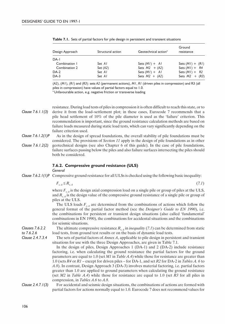
Clause 7.6.1.1(3)resistance. During load tests of piles in compression it is often difficult to reach this state, or toderive it from the load–settlement plot; in these cases, Eurocode 7 recommends that apile head settlement of 10% of the pile diameter is used as the ‘failure’ criterion. Thisrecommendation is important, since the ground resistance calculation methods are based onfailure loads measured during static load tests, which can vary significantly depending on thefailure criterion used.
Clause 7.6.1.2(1)P
Clause 7.6.1.2(2)
As in the design of spread foundations, the overall stability of pile foundations must beconsidered. The provisions of Section 11 apply in the design of pile foundations as in othergeotechnical designs (see also Chapter 6 of this guide). In the case of pile foundations,failure surfaces passing below the piles and also failure surfaces intersecting the piles shouldboth be considered.
7.6.2. Compressive ground resistance (ULS)General
Clause 7.6.2.1(1)P Compressive ground resistance for all ULSs is checked using the following basic inequality:
Fc, d £ Rc, d (7.1)
where Fc, d is the design axial compression load on a single pile or group of piles at the ULS,and Rc, d is the design value of the compressive ground resistance of a single pile or group ofpiles at the ULS.
The ULS loads Fc, d are determined from the combinations of actions which follow thegeneral format of the partial factor method (see the Designer’s Guide to EN 1990), i.e.the combinations for persistent or transient design situations (also called ‘fundamental’combinations in EN 1990), the combinations for accidental situations and the combinationsfor seismic situations.
Clauses 7.6.2.2to 7.6.2.6
The ultimate compressive resistance Rc, d in inequality (7.1) can be determined from staticload tests, from ground test results or on the basis of dynamic load tests.
Clause 2.4.7.3.4 The sets of partial factors of Annex A, applicable to pile design in persistent and transientsituations for use with the three Design Approaches, are given in Table 7.1.
In the design of piles, Design Approaches 1 (DA-1) and 2 (DA-2) include resistancefactoring, i.e. when calculating the ground resistance the partial factors for the groundparameters are equal to 1.0 (set M1 in Table A.4) while those for resistance are greater than1.0 (sets R4 or R1 – except for driven piles – for DA-1, and set R2 for DA-2 in Tables A. 6 toA.8). In contrast, Design Approach 3 (DA-3) involves material factoring, i.e. partial factorsgreater than 1.0 are applied to ground parameters when calculating the ground resistance(set M2 in Table A.4) while those for resistance are equal to 1.0 (set R3 for all piles incompression, in Tables A.6 to A.8.
Clause 2.4.7.1(3) For accidental and seismic design situations, the combinations of actions are formed withpartial factors for actions normally equal to 1.0. Eurocode 7 does not recommend values for
106
DESIGNERS’ GUIDE TO EN 1997-1
Table 7.1. Sets of partial factors for pile design in persistent and transient situations
Design Approach Structural action Geotechnical actionaGroundresistance
DA-1Combination 1 Set A1 Sets (M1) + A1 Sets (M1) + (R1)Combination 2 Set (A2) Sets M2 + (A2) Sets (M1) + R4
DA-2 Set A1 Sets (M1) + A1 Sets (M1) + R2DA-3 Set A1 Sets M2 + (A2) Sets M2 + (R3)
(A2), (M1), (R1) and (R3): sets A2 (permanent actions), M1, R1 (driven piles in compression) and R3 (allpiles in compression) have values of partial factors equal to 1.0.a Unfavourable action, e.g. negative friction or transverse loading

the partial factors on the resistances in the case of accidental situations. It is usual practice toadopt values equal to 1.0, but they can depend on the particular design situation. For thevalues of the partial factors on pile resistances in the case of seismic design situations, seeEurocode 8 – Part 5.
It should be noted that inequality (7.1) is valid for the whole foundation, and does notnecessarily have to be checked for each individual pile independently. Equations (7.2) to(7.11) for Rc, d later on in Section 7 are intended to be used for the design of individual piles.
Clause 7.6.2.1(6)
Clause 7.6.2.1(5)P
It is also important to note that Eurocode 7 draws attention to the fact that a ULS is onlyreached when a significant number of piles fail simultaneously. In fact, as long as a pilefoundation does not become a mechanism (in the static sense), a ULS is not reached. Amechanism can be created by the resistance of several piles being exceeded, as well as byfailure of the structure connecting the piles.
Clause 7.6.2.2(9)Clause 7.6.2.3(7)
The analysis of a ULS failure involving a whole pile foundation is not frequently applied.It requires a non-linear analysis of the load redistribution among the piles. It may beassumed, however, that similar load redistribution effects may be accounted for in asimplified way, by selecting different characteristic pile resistances depending on thestiffness of the structure. Account of the structural stiffness may be introduced in asimplified way through the factor 1.1 of clauses 7.6.2.2(9) and 7.6.2.3(7). This factor shouldnot be used when the non-elastic load redistribution is explicitly taken into account.
Eurocode 7 draws attention to two other aspects for groups of piles:
Clause 7.6.2.1(8)• Special care is needed for edge piles, as they are usually more heavily loaded than theother piles in the case of eccentrically loaded stiff foundations or inclined loads and havea stiffer behaviour than centre piles, and hence attract more load.
Clause 7.6.2.1(3)PClause 7.6.2.1(4)
Clause 7.6.2.1(11)
• A group of piles loaded in compression may also fail as a block, consisting of the pilesand the ground contained between the piles. The code allows such a block to be treatedas a single pile of large diameter. The wording of clause 7.6.2 might be misleadingbecause the methods and equations given in this clause do not apply to such a case; thesingle-pile block is usually analysed by considering the vertical bearing resistance of anequivalent raft foundation, e.g. according to the calculation methods of Section 6.Clearly, a check against punching failure of such an equivalent raft should be carriedout, if relevant, as clause 7.6.2.1(11) also applies.
Clauses 7.6.2.1(9)Pto 7.6.2.1(13)
Clauses 7.6.2.1(9)P to 7.6.2.1(13) draw attention to other factors to be considered whenassessing the compressive resistance of single piles:
• the possible presence of a weak stratum below the pile base• the geometry of the base compared with that of the shaft• the possibility of a plug ‘effect’ for open-ended driven piles.
Ultimate compressive resistance from static load tests
Clause 7.6.2.2(2)PThe procedure for determining the compressive resistance of a pile from static load tests isbased on analysing the compressive resistance, Rc, m, values measured in static load tests onone or several trial piles. The trial piles must be of the same type as the piles of thefoundation, and must be founded in the same stratum.
Clause 7.6.2.2(7)PClause 7.6.2.2(11)P
An important requirement stated in Eurocode 7 is that the interpretation of the results ofthe pile load tests must take into account the variability of the ground over the site and thevariability due to deviation from the normal method of pile installation. In other words,there must be a careful examination of the results of the ground investigation and of the pileload tests results. The results of the pile load tests might lead, for example, to different‘homogeneous’ parts of the site being identified, each with its own particular characteristicpile compressive resistance.
The steps of the procedure for determining the design compressive resistance of a pilefoundation from static load tests are as follows:
107
CHAPTER 7. PILE FOUNDATIONS

Clause 7.6.2.2(8)P (1) From the measured compressive resistances Rc, m determine the characteristic value Rc, k
from the following equation:
Rc, k = Min{(Rc, m)mean/ξ1; (Rc, m)min/ξ2} (7.2)
Clause 7.6.2.2(7)Pwhere ξ1 and ξ2 are correlation factors related to the number n of piles tested, and areapplied to the mean (Rc, m)mean and to the lowest (Rc, m)min of Rc, m, respectively. Therecommended values for these correlation factors, given in Annex A, are intendedprimarily to cover the variability of the ground conditions over the site. However, theymay also cover some variability due to the effects of pile installation.
Clause 7.6.2.2(9) (2) If the structure connecting the piles is stiff and strong enough to transfer loads fromweaker piles to stronger piles, the values for ξ1 and ξ2 may be divided by 1.1, provided thevalue of ξ1, which is applied to the mean pile resistance, is not lower than 1.0.
Clause 7.6.2.2(7)PClause 7.6.2.2(10)P
(3) As mentioned above, when several load tests have been performed, the first estimateof an overall Rc, k value, based on all the load test results, might lead to different‘homogeneous’ parts of the site being identified. In this situation, the procedure isstarted again from step 1 for each ‘homogeneous’ part of the site. This can result in lessconservative Rc, k values than would be obtained if, as in the first estimate, the soilconditions were assumed to be the same over the whole site and the minimum value ofRc, m governs the Rc, k value over the whole site.
Clause 7.6.2.2(12)Clause 7.6.2.2(13)
(4) If necessary, Rc, k can be split into the characteristic shaft resistance Rs, k and thecharacteristic base resistance Rb, k. This is possible particularly when measurements todetermine the load in the pile have been made along the shaft of the tested pilesor when calculations based on the results of ground tests or dynamic tests have beencarried out.
Clause 7.6.2.2(14)P (5) The design pile compressive resistance, Rc, d is obtained by applying the partial factor γt
to the total characteristic resistance or the partial factors γs and γb to the characteristicshaft resistance and characteristic base resistance, respectively, in accordance with thefollowing equations:
Rc, d = Rc, k/γt (7.4)
or
Rc, d = Rb, k/γb + Rs, k/γs (7.5)
Rc, d for persistent and transient situations may be obtained from the results of pile loadtests using DA-1 and DA-2 and the recommended values for the partial factors γt or γs
and γb given in Tables A.6, A.7 and A.8. DA-3 is not applicable in the case of pile loadtests because the procedure using the results of load tests involves applying partialfactors directly to the characteristic resistances Rc, k or Rs, k and Rb, k, derived from loadtests, while DA-3 involves applying partial factors to the characteristic values of theground strength parameters. For accidental situations, unless stated otherwise in theNational Annex, it can be assumed that γt = γs = γb = 1.0.
Clause 7.6.2.1(3)PClausse 7.6.2.1(4)
In the case of pile groups, the compressive resistance of the whole foundation isdetermined either by summing the compressive resistances of the individual piles or byassuming a block failure, whichever yields the lower value.
Some background information on the recommended values for ξ1 and ξ2 given in Annex Acan be found in Bauduin (2001). These values are based on a reference value of about 10%for the coefficient of variation of the pile compressive resistance: for coefficient of variationvalues less than 10%, the mean of the measured resistances should govern the design,whereas for coefficient of variation values greater than 10%, the lowest measured resistanceshould govern.
Example 7.1 below illustrates the calculation of the design compressive resistance of asingle pile from the results of static load tests following the procedure described above.
108
DESIGNERS’ GUIDE TO EN 1997-1

Ultimate compressive resistance from ground tests resultsGeneral
Clause 7.6.2.3(1)PAs already mentioned, methods for predicting the compressive resistance of piles fromground test results can be used, provided that they have been established from pile load testsand from comparable experience.
Clause 7.6.2.3(2)To account for the additional uncertainty of the calculation method, Eurocode 7 allows amodel factor to be introduced in order to ensure that the prediction is safe enough. Thismodel factor is, in fact, a calibration factor for the method. However, no further informationis given about it in the code, but it is anticipated that it will play an important role when theexisting prediction methods are adapted to the new design procedures, partial factors andcoefficients being introduced by the Eurocodes. The value of the model factor should beobtained by comparing static load test results and corresponding predictions. It can beselected with the aim to provide a given reliability to the predictions: for instance, one maywish that, if static load tests were performed, 95% (or some other reliability level) of themeasured compressive resistances would be greater than the calculated predictions. Thevalue of the model factor can be obtained by statistical analyses of the data bank of load testsresults (e.g. see Bauduin, 2002b; Frank and Kovarik, 2005).
Design procedures with Design Approaches 1 and 2As in the design method based on the results of static load tests, the variability of the ground,and hence of the pile resistance over the site considered, should also be taken into accountwhen assessing the characteristic value of the compressive resistance. The following twoprocedures for accounting for the variability of the ground are introduced in Eurocode 7:
Clause 7.6.2.3(5)P• The first procedure, called the ‘model pile’ procedure in this guide, is where the valuesof the ground test results at each individual tested profile are used to calculatethe compressive resistance of a model, e.g. fictitious, pile at the same location. Theprocedure is, in fact, similar to that used with the results of static load tests, e.g. itinvolves applying ξ factors to the calculated resistance to account for the variability ofthe pile resistance and obtain the characteristic compressive resistance.
Clause 7.6.2.3(8)• The other procedure, referred to as the ‘alternative’ procedure, is where the ground testresults (shear strength, cone resistance, etc.) of all tested locations are first broughttogether before evaluating the characteristic values of base resistance and shaft resistancein the various strata based on a cautious assessment of the test results and withoutapplying the ξ factors.
‘Model pile’ procedureClause 7.6.2.3(5)P
Clause 7.6.2.3(6)P
The ‘model pile’ procedure for determining the design compressive resistance Rc, d from theresults of tests on the ground (these can be either laboratory or in situ tests) is based on theresults of one or more profiles of such tests. As in the case of pile load tests, Eurocode 7requires that, when determining Rc, d using this semi-empirical method, the interpretation ofthe results of the ground tests and the calculated resistances take into account the variabilityof the ground over the site. Careful examination of the calculated pile resistances might leadto different parts of the site being identified, each with different resistances. A clear exampleof this, involving the use of cone penetrometer test (CPT) results, is given by Bauduin (2002b).
The steps in the ‘model pile’ procedure for determining the design compressive resistanceof a pile foundation from ground tests results are as follows:
(1) Determine the calculated compressive resistance Rc, cal by applying the prediction methodto the results of each profile of tests independently in accordance with the followingequation:
Rc, cal = Rb, cal + Rs, cal (D7.1)
where Rb, cal and Rs, cal are the calculated base resistance and calculated shaft resistance,respectively, determined for the profile of ground tests results under consideration.
109
CHAPTER 7. PILE FOUNDATIONS

They include the model (calibration) factor. The result is the predicted resistance of apile if it were exactly at the location of the profile of ground tests. Hence this pile can becalled a model pile.
Clause 7.6.2.3(5)P (2) The characteristic values Rc, k, Rb, k and Rs, k are determined from the following equation:
Rc, k = (Rb, k+ Rs, k)Rc, k = (Rb, cal + Rs, cal)/ξ = Rc, cal/ξ = Min{(Rc, cal)mean/ξ3; (Rc, cal)min/ξ4} (7.8)
where ξ3 and ξ4 are correlation factors that depend on the number of profiles of tests, n,and are applied respectively– to the mean values
(Rc, cal)mean = (Rb, cal + Rs, cal)mean = (Rb, cal)mean+ (Rs, cal)mean
– and to the lowest values
(Rc, cal)min = (Rb, cal + Rs, cal)min
The recommended values for ξ1 and ξ2 given in Annex A are intended to cover thevariability in the ground and the calculated resistances over the site (see above).
Clause 7.6.2.3(7) (3) If the structure connecting the piles is stiff and strong enough to transfer loads fromweaker piles to stronger piles, the values for ξ3 and ξ4 may be divided by 1.1, provided thevalue of ξ3, which is applied to the mean value, is not lower than 1.0.
Clause 7.6.2.3(6)P (4) If several profiles of ground tests are available, the first estimate of an overall Rc, k value,based on all the profiles of ground tests, might lead to different ‘homogeneous’ parts ofthe site being identified. In this situation, the procedure is started again from step 2 foreach ‘homogeneous’ part of the site. This can result in less conservative Rc, k values thanwould be obtained if, as in the first estimate, the soil conditions were assumed to be thesame over the whole site and the minimum value of Rc, cal governs the Rc, k value over thewhole site.
Clause 7.6.2.3(3)PClause 7.6.2.3(4)P
(5) The design compressive resistance is obtained by applying the partial factors γs and γb tothe characteristic shaft resistance and to the characteristic base resistance, respectively,in accordance with the following equations:
Rc, d = Rb, d + Rs, d (7.6)Rc, d = Rb, k/γb + Rs, k/γs (7.7)
This model pile design procedure may be used with DA-1 and DA-2 and therecommended values for the partial factors γs and γb given in Annex A for persistent ortransient situations. The model pile procedure is not applicable to DA-3 because, asexplained in the case of compressive resistance obtained from pile load tests, theprocedure involves applying partial factors to the resistances while DA-3 involvesapplying partial factors to the characteristic values of the ground strength parameters.For accidental situations, unless otherwise stated in the National Annexes, it can beassumed that γs = γb = 1.0.
Clause 7.6.2.1(3)PClause 7.6.2.1(4)
(6) In the case of groups of piles, the bearing capacity of the whole foundation is determinedeither by summing up the individual compressive resistances or by assuming a blockfailure, whichever provides the lower value.
Examples 7.2 and 7.3 demonstrate the calculation of pile compressive resistance from theresults of ground tests following the procedure outlined above. Example 7.2 uses theresults of pressuremeter tests (PMTs) while Example 7.3 uses undrained shear strength (cu)measurements.
‘Alternative’ procedureClause 7.6.2.3(8) As an alternative to the ‘model pile’ procedure, Eurocode 7 allows the characteristic
resistance values Rb, k and Rs, k to be determined directly from the values of groundparameters:
110
DESIGNERS’ GUIDE TO EN 1997-1

(7.9)
where qb, k and qs, k, i are characteristic values of base resistance and shaft resistance per unitarea in the various strata, obtained using an appropriate method and the values of theground parameters.
The ‘alternative’ procedure then follows steps 5 and 6 of the ‘model pile’ procedure. Thisalternative procedure is intended to allow use of the traditional methods for calculating thecompressive resistance from ground test results.
The values of qb, k and qs, k, i (obtained from tabulated or chart values or from correlations)should account for the variability of the ground parameters, the volume of soil involved inthe failure mechanism considered, the spatial variability of the pile resistance, the variabilitydue to the effect of pile installation, and the stiffness of the structure. This is because the ξfactors are not used explicitly in this alternative method.
Clause 7.6.2.3(8)
The ‘alternative’ procedure treats the soil variability differently from the method based onthe results of static load tests or from the ‘model pile’ procedure based on ground test results.As the partial factors γb, γs and γt in Tables A.6, A.7 and A.8 are intended to be used inconjunction with the ξ factors, they may not be appropriate for use with the ‘alternative’procedure. A model factor may have to be introduced or directly included when determiningthe values of qb, k and qs, k.
Examples 7.2 and 7.3 demonstrate the use of the ‘alternative’ procedure.
Design Approach 3
Clause 7.6.2.3(9)PClause 2.4.5
Clause 2.4.6.2(1)P
As noted above, since DA-3 uses partial factors applied to the ground parameters, neitherthe ‘model pile’ procedure nor the ‘alternative’ procedure can be used with DA-3 becausethey both involve factors applied to the resistances. DA-3 is usually intended to be usedwith calculation models involving the design values of ground parameters obtained fromthe results of laboratory tests. When using DA-3, clause 7.6.2.3(9)P explains that thecharacteristic values of the ground parameters Xk are first determined in accordance withclause 2.4.5, and the design values Xd are then obtained by applying the material factors γM
(column M2 of Table A.4) in accordance with equation (2.2):
Xd = Xk/γM (2.2)
For pile design using DA-3, the design value of the compressive resistance Rc, d is deriveddirectly by inputting the design values of the ground strength parameters Xd in thecalculation model:
Rc, d = Rb, d + Rs, d = Rb, cal(Xd) + Rs, cal(Xd) (D7.2)
Example 7.3 shows the various possibilities for using DA-3 with the results of undrainedshear strength (cu) measurements.
Note that, where relevant in the above procedures, the values of the parameters to be usedto assess the shaft resistance should be cautious estimates of their mean values because thelength of the pile shaft in a given stratum is usually ‘large’. For the base resistance, as thevolume involved in the failure mechanism around the base is usually ‘small’, the values of theparameters to be used should be cautious estimates of their local values around the baselevel.
Ultimate compressive resistance from dynamic tests results
Clause 7.5.3The general requirements in Eurocode 7 for using dynamic tests to determine the compressiveresistance of piles are set out in clause 7.5.3. The use of different types of dynamictest results, as well as the use of redriving results, to assess the compressive resistanceof individual piles in compression, are mentioned in clause 7.6.2. The dynamic tests resultsare:
111
CHAPTER 7. PILE FOUNDATIONS
b, k b b, k
s, k s, s, k,i ii
R A q
R A q
=
= Â

Clause 7.6.2.4Clause 7.6.2.4(3)PClause 7.6.2.4(2)
• Dynamic impact (hammer blow) tests. During this type of test, it is assumed that thestrain is high enough to reach the (dynamic) ultimate compressive resistance. Thedynamic resistance should be measured. The test can also include a signal-matchingprocedure leading to an approximate estimate of the shaft and base resistances and ofthe load–settlement curve.
Clause 7.6.2.5 • Pile-driving formulae. The use of pile-driving formulae is the traditional way of takingadvantage of the penetration records during the driving of piles to determine thebearing resistance.
Clause 7.6.2.6 • Wave equation analyses. Wave equation analyses may be used to assess the designcompressive resistance of piles. However, this mathematical model (also called themass–spring model) is usually employed to study the driving conditions (hammerperformance, stresses in the pile).
When determining the compressive resistance of piles from dynamic tests, it is oftenrecommended that the driving records after redriving (by a few centimetres and some timeafter the end of the initial pile driving) are used.
Clause 7.6.2.4(4)PThe procedure for determining the compressive resistance of a pile from dynamic test
results is the same for the three types of test, although some specific requirements need to bemet for each type of test. The characteristic value is determined from the following equation:
Rc, k = Min{(Rc, m)mean/ξ5; (Rc, m)min/ξ6} (7.11)
where Rc, m are the static compressive resistances derived from the dynamic measurements,and ξ5 and ξ6 are correlation factors related to the number of piles tested, n, and are appliedto the mean (Rc, m)mean and the lowest (Rc, m)min. Recommended values for ξ5 and ξ6 are givenin Annex A. Note that the ξ values are not the same for the three types of dynamicmeasurements.
The design compressive resistance is then obtained from
Rc, d = Rc, k/γt (7.10)
where the partial factor on the total resistance γt is the same as for the other methods fordetermining the compressive resistance of pile foundations. For DA-1 and DA-2, the valuesof γt are given in Annex A. For accidental situations it can be assumed that γt = 1.0.
Clause 7.6.2.5(3)P Pile-driving formulae should only be used with the above procedure to assess the designcompressive resistance in the case of end-bearing piles in cohesionless soils. For other typesof pile and/or other types of soil the uncertainty is larger, and other methods or higher partialfactors should be used.
7.6.3. Ground tensile resistanceGeneral requirements
Clause 7.6.3.1(1)PClause 7.6.3.1(3)P
Many of the Eurocode 7 requirements for piles in compression also apply to piles in tension.For piles in tension, two ULSs must be checked:
• pull-out failure (tensile resistance) of individual piles• uplift failure of the block of ground containing the piles.
Clause 7.6.3.1(4)PAs in the case of the compressive resistance failure of piles, the pull-out resistance of
individual piles should be checked using the GEO set of partial factors and relevantinequality. However, for groups of piles in tension, possible uplift failure of the block ofground containing the piles should be checked using the UPL set of partial factors andrelevant inequality.
Clause 7.6.3.1(8)P Clause 7.6.3.1(8)P draws the designer’s attention to the situation where tensile pilesinteract in a group. Tension on one pile reduces the effective vertical stress close to thesurrounding piles, and hence reduces their shaft resistance. This applies to the resistance ofthe individual piles in the group and consequently to the resistance of the whole foundation.
112
DESIGNERS’ GUIDE TO EN 1997-1

Tensile resistance of individual pilesClause 7.6.3.1The methods for determining the ground resistance of piles in tension, either from static pile
load tests or from ground test results, are very similar to those for piles in compression. Themain differences are:
• The base resistance is always neglected.• The correlation factors ξ should not be divided by 1.1, even in the case of stiff structures.
This is due to the fact that ground failure of tensile piles is usually brittle (loss of strengthafter having reached the peak resistance). Hence, it is unsafe to assume load transferfrom failed to not yet failed piles, and therefore this is not allowed.
• The value of the partial factor on the total resistance (i.e. shaft resistance) in tension,γs, t, is larger than the value of γs in compression (see the tables in Annex A). It is commonpractice to be somewhat more cautious when attributing safety to tensile piles than tocompressive piles.
Clause 7.6.3Clause 7.6.2
Clause 7.6.3.3(4)PClause 7.6.3.3(6)Clause 7.6.3.3(7)P
Given these differences, the general design requirements for piles in tension in clause7.6.3 are the same as those in clause 7.6.2 for piles in compression. Also, the correlationfactors ξ1 and ξ2 (for measured tensile resistances) and ξ3 and ξ4 (for calculated tensileresistances) recommended by EN 1997-1-1 have the same values (Tables A.9 and A.10,respectively). When static load tests are used for designing tensile pile foundations, theseshould, as already noted in Section 7.5 of this guide, be carried to failure. For the design oftensile piles using ground tests results, the model pile procedure may be used, and EN 1997-1-1also allows the alternative procedure to be used. When using DA-3, partial factors areapplied to the characteristic ground parameters to calculate the design tensile resistance.
Clause 7.6.3.1(8)PClause 7.6.3.1(8)P draws the attention of the designer to the case where tensile pilesinteract in a group: tension on one pile reduces the effective vertical stress close to thesurrounding piles, and hence their shaft resistance. This applies to the resistance of theindividual piles in the group, and consequently to the resistance of the whole foundation.
Clause 7.6.3.1(9)PThe partial factors of Tables A.6, A.7 and A.10 are, in principle, valid for quasi-static loads.
Another important requirement of EN 1997-1 is that cyclic loadings or reversals of load,which might be very detrimental to tensile resistance of a pile, must be considered.Unfortunately, no precise provision as to how to deal with these loading conditions is givenin the code. Unless special calculation rules are applied, the effects of such loadings mayeither be taken into account by applying a model factor to the calculated results so that theyerr on the safe side or else, as is common practice, increased partial factors are simplyapplied to the actions for cyclic or reversed loading conditions.
It should be noted that when a large variable tensile load has to be combined with apermanent compressive load of similar magnitude, the design load on the pile can become atensile load, while the resulting characteristic load remains compressive. The foundationshould be designed for this tensile design value of the action.
Block failure of a group of pilesBlock failure of a group of piles occurs when all the piles and the soil included between themare lifted up by a tensile force. The tensile force causing this may come from a structureabove the water level and the pile group, or from upwards water pressure acting on the pilegroup and that part of the structure below water level, as shown in Figs 7.1a and 7.1b ofEN 1997-1-1.
Clause 7.6.3.1(5)It should be noted that, both for isolated piles and for group of piles, EN 1997-1-1recommends that the pull-out mechanism involving a cone of ground surrounding the piles ischecked, especially when an enlarged base or rock socket is used.
Clause 7.6.3.1
Eurocode 7 requires that the design against uplift failure of the block is treated as an uplift(UPL) ULS calculation with the appropriate partial factors (see Tables A.15 and A.16 inAnnex A, as well as Chapter 2 in this guide). Example 7.5 demonstrates the design of a groupof piles from an upwards water pressure against uplift in accordance with the requirementsof clause 7.6.3.1.
113
CHAPTER 7. PILE FOUNDATIONS

Clause 2.4.7.1(1)P It may also be appropriate to check the GEO ULS of groups of piles subjected to a tensileforce, in particular when the tensile force comes from the structure.
7.6.4. Vertical displacements of pile foundations
Clause 2.4.8Clause 2.4.9Clause 2.4.9(3)P
The design of foundations should be such that the movements are limited and do not lead tothe occurrence of limit states (serviceability or ultimate) in the supported structure. Thisgeneral principle is clearly recognized in EN 1997-1-1, in particular in clauses 2.4.8 and 2.4.9.The values of the allowable movements should be selected during the design. Someindicative limiting values of structural deformation are given in Annex H (informative).
Clause 7.6.4.1(1)P
Clause 7.6.4.1(2)Clause 2.4.8(4)
According to EN 1997-1, it is necessary to assess the settlements of axially loaded pilefoundations, such as those of shallow foundations, in order to ensure that the occurrence ofan SLS in the structure is sufficiently unlikely. Nevertheless, it is understood that most of thetime this assessment can only provide an estimate of the settlements because of all theuncertainties in the models for pile settlements. EN 1997-1 allows settlement calculations tobe replaced, in many circumstances, by a simplified design approach involving bearingresistance calculations with partial factors high enough such that a sufficiently low fraction ofthe ground strength is mobilized and no unacceptable deformation occurs in the supportedstructure, at least when common piles are used in known ground conditions and successfulprevious experience is available. This simplified design approach is common practice intraditional design (see also Chapter 6 of this guide).
Methods for calculating the displacement of pile foundations include the linear elasticapproach of Poulos and Davis (1980), as well as elasto-plastic finite-element calculations andt–z load transfer functions (curves of mobilization of shaft resistance, e.g. see Baguelin et al.,1982).
7.7. Transversely loaded pilesClause 7.4Clause 7.5
The design of transversely loaded piles must be consistent with the general requirements forthe design and load testing of piles given in clauses 7.4 and 7.5. In addition, the followingrequirements apply:
Clause 7.7.1(3) • the transverse resistance should be checked for situations involving rotational ortranslational failure in the ground in the case of short rigid piles, and for bending failureof the pile together with yield of the soil near the surface in the case of long slender piles
Clause 7.7.1(4)P • the group effect must be taken into accountClause 7.7.2Clause 7.7.3
• the transverse load resistance should be determined by means of static load tests or onthe basis of ground test results and pile strength parameters
• the strength of the pile to resist structural failure should be checked• the transverse displacement should be assessed.
Clause 7.7.2(3)PClause 7.7.2(4)Clause 7.7.3(4)P
Other requirements specifically for transversely loaded piles, which also should beaccounted for, concern the variability of the ground near the surface as well as the head fixityconditions at the connection between the piles and the structure.
Clause 7.7.3(3) The theory of a beam supported by elastic springs, characterized by the horizontal modulusof subgrade reaction, is explicitly mentioned in EN 1997-1 as an acceptable calculationmethod for the design of a long slender piles subjected to a transverse load at the top.
7.8. Structural design of piles
Clause 7.8(1)PClause 7.8(2)P
The structural design of piles is an important aspect, which forms an integral part ofthe design of pile foundations. However, most structural designs involve applying coderequirements relating to the behaviour of concrete, steel or wood. EN 1997-1 requires thatpiles are checked against structural failure in all relevant design situations, in accordance
114
DESIGNERS’ GUIDE TO EN 1997-1

with the requirements of the relevant material Eurocodes, in particular EN 1992, EN 1993and EN 1995.
Clause 7.8(4)PClause 7.8(5)
Slender piles passing through water or through a thick layer of very weak soil must bechecked against buckling. This check against buckling can be omitted if the undrained shearstrength cu is greater than 10 kPa.
For persistent or transient situations, the design values of actions for the ULS structuraldesign of piles are determined using DA-1, DA-2 or DA-3, depending on the nationalchoice. When DA-1 is used, Combination 1 usually governs the structural design of piles.
7.9. Supervision of construction
Clause 7.9(1)PClause 7.9(2)
Clause 7.9(3)PClause 7.9(6)P
The way piles are installed not only influences the design but also plays a fundamental role inensuring an adequate behaviour of the supported structure. EN 1997-1 requires that adetailed plan of the pile installation is prepared as a basis for the piling works and that theinstallation of all the piles is monitored and recorded. If there is doubt about the quality ofinstalled piles, relevant measures must be taken, including full-scale tests, the installation ofnew piles, redriving, etc.
Clause 7.9(4)Many aspects of pile design are often linked to the pile installation method. HenceEN 1997-1 repeats some requirements included in the relevant execution standards issuedby CEN/TC 288.
Clause 7.9(7)PClause 7.9(8)
When relevant, the integrity of piles must be checked. Dynamic low-strain tests are notalways suitable for this purpose, and hence other tests, such as sonic and vibration tests, orcoring, may be needed.
Example 7.1: design of a pile in compression from static load test resultsThe deep foundations of a major bridge in Europe have been designed by interpreting theresults of full-scale pile tests under both axial and transverse loadings (see Wastiaux et al.,1998). The present example, inspired by this project, deals only with the axial compressiveresistance of the piles, and aims to show how the results of static compression load testsshould be interpreted following Eurocode 7.
The foundations on open-ended driven piles have to be designed in order to carryvertical compressive loads. In the following design calculations, only ULSs in persistentand transient situations and accidental situations are considered. The permanent verticalcompressive load is 31 MN, and the vertical accidental load is 16 MN. The purpose of thedesign is to determine the number of driven piles of length 55.5 m required to carry thisload.
It is assumed that there is no need to take into account any group effect for the pilefoundation. The full design of the foundation would also require the SLSs to be checked,e.g. a check that the settlement of the foundation is acceptable.
A typical soil profile consists of 20–30 m of very soft clay (mud), muddy sands, sandsand clays, and, finally, sands and gravels at the level of the expected location of the base ofthe piles.
The results of four static load tests on driven piles with different lengths of embedmentare available (Fig. 7.1). In what follows, the resistance Rm of a pile of length L = 55.5 m isdeduced from the resistances measured in the static tests, taking into account thedifferences in pile length (and after subtracting the positive shaft resistance in the layerswhich will be submitted to downdrag). Hence, the estimated values of the resistances for apile of length L = 55.5 m, are the following:
• from pile test P8: Rm = 14.0 MN• from pile test P31: Rm = 14.4 MN• from pile test P79: Rm = 12.1 MN• from pile test P79b: Rm = 13.9 MN.
115
CHAPTER 7. PILE FOUNDATIONS

Clause 7.6.2.2(8)P According to EN 1997-1, the characteristic value of the axial pile resistance, Rk, isdetermined from the corresponding mean and minimum measured values (Rm, mean,Rm, min) using the following formula:
Rk = Min{Rm, mean/ξ1; Rm, min/ξ2 (} 7.2)
Clause 7.6.2.2(9)
The correlation factors (ξ1, ξ2) depend on the number n of static pile load tests. For n = 4,Table A.9 recommends ξ1 = 1.10 and ξ2 = 1.00. It is assumed that redistribution betweenweak and strong piles cannot be accounted for because the expected number of piles is toosmall. Thus, the reduction factor 1.1 on ξ1 and ξ2 proposed in clause 7.6.2.2(9) is notapplied.
Rm, mean = 13.6 MN
Rm, min = 12.1 MN
Thus,
Rk = Min{13.6/1.10; 12.1/1.00} = Min(12.4, 12.1) = 12.1 MN
which shows that the minimum measured pile resistance governs the design.For a single pier of the bridge, the characteristic values of the vertical loads, taking into
account the downdrag, are assumed to be:
• for persistent and transient situations: permanent loads Gk = 31 MN (the variableloads are considered to be negligible for the critical piers)
• for accidental situations: permanent and accidental loads Gk + Ak = 47 MN (theaccidental load is 16 kN).
Clause 7.6.2.2(14)P For persistent and transient situations, DA-1 (Combinations 1 and 2) and DA-2 areconsidered. The load tests yield directly the total (or shaft and base) characteristicresistances, and the design values are obtained by applying the resistance factors γt (or γs
116
DESIGNERS’ GUIDE TO EN 1997-1
P311
P79bis
P8
P31
P79
0 2500 5000 7500 10 000 12 500 15 000 17 500 20 000
Force (kN)
Dis
plac
emen
t (m
m)
100
110
120
130
70
80
90
40
50
60
10
0
20
30
Fig. 7.1. Results of static load tests on driven piles of diameter B = 1220 mm and of differentlengths of embedment (Wastiaux et al., 1998)
and γb). DA-3 is not intended to be used with pile load test results, as it is a ‘material’factor approach involving the use of ground strength parameters.
Design Approach 1
Clause2.4.7.3.4.2(2)P
DA-1 Combination 1 involves applying the partial factors from sets A1 and R1 of Annex A.This leads to the following design actions and design resistances:
Fc, d = 1.35Gk = 1.35 × 31 = 41.85 MN
Rc, d = Rc, k/γt = 12.1/1.0 = 12.1 MN
Thus, the number of piles needed is 41.85/12.1 = 4.Clause
2.4.7.3.4.2(2)PDA-1 Combination 2 involves applying the partial factors of sets A2 and R4 of Annex A.
This leads to the following design actions and design resistances:
Fc, d = 1.0Gk = 1.0 × 31 = 31 MN
Rc, d = Rc, k/γt = 12.1/1.3 = 9.3 MN
Thus, the number of piles needed is 31/9.3 = 4.The requirement for DA-1 is that the more conservative result of the two combinations
should be used. The number of piles being the same, there is no difference in this examplebetween the two methods for the design number of piles.
It should be noted that, in this Design Approach, Combination 1 provides an overallfactor of safety (OFS) on the characteristic resistance of at least
γFγt = 1.35 × 1.0 = 1.35
whereas Combination 2 provides an OFS of at least
γFγt = 1.0 × 1.3 = 1.3
In relation to the measured mean pile resistance, i.e. including ξ = 1.10, these figuresbecome OFS = 1.49 and 1.43, respectively.
Design Approach 2
Clause2.4.7.3.4.3(1)P
For DA-2, sets A1 and R2 of Annex A must be applied. Thus the design actions and designresistances are
Fc, d = 1.35Gk = 41.85 MN
Rc, d = Rc, k/γt = 12.1/1.1 = 11.0 MN
Thus, the number of piles needed is 41.85/11.0 = 4.Note that DA-2 provides an OFS on the characteristic resistance of at least
γFγt = 1.35 × 1.1 = 1.5
and an OFS of at least 1.65 on the measured mean pile resistance.
Accidental situation
Clause 2.4.7.1(3)For an accidental situation, all the partial factors on loads should be taken equal to 1.0. Itis assumed that a resistance factor equal to 1.0 is also relevant for the circumstances in thisparticular accidental situation. Thus, the design actions and design resistances are
Fc, d = 1.0Gk + 1.0Ak = 47 MN
Rc, d = Rc, k/γt = 18.1/1.0 = 12.1 MN
The number of piles needed is thus 47/12.1 = 4.In conclusion, for the given loads, the ULS designs of the piles for the bridge pier for
persistent and accidental situations, both require four piles of length L = 55.5 m.
117
CHAPTER 7. PILE FOUNDATIONS

Example 7.2: design of a pile in compression from in situ test resultsA foundation on driven piles in a slightly overconsolidated clay has to be designed to carrypermanent and variable vertical compressive loads. The characteristic values of the loadsare permanent load Gk = 3900 kN and variable load Qk = 800 kN.
Clause 7.6.2.3(6)P The results of three PMT profiles are available (P1, P2 and P3), and the area can beconsidered as ‘homogeneous’ (there is only a random variation in the ground test results).The diameter of the piles is B = 400 mm, and the expected embedment is L = 13 m.
In the following design calculation, only ULSs for persistent and transient situationsare considered. It is also assumed that there is no need to take into account any groupeffect in the design of the pile foundation. The full design of the foundation would alsorequire checking of:
• accidental situations, if relevant• SLSs, e.g. checking that the settlement of the foundation is acceptable.
Only DA-1 (Combinations 1 and 2) and DA-2 are considered. DA-3 is not intended, inprinciple, to be used with in situ test results. DA-3 uses material factoring, and is onlymeant to be used with laboratory test results and ground strength parameters.
Note that the sets of calculations for DA-1 and DA-2 would be exactly the same if CPTresults were to be used with the ‘model pile’ procedure.
Clause 7.6.2.3(2) The PMT calculation rules given in Annex D.3 of EN 1997-2 are used, and a model(calibration) factor γRD equal to 1.05 is applied. This value has been selected for use withthe recommended values of the partial factors given in Annex A for DA-2, in order to yieldthe same value of the overall factor of safety as in the present French code of practice withPMT calculation rules (see Frank, 1999). For the sake of comparison, γRD = 1.05 is alsoused below for DA-1.
From the three profiles of limit pressures pl, the mean net limit pressure valuesdetermined at the base, pl, base, and the net limit pressure values determined along theshaft, pl, shaft, are given in Table 7.2.
Clause 7.6.2.3(3)P The calculated design ultimate compressive resistance of the foundation is obtainedfrom
Rc, d = Rb, d + Rs, d (7.6)
where Rb, d is the design calculated pile base resistance obtained from Rs, d = Rs, k/γs, andRs, d is the design calculated shaft resistance obtained from Rb, d = Rb, k/γb.
‘Model pile’ procedure
Clause 7.6.2.3(5)P For DA-1 and DA-2, according to EN 1997-1, the characteristic value of the compressiveresistance Rc, k of a pile is determined from the corresponding mean and minimumcalculated values (Rcal, mean, Rcal, min) using the following formula:
Rc, k = Min{Rcal, mean/ξ3; Rcal, min/ξ4} (7.8)
The correlation factors (ξ3, ξ4) depend on the number n of ground profiles investigated,and Rcal, mean and Rcal, min are obtained by calculating the pile compressive resistance foreach profile (‘model pile’ procedure).
In the following, pressuremeter test results are used. All the calculation steps would beexactly the same if CPT results were to be used with the ‘model pile’ procedure, instead ofpressuremeter test results.
For the pressuremeter, the following design criteria are obtained (see EN 1997-2):
• the soil falls into the ‘Clay A’ category• the bearing (base) resistance factor is k = 1.4• for the shaft resistance, design curve 1 is used.
118
DESIGNERS’ GUIDE TO EN 1997-1
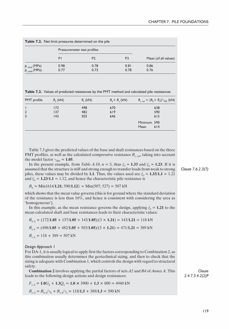
Table 7.3 gives the predicted values of the base and shaft resistances based on the threePMT profiles, as well as the calculated compressive resistance Rc, cal, taking into accountthe model factor γRD = 1.05.
Clause 7.6.2.3(7)In the present example, from Table A.10, n = 3, thus ξ3 = 1.33 and ξ4 = 1.23. If it is
assumed that the structure is stiff and strong enough to transfer loads from weak to strongpiles, these values may be divided by 1.1. Thus, the values used are ξ3 = 1.33/1.1 = 1.21and ξ4 = 1.23/1.1 = 1.12, and hence the characteristic pile resistance is
Rk = Min{614/1.21; 590/1.12} = Min(507; 527) = 507 kN
which shows that the mean value governs (this is for ground where the standard deviationof the resistance is less than 10%, and hence is consistent with considering the area as‘homogeneous’).
In this example, as the mean resistance governs the design, applying ξ3 = 1.21 to themean calculated shaft and base resistances leads to their characteristic values:
Rb, k = (172/1.05 + 137/1.05 + 143/1.05)/(3 × 1.21) = 143/1.21 = 118 kN
Rs, k = (498/1.05 + 482/1.05 + 503/1.05)/(3 × 1.21) = 471/1.21 = 389 kN
Rc, k = 118 + 389 = 507 kN
Design Approach 1For DA-1, it is usually logical to apply first the factors corresponding to Combination 2, asthis combination usually determines the geotechnical sizing, and then to check that thesizing is adequate with Combination 1, which controls the design with regard to structuralsafety.
Clause2.4.7.3.4.2(2)P
Combination 2 involves applying the partial factors of sets A2 and R4 of Annex A. Thisleads to the following design actions and design resistances:
Fc, d = 1.0Gk + 1.3Qk = 1.0 × 3900 + 1.3 × 800 = 4940 kN
Rc, d = Rb, k/γb + Rs, k/γs = 118/1.3 + 389/1.3 = 390 kN
119
CHAPTER 7. PILE FOUNDATIONS
Table 7.3. Values of predicted resistances by the PMT method and calculated pile resistances
PMT profile Rb (kN) Rs (kN) Rb+ Rs (kN) Rc, cal = (Rb+ Rs)/γRD (kN)
1 172 498 670 6382 137 482 619 5903 143 503 646 615
Minimum 590Mean 614
Table 7.2. Net limit pressures determined on the pile
Pressuremeter test profiles
Mean (of all values)P1 P2 P3
pl, base (MPa) 0.98 0.78 0.81 0.86pl, shaft (MPa) 0.77 0.73 0.78 0.76

Thus, the number of piles needed is 4940/390 = 12.7, which is rounded up to 13 piles. Theequivalent overall factor of safety, OFS, can be considered as the total predicted meanresistance of the foundation (Rb + Rs), i.e.
13 × (670 + 619 + 646)/3 = 13 × 645 kN
from Table 7.3, divided by the total applied characteristic load, i.e. 3800 kN + 800 kN,which gives
OFS = 13 × 645/4700 = 1.78
Clause2.4.7.3.4.2(2)P
Combination 1 involves applying the partial factors of sets A1 and R1 of Annex A. Thisleads to the following design actions and design resistances:
Fc, d = 1.35Gk + 1.5Qk = 1.35 × 3900 + 1.5 × 800 = 6465 kN
Rc, d = Rb, k/γb + Rs, k/γs = 118/1.0 + 389/1.0 = 507 kN
Thus, the number of piles needed is 6465/507 = 12.8, which also rounds up to 13 piles,and, as for Combination 2, the OFS = 1.78.
The requirement for DA-1 is that the more conservative result of the two combinationsshould be used. In this example, Combination 1 is marginally more conservative thanCombination 2, but as the number of piles is the same for both combinations, there is nodifference for the final foundation design using the two combinations.
Design Approach 2Clause2.4.7.3.4.3(1)P
For DA-2, sets A1 and R2 of Annex A are applied. Thus, the design actions and designresistances are
Fc, d = 1.35Gk + 1.5Qk = 1.35 × 3900 + 1.5 × 800 = 6465 kN
Rc, d = Rb, k/γb + Rs, k/γs = 118/1.1 + 389/1.1 = 461 kN
Thus, the number of piles needed is 6465/461 = 14. The equivalent overall factor of safetycan be considered as the total calculated mean resistance of the foundation, i.e. 14 × 645,divided by the total applied characteristic load, i.e. 3800 kN + 800 kN, which gives
OFS = 14 × 645/4700 = 1.92
‘Alternative’ procedure
Clause 7.6.2.3(8) For DA-1 (Combinations 1 and 2) and DA-2, clause 7.6.2.3(8) allows Rb, k and Rs, k to bedetermined directly from the ground parameter values. It is assumed that the samecalculation rules are used as for the ‘model pile’ procedure. They can be applied in twoways: with either the characteristic or mean values of the ground parameters.
Using the mean pl values along the shaft and at the base of the piles to predict the shaftand base resistances given in Table 7.2, which corresponds to more to traditional practice,one finds
Rmean = (Rs, k + Rb, k)/γRD = (495 + 151)/1.05 = 615 kN
Clause 7.6.2.3(8)
This value is 615/507 = 1.21 times larger than the characteristic value for the ‘model pile’procedure (it corresponds to the value of ξ3). This shows that if the same values forthe partial factors on loads and base and shaft resistances are to be used in DA-1(Combinations 1 and 2) and DA-2 when the alternative procedure is applied, the values ofthe partial factors in Annex A may need to be corrected by a model factor greater than 1.0(see the note in Clause 7.6.2.3(8)). The results of the alternative procedure, as comparedwith the ‘model pile’ procedure, will then be directly linked to the choice of this modelfactor.
120
DESIGNERS’ GUIDE TO EN 1997-1

Table 7.4 summarizes the values of Rk and Rd obtained in the various DesignApproaches and procedures.
Example 7.3: design of a pile in compression from laboratory test resultsThis example presents the ULS design of a single bored pile in clay (pile diameterB = 0.80 m using the undrained shear strength cu to avoid bearing resistance failure fora persistent or transient design situation. The characteristic values of the loads arepermanent load Gk = 600 kN and one single variable load Qk = 300 kN. The design aimsto check the required length (L) of the pile, which is expected to be 18.5 m.
The ground was investigated by boreholes and tests in three profiles (n = 3: BH1, BH2and BH3). Figure 7.2 shows the three profiles of undrained shear strength cu measured onsamples recovered from the boreholes.
121
CHAPTER 7. PILE FOUNDATIONS
Table 7.4. Values of Rk (or Rmean) and Rd (in kN)
Model pile procedure Alternative procedure
DA-1
DA-2 DA-1, DA-2Combination 2 Combination 1
Rk (kN) 507 507 507 Rmean: 615Rd (kN) 390 507 461 a
a Depends on the Design Approach used and the value of the supplementary model factor introduced
80Undrained shear strength (kPa)
20
16
12
8
4
0
0 20 40 60
Dep
th (
m)
BH1BH2BH3
Fig. 7.2. Undrained shear strength cu profiles for boreholes BH1, BH2 and BH3

The corresponding mean values of the undrained shear of the clay cu along the shaft ofthe pile (cu, shaft) and in the vicinity of pile base at a depth of 18.5 m (cu, base) are given inTable 7.5. The characteristic values have been determined using the method given inChapter 2 of this guide.
The axial bearing resistance of the pile is calculated by the formula
R = Rs + Rb
where
Rs = πBLαcu
is the shaft resistance (α = 0.75 in this case) and
Rb = (πB2/4)9cu
is the pile base resistance, and it is assumed that there is no need for a model factor (i.e.the model factor is taken equal to 1.0). The shaft resistance is governed by the meanvalues of the undrained shear resistance over the length of the shaft, while the baseresistance is governed by the local mean values close to the pile base.
The calculations are performed according to the ‘model pile’ and ‘alternative’procedures for DA-1 and DA-2, as well as for DA-3. The structure is considered not tohave sufficient strength and stiffness to allow redistribution of loads.
‘Model pile’ procedure
Clause 7.6.2.3(5)P For DA-1 and DA-2, according to EN 1997-1, the characteristic axial resistance, Rk, of apile is calculated from the corresponding mean and minimum values (Rmean, Rmin) by theformula (called the ‘model pile’ procedure)
Rk = Min{Rmean/ξ3; Rmin/ξ4}
The correlation factors (ξ3, ξ4) depend on the number n of ground profiles investigated;for n = 3, ξ3 = 1.33 and ξ4 = 1.23 (see Table A.10).
Rmean and Rmin are obtained by calculating the compressive resistance, Rc, for eachborehole using the mean cu values (cu in kilopascals and resistances in kilonewtons):
Rc = Rs + Rb = πBLαcu, shaft + (πB2/4)9cu, base
Rc = 34.9cu, shaft + 4.5cu, base
Thus,
R(BH1) = 1815 + 148 = 1963 kN
R(BH2) = 1605 + 135 = 1740 kN
R(BH3) = 1780 + 189 = 1969 kN
Hence
Rmean = (1963 + 1740 + 1969)/3 = 1891 kN
Rmin = 1740 kN
122
DESIGNERS’ GUIDE TO EN 1997-1
Table 7.5. Determination of characteristic values of cu, shaft and cu, base
Mean cu valuesMean of allvalues
Characteristicvalue of all values
BH1 BH2 BH3
cu, shaft (kPa) 52 46 51 50 47cu, base (kPa) 33 30 42 35 32

and
Rk = Min{1891/1.33; 1740/1.23}Rk = Min{1422 kN; 1415 kN} = 1415 kN
The minimum value governs the resistance, indicating a variability greater than 10% ofthe undrained shear strength over the site and hence of the resulting pile resistance.Hence, using the minimum mean cu values obtained from the BH2 profile, one can nowdeduce the characteristic base and shaft resistances:
Rs, k = 1605/1.23 = 1305 kN
Rb, k = 135/1.23 = 110 kN
A careful examination of the ground investigation results does not enable different‘homogeneous’ areas to be distinguished. These characteristic values are thus adopted forthe entire site.
Design Approach 1For DA-1, it is normally logical to apply first the factors corresponding to Combination 2,as this combination usually determines the geotechnical sizing, and then to check if thesizing is adequate with Combination 1, which is the relevant combination for determiningthe structural sizing.
Clause2.4.7.3.4.2(2)P
Combination 2 consists of applying the partial factors of sets A2 and R4 of Annex A.This results in the following design actions and resistances:
Fc, d = 1.0Gk + 1.3Qk = 1.0 × 600 + 1.3 × 300 = 990 kN
Rc, d = Rb, k/γb + Rs, k/γs = 1305/1.3 + 110/1.6 = 1073 kN
If the ‘degree of optimization’ is defined as DO = (Rc, d/Fc, d) – 1 expressed as a percentage,then in the present case DO = 8%.
Clause2.4.7.3.4.2(2)P
Combination 1 consists of applying the partial factors of sets A1 and R1 of Annex A.This results in the following design actions and resistances:
Fc, d = 1.35Gk + 1.5Qk = 1.35 × 600 + 1.5 × 300 = 1260 kN
Rc, d = Rb, k/γb + Rs, k/γs = 1305/1.0 + 110/1.25 = 1393 kN
Hence, DO = 11%.The requirement for DA-1 is that the more conservative result of the two combinations
should be used. In the present case, there is sufficient length (18.5 m) to fulfil bothconditions. The conclusion is that the piles can be slightly shortened.
Design Approach 2Clause
2.4.7.3.4.3(1)PFor DA-2, sets A1 and R2 of Annex A must be applied. Thus
Fc, d = 1.35Gk + 1.5Qk = 1.35 × 600 + 1.5 × 300 = 1260 kN
Rc, d = Rb, k/γb + Rs, k/γs = 1305/1.1 + 110/1.1 = 1286 kN
DO = 2%, which shows that the length of the pile (L = 18.5 m) is optimum with regardto DA-2.
Alternative procedure
Design Approaches 1 and 2Clause 7.6.2.3(8)For DA-1 (Combinations 1 and 2) and DA-2, clause 7.6.2.3(8) allows Rb, k and Rs, k to be
determined directly from the ground test results using the alternative procedure. It isassumed that the same calculation rules are used as for the ‘model pile’ procedure. In the
123
CHAPTER 7. PILE FOUNDATIONS
case where ground strength parameters are used as inputs, it seems in the logic ofEurocode 7 that the alternative method should be used with their characteristic values.Taking the characteristic values of cu from Table 7.5 results in the characteristic resistancebeing calculated as
Rk = Rs, k + Rb, k = 34.9cu, shaft, k + 4.5cu, base, k = 1640 + 144 = 1784 kN
This value is 26% greater than the value of 1415 kN obtained by applying the ξ correlationfactors as in the case of the ‘model pile’ procedure, and, thus, the following ‘degrees ofoverestimation’ are obtained:
• for DA-1 (Combination 2)
DO = 1.26 × 1.08 – 1 = 36%
• for DA-2
DO = 1.26 × 1.02 – 1 = 29%
This arises directly from the fact that the characteristic values of cu are very near the onesgoverning in the ‘model pile’ procedure (i.e. the minimum ones given by BH2) and that nocorrelation factor ξ is applied here.
Design Approach 3For DA-3, sets A1 and M2 (material factors) of Annex A must be applied (with resistancefactors γR = 1.0), thus
Fc, d = 1.35Gk + 1.5Qk = 1.35 × 600 + 1.5 × 300 = 1260 kN
The design resistance is calculated directly from the design values of the undrainedshear strength, which are derived from their characteristic values:
• for the pile shaft
cu, shaft, d = cu, shaft, k/γcu = 47/1.40 = 33.6 kPa
• for the pile base
cu, base, d = cu, base, k/γcu = 32/1.40 = 22.9 kPa
and
Rc, d = 34.9cu, shaft, d + 4.5cu, base, d = 1640 + 144 = 1276 kN
DO = 1%, which shows that the length of the pile (D = 18.5 m) in this particularexample is optimal with regard to DA-3.
Conclusion
If the alternative method is excluded, the three Eurocode Design Approaches give similarresults. DA-1 is the least conservative, DA-3 is the most conservative, while DA-2 gives anintermediate value (very near to that of DA-1). In the present example, the maximumdeviation between the three Design Approaches is very small in view of the usualuncertainties in the calculation models and in the estimation of the soil materialproperties. It is pointed out that the above conclusion is not universal; other combinationsof loads and material properties may result in different levels of conservatism for eachapproach.
The design of a pile may also have to include ULS calculations to check ULS accidentaland seismic situations as well as calculations to check SLS situations, i.e. to check that thesettlement of the pile is acceptable under the common working load combinations. TheSLS design calculations may demonstrate that a further increase of the pile length isrequired if the settlement tolerances are very small.
124
DESIGNERS’ GUIDE TO EN 1997-1

Example 7.4: design of a pile subject to downdragThis example involves a bored pile of diameter B = 300 mm, embedded in a stiff clayoverlain by 5 m of soft clay as shown in Fig. 7.3.
A surcharge is placed at ground level, causing settlement of the soft clay and downdrag(negative skin friction) on the pile. The pile is also subjected to a permanent vertical loadwith a characteristic value Gk = 300 kN.
In the following, the required embedment LR of the pile in the stiff clay is calculated forULSs in persistent situations, using the three Design Approaches (DA-1, DA-2 andDA-3).
The checks of SLSs would require prediction of the settlements under the characteristicvalues of the actions together with the characteristic values of the ground deformationparameters.
Clause 7.3.2.1(3)P
Clause 7.3.2.2(1)P
According to clause 7.3.2.1(3)P, the designer is free to choose either the groundsettlement or the downdrag (negative friction) load as the action. Taking the groundsettlement as the action is generally carried out using a full ground–pile interactionanalysis. It can be performed using the well-known ‘t–z curve’ approach, where ‘t’ is themobilized shaft friction and ‘z’ is the corresponding relative pile–ground displacement∆s = s – sg (where s is the settlement of the pile and sg is the ‘free’ ground settlement).The ground settlement sg can be taken as a function of depth, and the analysis enables, inparticular, the neutral point where∆s = 0 to be determined. Below the neutral point thepile settles more than the ground, so that the ground provides resistance to rather thanloads the pile, i.e. the skin friction becomes positive. This analysis is more complicatedthan the approach which consists of estimating a maximum (limiting) downdrag loadalong the entire length of the pile in the settling layer. The interaction analysis may beused to demonstrate that the actual downdrag load is less than the limiting value (eitherbecause the downdrag is not fully mobilized and/or because the neutral point is locatedsomewhat above the bottom of the layer).
Clause 2.4.7.3.4In this example, the main goal is to show how the three Design Approaches are appliedand, for simplicity, how the maximum downdrag load approach is used.
125
CHAPTER 7. PILE FOUNDATIONS
Rb = 0
Surcharge placed
Soft clay
Stiff clay
G
RS
0.3 m
5 m = LD
LR?
FD
FC
Fig. 7.3. Pile subjected to downdrag (Simpson and Driscoll, 1998)

The following assumptions are made:
Clause 7.3.2.2(1)P • The settlement of the soft clay is sufficient to mobilize the maximum downdrag(limiting negative skin friction) along the entire length of the pile in the soft clay layer,LD = 5 m.
Clause 2.4.5.2(8)• The characteristic value of the long-term downdrag per unit area (calculated in terms
of effective stress), on average over the depth LD, is q¢Dk = 20 kPa; this is an uppervalue, as downdrag is detrimental to the pile behaviour.
• The shaft resistance in the stiff clay is upwards (positive skin friction); i.e. it resists thedowndrag on the pile along the whole length LR in this layer.
• The characteristic value of the long-term shaft resistance per unit area in the stiff clay(calculated in terms of effective stress), on average over the depth LR, is q¢sk = 50 kPa.
• The ground resistance at the base of the pile is assumed to be negligible (Rb, k = 0).
Clause 2.4.7.3.4 From clause 2.4.7.3.4 and the corresponding tables in Annex A, the recommendedvalues of the partial factors for the three Design Approaches are given in Table 7.6.
Characteristic and design values of loads
The characteristic loads and resistance are:
• Permanent load:
Gk = 300 kN
• Total downdrag load:
FD, k = πBLD q¢Dk = π × 0.3 × 5 × 20 = 94.2 kN
• Shaft resistance in the stiff clay layer:
Rs, k = πBLRq¢sk = 47.1LR (in kN, with LR in m)
The design action (total vertical compression load) is
Fc, d = Gd + FD, d = γGGk + FD, d
and the design resistance is
Rs, d = Rs, k/γs
The condition to be fulfilled for all ULSs is Fc, d £ Rs, d.
126
DESIGNERS’ GUIDE TO EN 1997-1
Table 7.6. Recommended values of partial factors to apply when designing for downdrag(negative skin friction) treated as an action (effective stress analysis)
Design Approach
Permanentstructural action,γG
Downdrag (negative skin friction)Compressiveresistance (positivefriction), γ s (or γϕ)
Shear strengthparameter, γϕ Load, γG
DA-1Combination 1 Set A1: 1.35 Set M1: 1.0 Set A1: 1.35 Set R1: 1.0Combination 2 Set A2: 1.00 Set M2: 1.25a Set A2: 1.00 Set R4: 1.3
DA-2 Set A1: 1.35 Set M1: 1.0 Set A1: 1.35 Set R2: 1.1DA-3 Set A1: 1.35 Set M2: 1.25a Set A2: 1.00 Set M2: 1.25
a This guide recommends that this M2 value is applied as a partial action factor, not a material factor,because the downdrag force is usually estimated without recourse to the angle of shearing resistanceof the ground

The way the design value of the downdrag load FD, d is obtained from the characteristicvalue FD, k depends on the Design Approach being used.
Design Approach 1
For geotechnical design to DA-1, Combination 2 is normally considered first, as it is oftenthe prevailing approach, and the result is then checked against Combination 1.
Clause2.4.7.3.4.2(2)P
For Combination 2, set A2 in Table A.3, set M1 (on Rs, k) and M2 (on FD, k) in Table A.4and set R4 in Table A.7 are used:
• the design value of the downdrag load is taken as
FD, d = γϕFD, k
where γϕ = 1.25 is selected from Table 7.6. Thus,
FD, d = 1.25 × 94.2 = 117.8 kN
• the total design action is
Fc, d = γGGk + FD, d = 1.0 × 300 + 117.8 = 417.8 kN
• the design resistance is
Rs, d = Rs, k/γs = 47.1LR/1.3 = 36.2 LR (in kN, with LR in m)
The condition Fc, d £ Rs, d leads to LR ≥ 417.8/36.2 = 11.54 m.For Combination 1, sets A1, M1 and R1 are used:
• the design value of the downdrag load, considered as an unfavourable action, is
FD, d = γGFD, k = 1.35 × 94.2 = 127.2 kN
• the total design action is
Fc, d = γGGk + FD, d = 1.35 × 300 + 127.2 = 532.2 kN
• with LR = 11.54 m (from Combination 1), the design resistance is
Rs, d = Rs, k/γs = 47.1LR/1.0 = 47.1 × 11.54 = 543.5 kN
Thus, the condition Fc, d £ Rs, d is fulfilled and LR = 11.54 m is the final result of thedesign according to DA-1.
Note that for the structural design of the pile, the larger design value of the action(total vertical compression load) should be considered and is given by Combination 1:Fc, d = 532.2 kN.
Design Approach 2
Set A1, set M1 and set R2 are used:
• the design value of the downdrag load, considered as an unfavourable action, is
FD, d = γGFD, k = 1.35 × 94.2 = 127.2 kN
• the total design action is
Fc, d = γGGk + FD, d = 1.35 × 300 + 127.2 = 532.2 kN
• the design resistance is
Rs, d = Rs, k/γs = 47.1LR/1.1 = 42.8LR (in kN, with DR in m)
The condition Fc, d £ Rs, d leads to LR ≥ 532.2/42.8 = 12.43 m, and for the structuraldesign of the pile Fc, d = 532.2 kN should be used.
127
CHAPTER 7. PILE FOUNDATIONS
Clause2.4.7.3.4.2(2)P
Clause2.4.7.3.4.3(1)P

Design Approach 3
Sets A1 (on Gk) or A2 (on FD, k), M2 (on FD, k and Rs, k) and R3 are used:
• the design value of the downdrag load is obtained from FD, d = γϕFD, k, whereγϕ = 1.25 is selected from Table 7.6. Thus,
FD, d = 1.25 × 94.2 = 117.8 kN
• the total design action is
Fc, d = γGGk + FD, d = 1.35 × 300 + 117.8 = 522.8 kN
• the design resistance in the stiff clay is taken as
Rs, d = Rs, k(tan ϕ¢d) = Rs, k/γϕi.e. by applying the material partial factor γϕ directly to Rs, k (or q¢s, k) because Rs (or q¢s)is rather insensitive to the variations of tan ϕ¢k. Thus,
Rs, d = 47.1LR/1.25 = 37.7LR (in kN, with LR in m)
The condition Fc, d £ Rs, d leads to LR ≥ 522.8/37.7 = 13.87 m, and for the structuraldesign of the pile Fc, d = 522.8 kN should be used.
Conclusion
Clause 7.6.2.2(8)PClause 7.6.2.3(5)P
DA-3 requires the longest pile length of the three Design Approaches: LR = 13.87 m,compared with LR = 11.54 m for DA-1 and LR = 12.43 m for DA-2. This is clearly due tothe fact that for DA-3 the values of the three partial factors are equal to 1.25 or 1.35. It canalso be argued that the application of the correlation factor ξ to the estimated values ofshaft friction qs in DA-1 and DA-2 (see clauses 7.6.2.2(8)P and 7.6.2.3(5)P) would have ledto lower values for q¢s, k than in DA-3 (for which they are not used).
Example 7.5: uplift of piled structuresIntroduction and description of the problem
Clause 7.6.3.1(3)P
In this example of a buried structure subjected to uplift due to water pressure, onlythe UPL ultimate limit state is checked. It is found that tensile piles are needed toensure stability against failure due to uplift. The two failure mechanisms given in clause7.6.3.1(3)P which need to be considered in this situation are pull-out of the piles from theground mass, and uplift of the block of ground containing the piles. The stability of thestructure against both of these failure mechanisms is assessed in this example using onlythe UPL partial factors. However, as stability against failure due to pull-out of the pilesinvolves the strength of the ground providing resistance, this mechanism may also beassessed using the GEO partial factors.
The raft of a buried structure is located H = 20 m below the groundwater level, asshown in Fig. 7.4. The water pressures are hydrostatic. The structure is thus subjected toan upward water pressure with a characteristic value of γwaterH = 10 kN/m3 × 20 m =200 kN/m2. The structure extends above the groundwater level, so there is no downwardwater pressure acting on the structure.
The characteristic value of the permanent weight of the structure (calculated with lowcharacteristic values of the unit weights of the materials , e.g. 23.5 kN/m3 for concrete) isgk = 100 kN per square metre of the raft plan area.
Clause 7.6.3.3(4)PClause 7.6.3.3(6)Clause 7.6.3.3(2)
The structure is founded on tensile piles: initially, it is assumed that there will be onepile every 5 m2. The pile diameter is B = 0.5 m. The characteristic value of the unitshaft tensile resistance of the piles is qs, k = 70 kPa. This characteristic value has beenestablished according to one of the methods of Section 7 (using the ‘model pile’ procedureincluding the use of the ξ values or using the ‘alternative’ procedure; the model factor hasbeen taken equal to 1.0). The characteristic resistance has to account for the adverse
128
DESIGNERS’ GUIDE TO EN 1997-1
Clause2.4.7.3.4.4(1)P

effect of interaction between the tensile piles when they are close together. The weightdensity of the soil containing the piles is 20 kN/m3.
The length L of the piles and their optimum spacing are to be calculated.For the sake of simplicity, the construction is considered as being infinitely long;
side-effects (e.g. friction along the walls of the buried structure and the sides of the blockof soil containing the piles) are not considered in the example presented here.
Check against uplift failure
Clause 2.4.7.4The design requirements to prevent uplift failure are checked according to the followinginequality:
Vdst, d £ Gstb, d + Rd (2.8)
The recommended values of the partial factors for this UPL ULS in Table A.15 areγG, dstb = 1.0 on the permanent destabilizing action and γG, stb = 0.9 on the permanentstabilizing action. Hence:
• the design value of destabilizing uplift force (per m2) is
Vdst, d = γG, dstγwaterH = 1.0 × 10 × 20 = 200 kN
• the design value of stabilizing weight (per m2) is
Gstb, d = γG, stb gk = 0.9 × 100 = 90 kN
As Vdst, d = 200 kN > Gstb, d = 90 kN, the design requirement to prevent uplift failure isRd ≥ 110 kN (per m2), to be provided by tensile piles.
Design value of pile resistance and pile length: single-pile tensile failure
If the spacing of the piles is one pile every 5 m2, as shown in Fig. 7.5, the design values ofthe destabilizing and stabilizing forces over each 5 m2 area are Vdst, d = 5.0 × 200 =1000 kN and Gstb, d = 5.0 × 100 = 450 kN, respectively, so that tensile load to be carriedby each pile is
Rd ≥ Vdst, d – Gstb, d = 1000 – 450 = 550 kN
The characteristic tensile resistance of a single pile is given by
129
CHAPTER 7. PILE FOUNDATIONS
0
Permanent load, gk = 100 kN/m2
200 kPa swater
swater = 200 kPa
L = ?
H = 20 m
Hydrostaticwater pressure
Characteristic tensileresistance, qs, k = 70 kPa
Depth
Fig. 7.4. Description of the problem and data for Example 7.5

Rk = πBqs, kL = 3.14 × 0.5 × 70 × L = 110L (in kN, with L in m)
The design tensile resistance of the single pile Rd is determined by applying the UPLpartial factor γt, s = 1.40 to the characteristic tensile resistance of the pile Rk (see TableA.16):
Rd = Rk/γt, s = (110 × L)/1.4
Its length L is readily found from inequality (2.8):
550 £ 110 × L/1.4
Thus, L ≥ 7.0 m; i.e. the minimum required length for a single pile to fulfil the UPLrequirement is 7.0 m.
Note: the self-weight of the piles has been neglected in the previous calculation. If thesubmerged weight of the pile is included, one finds L = 6.85 m.
Block failure of the structure and the piles and soil included between the piles
Clause 7.6.3.1(4)PClause 2.4.7.4(1)P
The length of the piles and their spacing should be checked to ensure that the ULS ofblock failure, i.e. uplift failure of the structure and the block of soil containing thepiles, is not exceeded. Clause 7.6.3.1(4)P, together with clause 2.4.7.4(1)P, imply thatthe inequality for block failure should be written in terms of total stresses. In thefollowing, both total stress and the effective stress analyses are carried out for the sake ofcomparison.
(a) Total stress analysis• In a total stress analysis, the downward force per square metre is the weight of the
structure (100 kN) plus the total weight per square metre of the block of soilcontaining the piles:
gk + γsoilL
where L is the length of the piles in metres, and γsoil is the weight density of the soil inkilonewtons per cubic metre. The greater weight of the piles compared with theweight of the block of soil has been ignored in this calculation as this is conservativeand has little effect on the result.
• The upward force per square metre on the plane through the pile bases is the waterpressure:
130
DESIGNERS’ GUIDE TO EN 1997-1
Gstb, d = 0.9 × 100 × 5 = 450 kN: stabilizing action
Vdst, d = 1.0 × 10 × 20 × 5 = 1000 kN: destabilizing action
Rd = Rk /g = LBpqsk /1.4 = L × 0.5 × p × 70/1.4
Area = 5 m2
Fig. 7.5. Equilibrium equation for a single pile every 5 m2 under the UPL condition

γwater(H + L)
Clause A.4(1)PThe partial factors γG, stb and γG, dst are applied to the stabilizing actions and to thedestabilizing actions on the block of soil and structure. The design inequality for the UPLULS becomes
γG, dstγwater(H + L) £ γG, stb(gk + γsoilL)
Inserting the recommended values in Table A.15 for the partial factors, γG, stb = 0.9 andγG, dst = 1.0, and rearranging yields
L ≥ (1.0 × 10 × 20 – 0.9 × 100)/(0.9 × 20 – 1.0 × 10) = 13.75 m
(b) Effective stress analysis• Using an effective stress analysis, the downward force per unit area is the weight of
the structure per square metre plus the submerged (effective) weight per squaremetre of the block of soil containing the piles:
gk + γ ¢soilL
• The upward force per square metre is the water pressure acting on the raft:
γwaterH
Applying the partial factors γG, stb and γG, dst, the design inequality becomes
γG, dstγwater H £ γG, stb(gk + γ ¢soil L)
Inserting the recommended values for the partial factors, γG, stb = 0.9 and γG, dst = 1.0,yields
L ≥ (1.0 × 10 × 20 – 0.9 × 100)/(0.9 × 10) = 12.2 m
Comparison between total stress and effective stress analyses
The total stress analysis yields a more conservative result than the effective stress analysis(L ≥ 13.75 m compared with L ≥ 12.2 m). Note that the total stress analysis would haveyielded the same result as the effective stress analysis, if the water pressures on bothsides of the inequality had been treated in the same manner, i.e. applying the same(unfavourable) partial factor γG, dst to them on both sides of the inequality (according tothe ‘single-source’ principle).
In the following section, the more conservative result (the result of the total stressanalysis), is adopted: L ≥ 13.75 m. This is because:
Clause 7.6.3.1(4)P• the recommended values of Table A.15 are meant to be used with the total stressapproach, as indicated in clause 7.6.3.1(4)P
Clause 2.4.7.4(2)P• the equivalent overall factor of safety obtained by using the recommended partialfactor values from Table A.15 for γG, stb and γG, dst is already very low (γG, dst/γG, stb = 1.1).
As this pile length is longer than L = 7 m, as previously obtained, it is found that, in thisexample, the length of the piles is determined by the uplift failure criterion of the block ofsoil containing the piles and not by the sum of the tensile resistances of the single piles.
Optimization of the pile spacing
Since the pile length required to ensure that the ULS of uplift due to tensile resistancefailure of the piles is not exceeded, with one pile every 5 m2, is 7 m, while the length of thepiles required to ensure safety against uplift of the block of soil containing the structureand the piles is 13.75 m, the optimum spacing of the piles so that these two failuremechanisms are just not exceeded can now be determined.
131
CHAPTER 7. PILE FOUNDATIONS

As the piles have a design length of 13.75 m and a characteristic tensile resistance perunit length of 110 kN/m, their design tensile resistance becomes
Rd = 13.75 × 110/1.4 = 1080 kN
Since the design load to be supported per square metre is 110 kN, one pile is neededevery 1080/110 = 9.8 m2. This is the optimum pile spacing for both pile resistance failureand block failure to be just not exceeded.
Design value of the tensile force in a pile for ULS structural pile design
The structural design of the piles should be performed with the most severe UPL and STRaction factors. Clearly, STR factors are more severe than UPL factors, so that only theSTR check has to be performed with the STR action factors.
The permanent weight of the structure is a favourable action, so its design value iscalculated using the action factor for permanent favourable loads in STR and GEO ULSs(Table A.3):
Gd = 1.0 × 100 × 9.8 = 980 kN
The upward force due to the water pressure of 200 kN/m2 is an unfavourable action, soits design value acting on the pile is calculated using the action factor for permanentunfavourable loads in STR and GEO ULSs (Table A.3):
Wd = 1.35 × 200 × 9.8 = 2646 kN
Hence, the design action for structural design of the pile, denoted here as negative as itis a tensile force, is
Fd = Gd – Wd = 980 – 2646 = –1666 kN
Discussion
(1) In the example above, for convenience, the resisting block of soil has a simplifiedshape. More refined shapes may be used, accounting for the conical shape of thestabilizing soil mass at the base of the piles and around the edge piles.
(2) The equivalent overall factor of safety for the single pile under UPL conditionsis about 1.55ξ (i.e. (1.4/0.9)ξ), ξ being the correlation factor used to obtain thecharacteristic value of the shaft resistance for the piles. This is a rather low value,which can be increased by a model factor. The characteristic value of the skin frictionshould account for the adverse effect of interacting tensile piles.
(3) The recommended value for the equivalent overall factor of safety for block failureunder UPL conditions is about 1.1 (γG, dst/γG, stb). This is a rather low value, which maybe increased by a model factor, if necessary.
132
DESIGNERS’ GUIDE TO EN 1997-1

CHAPTER 8
Anchorages
This chapter is concerned with the geotechnical design of temporary and permanentanchorages as presented in Section 8 of EN 1997-1. The structure of the chapter largelyfollows that of Section 8:
8.1. General Clause 8.18.2. Ultimate limit state design Clause 8.58.3. Structural design of anchorages Clause 8.5.48.4. Load testing of ground anchorages Clauses 8.7 and 8.8
In common with other sections of EN 1997-1, Section 8 gives only the basic requirementsfor the design of anchorages without describing or specifying methods. To assist thedesigner, this chapter describes how to determine the design value of the anchorage loadfrom calculations of structures tied with anchorages and explains how to assess their designresistance. An example, using the anchorage reaction calculated in Example 9.2, illustratesthe process, from the calculated anchorage reactions obtained from the design of theretaining wall to the specification of the anchorage resistances to be proved by the suitabilityand acceptability tests.
8.1. GeneralClause 8.1.1(2)PAnchorages are characterized by a free length and a system to transmit tensile force
to the resisting ground. Anchorages may be prestressed (e.g. grouted anchorages) ornon-prestressed (e.g. deadman anchorages). Systems with bonding to the ground over thewhole length of the anchorage, such as nails or piles, are not covered in Section 8 ofEN 1997-1.
Section 8 is related to Sections 9 (‘Retaining structures’), 10 (‘Hydraulic failure’), 11 (‘Overallstability’) and 12 (‘Embankments’), since the design value of the action to be sustained by theanchorage in ultimate limit states (ULSs) and serviceability limit states (SLSs) has to bedetermined from the requirements of one or more of these sections. Uplift failure of a groupof anchorages is checked using the same principles as for pile groups subjected to UPLconditions, and is described in Chapter 7 of this guide.
Clause 8.1.2Clause 8.4
Clause 8.5.4Clause 8.7
Section 8 refers to EN 1537: 1999, Ground Anchors, for definitions and guidance on theexecution and testing of grouted anchorages. It should be noted that there is not alwaysperfect consistency between EN 1537 and EN 1997-1. The requirements for geotechnicaldesign in EN 1997-1 supersede those in EN 1537. Section 8.4 of this guide gives someconsideration to anchorage load testing.
Clause 8.4(9)PThe tendon inclination should be such that self-prestressing is provided by deformationsdue to a potential failure mechanism. This requirement will usually be met with flatanchorages that cross the failure surface at an angle of less than 90°.

8.2. Ultimate limit state design8.2.1. Design of the anchorageThe basic requirement of the ULS design of anchorages is:
Clause 8.5.1(1)P Pd £ Ra, d (8.1)
where Ra, d is the design value of the anchorage pull-out resistance and Pd is the design valueof the anchorage load (i.e. the design value of the load to be sustained by the anchorage).The anchorage load Pd is obtained as the ‘reaction’ in the design of the structure (e.g. aretaining wall where the anchorage resists earth pressures, a slope where anchorages resistsliding of the soil mass, or a buried structure where anchorages resist uplift pressures). Forprestressed anchorages, Pd is composed of the prestress force P0 (at lock-off) and thevariations in the force during construction (further excavations) and the life of the structure(loadings). The anchorage prestress (lock-off) force P0 is often a favourable action in thedesign of geotechnical structures (e.g. a retaining wall, a slope or a raft subjected to uplift)(Fig. 8.1).
Clause 8.2(1)P The anchorage has to be designed to sustain the anchorage load, Pd, to prevent (Fig. 8.2):
• Geotechnical failure: for grouted anchorages, failure at the interface between theground and the body of grout, or failure by excessive displacement of the anchor head orby creep; for deadman anchorages, failure by insufficient resistance of the ground infront of the deadman.
• Structural failure: failure of the tendon or anchor head; for grouted anchorages, failureof the bond between the tendon and the grout.
Clause 8.3(2)P The anchorage load Pd is thus an unfavourable action for the geotechnical and structuraldesign of the anchorage.
Clause 8.3(1)P It should be noted that forces can be applied to the anchorage during prestressing whichmay exceed the forces required for the design of the structure, e.g. during acceptance tests.
8.2.2. Design value of the anchorage loadClause 8.5.5(1)P The design value of the anchorage load, Pd, is obtained from:
• the design of the supported structure in ULSs and, if relevant,• the design of the supported structure in SLSs.
When using a calculation model for the supported structure where the earth pressures areintroduced as known actions in the calculations (e.g. see Chapter 9, where the designof embedded walls using equilibrium methods or an equivalent beam is discussed), ananchorage is usually modelled as a support. In these models, the lock-off force P0 is notintroduced in the calculation. The calculated reaction in the support is the design value ofthe anchorage load Pd in the design situation considered (ULS or SLS). The prestress(lock-off) force may be taken as a fraction, e.g. 50 to 70% or even more of the SLS reaction.
When using a (numerical) calculation model simulating the interaction between the soiland the supported structure, the anchorages are usually introduced as (linear) springs withappropriate stiffness (e.g. see Chapter 9, where the design of embedded walls as beams onnon-linear springs and finite elements is discussed); in such models the earth pressures arenot known at the start of the calculations. Prestress forces, P0, are introduced as favourableactions (with γG = 1.0). The reactions calculated in the anchorages are design values of theanchorage loads in the (ULS or SLS) design situation considered.
The choice of calculation model will depend on the required accuracy of the results.Models where earth pressures are introduced as known actions are usually well suited toULS design for simply supported walls. They are sometimes used in simplified methods forthe SLS check, using appropriate stresses (e.g. pressures at rest) and stress distributions. Aninteraction model is often used in ULS design of embedded walls supported by severalrows of anchorages or when the length of the wall deviates significantly from the length
134
DESIGNERS’ GUIDE TO EN 1997-1

corresponding to free earth support conditions, and when the SLS check requires thecalculation of a value of the displacement. These aspects are considered in more detail inChapter 9 of this guide.
ULS design calculations for the supported structure will deliver the value of theanchorage load Pd for whichever of the three Design Approaches is adopted. For STR/GEOULS design checks, the partial factors will be taken from Tables A.3 and A.4. For UPL designsituations, the partial factors will be taken from Tables A.15 and A.16.
SLS design calculations will deliver the value of the anchorage load PSLS complying withthe serviceability criteria. This value may be more severe for the design of the anchoragethan the value obtained from the ULS design, especially for stiff walls or stiff anchorages inheavily over-consolidated soils or in cases where very strict serviceability (displacement)criteria apply. In such cases, the earth pressures may not drop to their active values, and thedesign of the anchorage can be governed by the serviceability criteria for the retaining wall.The design value of the anchorage load Pd should then be assessed for the anchorage loadobtained in the serviceability design condition.
The following subsections present examples of the assessment of ULS anchorage loads forULS and SLS design of the supported structure.
Determination of the design anchorage load starting from the ULS check of the structureWhen non-prestressed anchorages are used, or when the serviceability requirements are notstringent, the first step in the design is usually a check on the ULSs of the geotechnical
135
CHAPTER 8. ANCHORAGES
Pd
Structural resistance of tendon
Resistance at grout–ground
Fig. 8.2. The design value, Pd, obtained from the wall design has to be sustained by the anchor: it isthe design value of the action on the anchorage
P0
qd
jdcd or cud
Fig. 8.1. Design of the retaining wall. The prestress force (lock-off), P0, is a favourable action in thedesign of the wall and for overall stability

structure (retaining wall, reinforced slope, anchored raft etc.). For STR/GEO ULS designchecks, the partial factors will be taken from Tables A.3 and A.4 according to the adoptedDesign Approach; for UPL design situations, the partial factors will be taken from TablesA.15 and A.16. The ULS calculation delivers design values of the anchorage loads Pd (as thedesign value of the ‘reactions’ of the supported structure), which will be the action used forchecking the ULS of the anchorage according to clause 8.5.
For prestressed anchorages, the prestress (lock-off) force will be introduced as an actionin the calculations using the partial factors for favourable actions (γF = 1.0). The soil–structure interaction models calculate a ‘reaction’ (e.g. the anchorage load to restrain anembedded wall or to tie down a raft), since the anchorage prestress force is a favourableaction for the geotechnical structure. As for non-prestressed anchorages, the ULS calculationwill deliver the design values of the anchorage loads necessary to ensure the stability of thestructure in ULS design conditions.
Figure 8.3 illustrates this design method.In overall ULS stability calculations of the type illustrated in Fig. 8.4, when using the
‘assumed failure surface method’ (see Section 11.5 of this guide), the design value ofthe anchorage resistance (or of the part of the anchorage outside the failure surface) isintroduced into the stability calculation as a favourable action.
Determination of the ULS design anchorage load starting from an SLS check of the structure
Clause 8.5.5(1)PWhen prestressed anchorages are used, the minimum prestress (lock-off) force P0 and thecorresponding anchorage reaction in SLS are often determined by SLS calculations, to avoidexcessive displacements of the supported structure. In such cases the ULS check of theanchorage is performed using the following procedures.
(1) When a soil–structure interaction model is applied, e.g. an elastic, prestressed springmodel for the anchorage and a non-linear spring model for the soil interacting with theretaining structure (see Chapter 9), the lock-off force P0, SLS is calculated, in a first step,by trial and error until the SLS displacement criteria are met. The ULS check of thestructure is performed in a second step using the partial factors for ULS design. In thisULS calculation, the prestress (lock-off) force P0, SLS is a favourable action on thestructure, and should be treated accordingly (partial action factor γF = 1.0). The ULScalculation will deliver the design value Pd of the anchorage load. Figure 8.5 illustratesthe two-step procedure.
136
DESIGNERS’ GUIDE TO EN 1997-1
qd
j ¢d, c ¢d or cu, d
j ¢d, c ¢d or cu, d
Lock-off force P0, jintroduced as afavourable action
Reaction from ULScalculation Pd
Excavation levelfor ULS design
Anchorage to bedesigned for action Pd
Fig. 8.3. ULS design model (STR plus GEO) for an embedded wall in which the prestress force isintroduced as a favourable action; the calculation delivers a design value of the anchorage load

137
CHAPTER 8. ANCHORAGES
Rd
qd
jd, cd
Fig. 8.4. Design model for overall stability using assumed failure surface. The design value of theanchorage resistance, Rd, is entered into the calculation
qk
j ¢k, c ¢k or cu, k
Step 1: SLS calculationqd
Pd
P0, d = 1.0P0, SLS
Step 2: ULS calculation
Lock-off forceP0, SLS to complywith SLS criteria
Input: P0 by trial and error until the displacement (SLS)requirements are met
Output: lock-off prestress force P0, SLS to comply withrequired wall deformation and characteristic value ofanchorage load Pk in serviceability conditions
Input: P0d = 1.0P0, SLS as a favourable action
Output: Pd, design value of anchorage load in ULS
j ¢d, c ¢d or cu, d
Fig. 8.5. Example of the sequence of calculations to obtain the design ULS anchorage load startingfrom an SLS check of the structure, using a soil–structure interaction model. The ULS design of theanchorage is based on the greater of 1.35Pk and Pd

Clause 8.6(4)
It is important to note that in Design Approaches 1 (DA-1) and 2 (DA-2), Pd is at leastequal to γGPk due to the use of the partial action factor γG in Table A.3 (recommendedvalue γG =1.35) applied in DA-1 Combination 1 and DA-2 (see Chapter 9 of this guidefor more details). In Design Approach 3 (DA-3), values of Pd /Pk as low as 1.1 or 1.2 canbe found, e.g. for stiff walls and highly prestressed anchorages. As the recommendedvalues of partial resistance factors γa for ULS design of the anchorages have beenestablished on the assumption that Pd ≥ 1.35Pk, it is advisable to perform the ULS designof the anchorages with a design value of the anchor load equal to the more severe of Pd
and γmodelPk, where Pd results from the ULS design of the structure and Pk results fromthe SLS design of the structure. γmodel is the model factor permitted in clause 8.6(4). Avalue for γmodel equal to the value of γG for unfavourable actions is recommended in thisguide (γG = 1.35 itself being recommended by EN 1997-1).
Clause 8.6(3) When using calculations based on spring models, the most adverse combination of thelow and high value of the spring constant of the anchorage and of the prestress (lock-off)force, respectively, should be selected. An estimate of the maximum anchorage stiffnessmay be made from the total length of the anchorage minus the tendon bond length; anestimate of the minimum anchorage stiffness is made from the total length of theanchorage minus half the tendon bond length.
Clause 8.6(4)
(2) When the SLS calculations are performed using limit equilibrium methods or equivalentbeam methods (i.e. methods where the earth pressures acting on the wall are assumed tobe known before the start of the calculations), the calculated SLS reaction should bemultiplied by a model factor to obtain the design value of the anchorage load. The valueof the model factor may be set in the National Annex. It is recommended that a value ofnot less than the value of γG for unfavourable actions be used (γG = 1.35 itself beingrecommended by EN 1997-1).
8.2.3. Design value of the anchorage resistanceClause 8.5.1(2) The design value of pull-out resistance may be determined from the results of tests or by
calculations.
Clause 8.5.2 Pull-out resistance determined from the results of testsClause 8.4(10)P For grouted anchorages and screw anchorages, the characteristic value of the pull-out
resistance Ra, k shall be determined on the basis of suitability tests. The design value of theanchorage resistance Ra, d is then obtained from the characteristic value by applying a partialfactor γa:
Ra, d = Ra, k/γa (8.2)
Clause 8.5.2(2) Recommended values of γa are given in Table A.12 for STR/GEO and may be changed inthe National Annex. The recommended value γa =1.0 for DA-3 (see column R3) does notapply for calculating the design value of anchorage resistance from pull-out tests since, inDA-3, the resistance of the anchorages is calculated using the shear strength parameters ofthe ground. This comment also applies in the case of the resistance of piles obtained fromload tests (see Chapter 7). For UPL design situations, recommended values of γa are given inTable A.16.
Clause 8.5.2(3) The characteristic value Ra, k should be related to the test results through a correlationfactor ξa that accounts for the number of tests and the variability of the test results. If a ξa
value is introduced, it may relate, for example, the minimum of the measured resistancesRa, measured, min and mean value of the measured tests resistances Ra, measured, mean to thecharacteristic value Ra, k by a relationship similar to the one introduced for piles:
Ra, k = Min{Ra, measured, mean/ξa, 1; Ra, measured, min/ξa, 2}
Recommended values of the correlation factors ξa are not given in EN 1997-1; they may beset by the National Annex. Values for ξa, 1 could range from 1.20 (one test) to 1.10 (three ormore tests); ξa, 2 would then range from 1.20 (one test) to 1.05 (three or more tests).
138
DESIGNERS’ GUIDE TO EN 1997-1

Combining inequality (8.1) and equation (8.2) yields
Clause 8.5.2(1)PPd £ Ra, d = Ra, k/γa or Ra, k ≥ Pdγa (D8.1)
If the anchorage load Pd is known, e.g. from the calculation of the wall, the requirementbecomes that the pull-out resistance of the anchorages is the more stringent of
Ra, measured, min ≥ Pdγaξa, 1
Ra, measured, mean ≥ Pdγaξa, 2
Clause 8.5.3Pull-out resistance determined by calculationsClause 8.5.3(1)PA calculated design value of the pull-out resistance has to be determined according to the
principles of clauses 2.4.7 and 2.4.8.
Deadman anchoragesA deadman anchorage uses the passive resistance of the soil in front of it. The design value ofthis passive resistance is calculated from the soil shear strength parameters ck¢ and ϕk¢ (or cuk)by applying the partial factors in Table A.4 and Table A.13 as follows:
• DA-1 and DA-3: obtain design values of the soil shear strength parameters by applyingthe partial factors of set M1 (DA-1 Combination 1) or M2 (DA-1 Combination 2 andDA-3) according to Table A.4. The values of γR, e are equal to 1.0 in both approaches.
• DA-2: divide the characteristic resistance of the deadman anchorage (calculated usingcharacteristic values of soil shear strength parameters) by the partial factor γR, e of set R2in Table A.13.
Grouted or screw anchoragesThe characteristic resistance of grouted anchorages may be assessed by using charts orother empirical rules and correlations. Such charts should have been established fromexperimental data and should deliver characteristic values of the anchorage pull-outresistance. EN 1997-1 is unclear on a method to assess the design value of the pull-outresistance when such charts are used. Due to the direct correlation between these charts andthe results of load tests, it is logical to determine the design value of the pull-out resistance byapplying equation (8.2):
Rd = Ra, k/γa
where γa is taken from Table A.12 (STR/GEO design situation) or Table A.16 (UPL designsituation). A complementary model factor may be used to account for the uncertainty ofsuch charts.
Lock-off force of prestressed anchoragesEN 1997-1 gives no recommendations about the lock-off force, but it is advisable to select avalue sufficiently lower than the characteristic resistance Ra, k to avoid creep deformation.EN 1537 recommends that the lock-off force should not be greater than 0.65 times thecharacteristic resistance Ra, k of the grouted anchorage.
Clause 8.5.48.3. Structural design of anchoragesClause 8.5.4(2)PThe structural design of the anchorage is performed using EN 1992, EN 1993 and EN 1537,
with the design value of the anchorage load Pd as obtained above.
Clause 8.5.4(1)P
The requirement is that a ULS is first attained in the soil (e.g. bond failure between thegrout and the soil or passive failure of a deadman anchorage), before a ULS is reached in thematerial of the anchorage. The reason for this is to avoid brittle failure in the anchoragematerial, as failure in the soil is often more ductile and gives ‘early warning’. For groutedanchorages, inequality (8.3) may be rewritten as
139
CHAPTER 8. ANCHORAGES

Rt, d = Rt, k/γstructural, a ≥ Ra, d = Ra, k/γa (D8.2)
or
Rt, k ≥ Ra, k(γstructural, a/γa)
where Rt, k is the characteristic material resistance of the anchorage and γstructural, a is thepartial factor for the anchorage material.
In contrast to this, EN 1537 recommends, in its Annex D (informative), clause D.5.3, thatRa, k > Rt, k. The EN 1997-1 and EN 1537 requirements are both fulfilled only if (γstructural, a/γa)is smaller than 1.0. The EN 1537 requirement in fact ensures that an SLS failure occurs firstin the tendon and then in the bond between grout and soil. In a case of conflict between theserequirements, EN 1997-1 supersedes EN 1537.
8.4. Load testing of ground anchoragesClause 8.8 8.4.1. Acceptance testsClause 8.1.2.3Clause 8.4(10)P
These tests are performed on all working anchorages to confirm that each meets the designrequirements. Clause 8.4(10)P, second sentence, requires the design resistance to be checkedby acceptance tests, in accordance with EN 1537. EN 1537 states in its Annex E (informative)that the proof load, PP, is the greater of 1.25P0 and Ra, d when the anchor is loaded inincremental steps (‘test method 3’), or PP = 1.25P0 when the anchor is loaded in cycles (‘testmethods 1 and 2’) from a datum load to the test load; P0 is the calculated prestress force(lock-off) and Ra, d is the design value of the anchorage resistance. Applying the test load inincremental steps is the most common method. The acceptance criterion is expressed as amaximum deformation per logarithmic time unit.
As the design value of the resistance of a grouted anchorage Ra, d is close to its characteristicresistance Ra, k (recommended value of partial factor γa= 1.1, see Annex A, Table A.12) and tothe failure load, the combination of the requirements of EN 1997-1 and EN 1537 leads tovery high values of the proof load compared with the working load of the anchorage; onaverage, a proof load Pp = Ra, d (where Ra, d ≥ Pd) would then become as much as 1.4–1.7times the working load under service conditions, Pk, because the ratio between anchorageload in a ULS and in an SLS, Pd /Pk, usually ranges from 1.4 to 1.7. The acceptance criteria setout in EN 1537, when applied to a proof load equal to Ra, d (‘method 3’), may be severe. Itshould be remembered in this respect that, in EN 1537, a value of γa ≥ 1.35 is applied(EN 1537, Annex D), whereas in EN 1997-1 the recommended value is 1.1. This guidetherefore recommends a broad interpretation of the wording ‘shall comply with EN 1537’ and‘meets the design requirement’; the consequences of running acceptance tests up to the designresistance, Rd, of the anchorage should be carefully evaluated. The acceptance test should beplanned in such a way that the proof load remains far enough from pull-out failure to avoidadverse affects on the anchorage, but close enough to prove that the as-built anchorage willmeet the design requirements. It may be preferable to apply a proof load equal to the moresevere of 1.1–1.3 times the load under serviceability conditions (the ‘working load’) or 1.25times the lock-off force, and to put an acceptance criterion on a measured deformation in adefined time interval.
Clause 8.7 8.4.2. Suitability testsClause 8.1.2.4
Clause 8.4(10)P
These tests are performed on selected anchors to confirm that a particular anchor design isadequate or to determine the characteristic resistance of the anchorage. Suitability testsshould preferably be run to failure in order to assess the characteristic pull-out resistance ofthe anchorage, Ra, k, from the measured pull-out resistance, Ra. The pull-out resistance Ra isdefined as the load corresponding to the vertical asymptote of the creep slope curve α inmillimetres per log cycle time (time in minutes) plotted against the applied load. If theasymptote cannot be defined, Ra is the load corresponding to α = 5 mm (see EN 1537,Annex E.4.4 (informative), Fig. E5).
140
DESIGNERS’ GUIDE TO EN 1997-1

Clause 8.5.2(3)The characteristic value of the pull–out resistance may be related to the results of thesuitability tests by applying a ξ factor (see Section 8.2.3 above).
If a certain design resistance Ra, d ≥ Pd has to be proven, the proof load should be at leastequal to the expected resistance of the anchorage, i.e. to
Pp ≥ ξa Ra, k = ξa Ra, dγa ≥ Pdγaξa (D8.3)
where Pd is the calculated design value of the anchorage load.At this value of the proof load, PP, the anchorage is adequate if it does not reach a state of
failure between grout and ground, as defined above, e.g. α < 5 mm.The establishment of test standards for anchorages is one of the tasks of CEN Technical
Committee 341 on ground investigation and testing.
Clause 8.1.2.58.4.3. Investigation testsClause 8.4(8)PInvestigation tests are necessary for new types of anchorage or for ground or load conditions
where no experience is available for the considered anchorage system. These tests arerequired to proceed to failure between the grout and the soil, or are performed as creeptests.
8.4.4. Proof load as an action to the structureThe proof load is an unfavourable (characteristic, monotonic) action applied to the structure.Thus, the structure (the wall, waling, etc.) has to be checked for this unfavourable actionaccording to the principles of clause 2.4.7.
Example 8.1: assessment of proof load for suitability and acceptance tests
The lock-off force and design values of the anchorage load per metre of wall in an SLS anda ULS are obtained from the SLS and ULS calculations given in Chapter 9 (see Example9.2: Table 9.6, for DA-1, DA-2 and DA-3 using the ‘limit equilibrium model’ (LEM);Table 9.7, for DA-2 using a spring model; and Table 9.9 for SLSs). The anchorages arespaced at 2.4 m intervals, and inclined at 10° to the horizontal. The design value of theaction to be sustained by the anchorage, Pd, in the ULS, and the SLS is obtained bymultiplying the design value of the horizontal component of the anchor force Fh by thedistance between the anchors (2.4 m) and correcting for the anchorage inclination by afactor 1/cos 10° = 1.015, as summarized in Table 8.1.
In this example, the proof load to be applied to the anchorages in suitability andacceptance tests will be assessed. At least three suitability tests will be performed.
The design value of the anchorage load in ULSs is greater than 1.35 times theanchorage load in SLSs; thus, the ULS design of the anchorage will start from the ULSanchorage loads.
Table 8.2 indicates:
• the required characteristic anchor resistances,
Ra, k = Ra, dγa ≥ Pdγa
• the required resistances to be proved by the suitability tests,
Ra, measured, min ≥ Ra, kξa, 2
for a ξa, 2 value equal to 1.05, or Ra, measured, mean ≥ Ra, kξa, 1 for ξa, 1 = 1.10 (three tests). Thevalues of ξa, 1 and ξa, 2 are chosen for the purposes of this example. As the partial factors ofDA-3 cannot be used to check the suitability of anchorages from the results of a load test,the partial factors of DA-2 are used to meet the requirements for the proof loads in thesuitability tests. Of course, the value Pd from the wall calculations of DA-3 are used; therequired proof loads for the acceptance test on each anchor are determined according to
141
CHAPTER 8. ANCHORAGES

142
DESIG
NERS’G
UID
ET
OEN
1997-1Table 8.1. Design value of anchorage load Pd obtained from SLS and ULS design of the retaining wall using DA-1, DA-2 and DA-3
Lock-offforce (kN/m)
ULS and SLS design value of horizontal anchorage load Fh from walldesign (kN/m)
Lock-offforce (kN)
ULS and SLS design value of anchorage load Pd (kN/anchorage)
SLSDA-1LEM
DA-2(L)LEM
DA-2(S)Springmodel
DA-3LEM SLS
DA-1LEM
DA-2(L)LEM
DA-2(S)springmodel
DA-3LEM
100 112 172 228 157 172 244 273 419 557 383 419
Table 8.2. Overview of required characteristic anchor resistance and proof loads for suitability and acceptance tests (all values are axial forces in the anchorage, inkN)
Lock-offforce, P0
Anchor loadin SLSs, PSLS
Required characteristic anchorresistance, Ra, k (γa = 1.1)
Required proof load for suitability tests(ξa = 1.1 and 1.05) Required proof load Pp for acceptance tests
DA-1 DA- 2(L) DA-2 (S) DA-3a DA-1 DA-2 (L) DA-2 (S) DA-3a DA-1 DA-2 (L) DA-2 (S) DA-3
244 273 461 611 421 461 Mean 484 642 442 484 EN 1537 419 557 383 419Minimum 507 672 463 507 Realistic 313 313 313 313
a Suitability to be checked for Pd calculated in DA-3 by applying the partial factors of DA-2

the requirement of EN 1537, i.e. the greater of 1.25P0 and Ra, d (see the first row of proofloads for acceptance tests).
Table 8.2 shows that, in all Design Approaches, the proof load for acceptance tests isvery high compared with the lock-off force and to the SLS anchorage load. These highproof loads, Pp, for acceptance tests can lead to creep of the anchors during testingbecause there is only a very small margin between the proof load and the anchorresistance (compare the values indicated for the proof load for suitability tests, keeping inmind that proof loads for the suitability tests are failure loads). Table 8.2 proposes a morerealistic proof load (second row, in bold) obtained from
PP = max{1.25P0, 1.15RSLS}
143
CHAPTER 8. ANCHORAGES

CHAPTER 9
Retaining structures
This chapter is concerned with the design of structures which retain ground (soil, rock orbackfill) and water. The material is covered in Section 9 of EN 1997-1 and in Annex C(‘Sample procedures to determine limit values of earth pressures on vertical walls’). Thestructure of this chapter follows that of Section 9:
9.1. General Clause 9.19.2. Limit States Clause 9.29.3. Actions, geometrical data and design situations Clause 9.39.4. Design and construction considerations Clause 9.49.5. Determination of earth pressures Clause 9.59.6. Water pressures Clause 9.69.7. Ultimate limit state design Clause 9.79.8. Serviceability limit state design Clause 9.8
Clause 9.1.2(1)The following three main types of retaining structures can be distinguished:
• Gravity walls, in which the weight of the wall, sometimes including stabilizing masses ofground (stem walls), plays a significant role in supporting the retained material.
• Embedded walls, which are relatively thin walls of steel, reinforced concrete or timber.These walls either rely for stability solely on the earth resistance due to the passive earthpressure in front of the walls (cantilever walls) or are supported by anchorages or strutsand by the resistance in the area of their toes (supported walls). The bending resistanceof an embedded wall plays a significant role in the support of the retained materialcompared with the weight of the wall.
• Composite retaining structures, which include walls combining elements of the previoustwo types. Typical examples are cofferdams and reinforced earth and nailed structures.
Section 9 applies the principles of Sections 1–4 in the design and construction of gravityand embedded walls. Composite retaining structures are not discussed, although many of thebasic design principles are still applicable.
Section 9 relies on Section 6 for the design of gravity retaining walls against bearingresistance failure, Section 8 for the design of anchorages against pull-out failure, Section 10for design against hydraulic failure and Section 11 for the design of retaining structuresagainst overall stability failure. Certain principles of Section 7 may also be used, whererelevant, when checking the vertical stability of embedded walls.
In common with other sections of EN 1997-1, Section 9 gives only the basic requirementsfor the design of retaining structures without describing or specifying particular calculationmethods. To assist the designer in this task, the present chapter describes typical calculationmethods for ultimate limit state (ULS) and serviceability limit state (SLS) designs (seeclauses 9.7 and 9.8), and includes the following worked examples:

• Example 9.1: ULS design of the foundation of a gravity (stem) wall against sliding failureand bearing failure.
• Example 9.2: ULS and SLS design of an embedded wall supported by a single row ofanchorages, including its design against hydraulic failure by heave. The design of theanchorage is presented in Chapter 8 (see Example 8.1).
9.1. GeneralClause 9.1.1(1)P
Clause 9.1.1(2)P
Section 9 applies to structures which retain ground materials and water. Ground material isretained if it is kept at a slope steeper than it would eventually adopt if no structure werepresent. Retained ground materials exert actions (earth pressures) on retaining structures.Earth pressures on gravity and embedded walls are within the scope of Section 9. Earthpressures on composite retaining structures are not discussed, while pressures from granularmaterials stored in silos are discussed in EN 1991-4 (Actions in Silos and Tanks).
Clause 2.1(19) Retaining structures of usual size typically belong to Geotechnical Category 2. Examplesare given in the note to Clause 2.1(19).
9.2. Limit statesClause 9.2(1)P When designing a retaining structure, all possible limit states should be considered. Typical
limit states include the following.
Ultimate limit states(1) Loss of overall stability (GEO ULS). It should be demonstrated that the occurrence of
an overall stability failure is sufficiently unlikely. As a minimum, limit modes of the typesillustrated in Fig. 9.1 should be considered, taking into account progressive failure andpossible strength degradation (e.g. due to excess pore pressure build-up).
Clause 6.5.4Clause 6.5.3
(2) Foundation failure of gravity and composite walls, i.e. exceedence of the sliding or thebearing resistance (GEO ULS). Examples of foundation failures are illustrated in Fig. 9.2.The principles of Section 6 should be applied as appropriate, especially when designingagainst bearing failure of the ground below the base of a wall under loads with largeeccentricities and inclinations and when designing against sliding failure. Uplift pressuresunder the foundation due to water seepage should also be included in the analyses.
(3) Foundation failure of gravity and composite walls by toppling (EQU ULS). EQU-typefailure (i.e. loss of equilibrium of the wall considered as a rigid body) is usually limited togravity walls founded on rock or propped at the toe.
(4) Failure of embedded walls by rotation or horizontal translation or by lack of verticalequilibrium (GEO ULS). Examples of such failures are illustrated in Figs 9.3 and 9.4.
(5) Failure of a structural element such as a wall, anchorage, wale or strut, including failure ofthe connection between such elements (STR ULS). Failure of an anchorage includesstructural failure (STR ULS) and pull-out failure in the ground (GEO ULS). Examples ofsuch failures are illustrated in Fig. 9.5 (structural failure) and Fig. 9.6 (geotechnical failure).
(6) Failure of a retaining structure by hydraulic heave, internal erosion or piping, unacceptableleakage of water, or transport of soil particles through or beneath the wall, all caused byexcessive hydraulic gradients (HYD ULS). This condition can arise at the bottom ofdeep excavations when there is a significant difference between the groundwater levelsat the opposite sides of the retaining wall (see also Section 10).
Serviceability limit states(1) Unacceptable movement of the retaining structure, which may affect the appearance or
functionality of the structure itself, or other structures or utilities influenced by thesemovements.
(2) Unacceptable change in the groundwater regime.
146
DESIGNERS’ GUIDE TO EN 1997-1

9.3. Actions, geometrical data and design situations9.3.1. Actions
Clause 2.4.2(4)Earth pressures on the active side of retaining structures are unfavourable geotechnicalactions, since their magnitude depends on the properties of the ground, namely its weightdensity, cohesion, angle of shearing resistance and wall–ground interface resistance (seeEN 1990, clause 1.5.3.7). Groundwater pressures are also geotechnical actions.
Although clause 2.4.2(4) states that ‘earth pressures should be considered for inclusion asactions’, without differentiating between earth pressures on the active and passive sides, theearth pressures on the passive side of embedded retaining walls in designs against GEO andSTR ULSs:
• may be treated either as favourable geotechnical actions or as earth resistances inDesign Approaches 1 (DA-1) and 3 (DA-3) with identical results (since the partialfactors for favourable actions and resistances are unity in both cases)
• should be treated as earth resistances in Design Approach 2 (DA-2), since this approachincludes a non-unit partial factor for ‘earth resistance’ (recommended value γR = 1.4,see Table A.13).
Clause 6.5.2.1(3)PClause 6.5.3(2)P
Earth pressures on the passive side of gravity retaining walls should be treated asfavourable actions when designing against bearing failure (see inequality (6.1) and clause6.5.2.1(3)P) and as resistances when designing against base sliding (see inequality (6.2) –term Rp, d). Actually, in DA-1 and DA-3 the earth pressure on the passive side of gravityretaining walls may be treated either as a favourable geotechnical action or as an earthresistance with identical results; in DA-2, however, the results are different.
In supported retaining walls, the forces from propping elements should be considered asfollows (see further discussion in Chapter 8):
(1) Struts are usually modelled as kinematic constraints (fixed points), and thus thecorresponding prop forces are calculated as reactions due to these constraints.
(2) In certain GEO ULS designs, where wall movements are sufficiently large to mobilizefully the resistance of the anchorages, prestressed or deadman anchorages may bemodelled as permanent favourable actions with design values equal to the designresistance of the anchorages (i.e. equal to the pull-out resistance, which should be lowerthan the structural resistance of the tendon according to Section 8).
(3) In SLS and certain ULS designs, wall movements may not be sufficiently large tomobilize fully the resistance of the anchorages. Such cases may include stiff pile ordiaphragm walls, where a plastic hinge in the concrete section (STR ULS) can developat small wall deflections which may be insufficient to cause pull-out or structuralcollapse of the anchorages (especially if they are long and flexible). In these cases,the forces from prestressed or deadman anchorages generally result from interactionbetween the wall and the ground, as follows:(a) Forces from struts, deadman anchors (and other non-prestressed anchorages) are
calculated as the reactions of springs having an appropriate stiffness (estimatedfrom the stiffness of the tendon and the deformability of the deadman anchor as theearth resistance is mobilized).
(b) Forces from prestressed anchorages consist of an action (equal to the knownprestressing lock-off force chosen by the designer) and a spring reaction (withstiffness calculated from the stiffness of the tendon). In practice, many prestressingsystems are fairly extensible, so the ‘reaction’ component may be neglected incomparison with the prestress action.
beginning of the calculation are considered as ‘actions’, while forces with initiallyunknown values, to be determined by the interaction of the retaining structure withsupport elements (ground springs, anchorages, struts, etc.), are considered as ‘reactions’.
147
CHAPTER 9. RETAINING STRUCTURES
Generally, the forces exerted on a retaining structure with values assumed known at the

9.3.2. Geometrical dataClause 9.3.2 Clause 9.3.2 deals with uncertainties in the geometrical data (excavation and water levels). In
most cases, small variations in geometrical data are considered to be accommodated bythe safety elements included in the calculations (mainly the characteristic values of thegeometrical data and the partial factors). However, because the design of retaining structuresmay be very sensitive to ground and water levels (especially for embedded walls in soils withhigh shear strength or high angles of shearing resistance), special requirements are includedin this clause, mainly for unforeseen overdig in front of the wall and groundwater levels onboth sides of the wall.
Unforeseen overdig in front of the wallClause 9.3.2.2(2) In ULS design calculations, where the wall stability depends on the earth resistance in front
of the wall, the level of the resisting soil should be lowered below the nominally expectedlevel by an amount∆a, which depends on the degree of control on the excavation level. Witha normal degree of control, ∆a should:
• for cantilever walls, be equal to 10% of the wall height above excavation level (up to amaximum of 0.5 m)
• for supported walls, be equal to 10% of the distance between the lowest support and theexcavation level (up to a maximum of 0.5 m).
Smaller values of the overdig (even equal to zero) may be used when the surface level iscontrolled reliably during the construction of the works, while larger values may be usedwhen the surface level is particularly uncertain.
The ground level reductions recommended in clause 9.3.2.2(2) are critical in the design,and should only be disregarded with great caution, particularly where embedded walls relyheavily on relatively short penetrations into the restraining ground. Simpson and Driscoll(1998) showed that unforeseen overdig can have a large influence on the safety againstpassive failure and on the calculated bending moments.
Groundwater levels in front of and behind the wallClause 9.3.2.3 The selection of the levels of the phreatic surfaces in front of and behind the wall must
consider long-term variations of the groundwater regime and/or the ground permeability,the presence of perched or artesian aquifers and the possibility that drainage behind the wallmay cease to function with time.
9.4. Design and construction considerationsClause 9.4.1(1)P According to clause 9.4.1(1)P, the design of earth retaining structures requires consideration
of all relevant ULSs and SLSs.When checking against the occurrence of a ULS, two sets of calculations should be
performed for all relevant design situations:
(1) GEO ULS calculations, which consist of a set of limit equilibrium calculations todetermine the proportions and geometry of the structure (the width of the base of agravity wall, the toe penetration depth of an embedded wall, the number and location ofanchorages or struts in a propped wall, etc.). These calculations should examine thehorizontal and vertical force equilibrium and the moment equilibrium of the wall underappropriate lateral earth pressure on the active side (and the passive side, if relevant),other external actions (e.g. the self weight of the wall, hydraulic actions, anchor and strutforces) and resistances (e.g. the sliding resistance at the base of a gravity wall).
(2) STR ULS calculations, which consist of a set of structural design calculations to determinethe size and properties of the structural sections necessary to resist the bending momentsand shear forces determined from the limit equilibrium calculations.
148
DESIGNERS’ GUIDE TO EN 1997-1

Clause 9.5Clause 9.7
The determination of appropriate earth pressures for ULS designs is discussed in clause9.5, and the design methodology is described in clause 9.7.
Clause 9.5Clause 9.8
SLS designs require estimates (and in some cases rigorous calculations) of thedisplacements of the wall and the retained ground, with the objective of ensuring that thesedo not exceed the serviceability requirements of influenced structures and utilities. Forretaining structures without strict serviceability requirements, the geometry is usuallydetermined by ULS design calculations and checked by SLS calculations (if relevant). Forretaining structures with strict serviceability requirements, the SLS requirements oftengovern the design. The determination of appropriate earth pressures for use in SLS designsis discussed in clause 9.5, and the design methodology is described in clause 9.8.
9.5. Determination of earth pressuresClause 9.5.1The determination of the appropriate earth pressures is a major issue in the design of
earth retaining structures, since earth pressures depend not only on the values of groundparameters but also on the movement and/or deflection that the wall can accommodate,due to kinematic constraints or serviceability requirements. Examples of kinematicconstraints resulting in different wall movements and/or deflections, and hence differentearth pressures, include walls with rigid connections to basement structures, cantilever andanchored embedded walls, gravity walls with surface foundations and walls founded on piles.An example of a serviceability requirement is the need to avoid cracking of structuresfounded on retained soil. The earth pressure values used in designs to EN 1997-1 areintended to give conservative estimates of the earth pressure on the active and passivesides of the wall (overestimates and underestimates, respectively) for the anticipated wallmovement/deflection at the relevant limit state and design situation.
Clause 9.5.1(10)According to clause 9.5.1(10), the magnitude of the appropriate earth pressures is generallydifferent in SLS and ULS calculations.
Clause 9.5.2
In principle, if a wall is installed without any disturbance to the ground and no subsequentmovement occurs, the earth pressures on both sides correspond to the at-rest conditions.Clause 9.5.2 gives equations for estimating the at-rest earth pressure coefficient (K0) fornormally consolidated and over-consolidated soils and for ground sloping upwards from thewall. However, earth pressures corresponding to the at-rest conditions are unlikely in mostretaining structures since the wall construction and excavation sequence will certainly inducemovements sufficient to modify the at-rest conditions.
Clause 9.5.3Clause 9.5.4
Clauses 9.5.3 and 9.5.4 discuss the dependence of the earth pressure on wall movement. Asthe wall moves and/or deflects, the earth pressure on the passive side increases, and themaximum value (limiting passive earth pressure) usually occurs at the ULS. On the activeside of a wall, the earth pressure generally decreases with wall movement, but the actuallymobilized value of the earth pressure for use in SLS and ULS designs depends on thestiffness of the wall, the stiffness of any support elements (struts, anchorages, etc.) and thestress–strain characteristics of the ground. Annex C gives guidance on the magnitude of wallmovement required for mobilization of the limiting active and passive earth pressures.
The methodology for determining the appropriate earth pressures for use in ULS and SLSdesigns is described below.
ULS designs
Clause C.1(1)
Clause 9.5.5(1)PClause 9.6(5)P
As ULS designs usually involve large wall deformations/deflections causing collapse of thesystem, limiting values of the earth pressures on both the active and passive sides of the wallcan be estimated by the usual methods of plastic analysis using the earth pressure equationsgiven in Annex C, which may be applied either in terms of total or effective stresses, asappropriate. The values of the limiting earth pressure coefficients forϕ¢ ranging from 10 to 45°and for different wall–ground interface parameters and ground inclinations are presented asgraphs in Annex C (based on Caquot et al., 1973). Account must be taken of increasedpressures due to compaction and due to possible water-filled tension or shrinkage cracks.
149
CHAPTER 9. RETAINING STRUCTURES
Clause 9.5.4
In walls which cannot move sufficiently to mobilize the limiting earth pressures, even inULSs (e.g. due to kinematic constraints), ULS design calculations should be performed withintermediate earth pressures compatible with the kinematic constraints, i.e. using highervalues than the limiting active pressure on the retained side and lower values than thelimiting passive earth pressure on the resisting side. Appropriate earth pressures maybe calculated using numerical analyses such as finite-element analyses, one-dimensionalmodels of walls supported on linear (Winkler-type) or non-linear (elasto-plastic) springs,or other methods which take account of earth pressure redistribution, or even by usingempirical earth pressure distributions, such as those described by Terzaghi and Peck (1967)and EAU (1980). The use of limiting earth pressures in such cases is usually not conservative,especially with regard to the calculated strut or anchor forces.
SLS designsIf analyses are performed which include interaction between the wall and the ground (e.g.using non-linear spring models or finite elements), a priori earth pressure determination isnot required since the appropriate earth pressures are automatically generated throughthe numerical model. When such analyses are considered impractical, the serviceabilityrequirements may be checked using simplified beam models of the wall loaded withappropriate earth pressures and supported by linear (Winkler-type) or non-linear soilsprings (see Section 9.7 for more details). In such cases, appropriate earth pressures shouldbe calculated using the fraction of the soil strength mobilized at strains compatible with theserviceability requirements.
Wall–ground friction and adhesionClause 9.5.1(5) The maximum shear stress (τ) which can be mobilized at the wall–ground interface is
determined from the equation
τ = a + σn¢ tan δ
where a is the adhesion between the wall and the ground, σn¢ is the normal effective stressacting on the wall, and δ is the interface parameter between the wall and the ground (angle ofshearing resistance).
Clauses 9.5.1(5)to 9.5.1(8)
Clauses 9.5.1(5) to 9.5.1(8) recommend the following design values of the wall–groundadhesion, a, and the interface parameter, δ, for ULS designs:
• For a completely smooth wall: δ = 0 and a = 0. For a completely rough wall, values ofa = c¢ and δ = ϕ¢ may be appropriate.
• For steel sheet piles in clay, immediately after driving: δ = 0. An increase in this valuemay take place over a period of time.
Clause 9.5.1(7) • For concrete walls cast against ground in sand or gravel: δ = ϕ¢cv.• For pre-cast concrete walls, or driven steel sheet pile walls, in sand or gravel: 2
3ϕ¢cv.
where c¢, ϕ¢ and ϕ¢cv are, respectively, the design values of the effective cohesion, angle ofshearing resistance and critical state angle of shearing resistance of the ground adjacent tothe wall.
The above values of the wall–ground interaction parameters (a, δ) are maximum (limiting)values since they correspond to the maximum shear stress which can be mobilized at thewall–ground interface. Lower values of the interaction parameters may actually bemobilized, depending on the vertical component of the ground displacement relative to thewall (on either of its two sides) and the requirement to ensure vertical equilibrium of thewall. This means that different values of the interaction parameters may be required oneither side of the wall to achieve vertical equilibrium. For example, in high embedded wallswith multiple levels of prestressed anchorages (especially when the anchorages are stronglyinclined towards the vertical), use of the maximum value of the δ parameter on the activeside, as recommended above, may have the consequence that vertical equilibrium of the wall
150
DESIGNERS’ GUIDE TO EN 1997-1

cannot be satisfied. In such cases, the actual value of d should not be assumed, but should becalculated from vertical equilibrium of the wall; this value is used subsequently in horizontalequilibrium calculations.
The vertical equilibrium requirement implies that the wall friction on the passive side(acting upwards) may not exceed the wall friction on the active side (acting downwards),taking into account any vertical forces on the wall (e.g. the vertical component of anchorforces). This requirement results in a reduction of the assumed maximum (limiting) frictionon the passive side or on the active side of the wall, depending on the need to reduce thevertical upward force or the vertical downward force.
Clause 9.5.5Clause 9.5.5 discusses the determination of earth pressures on walls with compactedbackfill. A method for calculating earth pressures due to compaction was published byIngold (1979). Compaction pressures should only be included in STR ULS designcalculations (structural design of the wall) and in SLS design calculations. In GEO ULSdesign calculations, compaction pressures should not be considered since they are normallyrelieved with relatively little horizontal movement of the wall.
9.6. Water pressuresThe determination of water pressures on retaining structures is very important since theirmagnitude often exceeds that of the earth pressures. If the equilibrium level of the watertable is well defined and measures are taken to prevent variations during heavy rain orflooding, the design water pressures can be calculated from the equilibrium water table,making due allowance for possible seasonal variations; otherwise, the most adverse waterpressure conditions should be used in design. Where a difference in water pressures is likelyto exist on opposite sides of the wall, account should be taken of seepage flow occurringaround the structure. A simplified method for calculating the water pressures on a wall dueto steady state seepage flow around it is based on the assumption of uniform head lossalong a flow path around the wall in the relatively less permeable ground layer (seeExample 9.2).
Since the actions derived from water pressures are considered as geotechnical actions, theappropriate partial factors for actions are applied to them. This is particularly significant inDA-3, where the partial factors on structural and geotechnical actions are different. Thepartial factors for actions are applied to the net water pressure acting on the wall, i.e. on thedifference between the water pressures acting on the two sides of the wall.
9.7. Ultimate limit state designClause 9.7
Clause 2.4.7.1(2)PThe provisions in clause 9.7 concern both permanent and temporary retaining structures.According to clause 2.4.7.1(2)P, the partial factors for use in ULS designs of retainingstructures for persistent and transient situations should be those defined in Annex A. Thesepartial factors are included in the following tables:
• Table A.3 – partial factors on actions or the effects of actions• Table A.4 – partial factors on soil parameters• Table A.12 – partial resistance factors for pre-stressed anchorages• Table A.13 – partial resistance factors for retaining structures.
Table 9.1 summarizes the values of the partial factors recommended in Annex A.
Clause 2.4.7.3.4
ULS designs of retaining structures for persistent and transient design situations arecarried out using appropriate earth pressures (see Section 9.5) and ensuring that the designvalues of the effects of actions do not exceed the corresponding design values of theresistances: Ed £ Rd. Either of the three Design Approaches (DA) described in clause2.4.7.3.4 may be used.
151
CHAPTER 9. RETAINING STRUCTURES

The design values of actions are calculated as follows (see also Chapter 2):
(1) In DA-1 (Combination 1) and DA-2, by applying appropriate partial factors on:(a) the characteristic values of the actions, i.e. Fd = γF Fk, for non-geotechnical actions
(e.g. the self-weight of the wall)(b) the values of the actions calculated using the characteristic values of the ground
parameters, i.e. Fd = γF F(Xk), for geotechnical actions (e.g. earth pressure).Alternatively, design values of actions may be calculated by applying appropriate partialfactors on the calculated effects of actions, i.e. Ed = γEE(Fk, Xk, ad), for example on thebending moments (M) in the wall, which are calculated using the characteristic actionsand ground parameters.
(2) In DA-1 (Combination 2) and DA-3, design values of non-geotechnical actions arecalculated from the equation Fd = γF Fk while design values of geotechnical actions arecalculated using design (factored) values of ground parameters, i.e. Fd = γF F(Xk/γM). Inboth cases, γF = 1.0, except for unfavourable variable actions (where the recommendedvalue is γF = 1.30 – see Table A.3).
Clause 2.4.7.3.2(2) According to clause 2.4.7.3.2(2), in some design situations the application of partialfactors to geotechnical actions (i.e. earth pressures on the ‘active’ side of walls and net waterpressures) may lead to design values of the effects of the actions which are unreasonable oreven physically impossible. A typical example is the calculation of the design value of thewater pressure on the ‘active’ side of a wall with a high groundwater table (near the ground
152
DESIGNERS’ GUIDE TO EN 1997-1
Table 9.1.(a) Recommended values of the partial factors on actions and effects of actions (persistent andtransient situations) according to Annex A
Design Approach (sets of partial factors)
Partial factors on actions
Unfavourable permanent,γG
aUnfavourable variable,γQ
b
DA-1 Combination 1 (A1 ‘+’ M1 ‘+’ R1) 1.35 1.5DA-1 Combination 2 (A2 ‘+’ M2 ‘+’ R1) 1.0 1.3DA-2 (A1 ‘+’ M1 ‘+’ R2) 1.35 1.5DA-3 (A2 or A1 ‘+’ M2 ‘+’ R3)
Geotechnical actionc
Structural actiond1.01.35
1.31.5
a For favourable permanent action: γG = 1.0b For favourable variable action: γQ = 0.0c Geotechnical action: action transmitted to the wall through the groundd Structural action: action from a supported structure applied directly to the wall
(b) Recommended values of the partial factors on soil parameters and resistances (persistent andtransient situations) according to Annex A
Design Approach (sets ofpartial factors)
Soil parameters, γM Resistances
Weightdensity tan ϕ¢: γϕ c¢: γc cu: γcu Passive, γR, e Anchor, γa
DA-1 Combination 1(A1 ‘+’ M1 ‘+’ R1)
1.0 1.0 1.0 1.0 1.0 1.1
DA-1 Combination 2(A2 ‘+’ M2 ‘+’ R1)
1.0 1.25 1.25 1.4 1.0 1.1
DA-2 (A1 ‘+’ M1 ‘+’ R2) 1.0 1.0 1.0 1.0 1.4 1.1DA-3 (A2 or A1 ‘+’ M2 ‘+’ R3) 1.0 1.25 1.25 1.4 1.0 1.0
surface), where the application of the relevant partial factor for actions (γF = 1.35in persistent and transient situations) may lead to unrealistic design water pressurescorresponding to groundwater levels above the crest of the wall. In these situations, thepartial factors for actions may be applied directly on the effects of the actions derived fromthe characteristic values of the actions, i.e. using the equation
Ed = γEE(Fk, Xk, ad)
For example, the appropriate partial factor for actions (γF) may be applied directly to theshear force and to the bending moment at a critical section of a cantilever retaining wall,and to other key design quantities (effects of actions), where these quantities have beencalculated using characteristic values of the actions and ground parameters (active earthpressures, water pressures, surcharges, etc.).
ULS design of gravity wallsClause 9.2
Clause 9.7.3A list of the ULSs that need to be considered in the case of gravity walls is provided in clause9.2, with the most important being bearing and sliding failure of the foundation (GEO ULS)and exceedence of the structural resistance in critical sections of stem walls (STR ULS).
Clause 6.5.4
The bases of gravity walls are usually spread foundations, often subjected to markedlyeccentric loads. EN 1997-1 includes no ‘middle third rule’ to limit highly eccentric loads onthe foundations of gravity walls, but requires design against bearing failure under eccentricloading (see clause 6.5.4). In walls founded below the water table, uplift forces on thefoundations due to water pressure should be included in the design.
In stem walls with significant heels, the earth pressure is usually assumed to act on the‘virtual back’ of the wall (i.e. a vertical plane from the rear extremity of the heel up to theground surface), provided that the length of the heel is large enough to permit thedevelopment of the conjugate (i.e. symmetrical with respect to the vertical) ‘failure surface’within the soil mass above the heel. In such cases, it can be shown that the active earthpressure is parallel to the ground surface behind the wall regardless of the angle of frictionalresistance of the ground (e.g. if the ground surface is horizontal the active earth pressure isalso horizontal).
The passive earth pressure force (Pp) acting on the resisting side of the wall should beconsidered as an earth resistance (with partial factors from Table A.13) when designingagainst base sliding, and as a favourable geotechnical action (with partial factors fromTable A.3) when designing against bearing failure of the foundation (see discussion inSection 9.3.1).
Example 9.1 presents the methodology for the ULS design of a stem gravity wall accordingto the three Design Approaches.
ULS design of embedded walls
Clause 9.7.4Clause 9.7.5
The aim in the ULS design of embedded walls is to determine the minimum wall penetrationrequired to prevent rotational failure and ensure vertical equilibrium and, for a given wallpenetration, to determine the distribution of the effects of the actions (e.g. bendingmoments and shear forces) along the height of the wall and the magnitude of the supportreactions (anchor or strut forces), in the case of supported walls.
The ULS design of embedded walls is usually more complicated than the design of othergeotechnical structures, not only because embedded walls require an interaction analysis butalso mainly because the fundamental assumption of any geotechnical ULS design (i.e. a limitstate occurring in the ground) usually cannot be satisfied simultaneously at all locations inthe ground affecting the wall, due to the kinematic constraints imposed at the toe of the walland at the positions of the supports. Consequently, the ‘simple’ ULS assumption thatlimiting earth pressures develop simultaneously on both the active and passive sides of thewall is not always realistic and cannot be used in walls with long toe penetrations and wallssupported at multiple levels. In these cases, calculation models should include wall–groundinteraction for the analysis of earth pressure development, thus complicating significantly
153
CHAPTER 9. RETAINING STRUCTURES

the application of the partial factors in the three Design Approaches (mainly because ofthe interplay between the stiffness-controlled wall–ground interaction and the strength-controlled earth pressures caused by the interaction). Such calculation models are discussedbelow.
In general, depending on the magnitude of toe penetration, embedded walls can bedesigned for any condition in the range between ‘free’- and ‘fixed’-earth support at theirtoes. In the free-earth support condition, wall penetration is the minimum required toensure toe stability, with forward movement and rotation of the toe permitted to a degreesufficient to mobilize the limiting passive earth pressure on the resisting side of the wall. Inthe fixed-earth support condition, wall penetration is sufficiently longer than the minimumto ensure complete toe fixation (zero forward movement and zero rotation). Walls designedfor free-earth support conditions obviously have the shortest length, but suffer largerbending moments, anchor forces and deflections compared to similar walls designed forfixed-earth support conditions.
The ULS design of embedded walls usually consists of the following steps:
Clause 9.3.2.2(1) The geometrical characteristics of the model are established, taking into account an
unforeseen overdig at the toe of the excavation, in accordance with clause 9.3.2.2.(2) In cases with a hydraulic head difference between the two sides of the wall, the pore
pressure distributions on the active and passive sides are determined as discussed inSection 9.6. Their difference is equal to the net water pressure acting on the wall.
(3) GEO ULS analyses, usually involving horizontal force and moment equilibrium, arenormally used to determine the minimum wall penetration. Vertical equilibrium isnormally used to determine the appropriate values of the wall–ground interface parameter(δ) on the active and passive sides of the wall. In supported walls, the free-earth supportcondition provides the minimum wall penetration satisfying the ULS requirement ofrotational stability, i.e. adequate safety against failure in the passive zone.
(4) The wall penetration may be increased beyond the required minimum, in order toreduce the bending moments or certain support reactions, or to reduce the movement inthe supported ground, or for hydraulic reasons (e.g. to reduce water seepage or preventhydraulic heave/uplift). In such cases, the above analyses should be repeated using thenew wall penetration depth and appropriate earth pressures (usually different from thelimiting values) compatible with the kinematic constraints imposed at the toe of thewall and at the positions of the supports. Calculation models for these analyses arerecommended below.
(5) The structural design of the wall and the design of the anchorages are performed usingthe design values of the effects of the actions (bending moments, shear forces) and theanchor forces calculated using the previous analyses.
(6) Other ULSs are analysed as relevant. Such limit states may include overall stabilityfailure, stability of anchorages at a lower failure plane (e.g. using a Kranz-type methodas described in EAU (1996)), vertical failure of the wall, hydraulic failure, etc. Theseanalyses may result in longer wall penetration, higher capacity of the wall and thesupport elements and/or increased length of the anchorage system.
The ULS design of embedded walls can be performed with several types of calculationmodel, including:
• assumed earth pressure models, such as limit equilibrium models (LEMs) and modelswith other assumed earth pressures (e.g. the Terzaghi and Peck earth pressures)
• wall–ground interaction models, such as models of beams on ground spring supports andfinite-element models.
Each type of model involves different assumptions concerning the magnitude of the earthpressures acting on the wall, thus limiting its applicability to those situations where theseassumptions are fulfilled. The following subsections describe the application of the threeDesign Approaches in the ULS design of embedded walls for persistent and transient
154
DESIGNERS’ GUIDE TO EN 1997-1
situations, using the above types of models. It is pointed out that wall–ground interactionmodels can also be used in SLS design calculations.
Limit equilibrium modelsLEMs assume that the limiting earth pressures develop along the full height of the wall(limiting active pressure on the back of the wall and limiting passive earth pressure on thefront, i.e. resisting, side). Because of this assumption, LEMs can be used to determine theminimum wall penetration required for rotational stability in cantilever walls and in wallssupported at a single level. These analyses also provide the design values of all the effects ofthe actions on the wall (bending moments and shear forces) and the anchorage forces for thisminimum wall penetration. For walls with longer penetrations than the above minimumvalue and for walls with multiple support levels, LEMs are not appropriate because, inthese cases, the mobilized earth pressures (on the active or the resisting side) can deviatesignificantly from the limiting values.
ULS calculations with LEMs in persistent and transient situations are performed usingdesign values of the limiting earth pressures, which are calculated as follows in each of thethree Design Approaches:
• In DA-1 Combination 2 and in DA-3, the design values of the active and passive earthpressures are obtained using the partial factors for soil parameters γM from Table A.4(set M2).
• In DA-2 and in DA-1 Combination 1 the design value of the active earth pressure isobtained by multiplying the characteristic values of the active pressure components bythe appropriate partial factor for actions (γG or γQ from Table A.3, set A1). The designvalue of the passive earth pressure is obtained by dividing the characteristic value by thepartial factor for earth resistance γR, e from Table A.13: set R1 for DA-1 Combination 1(recommended value: 1.0) and set R2 for DA-2 (recommended value: 1.4).
Figure 9.1 illustrates the implementation of LEMs in the case of a simply supported wallloaded with active earth pressure (σa), passive earth pressure (σp) and net water pressure(σw).
In DA-2, all partial factors are applied at the very end of the calculations (see p. 35), i.e.the total driving action (active earth pressure force plus the net water pressure force minusany support reaction) is multiplied by the partial factor on actions, and the result iscompared with the resultant resistance (passive earth pressure force) divided by the partialfactor on resistances, i.e.
FkγF £ Rk/γRe
Implementation of this procedure is complicated by the fact that the various componentsof the driving actions (favourable, unfavourable, permanent and variable) require differentvalues of the partial factor for actions (γF), and separation of the various components of thedriving actions is complicated (and results in inaccuracies in non-linear problems).
If the behaviour of the wall is linear (i.e. plastic hinges do not develop), DA-2can be applied using the following equivalent alternative procedure, called DA-2* forconvenience:
• Actions on the active side of the wall (active earth pressure, net water pressure and anyother permanent actions) enter the calculations with values equal to their characteristicvalues. Surface variable loads enter the calculation with the value q = qk(γQ /γG), whereqk is the characteristic value (in order to account for the difference between the partialfactor of variable and permanent actions).
• Earth resistances on the passive side of the wall enter the calculations with theircharacteristic value factored by 1/(γReγG), in order to account for the partial factor ofearth resistance (γRe) and the partial factor of permanent actions (γG) missing from theactions on the active side.
155
CHAPTER 9. RETAINING STRUCTURES

156
DESIGNERS’ GUIDE TO EN 1997-1
qd = 1.5qk
sw, d = 1.35sw, ks ¢p, h, d = Kp(j ¢k, c ¢k)g ¢hp/1.4
s ¢a, h, d = 1.35Ka(j ¢k, c ¢k)g ¢ha + 1.5Ka(j ¢k, c ¢k)qk
s ¢a, h, d = 1.35Ka(j ¢k, c ¢k)g ¢ha + 1.5Ka(j ¢k, c ¢k)qk
qd = 1.1qk
sw = 1.0sw, ks ¢p, h, d = Kp(j ¢k, c ¢k)g ¢hp/(1.4 × 1.35)
s ¢a, h, d = Ka(j ¢k, c ¢k)g ¢ha + 1.1Ka(j ¢k, c ¢k)qk
s ¢a, h, d = Ka(j ¢k, c ¢k)g ¢ha + 1.1Ka(j ¢k, c ¢k)qk
Fig. 9.1. (a) Application of an LEM in DA-1 Combination 2 and in DA-3. (b) Application of anLEM in DA-2; the same model may be used in DA-1 Combination 1 with γR, e = 1 (instead of 1.4).(c) Application of an LEM using the equivalent alternative procedure DA-2* described in the text
qd = 1.3qk
sw, d = 1.0sw, k
s ¢p, h, d = Kp(j ¢d, c ¢d)g ¢hp/1.0
s ¢a, h, d = Ka(j ¢d, c ¢d)(1.0g ¢ha + 1.3qk)
s ¢a, h, d = Ka(j ¢d, c ¢d)(1.0g ¢ha + 1.3qk)
(a)
(b)
(c)

• Equilibrium calculations are performed as for any other Design Approach giving theminimum wall penetration, the effects of the actions (e.g. bending moments) and thesupport reaction. The design values of the effects of the actions and the support reactionare obtained by multiplying the calculated values by the partial factor γG (since thisfactor was not applied to the actions on the active side).
If the behaviour of the wall is linear, DA-2* gives exactly the same results as DA-2.Figure 9.1c illustrates the implementation of LEMs with DA-2* (as described above) in
the case of a simply supported wall.
Beam models with assumed earth pressure loadsIn beam models with assumed earth pressure loads, the wall is modelled as a beam resting onsupports at the locations of the anchors (or struts) and at the point of application of theresultant earth resistance on the passive side. The beam is loaded by the net water pressureand the a priori known earth pressure distributions on the active side (e.g. the Terzaghi andPeck earth pressures for multi-strutted walls). Usually, the shape of the earth pressuredistribution on the resisting side of the wall is also assumed in order to estimate the locationof the point of application of the resultant earth resistance. For a given wall penetration,equilibrium calculations provide the design values of the effects of the actions on the wall,the support reactions and the earth resistance on the passive side required for equilibrium.The sufficiency of the wall penetration is ensured by checking that the design value of theearth resistance on the passive side calculated from equilibrium does not exceed the designvalue of the limiting earth resistance (limiting passive earth pressure force). LEMs belong tothe class of assumed earth pressure models, since in LEMs the earth pressures are known apriori (they are equal to the limiting values).
Figure 9.2 illustrates a beam model of a multi-supported wall with assumed earth pressureloads. In beam models with assumed earth pressurs, the three Design Approaches areapplied exactly in the same way as LEMs (see above).
The accuracy of beam models with assumed earth pressures depends on the accuracy ofthe assumed earth pressure distributions. As these pressure distributions strongly depend onthe lateral deflection of the wall (i.e. on the stiffness of the ground, the wall and the supportsand on the detailed construction sequence), more sophisticated models including wall–ground interaction are usually more appropriate. Such models, based on ground springs andon finite elements, are described below.
Beam models on ground spring supports (spring models)In spring models, the wall is modelled as a one-dimensional beam. Wall–ground interactionis treated in a simplified way, namely by independent non-linear spring supports arranged on
157
CHAPTER 9. RETAINING STRUCTURES
ActionsReactons;resistance
R4, d
s ¢h, d according tothe DA chosen
Fig. 9.2. Beam model of a multi-supported wall with assumed earth pressure loads

the active and passive sides of the wall, either continuously distributed or lumped atspecific locations along the wall. Spring models are appropriate in cases where wall–groundinteraction effects are important, i.e. for multi-propped walls, for walls with lengths exceedingthe minimum required for toe stability, for very stiff walls retaining overconsolidated soiland/or embedded in very stiff ground (e.g. rock), and for walls supported by very stiffelements (struts or anchorages) installed early and highly prestressed (see Fig. 9.5). Springmodels are also appropriate in the case of staged excavations and in cases involving gradual(multi-stage) prestressing of anchorages.
The stress–strain behaviour of the springs simulates as closely as possible the reactionof the ground as it is displaced from the initial K0 condition to the limiting condition(active or passive). The ground springs yield at pressures corresponding to the limitingactive and passive earth pressures, and their pre-yield stiffness can be either constant ormulti-linear. In this way, the earth pressures mobilized on the active and resisting sides ofthe wall are calculated from the ground spring reactions. The mobilized pressures are alsocompatible with the wall deflections, which are controlled by the stiffness of the wall and itssupports.
Spring models can be used with the three Eurocode Design Approaches as follows:
(1) DA-1 Combination 2 and DA-3. The design values of the ground strength parameters(obtained via the partial factors γM from Table A.4, set M2, are used to determine theyield (limiting) pressures of the ground springs. Thus, the calculations ensure that themobilized earth resistance on the passive side of the wall (i.e. the sum of the calculatedground spring reactions on the passive side of the wall) does not exceed the limitingearth resistance. The calculations provide directly the design values of all the effects ofthe actions on the wall (e.g. the design values of the support reactions). If the behaviourof the wall is taken as elasto-plastic, the yield value of the wall bending moment enteringthe calculations (Mu) should be taken as being equal to the design value of the wallultimate (plastic) moment of resistance, i.e. Mu = Mu, d = Mu, k/γM, where Mu, k is thecharacteristic moment of resistance of the wall section and γM is the partial factor for thewall material.
(2) DA-2 and DA-1 Combination 1. DA-2 and DA-1 Combination 1 normally involvefactoring the actions (earth and net water pressures) on the active side of the wall withpartial factors greater than unity (γG and γQ from Table A.3, set A1). However, suchfactoring is incompatible with wall–ground interaction analyses as it introduces artificialyielding in the ground springs, resulting in unrealistic stress redistributions along thewall. Thus, the following procedure can be adopted:(a) All ground parameters, net water pressures and other permanent actions enter the
calculations with values equal to their characteristic values. Surface variable loadsenter the calculations with a value q = qk(γQ /γG), where qk is the characteristicvalue, in order to account for the difference between the partial factors on variableand permanent actions. If the behaviour of the wall is taken as elasto-plastic, theyield value of the wall bending moment entering the calculations (Mu) should betaken as being equal to the design value of the wall ultimate (plastic) moment ofresistance divided by γG, i.e.
Mu = Mu, d /γG = Mu, k/(γMγG)
(b) Equilibrium calculations provide ‘unfactored’ values of the support reactions,effects of actions (e.g. bending moments) and the mobilized earth resistance (Rmob)on the passive side of the wall. The design values of these quantities are obtained bymultiplying the calculated values by the partial factor on unfavourable permanentactions (γG from Table A.3, set A1, recommended value: 1.35). For example, thedesign value of the mobilized earth resistance is
Rmob, d = γG Rmob
158
DESIGNERS’ GUIDE TO EN 1997-1

(c) The stability of the base of the wall against rotational failure is checked by ensuringthat the calculated design value of the mobilized earth resistance (Rmob, d) does notexceed the design value of the limiting earth resistance (Rp, d), i.e.
Rmob, d £ Rp, d
fi γG Rmob £ Rp, k/γR, e
fi Rmob £ Rp, k/γGγR, e
where the partial factor on earth resistance γR, e is obtained from Table A.13, setR1 for DA-1 Combination 1 (recommended value: 1.0) and set R2 for DA-2(recommended value: 1.4).
In DA-2, this method ensures that the actually mobilized earth resistance (Rmob)does not exceed about 50% of the limiting earth resistance (Rp, k), since
1/γGγR, e = 1/(1.35 × 1.4) = 1/1.89 = 0.53
i.e. it ensures a minimum overall factor of safety (OFS) ≥ 1.89 against rotationalfailure of the base of the wall. In DA-1 Combination 1, the available OFS is lower(≥ 1.35), but Combination 2 is usually more critical with regard to safety againstrotational failure of the base of the wall (thus providing a larger OFS).
In addition to the limiting values of the earth pressures, spring models also require thecoefficient of earth pressure at rest (K0), as it affects the initial loading of the wall prior to anydeflection, and other parameters such as the ground spring stiffness, the bending stiffness(EI) of the wall and the axial stiffness of the supports (struts or anchorages). Empiricalrules have been established to derive the ground spring stiffness from ground test results(pressuremeter and cone penetrometer tests). It is pointed out that the information includedin Annex C2 is related to the movements required to mobilize the limiting earth pressuresover the total length of the wall and is not appropriate for estimating the ground stiffness inspring models.
As ground displacements are crucial in ULS calculations with spring models, importantinteraction parameters are the initial ground stresses, the stress–strain relationship of theground from the initial K0 condition up to the limiting pressures (active and passive), thestiffness of the wall and its supports and, finally, the detailed construction sequence.Although EN 1997-1 does not provide guidance on the design values of these parameters, itis recommended that the design values of the ground spring stiffness, the K0 coefficient andother non-strength-related model parameters are set equal to their characteristic values.Usually, a safe design is obtained with a low characteristic value of the spring stiffness and ahigh characteristic value of K0. However, as it is often difficult to obtain reliable values of thespring stiffness and the K0 coefficient, it is recommended that the sensitivity of the design ischecked with regard to variations of these parameters. It is also recommended that, whererelevant, the design is checked with upper and lower values of the wall and supportstiffnesses.
Finite-element modelsFinite-element models include wall–ground interaction by treating the ground as a continuumin contact with the wall and by imposing displacement compatibility at the wall–groundinterface. Thus, finite-element models are appropriate in the design of any type of embeddedwall, but they are especially useful in cases where wall–ground interaction effects areimportant, i.e. in those cases where spring models are also appropriate (see above).
The advantage of finite-element models compared with spring models is that finite-element models avoid the interpretation of the ground stress–strain curve in the pressure–displacement relationship (as required by the spring models), thus eliminating the significantuncertainty involved in such interpretation.
159
CHAPTER 9. RETAINING STRUCTURES

Finite-element models can be used with the three Eurocode Design Approaches asfollows:
(1) DA-1 Combination 2 and DA-3. The procedure described above to determine the walllength when using the spring models for DA-1 Combination 1 and DA-2 with designvalues of the ground strength parameters can also be used with finite-element models.Alternatively, numerical calculations can be performed using the characteristic values ofthe ground strength parameters. In this case, when ULS requirements need to bechecked (i.e. the adequacy of the available margin of safety against toe failure at eachexcavation stage), the values of the ground strength parameters are gradually reduceddown to their design values (obtained via the partial factors γM from Table A.4, setM2) while ensuring that model stability is not compromised. The method of strengthreduction is discussed in more detail in Chapter 11, on overall stability.
Both procedures can provide the design values of the effects of the actions on the walland the support reactions, but the second procedure is preferable when the groundstress–strain relationship depends strongly on the loading history.
(2) DA-2 and DA-1 Combination 1. The procedure for DA-2 and DA-1 Combination 1described for the corresponding spring models can be used (see above), i.e. all groundparameters, net water pressures and other permanent actions enter the calculations withvalues equal to their characteristic values.
Specific comments on the application of DA-1 in all calculation modelsIn DA-1, which requires two calculations, the minimum wall penetration required for toestability is usually governed by the Combination 2 analysis. It is therefore recommended thatinitially, in the first calculation, the Combination 2 analysis is performed to determine therequired penetration length and then, in the second calculation, the Combination 1 analysisis performed to check that this length is in fact larger than the minimum length required bythe Combination 1 analysis. A spring (or finite-element) model is more appropriate for thissecond calculation (Combination 1 analysis), because the wall penetration calculated usingCombination 2 is most probably longer than the Combination 1 requirement, and thus themobilized earth pressure on the resisting side of the wall in the Combination 1 analysis willbe smaller than the limiting value. The wall moment of resistance in the second calculationmay be deduced from the maximum bending moment obtained in the first calculation. Thedesign of the wall section and the anchorage in DA-1 should be performed using thelarger of the maximum design bending moments and anchor forces obtained from the twocombinations using the same design length of the wall, i.e. the longer length obtained by thetwo previous analyses.
Example 9.2 presents the methodology for the ULS design of an embedded wall supportedwith a single row of anchorages, using the three Design Approaches. This example alsoprovides calculations for checking against base failure by hydraulic heave.
9.8. Serviceability limit state design9.8.1. General
Clause 9.8.1(5) Under serviceability conditions, wall movements are usually not sufficiently large to mobilizethe limiting earth pressures. This is especially relevant where the supported soil isoverconsolidated or heavily compacted, the retaining structure and its foundation are fairlyrigid (e.g. gravity walls founded on piles), or the displacement tolerance of the structuresbehind the wall is small. In these circumstances, the appropriate earth pressures are usuallylarger than the limiting earth pressures on the ‘active’ side of the wall and lower than thelimiting earth pressures on the passive side of the wall. The determination of the appropriateearth pressures for SLS design calculations is discussed in Section 9.5.
Clause 2.4.8(2) In SLS design calculations, as stated clause 2.4.8(2), the values of the partial factors shouldnormally be taken equal to unity so that the design values of all actions, resistances and
160
DESIGNERS’ GUIDE TO EN 1997-1

ground parameters are equal to their characteristic values. Hence, the design values of earthpressures for SLS calculations should normally be calculated using design values of allground parameters equal to their characteristic values.
9.8.2. DisplacementsClause 9.8.2EN 1997-1 requires the following approach when performing SLS designs of retaining
structures:
Clause 9.8.2(1)P(1) Determination of limiting acceptable values for the displacements of the wall and anysupported structures and services.
Clause 9.8.2(2)P(2) Cautious estimate of the wall deflection and displacements and their effects on supportedstructures and services on the basis of comparable experience.
Clause 9.8.2(3)PClause 9.8.2(5)P
(3) More detailed investigation, including rigorous displacement calculations, should beundertaken in any of the following situations:(a) the initial cautious estimate exceeds the allowable limiting values(b) comparable experience is not well established(c) nearby structures and services are unusually sensitive to displacement.
Clause 9.8.2(6)Clause 9.8.2(6) recommends that displacement calculations are considered in the case ofwalls retaining more than 6 m of cohesive soil of low plasticity or 3 m of high-plasticity soilsor in cases where the wall is supported by soft clay within its height or beneath its base.
Wall deflections and ground displacements under SLS conditions can be calculated usingnumerical analyses (e.g. finite-element models) of the ground–structure system, includingthe complete wall construction and, where relevant, the support installation sequence. Themain uncertainty in these analyses is the estimation of the appropriate ground stiffness, i.e. astiffness compatible with the level of strain, mode of deformation, ground anisotropy, etc.If such analyses are considered impractical, deflections of embedded walls can also becalculated by modelling the structure as a beam supported on elasto-plastic Winkler-typesprings, as discussed in ULS design (see Section 9.7). One of the limitations of these modelsis that displacements in the supported ground (and thus in influenced structures andutilities) are not calculated but need to be assessed indirectly.
Clause 2.4.5.2(2)P
Overdig is usually not introduced in SLS design. The characteristic resistance and groundparameter values should be selected as cautious estimates of the values governing theserviceability state considered. According to clause 4.2(8) of EN 1990 (Basis of StructuralDesign), characteristic values of stiffness parameters are equal to their mean values. This isaccepted for the structural stiffness but is over-ridden for the ground stiffness by EN 1997-1,which requires that the characteristic value of the ground stiffness is selected as a cautiousestimate of the mean value (and not the mean value). Finally, it is pointed out thatsince ground stiffness depends on strain, the value of ground stiffness used in SLS designcalculations may be different from the corresponding ‘elastic’ value used in ULS designcalculations performed via finite elements (where strains are usually larger than those in SLSdesigns).
Example 9.2 presents the methodology for the SLS design of an embedded wall supportedby a single row of anchorages.
Example 9.1: ULS design of a stem (gravity) wallThis example presents the ULS design of a concrete stem (gravity) wall according tothe three Design Approaches of EN 1997-1, and compares the results with those ofthe conventional OFS method. Figure 9.3 shows the wall supporting a cohesionlessmedium-dense to dense gravelly sand sloping at an angle β = 20°. The ground beneaththe wall base and the ground in front of the wall base providing earth resistance have thesame properties as the retained ground. The underside of the wall base is considered
161
CHAPTER 9. RETAINING STRUCTURES

rough (concrete cast against the ground), while the vertical face of the wall base on thepassive side is considered to be smooth (concrete cast against a smooth formwork). Forsimplicity, hydraulic effects are irrelevant by assuming that the water table is well belowthe zone of influence of the wall.
The following parameters are used in the design:
• Geometrical data (see Fig. 9.3):– Wall stem height: h = 6 m.– Toe embedment depth: h1 = 0.80 m. This includes some accidental overdig in
accordance with clause 9.3.2.2. An overdig less than 10% of h may be justified inthis case, since the wall relies only slightly on the earth resistance for stability andthe ground level on the passive side is usually well controlled.
– Height of base: h2 = 0.80 m.– Width of stem: top, b1 = 0.50 m; bottom, b3 = 0.70 m.– Width of toe: b2 = 0.95 m.
• Characteristic values of material parameters and actions:– Characteristic angle of shearing resistance of the backfill and the ground
(beneath the wall base and on the passive side): ϕk¢ = 32°. For simplicity, it isassumed that the peak strength angle is equal to the critical state angle.
– Weight density of the backfill and ground: γk = 20 kN/m3.– Wall–ground interface parameter (friction angle) on the underside of the
wall base (assumed rough; concrete cast on the ground; see clause 6.5.3(10):δk = ϕk¢ = 32°.
– Wall–ground interface parameter (friction angle) on the passive side (assumedsmooth; concrete cast against a smooth side-wall formwork): δpk = 20°.
– Weight density of the concrete: γbk = 24 kN/m3.– Surcharge at ground surface (variable action): qk = 10 kPa.
162
DESIGNERS’ GUIDE TO EN 1997-1
h =
6.00
m
H
h1 = h2 = 0.80 m
jk = 32˚gk = 20 kN/m3
qk = 10 kPa
b2
b1 = 0.5 m
eBB/2
b3 b
'Virt
ual b
ack'
b0.70.95
BO
b = 20˚
Fig. 9.3. Geometrical data for a concrete stem (gravity) wall

The objective of the design is to determine the required minimum width, b, of the heelfor stability and calculate the bending moments and shear forces at critical sections of thewall. The minimum width of the back heel is determined by checking the GEO ULSs inthe ground, namely exceedence of the sliding resistance on the wall base and bearingfailure of the foundation. The structural design of the wall (calculation of bendingmoments and shear forces in critical sections) is performed by checking STR ULSs at thebottom of the stem only; a similar procedure can be used for the design of other criticalsections (see Fig. 9.4).
For conciseness, an SLS design check has not been carried out in this example.Serviceability requirements relate to the displacements of the wall and the retainedground and to the performance of the concrete sections (especially with regard tocracking). The SLS design procedure is described in Section 9.8.2. It involves first makinga cautious estimate of the wall deflection and the resulting ground displacements on thebasis of comparable experience, and, if the limiting values are exceeded, performing amore detailed analysis using rigorous calculations (e.g. finite elements). In the presentexample, the ground behind and beneath the wall is relatively dense, and there are noimportant structures behind the wall. It thus appears that, on the basis of comparableexperience, the anticipated wall and ground displacements are acceptable.
In GEO ULSs, failure occurs in the ground, and thus the wall movement is sufficientlylarge to mobilize the active earth pressure (Pa) along the ‘virtual back’ of the wall (see Fig.9.4). This pressure is inclined at an angle equal to the slope of the ground surface(β = 20°), regardless of the angle of shearing resistance of the ground (see Section 9.7).Note that the use of the active earth pressure on the virtual back of the wall impliesthat the width of the heel is large enough to permit the development of a conjugateCoulomb-type ‘failure surface’ (inclined at 45 + ϕk¢/2 to the horizontal) within the soilmass above the heel, i.e. the length of the heel should not be much smaller than
bmin = h/tan(45 + ϕk¢/2) = 3.32 m
In GEO ULSs, the wall movement is also sufficient to mobilize the limiting earthresistance, i.e. the limiting passive earth pressure force (Pp) in front of the wall base.Usually, these ULSs are checked by ensuring that the design value of the effect of theaction does not exceed the design value of the corresponding resistance, i.e. Ed £ Rd. Theactions and resistances acting on the wall are shown in Fig. 9.4a. Note that, in thefollowing equations, the subscript ‘d’ (indicating design values) has been dropped forsimplicity.
163
CHAPTER 9. RETAINING STRUCTURES
q
(a)
Gs2
Pa, q + Pa, g
Gs1
Gb2
RV
RhPp
dp
Gb1
b = 20°
b
q
(b)
Pq + Pg
Gb1
b = 20°
b
Base of stem
Fig. 9.4. Actions and resistances in (a) GEO and (b) STR ULSs
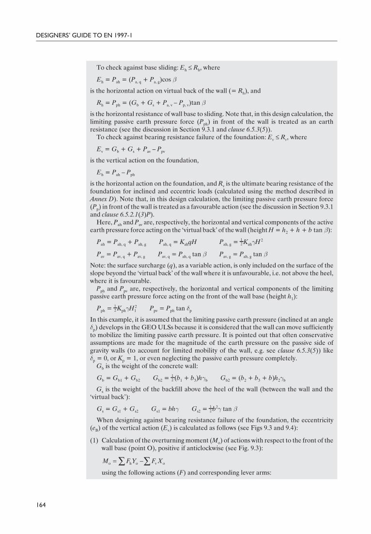
To check against base sliding: Eh £ Rh, where
Eh = Pah = (Pa, q + Pa, g)cos β
is the horizontal action on virtual back of the wall (= Rh), and
Rh = Pph = (Gb + Gs + Pa, v – Pp, v)tan β
is the horizontal resistance of wall base to sliding. Note that, in this design calculation, thelimiting passive earth pressure force (Pph) in front of the wall is treated as an earthresistance (see the discussion in Section 9.3.1 and clause 6.5.3(5)).
To check against bearing resistance failure of the foundation: Ev £ Rv, where
Ev = Gb + Gs + Pav – Ppv
is the vertical action on the foundation,
Eh = Pah – Pph
is the horizontal action on the foundation, and Rv is the ultimate bearing resistance of thefoundation for inclined and eccentric loads (calculated using the method described inAnnex D). Note that, in this design calculation, the limiting passive earth pressure force(Pp) in front of the wall is treated as a favourable action (see the discussion in Section 9.3.1and clause 6.5.2.1(3)P).
Here, Pah and Pav are, respectively, the horizontal and vertical components of the activeearth pressure force acting on the ‘virtual back’ of the wall (height H = h2 + h + b tan β):
Pah = Pah, q + Pah, g Pah, q = KahqH Pah, g = 12 KahγH
2
Pav = Pav, q + Pav, g Pav, q = Pah, q tan β Pav, g = Pah, g tan β
Note: the surface surcharge (q), as a variable action, is only included on the surface of theslope beyond the ‘virtual back’ of the wall where it is unfavourable, i.e. not above the heel,where it is favourable.
Pph and Ppv are, respectively, the horizontal and vertical components of the limitingpassive earth pressure force acting on the front of the wall base (height h1):
Pph = 12 KphγH1
2 Ppv = Pph tan δp
In this example, it is assumed that the limiting passive earth pressure (inclined at an angleδp) develops in the GEO ULSs because it is considered that the wall can move sufficientlyto mobilize the limiting passive earth pressure. It is pointed out that often conservativeassumptions are made for the magnitude of the earth pressure on the passive side ofgravity walls (to account for limited mobility of the wall, e.g. see clause 6.5.3(5)) likeδp = 0, or Kp = 1, or even neglecting the passive earth pressure completely.
Gb is the weight of the concrete wall:
Gb = Gb1 + Gb2 Gb2 = 12 (b1 + b3)hγb Gb2 = (b2 + b3 + b)h2γb
Gs is the weight of the backfill above the heel of the wall (between the wall and the‘virtual back’):
Gs = Gs1 + Gs2 Gs1 = bhγ Gs2 = 12 b2γ tan β
When designing against bearing resistance failure of the foundation, the eccentricity(eB) of the vertical action (Ev) is calculated as follows (see Figs 9.3 and 9.4):
(1) Calculation of the overturning moment (Mo) of actions with respect to the front of thewall base (point O), positive if anticlockwise (see Fig. 9.3):
using the following actions (F) and corresponding lever arms:
164
DESIGNERS’ GUIDE TO EN 1997-1
o h o v oM F Y F X= -Â Â

– Action Pah, q with lever arm Y = H/2, action Pah, g with lever arm Y = H/3.– Action Pav, q and Pav, g with lever arm X = b2 + b3 + b.– Action Gb1 with lever arm X = b2 + b3 /2, action Gb2 with lever arm
X = (b2 + b3 + b)/2, assuming that the stem of the wall is inclined symmetricallyat the front and back. The slight inclination of the back of the wall (0.95° to thevertical) is ignored in calculating the earth pressure in the STR-type ULS design.
– Action Gs1 with lever arm X = b2 + b3 + b/2.– Action Gs2 with lever arm X = b2 + b3 + 2
3 b.– Action (–Pph) with lever arm Y = h1/3.
(2) Calculation of the eccentricity (eB) of the vertical action (Ev):
where B = b2 + b3 + b is the total width of the wall base. The eccentricity is positive ifthe vertical action is applied to the right of the centre of the wall base (see Fig. 9.3).
In STR ULSs, failure occurs in a structural element (e.g. the base of the wall stem) bythe development of a plastic hinge at this location. The structural design of the wallsection at the base of the stem involves calculating the design bending moment and shearforce at this location due to the horizontal component of the appropriate force (Ph)resulting from the limiting active earth pressure acting over the height h of the wall stem(see Fig. 9.4b):
Ph = Ph, q + Ph, g Ph, q = Khqh Ph, g = 12 KhγH
2
The surface surcharge (q) is considered to act everywhere on the ground surface, since it isan unfavourable (geotechnical) action with respect to the wall stem.
In STR ULSs, the appropriate earth pressure coefficient (Kh) should be compatiblewith the wall rotation when a plastic hinge develops at the base of the stem. As therotation of the wall stem under this condition may not be sufficient to mobilize fully theactive earth pressure in the backfill, two alternative values of the earth pressure areconsidered in this example (other assumptions may also be appropriate, depending on thekinematic constraints of the wall):
(1) The active earth pressure, which is relevant if the wall movement is sufficiently largeto cause a ULS condition in the retained ground when a ULS condition occurs in thestructure (base of stem). Then, Kh = Kah.
(2) An intermediate earth pressure, corresponding to the earth pressure coefficientKh = 0.5(Kah + K0), i.e. the average of the horizontal earth pressure at-rest coefficient(K0) and the horizontal active earth pressure coefficient (Kah). An earth pressure ofabout this magnitude may be relevant (as an empirical rule) if the wall and thefoundation are stiff and a ULS condition develops in the concrete section prior to thedevelopment of a ULS in the retained ground. (see clause 9.5.4).
The design value of the ground angle of shearing resistance (ϕd¢) is calculated using theequation
where ϕk¢ is the characteristic angle of shearing resistance of the ground, and the partialfactor γϕ ¢ is obtained from Table A.4.
In DA-1 Combination 1 and DA-2, γϕ ¢ = 1 (Table A.4), and thusϕd¢ = ϕk¢ = 32°, and, onthe front of the wall, δd = δk = 20°, while, on the virtual back of the wall, δd = β = 20°. Thedesign (and characteristic) value of the active earth pressure coefficient (Kah) for the
165
CHAPTER 9. RETAINING STRUCTURES
d k1
arctan tanϕ
ϕ ϕγ ¢
Ê ˆ=¢ ¢Á ˜
Ë ¯
ob
v2MB
eE
Ê ˆ= - +Á ˜Ë ¯

backfill is determined from Fig. C.1.3 for ϕd¢ = 32°, β = 20° and δd /ϕd¢ = β/ϕd¢ = 0.625.Hence, Kah = 0.35. Note that the inclination of the earth pressure on the virtual back ofthe wall is assumed to be equal to the inclination of the ground surface, regardless of theground parameters (see Section 9.7). The design value of the at-rest horizontal earthpressure coefficient of the backfill is calculated from equation (9.2) with OCR = 1:
K0 = (1– sin ϕd¢)(1 + sin β) = 0.631
The design (and characteristic) value of the limiting passive earth pressure coefficient isobtained from Fig. C.2.1 forϕd¢ = 32°, β= 0° and δd /ϕd¢ = 20/32 = 0.625. Hence, Kph = 5.5.
In DA-1 Combination 2 and DA-3, γϕ ¢ = 1.25 (Table A.4), and thus ϕd¢ = 26.6°, and, onthe front of the wall, δd = tan–1(tan ϕk¢/1.25) = 16.2°, while, on the virtual back of the wall,δd = β = 20°. The design value of the active earth pressure coefficient (Kah) of the backfillis obtained from Fig. C.1.3 of Annex C for ϕd¢ = 26.6°, β = 20° and δd /ϕd¢ = β/ϕd¢ = 0.75.Hence, Kah = 0.48. The design value of the at-rest horizontal earth pressure coefficient ofthe backfill is calculated from equation (9.2) with OCR = 1:
K0 = (1 – sin ϕ¢)(1 + sin β) = 0.741
The design value of the limiting passive earth pressure coefficient is obtained from Fig.C.2.1 of Annex C for ϕd¢ = 26.6°, β = 0° and δd /ϕd¢ = 16.2/26.6 = 0.62. Hence, Kph = 3.9.
The sequence of the calculations and the main results for the three Design Approachesand for the conventional OFS method are listed in the following tables. The appropriatepartial factors (taken from Annex A) are also included in the tables for ease of reference.Note that in DA-1 the width of the footing is determined from the more critical of the twocombinations (in this example, Combination 2). In the OFS method, the ‘design values’ ofthe various quantities are identical to their ‘characteristic values’, since this methoddoes not include partial factors; the ‘characteristic values’ are calculated using thecharacteristic ground parameters of the Eurocode Design Approaches.
The characteristic and design values of the geotechnical (Pa, g, Pa, q) and non-geotechnical(Gb, Gs) actions are listed in Table 9.2, together with the design values of the effects of theactions (net vertical and horizontal actions on the foundation) for GEO ULS calculations.The application of the partial factors for calculating the design values of the actions isdescribed in Section 9.7. For example, the design value of the unfavourable variablegeotechnical action Pah, q is calculated using the equation
Fd = γF F(Xk /γM)
i.e.
Pah, q = Kah(γF q)H
with partial factors given in Table 9.2, as follows:
• In DA-1 Combination 1:
Pah, q = 0.35 × (1.5 × 10) × 7.70 = 40.43 kN/m
• In DA-1 Combination 2 and DA-3:
Pah, q = 0.48 × (1.3 × 10) × 8.21 = 51.23 kN/m
• In DA-2:
Pah, q = 0.35 × (1.5 × 10) × 7.84 = 41.16 kN/m
The different values of the height H (see Fig. 9.3) correspond to the different values ofthe heel width b in each Design Approach. Note that the earth pressure force on thepassive side of the wall (Pp) is considered as a favourable geotechnical action whendesigning against bearing resistance failure, and as an earth resistance when designingagainst base sliding (see the discussion in Section 9.3.1).
166
DESIGNERS’ GUIDE TO EN 1997-1
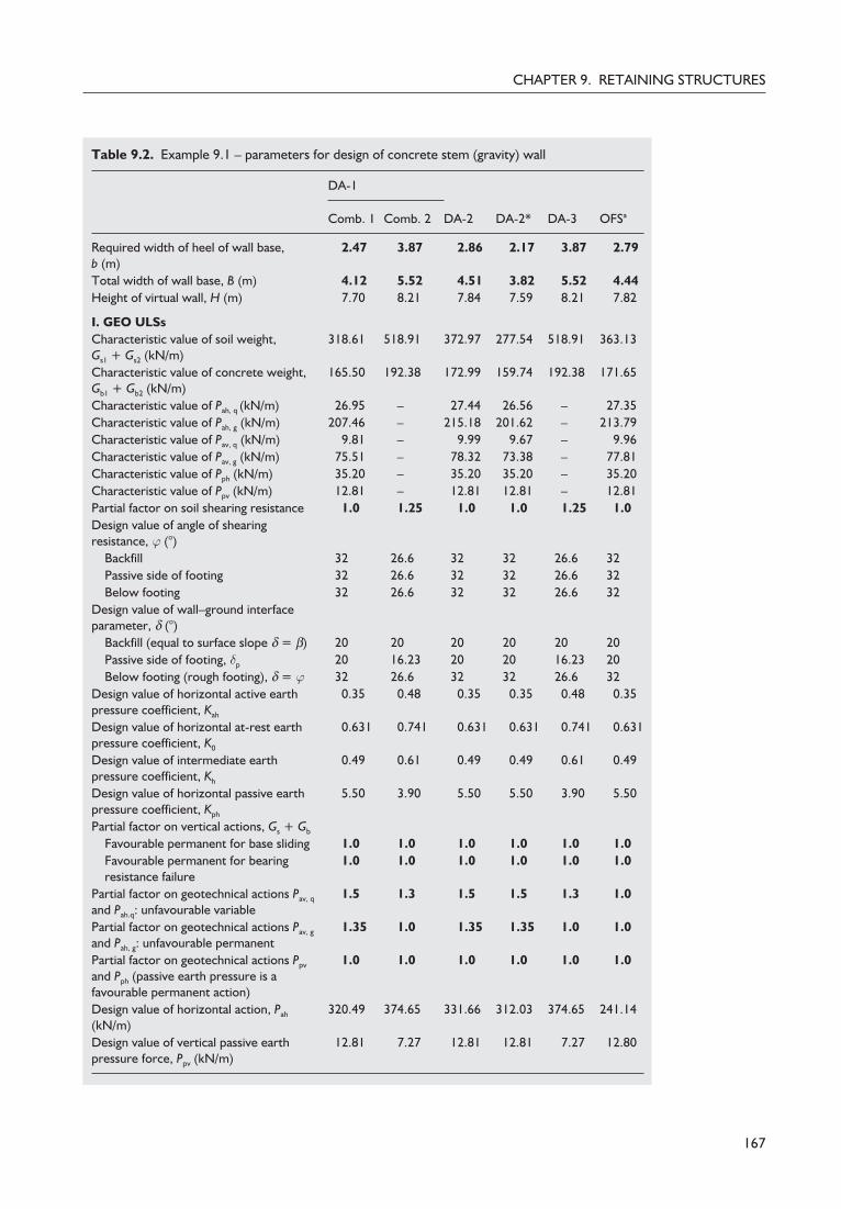
167
CHAPTER 9. RETAINING STRUCTURES
Table 9.2. Example 9.1 – parameters for design of concrete stem (gravity) wall
DA-1
DA-2 DA-2* DA-3 OFSaComb. 1 Comb. 2
Required width of heel of wall base,b (m)
2.47 3.87 2.86 2.17 3.87 2.79
Total width of wall base, B (m) 4.12 5.52 4.51 3.82 5.52 4.44Height of virtual wall, H (m) 7.70 8.21 7.84 7.59 8.21 7.82
I. GEO ULSsCharacteristic value of soil weight,Gs1 + Gs2 (kN/m)
318.61 518.91 372.97 277.54 518.91 363.13
Characteristic value of concrete weight,Gb1 + Gb2 (kN/m)
165.50 192.38 172.99 159.74 192.38 171.65
Characteristic value of Pah, q (kN/m) 26.95 – 27.44 26.56 – 27.35Characteristic value of Pah, g (kN/m) 207.46 – 215.18 201.62 – 213.79Characteristic value of Pav, q (kN/m) 9.81 – 9.99 9.67 – 9.96Characteristic value of Pav, g (kN/m) 75.51 – 78.32 73.38 – 77.81Characteristic value of Pph (kN/m) 35.20 – 35.20 35.20 – 35.20Characteristic value of Ppv (kN/m) 12.81 – 12.81 12.81 – 12.81Partial factor on soil shearing resistance 1.0 1.25 1.0 1.0 1.25 1.0Design value of angle of shearingresistance, ϕ (°)
Backfill 32 26.6 32 32 26.6 32Passive side of footing 32 26.6 32 32 26.6 32Below footing 32 26.6 32 32 26.6 32
Design value of wall–ground interfaceparameter, d (°)
Backfill (equal to surface slope d = b) 20 20 20 20 20 20Passive side of footing, δp 20 16.23 20 20 16.23 20Below footing (rough footing), d = ϕ 32 26.6 32 32 26.6 32
Design value of horizontal active earthpressure coefficient, Kah
0.35 0.48 0.35 0.35 0.48 0.35
Design value of horizontal at-rest earthpressure coefficient, K0
0.631 0.741 0.631 0.631 0.741 0.631
Design value of intermediate earthpressure coefficient, Kh
0.49 0.61 0.49 0.49 0.61 0.49
Design value of horizontal passive earthpressure coefficient, Kph
5.50 3.90 5.50 5.50 3.90 5.50
Partial factor on vertical actions, Gs + Gb
Favourable permanent for base sliding 1.0 1.0 1.0 1.0 1.0 1.0Favourable permanent for bearingresistance failure
1.0 1.0 1.0 1.0 1.0 1.0
Partial factor on geotechnical actions Pav, q
and Pah.q: unfavourable variable1.5 1.3 1.5 1.5 1.3 1.0
Partial factor on geotechnical actions Pav, g
and Pah, g: unfavourable permanent1.35 1.0 1.35 1.35 1.0 1.0
Partial factor on geotechnical actions Ppv
and Pph (passive earth pressure is afavourable permanent action)
1.0 1.0 1.0 1.0 1.0 1.0
Design value of horizontal action, Pah
(kN/m)320.49 374.65 331.66 312.03 374.65 241.14
Design value of vertical passive earthpressure force, Ppv (kN/m)
12.81 7.27 12.81 12.81 7.27 12.80

The design values of the effects of the actions are calculated from the designvalues of the relevant actions using the following equations (the index ‘d’ is omitted forconciseness):
• For base sliding (net horizontal action):
Eh = Pah = (Pa, q + Pa, g)cos β = Pah, q + Pah, g
• For bearing failure (resultant vertical action):
Ev = Gb + Gs + Pav – Ppv
Finally, note that the calculated width, b of the heel of the wall, in DA-1 and DA-3 isgreater than the minimum value, and in DA-2 is not much smaller than the minimumvalue,
bmin = h/tan(45 + ϕk¢/2) = 3.32 m
which permits the development of a conjugate Coulomb-type ‘failure surface’ (inclined at45 + ϕk¢/2 to the horizontal) within the soil mass above the heel. Thus these calculatedwidths validate the assumption of the active earth pressure acting on the ‘virtual back’ ofthe wall.
Note that in this example, the weight of the wall and soil (Gb + Gs) is a favourableaction when designing against bearing resistance failure, because its favourable effect inreducing the load eccentricity on the foundation (favourable effect) is more significantwith regard to the bearing resistance than its unfavourable effect in increasing thevertical load. In different wall configurations the significance of these effects may bereversed. Thus, it is recommended that two calculations are performed, one with partialfactors for ‘favourable’ and one for ‘unfavourable’ actions on the weight of the wall andthe soil.
The design values of the resistances required in the ULS analyses of the wall againstbase sliding and bearing resistance failure (GEO ULSs) are presented in Table 9.3. Thehorizontal resistance against base sliding is calculated using the equation
Rh = Pph + (Gb + Gs +Pav – Ppv)tan δ¢
168
DESIGNERS’ GUIDE TO EN 1997-1
Table 9.2. Contd
DA-1
DA-2 DA-2* DA-3 OFSaComb. 1 Comb. 2
Design value of horizontal passive earthpressure force, Pph (kN/m)
35.20 24.96 35.20 35.20 24.96 35.20
Design value of resultant vertical actionFor base sliding, Gs + Gb + Pav (kN/m)For bearing resistance failure,Gs + Gb + Pav – Ppv (kN/m)
600.76587.95
847.66840.39
666.68653.87
520.33538.04
847.66840.39
622.55609.74
Design value of resultant horizontalaction
For base sliding, Pah (kN/m)For bearing resistance failure, Pah – Pph
(kN/m)
320.49285.29
374.65349.69
331.66296.46
312.03276.83
374.65349.69
241.10205.94
a In the OFS method, all values are ‘nominal’ (characteristic) values

169
CHAPTER 9. RETAINING STRUCTURES
Table 9.3. Example 9.1 – results of the GEO design for the concrete stem (gravity) wall
DA-1
DA-2 DA-2* DA-3 OFSaComb. 1 Comb. 2
Width of heel of wall base, b (m) 2.47 3.87 2.86 2.17 3.87 2.79Total width of wall base, B (m) 4.12 5.52 4.51 3.82 5.52 4.44
A. Design against sliding(GEO ULS)Character value of horizontalsliding resistance Rh, k (kN/m)
– – – 352.3 – 416.2
Partial factor on sliding resistance(on Rv tan δ)
1.0 1.0 1.1 1.1 1.0 1.0
Partial factor on earth resistance(on Pph)
1.0 1.0 1.4 1.4 1.0 1.0
Design value of horizontal slidingresistance Rh, d (kN/m)
402.6 445.1 396.6 313.4 445.1 416.2
Design value of net horizontaleffect of the actions Eh, d (kN/m)
320.5 374.6 331.7 312.0 374.6 241.1
Over-design factor for DesignApproaches or OFS, Rh, d /Eh, d
1.26 1.19 1.20 1.00 1.19 1.73
Minimum required value ofRh, d /Eh, d for stability
1.0 1.0 1.0 1.0 1.0 1.5
Result for design: CR, critical;NCR, not critical
NCR NCR NCR CR NCR NCR
B. Design against bearingresistance failure (GEO ULS)Design value of overturningmoment with respect to O,Mdo (kN m/m) (positive ifanticlockwise – see Fig. 9.3)
–840.8 –1986.1 –1125.3 –755.0 –1986.1 –1177.3
Design value of total verticaleffect of the actions, Ev, d
(kN/m)
587.9 840.4 653.9 538.0 840.4 609.7
Design value of total horizontaleffect of the actions, Eh, d
(kN/m)
285.3 349.7 296.5 193.0 349.7 205.9
Design value of the overturningmoment with respect to thecentre of the wall base, Md
(kN m/m) (positive ifanticlockwise – seeFig. 9.3)
370.4 333.4 349.2 214.3 333.4 176.3
Design eccentricity of Ev, withrespect to the centre of thebase, eB (m) (positive if actionis to the right of centre – seeFig. 9.3)
–0.63 –0.40 –0.53 –0.42 –0.40 –0.29
Effective foundation width:B¢ = B – 2 × abs(eB) (m)
2.86 4.73 3.44 2.98 4.73 3.86
Partial factor on embedmentpressure (p): favourablepermanent action
1.0 1.0 1.0 1.0 1.0 1.0
Design value of embedmentpressure, p = γ h1 (kPa)
16.00 16.00 16.00 16.00 16.00 16.00

The vertical component of the bearing resistance (Rv) is calculated using the procedurerecommended in Annex D for surface foundations. In general, design values of resistancesare calculated using the equation
Rd = R[γF F(Xk/γM)]/γR
as follows (see example below):
(1) In DA-1 Combination 1, using design values of the actions, and design values of thesoil parameters (ϕ¢, δ¢) equal to the characteristic values (since γM = 1) and γR = 1.
(2) In DA-1 Combination 2 and DA-3, using design values of soil parameters and actionsand γR = 1.
(3) In DA-2, using design values of the soil parameters (ϕ¢, δ¢) equal to the characteristicvalues (since γM = 1), and design values of actions and appropriate partial factors forresistances (γR = 1.1 and 1.4 for sliding and γR = 1.4 for bearing resistance). Analternative calculation (DA-2*) is also performed, which is similar to DA-2 but usesthe characteristic (and not the design) values of the actions in the calculation ofdesign resistances.
The characteristic value of the resistance is not required in any of the Eurocode DesignApproaches (except in the variation DA-2*). It is only calculated in the OFS method. Forexample, the design value of the horizontal resistance against base sliding (Rh, d) iscalculated as follows:
• In DA-1 Combination 1:
Rh, d = 35.20/1.0 + [(484.11 + 116.65–12.81)tan 32]/1.0 = 402.6 kN/m
• In DA-1 Combination 2 and DA-3:
Rh, d = 24.96/1.0 + [(711.3 + 136.36–7.27)tan 26.6]/1.0 = 445.1 kN/m
170
DESIGNERS’ GUIDE TO EN 1997-1
Table 9.3. Continued
DA-1
DA-2 DA-2* DA-3 OFSaComb. 1 Comb. 2
Bearing resistance factorsNq 23.18 12.59 23.18 23.18 12.59 23.18Nγ 27.72 11.59 27.72 27.72 11.59 27.72iq 0.265 0.341 0.299 0.384 0.341 0.439iγ 0.136 0.199 0.163 0.238 0.199 0.290
Characteristic value of bearingresistance, Rvk (kN/m)
– – – 1007.8 – 1828.5
Partial factor on bearingresistance, γR
1.0 1.0 1.4 1.4 1.0 1.0
Design value of bearingresistance, Rvd (kN/m)
590.3 839.8 655.4 719.9 839.8 1828.5
Design value of total verticalaction, Ev, d (kN/m)
588.0 840.0 653.9 538.0 840.0 609.7
Over-design factor for DesignApproaches or OFS, Rv, d/Ev, d
1.00 1.00 1.00 1.34 1.00 3.00
Minimum required value ofRv, d/Ev, d for stability
1.00 1.00 1.00 1.00 1.00 3.00
Result for design: CR, critical;NCR, not critical
NCR CR CR NCR CR CR
a In the OFS method, all values are ‘nominal’ (characteristic) values

• In DA-2:
Rh, d = 35.20/1.4 + [(545.96 + 120.71–12.8)tan 32]/1.1 = 396.6 kN/m
• In DA-2*, using the width of heel of the wall, which is critical in DA-2 (b = 2.86 m),for comparison:
Rh, d = Pph, d + [(Gb + Gs +Pav – Ppv)tan δ¢]d
fi Rh, d = Pph, k/γR, e + [(Gb, k + Gs, k +Pav, k – Ppv, k)tan δ¢k]/γR, h
fi Rh, d = 35.20/1.4 + [(172.99 + 372.97 + 88.31–12.81)tan 32]/1.1 = 378.2 kN/m
The corresponding effect of the actions is
Ed = Pah, d = Pagh, d + Paqh, d = γGPagh, d + γQPaqh, d
fi Ed = 1.35 × 215.18 + 1.5 × 27.44 = 331.66
The wall is more than safe against base sliding since
Ed = 331.66 £ 378.2 = Rh, d
The over-design factor is
Rh, d /Ed = 378.2/331.66 = 1.14 ≥ 1
• In the OFS method:
Rh, d = 35.20 + (534.78 + 87.77–12.8) tan 32 = 416.2 kN/m
Note that DA-2 and DA-2* give slightly different results for Rh, d (396.6 and378.2 kN/m, respectively) when the same value of the width of the heel of the wall b isused. The difference is due to the unfavourable action Pav, which is factored by γF >1 inDA-2 (Pav = 120.71 kN/m) and factored by γF = 1 in DA-2* (Pav = 88.31 kN/m). Allthe other actions involved in the calculation of the sliding resistance are favourablepermanent actions, and thus are factored by γF = 1 in both variations of DA-2.
The cells in Table 9.3 denoted CR (critical) or NCR (not critical) indicate thecalculation which is critical in determining the width of the wall base. In this example,bearing resistance failure is found to be critical in all the Design Approaches. In DA-1,Combination 2 controls the width of the wall base.
Comparison of DA-2 with the alternative approach DA-2* indicates that DA-2* is lessconservative, since the required foundation width for DA-2* (3.82 m) is smaller than thatrequired for DA-2 (4.51 m); in fact, DA-2* is the least conservative of all the DesignApproaches, including the OFS method with minimum required overall factors of safetyof 1.5 against sliding and 3.0 against bearing failure.
The design values of the bending moment and the shear force at the bottom of the stemof the wall for structural (STR) ULSs are presented in Table 9.4, together with thecoefficients of earth pressure, partial action factors and earth pressure forces usedto calculate these. The calculations are performed for two alternative earth pressuremagnitudes: the active value and an earth pressure between the K0 and the active values,to illustrate the effect of the relative flexibility of the wall with respect to the retainedground, i.e. the occurrence of the structural ULS prior to, or simultaneously with, theULS in the retained ground (see the discussion on intermediate earth pressures for ULSdesign calculations in Section 9.5).
Bending moments and shear forces are the effects of actions and thus their designvalues are calculated using the design values of the relevant actions (the earth pressure, inthe case of the effects of actions at the bottom of the stem of the wall), i.e. using theequation Ed = E(Fd). In DA-1, the critical wall base width (obtained from Combination 2)is used.
171
CHAPTER 9. RETAINING STRUCTURES

The bending moments and shear forces of the Eurocode Design Approaches arefactored, while those of the conventional OFS method are unfactored, and thus are notdirectly comparable with the Eurocode 7 results. Specifically, the Eurocode 7 results areULS design values of the effects of actions for use directly in the structural design of theconcrete section (according to Eurocode 2). The bending moments calculated accordingto the OFS method may be used in the structural design of the concrete section (accordingto Eurocode 2) after application of the appropriate partial factors for actions. Forexample, the bending moment may be multiplied by a factor of 1.4 as an approximateequivalent partial factor weighting, corresponding to the Eurocode partial factors of 1.35and 1.5 for permanent and variable actions, respectively, in structural designs for STRULSs.
The following conclusions can be drawn from the results of the above analyses:
(1) For GEO ULSs, DA-1 and DA-3 give identical results since:(a) In DA-1 Combination 2 is critical in the design; this combination uses the same
material partial factors as DA-3.(b) All actions in the system are geotechnical (there are no structural actions);
geotechnical actions have the same partial factors in DA-1 Combination 2 andin DA-3.
172
DESIGNERS’ GUIDE TO EN 1997-1
Table 9.4. Example 9.1 – Results of STR design of concrete stem (gravity) wall
DA-1
DA-2 DA-2* DA-3 OFSaComb. 1 Comb. 2
Width of heel of wall base, b (m) 3.87 2.86 2.17 3.87 2.79Total width of footing, B (m) 5.52 4.51 3.82 5.52 4.44
II. STR ULSStructural design of wall (at bottomof stem)(a) Design using limiting active earthpressure
Characteristic value of Kah coefficient 0.35 – 0.35 0.35 – 0.35Design value of Kah coefficient 0.35 0.48 0.35 0.35 0.48 0.35Partial factor on action Pah, q 1.5 1.3 1.5 1.5 1.3 1.0Partial factor on action Pah, g 1.35 1.0 1.35 1.35 1.0 1.0Design value of Pah, q (kN/m) 31.5 37.4 31.5 31.5 37.4 21.0Design value of Pah, g (kN/m) 170.1 172.8 170.1 170.1 172.8 126.0Design value of bending moment,Md (kN m/m)
434.7 457.9 434.7 434.7 457.9 315.0
Design value of shear force, Vd (kN/m) 201.6 210.2 201.6 201.6 210.2 147.0(b) Design using intermediate earthpressure: K = 0.5(Ka + K0)
Characteristic value of Kh coefficient 0.49 – 0.49 0.49 – 0.49Design value of Kh coefficient 0.49 0.61 0.49 0.49 0.61 0.49Partial factor on action Ph, q 1.5 1.3 1.5 1.5 1.3 1. 0Partial factor on action Ph, g 1.35 1.0 1.35 1.35 1.0 1.0Design value of Ph, q (kN/m) 44.1 47.7 44.1 44.1 47.7 29.4Design value of Ph, g (kN/m) 238.3 220.0 238.3 238.3 220.0 176.6Design value of bending moment,Md (kN m/m)
609.1 582.9 609.1 609.1 582.9 441.4
Design value of shear force, Vd (kN/m) 282.4 267.6 282.4 282.4 267.6 206.0
a In the OFS method, all values are ‘nominal’ (characteristic) values

(2) For GEO ULSs, DA-2 and DA-2* are less conservative than DA-1 and DA-3, sincethe required width of the wall base (B = 4.51 m in DA-2 and B = 3.82 m in DA-2*) is18–31% smaller than that required by DA-1 and DA-3 (B = 5.52 m).
(3) For the structural design of the stem (STR ULSs), DA-2 and DA-2* are slightly lessconservative by about 5% (Md = 434.7 kN m/m) compared with DA-1 and DA-3(which give identical results: Md = 457.9 kN m/m).
(4) For STR-type limit states, the design values of the effects of actions (bending momentand shear force) at the bottom of the stem of the wall depend strongly on the assumedmagnitude of the earth pressure. For example, in DA-1 and DA-3, the effects ofactions calculated with the assumed intermediate earth pressure are 27% larger thanthose calculated using the active earth pressure (582.9 versus 457.9 kN m/m). Thisconclusion illustrates the importance of ensuring that the structural design of the wallallows some lateral movement.
(5) In DA-1, the Combination 2 set of partial factors is critical in the geotechnical design(GEO ULS). In the structural design (STR ULS) of the stem, Combination 2 iscritical if active earth pressures are used, while Combination 1 is critical if intermediateearth pressures are used.
(6) The OFS method is the least conservative in terms of the required width of the wallbase (B = 4.44 m compared with B = 5.52 m for DA-1 and DA-3, respectively, andB = 4.51 m for DA-2) with the exception of DA-2* (where B = 3.82 m). A possibleexplanation is that the OFS method makes no allowance for uncertainty in the activeforce on the virtual back of the wall. The wisdom of this is, however, questionable.
(7) In the structural design of the wall stem, the OFS method gives roughly the sameresults as the Eurocode Design Approaches since, using the multiplicationfactor of 1.4 (as mentioned above), the comparable ‘design’ bending moment of theconventional method is 315.0 × 1.4 = 441.0 kN m/m, i.e. about the same as thedesign values of all the Eurocode Design Approaches (457.9–434.7 kN m/m).
It should be pointed out that the above conclusions are applicable in the case of thisparticular example only. In other examples, involving different wall geometries andground parameters, the corresponding conclusions may be different.
Example 9.2: ULS and SLS design of an embedded sheet pile wallThis example presents the ULS and SLS design of an embedded sheet pile wall. The wall,shown in Fig. 9.5, has a nominal excavation depth of 5.0 m; an additional excavation depthto allow for accidental overdig (see Section 9.3.2) equal to 10% × 4.0 m = 0.40 m isadded, giving a design value of the excavation depth H = 5.40 m. The wall is supported byone row of anchorages at an elevation of –1.0 m (anchorage inclination β = 10°). Forexcavations in stiff clays, drained conditions are usually critical for stability; thus, effectivestress analyses are performed using effective stress ground parameters and steady statehydraulic conditions.
The ground profile consists of two layers (with the interface at an elevation of –4.0 m)having the following parameters for use in the ULS design (all values are characteristic):
• Layer A (medium-dense to dense gravelly sand):– Weight density above the water table: γk = 18 kN/m3.– Saturated weight density below the water table: γsk = 20 kN/m3.– Angle of shearing resistance: ϕk¢ = 35°.– Maximum value of wall–ground interface parameter used on active side
(clause 9.5.1(6)): δk = 23ϕk¢ = 23°.
• Layer B (stiff clay):– Saturated weight density below the water table: γsk = 20 kN/m3.– Angle of shearing resistance: ϕk¢ = 24°.
173
CHAPTER 9. RETAINING STRUCTURES

– Cohesion intercept: ck¢ = 5 kPa.– Maximum value of wall–ground interface parameter (indicative values for
long-term conditions used; other values may also be appropriate – see clause9.5.1(8)):
Active side: δak = 23ϕk¢ = 16°.
Passive side: δpk = 12ϕk¢ = 12°.
The water table in the sand layer is assumed to remain at an elevation of –1.0 m, wherethe ground level behind the wall is at an elevation of 0.0 m. Due to the excavation, thewater table in the pit is lowered to an elevation of –5.4 m. The gravelly sand (layer A) isassumed to maintain hydrostatic conditions, while the total hydraulic head difference(equal to 4.4 m) develops within the stiff clay; linear head loss is assumed along anidealized flow path starting from an elevation of –4.0 m (behind the wall), going aroundthe toe of the wall and exiting at an elevation of –5.4 m in front of the wall (total length ofpath: 2L + 1.4 m, where L is the wall penetration below the excavation level). Thismethod ensures that the water pressure at the toe of the wall (both sides) is in equilibrium,as anticipated. Thus, the water pressure on the active side of the wall is lower than thehydrostatic pressure (for the water table at an elevation of –1.0 m), while on the passiveside of the wall the water pressure is higher than hydrostatic (for the water table at anelevation of –5.4 m). Vertical effective stresses (σv¢) on both sides of the wall arecalculated using these water pressures (u) from the equation σv¢ = σv – u, where σv = γz isthe total vertical (geostatic) stress (z is measured from the ground surface behind the walland from the bottom of the excavation in front of the wall). Hydraulic failure of thebottom of the excavation by heave is examined according to the principles of Section 10.
Other input parameters are:
• Weight density of water: γk = 10 kN/m3.• Surcharge at ground surface (variable action): qk = 10 kPa.• Steel sheet pile (Frodingham 3N): Wel = 1688 cm3/m, Wpl ª 1900 cm3/m, steel grade
S355 GP, yield strength 355 MPa.
The design value of the ultimate moment of resistance (Mu, d) of the sheet pile(Frodingham 3N) is calculated according to EN 1993-5:
174
DESIGNERS’ GUIDE TO EN 1997-1
–5.0 m
–1.0 m
–4.0 m
0.4 m
Layer BLayer B
Layer A
0.0
WT = –5.4 m
WT = –1.0 m
qk = 10 kPa
H =
5.4
m
Fig. 9.5. Geometrical data for an embedded wall

Mu, d = Wpl fy /1.0 = 675 kN m/m
The value of the material partial factor for steel (1.0) is taken from EN 1993-5, and may beset by national determination.
In addition to the classical LEM , a spring model is also used below, in the ULS designwith DA-1 Combination 1 and DA-2 and in the SLS design. Spring models can be used inDA-1 Combination 2 and DA-3 designs following the recommendations given in Section9.7. In the spring model, the calculations use the characteristic values of all stiffnessparameters (soil, anchor and wall). This model requires soil stiffness parameters, the wallbending stiffness (EI), and the anchor axial stiffness and prestress force. The soil issimulated by an elastic–perfectly plastic spring yielding at the limiting active and passiveearth pressures. The characteristic value of the pre-yield spring stiffness (horizontalsubgrade modulus) is assumed equal to k = 10 000 kN/m3 in the sand andk = 6000 kN/m3 in the clay layer. The characteristic value of the coefficient of earthpressure at rest is K0, k = 0.50 in the sand and K0, k = 0.95 in the clay layer. Thecharacteristic anchor pre-yield axial stiffness K = EA/L is calculated from its free length(L = 11 m), cross-section (A = 1 cm2/m) and the Young modulus of steel (E = 210 GPa).The anchor prestress force (lock-off force) P0 = 100 kN/m was obtained by trial anderror. The sheet pile wall pre-yield bending stiffness is EI = 5 × 10⁴ kN m2/m.
In the LEM the design values of ground parameters and the corresponding calculatedhorizontal earth pressure coefficients for limiting active (Kah) and passive (Kph) conditionsare given in Table 9.5. The design values of Kah and Kph are obtained from Figs C.1.1 andC.2.1.
ULS design of the wall
In the ULS design of the embedded wall, the aim is to determine:
(1) The minimum embedment depth. This is calculated by assuming free-earth supportconditions at the toe, i.e. assuming that the wall moves sufficiently to mobilize thelimiting active and passive earth pressures on the retained and the resisting sides,respectively (LEM).
(2) The bending moment distribution on the wall and the anchor force. These may bedetermined by two methods:(a) Using known earth pressure distributions on the wall, namely the limiting earth
pressures (i.e. using a LEM without earth pressure redistribution).(b) Using a spring model, i.e. a beam model of the wall supported on soil springs with
appropriate stiffness. This model includes wall–ground interaction and earthpressure redistribution. Details concerning the application of spring models arepresented in Section 9.7.
The following horizontal actions are applied to the wall in the LEM:
(1) The horizontal component of the active earth pressure on the retained side:
p¢ah = p¢ah, g + p¢ah, q
at a depth z from ground surface, where
p¢ah, g = Kahσv¢ – 2c¢÷Kah
is an unfavourable permanent geotechnical action and σv¢ is the vertical effectivestress at depth z, and
p¢ah, q = Kahq
is an unfavourable variable geotechnical action.(2) The net water pressure (pressure on the retained side minus pressure on the resisting
side), which is an unfavourable permanent geotechnical action. The net water
175
CHAPTER 9. RETAINING STRUCTURES

pressure is zero at the toe of the wall, since at this point water pressures on both sidesare in equilibrium. Thus, the characteristic value of the net water pressure increaseslinearly from zero at an elevation of –1.0 m to 30 kPa at an elevation of –4.0 m,reaches a maximum value at an elevation of –5.4 m (depending on the wallpenetration) and then reduces linearly to zero at the toe of the wall (see Table 9.6).
The above horizontal actions are resisted by the horizontal component of the anchorforce and by the horizontal component of the limiting passive earth pressure on theretained side. The limiting passive earth pressure at a depth z¢ below the excavation base iscalculated from the equation
p¢ph = Kphσv¢ + 2c¢÷Kph
where σv¢ is the corresponding vertical effective stress. The limiting passive earth pressureis treated as a resistance (see the discussion in Section 9.3.1).
Design values of actions are calculated according to the method described in Section9.7. For example, the design value of the unfavourable variable geotechnical action p¢ah, q in
i.e.
Fd
= γFF(X
k/γ
M)
176
DESIGNERS’ GUIDE TO EN 1997-1
Table 9.5. Example 9.2 – LEM
DA-1 DA-2 DA-3 OFSa
Comb. 1 Comb. 2
Partial factor on ground strengthparameters, γM
1.0 1.25 1.0 1.25 1.0
Design value of the angle of shearingresistance, ϕ¢ (°)
533.92533.9253AreyaL426.91426.9142BreyaL
Design value of cohesion intercept,c¢ (kPa)
54545BreyaLMax. design value of wall–groundinterface parameter, d = 2
3ϕ¢ (°)Layer A – active side 23 19.6 23 19.6 23Layer B – active side 16 13.1 16 13.1 16Layer B – passive side 12 9.8 12 9.8 12
Design value of horizontal activeearth pressure coefficient, Kah
32.003.032.003.032.0AreyaL73.054.073.054.073.0BreyaL
Design value of horizontal passiveearth pressure coefficient, Kph
02.305.202.305.202.3BreyaLPartial factors for actions, γF
Unfavourable permanent 1.35 1.0 1.35 1.0 1.0Unfavourable variable 1.5 1.3 1.5 1.3 1.0Favourable permanent 1.0 1.0 1.0 1.0 1.0
Partial factor for earth resistance onpassive side, γR
1.0 1.0 1.4 1.0 1.0
a In the OFS method, all values are ‘nominal’ (characteristic) values

p¢ah, q = γFKahq
and with partial factors from Table 9.5:
• In DA-1 Combination 1, step 1, and DA-2:
p¢ah, q = 1.5 × 0.23 × 10 = 3.45 kPa
• In DA-1 Combination 2 and DA-3:
p¢ah, q = 1.3 × 0.30 × 10 = 3.90 kPa
The design value of the limiting passive earth pressure (resistance) is calculated usingthe equation:
Rd = R[F(Xk/γM)]γR
i.e.
pph = (Kphσv¢ + 2c¢÷Kph)/γR
with partial factors from Table 9.5. For example, at a depth z¢ = 3 m below the excavationbase, where the characteristic vertical effective stress σv¢ = 30 kPa and assuming
• In DA-1 Combination 1, step 1:
p¢ph = [3.2 × (1.0 × 30) + 2 × 5 × ÷(3.2)]/1.0 = 113.9 kPa
• In DA-2:
p¢ph = [3.2 × (1.0 × 30) + 2 × 5 × ÷(3.2)]/1.4 = 81.3 kPa
• In DA-1 Combination 2 and DA-3:
p¢ph = [2.5 × (1.0 × 30) + 2 × 4 × ÷(2.5)]/1.0 = 87.6 kPa
In fact, due to the upward water flow, the actual vertical effective stress (σv¢) issomewhat lower than the values obtained above, assuming hydrostatic water pressures.Note that the vertical effective stress at a particular depth varies in each Design Approachas the wall penetration is different. The correct value of the vertical effective stress wasused in the worked example (see Table 9.6), while the same hydrostatic pore pressure wasused in the above calculation in order to compare the three Design Approaches.
In the LEM, the required wall penetration is calculated by ensuring bending momentequilibrium of the design values of actions and resistances around the anchorage point(since free-earth support conditions are selected). Then, the design value of thehorizontal component of the anchor force (P0h) is calculated by ensuring equilibrium ofthe design values of horizontal actions and resistances.
The vertical equilibrium of the wall is finally checked by adjusting the design value ofthe wall–ground interface parameter (δa) on the active side, i.e. by calculating a factor (m)such that
P ¢ah tan mδa + Fh tan β = P ¢ph tan δp
where P ¢ah and P ¢ph are the resultant horizontal active and passive earth pressure forces onthe wall (all quantities in the equation enter with their design values). It is noted that thewall–ground interface parameter (δp) on the passive side is not adjusted since the walltends to move downwards and thus tends to reduce the friction on the active side only. Inthe unlikely case that the calculated m value is greater than 1, then m is set equal to 1, andthe parameter δp is reduced until equilibrium is verified (since in this case the wall movesupwards and reduces the friction on the passive side).
177
CHAPTER 9. RETAINING STRUCTURES
hydrostatic pore pressures (adjusted for equality at either side of the toe), the design value of the limiting passive earth pressure is:

Table 9.6 lists the main results of the ULS calculations based on the Eurocode DesignApproaches and the OFS method with an OFS of 2.0 on passive earth pressure (i.e.passive earth pressure is reduced to 50% of its characteristic value). The design values ofbending moments and shear forces listed in this table were determined from the designvalues of the earth and water pressures and support reactions.
178
DESIGNERS’ GUIDE TO EN 1997-1
Table 9.6. Example 9.2 – ULS design by LEM (except for step 2 of DA-1 Combination 1)
DA-1
DA-2 DA-3 OFSb
Comb. 1a Comb. 2
Step 1 Step 2
Required wall embedment, d, belowmaximum excavation (m)
5.89 6.62 6.62 7.89 6.62 8.27
Required length of sheet pile wall (m) 11.29 12.02 12.02 13.29 12.02 13.67Characteristic value of pore waterpressure (kPa)
Elevation –1.0 m (active side)and –5.40 m (passive side)
0 0 0 0 0 0
Elevation –4.0 m (active side) 30 30 30 30 30 30Elevation –5.4 m (active side) 39.3 39.3 39.8 40.4 39.8 40.6Toe of wall (both sides) 78.6 78.6 86.1 99.1 86.1 103.0
Characteristic value of the net waterpressure (kPa)
From elevation 0.0 to –1.0 m 0 0 0 0 0 0Elevation –4.0 m 30 30 30 30 30 30Elevation –5.4 m 39.3 39.3 39.8 40.4 39.8 40.6
Toe of wall 0 0 0 0 0 0Design value of total horizontal thruston the active side, P ¢ah + Pw (kN/m)
662.4 638.9 858.6 638.9 660.3
Design value of total horizontal resistanceon the passive side P ¢ph (kN/m)
475.1 466.9 630.1 466.9 486.9
Design value of the horizontal componentof the anchor force, P0h (kN/m)
167.0 172.0 228.5 172.0 173.4
Design value of the anchor force,P0 = P0h/cos b (kN/m)
169.6 174.6 232.1 174.6 176.1
Design value of the overturning (and theresisting) moments with respect to theanchorage level (kN m/m)
4021.1 5951.9 4021.1 4722.8
Design value of total vertical thrust onthe active side, Pav¢ (kN/m)
42.3 83.2 42.3 65.2
Design value of total vertical resistanceon the passive side P ¢pv (kN/m)
72.3 123.2 72.3 95.6
Maximum bending moment in wallDesign value, Mmax, d (kN m/m) 347.0 446.7 649.5 446.7 706.4Elevation (m) –5.40 –5.40 –5.40 –5.40 –6.04
Maximum shear force in wallDesign value, Sd (kN/m) 159.1 215.7 159.1 164.2Elevation (m) –1.00 –1.00 –1.00 –1.00
a The two calculation steps for DA-1 Combination 1 are first to determine the minimum wallpenetration (embedment) depth and then, in a separate calculation (using a soil spring model), todetermine the internal forces and the anchor forceb In the OFS method, all values are ‘nominal’ (characteristic) values
DA-1 Combination 1 – step 2In DA-1, as the wall penetration obtained from Combination 2 is larger than forCombination 1 (as is usually the case), a separate calculation (step 2) is performed withthe Combination 1 partial factors and the wall penetration d = 6.62 m, determined withthe Combination 2 partial factors as shown in Table 9.6. As the wall penetration is nowgreater than that required for the full mobilization of the limiting earth pressures with theCombination 1 partial factors (d = 6.62 m > 5.89 m), a wall–ground interaction modelis required to calculate the mobilized fraction of the limiting earth pressures. Theinteraction model used in this example is a spring model, as discussed in Section 9.7. Thespring model gives the following results:
• Design value of the horizontal component of the anchor force:
P0h = 1.35 × 123.7 = 167.0 kN/m
• Design value of the maximum bending moment in the wall for DA-1 Combination 1:
Mmax, d = 1.35 × 257 = 347 kN m/m < Mu, d = 675 kN m/m
Note that when it is obvious that step 1 of DA-1 requires a smaller wall penetrationthan DA-1 Combination 2, step 2 can be performed readily after calculating the wallpenetration using DA-1 Combination 2.
Table 9.6 leads to the following conclusions:
(1) In DA-1, Combination 2 provides the wall penetration depth (6.62 m). Combination2 is also critical for the structural design of the wall (maximum bendingmoment = 446.7 kN m/m).
(2) DA-3 gives identical results to DA-1 Combination 2.(3) DA-2 is the most conservative of the Eurocode Design Approaches as it gives
the greatest wall penetration (7.89 m) and the largest design bending moment(649.5 kN m/m). The OFS method gives even deeper wall penetration (8.27 m) and aslightly larger comparable design bending moment (1.4 × 504.6 = 706.4 kN m/m).
(4) The Frodingham 3N sheet pile section has sufficient ultimate moment of resistance(Mu, d = 675 kN m/m) to resist the calculated design bending moments in DA-1 andDA-3; a slightly heavier sheet pile section is required in DA-2 and in the OFS method(Mu, d ≥ 649.5 kN m/m and Mu, d ≥ 1.4 × 504.6 = 707 kN m/m, respectively).
DA-2 – use of an LEMIn the above application of DA-2 using the LEM, partial factors for actions are applied atthe source, i.e. on the limiting active earth pressure and the net water pressure.
The following equivalent alternative procedure can be used, called DA-2*:
(1) Permanent actions (e.g. limiting active earth pressure due to the soil weight and netwater pressure) enter the calculation with values equal to their characteristic values(i.e. using unit partial factors). Soil parameters (i.e. shear strength) also enter thecalculation with values equal to their characteristic values, as usual for DA-2.
(2) Unfavourable variable actions (e.g. limiting active earth pressure due to the surfacesurcharge) enter the calculation multiplied by 1.5/1.35 = 1.11, i.e. qd = 1.11 andqk = 11.1 kPa.
(3) The overturning moment (ME) is calculated, which is the sum of the moments of theactive earth pressure and the net water pressure (sum = Ek) with respect to theanchorage point. The corresponding design value is then calculated: MEd = 1.35ME.This is the design value of the effect of the actions for use in the ULS design.
(4) The horizontal component of the limiting earth resistance (Rp, k) is calculated, asis the stabilizing moment (MR) of Rp, k with respect to the anchorage point. The
179
CHAPTER 9. RETAINING STRUCTURES

corresponding design value is then calculated: MRd = MR/1.4. This is the design valueof the stabilizing moment for use in the ULS design calculation.
(5) The wall embedment is determined from the ULS requirement that MEd £ MRd, or,equivalently, ME £ MR/(1.35 × 1.4) = MR/1.89.
(6) After calculation of the required wall embedment, the characteristic value of theanchor force is determined by checking the horizontal equilibrium of the actions andresistances.
(7) Finally, the characteristic values of the bending moments along the wall arecalculated from the known actions, anchor force and earth pressure forces. Thedesign values of the anchor force and bending moments are obtained by multiplyingthe corresponding characteristic values by 1.35.
In this example, DA-2* gives the following results:
• Embedment depth d = 7.89 m.• Resultant active earth pressure and net water pressure force Ek = 636.0 kN/m.• Overturning moment of Ek with respect to the anchorage point ME = 4408.8 kN m/m.• Design value of the overturning moment MEd = 1.35 × 4408.8 = 5951.9 kN m/m.• Characteristic value of the horizontal component of the earth resistance Rk = 882.1 kN/m.• Stabilizing moment due to the earth resistance MR = 8335.3 kN m/m.• Design value of the stabilizing moment MRd = 8335.3/1.4 = 5953.8 kN m/m.• Thus, MEd = 5952 kN m/m £ MRd = 5954 kN m/m.
Calculation of the horizontal component of the anchor force (P0h):– Design value of P0h = 1.35 × Ek – Rk/1.4 = 1.35 × 636.0 – 882.1/1.4 = 228.5 kN/m.– Characteristic value of Fh = 228.5/1.35 = 169.3 kN/m.
• Characteristic value of the maximum bending moment = 481.14 kN m/m.• Design value of the maximum bending moment Md = 1.35 × 481.14 = 649.5 kN m/m.
Thus, DA-2 and DA-2* when using the LEM give the same value of the bendingmoments (see Table 9.6).
In conclusion, DA-2 and DA-2* give exactly the same results in this worked example.This is because the calculations are linear.
In the previous analyses (DA-1 Combination 2, DA-2, DA-2* and DA-3), the minimumrequired wall penetration depth, bending moments and shear forces along the wall arecalculated with the LEM, i.e. from the limiting earth pressure on the active side of thewall, without any pressure redistribution to account for wall deflections possibly smallerthan those required for the full mobilization of the limiting earth pressure. Such pressureredistribution can be analysed with interaction models (finite-element or beam withspring models) as discussed in Section 9.7.
Spring models, as discussed in Section 9.7, can be used for all three Design Approaches.The application of a spring model (with the input parameters given above) is illustrated inthis example for DA-2, and DA-1 Combination 1 as follows.
DA-2 – use of a spring model(1) The minimum embedment depth of the wall is determined with the standard
calculation presented above using limiting earth pressures (LEM). This calculationgives a design which is safe against failure on the passive side of the wall. Thecalculated minimum embedment for DA-2 is d = 7.89 m (see above). Alternatively,one can search by trial and error to determine the embedment of the wallleading to mobilization of 53% of the characteristic earth resistance (since1/γGγRe = 1/(1.35 × 1.4) = 0.53 using the recommended values).
(2) The spring model is employed to analyse the wall with the above embedmentdepth and determine the internal forces and the anchor force and to check that
180
DESIGNERS’ GUIDE TO EN 1997-1

the mobilization of the characteristic earth resistance does not exceed 53%(1/(1.35 × 1.4) = 0.53). It should be pointed out that greater wall penetration couldalso be used in this analysis (e.g. if the wall has to penetrate to an impervious layer).The characteristic values of the stiffness and strength parameters for the groundand the wall are used in the analysis. The surface load (q) is input with avalue q = 1.5 × 10/1.35 = 11.1 kPa. The calculated bending moments and anchorforces are then multiplied by the partial factor for permanent unfavourable actions(1.35) to determine their design values. The main calculation results are presented inTable 9.7.The design values of bending moments and anchor reactions obtained using thespring model for DA-2 are much lower than the values obtained using the LEM (seeTable 9.6). This is due to the fact that the spring model uses characteristic valuesof the earth resistance, and the partial factors on the earth resistance are onlyintroduced at the end to check the mobilization level.
DA-1 Combination 1 – use of a spring model(1) The minimum embedment depth of the wall is determined with the standard
calculation (LEM) for DA-1 Combination 2. The calculated minimum embedmentfor DA-1 Combination 2 is d = 6.62 m (see above).
(2) The spring model is employed to analyse the wall with the above embedment depthand determine the internal forces and the anchor force and to check whether themobilization of the characteristic earth resistance does not exceed 0.74 = 1/1.35.The surface load (q) is introduced with a value q = 1.5 × 10/1.35 = 11.1 kPa. Thecalculated bending moments and anchor forces are then multiplied by the partialfactor for permanent unfavourable actions (1.35) to determine their design values.The main calculation results are presented in Table 9.8.The equivalent OFS of DA-1 against passive failure is about 1.6, and about 1.9in DA-2. The bending moments and anchorage reactions calculated using the
181
CHAPTER 9. RETAINING STRUCTURES
Table 9.7. Example 9.2 – ULS design: results for DA-2 using the spring model
Calculated valueDesign value = 1.35 ×calculated value
Embedment depth From step 1: d = 7.89 m –Mobilized earth resistance 0.53a £ 1/(1.35 × 1.4) = 0.53 –Bending moment 209.5 kN m/m 1.35 × 209.5 = 283 kN m/mAnchor force 116.0 kN/m 1.35 × 116.0 = 157 kN/m
a Corrected anchor force accounting for active pressures on the back of the wall
Table 9.8. Example 9.2 – ULS design: results for DA-1 Combination 1 using the spring model (walllength from DA-1 Combination 2)
Calculated valueDesign value = 1.35 ×calculated value
Embedment depth From step 1: d = 6.62 m –Mobilized earth resistance 0.60a < 1/1.35 = 0.74 –Bending moment 257 kN m/m 1.35 × 257 = 347 kN m/mAnchor force 126 kN/m 1.35 × 126 = 170 kN/m
a Corrected accounting for active pressures at the back of the wall

spring model for DA-1 Combination 1 are larger than for DA-2 because the wall issomewhat longer in DA-2.
Note that, in all interaction models, the calculated bending moments and supportreactions depend on the selected value of the soil stiffness (spring stiffness) relative to thewall and anchor stiffness. As soil stiffness involves appreciable uncertainty, the sensitivityof the design to variations of the stiffness parameters should be checked. For a given walllength, low values of the soil spring stiffness combined with high values of the wallstiffness result in higher bending moments in the wall.
It should be pointed out that the above conclusions are relevant for this particularexample only. In other examples, involving different wall geometries and groundparameters, the corresponding conclusions may be different.
ULS design of excavation against failure by hydraulic heave
Upward groundwater seepage towards the bottom of a deep excavation may cause failureby hydraulic heave in soils with relatively uniform permeability, and failure by hydraulicuplift in cases where a low permeability layer overlies a high permeability layer. Althoughfailure by hydraulic heave is more relevant in high-permeability soils, as steady stateseepage is established relatively quickly, designing against heave is performed in thepresent example (stiff clay), mainly for illustrative purposes. The methodology adopted todesign against hydraulic heave is discussed in Chapter 10.
The hydraulic heave calculation model usually involves examining a thin groundcolumn between the bottom of the excavation and the elevation of the toe of the wall,neglecting the lateral frictional forces (conservative assumption). In this example, thedesign against failure by hydraulic heave is performed for the shortest embedment depth(d = 6.62 m) determined by DA-1 and DA-3.
According to clause 2.4.7.5, one inequality for designing against failure by hydraulicheave involves checking that, at the bottom of any ground column, the design value of thedestabilizing pore water pressure udst, d is less than the design value of the stabilizing totalvertical stress σstb, d (see Fig. 9.6 for a definition of the symbols), i.e.
udst, d £ σstb, d (2.9a)
Another inequality for designing against failure by hydraulic heave involves checkingthat the design value of the destabilizing seepage force Sdst, d in the ground column is lessthan the design value of the stabilizing buoyant (i.e. effective) weight G¢stb, d of the groundcolumn, i.e.
Sdst, d £ G¢stb, d (2.9b)
182
DESIGNERS’ GUIDE TO EN 1997-1
d
Bottom of excavation
dgwater
u = dgwater + idgwater
i
Fig. 9.6. Definition of symbols in the design against hydraulic heave

Inequality (2.9b) gives
Sdst, d = γG, dstγwater id £ γG, stb(γk – γwater)d = G¢stb, d
where i is the characteristic value of the hydraulic gradient, d is the height of the groundcolumn up to the level where heave failure is checked (Fig. 9.6), γwater is the characteristicvalue of the weight density of the water, γk is the characteristic value of the total weightdensity of soil layer B, γ ¢k = γk – γwater is the characteristic value of the buoyant (effective)weight density of soil layer B, and γG, stb and γG, dst are appropriate partial factors forstabilizing and destabilizing actions (see Table A.17).
The pore water pressure at the elevation of the toe of the wall (elevation –5.40 – 6.62 =–12.02 m) is calculated assuming a linear hydraulic head loss in layer B, as explainedpreviously (length of seepage path: L = 2d + 1.40 = 2 × 6.62 + 1.40 = 14.64 m). Thisassumption gives an upward hydraulic gradient:
i = ∆H/L = (–1.0 + 5.40)/14.64 = 0.30
The recommended values of the partial factors for hydraulic heave are (Table A.17)
γG, stb = 0.9 γG, dst = 1.35
Application of the above methodology of inequality (2.9b) gives
γG, dstγwater id £ γG, stb(γk – γwater)d
fi 1.35 × 10 × 0.30 × 6.62 £ 0.90 × (20 – 10) × 6.62
fi 26.8 kPa £ 59.6 kPa
indicating that safety against failure by hydraulic heave is sufficient.Note: inequality (2.9a) gives a result which is not the same as that given by inequality
(2.9b):
udst, d £ σstb, d fi γG, dstuk £ γG, stbσk
udst, d £ σstb, d fi γG, dst(γwater d + γwater id) £ γG, stbγkd
udst, d £ σstb, d fi γG, dstγwater id £ (γG, stbγk – γG, dstγwater )d
udst, d £ σstb, d fi 1.35 × 10 × 0.30 × 6.62 £ (0.9 × 20 – 1.35 × 10) × 6.62
udst, d £ σstb, d fi 26.8 kPa £ 29.8 kPa
In this example, inequality (2.9a) also indicates sufficient safety against failure byhydraulic heave (but with greater safety, because of the more stringent requirement onthe design excess pore water pressure γG, dstγwater id = 26.8 kPa). For a discussion about thedifferences between inequalities (2.9a) and (2.9b), see Chapter 10.
SLS design against wall deflections
The procedure for the SLS design against wall deflections is briefly described in clause9.8.2. It consists of obtaining a cautious estimate of the wall deflection and the resultingground displacements on the basis of comparable experience, and, if the limitingacceptable values are exceeded, a more detailed investigation is performed by carryingout rigorous calculations (see also the discussion in Section 9.8.2). This implies that, inmany SLS designs, calculations of wall deflections and ground displacements may beavoided if comparable experience is available.
In this example, wall deflections in the SLS are calculated using a one-dimensionalanalytical model that includes the ground interaction with the wall. The wall is consideredas a vertical beam, with the properties of the sheet pile and the ground (on both sides ofthe wall) modelled as a series of elasto-plastic springs yielding at the active and passiveearth pressures, as shown in Fig. 9.7. The stiffness of the soil springs is obtained by
183
CHAPTER 9. RETAINING STRUCTURES

considering the wall movement required to mobilize the active and passive earth pressures(see clause C.3 in Annex C). The design values of all actions, resistances and groundparameters, and wall and anchor stiffnesses are equal to their characteristic values. As themodel includes soil springs on the active side, no assumption is required about the earthpressure distribution on the active side. The net water pressure difference is considered asa known action. The anchorage is simulated as a prestressed elastic spring with thestiffness determined by the ULS design. The main calculation results are summarized inTable 9.9.
As the model is one-dimensional, it does not allow the ground displacements behindthe wall to be calculated directly in order to check the serviceability conditions ofany supported structures and utilities. Such estimates would require a two- or three-dimensional numerical model (e.g. using finite elements), as discussed in Section 9.8.2.Alternatively, indirect methods may be used to convert the calculated horizontal walldeflections in ground surface settlements.
The main calculation results are summarized in Table 9.9.
184
DESIGNERS’ GUIDE TO EN 1997-1
Earth pressure on wall
KPs ¢v
K0s ¢v
Kas ¢v
k
Wall displacement
Fig. 9.7. Model for the SLS design of an embedded wall with wall–ground interaction. The earthpressure distribution on the active side develops by elasto-plastic soil springs
Table 9.9. Example 9.2 – SLS design (all values are equal to the characteristic values)
DA-1 Combination 2 DA-2 DA-3
Wall penetration below the maximum excavationbase (m)
6.62 7.89 6.62
Total length of the sheet pile wall (m) 12.02 13.29 12.02Horizontal component of the prestressing(lock-off) force (kN/m)
100 100 100
Final horizontal component of the anchor force(kN/m) after completion of the excavation
112 112 112
Calculated wall deflection (mm)Elevation 0.0 m –2.6 2.6 –2.6Elevation –1.0 m 6.1 5.8 6.1Elevation –3.0 m 22 21 22Elevation –5.0 m 27.7 26 27.7Elevation –7.0 m 21 21 21Elevation –9.0 m 13 13 13Toe 5.5 7 5.5
Calculated maximum bending moments (kN m/m) 172 168 172

CHAPTER 10
Hydraulic failure
This chapter deals with the designs against the different types of hydraulic failure. Thematerial described in this chapter is covered by Section 10 of EN 1997-1, together with thepartial factors in Annex A. The structure of this chapter follows that of Section 10:
10.1. General Clause 10.110.2. Failure by uplift (UPL) Clause 10.210.3. Failure by heave (HYD) Clause 10.310.4. Internal erosion Clause 10.410.5. Failure by piping Clause 10.5
10.1. GeneralClause 10.1(1)PSection 10 of Eurocode 7 begins by listing the modes of hydraulic failure covered by the code,
which must be checked:
• failure by uplift• failure by heave• failure by internal erosion• failure by piping.
Definitions are then provided for these hydraulic failure modes, as the terms used forthem and their meaning can differ from country to country.
Table 10.1 summarizes the types of failure and how they are designed against.Clause 10.1(3)PHydraulic gradients, pore pressures and seepage forces are the predominant actions to be
considered in designs against hydraulic failures. For this reason, special attention has to begiven to those parameters which have the greatest influence on the actions due to the water,which are:
Table 10.1. Summary of the design procedures for different types of hydraulic failure
Type of failure ULS Basic inequalityTable of recommendedpartial factor values
Equivalent globalsafety factor
Uplift UPL Expression (2.8) Tables A.15 and 16 1.10Heave HYD Expression (2.9) Table A.17 1.50Internal erosion – Filter criteriaPiping – Determine flownet or the distribution of the hydraulic gradient for
possible adverse ground conditions and check for failure by hydraulicheave (for horizontal ground) or by slope failure (for inclined ground)

• the variation of soil permeability in time and space• variations in water levels and pore water pressure in time• modifications in the geometry.
An example illustrating that different soil conditions can result in different failuremechanisms is shown in Fig. 10.1. When a stratum of, for example, varved clay of lowpermeability is situated below the level of excavation, there will be practically nogroundwater flow, and it must be verified that there is sufficient safety against uplift of thestratum of low permeability. If, instead, the ground below the excavation is permeable (e.g.sand), groundwater will flow upwards into the excavation, and it must be checked that failureby heave of the ground below the excavation is avoided.
Design situations involving uplift, where there is no seepage of water, should be analysedusing the partial factors for the UPL ultimate limit state in Tables A.15 and A.16 in AnnexA.4. Design situations where there is seepage due to hydraulic gradients should be analysedusing the partial factors for the HYD ultimate limit state in Table A.17 in Annex A.5.
10.2. Failure by uplift (UPL)10.2.1. General
Clause 10.2(1)P Failure by uplift is checked by comparing the sum, Gdst, d and Qdst, d, of the design values of thedestabilizing permanent and variable vertical actions, i.e. the sum of the water pressuresunder the structure (permanent and variable parts) and any other upwards forces, with thesum, Gstb, d and Rd, of the design values of the stabilizing permanent vertical actions and thedesign value of any additional resistance to uplift provided, for example, by tension piles,ground anchorages or friction forces on the side of a buried structure:
Clause 2.4.7.4(1)P Gdst, d + Qdst, d £ Gstb, d + Rd (2.8)
Clause 2.4.7.4(3)P
This general inequality is applied when checking the stability of submerged structuresagainst uplift failure and the stability against uplift failure of impermeable layers inexcavations. The design procedure for a structure where tension piles are required toprovide additional stabilizing resistance is presented in a worked example in this guide (seeExample 7.5). For persistent and transient situations, the values of the partial factors on thedestabilizing and stabilizing actions should be selected from Table A.15, and the values of thepartial factors on the ground strength parameters or the resistance of geotechnical elementsshould be selected from Table A.16.
Clause 2.4.7.4(2) According to clause 2.4.7.4(2), the additional resistance to uplift due to tension piles,ground anchors or friction forces may be treated as a stabilizing permanent vertical action
186
DESIGNERS’ GUIDE TO EN 1997-1
Varved clay
Sand
(a) (b)
Fig. 10.1. Examples of hydraulic failure mechanisms due to different soil conditions: (a) failure byuplift and (b) failure by heave

rather than as a resistance, and hence the design value will be obtained by applying thepartial factor on permanent favourable actions to it (of which the recommended value is 0.9).If this procedure is adopted and the partial factor values on actions recommended in TableA.15 are applied, the resulting UPL design will be less conservative than if the partial soilparameter values in Table A.16 are applied to the additional resistance. This is becauseapplying the partial factor in Table A.16 to the additional tensile pile resistance is equivalentto multiplying the resistance by 0.71 (or, in the case of friction forces, to multiplying theground strength parameters by 0.8). It is clear from this that, if clause 2.4.7.4(2) is applied inthe case of the resistance from tension piles, ground anchors or friction, then the GEOultimate limit state should also be checked.
10.2.2. Submerged structuresAs an example of a design against failure by uplift, it may be useful to consider a tunnelcompletely below the groundwater level, as illustrated in Fig. 10.2. With the design values ofthe destabilizing uplift action Ud of the water and the design values of the stabilizing actionsof the weight Gstr, d of the structure, the weight Gsoil, d of the ground on top of the structureand the side friction force Td on the vertical walls, inequality (2.8) becomes
Ud £ Gstr, d + Gsoil, d + Td (D10.1)
Clause 2.4.2(9)P
If a structure is completely below the groundwater level, the water pressure acting on thetop of the structure could be regarded as a stabilizing action and the water pressure actingon the bottom as a destabilizing action. As the stabilizing and destabilizing actions aremultiplied by different partial factor values, the safety against uplift would then depend onthe water depth above the structure. Therefore, the principle described in the note to clause2.4.2(9)P may be applied in this situation: that is, a single partial factor may be applied to thedifference between these actions, i.e. to the difference between the characteristic permanentactions of the water pressure acting on the top and the bottom of the structure. Thedifference between the characteristic destabilizing actions due to the water pressures is
UK = γw(H2 – H1)A = γwHA (D10.2)
where A is the base area of the tunnel and the other symbols are as illustrated in Fig. 10.2.The design value of the destabilizing actions is then
187
CHAPTER 10. HYDRAULIC FAILURE
Gsoil, d
Gstr, d
T d T d
H 1
H 2
Ud
H
Fig. 10.2. Tunnel below the groundwater table

Ud = γG, dstγwHA (D10.3)
It should be noted that, when calculating the stabilizing action, the weight of the soil belowthe groundwater level should be calculated using the effective weight density γ¢ of the soil.
As indicated in inequality (D10.1), friction forces, e.g. on the walls of submerged structures,may be taken into account. They can be derived from
Td /A = Kσ¢v tan δd (D10.4)
The wall friction angle δd should be determined by dividing tan δk by γϕ from Table A.16 toobtain a conservative low friction force. If K, the coefficient of earth pressure, is calculatedfrom the angle of shearing resistance ϕ¢, an appropriately cautious value should be selectedfor ϕ¢.
10.2.3. Design against uplift of an impermeable layerIf friction forces are neglected, the design against uplift of an impermeable layer where thereis no seepage through the layer, e.g. at the bottom of, or below, an excavated building pit(Fig. 10.3), can use stresses instead of forces. In this case, the design value of the destabilizingtotal water pressure ud acting at the interface between the two layers must be less than orequal to the stabilizing total vertical stress σstb, d due to the total weight of soil above theinterface
udst, d £ σstb, d (D10.5)
Using the partial factors specified in Table A.15 and the symbols of Fig. 10.3, inequality(2.8) for design failure by uplift becomes
γG, dstγwHk £ γG, stbγd (D10.6)
Using the values for the partial factors given in Annex A.4, the method of EN 1997-1 isequivalent to an overall factor of safety (OFS) against uplift given by
OFS = γG, dst/γG, stb = 1.00/0.90 = 1.11 (D10.7)
10.2.4. Worked example of a design against upliftAn example of a design against uplift of a structure with tension piles is presented inExample 7.5 of this guide.
188
DESIGNERS’ GUIDE TO EN 1997-1
Hk
Water
Impermeablelayer
d
Permeablelayer
Fig. 10.3. Uplift of an impermeable layer

10.3. Failure by heave (HYD)10.3.1. General
Clause 10.1(1)PClause 2.4.7.5(1)P
Failure by heave occurs when upward seepage forces acting against the weight of the soilbecome so strong that the vertical effective stress is reduced to zero. According to clause2.4.7.5(1)P the stability of soil against heave must be checked for every relevant soil columneither by a calculation in terms of pore water pressures and total stresses (inequality (2.9a))or by a calculation in terms of seepage forces and submerged weight (inequality (2.9b)). Theleft side of the retaining wall in Fig. 10.4 illustrates an example of failure by heave. In thefollowing, any vertical friction forces (stabilizing) have been neglected.
10.3.2. Design using total stressesClause 10.3(1)When designing against seepage using total stresses it is necessary to check that the design
value of the destabilizing total pore pressure ud, dst at the bottom of the column is less than orequal to the design value of the stabilizing total vertical stress σd, stb:
ud, dst £ σd, stb (2.9a)
For the conditions on the left side in Fig. 10.4, the characteristic value of the destabilizingwater pressure at the toe of the wall is
uk, dst = γw(d + dw + ∆h) (D10.8)
The characteristic value of the stabilizing total stress at the toe of the wall is
σk, stb = (γ¢ + γw)d + γwdw (D10.9)
Applying the partial factors γG, dst and γG, stb to the destabilizing and stabilizing permanentstresses, inequality (2.9a) becomes
γG, dstuk, dst £ γG, stbσk, stb (D10.10)
189
CHAPTER 10. HYDRAULIC FAILURE
Water
Dh
dw
d
H
u
Sand
Fig. 10.4. Hydraulic heave under hydrodynamic conditions

i.e.
γG, dstγw(d + dw + ∆h) £ γG, stb[(γ¢ + γw)d + γwdw] (D10.11)
and, hence, using inequality (2.9a), the design excess pore water pressure is
γG, dstγw ∆h £ γG, stbγ¢d – (γG, dst – γG, stb)γw(d + dw) (D10.12)
Using the recommended values of γG, dst and γG, stb, equal to 1.35 and 0.9, respectively, in thesecond component of the right-hand side of the above inequality yields
γG, dstγw ∆h £ γG, stbγ¢d – 0.45γw(d + dw) (D10.13)
10.3.3. Design using submerged weightWhen designing against seepage using submerged (effective) weights, it is necessary to checkthat the design value of the destabilizing seepage force Sdst, d acting within the soil column isless than or equal to the design value of the stabilizing submerged weight G¢stb, d of the soilcolumn:
Sdst, d £ G¢stb, d (2.9b)
For the hydraulic situation shown on the left in Fig. 10.4, the design value of destabilizingseepage force is
Sdst, d = γdst, dγwid (D10.14)
where i is the hydraulic gradient in the soil column. With i = ∆h/d, the design value of thedestabilizing seepage force becomes
Sdst, d = γG, dstγw ∆h (D10.15)
With the design value of stabilizing submerged weight,
G¢stb, d = γG, stbγ¢d (D10.16)
inequality (2.9b) becomes
γG, dstγw ∆h £ γG, stbγ¢d (D10.17)
Comparing inequalities (D10.13) and (D10.17), it is seen that the design, i.e. allowable,excess pore water pressure, γG, dstγw∆h, calculated using inequality (2.9a) is always smallerthan the value calculated using inequality (2.9b) by the amount 0.45γw(d + dw). Hence,inequality (2.9a) provides greater safety than inequality (2.9b). This is shown by thecalculations in Example 9.2, where the two inequalities are used to analyse heave. Inequality(2.9b) is the inequality normally used when designing against hydraulic failure; however, insome situations, inequality (2.9a) may be preferred.
10.3.4. Determination of the relevant pore water pressureClause 10.3(2)P The pore water pressure distribution is influenced very strongly by the permeability
conditions of the ground. Small changes in the permeability, e.g. thin layers of lowpermeability soil, may change the pore water distribution dramatically. As a consequence ofthis, a realistic and safe assessment of the hydraulic conditions and the subsequentdetermination of the pore water pressure distribution form the most important part of thedesign. The most reliable way to assess the hydraulic conditions is to check the assumeddistribution by taking pore pressure measurements. If no measurements can be performed,the assumed hydraulic conditions should be on the safe side, which may often result in a veryconservative and costly design.
Clause 10.3(2)P Spatial effects originating from, for example, the edges of rectangular excavations orimpermeable structures in dams should be considered very carefully since onlythree-dimensional numerical simulations of the groundwater flow combined withmeasurements can give a realistic and safe assessment of the situation in such cases.
190
DESIGNERS’ GUIDE TO EN 1997-1

10.3.5. Worked example of a design against failure by heaveA worked example of a design against failure by heave is given in Example 9.2 of this guide.
10.3.6. Discussion on failure by uplift and failure by heaveWhen comparing the partial factors for failure by uplift and failure by heave in Tables A.15and A.17, it is found that the value of the partial factor on unfavourable permanent actionsfor uplift (1.0) is considerably smaller than that for heave (1.35). Looking at Fig. 10.3, wherean example of a design against uplift of an impermeable layer is shown, the question arises asto when is the layer ‘sufficiently’ impermeable that design against failure by uplift (UPL),with a smaller factor on unfavourable permanent actions, is relevant and when must thedesign be against failure by hydraulic heave (HYD), using the higher partial factor onunfavourable permanent actions.
With respect to their hydraulic properties, cohesive soils may be regarded asimpermeable. When subjected to pore water pressure in excess of hydrostatic, a stiffcohesive layer will not disintegrate into small grains. Therefore, a cohesive layer may beregarded as a compact impermeable block, and the partial factors for the UPL limit statemay be applied to the favourable and unfavourable actions on this block The basis fordeciding which type of limit state, UPL or HYD, is relevant in this situation depends onwhether or not the layer can be regarded as being an impermeable block due to its lowpermeability and cohesive strength. In cases of doubt, both limit states should be investigated.
10.4. Internal erosion10.4.1. Filter criteria and hydraulic criteria
Clause 10.4(1)PThe procedure for designing against failure due to internal erosion, which is materialtransport caused by seepage, will normally consist of a sequence of checks. Initially, it isnecessary to check if the geometry of the grain structure and the voids will prevent thetransport of fine particles by seepage. This can be investigated by checking if the filtercriteria are satisfied, either by the soil layer itself (Cistin, 1967) or at the interface betweentwo soil layers (e.g. Sherard et al., 1963). Erosion within a non-uniform, non-cohesive layer ischecked by dividing its grain size distribution into a fine and a coarse part, each of which isthen checked by applying filter criteria. If the filter criteria are satisfied, no materialtransport will occur, and the ground will be safe against internal erosion.
Clause 10.4(5)PIf the filter criteria cannot be satisfied, the safety against internal erosion can be checkedby investigating if the hydraulic gradient causing seepage is high enough to move the soilparticles. This check is based on determining the flownet for each case under consideration.In simple cases this can be achieved by plotting a flownet ‘by hand’, but generally speaking, anumerical simulation must be performed to find out where the hydraulic gradient maybecome critical and how high its value will become. The computed hydraulic gradient, ical atcrucial points within the ground, for example at the toe of a sheet pile wall or at the groundsurface, will then be compared with the critical gradient, icrit, required to transport soilparticles within the ground. For internal erosion, Busch and Luckner (1974) establishedformulae for determining the critical gradient icrit as a function of the grain size distributionof a soil.
Clause 10.4(6)PFor erosion at the interface between two layers, the critical gradient, icrit, is dependent onthe direction of the groundwater flow with respect to gravity and the orientation of thelayers. The critical hydraulic gradient icrit for nine combinations of fine to coarse soil layersand directions of flow is given in by Armbruster and Tröger (1993).
The filter criteria published in the geotechnical literature will normally incorporate somesort of safety margin, but which, however, is normally unquantified and therefore unknown.In addition, such criteria are often established on the basis of experience with certainregional or local types of soils. Care should therefore be taken when such criteria are used indesign, especially when their use is not based on comparable experience.
191
CHAPTER 10. HYDRAULIC FAILURE

10.4.2. Effects of material transportIf neither the filter criteria nor the hydraulic criteria can be satisfied, it is likely that materialtransport will take place. A method for estimating the quantities of fine soil particlestransported by groundwater seepage is given by Busch and Luckner (1974). According totheir empirical research, a material transport of 3% of the soil will not be critical. If, forexample, the serviceability of a structure or the stability of a dam is jeopardized by internalerosion, either different materials should be used for the dam or else structural measuresshould be taken to prevent the seepage causing internal erosion.
10.5. Failure by piping10.5.1. General
Clause 10.5(1)P Failure by piping is a particular form of failure by internal erosion where transport of soilmaterial begins at the ground surface, and erosion then regresses until a pipe-shapeddischarge tunnel is formed in the soil mass or between the soil and a foundation, or at theinterface between cohesive and non-cohesive soil strata. Failure occurs as soon as theupstream end of the eroded tunnel reaches the bottom of the reservoir. A typical situationwhere piping may occur is illustrated in Fig. 10.5. Here, piping may start in the ditch behind adam, where the impermeable top layer will crack due to failure by hydraulic heave caused bythe high water pressure in the subsoil during a flood. The crack will develop into a well with ahigh hydraulic gradient, where seepage forces will transport soil particles from the subsoilinto the ditch. Protected by the cohesive top layer, a pipe is formed by the continual transportof soil. As the pipe develops upstream, the hydraulic gradient in the subsoil increases, thusaccelerating the piping process.
10.5.2. Design against failure by pipingMost of the procedures to asses the danger of piping due to water percolating below a dam ora structure are based on global or weighted hydraulic gradients assuming homogeneousground (see Bligh, 1910; Lane, 1935). The effects of the presence of different strata cannotbe taken into account. Moreover, most failures due to piping are caused by heterogeneitiesat the interface between the ground and the structure. Therefore, the procedures referred toabove should only be used to provide an initial rough assessment.
As there is no direct procedure for checking that there is sufficient resistance againstpiping, Armbruster et al. (1999) have proposed an indirect procedure. The basis of thisprocedure is a sequence of investigations to check that water seepage cannot transport soilor soil particles from the ground to the ground surface. If this can be checked, then thestructure and the ground will be safe against piping, although transport of soil particles mayoccur within the soil mass. This may produce settlements that could have an adverse effect
192
DESIGNERS’ GUIDE TO EN 1997-1
FloodPiezometric level in thepermeable subsoil
Permeable subsoilPossible well,starting pointfor piping
Low permeability
Possible pipe
Fig.10.5. Piping below an impermeable dam and top layer

on the serviceability, but a disastrous collapse due to piping will be avoided as long as there isno transport of soil particles out of the ground.
Two checks are necessary to provide sufficient safety against failure by piping:
Clause 10.5(4)• Where the ground surface is horizontal, it should be checked if, even under the mostunfavourable hydraulic conditions, there is sufficient safety against hydraulic heave (seeSection 10.3 of this guide); where the ground surface is inclined, it should be checked ifthe slope has an adequate level of stability, taking into account the seepage force in theslope (see Chapter 11).
Clause 10.4(1)P• Furthermore, it should then be checked if the top layer at the ground surface has asufficient level of safety against internal erosion (see Section 10.4 of this guide). Sincesoil will be loosened by internal erosion, this should be prevented, as loose soil canfacilitate the process of piping.
The flownet or the distribution of the hydraulic gradient in the ground has to bedetermined for both checks. The flownet is not only influenced by the permeability of theground and its possible anisotropy but also by the geometry of a structure, itsthree-dimensional effects and by the way it was built. Interfaces between the ground and thestructure are very often preferred seepage paths along which the water can percolate withoutresistance, and the hydraulic gradient will therefore drop to zero in these places. Interfacesshould therefore be investigated carefully to determine if they are preferred flow paths andare likely to lead to piping before determining the flownet.
When checking safety against piping, the following stages should be performed:
• In the first stage, it is necessary to assess where preferred flow paths either already existor may develop due to distinctive features of the ground, the geometry of the structureor the way it was built. These areas or interfaces should be modelled by layers of highpermeability. It is also necessary to assess whether drainage systems and sealings willperform properly or not.
• In the second stage, the flownet is determined, taking into account the hydraulicassumptions and the boundary conditions assessed in the first stage. Preferably afinite-element analysis is performed for layered ground conditions with differentpermeabilities or where the three-dimensional effects of a structure have to be takeninto account. It may be necessary to perform several analyses in order to determine themost unfavourable flow conditions in the ground or near the structure.
• In the third stage, those areas where the water comes to the ground surface have to beinvestigated. In the case of slopes, the force of the seeping groundwater must be takeninto account when checking overall stability and local stability. If necessary, safety can beincreased by adding drainage layers or by flattening the slope. If the ground surface ishorizontal, the resistance to failure by hydraulic heave should be checked. In such cases,safety can also be increased by adding drainage layers at the surface or by usingprescriptive measures to increase the length of the seepage path.
• In the final stage, the susceptibility of the ground, and in particular the susceptibility ofthe top layer, to internal erosion should be checked. If the ground does not satisfy thefilter criteria, it must be replaced or covered by a drainage layer.
193
CHAPTER 10. HYDRAULIC FAILURE

CHAPTER 11
Overall stability
This chapter is concerned with the overall stability of natural slopes, embankments,excavations and retained ground, and with ground movement around foundations on slopingground and near excavations or coasts. The material is covered in Section 11 of EN 1997-1.The structure of the chapter follows that of Section 11:
11.1. General Clause 11.111.2. Limit states Clause 11.211.3. Actions and design situations Clause 11.311.4. Design and construction considerations Clause 11.411.5. Ultimate limit state design Clause 11.511.6. Serviceability limit state design Clause 11.611.7. Monitoring Clause 11.7
Example 11.1 applies the provisions of EN 1997-1 in checking the avoidance of instabilityof a cutting in stiff clay.
11.1. General
Clause 11.1.(2)In addition to the provisions of Section 11, overall stability issues are also discussed inSections 6–10 and 12, which refer to specific structures.
11.2. Limit statesChecking against overall stability failure should include all possible limit states. Typically,these include:
(1) Ultimate limit states (ULSs):(a) GEO-type limit states, where failure occurs in the ground only, such as failure of a
natural slope or a road embankment on soft clay.(b) STR-type limit states, with combined failure or large movement in the ground and
in certain structural members, such as failure of a deep excavation supported by an
rarely, the sheet pile).(2) Serviceability limit states (SLSs), such as excessive movements in the ground (e.g. in a
natural or artificial slope), due to shear deformations and settlements (e.g. in retainedground next to a deep excavation), vibration (e.g. ground densification due to theoperation of vibrating machinery) or heave in the supported structure (e.g. in swellingclays). The term ‘excessive movements’ includes movements causing loss of serviceabilityor damage in neighbouring structures, roads or utilities.
anchored sheet pile wall, where the failure surface cuts through the anchors (or,

The methods for analysing overall stability failure in ULSs and SLSs are discussed below,in Sections 11.5 and 11.6 respectively.
11.3. Actions and design situations
Clause 11.3(2)PA list of possible actions and situations in geotechnical design is given in clause 2.4.2.4(P).Clause 11.3(2)P provides some additional design considerations, mainly applicable in overallstability considerations. In addition to the above, future excavations that may trigger a globalinstability should be taken into account.
In checking ULSs, the most unfavourable loading, hydraulic and material parameterconditions that could occur in the relevant design situation should be considered. Inchecking SLSs, less severe conditions may be used, as appropriate.
11.4. Design and construction considerations
Clause 11.7
Overall stability should be checked during the design by calculations, taking into accountcomparable experience according to clause 1.5.2.2 of EN 1997-1. If checking indicatesinstability or unacceptable movements, the site should be judged to be unsuitable withoutstabilizing measures. In cases where overall stability is not certain, additional investigations,monitoring and analysis should be specified, according to the provisions of clause 11.7.
11.5. Ultimate limit state designClause 11.5.1(1)P
Clause 11.5.2Clause 11.5.3
The overall stability of slopes (including any existing or planned future structures on them)must be checked in all relevant ULSs (GEO and STR) with design values of actions, materialparameters and resistances. The partial factors should be selected from Tables A.3, A.4 andA.14 of EN 1997-1 (Annex A). The same provisions are also applicable to slopes and cuts inrock masses and for excavations.
Clause 11.5.1(4) Overall ULS stability checking is usually performed by one of the following calculationmethods:
(1) ‘Assumed failure surface’ methods. These methods are usually implementednumerically via ‘methods of slices’ (mainly in soil materials) or wedge-type methods(mainly in rock or rock-like materials). Assumed failure surface methods are the mostcommon methods for overall stability checking.
(2) Limit analysis methods. These methods give approximate lower- or upper-boundsolutions, i.e. solutions where the occurrence of instability is estimated conservatively orunconservatively, respectively. Available closed-form solutions are limited to simplegeometrical situations such as vertical cuts and infinite slopes.
Clause 11.5.1(11)P
(3) Advanced numerical methods (e.g. finite elements). These methods are more versatilein checking overall stability compared with the ‘assumed failure surface’ and limitanalysis methods. They are most appropriate in cases where instability includes combinedfailure of structural members and the ground, such as failure surfaces intersectingflexible walls, piles, ground anchorages or nails. In such cases, ground–structure interactionshould be considered by allowing for the difference in their relative stiffness. Sucheffects are investigated more accurately with numerical methods including deformationanalysis rather than simplified analyses of ULSs. Advanced numerical models can alsopermit the mobilization of different fractions of the strength of the ground and of thestructural member for a specific movement. Effectively, this means that the peak soilstrength and the peak resistance in the structural member need not be assumed to occursimultaneously.
196
DESIGNERS’ GUIDE TO EN 1997-1

‘Assumed failure surface’ and limit analysis methods are simplified methods which do notsatisfy stress equilibrium and strain compatibility conditions simultaneously, but givepriority to the failure criterion (usually Mohr–Coulomb). Advanced numerical methods(e.g. classical finite-element methods) satisfy both of these conditions globally (though notnecessarily at all points), but they are more complicated to use.
Clauses 11.5.1(5)to 11.5.1(9)
In ‘assumed failure surface’ methods, the location of a potential failure surface isassumed, and the mass of ground bounded by this surface is treated as a rigid body oras several rigid bodies moving simultaneously. Failure surfaces and interfaces betweenrigid bodies may have a variety of shapes including planar, circular or more complicatedshapes. The shape of the assumed failure surface may be selected using the followingrecommendations:
• In relatively homogeneous and isotropic soil materials, circular failure surfaces arenormally used.
• In layered or anisotropic soils with considerable variations of strength, failure surfacesnormally follow layers or directions with lower shear strength.
• In jointed rocks or intensely fissured stiff soils the shape of the failure surface is usuallygoverned by the discontinuities. In such cases, three-dimensional wedge-type failuresurfaces are normally assumed. The stability of slopes and cuts in rock masses shouldalso be checked against translational and rotational modes of failure involving isolatedrock blocks or large portions of the rock mass, and also against rockfalls, toppling andsliding. Particular attention should be given to the hydraulic pressure caused by confinedseepage water in joints and fissures.
• In slopes with pre-existing failure surfaces which may be reactivated, the assumed failuresurface should follow as closely as possible the geometry of the pre-existing failuresurface, which may be non-circular. If the failure surface deviates significantly fromplane-strain geometry, analysis of a three-dimensional failure surface may be required.
Clause 11.5.1(10)
In ‘assumed failure surface’ methods, stability is usually examined by dividing the slidingmass into a number of vertical slices and checking the equilibrium of each slice separately.Various assumptions are made about the direction of the inter-slice forces, leading tovarious numerical models (e.g. Fellenius, Bishop, Spencer and Morgenstern–Price,). Clause11.5.1(10) recommends that when horizontal equilibrium is not checked, inter-slice forcesshould be assumed to be horizontal (the Bishop method).
Using any of the above methods, overall stability checking may be performed according tothe following calculation sequence:
(1) The geometrical model is established including external loading, ground layering andhydraulic conditions.
(2) Undrained or drained stability analysis is selected according to the soil mechanicsprinciples, depending on the geometry, the ground type and the expected life of thestructure compared with the time required for drainage of the ground. Typically,undrained analyses are critical in cases involving loading of soft clays (e.g. constructionof an embankment, or construction on top of a natural slope), while drained analyses arecritical in cases involving unloading of stiff clays (e.g. in deep excavations). In caseswhere the most critical analysis is not obvious, both undrained and drained analysesshould be performed.
Undrained stability may be checked using effective-stress or total-stress conditions. Ifpiezometric data are sparse or unreliable, total-stress conditions with an appropriateinitial undrained shear strength (cu) of the ground are recommended. Effective-stressconditions with appropriate effective shear strength parameters (c¢, ϕ¢) may also be usedif reliable piezometric data are available.
Drained stability analyses should always be performed with effective stress conditionsand steady state piezometric levels.
(3) Appropriate characteristic values of ground strength parameters are selected.
197
CHAPTER 11. OVERALL STABILITY

In cases of ‘first-time failure’, shear strength parameters should be selected,considering ground deformation compatibility along the failure surface. This isespecially important in cases where the failure surface crosses materials with anappreciable contrast in stiffness and strength (e.g. a soft clay and a dense sand). Insimple cases involving relatively uniform soils, it may normally be appropriate to use thepeak strength parameters or, in some cases, somewhat lower values such as thosecorresponding to the post-rupture shear strength (the post-peak plateau of the stress–strain curve), but higher than the residual values corresponding to large relative slipalong the failure plane.
When re-activation of a pre-existing failure surface is examined, residual shearstrength (or a value somewhat higher than that) may normally be more appropriate. Insuch cases, shear strength parameters should preferably be selected by back-analysis.
Clause 11.5.1(12) Clause 11.5.1(12) recommends that, since a distinction between favourable andunfavourable gravity loads is not possible in assessing the most adverse slip surface, anyuncertainty about ground weight density should be considered by applying upper andlower characteristic values, in separate calculations.
(4) One of the three Design Approaches described in Chapter 2 of this guide and in Annex Bof EN 1997-1 is adopted, in accordance with the National Annex applying in the countryin which the structure is located.
Although not explicitly stated in EN 1997-1, in Design Approach 1 (DA-1), combination2 is normally the recommended method for overall stability checking in problems whereground is the main element providing resistance (i.e. in mainly GEO-type limit states);in such cases, Combination 1 is not relevant.
Treatment of permanent actions due to gravity loads and water is often difficult inDesign Approach 2 (DA-2) (and in DA-1 Combination 1 if relevant), since these loadsare usually unfavourable (i.e. they contribute to a positive driving moment) in part of thesliding mass but favourable (i.e. they contribute to a negative driving moment) inanother part. As the limit between the two parts varies with the location of the pointabout which moment equilibrium is checked, it is often difficult to assess the appropriatepartial factors for such permanent actions. Finally, note that the partial factors onactions due to gravity loads and water are not the same as the partial factors on weightdensities, γγ (which are equal to unity – see Table A.4 in Annex A of EN 1997-1).
The authors recommend the following procedure for the selection of partial factorsfor actions in DA-2 (and in DA-1 Combination 1, if relevant):(a) Partial factors for all permanent actions (favourable and unfavourable), both
structural and geotechnical, including gravity loads due to ground and water, are setequal to unity (instead of γG = 1.35 as recommended in Table A.3 of EN 1997-1 forthe unfavourable actions).
(b) The partial factor for variable unfavourable actions (e.g. traffic loads on the crest ofa slope) is set equal to γQ = 1.50/1.35 = 1.11 (instead of 1.5 as recommended inTable A.3). The partial factor for variable favourable actions is set equal to zero, asusual (see Table A.3).
(c) The missing partial factor (γG = 1.35) is accounted for at the end of the calculations,as described in items 5 and 6 below.
In DA-1 Combination 2 and DA-3, partial factors on geotechnical actions are obtainedfrom set A2 of Table A.3, as usual.
Clause 11.5.1(8)Partial factors for ground strength parameters are selected from Table A.4 of
EN 1997-1. Clause 11.5.1(8) mentions that, in cases where slopes with pre-existingfailure surfaces are analysed for potential re-activation of the instability, partial factorsnormally used for overall stability analyses may not be appropriate. The meaning of thisclause is that:(a) Unit values of all partial factors (γF = γM = γRe = 1) should be used in the
determination of ground strength parameters along pre-existing failure surfaces by
198
DESIGNERS’ GUIDE TO EN 1997-1

back-analysis, since a ULS is assumed, and the objective is to determine the actualmean value of the mobilized shear strength along the ‘known’ failure surface.
(b) The level of confidence in shear strength parameters determined by suchback-analyses is higher than usual (e.g. compared with the usual cases where shearstrength parameters are determined from laboratory or field tests), since thevolume of ground involved is appreciably larger. Thus, lower values of the partialfactors for ground strength parameters (γM), compared with those given in Annex Aof EN 1997-1, may be appropriate in subsequent checks of potential re-activationof the slope instability, after taking stabilizing measures (e.g. after water tabledraw-down).
(5) Overall stability is checked according to the adopted Design Approach and theappropriate partial factors for actions and ground strength parameters, using any ofthe above calculation methods (‘assumed failure surface’, limit analysis or advancednumerical methods).
If the effects of actions driving instability and the corresponding resistances arecalculated separately, overall stability is checked using expression (2.5) of EN 1997-1(Ed £ Rd), where Ed is the design value of the effects of actions driving instability (e.g. theoverturning moment of the sliding mass), and Rd is the design value of the correspondingresistance (e.g. the moment of the appropriate shearing resistance along the assumedfailure surface). In DA-2 (and in DA-1 Combination 1, if relevant), it is required toaccount for the missing partial factor of permanent unfavourable actions (γG = 1.35 –see item 4 above) by the modified expression: γGE £ Rd, where E is the value of the effectof the actions calculated with the partial factors for actions as recommended in item 4above.
(6) Many of the present-day computer codes do not provide separately the values of theeffect of actions driving instability (E) and the corresponding resistance (R) but insteadprovide only their ratio (factor F ∫ R/E), which is the ‘overall factor of safety’. In suchcases, overall stability can be checked by the following procedure, using the ‘overallfactor of safety’ (F) and an auxiliary factor, called the over-design factor (ODF), definedbelow.
In ‘assumed failure surface’ and limit analysis methods, the factor F is provideddirectly (as the overall factor of safety) by an analysis with actions and ground strengthparameters factored as discussed in item 4 above. The ODF is then calculated in terms ofF, as described in paragraphs I(f) and II(f) below.
In advanced numerical methods (e.g. the finite element method), the factor F andthe ODF are normally calculated using the ‘strength reduction’ (or ϕ-c reduction)procedure described below:I. Method for DA-1 Combination 1, DA-2, and for the application of DA-1 Combination
2 and DA-3 when ground parameters are factored (by the partial factors γM) at thebeginning of the calculations:(a) At each construction stage where overall stability is checked, the numerical
model is analysed using the appropriate design values of the ground strengthparameters (c¢d, ϕ¢d). The displacement (Dd) of a ‘control point’ is selected as thecontrol value. Such a ‘control point’ can be the centre of the crest of anembankment, the edge of the crest of a slope or a retaining wall, the centre ofthe footing of a structure, etc.
(b) The ground strength parameters are reduced (or increased, occasionally) byapplying a factor f > 1 (or f < 1, occasionally):
c¢dF = c¢d /f ϕ¢dF = arctan(tanϕ¢d /f)
(c) The model is re-analysed using the new values of the ground strength parameters(c¢dF, ϕ¢dF) and the new displacement (DdF) is calculated.
(d) The procedure is repeated for several values of ‘f’, until the calculateddisplacement (DdF) becomes appreciably large.
199
CHAPTER 11. OVERALL STABILITY

(e) The calculated values of (DdF) are plotted against ‘f’. The required factor F isthe value of ‘f’ (i.e. F = f) at the point along the curve where the calculateddisplacement (DdF) starts to increase rapidly, indicating that failure is imminent.
(f) The ODF is obtained from the equation
ODF = F/γGγRe
where:– γG is the partial factor for permanent unfavourable actions given in Table
A.3 of EN 1997-1. The recommended values of this factor are γG = 1.35in DA-2 and DA-1 Combination 1, and γG = 1.00 in DA-1 Combination2 and DA-3.
– γRe is the partial resistance factor for slopes and overall stability given inTable A.14 of EN 1997-1. The recommended values of this factor areγRe = 1.00 in DA-1 and DA-3, and γRe = 1.10 in DA-2.
The division of F by the partial factors γG, and γRe is required because thesefactors were not used in the calculation of F. Specifically, the division of F byγG = 1.35 in DA-2 and DA-1 Combination 1 aims to account for the ‘missing’partial factor of unfavourable permanent actions (see item 4, above).
Based on the values of γG and γRe recommended in Annex A of EN 1997-1, the ODFis related to the factor F as follows:
In DA-2: ODF = F/(1.35 × 1.10) fi ODF = F/1.485In DA-3 and DA-1 Combination 2: ODF = FIn DA-1 Combination 1 (when applicable): ODF = F/1.35.
II. Method for the application of DA-1 Combination 2 and DA-3 when calculationsare performed using the characteristic values of ground parameters, with partialfactors (γM) applied at the end:(a) At each construction stage where overall stability is checked, the numerical
model is analysed using the characteristic values of the ground strengthparameters (c¢k, ϕ¢k). The displacement (Dk) of a ‘control point’ is selected as thecontrol value. Such a ‘control point’ can be the centre of the crest of anembankment, the edge of the crest of a slope or a retaining wall, the centre ofthe footing of a structure, etc.
(b) The ground strength parameters are reduced by applying a factor f > 1:
c¢kF = c¢k/f ϕ¢kF = arctan(tan(ϕ¢k/f)
(c) The model is re-analysed using the new values of the ground strength parameters(c¢kF, ϕ¢kF), and the new displacement (DkF) is calculated.
(d) The procedure is repeated for several values of ‘f’, until the calculateddisplacement (DkF) becomes appreciably large.
(e) The calculated values of DkF are plotted against ‘f’. The factor F is obtainedfrom the equation F = f/γM, where γM is the partial factor for the groundstrength parameters and ‘f’ is the value at the point along the curve where thecalculated displacement (DkF) starts to increase rapidly, indicating that failureis imminent. The reason for dividing by γM is that the factor F aims to providethe margin of safety beyond that provided by the design values of the shearstrength parameters.
(f) The ODF is calculated by the equation ODF = F.The above two methods (I and II) of the ‘strength reduction’ procedure do not
provide exactly the same value of the ODF if the stress–strain relationship of the ground(used in the numerical model) is stress-path dependent and the construction sequenceinvolves non-linear stress paths (e.g. if undrained loading is followed by consolidation orif loading is followed by unloading).
200
DESIGNERS’ GUIDE TO EN 1997-1

In all the above methods, a value of the ODF equal to unity indicates that overallstability is exactly adequate, i.e. the available margin of safety is exactly that required byEN 1997-1. An ODF > 1 indicates that the available margin of safety is more thanadequate by EN 1997-1, while an ODF < 1 implies that safety is inadequate (but thestructure may not necessarily fail, since there may still exist some margin of safety whichis considered inadequate by EN 1997-1). In fact, the requirement ODF ≥ 1 is equivalentto the overall stability requirement of EN 1997-1 (Ed £ Rd, expression (2.5)), because:(a) In DA-1 Combination 1 and DA-2:
γGEk £ Rk/γRe fi (Rk/Ek)/γGγRe ≥ 1 fi F/γGγRe ∫ ODF ≥ 1
(b) In DA-1 Combination 2 and DA-3:
Rd/Ed ≥ 1 fi F ≥ 1 fi F/(1 × 1) ≥ 1 fi F/γGγRe ∫ ODF ≥ 1
Comparisons with the OFS in conventional design:On the basis of the above arguments, and with the values of the partial factors recommendedin Annex A of EN 1997-1, checking overall stability according to the three DesignApproaches in Eurocode 7 – Part 1 (i.e. the requirement Ed £ Rd or, equivalently, ODF = 1)corresponds to the following values of the OFS in conventional design, at least in casesinvolving circular failure surfaces and no variable loads:
• DA-1 Combination 2 and DA-3:
OFS = γM = 1.25 (effective stress stability analysis)
OFS = γM = 1.40 (total stress stability analysis)
• DA-1 Combination 1 (if applicable):
OFS = γG = 1.35
• DA-2:
OFS = γG γRe = 1.35 × 1.10 = 1.485
The above conclusions indicate that, with the values of the partial factors recommended inAnnex A of EN 1997-1, DA-2 is the most conservative, while DA-1 and DA-3 give identicalresults in typical problems. Equivalence between the three Design Approaches may beachieved either by changing the value of the partial resistance factor (γRe) for slopes andoverall stability in Table A.3 of EN 1997-1, or by introducing a ‘model factor’ (according tothe principles of EN 1990). For example, if the partial resistance factor for slopes and overallstability in DA-2 is changed to γRe = 1.0, the equivalent value of the overall factor of safetywill be reduced to OFS = 1.35.
Example 11.1 checks the overall instability of a cutting in stiff clay using the ‘assumedfailure surface’ method.
11.6. Serviceability limit state design
Clause 11.6(1)P
SLS design should demonstrate that ground deformations, under design actions and designground material parameters with partial factors equal to unity, will not exceed the serviceabilityrequirements for the structures and infrastructure on, or near, the particular ground.
Clause 11.6(3)
Estimates of ground deformations may be performed by analytical methods (typically forsimple problems) and by numerical methods such as finite elements. In the case of naturalslopes, clause 11.6(3) recommends that, since these methods usually do not provide reliablepredictions of the deformation, the occurrence of SLSs should be avoided either by limitingthe mobilized shear strength or by monitoring ground movements and specifying proceduresto reduce or prevent them, if necessary.
201
CHAPTER 11. OVERALL STABILITY

11.7. MonitoringClause 11.7 Clause 11.7 lists the conditions under which monitoring is required and the objectives of a
monitoring system in relation to overall stability requirements.
Example 11.1: overall stability of a cutting in stiff clayThis example checks the overall stability of a cutting in stiff, over-consolidated clay (Fig.11.1), of height H = 10 m and slope inclination 1:2 (slope angle β = 26.6° with respect tothe horizontal). A building exerting a uniform pressure with the characteristic valuegk = 35 kPa (permanent unfavourable action) is located at a distance of 2 m from theedge of the slope. The initial permanent groundwater table was located at a depthd = 3 m below the original ground surface (before the excavation was made). It isassumed that, due to the excavation, the water table is gradually lowered and eventuallyreaches the configuration shown in Fig. 11.1.
As unloading of the stiff over-consolidated clay is the dominant design situation failuremode in this case, drained stability failure is most critical. Thus, the stability analysis isperformed using effective-stress ground strength parameters (c¢, ϕ¢), in conjunction withsteady state piezometric levels corresponding to the water table shown in Fig. 11.1. Since a‘first-time’ stability failure is investigated, ground strength parameters somewhat lowerthan the peak values will be used. The characteristic values of the ground parameters are:
• Saturated weight density: γk = 20 kN/m3.• Effective angle of shearing resistance: ϕ¢k = 28°.• Effective cohesion intercept: c¢k = 10 kPa.
ULS analysis of the overall stability is performed using the Bishop method of slices. TheBishop method of slices belongs to the ‘assumed failure surface’ methods, and investigatescircular potential failure surfaces. The computer program examines a multitude ofcircular potential failure surfaces (several thousand in this case), and gives the minimumF value and the corresponding circle.
The stability check is performed for all three Design Approaches of EN 1997-1 and theconventional OFS method.
Although formally required by EN 1997-1, DA-1 Combination 1 is not relevant in thiscase, because:
(1) structural strengths do not provide resistance against overall stability failure(2) failure is controlled by uncertainty in the ground strength rather than uncertainty in
the actions (see Section 11.5 above).
If, however, an analysis is performed according to DA-1 combination 1, then:
202
DESIGNERS’ GUIDE TO EN 1997-1
H = 10 m
gk = 35 kPa
2 m
3 m
2
1Stiff clay
WT
10 m
Fig. 11.1. Geometrical data of a cutting in stiff clay

(1) the design value of the effect of the actions will be calculated by applying the partialfactor value 1.35 to the corresponding characteristic value
(2) the design value of the shearing resistance along the failure surface will be calculatedby applying a partial material factor, equal to 1.0, to the corresponding characteristicvalue.
SLS analysis of the cutting is not performed, for simplicity. Such analysis would requirethe determination of ground deformations due to the excavation and an assessment oftheir effects on the building located at the top of the slope, using numerical methods (e.g.finite elements).
Partial factors for actions are obtained using the recommendations in Section 11.5.The characteristic and design values of actions and ground strength parameters aresummarized in Table 11.1.
Figure 11.2 shows the critical failure surface and the minimum F value calculated forDA-2. The ODF is
ODF = F/γGγRe = 1.494/(1.35 × 1.1) = 1.006 ª 1.00
i.e. safety against overall stability failure is exactly adequate (the slope is not over-designed).In this example, the calculations according to the conventional design (OFS method)
are identical to those of DA-2, since all partial factors are equal to unity. Note that ifvariable, unfavourable actions existed (e.g. variable surface loads on the crest of theslope), DA-2 would use a partial factor
γQ = 1.50/1.35 = 1.11
203
CHAPTER 11. OVERALL STABILITY
Table 11.1. Characteristic and design values of actions and ground strength parameters
DA-1Combination 2a DA-2 DA-3
OFSmethod
Characteristic value of ground weight density(kN/m3)
20 20 20 20
Characteristic value of weight of water (kN/m3) 10 10 10 10Characteristic value of surface surcharge(permanent unfavourable) (kPa)
35 35 35 35
Partial factor for actionsFor surface surcharge (permanentunfavourable), γG
1.00 1.00b 1.00 1.00
For gravity (permanent unfavourable), γG 1.00 1.00b 1.00 1.00Design value of ground weight density (kN/m3) 20 20 20 20Design value of weight density of water (kN/m3) 10 10 10 10Design value of surface surcharge, gd = γG gk
(kPa)35 35 35 35
Characteristic value of angle of shearingresistance, ϕ¢ (°)
28 28 28 28
Characteristic value of cohesion intercept,c¢ (kPa)
10 10 10 10
Partial factor for ground strength parameters,γM
1.25 1.00 1.25 1.00
Design value of angle of shearing resistance,ϕ¢ (°)
23 28 23 28
Design value of cohesion intercept, c¢ (kPa) 8 10 8 10Partial factor for earth resistance, γRe 1.00 1.10 1.00 1.00
a Combination 1 is not relevant in this exampleb Adjusted factors. See discussion in Section 11.5 (item 4) in this chapter

for those actions, and thus the results of DA-2 and the OFS method would be somewhatdifferent.
Figure 11.3 shows the critical failure surface and the minimum F value calculated forDA-1 Combination 2 and for DA-3. As mentioned above, Combination 1 of DA-1 is notrelevant in this case. The ODF is
ODF = F/γGγRe = 1.193/(1.0 × 1.0) = 1.193 > 1.00
204
DESIGNERS’ GUIDE TO EN 1997-1
W
1.494
35.00 kN/m
Fig. 11.2. Design Approach 2: the calculated minimum F value is 1.494
W
1.193
35.00 kN/m
Fig. 11.3. DA-1 Combination 2 and DA-3: the calculated minimum F value is 1.193

i.e. safety against overall stability failure is more than adequate (the slope is over-designed by about 19%).
Table 11.1.2 summarizes the results of the overall stability calculations for all DesignApproaches and the OFS method.
The above calculations show that:
(1) DA-1 and DA-3 give identical results, as expected (see the discussion in Section 11.5above).
(2) For the values of the partial factors recommended in Annex A of EN 1997-1, DA-2 ispractically equivalent to the conventional OFS method (for OFSmin = 1.50), and isthe most conservative of the Design Approaches in EN 1997-1.
The above conclusions are applicable to all overall stability calculations, i.e. not only inthe present example, since they result from the choice of the partial factors for actions andresistances. For example, if the partial resistance factor in DA-2 is changed to γRe = 1.0(instead of 1.1), the ODF will become
ODF = F/γGγRe = 1.494/(1.35 × 1.0) = 1.11
(instead of 1.00) making DA-2 approach the results of DA-1 and DA-3. It is noted that achoice of γRe = 1.0 (instead of 1.1) in DA-2 is equivalent to requiring OFSmin = 1.35(instead of 1.35 × 1.1 = 1.485).
205
CHAPTER 11. OVERALL STABILITY
Table 11.2. Results of the overall stability calculations
DA-1Combination 2 DA-2 DA-3
OFSmethod
ODF calculated foroverall stability
1.193 1.00 1.193 1.00a
a In the OFS method, the required minimum OFS is assumed equal to OFSmin = 1.50, although lowervalues (OFSmin = 1.30–1.40) are often used in drained analyses. Thus, the equivalent ODF for theconventional design is ODF = F/OFSmin = 1.494/1.50 = 1.00

CHAPTER 12
Embankments
This chapter is concerned with the design requirements for embankments for small damsand for infrastructure, such as road and railway embankments. The material is covered inSection 12 of EN 1997-1. The structure of this chapter follows that of Section 12:
12.1. General Clause 12.112.2. Limit states Clause 12.212.3. Actions and design situations Clause 12.312.4. Design and construction considerations Clause 12.412.5. Ultimate limit state design Clause 12.512.6. Serviceability limit state design Clause 12.612.7. Supervision and monitoring Clause 12.7
The design requirements for embankments are closely related to the construction of filland to overall stability. A general reference is therefore made to Section 5, on fill, dewatering,ground improvement and reinforcement, and to Section 11, on overall stability.
For readers familiar with the ENV version of Eurocode 7 – Part 1 it may be noted that thatversion contained a section on embankments and slopes (Section 9). During the enquiryperiod for the ENV version it became evident that combining embankments and slopes inone section was inappropriate. For the present EN version of Eurocode 7 – Part 1 it wastherefore decided to divide the two items into two separate sections and to rename thesection on slopes to ‘Overall stability’.
12.1. GeneralClause 12.1(1)PSection 12 applies to embankments for small dams and for infrastructure. No definition,
however, is given in EN 1997-1 for the word ‘small’. Since Eurocode 7 – Part 1 is aimedmainly at the design of Geotechnical Category 2 structures, it is probably appropriate toassume that ‘small dams’ include dams (and embankments for infrastructure) up to a heightof approximately 10 m.
12.2. Limit states
Clause 12.2(2)The different limit states that should be considered in the design of embankments are givenas a checklist in clause 12.2(2). It should be noted that limit states involving adjacentstructures, roads and services are included in this list. This concern for the possible adverseinfluence of the embankment on adjacent structures, roads and services is likewise reflectedin the following discussion on clauses of Section 12 on actions and design situations, ondesign and construction considerations, and on ultimate and serviceability limit state design.

It should also be noted that, of the 12 limit states listed, three are directly concerned withwater:
• failure caused by internal erosion• failure caused by surface erosion or scour• deformations caused by hydraulic actions.
However, the presence of water also plays an important role when designing an embankmentagainst loss of overall stability, failure in the embankment slope or crest, and loss ofserviceability and creep by climatic influences. The fact that so many limit states forembankments are concerned with water demonstrates the importance of taking all aspects ofthe presence of water into account in the design of embankments. This concern is alsoreflected in the clauses of Section 12 discussed below.
12.3. Actions and design situationsClauses 12.3(5)Pto 12.3(7)P
In clause 12.3 on actions and design situations, it is again stressed how critically important itis to take the effects of water correctly into account in geotechnical designs. It is also stressedthat the most unfavourable groundwater condition within the embankment and free waterlevels in front of the embankment should be selected when assessing the stability.
12.4. Design and construction considerationsClause 12.4
Clause 12.4(1)P
Clause 12.4 on design and construction considerations contains a long list of items andoptions that need to be considered in the design and construction of embankments. It shouldbe noted that the first item listed in this clause is the need to take account of experience withembankments on similar ground and made of similar fill material. This emphasizes theimportance of visiting the site of a future embankment and observing and evaluating thestability and conditions of adjacent structures and utilities.
12.5. Ultimate limit state designClause 12.5Clause 12.5(7)PClause12.5(1)P
In clause 12.5, which is concerned with the ultimate limit state design of embankments, themost important clauses, clauses 12.5(7)P and 12.5(1)P, require that the provisions forpreventing hydraulic failure and fulfilling overall stability must be fulfilled. These provisionsare contained in Sections 10 and 11, and are discussed in Chapters 10 and 11 of this guide.
12.6. Serviceability limit state designClause 12.6(1)P
Clause 2.4.8(1)PClause 2.4.8(2)
Clause 12.6(1)P states that, in the serviceability limit state design of an embankment, it isnecessary to check that the deformation of the embankment does not lead to the occurrenceof a serviceability limit state in either the embankment or any adjacent structures, roads orservices. It should be noted that the serviceability limit state check is carried out using partialfactor values which are normally taken as equal to unity. Thus, in the serviceability limit statedesign of an embankment, the design values of the actions and material parameters, e.g.stiffness, are normally equal to the characteristic values.
12.7. Supervision and monitoringClause 2.7 The design of embankments normally involves many possible combinations of actions – of
which water pressures are often the most important – and many possible failure modes and
208
DESIGNERS’ GUIDE TO EN 1997-1
Clause 5.3.3
limit states. Use of the observational method supplementing design calculations is consequentlyhighly recommended for this type of structure. An essential element in the use of thismethod is the reliance on supervision and monitoring. This is especially important in theselection, placing and compaction of fill for the construction of embankments for small damsand for infrastructure.
Clause 12.7(4)Clause 12.7(4) provides a list of items for which it states records should be included in amonitoring programme for an embankment. In the authors’ view, the word ‘should’ in thisclause is not entirely appropriate; a better wording is ‘may contain the following and otherrecords as relevant’, since which particular items should be included will depend on theparticular design situation.
209
CHAPTER 12. EMBANKMENTS

References
Alonso, E. E., Josa, A. and Ledesma, A. (1984) Negative skin friction on piles: a simplifiedanalysis and prediction procedure. Géotechnique, 34, 341–357.
Armbruster, H. and Tröger, I. H. M.(1993) Underground erosion caused by raised waterlevels of impounded rivers. In: J. Brauns, M. Heibaum and U. Schuler (eds), Filters inGeotechnical and Hydraulic Design. Balkema, Rotterdam.
Armbruster, H., Heibaum, M. and Schuppener B. (1999) Principles of the recommendations:stability of dams for waterways. In: Proceedings of the 12th European Conference on SoilMechanics and Foundation Engineering, Amsterdam, Vol. 2.
Baguelin, F., Frank, R. and Jézéquel, J. F. (1982) Parameters for friction piles in marinesoils. In: Proceedings of the 2nd International Conference on Numerical Methods in OffshorePiling, Austin, pp. 197–214.
Bauduin, C. M. (2001) Design procedure according to Eurocode 7 and analysis of the testresults. In: Proceedings of the Symposium on Screw Piles – Installation and Design in StiffClay, Brussels. Balkema, Rotterdam, pp. 275–303.
Bauduin, C. M. (2002a) Determination of characteristic values. In: U. Smoltczyk (ed.),Geotechnical Engineering Handbook. Ernst, Berlin, Vol. I, pp. 17–50.
Bauduin, C. M. (2002b) Design of axially loaded piles according to Eurocode 7. In: Proceedingsof the 9th International Conference on Piling and Deep Foundations (DFI 2002), Nice.Presses de l’ENPC, Paris, pp. 301–312.
Bligh, W. G. (1910) Dams, barrages and weirs in porous foundations. Engineering News, 64,708–710.
Brinch Hansen, J. (1956) Limit Design and Safety Factors in Soil Mechanics. Danish GeotechnicalInstitute, Copenhagen, Bulletin No. 1 [in Danish with an English summary].
Burland, J. B., Broms, B. B. and De Mello, V. F. B. (1977) Behaviour of foundations andstructures. In: Proceedings of the 9th International Conference on Soil Mechanics andFoundation Engineering, Tokyo, Vol. 2, pp. 495–546.
Busch, K.-F. and Luckner, L. (1974) Geohydraulik. Enke, Stuttgart.Caquot, A., Kérisel, J. and Absi, E. (1973) Tables de Butée et de Poussée. Gauthier-Villars, Paris.Cistin, J. (1967) Zum Problem mechanischer Deformationen nichtbindiger Lockergesteine
durch die Sickerwasserströmung in Erddämmen. Wasserwirtschaft, 2.De Cock, F., Legrand, C. and Huybrechts, N. (2003) Axial static pile load test (ASPLT)
in compression or in tension – Recommendations from ERTC3 – Piles, ISSMGESubcommittee. In: Proceedings of the 13th European Conference on Soil Mechanics andGeothnical Engineering, Prague, Vol. 3, pp. 717–741.
EAU (1980) Recommendations of the Committee for Waterfront Structures. Ernst, Berlin.EAU (1996) Recommendations of the Committee for Waterfront Structures. Ernst, Berlin.European Commission (2003a) Guidance Paper L (Concerning the Construction Products
Directive – 99/106/EEC). Application and Use of Eurocodes, Version 27 November 2003.EC, Brussels.

European Commission (2003b) Commission recommendation of 11 December 2003. DocumentNo. C(2003) 4639. Official Journal of the European Union.
Frank, R. (1999) Calcul des Fondations Superficielles et Profondes. Presses de l’ENPC etTechniques de l’Ingénieur, Paris.
Frank, R. and Kovarik, J. B. (2005) Comparaison des niveaux de sécurité, calage d’uncoefficient de modèle pour la résistance ultime des pieux sous charges axiales. RevueFrançaise de Géotechnique, 110 (in press).
Gulvanessian, H., Calgaro, J.-A. and Holický, M. (2002) Designers’ Guide to EN 1990,Eurocode: Basis of Structural Design. Thomas Telford, London.
Ingold, T.S. (1979) The effects of compaction on retaining walls. Géotechnique, 29, 265–284.Institution of Structural Engineers (1955) Report on structural safety. Structural Engineer,
33, 141–149.ISSMGE (1981)Lexicon in 8 Languages, 5th edn. Bryant Press, Ontario.Lane, E. W. (1935) Security from under-seepage masonry dams on earth foundations.
Transactions of the American Society of Civil Engineers, 100, S.1233–S.1351.Lumb, P. (1974) Application of statistics in soil mechanics. In: I. K. Lee (ed.), Soil Mechanics –
New Horizons. Butterworth, London, Ch. 3.Mortensen, K. (1983) Is Limit State Design a Judgement Killer? Sixth Laurits Bjerrum Memorial
Lecture, 1982. Publication 148. Norwegian Geotechnical Institute, Oslo.Orr, T. L. L. and Farrell, E. R (1999) Geotechnical Design to Eurocode 7. Springer-Verlag,
London.Poulos, H. G. and Davis, E. H. (1980) Pile Foundation Analysis and Design. Wiley, New York.Rethati, L. (1988) Probabilistic Solutions in Geotechnics. Developments in Geotechnical
Engineering 46. Elsevier, Amsterdam.Schneider, H. R. (1999) Determination of characteristic soil properties. In: Proceedings of
the 12th European Conference on Soil Mechanics and Foundation Engineering, Amsterdam.Balkema, Rotterdam, Vol. 1, pp. 273–281.
Schuppener, B., Walz, B., Weissenbach, A. and Hock-Berghaus, K. (1998) EC7 – a criticalreview and a proposal for an improvement: a German perspective. Ground Engineering,31, 32–35.
Sherard, J. L., Woodward, R. J., Gizienski, S. F. and Clevenger, W. A. (1963) Earth andEarth–Rock Dams: Engineering Problems of Design and Construction. Wiley, New York.
Simpson, B. (2000) Partial factors: where to apply them? In: Proceedings of LSD2000:International Workshop on Limit State Design in Geotechnical Engineering, Melbourne.
Simpson, B. and Driscoll, R. (1998) Eurocode 7 – A Commentary. Construction ResearchCommunications, Watford.
Smoltczyk, U. (1985) Axial pile loading test – part 1: static loading. ISSMFE Subcommitteeon Field and Laboratory Testing. Geotechnical Testing Journal, 8, 79–90.
Terzaghi, K. and Peck, R.B. (1967) Soil Mechanics in Engineering Practice. Wiley, Chichester.Van Aalboom, G., and Mengé, P. (1999) The derivation of characteristic values of shear
strength parameters according to EC 7. In: Proceedings of the 12th European Conference onSoil Mechanics and Foundation Engineering, Amsterdam. Balkema, Rotterdam, Vol. 1,pp. 295–302.
Wastiaux, M., Ducroq, J. and Baguelin, F. (1998) Les fondations maritimes du Pont Vascode Gama. Travaux, 743, 33–41.
212
DESIGNERS’ GUIDE TO EN 1997-1

This page has been reformatted by Knovel to provide easier navigation.
INDEX
Index Terms Links
A
a priori knowledge 29
acceptance tests, anchorage 140
accidental loads 24
actions 24
design effect of 32
embankments 208
embedded walls 147
ground movements 102–3
pile foundations 102–3
stability 196
structural 88 91
active earth pressure, horizontal component 175
allowable stress on the soil 39
alternative procedure 109 110–12 120–1 123–4
128
anchorage load (Pd) 134–8
anchorage resistance 138–9
anchorages 133–43
ground, load testing 140–3
structural design 139–40
ultimate limit state design 134–9
Application Rules 16
assumed failure surface 136 196 197 199
201 202
axial pile resistance (Rk) 116
axially loaded piles 105–14
B
back-analysis 198 199
barrettes 101
base sliding (Eh) 168
Bayesian techniques 29

Index Terms Links
This page has been reformatted by Knovel to provide easier navigation.
beam models
on ground spring supports (spring models) 157–9
with assumed earth pressure loads 157
bearing failure (Ev) 168
bearing resistance (Rv)
retaining structures 170 171
spread foundations 72–8 96
Bishop method of slices 197 202
block failure of group of piles 113–14
C
characteristic base resistance (Rb, k) 108 110 111
characteristic shaft resistance (Rs, k) 108 110 111 112
characteristic value
of ground property 44–5 49
of structural material 44
coefficient of earth pressure at rest (K0) 159
cofferdams 145
compressive ground resistance 106–11
compressive resistance failure 105–6
computed hydraulic gradient (ical) 191
cone penetrometer test (CPT) 53 56 109
confidence in characteristic value 26
construction checking 63
content of Eurocode 7
control investigations 54 63
Coulomb-type failure surface 163 168
creep piles 101
critical hydraulic gradient (icrit) 191
D
deadman anchorages 133 147
resistance in 139
definitions 16–17
derived values 56
Design Approaches 3–7 33–7 70 72
151–2 155–7
design by calculation 23–39
design investigations 54
Index Terms Links
This page has been reformatted by Knovel to provide easier navigation.
design methods
direct 70
indirect 70
design requirements 19–20
design situations 20–1
destabilizing total water pressure (ud) 188
destabilizing uplift action (Ud) 187
development of Eurocode 7 2–3
dewatering 66
displacements of retaining structures 161
downdrag (negative friction) 103
durability 21
dynamic impact (hammer blow) tests 112
dynamic load tests on piles 105
E
earth pressure determination 149–51
earth resistance 147
eccentricity loads 80–1 98–9
effective stress analysis 131
effective-stress conditions 197
embankments 207–9
actions 208
design and construction considerations 208
limit states 207–8
serviceability limit state design 208
supervision and monitoring 208–9
ultimate limit state design 208
embedded walls 145
actions 147
design and construction 148–9
earth pressure determination 149–51
geometrical data 148
serviceability limit state 146 160–84
ultimate limit state 146 151–60
EN 1537 133 139 140
Eurocodes 1–2
examples
avoidance of instability of a cutting in stiff
clay 202–5

Index Terms Links
This page has been reformatted by Knovel to provide easier navigation.
examples (Cont.)
characteristic value selection 41–2
concrete stem (gravity) wall 161–73
embedded wall supported by single row of
anchorages 173–84
indirect method using pressuremeter test 99–100
pile in compression from in situ test results 118–21
pile in compression from laboratory test
results 121–4
pile in compression from static load test
results 115–17
pile subject to downdrag 125–8
spread foundation for a tower 93–9
square pad foundation on soft clay 86–93
uplift of piled structures 128–32
F
failure by heave (HYD) 30 189–91
design using total stresses 189–90
design using submerged weight 190
determination of relevant pore water
pressure 190
to seepage of water in the ground 37
failure by uplift (UPL) 30 186–8 191
avoidance of 36–7
failure criterion (pile foundations) 106
failure in the ground (GEO) 30 31–2 32
failure in the structure (STR) 30 31–2
Fellenius method 197
fill construction 66
finite-element analyses 150 159–60 193 196
197
fixed-earth support condition 154
free-earth support condition 154
fundamental requirements 65
G
Geotechnical Categories (GCs) 63
Geotechnical Design Report 39–44 58 61 62
63 64

Index Terms Links
This page has been reformatted by Knovel to provide easier navigation.
geotechnical failure of anchorage 134
geotechnical investigations 53–4
geotechnical parameters
assessment 57
calibration factors 57
characteristic values 24–30 58
correction factors 57
directly obtained and derived values 56–7
evaluation 54–8
measured values and test results 55–6
‘other relevant data’ 57–8
gravity walls 145
ULS design 153
ground conditions, checking 63
ground improvement and reinforcement 66–7
Ground Investigation Report 58–9
ground movements, actions due to 102–3
ground properties 24
characteristic value 44–6
ground resistance 34 35 105
ground stiffness 161
ground tensile resistance 112–14
groundwater effects 66
retaining wall and 148
grouted anchorages 133 138
resistance in 139
H
hammer blow tests 112
heave 103
homogeneous soil 46–50
hydraulic failure 185–91
failure by heave (HYD) 30 37 189–91
failure by piping 192–3
failure by uplift (UPL) 30 36–7 186–8 191
internal erosion 191–2 193
hydraulic heave, ULS design of excavation
against failure 182–3

Index Terms Links
This page has been reformatted by Knovel to provide easier navigation.
I
impermeable layer, design against uplift by 188
inequality, resistance in 33
informative annexes 7–8
internal erosion 191–2 193
effects of material transport 192
filter criteria and hydraulic criteria 191
investigation tests, anchorage 143
K
kinematic constraints, retaining walls 147 149
L
limit analysis 196 197 199
limit designs, definition 2
limit equilibrium models (LEMs) 141–2
retaining structures 154 155–7
limit states 19–20
design procedure 23
embankments 207–8
pile foundations 102
stability 195–6
see also serviceability limit states; ultimate
limit states
limiting earth pressures (LEM) 180 181
limiting earth resistance (Rp, k) 159
limiting earth resistance (Rp, d), design value 159
limiting load, definition 2
limiting passive earth pressure 176 177
load–displacement graph 104
loads 24
load–settlement curve 81–2
load test report, pile 105
local population 28
lock-off force of prestress anchorages 139
log-normal distributions 49
M
mass–spring model 112

Index Terms Links
This page has been reformatted by Knovel to provide easier navigation.
middle-third model 80
mobilization factors 84–5
mobilized earth resistance (Rmob) 158 159
model pile procedure 109–10 118–20 122–3 128
Mohr–Coulomb theory 56 197
Mohr’s envelope 42–3
monitoring 64
Morgenstern–Price method 197
N
National Annex 5–7
national implementation of Eurocode 7 5–7
national tasks for implementation of EN 1997–1 9
Nationally Determined Parameters (NDPs) 5–6
net water pressure 175–6
non-linear spring models 150
O
observational method 39
over-design factor (ODF) 199 200–1 202–5
overall factor of safety (OFS) 4
equivalent deterministic 88 89 91
overall stability 202–5
on pile foundations 117
retaining structures 159
overall stability 70–2 195–205
overdig, unforeseen 154
in front of retaining wall 148
overturning moment (ME) 179
P
packages of EN Eurocode parts 8
partial factors
format of checking using 30
selection of 198
values 30 31
Peck earth pressure 154 157
permanent loads 24
phi-c reduction 199

Index Terms Links
This page has been reformatted by Knovel to provide easier navigation.
pile base resistance 27
pile-driving formulae 112
pile foundations
actions 102–3
design considerations 103–4
design methods 103
limit states 102
structural design 114–15
supervision of construction 115
vertical displacements 114
pile–ground displacement 125
pile load tests 104–5
dynamic 105
static 104
pile shaft resistance 27
pile space optimization 131–2
populations with trend 28
populations without trend 28
preliminary investigations 54
prescriptive measures 39
prescriptive method, spread foundations 85
pressuremeter tests (PMTs) 110
prestress anchorages 147
Principles 16
probability theory 2
proof load 143
pull–out resistance 138–9 141
p-y curve 102
R
references 13–14
regional population 28
resistance 31
design 32–3
in the ground 32
inequality 33
retaining walls 145–84
rock type characterization 55

Index Terms Links
This page has been reformatted by Knovel to provide easier navigation.
S
safety factors on loads 23
see also overall safety factors
schedule of EN 1997–1 8
screw anchorages 138
resistance in 139
serviceability limit state (SLS) 19 37–9
embankments 208
embedded walls 146 160–84
spread foundations 69 70 82–4
single pile tensile failure 129–30
single-source principle 24 131
sliding resistance 78–80 94–5 96 97–8
spread foundations (SLS)
settlement calculations 82–4
simplified 84–5
soil–pile interaction analysis 103
soil–structure interaction model 136
soil type characterization 55
soil volume 26–7
Spencer method 197
spread foundations structural design 85–100
based on indirect method using pressuremeter
test results 99–100
square pad foundation on soft clay 86–93
ULS design of spread foundation for a tower 93–9
stability
actions 196
design and construction 196
of ground mass 70–2
limit states 195–6
monitoring 202–5
overall 70–2 195–205
serviceability limit state design 201
ultimate limit state design 196–201
stabilizing moment (MR) 179
static equilibrium (EQU ) 30 31
static load tests on piles 104
statistical methods 28–30 44–51
strength reduction method 199

Index Terms Links
This page has been reformatted by Knovel to provide easier navigation.
structural actions 88 91
structural failure
of anchorage 134
due to foundation movement 81–2
submerged structures, failure by uplift 187–8
suitability tests, anchorage 140–1
supervision
definition 62–3
embankments 208–9
embedded walls 115
pile construction 115–32
symbols 17
T
tensile resistance of individual piles 113
Terzaghi earth pressure for multi-strutted walls 154 157
Terzaghi’s logarithmic settlement formula 81 82
total stress analysis 130–1
total-stress conditions 197
transverse loading 103
transversely loaded piles 114
t-z curve 102 103 125
t-z load transfer functions 114
U
ultimate compressive resistance Rc, d 106
from dynamic tests results 111–12
from ground tests results 109
from static load tests 107–8
ultimate limit state (ULS) 19 30–2
anchorages 134–9
avoidance 31
spread foundations 69 70 72–82
analytical calculation 74–8
semi-empirical calculation 78
types 30
ultimate load, definition 2
ultimate moment of resistance (Mu, d) 174–5

Index Terms Links
This page has been reformatted by Knovel to provide easier navigation.
V
variable loads 24
vertical bearing resistance 94 96–7
Vx known 29 46–7 49
example 47–8
previous knowledge 49
Vx unknown 29 46–7
example 41–2
W
wall deflections, SLS design against 183–4
wall–ground friction and adhesion, retaining
walls 150–1
wall–ground interaction model 153–5 179
wall–ground interface resistance 147
water pressures, retaining structures 151
wave equation analyses 112
workmanship, requirements for 62